Anthropomorphic visual sensors

www.aspbs.com/eos

Encyclopedia of

SENSORS

Anthropomorphic Visual Sensors

Fabio Berton, Giulio Sandini, Giorgio MettaLIRA-Lab, DIST, Università di Genova, Genova, Italy

CONTENTS

1. Introduction and Motivations2. The Log-polar Mapping3. The Log-Polar Sensor4. Mathematical Properties of the Log-Polar Transform5. ApplicationsGlossaryReferences

1. INTRODUCTION AND MOTIVATIONSThe tentative of reproducing a biological eye with artificialelectronic devices has always had a major drawback. In factthere is an important difference between how a human eyesees the world and how a standard video camera does: whilethe common visual sensors generally have constant resolu-tion on each part of the image, in their biological counter-parts the picture elements are arranged in order to get avery high amount of information in the central part of thefield of view (the so called fovea) and a gradually decreasingdensity of photoreceptors while approaching the borders ofthe receptive field. There is a practical motivation behindthis evolutional choice: a human being needs both a highresolution in order to distinguish between the small detailsof a particular object for fine movements (the human eyehas actually a maximum resolution of about 1/60 degrees)and, at the same time, a large enough field of view (i.e.,about 150 degrees horizontally and about 120 vertically forthe human eye) so to have a sufficient perception of the sur-rounding environment. With a constant resolution array ofsensors, this two constraints would have increased the totalnumber of photoreceptors to an incredibly high value, andthe consequence of this would have been the need of otherunrealistic features such as an optic nerve having a diameterof few centimeters (the actual human optic nerve diameter isabout 1.5 mm), in order to transfer this amount of data, anda much bigger brain (weighting about 2300 kg, comparedto about 1.4 kg of our brain) in order to process all thisinformation, not considering the huge power requirementsof such a big brain.

Since a zooming capability would have implied a renounceto the simultaneity of the two features, the evolution hasanswered to the question on how to optimally arrange agiven number of photoreceptors over a finite small surface.A lot of different eyes evolved with the disposition of thephotoreceptors adapted to the particular niche. Examples ofthis diversity can be found in the eyes of insects (see, forexample, [1] for a review) and in those of some birds thathave two foveal regions to allow simultaneous flying andhunting ([2, 3]).

In the human eye (Fig. 1.1) we have a very high densityof cones (the color sensitive photoreceptors) in the cen-tral part of the retina and a decreasing density when wemove towards the periphery. The second kind of receptors(the rods, sensitive to luminance), are absent in fovea, butthey have a similar spatial distribution. In fact the conedensity in the foveola (the central part of the fovea) isestimated at about 150–180,000 cones/mm2 (see Fig. 1.1).Towards the retinal periphery, cone density decreases from6000 cones/mm2 at a distance of 1.5 mm from the foveato 2500 cells/mm2 close to the ora serrata (the extremityof the optic part of the retina, marking the limits of thepercipient portion of the membrane). Rod density peaks at150,000 rods/mm2 at a distance of about 3–5 mm from thefoveola. Cone diameter increases from the center (3.3 �m ata distance of 40 �m from the foveola) towards the periph-ery (about 10 �m). Rod diameter increases from 3 �mat the area with the highest rod density to 5.5 �m in theperiphery [4].

Since this sensor arrangement has been proven by theevolution to be an efficient one, we tried to investigate howthis higher efficiency could be translated in the world ofartificial vision. From the visual processing point of viewwe asked on one hand whether the morphology of thevisual sensor facilitates particular sensorimotor coordinationstrategies, and on the other, how vision determines andshapes the acquisition of behaviors that are not necessarilypurely visual in nature. Also in this case we must note thateyes and motor behaviors coevolved: it does not make senseto have a fovea if the eyes cannot be swiftly moved overpossible regions of interest (active vision). Humans devel-oped a sophisticated oculomotor apparatus that includessaccadic movements, smooth tracking, vergence, and variouscombinations of retinal and extra-retinal signals to maintain

ISBN: 1-58883-056-X/$50.00Copyright © 2006 by American Scientific PublishersAll rights of reproduction in any form reserved.

Encyclopedia of SensorsEdited by C. A. Grimes, E. C. Dickey, and M. V. Pishko

Volume X: Pages (1–16)

2 Anthropomorphic Visual Sensors

Cones

Blind Spot

Angular Distance from Fovea

Con

es a

nd R

ods

Den

sity

Rods

Figure 1.1. Cones and Rods Density—The density of the cones is max-imum in the center of the fovea, and rapidly decreases towards theperiphery. The rods are absent in fovea, but have a similar decreasingproperty.

vision efficient in a wide variety of situations (see [5] for areview).

Since the coupling of this space variant structure (Fig. 1.2)with an active vision system gives the capability of seeingthe regions of interest always with the best available quality,it is expected that the transposition of this principles to anartificial eye would be extremely efficient as well.

This addresses the question of why it might be worthcopying from biology and which are the motivations for pur-suing the realization of biologically inspired artifacts. Howthis has been done is presented in the following sectionswhere we shall talk about the development of a retina likecamera. Examples of applications are also discussed in thefield of image transmission and robotics. The image trans-mission problem resembles the issue of the limitation ofbandwidth/size of the optic nerve discussed above. The lim-itations in the case of autonomous robots are in terms ofcomputational resources and power consumption.

2. THE LOG-POLAR MAPPINGWhile the arrangement of photoreceptors on the humanretina is quite complex and irregular, there are some approx-imations that are able to reproduce well their disposition.The simple mathematical mapping that best fits this spacevariant sensor structure is the log-polar mapping, that is alsocalled, for this reason, retina like mapping [6–8].

(a) (b)

Figure 1.2. Biological eye: (a) The real world (courtesy Tom Dorsey/Salina Journal) and (b) how the human eye perceives it.

The log-polar transform is defined by the function [9]:

w = f �z� = log��z� (2.1)

where both z and w are complex variables.While

z = x + iy = r�cos�+ i · sin�� (2.2)

is the representation of a point in the cartesian domain,

w = �z�+ i · ��z� (2.3)

represents the position of a point on the log-polar plane.The equation (2.1) can also be written as:{

�r� �� = log� r

��r� �� = h · � (2.4)

Equations (2.4) point out the log-arithmic and the polarstructure of the mapping. In fact is directly linked to log� rand � is proportional to � when considering a traditionalpolar coordinates system defined by:

r = √

x2 + y2

� = arctany

x

(2.5)

In the Fig. (2.1)a it is possible to see how the regions ofthe rectangular grid in the log-polar domain are arranged, incartesian coordinates �x� y�, in concentric rings whose widthis proportional to their distance from the origin of the map-ping. Each ring is then divided in a certain number of recep-tive fields, each one corresponding to a pixel in the corticalimage 2.1b.

The receptive fields that lie on a radius are mapped onvertical lines on the plane ( � �), while those lying on con-centric circumferences centered on the origin are mappedon horizontal lines. The origin of the plane (x� y) has nocorresponding points on the plane ( � �), because of thesingularity that the complex logarithm function has in thispoint and, theoretically, an infinite number of concentricrings exist below any radius having a finite size. So a more

y

x

ρ

θ

(a) (b)

Figure 2.1. Log-polar Transform: (a) The grid in cartesian coordinatesand (b) Its transform. The areas marked in gray are each other’stransformation.

Anthropomorphic Visual Sensors 3

common expression for the log-polar transform is the fol-lowing:

�r� �� = log�

r

r0

��r� �� = h · �(2.6)

The logarithm base � is determined by the number ofpixels we want to lay on one ring, and by their shape.

While the qualitative shape of a pixel is fixed (it is theintersection between an annulus and a circular sector, seeFig. 2.2, its proportions may vary. If we require the photore-ceptor’s shape to be approximately square, we can state thatthe length of the segment BC should be equal to the lengthof the arc DC or of the arc AB.

In the first case the base of the logarithm will be:

� = 2� +N

N(2.7)

while in the second case we will have:

� = N

N − 2�(2.8)

Usually, when handling real situations, due to technolog-ical constraints, the size of a pixel in an actual sensor can-not boundlessly decrease, so the mapping has to stop whenthe size of the receptive field approximates the size of thesmallest pixel allowed by the used technology. The conse-quence is that there is an empty circular area in the centerof the field of view where the space variant sensor is blind.This lack of sensibility can be avoided by filling this areawith uniformly spaced photoreceptors, whose size is equalto the size of the smallest pixel in the logarithmic part of thesensor. The structure of the whole sensor then will have acentral part, i.e., the fovea, where the polar structure is stillpreserved and the space variant resolution (the logarithmicdecreasing) is lost. This choice automatically determines thevalue of the shift factor r0 in (2.6). In fact, if we decided toarrange i rings in fovea (with indices 0� � � � � i − 1), we willhave to assign an index i to the first logarithmic ring. Sincevarying the value of r0 we are able to overlap any chosenring of the logarithmic part of the sensor to the ith ring ofthe fovea, r0 is then determined.

Then the most general equation which describes the log-polar transform introduces in equation (2.6) a proportionalconstant k in order to scale the mapping to cover a desired

A B

CD

Figure 2.2. Log-polar pixel.

area, while keeping the total number of log-polar pixels, andthe previously mentioned shift constant r0:

�r� �� = k · log�

r

r0

��r� �� = h · �(2.9)

The equations needed to perform a log-polar transform(Eq. 2.10), and its anti-transform (2.11) then will be:

�x� y� = k · log�

√x2 + y2

r0

��x� y� = h · arctan y

x

(2.10)

and: x� � �� = r0 · � /k · cos �

h

y � � �� = r0 · � /k · sin �

h

(2.11)

Both the previous equations are valid for the logarithmicpart of the mapping, while in fovea the following equationsare used:

�x� y� = k ·√x2 + y2

��x� y� = h · arctan y

x

(2.12)

and: x� � �� =

k· cos �

h

y� � �� =

k· sin �

h

(2.13)

Generally the choice of the various parameters, especiallywhen handling the case of a discrete log-polar transform, iscrucial. It deeply affects, in fact, the quality of the images,the compression factor, the size and the relevance of variousartifacts and false colors [10]. Peters [11] has investigated amethod in order to optimally choose the parameters of themapping.

3. THE LOG-POLAR SENSORIn the 1980s various researchers have begun to transfer thisefficient idea from the biological world to the artificial one,so to take advantage of the reduced cost of the acquisitionof the images. As we stated before, this means lower powerconsumption, lower number of pixels to be acquired andshorter processing time. Moreover such a family of sensorsis important for an artificial being that mimics a complexsystem such as the human body.

Various approaches have been tried in order to build avisual system capable to produce foveated images, but eachchoice presented some drawbacks. The first, and more intu-itive solution has been a standard CCD video camera con-nected to a workstation with a frame grabber and a software,which was able to perform the log-polar transform. Unfor-tunately the technology that was available at that time did


not allow a software simulation of a log-polar mapping or,at best, when this was possible, its performances were notcomparable with those of a solid-state device. So the nextstep has been the design of a dedicated hardware (see, forexample, [12–16]) that was able to speed up the remappingprocess but the maximum resolution allowed was limited bythe resolution of the traditional camera, not considering theadditional cost of the electronic board and the need of anacquisition of a number of pixel which was much higher thanthe one in the output image. Another approach that permit-ted to get a foveated image has been the use of distortinglenses which were able to enlarge the central part of theimage while keeping the peripheral region unchanged [17,18], but in order to get an actual log-polar transform someadditional operations were needed. So it has been decided todesign an implementation in silicon of a biologically inspiredcompletely new visual system.

Besides our realizations a few other attempts have beenreported in the literature on the implementation of solid-state retina like sensors [19–21]. So far we are not aware ofany commercial device, besides those described here, thathave been realized based on log-polar retina like sensors.

3.1. The 2000 pixels CCD Sensor

Our first implementation of a solid-state foveated retina likesensor has been realized in the beginning of the 1990s usinga 1.5 �m CCD technology [22]. At that time it was the stateof the art technology and it allowed a size of the smallestpossible pixel (i.e., a pixel in the foveal part of the image)of about 30 �m, while the diameter of the whole sensor,for practical reasons was limited to 9.4 mm. This sensorwas composed of 30 rings, and each ring was covered by64 pixels, for a total of 1920 pixels in the log-polar partof the sensor (Fig. (3.1)a), to which we still have to add102 more pixels covering the fovea, for a total of 2022 ele-ments. The fovea was covered by a uniform grid of squarepixels arranged on a pseudo lozenge, roughly an 11 × 11cartesian grid with missing corners and one diagonal, like inFig. (3.1)b. Since the polar structure was not preserved inthe fovea, a major discontinuity was present on the borderbetween the two regions of the sensor.

Since the size of the largest pixel in this first CCD imple-mentation was about 412 �m, the ratio between the largestand the smallest pixels (R) was about 13.7. This parameterdescribes the amount of “space variancy” of the sensor and,of course, it is equal to 1 in the standard cartesian sensorswith constant resolution.

Another important parameter in space variant sensors isthe ratio between the total area of the sensor and the areaof the smallest pixel (or, alternatively, between the diameterof a pixel and the diameter of the whole sensor). Rojer andSchwartz [14] defined this value as Q, as a measure unit ofthe spatial quality of a space variant sensor. In order to havea reference term, consider that Q is obviously equal to thesize of the sensor (measured in pixels) in a constant resolu-tion array, while it can have values very close to 10,000 inthe human retina. The importance of this parameter can beunderstood by observing that its value represents the squareroot of the number of pixels we would need to cover thespace variant sensor with a constant resolution grid having

(a)

(b)

Figure 3.1. 2000 pixels CCD log-polar sensor: (a) Picture of the wholeCCD log-polar sensor. (b) Detail of the fovea.

the same maximum resolution of the log-polar sensor (andthe same field of view).

Rojer and Schwartz also proved that Q exponentiallyincreases with the total number of pixels in the log-polarsensor, so the addition of few more rings gives a much bettervalue of Q.

For the retina like CCD sensor, the parameter Q is equalto about 300, meaning that if we want to simulate electron-ically a log-polar camera starting from a traditional one,the latter should have a sensor which is able to acquire atleast a 300× 300 square image, in order to obtain the same


amount of information that the solid state retinical sensorcould obtain directly.

This first sensor has been the first solid state device ofthis kind in the world, but presented some drawbacks mostlyrelated to the use of the CCD technology itself, like thedifficulty of properly addressing the pixels, which causedthe presence of some blind areas on the sensor (one inthe fovea, along a diameter and a circular sector in theperiphery, which is about 14 degrees wide (or 2.5 pixels),both shown in Fig. 3.1).

3.2. The 8000 pixels CMOS Sensor

The next generation of the sensor had some very impor-tant new features. First of all, the evolution of the tech-nology allowed the construction of a much smaller pixel,and consequently a significantly greater number of pho-toreceptors could be fitted in a sensor having roughly thesame size of the CCD version. Moreover, in order to avoidsome of the problems that afflicted the previous version,we decided to move to the CMOS technology. Since theaddressability in this new sensor was much simpler, no blindareas were present on the surface. The chosen pixel for the8000 points sensor was the FUGA model from IMEC (nowFill Factory), in Loewen, Belgium. The pixels distinguishedthemselves from classical CCD or CMOS sensors becauseof their random addressability and logarithmic photoelec-tric transfer. The random addressability allowed, in theory,to read just some previously chosen parts of the sensor,while the logarithmic behavior allowed the sensor to cor-rectly acquire images even in extreme light conditions. Thelogarithmic response yielded a dynamic range beyond sixdecades (120 dB), by log-compression of the input opticalpower scale onto a linear output voltage scale: the new pixelcould view scenes with vastly different luminances in thesame image, without even the need of setting an exposuretime. It can be useful to note that this behavior mimics verywell that of the eyes in similar conditions.

The major drawback of this technology was the introduc-tion of the so-called fixed pattern noise (FPN), which is com-mon to all the CMOS visual sensors. The continuous-timereadout of a logarithmic pixel implied the impossibility ofthe removal of static pixel-to-pixel offsets. As a result, theraw image output of such a sensor contained a large over-all non-uniformity, often up to 50 or 100% of the actualacquired signal itself. However, things were not dramatic,since the FPN is almost static in time, so it can be nearlycompletely removed by a simple first order correction.

The second new feature was the preservation of the polarstructure in the fovea. Although the number of pixels perring was not constant anymore, the presence of a polararrangement minimized the effect of the discontinuity fovea-periphery. The fovea was structured with a central pixel,then a ring with 4 pixels, one with 8, 2 with 16, 5 with 32and 10 with 64 pixels per ring, for a total number of 845 pix-els on 20 rings. Starting from the 21st ring, the logarithmicincreasing was applied (Fig. 3.3).

The third macroscopic difference compared to the CCDsensor was that this time a color version of the chip hadbeen produced. Since a pixel, normally, is sensitive to justone wavelength, the color had to be reconstructed for each

(a)

⇔

(b) (c)

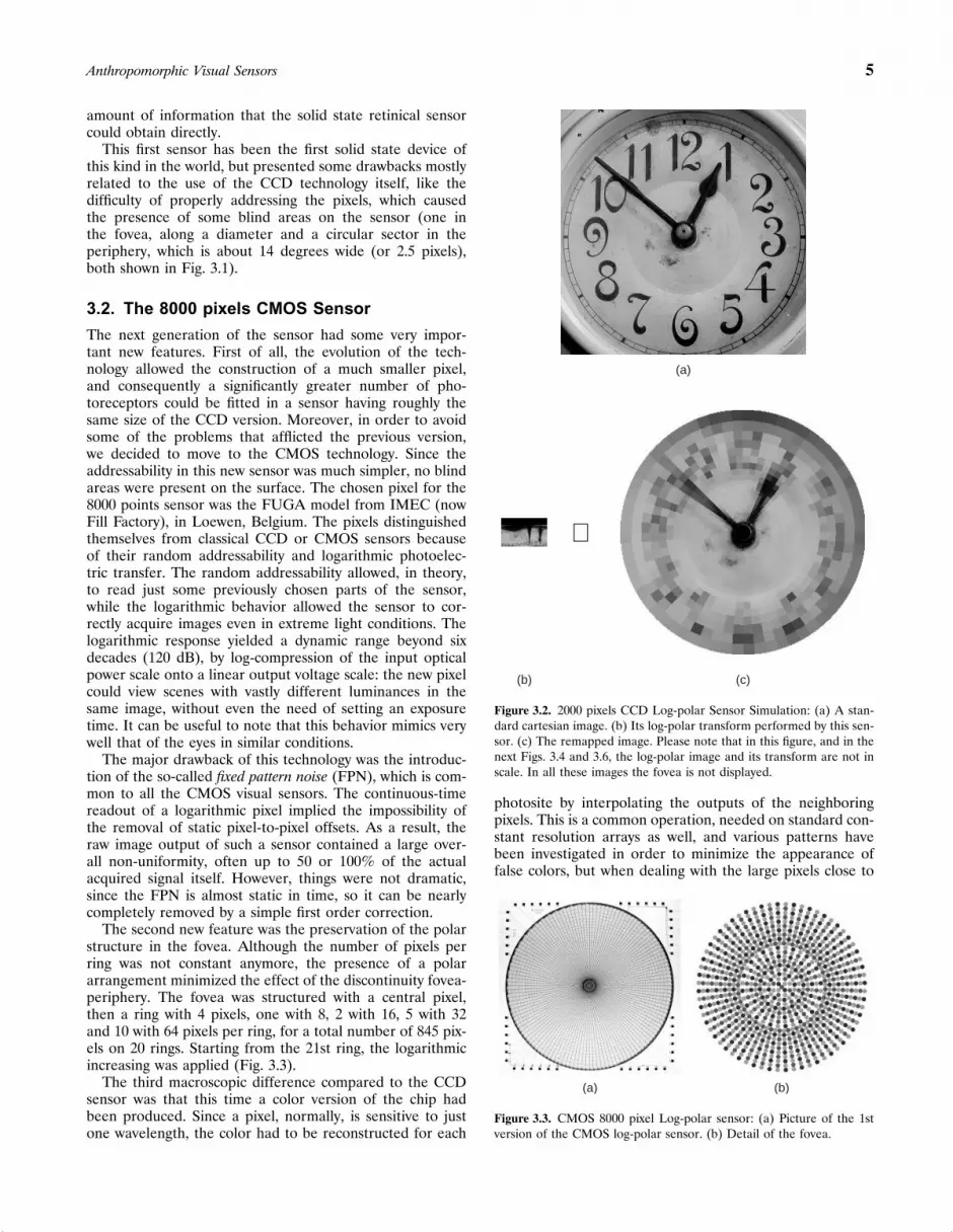
Figure 3.2. 2000 pixels CCD Log-polar Sensor Simulation: (a) A stan-dard cartesian image. (b) Its log-polar transform performed by this sen-sor. (c) The remapped image. Please note that in this figure, and in thenext Figs. 3.4 and 3.6, the log-polar image and its transform are not inscale. In all these images the fovea is not displayed.

photosite by interpolating the outputs of the neighboringpixels. This is a common operation, needed on standard con-stant resolution arrays as well, and various patterns havebeen investigated in order to minimize the appearance offalse colors, but when dealing with the large pixels close to

(a) (b)

Figure 3.3. CMOS 8000 pixel Log-polar sensor: (a) Picture of the 1stversion of the CMOS log-polar sensor. (b) Detail of the fovea.


⇔

(a) (b)

Figure 3.4. 8000 pixels CMOS Log-polar sensor simulation: (a) Thelog-polar transform of the image 3.2a performed by this sensor. (b) Theremapped image.

the external border (low spatial frequency), and when theimage presents very high spatial frequencies, it happens thatadjoining pixels “see” different elements of the image, andthe consequence is that the color components used for thereconstruction belong to uncorrelated object and that causesthe false colors.

3.3. The 33000 pixels CMOS Sensor

In the late 1990s the progress in the field of silicon manu-facturing allowed us to design a new chip using a 0.35 �mtechnology. This project had been developed within a EUfunded research project called SVAVISCA. The goal of theproject was to realize, besides the improved version of thesensor, a micro camera with special purpose lens allowing a140 degrees field of view. The miniaturization of the cam-era was possible because some of the electronics required todrive the sensor as well as the A/D converter were includedin the chip itself.

Table 1. A comparison between three generations of log-polar sensors.

Total Number Pixels in Pixels in Total NumberSensor Version of Pixels Fovea Periphery of Rings Pixels per Ring

CCD 2022 102 1920 30 64CMOS 8k 8013 845 7168 76 128CMOS 33k 33193 5473 27720 152 252

Rings in Pixels in AngularSensor Version Rings in Fovea Periphery Periphery Amplitude Logarithm Base

CCD — 30 1920 5.413� 1�094CMOS 8k 20 56 7168 2.812� 1�049CMOS 33k 42 110 27720 1.428� 1�02337

Ø of the Size of the Radius of theSensor Version Sensor Smallest Pixel R Q Technology Used Fovea

CCD 9400 �m 30 �m 13�7 300 1.5 �m 317 �mCMOS 8k 8100 �m 14 �m 14 600 0.7 �m 285 �mCMOS 33k 7100 �m 6.5 �m 17 1100 0.35 �m 273 �m

(a) (b)

Figure 3.5. CMOS 33000 pixel Log-polar sensor: (a) Picture of the 2ndversion of the CMOS log-polar sensor. (b) Detail of the fovea.

The main novelty introduced by this sensor has been thestructure of the fovea, which was, this time, completely filledby pixels. The 42 rings inside the fovea, while still having avariable number of pixel each, had a constant decrease ofthis parameter: so, not considering the ring 0, which was justa single pixel, the other rings had a number of pixel whichwas proportional to their distance from the center of thesensor (Fig. 3.5).

A minor change in the layout was the adoption of apseudo triangular tessellation, in order to minimize the arti-facts introduced by the low spatial frequency of the periph-ery. It means that each even ring has been rotated by half apixel (about 0.7 degrees) respect to the odd rings. This hadthe consequence that the average distance of a single pointfrom the closest red, green and blue pixel was inferior tothe one we had with the square tessellation, then it alloweda more accurate color reconstruction.

Since the parameter Q in this version is about 1100, forthe first time the Log-polar image acquired by the camerawas “better” than the images produced by the standard “offthe shelf” video cameras available at that time. Better means


⇔

(a) (b)

Figure 3.6. 33000 pixels CMOS Log-polar sensor simulation: (a) Thelog-polar transform of the image 3.2a performed by this sensor. (b) Theremapped image. Although the remapped images are not in scale, thelog-polar ones are in scale between them.

that the remapped log-polar image had a better maximumresolution than its cartesian counterpart, but using just aboutone thirthieth of the pixels. This allowed sending videostreams on low bandwidth channels at a very high framerate, using standard existing compression algorithms. It waseven possible to transmit a video stream over a GSM cellphone channel, which is a 9600 bit per second channel,achieving a frame rate between 1 and 2 frames per second.

3.4. A Comparison Between theLog-Polar Sensors

In order to have a better understanding of the evolutionof the log-polar sensor, it is useful to compare the maincharacteristics of the three versions.

The increasing of the quality of the image is evident fromthe Table 1, and it is shown in the simulated images inFigs. 3.2, 3.4, and 3.6: while the numbers in the clock arecompletely unreadable with the 2000 pixels sensor, they aremuch more defined in the last versions.

4. MATHEMATICAL PROPERTIES OF THELOG-POLAR TRANSFORM

The log-polar transform is not only the best compromisebetween biological motivation and simplicity of the mapping,but it also presents some interesting mathematical featureswhich can be used for a more efficient implementation ofmany image processing algorithms.

4.1. Conformity

The log-polar mapping is conformal. A conformal mapping,also known as conformal transformation, angle-preservingtransformation, or biholomorphic map, is a transformationthat preserves local angles [23]. An analytic function is con-formal at any point where it has a nonzero derivative. Con-versely, any conformal mapping of a complex variable thathas continuous partial derivatives is analytic.

The demonstration of the angle preserving propertycomes from the fact that if we consider a complex function:

w = f �z� = log��z� (4.1)

where z is a complex number in the cartesian domain thatis z = x + jy, and w is a complex number in the log-polardomain which is w = + j� = �w� · ej·arg�w�, then we get:

w = log(�z� · ej·arg�z�) = log �z� + j · arg�z� (4.2)

If we set: {�w = w −w0

�z = z− z0

(4.3)

and we consider the Taylor expansion of f �z� centered inz0, then we get:

f �z� = f �z0�+�∑n=1

f �n��z�

n! · ��z�n

⇒ f �z�− f �z0� =�∑n=1

f �n��z�

n! · ��z�n = �w (4.4)

If we stop at the first order approximation, then:

�w ≈ f ′�z0� · �z when f ′�z0� = 0 ⇒ 1z0

= 0 (4.5)

So, when � → 0, arg��w� = arg��z� + arg�f ′�z0��, andif we set arg��z� = � and arg�f ′�z0�� = �, then arg��w� =� + �.

This means that the segments in the cartesian plane arejust rotated (locally) by an angle � respect to the same seg-ments in the log-polar domain. Furthermore the segment �zis scaled in length by f ′�z0� = 1/z0.

The preservation of angles comes consequently, in fact, ifwe set: {

�z1 = �1

�z2 = �2

(4.6)

then:

arg��w2�− arg��w1� = ��2 + ��− ��1 + ��

= arg��z2�− arg��z1� (4.7)

So, when the derivative in z0 is not zero, which is alwaystrue for the logarithmic function, the angles are preserved(Fig. 4.1) and then the mapping is conformal.

The preservation of angles implies the preservation of theproximity (i.e., a couple of pixels which are close in thecartesian domain are still close in the log-polar one if wedo not consider the discontinuities that occur when � = 0,� = 2� and = 0�. These two peculiarities have the conse-quence that any algorithm involving local operators can beapplied to the log-polar image without any significant change(angle detection, edge detection, compression etc.) [8]. Inorder to avoid the problems introduced by these discontinu-ities, a graph theory based approach has been investigated,defining a connectivity graph matching the morphology ofthe sensor [15, 24].


y

x

θρ

⇔

(a) (b)

Figure 4.1. Angle Preservation: The angles are locally preserved after alog-polar Transformation. (a) Cartesian domain. (b) log-polar domain.Please note that both images a and b are particulars, so the origin ofthe mapping falls outside of the cartesian image.

4.2. Scale Change

One interesting and useful property of the log-polar trans-form is its invariancy to scale change. A pure scale changein the cartesian domain can be seen as a transformationwhere all the vectors representing each pixel of an objectare transformed in another set of vectors each proportionalby a common constant k to its pre-transformation counter-part. A scale change in the cartesian domain referred to thecenter of the log-polar mapping is then denoted by:

w = log�kz� ⇒ w = log��kz� · ej·arg�kz��= log �z� + log k + j arg�z� (4.8)

with k ∈ �+.This is equal to log�z�+K, with the constant K = log� k,

which is a pure translation along the axis in the log-polardomain (which is vertical in our representation, Fig. 4.2).

The invariance to scale change can be very importantand useful in applications where the camera moves along itsoptical axis, such as the time to impact detection in a mobilevehicle.

4.3. Rotation

Another property is the invariancy to rotation. A pure rota-tion in the cartesian domain can be seen as a transformationwhere all the vectors representing each pixel of an objectare transformed in another set of vectors whose phaseis increased by a common constant � compared to itspre-transformation counterpart. A rotation in the cartesiandomain referred to the center of the log-polar mapping isthen denoted by:

log��z� · ej·arg�z�+�� = log �z� + j�arg�z�+ �� (4.9)

this is equal to log�z�+ �0, with the constant �0 ∈ Im, whichis a pure translation along the � axis in the log-polar domain(horizontal in our representation, Fig. 4.3).

y

x ρθ

⇔

⇔

(a) (b)

(c) (d)

Figure 4.2. Scale Change: A pure scale change referred to the origin ofthe mapping, with no translational components, becomes a pure trans-lation after the log-polar transform. (a) Cartesian domain. (b) log-polardomain. (c), (d) Enlargement of the shaded areas respectively in (a)and (b).

y

x ρ

θ

⇔

⇔

(a) (b)

(c) (d)

Figure 4.3. Rotation: A pure rotation referred to the origin of themapping, with no translational components, becomes a pure transla-tion after the log-polar transform. (a) Cartesian domain. (b) log-polardomain. (c), (d)Enlargement of the shaded areas respectively in (a)and (b).


4.4. Translations

While a translation in the cartesian space can be performedwithout any change in the shape of an object, this is nolonger true in the log-polar domain.

In fact, given a point P�x0� y0�, its transform is

PLP� 0��0�=PLP

(12log�

[x2

0+y20

r0

]�arctan

[y0

x0

])(4.10)

this point, after a translation, becomes:

P�x0 + �x� y0 + �x�

= PLP

(12

log�

[�x0 + �x�2 + �y0 + �y�2

r0

]� arctan

[y0 + �y

x0 + �x

])= PLP � 0 + � �x0 + �x� y0 + �x�� 0 + ��x0 + �x� y0 + �x��

(4.11)

Since � and �� are non-linear functions, it follows that atranslation in the cartesian plane becomes a deformation inthe log-polar one, Fig. 4.4.

4.5. The Fourier-Mellin Transform

We have seen that the log-polar transform translates scalechanges and rotations into vertical and horizontal transla-tions. This property has one important application in theFourier-Mellin transform [25]. One of the most importantproperties of the Fourier transform is its magnitude invari-ancy to translations. The idea is to take advantage from thecombination between the properties of the Fourier and log-polar transforms in order to get a tool that is invariant totranslations, scale changes and rotations.

y

x ρ

θ

⇔

⇔

(a) (b)

(c) (d)

Figure 4.4. Translation: A pure translation implies a deformation of theobject after the log-polar transform. (a) Cartesian domain. (b) log-polardomain. (c), (d) Enlargement of the shaded areas respectively in (a)and (b).

The block diagram of the algorithm is described inFig. 4.5:

If we consider two images a�x� y� and b�x� y�, where b isa rotated, scaled and translated copy of a:

b�x�y�=a�k"cos�x+sin�y#−x0�k"−sin�x+cos�y#−y0�

(4.12)

� is the rotation angle, k is the scale factor and x0 and y0are the translation offsets. The Fourier transforms A�u� v�and B�u� v� of a and b respectively are related by:

B�u�v�= e−j�b�u�v�

k2·∣∣∣∣A

(ucos�+vsin�

k�−usin�+vcos�

k

)∣∣∣∣(4.13)

where �b�u� v� is the spectral phase of the image b�x� y�.This phase depends on the rotation, translation, and scalechange, but the spectral magnitude (4.14)

�B�u� v�� = 1k2

·∣∣∣∣A

(u cos�+ v sin�

k�−u sin�+ v cos�

k

)∣∣∣∣(4.14)

is invariant for translations. Equation (4.14) shows that arotation of image a�x� y� rotates the spectral magnitude bythe same angle � and that a scale change of k scales thespectral magnitude by k−1. However at the spectral origin�u= 0� v = 0� there is no change to scale change or rotation.Rotation and scale change can thus be decoupled aroundthis spectral origin by defining the spectral magnitudes of aand b in log-polar coordinates, obtaining:

BLP� � �� = k2ALP� − (� � − �� (4.15)

where = log�r� and ( = log�k�, while r and � are theusual polar coordinates. Hence an image rotation (�) shiftsthe image along the angular axis, and a scale change (k) isreduced to a shift along the radial axis and magnifies theintensity by a constant �k2�.

Input Image

FFT (magnitude)

Cartesian to log-polar

Mellin Transform

Output Image

Figure 4.5. The Fourier-Mellin Transform.


This leads to both rotation and scaling now being simpletranslations, so that taking a Fourier transform of this log-polar representation reduces these effects to phase shifts, sothat the magnitudes of the two images are the same.

This is known as a Fourier-Mellin transform and canbe used to compare a single template against an unknownimage which will be matched even if it has undergone rota-tion, scaling or translation.

4.6. Straight Line Invariancy

A generic straight line in the cartesian plane can be over-lapped to any other one performing a linear combination ofa rotation and a translation. If we note that a translation fora straight line of infinite length and zero width can also beseen as a scaling, then the remapped straight line does notchange its shape in the log-polar domain.

If we consider a generic straight line in the cartesiandomain and its corresponding transform:

f1�x� = �x + ) ⇔ f1LP �� = log�

()

r0�sin � − � cos ��

)(4.16)

we can easily see that another generic straight line is:

f2�x� = �′x + )′ ⇔ f2LP �� = log�

()′

r0�sin � − �′ cos ��

)(4.17)

Now we perform a pure rotation, so we set the followingvalues:

�′ = � cos �0 + sin �0

cos �0 + � sin �0

)′ = )

cos �0 + � sin �0

(4.18)

Then we get:

f2�x� = �′x + )′ ⇔ f2LP �� = log�

()′

r0�sin � − �′ cos ��

)

= f1LP �� − �0� (4.19)

which is a translation along the � axis.Then, considering a pure translation:

f3�x� = �′x + )′ + k ⇔ f2LP ��

= log�

()′ + k

r0�sin � − �′ cos ��

)(4.20)

since )′ and k are constants, we can set another constant� = )′+k

)′ in order to get: )′ + k = �)′

The equation (4.20) then becomes:

f3�x� = �′x + �)′ ⇔ f2LP �� = log�

(�)′

r0�sin � − �′ cos ��

)

= f1LP �� − �0�+* (4.21)

with * = log� �.

This is a pure translation of the original straight-line func-tion, translated by �0 horizontally and by −* vertically,Fig. 4.6.

It is interesting to note that if we set in (4.16):v = cot−1�−��

w = log�) · sin v

r0

(4.22)

the equation becomes:

f1LP �� = w − log� "cos�� − v�# (4.23)

where the point P = �w� v� is the point on the line whichis the closest to the origin of the log-polar mapping. Thispoint is unique and uniquely defines the line itself.

This feature is extremely important in various fields. Sinceit makes easier the detection of straight lines, it can be usedin object recognition application, when the object of interesthas straight borders. Bishay [26] has taken advantage of thisproperty in order to detect objects edges with an unknownorientation in an indoor scene.

Another application where the invariancy of the straightlines is helpful is, in stereo vision, the detection of the epipo-lar lines in a stereo pair [27].

4.7. Circumference Invariancy

In general, the shape of a circumference is not invariant inthe log-polar domain, but it is interesting to note that if wechange the sign of the equation of a generic straight linethat we saw in the previous section:

fLP �� = − log�

()

r0�sin � − � cos ��

)

= log�

(r0�sin � − � cos ��

)

)(4.24)

and then we transform it back to the cartesian domain,we get:

f �x� y� = )x2 + )y2 + r20�x + r2

0 y (4.25)

y

x ρ

θ

⇔

(a) (b)

Figure 4.6. Straight Line Invariancy: The shape of a straight line aftera log-polar transformation is invariant to its position and orientation.(a) Cartesian domain. (b) Log-polar domain.


which is the equation of a circumference passing throughthe center of the mapping, centered in:

Cx =r20�

2), Cy =

−r20

2)(4.26)

with radius:

R = r20

2)

√�+ 1 (4.27)

as shown in Fig. 4.7.Another significant family of circumferences is the set of

all the circles centered on the origin of the mapping. Since is constant for every value of �, if we transform the equation:

f �x� y� = x2 + y2 −R2 (4.28)

in log-polar coordinates, we get:

f � � �� = log�R2

r0(4.29)

Obviously, this is a constant expression, which is mappedin a horizontal straight line, as in Fig. 4.7. For details aboutthe straight line and the circumference invariancy see [28].

4.8. The Log-Polar Hough Transform

As we showed before, both straight lines and the circum-ferences passing through the origin are invariant in the log-polar space. A very useful tool that can be used to detectthese families of lines is the Hough transform. The HoughTransform [29] is a method for finding simple shapes (gener-ally straight lines) in an image. It sums the number of pixelselements that are in support of a particular line, defined ina uniformly discretized parametric Hough space. The trans-form is a map from points in an image to sinusoidal curvesin Hough space. In the ideal case, this curve represents thefamily of straight lines that could pass through the point.

y

x ρθ

⇔

(a) (b)

Figure 4.7. Circumference Invariancy: The shape of a circumference,passing through the origin of the mapping, after a log-polar transforma-tion is invariant to its position and orientation. (a) Cartesian domain.(b) Log-polar domain.

y

x ρ

θ

⇔

(a) (b)

Figure 4.8. Circumference Centered in the origin: The shape of a cir-cumference, centered in the origin of the mapping, after a log-polartransformation is a horizontal straight line. (a) Cartesian domain.(b) Log-polar domain.

The standard form of the transform is the equation of astraight line, parameterized in polar coordinates:

�� = xi cos � + yi sin � = d1 cos��1 − �� (4.30)

where (xi, yi) are the pixel cartesian coordinates, (xi, yi) arethe pixel polar coordinates, is the closest distance to theorigin, and � the slope of the normal to the line.

Using this transform, any edge point that appears in theimage votes for all lines that could possibly pass throughthat point. In this way, if there is a real line in the image,by transforming all of its points to Hough space, we willaccumulate a large number of votes for the actual line, andonly one for any other line (assuming no noise) in the image.

The vast majority of research on the Hough transformhas treated sensors that use a uniform distribution of sens-ing elements. For space-variant sensors various approacheshave been tried. Weiman [30] has proposed a log-Houghtransform, where equation (4.30) becomes:

log�� = log ��

0= log d − log 0 + log�cos�� − ��

(4.31)

Barnes [31] has investigated the log Hough transform inthe real (discrete) case of images acquired by a log-polarsensor.

4.9. Spirals

The last geometrical figure with some interesting character-istics is the logarithmic spiral. The parametric equations forsuch a spiral is:

{x = � cos�� · e)�y = � sin�� · e)� (4.32)

with � and ) arbitrary parameters.


y

x ρ

θ

⇔

(a) (b)

Figure 4.9. Logarithmic Spiral: Such a spiral, centered in the origin ofthe mapping, after a log-polar transformation becomes a straight line.(a) Cartesian domain. (b) Log-polar domain. Please note that in ourrepresentation we display the set of points �0 + 2k� all on �0.

The log-polar transform of (2.32) gives:

= log�� · e)�r0

(4.33)

If we set in (4.33): k1 = ln

a

r0

k2 =1

ln�

(4.34)

then we get:

= k2�k1 + )�� (4.35)

which is the equation of a straight line (Fig. 4.9).

5. APPLICATIONS

5.1. Panoramic View

Traditionally the acquisition of real time panoramic imageshas been performed by the usage of lenses or mirrors cou-pled with standard image sensors, but this solution presentsthe problems of having different resolutions on differentpart of the resulting images and the need of both the acqui-sition of a huge amount of pixels and the processing of theseacquired pixels.

The main objective of the OMNIVIEWS project [32] wasto integrate optical, hardware, and software technology forthe realization of a smart visual sensor, and to demonstrateits utility in key application areas. In particular the inten-tion was to design and realize a low-cost, miniaturized digi-tal camera acquiring panoramic (360�) images and perform-ing a useful low-level processing on the incoming stream ofimages, Fig. 5.1.

The solution proposed in OMINVIEWS was to inte-grate a retina like CMOS visual sensor, with a mirrorwith a specially designed, matching curvature. This match-ing, if feasible, provides panoramic images without the

(a) (b)

Figure 5.1. Panoramic View: (a) Image acquired by an OMNIVIEWSlog-polar camera (software simulation). (b) Image acquired by aconventional omnidirectional camera. Note that the image fromOMNIVIEWS camera is immediately understandable while the imagefrom a conventional camera requires more that 1.5 million operationsto be transformed into something similar with no added advantage.

need of computationally intensive processing and/or hard-ware remapper as required by conventional omnidirectionalcameras. Therefore reducing overall cost, size, energy con-sumption and computational power with respect to the cur-rently used devices. The panoramic images obtained witha log-polar technology are not only equivalent to the onesobtained with conventional devices but also these images canbe obtained at no computational cost. For example with ourcurrent prototype a panoramic image composed of about27,000 pixels is obtained by simply reading out the pixels(i.e., 27,000 operations) while with a conventional solutionthe same image would required more than 1.7 million oper-ations (about 50 times more). Besides that, unlike with awarped traditional image, we get the interesting side effectof a uniform resolution along the entire panoramic image.

The guiding principle is to design the profile of the mirrorso that if the camera is inserted inside a cylinder, the directcamera output provides an undistorted, constant resolutionimage of the internal surface of the cylinder. The advantageof such an approach lays in providing the observer with acomplete view of its surrounding in one image which can berefreshed at video rate.

For technical details about the design of the mirror, inFig. 5.2, see the OMNIVIEWS project report [33].

The panoramic vision has a lot of different applications,with or without the presence of a space variant sensor but,as we described above, the utilization of a log-polar sensorgreatly improves the performances of the system.

The most common usage of this technology (there are infact several commercial products already available based ona camera and a panoramic mirror) is in the field of remotesurveillance, where it is very useful to have a complete visionof the whole environment at once, maybe coupled with amotorized standard camera in order to zoom on the objectsof interest.

Other applications involve biological vessels (panoramicendoscopies) or industrial pipes investigation, where it isimportant to have a simultaneous view of the whole inter-nal surface of the cylinder, or robotic navigation, where theadvantage is represented by the need of just one camerain order to have a representation of the whole surroundingenvironment [34].


z

γ

φ

θ

ρ

ρ

F0

f

h(ρ)

d

60±0.2

20±0.2

15±0

.2

10±0

.5

3±0

.2

t

G (t)

2(R1)

17.8

0M8

(a) (b)

Figure 5.2. Mirror design: (a) Profile of the mirror. (b) The mirror isdesigned so that vertical resolution of a cylindrical surface is mappedinto constant radial resolution in the image plane.

5.2. Robotic Vision

The need of real-time image processing speed is particularlyrelevant in visually guided robotics. It can be achieved bothby increasing the computational power and by constrainingthe amount of data to be processed. We have seen that thelog-polar mapping is able to limit the number of pixels whilekeeping both a wide field of view and a high resolution inthe fovea. But this is not the only reason for such a choice:the biological motivation is very important too when dealingwith human-like robots.

Over the last few years, we have studied how sensorimo-tor patterns are acquired in a human being. This has beencarried out from the unique perspective of implementing thebehaviors we wanted to study in artificial systems.

The approach we have followed is biologically motivatedfrom at least three perspectives: the morphology of the arti-ficial being should be as close as possible to the human one,i.e., the sensors should approximate their biological coun-terparts; its physiology should be designed in order to haveits control structures and processing modeled after what isknown about human perception and motor control; its devel-opment, i.e., the acquisition of those sensorimotor patterns,should follow the process of biological development in thefirst few years of life.

The goal has been that of understanding human sensori-motor coordination and cognition rather than building moreefficient robots. So, instead of being interested in what arobot is able to do, we are interested in how it does it. Infact some of the design choices might even be question-able from a purely engineering point of view but they arepursued nonetheless because they improved the similaritywith, hence the understanding of, biological systems. Alongthis feat of investigating the human cognitive processes, ourgroup implemented various artifacts both in software (e.g.,image processing and machine learning) and hardware (e.g.,silicon implementation of the visual system, robotic heads,and robotic bodies).

The most part of the work has been carried out on ahumanoid robot called Babybot [35, 36] that resembles thehuman body from the waist up although in a simplifiedform, Fig. 5.3. It has eighteen degrees of freedom overalldistributed between the head, the arm, the torso and thehand. Its sensory system consists of cameras (the eyes), gyro-scopes (the vestibular system), microphones (the ears), posi-tion sensors at the joints (proprioception) and tactile sensorson the palm of hand. During the year 2004 a new humanoidis being developed. It will have 23 degrees of freedom, itwill be smaller and all its parts will be designed with thefinal goal of having the best possible similarity with theirbiological counterparts.

Investigation touched aspects such as the integration ofvisual and inertial information [37], and the interactionbetween vision and spatial hearing [38].

So, it is very important to understand why the visual sys-tem of the robot has to be as similar as possible to humanvision: we have to find out whether the morphology of thevisual sensors can improve particular sensorimotor strate-gies and how vision can have consequences on the behaviorswhich are not purely visual in nature. We should note againthat the eyes and motor behaviors coevolved: it is uselessto have a fovea if the eyes cannot be swiftly moved overpossible targets. Humans developed a sophisticated oculo-motor apparatus that includes saccadic movements, smoothtracking, vergence, and various combinations of retinal andextra-retinal signals to maintain vision efficient in a widevariety of situations.

As stated above, handling with log-polar images can besometimes uneasy and time consuming, due to the deforma-tion of the plane, but this drawbacks are always balanced

Figure 5.3. LIRA-Lab Humanoid: Babybot


by the highly reduced number of pixels that have to beprocessed.

Various algorithms have been developed to perform com-mon tasks in log-polar geometry, like vergence control anddisparity estimation [39]. In this last case, grossly simplifying,by employing a correlation measure, the algorithm evalu-ates the similarity of the left and right images for differenthorizontal shifts. It finally picks the shift relative to the max-imum correlation as a measure of the binocular disparity.The log-polar geometry, in this case, weighs differently thepixels in the fovea with respect to those in the periph-ery. More importance is thus accorded to the object beingtracked.

Positional information is important but for a few tasksoptic flow is a better choice. One example of use of opticflow is for the dynamic control of vergence as in [40]. Weimplemented a log-polar version of a quite standard algo-rithm [41]. The details of the implementation can be foundin [42]. The estimation of the optic flow requires taking intoaccount the log-polar geometry because it involves non-localoperations.

5.3. Video Conferencing, Video Telephonyand Image Compression

The log-polar transform of an image can be seen as a lossyimage compression algorithm, where all the data loss is con-centrated where the information should be less attractingfor the user. With our family of sensor the compression ratefor a single frame is between 30 and 40 to 1, which is (seeTable 1) given by:

Q2

NLP

(5.1)

where NLP is the total number of pixels in the log-polarimage. As we have seen, some algorithms can still be appliedwith no relevant change to the log-polar images, so we canprocess the image, or the video stream with virtually all thecompression algorithms commonly available. This impres-sive compressing factor can be used to send video streamson very narrow band channels.

One possible application has been investigated in the pastfew years with the EU funded project IBIDEM [43]. Thisproject has been inspired by the fact that hearing impair-ment prevents many people from using normal voice tele-phones for obvious reasons. A solution to this problem forthe hearing impaired is the use of videophones.

At that time available videophones working on standardtelephone lines (Public Switched Telephone Network) didnot meet the dynamic requirements necessary for lip read-ing, finger spelling and signing. The spatial resolution wasalso too small.

The main objective of IBIDEM was to develop a video-phone useful for lip reading by hearing impaired peoplebased on the space variant sensor and using standard tele-phone lines. The space variant nature of the sensor allowedto have high resolution in the area of interest, lips or fingers,while still maintaining a wide field of view in order to per-ceive, for example, the facial expression of the interlocutor,

but reducing drastically the amount of data to be sent onthe line (see Fig. 5.4).

After the IBIDEM project, its natural continuation was totest the performances of the log-polar cameras (which havebeen called Giotto, see Fig. 5.5) on even narrower band-widths. Extensive experiments on wireless image transmis-sion were conducted with a set-up composed of a remotePC running a web server embedded into an application thatacquires images from the a retina like camera and compressthem following one of the recommendations for video cod-ing over low bit rate communication line (H.263 in our case).

The remote receiving station was a palmtop PC actingas a client connected to the remote server through a dial-up GSM connection (9600 baud). Using a standard browserinterface the client could connect to the web server, receivethe compressed stream, decompress it and display the result-ing images on the screen. Due to the low amount of datato be processed and sent on the line, frame rates of up tofour images per second could be obtained. The only special-purpose hardware required is the log-polar camera; cod-ing/decoding and image remapping is done in software ona desktop PC (on the server side), and on the palmtop PC(on the client side). The aspect we wanted to stress in theseexperiments is the use of off-the-shelf components and theoverall physical size of the receiver. This performance interms of frame rate, image quality and cost cannot clearly beaccomplished by using conventional cameras. More recently(within a project called AMOVITE) we started realizing aportable camera that can be connected to the palmtop PCallowing bi-directional image transmission through GSM orGPRS communication lines. The sensor itself is not muchdifferent from the one previously described apart from theadoption of a companion chip allowing a much smallercamera.

The same principle has been adopted in other exper-iments of image transmission: Comaniciu [44] has addeda face-tracking algorithm to the software log-polar com-pression for remote surveillance purposes. Weiman [45],combining the log-polar transform with other compressionalgorithms has reached a compression factor of 1600:1.

(a) (b)

Figure 5.4. IBIDEM project finger spelling experiment: (a) Log-polarand (b) remapped images.


Figure 5.5. Giotto Camera.

GLOSSARYActive Vision The control of the optics and the mechanicalstructure of cameras or eyes to simplify the processing forvision.Cone A specialized nerve cell in the retina, which detectscolor.Field Of View (FOV) An angle that defines how far fromthe optical axis the view is spread.Fovea A high-resolution area in the retina, usually locatedin the center of the field of view.Foveola The central part of the fovea.Optical Axis An imaginary line that runs through the focusand center of a lens.Photoreceptor A mechanism that emits an electrical orchemical signal that varies in proportion to the amount oflight that strikes it.Receptive Field The portion of the sensory surface wherestimuli affect the activity of a sensory neuron.Rod A light-detecting cell in the retina, detects light andmovement, but not color.Saccadic Movement A rapid eye movement used to altereye position within the orbit, causing a rapid adjustment ofthe fixation point to different positions in the visual world.Vergence The angle between the optical axes of the eyes.Retina The light-sensitive layer of tissue that lines the backof the eyeball, sending visual impulses through the opticnerve to the brain.CCD (Charge-Coupled Device) A semiconductor technol-ogy used to build light-sensitive electronic devices such ascameras and image scanners. Such devices may detect eithercolour or black-and-white. Each CCD chip consists of anarray of light-sensitive photocells. The photocell is sensitizedby giving it an electrical charge prior to exposure.CMOS (Complementary Metal Oxide Semiconductor) Asemiconductor fabrication technology using a combinationof n- and p-doped semiconductor material to achieve lowpower dissipation. Any path through a gate through whichcurrent can flow includes both n and p type transistors.Only one type is turned on in any stable state so there is no

static power dissipation and current only flows when a gateswitches in order to charge the parasitic capacitance.

REFERENCES1. M. V. Srinivasan and S. Venkatesh, “From Living Eyes to Seeing

Machines.” Oxford University Press, Oxford, 1997.2. P. M. Blough, “Neural Mechanisms of Behavior in the Pigeon.”

Plenum Press, New York, 1979.3. Y. Galifret, Z. Zellforsch 86, 535 (1968).4. J. B. Jonas, U. Schneider, and G. O. Naumann, Graefes Arch. Clin.

Exp. Ophthalmol. 230, 505 (1992).5. R. H. S. Carpenter, “Movements of the Eyes,” 2nd Edn., Pion

Limited, London, 1988.6. G. Sandini and V. Tagliasco, Comp. Vision Graph. 14, 365 (1980).7. E. L. Schwartz, Biol. Cybern 37, 63 (1980).8. C. F. R. Weiman and G. Chaikin, Computer Graphic and Image

Processing 11, 197 (1979).9. E. L. Schwartz, Biol. Cybern 25, 181 (1977).

10. C. F. R. Weiman, Proc. SPIE Vol. 938 (1988).11. R. A. Peters II, M. Bishay, and T. Rogers, Tech Rep, Intelligent

Robotics Laboratory, Vanderbilt Univ, 1996.12. T. Fisher and R. Juday, Proc. SPIE Vol. 938 (1988).13. G. Engel, D. N. Greve, J. M. Lubin, and E. L. Schwartz, ICPR

(1994).14. A. Rojer and E. L. Schwartz, ICPR (1990).15. R. S. Wallace, P. W. Ong, B. B. Bederson, and E. L. Schwartz, Int.

J. Comput. Vision 13, 71 (1994).16. C. F. R. Weiman and R. D. Juday, Proc. SPIE, Vol. 1192 (1990).17. R. Suematsu and H. Yamada, Trans. of SICE, Vol. 31, 10, 1556

(1995).18. Y. Kuniyoshi, N. Kita, S. Rougeaux, and T. Suehiro, ACCV (1995).19. T. Baron, M. D. Levine, and Y. Yeshurun, ICPR (1994).20. T. Baron, M. D. Levine, V. Hayward, M. Bolduc, and D. A. Grant,

Proc. CASI (1995).21. R. Wodnicki, G. W. Roberts, and M. D. Levine, IEEE J. Solid-State

Circuits 32, 8, 1274 (1997).22. J. Van der Spiegel, G. Kreider, C. Claeys, I. Debusschere,

G. Sandini, P. Dario, F. Fantini, P. Bellutti, and G. Soncini, in“Analog VLSI and Neural Network Implementations” (C. Meadand M. Ismail, Eds.), DeKluwer Publ, Boston, 1989.

23. E. W. Weisstein. “Conformal Mapping.” From MathWorld–A Wol-fram Web Resource. http://mathworld.wolfram.com/Conformal-Mapping.html.

24. L. Grady, Ph.D. Thesis, 2004.25. R. Schalkoff, “Digital Image Processing and Computer Vision.”

Wiley and Sons, New York, 1989.26. M. Bishay, R. A. Peters II, and K. Kawamura, ICRA (1994).27. K. Schindler and H. Bischof, ICPR (2004).28. D. Young, BMVC (2000).29. Paul V. C. Hough, U.S. Patent No. 3,069,654 (1962).30. C. F. R. Weiman, Phase I SBIR Final Report, HelpMate Robotics

Inc. 1994.31. N. Barnes, Proc. OMNIVIS’04 Workshop at ECCV (2004).32. G. Sandini, J. Santos-Victor, T. Pajdla, and F. Berton, IEEE Sensors

(2002).33. S. Gächter, FET Project No: IST–1999–29017 (2001).34. J. Santos-Victor and A. Bernardino, “Robotics Research, 10th

International Symposium.” (R. Jarvis and A. Zelinsky, Eds.),Springer, 2003.

35. G. Metta, Ph.D. Thesis, 2000.36. G. Metta, G. Sandini, and J. Konczak, Neural Networks 12, 1413

(1999).37. F. Panerai, G. Metta, and G. Sandini, Robot Auton. Syst. 30, 195

(2000).38. L. Natale, G. Metta, and G. Sandini, Robot Auton. Syst. 39, 87

(2002).


39. R. Manzotti, A. Gasteratos, G. Metta, and G. Sandini, Comput.Vis. Image Und. 83, 97 (2001).

40. C. Capurro, F. Panerai, and G. Sandini, Int. J. Comput. Vision 24,79 (1997).

41. J. Koenderink and J. Van Doorn, J. Optical Soc. Am. 8, 377(1991).

42. H. Tunley and D. Young, ECCV (1994).43. F. Ferrari, J. Nielsen, P. Questa, and G. Sandini, Sensor Review 15,

17 (1995).44. D. Comaniciu, F. Berton, and V. Ramesh, Real Time Imaging 8,

427 (2002).45. C. F. R. Weiman, Proc. SPIE 1295, 266 (1990).

Documents

Anthropomorphic visual sensors