Anytime Optimal Coalition Structure Generation

Talal Rahwan1, Sarvapali D. Ramchurn1, Viet Dung Dang1, Andrea Giovannucci2,and Nicholas R. Jennings1

1 School of Electronics and Computer Science, University of Southampton, SO17 1BJ, UK{tr03r,sdr,vdd,nrj}@ecs.soton.ac.uk

2 Artificial Intelligence Research Institute, Spanish Research Council, Bellaterra, Spain,andrea@iiia.csic.es

Abstract. Forming effective coalitions is a major research challenge in the fieldof multi-agent systems. Central to this endeavour is the problem of determiningthe best groups of agents to select to achieve some goal. To this end, in this paper,we present a novel, optimal anytime algorithm for this coalition structure gen-eration problem that is significantly faster than previous algorithms designed forthis purpose. Specifically, our algorithm can generate solutions by partitioningthe space of all potential coalitions into sub-spaces that contain coalition struc-tures that are similar, according to some criterion, such that these sub-spaces canbe pruned by identifying their bounds. Using this representation, the algorithmthen searches through only valid and unique coalition structures and selects thebest among them using a branch-and-bound technique. We empirically show thatwe are able to find solutions that are optimal in 0.082% of the time taken by thestate of the art dynamic programming algorithm (for 27 agents) using much lessmemory (O(2|A|) instead of O(3|A|) for the set of agents A). Moreover, our al-gorithm is the first to be able to solve the coalition structure generation problemfor numbers of agents bigger than 27 in reasonable time (less than 90 minutes for27 agents as opposed to around 2 months for the best previous solution).

1 Introduction

Coalition formation (CF) is a fundamental form of interaction that allows the creationof coherent groupings of distinct, autonomous, agents in order to efficiently achievetheir individual or collective goals. Applications of CF include distributed vehicle rout-ing [9] and sensor networks [1], among others. Now, in many of these applications, theenvironment within which the agents operate is dynamic and time dependent in that thegains from achieving the goals decrease the further into the future they are achieved.Moreover, agents are usually limited in their computational resources. Hence, it is crit-ical that the CF process should be as fast as possible and have minimal memory andcomputational requirements. Furthermore, in the case where the search for the best so-lution may be lengthy, it is important that solutions are available at any time and thatthey get incrementally better as time passes.

One of the main bottlenecks that arise in the CF process is the coalition structuregeneration (CSG) problem. This involves selecting the best coalitions from the set of allpossible coalitions of agents such that each agent joins exactly one coalition. This is ahard problem, where the search space for n agents is O(nn) and ω(n

n2 ) [8]. Moreover,

the CSG problem has been shown to be NP-complete and existing algorithms cannotgenerate solutions within a reasonable time for even moderate numbers of agents (typ-ically bigger than 17).

Previous work, detailed further in section 6, has adopted three principal approachesto solving this problem. First, some anytime algorithms have been devised, but the worstcase bounds they provide are usually very low (up to 50% of the optimal in the best case)and they always have to search the whole space to guarantee an optimal solution. Any-time algorithms based on Integer programming do manage to prune the space searchedby employing linear programming relaxations of the problem, but these quickly runout of memory with small numbers of agents (typically for around 18 agents). Second,faster dynamic programming (DP) solutions have been developed that avoid searchingthe whole space to guarantee an optimal solution, but they cannot generate solutionsanytime. Moreover, the DP approach quickly becomes impractical for large numbers ofagents (e.g., about 2 months for 27 agents on a typical modern PC). Third, yet otherapproaches have tried to limit the size of coalitions that can be formed in an attempt toreduce the complexity of the problem. However, such constraints can greatly reduce theefficiency of the possible solutions since the solution chosen in this case can be arbitrar-ily far from the optimal (e.g., if the coalitions of the chosen size have a value of zero).In short, current state of the art algorithms that solve the CSG problem are typicallyappropriate for only small numbers of agents (typically less than 17) [8].

Against this background, we develop and evaluate a novel CSG algorithm that isanytime and that finds optimal solutions much faster than any previous algorithm de-signed for this purpose. The strength of our approach is founded upon three main com-ponents. First, we develop a new representation for the search space that allows us topartition it into much smaller, disjoint sub-spaces that can be explored independently tofind the optimal solution. Second, we devise a technique to compute upper and lowerbounds (which estimate the range within which the optimal solution lies) for each of thesub-spaces and, by comparing their bounds, we can easily prune some of them. Third,we develop an algorithm to search only through the best unique (i.e. avoiding repeti-tions) and valid (i.e. disjoint and covering the whole set) coalition structures. Hence,instead of searching the whole space of coalition structures, the algorithm splits it intosub-spaces and then directs the search process towards the most promising sub-spacesand searches very efficiently within each of them. Altogether, these components allowus to make massive performance gains over other existing approaches.

In more detail, we represent the space of coalition structures as a collection of sub-spaces, where each sub-space contains coalition structures that are similar in terms oftheir configuration (i.e. the size of coalitions that compose a coalition structure). For ex-ample, the coalition structures {{1}, {2}, {3, 4}} and {{3}, {4}, {5, 6}} have the sameconfiguration because they both contain coalition sizes {1, 1, 2}. This grouping of sim-ilar configurations is important because it defines an equivalence relation on the wholespace and, therefore, allows us to partition it into independent sub-spaces (equivalenceclasses). For each of these sub-spaces, we can then compute an upper and a lower boundby only scanning the input (which is a linear process) and, given such bounds, we canprune some of the sub-spaces straightaway (i.e. without searching within any of thesub-spaces). For the most promising sub-spaces, we then iteratively perform a number

of operations on the set of agents that allow us to cycle only through unique and validcoalition structures within each sub-space. At the same time, we apply a branch-and-bound technique [5] on these sub-spaces in order to speed up the selection of the bestamong them.

This paper advances the state of the art in the following ways. First, we developa novel optimal anytime coalition structure generation algorithm that is significantlyfaster than any previous algorithm designed for this purpose (e.g., it takes less than 90minutes (on average) to solve the 27 agents CSG problem, as opposed to more than 2months for the state of the art DP approach). Second, we provide a novel representationfor the search space of the CSG problem based on the similarity in the configuration.This representation allows agents (using any other search algorithm) to select only sub-spaces associated to particular configurations. For instance, we can choose, on the fly,whether coalition structures with larger or smaller coalitions should be selected. Also,we can analyse the trade-off between the size (i.e. the number of coalition structureswithin) of a sub-space and the improvement it may bring to the actual solution by virtueof its lower bound. Hence, rather than constraining the solution to fixed sizes, as perthe third strand of previous work discussed above, agents using our representation canmake a more informed decision about the sizes of coalitions to choose (since eachconfiguration describes the sizes of coalitions within the coalition structures). More-over, this representation allows easy pruning of the search space since we can establishbounds on sub-spaces and, therefore, we reach the optimal solution faster than otheranytime approaches. Finally, our algorithm can provide very high worst case guaran-tees on the quality of any computed solution very quickly (e.g, more than 95% of theoptimal within 0.5 seconds in the worst case for 21 agents) since it can rapidly (afterscanning the input) tighten the upper and lower bounds of the optimal solution duringthe search. This is desirable because good enough solutions may be more appropriatein a dynamic environments.

The rest of this paper is structured as follows. Section 2 presents the basic definitionsneeded to describe the CSG problem and section 3 describes our novel representationfor the search space. Section 4 details our CSG algorithm and shows how we use therepresentation to prune the search space and find the optimal coalition structure usinga branch-and-bound technique. Section 5 provides an empirical evaluation of the algo-rithm. Section 6 describes previous work in this area and section 7 concludes.

2 Basic Definitions

The CSG problem is equivalent to a complete set partitioning problem [12] where alldisjoint subsets (i.e. coalitions) of the set of agents need to be evaluated in order tofind the optimal partition (i.e. a coalition structure). The weight associated to a subsetis given by the value of the coalition. More formally, we denote the set of agents asA = {a1, a2, . . . , ai, . . . , a|A|} and a subset (or coalition) as C ⊆ A. Each coalitionhas a value given by a characteristic function v(C) ∈ <. A partition, or coalition struc-ture, is noted as CS ⊆ 2A and the set of all partitions of A is noted as P(A) (i.e. the setof unique disjoint coalition structures). For example, if A = {a1, a2, a3, a4}, a possiblecoalition structure could be {{a1, a2}, {a3}, {a4}} or {{a1, a3}, {a2, a4}}. The value

of a coalition structure is then given by the function V (CS) =∑

C∈CS v(C). Our goalis to find the optimal coalition structure, noted as CS∗ = arg maxCS∈P(A)(V (CS)),given v(C),∀C ⊆ A. Given these definitions, we next describe how the space of coali-tion structures can be divided into independent sub-spaces.

3 Problem Representation

The search space representation employed by most existing state of the art anytime al-gorithms is an undirected graph in which the vertices represent coalition structures [8,2]. The arcs represent the merging of two coalitions when followed downward, and thesplitting of a coalition into two when followed upward. Within such a representation itis comparatively easy to find integral worst case bounds from the optimal. Such boundscan be useful in giving an indication as to the quality of the solution found by searchingparts of the space (rather than obtaining a solution that could be infinitely far from theoptimal). However, it is not possible to establish upper bounds on parts of the searchspace, since the traversal of space is performed through all valid solutions. Therefore,such a representation cannot be used to compute any estimate of the distance of theactual best solution from the optimal one. Given this, algorithms that use such a repre-sentation are forced to explore the complete search space to guarantee that an optimalsolution is found. In contrast, the DP approach employs a more efficient representationof the search space, where pre-computed components of the final solution are reused,which allows it to prune the space [12, 7]. However, the DP approach does not selectincrementally better solutions, which makes it unsuitable when there is not sufficienttime to wait for an optimal solution.

Given the above, we believe an ideal representation for the search space should al-low the computation of solutions anytime, while establishing bounds on their qualityand permit the pruning of the space to speed up the search. With this objective in mind,in this section we describe just such a representation. In particular, it supports an effi-cient search for the following reasons. First, it partitions the search space into smallerindependent sub-spaces, for which we can identify upper and lower bounds (see section3.2), which allow us to compute a bound on solutions found during the search. Second,we can prune most of those sub-spaces since we can identify the ones that cannot con-tain a solution better than the one found so far (hence we can produce solutions anytime)(see section 4.1). Third, we can provide an indication about the most promising coali-tion structure configurations such that agents can balance their preference for certainconfigurations against the cost of computing the solution for these configurations.

3.1 Partitioning the Search Space

We partition the search space P(A) by defining sub-spaces that contain coalition struc-tures that are similar according to some criterion. The particular criterion we specifyhere3 is based on the integer partitions of the number of agents |A|. These integer parti-tions, of an integer n, are the sets of nonzero integers that add up to exactly n [11]. For

3 Other criteria could be developed to further partition the space into smaller sub-spaces but theone we develop here ensures that the sub-spaces are independent. Future work will look atfurther partitioning sub-spaces into smaller spaces.

example, the five distinct partitions of the number 4 are {4}, {3, 1}, {2, 2}, {2, 1, 1},and {1, 1, 1, 1}. It can easily be shown that the different ways in which a set of 4elements can be partitioned can be directly mapped to the integer partitions of thenumber 4. For instance, partitions (or coalition structures) of the set of four agents,{{a1, a2}, {a3}, {a4}} ∈ P(A), and {{a4, a1}, {a2}, {a3}} ∈ P(A) are associatedwith the integer partition {2, 1, 1}, where the parts (or elements) of the integer par-tition correspond to the cardinality of the elements (i.e. the size of the coalitions) ofthe set partition (i.e. the coalition structure). For example, for the coalition structure{{a4, a1}, {a2}, {a3}} ∈ P(A), the elements of its configuration can be obtained asfollows: |{a4, a1}| = 2, |{a2}| = 1, and |{a3}| = 1. This association is defined by thefunction F : P(A) → G, where G is the set of integer partitions of |A|. It is also easyto check that F defines an equivalence relation ∼ on P(A) such that CS ∼ CS′ if thecardinality of the elements of CS are the same as those of CS′. Given this, in the restof the paper we will refer to an integer partition as a coalition structure configuration.Then, the pre-image4 of a configuration G, noted as F−1[{G}], contains all coalitionstructures with the same configuration G. Figure 1 (in the centre) depicts the pre-imageF−1[{G}] as the set of coalition structures corresponding to each configuration G froma set of four agents. As can be seen, the pre-image of configurations G = {4} andG = {1, 1, 1, 1} only contain one coalition structure each and these are the grand coali-tion and the set of coalitions of single agents respectively. We describe the procedure toobtain these pre-images in section 4.2. Having partitioned the space, we next describehow we can compute bounds for each sub-space F−1[{G}].

Fig. 1. Representing the space using G and F−1[{G}] and the lists of coalitions CLs. The dif-ferent levels represent layers used in previous representations where worst case bounds can beestablished by searching particular layers. The numbers represent the indices of the agents (i.e. 1for a1, 4 for a4).

4 Recall that the pre-image or inverse image of a set B ⊆ G under F : P(A) → G is the subsetof P(A) defined by F−1[B] = {CS ∈ P(A)|F (CS) ∈ B}.

3.2 Computing Bounds for the Sub-Spaces

For each sub-space F−1[{G}], it is possible to compute an upper and a lower bound.To this end, we define the set of coalitions of the same size (or coalition lists) asCLs = {C ⊆ A| |C| = s}, where s ∈ {1, . . . , |A|} (see top right of figure 1 forA = a1, a2, a3, a4). We note as maxs,mins, and avgs, the maximum, minimum, andaverage value of coalitions of a given size s. Now, given a configuration G, we definea set SG =

∏s∈G CLs which is the cartesian product of the coalition lists CLs, where

s ∈ G. We will note as gn ∈ G (insteard of s) the elements of G where the index of theelement matters. Notice that the set SG contains many combinations of coalitions thatare invalid coalition structures since they may overlap with each other (i.e., two coali-tion structures may contain coalitions which contain the same agents). For example, acoalition structure of {{a1, a2}, {a1}, {a3}} is invalid since agent a1 appears in twocoalitions at the same time (and so does not appear in figure 1).

Now, consider the value UBG obtained by summing the maximum value of eachcoalition list involved in a set SG; that is, UBG =

∑s∈G maxs. As UBG defines

the maximum value of the elements in SG, it is easy to demonstrate that UBG is anupper bound for the coalition structures contained in F−1[{G}] which contains onlyvalid coalition structures. In a similar way, it is possible to compute a lower bound.Intuitively, one would expect to select

∑s∈G mins (i.e., the minimum value of an ele-

ment in SG) as a lower bound for all coalition structures (including invalid overlappingones). However, a better lower bound for the optimal value is actually the average ofthe coalition structures in F−1[{G}] since there is bound to be a coalition structurethat has a higher value than the average value and this average value is very likely tobe much greater than the minimum one (depending on the distribution of values). Thekey point to note is that this average can be obtained without having to go throughany coalition structure! This is because the average value of a sub-space can be proven(as we show in the appendix) to be the sum of the averages of the coalition lists (i.e.,AV GG =

∑s∈G avgs) and this can be computed with very little cost by only scanning

the input (see section 4.1).

Theorem 1 Let G be a configuration, G = {g1, . . . , gi, ...,g|G|}. Let AV GG be the average of all coalition structures in F−1[{G}] and avggi

bethe average of all coalitions in CLgi

, for every 1 ≤ i ≤ |G|. Then the following holds:

AV GG =∑gi∈G

avggi

See proof in appendix.

4 The Optimal Anytime Algorithm

Having described our representation, we now focus on how to search it. Here, we de-scribe the two main steps of the algorithm. First, we obtain the bounds UBG and AV GG

for every F−1[{G}]. Within the same process, we are able to compute an optimal so-lution for some sub-spaces (at a very small cost). Moreover, we can establish a worst

case bound on the quality of the solution found so far and prune parts of the space afterthis step. Second, we describe how the algorithm searches the elements of F−1[{G}]using a branch-and-bound technique to reduce the number of coalition structures thatwe need to go through, while further pruning the space.

4.1 Step 1: Generating Bounds

The input to the coalition structure generation problem is the value associated to eachcoalition (i.e. v(C) for all C ∈ 2A). We assume that the list of coalitions is partitionedinto lists of coalitions of the same size s, corresponding to CLs (see section 3.1). More-over, we assume that all such coalitions are ordered both horizontally and vertically (indescending and ascending order respectively) in the list as shown in the table of CLs infigure 1. For example, coalition {a1, a2, a4} has its elements ordered according to theirindices and the coalition itself is found above {a1, a2, a3} and below {a1, a3, a4} in thelist CL3. This ordering can easily be generated using the technique developed by [6].

The best and only coalition structure from F−1[{G}] such that |G| = 1 (corre-sponding to the grand coalition, G = {4} in figure 1) and F−1[{G}] such that |G| = |A|(corresponding to the coalitions of single agents, G = {1, 1, 1, 1} in figure 1) can di-rectly be obtained from the input. Now, let G2 = {G ∈ G| |G| = 2} denote the setof configurations where the number of elements in a given G is equal to 2 . Then wenote that, as a result of the ordering we employ, two complementary coalitions C andC ′ within any CS ∈ F−1[{G}], where G ∈ G2, are diametrically positioned in thecoalition lists CL|C| and CL|C′|. For example, coalitions {1} and {2, 3, 4} (see figure1) are diametrically positioned in the list CL1 and CL3 respectively. When |C| = |C ′|,then the coalitions are diametrically positioned in the same list. For example, coalitions{1, 2} and {3, 4} (see figure 1) can be found at the bottom and top respectively in thelist CL2. Given this, we can compute the value of all coalition structures with config-urations G ∈ G∈ by simply summing the values of the coalitions while scanning thelists CLs and CL|A|−s, starting at different extremities for each list. In so doing, wecan also record maxs and avgs (and max|A|−s and avg|A|−s). Note that this process isO(m) where m = 2|A| − 1 is the size of the input.

Having computed all maxs and avgs, we can now compute the upper bound (UBG)and lower bound (AV GG) for all sub-spaces as described in section 3.2. Then, we as-sign the lower bound to LB = max(AV G∗

G, V (CS′)), where AV G∗G = arg maxG∈G

(AV GG) is the highest lower bound of the sub-spaces and V (CS′) is the value of thebest coalition structure CS′ obtained by scanning the input. Hence, all sub-spaces withUBG < LB can be pruned straightaway. For example, as shown in figure 2, sub-spacescorresponding to G = {4}, G = {2, 2}, and G = {1, 1, 1, 1} can be pruned since theirupper bound is less than the lower bound (in this case established by the average ofthe sub-space corresponding to G = {1, 3}). Note that, after scanning the input, wecan establish that a worst case bound equal to |A|/2 on the value found so far accord-

ing to [8]. However, we can also specify a worst case bound equal toAV G∗

G2

UBmax , whereAV G∗

G2 = arg maxG∈G2(AV GG) and UBmax = maxG∈G(UBG). This is becausethe value of V (CS′) is at worst equal to AV G∗

G2 . Thus, while [8]’s bound is integraland is, at best 2 (i.e. the solution is guaranteed to be 50%), ours may not be an integer

and could be as high as 100%. Hence, the best of the two measures can be taken as theworst case bound of the solution. In the next subsection, we describe how we searchthrough the remaining sub-spaces.

Fig. 2. The width of the boxes represent the relative number of coalition structures a sub-spacecontains as depicted in figure 1. The optimal coalition structure is {{3, }{1, 2, 4}}. The boxesthat are pruned are found below LB.

4.2 Step 2: Selecting and Searching F −1[{G}]

Given a set of promising sub-spaces obtained after scanning the input, we need to selectthe one sub-space F−1[{G}] to search and then search for the best coalition structurewithin it (i.e., CS∗

G). These operations are performed repeatedly, one after the other, un-til either of the following termination conditions are reached, at which point the optimalsolution is obtained (i.e., CS∗ = CS∗

G):

1. If V (CS∗G) = UBmax – this means that this coalition structure is the best that can

be ever be found.2. If G = ∅ – this means that all nodes have been searched or the remaining sub-spaces

have been pruned.

As can be seen, unlike previous CSG algorithms, the speed with which our algorithmreaches the optimal value depends on the closeness of the upper bound to the optimalvalue. This closeness is determined by the spread of the distribution of the coalitionvalues (e.g., a larger variance means that the upper bound is more representative of themaximum and conversely for a tighter variance). Hence, in section 5, we will evaluatethe robustness of our algorithm against a number of distributions.

In the next subsection we describe how we select the next sub-space to search.

Selecting F −1[{G}] As discussed in the previous subsection, the optimal solution canonly be guaranteed if, either there are no sub-spaces left to search or the maximum upperbound has been reached. Either condition can only be reached if the sub-space with thehighest UBG (i.e. UBmax) is searched. Hence, we choose the F−1[{G}] according tothe following rule:

Select F−1[{G}], where G = arg maxG∈G

(UBG)

Note that this rule applies only if we are seeking the optimal solution. In case we areafter a near-optimal solution where a bound β ∈ [0, 1] is specified (e.g., β = 0.95means that the solution sought only needs to be 95% efficient in the worst case), thenthe selection function will be different since we do not need to search the sub-spacewith UBG = UBmax in order to return a possible solution at any time. Rather, weneed to search sub-spaces that are smaller but could give a value close to β × UBmax.The point to note is that, given our representation, we are able to specify β in caseswhere computing the optimal solution would be too costly and, given this, we modifythe selection function accordingly to speed up the search.

Another advantage of being able to control the configuration selected for the searchis that agents can choose what type of coalition structures to build according to theircomputational resources or private preferences [8, 10]. For example, it has been arguedthat the computation time could be reduced if we could limit the size of the coalitionsthat could be chosen. However, this is a very costly self-imposed constraint since itpossibly means neglecting a number of highly efficient solutions. Instead, using ourapproach, it is possible to determine, a priori (before performing the search), whichcoalition structure configurations that are most promising according to their upper andlower bounds. Therefore the computation time can be focused on these configurationsand the gains can be traded-off against the computation time since the size of a givenconfiguration can be exactly computed using the following equation:

|F−1[{G}]| =|CLg1 | × |CL

|A|−g1g2 | × . . .× |CL

|A|−∑k−2

i=1 gigk−1∏|A|

i=1,i∈E(G) ni!(1)

where E(G) is the underlying set of elements of G and ni is the multiplicity of i in G,∀i ∈ E(G). For example {1, 2} is the underlying set of {1, 1, 2}, in which case n1 = 2and n2 = 1.

In cases where agents do prefer coalition structures of particular types (e.g., contain-ing bigger or smaller coalitions), they can now, a priori, balance such preferences withthe quality of the solutions (bounded by AV GG) that can be obtained from such coali-tion structures. We next describe how we search the elements of the chosen sub-spaceF−1[{G}].

Searching within F −1[{G}] This stage is the main potential bottleneck since it couldultimately involve searching a space that could possibly equal the whole space of coali-tion structures (if all F−1[{G}] need to be searched). The challenge then lies in avoid-ing computing redundant, as well as invalid, solutions. Moreover, it is critical that we

identify those solutions that are bound to be lower than the current best and avoid com-puting them. In what follows, we first present a novel technique for cycling throughonly valid and unique coalition structures within F−1[{G}] and then describe a branch-and-bound approach that avoids the computation of solutions that have a lower valuethan the current best.

Our general approach to computing elements CS ∈ F−1[{G}] involves recursivelygoing through each element Cgn ∈ CLgn , where gn ∈ G, that can be matched withevery element Cgn+1 ∈ CLgn+1 until all coalitions that compose a CS are obtained.Now, there are two main types of repetitions that can occur in the coalition structureschosen. First, some could contain coalitions that have the same agent(s) in differentcoalitions (i.e. overlapping coalitions) and this would render the CS invalid. Second,two structures could actually contain the same coalitions. This can happen when theconfiguration requires multiple coalitions of the same size such that the same coalitionappears at different positions. Our procedure, described below, avoids both types.

Fig. 3. Composing a coalition structure for 7 agents with configuration G = {2, 2, 3}.

In more detail, assume the elements in G are in ascending order and that a CS isalso ordered according to G. This means that we note as Ck ∈ CS a coalition locatedat position 1 ≤ k ≤ |G| of CS. Let Ak be an ordered subset of agents (taken fromA) from which the members of Ck can be selected (where Ai

k ≤ Ai+1k and i is the

index of the agent in the vector e.g. A11 = 1 and A3

2 = 4 in figure 3). Finally, letMk : |Mk| = |Ck| be a temporary array that will be used to cycle through all possibleinstances of Ck. Each element of Mk represents an index of an element in Ak. The useof Mk here is mainly to show that we do not need to keep in memory all the coalitionstructures that can be constructed (while the DP approach requires storing parts of suchstructures). Given this, our memory requirements grow in O(2|A|) (i.e. the size of theinput) which is much slower than that of the state of the art DP approach which growsin O(3|A|) [12].Avoiding Overlapping Coalitions. Basically, for C1 we use M1 to cycle through thepossible instances of C1 (i.e., through the set of combinations of size |C1| taken from

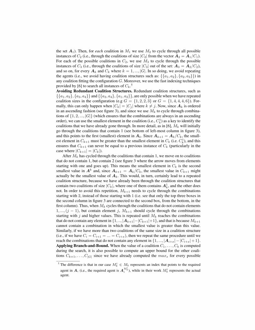
the set A1). Then, for each coalition in M1 we use M2 to cycle through all possibleinstances of C2 (i.e., through the coalitions of size |C2| from the vector A2 = A1/C1).For each of the possible coalitions in C2, we use M3 to cycle through the possibleinstances of C3 (i.e., through the coalitions of size |C3| out of the set: A3 = A2/C2),and so on, for every Ak and Ck where k = 1, ..., |G|. In so doing, we avoid repeatingthe agents (i.e., we avoid having coalition structures such as: {{a1, a2}, {a2, a3}}) inany coalition fitting the configuration G. Moreover, we use the fast indexing techniquesprovided by [6] to search all instances of Ck.5

Avoiding Redundant Coalition Structures. Redundant coalition structures, such as{{a1, a2}, {a3, a4}} and {{a3, a4}, {a1, a2}}, are only possible when we have repeatedcoalition sizes in the configuration (e.g G = {1, 2, 2, 3} or G = {1, 4, 4, 4, 6}). For-mally, this can only happen when |Ck| = |Cj | where k 6= j. Now, since Ak is orderedin an ascending fashion (see figure 3), and since we use Mk to cycle through combina-tions of {1, 2, ..., |G|} (which ensures that the combinations are always in an ascendingorder), we can use the smallest element in the coalition (i.e., C1

k) as a key to identify thecoalitions that we have already gone through. In more detail, as in [6], Mk will initiallygo through the coalitions that contain 1 (see bottom of left-most column in figure 3),and this points to the first (smallest) element in Ak. Since Ak+1 = Ak/Ck, the small-est element in Ck+1 must be greater than the smallest element in Ck (i.e. C1

k), and thisensures that Ck+1 can never be equal to a previous instance of Ck (particularly in thecase where |Ck+1| = |Ck|).

After Mk has cycled through the coalitions that contain 1, we move on to coalitionsthat do not contain 1, but contain 2 (see figure 3 where the arrow moves from elementsstarting with one and goes up). This means the smallest element in Ck is the secondsmallest value in Ak and, since Ak+1 = Ak/Ck, the smallest value in Ck+1 mightactually be the smallest value of Ak. This would, in turn, certainly lead to a repeatedcoalition structure, because we have already been through the coalition structures thatcontain two coalitions of size |Ck|, where one of them contains A1

k, and the other doesnot. In order to avoid this repetition, Mk+1 needs to cycle through the combinationsstarting with 2, instead of those starting with 1 (i.e. see that only the top three boxes inthe second column in figure 3 are connected to the second box, from the bottom, in thefirst column). Thus, when Mk cycles through the coalitions that do not contain elements1, ..., (j − 1), but contain element j, Mk+1 should cycle through the combinationsstarting with j and higher values. This is repeated until Mk reaches the combinationsthat do not contain any element in {1, .., |Ak+1|−|Ck+1|+1}, and that is because Mk+1

cannot contain a combination in which the smallest value is greater than this value.Similarly, if we have more than two coalitions of the same size in a coalition structure(i.e., if we have Ci = Ci+1 = ... = Ci+x), then we repeat the same procedure until wereach the combinations that do not contain any element in {1, ..., |Ai+x|− |Ci+x|+1}.Applying Branch-and-Bound. When the value of a coalition C1, . . . , Ck is computedduring the search, it is also possible to compute an upper bound for the other coali-tions Ck+1, . . . , C|G| since we have already computed the maxs for every possible

5 The difference is that in our case M ik ∈ Mk represents an index that points to the required

agent in Ai (i.e., the required agent is AMi

ki ), while in their work M i

k represents the actualagent.

coalition size s ∈ 1, 2, . . . , |A| (see section 4.1). Let this upper bound be computed asUBG/{g1,...,gk} =

∑g∈{gk+1,...,g|G|} maxg . Let LB be the current best solution found

so far and V (C1, ..., Ck) =∑g∈{g1,...,gk}Cg∈CS v(Cg). Then if LB > UBG/{g1,...,gk}+V (C1, ..., Ck), we do not

need to compute the value of CS. This is because the value of the coalition structurecomputed using any set of coalitions corresponding to Ck+1, . . . , C|G| are bound to belower than the current best solution. Graphically, this is expressed by avoiding the moveto rightmost columns (i.e. M2 or M3 depending on the difference the sum of v(C1) withmaximum value of coalitions of size 2 or size 3 respectively and the maximum valuefound so far) as in figure 3.

5 Experimental Evaluation

In this section we empirically evaluate and benchmark our algorithm. The general hy-pothesis is that it should perform better than those that have previously been developedfor this task. However, a potential criticism that can be levelled against our algorithmis that, contrary to the other approaches, it is dependent on computing upper and lowerbounds that are relatively close to the actual optimal value in order to prune large partsof the space and so guarantee that the optimal value has been found. Since this close-ness to the optimal is determined by the spread of the distribution of the values of thecoalitions, it is crucial that we test our algorithm against different distributions of inputvalues and show that it is robust to all of them. However, we also aim to determinewhich types of inputs allow us to clearly delineate the most promising sub-spaces veryquickly. We next describe the experimental setup.

5.1 Experimental Setup

We test our algorithm with four well known value distributions, also used by [4], tobenchmark CSG algorithms, namely:

1. Normal. v(C) = max(0, |C|×p), where p ∈ N(µ, σ)), where µ = 1 and σ = 0.1.2. Uniform. v(C) = max(0, |C| × p), where p ∈ U(a, b)), where a = 0 and b = 1.3. Sub-additive. v(C) ≤ v(C ′)+ v(C ′′) where C = C ′ ⋃ C ′′ and v(C) is uniform as

above. In this case it turns out that the coalitions of only one agent form the optimalstructure. In this case, it turns out that the grand coalition is the optimal coalitionstructure.

4. Super-additive. v(C) ≥ v(C ′) + v(C ′′), where C ′, C ′′ and v(C) are as definedabove. In this case it turns out that the coalitions of single agents form the optimalcoalition structure.

Using the same input, we tested the other state-of-the art algorithms, namely DPand Integer Programming (using ILOG’s CPLEX). We do not experiment with the otheranytime algorithms since they need to search the whole space to find the optimal valueand this is not generally feasible within reasonable time for numbers of agents above 8.

5.2 Results

Given the above setup, we ran DP, CPLEX6 and our algorithm 20 times for |A| ∈{15, 16, . . . , 26, 27} and recorded the clock time7 taken to find the optimal value. TheDP algorithm has a deterministic running time since it always performs the same oper-ations which grow in O(3|A|). Hence, we computed the results for DP up to 20 agentsand extrapolated the rest of the points (since the DP algorithm takes an unreasonableamount of time and runs out of memory for higher values). For each point, we computedthe 95% confidence interval which are plotted as error bars on the graphs.

Fig. 4. Running times for CSG algorithms for numbers of agents ranging from 15 to 25 (logscale).

As can be seen from figure 4 (in log scale), our algorithm always finds the optimalvalue for all distributions faster than the other algorithms. In the worst case, our algo-rithm finds the solution for 27 agents in 4.69 × 103 seconds (i.e. 1.3 hours), while theDP algorithm takes 5.67 × 106 seconds (i.e around 2 months) which means our algo-rithm takes 0.082% of the time DP takes for 27 agents (an improvement which gets

6 CPLEX was run with the option of ‘column elimination’ turned off since no columns can beeliminated in case all agents have to be selected in the final solution.

7 The experiments were carried out on a Xeon dual-core PC with 2GB of RAM. The algorithmswere implemented in Java 1.5.

exponentially better with increasing numbers of agents). Moreover, CPLEX is foundto be slower and also runs out of memory for numbers of agents higher than 17. Thisshows that our algorithm is robust to these general distributions.

Our algorithm performs worst, comparatively speaking, when the input is a normaldistribution of values. This corroborates our initial expectations about the relationshipbetween the spread of the distribution and the time it takes to find the optimal. Indeed,compared to the uniform distribution (against which our algorithm has a slowly increas-ing running time), the normal distribution concentrates most values around the mean.This means that there are very few values at the upper tail of the distribution that willfit into a valid coalition structure. It can also be noted that the sub-additive and super-additive distributions are solved nearly instantaneously (right after scanning the input,that is, after 1.241 seconds for 27 agents). This means that, in the best case, our algo-rithm takes 2.2× 10−5% of the time of the DP algorithm. In the sub and super-additivecase, it is easy to verify that our algorithm, by virtue of its computation of upper andlower bounds, identifies the optimal solution straight after scanning the input (see fig-ure 6) since the upper bound of the sub-spaces in these cases (without knowing whetherthe input is super or sub-additive) are always lower than the grand coalition (in the su-per additive case) or the coalitions of single agents (in the sub additive case). For theuniform distribution, it is noted that the optimal value is found much quicker than thenormal distribution and, as the number of agents grows beyond 23, the optimal value isfound as fast as in the sub or super-additive case. This can only happen if the optimalis found just after scanning the input (as in section 4.2). This could be explained bythe fact that as the number of agents increases, there is an increased likelihood that theoptimal solution will be found in the combination of coalitions of big sizes. Moreover,in the uniform case, we can expect most of the optimal coalition structures within a sub-space to have values close to the upper bound. This results in either the most promisingsub-space being indentified with a relatively high degree of accuracy or in the sub-spacebeing pruned right after scanning the input.

To further support our claim regarding the relationship between the distribution typeand the pruning of the search space, we studied the space remaining to be searched, aswell as the quality of the solution found during the search (in the case of 21 agents).To this end, we recorded the percentage of the space remaining at each pruning attemptas well as the value of the ratio of best solution found to the optimal value during thesearch (as described in section 4.2).

As can be seen from figure 5, the major drops in the space left to be search indicatethat large sub-spaces are being pruned, while when the graph is flat, branch-and-boundis being applied to reduce the solving time. In more detail, our algorithm tends to beless able to prune the space in the case of the normal distribution. In fact, most of thetime seems to be spent searching extremely small portions of the space (since the graphis flat most of the time) for a long time until the optimal value can be confirmed. Duringthis search, the solution does not improve much as can be seen from figure 6. In the caseof the sub-additive and super additive, it is nearly instantaneous (hence not depicted infigure 6) right after scanning the input. For the uniform case, we are able to prune mostof the space right from the beginning and then the algorithm takes some time to find theoptimal. From figure 6, we can see that the optimal is found fairly quickly and most of

Fig. 5. Space pruned for each distribution type for 21 agents.

the time is spent confirming that it is indeed optimal. Finally, it is also to be noted thatour algorithm can generate solutions of a very high quality anytime (see figure 6). Forexample, the solution found within 500ms is within 95% of the optimal for the normaldistribution.

Fig. 6. Quality of the solution obtained during the search for 21 agents.

6 Related Work

A number of algorithms have been developed to solve the CSG problem in the past fewyears. As discussed in section 1, three main approaches stand out. First, the anytime al-gorithms that have been developed mainly focus on establishing theoretical worst casebounds from the optimal via a specific search procedure [8, 2]. In such algorithms, it isusually assumed that V (CS) is known (as opposed to v(C) in our case). However, theyclaim to be applicable to the case where the input values (i.e., v(C) only) are known aswell [8, 2]. Given this, their search space consists of all coalition structures (see section1) even if they are given the values of v(C). Being more specific, Dang and Jennings[2004] devised an algorithm that provides guarantees of the worst case bound from theoptimal that improves upon [8] by several orders of magnitude. However, they onlyguarantee integral bounds up to 3 which means they can guarantee, in the worst case,

to produce a solution that is only 33% of the optimal value. Furthermore, as opposedto ours, their approach cannot avoid searching the whole space, in all cases, in order toguarantee the optimal solution. Other general-purpose techniques such as Integer pro-gramming (which apply branch-and-bound on a linear relaxation of the problem) havealso been used to solve large set partitioning problems [3]. However, as we have shownin section 5, an industry strength Integer programming toolkit such as CPLEX cannotpossibly cope with the sheer size of the input as soon as the number of agents goesbeyond 17. Second, dynamic programming solutions such as Yun Yeh’s algorithm [12](later rediscovered by Rothkopf et al. for combinatorial auctions [7]) is widely regardedas the fastest algorithm for coalition structure generation when the values of v(C) aregiven. This is why we used it to benchmark our algorithm. Their algorithm (which runsin O(3|A|)) is guaranteed to find the optimal solution, but while DP is computationallyless expensive than the other approaches, it is not anytime. Moreover, the DP approachbecomes impractical for agents with limited computational power (e.g., computing theoptimal CS for 27 agents requires around 7.4 × 1012 operations). Third, other ap-proaches such as [10] consider a more elaborate scenario and try to limit the sizes ofcoalitions that are allowed in an attempt to reduce the computation time. However, thiscan reduce the efficiency of the solution found. Our approach improves upon theirs byallowing agents to balance their computational costs against their private preferences(see section 4.2). Finally, recently, work by [6] reduced the time taken to cycle throughall possible coalitions of the same size without having to maintain the list of coalitionsin memory. In section 4.2, we build upon their approach to cycle through every elementof CLs in order to obtain coalition structure values.

7 Conclusions

In this paper, we have devised an algorithm that can come up with optimal solutionsfor extremely large search spaces of coalition structures. Our solution relies on a num-ber of techniques to achieve this. First, we use a novel representation of the searchspace based on configurations of coalition structures which allows agents to balancethe trade-offs between their preferences for certain coalition sizes against the computa-tion required to find the solution. Moreover, such trade-offs are better informed sincewe can compute good bounds on sub-spaces of the search space. These bounds allowus to prune the search space and guarantee the quality of the solution found during thesearch. They may also, depending on the distribution of the input values, allow us toobtain the optimal solution by only scanning (a process linear in time) the input (seesection 5). Second, we devise a technique that allows us to cycle through the list ofcoalition structures without creating any redundant or invalid ones. Third, we apply abranch-and-bound technique during the search in order to identify the best coalitionstructures and therefore prune the space further. When taken together, these techniqueshave enabled us to find the optimal coalition structure in 0.082% of the time to computethe optimal coalition structure using the DP approach for 27 agents (for larger numbersof agents, this improvement will be exponentially bigger). Moreover, our approach usesmuch less memory (O(2|A|) compared to O(3|A|) for DP).

Future work will look at more specific worst case distributions for our algorithm inorder to fully assess the robustness of our approach. We will also look at distributingthe search procedure among multiple agents since our representation easily allows us toassign each of them an independent portion of the space to search. Moreover, we aimto devise more refined representations of sub-spaces in order to improve the bounds tobe used by our branch-and-bound algorithm since most of the search time is spent inthis phase. Finally, we aim to determine the degree to which our algorithm be used tosolve other common incomplete set partitioning problems which occur in combinatorialauctions [7] or crew scheduling [3].

Appendix: Proof of Theorem 1

Let G = (g1, g2, ..., gk). That is, G contains elements of G with a lexicographic order-ing on them.

Then let F−1[{G}] return all ordered coalition structures(C1, C2, . . . , Ck), Ci ∈ CLgi

. That is, the lexicographic ordering of the elements Ci ofeach coalition structure is taken into consideration. For example, with a = 4 and G ={1, 1, 2}, G = {1, 1, 2}, considering ordered coalition structures in F−1[{G}], we havetwo ordered coalition structures: ({a1}, {a2}, {a3, a4}) and ({a2}, {a1}, {a3, a4}) thatcorrespond to one coalition structure {{a1}, {a2}, {a3, a4}} in F−1[{G}]. Moreover,as the number of repetitions of different coalition structures of F−1[{G}] in F−1[{G}]is always the same (e.g., in the above example with G = {1, 1, 2}, all coalition struc-tures in F−1[{G}] will appear twice in F−1[{G}]), we have:

AV GG = AV GG (2)

where AV GG is the average of coalition structures in F−1[{G}].Then, let Nn(g1, g2, ..., gk) (with n =

∑gi∈G gi) be the number of ordered coali-

tion structures in F−1[{G}] and Kn(gi) be the number of coalitions of size gi in asystem consisting of n agents. Clearly, Kn(gi) = n!

gi!(n−gi)!.

Now for each coalition Ci ∈ CLgi, there are Nn−gi

(g1, g2,..., gi−1, gi+1, ..., gk) ordered coalition structures that contains it, so we have:

Nn(g1, g2, ..., gk) = Kn(gi)Nn−gi(g1, ..., gi−1, gi+1, ..., gk) (3)

Also, we have:

AV GG =1

Nn(g1, g2, ..., gk)

∑CS∈F−1[{G}]

V (CS)

=1

Nn(g1, g2, ..., gk)

∑CS∈F−1[{G}]

k∑i=1,Ci∈CS

v(Ci)

Given this, we next compute AV GG as follows. Let CL′gi

be the set of all coalitionswith size gi and being the i − th coalition in an ordered coalition structure CS ∈

F−1[{G}]. Now for any Ci ∈ CL′gi

, the number of times that v(Ci) occurs in the sumof all coalition values in F−1[{G}] is Nn−gi

(g1, ..., gi−1, gi+1, ..., gk). Thus:

AV GG =1

Nn(g1, g2, ..., gk)k∑

i=1

∑Ci∈CL′

gi

Nn−gi(g1, ..., gi−1, gi+1, ..., sk)v(Ci)

=k∑

i=1

∑Ci∈CL′

gi

Nn−gi(g1, ..., gi−1, gi+1, ..., gk)Nn(g1, g2, ..., gk)

v(Ci)

=k∑

i=1

∑Ci∈CL′

gi

1Kn(gi)

v(Ci) (following equation (3))

=k∑

i=1

1Kn(gi)

∑Ci∈CL′

gi

v(Ci)

=

k∑i=1

avggi

As AV GG = AV GG (equation (2)), we have:

AV GG =

k∑i=1

avggi

�

References

1. V. D. Dang, R. K. Dash, A. Rogers, and N. R. Jennings. Overlapping coalition formation forefficient data fusion in multi-sensor networks. In AAAI, pages 635–640, 2006.

2. V. D. Dang and N. R. Jennings. Generating coalition structures with finite bound from theoptimal guarantees. In AAMAS, pages 564–571, 2004.

3. K.L. Hoffman and M. Padberg. Solving airline crew scheduling problems by branch-and-cut.Management Science, 39(6):657–682, 1993.

4. K. Larson and T. Sandholm. Anytime coalition structure generation: an average case study.J. Exp. and Theor. Artif. Intell., 12(1):23–42, 2000.

5. E.W. Lawler and D.E. Wood. Branch-and-bound methods: a survey. Operations Research,14:699–719, 1966.

6. T. Rahwan and N. R. Jennings. Distributing coalitional value calculations among cooperativeagents. In AAAI, pages 152–159, 2005.

7. M. H. Rothkopf, A. Pekec, and R. M. Harstad. Computationally manageable combinatorialauctions. Management Science, 44(8):1131–1147, 1998.

8. T. Sandholm, K. Larson, M. Andersson, O. Shehory, and F. Tohme. Coalition structuregeneration with worst case guarantees. Artif. Intelligence, 111(1-2):209–238, 1999.

9. Tuomas Sandholm and Victor R. Lesser. Coalitions among computationally bounded agents.Artif. Intelligence, 94(1-2):99–137, 1997.

10. O. Shehory and S. Kraus. Methods for task allocation via agent coalition formation. Artif.Intelligence, 101(1-2):165–200, 1998.

11. S. S. Skiena. The Algorithm Design Manual. Springer-Verlag, New York, 1998.12. D. Yun Yeh. A dynamic programming approach to the complete set partitioning problem.

BIT Numerical Mathematics, 26(4):467–474, 1986.