Embed Size (px)
Citation preview

Applying Reinforcement Learning
to RTS GamesMaster’s Thesis
Allan Mørk Christensen, Martin Midtgaard,
Jeppe Ravn Christiansen & Lars Vinther
Aalborg University,
Computer Science, Machine Intelligence
Spring 2010


Department of Computer Science, Software
at Aalborg University, Denmark
Title:
Applying Reinforcement Learning
to RTS Games
Theme:
Machine Intelligence
Project Unit:
Software Engineering
Master’s Thesis, Spring 2010
Project Group:
d613a
Participants:
Allan Mørk Christensen
Jeppe Ravn Christiansen
Martin Midtgaard
Lars Vinther
Supervisor:
Yifeng Zeng
Report Count: 7
Page Count: 74
Appendix: A-D
Finished: June 3, 2010
Synopsis:
This master’s thesis documents the work
of applying reinforcement learning on
various subtasks in a commercial-quality
RTS game.
Some of the main problems when working
with reinforcement learning are conver-
gence rates, handling concurrent agents,
and minimising the state space. Some
ideas to solve these problems, are to in-
clude time as an important factor dur-
ing learning, and to decompose the state
space by identifying independent objects
in the game world. Regarding concurrent
agents, we investigate how much infor-
mation each agent needs about the other
agents in order to behave optimally.
We found that, given certain restrictions
on the scenarios, we are able to improve
convergence rate as well as minimising
the state space for a task. We also iden-
tify how much concurrency information is
suitable for concurrent agents in various
scenarios. Finally, we provide a short dis-
cussion of how we can combine our so-
lutions to solve even more complex prob-
lems.
The contents of this report is freely available, but publication (with reference source) may only happen after agree-
ment with the authors.


Preface
This report documents a project made by the Software Engineering group d613a in the
spring of 2010, and is the final part of a Machine Intelligence master’s thesis. This
project is about using reinforcement learning concepts in RTS games to create a com-
puter opponent.
The reader is expected to have basic knowledge of RTS games, which is the type
of game that experiments in reinforcement learning will be conducted in. Thorough
knowledge about reinforcement learning is also expected.
References to literature and sources used in this report are written in square brack-
ets, such as “[RM02]”, and can be found in Appendix C. The report is accompanied by
a CD-ROM, that contains an electronic copy of the report, electronic versions of figures
and the source code used to conduct our experiments.
Allan Mørk Christensen Jeppe Ravn Christiansen
Martin Midtgaard Lars Vinther
I


Contents
1 Introduction 1
1.1 RTS games . . . . . . . . . . . . . . . . . . . . . . . . . . . . . . . . . . . . 2
1.2 AI Challenges . . . . . . . . . . . . . . . . . . . . . . . . . . . . . . . . . . 2
1.3 Learning . . . . . . . . . . . . . . . . . . . . . . . . . . . . . . . . . . . . . 3
2 Reinforcement Learning in RTS Games 5
2.1 Related Work . . . . . . . . . . . . . . . . . . . . . . . . . . . . . . . . . . 5
2.2 Challenges in Reinforcement Learning . . . . . . . . . . . . . . . . . . . . 6
2.3 Hierarchy of RTS Tasks . . . . . . . . . . . . . . . . . . . . . . . . . . . . . 7
2.4 Techniques . . . . . . . . . . . . . . . . . . . . . . . . . . . . . . . . . . . . 8
2.5 Balanced Annihilation . . . . . . . . . . . . . . . . . . . . . . . . . . . . . 12
3 Time-based Reward Shaping 15
3.1 Introduction . . . . . . . . . . . . . . . . . . . . . . . . . . . . . . . . . . . 15
3.2 Related Work . . . . . . . . . . . . . . . . . . . . . . . . . . . . . . . . . . 17
3.3 Time-based Reward Shaping . . . . . . . . . . . . . . . . . . . . . . . . . 17
3.4 Experiments . . . . . . . . . . . . . . . . . . . . . . . . . . . . . . . . . . . 21
3.5 Conclusions and Future Work . . . . . . . . . . . . . . . . . . . . . . . . . 24
4 Concurrent Agents 25
4.1 Introduction . . . . . . . . . . . . . . . . . . . . . . . . . . . . . . . . . . . 25
4.2 Related Work . . . . . . . . . . . . . . . . . . . . . . . . . . . . . . . . . . 27
4.3 Concurrent State Space . . . . . . . . . . . . . . . . . . . . . . . . . . . . . 27
4.4 Experiments . . . . . . . . . . . . . . . . . . . . . . . . . . . . . . . . . . . 30
III

CONTENTS
4.5 Results—Convergence Speed . . . . . . . . . . . . . . . . . . . . . . . . . 35
4.6 Results—Policy Equivalence . . . . . . . . . . . . . . . . . . . . . . . . . . 44
4.7 Conclusions and Discussions . . . . . . . . . . . . . . . . . . . . . . . . . 48
5 Parametrised State Spaces 51
5.1 Introduction . . . . . . . . . . . . . . . . . . . . . . . . . . . . . . . . . . . 51
5.2 Related Work . . . . . . . . . . . . . . . . . . . . . . . . . . . . . . . . . . 53
5.3 Parametrised State Spaces . . . . . . . . . . . . . . . . . . . . . . . . . . . 53
5.4 Comparison with Other Approaches . . . . . . . . . . . . . . . . . . . . . 56
5.5 Experiment . . . . . . . . . . . . . . . . . . . . . . . . . . . . . . . . . . . . 61
5.6 Results . . . . . . . . . . . . . . . . . . . . . . . . . . . . . . . . . . . . . . 66
5.7 Conclusions and Discussions . . . . . . . . . . . . . . . . . . . . . . . . . 68
6 Epilogue 71
6.1 Conclusions and Discussions . . . . . . . . . . . . . . . . . . . . . . . . . 71
6.2 Future Work . . . . . . . . . . . . . . . . . . . . . . . . . . . . . . . . . . . 73
A State Count Calculation I
A.1 Approach 3 Calculation . . . . . . . . . . . . . . . . . . . . . . . . . . . . III
B Threat Map V
B.1 Defining Threat . . . . . . . . . . . . . . . . . . . . . . . . . . . . . . . . . V
B.2 Applying Threat . . . . . . . . . . . . . . . . . . . . . . . . . . . . . . . . . VI
B.3 Retrieving Threat . . . . . . . . . . . . . . . . . . . . . . . . . . . . . . . . VI
B.4 What-if Analysis . . . . . . . . . . . . . . . . . . . . . . . . . . . . . . . . VII
C References IX
D CD XIII
IV

CHAPTER 1
Introduction
This chapter gives a general introduction to all the topics covered in the report, espe-
cially in regards to AI in RTS games and reinforcement learning. The rest of this report
is roughly divided into five parts, where three of them can be seen as independent
papers.
The first part covers the general concept of how to apply reinforcement learning in RTS
games, and introduces the game, techniques and ideas that will be used throughout
the report.
The second part, Chapter 3, explores the possibilities to use time as reward-shaping.
This is roughly our paper presented at ADMI10[CMCV10], which then again is based
on our previous report on this subject[CMCV09]. The scenario used in this paper con-
sists of a single agent which learns how to build a small base as fast as possible in
Balanced Annihilation, the RTS game described in Chapter 2.
The third part, Chapter 4, presents in-depth work with concurrent agents. We exper-
iment with how to let multiple identical agents cooperate to achieve a common goal
using reinforcement learning, and exactly what information they should share. The
common goal in the scenario used for the experiments, is letting multiple agents coop-
eratively build a base in Balanced Annihilation.
The fourth part, Chapter 5, introduces a novel approach to minimising a state space
when the agent has to choose one among a large number of similar actions. This re-
search is done in the context of learning our agent how to attack resource buildings
owned by the enemy.
Finally, in Chapter 6, we conclude, discuss and reflect on the previous three experimen-
tal parts.
1

CHAPTER 1: INTRODUCTION
1.1 RTS games
Real-Time Strategy(RTS) games are a genre of war games in which opposing forces
fight to destroy each other. The opposing forces fight to secure parts of a map, to
gain control over resources and strategic locations. Resource gathering is an important
part of most RTS games, and resources are normally scattered across the map, so map
control is also important. The opposing forces act by producing buildings and armed
forces, these are then used to pressure the opponent, which in the end should lead to
victory, e.g. when the opponent has lost all its units.
The sequence of buildings a player constructs early in the game is known as the build
order, this often has a great impact on the early strategy of the player. If a player focuses
on resource gathering early on, then he will be exposed to early attacks. But if a player
chooses to focus on attacking early on, he would risk not having a solid economy later
in the game.
Another important part of RTS games is when and where to attack, once you have an
army. This problem depends a lot on distances, due to the limited movement speed of
units. If one attacks far from his base, he is more vulnerable to counter attacks, as he
can not use his attacking force to defend his base. Also, if the agent ordered some units
to attack the enemy far away, the situation at the attack destination may very well have
changed before the units arrive.
1.2 AI Challenges
This section is based on a section from our previous report [CMCV09], but we consider
it important to mention some of the challenges with AI development for RTS games,
and some of the problems which exist in current RTS agents.
Creating a competitive agent for an RTS game is a complex task. Many actions have to
be carried out concurrently in different areas of the game, e.g. creating units, attacking
and building a base, while still maintaining an overall strategy. Furthermore it has to
be handled without using too much computational power from the computer, as the
game itself has to be rendered fluently to the player.
RTS agents are becoming more and more clever but they are still nowhere near the level
of good human players. Some of the major problems with general RTS agents are lack
of planning, and hard-coded build-orders, each described in the following sections.
2

CHAPTER 1: INTRODUCTION
1.2.1 Lack of Planning
One problem with RTS agents is that they are not able to make intelligent strategic
decisions. Humans are far superior in this area. Furthermore, the agent should be able
to adapt this strategy using changes in the environment and weaknesses found in their
opponents.
1.2.2 Hardcoded Build-orders
In the beginning of an RTS game, one normally has to build up a base in order to get
resources and be able to build an army. This phase is critical, meaning that starting
out poorly will set you far behind your opponent. It is therefore common for RTS
agents to just use a predefined script of what to build and in what order. While this is
good if you know the perfect build order, it is not very open to adaptation to changing
environments. This is also sometimes used to decide when to attack, meaning that the
agent might always attack after building 5 army units, or after 5 minutes of the game.
Human players will be able to recognise this behaviour, and easily perform counter-
measures in order for him to win the game.
1.3 Learning
Reinforcement learning [SB98] is an interesting area within machine learning. Algo-
rithms within reinforcement learning deal with an agent learning an optimal policy via
interaction with its environment. Instead of using some predefined scripted policy, the
agents will learn a policy using reinforcement learning. Even though both approaches
uses a defined policy, reinforcement learning allows for handling of more states (and
thereby in-game situations) than would be feasible with a scripted policy, and allows
adaptation to changes in the game.
1.3.1 Reinforcement Learning
In reinforcement learning, the agent is given a reward from its environment illustrating
the quality of taking a specific action. The reinforcement learning algorithms depend
on a value function to represent the value of being in any given state. The higher the
value, the better. This function can take all the possible future rewards into account, so
the algorithms can pick the actions leading to the best future states as well. Eventually
the agent is able to learn a so-called optimal policy illustrating the best action to take in
3
CHAPTER 1: INTRODUCTION
any given state. The value function can be implemented as a simple two-dimensional
table, but sometimes this is infeasible due to the size of the table.
Online reinforcement learning means that the agent learns as it plays the game. This
allows it to adapt completely to the behaviour of the opponent, as well as allowing a
dynamic adjustment of the difficulty level. In offline learning, on the other hand, the
agent is trained during development before the game is deployed. In this case, the
agent is, e.g. trained against experts or another instance of the same agent, and will not
continue to adapt after release of the game.
1.3.2 States
State spaces consist of a number of state variables representing the parts of the en-
vironment that are interesting for the learning agent. In practice, each of these state
variables are often split into a number of discrete intervals, {0− 1, 1− 3, 4− 7}. When
implementing a scripted policy states have to be handled explicitly. In practice this
could very well mean an if -condition for every single state variable interval, e.g.
i f (var > 1)elsei f (var > 3)else.... Since a policy learned even for relatively simple
problems could very well cover thousands of game states, it would be infeasible to
cover these states with a scripted policy.
The reason why reinforcement learning is better at handling many states is that it does
not need a programmer to explicitly handle every case, it can instead learn a proper
policy by playing a lot of games, and this process can often be automated. The devel-
opers of the agent are only required to hand the learning agent qualitative information
about which changes in the game state are good, and which are bad. The agent will
then learn a policy from this, and thereby it will eventually have a proper response for
all the states that it encountered while learning.
1.3.3 Adaptation
If online learning is used with reinforcement learning, this allows the agent to adapt
its policy to changes, e.g. if the opponent continually plays defensively, the agent will
become better at handling that. If this should be supported with a scripted policy, it
may require a new policy to be scripted, and then a decision module to choose between
the available policies. This decision module could be based on opponent classification,
which would have to choose the best policy for a given opponent class. Of course this
could also be used with reinforcement learning, thus requiring a policy to be learned
against all classifications.
4

CHAPTER 2
Reinforcement Learning in RTS
Games
This chapter gives an overview of the general use of reinforcement learning in RTS
games. Previous work on reinforcement learning, unsolved problems, and the RTS
game of choice for the later experiments, will be described.
We will present a simplified hierarchy of tasks in an RTS game. It is a subset of these
tasks that we will later solve using reinforcement learning in the following chapters.
A brief introduction is given to the reinforcement learning algorithms that will be used
in our experiments. Namely, SMDP and multi-agent SMDP. Additionally, various ter-
mination strategies in multi-agent SMDP problems are introduced.
Finally, the RTS game of choice for our reinforcement learning studies is presented:
Balanced Annihilation. Relevant game information, and the settings for the scenarios
used for the experiments are described.
2.1 Related Work
Related work specific to each chapter of the report can be found in the respective chap-
ter right after the introductory sections. The related work specified in this section is
about reinforcement learning in RTS games in general, and does not include specific
work about the sub-problems that will be discussed in the later chapters of this report.
Kresten et al previously applied reinforcement learning in a simple
RTS game[AZCT09], and how to make online learning feasible by decomposing the
state space into a hierarchy of tasks. They looked at all aspects of an agent in an RTS
game, where we will go in-depth with specific areas, base-building and attacking, and
5

CHAPTER 2: REINFORCEMENT LEARNING IN RTS GAMES
experiment with more advanced scenarios for these aspects.
Marthi et al apply hierarchical reinforcement learning to RTS tasks [MRLG05]. They
solve problems in which an agent controls multiple units simultaneously, both regard-
ing base-building, resource collection and attacking.
The work of Kresten et al, and Marthi et al proves that a complete hierarchical division
of all tasks in an RTS game is possible, and this is very important for the research
we will present in this report. Hierarchical decomposition implies that we are able to
identify isolated subtasks which can be solved independently. Each of the three main
parts in this report will address one such isolated subtask while addressing various
problems related to reinforcement learning.
2.2 Challenges in Reinforcement Learning
This section is based on our previous report[CMCV09]. We choose to include it in this
report as well, because we find that it is important to mention some of the problems
associated with using RL for RTS games, as we will try to tackle some of these problems
later in this report.
Some of the challenges associated with using reinforcement learning for implementing
an agent, for an RTS game, are described in the following sections.
2.2.1 Concurrent Actions
In RTS games, many actions are executed concurrently. Obviously there is a need to
both build units and attack at the same time. The problem is that these actions af-
fect each other. For example, if you attack the opponent with all your units, and at
the same time start building some resource building in your base, how should re-
ward be distributed? If you lose the game because of the first action, the second ac-
tion should not be penalised. Also, concurrent agents cooperating in achieving the
same goal should not be encouraged to work against each other. Concurrent rein-
forcement learning is currently an area of much interest to many machine intelligence
researchers[MRLG05][OV09].
2.2.2 State Space Size
The size of the state space in an RTS game can be very large and thus it can be a good
idea to make certain abstractions over the state space of such a game. If the state space
6
CHAPTER 2: REINFORCEMENT LEARNING IN RTS GAMES
becomes too large, storing the value function as an ordinary two-dimensional table of
real values becomes infeasible, and function approximators may need to be used in
order to limit the memory usage of the value function [SB98]. A very large state space
also makes learning more time consuming, as it takes longer time to visit all possible
states, and thereby the convergence rate is affected.
Another way to limit the size of the value function is to implement hierarchies in the
state space, where each node has its own value function. This is still not a perfect
solution though, since a certain level in the hierarchy may still depend on a lot of state
information. Chapter 5 describes a novel approach to minimising state spaces given
some constraints on the type of task to solve.
2.3 Hierarchy of RTS Tasks
Figure 2.1 illustrates a simplified hierarchy of tasks in a general RTS game. All the tasks
considered here can be split into actual primitive actions in our game.
At the top we have the three overall tasks: Attack, Build and Navigate. The two first
represent the problems to which we are going to apply reinforcement learning. If we
assume that we have learned an optimal policy for all subtasks in the hierarchy, we
will be able to answer questions such as, “given the current game state, which action
will be optimal; building something or attacking something?”. Each of the subtasks in
the hierarchy will then be able to answer more specific questions such as the Attack
subtask: the policy learned for this task, should be able to answer the question “where
is the best place to attack right now?”. Finally, the somewhat simple task of navigat-
ing will be handled using a standard A*-algorithm instead of reinforcement learning,
which could in fact have been used, though it is less applicable in an RTS game due to
the enormous state space it would have.
We do not cover the decision making of all the tasks in the hierarchy, which is required
to have a fully functioning agent which is able to play an RTS game. We do not consider
when and what type of units to build, and how this should be weighted compared to
constructing buildings and attacking. In this thesis we focus solely on isolated prob-
lems found in some of the subtasks in the hierarchy.
7

CHAPTER 2: REINFORCEMENT LEARNING IN RTS GAMES
RTS
Actions
Attack Build Navigate
Resources Units Commander Unit BuildingGo to
locationProduction
Figure 2.1: A hierarchy of actions in an RTS game.
2.4 Techniques
In this section we describe the various reinforcement learning techniques and termi-
nology that will used in the later chapters. The problems that will be used are single-
and multi-agent SMDP problems, which can be solved with an SMDP variant of Q-
learning. Regarding multi-agent problems, there are various termination strategies to
consider, and we coin our use of the term “identical agents”.
2.4.1 SMDP
A semi-Markov Decision Process, SMDP, is a simple generalisation over MDPs, where
an action does not necessarily take a single time step, but can span several time steps.
The state of the environment can change multiple times from an action has been initi-
ated until the next decision is initiated. Rewards are also slightly different from those
of standard MDPs, as the decision maker will both receive a lump sum reward for tak-
ing an action and also continuous rewards from the different states entered during the
decision epoch. This all means that SMDPs can describe more scenarios and environ-
ments than MDPs.[RR02]
Formally an SMDP can be described as the 5-tuple (S, A, T, F, R), where:
• S : the finite state set
• A : the finite set of actions
• T : the transition function defined by the probability distribution T(s′|s, a)
• F : the probability of transition time for each state-action pair defined by
8

CHAPTER 2: REINFORCEMENT LEARNING IN RTS GAMES
F(s′, τ|s, a)
• R : the reward function defined by R(s′|s, a)
The F function specifies the probability that action a will terminate in s′ after τ time
steps when starting from s.
2.4.2 Multi-agent SMDP
A multi-agent SMDP (MSMDP) problem is an SMDP problem in which there are mul-
tiple agents acting concurrently. These concurrent agents can both be cooperative and
opposing agents. Cooperative agents help each other to reach either a common or
individual non-conflicting goals, where opposing agents, on the other hand, have con-
flicting goals, which means that only one or some of the agents can reach their goal.
There are different approaches to solving MSMDPs, where either the agents are con-
trolled asynchronously or synchronously (at the same time). If controlling the agents
synchronously, the actions of all agents will have to be chosen at the same time, thus
making the action space the cross-product of the action spaces for all agents. If control-
ling agents asynchronously, a new action is chosen at the end of each decision epoch for
each agent, i.e. we do not choose new actions for all agents, but only one—namely the
one that just finished its action. In the asynchronous case the state-space may increase
in size since we need to know what the other agents are doing to make the right choice.
2.4.3 MSMDP Action Termination Strategy
If all units are controlled by a single agent, we need to consider when to have decision
epochs. This is especially true if the units carry out parallel actions of varying time
durations.
Rohanimanesh and Mahadevan introduced[RM02] three types of parallel termination
schemes:
τany The decision epochs occurs when any action has terminated, where all other par-
allel actions are interrupted.
τall The decision epochs occurs immediately after all parallel actions have terminated,
where previously terminated parallel actions take the idle action while waiting.
τcont A decision epoch occurs every time an action terminates, but only for that agent,
leaving the others to complete their current actions.
9

CHAPTER 2: REINFORCEMENT LEARNING IN RTS GAMES
Task Termination Strategy
In the experiments in Chapter 4, we do not use a single agent to control our units,
but instead we use separate agents to control each unit. This means that we do not
need to synchronise our decision epochs. This can be compared to the decision epoch
termination strategy τcont as this works in a similar way.
We choose this in order to focus on minimising the state space instead of the action
space.
When multiple agents have to cooperate to complete a common goal, only one of the
agents will be the one who carries out the final action that will complete the goal. How-
ever, since other agents at this point might still be in the middle of some other action,
we need to consider when to terminate the overall task. This is what we call the task
termination strategy. The three termination strategies described in this section can be
applied at this task level even though we control each unit with a separate agent. This
will be further discussed in Chapter 4.
2.4.4 Identical Agents
In multi-agent systems it is possible that several of the agents are similar or even iden-
tical, meaning that the agents have the same actions available to them, and they are
equally good at completing them. If the agents also share the same goal, then it is
possible for the agents to share the same Q-table. This could potentially increase the
learning speed, as all the agents will learn from the shared experience of all agents.
2.4.5 Q-Learning
Q-learning is an algorithm for finding an optimal policy for an MDP (not SMDP). It
does so by learning an action-value function (or Q-function) that returns the expected
future reward of taking an action in a specific state. Q-learning does not need a model
of its environment to be able to learn this function. The Q-function is a mapping from a
state and an action to a real number, which is the expected future reward: Q : S× A 7→R.
After the Q-function has been learned, it is trivial to find the optimal policy, as one
simply has to choose the action with the highest return from the Q-function in a given
state.
Learning the Q-function is done using an action-value, and with an update rule shown
in Equation 2.4.1. In addition, the algorithm chooses its actions in an ε-greedy manner.
10

CHAPTER 2: REINFORCEMENT LEARNING IN RTS GAMES
It has been shown that by using this update rule the algorithm converges to Q∗, the
optimal value function, and using this to choose actions will result in the optimal policy,
π∗ [SB98].
Q(st, at)← Q(st, at) + α[rt+1 + γ maxa
Q(st+1, a)−Q(st, at)] (2.4.1)
Q-learning is called an off-policy algorithm as it does not use its policy to update the
Q-function, but instead uses the best action given its current Q-function. This however
is not necessarily its policy, as the algorithm will have to perform exploration steps
from time to time. These exploration steps are needed for the algorithm to converge
to an optimal solution as it will have to take all actions in all states to be sure that it
converges to the optimal policy.
Sutton et al [RR02] proposed an algorithm, SMDPQ, which extends Q-learning to sup-
port SMDPs by changing the update rule. Normally the discount factor, γ, is multiplied
with the expected future reward, as all actions in MDP problems are assumed to take
constant time to complete. In the modified version, the discount factor is raised to the
power of the number of time steps that the action took to complete. This results in
a new update rule given in Equation 2.4.2, where Rt is the discounted accumulated
reward up to time step t.
[Q(st, at)← Q(st, at) + α(Rt + γk maxa
Q(st+1, a)−Q(st, at))] (2.4.2)
2.4.6 Reward Shaping
Ng et al. [NHR99] proposed reward shaping to speed up Q-learning while preserving
the policy optimality. Every optimal policy in an MDP, which does not use reward
shaping will also be an optimal policy in an MDP which uses reward shaping, and
vice versa. Formally reward shaping introduces a transformed reward function for the
MDP: R′(s, a, s′) = R(s, a, s′) + F(s, a, s′), where F : S× A× S 7→ R. To achieve this, we
need a function Φ(s) that can calculate a value based on state s, which should represent
the potential of the state, making it comparable to another state. The potential-based
shaping function is formally defined as:
F(s, a, s′) = γΦ(s′)−Φ(s) (2.4.3)
An example of such a function could be the negative euclidean distance to a goal from
a current position in a grid world. As a rule of thumb, Φ(s) = V∗M(s), where V∗M(s)
11

CHAPTER 2: REINFORCEMENT LEARNING IN RTS GAMES
means the value of the optimal policy for MDP M starting in state s, might be a good
shaping potential.
2.5 Balanced Annihilation
Balanced Annihilation is a game developed for the open-source engine Spring RTS. It
is a well balanced modern RTS game comparable to commercial closed-source games.
All Spring RTS games have very good support for AI implementation in many lan-
guages. We will be using the C++ interface to develop our agent.
In this section we will briefly describe the game and the two common RTS AI problems
that we will solve using reinforcement learning, base-building and attacking.
Figure 2.2: A screenshot of the scenario in Balanced Annihilation. This shows the state
of the game after five metal extractors, one solar collector, and two k-bot labs
have been build. The construction unit is currently in the process of build-
ing a third k-bot lab. At the top of the screen a white and a yellow indicator
can be seen, representing the current level of metal end solar energy, re-
spectively.
2.5.1 Overview
Balanced Annihilation is based on the first 3D RTS, Total Annihilation. The game is
designed such that resources are consumed and produced continuously. Furthermore,
resources are not gathered by worker units, but by resource buildings. Other notable
12

CHAPTER 2: REINFORCEMENT LEARNING IN RTS GAMES
buildings include production buildings, which are able to produce both attack- and
construction units. These are also the two basic types of units. Furthermore, both types
of units are available in four flavours: k-bots, tanks, boats and aircrafts.
Every player starts a game with a single unit called the “commander”, which is a spe-
cial type of builder-unit. Killing this special unit is actually the goal of the opponent.
This means that even though one player has a huge advantage in number of units and
buildings, a seemingly weak other player can win the game immediately by killing this
single “commander” unit. Figure 2.2 shows a graphical example state of the game.
2.5.2 Building a Base
One of the problems of an RTS game that we will address using reinforcement learning
in this report is getting a number of builder-units to cooperate in building a strong
base quickly. A good base composition is needed to be able to produce attack units
fast enough. This is achieved by constructing enough resource buildings to support
both the builder-units and the production buildings. If insufficient resource buildings
are constructed, then the production of units and the construction of buildings will be
slowed down. On the other hand, if too many resource buildings are constructed, then
time is wasted that could have been used to construct more production buildings and
thereby speed up the production of attack units.
There is a trade-off between constructing resource buildings and production buildings
to make sure that the workers are acting in a near-optimal way. In most RTS games this
is scripted by an expert, who knows the game and therefore knows an effective build
order. We propose to learn a good build order using reinforcement learning, where the
goal is to create a number of production buildings, leaving the agent with a good econ-
omy after each one of these is done, while not wasting time building excessive resource
buildings. Practically this could be used to learn a good base building order for any RTS
game, instead of letting an expert decide on a scripted build order. Furthermore this
easily allows for a more complex scenario, differentiating resource production and unit
costs from game to game, or map to map, without needing specifically created policies
for each of these scenarios.
2.5.3 Battle
The other RTS problem that we will address using reinforcement learning in this report
is how to attack the enemy. Attacking is essential to winning any RTS game, so careful
decision making is necessary before sending units on an attack mission, since a wrong
13

CHAPTER 2: REINFORCEMENT LEARNING IN RTS GAMES
decision may result in a huge loss for our agent. A good player should be able to exploit
weaknesses in the defense of his opponent, e.g. by attacking unprotected resource
buildings, and thereby destroying a part of the economy of the opponent without the
player losing any units. It is therefore important to know when and where to attack,
and this depends on the sizes and compositions of the armies as well as the general
state of the map, e.g. locations of bases, armies, resource buildings etc.
A sufficient representation (state space) of the game world for learning to attack may
very well include so many state variables and so many discrete intervals that reinforce-
ment learning could become infeasible. We need to investigate ways to abstract away
some of this information so that we will be able to represent the value of an attack in a
more compact, yet useful way.
14

CHAPTER 3
Time-based Reward Shaping
Abstract. Real-Time Strategy (RTS) games are challenging domains for AI, since
it involves not only a large state space, but also dynamic actions that agents ex-
ecute concurrently. This problem cannot be optimally solved through general Q-
learning techniques, so we propose a solution using a Semi Markov Decision Pro-
cess (SMDP). We present a time-based reward shaping technique, TRS, to speed
up the learning process in reinforcement learning. Especially, we show that our
technique preserves the solution optimality for some SMDP problems. We evalu-
ate the performance of our method in the Spring game Balanced Annihilation, and
provide some benchmarks showing the performance of our approach.
3.1 Introduction
Reinforcement learning is an interesting concept in game AI development since it
allows an agent to learn by trial-and-error by receiving feedback from the environ-
ment [SB98]. Learning can be done without a complete model of the environment
which means that reinforcement learning can be applied to even complex domains.
Reinforcement learning has been applied to many types of problems, including many
different board games [Gho04], a simple soccer game [Lit94] and robot naviga-
tion [Mat94]. In the context of RTS games, reinforcement learning has been applied to
a small resource gathering task [MRLG05], and a commercial real-time strategy game
(RTS) called MadRTS [SHS+07].
The benefit of applying reinforcement learning is to create adaptive agents (Non-player
characters in computer games) that may change their behaviour according to the way
opponents play throughout games. Generally, reinforcement learning requires that the
problem shall be formulated as a Markov decision process (MDP). This demands that
environmental states, as well as actions, must be well defined in the studied domain.
15

CHAPTER 3: TIME-BASED REWARD SHAPING
However, a complex and dynamic RTS game always involves a very large state-action
space. Moreover, agents’ actions may last several time steps and exhibit a dynamic
influence on the states. Both of these problems prevent a fast convergence to an optimal
policy in RTS games. Recently, Kresten et al. [AZCT09] showed that the hierarchical
decomposition of game states may mitigate the dimensional problem. This chapter
will investigate solutions to the second problem and speed up the convergence using
relevant techniques.
We resort to Semi Markov Decision Processes (SMDPs) that extend MDPs for a more
general problem formulation. SMDPs allow one single action to span multiple time
steps and change environmental states during the action period. This property matches
well with solutions to the dynamic actions within RTS games of our interest. However,
the problem of slow convergence occurs when an optimal policy needs to be compiled
in a short period of gameplay.
To speed up the learning process, we present a time-based reward shaping technique,
TRS, which makes it possible to apply the standard Q-learning to some SMDPs and
to solve SMDPs in a fast way. We let the agent get a negative reward only after it
completes an action, and the reward depends on how much time it takes to complete
the action. This means that after many trials, the agent will converge towards the fastest
way of completing the scenario, since all other solutions than the fastest possible one
will result in a larger negative reward. Our proposed approach puts some constraints
on the properties of the SMDP problems to which time-based reward shaping can be
applied without compromising the solution optimality.
We compare TRS to the Q-learning algorithm SMDPQ presented by Sutton et al [RR02].
SMDPQ extends Q-learning to support SMDPs by changing the update rule. We the-
oretically analyse the equivalence of optimal policies computed by both SMDPQ and
our proposed method, TRS, given the constraints. We evaluate performance of TRS on
a scenario in the RTS game of Balanced Annihilation and show a significant improve-
ment on the convergence of SMDPQ solutions. We also apply TRS to other reinforce-
ment learning methods such as Q-learning with eligibility traces, Q(λ), and show that
this also can be successfully extended to support some SMDP problems.
The rest of this chapter is organized as follows. Section 3.2 describes related work on
using reinforcement learning in computer games. Section 3.3 presents our proposed
method, TRS, and analyse the policy equivalence. Subsequently, Section 3.4 provides
experimental results to evaluate the method. Finally, Section 3.5 concludes our discus-
sion and provides interesting remarks for future work on this topic.
16
CHAPTER 3: TIME-BASED REWARD SHAPING
3.2 Related Work
Reinforcement learning methods have been well studied in the machine learning area
where much of the work focuses on the theoretical aspect of either the performance im-
provement or the extension from a single-agent case to a multi-agent case. Good survey
papers can be found in [KPLM96]. Although reinforcement learning techniques have
been demonstrated successfully in a classical board game [Tes94], computer games are
just recently starting to follow this path [Man04].
RTS games are very complex games, often with very large state- and action-spaces and
thus when applying reinforcement learning to these problems we need ways to speed
up learning in order to make the agent converge to an optimal solution in reasonable
time. For example, some methods like backtracking, eligibility traces [SB98], or reward
shaping [Lau04] have been proposed for this purpose. Laud demonstrates[Lau04] that
reward shaping allows much faster convergence in reinforcement learning because the
reward horizon is greatly decreased when using reward shaping, i.e. the time that
passes before the agent gets some useful feedback from the environment is decreased.
Meanwhile, Ng et al. [NHR99] prove if the reward shaping function takes the form of
the difference of potentials between two states the policy optimality is preserved.
The Q-learning variant SMDPQ[RR02] is used for proving policy equivalence with TRS
on the supported SMDP problems.
3.3 Time-based Reward Shaping
We observe that reward shaping can be used to extend the standard Q-learning algo-
rithm to support SMDPs. In this section, we firstly propose a time-based reward shap-
ing method, TRS, and discuss the solution optimality in connection with SMDP. Then,
we elaborate the validity of our proposed method through two counter examples.
3.3.1 Our Solution
We propose the simple solution of using the time spent for an action as an additional
negative reward given to the agent after it completes that action. Formally, we define
the time-based shaping function in Equation 3.3.1.
F(s, a, s′) = −τ(a) (3.3.1)
where τ(a) is the number of time steps it takes the agent to complete action a
17
CHAPTER 3: TIME-BASED REWARD SHAPING
As the time spent for an action is independent of transition states, the reward shap-
ing is not potential based. Consequently, we can not guarantee the solution optimality
for any SMDP problem. However, we observe that solution optimality may be pre-
served for some SMDP problems if the problem satisfies some properties. As shown in
[NHR99] the shaping function F must not allow a cycling sequence of positive reward,
since this will result in the agent finding a suboptimal solution.
We begin by showing that using reward shaping (in Equation 3.3.1), the agent will
never learn a solution consisting of a cyclic sequence of states for which the individual
rewards total to a positive reward. Then, we proceed to prove a guaranteed consis-
tency between the optimal policy when learning by our approach, time-based reward
shaping, and when using an approach like SMDPQ, i.e. that our approach converges
to the same policy as SMDPQ.
No Cyclic Policy
As shown in Equation 3.3.1, only negative reward is given in the learning process so
that it is clear that no cyclic sequence of states can result in a positive reward. This
ensures that the possible cyclic issue of a poorly chosen reward function can not occur
in our solution.
Policy Equivalence
In SMDPQ the algorithm selects the fastest path to the goal, by discounting the reward
over time, while our approach gives a negative reward for each time step used until
termination. Both of these approaches make sure that a faster path has a higher reward
than all of other paths. This however is only true if the reward received at the terminal
states is the same for all terminal states. If they were to differ, the two approaches
are not guaranteed to find the same policy, as the negative reward earned by the time
spent, together with the discounting, may have conflicting “priorities”.
The Q functions for TRS and SMDPQ , denoted QTRS and QSMDPQ, can be seen respec-
tively in Equation 3.3.2 and Equation 3.3.3. The shown values are only for special cases
where α is 1 for both approaches and γ is 1 for QTRS and between 0 and 1 for QSMDPQ.
τ is here the time to termination by taking action a in state s and following the policy
after this. The equation shows that any action that leads to a faster termination, will
have a higher Q-value, and as this is the case for both algorithms they end up with the
18

CHAPTER 3: TIME-BASED REWARD SHAPING
same policy.
QTRS(s, a) = r− τ (3.3.2)
QSMDPQ(s, a) = γτ ∗ r (3.3.3)
Formally, we assume that a specific group of SMDPs shall have the following proper-
ties:
1. Reward is only given at the end, by termination,
2. The goal must be to terminate with the lowest time consumption,
3. The reward must be the same for all terminal states.
Then, time-based reward shaping preserves the solution optimality of SMDPQ as indi-
cated in proposition 1. However, the policies can be equal even though the restrictions
do not hold, but this is not guaranteed.
Proposition 1 (Policy Equivalence).
∀s : arg maxa
Q∗TRS(s, a) = arg maxa
Q∗SMDPQ(s, a)
When using a MDP algorithm to solve the problem, we note that our approach is not
simply a matter of guiding the learning, but actually giving it essential information to
ever finding the optimal policy. When the algorithm converges the agent will choose
a policy allowing for the fastest solution of the given problem—measured in time and
not number of actions. The application of the reward penalty encourages the agent
to achieve a goal as fast as possible, thus making our approach independent of game-
specific properties such as specific units etc.
3.3.2 Counter Examples
Here we present two examples of why the previously mentioned properties on appli-
cable SMDPs have to be obeyed in order for TRS to converge to the optimal policy, i.e.
the same as the SMDPQ algorithm. We create examples for properties 1 and 3, and
show that if the properties are not obeyed, the two algorithms are not guaranteed to
converge to the same optimal policy.
19

CHAPTER 3: TIME-BASED REWARD SHAPING
Rewards in Non-Terminal States
Figure 3.1 shows an example of why it is important that any other reward should only
be given in terminal states in order for Q-learning w/ TRS to converge to the same opti-
mal policy as SMDPQ. For this case we use γ = 0.99, define the actions of the environ-
ment as A1, A2 and A3, and the time steps required to take transitions as τ(A1) = 1,
τ(A2) = 2, τ(A3) = 50. This results in the optimal policy using Q-learning w/ TRS
would go directly from S to T, but the optimal policy for SMDPQ would be from S to
T through S′.
S
S’
TA1
A2 A3
r = 50
r = 100
Figure 3.1: A case illustrating a counterexample of why it is important that rewards
are only given in terminal states.
The following shows the calculations resulting in the optimal policy using Q-learning
w/ TRS:
QTRS(S, A1) = (100− τ(A1))γ = 98.0
QTRS(S, A2) = (50− τ(A2))γ + (100− τ(A3))γ2 = 96.5
While the optimal policy using SMDPQ is calculated as follows:
QSMDPQ(S, A1) = γτ(A1)100 = 99.0
QSMDPQ(S, A2) = γτ(A2)50 + γτ(A2)+τ(A3)100 = 108.3
The goal of a TRS problem should be to reach termination in the fewest time steps,
which means that giving rewards in non-terminal states, and thereby not obeying the
restrictions, will result in a possible suboptimal solution.
Different Rewards in Terminal States
Figure 3.2 shows that it is important that all terminal states must yield the same re-
ward in order to assure that Q-learning w/ TRS converges to the same optimal policy
as SMDPQ. In this case the following parameter values are used: γ = 0.99, τ(A1) =
20

CHAPTER 3: TIME-BASED REWARD SHAPING
S
T2
T1A1
A2
r = 50
r = 100
Figure 3.2: A case illustrating a counterexample of why it is important that all the
rewards given in terminal states need to be the same.
60, τ(A2) = 1. This results in the optimal policy using Q-learning w/ TRS would go
from S to T2, but the optimal policy for SMDPQ would be T1 instead.
The following shows the reward calculations for the optimal policy using Q-learning w/
TRS:
QTRS(S, A1) = (100− τ(A1))γ = 39.6
QTRS(S, A2) = (50− τ(A2))γ = 48.5
While the reward calculations using SMDPQ are as follows:
QSMDPQ(S, A1) = γτ(A1)100 = 54.7
QSMDPQ(S, A2) = γτ(A2)50 = 49.5
All terminal states in a TRS problem must yield the same reward, and if this is not
obeyed the optimal policy will, as exemplified above, not be guaranteed to be equiva-
lent to the optimal policy of SMDPQ.
3.4 Experiments
To test the proposed time-based reward shaping, we set a simple scenario in the RTS
game Balanced Annihilation which can be described as an SMDP problem. The optimal
solution for this problem is learned using Q-learning and Q(λ)[SB98] with time-based
reward shaping, and the proven SMDP approach SMDPQ[RR02].
3.4.1 Game Scenario
The scenario is a very simple base-building scenario. The agent starts with a single
construction unit, a finite amount of resources and a low resource income. The agent
21

CHAPTER 3: TIME-BASED REWARD SHAPING
controls the actions of the construction unit, which is limited to the following three
actions:
• Build a k-bot lab, for producing attack-units (production building)
• Build a metal extractor, for retrieving metal resources (resource building)
• Build a solar collector, for retrieving solar energy (resource building)
All actions in the scenario are sequential, as the construction unit can only build one
building at a time. The goal of the scenario is to build four of the production buildings
as quickly as possible (in terms of game time). The build time depends on whether we
have enough available resources for constructing the building; e.g. if we have low re-
source income and our resource storage is empty, it takes much more time to complete
a new building than if we have high resource income. Therefore the optimal solution
is not to construct the four production buildings at once, without constructing any re-
source building, as this would be very slow.
As state variables, the number of each type of building is used; the number of produc-
tion building has the range [0; 4], and the number of each of the two types of resource
buildings has the range [0; 19]. This results in a state space of 5× 20× 20 = 2000 and
an state-action space of 2000× 3 = 6000. This means that it is not possible for the agent
to take the current amount of resources into account, as this may vary depending on
the order in which the buildings have been constructed. We do not think that this will
have a great impact on the final policy though.
3.4.2 Results
Figure 3.3 shows the results of four different settings of reinforcement learning in the
scenario: Standard Q-learning and Q(λ) with time-based reward shaping, and SMDPQ
both with and without time-based reward shaping.
The standard MDP Q-learning algorithm extended with time-based reward shaping
shows a significant improvement over standard SMDPQ. SMDPQ with reward shap-
ing also provides much faster convergence than standard SMDPQ. However, there is
no difference on applying reward shaping to standard MDP Q-learning and SMDPQ.
This can be explained by the fact that SMDPQ and our reward shaping both help solve
the problem as fast as possible, since the reward decreases as time increases. The al-
gorithms are not additive, so applying one time penalty-algorithm to another does not
increase the convergence rate. In addition, both algorithms only pass reward back one
step, and thus the two approaches converge at the same rate.
22

CHAPTER 3: TIME-BASED REWARD SHAPING
Figure 3.3: A graphical representation of the convergence of the different approaches
for SMDP support in Q-learning. Q-learning values are: α = 0.1, ε = 0.1,
γ = 0.9. Exponential smoothing factor = 0.02. This experiment was done
on the base-building scenario.
When using the MDP algorithm on the scenario, which is in fact an SMDP problem, this
kind of reward shaping is actually necessary in order to make the algorithm converge
to a correct solution. Without reward shaping, the agent would know nothing about the
time it took to complete an action, and so it would converge to the solution of building
four production buildings in as few steps as possible, namely four. This solution is not
the optimal one in terms of game time, since the production of resources would be very
low given the fact that the agent does not build any resource buildings.
From Figure 3.3 it is not clear whether or not SMDPQ without reward shaping actually
ever converges to the optimal policy. In this experiment SMDPQ converged to the
optimal policy after approximately 22000 runs, but this result is not a part of the figure,
since it would obfuscate the other information contained within the graph.
Adding eligibility traces, in this case Q(λ), to Q-learning with TRS further improves
the convergence rate, as it can be seen in Figure 3.3.
3.4.3 Discussion
By improving the convergence speed, we can reduce the time spent on learning, and
this is especially important when each learning episode is very long. In this case we
achieved an improvement in convergence speed from 22000 episodes to 700 episodes.
If each episode is very long, in terms of wall-time, this may result in a problem being
feasible to learn and not taking several hours or even days to learn.
TRS can be a good choice when using reinforcement learning for a subtask in a game,
where the agent must solve a problem as fast as possible and can not fail to achieve the
23

CHAPTER 3: TIME-BASED REWARD SHAPING
goal. This however does not include an RTS game as a whole, as it is possible to fail
to achieve the goal, by losing the game. General reward shaping can be applied to all
MDP problems, but it is especially important in games, where the state space can be
very large. Another task which could be solved using TRS is pathfinding (in general).
3.5 Conclusions and Future Work
Scenarios in computer games are often time dependent and agents’ actions may span
multiple time steps. We propose an SMDP solution to have agents learn adaptive be-
haviours. We make a further step to speed up the learning process through reward
shaping techniques. We propose a time-based reward shaping method, TRS that gives
reward according to the number of time steps it took to complete an action. In par-
ticular, we show that our method may result in the same policy as SMDP solutions
for some specific problems. Our experiments on the Balanced Annihilation game show
that applying time-based reward shaping is a significant improvement for both general
Q-learning, SMDPQ and Q(λ), allowing fast convergence when solving some SMDPs.
In addition, the technique allows us to solve SMDP problems with the standard Q-
learning algorithm.
We found a way to use reward shaping in Q-learning that reduced the number of runs
needed to converge for a restricted group of SMDP problems. It would be interest-
ing to see if this, or some similar approach, could be applied in a more general case.
There is already a general concept of reward shaping, which has been proved to work.
But we feel that some more specific concepts about including time usage in reward
shaping could really be beneficial. Improvements of this approach could result in elim-
inating the restrictions for applicable SMDP problems, optimally allowing support for
any SMDP problem.
Applying TRS to more advanced problems could also be done, to show whether this
approach is too limited. An example of such an advanced scenario could be one with
cooperative agents. This is especially relevant in RTS games, where units need to co-
operate in order to achieve their goals faster.
24

CHAPTER 4
Concurrent Agents
Abstract. Using reinforcement learning with cooperating or competing concur-
rent agents requires the state space to include information about the other agents.
No previous publications have specifically investigated different approaches to in-
clude such information in the state space, and compared their performance, so this
will be the main focus for this research. Examples of concurrency information to
consider includes which actions are being carried out by which agents, and how
far these actions are from being completed. We will also investigate how much
abstraction can be done on this information while still ensuring convergence to a
near-optimal policy. We present four approaches to including concurrency infor-
mation in a state space and compare their performance in an RTS base-building
scenario.
4.1 Introduction
In RTS games, it is often the case that several agents must either cooperate or compete
to solve a goal. Reinforcement learning is a commonly used approach for solving such
problems, since it allows learning without a complete model of the environment. When
dealing with reinforcement learning there are two main problems to consider; the size
of the state space represent the state of the environment, and the speed at which it is
possible to converge to an optimal policy. In addition, for multi-agent problems, there
is the problem of implementing inter-agent communication, since each agent may need
information about the other agents in the environment.
In this chapter we investigate how to minimise the information about concurrent
agents represented in the state space, in order to allow faster convergence to an optimal
policy for a multi-agent problem, while still being able to converge to a near-optimal
solution.
25

CHAPTER 4: CONCURRENT AGENTS
Others have investigated how to use reinforcement learning with multiple agents
[MMG01][Tan93], but have not investigated how to optimally represent the required
concurrency information. We introduce four different approaches to representing con-
currency information, compare their convergence rate and the learned policies, and
discuss in which cases each could be useful.
To experiment with the different approaches for designing the concurrency state
spaces, we will use a scenario set in an RTS game, where the agents cooperate to com-
plete a base-building scenario. In Chapter 3 we investigated how to solve such a simple
base-building scenario in an RTS game using a single builder agent. However, letting
multiple builder agents cooperate to complete the task of building a base in an RTS
game is more complex. This type of problem may be classified as an MSMDP problem
(Multi-agent SMDP problem).
In the scenario that we will use to conduct the experiments, it is important that the
agents are heavily dependent on each other, making cooperation very important. We
achieve this in our scenario, by letting the action chosen by one agent heavily influ-
ence the time it will take any other agent to complete an action. This is due to the
fact that resources will be shared between all cooperating agents, making cooperation
very important in this extended version of our initial single-agent scenario described
in Section 3.4.1.
Through experimentation in this scenario we will investigate the performance of the
four state space approaches, and thereby show how much information is required to
allow convergence to an optimal policy with a fast convergence rate, for concurrent
identical agents. Furthermore, we will investigate how the termination strategies men-
tioned in Section 2.4.3 can be used to interleave the tasks, and whether this influences
the requirements on the state-space information concerning concurrency.
In Section 4.2 we present some of the related work on this topic, and further specify
which area we will contribute to. Section 4.3 defines the four state space approaches
for including information about the actions of the concurrent agents in the state space.
The scenario and reinforcement learning set up used to experiment with the state space
approaches is described in Section 4.4, of which the results of are described in Sec-
tion 4.5 and Section 4.6. Lastly we conclude and discuss the usefulness of the findings
in Section 4.7.
26

CHAPTER 4: CONCURRENT AGENTS
4.2 Related Work
Makar et al[MMG01] extended MAXQ to support multi-agent problems. This allowed
them to limit the concurrent state-space by only using information about higher-level
joint actions instead of primitive actions.
Ming Tan[Tan93] looked at the importance of having information about the concurrent
agents, compared to letting the agents be independent. As information for the coopera-
tive concurrent agents, he studied three types of shared information: sharing sensation,
sharing episodes and sharing learned policies.
Common for the related work is that it does not carry out an in-depth study about
which information, about the actions of the concurrent agents, should be shared in or-
der for multiple agents to cooperate in an MSMDP problem. Here we will look at how
little information can be sufficient, and how much information can be added before it
becomes irrelevant.
4.3 Concurrent State Space
When implementing learning with concurrent agents, we need to include information
about the other agents in the state space. This means that for n agents we need infor-
mation about n − 1 concurrent agents. First of all, this information needs to include
which action each of the concurrent agents is currently executing. We need to consider
that some scenarios might involve complex problems, where e.g. the actions chosen by
one agent have an impact on another action being carried out by another agent. To en-
sure support for this and other possible scenarios, we need to figure out what level of
information is optimal to represent in the state-space: e.g. complete action information
for each agent, or some abstraction of this.
In this section we will present four different approaches to designing the concurrent
part of the state space. Each approach contains a varying amount of information about
the concurrent agents and their current actions. In the following state space repre-
sentations, a represents the number of actions (excluding the mandatory nil-action). n
represents the total number of agents.
For each approach we calculate how many states are required to represent the state
space depending on the concurrency variables. These calculations can give a good idea
of how fast it will be possible to converge, using that particular approach to design the
concurrent state space.
27

CHAPTER 4: CONCURRENT AGENTS
4.3.1 Approach 1
In this approach we include action information about all agents. For all concurrent
agents we want to know if it has not yet started any action (nil-action), or which of the
a actions it is currently executing. This means, that an agent knows exactly which action
each of the other agents is executing, and that the state space will grow exponentially
in the number of agents. The number of states needed to represent the information for
this approach, can be calculated using Equation 4.3.1.
f1(a, n) = (a + 1)(n−1) (4.3.1)
4.3.2 Approach 2
Approach 2 adds additional information about the concurrent agents. If an agent is
carrying out one of the a actions, we want to know how far that action is from being
completed. This means that we will need to define a state variable representing time
intervals to illustrate how far an executing action is from completion. If we define t
time intervals for that variable, the number of states in the concurrent state space can
be calculated by Equation 4.3.2.
f2(a, n, t) = (a ∗ t + 1)(n−1) (4.3.2)
A reasonable number of time intervals may be around 3, which could represent the
beginning, middle and end of an action-execution. This is what we have used in our ex-
periments. This too will grow exponentially, but at an even greater rate than approach
1, since more information is added to the state space.
4.3.3 Approach 3
In approach 3 we try to limit the amount of information in the concurrent state space.
Since all the agents in our scenario are clones, it is irrelevant to know which of the
concurrent agents are executing which action, and therefore we can neglect this infor-
mation. Instead, for each action, we just include the number of agents that are currently
carrying out that action. Since e.g. the case where all actions are being executed by all
agents can not happen, but all agents can execute the same single action, the number
of states can not simply be calculated by na. Instead the calculation is less straight for-
28

CHAPTER 4: CONCURRENT AGENTS
ward, but the already known definition of Pascal’s triangle1 can be used to calculate
the required number of states, as seen in Equation 4.3.3. The logic used to find this
calculation, can be seen in Appendix A.
pascal(n, k) =n!
k!(n− k)!
f3(a, n) = pascal(n + a− 1, a)
f3(a, n) =(n + a− 1)!a!(n− 1)!
(4.3.3)
4.3.4 Approach 4
Instead of including the exact number of agents executing each action, it might be suf-
ficient to include some abstraction of this number. We let i represent the number of
states that this action-information is divided into. Examples of ways to represent the
action-information could be: number of agents executing an action or the percentage
of agents executing an action.
As a specific example, the most restrictive abstraction could be just to represent
whether an action is being carried out by any concurrent agent, or not (i=2). If i ≥ n
then this approach will simply be equal to Approach 3, so this is not what is intended.
If i < n then the number of states needed to represent the concurrent state space is
rather complex to calculate, compared to the previous approaches.
An upper-bound for the number of states used for this approach can be calculated as
seen in Equation 4.3.4.
f4(a, i) = ia (4.3.4)
We have not found a compact mathematical function capable of calculation the exact
number of states, so instead we can illustrate the calculation using the pseudo-code
algorithm presented in Appendix A. Using this algorithm, the exact number of states
can simply be calculated as calc-states(a, i, n).
1Ask Dr. Math—Pascal’s triangle: http://mathforum.org/dr.math/faq/faq.pascal.triangle.html
29

CHAPTER 4: CONCURRENT AGENTS
4.4 Experiments
This section introduces the settings, in which our experiments with the state space
approaches presented in Section 4.3 will be conducted.
First we describe the reinforcement learning methods and settings which are used
throughout all experiments. This is followed by a detailed description of the scenario
in Balanced Annihilation, and the main problem within this scenario that we will solve
using reinforcement learning. Afterwards, we define how we give reward to the con-
current agents. All approaches will be tested with two of the task termination strategies
(τall and τcont) mentioned in Section 2.4.3 to show whether this yields different results.
The third task termination strategy, τany, will not be considered because the actions in
our scenario does not make sense to interrupt, since half a building is not useful.
4.4.1 Reinforcement Learning
In our experiments the multiple concurrent agents take actions individually, one at a
time. However, since they are identical agents, as described in Section 2.4.4, they do
not each learn their own Q-table, but share a common Q-table, which they all read from
and update accordingly. But other than this, they act on their own, keep their own state
information and history, and updates according to this information. Using a common
Q-table is possible because all the agents are identical in our experiment.
To conduct the experiments on our proposed state space designs, we use well-known
reinforcement learning algorithms. The SMDP variant of Q-learning, with a reward-
function inspired by TRS, is used as base for solving the MSMDP problem. For all
experiments, Q-learning is set up using the following constants: γ = 0.9, α = 0.1,
ε = 0.1. For ε we do not use any decay, to allow fair comparison between the results.
This means that faster convergence than what is shown in the results, can rather easily
be achieved—e.g. by using Q(λ). Furthermore, the results will not show convergence
towards an optimal policy since there will be constant exploration.
We will compare the four approaches from Section 4.3, to find the sufficient amount of
information about concurrent agents required to converge to a good policy and with a
good rate. This is a state space-size versus information-detail comparison.
4.4.2 Scenario
In our multi-agent scenario in the Spring-based RTS game Balanced Annihilation, each
agent controls one worker that has the following actions:
30

CHAPTER 4: CONCURRENT AGENTS
• Build a k-bot lab, for producing attack-units (production building)
• Build a metal extractor, for retrieving metal resources (resource building)
• Build a solar collector, for retrieving solar energy (resource building)
Every completed production building is set to continuously build a predefined attack-
unit in order to simulate the normal use of a production building. This means that the
resource usage is increased every time a production building is completed.
Constructing the different buildings has different effects on the economy. The produc-
tion cost of each building and the time it takes to construct it, is unique for each type
of building. When a building has been completed it will either produce or consume
resources indefinitely. Production buildings consume a lot of metal and energy while
producing attack-units. The metal extractor consumes energy while producing metal,
and lastly the solar collector produces energy without any consumption.
If the energy production and storage is so low that it can not cover the needs from
other buildings and workers, then the metal production as well as the construction of
buildings, will be slowed down accordingly. If the metal production and storage is not
sufficient for the construction of buildings, the construction rate will also be slowed
down. This all means that the action choice of one agent may drastically change the
time it takes the other agents to complete their actions.
The goal of each episode in the learning session is to build ten production buildings
in what we consider a reasonable time, while still leaving a reasonable economy after
each production building is completed. This can be accomplished by building resource
buildings before the production buildings finish. The motivation for having a good
economy after each production building is finished, is that the agent can then produce
attack units at full speed. The agent will also be able to change its strategy easier, if it
has a good economy. In practice it is not too important how exactly time and economy
is weighted compared to each other in these experiments, even though varying weights
will give varying policies. In our experiments we just use predefined weights that
result in what we consider reasonable time and economy. Later, in Section 4.6, we look
into how exactly the time impacts the learned policy.
4.4.3 State Space Design
We already covered the four different approaches to storing concurrent agent informa-
tion, so the only additional state space information we need to consider for this scenario
is economy.
31

CHAPTER 4: CONCURRENT AGENTS
The last time we considered the base-building-scenario, in Chapter 3, we included
building-counts in the state-space. While this worked very well, it was still limited
in the sense that the agent would only know what to do, up to the point of what the
state space was able to represent. Furthermore, since the goal of building four con-
struction buildings was used during learning, it is natural to assume that the policy to
which the agent converged would not necessarily involve having a usable base before
reaching the goal of four constructing buildings. E.g. the agent may first build a lot of
metal extractors, followed by a lot of solar collectors, followed by four k-bot labs. The
new state space should be able to address this issue.
To overcome these issues, we redefine the state space completely. Instead of looking
at building-counts, we look at metal and energy economy, dividing each into usable
discrete intervals. The terminal action in this state space is to just build a single pro-
duction building, and reward is given according to the time it took, and the economy
after this action has been completed.
This also means that while we still include a fixed goal of building ten production
buildings, this does not limit the learned policy to only support up to ten production
buildings, since the limit lies only in the configuration of the simulator used for the
learning process. The goal is just set in order to allow the agents to reach all states
related to the economy.
In Balanced Annihilation the economy consists of two types of resources: metal and
energy. For each of these there is a current storage, income and usage at any given time
in the game. The economy is shared among all units in a team—hence the cooperative
agents controlling the builder-units also have to consider the shared resources.
We choose to represent the storage and the gain (income minus usage) as two state
variables in discrete intervals for each resource type. These intervals are necessary as
we do not support an infinite state space, which would be the result if we just used the
storage and gain directly in the state space. The intervals start at a low value where
any thing that is below this value will be represented by the first interval state, and
everything above the highest interval value is represented by the last interval state.
The values that are in between the low and the high value are divided into a number of
intervals to keep the state space size to a minimum. The number of intervals is chosen
in such a way that we have enough states to represent enough important states, but
few enough to still keep the state space small enough. Specifically in this setup, we use
evenly divided intervals of 6 to 10 states for each value to represent.
32

CHAPTER 4: CONCURRENT AGENTS
4.4.4 Reward
Since the goal is to build production buildings as fast as possible, while leaving the
agents with a predefined reasonable economy afterwards, these are also the two factors
that must have an impact on the returned reward for completing the scenario.
Economy
The reward that will be issued to all agents after a production building has been com-
pleted, is partly calculated by looking at the economy after completion. The reward
is first calculated by looking at the worst of either current metal- or energy-gain, rep-
resented as a [0; 100] reward. To this the lowest of either metal- or energy-storage is
added in the form of a [0; 100] reward, resulting in a total reward of [0; 200] for one
production building. The only time this reward is issued is after a production building
has been built, and this reward is given to all the agents. All agents get the exact same
common reward, so that there will not be any battle between the agents who, e.g. gets
to build the production building.
Time
A good economy is not enough to be a good base builder in a competitive RTS game,
speed is very important too. A fast build order is often key when it comes to winning
the early game. To get a faster completion time, the agent needs to know that a faster
solution is a better solution, therefore we could use some of the principles from Time-
based Reward Shaping(TRS), described in Chapter 3. This means that the agent will
get a negative reward for each time step it uses, so that if it wastes any time it will get a
lower reward. This reward is given after each action, and only to the single agent that
completes the action. We can directly influence how important the speed is compared
to the economy, by scaling the punishment the agent gets for each time step. Specif-
ically in this scenario, a negative reward of 1 will be given for each time step in the
game.
TRS is not used as reward shaping in order to speed up the convergence rate as we did
in Chapter 3. In this case we are not interested in keeping the same policy as without
TRS, on the contrary we want our policy to be affected by the inclusion of TRS. The
policy we are interested in is faster and should differ significantly from the policy we
would get, if we choose not to give this negative reward.
33

CHAPTER 4: CONCURRENT AGENTS
4.4.5 Interleaving Tasks
With the goal of the scenario in mind, we define a task as the completion of a single
production building. Since we reward each agent based on the time it took to complete
a task, and based on the economy after completion of that task, each agent may build
an arbitrary number of other buildings before constructing the production building.
The reason for this is that the agent may get a higher reward if it initially builds some
resource buildings—this will be the case if an agent starts a task with a really poor
economy. This means that each task has many decision epochs for which termination
strategy can be considered, but here we will only consider the termination strategy for
the tasks.
As mentioned in Section 2.4.3, we use what can be considered τcont for the decision
epochs, and now we want to consider whether this is also possible as task termination
strategy. By this we mean that whenever an agent finishes its last action in a task, it can
continue with the next task even though other agents might still be completing their
last action in the previous task. However, this requires some extra considerations about
when the agents get their rewards.
Therefore we both consider the straightforward τall approach where building a single
production building is a goal, which should be completed x times each episode, and
the τcont approach where the goal is to complete x production buildings each episode.
τall
Using this approach the agents will keep starting new actions as long as a production
building has not been finished. When a production building has been finished, the
agents will complete their current tasks and terminate after this. This means, that when
completing multiple tasks, agents will be idling, while they wait for the other agents to
finish, before they can start with the next task.
τcont
The problem with the above approach, of wasting time on idling, can be avoided by
letting the agents start the next task before the other agents have finished their previous
task. Using this approach we do not allow the agents to idle. Instead of letting the
agents idle while the remaining agents are still executing their last action, the finished
agents continue towards the next goal of building the next production building. This is
a much more efficient approach, considering that no time is wasted on idling, and the
34

CHAPTER 4: CONCURRENT AGENTS
extra time can be used to get an even better economy than would be possible otherwise.
As earlier mentioned, this approach leaves some considerations regarding when to give
the agents reward. When it is tested in our scenario, the reward is given to all agents
every time a production building has been completed. However, the reward is actually
only picked up by each agent when they complete their current action—hence the only
agent that receives it immediately is the agent that completes the production building.
4.4.6 Simulator
When working with reinforcement learning you often have to change, e.g. the state
space and other learning variables, and this can be very cumbersome to work with if
you have to wait a long time for the results of your changes. We therefore developed a
simulator that can simulate a limited part of Balanced Annihilation, more precisely the
economics of base building. The simulator does not take into account the placement
of buildings, and thus not the time it would take a builder to move from build-site to
build-site. Furthermore, it does not in any way simulate opponents or combat, as this
is not part of the scenario we are working on here. However, a policy learned in the
simulator should be fine to use in the real game, as the economics work in the same
way, and the time it takes to move around has a minor impact on the policy. More
information on the simulator can be found in our previous report[CMCV09].
4.5 Results—Convergence Speed
Here we compare the results from our experiments carried out on the four concurrent
state space designs presented in Section 4.3, for 2 to 10 cooperative agents.
For reference, Table 4.1 shows the varying number of states required to represent the
cooperative agents in the four approaches.
The figures in the following sections will show the convergence graphs for the experi-
ments with varying settings. In the four following sections, showing the results of the
experiments with the state-space approaches for 2 to 10 agents, each figure will contain
four graphs; one for each of the cooperative state space approaches. In the legends of
these graphs, these will be referred to as S1, S2, S3, S4. S0 simply implies that no coop-
erative information is used. Following that notation, will be a notation showing the N
number of agents used for that particular graph, shown as xN.
Each experiment is carried out both with interleaved and non-interleaved tasks to il-
lustrate the differences between these two approaches.
35

CHAPTER 4: CONCURRENT AGENTS
Agents State-space 1 State-space 2 State-space 3 State-space 4
2 4 10 4 4
3 16 100 10 7
4 64 1000 20 8
5 256 10000 35 8
6 1024 100000 56 8
7 4096 1000000 84 8
8 16384 10000000 120 8
9 65536 100000000 165 8
10 262144 1000000000 220 8
Table 4.1: Number of states required for 2 to 10 agents for each of the state space ap-
proaches, given that a = 3, i = 2 and t = 3
4.5.1 No Cooperative Information
As a reference for the later results, we first show how important information about the
other concurrent agents is in the state space. To do this, we show how the learning per-
forms for two agents with interleaved and non-interleaved tasks using no information
about the other agents. The results can be seen in Figure 4.1.
1 2 3 4 5 6 7 8 9 10
x 105
−4000
−3000
−2000
−1000
0
1000
Number of runs
Rew
ard
S0 x2 SMDPQ w/ Interleaved tasksS0 x2 SMDPQ
Figure 4.1: Learning with 2 agents, using no cooperative information in the state
space, both with interleaved and non-interleaved tasks.
In the two settings the learning does converge to some policy, but as it can be seen in the
following experiments, where cooperative information is used, the policy learned with
non-interleaved tasks are by no means optimal. Furthermore, it is clear that both the
convergence speed and the reward received with interleaved tasks are better that with
36

CHAPTER 4: CONCURRENT AGENTS
non-interleaved. This fact will be described later in Section 4.5.2 when more results
have been compared.
However, in this experiment, with only 2 agents and no cooperative information, with
non-interleaved tasks the overall reward and policy confidence is much lower than
with interleaved tasks—even worse than what we will see in the later experiments
with cooperative information. This is due to the fact that time has a very big influence
on the reward in this set-up, which means that when looking at the goal of building
a single production lab, the optimal policy is to only build that, resulting in very bad
economy and acceptable time consumption. In this case, this means that the agents
both only build the production building during each task completion. Even though
this is the best solution for this specific set-up of the problem, letting the time have less
impact on the reward, will make the agent choose are more far-sighted solution, as we
will later see in Section 4.6. As we further discuss later, these problems does not have
as huge an impact when using interleaved tasks.
4.5.2 2 Agents
As it can be seen in Figure 4.2, having only two concurrent agents does not show any
significant difference in convergence rate for the different state space approaches ex-
cept approach 2. This approach has significantly more information than the other ap-
proaches and therefore a much larger state space, which means that it converges slower.
The other three approaches has exactly the same amount of information and therefore
converges equally fast.
1 2 3 4 5 6 7 8 9
x 105
−2000
−1500
−1000
−500
0
500
Number of runs
Rew
ard
S1 x2 SMDPQS2 x2 SMDPQS3 x2 SMDPQS4 x2 SMDPQ
Figure 4.2: Learning with 2 agents, using Approach 1-4 with non-interleaved tasks.
What should be noted is that with non-interleaved tasks, after several runs approach 2
37

CHAPTER 4: CONCURRENT AGENTS
actually outperforms the other approaches because of the extra information; showing
that the information actually is helping the agent. When interleaved tasks on the other
hand is used, as seen in Figure 4.3, all approaches converge to a much better solution
(higher reward), which seems to be near-optimal since approach 2 does not outperform
the others in this case.
1 2 3 4 5 6 7 8 9 10
x 104
−3000
−2000
−1000
0
1000
Number of runs
Rew
ard
S1 x2 SMDPQ w/ Interleaved tasksS2 x2 SMDPQ w/ Interleaved tasksS3 x2 SMDPQ w/ Interleaved tasksS4 x2 SMDPQ w/ Interleaved tasks
Figure 4.3: Learning with 2 agents, using Approach 1-4 with interleaved tasks.
The fact that interleaved tasks allows the agents to find a better solution is because
the concurrent agents are able to improve the economy by building resource build-
ings, while they, with non-interleaved tasks, would have spent some time idling. They
are also able to build production buildings from different tasks simultaneously, which
could significantly reduce the time needed to solve the goal.
Another interesting note about using interleaved tasks, is that with two agents and
cooperative information, they converge to a policy with the same reward as without
cooperative information (as shown in Section 4.5.1), i.e. in this case the cooperative
information adds no value. This will be further explained when more experiments
have been conducted, in Section 4.5.5.
4.5.3 3 Agents
As it can be seen in Figure 4.4, approach 2 converges much more slowly than before
because of the large increase in state space size for each increment in number of agents.
Eventually it still converges to a higher reward than the other approaches with non-
interleaved tasks, but this information has been removed from the graph to focus on
the other approaches.
38

CHAPTER 4: CONCURRENT AGENTS
1 2 3 4 5 6 7 8 9 10
x 105
−1200
−1000
−800
−600
−400
−200
0
200
400
600
Number of runs
Rew
ard
S1 x3 SMDPQS2 x3 SMDPQS3 x3 SMDPQS4 x3 SMDPQ
Figure 4.4: Learning with 3 agents, using Approach 1-4 with non-interleaved tasks.
The remaining approaches now slowly start to show differences because they represent
different information at this point. Using interleaved tasks, as seen in Figure 4.5, shows
similar results.
1 2 3 4 5 6 7 8 9 10
x 105
0
200
400
600
800
1000
Number of runs
Rew
ard
S1 x3 SMDPQ w/ Interleaved tasksS2 x3 SMDPQ w/ Interleaved tasksS3 x3 SMDPQ w/ Interleaved tasksS4 x3 SMDPQ w/ Interleaved tasks
Figure 4.5: Learning with 3 agents, using Approach 1-4 with interleaved tasks.
It should be noted that the reward received when using any of the approaches is higher
with three agents than with two. This is because more agents working together to
achieve the goal, means that it can be achieved faster, and with a better economy. How-
ever, since the goal is to only build ten production buildings, there can also be too many
agents. This will be further explained later, in Section 4.5.6.
39

CHAPTER 4: CONCURRENT AGENTS
4.5.4 4 Agents
Figure 4.6 shows that approach 4 converges to a worse solution than the other ap-
proaches with non-interleaved tasks. The very limited information is now becoming
a problem in order for the agents to get the same reward as the other approaches.
Though, an interesting result shown by this experiment is that with interleaved tasks,
approach 4 actually performs very well, seen in Figure 4.7. It is the first to converge
to, what seems to be, the same reward as the other approaches. This will be discussed
further in the next experiment.
Approach 2 is naturally even worse in convergence rate than before, but it still con-
verges to a better solution than the others with non-interleaved tasks.
0 0.5 1 1.5 2 2.5 3 3.5
x 106
−1000
−800
−600
−400
−200
0
200
400
600
800
1000
Number of runs
Rew
ard
S1 x4 SMDPQS2 x4 SMDPQS3 x4 SMDPQS4 x4 SMDPQ
Figure 4.6: Learning with 4 agents, using Approach 1-4 with non-interleaved tasks.
4.5.5 5 Agents
As it can be seen in Figure 4.8 having 5 agents shows the clearest distinction between
the approaches until now. The number of states used for each approach is now varying
from 8 to 10000 states used for the cooperative information.
Now it also becomes partly visible that when using approach 4 with interleaved tasks,
it actually converges to a policy with a reward which is a bit lower than approach 3, as
seen in Figure 4.9, but it still converges at the fastest rate.
The reason why approach 4 with interleaved tasks is able to achieve almost the same re-
ward as approach 3 with interleaved tasks for agent counts less than 5, is that when in-
40

CHAPTER 4: CONCURRENT AGENTS
0.5 1 1.5 2 2.5 3 3.5
x 106
−500
0
500
1000
1500
Number of runs
Rew
ard
S1 x4 SMDPQ w/ Interleaved tasksS2 x4 SMDPQ w/ Interleaved tasksS3 x4 SMDPQ w/ Interleaved tasksS4 x4 SMDPQ w/ Interleaved tasks
Figure 4.7: Learning with 4 agents, using Approach 1-4 with interleaved tasks.
0.5 1 1.5 2 2.5 3 3.5 4 4.5
x 106
−1500
−1000
−500
0
500
1000
Number of runs
Rew
ard
S1 x5 SMDPQS2 x5 SMDPQS3 x5 SMDPQS4 x5 SMDPQ
Figure 4.8: Learning with 5 agents, using Approach 1-4 with non-interleaved tasks.
terleaved tasks are not used, the agents are forced to synchronise their decision epochs
after a production building has been built. This means that most of the economy state
variables will end up having the exact same value, resulting in a higher chance that
the economy states at decision epochs will be the same for all agents. However, when
using interleaved tasks, the agents will often not have synchronised decision epochs,
allowing them to make better use of the economy state variables.
In practice this allows the agents to learn a policy that makes use of these economy
variables as a substitution for the concurrency variables present, e.g. in approach 3.
41

CHAPTER 4: CONCURRENT AGENTS
0.5 1 1.5 2 2.5 3 3.5 4 4.5
x 106
−400
−200
0
200
400
600
800
1000
1200
1400
Number of runs
Rew
ard
S1 x5 SMDPQ w/ Interleaved tasksS2 x5 SMDPQ w/ Interleaved tasksS3 x5 SMDPQ w/ Interleaved tasksS4 x5 SMDPQ w/ Interleaved tasks
Figure 4.9: Learning with 5 agents, using Approach 1-4 with interleaved tasks.
Though, it is important to note that even though the cooperative information is less
important with interleaved tasks, it still allows convergence to a better policy when the
number of agent increases. This will be thoroughly explained and illustrated in Sec-
tion 4.6 where we compare the policies learned from this experiment with interleaved
tasks with and without cooperative information from approach 3.
Approach 2 is getting less and less computationally feasible—simply requiring way too
many runs to converge compared to the other approaches.
4.5.6 5+ Agents
Approach 4 clearly is the fastest to converge compared to the others when the number
of agents is increased. However, its limited information in the state space makes it
impossible to converge to a policy that is as good as what the other approaches allow.
Furthermore, the more agents that are used with this approach (with a fixed i), the more
random the obtained solution seems, meaning that the state space is not representative
enough for the state of the game.
Even though approach 2 contains so much information that it can converge to a better
solution than the others with non-interleaved tasks, it is computationally infeasible for
more than five agents.
We consider approach 3 the best for this scenario. It is one of the first to converge
42
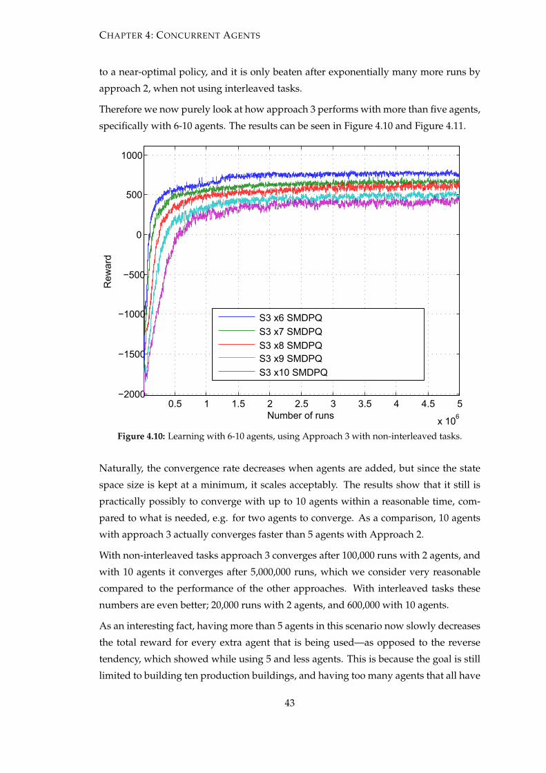
CHAPTER 4: CONCURRENT AGENTS
to a near-optimal policy, and it is only beaten after exponentially many more runs by
approach 2, when not using interleaved tasks.
Therefore we now purely look at how approach 3 performs with more than five agents,
specifically with 6-10 agents. The results can be seen in Figure 4.10 and Figure 4.11.
0.5 1 1.5 2 2.5 3 3.5 4 4.5 5
x 106
−2000
−1500
−1000
−500
0
500
1000
Number of runs
Rew
ard
S3 x6 SMDPQS3 x7 SMDPQS3 x8 SMDPQS3 x9 SMDPQS3 x10 SMDPQ
Figure 4.10: Learning with 6-10 agents, using Approach 3 with non-interleaved tasks.
Naturally, the convergence rate decreases when agents are added, but since the state
space size is kept at a minimum, it scales acceptably. The results show that it still is
practically possibly to converge with up to 10 agents within a reasonable time, com-
pared to what is needed, e.g. for two agents to converge. As a comparison, 10 agents
with approach 3 actually converges faster than 5 agents with Approach 2.
With non-interleaved tasks approach 3 converges after 100,000 runs with 2 agents, and
with 10 agents it converges after 5,000,000 runs, which we consider very reasonable
compared to the performance of the other approaches. With interleaved tasks these
numbers are even better; 20,000 runs with 2 agents, and 600,000 with 10 agents.
As an interesting fact, having more than 5 agents in this scenario now slowly decreases
the total reward for every extra agent that is being used—as opposed to the reverse
tendency, which showed while using 5 and less agents. This is because the goal is still
limited to building ten production buildings, and having too many agents that all have
43

CHAPTER 4: CONCURRENT AGENTS
1 2 3 4 5 6 7 8 9 10
x 105
0
500
1000
1500
Number of runs
Rew
ard
S3 x6 SMDPQ w/ Interleaved tasksS3 x7 SMDPQ w/ Interleaved tasksS3 x8 SMDPQ w/ Interleaved tasksS3 x9 SMDPQ w/ Interleaved tasksS3 x10 SMDPQ w/ Interleaved tasks
Figure 4.11: Learning with 6-10 agents, using Approach 3 with interleaved tasks.
to perform actions means that an excessive amount of economy buildings are being
built.
4.6 Results—Policy Equivalence
We have now shown how the presented concurrency approaches converge, we will
now investigate what differences this leads to in the learned policies. Apart from com-
paring policies learned with varying concurrent state-space information, we also look
into policy differences gained with interleaved tasks and altered time impact on the
reward.
Comparing policies can be a difficult task as all action choices for all the possible states
the agent can be in, have to be compared. A more simple way to compare the policies
learned by our agents could be to compare the rewards received from a single run, this
however does not show any differences between two policies that get the same reward
with different policies. A reasonable middle course is to compare what actions an agent
takes at any given time, during a single run following a policy. This allows us to show a
table view of what each agent is doing at any time for a policy, giving a good overview
for comparison.
The following sections compare policies to illustrate differences in various policies
which were discussed throughout Section 4.5. Each policy is illustrated using a table,
with one row for the actions of each agent, and each cell represents an action. There are
44

CHAPTER 4: CONCURRENT AGENTS
no distinct columns, as the width of each cell represents the time spent on completing
that action. Each cell is labelled with one of three action identifiers, which are defined
as follows: S=resource building (solar), M=resource building (metal), L=production
building (k-bot lab). A blank cell represents an idling agent.
It must be noted that, when comparing the time it takes to reach the goal of the
episodes, it is not important to look at the time it takes to complete all the shown
actions. Since the number of built production buildings is not included in the state-
space, the agent might start to build extra production buildings while completing the
10th, which is the actual goal. Hence, the important time to look at is when the 10th
production buildings has been completed.
4.6.1 Cooperative Information: Full vs. Limited vs. None
Here we look at the impact of cooperative information in the state space on the learned
policy. We use approach 4 for this with i = 1, 2, ∞ , representing none, limited and full
cooperative information, respectively. The policies for this comparison can be seen in
Figure 4.12, Figure 4.13 and Figure 4.14.
This shows that the policies with full cooperative information and limited (i = 2) coop-
erative information are actually very similar, where having full information only shows
a marginally faster solution. Without cooperative information the policy learned is very
poor, spending too much time on building an excessive amount of economy buildings
near the end. This strange behaviour is an example of lacking information in the state-
space resulting in somewhat random behaviour.
Figure 4.12: Full cooperative information
Figure 4.13: Limited cooperative information
45

CHAPTER 4: CONCURRENT AGENTS
Figure 4.14: No cooperative information
4.6.2 5 vs. 10 Agents
As mentioned earlier, solving the problem of building 10 production buildings is op-
timal with 5 agents, because adding more agents forces the agents to build more re-
sources than necessary. Here we illustrate the difference in the policies learned with
5 and 10 agents. The policies for this comparison can be seen in Figure 4.12 from the
previous comparison and Figure 4.15.
Ten agents did in this example-run learn a policy which allows completion of the
episode marginally faster than five agents. However, the initial economy is too weak
to support ten simultaneous actions in the beginning of the episode. This fact can be
seen exemplified when all the agents complete their first action, they spend much more
time on completing these than is necessary later in that episode, or was necessary with
five agents.
Figure 4.15: 10 agents with interleaved tasks
4.6.3 Interleaved Tasks vs. Non-Interleaved Tasks
Here we investigate differences in the policies with interleaved and non-interleaved
tasks. We know that idling time will be introduced with non-interleaved tasks, so it
is impossible for this approach to complete its goal faster than with interleaved tasks,
but it does result in a completed and operational base after each task has terminated.
The interleaved approach does not result in a policy where the construction of produc-
tion buildings is as evenly spread throughout the episode as with non-interleaved, but
still gives a better policy than was possible to achieve with the approach presented in
46

CHAPTER 4: CONCURRENT AGENTS
Chapter 3. This difference could very well change with adjusted weights for the time
and economy reward. The policies for this comparison can be seen in Figure 4.12 from
the earlier comparison and in Figure 4.16.
As expected, the agents take much longer to complete the goal with non-interleaved
tasks. However, as it can be seen in the illustration, the agents have a good base with
both economy and production buildings throughout the complete run. Since the ter-
mination of each task is synchronised, we can also see that it almost always is the first
agents that make the decision to create a production building. This is because the agent
number matches the order in which the agents are asked to take their decision in each
decision epoch. Furthermore, it might seem like a bad policy that within most of the
task completions, more than one agent is building a production building, which results
in the agents actually creating 19 instead of 10 production buildings. This just means
that the economy already is perfect, so it does not really matter what action the agents
choose at this point, and hence chooses to build a production building. Building these
extra buildings does not waste any time, since they will be completed at the exact same
time as the other production buildings being built in that task completion.
Figure 4.16: 5 agents with non-interleaved tasks
4.6.4 Time Impact
In Section 4.5.1 we mentioned how the the weighting of time in the reward function
influences the policy. In this section we look at three policies, where in the first, the
time factor used is the same as in all other results, a negative reward of 1 for each time
step in the game (= a factor of 1/1), and in the others the factor is 1/5 and 1/10. The
policies for this comparison can be seen in Figure 4.12 from the earlier comparison,
Figure 4.17 and Figure 4.18.
The results show that with 1/5 time factor the agents actually learn a policy that
completes the goal faster than the other two. Even though this might seem counter-
intuitive, it is because giving less priority to time, and thereby giving higher priority
to the economy, makes the agents more far-sighted. However, if the time impact is too
small, as seen in policy with the 1/10 factor, the need to also include time becomes
visible, because the agents at this point begin spending more time to solve the goal of
47

CHAPTER 4: CONCURRENT AGENTS
the episode.
Figure 4.17: 5 agents with non-interleaved tasks and 1/5 time impact
Figure 4.18: 5 agents with non-interleaved tasks and 1/10 time impact
4.7 Conclusions and Discussions
In this chapter we showed how much information about concurrent actions should be
represented in the state space in an MSMDP problem using reinforcement learning.
In the scenario in which the experiments were carried out we found the state space
approach that allowed fast convergence to an optimal policy, while allowing very good
scalability in regards to number of concurrent agents. While the scenario is very specific
towards an RTS game subtask, it can still be generalized to other problems involving
concurrent identical agents.
Regarding the state space approaches, it could seem natural to include information
about which action each agent is carrying out (approach 1), but since the agents are
identical, this includes irrelevant information in the state space. Instead we got the best
performance and scalability by only representing how many agents are carrying out
each action (approach 3). Even though this might seem logical for some, we have now
documented the performance differences of these approaches. If this still gives too bad
scalability with too many agents, this approach can be limited even more, by limiting
the agent-count for each action, if a good policy is acceptable instead of the optimal-
policy (approach 4). Finally, we showed that in some cases, where convergence speed
is irrelevant, it might be beneficial to include information about the time remaining for
completing each currently executing action in the state space (approach 2).
Finally we showed how interleaved tasks can be used to solve the somewhat same
problem more efficiently, finding an optimal policy which is better than the optimal
policy found in the problem with non-interleaved tasks. At least in our scenario, the
48

CHAPTER 4: CONCURRENT AGENTS
use of interleaved tasks also made better use of the state space, because the agents are
not forced to make decisions at largely similar game-states, and thereby the economy
state variables can be used as a substitution for concurrency state variables.
For all the approaches discussed here we did comparisons of the policies learned. This
was done since two runs converging to the same reward, does not mean that their poli-
cies are identical. The comparisons were done by comparing action-choices through-
out a complete run for each policy, and this gave a solid base for comparison. We also
showed how significant the time impact is on the reward for our scenario.
49


CHAPTER 5
Parametrised State Spaces
Abstract. We present a novel approach, called parametrised state spaces, to min-
imising the state space in reinforcement learning. This approach can be applied
when the task is to choose one among a large, and potentially varying, number of
similar actions. In this case it means that the task always terminates after having
completed one action. This can be seen in contrast to hierarchical reinforcement
learning, where the decomposition allows us to represent distinct subtasks in each
hierarchy node, and potentially more than one subtask must be terminated before
the parent task can terminate. The parameter values used in a parametrised state
space allow us to perform a large amount of assumptions as well as abstractions,
so we only need to represent state variables pertaining to a single optimal action,
rather than representing all actions in the state-action space.
5.1 Introduction
When dealing with reinforcement learning in complex domains like an RTS game, often
this implies very large state-action spaces. Actually the size of a state space grows
exponentially when new state variables are added. Measures to address this curse of
dimensionality [BM03] need to be invented so that we will be able to efficiently apply
reinforcement learning to complex domains. The curse of dimensionality also affects
the convergence rate, since a very large state space will require many runs in order for
the agent to find an optimal policy.
Previous research has focused on decomposing a state space into a hierarchy of sub-
tasks, e.g. hierarchical reinforcement learning with the MAXQ framework [Die00].
Such a way of minimising a state space assumes that it is possible to clearly divide the
actions in a monolithic state-action space into separate state-action spaces, where each
one only models elements with which the subtask is concerned. This is only possible if
51

CHAPTER 5: PARAMETRISED STATE SPACES
the utility of each action does not depend on all state variables in the state space, or the
state variables on which each action depends, model significantly different elements in
the game world. If this is the case, then the actions can be regarded as dissimilar, and at
least partially, independent actions. They are thus eligible for being decomposed into
separate subtasks each with their own state spaces.
A problem arises if a state-action space contains several very similar and independent
actions, which only differ by a few parameters. Furthermore, if these actions can be
modelled by very similar state variables, also only differing by a few parameters, it is
hard to decompose the state-action space in a way that improves the convergence rate.
A further complication is introduced if a parent task always only needs to execute one
of its child tasks in order to terminate. In a hierarchical approach, one would normally
create the state space of the parent using information about the termination conditions
of several of its child nodes. If always only one of the child nodes need to terminate,
the state space of the parent node can not, e.g. keep track of how far this parent task
is from being completed. Thus it needs to include much more information in its state
space in order to decide between the different children.
A limitation in both flat and hierarchical state spaces is that they force the designer
to put an upper limit on the number of actions. Since games are very dynamic in
their nature, we can easily imagine cases where the number of similar actions can be
arbitrarily large depending on the game state. Such a situation will be extremely hard,
if not impossible, to implement with the traditional flat and hierarchical approaches.
These facts indicate that we need to take a different approach if we want to efficiently
be able to learn in such a domain, where we have to choose between an arbitrarily large
collection of similar independent actions.
In this chapter we propose a novel approach, called parametrised state spaces, to effi-
ciently solve the problem of choosing a single action of a collection of similar actions,
where the single action terminates the overall task. We show how this approach allows
us to minimise a state space, which would otherwise have to include an extremely large
amount of information. The key observation on which our proposition is based, is that
the exponential growth when adding new state variables in a flat state space seems un-
necessary, since we know that the independent actions are very similar in their nature.
We exploit the fact that the actions are similar, and at least partially independent, in or-
der to find a collection of common state variables, which are able to describe the utility
of all these actions. By doing this we avoid having to include separate state variables
modelling each of the similar actions.
In Section 5.2 we will present some of the related work on hierarchical reinforcement
52

CHAPTER 5: PARAMETRISED STATE SPACES
learning, and in Section 5.3 we will describe parametrised state spaces in-depth, as
well as provide some examples to facilitate the understanding of the idea. Section 5.4
compares the size of parametrised state spaces to the size of flat and hierarchical ap-
proaches. In Section 5.5 we describe how we apply parametrised state spaces in a
hierarchy of tasks, and introduce some test scenarios, and in Section 5.6 we discuss the
results of the experiments. Finally in Section 5.7 we conclude on our work and provide
topics for future work on parametrised state spaces.
5.2 Related Work
Hierarchical reinforcement learning refers to the idea of decomposing a complex task
into subtasks to minimise the size of the state space for the various tasks. Designing a
hierarchy of subtasks solving the overall task has been shown to yield a smaller state
space while still ensuring good performance using, e.g. the MAXQ framework [Die00],
later extended to the multi-agent case [MM01], and HAM (Hierarchies of Abstract Ma-
chines) [PR98].
In the MAXQ framework the number of child nodes for each node in the hierarchy is
assumed to be known when designing the hierarchy, i.e. a parent node having three
children means that three subtasks constitute the task of solving the parent task. The
child nodes of a parent task in the hierarchy are assumed to be dissimilar tasks, which
learn based on their own local Q-table and local reward function. Each child node
contributes with its own unique part to solving some overall parent task, and typically
more than one subtask must be completed before the parent task is completed.
Parametrised state spaces differ from normal hierarchical reinforcement learning by ad-
dressing the issue of having to choose among a large, and potentially varying, amount
of similar actions. Completing either of these actions solves the overall task to which a
parametrised state space is applied, meaning that we will not have to complete more
than one of these actions.
5.3 Parametrised State Spaces
Representing a state space in a way that makes it contain a sufficient amount of useful
information, and at the same time minimising its size, is two contradictory goals. The
motivation behind minimising the state space size is to minimise the learning required
(the time to learn) and the space needed for storing the Q-table.
53

CHAPTER 5: PARAMETRISED STATE SPACES
We propose an approach to task decomposition which we call parametrised state
spaces. The main idea behind this is that the agent at each decision epoch has to choose
among a varying amount of similar actions, while avoiding explicitly representing all
those similar actions in the state-action space. Scenarios of this kind can be seen as
multiple-choice scenarios. For a state space including several similar actions, we need
to identify a collection of common state variables which is able to represent the util-
ity of these similar actions, so we do not have to include many closely related state
variables in the state space. The current state of a parametrised state space can be eval-
uated by passing it a collection of parameter values, with which the state variables are
concerned.
5.3.1 Example 1: Magic Boxes
Imagine a scenario where the agent is located in a room that changes state periodically
according to some arbitrary state variables. At each decision epoch the agent has to
open one of a varying amount of magic boxes, and the reward received depends on the
current state of the room, and some details specific to the magic box.
Without a parametrised state space we would have to include an action for each magic
box (thereby putting an upper bound on this number directly in the state space). In
addition we would have to model relevant details about each magic box in the state
space, resulting in a very large state-action space. Assuming that the reward of opening
one magic box does not depend on the state of any of the other magic boxes, it can be
considered a “waste” of state space to include complete information about all magic
boxes, since the actions are similar and independent.
Implementing this scenario in a parametrised state space would allow us to pass the
details of the various magic boxes as a parameter to the state, and then only model
one magic box and some details about the room in the state space. This dramatically
decreases the required number of states and actions in the state-action space. In fact
we have just made the size of the state-action space completely independent of the
number of magic boxes, whereas before it scaled exponentially in the number of boxes.
Parametrising a state space may in some cases allow us to decompose a large prob-
lem into several smaller problems, which means that we can define a state space for
only a small part of the game world and ignore the rest. The higher the degree of in-
dependence between each magic box in our example, the higher the gain of using a
parametrised state space to represent the problem.
54

CHAPTER 5: PARAMETRISED STATE SPACES
5.3.2 State Selection
Given a list of parameter values we evaluate the different possible states, look up action
values in a table and ultimately end up with a specific state and action choice. In
contrast to normal Q-learning where the only task is to select an action, a parametrised
state space also requires that we select a state out of all the possible choices. We may
even apply exploration policies as known from normal Q-learning so that in some cases
we choose a different state than the one that yields the highest expected value (an
exploration step).
5.3.3 Filtering the Game World
In order to apply the idea of parametrised state spaces we need to be able to “filter” the
game world according to a set of parameters, and this logic is application-specific. In
general, the parameters used in the parametrised state space must have some influence
on the returned state.
Parametrising the state space actually allows the agent to filter out a large part of the
game world. When our agent has decided on an action, it is not important to know
any details of other objects in the game world, assuming that the utility of the action
does not depend on the state of any other object in the game world. Thus we omit
this irrelevant information from the state space and only focus on the information that
is important—information specific to whatever game object is given by the parameter
values.
5.3.4 Example 2: Attacking in Balanced Annihilation
In this section we show a small example illustrating the practical use of parametrised
state spaces in Balanced Annihilation.
The illustration in Figure 5.1 represents a situation where our attack group, represented
by the star, can perceive the world in a number of different ways. The dots represent
resource buildings of a particular type, and the shading of the cells indicates the threat
in that cell. Darker shading means more threat. In this example, the agent can choose
three different focuses on the game world—the attack group itself and one of the fol-
lowing:
• The group of resource buildings in the top left cell
• The group of resource buildings in the top right cell
55

CHAPTER 5: PARAMETRISED STATE SPACES
• The group of resource buildings in the bottom left cell
Figure 5.1: A view of a part of the game world. The star represent our attack group
and the dots represent resource buildings of a particular type. The shading
of the cells illustrate the threat in that cell. Darker shading means more
threat.
The three groups of resource buildings are fed as a parameter to the state, so now the
task is to evaluate which choice would return the best value. The agent may choose
one of three different focuses on the game world in relation to the resource buildings: a
single heavily protected resource building, three less heavily protected resource build-
ings, or four resource buildings placed in an area where the enemy has no military
presence. Clearly the best focus will be to consider the game world as consisting of the
four resource buildings in the top left cell, and ignoring all the other resource buildings.
In practice when feeding the locations of the resource buildings to the parametrised
state space, the three configurations are evaluated. The way that the evaluation is done
is that a unique state identifier is calculated based on properties of each of the three
groups in turn and then we perform a lookup in the Q-table. After all the different
states, three in this case, have been evaluated, it would be the action of attacking the
buildings in the top left cell which yields the highest reward. Using parametrised state
spaces allows us to represent all the resource buildings and the threat associated with
their locations in a very compact way since we only need to concern ourselves with a
single group of resource buildings at a time.
5.4 Comparison with Other Approaches
In this section we will compare our parametrised state space design approach to two
other approaches: flat and hierarchical. We use the example from Section 5.3.1 as a
56

CHAPTER 5: PARAMETRISED STATE SPACES
base for the comparison between the different approaches. To ease the comparison we
assume that at all times our agent can take at most three actions and that these actions
are primitive, i.e. we have a room with at most three similar magic boxes. In addition,
we assume that the three actions are independent tasks, where the utility of each action
can be determined by a total of 100 states.
We present a few equations to illustrate various state-action space sizes. In these equa-
tions numChoices means the number of actions (magic boxes), and in f oSize means the
required number of states needed to represent the utility of a single independent action.
5.4.1 Flat State Space
If the state space is flat it means that it must be able to describe an entire task in all its
relevant details and include all the actions the agent is able to take. Since we have three
actions, where the utility of each can be determined by 100 states the total size of the
state-action space is 100 · 100 · 100 · 3 = 300000.
100
100
100
Figure 5.2: Visual representation of a flat state space with three independent actions.
We represent it as a cube because the state space must be able to represent
the utility of three independent actions.
Here we store all information at a single level, and we observe that the state-action
space grows exponentially when we add new independent actions. This will quickly
become too large to handle if we have more than a few independent actions, each need-
ing information specific to that action to represent its utility.
The total size of such a state-action space can be expressed by Equation 5.4.1:
Size f lat = in f oSizenumChoices · numChoices (5.4.1)
5.4.2 Hierarchical State Space
When we have several similar actions it is very hard to decompose the flat state space
into a hierarchy of subtasks since the actions depend on largely similar state variables.
Additionally, in normal hierarchical reinforcement learning several of the subtasks are
partial solutions to the parent task, whereas in our scenario each of the subtasks are
57

CHAPTER 5: PARAMETRISED STATE SPACES
in fact the complete solution to the parent task, but each one yielding very different
utility.
Hierarchical reinforcement learning is very cumbersome to apply to problems of this
type. This is due to the fact that the termination of a single child task is able to terminate
its parent task, thus making it impossible in the parent node to keep track of how far
this parent task is from completion. This means that the parent node would actually
need to model the entire problem in order to be able to choose which of its child nodes
to execute—making it equal to the flat approach in Figure 5.2. Each of the child nodes
constituting the three primitive tasks would be “stateless” since they do not need to
model anything. They simply get a reward from the environment, which is passed
back to the parent node—thus we only add more overhead when applying hierarchical
reinforcement learning to problems of this kind.
Figure 5.3 illustrates the hierarchical decomposition. We have the flat state space at the
top level and primitive tasks as leaf nodes.
1 1 1
100
100
100
Figure 5.3: Visual representation of a hierarchical state space with three independent
actions. At the top level we have a flat state space to indicate the utility of
each subtask. The subtasks are primitive tasks which return immediately.
The total size of such a state-action space can be expressed by Equation 5.4.2:
Sizehierarchical = in f oSizenumChoices · numChoices + numChoices (5.4.2)
An alternative view of the problem may include a selector mechanism as the parent
node. This mechanism will be responsible for choosing which of the subtasks the agent
is going to solve. Each of the subtasks can then be modelled with a state-action space of
100 (1 action and 100 states to represent the utility). The drawback of this approach is
that each of the subtasks will use their own local Q-table, meaning that the first Q-table
represents the utility of opening the first box and so on. Since the three tasks are similar
it can be considered a waste to learn each of the three Q-tables individually, since in fact
the utility of all three subtasks can be learned collectively. This is the main idea behind
58

CHAPTER 5: PARAMETRISED STATE SPACES
parametrised state spaces.
Figure 5.4 illustrates hierarchical decomposition using a selector mechanism. The se-
lector queries its children in order to find out which one is the optimal action given the
current state.
100 100 100
Selector
Figure 5.4: Visual representation of a hierarchical state space with three independent
actions and a selector mechanism. At the top level we have a selector
mechanism which can query each of its child nodes to find out which one
yields the best reward in a given state. Each child node learns its own
Q-table.
5.4.3 Parametrised State Space
With a parametrised state space we can exploit the fact that the tasks are similar, mean-
ing that all subtasks can use the same Q-table and thus share the same state space. This
results in a much smaller state space since we now only need to store information about
a single task in the state space, and we can simply let a state selector perform a lookup
in the Q-table for each possible task to see which is the better task given the current
game world.
Figure 5.5 represents a parametrised state space. At the top level we have a selector
mechanism which can query each of its child nodes to find out which one yields the
best reward in a given state. The various child nodes are not modelled explicitly in
the state space, as illustrated by the dashed lines. Rather, learning is done in a single
Q-table.
The total size of a parametrised state space can be expressed by Equation 5.4.3:
Sizeparametrised = in f oSize (5.4.3)
59
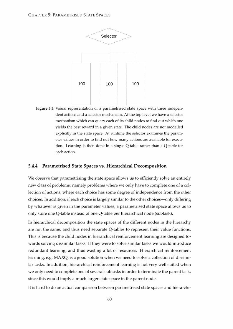
CHAPTER 5: PARAMETRISED STATE SPACES
100 100 100
Selector
Figure 5.5: Visual representation of a parametrised state space with three indepen-
dent actions and a selector mechanism. At the top level we have a selector
mechanism which can query each of its child nodes to find out which one
yields the best reward in a given state. The child nodes are not modelled
explicitly in the state space. At runtime the selector examines the param-
eter values in order to find out how many actions are available for execu-
tion. Learning is then done in a single Q-table rather than a Q-table for
each action.
5.4.4 Parametrised State Spaces vs. Hierarchical Decomposition
We observe that parametrising the state space allows us to efficiently solve an entirely
new class of problems: namely problems where we only have to complete one of a col-
lection of actions, where each choice has some degree of independence from the other
choices. In addition, if each choice is largely similar to the other choices—only differing
by whatever is given in the parameter values, a parametrised state space allows us to
only store one Q-table instead of one Q-table per hierarchical node (subtask).
In hierarchical decomposition the state spaces of the different nodes in the hierarchy
are not the same, and thus need separate Q-tables to represent their value functions.
This is because the child nodes in hierarchical reinforcement learning are designed to-
wards solving dissimilar tasks. If they were to solve similar tasks we would introduce
redundant learning, and thus wasting a lot of resources. Hierarchical reinforcement
learning, e.g. MAXQ, is a good solution when we need to solve a collection of dissimi-
lar tasks. In addition, hierarchical reinforcement learning is not very well suited when
we only need to complete one of several subtasks in order to terminate the parent task,
since this would imply a much larger state space in the parent node.
It is hard to do an actual comparison between parametrised state spaces and hierarchi-
60

CHAPTER 5: PARAMETRISED STATE SPACES
cal reinforcement learning since the two approaches solve two very different classes of
problems, and both are good solutions to the problems they are designed for.
An added bonus is that a parametrised state space is completely independent of the
number of subtasks. The flat and hierarchical approaches can only be applied if we
can guarantee that there will never be more than n subtasks, since we need to model
all subtasks explicitly. Using a parametrised state space allows the number of indepen-
dent similar subtasks to increase or decrease arbitrarily, since the state space is only
concerned with the state of one of these subtasks. The selector mechanism queries
the Q-table a number of times depending on the parameter values, i.e. once for each
unique state we are able to produce from the parameter values, and finally it selects the
action with the highest reward.
5.5 Experiment
In this section we describe how we apply a parametrised state space to some of the
nodes in a hierarchy of tasks. First we describe a simple hierarchy of tasks constituting
the overall task of attacking in Balanced Annihilation. Then we describe how we design
the parametrised state space and show some additional benefits of using such a state
space. We also provide a few test results run in Balanced Annihilation proving that it
is possible to obtain a reasonable policy using parametrised state spaces.
5.5.1 Design of the Hierarchy
The task of attacking in Balanced Annihilation is very complex, and requires the state
space to include much information in order for the agent to make qualified decisions
about what to attack at any given time.
We decompose the various attack actions into a simple hierarchy to gain an overview
of the overall task of attacking in Balanced Annihilation. The hierarchy is by no
means complete—in a full hierarchy we would need, e.g. to include child nodes for
Production, but it illustrates how parametrised state spaces can be applied to some of
the nodes in an already existing hierarchy of reinforcement learning tasks.
At the top level we have four different basic types of targets for our attacks:
1. Enemy resource production buildings
2. Enemy units
61
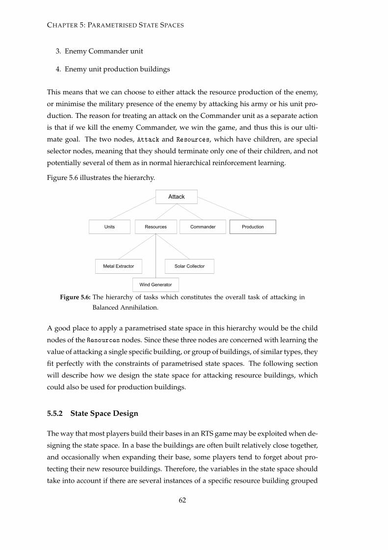
CHAPTER 5: PARAMETRISED STATE SPACES
3. Enemy Commander unit
4. Enemy unit production buildings
This means that we can choose to either attack the resource production of the enemy,
or minimise the military presence of the enemy by attacking his army or his unit pro-
duction. The reason for treating an attack on the Commander unit as a separate action
is that if we kill the enemy Commander, we win the game, and thus this is our ulti-
mate goal. The two nodes, Attack and Resources, which have children, are special
selector nodes, meaning that they should terminate only one of their children, and not
potentially several of them as in normal hierarchical reinforcement learning.
Figure 5.6 illustrates the hierarchy.
ResourcesUnits Commander
Solar Collector
Wind Generator
Metal Extractor
Attack
Production
Figure 5.6: The hierarchy of tasks which constitutes the overall task of attacking in
Balanced Annihilation.
A good place to apply a parametrised state space in this hierarchy would be the child
nodes of the Resources nodes. Since these three nodes are concerned with learning the
value of attacking a single specific building, or group of buildings, of similar types, they
fit perfectly with the constraints of parametrised state spaces. The following section
will describe how we design the state space for attacking resource buildings, which
could also be used for production buildings.
5.5.2 State Space Design
The way that most players build their bases in an RTS game may be exploited when de-
signing the state space. In a base the buildings are often built relatively close together,
and occasionally when expanding their base, some players tend to forget about pro-
tecting their new resource buildings. Therefore, the variables in the state space should
take into account if there are several instances of a specific resource building grouped
62

CHAPTER 5: PARAMETRISED STATE SPACES
closely together, because often this will be the case. In addition we need to consider the
threat at the different locations at which the enemy has constructed resource buildings
in order to find any unprotected buildings.
State Space Explosion
Since we need to include information about threat on the map, this implies the use
of our threat map, which is described in Appendix B. Including the entire threat map
in the state space is infeasible since this would require 464 states (64 threat map cells,
each of which may be in one of four states). This means that we cannot have complete
information about the threat distribution across the map, but we still need to know the
threat level at an arbitrary number of locations on the map.
Including the entire threat map can be avoided when using a parametrised state space
as we shall see in this section. Instead of modelling the location and threat of all re-
source buildings, it will suffice to only model these details of a single group, and let the
state be parametrised by a resource building group. Now the state space is only con-
cerned with one group of resource buildings even though in reality there will be many
more groups of resource buildings, but we do not need to include this information in
the state space.
Imagine that we have already decided on which group we want to attack, then we
do not need to know the threat at various other locations on the map, which does not
influence our attack. Parametrising the state space puts a filter on the game state so we
only need to include the necessary information.
State Space Representation
We represent our parametrised state space as the following variables:
• SizeO f BuildingGroup
• DistanceToGroup
• ImaginaryIn f luenceAtGroup
• SpeedO f MilitaryGroup
• In f luenceAtStartLocation
The first three variables depend on the parameter, i.e. the particular group of resource
buildings currently under consideration. It is obvious that different parameter values
will likely yield different states, and thus different values in the Q-table. The variable
ImaginaryIn f luenceAtGroup is explained in Appendix B.4
63

CHAPTER 5: PARAMETRISED STATE SPACES
Limiting the Number of State Variable Values
Parametrised state spaces may allow further optimisations to the learning process in
terms of state space size. One of the main contributors to the state space size is the
number of unique values each of the state variables in the state space may take. The
different values of the state variables are used as basis for decision making, and thus
we must be very careful when limiting the number of values, since we may accidentally
remove information that is vital for the agent to perform optimally.
Parametrised state spaces may allow us to eliminate certain variable values as seen
in the following example: our SizeO f BuildingGroup variable defined in the previous
section represents the size of a given group of resource buildings. If the size is zero,
it means that the group is empty, and we will not be able to attack it—thus, we can
omit the value zero from this variable, and thereby saving state space size. We can
assume in the state space design that a group of resource buildings will always exist—
if no groups exist we will not have any parameters to pass to the state, thus it will
never be evaluated and will simply be set to a nil-value. In this way we can avoid
wasting room in our state space for states which do not allow our agent to take any
actions. Using a different approach may have forced us to explicitly model the case
where SizeO f BuildingGroup would be zero.
5.5.3 Test Design
Since an attack is treated as an atomic action where learning terminates immediately
after the agent completes a single action, we cannot test convergence speed, nor policy
optimality for parametrised state spaces, compared to other approaches, e.g. flat or
hierarchical reinforcement learning. In fact, comparing parametrised state spaces with,
e.g. flat reinforcement learning is not possible since the resulting state-action space
would simply be too huge. In addition we would need to put some upper limit on
the number of groups of resource buildings we would like to be able to handle, and
thereby limiting the action-space size, since we need one action for each group. The
size of the state space given in Section 5.5.2 is approximately 500, so it would explode
to 500n where n is the maximum number of groups we would like our agent to be able
to handle. If a given game state only has, e.g. 2 groups of resource buildings, and our
state space represents up to 10 groups, this clearly shows that much of the state space
will be wasted using a flat approach. In addition, the size of the state-action space will
be 50010 · 10.
It would only be possible to directly compare the parametrised approach with either
64

CHAPTER 5: PARAMETRISED STATE SPACES
a flat or a hierarchical approach, if we could be certain that we would always have at
most n actions in our game world (and of course assuming that the resulting flat state
space has a manageable size). Since this is not the case for our game world this type of
comparison is not possible here.
Instead we choose to create a few scenarios where we have a single attack group, a
number of enemy units, and some enemy resource buildings. We will then monitor the
decision made by our agent so we can see if this decision could be regarded as optimal
given the scenario. Before running these scenarios we trained our agent against another
agent, which was already developed for Balanced Annihilation.
Scenario 1
Figure 5.7: A scenario illustrating decision making of our reinforcement learning at-
tack agent. The circles represent resource buildings, the star represents our
attack group, and the shading in the tiles illustrate threat. Darker shading
means more threat.
In the first scenario we have three building groups of different sizes. The first thing we
do, is to feed the locations of these buildings to a state selector mechanism. Given the
configuration in Figure 5.7 our agent is able to generate three different states from the
overall global state. Each of these three states corresponds to different state identifiers
which can be looked up in the Q-table to find the best state (the one with the best Q-
value). In this case the optimal decision may be to attack the group to the top left since
it is located in an area with no threat, and so we can expect this action to have the
best Q-value given our reward function. Attacking the other groups may result in our
attack group taking damage, and thus we get a smaller reward from these actions.
65

CHAPTER 5: PARAMETRISED STATE SPACES
Scenario 2
Figure 5.8: Another scenario illustrating decision making of our reinforcement learn-
ing attack agent. The circles represent resource buildings, the star repre-
sents our attack group. There is no threat in any of the cells containing
resource buildings.
In the second scenario, shown in Figure 5.8, our agent is still able to generate three
different states, but this time it is not the amount of threat that decides which group to
attack. A part of the state space definition includes information about how far away a
given group is, and the number of buildings in it. We can expect that in this scenario
the optimal action would be to attack the group to the bottom left of our army, since this
is a large, unprotected group in contrast to the smaller group to the right. The group at
the top left corner will also be a good target for our attack group, but it is likely that it is
not as feasible to attack as the bottom group. This is further explained in Section 5.6.2.
5.6 Results
The reward function used when attacking resource buildings gives reward according
to the amount of damage our attack group took while carrying out the attack action. In
addition reward is given for the amount of buildings that we succeeded in destroying—
destroying more resource buildings yields a greater reward, up to a limit of three since
the SizeO f BuildingGroup state variable is divided into these intervals {1, 2, 3+}, mean-
ing that our state space does not distinguish between, e.g. three and four resource
buildings in the group, so destroying either amount must yield the same reward. A
poor reward is returned if our attack group took a lot of damage while carrying out the
attack.
66

CHAPTER 5: PARAMETRISED STATE SPACES
The exact reward calculation can be seen in Algorithm 2.
Algorithm 1 Code for calculating reward for attacking resource buildings
unitsKilledCounter = GetUnitsKilled()
reward = (unitsKilledCounter/totalUnitsToKill)*100
reward *= (unitsKilledCounter/3)*unitDamageRatio
The unitsKilledCounter variable keeps track of the number of resource buildings we
destroyed in the attack up to a maximum of three. The variable totalUnitsToKill keeps
track of the total number of buildings in the group (also to a maximum of three), and
unitDamageRatio is a variable with values ranging from zero to one indicating how
much damage our group took. A value of one means that no units took damage, and a
value of zero means that all our units were completely destroyed.
Given our constraint of only considering building group sizes of up to three, means that
completely destroying a group of three buildings without taking any damage yields a
reward of 100 (the maximum achievable reward).
5.6.1 Scenario 1
The three states that our agent is able to create from the scenario given in Figure 5.7
yield three different rewards. We will describe the three possible states in the following:
Top Left Group: Attacking this group yields a reward of approximately 33, which
means that each time our agent encountered this state during learning it suc-
ceeded in destroying the building in the nearby group without any of its own
units taking any damage.
Top Right Group: Attacking this group yields a reward of approximately 25 meaning
that we can expect our units to take a lot of damage if we choose to go there. It is
not clear how many of the buildings we may be able to destroy.
Bottom Left Group: Attacking this group yields a reward of approximately 11, mean-
ing that this state is even worse. This is due to the smaller potential pay-off, i.e.
the group of resource buildings is smaller than the top right group.
Our agent chooses to attack the unprotected building because it does not run the risk
of encountering any enemy units, and so it can safely destroy that building.
67
CHAPTER 5: PARAMETRISED STATE SPACES
5.6.2 Scenario 2
It is also possible to generate three unique states from scenario 2 Figure 5.8. The fol-
lowing is a description of the results of this experiment:
Top Right Group: Attacking this group yields a reward of approximately 33. This
means that during learning, each time our agent encountered this state it suc-
ceeded in destroying the one building in the nearby group without any of its
own units taking any damage.
Top Left Group: Attacking this group yields a reward of approximately 80 meaning
that during learning we often succeeded in destroying the entire group of re-
source buildings, but we run the risk that our units may take damage while at-
tacking. This is due to the greater distance they must travel to get to the location—
they may run into enemy units along the way. Apparently this happened during
learning, else we would get a reward of 100.
Bottom Left Group: Attacking this group yields a reward of 100, meaning that every
time we encountered this state we succeeded in destroying all buildings in the
group, without taking any damage.
This scenario illustrates that our agent learns that it may be more dangerous to launch
an attack on a group of resource buildings which is far away compared to a nearby
group. This, of course, is due to the fact that the environment is non-stationary, and so
it may change at any given time, e.g. our attack group may run into a group of enemies
during its travel to the resource buildings.
5.7 Conclusions and Discussions
We have investigated a novel approach to limiting the curse of dimensionality in state-
action spaces when choosing one among an arbitrarily large collection of similar ac-
tions. We showed that our approach, parametrised state spaces, is able to produce a
much smaller state space than what is possible with both a flat, and a hierarchical ap-
proach. When implementing a hierarchical solution with a selector mechanism at the
top level we need to learn separate Q-tables for each of the similar subtasks. When im-
plementing normal hierarchical decomposition for similar subtasks we only make the
collective state space even bigger, because of the fact that the termination of a single
subtask terminates the parent task.
68

CHAPTER 5: PARAMETRISED STATE SPACES
The flat and hierarchical approaches are counter-intuitive to use for problems where we
have to execute one of a collection of similar actions to complete the overall task—they
introduce either redundant learning or much too large state spaces. This proves the
need for an approach like parametrised state spaces. For our scenario, namely attacking
resource buildings in RTS games, we further need to be able to support an arbitrary
number of available actions each having their own distinct utility. This is possible if
using a parametrised state space, and it adds some flexibility to our approach.
We showed how we can exploit the similarity of the tasks, in order to avoid includ-
ing multiple similar Q-tables, and we also showed how this affects the size of the state
space. Finally, we carried out a few experiments to test if the agent has learned a mean-
ingful policy by setting up a few scenarios within Balanced Annihilation. We found
that parametrising the state space allows us to find a good policy.
As possible future work we will need to investigate the possibilities for applying a
parametrised state space to a multi-agent system. Possible solutions could be to include
information about the other concurrent agents as a parameter to the state space, in
order to avoid representing vast amounts of concurrency information directly in the
state space when dealing with a very large multi-agent system.
69


CHAPTER 6
Epilogue
In this chapter we take a look at what was covered in this report, and what contribution
it has made to the field of reinforcement learning. Especially the three central parts of
the report are drawn in, and concluded upon in regards to each other.
Lastly, we consider future work. We describe what needs to be studied in order to be
able to create a fully functioning opponent for a commercial class RTS game.
6.1 Conclusions and Discussions
This report covered many aspects of reinforcement learning in RTS games. In this sec-
tion we give an overview of what was achieved in each area, and how these areas might
be possible to combine.
We started out with applying reinforcement learning to a very simple scenario consist-
ing of a single agent building a base. We showed that by using TRS with Q-learning
it is possible to converge to an optimal policy even though the problem is in fact an
SMDP problem. In addition, applying TRS to the Q-learning algorithm makes it con-
verge much faster in comparison to SMDPQ, since the time penalty works as a heuris-
tic. However, TRS has a number of constraints which must be respected, else it is not
guaranteed that we converge to the same policy as SMDPQ.
Following the simple scenario of building a base with a single agent, we moved on
to expand that to a multi-agent scenario. This required a rework of the state space,
and inclusion of information about concurrent agents in this. We compared four ap-
proaches, each with a varying amount of concurrent information. The results showed
that for concurrent identical agents, in most cases, the optimal concurrent information
is to include the number of agents carrying out each action. Limiting the number of
possible values for each state variable in the concurrent state space could be beneficial
71

CHAPTER 6: EPILOGUE
if an optimal policy is not required, and in some cases including the time remaining for
completion of each action could result in an even better policy.
We came up with a novel approach to representing scenarios where the agent has
to choose between one of many similar actions. Our approach, called parametrised
state spaces, allows us to represent a complex problem in a really compact way. We
showed how our approach differs from a hierarchical approach, and also how the two
paradigms can be combined by applying parameters to some of the nodes in a rein-
forcement learning hierarchy. Parametrised state spaces are especially effective when
the number of similar actions is not known in advance, and can be possibly arbitrarily
large. Such a task is impossible to represent in flat reinforcement learning due to the
state space explosion. If we used hierarchical reinforcement learning, we would either
introduce redundant learning, or make the state space explosion problem even worse.
Thus parametrising the state space allows us to efficiently solve a new class of prob-
lems, namely problems where we have to select one of a large collection of similar and
independent tasks, while still preserving a minimal state space.
Reinforcement learning might be considered overhead to use in some of the discussed
scenarios. Even though convergence is possible, it requires so many trials that it is
infeasible to use for online learning in most RTS scenarios. If it is necessary to do
offline-learning before releasing the agent for a game, then scripting the agent could
probably be easier if the scenario is not too complex. However, even when using off-
line reinforcement learning it is possible to cover many more game states than would
be practically possible to cover with scripted policies. Optimally, using reinforcement
learning, means that no considerations have to be made about any type of game strat-
egy by the developer. As long as the state-action space and reward function is set up
properly, any RTS scenario is possible to solve optimally. Though, in order to do this in
most RTS games, some sort of opponent modelling would also be necessary to include.
We studied some of the important learning problems of an agent for an RTS game,
and found efficient ways to apply reinforcement learning to several of these problems.
While they were exemplified in RTS scenarios, the solutions can easily be generalised to
a wider class of learning problems. Having time as an important factor when learning
a policy, having multiple concurrent agents, and minimising the state space, are all
relevant topics to almost any learning problem.
72

CHAPTER 6: EPILOGUE
6.2 Future Work
We investigated several theoretical aspects of applying reinforcement learning to an
RTS game, and complemented this with some practical examples and test scenarios.
However, more work is needed to have a fully functioning opponent for Balanced An-
nihilation, and there are some theoretical aspects that should be further studied. This
section will discuss some of the key elements which our agent lacks in order to be able
to play Balanced Annihilation.
6.2.1 Building Units
We have not looked into the decision of when and which units to construct. This is an
important task to consider if we were to make a complete RTS opponent, as the right
unit composition can mean success or failure in battle. We would need some clever
higher level decision process that would decide how to allocate resources between unit
and building construction. Furthermore, we would need to decide on what units to
build. This decision module needs to take into account the known enemy units, and
then try to come up with a good counter measure for those.
6.2.2 Attacking
We looked into the problem of what to attack, and this is a very important part of the
decision making in RTS games. But to make a complete RTS agent, we need to know
when to attack, and also how we should control our units in battle, i.e. micromanage-
ment of units. The agent should never attack unless it would improve its position in
the game, so it is important to also find out when to attack. Furthermore, we need to
make sure that the agent controls the units properly when in battle. This includes not
sending the artillery in at the front line and other suboptimal strategies.
6.2.3 Defences
The best defence is a good offence, but sometimes the agent will be forced to rely on its
defences. To be considered a complete RTS opponent, our agent should also be able to
intelligently build and place defensive structures and place its army in well-protected
positions. This however is not a trivial algorithm as the agent will have to consider
paths on the map and the placement of the already existing defences.
73

CHAPTER 6: EPILOGUE
6.2.4 Commander
The RTS agent needs to be able to control the commander as well as a varying number
of workers simultaneously, and we currently do not have support for this. We would
have to handle the commander as a special builder unit, as it builds faster than any
other builder, and thereby uses more resources. We would also need to be able to
determine when it would be beneficial to create another worker, as we start out with
just the commander.
6.2.5 Multiple Agents with Parametrised State Spaces
The combination of concurrent agents and parametrised state spaces could yield inter-
esting results. This would make it possible to implement scenarios where a collection
of similar agents are cooperating to complete one of a collection of similar actions. Hav-
ing multiple agents cooperate using a parametrised state space would make it possible
to solve complex multi-agent SMDP problems with a drastically minimised state space,
thereby allowing an improved convergence rate for such complex problems.
74
APPENDIX A
State Count Calculation
Regarding state space information for concurrent agents, we find that it does not make
sense to keep track of specific agents, when all the agents in the scenario are identical.
This means that we can reduce the state-space significantly, simply by looking at how
many agents are carrying out each action, instead of keeping track of what action each
agent is carrying out.
To calculate the number of states required to represent this information, we use Algo-
rithm 2. This algorithm loops through each combination of agents assigned to actions,
and discards the states that are unreachable or ignorable, thereby only counting the
reachable states. The value returned from the algorithm is this total number of unique
states. The algorithm is called with three arguments: a, i and n. Where a is the the
number of actions, i is the limit of the number of agents that can do a specific action
that we keep track of, and n is the total number of agents.
The possible states found by the algorithm when called with the arguments n = 3, a =
2, i = ∞, can be seen in A.1. The arguments mean that we have to keep track of 2 other
agents, being able to do 2 actions, with no limit on the number of agents we want to
track for each action. This results in 6 states, as the algorithm excludes states that are
unreachable, e.g. where 2 actions are being carried out by 2 agents each (This state is
unreachable as we only keep track of 2 agents and not 4).
If we are only interested in knowing what actions are being carried out, and not how
many agents are carrying out each action, then we could change i to 2. This allows for
two states to be used per action, and the found states would now be the ones shown
in A.2. This results in less states than the previous approach, but we also have less
information represented.
I

APPENDIX A: STATE COUNT CALCULATION
Algorithm 2 Pseudo-code for calculating number of states used by Approach 3 and 4
with identical agents, depending on a, i and n
function calc− states(a, i, n)
bool good = true;
int count = 0;
actions[a] = 0;
while good do
count++;
good = inc(actions, 0, a, i, n);
end while
return count;
end function
function INC(actions, x, a, i, n)
if x >= a then
return f alse;
end if
actions[x]++;
if actions[x] >= i or sumO f Elements(actions) >= n then
actions[x] = 0;
return inc(actions, x + 1, a, i, n);
end if
return true;
end function
Table A.1: States found by calc-states(2,∞,3)
# action1 action2
1 0 0
2 1 0
3 2 0
4 0 1
5 1 1
6 0 2
II

APPENDIX A: STATE COUNT CALCULATION
Table A.2: States found by calc-states(2,2,3)
# action1 action2
1 0 0
2 1 0
3 0 1
4 1 1
A.1 Approach 3 Calculation
In Approach 3 we do not differentiate the agents in the state-space, meaning that we
only keep track of how many agents are executing each action and not what agents
are executing what actions. This can be represented by a number of integers, one for
each action. However the sum of these integers must not be larger than the number of
agents that you are keeping track of, as these states would be unreachable. Algorithm 3
calculates the number of unique reachable states.
Algorithm 3 Pseudo-code for calculating number of states used by Approach 3, de-
pending on a and n
function f3(a, n)
return calc-states(a, ∞, n);
end function
Table A.3 shows the result of running the algorithm with a and n ranging from 0 to 10.
If you compare the table with Pascals triangle you will see that the table just needs a
minor offset adjustments to be identical to Pascals triangle. This means that we can find
a lot simpler way of calculating the total number of states, instead of the comprehensive
algorithm, by using the formula for a cell in Pascals triangle.
III

APPENDIX A: STATE COUNT CALCULATION
a\n 0 1 2 3 4 5 6 7 8 9 10
0 1 1 1 1 1 1 1 1 1 1 1
1 1 1 2 3 4 5 6 7 8 9 10
2 1 1 3 6 10 15 21 28 36 45 55
3 1 1 4 10 20 35 56 84 120 165 220
4 1 1 5 15 35 70 126 210 330 495 715
5 1 1 6 21 56 126 252 462 792 1287 2002
6 1 1 7 28 84 210 462 924 1716 3003 5005
7 1 1 8 36 120 330 792 1716 3432 6435 11440
8 1 1 9 45 165 495 1287 3003 6435 12870 24310
9 1 1 10 55 220 715 2002 5005 11440 24310 48620
10 1 1 11 66 286 1001 3003 8008 19448 43758 92378
Table A.3: Table of the returned state counts found using Algorithm 3 with a and n
ranging from 0 to 10
IV

APPENDIX B
Threat Map
The threat map, is very important when we need to determine which areas on the
battlefield are safe, and which are not. The threat map is layered on top of the real
map, and divides it into a discrete set of cells. Each cell represents the threat that our
agent, and the enemy agent, is able to inflict in that cell.
B.1 Defining Threat
The first question that pops up when designing a threat map is how to define “threat”.
In our case we define it as how threatening we are compared to the opponent at a given
area on the map. The amount of damage depends on the type of enemy units in the
cell, i.e. some units are more powerful against some units than against other units, and
some units are not able to hit each other at all.
To simplify the interface to the threat map, we define four results that a query for threat
in a given cell may return:
1. No enemy threat
2. Inferior
3. Equal
4. Superior
The first case illustrates the situation where the opponent is not able to inflict any dam-
age to our units in a specific cell. All other results should be self-explanatory except in
the case where both sides are able to inflict damage to each other in a given cell. We
define that a side can only be considered superior or inferior if there is at least a 25 %
V

APPENDIX B: THREAT MAP
difference in the amount of damage the two sides are able to inflict. In addition, the
amount of damage itself must exceed a lower threshold. In all other cases, the threat in
the cell is considered equal between the two sides.
B.2 Applying Threat
Special care needs to be taken when both applying and retrieving threat values in the
threat map. E.g. when inserting a unit in a threat map it would be a poor solution to
simply add threat to the single cell that corresponds to the position of the unit. Instead,
we choose to add threat to some of the neighbouring cells as well. The neighbours to
which we should also add threat are determined by the range of the weapons which the
unit carries. If the range of a given weapon allows the unit to shoot as far as the centre
position of a neighbouring cell, threat is added to that cell as illustrated in Figure B.1.
Figure B.1: Illustration of how we apply threat to cells. The black squares illustrate
centres of threat cells. The black dot is the position of a friendly unit, and
the circle is the range of one of its weapons. The blank squares are threat
cells.
In this case threat is added to the two cells which have their centres contained within
the circle.
B.3 Retrieving Threat
When retrieving a threat value for a given cell in the threat map it would give a very
distorted image of the real situation if we simply returned the single value for the given
cell. Instead we take an average over the given cell and all of its immediate neighbours
so that the threat is divided across more cells, allowing our agent to take a safer path
VI

APPENDIX B: THREAT MAP
around a group of really superior units.
Figure B.2 is an example of a threatmap where threat is retrieved as a single large value
stored in a single cell.
Figure B.2: Threatmap with naive threat calculation. The shaded area illustrates
threat. The blank squares illustrate cells with no threat. The black dot
illustrates the position of a friendly unit.
Using such a threatmap would indicate that it is completely safe to move units next
to the area with high threat (where we are inferior). However, if those enemy units
generating the high amount of threat moved just a short distance, we would suddenly
discover that our own units are in a really unsafe place, but at this point it may be too
late (our units may get killed quickly). This threatmap does not take into account the
fact that it is dangerous to have weaker units stand close to superior enemy units.
Figure B.3 is an example of a threatmap where the threat is retrieved as an average of
at most 9 different threat cells (the cell itself, and all its immediate neighbours).
Using such a threatmap allows our agent to recognise a potentially dangerous situa-
tion before it moves any units near a given location. This means that we can use the
threatmap to perform, e.g. advanced pathfinding where we find a safe path to travel
by walking in a safe distance around dangerous positions on the map. Finding a safe
path would be much more difficult with the threatmap illustrated in Figure B.2.
B.4 What-if Analysis
An important functionality of the threatmap is that it should support some degree of
what-if analysis, i.e. we should be able to answer questions such as: “if we moved
group x to this new location how would this change our threatmap?”. This would
VII

APPENDIX B: THREAT MAP
Figure B.3: Threatmap with averaged threat calculation. The shaded areas illustrate
threat. The blank squares illustrate cells with no threat. The black dot
illustrates the position of a friendly unit
allow us to detect if moving a group of units would result in our base being vulnerable
to enemy attacks, and it can also be used to calculate a safe path through the map,
where we avoid confronting any superior enemy units.
VIII

APPENDIX C
References
[AZCT09] Kresten Toftgaard Andersen, Yifeng Zeng, Dennis Dahl Christensen, and
Dung Tran. Experiments with online reinforcement learning in real-time
strategy games. Applied Artificial Intelligence, 23(9):855–871, 2009.
[BM03] Andrew G. Barto and Sridhar Mahadevan. Recent advances in hierarchical
reinforcement learning, 2003.
[CMCV09] Allan Mørk Christensen, Martin Midtgaard, Jeppe Ravn Christiansen, and
Lars Vinther. Reinforcement Learning in RTS Games, 2009.
[CMCV10] Allan Mørk Christensen, Martin Midtgaard, Jeppe Ravn Christiansen, and
Lars Vinther. Time-based Reward Shaping in Real-Time Strategy Games.
In ADMI10, 2010.
[Die00] Thomas G. Dietterich. Hierarchical reinforcement learning with the maxq
value function decomposition, 2000.
[Gho04] Imran Ghory. Reinforcement learning in board games, 2004.
[KPLM96] Kaelbling, L. P., M. L. Littman, and A. W. Moore. Reinforcement learning:
a survey. Artificial Intelligence Research 4, pages 237–285, 1996.
[Lau04] Adam Daniel Laud. Theory and application of reward shaping in rein-
forcement learning, 2004.
[Lit94] Michael L. Littman. Markov games as a framework for multi-agent rein-
forcement learning. In Eleventh International Conference on Machine Learning,
pages 157–163, 1994.
[Man04] Manslow. Using reinforcement learning to solve ai control problems. AI
Game Programming Wisdom 2, pages 591–601, 2004.
IX

APPENDIX C: REFERENCES
[Mat94] Maja J. Mataric. Reward Functions for Accelerated Learning. In Eleventh
International Conference on Machine Learning, pages 181–189, 1994.
[MM01] Rajbala Makar and Sridhar Mahadevan. Hierarchical multi agent reinforce-
ment learning, 2001.
[MMG01] Rajbala Makar, Sridhar Mahadevan, and Mohammad Ghavamzadeh. Hier-
archical multi-agent reinforcement learning. In Eleventh International Con-
ference on Machine Learning, pages 246–253, New York, NY, USA, 2001.
ACM.
[MRLG05] Bhaskara Marthi, Stuart Russell, David Latham, and Carlos Guestrin. Con-
current hierarchical reinforcement learning, 2005.
[NHR99] Andrew Y. Ng, Daishi Harada, and Stuart Russell. Policy invariance under
reward transformations: Theory and application to reward shaping. In
In Proceedings of the Sixteenth International Conference on Machine Learning,
pages 278–287. Morgan Kaufmann, 1999.
[OV09] Robert B. Ollington and Peter W. Vamplew. Concurrent q-learning: Rein-
forcement learning for dynamic goals and environments, 2009.
[PR98] Ronald Parr and Stuart Russell. Reinforcement learning with hierarchies
of machines, 1998.
[RM02] Khashayar Rohanimanesh and Sridhar Mahadevan. Learning to Take Con-
current Actions. In NIPS, pages 1619–1626, 2002.
[RR02] Malcolm Ross and Kinsella Ryan. Hierarchical reinforcement learning: a hy-
brid approach. PhD thesis, The University of New South Wales, New South
Wales, Australia, 2002. Supervisor-Sammut, Claude.
[SB98] Richard S. Sutton and Andrew G. Barto. Reinforcement Learning: An Intro-
duction. MIT Press, 1998.
[SHS+07] Manu Sharma, Michael Holmes, Juan Santamaria, Arya Irani, Charles Is-
bell, and Ashwin Ram. Transfer Learning in Real-Time Strategy Games
Using Hybrid CBR/RL. In 20th international joint conference on Artifical in-
telligence, pages 1041–1046, 2007.
[Tan93] Ming Tan. Multi-agent reinforcement learning: Independent versus coop-
erative agents. In ICML, pages 330–337, 1993.
X

APPENDIX C: REFERENCES
[Tes94] G. Tesauro. Td-gammon, a self-teaching backgammon program, achieves
master-level play. Neural Comput. 6(2), pages 215–219, 1994.
XI


APPENDIX D
CD
The CD contains the following items:
• Report
An electronic copy of the report.
• brAIn
The source code of the reinforcement learning framework developed for Spring:
Balanced Annihilation throughout this project.
• RL-Learner
The simulator used for the experiments done on the base-building scenarios.
Reinforcement learning configuration is done by giving arguments to the exe-
cutable, the proper arguments can be seen by giving the “–help”-argument. The
output of the RL-Learner can both be used for plotting graphs and be handed
to the Policy illustrator. The source code is compatible with both gcc and Visual
Studio.
• Q-Reader
A C# visual viewer for the files containing the Q-tables, generated by both brAIn
and RL-Learner. Includes both the C# source code, and the .NET windows exe-
cutable.
• Policy Illustrator
The JavaScript/HTML script that is used to illustrate a multi-agent base-building
policy in a table overview.
• Utilities
A collection of different utilities created to improve the workflow of experiment-
ing with Reinforcement Learning—including the Maple and MatLab worksheets
XIII

APPENDIX D: CD
for generating the graphs.
• Data
The data files used to plot the graphs included in the report.
XIV


