Embed Size (px)
Citation preview
Approaching nuclear interactionswith lattice QCD
Marc Illa Subiña
PhD advisor:
Dra. Assumpta Parreño García

Approaching nuclear interactionswith lattice QCD
Memòria presentada per optar al grau de doctor per la Universitat de Barcelona
Programa de Doctorat en Física
Autor:Marc Illa Subiña
Directora:Dra. Assumpta Parreño García
Tutor:Dr. Joan Soto i Riera
Departament de Física Quàntica i AstrofísicaInstitut de Ciències del Cosmos
Universitat de Barcelona

Resum
La descripció de les propietats bàsiques dels nuclis a partir dels seus constituents més fonamen-tals, els quarks i els gluons, és un dels principals objectius de la física nuclear, però degut alcomportament singular de QCD a baixes energies, solucions teòriques en aquest rang han estatimpossibles durant molts anys. La finalitat d’aquesta tesi doctoral és l’estudi de les interaccionsentre dos barions, incloent aquells d’estranyesa diferent de zero, els anomenats hiperons, a partirde la teoria fonamental de la interacció forta, la Cromodinàmica Quàntica (QCD). Donat que abaixes energies la constant d’acoblament de QCD adquireix un valor molt gran, no és possibleaplicar les tècniques pertorbatives, i s’han d’utilitzar altres mètodes alternatius. En el nostre cas,fem servir lattice QCD (LQCD), proposat per K. G. Wilson l’any 1974 [1].
Si ens fixem només en el sector dels quarks up i down, els únics quarks estables que formenprotons i neutrons, podem trobar una immensa quantitat de dades experimentals provinents del’estudi de la dispersió de dos nucleons o dels nivells d’energia de nuclis atòmics. Això permetconstruir models fenomenològics que, juntament amb tècniques de sistemes de molts cossos,s’utilitzen per estudiar una gran varietat de problemes. El problema amb aquests models ésque no hi ha una connexió directe amb QCD, fet que va motivar que S. Weinberg, l’any 1990,introduís el concepte de les teories de camp efectives (EFT) [2], que permeten descriure processosen el règim energètic no-pertorbatiu a partir de les simetries inherents de la teoria fonamental,QCD. Tot i aquest avenç, els graus de llibertat que s’utilitzen són components efectius i no elsfonamentals (és a dir, hadrons i no quarks i gluons). El Lagrangià efectiu es construeix a partird’operadors que reflecteixen aquelles simetries, acompanyats de coeficients de baixa energia (LEC),que encapsulen tota la física que no es té en compte de forma explícita, i s’han de determinarajustant els càlculs fets utilitzant EFTs a les dades experimentals corresponents.
Si anem més enllà dels sistemes nuclears convencionals i considerem barions que contenenquarks strange, observem que són inestables i es desintegren mitjançant processos febles. Un delsàmbits científics on els hiperons juguen un paper important és el de l’astrofísica nuclear, ja queaquests són determinants a l’hora d’estudiar l’estructura i dinàmica de les estrelles de neutrons.Nombrosos estudis teòrics demostren que quan s’introdueixen hiperons a l’equació d’estat del’estrella, la seva massa màxima es situa per sota del valor observat (al voltant de dues massessolars), llevat que s’introdueixi una interacció repulsiva entre hiperons i nucleons.
Aquest problema, conegut com hyperon puzzle, ha motivat diverses propostes teòriques per ala seva solució [3–5], i està lligat, per una banda, a la falta de dades experimentals de dispersióentre hiperó-nucleó i hiperó-hiperó que ajudin a determinar amb millor precisió les interaccionsentre barions en el sector estrany, ja que entren necessàriament en la resolució de l’equació d’estat,i per altra, al desconeixement de la força a tres cossos en presència d’hiperons.
Degut a aquestes limitacions, tots els models teòrics fan servir la simetria de sabor SUp3q quepermet relacionar quantitats de les quals tenim dades experimentals a canals menys o totalmentdesconeguts. Per exemple, les dades dels sistemes amb estranyesa 0 i ´1 es poden utilitzar per ferprediccions pels canals amb estranyesa ´2, ´3 i ´4. Com que aquesta simetria és aproximada (elstres quarks no tenen la mateixa massa), la EFT també ha d’incorporar termes que contribueixenal trencament de SUp3q, però degut a la poca quantitat de dades experimentals, només un LECs’ha pogut determinar [6]. El coneixement insatisfactori d’aquestes interaccions fa necessari eldesenvolupament i aplicació de mètodes alternatius, més directes, com és el de LQCD. Aquest
i
formalisme ens permet solucionar les equacions de QCD fent servir un espai-temps discret iutilitzant mètodes numèrics a gran escala. La peculiaritat que fa que LQCD sigui l’eina ideal perinvestigar la interacció hipernuclear forta és que, a diferència del que passa a la natura, podem“desconnectar” la interacció feble i programar únicament el Lagrangià fort, fent que els hiperonses converteixin en partícules estables i eludint la principal complicació en l’estudi experimentald’aquests sistemes. No obstant això, també hi ha obstacles en estudis numèrics d’aquest tipus,com és per exemple la degradació del senyal en sistemes de més d’un barió, fet que comportarealitzar càlculs amb valors de les masses dels quarks lleugers per sobre dels valors físics.
En aquesta tesi demostrem la viabilitat d’aquests tipus de càlculs i la seva importància a l’horad’estudiar sistemes de dos barions (malgrat fer-ho amb unes masses dels quarks up i down quedonen lloc a una massa del pió de 450 MeV), i així determinar les propietats de la interacció, compoden ser els desfasatges de dispersió, els paràmetres de dispersió a baixa energia (longitud dedispersió i rang efectiu), les energies de lligam o els LECs que descriuen la interacció. D’aquestamanera, LQCD pot proveir d’informació que pugui complementar la que obtenim directament deles dades experimentals, i ajudar a delimitar millor els models fenomenològics i teories efectivesde les forces hipernuclears.
L’estructura de la tesi és la següent. Al Capítol 2, hi ha una introducció al formalisme deLQCD, passant primer per la teoria fonamental en el continu, QCD, per després posar-la en elreticle i fer les modificacions necessàries per tal de poder utilitzar les tècniques de Monte Carlo iextreure’n observables. N’hi ha de dos classes: podem calcular les energies d’un sistema (a partirde funcions de correlació de dos punts) i també calcular la interacció del sistema amb un correntextern (a partir de funcions de correlació de tres punts). Per acabar, aquest capítol repassa elmètode de Lüscher [7,8], que ens ajuda a calcular els desfasatges de dispersió i l’energia de lligama partir de les energies extretes quan tenim un sistema dins d’un volum finit.
Al Capítol 3, ens centrem en l’estudi estadístic de les funcions de correlació de dos punts enrelació a l’obtenció dels nivells d’energia. Primer descrivim detalladament l’algoritme que s’hadesenvolupat específicament per ajustar les dades de LQCD a una suma d’exponencials [9]. Pertal de fer una estimació dels errors sistemàtics, fem un estudi exhaustiu variant la quantitat dedades que s’inclouen en l’ajust, així com el nombre d’exponencials. En aquest capítol tambédiscutim altres mètodes que ajuden a reduir la contaminació dels estats excitats, i finalitzemdescrivim diferents mètodes per a l’estimació dels errors de les funcions de correlació.
Al Capítol 4, comencem amb un resum de la situació actual sobre el coneixement, tantexperimental com teòric, de la interacció de dos barions. També repassem tots els càlculs deLQCD realitzats, i comparem els diferents mètodes utilitzats (es poden dividir en dos, el mètodedirecte i el mètode del potencial). A continuació passem a descriure les diferents EFTs que volemestudiar. Donat que estem interessants en el règim de baixa energia, aquestes teories noméscontenen operadors de contacte, sense cap intercanvi de mesons (pionless EFTs). Estudiem doscasos: suposant que hi ha simetria de sabor SUp3q [10, 11], o que hi ha simetria de spin-saborSUp6q [12]. La primera treballa amb valors iguals de les masses dels tres quarks up, down i strange(fet que es pot justificar davant de la gran diferència amb la massa del següent quark més massiu,el charm, „ 1 GeV per sobre de la del strange), i la segona és una predicció en el límit d’un grannúmero de colors (QCD assumeix l’existència de tres càrregues de color). L’última part d’aquestcapítol presenta els resultats principals de la tesi. En concret, estudiem sistemes amb estranyesaentre 0 i ´4, i són NN , ΣN (I “ 32) i ΞΞ amb spin singlet i triplet, ΣΣ (I “ 2) i ΞΣ (I “ 32)amb spin triplet, i ΞN (I “ 0) amb spin singlet. Els càlculs s’han realitzat treballant amb tresvolums diferents (en la direcció espacial, van des de 2.8 fm fins a 5.6 fm) i amb un sol valorde l’espaiat del reticle (0.1167 fm) [13]. Els nivells d’energia de cada volum es poden fer servirper determinar els desfasatges de dispersió utilitzant el formalisme de Lüscher, revelant tretsinteressants sobre la naturalesa de les forces entre dos barions quan les masses dels quarks prenenvalors no físics. Concretament, els paràmetres de dispersió obtinguts ens permeten determinar elsLECs de les EFTs, i en particular els coeficients relacionats amb el trencament de la simetria de
ii
sabor SUp3q. Malgrat la diferència en massa reflectida en el trencament de simetria, els coeficientsobtinguts resulten ser compatibles amb zero, possibilitant l’estudi de la simetria spin-sabor, iobservem que les interaccions entre dos barions presenten simetria SUp6q. Aquesta simetria ja esva observar en un estudi previ [14], on les tres masses dels quarks prenien els mateixos valors,generant un pió amb una massa de „ 806 MeV. Mentre que l’estudi a 806 MeV va posar demanifest la simetria accidental SUp16q, és a dir, que amb un sol LEC es van poder descriure totsels canals d’interacció barió-barió amb estranyesa 0 fins a ´4, en el present estudi a 450 MeV nol’observem amb tanta claredat. Serà interessant veure com evoluciona la manifestació d’aquestessimetries a mesura que ens acostem al punt físic. En aquest capítol també es discuteixen canalspels quals no ha estat possible extreure els paràmetres de dispersió directament de les dadesde LQCD. En aquests casos, hem utilitzat els valors dels LECs determinats prèviament per adeterminar els valors corresponents. Dins d’aquest capítol, també presentem les energies de lligamdels sistemes, i juntament amb els resultats a 806 MeV, les extrapolem fins al valor físic de lesmasses dels quarks utilitzant dues dependències funcionals molt simples per a poder compararamb les prediccions dels models fenomenològics o EFTs, i també observar quina és la tendència amesura que reduïm la massa dels quarks. Per exemple, s’observa el caràcter repulsiu dels canalsΣN p3S1q i ΞΞ p3S1q, tal i com prediuen la majoria de models, com també l’atracció en els canalsΞΣ p1S0q i ΞΞ p1S0q. La dispersió observada entre les diferents prediccions teòriques, així comles conclusions contradictòries a què arriben diferents models, posen de manifest la necessitat derealitzar estudis de LQCD a prop del punt físic en el futur immediat.
Finalment, les conclusions de la tesi es presenten al Capítol 5, seguides d’un conjunt d’apèndixsamb taules i figures que s’han omès en el text principal per facilitar la seva lectura.
iii

iv
Abstract
Nuclei make up the majority of the visible matter in the Universe; obtaining a first principlesdescription of the nuclear properties and interactions between nuclei directly from the underlyingtheory of the strong interaction, Quantum Chromodynamics (QCD), is one of the main goalsof the nuclear physics community. Although the theory was established nearly fifty years ago,the complexities of QCD at low energies precludes analytical solutions of the simplest hadronicsystems, let alone the features of the nuclear forces.
Until the beginning of the century, the only way to overcome this handicap in the low-energyregime was to use phenomenological descriptions of nuclei or effective field theories (EFTs). Whilethey have been very successful, these approaches rely heavily on experimental data. In contrastto what happens in the study of nucleon-nucleon interactions, where the amount of experimentaldata is overwhelming, the study of hadronic systems beyond the up-down quarks sector becomesmore limited. This is because hyperons (baryons containing the next lightest quark, the strangequark) are unstable against weak interaction processes, making the experimental study of theinteraction between hyperons and nucleons, and among hyperons, very difficult.
In this thesis we follow the lattice QCD (LQCD) approach, according to which QCD is solvednon-perturbatively in a discretized space-time via large-scale numerical calculations. Specifically,the interactions between two octet baryons are studied at low energies with larger-than-physicalquark masses corresponding to a pion mass of mπ „ 450 MeV and a kaon mass of mK „ 596MeV. The two-baryon systems that are analyzed have strangeness ranging from S “ 0 to S “ ´4and include the spin-singlet and triplet NN , ΣN (I “ 32), and ΞΞ states, the spin-singlet ΣΣ(I “ 2) and ΞΣ (I “ 32) states, and the spin-triplet ΞN (I “ 0) state.
Due to the inherent large noise in multi-baryon calculations (mitigated by the use of unphysicalquark masses), the finite-volume energies are extracted using a robust fitting methodology, wherein order to reliably estimate the systematic uncertainties, both the fitting form and the fittingrange are varied. Then, the corresponding S-wave scattering phase shifts, low-energy scatteringparameters, and binding energies when applicable, are extracted using Lüscher’s formalism. Whilethe results are consistent with most of the systems being bound at this pion mass, the interactionsin the spin-triplet ΣN and ΞΞ channels are found to be repulsive and do not support bound states.Using results from previous studies of these systems at a larger pion mass, an extrapolation of thebinding energies to the physical point is performed and is compared with available experimentalvalues and phenomenological predictions.
The low-energy coefficients in pionless EFT relevant for two-baryon interactions, includingthose responsible for SUp3q flavor-symmetry breaking, are constrained. The SUp3q flavor sym-metry is observed to hold approximately at the chosen values of the quark masses, as well asthe SUp6q spin-flavor symmetry, predicted at large Nc. A remnant of an accidental SUp16qsymmetry found previously at a larger pion mass is further observed. The SUp6q-symmetricEFT constrained by these LQCD calculations is used to make predictions for two-baryon systemsfor which the low-energy scattering parameters could not be determined within the presentLQCD study, and to constrain the coefficients of all leading SUp3q flavor-symmetric interactions,demonstrating the predictive power of two-baryon EFTs matched to LQCD.
v

vi
Acknowledgements
Primer de tot vull donar les gràcies a la meva directora, l’Assumpta Parreño, per haver-meintroduit en el món màgic de la física hipernuclear, per haver-me inculcat totes les pràctiques queha de seguir un bon investigador, i per haver-me guiat durant més de sis anys, ja des del grau ipassant pel màster. No saps que bé que m’ho he passat fent física amb tu.
I want to thank all the members of the NPLQCD Collaboration, with special mention to SilasBeane, Zohreh Davoudi, William Detmold, Martin Savage, Phiala Shanahan and Mike Wagman.I have learned a lot from you, and I am really grateful for your hospitality during my brief visitsto your institutions. I also want to thank the collaboration for providing me with all the latticedata that is analyzed in this thesis, as well as for the permission to show the figures and resultsthat are already published.
També vull agraïr a la gent del departament de Física Quàntica i Astrofísica i a l’Institut deCiències del Cosmos, en especial a l’Àngels Ramos, en Volodymir Magas, en Bruno Julià, l’ArturPolls, en Javier Menéndez, en Joan Soto, en Federico Mescia i la María Concepción González,juntament amb la Laura Tolós i l’Isaac Vidaña, per ajudar-me sempre que ho he necessitat, i peraportar el seu gra de sorra en el meu desenvolupament.
No puc oblidar-me de la persona que encara no entenc d’on ha tret tanta paciència peraguantar-me al despatx, la Glòria, com també d’en Pere i en Jordi. A tots els companys quehe conegut durant el doctorat, l’Adrià, l’Albert, l’Alejandro, l’Andreu, en Chiranjib, la Clàudia,l’Iván, en Javi, els Joseps i en Marc, com també als companys de grau i màster, en especial al’Adrià, les Anes, la Caterina, la Clara, l’Elena, la Gemma, en Guillem, en Jordi, la Maria, enManel, les Núries, en Pau, en Pere, en Pol, la Sara, en Sergi, en Xavi i la Xènia. Moltes gràcies atots vosaltres per fer-me riure cada dos per tres.
Finalment vull agraïr el suport incondicional que he rebut de la meva família. Sort n’he tingutde vosaltres.
Aquesta tesi s’ha realitzat amb el suport de l’ajut APIF de la Universitat de Barcelona, delprojecte MDM-2014-0369 de l’ICCUB (Unidad de Excelencia “María de Maeztu”) del Ministeriode Economía y Competitividad (MINECO), del contracte FIS2017-87534-P provinent dels fonseuropeus FEDER i del projecte EU STRONG-2020 del programa H2020-INFRAIA-2018-1 (grantagreement No. 824093).
vii

viii
Contents
Resum i
Abstract v
Acknowledgements vii
1 Introduction 1
2 QCD on the computer 52.1 Quantum Chromodynamics . . . . . . . . . . . . . . . . . . . . . . . . . . . . . . 52.2 Discretization of QCD . . . . . . . . . . . . . . . . . . . . . . . . . . . . . . . . . 62.3 Extracting observables . . . . . . . . . . . . . . . . . . . . . . . . . . . . . . . . . 11
2.3.1 Two-point correlation functions . . . . . . . . . . . . . . . . . . . . . . . . 132.3.2 Three-point correlation functions . . . . . . . . . . . . . . . . . . . . . . . 18
2.4 Scattering in finite volume . . . . . . . . . . . . . . . . . . . . . . . . . . . . . . . 222.4.1 Angular momentum group theory . . . . . . . . . . . . . . . . . . . . . . . 232.4.2 Lüscher’s formalism . . . . . . . . . . . . . . . . . . . . . . . . . . . . . . 272.4.3 Binding energy extraction . . . . . . . . . . . . . . . . . . . . . . . . . . . 32
3 Analysis of two-point correlation functions 333.1 Extraction of the ground-state energy . . . . . . . . . . . . . . . . . . . . . . . . 33
3.1.1 Exponential fitting . . . . . . . . . . . . . . . . . . . . . . . . . . . . . . . 333.1.2 Generalized pencil-of-functions method . . . . . . . . . . . . . . . . . . . . 383.1.3 Prony method . . . . . . . . . . . . . . . . . . . . . . . . . . . . . . . . . . 393.1.4 Variational method . . . . . . . . . . . . . . . . . . . . . . . . . . . . . . . 41
3.2 Error estimation . . . . . . . . . . . . . . . . . . . . . . . . . . . . . . . . . . . . 423.2.1 Jackknife method . . . . . . . . . . . . . . . . . . . . . . . . . . . . . . . . 433.2.2 Bootstrap method . . . . . . . . . . . . . . . . . . . . . . . . . . . . . . . 443.2.3 Hodges–Lehmann estimator . . . . . . . . . . . . . . . . . . . . . . . . . . 44
4 The strong baryon-baryon interaction 474.1 Present status . . . . . . . . . . . . . . . . . . . . . . . . . . . . . . . . . . . . . . 474.2 Effective description of two baryons at low energies . . . . . . . . . . . . . . . . . 53
4.2.1 Assuming SUp3q flavor symmetry . . . . . . . . . . . . . . . . . . . . . . . 534.2.2 Assuming SUp6q spin-flavor symmetry . . . . . . . . . . . . . . . . . . . . 574.2.3 Matching the LECs to the scattering amplitude . . . . . . . . . . . . . . . 60
4.3 Lattice results for mπ „ 450 MeV . . . . . . . . . . . . . . . . . . . . . . . . . . . 674.3.1 Low-lying finite-volume spectra of two baryons . . . . . . . . . . . . . . . 684.3.2 Low-energy scattering phase shifts and effective range parameters . . . . . 724.3.3 Binding energies . . . . . . . . . . . . . . . . . . . . . . . . . . . . . . . . 804.3.4 Validity of the extraction of the lowest-lying energies and the corresponding
scattering amplitudes . . . . . . . . . . . . . . . . . . . . . . . . . . . . . 84
ix
4.3.5 Constraints on the EFTs LECs . . . . . . . . . . . . . . . . . . . . . . . . 87
5 Summary and conclusions 95
A Group theory tables 99
B Evaluation of the Z-function 107
C Summary tables of baryon-baryon channels 111
D SUp3q flavor decomposition of two-baryon channels 121
E Partial-wave analysis of the NLO terms in the EFT 127
F On leading flavor-symmetry breaking coefficients in the EFT 131
G Comparison with previous results and low-energy theorems 133
H Supplementary figures and tables of Section 4.3 141
Bibliography 157
x
Chapter 1
Introduction
The description of the basic properties of nuclei from their fundamental constituents, quarksand gluons, is one of the key objectives of nuclear physics. At the most fundamental level, thestrong interaction binds quarks together forming nucleons (N), according to the rules of QuantumChromodynamics (QCD), which combined with Quantum Electrodynamics (QED), the theory ofthe weak interaction, and the much weaker gravity, dictates how elementary particles interactwith each other. For many years, QCD has been elusive to theoretical solutions in the energyregime characterizing nuclear processes. The strength of the interaction between quarks andgluons increases as the characteristic energy of a process decreases [15, 16], and at nuclear scales,perturbative techniques based on coupling expansion cannot be applied to find solutions of thetheory starting from the elementary degrees of freedom.
Since the up and down quarks are the only stable quarks, a vast amount of data fromscattering experiments and spectroscopy are available [17] to constrain theoretical studies ofnuclear properties and interactions. These have proceeded by combining many-body techniqueswith phenomenological models describing the interaction of point-like nucleons [18]. Examples ofsuch successful approaches are the Urbana v14 [19] and Argonne v14 [20] and v18 [21] potentials,or boson-exchange models inspired in Yukawa’s meson theory [22], like the Nijmegen [23, 24], theCD-Bonn [25], and the Stadler-Gross [26] potentials.
Aiming at a model-independent description of the strong interaction, S. Weinberg introducedat the beginning of the 1990s a new formulation [2] which, over the years, has become establishedas an efficient and systematic way of studying nuclear systems from first principles. This effectivefield theory (EFT) approach is especially useful when different energy scales can be identified inthe physical problem under study, and it is based on retaining only those degrees of freedom thatappear explicitly below the largest energy scale that characterizes the process. A small parametercan be then formed from the ratio of the given scales. For example, in the study of NN interactionat low energies, a convenient parameter is constructed from the ratio of the typical momentumcarried by the nucleons to the chiral symmetry breaking scale (approximately the nucleon mass).The effective Lagrangian is then constructed by incorporating all allowed operators respectingthe symmetries of the underlying QCD interactions and organized in increasing order accordingto an expansion in the small parameter, and therefore, as a power expansion on the momentum.Each term of the expansion is accompanied by a low-energy coefficient (LEC) that encapsulatesthe physics that is not explicitly retained, corresponding to energies beyond the largest scaleidentified in the problem, and which is determined by fitting EFT calculations to experimentaldata. Therefore, the predictive power of the method relies mainly on two things: the presence ofsufficiently separated energy scales and the availability of precise experimental data for a givenphysics process. For example, two groups, the Bochum [27,28] and Idaho-Salamanca [29] groups,have precisely extracted the phase shifts for the lowest partial waves and the low-energy scatteringparameters of NN up to fifth order using chiral effective field theory (χEFT), and the sixth orderis being explored [30].
1

2 Chapter 1. Introduction
Beyond nucleons we find hyperons (Y ), particles with at least one strange quark, which areexpected to appear in the interior of neutron stars [31]. The main problem found when dealingwith hyperons is that unless the strong interactions between hyperons and nucleons are sufficientlyrepulsive, the equation of state (EoS) of dense nuclear matter will be softer than for purelynon-strange matter, leading to correspondingly lower maximum values for neutron star masses.While experimental data on scattering cross sections in the majority of the Y N channels are scarce,there are reasonably precise constraints on the interactions in the ΛN channel from scatteringand hypernuclear spectroscopy experiments [32,33], and they indicate that the interactions in thischannel are attractive. Given that the Λ baryon is lighter than the other hyperons, it is likely themost abundant hyperon in the interior of neutron stars. However, models of the EoS includingΛ baryons and attractive ΛN interactions [34] predict a maximum neutron star mass that isbelow the maximum observed mass at 2Md [35–39].1 Several remedies have been suggestedto solve this problem, known in the literature as the “hyperon puzzle” [3–5]. For example, ifhyperons other than the Λ baryon (such as Σ baryons) are present in the interior of neutronstars and the interactions in the corresponding Y N and Y Y channels are sufficiently repulsive,the EoS would become more stiff [41, 42]. Another suggestion is that repulsive interactionsin the Y NN , Y Y N , and Y Y Y channels may render the EoS stiff enough to produce a 2Md
neutron star [34,41,43–45]. Repulsive density-dependent interactions in systems involving the Λand other hyperons have also been suggested, along with the possibility of a phase transitionto quark matter in the interior of neutron stars; see Refs. [3–5] for recent reviews. Given thescarcity or complete lack of experimental data on Y N and Y Y scattering and all three-bodyinteractions involving hyperons, SUp3q flavor symmetry (SUp3qf ) is used to constrain EFTs andphenomenological meson-exchange models of hypernuclear interactions. In this way, quantities inchannels for which experimental data exist can be related via symmetries to those in channelswhich lack such phenomenological constraints. For example, the lowest-order effective interactionsin several channels with strangeness S P t´2,´3,´4u were constrained using experimental dataon pp phase shifts and the Σ`p cross section in the same SUp3qf representation in the frameworkof χEFT in Refs. [6, 46, 47]. However, only a few of the SUp3qf -breaking LECs of the EFT couldbe constrained [6]. To date, the knowledge of these interactions in nature remains unsatisfactory,demanding more direct theoretical approaches.
During the last twenty years major formal, technological, and algorithmic advances haveenabled rigorous exploration of the low-energy regime of QCD using large-scale numericalcalculations. By performing a numerical evaluation of the equations of QCD in a discretizedspace-time, lattice QCD (LQCD) has been used to compute hadronic properties with highprecision, in exceptional cases with more accuracy than that given by experiments [48]. Specificto nuclear physics, it has allowed a wealth of observables, from hadronic spectra and structureto nuclear matrix elements [49–51], to be calculated directly from interactions of quarks andgluons, albeit with uncertainties that are yet to be fully controlled. In the context of constraininghypernuclear interactions, LQCD is a powerful theoretical tool because the lowest-lying hyperonsare stable when only strong interactions are included in the computation, circumventing thelimitations faced by experiments on hyperons and hypernuclei. Nonetheless, LQCD studies inthe multi-baryon sector require large computing resources as there is an inherent signal-to-noisedegradation present in the correlation functions of baryons [52–57], among other issues as discussedin a recent review [51]. Consequently, most studies of two-baryon systems to date [13,14,56,58–79]have used larger-than-physical quark masses to expedite computations, and only recently haveresults at the physical values of the quark masses emerged [80–82], making it possible to directlycompare with experimental data [83]. The existing studies are primarily based on two distinctapproaches. In one approach, the low-lying spectra of two baryons in finite spatial volumes are
1Very recently, the gravitational wave signal GW190814, originated from the merger of a 23Md black hole anda 2.6Md compact object, was reported [40], where the nature of the compact object is a subject of discussion. Ifthis compact object was a neutron star, it would have been the most massive one known, imposing a mass-limitconstraint very difficult to fulfill for the majority of existing nuclear EoS models.
3
determined from the time dependence of Euclidean correlation functions computed with LQCD,and are then converted to scattering amplitudes at the corresponding energies through the use ofLüscher’s formula [7, 8] or its generalizations [84–100]. In another approach, non-local potentialsare constructed based on the Bethe-Salpeter wavefunctions determined from LQCD correlationfunctions, and are subsequently used in the Lippmann-Schwinger equation to solve for scatteringphase shifts [101].
While LQCD studies at unphysical values of the quark masses already shed light on theunderstanding of (hyper)nuclear and dense-matter physics, a full account of all systematicuncertainties, including precise extrapolations to the physical quark mass, is required to furtherimpact phenomenology. Additionally, LQCD results for scattering amplitudes can be used tobetter constrain the low-energy interactions within given phenomenological models and applicableEFTs. In the case of exact SUp3qf symmetry and including only the lowest-lying octet baryons,there are six two-baryon interactions at leading order (LO) in pionless EFT [102,103] that canbe constrained by the S-wave scattering lengths in two-baryon scattering [10]. LQCD has beenused in Ref. [14] to constrain the corresponding LECs of these interactions by computing theS-wave scattering parameters of two baryons at an SUp3q flavor-symmetric point with mπ „ 806MeV. Strikingly, the first evidence of a long-predicted SUp6q spin-flavor symmetry in nuclear andhypernuclear interactions in the limit of a large number of colors (Nc) [12] was observed in thatstudy, along with an accidental SUp16q symmetry. This extended symmetry has been suggestedin Ref. [104] to support the conjecture of entanglement suppression in nuclear and hypernuclearforces at low energies, pointing to intriguing aspects of strong interactions in nature.
The objective of this thesis is to extend the previous studies to quark masses that are closerto their physical values, corresponding to a pion mass of „ 450 MeV and a kaon mass of „ 596MeV, and further to study these systems in a setting with broken SUp3qf symmetry as is thecase in nature. Therefore, it provides new constraints that allow preliminary extrapolations tophysical quark masses to be performed, and complements previous independent LQCD studiesat nearby quark masses [56, 58–60, 62, 63, 66, 69, 70, 73, 74]. The LQCD results presented hereare used to constrain the leading SUp3qf symmetry-breaking coefficients in pionless EFT. ThisEFT matching enables the exploration of large-Nc predictions, pointing to the validity of SUp6qspin-flavor symmetry at this pion mass as well, and revealing a remnant of an accidental SUp16qsymmetry that was observed at a larger pion mass in Ref. [14]. Strategies to make use of theQCD-constrained EFTs to advance the ab initio many-body studies of larger hypernuclear isotopesand dense nuclear matter are beyond the scope of this work. Nevertheless, the methods appliedin Refs. [105–107] to connect the results of LQCD calculations to higher-mass nuclei can also beapplied in the hypernuclear sector using the results presented.
The structure of this theses is organized as follows. Chapter 2 gives a brief introduction of QCD,followed by a description of the LQCD method. For that, the discretization of QCD is explained,together with the observables that can be extracted (energies and matrix elements). Finally,the study of scattering processes in finite volume is detailed, with an appropriate summaryof the necessary group-theoretical tools. Chapter 3 is devoted to the main tools to analyzethe correlation functions, including several more sophisticated methods to reduce excited-statecontamination. Chapter 4 is focused on the baryon-baryon interaction. First, a summary of thepresent status of the field, both experimentally and theoretically, is presented. After the EFTLagrangians that will be constrained are explained, the main LQCD results are showed, whichare the lowest-lying energies, the S-wave scattering parameters, and the binding energies (with apreliminary extrapolation to the physical point) of several two-baryons channels, followed by theconstraints that these results impose on the LECs of the EFTs. To conclude the thesis, Chapter 5summarizes the work. Several appendices follow to supplement the thesis, omitted from the mainbody for clarity of presentation. Appendix A shows all the relevant group-theoretical relationsbetween the point (and double) and continuum angular momentum groups relevant for the statesstudied in this work. Appendix B presents the derivation of the exponentially-accelerated version
4 Chapter 1. Introduction
of the Z-function. Appendix C tabulates the scattering parameters predicted by the availabletheoretical models for the baryon-baryon channels studied in this thesis, as well as the bindingenergies extracted from fully-dynamical LQCD calculations. Appendix D explicitly states the fullSUp3qf decomposition of all octet baryon-baryon channels. Appendix E contains the partial-wavedecomposition of all the next-to-leading order (NLO) terms that appear in the Lagrangian ofRef. [11]. Appendix F includes relations among the LECs of the three-flavor EFT Lagrangianof Ref. [11] and the ones used in the present work, as well as a recipe to access the full set ofleading symmetry-breaking coefficients from future studies of a more complete set of two-baryonsystems. Appendix G presents an exhaustive comparison between the results obtained in thiswork and previous results presented in Ref. [66] for the two-nucleon channels using the sameLQCD correlation functions, as well as with the predictions of the low-energy theorems analyzedin Ref. [108]. Appendix H contains additional figures and tables related to the LQCD resultspresented in Section 4.3.
Chapter 2
QCD on the computer
2.1 Quantum Chromodynamics
More than two centuries have passed since the beginning of nuclear physics, with the accidentaldiscovery of radioactivity by H. Becquerel in 1896. A great deal of experiments and theoreticalbreakthroughs were needed to pinpoint the fundamental forces behind very distinct processes andelaborate what we know today as the Standard Model (SM). Some of these milestones, relevantfor this thesis, are the first proposal for the description of the strong force by H. Yukawa [22], thediscovery of the first strange particles, the K0 meson1 by G. D. Rochester and C. C. Butler [109]and the Λ baryon by V. D. Hopper and S. Biswas [110]. In order to understand and organizethe large number of particles discovered, the eightfold way was proposed by M. Gell-Mann [111]and Y. Ne’eman [112], followed by the more fundamental quark model by M. Gell-Mann [113]and Z. Zweig [114]. The proposal of a new quantum number, later on called color charge, byW. Greenberg [115], M. Y. Han, and Y. Nambu [116], was one of the last steps before the definitionof the QCD Lagrangian by H. Fritzsch, M. Gell-Mann, and H. Leutwyler [117].
From that point forward, it is known that the degrees of freedom of QCD are quarks andgluons. Mathematically, the quarks are spin-1
2 Dirac spinors α P t1, 2, 3, 4u that carry colora P t1, 2, 3u and flavor q P tup, down, strange, charm, bottom, topu indices, ψaq,α, and transformunder the fundamental (triplet) representation of SUp3qc as
ψpxq Ñ ψ1pxq “ Ωpxqψpxq “ e´igθapxqTaψpxq , with Ωpxq P SUp3qc , (2.1)
where g is the strong coupling constant, θapxq is the parameter of the transformation that dependson the position (to account for the local gauge invariance), and Ta are the generators of the SUp3qcLie algebra, with a P t1, . . . , 8u (the number of SUpNq generators equals the dimension of theadjoint representation, N2 ´ 1 “ 8 for N “ 3), which can be written as Ta “ λa2, with λa beingthe Gell-Mann matrices [118]. These generators are traceless Hermitian matrices, normalizedsuch that TrpTaTbq “
12δab, obeying the commutation relation rTa, Tbs “ ifabcTc, where fabc are
the structure constants of SUp3qc.The mediators of the interaction, the gluons, are spin-1 gauge bosons that are usually written
as Aµ “ TaAaµ. They transform under the adjoint (octet) representation of SUp3qc as
Aµpxq Ñ A1µpxq “ ΩpxqAµpxqΩ:pxq `
i
g
“
BµΩpxq‰
Ω:pxq . (2.2)
The Lagrangian of QCD has to be invariant under these local gauge transformations, and it canbe written as
LQCD “ÿ
q
ψq`
iγµDµ ´mq
˘
ψq ´1
4GaµνG
a,µν , (2.3)
1That is the reason why the strangeness quantum number is negative, since the kaon was given S “ 1 althoughit carries an anti-strange quark.
5
6 Chapter 2. QCD on the computer
where γµ are the Dirac matrices, mq are the masses of the quarks, and the covariant derivativeDµ contains the term that couples the quark and gluons, Dµ “ Bµ ` igTaA
aµ.
The purely gluonic part is written in terms of the gluon field strength tensor Gaµν “ BµA
aν ´
BνAaµ ´ gfabcA
bµA
cν , where the last term is characteristic of non-Abelian theories (no such term
appears in the QED Lagrangian), and is responsible for the three- and four-gluon self-interactions.The reason why these types of interactions appear is due to the fact that the gluon is chargedwith color (the photon does not have electric charge), so it is able to interact with other chargedparticles, like quarks and other gluons. Since a term of the form mgAµA
µ is not gauge invariant,gluons are massless particles.
Another term that we have not included in Eq. (2.3) but is allowed by gauge invariance isone proportional to θεµνρωGa
µνGaρω, known as the θ-term. This term, unlike the others, violates
CP-symmetry, and the value of θ (specifically, the combination θ1 “ θ ` arg detmq) has beenconstrained experimentally with the electric dipole moment of the neutron, giving an upper limitof |θ1| À 10´10 [119]. The reason why the value of θ is so small is still not understood, and itis known as the strong CP problem. There are additional terms in the Lagrangian of Eq. (2.3),such as the gauge fixing term (with the fictitious Faddeev-Popov ghosts) and the correspondingcounterterms, but they are not relevant for the subject of this thesis, LQCD [120].
One of the most striking features of QCD is how the value of g depends on the energy scaleof the process. This is known as asymptotic freedom, and it was discovered by D. J. Gross,F. Wilczek [15], and H. D. Politzer [16] (the three of them were awarded the Nobel Prize inPhysics in 2004). At very high energies (or very small distances) the coupling constant becomessmall, so the quarks and gluons interact very weakly, and perturbation theory can be used tostudy processes in this energy regime. However, at low energies the situation is the opposite,with g increasing in value as the energy decreases to the point where g „ Op1q (around ΛQCD)and perturbation techniques are no longer adequate. In this regime, the quarks and gluons arebound inside color-singlet hadrons, known as confinement. The most common hadrons are themesons (pair of quark-antiquark) and baryons (three quarks), although more exotic ones, likepentaquarks or glueballs, are not prohibited by QCD.
Since perturbation theory is no longer applicable at low energies, several alternative methodsand models have been developed to circumvent this problem. Examples are the use of phenomeno-logical models and EFTs for the nuclear sector as mentioned in Chapter 1. The one we will focuson in this thesis is LQCD, the only non-perturbative method in which quantities are computeddirectly using quarks and gluons, and is systematically improvable.
2.2 Discretization of QCD
The formalism of LQCD was first introduced by K. G. Wilson [1], and it is based on the pathintegral formalism of R. P. Feynman [121], where observables are computed as vacuum expectationvalues of operators,
xOy “1
Z
ż
DψDψDAµ O eiSQCD , (2.4)
with Z being the QCD partition function, Z “ş
DψDψDAµ eiSQCD , and SQCD the QCD action,SQCD “
ş
d4xLQCD.Notice that this formalism resembles the one used in statistical mechanics (see Ref. [120])
except the imaginary unit in the exponential, which renders an oscillatory factor, troublesomefor numerical evaluations. A solution to this problem is to perform a Wick rotation [122], whichtransforms the p3 ` 1q-dimensional Minkowski field theory to a 4-dimensional Euclidean field
2.2. Discretization of QCD 7
theory. Under this rotation,
ηµν “ diagp`1,´1,´1,´1q Ñ ηpEqµν “ δµν “ diagp`1,`1,`1,`1q
t “ x0 Ñ ´ixpEq4 “ ´iτ , xi Ñ x
pEqi , with i P t1, 2, 3u ,
B0 Ñ iBpEq4 , Bi Ñ B
pEqi ,
γ0 Ñ γ4pEq , γi Ñ iγipEq ,
A0 Ñ iApEq4 , Ai Ñ A
pEqi .
(2.5)
Note that, with the new metric tensor ηpEqµν , in Euclidean space-time one does not need to worryabout the position of the indices, since there will be no extra ´1 factors when raising or loweringthem. If we apply these changes to Eq. (2.3), the QCD Lagrangian becomes
LQCD “ÿ
q
ψq`
iγµDµ ´mq
˘
ψq ´1
4GaµνG
a,µν
“ÿ
q
ψq`
iγ0D0 ` iγiDi ´mq
˘
ψq ´1
4
`
´Ga0iG
a0i `G
aijG
aij
˘
Ñ´ÿ
q
ψq
´
γpEq4 D
pEq4 ` γ
pEqi D
pEqi `mq
¯
ψq ´1
4
´
GpEqa4i G
pEqa4i `G
pEqaij G
pEqaij
¯
“ ´
«
ÿ
q
ψq
´
γpEqµ D
pEqµ `mq
¯
ψq `1
4GpEqaµν G
pEqaµν
ff
“ ´LpEqQCD ,
(2.6)
and the Euclidean QCD action is expressed as
SQCD “
ż
d4xLQCD Ñż
p´iqdτ
ż
d3x p´LpEqQCDq “ i
ż
d4xpEq LpEqQCD “ iSpEqQCD , (2.7)
making the phase in Eq. (2.4) real. Therefore, and omitting the superscript pEq for simplicity,
xOy “1
Z
ż
DψDψDAµ O e´SQCD . (2.8)
Similar changes occur in the partition function. With the current form, one can identify e´SQCDas a probability distribution function and apply Monte Carlo methods to perform this multi-dimensional integral. Before we get to this point, we have to discretize SQCD.2
The simplest way to discretize QCD is by using an isotropic hypercubic lattice Λ,
Λ “!
xµ “ px1, x2, x3, x4 “ τqˇ
ˇ
ˇ0 ď x1, x2, x3 ă L , 0 ď x4 ă T
)
, (2.9)
where L is the spatial extent and T is the temporal extent (with total volume V “ L3 ˆ T ). Thelattice spacing b in this case is the same in both directions.3 The discretization of QCD has twopurposes: to make it amenable for computational calculations, and to introduce an ultravioletcutoff (inverse of the lattice spacing), regularizing the theory. As will be discussed later, tomake the connection to the physical world, the limits of zero lattice spacing bÑ 0 and infinitevolume LÑ8 have to be taken. The calculations with non-zero b and finite L have to be chosencarefully: the mesh has to be fine enough so that it resolves the hadronic scale (b ! ΛQCD), andthe spatial extent must be large compared to the typical range of the hadronic interactions understudy, which is set by the Compton wavelength of the lightest particle exchanged (for the NNinteraction, this implies L " m´1
π ).2For a complete introduction and development of lattice gauge theories, see Refs. [123–127].3Other types of geometries are also used, like anisotropic lattices (where the temporal extent has a finer lattice
spacing) [128,129] or asymmetric lattices [130,131].
8 Chapter 2. QCD on the computer
Within this formulation, the quarks, spin-12 objects with Dirac, color, and flavor indices, reside
on the nodes of the lattice, ψpxq. Due to the finite volume, boundary conditions (BC) are appliedto both fields, quarks and gluons (discussed with more detail below). On the spatial direction,one typically applies periodic BC to both fields, although more sophisticated choices, like twistedBC [86,132], are also possible. For the temporal direction, anti-periodic BC are imposed to thequarks (that are fermions) while periodic BC are imposed to gluons (bosons), so as to ensure thecorrect statistics.
To illustrate some of the problems inherent in the discretization method, we discuss belowthe simplest approximation, the so-called naive discretization, for the free quark case, for whichthe QCD action reads
ż
d4x ψpxqpγµBµ `mqψpxq Ñ b4ÿ
xPΛ
ψpxq
"
γµ1
2brψpx` µq ´ ψpx´ µqs `mψpxq
*
, (2.10)
where the integral is now a sum over the lattice sites, and the derivative has been discretized bya symmetric finite difference. We can further simplify this expression by using the Dirac operatorMpx, yq,
b4ÿ
x,yPΛ
ψpxq
„
γµ1
2b
`
δx`µ,y ´ δx´µ,y˘
`mδx,y
ψpyq “ b4ÿ
x,yPΛ
ψpxqMpx, yqψpyq . (2.11)
To look at the spectrum, it is easier to go to momentum space,
δx,y “
ż πb
´πb
d4p
p2πq4eippx´yq , (2.12)
where the limits of the integration correspond to the first Brillouin zone (BZ), p´πb, πbs. TheDirac matrix can thus be written as
Mppq “ γµ1
2b
´
eipµb ´ e´ipµb¯
`m “i
bγµ sinppµbq `m, (2.13)
whose inverse is related to the quark propagator,
M´1ppq “1
ibγ
µ sinppµbq `m“´ ibγ
µ sinppµbq `m1b2
sin2ppµbq `m2. (2.14)
In the limit mÑ 0, the poles of the propagator one finds are the usual pµ “ p0, 0, 0, 0q, expectedin the continuum theory, plus 15 unphysical poles at the corners of the BZ, pµ P tpπb , 0, 0, 0q, . . . ,pπb ,
πb ,
πb ,
πb qu. These extra poles are the so-called doublers and are purely lattice artifacts [133].
The reason these doublers appear is explained by the Nielsen-Ninomiya no-go theorem [134],which states that one cannot define an Hermitian, translational invariant, local, and chirallysymmetric lattice regularized gauge theory without doublers.
There are several ways to remove these unwanted states. Since in Chapter 4 the lattice resultsshown are computed using the Wilson approach [133], we will focus on this one, and the rest willonly be mentioned. The proposed solution by Wilson consisted in adding the following irrelevantoperator, ´1
2brψBµBµψ , with r being the Wilson parameter, which is usually set to 1 (note that
the added term vanishes in the limit bÑ 0). The corresponding discretized version is
´r
2bψpxq
`
δx`µ,y ´ 2δx,y ` δx´µ,y˘
ψpyq , (2.15)
with the momentum-space Dirac operator being
Mppq “i
bγµ sinppµbq `
r
b
ÿ
µ
r1´ cosppµbqs `m. (2.16)
2.2. Discretization of QCD 9
If we compute the propagator and look at the poles, we see that the original pole is undisturbed,while the doublers acquire an extra factor proportional to rb, which in the continuum limit willbecome infinitely massive and decouple from the theory. The usual way to write the (free) Wilsonaction is in terms of κ “ p2mb` 8rq´1,
SW “ b4ÿ
x,yPΛ
ψpxqMpx, yqψpyq , Mpx, yq “ δx,y´κ“
pr ´ γµqδx`µ,y ` pr ` γµqδx´µ,y
‰
, (2.17)
where we have redefined ψ Ñ?
2κbψ.We are ready now to introduce the gluons into the calculation in a gauge invariant way. Finite
differences contain terms like ψpxqψpx` µq, which transform like
ψpxqψpx` µq Ñ ψ1pxqψ1px` µq “ ψpxqΩ:pxqΩpx` µqψpx` µq ‰ ψpxqψpx` µq . (2.18)
For these terms to be invariant under a local gauge transformation, we need to introduce anadditional field, Uµpxq, transforming as
Uµpxq Ñ U 1µpxq “ ΩpxqUµpxqΩ:px` µq . (2.19)
Now ψpxqUµpxqψpx` µq is invariant under local gauge transformation. In the continuum, suchobject already exists, and is the path-ordered exponential integral of the gauge field Aµ along acurve C connecting two points x and y,
Upx, yq “ P eigş
C A¨dl . (2.20)
Therefore, we can interpret Uµpxq, named link variables, as the lattice version of the gaugetransporter connecting the points x and x` µ, taking the following form Uµpxq “ eigbAµpxq, withU :
µpxq “ U´µpx´ µq. Then, the Dirac operator of the (gauge-invariant) Wilson action is
Mpx, yq “ δx,y ´ κ“
p1´ γµqUµpxqδx`µ,y ` p1` γµqU´µpxqδx´µ,y
‰
. (2.21)
An important property of this operator is the γ5-hermiticity, which implies γ5Mpx, yqγ5 “
M :py, xq. This property will come in handy later, when dealing with propagators and correlation
functions for mesons, but most importantly it forces the determinant of Mpx, yq to be real.The Wilson action is only correct up to Opbq discretization errors. To improve the situation
(avoiding calculations with very small b), one can introduce higher-dimensional operators to theaction that cancel the Opbq errors. This is known as the Symanzik improvement program [135].For the Wilson action, this correction was computed by B. Sheikholeslami and R. Wohlert [136]by adding the following operator,
SSW “ SW ´ b5cSWÿ
xPΛ
ψpxq1
2κσµνGµνpxqψpxq , (2.22)
where the coefficient cSW has to be tuned so that it cancels the Opbq errors [137], σµν “ rγµ, γνs2,and Gµνpxq is the gluon field strength tensor. This term is usually called the clover term due tothe way Gµνpxq is discretized, resembling a clover leaf,
Qµνpxq “ ,Gµνpxq “
18
“
Qµνpxq ´Qνµpxq‰
,
Qµνpxq “ Pµνpxq ` Pν´µpxq ` P´νµpxq ` P´µ´νpxq .(2.23)
The objects Pµνpxq are called the plaquettes, and will be discussed later, in the context of thediscretization of the purely-gluonic action.
This clover-improved action, although it removes the problem of the doublers, breaks chiralsymmetry explicitly. Despite this, it is widely used in the LQCD community, resulting in some
10 Chapter 2. QCD on the computer
remarkable results. As an example, the BMW Collaboration has computed the mass-splittingsbetween iso-multiplets [138] in total agreement with experimental data, and in some cases withbetter precision.
As mentioned before, there are alternative ways to remove the doublers besides the Wilsonapproach. These are summarized below:
– Twisted-mass fermions [139, 140] are a variant of the Wilson fermions, where the quarksare rotated in flavor space by some angle, which can be tuned to remove the Opbq latticeartifacts. However, it breaks isospin symmetry (see Ref. [141]). Using this formulation, theETM Collaboration was able, for example, to make a full flavor decomposition of the spinand momentum fraction of the proton [142].
– Staggered fermions [143] do not remove explicitly the doublers, but simply re-distributethem among lattice sites, leaving in the end 4 doublers (called tastes, similar to flavors butunphysical), which are removed using the so-called “fourth-root procedure” (see Ref. [144]).These types of fermions are used, for example, to study thermodynamical properties, likethe QCD equation of state [145,146].
– Domain-wall [147–150] and overlap fermions [151,152] are formulations whose main purposeis to maintain chiral symmetry (more specifically, a lattice version of it, known as theGinsparg–Wilson equation [153]) at the cost, for example, of adding an extra dimension forthe case of domain-wall. The main problem with these formulations is that they are 10´100times computationally more expensive than the rest. As an example, the RBC/UKQCDCollaboration used domain-wall fermions to compute the K Ñ ππ decay [154].
Now we can focus on the discretization of the gauge part of the action. To maintain gaugeinvariance, we have introduced the link variables Uµpxq, which are related to the Aµ fields.Working with only link variables, the only gauge invariant object is the trace of a path orderedclosed loop, also called Wilson loop, TrWµ¨¨¨νpxq “ TrrUµpxq ¨ ¨ ¨U
:
νpxqs. The simplest case is theplaquette (introduced previously for the clover term), which has the following form,
Pµνpxq “ , Pµνpxq “ UµpxqUνpx` µqU:
µpx` νqU:
νpxq . (2.24)
With this simple loop, we can write the action asż
d4x1
4GaµνG
a,µν Ñ βÿ
xPΛ
ÿ
µăν
Re Tr1
3
“
1´ Pµνpxq‰
, (2.25)
where β “ 6g2. It can be shown (using the Baker-Campbell-Hausdorff formula and performinga Taylor expansion of Aµ around n) that the discretized version is correct up to Opb2q. TheSymanzik improvement program [135] can also be applied here, where now the higher-dimensionaloperators correspond to larger Wilson loops, which for the case of the Lüscher-Weisz action [155]correspond to rectangular and parallelogram-shaped loops (besides the plaquette),
Pplpxq “
Rrtpxq “
Gpgpxq “
SLW “ βÿ
xPΛ
!
ÿ
pl
c0 Re Tr1
3
“
1´ Pplpxq‰
`ÿ
rt
c1 Re Tr1
3r1´Rrtpxqs
`ÿ
pg
c2 Re Tr1
3
“
1´Gpgpxq‰
)
.
(2.26)
In order to recover the original action, a relation between the coefficients ci has to be satisfied:c0`8c1`8c2 “ 1. By choosing specific values for these coefficients, as it is the case of the Iwasakiaction [156], where c0 “ 1´ 8c1, c1 “ ´0.331, and c2 “ 0, the error can be reduced to Opb4q.
2.3. Extracting observables 11
2.3 Extracting observables
With the action discretized according to the previous section, we can now rewrite Eq. (2.4) as
xOy “1
Z
ż
DψDψDUµ Opψ, ψ, Uq e´SLW pUq´SSW pψ,ψ,Uq , (2.27)
where we have split the action into the gluonic and the quark parts. Since quarks are anticommutingvariables (they are fermions), they are described by Grassmann numbers. As such, and given theform of the quark action SSW “
ř
ψpxqMpx, yqψpyq, one can perform the integral over ψ and ψanalytically, and Eq. (2.27) is now written as
xOy “1
Z
ż
DUµ OrM´1pUq, U sdet rMpUqs e´SLW pUq . (2.28)
All the dependence on ψ and ψ has disappeared: the quark action in the exponential gives rise tothe determinant of the Dirac operator (similar for Z), and the fields in the operator O have beencontracted via the Wick theorem [157] to quark propagators (M´1pUq) that only depend on thelink fields.
As mentioned before, the only possible way to compute this integral is via Monte Carlomethods. Summarized below are the steps in a typical LQCD calculation:
(i) If we want to perform the integral in a stochastic manner, we have to generate a set of gaugefield configurations tUu sampled from the distribution function 1
Z det rMpUqs e´SLW pUq.
This is usually done via Markov chain Monte Carlo algorithms, such as the hybrid MonteCarlo algorithm [158,159], but new ideas using machine-learning based methods are startingto appear that do not suffer from critical slowing down [160–162].
(ii) Most of the observables require the computation of quark propagators (except the purely-gluoinc ones, like the study of the spectrum of glueballs). This is done by solving thefollowing linear equation (where we have made all the indices explicit),
ÿ
y,b,β
Mabαβpx, yqS
bcβγpy, zq “ φacαγpx, zq , (2.29)
where S is the propagator, M is the Dirac operator and φ is the source (usually a point-source written as a delta in position, color and spin-space). Due to the sparsity of the Diracoperator (there are only nearest-neighbour interactions), Krylov subspace solvers, suchas the BiConjugate Gradient Stabilized (Bi-CGStab) [163] or the Generalized MinimumResidual Method (GMRES) [164], are used. The convergence of these methods can berelated to the condition number of the Dirac matrix, which is the ratio between the largestand the smallest eigenvalue. Since the smallest eigenvalue is proportional to the mass of thelightest quark, as we approach the physical point the condition number increases rapidly,entering a region where these types of solvers are known for critical slowing down. Inorder to reduce the value of the condition number and increase the speed of convergence,preconditioners are used [125,127]. Examples are the even-odd preconditioning [165], domaindecomposition [166], and the multigrid method [167–170], which is the most widely used incurrent LQCD calculations at (or near) the physical point.
(iii) Once we have generated enough gauge-field configurations tUu, we can approximate theintegral in Eq. (2.28) by the mean value of the operator O over the set of configurations,
xOy «1
Ncfg
Ncfgÿ
n“1
OptUunq . (2.30)
12 Chapter 2. QCD on the computer
Since we have a finite number of Ncfg, an (statistical) uncertainty has to be assigned tothe result. Other sources of uncertainty can be cast into the systematics, and can comefrom the extrapolation to bÑ 0 and LÑ8, or from the choice of fitting method used toextract O.
(iv) In order to compare the results of LQCD calculations to experimental values, we need toexpress them not in lattice units, but in physical units, for which we need to know the valueof the lattice spacing, b. However, its value is not known a priori since the configurations inthe first step are generated by fixing the gauge coupling g, and there is no analytical relationbetween the two (one can compute the running of g with b, but only perturbatively). Tocompute b, a dimensionful quantity X that is assumed to be insensitive to the quark massesis compared to its experimental value, so that b “ pbXlattqXexp. The typical quantitiesused to determine the spacing are the mass of some heavy baryon (e.g., Ω or Υ), thepseudoscalar decay constants (e.g., fπ or fK), or the Sommer scale r0, related to the staticquark potential (for a summary, see Ref. [171]).
Several simplifications to these steps have been done in the past for computational purposes.The roughest one, known as quenching, consists in setting det rMpUqs “ 1 during the gauge-fieldgeneration. Physically, this is equivalent to turning off the sea-quark effects. Halfway betweenthe quenched and fully dynamical calculations are the partially quenched ones, where the massesof the sea quarks are different than the masses used for the valence quarks in the propagators.An analogous approach entails the use of a mixed action, where the action for the sea quarks isdifferent than the one for valence quarks (e.g., in Ref. [172], staggered sea quarks and domain-wallvalence quarks were used by the NPLQCD Collaboration to study πK scattering).
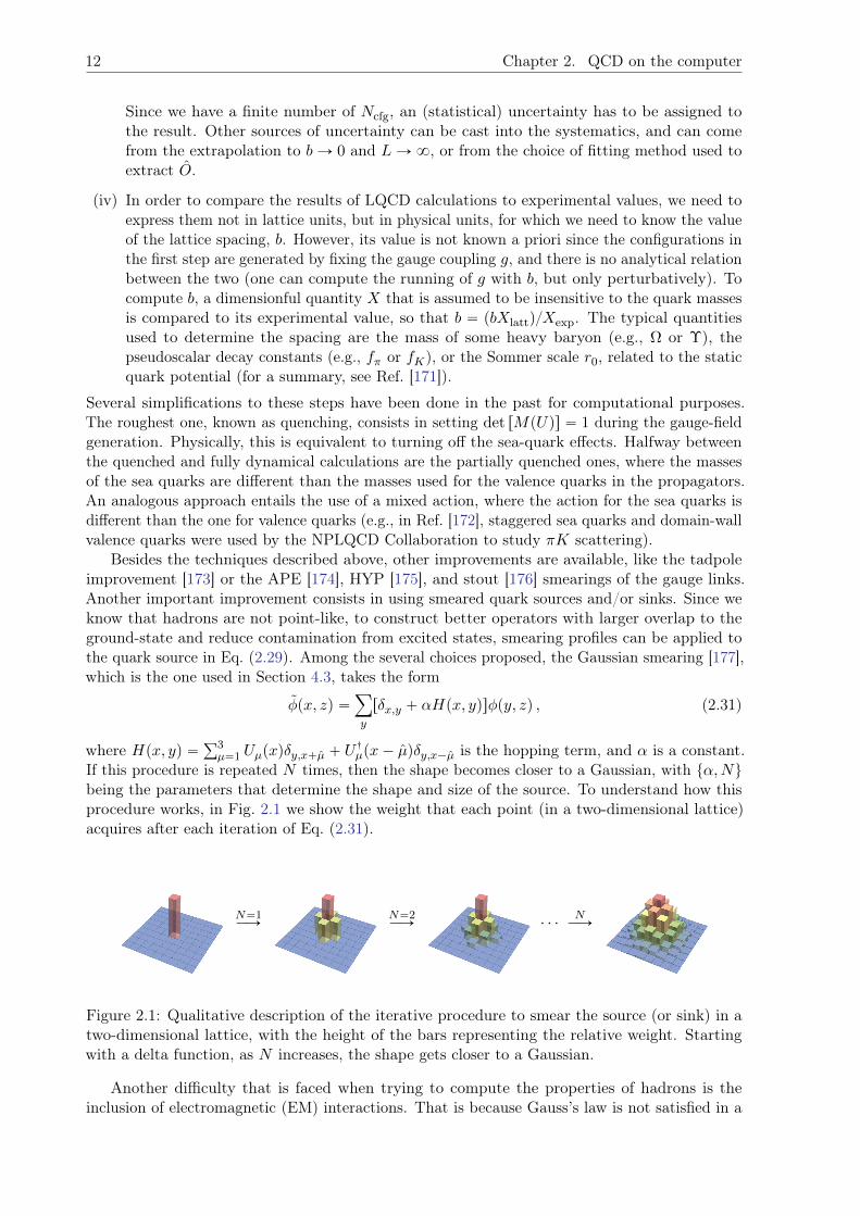
Besides the techniques described above, other improvements are available, like the tadpoleimprovement [173] or the APE [174], HYP [175], and stout [176] smearings of the gauge links.Another important improvement consists in using smeared quark sources and/or sinks. Since weknow that hadrons are not point-like, to construct better operators with larger overlap to theground-state and reduce contamination from excited states, smearing profiles can be applied tothe quark source in Eq. (2.29). Among the several choices proposed, the Gaussian smearing [177],which is the one used in Section 4.3, takes the form
φpx, zq “ÿ
y
rδx,y ` αHpx, yqsφpy, zq , (2.31)
where Hpx, yq “ř3µ“1 Uµpxqδy,x`µ ` U
:
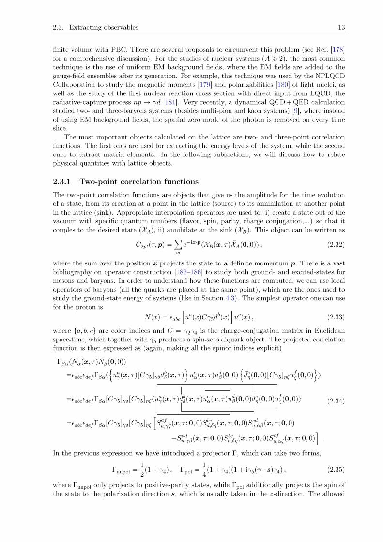
µpx´ µqδy,x´µ is the hopping term, and α is a constant.If this procedure is repeated N times, then the shape becomes closer to a Gaussian, with tα,Nubeing the parameters that determine the shape and size of the source. To understand how thisprocedure works, in Fig. 2.1 we show the weight that each point (in a two-dimensional lattice)acquires after each iteration of Eq. (2.31).
N“1ÝÑ
N“2ÝÑ ¨ ¨ ¨
NÝÑ
Figure 2.1: Qualitative description of the iterative procedure to smear the source (or sink) in atwo-dimensional lattice, with the height of the bars representing the relative weight. Startingwith a delta function, as N increases, the shape gets closer to a Gaussian.
Another difficulty that is faced when trying to compute the properties of hadrons is theinclusion of electromagnetic (EM) interactions. That is because Gauss’s law is not satisfied in a
2.3. Extracting observables 13
finite volume with PBC. There are several proposals to circumvent this problem (see Ref. [178]for a comprehensive discussion). For the studies of nuclear systems (A ě 2), the most commontechnique is the use of uniform EM background fields, where the EM fields are added to thegauge-field ensembles after its generation. For example, this technique was used by the NPLQCDCollaboration to study the magnetic moments [179] and polarizabilities [180] of light nuclei, aswell as the study of the first nuclear reaction cross section with direct input from LQCD, theradiative-capture process np Ñ γd [181]. Very recently, a dynamical QCD`QED calculationstudied two- and three-baryons systems (besides multi-pion and kaon systems) [9], where insteadof using EM background fields, the spatial zero mode of the photon is removed on every timeslice.
The most important objects calculated on the lattice are two- and three-point correlationfunctions. The first ones are used for extracting the energy levels of the system, while the secondones to extract matrix elements. In the following subsections, we will discuss how to relatephysical quantities with lattice objects.
2.3.1 Two-point correlation functions
The two-point correlation functions are objects that give us the amplitude for the time evolutionof a state, from its creation at a point in the lattice (source) to its annihilation at another pointin the lattice (sink). Appropriate interpolation operators are used to: i) create a state out of thevacuum with specific quantum numbers (flavor, spin, parity, charge conjugation,...) so that itcouples to the desired state (XA), ii) annihilate at the sink (XB). This object can be written as
C2ptpτ,pq “ÿ
x
e´ix¨pxXBpx, τqXAp0, 0qy , (2.32)
where the sum over the position x projects the state to a definite momentum p. There is a vastbibliography on operator construction [182–186] to study both ground- and excited-states formesons and baryons. In order to understand how these functions are computed, we can use localoperators of baryons (all the quarks are placed at the same point), which are the ones used tostudy the ground-state energy of systems (like in Section 4.3). The simplest operator one can usefor the proton is
Npxq “ εabc
”
uapxqCγ5dbpxq
ı
ucpxq , (2.33)
where ta, b, cu are color indices and C “ γ2γ4 is the charge-conjugation matrix in Euclideanspace-time, which together with γ5 produces a spin-zero diquark object. The projected correlationfunction is then expressed as (again, making all the spinor indices explicit)
ΓβαxNαpx, τqNβp0, 0qy
“εabcεdefΓβαx!
uaγpx, τqrCγ5sγδdbδpx, τq
)
ucαpx, τqudβp0, 0q
!
deηp0, 0qrCγ5sηζ ufζ p0, 0q
)
y
“εabcεdefΓβαrCγ5sγδrCγ5sηζxuaγpx, τqd
bδpx, τqu
cαpx, τqu
dβp0, 0qd
eηp0, 0qu
fζ p0, 0qy
“εabcεdefΓβαrCγ5sγδrCγ5sηζ
”
Safu,γζpx, τ ;0, 0qSbed,δηpx, τ ;0, 0qScdu,αβpx, τ ;0, 0q
´Sadu,γβpx, τ ;0, 0qSbed,δηpx, τ ;0, 0qScfu,αζpx, τ ;0, 0qı
.
(2.34)
In the previous expression we have introduced a projector Γ, which can take two forms,
Γunpol “1
2p1` γ4q , Γpol “
1
4p1` γ4qp1` iγ5pγ ¨ sqγ4q , (2.35)
where Γunpol only projects to positive-parity states, while Γpol additionally projects the spin ofthe state to the polarization direction s, which is usually taken in the z-direction. The allowed
14 Chapter 2. QCD on the computer
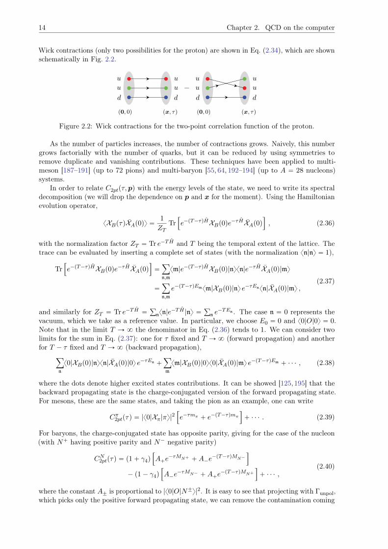
Wick contractions (only two possibilities for the proton) are shown in Eq. (2.34), which are shownschematically in Fig. 2.2.
u u
u u
d d
p0, 0q px, τq
´
u u
u u
d d
p0, 0q px, τq
Figure 2.2: Wick contractions for the two-point correlation function of the proton.
As the number of particles increases, the number of contractions grows. Naively, this numbergrows factorially with the number of quarks, but it can be reduced by using symmetries toremove duplicate and vanishing contributions. These techniques have been applied to multi-meson [187–191] (up to 72 pions) and multi-baryon [55, 64, 192–194] (up to A “ 28 nucleons)systems.
In order to relate C2ptpτ,pq with the energy levels of the state, we need to write its spectraldecomposition (we will drop the dependence on p and x for the moment). Using the Hamiltonianevolution operator,
xXBpτqXAp0qy “1
ZTTr
”
e´pT´τqHXBp0qe´τHXAp0qı
, (2.36)
with the normalization factor ZT “ Tr e´TH and T being the temporal extent of the lattice. Thetrace can be evaluated by inserting a complete set of states (with the normalization xn|ny “ 1),
Tr”
e´pT´τqHXBp0qe´τHXAp0qı
“ÿ
n,m
xm|e´pT´τqHXBp0q|nyxn|e´τHXAp0q|my
“ÿ
n,m
e´pT´τqEmxm|XBp0q|ny e´τEnxn|XAp0q|my ,(2.37)
and similarly for ZT “ Tr e´TH “ř
nxn|e´TH |ny “
ř
n e´TEn . The case n “ 0 represents the
vacuum, which we take as a reference value. In particular, we choose E0 “ 0 and x0|O|0y “ 0.Note that in the limit T Ñ 8 the denominator in Eq. (2.36) tends to 1. We can consider twolimits for the sum in Eq. (2.37): one for τ fixed and T Ñ8 (forward propagation) and anotherfor T ´ τ fixed and T Ñ8 (backward propagation),
ÿ
n
x0|XBp0q|nyxn|XAp0q|0y e´τEn `ÿ
m
xm|XBp0q|0yx0|XAp0q|my e´pT´τqEm ` ¨ ¨ ¨ , (2.38)
where the dots denote higher excited states contributions. It can be showed [125,195] that thebackward propagating state is the charge-conjugated version of the forward propagating state.For mesons, these are the same states, and taking the pion as an example, one can write
Cπ2ptpτq “ |x0|Xπ|πy|2”
e´τmπ ` e´pT´τqmπı
` ¨ ¨ ¨ . (2.39)
For baryons, the charge-conjugated state has opposite parity, giving for the case of the nucleon(with N` having positive parity and N´ negative parity)
CN2ptpτq “ p1` γ4q
”
A`e´τMN` `A´e
´pT´τqMN´
ı
´ p1´ γ4q
”
A´e´τMN´ `A`e
´pT´τqMN`
ı
` ¨ ¨ ¨ ,(2.40)
where the constant A˘ is proportional to |x0|O|N˘y|2. It is easy to see that projecting with Γunpol,which picks only the positive forward propagating state, we can remove the contamination coming
2.3. Extracting observables 15
0 100 200
τ [l.u.]
10−4
10−3
10−2
Cπ 2pt(τ
)
0 100 200
τ [l.u.]
10−14
10−11
10−8
10−5
CN 2pt(τ
)0 100 200
τ [l.u.]
−0.10
−0.05
0.00
0.05
0.10
mπ(τ
)[l.u.]
0 100 200
τ [l.u.]
−0.4
−0.2
0.0
0.2
0.4
MN
(τ)
[l.u.]
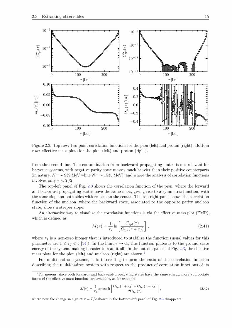
Figure 2.3: Top row: two-point correlation functions for the pion (left) and proton (right). Bottomrow: effective mass plots for the pion (left) and proton (right).
from the second line. The contamination from backward-propagating states is not relevant forbaryonic systems, with negative parity state masses much heavier than their positive counterparts(in nature, N` „ 939 MeV while N´ „ 1535 MeV), and where the analysis of correlation functionsinvolves only τ ă T 2.
The top-left panel of Fig. 2.3 shows the correlation function of the pion, where the forwardand backward propagating states have the same mass, giving rise to a symmetric function, withthe same slope on both sides with respect to the center. The top-right panel shows the correlationfunction of the nucleon, where the backward state, associated to the opposite parity nucleonstate, shows a steeper slope.
An alternative way to visualize the correlation functions is via the effective mass plot (EMP),which is defined as
Mpτq “1
τJln
„
C2ptpτq
C2ptpτ ` τJq
, (2.41)
where τJ is a non-zero integer that is introduced to stabilize the function (usual values for thisparameter are 1 ď τJ ď 5 [54]). In the limit τ Ñ8, this function plateaus to the ground stateenergy of the system, making it easier to read it off. In the bottom panels of Fig. 2.3, the effectivemass plots for the pion (left) and nucleon (right) are shown.4
For multi-hadron systems, it is interesting to form the ratio of the correlation functiondescribing the multi-hadron system with respect to the product of correlation functions of its
4For mesons, since both forward- and backward-propagating states have the same energy, more appropriateforms of the effective mass functions are available, as for example
Mpτq “1
τJarccosh
„
C2ptpτ ` τJq ` C2ptpτ ´ τJq
2C2ptpτq
, (2.42)
where now the change in sign at τ “ T 2 shown in the bottom-left panel of Fig. 2.3 disappears.
16 Chapter 2. QCD on the computer
constituents. For the case of two baryons, B1 and B2, this ratio reads
RB1B2pτq “
CB1B2pτq
CB1pτqCB2
pτq. (2.43)
We can construct an equivalent of the EMP for multi-baryons, called an effective energy-shiftfunction,
∆EB1B2pτq “
1
τJln
„
RB1B2pτq
RB1B2pτ ` τJq
, (2.44)
which in the limit τ Ñ8 it plateaus to ∆EB1B2“ EB1B2
´MB1´MB2
.From Fig. 2.3, we notice the different statistical behavior between meson and baryon correlation
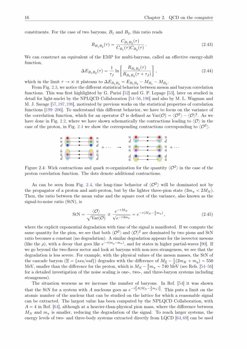
functions. This was first highlighted by G. Parisi [52] and G. P. Lepage [53], later on studied indetail for light-nuclei by the NPLQCD Collaboration [54–56,196] and also by M. L. Wagman andM. J. Savage [57,197,198], motivated by previous works on the statistical properties of correlationfunctions [199–206]. To understand this different behavior, we have to focus on the variance ofthe correlation function, which for an operator O is defined as VarpOq “ xO2y ´ xOy2. As wehave done in Fig. 2.2, where we have shown schematically the contractions leading to xOy in thecase of the proton, in Fig. 2.4 we show the corresponding contractions corresponding to xO2y.
u uu ud d
u uu ud d
` ¨ ¨ ¨ Ñ
u ud du uu u
d du u
` ¨ ¨ ¨
Figure 2.4: Wick contractions and quark re-organization for the quantity xO2y in the case of theproton correlation function. The dots denote additional contractions.
As can be seen from Fig. 2.4, the long-time behavior of xO2y will be dominated not bythe propagator of a proton and anti-proton, but by the lighter three-pion state (3mπ ă 2MN ).Then, the ratio between the mean value and the square root of the variance, also known as thesignal-to-noise ratio (StN), is
StN “xOy
a
VarpOq9
e´τMN
?e´τ3mπ
“ e´τpMN´32mπq , (2.45)
where the explicit exponential degradation with time of the signal is manifested. If we compute thesame quantity for the pion, we see that both xO2y and xOy2 are dominated by two pions and StNratio becomes a constant (no degradation). A similar degradation appears for the isovector mesons(like the ρ), with a decay that goes like e´τpmρ´mπq, and for states in higher partial-waves [90]. Ifwe go beyond the two-flavor sector and look at baryons with non-zero strangeness, we see that thedegradation is less severe. For example, with the physical values of the meson masses, the StN ofthe cascade baryon (Ξ “ tssussdu) degrades with the difference of MΞ ´
12p2mK `mηq „ 550
MeV, smaller than the difference for the proton, which isMN ´32mπ „ 740 MeV (see Refs. [54–56]
for a detailed investigation of the noise scaling is one-, two-, and three-baryon systems includingstrangeness).
The situation worsens as we increase the number of baryons. In Ref. [54] it was shownthat the StN for a system with A nucleons goes as e´τrApMN´
32mπqs. This puts a limit on the
atomic number of the nucleus that can be studied on the lattice for which a reasonable signalcan be extracted. The largest value has been computed by the NPLQCD Collaboration, withA “ 4 in Ref. [64], although at a heavier-than-physical pion mass, where the difference betweenMN and mπ is smaller, reducing the degradation of the signal. To reach larger systems, theenergy levels of two- and three-body systems extracted directly from LQCD [64,69] can be used
2.3. Extracting observables 17
5 10 15 20 25 30 35 40
A
0
10
20
30
40
BArM
eVs
NPLQCD [64]Ref. [105]Ref. [106]Ref. [107]Experimental
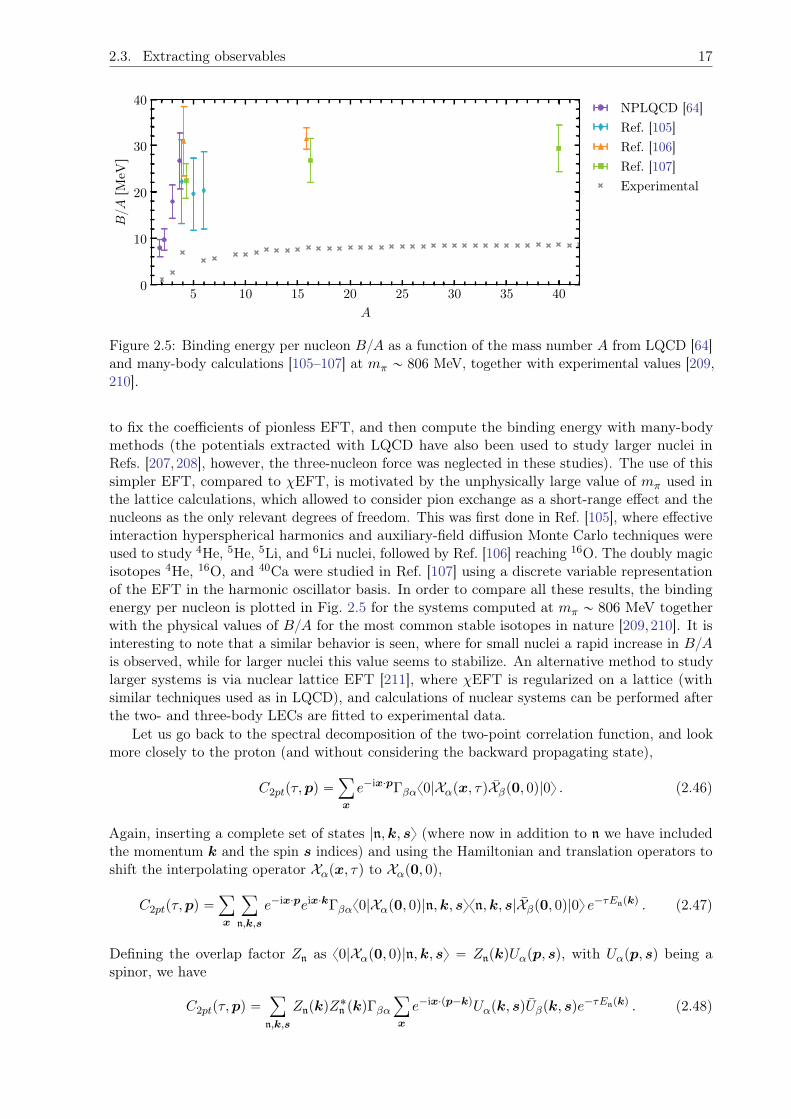
Figure 2.5: Binding energy per nucleon BA as a function of the mass number A from LQCD [64]and many-body calculations [105–107] at mπ „ 806 MeV, together with experimental values [209,210].
to fix the coefficients of pionless EFT, and then compute the binding energy with many-bodymethods (the potentials extracted with LQCD have also been used to study larger nuclei inRefs. [207, 208], however, the three-nucleon force was neglected in these studies). The use of thissimpler EFT, compared to χEFT, is motivated by the unphysically large value of mπ used inthe lattice calculations, which allowed to consider pion exchange as a short-range effect and thenucleons as the only relevant degrees of freedom. This was first done in Ref. [105], where effectiveinteraction hyperspherical harmonics and auxiliary-field diffusion Monte Carlo techniques wereused to study 4He, 5He, 5Li, and 6Li nuclei, followed by Ref. [106] reaching 16O. The doubly magicisotopes 4He, 16O, and 40Ca were studied in Ref. [107] using a discrete variable representationof the EFT in the harmonic oscillator basis. In order to compare all these results, the bindingenergy per nucleon is plotted in Fig. 2.5 for the systems computed at mπ „ 806 MeV togetherwith the physical values of BA for the most common stable isotopes in nature [209,210]. It isinteresting to note that a similar behavior is seen, where for small nuclei a rapid increase in BAis observed, while for larger nuclei this value seems to stabilize. An alternative method to studylarger systems is via nuclear lattice EFT [211], where χEFT is regularized on a lattice (withsimilar techniques used as in LQCD), and calculations of nuclear systems can be performed afterthe two- and three-body LECs are fitted to experimental data.
Let us go back to the spectral decomposition of the two-point correlation function, and lookmore closely to the proton (and without considering the backward propagating state),
C2ptpτ,pq “ÿ
x
e´ix¨pΓβαx0|Xαpx, τqXβp0, 0q|0y . (2.46)
Again, inserting a complete set of states |n,k, sy (where now in addition to n we have includedthe momentum k and the spin s indices) and using the Hamiltonian and translation operators toshift the interpolating operator Xαpx, τq to Xαp0, 0q,
C2ptpτ,pq “ÿ
x
ÿ
n,k,s
e´ix¨peix¨kΓβαx0|Xαp0, 0q|n,k, syxn,k, s|Xβp0, 0q|0y e´τEnpkq . (2.47)
Defining the overlap factor Zn as x0|Xαp0, 0q|n,k, sy “ ZnpkqUαpp, sq, with Uαpp, sq being aspinor, we have
C2ptpτ,pq “ÿ
n,k,s
ZnpkqZ˚n pkqΓβα
ÿ
x
e´ix¨pp´kqUαpk, sqUβpk, sqe´τEnpkq . (2.48)
18 Chapter 2. QCD on the computer
If we perform the sum over x and k, we project all momenta to p. Finally, by summing over spin,ÿ
s
Uαpp, sqUβpp, sq “ rEppqγ4 ´ ip ¨ γ `MN sαβ , (2.49)
we obtainC2ptpτ,pq “
ÿ
n
ZnppqZ˚n ppqΓβαrEnppqγ4 ´ ip ¨ γ `MN sαβ e
´τEnppq
“ÿ
n
ZnppqZ˚n ppqTrtΓrEnppqγ4 ´ ip ¨ γ `MN sue
´τEnppq
“ÿ
n
ZnppqZ˚n ppqFnpΓqe
´τEnppq ,
(2.50)
where the trace, FnpΓq, can be evaluated using the gamma-matrix properties, leading toFnpΓunpolq “ 2rEnppq`MN s for the case where Γ only projects to positive parity, and FnpΓpolq “
rEnppq `MN s when, in addition, the spin projection is made. Nevertheless, these factors are notexplicitly shown and are usually absorbed into the overlap factors. In the next chapter, we willdiscuss how to fit this two-point correlation function to extract the energy levels of the system.
2.3.2 Three-point correlation functions
In order to extract matrix elements (MEs), we need to couple the quarks (or gluons) fields toexternal currents by calculating a three-point correlation function. The most common definitionis the following,
C3ptpτ, τ1,p,p1q “
ÿ
x,y
e´ix¨p1e´iy¨pp1´pqΓβαx0|Xαpx, τqQpy, τ 1qXβp0, 0q|0y , (2.51)
with Q being the current inserted at time τ 1, and p and p1 the initial and final state momenta(with the transferred momentum being q “ p1 ´ p). Focusing on bilinear operators, Q “ qΦq,and for currents that do not change the quark flavor, we can draw schematically the contractionsin Fig. 2.6 (again for the case of the proton).
u u
u u
d d
bQ
p0, 0q py, τ 1q px, τq
`
u u
u u
d d
bQ
p0, 0q py, τ 1q px, τq
` ¨ ¨ ¨
Figure 2.6: Possible Wick contractions for the three-point correlation function of the protoninteracting with an external current of the form Q “ uΦu.
Now we see that besides the usual connected diagrams, there is also the possibility of havingdisconnected diagrams, which originate in the Wick contraction of the quarks in the operatorQ. As we can see in Fig. 2.6, these disconnected diagrams start and finish at the same spatialpoint, meaning that we will have to compute all-to-all propagators, which are more expensivethat the point-to-all propagators from Eq. (2.29), since the whole Dirac matrix has to be inverted(stochastic methods are used to evaluate these types of contributions, e.g., see Ref. [212]). Thesedisconnected contributions can be cancelled if certain combinations of Q are made, as we will seebelow.
Among the possible Q operators, hadronic form factors (more specific, their correspondingcharges), tell us about the internal structure of the hadrons as well as their interaction withother particles. For example, the electromagnetic form factors tell us about the charge and
2.3. Extracting observables 19
magnetic distribution of the hadron, and they are fairly simple to access experimentally usingelectron-proton scattering [213]. On the other hand, if we want to study the spin and gluonstructure of the hadrons, nuclear reactions like double β-decay, or the interaction with scalarparticles (dark matter candidates), QCD plays an important role, and for some of these quantitiesthere is no clean extractions from experiments. Related to these quantities we have three differentcurrents giving scalar, axial, and tensor MEs.
Scalar ME
Weakly interacting massive particles (WIMPs) are possible dark matter candidates, an extensionof the SM. One of the problems when trying to study experimentally the interaction betweenWIMPs and nuclei is the large uncertainty in the spin-independent interaction, the scalar ME orsigma terms, which are defined as the ME of the scalar quark currents between hadronic h states,
σπh “ mud xh|uu` dd|hy ,
σsh “ ms xh|ss|hy ,(2.52)
where mud is the average of the up and down quark masses. What is interesting is that, in aLQCD calculation at mπ „ 806 MeV, the scalar MEs for multi-hadronic states were found to bedifferent from the naive estimation assuming a sum of free nucleons [214], so quantifying thesedifferences for light nuclei with LQCD with high accuracy will be needed for experiments usingbig elements (like xenon, germanium or argon) as detectors [215].
Also, scalar MEs are used to access the strange content of the hadron. In principle, if we onlyconsider hadrons with no strange valence quarks (like the proton or deuteron), the net strangenessis zero. However, the valence quarks are surrounded by a sea of qq pairs, and computing thevacuum contributions of this sea to observables is pertinent.
Experimentally, the σπN has been extracted from pion-nucleon scattering experiments, σπN »45 MeV [216], but the σsN is not directly accessible. Instead, the flavour-singlet quantityσ0 “ mud xN |uu` dd´ 2ss|Ny can be extracted from octet baryon mass splittings, giving a valueof σ0 “ 36p7q MeV [217]. However, when trying to use these two quantities to extract σsN , onegets large uncertainties. Therefore, a direct LQCD calculation can be very illuminating.
Axial ME
The hadron axial structure is characterized by the hadron axial form factors found in the ME ofthe axial-vector quark current, Aa,µ “ qγµγ5 τa
2 q [126],
xhpp1, s1q|Aa,µ|hpp, sqy “ Uhpp1, s1q
„
γµγ5GaApQ
2q `qµγ5
2mhGaP pQ
2q
` iσµνqνγ
5
2mhGaT pQ
2q
Uhpp, sq ,
(2.53)
where Q2 “ ´q2, τ a is the isospin Pauli matrix,5 and the form factors GaApQ
2q, GaP pQ
2q, andGaT pQ
2q are the axial, induced pseudoscalar, and tensor form factors, respectively.In the forward limit Q2 “ 0, the axial form factor gives the hadronic axial charge GAp0q “ gA.
Experimentally, the nucleon axial charge has been measured with great accuracy, with a valueof gA “ gu´dA “ 1.2723p23q [218]. This axial current also allows us to study β-decay processes,although it requires a current that changes quark flavor. On the lattice, we can simplify thiscalculation by using isospin symmetry with the raising and lowering operators T˘,
xp|uγµγ5d|ny “ xp|uγµγ5dpT´T`q|ny “ xp|uγµγ5d T´|py “ xp|uγ
µγ5u´ dγµγ5d|py , (2.54)5For this example, since we work in SUp2qf , q “ pu dqJ and we use the Pauli matrices τa, but for SUp3qf ,
q “ pu d sqJ and we shall use the Gell-Mann matrices.
20 Chapter 2. QCD on the computer
where we have transformed the ME for the neutron β-decay to an isovector axial proton ME (inwhich the disconnected diagrams cancel with each other since the masses of u and d are set to bethe same).
Tensor ME
The ME of the tensor quark current, T a,µν “ q iσµν τa
2 q, can be parametrized by three formfactors [219],
xhpp1, s1q|T a,µν |hpp, sqy “ Uhpp1, s1q
„
iσµνHaT pQ
2q `γµqν ´ qµγν
2mhEaT pQ
2q
`nµqν ´ qµnν
2m2h
HaT pQ
2q
Uhpp, sq ,
(2.55)
where nµ “ p1µ ` pµ. Again, in the forward limit, the tensor charge is defined as HT p0q “ gT .Tensor charges are involved in the quark electric dipole moment, a new source of CP violation insome beyond-SM models [220, 221], since the two sources in the SM (the θ-term and the complexphase in the quark mixing matrix) are too small to explain the unbalance between matter andantimatter.
This quantity is accessible through the quark transversity distribution h1pxq, which measuresthe number of quarks with transverse polarization parallel to that of the hadron minus that ofquarks with antiparallel polarization. The first moment of h1pxq is related to gT [222],
ż 1
0dxrh1pxq ´ h1pxqs “ gT , (2.56)
where h1pxq is the antiquark transversity distribution and x is the Bjorken variable (related todeep inelastic scattering). The most recent values obtained using this approach are given inRef. [223] using data from COMPASS, HERMES, and JLab, with gT “ gu´dT “ 0.61
p`0.26qp´0.51q for
the isovector nucleon tensor charge, and g0T “ gu`dT “ 0.17
p`0.47qp´0.30q for the isoscalar one (both at
90% C.L.). It should be said that the future upgrade of JLab to 12 GeV is expected to improvethe precision up to one order of magnitude [224]. Given the challenging experimental extractionof the tensor charge, its estimation with LQCD calculations is extremely helpful.
All these charges have been computed in the single-baryon sector, as compiled in the mostrecent FLAG summary [48], as well for two- and three-nucleon states [214,225]. One can extractthese charges from the spectral decomposition of C3pt,
C3ptpτ, τ1q “
ÿ
x,y
ÿ
n,k,s
ÿ
m,k1,s1
eix¨k1e´iy¨pk1´kqΓβα
ˆ x0|Xαp0, 0q|m,k1, s1yxm,k1, s1|Qp0, 0q|n,k, syxn,k, s|Xβp0, 0q|0yˆ e´pτ´τ
1qEnpkqe´τ1Empk
1q ,
(2.57)
where we have taken p “ p1 “ 0 (and dropped the p and p1 labels) for simplicity. The operatorbracket gives us xm,k1, s1|Qp0, 0q|n,k, sy “ Uγpk
1, s1qΦγδUδpk, sqgΦ, with gΦ being the charge.Therefore,
C3ptpτ, τ1q “
ÿ
n,m
ZnZ˚m TrrΓpEmγ4 `MN qΦpEnγ4 `MN qse
´pτ´τ 1qEne´τ1EmgΦ
“ÿ
n,m
ZnZ˚mFnmpΓ,Φqe
´pτ´τ 1qEne´τ1EmgΦ .
(2.58)
We note that while for scalar currents, 2FnmpΓunpol, 1q “ FnmpΓpol, 1q “ pEm ` MN qpEn `
MN q, the axial and tensor currents have to be computed using Γpol, since FnmpΓunpol, γµγ5q “
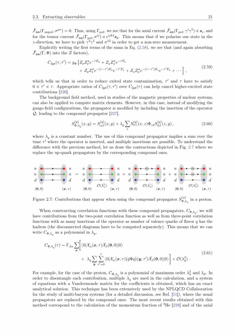
2.3. Extracting observables 21
FnmpΓunpol, σµνq “ 0. Thus, using Γpol, we see that for the axial current FnmpΓpol, γ
iγ5q9 si, andfor the tensor current FnmpΓpol, σ
ijq9 εijk4sk. This means that if we polarize our state in thez-direction, we have to pick γ3γ5 and σ12 in order to get a non-zero measurement.
Explicitly writing the first terms of the sums in Eq. (2.58), we see that (and again absorbingFnmpΓ,Φq into the Z factors),
C3ptpτ, τ1q “ gΦ
“
Z0Z˚0 e´τE0 ` Z1Z
˚1 e´τE1
` Z0Z˚1 e´pτ´τ 1qE0e´τ
1E1 ` Z1Z˚0 e´pτ´τ 1qE1e´τ
1E0 ` ¨ ¨ ¨
ı
,(2.59)
which tells us that in order to reduce exited state contamination, τ 1 and τ have to satisfy0 ! τ 1 ! τ . Appropriate ratios of C3ptpτ, τ
1q over C2ptpτq can help cancel higher-excited statecontributions [226].
The background field method, used in studies of the magnetic properties of nuclear systems,can also be applied to compute matrix elements. However, in this case, instead of modifying thegauge-field configurations, the propagator is modified by including the insertion of the operatorQ, leading to the compound propagator [227],
SpqqΦ,λq
px, yq “ Spqqαβ px, yq ` λq
ÿ
z
Spqqαγ px, zqΦγδS
pqqδβ pz, yq , (2.60)
where λq is a constant number. The use of this compound propagator implies a sum over thetime τ 1 where the operator is inserted, and multiple insertions are possible. To understand thedifference with the previous method, let us draw the contractions depicted in Fig. 2.7 where wereplace the up-quark propagators by the corresponding compound ones.
u u
u u
d d
p0, 0q px, τq
“
u u
u u
d d
p0, 0qOpλ0
uqpx, τq
`
u u
u u
d d
b
p0, 0qOpλ1
uqpx, τq
`
u u
u u
d d
b
b
p0, 0qOpλ2
uqpx, τq
Figure 2.7: Contributions that appear when using the compound propagator SpuqΦ,λuin a proton.
When constructing correlation functions with these compound propagators, CΦ,λq, we will
have contributions from the two-point correlation function as well as from three-point correlationfunctions with as many insertions of the operator as number of valence quarks of flavor q has thehadron (the disconnected diagrams have to be computed separately). This means that we canwrite CΦ,λq
as a polynomial in λq,
CΦ,λqpτq “ Γβα
ÿ
x
„
x0|Xαpx, τqXβp0, 0q|0y
` λqÿ
y
τÿ
τ 1“0
x0|Xαpx, τqtqΦqupy, τ 1qXβp0, 0q|0y
`Opλ2qq .
(2.61)
For example, for the case of the proton, CΦ,λqis a polynomial of maximum order λ2
u and λd. Inorder to disentangle each contribution, multiple λq are used in the calculation, and a systemof equations with a Vandermonde matrix for the coefficients is obtained, which has an exactanalytical solution. This technique has been extensively used by the NPLQCD Collaborationfor the study of multi-baryon systems (for a detailed discussion, see Ref. [51]), where the usualpropagators are replaced by the compound ones. The most recent results obtained with thismethod correspond to the calculation of the momentum fraction of 3He [228] and of the axial
22 Chapter 2. QCD on the computer
charge of the triton [225], which only need the evaluation of the Opλqq contribution. Processesthat require the Opλ2
qq components are, for example, double-β decays [229,230].
Looking at the spectral decomposition of CΦ,λq
ˇ
ˇ
ˇ
Opλqqwe see that, compared to Eq. (2.58), the
sum over τ 1 yields different time-dependence for the ground state as well as different excited-statecontamination,
CΦ,λq
ˇ
ˇ
ˇ
Opλqq“
ÿ
n,m
ZnZ˚m gΦ e
´τEn
τÿ
τ 1“0
e´τ1pEm´Enq
“ÿ
n,m
ZnZ˚m gΦ
„
e´τEn
1´ eEn´Em`
e´τEm
1´ eEm´En
“ÿ
n
ZnZ˚n gΦp1` τqe
´τEn `ÿ
n
ÿ
m‰n
ZnZ˚m gΦ
„
e´τEn
1´ eEn´Em`
e´τEm
1´ eEm´En
.
(2.62)
Again, appropriate combinations and ratios of CΦ,λq
ˇ
ˇ
ˇ
Opλqqand C2pt can help extract gΦ more
cleanly [228].All these matrix elements obtained from the lattice are computed in the “lattice” scheme.
What this means is that the lattice itself is a regularization scheme (the lattice spacing imposes anultraviolet cutoff, Λlatt “ b´1), so the operators computed in the lattice will be regularized in thisparticular scheme. These are what we call bare operators. If we want to compare them to theircontinuum counterparts, we need to switch to an appropriate renormalization scheme, which isusually the modified subtraction scheme (MS) at a scale µ “ 2 GeV [125] (typical renormalizationscale used when dealing with experimental data),
ORΦpµq “ ZΦpµ, bqOlatt
Φ pbq , (2.63)
where ZΦ is called the renormalization constant, which depends on the lattice action used and theoperator, but not on the external states in the ME. To be precise, the renormalization procedureis divided in two steps, since one cannot apply the MS scheme directly on the lattice. First, anon-perturbative calculation of ZΦ is done on the lattice using a specific scheme, such as theRI-MOM scheme (Regularization Independent MOMentum subtraction scheme [231]). Then, aperturbative matching between the RI-MOM and MS schemes is performed.
Since the lattice version of QCD is written in Euclidean space-time, the original Lorentz groupis replaced by the orthogonal group Op4q, which is further reduced due to the discretization ofspace-time to the hypercubic group Hp4q Ă Op4q [232]. Just as it happens with the angularmomentum (we will give more details in the next section), since Hp4q is a finite group, mixingbetween different operators is possible, and ZΦpµ, bq is, in general, a matrix with non-zerooff-diagonal elements, rather than just a number.
2.4 Scattering in finite volume
Computing the relevant parameters in the description of the interaction of two (and more)hadrons directly from QCD is one of the goals of nuclear physics. Typically, phase shifts aredetermined from scattering experiments by parametrizing the scattering amplitude at low-energiesas a function of the energy in the center-of-mass (c.m.) frame. For baryon-baryon processes, acommon parametrization below the t-channel cut is the effective range expansion (ERE) [233–235],which for the case of S wave can be written as
k˚ cot δpk˚q “ ´1
a`
1
2rk˚2 ` Pk˚4 `Opk˚6q , (2.64)
where a is the scattering length, r is the effective range, and P is the leading shape parameter.For other types of processes, like the study of resonances, different parametrizations are more
2.4. Scattering in finite volume 23
suitable (e.g., see Ref. [236,237]). When trying to study scattering processes with LQCD, we haveto confront the Maiani-Testa no-go theorem [238], which states that scattering matrix elementscannot be extracted from infinite-volume Euclidean correlation functions except at kinematicthresholds. An easy way to circumvent this problem is by computing correlation functions atfinite volume. The method was formalized by M. Lüscher [7, 8], who extracted S-wave scatteringelements from the discrete spectrum of the two particle state in a finite three-dimensional boxbelow inelastic thresholds. Before diving into the formalism, we need to understand how do thespin, orbital, and total momentum of the system get modified when it is put in a box.
2.4.1 Angular momentum group theory
The study of angular momentum on the lattice requires some knowledge of group theory. Asummary of the main concepts (taken from Refs. [239–244]) and useful definitions are given below.
Elements of group theory
Definition 1. A collection of elements A,B,C, . . . form a group when the following four conditionsare satisfied:
(i) The product of any two elements of the group is also a member of the group.
(ii) The associative law applies to the product of three elements, i.e., pABqC “ ApBCq.
(iii) There exists a unit element E (or identity element) such that EA “ AE “ A.
(iv) Each element has an inverse element which is also a member of the group, i.e., for everyelement A there exists an inverse element A´1 such that A´1A “ AA´1 “ E.
Definition 2. The order of a group h is the number of elements in the group.
Definition 3. A subgroup is a collection of elements within a group that by themselves satisfythe group postulates.
Definition 4. Two groups G and G1 are isomorphic when to each element of G there correspondsone, and only one, element of G1, and conversely (one-to-one correspondence).
Definition 5. Two groups G and G1 are homomorphic when to each element of G there corre-sponds one, and only one, element of G1, but to each element of G1 there corresponds at least oneand possibly more than one element of G (many-to-one correspondence).
Definition 6. If a group G contains two subgroups Ga and Gb whose elements commute, and ifevery element of G can be written uniquely as a product of the elements of Ga and Gb, then G isthe direct product of Ga and Gb and is written G “ Ga bGb.
Definition 7. An element B conjugate of A is by definition B “ XAX´1, where X is somemember of the group.
Definition 8. A class is the totality of elements which can be obtained from a given groupelement by conjugation. For an Abelian group, since all members are selfconjugate, the numberof classes is equal to the order h of the group.
Definition 9. A representation of an abstract group is a substitution group (matrix groupwith square matrices with non-vanishing determinants) such that the substitution group ishomomorphic (or isomorphic) to the abstract group. We assign a matrix ΠpAq to each element Aof the abstract group such that ΠpABq “ ΠpAqΠpBq. These representations are not unique.
Definition 10. The dimensionality of a representation is equal to the dimensionality of each ofits matrices.
24 Chapter 2. QCD on the computer
Definition 11. If by means of the same equivalence transformation, all the matrices in therepresentation of a group can be made to acquire the same block form, then the representation issaid to be reducible; otherwise it is irreducible. An irreducible representation (irrep) cannot beexpressed in terms of representations of lower dimensionality.
If Π is a reducible representation, then the reduction is expressed by writing
Π “à
i
miΠpiq , (2.65)
where each mi is a positive integer that indicates how many times the representation matrixΠpiqpRq appears along the main diagonal of ΠpRq. The number of non-equivalent irreps is equalto the number of classes. Furthermore, there is a restriction on the dimensions of the irreps. If liis the dimension of the ith irrep and h the order of the group, then
ÿ
i
l2i “ h . (2.66)
Definition 12. The character of a representation matrix ΠpjqpRq is the trace of the matrix. Thecharacter for each element in a class is the same.
The usual way to summarize the information on the characters of the representations of agroup is using the character table. In a character table we list the irreps as columns and the classas rows. Looking at Eq. (2.65), it follows that the character χ of Π is related to the irreduciblecharacters by a similar equation. If χpRq denotes the character of Π for an element in a class R,then
χpRq “ÿ
i
miχpiqpRq . (2.67)
It is obviously of interest, given R, to be able to deduce the mi, which can be done if theirreducible characters χpiqpRq are known,
mi “1
h
ÿ
R
nR χpiqpRq˚χpRq , (2.68)
where nR denotes the number of elements in class R.
Angular momentum in the continuum
In the continuum, the relevant group is the Op3q group, which is the full three-dimensionalrotation group. This group includes 3ˆ 3 real matrices with determinant ˘1. This means thatOp3q does not only include the proper rotations (matrices with det “ `1), but also the improperrotations (with det “ ´1). These improper rotations correspond to proper rotations combinedwith a spatial inversion (also known as parity). Therefore, Op3q “ SOp3q b Ci, where the groupCi contains just two elements: the identity element E and the inversion element I.
Since Op3q is the direct product of SOp3q and Ci, each irrep of Op3q can be regarded as thedirect product of an irrep of SOp3q with an irrep of Ci. We already know the irreps of SOp3q,there are an infinite number of irreps with dimension p2L ` 1q, which are labeled by integerangular momentum L P t0, 1, 2, . . .u. For the group Ci, since it is an Abelian group with twoelements, there will be two 1-dimensional irreps, which separates states between proper andimproper states of parity. Then, the character of the irreps of Op3q is given by
χpLqpθ, properq “sin
“`
L` 12
˘
θ‰
sin`
θ2
˘ , χpLqpθ, improperq “ p´1qLsin
“`
L` 12
˘
θ‰
sin`
θ2
˘ . (2.69)
2.4. Scattering in finite volume 25
If we want to include half-integer angular momentum (required for fermions), we need toconsider the double cover representation of SOp3q, which is SUp2q. This can be argued as follows.If we look at the first expression in Eq. (2.69), under the rotation θ ` 2π,
χpJqpθ ` 2πq “sin
“`
J ` 12
˘
pθ ` 2πq‰
sin`
θ`2π2
˘ “sin
“`
J ` 12
˘
θ‰
cos“`
J ` 12
˘
2π‰
sin`
θ2
˘
cospπq. (2.70)
For integer values of J , cos“`
J ` 12
˘
2π‰
“ ´1, while for half-integer values of J it takes the value`1. Therefore, we have the important relation
χpJqpθ ` 2πq “ p´1q2JχpJqpθq , (2.71)
which implies that for integer J , a rotation by θ, θ ˘ 2π, θ ˘ 4π, . . . yields identical characters,but for half-integer values of J , we have
χpJqpθ ` 2πq “ ´χpJqpθq , χpJqpθ ` 4πq “ χpJqpθq . (2.72)
The need to rotate by 4π rather than by 2π to generate the identity operation leads to theconcept of double groups. For the improper rotations with half-integer J , the change of sign inEq. (2.69) depends on the parity (P ) of the system. If P “ `, no modification is required, butif P “ ´, one needs to multiply by p´1q. The same will happen when J comes from couplingorbital angular momentum L to spin s. For the rest of the discussion and for simplicity, we willuse J “ L (s “ 0) for J integer (and parity p´1qL).
An interesting property of χpJqpθq that will be used later on is to see what happens whenJ Ñ J ` 12n,
χpJ`12nqpθq “sin
“`
J ` 12
˘
θ‰
cosp12nθq ` cos“`
J ` 12
˘
θ‰
sinp12nθq
sin`
θ2
˘ . (2.73)
The rotations relevant for the lattice are only θ P tπ, π2, π3u (and multiples). Therefore,cosp12nθq “ 1 @θ, and
χpJ`12nqpθq “ χpJqpθq `cos
“`
J ` 12
˘
θ‰
sinp12nθq
sin`
θ2
˘ “
#
χpJqpθq ` 24np´1q2mJ , θ “ 2mπ
χpJqpθq, otherwise.
(2.74)
Angular momentum on the lattice
The lattice is symmetric with respect to a set of rotations that form the octahedral group O,which is a subgroup of the continuum rotational group SOp3q (if we boost the system, or usean asymmetrical lattice, the symmetry will be broken down to a more restrictive one). Theoctahedral group consists of 24 group elements, each corresponding to a discrete rotation thatleaves invariant a cube, which are enumerated in the following 5 classes:
– E: identity.
– 8C3: rotations of ˘2π3 about the four body diagonals.
– 3C2: rotations of π about the coordinate axes.
– 6C4: rotations of ˘π2 about the coordinate axes.
– 6C 12: rotations of π about the six axes parallel to the six face diagonals.
If we consider spatial inversion, we get the octahedral group Oh, where Oh “ O b Ci. With theinclusion of inversion, we get 24 more group elements, which are also organized into 5 classes:
26 Chapter 2. QCD on the computer
– I: inversion
– 8IC3 “ 8S6: rotations of ˘2π3 about the four body diagonals + inversion.
– 3IC2 “ 3σh: rotations of π about the coordinate axes + inversion.
– 6IC4 “ 6S4: rotations of ˘π2 about the coordinate axes + inversion.
– 6IC 12 “ 6σd: rotations of π about the six axes parallel to the six face diagonals + inversion.
Therefore, Oh has 48 elements divided into 10 classes. This will correspond to 10 irreps (5 irrepsfor each parity), which are denoted as A˘1 , A
˘2 , E
˘, T˘1 , T˘2 , with respective dimensions 1, 1, 2, 3, 3.
When the objects that are rotated involve half-integer values of the angular momentum, thegroup elements double, forming the double octahedral group ODh . The elements of this group arelabeled with a horizontal line over the name of the element. The doubling of the elements doesnot mean that the classes also double (e.g., if it is a class of rotation by π, the original elementsand the elements of the double group are members of the same class). Therefore, there will onlybe 6 more classes, with 6 more irreps, G˘1 , G
˘2 , H
˘, with respective dimensions 2, 2, 4.When we boost the system inside the lattice, the Lorentz transformation deforms the cubical
volume and only some subgroups of the original ODh group survive. Since we only work withboosts of the form d “ p0, 0, nq, the relevant symmetry groups are the tetragonal point group D4h
(if both particles have the same mass) and C4v (if both particles have different masses). For amore general boost, the relevant point and double groups are summarized in Refs. [84, 245]. Thetetragonal point group D4h has 8ˆ 2 (including parity) elements grouped into 10 classes, and thecorresponding irreps are denoted as A˘1 , A
˘2 , B
˘1 , B
˘2 , E
˘, with respective dimensions 1, 1, 1, 1, 2.For the double tetragonal group DD
4h, there are only 4 more classes, so 4 more irreps, G˘1 , G˘2 ,
with respective dimensions 2, 2. The tetragonal point group C4v has 8 elements (the spatialinversion is not an element) grouped into 5 classes, with the irreps denoted as A1, A2, B1, B2, E,with respective dimensions 1, 1, 1, 1, 2. For the double tetragonal group CD4v (also known as Dic4),there are only 2 more classes, so 2 more irreps, G1, G2, with respective dimensions 2, 2.
The character tables of ODh , DD4h, and C
D4v are shown in Tables A.1, A.2, and A.3, respectively,
from Appendix A, where the values of θ are also included.
Decomposition of the angular momentum
In order to determine the decomposition of the angular momentum in the continuum into thecorresponding lattice group, we have to extract the coefficients mi from the combination of thecharacters of SOp3q (see Eq. (2.69)) and the characters of the corresponding point (double) group(see Tables A.1, A.2, and A.3) into Eq. (2.68). For example, let us try to compute the case J “ 0for the group ODh . Starting with A`1 ,
mA`1“
1
h
ÿ
R
nR χA`1 pRqχpJ“0qpRq
“1
96
”
χA`1 pEqχp0qp4πq ` χA
`1 pEqχp0qp2πq ` 8χA
`1 pC3qχ
p0qp2π3q ` ¨ ¨ ¨ı
“1
96r1 ¨ 1` 1 ¨ 1` 8p1 ¨ 1q ` ¨ ¨ ¨ s “ 1 ,
(2.75)
while for the rest of the irreps we get mA`2“ mE` “ ¨ ¨ ¨ “ mH´ “ 0. Therefore, J “ 0 is
only described by the A`1 irrep. Doing the same for angular momentum up to J ă 12, we getTable A.4 for the group ODh , Table A.5 for the group DD
4h, and Table A.6 for the group CD4v.Having calculated the values for J ă 12, Eq. (2.74) allows us to find the J ` 12n values:
2.4. Scattering in finite volume 27
J ` 12n integer J ` 12n half-integer
ODh ΓpJq ‘ npA˘1 ‘A˘2 ‘ 2E˘ ‘ 3T˘1 ‘ 3T˘2 q ΓpJq ‘ 2npG˘1 ‘G
˘2 ‘ 2H˘q
DD4h ΓpJq ‘ 3npA˘1 ‘A
˘2 ‘B
˘1 ‘B
˘2 ‘ 2E˘q ΓpJq ‘ 6npG˘1 ‘G
˘2 q
CD4v ΓpJq ‘ 3npA1 ‘A2 ‘B1 ‘B2 ‘ 2Eq ΓpJq ‘ 6npG1 ‘G2q
where ΓpJq is the corresponding decomposition of the angular momentum J .However, when working on the lattice, we have the inverse problem: we want to know the
momentum content of a lattice energy eigenstate transforming as a single irrep of the correspondingpoint (or double) group (the operators are build to transform correctly under the discrete groups,and not the full rotation group). In other words, we want the inverse of the correspondence givenby Eq. (2.68) and Table A.4. The results for the group ODh are given in Table A.7, for the groupDD
4h in Table A.8, and for the group CD4v in Table A.9. It is interesting to see that the groupsthat do not have inversion as an element, mix partial waves with opposite parity.
2.4.2 Lüscher’s formalism
When two hadrons are put inside a box with periodic BC, the energy levels of the system, nowquantized, will shift from the free-particle values due to their mutual interactions. The connectionbetween these finite-volume levels and the infinite-volume scattering parameters, below three-particle production, was first presented in Refs. [7, 8], and later generalized to two-hadrons withnon-zero momenta and non-zero spin [84–100,246–248] and even three-particle states [249–255].Throughout this section as well as in Section 4.3, where the results will be discussed, we willassume that the box is larger than the range of the interaction of the system [256], given bythe lightest particle that can be exchanged, which for all the baryon-baryon channels studiedin this work is the pion, so mπL " 1 (corrections that take into account these effects have beencomputed in Refs. [257,258]).
We will follow the notation of Refs. [90, 96, 97], where two-baryon systems are labeled bythe spin s and orbital momentum L, both coupled to give a total angular momentum J . TheLüscher’s quantization condition (QC) is given by
det“
pM8q´1 ` δGV‰
“ 0 , (2.76)
where M8 is the infinite volume scattering amplitude. In the non-relativistic limit, for channelswith no partial-wave mixing (like in the NN spin-singlet state), it has the following form,
pM8qLL1;sJMJ
“2π
Mk˚e2iδLsJ ´ 1
2iδL,L1δL,J “
2π
Mk˚1
cot δLsJ ´ iδL,L1δL,J , (2.77)
where M is the reduced mass of the system, k˚ is the momentum of each baryon in the c.m.frame, and δLsJ is the scattering phase shift. When partial-wave mixing is possible (like in theNN spin-triplet state), some paramerization of the scattering amplitude has to be used, likethe Stapp-Ypsilantis-Metropolis (or barred) [259], the Blatt–Biedenharn [260,261], the Bryan-Klarsfeld-Sprung [262–265], or the Kabir-Kermode [266] parametrization. In this work we willuse the Blatt–Biedenharn one, which has the following form,
pM8qJ˘1J˘1;sJMJ
“2π
Mk˚cos2pεJqe
2iδLsJ ` sin2pεJqe2iδL
1sJ ´ 1
2iδL,J´1δL1,J`1 ,
pM8qJ˘1J¯1;sJMJ
“2π
Mk˚cospεJq sinpεJqpe
2iδLsJ ´ e2iδL1s
J q
2iδL,J´1δL1,J`1 ,
(2.78)
28 Chapter 2. QCD on the computer
where now we have two scattering phase shifts and a mixing angle εJ . This parametrization isusually written in terms of the S matrix,
S “ 1` iMk˚
πM8
“
˜
cospεJq ´ sinpεJq
sinpεJq cospεJq
¸˜
e2iδJ´1,sJ 0
0 e2iδJ`1,sJ
¸˜
cospεJq ´ sinpεJq
sinpεJq cospεJq
¸
.
(2.79)
The second term, δGV , is a function of the finite-volume energy levels, and has the followingform,
rδGV sJMJ ,Ls;J1MJ1 ,L
1s1 “iMk˚
2πδss1
”
δJJ 1δMJMJ1δLL1 ` iF
pFV qJMJ ,L;J 1MJ1 ,L
1
ı
, (2.80)
with
FpFV qJMJ ,L;J 1MJ1 ,L
1 “ÿ
m,m1,ν
xLm; sν|JMJyxL1m1; sν|J 1MJ 1y F
pFV qLm;L1m1 ,
FpFV qLm;L1m1 “
p´1qm1
qγπ32
a
p2L` 1qp2L1 ` 1q
|L`L1|ÿ
l“|L´L1|
a
2l ` 1
ql
ˆ
lÿ
m“´l
ˆ
L l L1
0 0 0
˙ˆ
L l L1
´m ´m m1
˙
Zdl,mp1; q2q ,
(2.81)
where q “ k˚Ls2π (here Ls is the spatial size of the lattice, to avoid confusion with the angular mo-
mentum L), xL1m1; sν|J 1MJ 1y are Clebsch-Gordan coefficients, andˆ
l1 l2 l3m1 m2 m3
˙
are Wigner
3j symbols [267]. The generalized Z-function is defined through the equation
Zdlmps; q
2q “ÿ
rPPd
Ylmprqp|r|2 ´ q2q
s , (2.82)
where Ylmprq “ |r|lYlmprq, with Ylmprq being the spherical harmonics, and the summation isover the set
Pd “
rˇ
ˇ r “ γ´1 pn´ αdq , n P Z3(
. (2.83)
In order to understand this relation and the new quantities that appear, we need to introducesome new definitions. Let us consider a system of two hadrons (with masses m1 and m2) in afinite box with spatial dimensions L3
s with periodic BC. The system, in the laboratory frame(LAB), is given a non-zero total three-momentum P , which has to satisfy the following condition(in the non-interacting case),
P “ p1 ` p2 “2π
Lsd , d P Z3 . (2.84)
Then, the energy eigenvalues for this system are E “a
m21 ` |p1|
2 `a
m22 ` |p2|
2. In thec.m. frame (denoted with an asterisk ˚), the total momentum is zero, and the relative one isp˚ “ p˚1 “ ´p˚2 . Knowing that the total four-momentum squared is invariant, the relationbetween the LAB and c.m. frames is
E˚2“ E2 ´ P 2 . (2.85)
Since the c.m. frame moves with a velocity v “ P E with respect to the LAB frame, the momentapi and p˚ are related via the standard Lorentz transformation,
p1 “ γpp˚ ` vE˚1 q , p2 “ γp´p˚ ` vE˚2 q , (2.86)
2.4. Scattering in finite volume 29
where the boost factor γ acts in the direction of v (which is the same direction as d),
γn “ γn‖ ` nK , γ´1n “ γ´1n‖ ` nK , n‖ “n ¨ d
|d|2d, nK “ n´ n‖ , (2.87)
and E˚1 and E˚2 are the energy eigenvalues of the particles 1 and 2 in the c.m. frame, respectively.
To extract them, knowing that E˚i “b
m2i ` |p
˚|2, we can write p˚ in terms of E˚ and m1,2,and then substitute it back to E˚i ,
E˚1 “
c
m21 `
1
4E˚2
“
pE˚2 ´m21 ´m
22q
2 ´ 4m21m
22
‰
“E˚
2
ˆ
1`m2
1 ´m22
E˚2
˙
. (2.88)
For E˚2 , we get the same as for E˚1 , but with m1 and m2 interchanged. To know the values of theallowed momenta p˚ in the c.m. frame for the non-interacting case, we use Eqs. (2.84), (2.86)and (2.88),
p˚ “ γ´1p1 ´ vE˚1 “ γ´1pp1 ´ γvE
˚1 q “ γ´1
„
p1 ´E
E˚P
E
E˚
2
ˆ
1`m2
1 ´m22
E˚2
˙
“ γ´1
„
p1 ´P
2
ˆ
1`m2
1 ´m22
E˚2
˙
“ γ´1 pp1 ´ αP q ,
(2.89)
where we have defined α “ 12
´
1`m2
1´m22
E˚2
¯
. Thus, we see that p˚ is quantized to the values
p˚ “ 2πL r, with r P Pd, shown in Eq. (2.83).
The sum in (2.82) converges when Rep2sq ą l ` 3, but can be analytically continued to thewhole complex plane, since we are interested in evaluating the Z-function at s “ 1. This is shownin Appendix B, where a convenient expression has been derived to exponentially accelerate thenumerical evaluation of the function. The symmetry properties of Zd
lm follow directly from thedefinition in Eq. (2.82) and the properties of the spherical harmonic functions under symmetryoperations:
(i) Under the interchange m1 Ø m2, it can be shown that
rˇ
ˇ r “ γ´1 rn´ αpm1,m2qds(
“
´rˇ
ˇ r “ γ´1 rn´ αpm2,m1qds(
, (2.90)
which, using Ylmp´rq “ p´1qlYlmprq, results in
Zdpm1,m2q
lm ps; q2q “ p´1qlZdpm2,m1q
lm ps; q2q . (2.91)
(ii) A consequence of the previous result is that for odd l the Z-function must vanish whenm1 “ m2 or d “ 0,
Zlmps; q2q “ 0 for l odd . (2.92)
(iii) The property Yl´m “ p´1qmY ˚lm translates directly to
Zdl´mps; q
2q “ p´1qmrZdlmps; q
2qs˚ . (2.93)
(iv) For d “ 0 or d “ p0, 0, nq, the system is symmetric under rotations around the z-axis byπ2, ϕÑ ϕ` π2, so Ylmpθ, ϕ` π2q “ fpθqeimpϕ`π2q “ Ylme
imπ2,
Zdlmps; q
2q “ imZdlmps; q
2q ñ Zdlmps; q
2q “ 0 for m ‰ 0, 4, 8, . . . (2.94)
(v) For d “ 0 or d “ p0, 0, nq, the system is symmetric under a mirror reflection about thexz-plane, ϕÑ 2π ´ ϕ, so Ylmpθ, ϕq “ Ylmpθ, 2π ´ ϕq “ Y ˚lmpθ, ϕq,
Zdlmps; q
2q “ Zdl´mps; q
2q . (2.95)
30 Chapter 2. QCD on the computer
(vi) Additional relations between non-zero Zlm can be found by looking at the symmetries of thespherical harmonics. For any rotation matrix R corresponding to each symmetry operationof the discrete group,
YlmpRrq “lÿ
m1“l
Dplqmm1pRqYlm1prq , (2.96)
where Dplqmm1pRq is the Wigner D-matrix [8] (this matrix is written in terms of the Eulerangles of the rotation, which can be read off from, e.g., Ref. [99]). Then, by looking atEq. (2.82), we see that
Zdlmps; q
2q “
lÿ
m1“l
Dplqmm1pRqZdlm1ps; q
2q . (2.97)
For example, if we look at the group ODh (with d “ 0), we obtain that Z20ps; q2q “ 0. Other
possible relations are
Z44ps; q2q “
c
5
14Z40ps; q
2q , Z64ps; q2q “ ´
c
7
2Z60ps; q
2q ,
Z84ps; q2q “
1
3
c
14
11Z80ps; q
2q , Z88ps; q2q “
1
3
c
65
22Z80ps; q
2q .
(2.98)
For the relations between Zlm with higher values of l and other groups, see Refs. [90, 95,96,268].
A useful short-hand notation that we will use when writing the QCs is the following,
zlm “1
ql`1γπ32?
2l ` 1Zdlmp1; q2q . (2.99)
The QC in Eq. (2.76) is written in the basis |JMJLy, not suitable for lattice calculations,where we work in the basis of the irreps Γ of the point (or double) group. This basis can bewritten as |ΓσνJLy, with σ P t1, . . . ,dim Γu and ν P t1, . . . , NpΓ, Jqu, where NpΓ, Jq denotes themultiplicity of J in the irrep Γ. The basis vectors |ΓσνJLy can be decomposed in terms of the|JMJLy basis,
|ΓσνJLy “ÿ
MJ
cΓσνJMJ
|JMJLy , (2.100)
where the coefficients cΓσνJMJ
can be read off directly from Tables A.10, A.11, and A.12, in which thebasis vectors of Oh, D4h, and C4h are listed (only for integer values of total angular momentum).The matrix elements of δGV in the new basis are given by
xΓσνJL|δGV |Γ1σ1ν 1J 1L1y “ÿ
MJ ,MJ1
`
cΓσνJMJ
˘˚cΓ1σ1ν1
J 1MJ1rδGV sJMJL;J 1MJ1L
1 . (2.101)
A similar block-diagonalization procedure is presented in Refs. [90, 96]. According to Schur’slemma [269], δGV is partially diagonalized in this new basis,
xΓσνJL|δGV |Γ1σ1ν 1J 1L1y “ δΓΓ1δσσ1rδGV sΓJLν;J 1L1ν1 , (2.102)
and Eq. (2.76) can thus be rewritten asź
Γ
det
"
´
rM8sLL1
J
¯´1δJJ 1δνν1 ` rδGV sΓJLν;J 1L1ν1
*
“ 0 , (2.103)
which is independent of σ. For practical reasons, the matrices are truncated in the space of totalangular momentum J and orbital momentum L. Now let us look in detail at the different QCsfor baryon-baryon systems in both spin-singlet and spin-triplet states. Since we will study thesystems at very low energy, we will only need the relevant irrep that couple to the lowest J value(like the A1 for J “ 0). A full list of the QCs for all the irreps in both NN spin channels can befound in Refs. [96,97].
2.4. Scattering in finite volume 31
Spin-singlet states
For spin-singlet states, no mixing between different partial waves is possible, and the parametriza-tion of the scattering amplitude in Eq. (2.77) can be used, simplifying the QC,
det”
δJJ 1δνν1 cot δJ ´ FpFV,ΓqJν;J 1ν1
ı
“ 0 . (2.104)
For the Oh group, A`1 is the only irrep that couples to J “ 0. Evaluating Eq. (2.104) up to J “ 4,and using the short-hand notation zlm from Eq. (2.99),
det
»
–
ˆ
cot δ1S00
0 cot δ1G4
˙
´
¨
˝
z00
b
1087 z40
b
1087 z40 z00 `
324143z40 `
8011z60 `
560143z80
˛
‚
fi
fl “ 0 . (2.105)
Assuming that the phase shift from higher partial waves (like L “ 4) vanish, the QC reduces to
cot δ1S0´ z00 “ 0 Ñ k˚ cot δ1S0
“2
?πL
Z00p1; q2q . (2.106)
Boosts of the form d “ p0, 0, 2nq will be used in the present work. Ref. [96] showed that,in the non-relativistic limit, systems with equal masses and with boost given by d “ p0, 0, 2nqbehave as if they were boosted with d “ p0, 0, 0q. While this is no longer true when masses areunequal, the same QC, given by Eq. (2.106), can be used when higher partial waves are neglected,a reasonable assumption in the low-energy regime. Therefore,
k˚ cot δ1S0“
2?πγL
Zd00p1; q2q . (2.107)
Spin-triplet states
For spin-triplet states, the strong interaction mixes different partial waves for a given J value,L P tJ ´ 1, J ` 1u, and some type of parametrization of the scattering amplitude has to be used,like Eq. (2.78). Now, for the Oh group, T`1 is the only irrep that couples to J “ 1. Let us analyzethe mixing between the S and D waves, which can be done by taking J “ 1 as the maximumvalue. Rewriting the QC in terms of the S matrix (see Eq. (2.79)),
det”
S´
i´ F pFV,T`1 q¯
`
´
i` F pFV,T`1 q¯ı
“ 0 , (2.108)
where F pFV,T`1 q only has diagonal entries, both being z00. The two phase shifts from the
Blatt–Biedenharn parametrization are usually called the α-wave δα and the β-wave δβ. Whilethe first one is predominantly S wave with a small admixture of D wave, the second one ispredominantly D wave with a small admixture of S wave. For this case, if we do not considercontamination from the δβ since it is expected to be small, we get
cot δα ´ z00 “ 0 Ñ k˚ cot δα “2
?πL
Z00p1; q2q , (2.109)
and we recover Eq. (2.106). The same argument made for the spin-singlet states with boosts ofthe form d “ p0, 0, 2nq applies here too.
In order to have access to the mixing parameter ε1, one has to go to a boosted frame. InRef. [97] it was shown that the QC for the irreps A`2 and E` from the group D4h gives us accessto both δα and ε1. In Ref. [66], the NPLQCD Collaboration attempted to extract this mixingparameter by building correlation functions of the deuteron with boost d “ p0, 0, 1q. The A`2irrep was accessed by projecting the spin in the perpendicular direction of d (jz “ 0), while theE` irrep was obtained from the corresponding parallel spin projections (jz “ ˘1). However,since the energy difference between these two irreps was statistically consistent with zero, nouseful bound was placed on ε1.
For clarity, the δα will be denoted as δ3S1for the rest of the thesis.
32 Chapter 2. QCD on the computer
2.4.3 Binding energy extraction
As first explored in Ref. [85], being later on expanded in Refs. [91, 270–272], Lüscher’s formalismcan be applied to extract the binding momenta from the finite-volume ground-state energies.
The bound states in the infinite-volume limit correspond to poles of the scattering amplitude.Since we are dealing with the region k˚2 ă 0, we define the binding momentum as k˚ ” iκp8q (sothat κp8q2 ą 0), and the pole position can be obtained from
k˚ cot δ|k˚“iκp8q ` κp8q “ 0 . (2.110)
However, in finite-volume this relation gets modified. We can start by expanding Eq. (2.82) forthe l “ m “ 0 case in the region where q2 ă 0. This expansion was first derived in Ref. [273],and it uses the Poisson summation formula given in Appendix B (Eq. (B.4)),
1?
4π
ÿ
rPPd
1
p|r|2 ´ q2qs “
γ?
4π
ÿ
mPZ3
ż
d3r1
p|r|2 ´ q2qs e
i2πmpγr´αdq . (2.111)
To compute this integral, we separate the contribution in the sum coming from m “ 0 and therest. For the first one, we keep s different from 1, since the integral is only convergent for s ą 3
2 ,but in the end we analytically continue it to s “ 1,
γ?
4π
ż
d3r1
p|r|2 ´ q2qs “
γ?
4πp´q2q32´sπ32 Γps´ 3
2q
ΓpsqsÑ1ÝÑ ´γπ32
a
´q2 . (2.112)
For the second one, we do not have this problem and we can set s “ 1 from the beginning,
γ?
4π
ÿ
m‰0
ż
d3r1
|r|2 ´ q2ei2πmpγr´αdq “
γ?
4π
ÿ
m‰0
π
|γm|e´i2παm¨de´i2π|γm|
?´q2 . (2.113)
Combining both expressions we get6
Zd00p1; q2q
q2ă0ÝÑ
γ?
4π
˜
´2π2a
´q2 `ÿ
m‰0
π
|γm|e´i2παm¨de´2π|γm|
?´q2
¸
. (2.114)
Inserting this relation into either Eq. (2.106) or (2.109), and setting k˚ “ iκ, we obtain thefollowing QC,
k˚ cot δ|k˚“iκ ` κ “1
L
ÿ
m‰0
1
|γm|e´i2παm¨d e´|γm|κL “
1
LFdpκLq , (2.115)
where the infinite-volume relation (2.110) is recovered when taking the limit L Ñ 8. In thislimit, a perturbative solution to Eq. (2.115) can be found [85,91],
|k˚| “ κp8q `Z2
LFdpκp8qLq `Ope´2κp8qLLq , (2.116)
where Z2 is the residue of the scattering amplitude at the bound-state pole. This expression canbe used to extract κp8q by fitting the finite-volume values |k˚| obtained with different boosts d.
An alternative way to extract the binding energies in lattice calculations is by first constrainingk˚ cot δ using higher energies besides the ground-state value, and then solving Eq. (2.110) toextract κp8q. This approach, therefore, requires an intermediate step compared with the firstmethod, but does not require a truncation of the sum in Eq. (2.116). These two approaches willbe discussed in Section 4.3.3.
6The different sign in the first exponential compared to Ref. [91] comes from the different sign in the definitionof Pd in Eq. (2.83).
Chapter 3
Analysis of two-point correlationfunctions
3.1 Extraction of the ground-state energy
As we have discussed in the previous chapter, the two-point correlation functions constructedhave the following spectral representation in Euclidean spacetime,
Cpτq “ÿ
n
ZnZ˚n e´τEn , (3.1)
where all quantities are expressed in lattice units. En is the energy of the nth eigenstate |Eny andZn is an overlap factor. The lowest-lying energies of the one- and two-baryon systems requiredfor the subsequent analyses can be extracted by fitting the correlation functions to this form.To reliably discern the first few exponents given the discrete τ values and the finite statisticalprecision of the computations is a challenging task. In particular, as mentioned in Section 2.3.1,a well-known problem in the study of baryons with LQCD is the exponential degradation of thesignal-to-noise ratio in the correlation function as the source-sink time separation increases—anissue that worsens as the masses of the light quarks approach their physical values. Anotherproblem that complicates the study of multi-baryon systems is the small energy separationbetween the excited states in the finite-volume spectrum, that leads to significant excited-statecontributions to correlation functions. To overcome these issues, sophisticated methods have beendeveloped to analyze the correlation functions, such as the generalized pencil-of-function [274] andmatrix-Prony [54] techniques, as well as signal-to-noise optimization techniques [275]. Ultimately,a large set of single- and multi-baryon interpolating operators with the desired quantum numbersmust be constructed to provide a reliable variational basis to isolate the lowest-lying energyeigenvalues via solving a generalized eigenvalue problem [276,277] (all these methods are related,as shown in Ref. [278]). Such an approach is not yet widely applied to the study of two-baryoncorrelation functions, given the large amount of computational resources that are required, butprogress is being made. In Refs. [76–78], a partial set of two-baryon scattering interpolatingoperators were used to study the two-nucleon and H-dibaryon channels at the SUp3q flavor-symmetric point, with results that, in general, disagreed with previous works at similar pionmasses [14,60,64,75]. An extension of these studies has been carried out [79], where additionaloperators, like hexaquark and quasi-local operators, are included. Investigations continue tounderstand and resolve the observed discrepancies [14, 50,51,279–282].
3.1.1 Exponential fitting
The straightforward fitting strategy consists in using Eq. (3.1) to fit the calculated correlationfunctions. Given that correlation functions are only evaluated at a finite number of times andwith finite precision, the spectral representation has to be truncated to a relatively small number
33
34 Chapter 3. Analysis of two-point correlation functions
of exponentials and in a given time range. These choices introduce systematic uncertainties thathave to be included in the final result in order to have a good estimation of the total uncertainty.The approach that we will describe, and use later in Section 4.3, was used for the first time inRef. [9] and then applied to other investigations [13,225,228].
The first step in this approach is fixing the time range rτmin, τmaxs to be used in the fit. Dueto the StN problem with multi-baryon correlation functions, the points at large Euclidean timedo not significantly contribute to the χ2 as compared to the points at earlier times. Therefore,the result should be quite insensitive to the value of τmax, which can be fixed to a single valueduring the whole fitting process. In order to find the optimal τmax value, several conditionshave to be satisfied. The first is that the chosen τmax is such that the StN has not degraded tothe point where estimations of the correlation functions are not reliable. To achieve this, wefix a threshold value for the noise tolerance, the inverse of the StN, VarrCpτqsCpτq. In ourcalculations, this value is fixed to tolnoise “ 0.1. Another fact that we have to consider is that dueto limited statistics, the mean value of the correlation function might become negative, pointsthat must be avoided in the fitting procedure. Finally, we could have the situation where verylarge values for τ are reached, like τ ą T 2, where contributions from the opposite parity statebecome important. Therefore, we also have to impose a limit on τ , fixed by toltemp, which is setto be smaller than T 2 (in practice, when working with baryonic systems, this last conditionis not needed since the StN goes above tolnoise before reaching T 2). The value of τmin doeshave a big impact in the calculation, since excited states contamination is more noticeable atshort times. In order to explore its effects, we sample τmin over a range of values. The smallestvalue is fixed by the temporal non-locality in the lattice action, and given that for the improvedaction used in Section 4.3 the transfer matrix involves fields on two adjacent timeslices [155],τmin ě 2 is required. As for the largest value, the minimum length of the fitting window, τplateau,is introduced as a free parameter, so τmin ď τmax ´ τplateau. In this study, we choose τplateau “ 5,which means that a minimum of five points are fitted. Therefore, for each correlation functionto be fitted, τmin is randomly sampled between r2, τmax ´ τplateaus for a maximum of Nfits “ 200times or after all possible choices have been explored.
The next step is to compute the covariance matrix Cijττ 1 for the time range selected previously,tτ, τ 1u P tτmin, . . . , τmaxu, and for as many different operators ti, ju P t1, . . . , Nopu available (as itwill be explained in Section 4.3, different smearings are used, producing two different correlationfunctions) from the n P t1, . . . , Nmeasu number of correlation functions computed Cinpτq. Thismatrix will be used during the χ2 minimization step, and its calculation will be discussed indetail in the next section. However, it is appropriate to note that fits with a large number ofpoints may render the covariance matrix ill-defined if not enough statistical ensembles are usedduring the evaluation due to finite sample-size fluctuations, making it impossible to computethe inverse, needed for the χ2. Shrinkage techniques [283–285] are available to better estimatethe underlying covariance matrix in these situations. For that, the estimator Cijττ 1 is defined as acombination of the original covariance matrix Cijττ 1 and a well-conditioned matrix, which is takento be a diagonal matrix, with its elements taken from diagpCijττ 1q [285],
Cijττ 1pλq “ p1´ λqCijττ 1 ` λ
b
Ciiττ
Cjjτ 1τ 1δijδττ 1 , (3.2)
where λ is the shrinkage parameter. The two extreme values of this parameter are λ “ 0, wherewe recover the original matrix, and λ “ 1, where all the off-diagonal elements are set to zero andwe have an uncorrelated covariance matrix. In the infinite-statistics limit, the optimal value ofλ is zero, but for a finite ensemble, a new parameter λ˚ is defined, which reduces the averagemean-squared difference between Cijττ 1pλq and the underlying covariance matrix [285],
λ˚ “ min
˜
b2
d2, 1
¸
, (3.3)
3.1. Extraction of the ground-state energy 35
where the quantities b2 and d2 are defined as
b2“
1
Nmeas
Nmeasÿ
n“1
τmaxÿ
τ,τ 1“τmin
Nopÿ
i,j“1
”
yinpτqyjnpτ
1q ´ ρijττ 1ı2,
d2 “
τmaxÿ
τ,τ 1“τmin
Nopÿ
i,j“1
´
ρijττ 1 ´ δijδττ 1¯2
,
yinpτq “Cinpτq ´ x
ipτqb
Siiττ
, xipτq “1
Nmeas
Nmeasÿ
n“1
Cinpτq ,
ρijττ 1 “Sijττ 1
b
SiiττSjjτ 1τ 1
, Sijττ 1 “1
Nmeas ´ 1
Nmeasÿ
n“1
“
Cinpτq ´ xipτq
‰ “
Cjnpτ1q ´ xjpτ 1q
‰
.
(3.4)
Therefore, the covariance matrix with the optimal shrinkage parameter is given by Cijττ 1pλ˚q. Withthis matrix, we can build the χ2 to be minimized and obtain the fit parameters.
With the spectral decomposition from Eq. (3.1), it is evident that the function f to be fittedcan be written as fpτ ;E,Zq “
řen“0 Zne
´τEn , where e is the number of total excited statesincluded, and tE,Zu are the parameters (energies and overlap factors) to fit. While the values ofZ are different for different operators, the values of E are set to be the same (different operatorsmight have different overlap to the ground- and excited-states, but the energy of these levels hasto be the same). Then,
χ2 “
τmaxÿ
τ,τ 1“τmin
Nopÿ
i,j“1
”
Cipτq ´ fpτ ;E,Zq
ı ”
C´1pλ˚qıij
ττ 1
”
Cjpτ 1q ´ fpτ 1;E,Zq
ı
. (3.5)
Again, depending on the error estimation procedure used, the average value of the correlationfunction Cipτq will be computed differently (as explained in Section 3.2). In particular, for theanalysis presented here, we choose the bootstrap method. Given the linear Z dependence of f ,variable projection (VarPro) techniques [286, 287] can be used so that only the E parametersenter in the non-linear minimization procedure. For a given value of E, the Z factors can beobtained by solving a system of linear equations. This can be seen if we write Eq. (3.5) in matrixform, and imposing that the partial derivative with respect to Z is zero,
χ2 “ rC ´XZsJC´1rC ´XZs Ñ
Bχ2
BZ“ 0 ñ Z “ pXJC´1
Xq´1XJC´1C , (3.6)
where X is the matrix with components e´τEn , whose columns contain the different energy levels(different n) and rows the different times τ and operators (as said before, given n, the valueEn is the same for different operator choices). Another technicality is that to ensure a positivespectrum and avoid degenerate levels, the parameters that enter into the optimization procedureare not En directly but logE0 for the ground state and logpEk ´ Ek´1q for the excited states,with 1 ď k ď e.
In order to fix the number of excited states e to include in the function f , the first fit isperformed with only one exponential for the ground state (e “ 0). Then, additional exponentialsare added until there is no further improvement according to some information criteria. Inour case we use the Akaike information criterion (AIC) [288], but others are available, like theBayesian information criterion [289]. When comparing two models, the AIC value for each onehas to be computed. For a model with e excited states,
AICpeq “ χ2peq ` 2Nparampeq , (3.7)
36 Chapter 3. Analysis of two-point correlation functions
where Nparam is the number of parameters fitted. Then, to penalize overfitting the data, weimpose that ∆AIC “ AICpeq ´ AICpe ´ 1q ă ´ANdofpeq, where A is a free parameter andNdofpeq “ Npts ´ Nparampeq is the number of degrees of freedom, with Npts being the numberof points included in the fit. Let us assume the following criterion: we want the reduced χ2,χ2dof “ χ2Ndof, to improve by Op1q when adding an extra exponential to the calculation. Then,
for this condition to hold, A must fulfill the following relation,
χ2dofpeq ´ χ
2dofpe´ 1q ´
Ndofpeq ´Ndofpe´ 1q
Ndofpeq
“
2´ χ2dofpe´ 1q
‰
looooooooooooooooooooooooomooooooooooooooooooooooooon
!1
ă ´A , (3.8)
which leads us to χ2dofpeq « χ2
dofpe´ 1q ´Op1q when A « Op1q, as we required. In our case, weset A “ 0.5, but other values were explored and consistent results were obtained. Therefore, if∆AIC ă ´ANdofpeq, we accept the model with e excited states and compute the one with e` 1,otherwise, we reject it and keep the one with e´ 1 excited states.
After the model has been selected, with fitted parameters tEf ,Zfu, and before the confidenceintervals of these parameters are computed, we conduct two tests: i) we impose that the value ofχ2dof has to be smaller than some specific tolerance tolχ2 (in our case set to 2), ii) we require that
fits resulting from different optimization algorithms must agree with the energies within the sameabsolute tolerance (tolsol “ 10´5 in the present study). For this last test, the Nelder-Mead (NM)and gradient-based Newton solver (CG) are compared.
Once these two checks have been passed, the confidence intervals of the parameters arecomputed using bootstrap resampling methods (as it is explained in the next section), and Nbootbootstrap resampled ensembles are generated, tEb,f ,Zb,fu. Afterwards, the 67% confidenceintervals for the energies are extracted by using the 5
6th and 16th quantiles (Q) of the difference
between tEb,f ,Zb,fu and the central values tEf ,Zfu,
δEf “Q56pE
b,f ´Ef q ´Q16pEb,f ´Ef q
2, (3.9)
with a similar expression for δZf . With the bootstrap ensemble and uncertainty computed, twoadditional checks are performed: i) the results of a given uncorrelated χ2 minimization (this canbe done by setting λ “ 1 in Eq. (3.2)) must agree with tEf ,Zfu within a tolerance of tolcorr “ 5σ(with σ being δEf or δZf ), and ii) the bootstrap median (computed with Q12) must reproducethe mean within a tolerance tolmed “ 2σ.
In Fig. 3.1, as a summary, a flowchart of the fitting algorithm for a specific rτmin, τmaxs rangeis shown. This algorithm has been implemented with the Julia language [290], together with theOptim package [291].
Once all the possible values of τmin have been used (or Nfits fits have been performed), a list ofNacc accepted fits is obtained. The final step is to combine them and give a reliable estimation ofthe associated statistical and systematic uncertainties. The only quantity that will be extracted,being the one we are interested in, is the ground-state energy E0. For that, we have to definesome weights for each result, ωf , that takes into account the quality of the fit and its accuracy(see Ref. [292] for a Bayesian framework). The quality will be given by the p-value,
pf ” Probpχ2f,dof ď χ2q “
ΓpNdof2, χ2f2q
ΓpNdof2q, (3.10)
where Γpx, yq is the upper incomplete gamma function, Γpx, yq “ş8
y dt tx´1e´t, and χ2
f iscomputed inserting the tEf ,Zfu values in Eq. (3.5). The statistical uncertainty is chosen to bethe 67% confidence region δEf0 . In terms of these quantities, the weights and the mean energyvalue read [285]
ωf “pf
´
δEf0
¯´2
řNaccf 1“1 pf 1
´
δEf1
0
¯´2 , E0 “
Naccÿ
f“1
ωfEf0 . (3.11)
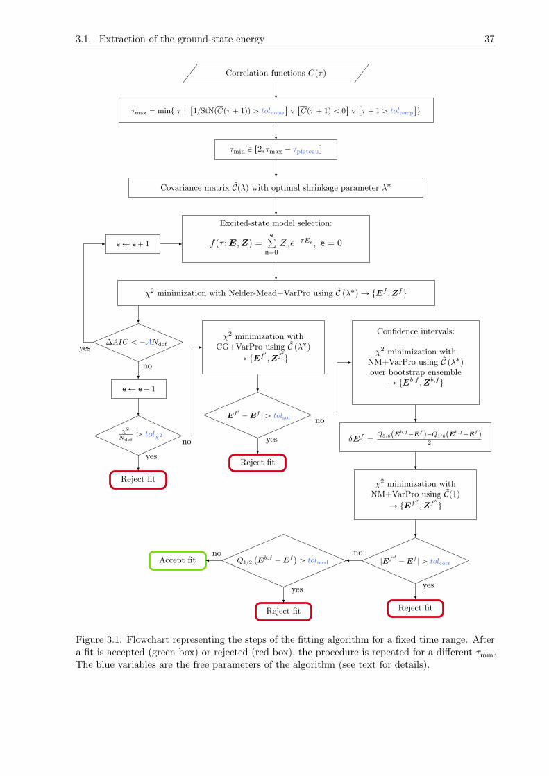
3.1. Extraction of the ground-state energy 37
Correlation functions Cpτq
τmin P r2, τmax ´ τplateaus
τmax “ mint τ |“
1StNpCpτ ` 1qq ą tolnoise‰
_“
Cpτ ` 1q ă 0‰
_“
τ ` 1 ą toltemp‰
u
Excited-state model selection:
fpτ ;E,Zq “eř
n“0Zne
´τEn , e “ 0
χ2 minimization with Nelder-Mead+VarPro using C pλ˚q Ñ tEf ,Zfu
∆AIC ă ´ANdof
|Ef 1´Ef
| ą tolsol
yes
eÐ e` 1
eÐ e´ 1
Reject fit
χ2
Ndofą tolχ2
Accept fit
no
χ2 minimization withCG+VarPro using C pλ˚q
Ñ tEf 1 ,Zf1
u
Confidence intervals:
χ2 minimization withNM+VarPro using C pλ˚qover bootstrap ensemble
Ñ tEb,f ,Zb,fu
Reject fit
no
yes
yes
no
Reject fitReject fit
δEf “Q56pE
b,f´Efq´Q16pE
b,f´Efq
2
|Ef2´Ef
| ą tolcorr
χ2 minimization withNM+VarPro using Cp1q
Ñ tEf2 ,Zf2
u
yes
noQ12
`
Eb,f´Ef
˘
ą tolmed
yes
no
Covariance matrix Cpλq with optimal shrinkage parameter λ˚
Figure 3.1: Flowchart representing the steps of the fitting algorithm for a fixed time range. Aftera fit is accepted (green box) or rejected (red box), the procedure is repeated for a different τmin.The blue variables are the free parameters of the algorithm (see text for details).
38 Chapter 3. Analysis of two-point correlation functions
In the present work, we define the statistical uncertainty as that of the fit with the highest weight,while the systematic uncertainty is defined as the average difference between the weighted meanvalue and each of the accepted fits,
δEstat “ δEf :maxrtωf us0 , δEsys “
g
f
f
e
Naccÿ
f“1
ωf
´
Ef0 ´ E0
¯2. (3.12)
An alternative way to extract the energy of the system is by using the EMP as defined inEq. (2.41), based in the assumption that the overlap to the ground state is stronger than the oneto excited states, which allows us to use as a fitting function a constant, E0, plus exponentials toaccount for excited states contributions.
In previous works (as in Ref. [66]), the energy shift in the finite-volume energies of twointeracting baryons, ∆E0 “ E0 ´MB1
´MB2, was obtained by fitting a constant to the effective
energy-shift function given by Eq. (2.44). In these calculations, the correlation functions for boththe single- and two-baryon systems are required to be described by a single-state fit within thefitting time range. This is due to the fact that otherwise, cancellations may occur between excitedstates (including the finite-volume states that would correspond to elastic scattering states in theinfinite volume), either in the correlation function or in ratios of correlation functions, producinga “mirage plateau” [279] (see further discussion in Section 4.1). To minimize this problem, herethe single- and two-baryon correlation functions are fitted separately to multi-exponential formswithin the same fitting range, and afterwards the energy shifts are computed at the bootstraplevel, in such a way that correlations between the different correlation functions are taken intoaccount. The use of correlated differences of multi-state fit results is particularly convenient forautomated fit-range sampling, since the number of excited states can be varied independently forone- and two-baryon correlation functions, unlike fits to the ratio in Eq. (2.43). Despite this fact,consistent results were obtained with fits to the ratio in Eq. (2.43) in the allowed time regions.
3.1.2 Generalized pencil-of-functions method
Before discussing the variational method, there are a few improvements that we can do inorder to remove excited-state contributions, which would allow us to extend the time range atearly times. When only a single type of operator is computed, such method is the generalizedpencil-of-functions method (GPoF) [274,293,294], where a set of linearly-independent operatorsare created via the time evolution operator,
Xδτ pτq “ eδτHX pτqe´δτH “ X pτ ` δτq . (3.13)
Then, a correlation function matrix can be built with the two operators, X and Xδτ ,
CGPoFpτq “
ˆ
xX pτqX p0qy xX pτqXδτ p0qyxXδτ pτqX p0qy xXδτ pτqXδτ p0qy
˙
“
ˆ
xX pτqX p0qy xX pτqX p´δτqyxX pτ ` δτqX p0qy xX pτ ` δτqX p´δτqy
˙
“
ˆ
Cpτq Cpτ ` δτqCpτ ` δτq Cpτ ` 2δτq
˙
,
(3.14)
where in the last step we have used the time-translation invariance of the correlation functions.This procedure can be generalized to construct a larger matrix by using multiple δτ shifts, Xnδτ ,and it can also be applied to three-point correlation functions [274]. Once this matrix is built,the generalized eigenvalue problem (GEVP) can be solved (discussed in Section 3.1.4) and theenergies can be extracted. In order to illustrate this method (as well as the following ones), thedata from Ref. [79] will be used. In Fig. 3.2, the EMP for the proton is shown, comparing theraw C2ptpτq correlation function data with the results from a 2ˆ 2 GPoF analysis with δτ “ 2.It can be seen that while the excited state contamination for small τ is reduced for the groundstate, the errors increase faster at earlier times than the raw correlator. It can be noticed thatthe excited state cannot be extracted reliably, and more suitable methods, like the variationalmethod, are better when dealing with these states.
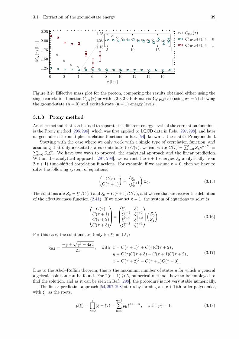
3.1. Extraction of the ground-state energy 39
0 2 4 6 8 10 12 14 16
τ [l.u.]
1.25
1.50
1.75
2.00
2.25MN
(τ)
[l.u.]
C2pt(τ)
CGPoF(τ), n = 0
CGPoF(τ), n = 15 10 15
1.15
1.20
1.25
Figure 3.2: Effective mass plot for the proton, comparing the results obtained either using thesingle correlation function C2ptpτq or with a 2ˆ 2 GPoF matrix CGPoFpτq (using δτ “ 2) showingthe ground-state (n “ 0) and excited-state (n “ 1) energy levels.
3.1.3 Prony method
Another method that can be used to separate the different energy levels of the correlation functionsis the Prony method [295,296], which was first applied to LQCD data in Refs. [297,298], and lateron generalized for multiple correlation functions in Ref. [54], known as the matrix-Prony method.
Starting with the case where we only work with a single type of correlation function, andassuming that only e excited states contribute to Cpτq, we can write Cpτq “
řen“0 Zne
´τEn ”ře
n“0 Znξτn . We have two ways to proceed, the analytical approach and the linear prediction.
Within the analytical approach [297, 298], we extract the e ` 1 energies ξn analytically from2pe ` 1q time-shifted correlation functions. For example, if we assume e “ 0, then we have tosolve the following system of equations,
ˆ
CpτqCpτ ` 1q
˙
“
ˆ
ξτ0ξτ`1
0
˙
Z0 . (3.15)
The solutions are Z0 “ ξτ0 Cpτq and ξ0 “ Cpτ`1qCpτq, and we see that we recover the definitionof the effective mass function (2.41). If we now set e “ 1, the system of equations to solve is
¨
˚
˚
˝
CpτqCpτ ` 1qCpτ ` 2qCpτ ` 3q
˛
‹
‹
‚
“
¨
˚
˚
˝
ξτ0 ξτ1ξτ`1
0 ξτ`11
ξτ`20 ξτ`2
1
ξτ`30 ξτ`3
1
˛
‹
‹
‚
ˆ
Z0
Z1
˙
. (3.16)
For this case, the solutions are (only for ξ0 and ξ1)
ξ0,1 “´y ˘
a
y2 ´ 4xz
2x, with x “ Cpτ ` 1q2 ` CpτqCpτ ` 2q ,
y “ CpτqCpτ ` 3q ´ Cpτ ` 1qCpτ ` 2q ,
z “ Cpτ ` 2q2 ´ Cpτ ` 1qCpτ ` 3q .
(3.17)
Due to the Abel–Ruffini theorem, this is the maximum number of states e for which a generalalgebraic solution can be found. For 2pe` 1q ě 5, numerical methods have to be employed tofind the solution, and as it can be seen in Ref. [298], the procedure is not very stable numerically.
The linear prediction approach [54, 297,298] starts by forming an pe` 1qth order polynomial,with ξn as the roots,
ppξq “eź
n“0
pξ ´ ξnq “e`1ÿ
k“0
pk ξe`1´k , with p0 “ 1 . (3.18)
40 Chapter 3. Analysis of two-point correlation functions
Since ξn are the roots of this polynomial (ppξnq “ 0), we can rewrite it as
ξmn “ ´e`1ÿ
k“1
pk ξm´kn , with m ě e` 1 . (3.19)
With this last expression, we can write the correlation function as
Cpτq “eÿ
n“0
Znξτn “ ´
eÿ
n“0
Zn
e`1ÿ
k“1
pk ξτ´kn “ ´
e`1ÿ
k“1
pkCpτ ´ kq , with τ ě e` 1 . (3.20)
This is the reason why this method is called linear prediction, since we predict Cpτq using thevalues of the correlation function at earlier times. Once the values of pk have been obtainedby solving Eq. (3.20), they can be used to solve for the roots of the polynomial ppξq. An easyexample to see how this works is by setting e “ 0, in which case we get
Cpτ ` 1q ` p1Cpτq “ 0 and ppξq “ ξ ` p1 , (3.21)
again recovering the effective mass function.For the matrix-Prony method [54], we assume we have computed Nop different correlation
functions, so we can write them in a vector form,
cpτq “`
C1pτq ¨ ¨ ¨ CNoppτq˘J
. (3.22)
Since correlation functions can be written as a sum of exponentials, we want to build an operatorsuch that cpτ ` τtq “ Tcpτq (similar to the linear prediction approach). Defining T “M´1V ,we get the following relation,
Mcpτ ` τtq “ V cpτq . (3.23)
A simple solution for the matrices M and V is
M “
«
τ`τ1ÿ
τ 1“τ
cpτ 1 ` τtqcJpτ 1q
ff´1
, V “
«
τ`τ1ÿ
τ 1“τ
cpτ 1qcJpτ 1q
ff´1
. (3.24)
The value of τ1 has to be large enough to make the matrices inside the brackets full rank (thishappens for τ1 ě Nop). With these matrices, a GEVP can be solved,
Muα “ pλαqτtV uα , (3.25)
with uα being the general eigenvectors and λα “ eEα the general eigenvalues (again, this systemwill be discussed in Section 3.1.4). The parameter τt can be varied to improve stability. Toillustrate the method, we use two correlation functions (so τ1 ě 2) for the proton, correspondingto two different smearings: a narrow (N) and a wide (W ) Gaussian profile at both source andsink. Then, according to Eq. (3.25), these correlation functions can be written as
ˆ
CN pτqCW pτq
˙
“ Z 10
ˆ
u0N
u0W
˙
pλ0q´τ ` Z 11
ˆ
u1N
u1W
˙
pλ1q´τ . (3.26)
In order to extract the energies λα, we need to find the correct combination of CNW pτq with thecomponents of the eigenvectors uαNW (the remaining overlap factors Z 1α are not relevant in thepresent discussion, since they cancel out in the ratios which define the EMPs). With a bit ofalgebra, we arrive at
pλ0q´τ 9
u1NC
W pτq ´ u1WC
N pτq
u0Nu
1W ´ u1
Nu0W
, pλ1q´τ 9
u0NC
W pτq ´ u0WC
N pτq
u0Nu
1W ´ u1
Nu0W
. (3.27)
In Fig. 3.3, the EMP for the proton is shown, comparing the raw C2ptpτq correlation functiondata with the results from a matrix-Prony analysis with tτt, τ1u “ t2, 3u. Like in the GPoF case,the effective mass for the ground-state reaches the plateau at small times, but the excited statecannot be reliably extracted.
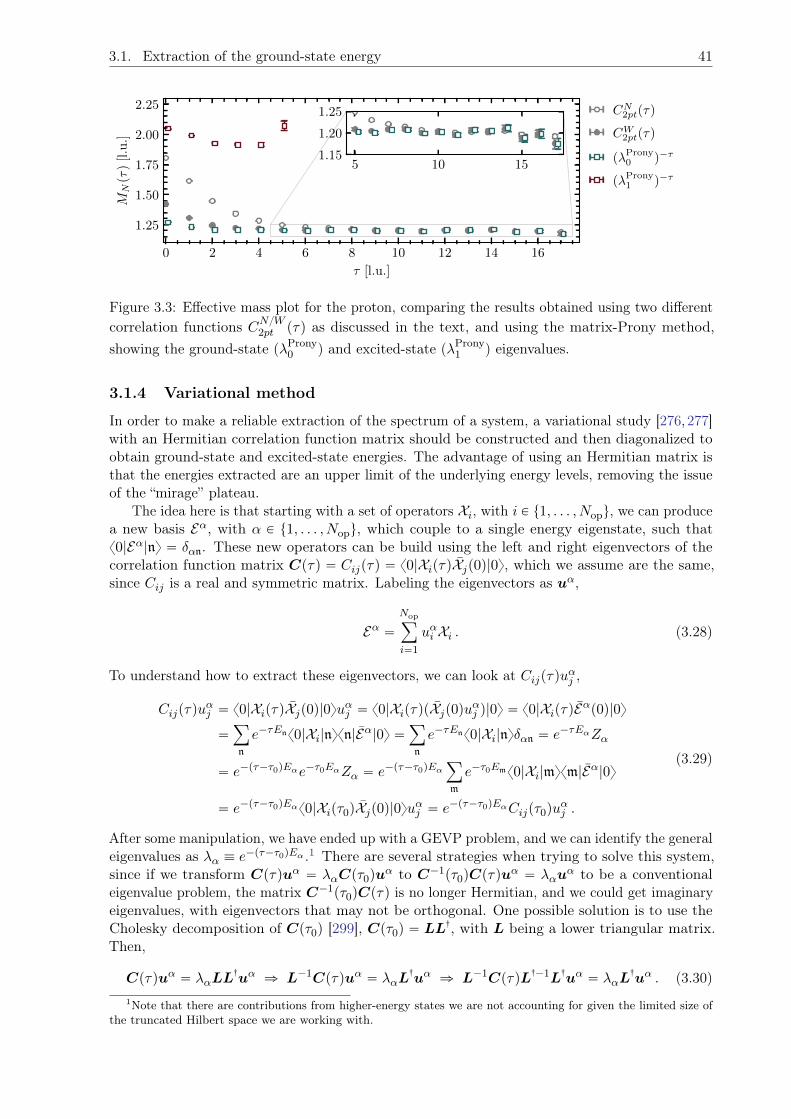
3.1. Extraction of the ground-state energy 41
0 2 4 6 8 10 12 14 16
τ [l.u.]
1.25
1.50
1.75
2.00
2.25MN
(τ)
[l.u.]
CN2pt(τ)
CW2pt(τ)
(λProny0 )−τ
(λProny1 )−τ
5 10 151.15
1.20
1.25
Figure 3.3: Effective mass plot for the proton, comparing the results obtained using two differentcorrelation functions CNW2pt pτq as discussed in the text, and using the matrix-Prony method,showing the ground-state (λProny0 ) and excited-state (λProny1 ) eigenvalues.
3.1.4 Variational method
In order to make a reliable extraction of the spectrum of a system, a variational study [276,277]with an Hermitian correlation function matrix should be constructed and then diagonalized toobtain ground-state and excited-state energies. The advantage of using an Hermitian matrix isthat the energies extracted are an upper limit of the underlying energy levels, removing the issueof the “mirage” plateau.
The idea here is that starting with a set of operators Xi, with i P t1, . . . , Nopu, we can producea new basis Eα, with α P t1, . . . , Nopu, which couple to a single energy eigenstate, such thatx0|Eα|ny “ δαn. These new operators can be build using the left and right eigenvectors of thecorrelation function matrix Cpτq “ Cijpτq “ x0|XipτqXjp0q|0y, which we assume are the same,since Cij is a real and symmetric matrix. Labeling the eigenvectors as uα,
Eα “Nopÿ
i“1
uαi Xi . (3.28)
To understand how to extract these eigenvectors, we can look at Cijpτquαj ,
Cijpτquαj “ x0|XipτqXjp0q|0yuαj “ x0|XipτqpXjp0quαj q|0y “ x0|XipτqEαp0q|0y“
ÿ
n
e´τEnx0|Xi|nyxn|Eα|0y “ÿ
n
e´τEnx0|Xi|nyδαn “ e´τEαZα
“ e´pτ´τ0qEαe´τ0EαZα “ e´pτ´τ0qEαÿ
m
e´τ0Emx0|Xi|myxm|Eα|0y
“ e´pτ´τ0qEαx0|Xipτ0qXjp0q|0yuαj “ e´pτ´τ0qEαCijpτ0quαj .
(3.29)
After some manipulation, we have ended up with a GEVP problem, and we can identify the generaleigenvalues as λα ” e´pτ´τ0qEα .1 There are several strategies when trying to solve this system,since if we transform Cpτquα “ λαCpτ0qu
α to C´1pτ0qCpτquα “ λαu
α to be a conventionaleigenvalue problem, the matrix C´1pτ0qCpτq is no longer Hermitian, and we could get imaginaryeigenvalues, with eigenvectors that may not be orthogonal. One possible solution is to use theCholesky decomposition of Cpτ0q [299], Cpτ0q “ LL
:, with L being a lower triangular matrix.Then,
Cpτquα “ λαLL:uα ñ L´1Cpτquα “ λαL
:uα ñ L´1CpτqL
:´1L:uα “ λαL
:uα . (3.30)
1Note that there are contributions from higher-energy states we are not accounting for given the limited size ofthe truncated Hilbert space we are working with.
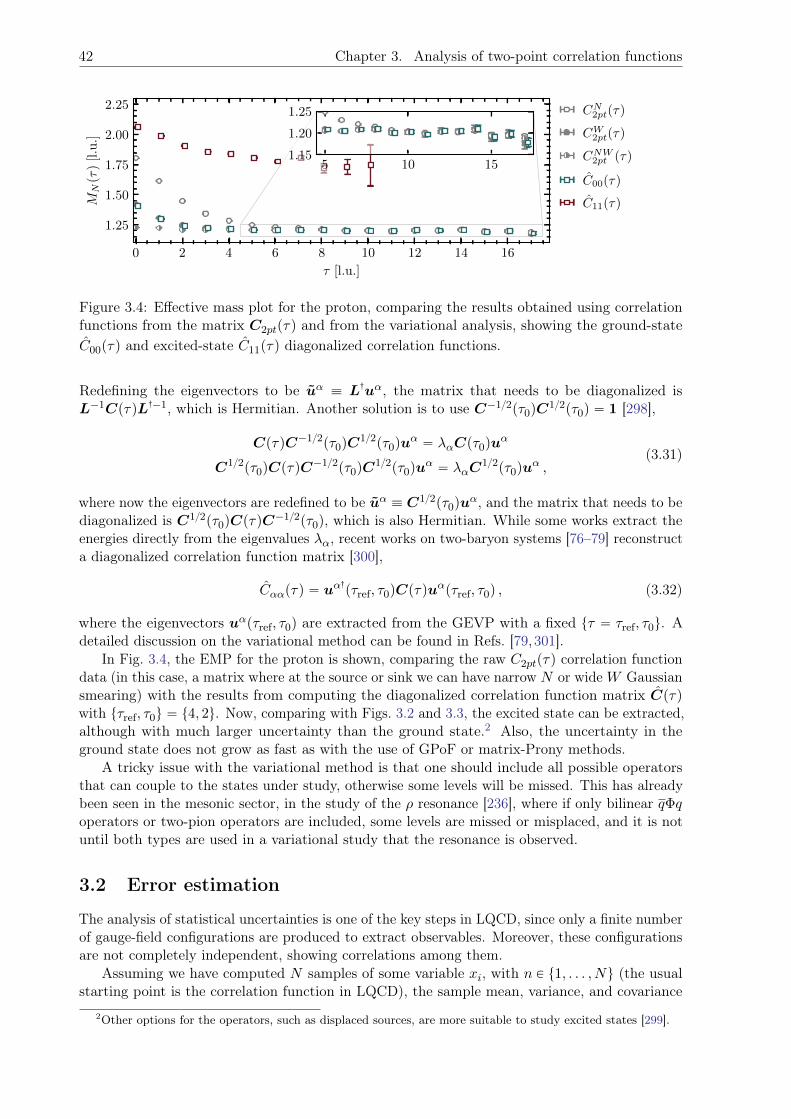
42 Chapter 3. Analysis of two-point correlation functions
0 2 4 6 8 10 12 14 16
τ [l.u.]
1.25
1.50
1.75
2.00
2.25MN
(τ)
[l.u.]
CN2pt(τ)
CW2pt(τ)
CNW2pt (τ)
C00(τ)
C11(τ)
5 10 151.15
1.20
1.25
Figure 3.4: Effective mass plot for the proton, comparing the results obtained using correlationfunctions from the matrix C2ptpτq and from the variational analysis, showing the ground-stateC00pτq and excited-state C11pτq diagonalized correlation functions.
Redefining the eigenvectors to be uα ” L:uα, the matrix that needs to be diagonalized isL´1CpτqL:´1, which is Hermitian. Another solution is to use C´12pτ0qC
12pτ0q “ 1 [298],
CpτqC´12pτ0qC12pτ0qu
α “ λαCpτ0quα
C12pτ0qCpτqC´12pτ0qC
12pτ0quα “ λαC
12pτ0quα ,
(3.31)
where now the eigenvectors are redefined to be uα ” C12pτ0quα, and the matrix that needs to be
diagonalized is C12pτ0qCpτqC´12pτ0q, which is also Hermitian. While some works extract the
energies directly from the eigenvalues λα, recent works on two-baryon systems [76–79] reconstructa diagonalized correlation function matrix [300],
Cααpτq “ uα:pτref, τ0qCpτqu
αpτref, τ0q , (3.32)
where the eigenvectors uαpτref, τ0q are extracted from the GEVP with a fixed tτ “ τref, τ0u. Adetailed discussion on the variational method can be found in Refs. [79,301].
In Fig. 3.4, the EMP for the proton is shown, comparing the raw C2ptpτq correlation functiondata (in this case, a matrix where at the source or sink we can have narrow N or wideW Gaussiansmearing) with the results from computing the diagonalized correlation function matrix Cpτqwith tτref, τ0u “ t4, 2u. Now, comparing with Figs. 3.2 and 3.3, the excited state can be extracted,although with much larger uncertainty than the ground state.2 Also, the uncertainty in theground state does not grow as fast as with the use of GPoF or matrix-Prony methods.
A tricky issue with the variational method is that one should include all possible operatorsthat can couple to the states under study, otherwise some levels will be missed. This has alreadybeen seen in the mesonic sector, in the study of the ρ resonance [236], where if only bilinear qΦqoperators or two-pion operators are included, some levels are missed or misplaced, and it is notuntil both types are used in a variational study that the resonance is observed.
3.2 Error estimation
The analysis of statistical uncertainties is one of the key steps in LQCD, since only a finite numberof gauge-field configurations are produced to extract observables. Moreover, these configurationsare not completely independent, showing correlations among them.
Assuming we have computed N samples of some variable xi, with n P t1, . . . , Nu (the usualstarting point is the correlation function in LQCD), the sample mean, variance, and covariance
2Other options for the operators, such as displaced sources, are more suitable to study excited states [299].
3.2. Error estimation 43
with another variable yn are given by
x “1
N
Nÿ
n“1
xn , σ2x “
1
NpN ´ 1q
Nÿ
n“1
pxn ´ xq2 , Cpx, yq “ 1
N ´ 1
Nÿ
n“1
pxn ´ xqpyn ´ yq . (3.33)
As we have seen in the previous sections, the correlation functions are usually manipulated andinserted into functions, such as the effective mass. Then, when we look at some function f , theaverage value, labeled as fpXq, can be computed by using fpxq (and not fpxq “
ř
n fpxnqN ,since it would be a biased estimator [302]), and the uncertainty can be obtained via errorpropagation,
σfpxq “ σx
ˇ
ˇ
ˇ
ˇ
df
dx
ˇ
ˇ
ˇ
ˇ
x“x
. (3.34)
However, as the number of variables in f increases, and for correlated data, this formula isno longer practical, and alternative methods have to be used. In our case, such methods areresampling methods, the jackknife and bootstrap methods, both widely used in the LQCDcommunity (for an extended and detailed discussion, see Refs. [206,302,303]).
3.2.1 Jackknife method
The starting point is to construct the jackknife samples xJn, which are defined by taking theaverage of the variable x without including the nth sample,
xJn “1
N ´ 1
ÿ
m‰n
xm “N
N ´ 1x´
1
N ´ 1xn . (3.35)
Then, the mean value of the function f and the estimation of its uncertainty is
fpXq » fJx “
1
N
Nÿ
n“1
fpxJnq , σ2fpXq »
N ´ 1
N
Nÿ
n“1
”
fpxJnq ´ fJx
ı2. (3.36)
An easy check that we can perform is to see that if fpxq “ x, we recover the expressions fromEq. (3.33),
x “1
N
Nÿ
n“1
xJn “1
N
Nÿ
n“1
ˆ
N
N ´ 1x´
1
N ´ 1xn
˙
“N
N ´ 1x´
1
N ´ 1x “ x ,
σ2x “
N ´ 1
N
Nÿ
n“1
`
xJn ´ x˘2“N ´ 1
N
Nÿ
n“1
ˆ
N
N ´ 1x´
1
N ´ 1xn ´ x
˙2
“1
NpN ´ 1q
Nÿ
n“1
pxn ´ xq2“ σ2
x .
(3.37)
As pointed out in Ref. [302], a better estimator for fpXq that includes 1N bias correction isgiven by
fpXq » Nfpxq ´ pN ´ 1qfJx . (3.38)
Also, this method can be used to compute the covariance matrix, needed when performing χ2
minimizations for the fitting of the correlation function. It is given by
CJ rfpxq, fpyqs “ N ´ 1
N
Nÿ
n“1
”
fpxJnq ´ fJx
ı ”
fpyJnq ´ fJy
ı
. (3.39)
A generalization of the jackknife method is based on not only subtracting one sample fromthe set, but k samples, ending with Nk “ Nk jackknife samples.
44 Chapter 3. Analysis of two-point correlation functions
3.2.2 Bootstrap method
The bootstrap resampling method, compared to the jackknife one, creates Nboot bootstrap samplesxBα , with α P t1, . . . , Nbootu, where each one is obtained from a random selection from the originalsample N points (with repetitions allowed),
xBα “1
N
Nÿ
n“1
xrandp1,Nq “1
N
Nÿ
n“1
rαnxn , (3.40)
where rαn is the number of times xn appears in the αth bootstrap sample, with the constrain thatř
n rαn “ N , which follows a binomial distribution [302],
P prαnq “N !
rαn !pN ´ rαnq!prαn p1´ pqN´r
αn , (3.41)
where p “ 1N is the probability that xn is chosen. With this method, we can also write how tocompute the mean value of the function f and the estimation of its uncertainty,
fpXq » fBx “
1
Nboot
Nbootÿ
α“1
fpxBα q , σ2fpXq »
N
N ´ 1
1
Nboot
Nbootÿ
α“1
”
fpxBα q ´ fBx
ı2. (3.42)
In the case of fpxq “ x, we recover the known formulas. For example, for the mean value,
x “1
Nboot
Nbootÿ
α“1
xBα “1
N
Nÿ
n“1
˜
1
Nboot
Nbootÿ
α“1
rαn
¸
xn “1
N
Nÿ
n“1
xn “ x , (3.43)
where we have assumed that Nboot is very large, so we can use the mean value of a binomialvariable, which is Np ( with p “ 1N , we get Np “ 1).
A better estimator for fpXq, which reduces the bias from order 1N to 1N2 [302], is
fpXq » 2fpxq ´ fBx . (3.44)
The covariance matrix can also be estimated with bootstrap,
CBrfpxq, fpyqs “ N
N ´ 1
1
Nboot
Nbootÿ
α“1
”
fpxBα q ´ fBx
ı ”
fpyBα q ´ fBy
ı
. (3.45)
What is interesting with the bootstrap resampling method is that we can look at the distribu-tion function of fpxq and compute the errors with the quantiles (as it is done in the Section 3.1.1).Also, the confidence regions of the parameters in some non-linear fits can be extracted easily.
3.2.3 Hodges–Lehmann estimator
One possible issue that we might encounter with LQCD data is the presence of outliers in thecorrelation functions due to fluctuations in a finite-size sample. For these cases there exists whatare called robust estimators, which are more resilient to these outliers than the usual estimators,like Eq. (3.33). The Hodges–Lehmann (HL) is an example of such estimators [304]. The startingpoint, similar to the bootstrap method, is to generate NHL HL samples xHLµ , µ P t1, . . . , NHLu,taking N random points from the original sample, compute the pairwise averages (known as theWalsh averages [305]) and take the median,
xHLµ “ Median„"
xn ` xm2
*
, with xn “ xrandp1,Nq and 1 ď n,m ď N . (3.46)
3.2. Error estimation 45
Then, a robust estimator of the median is defined as
fpXq » fHLx “ Median
“
fpxHLµ q(‰
. (3.47)
For the uncertainty associated to this estimator and the computation of covariance matrices, themedian absolute deviation (MAD) is used,
σfpXq “1
Φ´1p34q
Medianrt|fpxHLµ q ´ fHLx |us ,
CHLrfpxq, fpyqs “ MedianrtpfpxHLµ q ´ fHLx qpfpyHLµ q ´ f
HLy qus ,
(3.48)
where Φ´1p34q “ 0.67449 is the inverse of the normal cumulative distribution function (this factor
is needed to convert to the usual error definition of „ 68% coverage, since the MAD only covers„ 50%). In Appendix G, a detailed comparison with the bootstrap method is performed, and foradditional discussions applied to LQCD, see Refs. [66, 206].

46 Chapter 3. Analysis of two-point correlation functions
Chapter 4
The strong baryon-baryon interaction
4.1 Present status
In order to see what the current knowledge of the strong interaction between two baryons at lowenergies is, let us summarize the present status in the three main fronts: experimental, theoretical,and lattice. For a review on some of these topics, see Refs. [5, 32,33,306].
Experimental front
Up until the last decade, the main sources of experimental information on the low-energy stronginteraction between two baryons were scattering experiments and the study of hypernuclei.Regarding scattering data in the strange sector, the standard set of data used for constrainingtheoretical models is composed of 36 points, 35 of which are total cross sections: 12 for ΛpÑΛp [307, 308], 4 for Σ`p Ñ Σ`p, 7 for Σ´p Ñ Σ´p [309], 6 for Σ´p Ñ Σ0n, and 6 forΣ´pÑ Λn [310]. In addition, the inelastic capture rate of Σ´p at rest [311,312] is included. Itis interesting to notice that all the experimental data used was obtained in the early 70s (olderdata is also available, see [17]) with quite large uncertainties, and only for systems with only onestrange quark (none for S ď ´2). Additional points at slightly higher energies are also included:7 for Λp Ñ Λp, 4 for Λp Ñ Σ0p [313], 3 for Σ´p Ñ Σ´p [314], and 3 for Σ`p Ñ Σ`p [315],bringing the total number of points to 53 (differential cross sections have also been reported inRefs. [309,310,314,315], but they are not usually included in this fitting set). For systems withS “ ´2, there are some upper limits on the total cross section for the channels Ξ´pÑ Ξ´p andΞ´pÑ ΛΛ [316], and other in-medium values [317,318]. All these points are plotted in Fig. 4.1,an updated version of a similar figure appearing in Ref. [319]. Additional experiments are runningto increase this database, such as the E40 at J-PARC [320,321], which focuses on Σ˘p elasticand inelastic channels. For the sake of comparison, a total of 6713 points have been collected inthe NN sector (2996 for pp and 3717 for np) for energies below 350 MeV [322, 323], includingtotal and differential cross sections, analyzing powers, depolarizations, etc.
An alternative way to learn about two-baryon interactions is by means of the femtoscopytechnique, in which two-particle correlation functions in momentum space are measured in high-energy collisions [324]. This correlation function can be computed theoretically, so comparisonswith theoretical models [325, 326] as well as extraction of scattering parameters are possible. Thefirst application of this method to hyperon physics was performed by the STAR Collaborationusing heavy-ion collisions, where the p–Λ correlation function was extracted [327], although withlarge uncertainties. Several studies have followed by other collaborations, mainly HADES andALICE. The channels that have been studied are p–Λ [327–330], Λ–Λ [330–332], p–Σ0 [333],p–Ξ´ [334], and p–Ω´ [83,335]. The most important contribution of this method is the possibilityto access experimentally systems with S ď ´2, very challenging for scattering experiments.Although some constraints on the scattering parameters for ΛΛ have been obtained (with quitelarge uncertainties) [332], at the moment the data extracted from femtoscopy is used to compare
47
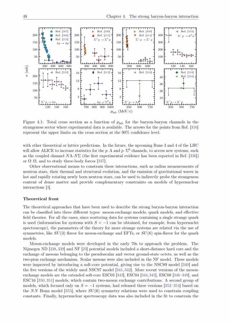
48 Chapter 4. The strong baryon-baryon interaction
200 400 600 800
50
100
150
200
ΛpÑ Λp
Ref. [307]Ref. [308]Ref. [313]
200 400 600 800
50
100
150
200
Σ`pÑ Σ
`p
Ref. [309]Ref. [315]
200 400 600
50
100
150
200
Σ´pÑ Σ
´p
Ref. [309]Ref. [314]
120 140 160
100
200
300
400 Σ´pÑ Σ
0n
Ref. [310]
120 140 160
50
100
150
200
Σ´pÑ Λn
Ref. [310]
700 800 900 1000
4
8
12
16
ΛpÑ Σ0p
Ref. [313]
250 500 750
4
8
12
16
Ξ´pÑ ΛΛ
Ref. [316]
250 500 750
10
20
30
40
Ξ´pÑ Ξ
´p
Ref. [318]Ref. [316]σ
(mb)
plab (MeV/c)
Figure 4.1: Total cross section as a function of plab for the baryon-baryon channels in thestrangeness sector where experimental data is available. The arrows for the points from Ref. [316]represent the upper limits on the cross section at the 90% confidence level.
with other theoretical or lattice predictions. In the future, the upcoming Runs 3 and 4 of the LHCwill allow ALICE to increase statistics for the p–Λ and p–Σ0 channels, to access new systems, suchas the coupled channel NΛ-NΣ (the first experimental evidence has been reported in Ref. [336])or Ω–Ω, and to study three-body forces [337].
Other observational means to constrain these interactions, such as radius measurements ofneutron stars, their thermal and structural evolution, and the emission of gravitational waves inhot and rapidly rotating newly born neutron stars, can be used to indirectly probe the strangenesscontent of dense matter and provide complementary constraints on models of hypernuclearinteractions [3].
Theoretical front
The theoretical approaches that have been used to describe the strong baryon-baryon interactioncan be classified into three different types: meson-exchange models, quark models, and effectivefield theories. For all the cases, since scattering data for systems containing a single strange quarkis used (information for systems with S ă ´1 can be obtained, for example, from hypernucleispectroscopy), the parameters of the theory for more strange systems are related via the use ofsymmetries, like SUp3q flavor for meson-exchange and EFTs, or SUp6q spin-flavor for the quarkmodels.
Meson-exchange models were developed in the early 70s to approach the problem. TheNijmegen ND [338,339] and NF [23] potential models included a short-distance hard core and theexchange of mesons belonging to the pseudoscalar and vector ground-state octets, as well as thetwo-pion exchange mechanism. Scalar mesons were also included in the NF model. These modelswere improved by introducing a soft-core potential, giving rise to the NSC89 model [340] andthe five versions of the widely used NSC97 model [341,342]. More recent versions of the meson-exchange models are the extended soft-core ESC03 [343], ESC04 [344,345], ESC08 [346–349], andESC16 [350,351] models, which contain two-meson exchange contributions. A second group ofmodels, which focused only on S “ ´1 systems, had released three versions [352–354] based onthe NN Bonn model [355], where SUp6q symmetry relations were used to constrain couplingconstants. Finally, hypernuclear spectroscopy data was also included in the fit to constrain the
4.1. Present status 49
Ehime potential [356–358], an extension of the meson-exchange model of Refs. [359,360], whichsupplemented the contribution of pseudoscalar, scalar, and vector mesons with the isoscalar scalarpart of the uncorrelated and correlated two-pion exchanges.
The second type of approach is non-relativistic quark models, which are based on the resonating-group method [361–363]. While the repulsive short-distance physics is well described via thequark-quark interaction (color-magnetic interaction and Pauli effect), the medium- and long-rangeeffects have to be included by hand via the exchange of mesons. The most known versions areFSS [364–366] and fss2 [367, 368], although other versions like RGM-F and RGM-H are alsoavailable [365,366,369–371].
Lastly, the EFT approach is a model-independent technique based only on the symmetriesof the fundamental theory, QCD. Using a power counting scheme, the approach allows us towrite the Lagrangian as an expansion, typically in powers of the (low) momenta of the particles,and estimate the error of a calculation at a given order produced by the neglected higher-orderterms. This approach was first applied in Ref. [10] to the study of the modification of the baryonmasses in nuclear matter. Later on, the first study of hyperon-nucleon scattering was performedin Ref. [372] within the EFT formalism of Ref. [10]. Following the studies in the NN sector,χEFT calculations at LO [47,373,374] and NLO [6,46,375–377] were performed for baryon-baryonchannels up to S “ ´4. In these studies, several values of the cutoff used to regularize theresulting potential were used to assess the uncertainty, and the difference between the LO andNLO contributions was used to address convergence issues (more detailed studies of uncertaintyquantification in EFTs are available for the NN sector [378–380]).
Before discussing the lattice state-of-the-art calculations, it is interesting to see what arethe predictions for the scattering parameters obtained with all the above-mentioned theoreticalmodels and compare them to the few available experimental extractions. All the values aretabulated in Tables C.1-C.7 of Appendix C, and plotted in Fig. 4.2 for the cases where both thescattering length and effective range are calculated. Moreover, the first two panels in Fig. 4.2 arefor the NN channels, showing the scattering parameters computed with the same models as theones used for the hyperon channels (not specific for NN) [23,338,342,346,365,381–385] as wellas the experimental values [25], where one can see the impact of the quality and quantity of dataon the final values.
Lattice front
The search for complementary inputs besides experimental data on baryon-baryon scatteringhas led LQCD to be an important tool to help constrain theoretical models. The first study ofthe interaction between two baryons was performed by the CP-PACS Collaboration [67,386] forthe NN sector, using a quenched calculation with unphysical quark masses. This seminal workmotivated more studies of the baryon-baryon interaction, by several groups and collaborations,using two different methods: the direct and the potential method. The differences and issuesbetween these two methods will be discussed after presenting a summary of the work and resultspublished to date.
Ten years later after the appearance of the CP-PACS paper, the NPLQCD Collaborationstudied the NN systems in finite volume in detail [85] considering both scattering and boundstates, and also presented the advantages of using LQCD to approach hypernuclear physics [387].The same collaboration made the first fully-dynamical calculations for the nucleon-nucleon [58]and hyperon-nucleon [59] systems with a pion mass of around 350, 490, and 590 MeV (earlierinvestigations on the Λp system were performed by other authors using the quenched approximationin Ref. [388]). These works were followed by a high statistics analysis of several baryon-baryonsystems with strangeness ranging from 0 to ´4 [56, 62] at a pion mass of 350 MeV (the firstfully-dynamical three-baryon calculations were also part of this analysis [55]), with special interestin the H-dibaryon [60,61] (some previous quenched calculations on this system are summarizedin Ref. [61]). The ΣN system was studied in Ref. [63], where the authors extrapolated the
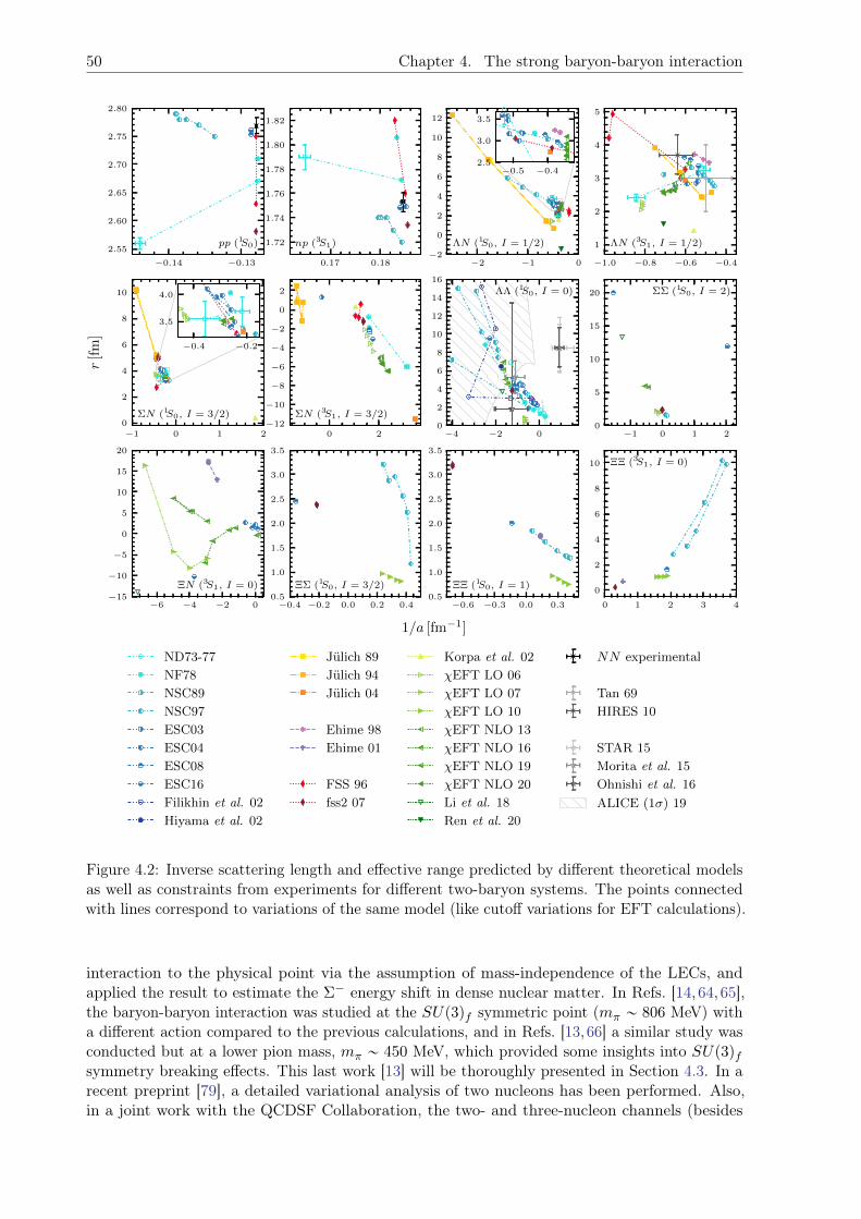
50 Chapter 4. The strong baryon-baryon interaction
−0.14 −0.13
2.55
2.60
2.65
2.70
2.75
2.80
pp (1S0)
0.17 0.18
1.72
1.74
1.76
1.78
1.80
1.82
np (3S1)
−2 −1 0−2
0
2
4
6
8
10
12
ΛN (1S0, I = 1/2)
−0.5 −0.42.5
3.0
3.5
−1.0 −0.8 −0.6 −0.4
1
2
3
4
5
ΛN (3S1, I = 1/2)
−1 0 1 20
2
4
6
8
10
ΣN (1S0, I = 3/2)
−0.4 −0.2
3.5
4.0
0 2−12
−10
−8
−6
−4
−2
0
2
ΣN (3S1, I = 3/2)
−4 −2 00
2
4
6
8
10
12
14
16
ΛΛ (1S0, I = 0)
−1 0 1 20
5
10
15
20 ΣΣ (1S0, I = 2)
−6 −4 −2 0−15
−10
−5
0
5
10
15
20
ΞN (3S1, I = 0)
−0.4 −0.2 0.0 0.2 0.40.5
1.0
1.5
2.0
2.5
3.0
3.5
ΞΣ (1S0, I = 3/2)
−0.6 −0.3 0.0 0.30.5
1.0
1.5
2.0
2.5
3.0
3.5
ΞΞ (1S0, I = 1)
0 1 2 3 4
0
2
4
6
8
10 ΞΞ (3S1, I = 0)
0.0 0.2 0.4 0.6 0.8 1.0
1/a [fm−1]
0.0
0.2
0.4
0.6
0.8
1.0
r[f
m]
ND73-77
NF78
NSC89
NSC97
ESC03
ESC04
ESC08
ESC16
Filikhin et al. 02
Hiyama et al. 02
Julich 89
Julich 94
Julich 04
Ehime 98
Ehime 01
FSS 96
fss2 07
Korpa et al. 02
χEFT LO 06
χEFT LO 07
χEFT LO 10
χEFT NLO 13
χEFT NLO 16
χEFT NLO 19
χEFT NLO 20
Li et al. 18
Ren et al. 20
NN experimental
Tan 69
HIRES 10
STAR 15
Morita et al. 15
Ohnishi et al. 16
ALICE (1σ) 19
Figure 4.2: Inverse scattering length and effective range predicted by different theoretical modelsas well as constraints from experiments for different two-baryon systems. The points connectedwith lines correspond to variations of the same model (like cutoff variations for EFT calculations).
interaction to the physical point via the assumption of mass-independence of the LECs, andapplied the result to estimate the Σ´ energy shift in dense nuclear matter. In Refs. [14,64,65],the baryon-baryon interaction was studied at the SUp3qf symmetric point (mπ „ 806 MeV) witha different action compared to the previous calculations, and in Refs. [13, 66] a similar study wasconducted but at a lower pion mass, mπ „ 450 MeV, which provided some insights into SUp3qfsymmetry breaking effects. This last work [13] will be thoroughly presented in Section 4.3. In arecent preprint [79], a detailed variational analysis of two nucleons has been performed. Also,in a joint work with the QCDSF Collaboration, the two- and three-nucleon channels (besides
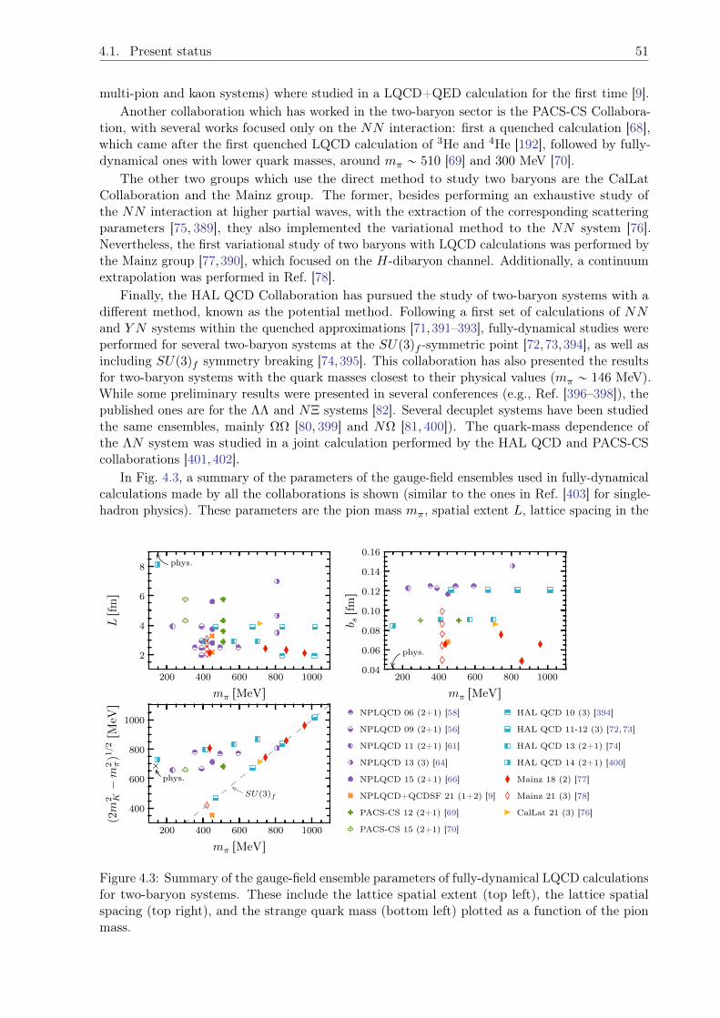
4.1. Present status 51
multi-pion and kaon systems) where studied in a LQCD+QED calculation for the first time [9].Another collaboration which has worked in the two-baryon sector is the PACS-CS Collabora-
tion, with several works focused only on the NN interaction: first a quenched calculation [68],which came after the first quenched LQCD calculation of 3He and 4He [192], followed by fully-dynamical ones with lower quark masses, around mπ „ 510 [69] and 300 MeV [70].
The other two groups which use the direct method to study two baryons are the CalLatCollaboration and the Mainz group. The former, besides performing an exhaustive study ofthe NN interaction at higher partial waves, with the extraction of the corresponding scatteringparameters [75, 389], they also implemented the variational method to the NN system [76].Nevertheless, the first variational study of two baryons with LQCD calculations was performed bythe Mainz group [77, 390], which focused on the H-dibaryon channel. Additionally, a continuumextrapolation was performed in Ref. [78].
Finally, the HAL QCD Collaboration has pursued the study of two-baryon systems with adifferent method, known as the potential method. Following a first set of calculations of NNand Y N systems within the quenched approximations [71, 391–393], fully-dynamical studies wereperformed for several two-baryon systems at the SUp3qf -symmetric point [72, 73,394], as well asincluding SUp3qf symmetry breaking [74,395]. This collaboration has also presented the resultsfor two-baryon systems with the quark masses closest to their physical values (mπ „ 146 MeV).While some preliminary results were presented in several conferences (e.g., Ref. [396–398]), thepublished ones are for the ΛΛ and NΞ systems [82]. Several decuplet systems have been studiedthe same ensembles, mainly ΩΩ [80, 399] and NΩ [81, 400]). The quark-mass dependence ofthe ΛN system was studied in a joint calculation performed by the HAL QCD and PACS-CScollaborations [401,402].
In Fig. 4.3, a summary of the parameters of the gauge-field ensembles used in fully-dynamicalcalculations made by all the collaborations is shown (similar to the ones in Ref. [403] for single-hadron physics). These parameters are the pion mass mπ, spatial extent L, lattice spacing in the
200 400 600 800 1000
mπ rMeVs
2
4
6
8
Lrf
ms
phys.
200 400 600 800 1000
mπ rMeVs
400
600
800
1000
p2m
2 K´m
2 πq12rM
eVs
SUp3qf
phys.
200 400 600 800 1000
mπ rMeVs
0.04
0.06
0.08
0.10
0.12
0.14
0.16
b srf
ms
phys.
NPLQCD 06 (2+1) [58]
NPLQCD 09 (2+1) [56]
NPLQCD 11 (2+1) [61]
NPLQCD 13 (3) [64]
NPLQCD 15 (2+1) [66]
NPLQCD+QCDSF 21 (1+2) [9]
PACS-CS 12 (2+1) [69]
PACS-CS 15 (2+1) [70]
HAL QCD 10 (3) [394]
HAL QCD 11-12 (3) [72,73]
HAL QCD 13 (2+1) [74]
HAL QCD 14 (2+1) [400]
Mainz 18 (2) [77]
Mainz 21 (3) [78]
CalLat 21 (3) [76]
Figure 4.3: Summary of the gauge-field ensemble parameters of fully-dynamical LQCD calculationsfor two-baryon systems. These include the lattice spatial extent (top left), the lattice spatialspacing (top right), and the strange quark mass (bottom left) plotted as a function of the pionmass.
52 Chapter 4. The strong baryon-baryon interaction
spatial direction bs (this clarification is needed for the anisotropic calculations), and the quantityp2m2
K ´m2πq
12, which is proportional to the strange quark mass (see Eq. (4.16)). In all of theseplots, the physical point is indicated with a cross or an arrow labeled with “phys.”, and in theleft-bottom panel the SUp3qf case (mu “ md “ ms) with a dashed line. Some of the ensembleshave been used more than one time (e.g., “NPLQCD 15” was first used in 2015 in Ref. [66] andlater on re-analyzed in 2020 in Ref. [13]) and by more than one collaboration (e.g., “NPLQCD 13”was first used by the NPLQCD Collaboration in Refs. [64,65] and later one re-used by the CalLatCollaboration in Ref. [75]), so they are labeled by the first publication (collaboration and year).In Tables C.8-C.15 of Appendix C, the binding energies computed by all these collaborations(only for fully dynamical calculations) are summarized.
Discrepancies in the spectrum of baryon-baryon systems obtained with the two methodsexist (as seen in the tables in Appendix C), in particular whether there are bound-states ornot at heavier-than-physical quark masses. A summary of these can be found in the followingreviews [50,51], and we recapitulate them here:
– The direct (or Lüscher) method relies on extracting the finite-volume energy levels ofthe system directly from two-point correlation functions, and then applying Lüscher QCs,which are model independent, to extract phase shifts and binding energies. The principalcriticism [279,404,405] is that two-baryon correlation functions are contaminated by smallelastic excitation gaps (few MeV) at „ 1 fm (typical time which the region of the plateau,where the fits are performed, starts), and cancellations between these excited states producea “mirage” plateau, requiring the extension of the fitting region to include larger times („ 8fm, entering the noise region) to correctly extract the ground-state energy. This incorrectidentification is then observed in the phase shift extracted, with some unphysical behaviors.These criticisms have been refuted in Refs. [13, 14, 280,281], where one of the arguments isthe volume-independence of the bound ground-state energies, indicating that it is unlikelythat the contamination from excited states is the same in all the volumes studied (since thiscontamination comes from scattering states, which are volume dependent). In Ref. [282],the authors showed that with high-enough statistics, their correlation functions are operatorindependent, and that optimized operators can reduce excited state contamination andproduce a plateau at early times. One possible way to face this issue is via the use of thevariational method, as it is done in Refs. [76–78] with the inclusion of dibaryon operators,and Ref. [79], where a more complete set, including hexaquark and quasi-local operators, isused. Another possible explanation for the discrepancies may be related to discretizationerrors, not studied until Ref. [78], where quite large lattice spacing effects on the bindingenergy of the H-dibaryon are seen.
– The potential (or HAL QCD) method first computes the Bethe-Salpeter wavefunction ofthe two-baryon system from two-point correlation functions, then extracts the non-localpotential, parametrized in a truncated velocity (derivative) expansion, by solving theSchrödinger equation in the infinite volume. Then, using this potential, the phase shiftsand binding energy of the system can be computed. This method has two variants: thetime-independent [391] and time-dependent [406] one. The difference between both variantsis that the latter, which is the one currently used by HAL QCD, allegedly does not requireground-state saturation (in contrast to the former and the direct method). Several criticismsfor unaccounted systematic uncertainties in this method are collected and discussed inRefs. [196,407–410], and answered in Refs. [411,412]. On the one hand, the potential (andphase shift) computed is only defined at the energy extracted from the correlation function,not for all values of the momentum. Then, the velocity expansion has momentum-dependentcoefficients, and its convergence is not clear. On the other hand, the potential is not aphysical quantity [413] and is operator-dependent in its short-distance behavior. Also, itslong-distance behavior is qualitatively different from the expected one from meson-exchangemodels in some channels, like ΩN and ΩΩ [414].
4.2. Effective description of two baryons at low energies 53
Progress is being made to try to understand the differences, as mentioned before. Regarding thelattice results that will be shown later on in this chapter, all possible consistency checks examinedconfirm the robustness of the extracted energies (see Section 4.3.4).
4.2 Effective description of two baryons at low energies
In this section we describe the two EFTs that will be used to describe the interaction betweentwo octet baryons. One based on SUp3qf symmetry, with the inclusion of SUp3qf breaking terms,and the other based on SUp6q spin-flavor symmetry, predicted in the limit of large number ofcolors Nc.
4.2.1 Assuming SUp3q flavor symmetry
The Lagrangian for the low-energy interactions of two octet baryons under the assumptionof SUp3qf was first constructed in Ref. [10] using the heavy-baryon chiral EFT (HBχEFT)formalism [415], and consists of two-baryon contact operators at LO. Ten years later, Refs. [373,416]studied these interactions using chiral perturbation theory (χPT), where in addition to themomentum-independent operators at LO, the pseudoscalar-meson exchanges were included inthe interacting potential. At LO, all terms in both HBχEFT and χPT are SUp3qf symmetric.At NLO, there are two types of contributions: the SUp3qf -symmetric interactions, obtainedby the addition of derivative terms to the LO Lagrangian, and the SUp3qf symmetry-breakinginteractions, denoted bySUp3qf hereafter, that arise from the inclusion of the quark-mass matrix.Higher partial waves were included in the NLO extension of the two-baryon potential in χPT,which first appeared in Refs. [11,375].
In this thesis, two-baryon systems are analyzed at low energies; therefore only S-waveinteractions are considered. Also, pionless EFT [102,103] in the hypernuclear sector is considered,so only contact terms are used. The octet-baryon fields are introduced as a 3ˆ 3 matrix in flavorspace,
B “
¨
˚
˚
˝
Σ0?
2` Λ?
6Σ` p
Σ´ ´Σ0?
2` Λ?
6n
Ξ´ Ξ0 ´
b
23Λ
˛
‹
‹
‚
, (4.1)
that transforms under the chiral symmetry group SUp3qL ˆ SUp3qR as B Ñ UBU :, where Udepends on L,R P SUp3qL,R and the pseudoscalar meson matrix [417]. At LO, we need twobaryon fields B and two adjoint baryon fields B: (with no external fields), which can be arrangedin seven different ways,
O1 “ TrpB:
iBiB:
jBjq , O2 “ TrpB:
iBjB:
jBiq ,
O3 “ TrpB:
iB:
jBiBjq , O4 “ TrpB:
iB:
jBjBiq ,
O5 “ TrpB:
iBiqTrpB:
jBjq , O6 “ TrpB:
iBjqTrpB:
jBiq ,
O7 “ TrpB:
iB:
jqTrpBiBjq ,
(4.2)
where the indices i and j denote spin indices (up and down). The last term, O7, can be eliminatedusing the Cayley-Hamilton identity [418], which relates the product of traces involving four 3ˆ 3matrices, Ak with k P t1, 2, 3, 4u, as
0 “ÿ
6 permTrpA1A2A3A4q ´
ÿ
8 permTrpA1A2A3qTrpA4q ´
ÿ
3 permTrpA1A2qTrpA3A4q
`ÿ
6 permTrpA1A2qTrpA3qTrpA4q ´ TrpA1qTrpA2qTrpA3qTrpA4q .
(4.3)
54 Chapter 4. The strong baryon-baryon interaction
Since in our case the baryon matrix is traceless, as it can be seen in Eq. (4.1), TrpAkq “ 0, theprevious relation becomes
ÿ
6 permTrpA1A2A3A4q “
ÿ
3 permTrpA1A2qTrpA3A4q . (4.4)
Taking A1 “ B:
i , A2 “ B:
j , A3 “ Bi, and A4 “ Bj , we get
TrpB:
iB:
jBiBjq ` TrpB:
iBiB:
jBjq ` TrpB:
jB:
iBiBjq ` TrpB:
jBiB:
iBjq ` TrpBiB:
iB:
jBjq
` TrpBiB:
jB:
iBjq “ TrpB:
iB:
jqTrpBiBjq ` TrpB:
iBiqTrpB:
jBjq ` TrpB:
iBjqTrpB:
jBiq .(4.5)
We notice that on the left-hand side of Eq. (4.5) there are some terms that are equal (using thecyclic property of the trace),
TrpB:
iB:
jBiBjq ` TrpB:
jB:
iBiBjq ` TrpBiB:
iB:
jBjq ` TrpBiB:
jB:
iBjq
“ TrpB:
iB:
jBiBjq ` TrpB:
jB:
iBiBjqloooooooomoooooooon
iØj
`TrpB:
iB:
jBjBiq ` TrpB:
jB:
iBjBiqloooooooomoooooooon
iØj
“ 2 TrpB:
iB:
jBiBjq ` 2 TrpB:
iB:
jBjBiq ,
(4.6)
leading toTrpB
:
iB:
jqTrpBiBjq “ O7 “ O1 `O2 ` 2O3 ` 2O4 ´O5 ´O6 . (4.7)
Therefore, the LO Lagrangian can be written as
Lp0q, SUp3qfBB “´ c1 TrpB:
iBiB:
jBjq ´ c2 TrpB:
iBjB:
jBiq ´ c3 TrpB:
iB:
jBiBjq
´ c4 TrpB:
iB:
jBjBiq ´ c5 TrpB:
iBiqTrpB:
jBjq ´ c6 TrpB:
iBjqTrpB:
jBiq .(4.8)
The coefficients ci are known as Savage-Wise coefficients [10]. We can compare this expressionwith the non-relativistic LO Lagrangian that follows from Ref. [11],
Lp0q “ a1,1 TrpB1B1B2B2q ` a2,1 TrpB1B2B1B2q ` a3,1 TrpB1B1qTrpB2B2q
` a1,2 TrrB1pγ5γµBq1B2pγ5γµBq2s ` a1,3 TrrB1pσ
µνBq1B2pσµνBq2s` a2,2 TrrB1B2pγ5γ
µBq1pγ5γµBq2s ` a2,3 TrrB1B2pσµνBq1pσµνBq2s
` a3,2 TrrB1pγ5γµBq1sTrrB2pγ5γµBq2s ` a3,3 TrrB1pσ
µνBq1sTrrB2pσµνBq2s ,
(4.9)
where here B is the baryon matrix with the baryon fields being full four-component spinors. We canobtain an equivalent expression to Eq. (4.8) and reduce the number of terms to six by consideringonly the large components of the spinor (the two upper ones), and the terms ai,2 and ai,3 areproportional to each other. These terms lead to expressions involving Pauli matrices, and we canget rid of them by using the Majorana exchange operator pσkBqipσkBqj “ 2BjBi ´BiBj [419].
The reason why there are only six terms can be understood from group-theoretical considera-tions. In the spin-flavor decomposition of the product of two octet baryons with JP “ 1
2
`, the 64existing channels can be grouped into six different irreps,
8b 8 “ 27‘ 8s ‘ 1‘ 10‘ 10‘ 8a . (4.10)
There are several ways to find out which two-baryon states belong to which irrep. One possibilityis to use the SUp3qf Clebsch-Gordan coefficients [420,421], to use the quadratic and cubic SUp3qCasimir operators, as well as the V -spin, U -spin, and isospin raising and lowering operators [64],or to compute the coefficients using the Lagrangian in Eq. (4.8) for all the two-baryon systems,and diagonalize the flavor matrix, giving directly the combination of baryons and ci for each irrep.
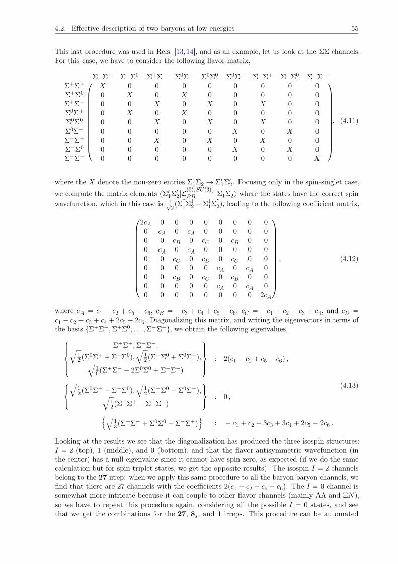
4.2. Effective description of two baryons at low energies 55
This last procedure was used in Refs. [13, 14], and as an example, let us look at the ΣΣ channels.For this case, we have to consider the following flavor matrix,
Σ`Σ` Σ`Σ0 Σ`Σ´ Σ0Σ` Σ0Σ0 Σ0Σ´ Σ´Σ` Σ´Σ0 Σ´Σ´¨
˚
˚
˚
˚
˚
˚
˚
˚
˚
˚
˚
˚
˝
˛
‹
‹
‹
‹
‹
‹
‹
‹
‹
‹
‹
‹
‚
Σ`Σ` X 0 0 0 0 0 0 0 0Σ`Σ0 0 X 0 X 0 0 0 0 0Σ`Σ´ 0 0 X 0 X 0 X 0 0Σ0Σ` 0 X 0 X 0 0 0 0 0Σ0Σ0 0 0 X 0 X 0 X 0 0Σ0Σ´ 0 0 0 0 0 X 0 X 0Σ´Σ` 0 0 X 0 X 0 X 0 0Σ´Σ0 0 0 0 0 0 X 0 X 0Σ´Σ´ 0 0 0 0 0 0 0 0 X
, (4.11)
where the X denote the non-zero entries Σ1Σ2 Ñ Σ11Σ12. Focusing only in the spin-singlet case,we compute the matrix elements xΣ11Σ12|L
p0q, SUp3qfBB |Σ1Σ2y where the states have the correct spin
wavefunction, which in this case is 1?2pΣÒ1ΣÓ2 ´ ΣÓ1ΣÒ2q, leading to the following coefficient matrix,
¨
˚
˚
˚
˚
˚
˚
˚
˚
˚
˚
˚
˚
˝
2cA 0 0 0 0 0 0 0 00 cA 0 cA 0 0 0 0 00 0 cB 0 cC 0 cB 0 00 cA 0 cA 0 0 0 0 00 0 cC 0 cD 0 cC 0 00 0 0 0 0 cA 0 cA 00 0 cB 0 cC 0 cB 0 00 0 0 0 0 cA 0 cA 00 0 0 0 0 0 0 0 2cA
˛
‹
‹
‹
‹
‹
‹
‹
‹
‹
‹
‹
‹
‚
, (4.12)
where cA “ c1 ´ c2 ` c5 ´ c6, cB “ ´c3 ` c4 ` c5 ´ c6, cC “ ´c1 ` c2 ´ c3 ` c4, and cD “
c1 ´ c2 ´ c3 ` c4 ` 2c5 ´ 2c6. Diagonalizing this matrix, and writing the eigenvectors in terms ofthe basis tΣ`Σ`,Σ`Σ0, . . . ,Σ´Σ´u, we obtain the following eigenvalues,
$
’
’
&
’
’
%
Σ`Σ`,Σ´Σ´,b
12pΣ
0Σ` ` Σ`Σ0q,b
12pΣ
´Σ0 ` Σ0Σ´q,b
16pΣ
`Σ´ ´ 2Σ0Σ0 ` Σ´Σ`q
,
/
/
.
/
/
-
: 2pc1 ´ c2 ` c5 ´ c6q ,
$
&
%
b
12pΣ
0Σ` ´ Σ`Σ0q,b
12pΣ
´Σ0 ´ Σ0Σ´q,b
12pΣ
´Σ` ´ Σ`Σ´q
,
.
-
: 0 ,
!b
13pΣ
`Σ´ ` Σ0Σ0 ` Σ´Σ`q)
: ´ c1 ` c2 ´ 3c3 ` 3c4 ` 2c5 ´ 2c6 .
(4.13)
Looking at the results we see that the diagonalization has produced the three isospin structures:I “ 2 (top), 1 (middle), and 0 (bottom), and that the flavor-antisymmetric wavefunction (inthe center) has a null eigenvalue since it cannot have spin zero, as expected (if we do the samecalculation but for spin-triplet states, we get the opposite results). The isospin I “ 2 channelsbelong to the 27 irrep: when we apply this same procedure to all the baryon-baryon channels, wefind that there are 27 channels with the coefficients 2pc1 ´ c2 ` c5 ´ c6q. The I “ 0 channel issomewhat more intricate because it can couple to other flavor channels (mainly ΛΛ and ΞN),so we have to repeat this procedure again, considering all the possible I “ 0 states, and seethat we get the combinations for the 27, 8s, and 1 irreps. This procedure can be automated
56 Chapter 4. The strong baryon-baryon interaction
using Mathematica [422] together with the grassmann package [423], which leads to the followingcombination of Savage-Wise coefficients for each irrep,
cp27q “ 2pc1 ´ c2 ` c5 ´ c6q , cp10q “ 2pc1 ` c2 ` c5 ` c6q ,
cp8sq “1
3p´4c1 ` 4c2 ´ 5c3 ` 5c4 ` 6c5 ´ 6c6q, cp10q “ 2p´c1 ´ c2 ` c5 ` c6q ,
cp1q “2
3p´c1 ` c2 ´ 8c3 ` 8c4 ` 3c5 ´ 3c6q , cp8aq “ 3c3 ` 3c4 ` 2c5 ` 2c6 .
(4.14)
As we will see later on, this set of combinations is the one that we can access with LQCD data,and since we do not study all irreps, in principle we cannot invert this relation and compute eachci separately. In Appendix D, the full flavor decomposition of all two-baryon channels in theirSUp3qf irreps is shown.
Let us focus now on the NLO terms. The non-relativistic SUp3qf -symmetric Lagrangianobtained from Ref. [11] contains 19 terms with different derivative structures. However, herewe are only interested in systems that are in the S wave, so we need to find out which termscontribute to which partial wave. After a detailed analysis, found in Appendix E, only the secondderivatives contribute to the S wave, so the SUp3qf NLO Lagrangian, following the organizationof the LO terms in Eq. (4.8), has the form
Lp2q, SUp3qfBB “´ c1 TrpB:
i∇2BiB:
jBj ` h.c.q ´ c2 TrpB:
i∇2BjB:
jBi ` h.c.q
´ c3 TrpB:
iB:
j∇2BiBj ` h.c.q ´ c4 TrpB:
iB:
j∇2BjBi ` h.c.q
´ c5rTrpB:
i∇2BiqTrpB:
jBjq ` h.c.s ´ c6rTrpB:
i∇2BjqTrpB:
jBiq ` h.c.s ,
(4.15)
where the same relations as in Eq. (4.14) hold for cpirrepq, just by replacing ci with ci.For theSUp3qf terms, as pointed out in Ref. [11], we need to introduce the quark mass matrix
χ,
χ “ 2B0
¨
˝
mu 0 00 md 00 0 ms
˛
‚«
¨
˝
m2π 0 0
0 m2π 0
0 0 2m2K ´m
2π
˛
‚ , (4.16)
where B0 is proportional to the quark condensate, and we have used the Gell-Mann–Oakes–Rennerrelation [424] to write this matrix in terms of the meson masses instead of the quark masses,
m2π « pmu `mdqB0 “ 2mlB0 , m2
K « pml `msqB0 , (4.17)
with ml “ mu “ md. Since this part of the Lagrangian breaks SUp3qf , we will not have sixterms, and we need to find all possible combinations involving Eqs. (4.8) and (4.16). Again, thiswas first derived in Ref. [11] (the relations between both sets of SUp3qf coefficients are presentedin Table F.1 of Appendix F), and we write it here with the terms following the organization aspresented in the LO case,
Lp2q,SUp3qfBB “´ cχ1 TrpB
:
iχBiB:
jBjq ´ cχ2 TrpB
:
iχBjB:
jBiq
´ cχ3 TrpB:
iBiχB:
jBjq ´ cχ4 TrpB
:
iBjχB:
jBiq
´ cχ5 TrpB:
iχB:
jBiBj ` h.c.q ´ cχ6 TrpB:
iχB:
jBjBi ` h.c.q
´ cχ7 TrpB:
iB:
jχBiBjq ´ cχ8 TrpB
:
iB:
jχBjBiq
´ cχ9 TrpB:
iB:
jBiBjχq ´ cχ10 TrpB
:
iB:
jBjBiχq
´ cχ11 TrpB:
iχBiqTrpB:
jBjq ´ cχ12 TrpB
:
iχBjqTrpB:
jBiq .
(4.18)
Now, when writing the elements xB11B12|Lp2q,SUp3qfBB |B1B2y, we will separate the contributions to
the cχi coefficients that are accompanied by m2K ´m2
π from the ones that are accompanied by
4.2. Effective description of two baryons at low energies 57
m2π. Let us look at an example to understand why,
xΣ`p|Lp2q,SUp3qfBB |Σ`py “ 2pcχ3 ´ c
χ4 qm
2K ` 2pcχ1 ´ c
χ2 ´ c
χ11 ` c
χ12qm
2π
“ 2pcχ3 ´ cχ4 qpm
2K ´m
2πq ` 2pcχ1 ´ c
χ2 ` c
χ3 ´ c
χ4 ´ c
χ11 ` c
χ12qm
2π .
(4.19)
The coefficients accompanied by m2K ´m
2π are the coefficients that contribute to the symmetry
breaking, since they vary for different channels belonging to the same irrep (we will write themas cχi ” cχi pm
2K ´m
2πq for simplicity), while the rest (accompanied by m2
π) are the same for allthe channels in the same irrep, and therefore can be reabsorbed in the LO terms.
The final expression for the Lagrangian we will be using is
LBB “ Lp0q, SUp3qBB ` Lp2q, SUp3qBB ` Lp2q,SUp3qBB , (4.20)
built from the expressions given in Eqs. (4.8), (4.15), and (4.18). In Section 4.3.5, the specificLECs that we will have access to with the LQCD data available will be discussed.
4.2.2 Assuming SUp6q spin-flavor symmetry
In the limit of SUp3qf symmetry and large Nc, two-baryon interactions are predicted to beinvariant under an SUp6q spin-flavor symmetry, with corrections that generally scale as 1Nc [12](this symmetry was previously discussed in Refs. [425–427], as the natural extension of theSUp4q spin-flavor Wigner symmetry when including strangeness). In the two-nucleon sector, thisencompasses the SUp4q spin-flavor Wigner symmetry [428–430], with corrections that scale as1N2
c (a recent study has proven again that this is an approximate symmetry at the physicalpoint [431], but it is only seen at an optimal momentum resolution scale). Under SUp6q grouptransformations, the baryons transform as a three-index symmetric tensor Ψµνρ, where eachSUp6q index µ is a pair of spin and flavor indices piαq. At LO, only two independent termscontribute to the two-baryon interacting Lagrangian,
Lp0q,SUp6qBB “ ´apΨ:
µνρΨµνρq2 ´ bΨ
:
µνσΨµντΨ:
ρδτΨρδσ , (4.21)
where the baryon tensor can be expressed as a function of the octet B and decuplet T baryonmatrices,
Ψµνρ “ Ψpiαqpjβqpkγq “ Tαβγijk `1?
18
´
Bαω,iε
ωβγεjk `Bβω,jε
ωγαεik `Bγω,kε
ωαβεij
¯
. (4.22)
Here, α, β, γ, ω are flavor indices, i, j, k are spin indices, and the Levi-Civita tensor ε is in eitherflavor or spin space depending on the type and number of indices.
In order to understand why there are only two terms and why the baryons are writtenas a symmetric tensor, we will derive the SUp6q spin-flavor symmetry of the nuclear (andhypernuclear) forces from group-theoretical arguments [432,433], using the Mathematica packageLieArt [434,435] for the group-theory calculations.
The main idea behind is that if we assume SUp3qf symmetry together with SUp2qJ spinsymmetry, all the baryons will have the same mass regardless of the spin (1
2 or 32) value. This
means that all these objects remain invariant under transformations of the unitary group SUp6q,which has as subgroups the product SUp3qf b SUp2qJ . Therefore, now the quarks will bedimension-six objects, living in the fundamental representation,
qi “`
uÒ uÓ dÒ dÓ sÒ sÓ˘J
. (4.23)
To identify the SUp6q irrep where the octet and decuplet baryons live, we start by taking theproduct of three 6,
6b 6b 6 “ 2 70‘ 56‘ 20 , (4.24)
58 Chapter 4. The strong baryon-baryon interaction
and write it in terms of the irreps from the product of the subgroups SUp3qf b SUp2qJ ,
3b 3b 3 “ 10‘ 2 8‘ 1 , 2b 2b 2 “ 4‘ 2 2 . (4.25)
To continue, we can use the Young tableaux to study the symmetry of each irrep: totallysymmetric (SS), totally antisymmetric (AA), and mixed symmetry (SA).1 Therefore, for theSUp6q irreps,
70 Ñ (SA) , 56 Ñ (SS) , 20 Ñ (AA) , (4.26)
and for the SUp3qf and SUp2qJ irreps,
10 Ñ (SS) , 8 Ñ (SA) , 1 Ñ (AA) ,
4 Ñ (SS) , 2 Ñ (SA) .(4.27)
In order to obtain an SS state, we can take the product of (SS,SS), (AA,AA), and (SA,SA);for AA, we can do (SS,AA) or (SA,SA); and for SA, we can do (SS,AS), (AA,AS), or (AS,AS).Therefore,
70Ñ p10,2q ‘ p8,2q ‘ p8,4q ‘ p1,2q , 56Ñ p10,4q ‘ p8,2q , 20Ñ p8,2q ‘ p1,4q . (4.28)
From these symmetry arguments, we see that the only irrep where the octet p8,2q and decupletp10,4q live is the 56 irrep. Therefore, since 56 is completely symmetric, the baryons can bewritten as a completely symmetric tensor [12,433], like in Eq. (4.22).
When looking at the interaction of two baryons, we have to perform the tensor product oftwo 56 to see how many parameters will be needed to describe it,
56b 56 “ 462‘ 490‘ 10502 ‘ 11341 . (4.29)
Contrary to the arguments in Ref. [12], we see that in principle there should be four parameters,and not only two. To elucidate this point, we write these irreps in terms of the correspondingones in SUp3qf b SUp2qJ . For two octet baryons, the flavor and spin decomposition is
8b 8 “ 27‘ 10‘ 10‘ 8s ‘ 8a ‘ 1 , 2b 2 “ 1‘ 3 . (4.30)
In order to identify the correct flavor-spin combinations for a baryon-baryon system, it is convenientto identify at least one system of two identical particles in each irrep,
27 : pp 10 : 1?2pΞ0Ξ´ ´ Ξ´Ξ0q ,
10 : 1?2pnp´ pnq , 8s : ΛΛ ,
8a : 1?2pΣ´Σ0 ´ Σ0Σ´q , 1 : ΛΛ .
(4.31)
We see that the irreps 27, 8s, and 1 are symmetric with respect to the exchange of both baryons,while the irreps 10, 10, and 8a are antisymmetric with respect to the exchange of both baryons.Taking into account that the spin-singlet state is antisymmetric and the spin-triplet state issymmetric with respect to the exchange of the spin of the baryons, the allowed (spin-flavor)combinations are
BB Ñ BB : p27,1q, p8,1q, p1,1q, p10,3q, p10,3q, p8,3q . (4.32)1As a reminder, irreps with only a row of boxes are SS, with only a column of boxes are AA, and a mix of both
are SA.
4.2. Effective description of two baryons at low energies 59
In the case of having two baryons of the decuplet [436], the corresponding flavor and spindecompositions are
10b 10 “ 35‘ 28‘ 27‘ 10 , 4b 4 “ 1‘ 3‘ 5‘ 7 . (4.33)
While the spin-0 and spin-2 wavefunctions are antisymmetric (1 and 5 irreps), the spin-1 andspin-3 wavefunctions are symmetric (3 and 7 irreps). Considering the following two-particlestates for each SUp3qf irrep,
35 : 1?2
`
∆``∆` ´∆`∆``˘
, 28 : Ω´Ω´ ,
27 : Ξ˚0Ξ˚0 , 10 : 1?2pΣ˚0Σ˚` ´ Σ˚`Σ˚0q ,
(4.34)
the irreps 28 and 27 are symmetric and the irreps 35 and 10 are antisymmetric, and the possiblecombinations are
TT Ñ TT : p28,1q, p28,5q, p27,1q, p27,5q, p35,3q, p35,7q, p10,3q, p10,7q . (4.35)
Lastly, for the system composed of one baryon from the octet and one of the decuplet, the flavorand spin decompositions are
8b 10 “ 35‘ 27‘ 10‘ 8 , 2b 4 “ 3‘ 5 . (4.36)
Since in this case the two fermions are distinguishable, the Pauli principle does not apply, andany combination is allowed,
BT Ñ BT : p35,3q, p27,3q, p10,3q, p8,3q, p35,5q, p27,5q, p10,5q, p8,5q . (4.37)
For the crossed channels (BB Ñ TB, BB Ñ TT and TB Ñ TT ), the possible irreps will bethose that appear in both the initial and final states. As a summary,
BB Ñ BB : p27,1q, p8,1q, p1,1q, p10,3q, p10,3q, p8,3q ,
BB Ñ TB : p10,3q, p8,3q ,
BB Ñ TT : p27,1q, p10,3q ,
TB Ñ TB : p35,3q, p27,3q, p10,3q, p8,3q, p35,5q, p27,5q, p10,5q, p8,5q ,
TB Ñ TT : p35,3q, p27,5q ,
TT Ñ TT : p28,1q, p28,5q, p27,1q, p27,5q, p35,3q, p35,7q, p10,3q, p10,7q .
(4.38)
From the SUp6q tensor product, decomposing the four irreps into SUp3qf b SUp2qJ multipletsgives
462 “ p10,1q ‘ p27,3q ‘ p28,7q ‘ p35,5q ,
490 “ p1,1q ‘ p8,3q ‘ p10,3q ‘ p10,3q ‘ p8,5q ‘ p10,7q ‘ p27,1q ‘ p28,1q
‘ p27,5q ‘ p35,3q ,
10502 “ p8,1q ‘ p8,3q ‘ p10,3q ‘ p10,3q ‘ p10,5q ‘ p27,1q ‘ p27,3q ‘ p27,5q
‘ p28,5q ‘ p35,3q ‘ p35,5q ‘ p35,7q ,
11341 “ p1,3q ‘ p8,1q ‘ 2p8,3q ‘ p10,1q ‘ p10,1q ‘ p10,3q ‘ p8,5q ‘ p10,5q
‘ p10,5q ‘ 2p27,3q ‘ p28,3q ‘ p27,5q ‘ p27,7q ‘ p35,1q ‘ p35,3q ‘ p35,5q,
(4.39)
where the gray-colored numbers are non-physical states with symmetric wavefunctions, notappearing in Eq. (4.38). For example, the combination p28,7q is not possible because 28 hasa symmetric flavor wavefunction and 7 also has a symmetric spin wavefunction, and with thecombination of both a total symmetric wavefunction is prohibited by the Pauli principle. The
60 Chapter 4. The strong baryon-baryon interaction
only irreps that survive are the ones that contain only physical states, therefore we are left withtwo, 490 and 10502, meaning that we only need two coefficients to describe the baryon-baryoninteraction, as in Eq. (4.21).
We can match the SUp6q LO Kaplan-Savage coefficients a and b to the SUp3qf LO Savage-Wisecoefficients ci by computing xB11B12|L
p0q, SUp6qBB |B1B2y,
cp27q “ 2a´2b
27`O
ˆ
1
N2c
˙
, cp10q “ 2a´2b
27`O
ˆ
1
N2c
˙
,
cp8sq “ 2a`2b
3`O
ˆ
1
Nc
˙
, cp10q “ 2a`14b
27`O
ˆ
1
Nc
˙
,
cp1q “ 2a´2b
3`O
ˆ
1
Nc
˙
, cp8aq “ 2a`2b
27`O
ˆ
1
Nc
˙
.
(4.40)
4.2.3 Matching the LECs to the scattering amplitude
In order to constrain the LECs with the LQCD data, our approach is to match them to a momentumexpansion of the scattering amplitude. We will follow the formalism from Refs. [437,438], wherethey work for simplicity with a toy model: two heavy spinless baryons Bi in the non-relativisticlimit (with masses M1 and M2), whose interaction is characterized by a scale Λ. Then, the EFTwill describe scattering at a c.m. momentum k˚ ! Λ using contact interactions in a derivativeexpansion,
L “ B:
1
ˆ
iB0 `∇2
2M1
˙
B1 ` B:
2
ˆ
iB0 `∇2
2M2
˙
B2
`
´µ
2
¯4´D"
C0
´
B:
1B2
¯2` C
piq2
´
B:
1∇~~
B2
¯2` C
piiq2
„
i~∇´
B:
1B2
¯2
` ¨ ¨ ¨
*
,
(4.41)
where the ellipses denote higher derivative terms. The mass scale µ2 is introduced because wewill use dimensional regularization for the loop integrals. Also, if the spacetime dimension is D,one can check that the couplings C2n will have the same dimensions regardless of the value of D,
rSs “ adim.Ñ rLs “MD Ñ rBs “MD´12 Ñ rC2ns “M´2p1`nq . (4.42)
From Section 2.4, we know that the scattering amplitude M can be written in terms of thephase shift,
M “2π
M
1
k˚ cot δ ´ ik˚. (4.43)
We also know that k˚ cot δ has an expansion (ERE) for k˚ ! Λ. Writing Eq. (2.64) slightlydifferently,
k˚ cot δ “ ´1
a`
1
2Λ2
8ÿ
n“0
rn
ˆ
k˚2
Λ2
˙n`1
. (4.44)
For the baryon-baryon interaction, all rn are of the order Op1Λq, but a can take any value.Therefore, the radius of convergence of the momentum expansion of M will depend on the size ofthe scattering length. We will study two cases: the first one will be for natural interactions, with|a| „ 1Λ, and the second one for unnatural interactions, with |a| " 1Λ.2
2For a detailed discussion of naturalness in EFTs, see Ref. [439].
4.2. Effective description of two baryons at low energies 61
Scattering length of natural size
For natural interactions, |a| „ 1Λ and |rn| „ 1Λ, and M has a simple momentum expansion,
Mpk˚q “ Mp0q `M1p0qk˚ `1
2!M2p0qk˚2 ` ¨ ¨ ¨
“ ´2πa
M`
2πia2
Mk˚ `
2π
M
„
p´aq3p´iq2 ´ra2
2
k˚2 `Opk˚3Λ4q
“ ´2πa
M
”
1´ iak˚ `´ra
2´ a2
¯
k˚2 `Opk˚3Λ3q
ı
.
(4.45)
This expansion converges for momenta up to k˚ „ Λ,
M „1
Λ`k˚
Λ2`k˚2
Λ3` ¨ ¨ ¨ . (4.46)
This is the expansion we want to obtain starting from the EFT Lagrangian of Eq. (4.41).The scattering amplitude M will be given by the sum of all the Feynman diagrams of this
theory. At tree level, the S-wave amplitude is given by
iMtree “ ´i´µ
2
¯4´D 8ÿ
n“1
C2npµqk˚2n , (4.47)
with C2n being linear combinations of the couplings in the Lagrangian. The full amplitude canbe obtained from the following diagrammatic sum,
M “ + + + … , with += + … , (4.48)
where loop integrals are of the form
In “ ´i´µ
2
¯4´Dż
dDq
p2πqDq2n i
E2 ´ q0 ´
q2
2M1` iε
iE2 ` q0 ´
q2
2M2` iε
, (4.49)
where E is the energy of the incoming two-baryon system, and q the loop momentum, whichhas to be integrated out. First, we can integrate q0 by forming a contour closing the pole in theupper half of the complex plane and using the residue theorem,
In “ ´i´µ
2
¯4´Dż
dD´1q
p2πqDq2n
ż
dq0i
E2 ´ q0 ´
q2
2M1` iε
iE2 ` q0 ´
q2
2M2` iε
“ ´i´µ
2
¯4´Dż
dD´1q
p2πqDq2np2πiq
ÿ
Respq0q
“ ´i´µ
2
¯4´Dż
dD´1q
p2πqDq2np2πiq
´i2
E2 `
´
E2 ´
q2
2M1` iε
¯
´q2
2M2` iε
“
´µ
2
¯4´Dż
dD´1q
p2πqD´1
q2n
E ´ q2
2
´
1M1` 1
M2
¯
` iε“
´µ
2
¯4´Dż
dD´1q
p2πqD´1
q2n
E ´ q2
2M` iε
.
(4.50)
We can split dD´1q in a radial and an angular part in pD ´ 1q-spherical coordinates,
In “´µ
2
¯4´Dż
dD´1q
p2πqD´1
q2n
E ´ q2
2M` iε
“
´µ
2
¯4´Dż
dΩD´1
ż 8
0
dq
p2πqD´1qD´2 q2n
E ´ q2
2M` iε
“
´µ
2
¯4´D 2πD´12
p2πqD´1Γ`
D´12
˘
ż 8
0dq
q2n`D´2
E ´ q2
2M` iε
.
(4.51)
62 Chapter 4. The strong baryon-baryon interaction
The integral in the last line of Eq. (4.51) can rearranged asż 8
0dq
q2n`D´2
E ´ q2
2M` iε
“ 2M
ż 8
0dq
q2n`D´2
2ME ´ q2 ` iε“ ´2M
ż 8
0dq
q2n`D´2
q2 ´ 2ME ´ iε
“´2M
´2ME ´ iε
ż 8
0dq
q2n`D´2
q2
´2ME´iε` 1
,
(4.52)
which, after applying the following change of variables p “ q2p´2ME ´ iεq, takes the form
´2M
´2ME ´ iε
ż 8
0dp
a
´2ME ´ iε
2?p
p´2ME ´ iεqn`D´22 pn`
D´22
p` 1
“ ´Mp´2MEqnp´2ME ´ iεqD´32
ż 8
0dppn`
D´32
p` 1.
(4.53)
This integral can be solved using the beta function,
Bpα, γq “
ż 8
0dp pα´1pp` 1q´α´γ “
Γ pαqΓ pγq
Γ pα` γq, (4.54)
with the following identification,
pα´1pp` 1q´α´γ “ pn`D´32 pp` 1q´1 ñ α “ n`
D ´ 1
2, γ “
3´D
2´ n . (4.55)
Collecting all the terms, we get
In “´µ
2
¯4´D 2πD´12
p2πqD´1Γ`
D´12
˘p´Mqp´2MEqnp´2ME ´ iεqD´32
Γ`
n` D´12
˘
Γ`
3´D2 ´ n
˘
Γ p1q
“ p´2Mqp´2MEqnp´2ME ´ iεqD´32
Γ`
n` D´12
˘
Γ`
3´D2 ´ n
˘
Γ`
D´12
˘
pµ2q4´D
p4πqD´12
.
(4.56)We can further simplify this expression by using the following relation,
Γp1` zq “ zΓpzq ñ Γpz ´ 1q “Γpzq
z ´ 1. (4.57)
Looking at specific values of n,
n “ 0 : Γ
ˆ
D ´ 1
2
˙
Γ
ˆ
3´D
2
˙
,
n “ 1 : Γ
ˆ
1`D ´ 1
2
˙
Γ
ˆ
3´D
2´ 1
˙
“
D´12
3´D2 ´ 1
Γ
ˆ
D ´ 1
2
˙
Γ
ˆ
3´D
2
˙
“
D´12
1´D2
Γ
ˆ
D ´ 1
2
˙
Γ
ˆ
3´D
2
˙
“ p´1qΓ
ˆ
D ´ 1
2
˙
Γ
ˆ
3´D
2
˙
,
n “ 2 : Γ
ˆ
2`D ´ 1
2
˙
Γ
ˆ
3´D
2´ 2
˙
“
D´12 ` 1
3´D2 ´ 2
Γ
ˆ
1`D ´ 1
2
˙
Γ
ˆ
3´D
2´ 1
˙
“
D`12
´1´D2
p´1qΓ
ˆ
D ´ 1
2
˙
Γ
ˆ
3´D
2
˙
“ p´1q2Γ
ˆ
D ´ 1
2
˙
Γ
ˆ
3´D
2
˙
,
...
n “ n : Γ
ˆ
n`D ´ 1
2
˙
Γ
ˆ
3´D
2´ n
˙
“ p´1qnΓ
ˆ
D ´ 1
2
˙
Γ
ˆ
3´D
2
˙
.
(4.58)
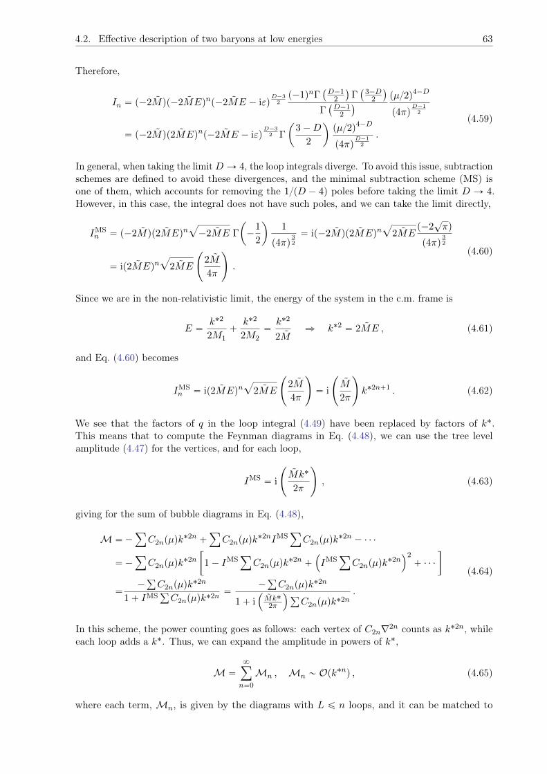
4.2. Effective description of two baryons at low energies 63
Therefore,
In “ p´2Mqp´2MEqnp´2ME ´ iεqD´32p´1qnΓ
`
D´12
˘
Γ`
3´D2
˘
Γ`
D´12
˘
pµ2q4´D
p4πqD´12
“ p´2Mqp2MEqnp´2ME ´ iεqD´32 Γ
ˆ
3´D
2
˙
pµ2q4´D
p4πqD´12
.
(4.59)
In general, when taking the limitD Ñ 4, the loop integrals diverge. To avoid this issue, subtractionschemes are defined to avoid these divergences, and the minimal subtraction scheme (MS) isone of them, which accounts for removing the 1pD ´ 4q poles before taking the limit D Ñ 4.However, in this case, the integral does not have such poles, and we can take the limit directly,
IMSn “ p´2Mqp2MEqn
a
´2ME Γ
ˆ
´1
2
˙
1
p4πq32
“ ip´2Mqp2MEqna
2MEp´2
?πq
p4πq32
“ ip2MEqna
2ME
˜
2M
4π
¸
.
(4.60)
Since we are in the non-relativistic limit, the energy of the system in the c.m. frame is
E “k˚2
2M1`
k˚2
2M2“k˚2
2Mñ k˚2 “ 2ME , (4.61)
and Eq. (4.60) becomes
IMSn “ ip2MEqn
a
2ME
˜
2M
4π
¸
“ i
˜
M
2π
¸
k˚2n`1 . (4.62)
We see that the factors of q in the loop integral (4.49) have been replaced by factors of k˚.This means that to compute the Feynman diagrams in Eq. (4.48), we can use the tree levelamplitude (4.47) for the vertices, and for each loop,
IMS “ i
˜
Mk˚
2π
¸
, (4.63)
giving for the sum of bubble diagrams in Eq. (4.48),
M “´ÿ
C2npµqk˚2n `
ÿ
C2npµqk˚2nIMS
ÿ
C2npµqk˚2n ´ ¨ ¨ ¨
“ ´ÿ
C2npµqk˚2n
„
1´ IMSÿ
C2npµqk˚2n `
´
IMSÿ
C2npµqk˚2n
¯2` ¨ ¨ ¨
“´ř
C2npµqk˚2n
1` IMSř
C2npµqk˚2n
“´ř
C2npµqk˚2n
1` i´
Mk˚
2π
¯
ř
C2npµqk˚2n
.
(4.64)
In this scheme, the power counting goes as follows: each vertex of C2n∇2n counts as k˚2n, whileeach loop adds a k˚. Thus, we can expand the amplitude in powers of k˚,
M “
8ÿ
n“0
Mn , Mn „ Opk˚nq , (4.65)
where each term, Mn, is given by the diagrams with L ď n loops, and it can be matched to
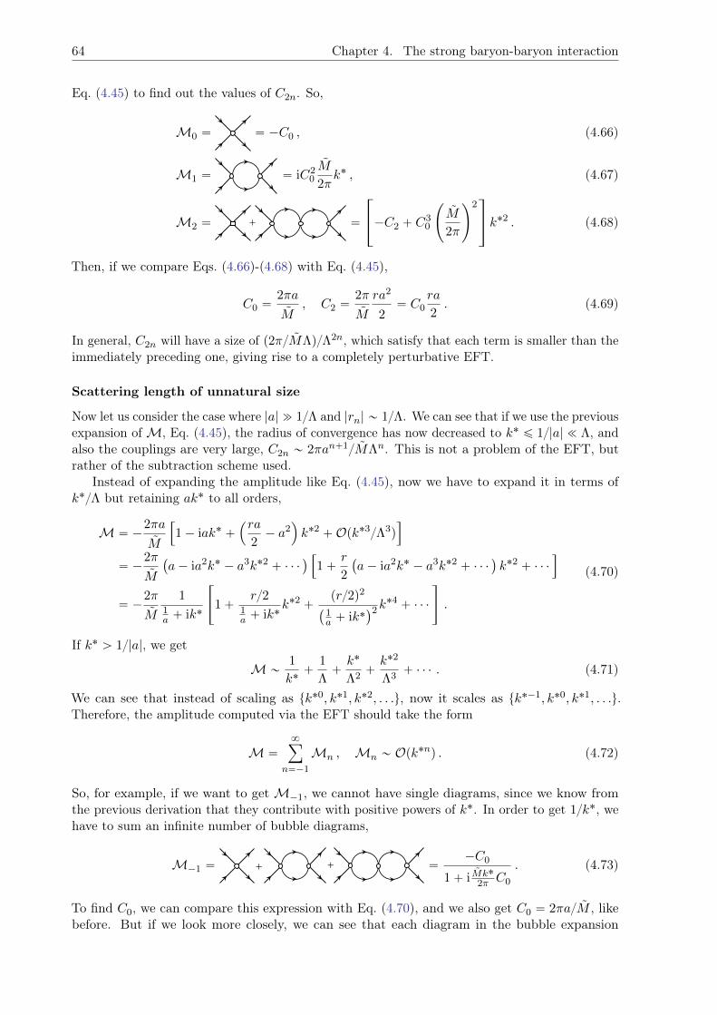
64 Chapter 4. The strong baryon-baryon interaction
Eq. (4.45) to find out the values of C2n. So,
M0 “ “ ´C0 , (4.66)
M1 “ “ iC20M
2πk˚ , (4.67)
M2 “ + “
»
–´C2 ` C30
˜
M
2π
¸2fi
fl k˚2 . (4.68)
Then, if we compare Eqs. (4.66)-(4.68) with Eq. (4.45),
C0 “2πa
M, C2 “
2π
M
ra2
2“ C0
ra
2. (4.69)
In general, C2n will have a size of p2πMΛqΛ2n, which satisfy that each term is smaller than theimmediately preceding one, giving rise to a completely perturbative EFT.
Scattering length of unnatural size
Now let us consider the case where |a| " 1Λ and |rn| „ 1Λ. We can see that if we use the previousexpansion of M, Eq. (4.45), the radius of convergence has now decreased to k˚ ď 1|a| ! Λ, andalso the couplings are very large, C2n „ 2πan`1MΛn. This is not a problem of the EFT, butrather of the subtraction scheme used.
Instead of expanding the amplitude like Eq. (4.45), now we have to expand it in terms ofk˚Λ but retaining ak˚ to all orders,
M “ ´2πa
M
”
1´ iak˚ `´ra
2´ a2
¯
k˚2 `Opk˚3Λ3q
ı
“ ´2π
M
`
a´ ia2k˚ ´ a3k˚2 ` ¨ ¨ ¨˘
”
1`r
2
`
a´ ia2k˚ ´ a3k˚2 ` ¨ ¨ ¨˘
k˚2 ` ¨ ¨ ¨
ı
“ ´2π
M
11a ` ik˚
«
1`r2
1a ` ik˚
k˚2 `pr2q2
`
1a ` ik˚
˘2k˚4 ` ¨ ¨ ¨
ff
.
(4.70)
If k˚ ą 1|a|, we get
M „1
k˚`
1
Λ`k˚
Λ2`k˚2
Λ3` ¨ ¨ ¨ . (4.71)
We can see that instead of scaling as tk˚0, k˚1, k˚2, . . .u, now it scales as tk˚´1, k˚0, k˚1, . . .u.Therefore, the amplitude computed via the EFT should take the form
M “
8ÿ
n“´1
Mn , Mn „ Opk˚nq . (4.72)
So, for example, if we want to get M´1, we cannot have single diagrams, since we know fromthe previous derivation that they contribute with positive powers of k˚. In order to get 1k˚, wehave to sum an infinite number of bubble diagrams,
M´1 “ ++ “´C0
1` iMk˚
2π C0
. (4.73)
To find C0, we can compare this expression with Eq. (4.70), and we also get C0 “ 2πaM , likebefore. But if we look more closely, we can see that each diagram in the bubble expansion
4.2. Effective description of two baryons at low energies 65
gets bigger and bigger, p2πaMqpiak˚qL, with L being the number of loops. Even if the totalsum is a small number, each new term is bigger than the previous one. This is not a goodexpansion parameter for an EFT, since |ak˚| ą 1. Without a good expansion parameter, wecannot determine the size of a particular diagram, and we do not know which ones contribute ata particular order.
The size of the contact interactions depends on the renormalization scheme, so we have torevisit the MS scheme (not the dimensional regularization). Also, since M´1 scales as 1k˚, ournew subtraction scheme must also produce a C0 such that it scales as 1k˚. The one proposedby D. Kaplan, M. Savage, M. Wise [437,438], and U. van Kolck [102] is called power divergencesubtraction (or PDS) scheme (also known as KSW-vK scheme), which consist in removing fromthe dimensional regularized loop not only the divergences coming from 1pD´ 4q poles (as in MS,which correspond to log divergences), but also poles from lower dimensions (which correspond topower law divergences at D “ 4).
In our case, looking at the loop integral In in Eq. (4.59), we see that it has a pole withD “ 3` 2ς, with ς being a small parameter,
In “ p´2Mqp2MEqnp´2ME ´ iεqςΓ p´ςqpµ2q1´2ς
p4πq1`ςς!1ÝÑ
2Mp2MEqn
ς
µ2
4π`Opς0q . (4.74)
This means that we have to add the following counterterm,
δIn “ ´Mp2MEqn
D ´ 3
µ
2π, (4.75)
and the total integral becomes
IPDSn “ In ` δIn “ p2MEqn
˜
M
2π
¸
pµ` ik˚q . (4.76)
The PDS scheme maintains the nice feature of MS that powers of q inside the loop integrationare replaced by powers of the external momentum k˚. Also, setting µ “ 0 we recover the resultobtained by the MS scheme.
In this scheme, the full amplitude is
M “´ř
C2npµqk˚2n
1` M2π pµ` ik˚q
ř
C2npµqk˚2n
. (4.77)
There are several ways to find the value of C0 in terms of the scattering parameters. One of themis by imposing that the amplitude is independent of the subtraction point µ. But we can do thesame as we did for the natural case, where we find which diagrams are the ones contributingat each order. To do that, we first need to see what is the size of C2n for µ " 1|a|. Using arearranged version of Eq. (4.43),
k˚ cot δ “ ik˚ `2π
MM“ ´
2π
Mř
C2npµqk˚2n
´ µ . (4.78)
Expanding k˚ cot δ with the ERE and in the limit µ " 1|a|,
µ`1
2Λ2
8ÿ
n“0
rn
ˆ
k˚2
Λ2
˙n`1
“ ´2π
Mř
C2npµqk˚2n
“ ´2π
M
ˆ
1
C0´C2
C20
k˚2 `C2
2 ´ C0C4
C30
k˚4 ` ¨ ¨ ¨
˙
.
(4.79)
Therefore, with rn „ 1Λ,
C0 „2π
Mµ, C2 „
2π
MΛµ2, C4 „
2π
MΛ2µ3Ñ C2n „
2π
MΛnµn`1. (4.80)
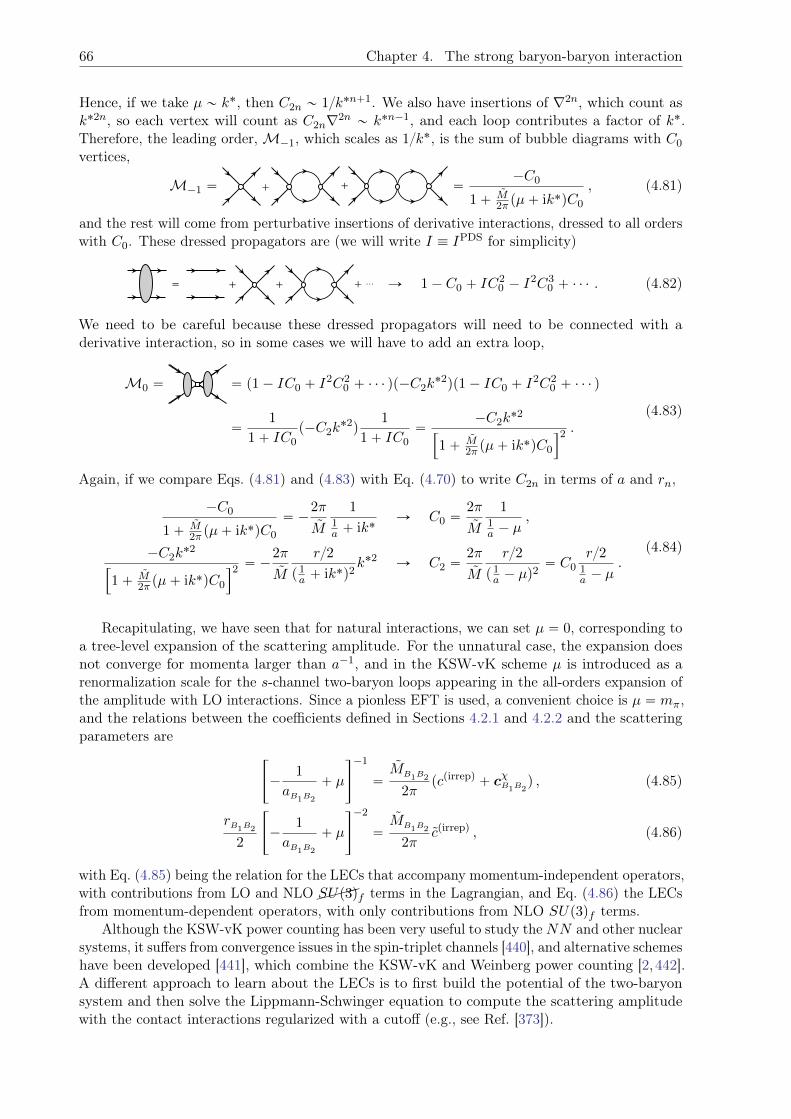
66 Chapter 4. The strong baryon-baryon interaction
Hence, if we take µ „ k˚, then C2n „ 1k˚n`1. We also have insertions of ∇2n, which count ask˚2n, so each vertex will count as C2n∇2n „ k˚n´1, and each loop contributes a factor of k˚.Therefore, the leading order, M´1, which scales as 1k˚, is the sum of bubble diagrams with C0
vertices,
M´1 “ ++ “´C0
1` M2π pµ` ik˚qC0
, (4.81)
and the rest will come from perturbative insertions of derivative interactions, dressed to all orderswith C0. These dressed propagators are (we will write I ” IPDS for simplicity)
+ …+= + Ñ 1´ C0 ` IC20 ´ I
2C30 ` ¨ ¨ ¨ . (4.82)
We need to be careful because these dressed propagators will need to be connected with aderivative interaction, so in some cases we will have to add an extra loop,
M0 “ “ p1´ IC0 ` I2C2
0 ` ¨ ¨ ¨ qp´C2k˚2qp1´ IC0 ` I
2C20 ` ¨ ¨ ¨ q
“1
1` IC0p´C2k
˚2q1
1` IC0“
´C2k˚2
”
1` M2π pµ` ik˚qC0
ı2 .(4.83)
Again, if we compare Eqs. (4.81) and (4.83) with Eq. (4.70) to write C2n in terms of a and rn,
´C0
1` M2π pµ` ik˚qC0
“ ´2π
M
11a ` ik˚
Ñ C0 “2π
M
11a ´ µ
,
´C2k˚2
”
1` M2π pµ` ik˚qC0
ı2 “ ´2π
M
r2
p 1a ` ik˚q2
k˚2 Ñ C2 “2π
M
r2
p 1a ´ µq
2“ C0
r21a ´ µ
.(4.84)
Recapitulating, we have seen that for natural interactions, we can set µ “ 0, corresponding toa tree-level expansion of the scattering amplitude. For the unnatural case, the expansion doesnot converge for momenta larger than a´1, and in the KSW-vK scheme µ is introduced as arenormalization scale for the s-channel two-baryon loops appearing in the all-orders expansion ofthe amplitude with LO interactions. Since a pionless EFT is used, a convenient choice is µ “ mπ,and the relations between the coefficients defined in Sections 4.2.1 and 4.2.2 and the scatteringparameters are
«
´1
aB1B2
` µ
ff´1
“MB1B2
2πpcpirrepq ` cχB1B2
q , (4.85)
rB1B2
2
«
´1
aB1B2
` µ
ff´2
“MB1B2
2πcpirrepq , (4.86)
with Eq. (4.85) being the relation for the LECs that accompany momentum-independent operators,with contributions from LO and NLO SUp3qf terms in the Lagrangian, and Eq. (4.86) the LECsfrom momentum-dependent operators, with only contributions from NLO SUp3qf terms.
Although the KSW-vK power counting has been very useful to study the NN and other nuclearsystems, it suffers from convergence issues in the spin-triplet channels [440], and alternative schemeshave been developed [441], which combine the KSW-vK and Weinberg power counting [2,442].A different approach to learn about the LECs is to first build the potential of the two-baryonsystem and then solve the Lippmann-Schwinger equation to compute the scattering amplitudewith the contact interactions regularized with a cutoff (e.g., see Ref. [373]).
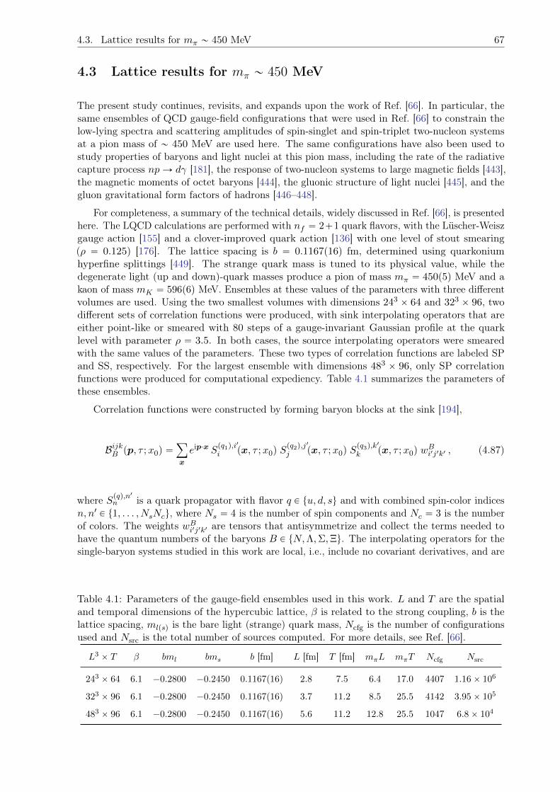
4.3. Lattice results for mπ „ 450 MeV 67
4.3 Lattice results for mπ „ 450 MeV
The present study continues, revisits, and expands upon the work of Ref. [66]. In particular, thesame ensembles of QCD gauge-field configurations that were used in Ref. [66] to constrain thelow-lying spectra and scattering amplitudes of spin-singlet and spin-triplet two-nucleon systemsat a pion mass of „ 450 MeV are used here. The same configurations have also been used tostudy properties of baryons and light nuclei at this pion mass, including the rate of the radiativecapture process npÑ dγ [181], the response of two-nucleon systems to large magnetic fields [443],the magnetic moments of octet baryons [444], the gluonic structure of light nuclei [445], and thegluon gravitational form factors of hadrons [446–448].
For completeness, a summary of the technical details, widely discussed in Ref. [66], is presentedhere. The LQCD calculations are performed with nf “ 2`1 quark flavors, with the Lüscher-Weiszgauge action [155] and a clover-improved quark action [136] with one level of stout smearing(ρ “ 0.125) [176]. The lattice spacing is b “ 0.1167p16q fm, determined using quarkoniumhyperfine splittings [449]. The strange quark mass is tuned to its physical value, while thedegenerate light (up and down)-quark masses produce a pion of mass mπ “ 450p5q MeV and akaon of mass mK “ 596p6q MeV. Ensembles at these values of the parameters with three differentvolumes are used. Using the two smallest volumes with dimensions 243 ˆ 64 and 323 ˆ 96, twodifferent sets of correlation functions were produced, with sink interpolating operators that areeither point-like or smeared with 80 steps of a gauge-invariant Gaussian profile at the quarklevel with parameter ρ “ 3.5. In both cases, the source interpolating operators were smearedwith the same values of the parameters. These two types of correlation functions are labeled SPand SS, respectively. For the largest ensemble with dimensions 483 ˆ 96, only SP correlationfunctions were produced for computational expediency. Table 4.1 summarizes the parameters ofthese ensembles.
Correlation functions were constructed by forming baryon blocks at the sink [194],
BijkB pp, τ ;x0q “ÿ
x
eip¨x Spq1q,i
1
i px, τ ;x0q Spq2q,j
1
j px, τ ;x0q Spq3q,k
1
k px, τ ;x0q wBi1j1k1 , (4.87)
where Spqq,n1
n is a quark propagator with flavor q P tu, d, su and with combined spin-color indicesn, n1 P t1, . . . , NsNcu, where Ns “ 4 is the number of spin components and Nc “ 3 is the numberof colors. The weights wBi1j1k1 are tensors that antisymmetrize and collect the terms needed tohave the quantum numbers of the baryons B P tN,Λ,Σ,Ξu. The interpolating operators for thesingle-baryon systems studied in this work are local, i.e., include no covariant derivatives, and are
Table 4.1: Parameters of the gauge-field ensembles used in this work. L and T are the spatialand temporal dimensions of the hypercubic lattice, β is related to the strong coupling, b is thelattice spacing, mlpsq is the bare light (strange) quark mass, Ncfg is the number of configurationsused and Nsrc is the total number of sources computed. For more details, see Ref. [66].
L3 ˆ T β bml bms b [fm] L [fm] T [fm] mπL mπT Ncfg Nsrc
243 ˆ 64 6.1 ´0.2800 ´0.2450 0.1167p16q 2.8 7.5 6.4 17.0 4407 1.16ˆ 106
323 ˆ 96 6.1 ´0.2800 ´0.2450 0.1167p16q 3.7 11.2 8.5 25.5 4142 3.95ˆ 105
483 ˆ 96 6.1 ´0.2800 ´0.2450 0.1167p16q 5.6 11.2 12.8 25.5 1047 6.8ˆ 104
68 Chapter 4. The strong baryon-baryon interaction
similar to Eq. (2.33). Explicitly,
Nα1α2α3pxq “ εabc
1?
2ruaα1
pxqdbα2pxq ´ daα1
pxqubα2pxqsucα3
pxq ,
Λα1α2α3pxq “ εabc
1?
2ruaα1
pxqdbα2pxq ´ daα1
pxqubα2pxqsscα3
pxq ,
Σα1α2α3pxq “ εabcuaα1
pxqubα2pxqscα3
pxq ,
Ξα1α2α3pxq “ εabcsaα1
pxqsbα2pxqucα3
pxq ,
(4.88)
where αi denote spin indices and a, b, c denote color indices [183]. Only the upper-spin componentsin the Dirac spinor basis were used, requiring specific values for the αi indices: pÒpxq “ N121pxq,
ΛÒpxq “ Λ121, Σ`Òpxq “
b
23 rΣ112pxq ´ Σ121pxqs, and Ξ0
Òpxq “b
23 rΞ112pxq ´ Ξ121pxqs. The
neutron, Σ´, and Ξ´ operators were obtained by simply swapping u Ø d in the expressionsabove. The sum over the sink position x in Eq. (4.87) projects the baryon blocks to well-definedthree-momentum value p. In particular, two-baryon correlation functions were generated withtotal momentum P “ p1`p2, where pi is the three-momentum of the ith baryon taking the valuespi “
2πL n with n P tp0, 0, 0q, p0, 0,˘1qu. Therefore, P “ 2π
L d, with d P tp0, 0, 0q, p0, 0,˘2qu.3
Additionally, two baryon correlation functions with back-to-back momenta were generated at thesink, p1 “ ´p2 “
2πL n. This latter choice provides interpolating operators for the two-baryon
system that primarily overlap with states that are unbound in the infinite-volume limit, providinga convenient means to identify excited states as well. The next step in the construction of thecorrelation functions consists in forming a fully antisymmetrized local quark-level wavefunctionat the location of the source, with quantum numbers of the two-baryon system of interest.Appropriate indices from the baryon blocks at the sink are then contracted with those at thesource, in a way that is dictated by the quark-level wavefunction, see Refs. [64, 194] for moredetail. The contraction codes used to produce the correlation functions in this study are the sameas those used to perform the contractions for the larger class of interpolating operators used inprevious studies of the SUp3qf -symmetric spectra of nuclei and hypernuclei up to A “ 5 [64], andtwo-baryon scattering [14,65,66].4
In this study, correlation functions for nine different two-baryon systems have been computed,ranging from strangeness S “ 0 to ´4. Using the notation p2s`1LJ , Iq, where s is the spin, L theorbital momentum, J the total angular momentum, and I the isospin, the systems are
S “ 0 : NN p1S0, 1q , NN p3S1, 0q ,
S “ ´1 : ΣN p1S0,32q , ΣNp3S1,
32q ,
S “ ´2 : ΣΣ p1S0, 2q , ΞN p3S1, 0q ,
S “ ´3 : ΞΣ p1S0,32q ,
S “ ´4 : ΞΞ p1S0, 1q , ΞΞ p3S1, 0q .
Under strong interactions, these channels do not mix with other two-baryon channels or otherhadronic states below three-particle inelastic thresholds. In the limit of exact SUp3q flavorsymmetry, the states belong to a single irrep of SUp3qf : 27 (all the singlet states), 10 (tripletNN), 10 (triplet ΣN and ΞΞ), and 8a (triplet ΞN). In the rest of this work, the isospin labelwill be dropped for simplicity.
4.3.1 Low-lying finite-volume spectra of two baryons
In order to extract the two-baryon energies, we first need to analyze the single baryon two-pointcorrelation functions. The EMPs for the N , Λ, Σ, and Ξ octet baryons are displayed in Fig. H.1
3For the rest of the thesis, d “ p0, 0,˘2q will be denoted as d “ p0, 0, 2q for brevity.4The same code was generalized to enable studies of np Ñ dγ [181], proton-proton fusion [227], and other
electroweak processes, as reviewed in Ref. [51]
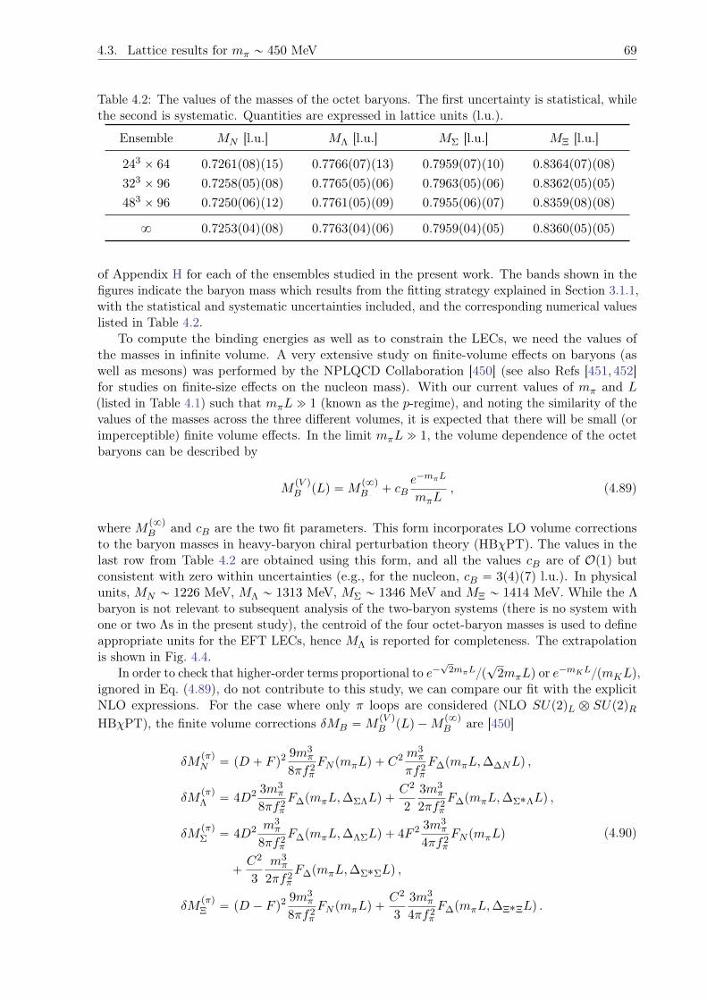
4.3. Lattice results for mπ „ 450 MeV 69
Table 4.2: The values of the masses of the octet baryons. The first uncertainty is statistical, whilethe second is systematic. Quantities are expressed in lattice units (l.u.).
Ensemble MN [l.u.] MΛ [l.u.] MΣ [l.u.] MΞ [l.u.]
243 ˆ 64 0.7261p08qp15q 0.7766p07qp13q 0.7959p07qp10q 0.8364p07qp08q
323 ˆ 96 0.7258p05qp08q 0.7765p05qp06q 0.7963p05qp06q 0.8362p05qp05q
483 ˆ 96 0.7250p06qp12q 0.7761p05qp09q 0.7955p06qp07q 0.8359p08qp08q
8 0.7253p04qp08q 0.7763p04qp06q 0.7959p04qp05q 0.8360p05qp05q
of Appendix H for each of the ensembles studied in the present work. The bands shown in thefigures indicate the baryon mass which results from the fitting strategy explained in Section 3.1.1,with the statistical and systematic uncertainties included, and the corresponding numerical valueslisted in Table 4.2.
To compute the binding energies as well as to constrain the LECs, we need the values ofthe masses in infinite volume. A very extensive study on finite-volume effects on baryons (aswell as mesons) was performed by the NPLQCD Collaboration [450] (see also Refs [451, 452]for studies on finite-size effects on the nucleon mass). With our current values of mπ and L(listed in Table 4.1) such that mπL " 1 (known as the p-regime), and noting the similarity of thevalues of the masses across the three different volumes, it is expected that there will be small (orimperceptible) finite volume effects. In the limit mπL " 1, the volume dependence of the octetbaryons can be described by
MpV qB pLq “M
p8q
B ` cBe´mπL
mπL, (4.89)
where M p8q
B and cB are the two fit parameters. This form incorporates LO volume correctionsto the baryon masses in heavy-baryon chiral perturbation theory (HBχPT). The values in thelast row from Table 4.2 are obtained using this form, and all the values cB are of Op1q butconsistent with zero within uncertainties (e.g., for the nucleon, cB “ 3p4qp7q l.u.). In physicalunits, MN „ 1226 MeV, MΛ „ 1313 MeV, MΣ „ 1346 MeV and MΞ „ 1414 MeV. While the Λbaryon is not relevant to subsequent analysis of the two-baryon systems (there is no system withone or two Λs in the present study), the centroid of the four octet-baryon masses is used to defineappropriate units for the EFT LECs, hence MΛ is reported for completeness. The extrapolationis shown in Fig. 4.4.
In order to check that higher-order terms proportional to e´?
2mπLp?
2mπLq or e´mKLpmKLq,ignored in Eq. (4.89), do not contribute to this study, we can compare our fit with the explicitNLO expressions. For the case where only π loops are considered (NLO SUp2qL b SUp2qRHBχPT), the finite volume corrections δMB “M
pV qB pLq ´M
p8q
B are [450]
δMpπqN “ pD ` F q2
9m3π
8πf2πFN pmπLq ` C
2 m3π
πf2πF∆pmπL,∆∆NLq ,
δMpπqΛ “ 4D2 3m3
π
8πf2πF∆pmπL,∆ΣΛLq `
C2
2
3m3π
2πf2πF∆pmπL,∆Σ˚ΛLq ,
δMpπqΣ “ 4D2 m3
π
8πf2πF∆pmπL,∆ΛΣLq ` 4F 2 3m3
π
4πf2πFN pmπLq
`C2
3
m3π
2πf2πF∆pmπL,∆Σ˚ΣLq ,
δMpπqΞ “ pD ´ F q2
9m3π
8πf2πFN pmπLq `
C2
3
3m3π
4πf2πF∆pmπL,∆Ξ˚ΞLq .
(4.90)
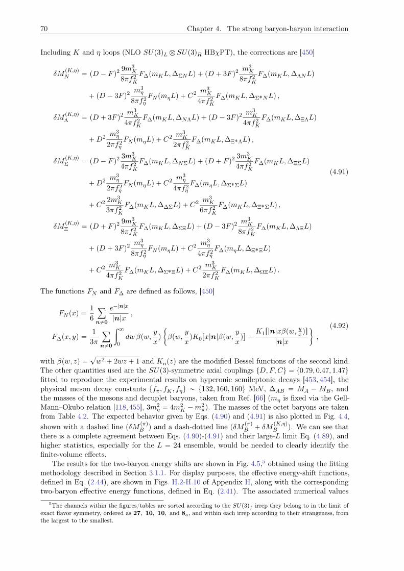
70 Chapter 4. The strong baryon-baryon interaction
Including K and η loops (NLO SUp3qL b SUp3qR HBχPT), the corrections are [450]
δMpK,ηqN “ pD ´ F q2
9m3K
8πf2K
F∆pmKL,∆ΣNLq ` pD ` 3F q2m3K
8πf2K
F∆pmKL,∆ΛNLq
` pD ´ 3F q2m3η
8πf2ηFN pmηLq ` C
2 m3K
4πf2K
F∆pmKL,∆Σ˚NLq ,
δMpK,ηqΛ “ pD ` 3F q2
m3K
4πf2K
F∆pmKL,∆NΛLq ` pD ´ 3F q2m3K
4πf2K
F∆pmKL,∆ΞΛLq
`D2 m3η
2πf2ηFN pmηLq ` C
2 m3K
2πf2K
F∆pmKL,∆Ξ˚ΛLq ,
δMpK,ηqΣ “ pD ´ F q2
3m3K
4πf2K
F∆pmKL,∆NΣLq ` pD ` F q2 3m3
K
4πf2K
F∆pmKL,∆ΞΣLq
`D2 m3η
2πf2ηFN pmηLq ` C
2 m3η
4πf2ηF∆pmηL,∆Σ˚ΣLq
` C2 2m3K
3πf2K
F∆pmKL,∆∆ΣLq ` C2 m3
K
6πf2K
F∆pmKL,∆Ξ˚ΣLq ,
δMpK,ηqΞ “ pD ` F q2
9m3K
8πf2K
F∆pmKL,∆ΣΞLq ` pD ´ 3F q2m3K
8πf2K
F∆pmKL,∆ΛΞLq
` pD ` 3F q2m3η
8πf2ηFN pmηLq ` C
2 m3η
4πf2ηF∆pmηL,∆Ξ˚ΞLq
` C2 m3K
4πf2K
F∆pmKL,∆Σ˚ΞLq ` C2 m3
K
2πf2K
F∆pmKL,∆ΩΞLq .
(4.91)
The functions FN and F∆ are defined as follows, [450]
FN pxq “1
6
ÿ
n‰0
e´|n|x
|n|x,
F∆px, yq “1
3π
ÿ
n‰0
ż 8
0dw βpw,
y
xq
"
βpw,y
xqK0rx|n|βpw,
y
xqs ´
K1r|n|xβpw,yxqs
|n|x
*
,
(4.92)
with βpw, zq “?w2 ` 2wz ` 1 and Knpzq are the modified Bessel functions of the second kind.
The other quantities used are the SUp3q-symmetric axial couplings tD,F,Cu “ t0.79, 0.47, 1.47ufitted to reproduce the experimental results on hyperonic semileptonic decays [453, 454], thephysical meson decay constants tfπ, fK , fηu „ t132, 160, 160u MeV, ∆AB “ MA ´MB, andthe masses of the mesons and decuplet baryons, taken from Ref. [66] (mη is fixed via the Gell-Mann–Okubo relation [118,455], 3m2
η “ 4m2K ´m
2π). The masses of the octet baryons are taken
from Table 4.2. The expected behavior given by Eqs. (4.90) and (4.91) is also plotted in Fig. 4.4,shown with a dashed line (δM pπq
B ) and a dash-dotted line (δM pπqB ` δM
pK,ηqB ). We can see that
there is a complete agreement between Eqs. (4.90)-(4.91) and their large-L limit Eq. (4.89), andhigher statistics, especially for the L “ 24 ensemble, would be needed to clearly identify thefinite-volume effects.
The results for the two-baryon energy shifts are shown in Fig. 4.5,5 obtained using the fittingmethodology described in Section 3.1.1. For display purposes, the effective energy-shift functions,defined in Eq. (2.44), are shown in Figs. H.2-H.10 of Appendix H, along with the correspondingtwo-baryon effective energy functions, defined in Eq. (2.41). The associated numerical values
5The channels within the figures/tables are sorted according to the SUp3qf irrep they belong to in the limit ofexact flavor symmetry, ordered as 27, 10, 10, and 8a, and within each irrep according to their strangeness, fromthe largest to the smallest.
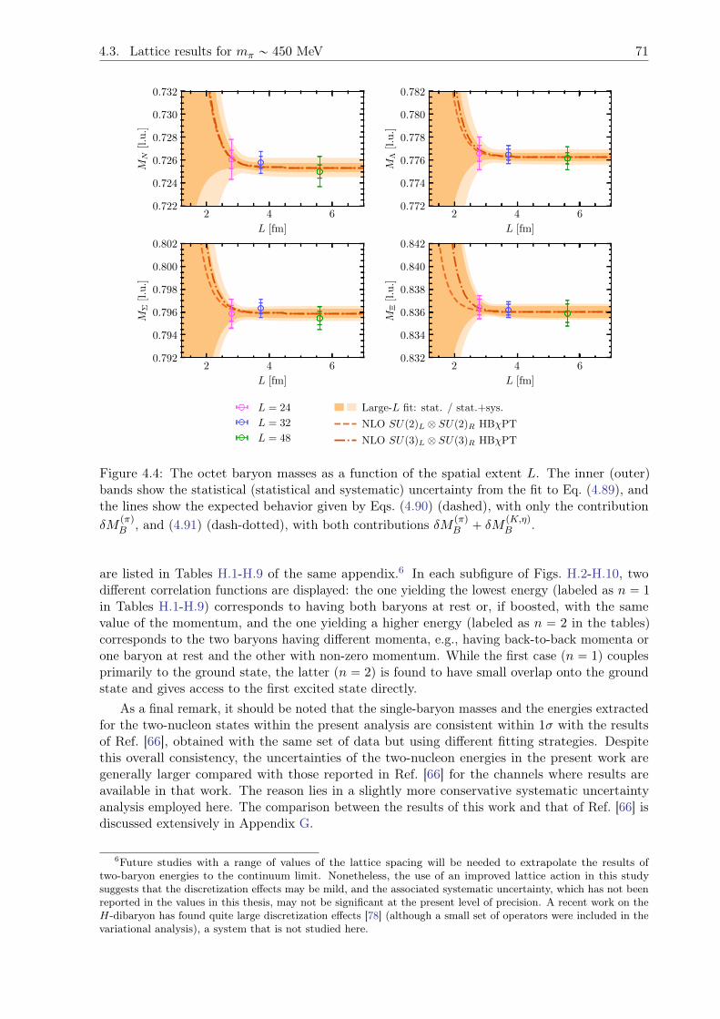
4.3. Lattice results for mπ „ 450 MeV 71
2 4 6
L [fm]
0.722
0.724
0.726
0.728
0.730
0.732
MN
[l.u.]
2 4 6
L [fm]
0.772
0.774
0.776
0.778
0.780
0.782
MΛ
[l.u.]
2 4 6
L [fm]
0.792
0.794
0.796
0.798
0.800
0.802
MΣ
[l.u.]
2 4 6
L [fm]
0.832
0.834
0.836
0.838
0.840
0.842
MΞ
[l.u.]
L = 24
L = 32
L = 48
Large-L fit: stat. / stat.+sys.
NLO SU(2)L ⊗ SU(2)R HBχPT
NLO SU(3)L ⊗ SU(3)R HBχPT
Figure 4.4: The octet baryon masses as a function of the spatial extent L. The inner (outer)bands show the statistical (statistical and systematic) uncertainty from the fit to Eq. (4.89), andthe lines show the expected behavior given by Eqs. (4.90) (dashed), with only the contributionδM
pπqB , and (4.91) (dash-dotted), with both contributions δM pπq
B ` δMpK,ηqB .
are listed in Tables H.1-H.9 of the same appendix.6 In each subfigure of Figs. H.2-H.10, twodifferent correlation functions are displayed: the one yielding the lowest energy (labeled as n “ 1in Tables H.1-H.9) corresponds to having both baryons at rest or, if boosted, with the samevalue of the momentum, and the one yielding a higher energy (labeled as n “ 2 in the tables)corresponds to the two baryons having different momenta, e.g., having back-to-back momenta orone baryon at rest and the other with non-zero momentum. While the first case (n “ 1) couplesprimarily to the ground state, the latter (n “ 2) is found to have small overlap onto the groundstate and gives access to the first excited state directly.
As a final remark, it should be noted that the single-baryon masses and the energies extractedfor the two-nucleon states within the present analysis are consistent within 1σ with the resultsof Ref. [66], obtained with the same set of data but using different fitting strategies. Despitethis overall consistency, the uncertainties of the two-nucleon energies in the present work aregenerally larger compared with those reported in Ref. [66] for the channels where results areavailable in that work. The reason lies in a slightly more conservative systematic uncertaintyanalysis employed here. The comparison between the results of this work and that of Ref. [66] isdiscussed extensively in Appendix G.
6Future studies with a range of values of the lattice spacing will be needed to extrapolate the results oftwo-baryon energies to the continuum limit. Nonetheless, the use of an improved lattice action in this studysuggests that the discretization effects may be mild, and the associated systematic uncertainty, which has not beenreported in the values in this thesis, may not be significant at the present level of precision. A recent work on theH-dibaryon has found quite large discretization effects [78] (although a small set of operators were included in thevariational analysis), a system that is not studied here.
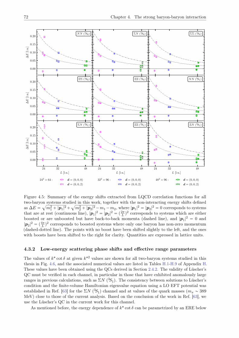
72 Chapter 4. The strong baryon-baryon interaction
24 32 48
0.00
0.05
0.10
0.15
0.20
∆E
[l.u.]
NN (1S0)
24 32 48
ΣN (1S0)
24 32 48
ΣΣ (1S0)
24 32 48
0.00
0.05
0.10
0.15
0.20
∆E
[l.u.]
ΞΣ (1S0)
24 32 48
ΞΞ (1S0)
24 32 48
NN (3S1)
24 32 48
L [l.u.]
0.00
0.05
0.10
0.15
0.20
∆E
[l.u.]
ΣN (3S1)
24 32 48
L [l.u.]
ΞΞ (3S1)
24 32 48
L [l.u.]
ΞN (3S1)
243 × 64 : d = (0, 0, 0)
d = (0, 0, 2)
323 × 96 : d = (0, 0, 0)
d = (0, 0, 2)
483 × 96 : d = (0, 0, 0)
d = (0, 0, 2)
Figure 4.5: Summary of the energy shifts extracted from LQCD correlation functions for alltwo-baryon systems studied in this work, together with the non-interacting energy shifts definedas ∆E “
a
m21 ` |p1|
2`a
m22 ` |p2|
2´m1´m2, where |p1|2 “ |p2|
2 “ 0 corresponds to systemsthat are at rest (continuous line), |p1|
2 “ |p2|2 “ p2π
L q2 corresponds to systems which are either
boosted or are unboosted but have back-to-back momenta (dashed line), and |p1|2 “ 0 and
|p2|2 “ p4π
L q2 corresponds to boosted systems where only one baryon has non-zero momentum
(dashed-dotted line). The points with no boost have been shifted slightly to the left, and the oneswith boosts have been shifted to the right for clarity. Quantities are expressed in lattice units.
4.3.2 Low-energy scattering phase shifts and effective range parameters
The values of k˚ cot δ at given k˚2 values are shown for all two-baryon systems studied in thisthesis in Fig. 4.6, and the associated numerical values are listed in Tables H.1-H.9 of Appendix H.These values have been obtained using the QCs derived in Section 2.4.2. The validity of Lüscher’sQC must be verified in each channel, in particular in those that have exhibited anomalously largeranges in previous calculations, such as ΣN p3S1q. The consistency between solutions to Lüscher’scondition and the finite-volume Hamiltonian eigenvalue equation using a LO EFT potential wasestablished in Ref. [63] for the ΣN p3S1q channel and at values of the quark masses (mπ „ 389MeV) close to those of the current analysis. Based on the conclusion of the work in Ref. [63], weuse the Lüscher’s QC in the current work for this channel.
As mentioned before, the energy dependence of k˚ cot δ can be parametrized by an ERE below
4.3. Lattice results for mπ „ 450 MeV 73
0.000 0.025 0.050 0.075−0.5
0.0
0.5
1.0
1.5
2.0
2.5
k∗
cotδ
[l.u.]
NN (1S0)
0.000 0.025 0.050 0.075−3
−2
−1
0
1
2
3
ΣN (1S0)
0.00 0.02 0.04 0.06
0
1
2
3
4
ΣΣ (1S0)
0.00 0.02 0.04 0.06
0.00
0.25
0.50
0.75
1.00
1.25
1.50
k∗
cotδ
[l.u.]
ΞΣ (1S0)
0.00 0.02 0.04 0.06
0.00
0.25
0.50
0.75
1.00
1.25
ΞΞ (1S0)
0.00 0.02 0.04 0.06
0
1
2
3
4 NN (3S1)
0.00 0.02 0.04 0.06 0.08 0.10
k∗2 [l.u.]
−0.8
−0.6
−0.4
−0.2
0.0
0.2
0.4
k∗
cotδ
[l.u.]
ΣN (3S1)
0.00 0.02 0.04 0.06 0.08
k∗2 [l.u.]
−1.50
−1.25
−1.00
−0.75
−0.50
−0.25
0.00
ΞΞ (3S1)
−0.02 0.00 0.02 0.04
k∗2 [l.u.]
−0.1
0.0
0.1
0.2 ΞN (3S1)
243 × 64 :
323 × 96 :
483 × 96 :
d = (0, 0, 0)
d = (0, 0, 0)
d = (0, 0, 0)
d = (0, 0, 2)
d = (0, 0, 2)
d = (0, 0, 2)
2√πLZ(0,0,0)
00 :
L = 24
L = 32
L = 48
2√πγLZ(0,0,2)
00 :
L = 24
L = 32
L = 48
Figure 4.6: k˚ cot δ values as a function of the squared c.m. momentum k˚2 for all two-baryonsystems studied in this work. The darker uncertainty bands are statistical, while the lighterbands show the statistical and systematic uncertainties combined in quadrature. The differentZ-functions are shown as continuous and dashed lines. Quantities are expressed in lattice units.
the t-channel cut, and since the pion is the lightest hadron that can be exchanged between anyof the two baryons considered in the present study, k˚t-cut “ mπ2. The scattering parameterscan be constrained by fitting k˚ cot δ values obtained from the use of Lüscher’s QC as a functionof k˚2. To this end, one could use a one-dimensional choice of the χ2 function, minimizing thevertical distance between the fitted point and the function,
χ2pa´1, r, P q “ÿ
i
rpk˚ cot δqi ´ fpa´1, r, P, k˚2
i qs2
σ2i
, (4.93)
where7 fpa´1, r, P, k˚2q corresponds to the ERE parametrization given by the right-hand side ofEq. (2.64), and the sum runs over all extracted pairs of tk˚2
i , pk˚ cot δqiu, where the compound
7The inverse scattering length can be constrained far more precisely compared with the scattering length itselfgiven that a´1 samples can cross zero in the channels considered. As a result, in the following all dependencies ona enter via a´1.
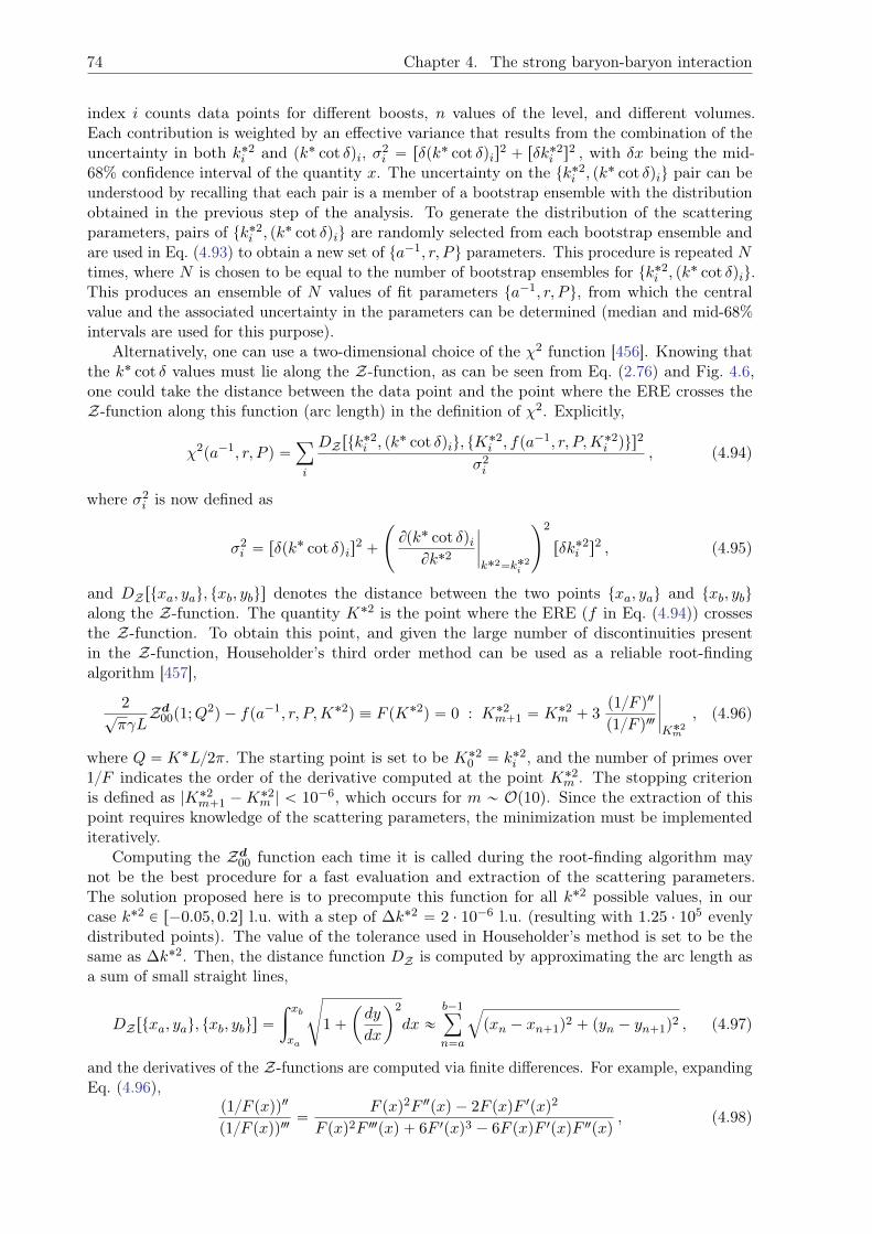
74 Chapter 4. The strong baryon-baryon interaction
index i counts data points for different boosts, n values of the level, and different volumes.Each contribution is weighted by an effective variance that results from the combination of theuncertainty in both k˚2
i and pk˚ cot δqi, σ2i “ rδpk
˚ cot δqis2 ` rδk˚2
i s2 , with δx being the mid-
68% confidence interval of the quantity x. The uncertainty on the tk˚2i , pk
˚ cot δqiu pair can beunderstood by recalling that each pair is a member of a bootstrap ensemble with the distributionobtained in the previous step of the analysis. To generate the distribution of the scatteringparameters, pairs of tk˚2
i , pk˚ cot δqiu are randomly selected from each bootstrap ensemble and
are used in Eq. (4.93) to obtain a new set of ta´1, r, P u parameters. This procedure is repeated Ntimes, where N is chosen to be equal to the number of bootstrap ensembles for tk˚2
i , pk˚ cot δqiu.
This produces an ensemble of N values of fit parameters ta´1, r, P u, from which the centralvalue and the associated uncertainty in the parameters can be determined (median and mid-68%intervals are used for this purpose).
Alternatively, one can use a two-dimensional choice of the χ2 function [456]. Knowing thatthe k˚ cot δ values must lie along the Z-function, as can be seen from Eq. (2.76) and Fig. 4.6,one could take the distance between the data point and the point where the ERE crosses theZ-function along this function (arc length) in the definition of χ2. Explicitly,
χ2pa´1, r, P q “ÿ
i
DZ rtk˚2i , pk
˚ cot δqiu, tK˚2i , fpa´1, r, P,K˚2
i qus2
σ2i
, (4.94)
where σ2i is now defined as
σ2i “ rδpk
˚ cot δqis2 `
˜
Bpk˚ cot δqiBk˚2
ˇ
ˇ
ˇ
ˇ
k˚2“k˚2i
¸2
rδk˚2i s
2 , (4.95)
and DZ rtxa, yau, txb, ybus denotes the distance between the two points txa, yau and txb, ybualong the Z-function. The quantity K˚2 is the point where the ERE (f in Eq. (4.94)) crossesthe Z-function. To obtain this point, and given the large number of discontinuities presentin the Z-function, Householder’s third order method can be used as a reliable root-findingalgorithm [457],
2?πγL
Zd00p1;Q2q ´ fpa´1, r, P,K˚2q ” F pK˚2q “ 0 : K˚2
m`1 “ K˚2m ` 3
p1F q2
p1F q3
ˇ
ˇ
ˇ
ˇ
K˚2m
, (4.96)
where Q “ K˚L2π. The starting point is set to be K˚20 “ k˚2
i , and the number of primes over1F indicates the order of the derivative computed at the point K˚2
m . The stopping criterionis defined as |K˚2
m`1 ´K˚2m | ă 10´6, which occurs for m „ Op10q. Since the extraction of this
point requires knowledge of the scattering parameters, the minimization must be implementediteratively.
Computing the Zd00 function each time it is called during the root-finding algorithm may
not be the best procedure for a fast evaluation and extraction of the scattering parameters.The solution proposed here is to precompute this function for all k˚2 possible values, in ourcase k˚2 P r´0.05, 0.2s l.u. with a step of ∆k˚2 “ 2 ¨ 10´6 l.u. (resulting with 1.25 ¨ 105 evenlydistributed points). The value of the tolerance used in Householder’s method is set to be thesame as ∆k˚2. Then, the distance function DZ is computed by approximating the arc length asa sum of small straight lines,
DZ rtxa, yau, txb, ybus “ż xb
xa
d
1`
ˆ
dy
dx
˙2
dx «b´1ÿ
n“a
b
pxn ´ xn`1q2 ` pyn ´ yn`1q
2 , (4.97)
and the derivatives of the Z-functions are computed via finite differences. For example, expandingEq. (4.96),
p1F pxqq2
p1F pxqq3“
F pxq2F 2pxq ´ 2F pxqF 1pxq2
F pxq2F3pxq ` 6F 1pxq3 ´ 6F pxqF 1pxqF 2pxq, (4.98)
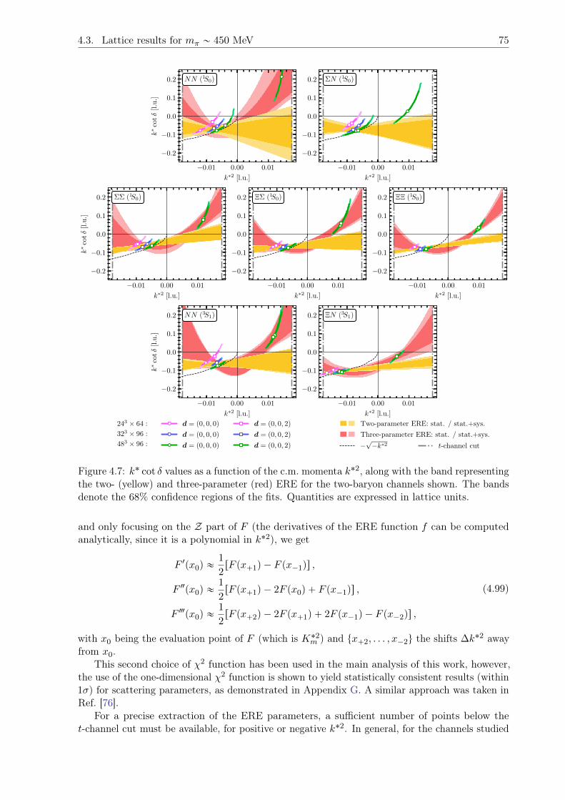
4.3. Lattice results for mπ „ 450 MeV 75
−0.01 0.00 0.01
k∗2 [l.u.]
−0.2
−0.1
0.0
0.1
0.2
k∗
cotδ
[l.u.]
NN (1S0)
−0.01 0.00 0.01
k∗2 [l.u.]
−0.2
−0.1
0.0
0.1
0.2 ΣN (1S0)
−0.01 0.00 0.01
k∗2 [l.u.]
−0.2
−0.1
0.0
0.1
0.2
k∗
cotδ
[l.u.]
ΣΣ (1S0)
−0.01 0.00 0.01
k∗2 [l.u.]
−0.2
−0.1
0.0
0.1
0.2 ΞΣ (1S0)
−0.01 0.00 0.01
k∗2 [l.u.]
−0.2
−0.1
0.0
0.1
0.2 ΞΞ (1S0)
−0.01 0.00 0.01
k∗2 [l.u.]
−0.2
−0.1
0.0
0.1
0.2
k∗
cotδ
[l.u.]
NN (3S1)
−0.01 0.00 0.01
k∗2 [l.u.]
−0.2
−0.1
0.0
0.1
0.2 ΞN (3S1)
243 × 64 :
323 × 96 :
483 × 96 :
d = (0, 0, 0)
d = (0, 0, 0)
d = (0, 0, 0)
d = (0, 0, 2)
d = (0, 0, 2)
d = (0, 0, 2)
Two-parameter ERE: stat. / stat.+sys.
Three-parameter ERE: stat. / stat.+sys.
−√−k∗2 t-channel cut
Figure 4.7: k˚ cot δ values as a function of the c.m. momenta k˚2, along with the band representingthe two- (yellow) and three-parameter (red) ERE for the two-baryon channels shown. The bandsdenote the 68% confidence regions of the fits. Quantities are expressed in lattice units.
and only focusing on the Z part of F (the derivatives of the ERE function f can be computedanalytically, since it is a polynomial in k˚2), we get
F 1px0q «1
2rF px`1q ´ F px´1qs ,
F 2px0q «1
2rF px`1q ´ 2F px0q ` F px´1qs ,
F3px0q «1
2rF px`2q ´ 2F px`1q ` 2F px´1q ´ F px´2qs ,
(4.99)
with x0 being the evaluation point of F (which is K˚2m ) and tx`2, . . . , x´2u the shifts ∆k˚2 away
from x0.This second choice of χ2 function has been used in the main analysis of this work, however,
the use of the one-dimensional χ2 function is shown to yield statistically consistent results (within1σ) for scattering parameters, as demonstrated in Appendix G. A similar approach was taken inRef. [76].
For a precise extraction of the ERE parameters, a sufficient number of points below thet-channel cut must be available, for positive or negative k˚2. In general, for the channels studied
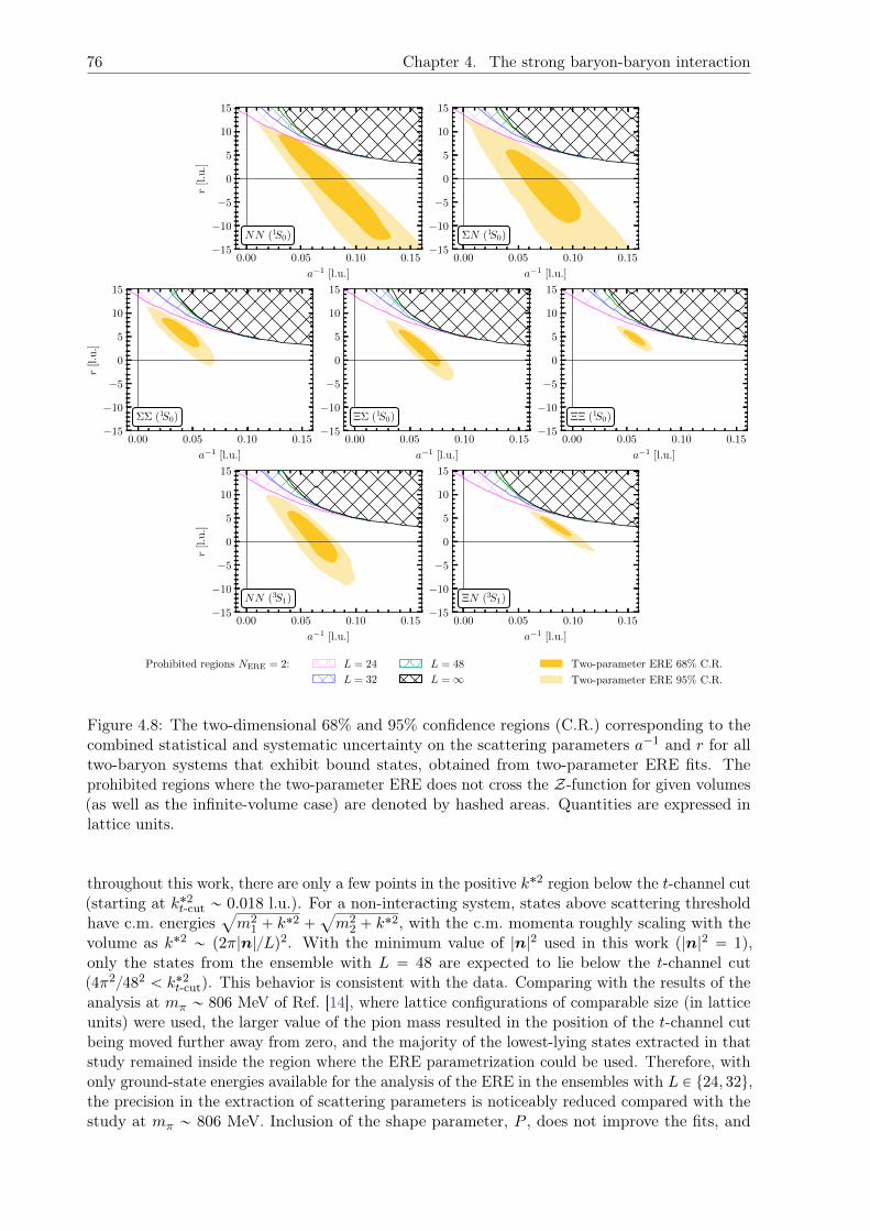
76 Chapter 4. The strong baryon-baryon interaction
0.00 0.05 0.10 0.15
a−1 [l.u.]
−15
−10
−5
0
5
10
15
r[l.u.]
NN (1S0)
0.00 0.05 0.10 0.15
a−1 [l.u.]
−15
−10
−5
0
5
10
15
ΣN (1S0)
0.00 0.05 0.10 0.15
a−1 [l.u.]
−15
−10
−5
0
5
10
15
r[l.u.]
ΣΣ (1S0)
0.00 0.05 0.10 0.15
a−1 [l.u.]
−15
−10
−5
0
5
10
15
ΞΣ (1S0)
0.00 0.05 0.10 0.15
a−1 [l.u.]
−15
−10
−5
0
5
10
15
ΞΞ (1S0)
0.00 0.05 0.10 0.15
a−1 [l.u.]
−15
−10
−5
0
5
10
15
r[l.u.]
NN (3S1)
0.00 0.05 0.10 0.15
a−1 [l.u.]
−15
−10
−5
0
5
10
15
ΞN (3S1)
Prohibited regions NERE = 2: L = 24
L = 32
L = 48
L =∞Two-parameter ERE 68% C.R.
Two-parameter ERE 95% C.R.
Figure 4.8: The two-dimensional 68% and 95% confidence regions (C.R.) corresponding to thecombined statistical and systematic uncertainty on the scattering parameters a´1 and r for alltwo-baryon systems that exhibit bound states, obtained from two-parameter ERE fits. Theprohibited regions where the two-parameter ERE does not cross the Z-function for given volumes(as well as the infinite-volume case) are denoted by hashed areas. Quantities are expressed inlattice units.
throughout this work, there are only a few points in the positive k˚2 region below the t-channel cut(starting at k˚2
t-cut „ 0.018 l.u.). For a non-interacting system, states above scattering thresholdhave c.m. energies
a
m21 ` k
˚2 `a
m22 ` k
˚2, with the c.m. momenta roughly scaling with thevolume as k˚2 „ p2π|n|Lq2. With the minimum value of |n|2 used in this work (|n|2 “ 1),only the states from the ensemble with L “ 48 are expected to lie below the t-channel cut(4π2482 ă k˚2
t-cut). This behavior is consistent with the data. Comparing with the results of theanalysis at mπ „ 806 MeV of Ref. [14], where lattice configurations of comparable size (in latticeunits) were used, the larger value of the pion mass resulted in the position of the t-channel cutbeing moved further away from zero, and the majority of the lowest-lying states extracted in thatstudy remained inside the region where the ERE parametrization could be used. Therefore, withonly ground-state energies available for the analysis of the ERE in the ensembles with L P t24, 32u,the precision in the extraction of scattering parameters is noticeably reduced compared with thestudy at mπ „ 806 MeV. Inclusion of the shape parameter, P , does not improve the fits, and
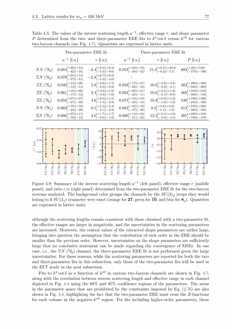
4.3. Lattice results for mπ „ 450 MeV 77
Table 4.3: The values of the inverse scattering length a´1, effective range r, and shape parameterP determined from the two- and three-parameter ERE fits to k˚ cot δ versus k˚2 for varioustwo-baryon channels (see Fig. 4.7). Quantities are expressed in lattice units.
Two-parameter ERE fit Three-parameter ERE fit
a´1 [l.u.] r [l.u.] a´1 [l.u.] r [l.u.] P [l.u.]
NN p1S0q 0.084p`20qp`44qp´42qp´35q ´2.4
p`8.4qp`8.3qp´5.5qp´9.0q 0.053
p`33qp`43qp´29qp´52q 15.4
p`6.5qp`20.8qp´6.2qp´5.7q 803
p`46qp`510qp´570qp´190q
ΣN p1S0q 0.079p`25qp`14qp´27qp´31q ´2.8
p`6.7qp`6.0qp´5.3qp´4.0q - - -
ΣΣ p1S0q 0.040p`15qp`06qp´13qp´14q 5.8
p`2.8qp`1.5qp´2.9qp´0.9q 0.059
p`17qp`41qp´28qp´18q 10.0
p`3.8qp`3.8qp´2.4qp´4.1q 563
p`200qp`490qp´330qp´260q
ΞΣ p1S0q 0.061p`16qp`06qp´17qp´12q 2.4
p`3.6qp`1.8qp´3.4qp´1.6q 0.062
p`28qp`21qp´22qp´11q 10.6
p`2.5qp`1.8qp´2.1qp´0.9q 469
p`310qp`210qp´280qp´140q
ΞΞ p1S0q 0.058p`07qp`07qp´07qp´08q 4.6
p`0.8qp`1.5qp´1.4qp´0.8q 0.075
p`16qp`19qp´22qp´16q 10.9
p`0.9qp`1.0qp´1.0qp´1.0q 538
p`190qp`200qp´250qp´180q
NN p3S1q 0.063p`18qp`10qp´24qp´09q 0.5
p`5.5qp`2.4qp´4.1qp´2.9q 0.082
p`42qp`18qp´47qp´26q 8.0
p`5.0qp`4.8qp´5.1qp´1.9q 812
p`570qp`300qp´560qp´340q
ΞN p3S1q 0.086p`07qp`11qp´10qp´13q 3.0
p`1.7qp`1.7qp´0.9qp´1.6q 0.080
p`14qp`23qp´21qp´22q 12.2
p`3.5qp`4.8qp´3.0qp´4.5q 307
p`220qp`310qp´190qp´170q
NN
(1S
0)
N
(1S
0)
(1S
0)
(1S
0)
(1S
0)
NN
(3S
1)
N
(3S
1)0.00
0.05
0.10
0.15
a
1[l.u
.]
NN
(1S
0)
N
(1S
0)
(1S
0)
(1S
0)
(1S
0)
NN
(3S
1)
N
(3S
1)15
10
5
0
5
10
r[l.u
.]
NN
(1S
0)
N
(1S
0)
(1S
0)
(1S
0)
(1S
0)
NN
(3S
1)
N
(3S
1)2.0
1.5
1.0
0.5
0.0
0.5
r/a
Figure 4.9: Summary of the inverse scattering length a´1 (left panel), effective range r (middlepanel), and ratio ra (right panel) determined from the two-parameter ERE fit for the two-baryonsystems analyzed. The background color groups the channels by the SUp3qf irreps they wouldbelong to if SUp3f q symmetry were exact (orange for 27, green for 10, and blue for 8a). Quantitiesare expressed in lattice units.
although the scattering lengths remain consistent with those obtained with a two-parameter fit,the effective ranges are larger in magnitude, and the uncertainties in the scattering parametersare increased. Moreover, the central values of the extracted shape parameters are rather large,bringing into question the assumption that the contribution of each order in the ERE should besmaller than the previous order. However, uncertainties on the shape parameters are sufficientlylarge that no conclusive statement can be made regarding the convergence of EREs. In onecase, i.e., the ΣN p1S0q channel, the three-parameter ERE fit is not performed given the largeuncertainties. For these reasons, while the scattering parameters are reported for both the two-and three-parameter fits in this subsection, only those of the two-parameter fits will be used inthe EFT study in the next subsection.
Fits to k˚ cot δ as a function of k˚2 in various two-baryon channels are shown in Fig. 4.7,along with the correlation between inverse scattering length and effective range in each channeldepicted in Fig. 4.8 using the 68% and 95% confidence regions of the parameters. The areasin the parameter space that are prohibited by the constraints imposed by Eq. (2.76) are alsoshown in Fig. 4.8, highlighting the fact that the two-parameter ERE must cross the Z-functionsfor each volume in the negative-k˚2 region. For fits including higher-order parameters, these
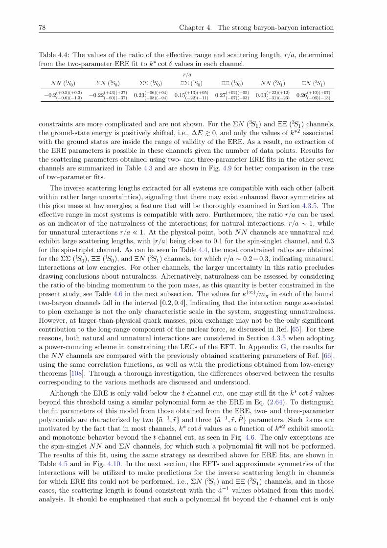
78 Chapter 4. The strong baryon-baryon interaction
Table 4.4: The values of the ratio of the effective range and scattering length, ra, determinedfrom the two-parameter ERE fit to k˚ cot δ values in each channel.
ra
NN p1S0q ΣN p1S0q ΣΣ p1S0q ΞΣ p1S0q ΞΞ p1S0q NN p3S1q ΞN p3S1q
´0.2p`0.5qp`0.3qp´0.6qp´1.3q ´0.22
p`43qp`27qp´60qp´37q 0.23
p`06qp`04qp´08qp´04q 0.15
p`13qp`05qp´22qp´11q 0.27
p`02qp`05qp´07qp´03q 0.03
p`22qp`12qp´31qp´23q 0.26
p`10qp`07qp´06qp´13q
constraints are more complicated and are not shown. For the ΣN p3S1q and ΞΞ p3S1q channels,the ground-state energy is positively shifted, i.e., ∆E Á 0, and only the values of k˚2 associatedwith the ground states are inside the range of validity of the ERE. As a result, no extraction ofthe ERE parameters is possible in these channels given the number of data points. Results forthe scattering parameters obtained using two- and three-parameter ERE fits in the other sevenchannels are summarized in Table 4.3 and are shown in Fig. 4.9 for better comparison in the caseof two-parameter fits.
The inverse scattering lengths extracted for all systems are compatible with each other (albeitwithin rather large uncertainties), signaling that there may exist enhanced flavor symmetries atthis pion mass at low energies, a feature that will be thoroughly examined in Section 4.3.5. Theeffective range in most systems is compatible with zero. Furthermore, the ratio ra can be usedas an indicator of the naturalness of the interactions; for natural interactions, ra „ 1, whilefor unnatural interactions ra ! 1. At the physical point, both NN channels are unnatural andexhibit large scattering lengths, with |ra| being close to 0.1 for the spin-singlet channel, and 0.3for the spin-triplet channel. As can be seen in Table 4.4, the most constrained ratios are obtainedfor the ΣΣ p1S0q, ΞΞ p1S0q, and ΞN p3S1q channels, for which ra „ 0.2´0.3, indicating unnaturalinteractions at low energies. For other channels, the larger uncertainty in this ratio precludesdrawing conclusions about naturalness. Alternatively, naturalness can be assessed by consideringthe ratio of the binding momentum to the pion mass, as this quantity is better constrained in thepresent study, see Table 4.6 in the next subsection. The values for κp8qmπ in each of the boundtwo-baryon channels fall in the interval r0.2, 0.4s, indicating that the interaction range associatedto pion exchange is not the only characteristic scale in the system, suggesting unnaturalness.However, at larger-than-physical quark masses, pion exchange may not be the only significantcontribution to the long-range component of the nuclear force, as discussed in Ref. [65]. For thesereasons, both natural and unnatural interactions are considered in Section 4.3.5 when adoptinga power-counting scheme in constraining the LECs of the EFT. In Appendix G, the results forthe NN channels are compared with the previously obtained scattering parameters of Ref. [66],using the same correlation functions, as well as with the predictions obtained from low-energytheorems [108]. Through a thorough investigation, the differences observed between the resultscorresponding to the various methods are discussed and understood.
Although the ERE is only valid below the t-channel cut, one may still fit the k˚ cot δ valuesbeyond this threshold using a similar polynomial form as the ERE in Eq. (2.64). To distinguishthe fit parameters of this model from those obtained from the ERE, two- and three-parameterpolynomials are characterized by two ta´1, ru and three ta´1, r, P u parameters. Such forms aremotivated by the fact that in most channels, k˚ cot δ values as a function of k˚2 exhibit smoothand monotonic behavior beyond the t-channel cut, as seen in Fig. 4.6. The only exceptions arethe spin-singlet NN and ΣN channels, for which such a polynomial fit will not be performed.The results of this fit, using the same strategy as described above for ERE fits, are shown inTable 4.5 and in Fig. 4.10. In the next section, the EFTs and approximate symmetries of theinteractions will be utilized to make predictions for the inverse scattering length in channelsfor which ERE fits could not be performed, i.e., ΣN p3S1q and ΞΞ p3S1q channels, and in thosecases, the scattering length is found consistent with the a´1 values obtained from this modelanalysis. It should be emphasized that such a polynomial fit beyond the t-channel cut is only
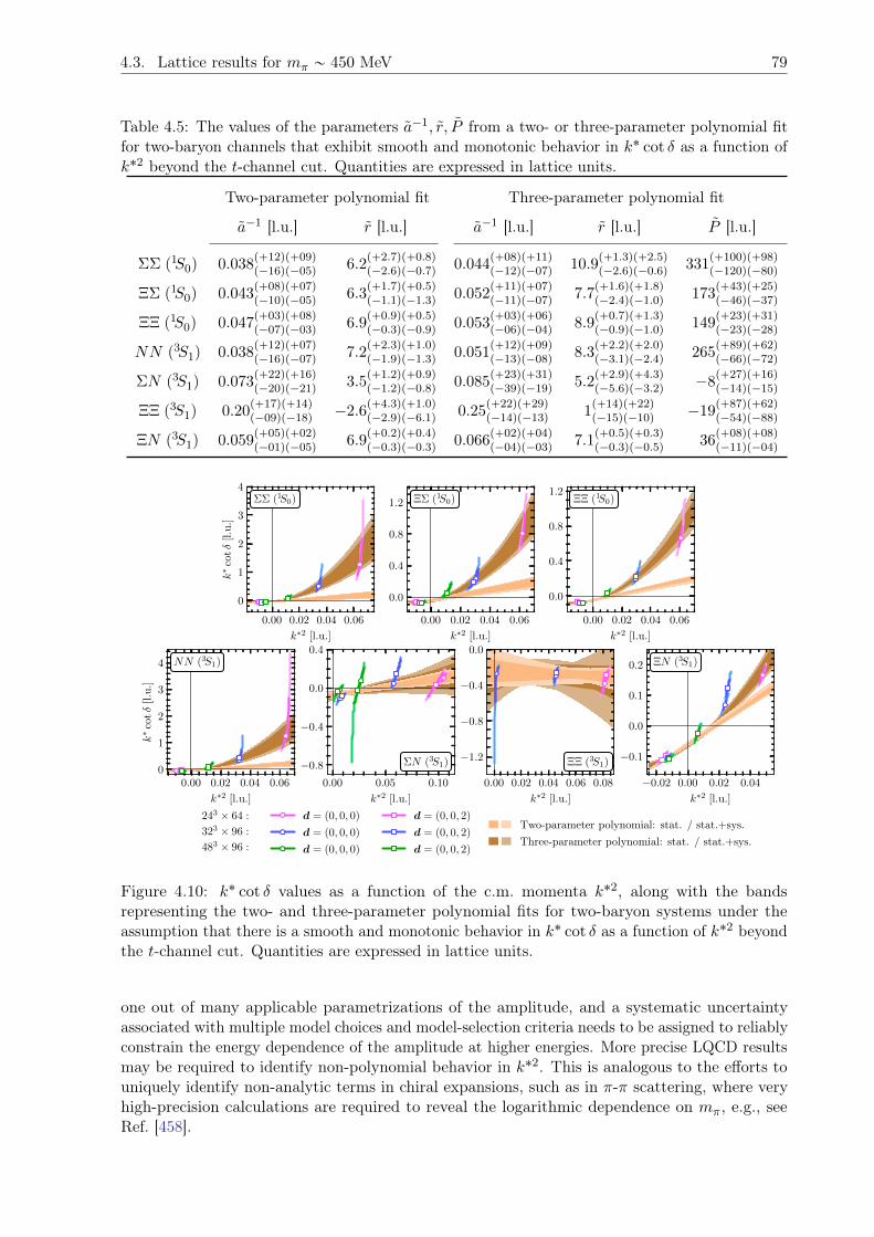
4.3. Lattice results for mπ „ 450 MeV 79
Table 4.5: The values of the parameters a´1, r, P from a two- or three-parameter polynomial fitfor two-baryon channels that exhibit smooth and monotonic behavior in k˚ cot δ as a function ofk˚2 beyond the t-channel cut. Quantities are expressed in lattice units.
Two-parameter polynomial fit Three-parameter polynomial fit
a´1 [l.u.] r [l.u.] a´1 [l.u.] r [l.u.] P [l.u.]
ΣΣ p1S0q 0.038p`12qp`09qp´16qp´05q 6.2
p`2.7qp`0.8qp´2.6qp´0.7q 0.044
p`08qp`11qp´12qp´07q 10.9
p`1.3qp`2.5qp´2.6qp´0.6q 331
p`100qp`98qp´120qp´80q
ΞΣ p1S0q 0.043p`08qp`07qp´10qp´05q 6.3
p`1.7qp`0.5qp´1.1qp´1.3q 0.052
p`11qp`07qp´11qp´07q 7.7
p`1.6qp`1.8qp´2.4qp´1.0q 173
p`43qp`25qp´46qp´37q
ΞΞ p1S0q 0.047p`03qp`08qp´07qp´03q 6.9
p`0.9qp`0.5qp´0.3qp´0.9q 0.053
p`03qp`06qp´06qp´04q 8.9
p`0.7qp`1.3qp´0.9qp´1.0q 149
p`23qp`31qp´23qp´28q
NN p3S1q 0.038p`12qp`07qp´16qp´07q 7.2
p`2.3qp`1.0qp´1.9qp´1.3q 0.051
p`12qp`09qp´13qp´08q 8.3
p`2.2qp`2.0qp´3.1qp´2.4q 265
p`89qp`62qp´66qp´72q
ΣN p3S1q 0.073p`22qp`16qp´20qp´21q 3.5
p`1.2qp`0.9qp´1.2qp´0.8q 0.085
p`23qp`31qp´39qp´19q 5.2
p`2.9qp`4.3qp´5.6qp´3.2q ´8
p`27qp`16qp´14qp´15q
ΞΞ p3S1q 0.20p`17qp`14qp´09qp´18q ´2.6
p`4.3qp`1.0qp´2.9qp´6.1q 0.25
p`22qp`29qp´14qp´13q 1
p`14qp`22qp´15qp´10q ´19
p`87qp`62qp´54qp´88q
ΞN p3S1q 0.059p`05qp`02qp´01qp´05q 6.9
p`0.2qp`0.4qp´0.3qp´0.3q 0.066
p`02qp`04qp´04qp´03q 7.1
p`0.5qp`0.3qp´0.3qp´0.5q 36
p`08qp`08qp´11qp´04q
0.00 0.02 0.04 0.06
k∗2 [l.u.]
0
1
2
3
4
k∗
cotδ
[l.u.]
ΣΣ (1S0)
0.00 0.02 0.04 0.06
k∗2 [l.u.]
0.0
0.4
0.8
1.2 ΞΣ (1S0)
0.00 0.02 0.04 0.06
k∗2 [l.u.]
0.0
0.4
0.8
1.2ΞΞ (1S0)
0.00 0.02 0.04 0.06
k∗2 [l.u.]
0
1
2
3
4
k∗
cotδ
[l.u.]
NN (3S1)
0.00 0.05 0.10
k∗2 [l.u.]
−0.8
−0.4
0.0
0.4
ΣN (3S1)
0.00 0.02 0.04 0.06 0.08
k∗2 [l.u.]
−1.2
−0.8
−0.4
0.0
ΞΞ (3S1)
−0.02 0.00 0.02 0.04
k∗2 [l.u.]
−0.1
0.0
0.1
0.2 ΞN (3S1)
243 × 64 :
323 × 96 :
483 × 96 :
d = (0, 0, 0)
d = (0, 0, 0)
d = (0, 0, 0)
d = (0, 0, 2)
d = (0, 0, 2)
d = (0, 0, 2)
Two-parameter polynomial: stat. / stat.+sys.
Three-parameter polynomial: stat. / stat.+sys.
Figure 4.10: k˚ cot δ values as a function of the c.m. momenta k˚2, along with the bandsrepresenting the two- and three-parameter polynomial fits for two-baryon systems under theassumption that there is a smooth and monotonic behavior in k˚ cot δ as a function of k˚2 beyondthe t-channel cut. Quantities are expressed in lattice units.
one out of many applicable parametrizations of the amplitude, and a systematic uncertaintyassociated with multiple model choices and model-selection criteria needs to be assigned to reliablyconstrain the energy dependence of the amplitude at higher energies. More precise LQCD resultsmay be required to identify non-polynomial behavior in k˚2. This is analogous to the efforts touniquely identify non-analytic terms in chiral expansions, such as in π-π scattering, where veryhigh-precision calculations are required to reveal the logarithmic dependence on mπ, e.g., seeRef. [458].
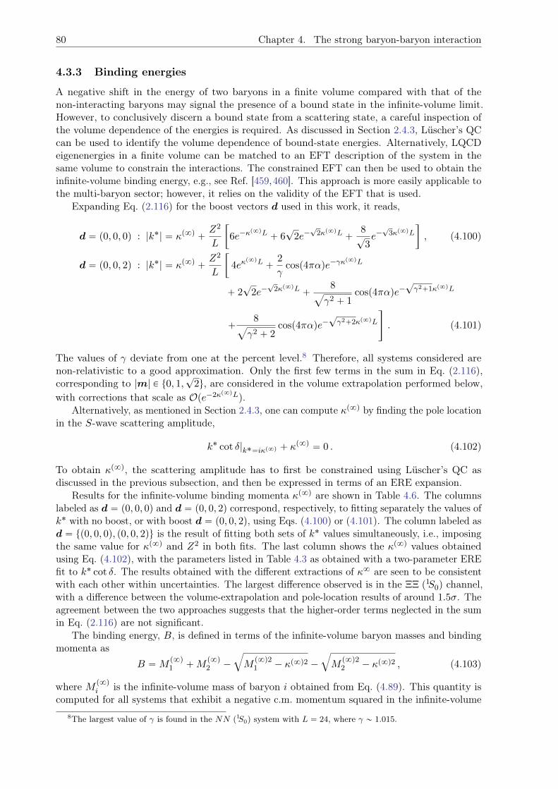
80 Chapter 4. The strong baryon-baryon interaction
4.3.3 Binding energies
A negative shift in the energy of two baryons in a finite volume compared with that of thenon-interacting baryons may signal the presence of a bound state in the infinite-volume limit.However, to conclusively discern a bound state from a scattering state, a careful inspection ofthe volume dependence of the energies is required. As discussed in Section 2.4.3, Lüscher’s QCcan be used to identify the volume dependence of bound-state energies. Alternatively, LQCDeigenenergies in a finite volume can be matched to an EFT description of the system in thesame volume to constrain the interactions. The constrained EFT can then be used to obtain theinfinite-volume binding energy, e.g., see Ref. [459,460]. This approach is more easily applicable tothe multi-baryon sector; however, it relies on the validity of the EFT that is used.
Expanding Eq. (2.116) for the boost vectors d used in this work, it reads,
d “ p0, 0, 0q : |k˚| “ κp8q `Z2
L
„
6e´κp8qL ` 6
?2e´
?2κp8qL `
8?
3e´?
3κp8qL
, (4.100)
d “ p0, 0, 2q : |k˚| “ κp8q `Z2
L
„
4eκp8qL `
2
γcosp4παqe´γκ
p8qL
` 2?
2e´?
2κp8qL `8
a
γ2 ` 1cosp4παqe´
?γ2`1κp8qL
`8
a
γ2 ` 2cosp4παqe´
?γ2`2κp8qL
ff
. (4.101)
The values of γ deviate from one at the percent level.8 Therefore, all systems considered arenon-relativistic to a good approximation. Only the first few terms in the sum in Eq. (2.116),corresponding to |m| P t0, 1,
?2u, are considered in the volume extrapolation performed below,
with corrections that scale as Ope´2κp8qLq.Alternatively, as mentioned in Section 2.4.3, one can compute κp8q by finding the pole location
in the S-wave scattering amplitude,
k˚ cot δ|k˚“iκp8q ` κp8q “ 0 . (4.102)
To obtain κp8q, the scattering amplitude has to first be constrained using Lüscher’s QC asdiscussed in the previous subsection, and then be expressed in terms of an ERE expansion.
Results for the infinite-volume binding momenta κp8q are shown in Table 4.6. The columnslabeled as d “ p0, 0, 0q and d “ p0, 0, 2q correspond, respectively, to fitting separately the values ofk˚ with no boost, or with boost d “ p0, 0, 2q, using Eqs. (4.100) or (4.101). The column labeled asd “ tp0, 0, 0q, p0, 0, 2qu is the result of fitting both sets of k˚ values simultaneously, i.e., imposingthe same value for κp8q and Z2 in both fits. The last column shows the κp8q values obtainedusing Eq. (4.102), with the parameters listed in Table 4.3 as obtained with a two-parameter EREfit to k˚ cot δ. The results obtained with the different extractions of κ8 are seen to be consistentwith each other within uncertainties. The largest difference observed is in the ΞΞ p1S0q channel,with a difference between the volume-extrapolation and pole-location results of around 1.5σ. Theagreement between the two approaches suggests that the higher-order terms neglected in the sumin Eq. (2.116) are not significant.
The binding energy, B, is defined in terms of the infinite-volume baryon masses and bindingmomenta as
B “Mp8q
1 `Mp8q
2 ´
b
Mp8q21 ´ κp8q2 ´
b
Mp8q22 ´ κp8q2 , (4.103)
where M p8q
i is the infinite-volume mass of baryon i obtained from Eq. (4.89). This quantity iscomputed for all systems that exhibit a negative c.m. momentum squared in the infinite-volume
8The largest value of γ is found in the NN p1S0q system with L “ 24, where γ „ 1.015.
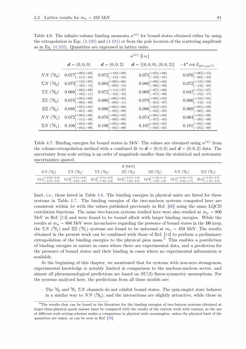
4.3. Lattice results for mπ „ 450 MeV 81
Table 4.6: The infinite-volume binding momenta κp8q for bound states obtained either by usingthe extrapolation in Eqs. (4.100) and (4.101) or from the pole location of the scattering amplitudeas in Eq. (4.102). Quantities are expressed in lattice units.
κp8q [l.u.]
d “ p0, 0, 0q d “ p0, 0, 2q d “ tp0, 0, 0q, p0, 0, 2qu ´k˚ cot δ|k˚“iκp8q
NN p1S0q 0.077p`08qp`06qp´11qp´04q 0.072
p`10qp`08qp´14qp´16q 0.075
p`05qp`06qp´10qp´01q 0.076
p`06qp`12qp´28qp´32q
ΣN p1S0q 0.073p`13qp`05qp´16qp´13q 0.083
p`09qp`06qp´09qp´13q 0.080
p`08qp`02qp´09qp´09q 0.072
p`12qp`09qp´14qp´24q
ΣΣ p1S0q 0.068p`08qp`08qp´10qp´11q 0.072
p`11qp`07qp´10qp´16q 0.069
p`07qp`06qp´07qp´09q 0.047
p`15qp`07qp´15qp´17q
ΞΣ p1S0q 0.078p`08qp`06qp´09qp´09q 0.080
p`08qp`05qp´08qp´11q 0.079
p`06qp`04qp´05qp´07q 0.066
p`10qp`05qp´14qp´14q
ΞΞ p1S0q 0.086p`05qp`05qp´05qp´06q 0.086
p`06qp`06qp´05qp´09q 0.086
p`04qp`04qp´03qp´05q 0.069
p`05qp`08qp´08qp´09q
NN p3S1q 0.072p`08qp`06qp´11qp´08q 0.076
p`08qp`03qp´09qp´08q 0.074
p`08qp`04qp´07qp´05q 0.064
p`10qp`08qp´20qp´08q
ΞN p3S1q 0.108p`04qp`06qp´04qp´08q 0.106
p`05qp`06qp´04qp´08q 0.107
p`03qp`05qp´03qp´05q 0.101
p`05qp`06qp´05qp´09q
Table 4.7: Binding energies for bound states in MeV. The values are obtained using κp8q fromthe volume-extrapolation method with a combined fit to d “ p0, 0, 0q and d “ p0, 0, 2q data. Theuncertainty from scale setting is an order of magnitude smaller than the statistical and systematicuncertainties quoted.
B [MeV]NN p1S0q ΣN p1S0q ΣΣ p1S0q ΞΣ p1S0q ΞΞ p1S0q NN p3S1q ΞN p3S1q
13.1p`2.0qp`2.3qp´3.1qp´0.4q 14.3
p`3.1qp`0.9qp´3.0qp´2.8q 10.2
p`2.1qp`2.0qp´1.9qp´2.3q 12.8
p`2.1qp`1.6qp´1.6qp´2.2q 14.9
p`1.5qp`1.4qp´1.0qp´1.8q 12.7
p`2.4qp`1.5qp´2.4qp´1.7q 25.3
p`1.5qp`2.2qp´1.5qp´2.2q
limit, i.e., those listed in Table 4.6. The binding energies in physical units are listed for thesesystems in Table 4.7. The binding energies of the two-nucleon systems computed here areconsistent within 1σ with the values published previously in Ref. [66] using the same LQCDcorrelation functions. The same two-baryon systems studied here were also studied at mπ „ 806MeV in Ref. [14] and were found to be bound albeit with larger binding energies. While theresults at mπ „ 806 MeV were inconclusive regarding the presence of bound states in the 10 irrep,the ΣN p3S1q and ΞΞ p3S1q systems are found to be unbound at mπ „ 450 MeV. The resultsobtained in the present work can be combined with those of Ref. [14] to perform a preliminaryextrapolation of the binding energies to the physical pion mass.9 This enables a postdictionof binding energies in nature in cases where there are experimental data, and a prediction forthe presence of bound states and their binding in cases where no experimental information isavailable.
At the beginning of this chapter, we mentioned that for systems with non-zero strangeness,experimental knowledge is notably limited in comparison to the nucleon-nucleon sector, andalmost all phenomenological predictions are based on SUp3q flavor-symmetry assumptions. Forthe systems analyzed here, the predictions from all these models are:
– The 1S0 and 3S1 ΣN channels do not exhibit bound states. The spin-singlet state behavesin a similar way to NN p1S0q, and the interactions are slightly attractive, while those in
9The results that can be found in the literature for the binding energies of two-baryon systems obtained atlarger-than-physical quark masses must be compared with the results of the current work with caution, as the useof different scale setting schemes makes a comparison in physical units meaningless, unless the physical limit of thequantities are taken, as can be seen in Ref. [78].
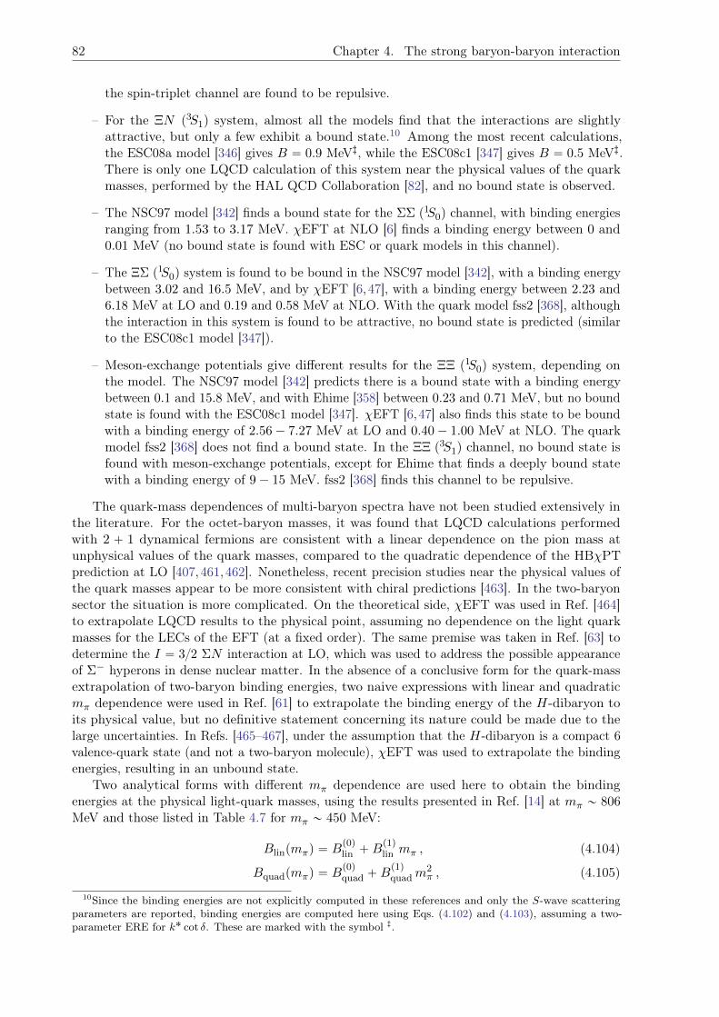
82 Chapter 4. The strong baryon-baryon interaction
the spin-triplet channel are found to be repulsive.
– For the ΞN p3S1q system, almost all the models find that the interactions are slightlyattractive, but only a few exhibit a bound state.10 Among the most recent calculations,the ESC08a model [346] gives B “ 0.9 MeV;, while the ESC08c1 [347] gives B “ 0.5 MeV;.There is only one LQCD calculation of this system near the physical values of the quarkmasses, performed by the HAL QCD Collaboration [82], and no bound state is observed.
– The NSC97 model [342] finds a bound state for the ΣΣ p1S0q channel, with binding energiesranging from 1.53 to 3.17 MeV. χEFT at NLO [6] finds a binding energy between 0 and0.01 MeV (no bound state is found with ESC or quark models in this channel).
– The ΞΣ p1S0q system is found to be bound in the NSC97 model [342], with a binding energybetween 3.02 and 16.5 MeV, and by χEFT [6,47], with a binding energy between 2.23 and6.18 MeV at LO and 0.19 and 0.58 MeV at NLO. With the quark model fss2 [368], althoughthe interaction in this system is found to be attractive, no bound state is predicted (similarto the ESC08c1 model [347]).
– Meson-exchange potentials give different results for the ΞΞ p1S0q system, depending onthe model. The NSC97 model [342] predicts there is a bound state with a binding energybetween 0.1 and 15.8 MeV, and with Ehime [358] between 0.23 and 0.71 MeV, but no boundstate is found with the ESC08c1 model [347]. χEFT [6,47] also finds this state to be boundwith a binding energy of 2.56´ 7.27 MeV at LO and 0.40´ 1.00 MeV at NLO. The quarkmodel fss2 [368] does not find a bound state. In the ΞΞ p3S1q channel, no bound state isfound with meson-exchange potentials, except for Ehime that finds a deeply bound statewith a binding energy of 9´ 15 MeV. fss2 [368] finds this channel to be repulsive.
The quark-mass dependences of multi-baryon spectra have not been studied extensively inthe literature. For the octet-baryon masses, it was found that LQCD calculations performedwith 2 ` 1 dynamical fermions are consistent with a linear dependence on the pion mass atunphysical values of the quark masses, compared to the quadratic dependence of the HBχPTprediction at LO [407,461,462]. Nonetheless, recent precision studies near the physical values ofthe quark masses appear to be more consistent with chiral predictions [463]. In the two-baryonsector the situation is more complicated. On the theoretical side, χEFT was used in Ref. [464]to extrapolate LQCD results to the physical point, assuming no dependence on the light quarkmasses for the LECs of the EFT (at a fixed order). The same premise was taken in Ref. [63] todetermine the I “ 32 ΣN interaction at LO, which was used to address the possible appearanceof Σ´ hyperons in dense nuclear matter. In the absence of a conclusive form for the quark-massextrapolation of two-baryon binding energies, two naive expressions with linear and quadraticmπ dependence were used in Ref. [61] to extrapolate the binding energy of the H-dibaryon toits physical value, but no definitive statement concerning its nature could be made due to thelarge uncertainties. In Refs. [465–467], under the assumption that the H-dibaryon is a compact 6valence-quark state (and not a two-baryon molecule), χEFT was used to extrapolate the bindingenergies, resulting in an unbound state.
Two analytical forms with different mπ dependence are used here to obtain the bindingenergies at the physical light-quark masses, using the results presented in Ref. [14] at mπ „ 806MeV and those listed in Table 4.7 for mπ „ 450 MeV:
Blinpmπq “ Bp0qlin `B
p1qlin mπ , (4.104)
Bquadpmπq “ Bp0qquad `B
p1qquadm
2π , (4.105)
10Since the binding energies are not explicitly computed in these references and only the S-wave scatteringparameters are reported, binding energies are computed here using Eqs. (4.102) and (4.103), assuming a two-parameter ERE for k˚ cot δ. These are marked with the symbol ;.
4.3. Lattice results for mπ „ 450 MeV 83
Table 4.8: Extrapolated binding energies (in MeV) at the physical quark masses for bound statesusing two different forms, linear and quadratic in mπ.
NN p1S0q ΣN p1S0q ΣΣ p1S0q ΞΣ p1S0q ΞΞ p1S0q NN p3S1q ΞN p3S1q
Blinpmphysπ q 6.4
p`6.3qp´6.5q 8.4
p`7.8qp´6.6q 1.0
p`6.1qp´6.1q 5.9
p`5.7qp´5.8q 9.6
p`4.5qp´4.7q ´0.9
p`6.1qp´6.1q 11.7
p`5.4qp´6.2q
Bquadpmphysπ q 9.9
p`4.6qp´4.5q 11.5
p`5.7qp´4.8q 5.8
p`4.2qp´4.3q 9.5
p`3.8qp´4.0q 12.4
p`3.0qp´3.1q 6.3
p`4.3qp´4.4q 18.9
p`3.8qp´4.1q
0.0 0.2 0.4 0.6
m2π [GeV2]
−10
0
10
20
30
40
B[M
eV]
NN (1S0)
0.0 0.2 0.4 0.6
m2π [GeV2]
−10
0
10
20
30
40ΣN (1S0)
0.0 0.2 0.4 0.6
m2π [GeV2]
−10
0
10
20
30
40
B[M
eV]
ΣΣ (1S0)
0.0 0.2 0.4 0.6
m2π [GeV2]
−10
0
10
20
30
40ΞΣ (1S0)
0.0 0.2 0.4 0.6
m2π [GeV2]
−10
0
10
20
30
40ΞΞ (1S0)
0.0 0.2 0.4 0.6
m2π [GeV2]
−10
0
10
20
30
40
B[M
eV]
NN (3S1)
0.0 0.2 0.4 0.6
m2π [GeV2]
−10
0
10
20
30
40
50ΞN (3S1)
NPLQCD nf = 3
NPLQCD nf = 2 + 1
Linear extrapolation in mπ
Quadratic extrapolation in mπ
NSC97
Ehime
ESC
χEFT LO
χEFT NLO
Experimental
Figure 4.11: Extrapolation of the binding energies of different two-baryon systems, using theresults obtained in this work and those at mπ „ 806 MeV from Ref. [14]. For comparison, theresults with values obtained using one-boson-exchange models or χEFTs are also shown (andwhere needed, are shifted slightly in the horizontal direction for clarity).
where Bp0qlin , Bp1qlin , B
p0qquad, and B
p1qquad are parameters to be constrained by fits to data. These fits
are shown in Fig. 4.11, along with the experimental values and predictions at the physical point.The binding energies extrapolated to the physical point, i.e., Blinpm
physπ q and Bquadpm
physπ q, are
summarized in Table 4.8.11 It should be emphasized that given the lack of knowledge of the
11Performing fits to dimensionless ratios of the binding energies to the baryon masses (to minimize the effects ofnon-zero lattice spacing) do not change the qualitative conclusions presented in the text (results agree within 1σ).
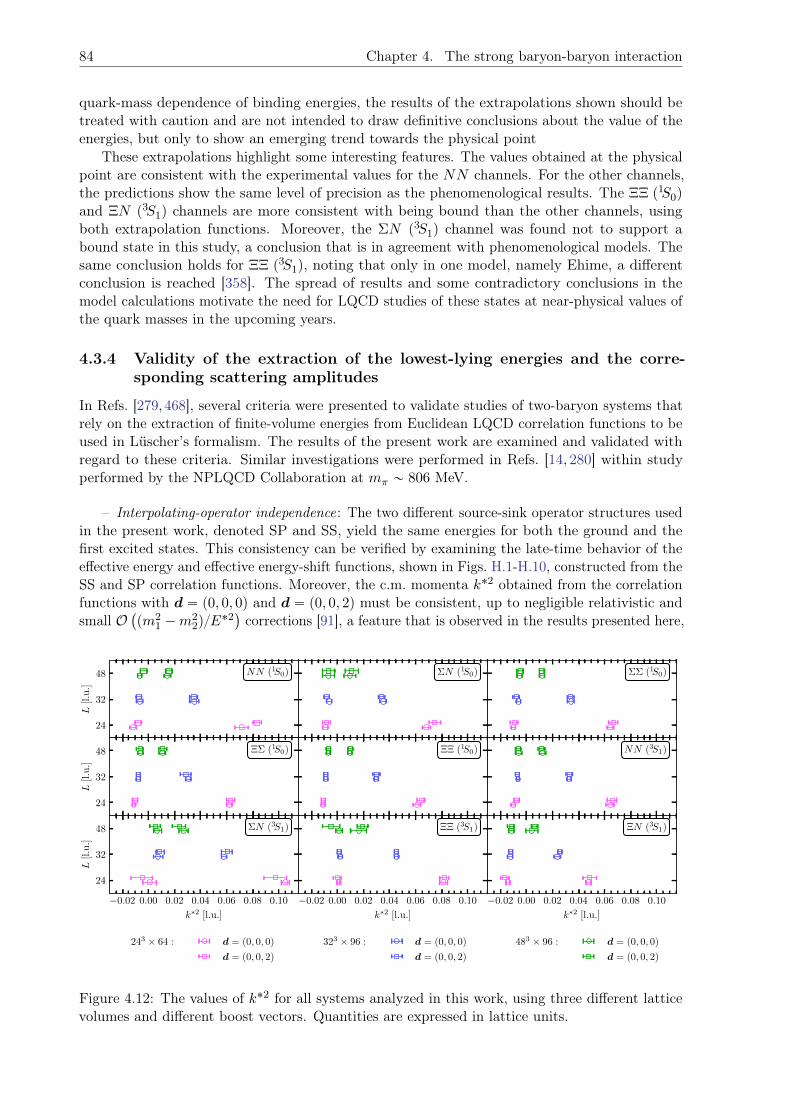
84 Chapter 4. The strong baryon-baryon interaction
quark-mass dependence of binding energies, the results of the extrapolations shown should betreated with caution and are not intended to draw definitive conclusions about the value of theenergies, but only to show an emerging trend towards the physical point
These extrapolations highlight some interesting features. The values obtained at the physicalpoint are consistent with the experimental values for the NN channels. For the other channels,the predictions show the same level of precision as the phenomenological results. The ΞΞ p1S0q
and ΞN p3S1q channels are more consistent with being bound than the other channels, usingboth extrapolation functions. Moreover, the ΣN p3S1q channel was found not to support abound state in this study, a conclusion that is in agreement with phenomenological models. Thesame conclusion holds for ΞΞ p3S1q, noting that only in one model, namely Ehime, a differentconclusion is reached [358]. The spread of results and some contradictory conclusions in themodel calculations motivate the need for LQCD studies of these states at near-physical values ofthe quark masses in the upcoming years.
4.3.4 Validity of the extraction of the lowest-lying energies and the corre-sponding scattering amplitudes
In Refs. [279, 468], several criteria were presented to validate studies of two-baryon systems thatrely on the extraction of finite-volume energies from Euclidean LQCD correlation functions to beused in Lüscher’s formalism. The results of the present work are examined and validated withregard to these criteria. Similar investigations were performed in Refs. [14, 280] within studyperformed by the NPLQCD Collaboration at mπ „ 806 MeV.
– Interpolating-operator independence: The two different source-sink operator structures usedin the present work, denoted SP and SS, yield the same energies for both the ground and thefirst excited states. This consistency can be verified by examining the late-time behavior of theeffective energy and effective energy-shift functions, shown in Figs. H.1-H.10, constructed from theSS and SP correlation functions. Moreover, the c.m. momenta k˚2 obtained from the correlationfunctions with d “ p0, 0, 0q and d “ p0, 0, 2q must be consistent, up to negligible relativistic andsmall O
`
pm21 ´m
22qE
˚2˘
corrections [91], a feature that is observed in the results presented here,
−0.02 0.00 0.02 0.04 0.06 0.08 0.10
24
32
48
L[l.u.]
NN (1S0)
−0.02 0.00 0.02 0.04 0.06 0.08 0.10
ΣN (1S0)
−0.02 0.00 0.02 0.04 0.06 0.08 0.10
ΣΣ (1S0)
−0.02 0.00 0.02 0.04 0.06 0.08 0.10
24
32
48
L[l.u.]
ΞΣ (1S0)
−0.02 0.00 0.02 0.04 0.06 0.08 0.10
ΞΞ (1S0)
−0.02 0.00 0.02 0.04 0.06 0.08 0.10
NN (3S1)
−0.02 0.00 0.02 0.04 0.06 0.08 0.10
k∗2 [l.u.]
24
32
48
L[l.u.]
ΣN (3S1)
−0.02 0.00 0.02 0.04 0.06 0.08 0.10
k∗2 [l.u.]
ΞΞ (3S1)
−0.02 0.00 0.02 0.04 0.06 0.08 0.10
k∗2 [l.u.]
ΞN (3S1)
243 × 64 : d = (0, 0, 0)
d = (0, 0, 2)
323 × 96 : d = (0, 0, 0)
d = (0, 0, 2)
483 × 96 : d = (0, 0, 0)
d = (0, 0, 2)
Figure 4.12: The values of k˚2 for all systems analyzed in this work, using three different latticevolumes and different boost vectors. Quantities are expressed in lattice units.
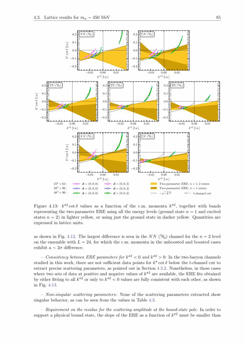
4.3. Lattice results for mπ „ 450 MeV 85
−0.01 0.00 0.01
k∗2 [l.u.]
−0.2
−0.1
0.0
0.1
0.2
k∗
cotδ
[l.u.]
NN (1S0)
−0.01 0.00 0.01
k∗2 [l.u.]
−0.2
−0.1
0.0
0.1
0.2 ΣN (1S0)
−0.01 0.00 0.01
k∗2 [l.u.]
−0.2
−0.1
0.0
0.1
0.2
k∗
cotδ
[l.u.]
ΣΣ (1S0)
−0.01 0.00 0.01
k∗2 [l.u.]
−0.2
−0.1
0.0
0.1
0.2 ΞΣ (1S0)
−0.01 0.00 0.01
k∗2 [l.u.]
−0.2
−0.1
0.0
0.1
0.2 ΞΞ (1S0)
−0.01 0.00 0.01
k∗2 [l.u.]
−0.2
−0.1
0.0
0.1
0.2
k∗
cotδ
[l.u.]
NN (3S1)
−0.01 0.00 0.01
k∗2 [l.u.]
−0.2
−0.1
0.0
0.1
0.2 ΞN (3S1)
243 × 64 :
323 × 96 :
483 × 96 :
d = (0, 0, 0)
d = (0, 0, 0)
d = (0, 0, 0)
d = (0, 0, 2)
d = (0, 0, 2)
d = (0, 0, 2)
Two-parameter ERE: n = 1, 2 states
Two-parameter ERE: n = 1 states
−√−k∗2 t-channel cut
Figure 4.13: k˚2 cot δ values as a function of the c.m. momenta k˚2, together with bandsrepresenting the two-parameter ERE using all the energy levels (ground state n “ 1 and excitedstates n “ 2) in lighter yellow, or using just the ground state in darker yellow. Quantities areexpressed in lattice units.
as shown in Fig. 4.12. The largest difference is seen in the NN p1S0q channel for the n “ 2 levelon the ensemble with L “ 24, for which the c.m. momenta in the unboosted and boosted casesexhibit a „ 2σ difference.
– Consistency between ERE parameters for k˚2 ă 0 and k˚2 ą 0: In the two-baryon channelsstudied in this work, there are not sufficient data points for k˚ cot δ below the t-channel cut toextract precise scattering parameters, as pointed out in Section 4.3.2. Nonetheless, in those caseswhere two sets of data at positive and negative values of k˚2 are available, the ERE fits obtainedby either fitting to all k˚2 or only to k˚2 ă 0 values are fully consistent with each other, as shownin Fig. 4.13.
– Non-singular scattering parameters: None of the scattering parameters extracted showsingular behavior, as can be seen from the values in Table 4.3.
– Requirement on the residue for the scattering amplitude at the bound-state pole: In order tosupport a physical bound state, the slope of the ERE as a function of k˚2 must be smaller than
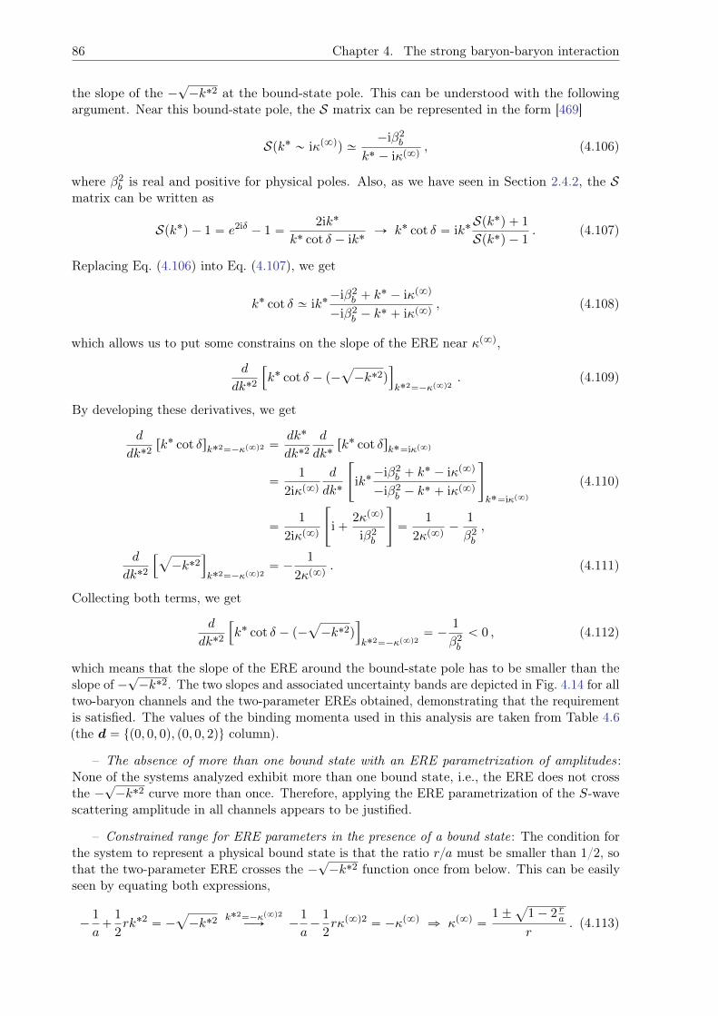
86 Chapter 4. The strong baryon-baryon interaction
the slope of the ´?´k˚2 at the bound-state pole. This can be understood with the following
argument. Near this bound-state pole, the S matrix can be represented in the form [469]
Spk˚ „ iκp8qq »´iβ2
b
k˚ ´ iκp8q, (4.106)
where β2b is real and positive for physical poles. Also, as we have seen in Section 2.4.2, the S
matrix can be written as
Spk˚q ´ 1 “ e2iδ ´ 1 “2ik˚
k˚ cot δ ´ ik˚Ñ k˚ cot δ “ ik˚
Spk˚q ` 1
Spk˚q ´ 1. (4.107)
Replacing Eq. (4.106) into Eq. (4.107), we get
k˚ cot δ » ik˚´iβ2
b ` k˚ ´ iκp8q
´iβ2b ´ k
˚ ` iκp8q, (4.108)
which allows us to put some constrains on the slope of the ERE near κp8q,
d
dk˚2
”
k˚ cot δ ´ p´a
´k˚2q
ı
k˚2“´κp8q2. (4.109)
By developing these derivatives, we get
d
dk˚2rk˚ cot δsk˚2“´κp8q2 “
dk˚
dk˚2
d
dk˚rk˚ cot δsk˚“iκp8q
“1
2iκp8qd
dk˚
«
ik˚´iβ2
b ` k˚ ´ iκp8q
´iβ2b ´ k
˚ ` iκp8q
ff
k˚“iκp8q
(4.110)
“1
2iκp8q
«
i`2κp8q
iβ2b
ff
“1
2κp8q´
1
β2b
,
d
dk˚2
”
a
´k˚2ı
k˚2“´κp8q2“ ´
1
2κp8q. (4.111)
Collecting both terms, we get
d
dk˚2
”
k˚ cot δ ´ p´a
´k˚2q
ı
k˚2“´κp8q2“ ´
1
β2b
ă 0 , (4.112)
which means that the slope of the ERE around the bound-state pole has to be smaller than theslope of ´
?´k˚2. The two slopes and associated uncertainty bands are depicted in Fig. 4.14 for all
two-baryon channels and the two-parameter EREs obtained, demonstrating that the requirementis satisfied. The values of the binding momenta used in this analysis are taken from Table 4.6(the d “ tp0, 0, 0q, p0, 0, 2qu column).
– The absence of more than one bound state with an ERE parametrization of amplitudes:None of the systems analyzed exhibit more than one bound state, i.e., the ERE does not crossthe ´
?´k˚2 curve more than once. Therefore, applying the ERE parametrization of the S-wave
scattering amplitude in all channels appears to be justified.
– Constrained range for ERE parameters in the presence of a bound state: The condition forthe system to represent a physical bound state is that the ratio ra must be smaller than 1/2, sothat the two-parameter ERE crosses the ´
?´k˚2 function once from below. This can be easily
seen by equating both expressions,
´1
a`
1
2rk˚2 “ ´
a
´k˚2 k˚2“´κp8q2ÝÑ ´
1
a´
1
2rκp8q2 “ ´κp8q ñ κp8q “
1˘a
1´ 2 rar
. (4.113)
4.3. Lattice results for mπ „ 450 MeV 87
−0.01 0.00 0.01
k∗2 [l.u.]
−0.2
−0.1
0.0
0.1
0.2
k∗
cotδ
[l.u.]
NN (1S0)
−0.01 0.00 0.01
k∗2 [l.u.]
−0.2
−0.1
0.0
0.1
0.2 ΣN (1S0)
−0.01 0.00 0.01
k∗2 [l.u.]
−0.2
−0.1
0.0
0.1
0.2
k∗
cotδ
[l.u.]
ΣΣ (1S0)
−0.01 0.00 0.01
k∗2 [l.u.]
−0.2
−0.1
0.0
0.1
0.2 ΞΣ (1S0)
−0.01 0.00 0.01
k∗2 [l.u.]
−0.2
−0.1
0.0
0.1
0.2 ΞΞ (1S0)
−0.01 0.00 0.01
k∗2 [l.u.]
−0.2
−0.1
0.0
0.1
0.2
k∗
cotδ
[l.u.]
NN (3S1)
−0.01 0.00 0.01
k∗2 [l.u.]
−0.2
−0.1
0.0
0.1
0.2 ΞN (3S1)
243 × 64 :
323 × 96 :
483 × 96 :
d = (0, 0, 0)
d = (0, 0, 0)
d = (0, 0, 0)
d = (0, 0, 2)
d = (0, 0, 2)
d = (0, 0, 2)
Two-parameter ERE
Tangent to −√−k∗2 at −κ(∞)2
−√−k∗2 t-channel cut
Figure 4.14: Comparison between the two-parameter ERE and the slope of ´?´k˚2 at k˚2 “
´κp8q2, where κp8q is taken from the d “ tp0, 0, 0q, p0, 0, 2qu column of Table 4.6. Quantities areexpressed in lattice units.
If we want to get a real solution, ra ă 12. Moreover, the ERE must cross the Z-functionscorresponding to different volumes to satisfy Lüscher’s QC, introducing more constraints onscattering parameters. With the use of the two-dimensional χ2 in this work to fit the k˚ cot δvalues, the confidence region of the ERE parameters does not cross these prohibited areas, as wasdemonstrated in Fig. 4.8.
4.3.5 Constraints on the EFTs LECs
As mentioned in Section 4.3.2, given the large uncertainties in the scattering parameters (inparticular in the effective range), the ratio ra shown in Table 4.4 is not well constrained, and doesnot conclusively prove unnaturalness in all channels. Since in at least two channels the interactionsseem unnatural, in the following both the natural and the unnatural cases will be considered inexpressing relations between LECs and the scattering parameters, given by Eqs. (4.85) and (4.86).The corresponding LECs for each two-baryon channel are given in Table 4.9.
Two sets of inputs can be used to constrain the numerical values of the LECs: 1) the scatteringparameters ta´1, ru obtained from two-parameter ERE fits, as discussed in Section 4.3.2 and listed
88 Chapter 4. The strong baryon-baryon interaction
in Table 4.3, can be used to compute the LECs of both momentum-independent and momentum-dependent operators (method I), and 2) the binding momenta from Section 4.3.3 can be used tocompute the corresponding scattering length, related at LO by ´a´1 ` κp8q “ 0, and this singleparameter can be used to constrain the LECs of momentum-independent operators (method II).This second method is motivated by the fact that κp8q is extracted with higher precision than theparameters from the ERE fits, therefore enabling tighter constraints on the LECs of momentum-independent operators. The results for both sets of LECs are presented in Table 4.10 and aredepicted in Fig. 4.15. Results are presented in units of 2πMB for the momentum-independentoperators and 4π2M2
B for the momentum-dependent operators, where MB is the centroid of theoctet-baryon masses, MB “
14MN `
18MΛ `
38MΣ `
14MΞ “ 0.78583p23qp30q l.u.
As can be seen from the values of the LECs that are obtained, the NLO SUp3qf coefficientshave large uncertainties, and are mostly consistent with zero, because the effective ranges used toconstrain them have rather large uncertainties. Another feature of the results is that assumingthe interactions to be unnatural leads to better-constrained parameters in general, as a non-zeroscale µ in the left-hand side of Eqs. (4.85) and (4.86) reduces the effect of uncertainties on thescattering lengths (this was also observed in Ref. [14] for systems at mπ „ 806 MeV). Furthermore,as expected, the values obtained with method II have smaller uncertainties than the ones obtainedfrom method I, given the more precise scattering lengths, although the method is limited to LOpredictions. Another anticipated feature is that in the cases where the effective range is resolvedfrom zero within uncertainties (e.g., in the ΞΞ p1S0q channel), the values from method II areslightly different from those obtained from method I, indicating the non-negligible effect of theNLO effective range contributions that are neglected in this method.
It should be noted that the input for scattering parameters is not sufficient to disentangle theLO SUp3qf and NLOSUp3qf coefficients in general, hence the cpirrepq` cχB1B2
entry in Table 4.10and Fig. 4.15. For the systems that belong to the 27 irrep, since the spin-singlet pairs tNN,ΣNuand tΞΣ,ΞΞu depend on the same SUp3qf LO and SUp3qf NLO LECs but with different linearcombinations of the coefficients, a system of equations can be formed to separate each contribution.The results are shown in Table 4.11 and Fig. 4.16, along with the result for the ΣΣ channel forcomparison purposes, as there is no contribution fromSUp3qf interactions for this channel at thisorder. From these results, it can be seen that the values of the symmetry-breaking coefficientscχ3 ´ c
χ4 and cχ1 ´ c
χ2 ` c
χ11´ c
χ12 are compatible with zero. Together with the observation that the
scattering lengths and binding energies in all of the systems are similar within uncertainties, itappears that the SUp3q flavor symmetry remains an approximate symmetry at the quark massesused in this study. These observations in the two-baryon sector are consistent with those in thesingle-baryon sector as presented in Ref. [66] at the same quark masses. There, the authors looked
Table 4.9: The LECs of the LO and NLO pionless EFT that contribute to the scattering amplitudeof the various two-baryon channel. The first three columns are total angular momentum (J),strangeness (S), and isospin (I).
J S I Channel SUp3qf LO SUp3qf NLO SUp3qf NLO
0 0 1 NN cp27q cp27q 4pcχ3 ´ cχ4 q
´1 32 ΣN cp27q cp27q 2pcχ3 ´ c
χ4 q
´2 2 ΣΣ cp27q cp27q 0
´3 32 ΞΣ cp27q cp27q 2pcχ1 ´ c
χ2 ` c
χ11 ´ c
χ12q
´4 1 ΞΞ cp27q cp27q 4pcχ1 ´ cχ2 ` c
χ11 ´ c
χ12q
1 0 0 NN cp10q cp10q 4pcχ3 ` cχ4 q
´1 32 ΣN cp10q cp10q ´2pcχ3 ` c
χ4 q
´4 0 ΞΞ cp10q cp10q ´4pcχ1 ` cχ2 ´ c
χ11 ´ c
χ12q
´2 0 ΞN cp8aq cp8aq 2p2cχ5 ` 2cχ6 ` 2cχ7 ` 2cχ8 ` 2cχ9 ` 2cχ10 ` cχ11 ` c
χ12q
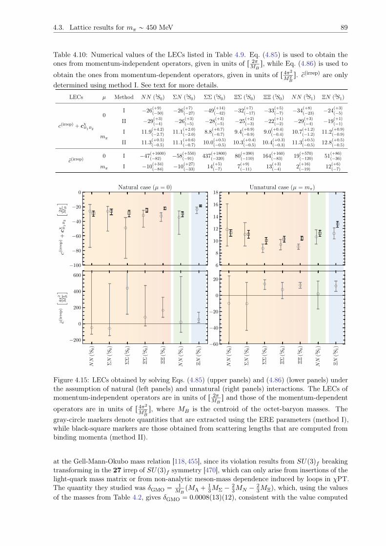
4.3. Lattice results for mπ „ 450 MeV 89
Table 4.10: Numerical values of the LECs listed in Table 4.9. Eq. (4.85) is used to obtain theones from momentum-independent operators, given in units of r 2π
MBs, while Eq. (4.86) is used to
obtain the ones from momentum-dependent operators, given in units of r 4π2
M2Bs. cpirrepq are only
determined using method I. See text for more details.
LECs µ Method NN p1S0q ΣN p1S0q ΣΣ p1S0q ΞΣ p1S0q ΞΞ p1S0q NN p3S1q ΞN p3S1q
cpirrepq ` cχB1B2
0I ´26
p`9qp´50q ´26
p`7qp´27q ´49
p`14qp´42q ´32
p`7qp´17q ´33
p`5qp´7q ´34
p`8qp´23q ´24
p`3qp´5q
II ´29p`3qp´4q ´26
p`3qp´5q ´28
p`3qp´5q ´25
p`2qp´3q ´22
p`1qp´2q ´29
p`3qp´4q ´19
p`1qp´1q
mπ
I 11.9p`4.2qp´2.7q 11.1
p`2.0qp´2.0q 8.8
p`0.7qp´0.7q 9.4
p`0.9qp´0.9q 9.0
p`0.4qp´0.4q 10.7
p`1.2qp´1.2q 11.2
p`0.9qp´0.9q
II 11.3p`0.5qp´0.5q 11.1
p`0.6qp´0.7q 10.0
p`0.5qp´0.5q 10.3
p`0.4qp´0.5q 10.4
p`0.3qp´0.3q 11.3
p`0.5qp´0.5q 12.8
p`0.5qp´0.5q
cpirrepq0 I ´47
p`1600qp´82q ´58
p`550qp´91q 437
p`1800qp´320q 80
p`390qp´110q 164
p`160qp´83q 19
p`570qp´120q 51
p`86qp´36q
mπ I ´10p`34qp´84q ´10
p`27qp´33q 14
p`5qp´7q 7
p`9qp´11q 13
p`3qp´4q 2
p`16qp´19q 12
p`6qp´7q
100
80
60
40
20
0
c(ir
rep)+
c B
1B
2
h2
MB
i
Natural case (µ = 0)
6
8
10
12
14
16
18Unnatural case (µ = m)
NN
(1S
0)
N
(1S
0)
(1S
0)
(1S
0)
(1S
0)
NN
(3S
1)
N
(3S
1)
200
0
200
400
600
c(ir
rep)h 4
2
M2 B
i
NN
(1S
0)
N
(1S
0)
(1S
0)
(1S
0)
(1S
0)
NN
(3S
1)
N
(3S
1)60
40
20
0
20
Figure 4.15: LECs obtained by solving Eqs. (4.85) (upper panels) and (4.86) (lower panels) underthe assumption of natural (left panels) and unnatural (right panels) interactions. The LECs ofmomentum-independent operators are in units of r 2π
MBs and those of the momentum-dependent
operators are in units of r 4π2
M2Bs, where MB is the centroid of the octet-baryon masses. The
gray-circle markers denote quantities that are extracted using the ERE parameters (method I),while black-square markers are those obtained from scattering lengths that are computed frombinding momenta (method II).
at the Gell-Mann-Okubo mass relation [118,455], since its violation results from SUp3qf breakingtransforming in the 27 irrep of SUp3qf symmetry [470], which can only arise from insertions of thelight-quark mass matrix or from non-analytic meson-mass dependence induced by loops in χPT.The quantity they studied was δGMO “
1MBpMΛ `
13MΣ ´
23MN ´
23MΞq, which, using the values
of the masses from Table 4.2, gives δGMO “ 0.0008p13qp12q, consistent with the value computed
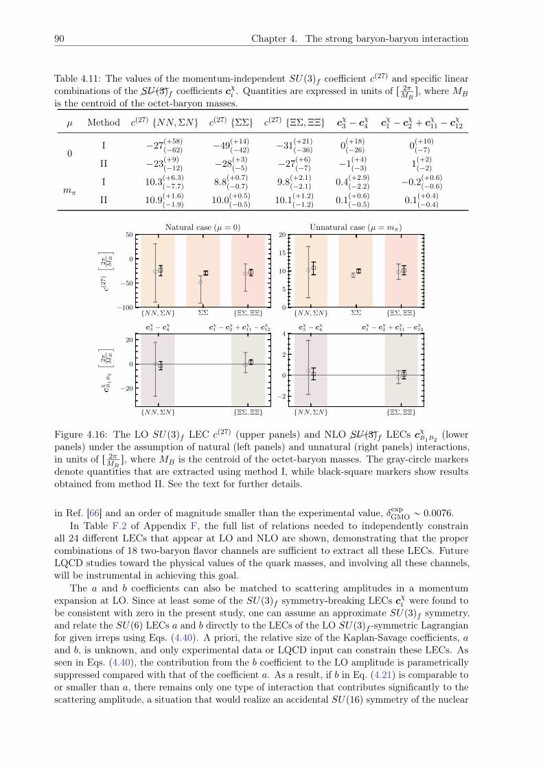
90 Chapter 4. The strong baryon-baryon interaction
Table 4.11: The values of the momentum-independent SUp3qf coefficient cp27q and specific linearcombinations of theSUp3qf coefficients cχi . Quantities are expressed in units of r 2π
MBs, where MB
is the centroid of the octet-baryon masses.
µ Method cp27q tNN,ΣNu cp27q tΣΣu cp27q tΞΣ,ΞΞu cχ3 ´ cχ4 cχ1 ´ c
χ2 ` c
χ11 ´ c
χ12
0I ´27
p`58qp´62q ´49
p`14qp´42q ´31
p`21qp´36q 0
p`18qp´26q 0
p`10qp´7q
II ´23p`9qp´12q ´28
p`3qp´5q ´27
p`6qp´7q ´1
p`4qp´3q 1
p`2qp´2q
mπ
I 10.3p`6.3qp´7.7q 8.8
p`0.7qp´0.7q 9.8
p`2.1qp´2.1q 0.4
p`2.9qp´2.2q ´0.2
p`0.6qp´0.6q
II 10.9p`1.6qp´1.9q 10.0
p`0.5qp´0.5q 10.1
p`1.2qp´1.2q 0.1
p`0.6qp´0.5q 0.1
p`0.4qp´0.4q
NN, N , 100
50
0
50
c(27)h
2
MB
i
Natural case (µ = 0)
NN, N , 0
5
10
15
20Unnatural case (µ = m)
NN, N ,
20
0
20
c B
1B
2
h2
MB
i
c3 c4 c1 c2 + c11 c12
NN, N ,
2
0
2
4c3 c4 c1 c2 + c11 c12
Figure 4.16: The LO SUp3qf LEC cp27q (upper panels) and NLO SUp3qf LECs cχB1B2(lower
panels) under the assumption of natural (left panels) and unnatural (right panels) interactions,in units of r 2π
MBs, where MB is the centroid of the octet-baryon masses. The gray-circle markers
denote quantities that are extracted using method I, while black-square markers show resultsobtained from method II. See the text for further details.
in Ref. [66] and an order of magnitude smaller than the experimental value, δexpGMO „ 0.0076.In Table F.2 of Appendix F, the full list of relations needed to independently constrain
all 24 different LECs that appear at LO and NLO are shown, demonstrating that the propercombinations of 18 two-baryon flavor channels are sufficient to extract all these LECs. FutureLQCD studies toward the physical values of the quark masses, and involving all these channels,will be instrumental in achieving this goal.
The a and b coefficients can also be matched to scattering amplitudes in a momentumexpansion at LO. Since at least some of the SUp3qf symmetry-breaking LECs cχi were found tobe consistent with zero in the present study, one can assume an approximate SUp3qf symmetry,and relate the SUp6q LECs a and b directly to the LECs of the LO SUp3qf -symmetric Lagrangianfor given irreps using Eqs. (4.40). A priori, the relative size of the Kaplan-Savage coefficients, aand b, is unknown, and only experimental data or LQCD input can constrain these LECs. Asseen in Eqs. (4.40), the contribution from the b coefficient to the LO amplitude is parametricallysuppressed compared with that of the coefficient a. As a result, if b in Eq. (4.21) is comparable toor smaller than a, there remains only one type of interaction that contributes significantly to thescattering amplitude, a situation that would realize an accidental SUp16q symmetry of the nuclear
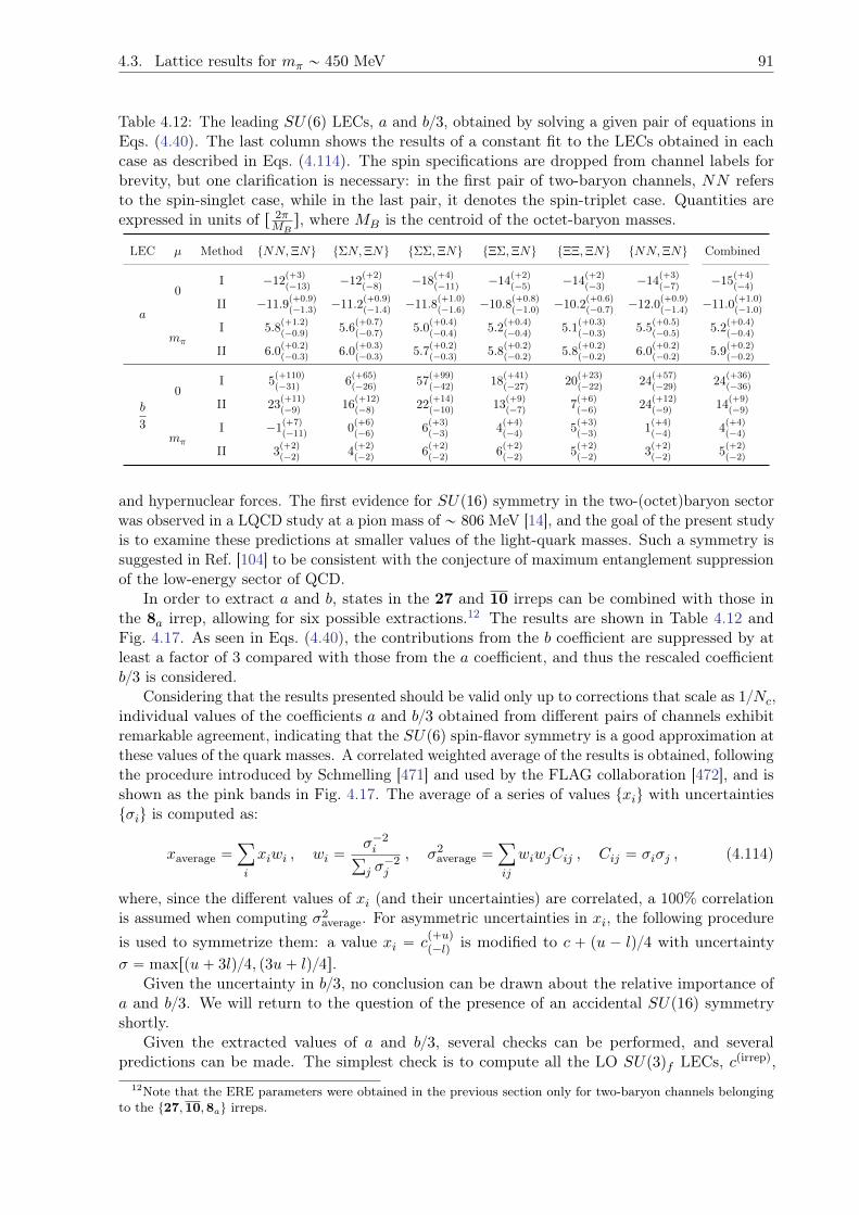
4.3. Lattice results for mπ „ 450 MeV 91
Table 4.12: The leading SUp6q LECs, a and b3, obtained by solving a given pair of equations inEqs. (4.40). The last column shows the results of a constant fit to the LECs obtained in eachcase as described in Eqs. (4.114). The spin specifications are dropped from channel labels forbrevity, but one clarification is necessary: in the first pair of two-baryon channels, NN refersto the spin-singlet case, while in the last pair, it denotes the spin-triplet case. Quantities areexpressed in units of r 2π
MBs, where MB is the centroid of the octet-baryon masses.
LEC µ Method tNN,ΞNu tΣN,ΞNu tΣΣ,ΞNu tΞΣ,ΞNu tΞΞ,ΞNu tNN,ΞNu Combined
a
0I ´12
p`3qp´13q ´12
p`2qp´8q ´18
p`4qp´11q ´14
p`2qp´5q ´14
p`2qp´3q ´14
p`3qp´7q ´15
p`4qp´4q
II ´11.9p`0.9qp´1.3q ´11.2
p`0.9qp´1.4q ´11.8
p`1.0qp´1.6q ´10.8
p`0.8qp´1.0q ´10.2
p`0.6qp´0.7q ´12.0
p`0.9qp´1.4q ´11.0
p`1.0qp´1.0q
mπ
I 5.8p`1.2qp´0.9q 5.6
p`0.7qp´0.7q 5.0
p`0.4qp´0.4q 5.2
p`0.4qp´0.4q 5.1
p`0.3qp´0.3q 5.5
p`0.5qp´0.5q 5.2
p`0.4qp´0.4q
II 6.0p`0.2qp´0.3q 6.0
p`0.3qp´0.3q 5.7
p`0.2qp´0.3q 5.8
p`0.2qp´0.2q 5.8
p`0.2qp´0.2q 6.0
p`0.2qp´0.2q 5.9
p`0.2qp´0.2q
b
3
0I 5
p`110qp´31q 6
p`65qp´26q 57
p`99qp´42q 18
p`41qp´27q 20
p`23qp´22q 24
p`57qp´29q 24
p`36qp´36q
II 23p`11qp´9q 16
p`12qp´8q 22
p`14qp´10q 13
p`9qp´7q 7
p`6qp´6q 24
p`12qp´9q 14
p`9qp´9q
mπ
I ´1p`7qp´11q 0
p`6qp´6q 6
p`3qp´3q 4
p`4qp´4q 5
p`3qp´3q 1
p`4qp´4q 4
p`4qp´4q
II 3p`2qp´2q 4
p`2qp´2q 6
p`2qp´2q 6
p`2qp´2q 5
p`2qp´2q 3
p`2qp´2q 5
p`2qp´2q
and hypernuclear forces. The first evidence for SUp16q symmetry in the two-(octet)baryon sectorwas observed in a LQCD study at a pion mass of „ 806 MeV [14], and the goal of the present studyis to examine these predictions at smaller values of the light-quark masses. Such a symmetry issuggested in Ref. [104] to be consistent with the conjecture of maximum entanglement suppressionof the low-energy sector of QCD.
In order to extract a and b, states in the 27 and 10 irreps can be combined with those inthe 8a irrep, allowing for six possible extractions.12 The results are shown in Table 4.12 andFig. 4.17. As seen in Eqs. (4.40), the contributions from the b coefficient are suppressed by atleast a factor of 3 compared with those from the a coefficient, and thus the rescaled coefficientb3 is considered.
Considering that the results presented should be valid only up to corrections that scale as 1Nc,individual values of the coefficients a and b3 obtained from different pairs of channels exhibitremarkable agreement, indicating that the SUp6q spin-flavor symmetry is a good approximation atthese values of the quark masses. A correlated weighted average of the results is obtained, followingthe procedure introduced by Schmelling [471] and used by the FLAG collaboration [472], and isshown as the pink bands in Fig. 4.17. The average of a series of values txiu with uncertaintiestσiu is computed as:
xaverage “ÿ
i
xiwi , wi “σ´2i
ř
j σ´2j
, σ2average “
ÿ
ij
wiwjCij , Cij “ σiσj , (4.114)
where, since the different values of xi (and their uncertainties) are correlated, a 100% correlationis assumed when computing σ2
average. For asymmetric uncertainties in xi, the following procedureis used to symmetrize them: a value xi “ c
p`uqp´lq is modified to c ` pu ´ lq4 with uncertainty
σ “ maxrpu` 3lq4, p3u` lq4s.Given the uncertainty in b3, no conclusion can be drawn about the relative importance of
a and b3. We will return to the question of the presence of an accidental SUp16q symmetryshortly.
Given the extracted values of a and b3, several checks can be performed, and severalpredictions can be made. The simplest check is to compute all the LO SUp3qf LECs, cpirrepq,
12Note that the ERE parameters were obtained in the previous section only for two-baryon channels belongingto the t27,10,8au irreps.
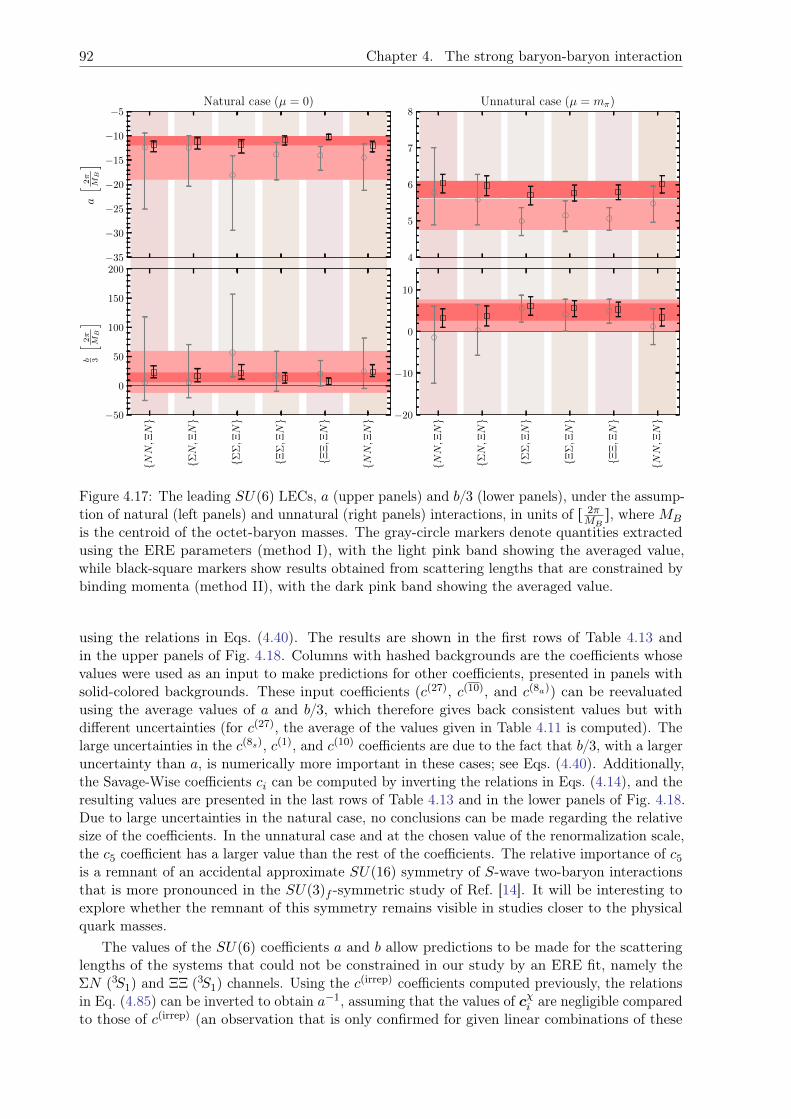
92 Chapter 4. The strong baryon-baryon interaction
35
30
25
20
15
10
5
ah
2
MB
i
Natural case (µ = 0)
4
5
6
7
8Unnatural case (µ = m)
NN
,N
N
,N
,N
,N
,N
NN
,N
50
0
50
100
150
200
b 3
h2
MB
i
NN
,N
N
,N
,N
,N
,N
NN
,N
20
10
0
10
Figure 4.17: The leading SUp6q LECs, a (upper panels) and b3 (lower panels), under the assump-tion of natural (left panels) and unnatural (right panels) interactions, in units of r 2π
MBs, where MB
is the centroid of the octet-baryon masses. The gray-circle markers denote quantities extractedusing the ERE parameters (method I), with the light pink band showing the averaged value,while black-square markers show results obtained from scattering lengths that are constrained bybinding momenta (method II), with the dark pink band showing the averaged value.
using the relations in Eqs. (4.40). The results are shown in the first rows of Table 4.13 andin the upper panels of Fig. 4.18. Columns with hashed backgrounds are the coefficients whosevalues were used as an input to make predictions for other coefficients, presented in panels withsolid-colored backgrounds. These input coefficients (cp27q, cp10q, and cp8aq) can be reevaluatedusing the average values of a and b3, which therefore gives back consistent values but withdifferent uncertainties (for cp27q, the average of the values given in Table 4.11 is computed). Thelarge uncertainties in the cp8sq, cp1q, and cp10q coefficients are due to the fact that b3, with a largeruncertainty than a, is numerically more important in these cases; see Eqs. (4.40). Additionally,the Savage-Wise coefficients ci can be computed by inverting the relations in Eqs. (4.14), and theresulting values are presented in the last rows of Table 4.13 and in the lower panels of Fig. 4.18.Due to large uncertainties in the natural case, no conclusions can be made regarding the relativesize of the coefficients. In the unnatural case and at the chosen value of the renormalization scale,the c5 coefficient has a larger value than the rest of the coefficients. The relative importance of c5
is a remnant of an accidental approximate SUp16q symmetry of S-wave two-baryon interactionsthat is more pronounced in the SUp3qf -symmetric study of Ref. [14]. It will be interesting toexplore whether the remnant of this symmetry remains visible in studies closer to the physicalquark masses.
The values of the SUp6q coefficients a and b allow predictions to be made for the scatteringlengths of the systems that could not be constrained in our study by an ERE fit, namely theΣN p3S1q and ΞΞ p3S1q channels. Using the cpirrepq coefficients computed previously, the relationsin Eq. (4.85) can be inverted to obtain a´1, assuming that the values of cχi are negligible comparedto those of cpirrepq (an observation that is only confirmed for given linear combinations of these
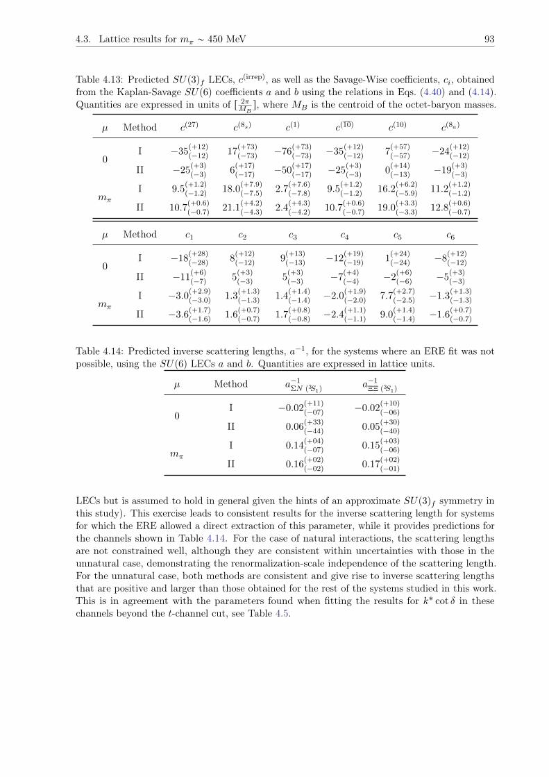
4.3. Lattice results for mπ „ 450 MeV 93
Table 4.13: Predicted SUp3qf LECs, cpirrepq, as well as the Savage-Wise coefficients, ci, obtainedfrom the Kaplan-Savage SUp6q coefficients a and b using the relations in Eqs. (4.40) and (4.14).Quantities are expressed in units of r 2π
MBs, where MB is the centroid of the octet-baryon masses.
µ Method cp27q cp8sq cp1q cp10q cp10q cp8aq
0I ´35
p`12qp´12q 17
p`73qp´73q ´76
p`73qp´73q ´35
p`12qp´12q 7
p`57qp´57q ´24
p`12qp´12q
II ´25p`3qp´3q 6
p`17qp´17q ´50
p`17qp´17q ´25
p`3qp´3q 0
p`14qp´13q ´19
p`3qp´3q
mπ
I 9.5p`1.2qp´1.2q 18.0
p`7.9qp´7.5q 2.7
p`7.6qp´7.8q 9.5
p`1.2qp´1.2q 16.2
p`6.2qp´5.9q 11.2
p`1.2qp´1.2q
II 10.7p`0.6qp´0.7q 21.1
p`4.2qp´4.3q 2.4
p`4.3qp´4.2q 10.7
p`0.6qp´0.7q 19.0
p`3.3qp´3.3q 12.8
p`0.6qp´0.7q
µ Method c1 c2 c3 c4 c5 c6
0I ´18
p`28qp´28q 8
p`12qp´12q 9
p`13qp´13q ´12
p`19qp´19q 1
p`24qp´24q ´8
p`12qp´12q
II ´11p`6qp´7q 5
p`3qp´3q 5
p`3qp´3q ´7
p`4qp´4q ´2
p`6qp´6q ´5
p`3qp´3q
mπ
I ´3.0p`2.9qp´3.0q 1.3
p`1.3qp´1.3q 1.4
p`1.4qp´1.4q ´2.0
p`1.9qp´2.0q 7.7
p`2.7qp´2.5q ´1.3
p`1.3qp´1.3q
II ´3.6p`1.7qp´1.6q 1.6
p`0.7qp´0.7q 1.7
p`0.8qp´0.8q ´2.4
p`1.1qp´1.1q 9.0
p`1.4qp´1.4q ´1.6
p`0.7qp´0.7q
Table 4.14: Predicted inverse scattering lengths, a´1, for the systems where an ERE fit was notpossible, using the SUp6q LECs a and b. Quantities are expressed in lattice units.
µ Method a´1ΣN p3S1q
a´1ΞΞ p3S1q
0I ´0.02
p`11qp´07q ´0.02
p`10qp´06q
II 0.06p`33qp´44q 0.05
p`30qp´40q
mπ
I 0.14p`04qp´07q 0.15
p`03qp´06q
II 0.16p`02qp´02q 0.17
p`02qp´01q
LECs but is assumed to hold in general given the hints of an approximate SUp3qf symmetry inthis study). This exercise leads to consistent results for the inverse scattering length for systemsfor which the ERE allowed a direct extraction of this parameter, while it provides predictions forthe channels shown in Table 4.14. For the case of natural interactions, the scattering lengthsare not constrained well, although they are consistent within uncertainties with those in theunnatural case, demonstrating the renormalization-scale independence of the scattering length.For the unnatural case, both methods are consistent and give rise to inverse scattering lengthsthat are positive and larger than those obtained for the rest of the systems studied in this work.This is in agreement with the parameters found when fitting the results for k˚ cot δ in thesechannels beyond the t-channel cut, see Table 4.5.
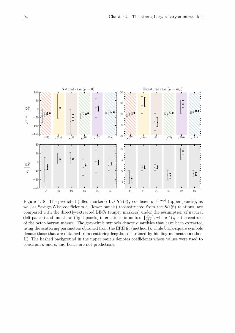
94 Chapter 4. The strong baryon-baryon interaction
c(27) c(8S) c(1) c(10) c(10) c(8A)150
100
50
0
50
100
c(ir
rep)h
2
MB
i
Natural case (µ = 0)
c(27) c(8S) c(1) c(10) c(10) c(8A)10
0
10
20
30Unnatural case (µ = m)
c1 c2 c3 c4 c5 c660
40
20
0
20
40
c i
h2
MB
i
c1 c2 c3 c4 c5 c6
5
0
5
10
Figure 4.18: The predicted (filled markers) LO SUp3qf coefficients cpirrepq (upper panels), aswell as Savage-Wise coefficients ci (lower panels) reconstructed from the SUp6q relations, arecompared with the directly-extracted LECs (empty markers) under the assumption of natural(left panels) and unnatural (right panels) interactions, in units of r 2π
MBs, where MB is the centroid
of the octet-baryon masses. The gray-circle symbols denote quantities that have been extractedusing the scattering parameters obtained from the ERE fit (method I), while black-square symbolsdenote those that are obtained from scattering lengths constrained by binding momenta (methodII). The hashed background in the upper panels denotes coefficients whose values were used toconstrain a and b, and hence are not predictions.
Chapter 5
Summary and conclusions
Nuclear and hypernuclear interactions are key inputs into investigations of the properties ofmatter, and their knowledge continues to be limited in systems with multiple neutrons or whenhyperons are present. As can be seen in the summary of the present status of the field, the majorlimitations come from the lack of experimental data, resulting in contradictory predictions forthe scattering parameters obtained with different theoretical models. In recent years, LQCDhas reached the stage where controlled first-principles studies of nuclei are feasible, and maysoon constrain nuclear and hypernuclear few-body interactions in nature. The present workdemonstrates such a capability in the case of two-baryon interactions, albeit at an unphysicallylarge value of the quark masses corresponding to a pion mass of „ 450 MeV and at only one valueof the lattice spacing. It illustrates how Euclidean two-point correlation functions of systems withthe quantum numbers of two baryons computed with LQCD can be used to constrain a wealth ofquantities, from scattering phase shifts to low-energy scattering parameters and binding energies,to EFTs of forces, or precisely the LECs describing the interactions of two baryons. The sametype of calculations are foreseen in the near future, with values of the quark masses closer to thephysical ones, and their output, in form of both finite-volume energy spectra and constrainedEFT interactions, is expected to serve as input of quantum many-body studies of larger isotopes,at both unphysical and physical values of quark masses; see e.g., Refs. [105–107] for previousstudies in the nuclear sector. By supplementing the missing experimental input for scatteringand spectra of two-baryon systems, such LQCD analyses can constrain phenomenological modelsand EFTs of hypernuclear forces.
In Chapter 2, we have introduced the method of lattice QCD. After a brief description of thefundamental theory in the continuum, QCD, the appropriate changes are applied to allow forthe computation of observables using Monte Carlo techniques. These observables are mainly theenergies of the system and its interactions with external currents. While in this thesis we haveonly studied the first type of observables via the construction of two-point correlation functions,a short explanation has been given on how three-point correlation functions behave and somerelevant results for nuclear physics have been presented as well. Also, in this chapter, we haveshown how the finite-volume energies can be mapped to the scattering phase-shifts using theLüscher’s formalism [7,8], with some detail on the group theory involved when systems are putin a finite volume and the subsequent modification of the angular momentum. Using the sameformalism, we have also presented how the ground-state energies obtained with different volumescan be extrapolated to infinite volume, leading to the binding energy of the system.
In Chapter 3, we have discussed how to extract the energy levels of two-point correlationfunctions, with special emphasis in systems where noise is significant, as it is the case of few-baryonsystems. First, we described a method that has been developed to robustly fit lattice data to asum of exponentials, where both the fitting range and the number of exponentials were varied toobtain a reliable estimation of the systematic uncertainty [9]. The discussion then focused onhow to remove excited-state contamination at early times, with the description of three methods:
95
96 Chapter 5. Summary and conclusions
the generalized pencil-of-functions [274], the matrix-Prony [54], and the variational [276, 277]method. We have also detailed the different ways in which the errors in the correlation functionscan be estimated, using the jackknife and bootstrap resampling methods, but also more robustestimators, like the Hodges–Lehmann estimator.
In Chapter 4, we have presented the experimental and theoretical status of the baryon-baryoninteraction, listing all relevant contributions, and comparing all theoretical predictions of thescattering parameters. We have also discussed and compared the different LQCD methods andresults of interest to the present work, namely the direct method and the potential method. Wethen moved on to describe the different EFTs that have been constrained with the lattice data.Since our focus is on the low-energy physics regime, we considered pionless EFTs (consistingonly of contact interactions) assuming SUp3q flavor [10,11] or SUp6q spin-flavor symmetry [12].We have complemented this section with group-theoretical arguments to justify the number ofoperators included at each order. In the last part of this section, we addressed the issue ofnaturalness of the two-baryon system, as well as its implications in the determination of the LECsof the EFTs from the LQCD results.
The last section of Chapter 4 includes the computation of the lowest-lying spectra of severaltwo-octet baryon systems with strangeness ranging from 0 to ´4. These results have beencomputed in three different volumes, using a single lattice spacing, and with unphysical values ofthe light-quark masses [13]. Assuming small discretization artifacts given the improved LQCDaction that is employed, the results reveal interesting features on the nature of two-baryonforces with larger-than-physical values of the quark masses. In particular, the determinationof scattering parameters of two-baryon systems at low energies has enabled us to constrainthe LO and NLO interactions of a pionless EFT, for both the SUp3q flavor-symmetric and thesymmetry-breaking interactions. The most precise results are obtained using the binding energyto fix the scattering length, and due to the large uncertainties in the effective ranges, the NLOSUp3qf symmetric LECs are mostly consistent with zero. While the two-baryon channels studiedin this work only allowed two sets of leading SUp3qf symmetry-breaking LECs to be constrained,and those values are seen to be consistent with zero, the present study is the first of this type ofanalysis to access these interactions, extending the previous EFT matching presented in Ref. [14]at an SUp3q flavor-symmetric point with mπ “ mK „ 806 MeV. Given the limited knowledgeof flavor-symmetry-breaking effects in the two-baryon sector in nature, this demonstrates thepotential of LQCD to improve the situation. Finally, the observation of an approximate SUp3qfsymmetry in the two-baryon systems included in the present work led to an investigation of thelarge-Nc predictions of Ref. [12], through matching the LQCD results for scattering amplitudesto the EFT. In particular, the S-wave interactions at LO have been found to exhibit an SUp6qspin-flavor symmetry at this pion mass, as also observed in Ref. [14] at a larger value of the pionmass. Both of the two independent spin-flavor-symmetric interactions at LO have been foundto contribute to the amplitude. Nonetheless, the extracted values of the coefficients of the LOSUp3q flavor-symmetric EFT suggest a remnant of an approximate accidental SUp16q symmetry,observed in the SUp3q flavor-symmetric study at mπ „ 806 MeV [14]. It will be interestingto examine these symmetry considerations in the hypernuclear forces at the physical values ofthe quark masses, particularly given the conjectured connections between the nature of forcesin nuclear physics and the quantum entanglement in the underlying systems [104]. Regardingthe binding energy of the systems, we find that most of the channels are bound, except for thespin-triplet ΣN and ΞΞ. While no attempt is made in the current work to constrain forces withinthe EFTs at the physical point, a naive extrapolation has been performed using the results of thiswork and those at mπ „ 806 MeV, with simple extrapolation functions, to make predictions of thebinding energies of several two-baryon channels. The obtained results for ground-state energiesof two-nucleon systems are found to be compatible with the experimental values. Furthermore,stronger evidence for the existence of bound states in the ΞΞ p1S0q and ΞN p3S1q channels isobserved in comparison with other two-baryon systems. Such predictions are in agreement with

97
current phenomenological models and EFT predictions. However, conclusive results can only bereached by performing LQCD studies of multi-baryon systems at or near the physical values ofthe quark masses, and upon taking the continuum limit using multiple values of lattice spacing, aprogram that will be pursued in the upcoming years.

98 Chapter 5. Summary and conclusions
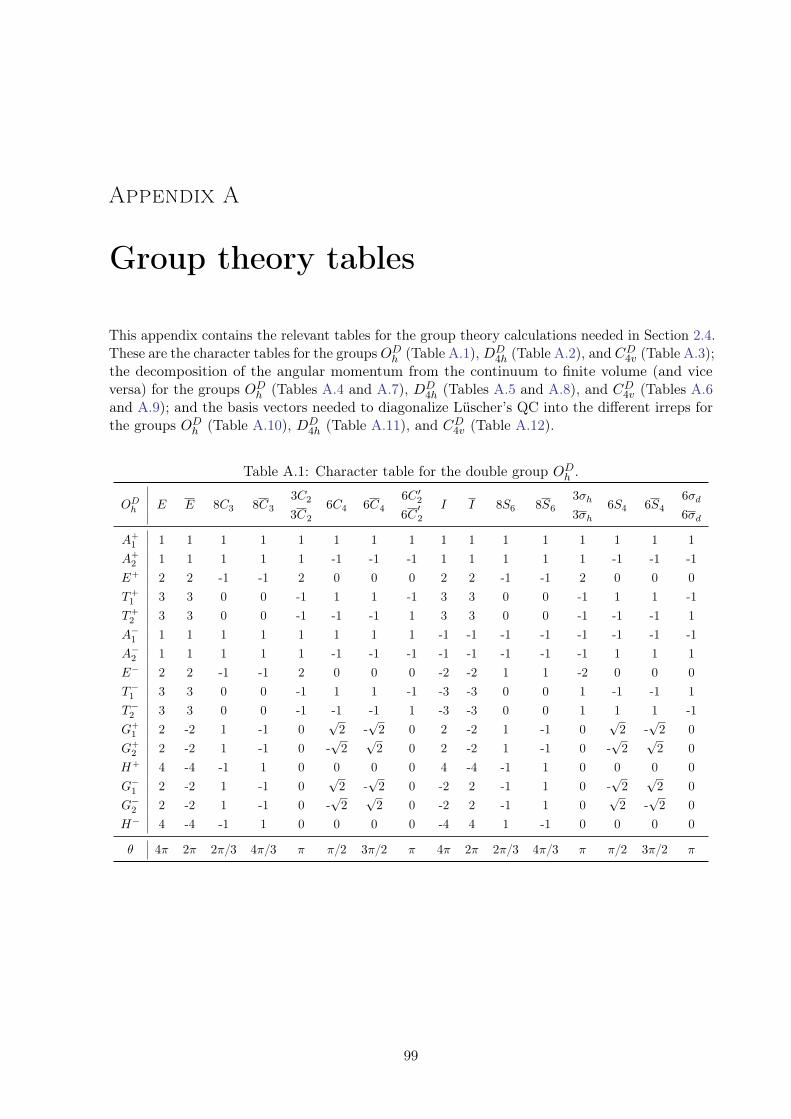
Appendix A
Group theory tables
This appendix contains the relevant tables for the group theory calculations needed in Section 2.4.These are the character tables for the groupsODh (Table A.1),DD
4h (Table A.2), and CD4v (Table A.3);
the decomposition of the angular momentum from the continuum to finite volume (and viceversa) for the groups ODh (Tables A.4 and A.7), DD
4h (Tables A.5 and A.8), and CD4v (Tables A.6and A.9); and the basis vectors needed to diagonalize Lüscher’s QC into the different irreps forthe groups ODh (Table A.10), DD
4h (Table A.11), and CD4v (Table A.12).
Table A.1: Character table for the double group ODh .
ODh E E 8C3 8C3
3C2 6C4 6C4
6C 12 I I 8S6 8S6
3σh 6S4 6S4
6σd
3C2 6C1
2 3σh 6σd
A`1 1 1 1 1 1 1 1 1 1 1 1 1 1 1 1 1A`2 1 1 1 1 1 -1 -1 -1 1 1 1 1 1 -1 -1 -1E` 2 2 -1 -1 2 0 0 0 2 2 -1 -1 2 0 0 0T`1 3 3 0 0 -1 1 1 -1 3 3 0 0 -1 1 1 -1T`2 3 3 0 0 -1 -1 -1 1 3 3 0 0 -1 -1 -1 1A´1 1 1 1 1 1 1 1 1 -1 -1 -1 -1 -1 -1 -1 -1A´2 1 1 1 1 1 -1 -1 -1 -1 -1 -1 -1 -1 1 1 1E´ 2 2 -1 -1 2 0 0 0 -2 -2 1 1 -2 0 0 0T´1 3 3 0 0 -1 1 1 -1 -3 -3 0 0 1 -1 -1 1T´2 3 3 0 0 -1 -1 -1 1 -3 -3 0 0 1 1 1 -1G`1 2 -2 1 -1 0
?2 -
?2 0 2 -2 1 -1 0
?2 -
?2 0
G`2 2 -2 1 -1 0 -?
2?
2 0 2 -2 1 -1 0 -?
2?
2 0H` 4 -4 -1 1 0 0 0 0 4 -4 -1 1 0 0 0 0G´1 2 -2 1 -1 0
?2 -
?2 0 -2 2 -1 1 0 -
?2
?2 0
G´2 2 -2 1 -1 0 -?
2?
2 0 -2 2 -1 1 0?
2 -?
2 0H´ 4 -4 -1 1 0 0 0 0 -4 4 1 -1 0 0 0 0
θ 4π 2π 2π3 4π3 π π2 3π2 π 4π 2π 2π3 4π3 π π2 3π2 π
99
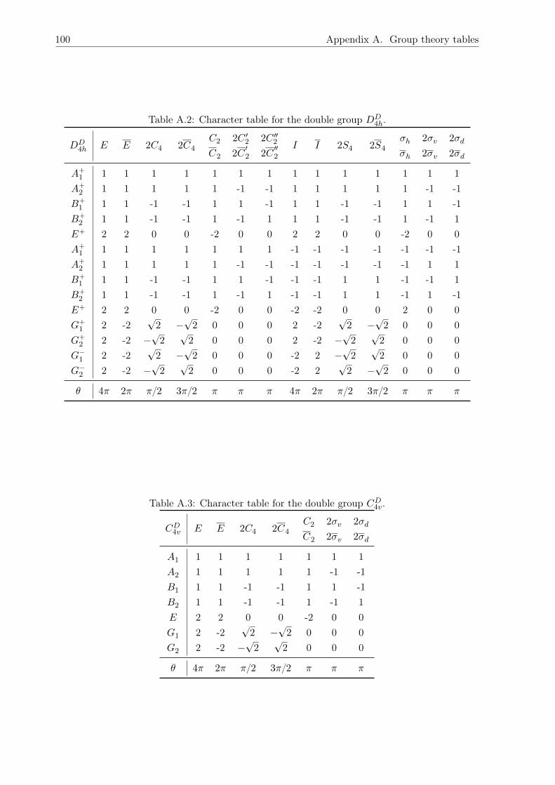
100 Appendix A. Group theory tables
Table A.2: Character table for the double group DD4h.
DD4h E E 2C4 2C4
C2 2C 12 2C22 I I 2S4 2S4
σh 2σv 2σd
C2 2C1
2 2C2
2 σh 2σv 2σd
A`1 1 1 1 1 1 1 1 1 1 1 1 1 1 1A`2 1 1 1 1 1 -1 -1 1 1 1 1 1 -1 -1B`1 1 1 -1 -1 1 1 -1 1 1 -1 -1 1 1 -1B`2 1 1 -1 -1 1 -1 1 1 1 -1 -1 1 -1 1E` 2 2 0 0 -2 0 0 2 2 0 0 -2 0 0A`1 1 1 1 1 1 1 1 -1 -1 -1 -1 -1 -1 -1A`2 1 1 1 1 1 -1 -1 -1 -1 -1 -1 -1 1 1B`1 1 1 -1 -1 1 1 -1 -1 -1 1 1 -1 -1 1B`2 1 1 -1 -1 1 -1 1 -1 -1 1 1 -1 1 -1E` 2 2 0 0 -2 0 0 -2 -2 0 0 2 0 0G`1 2 -2
?2 ´
?2 0 0 0 2 -2
?2 ´
?2 0 0 0
G`2 2 -2 ´?
2?
2 0 0 0 2 -2 ´?
2?
2 0 0 0G´1 2 -2
?2 ´
?2 0 0 0 -2 2 ´
?2
?2 0 0 0
G´2 2 -2 ´?
2?
2 0 0 0 -2 2?
2 ´?
2 0 0 0
θ 4π 2π π2 3π2 π π π 4π 2π π2 3π2 π π π
Table A.3: Character table for the double group CD4v.
CD4v E E 2C4 2C4
C2 2σv 2σd
C2 2σv 2σd
A1 1 1 1 1 1 1 1A2 1 1 1 1 1 -1 -1B1 1 1 -1 -1 1 1 -1B2 1 1 -1 -1 1 -1 1E 2 2 0 0 -2 0 0G1 2 -2
?2 ´
?2 0 0 0
G2 2 -2 ´?
2?
2 0 0 0
θ 4π 2π π2 3π2 π π π
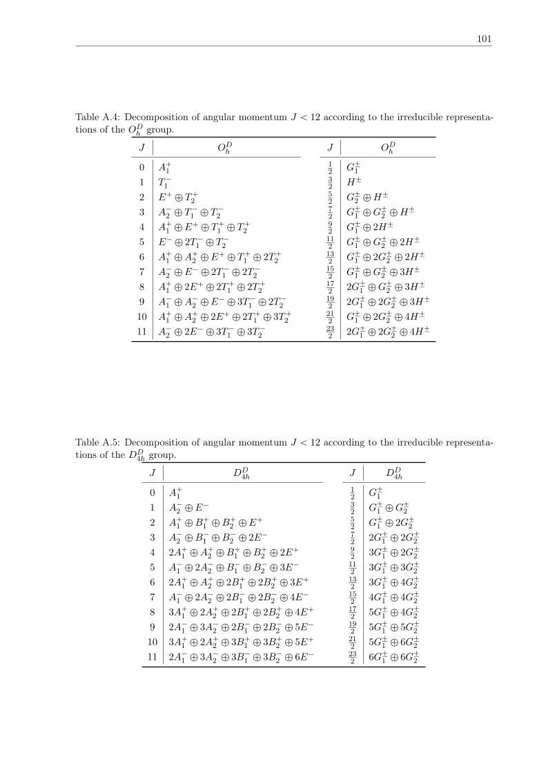
101
Table A.4: Decomposition of angular momentum J ă 12 according to the irreducible representa-tions of the ODh group.
J ODh J ODh
0 A`112 G˘1
1 T´132 H˘
2 E` ‘ T`252 G˘2 ‘H
˘
3 A´2 ‘ T´1 ‘ T
´2
72 G˘1 ‘G
˘2 ‘H
˘
4 A`1 ‘ E` ‘ T`1 ‘ T
`2
92 G˘1 ‘ 2H˘
5 E´ ‘ 2T´1 ‘ T´2
112 G˘1 ‘G
˘2 ‘ 2H˘
6 A`1 ‘A`2 ‘ E
` ‘ T`1 ‘ 2T`2132 G˘1 ‘ 2G˘2 ‘ 2H˘
7 A´2 ‘ E´ ‘ 2T´1 ‘ 2T´2
152 G˘1 ‘G
˘2 ‘ 3H˘
8 A`1 ‘ 2E` ‘ 2T`1 ‘ 2T`2172 2G˘1 ‘G
˘2 ‘ 3H˘
9 A´1 ‘A´2 ‘ E
´ ‘ 3T´1 ‘ 2T´2192 2G˘1 ‘ 2G˘2 ‘ 3H˘
10 A`1 ‘A`2 ‘ 2E` ‘ 2T`1 ‘ 3T`2
212 G˘1 ‘ 2G˘2 ‘ 4H˘
11 A´2 ‘ 2E´ ‘ 3T´1 ‘ 3T´2232 2G˘1 ‘ 2G˘2 ‘ 4H˘
Table A.5: Decomposition of angular momentum J ă 12 according to the irreducible representa-tions of the DD
4h group.
J DD4h J DD
4h
0 A`112 G˘1
1 A´2 ‘ E´ 3
2 G˘1 ‘G˘2
2 A`1 ‘B`1 ‘B
`2 ‘ E
` 52 G˘1 ‘ 2G˘2
3 A´2 ‘B´1 ‘B
´2 ‘ 2E´ 7
2 2G˘1 ‘ 2G˘24 2A`1 ‘A
`2 ‘B
`1 ‘B
`2 ‘ 2E` 9
2 3G˘1 ‘ 2G˘25 A´1 ‘ 2A´2 ‘B
´1 ‘B
´2 ‘ 3E´ 11
2 3G˘1 ‘ 3G˘26 2A`1 ‘A
`2 ‘ 2B`1 ‘ 2B`2 ‘ 3E` 13
2 3G˘1 ‘ 4G˘27 A´1 ‘ 2A´2 ‘ 2B´1 ‘ 2B´2 ‘ 4E´ 15
2 4G˘1 ‘ 4G˘28 3A`1 ‘ 2A`2 ‘ 2B`1 ‘ 2B`2 ‘ 4E` 17
2 5G˘1 ‘ 4G˘29 2A´1 ‘ 3A´2 ‘ 2B´1 ‘ 2B´2 ‘ 5E´ 19
2 5G˘1 ‘ 5G˘210 3A`1 ‘ 2A`2 ‘ 3B`1 ‘ 3B`2 ‘ 5E` 21
2 5G˘1 ‘ 6G˘211 2A´1 ‘ 3A´2 ‘ 3B´1 ‘ 3B´2 ‘ 6E´ 23
2 6G˘1 ‘ 6G˘2
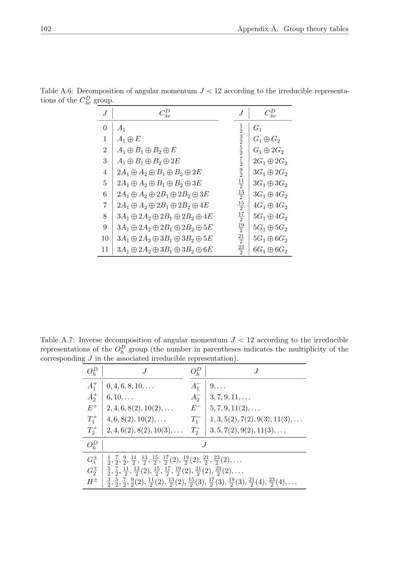
102 Appendix A. Group theory tables
Table A.6: Decomposition of angular momentum J ă 12 according to the irreducible representa-tions of the CD4v group.
J CD4v J CD4v
0 A112 G1
1 A1 ‘ E32 G1 ‘G2
2 A1 ‘B1 ‘B2 ‘ E52 G1 ‘ 2G2
3 A1 ‘B1 ‘B2 ‘ 2E 72 2G1 ‘ 2G2
4 2A1 ‘A2 ‘B1 ‘B2 ‘ 2E 92 3G1 ‘ 2G2
5 2A1 ‘A2 ‘B1 ‘B2 ‘ 3E 112 3G1 ‘ 3G2
6 2A1 ‘A2 ‘ 2B1 ‘ 2B2 ‘ 3E 132 3G1 ‘ 4G2
7 2A1 ‘A2 ‘ 2B1 ‘ 2B2 ‘ 4E 152 4G1 ‘ 4G2
8 3A1 ‘ 2A2 ‘ 2B1 ‘ 2B2 ‘ 4E 172 5G1 ‘ 4G2
9 3A1 ‘ 2A2 ‘ 2B1 ‘ 2B2 ‘ 5E 192 5G1 ‘ 5G2
10 3A1 ‘ 2A2 ‘ 3B1 ‘ 3B2 ‘ 5E 212 5G1 ‘ 6G2
11 3A1 ‘ 2A2 ‘ 3B1 ‘ 3B2 ‘ 6E 232 6G1 ‘ 6G2
Table A.7: Inverse decomposition of angular momentum J ă 12 according to the irreduciblerepresentations of the ODh group (the number in parentheses indicates the multiplicity of thecorresponding J in the associated irreducible representation).
ODh J ODh J
A`1 0, 4, 6, 8, 10, . . . A´1 9, . . .
A`2 6, 10, . . . A´2 3, 7, 9, 11, . . .
E` 2, 4, 6, 8p2q, 10p2q, . . . E´ 5, 7, 9, 11p2q, . . .
T`1 4, 6, 8p2q, 10p2q, . . . T´1 1, 3, 5p2q, 7p2q, 9p3q, 11p3q, . . .
T`2 2, 4, 6p2q, 8p2q, 10p3q, . . . T´2 3, 5, 7p2q, 9p2q, 11p3q, . . .
ODh J
G˘112 ,
72 ,
92 ,
112 ,
132 ,
152 ,
172 p2q,
192 p2q,
212 ,
232 p2q, . . .
G˘252 ,
72 ,
112 ,
132 p2q,
152 ,
172 ,
192 p2q,
212 p2q,
232 p2q, . . .
H˘ 32 ,
52 ,
72 ,
92p2q,
112 p2q,
132 p2q,
152 p3q,
172 p3q,
192 p3q,
212 p4q,
232 p4q, . . .
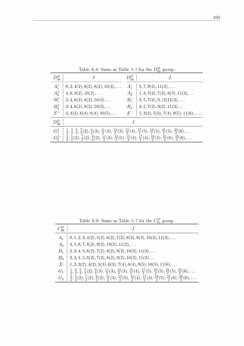
103
Table A.8: Same as Table A.7 for the DD4h group.
DD4h J DD
4h J
A`1 0, 2, 4p2q, 6p2q, 8p2q, 10p3q, . . . A´1 5, 7, 9p2q, 11p2q, . . .
A`2 4, 6, 8p2q, 10p2q, . . . A´2 1, 3, 5p2q, 7p2q, 9p3q, 11p3q, . . .
B`1 2, 4, 6p2q, 8p2q, 10p3q, . . . B´1 3, 5, 7p2q, 9, p2q11p3q, . . .
B`2 2, 4, 6p2q, 8p2q, 10p3q, . . . B´2 3, 5, 7p2q, 9p2q, 11p3q, . . .
E` 2, 4p2q, 6p3q, 8p4q, 10p5q, . . . E´ 1, 3p2q, 5p3q, 7p4q, 9p5q, 11p6q, . . .
DD4h J
G˘112 ,
32 ,
52 ,
72p2q,
92p3q,
112 p3q,
132 p3q,
152 p4q,
172 p5q,
192 p5q,
212 p5q,
232 p6q, . . .
G˘232 ,
52p2q,
72p2q,
92p2q,
112 p3q,
132 p5q,
152 p4q,
172 p4q,
192 p5q,
212 p6q,
232 p6q, . . .
Table A.9: Same as Table A.7 for the CD4v group.
CD4h J
A1 0, 1, 2, 3, 4p2q, 5p2q, 6p2q, 7p2q, 8p3q, 9p3q, 10p3q, 11p3q, . . .
A2 4, 5, 6, 7, 8p2q, 9p2q, 10p2q, 11p2q, . . .
B1 2, 3, 4, 5, 6p2q, 7p2q, 8p2q, 9p2q, 10p3q, 11p3q, . . .
B2 2, 3, 4, 5, 6p2q, 7p2q, 8p2q, 9p2q, 10p3q, 11p3q, . . .
E 1, 2, 3p2q, 4p2q, 5p3q, 6p3q, 7p4q, 8p4q, 9p5q, 10p5q, 11p6q, . . .
G112 ,
32 ,
52 ,
72p2q,
92p3q,
112 p3q,
132 p3q,
152 p4q,
172 p5q,
192 p5q,
212 p5q,
232 p6q, . . .
G232 ,
52p2q,
72p2q,
92p2q,
112 p3q,
132 p5q,
152 p4q,
172 p4q,
192 p5q,
212 p6q,
232 p6q, . . .
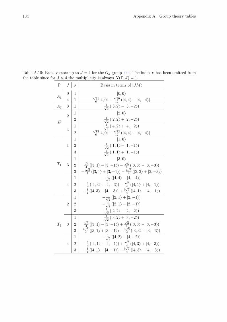
104 Appendix A. Group theory tables
Table A.10: Basis vectors up to J “ 4 for the Oh group [99]. The index ν has been omitted fromthe table since for J ď 4 the multiplicity is always NpΓ, Jq “ 1.
Γ J σ Basis in terms of |JMy
A1
0 1 |0, 0y
4 1?
216 |4, 0y `
?30
12 p|4, 4y ` |4,´4yq
A2 3 1 1?2p|3, 2y ´ |3,´2yq
E
21 |2, 0y
2 1?2p|2, 2y ` |2,´2yq
41 1?
2p|4, 2y ` |4,´2yq
2?
156 |4, 0y ´
?42
12 p|4, 4y ` |4,´4yq
T1
11 |1, 0y
2 1?2p|1, 1y ´ |1,´1yq
3 i?2p|1, 1y ` |1,´1yq
31 |3, 0y
2?
34 p|3, 1y ´ |3,´1yq ´
?5
4 p|3, 3y ´ |3,´3yq
3 ´ i?
34 p|3, 1y ` |3,´1yq ´ i
?5
4 p|3, 3y ` |3,´3yq
4
1 ´ 1?2p|4, 4y ´ |4,´4yq
2 ´14 p|4, 3y ` |4,´3yq ´
?7
4 p|4, 1y ` |4,´1yq
3 ´ i4 p|4, 3y ´ |4,´3yq ` i
?7
4 p|4, 1y ´ |4,´1yq
T2
2
1 ´ 1?2p|2, 1y ` |2,´1yq
2 ´ i?2p|2, 1y ´ |2,´1yq
3 1?2p|2, 2y ´ |2,´2yq
3
1 1?2p|3, 2y ` |3,´2yq
2?
54 p|3, 1y ´ |3,´1yq `
?3
4 p|3, 3y ´ |3,´3yq
3 i?
54 p|3, 1y ` |3,´1yq ´ i
?3
4 p|3, 3y ` |3,´3yq
4
1 ´ 1?2p|4, 2y ´ |4,´2yq
2 ´14 p|4, 1y ` |4,´1yq `
?7
4 p|4, 3y ` |4,´3yq
3 ´ i4 p|4, 1y ´ |4,´1yq ´ i
?7
4 p|4, 3y ´ |4,´3yq
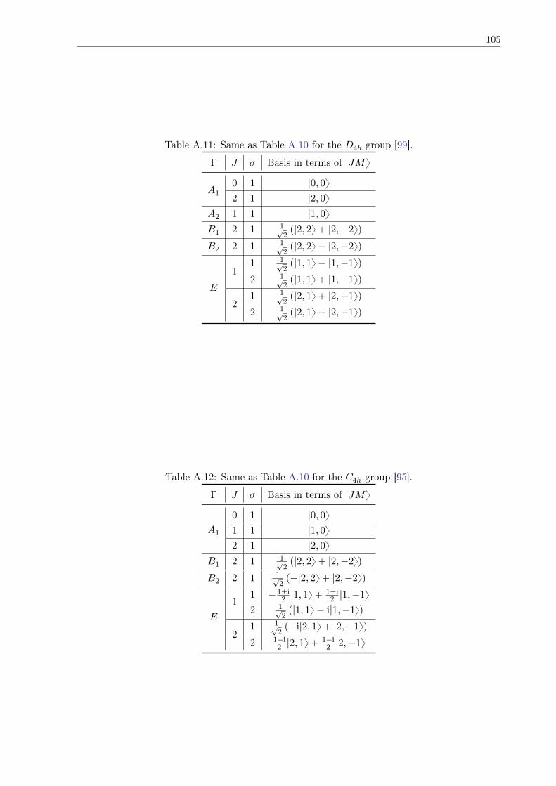
105
Table A.11: Same as Table A.10 for the D4h group [99].
Γ J σ Basis in terms of |JMy
A1
0 1 |0, 0y
2 1 |2, 0y
A2 1 1 |1, 0y
B1 2 1 1?2p|2, 2y ` |2,´2yq
B2 2 1 1?2p|2, 2y ´ |2,´2yq
E
11 1?
2p|1, 1y ´ |1,´1yq
2 1?2p|1, 1y ` |1,´1yq
21 1?
2p|2, 1y ` |2,´1yq
2 1?2p|2, 1y ´ |2,´1yq
Table A.12: Same as Table A.10 for the C4h group [95].
Γ J σ Basis in terms of |JMy
A1
0 1 |0, 0y
1 1 |1, 0y
2 1 |2, 0y
B1 2 1 1?2p|2, 2y ` |2,´2yq
B2 2 1 1?2p´|2, 2y ` |2,´2yq
E
11 ´1`i
2 |1, 1y `1´i2 |1,´1y
2 1?2p|1, 1y ´ i|1,´1yq
21 1?
2p´i|2, 1y ` |2,´1yq
2 1`i2 |2, 1y `
1´i2 |2,´1y

106 Appendix A. Group theory tables
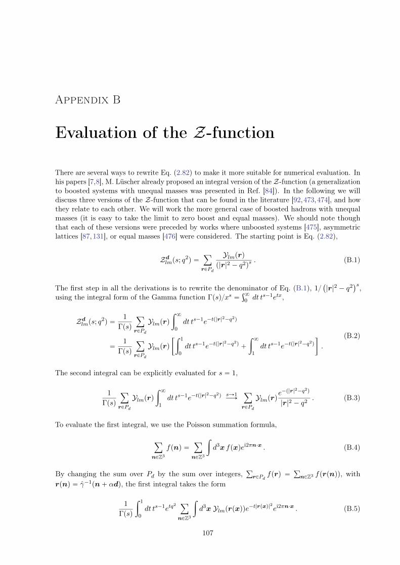
Appendix B
Evaluation of the Z-function
There are several ways to rewrite Eq. (2.82) to make it more suitable for numerical evaluation. Inhis papers [7,8], M. Lüscher already proposed an integral version of the Z-function (a generalizationto boosted systems with unequal masses was presented in Ref. [84]). In the following we willdiscuss three versions of the Z-function that can be found in the literature [92,473,474], and howthey relate to each other. We will work the more general case of boosted hadrons with unequalmasses (it is easy to take the limit to zero boost and equal masses). We should note thoughthat each of these versions were preceded by works where unboosted systems [475], asymmetriclattices [87,131], or equal masses [476] were considered. The starting point is Eq. (2.82),
Zdlmps; q
2q “ÿ
rPPd
Ylmprqp|r|2 ´ q2q
s . (B.1)
The first step in all the derivations is to rewrite the denominator of Eq. (B.1), 1`
|r|2 ´ q2˘s,
using the integral form of the Gamma function Γpsqxs “ş8
0 dt ts´1etx,
Zdlmps; q
2q “1
Γpsq
ÿ
rPPd
Ylmprqż 8
0dt ts´1e´tp|r|
2´q2q
“1
Γpsq
ÿ
rPPd
Ylmprq„ż 1
0dt ts´1e´tp|r|
2´q2q `
ż 8
1dt ts´1e´tp|r|
2´q2q
.
(B.2)
The second integral can be explicitly evaluated for s “ 1,
1
Γpsq
ÿ
rPPd
Ylmprqż 8
1dt ts´1e´tp|r|
2´q2q sÑ1ÝÑ
ÿ
rPPd
Ylmprqe´p|r|
2´q2q
|r|2 ´ q2. (B.3)
To evaluate the first integral, we use the Poisson summation formula,
ÿ
nPZ3
fpnq “ÿ
nPZ3
ż
d3x fpxqei2πn¨x . (B.4)
By changing the sum over Pd by the sum over integers,ř
rPPdfprq “
ř
nPZ3 fprpnqq, withrpnq “ γ´1pn` αdq, the first integral takes the form
1
Γpsq
ż 1
0dt ts´1etq
2ÿ
nPZ3
ż
d3x Ylmprpxqqe´t|rpxq|2ei2πn¨x . (B.5)
107
108 Appendix B. Evaluation of the Z-function
Changing the integration variables from x to r, such that x “ γr ´ αd and d3x “ γd3r,
1
Γpsq
ż 1
0dt ts´1etq
2ÿ
nPZ3
ż
γd3r Ylmprqe´t|r|2ei2πn¨pγr´αdq
“γ
Γpsq
ż 1
0dt ts´1etq
2ÿ
nPZ3
e´i2παn¨d
ż
d3r |r|lYlmprqe´t|r|2ei2πn¨pγrq
“γ
Γpsq
ż 1
0dt ts´1etq
2ÿ
nPZ3
e´i2παn¨d
ż 8
0|r|2d|r| e´t|r|
2|r|l
ż
dΩr Ylmprqeik¨r ,
(B.6)
with k “ 2πγn, and where we have rewritten n¨pγrq “ pn‖`nKq¨pγr‖`rKq “ γn‖ ¨r‖`nK ¨rK “pγnq ¨ r. The angular integral can be performed by expanding eik¨r in spherical harmonics,
ż
dΩr Ylmprqeik¨r “
ż
dΩr Ylmprq4π8ÿ
l1“0
l1ÿ
m1“´l1
il1
jl1p|k||r|qYl1m1pkqY˚l1m1prq
“ 4π8ÿ
l1“0
l1ÿ
m1“´l1
il1
jl1p|k||r|qYl1m1pkq
ż
dΩr YlmprqY˚l1m1prq
loooooooooooomoooooooooooon
δll1δmm1
“ 4π iljlp|k||r|qYlmpkq ,
(B.7)
with jlpxq being the spherical Bessel functions. Now, the integral over |r| can be analyticallycomputed, which gives
ż 8
0|r|2d|r| e´t|r|
2|r|ljlp|k||r|q “
1
4π
´π
t
¯32ˆ
|k|
2t
˙l
e´|k|24t . (B.8)
Collecting all the terms, the first integral looks like
γ
Γpsq
ż 1
0dt ts´1etq
2ÿ
nPZ3
e´i2παn¨d´π
t
¯32ilˆ
|k|
2t
˙l
Ylmpkqloooooooomoooooooon
Ylmpk2tq
e´|k|24t
“γ
Γpsq
ż 1
0dt ts´1etq
2ÿ
nPZ3
e´i2παn¨d´π
t
¯32il Ylmpπγntqe´π
2|γn|2t .
(B.9)
In the case of s “ 1, the integral over t is finite for all n except for n “ 0. In this case, thedivergence occurs only for l “ m “ 0, since Ylmpn “ 0q9 δl0δm0. Then, splitting the sum betweenn “ 0 and n ‰ 0, and looking at the n “ 0 part,
γ
Γpsq
ż 1
0dt ts´1etq
2´π
t
¯32 1?
4πδl0δm0 “
γ
Γpsq
π
2
ż 1
0dt ts´52etq
2δl0δm0 . (B.10)
Up to here, all derivations follow these steps.1 The differences between the different versionsappear in the way this divergent integral is computed:
• In Ref. [92], by adding and subtracting ts´52 into the integral,ż 1
0dt ts´52etq
2“
ż 1
0dt ts´52
´
etq2´ 1
¯
`
ż 1
0dt ts´52 , (B.11)
the first integral becomes finite for s “ 1, while the second integral, which comes out
finite only for s ą 32,ş10 dt t
s´52 są32“ 1
s´32 , can be analytically continued to s “ 1,1
s´32sÑ1ÝÑ ´2.
1In the case of Ref. [473], the steps are slightly different, but the final result is the same.
109
• In Ref. [473], the exponential is replaced by its Taylor expansion,ż 1
0dt ts´52etq
2“
ż 1
0dt ts´52
8ÿ
ρ“0
ptq2qρ
ρ!“
8ÿ
ρ“0
pq2qρ
ρ!
ż 1
0dt ts`ρ´52 . (B.12)
Again, the integral is finite only for s ą 32, but it is analytically continued to s “ 1,
8ÿ
ρ“0
pq2qρ
ρ!
1
s` ρ´ 32sÑ1ÝÑ
8ÿ
ρ“0
pq2qρ
ρ!
1
ρ´ 12. (B.13)
• In Ref. [474], the divergent integral is integrated by parts, and in the last step it is analyticallycontinued to s “ 1,
ż 1
0dt ts´52etq
2“
eq2
s´ 32´
ż 1
0dt q2etq
2 ts´32
s´ 32
sÑ1ÝÑ ´2eq
2`
ż 1
0dt etq
22t´12q2 “ ´2eq
2`
ż 1
0dtetq
2
t322tq2 ,
(B.14)
To recover the result from Ref. [131], one has to perform another integration by parts,
´ 2eq2`
ż 1
0dtetq
2
t322tq2 “ 2eq
2p2q2 ´ 1q ´
ż 1
0dtetq
2
t324t2q4 . (B.15)
Therefore, the final version can be written as
Zdlmp1; q2q “γ
ż 1
0dt etq
2ÿ
nPZ3
n‰0
e´i2παn¨d´π
t
¯32il Ylmpπγntqe´π
2|γn|2t
`ÿ
rPPd
Ylmprqe´p|r|
2´q2q
|r|2 ´ q2` γ
π
2
$
’
’
’
’
&
’
’
’
’
%
ş10 dt
1t32petq
2´ 1q ´ 2
ř8ρ“0
1ρ´12
pq2qρ
ρ!
ş10 dt
etq2
t322tq2 ´ 2eq
2
,
/
/
/
/
.
/
/
/
/
-
δl0δm0 ,
(B.16)
where each row inside the curly brackets represents the result of each version. The first and thirdintegral give the same result [422],
ż 1
0dt
1
t32petq
2´ 1q ´ 2 “
ż 1
0dtetq
2
t322tq2 ´ 2eq
2“ 2eq
2”
´1` 2a
q2D´
a
q2¯ı
, (B.17)
where Dpxq is the Dawson integral [477], which is defined as Dpxq “ e´x2 şx
0 dy ey2 . For the sum,
the result is8ÿ
ρ“0
1
ρ´ 12
pq2qρ
ρ!“ ´2 1F1
ˆ
´1
2;1
2; q2
˙
, (B.18)
where 1F1pa; b;xq is the confluent hypergeometric function of the first kind [478],
1F1pa; b;xq “8ÿ
ρ“0
paqρpbqρ
xρ
ρ!, with pϑqρ “ Γpϑ` ρqΓpϑq . (B.19)
In Ref. [479], the relation between the Dawson integral and 1F1 is shown,
D´
a
q2¯
“a
q2e´q2
1F1
ˆ
1
2;3
2; q2
˙
. (B.20)
110 Appendix B. Evaluation of the Z-function
The only piece left is to relate 1F1
`
´12 ; 1
2 ; q2˘
with 1F1
`
12 ; 3
2 ; q2˘
, which can be done using thefollowing recurrence relation [478],
b 1F1 pa; b;xq ´ b 1F1 pa´ 1; b;xq ´ x 1F1 pa; b` 1;xq “ 0 . (B.21)
Setting a “ b “ 12 and combining Eqs. (B.18) and (B.20),
´2 1F1
ˆ
´1
2;1
2; q2
˙
“ ´2 1F1
ˆ
1
2;1
2; q2
˙
` 4q21F1
ˆ
1
2;3
2; q2
˙
“ ´2eq2` 4eq
2a
q2D´
a
q2¯
,
(B.22)
which is exactly Eq. (B.17).To conclude, just note that an intermediate version between the raw and accelerated form
can be found in early studies of baryon-baryon interactions [85, 387], where the evaluation of theZ-function by brute force takes to the following form,
Z00p1; q2q “ limΛÑ8
˜
Λÿ
n“0
1
|n|2 ´ q2´ 4πΛ
¸
. (B.23)
Appendix C
Summary tables of baryon-baryonchannels
This appendix contains summary tables of the scattering parameters predicted by phenomenolog-ical models and EFTs for different two-baryon systems: ΛN (Table C.1), ΣN (Table C.2), ΛΛ orH-dibaryon (Table C.3), ΣΣ (Table C.4), ΞN (Table C.5), ΞΣ (Table C.6), and ΞΞ (Table C.7).
This appendix also contains summary tables of the binding energies, as defined in Eq. (4.103),computed with fully dynamical LQCD calculations: NN (Table C.8), ΛN (Table C.9), ΣN(Table C.10), ΛΛ orH-dibaryon (Table C.11), ΣΣ (Table C.12), ΞN (Table C.13), ΞΣ (Table C.14),and ΞΞ (Table C.15). Some results, by virtue of SUp3qf symmetry, are applicable to differentchannels belonging to the same irrep (e.g., the CalLat Collaboration is only focused on the NNchannels, but since their calculations are performed with nf “ 3, their results also apply toother channels belonging to the 27 irrep). In these tables, there are three additional symbols:: indicates that Lüscher’s formalism is used to compute the binding energy, ; indicates thata continuum extrapolation is performed, and § that only the potential is shown (no physicalquantity, like the energy shift or the phase shift).
The references in the tables are sorted chronologically.
111
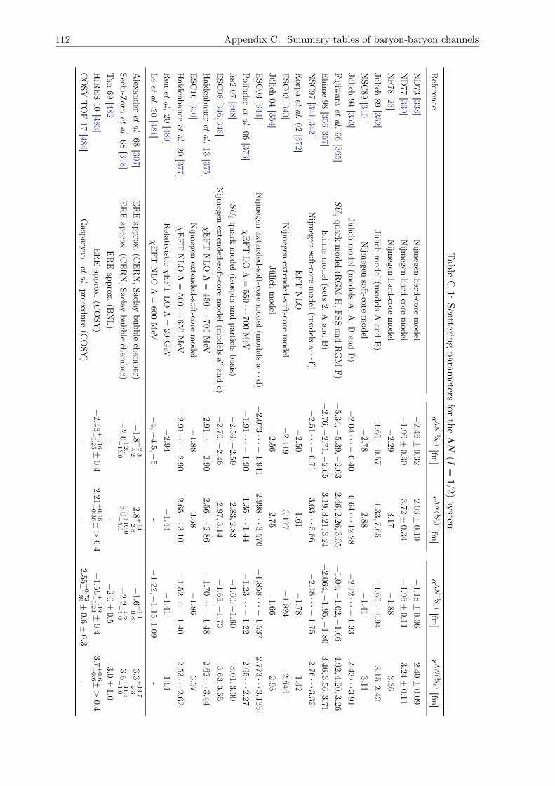
112 Appendix C. Summary tables of baryon-baryon channels
Table
C.1:
Scatteringparam
etersfor
theΛN
(I“
12)
systemReference
aΛNp1S
0q[fm
]r
ΛNp1S
0q[fm
]a
ΛNp3S
1q[fm
]r
ΛNp3S
1q[fm
]
ND73
[338]Nijm
egenhard-core
model
´2.46
˘0.32
2.03˘
0.10´
1.18˘
0.062.4
0˘
0.09
ND77
[339]Nijm
egenhard-core
model
´1.90
˘0.30
3.72˘
0.34´
1.96˘
0.113.24˘
0.11
NF78
[23]Nijm
egenhard-core
model
´2.29
3.17´
1.88
3.3
6
Jülich89
[352]Jülich
model(m
odelsA
andB)
´1.60,
´0.57
1.33,7.65´
1.60,´
1.94
3.1
5,2.42
NSC
89[340]
Nijm
egensoft-core
model
´2.78
2.88´
1.41
3.11
Jülich94
[353]Jülich
model(m
odelsA,A
,Band
B)
´2.04¨¨¨´
0.400.64¨¨¨12.28
´2.12¨¨¨´
1.332.4
3¨¨¨3.9
1
Fujiwara
etal.
96[365]
SU
6quark
model(R
GM-H
,FSS
andRGM-F)
´5.34,
´5.39,
´2.03
2.46,2.26,3.05´
1.04,
´1.02,
´1.66
4.9
2,4.20,3.2
6
Ehim
e98
[356,357]Ehim
emodel(sets
2,Aand
B)
´2.76,
´2.71
,´
2.653.19,3.21
,3.24
´2.064
,´
1.95,´
1.80
3.46,3.5
6,3.71
NSC
97[341,342]
Nijm
egensoft-core
model(m
odelsa¨¨¨f)
´2.51
¨¨¨´
0.713.03¨¨¨5.86
´2.18
¨¨¨´
1.752.7
6¨¨¨3.32
Korpa
etal.
02[372]
EFT
NLO
´2.50
1.61´
1.781.4
2
ESC
03[343]
Nijm
egenextended-soft-core
model
´2.119
3.177´
1.824
2.8
46
Jülich04
[354]Jülich
model
´2.56
2.75´
1.662.9
3
ESC
04[344]
Nijm
egenextended-soft-core
model(m
odelsa¨¨¨d)
´2.073
¨¨¨´
1.9412.998
¨¨¨3.570
´1.858
¨¨¨´
1.5372.77
3¨¨¨3.1
33
Polinder
etal.
06[373]
χEFT
LOΛ“
550¨¨¨700
MeV
´1.91
¨¨¨´
1.90
1.35¨¨¨1.44
´1.23
¨¨¨´
1.22
2.05¨¨¨2.2
7
fss207
[368]SU
6quark
model(isospin
andparticle
basis)´
2.59,
´2.59
2.83,2.83
´1.60,
´1.60
3.01,3.0
0
ESC
08[346,348]
Nijm
egenextended-soft-core
model(m
odelsa”
andc)
´2.70,
´2.46
2.97,3.14
´1.65,
´1.73
3.6
3,3.55
Haidenbauer
etal.
13[375]
χEFT
NLO
Λ“
450¨¨¨700
MeV
´2.91
¨¨¨´
2.90
2.56¨¨¨2.86
´1.70
¨¨¨´
1.48
2.62¨¨¨3.4
4
ESC
16[350]
Nijm
egenextended-soft-core
model
´1.88
3.58´
1.86
3.3
7
Haidenbauer
etal.
20[377]
χEFT
NLO
Λ“
500¨¨¨650
MeV
´2.91
¨¨¨´
2.90
2.65¨¨¨3.10
´1.52
¨¨¨´
1.40
2.53¨¨¨2.6
2
Ren
etal.
20[480]
Relativistic
χEFT
LOΛ“
20GeV
´2.94
´1.44
´1.41
1.61
Leet
al.20
[481]χE
FT
NLO
Λ“
600MeV
´4,´
4.5,´
5-
´1.22,
´1.15,1.09
-
Alexander
etal.
68[307]
ERE
approx.(CERN,Saclay
bubblecham
ber)´
1.8`
2.3
´4.2
2.8`
14
´2.8
´1.6
`1.1
´0.8
3.3`
13.7
´2.3
Sechi-Zornet
al.68
[308]ERE
approx.(CERN,Saclay
bubblecham
ber)´
2.0`
2.0
´13.0
5.0`
10.0
´5.0
´2.2
`1.6
´1.0
3.5`
11.5
´1.0
Tan
69[482]
ERE
approx.(BNL)
--
´2.0˘
0.5
3.0˘
1.0
HIR
ES10
[483]ERE
approx.(COSY
)´
2.43
`0.1
6´
0.2
5˘
0.4
2.21
`0.1
6´
0.3
6˘ą
0.4´
1.56
`0.1
9´
0.2
2˘
0.4
3.7`
0.6
´0.6˘ą
0.4
COSY
-TOF17
[484]Gasparyan
etal.
procedure(C
OSY
)-
-´
2.55
`0.7
2´
1.3
9˘
0.6˘
0.3-
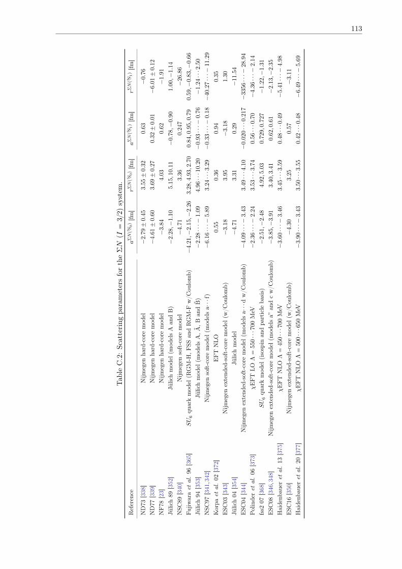
113
Tab
leC.2:Sc
attering
parametersforthe
ΣN
(I“
32)
system
.Reference
aΣNp1S0q[fm
]rΣ
Np1S0q[fm
]a
ΣNp3S1q[fm
]rΣ
Np3S1q[fm
]
ND73
[338]
Nijm
egen
hard-coremod
el´
2.7
9˘
0.45
3.5
5˘
0.3
20.6
3´
0.76
ND77
[339]
Nijm
egen
hard-coremod
el´
4.61˘
0.60
3.6
9˘
0.2
70.
32˘
0.0
1´
6.0
1˘
0.1
2
NF78
[23]
Nijm
egen
hard-coremod
el´
3.8
44.
030.6
2´
1.91
Jülich89
[352]
Jülichmod
el(m
odelsA
andB)
´2.
28,´
1.10
5.15,
10.1
1´
0.78,´
0.90
1.00,´
1.1
4
NSC
89[340]
Nijm
egen
soft-coremod
el´
4.7
13.
36
0.2
47
´26.
86
Fujiw
araet
al.96
[365]
SU
6qu
arkmod
el(R
GM-H
,FSS
andRGM-F
w/C
oulomb)
´4.2
1,´
2.1
5,´
2.2
63.
28,4.9
3,2.7
00.
84,0.9
5,0.7
90.5
9,´
0.83,´
0.66
Jülich94
[353]
Jülichmod
el(m
odelsA,A
,Ban
dB)
´2.2
8¨¨¨´
1.0
94.
96¨¨¨10.2
0´
0.9
3¨¨¨´
0.7
6´
1.2
4¨¨¨2.
50
NSC
97[341,342]
Nijm
egen
soft-coremod
el(m
odelsa¨¨¨f)
´6.1
6¨¨¨´
5.8
93.
24¨¨¨3.
29
´0.3
3¨¨¨´
0.1
8´
40.
27¨¨¨´
11.
29
Korpa
etal.02
[372]
EFT
NLO
0.55
0.36
0.9
40.3
5
ESC
03[343]
Nijm
egen
extend
ed-soft-core
mod
el(w
/Cou
lomb)
´3.1
83.
95´
3.1
81.
30
Jülich04
[354]
Jülichmod
el´
4.7
13.
310.2
9´
11.
54
ESC
04[344]
Nijm
egen
extend
ed-soft-core
mod
el(m
odelsa¨¨¨dw/C
oulomb)
´4.0
9¨¨¨´
3.4
33.
49¨¨¨4.1
0´
0.0
20¨¨¨0.
217
´3356¨¨¨´
28.
94
Polinderet
al.06
[373]
χEFT
LOΛ“
550¨¨¨70
0MeV
´2.3
6¨¨¨´
2.2
43.
53¨¨¨3.7
40.
56¨¨¨0.
70
´4.
36¨¨¨´
2.1
4
fss2
07[368]
SU
6qu
arkmod
el(isospin
andpa
rticle
basis)
´2.
51,´
2.48
4.92,5.0
30.7
29,0.7
27
´1.2
2,´
1.31
ESC
08[346,348]
Nijm
egen
extend
ed-soft-core
mod
el(m
odelsa”
andcw/C
oulomb)
´3.
85,´
3.91
3.40,
3.4
10.6
2,0.6
1´
2.1
3,´
2.35
Haidenb
auer
etal.13
[375]
χEFT
NLO
Λ“
450¨¨¨70
0MeV
´3.6
0¨¨¨´
3.4
63.
45¨¨¨3.5
90.
48¨¨¨0.
49´
5.41¨¨¨´
4.9
8
ESC
16[350]
Nijm
egen
extend
ed-soft-core
mod
el(w
/Cou
lomb)
´4.3
03.
25
0.5
7´
3.1
1
Haidenb
auer
etal.20
[377]
χEFT
NLO
Λ“
500¨¨¨65
0MeV
´3.9
0¨¨¨´
3.4
33.
50¨¨¨3.5
50.
42¨¨¨0.4
8´
6.49¨¨¨´
5.6
9
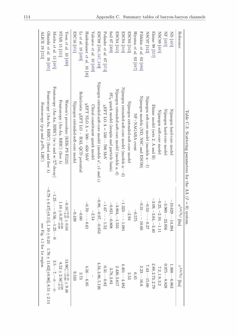
114 Appendix C. Summary tables of baryon-baryon channels
Table
C.3:
Scatteringparam
etersfor
theΛ
Λ(I“
0)system
.
Reference
aΛ
Λp1S
0q[fm
]r
ΛΛp1S
0q[fm
]
ND
[485]Nijm
egenhard-core
model
´10.629
¨¨¨14.394
1.300
¨¨¨6.863
NF[485]
Nijm
egenhard-core
model
´3.960
¨¨¨23.956
0.975
¨¨¨8.828
NSC
89[485]
Nijm
egensoft-core
model
´0.25,
´2.10,
´1.11
7.2,1.9,3.2
Ehim
e98
[357]Ehim
emodel(sets
2,Aand
B)
´3.09,
´3.64,
´3.40
2.89,2.73,2.79
NSC
97[342]
Nijm
egensoft-core
model(m
odelsa¨¨¨f)
´0.53¨¨¨´
0.277.43
¨¨¨15.00
Filikhin
etal.
02[486]
Nijm
egenmodels
(ND,N
SCand
ESC
00)´
0.31¨¨¨´
10.602.23
¨¨¨16.6
Hiyam
aet
al.02
[487]NF+NAGARA
event´
0.575
6.45
ESC
03[343]
Nijm
egenextended-soft-core
model
´2.94
2.53
ESC
04[344]
Nijm
egenextended-soft-core
model(m
odelsa¨¨¨d)
´1.323
¨¨¨´
1.081
4.401¨¨¨4.482
ESC
04[345]
Nijm
egenextended-soft-core
model(m
odelsa,d)
´3.804
,´
1.555
2.420,3.617
fss207
[368]SU
6quark
model(isospin
andparticle
basis)´
0.821
,´
0.808
3.78,3.83
Polinder
etal.
07[374]
χEFT
LOΛ“
550¨¨¨700
MeV
´1.67¨¨¨´
1.520.31
¨¨¨0.82
ESC
08[346,347,349]
Nijm
egenextended-soft-core
model(m
odelsa”,c1
andc)
´0.88,
´0.97,
´0.853
4.34,3.86,5.126
Valcarce
etal.
10[488]
Chiralconstituent
quarkmodel
´2.54
-Haidenbauer
etal.
16[46]
χEFT
NLO
Λ“
500¨¨¨650
MeV
´0.70¨¨¨´
0.614.56
¨¨¨6.95
Lietal.
18[489]
Relativistic
χEFT
LO+
HALQCD
potential´
0.603.73
ESC
16[351]
Nijm
egenextended-soft-core
model
´0.439
9.533
Yoon
etal.
10[490]
Watson’s
procedure(K
EK-P
SE522)
´0.10
`0.4
5´
2.3
7˘
0.0413.90
ą`
16.1
0ă´
13.9
0˘
9.48
STAR
15[331]
Femtoscopy
(Au-A
u,RHIC
)(free
λ)1.10
˘0.37
`0.6
8´
0.0
88.52˘
2.56
`2.0
9´
0.7
4
Morita
etal.
15[485]
Femtoscopy
(Au-A
u,RHIC
)(w
/oand
w/Σ
0-decay)´
1.25¨¨¨´
0.56,
´1.25¨¨¨0
3.5¨¨¨7,´8¨¨¨8
Ohnishiet
al.16
[491]Fem
toscopy(A
u-Au,R
HIC
)(fixed
andfree
λ)´
0.79˘
0.47r˘
0.11s,1.10
˘0.24
1.76˘
11.62r˘
0.86s,8.51˘
2.14
ALIC
E19
[332]Fem
toscopy(p-p
andp-P
b,LHC)
seeFig.4.2
for1σ
region
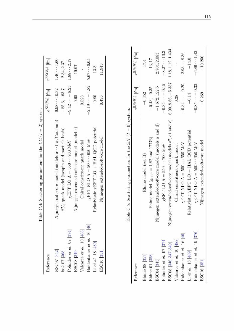
115
Tab
leC.4:Sc
attering
parametersforthe
ΣΣ
(I“
2)system
.
Reference
aΣ
Σp1S0q[fm
]rΣ
Σp1S0q[fm
]
NSC
97[342
]Nijm
egen
soft-coremod
el(m
odelsa¨¨¨fw/C
oulomb)
6.98¨¨¨10.
321.4
6¨¨¨1.6
0
fss2
07[368
]SU
6qu
arkmod
el(isospin
andpa
rticle
basis)
´85.
3,´
63.7
2.3
4,2.3
7
Polinderet
al.07
[374
]χEFT
LOΛ“
550¨¨¨70
0MeV
´9.
42¨¨¨´
6.2
31.
88¨¨¨2.1
7
ESC
08[349
]Nijm
egen
extend
ed-soft-core
mod
el(m
odel
c)´
0.65
19.9
7
Valcarceet
al.10
[488
]Chiralc
onstitue
ntqu
arkmod
el0.5
23-
Haidenb
auer
etal.16
[46]
χEFT
NLO
Λ“
500¨¨¨65
0MeV
´2.
19¨¨¨´
1.8
25.
67¨¨¨6.0
5
Liet
al.18
[489
]RelativisticχEFT
LO+
HALQCD
potential
´0.
80
13.3
ESC
16[351
]Nijm
egen
extend
ed-soft-core
mod
el0.4
9511.9
43
Tab
leC.5:Sc
attering
parametersforthe
ΞN
(I“
0)system
.
Reference
aΞNp3S1q[fm
]rΞNp3S1q[fm
]
Ehime98
[357
]Ehimemod
el(set
B)
´0.3
52
17.4
Ehime01
[358
]Ehimemod
el(g
ΞΞσ“
1.8
2an
d17
776)
´0.
43,´
0.35
13,1
7
ESC
04[345
]Nijm
egen
extend
ed-soft-core
mod
el(m
odelsaan
dd)
´1.
672,1
22.5
2.7
04,2.0
83
Polinderet
al.07
[374
]χEFT
LOΛ“
550¨¨¨70
0MeV
´0.3
4¨¨¨´
0.1
5´
8.27¨¨¨16.3
ESC
08[346
,347
,349
]Nijm
egen
extend
ed-soft-core
mod
el(m
odelsa”,c
1an
dc)
6.90,8.8
6,´
5.35
71.
18,
1.12,1.4
34
Valcarceet
al.10
[488
]Chiralc
onstitue
ntqu
arkmod
el0.2
8-
Haidenb
auer
etal.16
[46]
χEFT
NLO
Λ“
500¨¨¨65
0MeV
´0.3
4¨¨¨´
0.2
02.9
3¨¨¨8.3
6
Liet
al.18
[489
]RelativisticχEFT
LO+
HALQCD
potential
´0.1
4´
14.
0
Haidenb
auer
etal.19
[376
]χEFT
NLO
Λ“
500¨¨¨65
0MeV
´0.8
5¨¨¨´
0.3
3´
6.86¨¨¨1.
42
ESC
16[351
]Nijm
egen
extend
ed-soft-core
mod
el´
0.2
69
´10.2
50
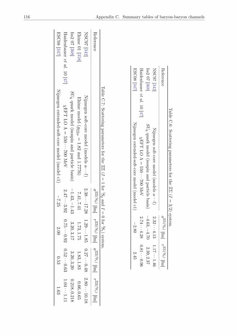
116 Appendix C. Summary tables of baryon-baryon channels
Table
C.6:
Scatteringparam
etersfor
theΞ
Σ(I“
32)
system.
Reference
aΞ
Σp1S
0q[fm
]r
ΞΣp1S
0q[fm
]
NSC
97[342]
Nijm
egensoft-core
model(m
odelsa¨¨¨f)
2.32¨¨¨4.13
1.17¨¨¨1.46
fss207
[368]SU
6quark
model(isospin
andparticle
basis)´
4.63,´
4.70
2.39,2.37
Haidenbauer
etal.
10[47]
χEFT
LOΛ“
550¨¨¨700
MeV
2.74¨¨¨4.28
0.81¨¨¨0.96
ESC
08[347]
Nijm
egenextended-soft-core
model(m
odelc1)´
2.80
2.45
Table
C.7:
Scatteringparam
etersfor
theΞ
Ξ(I“
1for
1S0and
I“
0for
3S1 )
system.
Reference
aΞ
Ξp1S
0q[fm
]r
ΞΞp1S
0q[fm
]a
ΞΞp3S
1q[fm
]r
ΞΞp3S
1q[fm
]
NSC
97[342]
Nijm
egensoft-core
model(m
odelsa¨¨¨f)
2.38¨¨¨17.28
1.29¨¨¨1.85
0.27¨¨¨0.48
2.8
0¨¨¨10.18
Ehim
e01
[358]Ehim
emodel(g
ΞΞσ“
1.82
and1.7776)
7.41,7.41
1.73,1.75
1.8
3,1.830.66,0
.65
fss207
[368]SU
6quark
model(isospin
andparticle
basis)´
1.43,´
1.433.20,3
.17
3.20,3.20
0.218
,0.218
Haidenbauer
etal.
10[47]
χEFT
LOΛ“
550¨¨¨7
00MeV
2.47¨¨¨3.92
0.75¨¨¨0.92
0.52¨¨¨0.63
1.04¨¨¨1.11
ESC
08[347]
Nijm
egenextended-soft-core
model(m
odelc1)´
7.25
2.00
0.53
1.63
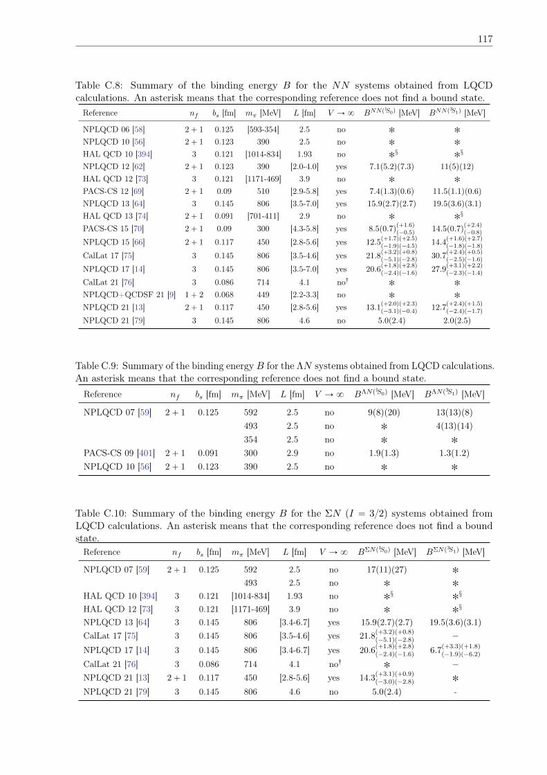
117
Table C.8: Summary of the binding energy B for the NN systems obtained from LQCDcalculations. An asterisk means that the corresponding reference does not find a bound state.Reference nf bs [fm] mπ [MeV] L [fm] V Ñ8 BNNp1S0q [MeV] BNNp3S1q [MeV]
NPLQCD 06 [58] 2` 1 0.125 [593-354] 2.5 no ˚ ˚
NPLQCD 10 [56] 2` 1 0.123 390 2.5 no ˚ ˚
HAL QCD 10 [394] 3 0.121 [1014-834] 1.93 no ˚§ ˚§
NPLQCD 12 [62] 2` 1 0.123 390 [2.0-4.0] yes 7.1p5.2qp7.3q 11p5qp12q
HAL QCD 12 [73] 3 0.121 [1171-469] 3.9 no ˚ ˚
PACS-CS 12 [69] 2` 1 0.09 510 [2.9-5.8] yes 7.4p1.3qp0.6q 11.5p1.1qp0.6q
NPLQCD 13 [64] 3 0.145 806 [3.5-7.0] yes 15.9p2.7qp2.7q 19.5p3.6qp3.1q
HAL QCD 13 [74] 2` 1 0.091 [701-411] 2.9 no ˚ ˚§
PACS-CS 15 [70] 2` 1 0.09 300 [4.3-5.8] yes 8.5p0.7qp`1.6qp´0.5q 14.5p0.7q
p`2.4qp´0.8q
NPLQCD 15 [66] 2` 1 0.117 450 [2.8-5.6] yes 12.5p`1.7qp`2.5qp´1.9qp´4.5q 14.4
p`1.6qp`2.7qp´1.8qp´1.8q
CalLat 17 [75] 3 0.145 806 [3.5-4.6] yes 21.8p`3.2qp`0.8qp´5.1qp´2.8q 30.7
p`2.4qp`0.5qp´2.5qp´1.6q
NPLQCD 17 [14] 3 0.145 806 [3.5-7.0] yes 20.6p`1.8qp`2.8qp´2.4qp´1.6q 27.9
p`3.1qp`2.2qp´2.3qp´1.4q
CalLat 21 [76] 3 0.086 714 4.1 no: ˚ ˚
NPLQCD+QCDSF 21 [9] 1` 2 0.068 449 [2.2-3.3] no ˚ ˚
NPLQCD 21 [13] 2` 1 0.117 450 [2.8-5.6] yes 13.1p`2.0qp`2.3qp´3.1qp´0.4q 12.7
p`2.4qp`1.5qp´2.4qp´1.7q
NPLQCD 21 [79] 3 0.145 806 4.6 no 5.0p2.4q 2.0p2.5q
Table C.9: Summary of the binding energyB for the ΛN systems obtained from LQCD calculations.An asterisk means that the corresponding reference does not find a bound state.Reference nf bs [fm] mπ [MeV] L [fm] V Ñ8 BΛNp1S0q [MeV] BΛNp3S1q [MeV]
NPLQCD 07 [59] 2` 1 0.125 592 2.5 no 9p8qp20q 13p13qp8q
493 2.5 no ˚ 4p13qp14q
354 2.5 no ˚ ˚
PACS-CS 09 [401] 2` 1 0.091 300 2.9 no 1.9p1.3q 1.3p1.2q
NPLQCD 10 [56] 2` 1 0.123 390 2.5 no ˚ ˚
Table C.10: Summary of the binding energy B for the ΣN pI “ 32q systems obtained fromLQCD calculations. An asterisk means that the corresponding reference does not find a boundstate.Reference nf bs [fm] mπ [MeV] L [fm] V Ñ8 BΣNp1S0q [MeV] BΣNp3S1q [MeV]
NPLQCD 07 [59] 2` 1 0.125 592 2.5 no 17p11qp27q ˚
493 2.5 no ˚ ˚
HAL QCD 10 [394] 3 0.121 [1014-834] 1.93 no ˚§ ˚§
HAL QCD 12 [73] 3 0.121 [1171-469] 3.9 no ˚ ˚§
NPLQCD 13 [64] 3 0.145 806 [3.4-6.7] yes 15.9p2.7qp2.7q 19.5p3.6qp3.1q
CalLat 17 [75] 3 0.145 806 [3.5-4.6] yes 21.8p`3.2qp`0.8qp´5.1qp´2.8q ´
NPLQCD 17 [14] 3 0.145 806 [3.4-6.7] yes 20.6p`1.8qp`2.8qp´2.4qp´1.6q 6.7
p`3.3qp`1.8qp´1.9qp´6.2q
CalLat 21 [76] 3 0.086 714 4.1 no: ˚ ´
NPLQCD 21 [13] 2` 1 0.117 450 [2.8-5.6] yes 14.3p`3.1qp`0.9qp´3.0qp´2.8q ˚
NPLQCD 21 [79] 3 0.145 806 4.6 no 5.0p2.4q -
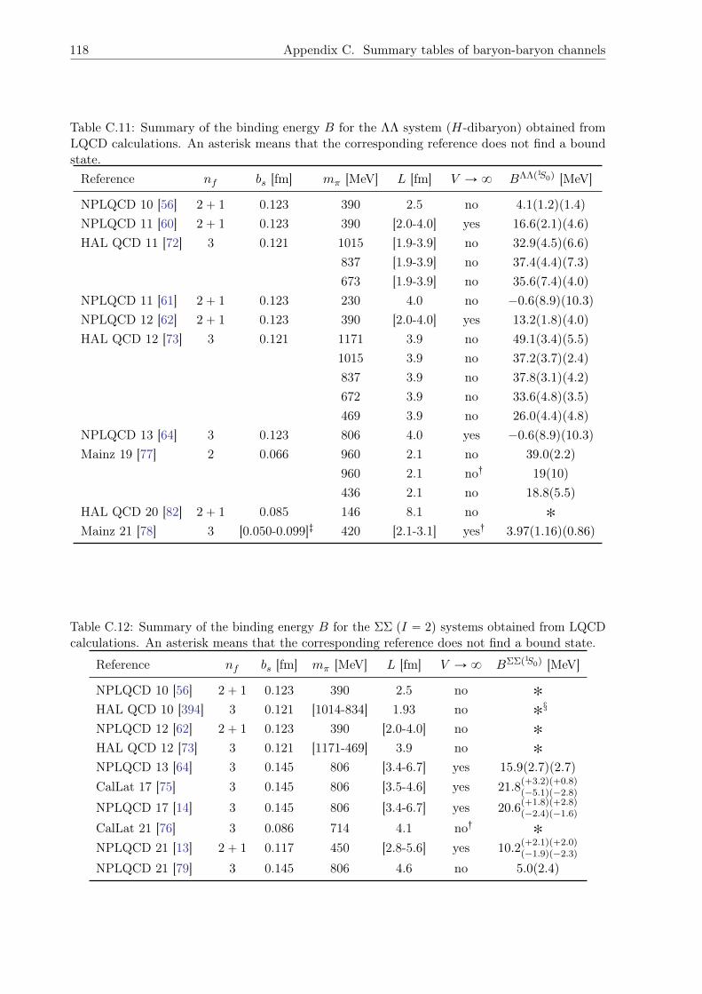
118 Appendix C. Summary tables of baryon-baryon channels
Table C.11: Summary of the binding energy B for the ΛΛ system (H-dibaryon) obtained fromLQCD calculations. An asterisk means that the corresponding reference does not find a boundstate.Reference nf bs [fm] mπ [MeV] L [fm] V Ñ8 BΛΛp1S0q [MeV]
NPLQCD 10 [56] 2` 1 0.123 390 2.5 no 4.1p1.2qp1.4q
NPLQCD 11 [60] 2` 1 0.123 390 [2.0-4.0] yes 16.6p2.1qp4.6q
HAL QCD 11 [72] 3 0.121 1015 [1.9-3.9] no 32.9p4.5qp6.6q
837 [1.9-3.9] no 37.4p4.4qp7.3q
673 [1.9-3.9] no 35.6p7.4qp4.0q
NPLQCD 11 [61] 2` 1 0.123 230 4.0 no ´0.6p8.9qp10.3q
NPLQCD 12 [62] 2` 1 0.123 390 [2.0-4.0] yes 13.2p1.8qp4.0q
HAL QCD 12 [73] 3 0.121 1171 3.9 no 49.1p3.4qp5.5q
1015 3.9 no 37.2p3.7qp2.4q
837 3.9 no 37.8p3.1qp4.2q
672 3.9 no 33.6p4.8qp3.5q
469 3.9 no 26.0p4.4qp4.8q
NPLQCD 13 [64] 3 0.123 806 4.0 yes ´0.6p8.9qp10.3q
Mainz 19 [77] 2 0.066 960 2.1 no 39.0p2.2q
960 2.1 no: 19p10q
436 2.1 no 18.8p5.5q
HAL QCD 20 [82] 2` 1 0.085 146 8.1 no ˚
Mainz 21 [78] 3 [0.050-0.099]; 420 [2.1-3.1] yes: 3.97p1.16qp0.86q
Table C.12: Summary of the binding energy B for the ΣΣ pI “ 2q systems obtained from LQCDcalculations. An asterisk means that the corresponding reference does not find a bound state.
Reference nf bs [fm] mπ [MeV] L [fm] V Ñ8 BΣΣp1S0q [MeV]
NPLQCD 10 [56] 2` 1 0.123 390 2.5 no ˚
HAL QCD 10 [394] 3 0.121 [1014-834] 1.93 no ˚§
NPLQCD 12 [62] 2` 1 0.123 390 [2.0-4.0] no ˚
HAL QCD 12 [73] 3 0.121 [1171-469] 3.9 no ˚
NPLQCD 13 [64] 3 0.145 806 [3.4-6.7] yes 15.9p2.7qp2.7q
CalLat 17 [75] 3 0.145 806 [3.5-4.6] yes 21.8p`3.2qp`0.8qp´5.1qp´2.8q
NPLQCD 17 [14] 3 0.145 806 [3.4-6.7] yes 20.6p`1.8qp`2.8qp´2.4qp´1.6q
CalLat 21 [76] 3 0.086 714 4.1 no: ˚
NPLQCD 21 [13] 2` 1 0.117 450 [2.8-5.6] yes 10.2p`2.1qp`2.0qp´1.9qp´2.3q
NPLQCD 21 [79] 3 0.145 806 4.6 no 5.0p2.4q
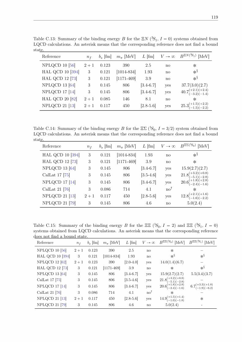
119
Table C.13: Summary of the binding energy B for the ΞN p3S1, I “ 0q systems obtained fromLQCD calculations. An asterisk means that the corresponding reference does not find a boundstate.
Reference nf bs [fm] mπ [MeV] L [fm] V Ñ8 BΞNp3S1q [MeV]
NPLQCD 10 [56] 2` 1 0.123 390 2.5 no ˚
HAL QCD 10 [394] 3 0.121 [1014-834] 1.93 no ˚§
HAL QCD 12 [73] 3 0.121 [1171-469] 3.9 no ˚§
NPLQCD 13 [64] 3 0.145 806 [3.4-6.7] yes 37.7p3.0qp2.7q
NPLQCD 17 [14] 3 0.145 806 [3.4-6.7] yes 40.7p`2.1qp`2.4qp´3.2qp´1.4q
HAL QCD 20 [82] 2` 1 0.085 146 8.1 no ˚
NPLQCD 21 [13] 2` 1 0.117 450 [2.8-5.6] yes 25.3p`1.5qp`2.2qp´1.5qp´2.2q
Table C.14: Summary of the binding energy B for the ΞΣ p1S0, I “ 32q system obtained fromLQCD calculations. An asterisk means that the corresponding reference does not find a boundstate.
Reference nf bs [fm] mπ [MeV] L [fm] V Ñ8 BΞΣp1S0q [MeV]
HAL QCD 10 [394] 3 0.121 [1014-834] 1.93 no ˚§
HAL QCD 12 [73] 3 0.121 [1171-469] 3.9 no ˚
NPLQCD 13 [64] 3 0.145 806 [3.4-6.7] yes 15.9p2.7qp2.7q
CalLat 17 [75] 3 0.145 806 [3.5-4.6] yes 21.8p`3.2qp`0.8qp´5.1qp´2.8q
NPLQCD 17 [14] 3 0.145 806 [3.4-6.7] yes 20.6p`1.8qp`2.8qp´2.4qp´1.6q
CalLat 21 [76] 3 0.086 714 4.1 no: ˚
NPLQCD 21 [13] 2` 1 0.117 450 [2.8-5.6] yes 12.8p`2.1qp`1.6qp´1.6qp´2.2q
NPLQCD 21 [79] 3 0.145 806 4.6 no 5.0p2.4q
Table C.15: Summary of the binding energy B for the ΞΞ p1S0, I “ 2q and ΞΞ p3S1, I “ 0qsystems obtained from LQCD calculations. An asterisk means that the corresponding referencedoes not find a bound state.Reference nf bs [fm] mπ [MeV] L [fm] V Ñ8 BΞΞp1S0q [MeV] BΞΞp3S1q [MeV]
NPLQCD 10 [56] 2` 1 0.123 390 2.5 no ˚ ´
HAL QCD 10 [394] 3 0.121 [1014-834] 1.93 no ˚§ ˚§
NPLQCD 12 [62] 2` 1 0.123 390 [2.0-4.0] yes 14.0p1.4qp6.7q ´
HAL QCD 12 [73] 3 0.121 [1171-469] 3.9 no ˚ ˚§
NPLQCD 13 [64] 3 0.145 806 [3.4-6.7] yes 15.9p2.7qp2.7q 5.5p3.4qp3.7q
CalLat 17 [75] 3 0.145 806 [3.5-4.6] yes 21.8p`3.2qp`0.8qp´5.1qp´2.8q ´
NPLQCD 17 [14] 3 0.145 806 [3.4-6.7] yes 20.6p`1.8qp`2.8qp´2.4qp´1.6q 6.7
p`3.3qp`1.8qp´1.9qp´6.2q
CalLat 21 [76] 3 0.086 714 4.1 no: ˚ ´
NPLQCD 21 [13] 2` 1 0.117 450 [2.8-5.6] yes 14.9p`1.5qp`1.4qp´1.0qp´1.8q ˚
NPLQCD 21 [79] 3 0.145 806 4.6 no 5.0p2.4q -

120 Appendix C. Summary tables of baryon-baryon channels
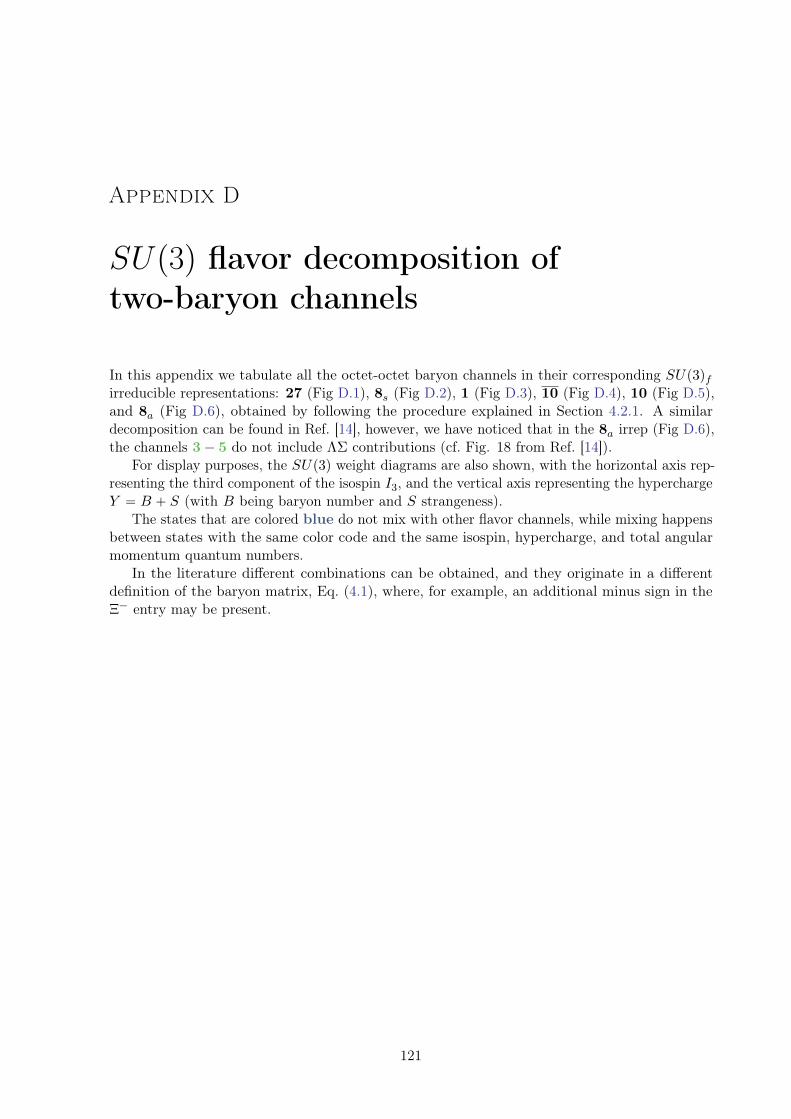
Appendix D
SUp3q flavor decomposition oftwo-baryon channels
In this appendix we tabulate all the octet-octet baryon channels in their corresponding SUp3qfirreducible representations: 27 (Fig D.1), 8s (Fig D.2), 1 (Fig D.3), 10 (Fig D.4), 10 (Fig D.5),and 8a (Fig D.6), obtained by following the procedure explained in Section 4.2.1. A similardecomposition can be found in Ref. [14], however, we have noticed that in the 8a irrep (Fig D.6),the channels 3´ 5 do not include ΛΣ contributions (cf. Fig. 18 from Ref. [14]).
For display purposes, the SUp3q weight diagrams are also shown, with the horizontal axis rep-resenting the third component of the isospin I3, and the vertical axis representing the hyperchargeY “ B ` S (with B being baryon number and S strangeness).
The states that are colored blue do not mix with other flavor channels, while mixing happensbetween states with the same color code and the same isospin, hypercharge, and total angularmomentum quantum numbers.
In the literature different combinations can be obtained, and they originate in a differentdefinition of the baryon matrix, Eq. (4.1), where, for example, an additional minus sign in theΞ´ entry may be present.
121
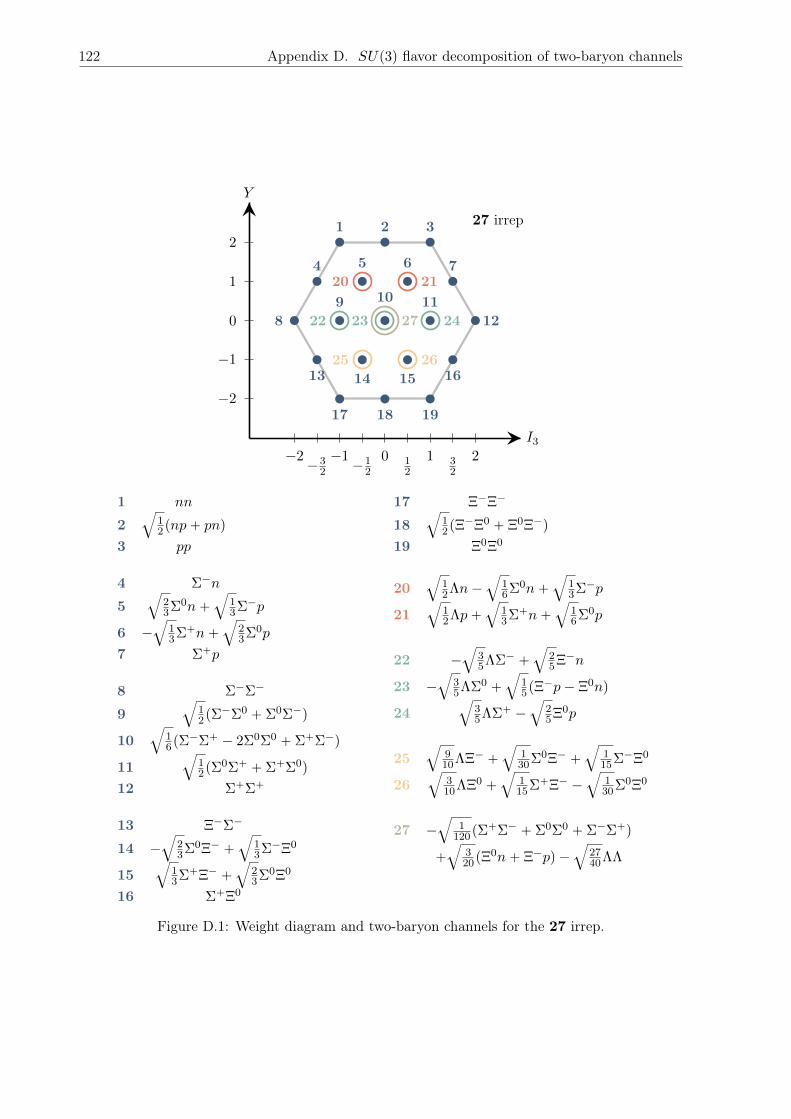
122 Appendix D. SUp3q flavor decomposition of two-baryon channels
1 2 3
4 5 6 7
89 10 11
12
13 14 15 16
17 18 19
20 21
22 23 24
25 26
27
I3
Y
210´1´2 32
12´1
2´32
2
1
0
´1
´2
27 irrep
1 nn
2b
12pnp` pnq
3 pp
4 Σ´n
5b
23Σ0n`
b
13Σ´p
6 ´
b
13Σ`n`
b
23Σ0p
7 Σ`p
8 Σ´Σ´
9b
12pΣ
´Σ0 ` Σ0Σ´q
10b
16pΣ
´Σ` ´ 2Σ0Σ0 ` Σ`Σ´q
11b
12pΣ
0Σ` ` Σ`Σ0q
12 Σ`Σ`
13 Ξ´Σ´
14 ´
b
23Σ0Ξ´ `
b
13Σ´Ξ0
15b
13Σ`Ξ´ `
b
23Σ0Ξ0
16 Σ`Ξ0
17 Ξ´Ξ´
18b
12pΞ
´Ξ0 ` Ξ0Ξ´q
19 Ξ0Ξ0
20b
12Λn´
b
16Σ0n`
b
13Σ´p
21b
12Λp`
b
13Σ`n`
b
16Σ0p
22 ´
b
35ΛΣ´ `
b
25Ξ´n
23 ´
b
35ΛΣ0 `
b
15pΞ
´p´ Ξ0nq
24b
35ΛΣ` ´
b
25Ξ0p
25b
910ΛΞ´ `
b
130Σ0Ξ´ `
b
115Σ´Ξ0
26b
310ΛΞ0 `
b
115Σ`Ξ´ ´
b
130Σ0Ξ0
27 ´
b
1120pΣ
`Σ´ ` Σ0Σ0 ` Σ´Σ`q
`
b
320pΞ
0n` Ξ´pq ´b
2740ΛΛ
Figure D.1: Weight diagram and two-baryon channels for the 27 irrep.
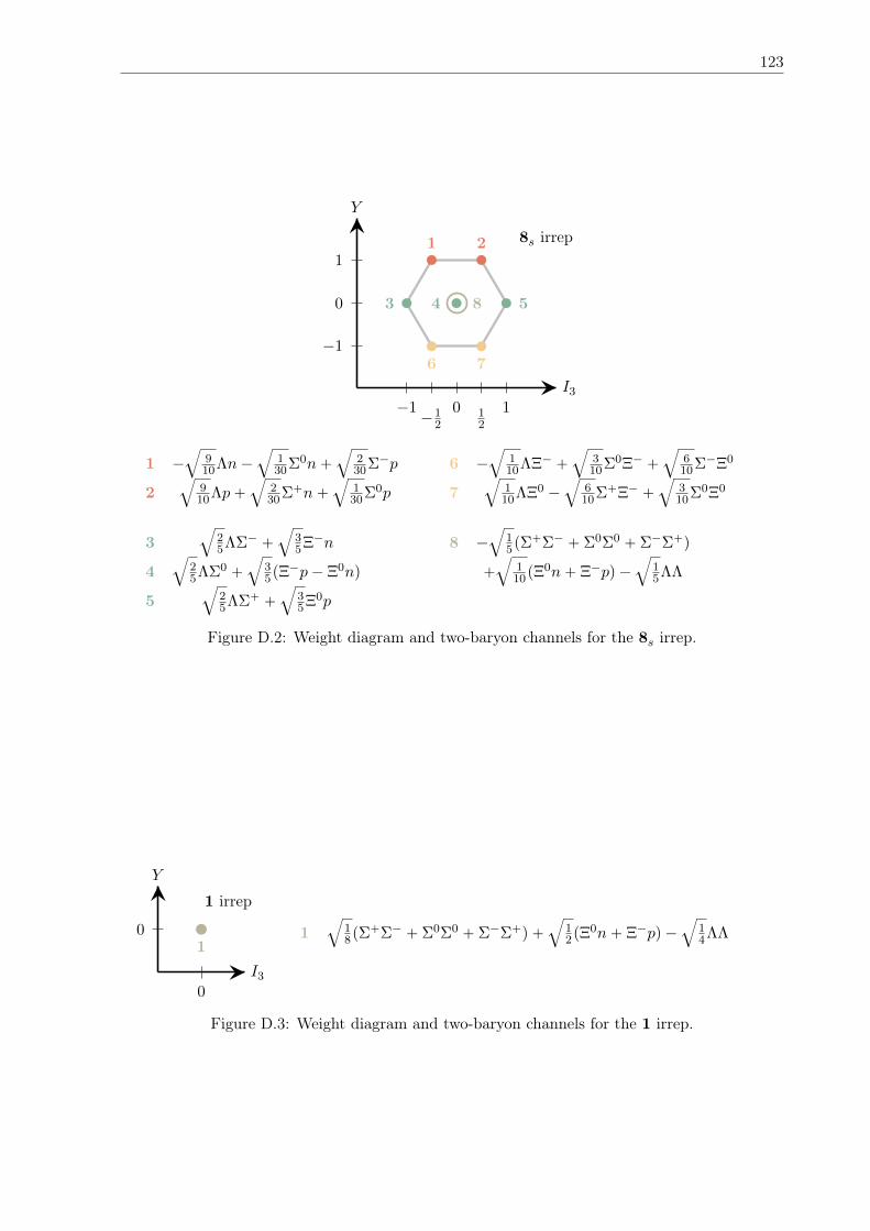
123
1 2
3 4 5
6 7
8
I3
Y
10´1 12´1
2
1
0
´1
8s irrep
1 ´
b
910Λn´
b
130Σ0n`
b
230Σ´p
2b
910Λp`
b
230Σ`n`
b
130Σ0p
3b
25ΛΣ´ `
b
35Ξ´n
4b
25ΛΣ0 `
b
35pΞ
´p´ Ξ0nq
5b
25ΛΣ` `
b
35Ξ0p
6 ´
b
110ΛΞ´ `
b
310Σ0Ξ´ `
b
610Σ´Ξ0
7b
110ΛΞ0 ´
b
610Σ`Ξ´ `
b
310Σ0Ξ0
8 ´
b
15pΣ
`Σ´ ` Σ0Σ0 ` Σ´Σ`q
`
b
110pΞ
0n` Ξ´pq ´b
15ΛΛ
Figure D.2: Weight diagram and two-baryon channels for the 8s irrep.
1I3
Y
0
0
1 irrep
1b
18pΣ
`Σ´ ` Σ0Σ0 ` Σ´Σ`q `b
12pΞ
0n` Ξ´pq ´b
14ΛΛ
Figure D.3: Weight diagram and two-baryon channels for the 1 irrep.
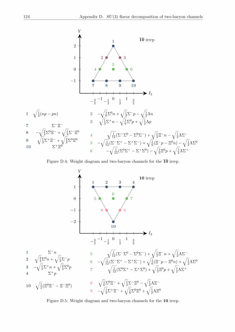
124 Appendix D. SUp3q flavor decomposition of two-baryon channels
1
2 3
45
6
7 8 9 10
I3
Y
10´1 32
12´1
2´32
2
1
0
´1
10 irrep
1b
12pnp´ pnq
7 Σ´Ξ´
8 ´
b
23Σ0Ξ´ `
b
13Σ´Ξ0
9b
13Σ`Ξ´ `
b
23Σ0Ξ0
10 Σ`Ξ0
2 ´
b
16Σ0n`
b
13Σ´p´
b
12Λn
3b
13Σ`n´
b
16Σ0p`
b
12Λp
4b
112pΣ
´Σ0 ´ Σ0Σ´q `b
13Ξ´n´
b
12ΛΣ´
5 ´
b
112pΣ
´Σ` ´ Σ`Σ´q `b
16pΞ
´p´ Ξ0nq ´b
12ΛΣ0
6 ´
b
112pΣ
0Σ` ´ Σ`Σ0q ´
b
13Ξ0p`
b
12ΛΣ`
Figure D.4: Weight diagram and two-baryon channels for the 10 irrep.
1 2 3 4
56
7
8 9
10I3
Y
10´1 32
12´1
2´32
1
0
´1
´2
10 irrep
1 Σ´n
2b
23Σ0n`
b
13Σ´p
3 ´
b
13Σ`n`
b
23Σ0p
4 Σ`p
10b
12pΞ
0Ξ´ ´ Ξ´Ξ0q
5b
112pΣ
´Σ0 ´ Σ0Σ´q `b
13Ξ´n`
b
12ΛΣ´
6 ´
b
112pΣ
´Σ` ´ Σ`Σ´q `b
16pΞ
´p´ Ξ0nq `b
12ΛΣ0
7b
112pΣ
0Σ` ´ Σ`Σ0q `
b
13Ξ0p`
b
12ΛΣ`
8b
16Σ0Ξ´ `
b
13Σ´Ξ0 ´
b
12ΛΞ´
9 ´
b
13Σ`Ξ´ `
b
16Σ0Ξ0 `
b
12ΛΞ0
Figure D.5: Weight diagram and two-baryon channels for the 10 irrep.
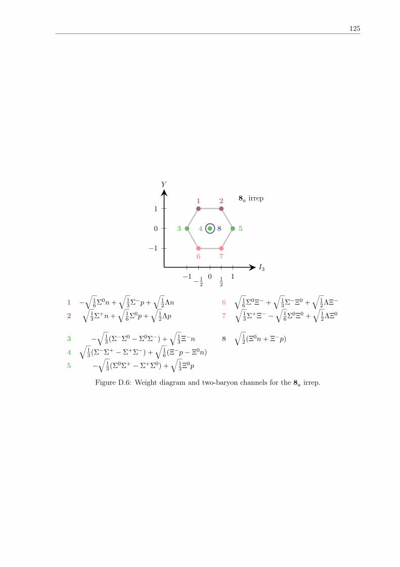
125
1 2
3 4 5
6 7
8
I3
Y
10´1 12´1
2
1
0
´1
8a irrep
1 ´
b
16Σ0n`
b
13Σ´p`
b
12Λn
2b
13Σ`n`
b
16Σ0p`
b
12Λp
3 ´
b
13pΣ
´Σ0 ´ Σ0Σ´q `b
13Ξ´n
4b
13pΣ
´Σ` ´ Σ`Σ´q `b
16pΞ
´p´ Ξ0nq
5 ´
b
13pΣ
0Σ` ´ Σ`Σ0q `
b
13Ξ0p
6b
16Σ0Ξ´ `
b
13Σ´Ξ0 `
b
12ΛΞ´
7b
13Σ`Ξ´ ´
b
16Σ0Ξ0 `
b
12ΛΞ0
8b
12pΞ
0n` Ξ´pq
Figure D.6: Weight diagram and two-baryon channels for the 8a irrep.

126 Appendix D. SUp3q flavor decomposition of two-baryon channels
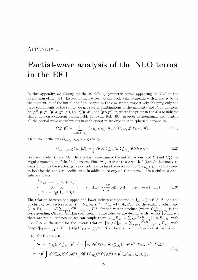
Appendix E
Partial-wave analysis of the NLO termsin the EFT
In this appendix we classify all the 19 SUp3qf -symmetric terms appearing at NLO in theLagrangian of Ref. [11]. Instead of derivatives, we will work with momenta, with p and p1 beingthe momentum of the initial and final baryon in the c.m. frame, respectively. Keeping only thelarge components of the spinor, we get several combinations of the momenta and Pauli matrices:p2, p12, p ¨p1, pp ¨σqpp1 ¨σ1q, pp ¨σqpp ¨σ1q, and ppˆp1q ¨σ, where the prime in the σ is to indicatethat it acts on a different baryon field. Following Ref. [492], in order to disentangle and identifyall the partial wave contributions in each operator, we expand it in spherical harmonics,
Opp,p1q “ÿ
LMLL1M 1
L
OLML;L1M 1Lp|p|, |p1|qYLML
ppqYL1M 1Lpp1q , (E.1)
where the coefficients OLML;L1M 1Lare given by
OLML;L1M 1Lp|p|, |p1|q “
ż
dp dp1 Y ˚LMLppqY ˚L1M 1
Lpp1qOpp,p1q . (E.2)
We have labeled L (and ML) the angular momentum of the initial baryons, and L1 (and M 1L) the
angular momentum of the final baryons. Since we just want to see which L (and L1) has non-zerocontribution to the scattering, we do not have to find the exact form of OLML;L1M 1
L, we only need
to look for the non-zero coefficients. In addition, to expand these terms, it is useful to use thespherical basis,
$
’
&
’
%
A`1 “ ´1?2pAx ` iAyq
A0 “ AzA´1 “
1?2pAx ´ iAyq
,
/
.
/
-
ñ Am “
c
4π
3|A|Y1mpAq , with m P t˘1, 0u . (E.3)
The relation between the upper and lower indices components is Am “ p´1qmA´m, and theproduct of two vectors is A ¨ B “
ř
mAmBm “
ř
mp´1qmAmB´m for the scalar product andpA ˆ Bqm “ ´i
?2ř
m1m2C1m
1m1;1m2Am1
Bm2 for the vector product (where CJMj1m1;j2m2is the
corresponding Clebsch-Gordan coefficient). Since here we are dealing with vectors (p and σ),these are rank 1 tensors, so we can couple them, Am1
Bm2“
ř
JM CJM1m1;1m2rA b BsJM , with
0 ď J ď 2 (the same for the inverse relation, rA b BsJM “ř
m1m2CJM1m1;1m2
Am1Bm2
, withrAbBs00 “ ´
1?3A ¨B or rAbBs1M “ i?
2pAˆBqM , for example). Let us look at each term:
(i) For the term p2,ż
dp dp1 Y ˚LMLppqY ˚L1M 1
Lpp1qp2 “
ż
dp dp1 Y ˚LMLppqY ˚L1M 1
Lpp1qp2
?4πY00ppq
?4πY00pp
1q
“ 4πp2
ż
dpY ˚LMLppqY00ppq
ż
dp1 Y ˚L1M 1Lpp1qY00pp
1q 9 p2δL0δML0δL10δM 1L0 .
(E.4)
127
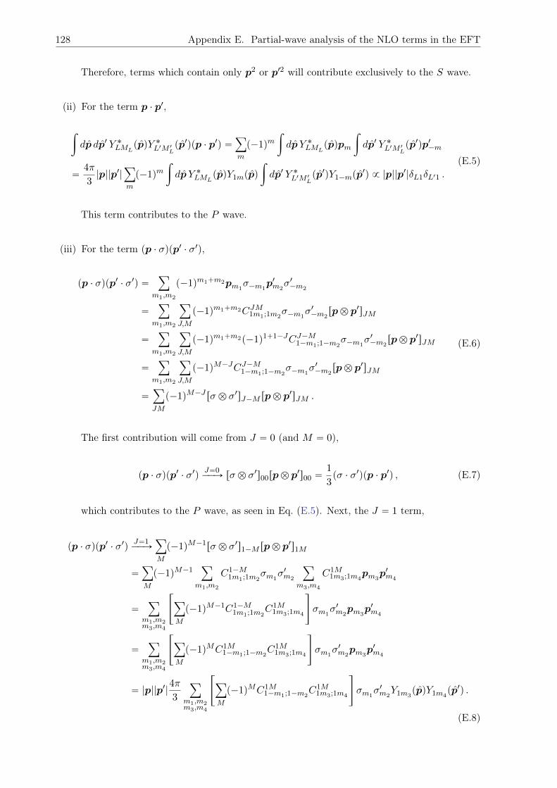
128 Appendix E. Partial-wave analysis of the NLO terms in the EFT
Therefore, terms which contain only p2 or p12 will contribute exclusively to the S wave.
(ii) For the term p ¨ p1,
ż
dp dp1 Y ˚LMLppqY ˚L1M 1
Lpp1qpp ¨ p1q “
ÿ
m
p´1qmż
dpY ˚LMLppqpm
ż
dp1 Y ˚L1M 1Lpp1qp1´m
“4π
3|p||p1|
ÿ
m
p´1qmż
dpY ˚LMLppqY1mppq
ż
dp1 Y ˚L1M 1Lpp1qY1´mpp
1q 9 |p||p1|δL1δL11 .
(E.5)
This term contributes to the P wave.
(iii) For the term pp ¨ σqpp1 ¨ σ1q,
pp ¨ σqpp1 ¨ σ1q “ÿ
m1,m2
p´1qm1`m2pm1σ´m1
p1m2σ1´m2
“ÿ
m1,m2
ÿ
J,M
p´1qm1`m2CJM1m1;1m2σ´m1
σ1´m2rpb p1sJM
“ÿ
m1,m2
ÿ
J,M
p´1qm1`m2p´1q1`1´JCJ´M1´m1;1´m2σ´m1
σ1´m2rpb p1sJM
“ÿ
m1,m2
ÿ
J,M
p´1qM´JCJ´M1´m1;1´m2σ´m1
σ1´m2rpb p1sJM
“ÿ
JM
p´1qM´J rσ b σ1sJ´M rpb p1sJM .
(E.6)
The first contribution will come from J “ 0 (and M “ 0),
pp ¨ σqpp1 ¨ σ1qJ“0ÝÝÑ rσ b σ1s00rpb p
1s00 “1
3pσ ¨ σ1qpp ¨ p1q , (E.7)
which contributes to the P wave, as seen in Eq. (E.5). Next, the J “ 1 term,
pp ¨ σqpp1 ¨ σ1qJ“1ÝÝÑ
ÿ
M
p´1qM´1rσ b σ1s1´M rpb p1s1M
“ÿ
M
p´1qM´1ÿ
m1,m2
C1´M1m1;1m2
σm1σ1m2
ÿ
m3,m4
C1M1m3;1m4
pm3p1m4
“ÿ
m1,m2m3,m4
«
ÿ
M
p´1qM´1C1´M1m1;1m2
C1M1m3;1m4
ff
σm1σ1m2
pm3p1m4
“ÿ
m1,m2m3,m4
«
ÿ
M
p´1qMC1M1´m1;1´m2
C1M1m3;1m4
ff
σm1σ1m2
pm3p1m4
“ |p||p1|4π
3
ÿ
m1,m2m3,m4
«
ÿ
M
p´1qMC1M1´m1;1´m2
C1M1m3;1m4
ff
σm1σ1m2
Y1m3ppqY1m4
pp1q .
(E.8)
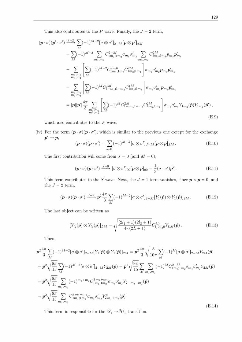
129
This also contributes to the P wave. Finally, the J “ 2 term,
pp ¨ σqpp1 ¨ σ1qJ“2ÝÝÑ
ÿ
M
p´1qM´2rσ b σ1s2´M rpb p1s2M
“ÿ
M
p´1qM´2ÿ
m1,m2
C2´M1m1;1m2
σm1σ1m2
ÿ
m3,m4
C2M1m3;1m4
pm3p1m4
“ÿ
m1,m2m3,m4
«
ÿ
M
p´1qM´2C2´M1m1;1m2
C2M1m3;1m4
ff
σm1σ1m2
pm3p1m4
“ÿ
m1,m2m3,m4
«
ÿ
M
p´1qMC1M1´m1;1´m2
C1M1m3;1m4
ff
σm1σ1m2
pm3p1m4
“ |p||p1|4π
3
ÿ
m1,m2m3,m4
«
ÿ
M
p´1qMC2M1´m1;1´m2
C2M1m3;1m4
ff
σm1σ1m2
Y1m3ppqY1m4
pp1q ,
(E.9)which also contributes to the P wave.
(iv) For the term pp ¨ σqpp ¨ σ1q, which is similar to the previous one except for the exchangep1 Ñ p,
pp ¨ σqpp ¨ σ1q “ÿ
J,M
p´1qM´J rσ b σ1sJ´M rpb psJM . (E.10)
The first contribution will come from J “ 0 (and M “ 0),
pp ¨ σqpp ¨ σ1qJ“0ÝÝÑ rσ b σ1s00rpb ps00 “
1
3pσ ¨ σ1qp2 . (E.11)
This term contributes to the S wave. Next, the J “ 1 term vanishes, since pˆ p “ 0, andthe J “ 2 term,
pp ¨ σqpp ¨ σ1qJ“2ÝÝÑ p2 4π
3
ÿ
M
p´1qM´2rσ b σ1s2´M rY1ppq b Y1ppqs2M . (E.12)
The last object can be written as
rYl1ppq b Yl2ppqsLM “
d
p2l1 ` 1qp2l2 ` 1q
4πp2L` 1qCL0l10;l20YLM ppq . (E.13)
Then,
p2 4π
3
ÿ
M
p´1qM´2rσ b σ1s2´M rY1ppq b Y1ppqs2M “ p2 4π
3
c
3
10π
ÿ
M
p´1qM rσ b σ1s2´MY2M ppq
“ p2
c
8π
15
ÿ
M
p´1qM´2rσ b σ1s2´MY2M ppq “ p2
c
8π
15
ÿ
M
ÿ
m1,m2
p´1qMC2´M1m1;1m2
σm1σ1m2
Y2M ppq
“ p2
c
8π
15
ÿ
m1,m2
p´1qm1`m2C2m1`m21m1;1m2
σm1σ1m2
Y2´m1´m2ppq
“ p2
c
8π
15
ÿ
m1,m2
C2m1`m21m1;1m2
σm1σ1m2
Y ˚2m1`m2ppq .
(E.14)This term is responsible for the 3S1 Ñ
3D1 transition.

130 Appendix E. Partial-wave analysis of the NLO terms in the EFT
(v) For the term ppˆ p1q ¨ σ,
ppˆ p1q ¨ σ “ ´i?
2ÿ
m1,m2,m3
p´1qm3C1m31m1;1m2
pm1p1m2
σ´m3
“ ´i?
2|p||p1|4π
3
ÿ
m1,m2,m3
p´1qm3C1m31m1;1m2
Y1m1ppqY1m2
pp1qσ´m3,
(E.15)
which is responsible for the 1P1 Ñ3P1 transition.
After analyzing all the terms, the ones that contribute to the S wave contain p2 and p12, so theLagrangian will only contain second derivatives, as written in Eq. (4.15).
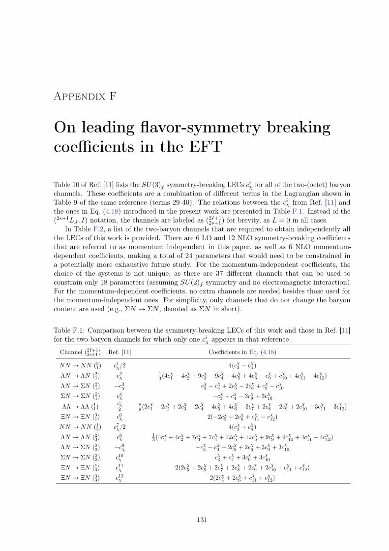
Appendix F
On leading flavor-symmetry breakingcoefficients in the EFT
Table 10 of Ref. [11] lists the SUp3qf symmetry-breaking LECs ciχ for all of the two-(octet) baryonchannels. These coefficients are a combination of different terms in the Lagrangian shown inTable 9 of the same reference (terms 29-40). The relations between the ciχ from Ref. [11] andthe ones in Eq. (4.18) introduced in the present work are presented in Table F.1. Instead of thep2s`1LJ , Iq notation, the channels are labeled as p2I`1
2s`1q for brevity, as L “ 0 in all cases.In Table F.2, a list of the two-baryon channels that are required to obtain independently all
the LECs of this work is provided. There are 6 LO and 12 NLO symmetry-breaking coefficientsthat are referred to as momentum independent in this paper, as well as 6 NLO momentum-dependent coefficients, making a total of 24 parameters that would need to be constrained ina potentially more exhaustive future study. For the momentum-independent coefficients, thechoice of the systems is not unique, as there are 37 different channels that can be used toconstrain only 18 parameters (assuming SUp2qf symmetry and no electromagnetic interaction).For the momentum-dependent coefficients, no extra channels are needed besides those used forthe momentum-independent ones. For simplicity, only channels that do not change the baryoncontent are used (e.g., ΣN Ñ ΣN , denoted as ΣN in short).
Table F.1: Comparison between the symmetry-breaking LECs of this work and those in Ref. [11]for the two-baryon channels for which only one ciχ appears in that reference.
Channel p2I`12s`1q Ref. [11] Coefficients in Eq. (4.18)
NN Ñ NN p31q c1χ2 4pcχ3 ´ c
χ4 q
ΛN Ñ ΛN p21q c2χ
13p4c
χ1 ´ 4cχ2 ` 9cχ3 ´ 9cχ4 ´ 4cχ5 ` 4cχ6 ´ c
χ9 ` c
χ10 ` 4cχ11 ´ 4cχ12q
ΛN Ñ ΣN p21q ´c3χ cχ3 ´ c
χ4 ` 2cχ5 ´ 2cχ6 ` c
χ9 ´ c
χ10
ΣN Ñ ΣN p21q c4χ ´cχ3 ` c
χ4 ´ 3cχ9 ` 3cχ10
ΛΛ Ñ ΛΛ p11qc5χ2
89p2c
χ1 ´ 2cχ2 ` 2cχ3 ´ 2cχ4 ´ 4cχ5 ` 4cχ6 ´ 2cχ7 ` 2cχ8 ´ 2cχ9 ` 2cχ10 ` 3cχ11 ´ 3cχ12q
ΞN Ñ ΞN p31q c6χ 2p´2cχ5 ` 2cχ6 ` c
χ11 ´ c
χ12q
NN Ñ NN p13q c7χ2 4pcχ3 ` c
χ4 q
ΛN Ñ ΛN p23q c8χ
13p4c
χ1 ` 4cχ2 ` 7cχ3 ` 7cχ4 ` 12cχ5 ` 12cχ6 ` 9cχ9 ` 9cχ10 ` 4cχ11 ` 4cχ12q
ΛN Ñ ΣN p23q ´c9χ ´cχ3 ´ c
χ4 ` 2cχ5 ` 2cχ6 ` 3cχ9 ` 3cχ10
ΣN Ñ ΣN p23q c10χ cχ3 ` c
χ4 ` 3cχ9 ` 3cχ10
ΞN Ñ ΞN p13q c11χ 2p2cχ5 ` 2cχ6 ` 2cχ7 ` 2cχ8 ` 2cχ9 ` 2cχ10 ` c
χ11 ` c
χ12q
ΞN Ñ ΞN p33q c12χ 2p2cχ5 ` 2cχ6 ` c
χ11 ` c
χ12q
131
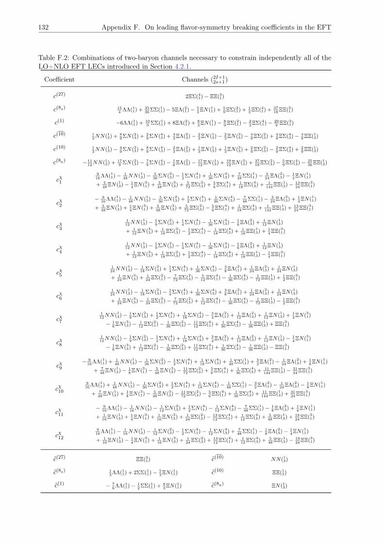
132 Appendix F. On leading flavor-symmetry breaking coefficients in the EFT
Table F.2: Combinations of two-baryon channels necessary to constrain independently all of theLO+NLO EFT LECs introduced in Section 4.2.1.
Coefficient Channels p2I`12s`1q
cp27q 2ΞΣp41q ´ ΞΞp31q
cp8sq 154
ΛΛp11q `3536
ΣΣp11q ´ 5ΞΛp21q ´53ΞNp11q `
59ΞΣp21q `
13ΞΣp41q `
3718
ΞΞp31q
cp1q ´6ΛΛp11q `109
ΣΣp11q ` 8ΞΛp21q `83ΞNp11q ´
89ΞΣp21q ´
23ΞΣp41q ´
299
ΞΞp31q
cp10q 13NNp13q `
89ΣNp23q `
29ΣNp43q `
43ΞΛp23q ´
23ΞNp13q ´
23ΞNp33q ´
49ΞΣp23q `
49ΞΣp43q ´
49ΞΞp13q
cp10q 13NNp13q ´
49ΣNp23q `
89ΣNp43q ´
23ΞΛp23q `
13ΞNp13q `
13ΞNp33q `
29ΞΣp23q ´
29ΞΣp43q `
29ΞΞp13q
cp8aq ´ 1112NNp13q `
179
ΣNp23q ´79ΣNp43q ´
16ΞΛp23q ´
1712
ΞNp13q `1912
ΞNp33q `3718
ΞΣp23q ´59ΞΣp43q ´
2536
ΞΞp13q
cχ1
916
ΛΛp11q ´148NNp13q ´
536
ΣNp23q ´12ΣNp41q `
136
ΣNp43q `748
ΣΣp11q ´524
ΞΛp23q ´14ΞNp11q
` 548
ΞNp13q ´14ΞNp31q `
548
ΞNp33q `572
ΞΣp23q `56ΞΣp41q `
118
ΞΣp43q `1
144ΞΞp13q ´
1324
ΞΞp31q
cχ2´ 9
16ΛΛp11q ´
148NNp13q ´
536
ΣNp23q `12ΣNp41q `
136
ΣNp43q ´748
ΣΣp11q ´524
ΞΛp23q `14ΞNp11q
` 548
ΞNp13q `14ΞNp31q `
548
ΞNp33q `572
ΞΣp23q ´56ΞΣp41q `
118
ΞΣp43q `1
144ΞΞp13q `
1324
ΞΞp31q
cχ3
112NNp13q ´
19ΣNp23q `
14ΣNp41q ´
136
ΣNp43q ´16ΞΛp23q `
112
ΞNp13q
` 112
ΞNp33q `118
ΞΣp23q ´12ΞΣp41q ´
118
ΞΣp43q `118
ΞΞp13q `14ΞΞp31q
cχ4
112NNp13q ´
19ΣNp23q ´
14ΣNp41q ´
136
ΣNp43q ´16ΞΛp23q `
112
ΞNp13q
` 112
ΞNp33q `118
ΞΣp23q `12ΞΣp41q ´
118
ΞΣp43q `118
ΞΞp13q ´14ΞΞp31q
cχ5
124NNp13q ´
118
ΣNp23q `14ΣNp41q `
136
ΣNp43q ´38ΞΛp21q `
124
ΞΛp23q `124
ΞNp13q
` 124
ΞNp33q `124
ΞΣp21q ´772
ΞΣp23q ´512
ΞΣp41q ´136
ΞΣp43q ´172
ΞΞp13q `12ΞΞp31q
cχ6
124NNp13q ´
118
ΣNp23q ´14ΣNp41q `
136
ΣNp43q `38ΞΛp21q `
124
ΞΛp23q `124
ΞNp13q
` 124
ΞNp33q ´124
ΞΣp21q ´772
ΞΣp23q `512
ΞΣp41q ´136
ΞΣp43q ´172
ΞΞp13q ´12ΞΞp31q
cχ7
112NNp13q ´
19ΣNp23q `
12ΣNp41q `
118
ΣNp43q ´34ΞΛp21q `
112
ΞΛp23q `112
ΞNp13q `14ΞNp31q
´ 16ΞNp33q ´
112
ΞΣp21q ´136
ΞΣp23q ´1112
ΞΣp41q `136
ΞΣp43q ´136
ΞΞp13q ` ΞΞp31q
cχ8
112NNp13q ´
19ΣNp23q ´
12ΣNp41q `
118
ΣNp43q `34ΞΛp21q `
112
ΞΛp23q `112
ΞNp13q ´14ΞNp31q
´ 16ΞNp33q `
112
ΞΣp21q ´136
ΞΣp23q `1112
ΞΣp41q `136
ΞΣp43q ´136
ΞΞp13q ´ ΞΞp31q
cχ9´ 9
16ΛΛp11q `
148NNp13q ´
136
ΣNp23q ´12ΣNp41q `
118
ΣNp43q `148
ΣΣp11q `32ΞΛp21q ´
124
ΞΛp23q `18ΞNp11q
` 748
ΞNp13q ´18ΞNp31q ´
548
ΞNp33q ´1172
ΞΣp23q `56ΞΣp41q `
136
ΞΣp43q `11144
ΞΞp13q ´3124
ΞΞp31q
cχ10
916
ΛΛp11q `148NNp13q ´
136
ΣNp23q `12ΣNp41q `
118
ΣNp43q ´148
ΣΣp11q ´32ΞΛp21q ´
124
ΞΛp23q ´18ΞNp11q
` 748
ΞNp13q `18ΞNp31q ´
548
ΞNp33q ´1172
ΞΣp23q ´56ΞΣp41q `
136
ΞΣp43q `11144
ΞΞp13q `3124
ΞΞp31q
cχ11
´ 916
ΛΛp11q ´116NNp13q ´
112
ΣNp23q `12ΣNp41q ´
112
ΣNp43q ´748
ΣΣp11q ´18ΞΛp23q `
14ΞNp11q
` 116
ΞNp13q `14ΞNp31q `
116
ΞNp33q `124
ΞΣp23q ´1312
ΞΣp41q `112
ΞΣp43q `548
ΞΞp13q `1924
ΞΞp31q
cχ12
916
ΛΛp11q ´116NNp13q ´
112
ΣNp23q ´12ΣNp41q ´
112
ΣNp43q `748
ΣΣp11q ´18ΞΛp23q ´
14ΞNp11q
` 116
ΞNp13q ´14ΞNp31q `
116
ΞNp33q `124
ΞΣp23q `1312
ΞΣp41q `112
ΞΣp43q `548
ΞΞp13q ´1924
ΞΞp31q
cp27q ΞΞp31q cp10q NNp13q
cp8sq 13ΛΛp11q ` 2ΣΣp11q ´
53ΞNp11q cp10q ΞΞp13q
cp1q ´ 76ΛΛp11q ´
12ΣΣp11q `
83ΞNp11q cp8aq ΞNp13q
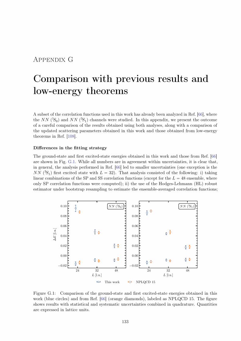
Appendix G
Comparison with previous results andlow-energy theorems
A subset of the correlation functions used in this work has already been analyzed in Ref. [66], wherethe NN p1S0q and NN p3S1q channels were studied. In this appendix, we present the outcomeof a careful comparison of the results obtained using both analyses, along with a comparison ofthe updated scattering parameters obtained in this work and those obtained from low-energytheorems in Ref. [108].
Differences in the fitting strategy
The ground-state and first excited-state energies obtained in this work and those from Ref. [66]are shown in Fig. G.1. While all numbers are in agreement within uncertainties, it is clear that,in general, the analysis performed in Ref. [66] led to smaller uncertainties (one exception is theNN p3S1q first excited state with L “ 32). That analysis consisted of the following: i) takinglinear combinations of the SP and SS correlation functions (except for the L “ 48 ensemble, whereonly SP correlation functions were computed); ii) the use of the Hodges-Lehmann (HL) robustestimator under bootstrap resampling to estimate the ensemble-averaged correlation functions;
24 32 48
L [l.u.]
−0.02
0.00
0.02
0.04
0.06
0.08
0.10
∆E
[l.u.]
NN (1S0)
24 32 48
L [l.u.]
−0.02
0.00
0.02
0.04
0.06
0.08
0.10 NN (3S1)
This work NPLQCD 15
Figure G.1: Comparison of the ground-state and first excited-state energies obtained in thiswork (blue circles) and from Ref. [66] (orange diamonds), labeled as NPLQCD 15. The figureshows results with statistical and systematic uncertainties combined in quadrature. Quantitiesare expressed in lattice units.
133
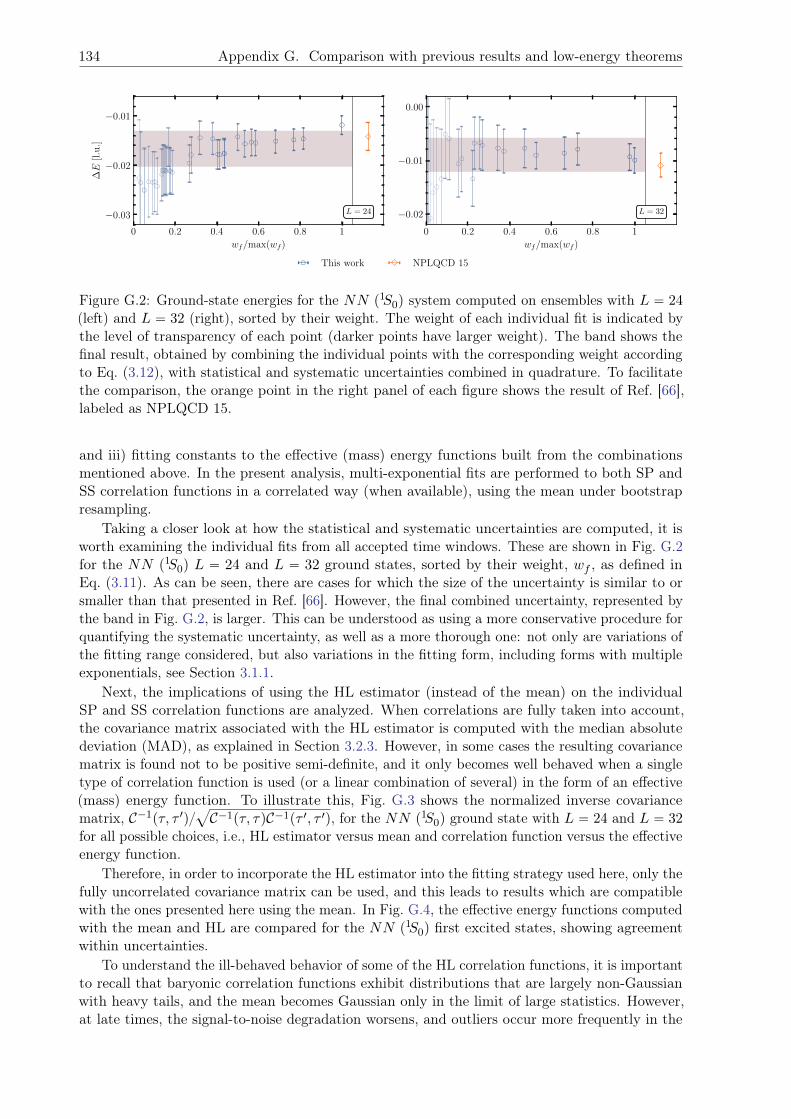
134 Appendix G. Comparison with previous results and low-energy theorems
0 0.2 0.4 0.6 0.8 1
wf/max(wf )
−0.03
−0.02
−0.01
∆E
[l.u.]
L = 24
0 0.2 0.4 0.6 0.8 1
wf/max(wf )
−0.02
−0.01
0.00
L = 32
This work NPLQCD 15
Figure G.2: Ground-state energies for the NN p1S0q system computed on ensembles with L “ 24(left) and L “ 32 (right), sorted by their weight. The weight of each individual fit is indicated bythe level of transparency of each point (darker points have larger weight). The band shows thefinal result, obtained by combining the individual points with the corresponding weight accordingto Eq. (3.12), with statistical and systematic uncertainties combined in quadrature. To facilitatethe comparison, the orange point in the right panel of each figure shows the result of Ref. [66],labeled as NPLQCD 15.
and iii) fitting constants to the effective (mass) energy functions built from the combinationsmentioned above. In the present analysis, multi-exponential fits are performed to both SP andSS correlation functions in a correlated way (when available), using the mean under bootstrapresampling.
Taking a closer look at how the statistical and systematic uncertainties are computed, it isworth examining the individual fits from all accepted time windows. These are shown in Fig. G.2for the NN p1S0q L “ 24 and L “ 32 ground states, sorted by their weight, wf , as defined inEq. (3.11). As can be seen, there are cases for which the size of the uncertainty is similar to orsmaller than that presented in Ref. [66]. However, the final combined uncertainty, represented bythe band in Fig. G.2, is larger. This can be understood as using a more conservative procedure forquantifying the systematic uncertainty, as well as a more thorough one: not only are variations ofthe fitting range considered, but also variations in the fitting form, including forms with multipleexponentials, see Section 3.1.1.
Next, the implications of using the HL estimator (instead of the mean) on the individualSP and SS correlation functions are analyzed. When correlations are fully taken into account,the covariance matrix associated with the HL estimator is computed with the median absolutedeviation (MAD), as explained in Section 3.2.3. However, in some cases the resulting covariancematrix is found not to be positive semi-definite, and it only becomes well behaved when a singletype of correlation function is used (or a linear combination of several) in the form of an effective(mass) energy function. To illustrate this, Fig. G.3 shows the normalized inverse covariancematrix, C´1pτ, τ 1q
a
C´1pτ, τqC´1pτ 1, τ 1q, for the NN p1S0q ground state with L “ 24 and L “ 32for all possible choices, i.e., HL estimator versus mean and correlation function versus the effectiveenergy function.
Therefore, in order to incorporate the HL estimator into the fitting strategy used here, only thefully uncorrelated covariance matrix can be used, and this leads to results which are compatiblewith the ones presented here using the mean. In Fig. G.4, the effective energy functions computedwith the mean and HL are compared for the NN p1S0q first excited states, showing agreementwithin uncertainties.
To understand the ill-behaved behavior of some of the HL correlation functions, it is importantto recall that baryonic correlation functions exhibit distributions that are largely non-Gaussianwith heavy tails, and the mean becomes Gaussian only in the limit of large statistics. However,at late times, the signal-to-noise degradation worsens, and outliers occur more frequently in the
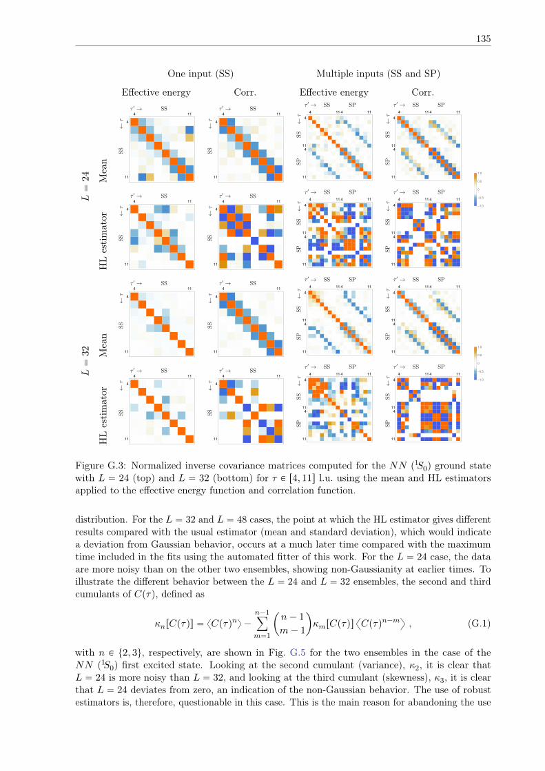
135
One input (SS) Multiple inputs (SS and SP)
Effective energy Corr. Effective energy Corr.
-1.0
-0.5
0
0.5
1.0
L“
24
Mean
4
11
4 11
4
11
4 114
114
11
4 11 4 11
4
114
11
4 11 4 11
HLestimator
4
11
4 11
4
11
4 114
114
11
4 11 4 11
4
114
11
4 11 4 11
L“
32 Mean
4
11
4 11
4
11
4 114
114
11
4 11 4 11
4
114
11
4 11 4 11
-1.0
-0.5
0
0.5
1.0
HLestimator
4
11
4 11
4
11
4 114
114
11
4 11 4 11
4
114
11
4 11 4 11
Figure G.3: Normalized inverse covariance matrices computed for the NN p1S0q ground statewith L “ 24 (top) and L “ 32 (bottom) for τ P r4, 11s l.u. using the mean and HL estimatorsapplied to the effective energy function and correlation function.
distribution. For the L “ 32 and L “ 48 cases, the point at which the HL estimator gives differentresults compared with the usual estimator (mean and standard deviation), which would indicatea deviation from Gaussian behavior, occurs at a much later time compared with the maximumtime included in the fits using the automated fitter of this work. For the L “ 24 case, the dataare more noisy than on the other two ensembles, showing non-Gaussianity at earlier times. Toillustrate the different behavior between the L “ 24 and L “ 32 ensembles, the second and thirdcumulants of Cpτq, defined as
κnrCpτqs “ xCpτqny ´
n´1ÿ
m“1
ˆ
n´ 1
m´ 1
˙
κmrCpτqs@
Cpτqn´mD
, (G.1)
with n P t2, 3u, respectively, are shown in Fig. G.5 for the two ensembles in the case of theNN p1S0q first excited state. Looking at the second cumulant (variance), κ2, it is clear thatL “ 24 is more noisy than L “ 32, and looking at the third cumulant (skewness), κ3, it is clearthat L “ 24 deviates from zero, an indication of the non-Gaussian behavior. The use of robustestimators is, therefore, questionable in this case. This is the main reason for abandoning the use
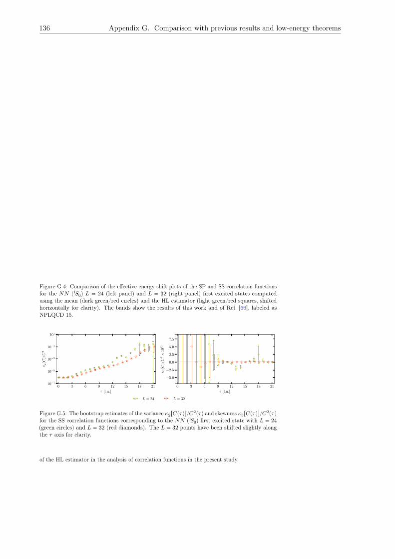
136 Appendix G. Comparison with previous results and low-energy theorems
4 6 8 10 12 14 16
τ [l.u.]
0.08
0.10
0.12
0.14
0.16
0.18∆E
[l.u.]
SP, L = 24
4 6 8 10 12 14 16
τ [l.u.]
0.02
0.04
0.06
0.08
0.10
0.12
0.14 SP, L = 32
4 6 8 10 12 14 16
τ [l.u.]
0.08
0.10
0.12
0.14
0.16
0.18
∆E
[l.u.]
SS, L = 24
4 6 8 10 12 14 16
τ [l.u.]
0.02
0.04
0.06
0.08
0.10
0.12
0.14 SS, L = 32
Mean
Hodges-Lehmann estimator
This work
NPLQCD 15
Figure G.4: Comparison of the effective energy-shift plots of the SP and SS correlation functionsfor the NN p1S0q L “ 24 (left panel) and L “ 32 (right panel) first excited states computedusing the mean (dark green/red circles) and the HL estimator (light green/red squares, shiftedhorizontally for clarity). The bands show the results of this work and of Ref. [66], labeled asNPLQCD 15.
0 3 6 9 12 15 18 21
τ [l.u.]
10−7
10−5
10−3
10−1
101
κ2(C
)/C
2
0 3 6 9 12 15 18 21
τ [l.u.]
−5.0
−2.5
0.0
2.5
5.0
7.5
κ3(C
)/C
2×
1021
L = 24 L = 32
Figure G.5: The bootstrap estimates of the variance κ2rCpτqsC2pτq and skewness κ3rCpτqsC
2pτqfor the SS correlation functions corresponding to the NN p1S0q first excited state with L “ 24(green circles) and L “ 32 (red diamonds). The L “ 32 points have been shifted slightly alongthe τ axis for clarity.
of the HL estimator in the analysis of correlation functions in the present study.
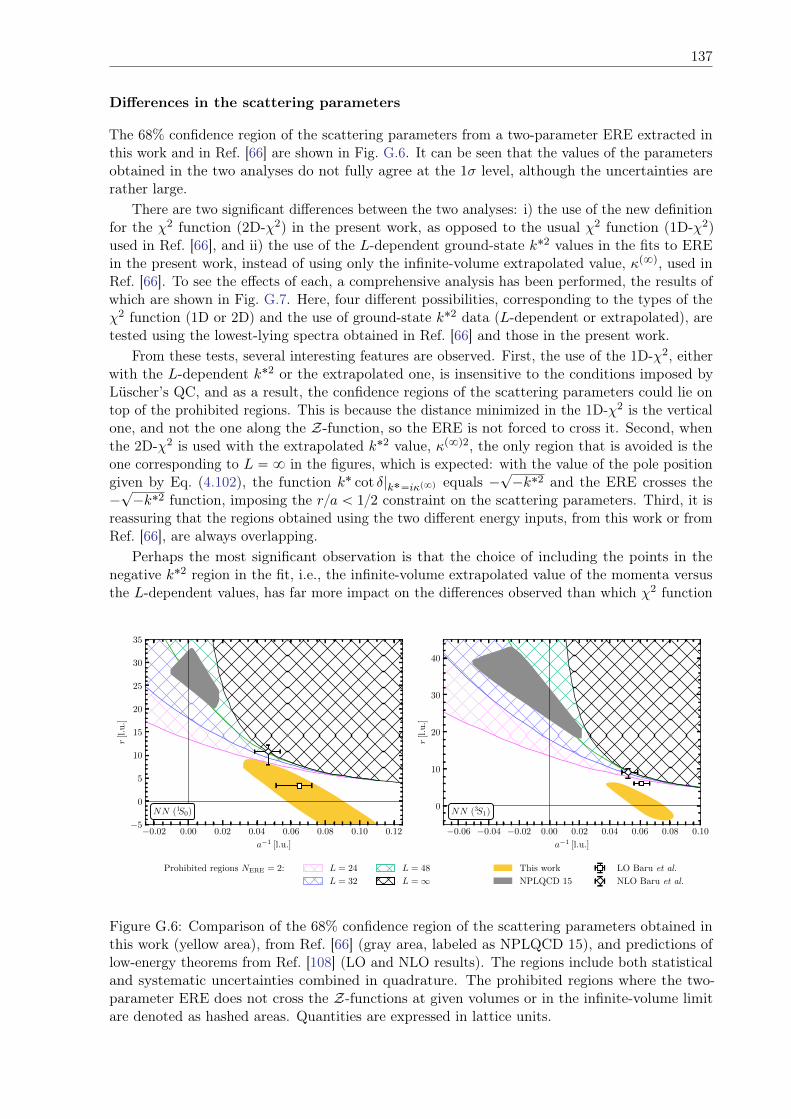
137
Differences in the scattering parameters
The 68% confidence region of the scattering parameters from a two-parameter ERE extracted inthis work and in Ref. [66] are shown in Fig. G.6. It can be seen that the values of the parametersobtained in the two analyses do not fully agree at the 1σ level, although the uncertainties arerather large.
There are two significant differences between the two analyses: i) the use of the new definitionfor the χ2 function (2D-χ2) in the present work, as opposed to the usual χ2 function (1D-χ2)used in Ref. [66], and ii) the use of the L-dependent ground-state k˚2 values in the fits to EREin the present work, instead of using only the infinite-volume extrapolated value, κp8q, used inRef. [66]. To see the effects of each, a comprehensive analysis has been performed, the results ofwhich are shown in Fig. G.7. Here, four different possibilities, corresponding to the types of theχ2 function (1D or 2D) and the use of ground-state k˚2 data (L-dependent or extrapolated), aretested using the lowest-lying spectra obtained in Ref. [66] and those in the present work.
From these tests, several interesting features are observed. First, the use of the 1D-χ2, eitherwith the L-dependent k˚2 or the extrapolated one, is insensitive to the conditions imposed byLüscher’s QC, and as a result, the confidence regions of the scattering parameters could lie ontop of the prohibited regions. This is because the distance minimized in the 1D-χ2 is the verticalone, and not the one along the Z-function, so the ERE is not forced to cross it. Second, whenthe 2D-χ2 is used with the extrapolated k˚2 value, κp8q2, the only region that is avoided is theone corresponding to L “ 8 in the figures, which is expected: with the value of the pole positiongiven by Eq. (4.102), the function k˚ cot δ|k˚“iκp8q equals ´
?´k˚2 and the ERE crosses the
´?´k˚2 function, imposing the ra ă 12 constraint on the scattering parameters. Third, it is
reassuring that the regions obtained using the two different energy inputs, from this work or fromRef. [66], are always overlapping.
Perhaps the most significant observation is that the choice of including the points in thenegative k˚2 region in the fit, i.e., the infinite-volume extrapolated value of the momenta versusthe L-dependent values, has far more impact on the differences observed than which χ2 function
−0.02 0.00 0.02 0.04 0.06 0.08 0.10 0.12
a−1 [l.u.]
−5
0
5
10
15
20
25
30
35
r[l.u.]
NN (1S0)
−0.06 −0.04 −0.02 0.00 0.02 0.04 0.06 0.08 0.10
a−1 [l.u.]
0
10
20
30
40
r[l.u.]
NN (3S1)
Prohibited regions NERE = 2: L = 24
L = 32
L = 48
L =∞This work
NPLQCD 15
LO Baru et al.
NLO Baru et al.
Figure G.6: Comparison of the 68% confidence region of the scattering parameters obtained inthis work (yellow area), from Ref. [66] (gray area, labeled as NPLQCD 15), and predictions oflow-energy theorems from Ref. [108] (LO and NLO results). The regions include both statisticaland systematic uncertainties combined in quadrature. The prohibited regions where the two-parameter ERE does not cross the Z-functions at given volumes or in the infinite-volume limitare denoted as hashed areas. Quantities are expressed in lattice units.
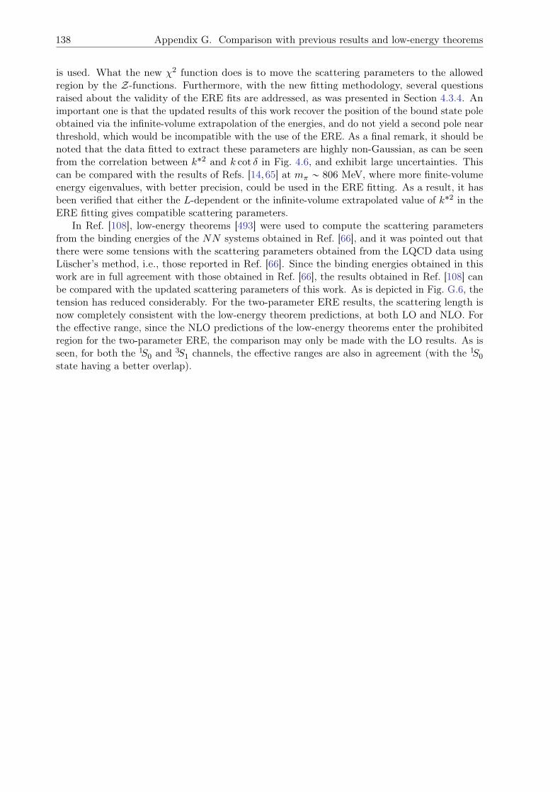
138 Appendix G. Comparison with previous results and low-energy theorems
is used. What the new χ2 function does is to move the scattering parameters to the allowedregion by the Z-functions. Furthermore, with the new fitting methodology, several questionsraised about the validity of the ERE fits are addressed, as was presented in Section 4.3.4. Animportant one is that the updated results of this work recover the position of the bound state poleobtained via the infinite-volume extrapolation of the energies, and do not yield a second pole nearthreshold, which would be incompatible with the use of the ERE. As a final remark, it should benoted that the data fitted to extract these parameters are highly non-Gaussian, as can be seenfrom the correlation between k˚2 and k cot δ in Fig. 4.6, and exhibit large uncertainties. Thiscan be compared with the results of Refs. [14,65] at mπ „ 806 MeV, where more finite-volumeenergy eigenvalues, with better precision, could be used in the ERE fitting. As a result, it hasbeen verified that either the L-dependent or the infinite-volume extrapolated value of k˚2 in theERE fitting gives compatible scattering parameters.
In Ref. [108], low-energy theorems [493] were used to compute the scattering parametersfrom the binding energies of the NN systems obtained in Ref. [66], and it was pointed out thatthere were some tensions with the scattering parameters obtained from the LQCD data usingLüscher’s method, i.e., those reported in Ref. [66]. Since the binding energies obtained in thiswork are in full agreement with those obtained in Ref. [66], the results obtained in Ref. [108] canbe compared with the updated scattering parameters of this work. As is depicted in Fig. G.6, thetension has reduced considerably. For the two-parameter ERE results, the scattering length isnow completely consistent with the low-energy theorem predictions, at both LO and NLO. Forthe effective range, since the NLO predictions of the low-energy theorems enter the prohibitedregion for the two-parameter ERE, the comparison may only be made with the LO results. As isseen, for both the 1S0 and 3S1 channels, the effective ranges are also in agreement (with the 1S0
state having a better overlap).
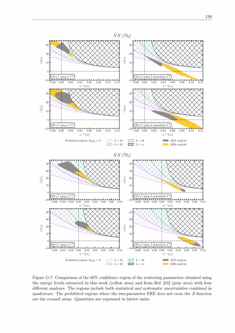
139
−0.02 0.00 0.02 0.04 0.06 0.08 0.10 0.12
a−1 [l.u.]
−10
0
10
20
30
r[l.u.]
1D-χ2 using κ(∞)2
−0.02 0.00 0.02 0.04 0.06 0.08 0.10 0.12
a−1 [l.u.]
−10
0
10
20
30
r[l.u.]
1D-χ2 using L-dependent k∗2
−0.02 0.00 0.02 0.04 0.06 0.08 0.10 0.12
a−1 [l.u.]
−10
0
10
20
30
r[l.u.]
2D-χ2 using κ(∞)2
−0.02 0.00 0.02 0.04 0.06 0.08 0.10 0.12
a−1 [l.u.]
−10
0
10
20
30
r[l.u.]
2D-χ2 using L-dependent k∗2
NN (1S0)
Prohibited regions NERE = 2: L = 24
L = 32
L = 48
L =∞2015 analysis
2020 analysis
−0.06 −0.04 −0.02 0.00 0.02 0.04 0.06 0.08 0.10
a−1 [l.u.]
−10
0
10
20
30
40
r[l.u.]
1D-χ2 using κ(∞)2
−0.06 −0.04 −0.02 0.00 0.02 0.04 0.06 0.08 0.10
a−1 [l.u.]
−10
0
10
20
30
40
r[l.u.]
1D-χ2 using L-dependent k∗2
−0.06 −0.04 −0.02 0.00 0.02 0.04 0.06 0.08 0.10
a−1 [l.u.]
−10
0
10
20
30
40
r[l.u.]
2D-χ2 using κ(∞)2
−0.06 −0.04 −0.02 0.00 0.02 0.04 0.06 0.08 0.10
a−1 [l.u.]
−10
0
10
20
30
40
r[l.u.]
2D-χ2 using L-dependent k∗2
NN (3S1)
Prohibited regions NERE = 2: L = 24
L = 32
L = 48
L =∞2015 analysis
2020 analysis
Figure G.7: Comparison of the 68% confidence region of the scattering parameters obtained usingthe energy levels extracted in this work (yellow area) and from Ref. [66] (gray area) with fourdifferent analyses. The regions include both statistical and systematic uncertainties combined inquadrature. The prohibited regions where the two-parameter ERE does not cross the Z-functionare the crossed areas. Quantities are expressed in lattice units.

140 Appendix G. Comparison with previous results and low-energy theorems
Appendix H
Supplementary figures and tables ofSection 4.3
This appendix contains all the figures omitted from the main body of the paper for ease ofpresentation. These include the effective mass plots of the single baryons in Fig. H.1, and theeffective energy and effective energy-shift plots for the two-baryon systems NN p1S0q (Fig. H.2),ΣN p1S0q (Fig. H.3), ΣΣ p1S0q (Fig. H.4), ΞΣ p1S0q (Fig. H.5), ΞΞ p1S0q (Fig. H.6), NN p3S1q
(Fig. H.7), ΣN p3S1q (Fig. H.8), ΞΞ p3S1q (Fig. H.9), and ΞN p3S1q (Fig. H.10). In Fig. H.1, thethin horizontal line and the horizontal band surrounding it represent, respectively, the centralvalue of the baryon mass at each volume and the associated statistical and systematic uncertaintiescombined in quadrature, obtained with the fitting procedure described in Section 3.1.1. Similarly,in Figs. H.2-H.10 the line and the band represent, respectively, the central value of the two-baryonenergy shifts compared to non-interacting baryons at rest (bottom panels) for each volume, andthe associated statistical and systematic uncertainties combined in quadrature.
The appendix also contains the numerical results that were omitted from the main body.These include the energy shifts ∆E of the two-baryon systems, the c.m. momenta k˚2, and thevalue of k˚ cot δ for all the systems: NN p1S0q (Table H.1), ΣN p1S0q (Table H.2), ΣΣ p1S0q
(Table H.3), ΞΣ p1S0q (Table H.4), ΞΞ p1S0q (Table H.5), NN p3S1q (Table H.6), ΣN p3S1q
(Table H.7), ΞΞ p3S1q (Table H.8), and ΞN p3S1q (Table H.9). In these tables, the values in thefirst and second parentheses correspond to statistical and systematic uncertainties, respectively,while those in the upper and lower parentheses are, respectively, the right and left uncertaintieswhen the error bars are asymmetric, as is generally the case for the k˚ cot δ values. When there isa dash sign in the tables, it indicates that the quantity k˚ cot δ diverges due to the singularitiesin the Zd
00 function.All quantities in the plots and tables are expressed in lattice units.
141
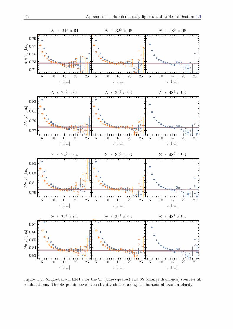
142 Appendix H. Supplementary figures and tables of Section 4.3
5 10 15 20 25
τ [l.u.]
0.71
0.73
0.75
0.77
0.79
MN
(τ)
[l.u.]
N : 243 × 64
5 10 15 20 25
τ [l.u.]
N : 323 × 96
5 10 15 20 25
τ [l.u.]
N : 483 × 96
5 10 15 20 25
τ [l.u.]
0.77
0.79
0.81
0.83
MΛ
(τ)
[l.u.]
Λ : 243 × 64
5 10 15 20 25
τ [l.u.]
Λ : 323 × 96
5 10 15 20 25
τ [l.u.]
Λ : 483 × 96
5 10 15 20 25
τ [l.u.]
0.79
0.81
0.83
0.85
MΣ
(τ)
[l.u.]
Σ : 243 × 64
5 10 15 20 25
τ [l.u.]
Σ : 323 × 96
5 10 15 20 25
τ [l.u.]
Σ : 483 × 96
5 10 15 20 25
τ [l.u.]
0.83
0.84
0.85
0.86
0.87
MΞ
(τ)
[l.u.]
Ξ : 243 × 64
5 10 15 20 25
τ [l.u.]
Ξ : 323 × 96
5 10 15 20 25
τ [l.u.]
Ξ : 483 × 96
Figure H.1: Single-baryon EMPs for the SP (blue squares) and SS (orange diamonds) source-sinkcombinations. The SS points have been slightly shifted along the horizontal axis for clarity.
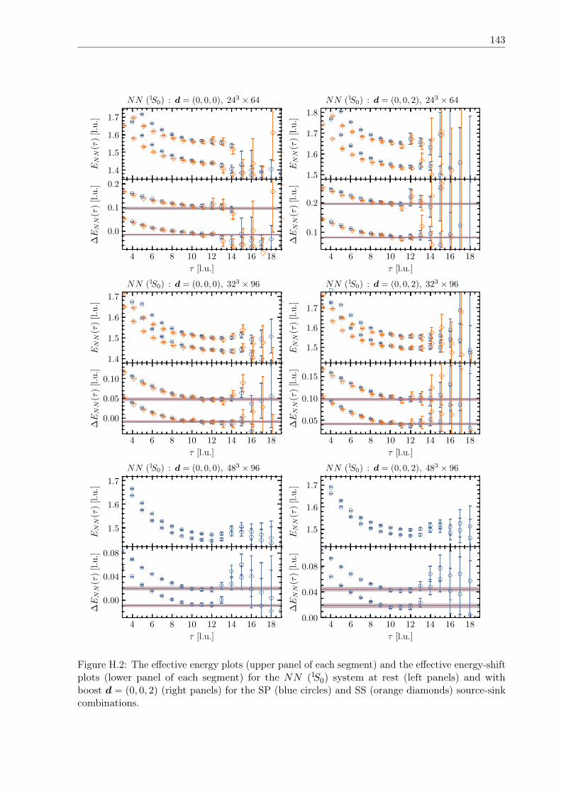
143
4 6 8 10 12 14 16 18
1.4
1.5
1.6
1.7
ENN
(τ)
[l.u.]
4 6 8 10 12 14 16 18
τ [l.u.]
0.0
0.1
0.2
∆ENN
(τ)
[l.u.]
4 6 8 10 12 14 16 181.4
1.5
1.6
1.7
ENN
(τ)
[l.u.]
4 6 8 10 12 14 16 18
τ [l.u.]
0.00
0.05
0.10
∆ENN
(τ)
[l.u.]
4 6 8 10 12 14 16 18
1.5
1.6
1.7
ENN
(τ)
[l.u.]
4 6 8 10 12 14 16 18
τ [l.u.]
0.00
0.04
0.08
∆ENN
(τ)
[l.u.]
4 6 8 10 12 14 16 181.5
1.6
1.7
1.8
ENN
(τ)
[l.u.]
4 6 8 10 12 14 16 18
τ [l.u.]
0.1
0.2
∆ENN
(τ)
[l.u.]
4 6 8 10 12 14 16 18
1.5
1.6
1.7
ENN
(τ)
[l.u.]
4 6 8 10 12 14 16 18
τ [l.u.]
0.05
0.10
0.15
∆ENN
(τ)
[l.u.]
4 6 8 10 12 14 16 18
1.5
1.6
1.7
ENN
(τ)
[l.u.]
4 6 8 10 12 14 16 18
τ [l.u.]
0.00
0.04
0.08
∆ENN
(τ)
[l.u.]
NN (1S0) : d = (0, 0, 0), 243 × 64
NN (1S0) : d = (0, 0, 0), 323 × 96
NN (1S0) : d = (0, 0, 0), 483 × 96
NN (1S0) : d = (0, 0, 2), 243 × 64
NN (1S0) : d = (0, 0, 2), 323 × 96
NN (1S0) : d = (0, 0, 2), 483 × 96
Figure H.2: The effective energy plots (upper panel of each segment) and the effective energy-shiftplots (lower panel of each segment) for the NN p1S0q system at rest (left panels) and withboost d “ p0, 0, 2q (right panels) for the SP (blue circles) and SS (orange diamonds) source-sinkcombinations.
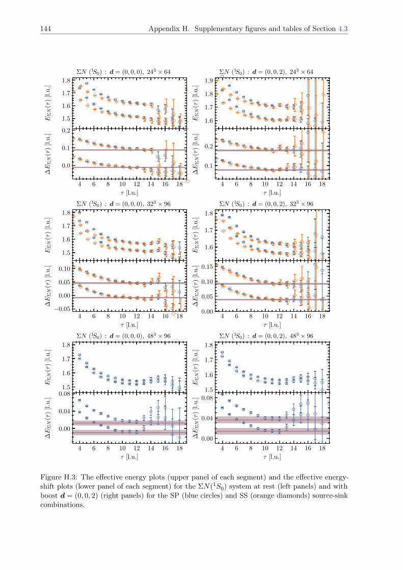
144 Appendix H. Supplementary figures and tables of Section 4.3
4 6 8 10 12 14 16 18
1.5
1.6
1.7
1.8
EΣN
(τ)
[l.u.]
4 6 8 10 12 14 16 18
τ [l.u.]
0.0
0.1
0.2
∆E
ΣN
(τ)
[l.u.]
4 6 8 10 12 14 16 18
1.5
1.6
1.7
1.8
EΣN
(τ)
[l.u.]
4 6 8 10 12 14 16 18
τ [l.u.]
−0.05
0.00
0.05
0.10
∆E
ΣN
(τ)
[l.u.]
4 6 8 10 12 14 16 18
1.5
1.6
1.7
1.8
EΣN
(τ)
[l.u.]
4 6 8 10 12 14 16 18
τ [l.u.]
0.00
0.04
0.08
∆E
ΣN
(τ)
[l.u.]
4 6 8 10 12 14 16 18
1.6
1.7
1.8
1.9
EΣN
(τ)
[l.u.]
4 6 8 10 12 14 16 18
τ [l.u.]
0.1
0.2
∆E
ΣN
(τ)
[l.u.]
4 6 8 10 12 14 16 18
1.6
1.7
1.8
EΣN
(τ)
[l.u.]
4 6 8 10 12 14 16 18
τ [l.u.]
0.00
0.05
0.10
0.15
∆E
ΣN
(τ)
[l.u.]
4 6 8 10 12 14 16 181.5
1.6
1.7
1.8
EΣN
(τ)
[l.u.]
4 6 8 10 12 14 16 18
τ [l.u.]
0.00
0.04
0.08
∆E
ΣN
(τ)
[l.u.]
ΣN (1S0) : d = (0, 0, 0), 243 × 64
ΣN (1S0) : d = (0, 0, 0), 323 × 96
ΣN (1S0) : d = (0, 0, 0), 483 × 96
ΣN (1S0) : d = (0, 0, 2), 243 × 64
ΣN (1S0) : d = (0, 0, 2), 323 × 96
ΣN (1S0) : d = (0, 0, 2), 483 × 96
Figure H.3: The effective energy plots (upper panel of each segment) and the effective energy-shift plots (lower panel of each segment) for the ΣNp1S0q system at rest (left panels) and withboost d “ p0, 0, 2q (right panels) for the SP (blue circles) and SS (orange diamonds) source-sinkcombinations.
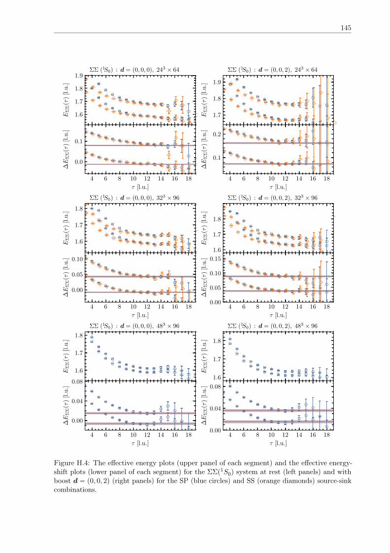
145
4 6 8 10 12 14 16 18
1.6
1.7
1.8
1.9
EΣ
Σ(τ
)[l.u.]
4 6 8 10 12 14 16 18
τ [l.u.]
0.0
0.1
∆E
ΣΣ
(τ)
[l.u.]
4 6 8 10 12 14 16 18
1.6
1.7
1.8
EΣ
Σ(τ
)[l.u.]
4 6 8 10 12 14 16 18
τ [l.u.]
0.00
0.05
0.10
∆E
ΣΣ
(τ)
[l.u.]
4 6 8 10 12 14 16 18
1.6
1.7
1.8
EΣ
Σ(τ
)[l.u.]
4 6 8 10 12 14 16 18
τ [l.u.]
0.00
0.04
0.08
∆E
ΣΣ
(τ)
[l.u.]
4 6 8 10 12 14 16 18
1.7
1.8
1.9
EΣ
Σ(τ
)[l.u.]
4 6 8 10 12 14 16 18
τ [l.u.]
0.1
0.2
∆E
ΣΣ
(τ)
[l.u.]
4 6 8 10 12 14 16 181.6
1.7
1.8
EΣ
Σ(τ
)[l.u.]
4 6 8 10 12 14 16 18
τ [l.u.]
0.00
0.05
0.10
0.15
∆E
ΣΣ
(τ)
[l.u.]
4 6 8 10 12 14 16 18
1.6
1.7
1.8
EΣ
Σ(τ
)[l.u.]
4 6 8 10 12 14 16 18
τ [l.u.]
0.00
0.04
0.08
∆E
ΣΣ
(τ)
[l.u.]
ΣΣ (1S0) : d = (0, 0, 0), 243 × 64
ΣΣ (1S0) : d = (0, 0, 0), 323 × 96
ΣΣ (1S0) : d = (0, 0, 0), 483 × 96
ΣΣ (1S0) : d = (0, 0, 2), 243 × 64
ΣΣ (1S0) : d = (0, 0, 2), 323 × 96
ΣΣ (1S0) : d = (0, 0, 2), 483 × 96
Figure H.4: The effective energy plots (upper panel of each segment) and the effective energy-shift plots (lower panel of each segment) for the ΣΣp1S0q system at rest (left panels) and withboost d “ p0, 0, 2q (right panels) for the SP (blue circles) and SS (orange diamonds) source-sinkcombinations.
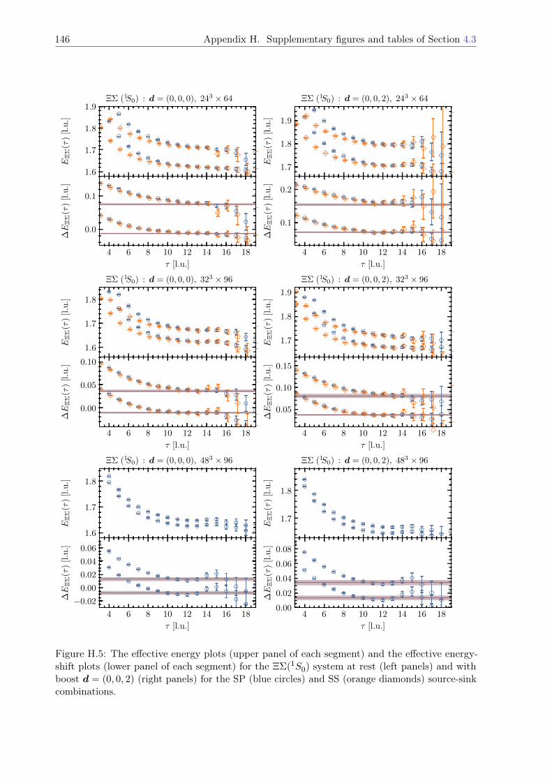
146 Appendix H. Supplementary figures and tables of Section 4.3
4 6 8 10 12 14 16 181.6
1.7
1.8
1.9
EΞ
Σ(τ
)[l.u.]
4 6 8 10 12 14 16 18
τ [l.u.]
0.0
0.1
∆E
ΞΣ
(τ)
[l.u.]
4 6 8 10 12 14 16 18
1.6
1.7
1.8
EΞ
Σ(τ
)[l.u.]
4 6 8 10 12 14 16 18
τ [l.u.]
0.00
0.05
0.10
∆E
ΞΣ
(τ)
[l.u.]
4 6 8 10 12 14 16 18
1.6
1.7
1.8
EΞ
Σ(τ
)[l.u.]
4 6 8 10 12 14 16 18
τ [l.u.]
−0.02
0.00
0.02
0.04
0.06
∆E
ΞΣ
(τ)
[l.u.]
4 6 8 10 12 14 16 18
1.7
1.8
1.9
EΞ
Σ(τ
)[l.u.]
4 6 8 10 12 14 16 18
τ [l.u.]
0.1
0.2
∆E
ΞΣ
(τ)
[l.u.]
4 6 8 10 12 14 16 18
1.7
1.8
1.9
EΞ
Σ(τ
)[l.u.]
4 6 8 10 12 14 16 18
τ [l.u.]
0.05
0.10
0.15
∆E
ΞΣ
(τ)
[l.u.]
4 6 8 10 12 14 16 18
1.7
1.8
EΞ
Σ(τ
)[l.u.]
4 6 8 10 12 14 16 18
τ [l.u.]
0.00
0.02
0.04
0.06
0.08
∆E
ΞΣ
(τ)
[l.u.]
ΞΣ (1S0) : d = (0, 0, 0), 243 × 64
ΞΣ (1S0) : d = (0, 0, 0), 323 × 96
ΞΣ (1S0) : d = (0, 0, 0), 483 × 96
ΞΣ (1S0) : d = (0, 0, 2), 243 × 64
ΞΣ (1S0) : d = (0, 0, 2), 323 × 96
ΞΣ (1S0) : d = (0, 0, 2), 483 × 96
Figure H.5: The effective energy plots (upper panel of each segment) and the effective energy-shift plots (lower panel of each segment) for the ΞΣp1S0q system at rest (left panels) and withboost d “ p0, 0, 2q (right panels) for the SP (blue circles) and SS (orange diamonds) source-sinkcombinations.
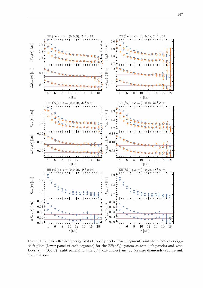
147
4 6 8 10 12 14 16 18
1.7
1.8
1.9
EΞ
Ξ(τ
)[l.u.]
4 6 8 10 12 14 16 18
τ [l.u.]
0.0
0.1
∆E
ΞΞ
(τ)
[l.u.]
4 6 8 10 12 14 16 18
1.7
1.8
EΞ
Ξ(τ
)[l.u.]
4 6 8 10 12 14 16 18
τ [l.u.]
0.00
0.05
0.10
∆E
ΞΞ
(τ)
[l.u.]
4 6 8 10 12 14 16 18
1.7
1.8
EΞ
Ξ(τ
)[l.u.]
4 6 8 10 12 14 16 18
τ [l.u.]
−0.02
0.00
0.02
0.04
0.06
∆E
ΞΞ
(τ)
[l.u.]
4 6 8 10 12 14 16 181.7
1.8
1.9
2.0
EΞ
Ξ(τ
)[l.u.]
4 6 8 10 12 14 16 18
τ [l.u.]
0.1
0.2
∆E
ΞΞ
(τ)
[l.u.]
4 6 8 10 12 14 16 18
1.7
1.8
1.9
EΞ
Ξ(τ
)[l.u.]
4 6 8 10 12 14 16 18
τ [l.u.]
0.05
0.10
0.15
∆E
ΞΞ
(τ)
[l.u.]
4 6 8 10 12 14 16 18
1.7
1.8
1.9
EΞ
Ξ(τ
)[l.u.]
4 6 8 10 12 14 16 18
τ [l.u.]
0.00
0.02
0.04
0.06
0.08
∆E
ΞΞ
(τ)
[l.u.]
ΞΞ (1S0) : d = (0, 0, 0), 243 × 64
ΞΞ (1S0) : d = (0, 0, 0), 323 × 96
ΞΞ (1S0) : d = (0, 0, 0), 483 × 96
ΞΞ (1S0) : d = (0, 0, 2), 243 × 64
ΞΞ (1S0) : d = (0, 0, 2), 323 × 96
ΞΞ (1S0) : d = (0, 0, 2), 483 × 96
Figure H.6: The effective energy plots (upper panel of each segment) and the effective energy-shift plots (lower panel of each segment) for the ΞΞp1S0q system at rest (left panels) and withboost d “ p0, 0, 2q (right panels) for the SP (blue circles) and SS (orange diamonds) source-sinkcombinations.
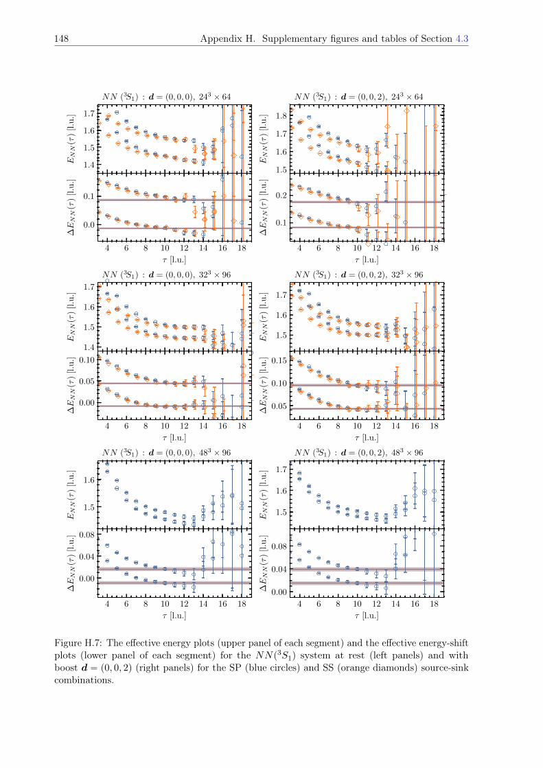
148 Appendix H. Supplementary figures and tables of Section 4.3
4 6 8 10 12 14 16 18
1.4
1.5
1.6
1.7
ENN
(τ)
[l.u.]
4 6 8 10 12 14 16 18
τ [l.u.]
0.0
0.1
∆ENN
(τ)
[l.u.]
4 6 8 10 12 14 16 181.4
1.5
1.6
1.7
ENN
(τ)
[l.u.]
4 6 8 10 12 14 16 18
τ [l.u.]
0.00
0.05
0.10
∆ENN
(τ)
[l.u.]
4 6 8 10 12 14 16 18
1.5
1.6
ENN
(τ)
[l.u.]
4 6 8 10 12 14 16 18
τ [l.u.]
0.00
0.04
0.08
∆ENN
(τ)
[l.u.]
4 6 8 10 12 14 16 181.5
1.6
1.7
1.8
ENN
(τ)
[l.u.]
4 6 8 10 12 14 16 18
τ [l.u.]
0.1
0.2
∆ENN
(τ)
[l.u.]
4 6 8 10 12 14 16 18
1.5
1.6
1.7
ENN
(τ)
[l.u.]
4 6 8 10 12 14 16 18
τ [l.u.]
0.05
0.10
0.15
∆ENN
(τ)
[l.u.]
4 6 8 10 12 14 16 18
1.5
1.6
1.7
ENN
(τ)
[l.u.]
4 6 8 10 12 14 16 18
τ [l.u.]
0.00
0.04
0.08
∆ENN
(τ)
[l.u.]
NN (3S1) : d = (0, 0, 0), 243 × 64
NN (3S1) : d = (0, 0, 0), 323 × 96
NN (3S1) : d = (0, 0, 0), 483 × 96
NN (3S1) : d = (0, 0, 2), 243 × 64
NN (3S1) : d = (0, 0, 2), 323 × 96
NN (3S1) : d = (0, 0, 2), 483 × 96
Figure H.7: The effective energy plots (upper panel of each segment) and the effective energy-shiftplots (lower panel of each segment) for the NNp3S1q system at rest (left panels) and withboost d “ p0, 0, 2q (right panels) for the SP (blue circles) and SS (orange diamonds) source-sinkcombinations.
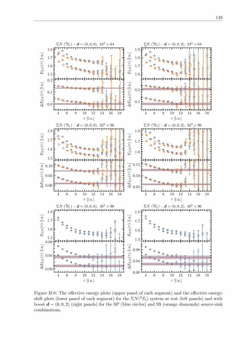
149
4 6 8 10 12 14 16 18
1.5
1.6
1.7
1.8
EΣN
(τ)
[l.u.]
4 6 8 10 12 14 16 18
τ [l.u.]
0.0
0.1
0.2
∆E
ΣN
(τ)
[l.u.]
4 6 8 10 12 14 16 181.5
1.6
1.7
1.8
EΣN
(τ)
[l.u.]
4 6 8 10 12 14 16 18
τ [l.u.]
0.00
0.05
0.10
∆E
ΣN
(τ)
[l.u.]
4 6 8 10 12 14 16 18
1.5
1.6
1.7
1.8
EΣN
(τ)
[l.u.]
4 6 8 10 12 14 16 18
τ [l.u.]
0.00
0.04
0.08
∆E
ΣN
(τ)
[l.u.]
4 6 8 10 12 14 16 18
1.6
1.7
1.8
1.9
EΣN
(τ)
[l.u.]
4 6 8 10 12 14 16 18
τ [l.u.]
0.1
0.2
∆E
ΣN
(τ)
[l.u.]
4 6 8 10 12 14 16 18
1.6
1.7
1.8E
ΣN
(τ)
[l.u.]
4 6 8 10 12 14 16 18
τ [l.u.]
0.05
0.10
0.15
∆E
ΣN
(τ)
[l.u.]
4 6 8 10 12 14 16 181.5
1.6
1.7
1.8
EΣN
(τ)
[l.u.]
4 6 8 10 12 14 16 18
τ [l.u.]
0.00
0.04
0.08
∆E
ΣN
(τ)
[l.u.]
ΣN (3S1) : d = (0, 0, 0), 243 × 64
ΣN (3S1) : d = (0, 0, 0), 323 × 96
ΣN (3S1) : d = (0, 0, 0), 483 × 96
ΣN (3S1) : d = (0, 0, 2), 243 × 64
ΣN (3S1) : d = (0, 0, 2), 323 × 96
ΣN (3S1) : d = (0, 0, 2), 483 × 96
Figure H.8: The effective energy plots (upper panel of each segment) and the effective energy-shift plots (lower panel of each segment) for the ΣNp3S1q system at rest (left panels) and withboost d “ p0, 0, 2q (right panels) for the SP (blue circles) and SS (orange diamonds) source-sinkcombinations.
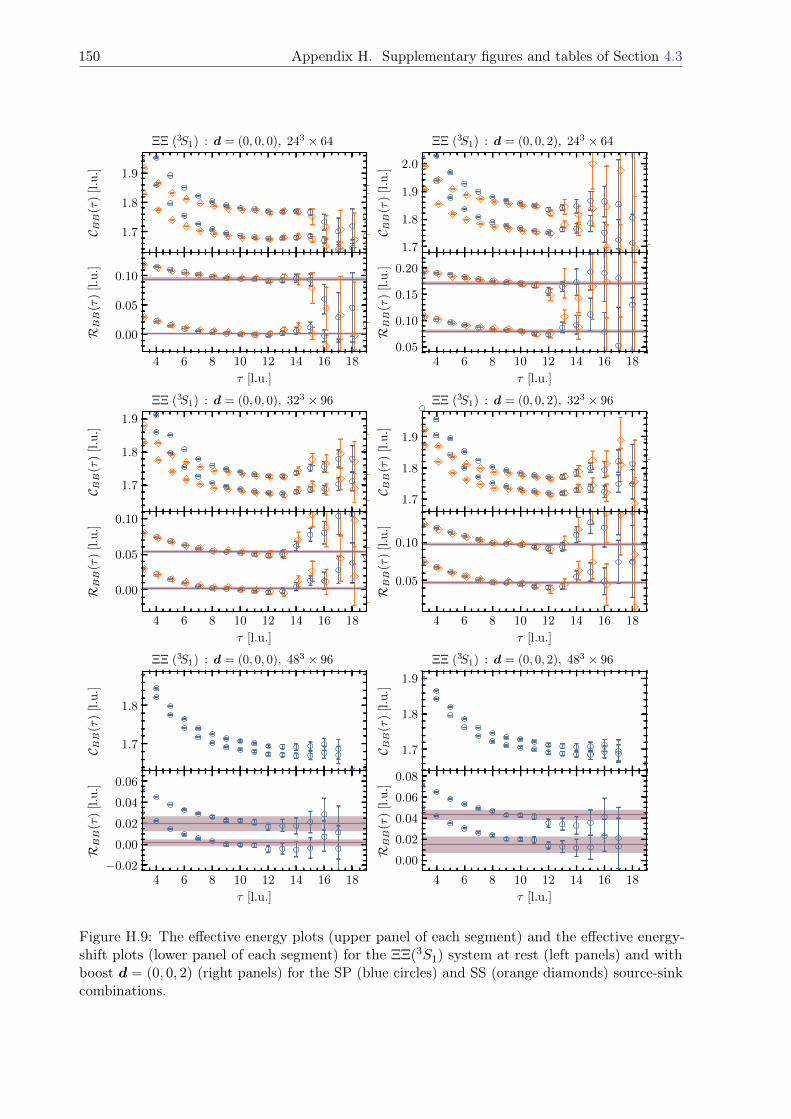
150 Appendix H. Supplementary figures and tables of Section 4.3
4 6 8 10 12 14 16 18
1.7
1.8
1.9
C BB
(τ)
[l.u.]
4 6 8 10 12 14 16 18
τ [l.u.]
0.00
0.05
0.10
RBB
(τ)
[l.u.]
4 6 8 10 12 14 16 18
1.7
1.8
1.9
C BB
(τ)
[l.u.]
4 6 8 10 12 14 16 18
τ [l.u.]
0.00
0.05
0.10
RBB
(τ)
[l.u.]
4 6 8 10 12 14 16 18
1.7
1.8
C BB
(τ)
[l.u.]
4 6 8 10 12 14 16 18
τ [l.u.]
−0.02
0.00
0.02
0.04
0.06
RBB
(τ)
[l.u.]
4 6 8 10 12 14 16 181.7
1.8
1.9
2.0
C BB
(τ)
[l.u.]
4 6 8 10 12 14 16 18
τ [l.u.]
0.05
0.10
0.15
0.20
RBB
(τ)
[l.u.]
4 6 8 10 12 14 16 18
1.7
1.8
1.9
C BB
(τ)
[l.u.]
4 6 8 10 12 14 16 18
τ [l.u.]
0.05
0.10
RBB
(τ)
[l.u.]
4 6 8 10 12 14 16 18
1.7
1.8
1.9
C BB
(τ)
[l.u.]
4 6 8 10 12 14 16 18
τ [l.u.]
0.00
0.02
0.04
0.06
0.08
RBB
(τ)
[l.u.]
ΞΞ (3S1) : d = (0, 0, 0), 243 × 64
ΞΞ (3S1) : d = (0, 0, 0), 323 × 96
ΞΞ (3S1) : d = (0, 0, 0), 483 × 96
ΞΞ (3S1) : d = (0, 0, 2), 243 × 64
ΞΞ (3S1) : d = (0, 0, 2), 323 × 96
ΞΞ (3S1) : d = (0, 0, 2), 483 × 96
Figure H.9: The effective energy plots (upper panel of each segment) and the effective energy-shift plots (lower panel of each segment) for the ΞΞp3S1q system at rest (left panels) and withboost d “ p0, 0, 2q (right panels) for the SP (blue circles) and SS (orange diamonds) source-sinkcombinations.
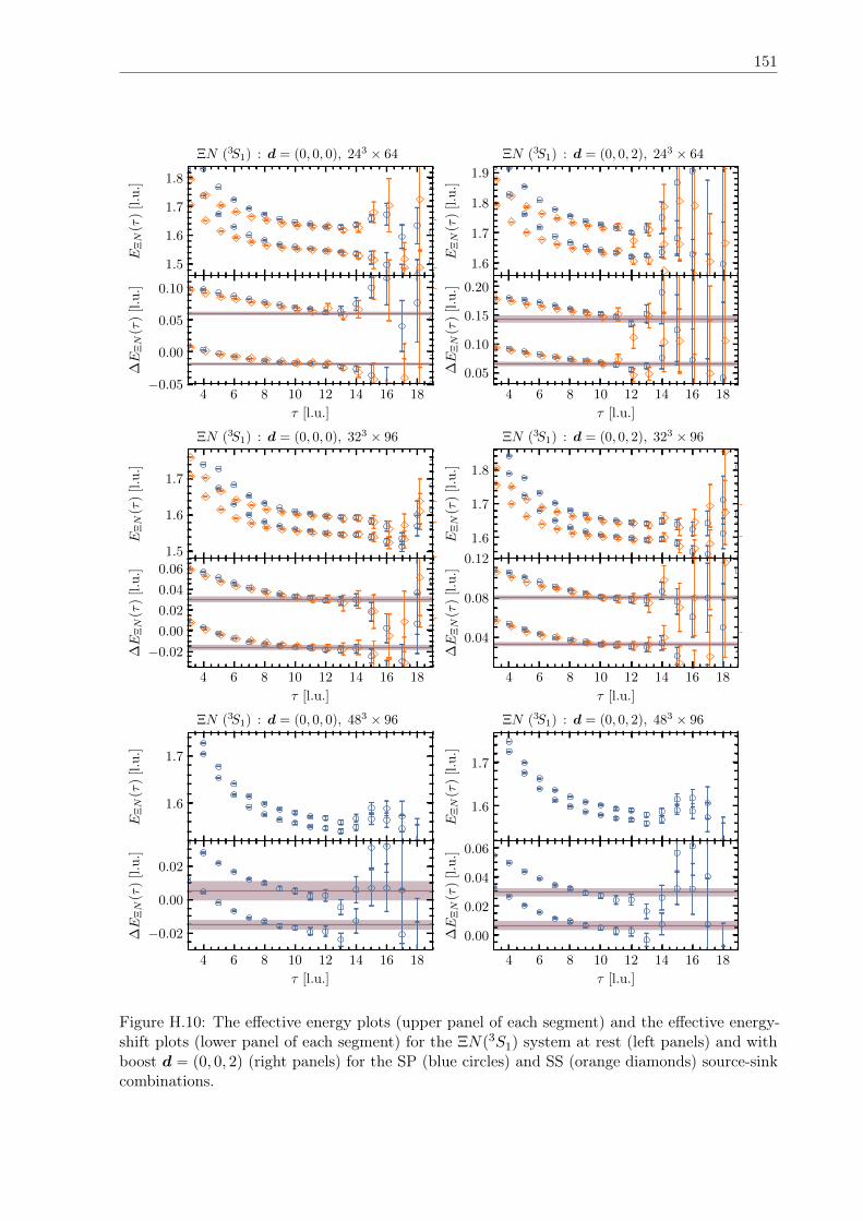
151
4 6 8 10 12 14 16 18
1.5
1.6
1.7
1.8
EΞN
(τ)
[l.u.]
4 6 8 10 12 14 16 18
τ [l.u.]
−0.05
0.00
0.05
0.10
∆E
ΞN
(τ)
[l.u.]
4 6 8 10 12 14 16 181.5
1.6
1.7
EΞN
(τ)
[l.u.]
4 6 8 10 12 14 16 18
τ [l.u.]
−0.02
0.00
0.02
0.04
0.06
∆E
ΞN
(τ)
[l.u.]
4 6 8 10 12 14 16 18
1.6
1.7
EΞN
(τ)
[l.u.]
4 6 8 10 12 14 16 18
τ [l.u.]
−0.02
0.00
0.02
∆E
ΞN
(τ)
[l.u.]
4 6 8 10 12 14 16 18
1.6
1.7
1.8
1.9
EΞN
(τ)
[l.u.]
4 6 8 10 12 14 16 18
τ [l.u.]
0.05
0.10
0.15
0.20
∆E
ΞN
(τ)
[l.u.]
4 6 8 10 12 14 16 18
1.6
1.7
1.8
EΞN
(τ)
[l.u.]
4 6 8 10 12 14 16 18
τ [l.u.]
0.04
0.08
0.12
∆E
ΞN
(τ)
[l.u.]
4 6 8 10 12 14 16 18
1.6
1.7
EΞN
(τ)
[l.u.]
4 6 8 10 12 14 16 18
τ [l.u.]
0.00
0.02
0.04
0.06
∆E
ΞN
(τ)
[l.u.]
ΞN (3S1) : d = (0, 0, 0), 243 × 64
ΞN (3S1) : d = (0, 0, 0), 323 × 96
ΞN (3S1) : d = (0, 0, 0), 483 × 96
ΞN (3S1) : d = (0, 0, 2), 243 × 64
ΞN (3S1) : d = (0, 0, 2), 323 × 96
ΞN (3S1) : d = (0, 0, 2), 483 × 96
Figure H.10: The effective energy plots (upper panel of each segment) and the effective energy-shift plots (lower panel of each segment) for the ΞNp3S1q system at rest (left panels) and withboost d “ p0, 0, 2q (right panels) for the SP (blue circles) and SS (orange diamonds) source-sinkcombinations.
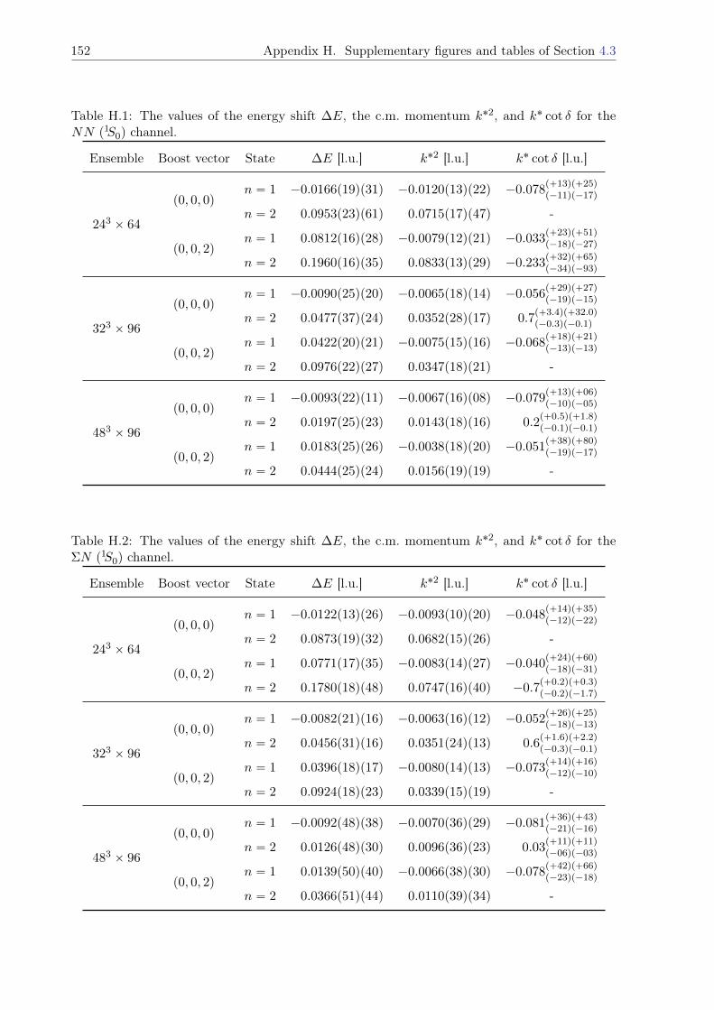
152 Appendix H. Supplementary figures and tables of Section 4.3
Table H.1: The values of the energy shift ∆E, the c.m. momentum k˚2, and k˚ cot δ for theNN p1S0q channel.
Ensemble Boost vector State ∆E [l.u.] k˚2 [l.u.] k˚ cot δ [l.u.]
243 ˆ 64
p0, 0, 0qn “ 1 ´0.0166p19qp31q ´0.0120p13qp22q ´0.078
p`13qp`25qp´11qp´17q
n “ 2 0.0953p23qp61q 0.0715p17qp47q -
p0, 0, 2qn “ 1 0.0812p16qp28q ´0.0079p12qp21q ´0.033
p`23qp`51qp´18qp´27q
n “ 2 0.1960p16qp35q 0.0833p13qp29q ´0.233p`32qp`65qp´34qp´93q
323 ˆ 96
p0, 0, 0qn “ 1 ´0.0090p25qp20q ´0.0065p18qp14q ´0.056
p`29qp`27qp´19qp´15q
n “ 2 0.0477p37qp24q 0.0352p28qp17q 0.7p`3.4qp`32.0qp´0.3qp´0.1q
p0, 0, 2qn “ 1 0.0422p20qp21q ´0.0075p15qp16q ´0.068
p`18qp`21qp´13qp´13q
n “ 2 0.0976p22qp27q 0.0347p18qp21q -
483 ˆ 96
p0, 0, 0qn “ 1 ´0.0093p22qp11q ´0.0067p16qp08q ´0.079
p`13qp`06qp´10qp´05q
n “ 2 0.0197p25qp23q 0.0143p18qp16q 0.2p`0.5qp`1.8qp´0.1qp´0.1q
p0, 0, 2qn “ 1 0.0183p25qp26q ´0.0038p18qp20q ´0.051
p`38qp`80qp´19qp´17q
n “ 2 0.0444p25qp24q 0.0156p19qp19q -
Table H.2: The values of the energy shift ∆E, the c.m. momentum k˚2, and k˚ cot δ for theΣN p1S0q channel.
Ensemble Boost vector State ∆E [l.u.] k˚2 [l.u.] k˚ cot δ [l.u.]
243 ˆ 64
p0, 0, 0qn “ 1 ´0.0122p13qp26q ´0.0093p10qp20q ´0.048
p`14qp`35qp´12qp´22q
n “ 2 0.0873p19qp32q 0.0682p15qp26q -
p0, 0, 2qn “ 1 0.0771p17qp35q ´0.0083p14qp27q ´0.040
p`24qp`60qp´18qp´31q
n “ 2 0.1780p18qp48q 0.0747p16qp40q ´0.7p`0.2qp`0.3qp´0.2qp´1.7q
323 ˆ 96
p0, 0, 0qn “ 1 ´0.0082p21qp16q ´0.0063p16qp12q ´0.052
p`26qp`25qp´18qp´13q
n “ 2 0.0456p31qp16q 0.0351p24qp13q 0.6p`1.6qp`2.2qp´0.3qp´0.1q
p0, 0, 2qn “ 1 0.0396p18qp17q ´0.0080p14qp13q ´0.073
p`14qp`16qp´12qp´10q
n “ 2 0.0924p18qp23q 0.0339p15qp19q -
483 ˆ 96
p0, 0, 0qn “ 1 ´0.0092p48qp38q ´0.0070p36qp29q ´0.081
p`36qp`43qp´21qp´16q
n “ 2 0.0126p48qp30q 0.0096p36qp23q 0.03p`11qp`11qp´06qp´03q
p0, 0, 2qn “ 1 0.0139p50qp40q ´0.0066p38qp30q ´0.078
p`42qp`66qp´23qp´18q
n “ 2 0.0366p51qp44q 0.0110p39qp34q -
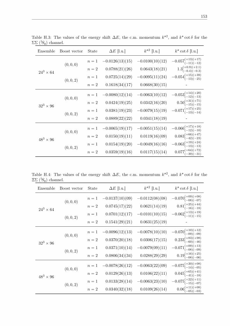
153
Table H.3: The values of the energy shift ∆E, the c.m. momentum k˚2, and k˚ cot δ for theΣΣ p1S0q channel.
Ensemble Boost vector State ∆E [l.u.] k˚2 [l.u.] k˚ cot δ [l.u.]
243 ˆ 64
p0, 0, 0qn “ 1 ´0.0126p13qp15q ´0.0100p10qp12q ´0.057
p`13qp`17qp´11qp´12q
n “ 2 0.0788p21qp26q 0.0643p18qp21q 1.3p`0.9qp`2.1qp´0.4qp´0.3q
p0, 0, 2qn “ 1 0.0725p14qp29q ´0.0095p11qp24q ´0.054
p`15qp`39qp´13qp´25q
n “ 2 0.1618p34qp17q 0.0668p30qp15q -
323 ˆ 96
p0, 0, 0qn “ 1 ´0.0080p12qp14q ´0.0063p10qp12q ´0.053
p`14qp`20qp´12qp´13q
n “ 2 0.0424p19qp25q 0.0342p16qp20q 0.50p`31qp`71qp´15qp´15q
p0, 0, 2qn “ 1 0.0381p19qp23q ´0.0079p15qp19q ´0.071
p`17qp`25qp´13qp´14q
n “ 2 0.0889p22qp22q 0.0341p18qp19q -
483 ˆ 96
p0, 0, 0qn “ 1 ´0.0065p19qp17q ´0.0051p15qp14q ´0.066
p`17qp`18qp´12qp´10q
n “ 2 0.0150p19qp11q 0.0119p16qp09q 0.083p`66qp`47qp´42qp´23q
p0, 0, 2qn “ 1 0.0154p19qp20q ´0.0049p16qp16q ´0.063
p`19qp`24qp´13qp´13q
n “ 2 0.0359p19qp16q 0.0117p15qp14q 0.077p`64qp`72qp´39qp´31q
Table H.4: The values of the energy shift ∆E, the c.m. momentum k˚2, and k˚ cot δ for theΞΣ p1S0q channel.
Ensemble Boost vector State ∆E [l.u.] k˚2 [l.u.] k˚ cot δ [l.u.]
243 ˆ 64
p0, 0, 0qn “ 1 ´0.0137p10qp09q ´0.0112p08qp08q ´0.070
p`09qp`08qp´08qp´07q
n “ 2 0.0745p17qp22q 0.0621p14qp19q 0.81p`25qp`44qp´16qp´18q
p0, 0, 2qn “ 1 0.0701p12qp17q ´0.0101p10qp15q ´0.062
p`13qp`19qp´11qp´15q
n “ 2 0.1541p29qp21q 0.0631p25qp19q -
323 ˆ 96
p0, 0, 0qn “ 1 ´0.0096p12qp13q ´0.0078p10qp10q ´0.070
p`10qp`12qp´09qp´09q
n “ 2 0.0370p20qp18q 0.0306p17qp15q 0.233p`83qp`98qp´60qp´46q
p0, 0, 2qn “ 1 0.0371p10qp14q ´0.0079p09qp11q ´0.071
p`09qp`13qp´08qp´09q
n “ 2 0.0806p34qp34q 0.0288p29qp29q 0.19p`16qp`25qp´08qp´06q
483 ˆ 96
p0, 0, 0qn “ 1 ´0.0078p26qp12q ´0.0063p22qp09q ´0.075
p`20qp`08qp´14qp´05q
n “ 2 0.0129p26qp13q 0.0106p22qp11q 0.045p`65qp`41qp´41qp´18q
p0, 0, 2qn “ 1 0.0133p28qp14q ´0.0063p23qp10q ´0.075
p`22qp`11qp´15qp´07q
n “ 2 0.0340p32qp18q 0.0109p26qp14q 0.06p`11qp`08qp´05qp´03q
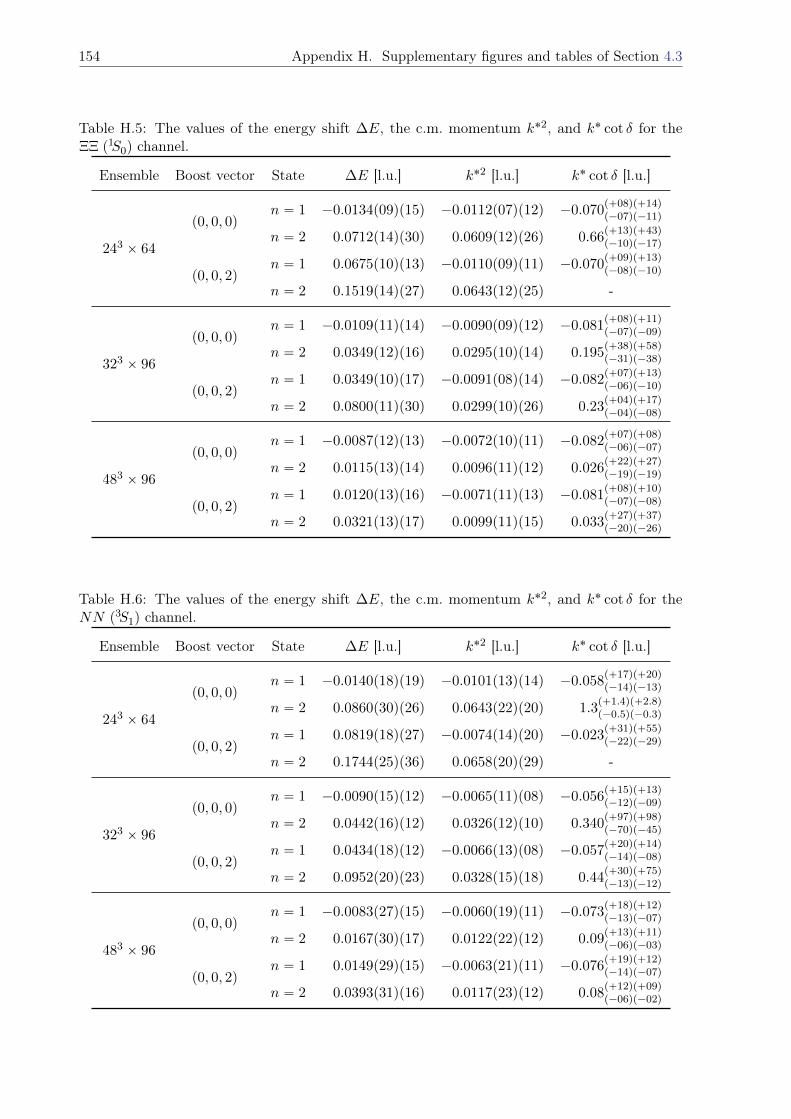
154 Appendix H. Supplementary figures and tables of Section 4.3
Table H.5: The values of the energy shift ∆E, the c.m. momentum k˚2, and k˚ cot δ for theΞΞ p1S0q channel.
Ensemble Boost vector State ∆E [l.u.] k˚2 [l.u.] k˚ cot δ [l.u.]
243 ˆ 64
p0, 0, 0qn “ 1 ´0.0134p09qp15q ´0.0112p07qp12q ´0.070
p`08qp`14qp´07qp´11q
n “ 2 0.0712p14qp30q 0.0609p12qp26q 0.66p`13qp`43qp´10qp´17q
p0, 0, 2qn “ 1 0.0675p10qp13q ´0.0110p09qp11q ´0.070
p`09qp`13qp´08qp´10q
n “ 2 0.1519p14qp27q 0.0643p12qp25q -
323 ˆ 96
p0, 0, 0qn “ 1 ´0.0109p11qp14q ´0.0090p09qp12q ´0.081
p`08qp`11qp´07qp´09q
n “ 2 0.0349p12qp16q 0.0295p10qp14q 0.195p`38qp`58qp´31qp´38q
p0, 0, 2qn “ 1 0.0349p10qp17q ´0.0091p08qp14q ´0.082
p`07qp`13qp´06qp´10q
n “ 2 0.0800p11qp30q 0.0299p10qp26q 0.23p`04qp`17qp´04qp´08q
483 ˆ 96
p0, 0, 0qn “ 1 ´0.0087p12qp13q ´0.0072p10qp11q ´0.082
p`07qp`08qp´06qp´07q
n “ 2 0.0115p13qp14q 0.0096p11qp12q 0.026p`22qp`27qp´19qp´19q
p0, 0, 2qn “ 1 0.0120p13qp16q ´0.0071p11qp13q ´0.081
p`08qp`10qp´07qp´08q
n “ 2 0.0321p13qp17q 0.0099p11qp15q 0.033p`27qp`37qp´20qp´26q
Table H.6: The values of the energy shift ∆E, the c.m. momentum k˚2, and k˚ cot δ for theNN p3S1q channel.
Ensemble Boost vector State ∆E [l.u.] k˚2 [l.u.] k˚ cot δ [l.u.]
243 ˆ 64
p0, 0, 0qn “ 1 ´0.0140p18qp19q ´0.0101p13qp14q ´0.058
p`17qp`20qp´14qp´13q
n “ 2 0.0860p30qp26q 0.0643p22qp20q 1.3p`1.4qp`2.8qp´0.5qp´0.3q
p0, 0, 2qn “ 1 0.0819p18qp27q ´0.0074p14qp20q ´0.023
p`31qp`55qp´22qp´29q
n “ 2 0.1744p25qp36q 0.0658p20qp29q -
323 ˆ 96
p0, 0, 0qn “ 1 ´0.0090p15qp12q ´0.0065p11qp08q ´0.056
p`15qp`13qp´12qp´09q
n “ 2 0.0442p16qp12q 0.0326p12qp10q 0.340p`97qp`98qp´70qp´45q
p0, 0, 2qn “ 1 0.0434p18qp12q ´0.0066p13qp08q ´0.057
p`20qp`14qp´14qp´08q
n “ 2 0.0952p20qp23q 0.0328p15qp18q 0.44p`30qp`75qp´13qp´12q
483 ˆ 96
p0, 0, 0qn “ 1 ´0.0083p27qp15q ´0.0060p19qp11q ´0.073
p`18qp`12qp´13qp´07q
n “ 2 0.0167p30qp17q 0.0122p22qp12q 0.09p`13qp`11qp´06qp´03q
p0, 0, 2qn “ 1 0.0149p29qp15q ´0.0063p21qp11q ´0.076
p`19qp`12qp´14qp´07q
n “ 2 0.0393p31qp16q 0.0117p23qp12q 0.08p`12qp`09qp´06qp´02q
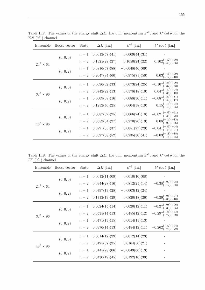
155
Table H.7: The values of the energy shift ∆E, the c.m. momentum k˚2, and k˚ cot δ for theΣN p3S1q channel.
Ensemble Boost vector State ∆E [l.u.] k˚2 [l.u.] k˚ cot δ [l.u.]
243 ˆ 64
p0, 0, 0qn “ 1 0.0012p57qp41q 0.0009p44qp31q -
n “ 2 0.1325p28qp27q 0.1050p24qp22q 0.102p`42qp`40qp´40qp´36q
p0, 0, 2qn “ 1 0.0816p57qp88q ´0.0048p46qp69q -
n “ 2 0.2047p84qp60q 0.0975p71qp50q 0.03p`13qp`09qp´12qp´10q
323 ˆ 96
p0, 0, 0qn “ 1 0.0096p32qp33q 0.0073p24qp25q ´0.107
p`27qp`26qp´37qp´53q
n “ 2 0.0742p22qp13q 0.0578p18qp10q 0.047p`40qp`24qp´38qp´18q
p0, 0, 2qn “ 1 0.0609p38qp16q 0.0088p30qp11q ´0.087
p`29qp`11qp´40qp´17q
n “ 2 0.1252p46qp25q 0.0604p38qp19q 0.15p`14qp`08qp´10qp´05q
483 ˆ 96
p0, 0, 0qn “ 1 0.0087p32qp25q 0.0066p24qp18q ´0.021
p`37qp`31qp´33qp´28q
n “ 2 0.0352p34qp27q 0.0270p26qp19q 0.08p`14qp`13qp´09qp´06q
p0, 0, 2qn “ 1 0.0291p35qp37q 0.0051p27qp29q ´0.041
p`39qp`44qp´45qp´91q
n “ 2 0.0527p38qp52q 0.0235p30qp41q ´0.03p`11qp`18qp´14qp´65q
Table H.8: The values of the energy shift ∆E, the c.m. momentum k˚2, and k˚ cot δ for theΞΞ p3S1q channel.
Ensemble Boost vector State ∆E [l.u.] k˚2 [l.u.] k˚ cot δ [l.u.]
243 ˆ 64
p0, 0, 0qn “ 1 0.0012p11qp09q 0.0010p10qp08q -
n “ 2 0.0944p28qp16q 0.0812p25qp14q ´0.38p`09qp`05qp´12qp´08q
p0, 0, 2qn “ 1 0.0797p13qp28q ´0.0003p12qp24q -
n “ 2 0.1712p19qp29q 0.0820p18qp26q ´0.29p`05qp`07qp´06qp´10q
323 ˆ 96
p0, 0, 0qn “ 1 0.0024p15qp14q 0.0020p12qp11q ´0.27
p`08qp`06qp´30qp´95q
n “ 2 0.0535p14qp13q 0.0455p12qp12q ´0.297p`57qp`53qp´77qp´89q
p0, 0, 2qn “ 1 0.0471p13qp15q 0.0014p11qp13q -
n “ 2 0.0976p14qp13q 0.0454p12qp11q ´0.262p`52qp`44qp´73qp´72q
483 ˆ 96
p0, 0, 0qn “ 1 0.0014p17qp29q 0.0012p14qp23q -
n “ 2 0.0195p67qp25q 0.0164p56qp21q -
p0, 0, 2qn “ 1 0.0145p78qp06q ´0.0049p66qp13q -
n “ 2 0.0430p19qp45q 0.0192p16qp39q -
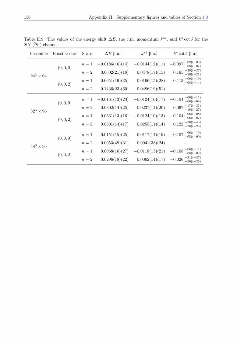
156 Appendix H. Supplementary figures and tables of Section 4.3
Table H.9: The values of the energy shift ∆E, the c.m. momentum k˚2, and k˚ cot δ for theΞN p3S1q channel.
Ensemble Boost vector State ∆E [l.u.] k˚2 [l.u.] k˚ cot δ [l.u.]
243 ˆ 64
p0, 0, 0qn “ 1 ´0.0186p16qp14q ´0.0144p12qp11q ´0.097
p`09qp`09qp´08qp´07q
n “ 2 0.0602p21qp18q 0.0478p17qp15q 0.165p`29qp`27qp´26qp´21q
p0, 0, 2qn “ 1 0.0651p19qp35q ´0.0166p15qp28q ´0.113
p`09qp`19qp´08qp´14q
n “ 2 0.1436p23qp60q 0.0486p19qp51q -
323 ˆ 96
p0, 0, 0qn “ 1 ´0.0161p13qp23q ´0.0124p10qp17q ´0.104
p`06qp`11qp´06qp´09q
n “ 2 0.0302p14qp25q 0.0237p11qp20q 0.067p`17qp`35qp´16qp´27q
p0, 0, 2qn “ 1 0.0331p13qp16q ´0.0124p10qp13q ´0.104
p`06qp`08qp´06qp´07q
n “ 2 0.0801p14qp17q 0.0255p11qp14q 0.122p`30qp`45qp´26qp´29q
483 ˆ 96
p0, 0, 0qn “ 1 ´0.0151p15qp25q ´0.0117p11qp19q ´0.107
p`06qp`10qp´05qp´09q
n “ 2 0.0053p49qp31q 0.0041p38qp24q -
p0, 0, 2qn “ 1 0.0068p16qp27q ´0.0118p13qp21q ´0.108
p`06qp`11qp´06qp´09q
n “ 2 0.0296p18qp22q 0.0062p14qp17q ´0.026p`21qp`27qp´20qp´25q
Bibliography
[1] K. G. Wilson, “Confinement of quarks,” Phys. Rev. D 10 (1974) 2445.
[2] S. Weinberg, “Nuclear forces from chiral Lagrangians,” Phys. Lett. B 251 (1990) 288.
[3] D. Chatterjee and I. Vidaña, “Do hyperons exist in the interior of neutron stars?,” Eur.Phys. J. A 52 (2016) 29, arXiv:1510.06306 [nucl-th].
[4] I. Vidaña, “Hyperons: the strange ingredients of the nuclear equation of state,” Proc. Roy.Soc. Lond. A 474 (2018) 0145, arXiv:1803.00504 [nucl-th].
[5] L. Tolos and L. Fabbietti, “Strangeness in Nuclei and Neutron Stars,” Prog. Part. Nucl.Phys. 112 (2020) 103770, arXiv:2002.09223 [nucl-ex].
[6] J. Haidenbauer, U.-G. Meißner, and S. Petschauer, “Do ΞΞ bound states exist?,” Eur. Phys.J. A 51 (2015) 17, arXiv:1412.2991 [nucl-th].
[7] M. Lüscher, “Volume Dependence of the Energy Spectrum in Massive Quantum FieldTheories. 2. Scattering States,” Commun. Math. Phys. 105 (1986) 153.
[8] M. Lüscher, “Two particle states on a torus and their relation to the scattering matrix,”Nucl. Phys. B 354 (1991) 531.
[9] NPLQCD, QCDSF Collaborations, S. R. Beane, W. Detmold, R. Horsley, M. Illa,M. Jafry, D. J. Murphy, Y. Nakamura, H. Perlt, P. E. L. Rakow, G. Schierholz, P. E.Shanahan, H. Stüben, M. L. Wagman, F. Winter, R. D. Young, and J. M. Zanotti,“Charged multi-hadron systems in lattice QCD+QED,” Phys. Rev. D 103 (2021) 054504,arXiv:2003.12130 [hep-lat].
[10] M. J. Savage and M. B. Wise, “Hyperon masses in nuclear matter,” Phys. Rev. D 53 (1996)349, arXiv:hep-ph/9507288.
[11] S. Petschauer and N. Kaiser, “Relativistic SUp3q chiral baryon-baryon Lagrangian up toorder q2,” Nucl. Phys. A 916 (2013) 1, arXiv:1305.3427 [nucl-th].
[12] D. B. Kaplan and M. J. Savage, “The Spin flavor dependence of nuclear forces from large-NQCD,” Phys. Lett. B 365 (1996) 244, arXiv:hep-ph/9509371.
[13] NPLQCD Collaboration, M. Illa, S. R. Beane, E. Chang, Z. Davoudi, W. Detmold, D. J.Murphy, K. Orginos, A. Parreño, M. J. Savage, P. E. Shanahan, M. L. Wagman, andF. Winter, “Low-energy Scattering and Effective Interactions of Two Baryons at mπ „
450 MeV from Lattice Quantum Chromodynamics,” Phys. Rev. D 103 (2021) 054508,arXiv:2009.12357 [hep-lat].
[14] NPLQCD Collaboration, M. L. Wagman, F. Winter, E. Chang, Z. Davoudi, W. Detmold,K. Orginos, M. J. Savage, and P. E. Shanahan, “Baryon-Baryon Interactions and Spin-Flavor Symmetry from Lattice Quantum Chromodynamics,” Phys. Rev. D 96 (2017) 114510,arXiv:1706.06550 [hep-lat].
157
158 Bibliography
[15] D. J. Gross and F. Wilczek, “Ultraviolet Behavior of Nonabelian Gauge Theories,” Phys.Rev. Lett. 30 (1973) 1343.
[16] H. D. Politzer, “Reliable Perturbative Results for Strong Interactions?,” Phys. Rev. Lett. 30(1973) 1346.
[17] “NN-OnLine.” https://nn-online.org.
[18] R. Machleidt and F. Sammarruca, “Can chiral EFT give us satisfaction?,” Eur. Phys. J. A56 (2020) 95, arXiv:2001.05615 [nucl-th].
[19] I. E. Lagaris and V. R. Pandharipande, “Phenomenological two-nucleon interaction operator,”Nucl. Phys. A 359 (1981) 331.
[20] R. B. Wiringa, R. A. Smith, and T. L. Ainsworth, “Nucleon-nucleon potentials with andwithout ∆p1232q degrees of freedom,” Phys. Rev. C 29 (1984) 1207.
[21] R. B. Wiringa, V. G. J. Stoks, and R. Schiavilla, “An Accurate nucleon-nucleon potentialwith charge independence breaking,” Phys. Rev. C 51 (1995) 38, arXiv:nucl-th/9408016.
[22] H. Yukawa, “On the Interaction of Elementary Particles I,” Proc. Phys. Math. Soc. Jap. 17(1935) 48.
[23] M. M. Nagels, T. A. Rijken, and J. J. de Swart, “Baryon-baryon scattering in a one-boson-exchange-potential approach. III. A nucleon-nucleon and hyperon-nucleon analysis includingcontributions of a nonet of scalar mesons,” Phys. Rev. D 20 (1979) 1633.
[24] V. G. J. Stoks, R. A. M. Klomp, M. C. M. Rentmeester, and J. J. de Swart, “Partial waveanalysis of all nucleon-nucleon scattering data below 350 MeV,” Phys. Rev. C 48 (1993)792.
[25] R. Machleidt, “The High precision, charge dependent Bonn nucleon-nucleon potential(CD-Bonn),” Phys. Rev. C 63 (2001) 024001, arXiv:nucl-th/0006014.
[26] F. Gross and A. Stadler, “Covariant spectator theory of np scattering: Phase shiftsobtained from precision fits to data below 350 MeV,” Phys. Rev. C 78 (2008) 014005,arXiv:0802.1552 [nucl-th].
[27] E. Epelbaum, H. Krebs, and U.-G. Meißner, “Precision nucleon-nucleon potential at fifthorder in the chiral expansion,” Phys. Rev. Lett. 115 (2015) 122301, arXiv:1412.4623[nucl-th].
[28] P. Reinert, H. Krebs, and E. Epelbaum, “Semilocal momentum-space regularized chiraltwo-nucleon potentials up to fifth order,” Eur. Phys. J. A 54 (2018) 86, arXiv:1711.08821[nucl-th].
[29] D. R. Entem, R. Machleidt, and Y. Nosyk, “High-quality two-nucleon potentials up tofifth order of the chiral expansion,” Phys. Rev. C 96 (2017) 024004, arXiv:1703.05454[nucl-th].
[30] D. R. Entem, N. Kaiser, R. Machleidt, and Y. Nosyk, “Dominant contributions to thenucleon-nucleon interaction at sixth order of chiral perturbation theory,” Phys. Rev. C 92(2015) 064001, arXiv:1505.03562 [nucl-th].
[31] V. A. Ambartsumyan and G. S. Saakyan, “The degenerate superdense gas of elementaryparticles,” Sov. Astron. 4 (1960) 187.
Bibliography 159
[32] A. Feliciello and T. Nagae, “Experimental review of hypernuclear physics: recent achieve-ments and future perspectives,” Rept. Prog. Phys. 78 (2015) 096301.
[33] A. Gal, E. V. Hungerford, and D. J. Millener, “Strangeness in nuclear physics,” Rev. Mod.Phys. 88 (2016) 035004, arXiv:1605.00557 [nucl-th].
[34] D. Lonardoni, A. Lovato, S. Gandolfi, and F. Pederiva, “Hyperon Puzzle: Hints fromQuantum Monte Carlo Calculations,” Phys. Rev. Lett. 114 (2015) 092301, arXiv:1407.4448[nucl-th].
[35] D. J. Champion et al., “An Eccentric Binary Millisecond Pulsar in the Galactic Plane,”Science 320 (2008) 1309, arXiv:0805.2396 [astro-ph].
[36] P. C. C. Freire et al., “On the nature and evolution of the unique binary pulsar J1903+0327,”Mon. Not. Roy. Astron. Soc. 412 (2011) 2763, arXiv:1011.5809 [astro-ph.GA].
[37] P. Demorest, T. Pennucci, S. Ransom, M. Roberts, and J. Hessels, “A two-solar-massneutron star measured using Shapiro delay,” Nature 467 (2010) 1081, arXiv:1010.5788[astro-ph.HE].
[38] J. Antoniadis et al., “A Massive Pulsar in a Compact Relativistic Binary,” Science 340(2013) 6131, arXiv:1304.6875 [astro-ph.HE].
[39] NANOGrav Collaboration, H. T. Cromartie et al., “Relativistic Shapiro delay mea-surements of an extremely massive millisecond pulsar,” Nat. Astron. 4 (2019) 72,arXiv:1904.06759 [astro-ph.HE].
[40] LIGO Scientific, Virgo Collaborations, R. Abbott et al., “GW190814: GravitationalWaves from the Coalescence of a 23 Solar Mass Black Hole with a 2.6 Solar Mass CompactObject,” Astrophys. J. Lett. 896 (2020) L44, arXiv:2006.12611 [astro-ph.HE].
[41] I. Vidaña, D. Logoteta, C. Providência, A. Polls, and I. Bombaci, “Estimation of the effectof hyperonic three-body forces on the maximum mass of neutron stars,” EPL 94 (2011)11002, arXiv:1006.5660 [nucl-th].
[42] S. Petschauer, J. Haidenbauer, N. Kaiser, U.-G. Meißner, and W. Weise, “Hyperons innuclear matter from SU(3) chiral effective field theory,” Eur. Phys. J. A 52 (2016) 15,arXiv:1507.08808 [nucl-th].
[43] Y. Yamamoto, T. Furumoto, N. Yasutake, and T. A. Rijken, “Multi-pomeron repulsion andthe Neutron-star mass,” Phys. Rev. C 88 (2013) 022801, arXiv:1308.2130 [nucl-th].
[44] T. Furumoto, Y. Sakuragi, and Y. Yamamoto, “Medium effect in the high-density re-gion probed by nucleus-nucleus elastic scattering,” Phys. Rev. C 90 (2014) 041601,arXiv:1406.3718 [nucl-th].
[45] D. Logoteta, I. Vidaña, and I. Bombaci, “Impact of chiral hyperonic three-body forces onneutron stars,” Eur. Phys. J. A 55 (2019) 207, arXiv:1906.11722 [nucl-th].
[46] J. Haidenbauer, U.-G. Meißner, and S. Petschauer, “Strangeness S “ ´2 baryon-baryoninteraction at next-to-leading order in chiral effective field theory,” Nucl. Phys. A 954(2016) 273, arXiv:1511.05859 [nucl-th].
[47] J. Haidenbauer and U.-G. Meißner, “Predictions for the strangeness S “ ´3 and ´4baryon-baryon interactions in chiral effective field theory,” Phys. Lett. B 684 (2010) 275,arXiv:0907.1395 [nucl-th].
160 Bibliography
[48] FLAG Collaboration, S. Aoki et al., “FLAG Review 2019,” Eur. Phys. J. C 80 (2020) 113,arXiv:1902.08191 [hep-lat].
[49] USQCD Collaboration, W. Detmold, R. G. Edwards, J. J. Dudek, M. Engelhardt, H.-W.Lin, S. Meinel, K. Orginos, and P. Shanahan, “Hadrons and Nuclei,” Eur. Phys. J. A 55(2019) 193, arXiv:1904.09512 [hep-lat].
[50] C. Drischler, W. Haxton, K. McElvain, E. Mereghetti, A. Nicholson, P. Vranas, andA. Walker-Loud, “Towards grounding nuclear physics in QCD,” Prog. Part. Nucl. Phys.(2021) 103888, arXiv:1910.07961 [nucl-th].
[51] Z. Davoudi, W. Detmold, P. Shanahan, K. Orginos, A. Parreño, M. J. Savage, and M. L.Wagman, “Nuclear matrix elements from lattice QCD for electroweak and beyond-Standard-Model processes,” Phys. Rept. 900 (2021) 1, arXiv:2008.11160 [hep-lat].
[52] G. Parisi, “The Strategy for Computing the Hadronic Mass Spectrum,” Phys. Rept. 103(1984) 203.
[53] G. P. Lepage, “The Analysis of Algorithms for Lattice Field Theory,” in Theoretical AdvancedStudy Institute in Elementary Particle Physics, p. 97. Boulder, 1989.
[54] NPLQCD Collaboration, S. R. Beane, W. Detmold, T. C. Luu, K. Orginos, A. Parreño,M. J. Savage, A. Torok, and A. Walker-Loud, “High Statistics Analysis using AnisotropicClover Lattices: (I) Single Hadron Correlation Functions,” Phys. Rev. D 79 (2009) 114502,arXiv:0903.2990 [hep-lat].
[55] NPLQCD Collaboration, S. R. Beane, W. Detmold, T. C. Luu, K. Orginos, A. Par-reño, M. J. Savage, A. Torok, and A. Walker-Loud, “High Statistics Analysis usingAnisotropic Clover Lattices: (II) Three-Baryon Systems,” Phys. Rev. D 80 (2009) 074501,arXiv:0905.0466 [hep-lat].
[56] NPLQCD Collaboration, S. R. Beane, W. Detmold, H.-W. Lin, T. C. Luu, K. Orginos,M. J. Savage, A. Torok, and A. Walker-Loud, “High Statistics Analysis using AnisotropicClover Lattices: (III) Baryon-Baryon Interactions,” Phys. Rev. D 81 (2010) 054505,arXiv:0912.4243 [hep-lat].
[57] M. L. Wagman and M. J. Savage, “Statistics of baryon correlation functions in lattice QCD,”Phys. Rev. D 96 (2017) 114508, arXiv:1611.07643 [hep-lat].
[58] NPLQCD Collaboration, S. R. Beane, P. F. Bedaque, K. Orginos, and M. J. Savage,“Nucleon-nucleon scattering from fully-dynamical lattice QCD,” Phys. Rev. Lett. 97 (2006)012001, arXiv:hep-lat/0602010.
[59] NPLQCD Collaboration, S. R. Beane, P. F. Bedaque, T. C. Luu, K. Orginos, E. Pallante,A. Parreño, and M. J. Savage, “Hyperon-Nucleon Scattering from Fully-Dynamical LatticeQCD,” Nucl. Phys. A 794 (2007) 62, arXiv:hep-lat/0612026.
[60] NPLQCD Collaboration, S. R. Beane, E. Chang, W. Detmold, B. Joó, H. W. Lin, T. C. Luu,K. Orginos, A. Parreño, M. J. Savage, A. Torok, and A. Walker-Loud, “Evidence for a BoundH-dibaryon from Lattice QCD,” Phys. Rev. Lett. 106 (2011) 162001, arXiv:1012.3812[hep-lat].
[61] NPLQCD Collaboration, S. R. Beane, E. Change, W. Detmold, B. Joó, H.-W. Lin, T. C.Luu, K. Orginos, A. Parreño, M. J. Savage, A. Torok, and A. Walker-Loud, “PresentConstraints on the H-dibaryon at the Physical Point from Lattice QCD,” Mod. Phys. Lett.A 26 (2011) 2587, arXiv:1103.2821 [hep-lat].
Bibliography 161
[62] NPLQCD Collaboration, S. R. Beane, E. Chang, W. Detmold, H. W. Lin, T. C. Luu,K. Orginos, A. Parreño, M. J. Savage, A. Torok, and A. Walker-Loud, “The Deuteronand Exotic Two-Body Bound States from Lattice QCD,” Phys. Rev. D 85 (2012) 054511,arXiv:1109.2889 [hep-lat].
[63] NPLQCD Collaboration, S. R. Beane, E. Chang, S. D. Cohen, W. Detmold, H.-W. Lin,T. C. Luu, K. Orginos, A. Parreño, M. J. Savage, and A. Walker-Loud, “Hyperon-NucleonInteractions and the Composition of Dense Nuclear Matter from Quantum Chromodynamics,”Phys. Rev. Lett. 109 (2012) 172001, arXiv:1204.3606 [hep-lat].
[64] NPLQCD Collaboration, S. R. Beane, E. Chang, S. D. Cohen, W. Detmold, H.-W. Lin,T. C. Luu, K. Orginos, A. Parreño, M. J. Savage, and A. Walker-Loud, “Light Nuclei andHypernuclei from Quantum Chromodynamics in the Limit of SUp3q Flavor Symmetry,”Phys. Rev. D 87 (2013) 034506, arXiv:1206.5219 [hep-lat].
[65] NPLQCD Collaboration, S. R. Beane, E. Chang, S. D. Cohen, W. Detmold, P. Junnarkar,H.-W. Lin, T. C. Luu, K. Orginos, A. Parreño, M. J. Savage, and A. Walker-Loud, “Nucleon-Nucleon Scattering Parameters in the Limit of SUp3q Flavor Symmetry,” Phys. Rev. C 88(2013) 024003, arXiv:1301.5790 [hep-lat].
[66] NPLQCD Collaboration, K. Orginos, A. Parreño, M. J. Savage, S. R. Beane, E. Chang,and W. Detmold, “Two nucleon systems at mπ „ 450 MeV from lattice QCD,” Phys. Rev.D 92 (2015) 114512, arXiv:1508.07583 [hep-lat]. [Erratum: Phys. Rev. D 102 (2020)039903].
[67] M. Fukugita, Y. Kuramashi, M. Okawa, H. Mino, and A. Ukawa, “Hadron scattering lengthsin lattice QCD,” Phys. Rev. D 52 (1995) 3003, arXiv:hep-lat/9501024.
[68] PACS-CS Collaboration, T. Yamazaki, Y. Kuramashi, and A. Ukawa, “Two-NucleonBound States in Quenched Lattice QCD,” Phys. Rev. D 84 (2011) 054506, arXiv:1105.1418[hep-lat].
[69] T. Yamazaki, K.-I. Ishikawa, Y. Kuramashi, and A. Ukawa, “Helium nuclei, deuteron anddineutron in 2` 1 flavor lattice QCD,” Phys. Rev. D 86 (2012) 074514, arXiv:1207.4277[hep-lat].
[70] T. Yamazaki, K.-I. Ishikawa, Y. Kuramashi, and A. Ukawa, “Study of quark mass dependenceof binding energy for light nuclei in 2 ` 1 flavor lattice QCD,” Phys. Rev. D 92 (2015)014501, arXiv:1502.04182 [hep-lat].
[71] H. Nemura, N. Ishii, S. Aoki, and T. Hatsuda, “Hyperon-nucleon force from lattice QCD,”Phys. Lett. B 673 (2009) 136, arXiv:0806.1094 [nucl-th].
[72] HAL QCD Collaboration, T. Inoue, N. Ishii, S. Aoki, T. Doi, T. Hatsuda, Y. Ikeda,K. Murano, H. Nemura, and K. Sasaki, “Bound H-dibaryon in Flavor SU(3) Limit of LatticeQCD,” Phys. Rev. Lett. 106 (2011) 162002, arXiv:1012.5928 [hep-lat].
[73] HAL QCD Collaboration, T. Inoue, S. Aoki, T. Doi, T. Hatsuda, Y. Ikeda, N. Ishii, K. Mu-rano, H. Nemura, and K. Sasaki, “Two-Baryon Potentials and H-Dibaryon from 3-flavorLattice QCD Simulations,” Nucl. Phys. A 881 (2012) 28, arXiv:1112.5926 [hep-lat].
[74] N. Ishii, “2` 1 Flavor QCD Results of Nuclear Forces,” Few Body Syst. 54 (2013) 1071.
[75] CalLat Collaboration, E. Berkowitz, T. Kurth, A. Nicholson, B. Joó, E. Rinaldi, M. Strother,P. M. Vranas, and A. Walker-Loud, “Two-Nucleon Higher Partial-Wave Scattering fromLattice QCD,” Phys. Lett. B 765 (2017) 285, arXiv:1508.00886 [hep-lat].
162 Bibliography
[76] B. Hörz, D. Howarth, E. Rinaldi, A. Hanlon, C. C. Chang, C. Körber, E. Berkowitz, J. Bulava,M. A. Clark, W. T. Lee, C. Morningstar, A. Nicholson, P. Vranas, and A. Walker-Loud,“Two-nucleon S-wave interactions at the SUp3q flavor-symmetric point with mud » mphys
s :A first lattice QCD calculation with the stochastic Laplacian Heaviside method,” Phys. Rev.C 103 (2021) 014003, arXiv:2009.11825 [hep-lat].
[77] A. Francis, J. R. Green, P. M. Junnarkar, C. Miao, T. D. Rae, and H. Wittig, “LatticeQCD study of the H dibaryon using hexaquark and two-baryon interpolators,” Phys. Rev.D 99 (2019) 074505, arXiv:1805.03966 [hep-lat].
[78] J. R. Green, A. D. Hanlon, P. M. Junnarkar, and H. Wittig, “Weakly bound H dibaryonfrom SU(3)-flavor-symmetric QCD,” arXiv:2103.01054 [hep-lat].
[79] S. Amarasinghe, R. Baghdadi, Z. Davoudi, W. Detmold, M. Illa, A. Parreño, A. Pochinsky,P. E. Shanahan, and M. L. Wagman, “A variational study of two-nucleon systems withlattice QCD,” arXiv:2108.10835 [hep-lat].
[80] HAL QCD Collaboration, S. Gongyo, K. Sasaki, S. Aoki, T. Doi, T. Hatsuda, Y. Ikeda,T. Inoue, T. Iritani, N. Ishii, T. Miyamoto, and H. Nemura, “Most Strange Dibaryon fromLattice QCD,” Phys. Rev. Lett. 120 (2018) 212001, arXiv:1709.00654 [hep-lat].
[81] HAL QCD Collaboration, T. Iritani, S. Aoki, T. Doi, F. Etminan, S. Gongyo, T. Hatsuda,Y. Ikeda, T. Inoue, N. Ishii, T. Miyamoto, and K. Sasaki, “NΩ dibaryon from lattice QCDnear the physical point,” Phys. Lett. B 792 (2019) 284, arXiv:1810.03416 [hep-lat].
[82] HAL QCD Collaboration, K. Sasaki, S. Aoki, T. Doi, S. Gongyo, T. Hatsuda, Y. Ikeda,T. Inoue, T. Iritani, N. Ishii, K. Murano, and T. Miyamoto, “ΛΛ and NΞ interactions fromLattice QCD near the physical point,” Nucl. Phys. A 998 (2020) 121737, arXiv:1912.08630[hep-lat].
[83] ALICE Collaboration, S. Acharya et al., “Unveiling the strong interaction among hadronsat the LHC,” Nature 588 (2020) 232, arXiv:2005.11495 [nucl-ex]. [Erratum: Nature590 (2021) E13].
[84] K. Rummukainen and S. A. Gottlieb, “Resonance scattering phase shifts on a nonrest framelattice,” Nucl. Phys. B 450 (1995) 397, arXiv:hep-lat/9503028.
[85] S. R. Beane, P. F. Bedaque, A. Parreño, and M. J. Savage, “Two nucleons on a lattice,”Phys. Lett. B 585 (2004) 106, arXiv:hep-lat/0312004.
[86] P. F. Bedaque, “Aharonov-Bohm effect and nucleon nucleon phase shifts on the lattice,”Phys. Lett. B 593 (2004) 82, arXiv:nucl-th/0402051.
[87] X. Feng, X. Li, and C. Liu, “Two particle states in an asymmetric box and the elasticscattering phases,” Phys. Rev. D 70 (2004) 014505, arXiv:hep-lat/0404001.
[88] C. H. Kim, C. T. Sachrajda, and S. R. Sharpe, “Finite-volume effects for two-hadron statesin moving frames,” Nucl. Phys. B 727 (2005) 218, arXiv:hep-lat/0507006.
[89] S. He, X. Feng, and C. Liu, “Two particle states and the S-matrix elements in multi-channelscattering,” JHEP 07 (2005) 011, arXiv:hep-lat/0504019.
[90] T. Luu and M. J. Savage, “Extracting Scattering Phase-Shifts in Higher Partial-Waves fromLattice QCD Calculations,” Phys. Rev. D 83 (2011) 114508, arXiv:1101.3347 [hep-lat].
[91] Z. Davoudi and M. J. Savage, “Improving the Volume Dependence of Two-Body BindingEnergies Calculated with Lattice QCD,” Phys. Rev. D 84 (2011) 114502, arXiv:1108.5371[hep-lat].
Bibliography 163
[92] L. Leskovec and S. Prelovsek, “Scattering phase shifts for two particles of differentmass and non-zero total momentum in lattice QCD,” Phys. Rev. D 85 (2012) 114507,arXiv:1202.2145 [hep-lat].
[93] M. T. Hansen and S. R. Sharpe, “Multiple-channel generalization of Lellouch-Lüscherformula,” Phys. Rev. D 86 (2012) 016007, arXiv:1204.0826 [hep-lat].
[94] R. A. Briceño and Z. Davoudi, “Moving multichannel systems in a finite volume withapplication to proton-proton fusion,” Phys. Rev. D 88 (2013) 094507, arXiv:1204.1110[hep-lat].
[95] M. Göckeler, R. Horsley, M. Lage, U.-G. Meißner, P. E. L. Rakow, A. Rusetsky, G. Schierholz,and J. M. Zanotti, “Scattering phases for meson and baryon resonances on general moving-frame lattices,” Phys. Rev. D 86 (2012) 094513, arXiv:1206.4141 [hep-lat].
[96] R. A. Briceño, Z. Davoudi, and T. C. Luu, “Two-Nucleon Systems in a Finite Volume. I.Quantization Conditions,” Phys. Rev. D 88 (2013) 034502, arXiv:1305.4903 [hep-lat].
[97] R. A. Briceño, Z. Davoudi, T. Luu, and M. J. Savage, “Two-nucleon systems in a finitevolume. II. 3S1 ´
3 D1 coupled channels and the deuteron,” Phys. Rev. D 88 (2013) 114507,arXiv:1309.3556 [hep-lat].
[98] R. A. Briceño, Z. Davoudi, T. C. Luu, and M. J. Savage, “Two-Baryon Systems with TwistedBoundary Conditions,” Phys. Rev. D 89 (2014) 074509, arXiv:1311.7686 [hep-lat].
[99] F. X. Lee and A. Alexandru, “Scattering phase-shift formulas for mesons and baryons inelongated boxes,” Phys. Rev. D 96 (2017) 054508, arXiv:1706.00262 [hep-lat].
[100] R. A. Briceño, J. J. Dudek, and R. D. Young, “Scattering processes and resonances fromlattice QCD,” Rev. Mod. Phys. 90 (2018) 025001, arXiv:1706.06223 [hep-lat].
[101] S. Aoki and T. Doi, “Lattice QCD and baryon-baryon interactions: HAL QCD method,”Front. in Phys. 8 (2020) 307, arXiv:2003.10730 [hep-lat].
[102] U. van Kolck, “Effective field theory of short range forces,” Nucl. Phys. A 645 (1999) 273,arXiv:nucl-th/9808007.
[103] J.-W. Chen, G. Rupak, and M. J. Savage, “Nucleon-nucleon effective field theory withoutpions,” Nucl. Phys. A 653 (1999) 386, arXiv:nucl-th/9902056.
[104] S. R. Beane, D. B. Kaplan, N. Klco, and M. J. Savage, “Entanglement Suppressionand Emergent Symmetries of Strong Interactions,” Phys. Rev. Lett. 122 (2019) 102001,arXiv:1812.03138 [nucl-th].
[105] N. Barnea, L. Contessi, D. Gazit, F. Pederiva, and U. van Kolck, “Effective Field Theoryfor Lattice Nuclei,” Phys. Rev. Lett. 114 (2015) 052501, arXiv:1311.4966 [nucl-th].
[106] L. Contessi, A. Lovato, F. Pederiva, A. Roggero, J. Kirscher, and U. van Kolck, “Ground-state properties of 4He and 16O extrapolated from lattice QCD with pionless EFT,” Phys.Lett. B 772 (2017) 839, arXiv:1701.06516 [nucl-th].
[107] A. Bansal, S. Binder, A. Ekström, G. Hagen, G. R. Jansen, and T. Papenbrock, “Pion-lesseffective field theory for atomic nuclei and lattice nuclei,” Phys. Rev. C 98 (2018) 054301,arXiv:1712.10246 [nucl-th].
[108] V. Baru, E. Epelbaum, and A. A. Filin, “Low-energy theorems for nucleon-nucleon scatteringat Mπ “ 450 MeV,” Phys. Rev. C 94 (2016) 014001, arXiv:1604.02551 [nucl-th].
164 Bibliography
[109] G. D. Rochester and C. C. Butler, “Evidence for the Existence of New Unstable ElementaryParticles,” Nature 160 (1947) 855.
[110] V. D. Hopper and S. Biswas, “Evidence Concerning the Existence of the New UnstableElementary Neutral Particle,” Phys. Rev. 80 (1950) 1099.
[111] M. Gell-Mann, “The Eightfold Way: A Theory of strong interaction symmetry,” 1961.
[112] Y. Ne’eman, “Derivation of strong interactions from a gauge invariance,” Nucl. Phys. 26(1961) 222.
[113] M. Gell-Mann, “A Schematic Model of Baryons and Mesons,” Phys. Lett. 8 (1964) 214.
[114] G. Zweig, “An SU3 model for strong interaction symmetry and its breaking,” 1964.
[115] O. W. Greenberg, “Spin and Unitary Spin Independence in a Paraquark Model of Baryonsand Mesons,” Phys. Rev. Lett. 13 (1964) 598.
[116] M. Y. Han and Y. Nambu, “Three Triplet Model with Double SU(3) Symmetry,” Phys. Rev.139 (1965) B1006.
[117] H. Fritzsch, M. Gell-Mann, and H. Leutwyler, “Advantages of the Color Octet GluonPicture,” Phys. Lett. B 47 (1973) 365.
[118] M. Gell-Mann, “Symmetries of Baryons and Mesons,” Phys. Rev. 125 (1962) 1067.
[119] B. Graner, Y. Chen, E. G. Lindahl, and B. R. Heckel, “Reduced Limit on the PermanentElectric Dipole Moment of 199Hg,” Phys. Rev. Lett. 116 (2016) 161601, arXiv:1601.04339[physics.atom-ph]. [Erratum: Phys. Rev. Lett. 119 (2017) 119901].
[120] R. Gupta, “Introduction to lattice QCD,” in Les Houches Summer School in TheoreticalPhysics, Session 68: Probing the Standard Model of Particle Interactions, p. 83. 1997.arXiv:hep-lat/9807028.
[121] R. P. Feynman, “Space-Time Approach to Non-Relativistic Quantum Mechanics,” Rev. Mod.Phys. 20 (1948) 367.
[122] G. C. Wick, “Properties of Bethe-Salpeter Wave Functions,” Phys. Rev. 96 (1954) 1124.
[123] H. J. Rothe, Lattice Gauge Theories: An introduction, vol. 74 of World Scientific lecturenotes in physics. World Scientific Publishing Co., Singapore, 3rd ed., 2005.
[124] T. DeGrand and C. DeTar, Lattice Methods for Quantum Chromodynamics. World ScientificPublishing Co., Singapore, 2006.
[125] C. Gattringer and C. B. Lang, Quantum Chromodynamics on the Lattice: An IntroductoryPresentation, vol. 788 of Lecture Notes in Physics. Springer, Berlin, Heidelberg, 2010.
[126] H.-W. Lin and H. B. Meyer, eds., Lattice QCD for Nuclear Physics, vol. 889 of LectureNotes in Physics. Springer, Cham, 2015.
[127] F. Knechtli, M. Günther, and M. Peardon, Lattice Quantum Chromodynamics: PracticalEssentials. SpringerBriefs in Physics. Springer Netherlands, 2017.
[128] G. Burgers, F. Karsch, A. Nakamura, and I. O. Stamatescu, “QCD on anisotropic lattices,”Nucl. Phys. B 304 (1988) 587.
[129] T. R. Klassen, “The Anisotropic Wilson gauge action,” Nucl. Phys. B 533 (1998) 557,arXiv:hep-lat/9803010.
Bibliography 165
[130] X. Li and C. Liu, “Two particle states in an asymmetric box,” Phys. Lett. B 587 (2004)100, arXiv:hep-lat/0311035.
[131] W. Detmold and M. J. Savage, “Electroweak matrix elements in the two nucleon sectorfrom lattice QCD,” Nucl. Phys. A 743 (2004) 170, arXiv:hep-lat/0403005.
[132] N. Byers and C. N. Yang, “Theoretical Considerations Concerning Quantized MagneticFlux in Superconducting Cylinders,” Phys. Rev. Lett. 7 (1961) 46.
[133] K. G. Wilson, “Quarks and Strings on a Lattice,” in 13th International School of SubnuclearPhysics: New Phenomena in Subnuclear Physics, p. 99. 1975.
[134] H. B. Nielsen and M. Ninomiya, “A no-go theorem for regularizing chiral fermions,” Phys.Lett. B 105 (1981) 219.
[135] K. Symanzik, “Continuum Limit and Improved Action in Lattice Theories. 1. Principlesand φ4 Theory,” Nucl. Phys. B 226 (1983) 187.
[136] B. Sheikholeslami and R. Wohlert, “Improved Continuum Limit Lattice Action for QCDwith Wilson Fermions,” Nucl. Phys. B 259 (1985) 572.
[137] M. Lüscher, S. Sint, R. Sommer, and P. Weisz, “Chiral symmetry and Opaq improvement inlattice QCD,” Nucl. Phys. B 478 (1996) 365, arXiv:hep-lat/9605038.
[138] S. Borsányi, S. Durr, Z. Fodor, C. Hoelbling, S. D. Katz, S. Krieg, L. Lellouch, T. Lippert,A. Portelli, K. K. Szabo, and B. C. Toth, “Ab initio calculation of the neutron-proton massdifference,” Science 347 (2015) 1452, arXiv:1406.4088 [hep-lat].
[139] S. Aoki, “New Phase Structure for Lattice QCD with Wilson Fermions,” Phys. Rev. D 30(1984) 2653.
[140] ALPHA Collaboration, R. Frezzotti, P. A. Grassi, S. Sint, and P. Weisz, “Lattice QCD witha chirally twisted mass term,” J. High Energ. Phys. 08 (2001) 058, arXiv:hep-lat/0101001.
[141] A. Shindler, “Twisted mass lattice QCD,” Phys. Rept. 461 (2008) 37, arXiv:0707.4093[hep-lat].
[142] ETM Collaboration, C. Alexandrou, S. Bacchio, M. Constantinou, J. Finkenrath, K. Had-jiyiannakou, K. Jansen, G. Koutsou, H. Panagopoulos, and G. Spanoudes, “Completeflavor decomposition of the spin and momentum fraction of the proton using lattice QCDsimulations at physical pion mass,” Phys. Rev. D 101 (2020) 094513, arXiv:2003.08486[hep-lat].
[143] J. B. Kogut and L. Susskind, “Hamiltonian Formulation of Wilson’s Lattice Gauge Theories,”Phys. Rev. D 11 (1975) 395.
[144] MILC Collaboration, A. Bazavov, D. Toussaint, C. Bernard, J. Laiho, C. DeTar, L. Levkova,M. B. Oktay, S. Gottlieb, U. M. Heller, J. E. Hetrick, P. B. Mackenzie, R. Sugar, andR. S. Van de Water, “Nonperturbative QCD Simulations with 2` 1 Flavors of ImprovedStaggered Quarks,” Rev. Mod. Phys. 82 (2010) 1349, arXiv:0903.3598 [hep-lat].
[145] S. Borsányi, Z. Fodor, C. Hoelbling, S. D. Katz, S. Krieg, and K. K. Szabó, “Full result for theQCD equation of state with 2` 1 flavors,” Phys. Lett. B 730 (2014) 99, arXiv:1309.5258[hep-lat].
[146] HotQCD Collaboration, A. Bazavov et al., “Equation of state in (2`1)-flavor QCD,” Phys.Rev. D 90 (2014) 094503, arXiv:1407.6387 [hep-lat].
166 Bibliography
[147] D. B. Kaplan, “A Method for simulating chiral fermions on the lattice,” Phys. Lett. B 288(1992) 342, arXiv:hep-lat/9206013.
[148] D. B. Kaplan, “Chiral fermions on the lattice,” Nucl. Phys. B (Proc. Suppl.) 30 (1993) 597.
[149] Y. Shamir, “Chiral fermions from lattice boundaries,” Nucl. Phys. B 406 (1993) 90,arXiv:hep-lat/9303005.
[150] V. Furman and Y. Shamir, “Axial symmetries in lattice QCD with Kaplan fermions,” Nucl.Phys. B 439 (1995) 54, arXiv:hep-lat/9405004.
[151] R. Narayanan and H. Neuberger, “A Construction of lattice chiral gauge theories,” Nucl.Phys. B 443 (1995) 305, arXiv:hep-th/9411108.
[152] H. Neuberger, “Exactly massless quarks on the lattice,” Phys. Lett. B 417 (1998) 141,arXiv:hep-lat/9707022.
[153] P. H. Ginsparg and K. G. Wilson, “A Remnant of Chiral Symmetry on the Lattice,” Phys.Rev. D 25 (1982) 2649.
[154] RBC, UKQCD Collaborations, R. Abbott, T. Blum, P. A. Boyle, M. Bruno, N. H. Christ,D. Hoying, C. Jung, C. Kelly, C. Lehner, R. D. Mawhinney, D. J. Murphy, C. T. Sachrajda,A. Soni, M. Tomii, and T. Wang, “Direct CP violation and the ∆I “ 12 rule in K Ñ ππdecay from the standard model,” Phys. Rev. D 102 (2020) 054509, arXiv:2004.09440[hep-lat].
[155] M. Lüscher and P. Weisz, “On-Shell Improved Lattice Gauge Theories,” Commun. Math.Phys. 97 (1985) 59. [Erratum: Commun. Math. Phys. 98 (1985) 433].
[156] S. Itoh, Y. Iwasaki, Y. Oyanagi, and T. Yoshie, “Renormalization Group Improved LatticeSU(3) Gauge Action and Hadron Spectrum in Quenched QCD on a 83 ˆ 16 Lattice,” Phys.Lett. B 148 (1984) 153.
[157] G. C. Wick, “The Evaluation of the Collision Matrix,” Phys. Rev. 80 (1950) 268.
[158] S. Duane, A. D. Kennedy, B. J. Pendleton, and D. Roweth, “Hybrid Monte Carlo,” Phys.Lett. B 195 (1987) 216.
[159] S. A. Gottlieb, W. Liu, D. Toussaint, R. L. Renken, and R. L. Sugar, “Hybrid MolecularDynamics Algorithms for the Numerical Simulation of Quantum Chromodynamics,” Phys.Rev. D 35 (1987) 2531.
[160] M. S. Albergo, G. Kanwar, and P. E. Shanahan, “Flow-based generative models forMarkov chain Monte Carlo in lattice field theory,” Phys. Rev. D 100 (2019) 034515,arXiv:1904.12072 [hep-lat].
[161] G. Kanwar, M. S. Albergo, D. Boyda, K. Cranmer, D. C. Hackett, S. Racanière, D. J.Rezende, and P. E. Shanahan, “Equivariant flow-based sampling for lattice gauge theory,”Phys. Rev. Lett. 125 (2020) 121601, arXiv:2003.06413 [hep-lat].
[162] D. Boyda, G. Kanwar, S. Racanière, D. J. Rezende, M. S. Albergo, K. Cranmer, D. C.Hackett, and P. E. Shanahan, “Sampling using SUpNq gauge equivariant flows,” Phys. Rev.D 103 (2021) 074504, arXiv:2008.05456 [hep-lat].
[163] H. A. van der Vorst, “Bi-CGSTAB: A fast and smoothly converging variant of Bi-CG forthe solution of nonsymmetric linear systems,” SIAM J. Sci. Stat. Comput. 13 (1992) 631.
Bibliography 167
[164] Y. Saad and M. H. Schultz, “GMRES: A Generalized Minimal Residual Algorithm forSolving Nonsymmetric Linear Systems,” SIAM J. Sci. Stat. Comput. 7 (1986) 856.
[165] T. A. DeGrand, “A Conditioning Technique for Matrix Inversion for Wilson Fermions,”Comput. Phys. Commun. 52 (1988) 161.
[166] M. Lüscher, “Solution of the Dirac equation in lattice QCD using a domain decompositionmethod,” Comput. Phys. Commun. 156 (2004) 209, arXiv:hep-lat/0310048.
[167] R. Babich, J. Brannick, R. C. Brower, M. A. Clark, T. A. Manteuffel, S. F. McCormick,J. C. Osborn, and C. Rebbi, “Adaptive multigrid algorithm for the lattice Wilson-Diracoperator,” Phys. Rev. Lett. 105 (2010) 201602, arXiv:1005.3043 [hep-lat].
[168] A. Frommer, K. Kahl, S. Krieg, B. Leder, and M. Rottmann, “Adaptive Aggregation BasedDomain Decomposition Multigrid for the Lattice Wilson Dirac Operator,” SIAM J. Sci.Comput. 36 (2014) A1581, arXiv:1303.1377 [hep-lat].
[169] C. Alexandrou, S. Bacchio, J. Finkenrath, A. Frommer, K. Kahl, and M. Rottmann,“Adaptive Aggregation-based Domain Decomposition Multigrid for Twisted Mass Fermions,”Phys. Rev. D 94 (2016) 114509, arXiv:1610.02370 [hep-lat].
[170] R. C. Brower, M. A. Clark, A. Strelchenko, and E. Weinberg, “Multigrid algorithm forstaggered lattice fermions,” Phys. Rev. D 97 (2018) 114513, arXiv:1801.07823 [hep-lat].
[171] R. Sommer, “Scale setting in lattice QCD,” PoS LATTICE2013 (2014) 015,arXiv:1401.3270 [hep-lat].
[172] NPLQCD Collaboration, S. R. Beane, P. F. Bedaque, T. C. Luu, K. Orginos, E. Pallante,A. Parreño, and M. J. Savage, “πK scattering in full QCD with domain-wall valence quarks,”Phys. Rev. D 74 (2006) 114503, arXiv:hep-lat/0607036.
[173] G. P. Lepage and P. B. Mackenzie, “On the viability of lattice perturbation theory,” Phys.Rev. D 48 (1993) 2250, arXiv:hep-lat/9209022.
[174] APE Collaboration, M. Albanese et al., “Glueball Masses and String Tension in LatticeQCD,” Phys. Lett. B 192 (1987) 163.
[175] A. Hasenfratz and F. Knechtli, “Flavor symmetry and the static potential with hypercubicblocking,” Phys. Rev. D 64 (2001) 034504, arXiv:hep-lat/0103029.
[176] C. Morningstar and M. J. Peardon, “Analytic smearing of SU(3) link variables in latticeQCD,” Phys. Rev. D 69 (2004) 054501, arXiv:hep-lat/0311018.
[177] S. Güsken, “A Study of smearing techniques for hadron correlation functions,” Nucl. Phys.B (Proc. Suppl.) 17 (1990) 361.
[178] Z. Davoudi, J. Harrison, A. Jüttner, A. Portelli, and M. J. Savage, “Theoretical aspects ofquantum electrodynamics in a finite volume with periodic boundary conditions,” Phys. Rev.D 99 (2019) 034510, arXiv:1810.05923 [hep-lat].
[179] NPLQCD Collaboration, S. R. Beane, E. Chang, S. Cohen, W. Detmold, H.-W. Lin,K. Orginos, A. Parreño, M. J. Savage, and B. C. Tiburzi, “Magnetic moments of lightnuclei from lattice quantum chromodynamics,” Phys. Rev. Lett. 113 (2014) 252001,arXiv:1409.3556 [hep-lat].
[180] NPLQCD Collaboration, E. Chang, W. Detmold, K. Orginos, A. Parreño, M. J. Savage,B. C. Tiburzi, and S. R. Beane, “Magnetic structure of light nuclei from lattice QCD,” Phys.Rev. D 92 (2015) 114502, arXiv:1506.05518 [hep-lat].
168 Bibliography
[181] NPLQCD Collaboration, S. R. Beane, E. Chang, W. Detmold, K. Orginos, A. Parreño,M. J. Savage, and B. C. Tiburzi, “Ab initio Calculation of the npÑ dγ Radiative CaptureProcess,” Phys. Rev. Lett. 115 (2015) 132001, arXiv:1505.02422 [hep-lat].
[182] LHPC Collaboration, S. Basak, R. Edwards, G. T. Fleming, U. M. Heller, C. Morningstar,D. Richards, I. Sato, and S. J. Wallace, “Clebsch-Gordan construction of lattice interpolatingfields for excited baryons,” Phys. Rev. D 72 (2005) 074501, arXiv:hep-lat/0508018.
[183] S. Basak, R. G. Edwards, G. T. Fleming, U. M. Heller, C. Morningstar, D. Richards, I. Sato,and S. Wallace, “Group-theoretical construction of extended baryon operators in latticeQCD,” Phys. Rev. D 72 (2005) 094506, arXiv:hep-lat/0506029.
[184] HadSpec Collaboration, M. Peardon, J. Bulava, J. Foley, C. Morningstar, J. Dudek, R. G.Edwards, B. Joó, H.-W. Lin, D. G. Richards, and K. J. Juge, “A Novel quark-field creationoperator construction for hadronic physics in lattice QCD,” Phys. Rev. D 80 (2009) 054506,arXiv:0905.2160 [hep-lat].
[185] HadSpec Collaboration, J. J. Dudek, R. G. Edwards, M. J. Peardon, D. G. Richards, andC. E. Thomas, “Toward the excited meson spectrum of dynamical QCD,” Phys. Rev. D 82(2010) 034508, arXiv:1004.4930 [hep-ph].
[186] C. Morningstar, J. Bulava, J. Foley, K. J. Juge, D. Lenkner, M. Peardon, and C. H. Wong,“Improved stochastic estimation of quark propagation with Laplacian Heaviside smearing inlattice QCD,” Phys. Rev. D 83 (2011) 114505, arXiv:1104.3870 [hep-lat].
[187] NPLQCD Collaboration, S. R. Beane, W. Detmold, T. C. Luu, K. Orginos, M. J. Savage,and A. Torok, “Multi-Pion Systems in Lattice QCD and the Three-Pion Interaction,” Phys.Rev. Lett. 100 (2008) 082004, arXiv:0710.1827 [hep-lat].
[188] NPLQCD Collaboration, W. Detmold, M. J. Savage, A. Torok, S. R. Beane, T. C. Luu,K. Orginos, and A. Parreño, “Multi-Pion States in Lattice QCD and the Charged-PionCondensate,” Phys. Rev. D 78 (2008) 014507, arXiv:0803.2728 [hep-lat].
[189] NPLQCD Collaboration, W. Detmold, K. Orginos, M. J. Savage, and A. Walker-Loud,“Kaon Condensation with Lattice QCD,” Phys. Rev. D 78 (2008) 054514, arXiv:0807.1856[hep-lat].
[190] W. Detmold and M. J. Savage, “A method to study complex systems of mesons in LatticeQCD,” Phys. Rev. D 82 (2010) 014511, arXiv:1001.2768 [hep-lat].
[191] W. Detmold, K. Orginos, and Z. Shi, “Lattice QCD at non-zero isospin chemical potential,”Phys. Rev. D 86 (2012) 054507, arXiv:1205.4224 [hep-lat].
[192] PACS-CS Collaboration, T. Yamazaki, Y. Kuramashi, and A. Ukawa, “Helium Nuclei inQuenched Lattice QCD,” Phys. Rev. D 81 (2010) 111504, arXiv:0912.1383 [hep-lat].
[193] T. Doi and M. G. Endres, “Unified contraction algorithm for multi-baryon correlators onthe lattice,” Comput. Phys. Commun. 184 (2013) 117, arXiv:1205.0585 [hep-lat].
[194] W. Detmold and K. Orginos, “Nuclear correlation functions in lattice QCD,” Phys. Rev. D87 (2013) 114512, arXiv:1207.1452 [hep-lat].
[195] F. Fucito, G. Martinelli, C. Omero, G. Parisi, R. Petronzio, and F. Rapuano, “HadronSpectroscopy in Lattice QCD,” Nucl. Phys. B 210 (1982) 643.
[196] S. R. Beane, W. Detmold, K. Orginos, and M. J. Savage, “Nuclear Physics from LatticeQCD,” Prog. Part. Nucl. Phys. 66 (2011) 1, arXiv:1004.2935 [hep-lat].
Bibliography 169
[197] M. L. Wagman and M. J. Savage, “Taming the Signal-to-Noise Problem in Lattice QCD byPhase Reweighting,” arXiv:1704.07356 [hep-lat].
[198] M. L. Wagman, Statistical Angles on the Lattice QCD Signal-to-Noise Problem. PhD thesis,U. Washington, Seattle (main), 2017. arXiv:1711.00062 [hep-lat].
[199] M. G. Endres, D. B. Kaplan, J.-W. Lee, and A. N. Nicholson, “Noise, sign problems, andstatistics,” Phys. Rev. Lett. 107 (2011) 201601, arXiv:1106.0073 [hep-lat].
[200] M. G. Endres, D. B. Kaplan, J.-W. Lee, and A. N. Nicholson, “Lattice Monte Carlocalculations for unitary fermions in a harmonic trap,” Phys. Rev. A 84 (2011) 043644,arXiv:1106.5725 [hep-lat].
[201] J.-W. Lee, M. G. Endres, D. B. Kaplan, and A. N. Nicholson, “Extended study for unitaryfermions on a lattice using the cumulant expansion technique,” PoS LATTICE2011 (2011)203, arXiv:1111.3793 [hep-lat].
[202] M. G. Endres, D. B. Kaplan, J.-W. Lee, and A. N. Nicholson, “Listening to Noise,” PoSLATTICE2011 (2011) 017, arXiv:1112.4023 [hep-lat].
[203] T. DeGrand, “Log-normal distribution for correlators in lattice QCD?,” Phys. Rev. D 86(2012) 014512, arXiv:1204.4664 [hep-lat].
[204] D. Grabowska, D. B. Kaplan, and A. N. Nicholson, “Sign problems, noise, and chiral sym-metry breaking in a QCD-like theory,” Phys. Rev. D 87 (2013) 014504, arXiv:1208.5760[hep-lat].
[205] A. N. Nicholson, D. Grabowska, and D. B. Kaplan, “Elucidating the sign problem throughnoise distributions,” J. Phys.: Conf. Ser. 432 (2013) 012032, arXiv:1210.7250 [hep-lat].
[206] S. R. Beane, W. Detmold, K. Orginos, and M. J. Savage, “Uncertainty Quantification inLattice QCD Calculations for Nuclear Physics,” J. Phys. G: Nucl. Part. Phys. 42 (2015)034022, arXiv:1410.2937 [nucl-th].
[207] HAL QCD Collaboration, T. Inoue, S. Aoki, B. Charron, T. Doi, T. Hatsuda, Y. Ikeda,N. Ishii, K. Murano, H. Nemura, and K. Sasaki, “Medium-heavy nuclei from nucleon-nucleoninteractions in lattice QCD,” Phys. Rev. C 91 (2015) 011001, arXiv:1408.4892 [hep-lat].
[208] C. McIlroy, C. Barbieri, T. Inoue, T. Doi, and T. Hatsuda, “Doubly magic nuclei from latticeQCD forces at MPS “ 469 MeV/c2,” Phys. Rev. C 97 (2018) 021303, arXiv:1701.02607[nucl-th].
[209] W. J. Huang, M. Wang, F. G. Kondev, G. Audi, and S. Naimi, “The AME 2020 atomicmass evaluation (I). Evaluation of input data, and adjustment procedures,” Chin. Phys. C45 (2021) 030002.
[210] M. Wang, W. J. Huang, F. G. Kondev, G. Audi, and S. Naimi, “The AME 2020 atomicmass evaluation (II). Tables, graphs and references,” Chin. Phys. C 45 (2021) 030003.
[211] T. A. Lähde and U.-G. Meißner, Nuclear Lattice Effective Field Theory: An introduction,vol. 957 of Lecture Notes in Physics. Springer, Cham, 2019.
[212] A. S. Gambhir, A. Stathopoulos, and K. Orginos, “Deflation as a Method of VarianceReduction for Estimating the Trace of a Matrix Inverse,” SIAM J. Sci. Comput. 39 (2017)A532, arXiv:1603.05988 [hep-lat].
[213] C. F. Perdrisat, V. Punjabi, and M. Vanderhaeghen, “Nucleon Electromagnetic FormFactors,” Prog. Part. Nucl. Phys. 59 (2007) 694, arXiv:hep-ph/0612014.
170 Bibliography
[214] NPLQCD Collaboration, E. Chang, Z. Davoudi, W. Detmold, A. S. Gambhir, K. Orginos,M. J. Savage, P. E. Shanahan, M. L. Wagman, and F. Winter, “Scalar, Axial, and TensorInteractions of Light Nuclei from Lattice QCD,” Phys. Rev. Lett. 120 (2018) 152002,arXiv:1712.03221 [hep-lat].
[215] T. Marrodán Undagoitia and L. Rauch, “Dark matter direct-detection experiments,” J.Phys. G 43 (2016) 013001, arXiv:1509.08767 [physics.ins-det].
[216] J. Gasser, H. Leutwyler, and M. E. Sainio, “Sigma term update,” Phys. Lett. B 253 (1991)252.
[217] B. Borasoy and U.-G. Meißner, “Chiral Expansion of Baryon Masses and σ-Terms,” Ann.Phys. 254 (1997) 192, arXiv:hep-ph/9607432.
[218] PDG Collaboration, M. Tanabashi et al., “Review of Particle Physics,” Phys. Rev. D 98(2018) 030001.
[219] T. Ledwig, A. Silva, and H.-C. Kim, “Tensor charges and form factors of SUp3q baryonsin the self-consistent SUp3q chiral quark-soliton model,” Phys. Rev. D 82 (2010) 034022,arXiv:1004.3612 [hep-ph].
[220] M. Pospelov and A. Ritz, “Electric dipole moments as probes of new physics,” Annals Phys.318 (2005) 119, arXiv:hep-ph/0504231.
[221] M. Pitschmann, C.-Y. Seng, C. D. Roberts, and S. M. Schmidt, “Nucleon tensor charges andelectric dipole moments,” Phys. Rev. D 91 (2015) 074004, arXiv:1411.2052 [nucl-th].
[222] R. L. Jaffe and X.-D. Ji, “Chiral odd parton distributions and Drell-Yan processes,” Nucl.Phys. B 375 (1992) 527.
[223] Z.-B. Kang, A. Prokudin, P. Sun, and F. Yuan, “Extraction of Quark Transversity Distribu-tion and Collins Fragmentation Functions with QCD Evolution,” Phys. Rev. D 93 (2016)014009, arXiv:1505.05589 [hep-ph].
[224] Z. Ye, N. Sato, K. Allada, T. Liu, J.-P. Chen, H. Gao, Z.-B. Kang, A. Prokudin, P. Sun,and F. Yuan, “Unveiling the nucleon tensor charge at Jefferson Lab: A study of the SoLIDcase,” Phys. Lett. B 767 (2017) 91, arXiv:1609.02449 [hep-ph].
[225] NPLQCD Collaboration, A. Parreño, P. E. Shanahan, M. L. Wagman, F. Winter, E. Chang,W. Detmold, and M. Illa, “Axial charge of the triton from lattice QCD,” Phys. Rev. D 103(2021) 074511, arXiv:2102.03805 [hep-lat].
[226] LHPC, SESAM Collaborations, P. Hagler, J. W. Negele, D. B. Renner, W. Schroers,T. Lippert, and K. Schilling, “Moments of nucleon generalized parton distributions in latticeQCD,” Phys. Rev. D 68 (2003) 034505, arXiv:hep-lat/0304018.
[227] NPLQCD Collaboration, M. J. Savage, P. E. Shanahan, B. C. Tiburzi, M. L. Wagman,F. Winter, S. R. Beane, E. Chang, Z. Davoudi, W. Detmold, and K. Orginos, “Proton-ProtonFusion and Tritium β Decay from Lattice Quantum Chromodynamics,” Phys. Rev. Lett.119 (2017) 062002, arXiv:1610.04545 [hep-lat].
[228] NPLQCD Collaboration, W. Detmold, M. Illa, D. J. Murphy, P. Oare, K. Orginos,P. E. Shanahan, M. L. Wagman, and F. Winter, “Lattice QCD constraints on the partondistribution functions of 3He,” Phys. Rev. Lett. 126 (2021) 202001, arXiv:2009.05522[hep-lat].
Bibliography 171
[229] NPLQCD Collaboration, P. E. Shanahan, B. C. Tiburzi, M. L. Wagman, F. Winter,E. Chang, Z. Davoudi, W. Detmold, K. Orginos, and M. J. Savage, “Isotensor AxialPolarizability and Lattice QCD Input for Nuclear Double-β Decay Phenomenology,” Phys.Rev. Lett. 119 (2017) 062003, arXiv:1701.03456 [hep-lat].
[230] NPLQCD Collaboration, B. C. Tiburzi, M. L. Wagman, F. Winter, E. Chang, Z. Davoudi,W. Detmold, K. Orginos, M. J. Savage, and P. E. Shanahan, “Double-β Decay MatrixElements from Lattice Quantum Chromodynamics,” Phys. Rev. D 96 (2017) 054505,arXiv:1702.02929 [hep-lat].
[231] G. Martinelli, C. Pittori, C. T. Sachrajda, M. Testa, and A. Vladikas, “A General methodfor nonperturbative renormalization of lattice operators,” Nucl. Phys. B 445 (1995) 81,arXiv:hep-lat/9411010.
[232] M. Göckeler, R. Horsley, E.-M. Ilgenfritz, H. Perlt, P. E. L. Rakow, G. Schierholz, andA. Schiller, “Lattice operators for moments of the structure functions and their transforma-tion under the hypercubic group,” Phys. Rev. D 54 (1996) 5705, arXiv:hep-lat/9602029.
[233] J. Schwinger, “Lecture notes at Harvard University.” Unpublished, 1947.
[234] J. M. Blatt and J. Jackson, “On the Interpretation of Neutron-Proton Scattering Data bythe Schwinger Variational Method,” Phys. Rev. 76 (1949) 18.
[235] H. Bethe, “Theory of the Effective Range in Nuclear Scattering,” Phys. Rev. 76 (1949) 38.
[236] HadSpec Collaboration, J. J. Dudek, R. G. Edwards, and C. E. Thomas, “Energy depen-dence of the ρ resonance in ππ elastic scattering from lattice QCD,” Phys. Rev. D 87 (2013)034505, arXiv:1212.0830 [hep-ph]. [Erratum: Phys. Rev. D 90 (2014) 099902].
[237] HadSpec Collaboration, R. A. Briceño, J. J. Dudek, R. G. Edwards, and D. J. Wilson,“Isoscalar ππ,KK, ηη scattering and the σ, f0, f2 mesons from QCD,” Phys. Rev. D 97(2018) 054513, arXiv:1708.06667 [hep-lat].
[238] L. Maiani and M. Testa, “Final state interactions from Euclidean correlation functions,”Phys. Lett. B 245 (1990) 585.
[239] G. F. Koster, J. O. Dimmock, and R. G. Wheeler, Properties of the Thirty-two PointGroups. M.I.T. Press research monographs. M.I.T. Press, Cambridge, 1963.
[240] P. W. Atkins, M. S. Child, and C. S. G. Phillips, Tables for Group Theory. Oxford UniversityPress, 1970.
[241] M. Weissbluth, Atoms and Molecules. Academic Press, New York, 1978.
[242] J. P. Elliott and P. G. Dawber, Symmetry in Physics: Vol. 1, Principles and simpleapplications. Symmetry in Physics. Macmillan, London, 1979.
[243] R. C. Johnson, “Angular momentum on a lattice,” Phys. Lett. B 114 (1982) 147.
[244] M. S. Dresselhaus, G. Dresselhaus, and A. Jorio, Group Theory: Application to the Physicsof Condensed Matter. Springer-Verlag Berlin Heidelberg, 2008.
[245] D. C. Moore and G. T. Fleming, “Angular momentum on the lattice: The Case of non-zerolinear momentum,” Phys. Rev. D 73 (2006) 014504, arXiv:hep-lat/0507018. [Erratum:Phys. Rev. D 74 (2006) 079905 ].
172 Bibliography
[246] N. H. Christ, C. Kim, and T. Yamazaki, “Finite volume corrections to the two-particle decay of states with non-zero momentum,” Phys. Rev. D 72 (2005) 114506,arXiv:hep-lat/0507009.
[247] N. Ishizuka, “Derivation of Lüscher’s finite size formula for Nπ and NN system,” PoSLATTICE2009 (2009) 119, arXiv:0910.2772 [hep-lat].
[248] R. A. Briceño, “Two-particle multichannel systems in a finite volume with arbitrary spin,”Phys. Rev. D 89 (2014) 074507, arXiv:1401.3312 [hep-lat].
[249] M. T. Hansen and S. R. Sharpe, “Expressing the three-particle finite-volume spectrumin terms of the three-to-three scattering amplitude,” Phys. Rev. D 92 (2015) 114509,arXiv:1504.04248 [hep-lat].
[250] H.-W. Hammer, J.-Y. Pang, and A. Rusetsky, “Three particle quantization condition ina finite volume: 2. general formalism and the analysis of data,” J. High Energ. Phys. 10(2017) 115, arXiv:1707.02176 [hep-lat].
[251] M. Mai and M. Döring, “Three-body Unitarity in the Finite Volume,” Eur. Phys. J. A 53(2017) 240, arXiv:1709.08222 [hep-lat].
[252] R. A. Briceño, M. T. Hansen, and S. R. Sharpe, “Numerical study of the relativisticthree-body quantization condition in the isotropic approximation,” Phys. Rev. D 98 (2018)014506, arXiv:1803.04169 [hep-lat].
[253] M. Döring, H.-W. Hammer, M. Mai, J.-Y. Pang, A. Rusetsky, and J. Wu, “Three-bodyspectrum in a finite volume: the role of cubic symmetry,” Phys. Rev. D 97 (2018) 114508,arXiv:1802.03362 [hep-lat].
[254] M. Mai and M. Doring, “Finite-Volume Spectrum of π`π` and π`π`π` Systems,” Phys.Rev. Lett. 122 (2019) 062503, arXiv:1807.04746 [hep-lat].
[255] T. D. Blanton, F. Romero-López, and S. R. Sharpe, “Implementing the three-particlequantization condition including higher partial waves,” J. High Energ. Phys. 03 (2019) 106,arXiv:1901.07095 [hep-lat].
[256] M. Lüscher, “Volume Dependence of the Energy Spectrum in Massive Quantum FieldTheories. 1. Stable Particle States,” Commun. Math. Phys. 104 (1986) 177.
[257] P. F. Bedaque, I. Sato, and A. Walker-Loud, “Finite volume corrections to ππ scattering,”Phys. Rev. D 73 (2006) 074501, arXiv:hep-lat/0601033.
[258] I. Sato and P. F. Bedaque, “Fitting two nucleons inside a box: Exponentially suppressed cor-rections to the Lüscher’s formula,” Phys. Rev. D 76 (2007) 034502, arXiv:hep-lat/0702021.
[259] H. P. Stapp, T. J. Ypsilantis, and N. Metropolis, “Phase shift analysis of 310-MeV protonproton scattering experiments,” Phys. Rev. 105 (1957) 302.
[260] J. M. Blatt and L. C. Biedenharn, “Neutron-Proton Scattering with Spin-Orbit Coupling. 1.General Expressions,” Phys. Rev. 86 (1952) 399.
[261] J. M. Blatt and L. C. Biedenharn, “The Angular Distribution of Scattering and ReactionCross Sections,” Rev. Mod. Phys. 24 (1952) 258.
[262] R. Bryan, “Parametrization of the Elastic Sector of the Nucleon Nucleon Scattering, Matrix.I,” Phys. Rev. C 24 (1981) 2659.
Bibliography 173
[263] S. Klarsfeld, “Parametrization of the NN elastic scattering matrix,” Phys. Lett. B 126 (1983)148.
[264] R. Bryan, “Parametrization of the Elastic Sector of the Nucleon Nucleon Scattering, Matrix.II,” Phys. Rev. C 30 (1984) 305.
[265] D. W. L. Sprung, “Parametrization of the coupled channels S matrix in the inelastic case,”Phys. Rev. C 32 (1985) 699.
[266] A. Kabir and M. W. Kermode, “Parametrisation of the elastic component of the coupledchannel S-matrix in the inelastic case: a model comparison,” J. Phys. G: Nucl. Phys. 13(1987) 501.
[267] E. P. Wigner, Group Theory And Its Application To The Quantum Mechanics Of AtomicSpectra. Academic Press, New York, 1959.
[268] C. Morningstar, J. Bulava, B. Singha, R. Brett, J. Fallica, A. Hanlon, and B. Hörz,“Estimating the two-particle K-matrix for multiple partial waves and decay channels fromfinite-volume energies,” Nucl. Phys. B 924 (2017) 477, arXiv:1707.05817 [hep-lat].
[269] V. Bernard, M. Lage, U.-G. Meißner, and A. Rusetsky, “Resonance properties from thefinite-volume energy spectrum,” J. High Energ. Phys. 08 (2008) 024, arXiv:0806.4495[hep-lat].
[270] S. Sasaki and T. Yamazaki, “Signatures of S-wave bound-state formation in finite volume,”Phys. Rev. D 74 (2006) 114507, arXiv:hep-lat/0610081.
[271] S. Koenig, D. Lee, and H.-W. Hammer, “Volume Dependence of Bound States with AngularMomentum,” Phys. Rev. Lett. 107 (2011) 112001, arXiv:1103.4468 [hep-lat].
[272] S. Bour, S. Koenig, D. Lee, H.-W. Hammer, and U.-G. Meißner, “Topological phases forbound states moving in a finite volume,” Phys. Rev. D 84 (2011) 091503, arXiv:1107.1272[nucl-th].
[273] E. Elizalde, “Multidimensional extension of the generalized Chowla-Selberg formula,” Com-mun. Math. Phys. 198 (1998) 83, arXiv:hep-th/9707257.
[274] C. Aubin and K. Orginos, “A new approach for Delta form factors,” AIP Conf. Proc. 1374(2011) 621, arXiv:1010.0202 [hep-lat].
[275] W. Detmold and M. G. Endres, “Signal/noise enhancement strategies for stochastically esti-mated correlation functions,” Phys. Rev. D 90 (2014) 034503, arXiv:1404.6816 [hep-lat].
[276] C. Michael and I. Teasdale, “Extracting glueball masses from lattice QCD,” Nucl. Phys. B215 (1983) 433.
[277] M. Lüscher and U. Wolff, “How to Calculate the Elastic Scattering Matrix in Two-dimensionalQuantum Field Theories by Numerical Simulation,” Nucl. Phys. B 339 (1990) 222.
[278] M. Fischer, B. Kostrzewa, J. Ostmeyer, K. Ottnad, M. Ueding, and C. Urbach, “On thegeneralised eigenvalue method and its relation to Prony and generalised pencil of functionmethods,” Eur. Phys. J. A 56 (2020) 206, arXiv:2004.10472 [hep-lat].
[279] HAL QCD Collaboration, T. Iritani, S. Aoki, T. Doi, T. Hatsuda, Y. Ikeda, T. Inoue,N. Ishii, H. Nemura, and K. Sasaki, “Are two nucleons bound in lattice QCD for heavyquark masses? Consistency check with Lüscher’s finite volume formula,” Phys. Rev. D 96(2017) 034521, arXiv:1703.07210 [hep-lat].
174 Bibliography
[280] NPLQCD Collaboration, S. R. Beane, E. Chang, Z. Davoudi, W. Detmold, K. Orginos,A. Parreño, M. J. Savage, B. C. Tiburzi, P. E. Shanahan, M. L. Wagman, and F. Winter,“Comment on “Are two nucleons bound in lattice QCD for heavy quark masses? - Sanitycheck with Lüscher’s finite volume formula -”,” arXiv:1705.09239 [hep-lat].
[281] Z. Davoudi, “Lattice QCD input for nuclear structure and reactions,” EPJ Web Conf. 175(2018) 01022, arXiv:1711.02020 [hep-lat].
[282] PACS Collaboration, T. Yamazaki, K.-I. Ishikawa, and Y. Kuramashi, “Comparison ofdifferent source calculations in two-nucleon channel at large quark mass,” EPJ Web Conf.175 (2018) 05019, arXiv:1710.08066 [hep-lat].
[283] C. Stein, “Inadmissibility of the usual estimator for the mean of a multivariate normaldistribution,” in Berkeley Symposium on Mathematical Statistics and Probability, 3.1, p. 197.1956.
[284] O. Ledoit and M. Wolf, “A well-conditioned estimator for large-dimensional covariancematrices,” J. Multivar. Anal. 88 (2004) 365.
[285] E. Rinaldi, S. Syritsyn, M. L. Wagman, M. I. Buchoff, C. Schroeder, and J. Wasem, “LatticeQCD determination of neutron-antineutron matrix elements with physical quark masses,”Phys. Rev. D 99 (2019) 074510, arXiv:1901.07519 [hep-lat].
[286] G. Golub and V. Pereyra, “Separable nonlinear least squares: the variable projection methodand its applications,” Inverse Probl. 19 (2003) R1.
[287] D. O’leary and B. Rust, “Variable projection for nonlinear least squares problems,” Comput.Optim. Appl. 54 (2013) 579.
[288] H. Akaike, “A new look at the statistical model identification,” IEEE Trans. Autom. Control19 (1974) 716.
[289] G. Schwarz, “Estimating the Dimension of a Model,” Ann. Statist. 6 (1978) 461.
[290] J. Bezanson, A. Edelman, S. Karpinski, and V. B. Shah, “Julia: A fresh approach tonumerical computing,” SIAM Rev. 59 (2017) 65, arXiv:1411.1607 [cs.MS].
[291] P. K. Mogensen and A. N. Riseth, “Optim: A mathematical optimization package for Julia,”J. Open Source Software 3 (2018) 615.
[292] W. I. Jay and E. T. Neil, “Bayesian model averaging for analysis of lattice field theoryresults,” Phys. Rev. D 103 (2021) 114502, arXiv:2008.01069 [stat.ME].
[293] Y. Hua and T. K. Sarkar, “Generalized pencil-of-function method for extracting poles of anEM system from its transient response,” IEEE Trans. Antennas Propag. 37 (1989) 229.
[294] T. K. Sarkar and O. Pereira, “Using the matrix pencil method to estimate the parametersof a sum of complex exponentials,” IEEE Antennas Propag. Mag. 37 (1995) 48.
[295] B. G. R. de Prony, “Essai éxperimental et analytique: sur les lois de la dilatabilité defluides élastique et sur celles de la force expansive de la vapeur de l’alkool, à différentestempératures,” Journal de l’école Polytechnique 1 (1795) 24.
[296] F. Hildebrand, Introduction to Numerical Analysis. Dover Books on Mathematics. DoverPublications, New York, 2nd ed., 1987.
Bibliography 175
[297] G. T. Fleming, “What can lattice QCD theorists learn from NMR spectroscopists?,”in 3rd International Workshop on Numerical Analysis and Lattice QCD. 2004.arXiv:hep-lat/0403023.
[298] H.-W. Lin and S. D. Cohen, “Lattice QCD beyond ground states,” in 4th InternationalWorkshop on Numerical Analysis and Lattice QCD. 2007. arXiv:0709.1902 [hep-lat].
[299] J. J. Dudek, R. G. Edwards, N. Mathur, and D. G. Richards, “Charmonium excited statespectrum in lattice QCD,” Phys. Rev. D 77 (2008) 034501, arXiv:0707.4162 [hep-lat].
[300] J. Bulava, B. Fahy, B. Hörz, K. J. Juge, C. Morningstar, and C. H. Wong, “I “ 1 and I “ 2π ´ π scattering phase shifts from Nf “ 2` 1 lattice QCD,” Nucl. Phys. B 910 (2016) 842,arXiv:1604.05593 [hep-lat].
[301] ALPHA Collaboration, B. Blossier, M. Della Morte, G. von Hippel, T. Mendes, andR. Sommer, “On the generalized eigenvalue method for energies and matrix elements inlattice field theory,” J. High Energ. Phys. 04 (2009) 094, arXiv:0902.1265 [hep-lat].
[302] P. Young, “Jackknife and Bootstrap Resampling Methods in Statistical Analysis to Correctfor Bias.” https://young.physics.ucsc.edu/jackboot.pdf.
[303] B. Efron, The Jackknife, the Bootstrap and other resampling plans. CBMS-NSF RegionalConference Series in Applied Mathematics. SIAM, Philadelphia, PA, 1982.
[304] J. L. Hodges and E. L. Lehmann, “Estimates of Location Based on Rank Tests,” Ann. Math.Statist. 34 (1963) 598.
[305] J. E. Walsh, “Some Significance Tests for the Median which are Valid Under Very GeneralConditions,” Ann. Math. Statist. 20 (1949) 64.
[306] E. Hiyama and K. Nakazawa, “Structure of S “ ´2 Hypernuclei and Hyperon-HyperonInteractions,” Ann. Rev. Nucl. Part. Sci. 68 (2018) 131.
[307] G. Alexander, U. Karshon, A. Shapira, G. Yekutieli, R. Engelmann, H. Filthuth, andW. Lughofer, “Study of the Λ´N System in Low-Energy Λ´ p Elastic Scattering,” Phys.Rev. 173 (1968) 1452.
[308] B. Sechi-Zorn, B. Kehoe, J. Twitty, and R. A. Burnstein, “Low-Energy Λ-Proton ElasticScattering,” Phys. Rev. 175 (1968) 1735.
[309] F. Eisele, H. Filthuth, W. Föhlisch, V. Hepp, and G. Zech, “Elastic Σ˘p scattering at lowenergies,” Phys. Lett. B 37 (1971) 204.
[310] R. Engelmann, H. Filthuth, V. Hepp, and E. Kluge, “Inelastic Σ´p-interactions at lowmomenta,” Phys. Lett. 21 (1966) 587.
[311] V. Hepp and H. Schleich, “A New Determination of the Capture Ratio rc “ pΣ´p ÑΣ0nqrpΣ´pÑ Σ0nq ` pΣ´pÑ Λnqs, the Λ0-Lifetime and Σ´Λ0 Mass Difference,” Z. Phys.214 (1968) 71.
[312] D. Stephen, Study of Σ´p inelastic interaction with Σ´ momentum from 0 to 650 MeV/c.PhD thesis, University of Massachusetts, 1970. unpublished.
[313] J. A. Kadyk, G. Alexander, J. H. Chan, P. Gaposchkin, and G. H. Trilling, “Λp interactionsin momentum range 300 to 1500 MeV/c,” Nucl. Phys. B 27 (1971) 13.
176 Bibliography
[314] KEK-PS E289 Collaboration, Y. Kondo et al., “Σ´p elastic scattering in the region of400 ă pΣ´ ă 700 MeV/c with a scintillating fiber active target,” Nucl. Phys. A 676 (2000)371.
[315] KEK-PS E289 Collaboration, J. K. Ahn et al., “Σ`p elastic scattering cross sections inthe region of 350 ď PΣ` ď 750 MeV/c with a scintillating fiber active target,” Nucl. Phys.A 761 (2005) 41.
[316] J. K. Ahn et al., “Measurement of the Ξ´p scattering cross sections at low energy,” Phys.Lett. B 633 (2006) 214, arXiv:nucl-ex/0502010.
[317] S. Aoki et al., “Quasifree ppK´,K`qΞ´ reaction in nuclear emulsion,” Nucl. Phys. A 644(1998) 365.
[318] T. Tamagawa et al., “The ΞN interaction in quasifree Ξ´ production,” Nucl. Phys. A 691(2001) 234.
[319] C. B. Dover and H. Feshbach, “Unitary symmetry in baryon baryon scattering,” AnnalsPhys. 198 (1990) 321.
[320] Y. Nakada et al., “A Σp scattering Experiment at J-PARC and the Analysis Status,” JPSConf. Proc. 26 (2019) 023024.
[321] J-PARC E40 Collaboration, K. Miwa et al., “Measurement of the differential cross sectionsof the Σ´p elastic scattering in momentum range 470 to 850 MeV/c,” arXiv:2104.13608[nucl-ex].
[322] R. Navarro Pérez, J. E. Amaro, and E. Ruiz Arriola, “Partial Wave Analysis of Nucleon-Nucleon Scattering below pion production threshold,” Phys. Rev. C 88 (2013) 024002,arXiv:1304.0895 [nucl-th]. [Erratum: Phys. Rev. C 88 (2013) 069902].
[323] R. Navarro Pérez, J. E. Amaro, and E. Ruiz Arriola, “Coarse-grained potential analysis ofneutron-proton and proton-proton scattering below the pion production threshold,” Phys.Rev. C 88 (2013) 064002, arXiv:1310.2536 [nucl-th]. [Erratum: Phys. Rev. C 91 (2015)029901].
[324] M. A. Lisa, S. Pratt, R. Soltz, and U. Wiedemann, “Femtoscopy in relativistic heavy ioncollisions,” Ann. Rev. Nucl. Part. Sci. 55 (2005) 357, arXiv:nucl-ex/0505014.
[325] R. Lednicky and V. L. Lyuboshits, “Final State Interaction Effect on Pairing CorrelationsBetween Particles with Small Relative Momenta,” Sov. J. Nucl. Phys. 35 (1982) 770.
[326] D. L. Mihaylov, V. Mantovani Sarti, O. W. Arnold, L. Fabbietti, B. Hohlweger, and A. M.Mathis, “A femtoscopic Correlation Analysis Tool using the Schrödinger equation (CATS),”Eur. Phys. J. C 78 (2018) 394, arXiv:1802.08481 [hep-ph].
[327] STAR Collaboration, J. Adams et al., “Proton-Λ correlations in central Au+Au collisionsat ?sNN “ 200 GeV,” Phys. Rev. C 74 (2006) 064906, arXiv:nucl-ex/0511003.
[328] HADES Collaboration, G. Agakishiev et al., “Λ´ p femtoscopy in collisions of Ar`KClat 1.76A GeV,” Phys. Rev. C 82 (2010) 021901, arXiv:1004.2328 [nucl-ex].
[329] HADES Collaboration, J. Adamczewski-Musch et al., “Λp interaction studied via fem-toscopy in p ` Nb reactions at ?sNN “ 3.18 GeV,” Phys. Rev. C 94 (2016) 025201,arXiv:1602.08880 [nucl-ex].
Bibliography 177
[330] ALICE Collaboration, S. Acharya et al., “p´p, p´Λ, and Λ´Λ correlations studied via fem-toscopy in pp reactions at
?s “ 7 TeV,” Phys. Rev. C 99 (2019) 024001, arXiv:1805.12455
[nucl-ex].
[331] STAR Collaboration, L. Adamczyk et al., “ΛΛ Correlation Function in Au+Au collisionsat ?sNN “ 200 GeV,” Phys. Rev. Lett. 114 (2015) 022301, arXiv:1408.4360 [nucl-ex].
[332] ALICE Collaboration, S. Acharya et al., “Study of the Λ-Λ interaction with femtoscopycorrelations in pp and p-Pb collisions at the LHC,” Phys. Lett. B 797 (2019) 134822,arXiv:1905.07209 [nucl-ex].
[333] ALICE Collaboration, S. Acharya et al., “Investigation of the p-Σ0 interaction via fem-toscopy in pp collisions,” Phys. Lett. B 805 (2020) 135419, arXiv:1910.14407 [nucl-ex].
[334] ALICE Collaboration, S. Acharya et al., “First Observation of an Attractive Interac-tion between a Proton and a Cascade Baryon,” Phys. Rev. Lett. 123 (2019) 112002,arXiv:1904.12198 [nucl-ex].
[335] STAR Collaboration, J. Adam et al., “The proton-Ω correlation function in Au+Au colli-sions at ?sNN “ 200 GeV,” Phys. Lett. B 790 (2019) 490, arXiv:1808.02511 [hep-ex].
[336] ALICE Collaboration, S. Acharya et al., “Exploring the NΛ-NΣ coupled system with highprecision correlation techniques at the LHC,” arXiv:2104.04427 [nucl-ex].
[337] L. Fabbietti, V. M. Sarti, and O. V. Doce, “Hadron-hadron interactions measured by ALICEat the LHC,” arXiv:2012.09806 [nucl-ex].
[338] M. M. Nagels, T. A. Rijken, and J. J. De Swart, “A potential model for hyperon-nucleonscattering,” Ann. Phys. 79 (1973) 338.
[339] M. M. Nagels, T. A. Rijken, and J. J. de Swart, “Baryon-baryon scattering in a one-boson-exchange-potential approach. II. Hyperon-nucleon scattering,” Phys. Rev. D 15 (1977)2547.
[340] P. M. M. Maessen, T. A. Rijken, and J. J. de Swart, “Soft-core baryon-baryon one-boson-exchange models. II. Hyperon-nucleon potential,” Phys. Rev. C 40 (1989) 2226.
[341] T. A. Rijken, V. G. J. Stoks, and Y. Yamamoto, “Soft-core hyperon-nucleon potentials,”Phys. Rev. C 59 (1999) 21, arXiv:nucl-th/9807082 [nucl-th].
[342] V. G. J. Stoks and T. A. Rijken, “Soft-core baryon-baryon potentials for the completebaryon octet,” Phys. Rev. C 59 (1999) 3009, arXiv:nucl-th/9901028 [nucl-th].
[343] T. Rijken and Y. Yamamoto, “Recent soft-core baryon–baryon interactions,” Nucl. Phys. A754 (2005) 27.
[344] T. A. Rijken and Y. Yamamoto, “Extended-soft-core baryon-baryon model. II. Hyperon-nucleon interaction,” Phys. Rev. C 73 (2006) 044008, arXiv:nucl-th/0603042 [nucl-th].
[345] T. A. Rijken and Y. Yamamoto, “Extended-soft-core baryon-baryon model III. S “ ´2hyperon-hyperon/nucleon interaction,” arXiv:nucl-th/0608074 [nucl-th].
[346] T. A. Rijken, M. M. Nagels, and Y. Yamamoto, “Baryon-baryon interactions: Nijmegenextended-soft-core models,” Prog. Theor. Phys. Suppl. 185 (2010) 14.
[347] T. A. Rijken, M. M. Nagels, and Y. Yamamoto, “Baryon-Baryon Interactions S “
0,´1,´2,´3,´4,” Few Body Syst. 54 (2013) 801.
178 Bibliography
[348] M. M. Nagels, T. A. Rijken, and Y. Yamamoto, “Extended-soft-core Baryon-Baryon ModelESC08, II. Hyperon-Nucleon Interactions,” arXiv:1501.06636 [nucl-th].
[349] M. M. Nagels, T. A. Rijken, and Y. Yamamoto, “Extended-soft-core Baryon-BaryonModel ESC08, III. S “ ´2 Hyperon-hyperon/nucleon Interactions,” arXiv:1504.02634[nucl-th].
[350] M. M. Nagels, T. A. Rijken, and Y. Yamamoto, “Extended-soft-core baryon-baryon modelESC16. II. Hyperon-nucleon interactions,” Phys. Rev. C 99 (2019) 044003.
[351] M. M. Nagels, T. A. Rijken, and Y. Yamamoto, “Extended-soft-core baryon-baryon modelESC16. III. S “ ´2 hyperon-hyperon/nucleon interactions,” Phys. Rev. C 102 (2020)054003.
[352] B. Holzenkamp, K. Holinde, and J. Speth, “A meson exchange model for the hyperon-nucleoninteraction,” Nucl. Phys. A 500 (1989) 485.
[353] A. Reuber, K. Holinde, and J. Speth, “Meson exchange hyperon-nucleon interactions in freescattering and nuclear matter,” Nucl. Phys. A 570 (1994) 543.
[354] J. Haidenbauer and U.-G. Meißner, “The Julich hyperon-nucleon model revisited,” Phys.Rev. C 72 (2005) 044005, arXiv:nucl-th/0506019.
[355] R. Machleidt, K. Holinde, and C. Elster, “The Bonn Meson Exchange Model for the NucleonNucleon Interaction,” Phys. Rept. 149 (1987) 1.
[356] T. Ueda, K. Tominaga, M. Yamaguchi, N. Kijima, D. Okamoto, K. Miyagawa, and T. Ya-mada, “ΛN and ΛΛ Interactions in an OBE Model and Hypernuclei,” Prog. Theor. Phys.99 (1998) 891.
[357] K. Tominaga, T. Ueda, M. Yamaguchi, N. Kijima, D. Okamoto, K. Miyagawa, and T. Ya-mada, “A one-boson-exchange potential for ΛN , ΛΛ and ΞN systems and hypernuclei,”Nucl. Phys. A 642 (1998) 483.
[358] M. Yamaguchi, K. Tominaga, T. Ueda, and Y. Yamamoto, “ΞN and ΞΞ OBEP andΞ´–nucleus bound states,” Prog. Theor. Phys. 105 (2001) 627.
[359] T. Ueda and A. E. S. Green, “Realistic n´ n one-boson-exchange potentials,” Phys. Rev.174 (1968) 1304. https://link.aps.org/doi/10.1103/PhysRev.174.1304.
[360] T. Ueda, F. E. Riewe, and A. E. S. Green, “n ´ n one-boson-exchange potentials basedon generalized meson field theory,” Phys. Rev. C 17 (1978) 1763. https://link.aps.org/doi/10.1103/PhysRevC17.1763.
[361] M. Oka and K. Yazaki, “Nuclear force in a quark model,” Phys. Lett. B 90 (1980) 41.
[362] M. Oka and K. Yazaki, “Short Range Part of Baryon-Baryon Interaction in a Quark Model.I. Formulation,” Prog. Theor. Phys. 66 (1981) 556.
[363] M. Oka and K. Yazaki, “Short Range Part of Baryon-Baryon Interaction in a Quark Model.II. Numerical Results for S-Wave,” Prog. Theor. Phys. 66 (1981) 572.
[364] Y. Fujiwara, C. Nakamoto, and Y. Suzuki, “Unified Description of NN and Y N Interactionsin a Quark Model with Effective Meson-Exchange Potentials,” Phys. Rev. Lett. 76 (1996)2242.
[365] Y. Fujiwara, C. Nakamoto, and Y. Suzuki, “Effective meson-exchange potentials in the SU6
quark model for NN and Y N interactions,” Phys. Rev. C 54 (1996) 2180.
Bibliography 179
[366] T. Fujita, Y. Fujiwara, C. Nakamoto, and Y. Suzuki, “Scattering Observables of the NNand Y N Interactions in the SU6 Quark Model,” Prog. Theor. Phys. 100 (1998) 931.
[367] Y. Fujiwara, M. Kohno, C. Nakamoto, and Y. Suzuki, “Interactions between octet baryonsin the SU6 quark model,” Phys. Rev. C 64 (2001) 054001, arXiv:nucl-th/0106052.
[368] Y. Fujiwara, Y. Suzuki, and C. Nakamoto, “Baryon-baryon interactions in the SU6 quarkmodel and their applications to light nuclear systems,” Prog. Part. Nucl. Phys. 58 (2007)439, arXiv:nucl-th/0607013.
[369] C. Nakamoto, Y. Suzuki, and Y. Fujiwara, “Central Force of the Hyperon-Nucleon Interactionin the SU6 Quark Model,” Prog. Theor. Phys. 94 (1995) 65.
[370] Y. Fujiwara, C. Nakamoto, and Y. Suzuki, “RGM Study of the Hyperon-Nucleon Interactionin the SU6 Quark Model. I: Analysis of NN and Σ`p Systems,” Prog. Theor. Phys. 94(1995) 215.
[371] Y. Fujiwara, C. Nakamoto, and Y. Suzuki, “RGM Study of the Hyperon-Nucleon Interactionin the SU6 Quark Model. II: Analysis of ΛN ´ ΣN (I “ 12) Coupled-Channel System,”Prog. Theor. Phys. 94 (1995) 353.
[372] C. L. Korpa, A. E. L. Dieperink, and R. G. E. Timmermans, “Hyperon-nucleon scat-tering and hyperon masses in the nuclear medium,” Phys. Rev. C 65 (2002) 015208,arXiv:nucl-th/0109072.
[373] H. Polinder, J. Haidenbauer, and U.-G. Meißner, “Hyperon-nucleon interactions: A chiraleffective field theory approach,” Nucl. Phys. A 779 (2006) 244, arXiv:nucl-th/0605050.
[374] H. Polinder, J. Haidenbauer, and U.-G. Meißner, “Strangeness S “ ´2 baryon-baryon inter-actions using chiral effective field theory,” Phys. Lett. B 653 (2007) 29, arXiv:0705.3753[nucl-th].
[375] J. Haidenbauer, S. Petschauer, N. Kaiser, U.-G. Meißner, A. Nogga, and W. Weise, “Hyperon-nucleon interaction at next-to-leading order in chiral effective field theory,” Nucl. Phys. A915 (2013) 24, arXiv:1304.5339 [nucl-th].
[376] J. Haidenbauer and U.-G. Meißner, “In-medium properties of a ΞN interaction derived fromchiral effective field theory,” Eur. Phys. J. A 55 (2019) 23, arXiv:1810.04883 [nucl-th].
[377] J. Haidenbauer, U.-G. Meißner, and A. Nogga, “Hyperon-nucleon interaction within chi-ral effective field theory revisited,” Eur. Phys. J. A 56 (2020) 91, arXiv:1906.11681[nucl-th].
[378] E. Epelbaum, H. Krebs, and U.-G. Meißner, “Improved chiral nucleon-nucleon potential upto next-to-next-to-next-to-leading order,” Eur. Phys. J. A 51 (2015) 53, arXiv:1412.0142[nucl-th].
[379] J. A. Melendez, S. Wesolowski, and R. J. Furnstahl, “Bayesian truncation errors in chi-ral effective field theory: nucleon-nucleon observables,” Phys. Rev. C 96 (2017) 024003,arXiv:1704.03308 [nucl-th].
[380] S. Wesolowski, R. J. Furnstahl, J. A. Melendez, and D. R. Phillips, “Exploring Bayesianparameter estimation for chiral effective field theory using nucleon-nucleon phase shifts,” J.Phys. G 46 (2019) 045102, arXiv:1808.08211 [nucl-th].
[381] M. M. Nagels, T. A. Rijken, and J. J. de Swart, “Baryon-baryon scattering in a one-boson-exchange-potential approach. I. Nucleon-nucleon scattering,” Phys. Rev. D 12 (1975)744.
180 Bibliography
[382] T. A. Rijken, “Extended-soft-core baryon-baryon model. I. Nucleon-nucleon scattering withthe ESC04 interaction,” Phys. Rev. C 73 (2006) 044007, arXiv:nucl-th/0603041.
[383] M. M. Nagels, T. A. Rijken, and Y. Yamamoto, “Extended-soft-core Baryon-Baryon ModelESC08 I. Nucleon-Nucleon Scattering,” arXiv:1408.4825 [nucl-th].
[384] M. M. Nagels, T. A. Rijken, and Y. Yamamoto, “Extended-soft-core baryon-baryon modelESC16. I. Nucleon-nucleon scattering,” Phys. Rev. C 99 (2019) 044002.
[385] Y. Fujiwara, T. Fujita, M. Kohno, C. Nakamoto, and Y. Suzuki, “Resonating group studyof baryon baryon interactions for the complete baryon octet: NN interaction,” Phys. Rev.C 65 (2001) 014002, arXiv:nucl-th/0101014.
[386] M. Fukugita, Y. Kuramashi, H. Mino, M. Okawa, and A. Ukawa, “An Exploratory studyof nucleon-nucleon scattering lengths in lattice QCD,” Phys. Rev. Lett. 73 (1994) 2176,arXiv:hep-lat/9407012.
[387] S. R. Beane, P. F. Bedaque, A. Parreño, and M. J. Savage, “A framework for exploringthe interactions and decays of hyperons with lattice QCD,” Nucl. Phys. A 747 (2005) 55,arXiv:nucl-th/0311027.
[388] S. Muroya, A. Nakamura, and J. Nagata, “Lattice study of Λp scattering length,” Nucl.Phys. B (Proc. Suppl.) 129 (2004) 239.
[389] CalLat Collaboration, E. Berkowitz, D. Brantley, K. McElvain, A. Walker-Loud, C. C.Chang, M. A. Clark, T. Kurth, B. Joó, H. Monge-Camacho, A. Nicholson, E. Rinaldi,and P. Vranas, “Progress in Multibaryon Spectroscopy,” PoS LATTICE2018 (2018) 003,arXiv:1902.09416 [hep-lat].
[390] A. Hanlon, A. Francis, J. Green, P. Junnarkar, and H. Wittig, “The H dibaryon from latticeQCD with SU(3) flavor symmetry,” PoS LATTICE2018 (2018) 081, arXiv:1810.13282[hep-lat].
[391] N. Ishii, S. Aoki, and T. Hatsuda, “The Nuclear Force from Lattice QCD,” Phys. Rev. Lett.99 (2007) 022001, arXiv:nucl-th/0611096.
[392] S. Aoki, T. Hatsuda, and N. Ishii, “Nuclear Force from Monte Carlo Simulations of Lat-tice Quantum Chromodynamics,” Comput. Sci. Dis. 1 (2008) 015009, arXiv:0805.2462[hep-ph].
[393] S. Aoki, T. Hatsuda, and N. Ishii, “Theoretical Foundation of the Nuclear Force in QCDand its applications to Central and Tensor Forces in Quenched Lattice QCD Simulations,”Prog. Theor. Phys. 123 (2010) 89, arXiv:0909.5585 [hep-lat].
[394] HAL QCD Collaboration, T. Inoue, N. Ishii, S. Aoki, T. Doi, T. Hatsuda, Y. Ikeda,K. Murano, H. Nemura, and K. Sasaki, “Baryon-Baryon Interactions in the Flavor SUp3qLimit from Full QCD Simulations on the Lattice,” Prog. Theor. Phys. 124 (2010) 591,arXiv:1007.3559 [hep-lat].
[395] HAL QCD Collaboration, K. Murano, N. Ishii, S. Aoki, T. Doi, T. Hatsuda, Y. Ikeda,T. Inoue, H. Nemura, and K. Sasaki, “Spin–orbit force from lattice QCD,” Phys. Lett. B735 (2014) 19, arXiv:1305.2293 [hep-lat].
[396] HAL QCD Collaboration, T. Doi, S. Aoki, S. Gongyo, T. Hatsuda, Y. Ikeda, T. Inoue,T. Iritani, N. Ishii, T. Miyamoto, K. Murano, H. Nemura, and K. Sasaki, “First results ofbaryon interactions from lattice QCD with physical masses (1) – General overview andtwo-nucleon forces –,” PoS LATTICE2015 (2016) 086, arXiv:1512.01610 [hep-lat].
Bibliography 181
[397] HAL QCD Collaboration, T. Doi, S. Aoki, S. Gongyo, T. Hatsuda, Y. Ikeda, T. Inoue,T. Iritani, N. Ishii, T. Miyamoto, K. Murano, H. Nemura, and K. Sasaki, “Baryon interac-tions from lattice QCD with physical masses – Overview and S “ 0,´4 sectors –,” PoSLATTICE2016 (2017) 110, arXiv:1702.01600 [hep-lat].
[398] HAL QCD Collaboration, T. Doi, T. Iritani, S. Aoki, S. Gongyo, T. Hatsuda, Y. Ikeda,T. Inoue, N. Ishii, T. Miyamoto, H. Nemura, and K. Sasaki, “Baryon interactions fromlattice QCD with physical quark masses – Nuclear forces and ΞΞ forces –,” EPJ Web Conf.175 (2018) 05009, arXiv:1711.01952 [hep-lat].
[399] HAL QCD Collaboration, M. Yamada, K. Sasaki, S. Aoki, T. Doi, T. Hatsuda, Y. Ikeda,T. Inoue, N. Ishii, K. Murano, and H. Nemura, “ΩΩ interaction from 2` 1 flavor latticeQCD,” Prog. Theor. Exp. Phys. 2015 (2015) 071B01, arXiv:1503.03189 [hep-lat].
[400] HAL QCD Collaboration, F. Etminan, H. Nemura, S. Aoki, T. Doi, T. Hatsuda, Y. Ikeda,T. Inoue, N. Ishii, K. Murano, and K. Sasaki, “Spin-2 NΩ dibaryon from Lattice QCD,”Nucl. Phys. A 928 (2014) 89, arXiv:1403.7284 [hep-lat].
[401] PACS-CS Collaboration, H. Nemura, N. Ishii, S. Aoki, and T. Hatsuda, “Lambda-nucleonforce from lattice QCD,” PoS LATTICE2008 (2009) 156, arXiv:0902.1251 [hep-lat].
[402] HAL QCD, PACS-CS Collaborations, H. Nemura, “Central and tensor Lambda-nucleonpotentials from lattice QCD,” PoS LAT2009 (2009) 152, arXiv:1005.5352 [hep-lat].
[403] C. Hoelbling, “Light hadron spectroscopy and pseudoscalar decay constants,” PoS LAT-TICE2010 (2010) 011, arXiv:1102.0410 [hep-lat].
[404] HAL QCD Collaboration, T. Iritani, T. Doi, S. Aoki, S. Gongyo, T. Hatsuda, Y. Ikeda,T. Inoue, N. Ishii, K. Murano, H. Nemura, and K. Sasaki, “Mirage in Temporal Correlationfunctions for Baryon-Baryon Interactions in Lattice QCD,” J. High Energ. Phys. 10 (2016)101, arXiv:1607.06371 [hep-lat].
[405] S. Aoki, T. Doi, and T. Iritani, “Sanity check for NN bound states in lattice QCD withLüscher’s finite volume formula – Disclosing Symptoms of Fake Plateaux –,” EPJ Web Conf.175 (2018) 05006, arXiv:1707.08800 [hep-lat].
[406] HAL QCD Collaboration, N. Ishii, S. Aoki, T. Doi, T. Hatsuda, Y. Ikeda, T. Inoue,K. Murano, H. Nemura, and K. Sasaki, “Hadron–hadron interactions from imaginary-time Nambu–Bethe–Salpeter wave function on the lattice,” Phys. Lett. B 712 (2012) 437,arXiv:1203.3642 [hep-lat].
[407] A. Walker-Loud, “Nuclear Physics Review,” PoS LATTICE2013 (2014) 013,arXiv:1401.8259 [hep-lat].
[408] M. J. Savage, “Nuclear Physics,” PoS LATTICE2016 (2016) 021, arXiv:1611.02078[hep-lat].
[409] T. Yamazaki and Y. Kuramashi, “Relation between scattering amplitude and Bethe-Salpeterwave function in quantum field theory,” Phys. Rev. D 96 (2017) 114511, arXiv:1709.09779[hep-lat].
[410] T. Yamazaki and Y. Kuramashi, “Reply to “Comment on ‘Relation between scatteringamplitude and Bethe-Salpeter wave function in quantum field theory” ’,” Phys. Rev. D 98(2018) 038502, arXiv:1808.06299 [hep-lat].
182 Bibliography
[411] S. Aoki, T. Doi, T. Hatsuda, and N. Ishii, “Comment on “Relation between scatteringamplitude and Bethe-Salpeter wave function in quantum field theory”,” Phys. Rev. D 98(2018) 038501, arXiv:1711.09344 [hep-lat].
[412] HAL QCD Collaboration, T. Iritani, S. Aoki, T. Doi, S. Gongyo, T. Hatsuda, Y. Ikeda,T. Inoue, N. Ishii, H. Nemura, and K. Sasaki, “Systematics of the HAL QCD Potentialat Low Energies in Lattice QCD,” Phys. Rev. D 99 (2019) 014514, arXiv:1805.02365[hep-lat].
[413] M. C. Birse, “Potential problems with interpolating fields,” Eur. Phys. J. A 53 (2017) 223,arXiv:1208.4807 [nucl-th].
[414] J. Haidenbauer and U.-G. Meißner, “Phenomenological view on baryon-baryon poten-tials from lattice QCD simulations,” Eur. Phys. J. A 55 (2019) 70, arXiv:1901.01801[nucl-th].
[415] E. E. Jenkins and A. V. Manohar, “Baryon chiral perturbation theory using a heavy fermionLagrangian,” Phys. Lett. B 255 (1991) 558.
[416] J. Haidenbauer, U.-G. Meißner, A. Nogga, and H. Polinder, “The Hyperon-nucleon interac-tion: Conventional versus effective field theory approach,” Lect. Notes Phys. 724 (2007)113, arXiv:nucl-th/0702015.
[417] P. A. Carruthers, Introduction to unitary symmetry. Interscience Publishers, New York,1966.
[418] R. Urech, “Virtual photons in chiral perturbation theory,” Nucl. Phys. B 433 (1995) 234,arXiv:hep-ph/9405341.
[419] G. A. Miller, “Detecting Strangeness ´4 Dibaryon States,” Chin. J. Phys. 51 (2013) 466–472,arXiv:nucl-th/0607006.
[420] J. J. de Swart, “The Octet Model and its Clebsch-Gordan Coefficients,” Rev. Mod. Phys.35 (1963) 916.
[421] P. McNamee, S. J., and F. Chilton, “Tables of Clebsch-Gordan Coefficients of SU3,” Rev.Mod. Phys. 36 (1964) 1005.
[422] W. R. Inc., “Mathematica, Version 12.0.” https://www.wolfram.com/mathematica. Cham-paign, IL, 2019.
[423] M. Headrick, J. Michelson, J. Guffin, and L. Hlavaty, “Grassmann Mathematica package.”http://people.brandeis.edu/~headrick/Mathematica/. 2009.
[424] M. Gell-Mann, R. J. Oakes, and B. Renner, “Behavior of current divergences under SU3 ˆ
SU3,” Phys. Rev. 175 (1968) 2195.
[425] F. Gürsey and L. A. Radicati, “Spin and unitary spin independence of strong interactions,”Phys. Rev. Lett. 13 (1964) 173.
[426] A. Pais, “Implications of Spin-Unitary Spin Independence,” Phys. Rev. Lett. 13 (1964) 175.
[427] F. Dyson and N. H. Xuong, “Y “ 2 States in SUp6q Theory,” Phys. Rev. Lett. 13 (1964)815.
[428] E. Wigner, “On the Consequences of the Symmetry of the Nuclear Hamiltonian on theSpectroscopy of Nuclei,” Phys. Rev. 51 (1937) 106.
Bibliography 183
[429] E. Wigner, “On the Structure of Nuclei Beyond Oxygen,” Phys. Rev. 51 (1937) 947.
[430] E. Wigner, “On Coupling Conditions in Light Nuclei and the Lifetimes of beta-Radioactivities,” Phys. Rev. 56 (1939) 519.
[431] D. Lee, S. Bogner, B. A. Brown, S. Elhatisari, E. Epelbaum, H. Hergert, M. Hjorth-Jensen,H. Krebs, N. Li, B.-N. Lu, and U.-G. Meißner, “Hidden spin-isospin exchange symmetry,”Phys. Rev. Lett. 127 (2021) 062501, arXiv:2010.09420 [nucl-th].
[432] D. B. Lichtenberg, Unitary Symmetry and Elementary Particles. Academic Press, NewYork, 1978.
[433] H.-K. Quang and X.-Y. Pham, Elementary Particles and Their Interactions: Concepts andPhenomena. Springer-Verlag Berlin Heidelberg, 1998.
[434] R. Feger and T. W. Kephart, “LieART—A Mathematica application for Lie algebras andrepresentation theory,” Comput. Phys. Commun. 192 (2015) 166–195, arXiv:1206.6379[math-ph].
[435] R. Feger, T. W. Kephart, and R. J. Saskowski, “LieART 2.0 – A Mathematica applicationfor Lie Algebras and Representation Theory,” Comput. Phys. Commun. 257 (2020) 107490,arXiv:1912.10969 [hep-th].
[436] J. Haidenbauer, S. Petschauer, N. Kaiser, U.-G. Meißner, and W. Weise, “Scatteringof decuplet baryons in chiral effective field theory,” Eur. Phys. J. C 77 (2017) 760,arXiv:1708.08071 [nucl-th].
[437] D. B. Kaplan, M. J. Savage, and M. B. Wise, “A New expansion for nucleon-nucleoninteractions,” Phys. Lett. B 424 (1998) 390, arXiv:nucl-th/9801034.
[438] D. B. Kaplan, M. J. Savage, and M. B. Wise, “Two nucleon systems from effective fieldtheory,” Nucl. Phys. B 534 (1998) 329, arXiv:nucl-th/9802075.
[439] U. van Kolck, “Naturalness in nuclear effective field theories,” Eur. Phys. J. A 56 (2020)97, arXiv:2003.09974 [nucl-th].
[440] S. Fleming, T. Mehen, and I. W. Stewart, “NNLO corrections to nucleon-nucleon scatteringand perturbative pions,” Nucl. Phys. A 677 (2000) 313, arXiv:nucl-th/9911001.
[441] S. R. Beane, P. F. Bedaque, M. J. Savage, and U. van Kolck, “Towards a perturbativetheory of nuclear forces,” Nucl. Phys. A 700 (2002) 377, arXiv:nucl-th/0104030.
[442] S. Weinberg, “Effective chiral Lagrangians for nucleon - pion interactions and nuclear forces,”Nucl. Phys. B 363 (1991) 3.
[443] NPLQCD Collaboration, W. Detmold, K. Orginos, A. Parreño, M. J. Savage, B. C. Tiburzi,S. R. Beane, and E. Chang, “Unitary Limit of Two-Nucleon Interactions in Strong MagneticFields,” Phys. Rev. Lett. 116 (2016) 112301, arXiv:1508.05884 [hep-lat].
[444] A. Parreño, M. J. Savage, B. C. Tiburzi, J. Wilhelm, E. Chang, W. Detmold, and K. Orginos,“Octet baryon magnetic moments from lattice QCD: Approaching experiment from a three-flavor symmetric point,” Phys. Rev. D 95 (2017) 114513, arXiv:1609.03985 [hep-lat].
[445] NPLQCD Collaboration, F. Winter, W. Detmold, A. S. Gambhir, K. Orginos, M. J.Savage, P. E. Shanahan, and M. L. Wagman, “First lattice QCD study of the gluonicstructure of light nuclei,” Phys. Rev. D 96 (2017) 094512, arXiv:1709.00395 [hep-lat].
184 Bibliography
[446] W. Detmold, D. Pefkou, and P. E. Shanahan, “Off-forward gluonic structure of vectormesons,” Phys. Rev. D 95 (2017) 114515, arXiv:1703.08220 [hep-lat].
[447] P. E. Shanahan and W. Detmold, “Gluon gravitational form factors of the nucleon and thepion from lattice QCD,” Phys. Rev. D 99 (2019) 014511, arXiv:1810.04626 [hep-lat].
[448] P. E. Shanahan and W. Detmold, “Pressure Distribution and Shear Forces inside the Proton,”Phys. Rev. Lett. 122 (2019) 072003, arXiv:1810.07589 [nucl-th].
[449] S. Meinel. (private communication), 2015.
[450] NPLQCD Collaboration, S. R. Beane, E. Chang, W. Detmold, H.-W. Lin, T. C. Luu,K. Orginos, A. Parreño, M. J. Savage, A. Torok, and A. Walker-Loud, “High StatisticsAnalysis using Anisotropic Clover Lattices: (IV) Volume Dependence of Light HadronMasses,” Phys. Rev. D 84 (2011) 014507, arXiv:1104.4101 [hep-lat]. [Erratum: Phys.Rev. D 84 (2011) 039903].
[451] QCDSF-UKQCD Collaboration, A. Ali Khan, T. Bakeyev, M. Göckeler, T. Hemmert,R. Horsley, A. C. Irving, B. Joó, D. Pleiter, P. E. L. Rakow, G. Schierholz, and H. Stüben,“The Nucleon mass in Nf “ 2 lattice QCD: Finite size effects from chiral perturbationtheory,” Nucl. Phys. B 689 (2004) 175, arXiv:hep-lat/0312030.
[452] S. R. Beane, “Nucleon masses and magnetic moments in a finite volume,” Phys. Rev. D 70(2004) 034507, arXiv:hep-lat/0403015.
[453] E. E. Jenkins, “Baryon masses in chiral perturbation theory,” Nucl. Phys. B 368 (1992)190.
[454] R. Flores-Mendieta, E. E. Jenkins, and A. V. Manohar, “SUp3q symmetry breaking inhyperon semileptonic decays,” Phys. Rev. D 58 (1998) 094028, arXiv:hep-ph/9805416.
[455] S. Okubo, “Note on unitary symmetry in strong interactions,” Prog. Theor. Phys. 27 (1962)949.
[456] S. Aoki. (private communication), 2019.
[457] A. S. Householder, The Numerical Treatment of a Single Nonlinear Equation. Internationalseries in pure and applied mathematics. McGraw-Hill, New York, 1970.
[458] S. R. Beane, T. C. Luu, K. Orginos, A. Parreño, M. J. Savage, A. Torok, and A. Walker-Loud, “Precise Determination of the I “ 2 ππ Scattering Length from Mixed-Action LatticeQCD,” Phys. Rev. D 77 (2008) 014505, arXiv:0706.3026 [hep-lat].
[459] M. Eliyahu, B. Bazak, and N. Barnea, “Extrapolating Lattice QCD Results using EffectiveField Theory,” Phys. Rev. C 102 (2020) 044003, arXiv:1912.07017 [nucl-th].
[460] W. Detmold and P. E. Shanahan, “Few-nucleon matrix elements in pionless effective fieldtheory in a finite volume,” Phys. Rev. D 103 (2021) 074503, arXiv:2102.04329 [nucl-th].
[461] A. Walker-Loud et al., “Light hadron spectroscopy using domain wall valence quarks on anAsqtad sea,” Phys. Rev. D 79 (2009) 054502, arXiv:0806.4549 [hep-lat].
[462] A. Walker-Loud, “New lessons from the nucleon mass, lattice QCD and heavy baryon chiralperturbation theory,” PoS LATTICE2008 (2008) 005, arXiv:0810.0663 [hep-lat].
[463] S. Borsanyi, Z. Fodor, C. Hoelbling, L. Lellouch, K. K. Szabo, C. Torrero, and L. Varnhorst,“Ab-initio calculation of the proton and the neutron’s scalar couplings for new physicssearches,” arXiv:2007.03319 [hep-lat].
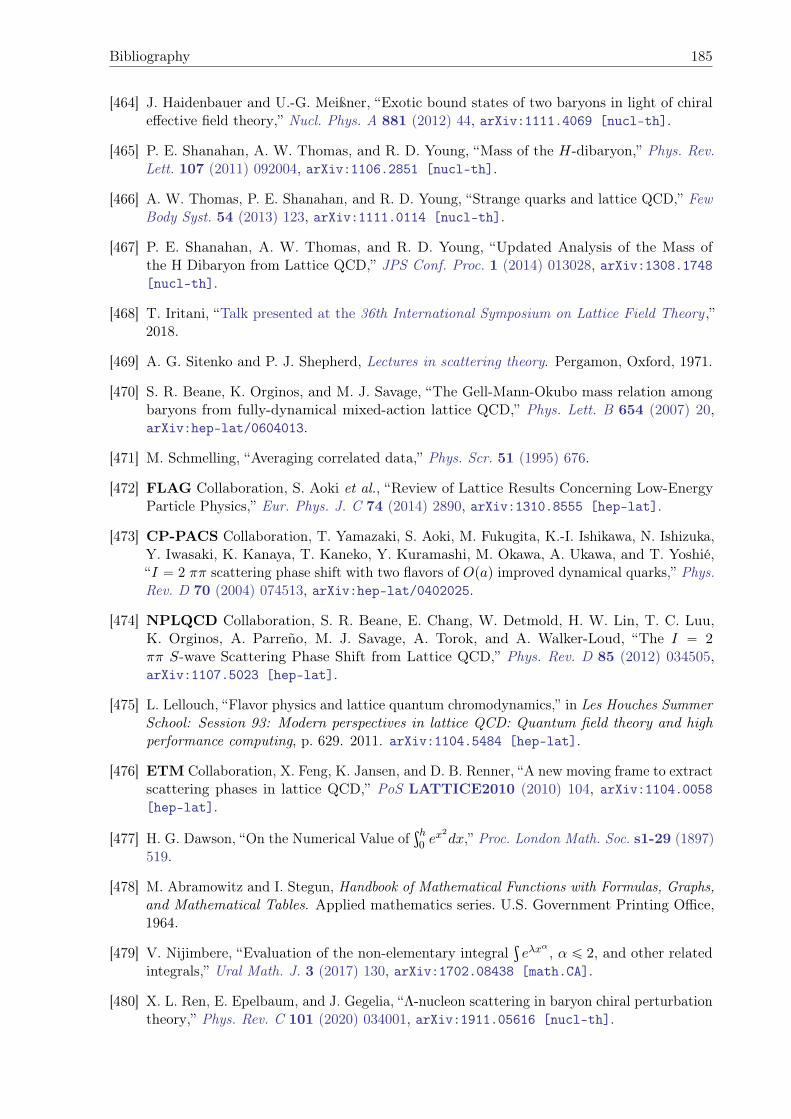
Bibliography 185
[464] J. Haidenbauer and U.-G. Meißner, “Exotic bound states of two baryons in light of chiraleffective field theory,” Nucl. Phys. A 881 (2012) 44, arXiv:1111.4069 [nucl-th].
[465] P. E. Shanahan, A. W. Thomas, and R. D. Young, “Mass of the H-dibaryon,” Phys. Rev.Lett. 107 (2011) 092004, arXiv:1106.2851 [nucl-th].
[466] A. W. Thomas, P. E. Shanahan, and R. D. Young, “Strange quarks and lattice QCD,” FewBody Syst. 54 (2013) 123, arXiv:1111.0114 [nucl-th].
[467] P. E. Shanahan, A. W. Thomas, and R. D. Young, “Updated Analysis of the Mass ofthe H Dibaryon from Lattice QCD,” JPS Conf. Proc. 1 (2014) 013028, arXiv:1308.1748[nucl-th].
[468] T. Iritani, “Talk presented at the 36th International Symposium on Lattice Field Theory ,”2018.
[469] A. G. Sitenko and P. J. Shepherd, Lectures in scattering theory. Pergamon, Oxford, 1971.
[470] S. R. Beane, K. Orginos, and M. J. Savage, “The Gell-Mann-Okubo mass relation amongbaryons from fully-dynamical mixed-action lattice QCD,” Phys. Lett. B 654 (2007) 20,arXiv:hep-lat/0604013.
[471] M. Schmelling, “Averaging correlated data,” Phys. Scr. 51 (1995) 676.
[472] FLAG Collaboration, S. Aoki et al., “Review of Lattice Results Concerning Low-EnergyParticle Physics,” Eur. Phys. J. C 74 (2014) 2890, arXiv:1310.8555 [hep-lat].
[473] CP-PACS Collaboration, T. Yamazaki, S. Aoki, M. Fukugita, K.-I. Ishikawa, N. Ishizuka,Y. Iwasaki, K. Kanaya, T. Kaneko, Y. Kuramashi, M. Okawa, A. Ukawa, and T. Yoshié,“I “ 2 ππ scattering phase shift with two flavors of Opaq improved dynamical quarks,” Phys.Rev. D 70 (2004) 074513, arXiv:hep-lat/0402025.
[474] NPLQCD Collaboration, S. R. Beane, E. Chang, W. Detmold, H. W. Lin, T. C. Luu,K. Orginos, A. Parreño, M. J. Savage, A. Torok, and A. Walker-Loud, “The I “ 2ππ S-wave Scattering Phase Shift from Lattice QCD,” Phys. Rev. D 85 (2012) 034505,arXiv:1107.5023 [hep-lat].
[475] L. Lellouch, “Flavor physics and lattice quantum chromodynamics,” in Les Houches SummerSchool: Session 93: Modern perspectives in lattice QCD: Quantum field theory and highperformance computing, p. 629. 2011. arXiv:1104.5484 [hep-lat].
[476] ETM Collaboration, X. Feng, K. Jansen, and D. B. Renner, “A new moving frame to extractscattering phases in lattice QCD,” PoS LATTICE2010 (2010) 104, arXiv:1104.0058[hep-lat].
[477] H. G. Dawson, “On the Numerical Value ofşh0 e
x2dx,” Proc. London Math. Soc. s1-29 (1897)519.
[478] M. Abramowitz and I. Stegun, Handbook of Mathematical Functions with Formulas, Graphs,and Mathematical Tables. Applied mathematics series. U.S. Government Printing Office,1964.
[479] V. Nijimbere, “Evaluation of the non-elementary integralş
eλxα , α ď 2, and other related
integrals,” Ural Math. J. 3 (2017) 130, arXiv:1702.08438 [math.CA].
[480] X. L. Ren, E. Epelbaum, and J. Gegelia, “Λ-nucleon scattering in baryon chiral perturbationtheory,” Phys. Rev. C 101 (2020) 034001, arXiv:1911.05616 [nucl-th].
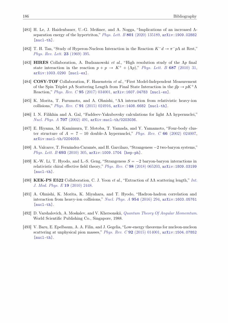
186 Bibliography
[481] H. Le, J. Haidenbauer, U.-G. Meißner, and A. Nogga, “Implications of an increased Λ-separation energy of the hypertriton,” Phys. Lett. B 801 (2020) 135189, arXiv:1909.02882[nucl-th].
[482] T. H. Tan, “Study of Hyperon-Nucleon Interaction in the Reaction K´dÑ π´pΛ at Rest,”Phys. Rev. Lett. 23 (1969) 395.
[483] HIRES Collaboration, A. Budzanowski et al., “High resolution study of the Λp finalstate interaction in the reaction p ` p Ñ K` ` pΛpq,” Phys. Lett. B 687 (2010) 31,arXiv:1003.0290 [nucl-ex].
[484] COSY-TOF Collaboration, F. Hauenstein et al., “First Model-Independent Measurementof the Spin Triplet pΛ Scattering Length from Final State Interaction in the ~ppÑ pK`ΛReaction,” Phys. Rev. C 95 (2017) 034001, arXiv:1607.04783 [nucl-ex].
[485] K. Morita, T. Furumoto, and A. Ohnishi, “ΛΛ interaction from relativistic heavy-ioncollisions,” Phys. Rev. C 91 (2015) 024916, arXiv:1408.6682 [nucl-th].
[486] I. N. Filikhin and A. Gal, “Faddeev-Yakubovsky calculations for light ΛΛ hypernuclei,”Nucl. Phys. A 707 (2002) 491, arXiv:nucl-th/0203036.
[487] E. Hiyama, M. Kamimura, T. Motoba, T. Yamada, and Y. Yamamoto, “Four-body clus-ter structure of A “ 7 ´ 10 double-Λ hypernuclei,” Phys. Rev. C 66 (2002) 024007,arXiv:nucl-th/0204059.
[488] A. Valcarce, T. Fernández-Caramés, and H. Garcilazo, “Strangeness ´2 two-baryon systems,”Phys. Lett. B 693 (2010) 305, arXiv:1009.1704 [hep-ph].
[489] K.-W. Li, T. Hyodo, and L.-S. Geng, “Strangeness S “ ´2 baryon-baryon interactions inrelativistic chiral effective field theory,” Phys. Rev. C 98 (2018) 065203, arXiv:1809.03199[nucl-th].
[490] KEK-PS E522 Collaboration, C. J. Yoon et al., “Extraction of ΛΛ scattering length,” Int.J. Mod. Phys. E 19 (2010) 2448.
[491] A. Ohnishi, K. Morita, K. Miyahara, and T. Hyodo, “Hadron-hadron correlation andinteraction from heavy-ion collisions,” Nucl. Phys. A 954 (2016) 294, arXiv:1603.05761[nucl-th].
[492] D. Varshalovich, A. Moskalev, and V. Khersonskii, Quantum Theory Of Angular Momemtum.World Scientific Publishing Co., Singapore, 1988.
[493] V. Baru, E. Epelbaum, A. A. Filin, and J. Gegelia, “Low-energy theorems for nucleon-nucleonscattering at unphysical pion masses,” Phys. Rev. C 92 (2015) 014001, arXiv:1504.07852[nucl-th].


