Embed Size (px)
Citation preview
Fabio MaltoniCERN School, University of Chinese Academy of Science Fabio Maltoni
Fabio Maltoni Center for Cosmology, Particle Physics and Phenomenology (CP3)
Université Catholique de Louvain
Lecture II
1
Basics of QCD
Fabio MaltoniCERN School, University of Chinese Academy of Science Fabio Maltoni
AEPSHEP 2016
e+ e- collisions : QCD in the final state
1. Infrared safety
2. Towards realistic final states
3. Jets
2
Fabio MaltoniCERN School, University of Chinese Academy of Science Fabio Maltoni
AEPSHEP 2016
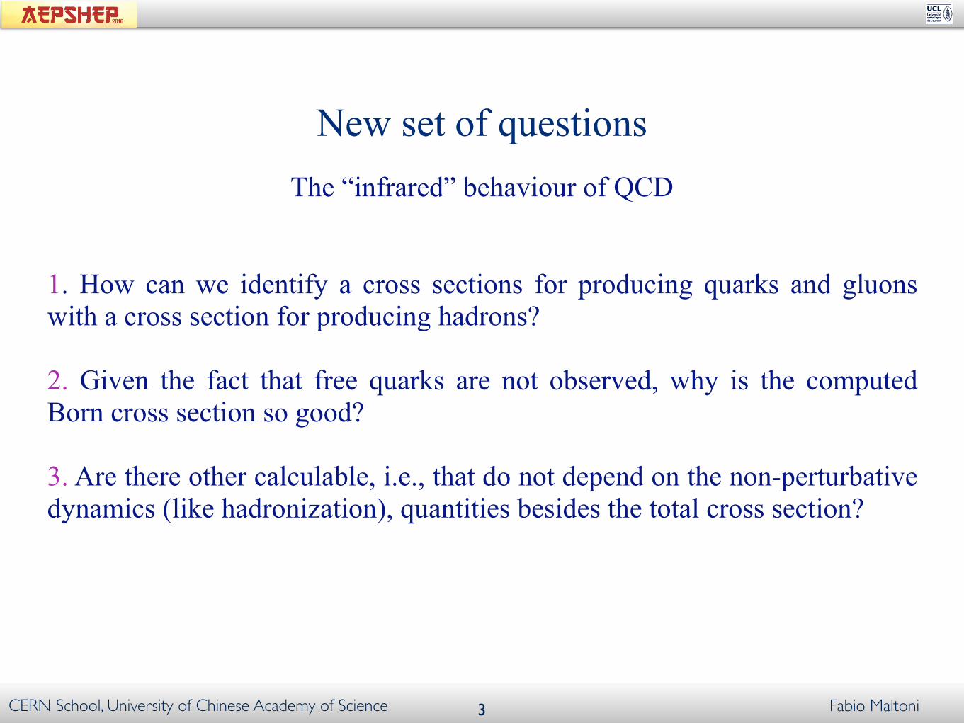
New set of questions
1. How can we identify a cross sections for producing quarks and gluons with a cross section for producing hadrons? !2. Given the fact that free quarks are not observed, why is the computed Born cross section so good? !3. Are there other calculable, i.e., that do not depend on the non-perturbative dynamics (like hadronization), quantities besides the total cross section?
The “infrared” behaviour of QCD
3
Fabio MaltoniCERN School, University of Chinese Academy of Science Fabio Maltoni
AEPSHEP 2016
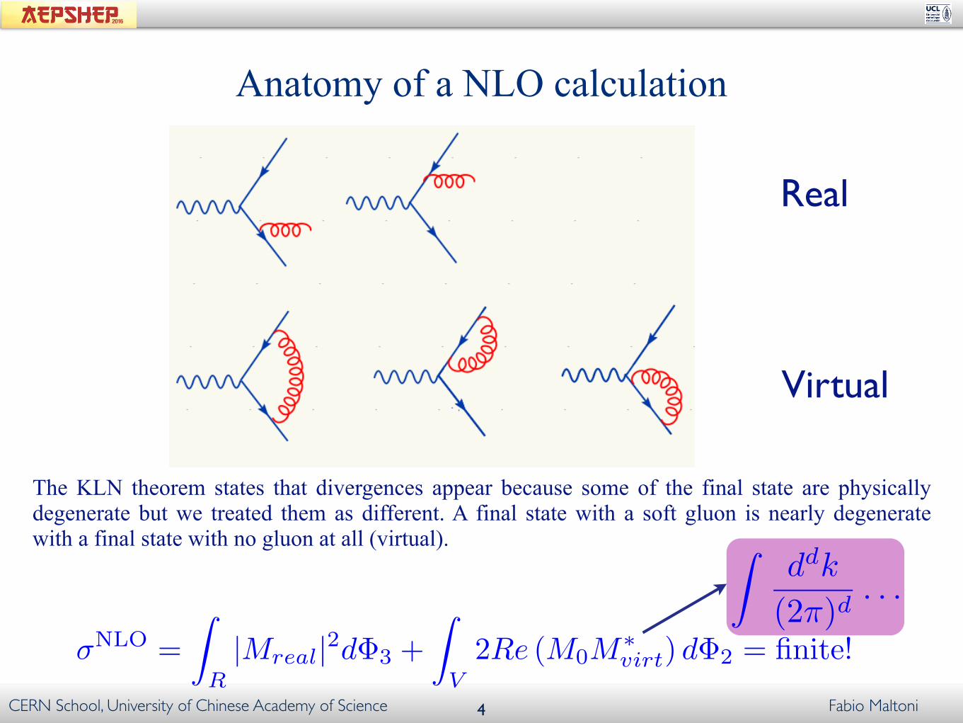
Real
Virtual
Anatomy of a NLO calculation
σNLO =
!R
|Mreal|2dΦ3 +
!V
2Re (M0M∗
virt) dΦ2 = finite!
!ddk
(2π)d. . .
The KLN theorem states that divergences appear because some of the final state are physically degenerate but we treated them as different. A final state with a soft gluon is nearly degenerate with a final state with no gluon at all (virtual).
4
Fabio MaltoniCERN School, University of Chinese Academy of Science Fabio Maltoni
AEPSHEP 2016
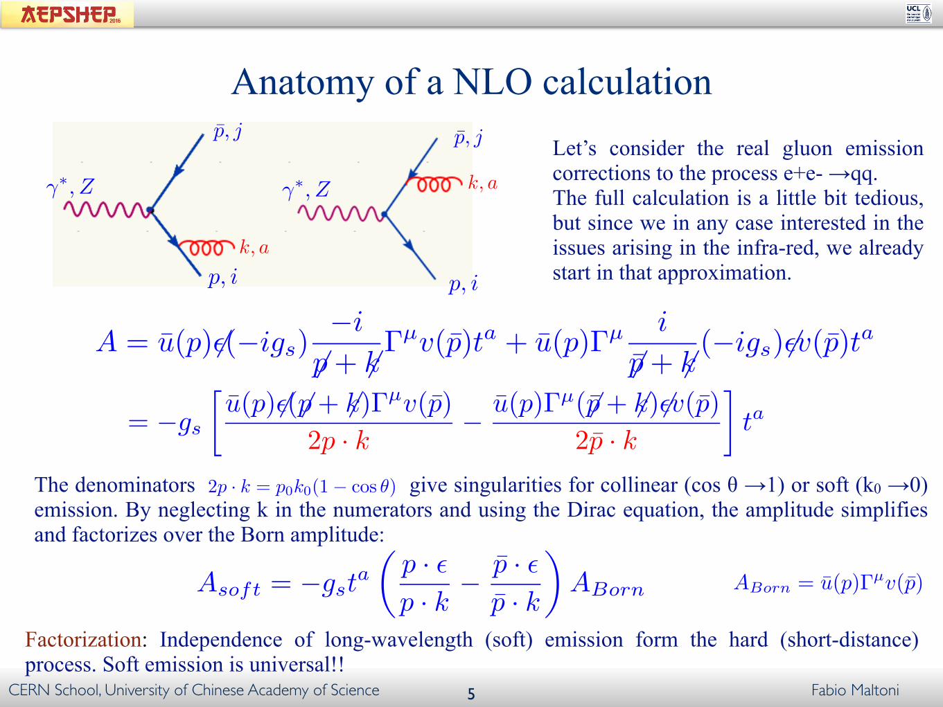
p, j
p, i
k, a
p, j
p, i
k, a
γ∗, Z γ∗, Z
A = u(p)ϵ(−igs)−i
p + kΓµv(p)ta + u(p)Γµ
i
p + k(−igs)ϵv(p)ta
= −gs
!
u(p)ϵ(p + k)Γµv(p)
2p · k−
u(p)Γµ(p + k)ϵv(p)
2p · k
"
ta
The denominators give singularities for collinear (cos θ →1) or soft (k0 →0) emission. By neglecting k in the numerators and using the Dirac equation, the amplitude simplifies and factorizes over the Born amplitude:
2p · k = p0k0(1 − cos θ)
ABorn = u(p)Γµv(p)Asoft = −gsta
!
p · ϵ
p · k−
p · ϵ
p · k
"
ABorn
Factorization: Independence of long-wavelength (soft) emission form the hard (short-distance) process. Soft emission is universal!!
Let’s consider the real gluon emission corrections to the process e+e- →qq. The full calculation is a little bit tedious, but since we in any case interested in the issues arising in the infra-red, we already start in that approximation.
Anatomy of a NLO calculation
5
Fabio MaltoniCERN School, University of Chinese Academy of Science Fabio Maltoni
AEPSHEP 2016
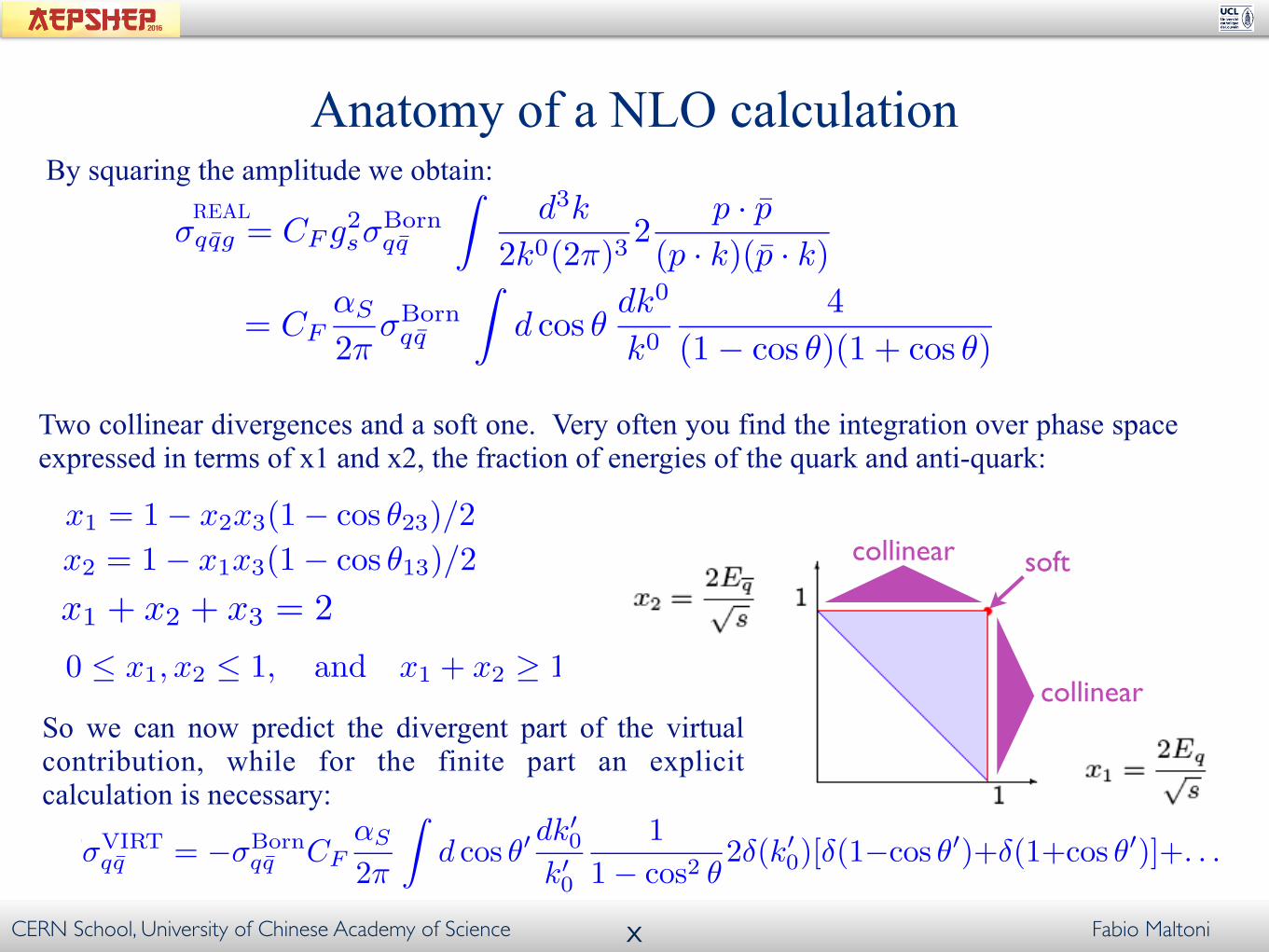
0 ≤ x1, x2 ≤ 1, and x1 + x2 ≥ 1
Two collinear divergences and a soft one. Very often you find the integration over phase space expressed in terms of x1 and x2, the fraction of energies of the quark and anti-quark:
x1 = 1 − x2x3(1 − cos θ23)/2
x2 = 1 − x1x3(1 − cos θ13)/2
x1 + x2 + x3 = 2
collinear soft
collinear
dσVIRTqq = −σ
Bornqq CF
αS
2π
!d cos θ
′dk′
0
k′
0
1
1 − cos2 θ2δ(k′
0)[δ(1−cos θ′)+δ(1+cos θ
′)]+. . .
So we can now predict the divergent part of the virtual contribution, while for the finite part an explicit calculation is necessary:
Anatomy of a NLO calculationBy squaring the amplitude we obtain:
σqqg = CF g2sσBorn
!d3k
2k0(2π)32
p · p
(p · k)(p · k)
= CFαS
2πσ
Bornqq
!d cos θ
dk0
k0
4
(1 − cos θ)(1 + cos θ)
REAL
X
Fabio MaltoniCERN School, University of Chinese Academy of Science Fabio Maltoni
AEPSHEP 2016
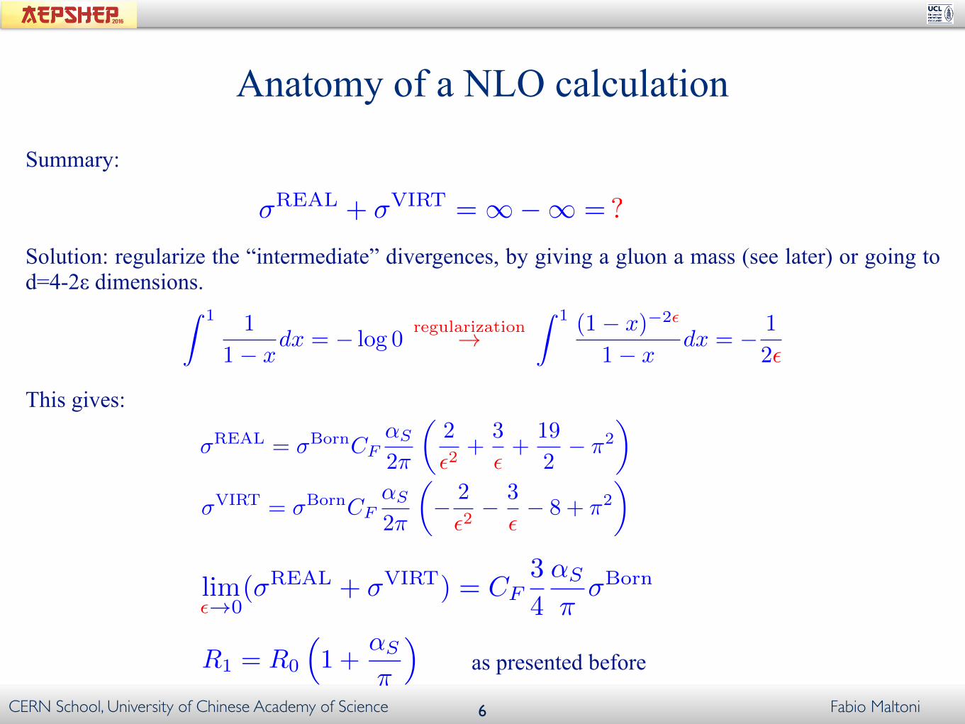
Anatomy of a NLO calculation
Summary:
�REAL + �VIRT = 1�1 =?
Solution: regularize the “intermediate” divergences, by giving a gluon a mass (see later) or going to d=4-2ε dimensions.
Z1
1
1� x
dx = � log 0
regularization!Z
1
(1� x)
�2✏
1� x
dx = � 1
2✏
lim✏!0
(�REAL + �VIRT) = CF3
4
↵S
⇡�Born
R1 = R0
!
1 +αS
π
"
as presented before
�REAL = �BornCF↵S
2⇡
✓2
✏2+
3
✏+
19
2� ⇡2
◆
�VIRT = �BornCF↵S
2⇡
✓� 2
✏2� 3
✏� 8 + ⇡2
◆
This gives:
6
Fabio MaltoniCERN School, University of Chinese Academy of Science Fabio Maltoni
AEPSHEP 2016
1. How can we identify a cross sections for producing (few) quarks and gluons with a cross section for producing (many) hadrons? !2. Given the fact that free quarks are not observed, why is the computed Born cross section so good?
Answers: !
The Born cross section IS NOT the cross section for producing q qbar, since the coefficients of the perturbative expansion are infinite! But this is not a problem since we don’t observe q qbar and nothing else. So there is no contradiction here. !On the other hand the cross section for producing hadrons is finite order by order and its lowest order approximation IS the Born. !A further insight can be gained by thinking of what happens in QED and what is different there. For instance soft and collinear divergence are also there. In QED one can prove that cross section for producing “only two muons” is zero...
New set of questions
7
Fabio MaltoniCERN School, University of Chinese Academy of Science Fabio Maltoni
AEPSHEP 2016
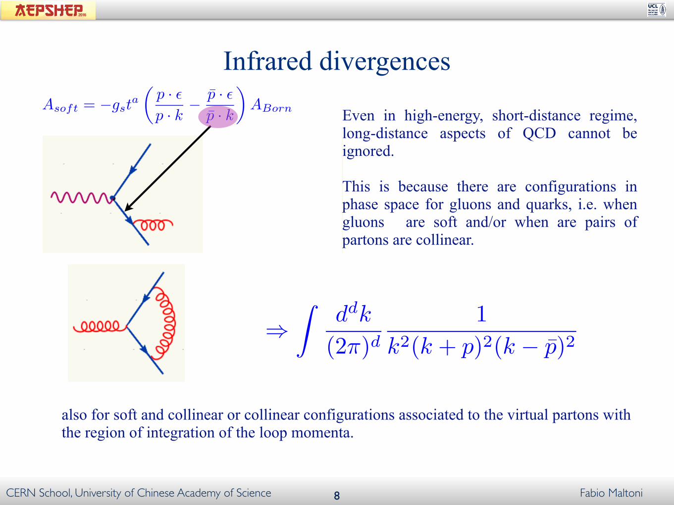
Infrared divergences
Even in high-energy, short-distance regime, long-distance aspects of QCD cannot be ignored. This is because there are configurations in phase space for gluons and quarks, i.e. when gluons are soft and/or when are pairs of partons are collinear.
⇒
!ddk
(2π)d
1
k2(k + p)2(k − p)2
also for soft and collinear or collinear configurations associated to the virtual partons with the region of integration of the loop momenta.
Asoft = −gsta
!
p · ϵ
p · k−
p · ϵ
p · k
"
ABorn
8
Fabio MaltoniCERN School, University of Chinese Academy of Science Fabio Maltoni
AEPSHEP 2016
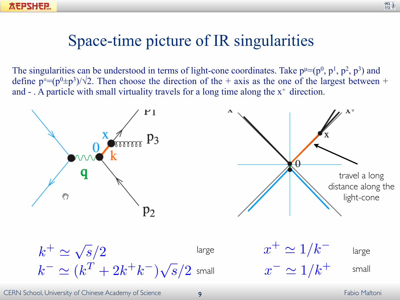
k+≃
√s/2
k−
≃ (kT + 2k+k−)√
s/2
x+≃ 1/k−
x−
≃ 1/k+
large
small
large
small
travel a long distance along the
light-cone
Space-time picture of IR singularities
The singularities can be understood in terms of light-cone coordinates. Take pµ=(p0, p1, p2, p3) and define p±=(p0±p3)/√2. Then choose the direction of the + axis as the one of the largest between + and - . A particle with small virtuality travels for a long time along the x+ direction.
9
Fabio MaltoniCERN School, University of Chinese Academy of Science Fabio Maltoni
AEPSHEP 2016
Infrared divergences
Infrared divergences arise from interactions that happen a long time after the creation of the quark/antiquark pair. !When distances become comparable to the hadron size of ~1 Fermi, quasi-free partons of the perturbative calculation are confined/hadronized non-perturbatively. !We have seen that in total cross sections such divergences cancel. But what about for other quantities? !Obviously, the only possibility is to try to use the pQCD calculations for quantities that are not sensitive to the to the long-distance physics. !Can we formulate a criterium that is valid in general?
YES! It is called INFRARED SAFETY
10
Fabio MaltoniCERN School, University of Chinese Academy of Science Fabio Maltoni
AEPSHEP 2016
Infrared-safe quantities
DEFINITION: quantities are that are insensitive to soft and collinear branching. !For these quantities, an extension of the general theorem (KLN) exists which proves that infrared divergences cancel between real and virtual or are simply removed by kinematic factors. !Such quantities are determined primarily by hard, short-distance physics. Long-distance effects give power corrections, suppressed by the inverse power of a large momentum scale (which must be present in the first place to justify the use of PT). !Examples: 1. Multiplicity of gluons is not IRC safe 2. Energy of hardest particle is not IRC safe 3. Energy flow into a cone is IRC safe
11
Fabio MaltoniCERN School, University of Chinese Academy of Science Fabio Maltoni
AEPSHEP 2016
q
q
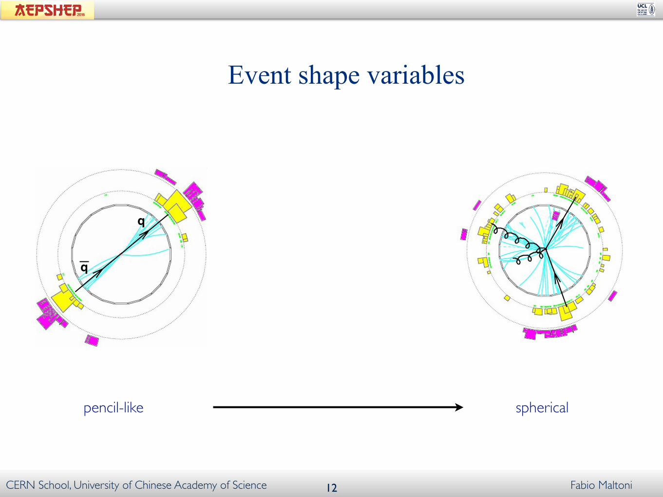
Event shape variables
pencil-like spherical
12
Fabio MaltoniCERN School, University of Chinese Academy of Science Fabio Maltoni
AEPSHEP 2016
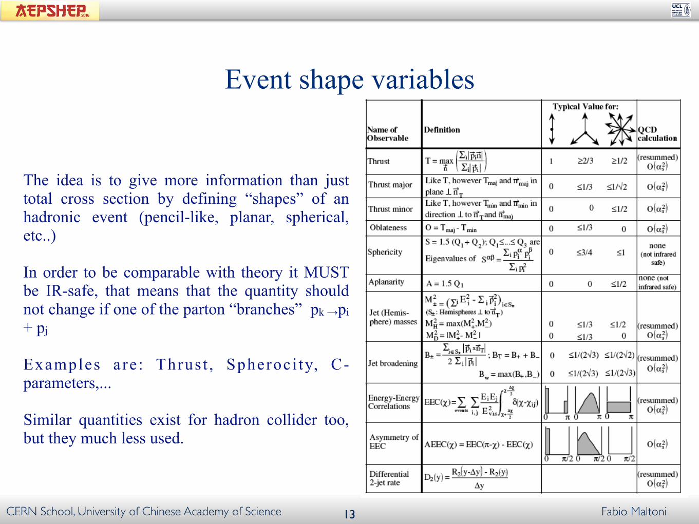
Event shape variables
The idea is to give more information than just total cross section by defining “shapes” of an hadronic event (pencil-like, planar, spherical, etc..) !In order to be comparable with theory it MUST be IR-safe, that means that the quantity should not change if one of the parton “branches” pk →pi + pj !Examples are : Thrus t , Spheroci ty, C-parameters,... !Similar quantities exist for hadron collider too, but they much less used.
13
Fabio MaltoniCERN School, University of Chinese Academy of Science Fabio Maltoni
AEPSHEP 2016
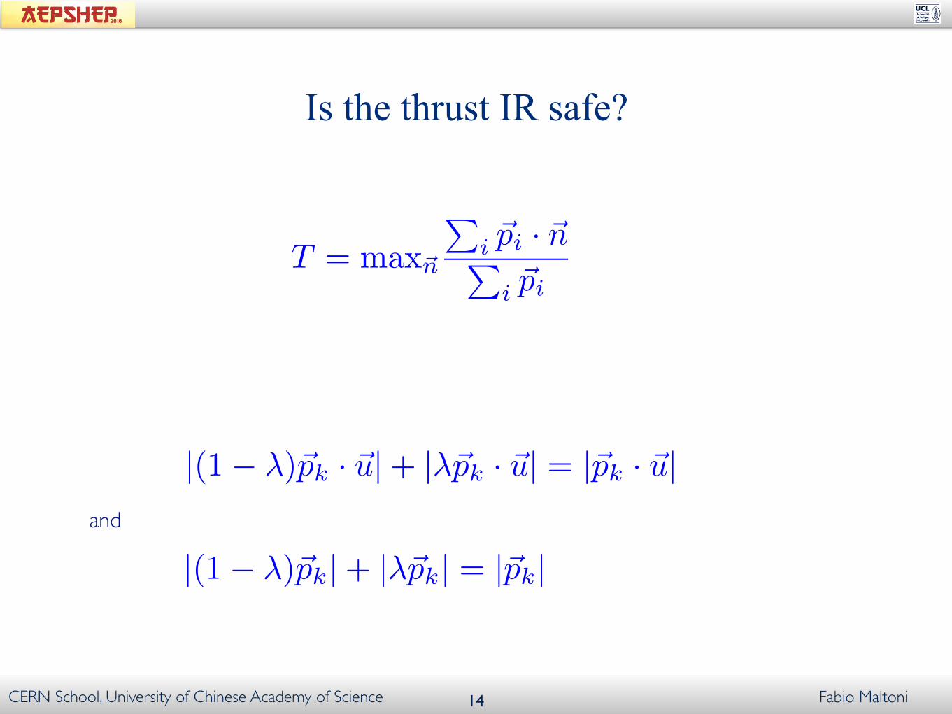
Is the thrust IR safe?
T = maxn
!ipi · n!ipi
|(1� �)~pk · ~u|+ |�~pk · ~u| = |~pk · ~u|
|(1� �)~pk|+ |�~pk| = |~pk|and
14
Fabio MaltoniCERN School, University of Chinese Academy of Science Fabio Maltoni
AEPSHEP 2016
1
σ
dσ
dT= CF
αS
2π
!
2(3T 2− 3T + 2)
T (1 − T )log
"
2T − 1
1 − T
#
−
3(3T − 2)(2 − T )
1 − T
$
.
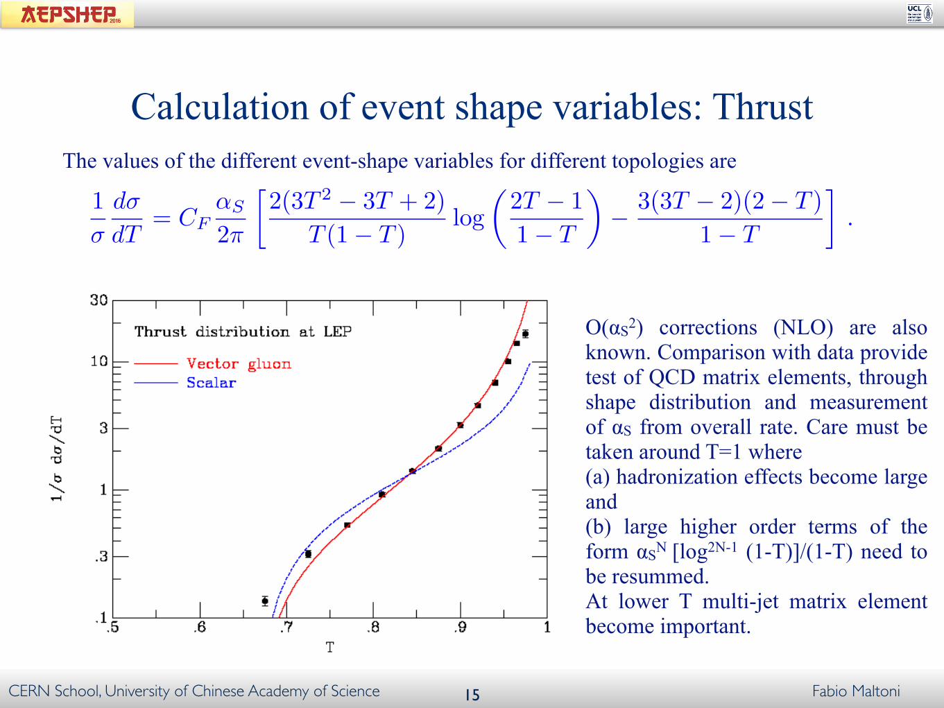
Calculation of event shape variables: ThrustThe values of the different event-shape variables for different topologies are
O(αS2) corrections (NLO) are also known. Comparison with data provide test of QCD matrix elements, through shape distribution and measurement of αS from overall rate. Care must be taken around T=1 where (a) hadronization effects become large and (b) large higher order terms of the form αSN [log2N-1 (1-T)]/(1-T) need to be resummed. At lower T multi-jet matrix element become important.
15
Fabio MaltoniCERN School, University of Chinese Academy of Science Fabio Maltoni
AEPSHEP 2016
QCD in the final state
1. Infrared safety
2. Towards realistic final states
3. Jets
16
Fabio MaltoniCERN School, University of Chinese Academy of Science Fabio Maltoni
AEPSHEP 2016
?γ*,Z
17
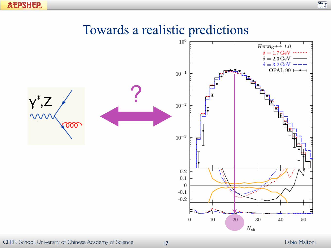
Towards a realistic predictions
Fabio MaltoniCERN School, University of Chinese Academy of Science Fabio Maltoni
AEPSHEP 2016
�2j = �Born
"1� ↵SCF
⇡log
2 y +1
2!
✓↵SCF
⇡log
2 y
◆2
+ . . .
#= �Borne�
↵SCF⇡ log
2 y
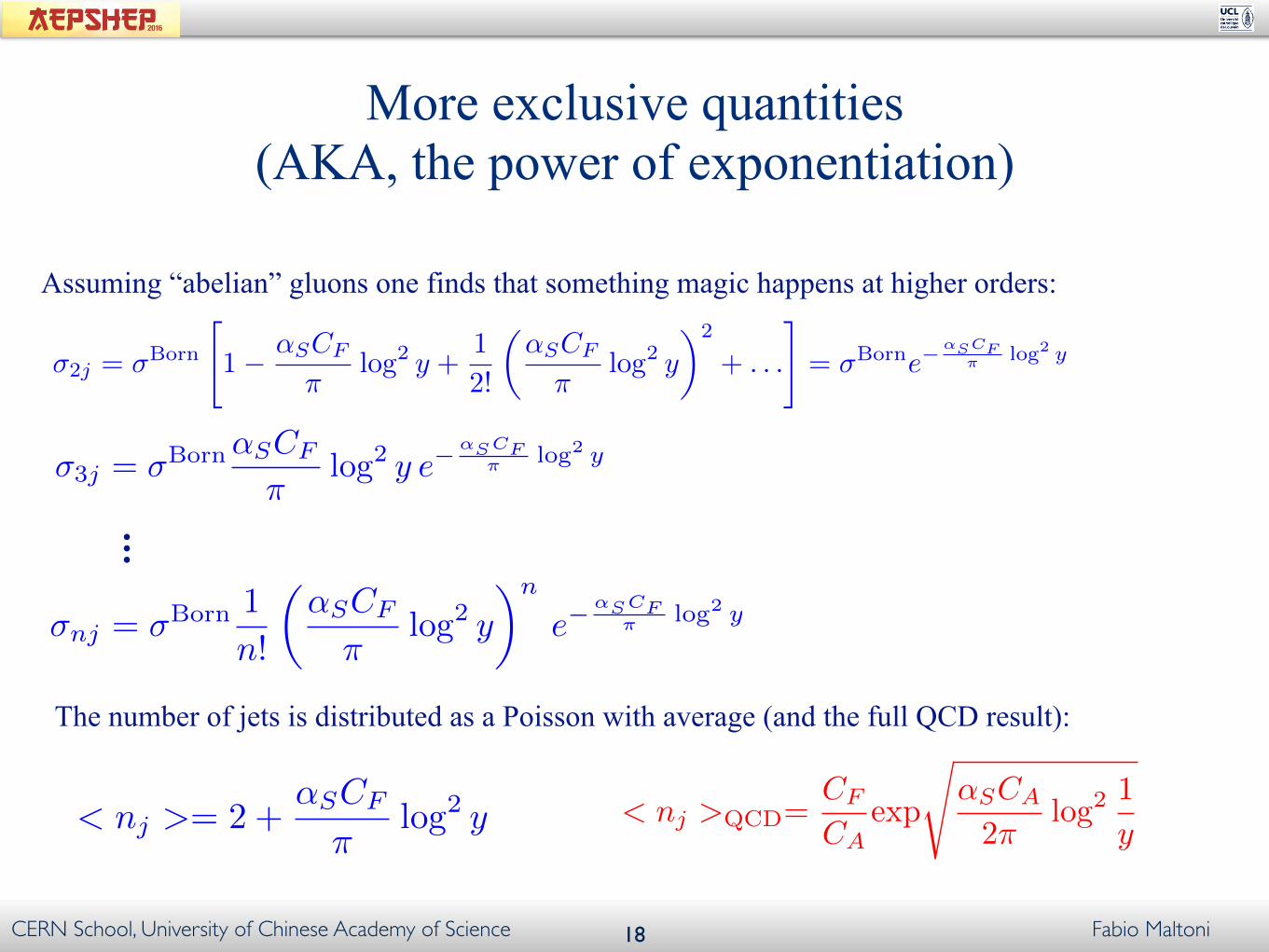
Assuming “abelian” gluons one finds that something magic happens at higher orders:
�3j = �Born
↵SCF
⇡log
2 y e�↵SCF
⇡ log
2 y
�nj = �Born
1
n!
✓↵SCF
⇡log
2 y
◆n
e�↵SCF
⇡ log
2 y
...
The number of jets is distributed as a Poisson with average (and the full QCD result):
< nj >= 2 +
↵SCF
⇡log
2 y < nj >QCD=CF
CAexp
s↵SCA
2⇡log
2 1
y
18
More exclusive quantities (AKA, the power of exponentiation)
Fabio MaltoniCERN School, University of Chinese Academy of Science Fabio Maltoni
AEPSHEP 2016
More exclusive quantities (AKA, the power of exponentiation)
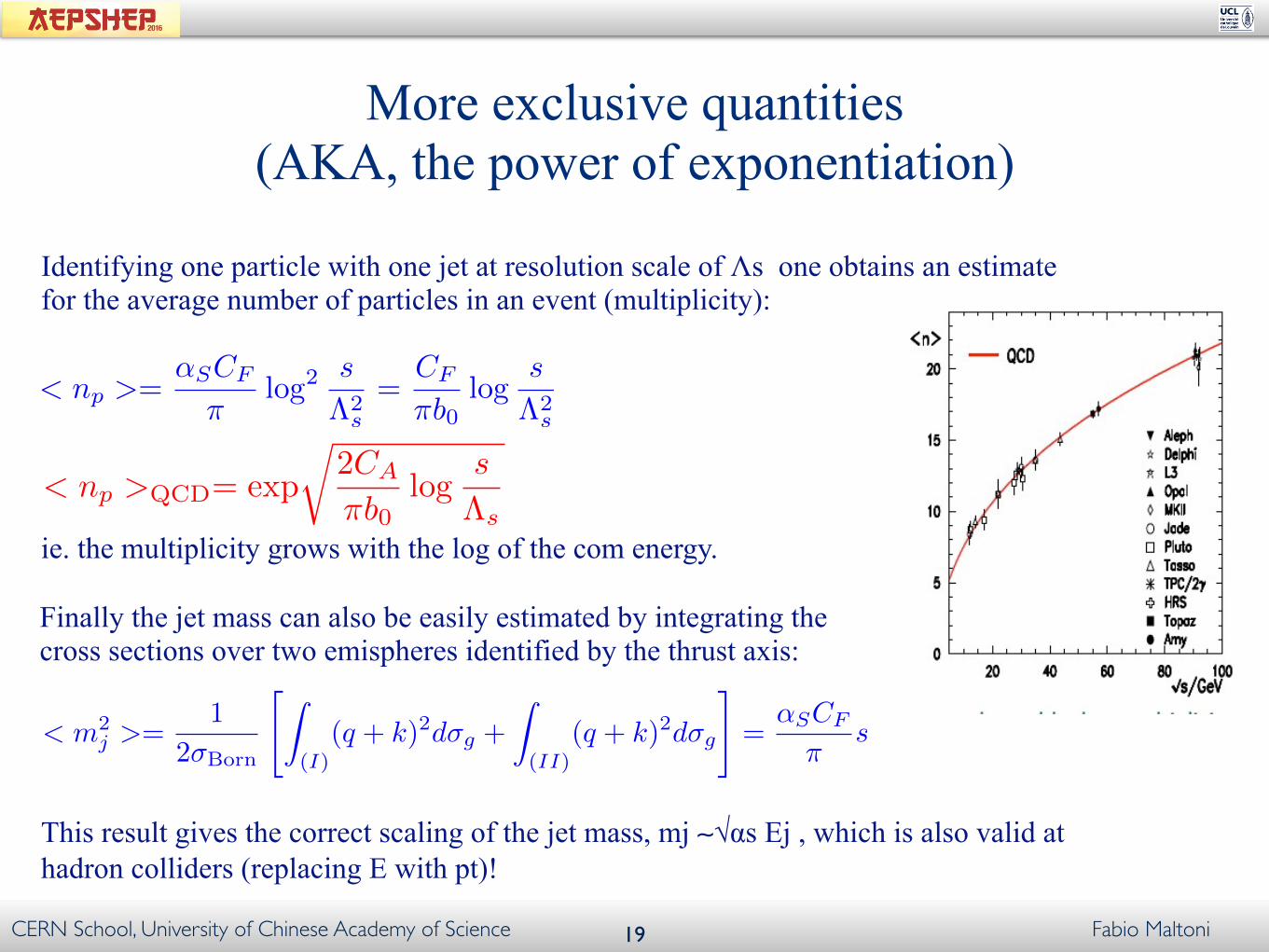
Identifying one particle with one jet at resolution scale of Λs one obtains an estimate for the average number of particles in an event (multiplicity):
< np >=
↵SCF
⇡log
2 s
⇤
2s
=
CF
⇡b0log
s
⇤
2s
ie. the multiplicity grows with the log of the com energy.
Finally the jet mass can also be easily estimated by integrating the cross sections over two emispheres identified by the thrust axis:
< m2
j >=1
2�Born
"Z
(I)(q + k)2d�g +
Z
(II)(q + k)2d�g
#=
↵SCF
⇡s
This result gives the correct scaling of the jet mass, mj ∼√αs Ej , which is also valid at hadron colliders (replacing E with pt)!
< np >QCD= exp
r2CA
⇡b0log
s
⇤s
19
Fabio MaltoniCERN School, University of Chinese Academy of Science Fabio Maltoni
AEPSHEP 2016
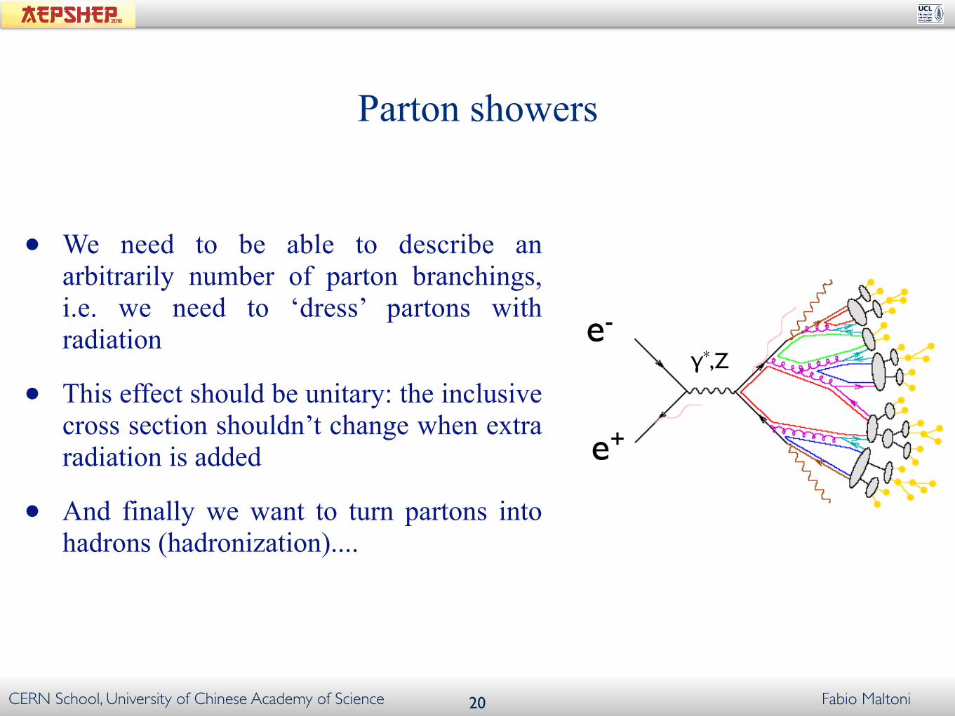
Parton showers
• We need to be able to describe an arbitrarily number of parton branchings, i.e. we need to ‘dress’ partons with radiation
• This effect should be unitary: the inclusive cross section shouldn’t change when extra radiation is added
• And finally we want to turn partons into hadrons (hadronization)....
20
e-
e+
γ*,Z
Fabio MaltoniCERN School, University of Chinese Academy of Science Fabio Maltoni
AEPSHEP 2016
2a
b
cθ
Mn+1θ ➞ 0
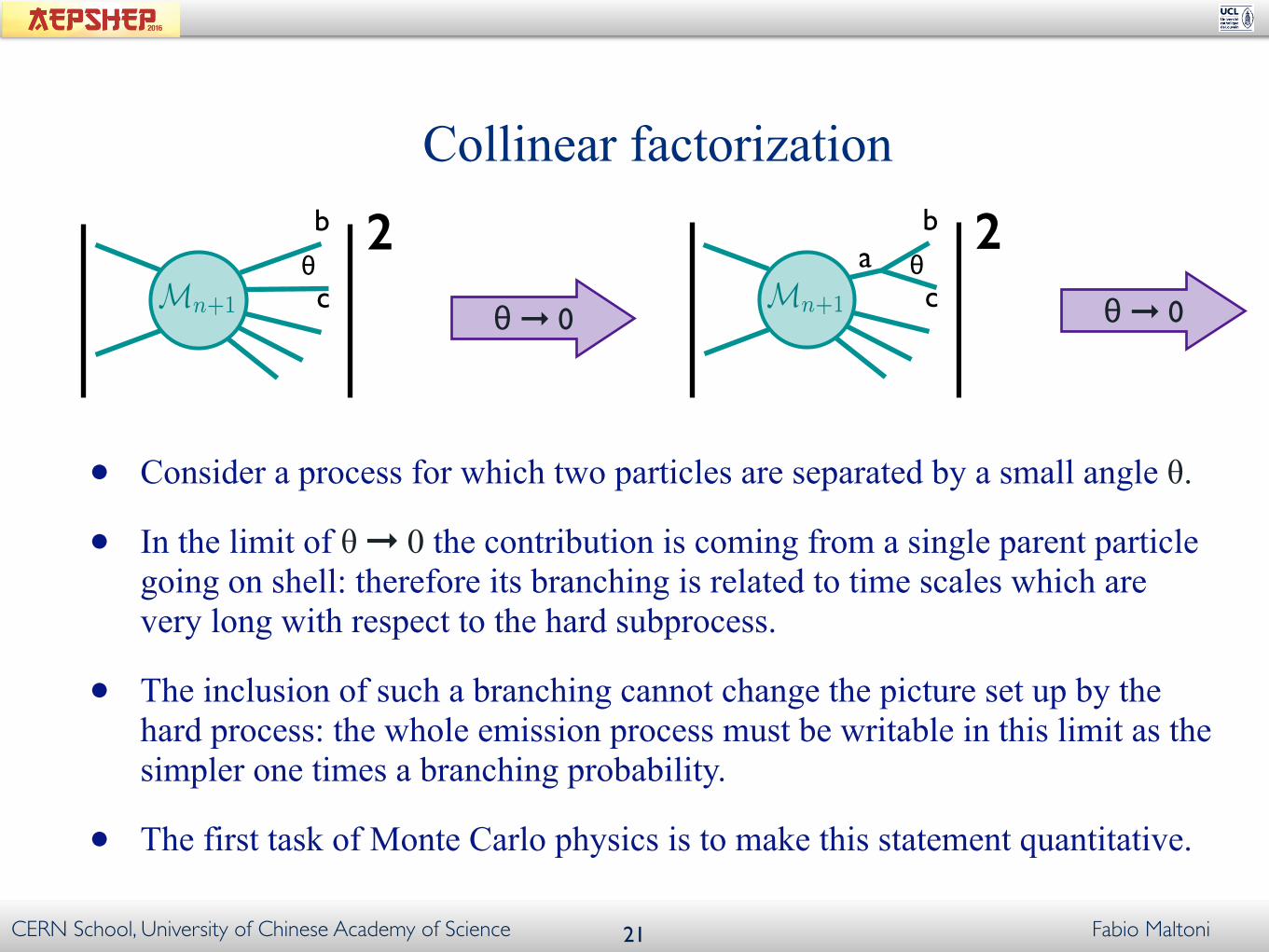
Collinear factorization
• Consider a process for which two particles are separated by a small angle θ.
• In the limit of θ ➞ 0 the contribution is coming from a single parent particle going on shell: therefore its branching is related to time scales which are very long with respect to the hard subprocess.
• The inclusion of such a branching cannot change the picture set up by the hard process: the whole emission process must be writable in this limit as the simpler one times a branching probability.
• The first task of Monte Carlo physics is to make this statement quantitative.
21
θ ➞ 0
2b
cθ
Mn+1
Fabio MaltoniCERN School, University of Chinese Academy of Science Fabio Maltoni
AEPSHEP 2016
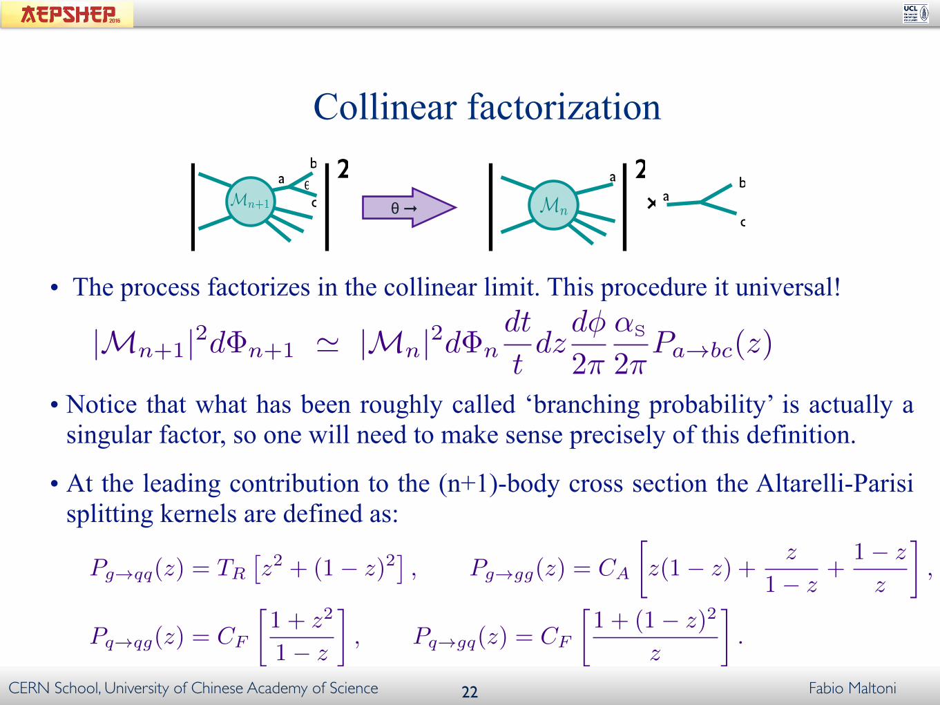
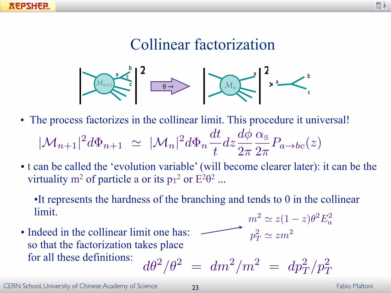
• The process factorizes in the collinear limit. This procedure it universal!
22
2ab
cθ
Mn+1 θ ➞ ×b
c
a2a
Mn
|Mn+1|2d�n+1 ' |Mn|2d�ndt
tdz
d�
2⇡
↵S
2⇡Pa!bc(z)
Pg!qq(z) = TR
⇥z2 + (1� z)2
⇤, Pg!gg(z) = CA
z(1� z) +
z
1� z+
1� z
z
�,
Pq!qg(z) = CF
1 + z2
1� z
�, Pq!gq(z) = CF
1 + (1� z)2
z
�.
• Notice that what has been roughly called ‘branching probability’ is actually a singular factor, so one will need to make sense precisely of this definition.
• At the leading contribution to the (n+1)-body cross section the Altarelli-Parisi splitting kernels are defined as:
Collinear factorization
Fabio MaltoniCERN School, University of Chinese Academy of Science Fabio Maltoni
AEPSHEP 2016
• t can be called the ‘evolution variable’ (will become clearer later): it can be the virtuality m2 of particle a or its pT2 or E2θ2 ...
•It represents the hardness of the branching and tends to 0 in the collinear limit.
• Indeed in the collinear limit one has: so that the factorization takes place for all these definitions:
d✓2/✓2 = dm2/m2 = dp2T /p2T
23
2ab
cθ
Mn+1 θ ➞ ×b
c
a2a
Mn
|Mn+1|2d�n+1 ' |Mn|2d�ndt
tdz
d�
2⇡
↵S
2⇡Pa!bc(z)
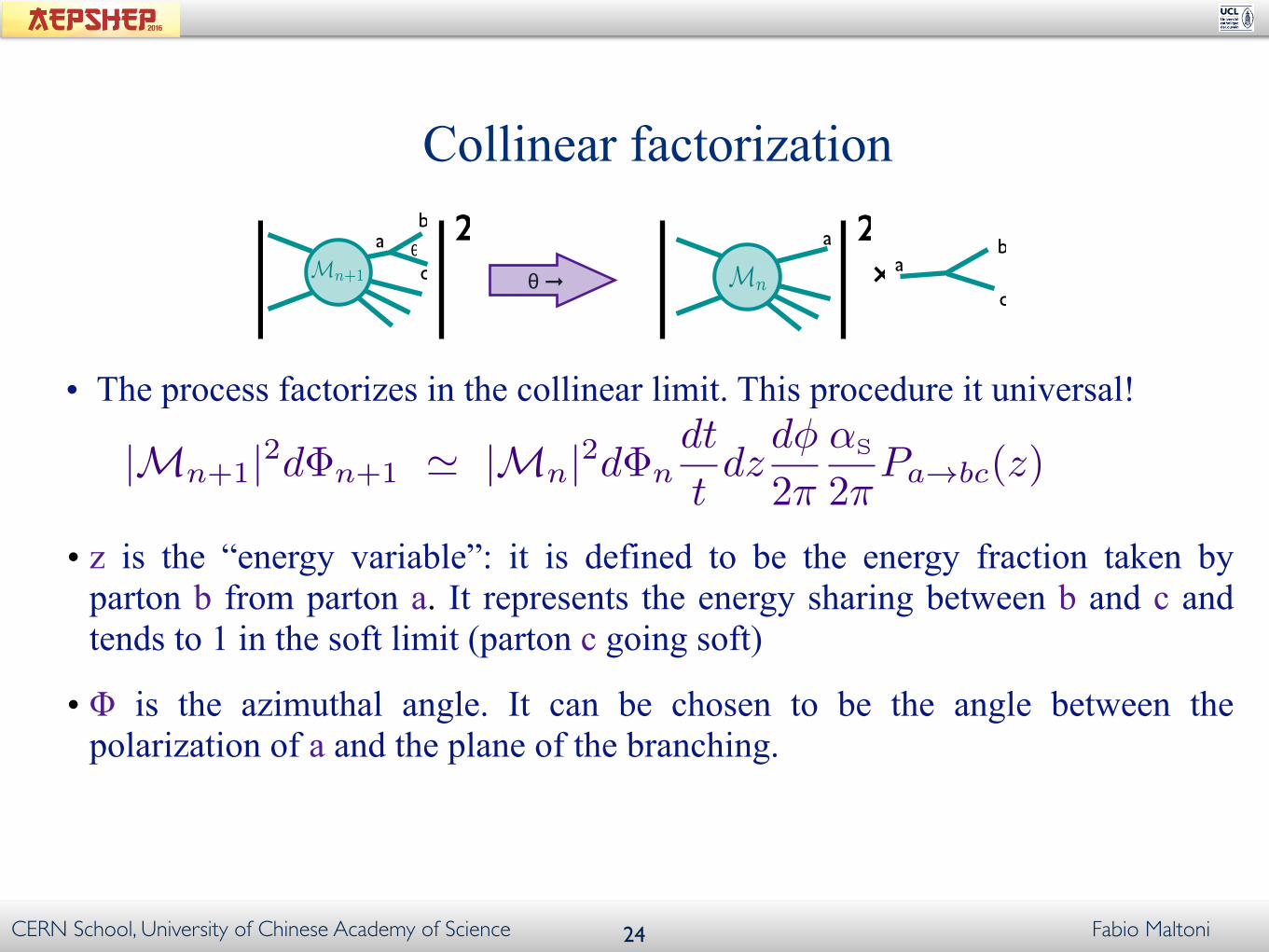
• The process factorizes in the collinear limit. This procedure it universal!
m2 ' z(1� z)✓2E2a
p2T ' zm2
Collinear factorization
Fabio MaltoniCERN School, University of Chinese Academy of Science Fabio Maltoni
AEPSHEP 2016
24
2ab
cθ
Mn+1 θ ➞ ×b
c
a2a
Mn
|Mn+1|2d�n+1 ' |Mn|2d�ndt
tdz
d�
2⇡
↵S
2⇡Pa!bc(z)
• The process factorizes in the collinear limit. This procedure it universal!
Collinear factorization
• z is the “energy variable”: it is defined to be the energy fraction taken by parton b from parton a. It represents the energy sharing between b and c and tends to 1 in the soft limit (parton c going soft)
• Φ is the azimuthal angle. It can be chosen to be the angle between the polarization of a and the plane of the branching.
Fabio MaltoniCERN School, University of Chinese Academy of Science Fabio Maltoni
AEPSHEP 2016
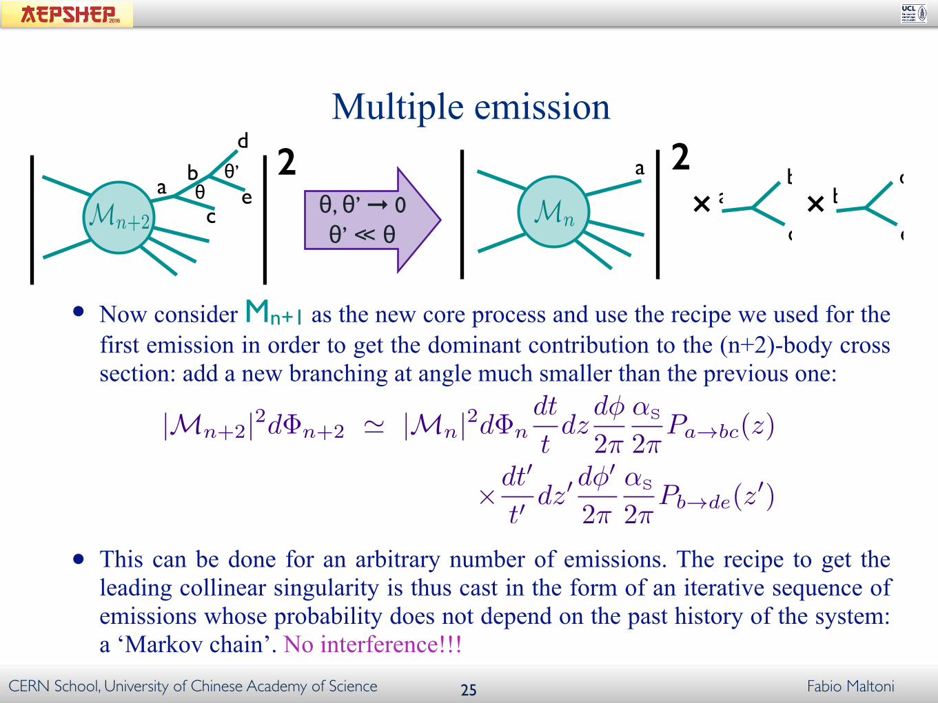
• Now consider Mn+1 as the new core process and use the recipe we used for the first emission in order to get the dominant contribution to the (n+2)-body cross section: add a new branching at angle much smaller than the previous one:
!
• This can be done for an arbitrary number of emissions. The recipe to get the leading collinear singularity is thus cast in the form of an iterative sequence of emissions whose probability does not depend on the past history of the system: a ‘Markov chain’. No interference!!!
Multiple emission
25
|Mn+2|2d�n+2 ' |Mn|2d�ndt
tdz
d�
2⇡
↵S
2⇡Pa!bc(z)
⇥dt0
t0dz0
d�0
2⇡
↵S
2⇡Pb!de(z
0)
θ, θ’ ➞ 0 θ’ ≪ θ
2a
b
cθ
θ’
d
e ×b
c
a
2a
Mn
d
e
b×Mn+2
Fabio MaltoniCERN School, University of Chinese Academy of Science Fabio Maltoni
AEPSHEP 2016
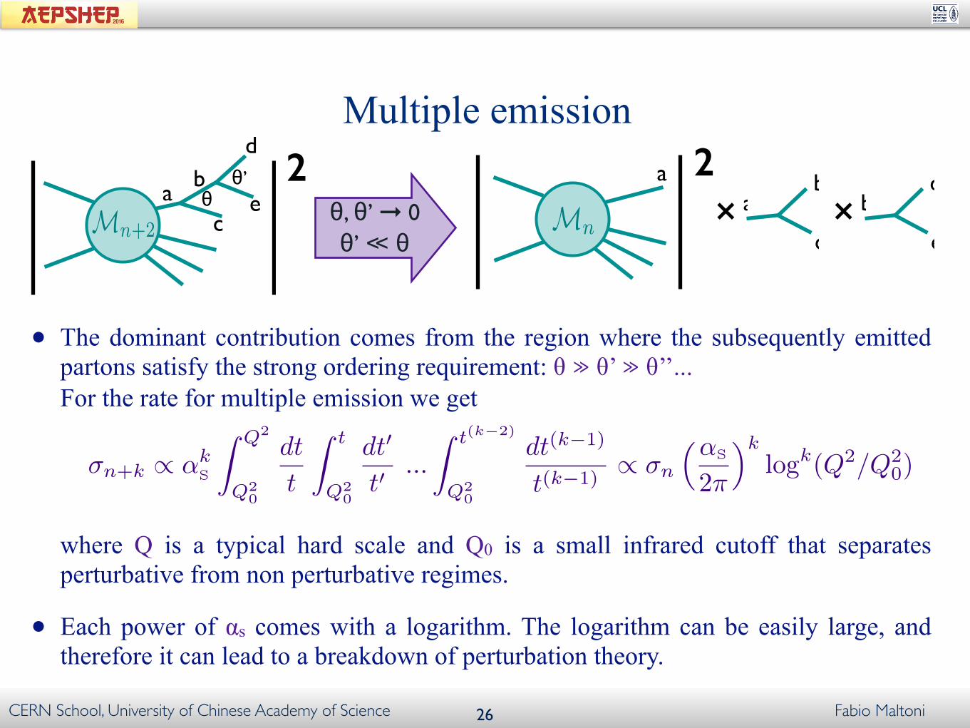
• The dominant contribution comes from the region where the subsequently emitted partons satisfy the strong ordering requirement: θ ≫ θ’ ≫ θ’’...For the rate for multiple emission we get where Q is a typical hard scale and Q0 is a small infrared cutoff that separates perturbative from non perturbative regimes.
• Each power of αs comes with a logarithm. The logarithm can be easily large, and therefore it can lead to a breakdown of perturbation theory.
26
�n+k / ↵kS
Z Q2
Q20
dt
t
Z t
Q20
dt0
t0...
Z t(k�2)
Q20
dt(k�1)
t(k�1)/ �n
⇣↵S
2⇡
⌘klog
k(Q2/Q2
0)
θ, θ’ ➞ 0 θ’ ≪ θ
2a
b
cθ
θ’
d
e ×b
c
a
2a
Mn
d
e
b×Mn+2
Multiple emission
Fabio MaltoniCERN School, University of Chinese Academy of Science Fabio Maltoni
AEPSHEP 2016
Absence of interference
• The collinear factorization picture gives a branching sequence for a given leg starting from the hard subprocess all the way down to the non-perturbative region.
• Suppose you want to describe two such histories from two different legs: these two legs are treated in a completely uncorrelated way. And even within the same history, subsequent emissions are uncorrelated.
• The collinear picture completely misses the possible interference effects between the various legs. The extreme simplicity comes at the price of quantum inaccuracy.
• Nevertheless, the collinear picture captures the leading contributions: it gives an excellent description of an arbitrary number of (collinear) emissions:
• it is a “resummed computation”
• it bridges the gap between fixed-order perturbation theory and the non-perturbative hadronization.
27
Fabio MaltoniCERN School, University of Chinese Academy of Science Fabio Maltoni
AEPSHEP 2016
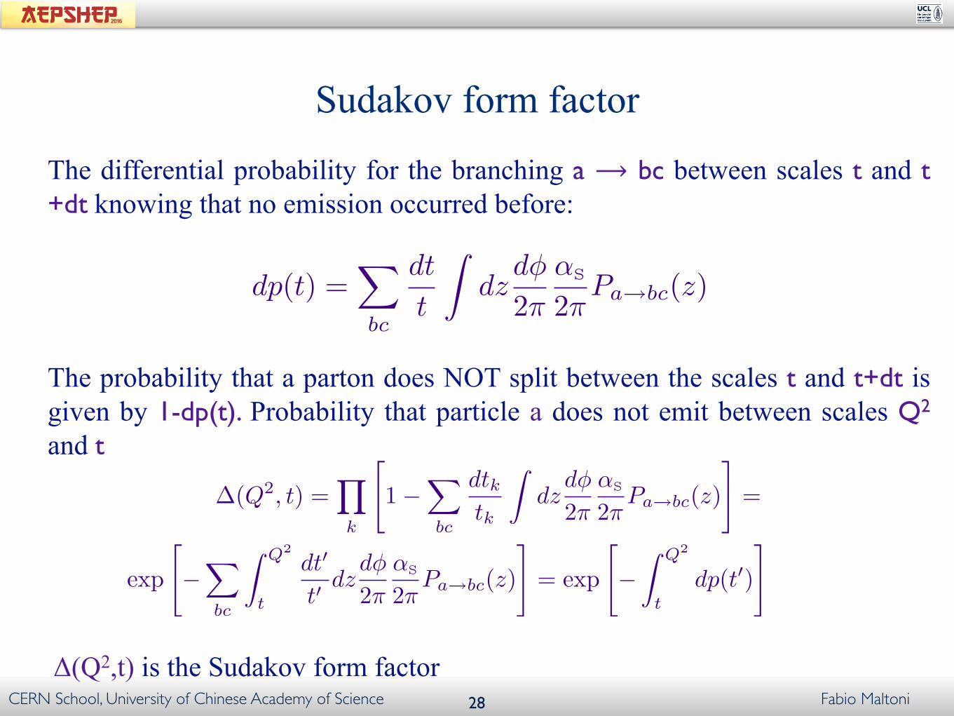
The differential probability for the branching a ⟶ bc between scales t and t+dt knowing that no emission occurred before:
!
The probability that a parton does NOT split between the scales t and t+dt is given by 1-dp(t). Probability that particle a does not emit between scales Q2 and t
Sudakov form factor
28
�(Q2, t) =⌅
k
�1�
⇤
bc
dtktk
⇧dz
d⇤
2⇥
�S
2⇥Pa�bc(z)
⇥=
exp
��
⇤
bc
⇧ Q2
t
dt⇥
t⇥dz
d⇤
2⇥
�S
2⇥Pa�bc(z)
⇥= exp
��
⇧ Q2
tdp(t⇥)
⇥
dp(t) =�
bc
dt
t
⇥dz
d⇤
2⇥
�S
2⇥Pa�bc(z)
Δ(Q2,t) is the Sudakov form factor
Fabio MaltoniCERN School, University of Chinese Academy of Science Fabio Maltoni
AEPSHEP 2016
Parton shower algorithm
29
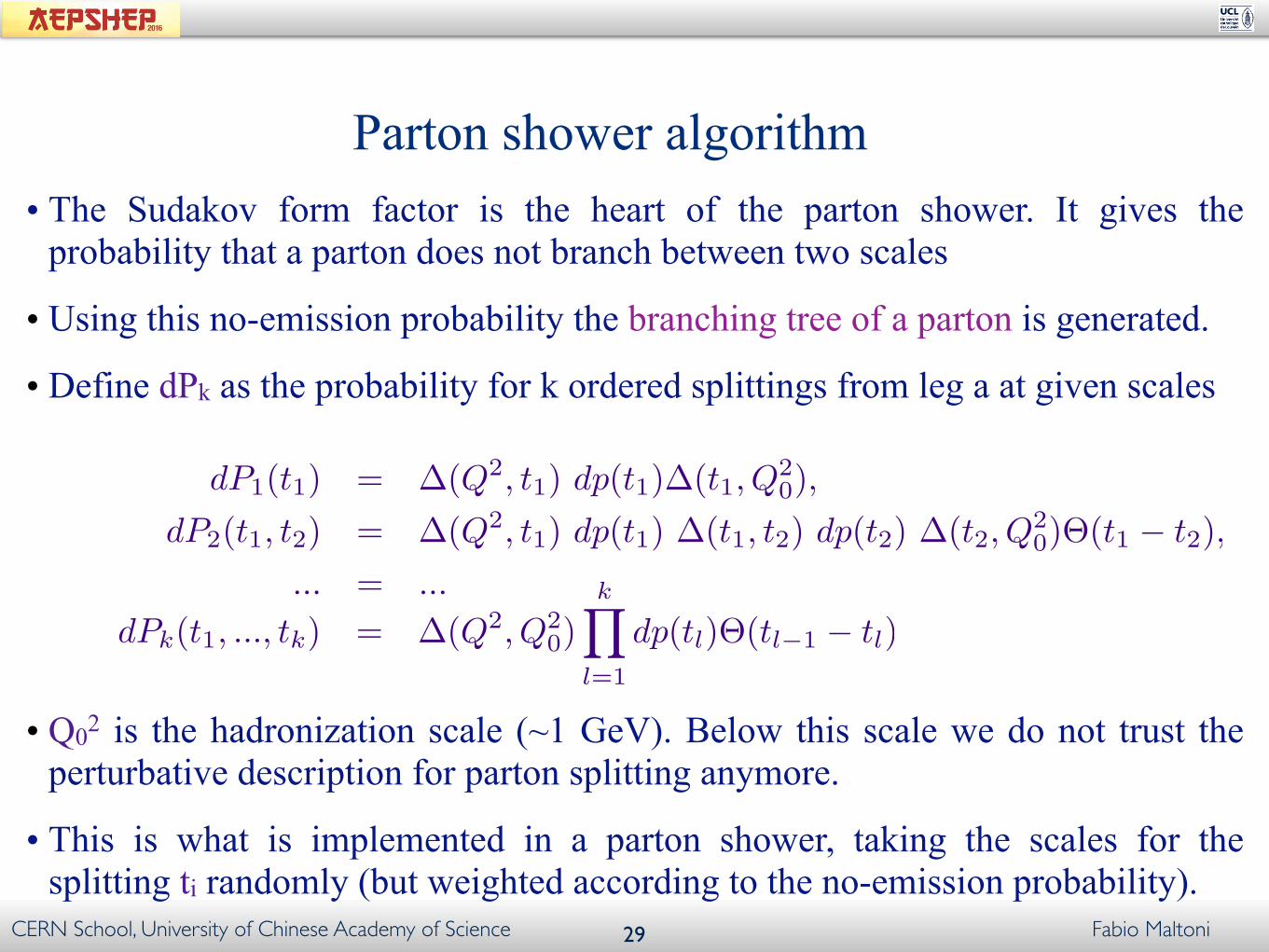
• The Sudakov form factor is the heart of the parton shower. It gives the probability that a parton does not branch between two scales
• Using this no-emission probability the branching tree of a parton is generated.
• Define dPk as the probability for k ordered splittings from leg a at given scales
!
• Q02 is the hadronization scale (~1 GeV). Below this scale we do not trust the perturbative description for parton splitting anymore.
• This is what is implemented in a parton shower, taking the scales for the splitting ti randomly (but weighted according to the no-emission probability).
dP1(t1) = �(Q2, t1) dp(t1)�(t1, Q20),
dP2(t1, t2) = �(Q2, t1) dp(t1) �(t1, t2) dp(t2) �(t2, Q20)⇥(t1 � t2),
... = ...
dPk(t1, ..., tk) = �(Q2, Q20)
k�
l=1
dp(tl)⇥(tl�1 � tl)
Fabio MaltoniCERN School, University of Chinese Academy of Science Fabio Maltoni
AEPSHEP 2016
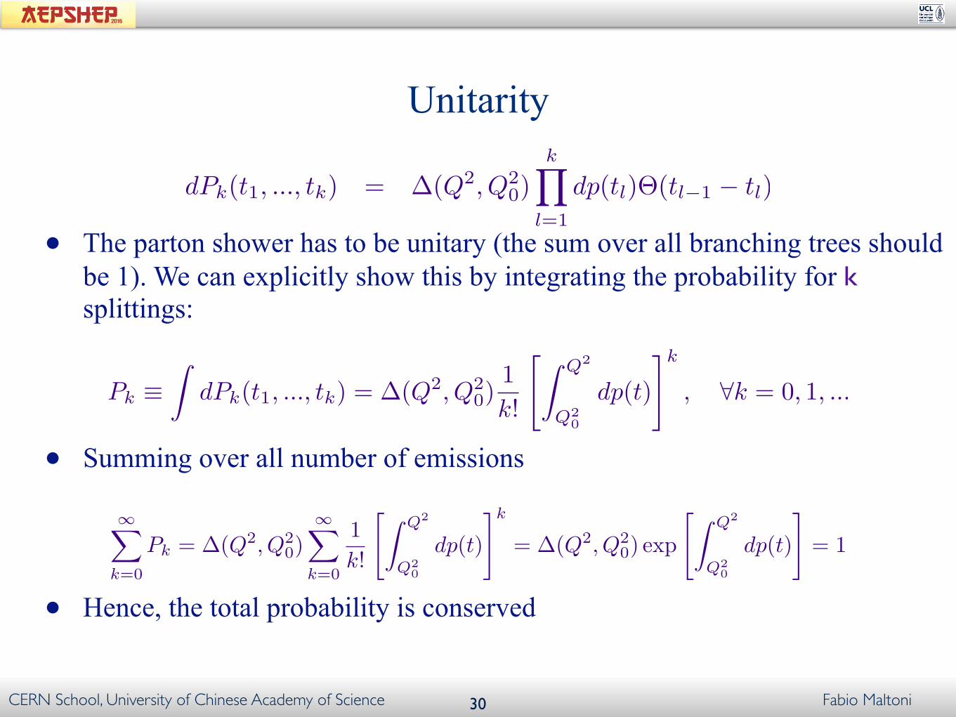
Unitarity
• The parton shower has to be unitary (the sum over all branching trees should be 1). We can explicitly show this by integrating the probability for k splittings:
• Summing over all number of emissions
• Hence, the total probability is conserved
30
dPk(t1, ..., tk) = �(Q2, Q20)
k�
l=1
dp(tl)⇥(tl�1 � tl)
Pk �⇤
dPk(t1, ..., tk) = �(Q2, Q20)
1k!
�⇤ Q2
Q20
dp(t)
⇥k
, ⇥k = 0, 1, ...
�⇤
k=0
Pk = �(Q2, Q20)�⇤
k=0
1k!
�⌅ Q2
Q20
dp(t)
⇥k
= �(Q2, Q20) exp
�⌅ Q2
Q20
dp(t)
⇥= 1
Fabio MaltoniCERN School, University of Chinese Academy of Science Fabio Maltoni
AEPSHEP 2016
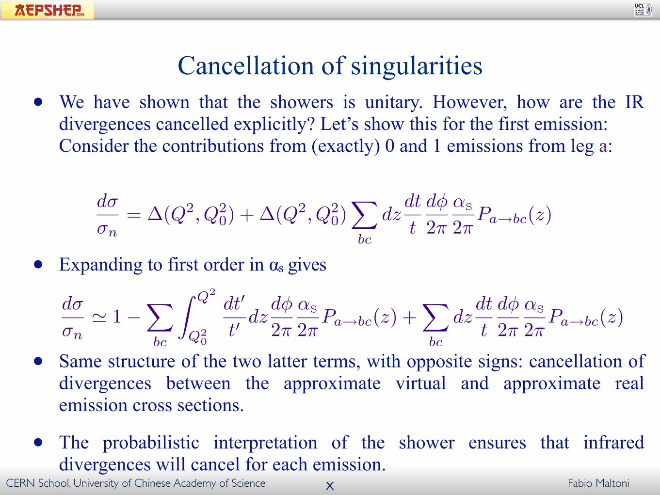
• We have shown that the showers is unitary. However, how are the IR divergences cancelled explicitly? Let’s show this for the first emission: Consider the contributions from (exactly) 0 and 1 emissions from leg a:
!
• Expanding to first order in αs gives
!
• Same structure of the two latter terms, with opposite signs: cancellation of divergences between the approximate virtual and approximate real emission cross sections.
• The probabilistic interpretation of the shower ensures that infrared divergences will cancel for each emission.
Cancellation of singularities
X
d⇤
⇤n= �(Q2, Q2
0) + �(Q2, Q20)
�
bc
dzdt
t
d⌅
2⇥
�S
2⇥Pa�bc(z)
d⇤
⇤n⇥ 1�
�
bc
⇥ Q2
Q20
dt⇥
t⇥dz
d⌅
2⇥
�S
2⇥Pa�bc(z) +
�
bc
dzdt
t
d⌅
2⇥
�S
2⇥Pa�bc(z)
Fabio MaltoniCERN School, University of Chinese Academy of Science Fabio Maltoni
AEPSHEP 2016
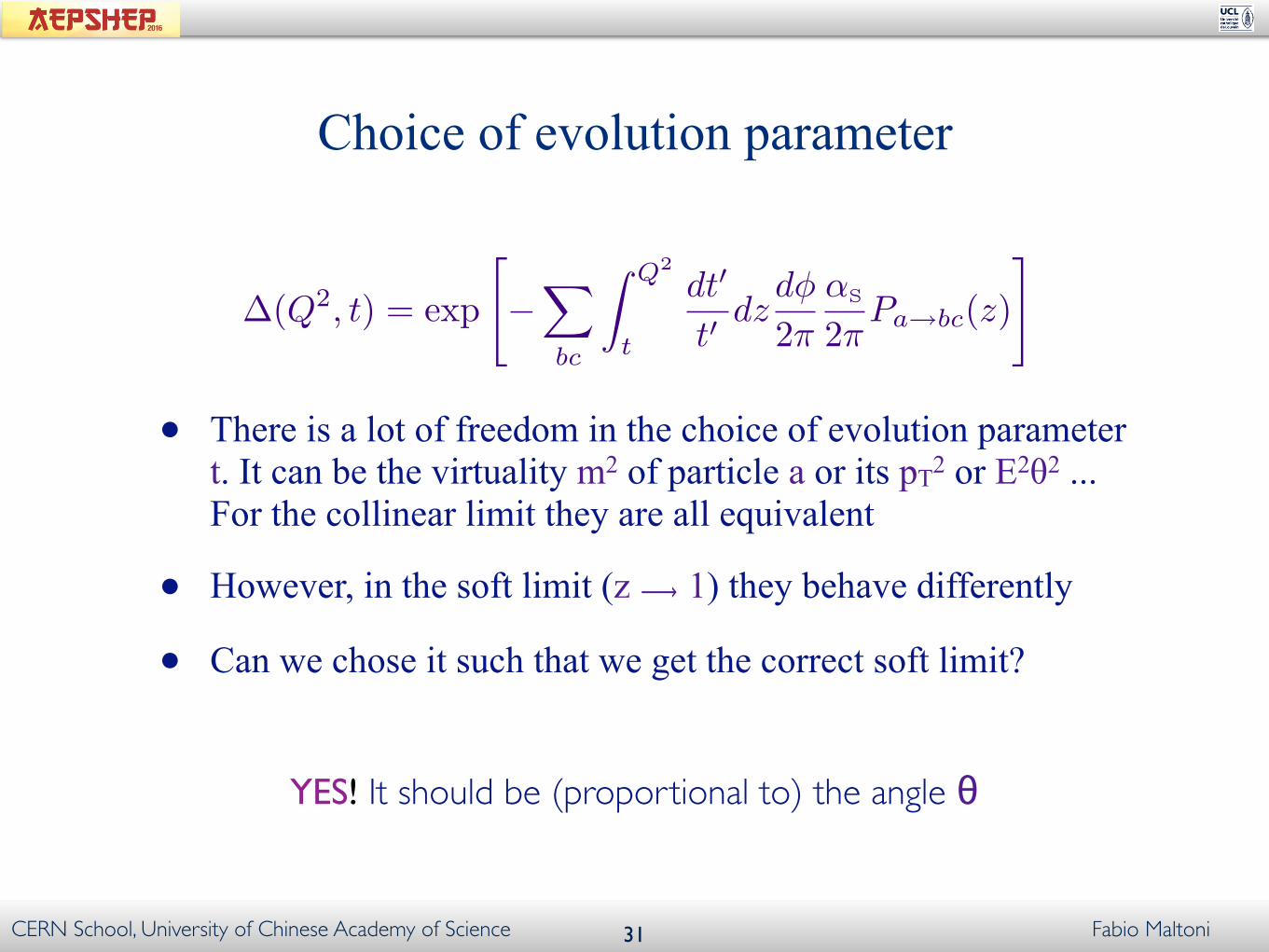
Choice of evolution parameter
• There is a lot of freedom in the choice of evolution parameter t. It can be the virtuality m2 of particle a or its pT2 or E2θ2 ... For the collinear limit they are all equivalent
• However, in the soft limit (z ⟶ 1) they behave differently
• Can we chose it such that we get the correct soft limit?
31
�(Q2, t) = exp
��
⇤
bc
⌅ Q2
t
dt⇥
t⇥dz
d⇤
2⇥
�S
2⇥Pa�bc(z)
⇥
YES! It should be (proportional to) the angle θ
Fabio MaltoniCERN School, University of Chinese Academy of Science Fabio Maltoni
AEPSHEP 2016
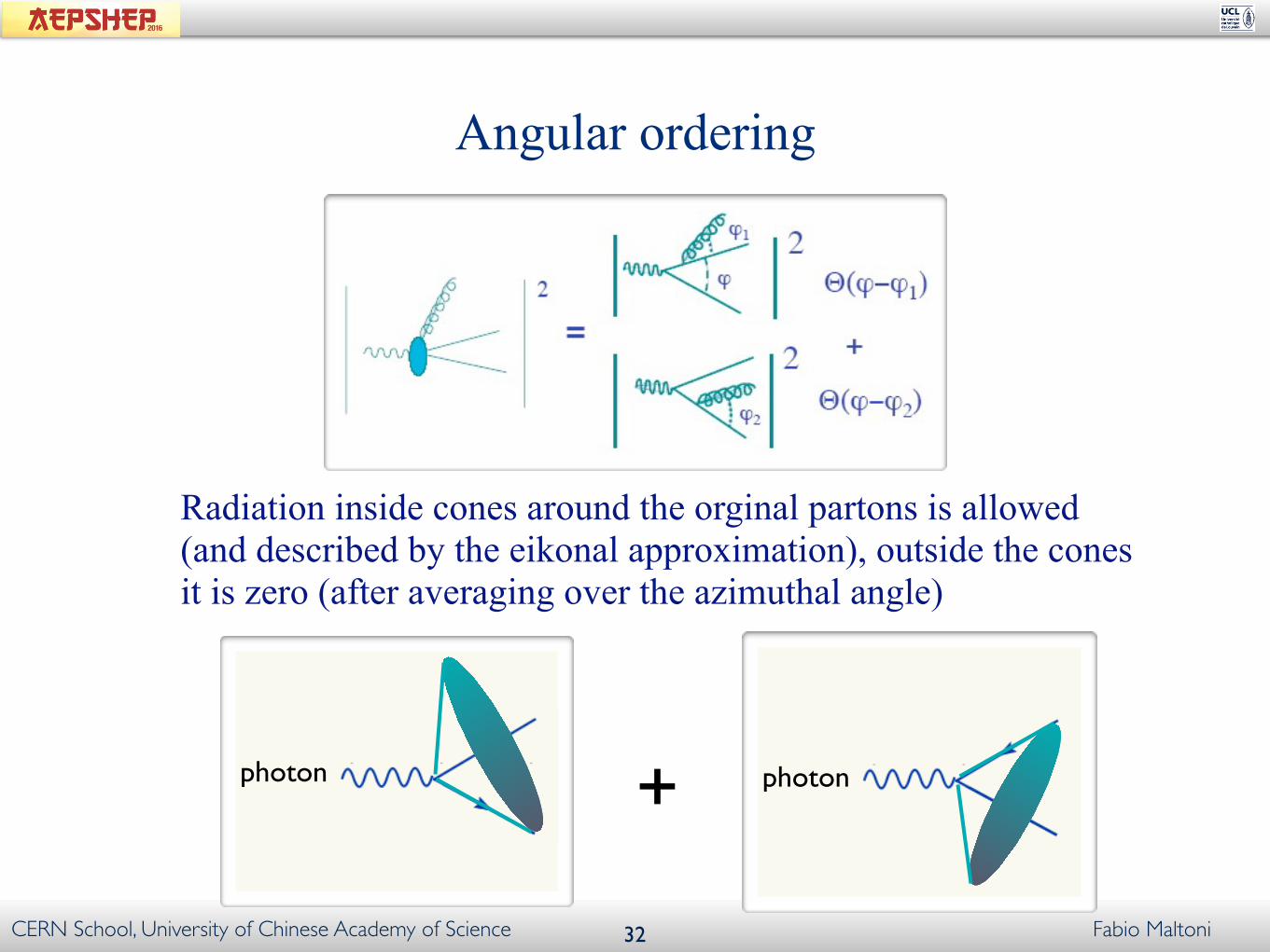
Angular ordering
Radiation inside cones around the orginal partons is allowed (and described by the eikonal approximation), outside the cones it is zero (after averaging over the azimuthal angle)
32
photon+photon
Fabio MaltoniCERN School, University of Chinese Academy of Science Fabio Maltoni
AEPSHEP 2016
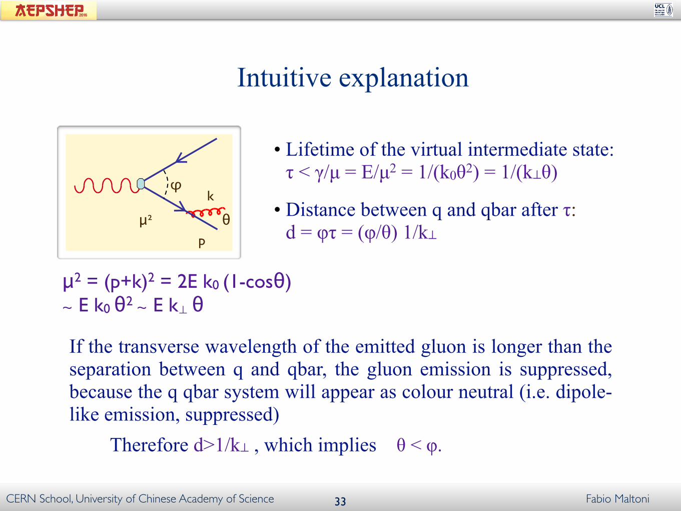
Intuitive explanation
!If the transverse wavelength of the emitted gluon is longer than the separation between q and qbar, the gluon emission is suppressed, because the q qbar system will appear as colour neutral (i.e. dipole-like emission, suppressed)
Therefore d>1/k⊥ , which implies θ < φ.
Angular ordering(slide by M. Mangano)
An intuitive explanation of angular ordering
φ
θμ!k
p
Distance between q and qbar after τ:
d = φτ = (φ/θ) 1/k⊥
If the transverse wavelength of the emitted gluon is longer than the separation between q and qbar, the gluon emission is suppressed, because the q qbar system will appear as colour neutral (=> dipole-like emission, suppressed)
μ! = (p+k)! = 2E k₀ (1-cosθ) ∼ E k₀ θ! ∼ E k⊥ θ
Lifetime of the virtual intermediate state:
τ < γ/μ = E/μ! = 1 / (k₀θ!)= 1/(k⊥θ)
Therefore d> 1/k⊥ , which implies θ < φ12Paolo Torrielli (EPFL) Interfacing NLO with Parton Showers ThinkTank on Physics @ LHC 25 / 83
33
• Lifetime of the virtual intermediate state: τ < γ/µ = E/µ2 = 1/(k0θ2) = 1/(k⊥θ)
• Distance between q and qbar after τ:d = φτ = (φ/θ) 1/k⊥
μ2 = (p+k)2 = 2E k0 (1-cosθ) ∼ E k0 θ2 ∼ E k⊥ θ
Fabio MaltoniCERN School, University of Chinese Academy of Science Fabio Maltoni
AEPSHEP 2016
Angular ordering
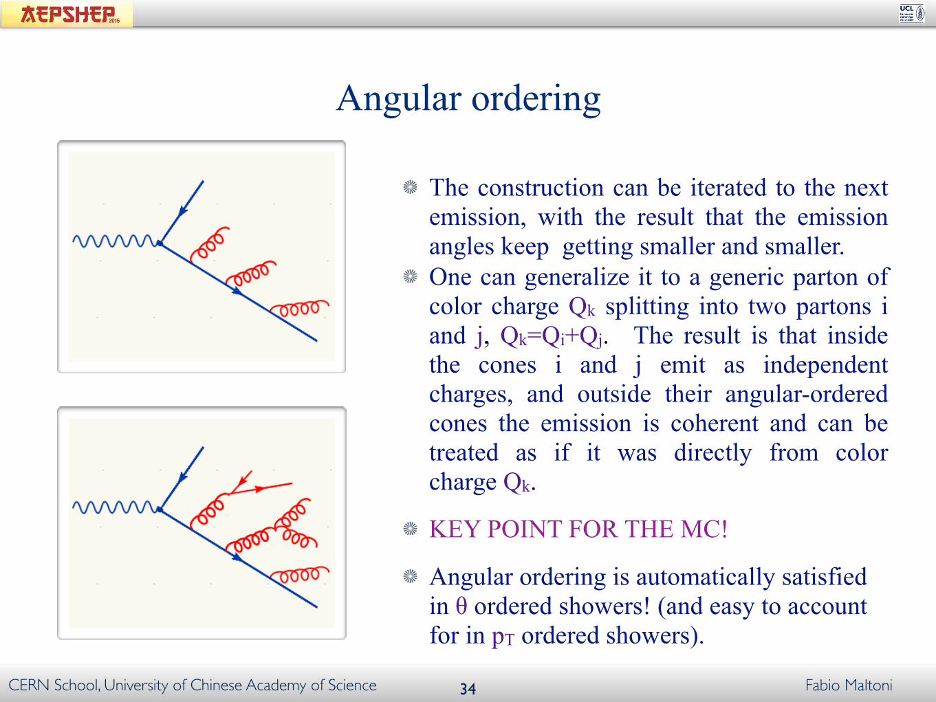
The construction can be iterated to the next emission, with the result that the emission angles keep getting smaller and smaller. One can generalize it to a generic parton of color charge Qk splitting into two partons i and j, Qk=Qi+Qj. The result is that inside the cones i and j emit as independent charges, and outside their angular-ordered cones the emission is coherent and can be treated as if it was directly from color charge Qk.
KEY POINT FOR THE MC!
Angular ordering is automatically satisfied in θ ordered showers! (and easy to account for in pT ordered showers).
34
Fabio MaltoniCERN School, University of Chinese Academy of Science Fabio Maltoni
AEPSHEP 2016
e-
e+
Cluster model
35
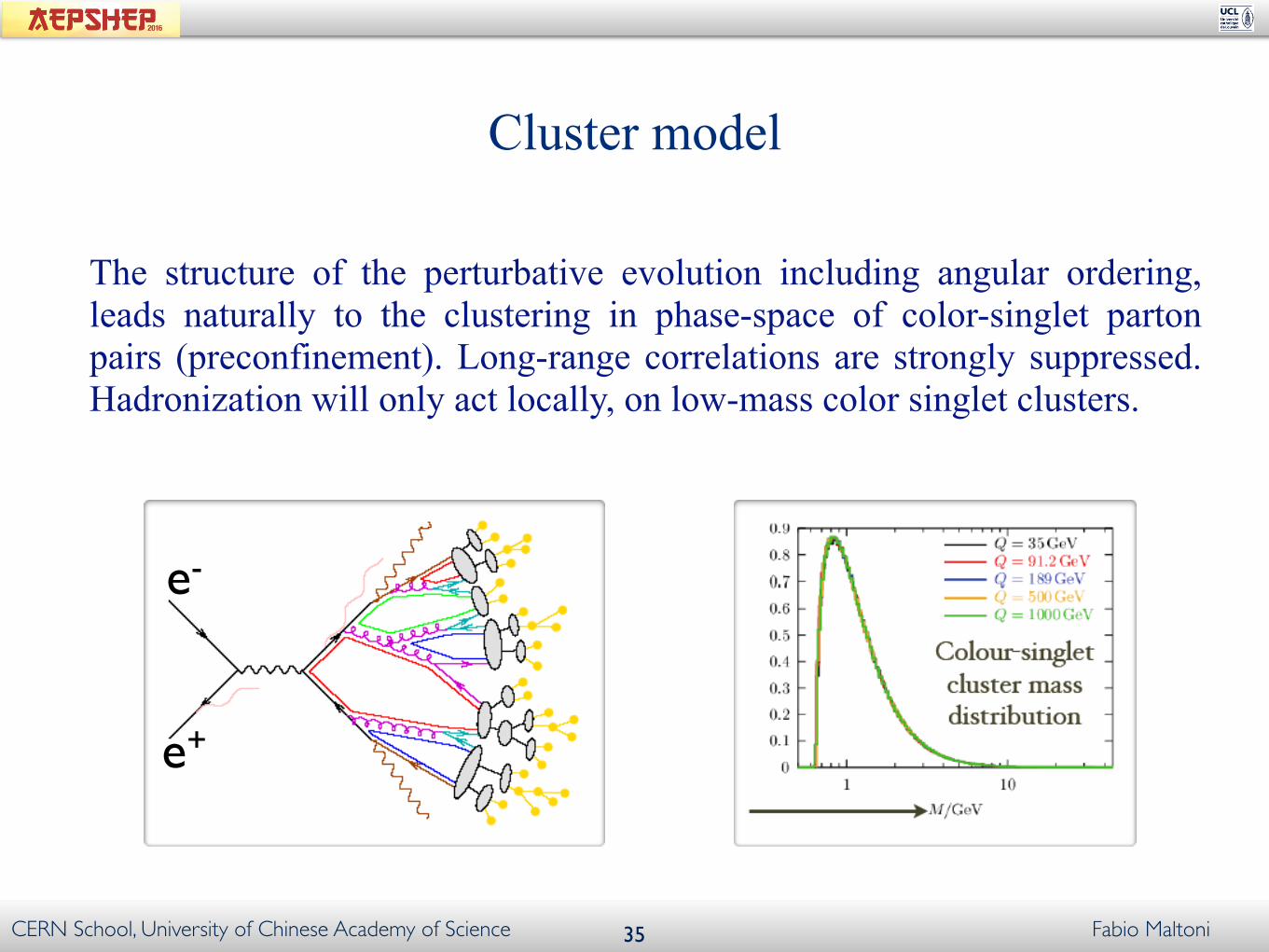
The structure of the perturbative evolution including angular ordering, leads naturally to the clustering in phase-space of color-singlet parton pairs (preconfinement). Long-range correlations are strongly suppressed. Hadronization will only act locally, on low-mass color singlet clusters.
Fabio MaltoniCERN School, University of Chinese Academy of Science Fabio Maltoni
AEPSHEP 2016
Parton Shower MC
36
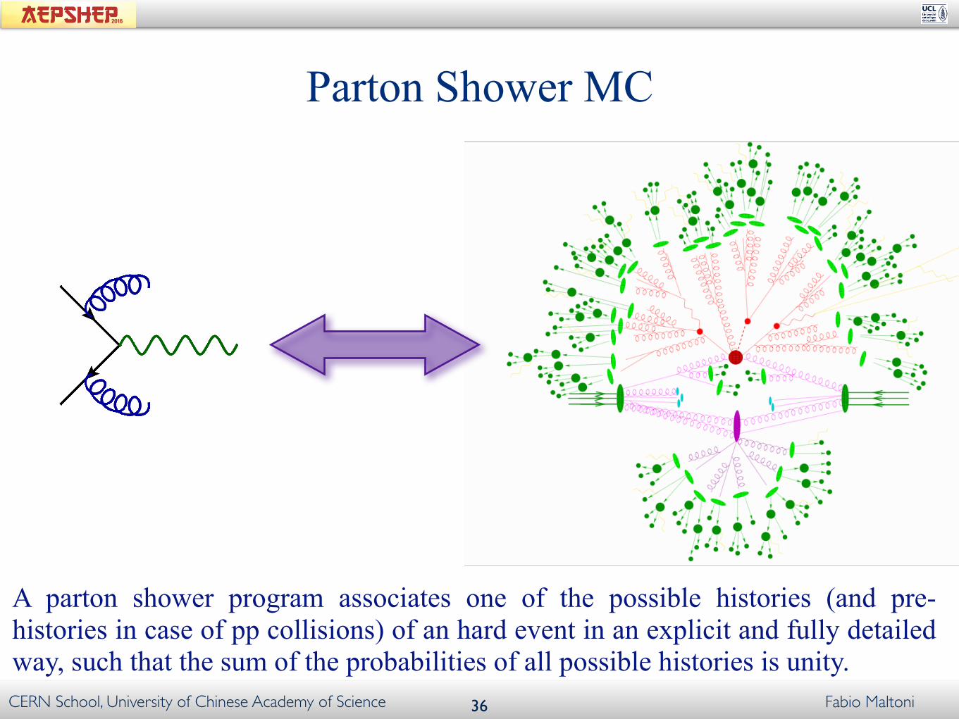
A parton shower program associates one of the possible histories (and pre-histories in case of pp collisions) of an hard event in an explicit and fully detailed way, such that the sum of the probabilities of all possible histories is unity.
Fabio MaltoniCERN School, University of Chinese Academy of Science Fabio Maltoni
AEPSHEP 2016
QCD in the final state
1. Infrared safety
2. Towards realistic final states
3. Jets
37
Fabio MaltoniCERN School, University of Chinese Academy of Science Fabio Maltoni
AEPSHEP 2016
q
q
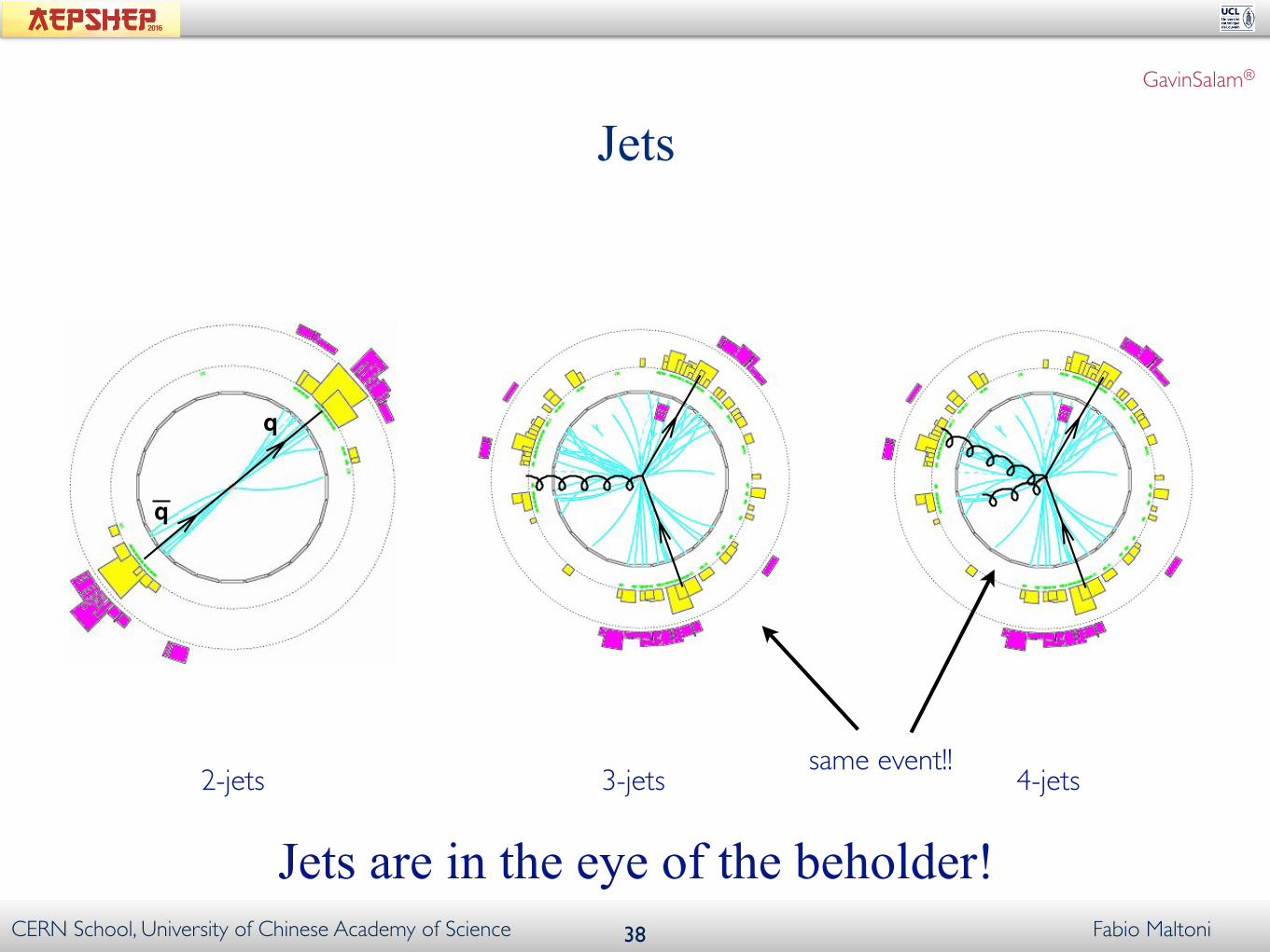
Jets
2-jets 3-jets 4-jets
Jets are in the eye of the beholder!
GavinSalam®
same event!!
38
Fabio MaltoniCERN School, University of Chinese Academy of Science Fabio Maltoni
AEPSHEP 2016
Jet algorithms
jet 1 jet 2
LO partons
Jet Def n
jet 1 jet 2
Jet Def n
NLO partons
jet 1 jet 2
Jet Def n
parton shower
jet 1 jet 2
Jet Def n
hadron level
π π
K
p φ
GavinSalam®
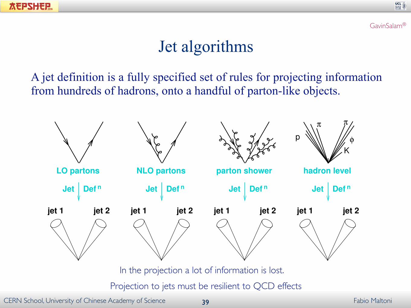
Projection to jets must be resilient to QCD effects
A jet definition is a fully specified set of rules for projecting information from hundreds of hadrons, onto a handful of parton-like objects.
In the projection a lot of information is lost.
39
Fabio MaltoniCERN School, University of Chinese Academy of Science Fabio Maltoni
AEPSHEP 2016
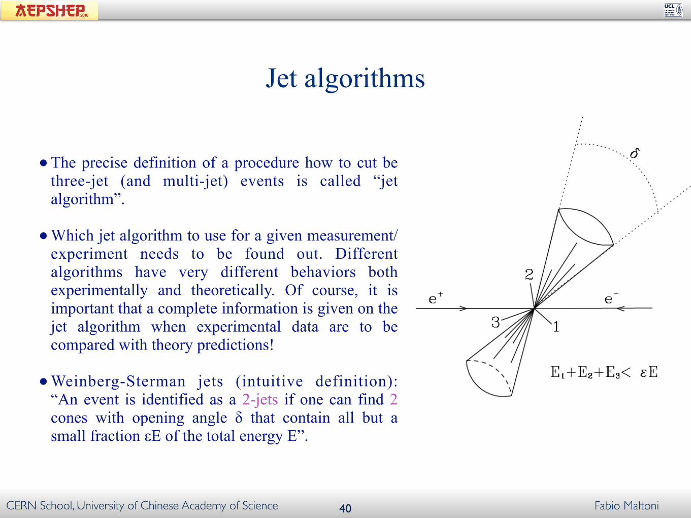
•The precise definition of a procedure how to cut be three-jet (and multi-jet) events is called “jet algorithm”. !
•Which jet algorithm to use for a given measurement/experiment needs to be found out. Different algorithms have very different behaviors both experimentally and theoretically. Of course, it is important that a complete information is given on the jet algorithm when experimental data are to be compared with theory predictions! !
•Weinberg-Sterman jets (intuitive definition): “An event is identified as a 2-jets if one can find 2 cones with opening angle δ that contain all but a small fraction εE of the total energy E”.
Jet algorithms
40
Fabio MaltoniCERN School, University of Chinese Academy of Science Fabio Maltoni
AEPSHEP 2016
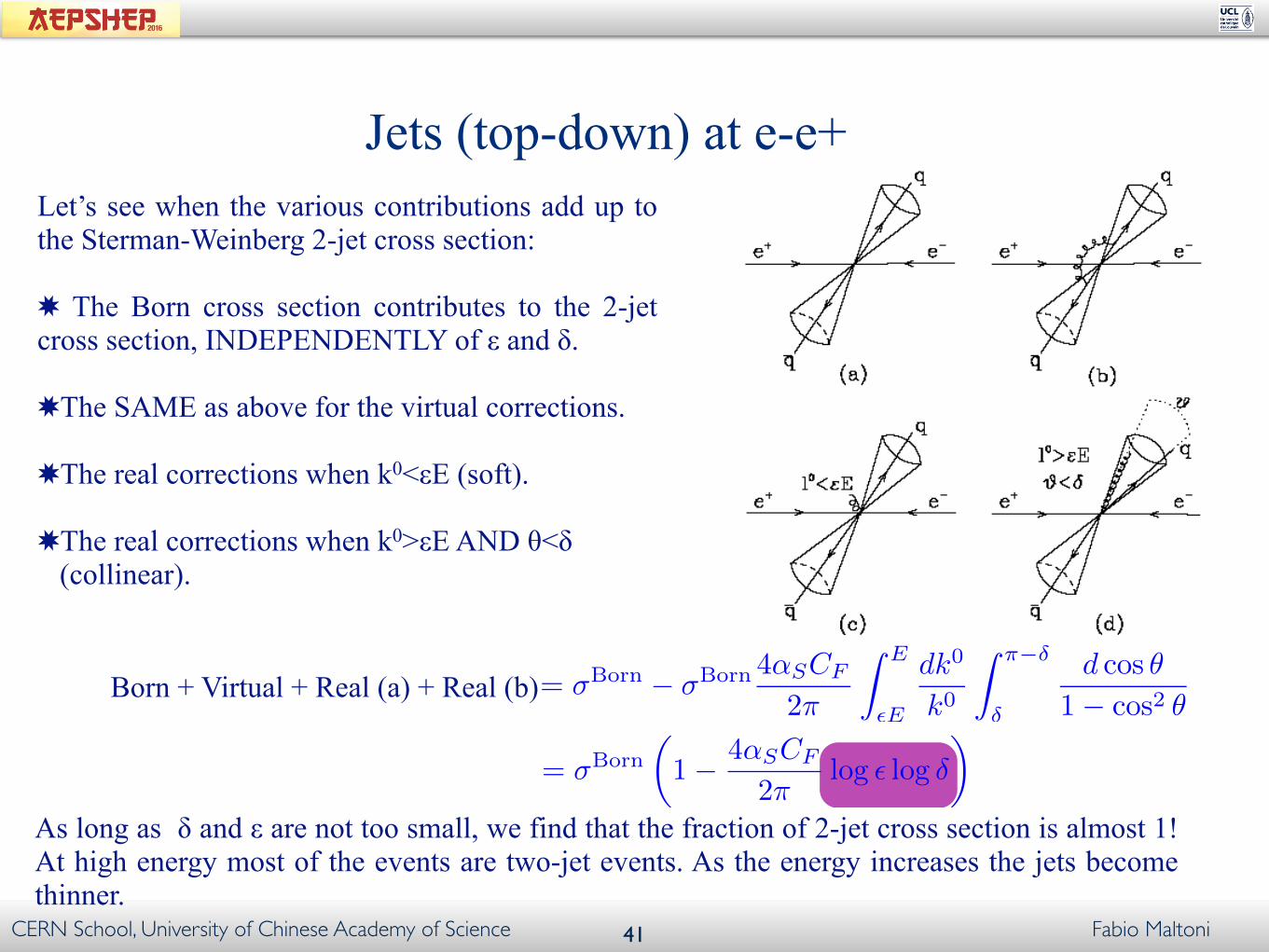
Jets (top-down) at e-e+Let’s see when the various contributions add up to the Sterman-Weinberg 2-jet cross section: !✸ The Born cross section contributes to the 2-jet cross section, INDEPENDENTLY of ε and δ. !✸The SAME as above for the virtual corrections. !✸The real corrections when k0<εE (soft). !✸The real corrections when k0>εE AND θ<δ (collinear).
Born + Virtual + Real (a) + Real (b)= σBorn
− σBorn 4αSCF
2π
! E
ϵE
dk0
k0
! π−δ
δ
d cos θ
1 − cos2 θ
As long as δ and ε are not too small, we find that the fraction of 2-jet cross section is almost 1! At high energy most of the events are two-jet events. As the energy increases the jets become thinner.
= �Born
✓1� 4↵SCF
2⇡log ✏ log �
◆
41
Fabio MaltoniCERN School, University of Chinese Academy of Science Fabio Maltoni
AEPSHEP 2016
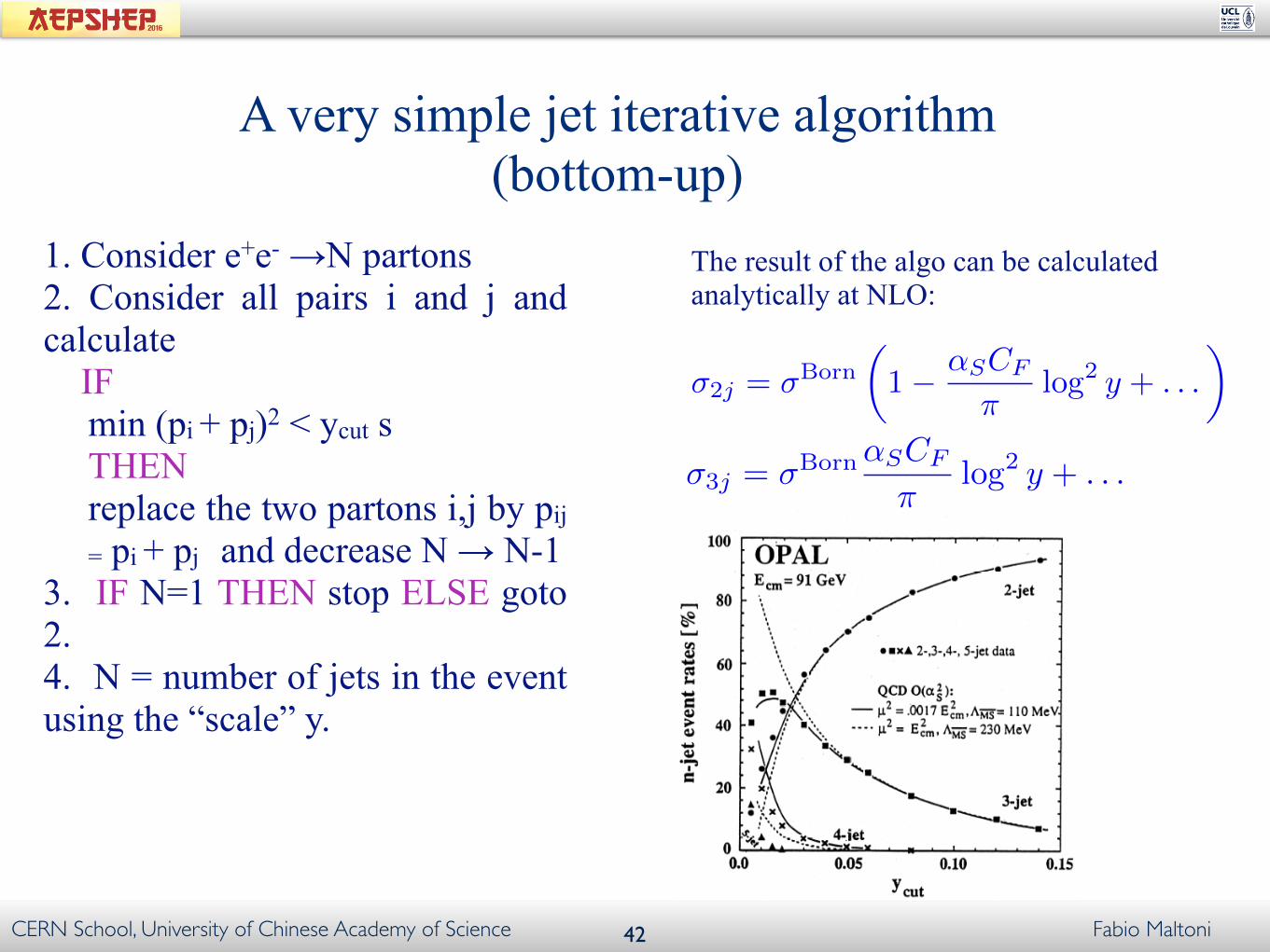
A very simple jet iterative algorithm (bottom-up)
1. Consider e+e- →N partons 2. Consider all pairs i and j and calculate IF
min (pi + pj)2 < ycut s THEN replace the two partons i,j by pij
= pi + pj and decrease N → N-1 3. IF N=1 THEN stop ELSE goto 2. 4. N = number of jets in the event using the “scale” y.
The result of the algo can be calculated analytically at NLO:
�2j = �Born
✓1� ↵SCF
⇡log
2 y + . . .
◆
�3j = �Born
↵SCF
⇡log
2 y + . . .
42
Fabio MaltoniCERN School, University of Chinese Academy of Science Fabio Maltoni
AEPSHEP 2016
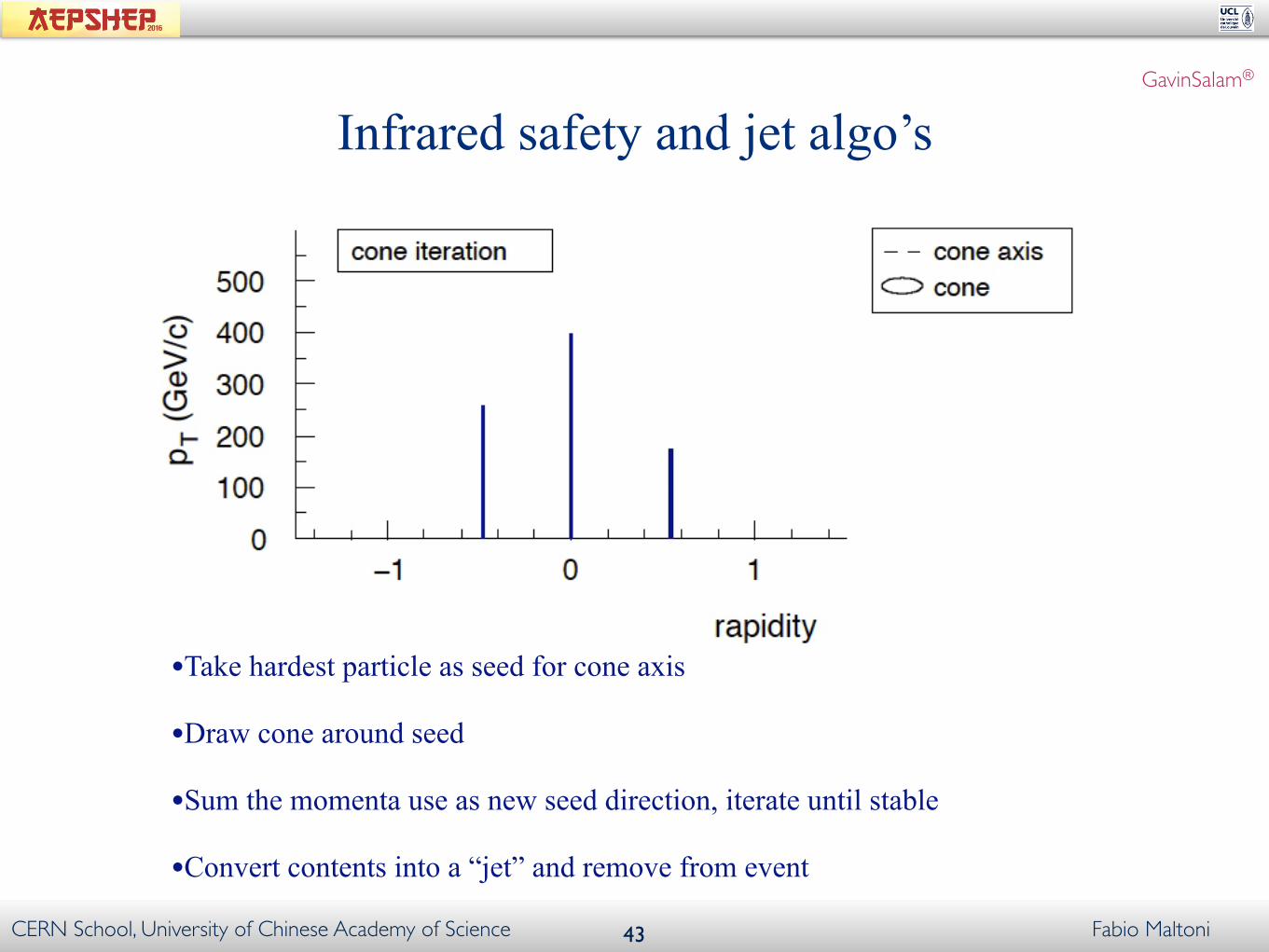
Infrared safety and jet algo’sGavinSalam®
•Take hardest particle as seed for cone axis !
•Draw cone around seed !
•Sum the momenta use as new seed direction, iterate until stable !
•Convert contents into a “jet” and remove from event
43
Fabio MaltoniCERN School, University of Chinese Academy of Science Fabio Maltoni
AEPSHEP 2016
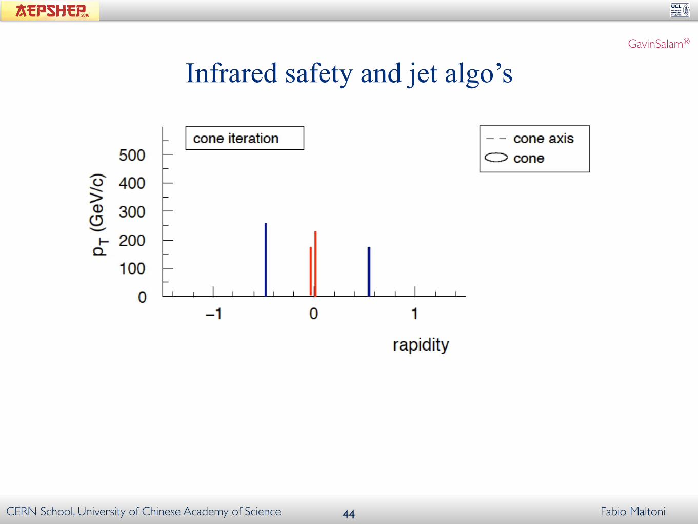
Infrared safety and jet algo’sGavinSalam®
44
Fabio MaltoniCERN School, University of Chinese Academy of Science Fabio Maltoni
AEPSHEP 2016
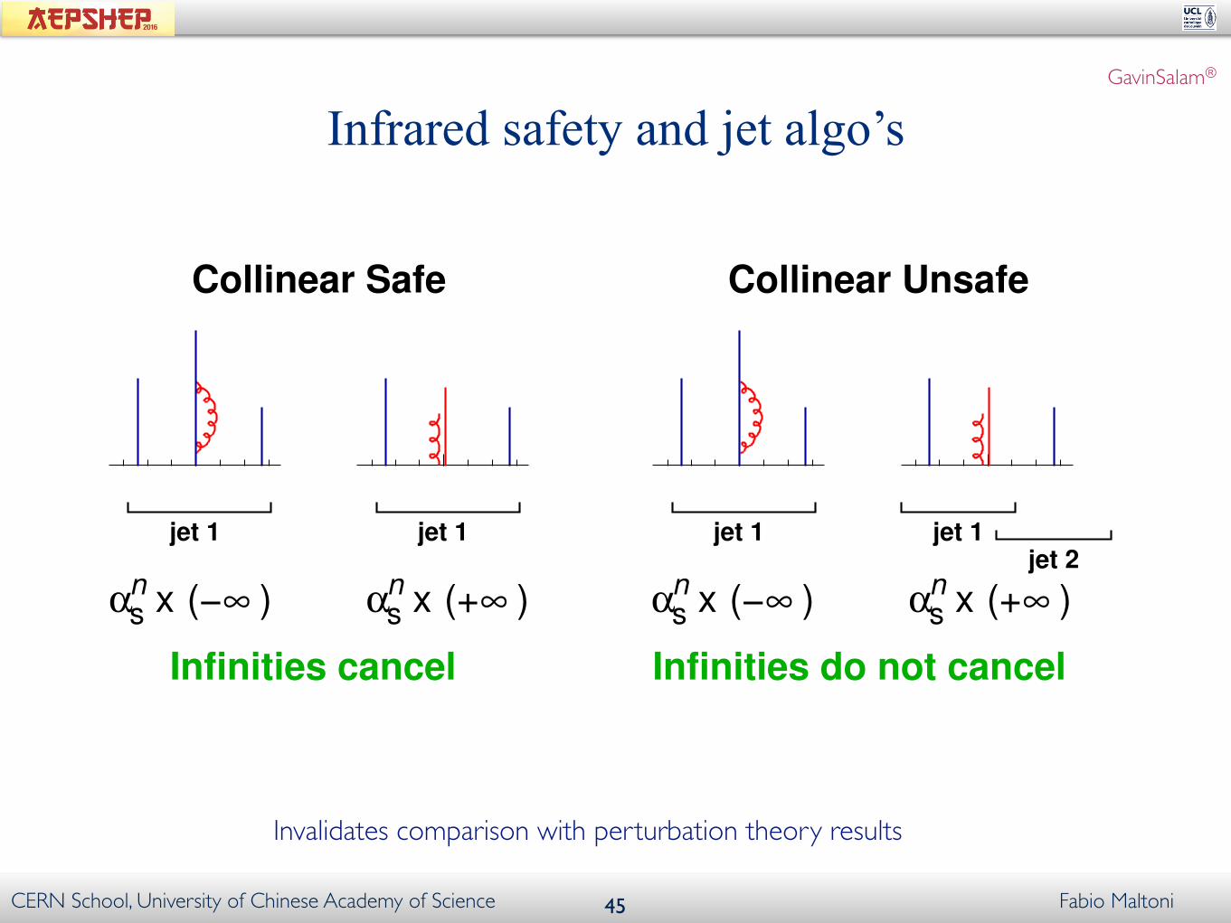
Infrared safety and jet algo’s
jet 2jet 1jet 1jet 1 jet 1
αs x (+ )∞n
αs x (− )∞n
αs x (+ )∞n
αs x (− )∞n
Collinear Safe Collinear Unsafe
Infinities cancel Infinities do not cancel
GavinSalam®
Invalidates comparison with perturbation theory results
45
Fabio MaltoniCERN School, University of Chinese Academy of Science Fabio Maltoni
AEPSHEP 2016
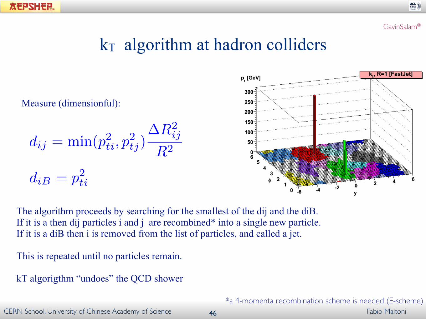
kT algorithm at hadron colliders
Measure (dimensionful):
dij = min(p2ti, p2tj)
�R2ij
R2
diB = p2ti
The algorithm proceeds by searching for the smallest of the dij and the diB. If it is a then dij particles i and j are recombined* into a single new particle. If it is a diB then i is removed from the list of particles, and called a jet. !This is repeated until no particles remain. !kT algorigthm “undoes” the QCD shower
*a 4-momenta recombination scheme is needed (E-scheme)
GavinSalam®
46
Fabio MaltoniCERN School, University of Chinese Academy of Science Fabio Maltoni
AEPSHEP 2016
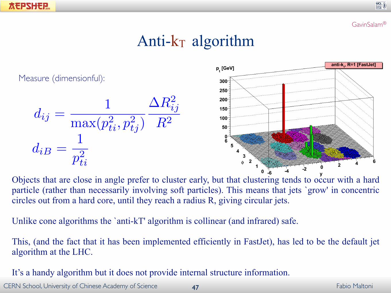
Anti-kT algorithm
Measure (dimensionful):
dij =1
max(p2ti, p2tj)
�R2ij
R2
diB =1
p2tiObjects that are close in angle prefer to cluster early, but that clustering tends to occur with a hard particle (rather than necessarily involving soft particles). This means that jets `grow' in concentric circles out from a hard core, until they reach a radius R, giving circular jets. !Unlike cone algorithms the `anti-kT' algorithm is collinear (and infrared) safe. !This, (and the fact that it has been implemented efficiently in FastJet), has led to be the default jet algorithm at the LHC. !It’s a handy algorithm but it does not provide internal structure information.
GavinSalam®
47
Fabio MaltoniCERN School, University of Chinese Academy of Science Fabio Maltoni
AEPSHEP 2016
Summary
1. We have studied the problem of infrared divergences in the calculation of the fully inclusive cross section, with the help of the soft limit. !2. We have introduced the concept of an Infrared Safe quantity, i.e. an observable which is both computable at all orders in pQCD and has a well defined counterpart at the experimental level. !3. We have discussed more exclusive quantities, from shape functions to fully exclusive quantities and compared them with e+ e- data. !3. We have explained the basic concept idea of a parton shower MC. !4. We have introduced the idea of jet algorithms (top-down and bottom-up) and discussed the most recent algorithms.
48