Embed Size (px)
Citation preview

© 2020 by Waterloo Hydrogeologic
User's Manual
AquiferTest Pro 10.0Pumping & Slug Test Analysis, Interpretation & Visualization Software

Waterloo Hydrogeologic, Inc.630 Riverbend Drive, Sui te 100Kitchener, ON N2K 3S2CANADA
www.waterloohydrogeologic.com © 2020 by Waterloo Hydrogeologic . Al l rights reserved.
Publ ished: Apri l 2020 in Waterloo, Canada
Al l rights reserved. No parts of this work may be reproduced in anyform or by any means - graphic, electronic, or mechanica l , includingphotocopying, recording, taping, or information s torage and retrieva lsystems - without the wri tten permiss ion of the publ isher. Whi le theinformation presented herein i s bel ieved to be accurate, i t i sprovided "as -i s" without express or impl ied warranty.
Speci fications are current at the time of printing.Errors and omiss ions excepted
AquiferTest Pro 10.0User's Manual
1Contents
1
© 2020 by Waterloo Hydrogeologic
Table of Contents
Foreword 0
Part 1 Introduction 1
................................................................................................................................... 31 Installation and System Requirements
................................................................................................................................... 52 Updating Old Projects
................................................................................................................................... 53 Learning AquiferTest
................................................................................................................................... 64 About the Interface
................................................................................................................................... 145 What's New
................................................................................................................................... 226 Quick Start Demo Tutorial
.......................................................................................................................................................... 23Tutorial 1: Confined Aquifer Pumping Test Analysis
.......................................................................................................................................................... 55Tutorial 2: Predictive Analysis
.......................................................................................................................................................... 61Tutorial 3: Single Well Analysis
.......................................................................................................................................................... 68Tutorial 4: Slug Test Analysis
Part 2 Demonstration Exercises and Benchmark Tests 76
................................................................................................................................... 771 Exercise 1: Confined Aquifer - Theis Analysis
................................................................................................................................... 852 Exercise 2: Leaky Aquifer - Hantush - Jacob Analysis
................................................................................................................................... 963 Exercise 3: Recovery Data Analysis - Agarwal Solution
................................................................................................................................... 1094 Exercise 4: Confined Aquifer, Multiple Pumping Wells
.......................................................................................................................................................... 109Determining Aquifer Parameters
.......................................................................................................................................................... 117Determining the Effect of a Second Pumping Well
.......................................................................................................................................................... 121Predicting Drawdown at Any Distance from the Pumping well
................................................................................................................................... 1255 Exercise 5: Adding Data Trend Correction
................................................................................................................................... 1306 Exercise 6: Adding Barometric Correction
................................................................................................................................... 1367 Exercise 7: Slug Test Analysis - Bouwer & Rice
................................................................................................................................... 1448 Exercise 8: High-K Butler Method
................................................................................................................................... 1489 Exercise 9: Derivative Smoothing
................................................................................................................................... 15110 Exercise 10: Horizontal Wells
................................................................................................................................... 15911 Exercise 11: Wellbore Storage and Skin Effects
................................................................................................................................... 16712 Exercise 12: Lugeon Test
................................................................................................................................... 17313 Exercise 13: Multi-Layer Aquifer
................................................................................................................................... 18714 Exercise 14: Slug Test Analysis - Binkhorst and Robbins
................................................................................................................................... 19315 Additional AquiferTest Examples
Part 3 Program Options 196
................................................................................................................................... 1961 General Info
.......................................................................................................................................................... 196Project Navigator Panel
......................................................................................................................................................... 197Tests Frame
......................................................................................................................................................... 198Wells Frame
......................................................................................................................................................... 198Discharge Rates Frame
......................................................................................................................................................... 198Water Level Measurements Frame
AquiferTest 10.0 Help2
© 2020 by Waterloo Hydrogeologic
......................................................................................................................................................... 198Analyses Frame
......................................................................................................................................................... 199Additional Tasks Frame
.......................................................................................................................................................... 200Navigation Tabs
......................................................................................................................................................... 201Pumping Test Tab
......................................................................................................................................................... 205Slug Test Tab
......................................................................................................................................................... 237Lugeon Test Tab
......................................................................................................................................................... 206Discharge Tab
......................................................................................................................................................... 208Water Levels Tab
......................................................................................................................................................... 217Analysis Tab
......................................................................................................................................................... 237Drawdown Tab
......................................................................................................................................................... 237Lugeon Test Data and Analysis Tab
......................................................................................................................................................... 237Site Plan Tab
......................................................................................................................................................... 238Report Tab
................................................................................................................................... 2422 Main Menu Bar
.......................................................................................................................................................... 242File Menu
.......................................................................................................................................................... 260Edit Menu
.......................................................................................................................................................... 263View Menu
.......................................................................................................................................................... 267Test Menu
.......................................................................................................................................................... 270Analysis Menu
.......................................................................................................................................................... 278Tools Menu
.......................................................................................................................................................... 294Help Menu
Part 4 Pumping Test: Theory and Analysis Methods 296
................................................................................................................................... 2961 Analysis Parameters and Curve Fitting
................................................................................................................................... 3042 Methodology
................................................................................................................................... 3043 Theory of Superposition
.......................................................................................................................................................... 306Variable Discharge Rates
.......................................................................................................................................................... 308Multiple Pumping Wells
.......................................................................................................................................................... 309Boundary Effects
.......................................................................................................................................................... 314Effects of Vertical Anisotropy and Partially Penetrating Wells
................................................................................................................................... 3184 Pumping Test Background
................................................................................................................................... 3205 Pumping Test Analysis Methods - Fixed Assumptions
.......................................................................................................................................................... 320Theis Recovery Test (confined)
.......................................................................................................................................................... 324Cooper-Jacob Method (confined; small r or large time)
................................................................................................................................... 3296 Pumping Test Analysis Methods - Flexible Assumptions
.......................................................................................................................................................... 330Drawdown vs. Time
.......................................................................................................................................................... 331Drawdown vs. Time with Discharge
.......................................................................................................................................................... 332Confined - Theis
.......................................................................................................................................................... 336Leaky - Hantush-Jacob (Walton)
.......................................................................................................................................................... 339Hantush - Storage in Aquitard
.......................................................................................................................................................... 343Wellbore Storage and Skin Effects (Agarwal 1970)
.......................................................................................................................................................... 344Unconfined, Isotropic - Theis with Jacob Correction
.......................................................................................................................................................... 346Unconfined, Anisotropic
.......................................................................................................................................................... 354Fracture Flow, Double Porosity
.......................................................................................................................................................... 367Single Well Analysis with Well Effects
.......................................................................................................................................................... 368Large Diameter Wells with WellBore Storage - Papadopulos-Cooper
.......................................................................................................................................................... 372Recovery Analysis - Agarwal Solution (1980)
.......................................................................................................................................................... 376Horizontal Wells (Clonts & Ramey)
.......................................................................................................................................................... 380Neuman & Witherspoon
.......................................................................................................................................................... 384Multi-Layer-Aquifer-Analysis
................................................................................................................................... 3907 Diagnostic Plots and Interpretation
3Contents
3
© 2020 by Waterloo Hydrogeologic
Part 5 Well Performance Methods 400
................................................................................................................................... 4001 Specific Capacity
................................................................................................................................... 4022 Hantush-Bierschenk Well Loss Solution
................................................................................................................................... 4103 Well Efficiency
Part 6 Slug Test Solution Methods 412
................................................................................................................................... 4121 Hvorslev Slug Test
................................................................................................................................... 4162 Bouwer-Rice Slug Test
................................................................................................................................... 4213 Cooper-Bredehoeft-Papadopulos Slug Test
................................................................................................................................... 4254 High-K Butler
................................................................................................................................... 4275 Dagan Slug Test
................................................................................................................................... 4286 Binkhorst and Robbins Slug Test
Part 7 Lugeon Tests 430
................................................................................................................................... 4311 Test Description
................................................................................................................................... 4342 Theory
................................................................................................................................... 4363 Data Requirements
................................................................................................................................... 4364 Analysis and Interpretation
................................................................................................................................... 4415 Lugeon Test Examples
Part 8 Data Pre-Processing 442
................................................................................................................................... 4431 Baseline Trend Analysis and Correction
................................................................................................................................... 4452 Customized Water Level Trends
................................................................................................................................... 4483 Barometric Trend Analysis and Correction
................................................................................................................................... 4574 Modifying Corrections
................................................................................................................................... 4575 Deleting Corrections
Part 9 Mapping and Contouring 459
................................................................................................................................... 4591 About the Interface
................................................................................................................................... 4692 Data Series
................................................................................................................................... 4713 Contouring and Color Shading Properties
.......................................................................................................................................................... 471Contour lines tab
.......................................................................................................................................................... 471Color Shading tab
................................................................................................................................... 4744 Regional Flow
................................................................................................................................... 4785 Streamlines
................................................................................................................................... 4816 Surfer Scripting
................................................................................................................................... 4827 Base Maps using a Tile Server
................................................................................................................................... 4848 Example
Part 10 References 505

AquiferTest 10.0 Help4
© 2020 by Waterloo Hydrogeologic
Index 511
Introduction 1
© 2020 by Waterloo Hydrogeologic
1 Introduction
Congratulations on your purchase of AquiferTest, the most popular software packageavailable for graphical analysis and reporting of pumping test and slug test data!
AquiferTest is designed by hydrogeologists for hydrogeologists giving you all the tools youneed to efficiently manage hydraulic testing results and provide a selection of the mostcommonly used solution methods for data analysis - all in an intuitive and easy-to-useenvironment.
AquiferTest has the following key features and enhancements:
· Easy-to-use, intuitive interface
· Solution methods for unconfined, confined, leaky confined and fractured rock aquifers
· Derivative drawdown plots
· Professional, print-ready reports
· Easily create and compare multiple analysis methods based on the same data set
· Step test/well loss methods
· Single well solutions
· Universal Data Logger Import utility (supports a wide variety of column delimiters andfile layouts).
· Support for Level Loggers and Diver Dataloggers
· Import well locations and geometry from an ASCII file
· Import water level data from text or Excel format
· Windows clipboard support for cutting and pasting external data into grids, and outputgraphics directly into your project report
· Site map support for .dxf files, bitmap (.bmp), and JPEG (.jpg) images, as well asimages from tile services
· Contouring of drawdown data
· Dockable, customizable tool bar and navigation panels
· Numerous short-cut keys to speed program navigation
AquiferTest provides a flexible, user-friendly environment that will allow you to become moreefficient in your aquifer testing projects. Data can be directly entered in AquiferTest via thekeyboard, imported from a Microsoft Excel workbook file, or imported from any data logger file(in ASCII format). Test data can also be inserted from a Windows text editor, spreadsheet, ordatabase by cutting and pasting through the clipboard.
Automatic type curve fitting to a data set can be performed for standard graphical solutionmethods in AquiferTest. However, you are encouraged to use your professional judgment tovalidate the graphical match based on your knowledge of the geologic and hydrogeologicsetting of the test. To refine the curve fit, you can manually fit the data to a type curve usingyour mouse or the parameter controls.
With AquiferTest, you can analyze three types of test results:
· Pumping Tests
· Slug (or bail) Tests
AquiferTest 10.0 Help2
© 2020 by Waterloo Hydrogeologic
· Lugeon (or Packer) Tests
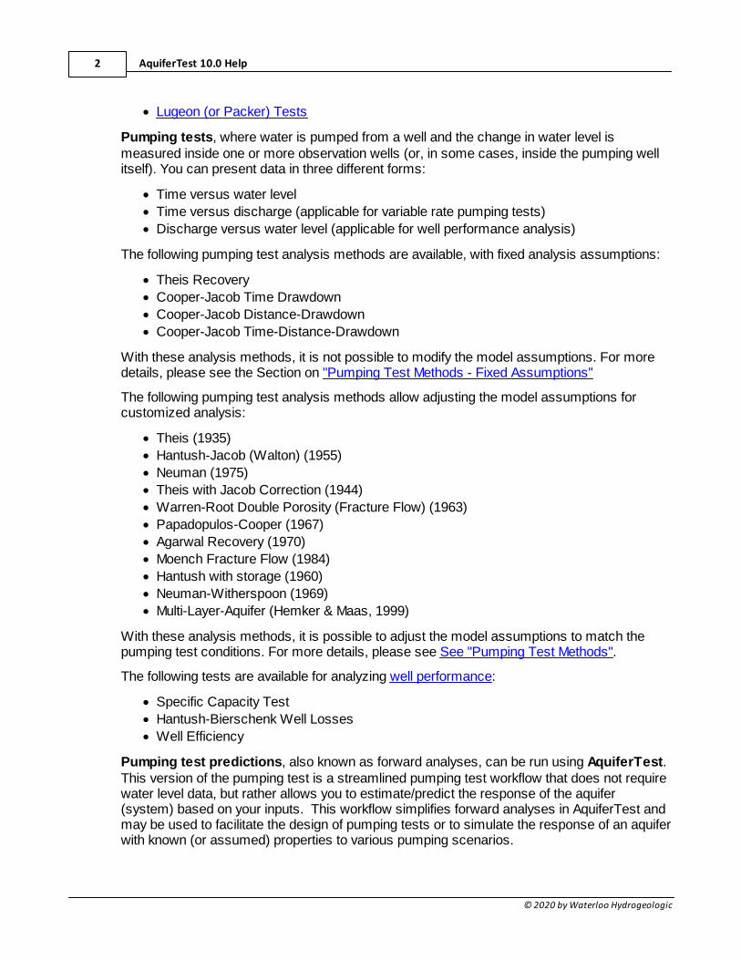
Pumping tests, where water is pumped from a well and the change in water level ismeasured inside one or more observation wells (or, in some cases, inside the pumping wellitself). You can present data in three different forms:
· Time versus water level
· Time versus discharge (applicable for variable rate pumping tests)
· Discharge versus water level (applicable for well performance analysis)
The following pumping test analysis methods are available, with fixed analysis assumptions:
· Theis Recovery
· Cooper-Jacob Time Drawdown
· Cooper-Jacob Distance-Drawdown
· Cooper-Jacob Time-Distance-Drawdown
With these analysis methods, it is not possible to modify the model assumptions. For moredetails, please see the Section on "Pumping Test Methods - Fixed Assumptions"
The following pumping test analysis methods allow adjusting the model assumptions forcustomized analysis:
· Theis (1935)
· Hantush-Jacob (Walton) (1955)
· Neuman (1975)
· Theis with Jacob Correction (1944)
· Warren-Root Double Porosity (Fracture Flow) (1963)
· Papadopulos-Cooper (1967)
· Agarwal Recovery (1970)
· Moench Fracture Flow (1984)
· Hantush with storage (1960)
· Neuman-Witherspoon (1969)
· Multi-Layer-Aquifer (Hemker & Maas, 1999)
With these analysis methods, it is possible to adjust the model assumptions to match thepumping test conditions. For more details, please see See "Pumping Test Methods".
The following tests are available for analyzing well performance:
· Specific Capacity Test
· Hantush-Bierschenk Well Losses
· Well Efficiency
Pumping test predictions, also known as forward analyses, can be run using AquiferTest.This version of the pumping test is a streamlined pumping test workflow that does not requirewater level data, but rather allows you to estimate/predict the response of the aquifer(system) based on your inputs. This workflow simplifies forward analyses in AquiferTest andmay be used to facilitate the design of pumping tests or to simulate the response of an aquiferwith known (or assumed) properties to various pumping scenarios.
Introduction 3
© 2020 by Waterloo Hydrogeologic
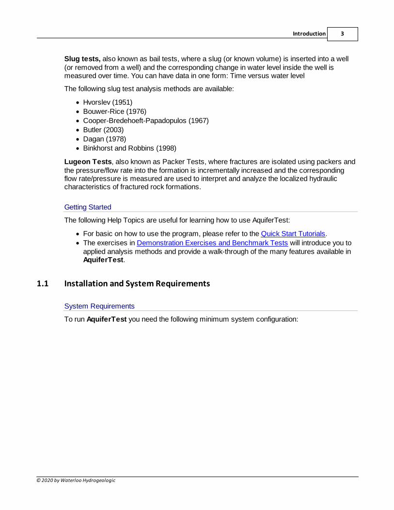
Slug tests, also known as bail tests, where a slug (or known volume) is inserted into a well(or removed from a well) and the corresponding change in water level inside the well ismeasured over time. You can have data in one form: Time versus water level
The following slug test analysis methods are available:
· Hvorslev (1951)
· Bouwer-Rice (1976)
· Cooper-Bredehoeft-Papadopulos (1967)
· Butler (2003)
· Dagan (1978)
· Binkhorst and Robbins (1998)
Lugeon Tests, also known as Packer Tests, where fractures are isolated using packers andthe pressure/flow rate into the formation is incrementally increased and the correspondingflow rate/pressure is measured are used to interpret and analyze the localized hydrauliccharacteristics of fractured rock formations.
Getting Started
The following Help Topics are useful for learning how to use AquiferTest:
· For basic on how to use the program, please refer to the Quick Start Tutorials.
· The exercises in Demonstration Exercises and Benchmark Tests will introduce you toapplied analysis methods and provide a walk-through of the many features available inAquiferTest.
1.1 Installation and System Requirements
System Requirements
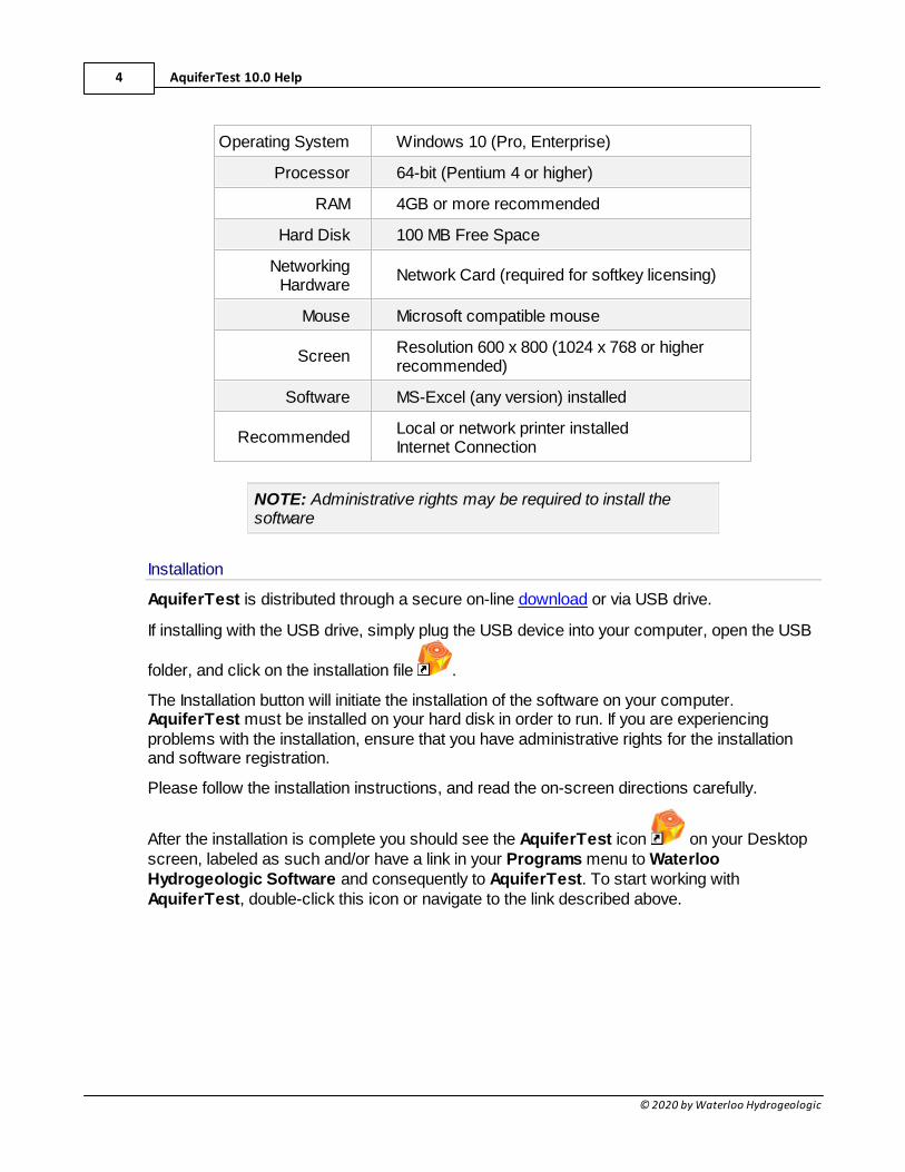
To run AquiferTest you need the following minimum system configuration:
AquiferTest 10.0 Help4
© 2020 by Waterloo Hydrogeologic
Operating System Windows 10 (Pro, Enterprise)
Processor 64-bit (Pentium 4 or higher)
RAM 4GB or more recommended
Hard Disk 100 MB Free Space
NetworkingHardware
Network Card (required for softkey licensing)
Mouse Microsoft compatible mouse
ScreenResolution 600 x 800 (1024 x 768 or higherrecommended)
Software MS-Excel (any version) installed
RecommendedLocal or network printer installedInternet Connection
NOTE: Administrative rights may be required to install thesoftware
Installation
AquiferTest is distributed through a secure on-line download or via USB drive.
If installing with the USB drive, simply plug the USB device into your computer, open the USB
folder, and click on the installation file .
The Installation button will initiate the installation of the software on your computer.AquiferTest must be installed on your hard disk in order to run. If you are experiencingproblems with the installation, ensure that you have administrative rights for the installationand software registration.
Please follow the installation instructions, and read the on-screen directions carefully.
After the installation is complete you should see the AquiferTest icon on your Desktopscreen, labeled as such and/or have a link in your Programs menu to WaterlooHydrogeologic Software and consequently to AquiferTest. To start working withAquiferTest, double-click this icon or navigate to the link described above.
Introduction 5
© 2020 by Waterloo Hydrogeologic
1.2 Updating Old Projects
AquiferTest is backwards compatible, and is able to open projects from previous releases,including version 7.0 through 9.0 and 2013.x through 2016.x. However, it is recommendedthat you ALWAYS create a backup copy of any project files before you open them in the newversion. Specifically, ensure that you back up your original AquiferTest (.HYT) and/or MS-Access database (.MDB), which contain all project data.
NOTE: Waterloo Hydrogeologic is not responsible for anydirect or indirect damages caused to projects duringconversion. It is strongly recommended that you create asecure, independent backup of projects before converting.
1.3 Learning AquiferTest
Help Documentation
This User’s Manual is available in three formats:
· Compiled Help File: Select Help, then Content to open the compiled help file. Thisversion will be based on the installed version of AquiferTest.
· Online Help: Access through your internet browser at:https://www.waterloohydrogeologic.com/help/aquifertest/. This version will be currentto the latest release.
· PDF Document: Available for download here:https://www.waterloohydrogeologic.com/wp-content/uploads/PDFs/aquifertest/AquiferTest_Users_Manual.pdf. This version will becurrent to the latest release.
Sample Tutorials and Exercises
There are several sample projects included with AquiferTest, which demonstrate numerousfeatures, and allow you learn to effectively navigate and use the program. Feel free to perusethrough these samples.
To familiarize yourself with AquiferTest, please refer to the step-by-step Quick Start DemoTutorials:
· Tutorial 1: Confined Aquifer Pumping Test Analysis
· Tutorial 2: Predictive Analysis
· Tutorial 3: Single Well Analysis
· Tutorial 4: Slug Test Analysis
AquiferTest 10.0 Help6
© 2020 by Waterloo Hydrogeologic
To begin working with your own data, please refer to the step-by-step DemonstrationExercises:
· Exercise 1: How to create a pumping test
· Exercise 7: How to create a slug test
· Exercise 12: How to create a Lugeon (packer) test
In all, there are 4 tutorials, 14 exercises, and 19 additional benchmark example files that youmay refer to to help you learn how to use AquiferTest and the incorporated aquifer analysismethods.
Suggested Reference Material
Additional information can be obtained from hydrogeology texts such as:
Dominico, P.A. and F.W. Schwartz, 1990. Physical and Chemical Hydrogeology. JohnWiley & Sons, Inc. 824 p.
Driscoll, F. G., 1987. Groundwater and Wells, Johnson Division, St. Paul, Minnesota55112, 1089 p.Fetter, C.W., 1994. Applied Hydrogeology, Third Edition, Prentice-Hall, Inc., Upper Saddle River, New Jersey, 691 p.
Freeze, R.A., and Cherry, J.A., 1979. Groundwater. Prentice-Hall Inc. Englewood Cliffs,New Jersey. 604 pp. http://hydrogeologistswithoutborders.org/wordpress/1979-english/
Kruseman, G.P. and N.A. de Ridder, 1990. Analysis and Evaluation of Pumping TestData Second Edition (Completely Revised) ILRI publication 47. Intern. Inst. for LandReclamation and Improvements, Wageningen, Netherlands, 377 p.
The complete list of references for AquiferTest can be found in the References Section.
1.4 About the Interface
AquiferTest is designed to automate the most common tasks that hydrogeologists and otherwater supply professionals typically encounter when planning and analyzing the results of anaquifer test. The program design allows you to efficiently manage all the information from youraquifer test and perform more analyses, consistently, and in less time. For example, youneed to enter information about your testing wells (e.g. X and Y coordinates, elevation, screenlength, etc.) only once in AquiferTest. After you create a well, you can see it in the navigatorpanel, or in the wells grid.
When you import data or create an analysis, you specify which wells to include from the list ofavailable wells in the project. If you decide to perform additional analyses, you can againspecify from the available wells without re-creating them in AquiferTest. There is no need tore-enter your data or create a new project. Your analysis graph is refreshed, and the data re-analyzed using the selected solution method. This is useful for quickly comparing the results
Introduction 7
© 2020 by Waterloo Hydrogeologic
of data analysis using different solution methods. If you need solution-specific information forthe new analysis, AquiferTest prompts you for the required data.
Getting Around
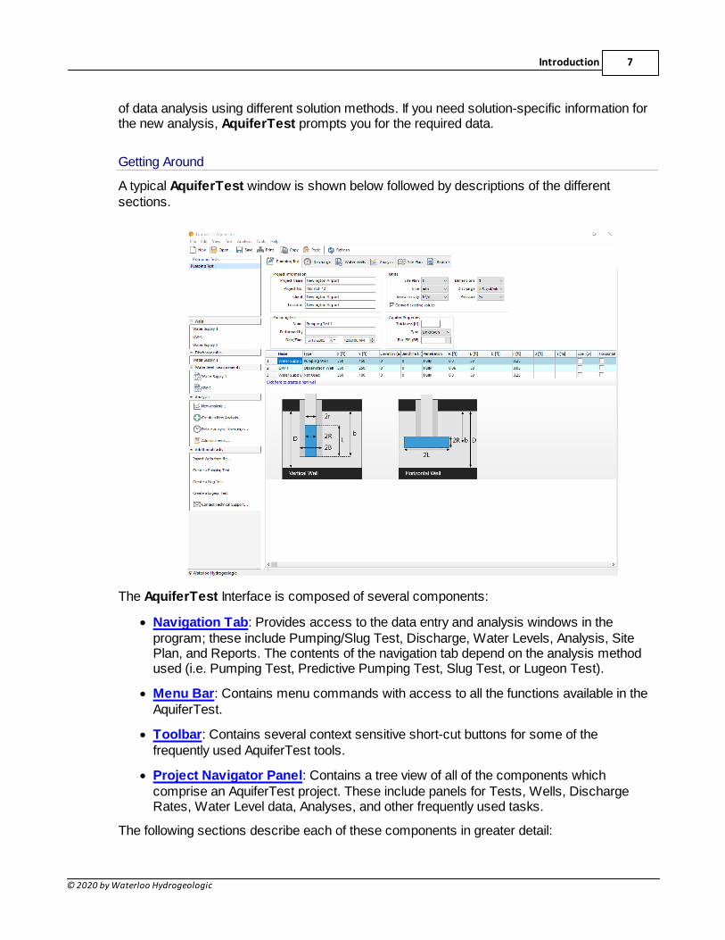
A typical AquiferTest window is shown below followed by descriptions of the differentsections.
The AquiferTest Interface is composed of several components:
· Navigation Tab: Provides access to the data entry and analysis windows in theprogram; these include Pumping/Slug Test, Discharge, Water Levels, Analysis, SitePlan, and Reports. The contents of the navigation tab depend on the analysis methodused (i.e. Pumping Test, Predictive Pumping Test, Slug Test, or Lugeon Test).
· Menu Bar: Contains menu commands with access to all the functions available in theAquiferTest.
· Toolbar: Contains several context sensitive short-cut buttons for some of thefrequently used AquiferTest tools.
· Project Navigator Panel: Contains a tree view of all of the components whichcomprise an AquiferTest project. These include panels for Tests, Wells, DischargeRates, Water Level data, Analyses, and other frequently used tasks.
The following sections describe each of these components in greater detail:
AquiferTest 10.0 Help8
© 2020 by Waterloo Hydrogeologic
Navigation Tabs
The interface in AquiferTest has been designed so that information can be quickly and easilyentered, and modified at any time later if needed. The data entry and analysis windows havebeen separated into navigation tabs; the tabs are logically ordered such that the informationflow is in a left-to-right fashion; this means that data is first entered in the far left tab, then theprocess proceeds to the right from there. The tabs are explained below:
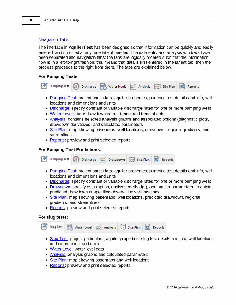
For Pumping Tests:
· Pumping Test: project particulars, aquifer properties, pumping test details and info, welllocations and dimensions and units
· Discharge: specify constant or variable discharge rates for one or more pumping wells
· Water Levels: time drawdown data, filtering, and trend affects
· Analysis: contains selected analysis graphs and associated options (diagnostic plots,drawdown derivatives) and calculated parameters
· Site Plan: map showing basemaps, well locations, drawdown, regional gradients, andstreamlines.
· Reports: preview and print selected reports
For Pumping Test Predictions:
· Pumping Test: project particulars, aquifer properties, pumping test details and info, welllocations and dimensions and units
· Discharge: specify constant or variable discharge rates for one or more pumping wells
· Drawdown: specify assumption, analysis method(s), and aquifer parameters, to obtainpredicted drawdown at specified observation well locations.
· Site Plan: map showing basemaps, well locations, predicted drawdown, regionalgradients, and streamlines.
· Reports: preview and print selected reports
For slug tests:
· Slug Test: project particulars, aquifer properties, slug test details and info, well locationsand dimensions, and units
· Water Level: water level data
· Analysis: analysis graphs and calculated parameters
· Site Plan: map showing basemaps and well locations
· Reports: preview and print selected reports
Introduction 9
© 2020 by Waterloo Hydrogeologic
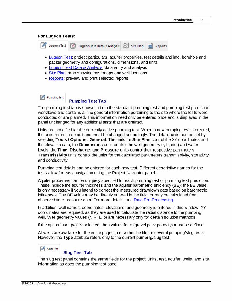
For Lugeon Tests:
· Lugeon Test: project particulars, aquifer properties, test details and info, borehole andpacker geometry and configurations, dimensions, and units
· Lugeon Test Data & Analysis: data entry and analysis
· Site Plan: map showing basemaps and well locations
· Reports: preview and print selected reports
Pumping Test Tab
The pumping test tab is shown in both the standard pumping test and pumping test predictionworkflows and contains all the general information pertaining to the site where the tests wereconducted or are planned. This information need only be entered once and is displayed in thepanel unchanged for any additional tests that are created.
Units are specified for the currently active pumping test. When a new pumping test is created,the units return to default and must be changed accordingly. The default units can be set byselecting Tools / Options / General. The units for Site Plan control the XY coordinates andthe elevation data; the Dimensions units control the well geometry (r, L, etc.) and waterlevels; the Time, Discharge, and Pressure units control their respective parameters;Transmissivity units control the units for the calculated parameters transmissivity, storativity,and conductivity.
Pumping test details can be entered for each new test. Different descriptive names for thetests allow for easy navigation using the Project Navigator panel.
Aquifer properties can be uniquely specified for each pumping test or pumping test prediction.These include the aquifer thickness and the aquifer barometric efficiency (BE); the BE valueis only necessary if you intend to correct the measured drawdown data based on barometricinfluences. The BE value may be directly entered in the field, or may be calculated fromobserved time-pressure data. For more details, see Data Pre-Processing.
In addition, well names, coordinates, elevations, and geometry is entered in this window. XYcoordinates are required, as they are used to calculate the radial distance to the pumpingwell. Well geometry values (r, R, L, b) are necessary only for certain solution methods.
If the option “use r(w)” is selected, then values for n (gravel pack porosity) must be defined.
All wells are available for the entire project, i.e. within the file for several pumping/slug tests.However, the Type attribute refers only to the current pumping/slug test.
Slug Test Tab
The slug test panel contains the same fields for the project, units, test, aquifer, wells, and siteinformation as does the pumping test panel.
AquiferTest 10.0 Help10
© 2020 by Waterloo Hydrogeologic
Lugeon Test Tab
The Lugeon test panel contains similar fields for the project, units, test, wells. Additionalinformation is required for the Test and Packager configurations.
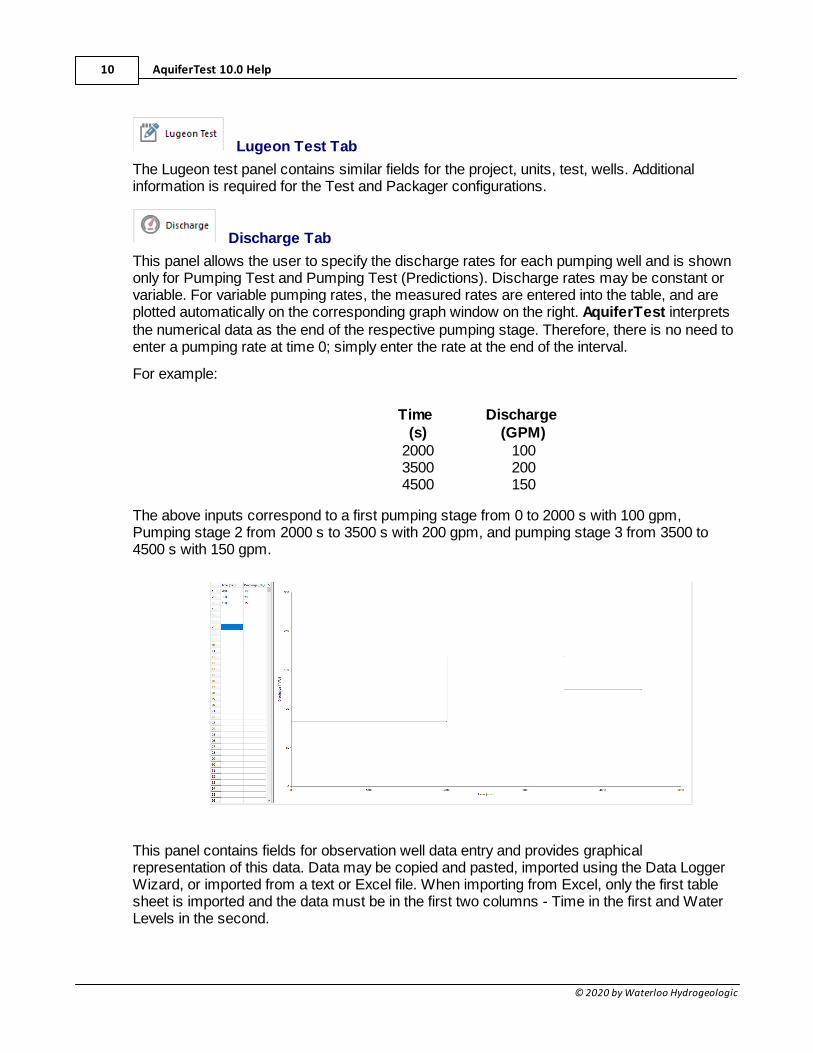
Discharge Tab
This panel allows the user to specify the discharge rates for each pumping well and is shownonly for Pumping Test and Pumping Test (Predictions). Discharge rates may be constant orvariable. For variable pumping rates, the measured rates are entered into the table, and areplotted automatically on the corresponding graph window on the right. AquiferTest interpretsthe numerical data as the end of the respective pumping stage. Therefore, there is no need toenter a pumping rate at time 0; simply enter the rate at the end of the interval.
For example:
Time (s)
Discharge (GPM)
2000 1003500 2004500 150
The above inputs correspond to a first pumping stage from 0 to 2000 s with 100 gpm,Pumping stage 2 from 2000 s to 3500 s with 200 gpm, and pumping stage 3 from 3500 to4500 s with 150 gpm.
Water Levels TabThis panel contains fields for observation well data entry and provides graphicalrepresentation of this data. Data may be copied and pasted, imported using the Data LoggerWizard, or imported from a text or Excel file. When importing from Excel, only the first tablesheet is imported and the data must be in the first two columns - Time in the first and WaterLevels in the second.
Introduction 11
© 2020 by Waterloo Hydrogeologic
In addition, there are data filtering options, and data corrections (trend affects, barometricaffects, etc.) By reducing the number of measured values, you can improve the programperformance, and calculate the aquifer parameters quicker.
Water Level Tab
This panel allows the user to specify the water level observations made during the applicablepumping or slug tests. Water levels can be specified in a variety of vertical datums, includingelevation above mean sea level (AMSL), elevation relative to a benchmark, depth to waterfrom the top of casing (TOC), and drawdown. Several data handling tools are available at thisstep in including:
· data corrections foro barometric effects and o trend removal:
§ simple delta,§ linear,§ logarithmic,§ sinusoidal), and
· data filtering:o by log or linear time differenceo elevation change
This step is made easy to work with by providing numerous options to enter the water leveldata, including direct entry, import of a wide variety of file formats, and pasting from theclipboard.
Analysis Tab
The analysis panel contains the workspace for calculating aquifer parameters using theabundance of graphical solution methods for pumping and slug tests. There are two maintabs available: Diagnostic and Analysis.
Diagnostic graphs
The Diagnostic graph provides tools for interpreting the drawdown data, and is avisual aid for determining the aquifer type if this is not well understood. The measureddrawdown data are plotted on a log-log scale, or a semi-log scale and is available forpumping tests only.
On the right side, apart from the actual graph, the processes characteristic ofdifferent aquifer types are schematically represented. By comparing the observeddata to the pre-defined templates, it is possible to identify the aquifer type andconditions (confined, well bore storage, boundary influences, etc.) Using thisknowledge, an appropriate solution method and assumptions can then be selectedfrom the Analysis tab, and the aquifer parameters calculated.
In addition, AquiferTest calculates and displays the derivative of the measureddrawdown values; this is helpful since quite often it is much easier to analyze and
AquiferTest 10.0 Help12
© 2020 by Waterloo Hydrogeologic
interpret the derivative of the drawdown data, then just the measured drawdown dataitself.
Analysis graph tab
In the Analysis tab, there are several panels on the right hand side of the graph thatallow setting up the graph, changing the aquifer parameters to achieve an optimalcurve fit, model assumptions, display and other settings.
For more information, please see the Analysis Tab section.
Drawdown Tab
The drawdown analysis panel is similar to the Analysis tab and contains the workspace forestimating drawdown associated with specified pumping discharge, aquifer conditions, andparameters based on the selected analytical solution method. There are several panels onthe right hand side of the graph that allow you to specify the Prediction method (i.e. theanalytical solution), associated parameters, model assumptions, and various chart settings.
Lugeon Test Data & Analysis
The Lugeon Test Data and Analysis tab contains the workspace of entering the test data,standard Lugeon Test plots, and companion example charts to facilitate interpretation of theLugeon Test.
Site Plan Tab
AquiferTest automatically plots the wells on a map layout. The site map layout may contain aCAD file or raster image (e.g. a topographic map, an air or satellite photograph etc.). Rasterimages must be georeferenced using two known co-ordinates, at the corners of the image.For more details, see the Import Map Image... section.
Reports Tab
The Reports page displays report previews, and allows the user to select from various reporttemplates. The reports are listed in hierarchical order for the current pumping/slug test. Azoom feature is available, with preview settings.
The dark grey area around the page displays the margins for the current printer. You canmodify these settings by selecting File/Printer Setup.
Select Print on this page to print all selected reports. Using Print on a selected tab will printthe context related report directly - such as a data report from the Water Levels page.
Menu Bar
The menu bar provides access to most of the features available in AquiferTest. For moredetails, see the Main Menu Bar section.
Introduction 13
© 2020 by Waterloo Hydrogeologic
AquiferTest Toolbar
The following sections describe each of the items on the toolbar, and the equivalent icons.For a short description of an icon, move the mouse pointer over the icon without clicking eithermouse button.
The toolbars that appear beneath the menu bar are dynamic, changing as you move from onewindow to another. Some toolbar buttons become available only when certain windows are inview, or in a certain context. For example, the Paste button is only available after the Copycommand has been used.
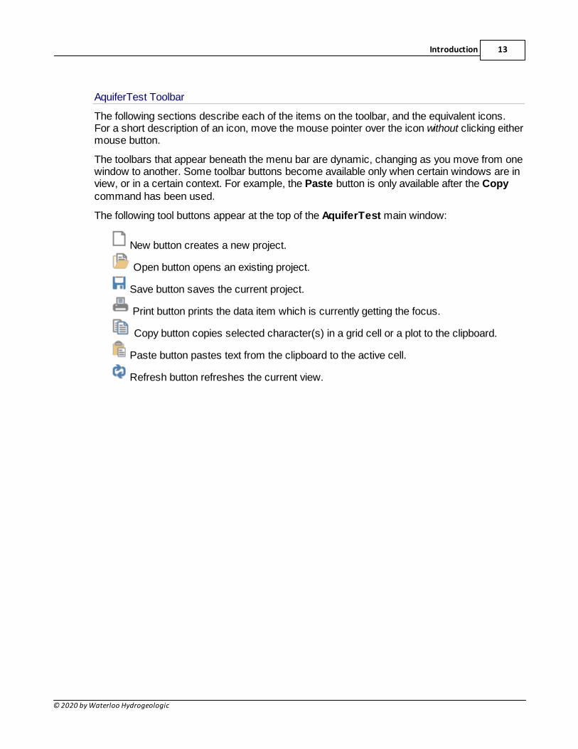
The following tool buttons appear at the top of the AquiferTest main window:
New button creates a new project.
Open button opens an existing project.
Save button saves the current project.
Print button prints the data item which is currently getting the focus.
Copy button copies selected character(s) in a grid cell or a plot to the clipboard.
Paste button pastes text from the clipboard to the active cell.
Refresh button refreshes the current view.
AquiferTest 10.0 Help14
© 2020 by Waterloo Hydrogeologic
Project Navigator Panel
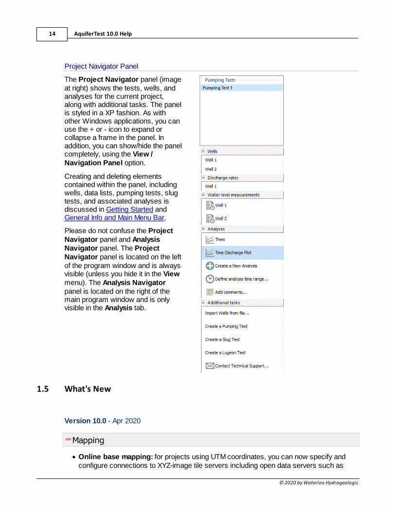
The Project Navigator panel (imageat right) shows the tests, wells, andanalyses for the current project,along with additional tasks. The panelis styled in a XP fashion. As withother Windows applications, you canuse the + or - icon to expand orcollapse a frame in the panel. Inaddition, you can show/hide the panelcompletely, using the View /Navigation Panel option.
Creating and deleting elementscontained within the panel, includingwells, data lists, pumping tests, slugtests, and associated analyses isdiscussed in Getting Started andGeneral Info and Main Menu Bar.
Please do not confuse the ProjectNavigator panel and AnalysisNavigator panel. The ProjectNavigator panel is located on the leftof the program window and is alwaysvisible (unless you hide it in the Viewmenu). The Analysis Navigatorpanel is located on the right of themain program window and is onlyvisible in the Analysis tab.
1.5 What's New
Version 10.0 - Apr 2020
Mapping
· Online base mapping: for projects using UTM coordinates, you can now specify andconfigure connections to XYZ-image tile servers including open data servers such as
Introduction 15
© 2020 by Waterloo Hydrogeologic
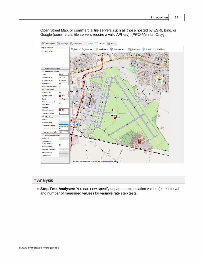
Open Street Map, or commercial tile servers such as those hosted by ESRI, Bing, orGoogle (commercial tile servers require a valid API key). [PRO-Version Only]
Analysis
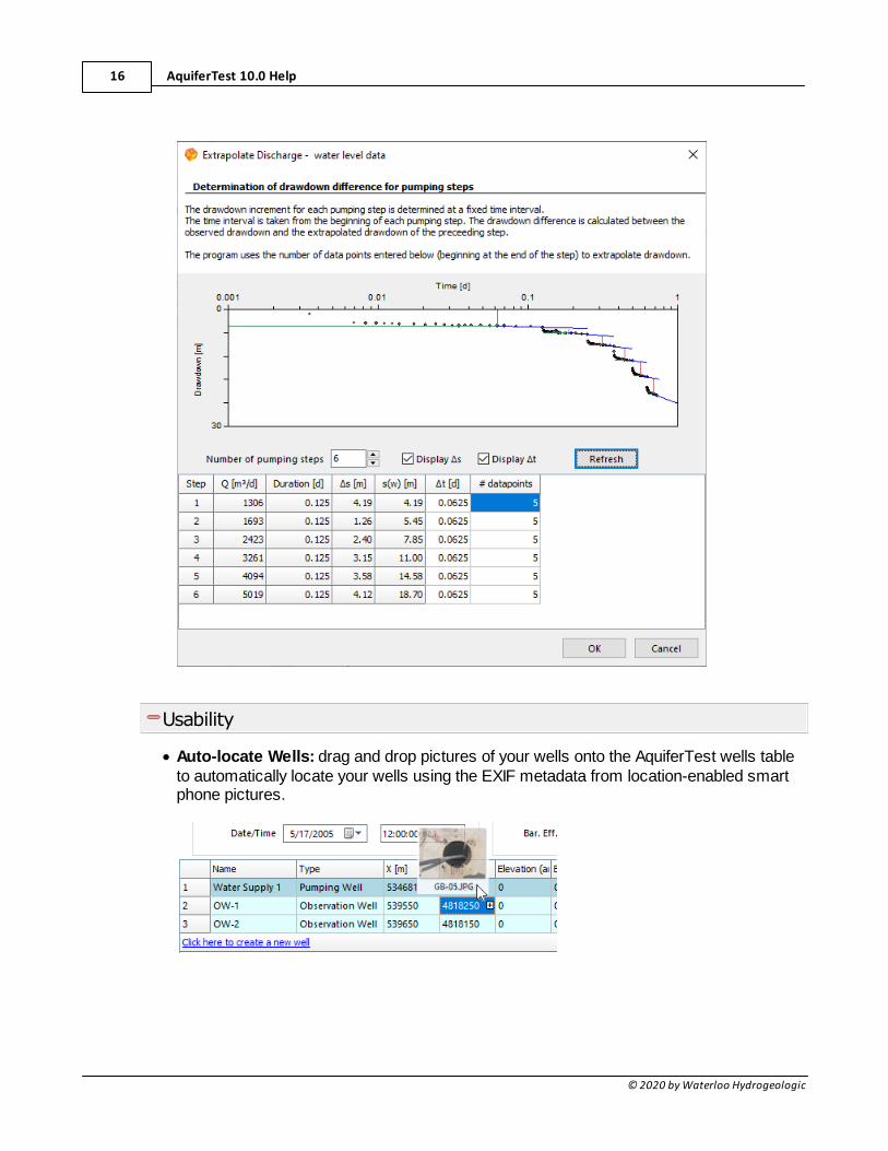
· Step Test Analyses: You can now specify separate extrapolation values (time intervaland number of measured values) for variable rate step tests.
AquiferTest 10.0 Help16
© 2020 by Waterloo Hydrogeologic
Usability
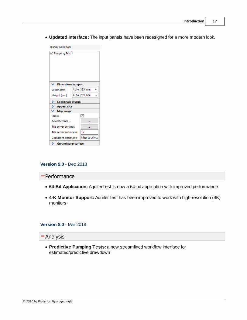
· Auto-locate Wells: drag and drop pictures of your wells onto the AquiferTest wells tableto automatically locate your wells using the EXIF metadata from location-enabled smartphone pictures.
Introduction 17
© 2020 by Waterloo Hydrogeologic
· Updated Interface: The input panels have been redesigned for a more modern look.
Version 9.0 - Dec 2018
Performance
· 64-Bit Application: AquiferTest is now a 64-bit application with improved performance
· 4-K Monitor Support: AquiferTest has been improved to work with high-resolution (4K)monitors
Version 8.0 - Mar 2018
Analysis
· Predictive Pumping Tests: a new streamlined workflow interface forestimated/predictive drawdown
AquiferTest 10.0 Help18
© 2020 by Waterloo Hydrogeologic
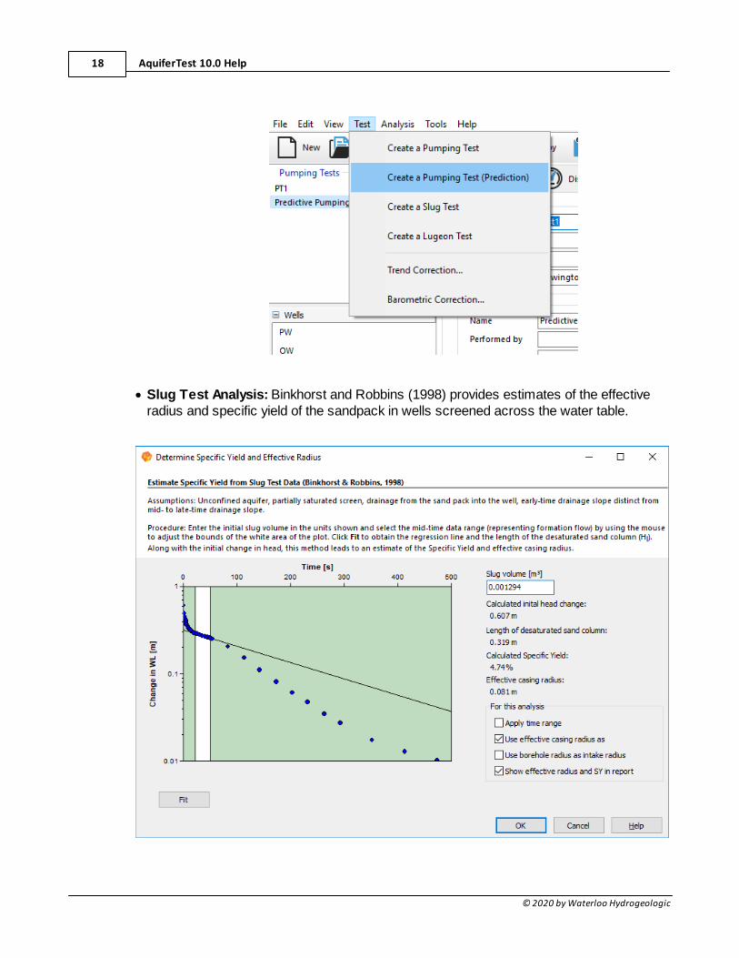
· Slug Test Analysis: Binkhorst and Robbins (1998) provides estimates of the effectiveradius and specific yield of the sandpack in wells screened across the water table.
Introduction 19
© 2020 by Waterloo Hydrogeologic
Site Plan
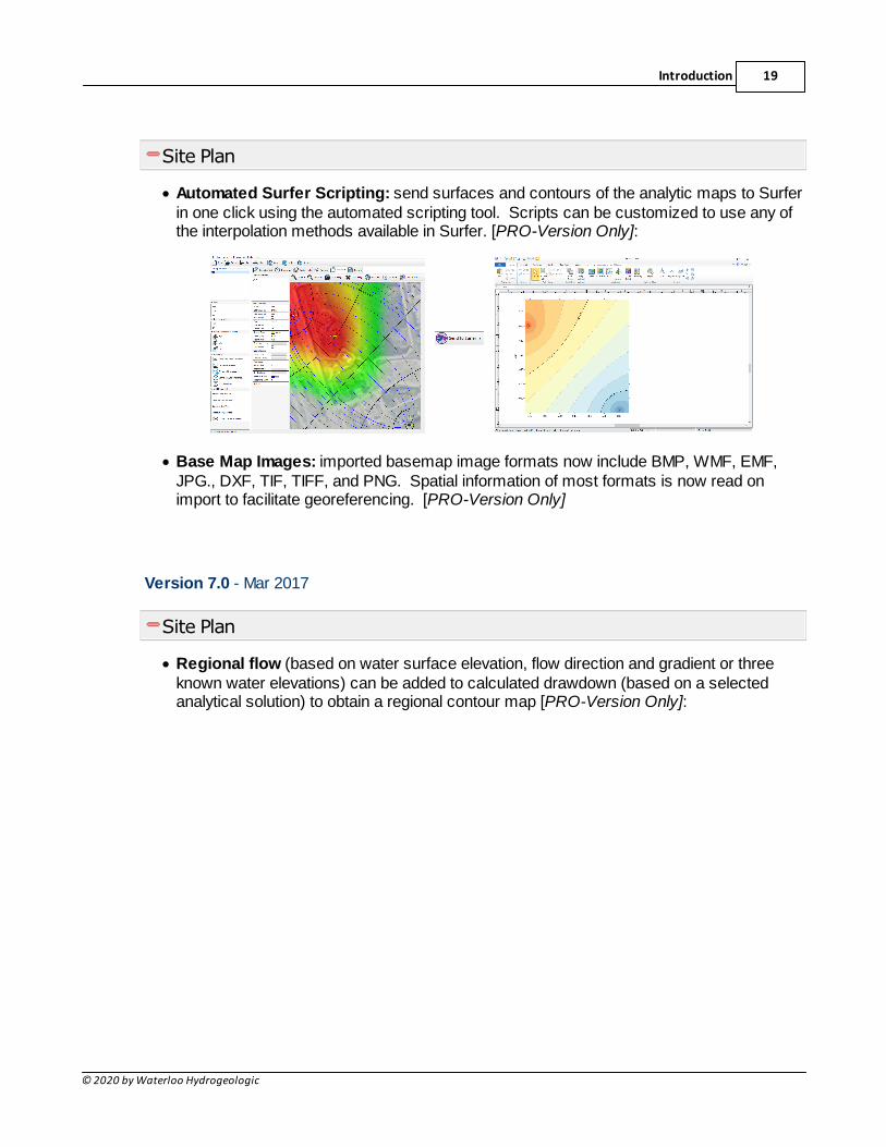
· Automated Surfer Scripting: send surfaces and contours of the analytic maps to Surferin one click using the automated scripting tool. Scripts can be customized to use any ofthe interpolation methods available in Surfer. [PRO-Version Only]:
· Base Map Images: imported basemap image formats now include BMP, WMF, EMF,JPG., DXF, TIF, TIFF, and PNG. Spatial information of most formats is now read onimport to facilitate georeferencing. [PRO-Version Only]
Version 7.0 - Mar 2017
Site Plan
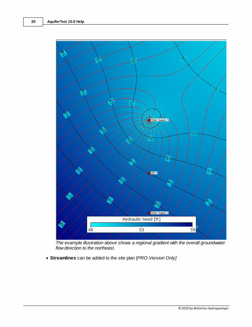
· Regional flow (based on water surface elevation, flow direction and gradient or threeknown water elevations) can be added to calculated drawdown (based on a selectedanalytical solution) to obtain a regional contour map [PRO-Version Only]:
AquiferTest 10.0 Help20
© 2020 by Waterloo Hydrogeologic
The example illustration above shows a regional gradient with the overall groundwaterflow direction to the northeast.
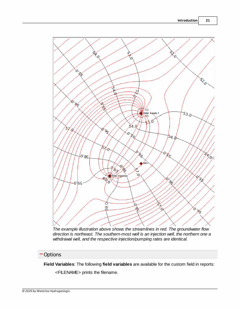
· Streamlines can be added to the site plan [PRO-Version Only]
Introduction 21
© 2020 by Waterloo Hydrogeologic
The example illustration above shows the streamlines in red. The groundwater flowdirection is northeast. The southern-most well is an injection well, the northern one awithdrawal well, and the respective injection/pumping rates are identical.
Options
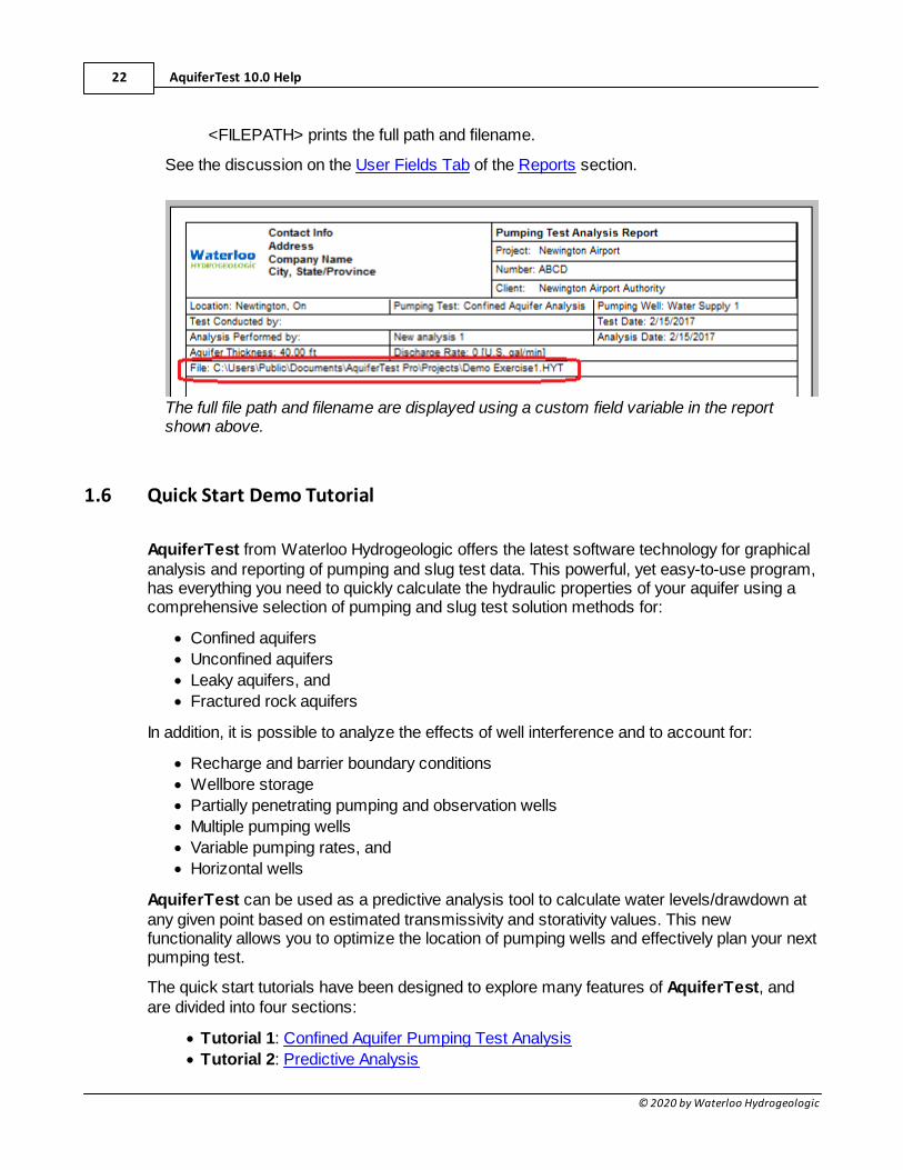
Field Variables: The following field variables are available for the custom field in reports:
<FILENAME> prints the filename.
AquiferTest 10.0 Help22
© 2020 by Waterloo Hydrogeologic
<FILEPATH> prints the full path and filename.
See the discussion on the User Fields Tab of the Reports section.
The full file path and filename are displayed using a custom field variable in the reportshown above.
1.6 Quick Start Demo Tutorial
AquiferTest from Waterloo Hydrogeologic offers the latest software technology for graphicalanalysis and reporting of pumping and slug test data. This powerful, yet easy-to-use program,has everything you need to quickly calculate the hydraulic properties of your aquifer using acomprehensive selection of pumping and slug test solution methods for:
· Confined aquifers
· Unconfined aquifers
· Leaky aquifers, and
· Fractured rock aquifers
In addition, it is possible to analyze the effects of well interference and to account for:
· Recharge and barrier boundary conditions
· Wellbore storage
· Partially penetrating pumping and observation wells
· Multiple pumping wells
· Variable pumping rates, and
· Horizontal wells
AquiferTest can be used as a predictive analysis tool to calculate water levels/drawdown atany given point based on estimated transmissivity and storativity values. This newfunctionality allows you to optimize the location of pumping wells and effectively plan your nextpumping test.
The quick start tutorials have been designed to explore many features of AquiferTest, andare divided into four sections:
· Tutorial 1: Confined Aquifer Pumping Test Analysis
· Tutorial 2: Predictive Analysis
Introduction 23
© 2020 by Waterloo Hydrogeologic
· Tutorial 3: Single Well Analysis
· Tutorial 4: Slug Test Analysis
1.6.1 Tutorial 1: Confined Aquifer Pumping Test Analysis
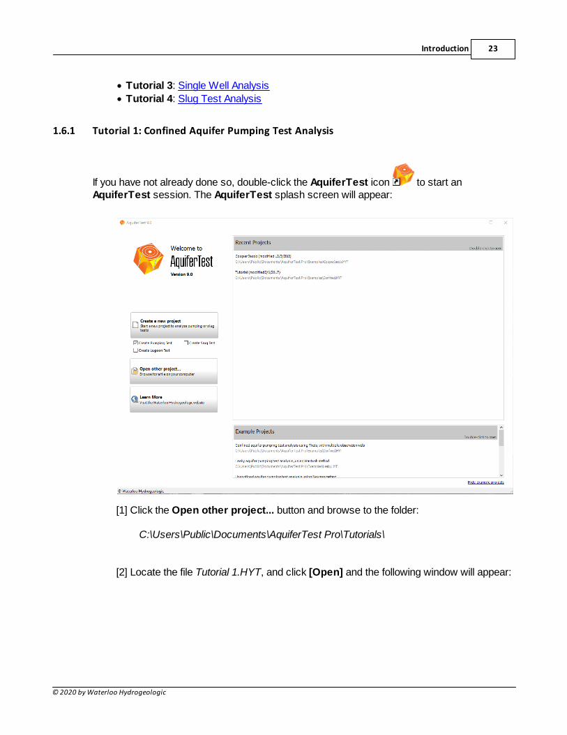
If you have not already done so, double-click the AquiferTest icon to start anAquiferTest session. The AquiferTest splash screen will appear:
[1] Click the Open other project... button and browse to the folder:
C:\Users\Public\Documents\AquiferTest Pro\Tutorials\
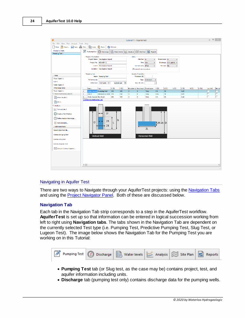
[2] Locate the file Tutorial 1.HYT, and click [Open] and the following window will appear:
AquiferTest 10.0 Help24
© 2020 by Waterloo Hydrogeologic
Navigating in Aquifer Test
There are two ways to Navigate through your AquiferTest projects: using the Navigation Tabsand using the Project Navigator Panel. Both of these are discussed below.
Navigation Tab
Each tab in the Navigation Tab strip corresponds to a step in the AquiferTest workflow. AquiferTest is set up so that information can be entered in logical succession working fromleft to right using Navigation tabs. The tabs shown in the Navigation Tab are dependent onthe currently selected Test type (i.e. Pumping Test, Predictive Pumping Test, Slug Test, orLugeon Test). The image below shows the Navigation Tab for the Pumping Test you areworking on in this Tutorial:
· Pumping Test tab (or Slug test, as the case may be) contains project, test, andaquifer information including units.
· Discharge tab (pumping test only) contains discharge data for the pumping wells.
Introduction 25
© 2020 by Waterloo Hydrogeologic
· Water Levels tab contains data for observation wells, pumping wells, andpiezometers used in the selected test.
· Analysis tab houses all functions needed to perform all analyses available inAquiferTest.
· Site Plan tab allows wells to be plotted on a site map, and also contour drawdowndata.
· Reports tab allows you to easily generate printable reports of your analyses anddata.
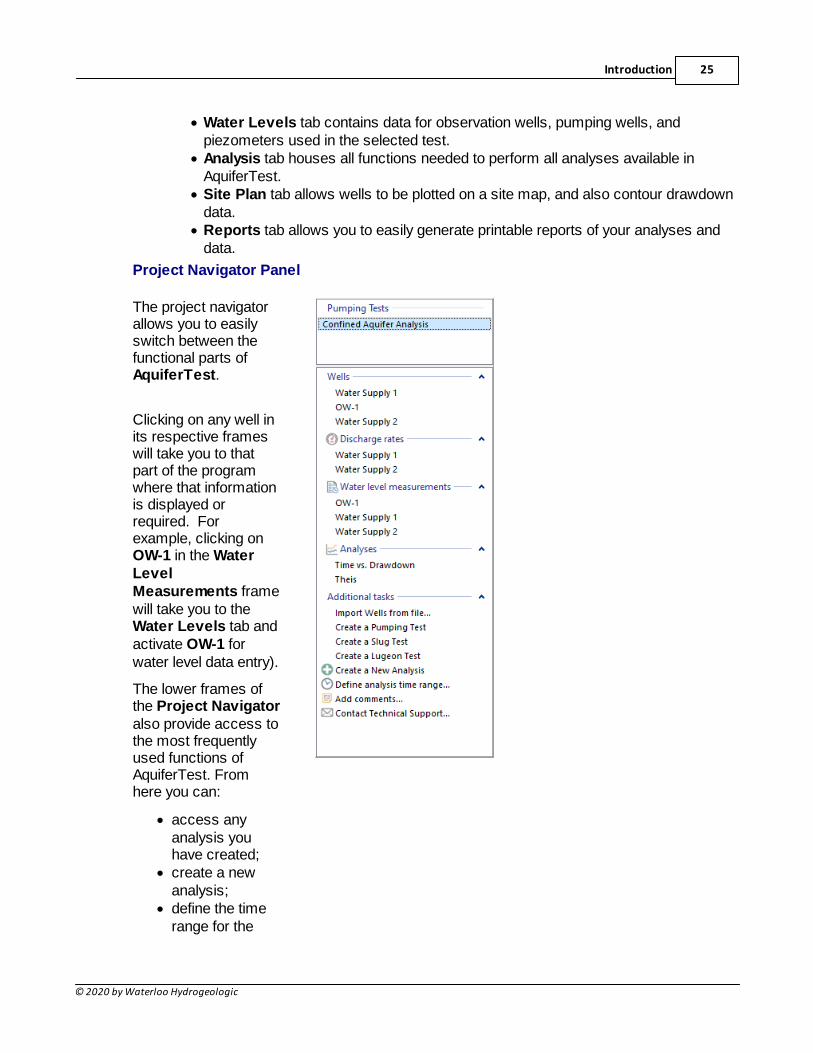
Project Navigator Panel
The project navigatorallows you to easilyswitch between thefunctional parts ofAquiferTest.
Clicking on any well inits respective frameswill take you to thatpart of the programwhere that informationis displayed orrequired. Forexample, clicking onOW-1 in the WaterLevelMeasurements framewill take you to theWater Levels tab andactivate OW-1 forwater level data entry).
The lower frames ofthe Project Navigatoralso provide access tothe most frequentlyused functions ofAquiferTest. Fromhere you can:
· access anyanalysis youhave created;
· create a newanalysis;
· define the timerange for the
AquiferTest 10.0 Help26
© 2020 by Waterloo Hydrogeologic
data used inanalysis;
· add commentsto the analysis;
· import wellsfrom a data file;
· create a newpumping test,slug test, orlugeon test; and
· contact techsupport.
You can hide theProject Navigator bychoosingView/NavigationPanel.
You can collapse anyand all frames in theProject Navigator byclicking the [-] buttonbeside the header ofeach frame.
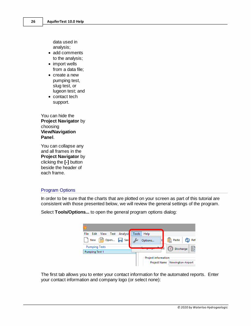
Program Options
In order to be sure that the charts that are plotted on your screen as part of this tutorial areconsistent with those presented below, we will review the general settings of the program.
Select Tools/Options... to open the general program options dialog:
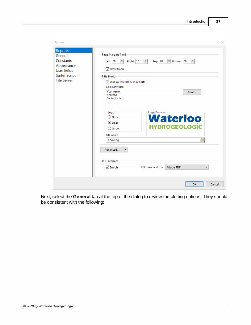
The first tab allows you to enter your contact information for the automated reports. Enteryour contact information and company logo (or select none):
Introduction 27
© 2020 by Waterloo Hydrogeologic
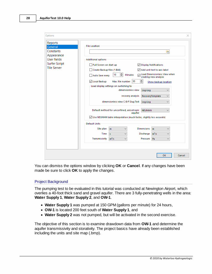
Next, select the General tab at the top of the dialog to review the plotting options. They shouldbe consistent with the following:
AquiferTest 10.0 Help28
© 2020 by Waterloo Hydrogeologic
You can dismiss the options window by clicking OK or Cancel. If any changes have beenmade be sure to click OK to apply the changes.
Project Background
The pumping test to be evaluated in this tutorial was conducted at Newington Airport, whichoverlies a 40-foot thick sand and gravel aquifer. There are 3 fully-penetrating wells in the area:Water Supply 1, Water Supply 2, and OW-1.
· Water Supply 1 was pumped at 150 GPM (gallons per minute) for 24 hours,
· OW-1 is located 200 feet south of Water Supply 1, and
· Water Supply 2 was not pumped, but will be activated in the second exercise.
The objective of this section is to examine drawdown data from OW-1 and determine theaquifer transmissivity and storativity. The project basics have already been establishedincluding the units and site map (.bmp).
Introduction 29
© 2020 by Waterloo Hydrogeologic
Pumping Test
The top portion of the Pumping Test tab contains information that describes the projectdetails, test details, units, and aquifer parameters. Most of the information has been enteredfor you; however, some additional information is required.
[3] In the Pumping Test frame enter the following:
· Pumping Test Name: Confined Aquifer Analysis
· Performed by: Your Name
[4] In the Aquifer Properties frame enter the following:
· Aquifer Thickness: 40
· Type: Confined
· Bar. Eff.: leave blank
As mentioned before, the units have been preset in this example, however you can easilychange them using the drop-down menus beside each category and selecting the unit fromthe provided list.
The Convert existing values checkbox allows you to convert the values to the new unitswithout having to calculate and re-enter them manually.
On the other hand if you created a pumping test with incorrect unit labels, you can switch thelabels by de-selecting the Convert existing values option. That way, the physical labels willchange but the numerical values remain the same.
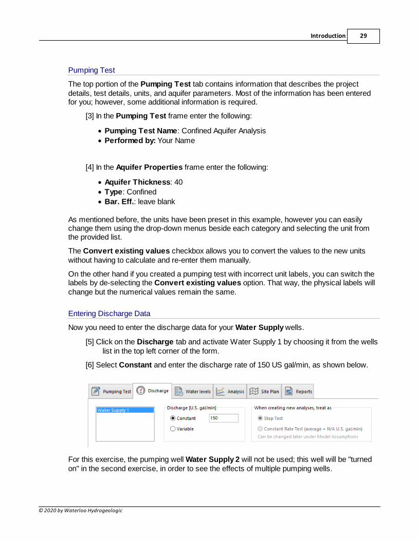
Entering Discharge Data
Now you need to enter the discharge data for your Water Supply wells.
[5] Click on the Discharge tab and activate Water Supply 1 by choosing it from the wellslist in the top left corner of the form.
[6] Select Constant and enter the discharge rate of 150 US gal/min, as shown below.
For this exercise, the pumping well Water Supply 2 will not be used; this well will be "turnedon" in the second exercise, in order to see the effects of multiple pumping wells.
AquiferTest 10.0 Help30
© 2020 by Waterloo Hydrogeologic
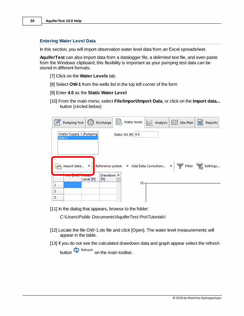
Entering Water Level Data
In this section, you will import observation water level data from an Excel spreadsheet.
AquiferTest can also import data from a datalogger file, a delimited text file, and even pastefrom the Windows clipboard; this flexibility is important as your pumping test data can bestored in different formats.
[7] Click on the Water Levels tab.
[8] Select OW-1 from the wells list in the top left corner of the form
[9] Enter 4.0 as the Static Water Level
[10] From the main menu, select File/Import/Import Data, or click on the Import data...button (circled below)
[11] In the dialog that appears, browse to the folder:
C:\Users\Public Documents\AquiferTest Pro\Tutorials\
[12] Locate the file OW-1.xls file and click [Open]. The water level measurements willappear in the table.
[13] If you do not see the calculated drawdown data and graph appear select the refresh
button on the main toolbar.
Introduction 31
© 2020 by Waterloo Hydrogeologic
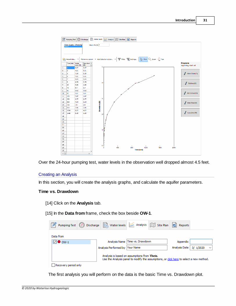
Over the 24-hour pumping test, water levels in the observation well dropped almost 4.5 feet.
Creating an Analysis
In this section, you will create the analysis graphs, and calculate the aquifer parameters.
Time vs. Drawdown
[14] Click on the Analysis tab.
[15] In the Data from frame, check the box beside OW-1.
The first analysis you will perform on the data is the basic Time vs. Drawdown plot.
AquiferTest 10.0 Help32
© 2020 by Waterloo Hydrogeologic
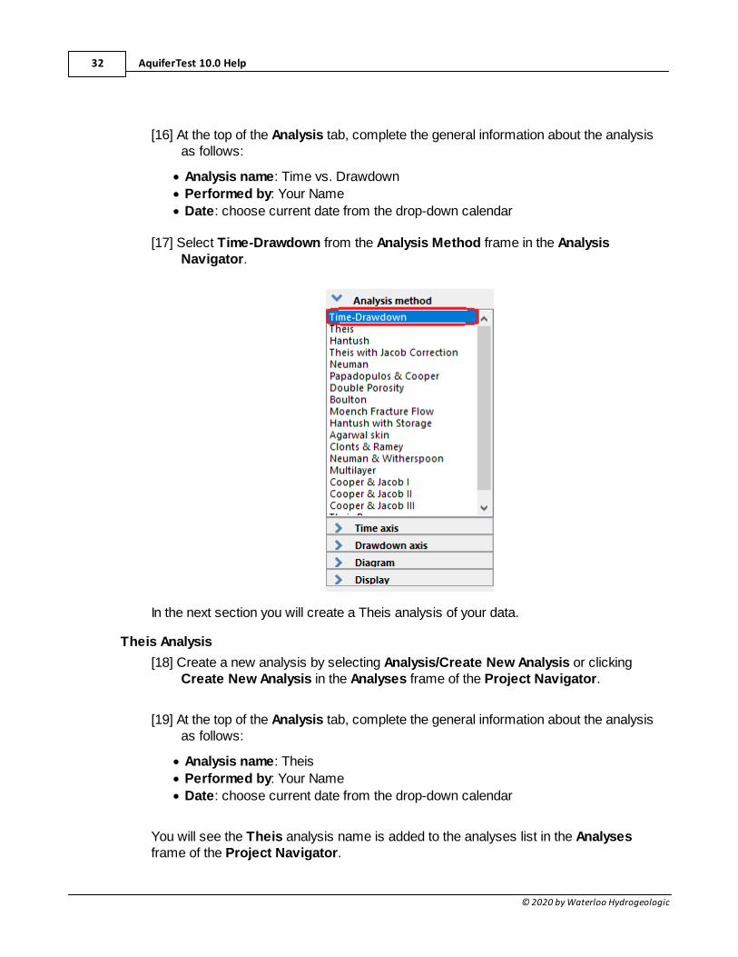
[16] At the top of the Analysis tab, complete the general information about the analysisas follows:
· Analysis name: Time vs. Drawdown
· Performed by: Your Name
· Date: choose current date from the drop-down calendar
[17] Select Time-Drawdown from the Analysis Method frame in the AnalysisNavigator.
In the next section you will create a Theis analysis of your data.
Theis Analysis
[18] Create a new analysis by selecting Analysis/Create New Analysis or clickingCreate New Analysis in the Analyses frame of the Project Navigator.
[19] At the top of the Analysis tab, complete the general information about the analysisas follows:
· Analysis name: Theis
· Performed by: Your Name
· Date: choose current date from the drop-down calendar
You will see the Theis analysis name is added to the analyses list in the Analysesframe of the Project Navigator.
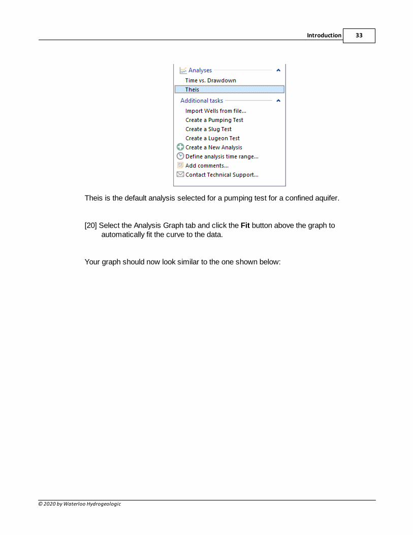
Introduction 33
© 2020 by Waterloo Hydrogeologic
Theis is the default analysis selected for a pumping test for a confined aquifer.
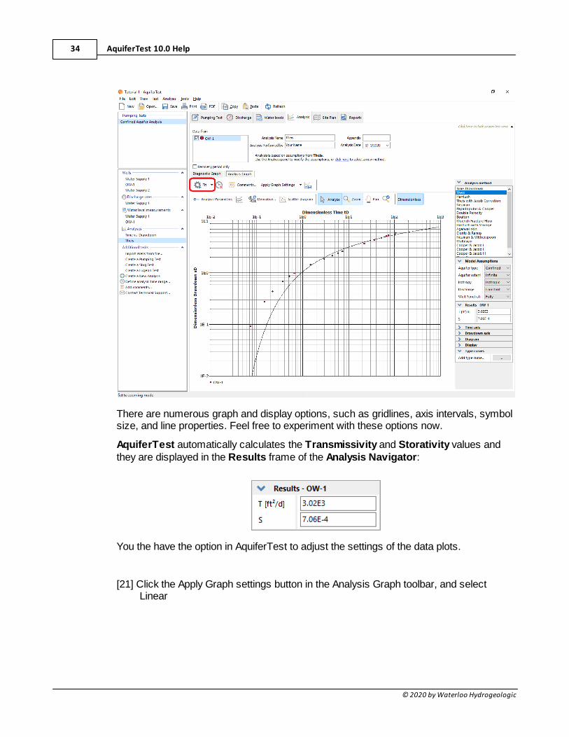
[20] Select the Analysis Graph tab and click the Fit button above the graph toautomatically fit the curve to the data.
Your graph should now look similar to the one shown below:
AquiferTest 10.0 Help34
© 2020 by Waterloo Hydrogeologic
There are numerous graph and display options, such as gridlines, axis intervals, symbolsize, and line properties. Feel free to experiment with these options now.
AquiferTest automatically calculates the Transmissivity and Storativity values andthey are displayed in the Results frame of the Analysis Navigator:
You the have the option in AquiferTest to adjust the settings of the data plots.
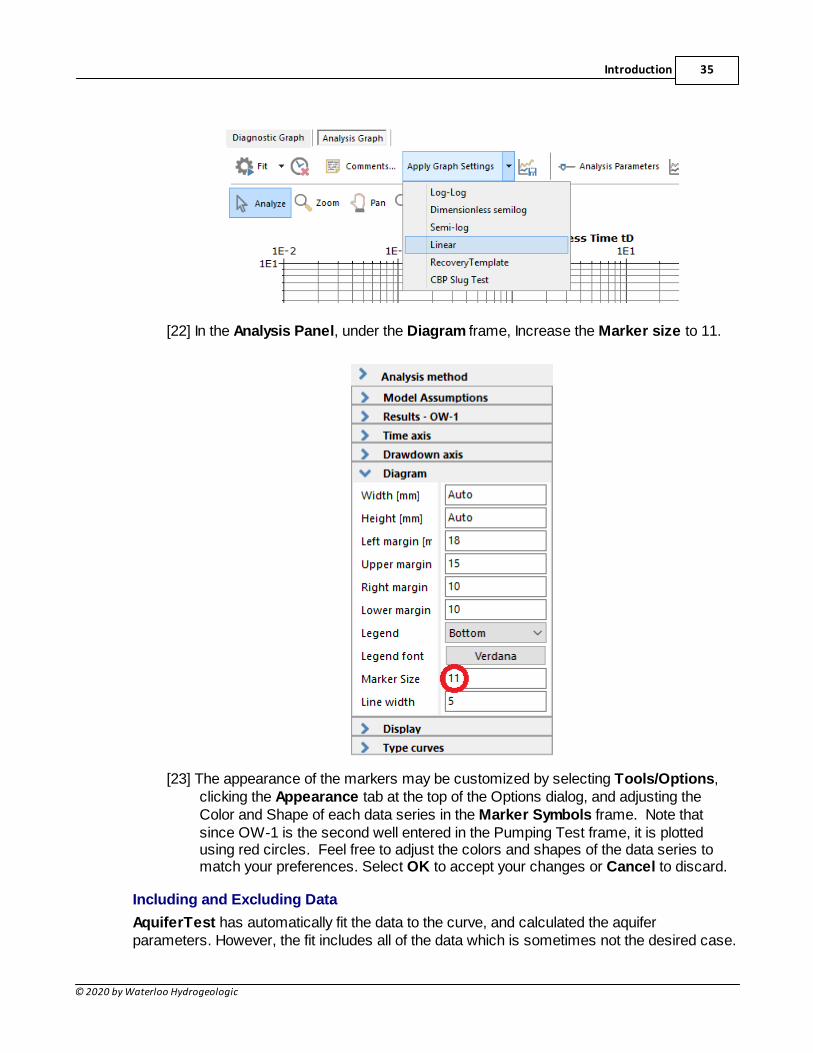
[21] Click the Apply Graph settings button in the Analysis Graph toolbar, and selectLinear
Introduction 35
© 2020 by Waterloo Hydrogeologic
[22] In the Analysis Panel, under the Diagram frame, Increase the Marker size to 11.
[23] The appearance of the markers may be customized by selecting Tools/Options,clicking the Appearance tab at the top of the Options dialog, and adjusting theColor and Shape of each data series in the Marker Symbols frame. Note thatsince OW-1 is the second well entered in the Pumping Test frame, it is plottedusing red circles. Feel free to adjust the colors and shapes of the data series tomatch your preferences. Select OK to accept your changes or Cancel to discard.
Including and Excluding Data
AquiferTest has automatically fit the data to the curve, and calculated the aquiferparameters. However, the fit includes all of the data which is sometimes not the desired case.
AquiferTest 10.0 Help36
© 2020 by Waterloo Hydrogeologic
For example you may wish to place more emphasis on the early time data if you suspect theaquifer is leaky or some other boundary feature is affecting the results.
In this pumping test, there is a boundary condition affecting the water levels/drawdownbetween 700 - 1,000 feet south of Water Supply 1. You need to remove the data points aftertime = 100 minutes.
There are several ways to do this, either by de-activating data points in the analysis (they willremain visible but will not be considered in the current analysis) or by applying a time limit tothe data (data outside the time limit is removed from the display). You will examine bothoptions.
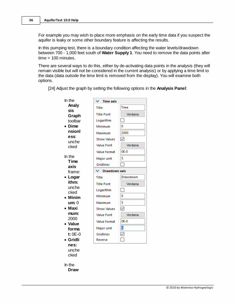
[24] Adjust the graph by setting the following options in the Analysis Panel:
In theAnalysisGraphtoolbar
· Dimensionless:unchecked
In theTimeaxisframe:
· Logarithm:unchecked
· Minimum: 0
· Maximum:2000
· Valueformat: 0E-0
· Gridlines:unchecked
In theDraw
Introduction 37
© 2020 by Waterloo Hydrogeologic
downaxisframe:
· Logarithm:unchecked
· Minimum: 0
· Maximum:5
· Valueformat: 0E-0
· Gridlines:unchecked
· Reverse:unchecked
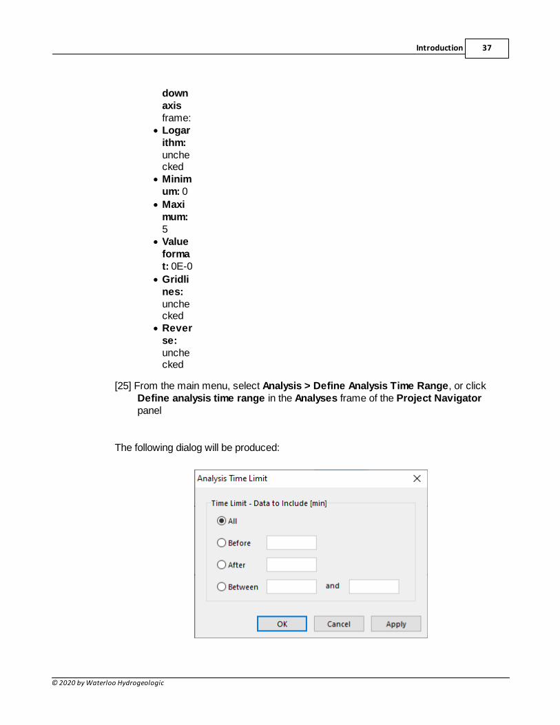
[25] From the main menu, select Analysis > Define Analysis Time Range, or clickDefine analysis time range in the Analyses frame of the Project Navigatorpanel
The following dialog will be produced:
AquiferTest 10.0 Help38
© 2020 by Waterloo Hydrogeologic
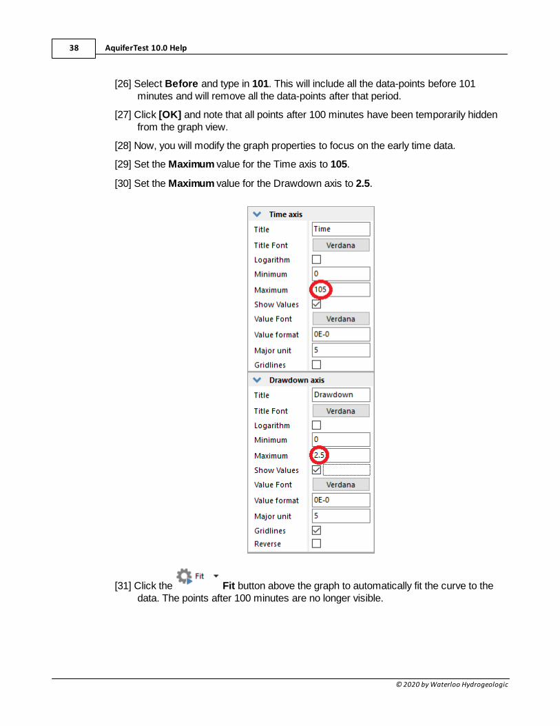
[26] Select Before and type in 101. This will include all the data-points before 101minutes and will remove all the data-points after that period.
[27] Click [OK] and note that all points after 100 minutes have been temporarily hiddenfrom the graph view.
[28] Now, you will modify the graph properties to focus on the early time data.
[29] Set the Maximum value for the Time axis to 105.
[30] Set the Maximum value for the Drawdown axis to 2.5.
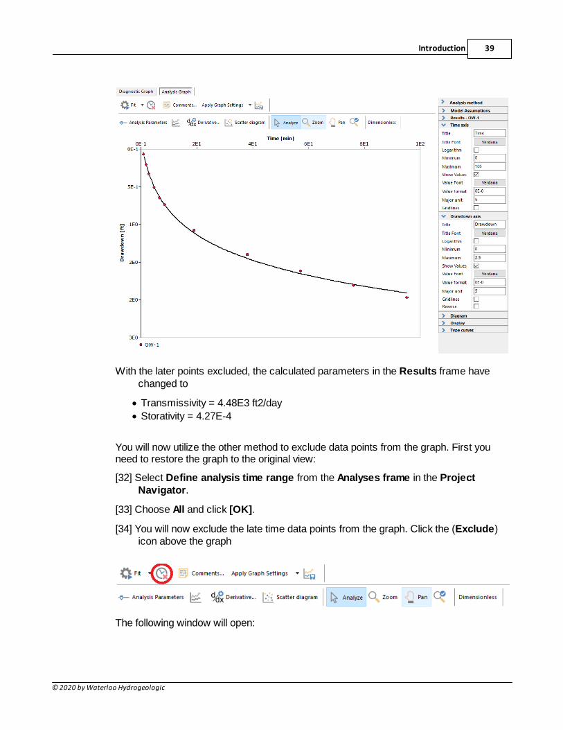
[31] Click the Fit button above the graph to automatically fit the curve to thedata. The points after 100 minutes are no longer visible.
Introduction 39
© 2020 by Waterloo Hydrogeologic
With the later points excluded, the calculated parameters in the Results frame havechanged to
· Transmissivity = 4.48E3 ft2/day
· Storativity = 4.27E-4
You will now utilize the other method to exclude data points from the graph. First youneed to restore the graph to the original view:
[32] Select Define analysis time range from the Analyses frame in the ProjectNavigator.
[33] Choose All and click [OK].
[34] You will now exclude the late time data points from the graph. Click the (Exclude)icon above the graph
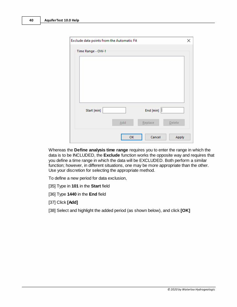
The following window will open:
AquiferTest 10.0 Help40
© 2020 by Waterloo Hydrogeologic
Whereas the Define analysis time range requires you to enter the range in which thedata is to be INCLUDED, the Exclude function works the opposite way and requires thatyou define a time range in which the data will be EXCLUDED. Both perform a similarfunction; however, in different situations, one may be more appropriate than the other.Use your discretion for selecting the appropriate method.
To define a new period for data exclusion,
[35] Type in 101 in the Start field
[36] Type 1440 in the End field
[37] Click [Add]
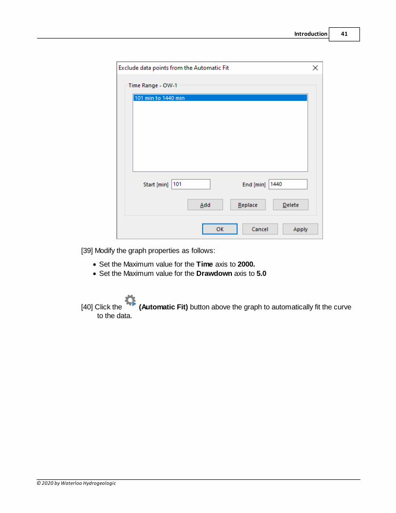
[38] Select and highlight the added period (as shown below), and click [OK]
Introduction 41
© 2020 by Waterloo Hydrogeologic
[39] Modify the graph properties as follows:
· Set the Maximum value for the Time axis to 2000.
· Set the Maximum value for the Drawdown axis to 5.0
[40] Click the (Automatic Fit) button above the graph to automatically fit the curveto the data.
AquiferTest 10.0 Help42
© 2020 by Waterloo Hydrogeologic
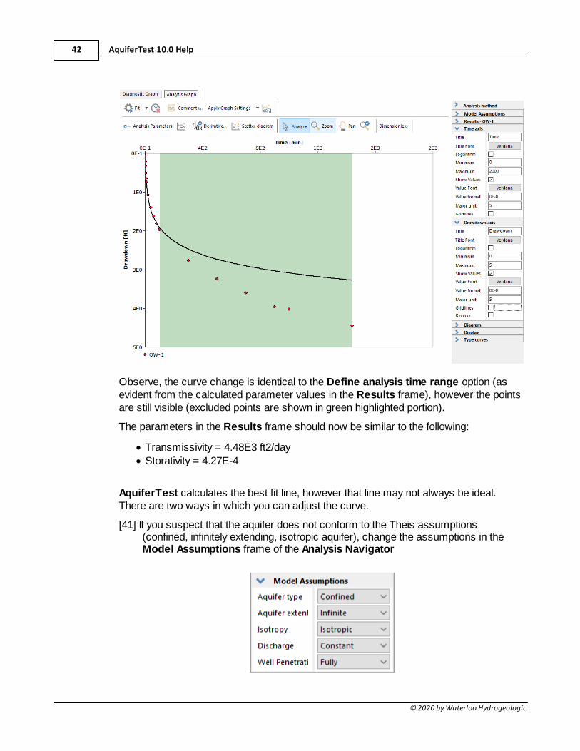
Observe, the curve change is identical to the Define analysis time range option (asevident from the calculated parameter values in the Results frame), however the pointsare still visible (excluded points are shown in green highlighted portion).
The parameters in the Results frame should now be similar to the following:
· Transmissivity = 4.48E3 ft2/day
· Storativity = 4.27E-4
AquiferTest calculates the best fit line, however that line may not always be ideal.There are two ways in which you can adjust the curve.
[41] If you suspect that the aquifer does not conform to the Theis assumptions(confined, infinitely extending, isotropic aquifer), change the assumptions in theModel Assumptions frame of the Analysis Navigator
Introduction 43
© 2020 by Waterloo Hydrogeologic
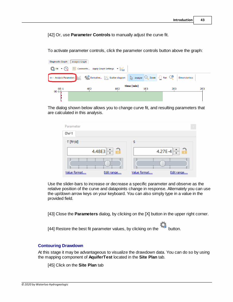
[42] Or, use Parameter Controls to manually adjust the curve fit.
To activate parameter controls, click the parameter controls button above the graph:
The dialog shown below allows you to change curve fit, and resulting parameters thatare calculated in this analysis.
Use the slider-bars to increase or decrease a specific parameter and observe as therelative position of the curve and datapoints change in response. Alternately you can usethe up/down arrow keys on your keyboard. You can also simply type in a value in theprovided field.
[43] Close the Parameters dialog, by clicking on the [X] button in the upper right corner.
[44] Restore the best fit parameter values, by clicking on the button.
Contouring Drawdown
At this stage it may be advantageous to visualize the drawdown data. You can do so by usingthe mapping component of AquiferTest located in the Site Plan tab.
[45] Click on the Site Plan tab
AquiferTest 10.0 Help44
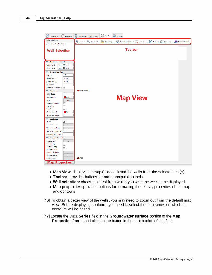
© 2020 by Waterloo Hydrogeologic
· Map View: displays the map (if loaded) and the wells from the selected test(s)
· Toolbar: provides buttons for map manipulation tools
· Well selection: choose the test from which you wish the wells to be displayed
· Map properties: provides options for formatting the display properties of the mapand contours
[46] To obtain a better view of the wells, you may need to zoom out from the default mapview. Before displaying contours, you need to select the data series on which thecontours will be based.
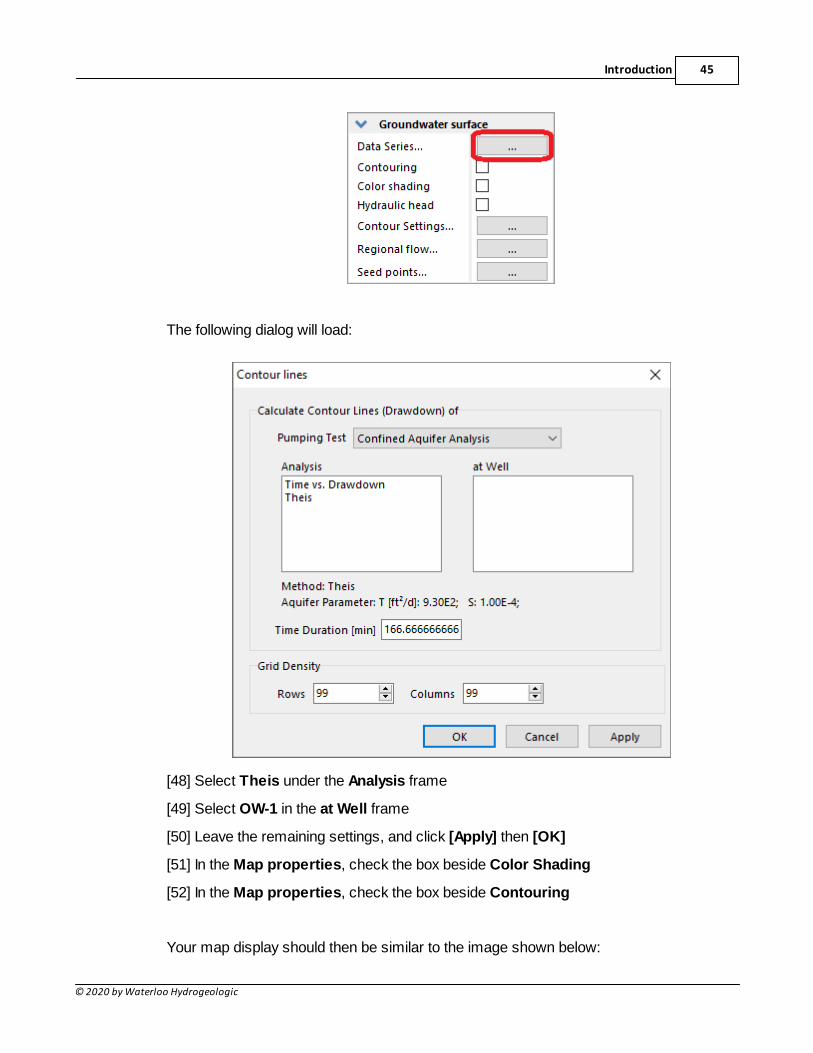
[47] Locate the Data Series field in the Groundwater surface portion of the MapProperties frame, and click on the button in the right portion of that field.
Introduction 45
© 2020 by Waterloo Hydrogeologic
The following dialog will load:
[48] Select Theis under the Analysis frame
[49] Select OW-1 in the at Well frame
[50] Leave the remaining settings, and click [Apply] then [OK]
[51] In the Map properties, check the box beside Color Shading
[52] In the Map properties, check the box beside Contouring
Your map display should then be similar to the image shown below:
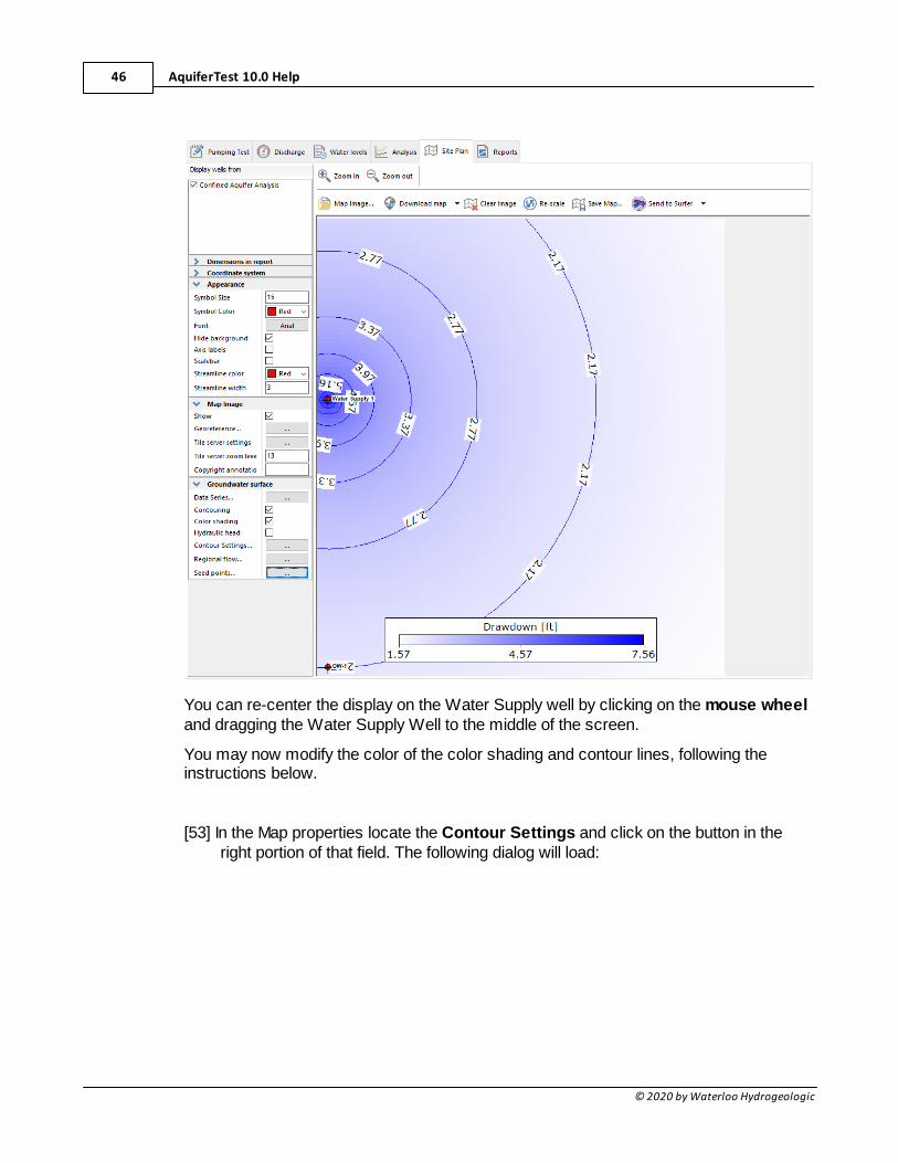
AquiferTest 10.0 Help46
© 2020 by Waterloo Hydrogeologic
You can re-center the display on the Water Supply well by clicking on the mouse wheeland dragging the Water Supply Well to the middle of the screen.
You may now modify the color of the color shading and contour lines, following theinstructions below.
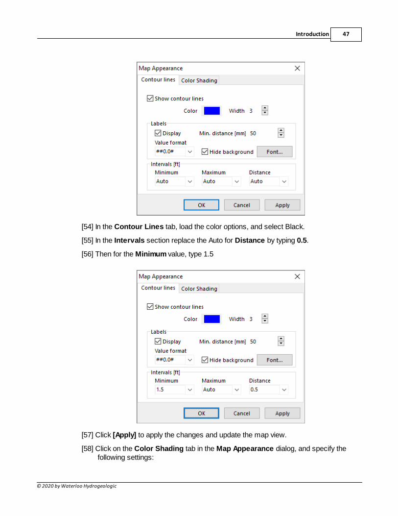
[53] In the Map properties locate the Contour Settings and click on the button in theright portion of that field. The following dialog will load:
Introduction 47
© 2020 by Waterloo Hydrogeologic
[54] In the Contour Lines tab, load the color options, and select Black.
[55] In the Intervals section replace the Auto for Distance by typing 0.5.
[56] Then for the Minimum value, type 1.5
[57] Click [Apply] to apply the changes and update the map view.
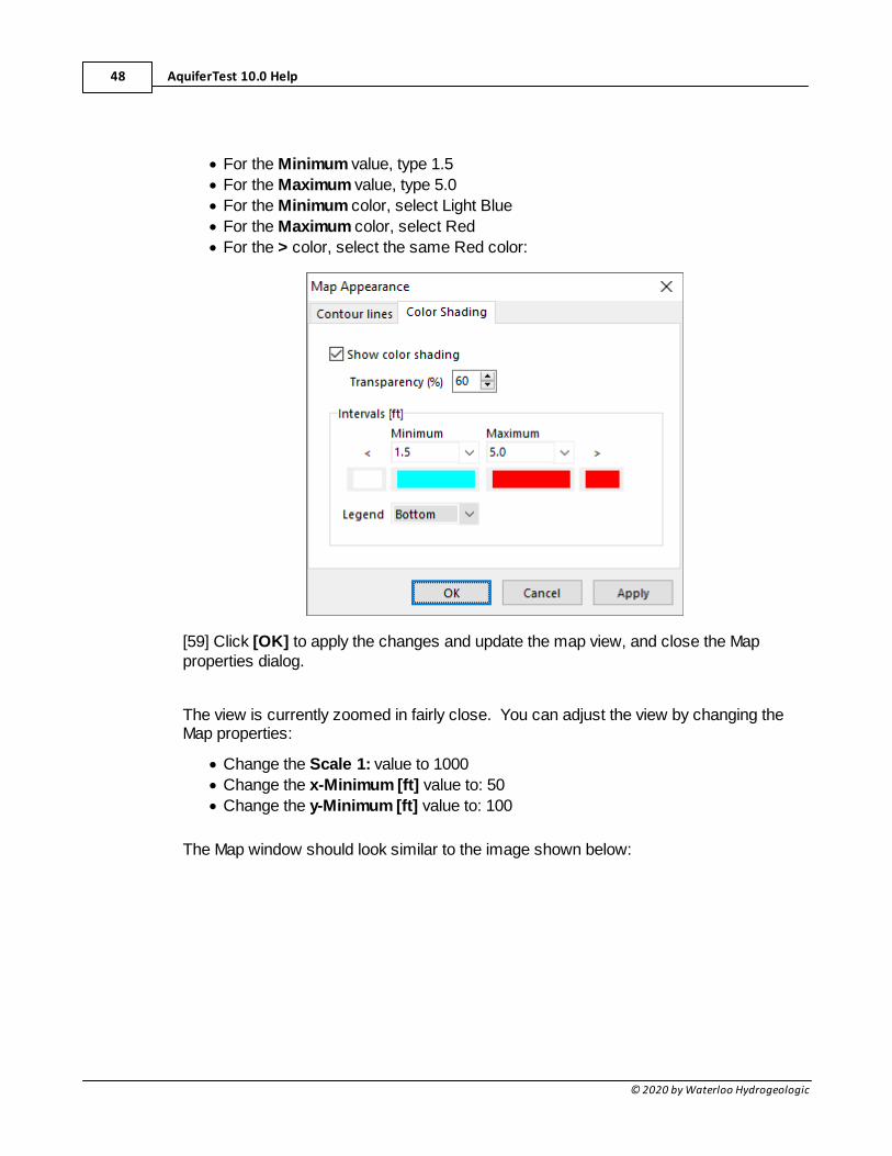
[58] Click on the Color Shading tab in the Map Appearance dialog, and specify thefollowing settings:
AquiferTest 10.0 Help48
© 2020 by Waterloo Hydrogeologic
· For the Minimum value, type 1.5
· For the Maximum value, type 5.0
· For the Minimum color, select Light Blue
· For the Maximum color, select Red
· For the > color, select the same Red color:
[59] Click [OK] to apply the changes and update the map view, and close the Mapproperties dialog.
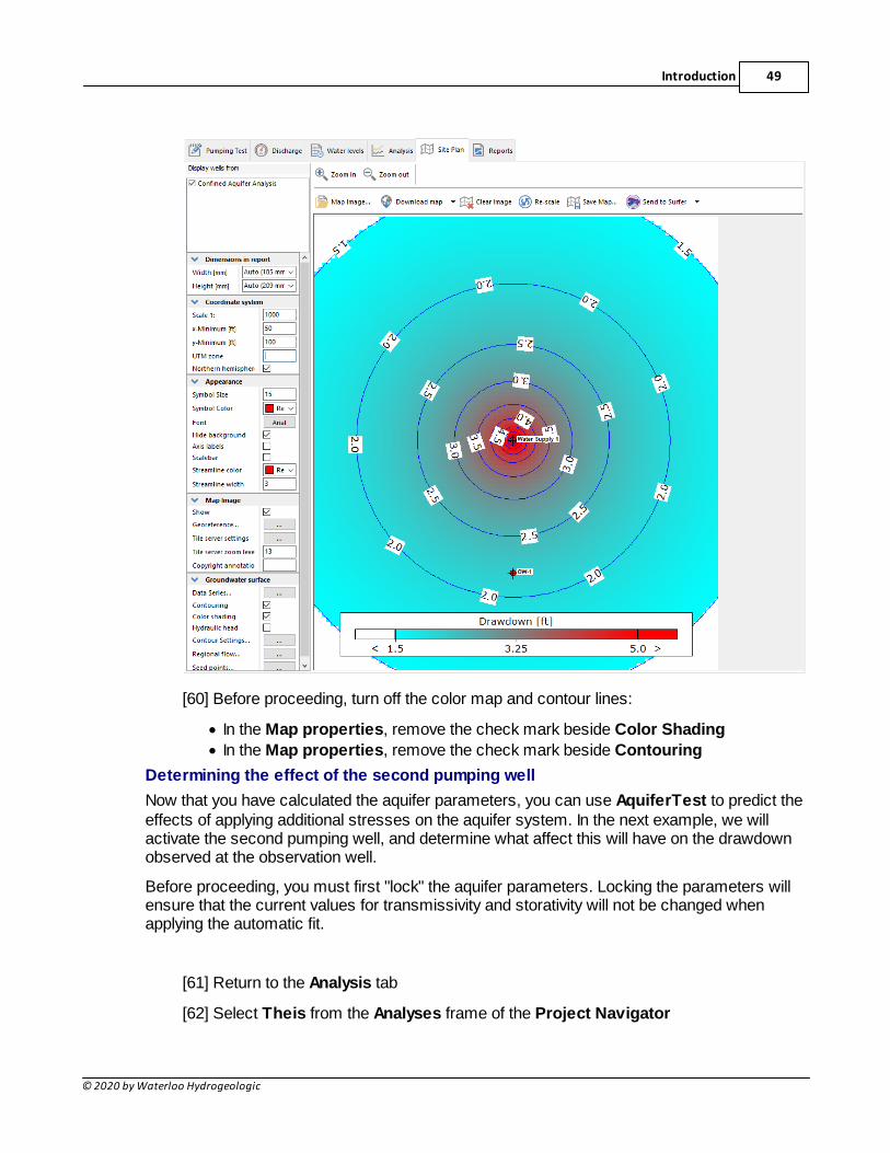
The view is currently zoomed in fairly close. You can adjust the view by changing theMap properties:
· Change the Scale 1: value to 1000
· Change the x-Minimum [ft] value to: 50
· Change the y-Minimum [ft] value to: 100
The Map window should look similar to the image shown below:
Introduction 49
© 2020 by Waterloo Hydrogeologic
[60] Before proceeding, turn off the color map and contour lines:
· In the Map properties, remove the check mark beside Color Shading
· In the Map properties, remove the check mark beside Contouring
Determining the effect of the second pumping well
Now that you have calculated the aquifer parameters, you can use AquiferTest to predict theeffects of applying additional stresses on the aquifer system. In the next example, we willactivate the second pumping well, and determine what affect this will have on the drawdownobserved at the observation well.
Before proceeding, you must first "lock" the aquifer parameters. Locking the parameters willensure that the current values for transmissivity and storativity will not be changed whenapplying the automatic fit.
[61] Return to the Analysis tab
[62] Select Theis from the Analyses frame of the Project Navigator
AquiferTest 10.0 Help50
© 2020 by Waterloo Hydrogeologic
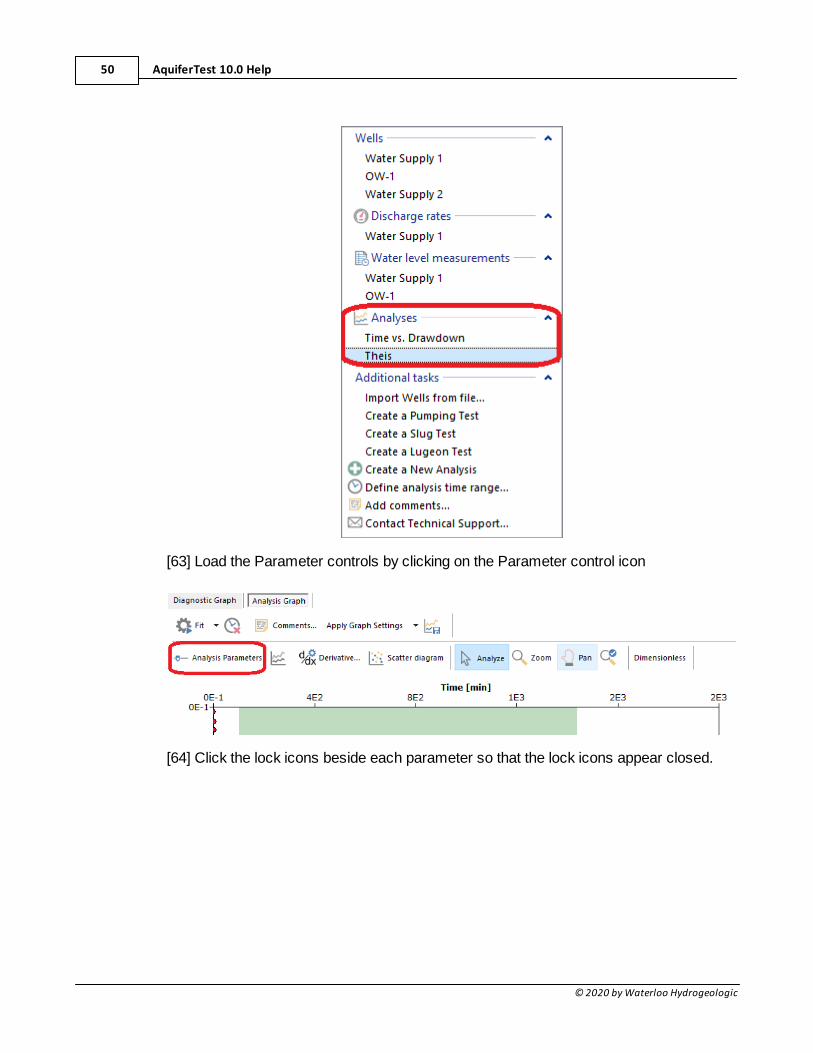
[63] Load the Parameter controls by clicking on the Parameter control icon
[64] Click the lock icons beside each parameter so that the lock icons appear closed.
Introduction 51
© 2020 by Waterloo Hydrogeologic
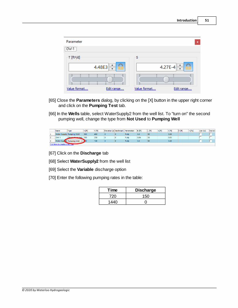
[65] Close the Parameters dialog, by clicking on the [X] button in the upper right cornerand click on the Pumping Test tab.
[66] In the Wells table, select WaterSupply2 from the well list. To "turn on" the secondpumping well, change the type from Not Used to Pumping Well
[67] Click on the Discharge tab
[68] Select WaterSupply2 from the well list
[69] Select the Variable discharge option
[70] Enter the following pumping rates in the table:
Time Discharge
720 150
1440 0
AquiferTest 10.0 Help52
© 2020 by Waterloo Hydrogeologic
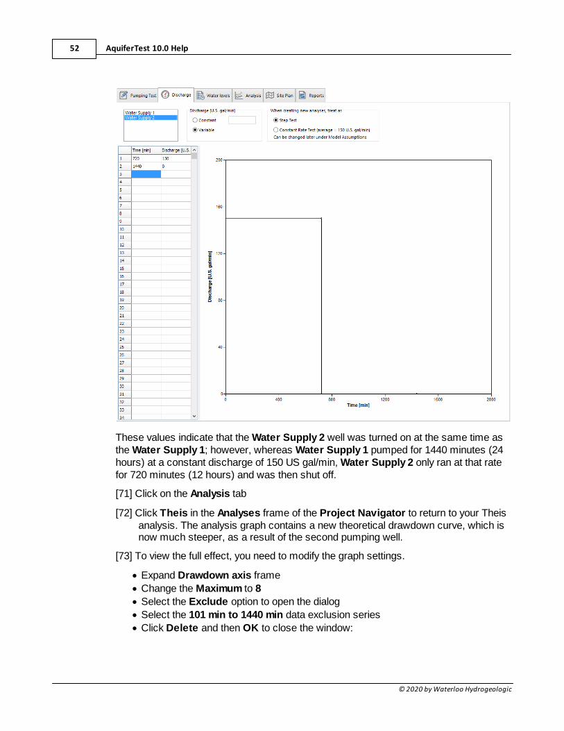
These values indicate that the Water Supply 2 well was turned on at the same time asthe Water Supply 1; however, whereas Water Supply 1 pumped for 1440 minutes (24hours) at a constant discharge of 150 US gal/min, Water Supply 2 only ran at that ratefor 720 minutes (12 hours) and was then shut off.
[71] Click on the Analysis tab
[72] Click Theis in the Analyses frame of the Project Navigator to return to your Theisanalysis. The analysis graph contains a new theoretical drawdown curve, which isnow much steeper, as a result of the second pumping well.
[73] To view the full effect, you need to modify the graph settings.
· Expand Drawdown axis frame
· Change the Maximum to 8
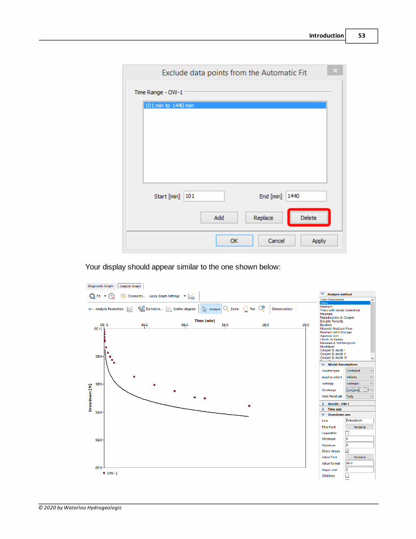
· Select the Exclude option to open the dialog
· Select the 101 min to 1440 min data exclusion series
· Click Delete and then OK to close the window:
Introduction 53
© 2020 by Waterloo Hydrogeologic
Your display should appear similar to the one shown below:
AquiferTest 10.0 Help54
© 2020 by Waterloo Hydrogeologic
When a variable discharge rate is entered, the model assumptions should automaticallyupdate to reflect that. If the discharge in the Model Assumptions frame has notautomatically updated, you can change the value manually by expanding the ModelAssumptions frame and selecting Variable from the dropdown menu.
[74] Expand the Model assumptions frame
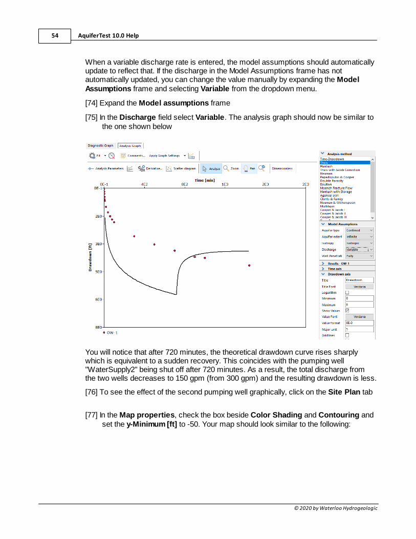
[75] In the Discharge field select Variable. The analysis graph should now be similar tothe one shown below
You will notice that after 720 minutes, the theoretical drawdown curve rises sharplywhich is equivalent to a sudden recovery. This coincides with the pumping well"WaterSupply2" being shut off after 720 minutes. As a result, the total discharge fromthe two wells decreases to 150 gpm (from 300 gpm) and the resulting drawdown is less.
[76] To see the effect of the second pumping well graphically, click on the Site Plan tab
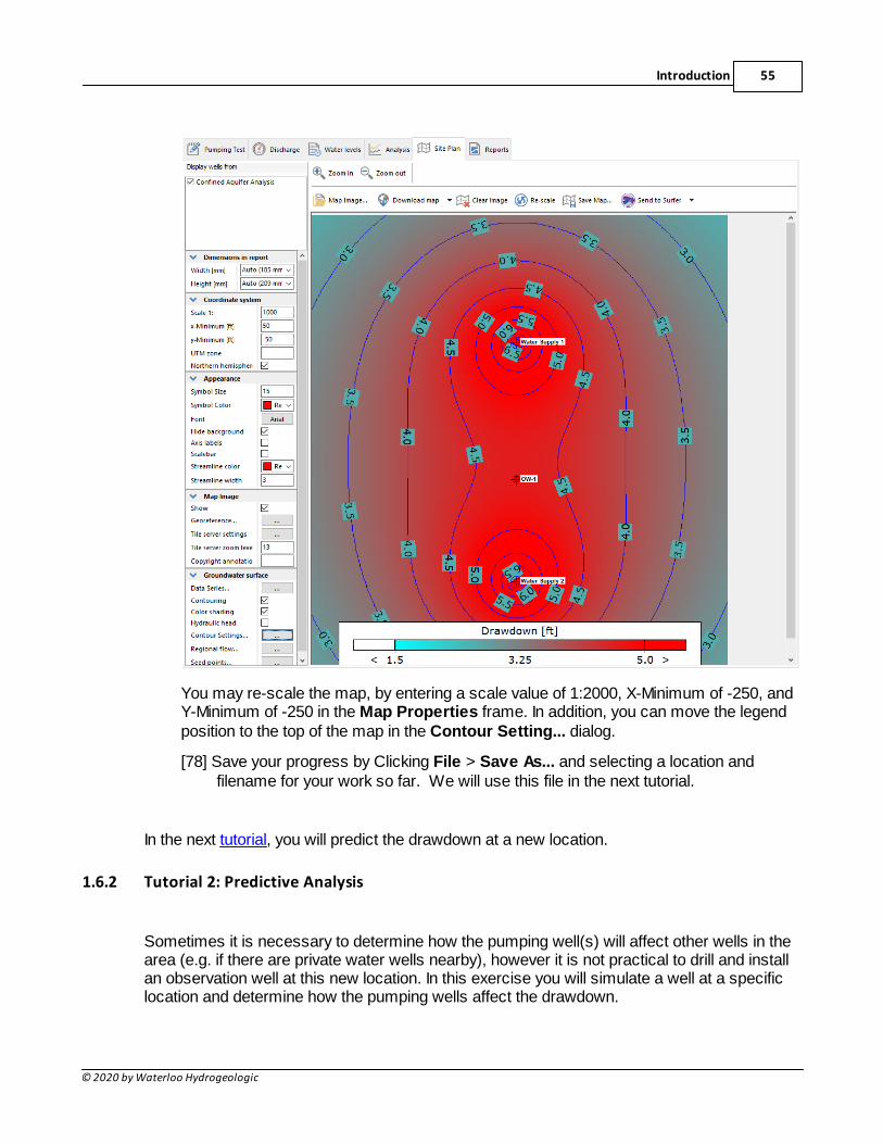
[77] In the Map properties, check the box beside Color Shading and Contouring andset the y-Minimum [ft] to -50. Your map should look similar to the following:
Introduction 55
© 2020 by Waterloo Hydrogeologic
You may re-scale the map, by entering a scale value of 1:2000, X-Minimum of -250, andY-Minimum of -250 in the Map Properties frame. In addition, you can move the legendposition to the top of the map in the Contour Setting... dialog.
[78] Save your progress by Clicking File > Save As... and selecting a location andfilename for your work so far. We will use this file in the next tutorial.
In the next tutorial, you will predict the drawdown at a new location.
1.6.2 Tutorial 2: Predictive Analysis
Sometimes it is necessary to determine how the pumping well(s) will affect other wells in thearea (e.g. if there are private water wells nearby), however it is not practical to drill and installan observation well at this new location. In this exercise you will simulate a well at a specificlocation and determine how the pumping wells affect the drawdown.

AquiferTest 10.0 Help56
© 2020 by Waterloo Hydrogeologic
[1] If you are continuing on from Tutorial 1, Return to the Pumping Test tab. Otherwise,open the file:
C:\Users\Public\Documents\AquiferTest Pro\Tutorials\Tutorial 2.HYT
[2] Create a new well by clicking "Click here to create a new well" link under the wellsgrid.
For the new well set the information as follows:
· Name: OW-2
· Type: Observation Well
· X: 700
· Y: 850
· Elevation: 0
· Benchmark: 0
· Penetration: Fully
· R: 0.30
· L: 50
· r: 0.25
The well is created as "Observation" by default, however, you can change the type ofany well by clicking in the Type field once to activate it and then again to produce thedrop-down menu.
[3] Click on the Water Levels tab.
[4] Select OW-2 from the frame in the upper left corner.
[5] Enter 0 as the Static Water Level.
Now you need to enter water level data for the new well. You will enter a few "dummy"points which will be used to set the timeline for the curve. The water levelmeasurements can be any values, but for simplicity, a value of 1 will be used.
Enter the following values in the Water Level table:
Time Water level
1 1
500 1
Introduction 57
© 2020 by Waterloo Hydrogeologic
1000 1
1440 1
[6] Click Theis from the Analyses frame of the Project Navigator to move to yourTheis analysis. Note that the second observation well, OW-2, now shows up in theData from list.
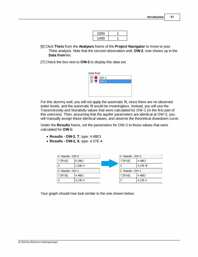
[7] Check the box next to OW-2 to display this data set.
For this dummy well, you will not apply the automatic fit, since there are no observedwater levels, and the automatic fit would be meaningless. Instead, you will use theTransmissivity and Storativity values that were calculated for OW-1 (in the first part ofthis exercise). Then, assuming that the aquifer parameters are identical at OW-2, youwill manually assign these identical values, and observe the theoretical drawdown curve.
Under the Results frame, set the parameters for OW-2 to those values that werecalculated for OW-1:
· Results - OW-2, T, type: 4.48E3
· Results - OW-2, S, type: 4.27E-4
Your graph should now look similar to the one shown below:
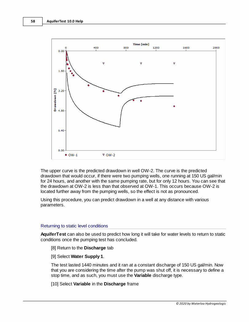
AquiferTest 10.0 Help58
© 2020 by Waterloo Hydrogeologic
The upper curve is the predicted drawdown in well OW-2. The curve is the predicteddrawdown that would occur, if there were two pumping wells, one running at 150 US gal/minfor 24 hours, and another with the same pumping rate, but for only 12 hours. You can see thatthe drawdown at OW-2 is less than that observed at OW-1. This occurs because OW-2 islocated further away from the pumping wells, so the effect is not as pronounced.
Using this procedure, you can predict drawdown in a well at any distance with variousparameters.
Returning to static level conditions
AquiferTest can also be used to predict how long it will take for water levels to return to staticconditions once the pumping test has concluded.
[8] Return to the Discharge tab
[9] Select Water Supply 1.
The test lasted 1440 minutes and it ran at a constant discharge of 150 US gal/min. Nowthat you are considering the time after the pump was shut off, it is necessary to define astop time, and as such, you must use the Variable discharge type.
[10] Select Variable in the Discharge frame
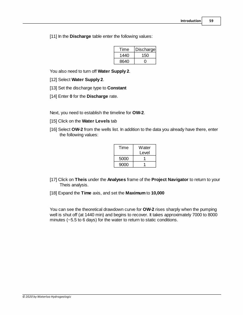
Introduction 59
© 2020 by Waterloo Hydrogeologic
[11] In the Discharge table enter the following values:
Time Discharge
1440 150
8640 0
You also need to turn off Water Supply 2.
[12] Select Water Supply 2.
[13] Set the discharge type to Constant
[14] Enter 0 for the Discharge rate.
Next, you need to establish the timeline for OW-2.
[15] Click on the Water Levels tab
[16] Select OW-2 from the wells list. In addition to the data you already have there, enterthe following values:
Time WaterLevel
5000 1
9000 1
[17] Click on Theis under the Analyses frame of the Project Navigator to return to yourTheis analysis.
[18] Expand the Time axis, and set the Maximum to 10,000
You can see the theoretical drawdown curve for OW-2 rises sharply when the pumpingwell is shut off (at 1440 min) and begins to recover. It takes approximately 7000 to 8000minutes (~5.5 to 6 days) for the water to return to static conditions.
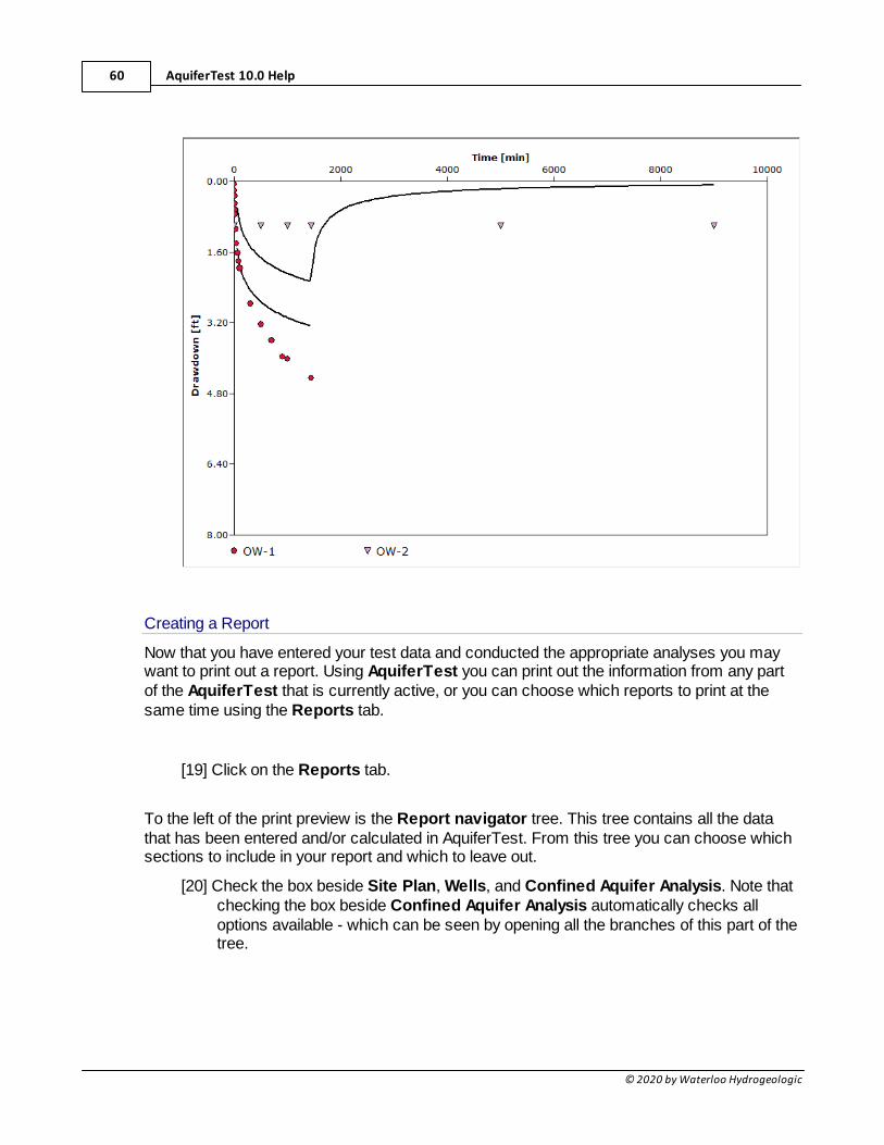
AquiferTest 10.0 Help60
© 2020 by Waterloo Hydrogeologic
Creating a Report
Now that you have entered your test data and conducted the appropriate analyses you maywant to print out a report. Using AquiferTest you can print out the information from any partof the AquiferTest that is currently active, or you can choose which reports to print at thesame time using the Reports tab.
[19] Click on the Reports tab.
To the left of the print preview is the Report navigator tree. This tree contains all the datathat has been entered and/or calculated in AquiferTest. From this tree you can choose whichsections to include in your report and which to leave out.
[20] Check the box beside Site Plan, Wells, and Confined Aquifer Analysis. Note thatchecking the box beside Confined Aquifer Analysis automatically checks alloptions available - which can be seen by opening all the branches of this part of thetree.
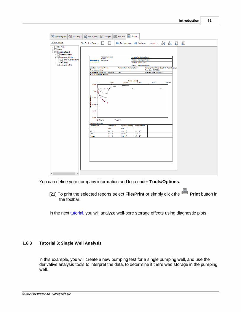
Introduction 61
© 2020 by Waterloo Hydrogeologic
You can define your company information and logo under Tools/Options.
[21] To print the selected reports select File/Print or simply click the Print button inthe toolbar.
In the next tutorial, you will analyze well-bore storage effects using diagnostic plots.
1.6.3 Tutorial 3: Single Well Analysis
In this example, you will create a new pumping test for a single pumping well, and use thederivative analysis tools to interpret the data, to determine if there was storage in the pumpingwell.
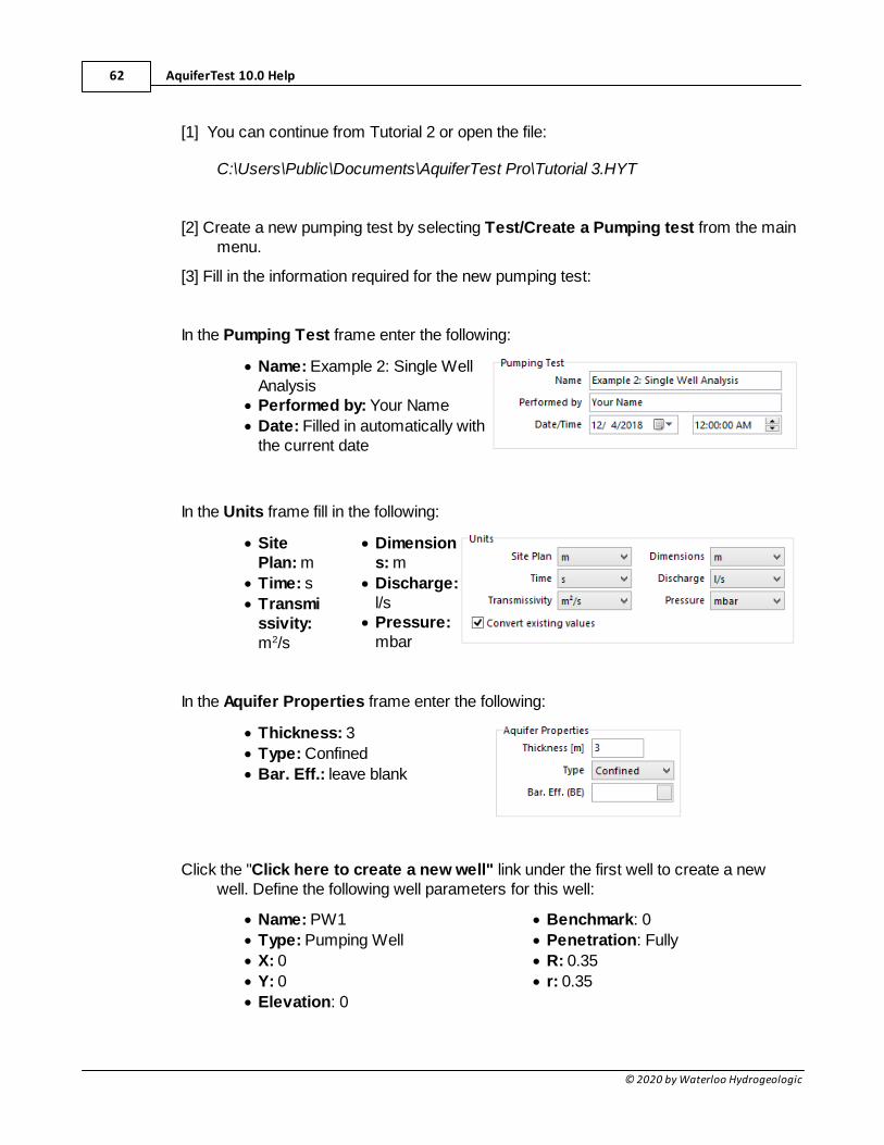
AquiferTest 10.0 Help62
© 2020 by Waterloo Hydrogeologic
[1] You can continue from Tutorial 2 or open the file:
C:\Users\Public\Documents\AquiferTest Pro\Tutorial 3.HYT
[2] Create a new pumping test by selecting Test/Create a Pumping test from the mainmenu.
[3] Fill in the information required for the new pumping test:
In the Pumping Test frame enter the following:
· Name: Example 2: Single WellAnalysis
· Performed by: Your Name
· Date: Filled in automatically withthe current date
In the Units frame fill in the following:
· SitePlan: m
· Time: s
· Transmissivity:m2/s
· Dimensions: m
· Discharge:l/s
· Pressure:mbar
In the Aquifer Properties frame enter the following:
· Thickness: 3
· Type: Confined
· Bar. Eff.: leave blank
Click the "Click here to create a new well" link under the first well to create a newwell. Define the following well parameters for this well:
· Name: PW1
· Type: Pumping Well
· X: 0
· Y: 0
· Elevation: 0
· Benchmark: 0
· Penetration: Fully
· R: 0.35
· r: 0.35
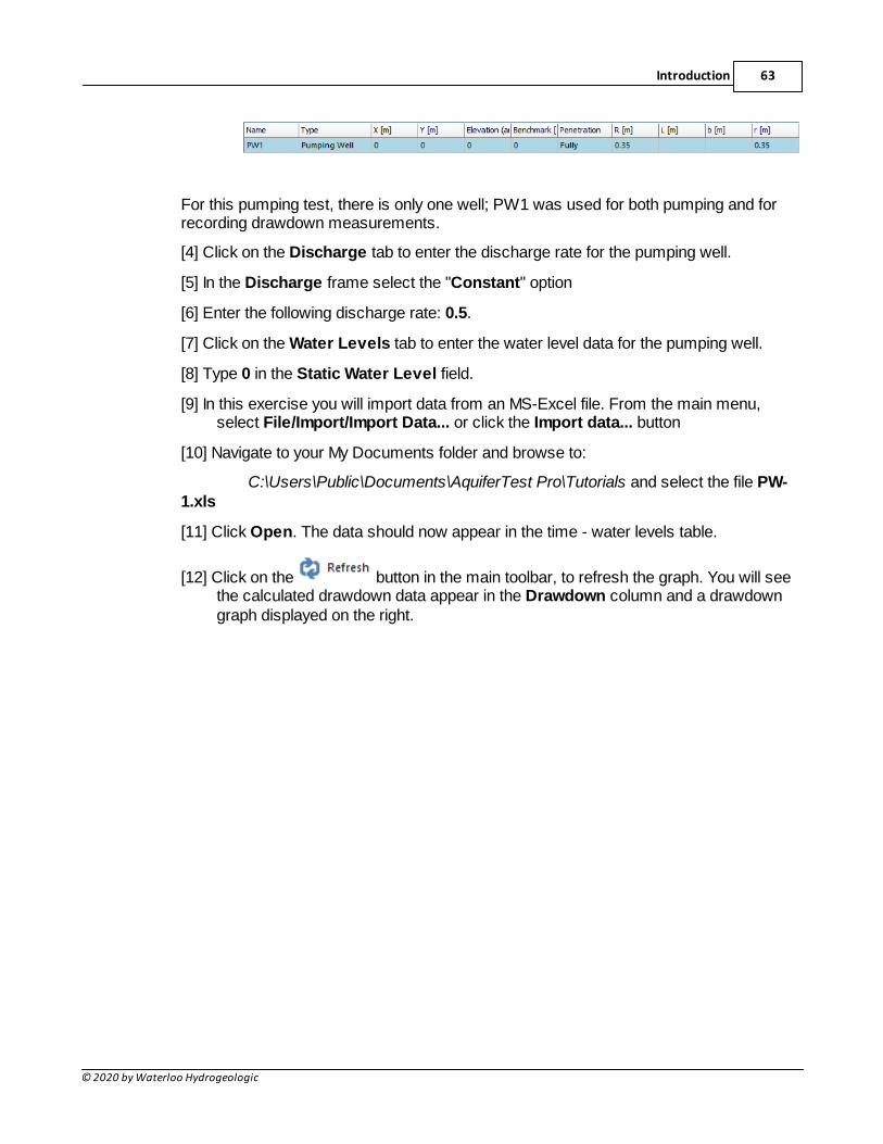
Introduction 63
© 2020 by Waterloo Hydrogeologic
For this pumping test, there is only one well; PW1 was used for both pumping and forrecording drawdown measurements.
[4] Click on the Discharge tab to enter the discharge rate for the pumping well.
[5] In the Discharge frame select the "Constant" option
[6] Enter the following discharge rate: 0.5.
[7] Click on the Water Levels tab to enter the water level data for the pumping well.
[8] Type 0 in the Static Water Level field.
[9] In this exercise you will import data from an MS-Excel file. From the main menu,select File/Import/Import Data... or click the Import data... button
[10] Navigate to your My Documents folder and browse to:
C:\Users\Public\Documents\AquiferTest Pro\Tutorials and select the file PW-1.xls
[11] Click Open. The data should now appear in the time - water levels table.
[12] Click on the button in the main toolbar, to refresh the graph. You will seethe calculated drawdown data appear in the Drawdown column and a drawdowngraph displayed on the right.
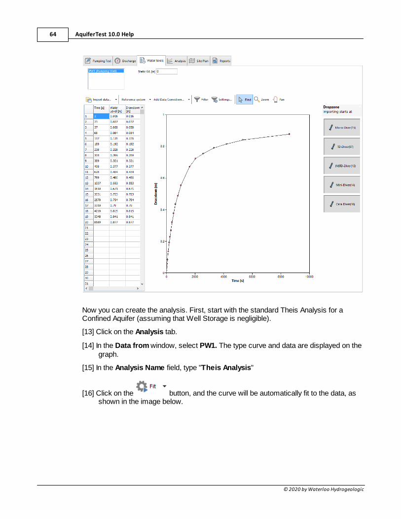
AquiferTest 10.0 Help64
© 2020 by Waterloo Hydrogeologic
Now you can create the analysis. First, start with the standard Theis Analysis for aConfined Aquifer (assuming that Well Storage is negligible).
[13] Click on the Analysis tab.
[14] In the Data from window, select PW1. The type curve and data are displayed on thegraph.
[15] In the Analysis Name field, type "Theis Analysis"
[16] Click on the button, and the curve will be automatically fit to the data, asshown in the image below.
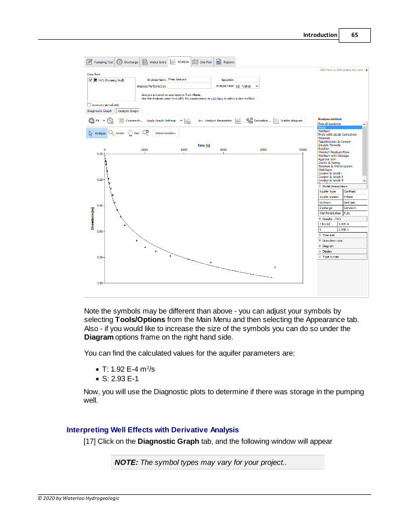
Introduction 65
© 2020 by Waterloo Hydrogeologic
Note the symbols may be different than above - you can adjust your symbols byselecting Tools/Options from the Main Menu and then selecting the Appearance tab. Also - if you would like to increase the size of the symbols you can do so under theDiagram options frame on the right hand side.
You can find the calculated values for the aquifer parameters are:
· T: 1.92 E-4 m2/s
· S: 2.93 E-1
Now, you will use the Diagnostic plots to determine if there was storage in the pumpingwell.
Interpreting Well Effects with Derivative Analysis
[17] Click on the Diagnostic Graph tab, and the following window will appear
NOTE: The symbol types may vary for your project..
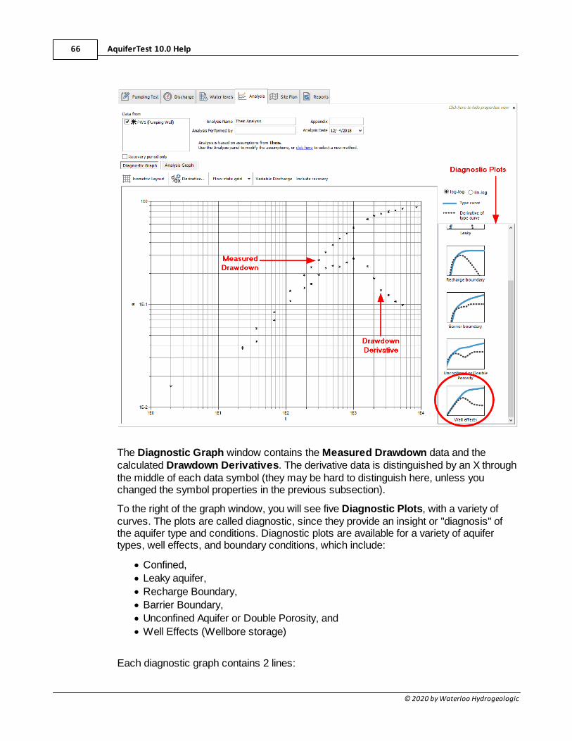
AquiferTest 10.0 Help66
© 2020 by Waterloo Hydrogeologic
The Diagnostic Graph window contains the Measured Drawdown data and thecalculated Drawdown Derivatives. The derivative data is distinguished by an X throughthe middle of each data symbol (they may be hard to distinguish here, unless youchanged the symbol properties in the previous subsection).
To the right of the graph window, you will see five Diagnostic Plots, with a variety ofcurves. The plots are called diagnostic, since they provide an insight or "diagnosis" ofthe aquifer type and conditions. Diagnostic plots are available for a variety of aquifertypes, well effects, and boundary conditions, which include:
· Confined,
· Leaky aquifer,
· Recharge Boundary,
· Barrier Boundary,
· Unconfined Aquifer or Double Porosity, and
· Well Effects (Wellbore storage)
Each diagnostic graph contains 2 lines:
Introduction 67
© 2020 by Waterloo Hydrogeologic
· Type curve (solid blue line)
· Derivative of type curve (dashed black line).
These plots can be displayed on a log-log or semi-log scale, by selecting the appropriateradio button above the diagnostic graphs.
For this pumping test, the presence of well effects (well bore storage) can be confirmedby comparing the derivative drawdown data (outlined in the image above) to the dashedline in the Well Effects diagnostic plot (circled in the image above). You can see thecurves are very similar in shape. However, the observed drawdown values did notstabilize and reach a constant. Therefore, it would have been ideal if the pumpingduration had been extended, and there was additional data available for the late pumpingdurations.
Nevertheless, the drawdown curve is characteristic of well bore storage conditions: atthe beginning of the pumping test, there is a delay in drawdown as a result of storage inthe pumping well, and the drawdown deviates from the theoretical Theis curve. Aspumping durations increase, the drawdown curve becomes more similar to thetheoretical Theis curve.
These well effects are more easily identified in the semi-log plot.
[18] Select the Lin-Log radio button above the diagnostic graphs, and the Diagnosticplots will appear in a new scale
In the Semi-Log plot, you can compare the observed drawdown curve to the diagnosticplots. In this example, it is evident that the observed drawdown curve displays delayeddrawdown (outlined in the image above), then returns to the typical Theis curve aspumping duration increases. When comparing this to the diagnostic plot for Well Effects(circled in the image above), there is strong evidence indicating the presence of welleffects during this pumping test.
Now that you are confident that there is a wellbore storage component, you can selectthe appropriate solution method (Papadopulos & Cooper), and calculate the aquiferparameters.
[19] Return to the Analysis Graph tab.
[20] From the main menu, select Analysis/Create Pumping well analysis/Createanalysis considering well effects.
[21] Click on the button, and the curve will be fit to the data, as shown in theimage below
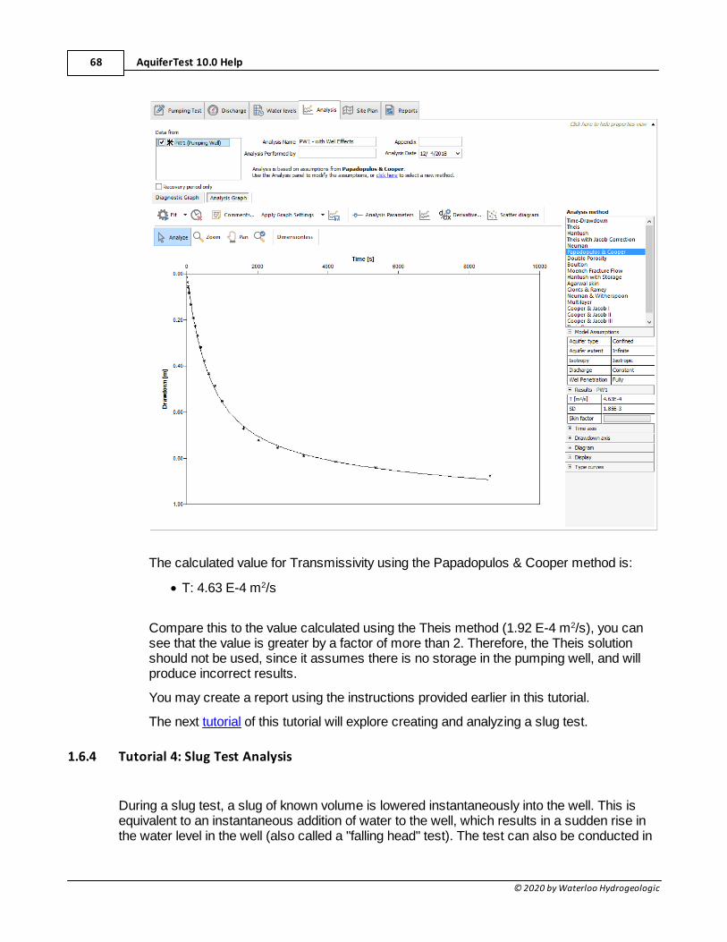
AquiferTest 10.0 Help68
© 2020 by Waterloo Hydrogeologic
The calculated value for Transmissivity using the Papadopulos & Cooper method is:
· T: 4.63 E-4 m2/s
Compare this to the value calculated using the Theis method (1.92 E-4 m2/s), you cansee that the value is greater by a factor of more than 2. Therefore, the Theis solutionshould not be used, since it assumes there is no storage in the pumping well, and willproduce incorrect results.
You may create a report using the instructions provided earlier in this tutorial.
The next tutorial of this tutorial will explore creating and analyzing a slug test.
1.6.4 Tutorial 4: Slug Test Analysis
During a slug test, a slug of known volume is lowered instantaneously into the well. This isequivalent to an instantaneous addition of water to the well, which results in a sudden rise inthe water level in the well (also called a "falling head" test). The test can also be conducted in
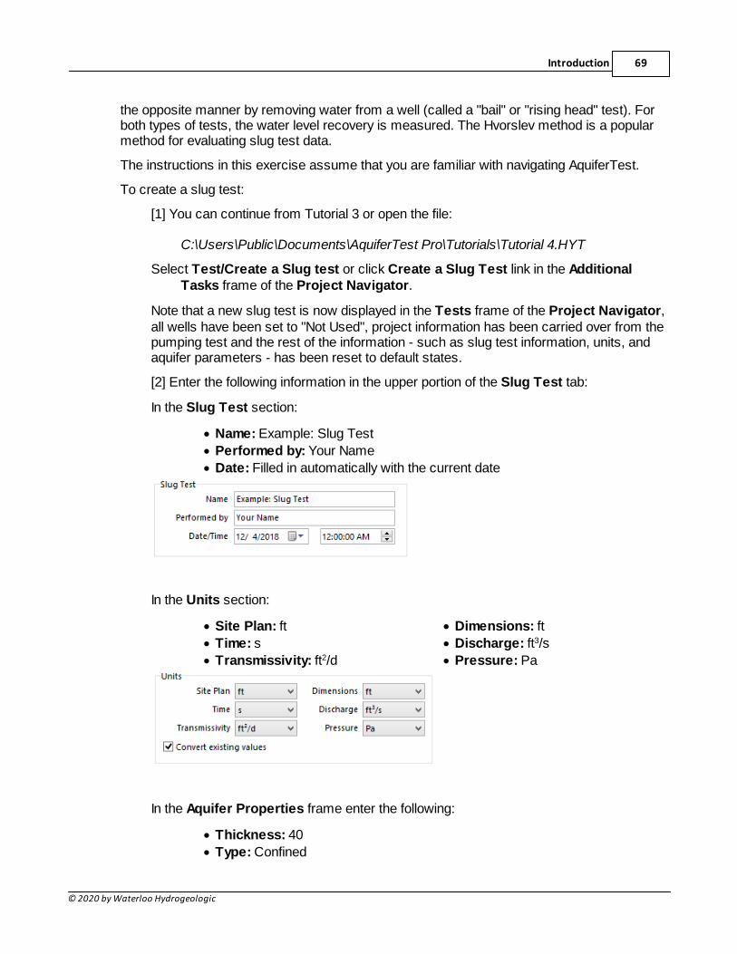
Introduction 69
© 2020 by Waterloo Hydrogeologic
the opposite manner by removing water from a well (called a "bail" or "rising head" test). Forboth types of tests, the water level recovery is measured. The Hvorslev method is a popularmethod for evaluating slug test data.
The instructions in this exercise assume that you are familiar with navigating AquiferTest.
To create a slug test:
[1] You can continue from Tutorial 3 or open the file:
C:\Users\Public\Documents\AquiferTest Pro\Tutorials\Tutorial 4.HYT
Select Test/Create a Slug test or click Create a Slug Test link in the AdditionalTasks frame of the Project Navigator.
Note that a new slug test is now displayed in the Tests frame of the Project Navigator,all wells have been set to "Not Used", project information has been carried over from thepumping test and the rest of the information - such as slug test information, units, andaquifer parameters - has been reset to default states.
[2] Enter the following information in the upper portion of the Slug Test tab:
In the Slug Test section:
· Name: Example: Slug Test
· Performed by: Your Name
· Date: Filled in automatically with the current date
In the Units section:
· Site Plan: ft
· Time: s
· Transmissivity: ft2/d
· Dimensions: ft
· Discharge: ft3/s
· Pressure: Pa
In the Aquifer Properties frame enter the following:
· Thickness: 40
· Type: Confined
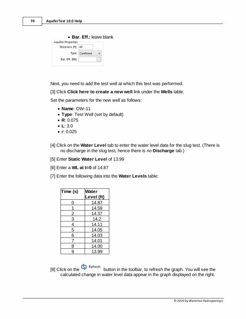
AquiferTest 10.0 Help70
© 2020 by Waterloo Hydrogeologic
· Bar. Eff.: leave blank
Next, you need to add the test well at which this test was performed.
[3] Click Click here to create a new well link under the Wells table.
Set the parameters for the new well as follows:
· Name: OW-11
· Type: Test Well (set by default)
· R: 0.075
· L: 3.0
· r: 0.025
[4] Click on the Water Level tab to enter the water level data for the slug test. (There isno discharge in the slug test, hence there is no Discharge tab.)
[5] Enter Static Water Level of 13.99
[6] Enter a WL at t=0 of 14.87
[7] Enter the following data into the Water Levels table:
Time (s) WaterLevel (ft)
0 14.871 14.592 14.373 14.24 14.115 14.056 14.037 14.018 14.009 13.99
[8] Click on the button in the toolbar, to refresh the graph. You will see thecalculated change in water level data appear in the graph displayed on the right.
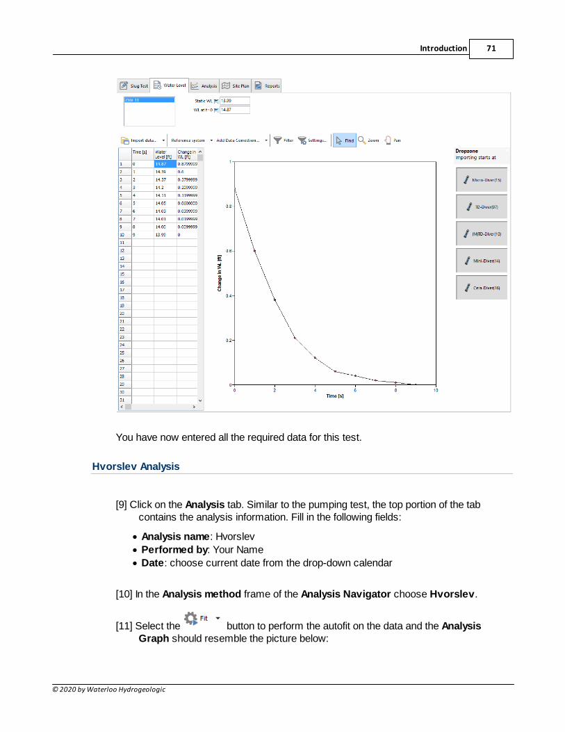
Introduction 71
© 2020 by Waterloo Hydrogeologic
You have now entered all the required data for this test.
Hvorslev Analysis
[9] Click on the Analysis tab. Similar to the pumping test, the top portion of the tabcontains the analysis information. Fill in the following fields:
· Analysis name: Hvorslev
· Performed by: Your Name
· Date: choose current date from the drop-down calendar
[10] In the Analysis method frame of the Analysis Navigator choose Hvorslev.
[11] Select the button to perform the autofit on the data and the AnalysisGraph should resemble the picture below:
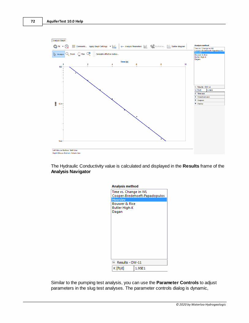
AquiferTest 10.0 Help72
© 2020 by Waterloo Hydrogeologic
The Hydraulic Conductivity value is calculated and displayed in the Results frame of theAnalysis Navigator
Similar to the pumping test analysis, you can use the Parameter Controls to adjustparameters in the slug test analyses. The parameter controls dialog is dynamic,
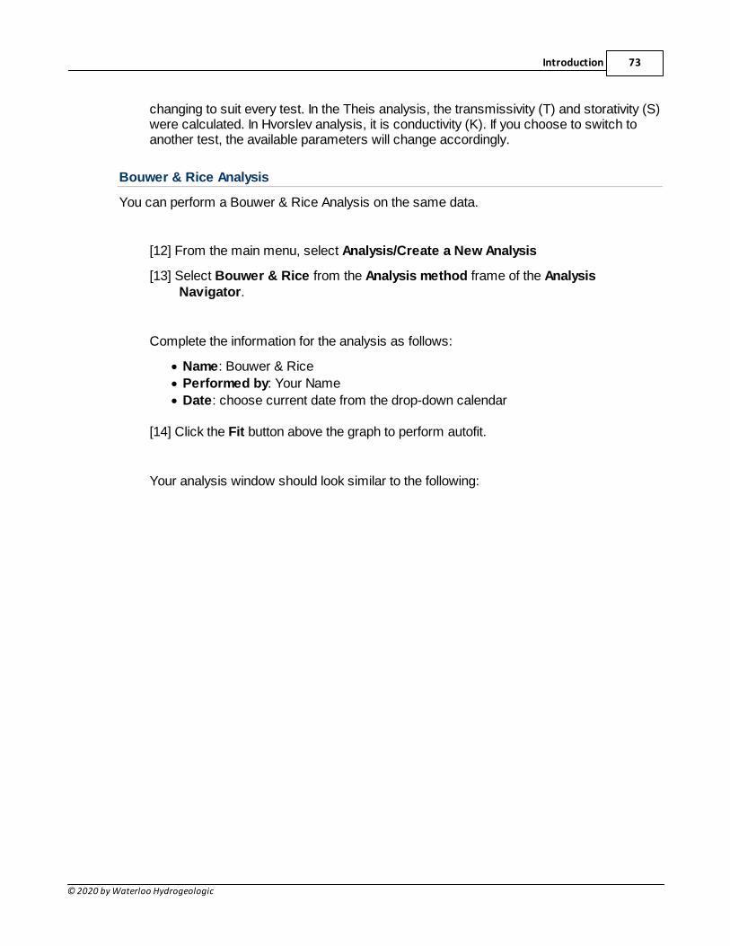
Introduction 73
© 2020 by Waterloo Hydrogeologic
changing to suit every test. In the Theis analysis, the transmissivity (T) and storativity (S)were calculated. In Hvorslev analysis, it is conductivity (K). If you choose to switch toanother test, the available parameters will change accordingly.
Bouwer & Rice Analysis
You can perform a Bouwer & Rice Analysis on the same data.
[12] From the main menu, select Analysis/Create a New Analysis
[13] Select Bouwer & Rice from the Analysis method frame of the AnalysisNavigator.
Complete the information for the analysis as follows:
· Name: Bouwer & Rice
· Performed by: Your Name
· Date: choose current date from the drop-down calendar
[14] Click the Fit button above the graph to perform autofit.
Your analysis window should look similar to the following:
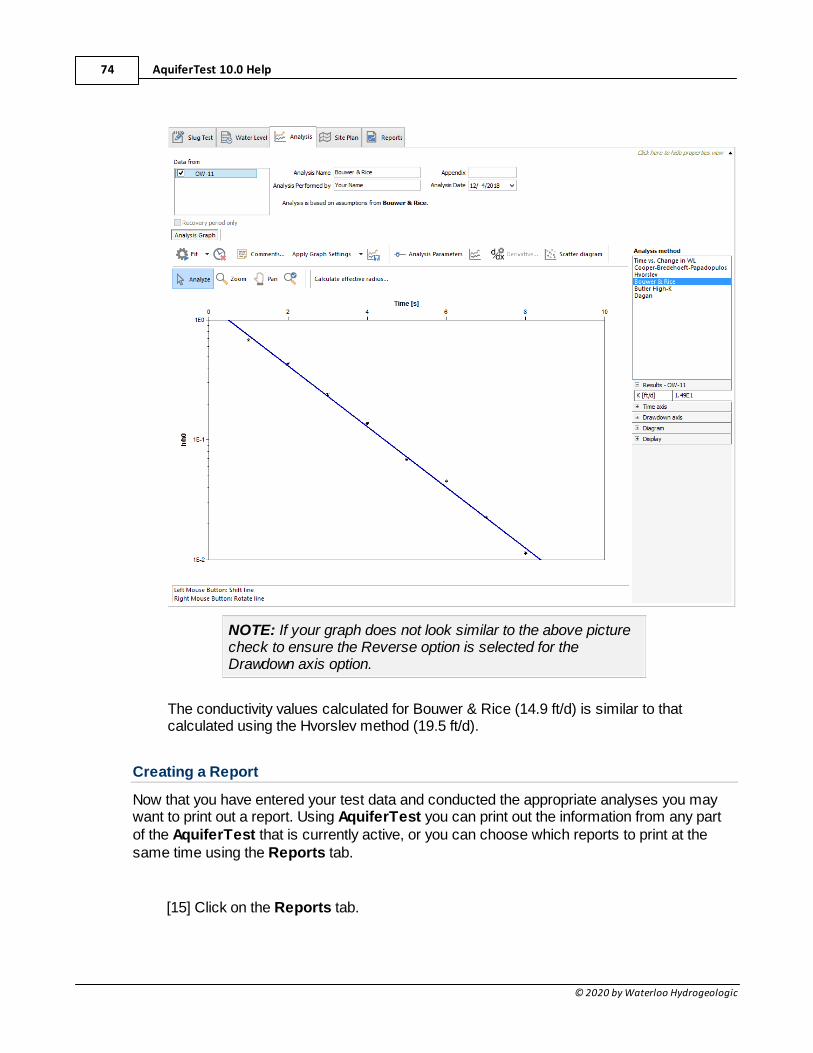
AquiferTest 10.0 Help74
© 2020 by Waterloo Hydrogeologic
NOTE: If your graph does not look similar to the above picturecheck to ensure the Reverse option is selected for theDrawdown axis option.
The conductivity values calculated for Bouwer & Rice (14.9 ft/d) is similar to thatcalculated using the Hvorslev method (19.5 ft/d).
Creating a Report
Now that you have entered your test data and conducted the appropriate analyses you maywant to print out a report. Using AquiferTest you can print out the information from any partof the AquiferTest that is currently active, or you can choose which reports to print at thesame time using the Reports tab.
[15] Click on the Reports tab.
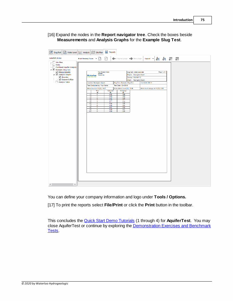
Introduction 75
© 2020 by Waterloo Hydrogeologic
[16] Expand the nodes in the Report navigator tree. Check the boxes besideMeasurements and Analysis Graphs for the Example Slug Test.
You can define your company information and logo under Tools / Options.
[17] To print the reports select File/Print or click the Print button in the toolbar.
This concludes the Quick Start Demo Tutorials (1 through 4) for AquiferTest. You mayclose AquiferTest or continue by exploring the Demonstration Exercises and BenchmarkTests.
AquiferTest 10.0 Help76
© 2020 by Waterloo Hydrogeologic
2 Demonstration Exercises and Benchmark Tests
This section will explore many features of AquiferTest including various single and multiplepumping well solution methods, importing data from MS-Excel and a datalogger file (.ASC),and planning a pumping test. The functionality of each feature is explained in detail in thefollowing exercises:
· Exercise 1: Confined Aquifer - Theis Analysis
· Exercise 2: Leaky Aquifer - Hantush - Jacob Analysis
· Exercise 3: Recovery Data Analysis - Agarwal Solution
· Exercise 4: Confined Aquifer, Multiple Pumping Wells
· Exercise 5: Adding Data Trend Correction
· Exercise 6: Adding Barometric Correction
· Exercise 7: Slug Test Analysis - Bouwer & Rice
· Exercise 8: High-K Butler Method
· Exercise 9: Derivative Smoothing
· Exercise 10: Horizontal Wells
· Exercise 11: Wellbore Storage and Skin Effects
· Exercise 12: Lugeon Test Analysis
· Exercise 13: Multi-Layer Aquifer Analysis
· Exercise 14: Slug Test Analysis - Binkhorst and Robbins
An additional 19 Benchmarking Examples are also available for reference and reviewpurposes.
These exercises are designed to help you familiarize yourself with various functions of theprogram, but also to provide you with comparisons of the results obtained from AquiferTestto some other sources including published references.
The sequence of a typical AquiferTest session is:
[1] Open or create a project
[2] Enter and/or import well information and data
[3] Select an analysis method
[4] Fit the type curve
[5] Print the output
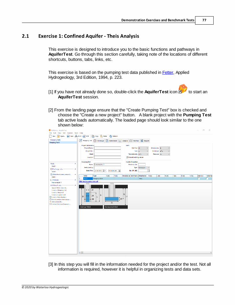
Demonstration Exercises and Benchmark Tests 77
© 2020 by Waterloo Hydrogeologic
2.1 Exercise 1: Confined Aquifer - Theis Analysis
This exercise is designed to introduce you to the basic functions and pathways inAquiferTest. Go through this section carefully, taking note of the locations of differentshortcuts, buttons, tabs, links, etc.
This exercise is based on the pumping test data published in Fetter, AppliedHydrogeology, 3rd Edition, 1994, p. 223.
[1] If you have not already done so, double-click the AquiferTest icon to start anAquiferTest session.
[2] From the landing page ensure that the "Create Pumping Test" box is checked andchoose the "Create a new project" button. A blank project with the Pumping Testtab active loads automatically. The loaded page should look similar to the oneshown below:
[3] In this step you will fill in the information needed for the project and/or the test. Not allinformation is required, however it is helpful in organizing tests and data sets.
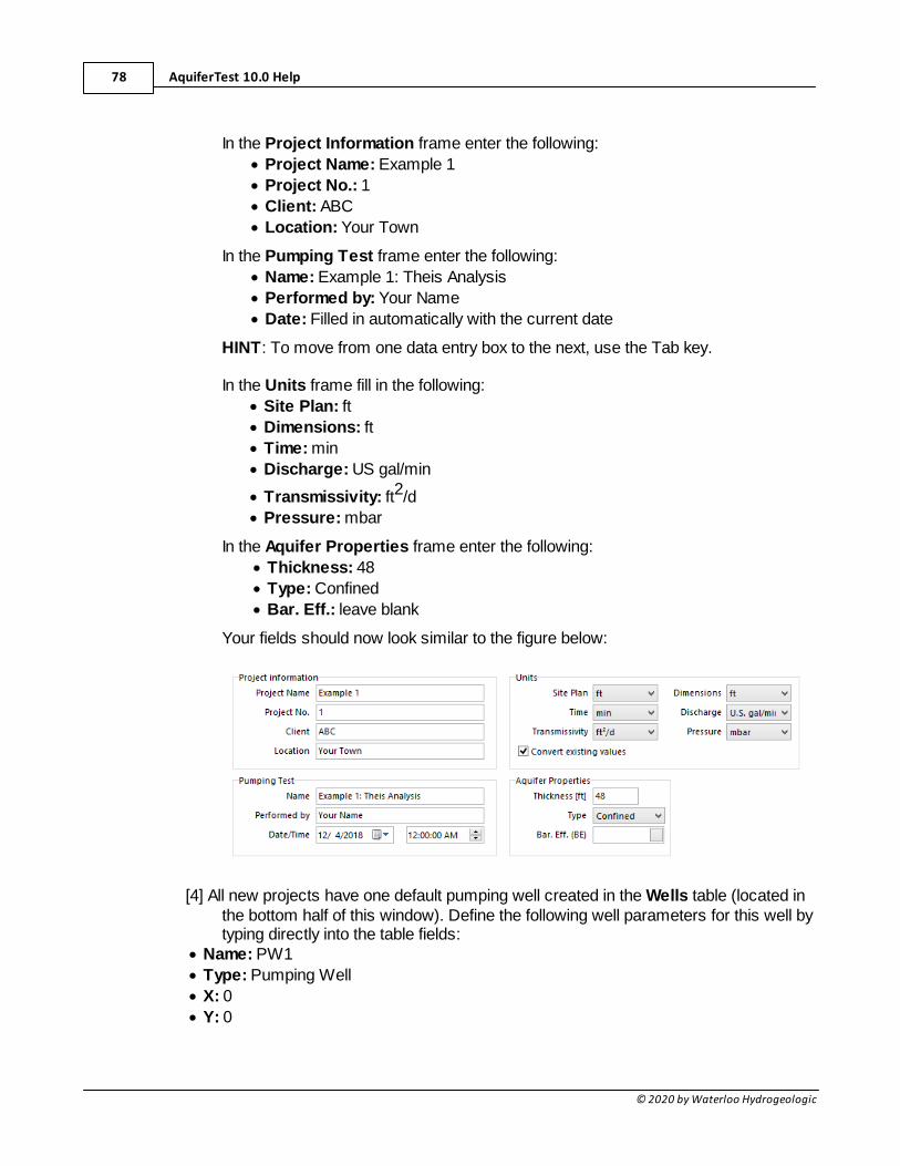
AquiferTest 10.0 Help78
© 2020 by Waterloo Hydrogeologic
In the Project Information frame enter the following:
· Project Name: Example 1
· Project No.: 1
· Client: ABC
· Location: Your Town
In the Pumping Test frame enter the following:
· Name: Example 1: Theis Analysis
· Performed by: Your Name
· Date: Filled in automatically with the current date
HINT: To move from one data entry box to the next, use the Tab key.
In the Units frame fill in the following:
· Site Plan: ft
· Dimensions: ft
· Time: min
· Discharge: US gal/min
· Transmissivity: ft2/d
· Pressure: mbar
In the Aquifer Properties frame enter the following:
· Thickness: 48
· Type: Confined
· Bar. Eff.: leave blank
Your fields should now look similar to the figure below:
[4] All new projects have one default pumping well created in the Wells table (located inthe bottom half of this window). Define the following well parameters for this well bytyping directly into the table fields:
· Name: PW1
· Type: Pumping Well
· X: 0
· Y: 0
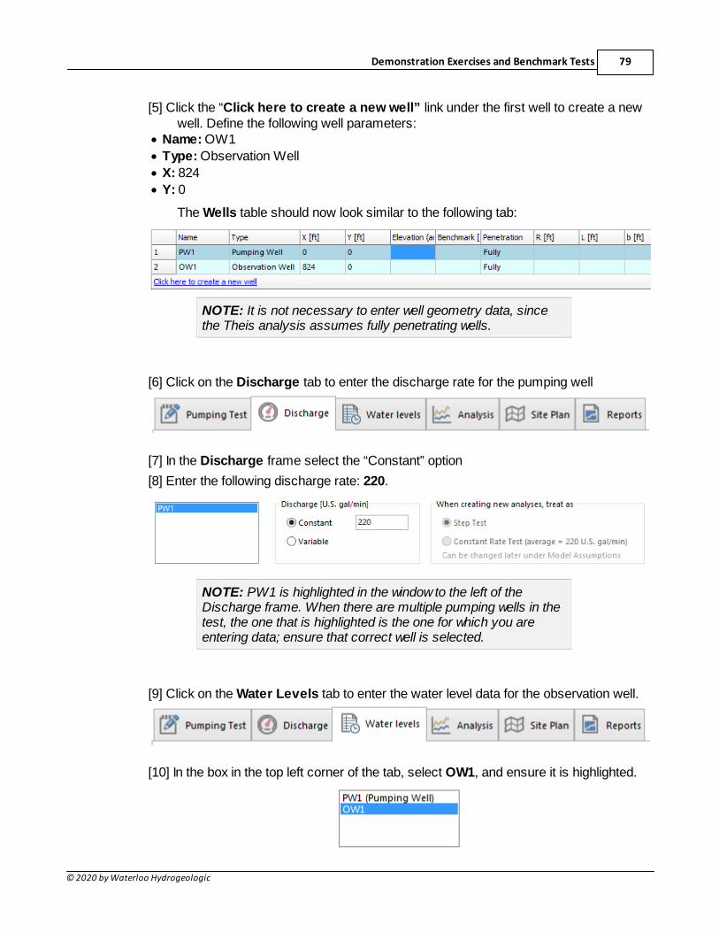
Demonstration Exercises and Benchmark Tests 79
© 2020 by Waterloo Hydrogeologic
[5] Click the “Click here to create a new well” link under the first well to create a newwell. Define the following well parameters:
· Name: OW1
· Type: Observation Well
· X: 824
· Y: 0
The Wells table should now look similar to the following tab:
NOTE: It is not necessary to enter well geometry data, sincethe Theis analysis assumes fully penetrating wells.
[6] Click on the Discharge tab to enter the discharge rate for the pumping well
[7] In the Discharge frame select the “Constant” option
[8] Enter the following discharge rate: 220.
NOTE: PW1 is highlighted in the window to the left of theDischarge frame. When there are multiple pumping wells in thetest, the one that is highlighted is the one for which you areentering data; ensure that correct well is selected.
[9] Click on the Water Levels tab to enter the water level data for the observation well.
[10] In the box in the top left corner of the tab, select OW1, and ensure it is highlighted.
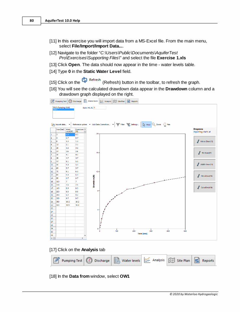
AquiferTest 10.0 Help80
© 2020 by Waterloo Hydrogeologic
[11] In this exercise you will import data from a MS-Excel file. From the main menu,select File/Import/Import Data....
[12] Navigate to the folder “C:\Users\Public\Documents\AquiferTestPro\Exercises\Supporting Files\" and select the file Exercise 1.xls
[13] Click Open. The data should now appear in the time - water levels table.
[14] Type 0 in the Static Water Level field.
[15] Click on the (Refresh) button in the toolbar, to refresh the graph.
[16] You will see the calculated drawdown data appear in the Drawdown column and adrawdown graph displayed on the right.
[17] Click on the Analysis tab
[18] In the Data from window, select OW1
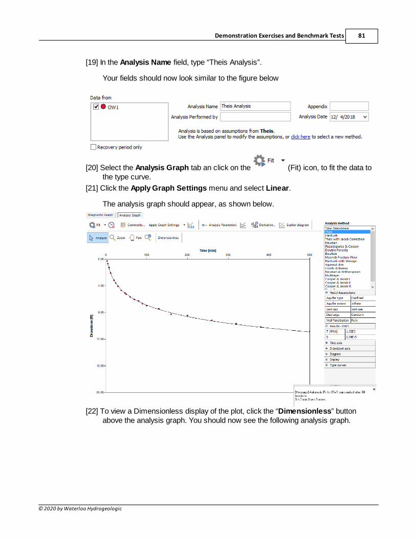
Demonstration Exercises and Benchmark Tests 81
© 2020 by Waterloo Hydrogeologic
[19] In the Analysis Name field, type “Theis Analysis”.
Your fields should now look similar to the figure below
[20] Select the Analysis Graph tab an click on the (Fit) icon, to fit the data tothe type curve.
[21] Click the Apply Graph Settings menu and select Linear.
The analysis graph should appear, as shown below.
[22] To view a Dimensionless display of the plot, click the “Dimensionless” buttonabove the analysis graph. You should now see the following analysis graph.
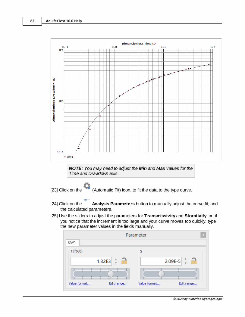
AquiferTest 10.0 Help82
© 2020 by Waterloo Hydrogeologic
NOTE: You may need to adjust the Min and Max values for theTime and Drawdown axis.
[23] Click on the (Automatic Fit) icon, to fit the data to the type curve.
[24] Click on the Analysis Parameters button to manually adjust the curve fit, andthe calculated parameters.
[25] Use the sliders to adjust the parameters for Transmissivity and Storativity, or, ifyou notice that the increment is too large and your curve moves too quickly, typethe new parameter values in the fields manually.
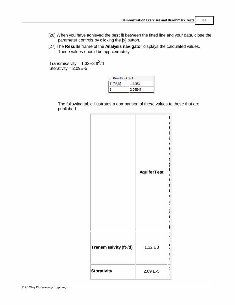
Demonstration Exercises and Benchmark Tests 83
© 2020 by Waterloo Hydrogeologic
[26] When you have achieved the best fit between the fitted line and your data, close theparameter controls by clicking the [x] button.
[27] The Results frame of the Analysis navigator displays the calculated values.These values should be approximately:
Transmissivity = 1.32E3 ft2/dStorativity = 2.09E-5
The following table illustrates a comparison of these values to those that arepublished.
AquiferTest
Published(Fetter,1994)
Transmissivity (ft2/d) 1.32 E3
1.40E3
Storativity 2.09 E-52.
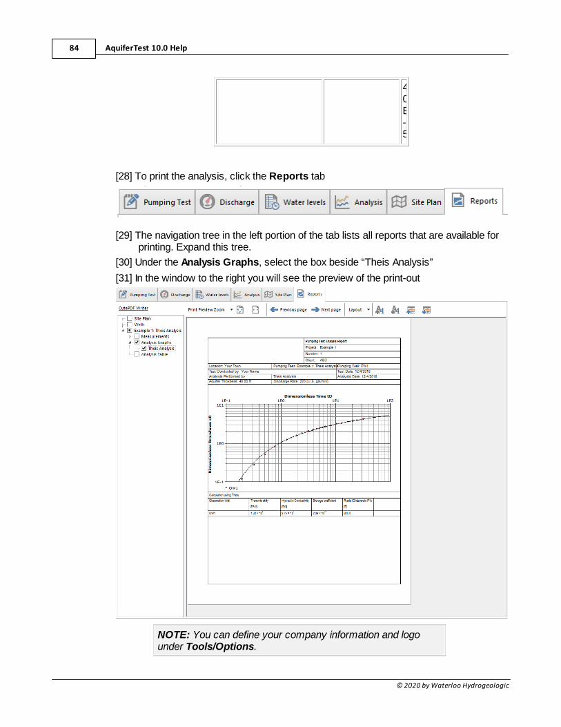
AquiferTest 10.0 Help84
© 2020 by Waterloo Hydrogeologic
40E-5
[28] To print the analysis, click the Reports tab
[29] The navigation tree in the left portion of the tab lists all reports that are available forprinting. Expand this tree.
[30] Under the Analysis Graphs, select the box beside “Theis Analysis”
[31] In the window to the right you will see the preview of the print-out
NOTE: You can define your company information and logounder Tools/Options.
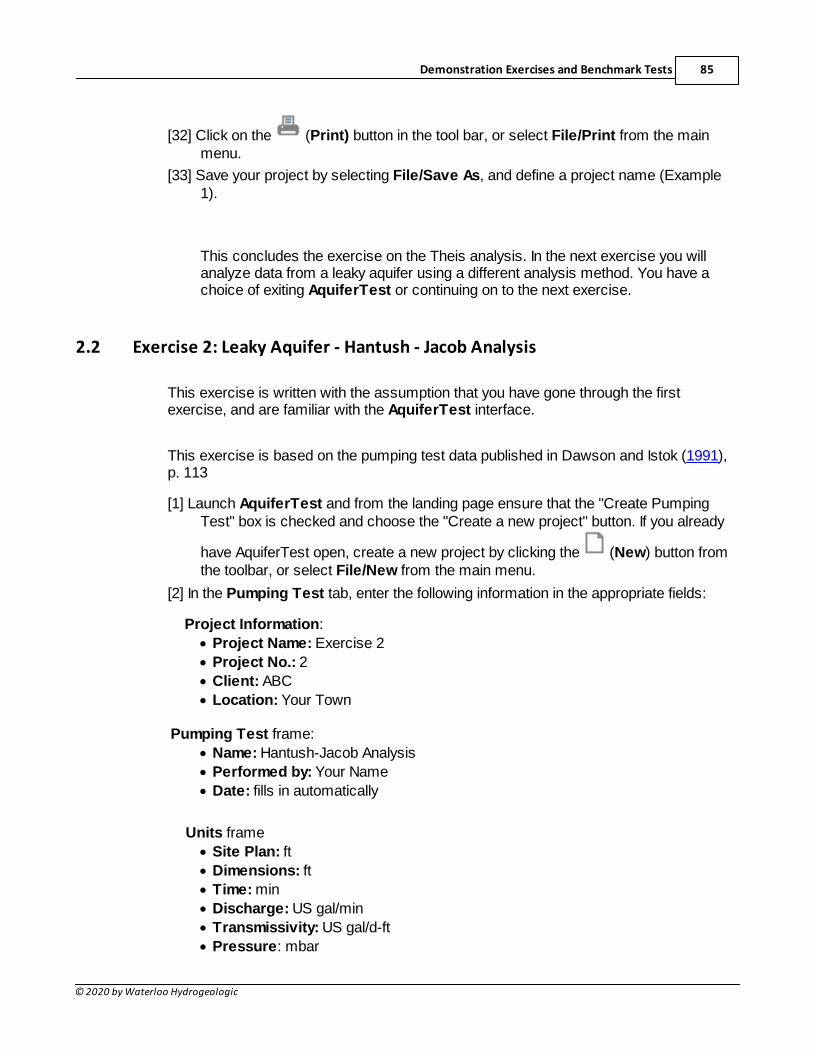
Demonstration Exercises and Benchmark Tests 85
© 2020 by Waterloo Hydrogeologic
[32] Click on the (Print) button in the tool bar, or select File/Print from the mainmenu.
[33] Save your project by selecting File/Save As, and define a project name (Example1).
This concludes the exercise on the Theis analysis. In the next exercise you willanalyze data from a leaky aquifer using a different analysis method. You have achoice of exiting AquiferTest or continuing on to the next exercise.
2.2 Exercise 2: Leaky Aquifer - Hantush - Jacob Analysis
This exercise is written with the assumption that you have gone through the firstexercise, and are familiar with the AquiferTest interface.
This exercise is based on the pumping test data published in Dawson and Istok (1991),p. 113
[1] Launch AquiferTest and from the landing page ensure that the "Create PumpingTest" box is checked and choose the "Create a new project" button. If you already
have AquiferTest open, create a new project by clicking the (New) button fromthe toolbar, or select File/New from the main menu.
[2] In the Pumping Test tab, enter the following information in the appropriate fields:
Project Information:
· Project Name: Exercise 2
· Project No.: 2
· Client: ABC
· Location: Your Town
Pumping Test frame:
· Name: Hantush-Jacob Analysis
· Performed by: Your Name
· Date: fills in automatically
Units frame
· Site Plan: ft
· Dimensions: ft
· Time: min
· Discharge: US gal/min
· Transmissivity: US gal/d-ft
· Pressure: mbar
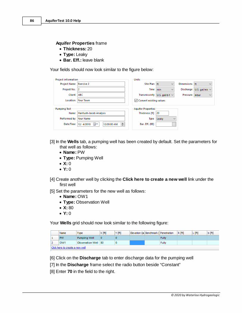
AquiferTest 10.0 Help86
© 2020 by Waterloo Hydrogeologic
Aquifer Properties frame
· Thickness: 20
· Type: Leaky
· Bar. Eff.: leave blank
Your fields should now look similar to the figure below:
[3] In the Wells tab, a pumping well has been created by default. Set the parameters forthat well as follows:· Name: PW
· Type: Pumping Well
· X: 0
· Y: 0
[4] Create another well by clicking the Click here to create a new well link under thefirst well
[5] Set the parameters for the new well as follows:· Name: OW1
· Type: Observation Well
· X: 80
· Y: 0
Your Wells grid should now look similar to the following figure:
[6] Click on the Discharge tab to enter discharge data for the pumping well
[7] In the Discharge frame select the radio button beside “Constant”
[8] Enter 70 in the field to the right.
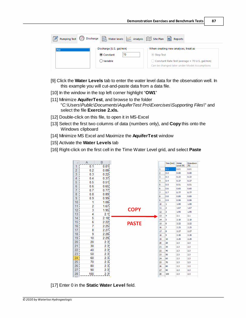
Demonstration Exercises and Benchmark Tests 87
© 2020 by Waterloo Hydrogeologic
[9] Click the Water Levels tab to enter the water level data for the observation well. Inthis example you will cut-and-paste data from a data file.
[10] In the window in the top left corner highlight “OW1”
[11] Minimize AquiferTest, and browse to the folder "C:\Users\Public\Documents\AquiferTest Pro\Exercises\Supporting Files\" andselect the file Exercise 2.xls.
[12] Double-click on this file, to open it in MS-Excel
[13] Select the first two columns of data (numbers only), and Copy this onto theWindows clipboard
[14] Minimize MS Excel and Maximize the AquiferTest window
[15] Activate the Water Levels tab
[16] Right-click on the first cell in the Time Water Level grid, and select Paste
[17] Enter 0 in the Static Water Level field.
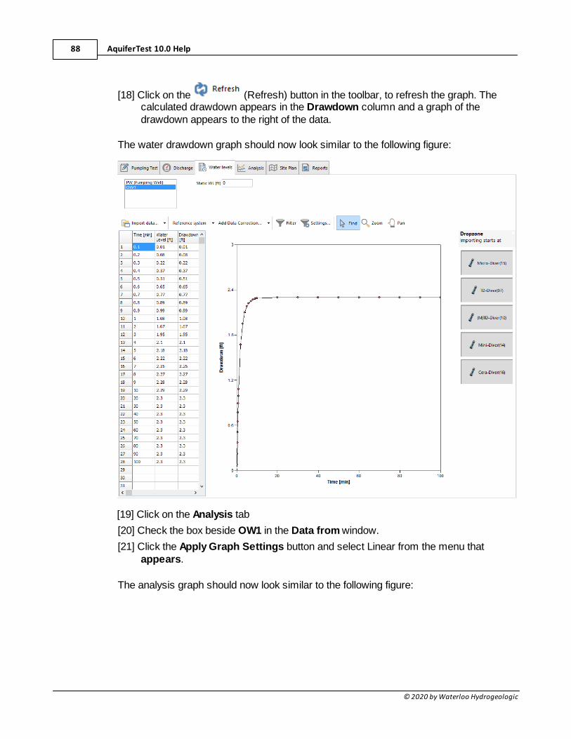
AquiferTest 10.0 Help88
© 2020 by Waterloo Hydrogeologic
[18] Click on the (Refresh) button in the toolbar, to refresh the graph. Thecalculated drawdown appears in the Drawdown column and a graph of thedrawdown appears to the right of the data.
The water drawdown graph should now look similar to the following figure:
[19] Click on the Analysis tab
[20] Check the box beside OW1 in the Data from window.
[21] Click the Apply Graph Settings button and select Linear from the menu thatappears.
The analysis graph should now look similar to the following figure:
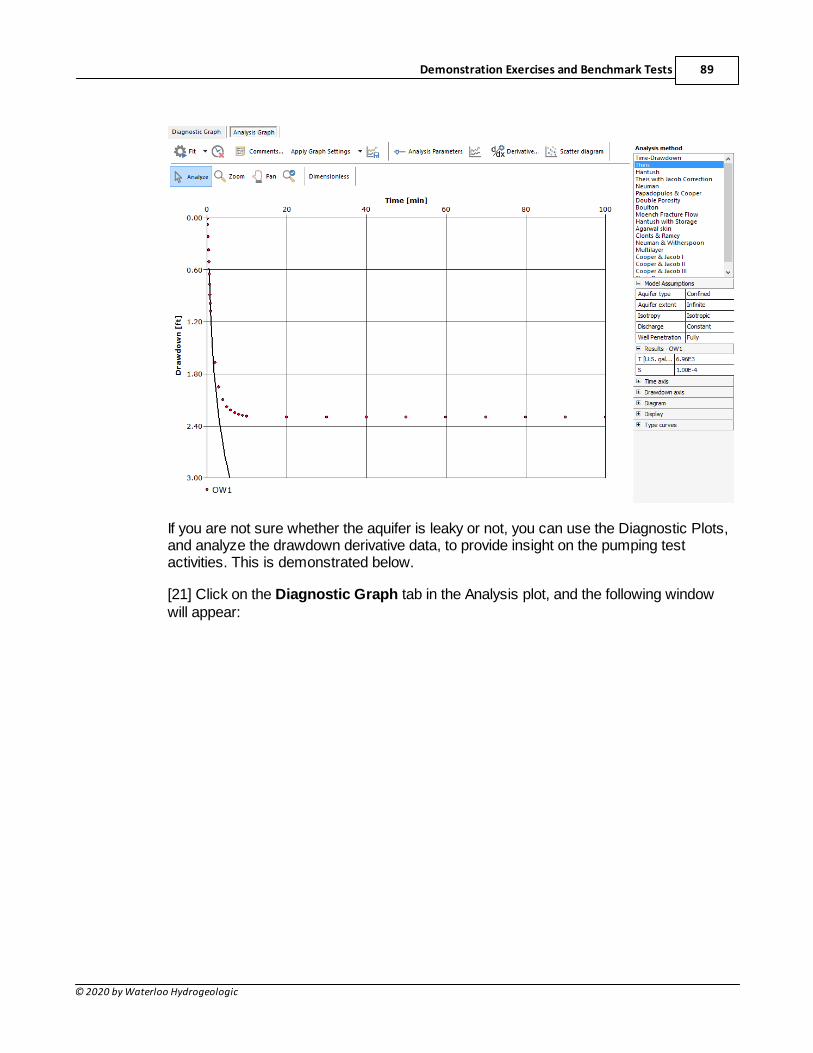
Demonstration Exercises and Benchmark Tests 89
© 2020 by Waterloo Hydrogeologic
If you are not sure whether the aquifer is leaky or not, you can use the Diagnostic Plots,and analyze the drawdown derivative data, to provide insight on the pumping testactivities. This is demonstrated below.
[21] Click on the Diagnostic Graph tab in the Analysis plot, and the following windowwill appear:
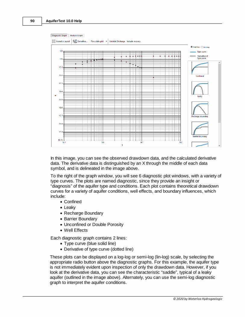
AquiferTest 10.0 Help90
© 2020 by Waterloo Hydrogeologic
In this image, you can see the observed drawdown data, and the calculated derivativedata. The derivative data is distinguished by an X through the middle of each datasymbol, and is delineated in the image above.
To the right of the graph window, you will see 6 diagnostic plot windows, with a variety oftype curves. The plots are named diagnostic, since they provide an insight or“diagnosis” of the aquifer type and conditions. Each plot contains theoretical drawdowncurves for a variety of aquifer conditions, well effects, and boundary influences, whichinclude:
· Confined
· Leaky
· Recharge Boundary
· Barrier Boundary
· Unconfined or Double Porosity
· Well Effects
Each diagnostic graph contains 2 lines:· Type curve (blue solid line)
· Derivative of type curve (dotted line)
These plots can be displayed on a log-log or semi-log (lin-log) scale, by selecting theappropriate radio button above the diagnostic graphs. For this example, the aquifer typeis not immediately evident upon inspection of only the drawdown data. However, if youlook at the derivative data, you can see the characteristic “saddle”, typical of a leakyaquifer (outlined in the image above). Alternately, you can use the semi-log diagnosticgraph to interpret the aquifer conditions.
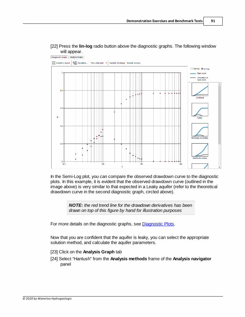
Demonstration Exercises and Benchmark Tests 91
© 2020 by Waterloo Hydrogeologic
[22] Press the lin-log radio button above the diagnostic graphs. The following windowwill appear.
In the Semi-Log plot, you can compare the observed drawdown curve to the diagnosticplots. In this example, it is evident that the observed drawdown curve (outlined in theimage above) is very similar to that expected in a Leaky aquifer (refer to the theoreticaldrawdown curve in the second diagnostic graph, circled above).
NOTE: the red trend line for the drawdown derivatives has beendrawn on top of this figure by hand for illustration purposes
For more details on the diagnostic graphs, see Diagnostic Plots.
Now that you are confident that the aquifer is leaky, you can select the appropriatesolution method, and calculate the aquifer parameters.
[23] Click on the Analysis Graph tab
[24] Select “Hantush” from the Analysis methods frame of the Analysis navigatorpanel
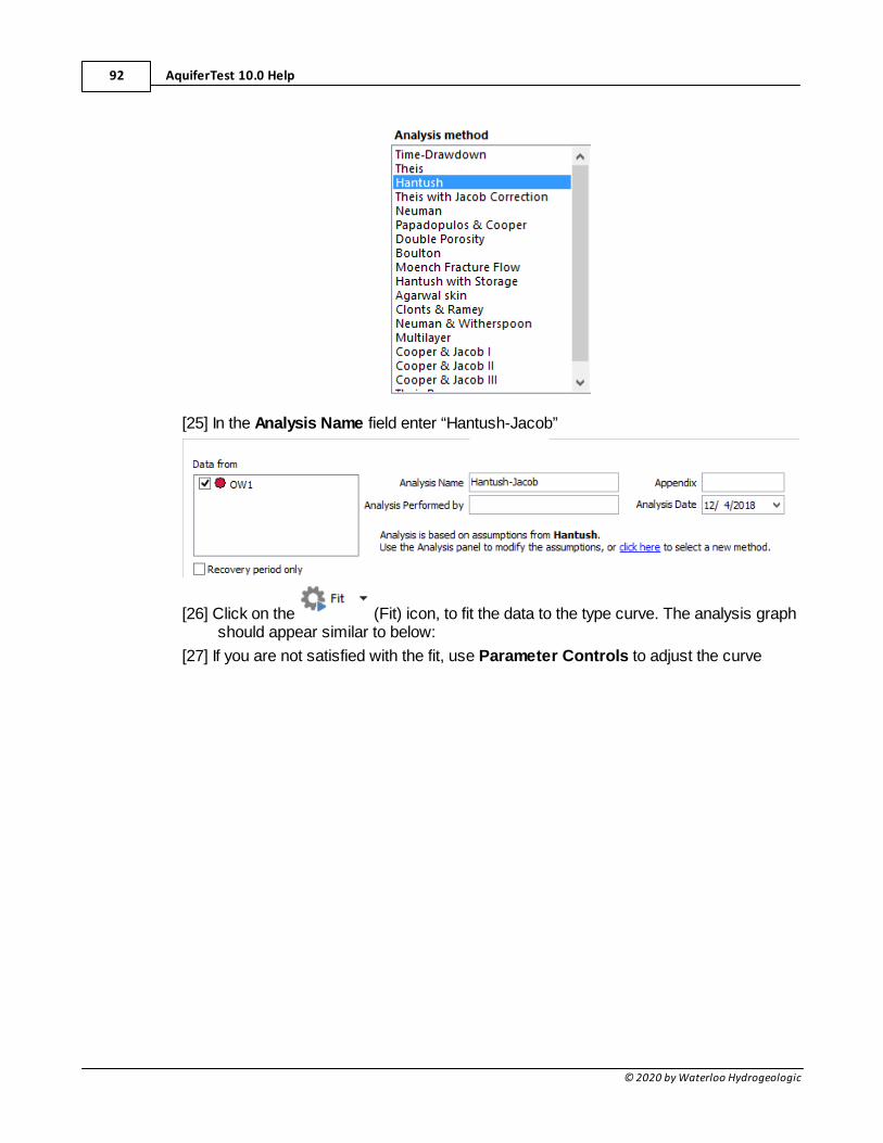
AquiferTest 10.0 Help92
© 2020 by Waterloo Hydrogeologic
[25] In the Analysis Name field enter “Hantush-Jacob”
[26] Click on the (Fit) icon, to fit the data to the type curve. The analysis graphshould appear similar to below:
[27] If you are not satisfied with the fit, use Parameter Controls to adjust the curve
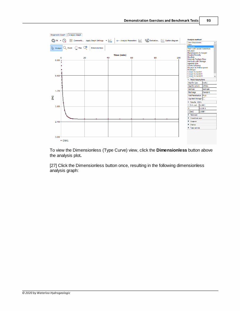
Demonstration Exercises and Benchmark Tests 93
© 2020 by Waterloo Hydrogeologic
To view the Dimensionless (Type Curve) view, click the Dimensionless button abovethe analysis plot.
[27] Click the Dimensionless button once, resulting in the following dimensionlessanalysis graph:
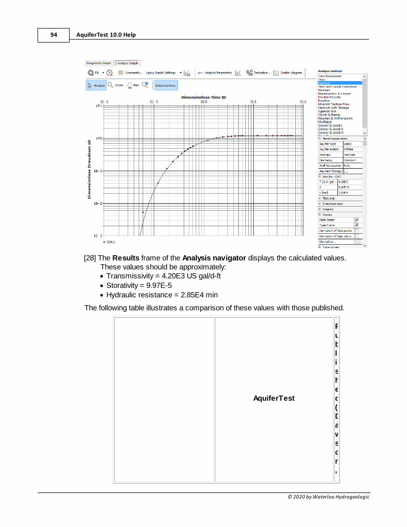
AquiferTest 10.0 Help94
© 2020 by Waterloo Hydrogeologic
[28] The Results frame of the Analysis navigator displays the calculated values.These values should be approximately:· Transmissivity = 4.20E3 US gal/d-ft
· Storativity = 9.97E-5
· Hydraulic resistance = 2.85E4 min
The following table illustrates a comparison of these values with those published.
AquiferTest
Published(Dawson,
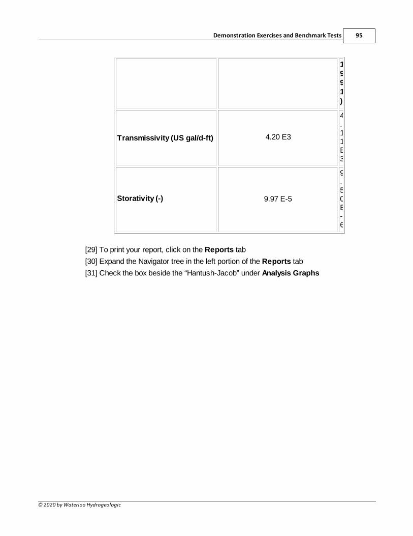
Demonstration Exercises and Benchmark Tests 95
© 2020 by Waterloo Hydrogeologic
1991)
Transmissivity (US gal/d-ft) 4.20 E3
4.11E3
Storativity (-) 9.97 E-5
9.50E-6
[29] To print your report, click on the Reports tab
[30] Expand the Navigator tree in the left portion of the Reports tab
[31] Check the box beside the “Hantush-Jacob” under Analysis Graphs
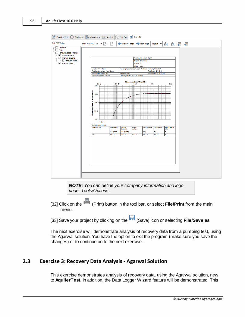
AquiferTest 10.0 Help96
© 2020 by Waterloo Hydrogeologic
NOTE: You can define your company information and logounder Tools/Options.
[32] Click on the (Print) button in the tool bar, or select File/Print from the mainmenu.
[33] Save your project by clicking on the (Save) icon or selecting File/Save as
The next exercise will demonstrate analysis of recovery data from a pumping test, usingthe Agarwal solution. You have the option to exit the program (make sure you save thechanges) or to continue on to the next exercise.
2.3 Exercise 3: Recovery Data Analysis - Agarwal Solution
This exercise demonstrates analysis of recovery data, using the Agarwal solution, newto AquiferTest. In addition, the Data Logger Wizard feature will be demonstrated. This
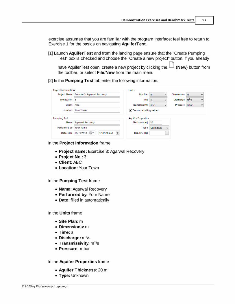
Demonstration Exercises and Benchmark Tests 97
© 2020 by Waterloo Hydrogeologic
exercise assumes that you are familiar with the program interface; feel free to return toExercise 1 for the basics on navigating AquiferTest.
[1] Launch AquiferTest and from the landing page ensure that the "Create PumpingTest" box is checked and choose the "Create a new project" button. If you already
have AquiferTest open, create a new project by clicking the (New) button fromthe toolbar, or select File/New from the main menu.
[2] In the Pumping Test tab enter the following information:
In the Project Information frame
· Project name: Exercise 3: Agarwal Recovery
· Project No.: 3
· Client: ABC
· Location: Your Town
In the Pumping Test frame
· Name: Agarwal Recovery
· Performed by: Your Name
· Date: filled in automatically
In the Units frame
· Site Plan: m
· Dimensions: m
· Time: s
· Discharge: m3/s
· Transmissivity: m2/s
· Pressure: mbar
In the Aquifer Properties frame
· Aquifer Thickness: 20 m
· Type: Unknown
AquiferTest 10.0 Help98
© 2020 by Waterloo Hydrogeologic
· Bar. Eff. (BE): Leave blank
[3] The new project will contain one pumping well, by default. Set the parameters for thiswell as follows:
Well 1
· Name: PW
· Type: Pumping Well
· X: 0
· Y: 0
Next, create a new well. Click on the “Click here to create a new well” link to add anew well to the table. Define the parameters for this new well, as follows:
Well 2
· Name: OW1
· Type: Observation well
· X:10
· Y: 0
[4] Click on the Discharge tab
[5] Select Constant discharge
[6] Enter the value 0.0015 in the "required" field beside
[7] Click on the Water Levels tab
[8] Highlight “OW1” in the wells list in the top left corner of the tab. For this well, you willimport the time-water level data from a data logger file.
[9] Select File/Import/ Import Data Logger file... from the main menu
[10] Browse to the folder “C:\Users\Public\Documents\AquiferTestPro\Exercises\Supporting Files\" and select the Exercise3.asc file.
[11] Highlight the file and click Open. This will launch the 6-step data logger importwizard.
[12] In the first step, you may select previously saved import settings. This is a greattime saver when importing many files with similar format. Since there are noexisting settings, you must define the required settings manually.
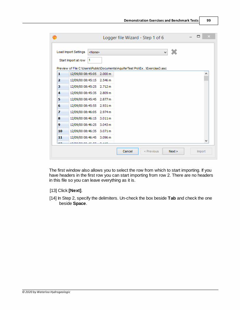
Demonstration Exercises and Benchmark Tests 99
© 2020 by Waterloo Hydrogeologic
The first window also allows you to select the row from which to start importing. If youhave headers in the first row you can start importing from row 2. There are no headersin this file so you can leave everything as it is.
[13] Click [Next].
[14] In Step 2, specify the delimiters. Un-check the box beside Tab and check the onebeside Space.
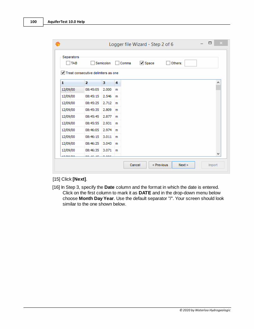
AquiferTest 10.0 Help100
© 2020 by Waterloo Hydrogeologic
[15] Click [Next].
[16] In Step 3, specify the Date column and the format in which the date is entered.Click on the first column to mark it as DATE and in the drop-down menu belowchoose Month Day Year. Use the default separator "/". Your screen should looksimilar to the one shown below.
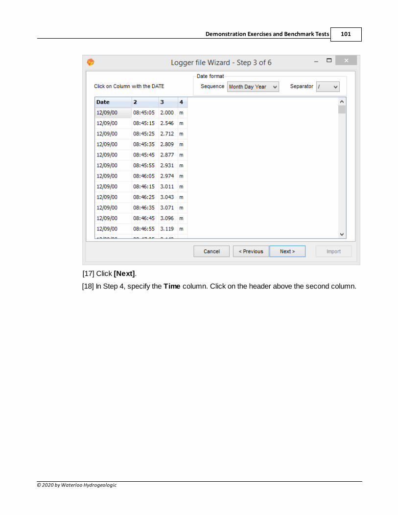
Demonstration Exercises and Benchmark Tests 101
© 2020 by Waterloo Hydrogeologic
[17] Click [Next].
[18] In Step 4, specify the Time column. Click on the header above the second column.
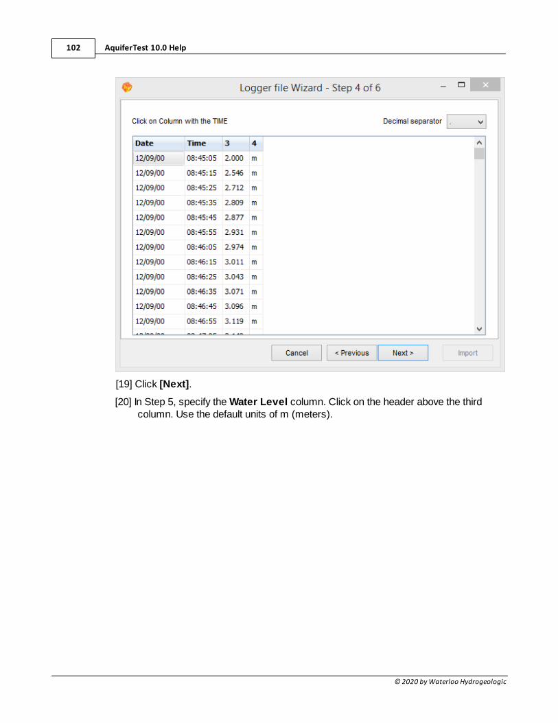
AquiferTest 10.0 Help102
© 2020 by Waterloo Hydrogeologic
[19] Click [Next].
[20] In Step 5, specify the Water Level column. Click on the header above the thirdcolumn. Use the default units of m (meters).
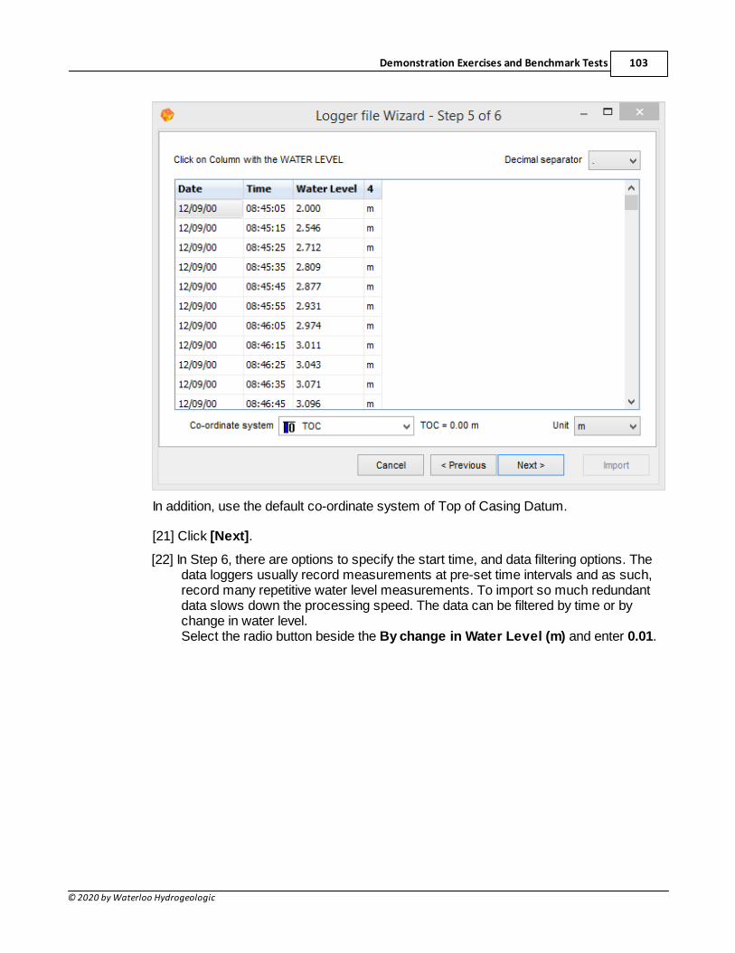
Demonstration Exercises and Benchmark Tests 103
© 2020 by Waterloo Hydrogeologic
In addition, use the default co-ordinate system of Top of Casing Datum.
[21] Click [Next].
[22] In Step 6, there are options to specify the start time, and data filtering options. Thedata loggers usually record measurements at pre-set time intervals and as such,record many repetitive water level measurements. To import so much redundantdata slows down the processing speed. The data can be filtered by time or bychange in water level.Select the radio button beside the By change in Water Level (m) and enter 0.01.
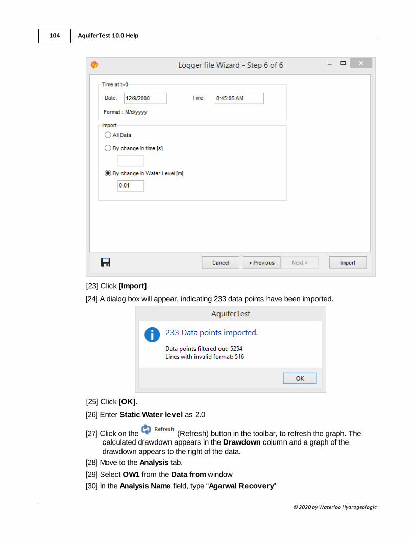
AquiferTest 10.0 Help104
© 2020 by Waterloo Hydrogeologic
[23] Click [Import].
[24] A dialog box will appear, indicating 233 data points have been imported.
[25] Click [OK].
[26] Enter Static Water level as 2.0
[27] Click on the (Refresh) button in the toolbar, to refresh the graph. Thecalculated drawdown appears in the Drawdown column and a graph of thedrawdown appears to the right of the data.
[28] Move to the Analysis tab.
[29] Select OW1 from the Data from window
[30] In the Analysis Name field, type “Agarwal Recovery”
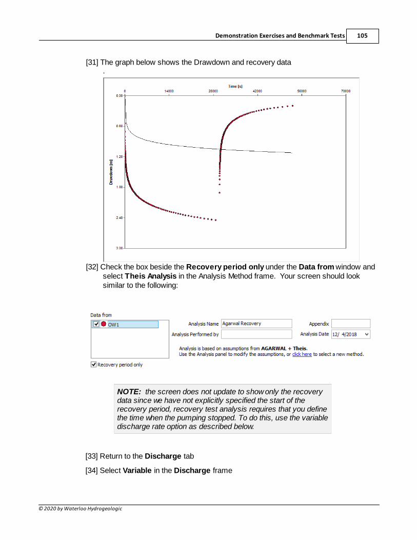
Demonstration Exercises and Benchmark Tests 105
© 2020 by Waterloo Hydrogeologic
[31] The graph below shows the Drawdown and recovery data.
[32] Check the box beside the Recovery period only under the Data from window andselect Theis Analysis in the Analysis Method frame. Your screen should looksimilar to the following:
NOTE: the screen does not update to show only the recoverydata since we have not explicitly specified the start of therecovery period, recovery test analysis requires that you definethe time when the pumping stopped. To do this, use the variabledischarge rate option as described below.
[33] Return to the Discharge tab
[34] Select Variable in the Discharge frame
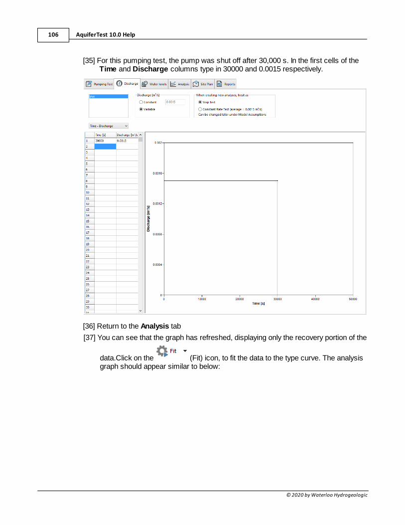
AquiferTest 10.0 Help106
© 2020 by Waterloo Hydrogeologic
[35] For this pumping test, the pump was shut off after 30,000 s. In the first cells of theTime and Discharge columns type in 30000 and 0.0015 respectively.
[36] Return to the Analysis tab
[37] You can see that the graph has refreshed, displaying only the recovery portion of the
data.Click on the (Fit) icon, to fit the data to the type curve. The analysisgraph should appear similar to below:
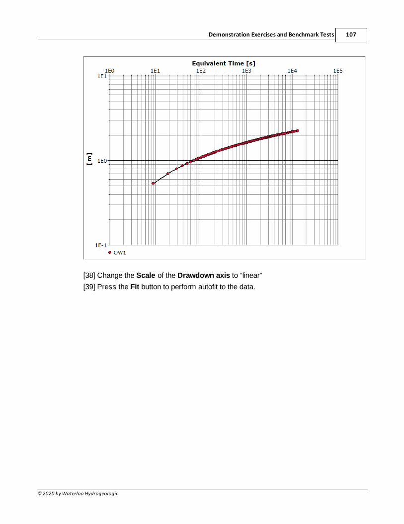
Demonstration Exercises and Benchmark Tests 107
© 2020 by Waterloo Hydrogeologic
[38] Change the Scale of the Drawdown axis to “linear”
[39] Press the Fit button to perform autofit to the data.
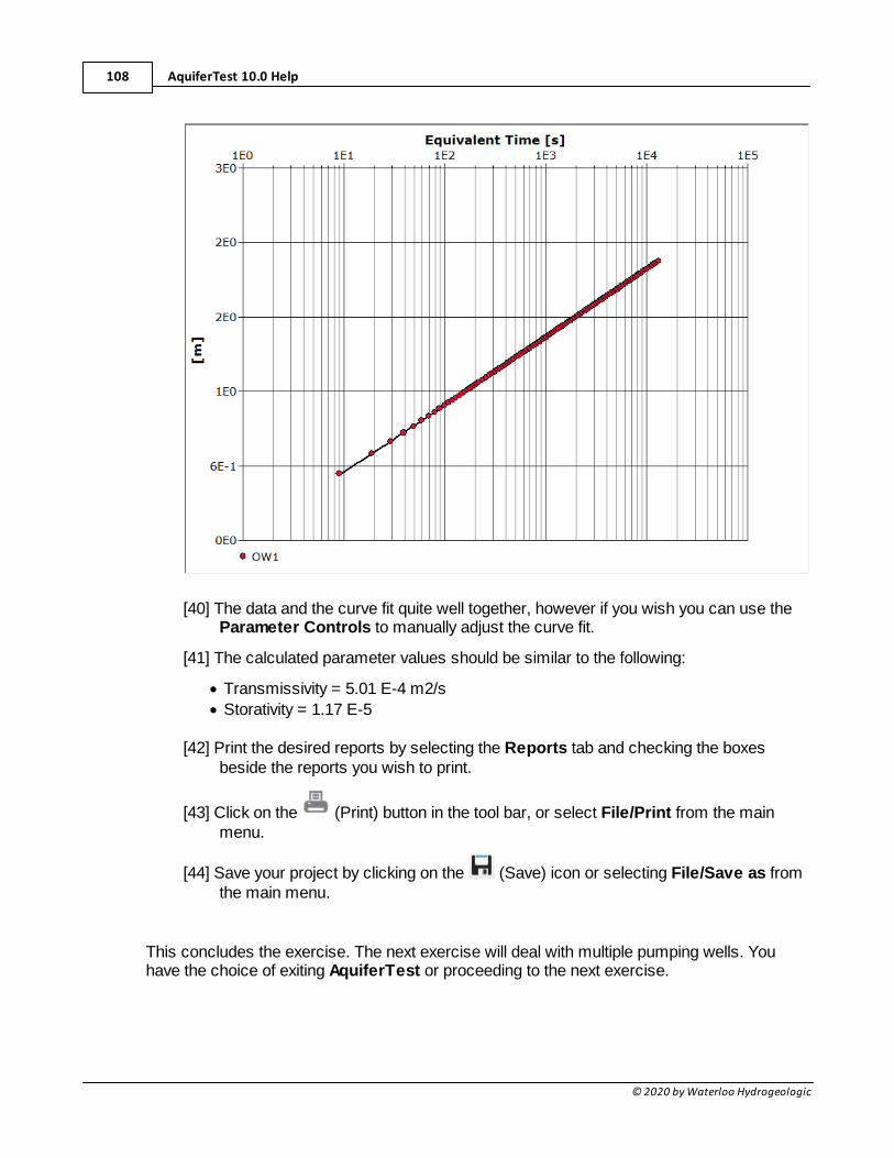
AquiferTest 10.0 Help108
© 2020 by Waterloo Hydrogeologic
[40] The data and the curve fit quite well together, however if you wish you can use theParameter Controls to manually adjust the curve fit.
[41] The calculated parameter values should be similar to the following:
· Transmissivity = 5.01 E-4 m2/s
· Storativity = 1.17 E-5
[42] Print the desired reports by selecting the Reports tab and checking the boxesbeside the reports you wish to print.
[43] Click on the (Print) button in the tool bar, or select File/Print from the mainmenu.
[44] Save your project by clicking on the (Save) icon or selecting File/Save as fromthe main menu.
This concludes the exercise. The next exercise will deal with multiple pumping wells. Youhave the choice of exiting AquiferTest or proceeding to the next exercise.
Demonstration Exercises and Benchmark Tests 109
© 2020 by Waterloo Hydrogeologic
2.4 Exercise 4: Confined Aquifer, Multiple Pumping Wells
In this exercise you will learn how to use AquiferTest to not only determine aquifer propertiesusing discharge and drawdown data, but also how to use these values to predict the effectthat an additional pumping well will have on drawdown at the observation well. You will alsolearn how to predict the drawdown in a well at any point in the effective area of the pumpingwell(s).
This exercise is divided into 3 sections: To begin, you will create a Theis analysis todetermine the aquifer parameters. Then, you will examine the effect a second pumping wellwill have on the drawdown at the observation well used in the first section. Finally, you willpredict the drawdown at a well at any point in the effective radius of the pumping wells.
Determining Aquifer Parameters
[1] Launch AquiferTest and from the landing page ensure that the "Create PumpingTest" box is checked and choose the "Create a new project" button. If you already
have AquiferTest open, create a new project by clicking the (New) button fromthe toolbar, or select File/New from the main menu.
[2] Complete the fields in the pumping test tab, as follows:
In the Project Information frame:
· Project Name: Exercise 4
· Project No.: 4
· Client: ABC
· Location: Your Town
In the Pumping Test frame:
· Pumping Test: Theis - Multiple Pumping Wells
· Performed by: Your Name
· Date: filled in automatically
In the Units frame
· Site Plan: ft
· Dimensions: ft
· Time: min
· Discharge: US gal/min
· Transmissivity: ft2/d
· Pressure: mbar
In the Aquifer Properties frame
· Thickness: 40
· Aquifer Type: Unknown
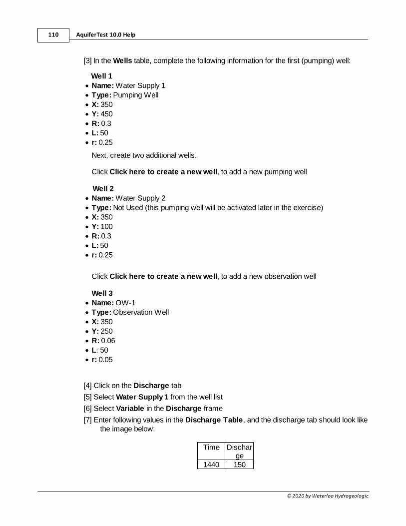
AquiferTest 10.0 Help110
© 2020 by Waterloo Hydrogeologic
[3] In the Wells table, complete the following information for the first (pumping) well:
Well 1
· Name: Water Supply 1
· Type: Pumping Well
· X: 350
· Y: 450
· R: 0.3
· L: 50
· r: 0.25
Next, create two additional wells.
Click Click here to create a new well, to add a new pumping well
Well 2
· Name: Water Supply 2
· Type: Not Used (this pumping well will be activated later in the exercise)
· X: 350
· Y: 100
· R: 0.3
· L: 50
· r: 0.25
Click Click here to create a new well, to add a new observation well
Well 3
· Name: OW-1
· Type: Observation Well
· X: 350
· Y: 250
· R: 0.06
· L: 50
· r: 0.05
[4] Click on the Discharge tab
[5] Select Water Supply 1 from the well list
[6] Select Variable in the Discharge frame
[7] Enter following values in the Discharge Table, and the discharge tab should look likethe image below:
Time Discharge
1440 150
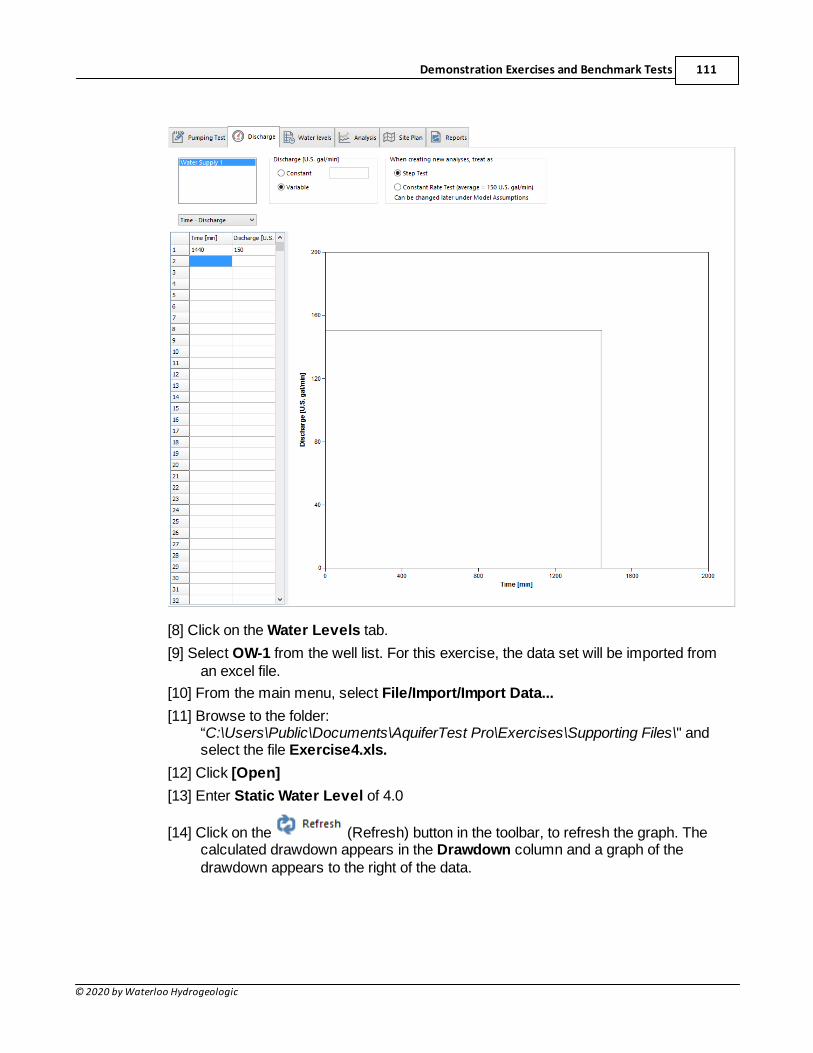
Demonstration Exercises and Benchmark Tests 111
© 2020 by Waterloo Hydrogeologic
[8] Click on the Water Levels tab.
[9] Select OW-1 from the well list. For this exercise, the data set will be imported froman excel file.
[10] From the main menu, select File/Import/Import Data...
[11] Browse to the folder: “C:\Users\Public\Documents\AquiferTest Pro\Exercises\Supporting Files\" andselect the file Exercise4.xls.
[12] Click [Open]
[13] Enter Static Water Level of 4.0
[14] Click on the (Refresh) button in the toolbar, to refresh the graph. Thecalculated drawdown appears in the Drawdown column and a graph of thedrawdown appears to the right of the data.
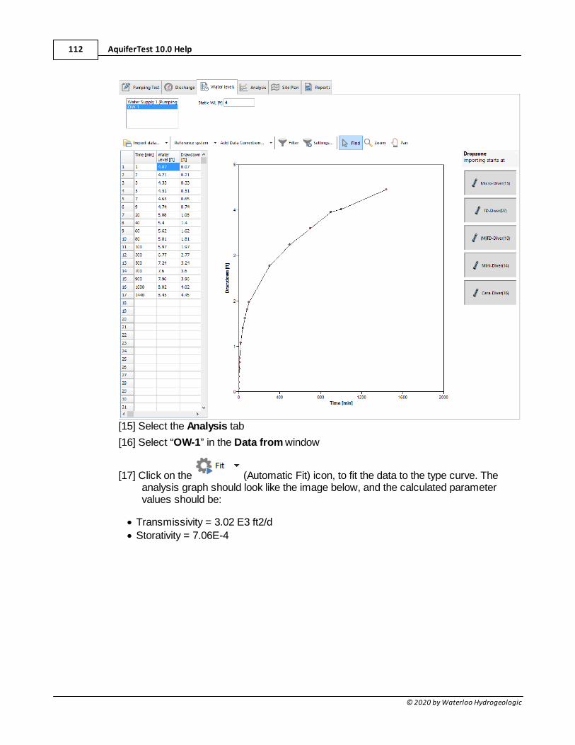
AquiferTest 10.0 Help112
© 2020 by Waterloo Hydrogeologic
[15] Select the Analysis tab
[16] Select “OW-1” in the Data from window
[17] Click on the (Automatic Fit) icon, to fit the data to the type curve. Theanalysis graph should look like the image below, and the calculated parametervalues should be:
· Transmissivity = 3.02 E3 ft2/d
· Storativity = 7.06E-4
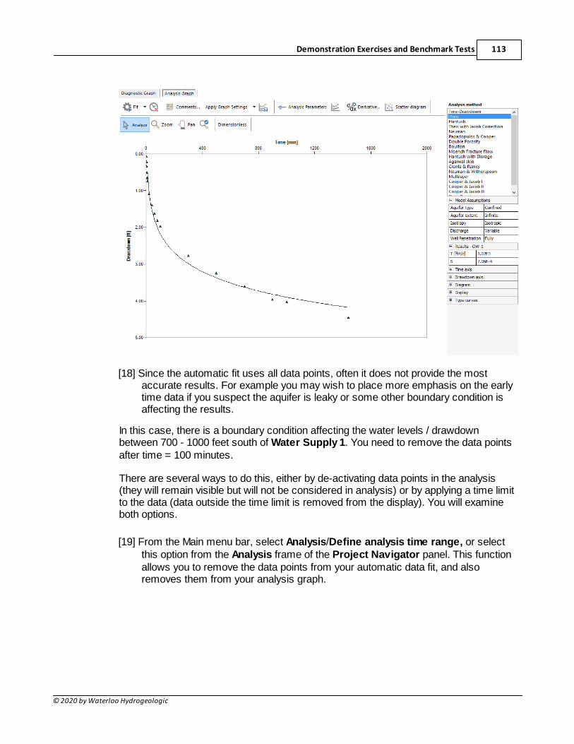
Demonstration Exercises and Benchmark Tests 113
© 2020 by Waterloo Hydrogeologic
[18] Since the automatic fit uses all data points, often it does not provide the mostaccurate results. For example you may wish to place more emphasis on the earlytime data if you suspect the aquifer is leaky or some other boundary condition isaffecting the results.
In this case, there is a boundary condition affecting the water levels / drawdownbetween 700 - 1000 feet south of Water Supply 1. You need to remove the data pointsafter time = 100 minutes.
There are several ways to do this, either by de-activating data points in the analysis(they will remain visible but will not be considered in analysis) or by applying a time limitto the data (data outside the time limit is removed from the display). You will examineboth options.
[19] From the Main menu bar, select Analysis/Define analysis time range, or selectthis option from the Analysis frame of the Project Navigator panel. This functionallows you to remove the data points from your automatic data fit, and alsoremoves them from your analysis graph.
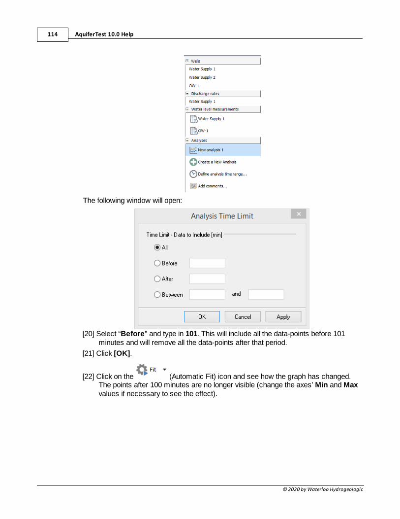
AquiferTest 10.0 Help114
© 2020 by Waterloo Hydrogeologic
The following window will open:
[20] Select “Before” and type in 101. This will include all the data-points before 101minutes and will remove all the data-points after that period.
[21] Click [OK].
[22] Click on the (Automatic Fit) icon and see how the graph has changed.The points after 100 minutes are no longer visible (change the axes’ Min and Maxvalues if necessary to see the effect).
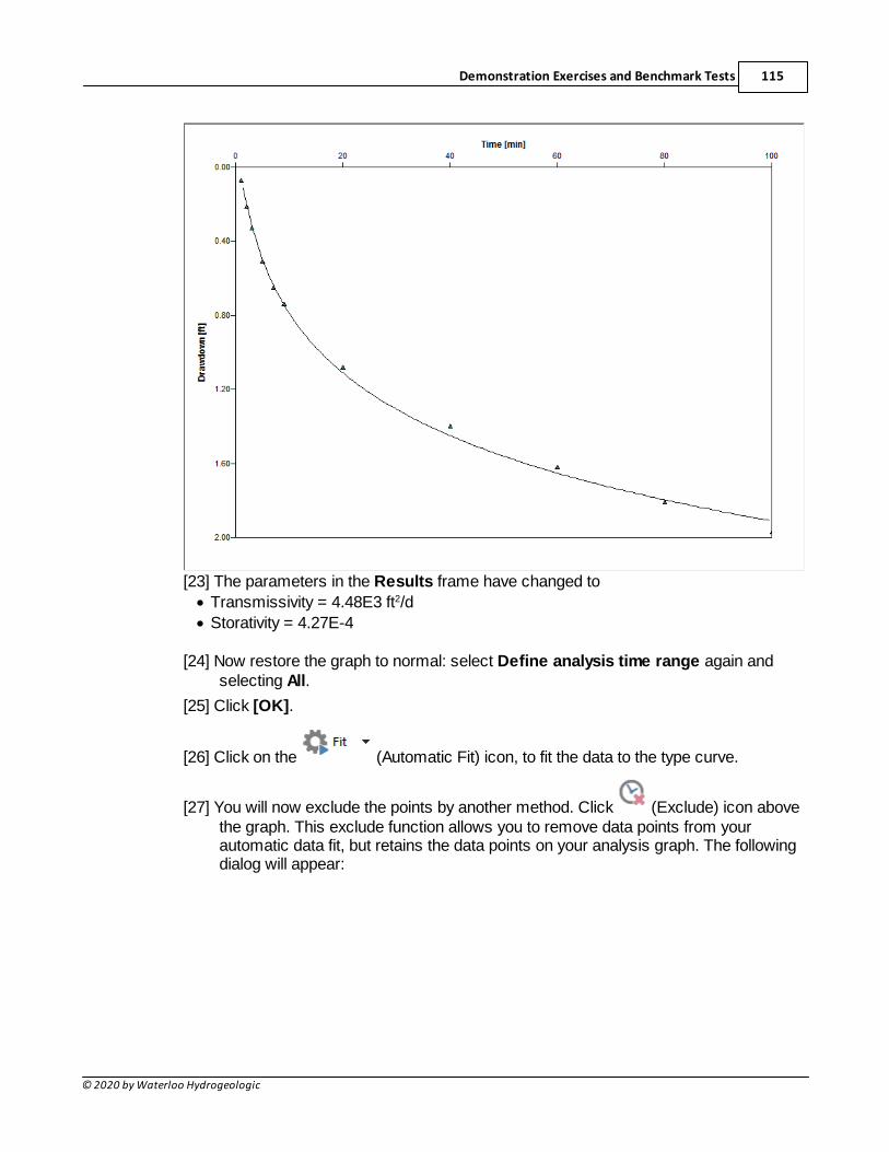
Demonstration Exercises and Benchmark Tests 115
© 2020 by Waterloo Hydrogeologic
[23] The parameters in the Results frame have changed to
· Transmissivity = 4.48E3 ft2/d
· Storativity = 4.27E-4
[24] Now restore the graph to normal: select Define analysis time range again andselecting All.
[25] Click [OK].
[26] Click on the (Automatic Fit) icon, to fit the data to the type curve.
[27] You will now exclude the points by another method. Click (Exclude) icon abovethe graph. This exclude function allows you to remove data points from yourautomatic data fit, but retains the data points on your analysis graph. The followingdialog will appear:
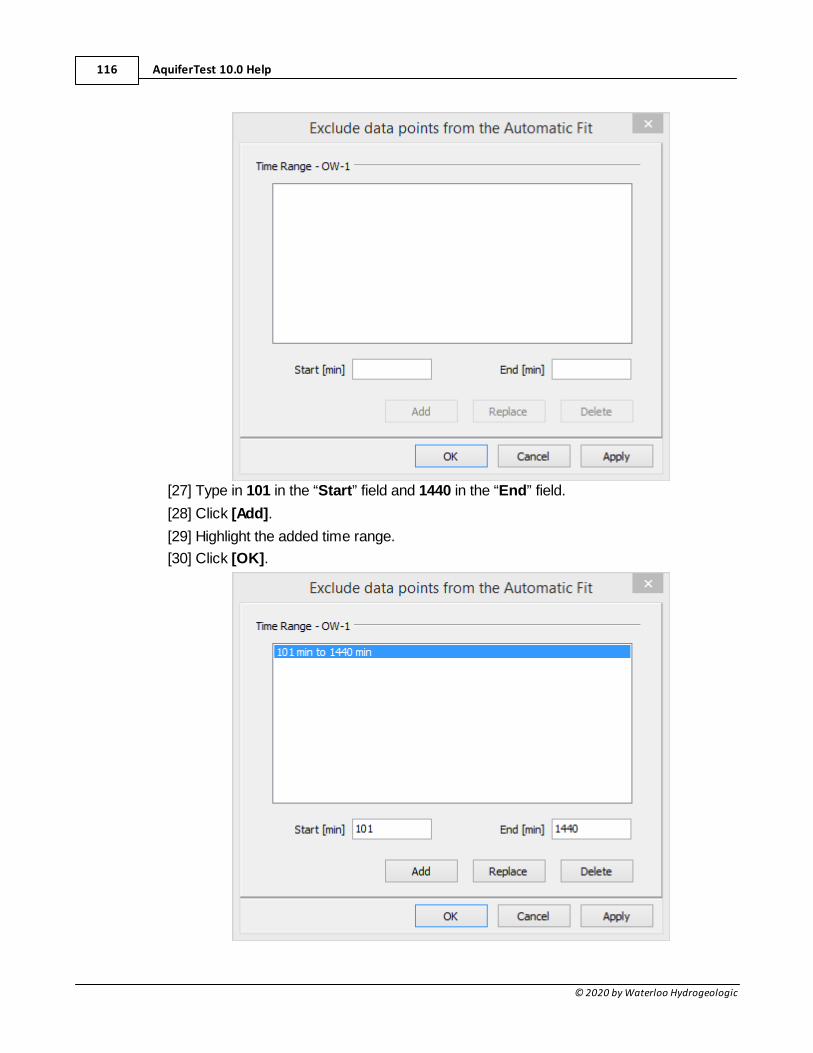
AquiferTest 10.0 Help116
© 2020 by Waterloo Hydrogeologic
[27] Type in 101 in the “Start” field and 1440 in the “End” field.
[28] Click [Add].
[29] Highlight the added time range.
[30] Click [OK].
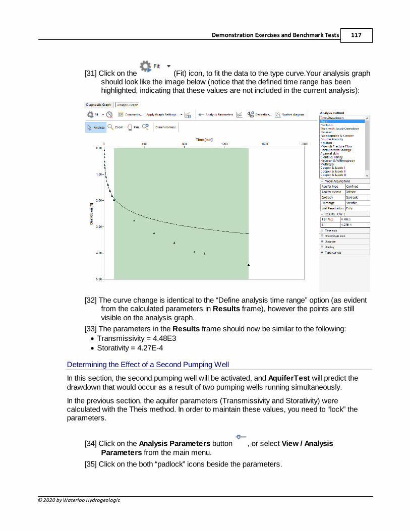
Demonstration Exercises and Benchmark Tests 117
© 2020 by Waterloo Hydrogeologic
[31] Click on the (Fit) icon, to fit the data to the type curve.Your analysis graphshould look like the image below (notice that the defined time range has beenhighlighted, indicating that these values are not included in the current analysis):
[32] The curve change is identical to the “Define analysis time range” option (as evidentfrom the calculated parameters in Results frame), however the points are stillvisible on the analysis graph.
[33] The parameters in the Results frame should now be similar to the following:
· Transmissivity = 4.48E3
· Storativity = 4.27E-4
Determining the Effect of a Second Pumping Well
In this section, the second pumping well will be activated, and AquiferTest will predict thedrawdown that would occur as a result of two pumping wells running simultaneously.
In the previous section, the aquifer parameters (Transmissivity and Storativity) werecalculated with the Theis method. In order to maintain these values, you need to “lock” theparameters.
[34] Click on the Analysis Parameters button , or select View / AnalysisParameters from the main menu.
[35] Click on the both “padlock” icons beside the parameters.
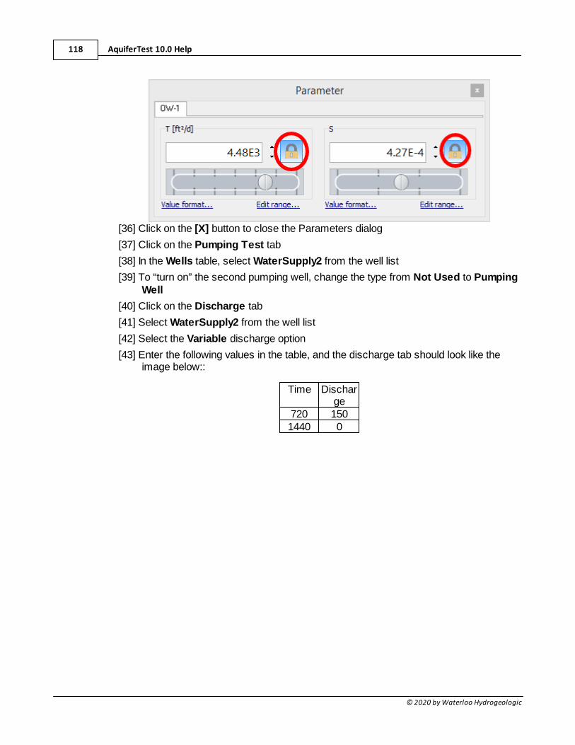
AquiferTest 10.0 Help118
© 2020 by Waterloo Hydrogeologic
[36] Click on the [X] button to close the Parameters dialog
[37] Click on the Pumping Test tab
[38] In the Wells table, select WaterSupply2 from the well list
[39] To “turn on” the second pumping well, change the type from Not Used to PumpingWell
[40] Click on the Discharge tab
[41] Select WaterSupply2 from the well list
[42] Select the Variable discharge option
[43] Enter the following values in the table, and the discharge tab should look like theimage below::
Time Discharge
720 1501440 0
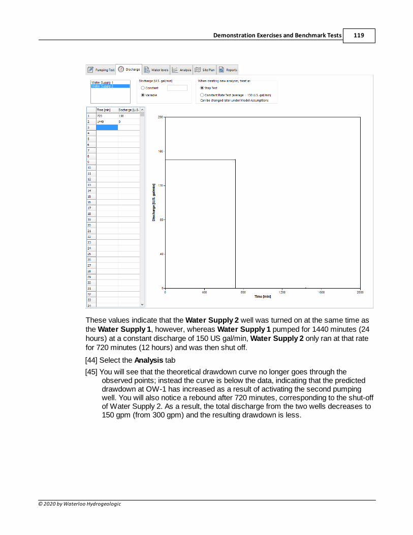
Demonstration Exercises and Benchmark Tests 119
© 2020 by Waterloo Hydrogeologic
These values indicate that the Water Supply 2 well was turned on at the same time asthe Water Supply 1, however, whereas Water Supply 1 pumped for 1440 minutes (24hours) at a constant discharge of 150 US gal/min, Water Supply 2 only ran at that ratefor 720 minutes (12 hours) and was then shut off.
[44] Select the Analysis tab
[45] You will see that the theoretical drawdown curve no longer goes through theobserved points; instead the curve is below the data, indicating that the predicteddrawdown at OW-1 has increased as a result of activating the second pumpingwell. You will also notice a rebound after 720 minutes, corresponding to the shut-offof Water Supply 2. As a result, the total discharge from the two wells decreases to150 gpm (from 300 gpm) and the resulting drawdown is less.
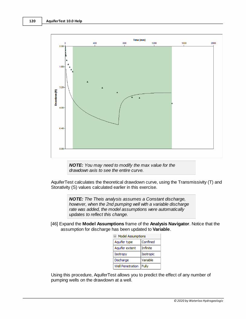
AquiferTest 10.0 Help120
© 2020 by Waterloo Hydrogeologic
NOTE: You may need to modify the max value for thedrawdown axis to see the entire curve.
AquiferTest calculates the theoretical drawdown curve, using the Transmissivity (T) andStorativity (S) values calculated earlier in this exercise.
NOTE: The Theis analysis assumes a Constant discharge,however, when the 2nd pumping well with a variable dischargerate was added, the model assumptions were automaticallyupdates to reflect this change.
[46] Expand the Model Assumptions frame of the Analysis Navigator. Notice that theassumption for discharge has been updated to Variable.
Using this procedure, AquiferTest allows you to predict the effect of any number ofpumping wells on the drawdown at a well.
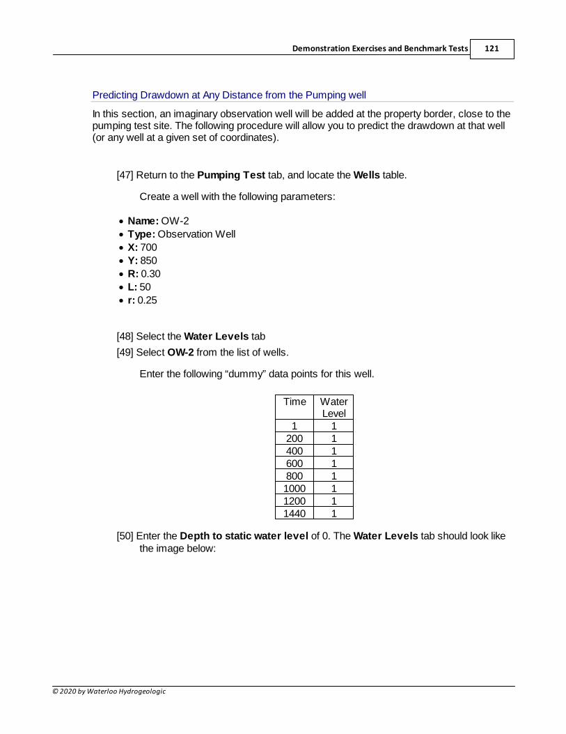
Demonstration Exercises and Benchmark Tests 121
© 2020 by Waterloo Hydrogeologic
Predicting Drawdown at Any Distance from the Pumping well
In this section, an imaginary observation well will be added at the property border, close to thepumping test site. The following procedure will allow you to predict the drawdown at that well(or any well at a given set of coordinates).
[47] Return to the Pumping Test tab, and locate the Wells table.
Create a well with the following parameters:
· Name: OW-2
· Type: Observation Well
· X: 700
· Y: 850
· R: 0.30
· L: 50
· r: 0.25
[48] Select the Water Levels tab
[49] Select OW-2 from the list of wells.
Enter the following “dummy” data points for this well.
Time WaterLevel
1 1200 1400 1600 1800 11000 11200 11440 1
[50] Enter the Depth to static water level of 0. The Water Levels tab should look likethe image below:
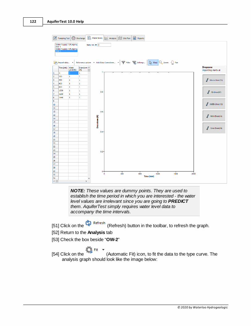
AquiferTest 10.0 Help122
© 2020 by Waterloo Hydrogeologic
NOTE: These values are dummy points. They are used toestablish the time period in which you are interested - the waterlevel values are irrelevant since you are going to PREDICTthem. AquiferTest simply requires water level data toaccompany the time intervals.
[51] Click on the (Refresh) button in the toolbar, to refresh the graph.
[52] Return to the Analysis tab
[53] Check the box beside “OW-2”
[54] Click on the (Automatic Fit) icon, to fit the data to the type curve. Theanalysis graph should look like the image below:
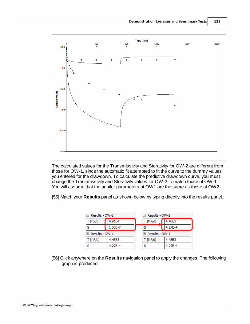
Demonstration Exercises and Benchmark Tests 123
© 2020 by Waterloo Hydrogeologic
The calculated values for the Transmissivity and Storativity for OW-2 are different fromthose for OW-1, since the automatic fit attempted to fit the curve to the dummy valuesyou entered for the drawdown. To calculate the predictive drawdown curve, you mustchange the Transmissivity and Storativity values for OW-2 to match those of OW-1.You will assume that the aquifer parameters at OW1 are the same as those at OW2.
[55] Match your Results panel as shown below by typing directly into the results panel.
[56] Click anywhere on the Results navigation panel to apply the changes. The followinggraph is produced:
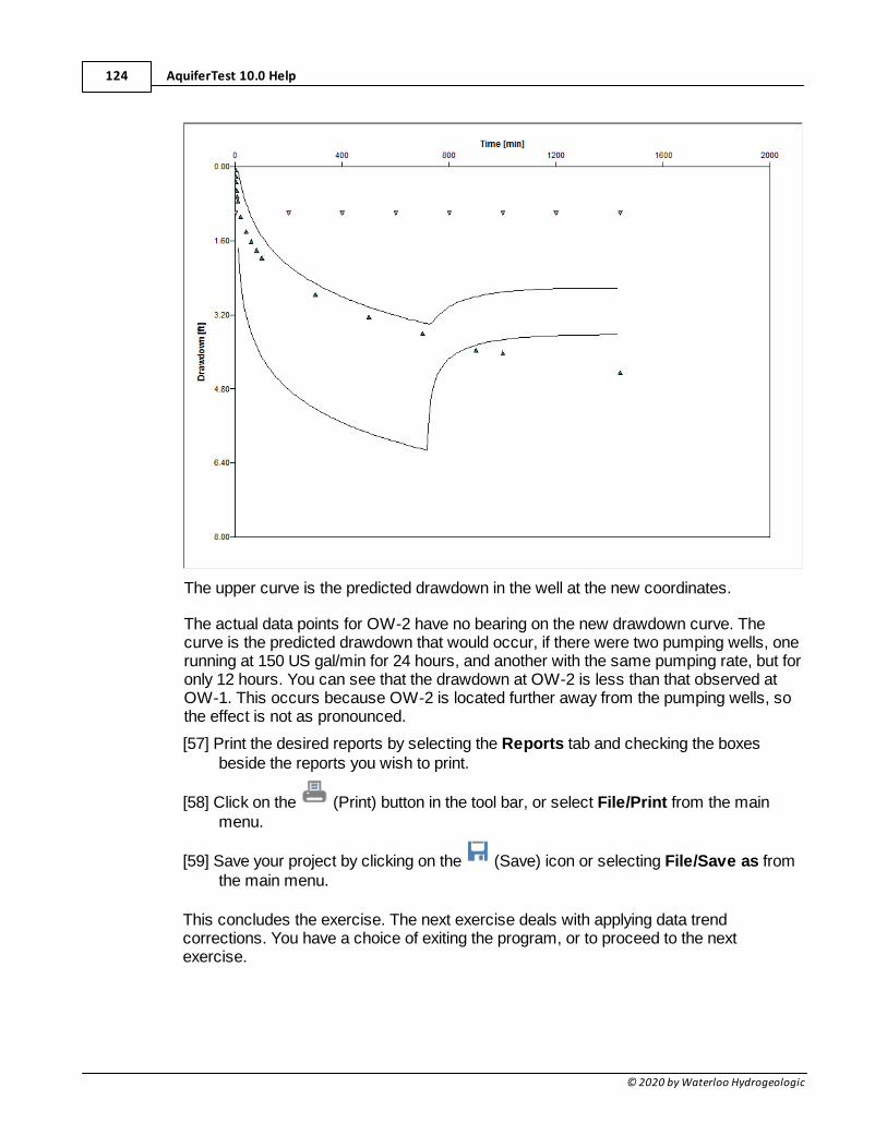
AquiferTest 10.0 Help124
© 2020 by Waterloo Hydrogeologic
The upper curve is the predicted drawdown in the well at the new coordinates.
The actual data points for OW-2 have no bearing on the new drawdown curve. Thecurve is the predicted drawdown that would occur, if there were two pumping wells, onerunning at 150 US gal/min for 24 hours, and another with the same pumping rate, but foronly 12 hours. You can see that the drawdown at OW-2 is less than that observed atOW-1. This occurs because OW-2 is located further away from the pumping wells, sothe effect is not as pronounced.
[57] Print the desired reports by selecting the Reports tab and checking the boxesbeside the reports you wish to print.
[58] Click on the (Print) button in the tool bar, or select File/Print from the mainmenu.
[59] Save your project by clicking on the (Save) icon or selecting File/Save as fromthe main menu.
This concludes the exercise. The next exercise deals with applying data trendcorrections. You have a choice of exiting the program, or to proceed to the nextexercise.
Demonstration Exercises and Benchmark Tests 125
© 2020 by Waterloo Hydrogeologic
2.5 Exercise 5: Adding Data Trend Correction
NOTE: Data Trend Correction Tools are only available in theAquiferTest Pro edition.
This exercise demonstrates the Data Trend Correction feature in AquiferTest. TheAquiferTest project for this exercise is already created; the exercise deals specificallywith the aspect of adding a data trend correction to the drawdown values. For moreinformation on the trend correction, please see Data Pre-Processing.
[1] Start AquiferTest and click on the (Open other project...) button, or ifAquiferTest was already, started then select File/Open from the main menu.
[2] Browse to the folder "C:\Users\Public\Documents\AquiferTest Pro\Exercises\", andselect the project: TrendEffects.hyt
[3] Click [Open].
The pumping test consists of one fully penetrating pumping well, pumping at 0.001 m3/sfor 30,000 s. Drawdown is observed at an observation well located 10 meters away.
[4] Select the Water Levels tab. Take a moment to review the time - drawdown data forWell 2 that was observed for this pumping test.
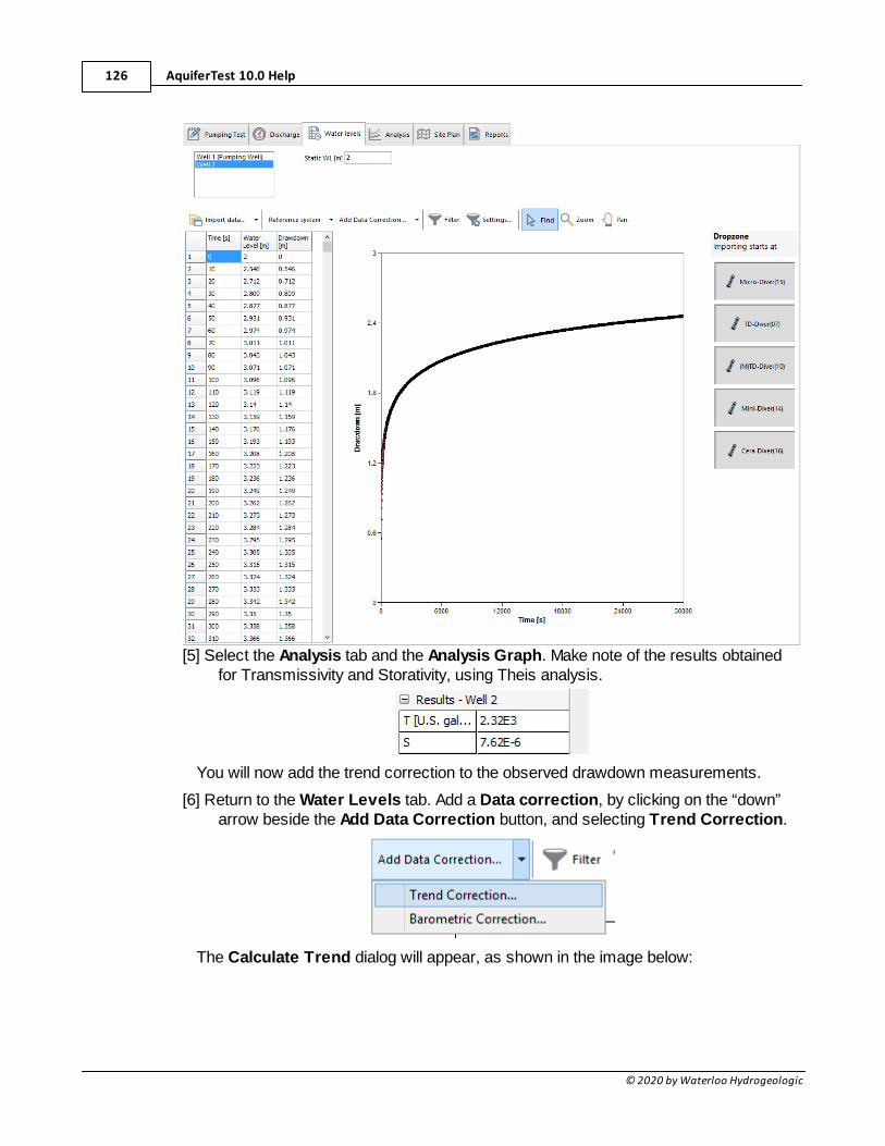
AquiferTest 10.0 Help126
© 2020 by Waterloo Hydrogeologic
[5] Select the Analysis tab and the Analysis Graph. Make note of the results obtainedfor Transmissivity and Storativity, using Theis analysis.
You will now add the trend correction to the observed drawdown measurements.
[6] Return to the Water Levels tab. Add a Data correction, by clicking on the “down”arrow beside the Add Data Correction button, and selecting Trend Correction.
The Calculate Trend dialog will appear, as shown in the image below:
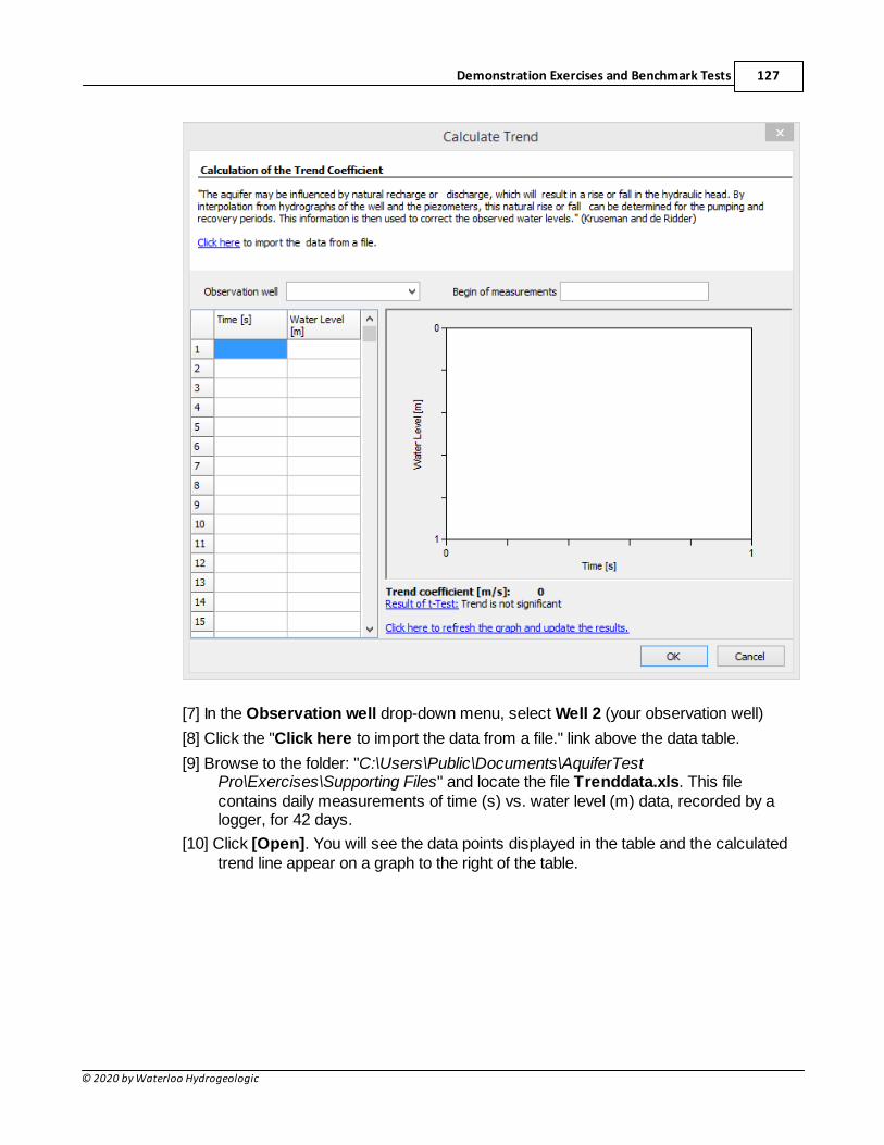
Demonstration Exercises and Benchmark Tests 127
© 2020 by Waterloo Hydrogeologic
[7] In the Observation well drop-down menu, select Well 2 (your observation well)
[8] Click the "Click here to import the data from a file." link above the data table.
[9] Browse to the folder: "C:\Users\Public\Documents\AquiferTestPro\Exercises\Supporting Files" and locate the file Trenddata.xls. This filecontains daily measurements of time (s) vs. water level (m) data, recorded by alogger, for 42 days.
[10] Click [Open]. You will see the data points displayed in the table and the calculatedtrend line appear on a graph to the right of the table.
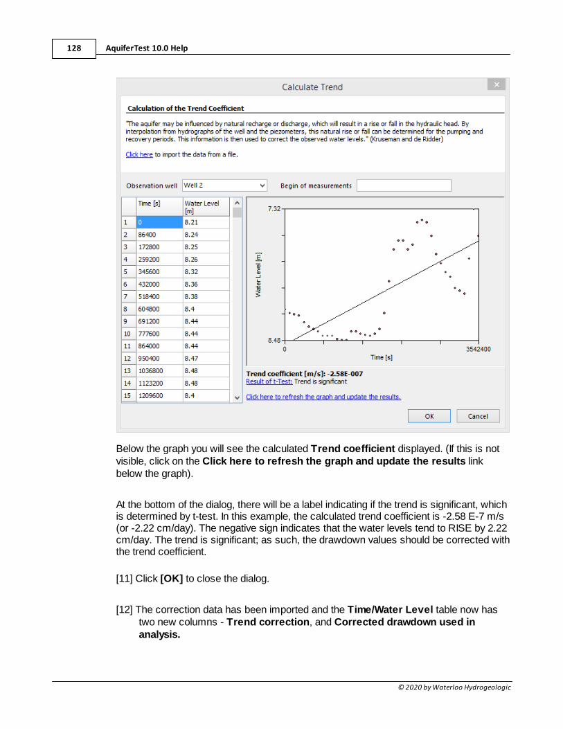
AquiferTest 10.0 Help128
© 2020 by Waterloo Hydrogeologic
Below the graph you will see the calculated Trend coefficient displayed. (If this is notvisible, click on the Click here to refresh the graph and update the results linkbelow the graph).
At the bottom of the dialog, there will be a label indicating if the trend is significant, whichis determined by t-test. In this example, the calculated trend coefficient is -2.58 E-7 m/s(or -2.22 cm/day). The negative sign indicates that the water levels tend to RISE by 2.22cm/day. The trend is significant; as such, the drawdown values should be corrected withthe trend coefficient.
[11] Click [OK] to close the dialog.
[12] The correction data has been imported and the Time/Water Level table now hastwo new columns - Trend correction, and Corrected drawdown used inanalysis.
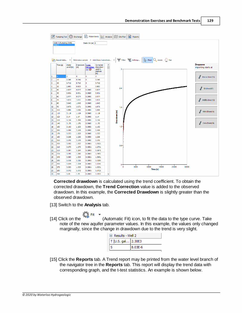
Demonstration Exercises and Benchmark Tests 129
© 2020 by Waterloo Hydrogeologic
Corrected drawdown is calculated using the trend coefficient. To obtain thecorrected drawdown, the Trend Correction value is added to the observeddrawdown. In this example, the Corrected Drawdown is slightly greater than theobserved drawdown.
[13] Switch to the Analysis tab.
[14] Click on the (Automatic Fit) icon, to fit the data to the type curve. Takenote of the new aquifer parameter values. In this example, the values only changedmarginally, since the change in drawdown due to the trend is very slight.
[15] Click the Reports tab. A Trend report may be printed from the water level branch ofthe navigator tree in the Reports tab. This report will display the trend data withcorresponding graph, and the t-test statistics. An example is shown below.
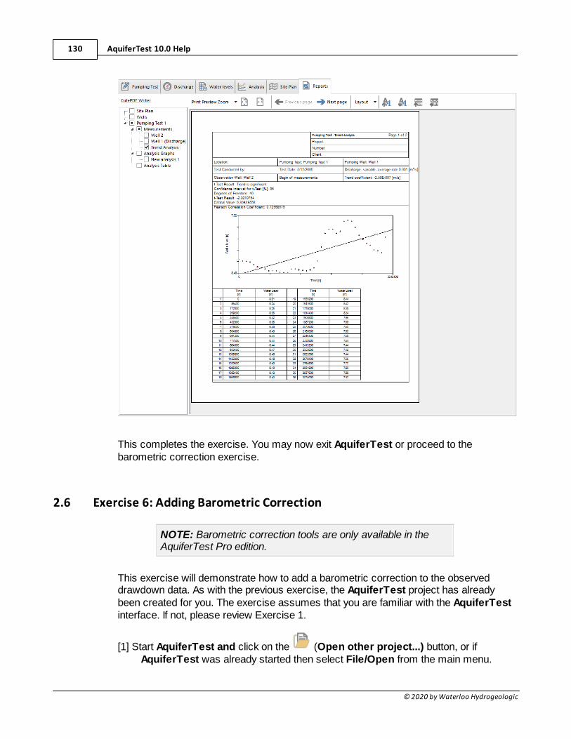
AquiferTest 10.0 Help130
© 2020 by Waterloo Hydrogeologic
This completes the exercise. You may now exit AquiferTest or proceed to thebarometric correction exercise.
2.6 Exercise 6: Adding Barometric Correction
NOTE: Barometric correction tools are only available in theAquiferTest Pro edition.
This exercise will demonstrate how to add a barometric correction to the observeddrawdown data. As with the previous exercise, the AquiferTest project has alreadybeen created for you. The exercise assumes that you are familiar with the AquiferTestinterface. If not, please review Exercise 1.
[1] Start AquiferTest and click on the (Open other project...) button, or ifAquiferTest was already started then select File/Open from the main menu.
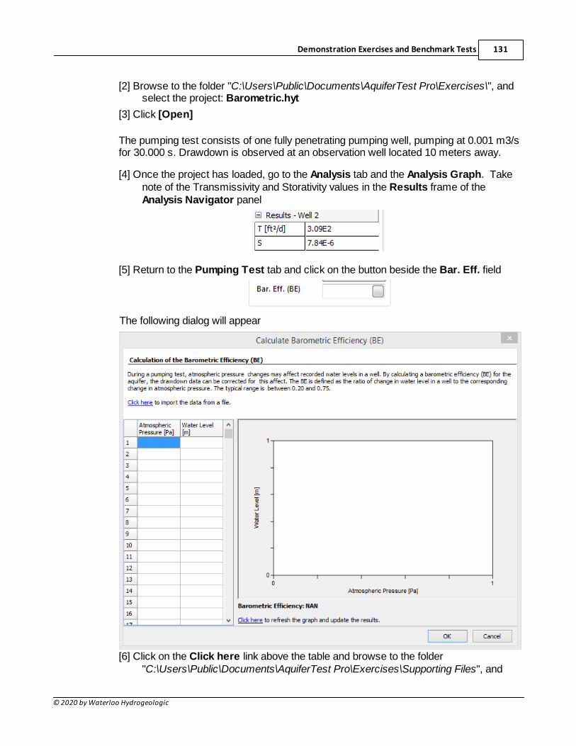
Demonstration Exercises and Benchmark Tests 131
© 2020 by Waterloo Hydrogeologic
[2] Browse to the folder "C:\Users\Public\Documents\AquiferTest Pro\Exercises\", andselect the project: Barometric.hyt
[3] Click [Open]
The pumping test consists of one fully penetrating pumping well, pumping at 0.001 m3/sfor 30.000 s. Drawdown is observed at an observation well located 10 meters away.
[4] Once the project has loaded, go to the Analysis tab and the Analysis Graph. Takenote of the Transmissivity and Storativity values in the Results frame of theAnalysis Navigator panel
[5] Return to the Pumping Test tab and click on the button beside the Bar. Eff. field
The following dialog will appear
[6] Click on the Click here link above the table and browse to the folder "C:\Users\Public\Documents\AquiferTest Pro\Exercises\Supporting Files", and
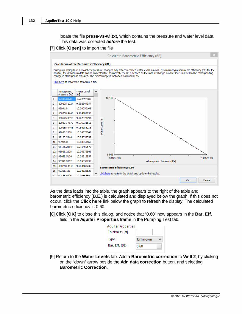
AquiferTest 10.0 Help132
© 2020 by Waterloo Hydrogeologic
locate the file press-vs-wl.txt, which contains the pressure and water level data.This data was collected before the test.
[7] Click [Open] to import the file
As the data loads into the table, the graph appears to the right of the table andbarometric efficiency (B.E.) is calculated and displayed below the graph. If this does notoccur, click the Click here link below the graph to refresh the display. The calculatedbarometric efficiency is 0.60.
[8] Click [OK] to close this dialog, and notice that “0.60” now appears in the Bar. Eff.field in the Aquifer Properties frame in the Pumping Test tab.
[9] Return to the Water Levels tab. Add a Barometric correction to Well 2, by clickingon the “down” arrow beside the Add data correction button, and selectingBarometric Correction.
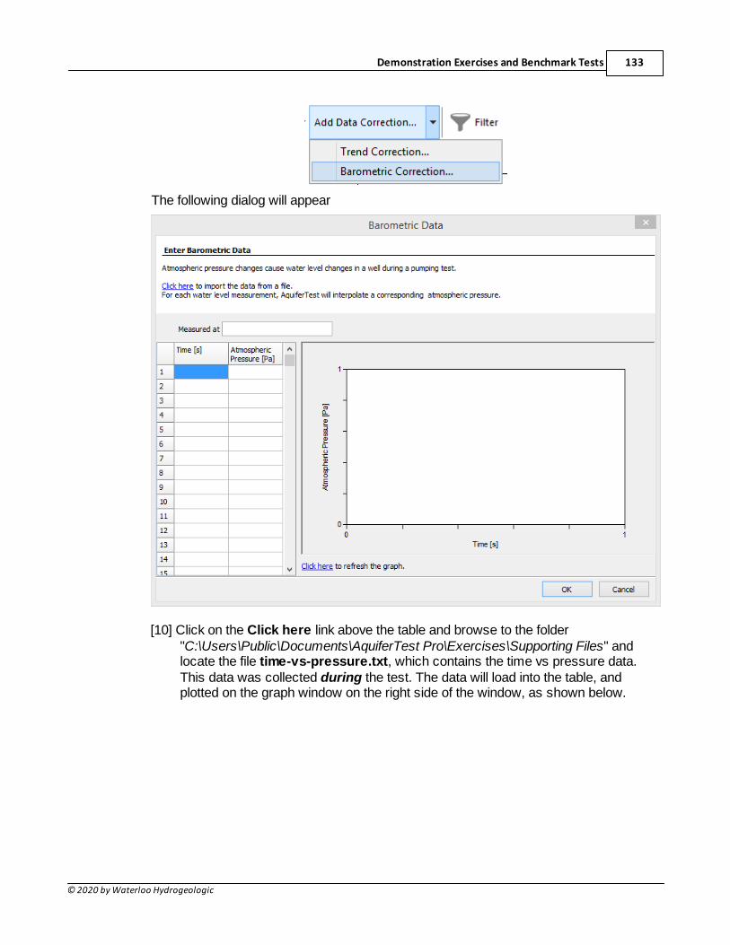
Demonstration Exercises and Benchmark Tests 133
© 2020 by Waterloo Hydrogeologic
The following dialog will appear
[10] Click on the Click here link above the table and browse to the folder"C:\Users\Public\Documents\AquiferTest Pro\Exercises\Supporting Files" andlocate the file time-vs-pressure.txt, which contains the time vs pressure data.This data was collected during the test. The data will load into the table, andplotted on the graph window on the right side of the window, as shown below.
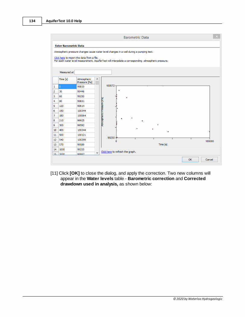
AquiferTest 10.0 Help134
© 2020 by Waterloo Hydrogeologic
[11] Click [OK] to close the dialog, and apply the correction. Two new columns willappear in the Water levels table - Barometric correction and Correcteddrawdown used in analysis, as shown below:
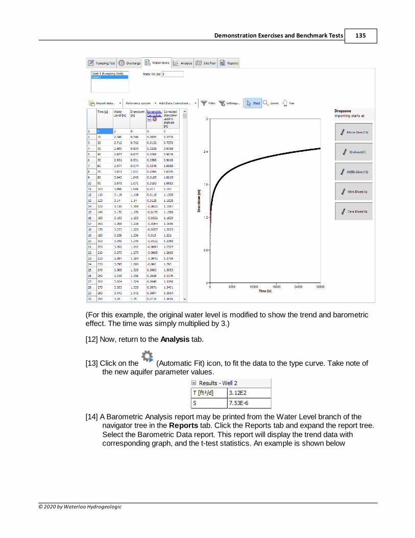
Demonstration Exercises and Benchmark Tests 135
© 2020 by Waterloo Hydrogeologic
(For this example, the original water level is modified to show the trend and barometriceffect. The time was simply multiplied by 3.)
[12] Now, return to the Analysis tab.
[13] Click on the (Automatic Fit) icon, to fit the data to the type curve. Take note ofthe new aquifer parameter values.
[14] A Barometric Analysis report may be printed from the Water Level branch of thenavigator tree in the Reports tab. Click the Reports tab and expand the report tree.Select the Barometric Data report. This report will display the trend data withcorresponding graph, and the t-test statistics. An example is shown below
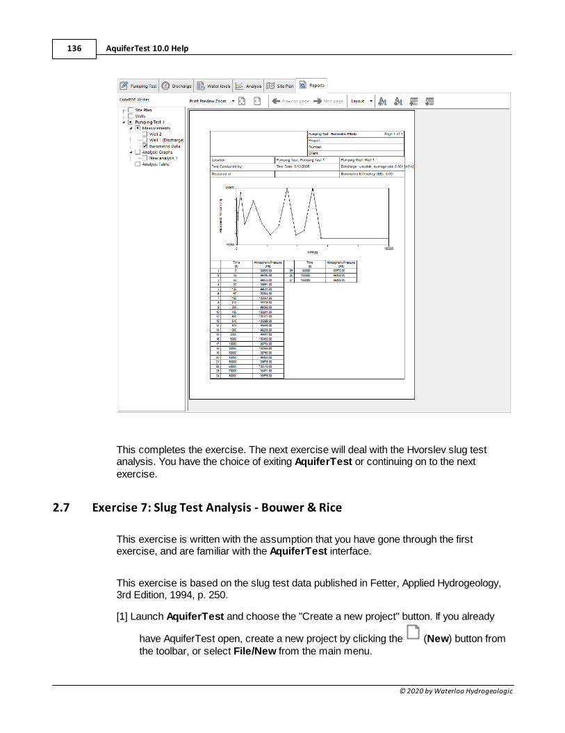
AquiferTest 10.0 Help136
© 2020 by Waterloo Hydrogeologic
This completes the exercise. The next exercise will deal with the Hvorslev slug testanalysis. You have the choice of exiting AquiferTest or continuing on to the nextexercise.
2.7 Exercise 7: Slug Test Analysis - Bouwer & Rice
This exercise is written with the assumption that you have gone through the firstexercise, and are familiar with the AquiferTest interface.
This exercise is based on the slug test data published in Fetter, Applied Hydrogeology,3rd Edition, 1994, p. 250.
[1] Launch AquiferTest and choose the "Create a new project" button. If you already
have AquiferTest open, create a new project by clicking the (New) button fromthe toolbar, or select File/New from the main menu.
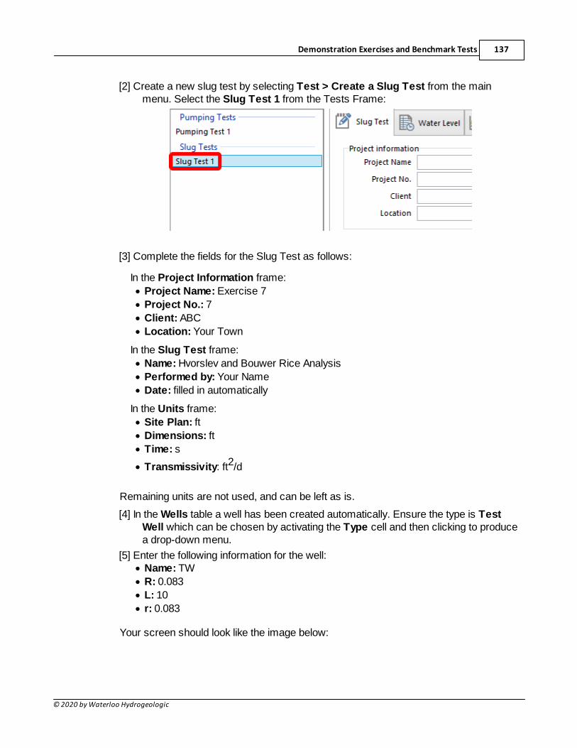
Demonstration Exercises and Benchmark Tests 137
© 2020 by Waterloo Hydrogeologic
[2] Create a new slug test by selecting Test > Create a Slug Test from the mainmenu. Select the Slug Test 1 from the Tests Frame:
[3] Complete the fields for the Slug Test as follows:
In the Project Information frame:
· Project Name: Exercise 7
· Project No.: 7
· Client: ABC
· Location: Your Town
In the Slug Test frame:
· Name: Hvorslev and Bouwer Rice Analysis
· Performed by: Your Name
· Date: filled in automatically
In the Units frame:
· Site Plan: ft
· Dimensions: ft
· Time: s
· Transmissivity: ft2/d
Remaining units are not used, and can be left as is.
[4] In the Wells table a well has been created automatically. Ensure the type is TestWell which can be chosen by activating the Type cell and then clicking to producea drop-down menu.
[5] Enter the following information for the well:· Name: TW
· R: 0.083
· L: 10
· r: 0.083
Your screen should look like the image below:
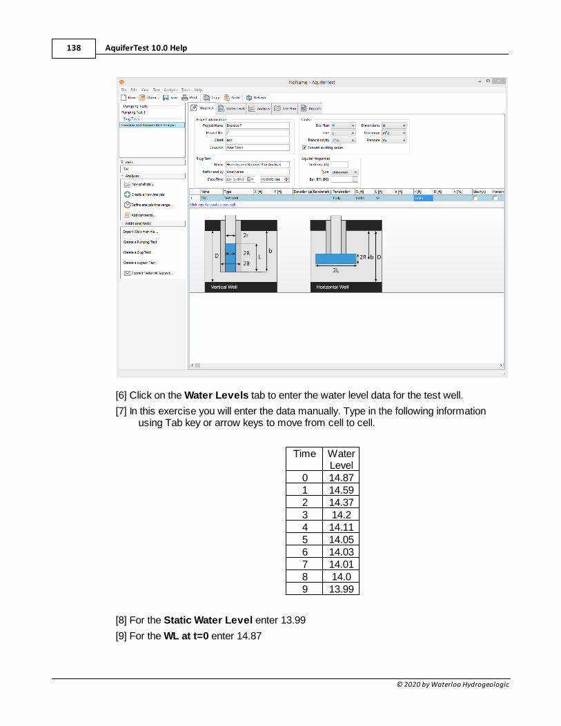
AquiferTest 10.0 Help138
© 2020 by Waterloo Hydrogeologic
[6] Click on the Water Levels tab to enter the water level data for the test well.
[7] In this exercise you will enter the data manually. Type in the following informationusing Tab key or arrow keys to move from cell to cell.
Time WaterLevel
0 14.871 14.592 14.373 14.24 14.115 14.056 14.037 14.018 14.09 13.99
[8] For the Static Water Level enter 13.99
[9] For the WL at t=0 enter 14.87
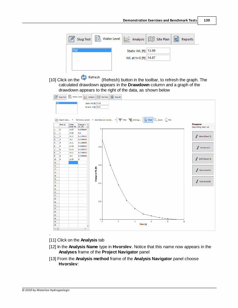
Demonstration Exercises and Benchmark Tests 139
© 2020 by Waterloo Hydrogeologic
[10] Click on the (Refresh) button in the toolbar, to refresh the graph. Thecalculated drawdown appears in the Drawdown column and a graph of thedrawdown appears to the right of the data, as shown below
.
[11] Click on the Analysis tab
[12] In the Analysis Name type in Hvorslev. Notice that this name now appears in theAnalyses frame of the Project Navigator panel
[13] From the Analysis method frame of the Analysis Navigator panel chooseHvorslev:
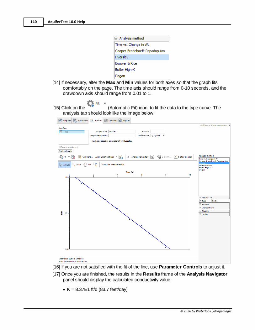
AquiferTest 10.0 Help140
© 2020 by Waterloo Hydrogeologic
[14] If necessary, alter the Max and Min values for both axes so that the graph fitscomfortably on the page. The time axis should range from 0-10 seconds, and thedrawdown axis should range from 0.01 to 1.
[15] Click on the (Automatic Fit) icon, to fit the data to the type curve. Theanalysis tab should look like the image below:
[16] If you are not satisfied with the fit of the line, use Parameter Controls to adjust it.
[17] Once you are finished, the results in the Results frame of the Analysis Navigatorpanel should display the calculated conductivity value:
· K = 8.37E1 ft/d (83.7 feet/day)
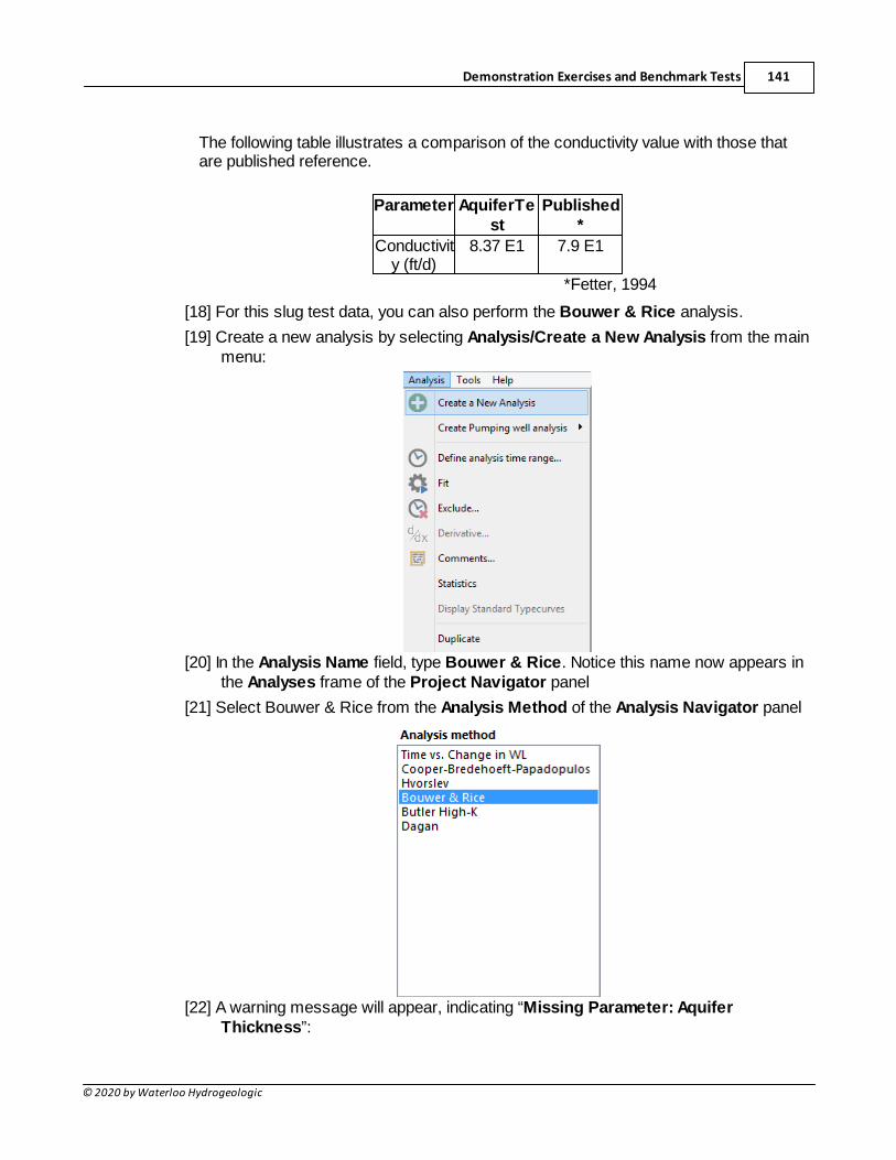
Demonstration Exercises and Benchmark Tests 141
© 2020 by Waterloo Hydrogeologic
The following table illustrates a comparison of the conductivity value with those thatare published reference.
Parameter AquiferTest
Published*
Conductivity (ft/d)
8.37 E1 7.9 E1
*Fetter, 1994
[18] For this slug test data, you can also perform the Bouwer & Rice analysis.
[19] Create a new analysis by selecting Analysis/Create a New Analysis from the mainmenu:
[20] In the Analysis Name field, type Bouwer & Rice. Notice this name now appears inthe Analyses frame of the Project Navigator panel
[21] Select Bouwer & Rice from the Analysis Method of the Analysis Navigator panel
[22] A warning message will appear, indicating “Missing Parameter: AquiferThickness”:
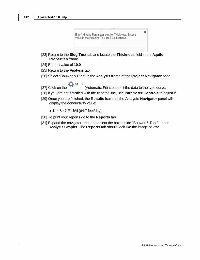
AquiferTest 10.0 Help142
© 2020 by Waterloo Hydrogeologic
[23] Return to the Slug Test tab and locate the Thickness field in the AquiferProperties frame
[24] Enter a value of 10.0
[25] Return to the Analysis tab
[26] Select “Bouwer & Rice” in the Analysis frame of the Project Navigator panel
[27] Click on the (Automatic Fit) icon, to fit the data to the type curve.
[28] If you are not satisfied with the fit of the line, use Parameter Controls to adjust it.
[29] Once you are finished, the Results frame of the Analysis Navigator panel willdisplay the conductivity value:
· K = 6.47 E1 ft/d (64.7 feet/day)
[30] To print your reports go to the Reports tab
[31] Expand the navigator tree, and select the box beside “Bouwer & Rice” underAnalysis Graphs. The Reports tab should look like the image below:
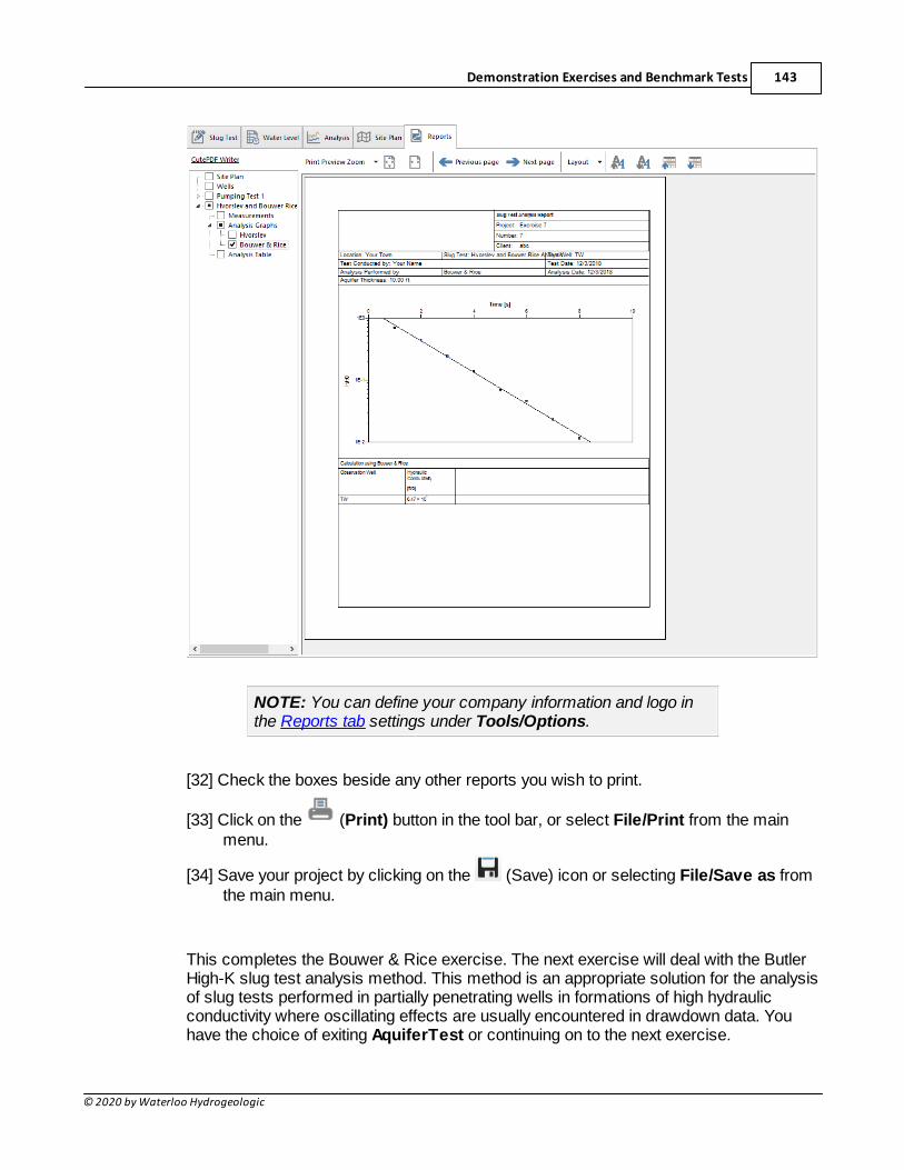
Demonstration Exercises and Benchmark Tests 143
© 2020 by Waterloo Hydrogeologic
NOTE: You can define your company information and logo inthe Reports tab settings under Tools/Options.
[32] Check the boxes beside any other reports you wish to print.
[33] Click on the (Print) button in the tool bar, or select File/Print from the mainmenu.
[34] Save your project by clicking on the (Save) icon or selecting File/Save as fromthe main menu.
This completes the Bouwer & Rice exercise. The next exercise will deal with the ButlerHigh-K slug test analysis method. This method is an appropriate solution for the analysisof slug tests performed in partially penetrating wells in formations of high hydraulicconductivity where oscillating effects are usually encountered in drawdown data. Youhave the choice of exiting AquiferTest or continuing on to the next exercise.
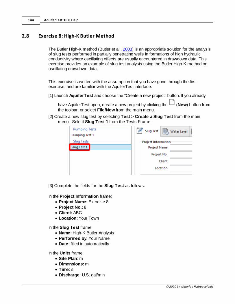
AquiferTest 10.0 Help144
© 2020 by Waterloo Hydrogeologic
2.8 Exercise 8: High-K Butler Method
The Butler High-K method (Butler et al., 2003) is an appropriate solution for the analysisof slug tests performed in partially penetrating wells in formations of high hydraulicconductivity where oscillating effects are usually encountered in drawdown data. Thisexercise provides an example of slug test analysis using the Butler High-K method onoscillating drawdown data.
This exercise is written with the assumption that you have gone through the firstexercise, and are familiar with the AquiferTest interface.
[1] Launch AquiferTest and choose the "Create a new project" button. If you already
have AquiferTest open, create a new project by clicking the (New) button fromthe toolbar, or select File/New from the main menu.
[2] Create a new slug test by selecting Test > Create a Slug Test from the mainmenu. Select Slug Test 1 from the Tests Frame:
[3] Complete the fields for the Slug Test as follows:
In the Project Information frame:
· Project Name: Exercise 8
· Project No.: 8
· Client: ABC
· Location: Your Town
In the Slug Test frame:
· Name: High-K Butler Analysis
· Performed by: Your Name
· Date: filled in automatically
In the Units frame:
· Site Plan: m
· Dimensions: m
· Time: s
· Discharge: U.S. gal/min
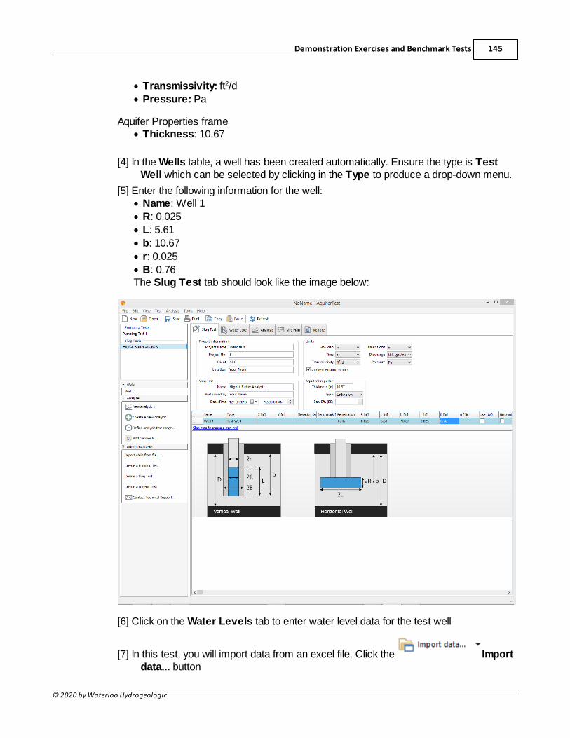
Demonstration Exercises and Benchmark Tests 145
© 2020 by Waterloo Hydrogeologic
· Transmissivity: ft2/d
· Pressure: Pa
Aquifer Properties frame· Thickness: 10.67
[4] In the Wells table, a well has been created automatically. Ensure the type is TestWell which can be selected by clicking in the Type to produce a drop-down menu.
[5] Enter the following information for the well:· Name: Well 1
· R: 0.025
· L: 5.61
· b: 10.67
· r: 0.025
· B: 0.76The Slug Test tab should look like the image below:
[6] Click on the Water Levels tab to enter water level data for the test well
[7] In this test, you will import data from an excel file. Click the Importdata... button
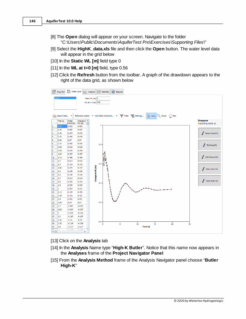
AquiferTest 10.0 Help146
© 2020 by Waterloo Hydrogeologic
[8] The Open dialog will appear on your screen. Navigate to the folder "C:\Users\Public\Documents\AquiferTest Pro\Exercises\Supporting Files\"
[9] Select the HighK_data.xls file and then click the Open button. The water level datawill appear in the grid below
[10] In the Static WL [m] field type 0
[11] In the WL at t=0 [m] field, type 0.56
[12] Click the Refresh button from the toolbar. A graph of the drawdown appears to theright of the data grid, as shown below
[13] Click on the Analysis tab
[14] In the Analysis Name type “High-K Butler”. Notice that this name now appears inthe Analyses frame of the Project Navigator Panel
[15] From the Analysis Method frame of the Analysis Navigator panel choose “ButlerHigh-K”
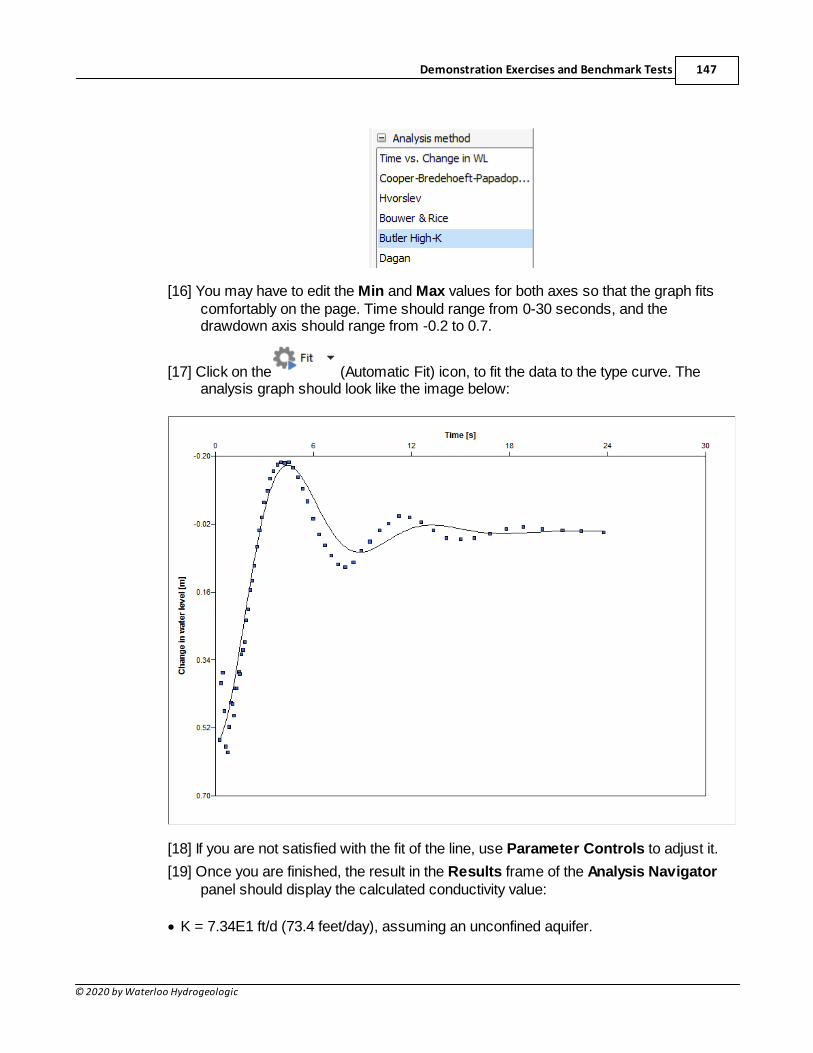
Demonstration Exercises and Benchmark Tests 147
© 2020 by Waterloo Hydrogeologic
[16] You may have to edit the Min and Max values for both axes so that the graph fitscomfortably on the page. Time should range from 0-30 seconds, and thedrawdown axis should range from -0.2 to 0.7.
[17] Click on the (Automatic Fit) icon, to fit the data to the type curve. Theanalysis graph should look like the image below:
[18] If you are not satisfied with the fit of the line, use Parameter Controls to adjust it.
[19] Once you are finished, the result in the Results frame of the Analysis Navigatorpanel should display the calculated conductivity value:
· K = 7.34E1 ft/d (73.4 feet/day), assuming an unconfined aquifer.
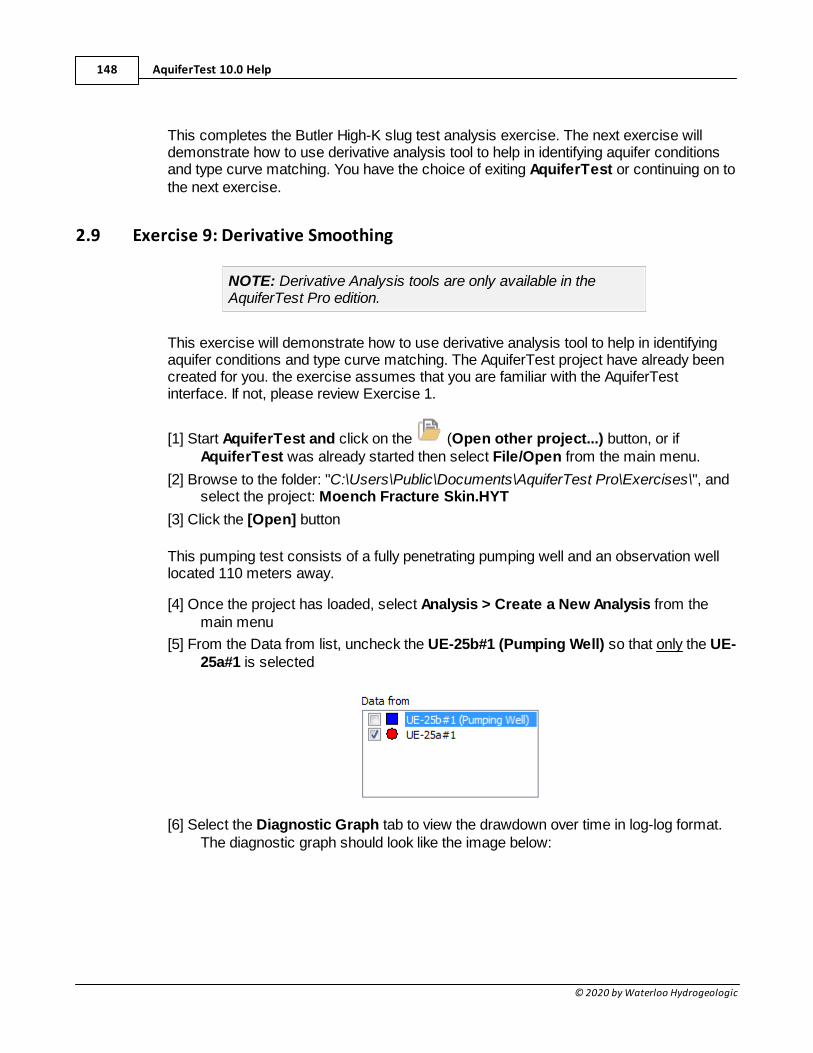
AquiferTest 10.0 Help148
© 2020 by Waterloo Hydrogeologic
This completes the Butler High-K slug test analysis exercise. The next exercise willdemonstrate how to use derivative analysis tool to help in identifying aquifer conditionsand type curve matching. You have the choice of exiting AquiferTest or continuing on tothe next exercise.
2.9 Exercise 9: Derivative Smoothing
NOTE: Derivative Analysis tools are only available in theAquiferTest Pro edition.
This exercise will demonstrate how to use derivative analysis tool to help in identifyingaquifer conditions and type curve matching. The AquiferTest project have already beencreated for you. the exercise assumes that you are familiar with the AquiferTestinterface. If not, please review Exercise 1.
[1] Start AquiferTest and click on the (Open other project...) button, or ifAquiferTest was already started then select File/Open from the main menu.
[2] Browse to the folder: "C:\Users\Public\Documents\AquiferTest Pro\Exercises\", andselect the project: Moench Fracture Skin.HYT
[3] Click the [Open] button
This pumping test consists of a fully penetrating pumping well and an observation welllocated 110 meters away.
[4] Once the project has loaded, select Analysis > Create a New Analysis from themain menu
[5] From the Data from list, uncheck the UE-25b#1 (Pumping Well) so that only the UE-25a#1 is selected
[6] Select the Diagnostic Graph tab to view the drawdown over time in log-log format.The diagnostic graph should look like the image below:
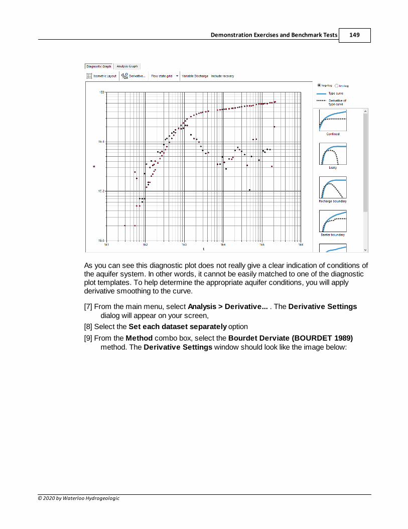
Demonstration Exercises and Benchmark Tests 149
© 2020 by Waterloo Hydrogeologic
As you can see this diagnostic plot does not really give a clear indication of conditions ofthe aquifer system. In other words, it cannot be easily matched to one of the diagnosticplot templates. To help determine the appropriate aquifer conditions, you will applyderivative smoothing to the curve.
[7] From the main menu, select Analysis > Derivative... . The Derivative Settingsdialog will appear on your screen,
[8] Select the Set each dataset separately option
[9] From the Method combo box, select the Bourdet Derviate (BOURDET 1989)method. The Derivative Settings window should look like the image below:
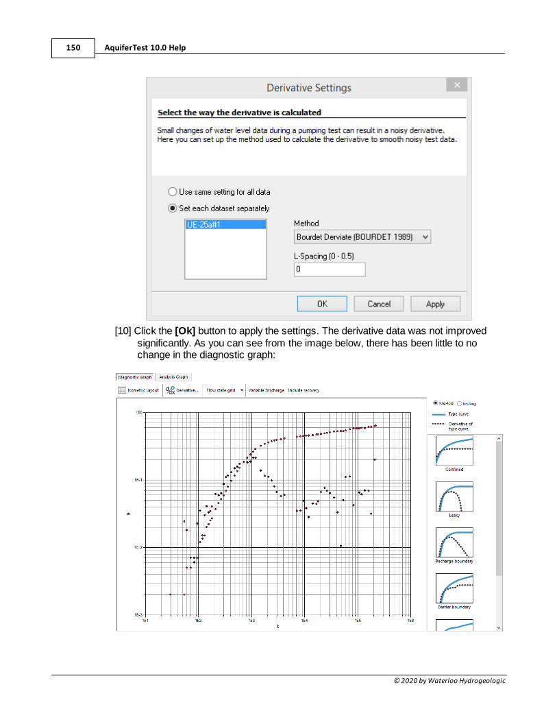
AquiferTest 10.0 Help150
© 2020 by Waterloo Hydrogeologic
[10] Click the [Ok] button to apply the settings. The derivative data was not improvedsignificantly. As you can see from the image below, there has been little to nochange in the diagnostic graph:
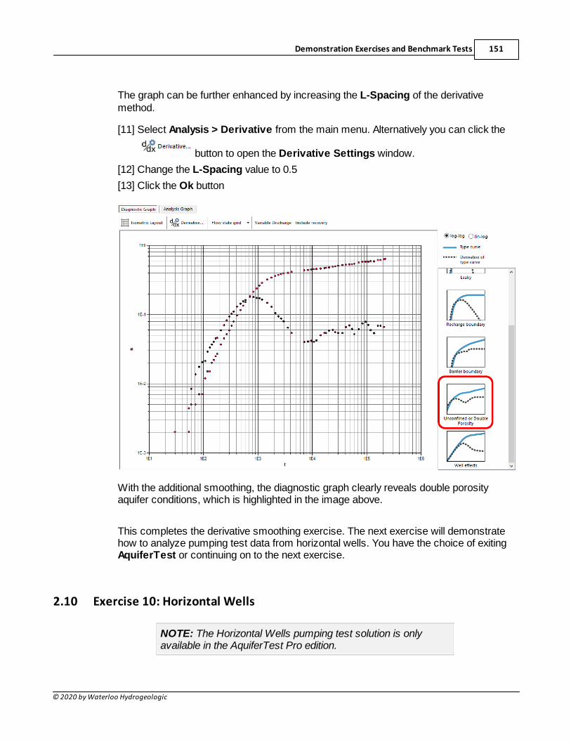
Demonstration Exercises and Benchmark Tests 151
© 2020 by Waterloo Hydrogeologic
The graph can be further enhanced by increasing the L-Spacing of the derivativemethod.
[11] Select Analysis > Derivative from the main menu. Alternatively you can click the
button to open the Derivative Settings window.
[12] Change the L-Spacing value to 0.5
[13] Click the Ok button
With the additional smoothing, the diagnostic graph clearly reveals double porosityaquifer conditions, which is highlighted in the image above.
This completes the derivative smoothing exercise. The next exercise will demonstratehow to analyze pumping test data from horizontal wells. You have the choice of exitingAquiferTest or continuing on to the next exercise.
2.10 Exercise 10: Horizontal Wells
NOTE: The Horizontal Wells pumping test solution is onlyavailable in the AquiferTest Pro edition.
AquiferTest 10.0 Help152
© 2020 by Waterloo Hydrogeologic
For general information about the horizontal well solution in AquiferTest, please refer tothe Section on Horizontal Wells.
In this example, a pumping test was performed in a confined aquifer underlain by animpermeable confining unit with a single pumping well and no observation wellsscreened over. The orientation of the pumping well screen is 90 degrees to the verticalshaft. AquifterTest Pro will be used to analyze the pumping test results.
[1] Launch AquiferTest and choose the "Create a new project" button. If you already
have AquiferTest open, create a new project by clicking the (New) button fromthe toolbar, or select File/New from the main menu.
[2] Complete the fields in the Pumping Test tab as follows:
Project Information frame· Project Name: Exercise 10
· Project No.: 10
· Client: ABC
· Location: Your Town
Pumping Test frame· Name: Clonts and Ramey Analysis
· Performed by: Your Name
· Date: filled in automatically
Units· Site Plan: m
· Time: min
· Transmissivity: m2/d
· Dimensions: m
· Discharge: m3/d
· Pressure: Pa
Aquifer Properties· Thickness: 100
· Type: Confined
[3] All new projects have one default pumping well created in the Wells table (located inthe bottom half of this window). Define the following well parameters for this well:
· Name: PW1
· Type: Pumping Well
· X [m]: 0
· Y[m]: 0
· Penetration: Fully
· R [m]: 0.075
· L [m]: 75
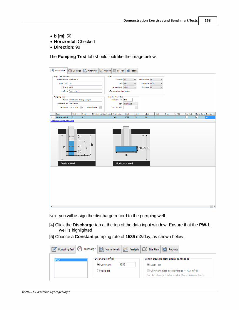
Demonstration Exercises and Benchmark Tests 153
© 2020 by Waterloo Hydrogeologic
· b [m]: 50
· Horizontal: Checked
· Direction: 90
The Pumping Test tab should look like the image below:
Next you will assign the discharge record to the pumping well.
[4] Click the Discharge tab at the top of the data input window. Ensure that the PW-1well is highlighted
[5] Choose a Constant pumping rate of 1536 m3/day, as shown below:
AquiferTest 10.0 Help154
© 2020 by Waterloo Hydrogeologic
Next you will assign water levels to the pumping well.
[6] Select the Water Levels tab.
[7] In the Static WL [m] field, type 0.
[8] In the Measurement point [m] field, type 0. The measurement point represents thedistance from the center point along the length of the horizontal well screen (i.e. thepumping well coordinates) where water level measurements are being measured.
You will now import water level information in the Time - Water Level (TOC) format
[9] Select File > Import > Import Data... from the main menu
[10] Browse to the "C:\Users\Public\Documents\AquiferTest Pro\Exercises\SupportingFiles\" folder
[11] Select the file horizontal.xls
[12] Click the Open button
The Water Levels tab should look like the image below:
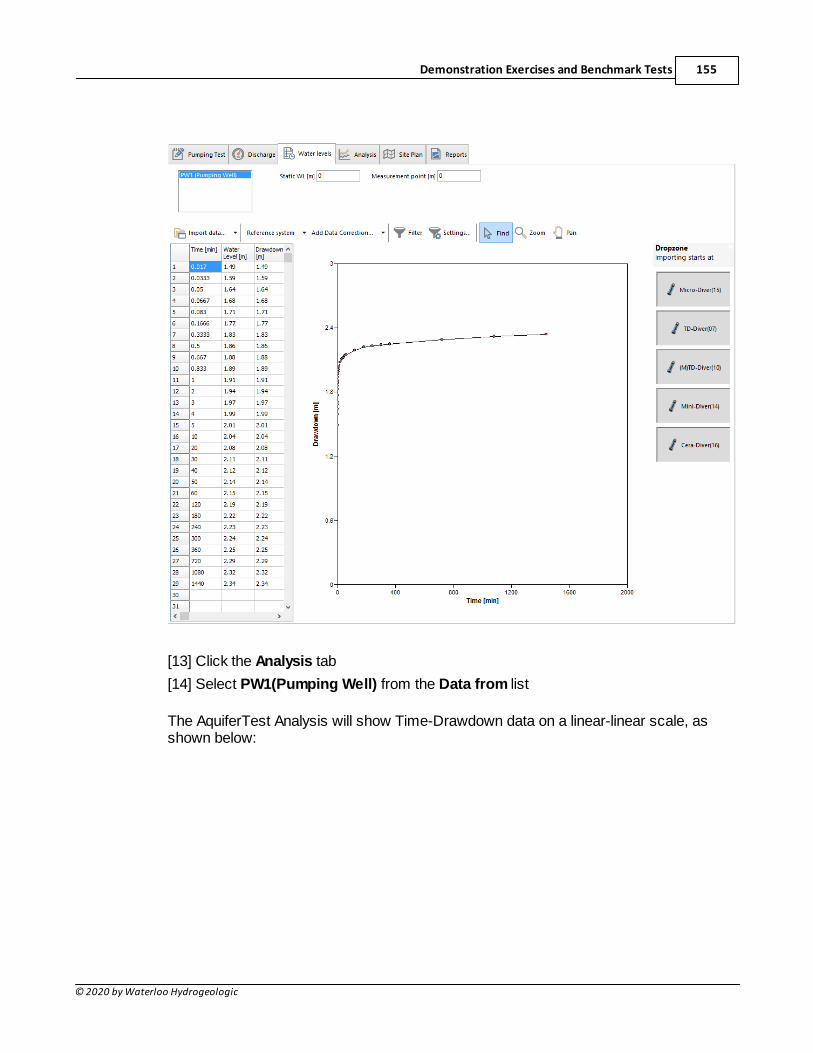
Demonstration Exercises and Benchmark Tests 155
© 2020 by Waterloo Hydrogeologic
[13] Click the Analysis tab
[14] Select PW1(Pumping Well) from the Data from list
The AquiferTest Analysis will show Time-Drawdown data on a linear-linear scale, asshown below:
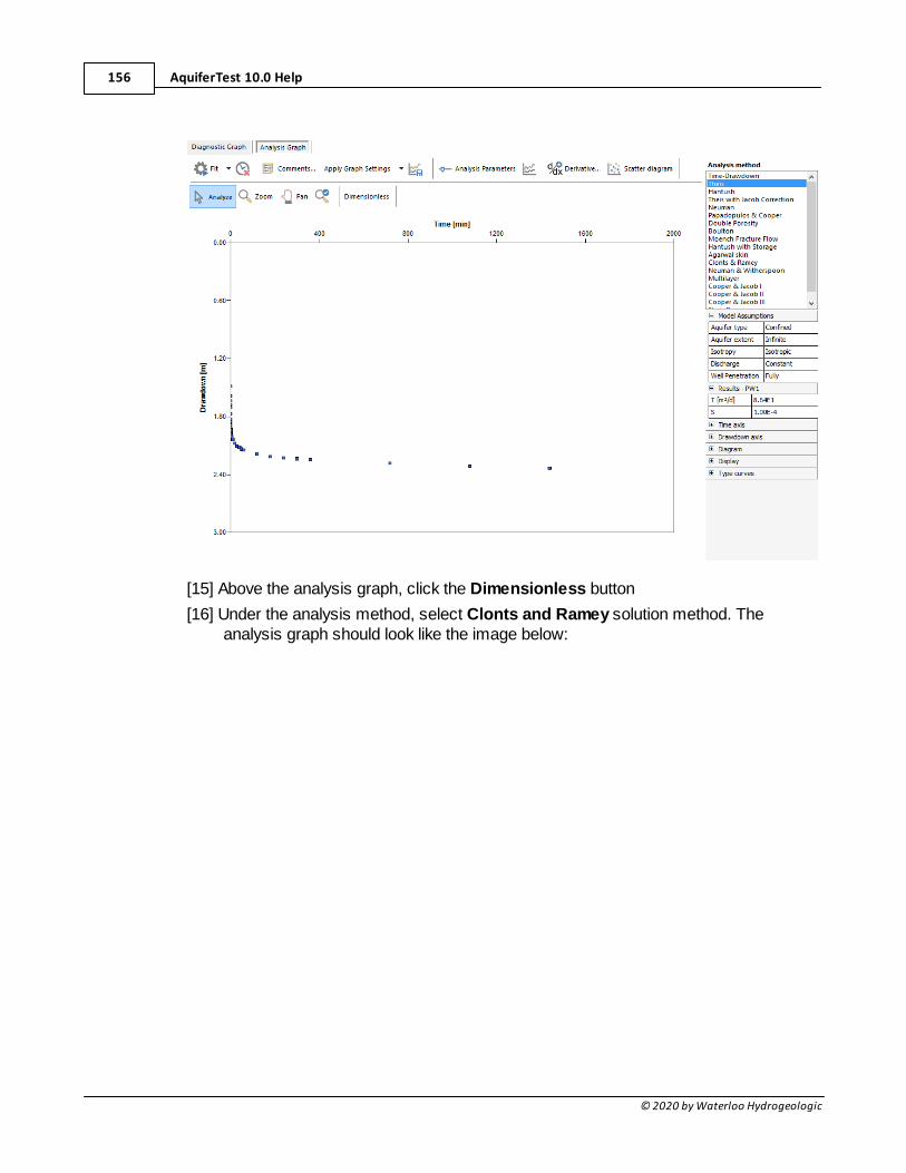
AquiferTest 10.0 Help156
© 2020 by Waterloo Hydrogeologic
[15] Above the analysis graph, click the Dimensionless button
[16] Under the analysis method, select Clonts and Ramey solution method. Theanalysis graph should look like the image below:
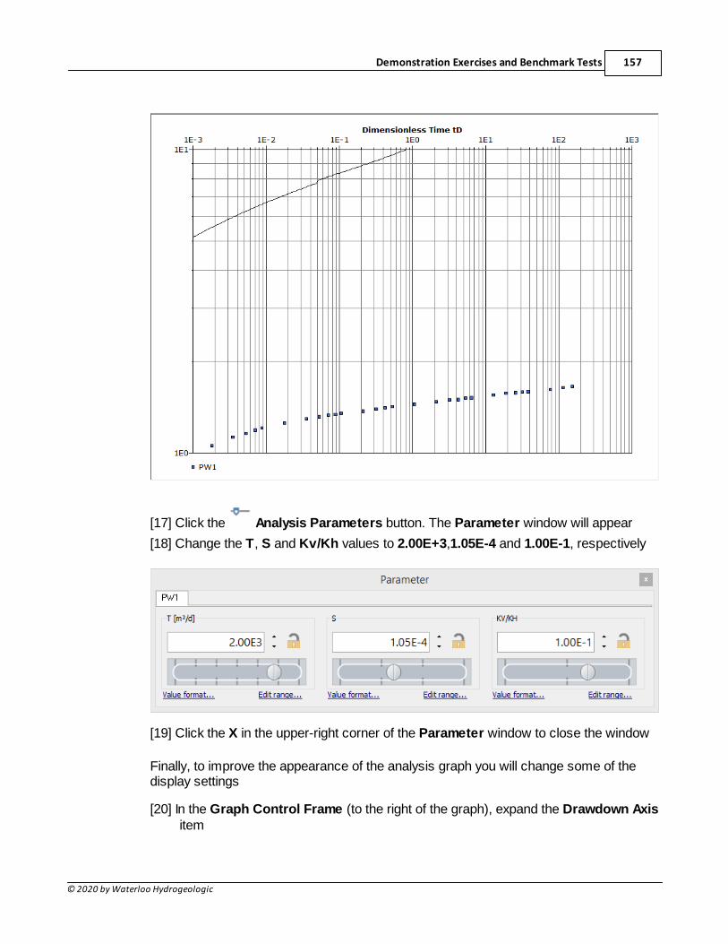
Demonstration Exercises and Benchmark Tests 157
© 2020 by Waterloo Hydrogeologic
[17] Click the Analysis Parameters button. The Parameter window will appear
[18] Change the T, S and Kv/Kh values to 2.00E+3,1.05E-4 and 1.00E-1, respectively
[19] Click the X in the upper-right corner of the Parameter window to close the window
Finally, to improve the appearance of the analysis graph you will change some of thedisplay settings
[20] In the Graph Control Frame (to the right of the graph), expand the Drawdown Axisitem
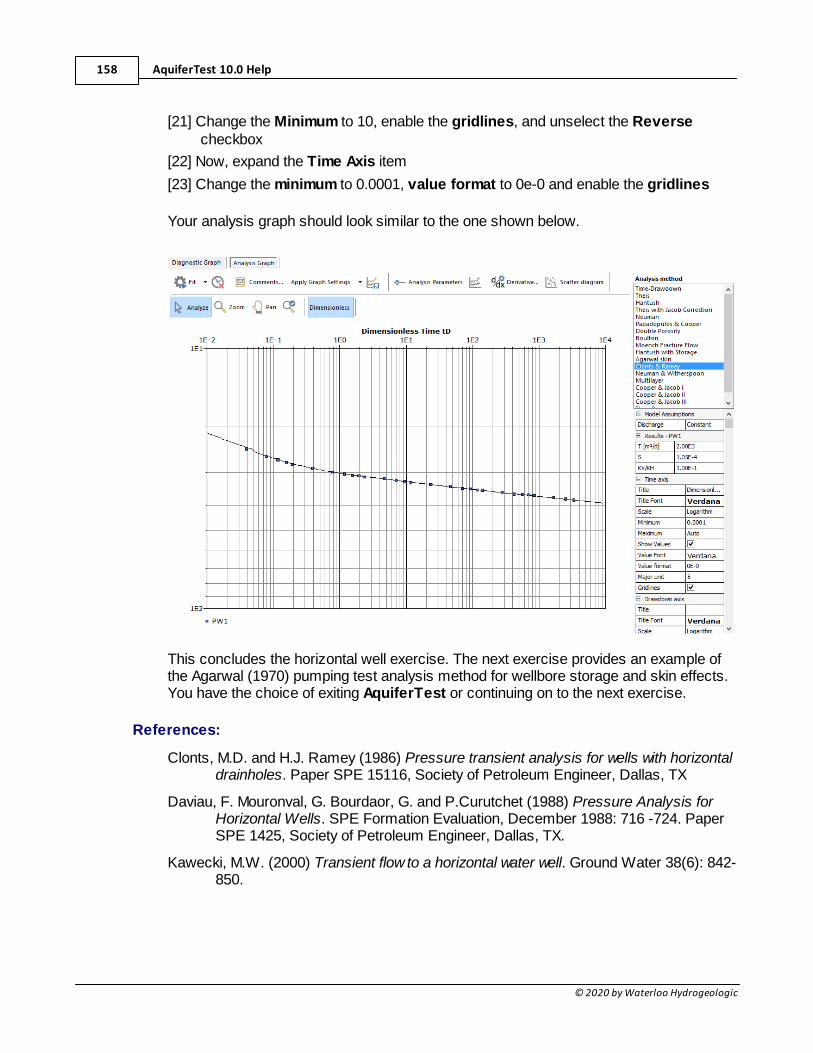
AquiferTest 10.0 Help158
© 2020 by Waterloo Hydrogeologic
[21] Change the Minimum to 10, enable the gridlines, and unselect the Reversecheckbox
[22] Now, expand the Time Axis item
[23] Change the minimum to 0.0001, value format to 0e-0 and enable the gridlines
Your analysis graph should look similar to the one shown below.
This concludes the horizontal well exercise. The next exercise provides an example ofthe Agarwal (1970) pumping test analysis method for wellbore storage and skin effects.You have the choice of exiting AquiferTest or continuing on to the next exercise.
References:
Clonts, M.D. and H.J. Ramey (1986) Pressure transient analysis for wells with horizontaldrainholes. Paper SPE 15116, Society of Petroleum Engineer, Dallas, TX
Daviau, F. Mouronval, G. Bourdaor, G. and P.Curutchet (1988) Pressure Analysis forHorizontal Wells. SPE Formation Evaluation, December 1988: 716 -724. PaperSPE 1425, Society of Petroleum Engineer, Dallas, TX.
Kawecki, M.W. (2000) Transient flow to a horizontal water well. Ground Water 38(6): 842-850.
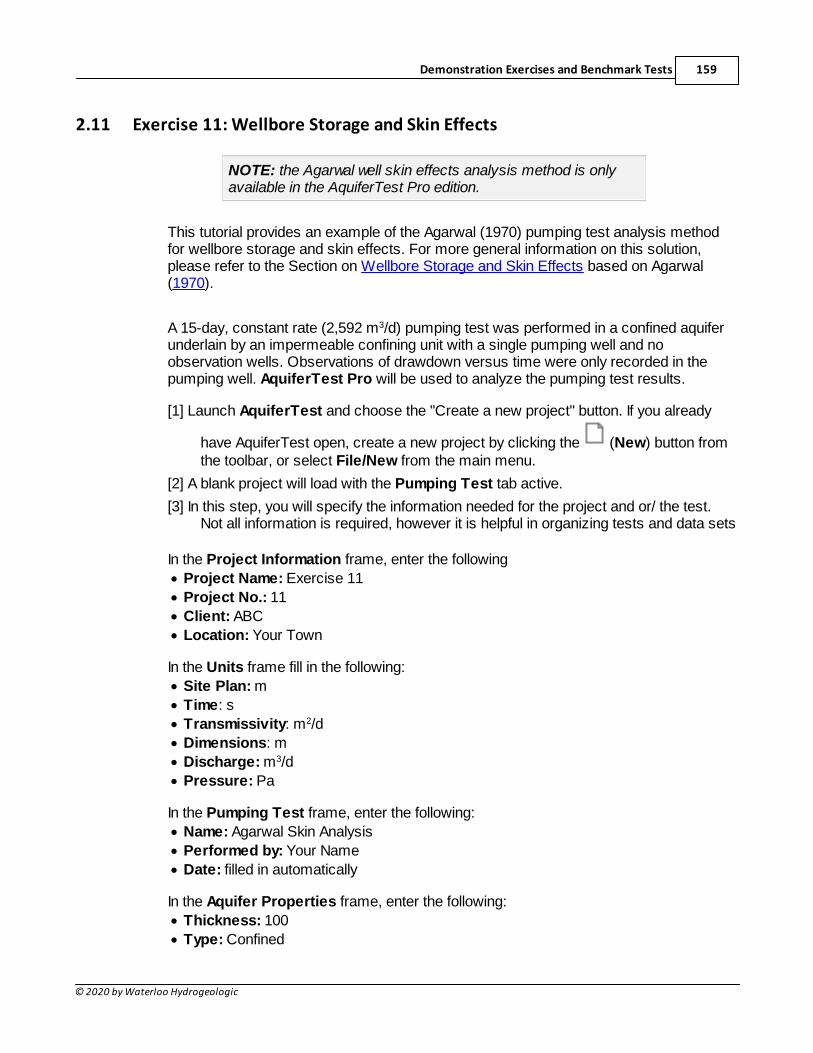
Demonstration Exercises and Benchmark Tests 159
© 2020 by Waterloo Hydrogeologic
2.11 Exercise 11: Wellbore Storage and Skin Effects
NOTE: the Agarwal well skin effects analysis method is onlyavailable in the AquiferTest Pro edition.
This tutorial provides an example of the Agarwal (1970) pumping test analysis methodfor wellbore storage and skin effects. For more general information on this solution,please refer to the Section on Wellbore Storage and Skin Effects based on Agarwal(1970).
A 15-day, constant rate (2,592 m3/d) pumping test was performed in a confined aquiferunderlain by an impermeable confining unit with a single pumping well and noobservation wells. Observations of drawdown versus time were only recorded in thepumping well. AquiferTest Pro will be used to analyze the pumping test results.
[1] Launch AquiferTest and choose the "Create a new project" button. If you already
have AquiferTest open, create a new project by clicking the (New) button fromthe toolbar, or select File/New from the main menu.
[2] A blank project will load with the Pumping Test tab active.
[3] In this step, you will specify the information needed for the project and or/ the test.Not all information is required, however it is helpful in organizing tests and data sets
In the Project Information frame, enter the following
· Project Name: Exercise 11
· Project No.: 11
· Client: ABC
· Location: Your Town
In the Units frame fill in the following:
· Site Plan: m
· Time: s
· Transmissivity: m2/d
· Dimensions: m
· Discharge: m3/d
· Pressure: Pa
In the Pumping Test frame, enter the following:
· Name: Agarwal Skin Analysis
· Performed by: Your Name
· Date: filled in automatically
In the Aquifer Properties frame, enter the following:
· Thickness: 100
· Type: Confined
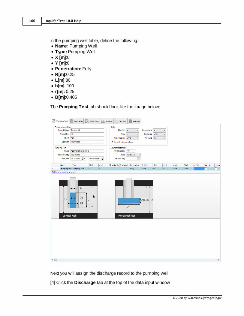
AquiferTest 10.0 Help160
© 2020 by Waterloo Hydrogeologic
In the pumping well table, define the following:· Name: Pumping Well
· Type: Pumping Well
· X [m]:0
· Y [m]:0
· Penetration: Fully
· R[m]:0.25
· L[m]:80
· b[m]: 100
· r[m]: 0.25
· B[m]:0.405
The Pumping Test tab should look like the image below:
Next you will assign the discharge record to the pumping well
[4] Click the Discharge tab at the top of the data input window
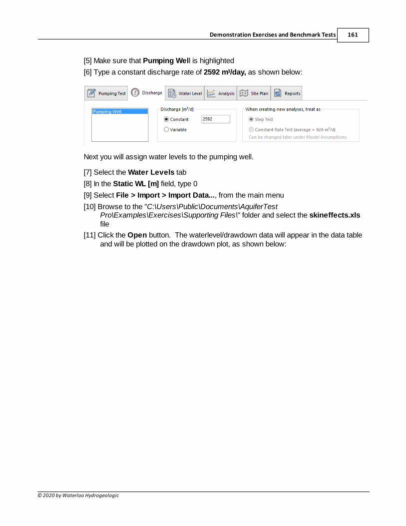
Demonstration Exercises and Benchmark Tests 161
© 2020 by Waterloo Hydrogeologic
[5] Make sure that Pumping Well is highlighted
[6] Type a constant discharge rate of 2592 m3/day, as shown below:
Next you will assign water levels to the pumping well.
[7] Select the Water Levels tab
[8] In the Static WL [m] field, type 0
[9] Select File > Import > Import Data..., from the main menu
[10] Browse to the "C:\Users\Public\Documents\AquiferTestPro\Examples\Exercises\Supporting Files\" folder and select the skineffects.xlsfile
[11] Click the Open button. The waterlevel/drawdown data will appear in the data tableand will be plotted on the drawdown plot, as shown below:
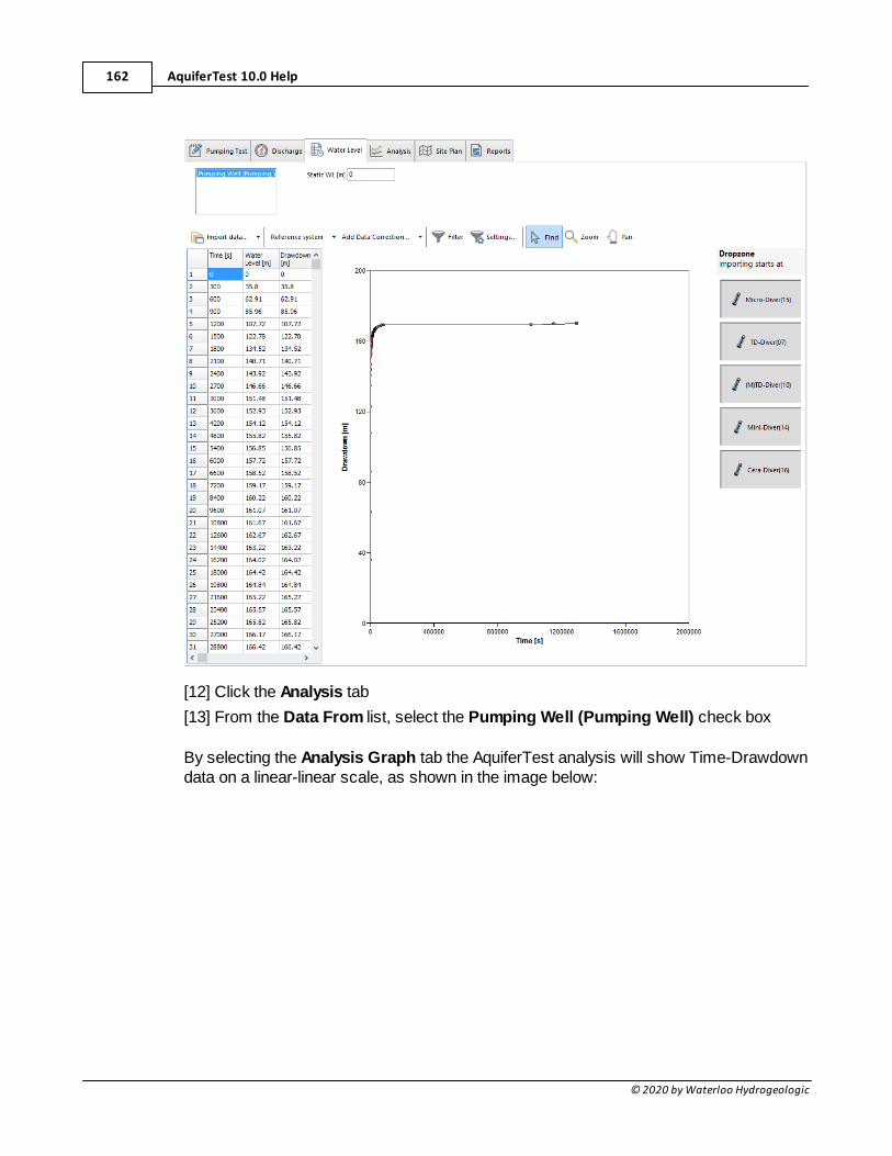
AquiferTest 10.0 Help162
© 2020 by Waterloo Hydrogeologic
[12] Click the Analysis tab
[13] From the Data From list, select the Pumping Well (Pumping Well) check box
By selecting the Analysis Graph tab the AquiferTest analysis will show Time-Drawdowndata on a linear-linear scale, as shown in the image below:
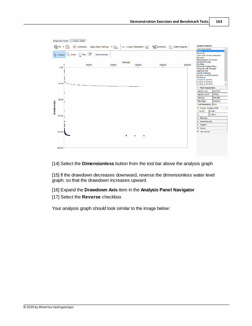
Demonstration Exercises and Benchmark Tests 163
© 2020 by Waterloo Hydrogeologic
[14] Select the Dimensionless button from the tool bar above the analysis graph
[15] If the drawdown decreases downward, reverse the dimensionless water levelgraph, so that the drawdown increases upward.
[16] Expand the Drawdown Axis item in the Analysis Panel Navigator
[17] Select the Reverse checkbox
Your analysis graph should look similar to the image below:
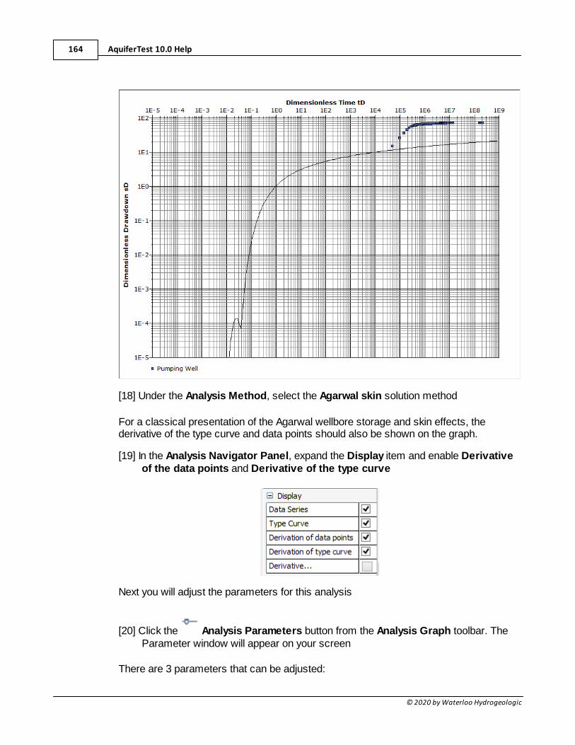
AquiferTest 10.0 Help164
© 2020 by Waterloo Hydrogeologic
[18] Under the Analysis Method, select the Agarwal skin solution method
For a classical presentation of the Agarwal wellbore storage and skin effects, thederivative of the type curve and data points should also be shown on the graph.
[19] In the Analysis Navigator Panel, expand the Display item and enable Derivativeof the data points and Derivative of the type curve
Next you will adjust the parameters for this analysis
[20] Click the Analysis Parameters button from the Analysis Graph toolbar. TheParameter window will appear on your screen
There are 3 parameters that can be adjusted:
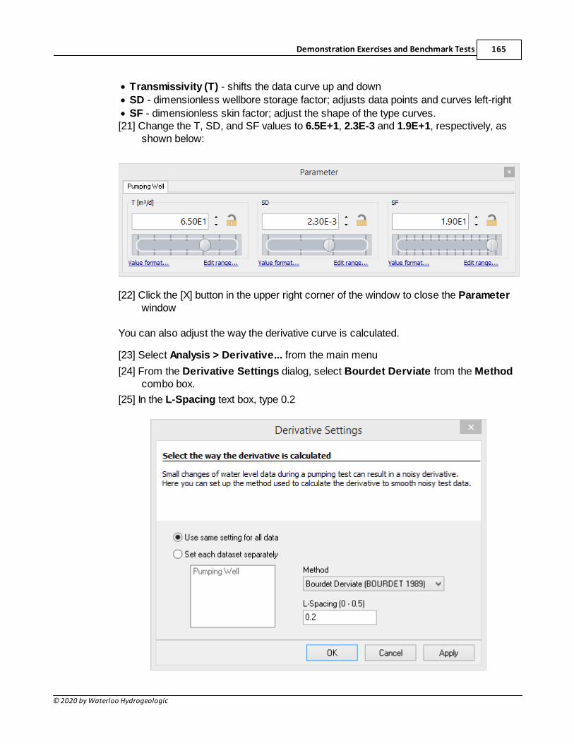
Demonstration Exercises and Benchmark Tests 165
© 2020 by Waterloo Hydrogeologic
· Transmissivity (T) - shifts the data curve up and down
· SD - dimensionless wellbore storage factor; adjusts data points and curves left-right
· SF - dimensionless skin factor; adjust the shape of the type curves.[21] Change the T, SD, and SF values to 6.5E+1, 2.3E-3 and 1.9E+1, respectively, as
shown below:
[22] Click the [X] button in the upper right corner of the window to close the Parameterwindow
You can also adjust the way the derivative curve is calculated.
[23] Select Analysis > Derivative... from the main menu
[24] From the Derivative Settings dialog, select Bourdet Derviate from the Methodcombo box.
[25] In the L-Spacing text box, type 0.2
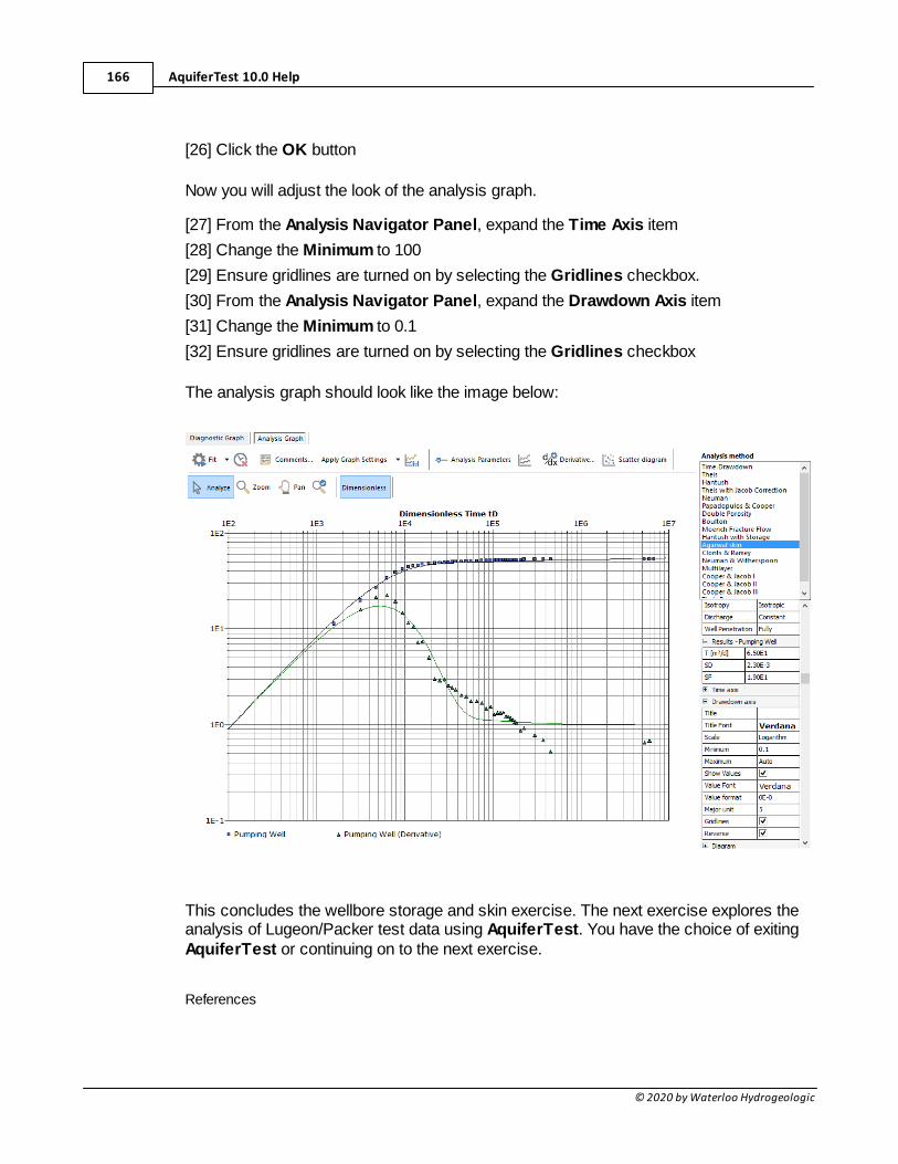
AquiferTest 10.0 Help166
© 2020 by Waterloo Hydrogeologic
[26] Click the OK button
Now you will adjust the look of the analysis graph.
[27] From the Analysis Navigator Panel, expand the Time Axis item
[28] Change the Minimum to 100
[29] Ensure gridlines are turned on by selecting the Gridlines checkbox.
[30] From the Analysis Navigator Panel, expand the Drawdown Axis item
[31] Change the Minimum to 0.1
[32] Ensure gridlines are turned on by selecting the Gridlines checkbox
The analysis graph should look like the image below:
This concludes the wellbore storage and skin exercise. The next exercise explores theanalysis of Lugeon/Packer test data using AquiferTest. You have the choice of exitingAquiferTest or continuing on to the next exercise.
References
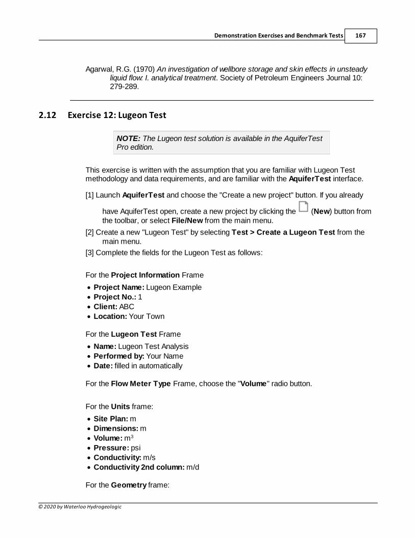
Demonstration Exercises and Benchmark Tests 167
© 2020 by Waterloo Hydrogeologic
Agarwal, R.G. (1970) An investigation of wellbore storage and skin effects in unsteadyliquid flow: I. analytical treatment. Society of Petroleum Engineers Journal 10:279-289.
2.12 Exercise 12: Lugeon Test
NOTE: The Lugeon test solution is available in the AquiferTestPro edition.
This exercise is written with the assumption that you are familiar with Lugeon Testmethodology and data requirements, and are familiar with the AquiferTest interface.
[1] Launch AquiferTest and choose the "Create a new project" button. If you already
have AquiferTest open, create a new project by clicking the (New) button fromthe toolbar, or select File/New from the main menu.
[2] Create a new "Lugeon Test" by selecting Test > Create a Lugeon Test from themain menu.
[3] Complete the fields for the Lugeon Test as follows:
For the Project Information Frame
· Project Name: Lugeon Example
· Project No.: 1
· Client: ABC
· Location: Your Town
For the Lugeon Test Frame
· Name: Lugeon Test Analysis
· Performed by: Your Name
· Date: filled in automatically
For the Flow Meter Type Frame, choose the "Volume" radio button.
For the Units frame:
· Site Plan: m
· Dimensions: m
· Volume: m3
· Pressure: psi
· Conductivity: m/s
· Conductivity 2nd column: m/d
For the Geometry frame:
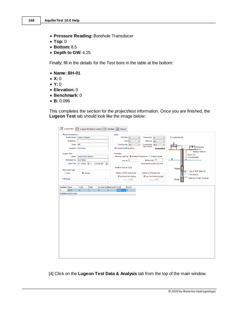
AquiferTest 10.0 Help168
© 2020 by Waterloo Hydrogeologic
· Pressure Reading: Borehole Transducer
· Top: 0
· Bottom: 8.5
· Depth to GW: 4.25
Finally, fill in the details for the Test bore in the table at the bottom:
· Name: BH-01
· X: 0
· Y: 0
· Elevation: 0
· Benchmark: 0
· B: 0.096
This completes the section for the project/test information. Once you are finished, theLugeon Test tab should look like the image below:
[4] Click on the Lugeon Test Data & Analysis tab from the top of the main window.
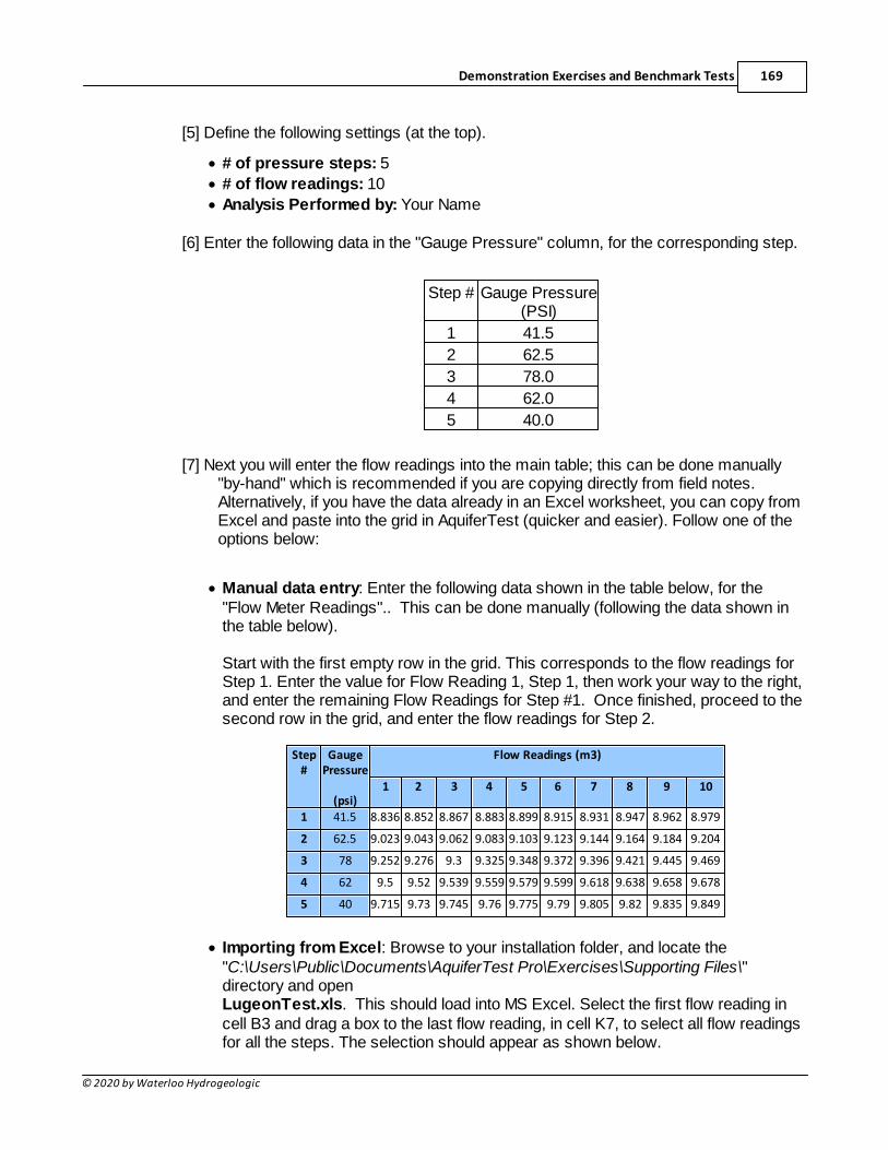
Demonstration Exercises and Benchmark Tests 169
© 2020 by Waterloo Hydrogeologic
[5] Define the following settings (at the top).
· # of pressure steps: 5
· # of flow readings: 10
· Analysis Performed by: Your Name
[6] Enter the following data in the "Gauge Pressure" column, for the corresponding step.
Step # Gauge Pressure(PSI)
1 41.5
2 62.5
3 78.0
4 62.0
5 40.0
[7] Next you will enter the flow readings into the main table; this can be done manually"by-hand" which is recommended if you are copying directly from field notes.Alternatively, if you have the data already in an Excel worksheet, you can copy fromExcel and paste into the grid in AquiferTest (quicker and easier). Follow one of theoptions below:
· Manual data entry: Enter the following data shown in the table below, for the"Flow Meter Readings".. This can be done manually (following the data shown inthe table below).
Start with the first empty row in the grid. This corresponds to the flow readings forStep 1. Enter the value for Flow Reading 1, Step 1, then work your way to the right,and enter the remaining Flow Readings for Step #1. Once finished, proceed to thesecond row in the grid, and enter the flow readings for Step 2.
Step#
GaugePressure
(psi)
Flow Readings (m3)
1 2 3 4 5 6 7 8 9 10
1 41.5 8.836 8.852 8.867 8.883 8.899 8.915 8.931 8.947 8.962 8.979
2 62.5 9.023 9.043 9.062 9.083 9.103 9.123 9.144 9.164 9.184 9.204
3 78 9.252 9.276 9.3 9.325 9.348 9.372 9.396 9.421 9.445 9.469
4 62 9.5 9.52 9.539 9.559 9.579 9.599 9.618 9.638 9.658 9.678
5 40 9.715 9.73 9.745 9.76 9.775 9.79 9.805 9.82 9.835 9.849
· Importing from Excel: Browse to your installation folder, and locate the "C:\Users\Public\Documents\AquiferTest Pro\Exercises\Supporting Files\"directory and open LugeonTest.xls. This should load into MS Excel. Select the first flow reading incell B3 and drag a box to the last flow reading, in cell K7, to select all flow readingsfor all the steps. The selection should appear as shown below.
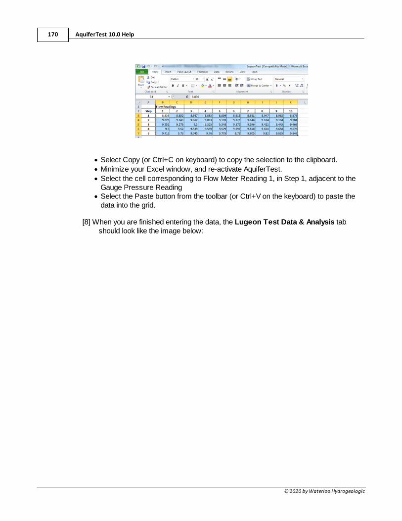
AquiferTest 10.0 Help170
© 2020 by Waterloo Hydrogeologic
· Select Copy (or Ctrl+C on keyboard) to copy the selection to the clipboard.
· Minimize your Excel window, and re-activate AquiferTest.
· Select the cell corresponding to Flow Meter Reading 1, in Step 1, adjacent to theGauge Pressure Reading
· Select the Paste button from the toolbar (or Ctrl+V on the keyboard) to paste thedata into the grid.
[8] When you are finished entering the data, the Lugeon Test Data & Analysis tabshould look like the image below:
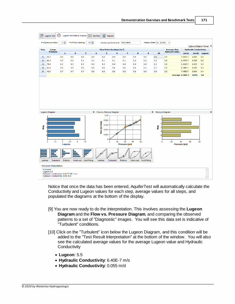
Demonstration Exercises and Benchmark Tests 171
© 2020 by Waterloo Hydrogeologic
Notice that once the data has been entered, AquiferTest will automatically calculate theConductivity and Lugeon values for each step, average values for all steps, andpopulated the diagrams at the bottom of the display.
[9] You are now ready to do the interpretation. This involves assessing the LugeonDiagram and the Flow vs. Pressure Diagram, and comparing the observedpatterns to a set of "Diagnostic" images. You will see this data set is indicative of"Turbulent" conditions.
[10] Click on the "Turbulent" icon below the Lugeon Diagram, and this condition will beadded to the "Test Result Interpretation" at the bottom of the window. You will alsosee the calculated average values for the average Lugeon value and HydraulicConductivity
· Lugeon: 5.5
· Hydraulic Conductivity: 6.40E-7 m/s
· Hydraulic Conductivity: 0.055 m/d
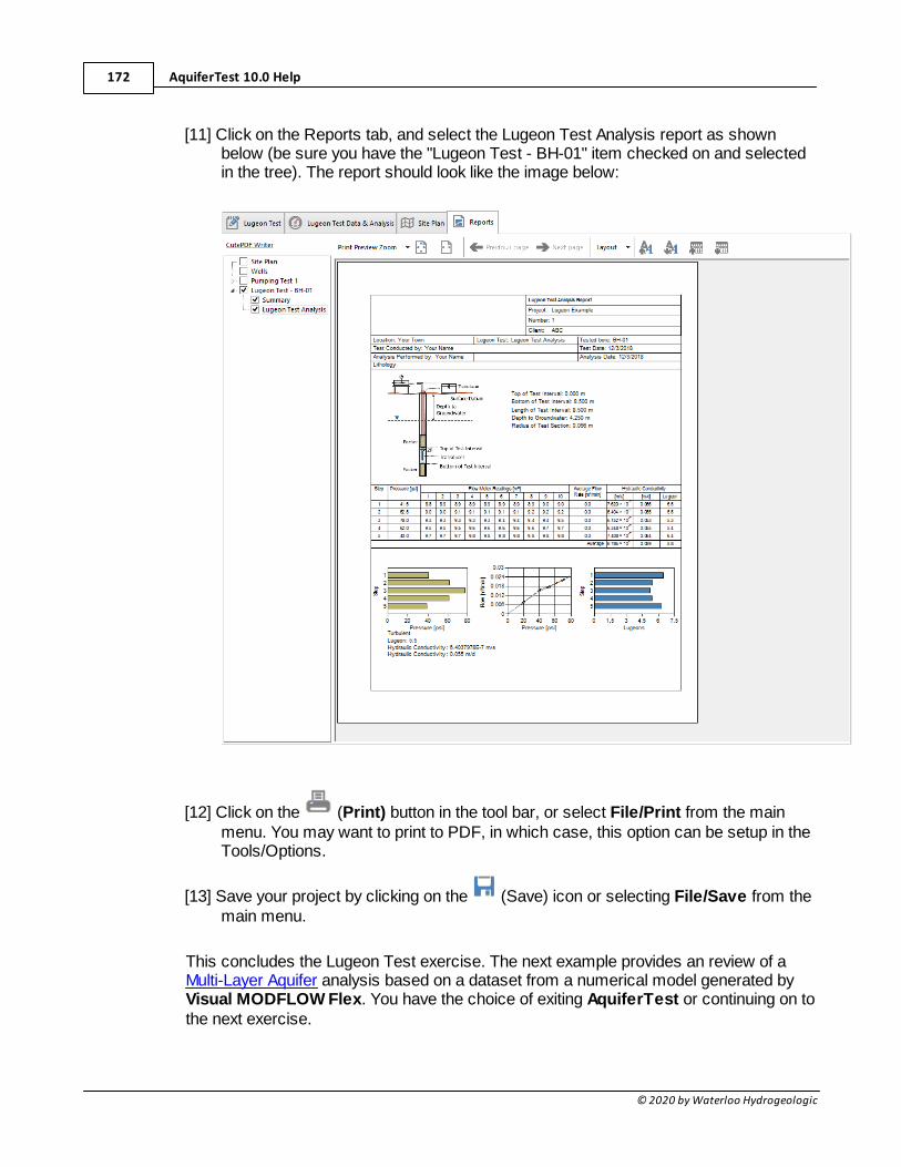
AquiferTest 10.0 Help172
© 2020 by Waterloo Hydrogeologic
[11] Click on the Reports tab, and select the Lugeon Test Analysis report as shownbelow (be sure you have the "Lugeon Test - BH-01" item checked on and selectedin the tree). The report should look like the image below:
[12] Click on the (Print) button in the tool bar, or select File/Print from the mainmenu. You may want to print to PDF, in which case, this option can be setup in theTools/Options.
[13] Save your project by clicking on the (Save) icon or selecting File/Save from themain menu.
This concludes the Lugeon Test exercise. The next example provides an review of aMulti-Layer Aquifer analysis based on a dataset from a numerical model generated byVisual MODFLOW Flex. You have the choice of exiting AquiferTest or continuing on tothe next exercise.
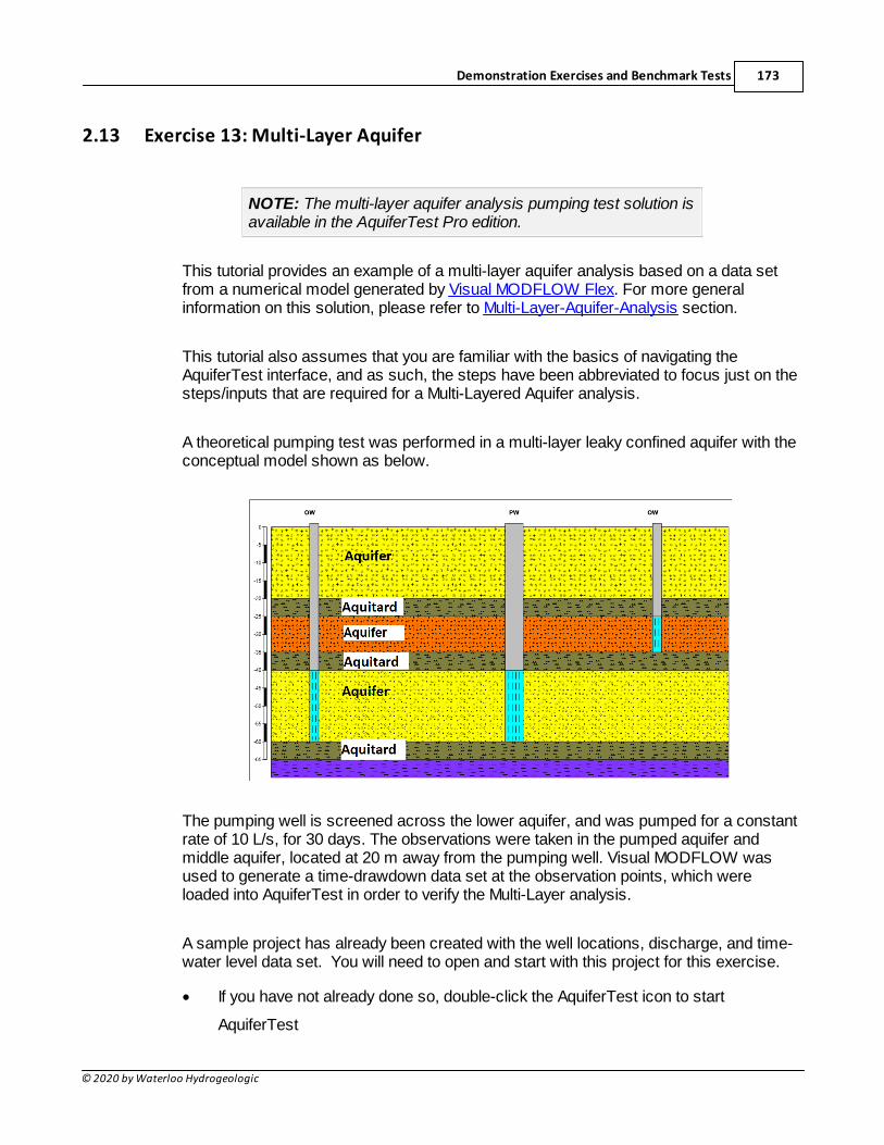
Demonstration Exercises and Benchmark Tests 173
© 2020 by Waterloo Hydrogeologic
2.13 Exercise 13: Multi-Layer Aquifer
NOTE: The multi-layer aquifer analysis pumping test solution isavailable in the AquiferTest Pro edition.
This tutorial provides an example of a multi-layer aquifer analysis based on a data setfrom a numerical model generated by Visual MODFLOW Flex. For more generalinformation on this solution, please refer to Multi-Layer-Aquifer-Analysis section.
This tutorial also assumes that you are familiar with the basics of navigating theAquiferTest interface, and as such, the steps have been abbreviated to focus just on thesteps/inputs that are required for a Multi-Layered Aquifer analysis.
A theoretical pumping test was performed in a multi-layer leaky confined aquifer with theconceptual model shown as below.
The pumping well is screened across the lower aquifer, and was pumped for a constantrate of 10 L/s, for 30 days. The observations were taken in the pumped aquifer andmiddle aquifer, located at 20 m away from the pumping well. Visual MODFLOW wasused to generate a time-drawdown data set at the observation points, which wereloaded into AquiferTest in order to verify the Multi-Layer analysis.
A sample project has already been created with the well locations, discharge, and time-water level data set. You will need to open and start with this project for this exercise.
· If you have not already done so, double-click the AquiferTest icon to start
AquiferTest
AquiferTest 10.0 Help174
© 2020 by Waterloo Hydrogeologic
· When you launch AquiferTest, the AquiferTest welcome page will load, with the
option to create a new project or open an existing project.
· Click the Open other project... button, and browse to the file:
"C:\Users\Public\Documents\AquiferTest Pro\Exercises\Multi-Layer-
Aquifer.HYT"
· The project will load with the Pumping Test tab selected.
· Click on the Water levels tab; you will see 3 wells listed; there are no data defined
for the pumping well.
· If you select OW-20-pumped-aq, you will see the time-water level data from the
observation point that is located in the pumped aquifer;
· Click on OW-20-unpumped-aq and you will see the time-water level data from the
observation point that is located in the unpumped (upper) aquifer. Note that a data
filter is applied to both data sets, which will keep only 15 data points per logarithmic
time scale.
· Click on the Analysis tab; by default, you should see a Time-Drawdown plot
displaying the data sets from both observation points.
· Click on Analysis/Create a New Analysis from the main menu
.
· From the Analysis Method panel on the right side, choose Multilayer. You should
then see a Multi-Layer Settings appear as shown below.
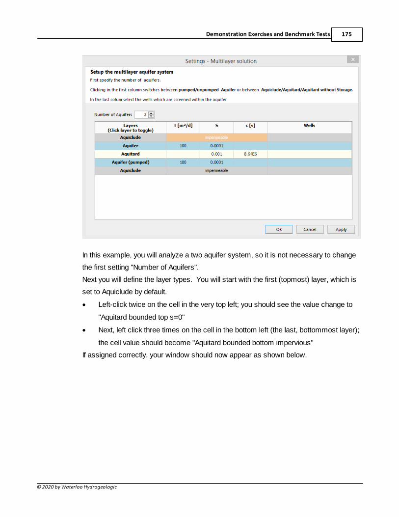
Demonstration Exercises and Benchmark Tests 175
© 2020 by Waterloo Hydrogeologic
In this example, you will analyze a two aquifer system, so it is not necessary to change
the first setting "Number of Aquifers".
Next you will define the layer types. You will start with the first (topmost) layer, which is
set to Aquiclude by default.
· Left-click twice on the cell in the very top left; you should see the value change to
"Aquitard bounded top s=0"
· Next, left click three times on the cell in the bottom left (the last, bottommost layer);
the cell value should become "Aquitard bounded bottom impervious"
If assigned correctly, your window should now appear as shown below.
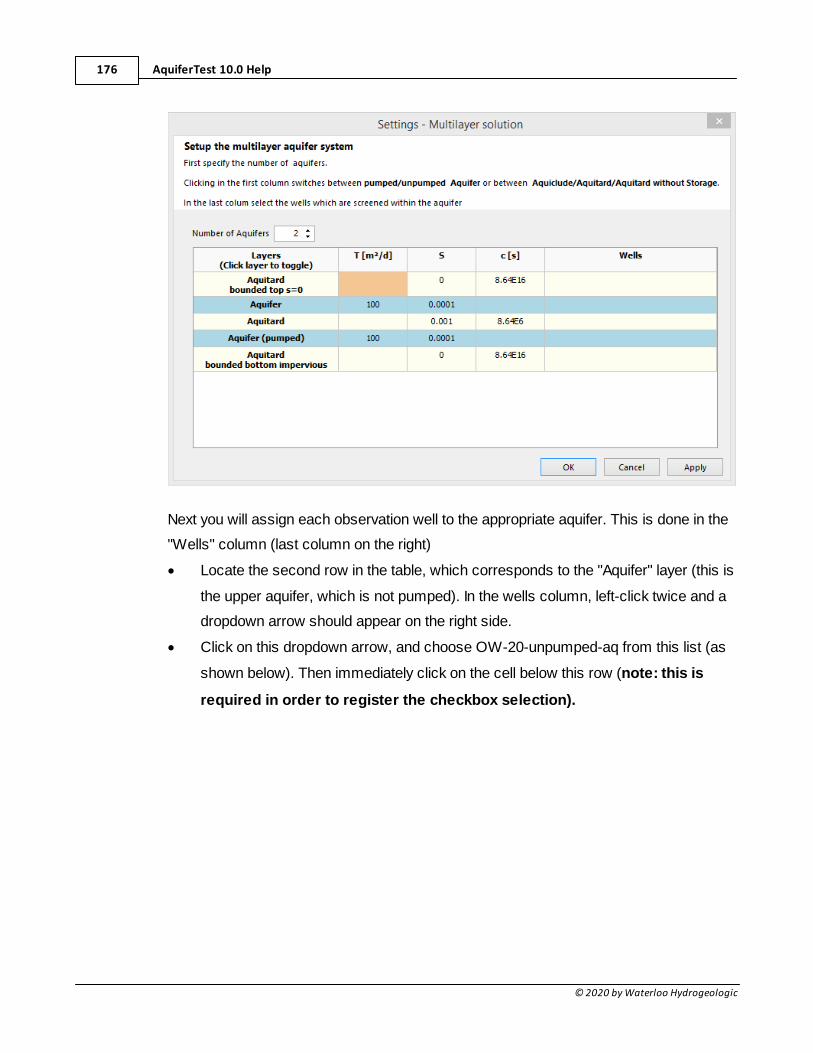
AquiferTest 10.0 Help176
© 2020 by Waterloo Hydrogeologic
Next you will assign each observation well to the appropriate aquifer. This is done in the
"Wells" column (last column on the right)
· Locate the second row in the table, which corresponds to the "Aquifer" layer (this is
the upper aquifer, which is not pumped). In the wells column, left-click twice and a
dropdown arrow should appear on the right side.
· Click on this dropdown arrow, and choose OW-20-unpumped-aq from this list (as
shown below). Then immediately click on the cell below this row (note: this is
required in order to register the checkbox selection).
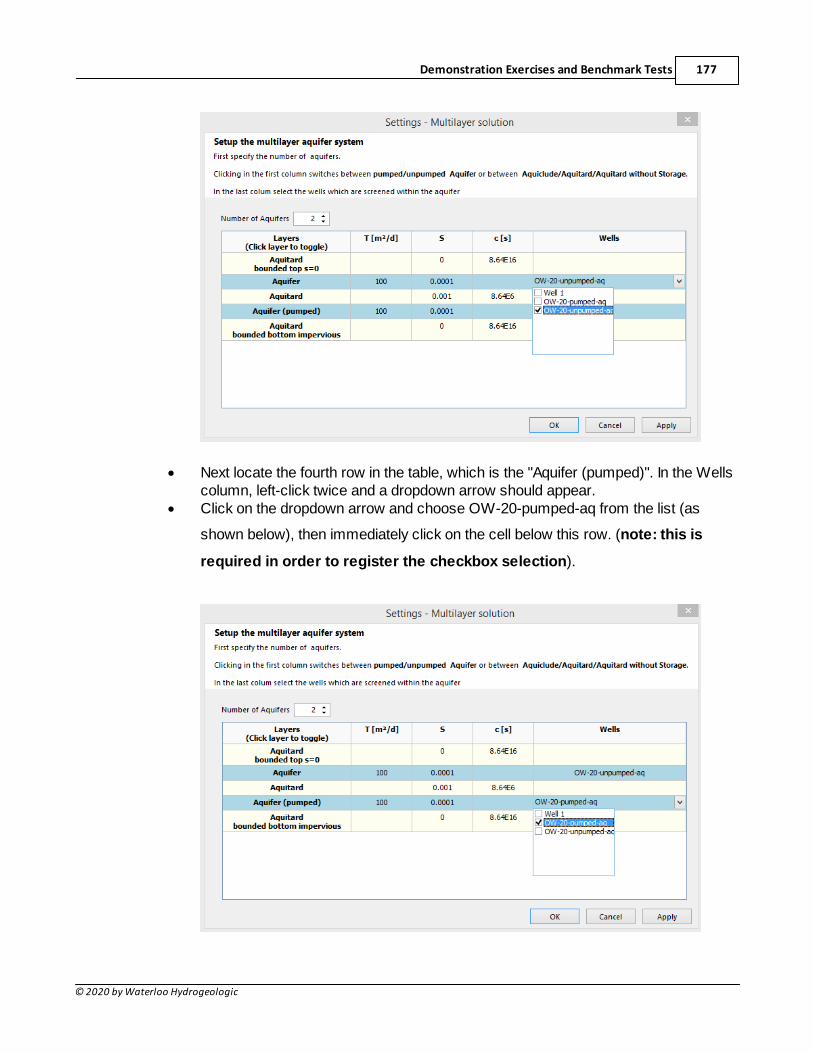
Demonstration Exercises and Benchmark Tests 177
© 2020 by Waterloo Hydrogeologic
· Next locate the fourth row in the table, which is the "Aquifer (pumped)". In the Wellscolumn, left-click twice and a dropdown arrow should appear.
· Click on the dropdown arrow and choose OW-20-pumped-aq from the list (as
shown below), then immediately click on the cell below this row. (note: this is
required in order to register the checkbox selection).
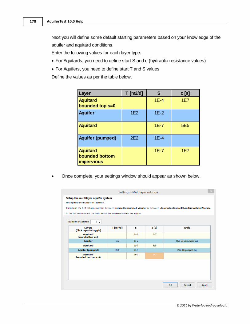
AquiferTest 10.0 Help178
© 2020 by Waterloo Hydrogeologic
Next you will define some default starting parameters based on your knowledge of the
aquifer and aquitard conditions.
Enter the following values for each layer type:
· For Aquitards, you need to define start S and c (hydraulic resistance values)
· For Aquifers, you need to define start T and S values
Define the values as per the table below.
Layer T [m2/d] S c [s]
Aquitardbounded top s=0
1E-4 1E7
Aquifer 1E2 1E-2
Aquitard 1E-7 5E5
Aquifer (pumped) 2E2 1E-4
Aquitardbounded bottomimpervious
1E-7 1E7
· Once complete, your settings window should appear as shown below.
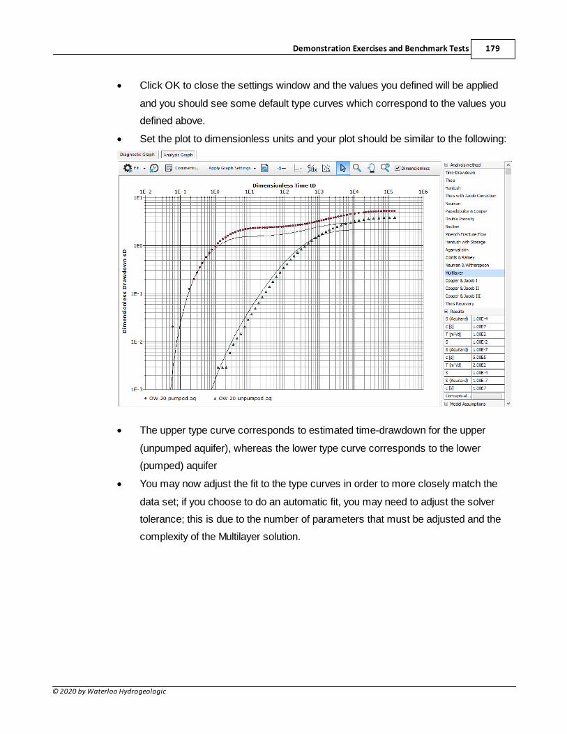
Demonstration Exercises and Benchmark Tests 179
© 2020 by Waterloo Hydrogeologic
· Click OK to close the settings window and the values you defined will be applied
and you should see some default type curves which correspond to the values you
defined above.
· Set the plot to dimensionless units and your plot should be similar to the following:
· The upper type curve corresponds to estimated time-drawdown for the upper
(unpumped aquifer), whereas the lower type curve corresponds to the lower
(pumped) aquifer
· You may now adjust the fit to the type curves in order to more closely match the
data set; if you choose to do an automatic fit, you may need to adjust the solver
tolerance; this is due to the number of parameters that must be adjusted and the
complexity of the Multilayer solution.
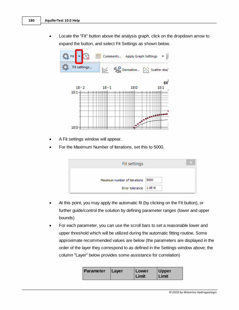
AquiferTest 10.0 Help180
© 2020 by Waterloo Hydrogeologic
· Locate the "Fit" button above the analysis graph, click on the dropdown arrow to
expand the button, and select Fit Settings as shown below.
· A Fit settings window will appear.
· For the Maximum Number of Iterations, set this to 5000.
· At this point, you may apply the automatic fit (by clicking on the Fit button), or
further guide/control the solution by defining parameter ranges (lower and upper
bounds)
· For each parameter, you can use the scroll bars to set a reasonable lower and
upper threshold which will be utilized during the automatic fitting routine. Some
approximate recommended values are below (the parameters are displayed in the
order of the layer they correspond to as defined in the Settings window above; the
column "Layer" below provides some assistance for correlation)
Parameter Layer LowerLimit
UpperLimit
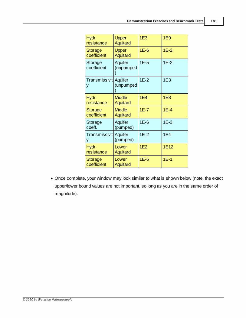
Demonstration Exercises and Benchmark Tests 181
© 2020 by Waterloo Hydrogeologic
Hydr.resistance
UpperAquitard
1E3 1E9
Storagecoefficient
UpperAquitard
1E-6 1E-2
Storagecoefficient
Aquifer(unpumped)
1E-5 1E-2
Transmissivity
Aquifer(unpumped)
1E-2 1E3
Hydr.resistance
MiddleAquitard
1E4 1E8
Storagecoefficient
MiddleAquitard
1E-7 1E-4
Storagecoeff.
Aquifer(pumped)
1E-6 1E-3
Transmissivity
Aquifer(pumped)
1E-2 1E4
Hydr.resistance
LowerAquitard
1E2 1E12
Storagecoefficient
LowerAquitard
1E-6 1E-1
· Once complete, your window may look similar to what is shown below (note, the exact
upper/lower bound values are not important, so long as you are in the same order of
magnitude).
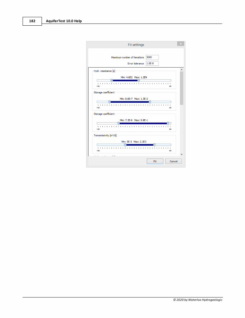
AquiferTest 10.0 Help182
© 2020 by Waterloo Hydrogeologic
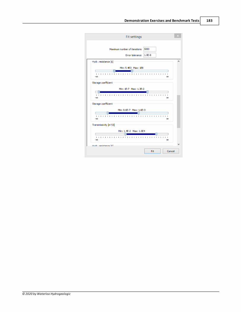
Demonstration Exercises and Benchmark Tests 183
© 2020 by Waterloo Hydrogeologic
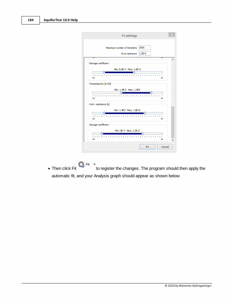
AquiferTest 10.0 Help184
© 2020 by Waterloo Hydrogeologic
· Then click Fit to register the changes. The program should then apply the
automatic fit, and your Analysis graph should appear as shown below.
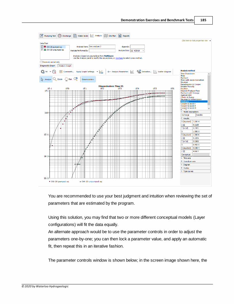
Demonstration Exercises and Benchmark Tests 185
© 2020 by Waterloo Hydrogeologic
You are recommended to use your best judgment and intuition when reviewing the set of
parameters that are estimated by the program.
Using this solution, you may find that two or more different conceptual models (Layer
configurations) will fit the data equally.
An alternate approach would be to use the parameter controls in order to adjust the
parameters one-by-one; you can then lock a parameter value, and apply an automatic
fit, then repeat this in an iterative fashion.
The parameter controls window is shown below; in the screen image shown here, the
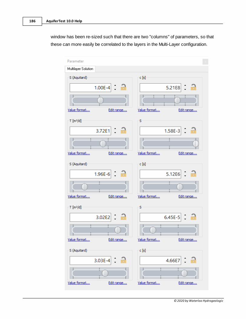
AquiferTest 10.0 Help186
© 2020 by Waterloo Hydrogeologic
window has been re-sized such that there are two "columns" of parameters, so that
these can more easily be correlated to the layers in the Multi-Layer configuration.
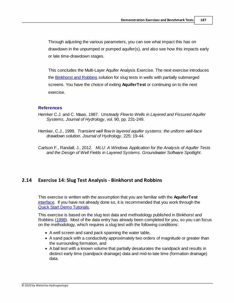
Demonstration Exercises and Benchmark Tests 187
© 2020 by Waterloo Hydrogeologic
Through adjusting the various parameters, you can see what impact this has on
drawdown in the unpumped or pumped aquifer(s), and also see how this impacts early
or late time-drawdown stages.
This concludes the Multi-Layer Aquifer Analysis Exercise. The next exercise introduces
the Binkhorst and Robbins solution for slug tests in wells with partially submerged
screens. You have the choice of exiting AquiferTest or continuing on to the next
exercise.
References
Hemker C.J. and C. Maas, 1987. Unsteady Flow to Wells in Layered and Fissured AquiferSystems, Journal of Hydrology, vol. 90, pp. 231-249.
Hemker, C.J., 1999. Transient well flow in layered aquifer systems: the uniform well-facedrawdown solution. Journal of Hydrology, 225: 19-44.
Carlson F., Randall, J., 2012. MLU: A Windows Application for the Analysis of Aquifer Testsand the Design of Well Fields in Layered Systems. Groundwater Software Spotlight.
2.14 Exercise 14: Slug Test Analysis - Binkhorst and Robbins
This exercise is written with the assumption that you are familiar with the AquiferTestinterface. If you have not already done so, it is recommended that you work through theQuick Start Demo Tutorials.
This exercise is based on the slug test data and methodology published in Binkhorst andRobbins (1998). Most of the data entry has already been completed for you, so you can focuson the methodology, which requires a slug test with the following conditions:
· A well screen and sand pack spanning the water table,
· A sand pack with a conductivity approximately two orders of magnitude or greater thanthe surrounding formation, and
· A bail test with a known volume that partially desaturates the sandpack and results indistinct early time (sandpack drainage) data and mid-to-late time (formation drainage)data.
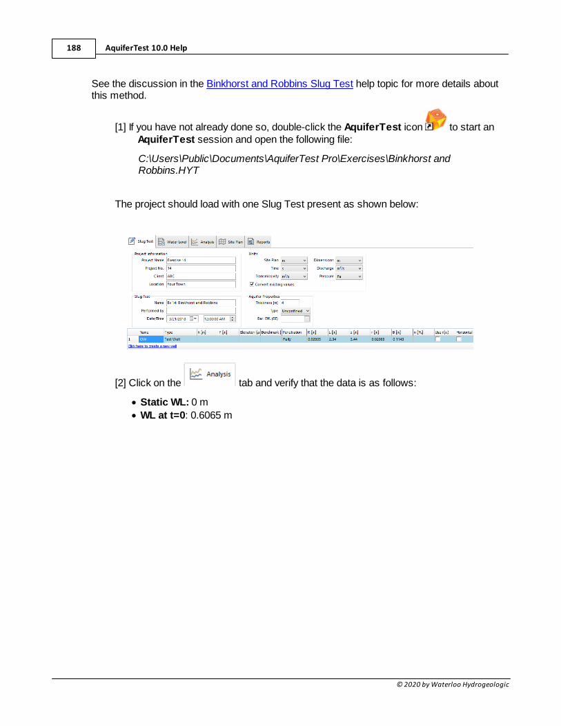
AquiferTest 10.0 Help188
© 2020 by Waterloo Hydrogeologic
See the discussion in the Binkhorst and Robbins Slug Test help topic for more details aboutthis method.
[1] If you have not already done so, double-click the AquiferTest icon to start anAquiferTest session and open the following file:
C:\Users\Public\Documents\AquiferTest Pro\Exercises\Binkhorst andRobbins.HYT
The project should load with one Slug Test present as shown below:
[2] Click on the tab and verify that the data is as follows:
· Static WL: 0 m
· WL at t=0: 0.6065 m
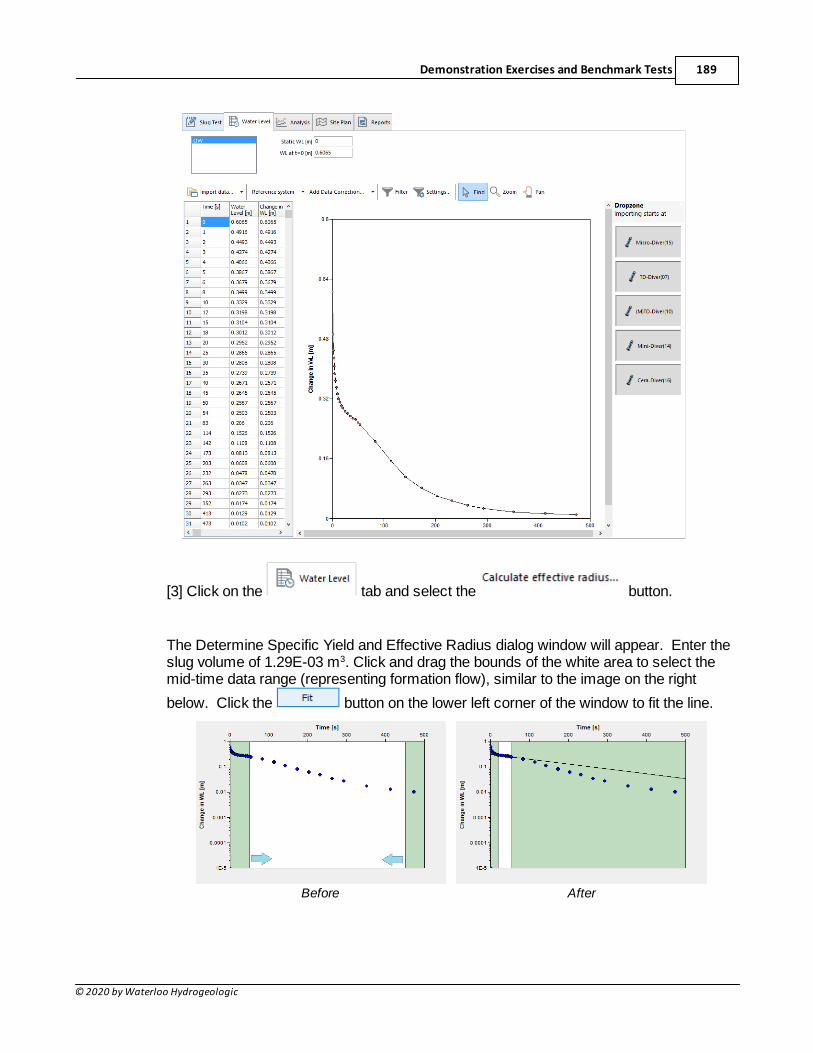
Demonstration Exercises and Benchmark Tests 189
© 2020 by Waterloo Hydrogeologic
[3] Click on the tab and select the button.
The Determine Specific Yield and Effective Radius dialog window will appear. Enter theslug volume of 1.29E-03 m3. Click and drag the bounds of the white area to select themid-time data range (representing formation flow), similar to the image on the right
below. Click the button on the lower left corner of the window to fit the line.
Before After
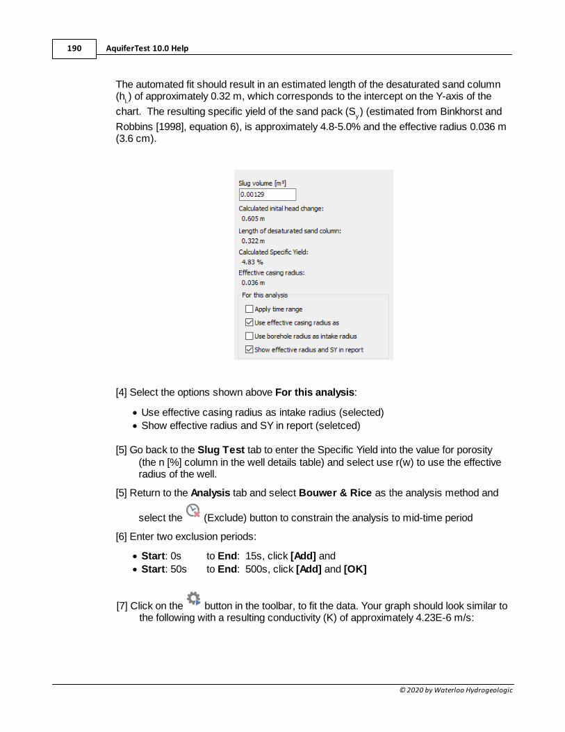
AquiferTest 10.0 Help190
© 2020 by Waterloo Hydrogeologic
The automated fit should result in an estimated length of the desaturated sand column(h
L) of approximately 0.32 m, which corresponds to the intercept on the Y-axis of the
chart. The resulting specific yield of the sand pack (Sy) (estimated from Binkhorst and
Robbins [1998], equation 6), is approximately 4.8-5.0% and the effective radius 0.036 m(3.6 cm).
[4] Select the options shown above For this analysis:
· Use effective casing radius as intake radius (selected)
· Show effective radius and SY in report (seletced)
[5] Go back to the Slug Test tab to enter the Specific Yield into the value for porosity(the n [%] column in the well details table) and select use r(w) to use the effectiveradius of the well.
[5] Return to the Analysis tab and select Bouwer & Rice as the analysis method and
select the (Exclude) button to constrain the analysis to mid-time period
[6] Enter two exclusion periods:
· Start: 0s to End: 15s, click [Add] and
· Start: 50s to End: 500s, click [Add] and [OK]
[7] Click on the button in the toolbar, to fit the data. Your graph should look similar tothe following with a resulting conductivity (K) of approximately 4.23E-6 m/s:
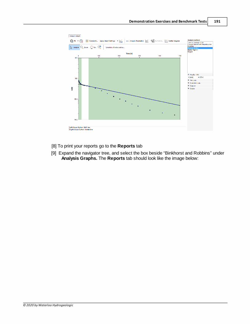
Demonstration Exercises and Benchmark Tests 191
© 2020 by Waterloo Hydrogeologic
[8] To print your reports go to the Reports tab
[9] Expand the navigator tree, and select the box beside “Binkhorst and Robbins” underAnalysis Graphs. The Reports tab should look like the image below:
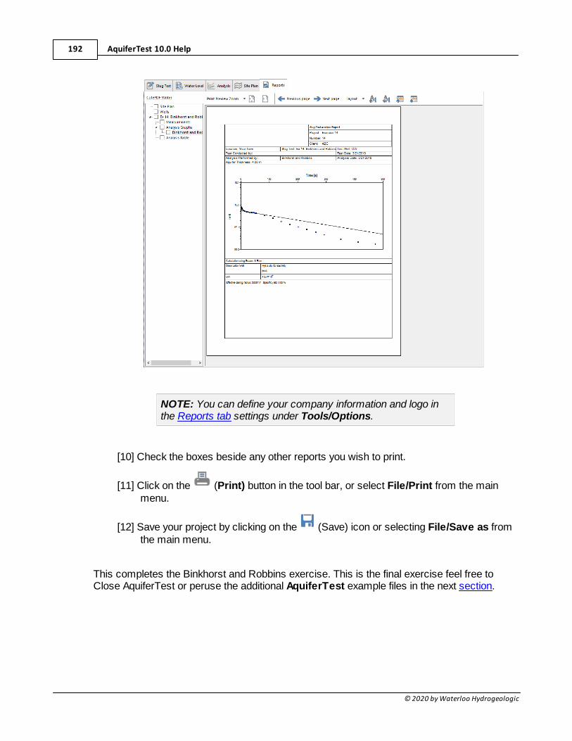
AquiferTest 10.0 Help192
© 2020 by Waterloo Hydrogeologic
NOTE: You can define your company information and logo inthe Reports tab settings under Tools/Options.
[10] Check the boxes beside any other reports you wish to print.
[11] Click on the (Print) button in the tool bar, or select File/Print from the mainmenu.
[12] Save your project by clicking on the (Save) icon or selecting File/Save as fromthe main menu.
This completes the Binkhorst and Robbins exercise. This is the final exercise feel free toClose AquiferTest or peruse the additional AquiferTest example files in the next section.
Demonstration Exercises and Benchmark Tests 193
© 2020 by Waterloo Hydrogeologic
2.15 Additional AquiferTest Examples
Once you have completed the exercises, feel free to explore the sample projects thathave been included in the Examples folder, which is located in:
C:\Users\Public\Documents\AquiferTest Pro\Examples
These examples encompass a wide variety of aquifer conditions, and appropriatesolutions. The following examples are available:
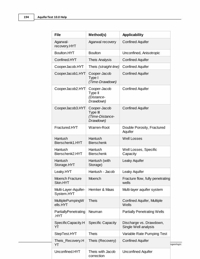
AquiferTest 10.0 Help194
© 2020 by Waterloo Hydrogeologic
File Method(s) Applicability
Agarwal-recovery.HYT
Agarwal recovery Confined Aquifer
Boulton.HYT Boulton Unconfined, Anisotropic
Confined.HYT Theis Analysis Confined Aquifer
CooperJacob.HYT Theis (straight-line) Confined Aquifer
CooperJacob1.HYT Cooper-JacobType I(Time-Drawdown)
Confined Aquifer
CooperJacob2.HYT Cooper-JacobType II(Distance-Drawdown)
Confined Aquifer
CooperJacob3.HYT Cooper-JacobType III(Time-Distance-Drawdown)
Confined Aquifer
Fractured.HYT Warren-Root Double Porosity, FracturedAquifer
HantushBierschenk1.HYT
HantushBierschenk
Well Losses
HantushBierschenk2.HYT
HantushBierschenk
Well Losses, SpecificCapacity
HantushStorage.HYT
Hantush (withStorage)
Leaky Aquifer
Leaky.HYT Hantush - Jacob Leaky Aquifer
Moench FractureSkin.HYT
Moench Fracture flow, fully penetratingwells
Multi-Layer-Aquifer-System.HYT
Hemker & Maas Multi-layer aquifer system
MultiplePumpingWells.HYT
Theis Confined Aquifer, MultipleWells
PartiallyPenetrating.HYT
Neuman Partially Penetrating Wells
SpecificCapacity.HYT
Specific Capacity Discharge vs. Drawdown,Single Well analysis
StepTest.HYT Theis Variable Rate Pumping Test
Theis_Recovery.HYT
Theis (Recovery) Confined Aquifer
Unconfined.HYT Theis with Jacobcorrection
Unconfined Aquifer
WellBoreStorage.HYT
Papadopulos -Cooper
Well Bore Storage
--- --- ---
ButlerHighKSlugTest.HYT
Butler High-K Confined/Unconfined SlugTest, Partially PenetratingWell, High-K Formation
SlugTest1.HYT Bouwer & Rice,Hvorslev
Confined/Unconfined SlugTest
SlugTest2.HYT Bouwer & Rice,Hvorslev
Confined/Unconfined SlugTest
--- --- ---
LugeonTest1.HYT Lugeon Multiple tests at variousdepths for a single borehole
LugeonTest2.HYT Lugeon Simple test with just threepressure steps

Demonstration Exercises and Benchmark Tests 195
© 2020 by Waterloo Hydrogeologic
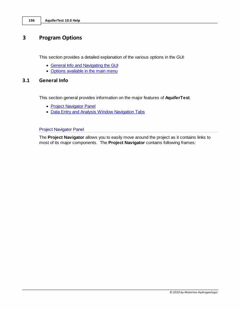
AquiferTest 10.0 Help196
© 2020 by Waterloo Hydrogeologic
3 Program Options
This section provides a detailed explanation of the various options in the GUI:
· General Info and Navigating the GUI
· Options available in the main menu
3.1 General Info
This section general provides information on the major features of AquiferTest.
· Project Navigator Panel
· Data Entry and Analysis Window Navigation Tabs
Project Navigator Panel
The Project Navigator allows you to easily move around the project as it contains links tomost of its major components. The Project Navigator contains following frames:
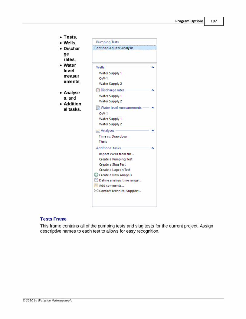
Program Options 197
© 2020 by Waterloo Hydrogeologic
· Tests,
· Wells,
· Dischargerates,
· Waterlevelmeasurements,
· Analyses, and
· Additional tasks.
Tests Frame
This frame contains all of the pumping tests and slug tests for the current project. Assigndescriptive names to each test to allows for easy recognition.
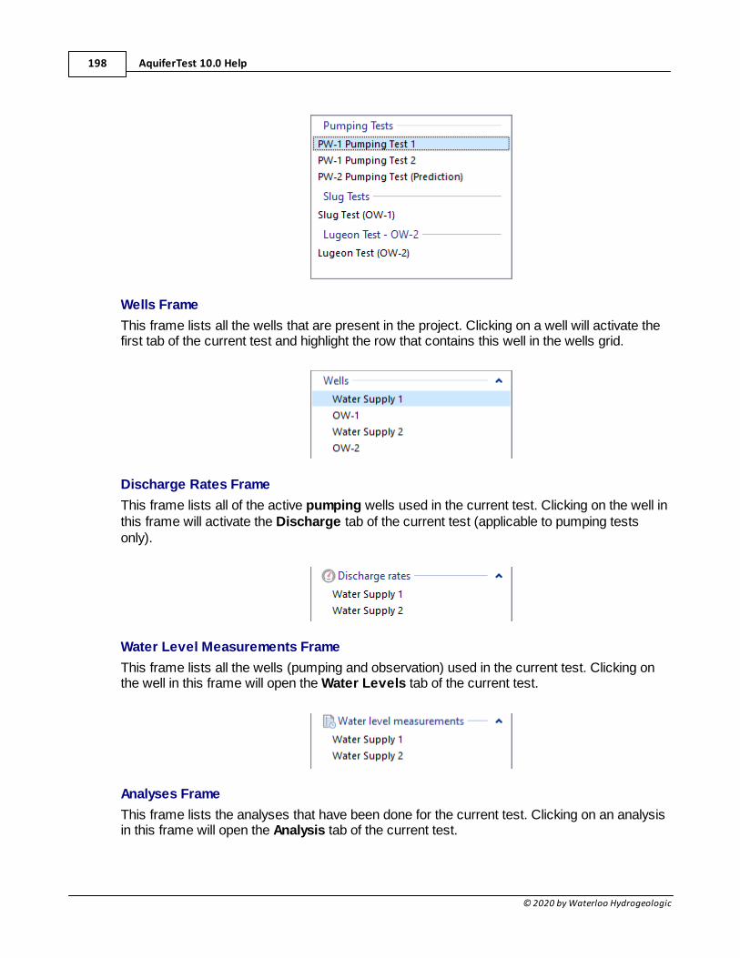
AquiferTest 10.0 Help198
© 2020 by Waterloo Hydrogeologic
Wells Frame
This frame lists all the wells that are present in the project. Clicking on a well will activate thefirst tab of the current test and highlight the row that contains this well in the wells grid.
Discharge Rates Frame
This frame lists all of the active pumping wells used in the current test. Clicking on the well inthis frame will activate the Discharge tab of the current test (applicable to pumping testsonly).
Water Level Measurements Frame
This frame lists all the wells (pumping and observation) used in the current test. Clicking onthe well in this frame will open the Water Levels tab of the current test.
Analyses Frame
This frame lists the analyses that have been done for the current test. Clicking on an analysisin this frame will open the Analysis tab of the current test.
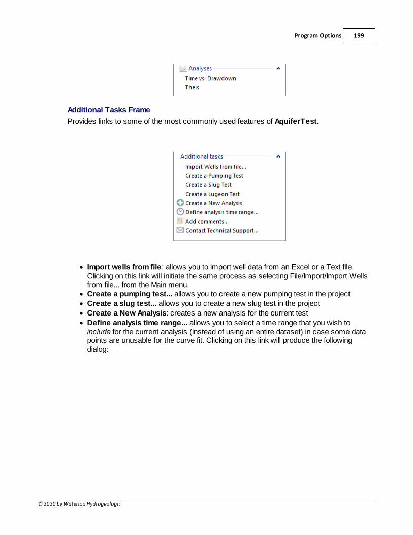
Program Options 199
© 2020 by Waterloo Hydrogeologic
Additional Tasks Frame
Provides links to some of the most commonly used features of AquiferTest.
· Import wells from file: allows you to import well data from an Excel or a Text file.Clicking on this link will initiate the same process as selecting File/Import/Import Wellsfrom file... from the Main menu.
· Create a pumping test... allows you to create a new pumping test in the project
· Create a slug test... allows you to create a new slug test in the project
· Create a New Analysis: creates a new analysis for the current test
· Define analysis time range... allows you to select a time range that you wish toinclude for the current analysis (instead of using an entire dataset) in case some datapoints are unusable for the curve fit. Clicking on this link will produce the followingdialog:
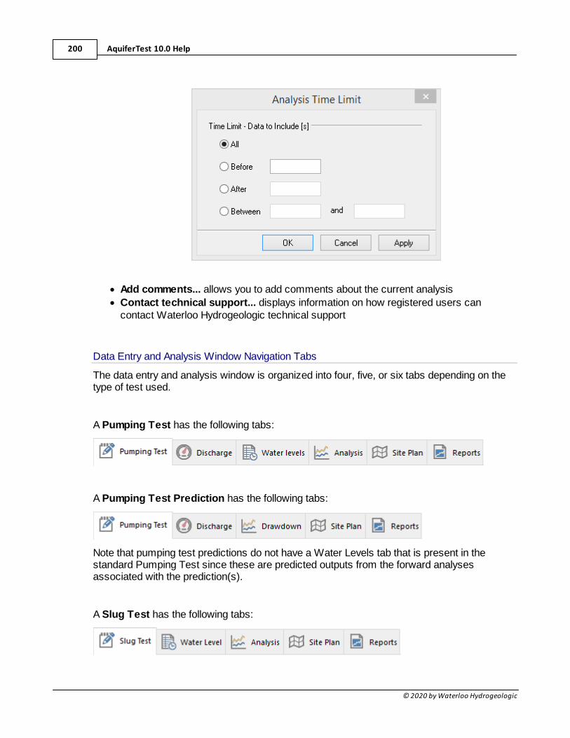
AquiferTest 10.0 Help200
© 2020 by Waterloo Hydrogeologic
· Add comments... allows you to add comments about the current analysis
· Contact technical support... displays information on how registered users cancontact Waterloo Hydrogeologic technical support
Data Entry and Analysis Window Navigation Tabs
The data entry and analysis window is organized into four, five, or six tabs depending on thetype of test used.
A Pumping Test has the following tabs:
A Pumping Test Prediction has the following tabs:
Note that pumping test predictions do not have a Water Levels tab that is present in thestandard Pumping Test since these are predicted outputs from the forward analysesassociated with the prediction(s).
A Slug Test has the following tabs:
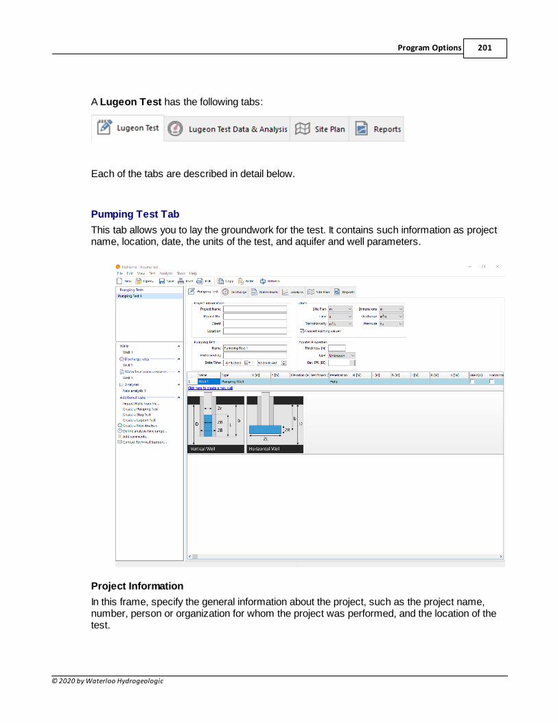
Program Options 201
© 2020 by Waterloo Hydrogeologic
A Lugeon Test has the following tabs:
Each of the tabs are described in detail below.
Pumping Test Tab
This tab allows you to lay the groundwork for the test. It contains such information as projectname, location, date, the units of the test, and aquifer and well parameters.
Project Information
In this frame, specify the general information about the project, such as the project name,number, person or organization for whom the project was performed, and the location of thetest.
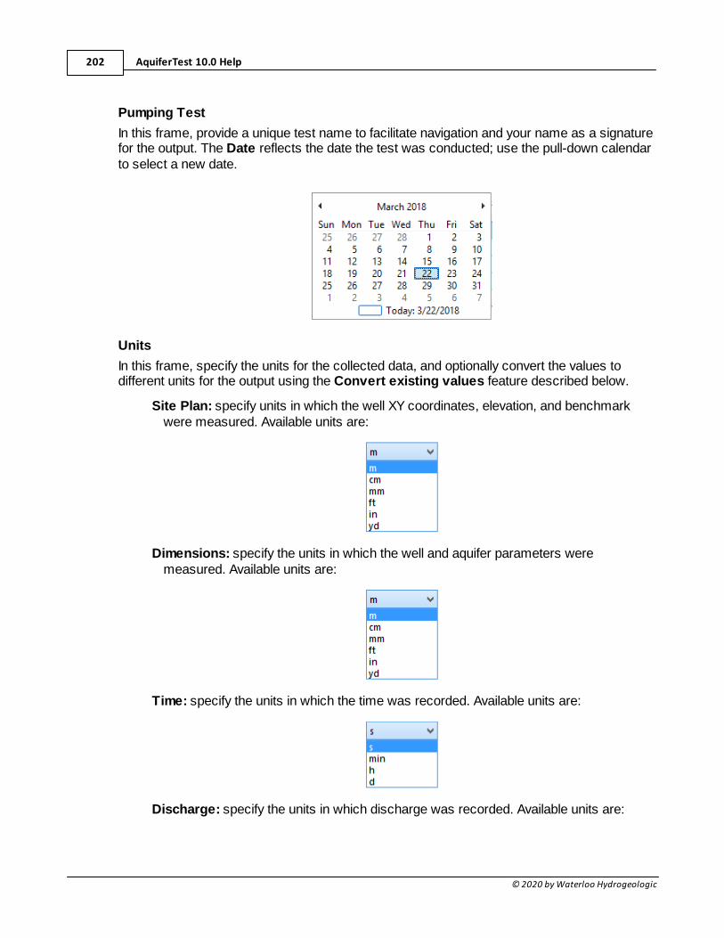
AquiferTest 10.0 Help202
© 2020 by Waterloo Hydrogeologic
Pumping Test
In this frame, provide a unique test name to facilitate navigation and your name as a signaturefor the output. The Date reflects the date the test was conducted; use the pull-down calendarto select a new date.
Units
In this frame, specify the units for the collected data, and optionally convert the values todifferent units for the output using the Convert existing values feature described below.
Site Plan: specify units in which the well XY coordinates, elevation, and benchmarkwere measured. Available units are:
Dimensions: specify the units in which the well and aquifer parameters weremeasured. Available units are:
Time: specify the units in which the time was recorded. Available units are:
Discharge: specify the units in which discharge was recorded. Available units are:
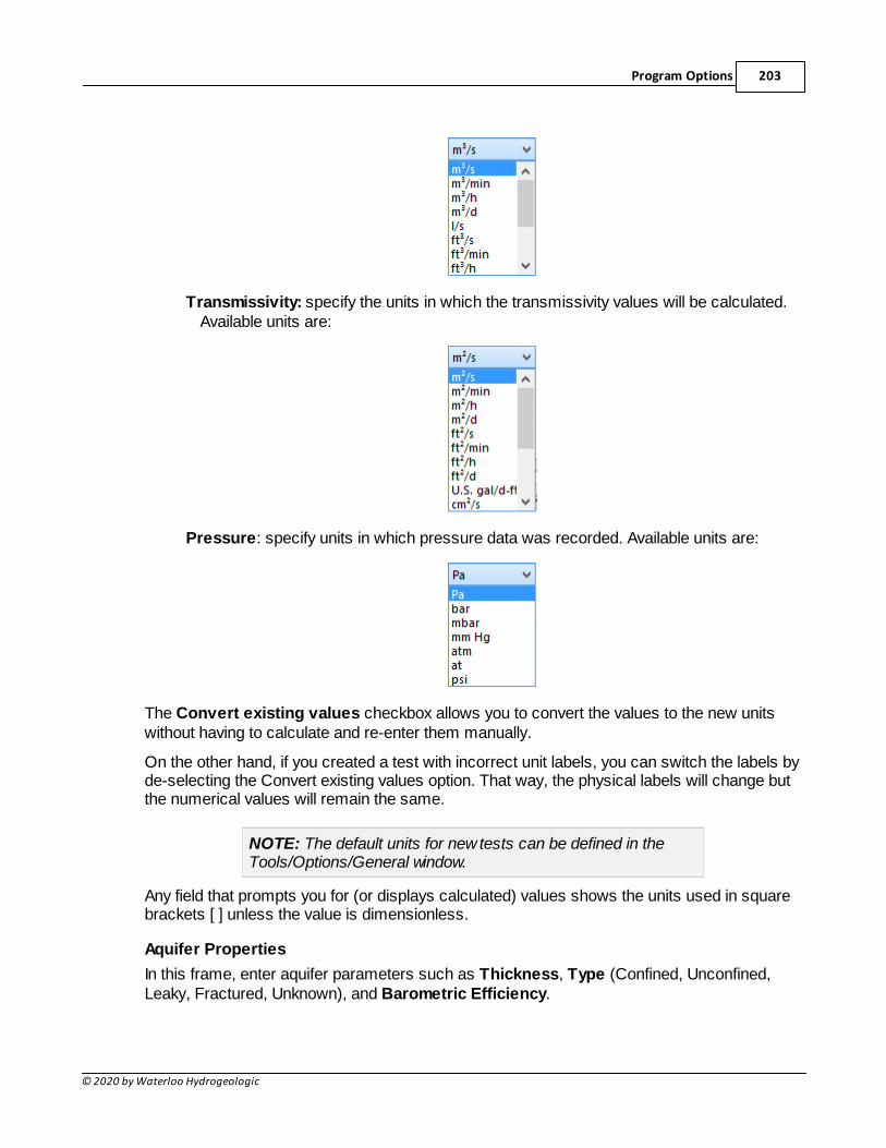
Program Options 203
© 2020 by Waterloo Hydrogeologic
Transmissivity: specify the units in which the transmissivity values will be calculated.Available units are:
Pressure: specify units in which pressure data was recorded. Available units are:
The Convert existing values checkbox allows you to convert the values to the new unitswithout having to calculate and re-enter them manually.
On the other hand, if you created a test with incorrect unit labels, you can switch the labels byde-selecting the Convert existing values option. That way, the physical labels will change butthe numerical values will remain the same.
NOTE: The default units for new tests can be defined in theTools/Options/General window.
Any field that prompts you for (or displays calculated) values shows the units used in squarebrackets [ ] unless the value is dimensionless.
Aquifer Properties
In this frame, enter aquifer parameters such as Thickness, Type (Confined, Unconfined,Leaky, Fractured, Unknown), and Barometric Efficiency.
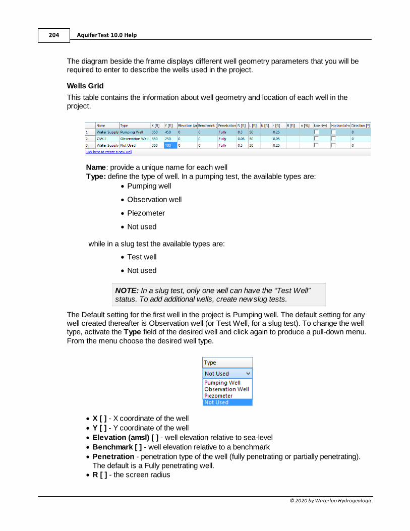
AquiferTest 10.0 Help204
© 2020 by Waterloo Hydrogeologic
The diagram beside the frame displays different well geometry parameters that you will berequired to enter to describe the wells used in the project.
Wells Grid
This table contains the information about well geometry and location of each well in theproject.
Name: provide a unique name for each wellType: define the type of well. In a pumping test, the available types are:
· Pumping well
· Observation well
· Piezometer
· Not used
while in a slug test the available types are:
· Test well
· Not used
NOTE: In a slug test, only one well can have the “Test Well”status. To add additional wells, create new slug tests.
The Default setting for the first well in the project is Pumping well. The default setting for anywell created thereafter is Observation well (or Test Well, for a slug test). To change the welltype, activate the Type field of the desired well and click again to produce a pull-down menu.From the menu choose the desired well type.
· X [ ] - X coordinate of the well
· Y [ ] - Y coordinate of the well
· Elevation (amsl) [ ] - well elevation relative to sea-level
· Benchmark [ ] - well elevation relative to a benchmark
· Penetration - penetration type of the well (fully penetrating or partially penetrating).The default is a Fully penetrating well.
· R [ ] - the screen radius
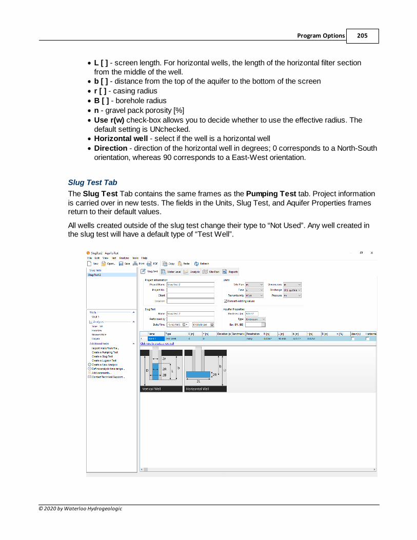
Program Options 205
© 2020 by Waterloo Hydrogeologic
· L [ ] - screen length. For horizontal wells, the length of the horizontal filter sectionfrom the middle of the well.
· b [ ] - distance from the top of the aquifer to the bottom of the screen
· r [ ] - casing radius
· B [ ] - borehole radius
· n - gravel pack porosity [%]
· Use r(w) check-box allows you to decide whether to use the effective radius. Thedefault setting is UNchecked.
· Horizontal well - select if the well is a horizontal well
· Direction - direction of the horizontal well in degrees; 0 corresponds to a North-Southorientation, whereas 90 corresponds to a East-West orientation.
Slug Test Tab
The Slug Test Tab contains the same frames as the Pumping Test tab. Project informationis carried over in new tests. The fields in the Units, Slug Test, and Aquifer Properties framesreturn to their default values.
All wells created outside of the slug test change their type to “Not Used”. Any well created inthe slug test will have a default type of “Test Well”.
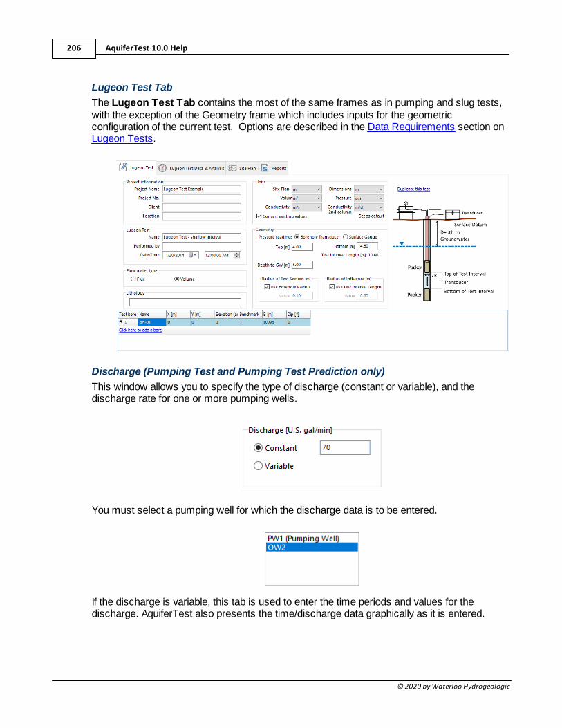
AquiferTest 10.0 Help206
© 2020 by Waterloo Hydrogeologic
Lugeon Test Tab
The Lugeon Test Tab contains the most of the same frames as in pumping and slug tests,with the exception of the Geometry frame which includes inputs for the geometricconfiguration of the current test. Options are described in the Data Requirements section onLugeon Tests.
Discharge (Pumping Test and Pumping Test Prediction only)
This window allows you to specify the type of discharge (constant or variable), and thedischarge rate for one or more pumping wells.
You must select a pumping well for which the discharge data is to be entered.
If the discharge is variable, this tab is used to enter the time periods and values for thedischarge. AquiferTest also presents the time/discharge data graphically as it is entered.
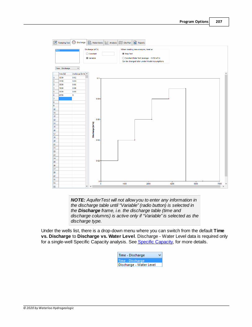
Program Options 207
© 2020 by Waterloo Hydrogeologic
NOTE: AquiferTest will not allow you to enter any information inthe discharge table until “Variable” (radio button) is selected inthe Discharge frame, i.e. the discharge table (time anddischarge columns) is active only if “Variable” is selected as thedischarge type.
Under the wells list, there is a drop-down menu where you can switch from the default Timevs. Discharge to Discharge vs. Water Level. Discharge - Water Level data is required onlyfor a single-well Specific Capacity analysis. See Specific Capacity, for more details.
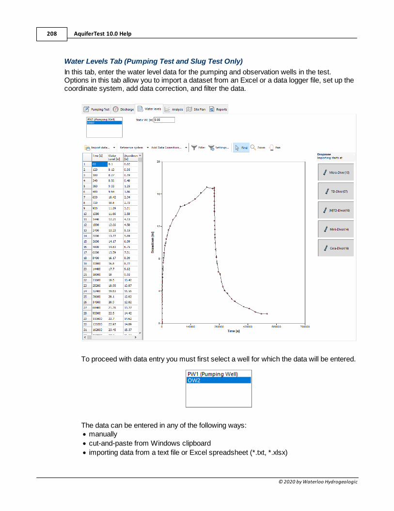
AquiferTest 10.0 Help208
© 2020 by Waterloo Hydrogeologic
Water Levels Tab (Pumping Test and Slug Test Only)
In this tab, enter the water level data for the pumping and observation wells in the test.Options in this tab allow you to import a dataset from an Excel or a data logger file, set up thecoordinate system, add data correction, and filter the data.
To proceed with data entry you must first select a well for which the data will be entered.
The data can be entered in any of the following ways:· manually
· cut-and-paste from Windows clipboard
· importing data from a text file or Excel spreadsheet (*.txt, *.xlsx)
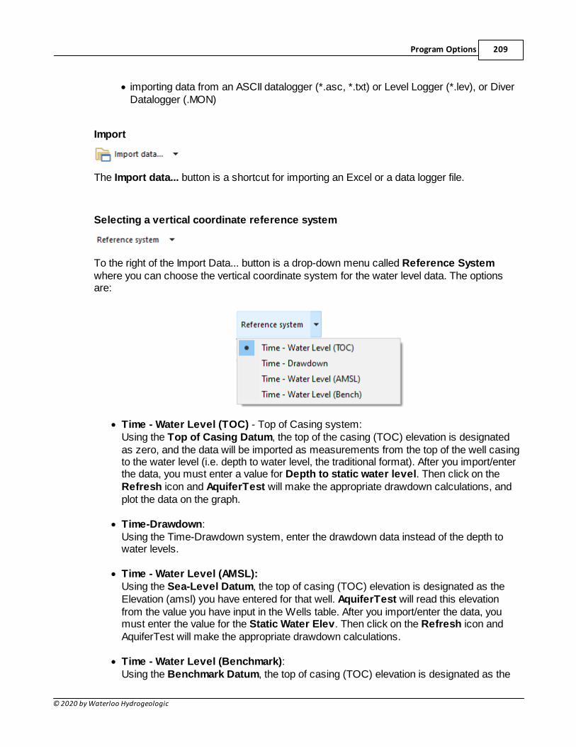
Program Options 209
© 2020 by Waterloo Hydrogeologic
· importing data from an ASCII datalogger (*.asc, *.txt) or Level Logger (*.lev), or DiverDatalogger (.MON)
Import
The Import data... button is a shortcut for importing an Excel or a data logger file.
Selecting a vertical coordinate reference system
To the right of the Import Data... button is a drop-down menu called Reference Systemwhere you can choose the vertical coordinate system for the water level data. The optionsare:
· Time - Water Level (TOC) - Top of Casing system:Using the Top of Casing Datum, the top of the casing (TOC) elevation is designatedas zero, and the data will be imported as measurements from the top of the well casingto the water level (i.e. depth to water level, the traditional format). After you import/enterthe data, you must enter a value for Depth to static water level. Then click on theRefresh icon and AquiferTest will make the appropriate drawdown calculations, andplot the data on the graph.
· Time-Drawdown:Using the Time-Drawdown system, enter the drawdown data instead of the depth towater levels.
· Time - Water Level (AMSL):Using the Sea-Level Datum, the top of casing (TOC) elevation is designated as theElevation (amsl) you have entered for that well. AquiferTest will read this elevationfrom the value you have input in the Wells table. After you import/enter the data, youmust enter the value for the Static Water Elev. Then click on the Refresh icon andAquiferTest will make the appropriate drawdown calculations.
· Time - Water Level (Benchmark):Using the Benchmark Datum, the top of casing (TOC) elevation is designated as the
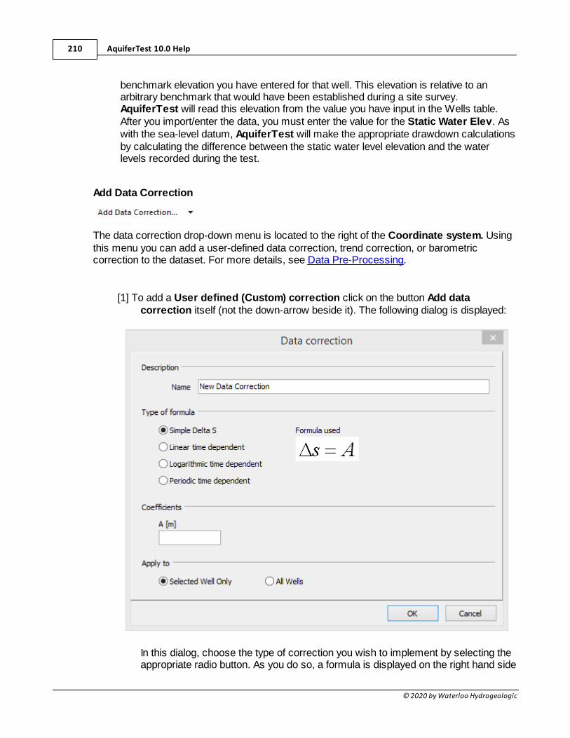
AquiferTest 10.0 Help210
© 2020 by Waterloo Hydrogeologic
benchmark elevation you have entered for that well. This elevation is relative to anarbitrary benchmark that would have been established during a site survey.AquiferTest will read this elevation from the value you have input in the Wells table.After you import/enter the data, you must enter the value for the Static Water Elev. Aswith the sea-level datum, AquiferTest will make the appropriate drawdown calculationsby calculating the difference between the static water level elevation and the waterlevels recorded during the test.
Add Data Correction
The data correction drop-down menu is located to the right of the Coordinate system. Usingthis menu you can add a user-defined data correction, trend correction, or barometriccorrection to the dataset. For more details, see Data Pre-Processing.
[1] To add a User defined (Custom) correction click on the button Add datacorrection itself (not the down-arrow beside it). The following dialog is displayed:
In this dialog, choose the type of correction you wish to implement by selecting theappropriate radio button. As you do so, a formula is displayed on the right hand side
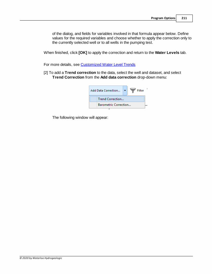
Program Options 211
© 2020 by Waterloo Hydrogeologic
of the dialog, and fields for variables involved in that formula appear below. Definevalues for the required variables and choose whether to apply the correction only tothe currently selected well or to all wells in the pumping test.
When finished, click [OK] to apply the correction and return to the Water Levels tab.
For more details, see Customized Water Level Trends
[2] To add a Trend correction to the data, select the well and dataset, and selectTrend Correction from the Add data correction drop-down menu:
The following window will appear:
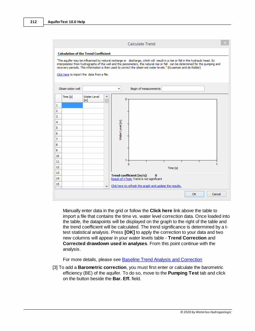
AquiferTest 10.0 Help212
© 2020 by Waterloo Hydrogeologic
Manually enter data in the grid or follow the Click here link above the table toimport a file that contains the time vs. water level correction data. Once loaded intothe table, the datapoints will be displayed on the graph to the right of the table andthe trend coefficient will be calculated. The trend significance is determined by a t-test statistical analysis. Press [OK] to apply the correction to your data and twonew columns will appear in your water levels table - Trend Correction andCorrected drawdown used in analyses. From this point continue with theanalysis.
For more details, please see Baseline Trend Analysis and Correction
[3] To add a Barometric correction, you must first enter or calculate the barometricefficiency (BE) of the aquifer. To do so, move to the Pumping Test tab and clickon the button beside the Bar. Eff. field.
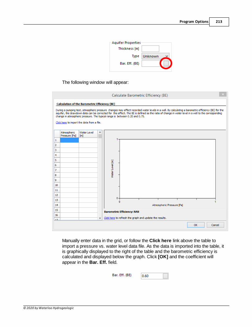
Program Options 213
© 2020 by Waterloo Hydrogeologic
The following window will appear:
Manually enter data in the grid, or follow the Click here link above the table toimport a pressure vs. water level data file. As the data is imported into the table, itis graphically displayed to the right of the table and the barometric efficiency iscalculated and displayed below the graph. Click [OK] and the coefficient willappear in the Bar. Eff. field.
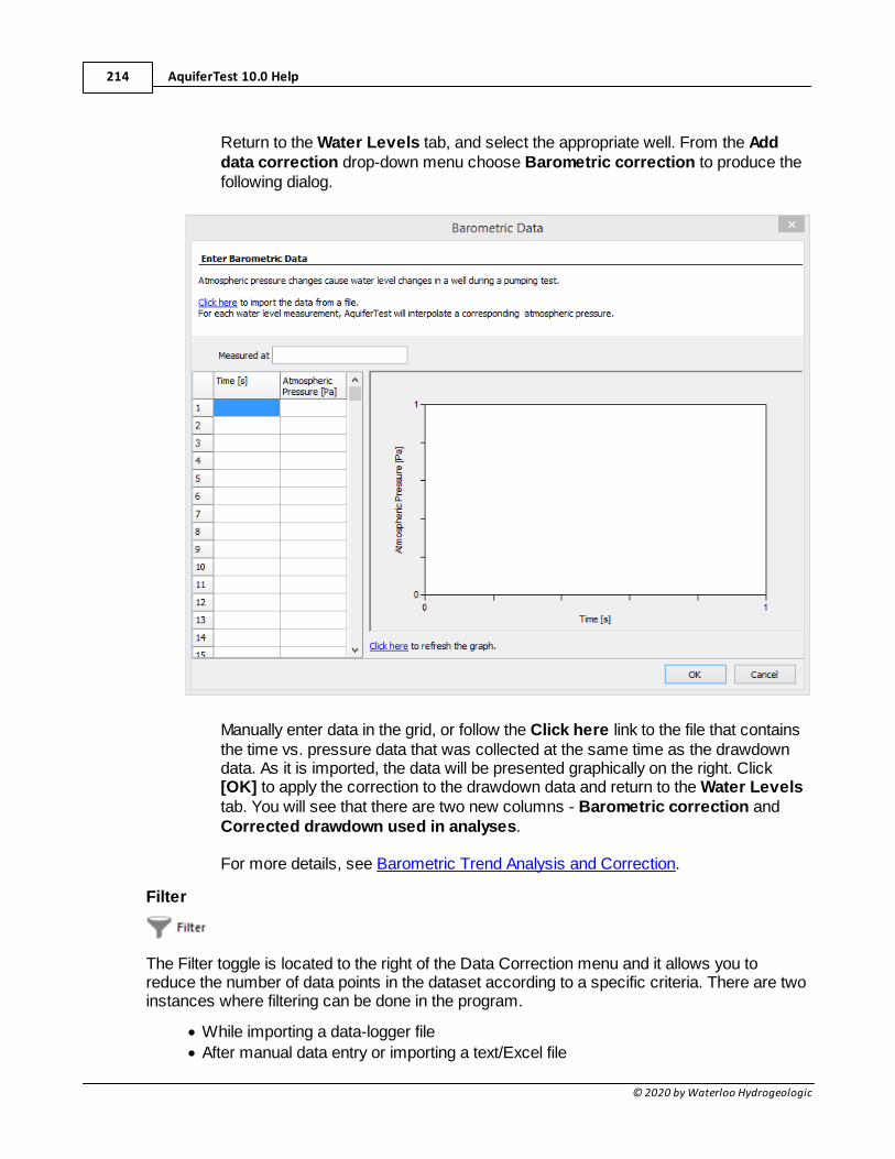
AquiferTest 10.0 Help214
© 2020 by Waterloo Hydrogeologic
Return to the Water Levels tab, and select the appropriate well. From the Adddata correction drop-down menu choose Barometric correction to produce thefollowing dialog.
Manually enter data in the grid, or follow the Click here link to the file that containsthe time vs. pressure data that was collected at the same time as the drawdowndata. As it is imported, the data will be presented graphically on the right. Click[OK] to apply the correction to the drawdown data and return to the Water Levelstab. You will see that there are two new columns - Barometric correction andCorrected drawdown used in analyses.
For more details, see Barometric Trend Analysis and Correction.
Filter
The Filter toggle is located to the right of the Data Correction menu and it allows you toreduce the number of data points in the dataset according to a specific criteria. There are twoinstances where filtering can be done in the program.
· While importing a data-logger file
· After manual data entry or importing a text/Excel file
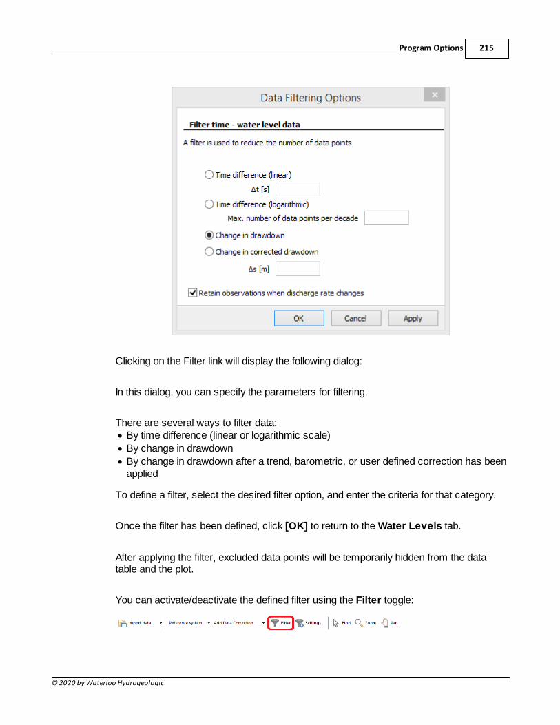
Program Options 215
© 2020 by Waterloo Hydrogeologic
Clicking on the Filter link will display the following dialog:
In this dialog, you can specify the parameters for filtering.
There are several ways to filter data:· By time difference (linear or logarithmic scale)
· By change in drawdown
· By change in drawdown after a trend, barometric, or user defined correction has beenapplied
To define a filter, select the desired filter option, and enter the criteria for that category.
Once the filter has been defined, click [OK] to return to the Water Levels tab.
After applying the filter, excluded data points will be temporarily hidden from the datatable and the plot.
You can activate/deactivate the defined filter using the Filter toggle:
AquiferTest 10.0 Help216
© 2020 by Waterloo Hydrogeologic
For more details on filtering during importing a data logger file, see "Data Import"section.
Zoom, Pan and Find
Find allows you to easily find particular data points. While this tool is selectedclicking any data point in the graph will highlight the associated data point in the table.
Zoom allows you to zoom in on a data set in the graph; after selecting the zoombutton, draw a box around the desired region, starting in the upper left and finishing inthe lower right. To zoom out, simply draw a box in the opposite direction; start at thebottom right and end at the lower left.
Pan allows you to shift the zoomed-in window, up, down, left, or right.
Depth to Static Water level
Enter the depth to the water level before the test began, for either a pumping or slug test.This depth is subtracted from the Water Level measurements to obtain the Drawdownvalues.
NOTE: The static water level should be entered before youproceed to enter / import the time - water level data.
Water Level at t=0 (Slug tests only)
This field is located below Depth to static water level field and contains the water level atthe start of the measuring period of the slug test - i.e. immediately after the slug hasbeen inserted or removed.
This completes the Data Entry portion of the program. The next section describes theanalysis of the data and report generation.
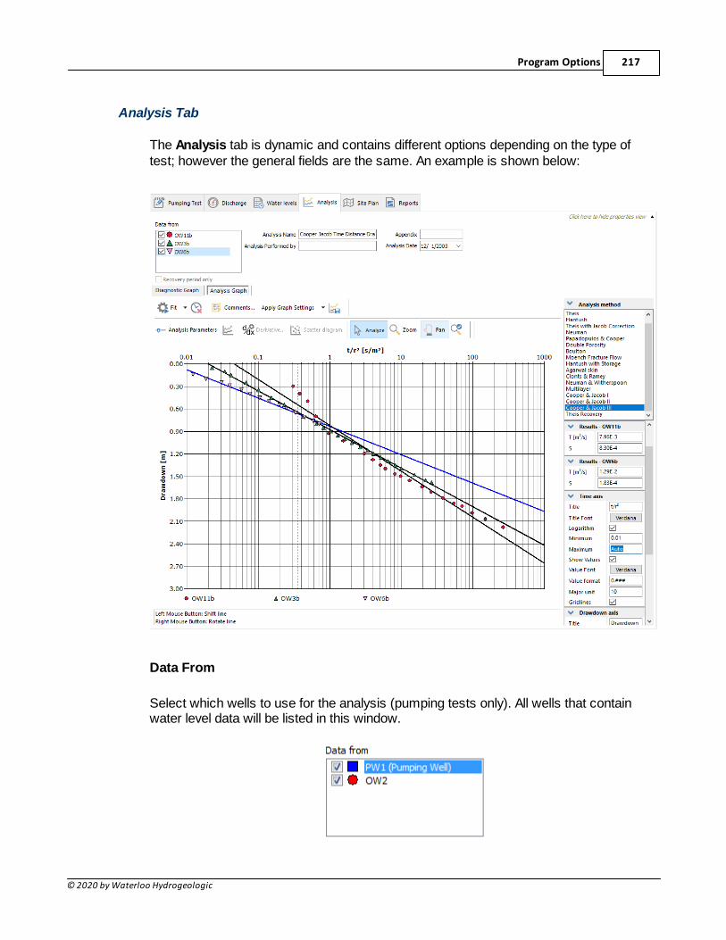
Program Options 217
© 2020 by Waterloo Hydrogeologic
Analysis Tab
The Analysis tab is dynamic and contains different options depending on the type oftest; however the general fields are the same. An example is shown below:
Data From
Select which wells to use for the analysis (pumping tests only). All wells that containwater level data will be listed in this window.
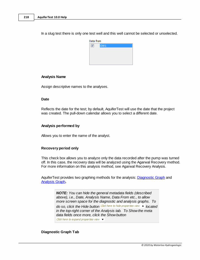
AquiferTest 10.0 Help218
© 2020 by Waterloo Hydrogeologic
In a slug test there is only one test well and this well cannot be selected or unselected.
Analysis Name
Assign descriptive names to the analyses.
Date
Reflects the date for the test; by default, AquiferTest will use the date that the projectwas created. The pull-down calendar allows you to select a different date.
Analysis performed by
Allows you to enter the name of the analyst.
Recovery period only
This check box allows you to analyze only the data recorded after the pump was turnedoff. In this case, the recovery data will be analyzed using the Agarwal Recovery method.For more information on this analysis method, see Agarwal Recovery Analysis.
AquiferTest provides two graphing methods for the analysis: Diagnostic Graph andAnalysis Graph.
NOTE: You can hide the general metadata fields (describedabove), i.e., Date, Analysis Name, Data From etc., to allowmore screen space for the diagnostic and analysis graphs. To
do so, click the Hide button locatedin the top-right corner of the Analysis tab. To Show the metadata fields once more, click the Show button
Diagnostic Graph Tab
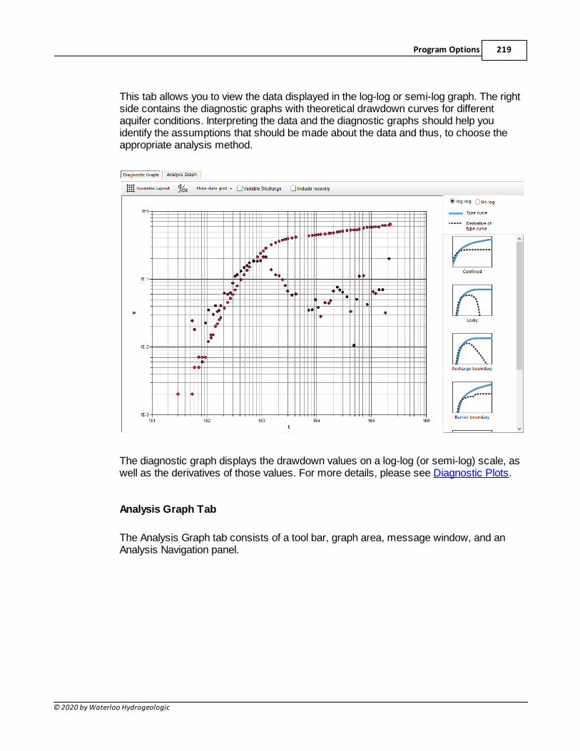
Program Options 219
© 2020 by Waterloo Hydrogeologic
This tab allows you to view the data displayed in the log-log or semi-log graph. The rightside contains the diagnostic graphs with theoretical drawdown curves for differentaquifer conditions. Interpreting the data and the diagnostic graphs should help youidentify the assumptions that should be made about the data and thus, to choose theappropriate analysis method.
The diagnostic graph displays the drawdown values on a log-log (or semi-log) scale, aswell as the derivatives of those values. For more details, please see Diagnostic Plots.
Analysis Graph Tab
The Analysis Graph tab consists of a tool bar, graph area, message window, and anAnalysis Navigation panel.
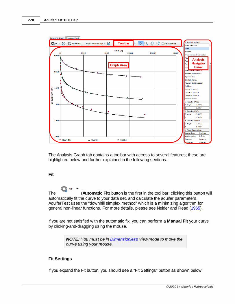
AquiferTest 10.0 Help220
© 2020 by Waterloo Hydrogeologic
The Analysis Graph tab contains a toolbar with access to several features; these arehighlighted below and further explained in the following sections.
Fit
The (Automatic Fit) button is the first in the tool bar; clicking this button willautomatically fit the curve to your data set, and calculate the aquifer parameters.AquiferTest uses the “downhill simplex method” which is a minimizing algorithm forgeneral non-linear functions. For more details, please see Nelder and Read (1965).
If you are not satisfied with the automatic fix, you can perform a Manual Fit your curveby clicking-and-dragging using the mouse.
NOTE: You must be in Dimensionless view mode to move thecurve using your mouse.
Fit Settings
If you expand the Fit button, you should see a "Fit Settings" button as shown below:
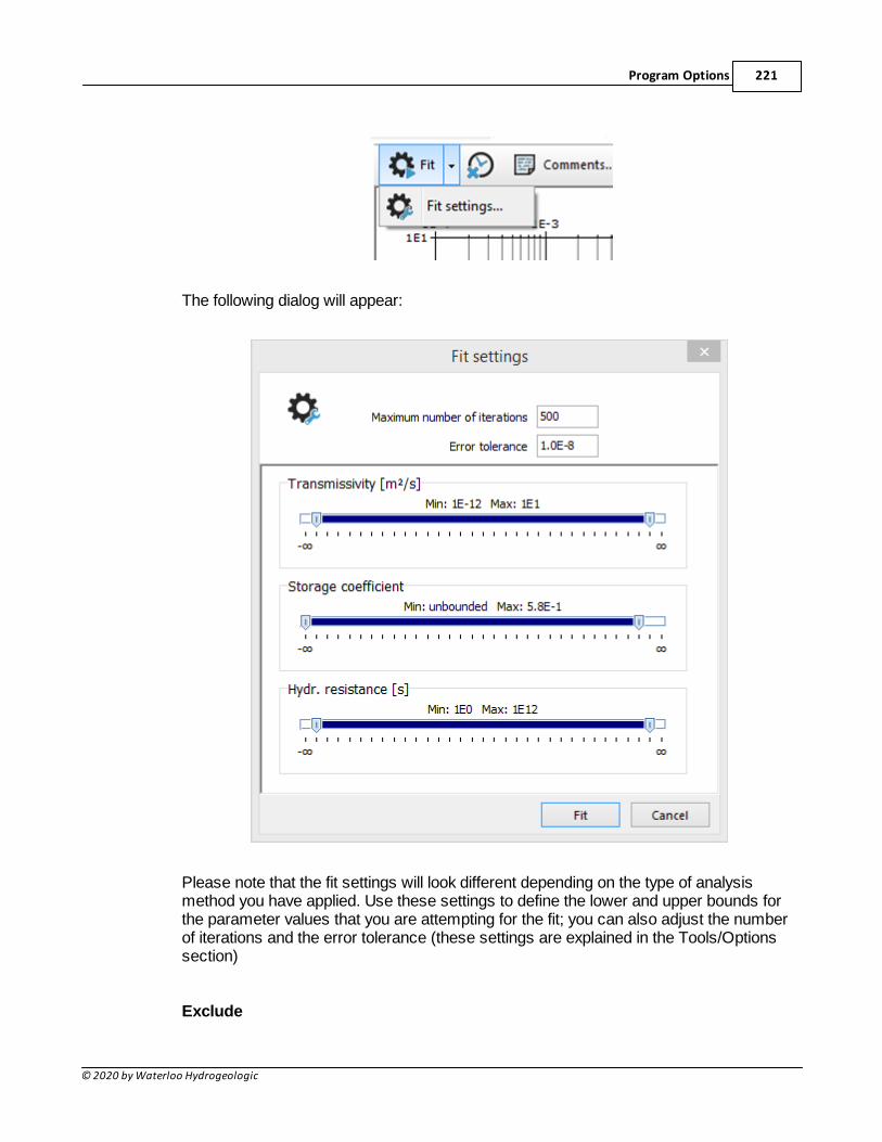
Program Options 221
© 2020 by Waterloo Hydrogeologic
The following dialog will appear:
Please note that the fit settings will look different depending on the type of analysismethod you have applied. Use these settings to define the lower and upper bounds forthe parameter values that you are attempting for the fit; you can also adjust the numberof iterations and the error tolerance (these settings are explained in the Tools/Optionssection)
Exclude
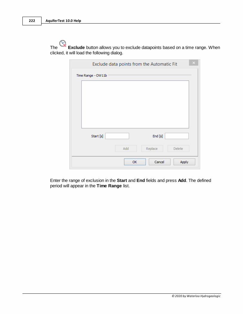
AquiferTest 10.0 Help222
© 2020 by Waterloo Hydrogeologic
The Exclude button allows you to exclude datapoints based on a time range. Whenclicked, it will load the following dialog.
Enter the range of exclusion in the Start and End fields and press Add. The definedperiod will appear in the Time Range list.
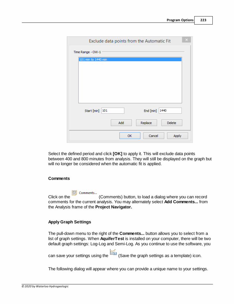
Program Options 223
© 2020 by Waterloo Hydrogeologic
Select the defined period and click [OK] to apply it. This will exclude data pointsbetween 400 and 800 minutes from analysis. They will still be displayed on the graph butwill no longer be considered when the automatic fit is applied.
Comments
Click on the (Comments) button, to load a dialog where you can recordcomments for the current analysis. You may alternately select Add Comments... fromthe Analysis frame of the Project Navigator.
Apply Graph Settings
The pull-down menu to the right of the Comments... button allows you to select from alist of graph settings. When AquiferTest is installed on your computer, there will be twodefault graph settings: Log-Log and Semi-Log. As you continue to use the software, you
can save your settings using the (Save the graph settings as a template) icon.
The following dialog will appear where you can provide a unique name to your settings.
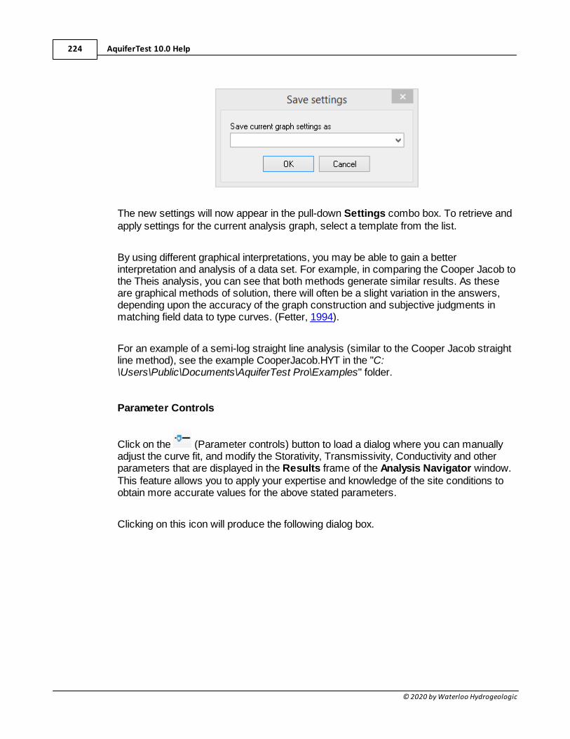
AquiferTest 10.0 Help224
© 2020 by Waterloo Hydrogeologic
The new settings will now appear in the pull-down Settings combo box. To retrieve andapply settings for the current analysis graph, select a template from the list.
By using different graphical interpretations, you may be able to gain a betterinterpretation and analysis of a data set. For example, in comparing the Cooper Jacob tothe Theis analysis, you can see that both methods generate similar results. As theseare graphical methods of solution, there will often be a slight variation in the answers,depending upon the accuracy of the graph construction and subjective judgments inmatching field data to type curves. (Fetter, 1994).
For an example of a semi-log straight line analysis (similar to the Cooper Jacob straightline method), see the example CooperJacob.HYT in the "C:\Users\Public\Documents\AquiferTest Pro\Examples" folder.
Parameter Controls
Click on the (Parameter controls) button to load a dialog where you can manuallyadjust the curve fit, and modify the Storativity, Transmissivity, Conductivity and otherparameters that are displayed in the Results frame of the Analysis Navigator window.This feature allows you to apply your expertise and knowledge of the site conditions toobtain more accurate values for the above stated parameters.
Clicking on this icon will produce the following dialog box.
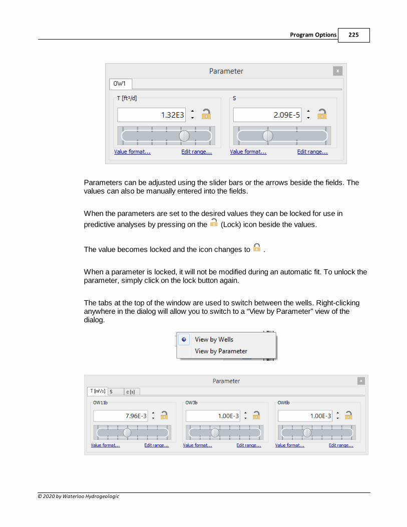
Program Options 225
© 2020 by Waterloo Hydrogeologic
Parameters can be adjusted using the slider bars or the arrows beside the fields. Thevalues can also be manually entered into the fields.
When the parameters are set to the desired values they can be locked for use in
predictive analyses by pressing on the (Lock) icon beside the values.
The value becomes locked and the icon changes to .
When a parameter is locked, it will not be modified during an automatic fit. To unlock theparameter, simply click on the lock button again.
The tabs at the top of the window are used to switch between the wells. Right-clickinganywhere in the dialog will allow you to switch to a “View by Parameter” view of thedialog.
AquiferTest 10.0 Help226
© 2020 by Waterloo Hydrogeologic
Now you can manipulate the parameter in both wells at the same time. The tabs at thetop of the window are used to switch between parameters. This feature is useful is youwish to set a parameter to the same value in both wells.
Show Family of Type Curves
Click the Show/Hide Family of Type Curves button to load a pre-defined set ofType Curves for certain analyses. See Automatic Type Curves for more details.
Derivative Smoothing Settings
Click the Derivative Settings button to load the input for the DerivativeSmoothing options. See Derivative Analysis... for more details.
Scatter Diagram
Click the Scatter Diagram button to load a scatter diagram of the current fit. Thediagram plots the observed drawdown values (X-axis) against the calculated drawdownvalues (Y-axis), providing a visual representation of the quality of the fit. The 45 degreeline colored red represents an ideal scenario, where the calculated values equal theobserved values. However, this is not likely to happen in many real-life scenarios. If thedata points appear above the line, then the calculated values are larger than theobserved values, which may indicate that the model is over-predicting. If the data pointsare under the line, then the calculated values are less than the observed values, whichmay indicate that the model is under-predicting.
The scatter diagram can also be viewed in the statistics report, which can be accessedby selecting Analysis / Statistics from the main menu.
NOTE: The Scatter Diagram is only available for analysismethods with model functions, e.g., Theis, Hantush, etc. It isnot available for the legacy methods (straight line methods),e.g., Cooper & Jacob, Hantush Bierschenk, Specific Capacity,Slug Tests, etc.
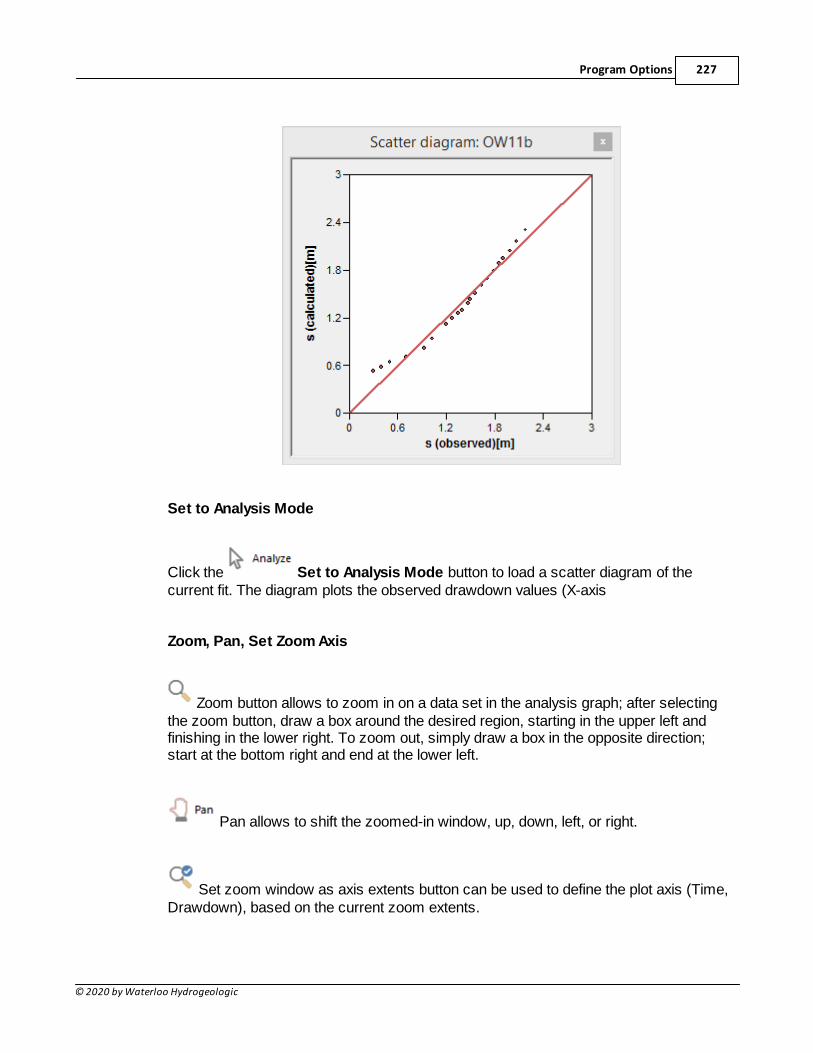
Program Options 227
© 2020 by Waterloo Hydrogeologic
Set to Analysis Mode
Click the Set to Analysis Mode button to load a scatter diagram of thecurrent fit. The diagram plots the observed drawdown values (X-axis
Zoom, Pan, Set Zoom Axis
Zoom button allows to zoom in on a data set in the analysis graph; after selectingthe zoom button, draw a box around the desired region, starting in the upper left andfinishing in the lower right. To zoom out, simply draw a box in the opposite direction;start at the bottom right and end at the lower left.
Pan allows to shift the zoomed-in window, up, down, left, or right.
Set zoom window as axis extents button can be used to define the plot axis (Time,Drawdown), based on the current zoom extents.
AquiferTest 10.0 Help228
© 2020 by Waterloo Hydrogeologic
Dimensionless
Click on the Dimensionless to enable this mode. When the
Dimensionless mode is active, it will appear highlighted:
Message window
The message window displays all the messages, warnings, and error reports that occurwhile you conduct the data analysis. This message fades after five seconds.
Analysis Navigator panel
The Analysis Navigator panel is located to the right of the graph area. It contains all thefunctions that control the analysis of the selected data and the display on the screen.The Analysis Navigator contains following frames:
· Analysis method
· Model Assumptions (pumping test only)
· Results
· Time axis
· Drawdown axis
· Diagram
· Display
· Type curves
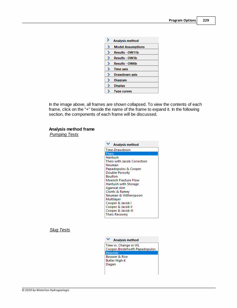
Program Options 229
© 2020 by Waterloo Hydrogeologic
In the image above, all frames are shown collapsed. To view the contents of eachframe, click on the “+” beside the name of the frame to expand it. In the followingsection, the components of each frame will be discussed.
Analysis method framePumping Tests
Slug Tests
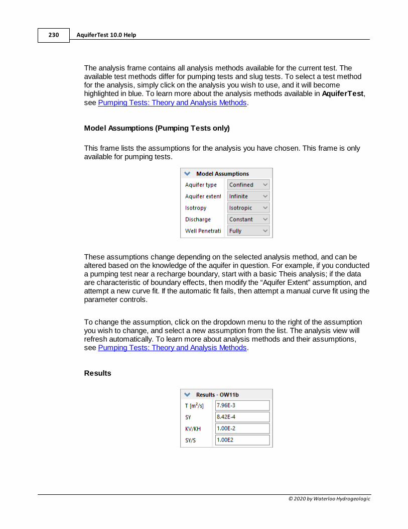
AquiferTest 10.0 Help230
© 2020 by Waterloo Hydrogeologic
The analysis frame contains all analysis methods available for the current test. Theavailable test methods differ for pumping tests and slug tests. To select a test methodfor the analysis, simply click on the analysis you wish to use, and it will becomehighlighted in blue. To learn more about the analysis methods available in AquiferTest,see Pumping Tests: Theory and Analysis Methods.
Model Assumptions (Pumping Tests only)
This frame lists the assumptions for the analysis you have chosen. This frame is onlyavailable for pumping tests.
These assumptions change depending on the selected analysis method, and can bealtered based on the knowledge of the aquifer in question. For example, if you conducteda pumping test near a recharge boundary, start with a basic Theis analysis; if the dataare characteristic of boundary effects, then modify the “Aquifer Extent” assumption, andattempt a new curve fit. If the automatic fit fails, then attempt a manual curve fit using theparameter controls.
To change the assumption, click on the dropdown menu to the right of the assumptionyou wish to change, and select a new assumption from the list. The analysis view willrefresh automatically. To learn more about analysis methods and their assumptions,see Pumping Tests: Theory and Analysis Methods.
Results
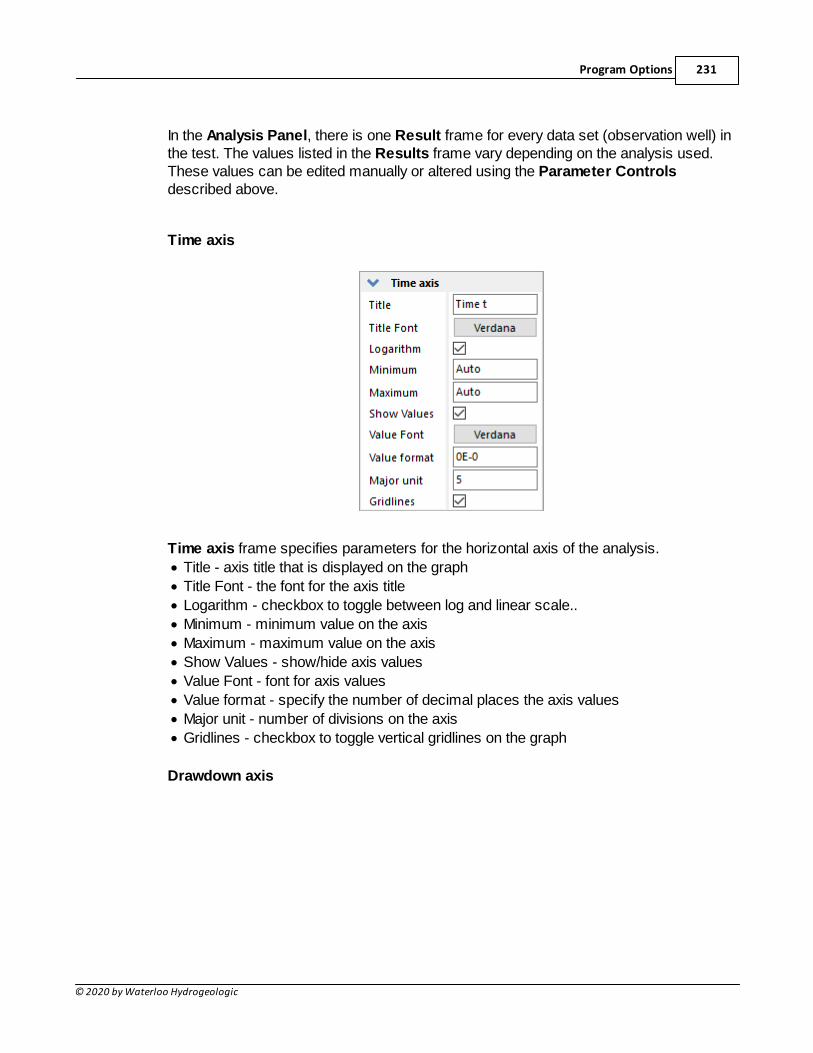
Program Options 231
© 2020 by Waterloo Hydrogeologic
In the Analysis Panel, there is one Result frame for every data set (observation well) inthe test. The values listed in the Results frame vary depending on the analysis used.These values can be edited manually or altered using the Parameter Controlsdescribed above.
Time axis
Time axis frame specifies parameters for the horizontal axis of the analysis.
· Title - axis title that is displayed on the graph
· Title Font - the font for the axis title
· Logarithm - checkbox to toggle between log and linear scale..
· Minimum - minimum value on the axis
· Maximum - maximum value on the axis
· Show Values - show/hide axis values
· Value Font - font for axis values
· Value format - specify the number of decimal places the axis values
· Major unit - number of divisions on the axis
· Gridlines - checkbox to toggle vertical gridlines on the graph
Drawdown axis
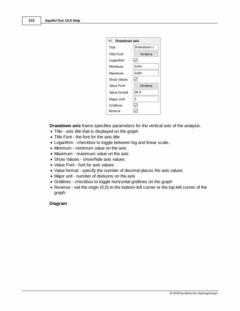
AquiferTest 10.0 Help232
© 2020 by Waterloo Hydrogeologic
Drawdown axis frame specifies parameters for the vertical axis of the analysis.
· Title - axis title that is displayed on the graph
· Title Font - the font for the axis title
· Logarithm - checkbox to toggle between log and linear scale..
· Minimum - minimum value on the axis
· Maximum - maximum value on the axis
· Show Values - show/hide axis values
· Value Font - font for axis values
· Value format - specify the number of decimal places the axis values
· Major unit - number of divisions on the axis
· Gridlines - checkbox to toggle horizontal gridlines on the graph
· Reverse - set the origin (0,0) to the bottom-left corner or the top-left corner of thegraph.
Diagram
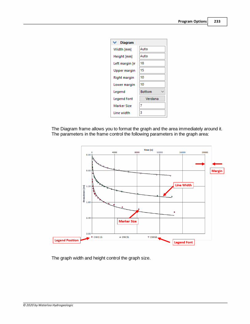
Program Options 233
© 2020 by Waterloo Hydrogeologic
The Diagram frame allows you to format the graph and the area immediately around it.The parameters in the frame control the following parameters in the graph area:
The graph width and height control the graph size.
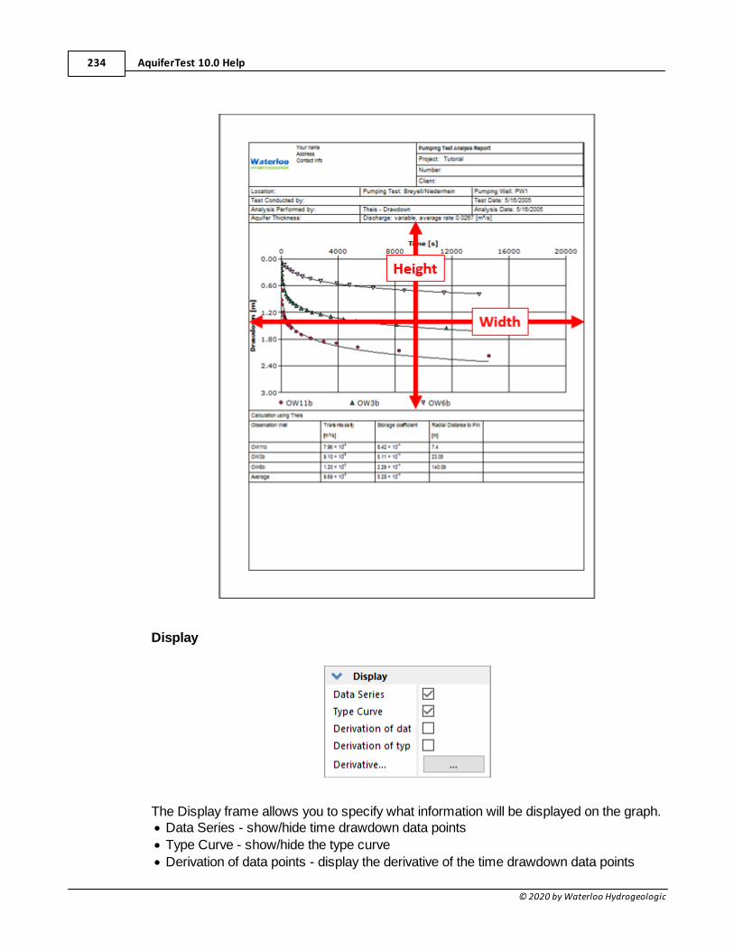
AquiferTest 10.0 Help234
© 2020 by Waterloo Hydrogeologic
Display
The Display frame allows you to specify what information will be displayed on the graph.· Data Series - show/hide time drawdown data points
· Type Curve - show/hide the type curve
· Derivation of data points - display the derivative of the time drawdown data points
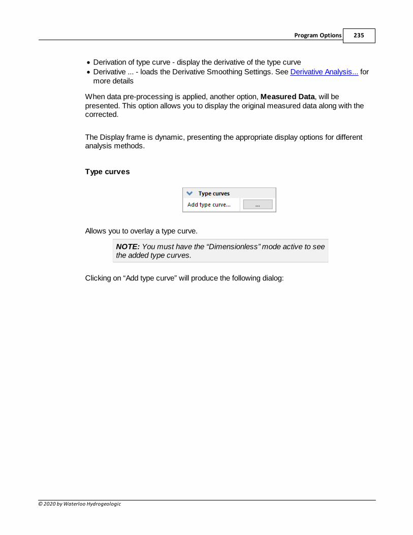
Program Options 235
© 2020 by Waterloo Hydrogeologic
· Derivation of type curve - display the derivative of the type curve
· Derivative ... - loads the Derivative Smoothing Settings. See Derivative Analysis... formore details
When data pre-processing is applied, another option, Measured Data, will bepresented. This option allows you to display the original measured data along with thecorrected.
The Display frame is dynamic, presenting the appropriate display options for differentanalysis methods.
Type curves
Allows you to overlay a type curve.
NOTE: You must have the “Dimensionless” mode active to seethe added type curves.
Clicking on “Add type curve” will produce the following dialog:
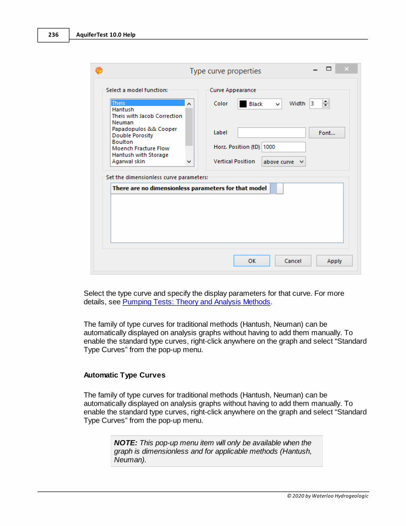
AquiferTest 10.0 Help236
© 2020 by Waterloo Hydrogeologic
Select the type curve and specify the display parameters for that curve. For moredetails, see Pumping Tests: Theory and Analysis Methods.
The family of type curves for traditional methods (Hantush, Neuman) can beautomatically displayed on analysis graphs without having to add them manually. Toenable the standard type curves, right-click anywhere on the graph and select “StandardType Curves” from the pop-up menu.
Automatic Type Curves
The family of type curves for traditional methods (Hantush, Neuman) can beautomatically displayed on analysis graphs without having to add them manually. Toenable the standard type curves, right-click anywhere on the graph and select “StandardType Curves” from the pop-up menu.
NOTE: This pop-up menu item will only be available when thegraph is dimensionless and for applicable methods (Hantush,Neuman).
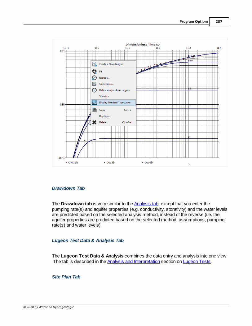
Program Options 237
© 2020 by Waterloo Hydrogeologic
Drawdown Tab
The Drawdown tab is very similar to the Analysis tab, except that you enter thepumping rate(s) and aquifer properties (e.g. conductivity, storativity) and the water levelsare predicted based on the selected analysis method, instead of the reverse (i.e. theaquifer properties are predicted based on the selected method, assumptions, pumpingrate(s) and water levels).
Lugeon Test Data & Analysis Tab
The Lugeon Test Data & Analysis combines the data entry and analysis into one view. The tab is described in the Analysis and Interpretation section on Lugeon Tests.
Site Plan Tab
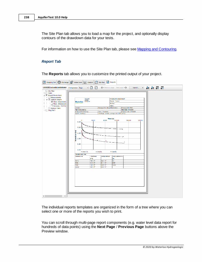
AquiferTest 10.0 Help238
© 2020 by Waterloo Hydrogeologic
The Site Plan tab allows you to load a map for the project, and optionally displaycontours of the drawdown data for your tests.
For information on how to use the Site Plan tab, please see Mapping and Contouring.
Report Tab
The Reports tab allows you to customize the printed output of your project.
The individual reports templates are organized in the form of a tree where you canselect one or more of the reports you wish to print.
You can scroll through multi-page report components (e.g. water level data report forhundreds of data points) using the Next Page / Previous Page buttons above thePreview window.
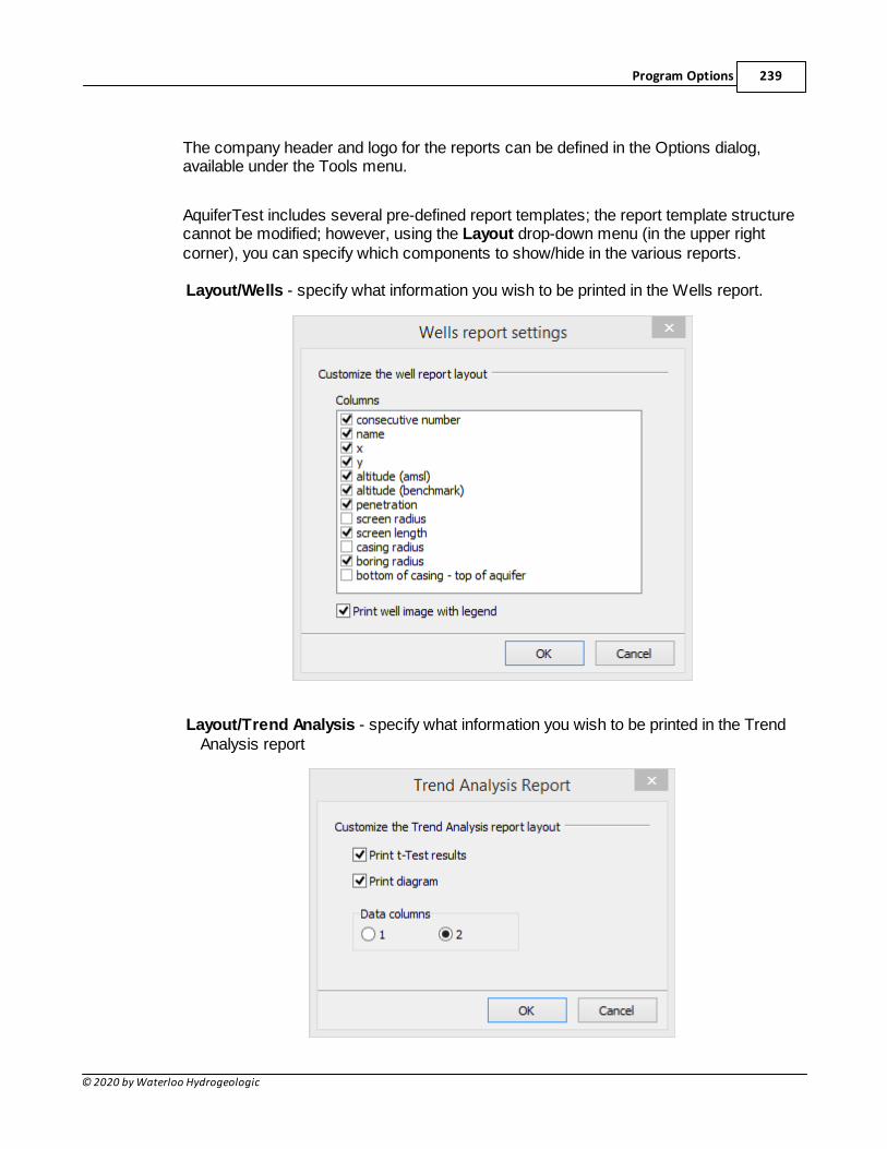
Program Options 239
© 2020 by Waterloo Hydrogeologic
The company header and logo for the reports can be defined in the Options dialog,available under the Tools menu.
AquiferTest includes several pre-defined report templates; the report template structurecannot be modified; however, using the Layout drop-down menu (in the upper rightcorner), you can specify which components to show/hide in the various reports.
Layout/Wells - specify what information you wish to be printed in the Wells report.
Layout/Trend Analysis - specify what information you wish to be printed in the TrendAnalysis report
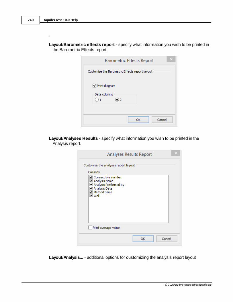
AquiferTest 10.0 Help240
© 2020 by Waterloo Hydrogeologic
.
Layout/Barometric effects report - specify what information you wish to be printed inthe Barometric Effects report.
Layout/Analyses Results - specify what information you wish to be printed in theAnalysis report.
Layout/Analysis... - additional options for customizing the analysis report layout
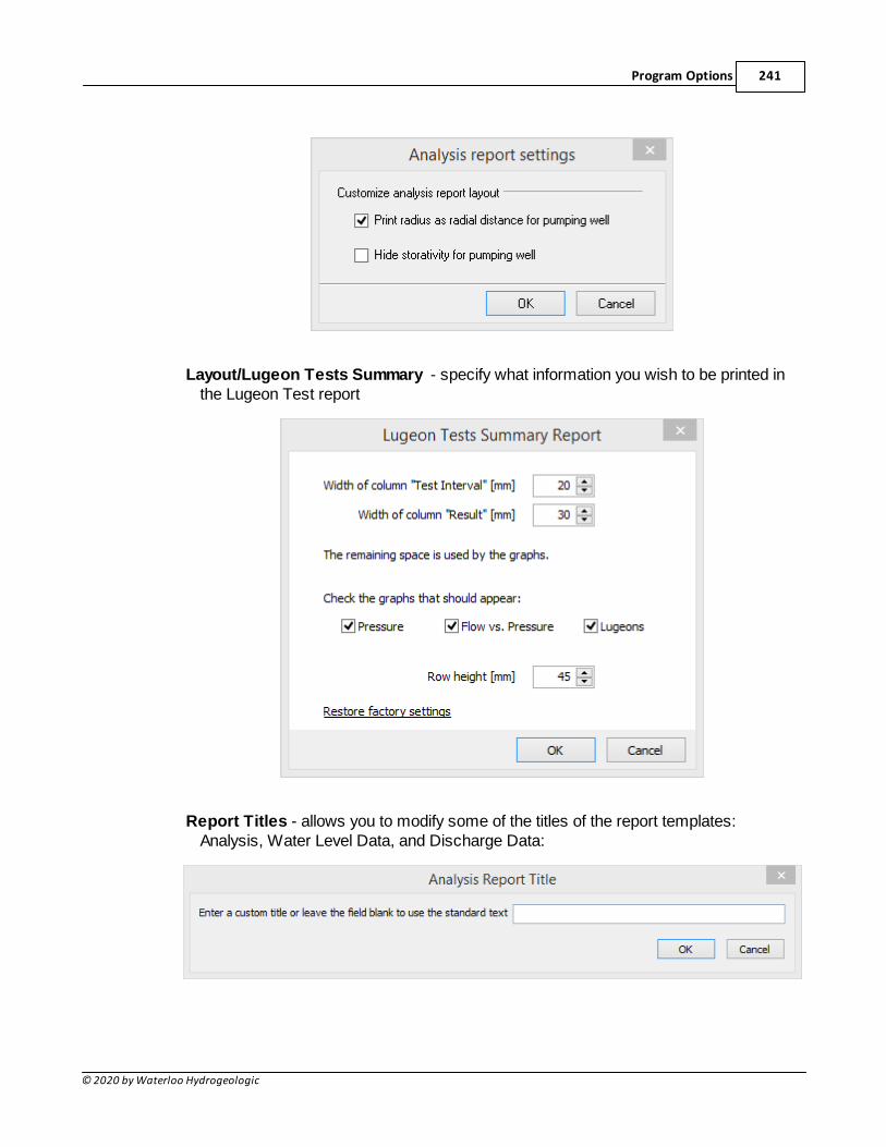
Program Options 241
© 2020 by Waterloo Hydrogeologic
Layout/Lugeon Tests Summary - specify what information you wish to be printed inthe Lugeon Test report
Report Titles - allows you to modify some of the titles of the report templates:Analysis, Water Level Data, and Discharge Data:
AquiferTest 10.0 Help242
© 2020 by Waterloo Hydrogeologic
The Report tab is test specific, i.e. it offers the options to print components only for thecurrently selected pumping or slug test.
To print specific reports, place a check mark beside the desired report, and click the
(Print) button, or select File / Print from main menu.
This concludes the description of the tabs. In the next section the main menu items willbe discussed.
3.2 Main Menu Bar
The items in the main menu bar are described in this Section and are categorized as follows:
· File
· Edit
· View
· Test
· Analysis
· Tools
· Help
File Menu
The File menu contains the following items:
New - Creates a new project. To return to the existing project, select Open Project.AquiferTest projects are saved with the extension .HYT.
Open - Opens an existing AquiferTest project. Recently opened projects appear at thebottom of the File Menu.
Close - Closes the current project.
Save - Saves the current project.
Save As - Saves the current project with a new file name.
Import
The import menu contains several options. You can import one of the following supported filetypes:
· Well locations and geometry (from an .ASC, .CSV, .TXT, .XLS, .XLSX or .SHP file)
· Site Maps (from a .BMP, .WMF, .EMF, .JPG, .DXF, .TIF, .TIFF or .PNG file)
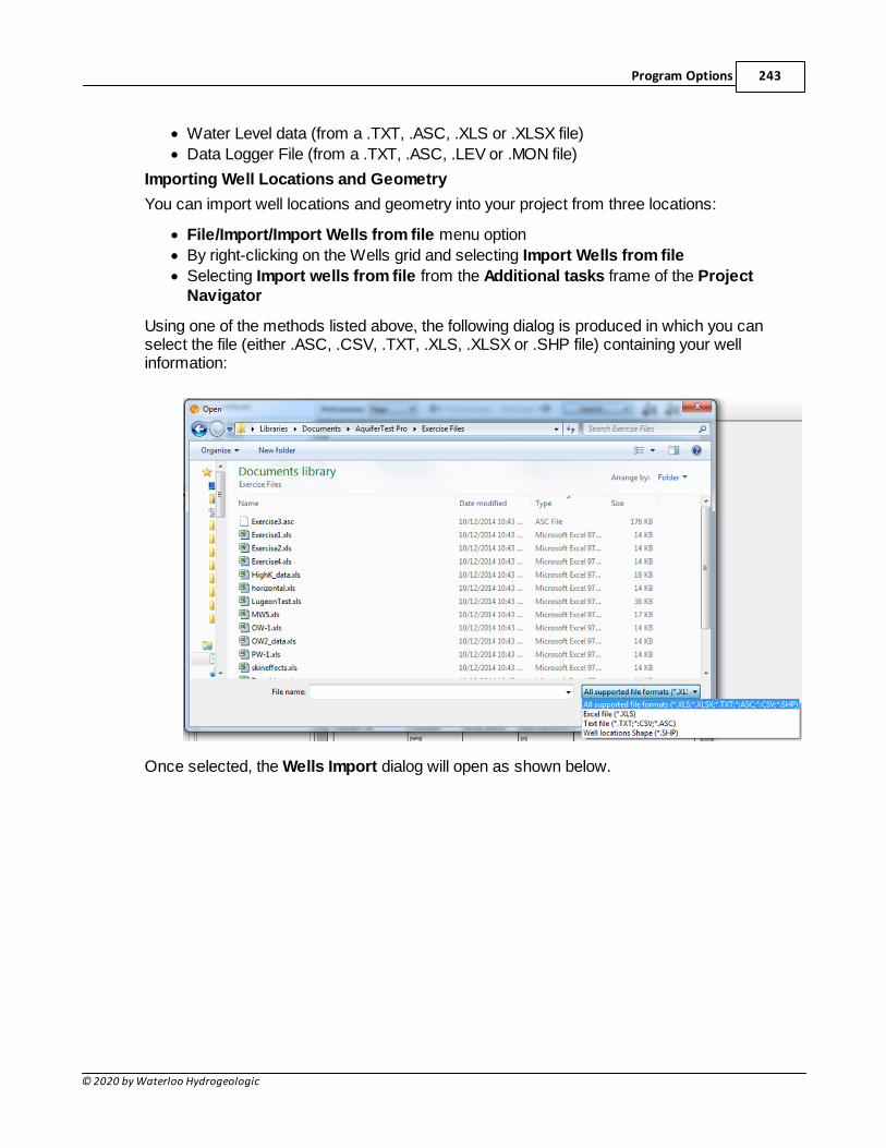
Program Options 243
© 2020 by Waterloo Hydrogeologic
· Water Level data (from a .TXT, .ASC, .XLS or .XLSX file)
· Data Logger File (from a .TXT, .ASC, .LEV or .MON file)
Importing Well Locations and Geometry
You can import well locations and geometry into your project from three locations:
· File/Import/Import Wells from file menu option
· By right-clicking on the Wells grid and selecting Import Wells from file
· Selecting Import wells from file from the Additional tasks frame of the ProjectNavigator
Using one of the methods listed above, the following dialog is produced in which you canselect the file (either .ASC, .CSV, .TXT, .XLS, .XLSX or .SHP file) containing your wellinformation:
Once selected, the Wells Import dialog will open as shown below.
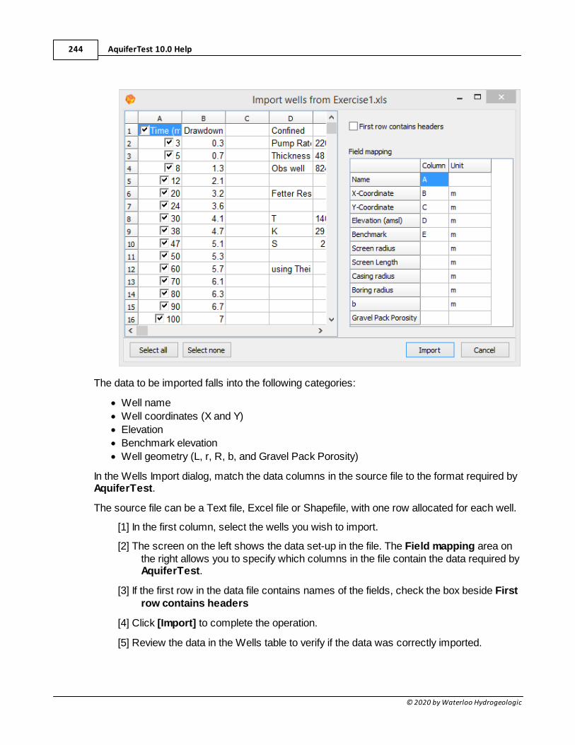
AquiferTest 10.0 Help244
© 2020 by Waterloo Hydrogeologic
The data to be imported falls into the following categories:
· Well name
· Well coordinates (X and Y)
· Elevation
· Benchmark elevation
· Well geometry (L, r, R, b, and Gravel Pack Porosity)
In the Wells Import dialog, match the data columns in the source file to the format required byAquiferTest.
The source file can be a Text file, Excel file or Shapefile, with one row allocated for each well.
[1] In the first column, select the wells you wish to import.
[2] The screen on the left shows the data set-up in the file. The Field mapping area onthe right allows you to specify which columns in the file contain the data required byAquiferTest.
[3] If the first row in the data file contains names of the fields, check the box beside Firstrow contains headers
[4] Click [Import] to complete the operation.
[5] Review the data in the Wells table to verify if the data was correctly imported.
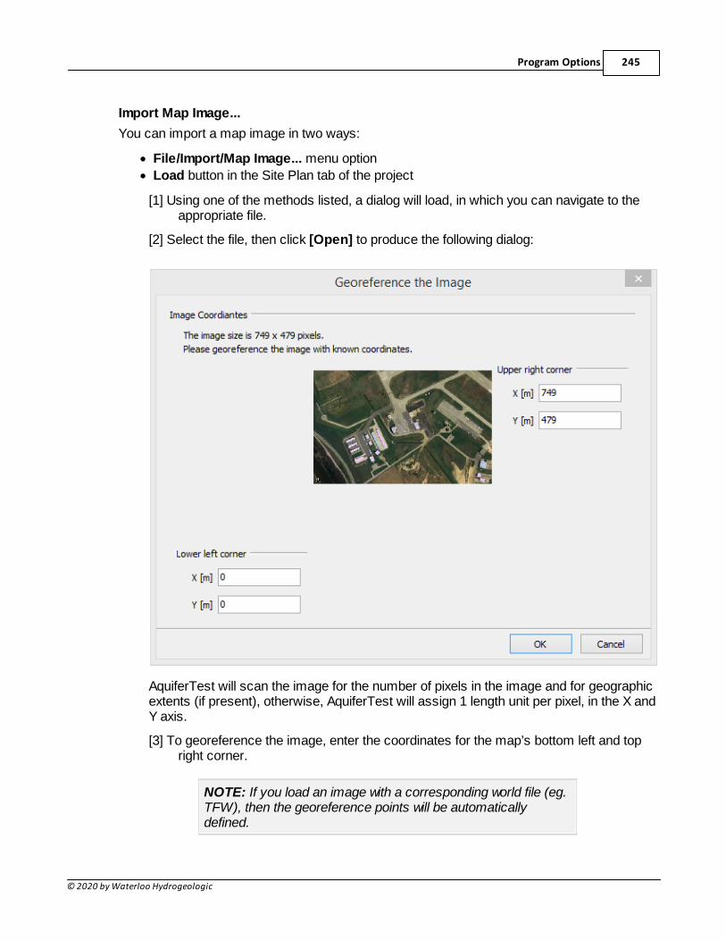
Program Options 245
© 2020 by Waterloo Hydrogeologic
Import Map Image...
You can import a map image in two ways:
· File/Import/Map Image... menu option
· Load button in the Site Plan tab of the project
[1] Using one of the methods listed, a dialog will load, in which you can navigate to theappropriate file.
[2] Select the file, then click [Open] to produce the following dialog:
AquiferTest will scan the image for the number of pixels in the image and for geographicextents (if present), otherwise, AquiferTest will assign 1 length unit per pixel, in the X andY axis.
[3] To georeference the image, enter the coordinates for the map’s bottom left and topright corner.
NOTE: If you load an image with a corresponding world file (eg.TFW), then the georeference points will be automaticallydefined.
AquiferTest 10.0 Help246
© 2020 by Waterloo Hydrogeologic
[4] Press [OK]
The map will be loaded in the Site Plan tab of the project. For more information on mapoptions and well symbols, see Mapping and Contouring.
Import Water Levels...
You can import water level data from an ASCII text file, or Excel spreadsheet, into your projectfrom three locations:
· File/Import/Import Data... menu option
· Clicking on the Import Data button in the Water Levels tab of the project
· Right clicking on the Water Level table and selecting Import data
[1] Using one of the methods listed, a dialog will load, in which you can navigate to theappropriate file.
[2] Select the file, then click [Open]
NOTE: Ensure that you are in the Water Levels tab and thatthe appropriate well is selected before importing water leveldata.
This procedure will copy the data into the Water Level table.
Text and Excel Import Format
To import data from a file, it must be set up in a specific format. The source data mustbe in a text (.TXT) or MSExcel (.XLS, .XLSX) file, containing two columns of data.
The first column must be in column A (far left side of the page) and it must contain theelapsed time data.
The second column must be in column B (immediately adjacent to the time data,separated by Tab), and it must contain water level data. This may be in the format ofdepth to water level, drawdown, or water elevations (amsl or above a benchmark). Anexample is shown below.
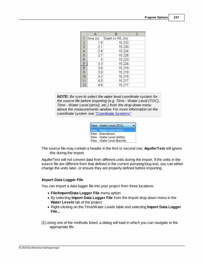
Program Options 247
© 2020 by Waterloo Hydrogeologic
NOTE: Be sure to select the water level coordinate system forthe source file before importing (e.g. Time - Water Level (TOC),Time - Water Level (amsl), etc.) from the drop-down menuabove the measurements window. For more information on thecoordinate system see "Coordinate Systems".
The source file may contain a header in the first or second row; AquiferTest will ignorethis during the import.
AquiferTest will not convert data from different units during the import. If the units in thesource file are different from that defined in the current pumping/slug test, you can eitherchange the units later, or ensure they are properly defined before importing.
Import Data Logger File
You can import a data logger file into your project from three locations:
· File/Import/Data Logger File menu option
· By selecting Import Data Logger File from the Import drop down menu in theWater Levels tab of the project
· Right-clicking on the Time/Water Levels table and selecting Import Data LoggerFile...
[1] Using one of the methods listed, a dialog will load in which you can navigate to theappropriate file.
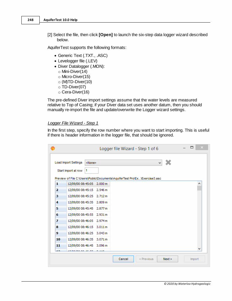
AquiferTest 10.0 Help248
© 2020 by Waterloo Hydrogeologic
[2] Select the file, then click [Open] to launch the six-step data logger wizard describedbelow.
AquiferTest supports the following formats:
· Generic Text (.TXT., .ASC)
· Levelogger file (.LEV)
· Diver Datalogger (.MON):o Mini-Diver(14)o Micro-Diver(15)o (M)TD-Diver(10)o TD-Diver(07)o Cera-Diver(16)
The pre-defined Diver import settings assume that the water levels are measuredrelative to Top of Casing; if your Diver data set uses another datum, then you shouldmanually re-import the file and update/overwrite the Logger wizard settings.
Logger File Wizard - Step 1
In the first step, specify the row number where you want to start importing. This is usefulif there is header information in the logger file, that should be ignored.
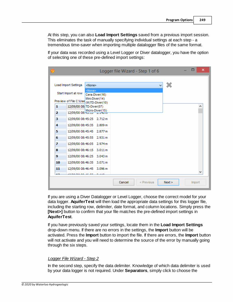
Program Options 249
© 2020 by Waterloo Hydrogeologic
At this step, you can also Load Import Settings saved from a previous import session.This eliminates the task of manually specifying individual settings at each step - atremendous time-saver when importing multiple datalogger files of the same format.
If your data was recorded using a Level Logger or Diver datalogger, you have the optionof selecting one of these pre-defined import settings:
If you are using a Diver Datalogger or Level Logger, choose the correct model for yourdata logger. AquiferTest will then load the appropriate data settings for this logger file,including the starting row, delimiter, date format, and column locations. Simply press the[Next>] button to confirm that your file matches the pre-defined import settings inAquiferTest.
If you have previously saved your settings, locate them in the Load Import Settingsdrop-down menu. If there are no errors in the settings, the Import button will beactivated. Press the Import button to import the file. If there are errors, the Import buttonwill not activate and you will need to determine the source of the error by manually goingthrough the six steps.
Logger File Wizard - Step 2
In the second step, specify the data delimiter. Knowledge of which data delimiter is usedby your data logger is not required. Under Separators, simply click to choose the
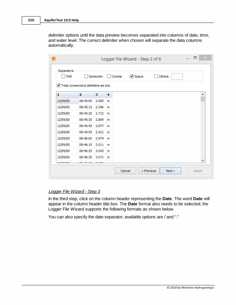
AquiferTest 10.0 Help250
© 2020 by Waterloo Hydrogeologic
delimiter options until the data preview becomes separated into columns of date, time,and water level. The correct delimiter when chosen will separate the data columnsautomatically.
Logger File Wizard - Step 3
In the third step, click on the column header representing the Date. The word Date willappear in the column header title box. The Date format also needs to be selected; theLogger File Wizard supports the following formats as shown below.
You can also specify the date separator; available options are / and "."
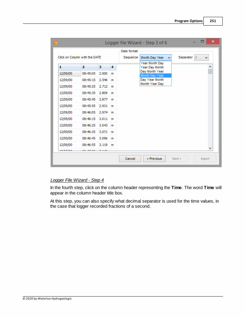
Program Options 251
© 2020 by Waterloo Hydrogeologic
Logger File Wizard - Step 4
In the fourth step, click on the column header representing the Time. The word Time willappear in the column header title box.
At this step, you can also specify what decimal separator is used for the time values, inthe case that logger recorded fractions of a second.
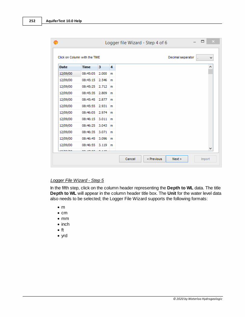
AquiferTest 10.0 Help252
© 2020 by Waterloo Hydrogeologic
Logger File Wizard - Step 5
In the fifth step, click on the column header representing the Depth to WL data. The titleDepth to WL will appear in the column header title box. The Unit for the water level dataalso needs to be selected; the Logger File Wizard supports the following formats:
· m
· cm
· mm
· inch
· ft
· yrd
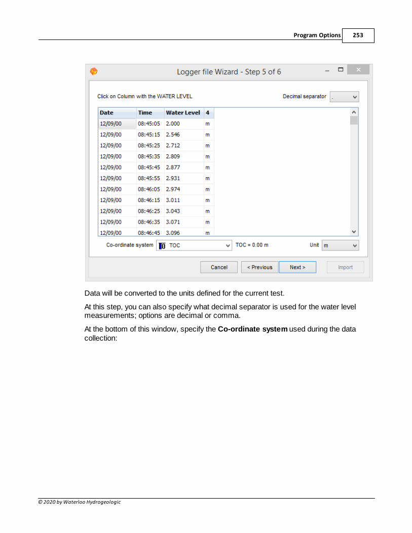
Program Options 253
© 2020 by Waterloo Hydrogeologic
Data will be converted to the units defined for the current test.
At this step, you can also specify what decimal separator is used for the water levelmeasurements; options are decimal or comma.
At the bottom of this window, specify the Co-ordinate system used during the datacollection:
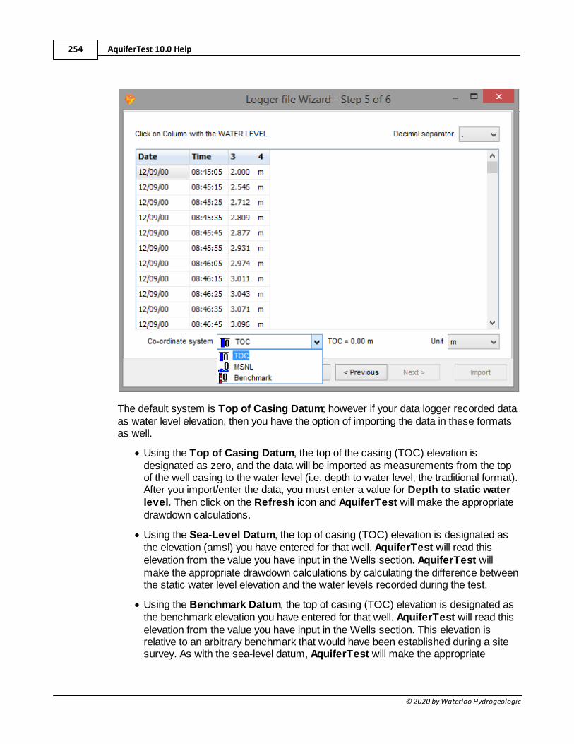
AquiferTest 10.0 Help254
© 2020 by Waterloo Hydrogeologic
The default system is Top of Casing Datum; however if your data logger recorded dataas water level elevation, then you have the option of importing the data in these formatsas well.
· Using the Top of Casing Datum, the top of the casing (TOC) elevation isdesignated as zero, and the data will be imported as measurements from the topof the well casing to the water level (i.e. depth to water level, the traditional format).After you import/enter the data, you must enter a value for Depth to static waterlevel. Then click on the Refresh icon and AquiferTest will make the appropriatedrawdown calculations.
· Using the Sea-Level Datum, the top of casing (TOC) elevation is designated asthe elevation (amsl) you have entered for that well. AquiferTest will read thiselevation from the value you have input in the Wells section. AquiferTest willmake the appropriate drawdown calculations by calculating the difference betweenthe static water level elevation and the water levels recorded during the test.
· Using the Benchmark Datum, the top of casing (TOC) elevation is designated asthe benchmark elevation you have entered for that well. AquiferTest will read thiselevation from the value you have input in the Wells section. This elevation isrelative to an arbitrary benchmark that would have been established during a sitesurvey. As with the sea-level datum, AquiferTest will make the appropriate
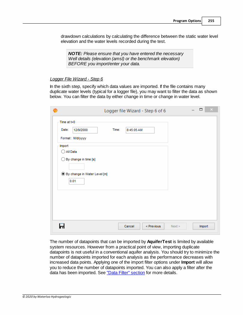
Program Options 255
© 2020 by Waterloo Hydrogeologic
drawdown calculations by calculating the difference between the static water levelelevation and the water levels recorded during the test.
NOTE: Please ensure that you have entered the necessaryWell details (elevation (amsl) or the benchmark elevation)BEFORE you import/enter your data.
Logger File Wizard - Step 6
In the sixth step, specify which data values are imported. If the file contains manyduplicate water levels (typical for a logger file), you may want to filter the data as shownbelow. You can filter the data by either change in time or change in water level.
The number of datapoints that can be imported by AquiferTest is limited by availablesystem resources. However from a practical point of view, importing duplicatedatapoints is not useful in a conventional aquifer analysis. You should try to minimize thenumber of datapoints imported for each analysis as the performance decreases withincreased data points. Applying one of the import filter options under Import will allowyou to reduce the number of datapoints imported. You can also apply a filter after thedata has been imported. See "Data Filter" section for more details.
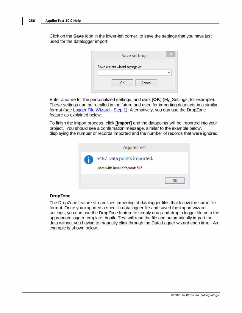
AquiferTest 10.0 Help256
© 2020 by Waterloo Hydrogeologic
Click on the Save icon in the lower-left corner, to save the settings that you have justused for the datalogger import:
Enter a name for the personalized settings, and click [OK] (My_Settings, for example).These settings can be recalled in the future and used for importing data sets in a similarformat (see Logger File Wizard - Step 1). Alternatively, you can use the DropZonefeature as explained below.
To finish the import process, click [Import] and the datapoints will be imported into yourproject. You should see a confirmation message, similar to the example below,displaying the number of records imported and the number of records that were ignored.
DropZone
The DropZone feature streamlines importing of datalogger files that follow the same fileformat. Once you imported a specific data logger file and saved the import wizardsettings, you can use the DropZone feature to simply drag-and-drop a logger file onto theappropriate logger template. AquiferTest will read the file and automatically import thedata without you having to manually click through the Data Logger wizard each time. Anexample is shown below.
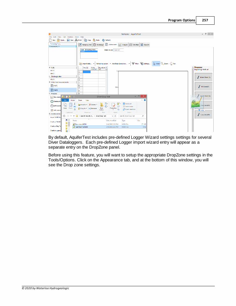
Program Options 257
© 2020 by Waterloo Hydrogeologic
By default, AquiferTest includes pre-defined Logger Wizard settings settings for severalDiver Dataloggers. Each pre-defined Logger import wizard entry will appear as aseparate entry on the DropZone panel.
Before using this feature, you will want to setup the appropriate DropZone settings in theTools/Options. Click on the Appearance tab, and at the bottom of this window, you willsee the Drop zone settings.
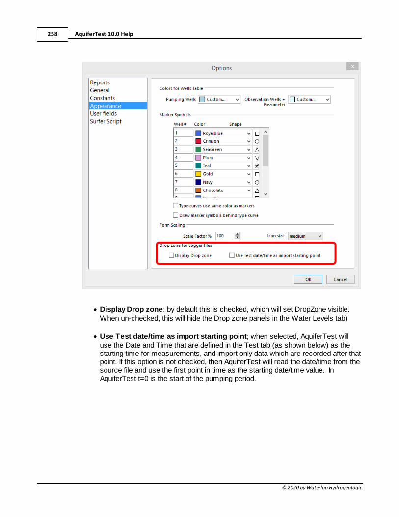
AquiferTest 10.0 Help258
© 2020 by Waterloo Hydrogeologic
· Display Drop zone: by default this is checked, which will set DropZone visible.When un-checked, this will hide the Drop zone panels in the Water Levels tab)
· Use Test date/time as import starting point; when selected, AquiferTest willuse the Date and Time that are defined in the Test tab (as shown below) as thestarting time for measurements, and import only data which are recorded after thatpoint. If this option is not checked, then AquiferTest will read the date/time from thesource file and use the first point in time as the starting date/time value. InAquiferTest t=0 is the start of the pumping period.
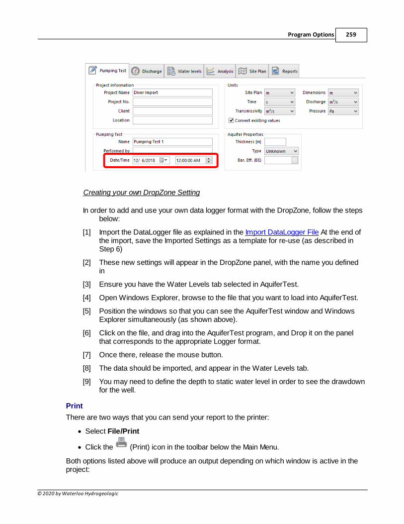
Program Options 259
© 2020 by Waterloo Hydrogeologic
Creating your own DropZone Setting
In order to add and use your own data logger format with the DropZone, follow the stepsbelow:
[1] Import the DataLogger file as explained in the Import DataLogger File At the end ofthe import, save the Imported Settings as a template for re-use (as described inStep 6)
[2] These new settings will appear in the DropZone panel, with the name you definedin
[3] Ensure you have the Water Levels tab selected in AquiferTest.
[4] Open Windows Explorer, browse to the file that you want to load into AquiferTest.
[5] Position the windows so that you can see the AquiferTest window and WindowsExplorer simultaneously (as shown above).
[6] Click on the file, and drag into the AquiferTest program, and Drop it on the panelthat corresponds to the appropriate Logger format.
[7] Once there, release the mouse button.
[8] The data should be imported, and appear in the Water Levels tab.
[9] You may need to define the depth to static water level in order to see the drawdownfor the well.
There are two ways that you can send your report to the printer:
· Select File/Print
· Click the (Print) icon in the toolbar below the Main Menu.
Both options listed above will produce an output depending on which window is active in theproject:
AquiferTest 10.0 Help260
© 2020 by Waterloo Hydrogeologic
· Pumping (Slug) Test/Wells tab - prints the list of wells in the project accompanied bythe coordinates and geometry
· Discharge - no output available
· Water Levels - print water levels for the currently active well
· Analysis - prints the current analysis graph and results
· Pumping (Slug) Test/Site Map tab - prints the current map view. This could include welllocations, basemaps, and drawdown contours or color shaded map
· Report - in the Report tab you have the opportunity to select from desired reporttemplates. To do so, expand the navigation tree in the left portion of the Reports taband select which printouts you wish to obtain, and press Print.
NOTE: A print preview of any printable report can be obtained inthe Reports tab by selecting the appropriate view from thenavigator tree.
Print options are not available for Discharge plots or the plots in the Diagnostic Graphs tab.Use the copy feature (Edit/Copy from the main menu), then paste these images into adocument or graphics editor.
Printer Setup
Selecting this option will load the dialog to set-up your printer.
Exit
Exit the program. Ensure that you have saved the project before exiting.
Edit Menu
The Edit menu contains the following items:
Copy
Copy the selected item from AquiferTest to the Windows clipboard. Depending on yourWindows System setup, the decimal sign used for the data will either be a period (.) or acomma (,). You can change this within Windows by selecting Start > Settings > ControlPanel > Regional Options.
Paste
Paste data from the Windows clipboard into AquiferTest. With this command, only the firsttwo columns are transferred. Therefore, ensure that the first two columns of the informationon the clipboard are the desired columns of data. When pasting data from a spreadsheet, thedata must be in adjacent columns with the time data on the left and the water level data on theright. When pasting data from a text editor, the columns of data must be separated by tabs(tab delimited).
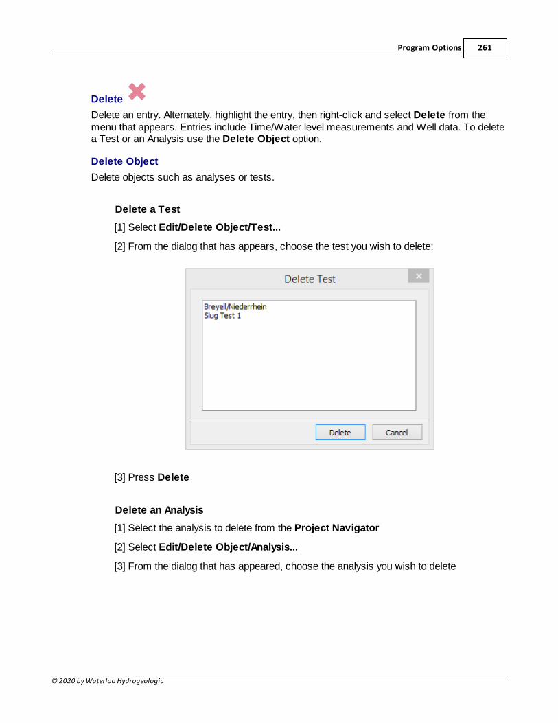
Program Options 261
© 2020 by Waterloo Hydrogeologic
Delete
Delete an entry. Alternately, highlight the entry, then right-click and select Delete from themenu that appears. Entries include Time/Water level measurements and Well data. To deletea Test or an Analysis use the Delete Object option.
Delete Object
Delete objects such as analyses or tests.
Delete a Test
[1] Select Edit/Delete Object/Test...
[2] From the dialog that has appears, choose the test you wish to delete:
[3] Press Delete
Delete an Analysis
[1] Select the analysis to delete from the Project Navigator
[2] Select Edit/Delete Object/Analysis...
[3] From the dialog that has appeared, choose the analysis you wish to delete
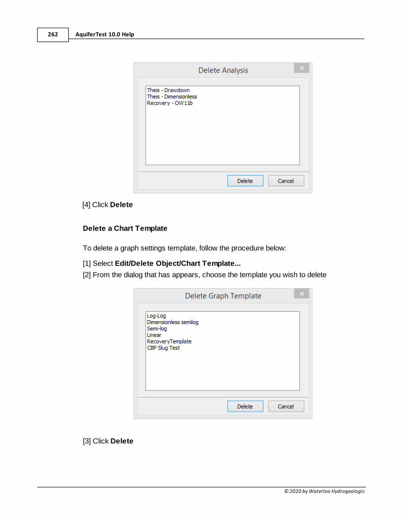
AquiferTest 10.0 Help262
© 2020 by Waterloo Hydrogeologic
[4] Click Delete
Delete a Chart Template
To delete a graph settings template, follow the procedure below:
[1] Select Edit/Delete Object/Chart Template...
[2] From the dialog that has appears, choose the template you wish to delete
[3] Click Delete
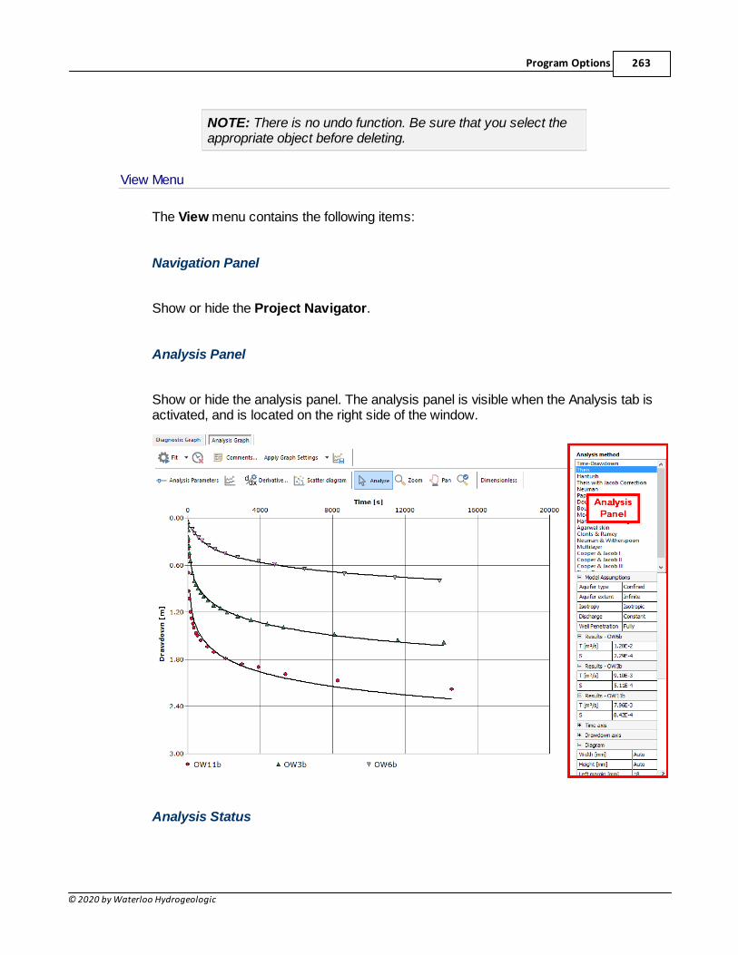
Program Options 263
© 2020 by Waterloo Hydrogeologic
NOTE: There is no undo function. Be sure that you select theappropriate object before deleting.
View Menu
The View menu contains the following items:
Navigation Panel
Show or hide the Project Navigator.
Analysis Panel
Show or hide the analysis panel. The analysis panel is visible when the Analysis tab isactivated, and is located on the right side of the window.
Analysis Status
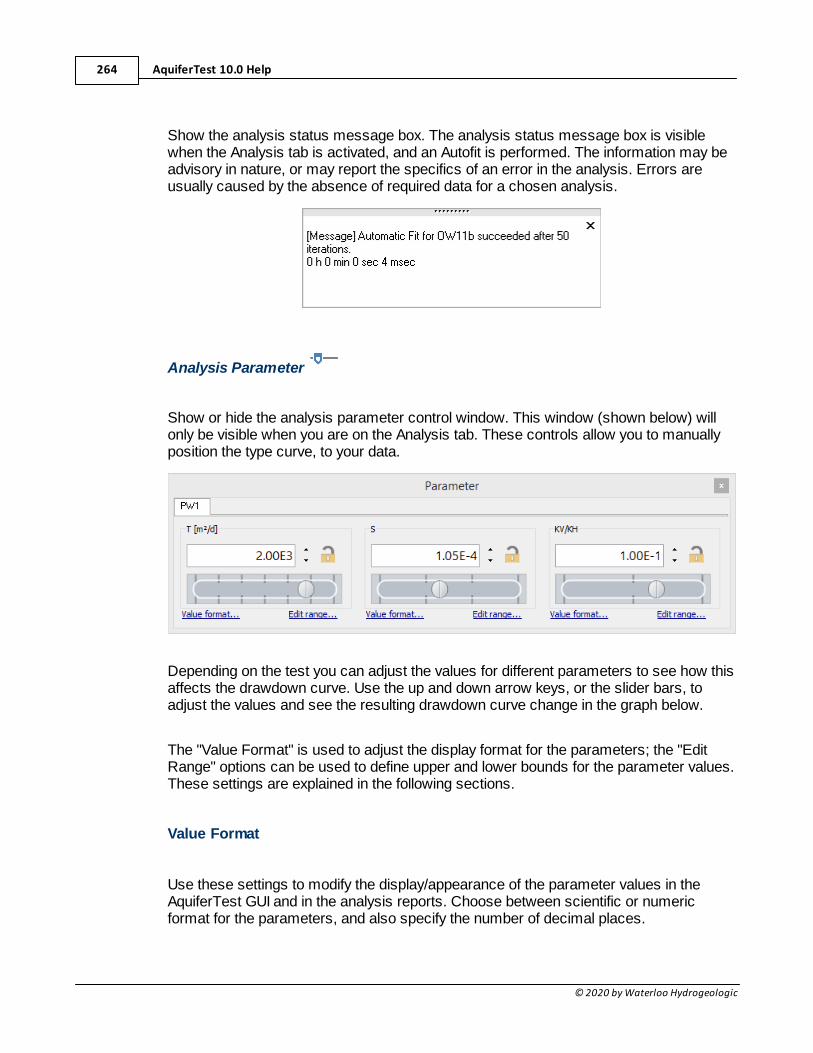
AquiferTest 10.0 Help264
© 2020 by Waterloo Hydrogeologic
Show the analysis status message box. The analysis status message box is visiblewhen the Analysis tab is activated, and an Autofit is performed. The information may beadvisory in nature, or may report the specifics of an error in the analysis. Errors areusually caused by the absence of required data for a chosen analysis.
Analysis Parameter
Show or hide the analysis parameter control window. This window (shown below) willonly be visible when you are on the Analysis tab. These controls allow you to manuallyposition the type curve, to your data.
Depending on the test you can adjust the values for different parameters to see how thisaffects the drawdown curve. Use the up and down arrow keys, or the slider bars, toadjust the values and see the resulting drawdown curve change in the graph below.
The "Value Format" is used to adjust the display format for the parameters; the "EditRange" options can be used to define upper and lower bounds for the parameter values.These settings are explained in the following sections.
Value Format
Use these settings to modify the display/appearance of the parameter values in theAquiferTest GUI and in the analysis reports. Choose between scientific or numericformat for the parameters, and also specify the number of decimal places.
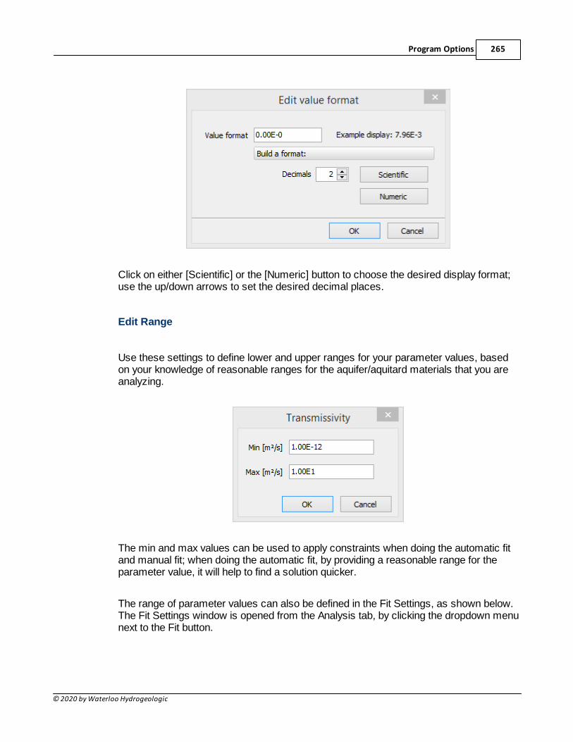
Program Options 265
© 2020 by Waterloo Hydrogeologic
Click on either [Scientific] or the [Numeric] button to choose the desired display format;use the up/down arrows to set the desired decimal places.
Edit Range
Use these settings to define lower and upper ranges for your parameter values, basedon your knowledge of reasonable ranges for the aquifer/aquitard materials that you areanalyzing.
The min and max values can be used to apply constraints when doing the automatic fitand manual fit; when doing the automatic fit, by providing a reasonable range for theparameter value, it will help to find a solution quicker.
The range of parameter values can also be defined in the Fit Settings, as shown below.The Fit Settings window is opened from the Analysis tab, by clicking the dropdown menunext to the Fit button.
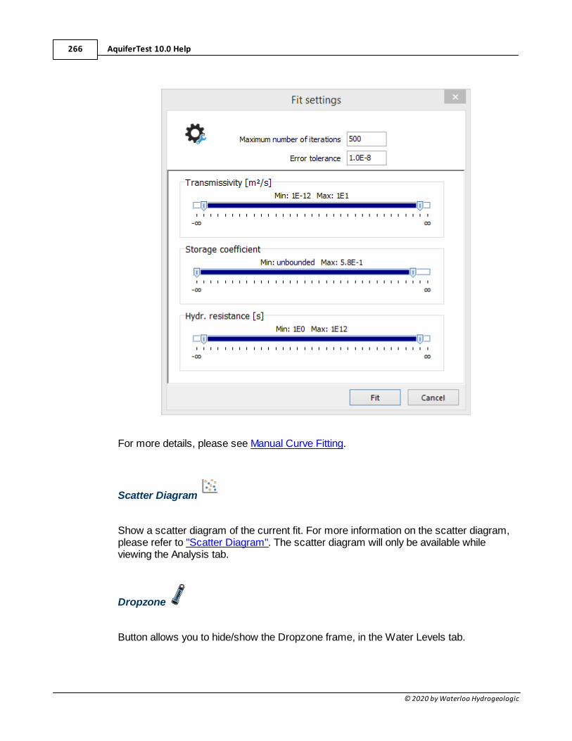
AquiferTest 10.0 Help266
© 2020 by Waterloo Hydrogeologic
For more details, please see Manual Curve Fitting.
Scatter Diagram
Show a scatter diagram of the current fit. For more information on the scatter diagram,please refer to "Scatter Diagram". The scatter diagram will only be available whileviewing the Analysis tab.
Dropzone
Button allows you to hide/show the Dropzone frame, in the Water Levels tab.
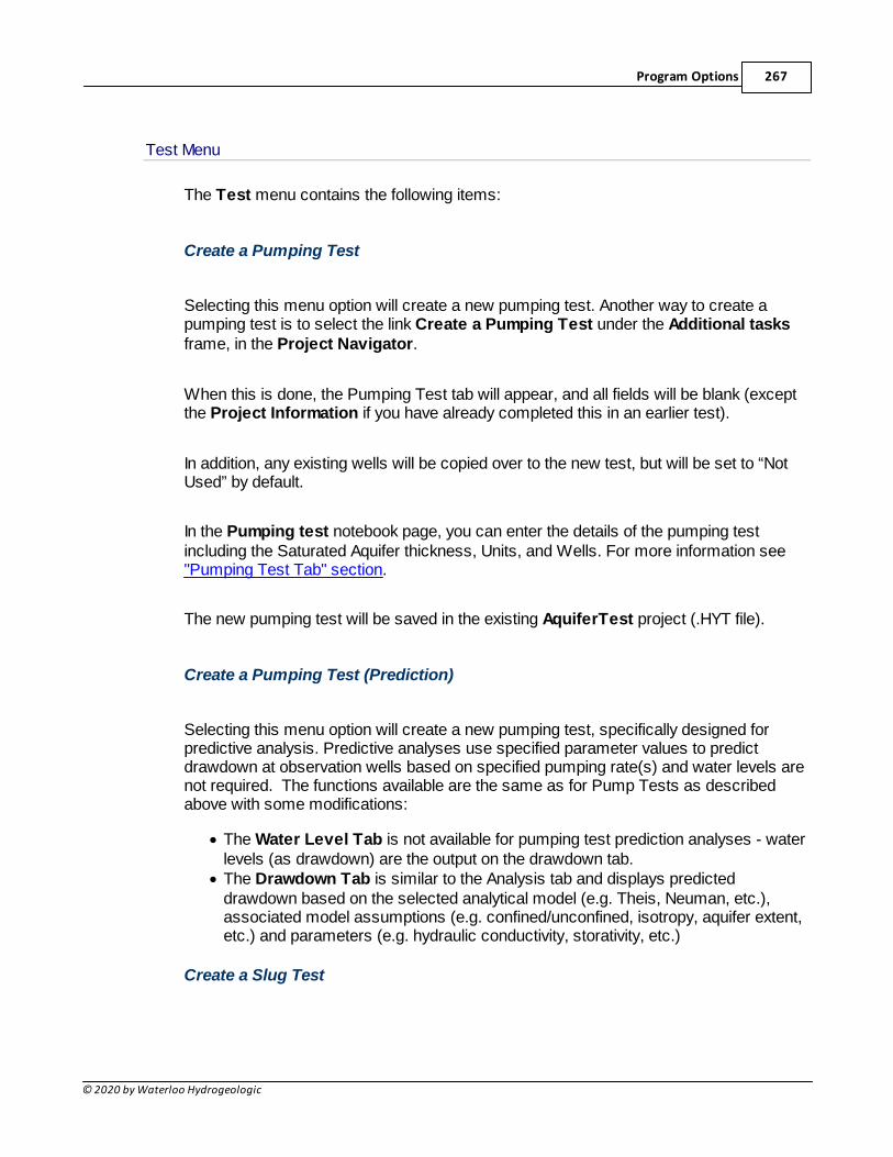
Program Options 267
© 2020 by Waterloo Hydrogeologic
Test Menu
The Test menu contains the following items:
Create a Pumping Test
Selecting this menu option will create a new pumping test. Another way to create apumping test is to select the link Create a Pumping Test under the Additional tasksframe, in the Project Navigator.
When this is done, the Pumping Test tab will appear, and all fields will be blank (exceptthe Project Information if you have already completed this in an earlier test).
In addition, any existing wells will be copied over to the new test, but will be set to “NotUsed” by default.
In the Pumping test notebook page, you can enter the details of the pumping testincluding the Saturated Aquifer thickness, Units, and Wells. For more information see"Pumping Test Tab" section.
The new pumping test will be saved in the existing AquiferTest project (.HYT file).
Create a Pumping Test (Prediction)
Selecting this menu option will create a new pumping test, specifically designed forpredictive analysis. Predictive analyses use specified parameter values to predictdrawdown at observation wells based on specified pumping rate(s) and water levels arenot required. The functions available are the same as for Pump Tests as describedabove with some modifications:
· The Water Level Tab is not available for pumping test prediction analyses - waterlevels (as drawdown) are the output on the drawdown tab.
· The Drawdown Tab is similar to the Analysis tab and displays predicteddrawdown based on the selected analytical model (e.g. Theis, Neuman, etc.),associated model assumptions (e.g. confined/unconfined, isotropy, aquifer extent,etc.) and parameters (e.g. hydraulic conductivity, storativity, etc.)
Create a Slug Test
AquiferTest 10.0 Help268
© 2020 by Waterloo Hydrogeologic
Selecting this menu option will create a new slug test. Another way to create a slug testis to select the link Create a Slug Test under the Additional tasks frame, in theProject Navigator.
When this is done, the Slug Test tab will appear, and all fields will be blank (except theProject Information if you have already completed this in an earlier test).
Any existing wells will be copied over to the new test, but will be set to “Not Used” bydefault.
For a slug test, only one well can be selected as the “Test Well”. This is done in the wellType column, in the Wells grid (in the Slug Test tab). Create a new slug test for eachadditional test well.
For more information see "Slug Test Tab" section.
Create a Lugeon Test
Selecting this menu option will create a new Lugeon/Packer test. Another way to createa Lugeon/Packer test is to select the link Create a Lugeon Test under the Additionaltasks frame, in the Project Navigator.
When this is done, the Lugeon Test tab will appear, and all fields will be blank (exceptthe Project Information if you have already completed this in an earlier test).
Any existing wells will be copied over to the new test.
For more information see "Lugeon Tests" section.
Trend Correction
Load options for correcting water levels due to trend effects.
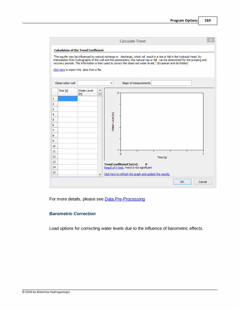
Program Options 269
© 2020 by Waterloo Hydrogeologic
For more details, please see Data Pre-Processing
Barometric Correction
Load options for correcting water levels due to the influence of barometric effects.
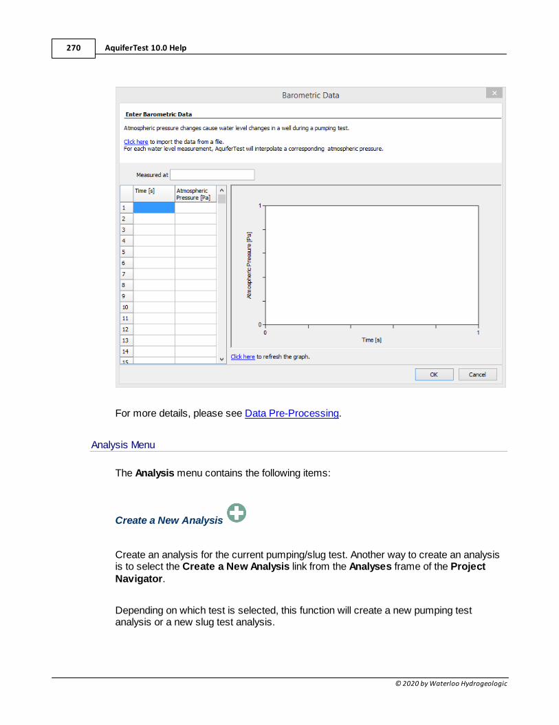
AquiferTest 10.0 Help270
© 2020 by Waterloo Hydrogeologic
For more details, please see Data Pre-Processing.
Analysis Menu
The Analysis menu contains the following items:
Create a New Analysis
Create an analysis for the current pumping/slug test. Another way to create an analysisis to select the Create a New Analysis link from the Analyses frame of the ProjectNavigator.
Depending on which test is selected, this function will create a new pumping testanalysis or a new slug test analysis.
Program Options 271
© 2020 by Waterloo Hydrogeologic
Create a New Scenario (Predictive Analyses)
Create a new analysis/scenario for the current predictive pumping test. Another way tocreate an scenario is to select the Create a New Scenario link from the Scenariosframe of the Project Navigator.
This button is only available when the currently selected test is a predictive pumpingtest.
Create Pumping Well Analysis
This menu allows you to initiate various techniques for calculating the efficiency of theproduction well. Pumping well analyses include the following three options:
Create Analysis Considering Well Effects
Creates an analysis using the Papadopulos-Cooper method, which accounts for well-bore storage. For more details see Theory and Analysis Methods.
Create Analysis for Specific Capacity
Creates a Specific Capacity analysis for the selected well. For more details, seeSpecific Capacity.
Well Losses
Creates a Hantush Biershenk analysis for the selected well. For more details, seeHantush-Bierschenk Well Loss Solution.
Well Efficiency
Creates a new well efficiency analysis. The efficiency of a pumping well expresses theratio of aquifer loss (theoretical drawdown) to total (measured) drawdown in the well.For more details, see the Well Efficiency section.
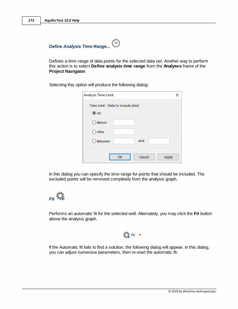
AquiferTest 10.0 Help272
© 2020 by Waterloo Hydrogeologic
Define Analysis Time Range...
Defines a time range of data points for the selected data set. Another way to performthis action is to select Define analysis time range from the Analyses frame of theProject Navigator.
Selecting this option will produce the following dialog:
In this dialog you can specify the time range for points that should be included. Theexcluded points will be removed completely from the analysis graph.
Fit
Performs an automatic fit for the selected well. Alternately, you may click the Fit buttonabove the analysis graph.
If the Automatic fit fails to find a solution, the following dialog will appear. In this dialog,you can adjust numerous parameters, then re-start the automatic fit:
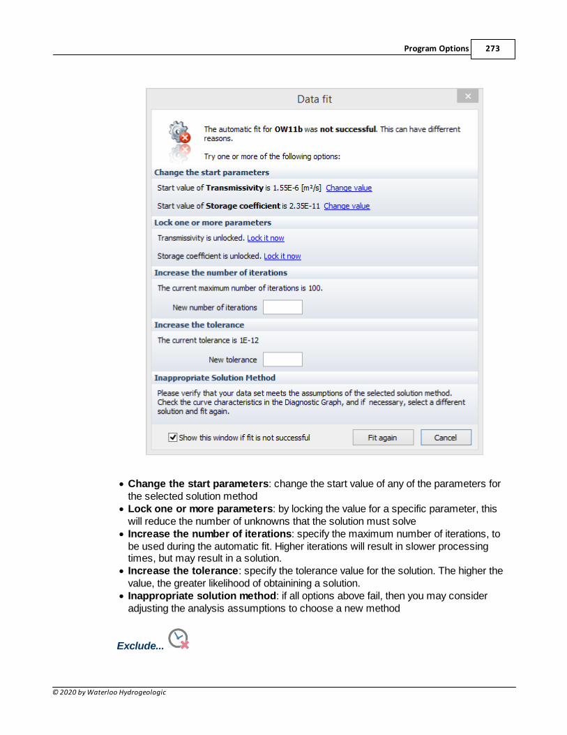
Program Options 273
© 2020 by Waterloo Hydrogeologic
· Change the start parameters: change the start value of any of the parameters forthe selected solution method
· Lock one or more parameters: by locking the value for a specific parameter, thiswill reduce the number of unknowns that the solution must solve
· Increase the number of iterations: specify the maximum number of iterations, tobe used during the automatic fit. Higher iterations will result in slower processingtimes, but may result in a solution.
· Increase the tolerance: specify the tolerance value for the solution. The higher thevalue, the greater likelihood of obtainining a solution.
· Inappropriate solution method: if all options above fail, then you may consideradjusting the analysis assumptions to choose a new method
Exclude...
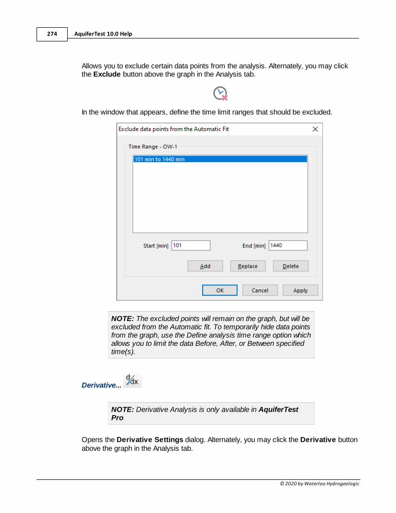
AquiferTest 10.0 Help274
© 2020 by Waterloo Hydrogeologic
Allows you to exclude certain data points from the analysis. Alternately, you may clickthe Exclude button above the graph in the Analysis tab.
In the window that appears, define the time limit ranges that should be excluded.
NOTE: The excluded points will remain on the graph, but will beexcluded from the Automatic fit. To temporarily hide data pointsfrom the graph, use the Define analysis time range option whichallows you to limit the data Before, After, or Between specifiedtime(s).
Derivative...
NOTE: Derivative Analysis is only available in AquiferTestPro
Opens the Derivative Settings dialog. Alternately, you may click the Derivative buttonabove the graph in the Analysis tab.
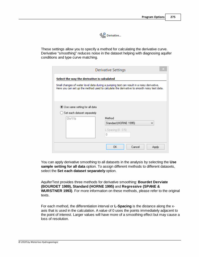
Program Options 275
© 2020 by Waterloo Hydrogeologic
These settings allow you to specify a method for calculating the derivative curve.Derivative “smoothing” reduces noise in the dataset helping with diagnosing aquiferconditions and type curve matching.
You can apply derivative smoothing to all datasets in the analysis by selecting the Usesample setting for all data option. To assign different methods to different datasets,select the Set each dataset separately option.
AquiferTest provides three methods for derivative smoothing: Bourdet Derviate(BOURDET 1989), Standard (HORNE 1995) and Regressive (SPANE &WURSTNER 1993). For more information on these methods, please refer to the originaltexts.
For each method, the differentiation interval or L-Spacing is the distance along the x-axis that is used in the calculation. A value of 0 uses the points immediately adjacent tothe point of interest. Larger values will have more of a smoothing effect but may cause aloss of resolution.
AquiferTest 10.0 Help276
© 2020 by Waterloo Hydrogeologic
Comments...
Allows you to add comments to the active analysis. Alternately, click the Commentsbutton.
In the window that appears enter any comments. These will appear when the Analysisreport is printed.
Statistics
Allows you to view statistics for the selected analysis, and current selected well. Thisoption may also be loaded by right-clicking on the Analysis graph, and selectingStatistics.
The following Statistics window will appear.
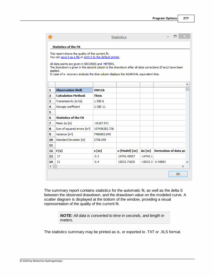
Program Options 277
© 2020 by Waterloo Hydrogeologic
The summary report contains statistics for the automatic fit, as well as the delta Sbetween the observed drawdown, and the drawdown value on the modeled curve. Ascatter diagram is displayed at the bottom of the window, providing a visualrepresentation of the quality of the current fit.
NOTE: All data is converted to time in seconds, and length inmeters.
The statistics summary may be printed as is, or exported to .TXT or .XLS format.
AquiferTest 10.0 Help278
© 2020 by Waterloo Hydrogeologic
Display Standard Typecurves
Allows you to show/hide a family of type curves for certain analysis.
Duplicate
Allows you to create a copy of the current analysis.
Tools Menu
Options
Specify settings for various program options.
Reports tab
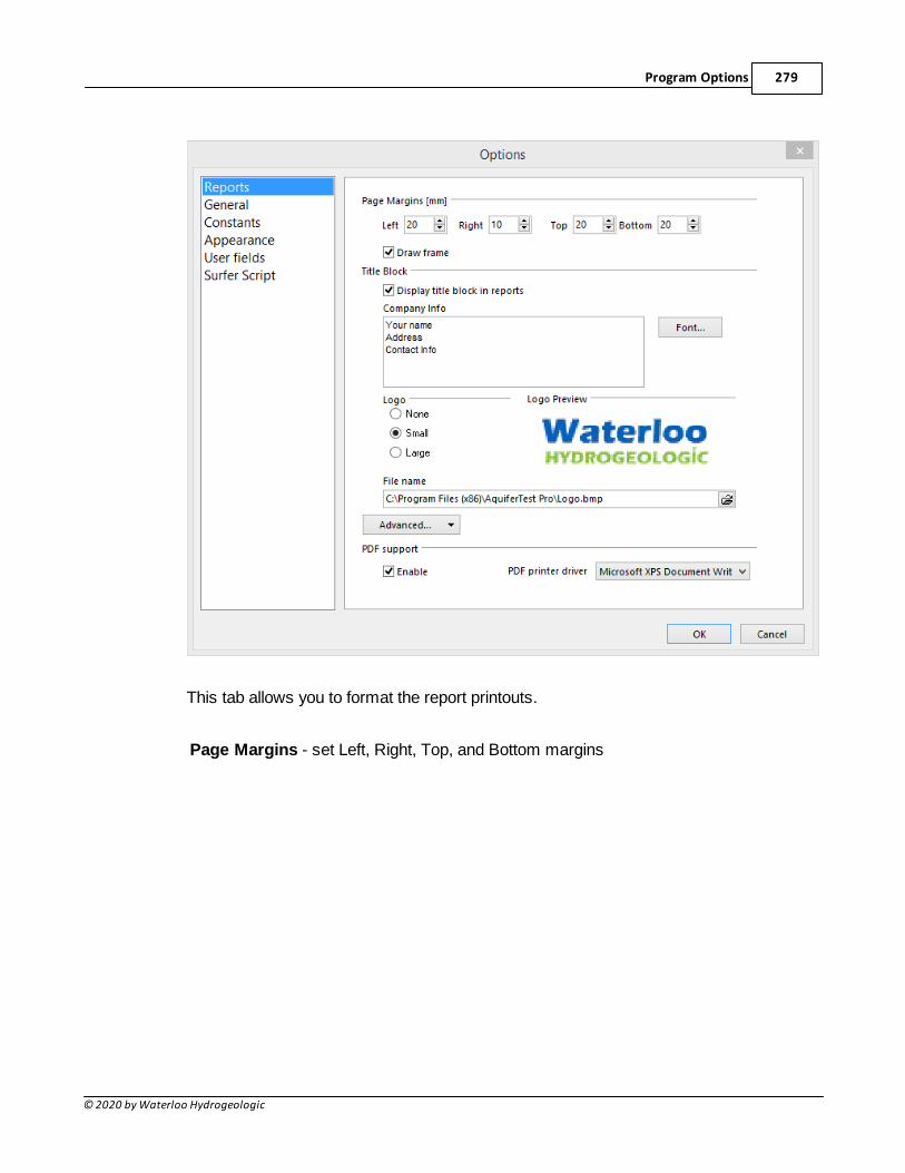
Program Options 279
© 2020 by Waterloo Hydrogeologic
This tab allows you to format the report printouts.
Page Margins - set Left, Right, Top, and Bottom margins
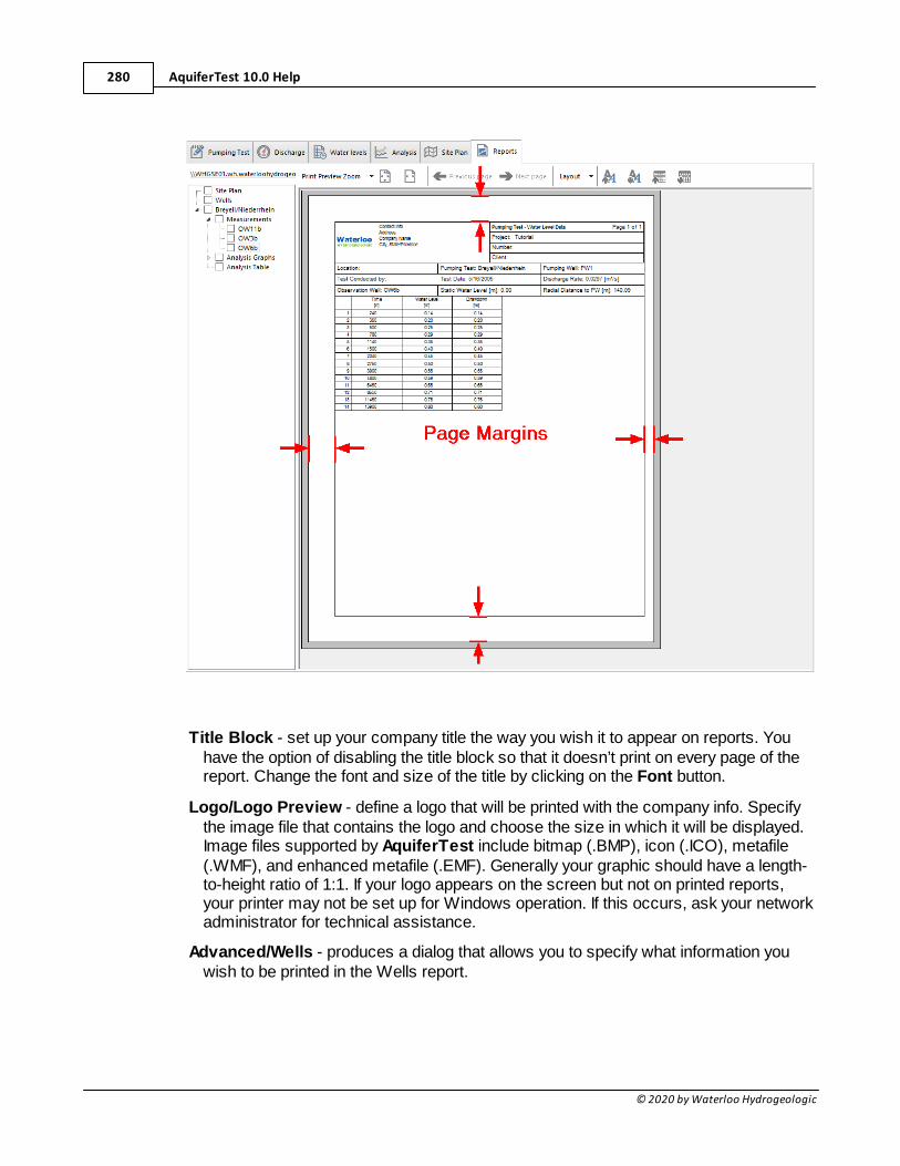
AquiferTest 10.0 Help280
© 2020 by Waterloo Hydrogeologic
Title Block - set up your company title the way you wish it to appear on reports. Youhave the option of disabling the title block so that it doesn’t print on every page of thereport. Change the font and size of the title by clicking on the Font button.
Logo/Logo Preview - define a logo that will be printed with the company info. Specifythe image file that contains the logo and choose the size in which it will be displayed.Image files supported by AquiferTest include bitmap (.BMP), icon (.ICO), metafile(.WMF), and enhanced metafile (.EMF). Generally your graphic should have a length-to-height ratio of 1:1. If your logo appears on the screen but not on printed reports,your printer may not be set up for Windows operation. If this occurs, ask your networkadministrator for technical assistance.
Advanced/Wells - produces a dialog that allows you to specify what information youwish to be printed in the Wells report.
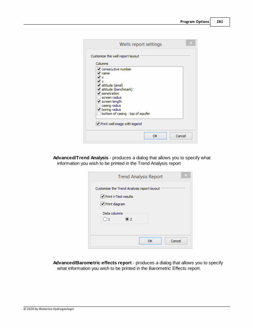
Program Options 281
© 2020 by Waterloo Hydrogeologic
Advanced/Trend Analysis - produces a dialog that allows you to specify whatinformation you wish to be printed in the Trend Analysis report
.
Advanced/Barometric effects report - produces a dialog that allows you to specifywhat information you wish to be printed in the Barometric Effects report.
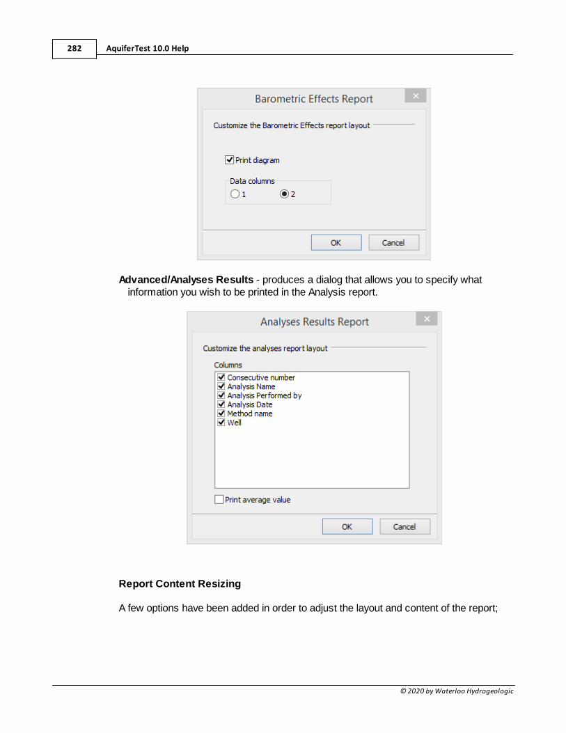
AquiferTest 10.0 Help282
© 2020 by Waterloo Hydrogeologic
Advanced/Analyses Results - produces a dialog that allows you to specify whatinformation you wish to be printed in the Analysis report.
Report Content Resizing
A few options have been added in order to adjust the layout and content of the report;
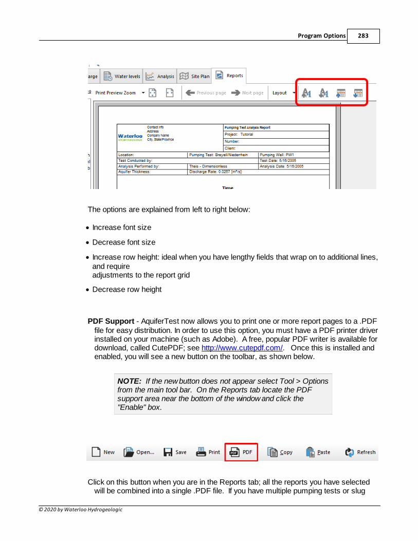
Program Options 283
© 2020 by Waterloo Hydrogeologic
The options are explained from left to right below:
· Increase font size
· Decrease font size
· Increase row height: ideal when you have lengthy fields that wrap on to additional lines,and requireadjustments to the report grid
· Decrease row height
PDF Support - AquiferTest now allows you to print one or more report pages to a .PDFfile for easy distribution. In order to use this option, you must have a PDF printer driverinstalled on your machine (such as Adobe). A free, popular PDF writer is available fordownload, called CutePDF; see http://www.cutepdf.com/. Once this is installed andenabled, you will see a new button on the toolbar, as shown below.
NOTE: If the new button does not appear select Tool > Optionsfrom the main tool bar. On the Reports tab locate the PDFsupport area near the bottom of the window and click the"Enable" box.
Click on this button when you are in the Reports tab; all the reports you have selectedwill be combined into a single .PDF file. If you have multiple pumping tests or slug
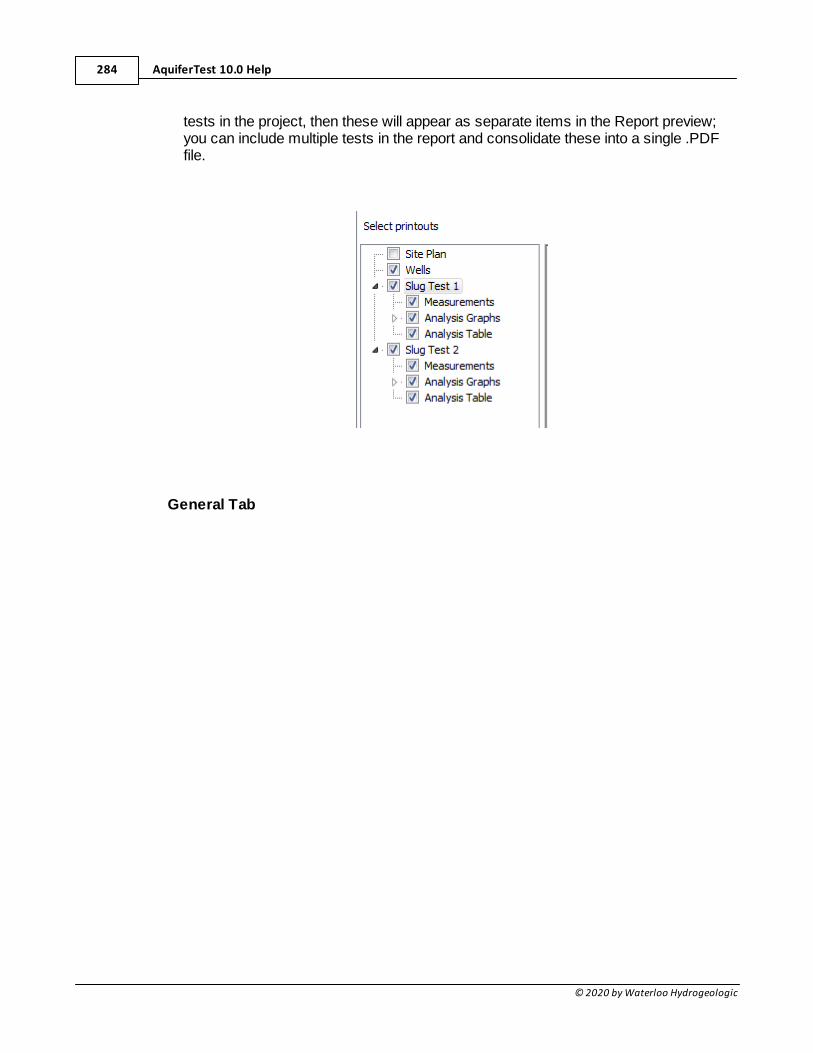
AquiferTest 10.0 Help284
© 2020 by Waterloo Hydrogeologic
tests in the project, then these will appear as separate items in the Report preview;you can include multiple tests in the report and consolidate these into a single .PDFfile.
General Tab
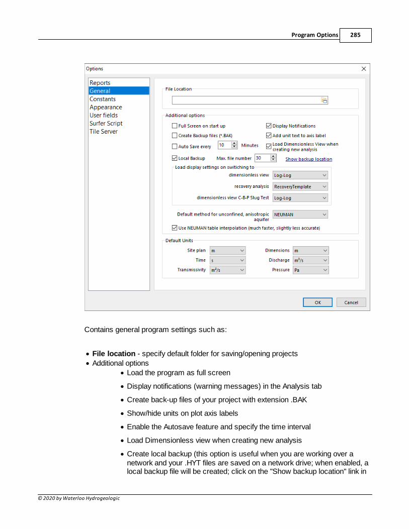
Program Options 285
© 2020 by Waterloo Hydrogeologic
Contains general program settings such as:
· File location - specify default folder for saving/opening projects
· Additional options
· Load the program as full screen
· Display notifications (warning messages) in the Analysis tab
· Create back-up files of your project with extension .BAK
· Show/hide units on plot axis labels
· Enable the Autosave feature and specify the time interval
· Load Dimensionless view when creating new analysis
· Create local backup (this option is useful when you are working over anetwork and your .HYT files are saved on a network drive; when enabled, alocal backup file will be created; click on the "Show backup location" link in
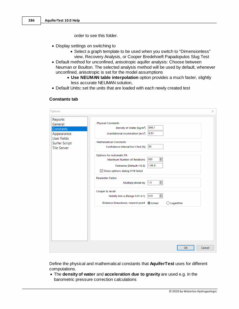
AquiferTest 10.0 Help286
© 2020 by Waterloo Hydrogeologic
order to see this folder.
· Display settings on switching to
· Select a graph template to be used when you switch to “Dimensionless”view, Recovery Analysis, or Cooper Bredehoeft Papadopulos Slug Test
· Default method for unconfined, anisotropic aquifer analysis: Choose betweenNeuman or Boulton. The selected analysis method will be used by default, wheneverunconfined, anisotropic is set for the model assumptions
· Use NEUMAN table interpolation option provides a much faster, slightlyless accurate NEUMAN solution,
· Default Units: set the units that are loaded with each newly created test
Constants tab
Define the physical and mathematical constants that AquiferTest uses for differentcomputations.· The density of water and acceleration due to gravity are used e.g. in the
barometric pressure correction calculations
Program Options 287
© 2020 by Waterloo Hydrogeologic
· The confidence interval of the t-test is used in the trend correction.
· Automatic fit: specify the maximum number of iterations, to be used during theautomatic fit, and display a progress bar in the Analysis graph window. Higheriterations will result in slower processing times.
· Parameter Factor: Set a factor for adjusting parameter values; this is used in theAnalysis Parameter controls, when doing the manual adjustment of the curve fit andaquifer parameters. The default interval value is 1.5.
· Cooper Jacob:o Set a value for u for the validity line. Value must be between 0.01 and 0.1
o Select the option for determining closest point, for the Cooper JacobDistance Drawdown analysis. When using this method, you are required toenter a time value for the analysis. If there is no observed water level forthis time value, AquiferTest will search for the next closest observationpoint, back and forward in time. Assume you are looking for the closestpoint for t = 100 s and you have data points at 10 s and 300 s. If Linear isselected the program takes the data point at 10 s, because delta t is 90 s(compared to the other point, where delta t is 200 s). If Log is selected theprogram uses the 300 s data point, because ABS (log(300) – log(100)) is0.477, compared to ABS (log(10)-log(100)) which is 1.
Appearance tab
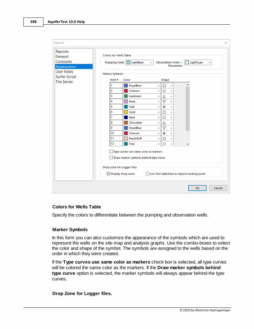
AquiferTest 10.0 Help288
© 2020 by Waterloo Hydrogeologic
Colors for Wells Table
Specify the colors to differentiate between the pumping and observation wells.
Marker Symbols
In this form you can also customize the appearance of the symbols which are used torepresent the wells on the site map and analysis graphs. Use the combo-boxes to selectthe color and shape of the symbol. The symbols are assigned to the wells based on theorder in which they were created.
If the Type curves use same color as markers check box is selected, all type curveswill be colored the same color as the markers. If the Draw marker symbols behindtype curve option is selected, the marker symbols will always appear behind the typecurves.
Drop Zone for Logger files.
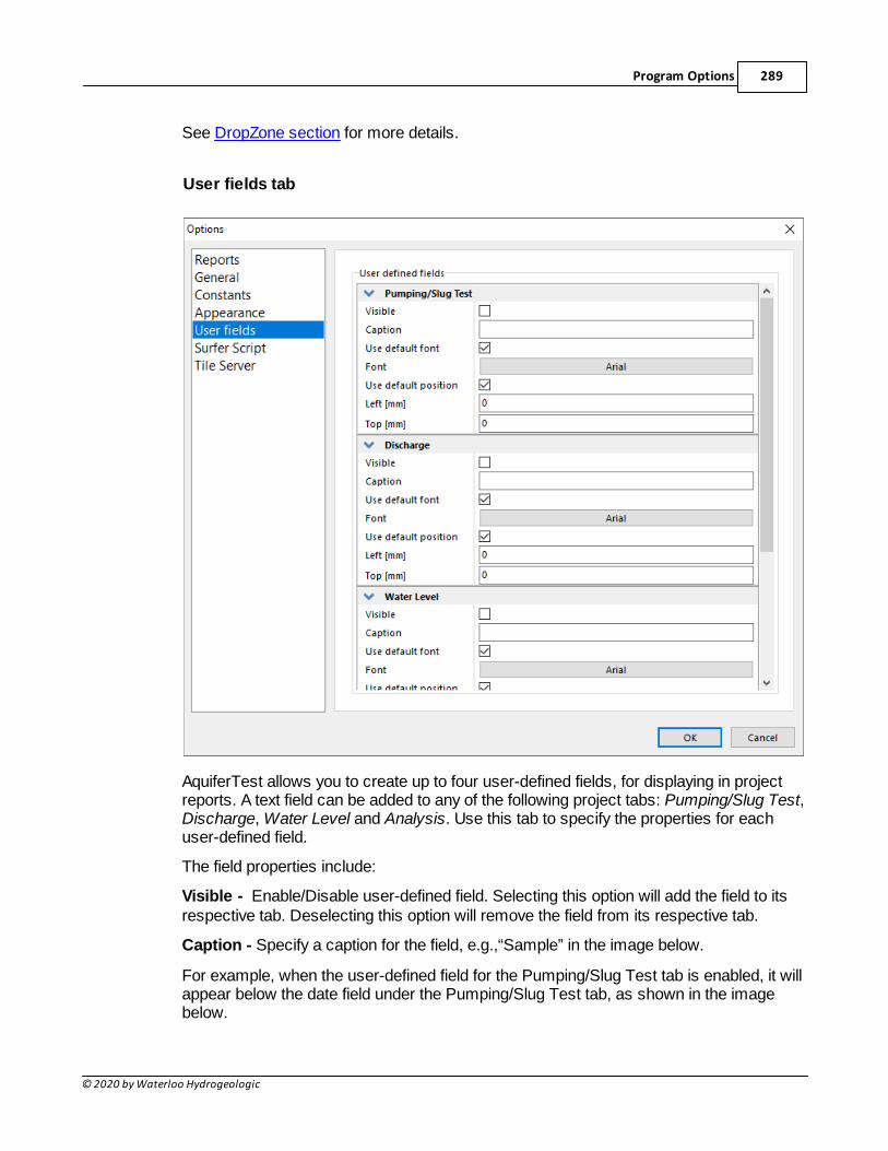
Program Options 289
© 2020 by Waterloo Hydrogeologic
See DropZone section for more details.
User fields tab
AquiferTest allows you to create up to four user-defined fields, for displaying in projectreports. A text field can be added to any of the following project tabs: Pumping/Slug Test,Discharge, Water Level and Analysis. Use this tab to specify the properties for eachuser-defined field.
The field properties include:
Visible - Enable/Disable user-defined field. Selecting this option will add the field to itsrespective tab. Deselecting this option will remove the field from its respective tab.
Caption - Specify a caption for the field, e.g.,“Sample” in the image below.
For example, when the user-defined field for the Pumping/Slug Test tab is enabled, it willappear below the date field under the Pumping/Slug Test tab, as shown in the imagebelow.
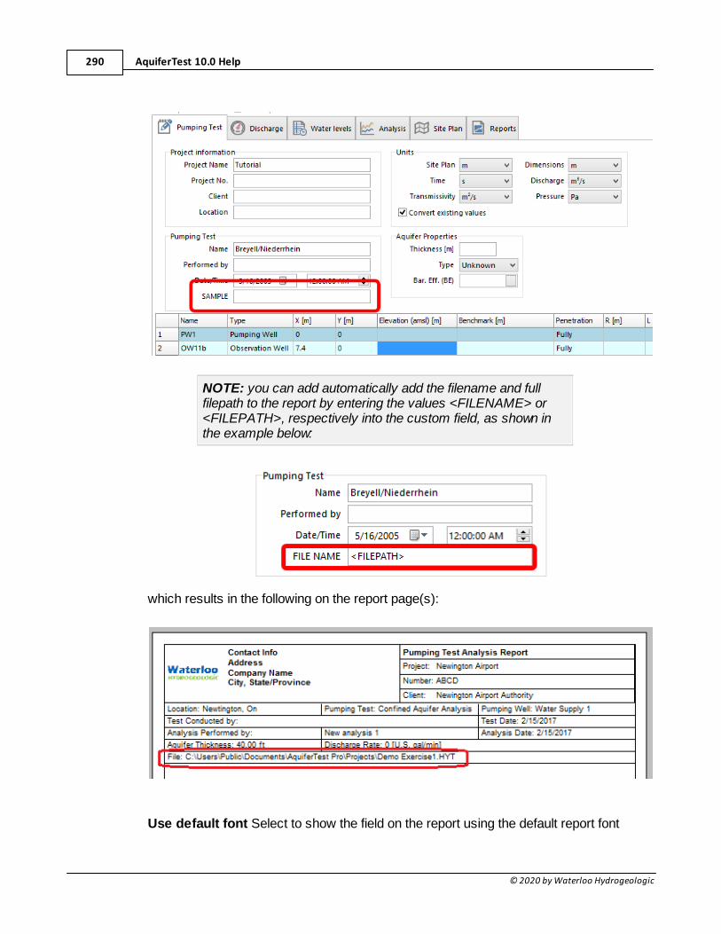
AquiferTest 10.0 Help290
© 2020 by Waterloo Hydrogeologic
NOTE: you can add automatically add the filename and fullfilepath to the report by entering the values <FILENAME> or<FILEPATH>, respectively into the custom field, as shown inthe example below:
which results in the following on the report page(s):
Use default font Select to show the field on the report using the default report font
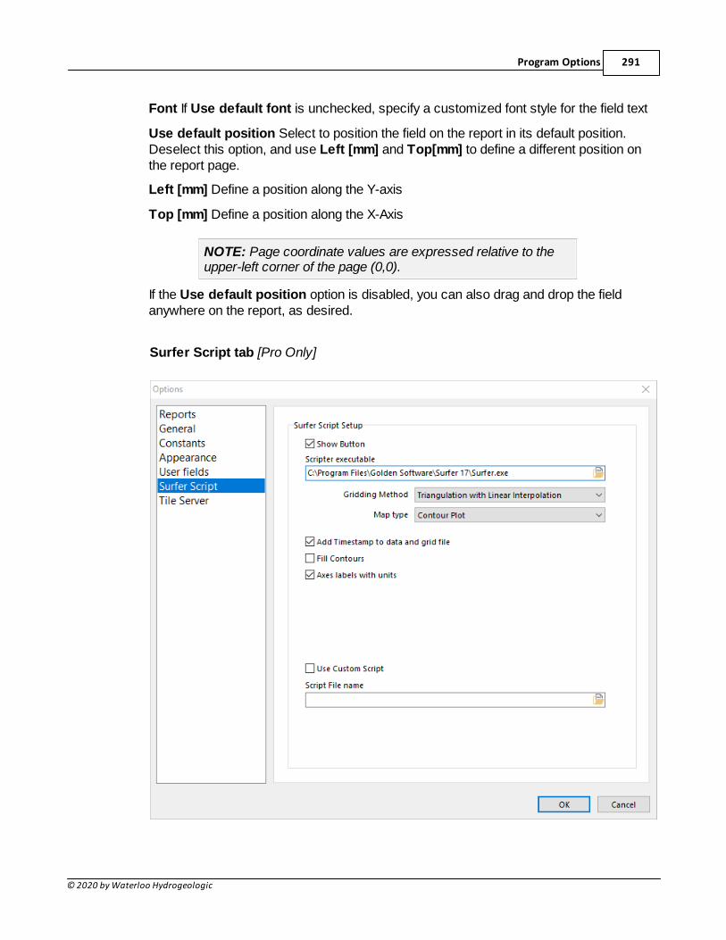
Program Options 291
© 2020 by Waterloo Hydrogeologic
Font If Use default font is unchecked, specify a customized font style for the field text
Use default position Select to position the field on the report in its default position.Deselect this option, and use Left [mm] and Top[mm] to define a different position onthe report page.
Left [mm] Define a position along the Y-axis
Top [mm] Define a position along the X-Axis
NOTE: Page coordinate values are expressed relative to theupper-left corner of the page (0,0).
If the Use default position option is disabled, you can also drag and drop the fieldanywhere on the report, as desired.
Surfer Script tab [Pro Only]
AquiferTest 10.0 Help292
© 2020 by Waterloo Hydrogeologic
AquiferTest Pro allows you to create surfaces/contours of the analytic maps, and toeasily export these objects to Surfer at the click of a button. The Surfer Script tab of theoptions window allows you to customize the way this Surfer exporting function works.
Show button: select whether or not the 'Send to Surfer' button appears in the toolbar ofthe Site Plan tab.
Scripter executable: specify the location of the Scripter executable file (included withSurfer) and typically located at: "C:\Program Files\Golden Software\Surfer15\Scripter.exe".
Gridding Method: select the gridding method. Two options are available directly:triangulation with linear interpolation and Kriging. (Other methods may be available byusing custom scripts).
Map Type: select the type of map to export. Three options are available: contour plots,3D wireframe and 3D surface.
Add Timestamp to data and grid file: select this option to include a timestamp to theexported data. Note that if the timestamp is not added, successive script runs willoverwrite previous versions.
Fill Contours: select this option to fill contours with a color map using the built-inGeology2 Fill Colors schema available in Surfer.
Axes labels with units: select this option to include axes labels and units in theexported data.
Use Custom Script: custom scripting is available. The user must specify the file nameand location of the custom Surfer script.
For more information on Scripting in Surfer, please refer to the Scripter Introductorydocumentation at the Golden Software website.
Tile Server tab [Pro Only]
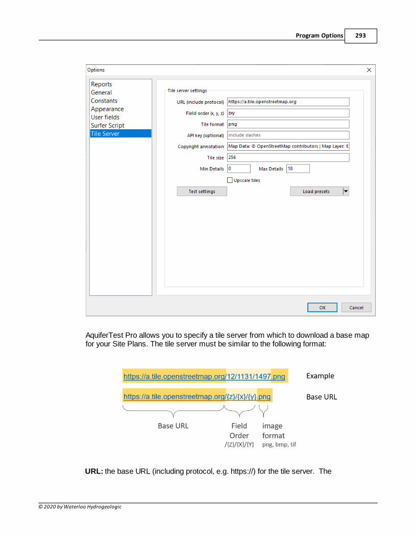
Program Options 293
© 2020 by Waterloo Hydrogeologic
AquiferTest Pro allows you to specify a tile server from which to download a base mapfor your Site Plans. The tile server must be similar to the following format:
URL: the base URL (including protocol, e.g. https://) for the tile server. The
AquiferTest 10.0 Help294
© 2020 by Waterloo Hydrogeologic
Field Order: the order in which tile zoom levels (z) and coordinates (x,y) are specifiedin the URL, typically this is ZXY; although settings can vary between tile servers.
Tile Format: select the image format that the tile server supports; typically this is PNG,JPG, BMP.
API Key: the API key used to access the tile server for commercial tile servers (e.g.Google, Bing, ESRI); not required for open source
Copyright annotation: annotation and attribution information for the tile server
Tile Size: standard image size, typically 256x256
Min/Max Details: the minimum/maximum tile zoom level (the z value). Typically rangesfrom 0 to 18.
Test Settings: clicking this button will test the connection to the tile server based on thecurrent settings to download a sample tile. If successful, you will see the example tiles.
Load Presets: Select from one of the available predefined tile server settings
Help Menu
The Help menu contains links to assist you, should problems arise while you areworking with AquiferTest.
Content...
Opens the table of contents of the off-line help file. The help file is identical to the printeduser’s manual, however it contains cross-referenced links that allow you to findinformation quicker.
Web Help...
Opens the table of contents of the on-line help file. The help file is updated morefrequently than that the printed user’s manual (which is updated on release) and itcontains cross-referenced links that allow you to find information quicker.
Tutorial...
Loads the Tutorial instructions. The “Quick Start Demo Tutorials” tutorial will guide youthrough most of the major functions of AquiferTest and is designed to highlight the
Program Options 295
© 2020 by Waterloo Hydrogeologic
program’s capabilities. The Demonstration Exercises and Benchmark Tests tutorialsprovide additional guidance for particular functions/capabilities within AquiferTest.
AquiferTest User Community...
Loads the AquiferTest Users group page on LinkedIn . This user group has severalhundred users and is a great place to ask questions and get quick support from anengaged group of users.
Pumping Test Solution Advisor...
Loads the AquiferTest Method Selection Advisor webpage. The Method SelectionAdvisor is an easy-to-use online tool which can provide guidance with respect to thepumping test solution methods which apply to your aquifer conditions/assumptions. TheMethod Selection Advisor is a simple decision tree; the user is presented with a seriesof simple questions pertaining to the aquifer properties and the well construction, andwhen all of the questions have been answered, one or more solution methods will besuggested.
Release Notes...
Loads the AquiferTest ReadMe page on the Waterloo Hydrogeologic website. TheReadMe notes provide a detailed history of new features/improvements with each newversion/build released.
About...
Displays license, version, and copyright information for AquiferTest and how to contactus.
AquiferTest 10.0 Help296
© 2020 by Waterloo Hydrogeologic
4 Pumping Test: Theory and Analysis Methods
AquiferTest is used to analyze data gathered from pumping tests and slug tests. Solutionmethods available in AquiferTest cover the full range of aquifer settings: unconfined,confined, leaky, and fractured.
The full theoretical background of each solution method is beyond the scope of this manual.However, a summary of each solution method, including limitations and applications, isincluded in this section. This information is presented to help you select the correct solutionmethod for your specific aquifer settings.
Additional information can be obtained from hydrogeology texts such as:
Dominico, P.A. and F.W. Schwartz, 1990. Physical and Chemical Hydrogeology. John Wiley& Sons, Inc. 824 p.
Driscoll, F. G., 1987. Groundwater and Wells, Johnson Division, St. Paul, Minnesota 55112,1089 p.
Fetter, C.W., 1994. Applied Hydrogeology, Third Edition, Prentice-Hall, Inc., Upper SaddleRiver, New Jersey, 691 p.
Freeze, R.A. and J.A. Cherry, 1979. Groundwater, Prentice-Hall, Inc. Englewood Cliffs, NewJersey 07632, 604 p.
Kruseman, G.P. and N.A. de Ridder, 1990. Analysis and Evaluation of Pumping Test DataSecond Edition (Completely Revised) ILRI publication 47. Intern. Inst. for LandReclamation and Improvements, Wageningen, Netherlands, 377 p.
A more complete list of publications is included in the References section.
4.1 Analysis Parameters and Curve Fitting
Automatic Curve Fitting
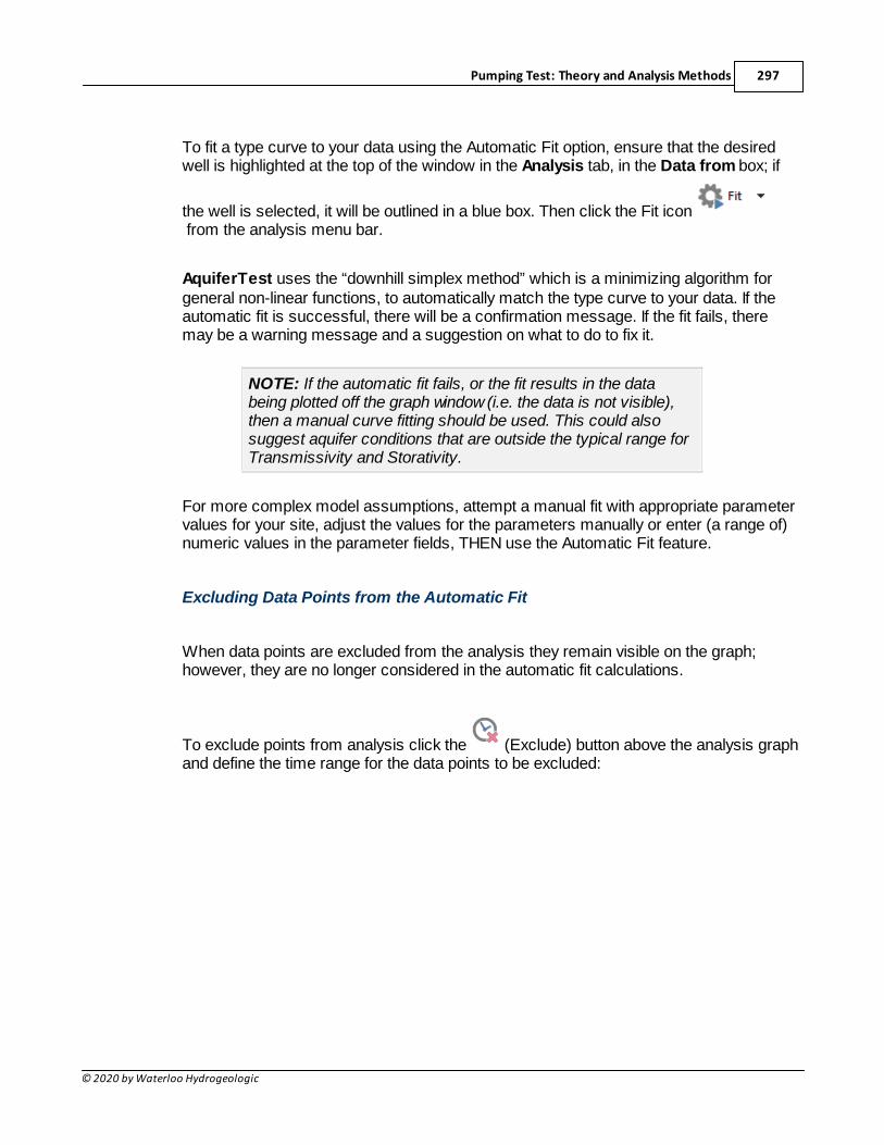
Pumping Test: Theory and Analysis Methods 297
© 2020 by Waterloo Hydrogeologic
To fit a type curve to your data using the Automatic Fit option, ensure that the desiredwell is highlighted at the top of the window in the Analysis tab, in the Data from box; if
the well is selected, it will be outlined in a blue box. Then click the Fit icon from the analysis menu bar.
AquiferTest uses the “downhill simplex method” which is a minimizing algorithm forgeneral non-linear functions, to automatically match the type curve to your data. If theautomatic fit is successful, there will be a confirmation message. If the fit fails, theremay be a warning message and a suggestion on what to do to fix it.
NOTE: If the automatic fit fails, or the fit results in the databeing plotted off the graph window (i.e. the data is not visible),then a manual curve fitting should be used. This could alsosuggest aquifer conditions that are outside the typical range forTransmissivity and Storativity.
For more complex model assumptions, attempt a manual fit with appropriate parametervalues for your site, adjust the values for the parameters manually or enter (a range of)numeric values in the parameter fields, THEN use the Automatic Fit feature.
Excluding Data Points from the Automatic Fit
When data points are excluded from the analysis they remain visible on the graph;however, they are no longer considered in the automatic fit calculations.
To exclude points from analysis click the (Exclude) button above the analysis graphand define the time range for the data points to be excluded:
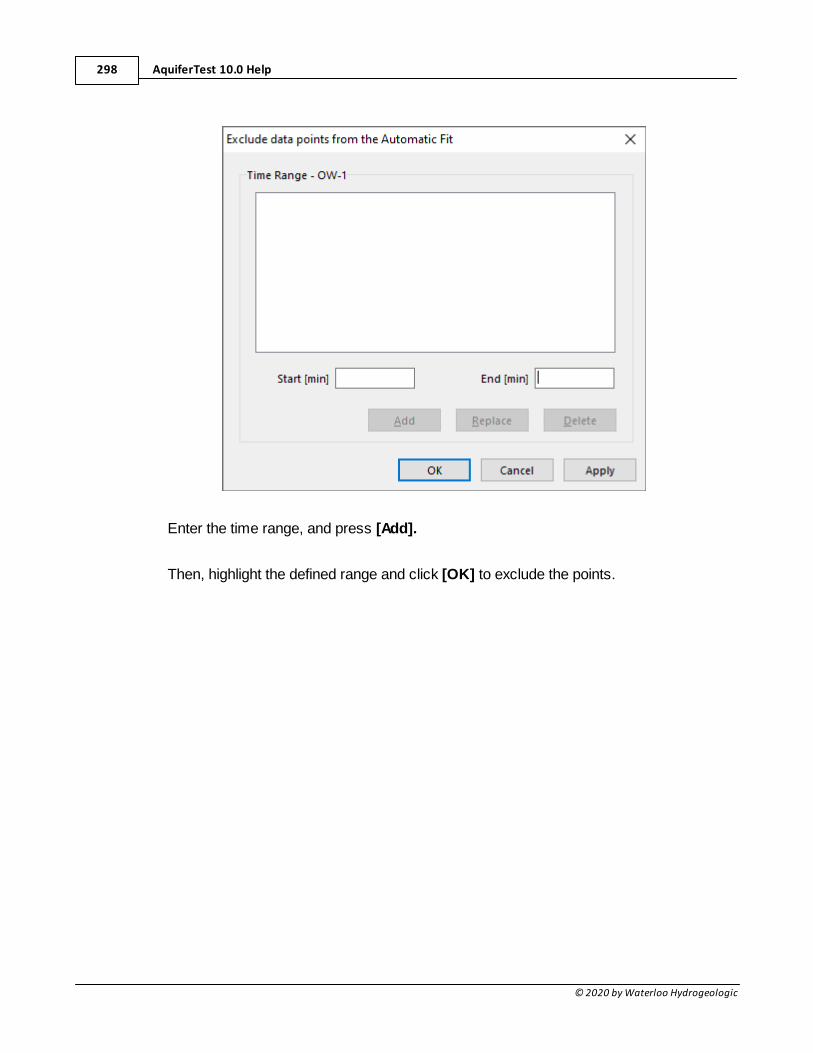
AquiferTest 10.0 Help298
© 2020 by Waterloo Hydrogeologic
Enter the time range, and press [Add].
Then, highlight the defined range and click [OK] to exclude the points.
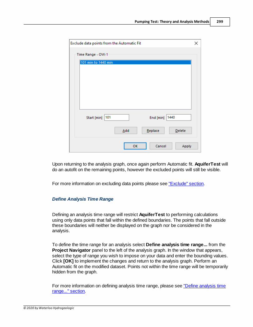
Pumping Test: Theory and Analysis Methods 299
© 2020 by Waterloo Hydrogeologic
Upon returning to the analysis graph, once again perform Automatic fit. AquiferTest willdo an autofit on the remaining points, however the excluded points will still be visible.
For more information on excluding data points please see "Exclude" section.
Define Analysis Time Range
Defining an analysis time range will restrict AquiferTest to performing calculationsusing only data points that fall within the defined boundaries. The points that fall outsidethese boundaries will neither be displayed on the graph nor be considered in theanalysis.
To define the time range for an analysis select Define analysis time range... from theProject Navigator panel to the left of the analysis graph. In the window that appears,select the type of range you wish to impose on your data and enter the bounding values.Click [OK] to implement the changes and return to the analysis graph. Perform anAutomatic fit on the modified dataset. Points not within the time range will be temporarilyhidden from the graph.
For more information on defining analysis time range, please see "Define analysis timerange..." section.
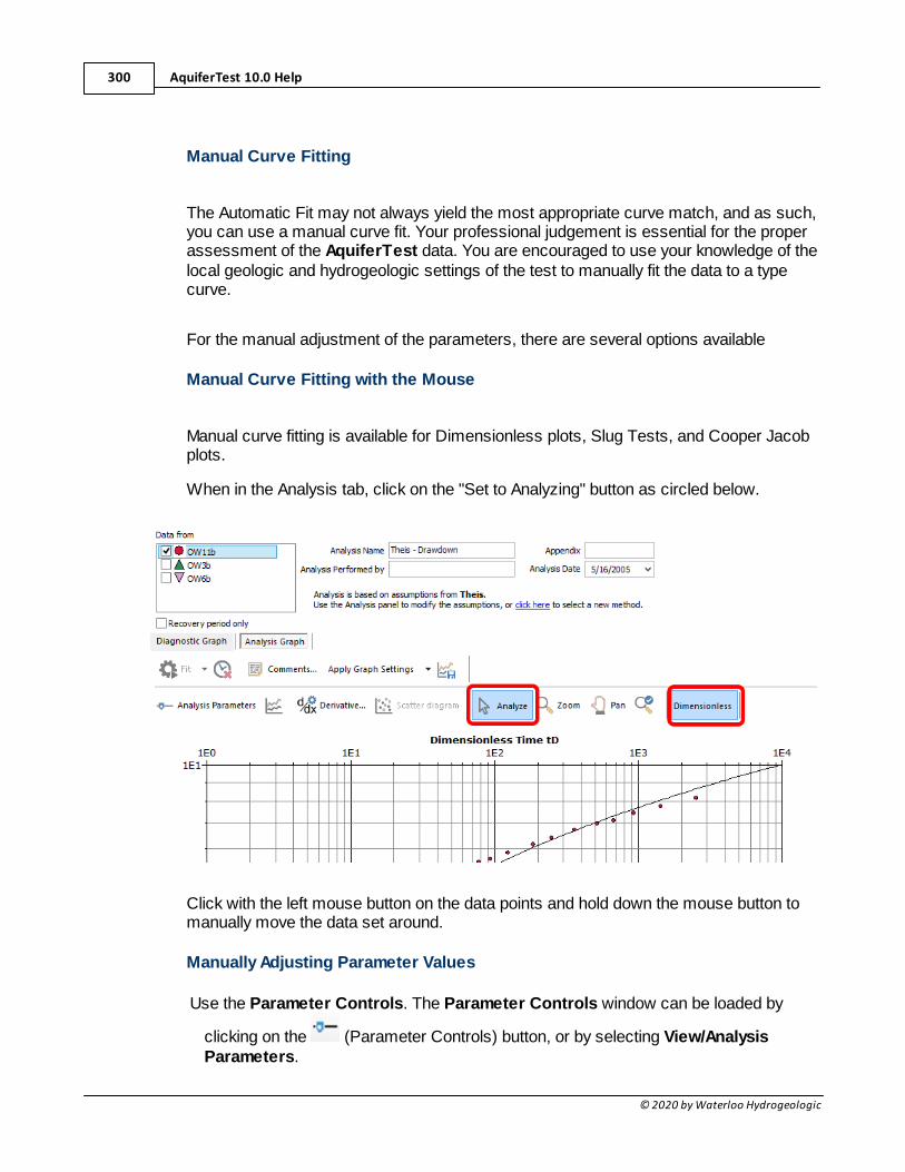
AquiferTest 10.0 Help300
© 2020 by Waterloo Hydrogeologic
Manual Curve Fitting
The Automatic Fit may not always yield the most appropriate curve match, and as such,you can use a manual curve fit. Your professional judgement is essential for the properassessment of the AquiferTest data. You are encouraged to use your knowledge of thelocal geologic and hydrogeologic settings of the test to manually fit the data to a typecurve.
For the manual adjustment of the parameters, there are several options available
Manual Curve Fitting with the Mouse
Manual curve fitting is available for Dimensionless plots, Slug Tests, and Cooper Jacobplots.
When in the Analysis tab, click on the "Set to Analyzing" button as circled below.
Click with the left mouse button on the data points and hold down the mouse button tomanually move the data set around.
Manually Adjusting Parameter Values
Use the Parameter Controls. The Parameter Controls window can be loaded by
clicking on the (Parameter Controls) button, or by selecting View/AnalysisParameters.
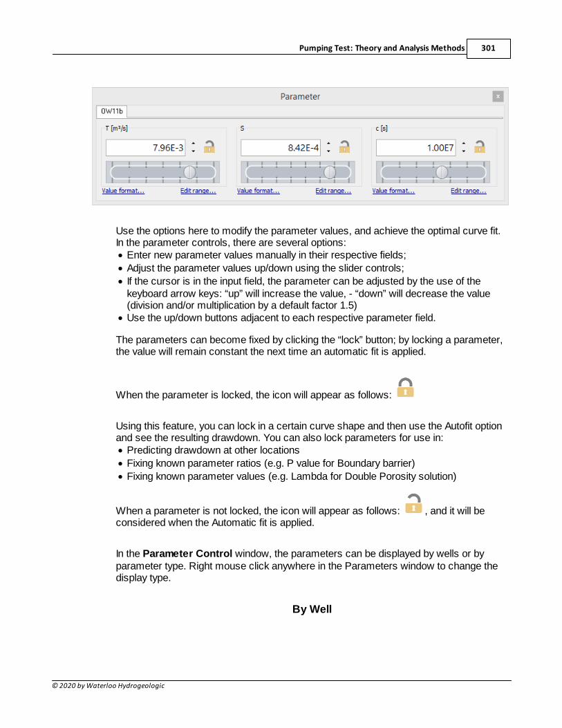
Pumping Test: Theory and Analysis Methods 301
© 2020 by Waterloo Hydrogeologic
Use the options here to modify the parameter values, and achieve the optimal curve fit.In the parameter controls, there are several options:· Enter new parameter values manually in their respective fields;
· Adjust the parameter values up/down using the slider controls;
· If the cursor is in the input field, the parameter can be adjusted by the use of thekeyboard arrow keys: “up” will increase the value, - “down” will decrease the value(division and/or multiplication by a default factor 1.5)
· Use the up/down buttons adjacent to each respective parameter field.
The parameters can become fixed by clicking the “lock” button; by locking a parameter,the value will remain constant the next time an automatic fit is applied.
When the parameter is locked, the icon will appear as follows:
Using this feature, you can lock in a certain curve shape and then use the Autofit optionand see the resulting drawdown. You can also lock parameters for use in:· Predicting drawdown at other locations
· Fixing known parameter ratios (e.g. P value for Boundary barrier)
· Fixing known parameter values (e.g. Lambda for Double Porosity solution)
When a parameter is not locked, the icon will appear as follows: , and it will beconsidered when the Automatic fit is applied.
In the Parameter Control window, the parameters can be displayed by wells or byparameter type. Right mouse click anywhere in the Parameters window to change thedisplay type.
By Well
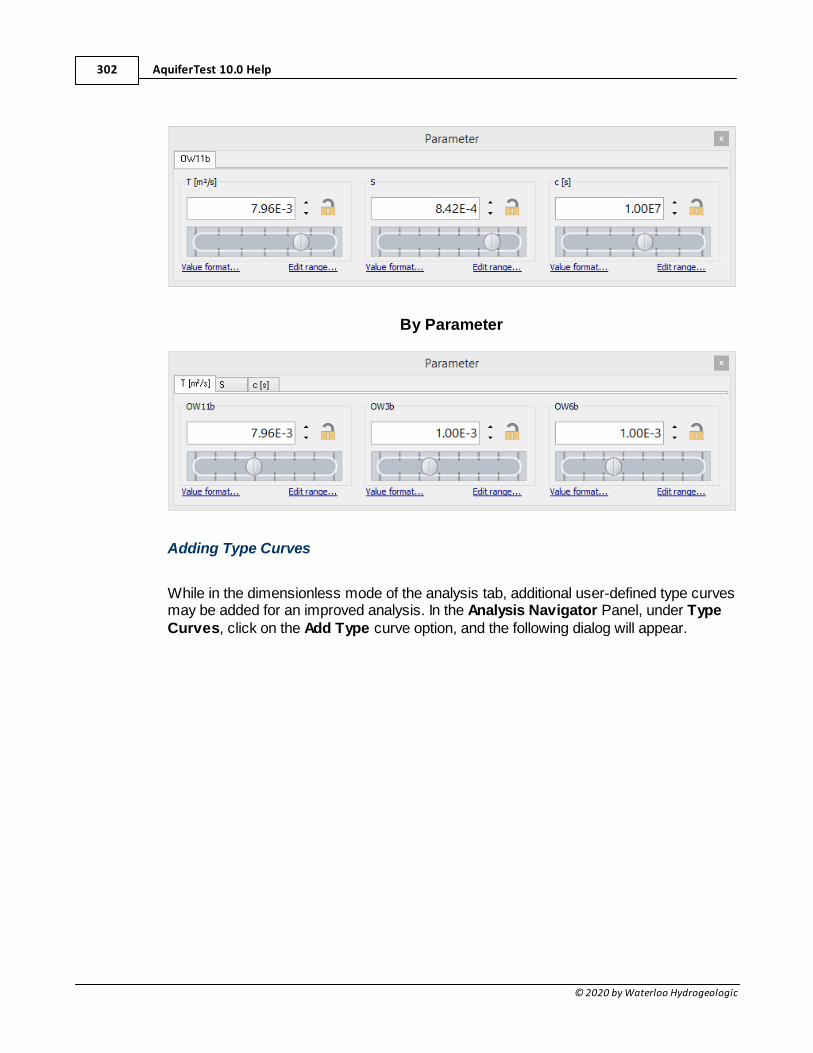
AquiferTest 10.0 Help302
© 2020 by Waterloo Hydrogeologic
By Parameter
Adding Type Curves
While in the dimensionless mode of the analysis tab, additional user-defined type curvesmay be added for an improved analysis. In the Analysis Navigator Panel, under TypeCurves, click on the Add Type curve option, and the following dialog will appear.
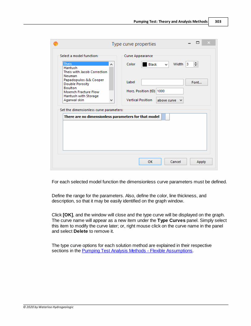
Pumping Test: Theory and Analysis Methods 303
© 2020 by Waterloo Hydrogeologic
For each selected model function the dimensionless curve parameters must be defined.
Define the range for the parameters. Also, define the color, line thickness, anddescription, so that it may be easily identified on the graph window.
Click [OK], and the window will close and the type curve will be displayed on the graph.The curve name will appear as a new item under the Type Curves panel. Simply selectthis item to modify the curve later; or, right mouse click on the curve name in the paneland select Delete to remove it.
The type curve options for each solution method are explained in their respectivesections in the Pumping Test Analysis Methods - Flexible Assumptions.
AquiferTest 10.0 Help304
© 2020 by Waterloo Hydrogeologic
4.2 Methodology
The abundance of solution methods can lead to some ambiguity and vaguenessconcerning the assumptions and limitations of an individual method. In AquiferTest,there is a single Theis method then by specifying the model assumptions, AquiferTestattempts to select the most suitable solution method, or applies Superposition to anexisting method. This allows you to account for the following conditions:
· Multiple pumping wells
· Variable pumping rates
· Boundary effects (barrier, recharge)
· Partially penetrating pumping wells
The process in AquiferTest is systematic, and as such, easier to understand. Byexplicitly indicating the known aquifer type and/or conditions, (which can be determinedusing the diagnostic plots), you know which effects are considered in the selectedsolution method.
Generally, it is recommended that you start with a simple model, and gradually increasethe complexity. That is, for a pumping test, start with the default Theis set ofassumptions, and change them only if you observe phenomena that do not fit thismodel. For example, if you know that the aquifer is bounded 400 m away, you couldinitially change the assumptions from “infinite” to “barrier bounded”, however this wouldnot be the correct approach. It takes some time until the depression cone reaches thatbarrier, and you might miss other important effects in the meantime.
Alternatively, you can select from solution methods that have "Fixed Assumptions";these include the "Classical" methods, such as:
· Theis Recovery
· Cooper-Jacob Method
4.3 Theory of Superposition
The pumping test solution methods included with AquiferTest are:
· Theis
· Theis with Jacob Correction
· Hantush-Jacob
· Neuman
· Papadopulos - Cooper
· Warren Root - Double Porosity
· Boulton
Pumping Test: Theory and Analysis Methods 305
© 2020 by Waterloo Hydrogeologic
· Hantush (Leaky, with storage in aquitard)
· Moench (Fractured flow, with skin)
· Agarwal Recovery
· Theis Recovery
· Cooper Jacob I: Time Drawdown
· Cooper Jacob II: Distance Drawdown
· Cooper Jacob III: Time Distance Drawdown
· Agarwal Skin
· Clonts & Ramey
These methods each have some general assumptions:
· aquifer extends radially and infinitely
· single pumping well
· constant pumping rate
· fully penetrating well (except for the Neuman method)
These assumptions may be modified if the pumping test data are analyzed utilizing the theoryof superposition. AquiferTest uses the theory of superposition to calculate drawdown invariable aquifer conditions. Superposition can be applied to any solution method.
Superposition may be used to account for the effects of pumping well interference, aquiferdiscontinuities, groundwater recharge, well/borehole storage and variable pumping rates. Thedifferential equations that describe groundwater flow are linear in the dependent variable(drawdown). Therefore, a linear combination of individual solutions is also a valid solution.This means that:
· The effects of multiple pumping wells on the predicted drawdown at a point can becomputed by summing the predicted drawdowns at the point for each well; and
· Drawdown in complex aquifer systems can be predicted by superimposing predicteddrawdowns for simpler aquifer systems (Dawson and Istok, 1991).
In AquiferTest, the standard solution methods can be enhanced by applying superposition;the various superposition principles are explained in the following sections:
· Variable Discharge Rates
· Multiple Pumping Wells
· Boundary Effects
· Effects of Vertical Anisotropy and Partially Penetrating Wells
As discussed above, most of the pumping test analysis methods implemented in AquiferTestcan be enhanced by applying superposition. However, certain solution methods are limited toa fixed set of assumptions. These methods with fixed assumptions are described in asubsequent section.
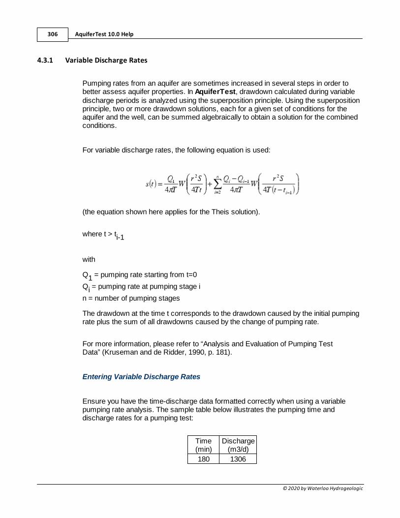
AquiferTest 10.0 Help306
© 2020 by Waterloo Hydrogeologic
4.3.1 Variable Discharge Rates
Pumping rates from an aquifer are sometimes increased in several steps in order tobetter assess aquifer properties. In AquiferTest, drawdown calculated during variabledischarge periods is analyzed using the superposition principle. Using the superpositionprinciple, two or more drawdown solutions, each for a given set of conditions for theaquifer and the well, can be summed algebraically to obtain a solution for the combinedconditions.
For variable discharge rates, the following equation is used:
(the equation shown here applies for the Theis solution).
where t > ti-1
with
Q1 = pumping rate starting from t=0
Qi = pumping rate at pumping stage i
n = number of pumping stages
The drawdown at the time t corresponds to the drawdown caused by the initial pumpingrate plus the sum of all drawdowns caused by the change of pumping rate.
For more information, please refer to “Analysis and Evaluation of Pumping TestData” (Kruseman and de Ridder, 1990, p. 181).
Entering Variable Discharge Rates
Ensure you have the time-discharge data formatted correctly when using a variablepumping rate analysis. The sample table below illustrates the pumping time anddischarge rates for a pumping test:
Time(min)
Discharge(m3/d)
180 1306
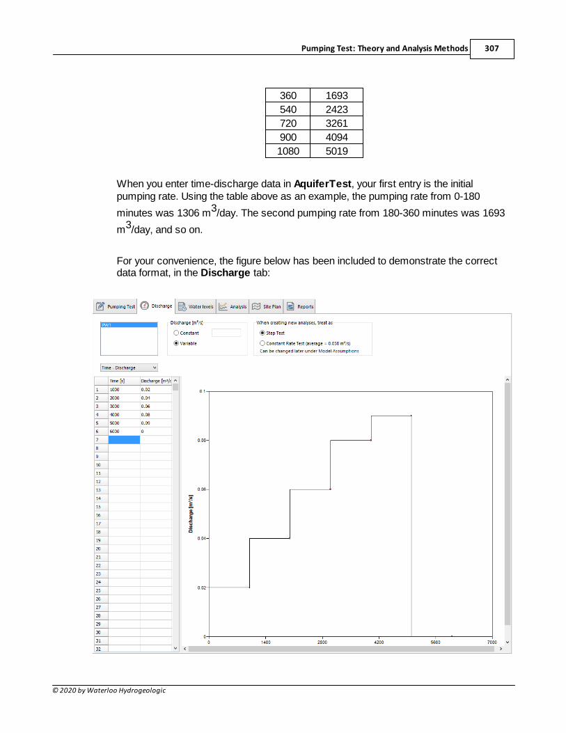
Pumping Test: Theory and Analysis Methods 307
© 2020 by Waterloo Hydrogeologic
360 1693
540 2423
720 3261
900 4094
1080 5019
When you enter time-discharge data in AquiferTest, your first entry is the initialpumping rate. Using the table above as an example, the pumping rate from 0-180
minutes was 1306 m3/day. The second pumping rate from 180-360 minutes was 1693
m3/day, and so on.
For your convenience, the figure below has been included to demonstrate the correctdata format, in the Discharge tab:
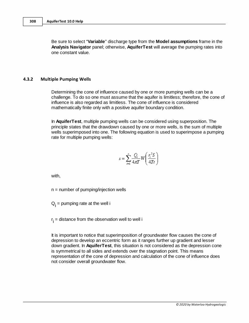
AquiferTest 10.0 Help308
© 2020 by Waterloo Hydrogeologic
Be sure to select “Variable” discharge type from the Model assumptions frame in theAnalysis Navigator panel; otherwise, AquiferTest will average the pumping rates intoone constant value.
4.3.2 Multiple Pumping Wells
Determining the cone of influence caused by one or more pumping wells can be achallenge. To do so one must assume that the aquifer is limitless; therefore, the cone ofinfluence is also regarded as limitless. The cone of influence is consideredmathematically finite only with a positive aquifer boundary condition.
In AquiferTest, multiple pumping wells can be considered using superposition. Theprinciple states that the drawdown caused by one or more wells, is the sum of multiplewells superimposed into one. The following equation is used to superimpose a pumpingrate for multiple pumping wells:
with,
n = number of pumping/injection wells
Qi = pumping rate at the well i
ri = distance from the observation well to well i
It is important to notice that superimposition of groundwater flow causes the cone ofdepression to develop an eccentric form as it ranges further up gradient and lesserdown gradient. In AquiferTest, this situation is not considered as the depression coneis symmetrical to all sides and extends over the stagnation point. This meansrepresentation of the cone of depression and calculation of the cone of influence doesnot consider overall groundwater flow.
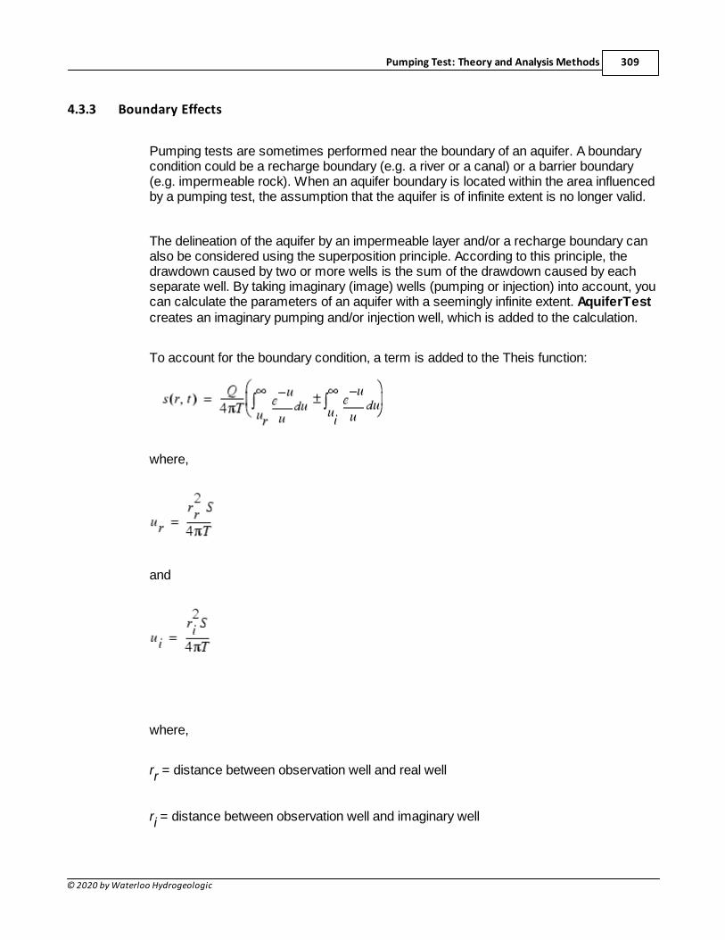
Pumping Test: Theory and Analysis Methods 309
© 2020 by Waterloo Hydrogeologic
4.3.3 Boundary Effects
Pumping tests are sometimes performed near the boundary of an aquifer. A boundarycondition could be a recharge boundary (e.g. a river or a canal) or a barrier boundary(e.g. impermeable rock). When an aquifer boundary is located within the area influencedby a pumping test, the assumption that the aquifer is of infinite extent is no longer valid.
The delineation of the aquifer by an impermeable layer and/or a recharge boundary canalso be considered using the superposition principle. According to this principle, thedrawdown caused by two or more wells is the sum of the drawdown caused by eachseparate well. By taking imaginary (image) wells (pumping or injection) into account, youcan calculate the parameters of an aquifer with a seemingly infinite extent. AquiferTestcreates an imaginary pumping and/or injection well, which is added to the calculation.
To account for the boundary condition, a term is added to the Theis function:
where,
and
where,
rr = distance between observation well and real well
ri = distance between observation well and imaginary well
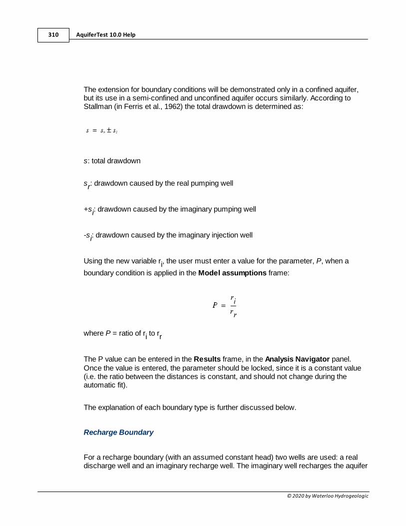
AquiferTest 10.0 Help310
© 2020 by Waterloo Hydrogeologic
The extension for boundary conditions will be demonstrated only in a confined aquifer,but its use in a semi-confined and unconfined aquifer occurs similarly. According toStallman (in Ferris et al., 1962) the total drawdown is determined as:
s: total drawdown
sr: drawdown caused by the real pumping well
+si: drawdown caused by the imaginary pumping well
-si: drawdown caused by the imaginary injection well
Using the new variable ri, the user must enter a value for the parameter, P, when a
boundary condition is applied in the Model assumptions frame:
where P = ratio of ri to rr
The P value can be entered in the Results frame, in the Analysis Navigator panel.Once the value is entered, the parameter should be locked, since it is a constant value(i.e. the ratio between the distances is constant, and should not change during theautomatic fit).
The explanation of each boundary type is further discussed below.
Recharge Boundary
For a recharge boundary (with an assumed constant head) two wells are used: a realdischarge well and an imaginary recharge well. The imaginary well recharges the aquifer
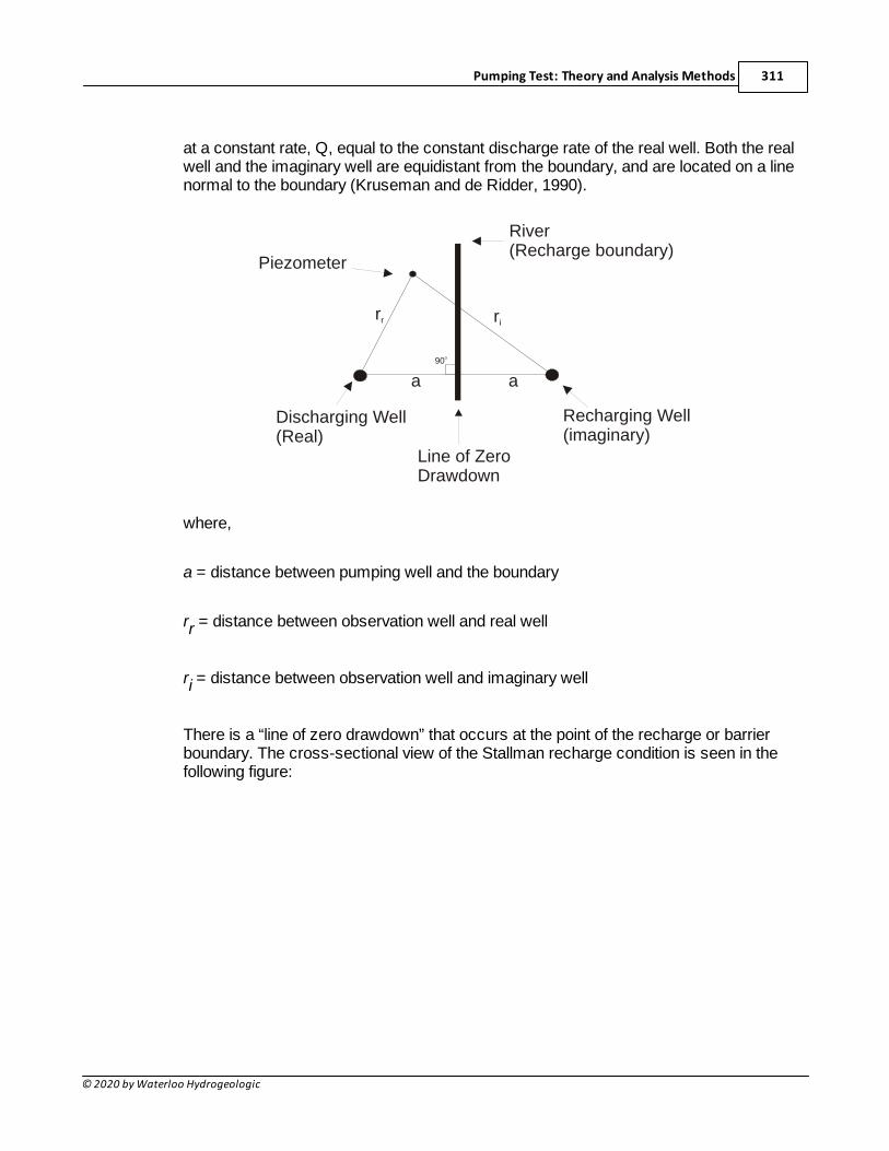
Pumping Test: Theory and Analysis Methods 311
© 2020 by Waterloo Hydrogeologic
at a constant rate, Q, equal to the constant discharge rate of the real well. Both the realwell and the imaginary well are equidistant from the boundary, and are located on a linenormal to the boundary (Kruseman and de Ridder, 1990).
Discharging Well(Real)
Recharging Well(imaginary)
Piezometer
River(Recharge boundary)
rr
a a
ri
90o
Line of ZeroDrawdown
where,
a = distance between pumping well and the boundary
rr = distance between observation well and real well
ri = distance between observation well and imaginary well
There is a “line of zero drawdown” that occurs at the point of the recharge or barrierboundary. The cross-sectional view of the Stallman recharge condition is seen in thefollowing figure:
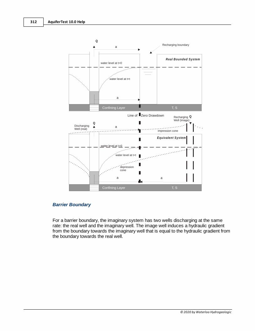
AquiferTest 10.0 Help312
© 2020 by Waterloo Hydrogeologic
Line of Zero Drawdown
Confining Layer
Recharging boundary
Q
a
a
T, S
water level at t=0
water level at t=t
Confining Layer
Qa
a
T, S
water level at t=0
water level at t=t
RechargingWell (image)
Q
depressioncone
Discharging Well (real)
impression cone
a
Real Bounded System
Equivalent System
Barrier Boundary
For a barrier boundary, the imaginary system has two wells discharging at the samerate: the real well and the imaginary well. The image well induces a hydraulic gradientfrom the boundary towards the imaginary well that is equal to the hydraulic gradient fromthe boundary towards the real well.
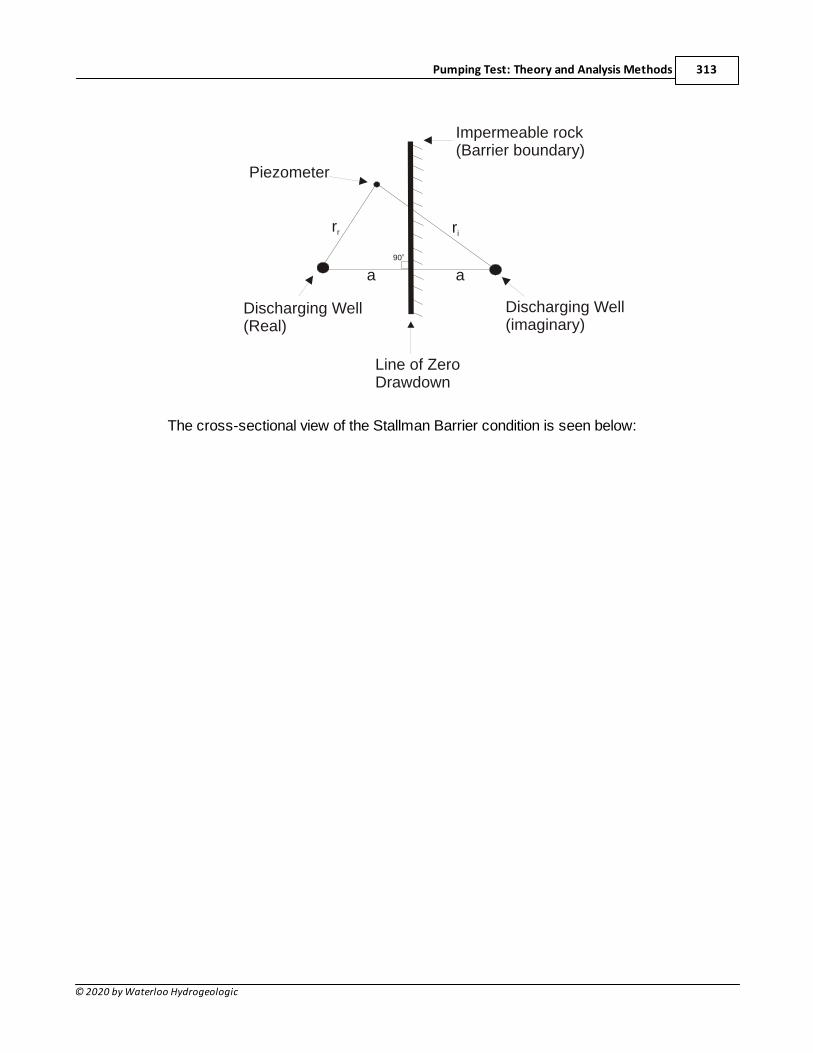
Pumping Test: Theory and Analysis Methods 313
© 2020 by Waterloo Hydrogeologic
Discharging Well(Real)
Discharging Well(imaginary)
Piezometer
Impermeable rock(Barrier boundary)
rr ri
a a
90o
Line of ZeroDrawdown
The cross-sectional view of the Stallman Barrier condition is seen below:

AquiferTest 10.0 Help314
© 2020 by Waterloo Hydrogeologic
Line of Zero Drawdown
Confining Layer
Q
a
T, S
water level at t=0
waterlevel at t=t
Confining Layer
Qa
a
T, S
water level at t=0
water level at t=t
DischargingWell (image)
Q
resulting depressioncone
Discharging Well (real)
a
Barrier boundary
Real Bounded System
Equivalent System
b
For more details, please see p. 109 of Kruseman and de Ridder (1994).
4.3.4 Effects of Vertical Anisotropy and Partially Penetrating Wells
Pumping wells and monitoring wells often only tap into an aquifer, and may notnecessarily fully penetrate the entire thickness. This means only a portion of the aquifer
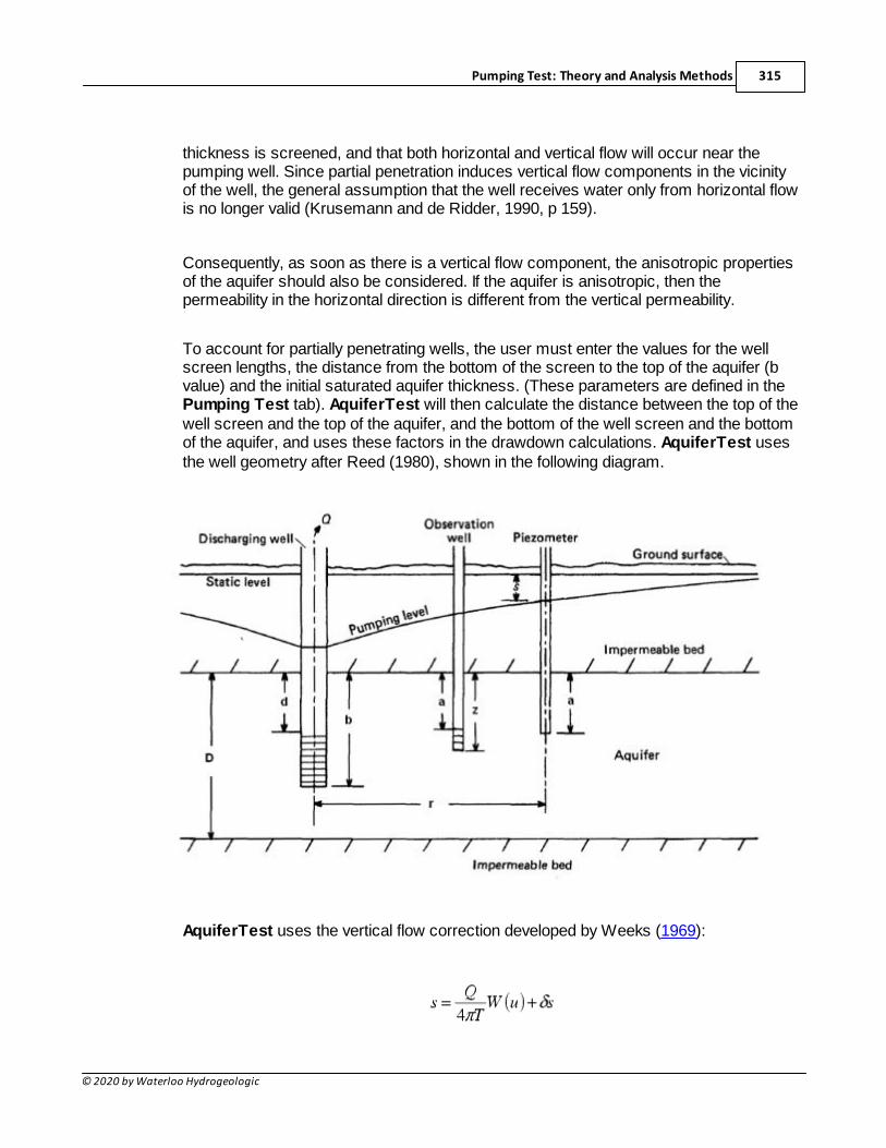
Pumping Test: Theory and Analysis Methods 315
© 2020 by Waterloo Hydrogeologic
thickness is screened, and that both horizontal and vertical flow will occur near thepumping well. Since partial penetration induces vertical flow components in the vicinityof the well, the general assumption that the well receives water only from horizontal flowis no longer valid (Krusemann and de Ridder, 1990, p 159).
Consequently, as soon as there is a vertical flow component, the anisotropic propertiesof the aquifer should also be considered. If the aquifer is anisotropic, then thepermeability in the horizontal direction is different from the vertical permeability.
To account for partially penetrating wells, the user must enter the values for the wellscreen lengths, the distance from the bottom of the screen to the top of the aquifer (bvalue) and the initial saturated aquifer thickness. (These parameters are defined in thePumping Test tab). AquiferTest will then calculate the distance between the top of thewell screen and the top of the aquifer, and the bottom of the well screen and the bottomof the aquifer, and uses these factors in the drawdown calculations. AquiferTest usesthe well geometry after Reed (1980), shown in the following diagram.
AquiferTest uses the vertical flow correction developed by Weeks (1969):
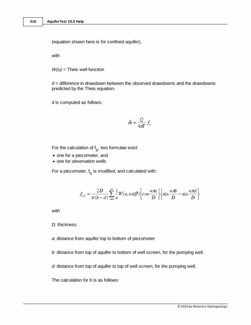
AquiferTest 10.0 Help316
© 2020 by Waterloo Hydrogeologic
(equation shown here is for confined aquifer).
with
W(u) = Theis well function
d = difference in drawdown between the observed drawdowns and the drawdownspredicted by the Theis equation.
d is computed as follows:
For the calculation of fs, two formulae exist:
· one for a piezometer, and
· one for observation wells
For a piezometer, fs is modified, and calculated with:
with
D: thickness
a: distance from aquifer top to bottom of piezometer
b: distance from top of aquifer to bottom of well screen, for the pumping well.
d: distance from top of aquifer to top of well screen, for the pumping well.
The calculation for b is as follows:
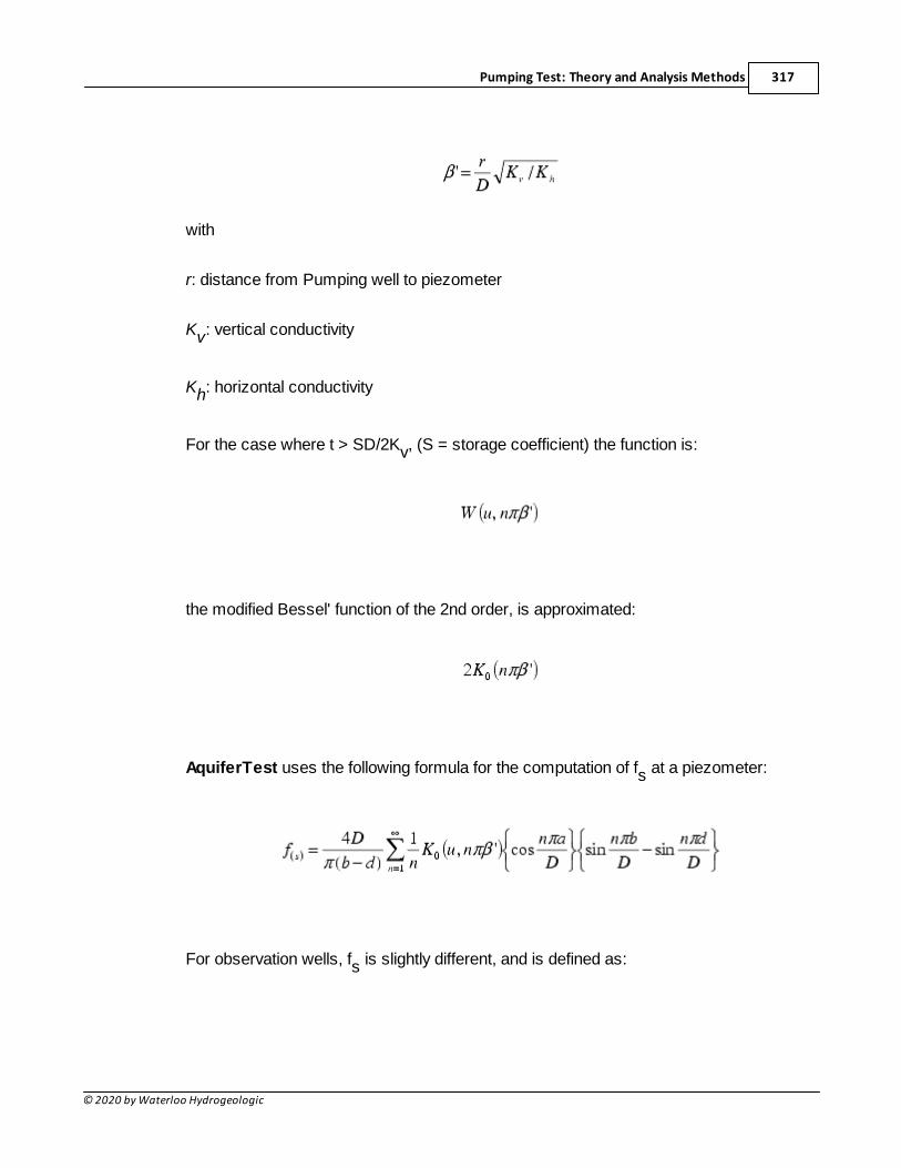
Pumping Test: Theory and Analysis Methods 317
© 2020 by Waterloo Hydrogeologic
with
r: distance from Pumping well to piezometer
Kv: vertical conductivity
Kh: horizontal conductivity
For the case where t > SD/2Kv, (S = storage coefficient) the function is:
the modified Bessel' function of the 2nd order, is approximated:
AquiferTest uses the following formula for the computation of fs at a piezometer:
For observation wells, fs is slightly different, and is defined as:
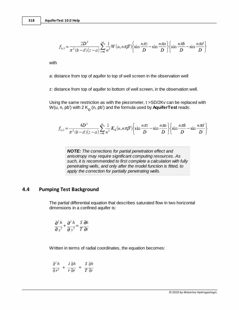
AquiferTest 10.0 Help318
© 2020 by Waterloo Hydrogeologic
with
a: distance from top of aquifer to top of well screen in the observation well
z: distance from top of aquifer to bottom of well screen, in the observation well.
Using the same restriction as with the piezometer, t >SD/2Kv can be replaced withW(u, n, pb’) with 2 Ko (n, pb’) and the formula used by AquiferTest reads:
NOTE: The corrections for partial penetration effect andanisotropy may require significant computing resources. Assuch, it is recommended to first complete a calculation with fullypenetrating wells, and only after the model function is fitted, toapply the correction for partially penetrating wells.
4.4 Pumping Test Background
The partial differential equation that describes saturated flow in two horizontaldimensions in a confined aquifer is:
Written in terms of radial coordinates, the equation becomes:
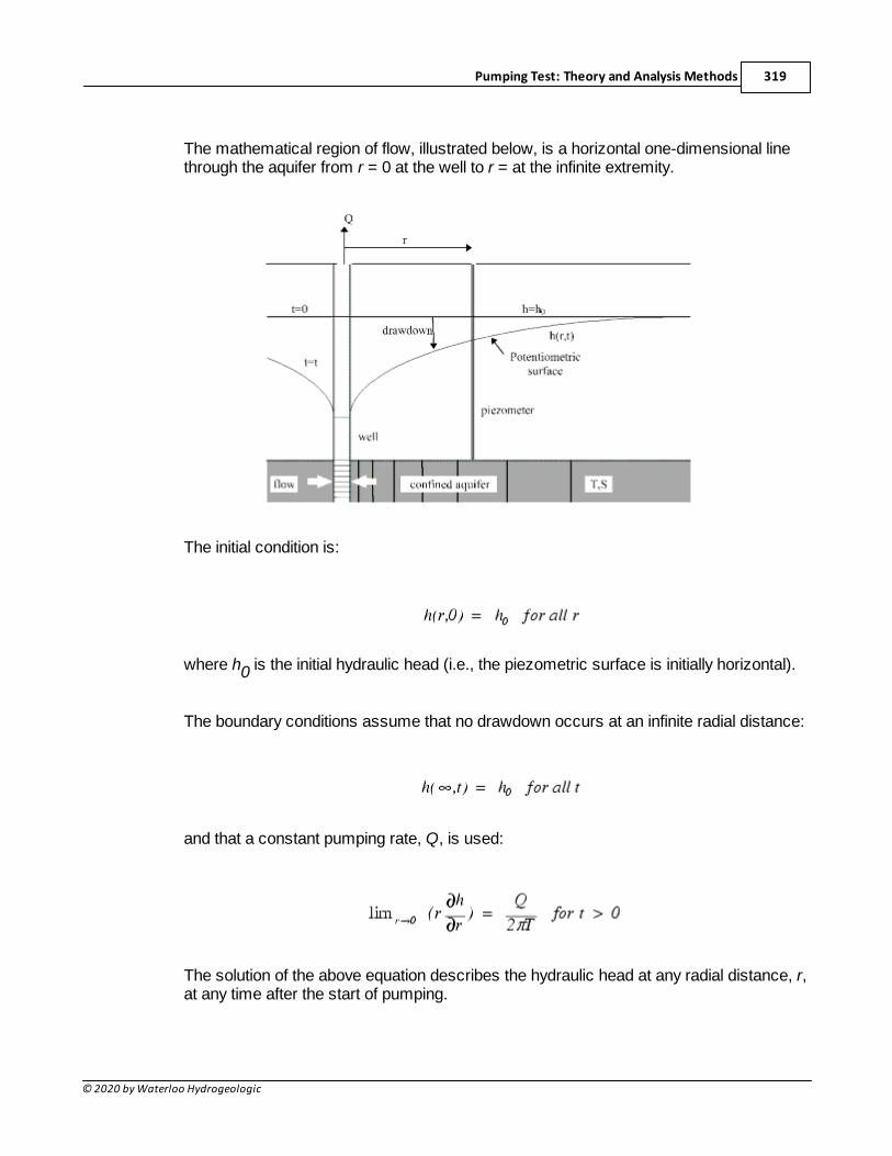
Pumping Test: Theory and Analysis Methods 319
© 2020 by Waterloo Hydrogeologic
The mathematical region of flow, illustrated below, is a horizontal one-dimensional linethrough the aquifer from r = 0 at the well to r = at the infinite extremity.
The initial condition is:
where h0 is the initial hydraulic head (i.e., the piezometric surface is initially horizontal).
The boundary conditions assume that no drawdown occurs at an infinite radial distance:
and that a constant pumping rate, Q, is used:
The solution of the above equation describes the hydraulic head at any radial distance, r,at any time after the start of pumping.
AquiferTest 10.0 Help320
© 2020 by Waterloo Hydrogeologic
4.5 Pumping Test Analysis Methods - Fixed Assumptions
The following pumping test methods require a fixed set of assumptions; as such, theseassumptions may not be modified on the Analysis plot. These include:
· Theis Recovery Analysis
· Cooper-Jacob Methods:o Cooper Jacob I: Time-Drawdowno Cooper Jacob II: Distance-Drawdowno Cooper Jacob III: Time-Distance Drawdown
4.5.1 Theis Recovery Test (confined)
When the pump is shut down after a pumping test, the water level inside the pumpingand observation wells will start to rise. This rise in water level is known as residualdrawdown (s'). Recovery-test measurements allow the transmissivity of the aquifer tobe calculated, thereby providing an independent check on the results of the pumpingtest.
Residual drawdown data can be more reliable than drawdown data because therecovery occurs at a constant rate, whereas constant discharge pumping is oftendifficult to achieve in the field. Residual drawdown data can be collected from both thepumping and observation wells.
Strictly applied, this solution is appropriate for the conditions shown in the followingfigure. However, if additional limiting conditions are satisfied, the Theis recovery solutionmethod can also be used for leaky, unconfined aquifers and aquifers with partiallypenetrating wells (Kruseman and de Ridder, 1990, p. 183).
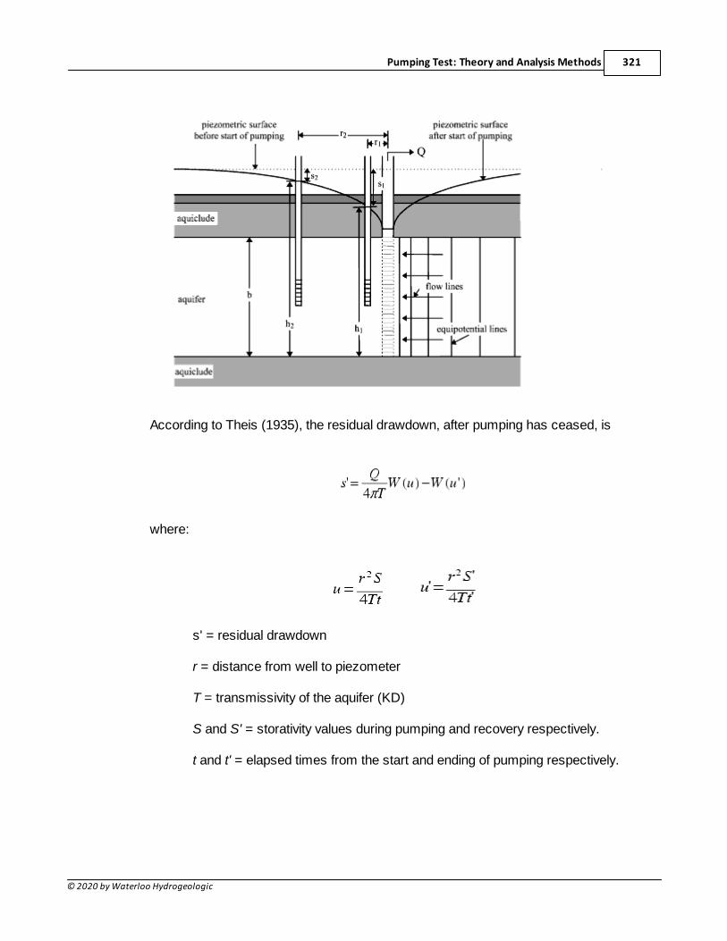
Pumping Test: Theory and Analysis Methods 321
© 2020 by Waterloo Hydrogeologic
According to Theis (1935), the residual drawdown, after pumping has ceased, is
where:
s' = residual drawdown
r = distance from well to piezometer
T = transmissivity of the aquifer (KD)
S and S' = storativity values during pumping and recovery respectively.
t and t' = elapsed times from the start and ending of pumping respectively.
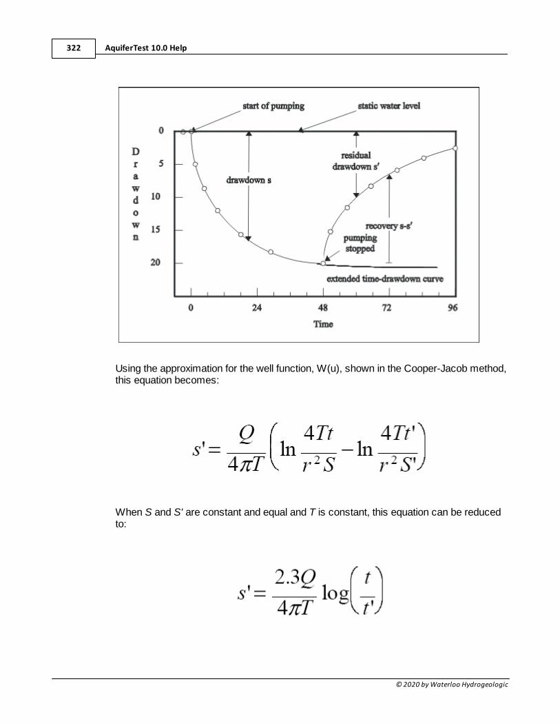
AquiferTest 10.0 Help322
© 2020 by Waterloo Hydrogeologic
Using the approximation for the well function, W(u), shown in the Cooper-Jacob method,this equation becomes:
When S and S' are constant and equal and T is constant, this equation can be reducedto:
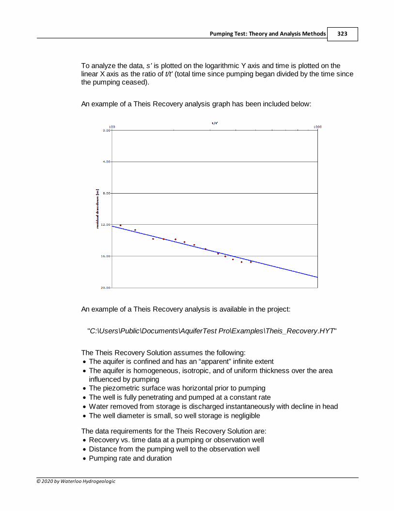
Pumping Test: Theory and Analysis Methods 323
© 2020 by Waterloo Hydrogeologic
To analyze the data, s' is plotted on the logarithmic Y axis and time is plotted on thelinear X axis as the ratio of t/t' (total time since pumping began divided by the time sincethe pumping ceased).
An example of a Theis Recovery analysis graph has been included below:
An example of a Theis Recovery analysis is available in the project:
"C:\Users\Public\Documents\AquiferTest Pro\Examples\Theis_Recovery.HYT"
The Theis Recovery Solution assumes the following:· The aquifer is confined and has an “apparent” infinite extent
· The aquifer is homogeneous, isotropic, and of uniform thickness over the areainfluenced by pumping
· The piezometric surface was horizontal prior to pumping
· The well is fully penetrating and pumped at a constant rate
· Water removed from storage is discharged instantaneously with decline in head
· The well diameter is small, so well storage is negligible
The data requirements for the Theis Recovery Solution are:· Recovery vs. time data at a pumping or observation well
· Distance from the pumping well to the observation well
· Pumping rate and duration
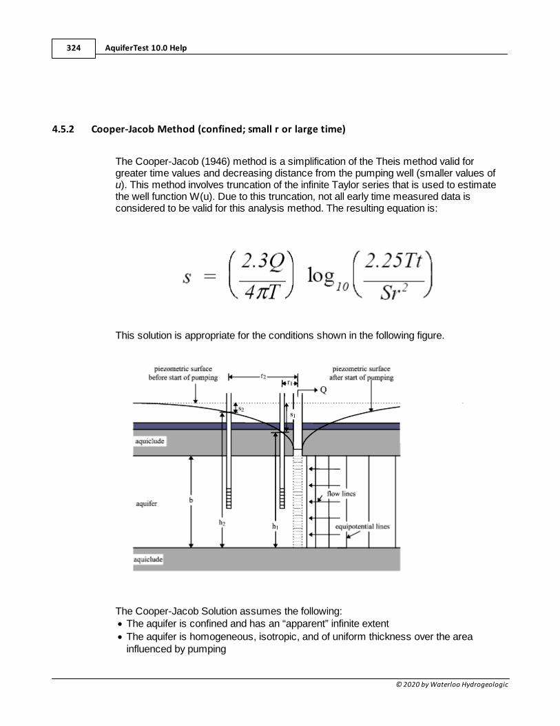
AquiferTest 10.0 Help324
© 2020 by Waterloo Hydrogeologic
4.5.2 Cooper-Jacob Method (confined; small r or large time)
The Cooper-Jacob (1946) method is a simplification of the Theis method valid forgreater time values and decreasing distance from the pumping well (smaller values ofu). This method involves truncation of the infinite Taylor series that is used to estimatethe well function W(u). Due to this truncation, not all early time measured data isconsidered to be valid for this analysis method. The resulting equation is:
This solution is appropriate for the conditions shown in the following figure.
The Cooper-Jacob Solution assumes the following:· The aquifer is confined and has an “apparent” infinite extent
· The aquifer is homogeneous, isotropic, and of uniform thickness over the areainfluenced by pumping
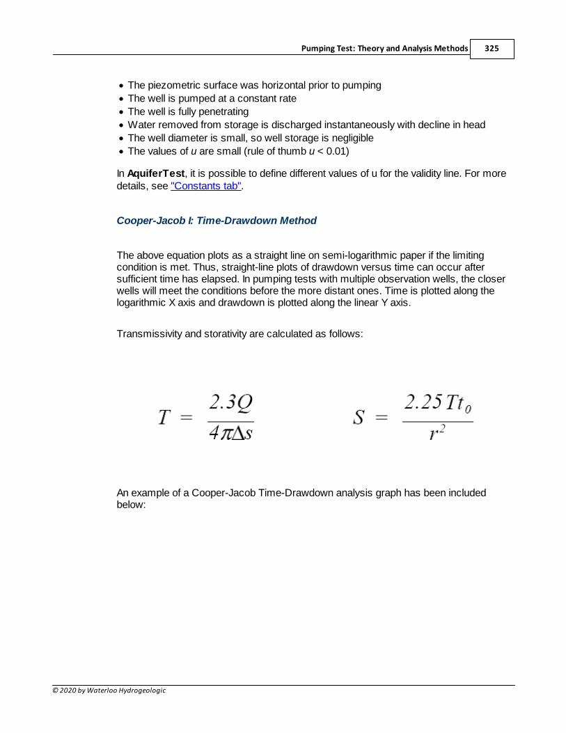
Pumping Test: Theory and Analysis Methods 325
© 2020 by Waterloo Hydrogeologic
· The piezometric surface was horizontal prior to pumping
· The well is pumped at a constant rate
· The well is fully penetrating
· Water removed from storage is discharged instantaneously with decline in head
· The well diameter is small, so well storage is negligible
· The values of u are small (rule of thumb u < 0.01)
In AquiferTest, it is possible to define different values of u for the validity line. For moredetails, see "Constants tab".
Cooper-Jacob I: Time-Drawdown Method
The above equation plots as a straight line on semi-logarithmic paper if the limitingcondition is met. Thus, straight-line plots of drawdown versus time can occur aftersufficient time has elapsed. In pumping tests with multiple observation wells, the closerwells will meet the conditions before the more distant ones. Time is plotted along thelogarithmic X axis and drawdown is plotted along the linear Y axis.
Transmissivity and storativity are calculated as follows:
An example of a Cooper-Jacob Time-Drawdown analysis graph has been includedbelow:
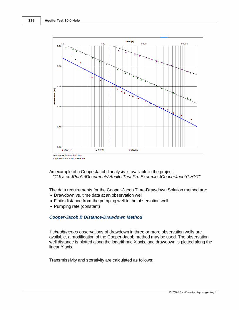
AquiferTest 10.0 Help326
© 2020 by Waterloo Hydrogeologic
An example of a CooperJacob I analysis is available in the project: "C:\Users\Public\Documents\AquiferTest Pro\Examples\CooperJacob1.HYT"
The data requirements for the Cooper-Jacob Time-Drawdown Solution method are:· Drawdown vs. time data at an observation well
· Finite distance from the pumping well to the observation well
· Pumping rate (constant)
Cooper-Jacob II: Distance-Drawdown Method
If simultaneous observations of drawdown in three or more observation wells areavailable, a modification of the Cooper-Jacob method may be used. The observationwell distance is plotted along the logarithmic X axis, and drawdown is plotted along thelinear Y axis.
Transmissivity and storativity are calculated as follows:
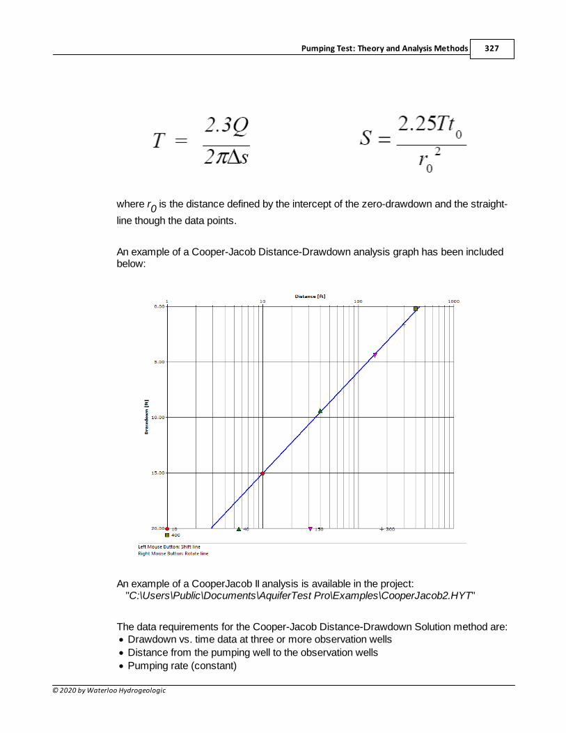
Pumping Test: Theory and Analysis Methods 327
© 2020 by Waterloo Hydrogeologic
where r0 is the distance defined by the intercept of the zero-drawdown and the straight-
line though the data points.
An example of a Cooper-Jacob Distance-Drawdown analysis graph has been includedbelow:
An example of a CooperJacob II analysis is available in the project: "C:\Users\Public\Documents\AquiferTest Pro\Examples\CooperJacob2.HYT"
The data requirements for the Cooper-Jacob Distance-Drawdown Solution method are:· Drawdown vs. time data at three or more observation wells
· Distance from the pumping well to the observation wells
· Pumping rate (constant)
AquiferTest 10.0 Help328
© 2020 by Waterloo Hydrogeologic
Both distance and drawdown values at a specific time are plotted, so you must specifythis time value.
Cooper-Jacob III: Time-Distance-Drawdown Method
As with the Distance-Drawdown Method, if simultaneous observations are made ofdrawdown in three or more observation wells, a modification of the Cooper-Jacob
method may be used. Drawdown is plotted along the linear Y axis and t/r2 is plottedalong the logarithmic X axis.
Transmissivity and storativity are calculated as follows:
where r0 is the distance defined by the intercept of the zero-drawdown and the straight-
line though the data points.
An example of a Cooper-Jacob Time-Distance-Drawdown analysis graph has beenincluded in the following figure:
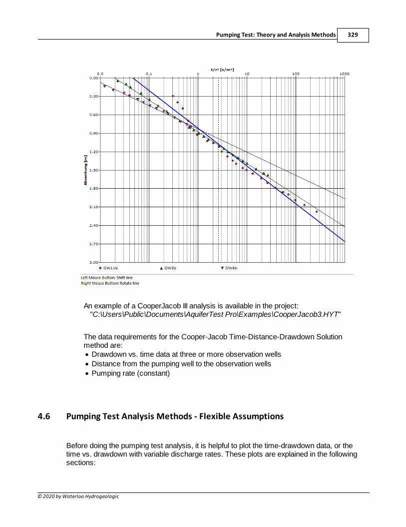
Pumping Test: Theory and Analysis Methods 329
© 2020 by Waterloo Hydrogeologic
An example of a CooperJacob III analysis is available in the project: "C:\Users\Public\Documents\AquiferTest Pro\Examples\CooperJacob3.HYT"
The data requirements for the Cooper-Jacob Time-Distance-Drawdown Solutionmethod are:· Drawdown vs. time data at three or more observation wells
· Distance from the pumping well to the observation wells
· Pumping rate (constant)
4.6 Pumping Test Analysis Methods - Flexible Assumptions
Before doing the pumping test analysis, it is helpful to plot the time-drawdown data, or thetime vs. drawdown with variable discharge rates. These plots are explained in the followingsections:
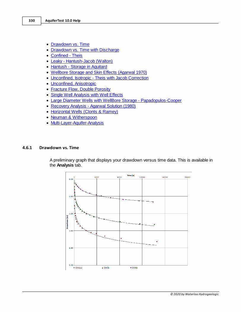
AquiferTest 10.0 Help330
© 2020 by Waterloo Hydrogeologic
· Drawdown vs. Time
· Drawdown vs. Time with Discharge
· Confined - Theis
· Leaky - Hantush-Jacob (Walton)
· Hantush - Storage in Aquitard
· Wellbore Storage and Skin Effects (Agarwal 1970)
· Unconfined, Isotropic - Theis with Jacob Correction
· Unconfined, Anisotropic
· Fracture Flow, Double Porosity
· Single Well Analysis with Well Effects
· Large Diameter Wells with WellBore Storage - Papadopulos-Cooper
· Recovery Analysis - Agarwal Solution (1980)
· Horizontal Wells (Clonts & Ramey)
· Neuman & Witherspoon
· Multi-Layer-Aquifer-Analysis
4.6.1 Drawdown vs. Time
A preliminary graph that displays your drawdown versus time data. This is available inthe Analysis tab.
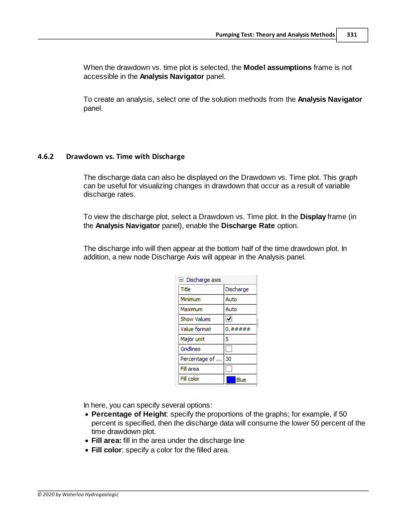
Pumping Test: Theory and Analysis Methods 331
© 2020 by Waterloo Hydrogeologic
When the drawdown vs. time plot is selected, the Model assumptions frame is notaccessible in the Analysis Navigator panel.
To create an analysis, select one of the solution methods from the Analysis Navigatorpanel.
4.6.2 Drawdown vs. Time with Discharge
The discharge data can also be displayed on the Drawdown vs. Time plot. This graphcan be useful for visualizing changes in drawdown that occur as a result of variabledischarge rates.
To view the discharge plot, select a Drawdown vs. Time plot. In the Display frame (inthe Analysis Navigator panel), enable the Discharge Rate option.
The discharge info will then appear at the bottom half of the time drawdown plot. Inaddition, a new node Discharge Axis will appear in the Analysis panel.
In here, you can specify several options:· Percentage of Height: specify the proportions of the graphs; for example, if 50
percent is specified, then the discharge data will consume the lower 50 percent of thetime drawdown plot.
· Fill area: fill in the area under the discharge line
· Fill color: specify a color for the filled area.
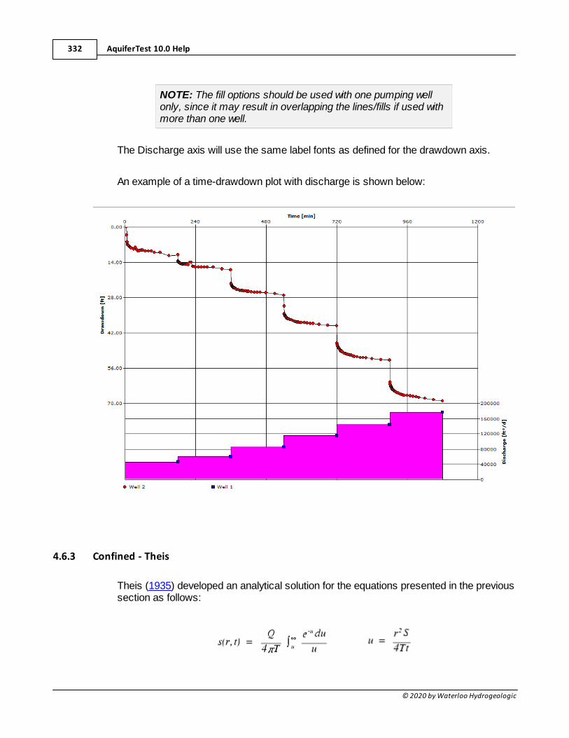
AquiferTest 10.0 Help332
© 2020 by Waterloo Hydrogeologic
NOTE: The fill options should be used with one pumping wellonly, since it may result in overlapping the lines/fills if used withmore than one well.
The Discharge axis will use the same label fonts as defined for the drawdown axis.
An example of a time-drawdown plot with discharge is shown below:
4.6.3 Confined - Theis
Theis (1935) developed an analytical solution for the equations presented in the previoussection as follows:
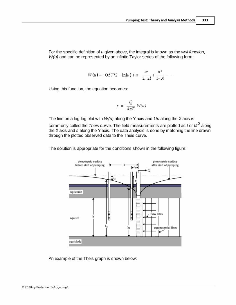
Pumping Test: Theory and Analysis Methods 333
© 2020 by Waterloo Hydrogeologic
For the specific definition of u given above, the integral is known as the well function,W(u) and can be represented by an infinite Taylor series of the following form:
Using this function, the equation becomes:
The line on a log-log plot with W(u) along the Y axis and 1/u along the X axis is
commonly called the Theis curve. The field measurements are plotted as t or t/r2 alongthe X axis and s along the Y axis. The data analysis is done by matching the line drawnthrough the plotted observed data to the Theis curve.
The solution is appropriate for the conditions shown in the following figure:
An example of the Theis graph is shown below:
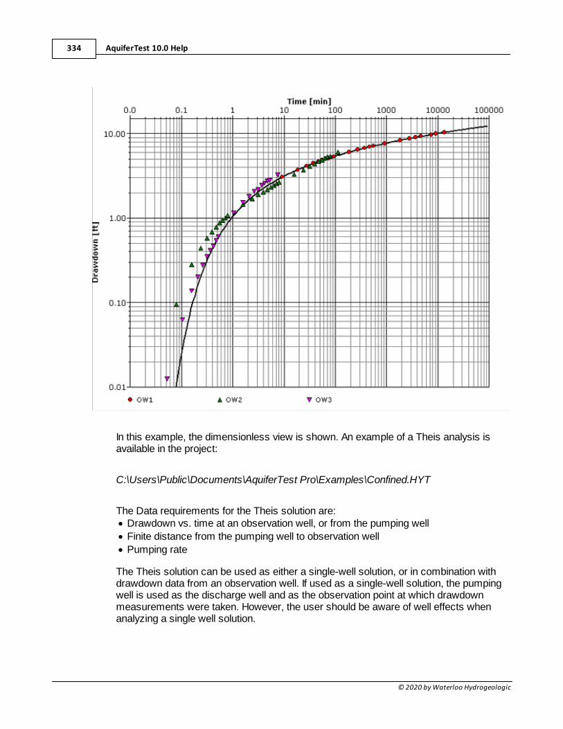
AquiferTest 10.0 Help334
© 2020 by Waterloo Hydrogeologic
In this example, the dimensionless view is shown. An example of a Theis analysis isavailable in the project:
C:\Users\Public\Documents\AquiferTest Pro\Examples\Confined.HYT
The Data requirements for the Theis solution are:· Drawdown vs. time at an observation well, or from the pumping well
· Finite distance from the pumping well to observation well
· Pumping rate
The Theis solution can be used as either a single-well solution, or in combination withdrawdown data from an observation well. If used as a single-well solution, the pumpingwell is used as the discharge well and as the observation point at which drawdownmeasurements were taken. However, the user should be aware of well effects whenanalyzing a single well solution.
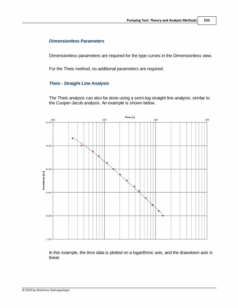
Pumping Test: Theory and Analysis Methods 335
© 2020 by Waterloo Hydrogeologic
Dimensionless Parameters
Dimensionless parameters are required for the type curves in the Dimensionless view.
For the Theis method, no additional parameters are required.
Theis - Straight Line Analysis
The Theis analysis can also be done using a semi-log straight line analysis; similar tothe Cooper-Jacob analysis. An example is shown below.
In this example, the time data is plotted on a logarithmic axis, and the drawdown axis islinear.
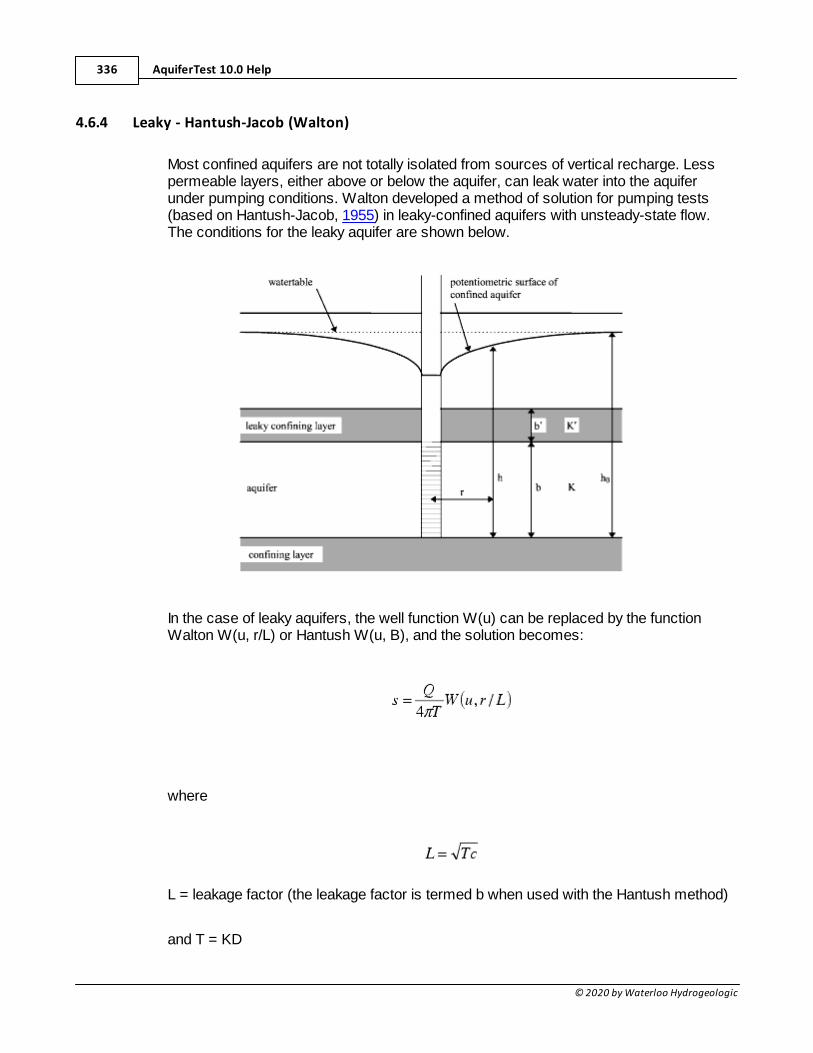
AquiferTest 10.0 Help336
© 2020 by Waterloo Hydrogeologic
4.6.4 Leaky - Hantush-Jacob (Walton)
Most confined aquifers are not totally isolated from sources of vertical recharge. Lesspermeable layers, either above or below the aquifer, can leak water into the aquiferunder pumping conditions. Walton developed a method of solution for pumping tests(based on Hantush-Jacob, 1955) in leaky-confined aquifers with unsteady-state flow.The conditions for the leaky aquifer are shown below.
In the case of leaky aquifers, the well function W(u) can be replaced by the functionWalton W(u, r/L) or Hantush W(u, B), and the solution becomes:
where
L = leakage factor (the leakage factor is termed b when used with the Hantush method)
and T = KD
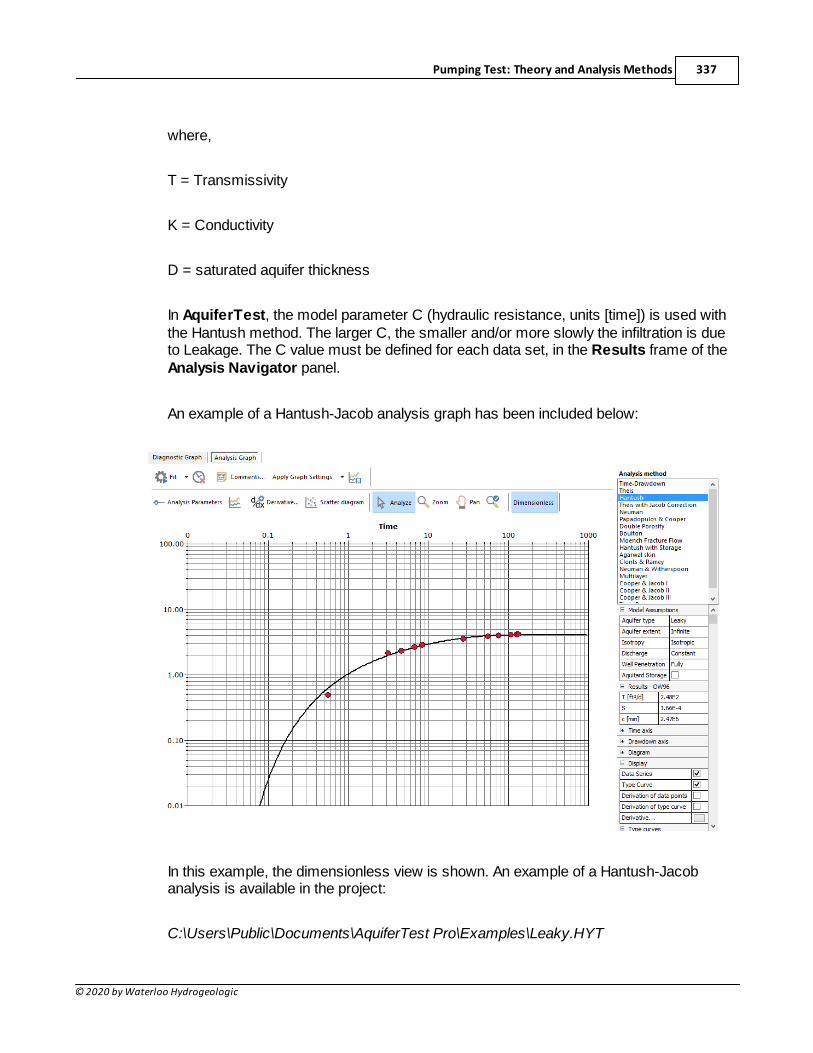
Pumping Test: Theory and Analysis Methods 337
© 2020 by Waterloo Hydrogeologic
where,
T = Transmissivity
K = Conductivity
D = saturated aquifer thickness
In AquiferTest, the model parameter C (hydraulic resistance, units [time]) is used withthe Hantush method. The larger C, the smaller and/or more slowly the infiltration is dueto Leakage. The C value must be defined for each data set, in the Results frame of theAnalysis Navigator panel.
An example of a Hantush-Jacob analysis graph has been included below:
In this example, the dimensionless view is shown. An example of a Hantush-Jacobanalysis is available in the project:
C:\Users\Public\Documents\AquiferTest Pro\Examples\Leaky.HYT
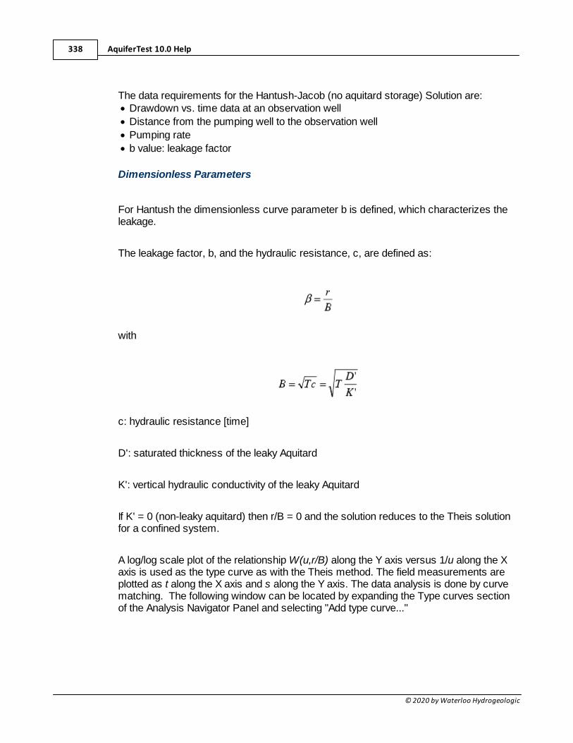
AquiferTest 10.0 Help338
© 2020 by Waterloo Hydrogeologic
The data requirements for the Hantush-Jacob (no aquitard storage) Solution are:· Drawdown vs. time data at an observation well
· Distance from the pumping well to the observation well
· Pumping rate
· b value: leakage factor
Dimensionless Parameters
For Hantush the dimensionless curve parameter b is defined, which characterizes theleakage.
The leakage factor, b, and the hydraulic resistance, c, are defined as:
with
c: hydraulic resistance [time]
D': saturated thickness of the leaky Aquitard
K': vertical hydraulic conductivity of the leaky Aquitard
If K' = 0 (non-leaky aquitard) then r/B = 0 and the solution reduces to the Theis solutionfor a confined system.
A log/log scale plot of the relationship W(u,r/B) along the Y axis versus 1/u along the Xaxis is used as the type curve as with the Theis method. The field measurements areplotted as t along the X axis and s along the Y axis. The data analysis is done by curvematching. The following window can be located by expanding the Type curves sectionof the Analysis Navigator Panel and selecting "Add type curve..."
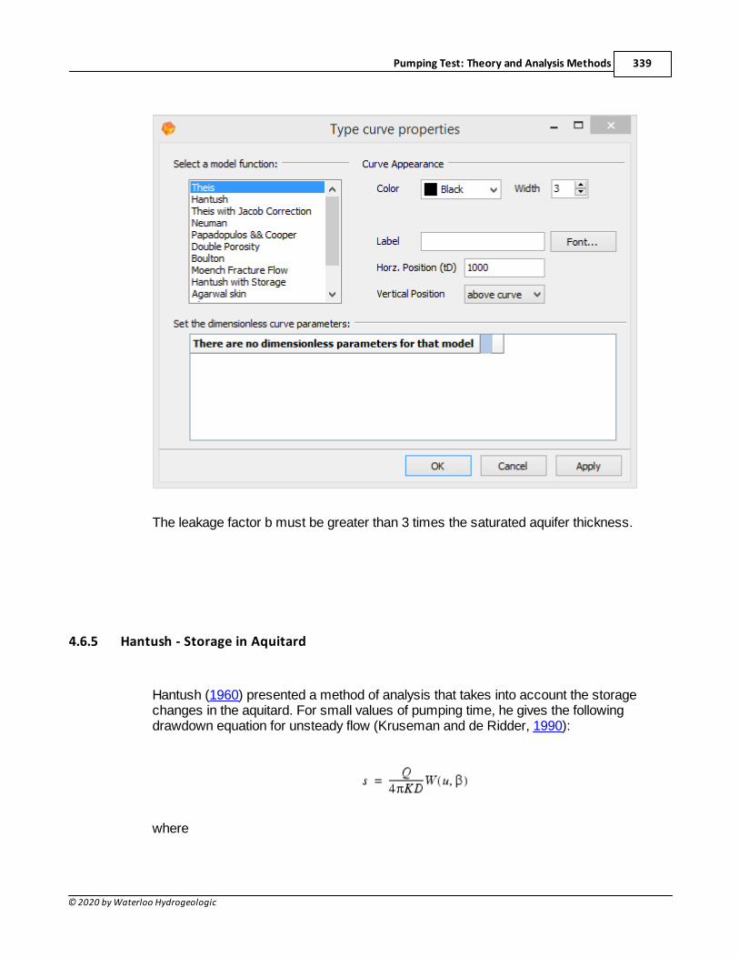
Pumping Test: Theory and Analysis Methods 339
© 2020 by Waterloo Hydrogeologic
The leakage factor b must be greater than 3 times the saturated aquifer thickness.
4.6.5 Hantush - Storage in Aquitard
Hantush (1960) presented a method of analysis that takes into account the storagechanges in the aquitard. For small values of pumping time, he gives the followingdrawdown equation for unsteady flow (Kruseman and de Ridder, 1990):
where
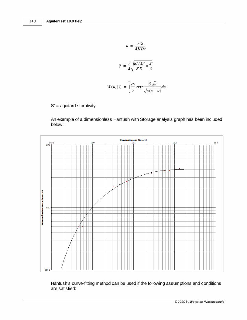
AquiferTest 10.0 Help340
© 2020 by Waterloo Hydrogeologic
S' = aquitard storativity
An example of a dimensionless Hantush with Storage analysis graph has been includedbelow:
Hantush’s curve-fitting method can be used if the following assumptions and conditionsare satisfied:
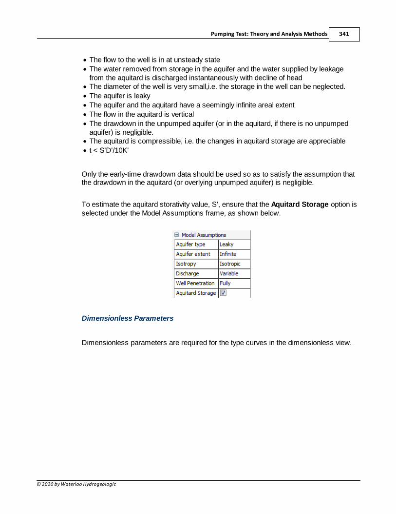
Pumping Test: Theory and Analysis Methods 341
© 2020 by Waterloo Hydrogeologic
· The flow to the well is in at unsteady state
· The water removed from storage in the aquifer and the water supplied by leakagefrom the aquitard is discharged instantaneously with decline of head
· The diameter of the well is very small,i.e. the storage in the well can be neglected.
· The aquifer is leaky
· The aquifer and the aquitard have a seemingly infinite areal extent
· The flow in the aquitard is vertical
· The drawdown in the unpumped aquifer (or in the aquitard, if there is no unpumpedaquifer) is negligible.
· The aquitard is compressible, i.e. the changes in aquitard storage are appreciable
· t < S'D'/10K'
Only the early-time drawdown data should be used so as to satisfy the assumption thatthe drawdown in the aquitard (or overlying unpumped aquifer) is negligible.
To estimate the aquitard storativity value, S', ensure that the Aquitard Storage option isselected under the Model Assumptions frame, as shown below.
Dimensionless Parameters
Dimensionless parameters are required for the type curves in the dimensionless view.
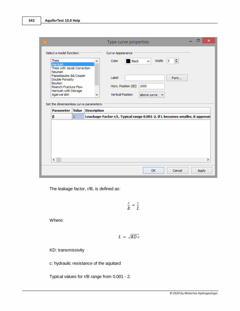
AquiferTest 10.0 Help342
© 2020 by Waterloo Hydrogeologic
The leakage factor, r/B, is defined as:
Where:
KD: transmissivity
c: hydraulic resistance of the aquitard
Typical values for r/B range from 0.001 - 2.
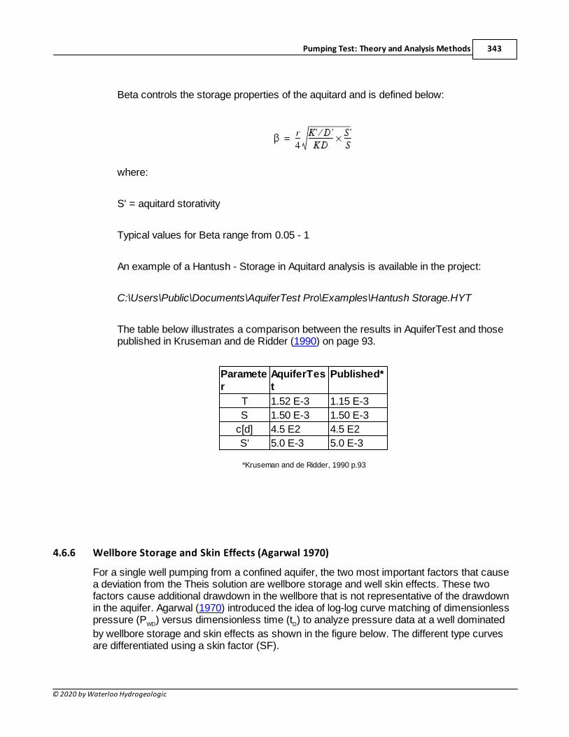
Pumping Test: Theory and Analysis Methods 343
© 2020 by Waterloo Hydrogeologic
Beta controls the storage properties of the aquitard and is defined below:
where:
S' = aquitard storativity
Typical values for Beta range from 0.05 - 1
An example of a Hantush - Storage in Aquitard analysis is available in the project:
C:\Users\Public\Documents\AquiferTest Pro\Examples\Hantush Storage.HYT
The table below illustrates a comparison between the results in AquiferTest and thosepublished in Kruseman and de Ridder (1990) on page 93.
Parameter
AquiferTest
Published*
T 1.52 E-3 1.15 E-3
S 1.50 E-3 1.50 E-3
c[d] 4.5 E2 4.5 E2
S' 5.0 E-3 5.0 E-3
*Kruseman and de Ridder, 1990 p.93
4.6.6 Wellbore Storage and Skin Effects (Agarwal 1970)
For a single well pumping from a confined aquifer, the two most important factors that causea deviation from the Theis solution are wellbore storage and well skin effects. These twofactors cause additional drawdown in the wellbore that is not representative of the drawdownin the aquifer. Agarwal (1970) introduced the idea of log-log curve matching of dimensionlesspressure (PWD) versus dimensionless time (tD) to analyze pressure data at a well dominated
by wellbore storage and skin effects as shown in the figure below. The different type curvesare differentiated using a skin factor (SF).

AquiferTest 10.0 Help344
© 2020 by Waterloo Hydrogeologic
AquiferTest has implemented the Agarwal wellbore storage and skin solution for water wellsusing the following assumptions:
· single pumping well
· confined aquifer
· observations only in the pumping well
For an example exercise of the Agarwal (1970) analysis method, please see "Exercise11: Wellbore Storage and Skin Effects"
4.6.7 Unconfined, Isotropic - Theis with Jacob Correction
The water table in an unconfined aquifer is equal to the elevation head (potential).Transmissivity is no longer constant, and it will decrease with increasing drawdown.This means that there is not only horizontal flow to the well, but there is also a verticalcomponent, which will increase the closer you get to the well.
Since transmissivity in unconfined aquifers is not constant, there is no closed solutionfor this aquifer type. That is why the measured drawdown is corrected, and the pumpingtest is interpreted as being in a confined aquifer.
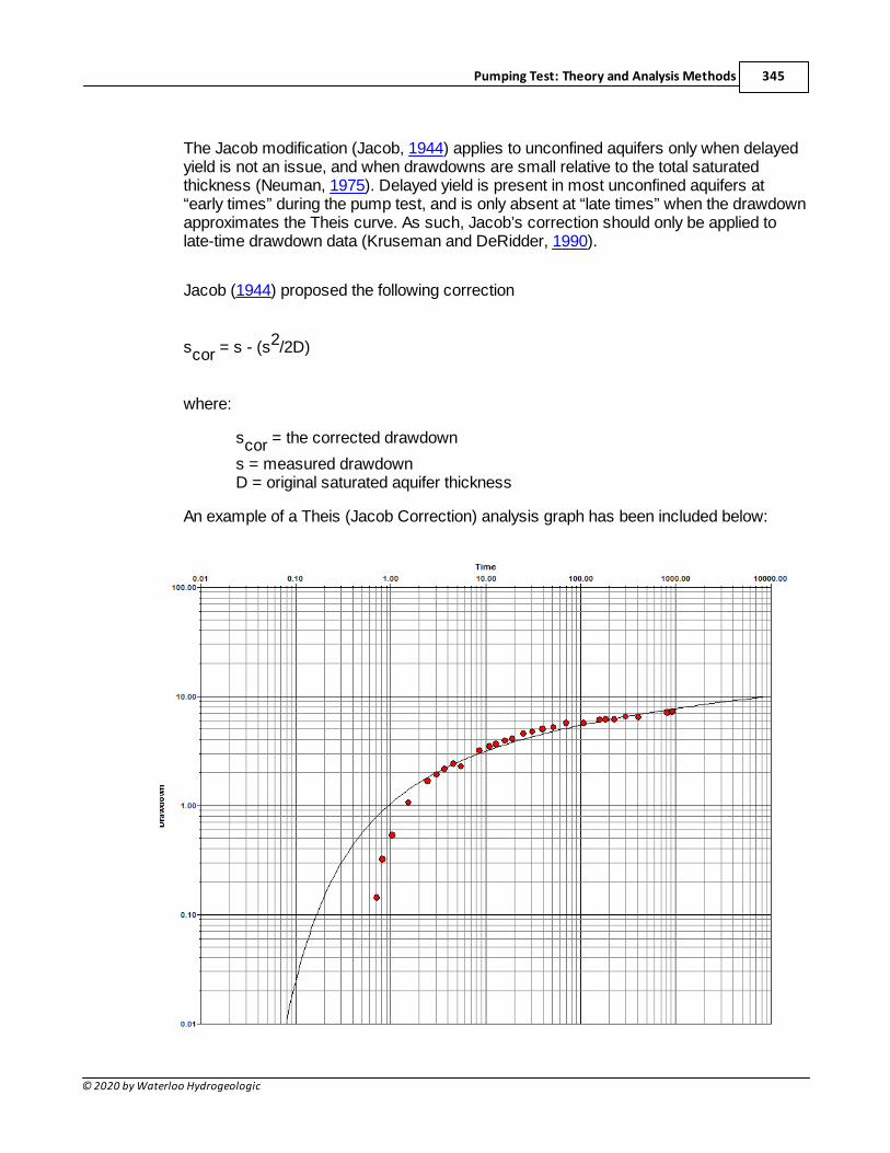
Pumping Test: Theory and Analysis Methods 345
© 2020 by Waterloo Hydrogeologic
The Jacob modification (Jacob, 1944) applies to unconfined aquifers only when delayedyield is not an issue, and when drawdowns are small relative to the total saturatedthickness (Neuman, 1975). Delayed yield is present in most unconfined aquifers at“early times” during the pump test, and is only absent at “late times” when the drawdownapproximates the Theis curve. As such, Jacob’s correction should only be applied tolate-time drawdown data (Kruseman and DeRidder, 1990).
Jacob (1944) proposed the following correction
scor = s - (s2/2D)
where:
scor = the corrected drawdown
s = measured drawdownD = original saturated aquifer thickness
An example of a Theis (Jacob Correction) analysis graph has been included below:
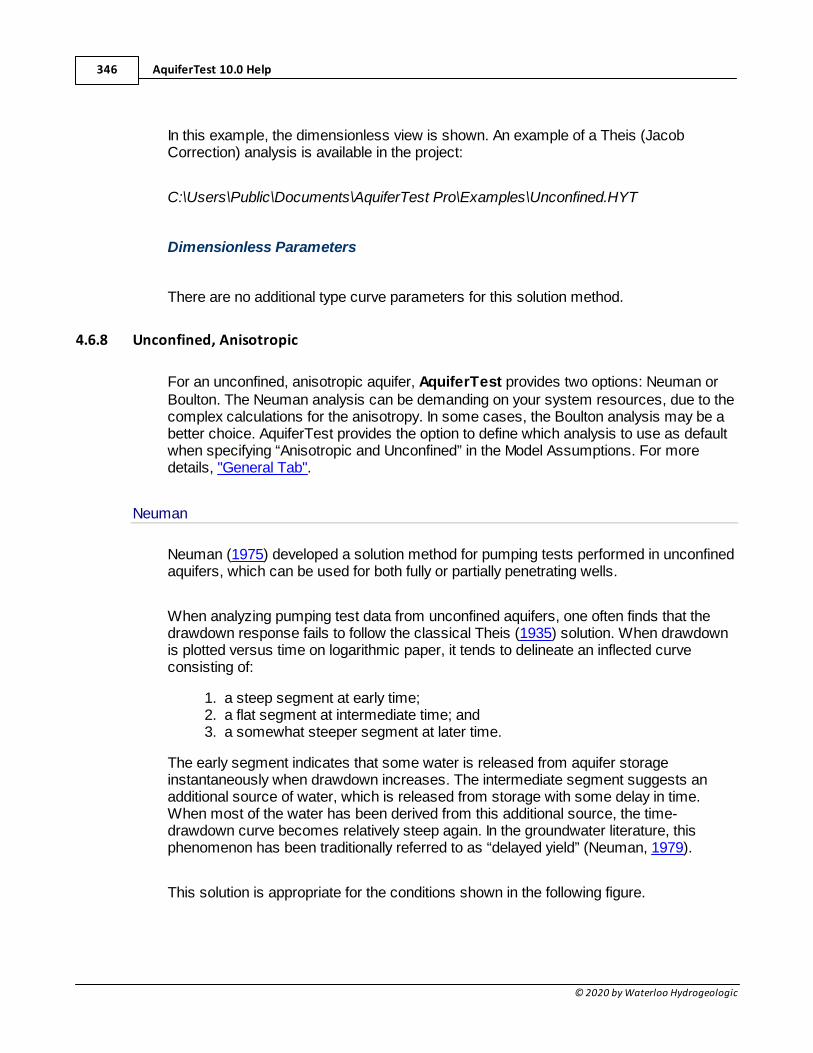
AquiferTest 10.0 Help346
© 2020 by Waterloo Hydrogeologic
In this example, the dimensionless view is shown. An example of a Theis (JacobCorrection) analysis is available in the project:
C:\Users\Public\Documents\AquiferTest Pro\Examples\Unconfined.HYT
Dimensionless Parameters
There are no additional type curve parameters for this solution method.
4.6.8 Unconfined, Anisotropic
For an unconfined, anisotropic aquifer, AquiferTest provides two options: Neuman orBoulton. The Neuman analysis can be demanding on your system resources, due to thecomplex calculations for the anisotropy. In some cases, the Boulton analysis may be abetter choice. AquiferTest provides the option to define which analysis to use as defaultwhen specifying “Anisotropic and Unconfined” in the Model Assumptions. For moredetails, "General Tab".
Neuman
Neuman (1975) developed a solution method for pumping tests performed in unconfinedaquifers, which can be used for both fully or partially penetrating wells.
When analyzing pumping test data from unconfined aquifers, one often finds that thedrawdown response fails to follow the classical Theis (1935) solution. When drawdownis plotted versus time on logarithmic paper, it tends to delineate an inflected curveconsisting of:
1. a steep segment at early time;2. a flat segment at intermediate time; and3. a somewhat steeper segment at later time.
The early segment indicates that some water is released from aquifer storageinstantaneously when drawdown increases. The intermediate segment suggests anadditional source of water, which is released from storage with some delay in time.When most of the water has been derived from this additional source, the time-drawdown curve becomes relatively steep again. In the groundwater literature, thisphenomenon has been traditionally referred to as “delayed yield” (Neuman, 1979).
This solution is appropriate for the conditions shown in the following figure.
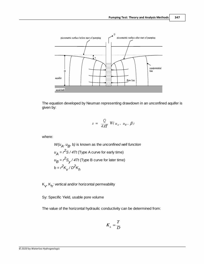
Pumping Test: Theory and Analysis Methods 347
© 2020 by Waterloo Hydrogeologic
The equation developed by Neuman representing drawdown in an unconfined aquifer isgiven by:
where:
W(uA, uB, b) is known as the unconfined well function
uA = r2S / 4Tt (Type A curve for early time)
uB = r2Sy / 4Tt (Type B curve for later time)
b = r2Kv / D2Kh
Kv, Kh: vertical and/or horizontal permeability
Sy: Specific Yield, usable pore volume
The value of the horizontal hydraulic conductivity can be determined from:
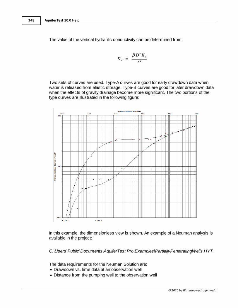
AquiferTest 10.0 Help348
© 2020 by Waterloo Hydrogeologic
The value of the vertical hydraulic conductivity can be determined from:
Two sets of curves are used. Type-A curves are good for early drawdown data whenwater is released from elastic storage. Type-B curves are good for later drawdown datawhen the effects of gravity drainage become more significant. The two portions of thetype curves are illustrated in the following figure:
In this example, the dimensionless view is shown. An example of a Neuman analysis isavailable in the project:
C:\Users\Public\Documents\AquiferTest Pro\Examples\PartiallyPenetratingWells.HYT.
The data requirements for the Neuman Solution are:· Drawdown vs. time data at an observation well
· Distance from the pumping well to the observation well
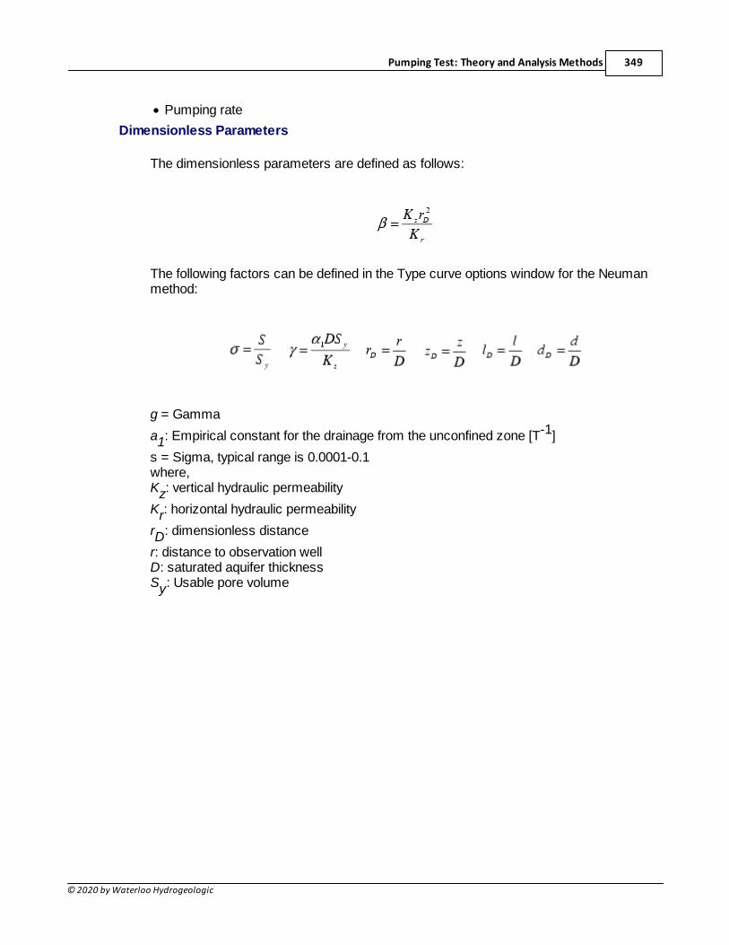
Pumping Test: Theory and Analysis Methods 349
© 2020 by Waterloo Hydrogeologic
· Pumping rate
Dimensionless Parameters
The dimensionless parameters are defined as follows:
The following factors can be defined in the Type curve options window for the Neumanmethod:
g = Gamma
a1: Empirical constant for the drainage from the unconfined zone [T-1]
s = Sigma, typical range is 0.0001-0.1where,Kz: vertical hydraulic permeability
Kr: horizontal hydraulic permeability
rD: dimensionless distance
r: distance to observation wellD: saturated aquifer thicknessSy: Usable pore volume
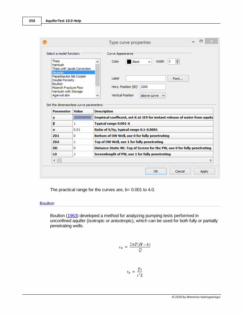
AquiferTest 10.0 Help350
© 2020 by Waterloo Hydrogeologic
The practical range for the curves are, b= 0.001 to 4.0.
Boulton
Boulton (1963) developed a method for analyzing pumping tests performed inunconfined aquifer (isotropic or anisotropic), which can be used for both fully or partiallypenetrating wells.
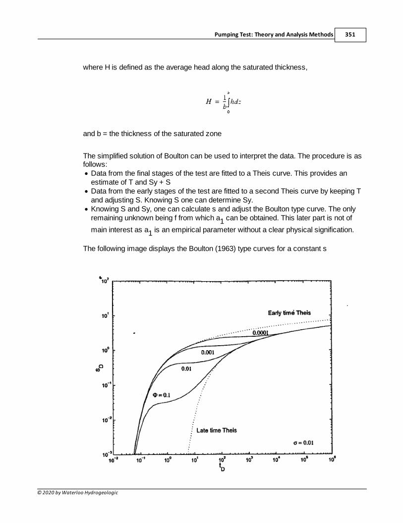
Pumping Test: Theory and Analysis Methods 351
© 2020 by Waterloo Hydrogeologic
where H is defined as the average head along the saturated thickness,
and b = the thickness of the saturated zone
The simplified solution of Boulton can be used to interpret the data. The procedure is asfollows:· Data from the final stages of the test are fitted to a Theis curve. This provides an
estimate of T and Sy + S· Data from the early stages of the test are fitted to a second Theis curve by keeping T
and adjusting S. Knowing S one can determine Sy.· Knowing S and Sy, one can calculate s and adjust the Boulton type curve. The only
remaining unknown being f from which a1 can be obtained. This later part is not of
main interest as a1 is an empirical parameter without a clear physical signification.
The following image displays the Boulton (1963) type curves for a constant s
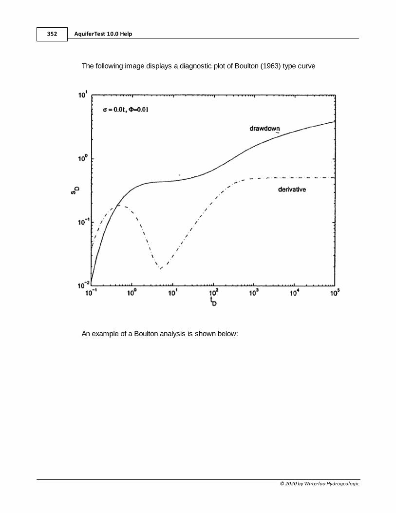
AquiferTest 10.0 Help352
© 2020 by Waterloo Hydrogeologic
The following image displays a diagnostic plot of Boulton (1963) type curve
An example of a Boulton analysis is shown below:
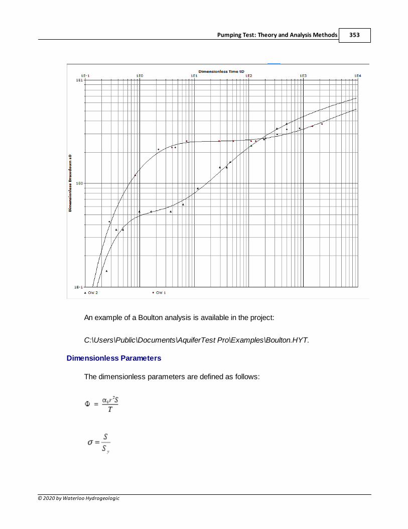
Pumping Test: Theory and Analysis Methods 353
© 2020 by Waterloo Hydrogeologic
An example of a Boulton analysis is available in the project:
C:\Users\Public\Documents\AquiferTest Pro\Examples\Boulton.HYT.
Dimensionless Parameters
The dimensionless parameters are defined as follows:
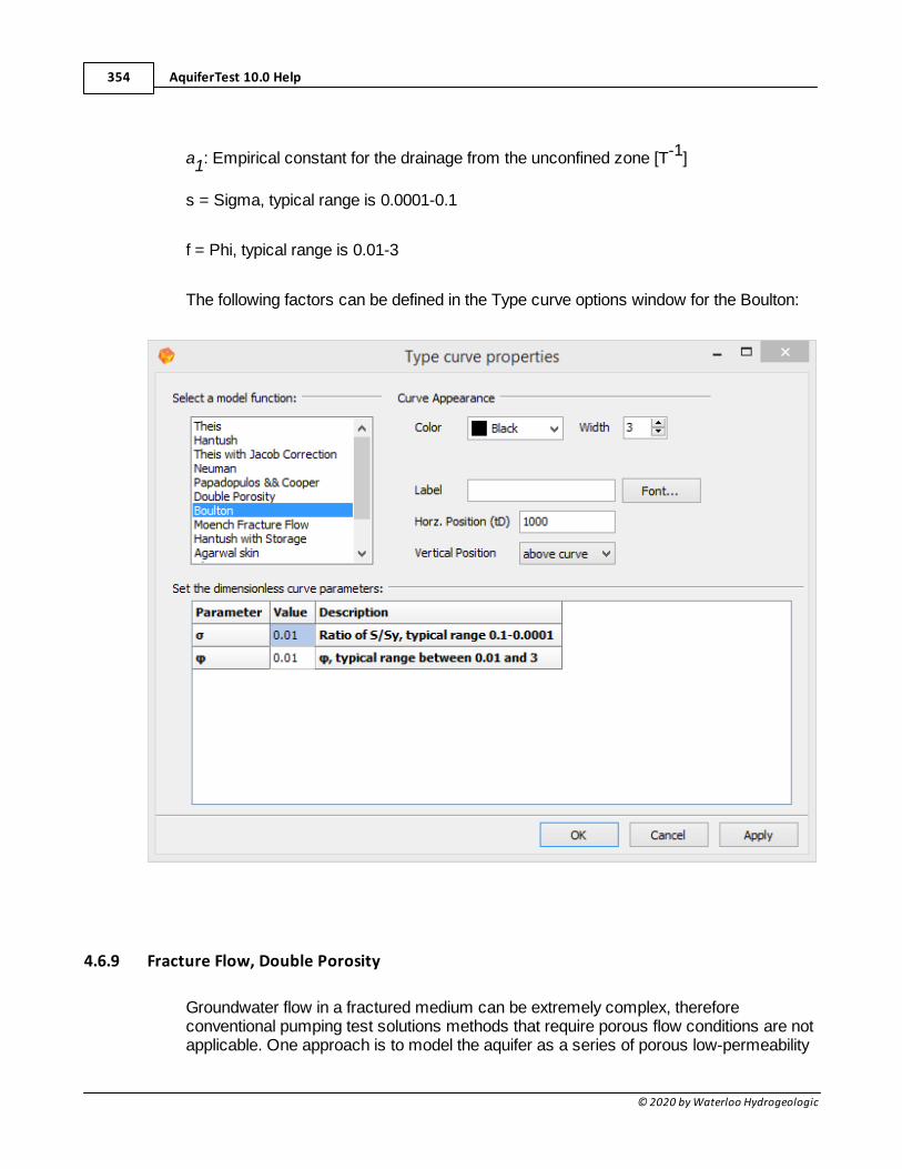
AquiferTest 10.0 Help354
© 2020 by Waterloo Hydrogeologic
a1: Empirical constant for the drainage from the unconfined zone [T-1]
s = Sigma, typical range is 0.0001-0.1
f = Phi, typical range is 0.01-3
The following factors can be defined in the Type curve options window for the Boulton:
4.6.9 Fracture Flow, Double Porosity
Groundwater flow in a fractured medium can be extremely complex, thereforeconventional pumping test solutions methods that require porous flow conditions are notapplicable. One approach is to model the aquifer as a series of porous low-permeability
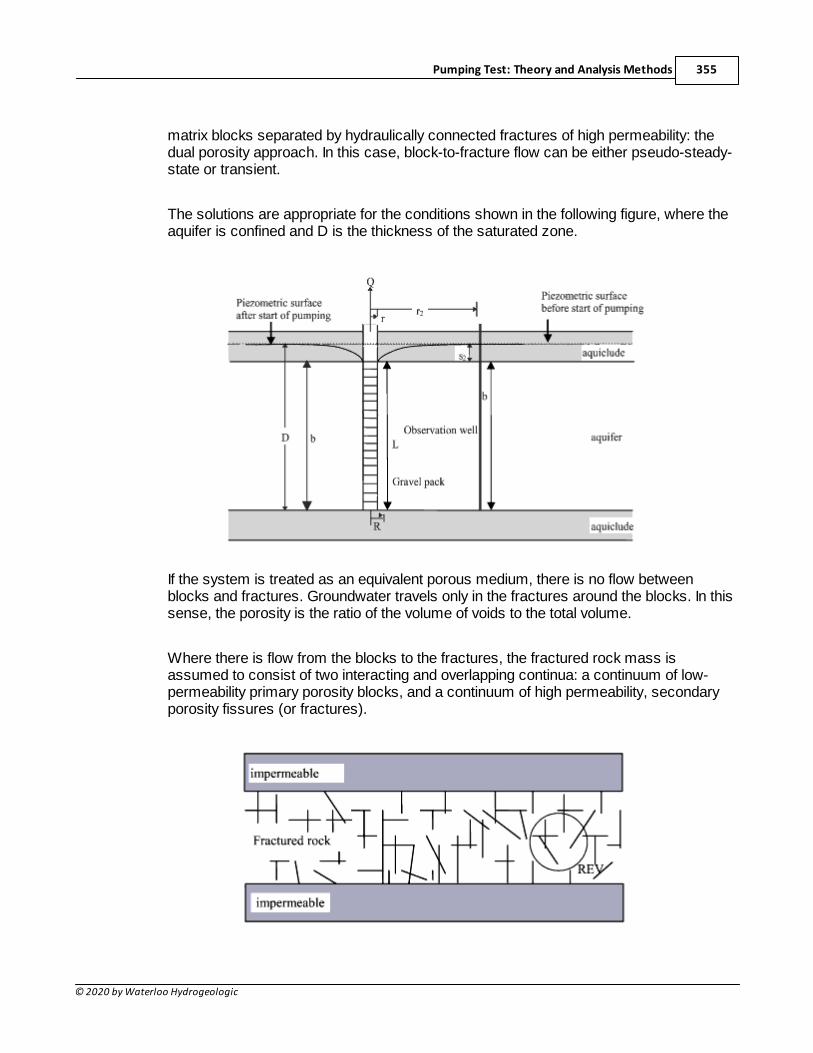
Pumping Test: Theory and Analysis Methods 355
© 2020 by Waterloo Hydrogeologic
matrix blocks separated by hydraulically connected fractures of high permeability: thedual porosity approach. In this case, block-to-fracture flow can be either pseudo-steady-state or transient.
The solutions are appropriate for the conditions shown in the following figure, where theaquifer is confined and D is the thickness of the saturated zone.
If the system is treated as an equivalent porous medium, there is no flow betweenblocks and fractures. Groundwater travels only in the fractures around the blocks. In thissense, the porosity is the ratio of the volume of voids to the total volume.
Where there is flow from the blocks to the fractures, the fractured rock mass isassumed to consist of two interacting and overlapping continua: a continuum of low-permeability primary porosity blocks, and a continuum of high permeability, secondaryporosity fissures (or fractures).
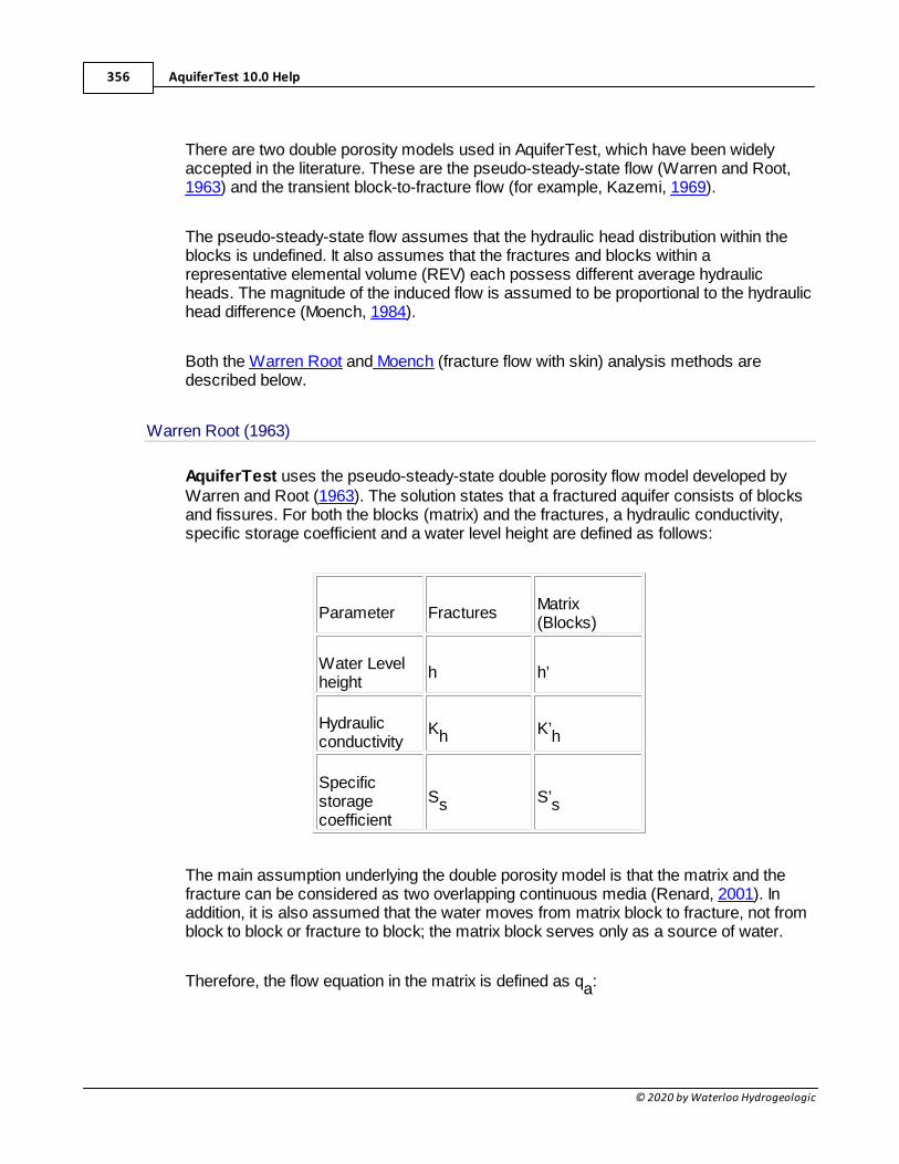
AquiferTest 10.0 Help356
© 2020 by Waterloo Hydrogeologic
There are two double porosity models used in AquiferTest, which have been widelyaccepted in the literature. These are the pseudo-steady-state flow (Warren and Root,1963) and the transient block-to-fracture flow (for example, Kazemi, 1969).
The pseudo-steady-state flow assumes that the hydraulic head distribution within theblocks is undefined. It also assumes that the fractures and blocks within arepresentative elemental volume (REV) each possess different average hydraulicheads. The magnitude of the induced flow is assumed to be proportional to the hydraulichead difference (Moench, 1984).
Both the Warren Root and Moench (fracture flow with skin) analysis methods aredescribed below.
Warren Root (1963)
AquiferTest uses the pseudo-steady-state double porosity flow model developed byWarren and Root (1963). The solution states that a fractured aquifer consists of blocksand fissures. For both the blocks (matrix) and the fractures, a hydraulic conductivity,specific storage coefficient and a water level height are defined as follows:
Parameter FracturesMatrix(Blocks)
Water Levelheight
h h’
Hydraulicconductivity
Kh K’h
Specificstoragecoefficient
Ss S’s
The main assumption underlying the double porosity model is that the matrix and thefracture can be considered as two overlapping continuous media (Renard, 2001). Inaddition, it is also assumed that the water moves from matrix block to fracture, not fromblock to block or fracture to block; the matrix block serves only as a source of water.
Therefore, the flow equation in the matrix is defined as qa:
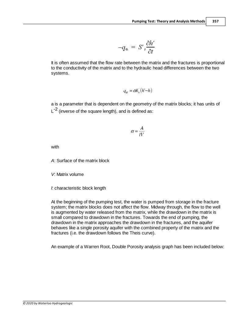
Pumping Test: Theory and Analysis Methods 357
© 2020 by Waterloo Hydrogeologic
It is often assumed that the flow rate between the matrix and the fractures is proportionalto the conductivity of the matrix and to the hydraulic head differences between the twosystems.
a is a parameter that is dependent on the geometry of the matrix blocks; it has units of
L-2 (inverse of the square length), and is defined as:
with
A: Surface of the matrix block
V: Matrix volume
l: characteristic block length
At the beginning of the pumping test, the water is pumped from storage in the fracturesystem; the matrix blocks does not affect the flow. Midway through, the flow to the wellis augmented by water released from the matrix, while the drawdown in the matrix issmall compared to drawdown in the fractures. Towards the end of pumping, thedrawdown in the matrix approaches the drawdown in the fractures, and the aquiferbehaves like a single porosity aquifer with the combined property of the matrix and thefractures (i.e. the drawdown follows the Theis curve).
An example of a Warren Root, Double Porosity analysis graph has been included below:
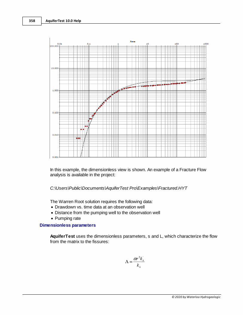
AquiferTest 10.0 Help358
© 2020 by Waterloo Hydrogeologic
In this example, the dimensionless view is shown. An example of a Fracture Flowanalysis is available in the project:
C:\Users\Public\Documents\AquiferTest Pro\Examples\Fractured.HYT
The Warren Root solution requires the following data:· Drawdown vs. time data at an observation well
· Distance from the pumping well to the observation well
· Pumping rate
Dimensionless parameters
AquiferTest uses the dimensionless parameters, s and L, which characterize the flowfrom the matrix to the fissures:
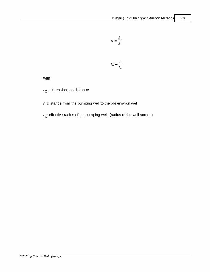
Pumping Test: Theory and Analysis Methods 359
© 2020 by Waterloo Hydrogeologic
with
rD: dimensionless distance
r: Distance from the pumping well to the observation well
rw: effective radius of the pumping well, (radius of the well screen)
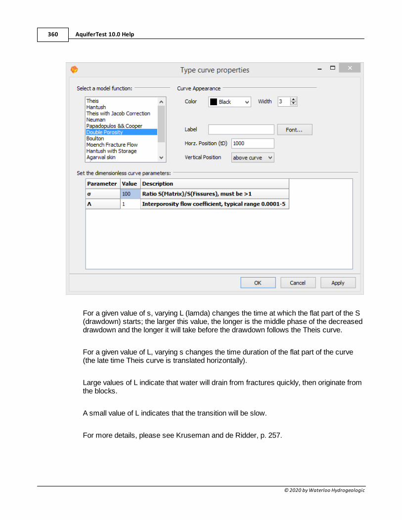
AquiferTest 10.0 Help360
© 2020 by Waterloo Hydrogeologic
For a given value of s, varying L (lamda) changes the time at which the flat part of the S(drawdown) starts; the larger this value, the longer is the middle phase of the decreaseddrawdown and the longer it will take before the drawdown follows the Theis curve.
For a given value of L, varying s changes the time duration of the flat part of the curve(the late time Theis curve is translated horizontally).
Large values of L indicate that water will drain from fractures quickly, then originate fromthe blocks.
A small value of L indicates that the transition will be slow.
For more details, please see Kruseman and de Ridder, p. 257.
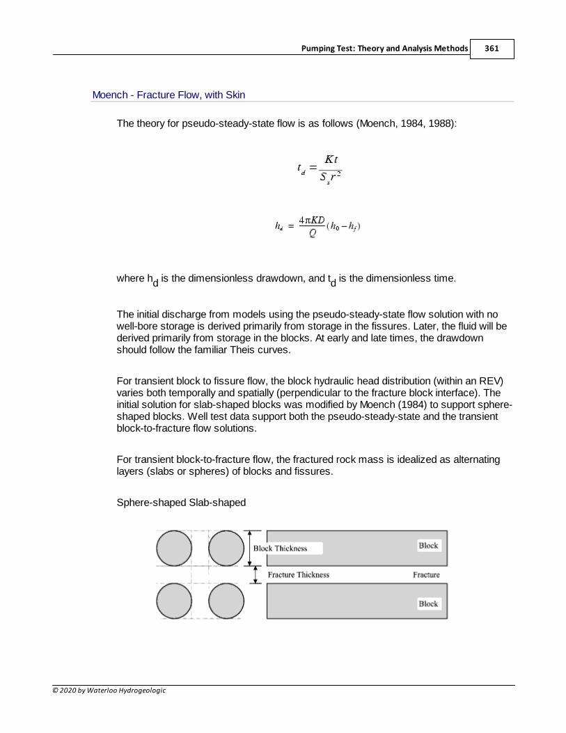
Pumping Test: Theory and Analysis Methods 361
© 2020 by Waterloo Hydrogeologic
Moench - Fracture Flow, with Skin
The theory for pseudo-steady-state flow is as follows (Moench, 1984, 1988):
where hd is the dimensionless drawdown, and td is the dimensionless time.
The initial discharge from models using the pseudo-steady-state flow solution with nowell-bore storage is derived primarily from storage in the fissures. Later, the fluid will bederived primarily from storage in the blocks. At early and late times, the drawdownshould follow the familiar Theis curves.
For transient block to fissure flow, the block hydraulic head distribution (within an REV)varies both temporally and spatially (perpendicular to the fracture block interface). Theinitial solution for slab-shaped blocks was modified by Moench (1984) to support sphere-shaped blocks. Well test data support both the pseudo-steady-state and the transientblock-to-fracture flow solutions.
For transient block-to-fracture flow, the fractured rock mass is idealized as alternatinglayers (slabs or spheres) of blocks and fissures.
Sphere-shaped Slab-shaped
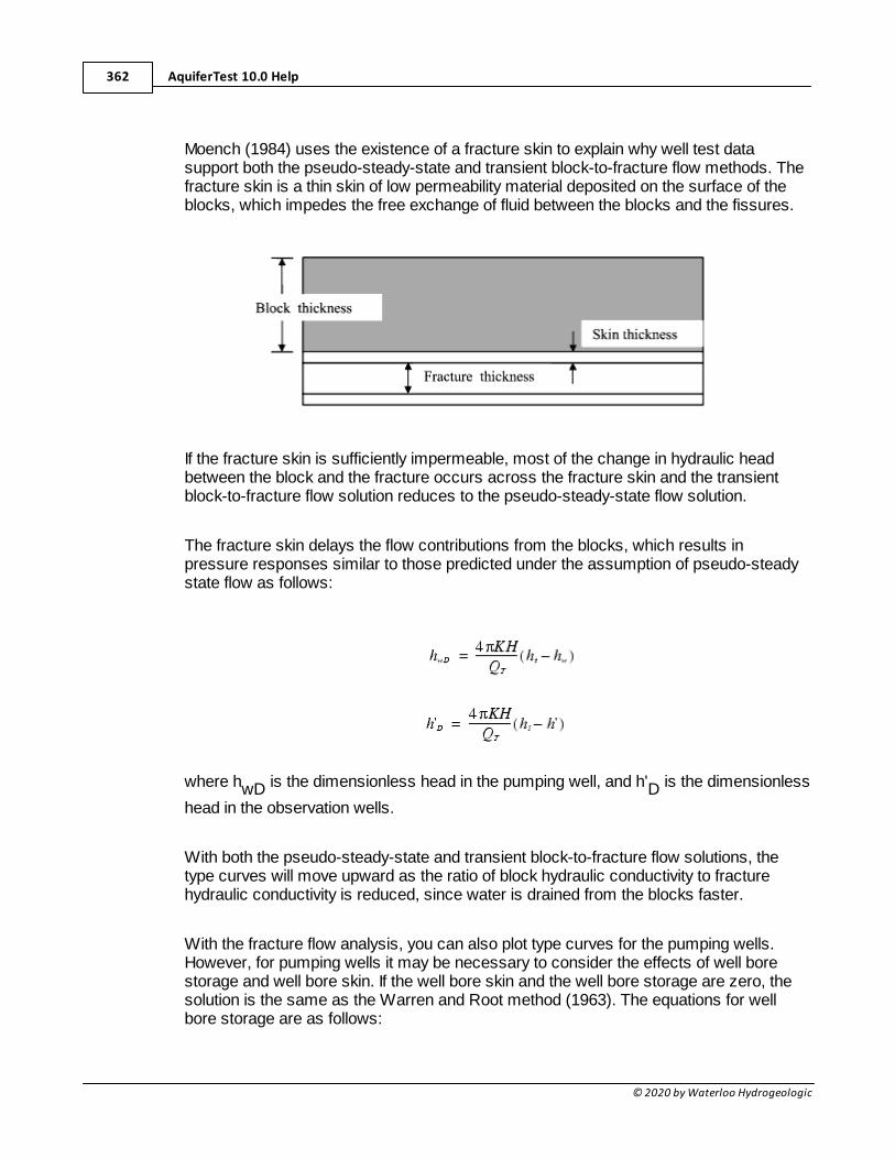
AquiferTest 10.0 Help362
© 2020 by Waterloo Hydrogeologic
Moench (1984) uses the existence of a fracture skin to explain why well test datasupport both the pseudo-steady-state and transient block-to-fracture flow methods. Thefracture skin is a thin skin of low permeability material deposited on the surface of theblocks, which impedes the free exchange of fluid between the blocks and the fissures.
If the fracture skin is sufficiently impermeable, most of the change in hydraulic headbetween the block and the fracture occurs across the fracture skin and the transientblock-to-fracture flow solution reduces to the pseudo-steady-state flow solution.
The fracture skin delays the flow contributions from the blocks, which results inpressure responses similar to those predicted under the assumption of pseudo-steadystate flow as follows:
where hwD is the dimensionless head in the pumping well, and h'D is the dimensionless
head in the observation wells.
With both the pseudo-steady-state and transient block-to-fracture flow solutions, thetype curves will move upward as the ratio of block hydraulic conductivity to fracturehydraulic conductivity is reduced, since water is drained from the blocks faster.
With the fracture flow analysis, you can also plot type curves for the pumping wells.However, for pumping wells it may be necessary to consider the effects of well borestorage and well bore skin. If the well bore skin and the well bore storage are zero, thesolution is the same as the Warren and Root method (1963). The equations for wellbore storage are as follows:
Pumping Test: Theory and Analysis Methods 363
© 2020 by Waterloo Hydrogeologic
where:
C=pR2 (for changing liquid levels) orC=VwrwgCobs
where Vw is volume of liquid in the pressurized section, rw is the density, g is the
gravitational constant, Cobs is the observed compressibility of the combined fluid-well
system, and S is the calculated storativity.
This solution, however, is iterative. If you move your data set to fit the curve, yourstorativity will change which in turn alters your well bore storage.
An example of a Moench Fracture Flow analysis graph has been included in thefollowing figure:
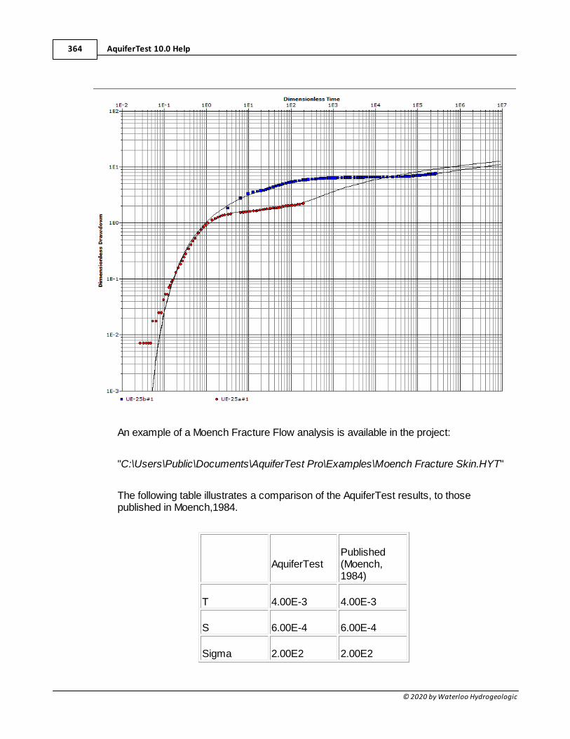
AquiferTest 10.0 Help364
© 2020 by Waterloo Hydrogeologic
An example of a Moench Fracture Flow analysis is available in the project:
"C:\Users\Public\Documents\AquiferTest Pro\Examples\Moench Fracture Skin.HYT"
The following table illustrates a comparison of the AquiferTest results, to thosepublished in Moench,1984.
AquiferTestPublished(Moench,1984)
T 4.00E-3 4.00E-3
S 6.00E-4 6.00E-4
Sigma 2.00E2 2.00E2
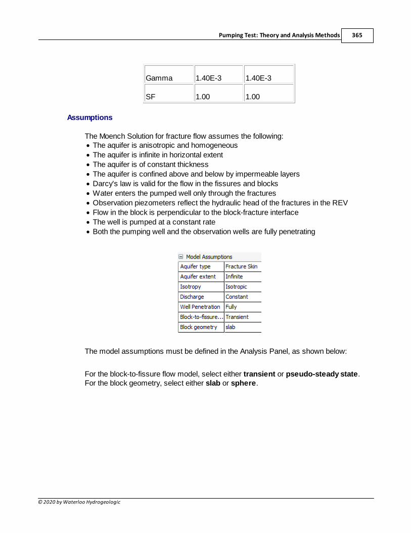
Pumping Test: Theory and Analysis Methods 365
© 2020 by Waterloo Hydrogeologic
Gamma 1.40E-3 1.40E-3
SF 1.00 1.00
Assumptions
The Moench Solution for fracture flow assumes the following:· The aquifer is anisotropic and homogeneous
· The aquifer is infinite in horizontal extent
· The aquifer is of constant thickness
· The aquifer is confined above and below by impermeable layers
· Darcy's law is valid for the flow in the fissures and blocks
· Water enters the pumped well only through the fractures
· Observation piezometers reflect the hydraulic head of the fractures in the REV
· Flow in the block is perpendicular to the block-fracture interface
· The well is pumped at a constant rate
· Both the pumping well and the observation wells are fully penetrating
The model assumptions must be defined in the Analysis Panel, as shown below:
For the block-to-fissure flow model, select either transient or pseudo-steady state.For the block geometry, select either slab or sphere.
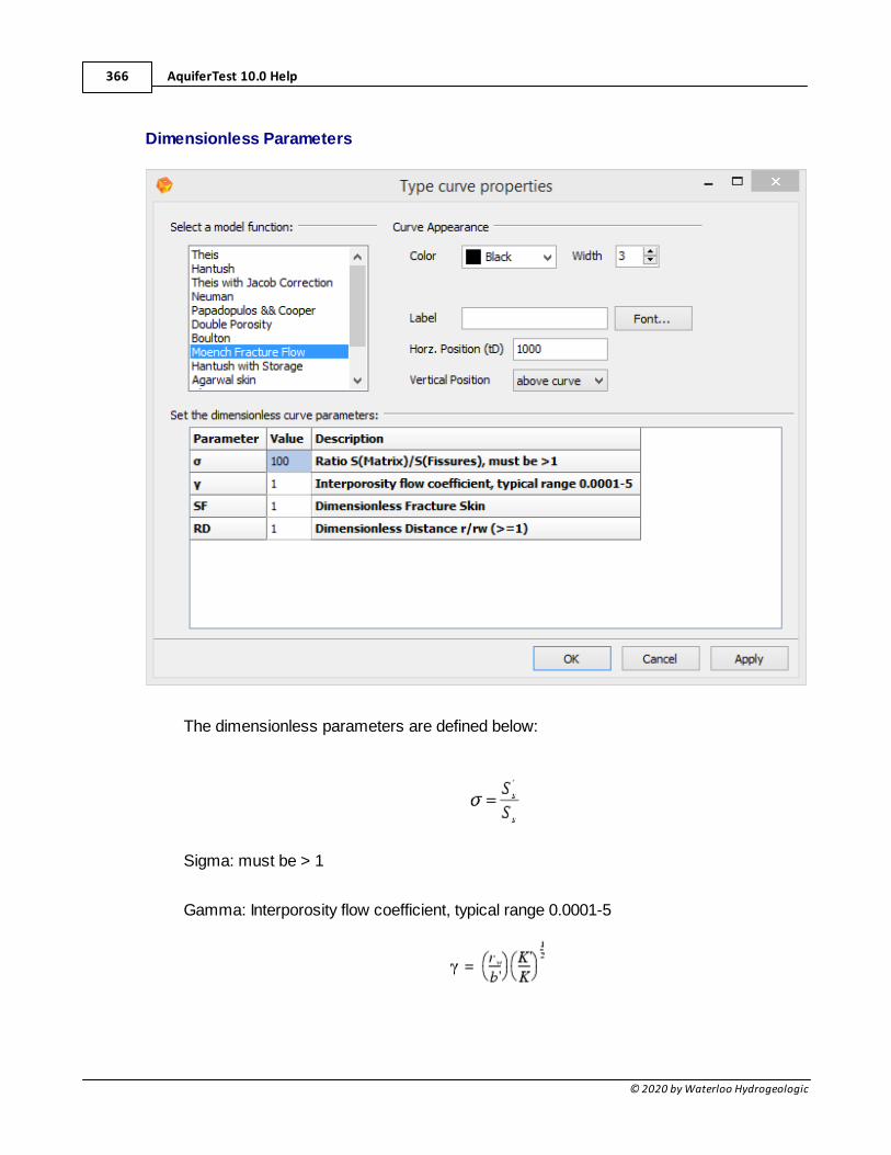
AquiferTest 10.0 Help366
© 2020 by Waterloo Hydrogeologic
Dimensionless Parameters
The dimensionless parameters are defined below:
Sigma: must be > 1
Gamma: Interporosity flow coefficient, typical range 0.0001-5
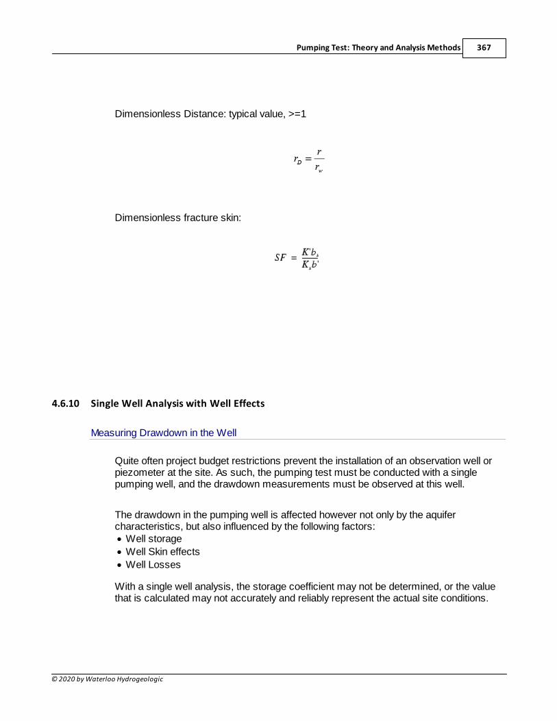
Pumping Test: Theory and Analysis Methods 367
© 2020 by Waterloo Hydrogeologic
Dimensionless Distance: typical value, >=1
Dimensionless fracture skin:
4.6.10 Single Well Analysis with Well Effects
Measuring Drawdown in the Well
Quite often project budget restrictions prevent the installation of an observation well orpiezometer at the site. As such, the pumping test must be conducted with a singlepumping well, and the drawdown measurements must be observed at this well.
The drawdown in the pumping well is affected however not only by the aquifercharacteristics, but also influenced by the following factors:· Well storage
· Well Skin effects
· Well Losses
With a single well analysis, the storage coefficient may not be determined, or the valuethat is calculated may not accurately and reliably represent the actual site conditions.
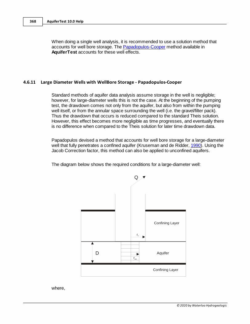
AquiferTest 10.0 Help368
© 2020 by Waterloo Hydrogeologic
When doing a single well analysis, it is recommended to use a solution method thataccounts for well bore storage. The Papadopulos-Cooper method available inAquiferTest accounts for these well effects.
4.6.11 Large Diameter Wells with WellBore Storage - Papadopulos-Cooper
Standard methods of aquifer data analysis assume storage in the well is negligible;however, for large-diameter wells this is not the case. At the beginning of the pumpingtest, the drawdown comes not only from the aquifer, but also from within the pumpingwell itself, or from the annular space surrounding the well (i.e. the gravel/filter pack).Thus the drawdown that occurs is reduced compared to the standard Theis solution.However, this effect becomes more negligible as time progresses, and eventually thereis no difference when compared to the Theis solution for later time drawdown data.
Papadopulos devised a method that accounts for well bore storage for a large-diameterwell that fully penetrates a confined aquifer (Kruseman and de Ridder, 1990). Using theJacob Correction factor, this method can also be applied to unconfined aquifers.
The diagram below shows the required conditions for a large-diameter well:
rc
rew
Confining Layer
Confining Layer
Aquifer
Q
D
where,
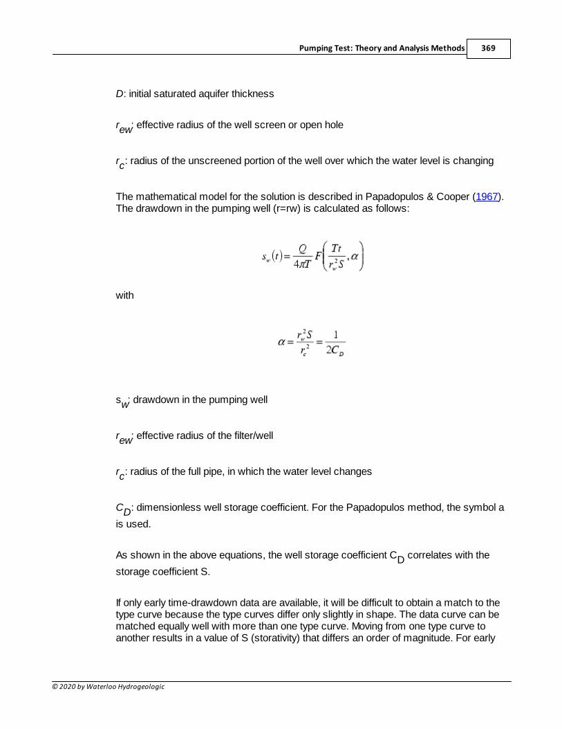
Pumping Test: Theory and Analysis Methods 369
© 2020 by Waterloo Hydrogeologic
D: initial saturated aquifer thickness
rew: effective radius of the well screen or open hole
rc: radius of the unscreened portion of the well over which the water level is changing
The mathematical model for the solution is described in Papadopulos & Cooper (1967).The drawdown in the pumping well (r=rw) is calculated as follows:
with
sw: drawdown in the pumping well
rew: effective radius of the filter/well
rc: radius of the full pipe, in which the water level changes
CD: dimensionless well storage coefficient. For the Papadopulos method, the symbol a
is used.
As shown in the above equations, the well storage coefficient CD correlates with the
storage coefficient S.
If only early time-drawdown data are available, it will be difficult to obtain a match to thetype curve because the type curves differ only slightly in shape. The data curve can bematched equally well with more than one type curve. Moving from one type curve toanother results in a value of S (storativity) that differs an order of magnitude. For early
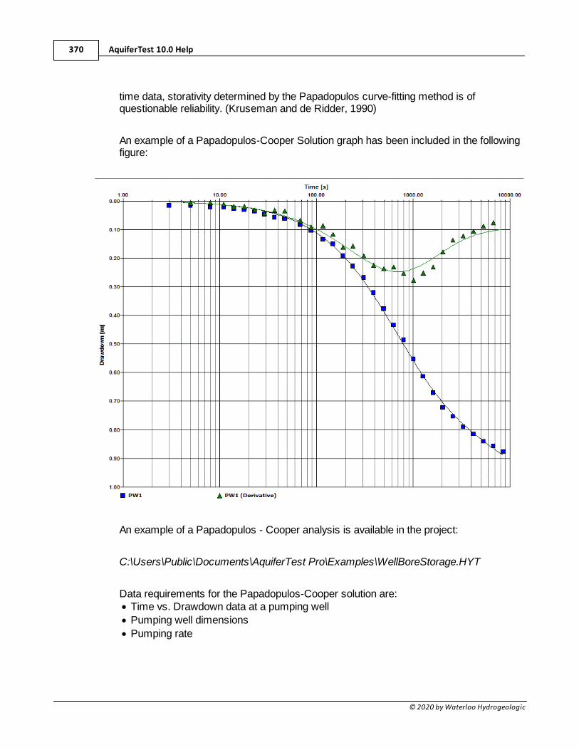
AquiferTest 10.0 Help370
© 2020 by Waterloo Hydrogeologic
time data, storativity determined by the Papadopulos curve-fitting method is ofquestionable reliability. (Kruseman and de Ridder, 1990)
An example of a Papadopulos-Cooper Solution graph has been included in the followingfigure:
An example of a Papadopulos - Cooper analysis is available in the project:
C:\Users\Public\Documents\AquiferTest Pro\Examples\WellBoreStorage.HYT
Data requirements for the Papadopulos-Cooper solution are:· Time vs. Drawdown data at a pumping well
· Pumping well dimensions
· Pumping rate
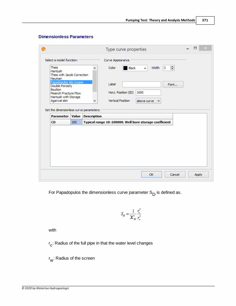
Pumping Test: Theory and Analysis Methods 371
© 2020 by Waterloo Hydrogeologic
Dimensionless Parameters
For Papadopulos the dimensionless curve parameter SD is defined as.
with
rc: Radius of the full pipe in that the water level changes
rw: Radius of the screen
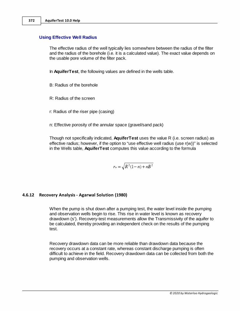
AquiferTest 10.0 Help372
© 2020 by Waterloo Hydrogeologic
Using Effective Well Radius
The effective radius of the well typically lies somewhere between the radius of the filterand the radius of the borehole (i.e. it is a calculated value). The exact value depends onthe usable pore volume of the filter pack.
In AquiferTest, the following values are defined in the wells table.
B: Radius of the borehole
R: Radius of the screen
r: Radius of the riser pipe (casing)
n: Effective porosity of the annular space (gravel/sand pack)
Though not specifically indicated, AquiferTest uses the value R (i.e. screen radius) aseffective radius; however, if the option to “use effective well radius (use r(w))” is selectedin the Wells table, AquiferTest computes this value according to the formula
4.6.12 Recovery Analysis - Agarwal Solution (1980)
When the pump is shut down after a pumping test, the water level inside the pumpingand observation wells begin to rise. This rise in water level is known as recoverydrawdown (s'). Recovery-test measurements allow the Transmissivity of the aquifer tobe calculated, thereby providing an independent check on the results of the pumpingtest.
Recovery drawdown data can be more reliable than drawdown data because therecovery occurs at a constant rate, whereas constant discharge pumping is oftendifficult to achieve in the field. Recovery drawdown data can be collected from both thepumping and observation wells.
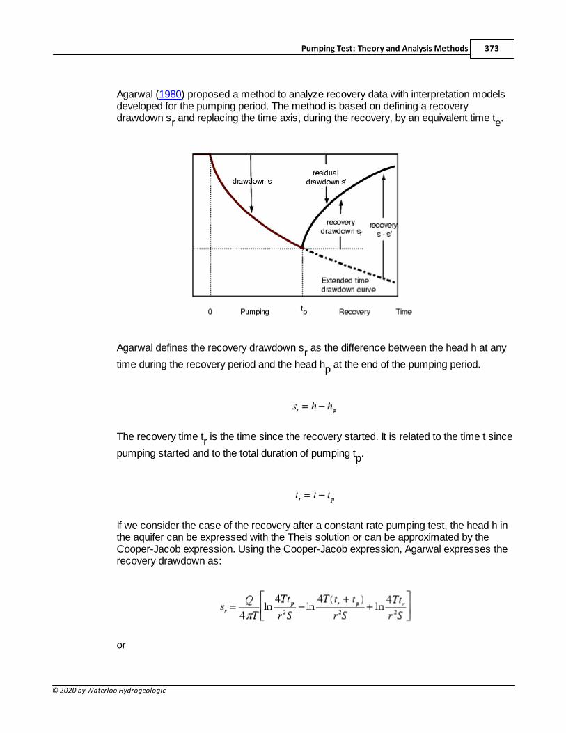
Pumping Test: Theory and Analysis Methods 373
© 2020 by Waterloo Hydrogeologic
Agarwal (1980) proposed a method to analyze recovery data with interpretation modelsdeveloped for the pumping period. The method is based on defining a recoverydrawdown sr and replacing the time axis, during the recovery, by an equivalent time te.
Agarwal defines the recovery drawdown sr as the difference between the head h at any
time during the recovery period and the head hp at the end of the pumping period.
The recovery time tr is the time since the recovery started. It is related to the time t since
pumping started and to the total duration of pumping tp.
If we consider the case of the recovery after a constant rate pumping test, the head h inthe aquifer can be expressed with the Theis solution or can be approximated by theCooper-Jacob expression. Using the Cooper-Jacob expression, Agarwal expresses therecovery drawdown as:
or
AquiferTest 10.0 Help374
© 2020 by Waterloo Hydrogeologic
with te the equivalent Agarwal time:
The expression of the recovery drawdown in this case is identical to the Cooper-Jacobexpression if one replaces the usual time by the equivalent Agarwal time te.
In the case of n successive pumping periods: with constant rate q1 for t=0 to t=t1,
constant rate q2 for t=t1 to t2, etc., the same result is obtained:
with an equivalent Agarwal time defined by:
with t0 = 0 and q0 = 0, and tr the time since the beginning of the recovery.
An example of a Agarwal Recovery analysis graph has been included below:
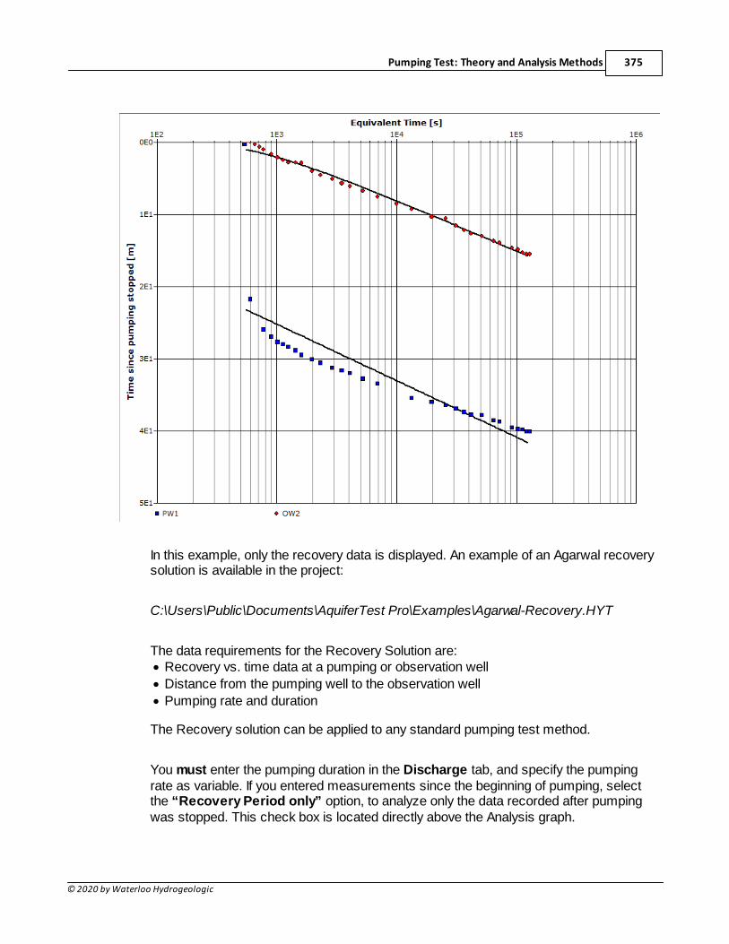
Pumping Test: Theory and Analysis Methods 375
© 2020 by Waterloo Hydrogeologic
In this example, only the recovery data is displayed. An example of an Agarwal recoverysolution is available in the project:
C:\Users\Public\Documents\AquiferTest Pro\Examples\Agarwal-Recovery.HYT
The data requirements for the Recovery Solution are:· Recovery vs. time data at a pumping or observation well
· Distance from the pumping well to the observation well
· Pumping rate and duration
The Recovery solution can be applied to any standard pumping test method.
You must enter the pumping duration in the Discharge tab, and specify the pumpingrate as variable. If you entered measurements since the beginning of pumping, selectthe “Recovery Period only” option, to analyze only the data recorded after pumpingwas stopped. This check box is located directly above the Analysis graph.
AquiferTest 10.0 Help376
© 2020 by Waterloo Hydrogeologic
You may enter recovery data only in the Water Levels tab, however, you still need todefine the pumping rate information.
Assumptions and Domain of Validity
Agarwal (1980) derived rigorously the previous expressions under the assumptions of atwo dimensional radial convergent flow field, in an infinite confined aquifer, with a fullypenetrating well, with or without skin effect, and no well-bore storage. It assumes alsothat the Cooper-Jacob approximation is valid (late time asymptote).
Agarwal shows empirically that the method is valid for a single well test with well borestorage and skin effect when the pumping time is large.
where:
T = Transmissivityrc = Casing radius if different from the screen radius
s = Skin factor
In addition, Agarwal demonstrates that the method provides good results for verticallyfractured wells with infinite and finite flow capacity fracture (Gringarten et al. solution).
4.6.13 Horizontal Wells (Clonts & Ramey)
NOTE: This method is only available in AquiferTest Pro.
Horizontal wells are being used more commonly for groundwater resource investigations andcontaminated site remediation projects. Horizontal wells provide a larger surface area forgroundwater withdrawal, and more focused extraction of groundwater and contaminantswhich migrate in a predominantly horizontal direction in high conductivity aquifers. A variety ofresearchers have looked into the analysis of time-drawdown data for horizontal wells (Clontsand Ramey, 1986; Daviau et al., 1988; Kawecki, 2000). The Clonts and Ramey solution todrawdown versus time for horizontal wells is implemented in AquiferTest Pro.
The following is the design of a horizontal well pumping from an infinite aquifer.
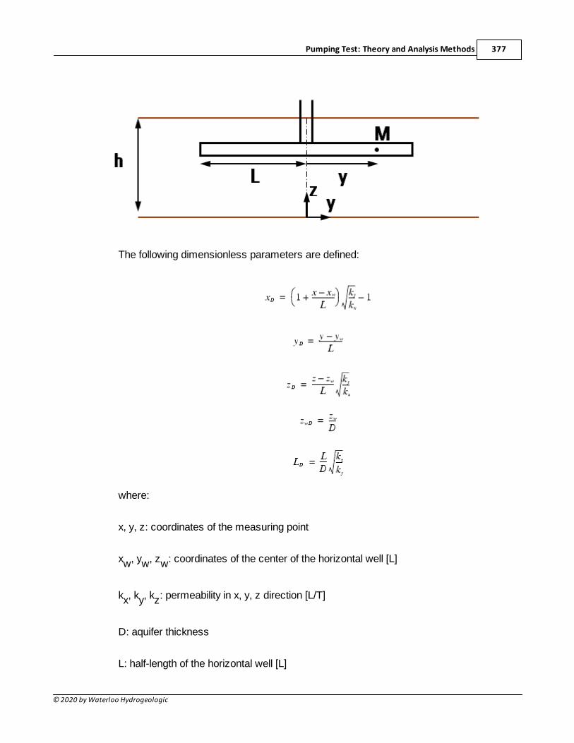
Pumping Test: Theory and Analysis Methods 377
© 2020 by Waterloo Hydrogeologic
The following dimensionless parameters are defined:
where:
x, y, z: coordinates of the measuring point
xw, yw, zw: coordinates of the center of the horizontal well [L]
kx, ky, kz: permeability in x, y, z direction [L/T]
D: aquifer thickness
L: half-length of the horizontal well [L]
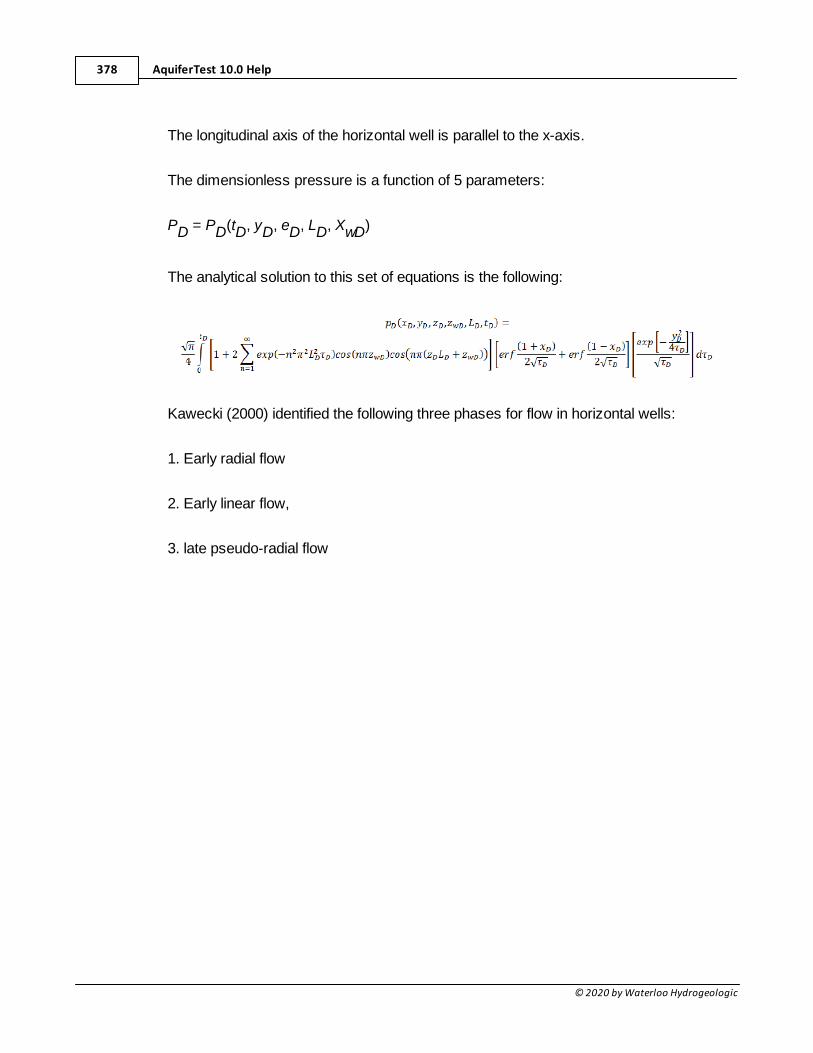
AquiferTest 10.0 Help378
© 2020 by Waterloo Hydrogeologic
The longitudinal axis of the horizontal well is parallel to the x-axis.
The dimensionless pressure is a function of 5 parameters:
PD = PD(tD, yD, eD, LD, XwD)
The analytical solution to this set of equations is the following:
Kawecki (2000) identified the following three phases for flow in horizontal wells:
1. Early radial flow
2. Early linear flow,
3. late pseudo-radial flow
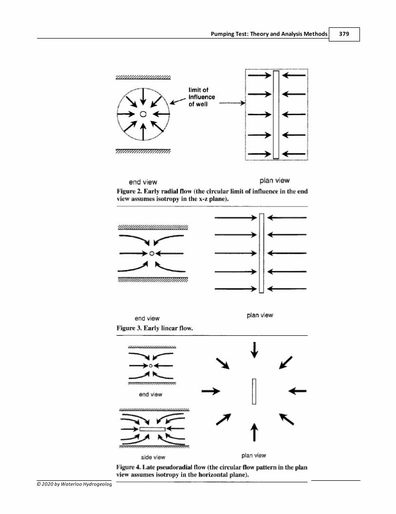
Pumping Test: Theory and Analysis Methods 379
© 2020 by Waterloo Hydrogeologic
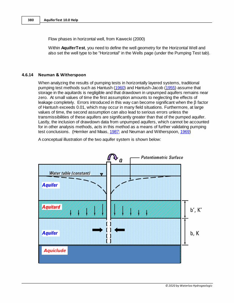
AquiferTest 10.0 Help380
© 2020 by Waterloo Hydrogeologic
Flow phases in horizontal well, from Kawecki (2000)
Within AquiferTest, you need to define the well geometry for the Horizontal Well andalso set the well type to be "Horizontal" in the Wells page (under the Pumping Test tab).
4.6.14 Neuman & Witherspoon
When analyzing the results of pumping tests in horizontally layered systems, traditionalpumping test methods such as Hantush (1960) and Hantush-Jacob (1955) assume thatstorage in the aquitards is negligible and that drawdown in unpumped aquifers remains nearzero. At small values of time the first assumption amounts to neglecting the effects ofleakage completely. Errors introduced in this way can become significant when the β factorof Hantush exceeds 0.01, which may occur in many field situations. Furthermore, at largevalues of time, the second assumption can also lead to serious errors unless thetransmissibilities of these aquifers are significantly greater than that of the pumped aquifer. Lastly, the inclusion of drawdown data from unpumped aquifers, which cannot be accountedfor in other analysis methods, acts in this method as a means of further validating pumpingtest conclusions. (Hemker and Maas, 1987; and Neuman and Witherspoon, 1969)
A conceptual illustration of the two aquifer system is shown below:
Pumping Test: Theory and Analysis Methods 381
© 2020 by Waterloo Hydrogeologic
AquiferTest supports the “Neuman & Witherspoon” conceptual model (confined two-aquifersystem), which allows you to estimate:.
· T and S of the pumped aquifer
· T and S of the unpumped aquifer
· c (hydraulic resistance) of the aquitard. From this parameter, Kv can be calculated usingalso the thickness of the aquitard. (See page 24 in Kruseman and de Ridder [1990] fordetails)
The leakage is between the two aquifers only, there is no leakage from outside the system. Furthermore, the order (from top downwards) must always be Aquifer-Aquitard-Aquifer, that isthe aquitard separates the two aquifers. The pumped aquifer can be either the top or thebottom one, but not both.
The solution technique used in AquiferTest is based on the "Eigenvalue analysis" presentedin Hemker and Maas (1987) . For further information on this method, you are encouraged toread Neuman and Witherspoon (1969) and Hemker and Mass (1987)
Assumptions
Important assumptions for this method include:
· Within this system, water flows horizontally in the aquifers, which are separated by anaquitard
· All layers are of infinite horizontal extent within the area of influence of the pumping test
· Aquifer layers have homogeneous and isotropic transmissivity and storativity values
· Aquitard layers have homogeneous vertical resistance and storativity values
· Only saturated groundwater flow is considered
· The top and base of the system have either no-drawdown or no-flow boundaries
· Well screens fully penetrate the aquifer layer
· Observation wells are screened in only one aquifer layer
· Only drawdown (or build-up) as a result of pumping is considered
· Darcy’s law is valid, except for turbulent flow near the well screen
· Water from storage is discharged instantaneously with decline of head
· Unsaturated zone flow does not influence drawdown
· The change in water levels does not affect the transmissivity or storativity of any of theaquifers or aquitards
· Seepage faces at the water-table well can be safely ignored
· Horizontal-deformation process effects are negligible
· The discharge rate in any screened layer of any pumping well is not affected by thedrawdown caused by any other pumping well.
· b < 1.0 (i.e. the radial distance from the well to the piezometers should be small
Within AquiferTest, the following assumptions can be relaxed using superposition, inorder to accommodate:
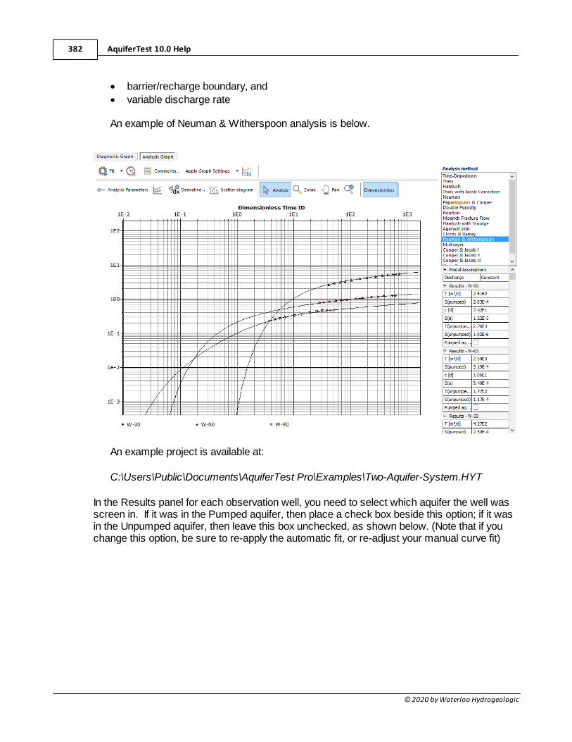
AquiferTest 10.0 Help382
© 2020 by Waterloo Hydrogeologic
· barrier/recharge boundary, and
· variable discharge rate
An example of Neuman & Witherspoon analysis is below.
An example project is available at:
C:\Users\Public\Documents\AquiferTest Pro\Examples\Two-Aquifer-System.HYT
In the Results panel for each observation well, you need to select which aquifer the well wasscreen in. If it was in the Pumped aquifer, then place a check box beside this option; if it wasin the Unpumped aquifer, then leave this box unchecked, as shown below. (Note that if youchange this option, be sure to re-apply the automatic fit, or re-adjust your manual curve fit)
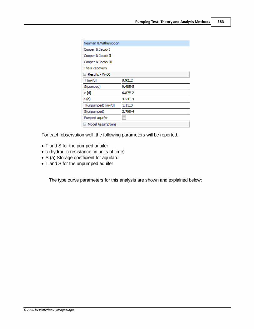
Pumping Test: Theory and Analysis Methods 383
© 2020 by Waterloo Hydrogeologic
For each observation well, the following parameters will be reported.
· T and S for the pumped aquifer
· c (hydraulic resistance, in units of time)
· S (a) Storage coefficient for aquitard
· T and S for the unpumped aquifer
The type curve parameters for this analysis are shown and explained below:
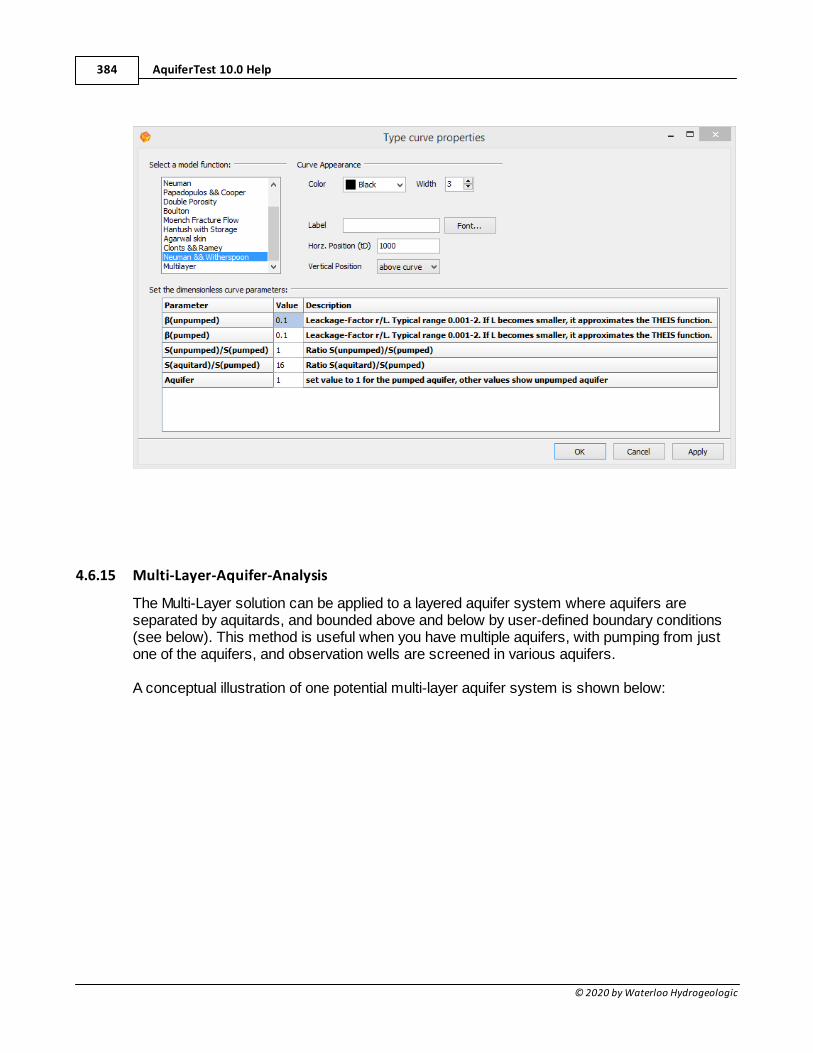
AquiferTest 10.0 Help384
© 2020 by Waterloo Hydrogeologic
4.6.15 Multi-Layer-Aquifer-Analysis
The Multi-Layer solution can be applied to a layered aquifer system where aquifers areseparated by aquitards, and bounded above and below by user-defined boundary conditions(see below). This method is useful when you have multiple aquifers, with pumping from justone of the aquifers, and observation wells are screened in various aquifers.
A conceptual illustration of one potential multi-layer aquifer system is shown below:
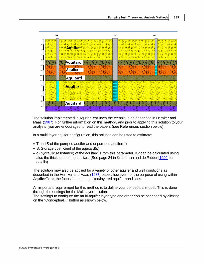
Pumping Test: Theory and Analysis Methods 385
© 2020 by Waterloo Hydrogeologic
The solution implemented in AquiferTest uses the technique as described in Hemker andMaas (1987). For further information on this method, and prior to applying this solution to youranalysis, you are encouraged to read the papers (see References section below).
In a multi-layer aquifer configuration, this solution can be used to estimate:
· T and S of the pumped aquifer and unpumped aquifer(s)
· S: Storage coefficient of the aquitard(s)
· c (hydraulic resistance) of the aquitard. From this parameter, Kv can be calculated usingalso the thickness of the aquitard.(See page 24 in Kruseman and de Ridder [1990] fordetails)
The solution may also be applied for a variety of other aquifer and well conditions asdescribed in the Hemker and Maas (1987) paper; however, for the purpose of using withinAquiferTest, the focus is on the stacked/layered aquifer conditions.
An important requirement for this method is to define your conceptual model. This is donethrough the settings for the MultiLayer solution. The settings to configure the multi-aquifer layer type and order can be accessed by clickingon the "Conceptual..." button as shown below.
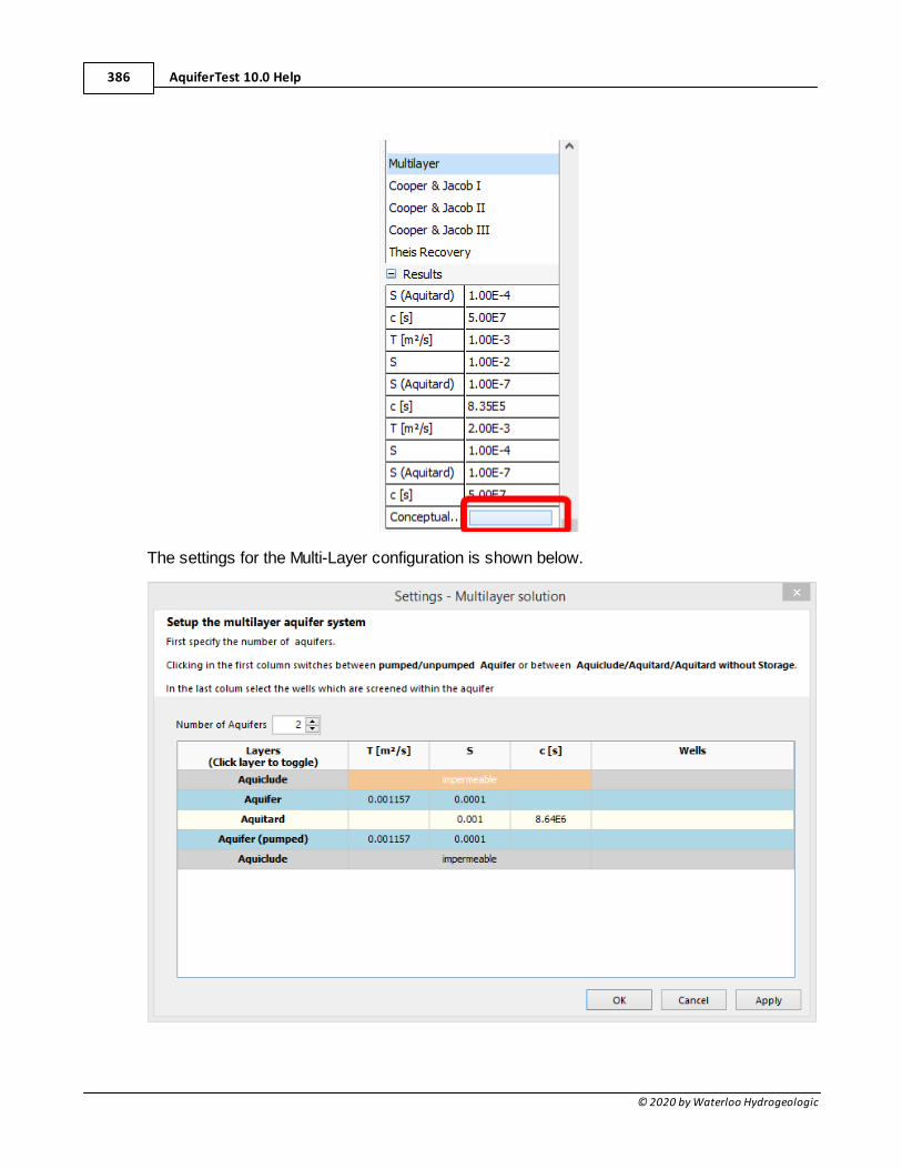
AquiferTest 10.0 Help386
© 2020 by Waterloo Hydrogeologic
The settings for the Multi-Layer configuration is shown below.
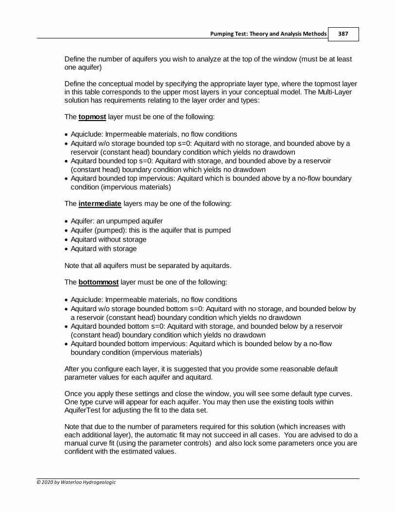
Pumping Test: Theory and Analysis Methods 387
© 2020 by Waterloo Hydrogeologic
Define the number of aquifers you wish to analyze at the top of the window (must be at leastone aquifer)
Define the conceptual model by specifying the appropriate layer type, where the topmost layerin this table corresponds to the upper most layers in your conceptual model. The Multi-Layersolution has requirements relating to the layer order and types:
The topmost layer must be one of the following:
· Aquiclude: Impermeable materials, no flow conditions
· Aquitard w/o storage bounded top s=0: Aquitard with no storage, and bounded above by areservoir (constant head) boundary condition which yields no drawdown
· Aquitard bounded top s=0: Aquitard with storage, and bounded above by a reservoir(constant head) boundary condition which yields no drawdown
· Aquitard bounded top impervious: Aquitard which is bounded above by a no-flow boundarycondition (impervious materials)
The intermediate layers may be one of the following:
· Aquifer: an unpumped aquifer
· Aquifer (pumped): this is the aquifer that is pumped
· Aquitard without storage
· Aquitard with storage
Note that all aquifers must be separated by aquitards.
The bottommost layer must be one of the following:
· Aquiclude: Impermeable materials, no flow conditions
· Aquitard w/o storage bounded bottom s=0: Aquitard with no storage, and bounded below bya reservoir (constant head) boundary condition which yields no drawdown
· Aquitard bounded bottom s=0: Aquitard with storage, and bounded below by a reservoir(constant head) boundary condition which yields no drawdown
· Aquitard bounded bottom impervious: Aquitard which is bounded below by a no-flowboundary condition (impervious materials)
After you configure each layer, it is suggested that you provide some reasonable defaultparameter values for each aquifer and aquitard.
Once you apply these settings and close the window, you will see some default type curves.One type curve will appear for each aquifer. You may then use the existing tools withinAquiferTest for adjusting the fit to the data set.
Note that due to the number of parameters required for this solution (which increases witheach additional layer), the automatic fit may not succeed in all cases. You are advised to do amanual curve fit (using the parameter controls) and also lock some parameters once you areconfident with the estimated values.
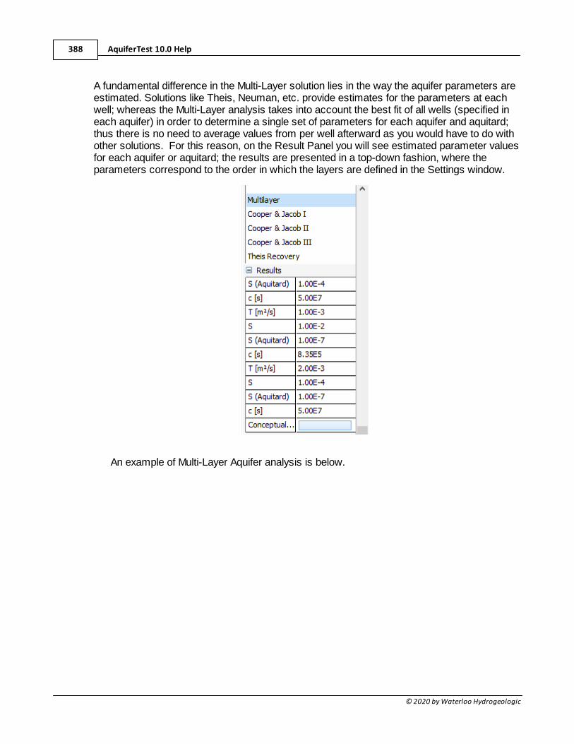
AquiferTest 10.0 Help388
© 2020 by Waterloo Hydrogeologic
A fundamental difference in the Multi-Layer solution lies in the way the aquifer parameters areestimated. Solutions like Theis, Neuman, etc. provide estimates for the parameters at eachwell; whereas the Multi-Layer analysis takes into account the best fit of all wells (specified ineach aquifer) in order to determine a single set of parameters for each aquifer and aquitard;thus there is no need to average values from per well afterward as you would have to do withother solutions. For this reason, on the Result Panel you will see estimated parameter valuesfor each aquifer or aquitard; the results are presented in a top-down fashion, where theparameters correspond to the order in which the layers are defined in the Settings window.
An example of Multi-Layer Aquifer analysis is below.
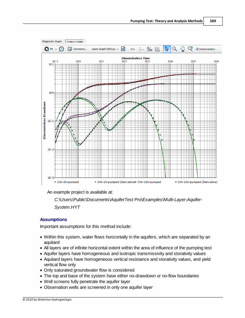
Pumping Test: Theory and Analysis Methods 389
© 2020 by Waterloo Hydrogeologic
An example project is available at:
C:\Users\Public\Documents\AquiferTest Pro\Examples\Multi-Layer-Aquifer-
System.HYT
Assumptions
Important assumptions for this method include:
· Within this system, water flows horizontally in the aquifers, which are separated by anaquitard
· All layers are of infinite horizontal extent within the area of influence of the pumping test
· Aquifer layers have homogeneous and isotropic transmissivity and storativity values
· Aquitard layers have homogeneous vertical resistance and storativity values, and yieldvertical flow only
· Only saturated groundwater flow is considered
· The top and base of the system have either no-drawdown or no-flow boundaries
· Well screens fully penetrate the aquifer layer
· Observation wells are screened in only one aquifer layer
AquiferTest 10.0 Help390
© 2020 by Waterloo Hydrogeologic
· Only drawdown (or build-up) as a result of pumping is considered
· Darcy’s law is valid, except for turbulent flow near the well screen
· Water from storage is discharged instantaneously with decline of head
· Unsaturated zone flow does not influence drawdown
· The change in water levels does not affect the transmissivity or storativity of any of theaquifers or aquitards
· Seepage faces at the water-table well can be safely ignored
· Horizontal-deformation process effects are negligible
· The discharge rate in any screened layer of any pumping well is not affected by thedrawdown caused by any other pumping well.
· b < 1.0 (i.e. the radial distance from the well to the piezometers should be small
The implementation of this solution within AquiferTest has the additional limitations:
· Single Pumping Well
· Pumping well is fully screened over only one aquifer layer
Within AquiferTest, the following assumptions can be relaxed using superposition, in orderto accommodate:
· barrier/recharge boundary, and
· variable discharge rate
References
Hemker C.J. and Maas, C., 1987. Unsteady Flow to Wells in Layered and Fissured AquiferSystems, Journal of Hydrology, vol. 90, pp. 231-249.
Hemker, C.J., 1999. Transient well flow in layered aquifer systems: the uniform well-facedrawdown solution. Journal of Hydrology, 225: 19-44.
Carlson F., Randall, J., 2012. MLU: A Windows Application for the Analysis of Aquifer Testsand the Design of Well Fields in Layered Systems. Groundwater Software Spotlight.
4.7 Diagnostic Plots and Interpretation
Calculating hydraulic characteristics would be relatively easy if the aquifer system (i.e.aquifer plus well) were precisely known. This is generally not the case, so interpreting apumping test is primarily a matter of identifying an unknown system. System
Pumping Test: Theory and Analysis Methods 391
© 2020 by Waterloo Hydrogeologic
identification relies on models, the characteristics of which are assumed to representthe characteristics of the real aquifer system (Kruseman and de Ridder, 1990).
In a pumping test the type of aquifer, the well effects (well losses and well bore storage,and partial penetration), and the boundary conditions (barrier or recharge boundaries)dominate at different times during the test. They affect the drawdown behavior of thesystem in their own individual ways. So, to identify an aquifer system, one mustcompare its drawdown behavior with that of the various theoretical models. The modelthat compares best with the real system is then selected for the calculation of thehydraulic parameters (Kruseman and de Ridder, 1990).
AquiferTest includes tools to help you to determine the aquifer type and conditionsbefore conducting the analysis. In AquiferTest, the various theoretical models arereferred to as Diagnostic plots. Diagnostic plots are plots of drawdown vs. the timesince pumping began; these plots are available in log-log or semi-log format. Thediagnostic plots allow the dominating flow regimes to be identified; these yield straightlines on specialized plots. The characteristic shape of the curves can help in selectingthe appropriate solution method (Kruseman and de Ridder, 1990).
In addition, the Diagnostic plots also display the theoretical drawdown derivative curves(i.e. the rate of change of drawdown over time). Quite often, the derivative data canprove to be more meaningful for choosing the appropriate solution method.
NOTE: Diagnostic Graphs are only available for PumpingTests when using AquiferTest Pro.
To view the Diagnostic Plots, load the Analysis tab, select the Diagnostic Graphstab, and the following window will appear:
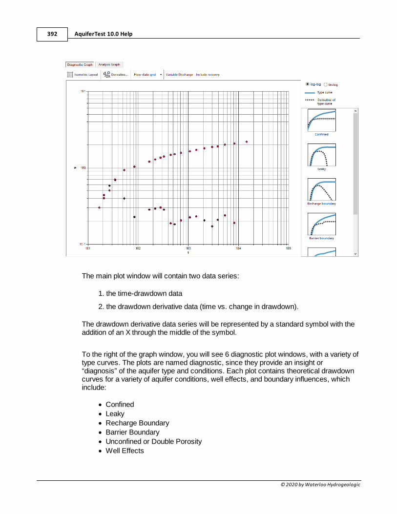
AquiferTest 10.0 Help392
© 2020 by Waterloo Hydrogeologic
The main plot window will contain two data series:
1. the time-drawdown data
2. the drawdown derivative data (time vs. change in drawdown).
The drawdown derivative data series will be represented by a standard symbol with theaddition of an X through the middle of the symbol.
To the right of the graph window, you will see 6 diagnostic plot windows, with a variety oftype curves. The plots are named diagnostic, since they provide an insight or“diagnosis” of the aquifer type and conditions. Each plot contains theoretical drawdowncurves for a variety of aquifer conditions, well effects, and boundary influences, whichinclude:
· Confined
· Leaky
· Recharge Boundary
· Barrier Boundary
· Unconfined or Double Porosity
· Well Effects
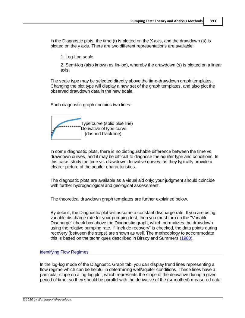
Pumping Test: Theory and Analysis Methods 393
© 2020 by Waterloo Hydrogeologic
In the Diagnostic plots, the time (t) is plotted on the X axis, and the drawdown (s) isplotted on the y axis. There are two different representations are available:
1. Log-Log scale
2. Semi-log (also known as lin-log), whereby the drawdown (s) is plotted on a linearaxis.
The scale type may be selected directly above the time-drawdown graph templates.Changing the plot type will display a new set of the graph templates, and also plot theobserved drawdown data in the new scale.
Each diagnostic graph contains two lines:
Type curve (solid blue line)Derivative of type curve
(dashed black line).
In some diagnostic plots, there is no distinguishable difference between the time vs.drawdown curves, and it may be difficult to diagnose the aquifer type and conditions. Inthis case, study the time vs. drawdown derivative curves, as they typically provide aclearer picture of the aquifer characteristics.
The diagnostic plots are available as a visual aid only; your judgment should coincidewith further hydrogeological and geological assessment.
The theoretical drawdown graph templates are further explained below.
By default, the Diagnostic plot will assume a constant discharge rate. If you are usingvariable discharge rate for your pumping test, then you must turn on the "VariableDischarge" check box above the Diagnostic graph, which normalizes the drawdownusing the relative pumping rate. If “Include recovery” is checked, the data points duringrecovery (between the steps) are shown as well. The methodology to accommodatethis is based on the techniques described in Birsoy and Summers (1980).
Identifying Flow Regimes
In the log-log mode of the Diagnostic Graph tab, you can display trend lines representing aflow regime which can be helpful in determining well/aquifer conditions. These lines have aparticular slope on a log-log plot, which represents the slope of the derivative during a givenperiod of time, so they should be parallel with the derivative of the (smoothed) measured data
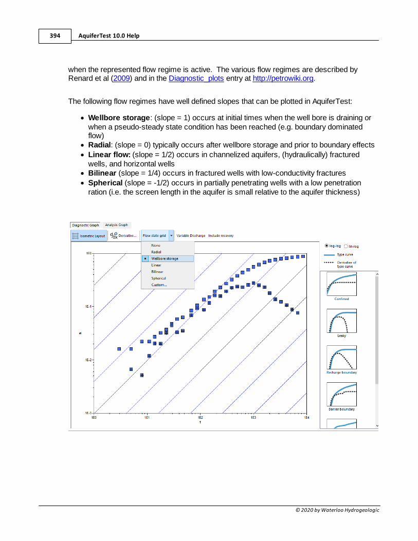
AquiferTest 10.0 Help394
© 2020 by Waterloo Hydrogeologic
when the represented flow regime is active. The various flow regimes are described byRenard et al (2009) and in the Diagnostic_plots entry at http://petrowiki.org.
The following flow regimes have well defined slopes that can be plotted in AquiferTest:
· Wellbore storage: (slope = 1) occurs at initial times when the well bore is draining orwhen a pseudo-steady state condition has been reached (e.g. boundary dominatedflow)
· Radial: (slope = 0) typically occurs after wellbore storage and prior to boundary effects
· Linear flow: (slope = 1/2) occurs in channelized aquifers, (hydraulically) fracturedwells, and horizontal wells
· Bilinear (slope = 1/4) occurs in fractured wells with low-conductivity fractures
· Spherical (slope = -1/2) occurs in partially penetrating wells with a low penetrationration (i.e. the screen length in the aquifer is small relative to the aquifer thickness)
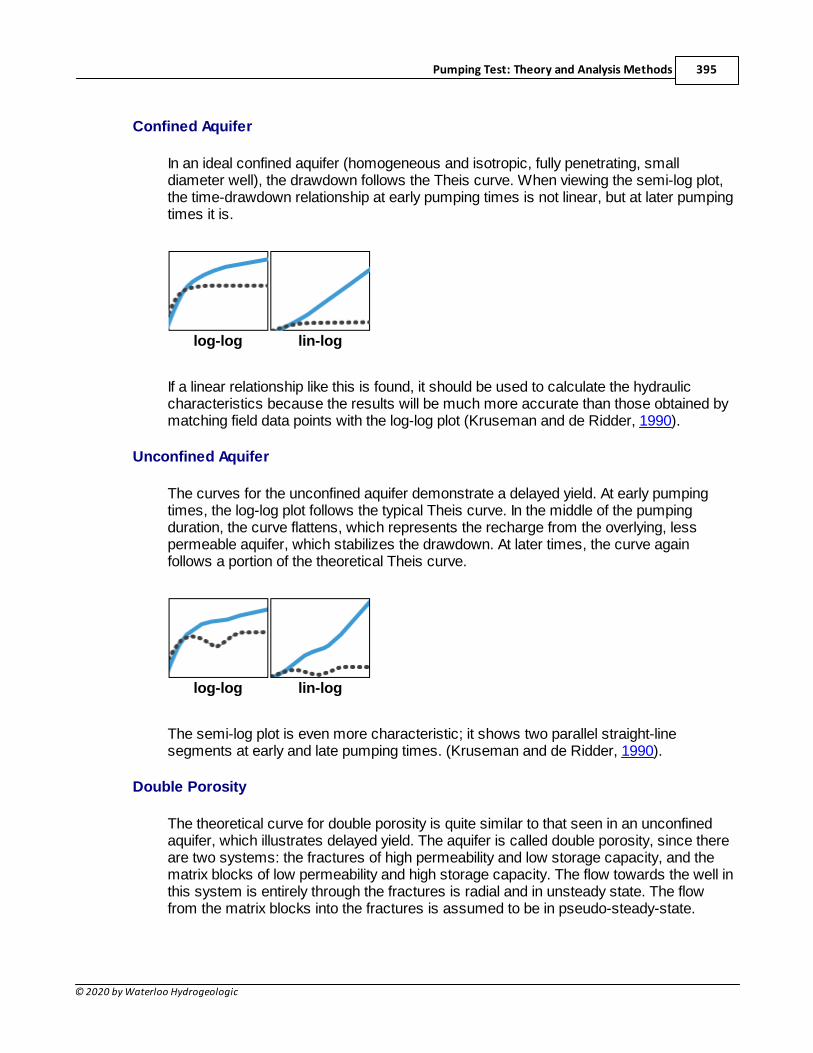
Pumping Test: Theory and Analysis Methods 395
© 2020 by Waterloo Hydrogeologic
Confined Aquifer
In an ideal confined aquifer (homogeneous and isotropic, fully penetrating, smalldiameter well), the drawdown follows the Theis curve. When viewing the semi-log plot,the time-drawdown relationship at early pumping times is not linear, but at later pumpingtimes it is.
log-log lin-log
If a linear relationship like this is found, it should be used to calculate the hydrauliccharacteristics because the results will be much more accurate than those obtained bymatching field data points with the log-log plot (Kruseman and de Ridder, 1990).
Unconfined Aquifer
The curves for the unconfined aquifer demonstrate a delayed yield. At early pumpingtimes, the log-log plot follows the typical Theis curve. In the middle of the pumpingduration, the curve flattens, which represents the recharge from the overlying, lesspermeable aquifer, which stabilizes the drawdown. At later times, the curve againfollows a portion of the theoretical Theis curve.
log-log lin-log
The semi-log plot is even more characteristic; it shows two parallel straight-linesegments at early and late pumping times. (Kruseman and de Ridder, 1990).
Double Porosity
The theoretical curve for double porosity is quite similar to that seen in an unconfinedaquifer, which illustrates delayed yield. The aquifer is called double porosity, since thereare two systems: the fractures of high permeability and low storage capacity, and thematrix blocks of low permeability and high storage capacity. The flow towards the well inthis system is entirely through the fractures is radial and in unsteady state. The flowfrom the matrix blocks into the fractures is assumed to be in pseudo-steady-state.
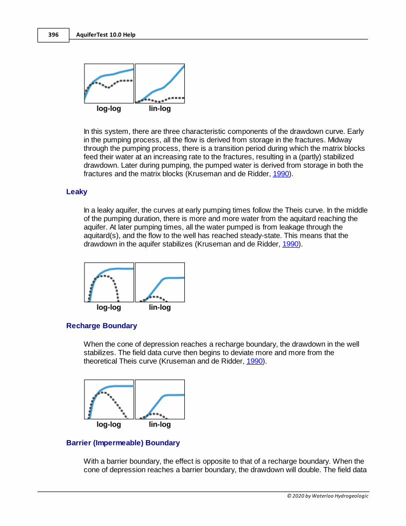
AquiferTest 10.0 Help396
© 2020 by Waterloo Hydrogeologic
log-log lin-log
In this system, there are three characteristic components of the drawdown curve. Earlyin the pumping process, all the flow is derived from storage in the fractures. Midwaythrough the pumping process, there is a transition period during which the matrix blocksfeed their water at an increasing rate to the fractures, resulting in a (partly) stabilizeddrawdown. Later during pumping, the pumped water is derived from storage in both thefractures and the matrix blocks (Kruseman and de Ridder, 1990).
Leaky
In a leaky aquifer, the curves at early pumping times follow the Theis curve. In the middleof the pumping duration, there is more and more water from the aquitard reaching theaquifer. At later pumping times, all the water pumped is from leakage through theaquitard(s), and the flow to the well has reached steady-state. This means that thedrawdown in the aquifer stabilizes (Kruseman and de Ridder, 1990).
log-log lin-log
Recharge Boundary
When the cone of depression reaches a recharge boundary, the drawdown in the wellstabilizes. The field data curve then begins to deviate more and more from thetheoretical Theis curve (Kruseman and de Ridder, 1990).
log-log lin-log
Barrier (Impermeable) Boundary
With a barrier boundary, the effect is opposite to that of a recharge boundary. When thecone of depression reaches a barrier boundary, the drawdown will double. The field data
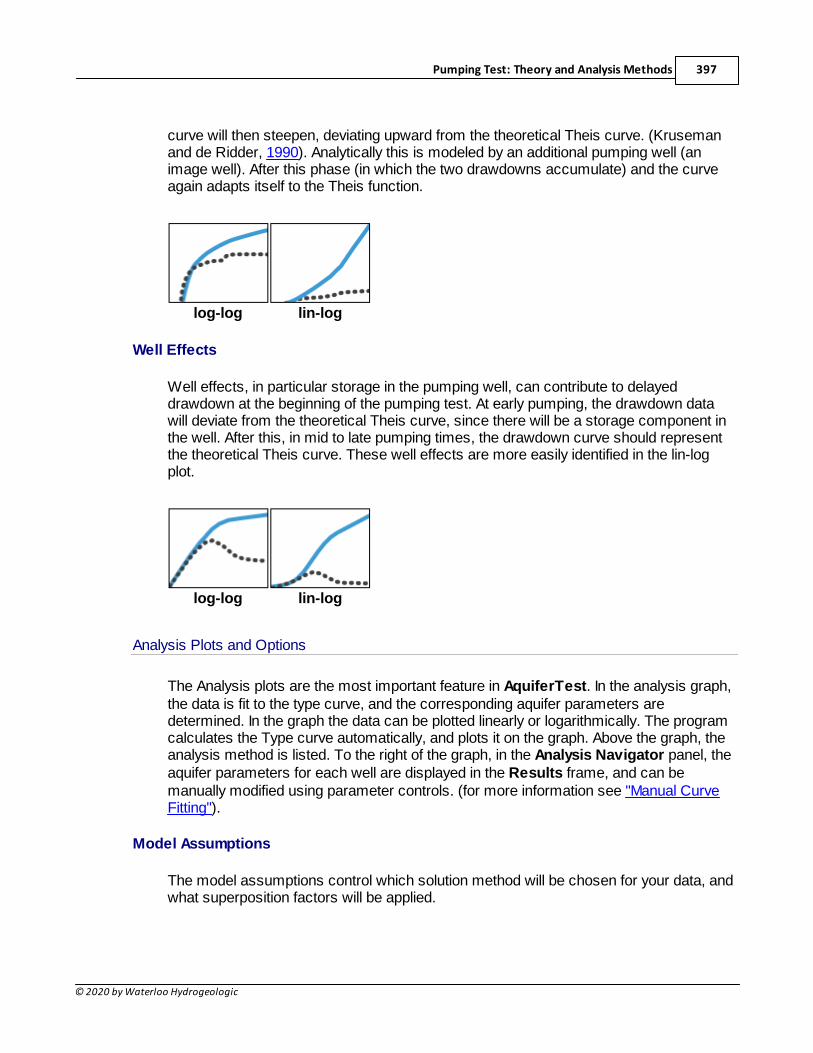
Pumping Test: Theory and Analysis Methods 397
© 2020 by Waterloo Hydrogeologic
curve will then steepen, deviating upward from the theoretical Theis curve. (Krusemanand de Ridder, 1990). Analytically this is modeled by an additional pumping well (animage well). After this phase (in which the two drawdowns accumulate) and the curveagain adapts itself to the Theis function.
log-log lin-log
Well Effects
Well effects, in particular storage in the pumping well, can contribute to delayeddrawdown at the beginning of the pumping test. At early pumping, the drawdown datawill deviate from the theoretical Theis curve, since there will be a storage component inthe well. After this, in mid to late pumping times, the drawdown curve should representthe theoretical Theis curve. These well effects are more easily identified in the lin-logplot.
log-log lin-log
Analysis Plots and Options
The Analysis plots are the most important feature in AquiferTest. In the analysis graph,the data is fit to the type curve, and the corresponding aquifer parameters aredetermined. In the graph the data can be plotted linearly or logarithmically. The programcalculates the Type curve automatically, and plots it on the graph. Above the graph, theanalysis method is listed. To the right of the graph, in the Analysis Navigator panel, theaquifer parameters for each well are displayed in the Results frame, and can bemanually modified using parameter controls. (for more information see "Manual CurveFitting").
Model Assumptions
The model assumptions control which solution method will be chosen for your data, andwhat superposition factors will be applied.
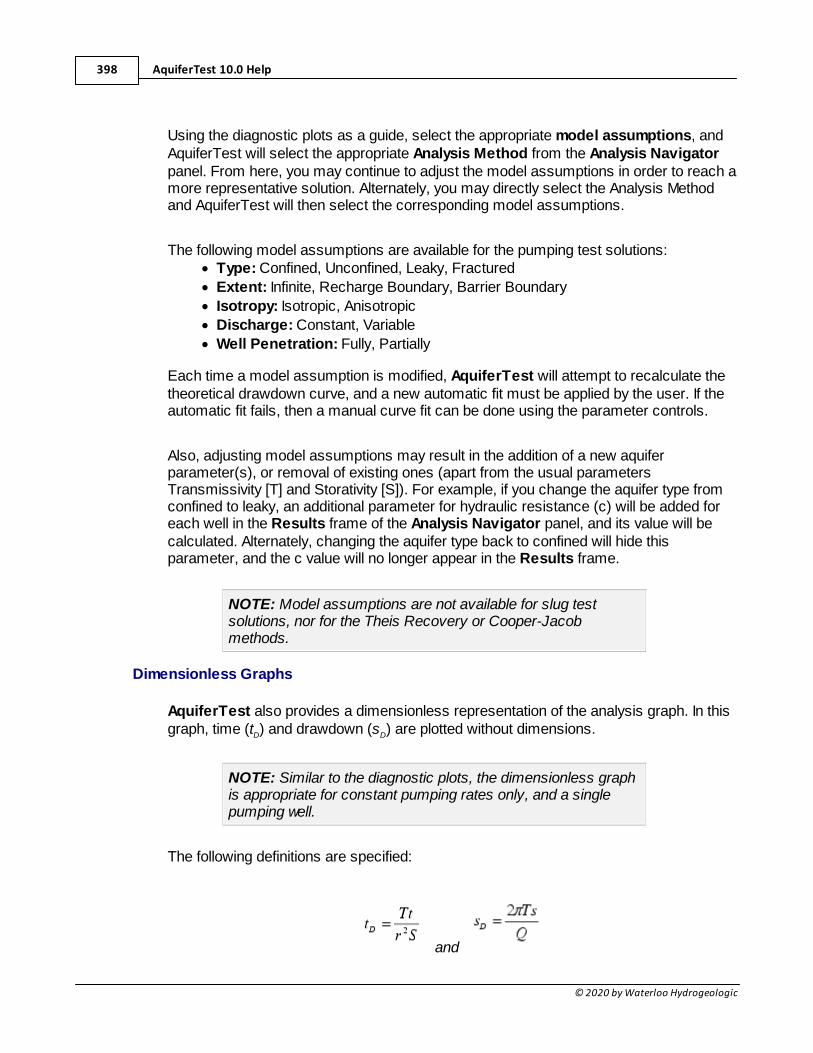
AquiferTest 10.0 Help398
© 2020 by Waterloo Hydrogeologic
Using the diagnostic plots as a guide, select the appropriate model assumptions, andAquiferTest will select the appropriate Analysis Method from the Analysis Navigatorpanel. From here, you may continue to adjust the model assumptions in order to reach amore representative solution. Alternately, you may directly select the Analysis Methodand AquiferTest will then select the corresponding model assumptions.
The following model assumptions are available for the pumping test solutions:· Type: Confined, Unconfined, Leaky, Fractured
· Extent: Infinite, Recharge Boundary, Barrier Boundary
· Isotropy: Isotropic, Anisotropic
· Discharge: Constant, Variable
· Well Penetration: Fully, Partially
Each time a model assumption is modified, AquiferTest will attempt to recalculate thetheoretical drawdown curve, and a new automatic fit must be applied by the user. If theautomatic fit fails, then a manual curve fit can be done using the parameter controls.
Also, adjusting model assumptions may result in the addition of a new aquiferparameter(s), or removal of existing ones (apart from the usual parametersTransmissivity [T] and Storativity [S]). For example, if you change the aquifer type fromconfined to leaky, an additional parameter for hydraulic resistance (c) will be added foreach well in the Results frame of the Analysis Navigator panel, and its value will becalculated. Alternately, changing the aquifer type back to confined will hide thisparameter, and the c value will no longer appear in the Results frame.
NOTE: Model assumptions are not available for slug testsolutions, nor for the Theis Recovery or Cooper-Jacobmethods.
Dimensionless Graphs
AquiferTest also provides a dimensionless representation of the analysis graph. In thisgraph, time (tD) and drawdown (sD) are plotted without dimensions.
NOTE: Similar to the diagnostic plots, the dimensionless graphis appropriate for constant pumping rates only, and a singlepumping well.
The following definitions are specified:
and
Pumping Test: Theory and Analysis Methods 399
© 2020 by Waterloo Hydrogeologic
where:
T: Transmissivity
t: Time since beginning of pumping
r: radial distance to the pumping well
S: Storage coefficient
s: Drawdown
Q: pumping rate
Reference
Renard, P., Glenz, D., and Mejias, M., 2009. Understanding diagnostic plots for well-testinterpretation. Hydrogeology Journal, Vol. 17, no. 3, pp. 589-600.
AquiferTest 10.0 Help400
© 2020 by Waterloo Hydrogeologic
5 Well Performance Methods
This section provides a summary of various techniques for calculating the efficiency of theproduction well.
· Specific Capacity Analysis
· Hantush-Bierschenk Well Loss Analysis
· Well Efficiency
5.1 Specific Capacity
This test is commonly used to evaluate over time the productivity of a well, which isexpressed in terms of its specific capacity, Cs. Specific capacity is defined as:
where,
Q = pumping rate
∆hw = drawdown in the well due to both aquifer drawdown and well loss.
Well loss is created by the turbulent flow of water through the well screen and into thepump intake. The results of testing are useful to track changes in well yield over time, orto compare yields between different wells.
Specific capacity is estimated by plotting discharge on a linear X axis and drawdown ona linear Y axis, and measuring the slope of the straight line fit.
An example of a Specific Capacity test has been included in the following figure:
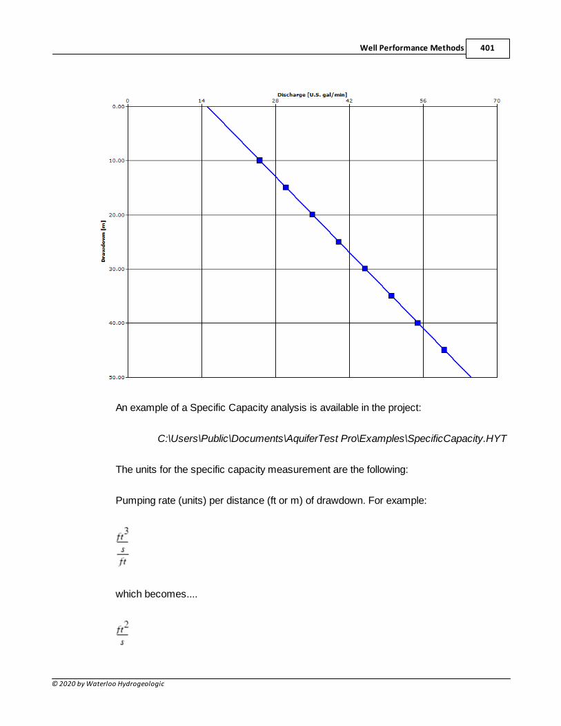
Well Performance Methods 401
© 2020 by Waterloo Hydrogeologic
An example of a Specific Capacity analysis is available in the project:
C:\Users\Public\Documents\AquiferTest Pro\Examples\SpecificCapacity.HYT
The units for the specific capacity measurement are the following:
Pumping rate (units) per distance (ft or m) of drawdown. For example:
which becomes....
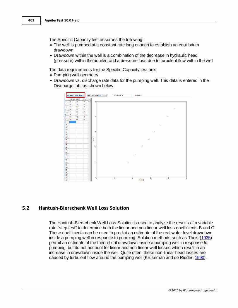
AquiferTest 10.0 Help402
© 2020 by Waterloo Hydrogeologic
The Specific Capacity test assumes the following:· The well is pumped at a constant rate long enough to establish an equilibrium
drawdown· Drawdown within the well is a combination of the decrease in hydraulic head
(pressure) within the aquifer, and a pressure loss due to turbulent flow within the well
The data requirements for the Specific Capacity test are:· Pumping well geometry
· Drawdown vs. discharge rate data for the pumping well. This data is entered in theDischarge tab, as shown below.
5.2 Hantush-Bierschenk Well Loss Solution
The Hantush-Bierschenk Well Loss Solution is used to analyze the results of a variablerate “step test” to determine both the linear and non-linear well loss coefficients B and C.These coefficients can be used to predict an estimate of the real water level drawdowninside a pumping well in response to pumping. Solution methods such as Theis (1935)permit an estimate of the theoretical drawdown inside a pumping well in response topumping, but do not account for linear and non-linear well losses which result in anincrease in drawdown inside the well. Quite often, these non-linear head losses arecaused by turbulent flow around the pumping well (Kruseman and de Ridder, 1990).
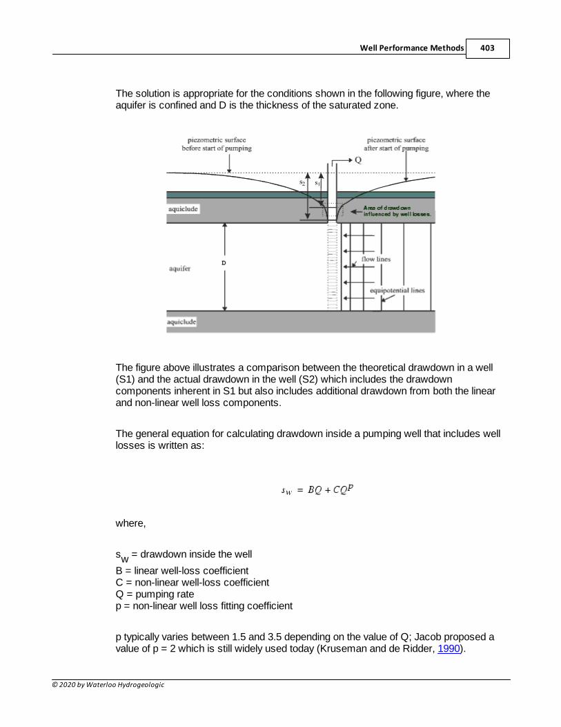
Well Performance Methods 403
© 2020 by Waterloo Hydrogeologic
The solution is appropriate for the conditions shown in the following figure, where theaquifer is confined and D is the thickness of the saturated zone.
The figure above illustrates a comparison between the theoretical drawdown in a well(S1) and the actual drawdown in the well (S2) which includes the drawdowncomponents inherent in S1 but also includes additional drawdown from both the linearand non-linear well loss components.
The general equation for calculating drawdown inside a pumping well that includes welllosses is written as:
where,
sw = drawdown inside the well
B = linear well-loss coefficientC = non-linear well-loss coefficientQ = pumping ratep = non-linear well loss fitting coefficient
p typically varies between 1.5 and 3.5 depending on the value of Q; Jacob proposed avalue of p = 2 which is still widely used today (Kruseman and de Ridder, 1990).
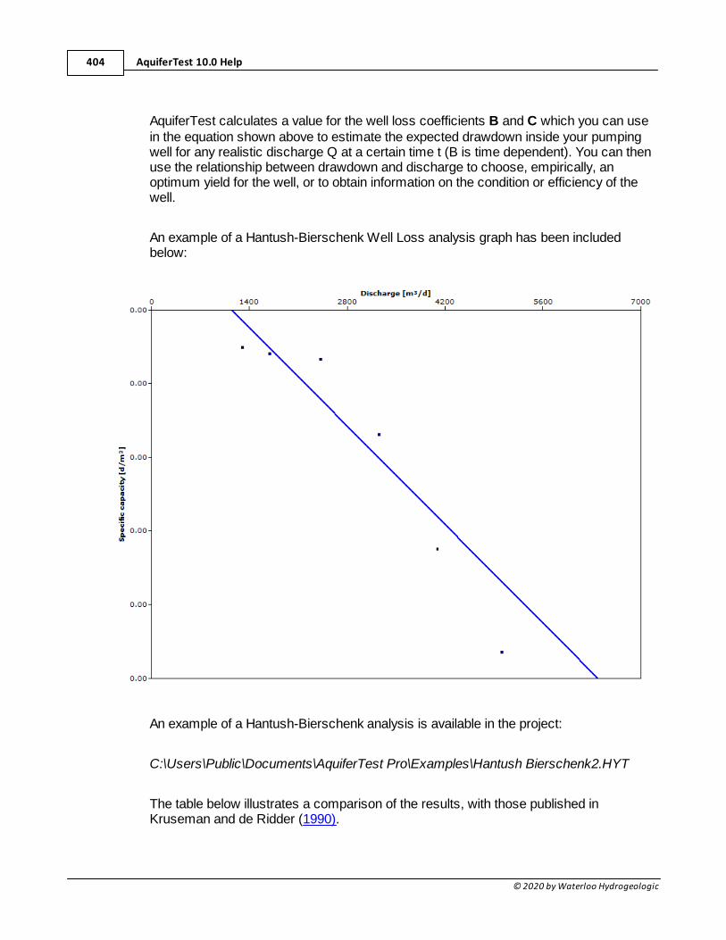
AquiferTest 10.0 Help404
© 2020 by Waterloo Hydrogeologic
AquiferTest calculates a value for the well loss coefficients B and C which you can usein the equation shown above to estimate the expected drawdown inside your pumpingwell for any realistic discharge Q at a certain time t (B is time dependent). You can thenuse the relationship between drawdown and discharge to choose, empirically, anoptimum yield for the well, or to obtain information on the condition or efficiency of thewell.
An example of a Hantush-Bierschenk Well Loss analysis graph has been includedbelow:
An example of a Hantush-Bierschenk analysis is available in the project:
C:\Users\Public\Documents\AquiferTest Pro\Examples\Hantush Bierschenk2.HYT
The table below illustrates a comparison of the results, with those published inKruseman and de Ridder (1990).
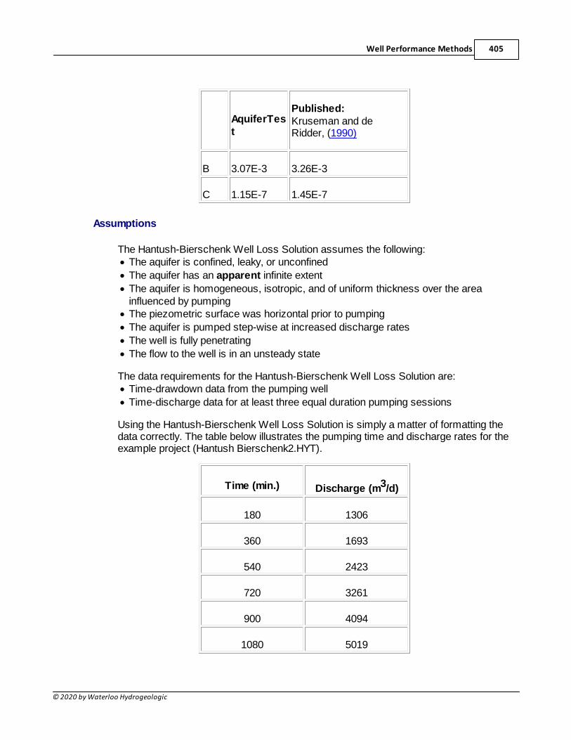
Well Performance Methods 405
© 2020 by Waterloo Hydrogeologic
AquiferTest
Published:Kruseman and deRidder, (1990)
B 3.07E-3 3.26E-3
C 1.15E-7 1.45E-7
Assumptions
The Hantush-Bierschenk Well Loss Solution assumes the following:· The aquifer is confined, leaky, or unconfined
· The aquifer has an apparent infinite extent
· The aquifer is homogeneous, isotropic, and of uniform thickness over the areainfluenced by pumping
· The piezometric surface was horizontal prior to pumping
· The aquifer is pumped step-wise at increased discharge rates
· The well is fully penetrating
· The flow to the well is in an unsteady state
The data requirements for the Hantush-Bierschenk Well Loss Solution are:· Time-drawdown data from the pumping well
· Time-discharge data for at least three equal duration pumping sessions
Using the Hantush-Bierschenk Well Loss Solution is simply a matter of formatting thedata correctly. The table below illustrates the pumping time and discharge rates for theexample project (Hantush Bierschenk2.HYT).
Time (min.) Discharge (m3/d)
180 1306
360 1693
540 2423
720 3261
900 4094
1080 5019
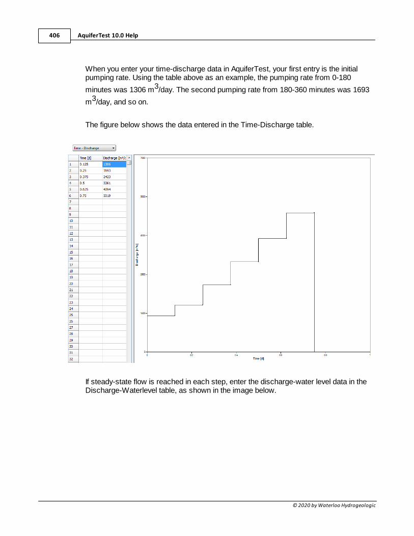
AquiferTest 10.0 Help406
© 2020 by Waterloo Hydrogeologic
When you enter your time-discharge data in AquiferTest, your first entry is the initialpumping rate. Using the table above as an example, the pumping rate from 0-180
minutes was 1306 m3/day. The second pumping rate from 180-360 minutes was 1693
m3/day, and so on.
The figure below shows the data entered in the Time-Discharge table.
If steady-state flow is reached in each step, enter the discharge-water level data in theDischarge-Waterlevel table, as shown in the image below.
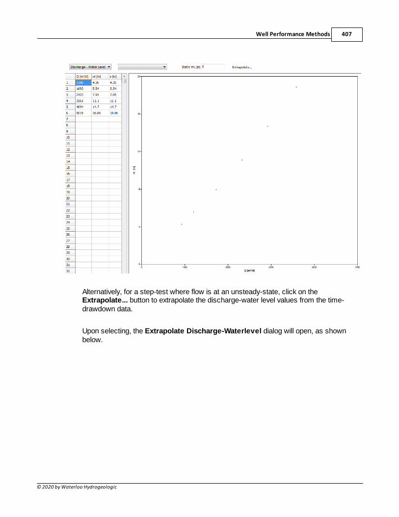
Well Performance Methods 407
© 2020 by Waterloo Hydrogeologic
Alternatively, for a step-test where flow is at an unsteady-state, click on theExtrapolate... button to extrapolate the discharge-water level values from the time-drawdown data.
Upon selecting, the Extrapolate Discharge-Waterlevel dialog will open, as shownbelow.
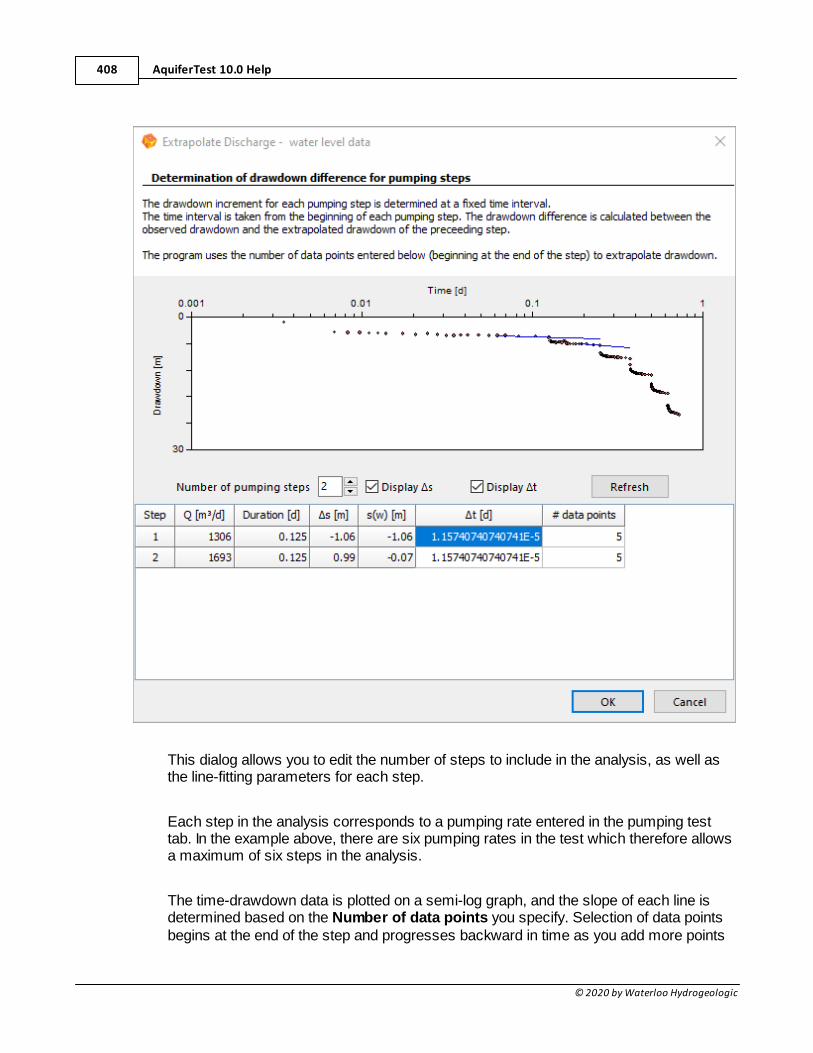
AquiferTest 10.0 Help408
© 2020 by Waterloo Hydrogeologic
This dialog allows you to edit the number of steps to include in the analysis, as well asthe line-fitting parameters for each step.
Each step in the analysis corresponds to a pumping rate entered in the pumping testtab. In the example above, there are six pumping rates in the test which therefore allowsa maximum of six steps in the analysis.
The time-drawdown data is plotted on a semi-log graph, and the slope of each line isdetermined based on the Number of data points you specify. Selection of data pointsbegins at the end of the step and progresses backward in time as you add more points
Well Performance Methods 409
© 2020 by Waterloo Hydrogeologic
for the line slope calculation. For example, if the number of points is equal to five for agiven step, then AquiferTest will use the last five data points in of that step to calculatethe slope.
The Time Interval is the time from the beginning of each step at which the change indrawdown (∆s) for each step is measured. The point of time for calculating ∆s iscalculated as follows:
where:ti = starting time of step
∆t = the specified time intervaltds = calculation point for ∆s
This measurement point is essential as the difference in drawdown is calculatedbetween each step. The selection of the time interval is left to the discretion of the user.
AquiferTest then uses the drawdown differences and the specified time interval toproduce two coefficients: B (linear well loss coefficient) and C (non-linear well losscoefficient). These coefficients can be used to estimate the expected drawdown insideyour pumping well for a realistic discharge (Q) at a certain time (t). This relationship canallow you to select an optimum yield for the well, or to obtain information on the conditionor efficiency of the well.
Finally, the Number of pumping steps allows you to edit the number of steps (i.e.changes in the discharge rate) to use in the discharge versus drawdown plot. Youshould have a minimum of three steps specified to assist in obtaining a good fit of theline to the analysis plot.
Once the extrapolation settings have been defined, click [OK] to accept the drawdownvalues. To select the analysis method, from the main menu, go to Analysis \ PumpingWell Analysis \ Well Losses.
For more information on the Hantush-Bierschenk Well Loss solution, please refer to apumping test reference such as Kruseman and de Ridder (1990).
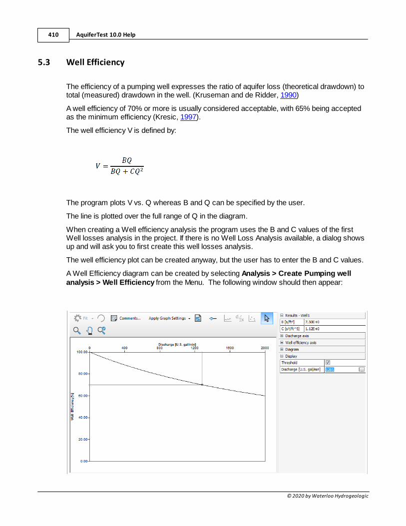
AquiferTest 10.0 Help410
© 2020 by Waterloo Hydrogeologic
5.3 Well Efficiency
The efficiency of a pumping well expresses the ratio of aquifer loss (theoretical drawdown) tototal (measured) drawdown in the well. (Kruseman and de Ridder, 1990)
A well efficiency of 70% or more is usually considered acceptable, with 65% being acceptedas the minimum efficiency (Kresic, 1997).
The well efficiency V is defined by:
The program plots V vs. Q whereas B and Q can be specified by the user.
The line is plotted over the full range of Q in the diagram.
When creating a Well efficiency analysis the program uses the B and C values of the firstWell losses analysis in the project. If there is no Well Loss Analysis available, a dialog showsup and will ask you to first create this well losses analysis.
The well efficiency plot can be created anyway, but the user has to enter the B and C values.
A Well Efficiency diagram can be created by selecting Analysis > Create Pumping wellanalysis > Well Efficiency from the Menu. The following window should then appear:
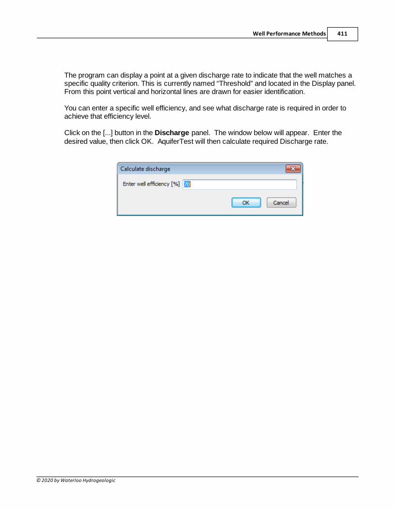
Well Performance Methods 411
© 2020 by Waterloo Hydrogeologic
The program can display a point at a given discharge rate to indicate that the well matches aspecific quality criterion. This is currently named “Threshold” and located in the Display panel.From this point vertical and horizontal lines are drawn for easier identification.
You can enter a specific well efficiency, and see what discharge rate is required in order toachieve that efficiency level.
Click on the [...] button in the Discharge panel. The window below will appear. Enter thedesired value, then click OK. AquiferTest will then calculate required Discharge rate.
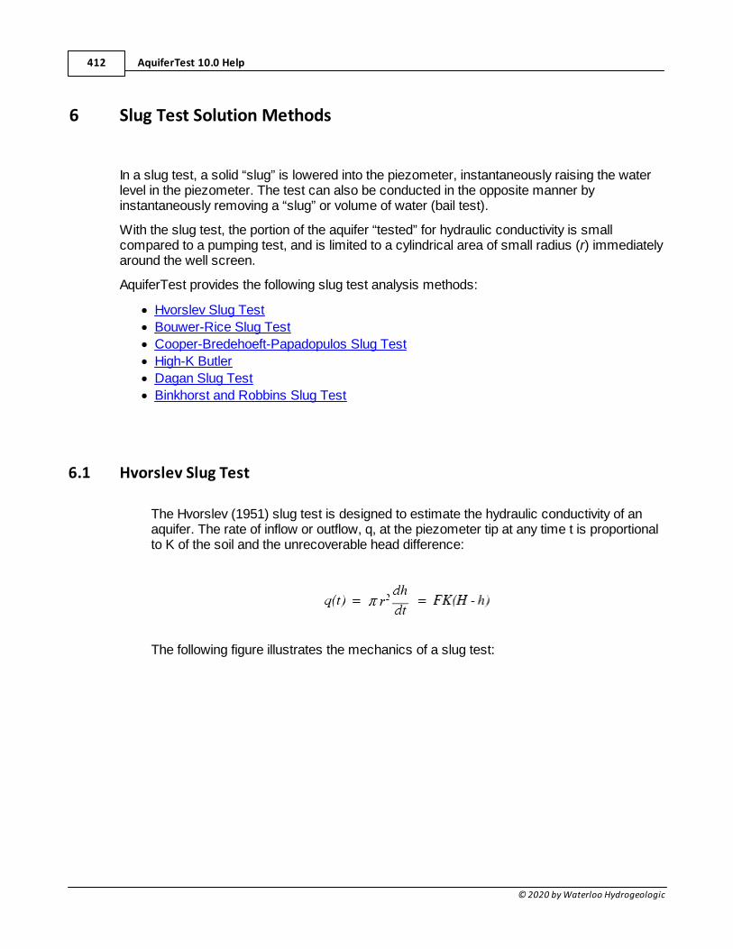
AquiferTest 10.0 Help412
© 2020 by Waterloo Hydrogeologic
6 Slug Test Solution Methods
In a slug test, a solid “slug” is lowered into the piezometer, instantaneously raising the waterlevel in the piezometer. The test can also be conducted in the opposite manner byinstantaneously removing a “slug” or volume of water (bail test).
With the slug test, the portion of the aquifer “tested” for hydraulic conductivity is smallcompared to a pumping test, and is limited to a cylindrical area of small radius (r) immediatelyaround the well screen.
AquiferTest provides the following slug test analysis methods:
· Hvorslev Slug Test
· Bouwer-Rice Slug Test
· Cooper-Bredehoeft-Papadopulos Slug Test
· High-K Butler
· Dagan Slug Test
· Binkhorst and Robbins Slug Test
6.1 Hvorslev Slug Test
The Hvorslev (1951) slug test is designed to estimate the hydraulic conductivity of anaquifer. The rate of inflow or outflow, q, at the piezometer tip at any time t is proportionalto K of the soil and the unrecoverable head difference:
The following figure illustrates the mechanics of a slug test:
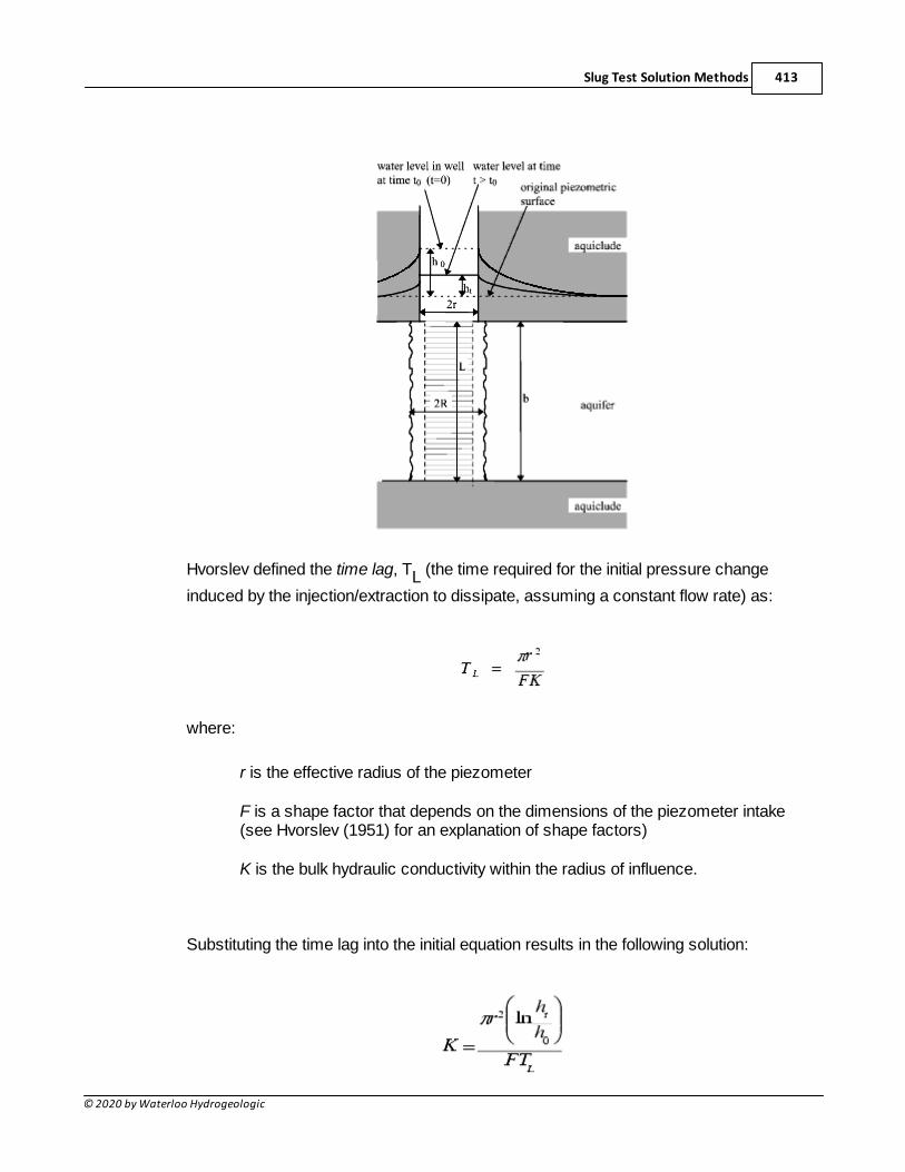
Slug Test Solution Methods 413
© 2020 by Waterloo Hydrogeologic
Hvorslev defined the time lag, TL (the time required for the initial pressure change
induced by the injection/extraction to dissipate, assuming a constant flow rate) as:
where:
r is the effective radius of the piezometer
F is a shape factor that depends on the dimensions of the piezometer intake(see Hvorslev (1951) for an explanation of shape factors)
K is the bulk hydraulic conductivity within the radius of influence.
Substituting the time lag into the initial equation results in the following solution:
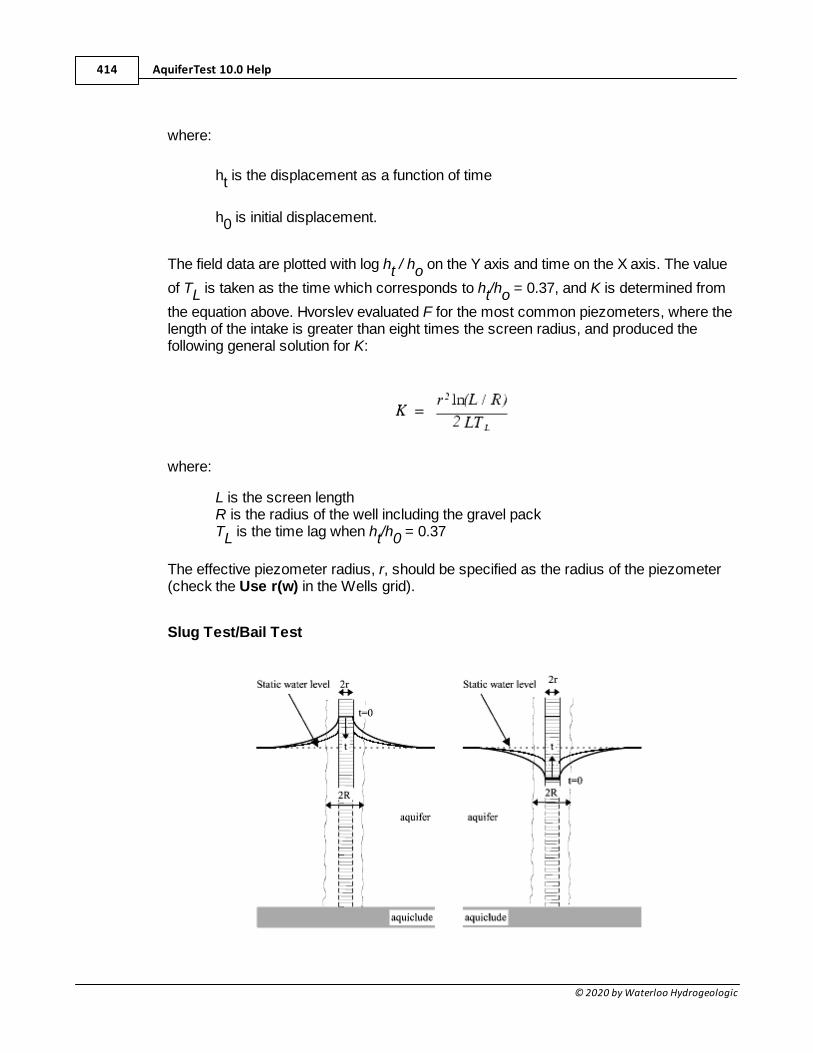
AquiferTest 10.0 Help414
© 2020 by Waterloo Hydrogeologic
where:
ht is the displacement as a function of time
h0 is initial displacement.
The field data are plotted with log ht / ho on the Y axis and time on the X axis. The value
of TL is taken as the time which corresponds to ht/ho = 0.37, and K is determined from
the equation above. Hvorslev evaluated F for the most common piezometers, where thelength of the intake is greater than eight times the screen radius, and produced thefollowing general solution for K:
where:
L is the screen lengthR is the radius of the well including the gravel packTL is the time lag when ht/h0 = 0.37
The effective piezometer radius, r, should be specified as the radius of the piezometer(check the Use r(w) in the Wells grid).
Slug Test/Bail Test
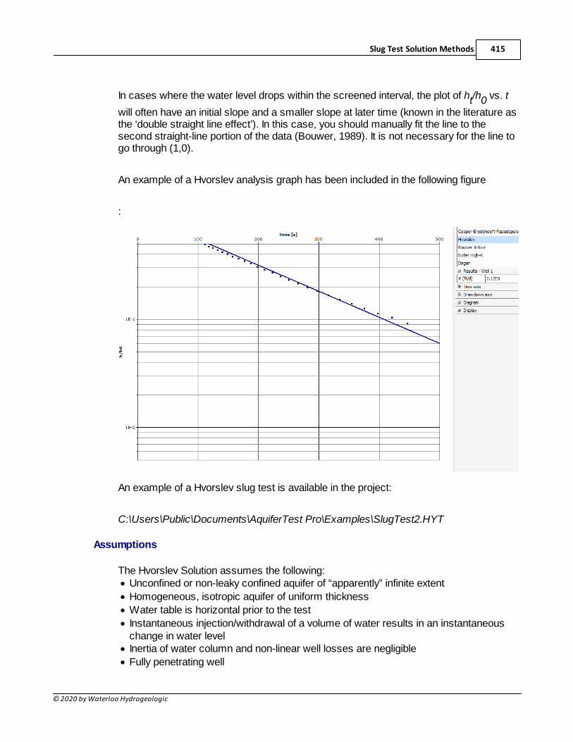
Slug Test Solution Methods 415
© 2020 by Waterloo Hydrogeologic
In cases where the water level drops within the screened interval, the plot of ht/h0 vs. t
will often have an initial slope and a smaller slope at later time (known in the literature asthe ‘double straight line effect’). In this case, you should manually fit the line to thesecond straight-line portion of the data (Bouwer, 1989). It is not necessary for the line togo through (1,0).
An example of a Hvorslev analysis graph has been included in the following figure
:
An example of a Hvorslev slug test is available in the project:
C:\Users\Public\Documents\AquiferTest Pro\Examples\SlugTest2.HYT
Assumptions
The Hvorslev Solution assumes the following:· Unconfined or non-leaky confined aquifer of “apparently” infinite extent
· Homogeneous, isotropic aquifer of uniform thickness
· Water table is horizontal prior to the test
· Instantaneous injection/withdrawal of a volume of water results in an instantaneouschange in water level
· Inertia of water column and non-linear well losses are negligible
· Fully penetrating well
AquiferTest 10.0 Help416
© 2020 by Waterloo Hydrogeologic
· The well is considered to be of an infinitesimal width
· Flow is horizontal toward or away from the well
Data requirements for the Hvorslev Solution are:· Drawdown / recovery vs. time data at a test well
· Observations beginning from time zero onward (the observation at t=0 is taken as theinitial displacement value, H0, and thus it must be a non-zero value)
NOTE: Hvorslev has presented numerous formulae for varyingwell and aquifer conditions. AquiferTest uses a formula methodthat can be applied to unconfined in addition to confinedconditions. This method could be applied to unconfinedconditions for most piezometer designs, where the length istypically quite a bit greater than the radius of the well screen. Inthis case, the user must assume that there is a minimal changein the saturated aquifer thickness during the test. Finally, it isalso assumed that the flow required for pressure equalizationdoes not cause any perceptible drawdown of the groundwaterlevel. For other conditions and more details, please refer to theoriginal Hvorslev paper.
For the Hvorslev analysis method, you must enter all values for the piezometergeometry.
The effective piezometer radius (r) should be entered as the inside radius of thepiezometer / well casing if the water level in the piezometer is always above the screen,
or as calculated by reff=[r2(1-n) + nR2]1/2 if the water level falls within the screened
interval during the slug test (where r = the inside radius of the well, R = the outsideradius of the filter material or developed zone, and n = porosity). To use effective radius,check the box in the Use r(w) column of the wells grid (scroll to the very right).
The radius of the developed zone (R) should be entered as the radius of the borehole,including the gravel/sand pack. The Length of the screened interval (L), should beentered as the length of screen within the saturated zone under static conditions.
6.2 Bouwer-Rice Slug Test
The Bouwer-Rice (1976) slug test is designed to estimate the hydraulic conductivity ofan aquifer. The solution is appropriate for the conditions shown in the following figure.
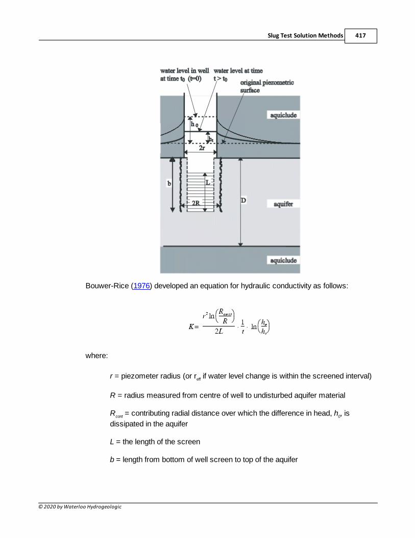
Slug Test Solution Methods 417
© 2020 by Waterloo Hydrogeologic
Bouwer-Rice (1976) developed an equation for hydraulic conductivity as follows:
where:
r = piezometer radius (or reff if water level change is within the screened interval)
R = radius measured from centre of well to undisturbed aquifer material
Rcont = contributing radial distance over which the difference in head, h0, is
dissipated in the aquifer
L = the length of the screen
b = length from bottom of well screen to top of the aquifer
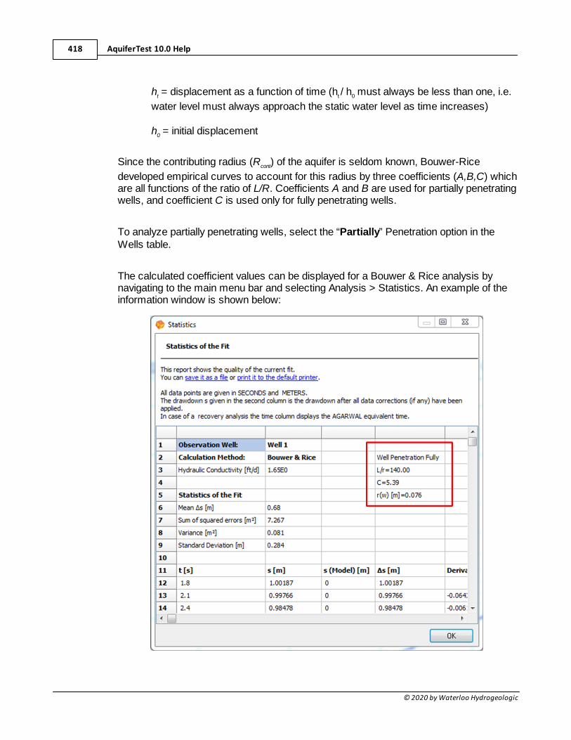
AquiferTest 10.0 Help418
© 2020 by Waterloo Hydrogeologic
ht = displacement as a function of time (ht / h0 must always be less than one, i.e.
water level must always approach the static water level as time increases)
h0 = initial displacement
Since the contributing radius (Rcont) of the aquifer is seldom known, Bouwer-Rice
developed empirical curves to account for this radius by three coefficients (A,B,C) whichare all functions of the ratio of L/R. Coefficients A and B are used for partially penetratingwells, and coefficient C is used only for fully penetrating wells.
To analyze partially penetrating wells, select the “Partially” Penetration option in theWells table.
The calculated coefficient values can be displayed for a Bouwer & Rice analysis bynavigating to the main menu bar and selecting Analysis > Statistics. An example of theinformation window is shown below:
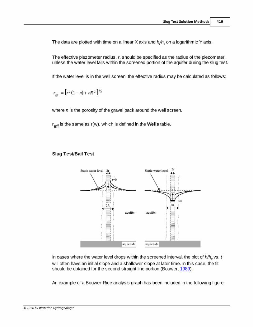
Slug Test Solution Methods 419
© 2020 by Waterloo Hydrogeologic
The data are plotted with time on a linear X axis and ht/ho on a logarithmic Y axis.
The effective piezometer radius, r, should be specified as the radius of the piezometer,unless the water level falls within the screened portion of the aquifer during the slug test.
If the water level is in the well screen, the effective radius may be calculated as follows:
where n is the porosity of the gravel pack around the well screen.
reff is the same as r(w), which is defined in the Wells table.
Slug Test/Bail Test
In cases where the water level drops within the screened interval, the plot of h/h0 vs. t
will often have an initial slope and a shallower slope at later time. In this case, the fitshould be obtained for the second straight line portion (Bouwer, 1989).
An example of a Bouwer-Rice analysis graph has been included in the following figure:
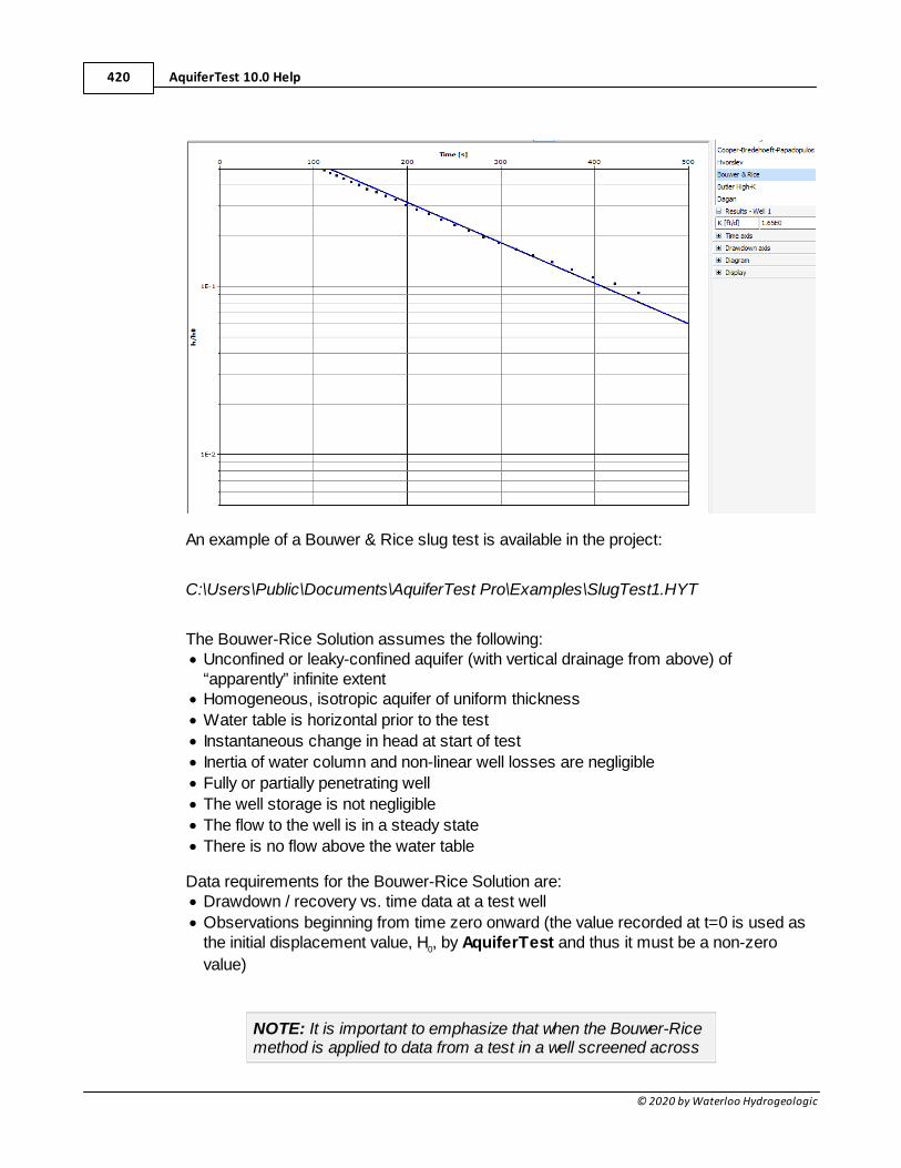
AquiferTest 10.0 Help420
© 2020 by Waterloo Hydrogeologic
An example of a Bouwer & Rice slug test is available in the project:
C:\Users\Public\Documents\AquiferTest Pro\Examples\SlugTest1.HYT
The Bouwer-Rice Solution assumes the following:· Unconfined or leaky-confined aquifer (with vertical drainage from above) of
“apparently” infinite extent· Homogeneous, isotropic aquifer of uniform thickness
· Water table is horizontal prior to the test
· Instantaneous change in head at start of test
· Inertia of water column and non-linear well losses are negligible
· Fully or partially penetrating well
· The well storage is not negligible
· The flow to the well is in a steady state
· There is no flow above the water table
Data requirements for the Bouwer-Rice Solution are:· Drawdown / recovery vs. time data at a test well
· Observations beginning from time zero onward (the value recorded at t=0 is used asthe initial displacement value, H0, by AquiferTest and thus it must be a non-zero
value)
NOTE: It is important to emphasize that when the Bouwer-Ricemethod is applied to data from a test in a well screened across
Slug Test Solution Methods 421
© 2020 by Waterloo Hydrogeologic
the water table, the analyst (user) is adopting a simplifiedrepresentation of the flow system, i.e., both the position of thewater table and the effective screen length, are not changingsignificantly during the course of the test (Butler, 1998).
For the Bouwer-Rice slug test method, you must enter all values for the piezometergeometry.
The effective piezometer radius (r) should be entered as the inside radius of thepiezometer/well casing if the water level in the piezometer is always above the screen,
or as calculated by reff=[r2(1-n) + nR2]1/2, where n = porosity, if the water level falls
within the screened interval during the slug test (where r = the inside radius of the well,R = the outside radius of the filter material or developed zone, and n = porosity). To usethe effective radius, check the box in the Use r(w) column in the wells grid (scroll to thevery right) of Slug test tab.
The radius of the developed zone (R) should be entered as the radius of the borehole,including the gravel/sand pack.
The Length of the screened interval (L), should be entered as the length of screen withinthe saturated zone under static conditions.
The height of the stagnant water column (b), should be entered as the length from thebottom of the well screen to the top of the aquifer.
The saturated thickness of the aquifer (D), should be entered as the saturated thicknessunder static conditions.
6.3 Cooper-Bredehoeft-Papadopulos Slug Test
The Cooper-Bredehoeft-Papadopulos (1967) slug test applies to the instantaneousinjection or withdrawal of a volume of water from a large diameter well cased in aconfined aquifer. If water is injected into the well, then the initial head is above theequilibrium level and the solution method predicts the buildup. On the other hand if wateris withdrawn from the well casing, then the initial head is below the equilibrium level andthe method calculates the drawdown. The drawdown or buildup s is given by thefollowing equation:
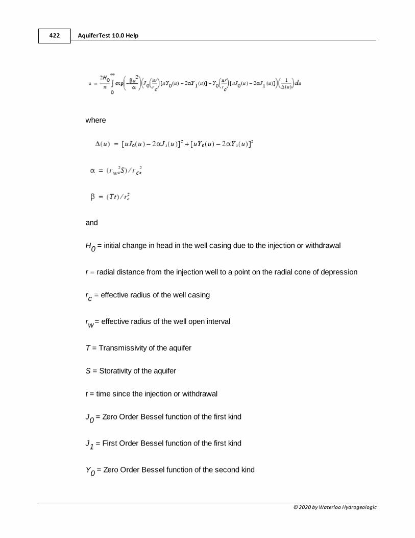
AquiferTest 10.0 Help422
© 2020 by Waterloo Hydrogeologic
where
and
H0 = initial change in head in the well casing due to the injection or withdrawal
r = radial distance from the injection well to a point on the radial cone of depression
rc = effective radius of the well casing
rw = effective radius of the well open interval
T = Transmissivity of the aquifer
S = Storativity of the aquifer
t = time since the injection or withdrawal
J0 = Zero Order Bessel function of the first kind
J1 = First Order Bessel function of the first kind
Y0 = Zero Order Bessel function of the second kind
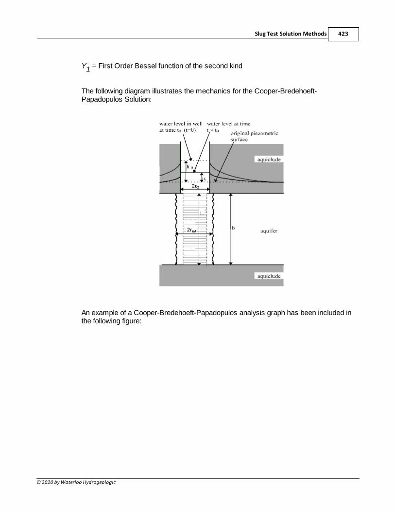
Slug Test Solution Methods 423
© 2020 by Waterloo Hydrogeologic
Y1 = First Order Bessel function of the second kind
The following diagram illustrates the mechanics for the Cooper-Bredehoeft-Papadopulos Solution:
An example of a Cooper-Bredehoeft-Papadopulos analysis graph has been included inthe following figure:
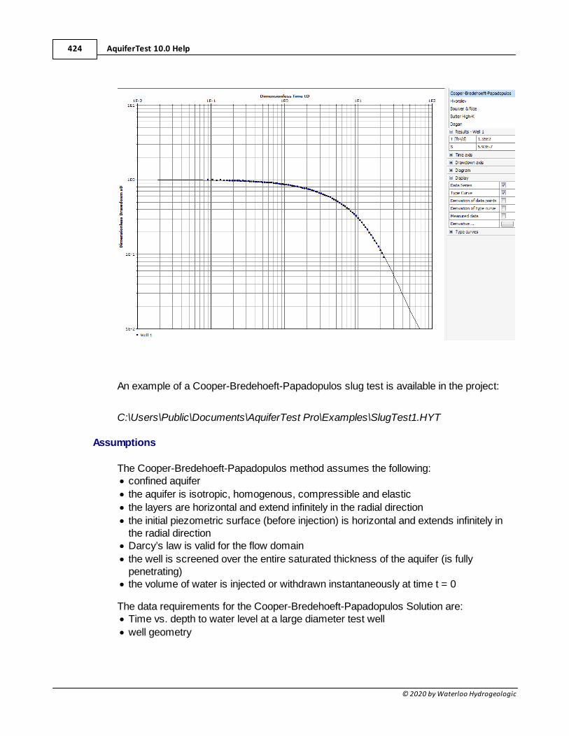
AquiferTest 10.0 Help424
© 2020 by Waterloo Hydrogeologic
An example of a Cooper-Bredehoeft-Papadopulos slug test is available in the project:
C:\Users\Public\Documents\AquiferTest Pro\Examples\SlugTest1.HYT
Assumptions
The Cooper-Bredehoeft-Papadopulos method assumes the following:· confined aquifer
· the aquifer is isotropic, homogenous, compressible and elastic
· the layers are horizontal and extend infinitely in the radial direction
· the initial piezometric surface (before injection) is horizontal and extends infinitely inthe radial direction
· Darcy’s law is valid for the flow domain
· the well is screened over the entire saturated thickness of the aquifer (is fullypenetrating)
· the volume of water is injected or withdrawn instantaneously at time t = 0
The data requirements for the Cooper-Bredehoeft-Papadopulos Solution are:· Time vs. depth to water level at a large diameter test well
· well geometry
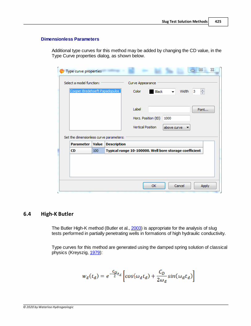
Slug Test Solution Methods 425
© 2020 by Waterloo Hydrogeologic
Dimensionless Parameters
Additional type curves for this method may be added by changing the CD value, in theType Curve properties dialog, as shown below.
6.4 High-K Butler
The Butler High-K method (Butler et al., 2003) is appropriate for the analysis of slugtests performed in partially penetrating wells in formations of high hydraulic conductivity.
Type curves for this method are generated using the damped spring solution of classicalphysics (Kreyszig, 1979):
AquiferTest 10.0 Help426
© 2020 by Waterloo Hydrogeologic
For CD < 2
For CD = 2
For CD > 2
where:
CD = Dimensionless damping parameter
g = gravitational accelerations
H0 = change in water level initiating a slut test (initial displacement)
Le = effective length of water column in well
td = dimensionless time parameter
w = deviation of water level from static level in well
wd = normalized water-level deviation (w/H0)
wd = dimensionless frequency parameter
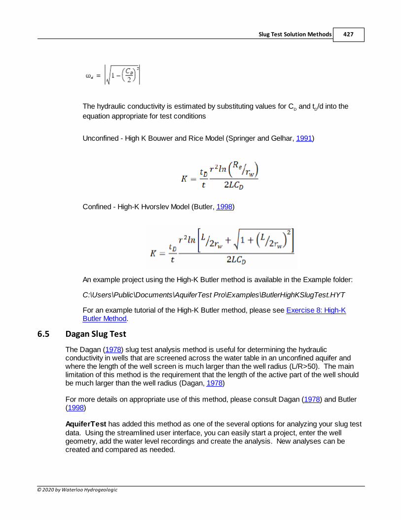
Slug Test Solution Methods 427
© 2020 by Waterloo Hydrogeologic
The hydraulic conductivity is estimated by substituting values for CD and tD/d into the
equation appropriate for test conditions
Unconfined - High K Bouwer and Rice Model (Springer and Gelhar, 1991)
Confined - High-K Hvorslev Model (Butler, 1998)
An example project using the High-K Butler method is available in the Example folder:
C:\Users\Public\Documents\AquiferTest Pro\Examples\ButlerHighKSlugTest.HYT
For an example tutorial of the High-K Butler method, please see Exercise 8: High-KButler Method.
6.5 Dagan Slug Test
The Dagan (1978) slug test analysis method is useful for determining the hydraulicconductivity in wells that are screened across the water table in an unconfined aquifer andwhere the length of the well screen is much larger than the well radius (L/R>50). The mainlimitation of this method is the requirement that the length of the active part of the well shouldbe much larger than the well radius (Dagan, 1978)
For more details on appropriate use of this method, please consult Dagan (1978) and Butler(1998)
AquiferTest has added this method as one of the several options for analyzing your slug testdata. Using the streamlined user interface, you can easily start a project, enter the wellgeometry, add the water level recordings and create the analysis. New analyses can becreated and compared as needed.
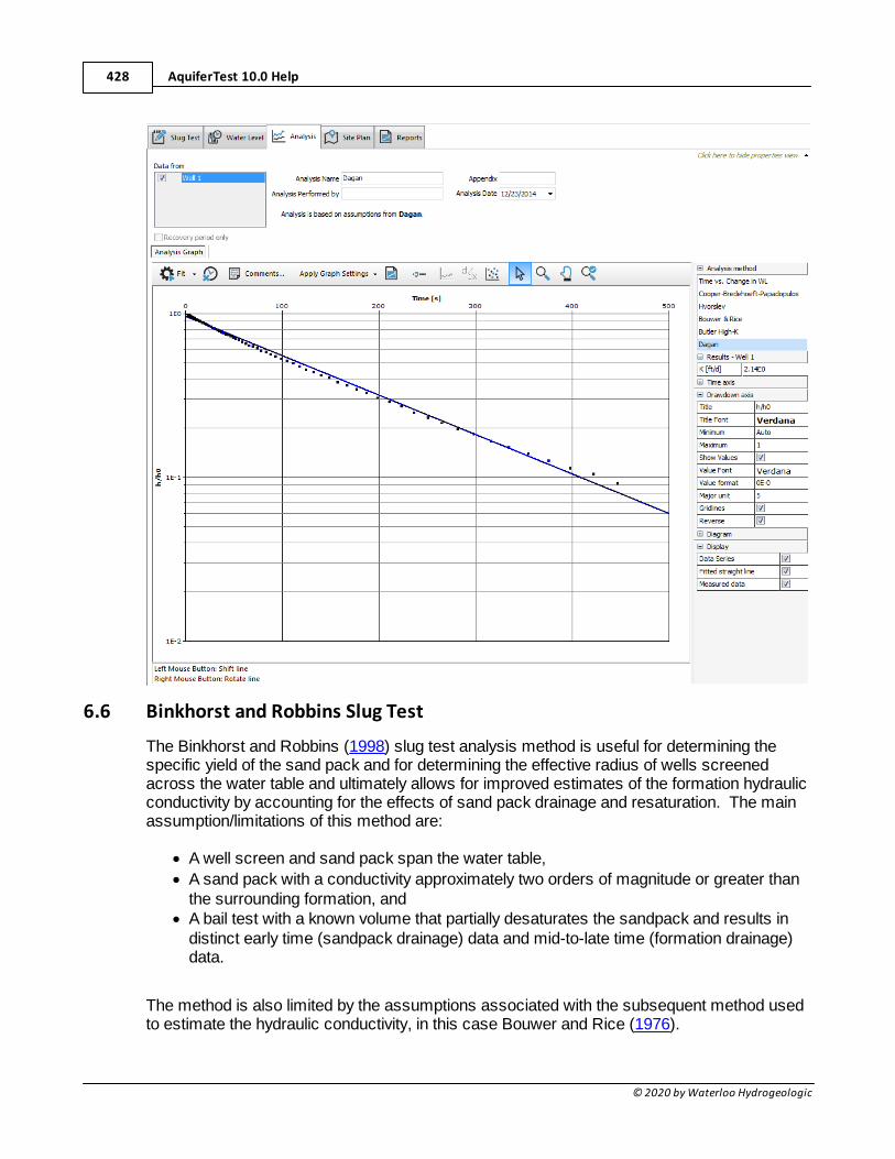
AquiferTest 10.0 Help428
© 2020 by Waterloo Hydrogeologic
6.6 Binkhorst and Robbins Slug Test
The Binkhorst and Robbins (1998) slug test analysis method is useful for determining thespecific yield of the sand pack and for determining the effective radius of wells screenedacross the water table and ultimately allows for improved estimates of the formation hydraulicconductivity by accounting for the effects of sand pack drainage and resaturation. The mainassumption/limitations of this method are:
· A well screen and sand pack span the water table,
· A sand pack with a conductivity approximately two orders of magnitude or greater thanthe surrounding formation, and
· A bail test with a known volume that partially desaturates the sandpack and results indistinct early time (sandpack drainage) data and mid-to-late time (formation drainage)data.
The method is also limited by the assumptions associated with the subsequent method usedto estimate the hydraulic conductivity, in this case Bouwer and Rice (1976).
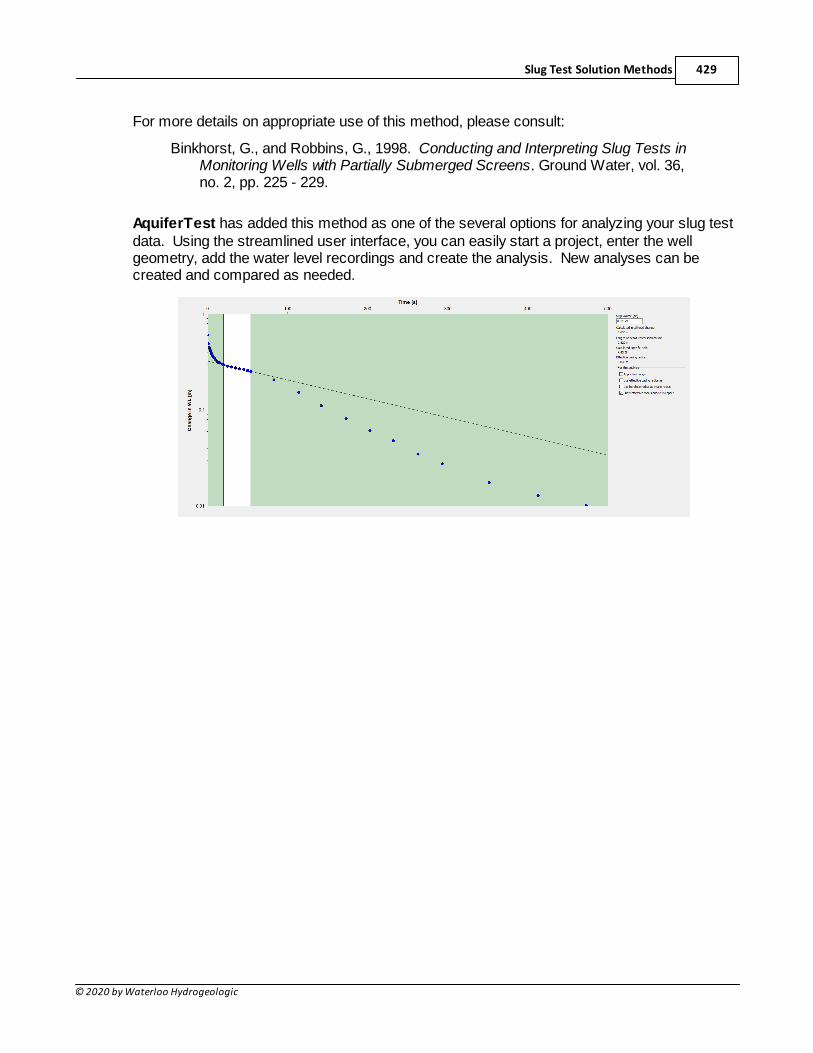
Slug Test Solution Methods 429
© 2020 by Waterloo Hydrogeologic
For more details on appropriate use of this method, please consult:
Binkhorst, G., and Robbins, G., 1998. Conducting and Interpreting Slug Tests inMonitoring Wells with Partially Submerged Screens. Ground Water, vol. 36,no. 2, pp. 225 - 229.
AquiferTest has added this method as one of the several options for analyzing your slug testdata. Using the streamlined user interface, you can easily start a project, enter the wellgeometry, add the water level recordings and create the analysis. New analyses can becreated and compared as needed.
AquiferTest 10.0 Help430
© 2020 by Waterloo Hydrogeologic
7 Lugeon Tests
The Lugeon test (or Packer Test) is an in-situ testing method widely used to estimate theaverage hydraulic conductivity of rock formations. The test is named after Maurice Lugeon(1933), a Swiss geologist who first formulated the test. The test is also referred to as a WaterPressure Test. The Lugeon test is a constant rate injection test carried out in a portion of aborehole isolated by inflated packers. Water is injected into the isolated portion of the boreholeusing a slotted pipe. Water is injected at specific pressure “steps” and the resulting pressureis recorded when the flow has reached a quasi-steady state condition. A pressure transduceris also located in that portion of the borehole to measure the pressure with a help of readingstation on the surface. The results provide information about hydraulic conductivity of the rockmass including the rock matrix and the discontinuities. (Royle, 2010)
Assumptions and Limitations
One of the main drawbacks of the Lugeon test is that only a limited volume of rock around thehole is actually affected by the test. It has been estimated that the effect of the Lugeon tests –with a test interval length of 10 feet - is restricted to an approximate radius of 30 feet aroundthe borehole (Bliss and Rushton, 1984). This suggests that the hydraulic conductivity valueestimated from this test is only representative for a cylinder of rock delimited by the length ofthe test interval and the radius given above. The test can be applied for both vertical andslanted/angled boreholes. AquiferTest assumes that flow meter readings are taken every oneminute.
References and Suggested Readings
Bliss, J. and Rushton, K., 1984. The reliability of packer tests for estimating the hydraulicconductivity of aquifers. Q. J. Eng. Geol. Vol. 17, pp. 81-91.
Fell, R., MacGregor, P., Stapledon. D., Bell, G., 2005. Geotechnical Engineering of Dams.Taylor & Francis. London. UK.
Houlsby, A., 1976. Routine Interpretation of the Lugeon Water-Test. Q. J. Eng. Geol. Vol. 9,pp. 303-313.
Lancaster-Jones, P. F. F. 1975. The interpretation of the Lugeon water-test. Quarterly Journalof Engineering Geology and Hydrogeology; 8(2):151-154.
Quiñones-Rozo, C., 2010. Lugeon test interpretation, revisited. In: CollaborativeManagement of Integrated Watersheds, US Society of Dams, 30th Annual Conference,S. 405–414.
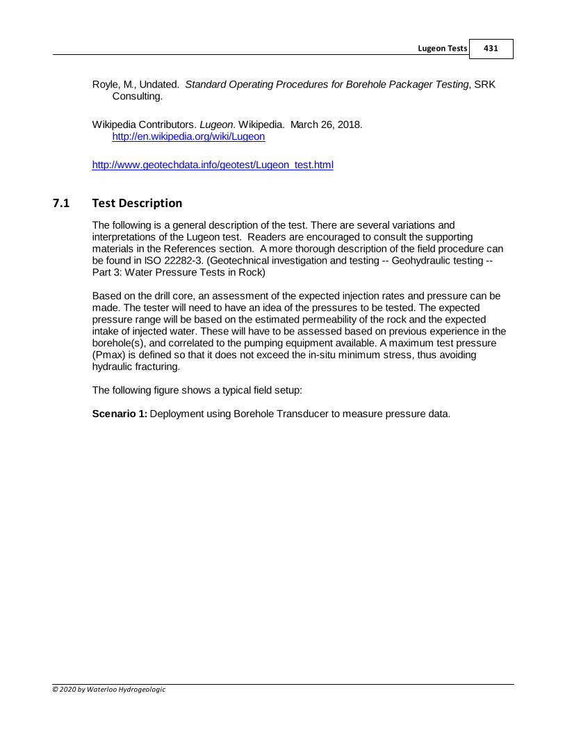
Lugeon Tests 431
© 2020 by Waterloo Hydrogeologic
Royle, M., Undated. Standard Operating Procedures for Borehole Packager Testing, SRKConsulting.
Wikipedia Contributors. Lugeon. Wikipedia. March 26, 2018. http://en.wikipedia.org/wiki/Lugeon
http://www.geotechdata.info/geotest/Lugeon_test.html
7.1 Test Description
The following is a general description of the test. There are several variations andinterpretations of the Lugeon test. Readers are encouraged to consult the supportingmaterials in the References section. A more thorough description of the field procedure canbe found in ISO 22282-3. (Geotechnical investigation and testing -- Geohydraulic testing --Part 3: Water Pressure Tests in Rock)
Based on the drill core, an assessment of the expected injection rates and pressure can bemade. The tester will need to have an idea of the pressures to be tested. The expectedpressure range will be based on the estimated permeability of the rock and the expectedintake of injected water. These will have to be assessed based on previous experience in theborehole(s), and correlated to the pumping equipment available. A maximum test pressure(Pmax) is defined so that it does not exceed the in-situ minimum stress, thus avoidinghydraulic fracturing.
The following figure shows a typical field setup:
Scenario 1: Deployment using Borehole Transducer to measure pressure data.
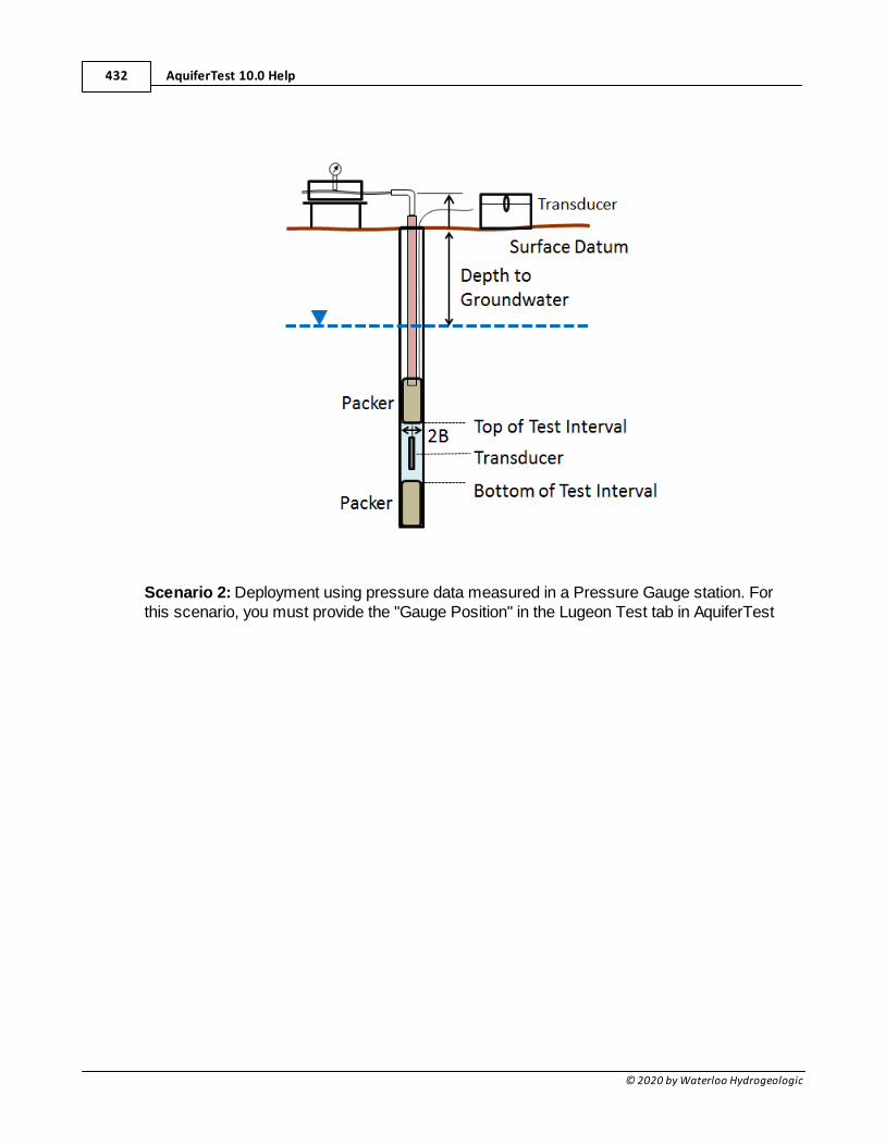
AquiferTest 10.0 Help432
© 2020 by Waterloo Hydrogeologic
Scenario 2: Deployment using pressure data measured in a Pressure Gauge station. Forthis scenario, you must provide the "Gauge Position" in the Lugeon Test tab in AquiferTest
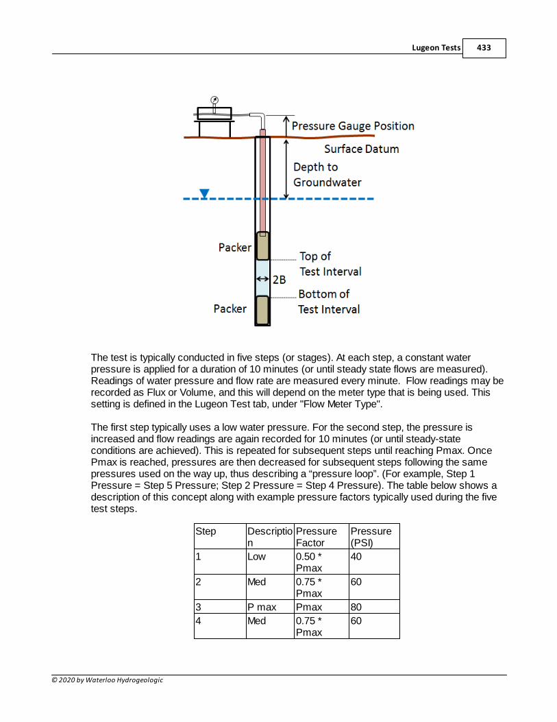
Lugeon Tests 433
© 2020 by Waterloo Hydrogeologic
The test is typically conducted in five steps (or stages). At each step, a constant waterpressure is applied for a duration of 10 minutes (or until steady state flows are measured).Readings of water pressure and flow rate are measured every minute. Flow readings may berecorded as Flux or Volume, and this will depend on the meter type that is being used. Thissetting is defined in the Lugeon Test tab, under "Flow Meter Type".
The first step typically uses a low water pressure. For the second step, the pressure isincreased and flow readings are again recorded for 10 minutes (or until steady-stateconditions are achieved). This is repeated for subsequent steps until reaching Pmax. OncePmax is reached, pressures are then decreased for subsequent steps following the samepressures used on the way up, thus describing a “pressure loop”. (For example, Step 1Pressure = Step 5 Pressure; Step 2 Pressure = Step 4 Pressure). The table below shows adescription of this concept along with example pressure factors typically used during the fivetest steps.
Step Description
PressureFactor
Pressure(PSI)
1 Low 0.50 *Pmax
40
2 Med 0.75 *Pmax
60
3 P max Pmax 80
4 Med 0.75 *Pmax
60
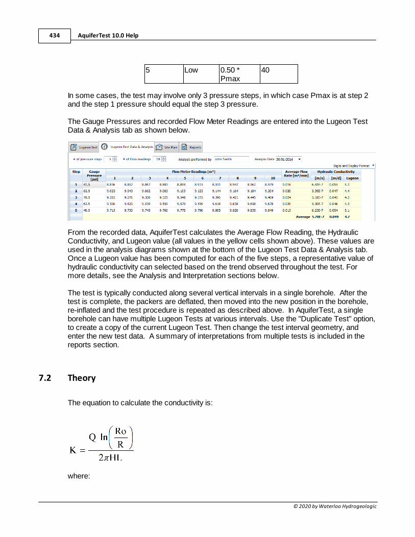
AquiferTest 10.0 Help434
© 2020 by Waterloo Hydrogeologic
5 Low 0.50 *Pmax
40
In some cases, the test may involve only 3 pressure steps, in which case Pmax is at step 2and the step 1 pressure should equal the step 3 pressure.
The Gauge Pressures and recorded Flow Meter Readings are entered into the Lugeon TestData & Analysis tab as shown below.
From the recorded data, AquiferTest calculates the Average Flow Reading, the HydraulicConductivity, and Lugeon value (all values in the yellow cells shown above). These values areused in the analysis diagrams shown at the bottom of the Lugeon Test Data & Analysis tab.Once a Lugeon value has been computed for each of the five steps, a representative value ofhydraulic conductivity can selected based on the trend observed throughout the test. Formore details, see the Analysis and Interpretation sections below.
The test is typically conducted along several vertical intervals in a single borehole. After thetest is complete, the packers are deflated, then moved into the new position in the borehole,re-inflated and the test procedure is repeated as described above. In AquiferTest, a singleborehole can have multiple Lugeon Tests at various intervals. Use the "Duplicate Test" option,to create a copy of the current Lugeon Test. Then change the test interval geometry, andenter the new test data. A summary of interpretations from multiple tests is included in thereports section.
7.2 Theory
The equation to calculate the conductivity is:
where:
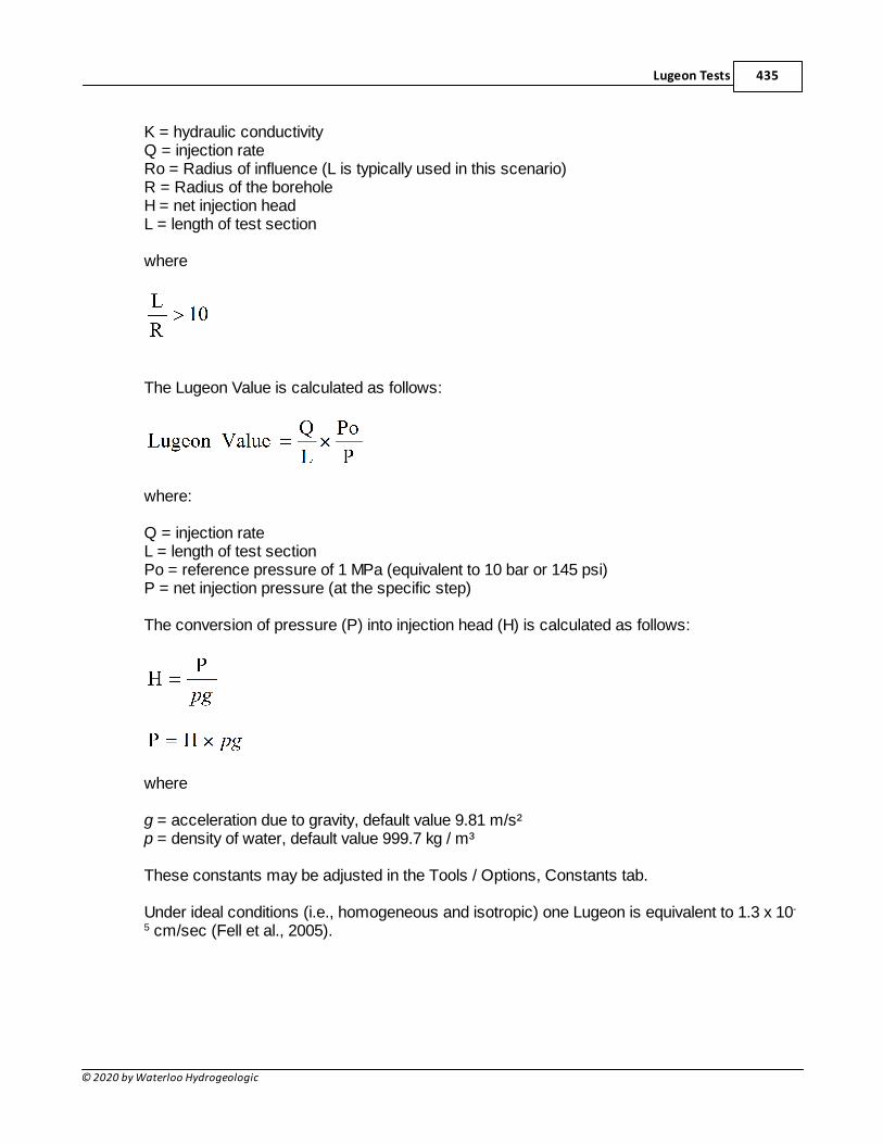
Lugeon Tests 435
© 2020 by Waterloo Hydrogeologic
K = hydraulic conductivityQ = injection rateRo = Radius of influence (L is typically used in this scenario)R = Radius of the boreholeH = net injection headL = length of test section
where
The Lugeon Value is calculated as follows:
where:
Q = injection rateL = length of test sectionPo = reference pressure of 1 MPa (equivalent to 10 bar or 145 psi)P = net injection pressure (at the specific step)
The conversion of pressure (P) into injection head (H) is calculated as follows:
where
g = acceleration due to gravity, default value 9.81 m/s²p = density of water, default value 999.7 kg / m³
These constants may be adjusted in the Tools / Options, Constants tab.
Under ideal conditions (i.e., homogeneous and isotropic) one Lugeon is equivalent to 1.3 x 10-
5 cm/sec (Fell et al., 2005).
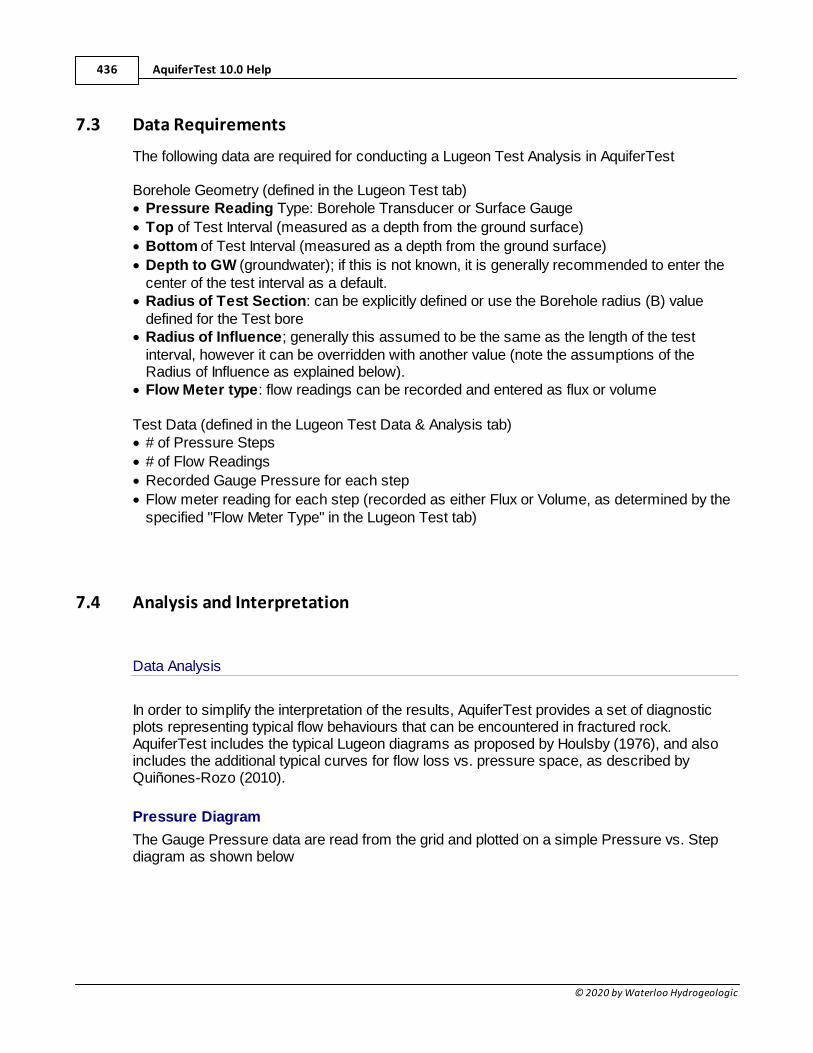
AquiferTest 10.0 Help436
© 2020 by Waterloo Hydrogeologic
7.3 Data Requirements
The following data are required for conducting a Lugeon Test Analysis in AquiferTest
Borehole Geometry (defined in the Lugeon Test tab)· Pressure Reading Type: Borehole Transducer or Surface Gauge
· Top of Test Interval (measured as a depth from the ground surface)
· Bottom of Test Interval (measured as a depth from the ground surface)
· Depth to GW (groundwater); if this is not known, it is generally recommended to enter thecenter of the test interval as a default.
· Radius of Test Section: can be explicitly defined or use the Borehole radius (B) valuedefined for the Test bore
· Radius of Influence; generally this assumed to be the same as the length of the testinterval, however it can be overridden with another value (note the assumptions of theRadius of Influence as explained below).
· Flow Meter type: flow readings can be recorded and entered as flux or volume
Test Data (defined in the Lugeon Test Data & Analysis tab)· # of Pressure Steps
· # of Flow Readings
· Recorded Gauge Pressure for each step
· Flow meter reading for each step (recorded as either Flux or Volume, as determined by thespecified "Flow Meter Type" in the Lugeon Test tab)
7.4 Analysis and Interpretation
Data Analysis
In order to simplify the interpretation of the results, AquiferTest provides a set of diagnosticplots representing typical flow behaviours that can be encountered in fractured rock. AquiferTest includes the typical Lugeon diagrams as proposed by Houlsby (1976), and alsoincludes the additional typical curves for flow loss vs. pressure space, as described byQuiñones-Rozo (2010).
Pressure Diagram
The Gauge Pressure data are read from the grid and plotted on a simple Pressure vs. Stepdiagram as shown below
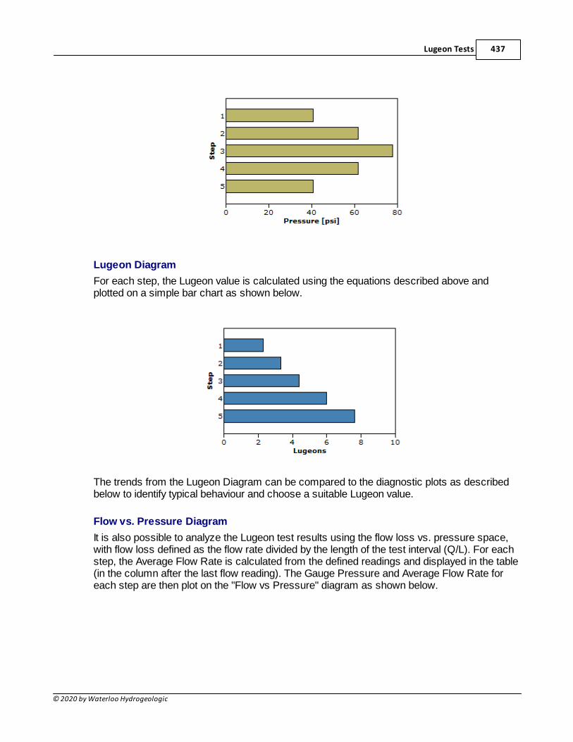
Lugeon Tests 437
© 2020 by Waterloo Hydrogeologic
Lugeon Diagram
For each step, the Lugeon value is calculated using the equations described above andplotted on a simple bar chart as shown below.
The trends from the Lugeon Diagram can be compared to the diagnostic plots as describedbelow to identify typical behaviour and choose a suitable Lugeon value.
Flow vs. Pressure Diagram
It is also possible to analyze the Lugeon test results using the flow loss vs. pressure space,with flow loss defined as the flow rate divided by the length of the test interval (Q/L). For eachstep, the Average Flow Rate is calculated from the defined readings and displayed in the table(in the column after the last flow reading). The Gauge Pressure and Average Flow Rate foreach step are then plot on the "Flow vs Pressure" diagram as shown below.
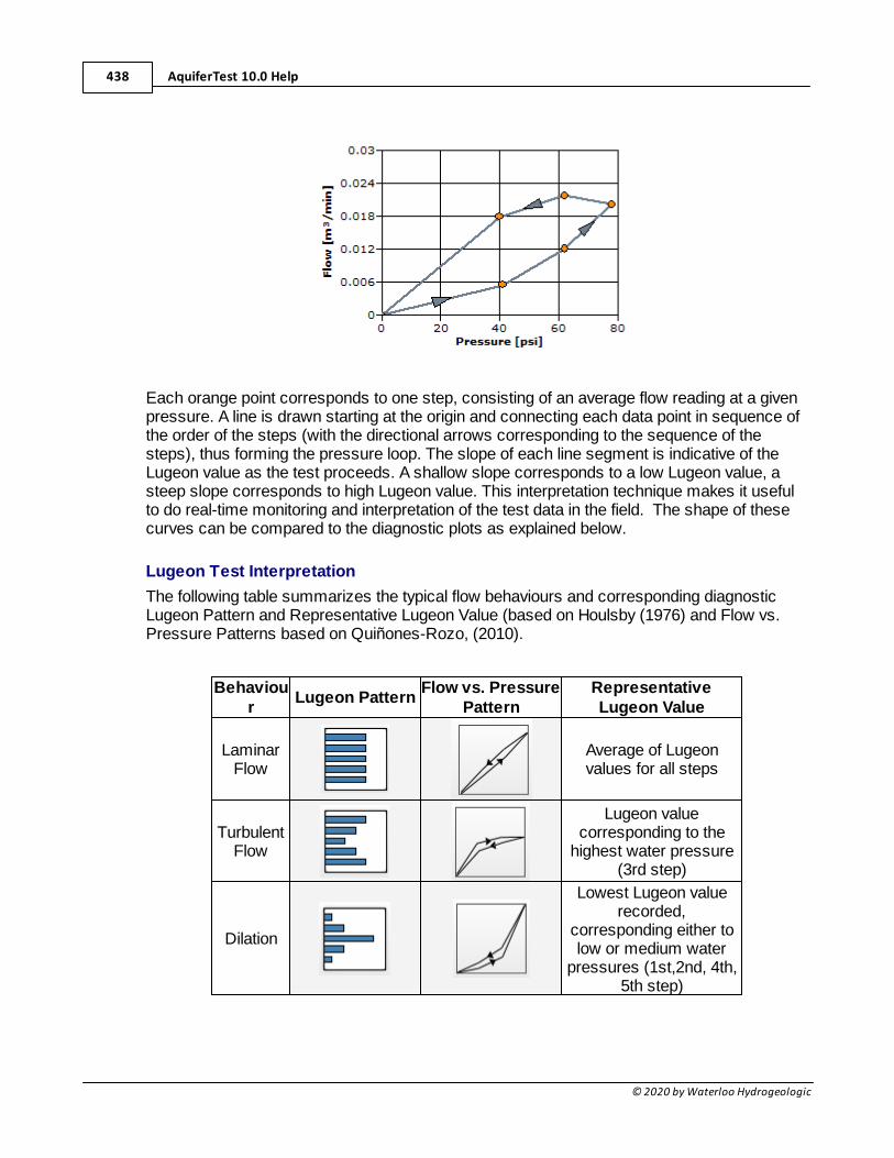
AquiferTest 10.0 Help438
© 2020 by Waterloo Hydrogeologic
Each orange point corresponds to one step, consisting of an average flow reading at a givenpressure. A line is drawn starting at the origin and connecting each data point in sequence ofthe order of the steps (with the directional arrows corresponding to the sequence of thesteps), thus forming the pressure loop. The slope of each line segment is indicative of theLugeon value as the test proceeds. A shallow slope corresponds to a low Lugeon value, asteep slope corresponds to high Lugeon value. This interpretation technique makes it usefulto do real-time monitoring and interpretation of the test data in the field. The shape of thesecurves can be compared to the diagnostic plots as explained below.
Lugeon Test Interpretation
The following table summarizes the typical flow behaviours and corresponding diagnosticLugeon Pattern and Representative Lugeon Value (based on Houlsby (1976) and Flow vs.Pressure Patterns based on Quiñones-Rozo, (2010).
Behaviour
Lugeon PatternFlow vs. Pressure
PatternRepresentativeLugeon Value
LaminarFlow
Average of Lugeonvalues for all steps
TurbulentFlow
Lugeon valuecorresponding to the
highest water pressure(3rd step)
Dilation
Lowest Lugeon valuerecorded,
corresponding either tolow or medium water
pressures (1st,2nd, 4th,5th step)
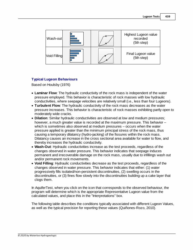
Lugeon Tests 439
© 2020 by Waterloo Hydrogeologic
Wash-outHighest Lugeon value
recorded(5th step)
Void FillingFinal Lugeon value
(5th step)
Typical Lugeon Behaviours
Based on Houlsby (1976)
· Laminar Flow: The hydraulic conductivity of the rock mass is independent of the waterpressure employed. This behavior is characteristic of rock masses with low hydraulicconductivities, where seepage velocities are relatively small (i.e., less than four Lugeons).
· Turbulent Flow: The hydraulic conductivity of the rock mass decreases as the waterpressure increases. This behavior is characteristic of rock masses exhibiting partly open tomoderately wide cracks.
· Dilation: Similar hydraulic conductivities are observed at low and medium pressures;however, a much greater value is recorded at the maximum pressure. This behavior –which is sometimes also observed at medium pressures – occurs when the waterpressure applied is greater than the minimum principal stress of the rock mass, thuscausing a temporary dilatancy (hydro-jacking) of the fissures within the rock mass.Dilatancy causes an increase in the cross sectional area available for water to flow, andthereby increases the hydraulic conductivity.
· Wash-Out: Hydraulic conductivities increase as the test proceeds, regardless of thechanges observed in water pressure. This behavior indicates that seepage inducespermanent and irrecoverable damage on the rock mass, usually due to infillings wash outand/or permanent rock movements.
· Void Filling: Hydraulic conductivities decrease as the test proceeds, regardless of thechanges observed in water pressure. This behavior indicates that either: (1) waterprogressively fills isolated/non-persistent discontinuities, (2) swelling occurs in thediscontinuities, or (3) fines flow slowly into the discontinuities building up a cake layer thatclogs them.
In AquiferTest, when you click on the icon that corresponds to the observed behaviour, theprogram will determine which is the appropriate Representative Lugeon value from thecalculated values, and place this in the "Interpretations" box.
The following table describes the conditions typically associated with different Lugeon Values,as well as the typical precision for reporting these values (Quiñones-Rozo, 2010).
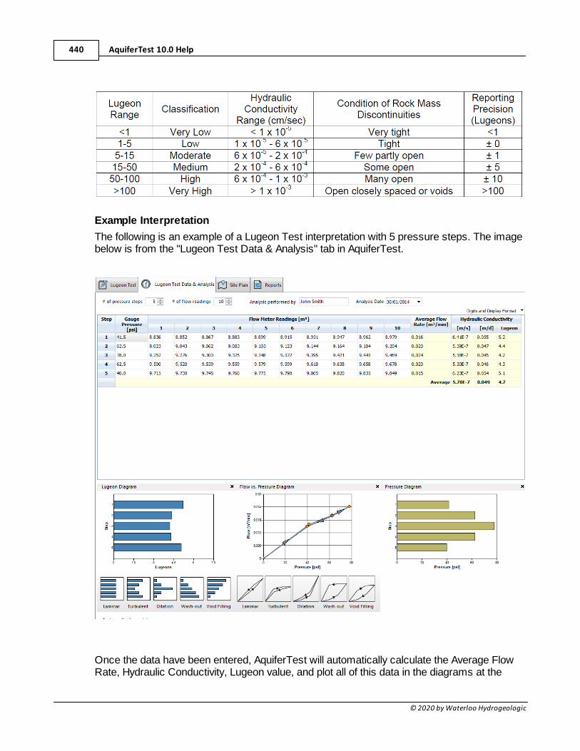
AquiferTest 10.0 Help440
© 2020 by Waterloo Hydrogeologic
Example Interpretation
The following is an example of a Lugeon Test interpretation with 5 pressure steps. The imagebelow is from the "Lugeon Test Data & Analysis" tab in AquiferTest.
Once the data have been entered, AquiferTest will automatically calculate the Average FlowRate, Hydraulic Conductivity, Lugeon value, and plot all of this data in the diagrams at the
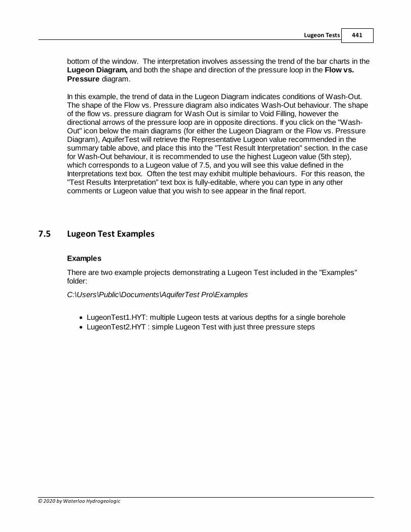
Lugeon Tests 441
© 2020 by Waterloo Hydrogeologic
bottom of the window. The interpretation involves assessing the trend of the bar charts in theLugeon Diagram, and both the shape and direction of the pressure loop in the Flow vs.Pressure diagram.
In this example, the trend of data in the Lugeon Diagram indicates conditions of Wash-Out.The shape of the Flow vs. Pressure diagram also indicates Wash-Out behaviour. The shapeof the flow vs. pressure diagram for Wash Out is similar to Void Filling, however thedirectional arrows of the pressure loop are in opposite directions. If you click on the "Wash-Out" icon below the main diagrams (for either the Lugeon Diagram or the Flow vs. PressureDiagram), AquiferTest will retrieve the Representative Lugeon value recommended in thesummary table above, and place this into the "Test Result Interpretation" section. In the casefor Wash-Out behaviour, it is recommended to use the highest Lugeon value (5th step),which corresponds to a Lugeon value of 7.5, and you will see this value defined in theInterpretations text box. Often the test may exhibit multiple behaviours. For this reason, the"Test Results Interpretation" text box is fully-editable, where you can type in any othercomments or Lugeon value that you wish to see appear in the final report.
7.5 Lugeon Test Examples
Examples
There are two example projects demonstrating a Lugeon Test included in the "Examples"folder:
C:\Users\Public\Documents\AquiferTest Pro\Examples
· LugeonTest1.HYT: multiple Lugeon tests at various depths for a single borehole
· LugeonTest2.HYT : simple Lugeon Test with just three pressure steps
AquiferTest 10.0 Help442
© 2020 by Waterloo Hydrogeologic
8 Data Pre-Processing
Surrounding water level trends and barometric effects may have a significant impact on thewater levels recorded during your pumping test. AquiferTest now includes the tools toanalyze these affects to determine if they played a role in your pumping test. Using the datapre-processor utilities, you can correct your water level measurements for baseline trends(trend effects) and barometric pressure changes. This corrected drawdown data should thenbe used for the calculation of the aquifer parameters.
NOTE: Data Pre-Processing tools are available in AquiferTestPro only.
According to the U.S. EPA-SOP for Pumping Tests (Osborne, 1993), data pre-processing isa critical step in any pumping test analysis:
“Collecting data on pre-test water levels is essential if the analysis of the test data is tobe completely successful. The baseline data provides a basis for correcting the testdata to account for on-going regional water level changes. Although the wells on-site arethe main target for baseline measurements, it is important to measure key wellsadjacent to the site and to account for off-site pumping which may affect the testresults.” (Osborne, 1993)
"During the baseline trend observation period, it is desirable to monitor and record thebarometric pressure to a sensitivity of +/- 0.01 inches of mercury. The monitoringshould continue throughout the test and for at least one day to a week after thecompletion of the recovery measurement period. This data, when combined with thewater level trends measured during the baseline period, can be used to correct for theeffects of barometric changes that may occur during the test.” (Osborne, 1993)
Sections
The following sections are available describing barometric and trend correction functionality inAquiferTest Pro:
· Baseline Trend Analysis and Correction
· Customized Water Level Trends
· Barometric Trend Analysis and Correction
· Modifying Corrections
· Deleting Corrections
Data Pre-Processing 443
© 2020 by Waterloo Hydrogeologic
8.1 Baseline Trend Analysis and Correction
Historic and baseline water level trends can impact the drawdown data you recordduring your pumping test. Surrounding pumping activities, or even surface disturbancessuch as trains, can effect the water level during the pumping test. It is important toidentify all major disturbances (especially cyclic activities) which may impact the testdata. Enough measurements have to be made to fully characterize the pre-pumpingtrends of these activities (Osborne, 1993). Therefore, the user must record water levelsnear or at the well, either before or after the test. (For example, daily water levelmeasurements taken 1 week prior to the test, up to the day of the test, is a generalrecommendation from the EPA.) Using the measured trend data, AquiferTest performsa line fit to calculate a trend coefficient. The program will also run a “t-test”, to see if thetrend is significant. If significant, the data is then corrected based on this trend.
As an example, a trend analysis shows a trend of water levels rising 2cm/hr due tosurrounding activities. During the pumping test, for a water level recorded 3 hours afterthe test begins, you need to add 6 cm to the water level measurements in order toconduct a representative analysis of the aquifer.
If the data trend is already known (i.e. water level fluctuations due to tidal or ebb-flows),then the trend can be defined using a simple linear time-dependent correction. For moredetails, "Customized Water Level Trends".
A trend analysis generally involves the following steps:
1. Collect baseline trend data (time vs. water level) prior to, and after, the test;measurements should be recorded at a location that will not be influenced by thepumping test activities.
2.AquiferTest calculates a baseline trend, and trend coefficient. AquiferTestcalculates the simple linear regression of the measured values and runs a t-test todetermine if the trend is significant.
3. Apply the trend coefficient to the data collected during the pumping test (time vs.water level), resulting in “corrected drawdown” measurements.
4. Use the corrected drawdown values for the calculation of the aquifer parameters.
Theory
The general formula for trend computation is a polynomial and a function of the time t:
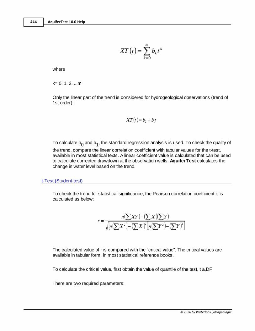
AquiferTest 10.0 Help444
© 2020 by Waterloo Hydrogeologic
where
k= 0, 1, 2, ...m
Only the linear part of the trend is considered for hydrogeological observations (trend of1st order):
To calculate b0 and b1, the standard regression analysis is used. To check the quality of
the trend, compare the linear correlation coefficient with tabular values for the t-test,available in most statistical texts. A linear coefficient value is calculated that can be usedto calculate corrected drawdown at the observation wells. AquiferTest calculates thechange in water level based on the trend.
t-Test (Student-test)
To check the trend for statistical significance, the Pearson correlation coefficient r, iscalculated as below:
The calculated value of r is compared with the “critical value”. The critical values areavailable in tabular form, in most statistical reference books.
To calculate the critical value, first obtain the value of quantile of the test, t a,DF
There are two required parameters:
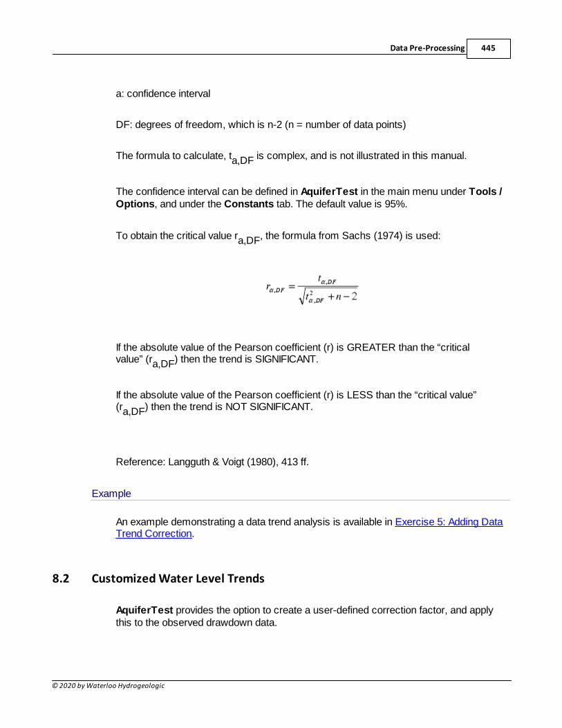
Data Pre-Processing 445
© 2020 by Waterloo Hydrogeologic
a: confidence interval
DF: degrees of freedom, which is n-2 (n = number of data points)
The formula to calculate, ta,DF is complex, and is not illustrated in this manual.
The confidence interval can be defined in AquiferTest in the main menu under Tools /Options, and under the Constants tab. The default value is 95%.
To obtain the critical value ra,DF, the formula from Sachs (1974) is used:
If the absolute value of the Pearson coefficient (r) is GREATER than the “criticalvalue” (ra,DF) then the trend is SIGNIFICANT.
If the absolute value of the Pearson coefficient (r) is LESS than the “critical value”(ra,DF) then the trend is NOT SIGNIFICANT.
Reference: Langguth & Voigt (1980), 413 ff.
Example
An example demonstrating a data trend analysis is available in Exercise 5: Adding DataTrend Correction.
8.2 Customized Water Level Trends
AquiferTest provides the option to create a user-defined correction factor, and applythis to the observed drawdown data.
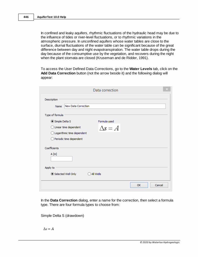
AquiferTest 10.0 Help446
© 2020 by Waterloo Hydrogeologic
In confined and leaky aquifers, rhythmic fluctuations of the hydraulic head may be due tothe influence of tides or river-level fluctuations, or to rhythmic variations in theatmospheric pressure. In unconfined aquifers whose water tables are close to thesurface, diurnal fluctuations of the water table can be significant because of the greatdifference between day and night evapotranspiration. The water table drops during theday because of the consumptive use by the vegetation, and recovers during the nightwhen the plant stomata are closed (Kruseman and de Ridder, 1991).
To access the User Defined Data Corrections, go to the Water Levels tab, click on theAdd Data Correction button (not the arrow beside it) and the following dialog willappear:
In the Data Correction dialog, enter a name for the correction, then select a formulatype. There are four formula types to choose from:
Simple Delta S (drawdown)
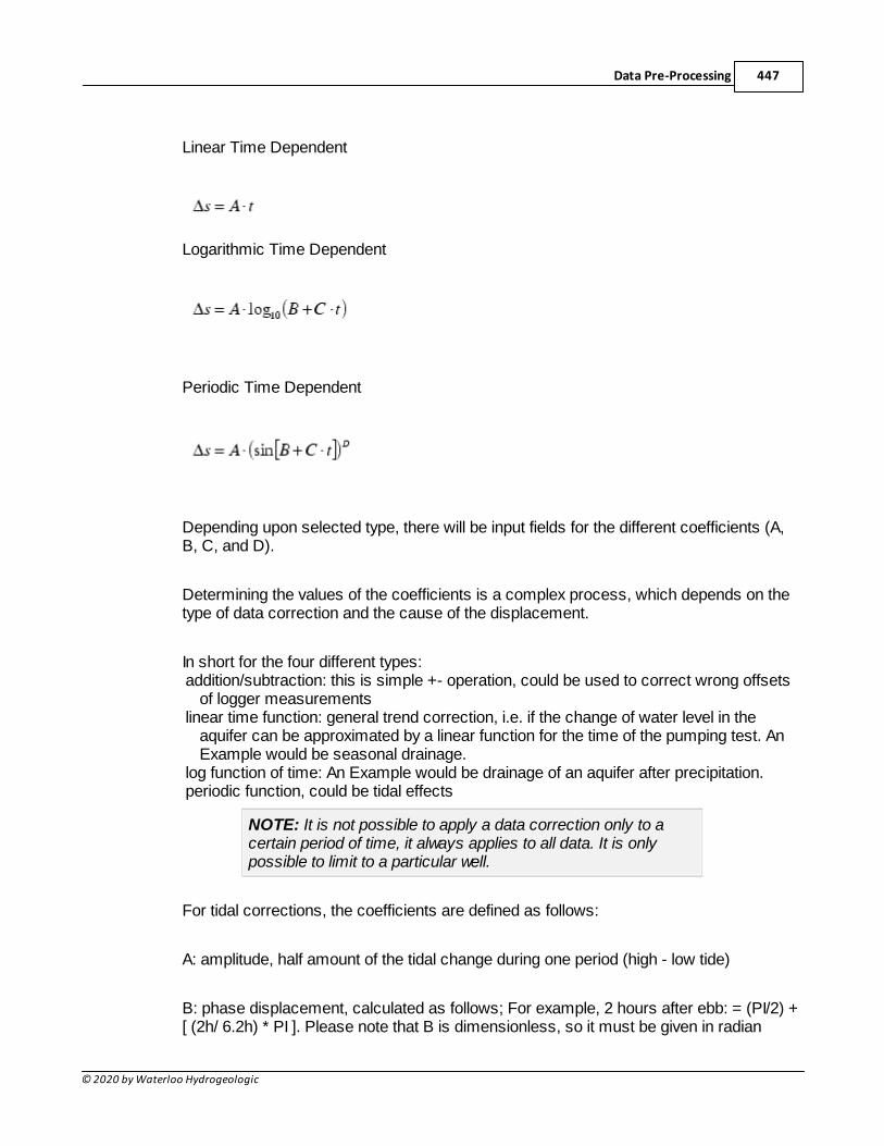
Data Pre-Processing 447
© 2020 by Waterloo Hydrogeologic
Linear Time Dependent
Logarithmic Time Dependent
Periodic Time Dependent
Depending upon selected type, there will be input fields for the different coefficients (A,B, C, and D).
Determining the values of the coefficients is a complex process, which depends on thetype of data correction and the cause of the displacement.
In short for the four different types:addition/subtraction: this is simple +- operation, could be used to correct wrong offsets
of logger measurementslinear time function: general trend correction, i.e. if the change of water level in the
aquifer can be approximated by a linear function for the time of the pumping test. AnExample would be seasonal drainage.
log function of time: An Example would be drainage of an aquifer after precipitation.periodic function, could be tidal effects
NOTE: It is not possible to apply a data correction only to acertain period of time, it always applies to all data. It is onlypossible to limit to a particular well.
For tidal corrections, the coefficients are defined as follows:
A: amplitude, half amount of the tidal change during one period (high - low tide)
B: phase displacement, calculated as follows; For example, 2 hours after ebb: = (PI/2) +[ (2h/ 6.2h) * PI ]. Please note that B is dimensionless, so it must be given in radian
AquiferTest 10.0 Help448
© 2020 by Waterloo Hydrogeologic
C: period = ( PI/12 h 25 min)
D: = 1
The range of application indicates whether the correction applies only to the current welldata set, or to all wells. For example, a local trend usually affects all wells, while aperiodic correction of the Tidal influences depends on the distance to the sea, andtherefore must be unique for each observation well.
When defining the coefficients, be aware of the sign (positive or negative). The result ofthe calculation is added to the drawdown values; i.e. if the value is positive, thedrawdown increases; for negative values, the drawdown decreases. For example, if youhave a local trend where the water table decreases 1cm/d, the value must then bedefined as negative, so that the appropriate amount is subtracted from the observeddrawdown. Alternatively, if the trend shows the water table elevation rising 1cm/day, thevalue must then be defined as positive, so that the appropriate amount is added to theobserved drawdown data.
Upon clicking OK, the data correction will be applied to the measured drawdown data,and an additional column will appear in the data table. This column will contain thecorrected drawdown using this data correction; the corrected drawdown will be used inthe analysis to calculate the aquifer parameters.
8.3 Barometric Trend Analysis and Correction
During the pumping test, changes in the barometric pressure can have an affect on therecorded drawdown data, and should be considered during the data analysis.AquiferTest includes the tools to correct drawdown data for barometric effects, usingdata pre-processor tools. Barometric pre-processing generally involves the followingsteps:
1. Collecting data (barometric pressure vs. water level) prior to, or after, the test;2. Use this data to calculate the barometric efficiency (BE) of the aquifer.3. During the pumping test, collect time vs. water level data AND time vs. barometric
pressure data.4. Using the BE value, determine the equivalent water level measurement at the
observed time. If the pressure is not recorded at the same time as the water levels,linear interpolation may be used to find and correct the next available water levelmeasurement.
5. Apply the correction to the observed drawdown data.6. Use the corrected water levels for determining the aquifer parameters.
Theory
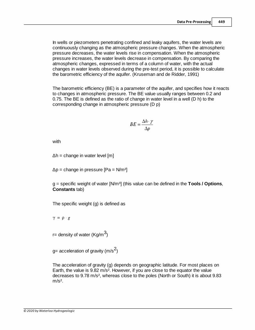
Data Pre-Processing 449
© 2020 by Waterloo Hydrogeologic
In wells or piezometers penetrating confined and leaky aquifers, the water levels arecontinuously changing as the atmospheric pressure changes. When the atmosphericpressure decreases, the water levels rise in compensation. When the atmosphericpressure increases, the water levels decrease in compensation. By comparing theatmospheric changes, expressed in terms of a column of water, with the actualchanges in water levels observed during the pre-test period, it is possible to calculatethe barometric efficiency of the aquifer. (Kruseman and de Ridder, 1991)
The barometric efficiency (BE) is a parameter of the aquifer, and specifies how it reactsto changes in atmospheric pressure. The BE value usually ranges between 0.2 and0.75. The BE is defined as the ratio of change in water level in a well (D h) to thecorresponding change in atmospheric pressure (D p)
with
∆h = change in water level [m]
∆p = change in pressure [Pa = N/m²]
g = specific weight of water [N/m³] (this value can be defined in the Tools / Options,Constants tab)
The specific weight (g) is defined as
r= density of water (Kg/m3)
g= acceleration of gravity (m/s2)
The acceleration of gravity (g) depends on geographic latitude. For most places onEarth, the value is 9.82 m/s². However, if you are close to the equator the valuedecreases to 9.78 m/s², whereas close to the poles (North or South) it is about 9.83m/s².
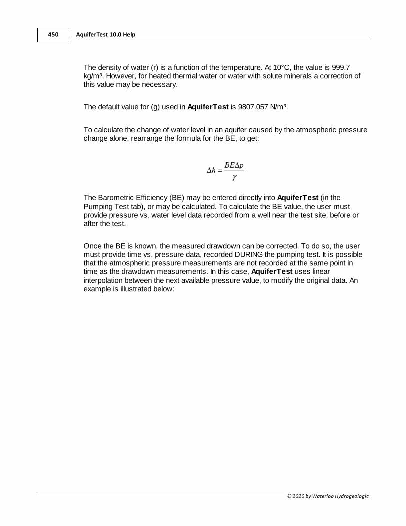
AquiferTest 10.0 Help450
© 2020 by Waterloo Hydrogeologic
The density of water (r) is a function of the temperature. At 10°C, the value is 999.7kg/m³. However, for heated thermal water or water with solute minerals a correction ofthis value may be necessary.
The default value for (g) used in AquiferTest is 9807.057 N/m³.
To calculate the change of water level in an aquifer caused by the atmospheric pressurechange alone, rearrange the formula for the BE, to get:
The Barometric Efficiency (BE) may be entered directly into AquiferTest (in thePumping Test tab), or may be calculated. To calculate the BE value, the user mustprovide pressure vs. water level data recorded from a well near the test site, before orafter the test.
Once the BE is known, the measured drawdown can be corrected. To do so, the usermust provide time vs. pressure data, recorded DURING the pumping test. It is possiblethat the atmospheric pressure measurements are not recorded at the same point intime as the drawdown measurements. In this case, AquiferTest uses linearinterpolation between the next available pressure value, to modify the original data. Anexample is illustrated below:
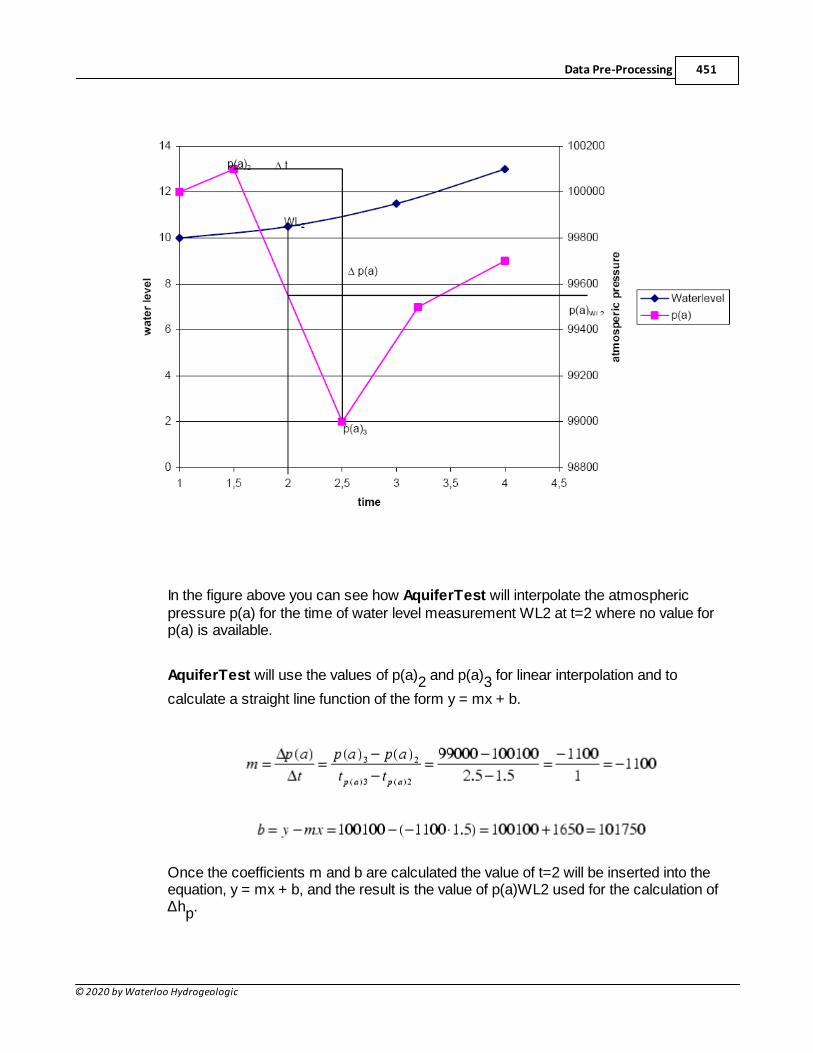
Data Pre-Processing 451
© 2020 by Waterloo Hydrogeologic
In the figure above you can see how AquiferTest will interpolate the atmosphericpressure p(a) for the time of water level measurement WL2 at t=2 where no value forp(a) is available.
AquiferTest will use the values of p(a)2 and p(a)3 for linear interpolation and to
calculate a straight line function of the form y = mx + b.
Once the coefficients m and b are calculated the value of t=2 will be inserted into theequation, y = mx + b, and the result is the value of p(a)WL2 used for the calculation of∆hp.
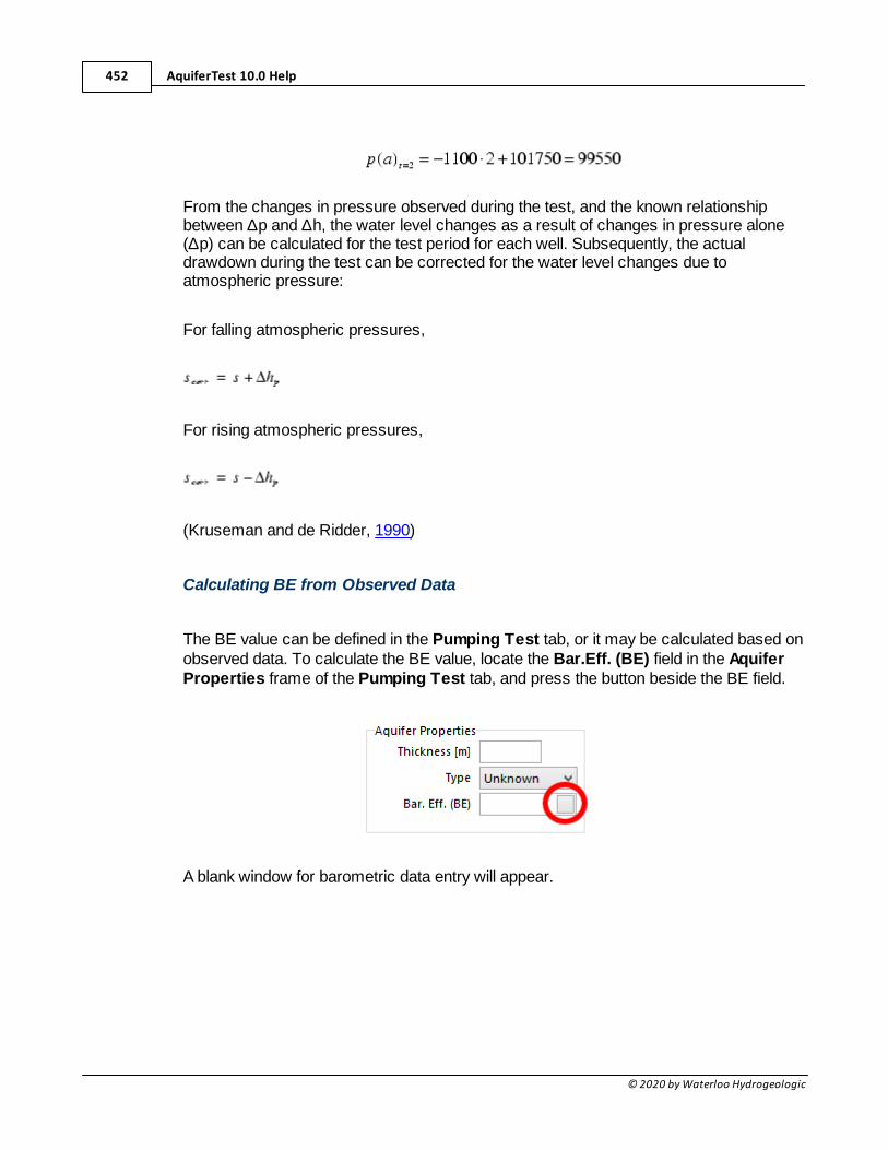
AquiferTest 10.0 Help452
© 2020 by Waterloo Hydrogeologic
From the changes in pressure observed during the test, and the known relationshipbetween ∆p and ∆h, the water level changes as a result of changes in pressure alone(∆p) can be calculated for the test period for each well. Subsequently, the actualdrawdown during the test can be corrected for the water level changes due toatmospheric pressure:
For falling atmospheric pressures,
For rising atmospheric pressures,
(Kruseman and de Ridder, 1990)
Calculating BE from Observed Data
The BE value can be defined in the Pumping Test tab, or it may be calculated based onobserved data. To calculate the BE value, locate the Bar.Eff. (BE) field in the AquiferProperties frame of the Pumping Test tab, and press the button beside the BE field.
A blank window for barometric data entry will appear.
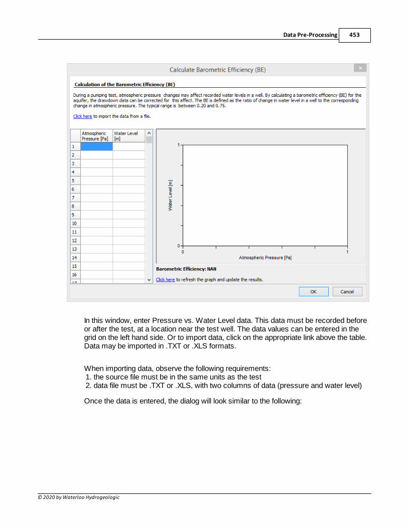
Data Pre-Processing 453
© 2020 by Waterloo Hydrogeologic
In this window, enter Pressure vs. Water Level data. This data must be recorded beforeor after the test, at a location near the test well. The data values can be entered in thegrid on the left hand side. Or to import data, click on the appropriate link above the table.Data may be imported in .TXT or .XLS formats.
When importing data, observe the following requirements:1. the source file must be in the same units as the test2. data file must be .TXT or .XLS, with two columns of data (pressure and water level)
Once the data is entered, the dialog will look similar to the following:
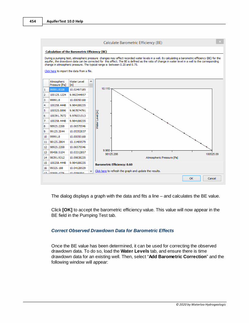
AquiferTest 10.0 Help454
© 2020 by Waterloo Hydrogeologic
The dialog displays a graph with the data and fits a line – and calculates the BE value.
Click [OK] to accept the barometric efficiency value. This value will now appear in theBE field in the Pumping Test tab.
Correct Observed Drawdown Data for Barometric Effects
Once the BE value has been determined, it can be used for correcting the observeddrawdown data. To do so, load the Water Levels tab, and ensure there is timedrawdown data for an existing well. Then, select “Add Barometric Correction” and thefollowing window will appear:
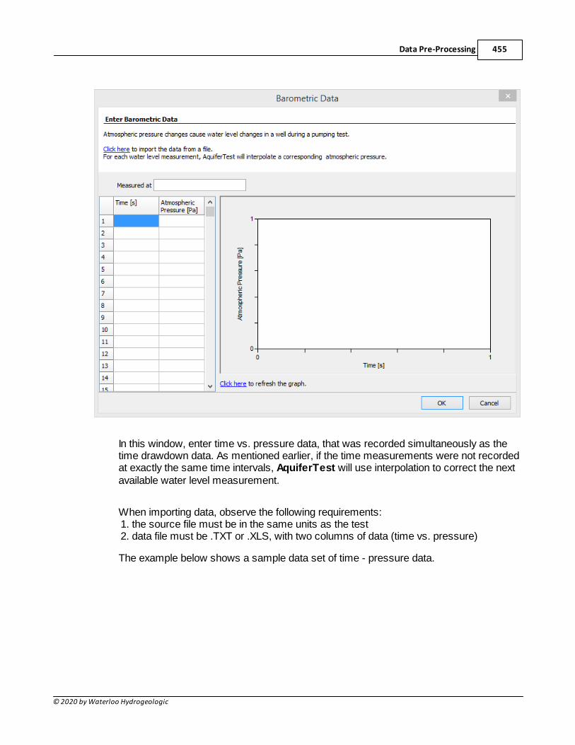
Data Pre-Processing 455
© 2020 by Waterloo Hydrogeologic
In this window, enter time vs. pressure data, that was recorded simultaneously as thetime drawdown data. As mentioned earlier, if the time measurements were not recordedat exactly the same time intervals, AquiferTest will use interpolation to correct the nextavailable water level measurement.
When importing data, observe the following requirements:1. the source file must be in the same units as the test2. data file must be .TXT or .XLS, with two columns of data (time vs. pressure)
The example below shows a sample data set of time - pressure data.
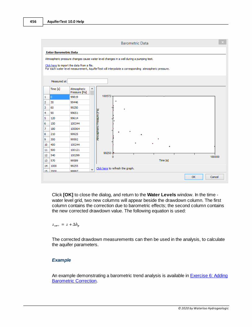
AquiferTest 10.0 Help456
© 2020 by Waterloo Hydrogeologic
Click [OK] to close the dialog, and return to the Water Levels window. In the time -water level grid, two new columns will appear beside the drawdown column. The firstcolumn contains the correction due to barometric effects; the second column containsthe new corrected drawdown value. The following equation is used:
The corrected drawdown measurements can then be used in the analysis, to calculatethe aquifer parameters.
Example
An example demonstrating a barometric trend analysis is available in Exercise 6: AddingBarometric Correction.
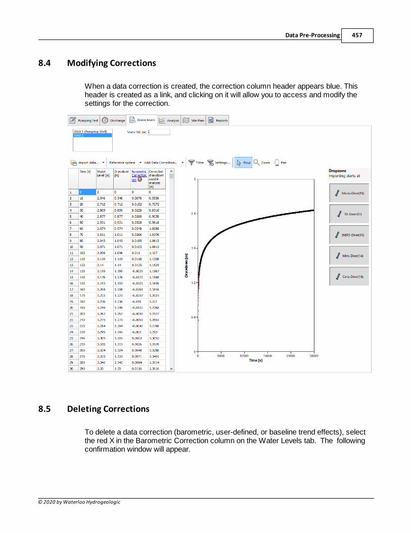
Data Pre-Processing 457
© 2020 by Waterloo Hydrogeologic
8.4 Modifying Corrections
When a data correction is created, the correction column header appears blue. Thisheader is created as a link, and clicking on it will allow you to access and modify thesettings for the correction.
8.5 Deleting Corrections
To delete a data correction (barometric, user-defined, or baseline trend effects), selectthe red X in the Barometric Correction column on the Water Levels tab. The followingconfirmation window will appear.

AquiferTest 10.0 Help458
© 2020 by Waterloo Hydrogeologic
This option is available only if the cursor is in the table and in a column with correctiondata.
Mapping and Contouring 459
© 2020 by Waterloo Hydrogeologic
9 Mapping and Contouring
AquiferTest now includes enhanced mapping features, which allow you to displaycontouring and color shading of drawdown data, along with site maps, in the Site Mapwindow.
NOTE: Contouring, Color Shading, Regional Flow andStreamlines are available in AquiferTest Pro only.
Sections
The following sections are available describing mapping and contouring functionality inAquiferTest Pro:
· About the Interface
· Data Series
· Contouring and Color Shading Propertieso Contour lines tabo Color Shading tab
· Regional Flow
· Streamlines
· Surfer Scripting
· Base Maps using a Tile Server
· Example
9.1 About the Interface
The mapping and contouring options are available under the Site Plan tab, displayed inthe image below:
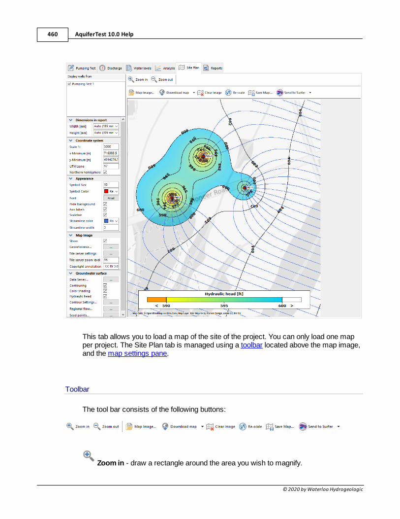
AquiferTest 10.0 Help460
© 2020 by Waterloo Hydrogeologic
This tab allows you to load a map of the site of the project. You can only load one mapper project. The Site Plan tab is managed using a toolbar located above the map image,and the map settings pane.
Toolbar
The tool bar consists of the following buttons:
Zoom in - draw a rectangle around the area you wish to magnify.
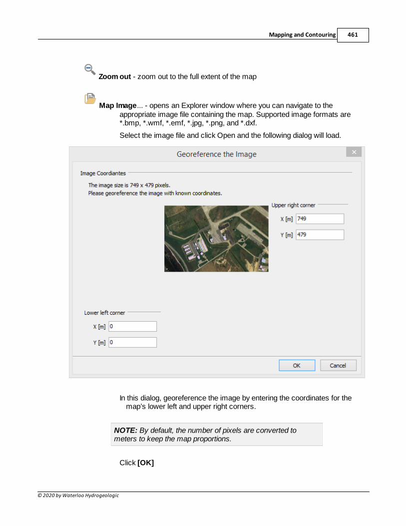
Mapping and Contouring 461
© 2020 by Waterloo Hydrogeologic
Zoom out - zoom out to the full extent of the map
Map Image... - opens an Explorer window where you can navigate to theappropriate image file containing the map. Supported image formats are*.bmp, *.wmf, *.emf, *.jpg, *.png, and *.dxf.
Select the image file and click Open and the following dialog will load.
In this dialog, georeference the image by entering the coordinates for themap’s lower left and upper right corners.
NOTE: By default, the number of pixels are converted tometers to keep the map proportions.
Click [OK]
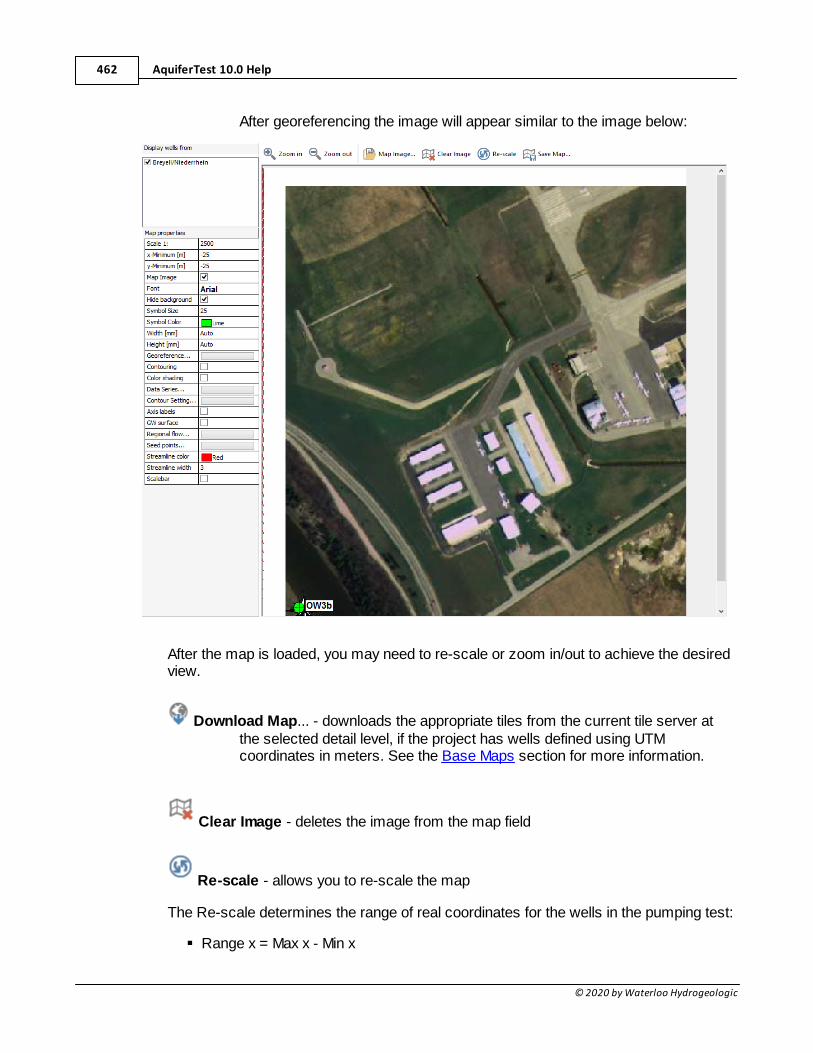
AquiferTest 10.0 Help462
© 2020 by Waterloo Hydrogeologic
After georeferencing the image will appear similar to the image below:
After the map is loaded, you may need to re-scale or zoom in/out to achieve the desiredview.
Download Map... - downloads the appropriate tiles from the current tile server atthe selected detail level, if the project has wells defined using UTMcoordinates in meters. See the Base Maps section for more information.
Clear Image - deletes the image from the map field
Re-scale - allows you to re-scale the map
The Re-scale determines the range of real coordinates for the wells in the pumping test:
§ Range x = Max x - Min x
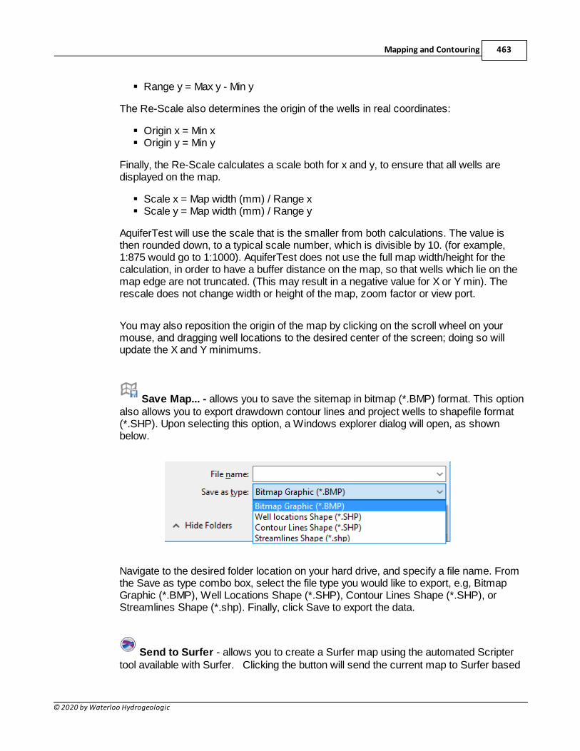
Mapping and Contouring 463
© 2020 by Waterloo Hydrogeologic
§ Range y = Max y - Min y
The Re-Scale also determines the origin of the wells in real coordinates:
§ Origin x = Min x§ Origin y = Min y
Finally, the Re-Scale calculates a scale both for x and y, to ensure that all wells aredisplayed on the map.
§ Scale x = Map width (mm) / Range x§ Scale y = Map width (mm) / Range y
AquiferTest will use the scale that is the smaller from both calculations. The value isthen rounded down, to a typical scale number, which is divisible by 10. (for example,1:875 would go to 1:1000). AquiferTest does not use the full map width/height for thecalculation, in order to have a buffer distance on the map, so that wells which lie on themap edge are not truncated. (This may result in a negative value for X or Y min). Therescale does not change width or height of the map, zoom factor or view port.
You may also reposition the origin of the map by clicking on the scroll wheel on yourmouse, and dragging well locations to the desired center of the screen; doing so willupdate the X and Y minimums.
Save Map... - allows you to save the sitemap in bitmap (*.BMP) format. This optionalso allows you to export drawdown contour lines and project wells to shapefile format(*.SHP). Upon selecting this option, a Windows explorer dialog will open, as shownbelow.
Navigate to the desired folder location on your hard drive, and specify a file name. Fromthe Save as type combo box, select the file type you would like to export, e.g, BitmapGraphic (*.BMP), Well Locations Shape (*.SHP), Contour Lines Shape (*.SHP), orStreamlines Shape (*.shp). Finally, click Save to export the data.
Send to Surfer - allows you to create a Surfer map using the automated Scriptertool available with Surfer. Clicking the button will send the current map to Surfer based
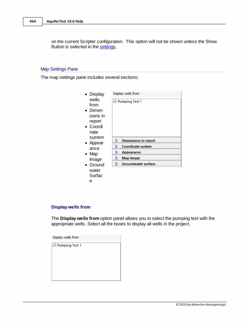
AquiferTest 10.0 Help464
© 2020 by Waterloo Hydrogeologic
on the current Scripter configuration. This option will not be shown unless the ShowButton is selected in the settings.
Map Settings Pane
The map settings pane includes several sections:
· Displaywellsfrom
· Dimensions inreport
· Coordinatesystem
· Appearance
· MapImage
· GroundwaterSurface
Display wells from
The Display wells from option panel allows you to select the pumping test with theappropriate wells. Select all the boxes to display all wells in the project.
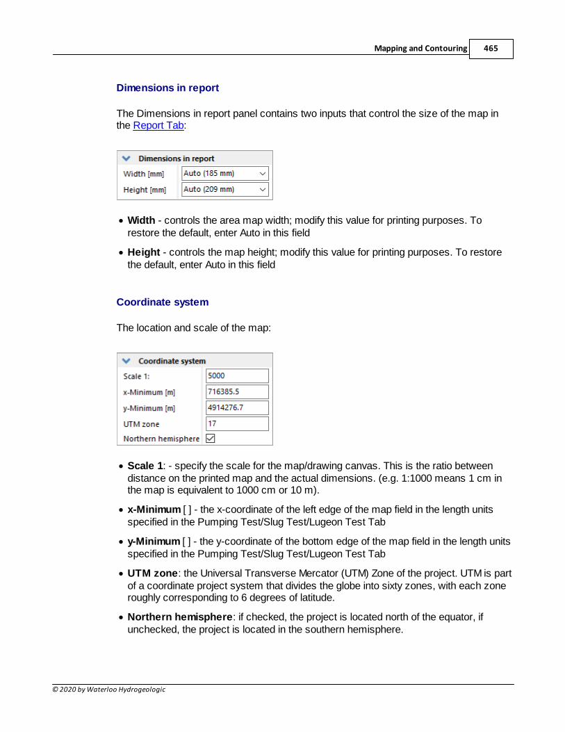
Mapping and Contouring 465
© 2020 by Waterloo Hydrogeologic
Dimensions in report
The Dimensions in report panel contains two inputs that control the size of the map inthe Report Tab:
· Width - controls the area map width; modify this value for printing purposes. Torestore the default, enter Auto in this field
· Height - controls the map height; modify this value for printing purposes. To restorethe default, enter Auto in this field
Coordinate system
The location and scale of the map:
· Scale 1: - specify the scale for the map/drawing canvas. This is the ratio betweendistance on the printed map and the actual dimensions. (e.g. 1:1000 means 1 cm inthe map is equivalent to 1000 cm or 10 m).
· x-Minimum [ ] - the x-coordinate of the left edge of the map field in the length unitsspecified in the Pumping Test/Slug Test/Lugeon Test Tab
· y-Minimum [ ] - the y-coordinate of the bottom edge of the map field in the length unitsspecified in the Pumping Test/Slug Test/Lugeon Test Tab
· UTM zone: the Universal Transverse Mercator (UTM) Zone of the project. UTM is partof a coordinate project system that divides the globe into sixty zones, with each zoneroughly corresponding to 6 degrees of latitude.
· Northern hemisphere: if checked, the project is located north of the equator, ifunchecked, the project is located in the southern hemisphere.
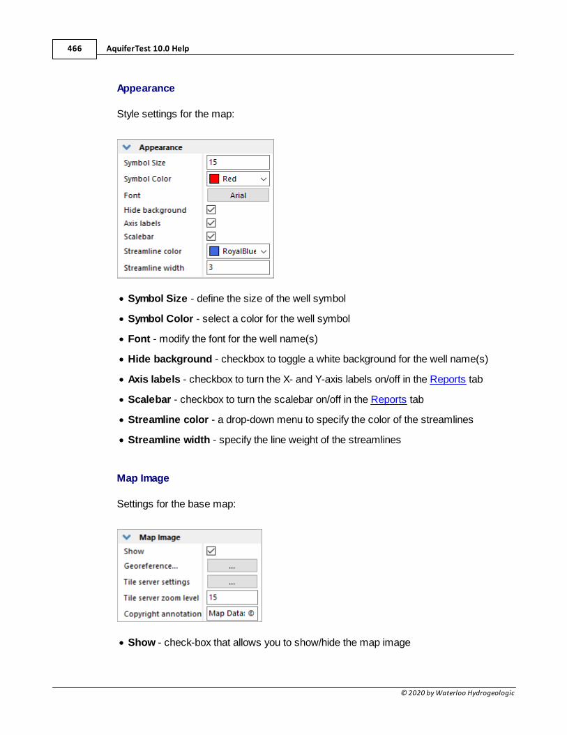
AquiferTest 10.0 Help466
© 2020 by Waterloo Hydrogeologic
Appearance
Style settings for the map:
· Symbol Size - define the size of the well symbol
· Symbol Color - select a color for the well symbol
· Font - modify the font for the well name(s)
· Hide background - checkbox to toggle a white background for the well name(s)
· Axis labels - checkbox to turn the X- and Y-axis labels on/off in the Reports tab
· Scalebar - checkbox to turn the scalebar on/off in the Reports tab
· Streamline color - a drop-down menu to specify the color of the streamlines
· Streamline width - specify the line weight of the streamlines
Map Image
Settings for the base map:
· Show - check-box that allows you to show/hide the map image
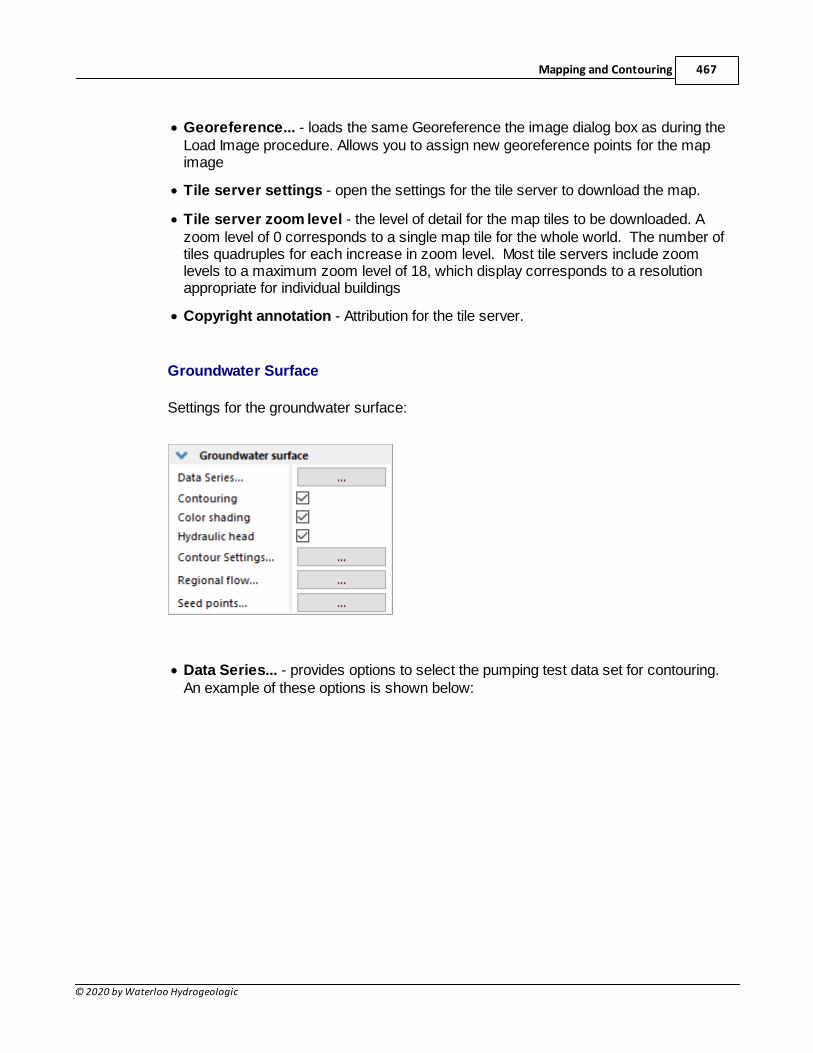
Mapping and Contouring 467
© 2020 by Waterloo Hydrogeologic
· Georeference... - loads the same Georeference the image dialog box as during theLoad Image procedure. Allows you to assign new georeference points for the mapimage
· Tile server settings - open the settings for the tile server to download the map.
· Tile server zoom level - the level of detail for the map tiles to be downloaded. Azoom level of 0 corresponds to a single map tile for the whole world. The number oftiles quadruples for each increase in zoom level. Most tile servers include zoomlevels to a maximum zoom level of 18, which display corresponds to a resolutionappropriate for individual buildings
· Copyright annotation - Attribution for the tile server.
Groundwater Surface
Settings for the groundwater surface:
· Data Series... - provides options to select the pumping test data set for contouring.An example of these options is shown below:
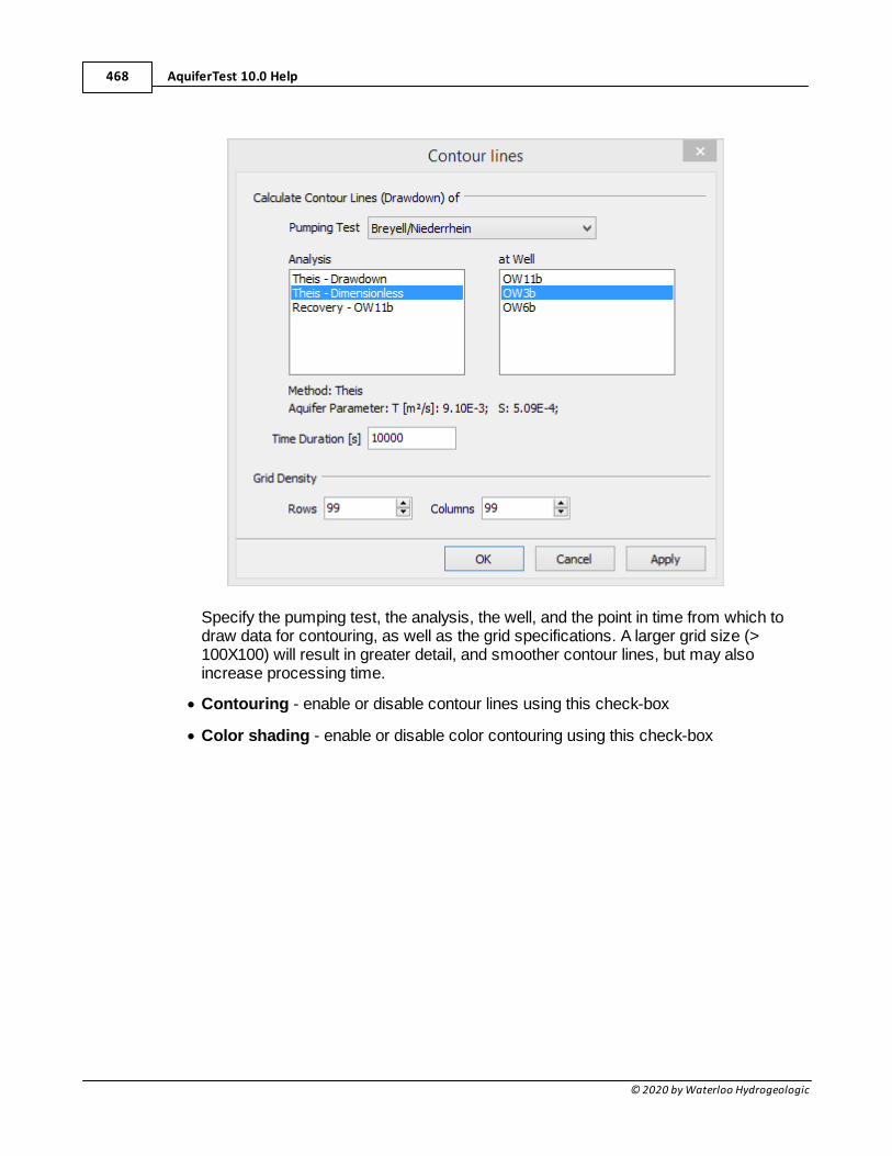
AquiferTest 10.0 Help468
© 2020 by Waterloo Hydrogeologic
Specify the pumping test, the analysis, the well, and the point in time from which todraw data for contouring, as well as the grid specifications. A larger grid size (>100X100) will result in greater detail, and smoother contour lines, but may alsoincrease processing time.
· Contouring - enable or disable contour lines using this check-box
· Color shading - enable or disable color contouring using this check-box
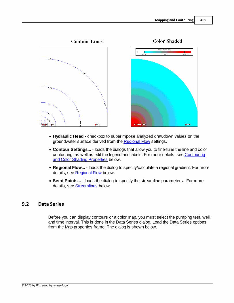
Mapping and Contouring 469
© 2020 by Waterloo Hydrogeologic
· Hydraulic Head - checkbox to superimpose analyzed drawdown values on thegroundwater surface derived from the Regional Flow settings.
· Contour Settings... - loads the dialogs that allow you to fine-tune the line and colorcontouring, as well as edit the legend and labels. For more details, see Contouringand Color Shading Properties below.
· Regional Flow... - loads the dialog to specify/calculate a regional gradient. For moredetails, see Regional Flow below.
· Seed Points... - loads the dialog to specify the streamline parameters. For moredetails, see Streamlines below.
9.2 Data Series
Before you can display contours or a color map, you must select the pumping test, well,and time interval. This is done in the Data Series dialog. Load the Data Series optionsfrom the Map properties frame. The dialog is shown below.
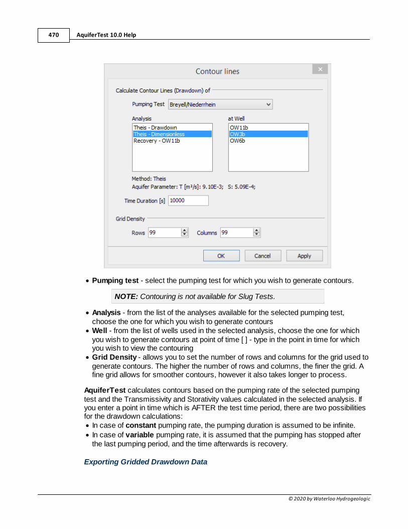
AquiferTest 10.0 Help470
© 2020 by Waterloo Hydrogeologic
· Pumping test - select the pumping test for which you wish to generate contours.
NOTE: Contouring is not available for Slug Tests.
· Analysis - from the list of the analyses available for the selected pumping test,choose the one for which you wish to generate contours
· Well - from the list of wells used in the selected analysis, choose the one for whichyou wish to generate contours at point of time [ ] - type in the point in time for whichyou wish to view the contouring
· Grid Density - allows you to set the number of rows and columns for the grid used togenerate contours. The higher the number of rows and columns, the finer the grid. Afine grid allows for smoother contours, however it also takes longer to process.
AquiferTest calculates contours based on the pumping rate of the selected pumpingtest and the Transmissivity and Storativity values calculated in the selected analysis. Ifyou enter a point in time which is AFTER the test time period, there are two possibilitiesfor the drawdown calculations:· In case of constant pumping rate, the pumping duration is assumed to be infinite.
· In case of variable pumping rate, it is assumed that the pumping has stopped afterthe last pumping period, and the time afterwards is recovery.
Exporting Gridded Drawdown Data
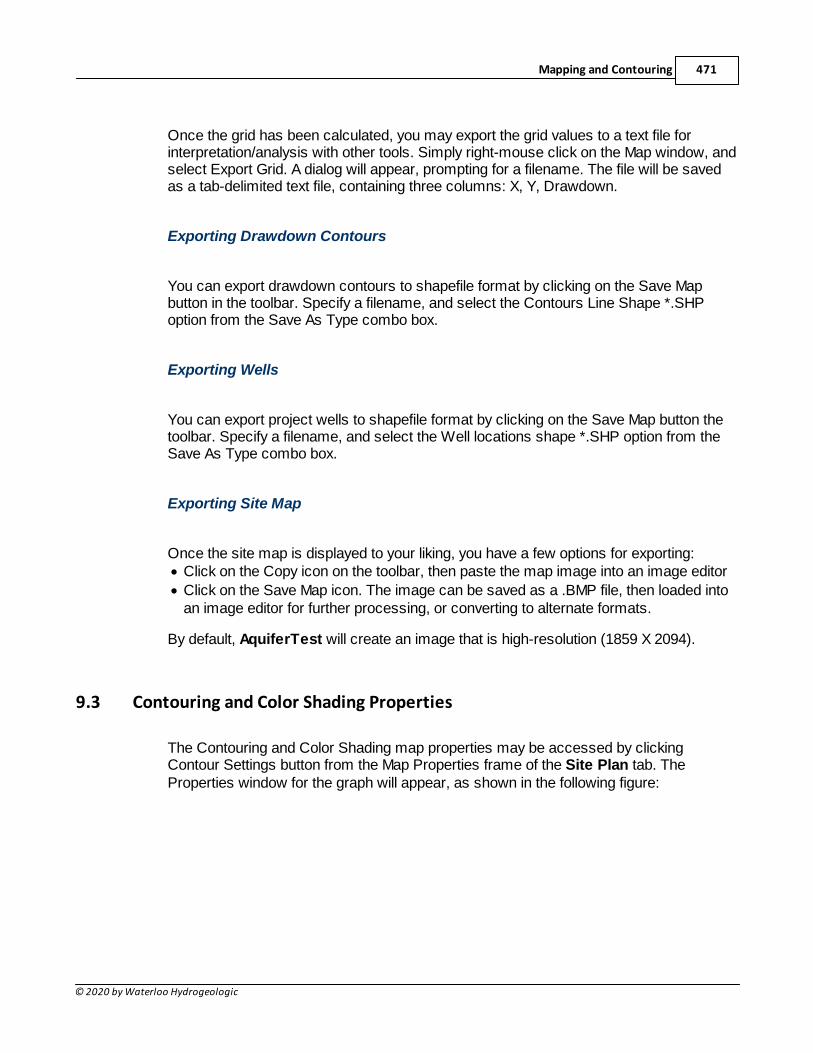
Mapping and Contouring 471
© 2020 by Waterloo Hydrogeologic
Once the grid has been calculated, you may export the grid values to a text file forinterpretation/analysis with other tools. Simply right-mouse click on the Map window, andselect Export Grid. A dialog will appear, prompting for a filename. The file will be savedas a tab-delimited text file, containing three columns: X, Y, Drawdown.
Exporting Drawdown Contours
You can export drawdown contours to shapefile format by clicking on the Save Mapbutton in the toolbar. Specify a filename, and select the Contours Line Shape *.SHPoption from the Save As Type combo box.
Exporting Wells
You can export project wells to shapefile format by clicking on the Save Map button thetoolbar. Specify a filename, and select the Well locations shape *.SHP option from theSave As Type combo box.
Exporting Site Map
Once the site map is displayed to your liking, you have a few options for exporting:· Click on the Copy icon on the toolbar, then paste the map image into an image editor
· Click on the Save Map icon. The image can be saved as a .BMP file, then loaded intoan image editor for further processing, or converting to alternate formats.
By default, AquiferTest will create an image that is high-resolution (1859 X 2094).
9.3 Contouring and Color Shading Properties
The Contouring and Color Shading map properties may be accessed by clickingContour Settings button from the Map Properties frame of the Site Plan tab. TheProperties window for the graph will appear, as shown in the following figure:
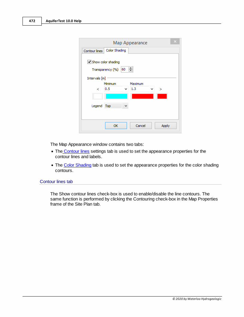
AquiferTest 10.0 Help472
© 2020 by Waterloo Hydrogeologic
The Map Appearance window contains two tabs:
· The Contour lines settings tab is used to set the appearance properties for thecontour lines and labels.
· The Color Shading tab is used to set the appearance properties for the color shadingcontours.
Contour lines tab
The Show contour lines check-box is used to enable/disable the line contours. Thesame function is performed by clicking the Contouring check-box in the Map Propertiesframe of the Site Plan tab.
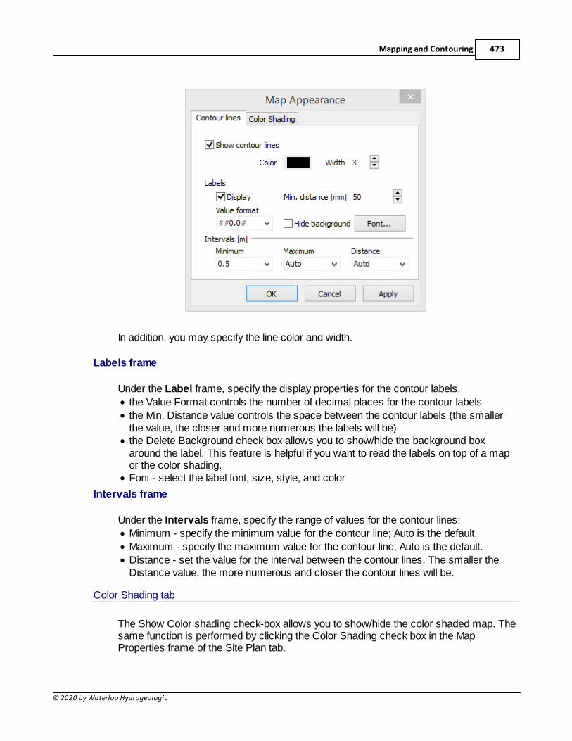
Mapping and Contouring 473
© 2020 by Waterloo Hydrogeologic
In addition, you may specify the line color and width.
Labels frame
Under the Label frame, specify the display properties for the contour labels.
· the Value Format controls the number of decimal places for the contour labels
· the Min. Distance value controls the space between the contour labels (the smallerthe value, the closer and more numerous the labels will be)
· the Delete Background check box allows you to show/hide the background boxaround the label. This feature is helpful if you want to read the labels on top of a mapor the color shading.
· Font - select the label font, size, style, and color
Intervals frame
Under the Intervals frame, specify the range of values for the contour lines:
· Minimum - specify the minimum value for the contour line; Auto is the default.
· Maximum - specify the maximum value for the contour line; Auto is the default.
· Distance - set the value for the interval between the contour lines. The smaller theDistance value, the more numerous and closer the contour lines will be.
Color Shading tab
The Show Color shading check-box allows you to show/hide the color shaded map. Thesame function is performed by clicking the Color Shading check box in the MapProperties frame of the Site Plan tab.
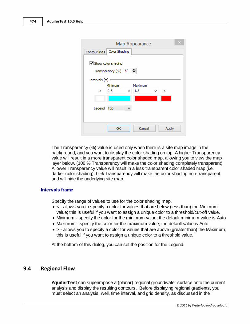
AquiferTest 10.0 Help474
© 2020 by Waterloo Hydrogeologic
The Transparency (%) value is used only when there is a site map image in thebackground, and you want to display the color shading on top. A higher Transparencyvalue will result in a more transparent color shaded map, allowing you to view the maplayer below. (100 % Transparency will make the color shading completely transparent).A lower Transparency value will result in a less transparent color shaded map (i.e.darker color shading). 0 % Transparency will make the color shading non-transparent,and will hide the underlying site map.
Intervals frame
Specify the range of values to use for the color shading map.· < - allows you to specify a color for values that are below (less than) the Minimum
value; this is useful if you want to assign a unique color to a threshold/cut-off value.· Minimum - specify the color for the minimum value; the default minimum value is Auto
· Maximum - specify the color for the maximum value; the default value is Auto
· > - allows you to specify a color for values that are above (greater than) the Maximum;this is useful if you want to assign a unique color to a threshold value.
At the bottom of this dialog, you can set the position for the Legend.
9.4 Regional Flow
AquiferTest can superimpose a (planar) regional groundwater surface onto the currentanalysis and display the resulting contours. Before displaying regional gradients, youmust select an analysis, well, time interval, and grid density, as discussed in the
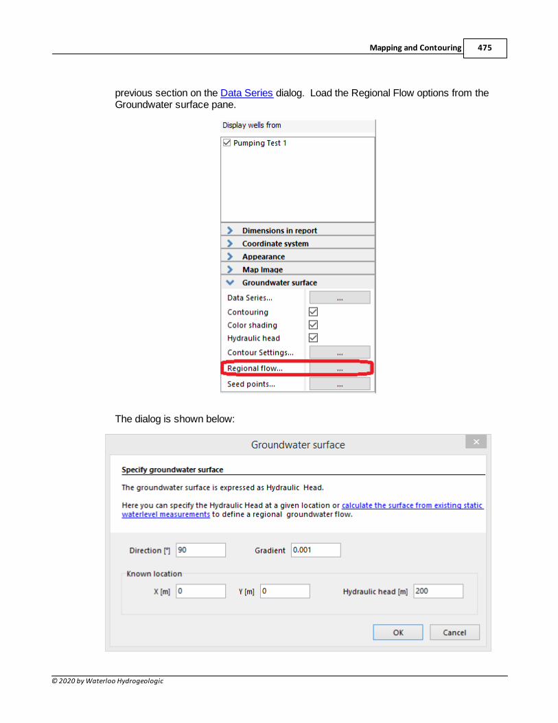
Mapping and Contouring 475
© 2020 by Waterloo Hydrogeologic
previous section on the Data Series dialog. Load the Regional Flow options from theGroundwater surface pane.
The dialog is shown below:
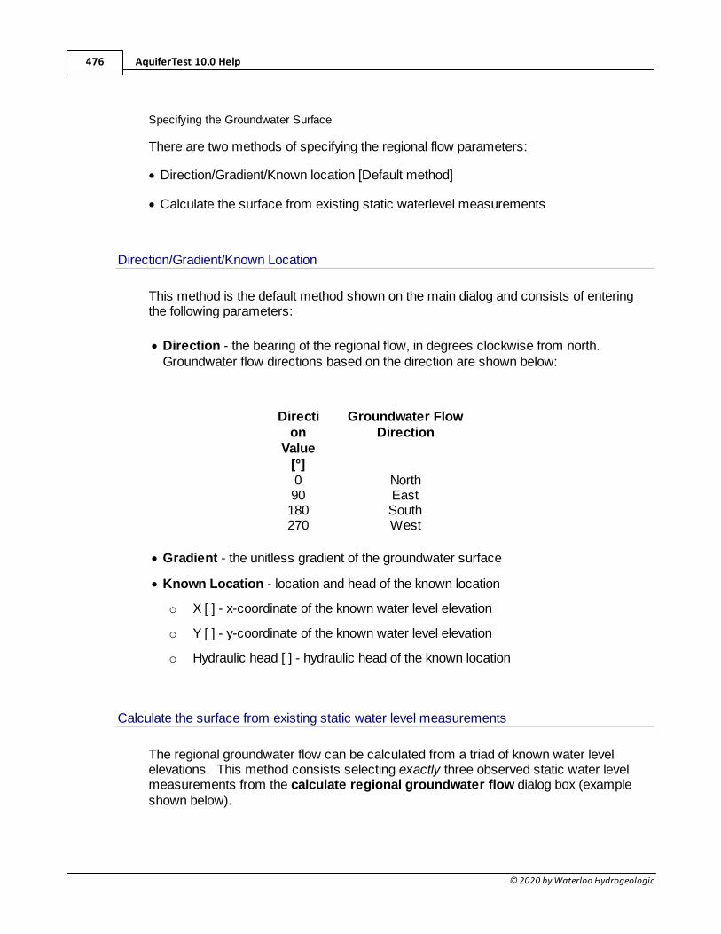
AquiferTest 10.0 Help476
© 2020 by Waterloo Hydrogeologic
Specifying the Groundwater Surface
There are two methods of specifying the regional flow parameters:
· Direction/Gradient/Known location [Default method]
· Calculate the surface from existing static waterlevel measurements
Direction/Gradient/Known Location
This method is the default method shown on the main dialog and consists of enteringthe following parameters:
· Direction - the bearing of the regional flow, in degrees clockwise from north. Groundwater flow directions based on the direction are shown below:
Direction
Value[°]
Groundwater FlowDirection
0 North90 East180 South270 West
· Gradient - the unitless gradient of the groundwater surface
· Known Location - location and head of the known location
o X [ ] - x-coordinate of the known water level elevation
o Y [ ] - y-coordinate of the known water level elevation
o Hydraulic head [ ] - hydraulic head of the known location
Calculate the surface from existing static water level measurements
The regional groundwater flow can be calculated from a triad of known water levelelevations. This method consists selecting exactly three observed static water levelmeasurements from the calculate regional groundwater flow dialog box (exampleshown below).
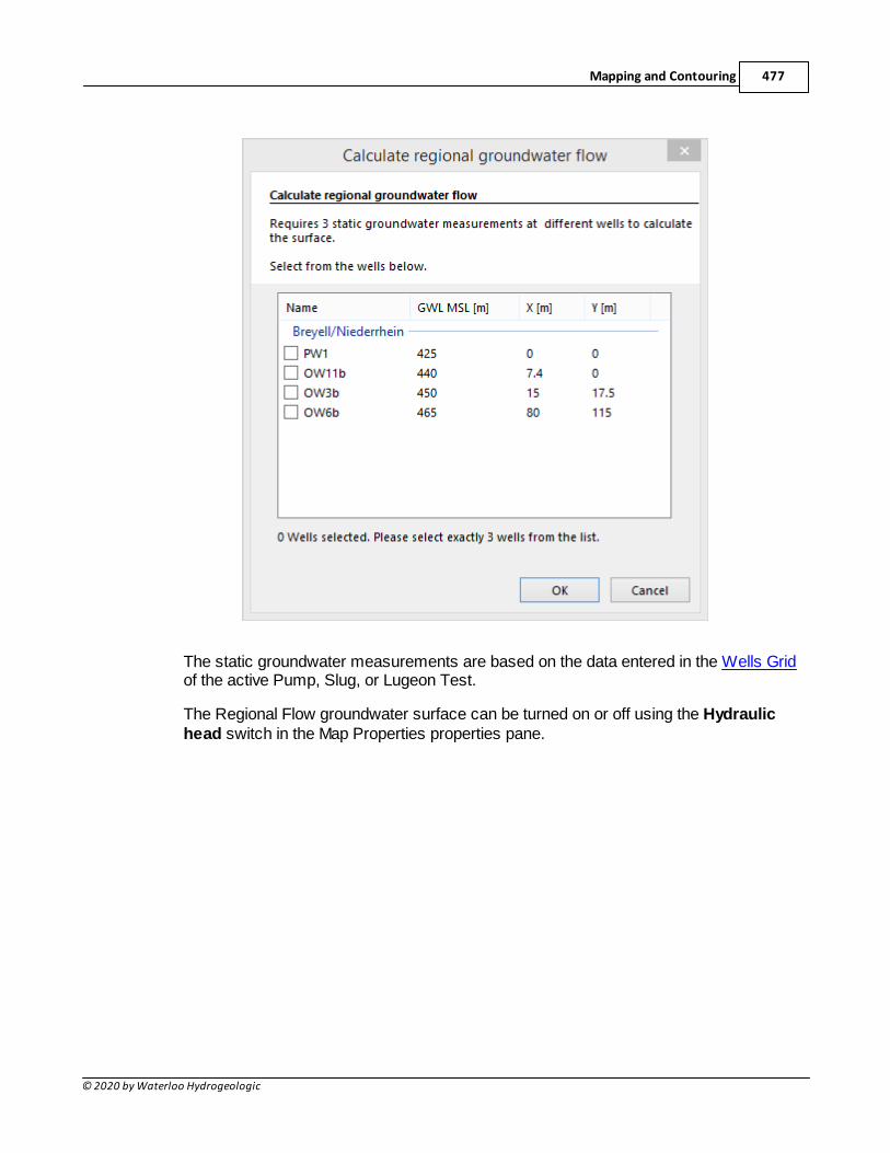
Mapping and Contouring 477
© 2020 by Waterloo Hydrogeologic
The static groundwater measurements are based on the data entered in the Wells Gridof the active Pump, Slug, or Lugeon Test.
The Regional Flow groundwater surface can be turned on or off using the Hydraulichead switch in the Map Properties properties pane.
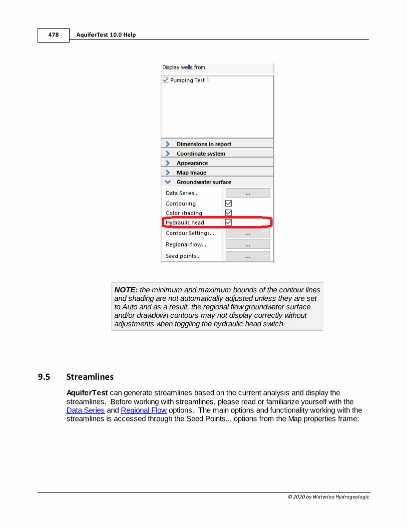
AquiferTest 10.0 Help478
© 2020 by Waterloo Hydrogeologic
NOTE: the minimum and maximum bounds of the contour linesand shading are not automatically adjusted unless they are setto Auto and as a result, the regional flow groundwater surfaceand/or drawdown contours may not display correctly withoutadjustments when toggling the hydraulic head switch.
9.5 Streamlines
AquiferTest can generate streamlines based on the current analysis and display thestreamlines. Before working with streamlines, please read or familiarize yourself with theData Series and Regional Flow options. The main options and functionality working with thestreamlines is accessed through the Seed Points... options from the Map properties frame:
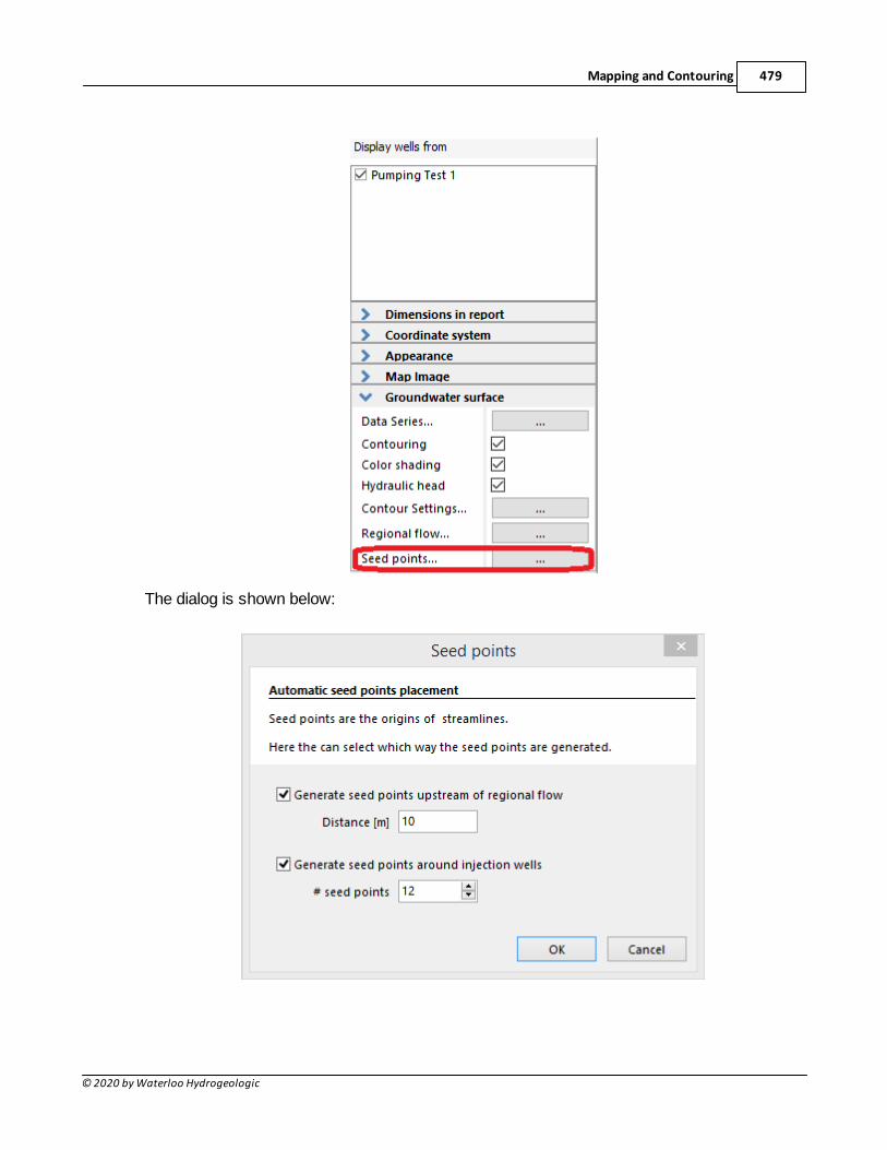
Mapping and Contouring 479
© 2020 by Waterloo Hydrogeologic
The dialog is shown below:
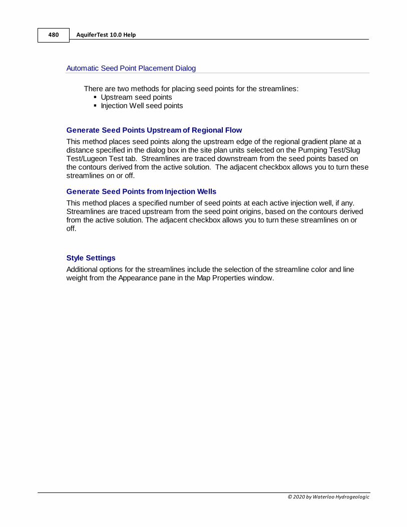
AquiferTest 10.0 Help480
© 2020 by Waterloo Hydrogeologic
Automatic Seed Point Placement Dialog
There are two methods for placing seed points for the streamlines:§ Upstream seed points§ Injection Well seed points
Generate Seed Points Upstream of Regional Flow
This method places seed points along the upstream edge of the regional gradient plane at adistance specified in the dialog box in the site plan units selected on the Pumping Test/SlugTest/Lugeon Test tab. Streamlines are traced downstream from the seed points based onthe contours derived from the active solution. The adjacent checkbox allows you to turn thesestreamlines on or off.
Generate Seed Points from Injection Wells
This method places a specified number of seed points at each active injection well, if any. Streamlines are traced upstream from the seed point origins, based on the contours derivedfrom the active solution. The adjacent checkbox allows you to turn these streamlines on oroff.
Style Settings
Additional options for the streamlines include the selection of the streamline color and lineweight from the Appearance pane in the Map Properties window.
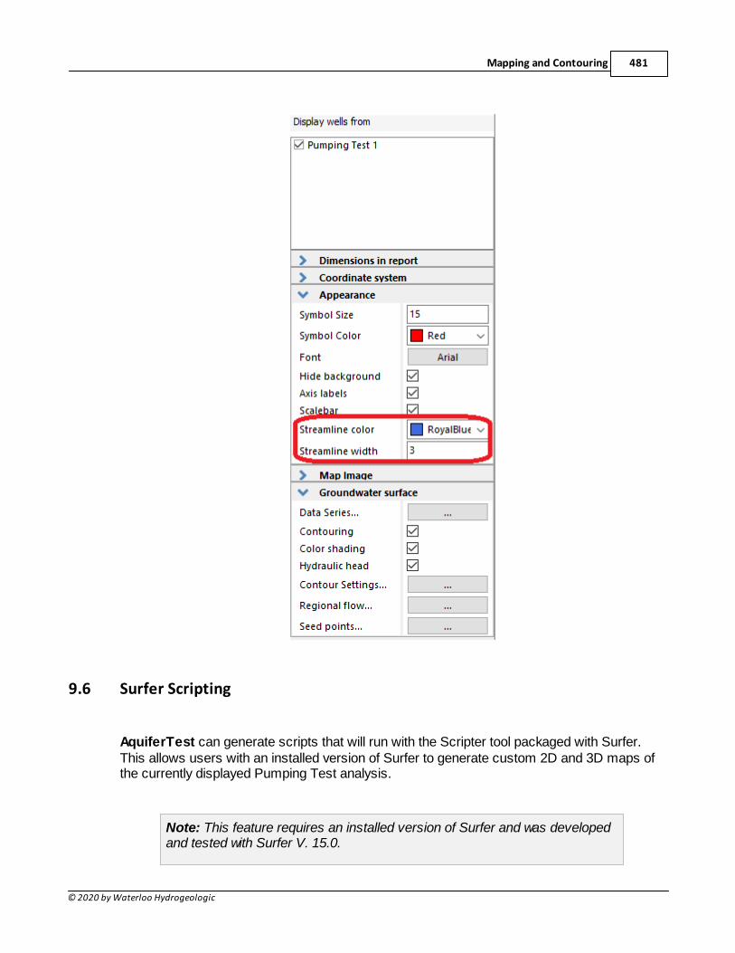
Mapping and Contouring 481
© 2020 by Waterloo Hydrogeologic
9.6 Surfer Scripting
AquiferTest can generate scripts that will run with the Scripter tool packaged with Surfer. This allows users with an installed version of Surfer to generate custom 2D and 3D maps ofthe currently displayed Pumping Test analysis.
Note: This feature requires an installed version of Surfer and was developedand tested with Surfer V. 15.0.
AquiferTest 10.0 Help482
© 2020 by Waterloo Hydrogeologic
Since we cannot control the development of Surfer, the full functionality of thescripting tool in AquiferTest cannot be guaranteed to work in older versions ofSurfer.
9.7 Base Maps using a Tile Server
Note: In order to use base maps from a Tile Server, the well coordinates must be specified inusing the Universal Transverse Mercator coordinate system with distance units in meters. However, any vertical coordinate system specified in meters or feet can be used. Anexample of how to use the tile server is provided in the Example in the next section.
To access the tile server settings, click Tools > Options from the main menu and open theTile Server tab from the Options Window:
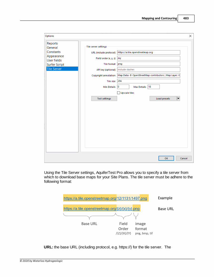
Mapping and Contouring 483
© 2020 by Waterloo Hydrogeologic
Using the Tile Server settings, AquiferTest Pro allows you to specify a tile server fromwhich to download base maps for your Site Plans. The tile server must be adhere to thefollowing format:
URL: the base URL (including protocol, e.g. https://) for the tile server. The
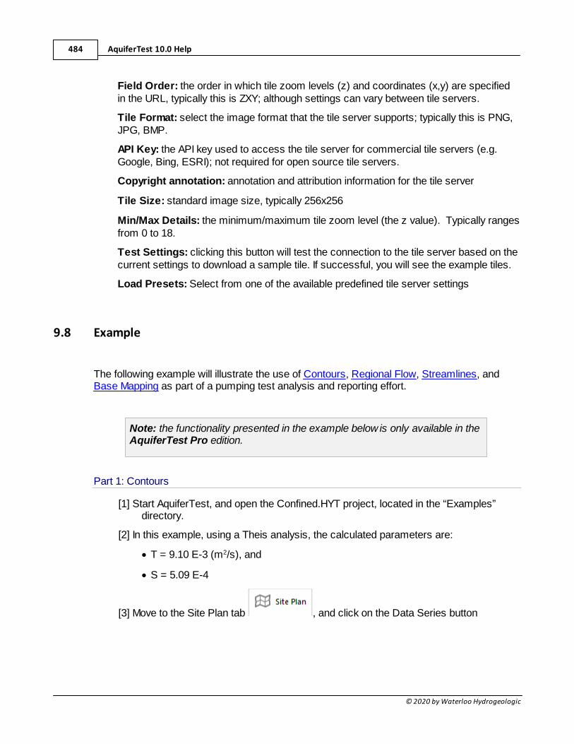
AquiferTest 10.0 Help484
© 2020 by Waterloo Hydrogeologic
Field Order: the order in which tile zoom levels (z) and coordinates (x,y) are specifiedin the URL, typically this is ZXY; although settings can vary between tile servers.
Tile Format: select the image format that the tile server supports; typically this is PNG,JPG, BMP.
API Key: the API key used to access the tile server for commercial tile servers (e.g.Google, Bing, ESRI); not required for open source tile servers.
Copyright annotation: annotation and attribution information for the tile server
Tile Size: standard image size, typically 256x256
Min/Max Details: the minimum/maximum tile zoom level (the z value). Typically rangesfrom 0 to 18.
Test Settings: clicking this button will test the connection to the tile server based on thecurrent settings to download a sample tile. If successful, you will see the example tiles.
Load Presets: Select from one of the available predefined tile server settings
9.8 Example
The following example will illustrate the use of Contours, Regional Flow, Streamlines, andBase Mapping as part of a pumping test analysis and reporting effort.
Note: the functionality presented in the example below is only available in theAquiferTest Pro edition.
Part 1: Contours
[1] Start AquiferTest, and open the Confined.HYT project, located in the “Examples”directory.
[2] In this example, using a Theis analysis, the calculated parameters are:
· T = 9.10 E-3 (m2/s), and
· S = 5.09 E-4
[3] Move to the Site Plan tab , and click on the Data Series button
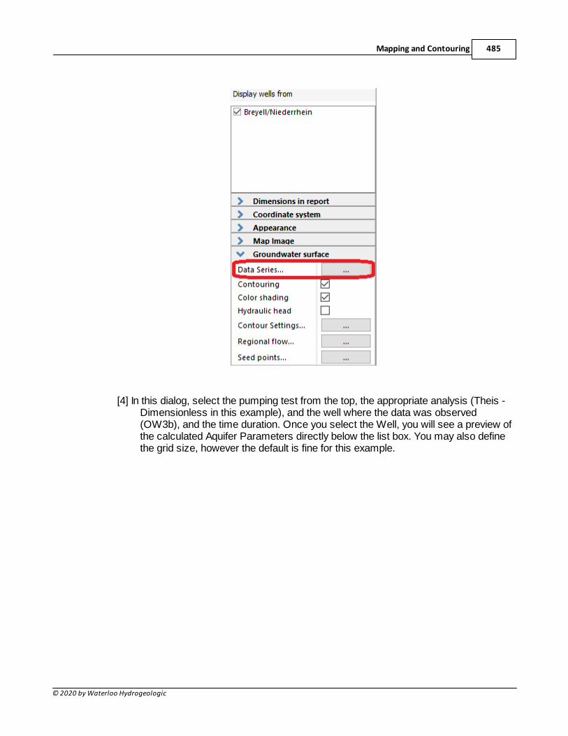
Mapping and Contouring 485
© 2020 by Waterloo Hydrogeologic
[4] In this dialog, select the pumping test from the top, the appropriate analysis (Theis -Dimensionless in this example), and the well where the data was observed(OW3b), and the time duration. Once you select the Well, you will see a preview ofthe calculated Aquifer Parameters directly below the list box. You may also definethe grid size, however the default is fine for this example.
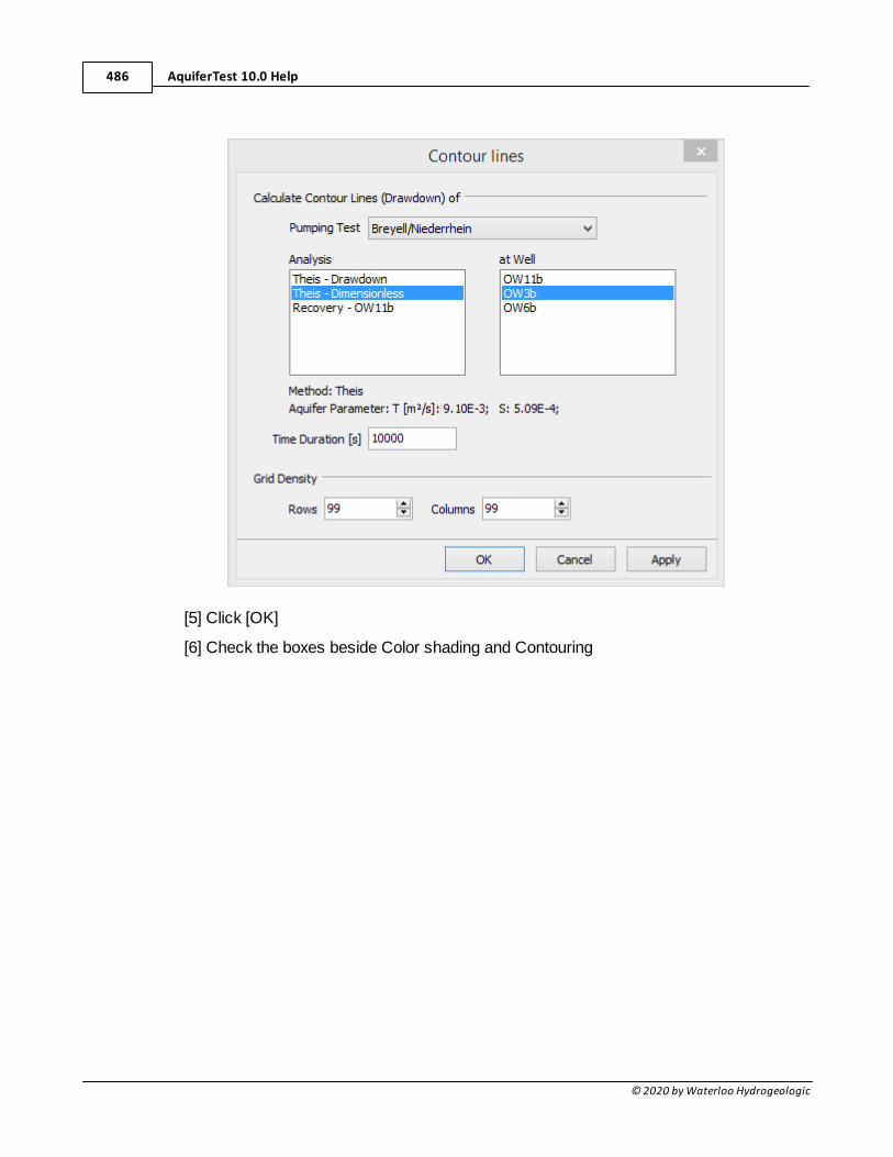
AquiferTest 10.0 Help486
© 2020 by Waterloo Hydrogeologic
[5] Click [OK]
[6] Check the boxes beside Color shading and Contouring
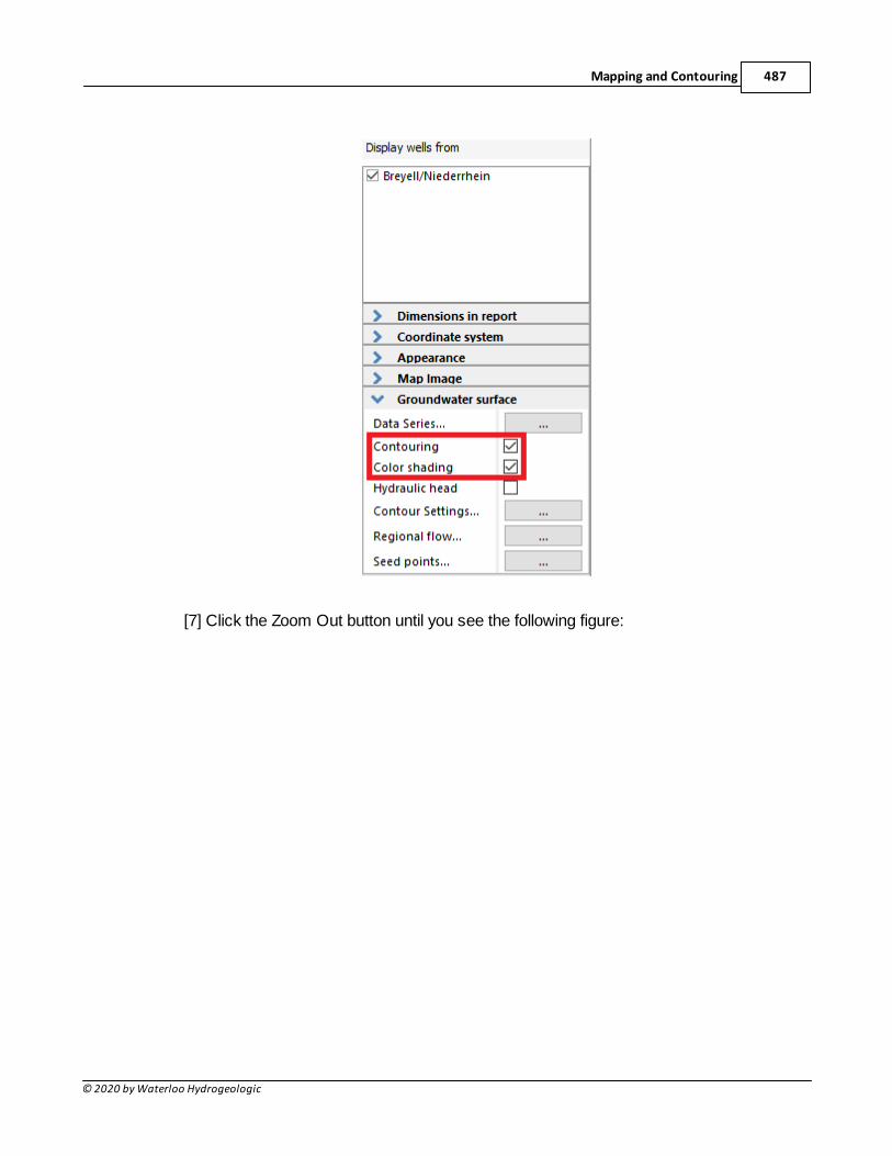
Mapping and Contouring 487
© 2020 by Waterloo Hydrogeologic
[7] Click the Zoom Out button until you see the following figure:
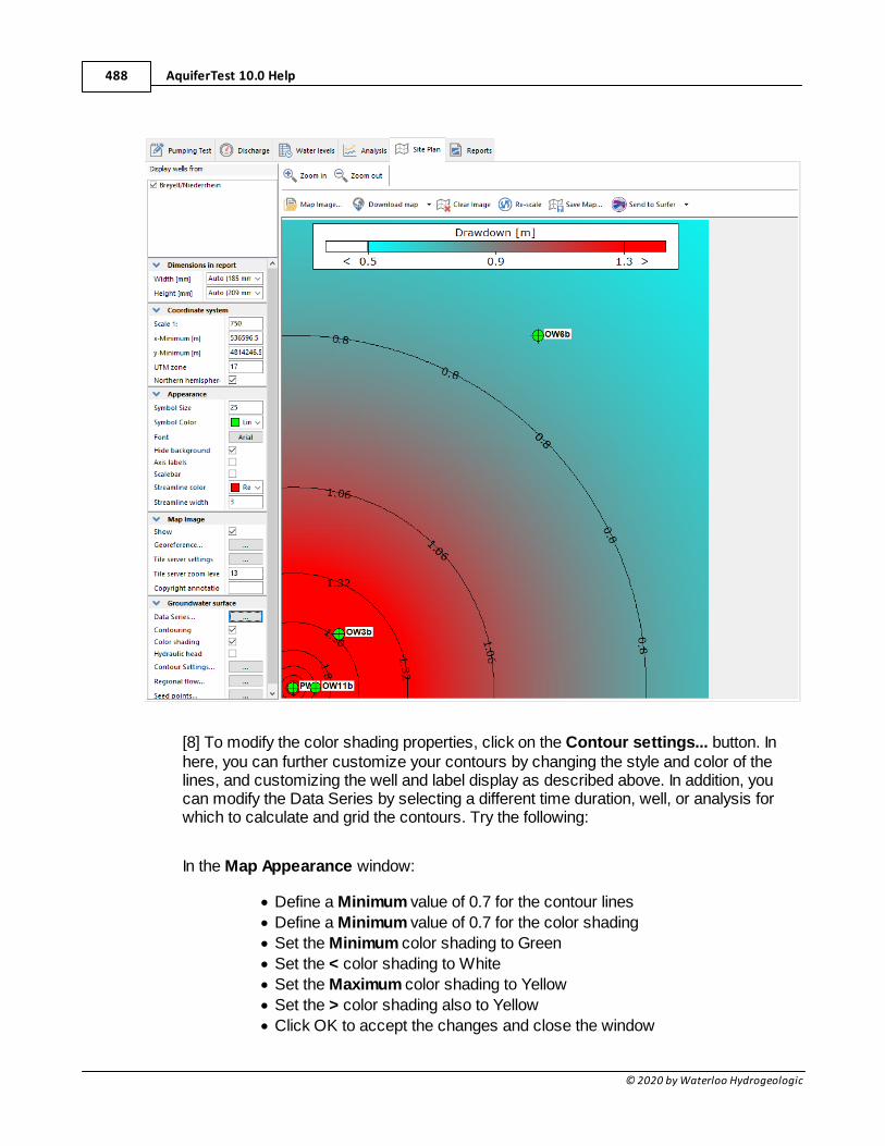
AquiferTest 10.0 Help488
© 2020 by Waterloo Hydrogeologic
[8] To modify the color shading properties, click on the Contour settings... button. Inhere, you can further customize your contours by changing the style and color of thelines, and customizing the well and label display as described above. In addition, youcan modify the Data Series by selecting a different time duration, well, or analysis forwhich to calculate and grid the contours. Try the following:
In the Map Appearance window:
· Define a Minimum value of 0.7 for the contour lines
· Define a Minimum value of 0.7 for the color shading
· Set the Minimum color shading to Green
· Set the < color shading to White
· Set the Maximum color shading to Yellow
· Set the > color shading also to Yellow
· Click OK to accept the changes and close the window
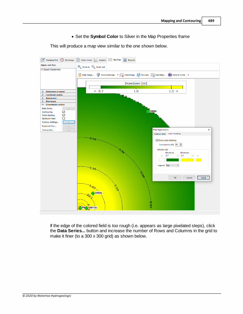
Mapping and Contouring 489
© 2020 by Waterloo Hydrogeologic
· Set the Symbol Color to Silver in the Map Properties frame
This will produce a map view similar to the one shown below.
If the edge of the colored field is too rough (i.e. appears as large pixelated steps), clickthe Data Series... button and increase the number of Rows and Columns in the grid tomake it finer (to a 300 x 300 grid) as shown below.
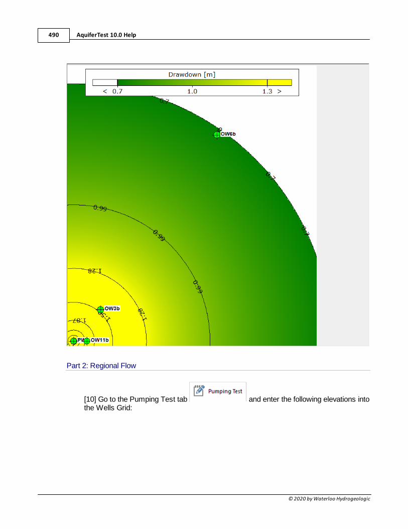
AquiferTest 10.0 Help490
© 2020 by Waterloo Hydrogeologic
Part 2: Regional Flow
[10] Go to the Pumping Test tab and enter the following elevations intothe Wells Grid:
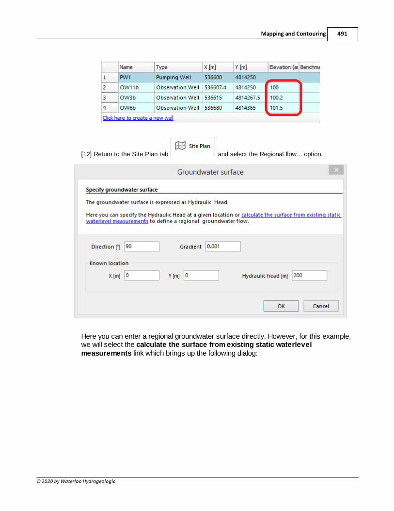
Mapping and Contouring 491
© 2020 by Waterloo Hydrogeologic
[12] Return to the Site Plan tab and select the Regional flow... option.
Here you can enter a regional groundwater surface directly. However, for this example,we will select the calculate the surface from existing static waterlevelmeasurements link which brings up the following dialog:
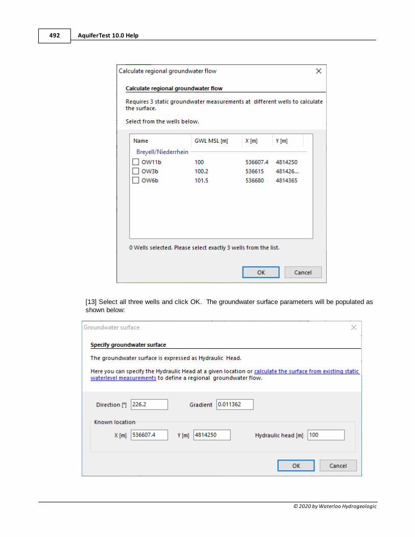
AquiferTest 10.0 Help492
© 2020 by Waterloo Hydrogeologic
[13] Select all three wells and click OK. The groundwater surface parameters will be populated asshown below:
Mapping and Contouring 493
© 2020 by Waterloo Hydrogeologic
[14] Since we are superimposing the drawdown analysis onto a regional groundwatersurface, the contour settings will have to be updated. Click on the Contour Settings...option in the Map Properties
In the Map Appearance window:
· In the Contour lines tab:o Define a Minimum value of 97o Define a Maximum value of 102o Define a Distance value of 0.5
· In the Color shading tabo Define a Minimum value of 98o Define a Maximum value of 101o Set the Minimum color shading to Dark Blueo Set the < color shading to Yellowo Set the Maximum color shading to Light Blueo Set the > color shading also to White
· Click OK to accept the changes and close the window
[15] Select the Hydraulic head checkbox in the Groundwater Surface pane to turn onthe surface. Let's zoom out to get a better view of regional properties. In the MapProperties area:
· Set the Scale 1: value to 1000
· X-Minimum [m] value to 536550
· Y-Minimum [m] value to 4814200
The groundwater surface should look something like the following:
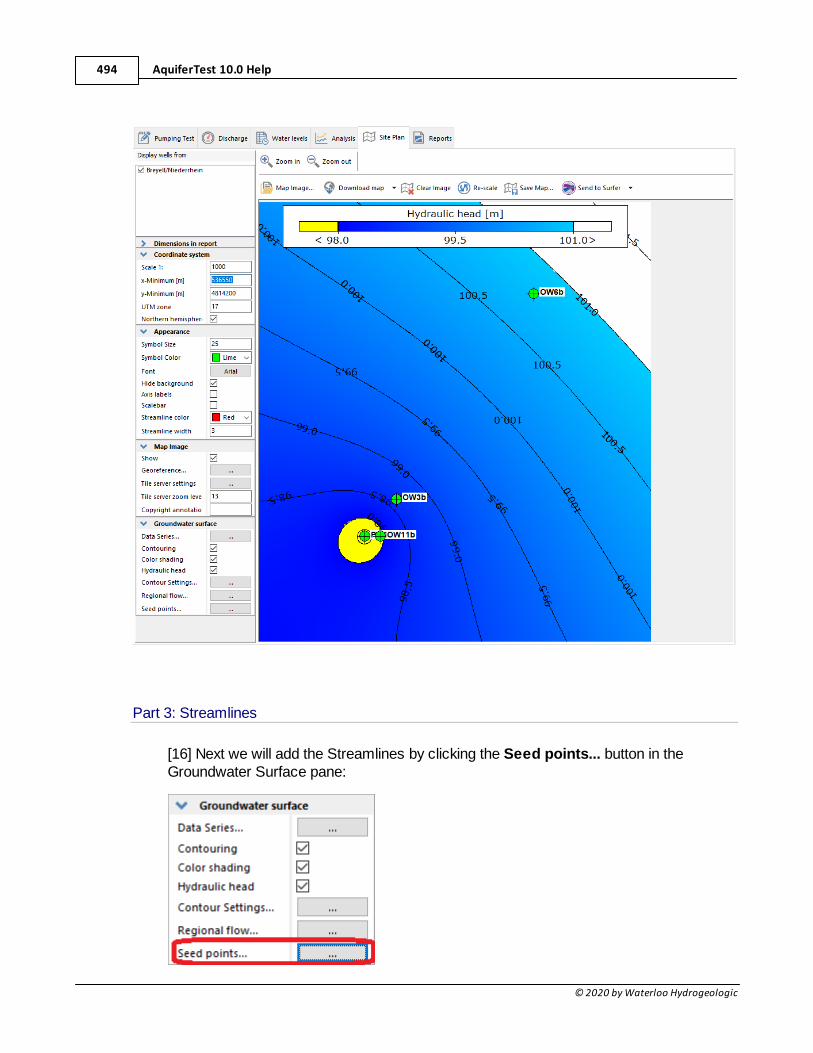
AquiferTest 10.0 Help494
© 2020 by Waterloo Hydrogeologic
Part 3: Streamlines
[16] Next we will add the Streamlines by clicking the Seed points... button in theGroundwater Surface pane:
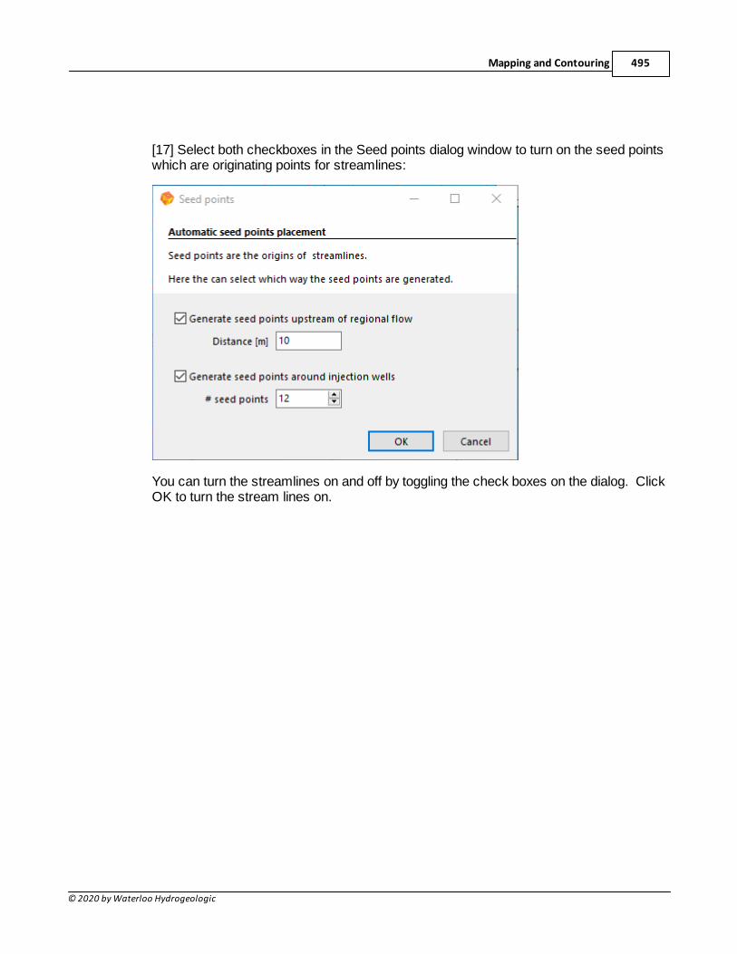
Mapping and Contouring 495
© 2020 by Waterloo Hydrogeologic
[17] Select both checkboxes in the Seed points dialog window to turn on the seed pointswhich are originating points for streamlines:
You can turn the streamlines on and off by toggling the check boxes on the dialog. ClickOK to turn the stream lines on.
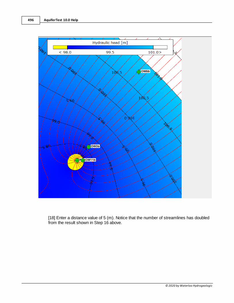
AquiferTest 10.0 Help496
© 2020 by Waterloo Hydrogeologic
[18] Enter a distance value of 5 (m). Notice that the number of streamlines has doubledfrom the result shown in Step 16 above.

Mapping and Contouring 497
© 2020 by Waterloo Hydrogeologic
You can also show the streamlines from an injection well. In order to do this, let's addan injection well to the analysis.
[19] Go to the Pumping Test tab and add a new injection well with thefollowing information:
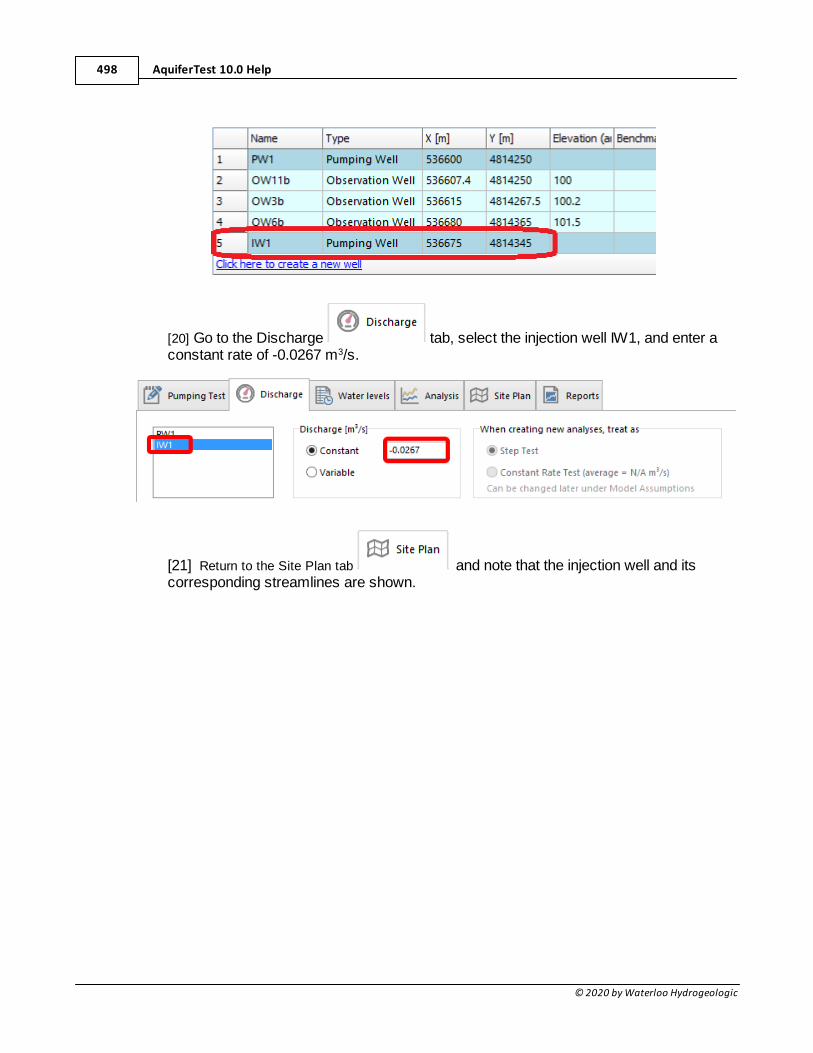
AquiferTest 10.0 Help498
© 2020 by Waterloo Hydrogeologic
[20] Go to the Discharge tab, select the injection well IW1, and enter aconstant rate of -0.0267 m3/s.
[21] Return to the Site Plan tab and note that the injection well and itscorresponding streamlines are shown.
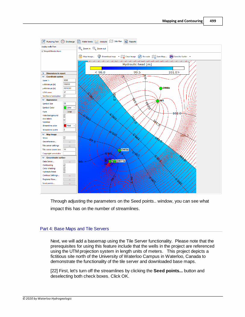
Mapping and Contouring 499
© 2020 by Waterloo Hydrogeologic
Through adjusting the parameters on the Seed points.. window, you can see what
impact this has on the number of streamlines.
Part 4: Base Maps and Tile Servers
Next, we will add a basemap using the Tile Server functionality. Please note that theprerequisites for using this feature include that the wells in the project are referencedusing the UTM projection system in length units of meters. This project depicts afictitious site north of the University of Waterloo Campus in Waterloo, Canada todemonstrate the functionality of the tile server and downloaded base maps.
[22] First, let's turn off the streamlines by clicking the Seed points... button anddeselecting both check boxes. Click OK.
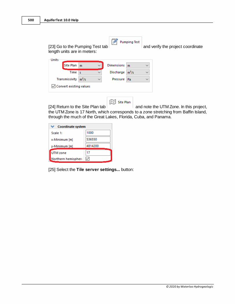
AquiferTest 10.0 Help500
© 2020 by Waterloo Hydrogeologic
[23] Go to the Pumping Test tab and verify the project coordinatelength units are in meters:
[24] Return to the Site Plan tab and note the UTM Zone. In this project,the UTM Zone is 17 North, which corresponds to a zone stretching from Baffin Island,through the much of the Great Lakes, Florida, Cuba, and Panama.
[25] Select the Tile server settings... button:
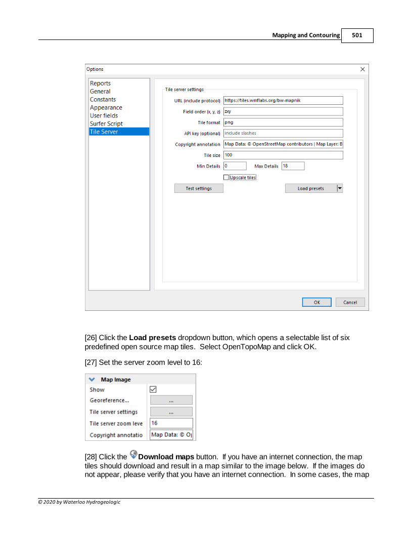
Mapping and Contouring 501
© 2020 by Waterloo Hydrogeologic
[26] Click the Load presets dropdown button, which opens a selectable list of sixpredefined open source map tiles. Select OpenTopoMap and click OK.
[27] Set the server zoom level to 16:
[28] Click the Download maps button. If you have an internet connection, the maptiles should download and result in a map similar to the image below. If the images donot appear, please verify that you have an internet connection. In some cases, the map
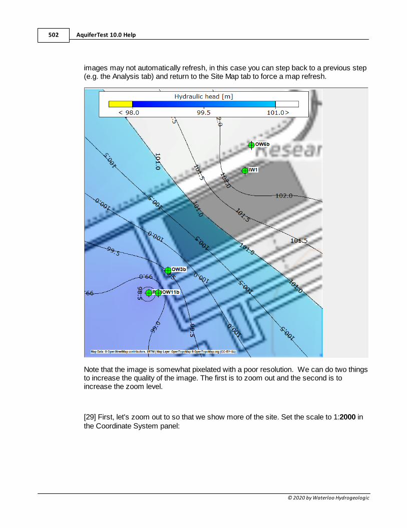
AquiferTest 10.0 Help502
© 2020 by Waterloo Hydrogeologic
images may not automatically refresh, in this case you can step back to a previous step(e.g. the Analysis tab) and return to the Site Map tab to force a map refresh.
Note that the image is somewhat pixelated with a poor resolution. We can do two thingsto increase the quality of the image. The first is to zoom out and the second is toincrease the zoom level.
[29] First, let's zoom out to so that we show more of the site. Set the scale to 1:2000 inthe Coordinate System panel:
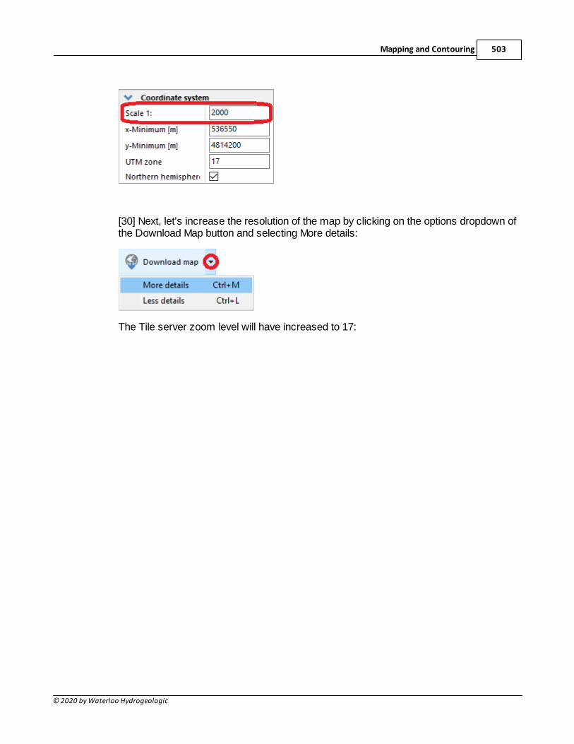
Mapping and Contouring 503
© 2020 by Waterloo Hydrogeologic
[30] Next, let's increase the resolution of the map by clicking on the options dropdown ofthe Download Map button and selecting More details:
The Tile server zoom level will have increased to 17:
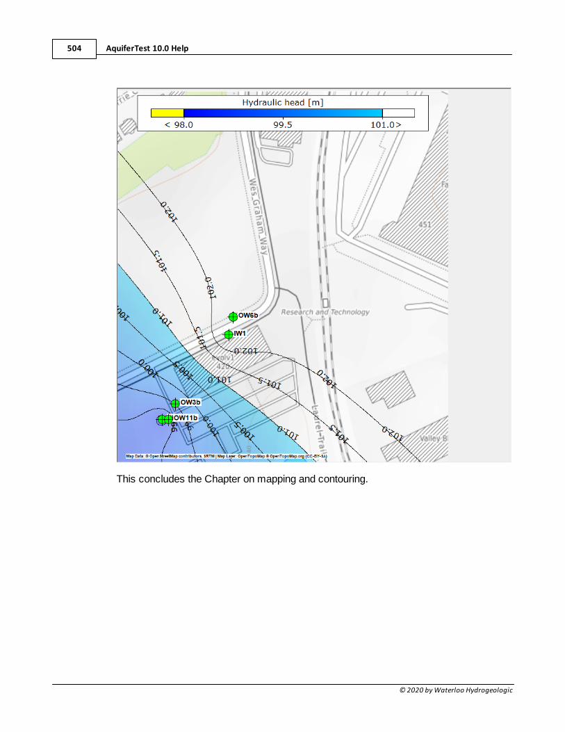
AquiferTest 10.0 Help504
© 2020 by Waterloo Hydrogeologic
This concludes the Chapter on mapping and contouring.
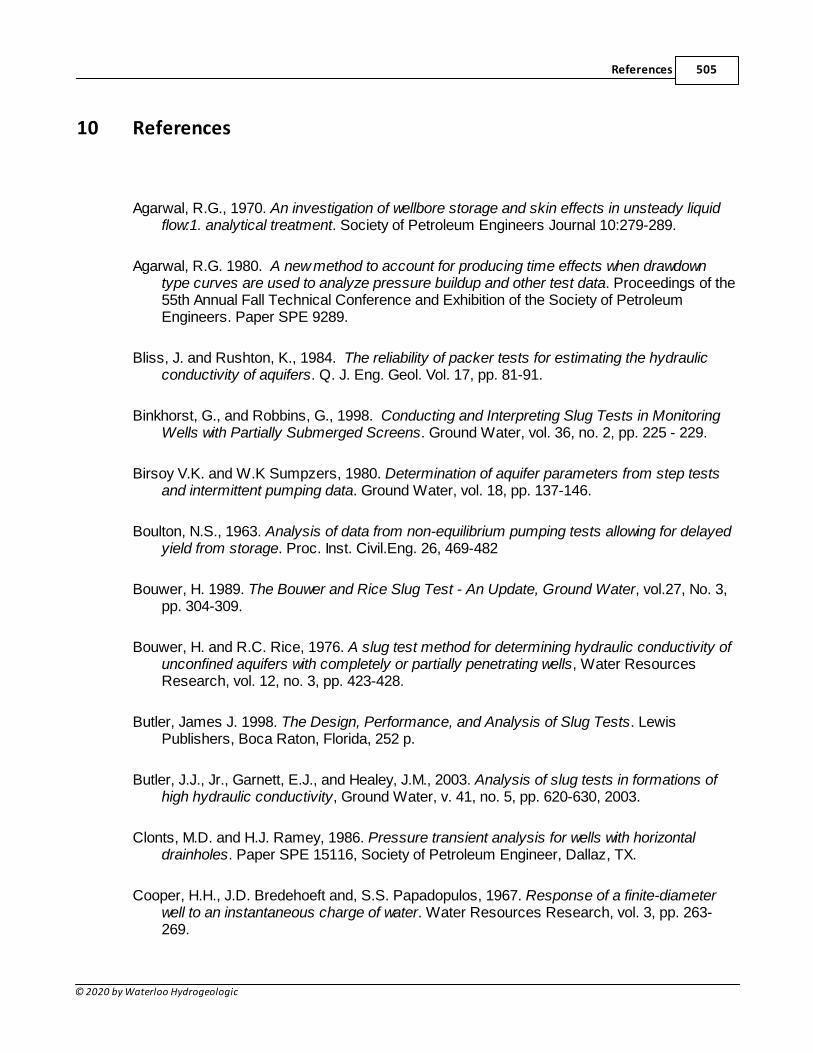
References 505
© 2020 by Waterloo Hydrogeologic
10 References
Agarwal, R.G., 1970. An investigation of wellbore storage and skin effects in unsteady liquidflow:1. analytical treatment. Society of Petroleum Engineers Journal 10:279-289.
Agarwal, R.G. 1980. A new method to account for producing time effects when drawdowntype curves are used to analyze pressure buildup and other test data. Proceedings of the55th Annual Fall Technical Conference and Exhibition of the Society of PetroleumEngineers. Paper SPE 9289.
Bliss, J. and Rushton, K., 1984. The reliability of packer tests for estimating the hydraulicconductivity of aquifers. Q. J. Eng. Geol. Vol. 17, pp. 81-91.
Binkhorst, G., and Robbins, G., 1998. Conducting and Interpreting Slug Tests in MonitoringWells with Partially Submerged Screens. Ground Water, vol. 36, no. 2, pp. 225 - 229.
Birsoy V.K. and W.K Sumpzers, 1980. Determination of aquifer parameters from step testsand intermittent pumping data. Ground Water, vol. 18, pp. 137-146.
Boulton, N.S., 1963. Analysis of data from non-equilibrium pumping tests allowing for delayedyield from storage. Proc. Inst. Civil.Eng. 26, 469-482
Bouwer, H. 1989. The Bouwer and Rice Slug Test - An Update, Ground Water, vol.27, No. 3,pp. 304-309.
Bouwer, H. and R.C. Rice, 1976. A slug test method for determining hydraulic conductivity ofunconfined aquifers with completely or partially penetrating wells, Water ResourcesResearch, vol. 12, no. 3, pp. 423-428.
Butler, James J. 1998. The Design, Performance, and Analysis of Slug Tests. LewisPublishers, Boca Raton, Florida, 252 p.
Butler, J.J., Jr., Garnett, E.J., and Healey, J.M., 2003. Analysis of slug tests in formations ofhigh hydraulic conductivity, Ground Water, v. 41, no. 5, pp. 620-630, 2003.
Clonts, M.D. and H.J. Ramey, 1986. Pressure transient analysis for wells with horizontaldrainholes. Paper SPE 15116, Society of Petroleum Engineer, Dallaz, TX.
Cooper, H.H., J.D. Bredehoeft and, S.S. Papadopulos, 1967. Response of a finite-diameterwell to an instantaneous charge of water. Water Resources Research, vol. 3, pp. 263-269.
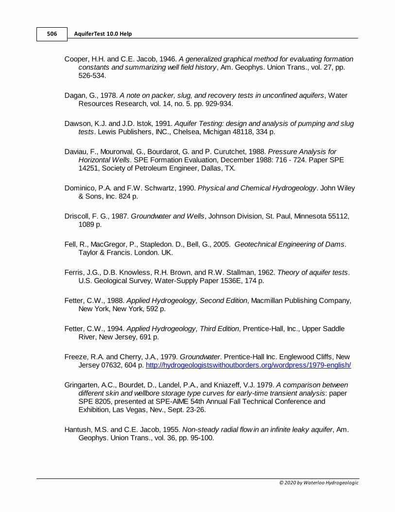
AquiferTest 10.0 Help506
© 2020 by Waterloo Hydrogeologic
Cooper, H.H. and C.E. Jacob, 1946. A generalized graphical method for evaluating formationconstants and summarizing well field history, Am. Geophys. Union Trans., vol. 27, pp.526-534.
Dagan, G., 1978. A note on packer, slug, and recovery tests in unconfined aquifers, WaterResources Research, vol. 14, no. 5. pp. 929-934.
Dawson, K.J. and J.D. Istok, 1991. Aquifer Testing: design and analysis of pumping and slugtests. Lewis Publishers, INC., Chelsea, Michigan 48118, 334 p.
Daviau, F., Mouronval, G., Bourdarot, G. and P. Curutchet, 1988. Pressure Analysis forHorizontal Wells. SPE Formation Evaluation, December 1988: 716 - 724. Paper SPE14251, Society of Petroleum Engineer, Dallas, TX.
Dominico, P.A. and F.W. Schwartz, 1990. Physical and Chemical Hydrogeology. John Wiley& Sons, Inc. 824 p.
Driscoll, F. G., 1987. Groundwater and Wells, Johnson Division, St. Paul, Minnesota 55112,1089 p.
Fell, R., MacGregor, P., Stapledon. D., Bell, G., 2005. Geotechnical Engineering of Dams.Taylor & Francis. London. UK.
Ferris, J.G., D.B. Knowless, R.H. Brown, and R.W. Stallman, 1962. Theory of aquifer tests.U.S. Geological Survey, Water-Supply Paper 1536E, 174 p.
Fetter, C.W., 1988. Applied Hydrogeology, Second Edition, Macmillan Publishing Company,New York, New York, 592 p.
Fetter, C.W., 1994. Applied Hydrogeology, Third Edition, Prentice-Hall, Inc., Upper SaddleRiver, New Jersey, 691 p.
Freeze, R.A. and Cherry, J.A., 1979. Groundwater. Prentice-Hall Inc. Englewood Cliffs, NewJersey 07632, 604 p. http://hydrogeologistswithoutborders.org/wordpress/1979-english/
Gringarten, A.C., Bourdet, D., Landel, P.A., and Kniazeff, V.J. 1979. A comparison betweendifferent skin and wellbore storage type curves for early-time transient analysis: paperSPE 8205, presented at SPE-AIME 54th Annual Fall Technical Conference andExhibition, Las Vegas, Nev., Sept. 23-26.
Hantush, M.S. and C.E. Jacob, 1955. Non-steady radial flow in an infinite leaky aquifer, Am.Geophys. Union Trans., vol. 36, pp. 95-100.
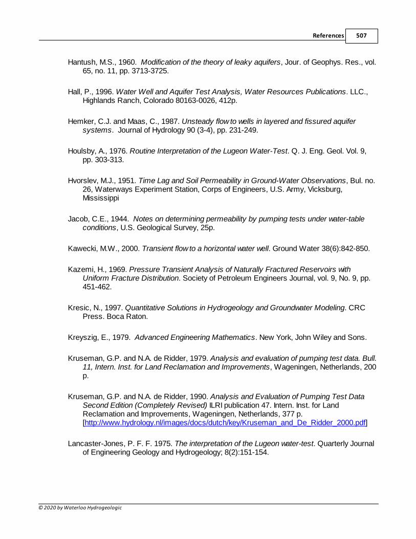
References 507
© 2020 by Waterloo Hydrogeologic
Hantush, M.S., 1960. Modification of the theory of leaky aquifers, Jour. of Geophys. Res., vol.65, no. 11, pp. 3713-3725.
Hall, P., 1996. Water Well and Aquifer Test Analysis, Water Resources Publications. LLC.,Highlands Ranch, Colorado 80163-0026, 412p.
Hemker, C.J. and Maas, C., 1987. Unsteady flow to wells in layered and fissured aquifersystems. Journal of Hydrology 90 (3-4), pp. 231-249.
Houlsby, A., 1976. Routine Interpretation of the Lugeon Water-Test. Q. J. Eng. Geol. Vol. 9,pp. 303-313.
Hvorslev, M.J., 1951. Time Lag and Soil Permeability in Ground-Water Observations, Bul. no.26, Waterways Experiment Station, Corps of Engineers, U.S. Army, Vicksburg,Mississippi
Jacob, C.E., 1944. Notes on determining permeability by pumping tests under water-tableconditions, U.S. Geological Survey, 25p.
Kawecki, M.W., 2000. Transient flow to a horizontal water well. Ground Water 38(6):842-850.
Kazemi, H., 1969. Pressure Transient Analysis of Naturally Fractured Reservoirs withUniform Fracture Distribution. Society of Petroleum Engineers Journal, vol. 9, No. 9, pp.451-462.
Kresic, N., 1997. Quantitative Solutions in Hydrogeology and Groundwater Modeling. CRCPress. Boca Raton.
Kreyszig, E., 1979. Advanced Engineering Mathematics. New York, John Wiley and Sons.
Kruseman, G.P. and N.A. de Ridder, 1979. Analysis and evaluation of pumping test data. Bull.11, Intern. Inst. for Land Reclamation and Improvements, Wageningen, Netherlands, 200p.
Kruseman, G.P. and N.A. de Ridder, 1990. Analysis and Evaluation of Pumping Test DataSecond Edition (Completely Revised) ILRI publication 47. Intern. Inst. for LandReclamation and Improvements, Wageningen, Netherlands, 377 p.[http://www.hydrology.nl/images/docs/dutch/key/Kruseman_and_De_Ridder_2000.pdf]
Lancaster-Jones, P. F. F. 1975. The interpretation of the Lugeon water-test. Quarterly Journalof Engineering Geology and Hydrogeology; 8(2):151-154.
AquiferTest 10.0 Help508
© 2020 by Waterloo Hydrogeologic
Moench, A.F., 1984. Double-Porosity Models for Fissured Groundwater Reservoir withFracture Skin. Water Resources Research, vol. 20, No. 7, pp. 831-846.
Moench, A.F., 1988. The Response of Partially Penetrating Wells to Pumpage from Double-Porosity Aquifers. Symposium Proceedings of International Conference on Fluid Flow inFractured Rocks. Hydrogeology Program-Department of Geology, Georgia StateUniversity, pp. 208-219.
Moench, A.F., 1993. Computation of Type Curves for Flow to Partially Penetrating Wells inWater-Table Aquifers. Ground Water, vol. 31, No. 6, pp. 966-971.
Moench, A.F., 1994. Specific Yield as Determined by Type-Curve analysis of Aquifer-TestData. Ground Water, vol. 32, No.6, pp. 949-957.
Moench, A.F., 1995. Combining the Neuman and Boulton Models for Flow to a Well in anUnconfined Aquifer. Ground Water, vol. 33, No. 3, pp. 378-384.
Moench, A.F., 1996. Flow to a Well in a Water-Table Aquifer: An Improved Laplace TransformSolution. Ground Water, vol. 34. No. 4, pp. 593-596.
Nelder, J.A. and Mead, R. 1965. A Simplex Method for Function Minimization, ComputerJournal 7 (1965) 308.
Neuman, S.P., 1975. Analysis of pumping test data from anisotropic unconfined aquifersconsidering delayed yield, Water Resources Research, vol. 11, no. 2, pp. 329-342.
Neuman, S.P., 1979. Perspective on 'Delayed Yield', Water Resources Research, vol. 15,no. 4, pp. 899-908.
Neuman, S.P. and P.A. Witherspoon, 1969. Theory of flow in a confined two aquifer system,Water Resources Research, vol. 5, no. 4, pp. 803-816.
Nwankwor, G.I., 1985. Delayed Yield Processes and Specific Yield in a Shallow Sand Aquifer.Ph.D. Thesis, Department of Earth Sciences, University of Waterloo.
Osborne, Paul S., 1993. EPA Groundwater Issue: Suggested Operating Procedures forAquifer Pumping Tests. EPA/540/S-93/503, February 1993 https://www.epa.gov/sites/production/files/2015-06/documents/sopaqu.pdf
Papadopulos, S.S., Cooper, H.H. Jr., 1967. Drawdown in a well of large diameter. WaterResources Res., Vol. 3, pp. 241-244.
References 509
© 2020 by Waterloo Hydrogeologic
Quiñones-Rozo, C., 2010. Lugeon test interpretation, revisited. In: CollaborativeManagement of Integrated Watersheds, US Society of Dams, 30th Annual Conference,S. 405–414.
Reed, J. C., 1980. Techniques of Water-Resource Investigations of the United StatesGeological Survey, Chapter B3, Type curves for selected problems of flow to wells inconfined aquifers. USGS, Book 3 Application of Hydraulics, Arlington, VA.
Renard, P., 2001. Quantitative analysis of groundwater field experiments. 222 S., ETH Zürich,unpublished.
Renard, P., Glenz, D., and Mejias, M., 2009. Understanding diagnostic plots for well-testinterpretation. Hydrogeology Journal, Vol. 17, no. 3, pp. 589-600.
Royle, M., Undated. Standard Operating Procedures for Borehole Packager Testing, SRKConsulting.
Spane Jr., F. A., and Wurstner, S.K., 1993. DERIV: A Computer Program for CalculatingPressure Derivatives for Use in Hydraulic Test Analysis, Ground Water, vol. 31. No. 5,pp. 814-822.
Springer, R.K. and Gelhar, L.W., 1991. Characterization of large-scale aquifer heterogeneityin glacial outwash by analysis of slug tests with oscillatory response, Cape Cod,Massachusetts, U.S. Geol. Surv. Water Res. Invest. Rep. 91-4034, pp. 36-40.
Theis, C.V., 1935. The relation between the lowering of the piezometric surface and the rateand duration of discharge of a well using groundwater storage, Am. Geophys. UnionTrans., vol. 16, pp. 519-524.
Walton, W.C., 1962. Selected analytical methods for well and aquifer elevation. Illinois StateWater Survey, Bull., No. 49; 81 pg.
Walton, W.C., 1996. Aquifer Test Analysis with WINDOWS Software. CRC Press, Inc., BocaRaton, Florida 33431, 301 p.
Warren, J.E. and Root, P.J., 1963. The behaviour of naturally fractured reservoirs. Soc. ofPetrol. Engrs. J., Vol. 3, 245-255.
Weeks, E.P., 1969. Determining the ratio of horizontal to vertical permeability by aquifer-testanalysis. Water Resources Res., Vol. 5, 196-214.

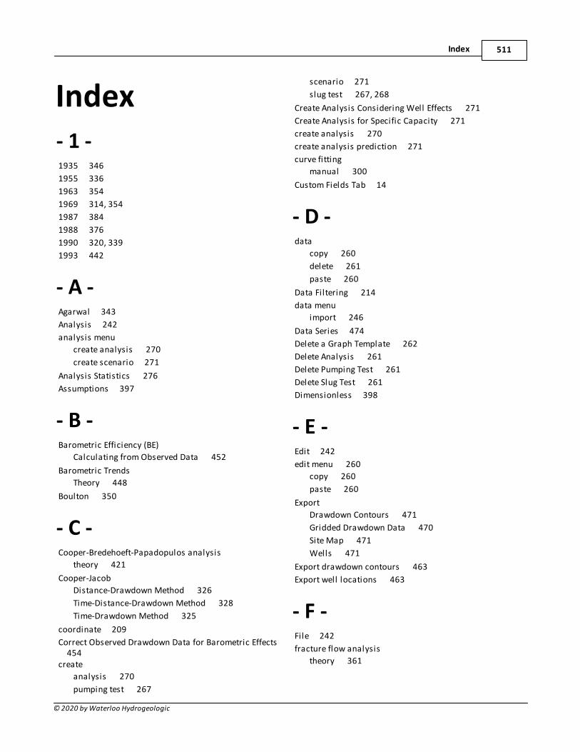
Index 511
© 2020 by Waterloo Hydrogeologic
Index- 1 -1935 346
1955 336
1963 354
1969 314, 354
1987 384
1988 376
1990 320, 339
1993 442
- A -Agarwal 343
Analysis 242
analysis menu
create analysis 270
create scenario 271
Analysis Statistics 276
Assumptions 397
- B -Barometric Efficiency (BE)
Calculating from Observed Data 452
Barometric Trends
Theory 448
Boulton 350
- C -Cooper-Bredehoeft-Papadopulos analysis
theory 421
Cooper-Jacob
Distance-Drawdown Method 326
Time-Distance-Drawdown Method 328
Time-Drawdown Method 325
coordinate 209
Correct Observed Drawdown Data for Barometric Effects
454
create
analysis 270
pumping test 267
scenario 271
slug test 267, 268
Create Analysis Considering Well Effects 271
Create Analysis for Specific Capacity 271
create analysis 270
create analysis prediction 271
curve fitting
manual 300
Custom Fields Tab 14
- D -data
copy 260
delete 261
paste 260
Data Filtering 214
data menu
import 246
Data Series 474
Delete a Graph Template 262
Delete Analysis 261
Delete Pumping Test 261
Delete Slug Test 261
Dimensionless 398
- E -Edit 242
edit menu 260
copy 260
paste 260
Export
Drawdown Contours 471
Gridded Drawdown Data 470
Site Map 471
Wells 471
Export drawdown contours 463
Export well locations 463
- F -File 242
fracture flow analysis
theory 361
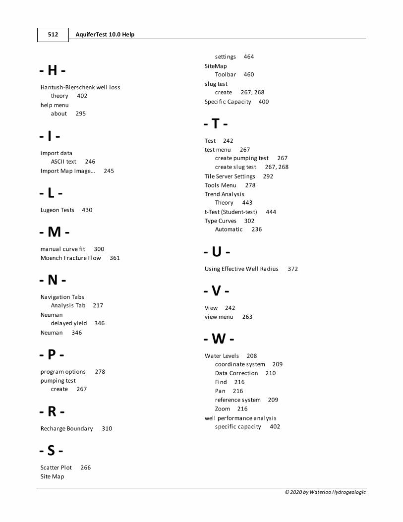
AquiferTest 10.0 Help512
© 2020 by Waterloo Hydrogeologic
- H -Hantush-Bierschenk well loss
theory 402
help menu
about 295
- I -import data
ASCII text 246
Import Map Image... 245
- L -Lugeon Tests 430
- M -manual curve fit 300
Moench Fracture Flow 361
- N -Navigation Tabs
Analysis Tab 217
Neuman
delayed yield 346
Neuman 346
- P -program options 278
pumping test
create 267
- R -Recharge Boundary 310
- S -Scatter Plot 266
Site Map
settings 464
SiteMap
Toolbar 460
slug test
create 267, 268
Specific Capacity 400
- T -Test 242
test menu 267
create pumping test 267
create slug test 267, 268
Tile Server Settings 292
Tools Menu 278
Trend Analysis
Theory 443
t-Test (Student-test) 444
Type Curves 302
Automatic 236
- U -Using Effective Well Radius 372
- V -View 242
view menu 263
- W -Water Levels 208
coordinate system 209
Data Correction 210
Find 216
Pan 216
reference system 209
Zoom 216
well performance analysis
specific capacity 402