Assessment of Aided-INS Performance

1

Assessment of Aided-INS Performance

Itzik Klein1,2

, Sagi Filin1, Tomer Toledo

1, Ilan Rusnak

2

1Faculty of Civil and Environmental Engineering

Technion – Israel Institute of Technology, Haifa 3200, Israel

2RAFAEL, P.O.Box 2250, Haifa 31021, Israel

Corresponding Author: [email protected] Phone: 972-4-8293080 Fax: 972-4-8295708

Published in Journal of Navigation 65, pp. 169-185, 2012

Abstract

Aided INS systems are commonly implemented in land vehicles for a variety of

applications. Several methods have been reported in the literature for evaluating

aided INS performance. Yet, the INS error-state-model dependency on time and

trajectory implies that no closed-form solutions exist for such evaluation. In this

paper, we derive analytical solutions to evaluate the fusion performance. We show

that the derived analytical solutions mange to predict the error covariance behavior

of the full aided INS error model. These solutions bring insight into the effect of the

various parameters involved in the fusion of the INS and an aiding.

Keywords: Aided Inertial Navigation Systems, Algebraic Riccati Equation

2

1. Introduction

Low cost continuous and accurate navigation solution is imperative for a variety of

applications, e.g., emergency services, intelligent transportation systems, and

services or military applications. Therefore, in-vehicle navigation solutions for real-

time accurate location of vehicles, have been receiving growing attention, seeing also

rapid commercial market growth. Typically, to meet the requirements of low-cost

continuous and accurate navigation Inertial Navigation Systems (INSs) are fused

with other sensors [1]. Such systems contain Inertial Measurement Units (IMU)

which measures the platforms acceleration and angular velocities, thus making the

INS a self-contained system, which is not affected by jamming or blockage. While

INSs are characterized by high bandwidth rate and insensitivity to the working

environment (urban, underground, underwater, and indoor), their accuracy degrades

with time due to measurement noise, which permeates into the navigation equations

and drifts the navigation solution.

To circumvent the drift, INS measurements are regularly fused with other sensors or

data, e.g., GPS [2], odometers [3], magnetic sensors [4], or vehicle constraints [5].

Fusion is carried out, in large, by comparing one or more of the INS outputs against

measured quantities derived from the aiding sensor during the Kalman filter

estimation process. The performance of such fusion (between INS and other sensors)

is evaluated during the early stages of design and system specification, aiming to

examine and verify the ability of the navigation system to meet its accuracy level.

Such evolution is carried out using such methods as the Monte-Carlo simulation [6]

and covariance analysis [7]. Nonetheless, due to the INS error-state model

3

dependency on time and vehicle dynamics, no closed-form solution exists to evaluate

the aided INS navigation performance.

The aim of our research is to find means for gaining analytical insight into the

parameters involved in a typical land vehicle aided INS scenario. To that end, we

derive two simplified time-invariant INS error models. For those models, we solve

analytically the corresponding Algebraic Riccati Equations (ARE) to obtain closed

form solutions to the continuous steady-state error covariance matrix.

In that manner, the number of parameters involved in an aided INS scenario was

reduced to contain only two (for position aiding) or three (for position and velocity

aiding) parameters enabling direct and immediate insight to the fusion scenario.

We evaluate the proposed approach in small fraction of the Schuler period (up to 8

minutes [9]), in which the Schuler feedback has relatively little effect on the growth

of the navigation errors. We verify the driven analytic solution against data collected

in field experiments, and show that the analytical solution of the ARE of the

simplified time-invariant error models are equivalent to those obtained solving

numerically the classical time-variant 15 error state model [8].

The rest of the paper is organized as follows: Section II introduces the fundamental

principles of INS error model and Kalman filtering; Section III presents the

derivation of the simplified aided INS error models; Section IV demonstrates the

application of the proposed models with analysis; and Section V presents conclusions

of this research.

2. Problem Formulation

The INS motion equations can be expressed in any reference frame. We employ here

the navigation frame (n-frame) which has its origin fixed at the earth surface at the

initial latitude/longitude position of the vehicle, x-axis points towards the geodetic

4

north, z-axis is on the local vertical pointing down and y-axis completes a right-

handed orthogonal frame. Thus the motion equations are given by [1]:

( )

1

1 2

nn

n b n b n n n n

ie en

b n b n b

nb

D vr

v T f g v

T T

ω ω

−

→

→ →

= + − + × Ω

(1)

( )

( ) ( )

−+

+

=−

100

0cos

10

001

1

φhN

hM

D

(2)

where, [ ]Tnr hφ λ= is the vehicle position, φ is the latitude, λ is the longitude

and h is the height above the Earth surface, [ ]Tn

N E Dv v v v= is the vehicle

velocity; b n

T→

and n b

T→

are the transformation matrices from the b-frame to the n-

frame and vice-versa, respectively; bf is the measured specific force vector;

n

ieω is

the Earth turn rate vector expressed in the n-frame; n

enω is the turn rate vector of the

n-frame with respect to the Earth; 1

ng is the local gravity vector, M and N are the

radii of curvature in the meridian and prime vertical respectively; and b

nbΩ is the

skew-symmetric form of the body rate vector with respect to the n-frame given by:

( )b b n b n n

nb ib ie enTω ω ω ω→= − + (3)

The motion equations (Eq. (1)), aka the INS mechanization equations, doesn't

provide a direct connection to the errors in the system states caused by the noisy

IMU measurements. Therefore, solving them directly, with noisy measurements,

leads to an erroneous solution. Several models (e.g. [1], [9]) were developed to link

the error-states and the measurements noise. Among them is the classical

5

perturbation analysis, in which navigation parameters are perturbed with respect to

their actual values. Perturbation is implemented via a first-order Taylor series

expansion of the states in Eq. (1). A complete derivation of this model can be found

in [11]. The error state vectorT

n n n

a gx r v b bδ δ δ ε δ δ = , 15

Rx∈δ consists of

position error, velocity and attitude errors, and accelerometer and gyro bias/drift. A

detailed description of the parameters of the corresponding state-space model can be

found in [8]. The error model is used in the navigation filter for the fusion process

between the INS and the aiding sensor. To demonstrate the proposed approach we

use here the continuous Kalman filter (detailed in Appendix A). Of particular

relevance in our study is the steady-state solution of the covariance, P , which is the

solution for the ARE

01 =−ΓΓ++ −PHRHPQFPPF

TTT (4)

where F is the system dynamics matrix defined by the type of error model

employed, Γ is the noise coefficient matrix, Q is the process noise covariance

matrix, H is the measurement matrix, and R is the measurement covariance matrix.

3. Simplified Aided INS Models

We derive two simplified time-invariant aided INS error-models, which are based on

the full time-variant 15 state-space error model. For each model, we derive closed

form expressions of the steady state estimation error covariance enabling the

evaluation of the aided INS performance. Two types of aidings are considered, i)

position measurement aiding, and ii) position and velocity measurements aiding. As

the ARE solution exist only when the system-dynamics-matrix is time-invariant, both

simplified error-models consist of a constant dynamics matrix. The first error-model

considers a single accelerometer in each axis, and can be regarded as the simplest

6

model with a constant dynamics matrix. The second error-model relates to a single

channel, consisting of a single accelerometer and gyro in each axis, and corresponds

to the most comprehensive model with a constant dynamics matrix.

As the ARE solution of the single channel model is cumbersome, no insight into the

core structure of solution is gained. Therefore, we derive a link between the single

channel and single accelerometer models.

3.1. Aided Single Accelerometer Error Model

We derive closed form expressions for the covariance and gain of the single

accelerometer (SA) error model for the position and position-and-velocity aiding

types. Prior to that, the actual SA error-model equations are derived.

1) Error Model Equations: Motion equations which are based on the

acceleration of the system have the following form

)()(

)()(

tatv

tvtp

=

=

(5)

where ( )p t , ( )v t , and ( )a t are the actual position, velocity, and acceleration,

respectively. Considering a biased accelerometer, the acceleration measurement

becomes

)()()(~ tbtatu += (6)

where ( )b t is a random walk process, described by the following differential

equation

)()( twtb b= (7)

wherebw , is a white Gaussian noise with a known spectral density 2

bQ

ωσ=

[(m/sec3)2/Hz]. The navigation equations are

7

)(~)(ˆ

)(ˆ)(ˆ

tutv

tvtp

=

=

(8)

where the hat symbol stands for the estimated value of a variable (e.g., x for x), and

the tilde for its measured value (e.g., x~ for x). The dynamics equations for the error

states, ppp ˆ−=δ and vvv ˆ−=δ , can be written as:

SASASA wxFx Γ+= δδ (9)

Where

=

b

v

p

x

δδδ

δ

,

=

000

100

010

SAF

,

=Γ

1

0

0

SA

(10)

pδ is the position error [m], vδ is velocity error [m/sec], bδ is the accelerometer

bias [m/sec2], and

SAw represents the accelerometer measurement error [m/sec3]. The

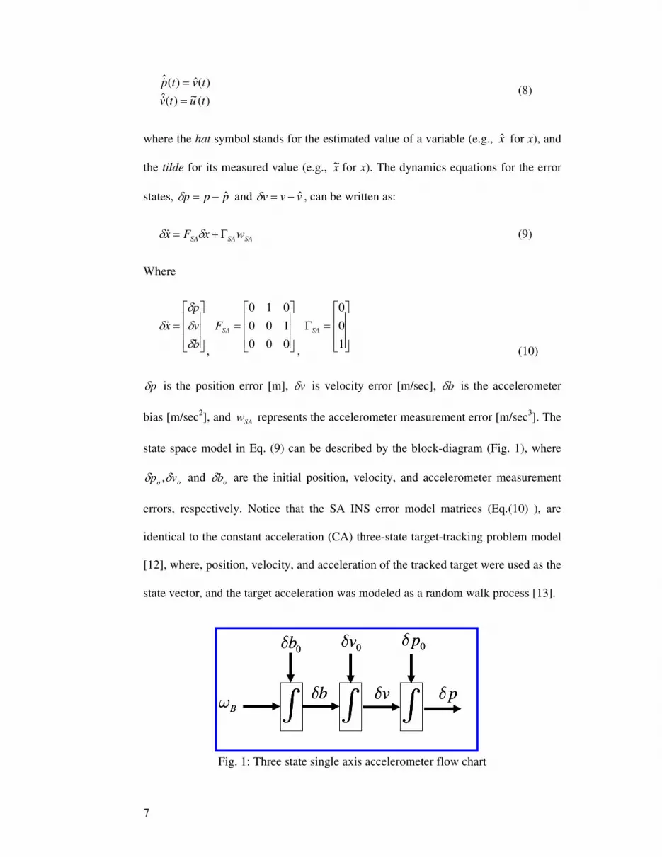
state space model in Eq. (9) can be described by the block-diagram (Fig. 1), where

oo vp δδ , and obδ are the initial position, velocity, and accelerometer measurement

errors, respectively. Notice that the SA INS error model matrices (Eq.(10) ), are

identical to the constant acceleration (CA) three-state target-tracking problem model

[12], where, position, velocity, and acceleration of the tracked target were used as the

state vector, and the target acceleration was modeled as a random walk process [13].

Fig. 1: Three state single axis accelerometer flow chart

∫∫pδ

0pδ

vδ

0vδ0bδ

bδBω ∫∫∫∫∫

pδ

0pδ

vδ

0vδ0bδ

bδBω ∫∫

8

2) Position Aiding: The SA error-model (Eq. (9)) with position aiding is given

by:

PP

SASASA

vxHz

wxFx

+=

Γ+=

δδδδ

(11)

where [ ]1 0 0pH = , and pv is the position measurement noise [m].

The measurement- and process-noise- covariances are given by

0

( ) ( ') ( ') ( ')

( ) ( ') ( ') ( ')

T

T

E w t w t Q t t q t t

E v t v t R t t r t t

δ δ

δ δ

= − = −

= − = − (12)

where q , is the spectral density of the acceleration’s random walk [(m/sec3)2/Hz];

and 0r , is the spectral density of the position measurement noise [m2/Hz]

As the model in Eq. (11) is similar to that of [13] for target tracking purposes (only

with different state vectors), the corresponding ARE solution is identical, thus:

=

=− sec

rad

r

qrP

PMSA6

0

0

5

0

4

0

3

0

4

0

3

0

2

0

3

0

2

00

0 ;

22

232

22

ωωωωωωωωωω

(13)

and the corresponding gains are:

2 3

0 0 02 2

T

SA PMK ω ω ω− = (14)

Notice that the covariance and gain depend on two parameters only – the IMU

quality ( q ), and the position aiding variance (0r ). Thus, the problem of aiding the

full 15 state error-model with position measurement, which inherently involves many

parameters, has been reduced into a two parameter problem that can be evaluated

analytically (Eqs. (13)-(14) ).

9

3) Position and Velocity Aiding: The SA error-model (Eq. (11)) with position

and velocity aiding is given by:

PVPV

SASASA

vxHz

wxFx

+=

Γ+=

δδδδ

(15)

where

=

=

V

P

PVPVv

vvH

0

0,

010

001 (16)

andPv and

Vv are the position [m] and velocity [m/sec] measurement noise,

respectively. The measurement noise covariance is given by

)'(0

0)'()'()(

0tt

r

rttRtvtvE

d

T −

=−= δδ (17)

where, r0 is the spectral density of the position measurement noise [m2/Hz], and rd, is

the spectral density of the velocity measurement noise [(m/sec)2/Hz].

We directly solve the ARE (Eq. (4)) by substituting the appropriate matrices in Eq.

(15) to obtain six nonlinear equations whose parameters are that of the covariance

matrix, P . The solution for the set of six nonlinear algebraic equations is derived in

[14] and given, in terms of the normalized covariances elements, by:

( ) ( )

( )

23 2213 33 13 12

1/22

11 13 12 13

13 11 12

23 11 22

12

1

1 3

1 11 1

2 2

41

3 2

w r

r r

r

r

Π ΠΠ = Π = Π Π +

+

Π = −Π Π = −Π

Π − Π ΠΠ = Π Π =

Π −

(18)

where

10

+−+=

2/1

211

βββ

rrw

(19)

++=

3/1

3/1 2

21

3

1

αα

βr

(20)

( ) ( )[ ]( )3 2

0

333,334324

qr

rrrrr d=

+++=α (21)

Their relation to the un-normalized elements is given in appendix B.

The normalized steady-state gain matrix may be easily obtained substituting Eq. (18)

into Eq. (A.4), leading to:

1123321331

22221221

12121111

Π=Π=ΓΠ=Γ

Π=ΓΠ=Γ

Π=ΓΠ=Γ

(22)

The covariance and gain depend only on three parameters representing the IMU

quality ( q ) and the position and velocity aiding noise (0r ,

dr ). Thus, the full 15 state

error-model aided by position and velocity measurements has been reduced into a

three parameter problem that can be evaluated analytically using Eqs. (18) & (22).

3.2. Aided Single Channel Error Model

The aided single channel (SC) is the second error model addressed here. Following

the derivation of the error model equations, the solution to the aided SC model is

derived by linking it to the aided SA model.

1) Error Model Equations: A simplified INS single channel error dynamics is

given by [8]:

11

0 1 0 0

0 0 0

0 1 / 0 1

g

e

p p

v g v w

R

δ δδ δδε δε

= +

−

(23)

where pδ is the position error [m], vδ is velocity error [m/sec], δε is the attitude

error [rad], and gw the gyro measurement error [rad/sec].

We use a first-order Gauss-Markov (GM) process (as in the full 15 state error model)

to model the INS error propagation due to accelerometer and gyro noise

( ) ( ) ( )1

c

b t b t w tτ

= − + (24)

where ( )b t is the random process, cτ is the correlation time, and ( )w t is the process

white noise. The SC model is obtained by augmenting the accelerometer and gyro

biases in their GM process representation (Eq. 24) with the INS error model (Eq.

(23))

0 1 0 0 0 0 0

0 0 1 0 0 0

0 1/ 0 0 1 0 0

0 0 0 1/ 0 1 0

0 0 0 0 1/ 0 1

a

e

g

a a a

g g g

p p

v g vw

Rw

b b

b b

δ δδ δδε δεδ τ δδ τ δ

− = + − −

(25)

where aτ is the accelerometer correlation time [sec], gτ is the gyro correlation time

[sec], aw is the driving noise for the accelerometer bias [m/sec

3] with spectral

density of 2

WaAW σ= [(m/sec3)2/Hz], and g

w is the driving noise for the gyro bias

[rad/sec] with spectral density of 2

WgGW σ= [(rad/sec)2/Hz].

2) A Semi-Analytical Solution for The Aided Error Model: The explicit closed

form solution of the aided SC INS error model either with position-and-velocity

12

measurements or with position measurements only is cumbersome and does not

enable gaining an insight into the heart of the solution.

As the system matrix for both models is time invariant (Eqs. (9) & (25)), we can

adopt the following approach: using the aided SA INS error-model covariance

solution, denotedSAP , as a core solution and present the aided SC INS error model

solution, denoted SCP , in the following layout

[ ] [ ]2 , , 1,2,3.SC ij SAij ij

P P i jκ= = (26)

where [ ]ik

P is the covariance matrix Eq. (34), and 2

ijκ are correction factors.

The correction factors of Eq. (18), linking between the SA and SC models, are a

function of the error state covariances. Thus, they depend on the IMU quality, aiding

type (position or position-and-velocity), and their measurement noise level only.

Consequently, the correction factors should be evaluated only once for a certain

IMU.

4. Analysis and Results

The closed form analytical solution of the simplified INS error models are evaluated

here using data collected from three field experiments. We elaborate on the analysis

of one trajectory, and then apply it to the other two. The actual covariances, for the

collected data, of the full 15 error-state model have been numerically calculated and

are compared to the analytically derived SA and SC covariances. Data were collected

with MEMS INS/GPS while driving in an urban environment. The vehicle was

equipped with a Microbotics MIDG II [15] INS/GPS system.

In the examined trajectory (Fig. 2), the stationary vehicle accelerated

to [ ]60 /v km h= , and then kept the velocity in the range between 60 and 80 [km/h].

13

In the examined experiment the height variations was about ~15 [m] along the

trajectory.

Fig. 2: Examined Trajectory 1

4.1. Aided Single Accelerometer Error Model

The SA INS error model with position and velocity aiding is addressed first. The

evaluation results are presented in Fig. 3, comparing the analytical and computed

square-root of the error covariances. Computed values are derived numerically from

the error covariances of the full 15-state model while the analytical values are

obtained from Eq. (18). As Fig. 3 shows, the analytical position components match

the numerical ones. The analytical expression also manages to predict the altitude

velocity component but not the actual north and east velocity components. This

behavior can be explained by the coupling of the north and east channels in the full

15 state model, which is not compensated for in the SA model. The altitude channel

covariance is evaluated correctly by the closed form expressions as it is weakly

affected by the other two channels and acts similarly to the SA in the full 15 state

model.

14

0 100 200

-1

0

1

σL

atit

ud

e [

m]

0 100 200

-1

0

1

σL

on

gitu

de [

m]

0 100 200

-1

-0.5

0

0.5

1

σH

eig

ht S

TD

[m

]

0 100 200

-0.1

-0.05

0

0.05

0.1

Time [sec]

σV

N

[m

/s]

0 100 200

-0.1

-0.05

0

0.05

0.1

Time [sec]

σV

E

[m

/s]

0 100 200

-0.05

0

0.05

Time [sec]

σV

D

[m

/s]

Fig. 3: Position (LLH) and velocity (NED) components of the single accelerometer error model

with position and velocity aiding. Red (straight lines) and blue lines represents the analytical

and computed square root of the error covariance, respectively

0 100 200

-5

0

5

σL

atit

ud

e [

m]

0 100 200

-5

0

5

σL

on

gitu

de [

m]

0 100 200

-4

-2

0

2

4

σH

eig

ht S

TD

[m

]

0 100 200

-1

0

1

Time [sec]

σV

N

[m

/s]

0 100 200

-1

0

1

Time [sec]

σV

E

[m

/s]

0 100 200

-0.2

0

0.2

Time [sec]

σV

D

[m

/s]

15


with position aiding. Red (straight lines) and blue lines represents the analytical and computed

square root of the error covariance, respectively

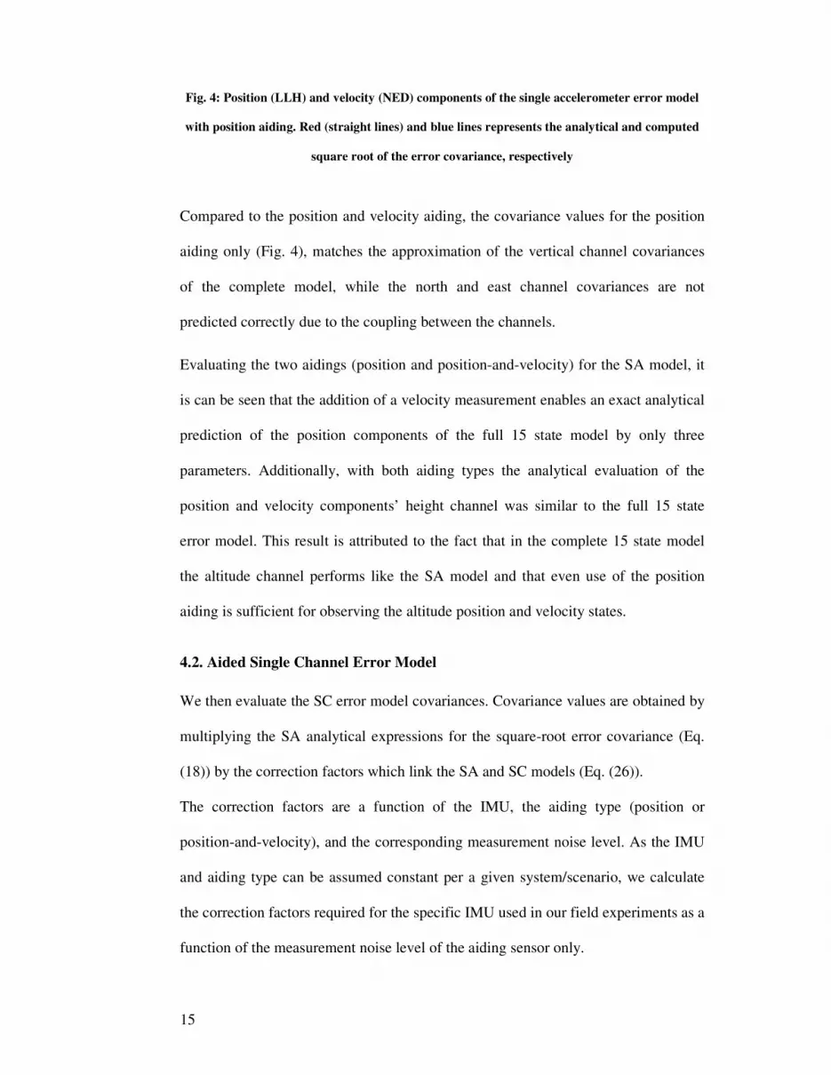
Compared to the position and velocity aiding, the covariance values for the position

aiding only (Fig. 4), matches the approximation of the vertical channel covariances

of the complete model, while the north and east channel covariances are not

predicted correctly due to the coupling between the channels.

Evaluating the two aidings (position and position-and-velocity) for the SA model, it

is can be seen that the addition of a velocity measurement enables an exact analytical

prediction of the position components of the full 15 state model by only three

parameters. Additionally, with both aiding types the analytical evaluation of the

position and velocity components’ height channel was similar to the full 15 state

error model. This result is attributed to the fact that in the complete 15 state model

the altitude channel performs like the SA model and that even use of the position

aiding is sufficient for observing the altitude position and velocity states.

4.2. Aided Single Channel Error Model

We then evaluate the SC error model covariances. Covariance values are obtained by

multiplying the SA analytical expressions for the square-root error covariance (Eq.

(18)) by the correction factors which link the SA and SC models (Eq. (26)).

The correction factors are a function of the IMU, the aiding type (position or

position-and-velocity), and the corresponding measurement noise level. As the IMU

and aiding type can be assumed constant per a given system/scenario, we calculate

the correction factors required for the specific IMU used in our field experiments as a

function of the measurement noise level of the aiding sensor only.

16

We use the analytical SA (Eq. (18)) and the numerical aided SC (Eq. (25)) error

model expressions and insert them into Eq. (26) in order to obtain the correction

factors. Fig. 5 presents the correction factors for the SA error model with position-

and-velocity aiding. They are plotted against the position-measurement-noise-level

and for various velocity noise-level magnitudes. posκ , which is equivalent to 11κ in

Eq. (26), is the correction factor for the position error state and velκ , which is

equivalent to 22κ in Eq. (26), is the correction factor for the velocity error state.

Fig. 5: Single accelerometer error model correction factors for position and velocity

measurements aiding

When the velocity aiding measurement noise is smaller than 0.1[m/s], the correction

factors for both velocity and position are constant regardless of the amount of the

position measurement noise. For higher velocity-measurement-noise values, both

correction factors (position and velocity) converge to a constant value. That is, the

correction factors can be considered constants regardless of the measurement noise

and used incessantly with the SA error-model. This is an expected result as the filter

gives lower weight to the measurement due to the amount of high measurement

noise.

Fig. 6 presents the position aiding correction factors as a function of the position

measurement noise (computed in a similar fashion as for Fig. 5). The velocity

17

correction factors increase as the amount of measurement noise increases, while the

position-correction-factor convergences to a constant value.

Fig. 6: Single accelerometer error model correction factors for position measurement aiding

Following the computation of the correction factors, results for position and velocity

aiding are presented in Fig. 7. There, the position and velocity components of the

square-root of the error covariance of the full 15-state model (which was calculated

numerically) match exactly the SC analytical expressions for the square-root of the

error covariance (Eq. (26)). This result was achieved, although the SC model has

constant time dynamics and no coupling between its three orthogonal axes, in

contrast to the full error model. Thus, we evaluate the results of the 15 error state

aided INS model covariances by the semi-analytical expressions, making the

numerical evaluation unnecessary.

The covariance values for the position aiding are presented in Fig. 8. The position

and velocity components of the square root of the error covariance of the full aided

INS 15 error state model, which was calculated numerically, match exactly, again,

the SC semi-analytical expressions for the square-root of the error covariance. Thus,

in the aided SC model, position measurement is sufficient to predict the position and

velocity states despite of the fact that it has constant time dynamics and no coupling

between its three orthogonal axes. Consequently, using only four variables of the

18

INS quality, aiding value, and position and velocity correction factors, the

covariances are evaluated.

Comparing the SC and SA aided models performance, shows that the SC model

outperforms the SA model in predicting the full aided INS 15 error state model. This

result was anticipated as the SC model is more accurate (because of the gyro and GM

error-states) relative to the full-model rather than the SA model.

0 100 200

-1

0

1

σL

atit

ud

e [

m]

0 100 200

-1

0

1

σL

on

gitu

de [

m]

0 100 200

-1

-0.5

0

0.5

1

σH

eig

ht S

TD

[m

]

0 100 200

-0.1

-0.05

0

0.05

0.1

Time [sec]

σV

N

[m

/s]

0 100 200

-0.1

-0.05

0

0.05

0.1

Time [sec]

σV

E

[m

/s]

0 100 200

-0.05

0

0.05

Time [sec]

σV

D

[m

/s]

Fig. 7: Position (LLH) and velocity (NED) components of the single channel error model with

position and velocity aiding. Red (straight lines) and blue lines represents the analytical and

computed square root of the error covariance, respectively

19

0 100 200

-5

0

5

σL

atit

ud

e [

m]

0 100 200

-5

0

5

σL

on

gitu

de [

m]

0 100 200

-4

-2

0

2

4

σH

eig

ht S

TD

[m

]

0 100 200

-1

0

1

Time [sec]

σV

N

[m

/s]

0 100 200

-1

0

1

Time [sec]

σV

E

[m

/s]

0 100 200

-0.2

0

0.2

Time [sec]

σV

D

[m

/s]


position aiding. Red (straight lines) and blue lines represents the analytical and computed

square root of the error covariance, respectively

4.3. Application to Additional Trajectories

Application of the model to two additional trajectories with different characteristics

shows the same prediction ability as with the analyzed trajectory. In this trajectory,

the stationary vehicle accelerated to [ ]60 /v km h= , and then kept a velocity in the

range of 60-80 [km/h]. The vehicle climbed along this trajectory ~100 [m] in

elevation. In the second trajectory, the stationary vehicle accelerated to [ ]40 /km h ,

and then kept a velocity in the range of 40-60 [km/h].

In order to evaluate the proposed approach in different noise levels, we used for the

second trajectory a noise-measurement-covariance which was five times bigger than

the one used in trajectory 1, for both aidings and aided INS simplified error models.

20

Yet we present here only the results for position and velocity aiding. As can be

observed in Figs. 9-10, for both SA and SC error models and both aiding types, a

similar behavior to the first trajectory was obtained even with the different

measurement noise level. That is, with the SA model and for both aiding types, the

analytical evaluation of the height channel’s position and velocity components was

similar to the full 15 state error model, while the addition of velocity measurement

enabled to evaluated analytically the complete position vector. With the SC model,

the position aiding was sufficient to predict the position and velocity states of the full

15 state model.

0 50 100

-2

0

2

σL

atit

ud

e [

m]

0 50 100

-2

0

2

σL

on

gitu

de [

m]

0 50 100

-2

0

2

σH

eig

ht S

TD

[m

]

0 50 100

-0.2

-0.1

0

0.1

0.2

Time [sec]

σV

N

[m

/s]

0 50 100

-0.2

-0.1

0

0.1

0.2

Time [sec]

σV

E

[m

/s]

0 50 100

-0.1

-0.05

0

0.05

0.1

Time [sec]

σV

D

[m

/s]




21

0 50 100

-2

0

2

σL

atit

ud

e [

m]

0 50 100

-2

0

2

σL

on

gitu

de [

m]

0 50 100

-2

0

2

σH

eig

ht S

TD

[m

]

0 50 100

-0.2

-0.1

0

0.1

0.2

Time [sec]

σV

N

[m

/s]

0 50 100

-0.2

-0.1

0

0.1

0.2

Time [sec]

σV

E

[m

/s]

0 50 100

-0.1

-0.05

0

0.05

0.1

Time [sec]σ

VD

[m

/s]




In order to evaluate the proposed approach in different noise levels, we used a one

hundred times bigger process noise covariance for the GM states for the third

trajectory. This was conducted for both aidings and both aided INS simplified error

models. However we present here only the results for position and velocity aiding

Results are presented in the Figs. 11-12. As can be observed, the same performance

as with the previous trajectories was obtained even with the different measurement

noise level. With the SA model and for both aiding types the analytical evaluation of

the height channel’s position and velocity components’ was similar to the full error

model, while the addition of velocity measurement enabled to evaluated analytically

22

the whole position vector. With the SC model, both aidings enabled prediction of the

position and velocity states of the full 15 state model.

0 100 200

-1

0

1

σL

atit

ud

e [

m]

0 100 200

-1

0

1

σL

on

gitu

de [

m]

0 100 200

-1

-0.5

0

0.5

1

σH

eig

ht S

TD

[m

]

0 100 200-0.2

-0.1

0

0.1

0.2

Time [sec]

σV

N

[m

/s]

0 100 200

-0.1

0

0.1

Time [sec]

σV

E

[m

/s]

0 100 200

-0.1

-0.05

0

0.05

0.1

Time [sec]

σV

D

[m

/s]




23

0 100 200

-1

0

1

σL

atit

ud

e [

m]

0 100 200

-1

0

1

σL

on

gitu

de [

m]

0 100 200

-1

-0.5

0

0.5

1

σH

eig

ht S

TD

[m

]

0 100 200-0.2

-0.1

0

0.1

0.2

Time [sec]

σV

N

[m

/s]

0 100 200

-0.1

0

0.1

Time [sec]

σV

E

[m

/s]

0 100 200

-0.1

-0.05

0

0.05

0.1

Time [sec]

σV

D

[m

/s]




5. Conclusions

Land navigation with aided-INS is needed for a variety of applications. Evaluation of

the navigation system in early stages of design and system implementation enables

examining the navigation system performance relative to desired navigation

accuracy. In this paper, an analytical insight into the parameters involved in the

fusion between INS and an aiding sensor was gained. To that end, two simplified

time-invariant aided-INS error models were employed. Using both models, closed

form solutions in terms of the continuous steady-state estimation error covariance

matrix, were derived for evaluating the fusion performance. The closed from

expressions of the simplified error models were compared to numerical results

obtained from data collected in a field experiment, using the full 15 state error

24

model. Results show that the derived closed form expressions managed to predict the

error covariance behavior of the full error model. Even though, these closed-from

expressions are valid only for small fractions of the Schuler period, they bring insight

into the effect of the various parameters involved in the fusion between the INS and

an aiding sensor. They may help the navigation system designer to better evaluate

and understand the connection of the parameters concerned in the fusion process.

Future work will examine the effect of Schuler feedback loop when evaluating the

closed form expressions in medium and long term time periods. Additionally, since

GPS is the main aiding sensor for the INS derivation of closed form expressions for

the non-linear tightly coupled approach is another potential expansion of the

presented models.

6. Appendix A

We consider here the linear stochastic system

( ) ( ) ( ) ( ) ( ) ( )( ) ( ) ( ) ( )tvtxtHtz

xtxtwttxtFtx

+=

=Γ+=

δδδδδδ 00,

(A.1)

where ( )txδ is the error state vector; ( )tzδ is the measurement residual; w(t) and v(t)

are the white Gaussian stochastic processes representing the system driving noise and

the measurement noise, respectively; ( )0txδ is a Gaussian random vector, and

,[ ] [ ( )] 0, [ ( )] 0,

[ ( ) ( ') ] ( - '), [ ( ) ( ') ] ( - '),

[ ( ) ( ') ] 0, [ ( ) ] 0, [ ( ) ] 0,

[( - ( ))( - ( ) ] .

o o

T T

T T T

o o

T

o o o o o

E x x E w t E v t

E w t w t Q t t E v t v t R t t

E w t v t E w t x E v t x

E x E x x E x P

δ δ

= = =

= =

= = =

= (A.2)

All vectors and matrices are of appropriate dimensions. The Kalman filter is [7]:

25

( ) ( ) ( ) ( ) ( ) ( ) ( )[ ] ( ) 00ˆ,ˆˆˆ xtxtxtHtztKtxtFtx δδδδδδ =−+=

(A.3)

( ) ( ) ( ) 1−= RtHtPtKT

(A.4)

( ) ( ) ( ) ( ) ( ) ( ) ( ) ( )00

1 , PtPtHPRHtPQtFtPtPtFtPTTT =−ΓΓ++= −

(A.5)

The steady-state solution of the covariance, P , is the solution of the ARE

.0 1PHRHPQFPPF

TTT −−ΓΓ++= (A.6)

With the steady-state solution obtained from Eq. (9), we have the explicit solution

[10]

( ) ( )0

1

1

0 0 0 0 0 0

1

0 0

( ) ( , ) ( , ) ( , ) ( , )

( , ) ( , )

t

T T T

t

T

P t P t t P P I t H R H t P P d t t

t t F PH R H t t

τ τ τ

−

−

−

= +Φ − + Φ Φ − Φ

Φ = − Φ

∫

(A.7)

7. Appendix B

The connection between the normalized and non-normalized steady-state error

covariance terms is given by:

11 2211 22 3

0 0 0 0

12 2312 232 4

0 0 0 0

13 3313 333 5

0 0 0 0

2 3

2 2

2

P P

r r

P P

r r

P P

r r

ω ω

ω ω

ω ω

Π = Π =

Π = Π =

Π = Π = (B.1)

The connection between the normalized and non-normalized steady-state gain terms

is given by:

26

4

0

32

323

0

13

31

3

0

22

222

0

21

21

2

0

12

12

0

11

11

2

32

22

ωω

ωω

ωω

rKK

rKK

rKK

=Γ=Γ

=Γ=Γ

=Γ=Γ

(B.2)

REFERENCES

[1] Titterton, D. H. and Weston, J. L., Strapdown Inertial Navigation Technology –

Second Edition, The American institute of aeronautics and astronautics and the

institution of electrical engineers, 2004.

[2] Groves, P. D., Principles of GNSS, inertial and multisensor integrated navigation

systems, Artech House, 2008.

[3] Stephen, J., and Lachapelle, G., "Development and Testing of a GPS-Augmented

Multi-Sensor Vehicle Navigation System", The Journal of Navigation, Vol. 54(2),

pp. 297-319, 2001.

[4] Godha, S., Petovello M. G., and Lachapelle G., "Performance analysis of MEMS

IMU/HSGPS/magnetic sensor integrated system in urban canyons", in

Proceedings of ION GPS, Long Beach, CA, U. S. Institute of Navigation, Fairfax

VA, pp. 1977-1990, , September 2005.

[5] Klein I., Filin S. and Toledo T., "Pseudo-measurements as aiding to INS during

GPS outages", NAVIGATION, Vol. 57, No. 1, pp. 25-34, 2010.

27

[6] Lin, C.-F., Modern navigation guidance and control processing, Prentice Hall

series in advanced navigation, guidance and control, and their applications, 1991.

[7] Zarchan, P. and Musoff, H., Fundamentals of Kalman filtering: a practical

approach second edition, The American Institute of Aeronautics and

Astronautics, Inc., Reston, Virginia, 2005.

[8] Farrell, J. A., Aided navigation GPS with high rate sensors, McGraw-Hill, 2008.

[9] Jekeli, C., Inertial Navigation Systems with Geodetic Applications, Walter de

Gruyter Berlin, Germany, 2000.

[10] Rusnak, I., "Almost Analytic Representation for the Solution of the Differential

Matrix Riccati Equation", IEEE Trans. on Automatic Control, Vol. AC-23, pp.

191-193, February 1988.

[11] Britting, K. R., Inertial navigation systems analysis, John Wily & Sons Inc.,

1971.

[12] Singer, R. A., "Estimating optimal tracking filter performance for manned

maneuvering targets", IEEE Trans .on Aerospace and Electronic Systems, AES-6,

pp. 473-483, July 1970.

[13] Fitzgerald, R. J., "Simple tracking filters: Closed-form solutions", IEEE Trans.

on Aerospace and Electronic Systems, Vol. AES-17, pp. 781-785, November

1981.

[14] Klein, I. and Rusnak, I., "Semi-Analytic Solution of ECA Filter with Position

and Velocity Measurements", 50th Israel Annual Conference on Aerospace

Sciences, Israel, February 17-18, 2010.

[15] Microbotics website – www.microboticsinc.com (last accessed 2010).

28

Documents

Assessment of Aided-INS Performance