Adaptive Kalman Filtering forLow-cost INS/GPS

Christopher Hide, Terry Moore and Martin Smith

(University of Nottingham)

This paper was first presented at ION GPS 2002, the 15th Technical Meeting of the Satellite

Division of the Institute of Navigation held at Portland Oregon, USA. The paper was awardeda Best Presentation award in Session C3a on MEMS Inertial Measuring Units.

GPS and low-cost INS sensors are widely used for positioning and attitude determinationapplications. Low-cost inertial sensors exhibit large errors that can be compensated usingposition and velocity updates from GPS. Combining both sensors using a Kalman filterprovides high-accuracy, real-time navigation. A conventional Kalman filter relies on the cor-

rect definition of the measurement and process noise matrices, which are generally defineda priori and remain fixed throughout the processing run.AdaptiveKalman filtering techniquesuse the residual sequences to adapt the stochastic properties of the filter on line to correspond

to the temporal dependence of the errors involved. This paper examines the use of threeadaptive filtering techniques. These are artificially scaling the predicted Kalman filter co-variance, the Adaptive Kalman Filter and Multiple Model Adaptive Estimation. The algor-

ithms are tested with theGPS and inertial data simulation software. A trajectory taken from areal marine trial is used to test the dynamic alignment of the inertial sensor errors. Resultsshow that on line estimation of the stochastic properties of the inertial system can significantlyimprove the speed of the dynamic alignment and potentially improve the overall navigation

accuracy and integrity.

KEY WORDS

1. Integration. 2. GPS. 3. INS.

1. INTRODUCTION. GPS and Inertial Navigation Systems (INS) are widelyused for positioning and attitude determination applications. A range of low-costInertial Motion Units (IMU) are available, but these inertial sensors exhibit largeerrors that must be compensated. The inertial sensor errors can be categorised pri-marily as first order biases, scale factors and misalignments. Conventional Kalmanfiltering using GPS position, velocity and, when available, attitude updates can pro-vide estimates of these errors.

To achieve the best performance from the Kalman filter, both the dynamic modeland the stochastic information provided to the filter must be accurate. The standardinertial navigation system error model described in texts such as Britting (1971) andTitterton and Weston (1997) is considered to be adequate for this research. However,the stochastic model is recognised to be limited when using a priori statistics to modelerrors that have time varying characteristics (Mohamed and Schwarz, 1999). Toachieve the best performance fromaKalmanfilter, it is therefore necessary to adapt the

THE JOURNAL OF NAVIGATION (2003), 56, 143–152. f The Royal Institute of NavigationDOI: 10.1017/S0373463302002151 Printed in the United Kingdom

stochastic model to accommodate for changes in vehicle dynamics and environmentalconditions. This paper examines the use of adaptive Kalman filtering algorithms forimproving Kalman filter performance.

An example of the time varying nature of the errors involved is highlighted throughthe initialisation of the inertial sensor error states.When estimating sensor errors, a lowprocess noise variance will result in a precise yet most likely biased estimate. This willresult in a long transition to the correct error estimate. Conversely, a larger a priori esti-mate of process noise will result in a quicker transition to the correct error estimate butwill result in a less precise estimate. By adapting the process noisematrix in theKalmanfilter, both characteristics can be utilized to result in a quick transition to a preciseunbiased estimate.

Several methods exist for adapting the measurement and process noise matrices in aKalman filter. TheAdaptiveKalmanFilter (AKF)was used inMohamed andSchwarz(1999) for integrating navigation grade INS measurements with GPS. Mohamed andSchwarz showed that the AKF resulted in a 20% (RMS) improvement in attitudeestimation (Mohamed, 1999). Wang et al. (1999) used adaptive Kalman filtering toestimate the GPSmeasurement noise with a tactical grade INS, specifically to improveambiguity resolution.

Another method used to adapt the weighting between the INS and GPS measure-ments is to adaptively scale the Kalman filter predicted covariance matrix. Hu et al.(2001) described the use of this method for reducing the dynamic modelling errors forfiltering DGPS measurements.

The final method considered here isMultipleModel Adaptive Estimation (MMAE)that selects the best state estimate from a bank of simultaneously operating Kalmanfilters. Previously, MMAE has not been examined due to the computational loadcaused by running simultaneous filters ; however, advances in processor technologynow makes this less of a limitation. This paper examines the use of these adaptive fil-tering techniques withReal TimeKinematic (RTK)GPS and low-cost inertial sensors.

2. ADAPTIVE KALMAN FILTERING ALGORITHMS. A numberof adaptive Kalman filtering techniques exist to achieve the criteria described inadapting the stochastic properties of the Kalman Filter. Most techniques use theinnovation sequence as the basis for adapting the measurement noise covariance,Rk, and the process noise covariance, Qk. These methods use a windowing functionon the most recent innovations. Correct identification of the window size also needsto be identified to obtain the correct balance between filter adaptivity and stability.Multiple Model Kalman filtering is also described as a potential method for filteradaptation.

2.1. Covariance Scaling. The covariance scaling method was used in Hu et al.(2001) for improving the stochastic modelling of differential pseudo-range GPS. Thepredicted covariance, P

(+)kx1, is artificially scaled by the factor Sk>1 to apply more

weight to the measurements:

P(+)k =Sk(WP

(x)kx1W

T+Qkx1): (1)

Different techniques can be used in estimating Sk. For example, a priorimethods canbe used in alignment of low-cost IMUs, where it is known that the inertial sensorerrors will be larger before the system has been aligned. Another proposed method is

144 C. HIDE, T. MOORE AND M. SMITH VOL. 56

presented in Hu et al. (2001), which uses an algorithm based on the magnitude of thepredicted residuals.

2.2. Adaptive Kalman Filter. The principle of the Adaptive Kalman Filter (AKF)is to make the Kalman filter residuals consistent with their theoretical co-variances(Mehra, 1972). An estimate of the covariance of the innovation residual is obtained byaveraging the previous residual sequence over a window length N :

Cv(x)

k

=1

N

Xk

j=kxN+1

v(x)j (v

(x)j )T, (2)

where: v(x)j =zkxHkx

(x)k is the innovation residual from the Kalman filter. The es-

timated measurement noise is computed by comparing the theoretical covariance(HkP

(x)k HT

k+Rk) with the estimated covariance to give :

RRk=Cv(x)

k

xHKP(x)k HT

k : (3)

The estimated process noise can also be obtained (see Wang et al. (1999)) to give:

QQk=1

N

Xk

j=kxN+1

DxjDxTj +P

(+)k xWP

(+)kx1W

T, (4)

where: Dxk=x(x)k xx

(+)k . This is known as a residual based estimate. Equation (4)

can be written in terms of the innovation sequence by making the following substi-tution for the covariance of the state corrections (Mohamed and Schwarz, 1999),

CCDxk �1

N

Xk

j=kxN+1

DxjDxTj � KkCCv

(x)

k

KTk : (5)

For a full derivation of these equations using the maximum likelihood method, seeMohamed (1999). These equations result in a full variance/covariance matrix thatattempts to model some of the inherent correlations.

2.3. Multiple Model Adaptive Estimation. Multiple Model Adaptive Estimation(MMAE) uses multiple Kalman filters that run simultaneously, in this case each usingdifferent stochastic properties (Brown and Hwang, 1997). The correct model is ident-ified using the residual probability density function. MMAE has not previously beenconsidered for navigation applications due to the substantial increase in processor loadcaused by running simultaneous Kalman filters. Recent improvements in processorspeed reduce this potential problem.

2.3.1. MMAE Algorithm. For each filter, the probability density function, fn(zk),for the nth Kalman filter is given by:

fn(zk)=1ffiffiffiffiffiffiffiffiffiffiffiffiffiffiffiffiffiffiffiffiffiffiffiffi

(2p)mjCv(x)

k

jq e

x12vkC

x1

v(x)

k

vTk

, (6)

where: m is the number of measurements. The probability pn(k) that the nth model iscorrect is computed from the recursive formula:

pn(k)=fn(zk) � pn(kx1)

PNj=1

fj(zk) � pj(kx1)

, (7)

NO. 1 ADAPTIVE KALMAN FILTERING 145

forNKalman filters. The optimal state estimate is computed using the weighted com-bination of states using:

xx(+)k =

XNj=1

pj(k)xx(+)kj

: (8)

This results in the identification of a single correct model for which pn(k) willconverge to unity, and the other models to zero. As a result, the filter will ignore newobservations; this deficiency can be overcome in a variety of ways. For example, athreshold value can be defined for pn(k), or the smallest value for fn(zk) could be used toidentify the best model at each epoch (Welch and Bishop, 2001).

3. SOFTWARE. The software used to process the measurements was devel-oped at the Institute of Engineering Surveying and Space Geodesy (IESSG) and iscalled KinPosi. KinPosi processes raw GPS and INS measurements using cen-tralised or decentralised Kalman filtering. The software can process dual-frequencypseudo-range, carrier-phase and doppler GPS observations and uses the LAMBDAambiguity resolution method (De Jonge and Tiberius, 1996). The filter containsnine navigation states and up to 24 inertial error states to estimate sensor bias, scalefactor and axis non-orthogonality errors. KinPosi provides the capability for all theadaptive Kalman filtering methodologies described in the previous section.

4. DATA SIMULATION. Data simulation is useful in assessing the per-formance of the algorithms described, as it allows direct control over all the errorparameters. Using simulated data for inertial measurements provides truth not onlyfor navigation errors, but also for sensor errors that can be compared to the Kalmanfilter estimates. The IESSG’s Navigation System Simulator (NSS) was developed forthe European Space Agency (ESA) Low-Cost Navigator (LCN) project.

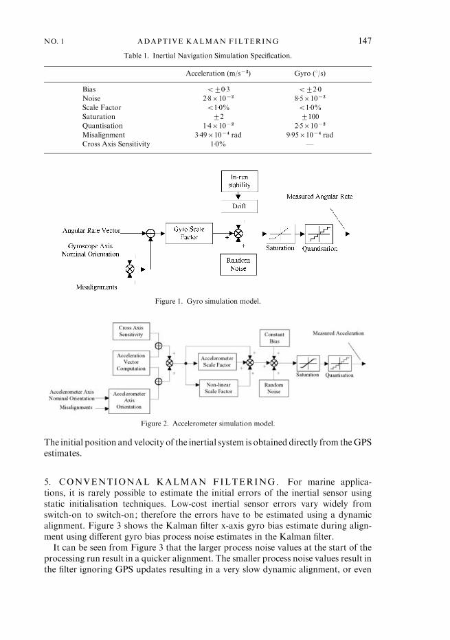
NSS creates raw GPS and inertial measurements from a kinematic trajectoryfile containing position and attitude measurements. The simulator creates L1 and L2pseudo-range, carrier and doppler measurements using ionospheric, troposphericand multipath models ; satellite and receiver clock errors ; satellite orbit errors ; andmeasurement noise. Cycle slips and unhealthy satellites can also be modelled. Thesimulator uses an SP3 format file to provide ephemeris data for any time period.The inertial measurements are simulated using themodels described in Figures 1 and 2.The body frame angular rate and accelerations are computed from the trajectoryinput, which is interpolated at the high rate of the inertial measurements.

Table 1 describes the inertial errors that are simulated and their respective values,which correspond to a typical low-cost MEMS sensor. The trajectory simulated istaken from a real trajectory obtained using a POS/MV system at a marine trial using asmall survey boat in Plymouth, UK. A range of dynamic manoeuvres were performedbeginning with figure-of-eight paths for alignment. The 15-minute trajectory used inthis paper corresponds to the alignment section of the trajectory. The initial attitudemisalignment is 0.6x,x1.6x, 2.0x for roll, pitch and yaw respectively, which correspondsto the level error of the boat on thewater, and a heading error whichwould be obtainedfrom, for example, the boat’s on-board compass. The IMUmeasurements are updatedat 100 Hz. TheKalman filter is run in loosely coupledmode withGPS updates at 1 Hz.

146 C. HIDE, T. MOORE AND M. SMITH VOL. 56

The initial position and velocity of the inertial system is obtained directly from theGPSestimates.

5. CONVENTIONAL KALMAN FILTERING. For marine applica-tions, it is rarely possible to estimate the initial errors of the inertial sensor usingstatic initialisation techniques. Low-cost inertial sensor errors vary widely fromswitch-on to switch-on; therefore the errors have to be estimated using a dynamicalignment. Figure 3 shows the Kalman filter x-axis gyro bias estimate during align-ment using different gyro bias process noise estimates in the Kalman filter.

It can be seen from Figure 3 that the larger process noise values at the start of theprocessing run result in a quicker alignment. The smaller process noise values result inthe filter ignoring GPS updates resulting in a very slow dynamic alignment, or even

Figure 1. Gyro simulation model.

Figure 2. Accelerometer simulation model.

Table 1. Inertial Navigation Simulation Specification.

Acceleration (m/sx2) Gyro (x/s)

Bias <t0.3 <t2.0

Noise 2.8r10x2 8.5r10x2

Scale Factor <1.0% <1.0%

Saturation t2 t100

Quantisation 1.4r10x2 2.5r10x2

Misalignment 3.49r10x4 rad 9.95r10x4 rad

Cross Axis Sensitivity 1.0% —

NO. 1 ADAPTIVE KALMAN FILTERING 147

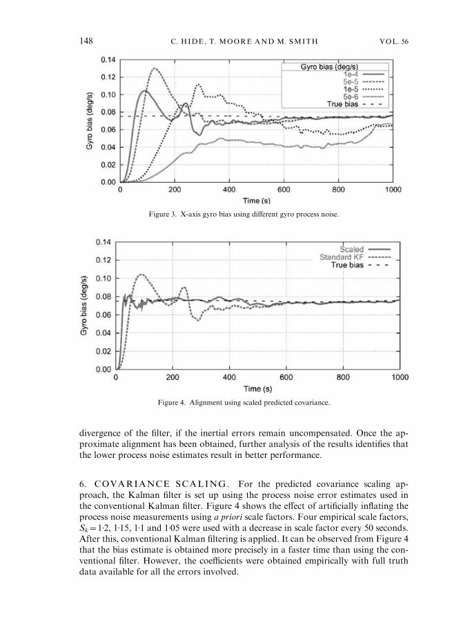
divergence of the filter, if the inertial errors remain uncompensated. Once the ap-proximate alignment has been obtained, further analysis of the results identifies thatthe lower process noise estimates result in better performance.

6. COVARIANCE SCALING. For the predicted covariance scaling ap-proach, the Kalman filter is set up using the process noise error estimates used inthe conventional Kalman filter. Figure 4 shows the effect of artificially inflating theprocess noise measurements using a priori scale factors. Four empirical scale factors,Sk=1.2, 1.15, 1.1 and 1.05 were used with a decrease in scale factor every 50 seconds.After this, conventional Kalman filtering is applied. It can be observed from Figure 4that the bias estimate is obtained more precisely in a faster time than using the con-ventional filter. However, the coefficients were obtained empirically with full truthdata available for all the errors involved.

Figure 3. X-axis gyro bias using different gyro process noise.

Figure 4. Alignment using scaled predicted covariance.

148 C. HIDE, T. MOORE AND M. SMITH VOL. 56

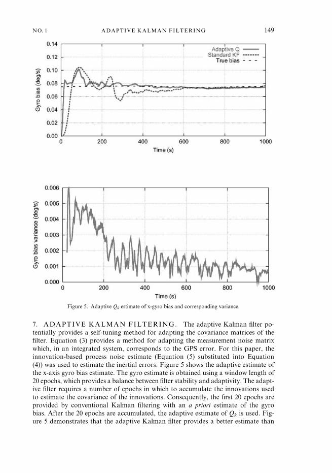
7. ADAPTIVE KALMAN FILTERING. The adaptive Kalman filter po-tentially provides a self-tuning method for adapting the covariance matrices of thefilter. Equation (3) provides a method for adapting the measurement noise matrixwhich, in an integrated system, corresponds to the GPS error. For this paper, theinnovation-based process noise estimate (Equation (5) substituted into Equation(4)) was used to estimate the inertial errors. Figure 5 shows the adaptive estimate ofthe x-axis gyro bias estimate. The gyro estimate is obtained using a window length of20 epochs, which provides a balance between filter stability and adaptivity. The adapt-ive filter requires a number of epochs in which to accumulate the innovations usedto estimate the covariance of the innovations. Consequently, the first 20 epochs areprovided by conventional Kalman filtering with an a priori estimate of the gyrobias. After the 20 epochs are accumulated, the adaptive estimate of Qk is used. Fig-ure 5 demonstrates that the adaptive Kalman filter provides a better estimate than

Figure 5. Adaptive Qk estimate of x-gyro bias and corresponding variance.

NO. 1 ADAPTIVE KALMAN FILTERING 149

the standard Kalman filter. The adaptive filter settles to a precise estimate of the gyrobias in just over 100 seconds. Similar results were obtained for resolution of theother sensor bias states.

Also shown in Figure 5 is the corresponding variance estimate provided by theadaptive filter. It can be observed from the estimated gyro variance that the overallmagnitude of the estimate reduces as the system becomes aligned. The fluctuations inthe gyro bias variance estimate are caused by the dynamics of the trajectory. This is dueto factors such as integration error and uncompensated scale factor error. This showsthat the adaptive filter is continually estimating and adapting the stochastic propertiesof the inertial measurements.

The disadvantages of the adaptive Kalman filter are primarily related to filterstability. Potentially, the estimate of Qk provides a full variance/covariance matrix.However, this estimate produced a divergent filter estimate. Consequently only thevariance estimates were used to form the estimated process noise matrix.

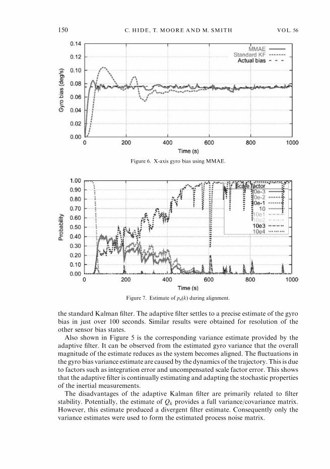
Figure 6. X-axis gyro bias using MMAE.

Figure 7. Estimate of pn(k) during alignment.

150 C. HIDE, T. MOORE AND M. SMITH VOL. 56

While the results obtained have produced stable estimates, further analysis would berequired to ensure filter robustness. Furthermore, due to the recursive nature of thefilter estimate, the performance of the filter is dependent on the a priori estimate ofQk

used in the initialisation of the adaptive filter. This means that the adaptive filter is notentirely self-tuning.

8. MULTIPLE MODEL ADAPTIVE ESTIMATION. To test theMMAE filtering approach, eight parallel Kalman filters were run with each filterusing a different process noise matrix. Each process noise matrix was formed fromthe matrix used in the conventional Kalman filter scaled by a coefficient Sn. Thefactors used were in powers of ten from 10x3 to 104. Figure 6 shows the MMAE es-timate for the x-gyro bias estimate compared to the conventional filter.

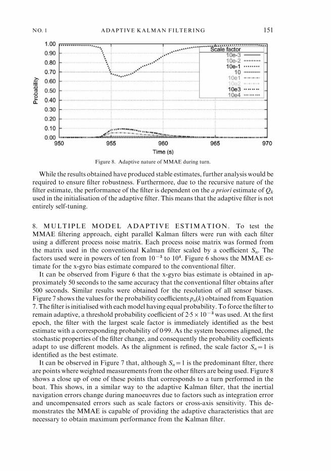
It can be observed from Figure 6 that the x-gyro bias estimate is obtained in ap-proximately 50 seconds to the same accuracy that the conventional filter obtains after500 seconds. Similar results were obtained for the resolution of all sensor biases.Figure 7 shows the values for the probability coefficients pn(k) obtained fromEquation7. The filter is initialisedwith eachmodel having equal probability. To force the filter toremain adaptive, a threshold probability coefficient of 2.5r10x3 was used. At the firstepoch, the filter with the largest scale factor is immediately identified as the bestestimate with a corresponding probability of 0.99. As the system becomes aligned, thestochastic properties of the filter change, and consequently the probability coefficientsadapt to use different models. As the alignment is refined, the scale factor Sn=1 isidentified as the best estimate.

It can be observed in Figure 7 that, although Sn=1 is the predominant filter, thereare points where weightedmeasurements from the other filters are being used. Figure 8shows a close up of one of these points that corresponds to a turn performed in theboat. This shows, in a similar way to the adaptive Kalman filter, that the inertialnavigation errors change during manoeuvres due to factors such as integration errorand uncompensated errors such as scale factors or cross-axis sensitivity. This de-monstrates the MMAE is capable of providing the adaptive characteristics that arenecessary to obtain maximum performance from the Kalman filter.

Figure 8. Adaptive nature of MMAE during turn.

NO. 1 ADAPTIVE KALMAN FILTERING 151

The primary limitation of MMAE is the increased computational burden imposedby the parallel filters. For the loosely coupled integration filter, the standard KalmanFilter running on a 1.4 GHz PC under the Linux operating system takes 0.01 secondsper epoch. For theMMAEfilter running eight parallelKalman filters, processing takes0.04 seconds per epoch. Such an increase in processing time can be considered negli-gible for many real-time applications. It has also been noted that the some of the filterestimates are not used in the computation of the state vector, and further analysis ofthese results can reduce the number of filters used. TheMMAEfilter provides amethodfor adapting the stochastic properties that is self-tuning. However, themultiple modelshave to be estimated initially, and the performance of the filter will be dependent on thedefinition of these models. MMAE further provides a potentially more robust filterwhere incorrect error models are effectively ignored.

9. CONCLUSIONS. This paper has shown that there are many differentways in which a Kalman filter can be configured. The innovation and residual se-quences provide a useful performance indicator that can be used to adaptively tunethe stochastic information used in the filter. This paper has shown the use of adapt-ive filtering techniques to improve the speed of the dynamic alignment of a MEMSIMU with RTK GPS for a marine application. Initial MEMS sensor errors can belarge and require fast resolution for the filter to remain stable. Also demonstratedwas that alignment can be obtained in approximately 50–100 seconds using adapt-ive methods compared to greater than 500 seconds for the conventional Kalmanfilter.

Work is currently being undertaken at the IESSG to validate the results with datacollected at the Plymouth trial, which was used to simulate the data used in this paper.Initial results indicate that the adaptive methods translate well to real data collectedwith a Crossbow MEMS IMU.

REFERENCES

Britting, K. R. (1971). Inertial Navigation Systems Analysis. John Wiley and Sons Inc.

Brown, R. B. and Hwang, P. Y. C. (1997). Introduction to Random Signals and Applied Kalman Filtering.

John Wiley and Sons Inc., 3rd edition.

De Jonge, P. and Tiberius, C. (1996). The LAMBDA method for integer ambiguity estimation: im-

plementation aspects. Technical Report 12, Delft Geodetic Computing Centre, LGR-Series.

Hu, C., Chen, Y. and Chen, W. (2001). Adaptive Kalman filtering for DGPS positioning. International

Symposium on Kinematic Systems in Geodesy, Geomatics and Navigation, 2001.

Mehra, R. K. (1972). Approaches to adaptive filtering. IEEE Transactions on automatic control,

AC-17:693–698, October.

Mohamed, A. H. (1999). Optimizing the Estimation Procedure in INS/GPS Integration for Kinematic

Applications. PhD thesis, University of Calgary.

Mohamed, A. H. and Schwarz, K. P. (1999). Adaptive Kalman filtering for INS/GPS. Journal of Geodesy,

73, 193–203.

Titterton,D. H. andWeston, J. L. (1997).Strapdown InertialNavigationTechnology. InstitutionofElectrical

Engineers.

Wang, J., Stewart,M. andTsakiri,M. (1999).Online stochasticmodelling for INS/GPS integration. Institute

of Navigation.

Welch, G. and Bishop, G. (2001).An introduction to the Kalman filter. Technical report, University of North

Carolina at Chapel Hill.

http://info.acm.org/pubs/toc/CRnotice.html.

152 C. HIDE, T. MOORE AND M. SMITH VOL. 56