A STOCK TRADING SYSTEM FOR A MEDIUM VOLATILE ASSETUSING MULTI LAYER PERCEPTRON

Ivan Letteri∗Department of Engineering, Computer Science and Maths

University of L’AquilaL’Aquila, Italy, 67100

ivan.letteri@univaq.it

Giuseppe Della PennaDepartment of Engineering, Computer Science and Maths

University of L’AquilaL’Aquila, Italy, 67100

giuseppe.dellapenna@univaq.it

Giovanni De GasperisDepartment of Engineering, Computer Science and Maths

University of L’AquilaL’Aquila, Italy, 67100

giovanni.degasperis@univaq.it

Abeer DyoubDepartment of Engineering, Computer Science and Maths

University of L’AquilaL’Aquila, Italy, 67100

abeer.dyoub@univaq.it

ABSTRACT

Stock market forecasting is a lucrative field of interest with promising profits but not without itsdifficulties and for some people could be even causes of failure. Financial markets by their nature arecomplex, non-linear and chaotic, which implies that accurately predicting the prices of assets that arepart of it becomes very complicated. In this paper we propose a stock trading system having as maincore the feed-forward deep neural networks (DNN) to predict the price for the next 30 days of openmarket, of the shares issued by Abercrombie & Fitch Co. (ANF) in the stock market of the New YorkStock Exchange (NYSE).

The system we have elaborated calculates the most effective technical indicator, applying it to thepredictions computed by the DNNs, for generating trades. The results showed an increase in valuessuch as Expectancy Ratio of 2.112% of profitable trades with Sharpe, Sortino, and Calmar Ratiosof 2.194, 3.340, and 12.403 respectively. As a verification, we adopted a backtracking simulationmodule in our system, which maps trades to actual test data consisting of the last 30 days of openmarket on the ANF asset. Overall, the results were promising bringing a total profit factor of 3.2% injust one month from a very modest budget of $100. This was possible because the system reducedthe number of trades by choosing the most effective and efficient trades, saving on commissions andslippage costs.

∗https://www.ivanletteri.it

arX

iv:2

201.

1228

6v1

[q-

fin.

ST]

17

Jan

2022

arXiv Template A PREPRINT

Keywords Deep Learning · Statistical Learning · Stock Market Prediction · Trading System · Algorithmic Trading

1 Introduction

Stock market forecasting is considered a research field with promising returns for investors. However, there areconsiderable challenges to predicting stock market trends accurately and precisely enough due to their chaotic andnon-linear nature, and also complexity. At the state of the art, there are numerous approaches for generating, processing,and optimizing a dataset, such as (Letteri et al. [2020a]).

Many artificial intelligence methods have been employed to classify cyber attacks (Letteri et al. [2018]), predict networktraffic anomalies (Letteri et al. [2019a]), course of a disease, and even the price trend in the stock market. Artificialneural networks (ANNs) to date remain a fairly popular choice for these kinds of tasks and are widely studied (Letteriet al. [2019b]), having exhibited good performance (Yetis et al. [2014]).

In particular, although deep neural networks (DNNs) are predominantly used for image recognition and natural languageprocessing, showing surprising results (Soniya et al. [2015]), they have also been applied to financial markets for stockprice prediction using textual news analysis (Day and Lee [2016]).

In this paper, we propose a trading system for the stock market that uses forecasts by four Price Action (PA)-basedDNNs to generate trading signals, and subsequently evaluate their performance in the stock market. This constitutespart of a work that aims to convert the DNNs forecasts into a profitable investment and trading system that can beautomated, using a robot advisor.

2 Data Set

This section describes the methodology with which the dataset is collected, the criteria adopted for the statistical analysisof the data collected, the training process and the series of tests conducted on the DNNs with optimized processes(Letteri et al. [2020b]). In the next section we will show the trading rules applied on the forecast output with the relatedtests on profitability verified by our backtracking system.

2.1 Technical Analysis

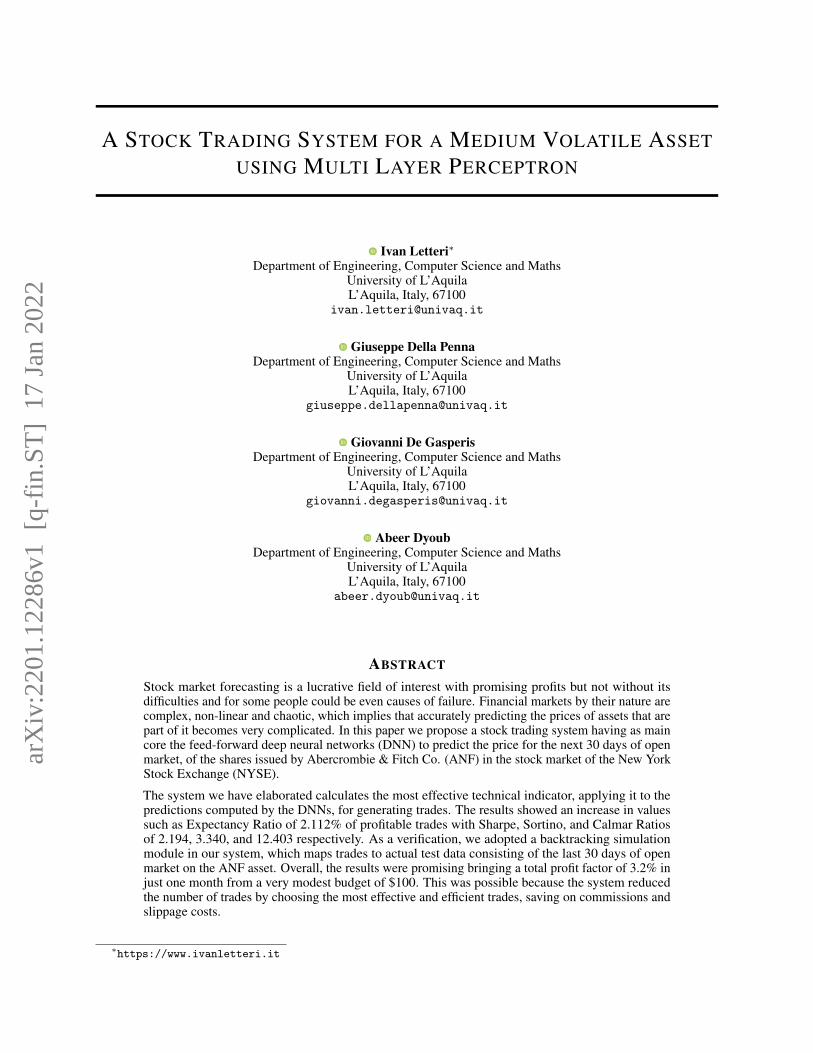
Technical analysis (TA) constitutes the type of investment analysis that uses simple mathematical formulations orgraphical representations of the time series of financial assets to explore trading opportunities. In its algorithmic form,TA uses the analysis of asset price history series (Wang et al. [2021]), defined as OHLC, i.e., the opening, highers,lowest and closing prices of an asset, typically represented with candlesticks charts (see, e.g. in fig. 1). For eachtimeframe t, the OHLC of an asset is represented as a 4-dimensional vector Xt = (x

(o)t , x

(h)t , x

(l)t , x

(c)t )T , where

x(l)t > 0, x(l)t < x

(h)t and x(o)t , x

(c)t ∈ [x

(l)t , x

(h)t ].

Figure 1: Example of candlestick chart.

Some stocks are more volatile than others. For example the shares of a large blue-chip company may not have largeprice fluctuations and are therefore said to have low volatility, whereas the shares of a tech stock may fluctuate oftenand therefore have high volatility. There are also stocks with medium volatility2, and this is the case of the asset that westudied in this article.

2https://www.fool.com/investing/how-to-invest/stocks/stock-market-volatility/

2

arXiv Template A PREPRINT

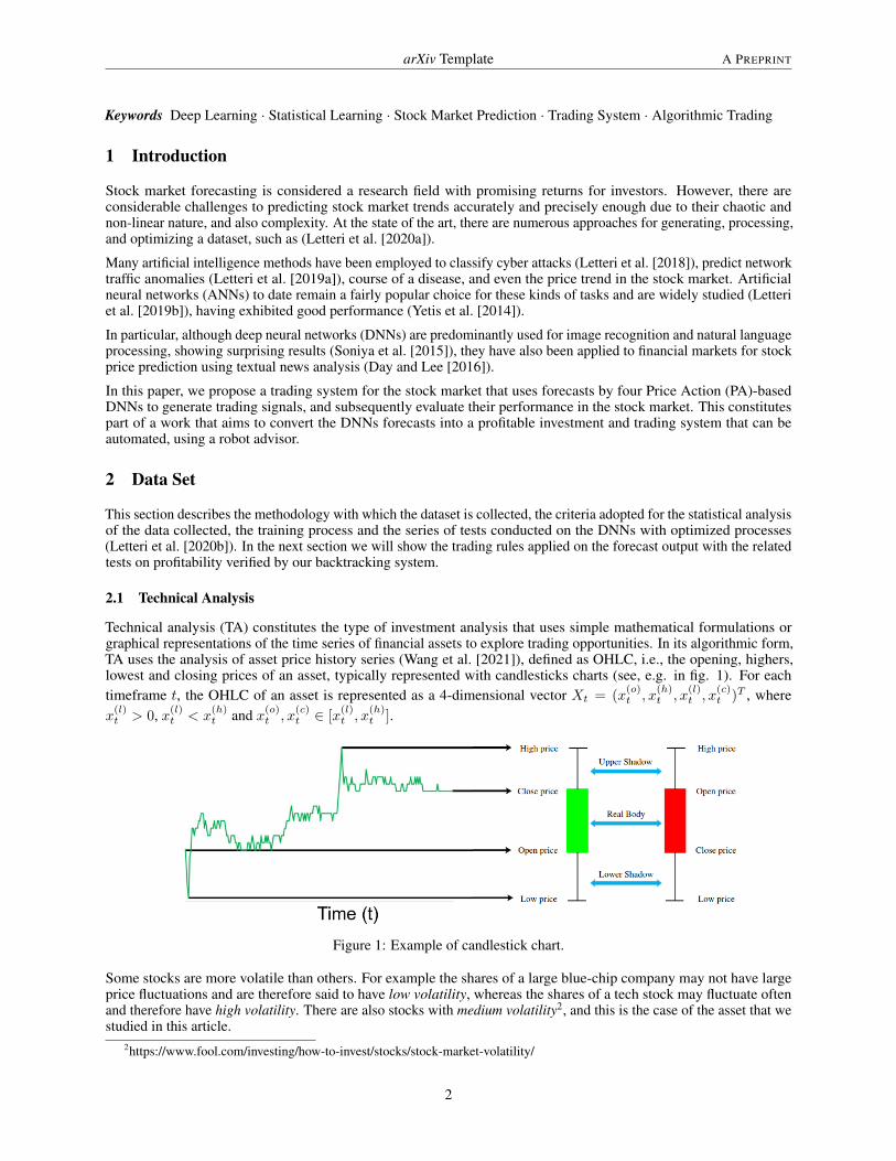
The dataset used in this work consists of historical OHLC prices data from the New York Stock Exchange (NYSE),the world’s largest stock exchange by trading volume and the second largest by number of listed companies. Its sharevolume was surpassed by NASDAQ in the 1990s, but the total capitalization of the 2800 companies on the NYSEis five times that of the competing technology exchange. The asset on which we conducted our study is the sharesissued by Abercrombie & Fitch Co. (ANF). From a summary of results for the third quarter ended October 30, 2021compared to the third quarter ended October 31, 2020, ANF reported net sales of $905 million, up 10% year-over-yearand 5% compared to net sales in the third quarter pre-COVID 2019. Digital net sales of $413 million increased 8%compared to last year and 55% compared to pre-COVID 2019 third quarter digital net sales. Gross profit rate of63.7%, down approximately 30 basis points from last year and up approximately 360 basis points from 2019 (sourceGlobeNewswire3).

Figure 2: ANF all trend.

ANF was born at the end of September 1996, and from April to October 2011 it came close to the All Time High (ATH)at various times, meeting punctually a resistance. This peculiarity, together with the others previously mentioned, hasled us to observe this stock with attention starting from the end of October 2011 (see fig. 2) when the downtrend periodbelow $70 begins, with the further intent to determine a potential opportune moment for a market entry by buying thisasset.

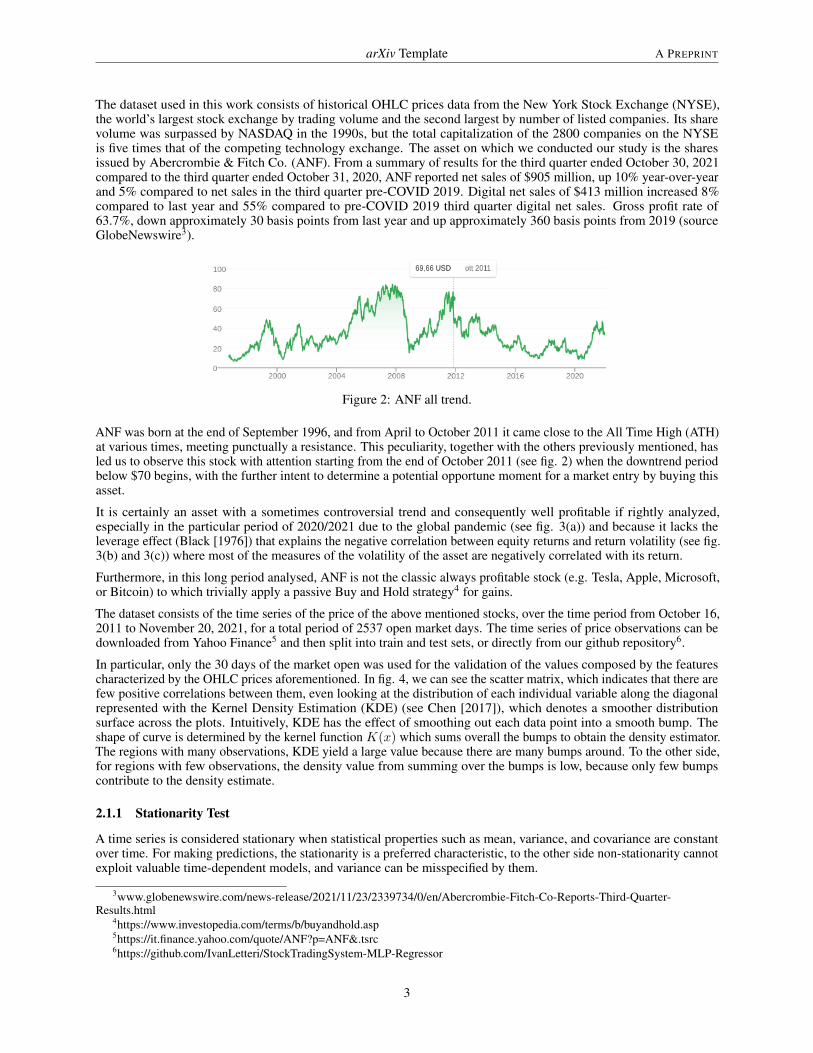
It is certainly an asset with a sometimes controversial trend and consequently well profitable if rightly analyzed,especially in the particular period of 2020/2021 due to the global pandemic (see fig. 3(a)) and because it lacks theleverage effect (Black [1976]) that explains the negative correlation between equity returns and return volatility (see fig.3(b) and 3(c)) where most of the measures of the volatility of the asset are negatively correlated with its return.

Furthermore, in this long period analysed, ANF is not the classic always profitable stock (e.g. Tesla, Apple, Microsoft,or Bitcoin) to which trivially apply a passive Buy and Hold strategy4 for gains.

The dataset consists of the time series of the price of the above mentioned stocks, over the time period from October 16,2011 to November 20, 2021, for a total period of 2537 open market days. The time series of price observations can bedownloaded from Yahoo Finance5 and then split into train and test sets, or directly from our github repository6.

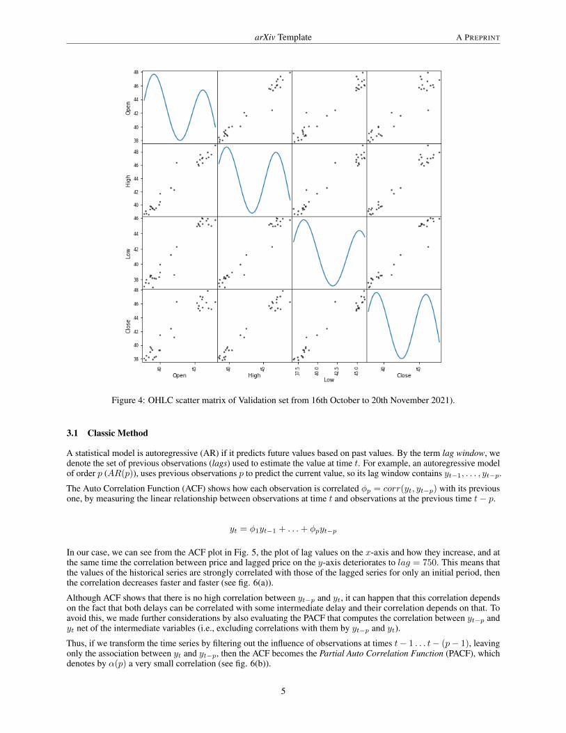
In particular, only the 30 days of the market open was used for the validation of the values composed by the featurescharacterized by the OHLC prices aforementioned. In fig. 4, we can see the scatter matrix, which indicates that there arefew positive correlations between them, even looking at the distribution of each individual variable along the diagonalrepresented with the Kernel Density Estimation (KDE) (see Chen [2017]), which denotes a smoother distributionsurface across the plots. Intuitively, KDE has the effect of smoothing out each data point into a smooth bump. Theshape of curve is determined by the kernel function K(x) which sums overall the bumps to obtain the density estimator.The regions with many observations, KDE yield a large value because there are many bumps around. To the other side,for regions with few observations, the density value from summing over the bumps is low, because only few bumpscontribute to the density estimate.

2.1.1 Stationarity Test

A time series is considered stationary when statistical properties such as mean, variance, and covariance are constantover time. For making predictions, the stationarity is a preferred characteristic, to the other side non-stationarity cannotexploit valuable time-dependent models, and variance can be misspecified by them.

3www.globenewswire.com/news-release/2021/11/23/2339734/0/en/Abercrombie-Fitch-Co-Reports-Third-Quarter-Results.html

4https://www.investopedia.com/terms/b/buyandhold.asp5https://it.finance.yahoo.com/quote/ANF?p=ANF&.tsrc6https://github.com/IvanLetteri/StockTradingSystem-MLP-Regressor

3

arXiv Template A PREPRINT

Figure 3: ANF price (a), return (b), and volatility (c) from October 30th 2011 to November 30th 2021.

To test whether our dataset is composed of a stationary time series, we used the stationary unit root as a statistical test.Given the time series yt = a ∗ yt−1 + εt, where yt is the value at instant t and εt is the error term. We evaluate, for allobservations yt = ap ∗ yt−p +

∑εt−i ∗ ai, if the value of a is 1 (unity), then the predictions will equal yt−p and the

sum of all errors from t− p to t, meaning that the variance increases over time.

To verify the unit root stationary tests, we used the Augmented Dickey Fuller (ADF) test by analyzing the test statistic,p-value, and critical value at 1%, 5%, and 10% confidence intervals.

Table 1: ADF test stationarity with AIC optimization.

Test Statistic p-value Lags Observations Critical Value1% 5% 10%

ANF -2.302 0.171 5 2529 -3.432 -2.863 -2.567

Tab. 1 shows the number of lags considered, automatically selected based on the Akaike Information Criterion (AIC)(see Akaike [1974]) on ANF stock prices. The p-value result above the threshold (such as 5% or 1%) suggests rejectingthe null hypothesis, so the time series turns out not to be stationary.

3 Methodology

In this paper, ARIMA model as a classical method and ANN as a deep learning model are chosen for ANF stocks priceprediction. In this section, we analyze the models, comparing their results and selecting the best model based on theperformance measures.

4

arXiv Template A PREPRINT

Figure 4: OHLC scatter matrix of Validation set from 16th October to 20th November 2021).

3.1 Classic Method

A statistical model is autoregressive (AR) if it predicts future values based on past values. By the term lag window, wedenote the set of previous observations (lags) used to estimate the value at time t. For example, an autoregressive modelof order p (AR(p)), uses previous observations p to predict the current value, so its lag window contains yt−1, . . . , yt−p.

The Auto Correlation Function (ACF) shows how each observation is correlated φp = corr(yt, yt−p) with its previousone, by measuring the linear relationship between observations at time t and observations at the previous time t− p.

yt = φ1yt−1 + . . .+ φpyt−p

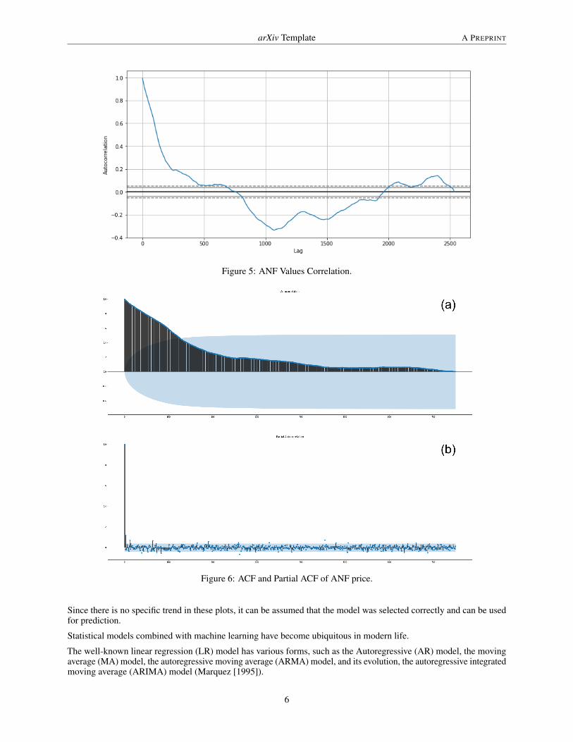
In our case, we can see from the ACF plot in Fig. 5, the plot of lag values on the x-axis and how they increase, and atthe same time the correlation between price and lagged price on the y-axis deteriorates to lag = 750. This means thatthe values of the historical series are strongly correlated with those of the lagged series for only an initial period, thenthe correlation decreases faster and faster (see fig. 6(a)).

Although ACF shows that there is no high correlation between yt−p and yt, it can happen that this correlation dependson the fact that both delays can be correlated with some intermediate delay and their correlation depends on that. Toavoid this, we made further considerations by also evaluating the PACF that computes the correlation between yt−p andyt net of the intermediate variables (i.e., excluding correlations with them by yt−p and yt).

Thus, if we transform the time series by filtering out the influence of observations at times t− 1 . . . t− (p− 1), leavingonly the association between yt and yt−p, then the ACF becomes the Partial Auto Correlation Function (PACF), whichdenotes by α(p) a very small correlation (see fig. 6(b)).

5

arXiv Template A PREPRINT

Figure 5: ANF Values Correlation.

Figure 6: ACF and Partial ACF of ANF price.

Since there is no specific trend in these plots, it can be assumed that the model was selected correctly and can be usedfor prediction.

Statistical models combined with machine learning have become ubiquitous in modern life.

The well-known linear regression (LR) model has various forms, such as the Autoregressive (AR) model, the movingaverage (MA) model, the autoregressive moving average (ARMA) model, and its evolution, the autoregressive integratedmoving average (ARIMA) model (Marquez [1995]).

6

arXiv Template A PREPRINT

As a benchmark from a statistical point of view, we used the Auto-ARIMA model by pmdarima 7 library. In the basicARIMA model, we need to provide the p, d, and q values using statistical techniques by performing the difference toeliminate the non-stationarity and plotting ACF and PACF graphs. In Auto-ARIMA, the model itself automaticallydiscovers the optimal order for an ARIMA model by conducting differentiation tests (i.e., Kwiatkowski-Phillips-Schmidt-Shin, Augmented Dickey-Fuller, or Phillips-Perron) to determine the order of differentiation, d, and thenfitting the models within defined ranges of beginning p, maximum p, beginning q, maximum q. If the seasonaloption is enabled, Auto-ARIMA also attempts to identify the optimal hyper-parameters P and Q after conducting theCanova-Hansen (Kurozumi [2002]) to determine the optimal order of seasonal differentiation, D.

Tab. 2 shows that the best model is ARIMA(0,1,0) by performing the stepwise search to minimize AIC (Stoica andSelen [2004]). Auto-ARIMA apply only one order of differenciation chosing the simple ARIMA called RandomWalking (see Danyliv et al. [2019]) with p = 0, d = 1, and q = 0.

Table 2: ARIMA (p,d,q) models performing stepwise search to minimize Akaike Information Criterion.

ARIMA AIC(2,1,2) 6831.648(0,1,0) 6830.378(1,1,0) 6829.872(0,1,1) 6829.776(0,1,0) 6828.926(1,1,1) 6830.470

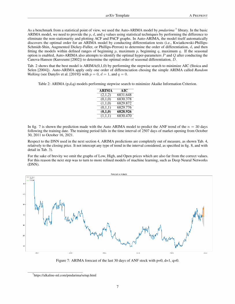
In fig. 7 is shown the prediction made with the Auto ARIMA model to predict the ANF trend of the n = 30 daysfollowing the training date. The training period falls in the time interval of 2507 days of market opening from October30, 2011 to October 16, 2021.

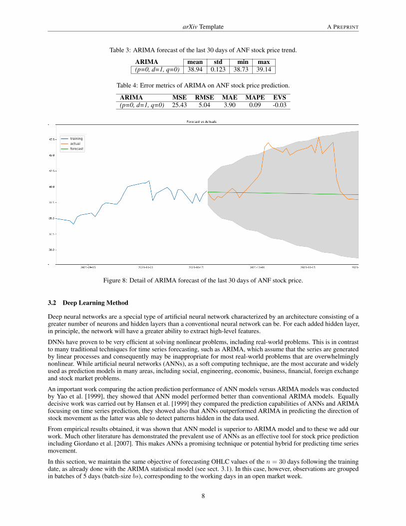
Respect to the DNN used in the next section 4, ARIMA predictions are completely out of measure, as shown Tab. 4,relatively to the closing price. It not intercept any type of trend in the interval considered, as specified in fig. 8, and withdetail in Tab. 3).

For the sake of brevity we omit the graphs of Low, High, and Open prices which are also far from the correct values.For this reason the next step was to turn to more refined models of machine learning, such as Deep Neural Networks(DNN).

Figure 7: ARIMA forecast of the last 30 days of ANF stock with p=0, d=1, q=0.

7https://alkaline-ml.com/pmdarima/setup.html

7

arXiv Template A PREPRINT

Table 3: ARIMA forecast of the last 30 days of ANF stock price trend.

ARIMA mean std min max(p=0, d=1, q=0) 38.94 0.123 38.73 39.14

Table 4: Error metrics of ARIMA on ANF stock price prediction.

ARIMA MSE RMSE MAE MAPE EVS(p=0, d=1, q=0) 25.43 5.04 3.90 0.09 -0.03

Figure 8: Detail of ARIMA forecast of the last 30 days of ANF stock price.

3.2 Deep Learning Method

Deep neural networks are a special type of artificial neural network characterized by an architecture consisting of agreater number of neurons and hidden layers than a conventional neural network can be. For each added hidden layer,in principle, the network will have a greater ability to extract high-level features.

DNNs have proven to be very efficient at solving nonlinear problems, including real-world problems. This is in contrastto many traditional techniques for time series forecasting, such as ARIMA, which assume that the series are generatedby linear processes and consequently may be inappropriate for most real-world problems that are overwhelminglynonlinear. While artificial neural networks (ANNs), as a soft computing technique, are the most accurate and widelyused as prediction models in many areas, including social, engineering, economic, business, financial, foreign exchangeand stock market problems.

An important work comparing the action prediction performance of ANN models versus ARIMA models was conductedby Yao et al. [1999], they showed that ANN model performed better than conventional ARIMA models. Equallydecisive work was carried out by Hansen et al. [1999] they compared the prediction capabilities of ANNs and ARIMAfocusing on time series prediction, they showed also that ANNs outperformed ARIMA in predicting the direction ofstock movement as the latter was able to detect patterns hidden in the data used.

From empirical results obtained, it was shown that ANN model is superior to ARIMA model and to these we add ourwork. Much other literature has demonstrated the prevalent use of ANNs as an effective tool for stock price predictionincluding Giordano et al. [2007]. This makes ANNs a promising technique or potential hybrid for predicting time seriesmovement.

In this section, we maintain the same objective of forecasting OHLC values of the n = 30 days following the trainingdate, as already done with the ARIMA statistical model (see sect. 3.1). In this case, however, observations are groupedin batches of 5 days (batch-size bs), corresponding to the working days in an open market week.

8

arXiv Template A PREPRINT

When building a neural network suitable for financial applications, the main consideration is to find a compromisebetween generalisation and convergence. Of particular importance is to try not to have too many nodes in the hiddenlayer, as this could lead the DNN to learn only by not acquiring the ability to generalise.

The prediction method that determines the number of input neurons to DNNs is based on the lag windowing criterion.This is a technique that consists in windowing the autocorrelation coefficients before estimating the linear predictioncoefficients (LPC).

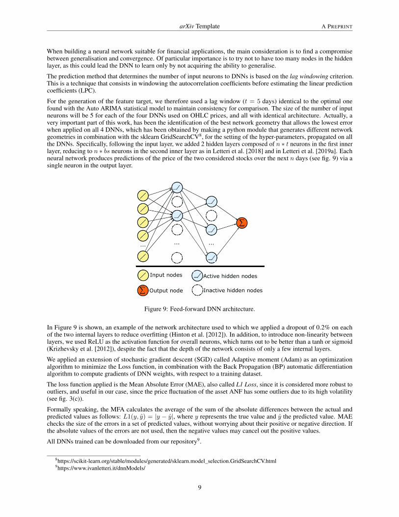
For the generation of the feature target, we therefore used a lag window (t = 5 days) identical to the optimal onefound with the Auto ARIMA statistical model to maintain consistency for comparison. The size of the number of inputneurons will be 5 for each of the four DNNs used on OHLC prices, and all with identical architecture. Actually, avery important part of this work, has been the identification of the best network geometry that allows the lowest errorwhen applied on all 4 DNNs, which has been obtained by making a python module that generates different networkgeometries in combination with the sklearn GridSearchCV8, for the setting of the hyper-parameters, propagated on allthe DNNs. Specifically, following the input layer, we added 2 hidden layers composed of n ∗ t neurons in the first innerlayer, reducing to n ∗ bs neurons in the second inner layer as in Letteri et al. [2018] and in Letteri et al. [2019a]. Eachneural network produces predictions of the price of the two considered stocks over the next n days (see fig. 9) via asingle neuron in the output layer.

Figure 9: Feed-forward DNN architecture.

In Figure 9 is shown, an example of the network architecture used to which we applied a dropout of 0.2% on eachof the two internal layers to reduce overfitting (Hinton et al. [2012]). In addition, to introduce non-linearity betweenlayers, we used ReLU as the activation function for overall neurons, which turns out to be better than a tanh or sigmoid(Krizhevsky et al. [2012]), despite the fact that the depth of the network consists of only a few internal layers.

We applied an extension of stochastic gradient descent (SGD) called Adaptive moment (Adam) as an optimizationalgorithm to minimize the Loss function, in combination with the Back Propagation (BP) automatic differentiationalgorithm to compute gradients of DNN weights, with respect to a training dataset.

The loss function applied is the Mean Absolute Error (MAE), also called L1 Loss, since it is considered more robust tooutliers, and useful in our case, since the price fluctuation of the asset ANF has some outliers due to its high volatility(see fig. 3(c)).

Formally speaking, the MFA calculates the average of the sum of the absolute differences between the actual andpredicted values as follows: L1(y, y) = |y − y|, where y represents the true value and y the predicted value. MAEchecks the size of the errors in a set of predicted values, without worrying about their positive or negative direction. Ifthe absolute values of the errors are not used, then the negative values may cancel out the positive values.

All DNNs trained can be downloaded from our repository9.

8https://scikit-learn.org/stable/modules/generated/sklearn.model_selection.GridSearchCV.html9https://www.ivanletteri.it/dnnModels/

9

arXiv Template A PREPRINT

3.3 Multi-layer Perceptron Regressor Training

The strategies of a trading system tell the investor when to buy or sell shares in such a way that the sequence of theseoperations is profitable.

The trading system we propose makes forecasts of OHLC share prices for the $30 open market days following thetraining date ending on October 16, 2021. The system’s trading rules follow the following logic: when the expectedclosing price is higher than the current opening price, it is time to buy, and vice versa, to sell all the shares (whenthey are in the portfolio) at the moment when the expected closing price is lower. We have developed similar criteriaconsidering the forecasts of the last month with the trained DNNs by defining a trading plan with a set of entry and exitrules.

We developed similar criteria by considering the forecasts of the last month with the trained DNNs defining a tradingplan with a set of rules entry and exit.

4 DNN Results

The evaluation is conducted through two components. The first one forecasts the OHLC prices of the asset, the secondone calculates the performance of the trading system.

4.1 Price Action Forecasting

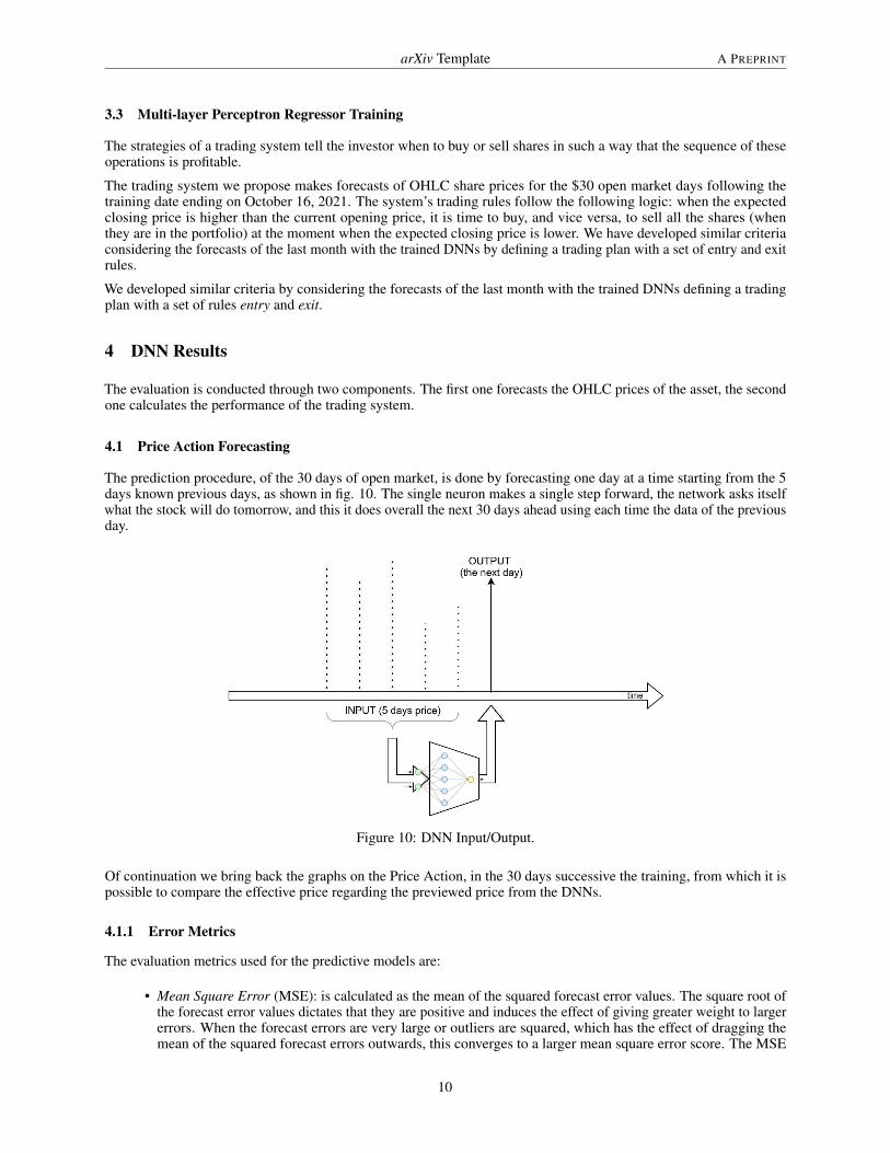
The prediction procedure, of the 30 days of open market, is done by forecasting one day at a time starting from the 5days known previous days, as shown in fig. 10. The single neuron makes a single step forward, the network asks itselfwhat the stock will do tomorrow, and this it does overall the next 30 days ahead using each time the data of the previousday.

Figure 10: DNN Input/Output.

Of continuation we bring back the graphs on the Price Action, in the 30 days successive the training, from which it ispossible to compare the effective price regarding the previewed price from the DNNs.

4.1.1 Error Metrics

The evaluation metrics used for the predictive models are:

• Mean Square Error (MSE): is calculated as the mean of the squared forecast error values. The square root ofthe forecast error values dictates that they are positive and induces the effect of giving greater weight to largererrors. When the forecast errors are very large or outliers are squared, which has the effect of dragging themean of the squared forecast errors outwards, this converges to a larger mean square error score. The MSE

10

arXiv Template A PREPRINT

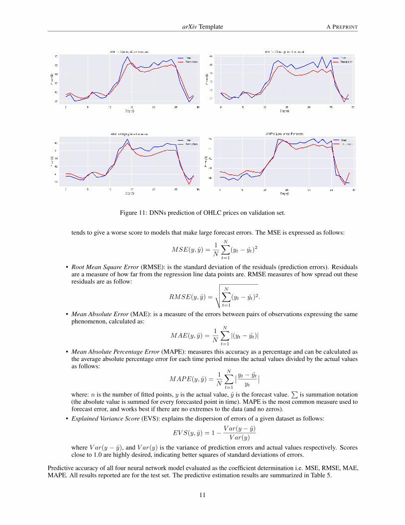
Figure 11: DNNs prediction of OHLC prices on validation set.

tends to give a worse score to models that make large forecast errors. The MSE is expressed as follows:

MSE(y, y) =1

N

N∑t=1

(yt − yt)2

• Root Mean Square Error (RMSE): is the standard deviation of the residuals (prediction errors). Residualsare a measure of how far from the regression line data points are. RMSE measures of how spread out theseresiduals are as follow:

RMSE(y, y) =

√√√√ N∑t=1

(yt − yt)2.

• Mean Absolute Error (MAE): is a measure of the errors between pairs of observations expressing the samephenomenon, calculated as:

MAE(y, y) =1

N

N∑t=1

|(yt − yt)|

• Mean Absolute Percentage Error (MAPE): measures this accuracy as a percentage and can be calculated asthe average absolute percentage error for each time period minus the actual values divided by the actual valuesas follows:

MAPE(y, y) =1

N

N∑t=1

∣∣yt − ytyt

∣∣where: n is the number of fitted points, y is the actual value, y is the forecast value.

∑is summation notation

(the absolute value is summed for every forecasted point in time). MAPE is the most common measure used toforecast error, and works best if there are no extremes to the data (and no zeros).

• Explained Variance Score (EVS): explains the dispersion of errors of a given dataset as follows:

EV S(y, y) = 1− V ar(y − y)

V ar(y)

where V ar(y − y), and V ar(y) is the variance of prediction errors and actual values respectively. Scoresclose to 1.0 are highly desired, indicating better squares of standard deviations of errors.

Predictive accuracy of all four neural network model evaluated as the coefficient determination i.e. MSE, RMSE, MAE,MAPE. All results reported are for the test set. The predictive estimation results are summarized in Table 5.

11

arXiv Template A PREPRINT

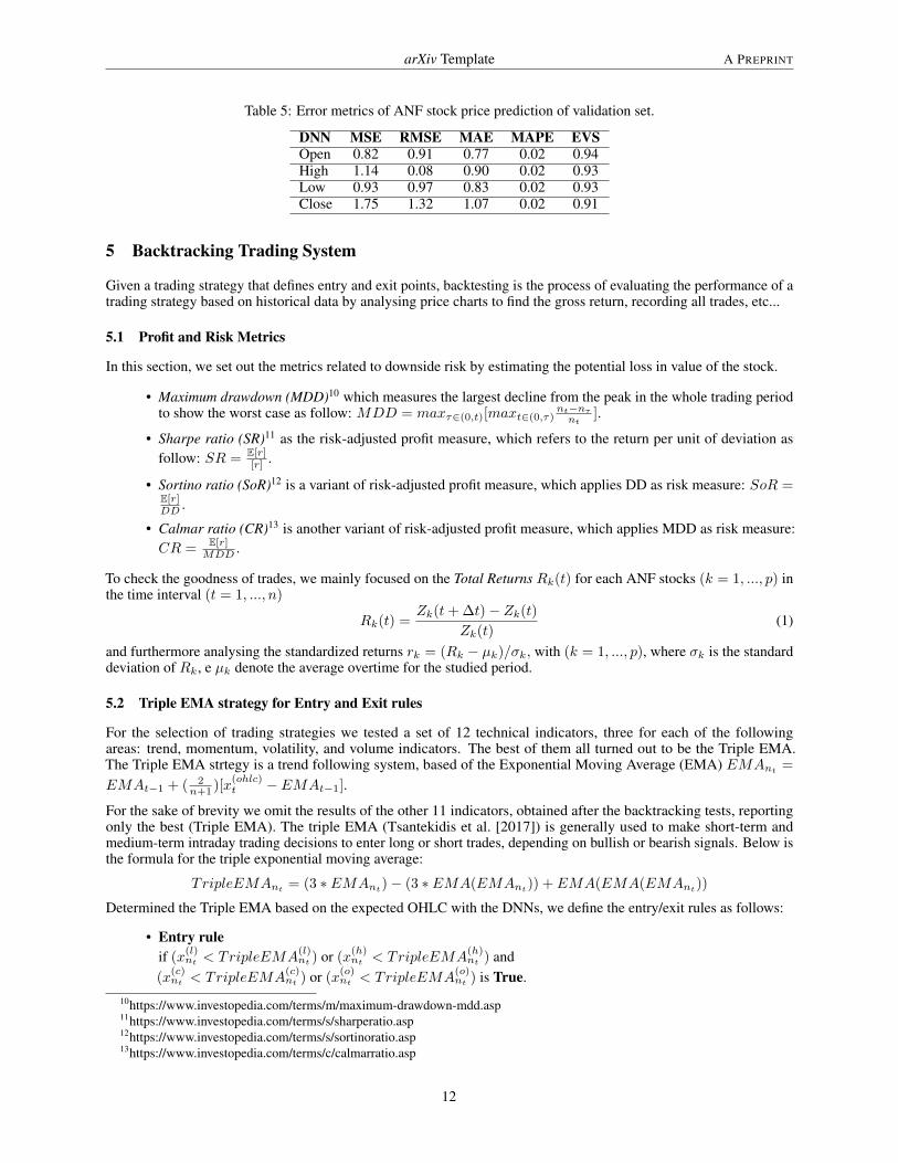
Table 5: Error metrics of ANF stock price prediction of validation set.

DNN MSE RMSE MAE MAPE EVSOpen 0.82 0.91 0.77 0.02 0.94High 1.14 0.08 0.90 0.02 0.93Low 0.93 0.97 0.83 0.02 0.93Close 1.75 1.32 1.07 0.02 0.91

5 Backtracking Trading System

Given a trading strategy that defines entry and exit points, backtesting is the process of evaluating the performance of atrading strategy based on historical data by analysing price charts to find the gross return, recording all trades, etc...

5.1 Profit and Risk Metrics

In this section, we set out the metrics related to downside risk by estimating the potential loss in value of the stock.

• Maximum drawdown (MDD)10 which measures the largest decline from the peak in the whole trading periodto show the worst case as follow: MDD = maxτ∈(0,t)[maxt∈(0,τ)

nt−nτnt

].

• Sharpe ratio (SR)11 as the risk-adjusted profit measure, which refers to the return per unit of deviation asfollow: SR = E[r]

[r] .

• Sortino ratio (SoR)12 is a variant of risk-adjusted profit measure, which applies DD as risk measure: SoR =E[r]DD .

• Calmar ratio (CR)13 is another variant of risk-adjusted profit measure, which applies MDD as risk measure:CR = E[r]

MDD .

To check the goodness of trades, we mainly focused on the Total Returns Rk(t) for each ANF stocks (k = 1, ..., p) inthe time interval (t = 1, ..., n)

Rk(t) =Zk(t+ ∆t)− Zk(t)

Zk(t)(1)

and furthermore analysing the standardized returns rk = (Rk − µk)/σk, with (k = 1, ..., p), where σk is the standarddeviation of Rk, e µk denote the average overtime for the studied period.

5.2 Triple EMA strategy for Entry and Exit rules

For the selection of trading strategies we tested a set of 12 technical indicators, three for each of the followingareas: trend, momentum, volatility, and volume indicators. The best of them all turned out to be the Triple EMA.The Triple EMA strtegy is a trend following system, based of the Exponential Moving Average (EMA) EMAnt =

EMAt−1 + ( 2n+1 )[x

(ohlc)t − EMAt−1].

For the sake of brevity we omit the results of the other 11 indicators, obtained after the backtracking tests, reportingonly the best (Triple EMA). The triple EMA (Tsantekidis et al. [2017]) is generally used to make short-term andmedium-term intraday trading decisions to enter long or short trades, depending on bullish or bearish signals. Below isthe formula for the triple exponential moving average:

TripleEMAnt = (3 ∗ EMAnt)− (3 ∗ EMA(EMAnt)) + EMA(EMA(EMAnt))

Determined the Triple EMA based on the expected OHLC with the DNNs, we define the entry/exit rules as follows:

• Entry ruleif (x

(l)nt < TripleEMA

(l)nt ) or (x

(h)nt < TripleEMA

(h)nt ) and

(x(c)nt < TripleEMA

(c)nt ) or (x

(o)nt < TripleEMA

(o)nt ) is True.

10https://www.investopedia.com/terms/m/maximum-drawdown-mdd.asp11https://www.investopedia.com/terms/s/sharperatio.asp12https://www.investopedia.com/terms/s/sortinoratio.asp13https://www.investopedia.com/terms/c/calmarratio.asp

12

arXiv Template A PREPRINT

• Exit ruleif(x(l)nt > TripleEMA

(l)nt ) or (x

(h)nt > TripleEMA

(h)nt ) and

(x(c)nt > TripleEMA

(c)nt ) or (x

(o)nt > TripleEMA

(o)nt ) is True.

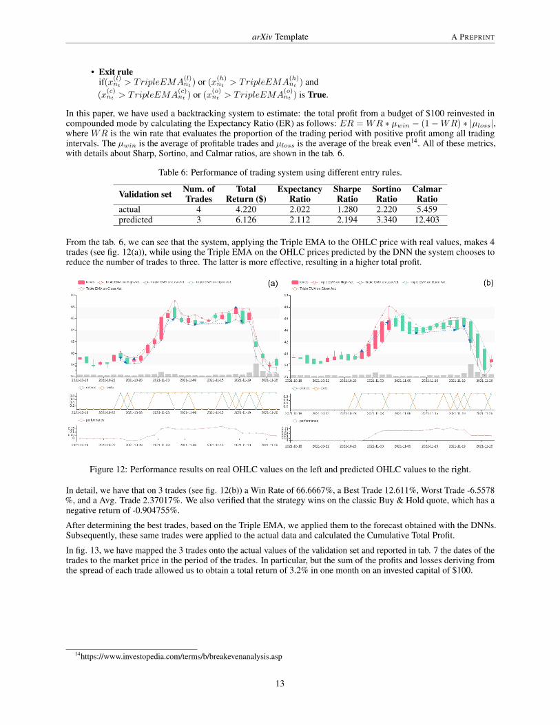
In this paper, we have used a backtracking system to estimate: the total profit from a budget of $100 reinvested incompounded mode by calculating the Expectancy Ratio (ER) as follows: ER = WR ∗ µwin − (1−WR) ∗ |µloss|,where WR is the win rate that evaluates the proportion of the trading period with positive profit among all tradingintervals. The µwin is the average of profitable trades and µloss is the average of the break even14. All of these metrics,with details about Sharp, Sortino, and Calmar ratios, are shown in the tab. 6.

Table 6: Performance of trading system using different entry rules.

Validation set Num. ofTrades

TotalReturn ($)

ExpectancyRatio

SharpeRatio

SortinoRatio

CalmarRatio

actual 4 4.220 2.022 1.280 2.220 5.459predicted 3 6.126 2.112 2.194 3.340 12.403

From the tab. 6, we can see that the system, applying the Triple EMA to the OHLC price with real values, makes 4trades (see fig. 12(a)), while using the Triple EMA on the OHLC prices predicted by the DNN the system chooses toreduce the number of trades to three. The latter is more effective, resulting in a higher total profit.

Figure 12: Performance results on real OHLC values on the left and predicted OHLC values to the right.

In detail, we have that on 3 trades (see fig. 12(b)) a Win Rate of 66.6667%, a Best Trade 12.611%, Worst Trade -6.5578%, and a Avg. Trade 2.37017%. We also verified that the strategy wins on the classic Buy & Hold quote, which has anegative return of -0.904755%.

After determining the best trades, based on the Triple EMA, we applied them to the forecast obtained with the DNNs.Subsequently, these same trades were applied to the actual data and calculated the Cumulative Total Profit.

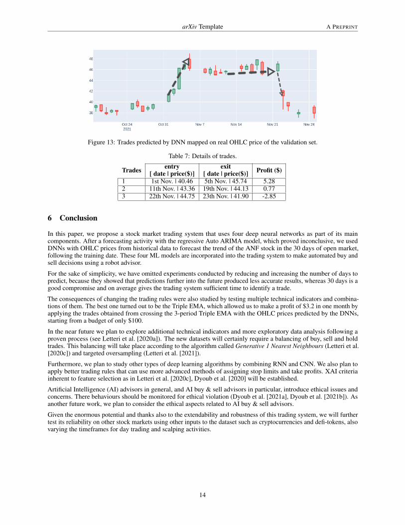
In fig. 13, we have mapped the 3 trades onto the actual values of the validation set and reported in tab. 7 the dates of thetrades to the market price in the period of the trades. In particular, but the sum of the profits and losses deriving fromthe spread of each trade allowed us to obtain a total return of 3.2% in one month on an invested capital of $100.

14https://www.investopedia.com/terms/b/breakevenanalysis.asp

13

arXiv Template A PREPRINT

Figure 13: Trades predicted by DNN mapped on real OHLC price of the validation set.

Table 7: Details of trades.

Trades entry[ date | price($)]

exit[ date | price($)] Profit ($)

1 1st Nov. | 40.46 5th Nov. | 45.74 5.282 11th Nov. | 43.36 19th Nov. | 44.13 0.773 22th Nov. | 44.75 23th Nov. | 41.90 -2.85

6 Conclusion

In this paper, we propose a stock market trading system that uses four deep neural networks as part of its maincomponents. After a forecasting activity with the regressive Auto ARIMA model, which proved inconclusive, we usedDNNs with OHLC prices from historical data to forecast the trend of the ANF stock in the 30 days of open market,following the training date. These four ML models are incorporated into the trading system to make automated buy andsell decisions using a robot advisor.

For the sake of simplicity, we have omitted experiments conducted by reducing and increasing the number of days topredict, because they showed that predictions further into the future produced less accurate results, whereas 30 days is agood compromise and on average gives the trading system sufficient time to identify a trade.

The consequences of changing the trading rules were also studied by testing multiple technical indicators and combina-tions of them. The best one turned out to be the Triple EMA, which allowed us to make a profit of $3.2 in one month byapplying the trades obtained from crossing the 3-period Triple EMA with the OHLC prices predicted by the DNNs,starting from a budget of only $100.

In the near future we plan to explore additional technical indicators and more exploratory data analysis following aproven process (see Letteri et al. [2020a]). The new datasets will certainly require a balancing of buy, sell and holdtrades. This balancing will take place according to the algorithm called Generative 1 Nearest Neighbours (Letteri et al.[2020c]) and targeted oversampling (Letteri et al. [2021]).

Furthermore, we plan to study other types of deep learning algorithms by combining RNN and CNN. We also plan toapply better trading rules that can use more advanced methods of assigning stop limits and take profits. XAI criteriainherent to feature selection as in Letteri et al. [2020c], Dyoub et al. [2020] will be established.

Artificial Intelligence (AI) advisors in general, and AI buy & sell advisors in particular, introduce ethical issues andconcerns. There behaviours should be monitored for ethical violation (Dyoub et al. [2021a], Dyoub et al. [2021b]). Asanother future work, we plan to consider the ethical aspects related to AI buy & sell advisors.

Given the enormous potential and thanks also to the extendability and robustness of this trading system, we will furthertest its reliability on other stock markets using other inputs to the dataset such as cryptocurrencies and defi-tokens, alsovarying the timeframes for day trading and scalping activities.

14

arXiv Template A PREPRINT

ReferencesIvan Letteri, Giuseppe Della Penna, Luca Di Vita, and Maria Teresa Grifa. Mta-kdd’19: A dataset for malware traffic

detection. 2597:153–165, 2020a. URL http://ceur-ws.org/Vol-2597/paper-14.pdf.

Ivan Letteri, Giuseppe Della Penna, and Giovanni De Gasperis. Botnet detection in software defined networks by deeplearning techniques. 11161:49–62, 2018. doi:10.1007/978-3-030-01689-0_4. URL https://doi.org/10.1007/978-3-030-01689-0_4.

Ivan Letteri, Giuseppe Della Penna, and Giovanni De Gasperis. Security in the internet of things: botnet detectionin software-defined networks by deep learning techniques. Int. J. High Perform. Comput. Netw., 15(3/4):170–182,2019a. doi:10.1504/IJHPCN.2019.106095. URL https://doi.org/10.1504/IJHPCN.2019.106095.

Ivan Letteri, Giuseppe Della Penna, and Pasquale Caianiello. Feature selection strategies for HTTP botnet traffic de-tection. pages 202–210, 2019b. doi:10.1109/EuroSPW.2019.00029. URL https://doi.org/10.1109/EuroSPW.2019.00029.

Yunus Yetis, Halid Kaplan, and Mo M. Jamshidi. Stock market prediction by using artificial neural network. 2014World Automation Congress (WAC), pages 718–722, 2014.

Soniya, Sandeep Paul, and Lotika Singh. A review on advances in deep learning. 2015 IEEE Workshop on ComputationalIntelligence: Theories, Applications and Future Directions (WCI), pages 1–6, 2015.

Min-Yuh Day and Chia-Chou Lee. Deep learning for financial sentiment analysis on finance news providers. 2016IEEE/ACM International Conference on Advances in Social Networks Analysis and Mining (ASONAM), pages1127–1134, 2016.

Ivan Letteri, Antonio Di Cecco, Abeer Dyoub, and Giuseppe Della Penna. A novel resampling technique for imbalanceddataset optimization. CoRR, abs/2012.15231, 2020b. URL https://arxiv.org/abs/2012.15231.

Huiwen Wang, Wenyang Huang, and Shanshan Wang. Forecasting open-high-low-close data contained in candlestickchart, 2021.

F. Black. Studies of stock price volatility changes. 3002:177–181, 1976.

Yen-Chi Chen. A tutorial on kernel density estimation and recent advances, 2017.

H. Akaike. A new look at the statistical model identification. IEEE Transactions on Automatic Control, 19(6):716–723,1974. doi:10.1109/TAC.1974.1100705.

Jamie Marquez. Time series analysis : James d. hamilton, 1994, (princeton university press, princeton, nj). InternationalJournal of Forecasting, 11(3):494–495, September 1995.

Eiji Kurozumi. The limiting properties of the canova and hansen test under local alternatives. Econometric Theory, 18(5):1197–1220, 2002. ISSN 02664666, 14694360. URL http://www.jstor.org/stable/3533370.

P. Stoica and Y. Selen. Model-order selection: a review of information criterion rules. IEEE Signal ProcessingMagazine, 21(4):36–47, 2004. doi:10.1109/MSP.2004.1311138.

Oleh Danyliv, Bruce Bland, and Alexandre Argenson. Random walk model from the point of view of algorithmictrading, 2019.

Jingtao Yao, Chew Lim Tan, and Hean-Lee Poh. Neural networks for technical analysis: a study on klci. Internationaljournal of theoretical and applied finance, 2(02):221–241, 1999.

James V Hansen, James B McDonald, and Ray D Nelson. Time series prediction with genetic-algorithm designed neuralnetworks: An empirical comparison with modern statistical models. Computational Intelligence, 15(3):171–184,1999.

Francesco Giordano, Michele La Rocca, and Cira Perna. Forecasting nonlinear time series with neural net-work sieve bootstrap. Computational Statistics & Data Analysis, 51(8):3871–3884, 2007. ISSN 0167-9473.doi:https://doi.org/10.1016/j.csda.2006.03.003. URL https://www.sciencedirect.com/science/article/pii/S0167947306000740.

Geoffrey E. Hinton, Nitish Srivastava, Alex Krizhevsky, Ilya Sutskever, and Ruslan Salakhutdinov. Improvingneural networks by preventing co-adaptation of feature detectors. CoRR, abs/1207.0580, 2012. URL http://arxiv.org/abs/1207.0580.

Alex Krizhevsky, Ilya Sutskever, and Geoffrey E. Hinton. Imagenet classification with deep convolutional neuralnetworks. In Proceedings of the 25th International Conference on Neural Information Processing Systems - Volume1, NIPS’12, page 1097–1105, Red Hook, NY, USA, 2012. Curran Associates Inc.

15

arXiv Template A PREPRINT

Avraam Tsantekidis, Nikolaos Passalis, Anastasios Tefas, Juho Kanniainen, Moncef Gabbouj, and Alexandros Iosifidis.Forecasting stock prices from the limit order book using convolutional neural networks. In 2017 IEEE 19thConference on Business Informatics (CBI), volume 01, pages 7–12, 2017. doi:10.1109/CBI.2017.23.

Ivan Letteri, Antonio Di Cecco, and Giuseppe Della Penna. Dataset optimization strategies for malware traffic detection.CoRR, abs/2009.11347, 2020c. URL https://arxiv.org/abs/2009.11347.

Ivan Letteri, Antonio Di Cecco, Abeer Dyoub, and Giuseppe Della Penna. Imbalanced dataset optimization withnew resampling techniques. In Kohei Arai, editor, Intelligent Systems and Applications - Proceedings of the 2021Intelligent Systems Conference, IntelliSys 2021, Amsterdam, The Netherlands, 2-3 September, 2021, Volume 2, volume295 of Lecture Notes in Networks and Systems, pages 199–215. Springer, 2021. doi:10.1007/978-3-030-82196-8_15.URL https://doi.org/10.1007/978-3-030-82196-8_15.

Abeer Dyoub, Stefania Costantini, Francesca Alessandra Lisi, and Ivan Letteri. Logic-based machine learning fortransparent ethical agents. In Francesco Calimeri, Simona Perri, and Ester Zumpano, editors, Proceedings of the 35thItalian Conference on Computational Logic - CILC 2020, Rende, Italy, October 13-15, 2020, volume 2710 of CEURWorkshop Proceedings, pages 169–183. CEUR-WS.org, 2020.

Abeer Dyoub, Stefania Costantini, Francesca A. Lisi, and Ivan Letteri. Ethical monitoring and evaluation of dialogueswith a mas. 3002:158–172, 2021a.

Abeer Dyoub, Stefania Costantini, Ivan Letteri, and Francesca A. Lisi. A logic-based multi-agent system for ethicalmonitoring and evaluation of dialogues. In Andrea Formisano, Yanhong Annie Liu, Bart Bogaerts, Alex Brik,Verónica Dahl, Carmine Dodaro, Paul Fodor, Gian Luca Pozzato, Joost Vennekens, and Neng-Fa Zhou, editors,Proceedings 37th International Conference on Logic Programming (Technical Communications), ICLP TechnicalCommunications 2021, Porto (virtual event), 20-27th September 2021, volume 345 of EPTCS, pages 182–188, 2021b.doi:10.4204/EPTCS.345.32. URL https://doi.org/10.4204/EPTCS.345.32.

16