Embed Size (px)
Citation preview


ATKINS’PHYSICALCHEMISTRY

This page intentionally left blank

ATKINS’PHYSICALCHEMISTRY
Eighth Edition
Peter AtkinsProfessor of Chemistry, University of Oxford,and Fellow of Lincoln College, Oxford
Julio de PaulaProfessor and Dean of the College of Arts and Sciences Lewis and Clark College,Portland, Oregon
W. H. Freeman and CompanyNew York

Library of Congress Control Number: 2005936591
Physical Chemistry, Eighth Edition© 2006 by Peter Atkins and Julio de PaulaAll rights reserved
ISBN: 0-7167-8759-8EAN: 9780716787594
Published in Great Britain by Oxford University PressThis edition has been authorized by Oxford University Press for sale in the United States and Canada only and not for export therefrom.
First printing
W. H. Freeman and Company41 Madison AvenueNew York, NY 10010www.whfreeman.com

Preface
We have taken the opportunity to refresh both the content and presentation of thistext while—as for all its editions—keeping it flexible to use, accessible to students,broad in scope, and authoritative. The bulk of textbooks is a perennial concern: wehave sought to tighten the presentation in this edition. However, it should always beborne in mind that much of the bulk arises from the numerous pedagogical featuresthat we include (such as Worked examples and the Data section), not necessarily fromdensity of information.
The most striking change in presentation is the use of colour. We have made everyeffort to use colour systematically and pedagogically, not gratuitously, seeing as amedium for making the text more attractive but using it to convey concepts and datamore clearly. The text is still divided into three parts, but material has been moved between chapters and the chapters have been reorganized. We have responded to theshift in emphasis away from classical thermodynamics by combining several chaptersin Part 1 (Equilibrium), bearing in mind that some of the material will already havebeen covered in earlier courses. We no longer make a distinction between ‘concepts’and ‘machinery’, and as a result have provided a more compact presentation of ther-modynamics with less artificial divisions between the approaches. Similarly, equilib-rium electrochemistry now finds a home within the chapter on chemical equilibrium,where space has been made by reducing the discussion of acids and bases.
In Part 2 (Structure) the principal changes are within the chapters, where we havesought to bring into the discussion contemporary techniques of spectroscopy and approaches to computational chemistry. In recognition of the major role that phys-ical chemistry plays in materials science, we have a short sequence of chapters on materials, which deal respectively with hard and soft matter. Moreover, we have introduced concepts of nanoscience throughout much of Part 2.
Part 3 has lost its chapter on dynamic electrochemistry, but not the material. Weregard this material as highly important in a contemporary context, but as a finalchapter it rarely received the attention it deserves. To make it more readily accessiblewithin the context of courses and to acknowledge that the material it covers is at homeintellectually with other material in the book, the description of electron transfer reactions is now a part of the sequence on chemical kinetics and the description ofprocesses at electrodes is now a part of the general discussion of solid surfaces.
We have discarded the Boxes of earlier editions. They have been replaced by morefully integrated and extensive Impact sections, which show how physical chemistry isapplied to biology, materials, and the environment. By liberating these topics fromtheir boxes, we believe they are more likely to be used and read; there are end-of-chapter problems on most of the material in these sections.
In the preface to the seventh edition we wrote that there was vigorous discussion inthe physical chemistry community about the choice of a ‘quantum first’ or a ‘thermo-dynamics first’ approach. That discussion continues. In response we have paid particu-lar attention to making the organization flexible. The strategic aim of this revision is to make it possible to work through the text in a variety of orders and at the end ofthis Preface we once again include two suggested road maps.
The concern expressed in the seventh edition about the level of mathematical ability has not evaporated, of course, and we have developed further our strategies for showing the absolute centrality of mathematics to physical chemistry and to makeit accessible. Thus, we give more help with the development of equations, motivate

vi PREFACE
them, justify them, and comment on the steps. We have kept in mind the strugglingstudent, and have tried to provide help at every turn.
We are, of course, alert to the developments in electronic resources and have madea special effort in this edition to encourage the use of the resources on our Web site (atwww.whfreeman.com/pchem8) where you can also access the eBook. In particular,we think it important to encourage students to use the Living graphs and their con-siderable extension as Explorations in Physical Chemistry. To do so, wherever we call out a Living graph (by an icon attached to a graph in the text), we include anExploration in the figure legend, suggesting how to explore the consequences ofchanging parameters.
Overall, we have taken this opportunity to refresh the text thoroughly, to integrateapplications, to encourage the use of electronic resources, and to make the text evenmore flexible and up to date.
Oxford P.W.A.Portland J.de P.

PREFACE vii

About the book
There are numerous features in this edition that are designed to make learning phys-ical chemistry more effective and more enjoyable. One of the problems that make thesubject daunting is the sheer amount of information: we have introduced several devices for organizing the material: see Organizing the information. We appreciatethat mathematics is often troublesome, and therefore have taken care to give help withthis enormously important aspect of physical chemistry: see Mathematics and Physicssupport. Problem solving—especially, ‘where do I start?’—is often a challenge, andwe have done our best to help overcome this first hurdle: see Problem solving. Finally,the web is an extraordinary resource, but it is necessary to know where to start, orwhere to go for a particular piece of information; we have tried to indicate the right direction: see About the Web site. The following paragraphs explain the features inmore detail.
Organizing the information
Checklist of key ideas
Here we collect together the major concepts introduced in thechapter. We suggest checking off the box that precedes eachentry when you feel confident about the topic.
Impact sections
Where appropriate, we have separated the principles fromtheir applications: the principles are constant and straightfor-ward; the applications come and go as the subject progresses.The Impact sections show how the principles developed in the chapter are currently being applied in a variety of moderncontexts.
Checklist of key ideas
1. A gas is a form of matter that fills any container it occupies.
2. An equation of state interrelates pressure, volume,temperature, and amount of substance: p = f(T,V,n).
3. The pressure is the force divided by the area to which the forceis applied. The standard pressure is p7 = 1 bar (105 Pa).
4. Mechanical equilibrium is the condition of equality ofpressure on either side of a movable wall.
5. Temperature is the property that indicates the direction of theflow of energy through a thermally conducting, rigid wall.
6. A diathermic boundary is a boundary that permits the passageof energy as heat. An adiabatic boundary is a boundary thatprevents the passage of energy as heat.
7. Thermal equilibrium is a condition in which no change ofstate occurs when two objects A and B are in contact througha diathermic boundary.
8. The Zeroth Law of thermodynamics states that, if A is inthermal equilibrium with B, and B is in thermal equilibriumwith C, then C is also in thermal equilibrium with A.
9. The Celsius and thermodynamic temperature scales arerelated by T/K = θ/°C + 273.15.
10. A perfect gas obeys the perfect gas equation, pV = nRT, exactly
12. The partial pressure of any gas ixJ = nJ/n is its mole fraction in apressure.
13. In real gases, molecular interactstate; the true equation of state icoefficients B, C, . . . : pVm = RT
14. The vapour pressure is the presswith its condensed phase.
15. The critical point is the point atend of the horizontal part of thea single point. The critical constpressure, molar volume, and temcritical point.
16. A supercritical fluid is a dense fltemperature and pressure.
17. The van der Waals equation of sthe true equation of state in whiby a parameter a and repulsionsparameter b: p = nRT/(V − nb) −
18. A reduced variable is the actual corresponding critical constant
IMPACT ON NANOSCIENCE
I20.2 Nanowires
We have already remarked (Impacts I9.1, I9.2, and I19.3) that research on nano-metre-sized materials is motivated by the possibility that they will form the basis forcheaper and smaller electronic devices. The synthesis of nanowires, nanometre-sizedatomic assemblies that conduct electricity, is a major step in the fabrication of nanodevices. An important type of nanowire is based on carbon nanotubes, which,like graphite, can conduct electrons through delocalized π molecular orbitals thatform from unhybridized 2p orbitals on carbon. Recent studies have shown a cor-relation between structure and conductivity in single-walled nanotubes (SWNTs)that does not occur in graphite. The SWNT in Fig. 20.45 is a semiconductor. If thehexagons are rotated by 60° about their sixfold axis, the resulting SWNT is a metallicconductor.
Carbon nanotubes are promising building blocks not only because they have usefulelectrical properties but also because they have unusual mechanical properties. Forexample, an SWNT has a Young’s modulus that is approximately five times larger anda tensile strength that is approximately 375 times larger than that of steel.
Silicon nanowires can be made by focusing a pulsed laser beam on to a solid targetcomposed of silicon and iron. The laser ejects Fe and Si atoms from the surface of the
ABOUT THE BOOK ix
Notes on good practice
Science is a precise activity and its language should be used accurately. We have used this feature to help encourage the useof the language and procedures of science in conformity to international practice and to help avoid common mistakes.
Justifications
On first reading it might be sufficient to appreciate the ‘bottomline’ rather than work through detailed development of amathematical expression. However, mathematical develop-ment is an intrinsic part of physical chemistry, and it is important to see how a particular expression is obtained. TheJustifications let you adjust the level of detail that you require toyour current needs, and make it easier to review material.
Molecular interpretation sections
Historically, much of the material in the first part of the textwas developed before the emergence of detailed models ofatoms, molecules, and molecular assemblies. The Molecularinterpretation sections enhance and enrich coverage of thatmaterial by explaining how it can be understood in terms ofthe behaviour of atoms and molecules.
q
A note on good practice We write T = 0, not T = 0 K for the zero temperature on the thermodynamic temperature scale. This scale is absolute, and the lowesttemperature is 0 regardless of the size of the divisions on the scale (just as we writep = 0 for zero pressure, regardless of the size of the units we adopt, such as bar orpascal). However, we write 0°C because the Celsius scale is not absolute.
5.8 The activities of regular solutions
The material on regular solutions presented in Section 5.4 gives further insight intothe origin of deviations from Raoult’s law and its relation to activity coefficients. Thestarting point is the expression for the Gibbs energy of mixing for a regular solution(eqn 5.31). We show in the following Justification that eqn 5.31 implies that the activ-ity coefficients are given by expressions of the form
ln γA = βxB2 ln γB = βxA
2 (5.57)
These relations are called the Margules equations.
Justification 5.4 The Margules equations
The Gibbs energy of mixing to form a nonideal solution is
∆mixG = nRT{xA ln aA + xB ln aB}
This relation follows from the derivation of eqn 5.31 with activities in place of molefractions. If each activity is replaced by γ x, this expression becomes
∆mixG = nRT{xA ln xA + xB ln xB + xA ln γA + xB ln γB}
Now we introduce the two expressions in eqn 5.57, and use xA + xB = 1, which gives
∆mixG = nRT{xA ln xA + xB ln xB + βxAxB2 + βxBxA
2}
= nRT{xA ln xA + xB ln xB + βxAxB(xA + xB)}
= nRT{xA ln xA + xB ln xB + βxAxB}
as required by eqn 5.31. Note, moreover, that the activity coefficients behave cor-rectly for dilute solutions: γA → 1 as xB → 0 and γB → 1 as xA → 0.
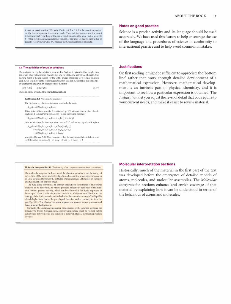
Molecular interpretation 5.2 The lowering of vapour pressure of a solvent in a mixture
The molecular origin of the lowering of the chemical potential is not the energy ofinteraction of the solute and solvent particles, because the lowering occurs even inan ideal solution (for which the enthalpy of mixing is zero). If it is not an enthalpyeffect, it must be an entropy effect.
The pure liquid solvent has an entropy that reflects the number of microstatesavailable to its molecules. Its vapour pressure reflects the tendency of the solu-tion towards greater entropy, which can be achieved if the liquid vaporizes to form a gas. When a solute is present, there is an additional contribution to the entropy of the liquid, even in an ideal solution. Because the entropy of the liquid is already higher than that of the pure liquid, there is a weaker tendency to form thegas (Fig. 5.22). The effect of the solute appears as a lowered vapour pressure, andhence a higher boiling point.
Similarly, the enhanced molecular randomness of the solution opposes the tendency to freeze. Consequently, a lower temperature must be reached beforeequilibrium between solid and solution is achieved. Hence, the freezing point islowered.
x ABOUT THE BOOK
Further information
In some cases, we have judged that a derivation is too long, too detailed, or too different in level for it to be included in the text. In these cases, the derivations will be found less obtrusively at the end of the chapter.
Appendices
Physical chemistry draws on a lot of background material, espe-cially in mathematics and physics. We have included a set ofAppendices to provide a quick survey of some of the informa-tion relating to units, physics, and mathematics that we drawon in the text.
Synoptic tables and the Data section
Long tables of data are helpful for assembling and solving exercises and problems, but can break up the flow of the text.We provide a lot of data in the Data section at the end of thetext and short extracts in the Synoptic tables in the text itself togive an idea of the typical values of the physical quantities weare introducing.
966 Appendix 2 MATHEMATICAL TECHNIQUES
A2.6 Partial derivatives
A partial derivative of a function of more than one variableof the function with respect to one of the variables, all theconstant (see Fig. 2.*). Although a partial derivative showwhen one variable changes, it may be used to determine when more than one variable changes by an infinitesimal ation of x and y, then when x and y change by dx and dy, res
df =y
dx +x
dy
where the symbol ∂ is used (instead of d) to denote a partidf is also called the differential of f. For example, if f = ax3y
y
= 3ax2yx
= ax3 + 2byDF
∂f
∂y
AC
DF
∂f
∂x
AC
DF
∂f
∂y
AC
DF
∂f
∂x
AC
1000 DATA SECTION
Table 2.8 Expansion coefficients, α, and isothermalcompressibilities, κT
a /(10 − 4 K−1) kT /(10 −6 atm−1)
Liquids
Benzene 12.4 92.1
Carbon tetrachloride 12.4 90.5
Ethanol 11.2 76.8
Mercury 1.82 38.7
Water 2.1 49.6
Solids
Copper 0.501 0.735
Diamond 0.030 0.187
Iron 0.354 0.589
Lead 0.861 2.21
The values refer to 20°C.Data: AIP(α), KL(κT).
Table 2.9 Inversion temperatures, nopoints, and Joule–Thomson coefficient
TI /K Tf /K
Air 603
Argon 723 83.8
Carbon dioxide 1500 194.7s
Helium 40
Hydrogen 202 14.0
Krypton 1090 116.6
Methane 968 90.6
Neon 231 24.5
Nitrogen 621 63.3
Oxygen 764 54.8
s: sublimes.Data: AIP, JL, and M.W. Zemansky, Heat and New York (1957).
0.2
0.4
0.6
0.8
1.0
0Po
tent
ial,
/(
/)
Zr D
0 0.5Distan
0.31 3
�
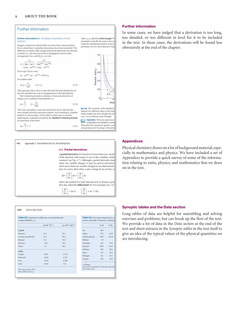
Fig. 5.36 The variation of the shielded Cdistance for different values of the DebyDebye length, the more sharply the potecase, a is an arbitrary unit of length.
Exploration Write an expression funshielded and shielded Coulom
Then plot this expression against rD andinterpretation for the shape of the plot.
Further information
Further information 5.1 The Debye–Hückel theory of ionicsolutions
Imagine a solution in which all the ions have their actual positions,but in which their Coulombic interactions have been turned off. Thedifference in molar Gibbs energy between the ideal and real solutionsis equal to we, the electrical work of charging the system in thisarrangement. For a salt MpXq, we write
Gm Gmideal
we = (pµ+ + qµ−) − (pµ+ideal + qµ−
ideal)
= p(µ+ − µ+ideal) + q(µ− − µ−
ideal)
From eqn 5.64 we write
µ+ − µ+ideal = µ− − µ−
ideal = RT ln γ±
So it follows that
ln γ± = s = p + q (5.73)
This equation tells us that we must first find the final distribution ofthe ions and then the work of charging them in that distribution.
The Coulomb potential at a distance r from an isolated ion ofcharge zie in a medium of permittivity ε is
φi = Zi = (5.74)
The ionic atmosphere causes the potential to decay with distancemore sharply than this expression implies. Such shielding is a familiarproblem in electrostatics, and its effect is taken into account byreplacing the Coulomb potential by the shielded Coulomb potential,an expression of the form
φi = e−r/rD (5.75)Zi
r
zte
4πεZi
r
we
sRT
5 4 4 6 4 4 75 4 6 4 7
where rD is called the Debye length. Whpotential is virtually the same as the unssmall, the shielded potential is much smpotential, even for short distances (Fig.
ABOUT THE BOOK xi
Comments
A topic often needs to draw on a mathematical procedure or aconcept of physics; a Comment is a quick reminder of the pro-cedure or concept.
Appendices
There is further information on mathematics and physics inAppendices 2 and 3, respectively. These appendices do not gointo great detail, but should be enough to act as reminders oftopics learned in other courses.
Mathematics and Physics support
Comment 1.2
A hyperbola is a curve obtained byplotting y against x with xy = constant.
ensre,
Comment 2.5
The partial-differential operation(∂z/∂x)y consists of taking the firstderivative of z(x,y) with respect to x,treating y as a constant. For example, if z(x,y) = x 2y, then
y
=y
= y = 2yx
Partial derivatives are reviewed inAppendix 2.
dx 2
dx
DEF∂[x 2y]
∂x
ABCDEF
∂z
∂x
ABC
ee
978 Appendix 3 ESSENTIAL CONCEPTS OF PHYSICS
Classical mechanics
Classical mechanics describes the behaviour of objects in texpresses the fact that the total energy is constant in the abother expresses the response of particles to the forces acti
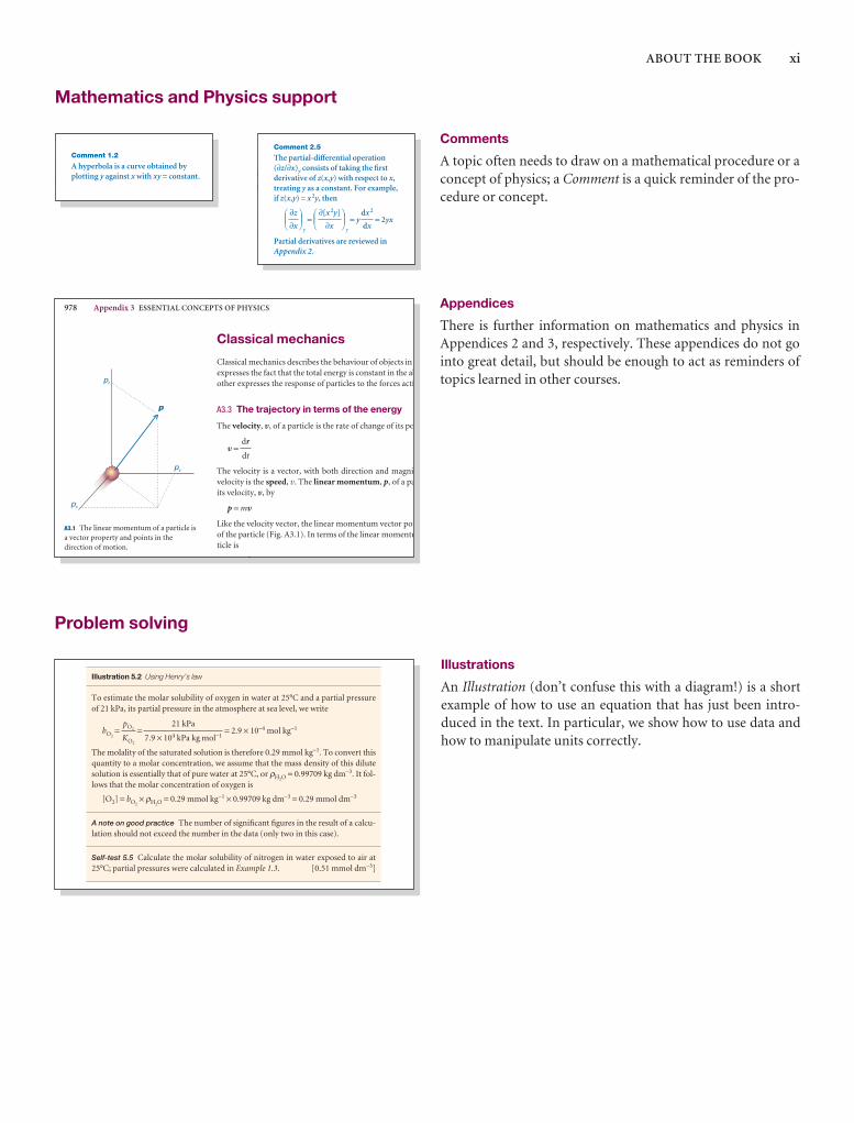
A3.3 The trajectory in terms of the energy
The velocity, V, of a particle is the rate of change of its po
V =
The velocity is a vector, with both direction and magnitvelocity is the speed, v. The linear momentum, p, of a paits velocity, V, by
p = mV
Like the velocity vector, the linear momentum vector poiof the particle (Fig. A3.1). In terms of the linear momentuticle is
2
dr
dt
p
pz
px
py
A3.1 The linear momentum of a particle isa vector property and points in thedirection of motion.
Illustration 5.2 Using Henry’s law
To estimate the molar solubility of oxygen in water at 25°C and a partial pressureof 21 kPa, its partial pressure in the atmosphere at sea level, we write
bO2= = = 2.9 × 10⁻⁴ mol kg−1
The molality of the saturated solution is therefore 0.29 mmol kg−1. To convert thisquantity to a molar concentration, we assume that the mass density of this dilutesolution is essentially that of pure water at 25°C, or ρH2O = 0.99709 kg dm−3. It fol-lows that the molar concentration of oxygen is
[O2] = bO2× ρH2O = 0.29 mmol kg−1 × 0.99709 kg dm−3 = 0.29 mmol dm−3
A note on good practice The number of significant figures in the result of a calcu-lation should not exceed the number in the data (only two in this case).
Self-test 5.5 Calculate the molar solubility of nitrogen in water exposed to air at25°C; partial pressures were calculated in Example 1.3. [0.51 mmol dm−3]
21 kPa
7.9 × 10⁴ kPa kg mol−1
pO2
KO2
Problem solving
Illustrations
An Illustration (don’t confuse this with a diagram!) is a shortexample of how to use an equation that has just been intro-duced in the text. In particular, we show how to use data andhow to manipulate units correctly.
xii ABOUT THE BOOK
Discussion questions
1.1 Explain how the perfect gas equation of state arises by combination ofBoyle’s law, Charles’s law, and Avogadro’s principle.
1.2 Explain the term ‘partial pressure’ and explain why Dalton’s law is alimiting law.
1.3 Explain how the compression factor varies with pressure and temperatureand describe how it reveals information about intermolecular interactions inreal gases.
1.4 What is the significance of the critical co
1.5 Describe the formulation of the van derrationale for one other equation of state in T
1.6 Explain how the van der Waals equationbehaviour.
Self-test 3.12 Calculate the change in Gm for ice at −10°C, with density 917 kg m−3,when the pressure is increased from 1.0 bar to 2.0 bar. [+2.0 J mol−1]
Example 8.1 Calculating the number of photons
Calculate the number of photons emitted by a 100 W yellow lamp in 1.0 s. Take thewavelength of yellow light as 560 nm and assume 100 per cent efficiency.
Method Each photon has an energy hν, so the total number of photons needed toproduce an energy E is E/hν. To use this equation, we need to know the frequencyof the radiation (from ν = c/λ) and the total energy emitted by the lamp. The latteris given by the product of the power (P, in watts) and the time interval for whichthe lamp is turned on (E = P∆t).
Answer The number of photons is
N = = =
Substitution of the data gives
N = = 2.8 × 10²⁰
Note that it would take nearly 40 min to produce 1 mol of these photons.
A note on good practice To avoid rounding and other numerical errors, it is bestto carry out algebraic mainpulations first, and to substitute numerical values intoa single, final formula. Moreover, an analytical result may be used for other datawithout having to repeat the entire calculation.
Self-test 8.1 How many photons does a monochromatic (single frequency) infrared rangefinder of power 1 mW and wavelength 1000 nm emit in 0.1 s?
[5 × 10¹⁴]
(5.60 × 10⁻⁷ m) × (100 J s−1) × (1.0 s)
(6.626 × 10⁻³⁴ J s) × (2.998 × 10⁸ m s−1)
λP∆t
hc
P∆t
h(c/λ)
E
hν
Worked examples
A Worked example is a much more structured form ofIllustration, often involving a more elaborate procedure. EveryWorked example has a Method section to suggest how to set upthe problem (another way might seem more natural: setting upproblems is a highly personal business). Then there is theworked-out Answer.
Self-tests
Each Worked example, and many of the Illustrations, has a Self-test, with the answer provided as a check that the procedure hasbeen mastered. There are also free-standing Self-tests where wethought it a good idea to provide a question to check under-standing. Think of Self-tests as in-chapter Exercises designed tohelp monitor your progress.
Discussion questions
The end-of-chapter material starts with a short set of questionsthat are intended to encourage reflection on the material andto view it in a broader context than is obtained by solving nu-merical problems.
ABOUT THE BOOK xiii
Exercises and Problems
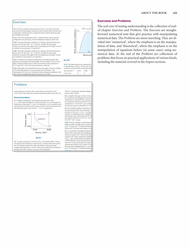
The real core of testing understanding is the collection of end-of-chapter Exercises and Problems. The Exercises are straight-forward numerical tests that give practice with manipulatingnumerical data. The Problems are more searching. They are di-vided into ‘numerical’, where the emphasis is on the manipu-lation of data, and ‘theoretical’, where the emphasis is on themanipulation of equations before (in some cases) using nu-merical data. At the end of the Problems are collections ofproblems that focus on practical applications of various kinds,including the material covered in the Impact sections.
max
Mo
lar
abso
rpti
on
co
effi
cien
t,
Wavenumb
( ) {1� �max�
max~
�� ��
�
�
Exercises
14.1a The term symbol for the ground state of N2+ is 2Σg. What is the total
spin and total orbital angular momentum of the molecule? Show that the termsymbol agrees with the electron configuration that would be predicted usingthe building-up principle.
14.1b One of the excited states of the C2 molecule has the valence electronconfiguration 1σ g
21σu21πu
31π g1. Give the multiplicity and parity of the term.
14.2a The molar absorption coefficient of a substance dissolved in hexane isknown to be 855 dm3 mol−1 cm−1 at 270 nm. Calculate the percentagereduction in intensity when light of that wavelength passes through 2.5 mm ofa solution of concentration 3.25 mmol dm−3.
14.2b The molar absorption coefficient of a substance dissolved in hexane isknown to be 327 dm3 mol−1 cm−1 at 300 nm. Calculate the percentagereduction in intensity when light of that wavelength passes through 1.50 mmof a solution of concentration 2.22 mmol dm−3.
14.3a A solution of an unknown component of a biological sample whenplaced in an absorption cell of path length 1.00 cm transmits 20.1 per cent oflight of 340 nm incident upon it. If the concentration of the component is0.111 mmol dm−3, what is the molar absorption coefficient?
14.3b When light of wavelength 400 nm passes through 3.5 mm of a solutionof an absorbing substance at a concentration 0.667 mmol dm−3, thetransmission is 65.5 per cent. Calculate the molar absorption coefficient of thesolute at this wavelength and express the answer in cm2 mol−1.
14.7b The following data were obtained for thin methylbenzene using a 2.50 mm cell. Calcucoefficient of the dye at the wavelength emplo
[dye]/(mol dm−3) 0.0010 0.0050 0.0
T /(per cent) 73 21 4.2
ll fill d h l
Fig. 14.49
Problems
Assume all gases are perfect unless stated otherwise. Note that 1 atm =1.013 25 bar. Unless otherwise stated, thermochemical data are for 298.15 K.
Numerical problems
2.1 A sample consisting of 1 mol of perfect gas atoms (for which CV,m = 3–
2 R) is taken through the cycle shown in Fig. 2.34. (a) Determine thetemperature at the points 1, 2, and 3. (b) Calculate q, w, ∆U, and ∆H for eachstep and for the overall cycle. If a numerical answer cannot be obtained fromthe information given, then write in +, −, 0, or ? as appropriate.
2.2 A sample consisting of 1.0 mol CaCO3(s) was heated to 800°C, when itdecomposed. The heating was carried out in a container fitted with a pistonthat was initially resting on the solid. Calculate the work done duringcomplete decomposition at 1.0 atm. What work would be done if instead ofhaving a piston the container was open to the atmosphere?
Fig. 2.34
Isotherm
1.00
0.50Pres
sure
,/a
tmp
22.44 44.88
Volume, /dmV 3
1 2
3
Table 2.2. Calculate the standard enthalpy offrom its value at 298 K.
2.8 A sample of the sugar d-ribose (C5H10Oin a calorimeter and then ignited in the presetemperature rose by 0.910 K. In a separate exthe combustion of 0.825 g of benzoic acid, focombustion is −3251 kJ mol−1, gave a temperthe internal energy of combustion of d-ribos
2.9 The standard enthalpy of formation of tbis(benzene)chromium was measured in a creaction Cr(C6H6)2(s) → Cr(s) + 2 C6H6(g) tFind the corresponding reaction enthalpy anof formation of the compound at 583 K. Theheat capacity of benzene is 136.1 J K−1 mol−1
81.67 J K−1 mol−1 as a gas.
2.10‡ From the enthalpy of combustion datalkanes methane through octane, test the ext∆cH
7 = k{(M/(g mol−1)}n holds and find the Predict ∆cH
7 for decane and compare to the
2.11 It is possible to investigate the thermochydrocarbons with molecular modelling mesoftware to predict ∆cH
7 values for the alkancalculate ∆cH
7 values, estimate the standard CnH2(n+1)(g) by performing semi-empirical cor PM3 methods) and use experimental stanvalues for CO2(g) and H2O(l). (b) Compare experimental values of ∆cH
7 (Table 2.5) andthe molecular modelling method. (c) Test th∆cH
7 = k{(M/(g mol−1)}n holds and find the
2 12‡ When 1 3584 g of sodium acetate trih

About the Web site
The Web site to accompany Physical Chemistry is available at:
www.whfreeman.com/pchem8
z
xy
dz2
dx y2 2�
dxy
dyz dz
10.16 The boundary surfaces of d orbitals.Two nodal planes in each orbital intersectat the nucleus and separate the lobes ofeach orbital. The dark and light areasdenote regions of opposite sign of thewavefunction.
Exploration To gain insight into theshapes of the f orbitals, use
mathematical software to plot theboundary surfaces of the sphericalharmonics Y3,ml
(θ,ϕ).
It includes the following features:
Living graphs
A Living graph is indicated in the text by the icon attachedto a graph. This feature can be used to explore how a propertychanges as a variety of parameters are changed. To encouragethe use of this resource (and the more extensive Explorations inPhysical Chemistry) we have added a question to each figurewhere a Living graph is called out.
ABOUT THE WEB SITE xv
Artwork
An instructor may wish to use the illustrations from this text in a lecture. Almost all the illustrations are available and can be used for lectures without charge (but not for commercialpurposes without specific permission). This edition is in fullcolour: we have aimed to use colour systematically and help-fully, not just to make the page prettier.
Tables of data
All the tables of data that appear in the chapter text are avail-able and may be used under the same conditions as the figures.
Web links
There is a huge network of information available about phys-ical chemistry, and it can be bewildering to find your way to it.Also, a piece of information may be needed that we have notincluded in the text. The web site might suggest where to findthe specific data or indicate where additional data can be found.
Tools
Interactive calculators, plotters and a periodic table for thestudy of chemistry.
Group theory tables
Comprehensive group theory tables are available for down-loading.
Explorations in Physical Chemistry
Now from W.H. Freeman & Company, the new edition of thepopular Explorations in Physical Chemistry is available on-lineat www.whfreeman.com/explorations, using the activationcode card included with Physical Chemistry 8e. The new edition consists of interactive Mathcad® worksheets and, forthe first time, interactive Excel® workbooks. They motivatestudents to simulate physical, chemical, and biochemical phenomena with their personal computers. Harnessing thecomputational power of Mathcad® by Mathsoft, Inc. andExcel® by Microsoft Corporation, students can manipulateover 75 graphics, alter simulation parameters, and solve equa-tions to gain deeper insight into physical chemistry. Completewith thought-stimulating exercises, Explorations in PhysicalChemistry is a perfect addition to any physical chemistrycourse, using any physical chemistry text book.
The Physical Chemistry, Eighth Edition eBook
A complete online version of the textbook. The eBook offersstudents substantial savings and provides a rich learning experience by taking full advantage of the electronic medium
integrating all student media resources and adds features uni-que to the eBook. The eBook also offers instructors unparalleledflexibility and customization options not previously possiblewith any printed textbook. Access to the eBook is includedwith purchase of the special package of the text (0-7167-8586-2), through use of an activation code card. Individual eBookcopies can be purchased on-line at www.whfreeman.com.
Key features of the eBook include:
• Easy access from any Internet-connected computer via astandard Web browser.
• Quick, intuitive navigation to any section or subsection,as well as any printed book page number.
• Integration of all Living Graph animations.
• Text highlighting, down to the level of individual phrases.
• A book marking feature that allows for quick reference toany page.
• A powerful Notes feature that allows students or instruc-tors to add notes to any page.
• A full index.
• Full-text search, including an option to also search theglossary and index.
• Automatic saving of all notes, highlighting, and bookmarks.
Additional features for lecturers:
• Custom chapter selection: Lecturers can choose the chap-ters that correspond with their syllabus, and students willget a custom version of the eBook with the selected chap-ters only.
• Instructor notes: Lecturers can choose to create an anno-tated version of the eBook with their notes on any page.When students in their course log in, they will see the lec-turer’s version.
• Custom content: Lecturer notes can include text, weblinks, and even images, allowing lecturers to place anycontent they choose exactly where they want it.
Physical Chemistry is now available in twovolumes!
For maximum flexibility in your physical chemistry course,this text is now offered as a traditional, full text or in two vol-umes. The chapters from Physical Chemistry, 8e that appear ineach volume are as follows:
Volume 1: Thermodynamics and Kinetics (0-7167-8567-6)
1. The properties of gases2. The first law
xvi ABOUT THE WEB SITE
3. The second law4. Physical transformations of pure substances5. Simple mixtures6. Phase diagrams7. Chemical equilibrium
21. Molecules in motion22. The rates of chemical reactions23. The kinetics of complex reactions24. Molecular reaction dynamics
Data sectionAnswers to exercisesAnswers to problemsIndex
Volume 2: Quantum Chemistry, Spectroscopy,and Statistical Thermodynamics (0-7167-8569-2)
8. Quantum theory: introduction and principles9. Quantum theory: techniques and applications
10. Atomic structure and atomic spectra11. Molecular structure12. Molecular symmetry13. Spectroscopy 1: rotational and vibrational spectra14. Spectroscopy 2: electronic transitions15. Spectroscopy 3: magnetic resonance16. Statistical thermodynamics: the concepts17. Statistical thermodynamics: the machinery
Data sectionAnswers to exercisesAnswers to problemsIndex
Solutions manualsAs with previous editions Charles Trapp, Carmen Giunta,and Marshall Cady have produced the solutions manuals to accompany this book. A Student’s Solutions Manual (0-7167-6206-4) provides full solutions to the ‘a’ exercises and the odd-numbered problems. An Instructor’s Solutions Manual(0-7167-2566-5) provides full solutions to the ‘b’ exercises andthe even-numbered problems.

Julio de Paula is Professor of Chemistry and Dean of the College of Arts & Sciences atLewis & Clark College. A native of Brazil, Professor de Paula received a B.A. degree inchemistry from Rutgers, The State University of New Jersey, and a Ph.D. in biophys-ical chemistry from Yale University. His research activities encompass the areas ofmolecular spectroscopy, biophysical chemistry, and nanoscience. He has taughtcourses in general chemistry, physical chemistry, biophysical chemistry, instrumentalanalysis, and writing.
About the authors
Peter Atkins is Professor of Chemistry at Oxford University, a fellow of LincolnCollege, and the author of more than fifty books for students and a general audience.His texts are market leaders around the globe. A frequent lecturer in the United Statesand throughout the world, he has held visiting prefessorships in France, Israel, Japan,China, and New Zealand. He was the founding chairman of the Committee onChemistry Education of the International Union of Pure and Applied Chemistry anda member of IUPAC’s Physical and Biophysical Chemistry Division.

Acknowledgements
A book as extensive as this could not have been written withoutsignificant input from many individuals. We would like to reiterateour thanks to the hundreds of people who contributed to the firstseven editions. Our warm thanks go Charles Trapp, Carmen Giunta,and Marshall Cady who have produced the Solutions manuals thataccompany this book.
Many people gave their advice based on the seventh edition, andothers reviewed the draft chapters for the eighth edition as theyemerged. We therefore wish to thank the following colleagues mostwarmly:
Joe Addison, Governors State UniversityJoseph Alia, University of Minnesota MorrisDavid Andrews, University of East AngliaMike Ashfold, University of BristolDaniel E. Autrey, Fayetteville State UniversityJeffrey Bartz, Kalamazoo CollegeMartin Bates, University of SouthamptonRoger Bickley, University of BradfordE.M. Blokhuis, Leiden UniversityJim Bowers, University of ExeterMark S. Braiman, Syracuse UniversityAlex Brown, University of AlbertaDavid E. Budil, Northeastern UniversityDave Cook, University of SheffieldIan Cooper, University of Newcastle-upon-TyneT. Michael Duncan, Cornell UniversityChrister Elvingson, Uppsala UniversityCherice M. Evans, Queens College—CUNYStephen Fletcher, Loughborough UniversityAlyx S. Frantzen, Stephen F. Austin State UniversityDavid Gardner, Lander UniversityRoberto A. Garza-López, Pomona CollegeRobert J. Gordon, University of Illinois at ChicagoPete Griffiths, Cardiff UniversityRobert Haines, University of Prince Edward IslandRon Haines, University of New South WalesArthur M. Halpern, Indiana State UniversityTom Halstead, University of YorkTodd M. Hamilton, Adrian CollegeGerard S. Harbison, University Nebraska at LincolnUlf Henriksson, Royal Institute of Technology, SwedenMike Hey, University of NottinghamPaul Hodgkinson, University of DurhamRobert E. Howard, University of TulsaMike Jezercak, University of Central OklahomaClarence Josefson, Millikin UniversityPramesh N. Kapoor, University of DelhiPeter Karadakov, University of York
Miklos Kertesz, Georgetown UniversityNeil R. Kestner, Louisiana State UniversitySanjay Kumar, Indian Institute of TechnologyJeffry D. Madura, Duquesne UniversityAndrew Masters, University of ManchesterPaul May, University of BristolMitchell D. Menzmer, Southwestern Adventist UniversityDavid A. Micha, University of FloridaSergey Mikhalovsky, University of BrightonJonathan Mitschele, Saint Joseph’s CollegeVicki D. Moravec, Tri-State UniversityGareth Morris, University of ManchesterTony Morton-Blake, Trinity College, DublinAndy Mount, University of EdinburghMaureen Kendrick Murphy, Huntingdon CollegeJohn Parker, Heriot Watt UniversityJozef Peeters, University of LeuvenMichael J. Perona, CSU StanislausNils-Ola Persson, Linköping UniversityRichard Pethrick, University of StrathclydeJohn A. Pojman, The University of Southern MississippiDurga M. Prasad, University of HyderabadSteve Price, University College LondonS. Rajagopal, Madurai Kamaraj UniversityR. Ramaraj, Madurai Kamaraj UniversityDavid Ritter, Southeast Missouri State UniversityBent Ronsholdt, Aalborg UniversityStephen Roser, University of BathKathryn Rowberg, Purdue University CalumetS.A. Safron, Florida State UniversityKari Salmi, Espoo-Vantaa Institute of TechnologyStephan Sauer, University of CopenhagenNicholas Schlotter, Hamline UniversityRoseanne J. Sension, University of MichiganA.J. Shaka, University of CaliforniaJoe Shapter, Flinders University of South AustraliaPaul D. Siders, University of Minnesota, DuluthHarjinder Singh, Panjab UniversitySteen Skaarup, Technical University of DenmarkDavid Smith, University of ExeterPatricia A. Snyder, Florida Atlantic UniversityOlle Söderman, Lund UniversityPeter Stilbs, Royal Institute of Technology, SwedenSvein Stølen, University of OsloFu-Ming Tao, California State University, FullertonEimer Tuite, University of NewcastleEric Waclawik, Queensland University of TechnologyYan Waguespack, University of Maryland Eastern ShoreTerence E. Warner, University of Southern Denmark

ACKNOWLEDGEMENTS xix
Richard Wells, University of AberdeenBen Whitaker, University of LeedsChristopher Whitehead, University of ManchesterMark Wilson, University College LondonKazushige Yokoyama, State University of New York at GeneseoNigel Young, University of HullSidney H. Young, University of South Alabama
We also thank Fabienne Meyers (of the IUPAC Secretariat) for help-ing us to bring colour to most of the illustrations and doing so on avery short timescale. We would also like to thank our two publishers,Oxford University Press and W.H. Freeman & Co., for their constantencouragement, advice, and assistance, and in particular our editorsJonathan Crowe, Jessica Fiorillo, and Ruth Hughes. Authors couldnot wish for a more congenial publishing environment.

This page intentionally left blank

Summary of contents
PART 1 Equilibrium 1
1 The properties of gases 32 The First Law 283 The Second Law 764 Physical transformations of pure substances 1175 Simple mixtures 1366 Phase diagrams 1747 Chemical equilibrium 200
PART 2 Structure 241
8 Quantum theory: introduction and principles 2439 Quantum theory: techniques and applications 277
10 Atomic structure and atomic spectra 32011 Molecular structure 36212 Molecular symmetry 40413 Molecular spectroscopy 1: rotational and vibrational spectra 43014 Molecular spectroscopy 2: electronic transitions 48115 Molecular spectroscopy 3: magnetic resonance 51316 Statistical thermodynamics 1: the concepts 56017 Statistical thermodynamics 2: applications 58918 Molecular interactions 62019 Materials 1: macromolecules and aggregates 65220 Materials 2: the solid state 697
PART 3 Change 745
21 Molecules in motion 74722 The rates of chemical reactions 79123 The kinetics of complex reactions 83024 Molecular reaction dynamics 86925 Processes at solid surfaces 909
Appendix 1: Quantities, units and notational conventions 959Appendix 2: Mathematical techniques 963Appendix 3: Essential concepts of physics 979Data section 988Answers to ‘a’ exercises 1028Answers to selected problems 1034Index 1040

This page intentionally left blank

Contents
PART 1 Equilibrium 1
1 The properties of gases 3
The perfect gas 3
1.1 The states of gases 3
1.2 The gas laws 7
I1.1 Impact on environmental science: The gas laws and the weather 11
Real gases 14
1.3 Molecular interactions 14
1.4 The van der Waals equation 17
1.5 The principle of corresponding states 21
Checklist of key ideas 23
Further reading 23
Discussion questions 23
Exercises 24
Problems 25
2 The First Law 28
The basic concepts 28
2.1 Work, heat, and energy 29
2.2 The internal energy 30
2.3 Expansion work 33
2.4 Heat transactions 37
2.5 Enthalpy 40
I2.1 Impact on biochemistry and materials science:Differential scanning calorimetry 46
2.6 Adiabatic changes 47
Thermochemistry 49
2.7 Standard enthalpy changes 49
I2.2 Impact on biology: Food and energy reserves 52
2.8 Standard enthalpies of formation 54
2.9 The temperature-dependence of reaction enthalpies 56
State functions and exact differentials 57
2.10 Exact and inexact differentials 57
2.11 Changes in internal energy 59
2.12 The Joule–Thomson effect 63
Checklist of key ideas 67
Further reading 68
Further information 2.1: Adiabatic processes 69
Further information 2.2: The relation between heat capacities 69
Discussion questions 70
Exercises 70
Problems 73
3 The Second Law 76
The direction of spontaneous change 77
3.1 The dispersal of energy 77
3.2 Entropy 78
I3.1 Impact on engineering: Refrigeration 85
3.3 Entropy changes accompanying specific processes 87
3.4 The Third Law of thermodynamics 92
Concentrating on the system 94
3.5 The Helmholtz and Gibbs energies 95
3.6 Standard reaction Gibbs energies 100
Combining the First and Second Laws 102
3.7 The fundamental equation 102
3.8 Properties of the internal energy 103
3.9 Properties of the Gibbs energy 105
Checklist of key ideas 109
Further reading 110
Further information 3.1: The Born equation 110
Further information 3.2: Real gases: the fugacity 111
Discussion questions 112
Exercises 113
Problems 114
4 Physical transformations of pure substances 117
Phase diagrams 117
4.1 The stabilities of phases 117
4.2 Phase boundaries 118
I4.1 Impact on engineering and technology: Supercritical fluids 119
4.3 Three typical phase diagrams 120
Phase stability and phase transitions 122
4.4 The thermodynamic criterion of equilibrium 122
4.5 The dependence of stability on the conditions 122
4.6 The location of phase boundaries 126
4.7 The Ehrenfest classification of phase transitions 129
Checklist of key ideas 131
Further reading 132
Discussion questions 132

xxiv CONTENTS
Exercises 132
Problems 133
5 Simple mixtures 136
The thermodynamic description of mixtures 136
5.1 Partial molar quantities 136
5.2 The thermodynamics of mixing 141
5.3 The chemical potentials of liquids 143
I5.1 Impact on biology: Gas solubility and breathing 147
The properties of solutions 148
5.4 Liquid mixtures 148
5.5 Colligative properties 150
I5.2 Impact on biology: Osmosis in physiology and biochemistry 156
Activities 158
5.6 The solvent activity 158
5.7 The solute activity 159
5.8 The activities of regular solutions 162
5.9 The activities of ions in solution 163
Checklist of key ideas 166
Further reading 167
Further information 5.1: The Debye–Hückel theory of ionic solutions 167
Discussion questions 169
Exercises 169
Problems 171
6 Phase diagrams 174
Phases, components, and degrees of freedom 174
6.1 Definitions 174
6.2 The phase rule 176
Two-component systems 179
6.3 Vapour pressure diagrams 179
6.4 Temperature–composition diagrams 182
6.5 Liquid–liquid phase diagrams 185
6.6 Liquid–solid phase diagrams 189
I6.1 Impact on materials science: Liquid crystals 191
I6.2 Impact on materials science: Ultrapurity and controlled impurity 192
Checklist of key ideas 193
Further reading 194
Discussion questions 194
Exercises 195
Problems 197
7 Chemical equilibrium 200
Spontaneous chemical reactions 200
7.1 The Gibbs energy minimum 200
7.2 The description of equilibrium 202
The response of equilibria to the conditions 210
7.3 How equilibria respond to pressure 210
7.4 The response of equilibria to temperature 211
I7.1 Impact on engineering: The extraction of metals from their oxides 215
Equilibrium electrochemistry 216
7.5 Half-reactions and electrodes 216
7.6 Varieties of cells 217
7.7 The electromotive force 218
7.8 Standard potentials 222
7.9 Applications of standard potentials 224
I7.2 Impact on biochemistry: Energy conversion in biological cells 225
Checklist of key ideas 233
Further reading 234
Discussion questions 234
Exercises 235
Problems 236
PART 2 Structure 241
8 Quantum theory: introduction and principles 243
The origins of quantum mechanics 243
8.1 The failures of classical physics 244
8.2 Wave–particle duality 249
I8.1 Impact on biology: Electron microscopy 253
The dynamics of microscopic systems 254
8.3 The Schrödinger equation 254
8.4 The Born interpretation of the wavefunction 256
Quantum mechanical principles 260
8.5 The information in a wavefunction 260
8.6 The uncertainty principle 269
8.7 The postulates of quantum mechanics 272
Checklist of key ideas 273
Further reading 273
Discussion questions 274
Exercises 274
Problems 275

CONTENTS xxv
9 Quantum theory: techniques and applications 277
Translational motion 277
9.1 A particle in a box 278
9.2 Motion in two and more dimensions 283
9.3 Tunnelling 286
I9.1 Impact on nanoscience: Scanning probe microscopy 288
Vibrational motion 290
9.4 The energy levels 291
9.5 The wavefunctions 292
Rotational motion 297
9.6 Rotation in two dimensions: a particle on a ring 297
9.7 Rotation in three dimensions: the particle on a sphere 301
I9.2 Impact on nanoscience: Quantum dots 306
9.8 Spin 308
Techniques of approximation 310
9.9 Time-independent perturbation theory 310
9.10 Time-dependent perturbation theory 311
Checklist of key ideas 312
Further reading 313
Further information 9.1: Dirac notation 313
Further information 9.2: Perturbation theory 313
Discussion questions 316
Exercises 316
Problems 317
10 Atomic structure and atomic spectra 320
The structure and spectra of hydrogenic atoms 320
10.1 The structure of hydrogenic atoms 321
10.2 Atomic orbitals and their energies 326
10.3 Spectroscopic transitions and selection rules 335
The structures of many-electron atoms 336
10.4 The orbital approximation 336
10.5 Self-consistent field orbitals 344
The spectra of complex atoms 345
I10.1 Impact on astrophysics: Spectroscopy of stars 346
10.6 Quantum defects and ionization limits 346
10.7 Singlet and triplet states 347
10.8 Spin–orbit coupling 348
10.9 Term symbols and selection rules 352
Checklist of key ideas 356
Further reading 357
Further information 10.1: The separation of motion 357
Discussion questions 358
Exercises 358
Problems 359
11 Molecular structure 362
The Born–Oppenheimer approximation 362
Valence-bond theory 363
11.1 Homonuclear diatomic molecules 363
11.2 Polyatomic molecules 365
Molecular orbital theory 368
11.3 The hydrogen molecule-ion 368
11.4 Homonuclear diatomic molecules 373
11.5 Heteronuclear diatomic molecules 379
I11.1 Impact on biochemistry: The biochemical reactivity of O2, N2, and NO 385
Molecular orbitals for polyatomic systems 386
11.6 The Hückel approximation 387
11.7 Computational chemistry 392
11.8 The prediction of molecular properties 396
Checklist of key ideas 398
Further reading 399
Discussion questions 399
Exercises 399
Problems 400
12 Molecular symmetry 404
The symmetry elements of objects 404
12.1 Operations and symmetry elements 405
12.2 The symmetry classification of molecules 406
12.3 Some immediate consequences of symmetry 411
Applications to molecular orbital theory and spectroscopy 413
12.4 Character tables and symmetry labels 413
12.5 Vanishing integrals and orbital overlap 419
12.6 Vanishing integrals and selection rules 423
Checklist of key ideas 425
Further reading 426
Discussion questions 426
Exercises 426
Problems 427
13 Molecular spectroscopy 1: rotational and vibrational spectra 430
General features of spectroscopy 431
13.1 Experimental techniques 431
13.2 The intensities of spectral lines 432
13.3 Linewidths 436
I13.1 Impact on astrophysics: Rotational and vibrational spectroscopy of interstellar space 438

xxvi CONTENTS
Pure rotation spectra 441
13.4 Moments of inertia 441
13.5 The rotational energy levels 443
13.6 Rotational transitions 446
13.7 Rotational Raman spectra 449
13.8 Nuclear statistics and rotational states 450
The vibrations of diatomic molecules 452
13.9 Molecular vibrations 452
13.10 Selection rules 454
13.11 Anharmonicity 455
13.12 Vibration–rotation spectra 457
13.13 Vibrational Raman spectra of diatomic molecules 459
The vibrations of polyatomic molecules 46013.14 Normal modes 460
13.15 Infrared absorption spectra of polyatomic molecules 461
I13.2 Impact on environmental science: Global warming 462
13.16 Vibrational Raman spectra of polyatomic molecules 464
I13.3 Impact on biochemistry: Vibrational microscopy 466
13.17 Symmetry aspects of molecular vibrations 466
Checklist of key ideas 469
Further reading 470
Further information 13.1: Spectrometers 470
Further information 13.2: Selection rules for rotational and vibrational spectroscopy 473
Discussion questions 476
Exercises 476
Problems 478
14 Molecular spectroscopy 2: electronic transitions 481
The characteristics of electronic transitions 481
14.1 The electronic spectra of diatomic molecules 482
14.2 The electronic spectra of polyatomic molecules 487
I14.1 Impact on biochemistry: Vision 490
The fates of electronically excited states 492
14.3 Fluorescence and phosphorescence 492
I14.2 Impact on biochemistry: Fluorescence microscopy 494
14.4 Dissociation and predissociation 495
Lasers 496
14.5 General principles of laser action 496
14.6 Applications of lasers in chemistry 500
Checklist of key ideas 505
Further reading 506
Further information 14.1: Examples of practical lasers 506
Discussion questions 508
Exercises 509
Problems 510
15 Molecular spectroscopy 3: magnetic resonance 513
The effect of magnetic fields on electrons and nuclei 513
15.1 The energies of electrons in magnetic fields 513
15.2 The energies of nuclei in magnetic fields 515
15.3 Magnetic resonance spectroscopy 516
Nuclear magnetic resonance 517
15.4 The NMR spectrometer 517
15.5 The chemical shift 518
15.6 The fine structure 524
15.7 Conformational conversion and exchange processes 532
Pulse techniqes in NMR 533
15.8 The magnetization vector 533
15.9 Spin relaxation 536
I15.1 Impact on medicine: Magnetic resonance imaging 540
15.10 Spin decoupling 541
15.11 The nuclear Overhauser effect 542
15.12 Two-dimensional NMR 544
15.13 Solid-state NMR 548
Electron paramagnetic resonance 549
15.14 The EPR spectrometer 549
15.15 The g-value 550
15.16 Hyperfine structure 551
I15.2 Impact on biochemistry: Spin probes 553
Checklist of key ideas 554
Further reading 555
Further information 15.1: Fourier transformation of the FID curve 555
Discussion questions 556
Exercises 556
Problems 557
16 Statistical thermodynamics 1: the concepts 560
The distribution of molecular states 561
16.1 Configurations and weights 561
16.2 The molecular partition function 564
I16.1 Impact on biochemistry: The helix–coil transition in polypeptides 571
The internal energy and the entropy 573
16.3 The internal energy 573
16.4 The statistical entropy 575

CONTENTS xxvii
Checklist of key ideas 646
Further reading 646
Further information 18.1: The dipole–dipole interaction 646
Further information 18.2: The basic principles of molecular beams 647
Discussion questions 648
Exercises 648
Problems 649
19 Materials 1: macromolecules and aggregates 652
Determination of size and shape 652
19.1 Mean molar masses 653
19.2 Mass spectrometry 655
19.3 Laser light scattering 657
19.4 Ultracentrifugation 660
19.5 Electrophoresis 663
I19.1 Impact on biochemistry: Gel electrophoresis in genomics and proteomics 664
19.6 Viscosity 665
Structure and dynamics 667
19.7 The different levels of structure 667
19.8 Random coils 668
19.9 The structure and stability of synthetic polymers 673
I19.2 Impact on technology: Conducting polymers 674
19.10 The structure of proteins 675
19.11 The structure of nucleic acids 679
19.12 The stability of proteins and nucleic acids 681
Self-assembly 681
19.13 Colloids 682
19.14 Micelles and biological membranes 685
19.15 Surface films 687
I19.3 Impact on nanoscience: Nanofabrication with self-assembled monolayers 690
Checklist of key ideas 690
Further reading 691
Further information 19.1: The Rayleigh ratio 691
Discussion questions 692
Exercises 692Problems 693
20 Materials 2: the solid state 697
Crystal lattices 697
20.1 Lattices and unit cells 697
20.2 The identification of lattice planes 700
20.3 The investigation of structure 702
I20.1 Impact on biochemistry: X-ray crystallography of biological macromolecules 711
20.4 Neutron and electron diffraction 713
The canonical partition function 577
16.5 The canonical ensemble 577
16.6 The thermodynamic information in the partition function 578
16.7 Independent molecules 579
Checklist of key ideas 581
Further reading 582
Further information 16.1: The Boltzmann distribution 582
Further information 16.2: The Boltzmann formula 583
Further information 16.3: Temperatures below zero 584
Discussion questions 585
Exercises 586
Problems 586
17 Statistical thermodynamics 2: applications 589
Fundamental relations 589
17.1 The thermodynamic functions 589
17.2 The molecular partition function 591
Using statistical thermodynamics 599
17.3 Mean energies 599
17.4 Heat capacities 601
17.5 Equations of state 604
17.6 Molecular interactions in liquids 606
17.7 Residual entropies 609
17.8 Equilibrium constants 610
Checklist of key ideas 615
Further reading 615
Discussion questions 617
Exercises 617
Problems 618
18 Molecular interactions 620
Electric properties of molecules 620
18.1 Electric dipole moments 620
18.2 Polarizabilities 624
18.3 Relative permittivities 627
Interactions between molecules 629
18.4 Interactions between dipoles 629
18.5 Repulsive and total interactions 637
I18.1 Impact on medicine: Molecular recognition and drug design 638
Gases and liquids 640
18.6 Molecular interactions in gases 640
18.7 The liquid–vapour interface 641
18.8 Condensation 645

xxviii CONTENTS
Crystal structure 715
20.5 Metallic solids 715
20.6 Ionic solids 717
20.7 Molecular solids and covalent networks 720
The properties of solids 721
20.8 Mechanical properties 721
20.9 Electrical properties 723
I20.2 Impact on nanoscience: Nanowires 728
20.10 Optical properties 728
20.11 Magnetic properties 733
20.12 Superconductors 736
Checklist of key ideas 738
Further reading 739
Discussion questions 739
Exercises 740
Problems 741
PART 3 Change 745
21 Molecules in motion 747
Molecular motion in gases 747
21.1 The kinetic model of gases 748
I21.1 Impact on astrophysics: The Sun as a ball ofperfect gas 754
21.2 Collision with walls and surfaces 755
21.3 The rate of effusion 756
21.4 Transport properties of a perfect gas 757
Molecular motion in liquids 761
21.5 Experimental results 761
21.6 The conductivities of electrolyte solutions 761
21.7 The mobilities of ions 764
21.8 Conductivities and ion–ion interactions 769
I21.2 Impact on biochemistry: Ion channels and ion pumps 770
Diffusion 772
21.9 The thermodynamic view 772
21.10 The diffusion equation 776
I21.3 Impact on biochemistry: Transport of non-electrolytes across biological membranes 779
21.11 Diffusion probabilities 780
21.12 The statistical view 781
Checklist of key ideas 783
Further reading 783
Further information 21.1: The transport characteristics of a perfect gas 784
Discussion questions 785
Exercises 786
Problems 788
22 The rates of chemical reactions 791
Empirical chemical kinetics 791
22.1 Experimental techniques 792
22.2 The rates of reactions 794
22.3 Integrated rate laws 798
22.4 Reactions approaching equilibrium 804
22.5 The temperature dependence of reaction rates 807
Accounting for the rate laws 809
22.6 Elementary reactions 809
22.7 Consecutive elementary reactions 811
I22.1 Impact on biochemistry: The kinetics of the helix–coil transition in polypeptides 818
22.8 Unimolecular reactions 820
Checklist of key ideas 823
Further reading 823
Further information 22.1: The RRK model of unimolecular reactions 824
Discussion questions 825
Exercises 825
Problems 826
23 The kinetics of complex reactions 830
Chain reactions 830
23.1 The rate laws of chain reactions 830
23.2 Explosions 833
Polymerization kinetics 835
23.3 Stepwise polymerization 835
23.4 Chain polymerization 836
Homogeneous catalysis 839
23.5 Features of homogeneous catalysis 839
23.6 Enzymes 840
Photochemistry 845
23.7 Kinetics of photophysical and photochemical processes 845
I23.1 Impact on environmental science: The chemistry of stratospheric ozone 853
I23.2 Impact on biochemistry: Harvesting of light during plant photosynthesis 856
23.8 Complex photochemical processes 858
I23.3 Impact on medicine: Photodynamic therapy 860
Checklist of key ideas 861
Further reading 862
Further information 23.1: The Förster theory of resonance energy transfer 862
Discussion questions 863
Exercises 863
Problems 864

CONTENTS xxix
24 Molecular reaction dynamics 869
Reactive encounters 869
24.1 Collision theory 870
24.2 Diffusion-controlled reactions 876
24.3 The material balance equation 879
Transition state theory 880
24.4 The Eyring equation 880
24.5 Thermodynamic aspects 883
The dynamics of molecular collisions 885
24.6 Reactive collisions 886
24.7 Potential energy surfaces 887
24.8 Some results from experiments and calculations 888
24.9 The investigation of reaction dynamics with ultrafast laser techniques 892
Electron transfer in homogeneous systems 894
24.10 The rates of electron transfer processes 894
24.11 Theory of electron transfer processes 896
24.12 Experimental results 898
I24.1 Impact on biochemistry: Electron transfer in andbetween proteins 900
Checklist of key ideas 902
Further reading 903
Further information 24.1: The Gibbs energy of activation of electron transfer and the Marcus cross-relation 903
Discussion questions 904
Exercises 904
Problems 905
25 Processes at solid surfaces 909
The growth and structure of solid surfaces 909
25.1 Surface growth 910
25.2 Surface composition 911
The extent of adsorption 916
25.3 Physisorption and chemisorption 916
25.4 Adsorption isotherms 917
25.5 The rates of surface processes 922
I25.1 Impact on biochemistry: Biosensor analysis 925
Heterogeneous catalysis 926
25.6 Mechanisms of heterogeneous catalysis 927
25.7 Catalytic activity at surfaces 928
I25.2 Impact on technology: Catalysis in the chemical industry 929
Processes at electrodes 932
25.8 The electrode–solution interface 932
25.9 The rate of charge transfer 934
25.10 Voltammetry 940
25.11 Electrolysis 944
25.12 Working galvanic cells 945
I25.3 Impact on technology: Fuel cells 947
25.13 Corrosion 948
I25.4 Impact on technology: Protecting materials against corrosion 949
Checklist of key ideas 951
Further reading 951
Further information 25.1: The relation between electrode potential and the Galvani potential 952
Discussion questions 952
Exercises 953
Problems 955
Appendix 1 Quantities, units, and notational conventions 959
Names of quantities 959
Units 960
Notational conventions 961
Further reading 962
Appendix 2 Mathematical techniques 963
Basic procedures 963
A2.1 Logarithms and exponentials 963
A2.2 Complex numbers and complex functions 963
A2.3 Vectors 964
Calculus 965
A2.4 Differentiation and integration 965
A2.5 Power series and Taylor expansions 967
A2.6 Partial derivatives 968
A2.7 Functionals and functional derivatives 969
A2.8 Undetermined multipliers 969
A2.9 Differential equations 971
Statistics and probability 973
A2.10 Random selections 973
A2.11 Some results of probability theory 974
Matrix algebra 975
A2.12 Matrix addition and multiplication 975
A2.13 Simultaneous equations 976
A2.14 Eigenvalue equations 977
Further reading 978
Appendix 3 Essential concepts of physics 979
Energy 979
A3.1 Kinetic and potential energy 979
A3.2 Energy units 979

xxx CONTENTS
Electrostatics 985
A3.11 The Coulomb interaction 986
A3.12 The Coulomb potential 986
A3.13 The strength of the electric field 986
A3.14 Electric current and power 987
Further reading 987
Data section 988Answers to ‘b’ exercises 1028Answers to selected problems 1034Index 1040
Classical mechanics 980
A3.3 The trajectory in terms of the energy 980
A3.4 Newton’s second law 980
A3.5 Rotational motion 981
A3.6 The harmonic oscillator 982
Waves 983
A3.7 The electromagnetic field 983
A3.8 Features of electromagnetic radiation 983
A3.9 Refraction 984
A3.10 Optical activity 985

List of impact sections
I1.1 Impact on environmental science: The gas laws and the weather 11
I2.1 Impact on biochemistry and materials science: Differential scanning calorimetry 46
I2.2 Impact on biology: Food and energy reserves 52
I3.1 Impact on engineering: Refrigeration 85
I4.1 Impact on engineering and technology: Supercritical fluids 119
I5.1 Impact on biology: Gas solubility and breathing 147
I5.2 Impact on biology: Osmosis in physiology and biochemistry 156
I6.1 Impact on materials science: Liquid crystals 191
I6.2 Impact on materials science: Ultrapurity and controlled impurity 192
I7.1 Impact on engineering: The extraction of metals from their oxides 215
I7.2 Impact on biochemistry: Energy conversion in biological cells 225
I8.1 Impact on biology: Electron microscopy 253
I9.1 Impact on nanoscience: Scanning probe microscopy 288
I9.2 Impact on nanoscience: Quantum dots 306
I10.1 Impact on astrophysics: Spectroscopy of stars 346
I11.1 Impact on biochemistry: The biochemical reactivity of O2, N2, and NO 385
I13.1 Impact on astrophysics: Rotational and vibrational spectroscopy interstellar space 438
I13.2 Impact on environmental science: Global warming 462
I13.3 Impact on biochemistry: Vibrational microscopy 466
I14.1 Impact on biochemistry: Vision 490
I14.2 Impact on biochemistry: Fluorescence microscopy 494
I15.1 Impact on medicine: Magnetic resonance imaging 540
I15.2 Impact on biochemistry: Spin probes 553
I16.1 Impact on biochemistry: The helix–coil transition in polypeptides 571
I18.1 Impact on medicine: Molecular recognition and drug design 638
I19.1 Impact on biochemistry: Gel electrophoresis in genomics and proteomics 664
I19.2 Impact on technology: Conducting polymers 674
I19.3 Impact on nanoscience: Nanofabrication with self-assembled monolayers 690
I20.1 Impact on biochemistry: X-ray crystallography of biological macromolecules 711
I20.2 Impact on nanoscience: Nanowires 728
I21.1 Impact on astrophysics: The Sun as a ball of perfect gas 754
I21.2 Impact on biochemistry: Ion channels and ion pumps 770
I21.3 Impact on biochemistry: Transport of non-electrolytes across biological membranes 779
I22.1 Impact on biochemistry: The kinetics of the helix–coil transition inpolypeptides 818
I23.1 Impact on environmental science: The chemistry of stratospheric ozone 853
I23.2 Impact on biochemistry: Harvesting of light during plant photosynthesis 856
I23.3 Impact on medicine: Photodynamic therapy 860
I24.1 Impact on biochemistry: Electron transfer in and between proteins 900
I25.1 Impact on biochemistry: Biosensor analysis 925
I25.2 Impact on technology: Catalysis in the chemical industry 929
I25.3 Impact on technology: Fuel cells 947
I25.4 Impact on technology: Protecting materials against corrosion 949

This page intentionally left blank

PART 1 Equilibrium
Part 1 of the text develops the concepts that are needed for the discussion of
equilibria in chemistry. Equilibria include physical change, such as fusion and
vaporization, and chemical change, including electrochemistry. The discussion is
in terms of thermodynamics, and particularly in terms of enthalpy and entropy.
We see that we can obtain a unified view of equilibrium and the direction of
spontaneous change in terms of the chemical potentials of substances. The
chapters in Part 1 deal with the bulk properties of matter; those of Part 2 will
show how these properties stem from the behaviour of individual atoms.
1 The properties of gases
2 The First Law
3 The Second Law
4 Physical transformations of pure substances
5 Simple mixtures
6 Phase diagrams
7 Chemical equilibrium

This page intentionally left blank
The propertiesof gases
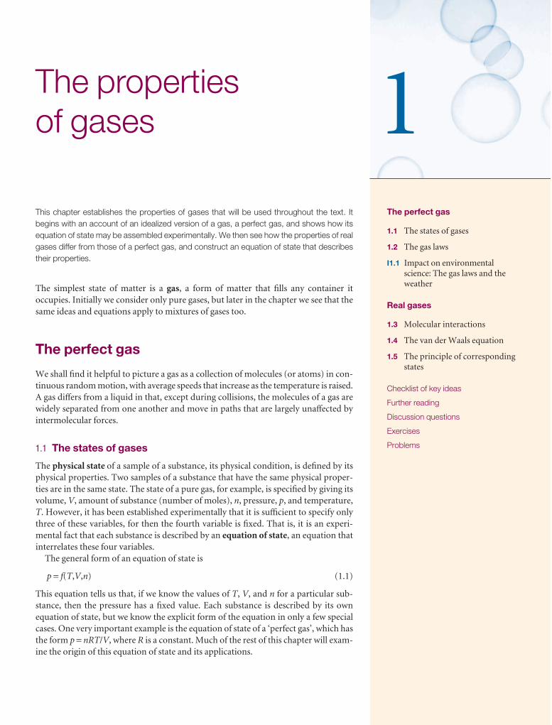
This chapter establishes the properties of gases that will be used throughout the text. It begins with an account of an idealized version of a gas, a perfect gas, and shows how itsequation of state may be assembled experimentally. We then see how the properties of realgases differ from those of a perfect gas, and construct an equation of state that describestheir properties.
The simplest state of matter is a gas, a form of matter that fills any container it occupies. Initially we consider only pure gases, but later in the chapter we see that thesame ideas and equations apply to mixtures of gases too.
The perfect gas
We shall find it helpful to picture a gas as a collection of molecules (or atoms) in con-tinuous random motion, with average speeds that increase as the temperature is raised.A gas differs from a liquid in that, except during collisions, the molecules of a gas arewidely separated from one another and move in paths that are largely unaffected byintermolecular forces.
1.1 The states of gases
The physical state of a sample of a substance, its physical condition, is defined by itsphysical properties. Two samples of a substance that have the same physical proper-ties are in the same state. The state of a pure gas, for example, is specified by giving itsvolume, V, amount of substance (number of moles), n, pressure, p, and temperature,T. However, it has been established experimentally that it is sufficient to specify onlythree of these variables, for then the fourth variable is fixed. That is, it is an experi-mental fact that each substance is described by an equation of state, an equation thatinterrelates these four variables.
The general form of an equation of state is
p = f(T,V,n) (1.1)
This equation tells us that, if we know the values of T, V, and n for a particular sub-stance, then the pressure has a fixed value. Each substance is described by its ownequation of state, but we know the explicit form of the equation in only a few specialcases. One very important example is the equation of state of a ‘perfect gas’, which hasthe form p = nRT/V, where R is a constant. Much of the rest of this chapter will exam-ine the origin of this equation of state and its applications.
1The perfect gas
1.1 The states of gases
1.2 The gas laws
I1.1 Impact on environmentalscience: The gas laws and theweather
Real gases
1.3 Molecular interactions
1.4 The van der Waals equation
1.5 The principle of correspondingstates
Checklist of key ideas
Further reading
Discussion questions
Exercises
Problems
4 1 THE PROPERTIES OF GASES
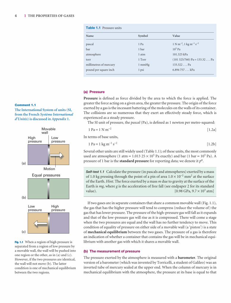
(a) Pressure
Pressure is defined as force divided by the area to which the force is applied. Thegreater the force acting on a given area, the greater the pressure. The origin of the forceexerted by a gas is the incessant battering of the molecules on the walls of its container.The collisions are so numerous that they exert an effectively steady force, which is experienced as a steady pressure.
The SI unit of pressure, the pascal (Pa), is defined as 1 newton per metre-squared:
1 Pa = 1 N m−2 [1.2a]
In terms of base units,
1 Pa = 1 kg m−1 s−2 [1.2b]
Several other units are still widely used (Table 1.1); of these units, the most commonlyused are atmosphere (1 atm = 1.013 25 × 105 Pa exactly) and bar (1 bar = 105 Pa). Apressure of 1 bar is the standard pressure for reporting data; we denote it p7.
Self-test 1.1 Calculate the pressure (in pascals and atmospheres) exerted by a massof 1.0 kg pressing through the point of a pin of area 1.0 × 10⁻² mm2 at the surfaceof the Earth. Hint. The force exerted by a mass m due to gravity at the surface of theEarth is mg, where g is the acceleration of free fall (see endpaper 2 for its standardvalue). [0.98 GPa, 9.7 × 10³ atm]
If two gases are in separate containers that share a common movable wall (Fig. 1.1),the gas that has the higher pressure will tend to compress (reduce the volume of) thegas that has lower pressure. The pressure of the high-pressure gas will fall as it expandsand that of the low-pressure gas will rise as it is compressed. There will come a stagewhen the two pressures are equal and the wall has no further tendency to move. Thiscondition of equality of pressure on either side of a movable wall (a ‘piston’) is a stateof mechanical equilibrium between the two gases. The pressure of a gas is thereforean indication of whether a container that contains the gas will be in mechanical equi-librium with another gas with which it shares a movable wall.
(b) The measurement of pressure
The pressure exerted by the atmosphere is measured with a barometer. The originalversion of a barometer (which was invented by Torricelli, a student of Galileo) was aninverted tube of mercury sealed at the upper end. When the column of mercury is inmechanical equilibrium with the atmosphere, the pressure at its base is equal to that
Comment 1.1
The International System of units (SI,from the French Système Internationald’Unités) is discussed in Appendix 1.
Table 1.1 Pressure units
Name Symbol Value
pascal 1 Pa 1 N m−2, 1 kg m−1 s−2
bar 1 bar 105 Pa
atmosphere 1 atm 101.325 kPa
torr 1 Torr (101 325/760) Pa = 133.32 . . . Pa
millimetres of mercury 1 mmHg 133.322 . . . Pa
pound per square inch 1 psi 6.894 757 . . . kPa
Highpressure
Highpressure
Lowpressure
Lowpressure
Equal pressures
(a)
(b)
(c)
Movablewall
Motion
Fig. 1.1 When a region of high pressure isseparated from a region of low pressure bya movable wall, the wall will be pushed intoone region or the other, as in (a) and (c).However, if the two pressures are identical,the wall will not move (b). The lattercondition is one of mechanical equilibriumbetween the two regions.
1.1 THE STATES OF GASES 5
�
l
1
1 The word dia is from the Greek for ‘through’.
exerted by the atmosphere. It follows that the height of the mercury column is pro-portional to the external pressure.
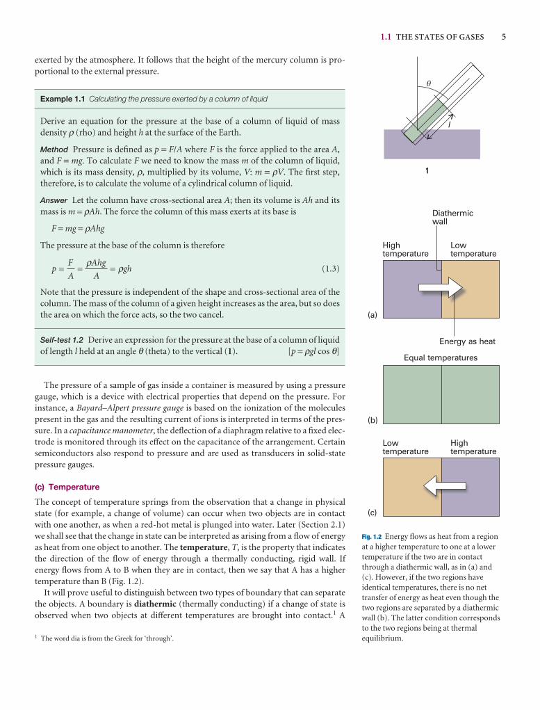
Example 1.1 Calculating the pressure exerted by a column of liquid
Derive an equation for the pressure at the base of a column of liquid of mass density ρ (rho) and height h at the surface of the Earth.
Method Pressure is defined as p = F/A where F is the force applied to the area A,and F = mg. To calculate F we need to know the mass m of the column of liquid,which is its mass density, ρ, multiplied by its volume, V: m = ρV. The first step,therefore, is to calculate the volume of a cylindrical column of liquid.
Answer Let the column have cross-sectional area A; then its volume is Ah and itsmass is m = ρAh. The force the column of this mass exerts at its base is
F = mg = ρAhg
The pressure at the base of the column is therefore
(1.3)
Note that the pressure is independent of the shape and cross-sectional area of thecolumn. The mass of the column of a given height increases as the area, but so doesthe area on which the force acts, so the two cancel.
Self-test 1.2 Derive an expression for the pressure at the base of a column of liquidof length l held at an angle θ (theta) to the vertical (1). [p = ρgl cos θ]
The pressure of a sample of gas inside a container is measured by using a pressuregauge, which is a device with electrical properties that depend on the pressure. Forinstance, a Bayard–Alpert pressure gauge is based on the ionization of the moleculespresent in the gas and the resulting current of ions is interpreted in terms of the pres-sure. In a capacitance manometer, the deflection of a diaphragm relative to a fixed elec-trode is monitored through its effect on the capacitance of the arrangement. Certainsemiconductors also respond to pressure and are used as transducers in solid-statepressure gauges.
(c) Temperature
The concept of temperature springs from the observation that a change in physicalstate (for example, a change of volume) can occur when two objects are in contactwith one another, as when a red-hot metal is plunged into water. Later (Section 2.1)we shall see that the change in state can be interpreted as arising from a flow of energyas heat from one object to another. The temperature, T, is the property that indicatesthe direction of the flow of energy through a thermally conducting, rigid wall. If energy flows from A to B when they are in contact, then we say that A has a highertemperature than B (Fig. 1.2).
It will prove useful to distinguish between two types of boundary that can separatethe objects. A boundary is diathermic (thermally conducting) if a change of state isobserved when two objects at different temperatures are brought into contact.1 A
pF
A
Ahg
Agh = = =
ρ ρ
Lowtemperature
Hightemperature
Lowtemperature
Hightemperature
Diathermicwall
Energy as heat
Equal temperatures
(a)
(b)
(c)
Fig. 1.2 Energy flows as heat from a region at a higher temperature to one at a lowertemperature if the two are in contactthrough a diathermic wall, as in (a) and (c). However, if the two regions haveidentical temperatures, there is no nettransfer of energy as heat even though thetwo regions are separated by a diathermicwall (b). The latter condition correspondsto the two regions being at thermalequilibrium.
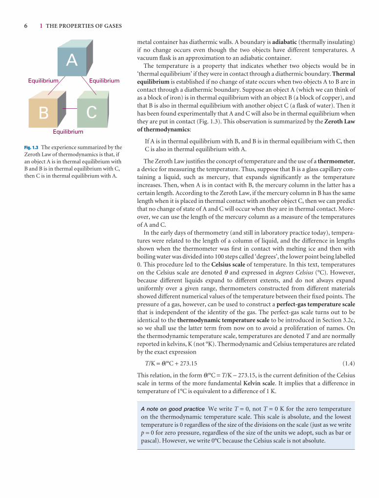
6 1 THE PROPERTIES OF GASES
metal container has diathermic walls. A boundary is adiabatic (thermally insulating)if no change occurs even though the two objects have different temperatures. A vacuum flask is an approximation to an adiabatic container.
The temperature is a property that indicates whether two objects would be in‘thermal equilibrium’ if they were in contact through a diathermic boundary. Thermalequilibrium is established if no change of state occurs when two objects A to B are incontact through a diathermic boundary. Suppose an object A (which we can think ofas a block of iron) is in thermal equilibrium with an object B (a block of copper), andthat B is also in thermal equilibrium with another object C (a flask of water). Then ithas been found experimentally that A and C will also be in thermal equilibrium whenthey are put in contact (Fig. 1.3). This observation is summarized by the Zeroth Lawof thermodynamics:
If A is in thermal equilibrium with B, and B is in thermal equilibrium with C, thenC is also in thermal equilibrium with A.
The Zeroth Law justifies the concept of temperature and the use of a thermometer,a device for measuring the temperature. Thus, suppose that B is a glass capillary con-taining a liquid, such as mercury, that expands significantly as the temperature increases. Then, when A is in contact with B, the mercury column in the latter has acertain length. According to the Zeroth Law, if the mercury column in B has the samelength when it is placed in thermal contact with another object C, then we can predictthat no change of state of A and C will occur when they are in thermal contact. More-over, we can use the length of the mercury column as a measure of the temperaturesof A and C.
In the early days of thermometry (and still in laboratory practice today), tempera-tures were related to the length of a column of liquid, and the difference in lengthsshown when the thermometer was first in contact with melting ice and then with boiling water was divided into 100 steps called ‘degrees’, the lower point being labelled0. This procedure led to the Celsius scale of temperature. In this text, temperatures on the Celsius scale are denoted θ and expressed in degrees Celsius (°C). However, because different liquids expand to different extents, and do not always expand uniformly over a given range, thermometers constructed from different materialsshowed different numerical values of the temperature between their fixed points. Thepressure of a gas, however, can be used to construct a perfect-gas temperature scalethat is independent of the identity of the gas. The perfect-gas scale turns out to beidentical to the thermodynamic temperature scale to be introduced in Section 3.2c, so we shall use the latter term from now on to avoid a proliferation of names. On the thermodynamic temperature scale, temperatures are denoted T and are normallyreported in kelvins, K (not °K). Thermodynamic and Celsius temperatures are relatedby the exact expression
T/K = θ/°C + 273.15 (1.4)
This relation, in the form θ/°C = T/K − 273.15, is the current definition of the Celsiusscale in terms of the more fundamental Kelvin scale. It implies that a difference intemperature of 1°C is equivalent to a difference of 1 K.
A note on good practice We write T = 0, not T = 0 K for the zero temperature on the thermodynamic temperature scale. This scale is absolute, and the lowesttemperature is 0 regardless of the size of the divisions on the scale (just as we writep = 0 for zero pressure, regardless of the size of the units we adopt, such as bar orpascal). However, we write 0°C because the Celsius scale is not absolute.
B
A
CEquilibrium
Equilibrium Equilibrium
Fig. 1.3 The experience summarized by theZeroth Law of thermodynamics is that, ifan object A is in thermal equilibrium withB and B is in thermal equilibrium with C,then C is in thermal equilibrium with A.
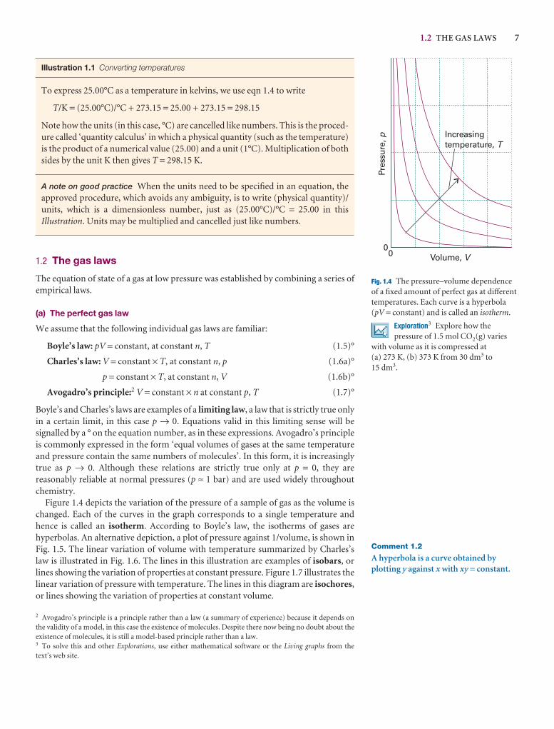
1.2 THE GAS LAWS 7
2 Avogadro’s principle is a principle rather than a law (a summary of experience) because it depends on the validity of a model, in this case the existence of molecules. Despite there now being no doubt about theexistence of molecules, it is still a model-based principle rather than a law.3 To solve this and other Explorations, use either mathematical software or the Living graphs from the text’s web site.
Comment 1.2
A hyperbola is a curve obtained byplotting y against x with xy = constant.
Volume, V
Pres
sure
,p Increasingtemperature, T
00
Fig. 1.4 The pressure–volume dependenceof a fixed amount of perfect gas at differenttemperatures. Each curve is a hyperbola(pV = constant) and is called an isotherm.
Exploration3 Explore how thepressure of 1.5 mol CO2(g) varies
with volume as it is compressed at (a) 273 K, (b) 373 K from 30 dm3 to15 dm3.
Illustration 1.1 Converting temperatures
To express 25.00°C as a temperature in kelvins, we use eqn 1.4 to write
T/K = (25.00°C)/°C + 273.15 = 25.00 + 273.15 = 298.15
Note how the units (in this case, °C) are cancelled like numbers. This is the proced-ure called ‘quantity calculus’ in which a physical quantity (such as the temperature)is the product of a numerical value (25.00) and a unit (1°C). Multiplication of bothsides by the unit K then gives T = 298.15 K.
A note on good practice When the units need to be specified in an equation, theapproved procedure, which avoids any ambiguity, is to write (physical quantity)/units, which is a dimensionless number, just as (25.00°C)/°C = 25.00 in thisIllustration. Units may be multiplied and cancelled just like numbers.
1.2 The gas laws
The equation of state of a gas at low pressure was established by combining a series ofempirical laws.
(a) The perfect gas law
We assume that the following individual gas laws are familiar:
Boyle’s law: pV = constant, at constant n, T (1.5)°
Charles’s law: V = constant × T, at constant n, p (1.6a)°
p = constant × T, at constant n, V (1.6b)°
Avogadro’s principle:2 V = constant × n at constant p, T (1.7)°
Boyle’s and Charles’s laws are examples of a limiting law, a law that is strictly true onlyin a certain limit, in this case p → 0. Equations valid in this limiting sense will be signalled by a ° on the equation number, as in these expressions. Avogadro’s principleis commonly expressed in the form ‘equal volumes of gases at the same temperatureand pressure contain the same numbers of molecules’. In this form, it is increasinglytrue as p → 0. Although these relations are strictly true only at p = 0, they are reasonably reliable at normal pressures (p ≈ 1 bar) and are used widely throughoutchemistry.
Figure 1.4 depicts the variation of the pressure of a sample of gas as the volume ischanged. Each of the curves in the graph corresponds to a single temperature andhence is called an isotherm. According to Boyle’s law, the isotherms of gases are hyperbolas. An alternative depiction, a plot of pressure against 1/volume, is shown inFig. 1.5. The linear variation of volume with temperature summarized by Charles’slaw is illustrated in Fig. 1.6. The lines in this illustration are examples of isobars, orlines showing the variation of properties at constant pressure. Figure 1.7 illustrates thelinear variation of pressure with temperature. The lines in this diagram are isochores,or lines showing the variation of properties at constant volume.
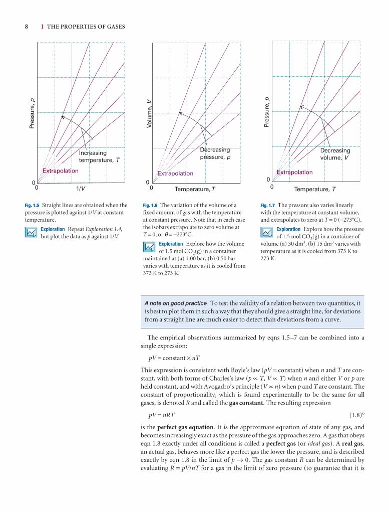
8 1 THE PROPERTIES OF GASES
A note on good practice To test the validity of a relation between two quantities, itis best to plot them in such a way that they should give a straight line, for deviationsfrom a straight line are much easier to detect than deviations from a curve.
The empirical observations summarized by eqns 1.5–7 can be combined into a single expression:
pV = constant × nT
This expression is consistent with Boyle’s law (pV = constant) when n and T are con-stant, with both forms of Charles’s law (p ∝ T, V ∝ T) when n and either V or p areheld constant, and with Avogadro’s principle (V ∝ n) when p and T are constant. Theconstant of proportionality, which is found experimentally to be the same for allgases, is denoted R and called the gas constant. The resulting expression
pV = nRT (1.8)°
is the perfect gas equation. It is the approximate equation of state of any gas, and becomes increasingly exact as the pressure of the gas approaches zero. A gas that obeyseqn 1.8 exactly under all conditions is called a perfect gas (or ideal gas). A real gas,an actual gas, behaves more like a perfect gas the lower the pressure, and is describedexactly by eqn 1.8 in the limit of p → 0. The gas constant R can be determined by evaluating R = pV/nT for a gas in the limit of zero pressure (to guarantee that it is
1/V
Pres
sure
,p
00
Increasingtemperature, T
Extrapolation
Volu
me,
V
0
Decreasingpressure, p
Extrapolation
Temperature,T0
Pres
sure
,p
00
Extrapolation
Decreasingvolume, V
Temperature, T
Fig. 1.5 Straight lines are obtained when thepressure is plotted against 1/V at constanttemperature.
Exploration Repeat Exploration 1.4,but plot the data as p against 1/V.
Fig. 1.6 The variation of the volume of afixed amount of gas with the temperatureat constant pressure. Note that in each casethe isobars extrapolate to zero volume at T = 0, or θ = −273°C.
Exploration Explore how the volumeof 1.5 mol CO2(g) in a container
maintained at (a) 1.00 bar, (b) 0.50 barvaries with temperature as it is cooled from373 K to 273 K.
Fig. 1.7 The pressure also varies linearlywith the temperature at constant volume,and extrapolates to zero at T = 0 (−273°C).
Exploration Explore how the pressureof 1.5 mol CO2(g) in a container of
volume (a) 30 dm3, (b) 15 dm3 varies withtemperature as it is cooled from 373 K to273 K.
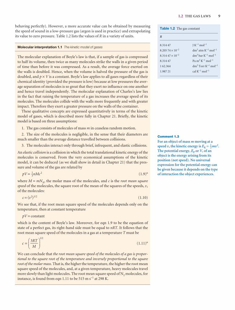
1.2 THE GAS LAWS 9
Table 1.2 The gas constant
R
8.314 47 J K−1 mol−1
8.205 74 × 10−2 dm3 atm K−1 mol−1
8.314 47 × 10−2 dm3 bar K−1 mol−1
8.314 47 Pa m3 K−1 mol−1
1 62.364 dm3 Torr K−1 mol−1
1.987 21 cal K−1 mol−1
Comment 1.3
For an object of mass m moving at aspeed 1, the kinetic energy is EK = 1–2 m12.The potential energy, EP or V, of anobject is the energy arising from itsposition (not speed). No universalexpression for the potential energy canbe given because it depends on the typeof interaction the object experiences.
behaving perfectly). However, a more accurate value can be obtained by measuringthe speed of sound in a low-pressure gas (argon is used in practice) and extrapolatingits value to zero pressure. Table 1.2 lists the values of R in a variety of units.
Molecular interpretation 1.1 The kinetic model of gases
The molecular explanation of Boyle’s law is that, if a sample of gas is compressed to half its volume, then twice as many molecules strike the walls in a given period of time than before it was compressed. As a result, the average force exerted on the walls is doubled. Hence, when the volume is halved the pressure of the gas isdoubled, and p × V is a constant. Boyle’s law applies to all gases regardless of theirchemical identity (provided the pressure is low) because at low pressures the aver-age separation of molecules is so great that they exert no influence on one anotherand hence travel independently. The molecular explanation of Charles’s law lies in the fact that raising the temperature of a gas increases the average speed of itsmolecules. The molecules collide with the walls more frequently and with greaterimpact. Therefore they exert a greater pressure on the walls of the container.
These qualitative concepts are expressed quantitatively in terms of the kineticmodel of gases, which is described more fully in Chapter 21. Briefly, the kineticmodel is based on three assumptions:
1. The gas consists of molecules of mass m in ceaseless random motion.
2. The size of the molecules is negligible, in the sense that their diameters aremuch smaller than the average distance travelled between collisions.
3. The molecules interact only through brief, infrequent, and elastic collisions.
An elastic collision is a collision in which the total translational kinetic energy of themolecules is conserved. From the very economical assumptions of the kineticmodel, it can be deduced (as we shall show in detail in Chapter 21) that the pres-sure and volume of the gas are related by
pV = nMc 2 (1.9)°
where M = mNA, the molar mass of the molecules, and c is the root mean squarespeed of the molecules, the square root of the mean of the squares of the speeds, v,of the molecules:
c = �v2�1/2 (1.10)
We see that, if the root mean square speed of the molecules depends only on thetemperature, then at constant temperature
pV = constant
which is the content of Boyle’s law. Moreover, for eqn 1.9 to be the equation ofstate of a perfect gas, its right-hand side must be equal to nRT. It follows that theroot mean square speed of the molecules in a gas at a temperature T must be
(1.11)°
We can conclude that the root mean square speed of the molecules of a gas is propor-tional to the square root of the temperature and inversely proportional to the squareroot of the molar mass. That is, the higher the temperature, the higher the root meansquare speed of the molecules, and, at a given temperature, heavy molecules travelmore slowly than light molecules. The root mean square speed of N2 molecules, forinstance, is found from eqn 1.11 to be 515 m s−1 at 298 K.
cRT
M
/
=⎛⎝⎜
⎞⎠⎟
31 2
13
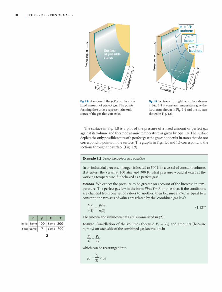
10 1 THE PROPERTIES OF GASES
Surfaceof possiblestates
Pres
sure
,pVolume, V
Tem
pera
ture
, T Pres
sure
,p
Tem
pera
ture
, TPres
sure
,p
Volume, V
p Tisochore
µ
p V1/isotherm
µ
V Tisobar
µ
Fig. 1.8 A region of the p,V,T surface of afixed amount of perfect gas. The pointsforming the surface represent the onlystates of the gas that can exist.
Fig. 1.9 Sections through the surface shownin Fig. 1.8 at constant temperature give theisotherms shown in Fig. 1.4 and the isobarsshown in Fig. 1.6.
n p V TInitial
Final
Same 100 300500?Same
Same
Same
2
The surface in Fig. 1.8 is a plot of the pressure of a fixed amount of perfect gasagainst its volume and thermodynamic temperature as given by eqn 1.8. The surfacedepicts the only possible states of a perfect gas: the gas cannot exist in states that do notcorrespond to points on the surface. The graphs in Figs. 1.4 and 1.6 correspond to thesections through the surface (Fig. 1.9).
Example 1.2 Using the perfect gas equation
In an industrial process, nitrogen is heated to 500 K in a vessel of constant volume.If it enters the vessel at 100 atm and 300 K, what pressure would it exert at theworking temperature if it behaved as a perfect gas?
Method We expect the pressure to be greater on account of the increase in tem-perature. The perfect gas law in the form PV/nT = R implies that, if the conditionsare changed from one set of values to another, then because PV/nT is equal to aconstant, the two sets of values are related by the ‘combined gas law’:
(1.12)°
The known and unknown data are summarized in (2).
Answer Cancellation of the volumes (because V1 = V2) and amounts (because n1 = n2) on each side of the combined gas law results in
which can be rearranged into
pT
Tp2
2
11 = ×
p
T
p
T1
1
2
2
=
p V
n T
p V
n T1 1
1 1
2 2
2 2
=
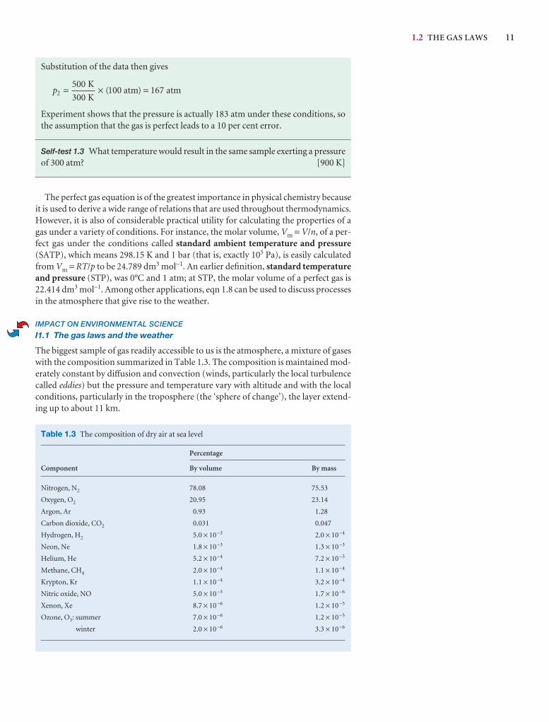
1.2 THE GAS LAWS 11
Table 1.3 The composition of dry air at sea level
Percentage
Component By volume By mass
Nitrogen, N2 78.08 75.53
Oxygen, O2 20.95 23.14
Argon, Ar 0.93 1.28
Carbon dioxide, CO2 0.031 0.047
Hydrogen, H2 5.0 × 10⁻³ 2.0 × 10⁻⁴
Neon, Ne 1.8 × 10⁻³ 1.3 × 10⁻³
Helium, He 5.2 × 10⁻⁴ 7.2 × 10⁻⁵
Methane, CH4 2.0 × 10⁻⁴ 1.1 × 10⁻⁴
Krypton, Kr 1.1 × 10⁻⁴ 3.2 × 10⁻⁴
Nitric oxide, NO 5.0 × 10⁻⁵ 1.7 × 10⁻⁶
Xenon, Xe 8.7 × 10⁻⁶ 1.2 × 10⁻⁵
Ozone, O3: summer 7.0 × 10⁻⁶ 1.2 × 10⁻⁵
winter 2.0 × 10⁻⁶ 3.3 × 10⁻⁶
Substitution of the data then gives
Experiment shows that the pressure is actually 183 atm under these conditions, sothe assumption that the gas is perfect leads to a 10 per cent error.
Self-test 1.3 What temperature would result in the same sample exerting a pressureof 300 atm? [900 K]
The perfect gas equation is of the greatest importance in physical chemistry becauseit is used to derive a wide range of relations that are used throughout thermodynamics.However, it is also of considerable practical utility for calculating the properties of agas under a variety of conditions. For instance, the molar volume, Vm = V/n, of a per-fect gas under the conditions called standard ambient temperature and pressure(SATP), which means 298.15 K and 1 bar (that is, exactly 105 Pa), is easily calculatedfrom Vm = RT/p to be 24.789 dm3 mol−1. An earlier definition, standard temperatureand pressure (STP), was 0°C and 1 atm; at STP, the molar volume of a perfect gas is22.414 dm3 mol−1. Among other applications, eqn 1.8 can be used to discuss processesin the atmosphere that give rise to the weather.
IMPACT ON ENVIRONMENTAL SCIENCE
I1.1 The gas laws and the weather
The biggest sample of gas readily accessible to us is the atmosphere, a mixture of gaseswith the composition summarized in Table 1.3. The composition is maintained mod-erately constant by diffusion and convection (winds, particularly the local turbulencecalled eddies) but the pressure and temperature vary with altitude and with the localconditions, particularly in the troposphere (the ‘sphere of change’), the layer extend-ing up to about 11 km.
p2500
300100 167 ( ) = × =
K
Katm atm
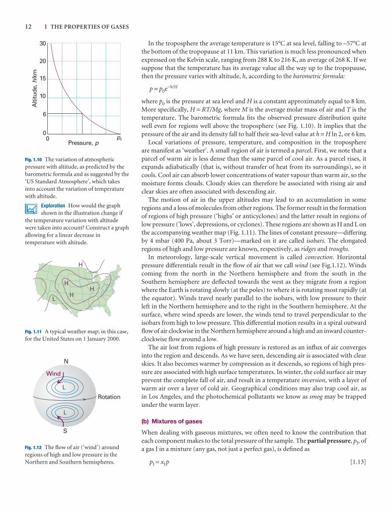
12 1 THE PROPERTIES OF GASES
In the troposphere the average temperature is 15°C at sea level, falling to –57°C atthe bottom of the tropopause at 11 km. This variation is much less pronounced whenexpressed on the Kelvin scale, ranging from 288 K to 216 K, an average of 268 K. If wesuppose that the temperature has its average value all the way up to the tropopause,then the pressure varies with altitude, h, according to the barometric formula:
p = p0e−h/H
where p0 is the pressure at sea level and H is a constant approximately equal to 8 km.More specifically, H = RT/Mg, where M is the average molar mass of air and T is thetemperature. The barometric formula fits the observed pressure distribution quitewell even for regions well above the troposphere (see Fig. 1.10). It implies that thepressure of the air and its density fall to half their sea-level value at h = H ln 2, or 6 km.
Local variations of pressure, temperature, and composition in the troposphere are manifest as ‘weather’. A small region of air is termed a parcel. First, we note that aparcel of warm air is less dense than the same parcel of cool air. As a parcel rises, it expands adiabatically (that is, without transfer of heat from its surroundings), so itcools. Cool air can absorb lower concentrations of water vapour than warm air, so themoisture forms clouds. Cloudy skies can therefore be associated with rising air andclear skies are often associated with descending air.
The motion of air in the upper altitudes may lead to an accumulation in some regions and a loss of molecules from other regions. The former result in the formationof regions of high pressure (‘highs’ or anticyclones) and the latter result in regions oflow pressure (‘lows’, depressions, or cyclones). These regions are shown as H and L onthe accompanying weather map (Fig. 1.11). The lines of constant pressure—differingby 4 mbar (400 Pa, about 3 Torr)—marked on it are called isobars. The elongated regions of high and low pressure are known, respectively, as ridges and troughs.
In meteorology, large-scale vertical movement is called convection. Horizontalpressure differentials result in the flow of air that we call wind (see Fig.1.12). Windscoming from the north in the Northern hemisphere and from the south in theSouthern hemisphere are deflected towards the west as they migrate from a regionwhere the Earth is rotating slowly (at the poles) to where it is rotating most rapidly (atthe equator). Winds travel nearly parallel to the isobars, with low pressure to theirleft in the Northern hemisphere and to the right in the Southern hemisphere. At thesurface, where wind speeds are lower, the winds tend to travel perpendicular to theisobars from high to low pressure. This differential motion results in a spiral outwardflow of air clockwise in the Northern hemisphere around a high and an inward counter-clockwise flow around a low.
The air lost from regions of high pressure is restored as an influx of air convergesinto the region and descends. As we have seen, descending air is associated with clearskies. It also becomes warmer by compression as it descends, so regions of high pres-sure are associated with high surface temperatures. In winter, the cold surface air mayprevent the complete fall of air, and result in a temperature inversion, with a layer ofwarm air over a layer of cold air. Geographical conditions may also trap cool air, as in Los Angeles, and the photochemical pollutants we know as smog may be trappedunder the warm layer.
(b) Mixtures of gases
When dealing with gaseous mixtures, we often need to know the contribution thateach component makes to the total pressure of the sample. The partial pressure, pJ, ofa gas J in a mixture (any gas, not just a perfect gas), is defined as
pJ = xJ p [1.13]
p0Pressure, p
0
Alti
tude
,/k
mh
6
10
15
20
30
0
H
LH
H
H
Fig. 1.10 The variation of atmosphericpressure with altitude, as predicted by thebarometric formula and as suggested by the‘US Standard Atmosphere’, which takesinto account the variation of temperaturewith altitude.
Exploration How would the graphshown in the illustration change if
the temperature variation with altitudewere taken into account? Construct a graphallowing for a linear decrease intemperature with altitude.
Fig. 1.11 A typical weather map; in this case,for the United States on 1 January 2000.
L
L
Wind
Rotation
N
S
Fig. 1.12 The flow of air (‘wind’) aroundregions of high and low pressure in theNorthern and Southern hemispheres.
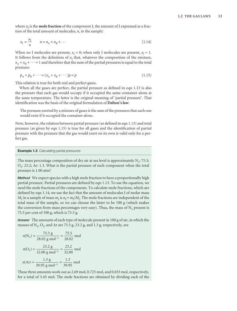
1.2 THE GAS LAWS 13
where xJ is the mole fraction of the component J, the amount of J expressed as a frac-tion of the total amount of molecules, n, in the sample:
n = nA + nB + · · · [1.14]
When no J molecules are present, xJ = 0; when only J molecules are present, xJ = 1.It follows from the definition of xJ that, whatever the composition of the mixture, xA + xB + · · · = 1 and therefore that the sum of the partial pressures is equal to the totalpressure:
pA + pB + · · · = (xA + xB + · · · )p = p (1.15)
This relation is true for both real and perfect gases.When all the gases are perfect, the partial pressure as defined in eqn 1.13 is also
the pressure that each gas would occupy if it occupied the same container alone at the same temperature. The latter is the original meaning of ‘partial pressure’. Thatidentification was the basis of the original formulation of Dalton’s law:
The pressure exerted by a mixture of gases is the sum of the pressures that each onewould exist if it occupied the container alone.
Now, however, the relation between partial pressure (as defined in eqn 1.13) and totalpressure (as given by eqn 1.15) is true for all gases and the identification of partialpressure with the pressure that the gas would exert on its own is valid only for a per-fect gas.
Example 1.3 Calculating partial pressures
The mass percentage composition of dry air at sea level is approximately N2: 75.5;O2: 23.2; Ar: 1.3. What is the partial pressure of each component when the totalpressure is 1.00 atm?
Method We expect species with a high mole fraction to have a proportionally highpartial pressure. Partial pressures are defined by eqn 1.13. To use the equation, weneed the mole fractions of the components. To calculate mole fractions, which aredefined by eqn 1.14, we use the fact that the amount of molecules J of molar massMJ in a sample of mass mJ is nJ = mJ/MJ. The mole fractions are independent of thetotal mass of the sample, so we can choose the latter to be 100 g (which makes the conversion from mass percentages very easy). Thus, the mass of N2 present is75.5 per cent of 100 g, which is 75.5 g.
Answer The amounts of each type of molecule present in 100 g of air, in which themasses of N2, O2, and Ar are 75.5 g, 23.2 g, and 1.3 g, respectively, are
These three amounts work out as 2.69 mol, 0.725 mol, and 0.033 mol, respectively,for a total of 3.45 mol. The mole fractions are obtained by dividing each of the
n( ) .
.
.
. Ar
g
g molmol= =
−1 3
39 95
1 3
39 951
n( ) .
.
.
. O
g
g molmol2 1
23 2
32 00
23 2
32 00= =
−
n( ) .
.
.
. N
g
g molmol2 1
75 5
28 02
75 5
28 02= =
−
xn
nJ
J=
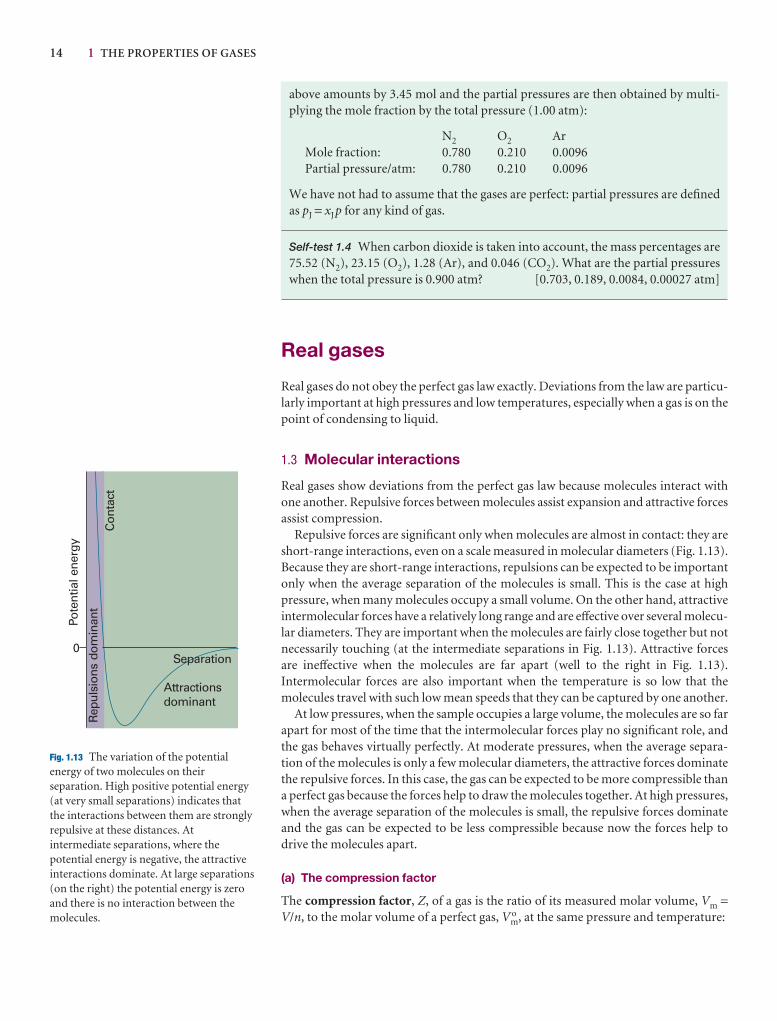
14 1 THE PROPERTIES OF GASES
Separation
Pote
ntia
l ene
rgy
0
Con
tact
Attractionsdominant
Rep
ulsi
ons
dom
inan
t
Fig. 1.13 The variation of the potentialenergy of two molecules on theirseparation. High positive potential energy(at very small separations) indicates thatthe interactions between them are stronglyrepulsive at these distances. Atintermediate separations, where thepotential energy is negative, the attractiveinteractions dominate. At large separations(on the right) the potential energy is zeroand there is no interaction between themolecules.
above amounts by 3.45 mol and the partial pressures are then obtained by multi-plying the mole fraction by the total pressure (1.00 atm):
N2 O2 ArMole fraction: 0.780 0.210 0.0096Partial pressure/atm: 0.780 0.210 0.0096
We have not had to assume that the gases are perfect: partial pressures are definedas pJ = xJ p for any kind of gas.
Self-test 1.4 When carbon dioxide is taken into account, the mass percentages are75.52 (N2), 23.15 (O2), 1.28 (Ar), and 0.046 (CO2). What are the partial pressureswhen the total pressure is 0.900 atm? [0.703, 0.189, 0.0084, 0.00027 atm]
Real gases
Real gases do not obey the perfect gas law exactly. Deviations from the law are particu-larly important at high pressures and low temperatures, especially when a gas is on thepoint of condensing to liquid.
1.3 Molecular interactions
Real gases show deviations from the perfect gas law because molecules interact withone another. Repulsive forces between molecules assist expansion and attractive forcesassist compression.
Repulsive forces are significant only when molecules are almost in contact: they areshort-range interactions, even on a scale measured in molecular diameters (Fig. 1.13).Because they are short-range interactions, repulsions can be expected to be importantonly when the average separation of the molecules is small. This is the case at highpressure, when many molecules occupy a small volume. On the other hand, attractiveintermolecular forces have a relatively long range and are effective over several molecu-lar diameters. They are important when the molecules are fairly close together but notnecessarily touching (at the intermediate separations in Fig. 1.13). Attractive forcesare ineffective when the molecules are far apart (well to the right in Fig. 1.13).Intermolecular forces are also important when the temperature is so low that themolecules travel with such low mean speeds that they can be captured by one another.
At low pressures, when the sample occupies a large volume, the molecules are so farapart for most of the time that the intermolecular forces play no significant role, andthe gas behaves virtually perfectly. At moderate pressures, when the average separa-tion of the molecules is only a few molecular diameters, the attractive forces dominatethe repulsive forces. In this case, the gas can be expected to be more compressible thana perfect gas because the forces help to draw the molecules together. At high pressures,when the average separation of the molecules is small, the repulsive forces dominateand the gas can be expected to be less compressible because now the forces help todrive the molecules apart.
(a) The compression factor
The compression factor, Z, of a gas is the ratio of its measured molar volume, Vm =V/n, to the molar volume of a perfect gas, V o
m, at the same pressure and temperature:
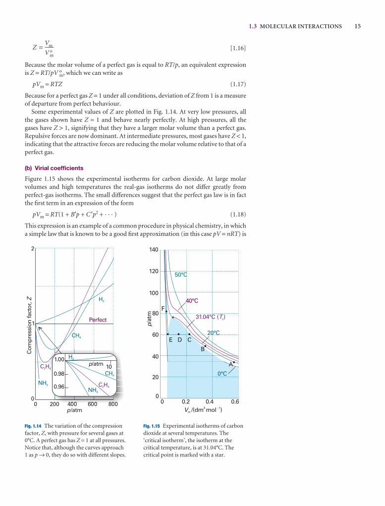
1.3 MOLECULAR INTERACTIONS 15
[1.16]
Because the molar volume of a perfect gas is equal to RT/p, an equivalent expressionis Z = RT/pV o
m, which we can write as
pVm = RTZ (1.17)
Because for a perfect gas Z = 1 under all conditions, deviation of Z from 1 is a measureof departure from perfect behaviour.
Some experimental values of Z are plotted in Fig. 1.14. At very low pressures, all the gases shown have Z ≈ 1 and behave nearly perfectly. At high pressures, all the gases have Z > 1, signifying that they have a larger molar volume than a perfect gas.Repulsive forces are now dominant. At intermediate pressures, most gases have Z < 1,indicating that the attractive forces are reducing the molar volume relative to that of aperfect gas.
(b) Virial coefficients
Figure 1.15 shows the experimental isotherms for carbon dioxide. At large molar volumes and high temperatures the real-gas isotherms do not differ greatly from perfect-gas isotherms. The small differences suggest that the perfect gas law is in factthe first term in an expression of the form
pVm = RT(1 + B′p + C ′p2 + · · · ) (1.18)
This expression is an example of a common procedure in physical chemistry, in whicha simple law that is known to be a good first approximation (in this case pV = nRT) is
ZV
V= m
mo
H2
CH4
C H2 4
NH3
p/atm
2
1
0 200 400 600 800
Perfect
0
Com
pres
sion
fact
or, Z
1.00
0.98
0.96
10
H2
CH4
C H2 4NH3
p/atm
140
120
100
80
60
40
20
00 0.2 0.4 0.6
50°C
40°C
31.04°C ( )Tc
0°C
p/at
m
Vm /(dm mol )3 1
E D C
B
A
F
*
20°C
-
Fig. 1.14 The variation of the compressionfactor, Z, with pressure for several gases at0°C. A perfect gas has Z = 1 at all pressures.Notice that, although the curves approach1 as p → 0, they do so with different slopes.
Fig. 1.15 Experimental isotherms of carbondioxide at several temperatures. The‘critical isotherm’, the isotherm at thecritical temperature, is at 31.04°C. Thecritical point is marked with a star.
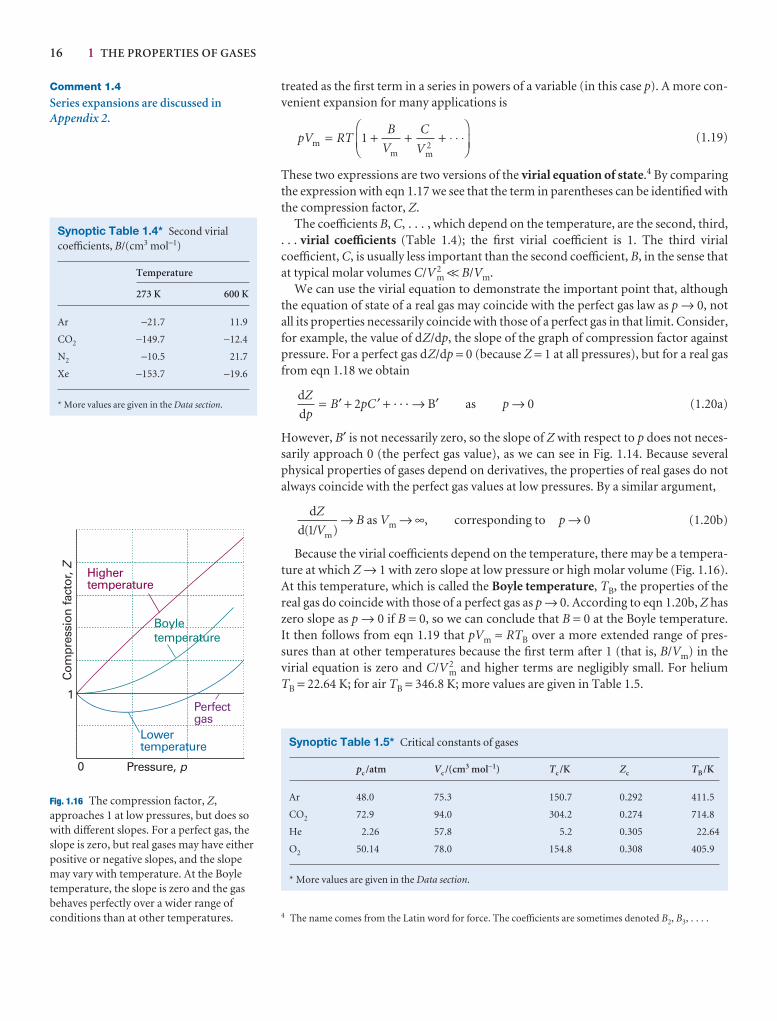
16 1 THE PROPERTIES OF GASES
treated as the first term in a series in powers of a variable (in this case p). A more con-venient expansion for many applications is
(1.19)
These two expressions are two versions of the virial equation of state.4 By comparingthe expression with eqn 1.17 we see that the term in parentheses can be identified withthe compression factor, Z.
The coefficients B, C, . . . , which depend on the temperature, are the second, third,. . . virial coefficients (Table 1.4); the first virial coefficient is 1. The third virialcoefficient, C, is usually less important than the second coefficient, B, in the sense thatat typical molar volumes C/V 2
m << B/Vm.We can use the virial equation to demonstrate the important point that, although
the equation of state of a real gas may coincide with the perfect gas law as p → 0, notall its properties necessarily coincide with those of a perfect gas in that limit. Consider,for example, the value of dZ/dp, the slope of the graph of compression factor againstpressure. For a perfect gas dZ/dp = 0 (because Z = 1 at all pressures), but for a real gasfrom eqn 1.18 we obtain
+ 2pC ′ + · · · → B′ as p → 0 (1.20a)
However, B′ is not necessarily zero, so the slope of Z with respect to p does not neces-sarily approach 0 (the perfect gas value), as we can see in Fig. 1.14. Because severalphysical properties of gases depend on derivatives, the properties of real gases do notalways coincide with the perfect gas values at low pressures. By a similar argument,
→ B as Vm → ∞, corresponding to p → 0 (1.20b)
Because the virial coefficients depend on the temperature, there may be a tempera-ture at which Z → 1 with zero slope at low pressure or high molar volume (Fig. 1.16).At this temperature, which is called the Boyle temperature, TB, the properties of thereal gas do coincide with those of a perfect gas as p → 0. According to eqn 1.20b, Z haszero slope as p → 0 if B = 0, so we can conclude that B = 0 at the Boyle temperature. It then follows from eqn 1.19 that pVm ≈ RTB over a more extended range of pres-sures than at other temperatures because the first term after 1 (that is, B/Vm) in thevirial equation is zero and C/V 2
m and higher terms are negligibly small. For helium TB = 22.64 K; for air TB = 346.8 K; more values are given in Table 1.5.
d
d m
Z
V( / )1
d
d
Z
pB= ′
pV RTB
V
C
Vmm m
= + + + ⋅ ⋅ ⋅⎛
⎝⎜⎞
⎠⎟1
2
Comment 1.4
Series expansions are discussed inAppendix 2.
4 The name comes from the Latin word for force. The coefficients are sometimes denoted B2, B3, . . . .
Synoptic Table 1.4* Second virialcoefficients, B/(cm3 mol−1)
Temperature
273 K 600 K
Ar −21.7 11.9
CO2 −149.7 −12.4
N2 −10.5 21.7
Xe −153.7 −19.6
* More values are given in the Data section.
Synoptic Table 1.5* Critical constants of gases
pc /atm Vc /(cm3 mol−1) Tc /K Zc TB /K
Ar 48.0 75.3 150.7 0.292 411.5
CO2 72.9 94.0 304.2 0.274 714.8
He 2.26 57.8 5.2 0.305 22.64
O2 50.14 78.0 154.8 0.308 405.9
* More values are given in the Data section.
Pressure, p
Highertemperature
Lowertemperature
Perfectgas
Boyletemperature
1
Com
pres
sion
fact
or, Z
0
Fig. 1.16 The compression factor, Z,approaches 1 at low pressures, but does sowith different slopes. For a perfect gas, theslope is zero, but real gases may have eitherpositive or negative slopes, and the slopemay vary with temperature. At the Boyletemperature, the slope is zero and the gasbehaves perfectly over a wider range ofconditions than at other temperatures.
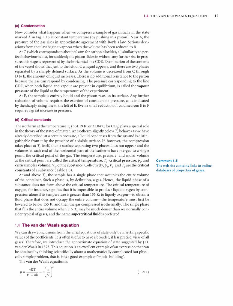
1.4 THE VAN DER WAALS EQUATION 17
(c) Condensation
Now consider what happens when we compress a sample of gas initially in the statemarked A in Fig. 1.15 at constant temperature (by pushing in a piston). Near A, thepressure of the gas rises in approximate agreement with Boyle’s law. Serious devi-ations from that law begin to appear when the volume has been reduced to B.
At C (which corresponds to about 60 atm for carbon dioxide), all similarity to per-fect behaviour is lost, for suddenly the piston slides in without any further rise in pres-sure: this stage is represented by the horizontal line CDE. Examination of the contentsof the vessel shows that just to the left of C a liquid appears, and there are two phasesseparated by a sharply defined surface. As the volume is decreased from C through D to E, the amount of liquid increases. There is no additional resistance to the pistonbecause the gas can respond by condensing. The pressure corresponding to the lineCDE, when both liquid and vapour are present in equilibrium, is called the vapourpressure of the liquid at the temperature of the experiment.
At E, the sample is entirely liquid and the piston rests on its surface. Any further reduction of volume requires the exertion of considerable pressure, as is indicated by the sharply rising line to the left of E. Even a small reduction of volume from E to Frequires a great increase in pressure.
(d) Critical constants
The isotherm at the temperature Tc (304.19 K, or 31.04°C for CO2) plays a special rolein the theory of the states of matter. An isotherm slightly below Tc behaves as we havealready described: at a certain pressure, a liquid condenses from the gas and is distin-guishable from it by the presence of a visible surface. If, however, the compressiontakes place at Tc itself, then a surface separating two phases does not appear and thevolumes at each end of the horizontal part of the isotherm have merged to a singlepoint, the critical point of the gas. The temperature, pressure, and molar volume at the critical point are called the critical temperature, Tc, critical pressure, pc, andcritical molar volume, Vc, of the substance. Collectively, pc, Vc, and Tc are the criticalconstants of a substance (Table 1.5).
At and above Tc, the sample has a single phase that occupies the entire volume of the container. Such a phase is, by definition, a gas. Hence, the liquid phase of a substance does not form above the critical temperature. The critical temperature ofoxygen, for instance, signifies that it is impossible to produce liquid oxygen by com-pression alone if its temperature is greater than 155 K: to liquefy oxygen—to obtain afluid phase that does not occupy the entire volume—the temperature must first belowered to below 155 K, and then the gas compressed isothermally. The single phasethat fills the entire volume when T > Tc may be much denser than we normally con-sider typical of gases, and the name supercritical fluid is preferred.
1.4 The van der Waals equation
We can draw conclusions from the virial equations of state only by inserting specificvalues of the coefficients. It is often useful to have a broader, if less precise, view of allgases. Therefore, we introduce the approximate equation of state suggested by J.D.van der Waals in 1873. This equation is an excellent example of an expression that canbe obtained by thinking scientifically about a mathematically complicated but physi-cally simple problem, that is, it is a good example of ‘model building’.
The van der Waals equation is
(1.21a)pnRT
V nba
n
V=
−−
⎛⎝⎜
⎞⎠⎟
2
Comment 1.5
The web site contains links to onlinedatabases of properties of gases.
18 1 THE PROPERTIES OF GASES
Synoptic Table 1.6* van der Waalscoefficients
a/(atm dm6 mol−2) b/(10−2 dm3 mol−1)
Ar 1.337 3.20
CO2 3.610 4.29
He 0.0341 2.38
Xe 4.137 5.16
* More values are given in the Data section.
and a derivation is given in Justification 1.1. The equation is often written in terms ofthe molar volume Vm = V/n as
(1.21b)
The constants a and b are called the van der Waals coefficients. They are characteris-tic of each gas but independent of the temperature (Table 1.6).
Justification 1.1 The van der Waals equation of state
The repulsive interactions between molecules are taken into account by supposingthat they cause the molecules to behave as small but impenetrable spheres. The non-zero volume of the molecules implies that instead of moving in a volume V they arerestricted to a smaller volume V − nb, where nb is approximately the total volumetaken up by the molecules themselves. This argument suggests that the perfect gaslaw p = nRT/V should be replaced by
when repulsions are significant. The closest distance of two hard-sphere moleculesof radius r, and volume Vmolecule = , is 2r, so the volume excluded is (2r)3, or8Vmolecule. The volume excluded per molecule is one-half this volume, or 4Vmolecule,so b ≈ 4VmoleculeNA.
The pressure depends on both the frequency of collisions with the walls and the force of each collision. Both the frequency of the collisions and their forceare reduced by the attractive forces, which act with a strength proportional to the molar concentration, n/V, of molecules in the sample. Therefore, because both the frequency and the force of the collisions are reduced by the attractive forces, the pressure is reduced in proportion to the square of this concentration. If the reduction of pressure is written as −a(n/V)2, where a is a positive constant charac-teristic of each gas, the combined effect of the repulsive and attractive forces is thevan der Waals equation of state as expressed in eqn 1.21.
In this Justification we have built the van der Waals equation using vague argu-ments about the volumes of molecules and the effects of forces. The equation can bederived in other ways, but the present method has the advantage that it shows howto derive the form of an equation out of general ideas. The derivation also has theadvantage of keeping imprecise the significance of the coefficients a and b: they aremuch better regarded as empirical parameters than as precisely defined molecularproperties.
Example 1.4 Using the van der Waals equation to estimate a molar volume
Estimate the molar volume of CO2 at 500 K and 100 atm by treating it as a van derWaals gas.
Method To express eqn 1.21b as an equation for the molar volume, we multiplyboth sides by (Vm – b)V 2
m, to obtain
(Vm – b)V 2m p = RTV 2
m – (Vm – b)a
and, after division by p, collect powers of Vm to obtain
V bRT
pV
a
pV
ab
pm m m3 2 0 − +
⎛⎝⎜
⎞⎠⎟
+⎛⎝⎜
⎞⎠⎟
− =
43 π4
33πr
pnRT
V nb=
−
pRT
V b
a
V=
−−
m m2
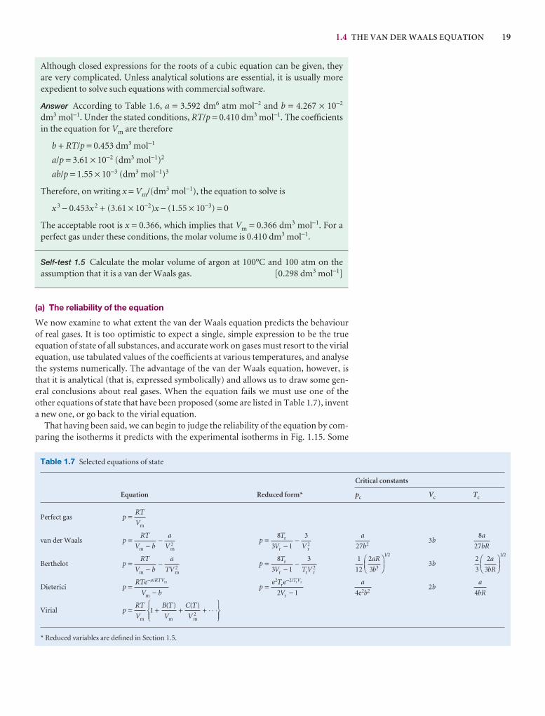
1.4 THE VAN DER WAALS EQUATION 19
Table 1.7 Selected equations of state
Critical constants
Equation Reduced form* pc Vc Tc
Perfect gas
van der Waals 3b
Berthelot 3b
Dieterici 2b
Virial
* Reduced variables are defined in Section 1.5.
pRT
V
B T
V
C T
V
( ) ( ) = + + + ⋅ ⋅ ⋅
⎧⎨⎩⎪
⎫⎬⎭⎪m m m
12
a
bR4
a
b4 2 2ep
T
V
T V/
=−
−e e2r
r
r r2
2 1p
RT
V b
a RTV/
=−
−e m
m
2
3
2
3
1 2a
bR
⎛⎝⎜
⎞⎠⎟
/1
12
2
3 3
1 2aR
b
⎛⎝⎜
⎞⎠⎟
/
pT
V T V=
−−
8
3 1
32
r
r r r
pRT
V b
a
TV=
−−
m m2
8
27
a
bR
a
b27 2p
T
V V=
−−
8
3 1
32
r
r r
pRT
V b
a
V=
−−
m m2
pRT
V=
m
Although closed expressions for the roots of a cubic equation can be given, they are very complicated. Unless analytical solutions are essential, it is usually more expedient to solve such equations with commercial software.
Answer According to Table 1.6, a = 3.592 dm6 atm mol−2 and b = 4.267 × 10⁻²
dm3 mol−1. Under the stated conditions, RT/p = 0.410 dm3 mol−1. The coefficientsin the equation for Vm are therefore
b + RT/p = 0.453 dm3 mol−1
a/p = 3.61 × 10⁻² (dm3 mol−1)2
ab/p = 1.55 × 10⁻³ (dm3 mol−1)3
Therefore, on writing x = Vm/(dm3 mol−1), the equation to solve is
x 3 − 0.453x 2 + (3.61 × 10⁻²)x − (1.55 × 10⁻³) = 0
The acceptable root is x = 0.366, which implies that Vm = 0.366 dm3 mol−1. For aperfect gas under these conditions, the molar volume is 0.410 dm3 mol−1.
Self-test 1.5 Calculate the molar volume of argon at 100°C and 100 atm on the assumption that it is a van der Waals gas. [0.298 dm3 mol−1]
(a) The reliability of the equation
We now examine to what extent the van der Waals equation predicts the behaviour of real gases. It is too optimistic to expect a single, simple expression to be the trueequation of state of all substances, and accurate work on gases must resort to the virialequation, use tabulated values of the coefficients at various temperatures, and analysethe systems numerically. The advantage of the van der Waals equation, however, isthat it is analytical (that is, expressed symbolically) and allows us to draw some gen-eral conclusions about real gases. When the equation fails we must use one of theother equations of state that have been proposed (some are listed in Table 1.7), inventa new one, or go back to the virial equation.
That having been said, we can begin to judge the reliability of the equation by com-paring the isotherms it predicts with the experimental isotherms in Fig. 1.15. Some
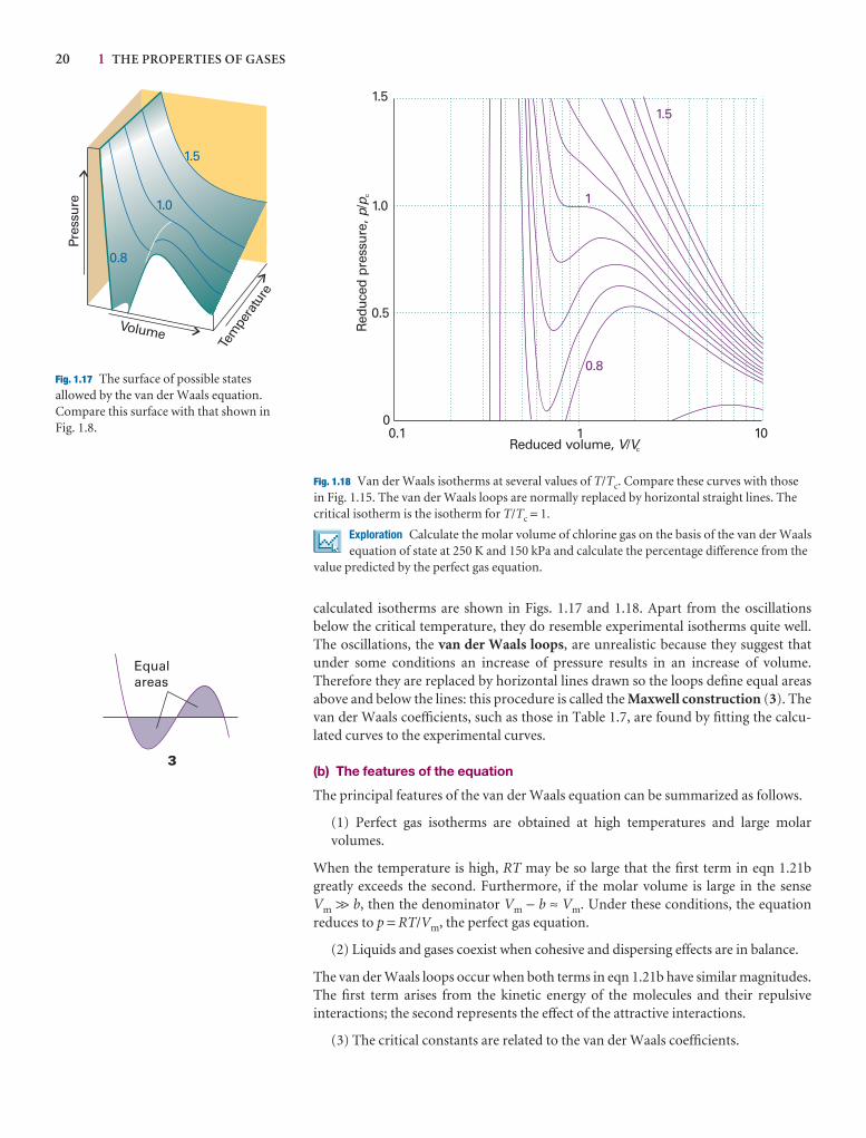
20 1 THE PROPERTIES OF GASES
calculated isotherms are shown in Figs. 1.17 and 1.18. Apart from the oscillationsbelow the critical temperature, they do resemble experimental isotherms quite well.The oscillations, the van der Waals loops, are unrealistic because they suggest thatunder some conditions an increase of pressure results in an increase of volume.Therefore they are replaced by horizontal lines drawn so the loops define equal areasabove and below the lines: this procedure is called the Maxwell construction (3). Thevan der Waals coefficients, such as those in Table 1.7, are found by fitting the calcu-lated curves to the experimental curves.
(b) The features of the equation
The principal features of the van der Waals equation can be summarized as follows.
(1) Perfect gas isotherms are obtained at high temperatures and large molar volumes.
When the temperature is high, RT may be so large that the first term in eqn 1.21bgreatly exceeds the second. Furthermore, if the molar volume is large in the sense Vm >> b, then the denominator Vm − b ≈ Vm. Under these conditions, the equation reduces to p = RT/Vm, the perfect gas equation.
(2) Liquids and gases coexist when cohesive and dispersing effects are in balance.
The van der Waals loops occur when both terms in eqn 1.21b have similar magnitudes.The first term arises from the kinetic energy of the molecules and their repulsive interactions; the second represents the effect of the attractive interactions.
(3) The critical constants are related to the van der Waals coefficients.
Pres
sure
Tem
pera
ture
1.0
1.5
0.8
Volume
1.5
1.0
0.5
00.1 1 10
1.5
1
0.8R
educ
ed p
ress
ure,
/pp c
Reduced volume, /V Vc
Fig. 1.17 The surface of possible statesallowed by the van der Waals equation.Compare this surface with that shown inFig. 1.8.
Fig. 1.18 Van der Waals isotherms at several values of T/Tc. Compare these curves with thosein Fig. 1.15. The van der Waals loops are normally replaced by horizontal straight lines. Thecritical isotherm is the isotherm for T/Tc = 1.
Exploration Calculate the molar volume of chlorine gas on the basis of the van der Waalsequation of state at 250 K and 150 kPa and calculate the percentage difference from the
value predicted by the perfect gas equation.
Equalareas
3
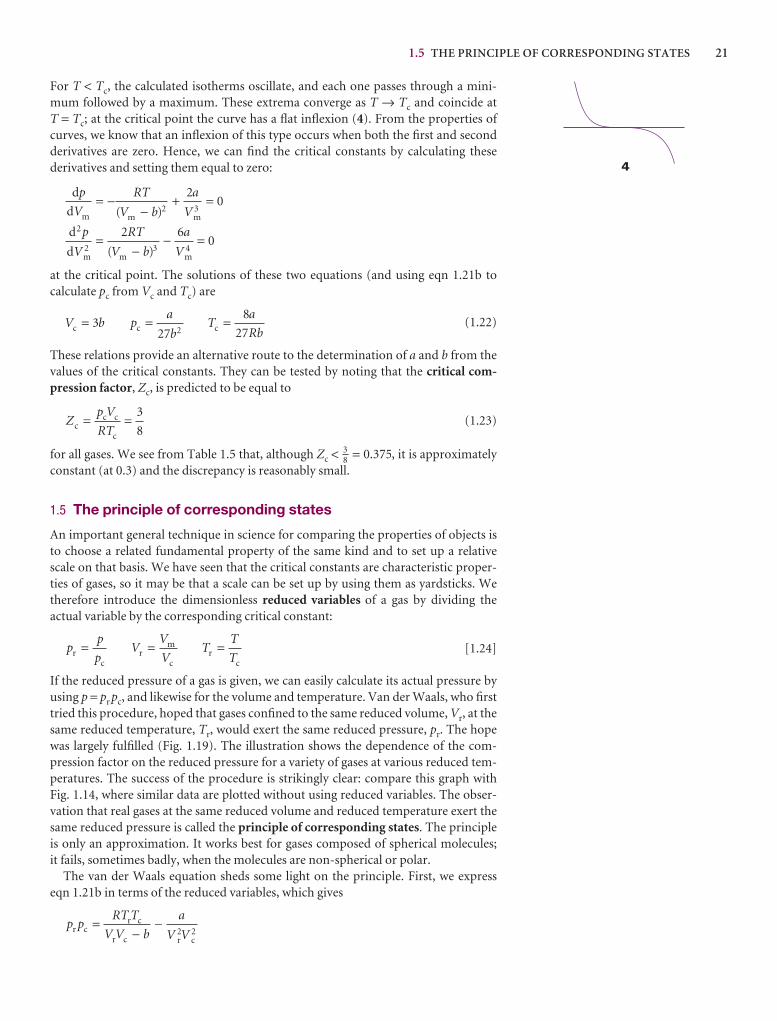
1.5 THE PRINCIPLE OF CORRESPONDING STATES 21
For T < Tc, the calculated isotherms oscillate, and each one passes through a mini-mum followed by a maximum. These extrema converge as T → Tc and coincide at T = Tc; at the critical point the curve has a flat inflexion (4). From the properties ofcurves, we know that an inflexion of this type occurs when both the first and secondderivatives are zero. Hence, we can find the critical constants by calculating thesederivatives and setting them equal to zero:
at the critical point. The solutions of these two equations (and using eqn 1.21b to calculate pc from Vc and Tc) are
(1.22)
These relations provide an alternative route to the determination of a and b from thevalues of the critical constants. They can be tested by noting that the critical com-pression factor, Zc, is predicted to be equal to
(1.23)
for all gases. We see from Table 1.5 that, although Zc < , it is approximatelyconstant (at 0.3) and the discrepancy is reasonably small.
1.5 The principle of corresponding states
An important general technique in science for comparing the properties of objects isto choose a related fundamental property of the same kind and to set up a relativescale on that basis. We have seen that the critical constants are characteristic proper-ties of gases, so it may be that a scale can be set up by using them as yardsticks. Wetherefore introduce the dimensionless reduced variables of a gas by dividing the actual variable by the corresponding critical constant:
[1.24]
If the reduced pressure of a gas is given, we can easily calculate its actual pressure byusing p = pr pc, and likewise for the volume and temperature. Van der Waals, who firsttried this procedure, hoped that gases confined to the same reduced volume, Vr, at thesame reduced temperature, Tr, would exert the same reduced pressure, pr. The hopewas largely fulfilled (Fig. 1.19). The illustration shows the dependence of the com-pression factor on the reduced pressure for a variety of gases at various reduced tem-peratures. The success of the procedure is strikingly clear: compare this graph withFig. 1.14, where similar data are plotted without using reduced variables. The obser-vation that real gases at the same reduced volume and reduced temperature exert thesame reduced pressure is called the principle of corresponding states. The principleis only an approximation. It works best for gases composed of spherical molecules; it fails, sometimes badly, when the molecules are non-spherical or polar.
The van der Waals equation sheds some light on the principle. First, we express eqn 1.21b in terms of the reduced variables, which gives
p pRT T
V V b
a
V Vr cr c
r c r c
=−
−2 2
pp
pV
V
VT
T
Trc
rm
cr
c
= = =
38 0 375 .=
Zp V
RTcc c
c
= =3
8
V b pa
bT
a
Rbc c c = = =327
8
272
d
d
2
m m m
p
V
RT
V b
a
V2 3 4
2 60
( ) =
−− =
d
d m m m
p
V
RT
V b
a
V( ) = −
−+ =
2 3
20
4
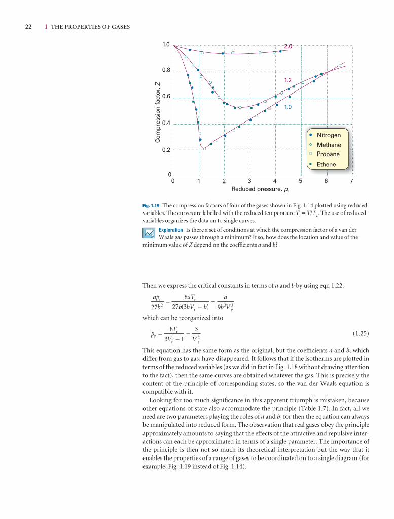
22 1 THE PROPERTIES OF GASES
2.0
1.2
1.0
1.0
0.8
0.6
0.4
0.2
01 3 5 7
Reduced pressure, pr
Com
pres
sion
fact
or, Z
0 2 4 6
Nitrogen
MethanePropane
Ethene
Fig. 1.19 The compression factors of four of the gases shown in Fig. 1.14 plotted using reducedvariables. The curves are labelled with the reduced temperature Tr = T/Tc. The use of reducedvariables organizes the data on to single curves.
Exploration Is there a set of conditions at which the compression factor of a van derWaals gas passes through a minimum? If so, how does the location and value of the
minimum value of Z depend on the coefficients a and b?
Then we express the critical constants in terms of a and b by using eqn 1.22:
which can be reorganized into
(1.25)
This equation has the same form as the original, but the coefficients a and b, whichdiffer from gas to gas, have disappeared. It follows that if the isotherms are plotted interms of the reduced variables (as we did in fact in Fig. 1.18 without drawing attentionto the fact), then the same curves are obtained whatever the gas. This is precisely thecontent of the principle of corresponding states, so the van der Waals equation iscompatible with it.
Looking for too much significance in this apparent triumph is mistaken, becauseother equations of state also accommodate the principle (Table 1.7). In fact, all weneed are two parameters playing the roles of a and b, for then the equation can alwaysbe manipulated into reduced form. The observation that real gases obey the principleapproximately amounts to saying that the effects of the attractive and repulsive inter-actions can each be approximated in terms of a single parameter. The importance ofthe principle is then not so much its theoretical interpretation but the way that it enables the properties of a range of gases to be coordinated on to a single diagram (forexample, Fig. 1.19 instead of Fig. 1.14).
pT
V Vrr
r r2
=−
−8
3 1
3
ap
b
aT
b bV b
a
b Vr r
r r22727
8
3 92 2( )=
−−

DISCUSSION QUESTIONS 23
Further reading
Articles and texts
J.L. Pauley and E.H. Davis, P-V-T isotherms of real gases:Experimental versus calculated values. J. Chem. Educ. 63, 466(1986).
M. Ross, Equations of state. In Encyclopedia of applied physics(ed. G.L. Trigg), 6, 291. VCH, New York (1993).
A. J. Walton, Three phases of matter. Oxford University Press (1983).
R.P. Wayne, Chemistry of atmospheres, an introduction to thechemistry of atmospheres of earth, the planets, and their satellites.Oxford University Press (2000).
Sources of data and information
J.H. Dymond and E.B. Smith, The virial coefficients of pure gases andmixtures. Oxford University Press (1980).
A.D. McNaught and A. Wilkinson, Compendium of chemicalterminology. Blackwell Scientific, Oxford (1997).
Discussion questions
1.1 Explain how the perfect gas equation of state arises by combination ofBoyle’s law, Charles’s law, and Avogadro’s principle.
1.2 Explain the term ‘partial pressure’ and explain why Dalton’s law is alimiting law.
1.3 Explain how the compression factor varies with pressure and temperatureand describe how it reveals information about intermolecular interactions inreal gases.
1.4 What is the significance of the critical constants?
1.5 Describe the formulation of the van der Waals equation and suggest arationale for one other equation of state in Table 1.7.
1.6 Explain how the van der Waals equation accounts for critical behaviour.
Checklist of key ideas
1. A gas is a form of matter that fills any container it occupies.
2. An equation of state interrelates pressure, volume,temperature, and amount of substance: p = f(T,V,n).
3. The pressure is the force divided by the area to which the forceis applied. The standard pressure is p7 = 1 bar (105 Pa).
4. Mechanical equilibrium is the condition of equality ofpressure on either side of a movable wall.
5. Temperature is the property that indicates the direction of theflow of energy through a thermally conducting, rigid wall.
6. A diathermic boundary is a boundary that permits the passageof energy as heat. An adiabatic boundary is a boundary thatprevents the passage of energy as heat.
7. Thermal equilibrium is a condition in which no change ofstate occurs when two objects A and B are in contact througha diathermic boundary.
8. The Zeroth Law of thermodynamics states that, if A is inthermal equilibrium with B, and B is in thermal equilibriumwith C, then C is also in thermal equilibrium with A.
9. The Celsius and thermodynamic temperature scales arerelated by T/K = θ/°C + 273.15.
10. A perfect gas obeys the perfect gas equation, pV = nRT, exactlyunder all conditions.
11. Dalton’s law states that the pressure exerted by a mixture ofgases is the sum of the partial pressures of the gases.
12. The partial pressure of any gas is defined as pJ = xJ p, where xJ = nJ/n is its mole fraction in a mixture and p is the totalpressure.
13. In real gases, molecular interactions affect the equation ofstate; the true equation of state is expressed in terms of virialcoefficients B, C, . . . : pVm = RT(1 + B/Vm + C/V 2
m + · · · ).
14. The vapour pressure is the pressure of a vapour in equilibriumwith its condensed phase.
15. The critical point is the point at which the volumes at eachend of the horizontal part of the isotherm have merged to a single point. The critical constants pc, Vc, and Tc are thepressure, molar volume, and temperature, respectively, at thecritical point.
16. A supercritical fluid is a dense fluid phase above its criticaltemperature and pressure.
17. The van der Waals equation of state is an approximation tothe true equation of state in which attractions are representedby a parameter a and repulsions are represented by aparameter b: p = nRT/(V − nb) − a(n/V)2.
18. A reduced variable is the actual variable divided by thecorresponding critical constant.
19. According to the principle of corresponding states, real gasesat the same reduced volume and reduced temperature exertthe same reduced pressure.

24 1 THE PROPERTIES OF GASES
Exercises
1.1(a) (a) Could 131 g of xenon gas in a vessel of volume 1.0 dm3 exert apressure of 20 atm at 25°C if it behaved as a perfect gas? If not, what pressurewould it exert? (b) What pressure would it exert if it behaved as a van derWaals gas?
1.1(b) (a) Could 25 g of argon gas in a vessel of volume 1.5 dm3 exert apressure of 2.0 bar at 30°C if it behaved as a perfect gas? If not, what pressurewould it exert? (b) What pressure would it exert if it behaved as a van derWaals gas?
1.2(a) A perfect gas undergoes isothermal compression, which reduces itsvolume by 2.20 dm3. The final pressure and volume of the gas are 5.04 bar and 4.65 dm3, respectively. Calculate the original pressure of the gas in (a) bar, (b) atm.
1.2(b) A perfect gas undergoes isothermal compression, which reduces itsvolume by 1.80 dm3. The final pressure and volume of the gas are 1.97 bar and2.14 dm3, respectively. Calculate the original pressure of the gas in (a) bar, (b) Torr.
1.3(a) A car tyre (i.e. an automobile tire) was inflated to a pressure of 24 lb in−2
(1.00 atm = 14.7 lb in−2) on a winter’s day when the temperature was –5°C.What pressure will be found, assuming no leaks have occurred and that thevolume is constant, on a subsequent summer’s day when the temperature is35°C? What complications should be taken into account in practice?
1.3(b) A sample of hydrogen gas was found to have a pressure of 125 kPawhen the temperature was 23°C. What can its pressure be expected to be whenthe temperature is 11°C?
1.4(a) A sample of 255 mg of neon occupies 3.00 dm3 at 122 K. Use the perfectgas law to calculate the pressure of the gas.
1.4(b) A homeowner uses 4.00 × 10³ m3 of natural gas in a year to heat ahome. Assume that natural gas is all methane, CH4, and that methane is aperfect gas for the conditions of this problem, which are 1.00 atm and 20°C.What is the mass of gas used?
1.5(a) A diving bell has an air space of 3.0 m3 when on the deck of a boat.What is the volume of the air space when the bell has been lowered to a depthof 50 m? Take the mean density of sea water to be 1.025 g cm−3 and assumethat the temperature is the same as on the surface.
1.5(b) What pressure difference must be generated across the length of a 15 cm vertical drinking straw in order to drink a water-like liquid of density1.0 g cm−3?
1.6(a) A manometer consists of a U-shaped tube containing a liquid. One sideis connected to the apparatus and the other is open to the atmosphere. Thepressure inside the apparatus is then determined from the difference inheights of the liquid. Suppose the liquid is water, the external pressure is 770 Torr, and the open side is 10.0 cm lower than the side connected to theapparatus. What is the pressure in the apparatus? (The density of water at25°C is 0.997 07 g cm−3.)
1.6(b) A manometer like that described in Exercise 1.6a contained mercury inplace of water. Suppose the external pressure is 760 Torr, and the open side is10.0 cm higher than the side connected to the apparatus. What is the pressurein the apparatus? (The density of mercury at 25°C is 13.55 g cm−3.)
1.7(a) In an attempt to determine an accurate value of the gas constant, R, astudent heated a container of volume 20.000 dm3 filled with 0.251 32 g ofhelium gas to 500°C and measured the pressure as 206.402 cm of water in amanometer at 25°C. Calculate the value of R from these data. (The density ofwater at 25°C is 0.997 07 g cm−3; the construction of a manometer is describedin Exercise 1.6a.)
1.7(b) The following data have been obtained for oxygen gas at 273.15 K.Calculate the best value of the gas constant R from them and the best value ofthe molar mass of O2.
p/atm 0.750 000 0.500 000 0.250 000
Vm/(dm3 mol−1) 29.9649 44.8090 89.6384
ρ/(g dm−3) 1.07144 0.714110 0.356975
1.8(a) At 500°C and 93.2 kPa, the mass density of sulfur vapour is 3.710 kg m−3. What is the molecular formula of sulfur under these conditions?
1.8(b) At 100°C and 1.60 kPa, the mass density of phosphorus vapour is0.6388 kg m−3. What is the molecular formula of phosphorus under theseconditions?
1.9(a) Calculate the mass of water vapour present in a room of volume 400 m3
that contains air at 27°C on a day when the relative humidity is 60 per cent.
1.9(b) Calculate the mass of water vapour present in a room of volume 250 m3
that contains air at 23°C on a day when the relative humidity is 53 per cent.
1.10(a) Given that the density of air at 0.987 bar and 27°C is 1.146 kg m−3,calculate the mole fraction and partial pressure of nitrogen and oxygenassuming that (a) air consists only of these two gases, (b) air also contains 1.0 mole per cent Ar.
1.10(b) A gas mixture consists of 320 mg of methane, 175 mg of argon, and225 mg of neon. The partial pressure of neon at 300 K is 8.87 kPa. Calculate(a) the volume and (b) the total pressure of the mixture.
1.11(a) The density of a gaseous compound was found to be 1.23 kg m−3 at330 K and 20 kPa. What is the molar mass of the compound?
1.11(b) In an experiment to measure the molar mass of a gas, 250 cm3 of thegas was confined in a glass vessel. The pressure was 152 Torr at 298 K and,after correcting for buoyancy effects, the mass of the gas was 33.5 mg. What isthe molar mass of the gas?
1.12(a) The densities of air at −85°C, 0°C, and 100°C are 1.877 g dm−3,1.294 g dm−3, and 0.946 g dm−3, respectively. From these data, and assumingthat air obeys Charles’s law, determine a value for the absolute zero oftemperature in degrees Celsius.
1.12(b) A certain sample of a gas has a volume of 20.00 dm3 at 0°C and 1.000 atm. A plot of the experimental data of its volume against the Celsiustemperature, θ, at constant p, gives a straight line of slope 0.0741 dm3 (°C)−1.From these data alone (without making use of the perfect gas law), determinethe absolute zero of temperature in degrees Celsius.
1.13(a) Calculate the pressure exerted by 1.0 mol C2H6 behaving as (a) aperfect gas, (b) a van der Waals gas when it is confined under the followingconditions: (i) at 273.15 K in 22.414 dm3, (ii) at 1000 K in 100 cm3. Use thedata in Table 1.6.
1.13(b) Calculate the pressure exerted by 1.0 mol H2S behaving as (a) a perfect gas, (b) a van der Waals gas when it is confined under the followingconditions: (i) at 273.15 K in 22.414 dm3, (ii) at 500 K in 150 cm3. Use the datain Table 1.6.
1.14(a) Express the van der Waals parameters a = 0.751 atm dm6 mol−2 andb = 0.0226 dm3 mol−1 in SI base units.
1.14(b) Express the van der Waals parameters a = 1.32 atm dm6 mol−2 andb = 0.0436 dm3 mol−1 in SI base units.
1.15(a) A gas at 250 K and 15 atm has a molar volume 12 per cent smallerthan that calculated from the perfect gas law. Calculate (a) the compressionfactor under these conditions and (b) the molar volume of the gas. Which aredominating in the sample, the attractive or the repulsive forces?

PROBLEMS 25
1.15(b) A gas at 350 K and 12 atm has a molar volume 12 per cent larger thanthat calculated from the perfect gas law. Calculate (a) the compression factorunder these conditions and (b) the molar volume of the gas. Which aredominating in the sample, the attractive or the repulsive forces?
1.16(a) In an industrial process, nitrogen is heated to 500 K at a constantvolume of 1.000 m3. The gas enters the container at 300 K and 100 atm. The mass of the gas is 92.4 kg. Use the van der Waals equation to determinethe approximate pressure of the gas at its working temperature of 500 K. For nitrogen, a = 1.352 dm6 atm mol−2, b = 0.0387 dm3 mol−1.
1.16(b) Cylinders of compressed gas are typically filled to a pressure of 200 bar. For oxygen, what would be the molar volume at this pressure and25°C based on (a) the perfect gas equation, (b) the van der Waals equation.For oxygen, a = 1.364 dm6 atm mol−2, b = 3.19 × 10⁻² dm3 mol−1.
1.17(a) Suppose that 10.0 mol C2H6(g) is confined to 4.860 dm3 at 27°C.Predict the pressure exerted by the ethane from (a) the perfect gas and (b) the van der Waals equations of state. Calculate the compression factorbased on these calculations. For ethane, a = 5.507 dm6 atm mol−2,b = 0.0651 dm3 mol−1.
1.17(b) At 300 K and 20 atm, the compression factor of a gas is 0.86. Calculate(a) the volume occupied by 8.2 mmol of the gas under these conditions and(b) an approximate value of the second virial coefficient B at 300 K.
1.18(a) A vessel of volume 22.4 dm3 contains 2.0 mol H2 and 1.0 mol N2 at273.15 K. Calculate (a) the mole fractions of each component, (b) their partialpressures, and (c) their total pressure.
1.18(b) A vessel of volume 22.4 dm3 contains 1.5 mol H2 and 2.5 mol N2 at273.15 K. Calculate (a) the mole fractions of each component, (b) their partialpressures, and (c) their total pressure.
1.19(a) The critical constants of methane are pc = 45.6 atm, Vc = 98.7 cm3 mol−1, and Tc = 190.6 K. Calculate the van der Waals parametersof the gas and estimate the radius of the molecules.
1.19(b) The critical constants of ethane are pc = 48.20 atm, Vc = 148 cm3 mol−1,and Tc = 305.4 K. Calculate the van der Waals parameters of the gas andestimate the radius of the molecules.
1.20(a) Use the van der Waals parameters for chlorine to calculateapproximate values of (a) the Boyle temperature of chlorine and (b) the radiusof a Cl2 molecule regarded as a sphere.
1.20(b) Use the van der Waals parameters for hydrogen sulfide to calculateapproximate values of (a) the Boyle temperature of the gas and (b) the radius of a H2S molecule regarded as a sphere (a = 4.484 dm6 atm mol−2,b = 0.0434 dm3 mol−1).
1.21(a) Suggest the pressure and temperature at which 1.0 mol of (a) NH3,(b) Xe, (c) He will be in states that correspond to 1.0 mol H2 at 1.0 atm and 25°C.
1.21(b) Suggest the pressure and temperature at which 1.0 mol of (a) H2S,(b) CO2, (c) Ar will be in states that correspond to 1.0 mol N2 at 1.0 atm and25°C.
1.22(a) A certain gas obeys the van der Waals equation with a = 0.50 m6 Pa mol−2.Its volume is found to be 5.00 × 10⁻⁴ m3 mol−1 at 273 K and 3.0 MPa. Fromthis information calculate the van der Waals constant b. What is thecompression factor for this gas at the prevailing temperature and pressure?
1.22(b) A certain gas obeys the van der Waals equation with a = 0.76 m6 Pa mol−2.Its volume is found to be 4.00 × 10⁻⁴ m3 mol−1 at 288 K and 4.0 MPa. Fromthis information calculate the van der Waals constant b. What is thecompression factor for this gas at the prevailing temperature and pressure?
Problems*
Numerical problems
1.1 Recent communication with the inhabitants of Neptune have revealedthat they have a Celsius-type temperature scale, but based on the meltingpoint (0°N) and boiling point (100°N) of their most common substance,hydrogen. Further communications have revealed that the Neptunians knowabout perfect gas behaviour and they find that, in the limit of zero pressure,the value of pV is 28 dm3 atm at 0°N and 40 dm3 atm at 100°N. What is thevalue of the absolute zero of temperature on their temperature scale?
1.2 Deduce the relation between the pressure and mass density, ρ, of a perfectgas of molar mass M. Confirm graphically, using the following data ondimethyl ether at 25°C, that perfect behaviour is reached at low pressures andfind the molar mass of the gas.
p/kPa 12.223 25.20 36.97 60.37 85.23 101.3
ρ/(kg m−3) 0.225 0.456 0.664 1.062 1.468 1.734
1.3 Charles’s law is sometimes expressed in the form V = V0(1 + αθ), where θis the Celsius temperature, α is a constant, and V0 is the volume of the sampleat 0°C. The following values for α have been reported for nitrogen at 0°C:
p/Torr 749.7 599.6 333.1 98.6
103α /(°C)−1 3.6717 3.6697 3.6665 3.6643
For these data calculate the best value for the absolute zero of temperature onthe Celsius scale.
1.4 The molar mass of a newly synthesized fluorocarbon was measured in agas microbalance. This device consists of a glass bulb forming one end of abeam, the whole surrounded by a closed container. The beam is pivoted, andthe balance point is attained by raising the pressure of gas in the container, soincreasing the buoyancy of the enclosed bulb. In one experiment, the balancepoint was reached when the fluorocarbon pressure was 327.10 Torr; for thesame setting of the pivot, a balance was reached when CHF3 (M = 70.014 g mol−1)was introduced at 423.22 Torr. A repeat of the experiment with a differentsetting of the pivot required a pressure of 293.22 Torr of the fluorocarbon and427.22 Torr of the CHF3. What is the molar mass of the fluorocarbon? Suggesta molecular formula.
1.5 A constant-volume perfect gas thermometer indicates a pressure of 6.69kPa at the triple point temperature of water (273.16 K). (a) What change ofpressure indicates a change of 1.00 K at this temperature? (b) What pressureindicates a temperature of 100.00°C? (c) What change of pressure indicates achange of 1.00 K at the latter temperature?
1.6 A vessel of volume 22.4 dm3 contains 2.0 mol H2 and 1.0 mol N2 at273.15 K initially. All the H2 reacted with sufficient N2 to form NH3. Calculatethe partial pressures and the total pressure of the final mixture.
1.7 Calculate the molar volume of chlorine gas at 350 K and 2.30 atm using(a) the perfect gas law and (b) the van der Waals equation. Use the answer to(a) to calculate a first approximation to the correction term for attraction andthen use successive approximations to obtain a numerical answer for part (b).
* Problems denoted with the symbol ‡ were supplied by Charles Trapp, Carmen Giunta, and Marshall Cady.
26 1 THE PROPERTIES OF GASES
1.8 At 273 K measurements on argon gave B = −21.7 cm3 mol−1 andC = 1200 cm6 mol−2, where B and C are the second and third virial coefficientsin the expansion of Z in powers of 1/Vm. Assuming that the perfect gas law holds sufficiently well for the estimation of the second and third terms of the expansion, calculate the compression factor of argon at 100 atm and 273 K. From your result, estimate the molar volume of argon under theseconditions.
1.9 Calculate the volume occupied by 1.00 mol N2 using the van der Waalsequation in the form of a virial expansion at (a) its critical temperature, (b) its Boyle temperature, and (c) its inversion temperature. Assume that the pressure is 10 atm throughout. At what temperature is the gas mostperfect? Use the following data: Tc = 126.3 K, a = 1.352 dm6 atm mol−2,b = 0.0387 dm3 mol−1.
1.10‡ The second virial coefficient of methane can be approximated by the empirical equation B′(T) = a + be−c/T2
, where a = −0.1993 bar−1,b = 0.2002 bar−1, and c = 1131 K2 with 300 K < T < 600 K. What is the Boyle temperature of methane?
1.11 The mass density of water vapour at 327.6 atm and 776.4 K is 133.2 kg m−3.Given that for water Tc = 647.4 K, pc = 218.3 atm, a = 5.464 dm6 atm mol−2,b = 0.03049 dm3 mol−1, and M = 18.02 g mol−1, calculate (a) the molarvolume. Then calculate the compression factor (b) from the data, (c) from the virial expansion of the van der Waals equation.
1.12 The critical volume and critical pressure of a certain gas are 160 cm3 mol−1 and 40 atm, respectively. Estimate the critical temperature byassuming that the gas obeys the Berthelot equation of state. Estimate the radiiof the gas molecules on the assumption that they are spheres.
1.13 Estimate the coefficients a and b in the Dieterici equation of state fromthe critical constants of xenon. Calculate the pressure exerted by 1.0 mol Xewhen it is confined to 1.0 dm3 at 25°C.
Theoretical problems
1.14 Show that the van der Waals equation leads to values of Z < 1 and Z > 1,and identify the conditions for which these values are obtained.
1.15 Express the van der Waals equation of state as a virial expansion inpowers of 1/Vm and obtain expressions for B and C in terms of the parametersa and b. The expansion you will need is (1 − x)−1 = 1 + x + x2 + · · · .Measurements on argon gave B = −21.7 cm3 mol−1 and C = 1200 cm6 mol−2
for the virial coefficients at 273 K. What are the values of a and b in thecorresponding van der Waals equation of state?
1.16‡ Derive the relation between the critical constants and the Dietericiequation parameters. Show that Zc = 2e−2 and derive the reduced form of theDieterici equation of state. Compare the van der Waals and Dietericipredictions of the critical compression factor. Which is closer to typicalexperimental values?
1.17 A scientist proposed the following equation of state:
p = − +
Show that the equation leads to critical behaviour. Find the critical constantsof the gas in terms of B and C and an expression for the critical compressionfactor.
1.18 Equations 1.18 and 1.19 are expansions in p and 1/Vm, respectively. Findthe relation between B, C and B′, C ′.
1.19 The second virial coefficient B′ can be obtained from measurements ofthe density ρ of a gas at a series of pressures. Show that the graph of p/ρagainst p should be a straight line with slope proportional to B′. Use the dataon dimethyl ether in Problem 1.2 to find the values of B′ and B at 25°C.
C
V 3m
B
V 2m
RT
Vm
1.20 The equation of state of a certain gas is given by p = RT/Vm +(a + bT)/V 2
m, where a and b are constants. Find (∂V/∂T)p.
1.21 The following equations of state are occasionally used for approximatecalculations on gases: (gas A) pVm = RT(1 + b/Vm), (gas B) p(Vm – b) = RT.Assuming that there were gases that actually obeyed these equations of state,would it be possible to liquefy either gas A or B? Would they have a criticaltemperature? Explain your answer.
1.22 Derive an expression for the compression factor of a gas that obeys theequation of state p(V – nb) = nRT, where b and R are constants. If the pressureand temperature are such that Vm = 10b, what is the numerical value of thecompression factor?
1.23‡ The discovery of the element argon by Lord Rayleigh and Sir WilliamRamsay had its origins in Rayleigh’s measurements of the density of nitrogenwith an eye toward accurate determination of its molar mass. Rayleighprepared some samples of nitrogen by chemical reaction of nitrogen-containing compounds; under his standard conditions, a glass globe filledwith this ‘chemical nitrogen’ had a mass of 2.2990 g. He prepared othersamples by removing oxygen, carbon dioxide, and water vapour fromatmospheric air; under the same conditions, this ‘atmospheric nitrogen’ had amass of 2.3102 g (Lord Rayleigh, Royal Institution Proceedings 14, 524 (1895)).With the hindsight of knowing accurate values for the molar masses ofnitrogen and argon, compute the mole fraction of argon in the latter sampleon the assumption that the former was pure nitrogen and the latter a mixtureof nitrogen and argon.
1.24‡ A substance as elementary and well known as argon still receivesresearch attention. Stewart and Jacobsen have published a review ofthermodynamic properties of argon (R.B. Stewart and R.T. Jacobsen, J. Phys.Chem. Ref. Data 18, 639 (1989)) that included the following 300 K isotherm.
p/MPa 0.4000 0.5000 0.6000 0.8000 1.000
Vm/(dm3 mol−1) 6.2208 4.9736 4.1423 3.1031 2.4795
p/MPa 1.500 2.000 2.500 3.000 4.000
Vm/(dm3 mol−1) 1.6483 1.2328 0.98357 0.81746 0.60998
(a) Compute the second virial coefficient, B, at this temperature. (b) Use non-linear curve-fitting software to compute the third virial coefficient, C,at this temperature.
Applications: to environmental science
1.25 Atmospheric pollution is a problem that has received much attention.Not all pollution, however, is from industrial sources. Volcanic eruptions canbe a significant source of air pollution. The Kilauea volcano in Hawaii emits200–300 t of SO2 per day. If this gas is emitted at 800°C and 1.0 atm, whatvolume of gas is emitted?
1.26 Ozone is a trace atmospheric gas that plays an important role inscreening the Earth from harmful ultraviolet radiation, and the abundance of ozone is commonly reported in Dobson units. One Dobson unit is thethickness, in thousandths of a centimetre, of a column of gas if it werecollected as a pure gas at 1.00 atm and 0°C. What amount of O3 (in moles) isfound in a column of atmosphere with a cross-sectional area of 1.00 dm2 if theabundance is 250 Dobson units (a typical mid-latitude value)? In the seasonalAntarctic ozone hole, the column abundance drops below 100 Dobson units;how many moles of ozone are found in such a column of air above a 1.00 dm2
area? Most atmospheric ozone is found between 10 and 50 km above thesurface of the earth. If that ozone is spread uniformly through this portion of the atmosphere, what is the average molar concentration corresponding to(a) 250 Dobson units, (b) 100 Dobson units?
1.27 The barometric formula relates the pressure of a gas of molar mass M atan altitude h to its pressure p0 at sea level. Derive this relation by showing that

PROBLEMS 27
the change in pressure dp for an infinitesimal change in altitude dh wherethe density is ρ is dp = −ρgdh. Remember that ρ depends on the pressure.Evaluate (a) the pressure difference between the top and bottom of alaboratory vessel of height 15 cm, and (b) the external atmospheric pressure at a typical cruising altitude of an aircraft (11 km) when the pressure atground level is 1.0 atm.
1.28 Balloons are still used to deploy sensors that monitor meteorologicalphenomena and the chemistry of the atmosphere. It is possible to investigatesome of the technicalities of ballooning by using the perfect gas law. Supposeyour balloon has a radius of 3.0 m and that it is spherical. (a) What amount ofH2 (in moles) is needed to inflate it to 1.0 atm in an ambient temperature of25°C at sea level? (b) What mass can the balloon lift at sea level, where thedensity of air is 1.22 kg m−3? (c) What would be the payload if He were usedinstead of H2?
1.29‡ The preceding problem is most readily solved (see the Solutionsmanual) with the use of the Archimedes principle, which states that the liftingforce is equal to the difference between the weight of the displaced air and theweight of the balloon. Prove the Archimedes principle for the atmospherefrom the barometric formula. Hint. Assume a simple shape for the balloon,perhaps a right circular cylinder of cross–sectional area A and height h.
1.30 ‡ Chlorofluorocarbons such as CCl3F and CCl2F2 have been linked to ozone depletion in Antarctica. As of 1994, these gases were found inquantities of 261 and 509 parts per trillion (1012) by volume (World Resources Institute, World resources 1996–97). Compute the molarconcentration of these gases under conditions typical of (a) the mid-latitudetroposphere (10°C and 1.0 atm) and (b) the Antarctic stratosphere (200 K and 0.050 atm).
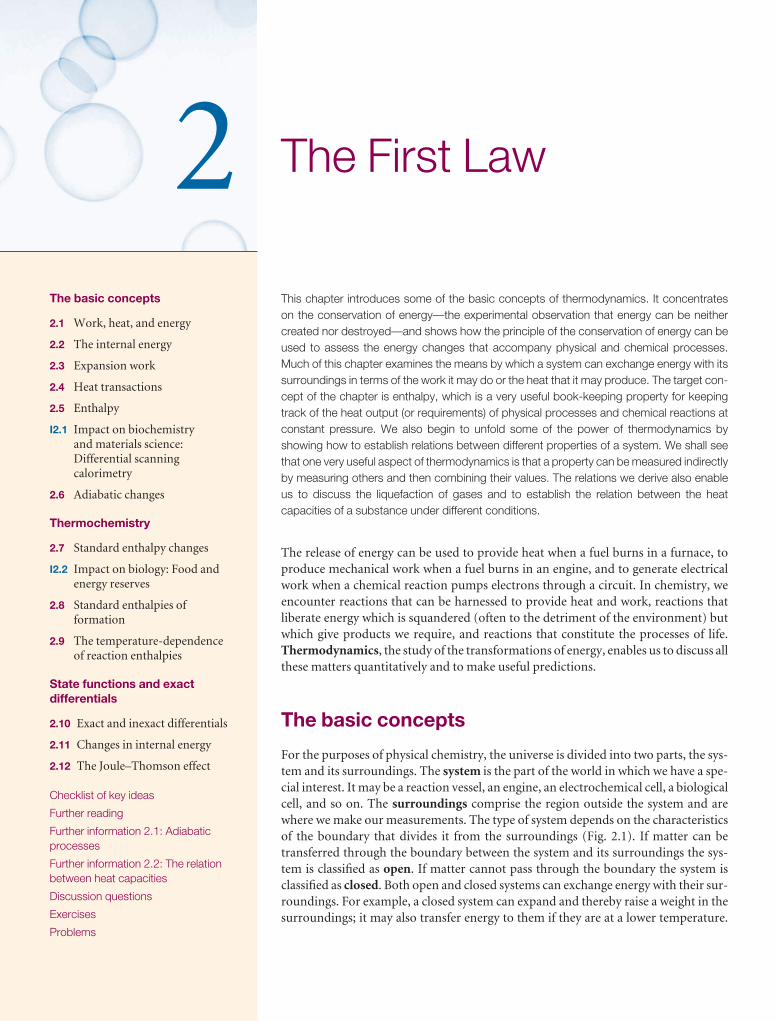
The First Law
This chapter introduces some of the basic concepts of thermodynamics. It concentrates on the conservation of energy—the experimental observation that energy can be neithercreated nor destroyed—and shows how the principle of the conservation of energy can beused to assess the energy changes that accompany physical and chemical processes.Much of this chapter examines the means by which a system can exchange energy with itssurroundings in terms of the work it may do or the heat that it may produce. The target con-cept of the chapter is enthalpy, which is a very useful book-keeping property for keepingtrack of the heat output (or requirements) of physical processes and chemical reactions atconstant pressure. We also begin to unfold some of the power of thermodynamics byshowing how to establish relations between different properties of a system. We shall seethat one very useful aspect of thermodynamics is that a property can be measured indirectlyby measuring others and then combining their values. The relations we derive also enableus to discuss the liquefaction of gases and to establish the relation between the heat capacities of a substance under different conditions.
The release of energy can be used to provide heat when a fuel burns in a furnace, toproduce mechanical work when a fuel burns in an engine, and to generate electricalwork when a chemical reaction pumps electrons through a circuit. In chemistry, weencounter reactions that can be harnessed to provide heat and work, reactions thatliberate energy which is squandered (often to the detriment of the environment) butwhich give products we require, and reactions that constitute the processes of life.Thermodynamics, the study of the transformations of energy, enables us to discuss allthese matters quantitatively and to make useful predictions.
The basic concepts
For the purposes of physical chemistry, the universe is divided into two parts, the sys-tem and its surroundings. The system is the part of the world in which we have a spe-cial interest. It may be a reaction vessel, an engine, an electrochemical cell, a biologicalcell, and so on. The surroundings comprise the region outside the system and arewhere we make our measurements. The type of system depends on the characteristicsof the boundary that divides it from the surroundings (Fig. 2.1). If matter can betransferred through the boundary between the system and its surroundings the sys-tem is classified as open. If matter cannot pass through the boundary the system isclassified as closed. Both open and closed systems can exchange energy with their sur-roundings. For example, a closed system can expand and thereby raise a weight in thesurroundings; it may also transfer energy to them if they are at a lower temperature.
The basic concepts
2.1 Work, heat, and energy
2.2 The internal energy
2.3 Expansion work
2.4 Heat transactions
2.5 Enthalpy
I2.1 Impact on biochemistry and materials science:Differential scanningcalorimetry
2.6 Adiabatic changes
Thermochemistry
2.7 Standard enthalpy changes
I2.2 Impact on biology: Food andenergy reserves
2.8 Standard enthalpies offormation
2.9 The temperature-dependenceof reaction enthalpies
State functions and exactdifferentials
2.10 Exact and inexact differentials
2.11 Changes in internal energy
2.12 The Joule–Thomson effect
Checklist of key ideas
Further reading
Further information 2.1: Adiabaticprocesses
Further information 2.2: The relationbetween heat capacities
Discussion questions
Exercises
Problems
2
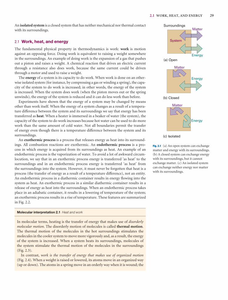
2.1 WORK, HEAT, AND ENERGY 29
Fig. 2.1 (a) An open system can exchangematter and energy with its surroundings.(b) A closed system can exchange energywith its surroundings, but it cannotexchange matter. (c) An isolated systemcan exchange neither energy nor matterwith its surroundings.
An isolated system is a closed system that has neither mechanical nor thermal contactwith its surroundings.
2.1 Work, heat, and energy
The fundamental physical property in thermodynamics is work: work is motionagainst an opposing force. Doing work is equivalent to raising a weight somewhere in the surroundings. An example of doing work is the expansion of a gas that pushesout a piston and raises a weight. A chemical reaction that drives an electric currentthrough a resistance also does work, because the same current could be driventhrough a motor and used to raise a weight.
The energy of a system is its capacity to do work. When work is done on an other-wise isolated system (for instance, by compressing a gas or winding a spring), the capa-city of the system to do work is increased; in other words, the energy of the system is increased. When the system does work (when the piston moves out or the springunwinds), the energy of the system is reduced and it can do less work than before.
Experiments have shown that the energy of a system may be changed by meansother than work itself. When the energy of a system changes as a result of a tempera-ture difference between the system and its surroundings we say that energy has beentransferred as heat. When a heater is immersed in a beaker of water (the system), thecapacity of the system to do work increases because hot water can be used to do morework than the same amount of cold water. Not all boundaries permit the transfer of energy even though there is a temperature difference between the system and itssurroundings.
An exothermic process is a process that releases energy as heat into its surround-ings. All combustion reactions are exothermic. An endothermic process is a pro-cess in which energy is acquired from its surroundings as heat. An example of an endothermic process is the vaporization of water. To avoid a lot of awkward circum-locution, we say that in an exothermic process energy is transferred ‘as heat’ to thesurroundings and in an endothermic process energy is transferred ‘as heat’ from the surroundings into the system. However, it must never be forgotten that heat is aprocess (the transfer of energy as a result of a temperature difference), not an entity.An endothermic process in a diathermic container results in energy flowing into thesystem as heat. An exothermic process in a similar diathermic container results in a release of energy as heat into the surroundings. When an endothermic process takesplace in an adiabatic container, it results in a lowering of temperature of the system;an exothermic process results in a rise of temperature. These features are summarizedin Fig. 2.2.
Molecular interpretation 2.1 Heat and work
In molecular terms, heating is the transfer of energy that makes use of disorderlymolecular motion. The disorderly motion of molecules is called thermal motion.The thermal motion of the molecules in the hot surroundings stimulates themolecules in the cooler system to move more vigorously and, as a result, the energyof the system is increased. When a system heats its surroundings, molecules of the system stimulate the thermal motion of the molecules in the surroundings (Fig. 2.3).
In contrast, work is the transfer of energy that makes use of organized motion (Fig. 2.4). When a weight is raised or lowered, its atoms move in an organized way(up or down). The atoms in a spring move in an orderly way when it is wound; the
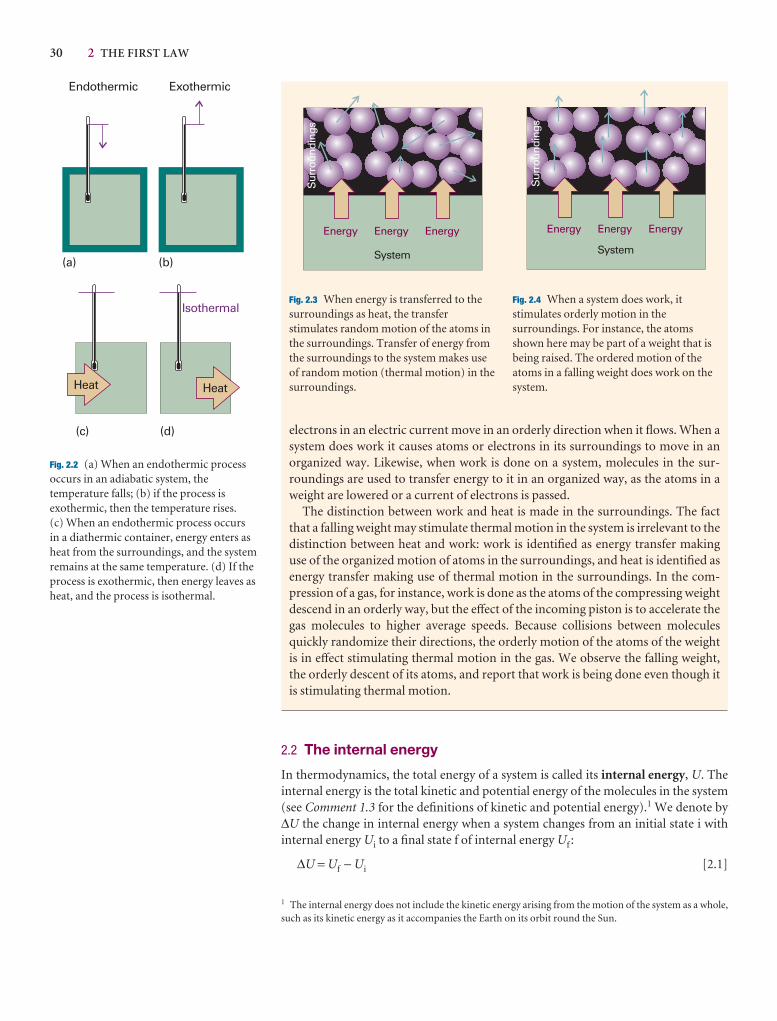
30 2 THE FIRST LAW
Fig. 2.2 (a) When an endothermic processoccurs in an adiabatic system, thetemperature falls; (b) if the process isexothermic, then the temperature rises. (c) When an endothermic process occursin a diathermic container, energy enters asheat from the surroundings, and the systemremains at the same temperature. (d) If theprocess is exothermic, then energy leaves asheat, and the process is isothermal.
1 The internal energy does not include the kinetic energy arising from the motion of the system as a whole,such as its kinetic energy as it accompanies the Earth on its orbit round the Sun.
Fig. 2.3 When energy is transferred to thesurroundings as heat, the transferstimulates random motion of the atoms inthe surroundings. Transfer of energy fromthe surroundings to the system makes useof random motion (thermal motion) in thesurroundings.
Fig. 2.4 When a system does work, itstimulates orderly motion in thesurroundings. For instance, the atomsshown here may be part of a weight that isbeing raised. The ordered motion of theatoms in a falling weight does work on thesystem.
electrons in an electric current move in an orderly direction when it flows. When a system does work it causes atoms or electrons in its surroundings to move in an organized way. Likewise, when work is done on a system, molecules in the sur-roundings are used to transfer energy to it in an organized way, as the atoms in aweight are lowered or a current of electrons is passed.
The distinction between work and heat is made in the surroundings. The factthat a falling weight may stimulate thermal motion in the system is irrelevant to thedistinction between heat and work: work is identified as energy transfer makinguse of the organized motion of atoms in the surroundings, and heat is identified asenergy transfer making use of thermal motion in the surroundings. In the com-pression of a gas, for instance, work is done as the atoms of the compressing weightdescend in an orderly way, but the effect of the incoming piston is to accelerate thegas molecules to higher average speeds. Because collisions between moleculesquickly randomize their directions, the orderly motion of the atoms of the weightis in effect stimulating thermal motion in the gas. We observe the falling weight,the orderly descent of its atoms, and report that work is being done even though itis stimulating thermal motion.
2.2 The internal energy
In thermodynamics, the total energy of a system is called its internal energy, U. Theinternal energy is the total kinetic and potential energy of the molecules in the system(see Comment 1.3 for the definitions of kinetic and potential energy).1 We denote by∆U the change in internal energy when a system changes from an initial state i withinternal energy Ui to a final state f of internal energy Uf :
∆U = Uf − Ui [2.1]
2.2 THE INTERNAL ENERGY 31
Comment 2.1
An extensive property is a property thatdepends on the amount of substance inthe sample. An intensive property is aproperty that is independent of theamount of substance in the sample. Twoexamples of extensive properties aremass and volume. Examples of intensiveproperties are temperature, massdensity (mass divided by volume), andpressure.
The internal energy is a state function in the sense that its value depends only on thecurrent state of the system and is independent of how that state has been prepared.In other words, it is a function of the properties that determine the current state of the system. Changing any one of the state variables, such as the pressure, results in a change in internal energy. The internal energy is an extensive property. That the internal energy is a state function has consequences of the greatest importance, as westart to unfold in Section 2.10.
Internal energy, heat, and work are all measured in the same units, the joule (J). Thejoule, which is named after the nineteenth-century scientist J.P. Joule, is defined as
1 J = 1 kg m2 s−2
A joule is quite a small unit of energy: for instance, each beat of the human heart con-sumes about 1 J. Changes in molar internal energy, ∆Um, are typically expressed inkilojoules per mole (kJ mol−1). Certain other energy units are also used, but are morecommon in fields other than thermodynamics. Thus, 1 electronvolt (1 eV) is definedas the kinetic energy acquired when an electron is accelerated from rest through a potential difference of 1 V; the relation between electronvolts and joules is 1 eV ≈0.16 aJ (where 1 aJ = 10−18 J). Many processes in chemistry have an energy of severalelectronvolts. Thus, the energy to remove an electron from a sodium atom is close to5 eV. Calories (cal) and kilocalories (kcal) are still encountered. The current definitionof the calorie in terms of joules is
1 cal = 4.184 J exactly
An energy of 1 cal is enough to raise the temperature of 1 g of water by 1°C.
Molecular interpretation 2.2 The internal energy of a gas
A molecule has a certain number of degrees of freedom, such as the ability to trans-late (the motion of its centre of mass through space), rotate around its centre of mass, or vibrate (as its bond lengths and angles change). Many physical andchemical properties depend on the energy associated with each of these modes ofmotion. For example, a chemical bond might break if a lot of energy becomes concentrated in it.
The equipartition theorem of classical mechanics is a useful guide to the averageenergy associated with each degree of freedom when the sample is at a temperatureT. First, we need to know that a ‘quadratic contribution’ to the energy means acontribution that can be expressed as the square of a variable, such as the positionor the velocity. For example, the kinetic energy an atom of mass m as it movesthrough space is
EK = 1–2mvx2 + 1–2mvy
2 + 1–2mvz2
and there are three quadratic contributions to its energy. The equipartition theorem then states that, for a collection of particles at thermal equilibrium at atemperature T, the average value of each quadratic contribution to the energy is thesame and equal to 1–2kT, where k is Boltzmann’s constant (k = 1.381 × 10⁻²³ J K−1).
The equipartition theorem is a conclusion from classical mechanics and is applicable only when the effects of quantization can be ignored (see Chapters 16and 17). In practice, it can be used for molecular translation and rotation but notvibration. At 25°C, 1–2kT = 2 zJ (where 1 zJ = 10−21 J), or about 13 meV.
According to the equipartition theorem, the average energy of each term in theexpression above is 1–2kT. Therefore, the mean energy of the atoms is 3–2kT and the
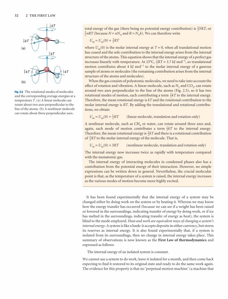
32 2 THE FIRST LAW
Fig. 2.5 The rotational modes of moleculesand the corresponding average energies at atemperature T. (a) A linear molecule canrotate about two axes perpendicular to theline of the atoms. (b) A nonlinear moleculecan rotate about three perpendicular axes.
total energy of the gas (there being no potential energy contribution) is 3–2NkT, or3–2 nRT (because N = nNA and R = NAk). We can therefore write
Um = Um(0) + 3–2RT
where Um(0) is the molar internal energy at T = 0, when all translational motionhas ceased and the sole contribution to the internal energy arises from the internalstructure of the atoms. This equation shows that the internal energy of a perfect gasincreases linearly with temperature. At 25°C, 3–2RT = 3.7 kJ mol−1, so translationalmotion contributes about 4 kJ mol−1 to the molar internal energy of a gaseous sample of atoms or molecules (the remaining contribution arises from the internalstructure of the atoms and molecules).
When the gas consists of polyatomic molecules, we need to take into account theeffect of rotation and vibration. A linear molecule, such as N2 and CO2, can rotatearound two axes perpendicular to the line of the atoms (Fig. 2.5), so it has two rotational modes of motion, each contributing a term 1–2kT to the internal energy.Therefore, the mean rotational energy is kT and the rotational contribution to themolar internal energy is RT. By adding the translational and rotational contribu-tions, we obtain
Um = Um(0) + 5–2RT (linear molecule, translation and rotation only)
A nonlinear molecule, such as CH4 or water, can rotate around three axes and,again, each mode of motion contributes a term 1–2kT to the internal energy.Therefore, the mean rotational energy is 3–2kT and there is a rotational contributionof 3–2RT to the molar internal energy of the molecule. That is,
Um = Um(0) + 3RT (nonlinear molecule, translation and rotation only)
The internal energy now increases twice as rapidly with temperature comparedwith the monatomic gas.
The internal energy of interacting molecules in condensed phases also has a contribution from the potential energy of their interaction. However, no simpleexpressions can be written down in general. Nevertheless, the crucial molecularpoint is that, as the temperature of a system is raised, the internal energy increasesas the various modes of motion become more highly excited.
It has been found experimentally that the internal energy of a system may bechanged either by doing work on the system or by heating it. Whereas we may knowhow the energy transfer has occurred (because we can see if a weight has been raisedor lowered in the surroundings, indicating transfer of energy by doing work, or if icehas melted in the surroundings, indicating transfer of energy as heat), the system isblind to the mode employed. Heat and work are equivalent ways of changing a system’sinternal energy. A system is like a bank: it accepts deposits in either currency, but storesits reserves as internal energy. It is also found experimentally that, if a system is isolated from its surroundings, then no change in internal energy takes place. Thissummary of observations is now known as the First Law of thermodynamics andexpressed as follows:
The internal energy of an isolated system is constant.
We cannot use a system to do work, leave it isolated for a month, and then come backexpecting to find it restored to its original state and ready to do the same work again.The evidence for this property is that no ‘perpetual motion machine’ (a machine that
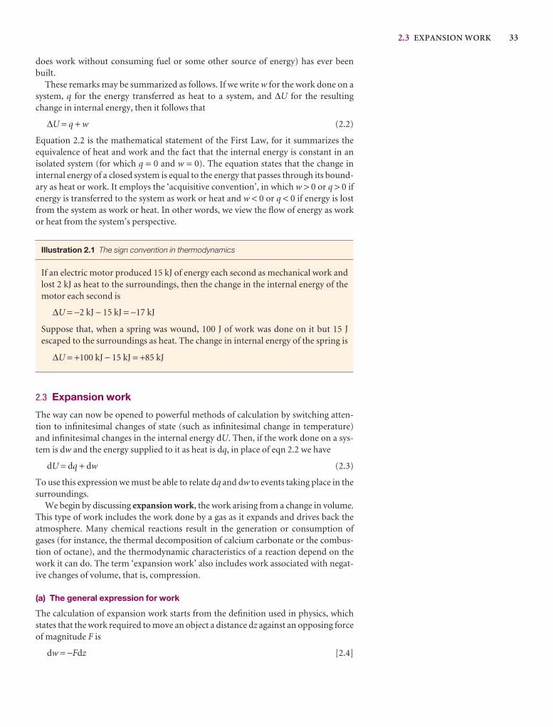
2.3 EXPANSION WORK 33
does work without consuming fuel or some other source of energy) has ever beenbuilt.
These remarks may be summarized as follows. If we write w for the work done on asystem, q for the energy transferred as heat to a system, and ∆U for the resultingchange in internal energy, then it follows that
∆U = q + w (2.2)
Equation 2.2 is the mathematical statement of the First Law, for it summarizes theequivalence of heat and work and the fact that the internal energy is constant in an isolated system (for which q = 0 and w = 0). The equation states that the change in internal energy of a closed system is equal to the energy that passes through its bound-ary as heat or work. It employs the ‘acquisitive convention’, in which w > 0 or q > 0 ifenergy is transferred to the system as work or heat and w < 0 or q < 0 if energy is lostfrom the system as work or heat. In other words, we view the flow of energy as workor heat from the system’s perspective.
Illustration 2.1 The sign convention in thermodynamics
If an electric motor produced 15 kJ of energy each second as mechanical work andlost 2 kJ as heat to the surroundings, then the change in the internal energy of themotor each second is
∆U = −2 kJ − 15 kJ = −17 kJ
Suppose that, when a spring was wound, 100 J of work was done on it but 15 J escaped to the surroundings as heat. The change in internal energy of the spring is
∆U = +100 kJ − 15 kJ = +85 kJ
2.3 Expansion work
The way can now be opened to powerful methods of calculation by switching atten-tion to infinitesimal changes of state (such as infinitesimal change in temperature)and infinitesimal changes in the internal energy dU. Then, if the work done on a sys-tem is dw and the energy supplied to it as heat is dq, in place of eqn 2.2 we have
dU = dq + dw (2.3)
To use this expression we must be able to relate dq and dw to events taking place in thesurroundings.
We begin by discussing expansion work, the work arising from a change in volume.This type of work includes the work done by a gas as it expands and drives back the atmosphere. Many chemical reactions result in the generation or consumption ofgases (for instance, the thermal decomposition of calcium carbonate or the combus-tion of octane), and the thermodynamic characteristics of a reaction depend on thework it can do. The term ‘expansion work’ also includes work associated with negat-ive changes of volume, that is, compression.
(a) The general expression for work
The calculation of expansion work starts from the definition used in physics, whichstates that the work required to move an object a distance dz against an opposing forceof magnitude F is
dw = −Fdz [2.4]
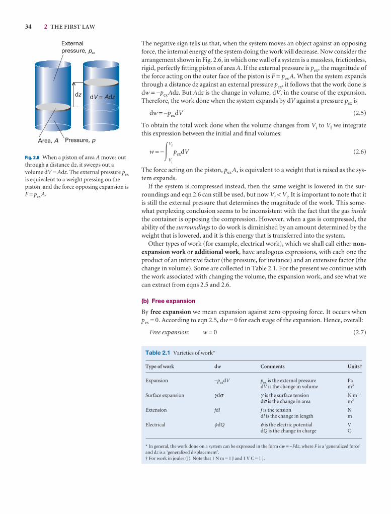
34 2 THE FIRST LAW
The negative sign tells us that, when the system moves an object against an opposingforce, the internal energy of the system doing the work will decrease. Now consider thearrangement shown in Fig. 2.6, in which one wall of a system is a massless, frictionless,rigid, perfectly fitting piston of area A. If the external pressure is pex, the magnitude ofthe force acting on the outer face of the piston is F = pex A. When the system expandsthrough a distance dz against an external pressure pex, it follows that the work done isdw = −pex Adz. But Adz is the change in volume, dV, in the course of the expansion.Therefore, the work done when the system expands by dV against a pressure pex is
dw = −pexdV (2.5)
To obtain the total work done when the volume changes from Vi to Vf we integratethis expression between the initial and final volumes:
w = −�Vf
Vi
pexdV (2.6)
The force acting on the piston, pex A, is equivalent to a weight that is raised as the sys-tem expands.
If the system is compressed instead, then the same weight is lowered in the sur-roundings and eqn 2.6 can still be used, but now Vf < Vi. It is important to note that itis still the external pressure that determines the magnitude of the work. This some-what perplexing conclusion seems to be inconsistent with the fact that the gas insidethe container is opposing the compression. However, when a gas is compressed, theability of the surroundings to do work is diminished by an amount determined by theweight that is lowered, and it is this energy that is transferred into the system.
Other types of work (for example, electrical work), which we shall call either non-expansion work or additional work, have analogous expressions, with each one theproduct of an intensive factor (the pressure, for instance) and an extensive factor (thechange in volume). Some are collected in Table 2.1. For the present we continue withthe work associated with changing the volume, the expansion work, and see what wecan extract from eqns 2.5 and 2.6.
(b) Free expansion
By free expansion we mean expansion against zero opposing force. It occurs when pex = 0. According to eqn 2.5, dw = 0 for each stage of the expansion. Hence, overall:
Free expansion: w = 0 (2.7)
Fig. 2.6 When a piston of area A moves outthrough a distance dz, it sweeps out avolume dV = Adz. The external pressure pex
is equivalent to a weight pressing on thepiston, and the force opposing expansion isF = pex A.
Table 2.1 Varieties of work*
Type of work dw Comments Units†
Expansion −pexdV pex is the external pressure Pa dV is the change in volume m3
Surface expansion γdσ γ is the surface tension N m−1
dσ is the change in area m2
Extension fdl f is the tension N dl is the change in length m
Electrical φdQ φ is the electric potential V dQ is the change in charge C
* In general, the work done on a system can be expressed in the form dw = −Fdz, where F is a ‘generalized force’and dz is a ‘generalized displacement’.† For work in joules (J). Note that 1 N m = 1 J and 1 V C = 1 J.
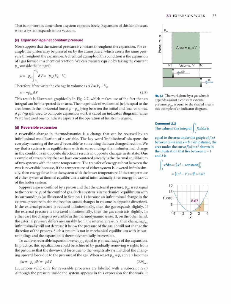
2.3 EXPANSION WORK 35
That is, no work is done when a system expands freely. Expansion of this kind occurswhen a system expands into a vacuum.
(c) Expansion against constant pressure
Now suppose that the external pressure is constant throughout the expansion. For ex-ample, the piston may be pressed on by the atmosphere, which exerts the same pres-sure throughout the expansion. A chemical example of this condition is the expansionof a gas formed in a chemical reaction. We can evaluate eqn 2.6 by taking the constantpex outside the integral:
w = −pex�Vf
Vi
dV = −pex(Vf − Vi)
Therefore, if we write the change in volume as ∆V = Vf − Vi,
w = −pex∆V (2.8)
This result is illustrated graphically in Fig. 2.7, which makes use of the fact that an integral can be interpreted as an area. The magnitude of w, denoted |w |, is equal to thearea beneath the horizontal line at p = pex lying between the initial and final volumes.A p,V-graph used to compute expansion work is called an indicator diagram; JamesWatt first used one to indicate aspects of the operation of his steam engine.
(d) Reversible expansion
A reversible change in thermodynamics is a change that can be reversed by aninfinitesimal modification of a variable. The key word ‘infinitesimal’ sharpens the everyday meaning of the word ‘reversible’ as something that can change direction. Wesay that a system is in equilibrium with its surroundings if an infinitesimal change in the conditions in opposite directions results in opposite changes in its state. Oneexample of reversibility that we have encountered already is the thermal equilibriumof two systems with the same temperature. The transfer of energy as heat between thetwo is reversible because, if the temperature of either system is lowered infinitesim-ally, then energy flows into the system with the lower temperature. If the temperatureof either system at thermal equilibrium is raised infinitesimally, then energy flows outof the hotter system.
Suppose a gas is confined by a piston and that the external pressure, pex, is set equalto the pressure, p, of the confined gas. Such a system is in mechanical equilibrium withits surroundings (as illustrated in Section 1.1) because an infinitesimal change in theexternal pressure in either direction causes changes in volume in opposite directions.If the external pressure is reduced infinitesimally, then the gas expands slightly. If the external pressure is increased infinitesimally, then the gas contracts slightly. In either case the change is reversible in the thermodynamic sense. If, on the other hand,the external pressure differs measurably from the internal pressure, then changing pex
infinitesimally will not decrease it below the pressure of the gas, so will not change thedirection of the process. Such a system is not in mechanical equilibrium with its sur-roundings and the expansion is thermodynamically irreversible.
To achieve reversible expansion we set pex equal to p at each stage of the expansion.In practice, this equalization could be achieved by gradually removing weights fromthe piston so that the downward force due to the weights always matched the chang-ing upward force due to the pressure of the gas. When we set pex = p, eqn 2.5 becomes
dw = −pexdV = −pdV (2.9)rev
(Equations valid only for reversible processes are labelled with a subscript rev.)Although the pressure inside the system appears in this expression for the work, it
Comment 2.2
The value of the integral �b
a
f(x)dx is
equal to the area under the graph of f(x)between x = a and x = b. For instance, thearea under the curve f(x) = x 2 shown inthe illustration that lies between x = 1and 3 is
�3
1
x 2dx = (1–3 x 3 + constant)3
1
= 1–3(33 − 13) = 26––3 ≈ 8.67
Fig. 2.7 The work done by a gas when itexpands against a constant externalpressure, pex, is equal to the shaded area inthis example of an indicator diagram.
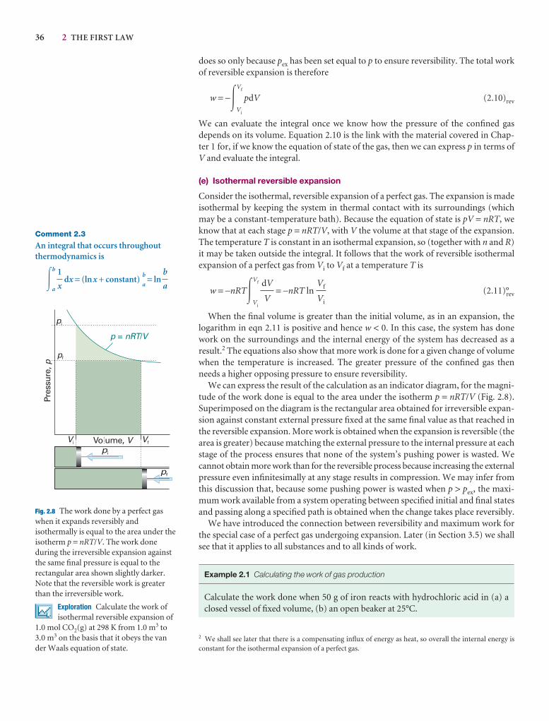
36 2 THE FIRST LAW
Comment 2.3
An integral that occurs throughoutthermodynamics is
�b
a
dx = (lnx + constant)b
a= ln
b
a
1
x
Fig. 2.8 The work done by a perfect gaswhen it expands reversibly andisothermally is equal to the area under theisotherm p = nRT/V. The work doneduring the irreversible expansion againstthe same final pressure is equal to therectangular area shown slightly darker.Note that the reversible work is greaterthan the irreversible work.
Exploration Calculate the work ofisothermal reversible expansion of
1.0 mol CO2(g) at 298 K from 1.0 m3 to3.0 m3 on the basis that it obeys the van der Waals equation of state.
2 We shall see later that there is a compensating influx of energy as heat, so overall the internal energy isconstant for the isothermal expansion of a perfect gas.
does so only because pex has been set equal to p to ensure reversibility. The total workof reversible expansion is therefore
w = −�Vf
Vi
pdV (2.10)rev
We can evaluate the integral once we know how the pressure of the confined gas depends on its volume. Equation 2.10 is the link with the material covered in Chap-ter 1 for, if we know the equation of state of the gas, then we can express p in terms ofV and evaluate the integral.
(e) Isothermal reversible expansion
Consider the isothermal, reversible expansion of a perfect gas. The expansion is madeisothermal by keeping the system in thermal contact with its surroundings (whichmay be a constant-temperature bath). Because the equation of state is pV = nRT, weknow that at each stage p = nRT/V, with V the volume at that stage of the expansion.The temperature T is constant in an isothermal expansion, so (together with n and R)it may be taken outside the integral. It follows that the work of reversible isothermalexpansion of a perfect gas from Vi to Vf at a temperature T is
w = −nRT�Vf
Vi
= −nRT ln (2.11)°rev
When the final volume is greater than the initial volume, as in an expansion, thelogarithm in eqn 2.11 is positive and hence w < 0. In this case, the system has donework on the surroundings and the internal energy of the system has decreased as a result.2 The equations also show that more work is done for a given change of volumewhen the temperature is increased. The greater pressure of the confined gas thenneeds a higher opposing pressure to ensure reversibility.
We can express the result of the calculation as an indicator diagram, for the magni-tude of the work done is equal to the area under the isotherm p = nRT/V (Fig. 2.8).Superimposed on the diagram is the rectangular area obtained for irreversible expan-sion against constant external pressure fixed at the same final value as that reached inthe reversible expansion. More work is obtained when the expansion is reversible (thearea is greater) because matching the external pressure to the internal pressure at eachstage of the process ensures that none of the system’s pushing power is wasted. Wecannot obtain more work than for the reversible process because increasing the externalpressure even infinitesimally at any stage results in compression. We may infer fromthis discussion that, because some pushing power is wasted when p > pex, the maxi-mum work available from a system operating between specified initial and final statesand passing along a specified path is obtained when the change takes place reversibly.
We have introduced the connection between reversibility and maximum work forthe special case of a perfect gas undergoing expansion. Later (in Section 3.5) we shallsee that it applies to all substances and to all kinds of work.
Example 2.1 Calculating the work of gas production
Calculate the work done when 50 g of iron reacts with hydrochloric acid in (a) aclosed vessel of fixed volume, (b) an open beaker at 25°C.
Vf
Vi
dV
V
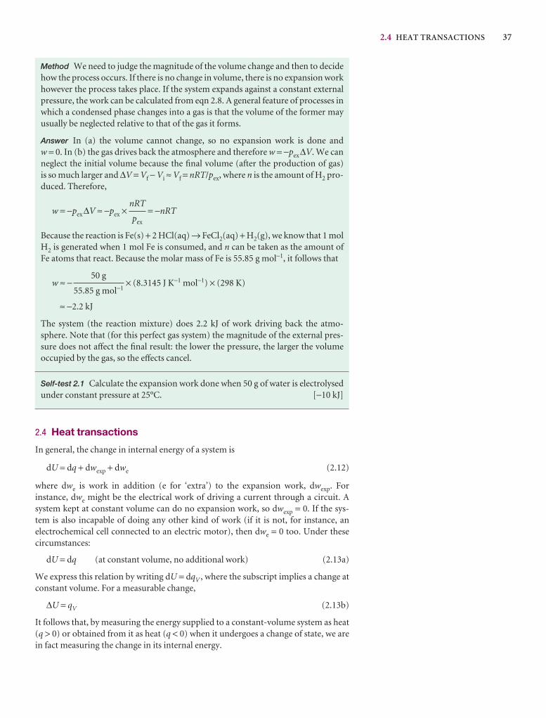
2.4 HEAT TRANSACTIONS 37
Method We need to judge the magnitude of the volume change and then to decidehow the process occurs. If there is no change in volume, there is no expansion workhowever the process takes place. If the system expands against a constant externalpressure, the work can be calculated from eqn 2.8. A general feature of processes inwhich a condensed phase changes into a gas is that the volume of the former mayusually be neglected relative to that of the gas it forms.
Answer In (a) the volume cannot change, so no expansion work is done and w = 0. In (b) the gas drives back the atmosphere and therefore w = −pex∆V. We canneglect the initial volume because the final volume (after the production of gas) is so much larger and ∆V = Vf − Vi ≈ Vf = nRT/pex, where n is the amount of H2 pro-duced. Therefore,
w = −pex∆V ≈ −pex × = −nRT
Because the reaction is Fe(s) + 2 HCl(aq) → FeCl2(aq) + H2(g), we know that 1 molH2 is generated when 1 mol Fe is consumed, and n can be taken as the amount ofFe atoms that react. Because the molar mass of Fe is 55.85 g mol−1, it follows that
w ≈ − × (8.3145 J K−1 mol−1) × (298 K)
≈ −2.2 kJ
The system (the reaction mixture) does 2.2 kJ of work driving back the atmo-sphere. Note that (for this perfect gas system) the magnitude of the external pres-sure does not affect the final result: the lower the pressure, the larger the volumeoccupied by the gas, so the effects cancel.
Self-test 2.1 Calculate the expansion work done when 50 g of water is electrolysedunder constant pressure at 25°C. [−10 kJ]
2.4 Heat transactions
In general, the change in internal energy of a system is
dU = dq + dwexp + dwe (2.12)
where dwe is work in addition (e for ‘extra’) to the expansion work, dwexp. For instance, dwe might be the electrical work of driving a current through a circuit. A system kept at constant volume can do no expansion work, so dwexp = 0. If the sys-tem is also incapable of doing any other kind of work (if it is not, for instance, an electrochemical cell connected to an electric motor), then dwe = 0 too. Under thesecircumstances:
dU = dq (at constant volume, no additional work) (2.13a)
We express this relation by writing dU = dqV , where the subscript implies a change atconstant volume. For a measurable change,
∆U = qV (2.13b)
It follows that, by measuring the energy supplied to a constant-volume system as heat(q > 0) or obtained from it as heat (q < 0) when it undergoes a change of state, we arein fact measuring the change in its internal energy.
50 g
55.85 g mol−1
nRT
pex
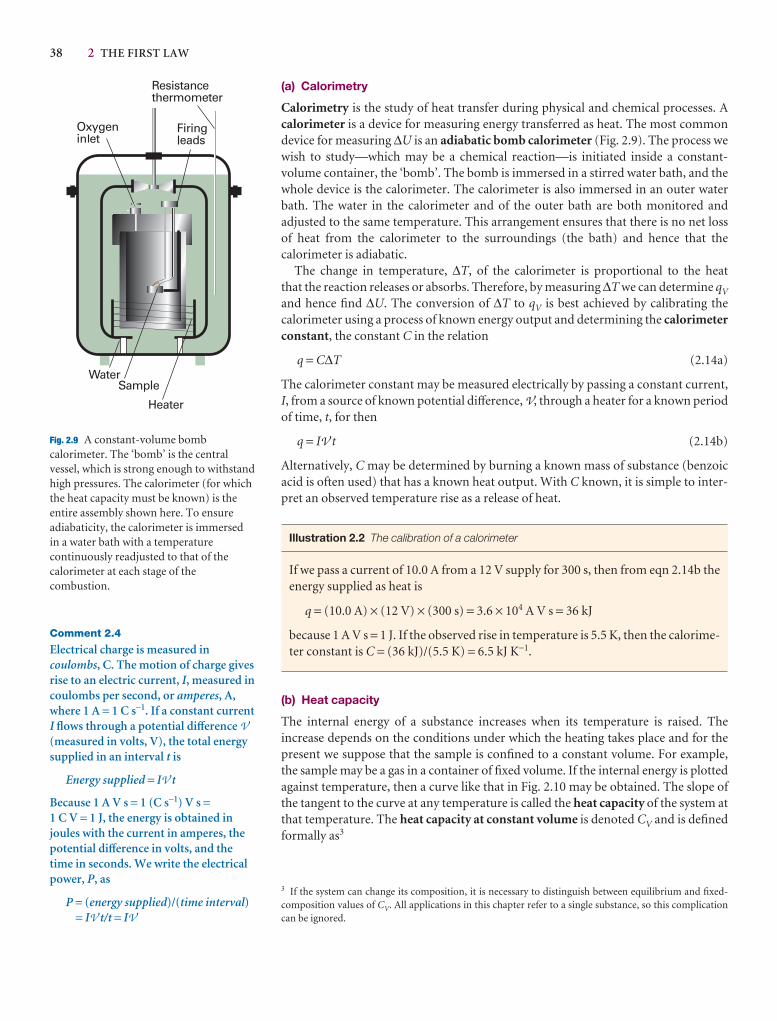
38 2 THE FIRST LAW
Fig. 2.9 A constant-volume bombcalorimeter. The ‘bomb’ is the centralvessel, which is strong enough to withstandhigh pressures. The calorimeter (for whichthe heat capacity must be known) is theentire assembly shown here. To ensureadiabaticity, the calorimeter is immersed in a water bath with a temperaturecontinuously readjusted to that of thecalorimeter at each stage of thecombustion.
Comment 2.4
Electrical charge is measured incoulombs, C. The motion of charge givesrise to an electric current, I, measured incoulombs per second, or amperes, A,where 1 A = 1 C s−1. If a constant currentI flows through a potential difference V(measured in volts, V), the total energysupplied in an interval t is
Energy supplied = IV t
Because 1 A V s = 1 (C s−1) V s =1 C V = 1 J, the energy is obtained injoules with the current in amperes, thepotential difference in volts, and thetime in seconds. We write the electricalpower, P, as
P = (energy supplied)/(time interval)= IV t/t = IV
3 If the system can change its composition, it is necessary to distinguish between equilibrium and fixed-composition values of CV. All applications in this chapter refer to a single substance, so this complicationcan be ignored.
(a) Calorimetry
Calorimetry is the study of heat transfer during physical and chemical processes. Acalorimeter is a device for measuring energy transferred as heat. The most commondevice for measuring ∆U is an adiabatic bomb calorimeter (Fig. 2.9). The process wewish to study—which may be a chemical reaction—is initiated inside a constant-volume container, the ‘bomb’. The bomb is immersed in a stirred water bath, and thewhole device is the calorimeter. The calorimeter is also immersed in an outer waterbath. The water in the calorimeter and of the outer bath are both monitored and adjusted to the same temperature. This arrangement ensures that there is no net lossof heat from the calorimeter to the surroundings (the bath) and hence that thecalorimeter is adiabatic.
The change in temperature, ∆T, of the calorimeter is proportional to the heat that the reaction releases or absorbs. Therefore, by measuring ∆T we can determine qV
and hence find ∆U. The conversion of ∆T to qV is best achieved by calibrating thecalorimeter using a process of known energy output and determining the calorimeterconstant, the constant C in the relation
q = C∆T (2.14a)
The calorimeter constant may be measured electrically by passing a constant current,I, from a source of known potential difference, V, through a heater for a known periodof time, t, for then
q = IV t (2.14b)
Alternatively, C may be determined by burning a known mass of substance (benzoicacid is often used) that has a known heat output. With C known, it is simple to inter-pret an observed temperature rise as a release of heat.
Illustration 2.2 The calibration of a calorimeter
If we pass a current of 10.0 A from a 12 V supply for 300 s, then from eqn 2.14b theenergy supplied as heat is
q = (10.0 A) × (12 V) × (300 s) = 3.6 × 10⁴ A V s = 36 kJ
because 1 A V s = 1 J. If the observed rise in temperature is 5.5 K, then the calorime-ter constant is C = (36 kJ)/(5.5 K) = 6.5 kJ K−1.
(b) Heat capacity
The internal energy of a substance increases when its temperature is raised. The increase depends on the conditions under which the heating takes place and for thepresent we suppose that the sample is confined to a constant volume. For example, the sample may be a gas in a container of fixed volume. If the internal energy is plottedagainst temperature, then a curve like that in Fig. 2.10 may be obtained. The slope ofthe tangent to the curve at any temperature is called the heat capacity of the system atthat temperature. The heat capacity at constant volume is denoted CV and is definedformally as3

2.4 HEAT TRANSACTIONS 39
Comment 2.5
The partial-differential operation(∂z/∂x)y consists of taking the firstderivative of z(x,y) with respect to x,treating y as a constant. For example, if z(x,y) = x 2y, then
y
=y
= y = 2yx
Partial derivatives are reviewed inAppendix 2.
dx 2
dx
DEF∂[x 2y]
∂x
ABCDEF
∂z
∂x
ABC
Fig. 2.11 The internal energy of a systemvaries with volume and temperature,perhaps as shown here by the surface. Thevariation of the internal energy withtemperature at one particular constantvolume is illustrated by the curve drawnparallel to T. The slope of this curve at any point is the partial derivative(∂U/∂T)V.
Fig. 2.10 The internal energy of a systemincreases as the temperature is raised; thisgraph shows its variation as the system isheated at constant volume. The slope of thetangent to the curve at any temperature isthe heat capacity at constant volume at thattemperature. Note that, for the systemillustrated, the heat capacity is greater at Bthan at A.
CV =V
[2.15]
In this case, the internal energy varies with the temperature and the volume of thesample, but we are interested only in its variation with the temperature, the volumebeing held constant (Fig. 2.11).
Illustration 2.3 Estimating a constant-volume heat capacity
The heat capacity of a monatomic perfect gas can be calculated by inserting the expression for the internal energy derived in Molecular interpretation 2.2. There wesaw that Um = Um(0) + 3–2RT, so from eqn 2.15
CV,m = (Um(0) + 3–2RT) = 3–2R
The numerical value is 12.47 J K−1 mol−1.
Heat capacities are extensive properties: 100 g of water, for instance, has 100 timesthe heat capacity of 1 g of water (and therefore requires 100 times the energy as heat to bring about the same rise in temperature). The molar heat capacity at constant volume, CV,m = CV /n, is the heat capacity per mole of material, and is an intensiveproperty (all molar quantities are intensive). Typical values of CV,m for polyatomicgases are close to 25 J K−1 mol−1. For certain applications it is useful to know thespecific heat capacity (more informally, the ‘specific heat’) of a substance, which isthe heat capacity of the sample divided by the mass, usually in grams: CV,s = CV /m. Thespecific heat capacity of water at room temperature is close to 4 J K−1 g−1. In general,
∂∂T
DF
∂U
∂T
AC
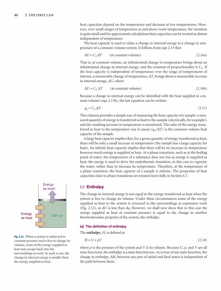
40 2 THE FIRST LAW
heat capacities depend on the temperature and decrease at low temperatures. How-ever, over small ranges of temperature at and above room temperature, the variationis quite small and for approximate calculations heat capacities can be treated as almostindependent of temperature.
The heat capacity is used to relate a change in internal energy to a change in tem-perature of a constant-volume system. It follows from eqn 2.15 that
dU = CV dT (at constant volume) (2.16a)
That is, at constant volume, an infinitesimal change in temperature brings about aninfinitesimal change in internal energy, and the constant of proportionality is CV. Ifthe heat capacity is independent of temperature over the range of temperatures of interest, a measurable change of temperature, ∆T, brings about a measurable increasein internal energy, ∆U, where
∆U = CV ∆T (at constant volume) (2.16b)
Because a change in internal energy can be identified with the heat supplied at con-stant volume (eqn 2.13b), the last equation can be written
qV = CV∆T (2.17)
This relation provides a simple way of measuring the heat capacity of a sample: a mea-sured quantity of energy is transferred as heat to the sample (electrically, for example),and the resulting increase in temperature is monitored. The ratio of the energy trans-ferred as heat to the temperature rise it causes (qV /∆T) is the constant-volume heat capacity of the sample.
A large heat capacity implies that, for a given quantity of energy transferred as heat,there will be only a small increase in temperature (the sample has a large capacity forheat). An infinite heat capacity implies that there will be no increase in temperaturehowever much energy is supplied as heat. At a phase transition, such as at the boilingpoint of water, the temperature of a substance does not rise as energy is supplied asheat: the energy is used to drive the endothermic transition, in this case to vaporize the water, rather than to increase its temperature. Therefore, at the temperature of a phase transition, the heat capacity of a sample is infinite. The properties of heat capacities close to phase transitions are treated more fully in Section 4.7.
2.5 Enthalpy
The change in internal energy is not equal to the energy transferred as heat when thesystem is free to change its volume. Under these circumstances some of the energysupplied as heat to the system is returned to the surroundings as expansion work (Fig. 2.12), so dU is less than dq. However, we shall now show that in this case the energy supplied as heat at constant pressure is equal to the change in another thermodynamic property of the system, the enthalpy.
(a) The definition of enthalpy
The enthalpy, H, is defined as
H = U + pV [2.18]
where p is the pressure of the system and V is its volume. Because U, p, and V are allstate functions, the enthalpy is a state function too. As is true of any state function, thechange in enthalpy, ∆H, between any pair of initial and final states is independent ofthe path between them.
Fig. 2.12 When a system is subjected toconstant pressure and is free to change itsvolume, some of the energy supplied asheat may escape back into thesurroundings as work. In such a case, thechange in internal energy is smaller thanthe energy supplied as heat.
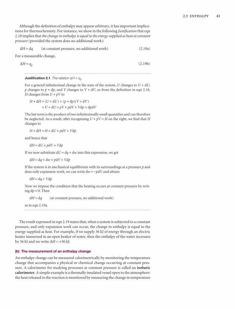
2.5 ENTHALPY 41
Although the definition of enthalpy may appear arbitrary, it has important implica-tions for thermochemisty. For instance, we show in the following Justification that eqn2.18 implies that the change in enthalpy is equal to the energy supplied as heat at constantpressure (provided the system does no additional work):
dH = dq (at constant pressure, no additional work) (2.19a)
For a measurable change,
∆H = qp (2.19b)
Justification 2.1 The relation ∆H = qp
For a general infinitesimal change in the state of the system, U changes to U + dU,p changes to p + dp, and V changes to V + dV, so from the definition in eqn 2.18, H changes from U + pV to
H + dH = (U + dU) + (p + dp)(V + dV)
= U + dU + pV + pdV + Vdp + dpdV
The last term is the product of two infinitesimally small quantities and can thereforebe neglected. As a result, after recognizing U + pV = H on the right, we find that Hchanges to
H + dH = H + dU + pdV + Vdp
and hence that
dH = dU + pdV + Vdp
If we now substitute dU = dq + dw into this expression, we get
dH = dq + dw + pdV + Vdp
If the system is in mechanical equilibrium with its surroundings at a pressure p anddoes only expansion work, we can write dw = −pdV and obtain
dH = dq + Vdp
Now we impose the condition that the heating occurs at constant pressure by writ-ing dp = 0. Then
dH = dq (at constant pressure, no additional work)
as in eqn 2.19a.
The result expressed in eqn 2.19 states that, when a system is subjected to a constantpressure, and only expansion work can occur, the change in enthalpy is equal to theenergy supplied as heat. For example, if we supply 36 kJ of energy through an electricheater immersed in an open beaker of water, then the enthalpy of the water increasesby 36 kJ and we write ∆H = +36 kJ.
(b) The measurement of an enthalpy change
An enthalpy change can be measured calorimetrically by monitoring the temperaturechange that accompanies a physical or chemical change occurring at constant pres-sure. A calorimeter for studying processes at constant pressure is called an isobariccalorimeter. A simple example is a thermally insulated vessel open to the atmosphere:the heat released in the reaction is monitored by measuring the change in temperature

42 2 THE FIRST LAW
of the contents. For a combustion reaction an adiabatic flame calorimeter may beused to measure ∆T when a given amount of substance burns in a supply of oxygen(Fig. 2.13). Another route to ∆H is to measure the internal energy change by using a bomb calorimeter, and then to convert ∆U to ∆H. Because solids and liquids havesmall molar volumes, for them pVm is so small that the molar enthalpy and molar internal energy are almost identical (Hm = Um + pVm ≈ Um). Consequently, if a pro-cess involves only solids or liquids, the values of ∆H and ∆U are almost identical.Physically, such processes are accompanied by a very small change in volume, the system does negligible work on the surroundings when the process occurs, so the energy supplied as heat stays entirely within the system. The most sophisticated wayto measure enthalpy changes, however, is to use a differential scanning calorimeter(DSC). Changes in enthalpy and internal energy may also be measured by noncalori-metric methods (see Chapter 7).
Example 2.2 Relating ∆H and ∆U
The internal energy change when 1.0 mol CaCO3 in the form of calcite converts toaragonite is +0.21 kJ. Calculate the difference between the enthalpy change and thechange in internal energy when the pressure is 1.0 bar given that the densities of thesolids are 2.71 g cm−3 and 2.93 g cm−3, respectively.
Method The starting point for the calculation is the relation between the enthalpyof a substance and its internal energy (eqn 2.18). The difference between the twoquantities can be expressed in terms of the pressure and the difference of theirmolar volumes, and the latter can be calculated from their molar masses, M, andtheir mass densities, ρ, by using ρ = M/Vm.
Answer The change in enthalpy when the transition occurs is
∆H = H(aragonite) − H(calcite)
= {U(a) + pV(a)} − {U(c) + pV(c)}
= ∆U + p{V(a) − V(c)} = ∆U + p∆V
The volume of 1.0 mol CaCO3 (100 g) as aragonite is 34 cm3, and that of 1.0 molCaCO3 as calcite is 37 cm3. Therefore,
p∆V = (1.0 × 10⁵ Pa) × (34 − 37) × 10− 6 m3 = −0.3 J
(because 1 Pa m3 = 1 J). Hence,
∆H − ∆U = −0.3 J
which is only 0.1 per cent of the value of ∆U. We see that it is usually justifiable toignore the difference between the enthalpy and internal energy of condensedphases, except at very high pressures, when pV is no longer negligible.
Self-test 2.2 Calculate the difference between ∆H and ∆U when 1.0 mol Sn(s, grey)of density 5.75 g cm−3 changes to Sn(s, white) of density 7.31 g cm−3 at 10.0 bar. At298 K, ∆H = +2.1 kJ. [∆H − ∆U = −4.4 J]
The enthalpy of a perfect gas is related to its internal energy by using pV = nRT inthe definition of H:
H = U + pV = U + nRT (2.20)°
Fig. 2.13 A constant-pressure flamecalorimeter consists of this componentimmersed in a stirred water bath.Combustion occurs as a known amount ofreactant is passed through to fuel the flame,and the rise of temperature is monitored.
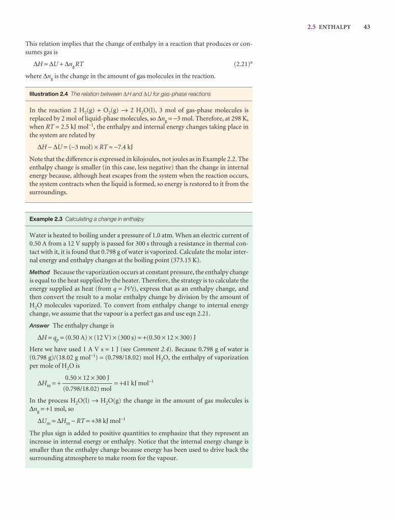
2.5 ENTHALPY 43
This relation implies that the change of enthalpy in a reaction that produces or con-sumes gas is
∆H = ∆U + ∆ng RT (2.21)°
where ∆ng is the change in the amount of gas molecules in the reaction.
Illustration 2.4 The relation between ∆H and ∆U for gas-phase reactions
In the reaction 2 H2(g) + O2(g) → 2 H2O(l), 3 mol of gas-phase molecules is replaced by 2 mol of liquid-phase molecules, so ∆ng = −3 mol. Therefore, at 298 K,when RT = 2.5 kJ mol−1, the enthalpy and internal energy changes taking place inthe system are related by
∆H − ∆U = (−3 mol) × RT ≈ −7.4 kJ
Note that the difference is expressed in kilojoules, not joules as in Example 2.2. Theenthalpy change is smaller (in this case, less negative) than the change in internalenergy because, although heat escapes from the system when the reaction occurs,the system contracts when the liquid is formed, so energy is restored to it from thesurroundings.
Example 2.3 Calculating a change in enthalpy
Water is heated to boiling under a pressure of 1.0 atm. When an electric current of0.50 A from a 12 V supply is passed for 300 s through a resistance in thermal con-tact with it, it is found that 0.798 g of water is vaporized. Calculate the molar inter-nal energy and enthalpy changes at the boiling point (373.15 K).
Method Because the vaporization occurs at constant pressure, the enthalpy changeis equal to the heat supplied by the heater. Therefore, the strategy is to calculate theenergy supplied as heat (from q = IV t), express that as an enthalpy change, andthen convert the result to a molar enthalpy change by division by the amount ofH2O molecules vaporized. To convert from enthalpy change to internal energychange, we assume that the vapour is a perfect gas and use eqn 2.21.
Answer The enthalpy change is
∆H = qp = (0.50 A) × (12 V) × (300 s) = +(0.50 × 12 × 300) J
Here we have used 1 A V s = 1 J (see Comment 2.4). Because 0.798 g of water is(0.798 g)/(18.02 g mol−1) = (0.798/18.02) mol H2O, the enthalpy of vaporizationper mole of H2O is
∆Hm = + = +41 kJ mol−1
In the process H2O(l) → H2O(g) the change in the amount of gas molecules is ∆ng = +1 mol, so
∆Um = ∆Hm − RT = +38 kJ mol−1
The plus sign is added to positive quantities to emphasize that they represent an increase in internal energy or enthalpy. Notice that the internal energy change issmaller than the enthalpy change because energy has been used to drive back thesurrounding atmosphere to make room for the vapour.
0.50 × 12 × 300 J
(0.798/18.02) mol
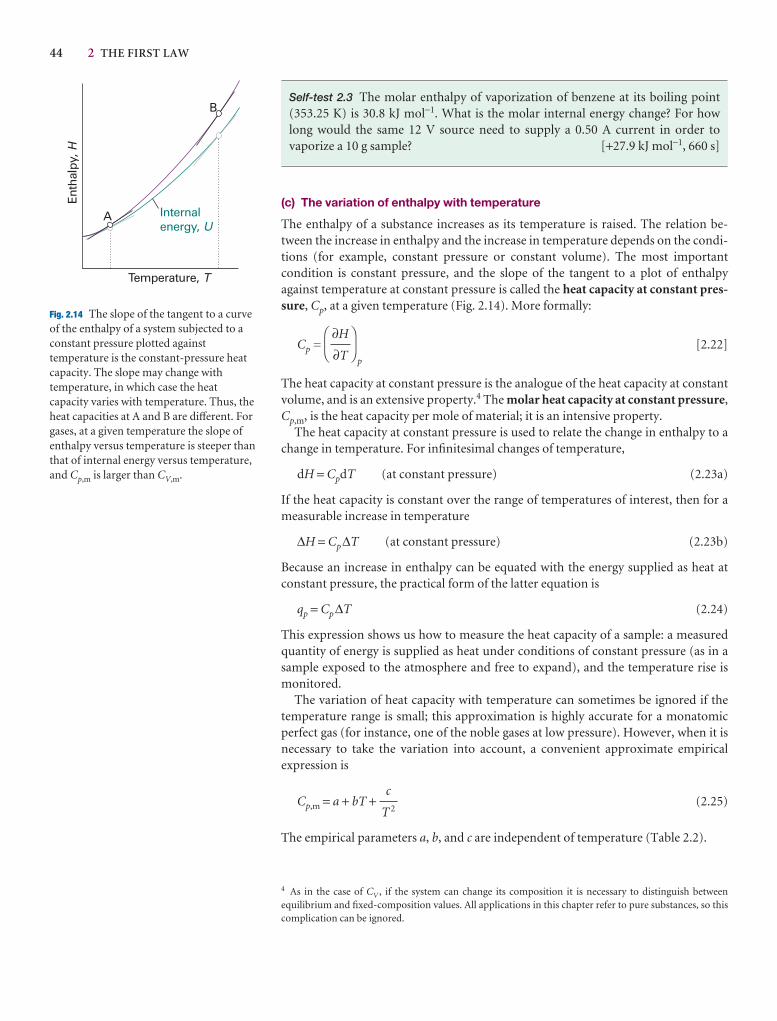
44 2 THE FIRST LAW
Self-test 2.3 The molar enthalpy of vaporization of benzene at its boiling point(353.25 K) is 30.8 kJ mol−1. What is the molar internal energy change? For howlong would the same 12 V source need to supply a 0.50 A current in order to vaporize a 10 g sample? [+27.9 kJ mol−1, 660 s]
(c) The variation of enthalpy with temperature
The enthalpy of a substance increases as its temperature is raised. The relation be-tween the increase in enthalpy and the increase in temperature depends on the condi-tions (for example, constant pressure or constant volume). The most importantcondition is constant pressure, and the slope of the tangent to a plot of enthalpyagainst temperature at constant pressure is called the heat capacity at constant pres-sure, Cp, at a given temperature (Fig. 2.14). More formally:
Cp =p
[2.22]
The heat capacity at constant pressure is the analogue of the heat capacity at constantvolume, and is an extensive property.4 The molar heat capacity at constant pressure,Cp,m, is the heat capacity per mole of material; it is an intensive property.
The heat capacity at constant pressure is used to relate the change in enthalpy to achange in temperature. For infinitesimal changes of temperature,
dH = CpdT (at constant pressure) (2.23a)
If the heat capacity is constant over the range of temperatures of interest, then for ameasurable increase in temperature
∆H = Cp∆T (at constant pressure) (2.23b)
Because an increase in enthalpy can be equated with the energy supplied as heat atconstant pressure, the practical form of the latter equation is
qp = Cp∆T (2.24)
This expression shows us how to measure the heat capacity of a sample: a measuredquantity of energy is supplied as heat under conditions of constant pressure (as in asample exposed to the atmosphere and free to expand), and the temperature rise ismonitored.
The variation of heat capacity with temperature can sometimes be ignored if thetemperature range is small; this approximation is highly accurate for a monatomicperfect gas (for instance, one of the noble gases at low pressure). However, when it isnecessary to take the variation into account, a convenient approximate empirical expression is
Cp,m = a + bT + (2.25)
The empirical parameters a, b, and c are independent of temperature (Table 2.2).
c
T 2
DF
∂H
∂T
AC
4 As in the case of CV , if the system can change its composition it is necessary to distinguish between equilibrium and fixed-composition values. All applications in this chapter refer to pure substances, so thiscomplication can be ignored.
Fig. 2.14 The slope of the tangent to a curveof the enthalpy of a system subjected to aconstant pressure plotted againsttemperature is the constant-pressure heatcapacity. The slope may change withtemperature, in which case the heatcapacity varies with temperature. Thus, theheat capacities at A and B are different. Forgases, at a given temperature the slope ofenthalpy versus temperature is steeper thanthat of internal energy versus temperature,and Cp,m is larger than CV,m.
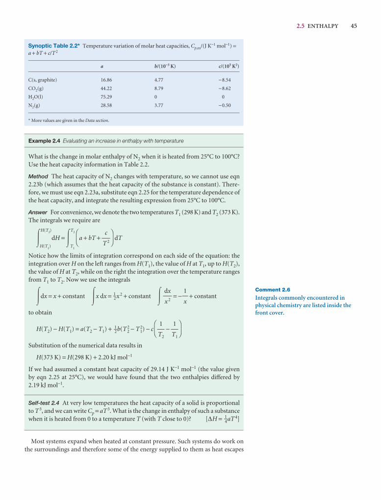
2.5 ENTHALPY 45
Synoptic Table 2.2* Temperature variation of molar heat capacities, Cp,m/(J K−1 mol−1) =a + bT + c/T 2
a b/(10−3 K) c/(105 K2)
C(s, graphite) 16.86 4.77 −8.54
CO2(g) 44.22 8.79 −8.62
H2O(l) 75.29 0 0
N2(g) 28.58 3.77 −0.50
* More values are given in the Data section.
Example 2.4 Evaluating an increase in enthalpy with temperature
What is the change in molar enthalpy of N2 when it is heated from 25°C to 100°C?Use the heat capacity information in Table 2.2.
Method The heat capacity of N2 changes with temperature, so we cannot use eqn2.23b (which assumes that the heat capacity of the substance is constant). There-fore, we must use eqn 2.23a, substitute eqn 2.25 for the temperature dependence ofthe heat capacity, and integrate the resulting expression from 25°C to 100°C.
Answer For convenience, we denote the two temperatures T1 (298 K) and T2 (373 K).The integrals we require are
�H
H(T1)
(T2)
dH = �T2
T1
a + bT + dT
Notice how the limits of integration correspond on each side of the equation: theintegration over H on the left ranges from H(T1), the value of H at T1, up to H(T2),the value of H at T2, while on the right the integration over the temperature rangesfrom T1 to T2. Now we use the integrals
�dx = x + constant �x dx = 1–2x 2 + constant � = − + constant
to obtain
H(T2) − H(T1) = a(T2 − T1) + 1–2b(T 22 − T 2
1) − c −
Substitution of the numerical data results in
H(373 K) = H(298 K) + 2.20 kJ mol−1
If we had assumed a constant heat capacity of 29.14 J K−1 mol−1 (the value given by eqn 2.25 at 25°C), we would have found that the two enthalpies differed by 2.19 kJ mol−1.
Self-test 2.4 At very low temperatures the heat capacity of a solid is proportionalto T3, and we can write Cp = aT3. What is the change in enthalpy of such a substancewhen it is heated from 0 to a temperature T (with T close to 0)? [∆H = 1–4aT 4]
Most systems expand when heated at constant pressure. Such systems do work onthe surroundings and therefore some of the energy supplied to them as heat escapes
DF
1
T1
1
T2
AC
1
x
dx
x 2
DF
c
T 2
AC
Comment 2.6
Integrals commonly encountered inphysical chemistry are listed inside thefront cover.
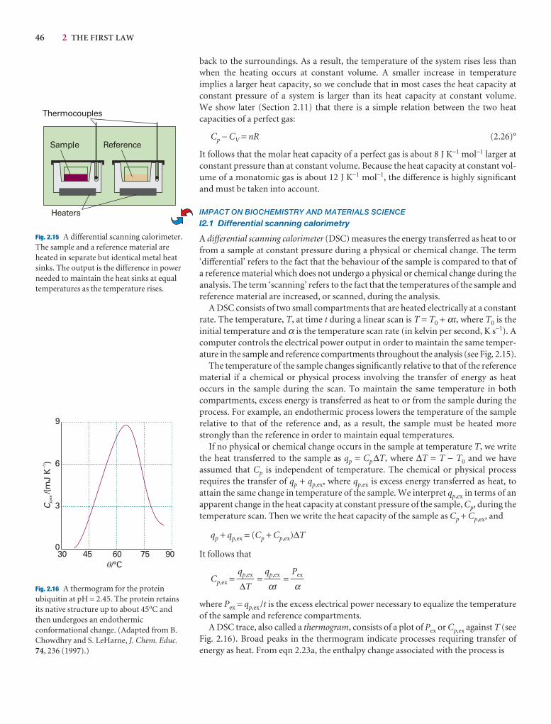
46 2 THE FIRST LAW
back to the surroundings. As a result, the temperature of the system rises less thanwhen the heating occurs at constant volume. A smaller increase in temperature implies a larger heat capacity, so we conclude that in most cases the heat capacity atconstant pressure of a system is larger than its heat capacity at constant volume. We show later (Section 2.11) that there is a simple relation between the two heat capacities of a perfect gas:
Cp − CV = nR (2.26)°
It follows that the molar heat capacity of a perfect gas is about 8 J K−1 mol−1 larger atconstant pressure than at constant volume. Because the heat capacity at constant vol-ume of a monatomic gas is about 12 J K−1 mol−1, the difference is highly significantand must be taken into account.
IMPACT ON BIOCHEMISTRY AND MATERIALS SCIENCE
I2.1 Differential scanning calorimetry
A differential scanning calorimeter (DSC) measures the energy transferred as heat to orfrom a sample at constant pressure during a physical or chemical change. The term‘differential’ refers to the fact that the behaviour of the sample is compared to that ofa reference material which does not undergo a physical or chemical change during theanalysis. The term ‘scanning’ refers to the fact that the temperatures of the sample andreference material are increased, or scanned, during the analysis.
A DSC consists of two small compartments that are heated electrically at a constantrate. The temperature, T, at time t during a linear scan is T = T0 + αt, where T0 is theinitial temperature and α is the temperature scan rate (in kelvin per second, K s−1). Acomputer controls the electrical power output in order to maintain the same temper-ature in the sample and reference compartments throughout the analysis (see Fig. 2.15).
The temperature of the sample changes significantly relative to that of the referencematerial if a chemical or physical process involving the transfer of energy as heat occurs in the sample during the scan. To maintain the same temperature in both compartments, excess energy is transferred as heat to or from the sample during theprocess. For example, an endothermic process lowers the temperature of the samplerelative to that of the reference and, as a result, the sample must be heated morestrongly than the reference in order to maintain equal temperatures.
If no physical or chemical change occurs in the sample at temperature T, we writethe heat transferred to the sample as qp = Cp∆T, where ∆T = T − T0 and we have assumed that Cp is independent of temperature. The chemical or physical process requires the transfer of qp + qp,ex, where qp,ex is excess energy transferred as heat, to attain the same change in temperature of the sample. We interpret qp,ex in terms of anapparent change in the heat capacity at constant pressure of the sample, Cp, during thetemperature scan. Then we write the heat capacity of the sample as Cp + Cp,ex, and
qp + qp,ex = (Cp + Cp,ex)∆T
It follows that
Cp,ex = = =
where Pex = qp,ex /t is the excess electrical power necessary to equalize the temperatureof the sample and reference compartments.
A DSC trace, also called a thermogram, consists of a plot of Pex or Cp,ex against T (seeFig. 2.16). Broad peaks in the thermogram indicate processes requiring transfer of energy as heat. From eqn 2.23a, the enthalpy change associated with the process is
Pex
αqp,ex
αt
qp,ex
∆T
Fig. 2.15 A differential scanning calorimeter.The sample and a reference material areheated in separate but identical metal heatsinks. The output is the difference in powerneeded to maintain the heat sinks at equaltemperatures as the temperature rises.
Fig. 2.16 A thermogram for the proteinubiquitin at pH = 2.45. The protein retainsits native structure up to about 45oC andthen undergoes an endothermicconformational change. (Adapted from B.Chowdhry and S. LeHarne, J. Chem. Educ.74, 236 (1997).)
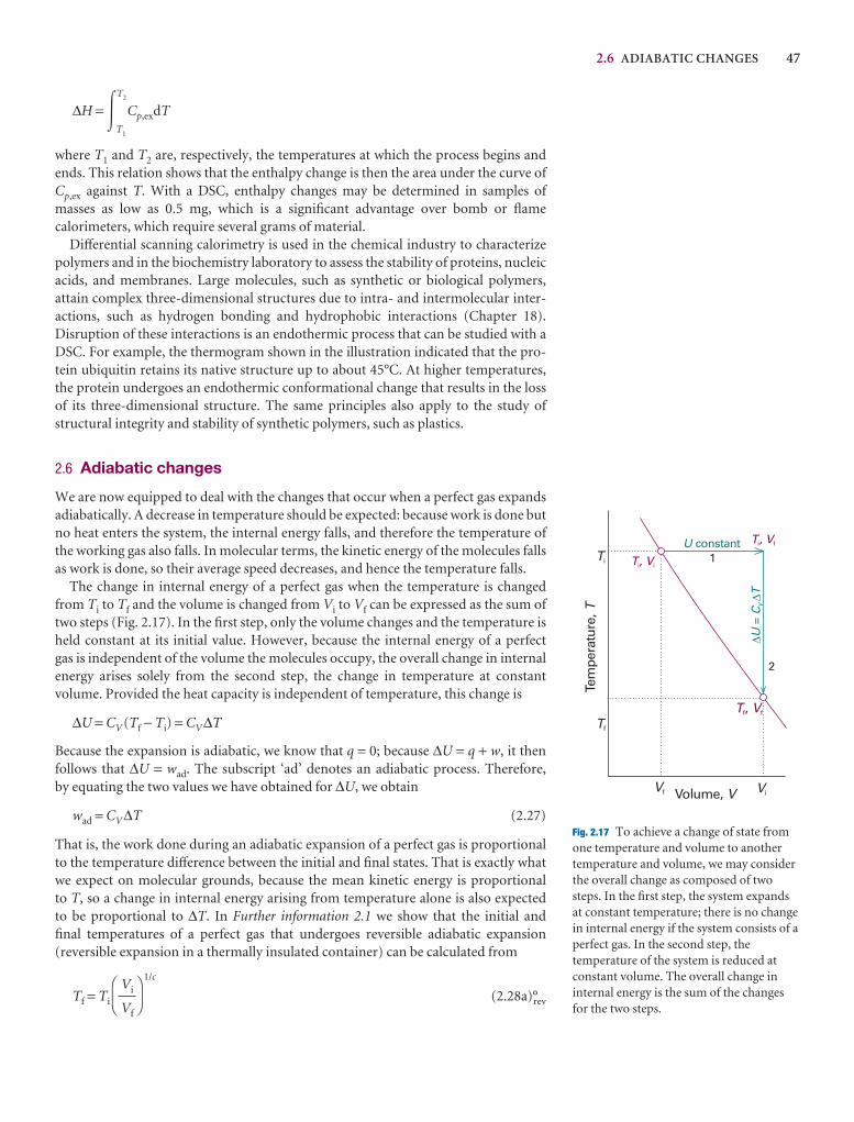
2.6 ADIABATIC CHANGES 47
Fig. 2.17 To achieve a change of state fromone temperature and volume to anothertemperature and volume, we may considerthe overall change as composed of twosteps. In the first step, the system expandsat constant temperature; there is no changein internal energy if the system consists of aperfect gas. In the second step, thetemperature of the system is reduced atconstant volume. The overall change ininternal energy is the sum of the changesfor the two steps.
∆H = �T2
T1
Cp,exdT
where T1 and T2 are, respectively, the temperatures at which the process begins andends. This relation shows that the enthalpy change is then the area under the curve ofCp,ex against T. With a DSC, enthalpy changes may be determined in samples ofmasses as low as 0.5 mg, which is a significant advantage over bomb or flamecalorimeters, which require several grams of material.
Differential scanning calorimetry is used in the chemical industry to characterizepolymers and in the biochemistry laboratory to assess the stability of proteins, nucleicacids, and membranes. Large molecules, such as synthetic or biological polymers, attain complex three-dimensional structures due to intra- and intermolecular inter-actions, such as hydrogen bonding and hydrophobic interactions (Chapter 18).Disruption of these interactions is an endothermic process that can be studied with aDSC. For example, the thermogram shown in the illustration indicated that the pro-tein ubiquitin retains its native structure up to about 45°C. At higher temperatures,the protein undergoes an endothermic conformational change that results in the lossof its three-dimensional structure. The same principles also apply to the study ofstructural integrity and stability of synthetic polymers, such as plastics.
2.6 Adiabatic changes
We are now equipped to deal with the changes that occur when a perfect gas expandsadiabatically. A decrease in temperature should be expected: because work is done butno heat enters the system, the internal energy falls, and therefore the temperature ofthe working gas also falls. In molecular terms, the kinetic energy of the molecules fallsas work is done, so their average speed decreases, and hence the temperature falls.
The change in internal energy of a perfect gas when the temperature is changedfrom Ti to Tf and the volume is changed from Vi to Vf can be expressed as the sum oftwo steps (Fig. 2.17). In the first step, only the volume changes and the temperature isheld constant at its initial value. However, because the internal energy of a perfect gas is independent of the volume the molecules occupy, the overall change in internal energy arises solely from the second step, the change in temperature at constant volume. Provided the heat capacity is independent of temperature, this change is
∆U = CV (Tf − Ti) = CV∆T
Because the expansion is adiabatic, we know that q = 0; because ∆U = q + w, it then follows that ∆U = wad. The subscript ‘ad’ denotes an adiabatic process. Therefore, by equating the two values we have obtained for ∆U, we obtain
wad = CV∆T (2.27)
That is, the work done during an adiabatic expansion of a perfect gas is proportionalto the temperature difference between the initial and final states. That is exactly whatwe expect on molecular grounds, because the mean kinetic energy is proportional to T, so a change in internal energy arising from temperature alone is also expected to be proportional to ∆T. In Further information 2.1 we show that the initial and final temperatures of a perfect gas that undergoes reversible adiabatic expansion (reversible expansion in a thermally insulated container) can be calculated from
Tf = Ti
1/c
(2.28a)°rev
DF
Vi
Vf
AC
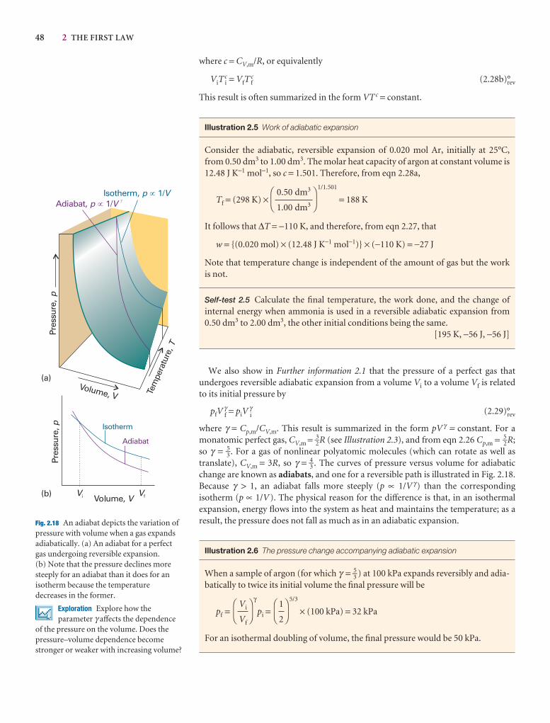
48 2 THE FIRST LAW
Fig. 2.18 An adiabat depicts the variation ofpressure with volume when a gas expandsadiabatically. (a) An adiabat for a perfectgas undergoing reversible expansion. (b) Note that the pressure declines moresteeply for an adiabat than it does for anisotherm because the temperaturedecreases in the former.
Exploration Explore how theparameter γ affects the dependence
of the pressure on the volume. Does thepressure–volume dependence becomestronger or weaker with increasing volume?
where c = CV,m/R, or equivalently
ViT ic = VfT f
c (2.28b)°rev
This result is often summarized in the form VT c = constant.
Illustration 2.5 Work of adiabatic expansion
Consider the adiabatic, reversible expansion of 0.020 mol Ar, initially at 25°C,from 0.50 dm3 to 1.00 dm3. The molar heat capacity of argon at constant volume is12.48 J K−1 mol−1, so c = 1.501. Therefore, from eqn 2.28a,
Tf = (298 K) ×1/1.501
= 188 K
It follows that ∆T = −110 K, and therefore, from eqn 2.27, that
w = {(0.020 mol) × (12.48 J K−1 mol−1)} × (−110 K) = −27 J
Note that temperature change is independent of the amount of gas but the work is not.
Self-test 2.5 Calculate the final temperature, the work done, and the change of internal energy when ammonia is used in a reversible adiabatic expansion from0.50 dm3 to 2.00 dm3, the other initial conditions being the same.
[195 K, −56 J, −56 J]
We also show in Further information 2.1 that the pressure of a perfect gas that undergoes reversible adiabatic expansion from a volume Vi to a volume Vf is relatedto its initial pressure by
pfV fγ = piV i
γ (2.29)°rev
where γ = Cp,m/CV,m. This result is summarized in the form pV γ = constant. For amonatomic perfect gas, CV,m = 3–2R (see Illustration 2.3), and from eqn 2.26 Cp,m = 5–2R;so γ = 5–3. For a gas of nonlinear polyatomic molecules (which can rotate as well astranslate), CV,m = 3R, so γ = 4–3 . The curves of pressure versus volume for adiabaticchange are known as adiabats, and one for a reversible path is illustrated in Fig. 2.18.Because γ > 1, an adiabat falls more steeply (p ∝ 1/V γ) than the correspondingisotherm (p ∝ 1/V). The physical reason for the difference is that, in an isothermal expansion, energy flows into the system as heat and maintains the temperature; as aresult, the pressure does not fall as much as in an adiabatic expansion.
Illustration 2.6 The pressure change accompanying adiabatic expansion
When a sample of argon (for which γ = 5–3 ) at 100 kPa expands reversibly and adia-batically to twice its initial volume the final pressure will be
pf =γ
pi =5/3
× (100 kPa) = 32 kPa
For an isothermal doubling of volume, the final pressure would be 50 kPa.
DF
1
2
AC
DF
Vi
Vf
AC
DF
0.50 dm3
1.00 dm3
AC
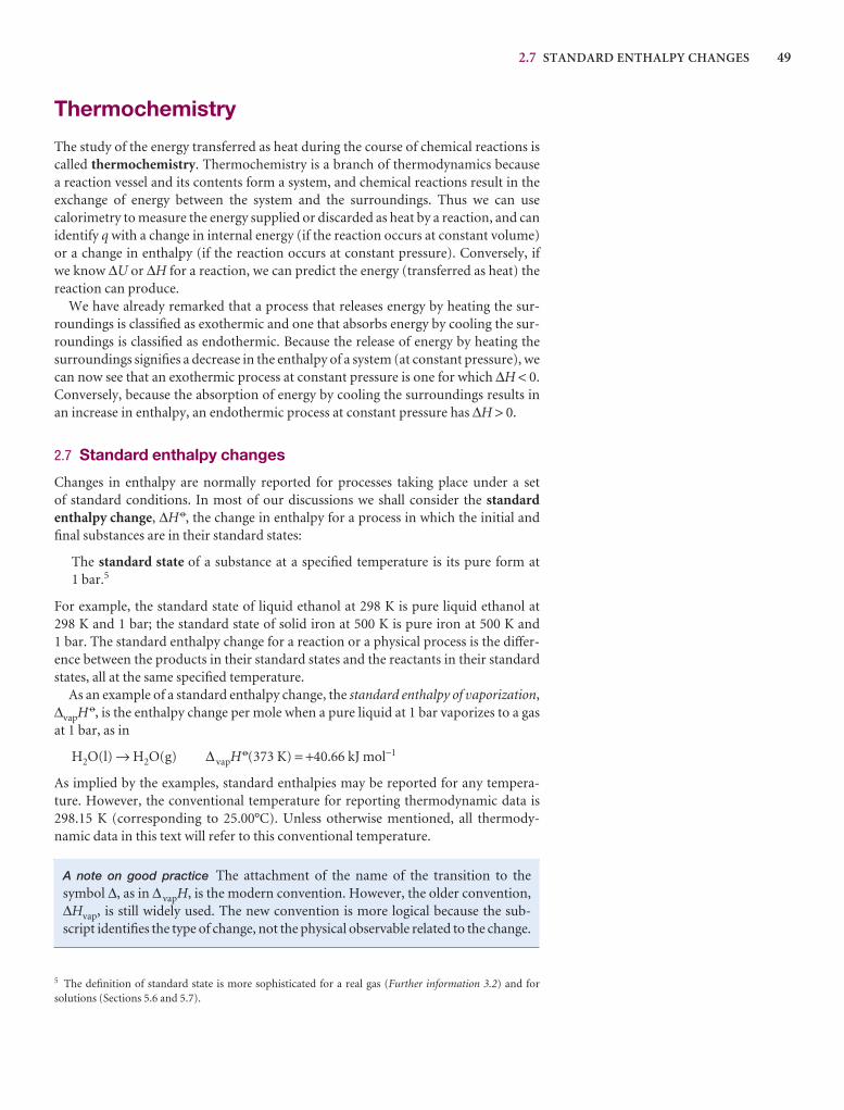
2.7 STANDARD ENTHALPY CHANGES 49
Thermochemistry
The study of the energy transferred as heat during the course of chemical reactions iscalled thermochemistry. Thermochemistry is a branch of thermodynamics because a reaction vessel and its contents form a system, and chemical reactions result in the exchange of energy between the system and the surroundings. Thus we can usecalorimetry to measure the energy supplied or discarded as heat by a reaction, and canidentify q with a change in internal energy (if the reaction occurs at constant volume)or a change in enthalpy (if the reaction occurs at constant pressure). Conversely, if we know ∆U or ∆H for a reaction, we can predict the energy (transferred as heat) the reaction can produce.
We have already remarked that a process that releases energy by heating the sur-roundings is classified as exothermic and one that absorbs energy by cooling the sur-roundings is classified as endothermic. Because the release of energy by heating thesurroundings signifies a decrease in the enthalpy of a system (at constant pressure), wecan now see that an exothermic process at constant pressure is one for which ∆H < 0.Conversely, because the absorption of energy by cooling the surroundings results inan increase in enthalpy, an endothermic process at constant pressure has ∆H > 0.
2.7 Standard enthalpy changes
Changes in enthalpy are normally reported for processes taking place under a set of standard conditions. In most of our discussions we shall consider the standardenthalpy change, ∆H 7, the change in enthalpy for a process in which the initial andfinal substances are in their standard states:
The standard state of a substance at a specified temperature is its pure form at 1 bar.5
For example, the standard state of liquid ethanol at 298 K is pure liquid ethanol at 298 K and 1 bar; the standard state of solid iron at 500 K is pure iron at 500 K and 1 bar. The standard enthalpy change for a reaction or a physical process is the differ-ence between the products in their standard states and the reactants in their standardstates, all at the same specified temperature.
As an example of a standard enthalpy change, the standard enthalpy of vaporization,∆vapH 7, is the enthalpy change per mole when a pure liquid at 1 bar vaporizes to a gasat 1 bar, as in
H2O(l) → H2O(g) ∆ vapH 7(373 K) = +40.66 kJ mol−1
As implied by the examples, standard enthalpies may be reported for any tempera-ture. However, the conventional temperature for reporting thermodynamic data is298.15 K (corresponding to 25.00°C). Unless otherwise mentioned, all thermody-namic data in this text will refer to this conventional temperature.
A note on good practice The attachment of the name of the transition to the symbol ∆, as in ∆ vapH, is the modern convention. However, the older convention,∆Hvap, is still widely used. The new convention is more logical because the sub-script identifies the type of change, not the physical observable related to the change.
5 The definition of standard state is more sophisticated for a real gas (Further information 3.2) and for solutions (Sections 5.6 and 5.7).
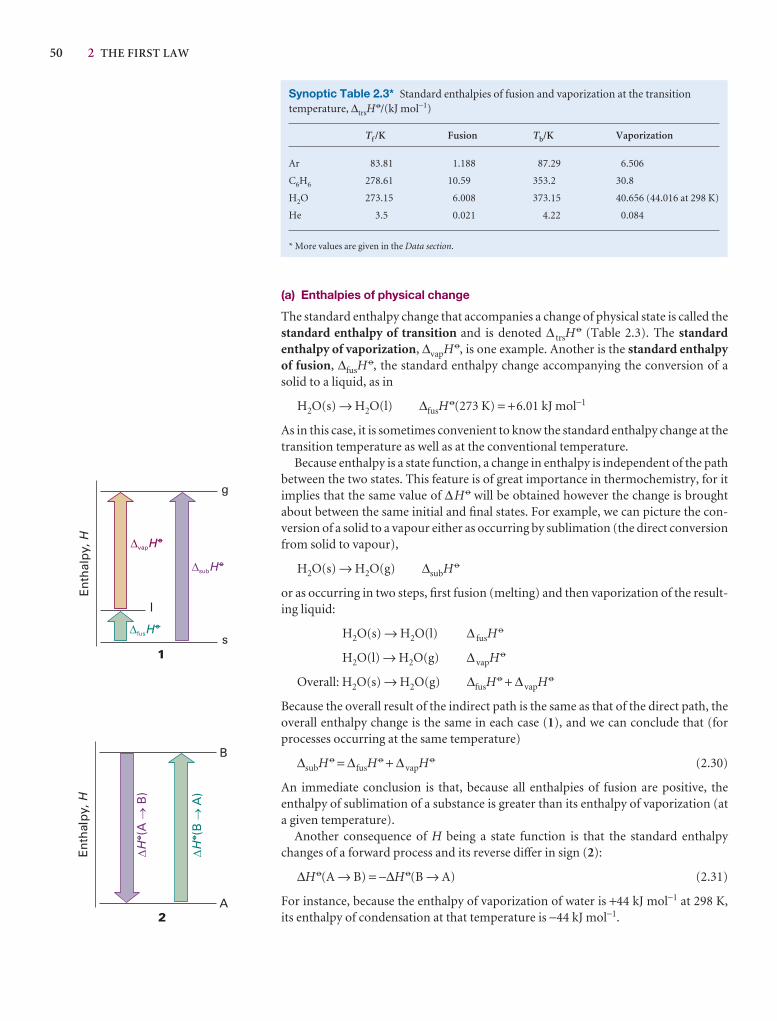
50 2 THE FIRST LAW
(a) Enthalpies of physical change
The standard enthalpy change that accompanies a change of physical state is called thestandard enthalpy of transition and is denoted ∆ trsH
7 (Table 2.3). The standardenthalpy of vaporization, ∆vapH 7, is one example. Another is the standard enthalpyof fusion, ∆fusH
7, the standard enthalpy change accompanying the conversion of asolid to a liquid, as in
H2O(s) → H2O(l) ∆fusH7(273 K) = +6.01 kJ mol−1
As in this case, it is sometimes convenient to know the standard enthalpy change at thetransition temperature as well as at the conventional temperature.
Because enthalpy is a state function, a change in enthalpy is independent of the pathbetween the two states. This feature is of great importance in thermochemistry, for itimplies that the same value of ∆H 7 will be obtained however the change is broughtabout between the same initial and final states. For example, we can picture the con-version of a solid to a vapour either as occurring by sublimation (the direct conversionfrom solid to vapour),
H2O(s) → H2O(g) ∆subH 7
or as occurring in two steps, first fusion (melting) and then vaporization of the result-ing liquid:
H2O(s) → H2O(l) ∆ fusH7
H2O(l) → H2O(g) ∆ vapH 7
Overall: H2O(s) → H2O(g) ∆fusH7 + ∆ vapH 7
Because the overall result of the indirect path is the same as that of the direct path, theoverall enthalpy change is the same in each case (1), and we can conclude that (forprocesses occurring at the same temperature)
∆subH 7 = ∆fusH7 + ∆ vapH 7 (2.30)
An immediate conclusion is that, because all enthalpies of fusion are positive, the enthalpy of sublimation of a substance is greater than its enthalpy of vaporization (ata given temperature).
Another consequence of H being a state function is that the standard enthalpychanges of a forward process and its reverse differ in sign (2):
∆H 7(A → B) = −∆H 7(B → A) (2.31)
For instance, because the enthalpy of vaporization of water is +44 kJ mol−1 at 298 K,its enthalpy of condensation at that temperature is −44 kJ mol−1.
Synoptic Table 2.3* Standard enthalpies of fusion and vaporization at the transitiontemperature, ∆trsH
7/(kJ mol−1)
Tf /K Fusion Tb/K Vaporization
Ar 83.81 1.188 87.29 6.506
C6H6 278.61 10.59 353.2 30.8
H2O 273.15 6.008 373.15 40.656 (44.016 at 298 K)
He 3.5 0.021 4.22 0.084
* More values are given in the Data section.
2.7 STANDARD ENTHALPY CHANGES 51
The different types of enthalpies encountered in thermochemistry are summarizedin Table 2.4. We shall meet them again in various locations throughout the text.
(b) Enthalpies of chemical change
Now we consider enthalpy changes that accompany chemical reactions. There are twoways of reporting the change in enthalpy that accompanies a chemical reaction. Oneis to write the thermochemical equation, a combination of a chemical equation andthe corresponding change in standard enthalpy:
CH4(g) + 2 O2(g) → CO2(g) + 2 H2O(l) ∆H 7 = −890 kJ
∆H 7 is the change in enthalpy when reactants in their standard states change to prod-ucts in their standard states:
Pure, separate reactants in their standard states→ pure, separate products in their standard states
Except in the case of ionic reactions in solution, the enthalpy changes accompanyingmixing and separation are insignificant in comparison with the contribution from thereaction itself. For the combustion of methane, the standard value refers to the reac-tion in which 1 mol CH4 in the form of pure methane gas at 1 bar reacts completelywith 2 mol O2 in the form of pure oxygen gas to produce 1 mol CO2 as pure carbondioxide at 1 bar and 2 mol H2O as pure liquid water at 1 bar; the numerical value is forthe reaction at 298 K.
Alternatively, we write the chemical equation and then report the standard reactionenthalpy, ∆r H 7. Thus, for the combustion of reaction, we write
CH4(g) + 2 O2(g) → CO2(g) + 2 H2O(l) ∆r H 7 = −890 kJ mol−1
For the reaction
2 A + B → 3 C + D
Table 2.4 Enthalpies of transition
Transition Process Symbol*
Transition Phase α → phase β ∆trsH
Fusion s → l ∆fusH
Vaporization l → g ∆vapH
Sublimation s → g ∆subH
Mixing Pure → mixture ∆mixH
Solution Solute → solution ∆solH
Hydration X±(g) → X±(aq) ∆hydH
Atomization Species(s, l, g) → atoms(g) ∆atH
Ionization X(g) → X+(g) + e−(g) ∆ionH
Electron gain X(g) + e−(g) → X−(g) ∆egH
Reaction Reactants → products ∆rH
Combustion Compounds(s, l, g) + O2(g) → CO2(g), H2O(l, g) ∆cH
Formation Elements → compound ∆fH
Activation Reactants → activated complex ∆‡H
* IUPAC recommendations. In common usage, the transition subscript is often attached to ∆H, as in ∆Htrs.
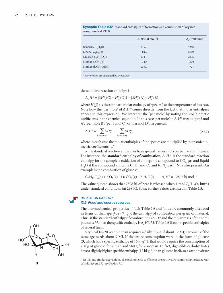
52 2 THE FIRST LAW
the standard reaction enthalpy is
∆ r H 7 = {3H 7m(C) + H 7
m(D)} − {2H 7m(A) + H 7
m(B)}
where H 7m(J) is the standard molar enthalpy of species J at the temperature of interest.
Note how the ‘per mole’ of ∆rH7 comes directly from the fact that molar enthalpies
appear in this expression. We interpret the ‘per mole’ by noting the stoichiometiccoefficients in the chemical equation. In this case ‘per mole’ in ∆rH
7 means ‘per 2 molA’, ‘per mole B’, ‘per 3 mol C’, or ‘per mol D’. In general,
∆rH7 =
Products∑νH 7
m −Reactants
∑νH 7m (2.32)
where in each case the molar enthalpies of the species are multiplied by their stoichio-metric coefficients, ν.6
Some standard reaction enthalpies have special names and a particular significance.For instance, the standard enthalpy of combustion, ∆c H 7, is the standard reactionenthalpy for the complete oxidation of an organic compound to CO2 gas and liquidH2O if the compound contains C, H, and O, and to N2 gas if N is also present. An example is the combustion of glucose:
C6H12O6(s) + 6 O2(g) → 6 CO2(g) + 6 H2O(l) ∆c H 7 = −2808 kJ mol−1
The value quoted shows that 2808 kJ of heat is released when 1 mol C6H12O6 burnsunder standard conditions (at 298 K). Some further values are listed in Table 2.5.
IMPACT ON BIOLOGY
I2.2 Food and energy reserves
The thermochemical properties of fuels Table 2.6 and foods are commonly discussedin terms of their specific enthalpy, the enthalpy of combustion per gram of material.Thus, if the standard enthalpy of combustion is ∆c H 7 and the molar mass of the com-pound is M, then the specific enthalpy is ∆cH7/M. Table 2.6 lists the specific enthalpiesof several fuels.
A typical 18–20 year old man requires a daily input of about 12 MJ; a woman of thesame age needs about 9 MJ. If the entire consumption were in the form of glucose (3; which has a specific enthalpy of 16 kJ g−1), that would require the consumption of750 g of glucose for a man and 560 g for a woman. In fact, digestible carbohydrateshave a slightly higher specific enthalpy (17 kJ g−1) than glucose itself, so a carbohydrate
Synoptic Table 2.5* Standard enthalpies of formation and combustion of organiccompounds at 298 K
∆ f H 7/(kJ mol−1) ∆cH 7/(kJ mol−1)
Benzene, C6H6(l) +49.0 −3268
Ethane, C2H6(g) −84.7 −1560
Glucose, C6H12O6(s) −1274 −2808
Methane, CH4(g) −74.8 −890
Methanol, CH3OH(l) −238.7 −721
* More values are given in the Data section.
6 In this and similar expressions, all stoichiometric coefficients are positive. For a more sophisticated wayof writing eqn 2.32, see Section 7.2.
2.7 STANDARD ENTHALPY CHANGES 53
diet is slightly less daunting than a pure glucose diet, as well as being more appropri-ate in the form of fibre, the indigestible cellulose that helps move digestion productsthrough the intestine.
The specific enthalpy of fats, which are long-chain esters like tristearin (beef fat), ismuch greater than that of carbohydrates, at around 38 kJ g−1, slightly less than the valuefor the hydrocarbon oils used as fuel (48 kJ g−1). Fats are commonly used as an energystore, to be used only when the more readily accessible carbohydrates have fallen intoshort supply. In Arctic species, the stored fat also acts as a layer of insulation; in desertspecies (such as the camel), the fat is also a source of water, one of its oxidation products.
Proteins are also used as a source of energy, but their components, the amino acids, are often too valuable to squander in this way, and are used to construct otherproteins instead. When proteins are oxidized (to urea, CO(NH2)2), the equivalent enthalpy density is comparable to that of carbohydrates.
The heat released by the oxidation of foods needs to be discarded in order to maintain body temperature within its typical range of 35.6–37.8°C. A variety of mechanisms contribute to this aspect of homeostasis, the ability of an organism tocounteract environmental changes with physiological responses. The general uni-formity of temperature throughout the body is maintained largely by the flow ofblood. When heat needs to be dissipated rapidly, warm blood is allowed to flowthrough the capillaries of the skin, so producing flushing. Radiation is one means ofdiscarding heat; another is evaporation and the energy demands of the enthalpy of vaporization of water. Evaporation removes about 2.4 kJ per gram of water perspired.When vigorous exercise promotes sweating (through the influence of heat selectorson the hypothalamus), 1–2 dm3 of perspired water can be produced per hour, cor-responding to a heat loss of 2.4–5.0 MJ h−1.
(c) Hess’s law
Standard enthalpies of individual reactions can be combined to obtain the enthalpy ofanother reaction. This application of the First Law is called Hess’s law:
The standard enthalpy of an overall reaction is the sum of the standard enthalpiesof the individual reactions into which a reaction may be divided.
The individual steps need not be realizable in practice: they may be hypothetical reactions, the only requirement being that their chemical equations should balance.The thermodynamic basis of the law is the path-independence of the value of ∆rH
7
and the implication that we may take the specified reactants, pass through any (pos-sibly hypothetical) set of reactions to the specified products, and overall obtain thesame change of enthalpy. The importance of Hess’s law is that information about a
Table 2.6 Thermochemical properties of some fuels
∆cH 7/ Specific enthalpy/ Enthalpy density/Fuel Combustion equation (kJ mol−1) (kJ g−1) (kJ dm−3)
Hydrogen H2(g) + 1–2 O2(g)
→ H2O(l) −286 142 13
Methane CH4(g) + 2 O2(g)→ CO2(g) + 2 H2O(l) −890 55 40
Octane C8H18(l) + 25––2 O2(g)
→ 8 CO2(g) + 9 H2O(l) −5471 48 3.8 × 10⁴
Methanol CH3OH(l) + 3–2 O2(g)
→ CO2(g) + 2 H2O(l) −726 23 1.8 × 10⁴
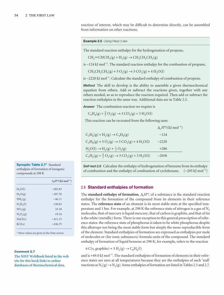
54 2 THE FIRST LAW
Comment 2.7
The NIST WebBook listed in the website for this book links to onlinedatabases of thermochemical data.
reaction of interest, which may be difficult to determine directly, can be assembledfrom information on other reactions.
Example 2.5 Using Hess’s law
The standard reaction enthalpy for the hydrogenation of propene,
CH2=CHCH3(g) + H2(g) → CH3CH2CH3(g)
is −124 kJ mol−1. The standard reaction enthalpy for the combustion of propane,
CH3CH2CH3(g) + 5 O2(g) → 3 CO2(g) + 4 H2O(l)
is −2220 kJ mol−1. Calculate the standard enthalpy of combustion of propene.
Method The skill to develop is the ability to assemble a given thermochemicalequation from others. Add or subtract the reactions given, together with any others needed, so as to reproduce the reaction required. Then add or subtract thereaction enthalpies in the same way. Additional data are in Table 2.5.
Answer The combustion reaction we require is
C3H6(g) + 9–2 O2(g) → 3 CO2(g) + 3 H2O(l)
This reaction can be recreated from the following sum:
∆r H 7/(kJ mol−1)
C3H6(g) + H2(g) → C3H8(g) −124
C3H8(g) + 5 O2(g) → 3 CO2(g) + 4 H2O(l) −2220
H2O(l) → H2(g) + 1–2 O2(g) +286
C3H6(g) + 9–2 O2(g) → 3 CO2(g) + 3 H2O(l) −2058
Self-test 2.6 Calculate the enthalpy of hydrogenation of benzene from its enthalpyof combustion and the enthalpy of combustion of cyclohexane. [−205 kJ mol−1]
2.8 Standard enthalpies of formation
The standard enthalpy of formation, ∆f H7, of a substance is the standard reaction
enthalpy for the formation of the compound from its elements in their referencestates. The reference state of an element is its most stable state at the specified tem-perature and 1 bar. For example, at 298 K the reference state of nitrogen is a gas of N2
molecules, that of mercury is liquid mercury, that of carbon is graphite, and that of tinis the white (metallic) form. There is one exception to this general prescription of refer-ence states: the reference state of phosphorus is taken to be white phosphorus despitethis allotrope not being the most stable form but simply the more reproducible formof the element. Standard enthalpies of formation are expressed as enthalpies per moleof molecules or (for ionic substances) formula units of the compound. The standardenthalpy of formation of liquid benzene at 298 K, for example, refers to the reaction
6 C(s, graphite) + 3 H2(g) → C6H6(l)
and is +49.0 kJ mol−1. The standard enthalpies of formation of elements in their refer-ence states are zero at all temperatures because they are the enthalpies of such ‘null’ reactions as N2(g) → N2(g). Some enthalpies of formation are listed in Tables 2.5 and 2.7.
Synoptic Table 2.7* Standardenthalpies of formation of inorganiccompounds at 298 K
∆fH7/(kJ mol−1)
H2O(l) −285.83
H2O(g) −187.78
NH3(g) −46.11
N2H4(l) +50.63
NO2(g) 33.18
N2O4(g) +9.16
NaCl(s) −411.15
KCl(s) −436.75
* More values are given in the Data section.
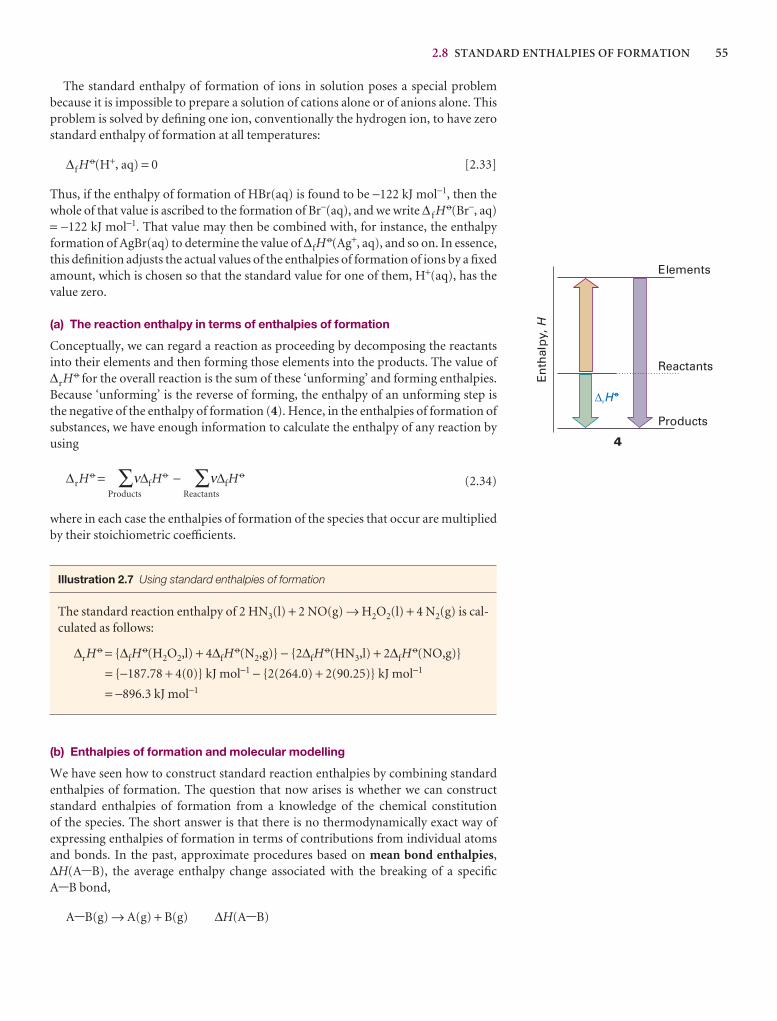
2.8 STANDARD ENTHALPIES OF FORMATION 55
The standard enthalpy of formation of ions in solution poses a special problem because it is impossible to prepare a solution of cations alone or of anions alone. Thisproblem is solved by defining one ion, conventionally the hydrogen ion, to have zerostandard enthalpy of formation at all temperatures:
∆f H7(H+, aq) = 0 [2.33]
Thus, if the enthalpy of formation of HBr(aq) is found to be −122 kJ mol−1, then thewhole of that value is ascribed to the formation of Br−(aq), and we write ∆ fH
7(Br−, aq)= −122 kJ mol−1. That value may then be combined with, for instance, the enthalpyformation of AgBr(aq) to determine the value of ∆fH
7(Ag+, aq), and so on. In essence,this definition adjusts the actual values of the enthalpies of formation of ions by a fixedamount, which is chosen so that the standard value for one of them, H+(aq), has thevalue zero.
(a) The reaction enthalpy in terms of enthalpies of formation
Conceptually, we can regard a reaction as proceeding by decomposing the reactantsinto their elements and then forming those elements into the products. The value of∆rH
7 for the overall reaction is the sum of these ‘unforming’ and forming enthalpies.Because ‘unforming’ is the reverse of forming, the enthalpy of an unforming step isthe negative of the enthalpy of formation (4). Hence, in the enthalpies of formation ofsubstances, we have enough information to calculate the enthalpy of any reaction byusing
∆rH7 =
Products∑ν∆fH
7 −Reactants
∑ν∆fH7
(2.34)
where in each case the enthalpies of formation of the species that occur are multipliedby their stoichiometric coefficients.
Illustration 2.7 Using standard enthalpies of formation
The standard reaction enthalpy of 2 HN3(l) + 2 NO(g) → H2O2(l) + 4 N2(g) is cal-culated as follows:
∆rH7 = {∆fH
7(H2O2,l) + 4∆fH7(N2,g)} − {2∆fH
7(HN3,l) + 2∆fH7(NO,g)}
= {−187.78 + 4(0)} kJ mol−1 − {2(264.0) + 2(90.25)} kJ mol−1
= −896.3 kJ mol−1
(b) Enthalpies of formation and molecular modelling
We have seen how to construct standard reaction enthalpies by combining standardenthalpies of formation. The question that now arises is whether we can constructstandard enthalpies of formation from a knowledge of the chemical constitution of the species. The short answer is that there is no thermodynamically exact way of expressing enthalpies of formation in terms of contributions from individual atomsand bonds. In the past, approximate procedures based on mean bond enthalpies,∆H(A-B), the average enthalpy change associated with the breaking of a specific A-B bond,
A-B(g) → A(g) + B(g) ∆H(A-B)
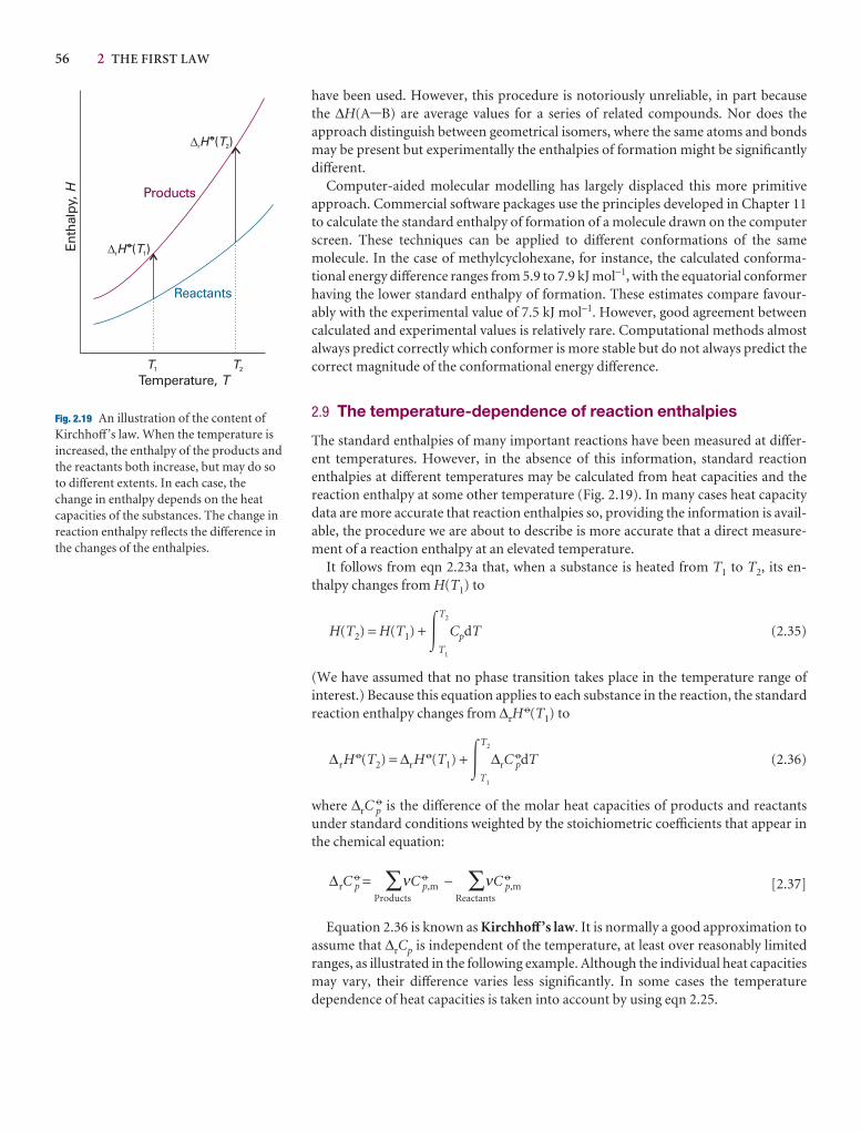
56 2 THE FIRST LAW
have been used. However, this procedure is notoriously unreliable, in part because the ∆H(A-B) are average values for a series of related compounds. Nor does the approach distinguish between geometrical isomers, where the same atoms and bondsmay be present but experimentally the enthalpies of formation might be significantlydifferent.
Computer-aided molecular modelling has largely displaced this more primitive approach. Commercial software packages use the principles developed in Chapter 11to calculate the standard enthalpy of formation of a molecule drawn on the computerscreen. These techniques can be applied to different conformations of the samemolecule. In the case of methylcyclohexane, for instance, the calculated conforma-tional energy difference ranges from 5.9 to 7.9 kJ mol−1, with the equatorial conformerhaving the lower standard enthalpy of formation. These estimates compare favour-ably with the experimental value of 7.5 kJ mol−1. However, good agreement betweencalculated and experimental values is relatively rare. Computational methods almostalways predict correctly which conformer is more stable but do not always predict thecorrect magnitude of the conformational energy difference.
2.9 The temperature-dependence of reaction enthalpies
The standard enthalpies of many important reactions have been measured at differ-ent temperatures. However, in the absence of this information, standard reaction enthalpies at different temperatures may be calculated from heat capacities and thereaction enthalpy at some other temperature (Fig. 2.19). In many cases heat capacitydata are more accurate that reaction enthalpies so, providing the information is avail-able, the procedure we are about to describe is more accurate that a direct measure-ment of a reaction enthalpy at an elevated temperature.
It follows from eqn 2.23a that, when a substance is heated from T1 to T2, its en-thalpy changes from H(T1) to
H(T2) = H(T1) + �T2
T1
CpdT (2.35)
(We have assumed that no phase transition takes place in the temperature range of interest.) Because this equation applies to each substance in the reaction, the standardreaction enthalpy changes from ∆rH
7(T1) to
∆rH7(T2) = ∆rH
7(T1) + �T2
T1
∆rC7pdT (2.36)
where ∆rC p7 is the difference of the molar heat capacities of products and reactants
under standard conditions weighted by the stoichiometric coefficients that appear inthe chemical equation:
∆rC7p =
Products∑νC 7
p,m −Reactants
∑νC 7p,m [2.37]
Equation 2.36 is known as Kirchhoff ’s law. It is normally a good approximation toassume that ∆rCp is independent of the temperature, at least over reasonably limitedranges, as illustrated in the following example. Although the individual heat capacitiesmay vary, their difference varies less significantly. In some cases the temperature dependence of heat capacities is taken into account by using eqn 2.25.
Fig. 2.19 An illustration of the content ofKirchhoff ’s law. When the temperature isincreased, the enthalpy of the products andthe reactants both increase, but may do soto different extents. In each case, thechange in enthalpy depends on the heatcapacities of the substances. The change inreaction enthalpy reflects the difference inthe changes of the enthalpies.
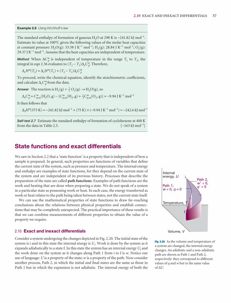
2.10 EXACT AND INEXACT DIFFERENTIALS 57
Fig. 2.20 As the volume and temperature ofa system are changed, the internal energychanges. An adiabatic and a non-adiabaticpath are shown as Path 1 and Path 2,respectively: they correspond to differentvalues of q and w but to the same value of ∆U.
Example 2.6 Using Kirchhoff’s law
The standard enthalpy of formation of gaseous H2O at 298 K is −241.82 kJ mol−1.Estimate its value at 100°C given the following values of the molar heat capacitiesat constant pressure: H2O(g): 33.58 J K−1 mol−1; H2(g): 28.84 J K−1 mol−1; O2(g):29.37 J K−1 mol−1. Assume that the heat capacities are independent of temperature.
Method When ∆C p7 is independent of temperature in the range T1 to T2, the
integral in eqn 2.36 evaluates to (T2 − T1)∆rC p7. Therefore,
∆rH7(T2) = ∆rH
7(T1) + (T2 − T1)∆rC p7
To proceed, write the chemical equation, identify the stoichiometric coefficients,and calculate ∆rC p
7 from the data.
Answer The reaction is H2(g) + 1–2 O2(g) → H2O(g), so
∆rC p7 = C 7
p,m(H2O, g) − {C 7p,m(H2, g) + 1–2C 7
p,m(O2, g)} = −9.94 J K−1 mol−1
It then follows that
∆fH7(373 K) = −241.82 kJ mol−1 + (75 K) × (−9.94 J K−1 mol−1) = −242.6 kJ mol−1
Self-test 2.7 Estimate the standard enthalpy of formation of cyclohexene at 400 Kfrom the data in Table 2.5. [−163 kJ mol−1]
State functions and exact differentials
We saw in Section 2.2 that a ‘state function’ is a property that is independent of how asample is prepared. In general, such properties are functions of variables that definethe current state of the system, such as pressure and temperature. The internal energyand enthalpy are examples of state functions, for they depend on the current state ofthe system and are independent of its previous history. Processes that describe thepreparation of the state are called path functions. Examples of path functions are thework and heating that are done when preparing a state. We do not speak of a systemin a particular state as possessing work or heat. In each case, the energy transferred aswork or heat relates to the path being taken between states, not the current state itself.
We can use the mathematical properties of state functions to draw far-reachingconclusions about the relations between physical properties and establish connec-tions that may be completely unexpected. The practical importance of these results isthat we can combine measurements of different properties to obtain the value of aproperty we require.
2.10 Exact and inexact differentials
Consider a system undergoing the changes depicted in Fig. 2.20. The initial state of thesystem is i and in this state the internal energy is Ui. Work is done by the system as itexpands adiabatically to a state f. In this state the system has an internal energy Uf andthe work done on the system as it changes along Path 1 from i to f is w. Notice our use of language: U is a property of the state; w is a property of the path. Now consideranother process, Path 2, in which the initial and final states are the same as those inPath 1 but in which the expansion is not adiabatic. The internal energy of both the
58 2 THE FIRST LAW
initial and the final states are the same as before (because U is a state function).However, in the second path an energy q′ enters the system as heat and the work w ′ isnot the same as w. The work and the heat are path functions. In terms of the moun-taineering analogy in Section 2.2, the change in altitude (a state function) is independent of the path, but the distance travelled (a path function) does depend onthe path taken between the fixed endpoints.
If a system is taken along a path (for example, by heating it), U changes from Ui toUf, and the overall change is the sum (integral) of all the infinitesimal changes alongthe path:
∆U = �f
i
dU (2.38)
The value of ∆U depends on the initial and final states of the system but is independ-ent of the path between them. This path-independence of the integral is expressed by saying that dU is an ‘exact differential’. In general, an exact differential is aninfinitesimal quantity that, when integrated, gives a result that is independent of thepath between the initial and final states.
When a system is heated, the total energy transferred as heat is the sum of all indi-vidual contributions at each point of the path:
q = �f
i, path
dq (2.39)
Notice the difference between this equation and eqn 2.38. First, we do not write ∆q,because q is not a state function and the energy supplied as heat cannot be expressedas qf − qi. Secondly, we must specify the path of integration because q depends on thepath selected (for example, an adiabatic path has q = 0, whereas a nonadiabatic pathbetween the same two states would have q ≠ 0). This path-dependence is expressed by saying that dq is an ‘inexact differential’. In general, an inexact differential is aninfinitesimal quantity that, when integrated, gives a result that depends on the pathbetween the initial and final states. Often dq is written pq to emphasize that it is in-exact and requires the specification of a path.
The work done on a system to change it from one state to another depends on the path taken between the two specified states; for example, in general the work isdifferent if the change takes place adiabatically and non-adiabatically. It follows thatdw is an inexact differential. It is often written pw.
Example 2.7 Calculating work, heat, and internal energy
Consider a perfect gas inside a cylinder fitted with a piston. Let the initial state beT, Vi and the final state be T, Vf. The change of state can be brought about in manyways, of which the two simplest are the following: Path 1, in which there is free expansion against zero external pressure; Path 2, in which there is reversible,isothermal expansion. Calculate w, q, and ∆U for each process.
Method To find a starting point for a calculation in thermodynamics, it is often a good idea to go back to first principles, and to look for a way of expressing the quantity we are asked to calculate in terms of other quantities that are easier to calculate. We saw in Molecular interpretation 2.2 that the internal energy of aperfect gas depends only on the temperature and is independent of the volumethose molecules occupy, so for any isothermal change, ∆U = 0. We also know thatin general ∆U = q + w. The question depends on being able to combine the two
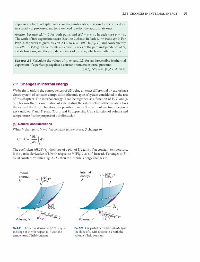
2.11 CHANGES IN INTERNAL ENERGY 59
Fig. 2.21 The partial derivative (∂U/∂V)T isthe slope of U with respect to V with thetemperature T held constant.
Fig. 2.22 The partial derivative (∂U/∂T)V isthe slope of U with respect to T with thevolume V held constant.
expressions. In this chapter, we derived a number of expressions for the work donein a variety of processes, and here we need to select the appropriate ones.
Answer Because ∆U = 0 for both paths and ∆U = q + w, in each case q = −w.The work of free expansion is zero (Section 2.3b); so in Path 1, w = 0 and q = 0. ForPath 2, the work is given by eqn 2.11, so w = −nRT ln(Vf /Vi) and consequently q = nRT ln(Vf /Vi). These results are consequences of the path independence of U,a state function, and the path dependence of q and w, which are path functions.
Self-test 2.8 Calculate the values of q, w, and ∆U for an irreversible isothermal expansion of a perfect gas against a constant nonzero external pressure.
[q = pex∆V, w = −pex∆V, ∆U = 0]
2.11 Changes in internal energy
We begin to unfold the consequences of dU being an exact differential by exploring aclosed system of constant composition (the only type of system considered in the restof this chapter). The internal energy U can be regarded as a function of V, T, and p,but, because there is an equation of state, stating the values of two of the variables fixesthe value of the third. Therefore, it is possible to write U in terms of just two independ-ent variables: V and T, p and T, or p and V. Expressing U as a function of volume andtemperature fits the purpose of our discussion.
(a) General considerations
When V changes to V + dV at constant temperature, U changes to
U ′ = U +T
dV
The coefficient (∂U/∂V)T , the slope of a plot of U against V at constant temperature,is the partial derivative of U with respect to V (Fig. 2.21). If, instead, T changes to T +dT at constant volume (Fig. 2.22), then the internal energy changes to
DF
∂U
∂V
AC
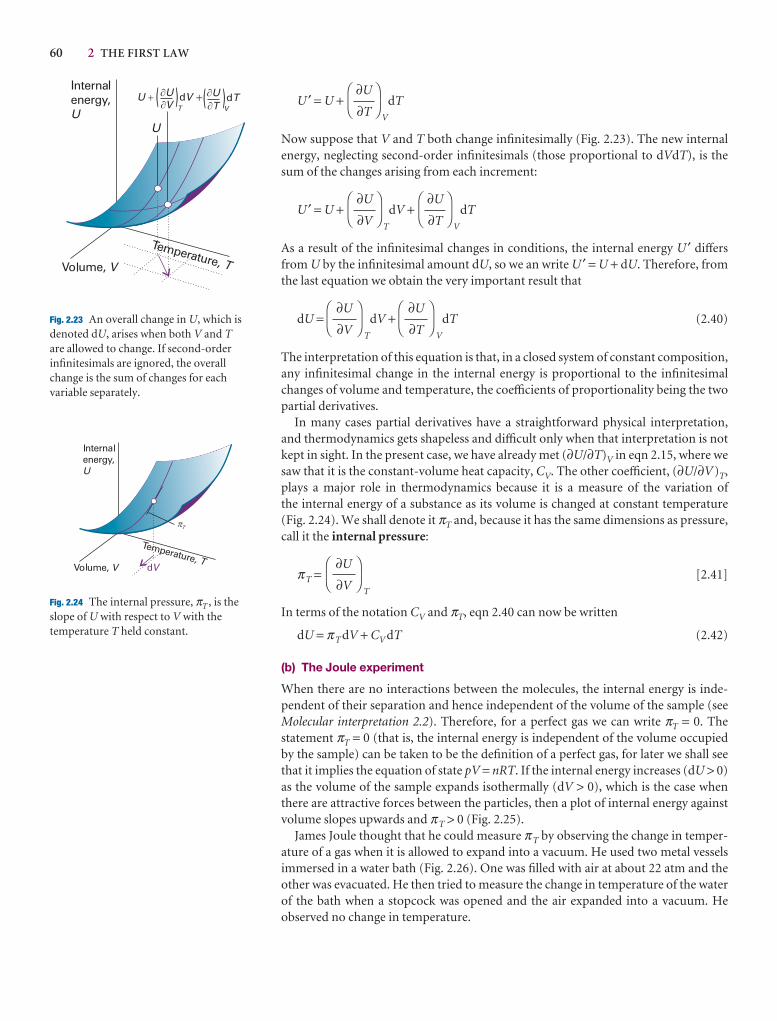
60 2 THE FIRST LAW
U ′ = U +V
dT
Now suppose that V and T both change infinitesimally (Fig. 2.23). The new internalenergy, neglecting second-order infinitesimals (those proportional to dVdT), is thesum of the changes arising from each increment:
U ′ = U +T
dV +V
dT
As a result of the infinitesimal changes in conditions, the internal energy U ′ differsfrom U by the infinitesimal amount dU, so we an write U ′ = U + dU. Therefore, fromthe last equation we obtain the very important result that
dU =T
dV +V
dT (2.40)
The interpretation of this equation is that, in a closed system of constant composition,any infinitesimal change in the internal energy is proportional to the infinitesimalchanges of volume and temperature, the coefficients of proportionality being the twopartial derivatives.
In many cases partial derivatives have a straightforward physical interpretation,and thermodynamics gets shapeless and difficult only when that interpretation is notkept in sight. In the present case, we have already met (∂U/∂T)V in eqn 2.15, where wesaw that it is the constant-volume heat capacity, CV. The other coefficient, (∂U/∂V)T,plays a major role in thermodynamics because it is a measure of the variation of the internal energy of a substance as its volume is changed at constant temperature(Fig. 2.24). We shall denote it πT and, because it has the same dimensions as pressure,call it the internal pressure:
πT =T
[2.41]
In terms of the notation CV and πT, eqn 2.40 can now be written
dU = πT dV + CV dT (2.42)
(b) The Joule experiment
When there are no interactions between the molecules, the internal energy is inde-pendent of their separation and hence independent of the volume of the sample (seeMolecular interpretation 2.2). Therefore, for a perfect gas we can write πT = 0. Thestatement πT = 0 (that is, the internal energy is independent of the volume occupiedby the sample) can be taken to be the definition of a perfect gas, for later we shall seethat it implies the equation of state pV = nRT. If the internal energy increases (dU > 0)as the volume of the sample expands isothermally (dV > 0), which is the case whenthere are attractive forces between the particles, then a plot of internal energy againstvolume slopes upwards and πT > 0 (Fig. 2.25).
James Joule thought that he could measure πT by observing the change in temper-ature of a gas when it is allowed to expand into a vacuum. He used two metal vesselsimmersed in a water bath (Fig. 2.26). One was filled with air at about 22 atm and theother was evacuated. He then tried to measure the change in temperature of the waterof the bath when a stopcock was opened and the air expanded into a vacuum. He observed no change in temperature.
DF
∂U
∂V
AC
DF
∂U
∂T
AC
DF
∂U
∂V
AC
DF
∂U
∂T
AC
DF
∂U
∂V
AC
DF
∂U
∂T
AC
Fig. 2.23 An overall change in U, which isdenoted dU, arises when both V and Tare allowed to change. If second-orderinfinitesimals are ignored, the overallchange is the sum of changes for eachvariable separately.
Fig. 2.24 The internal pressure, πT , is theslope of U with respect to V with thetemperature T held constant.
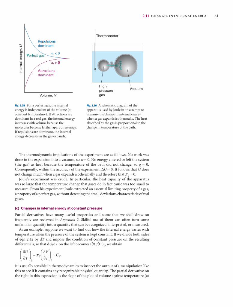
2.11 CHANGES IN INTERNAL ENERGY 61
The thermodynamic implications of the experiment are as follows. No work wasdone in the expansion into a vacuum, so w = 0. No energy entered or left the system(the gas) as heat because the temperature of the bath did not change, so q = 0.Consequently, within the accuracy of the experiment, ∆U = 0. It follows that U doesnot change much when a gas expands isothermally and therefore that πT = 0.
Joule’s experiment was crude. In particular, the heat capacity of the apparatus was so large that the temperature change that gases do in fact cause was too small tomeasure. From his experiment Joule extracted an essential limiting property of a gas,a property of a perfect gas, without detecting the small deviations characteristic of realgases.
(c) Changes in internal energy at constant pressure
Partial derivatives have many useful properties and some that we shall draw on frequently are reviewed in Appendix 2. Skilful use of them can often turn some unfamiliar quantity into a quantity that can be recognized, interpreted, or measured.
As an example, suppose we want to find out how the internal energy varies withtemperature when the pressure of the system is kept constant. If we divide both sidesof eqn 2.42 by dT and impose the condition of constant pressure on the resultingdifferentials, so that dU/dT on the left becomes (∂U/∂T)p, we obtain
p
= πTp
+ CV
It is usually sensible in thermodynamics to inspect the output of a manipulation likethis to see if it contains any recognizable physical quantity. The partial derivative onthe right in this expression is the slope of the plot of volume against temperature (at
DF
∂V
∂T
AC
DF
∂U
∂T
AC
Fig. 2.26 A schematic diagram of theapparatus used by Joule in an attempt tomeasure the change in internal energywhen a gas expands isothermally. The heatabsorbed by the gas is proportional to thechange in temperature of the bath.
Fig. 2.25 For a perfect gas, the internalenergy is independent of the volume (atconstant temperature). If attractions aredominant in a real gas, the internal energyincreases with volume because themolecules become farther apart on average.If repulsions are dominant, the internalenergy decreases as the gas expands.
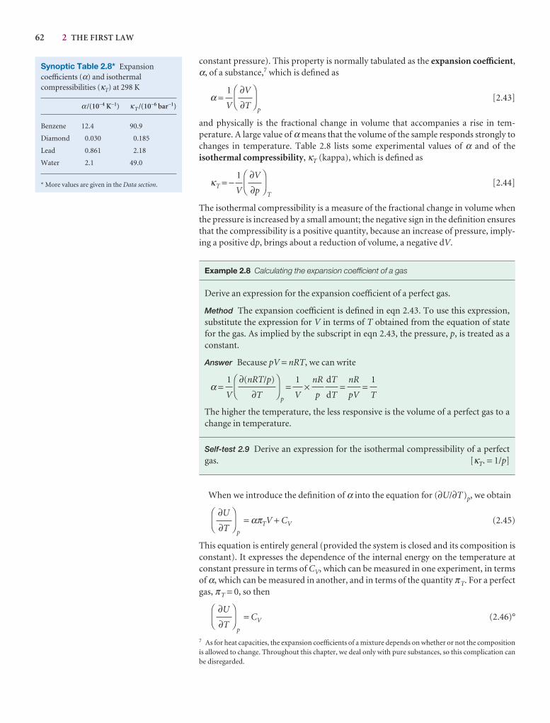
62 2 THE FIRST LAW
Synoptic Table 2.8* Expansioncoefficients (α) and isothermalcompressibilities (κT) at 298 K
α /(10−4 K−1) κ T /(10−6 bar−1)
Benzene 12.4 90.9
Diamond 0.030 0.185
Lead 0.861 2.18
Water 2.1 49.0
* More values are given in the Data section.
7 As for heat capacities, the expansion coefficients of a mixture depends on whether or not the compositionis allowed to change. Throughout this chapter, we deal only with pure substances, so this complication canbe disregarded.
constant pressure). This property is normally tabulated as the expansion coefficient,α, of a substance,7 which is defined as
α =p
[2.43]
and physically is the fractional change in volume that accompanies a rise in tem-perature. A large value of α means that the volume of the sample responds strongly tochanges in temperature. Table 2.8 lists some experimental values of α and of theisothermal compressibility, κT (kappa), which is defined as
κT = −T
[2.44]
The isothermal compressibility is a measure of the fractional change in volume whenthe pressure is increased by a small amount; the negative sign in the definition ensuresthat the compressibility is a positive quantity, because an increase of pressure, imply-ing a positive dp, brings about a reduction of volume, a negative dV.
Example 2.8 Calculating the expansion coefficient of a gas
Derive an expression for the expansion coefficient of a perfect gas.
Method The expansion coefficient is defined in eqn 2.43. To use this expression,substitute the expression for V in terms of T obtained from the equation of state for the gas. As implied by the subscript in eqn 2.43, the pressure, p, is treated as aconstant.
Answer Because pV = nRT, we can write
α =p
= × = =
The higher the temperature, the less responsive is the volume of a perfect gas to achange in temperature.
Self-test 2.9 Derive an expression for the isothermal compressibility of a perfectgas. [κT. = 1/p]
When we introduce the definition of α into the equation for (∂U/∂T)p, we obtain
p
= απTV + CV (2.45)
This equation is entirely general (provided the system is closed and its composition isconstant). It expresses the dependence of the internal energy on the temperature atconstant pressure in terms of CV, which can be measured in one experiment, in termsof α, which can be measured in another, and in terms of the quantity πT. For a perfectgas, πT = 0, so then
p
= CV (2.46)°DF
∂U
∂T
AC
DF
∂U
∂T
AC
1
T
nR
pV
dT
dT
nR
p
1
V
DF
∂(nRT/p)
∂T
AC
1
V
DF
∂V
∂p
AC
1
V
DF
∂V
∂T
AC
1
V
2.12 THE JOULE–THOMSON EFFECT 63
That is, although the constant-volume heat capacity of a perfect gas is defined as theslope of a plot of internal energy against temperature at constant volume, for a perfectgas CV is also the slope at constant pressure.
Equation 2.46 provides an easy way to derive the relation between Cp and CV for aperfect gas expressed in eqn 2.26. Thus, we can use it to express both heat capacities interms of derivatives at constant pressure:
Cp − CV =p
−p
(2.47)°
Then we introduce H = U + pV = U + nRT into the first term, which results in
Cp − CV =p
+ nR −p
= nR (2.48)°
which is eqn 2.26. We show in Further information 2.2 that in general
Cp − CV = (2.49)
Equation 2.49 applies to any substance (that is, it is ‘universally true’). It reduces toeqn 2.48 for a perfect gas when we set α = 1/T and κT = 1/p. Because expansioncoefficients α of liquids and solids are small, it is tempting to deduce from eqn 2.49that for them Cp ≈ CV. But this is not always so, because the compressibility κT mightalso be small, so α2/κT might be large. That is, although only a little work need be doneto push back the atmosphere, a great deal of work may have to be done to pull atomsapart from one another as the solid expands. As an illustration, for water at 25°C, eqn2.49 gives Cp,m = 75.3 J K−1 mol−1 compared with CV,m = 74.8 J K−1 mol−1. In somecases, the two heat capacities differ by as much as 30 per cent.
2.12 The Joule–Thomson effect
We can carry out a similar set of operations on the enthalpy, H = U + pV. The quantitiesU, p, and V are all state functions; therefore H is also a state function and dH is an exactdifferential. It turns out that H is a useful thermodynamic function when the pressureis under our control: we saw a sign of that in the relation ∆H = qp (eqn 2.19). We shalltherefore regard H as a function of p and T, and adapt the argument in Section 2.10 tofind an expression for the variation of H with temperature at constant volume. As setout in Justification 2.2, we find that for a closed system of constant composition,
dH = −µCpdp + CpdT (2.50)
where the Joule–Thomson coefficient, µ (mu), is defined as
µ =H
[2.51]
This relation will prove useful for relating the heat capacities at constant pressure andvolume and for a discussion of the liquefaction of gases.
Justification 2.2 The variation of enthalpy with pressure and temperature
By the same argument that led to eqn 2.40 but with H regarded as a function of p andT we can write
dH =T
dp +p
dT (2.52)DEF
∂H
∂T
ABCDEF
∂H
∂p
ABC
DF
∂T
∂p
AC
α2TV
κT
DF
∂U
∂T
AC
DF
∂U
∂T
AC
DF
∂U
∂T
AC
DF
∂H
∂T
AC
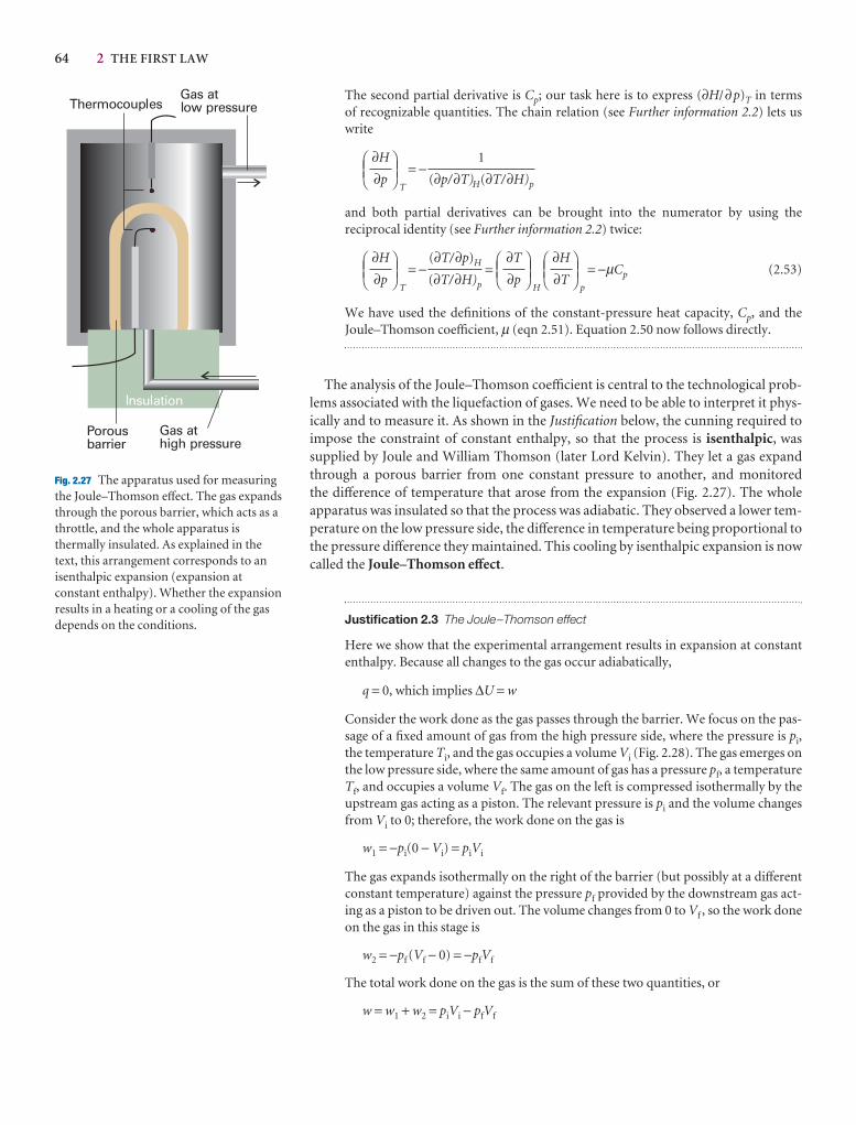
64 2 THE FIRST LAW
Fig. 2.27 The apparatus used for measuringthe Joule–Thomson effect. The gas expandsthrough the porous barrier, which acts as athrottle, and the whole apparatus isthermally insulated. As explained in thetext, this arrangement corresponds to anisenthalpic expansion (expansion atconstant enthalpy). Whether the expansionresults in a heating or a cooling of the gasdepends on the conditions.
The second partial derivative is Cp; our task here is to express (∂H/∂p)T in terms of recognizable quantities. The chain relation (see Further information 2.2) lets uswrite
T
= −
and both partial derivatives can be brought into the numerator by using the reciprocal identity (see Further information 2.2) twice:
T
= − =H p
= −µCp (2.53)
We have used the definitions of the constant-pressure heat capacity, Cp, and theJoule–Thomson coefficient, µ (eqn 2.51). Equation 2.50 now follows directly.
The analysis of the Joule–Thomson coefficient is central to the technological prob-lems associated with the liquefaction of gases. We need to be able to interpret it phys-ically and to measure it. As shown in the Justification below, the cunning required toimpose the constraint of constant enthalpy, so that the process is isenthalpic, wassupplied by Joule and William Thomson (later Lord Kelvin). They let a gas expandthrough a porous barrier from one constant pressure to another, and monitored the difference of temperature that arose from the expansion (Fig. 2.27). The wholeapparatus was insulated so that the process was adiabatic. They observed a lower tem-perature on the low pressure side, the difference in temperature being proportional tothe pressure difference they maintained. This cooling by isenthalpic expansion is nowcalled the Joule–Thomson effect.
Justification 2.3 The Joule–Thomson effect
Here we show that the experimental arrangement results in expansion at constantenthalpy. Because all changes to the gas occur adiabatically,
q = 0, which implies ∆U = w
Consider the work done as the gas passes through the barrier. We focus on the pas-sage of a fixed amount of gas from the high pressure side, where the pressure is pi,the temperature Ti, and the gas occupies a volume Vi (Fig. 2.28). The gas emerges onthe low pressure side, where the same amount of gas has a pressure pf, a temperatureTf, and occupies a volume Vf. The gas on the left is compressed isothermally by theupstream gas acting as a piston. The relevant pressure is pi and the volume changesfrom Vi to 0; therefore, the work done on the gas is
w1 = −pi(0 − Vi) = piVi
The gas expands isothermally on the right of the barrier (but possibly at a differentconstant temperature) against the pressure pf provided by the downstream gas act-ing as a piston to be driven out. The volume changes from 0 to Vf , so the work doneon the gas in this stage is
w2 = −pf (Vf − 0) = −pfVf
The total work done on the gas is the sum of these two quantities, or
w = w1 + w2 = piVi − pfVf
DEF∂H
∂T
ABCDEF
∂T
∂p
ABC(∂T/∂p)H
(∂T/∂H)p
DEF∂H
∂p
ABC
1
(∂p/∂T)H(∂T/∂H)p
DEF∂H
∂p
ABC
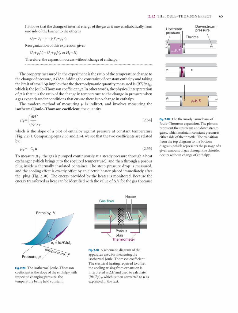
2.12 THE JOULE–THOMSON EFFECT 65
Fig. 2.28 The thermodynamic basis ofJoule–Thomson expansion. The pistonsrepresent the upstream and downstreamgases, which maintain constant pressureseither side of the throttle. The transitionfrom the top diagram to the bottomdiagram, which represents the passage of agiven amount of gas through the throttle,occurs without change of enthalpy.
Fig. 2.29 The isothermal Joule–Thomsoncoefficient is the slope of the enthalpy withrespect to changing pressure, thetemperature being held constant.
Fig. 2.30 A schematic diagram of theapparatus used for measuring theisothermal Joule–Thomson coefficient.The electrical heating required to offsetthe cooling arising from expansion isinterpreted as ∆H and used to calculate(∂H/∂p)T, which is then converted to µ asexplained in the text.
It follows that the change of internal energy of the gas as it moves adiabatically fromone side of the barrier to the other is
Uf − Ui = w = piVi − pfVf
Reorganization of this expression gives
Uf + pfVf = Ui + piVi, or Hf = Hi
Therefore, the expansion occurs without change of enthalpy.
The property measured in the experiment is the ratio of the temperature change tothe change of pressure, ∆T/∆p. Adding the constraint of constant enthalpy and takingthe limit of small ∆p implies that the thermodynamic quantity measured is (∂T/∂p)H,which is the Joule–Thomson coefficient, µ. In other words, the physical interpretationof µ is that it is the ratio of the change in temperature to the change in pressure whena gas expands under conditions that ensure there is no change in enthalpy.
The modern method of measuring µ is indirect, and involves measuring theisothermal Joule–Thomson coefficient, the quantity
µT =T
[2.54]
which is the slope of a plot of enthalpy against pressure at constant temperature (Fig. 2.29). Comparing eqns 2.53 and 2.54, we see that the two coefficients are relatedby:
µT = −Cpµ (2.55)
To measure µT , the gas is pumped continuously at a steady pressure through a heat exchanger (which brings it to the required temperature), and then through a porousplug inside a thermally insulated container. The steep pressure drop is measured, and the cooling effect is exactly offset by an electric heater placed immediately afterthe plug (Fig. 2.30). The energy provided by the heater is monitored. Because the energy transferred as heat can be identified with the value of ∆H for the gas (because
DF
∂H
∂p
AC
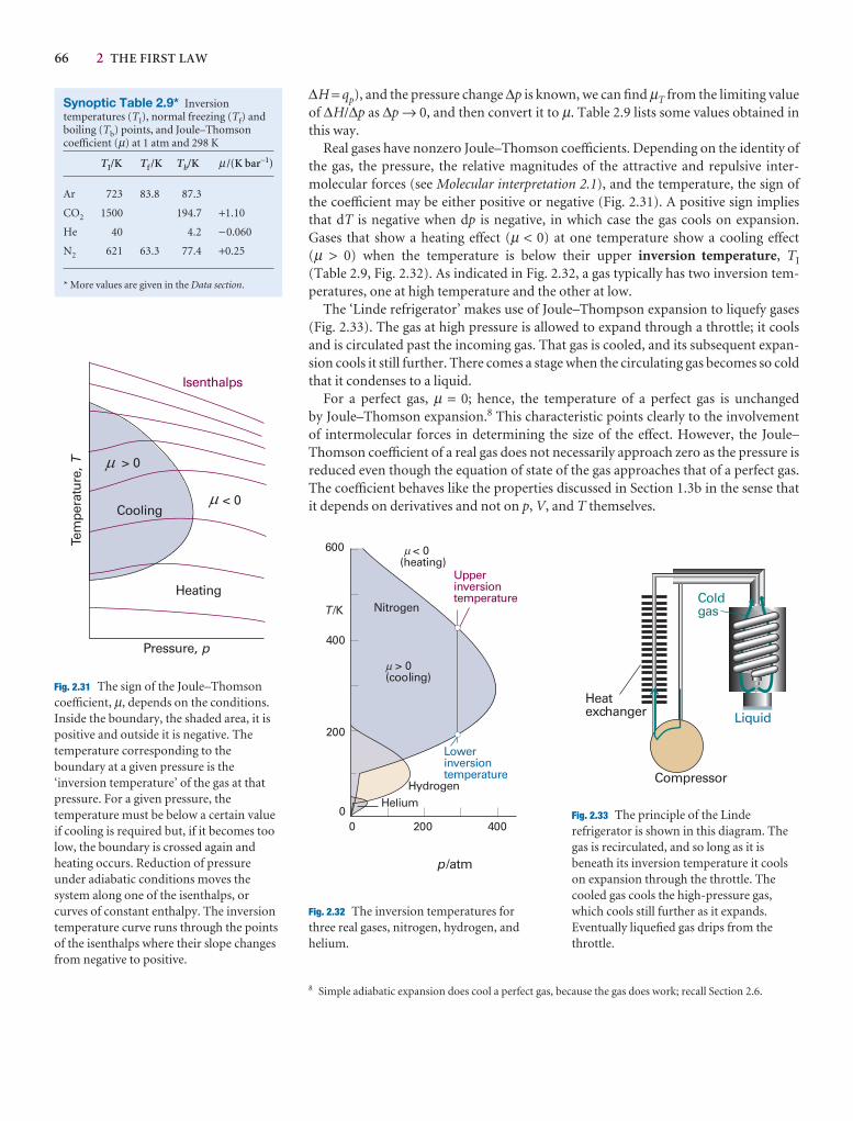
66 2 THE FIRST LAW
∆H = qp), and the pressure change ∆p is known, we can find µT from the limiting valueof ∆H/∆p as ∆p → 0, and then convert it to µ. Table 2.9 lists some values obtained inthis way.
Real gases have nonzero Joule–Thomson coefficients. Depending on the identity ofthe gas, the pressure, the relative magnitudes of the attractive and repulsive inter-molecular forces (see Molecular interpretation 2.1), and the temperature, the sign ofthe coefficient may be either positive or negative (Fig. 2.31). A positive sign impliesthat dT is negative when dp is negative, in which case the gas cools on expansion.Gases that show a heating effect (µ < 0) at one temperature show a cooling effect(µ > 0) when the temperature is below their upper inversion temperature, TI
(Table 2.9, Fig. 2.32). As indicated in Fig. 2.32, a gas typically has two inversion tem-peratures, one at high temperature and the other at low.
The ‘Linde refrigerator’ makes use of Joule–Thompson expansion to liquefy gases(Fig. 2.33). The gas at high pressure is allowed to expand through a throttle; it coolsand is circulated past the incoming gas. That gas is cooled, and its subsequent expan-sion cools it still further. There comes a stage when the circulating gas becomes so coldthat it condenses to a liquid.
For a perfect gas, µ = 0; hence, the temperature of a perfect gas is unchanged by Joule–Thomson expansion.8 This characteristic points clearly to the involvementof intermolecular forces in determining the size of the effect. However, the Joule–Thomson coefficient of a real gas does not necessarily approach zero as the pressure isreduced even though the equation of state of the gas approaches that of a perfect gas.The coefficient behaves like the properties discussed in Section 1.3b in the sense thatit depends on derivatives and not on p, V, and T themselves.
Fig. 2.31 The sign of the Joule–Thomsoncoefficient, µ, depends on the conditions.Inside the boundary, the shaded area, it ispositive and outside it is negative. Thetemperature corresponding to theboundary at a given pressure is the‘inversion temperature’ of the gas at thatpressure. For a given pressure, thetemperature must be below a certain valueif cooling is required but, if it becomes toolow, the boundary is crossed again andheating occurs. Reduction of pressureunder adiabatic conditions moves thesystem along one of the isenthalps, orcurves of constant enthalpy. The inversiontemperature curve runs through the pointsof the isenthalps where their slope changesfrom negative to positive.
Synoptic Table 2.9* Inversiontemperatures (TI), normal freezing (Tf) andboiling (Tb) points, and Joule–Thomsoncoefficient (µ) at 1 atm and 298 K
TI/K Tf /K Tb/K µ /(K bar−1)
Ar 723 83.8 87.3
CO2 1500 194.7 +1.10
He 40 4.2 −0.060
N2 621 63.3 77.4 +0.25
* More values are given in the Data section.
8 Simple adiabatic expansion does cool a perfect gas, because the gas does work; recall Section 2.6.
Fig. 2.32 The inversion temperatures forthree real gases, nitrogen, hydrogen, andhelium.
Fig. 2.33 The principle of the Linderefrigerator is shown in this diagram. Thegas is recirculated, and so long as it isbeneath its inversion temperature it coolson expansion through the throttle. Thecooled gas cools the high-pressure gas,which cools still further as it expands.Eventually liquefied gas drips from thethrottle.

CHECKLIST OF KEY IDEAS 67
Checklist of key ideas
1. Thermodynamics is the study of the transformations ofenergy.
2. The system is the part of the world in which we have a specialinterest. The surroundings is the region outside the systemwhere we make our measurements.
3. An open system has a boundary through which matter can betransferred. A closed system has a boundary through whichmatter cannot be transferred. An isolated system has aboundary through which neither matter nor energy can betransferred.
4. Energy is the capacity to do work. The internal energy is thetotal energy of a system.
5. Work is the transfer of energy by motion against an opposingforce, dw = −Fdz . Heat is the transfer of energy as a result of atemperature difference between the system and thesurroundings.
6. An exothermic process releases energy as heat to thesurroundings. An endothermic process absorbs energy as heatfrom the surroundings.
7. A state function is a property that depends only on the currentstate of the system and is independent of how that state hasbeen prepared.
8. The First Law of thermodynamics states that the internalenergy of an isolated system is constant, ∆U = q + w.
9. Expansion work is the work of expansion (or compression) ofa system, dw = −pexdV. The work of free expansion is w = 0.The work of expansion against a constant external pressure isw = −pex∆V. The work of isothermal reversible expansion of aperfect gas is w = −nRT ln(Vf /Vi).
10. A reversible change is a change that can be reversed by aninfinitesimal modification of a variable.
11. Maximum work is achieved in a reversible change.
Molecular interpretation 2.3 Molecular interactions and the Joule–Thomson effect
The kinetic model of gases (Molecular interpretation 1.1) and the equipartition theorem (Molecular interpretation 2.2) imply that the mean kinetic energy ofmolecules in a gas is proportional to the temperature. It follows that reducing theaverage speed of the molecules is equivalent to cooling the gas. If the speed of themolecules can be reduced to the point that neighbours can capture each other bytheir intermolecular attractions, then the cooled gas will condense to a liquid.
To slow the gas molecules, we make use of an effect similar to that seen when aball is thrown into the air: as it rises it slows in response to the gravitational attrac-tion of the Earth and its kinetic energy is converted into potential energy. We saw in Section 1.3 that molecules in a real gas attract each other (the attraction is not gravitational, but the effect is the same). It follows that, if we can cause themolecules to move apart from each other, like a ball rising from a planet, then theyshould slow. It is very easy to move molecules apart from each other: we simplyallow the gas to expand, which increases the average separation of the molecules.To cool a gas, therefore, we allow it to expand without allowing any energy to enterfrom outside as heat. As the gas expands, the molecules move apart to fill the avail-able volume, struggling as they do so against the attraction of their neighbours.Because some kinetic energy must be converted into potential energy to reachgreater separations, the molecules travel more slowly as their separation increases.This sequence of molecular events explains the Joule–Thomson effect: the coolingof a real gas by adiabatic expansion. The cooling effect, which corresponds to µ > 0, is observed under conditions when attractive interactions are dominant(Z < 1, eqn 1.17), because the molecules have to climb apart against the attractiveforce in order for them to travel more slowly. For molecules under conditionswhen repulsions are dominant (Z > 1), the Joule–Thomson effect results in the gasbecoming warmer, or µ < 0.

68 2 THE FIRST LAW
12. Calorimetry is the study of heat transfers during physical andchemical processes.
13. The heat capacity at constant volume is defined as CV = (∂U/∂T)V. The heat capacity at constant pressure is Cp = (∂H/∂T)p. For a perfect gas, the heat capacities are relatedby Cp − CV = nR.
14. The enthalpy is defined as H = U + pV. The enthalpy change isthe energy transferred as heat at constant pressure, ∆H = qp.
15. During a reversible adiabatic change, the temperature of aperfect gas varies according to Tf = Ti(Vi/Vf)
1/c, c = CV,m/R.The pressure and volume are related by pV γ = constant, with γ = Cp,m/CV,m.
16. The standard enthalpy change is the change in enthalpy for aprocess in which the initial and final substances are in theirstandard states. The standard state is the pure substance at 1 bar.
17. Enthalpy changes are additive, as in ∆subH 7 = ∆fusH7 + ∆vapH 7.
18. The enthalpy change for a process and its reverse are relatedby ∆forwardH 7 = −∆reverseH
7.
19. The standard enthalpy of combustion is the standard reactionenthalpy for the complete oxidation of an organic compoundto CO2 gas and liquid H2O if the compound contains C, H,and O, and to N2 gas if N is also present.
20. Hess’s law states that the standard enthalpy of an overallreaction is the sum of the standard enthalpies of the individualreactions into which a reaction may be divided.
21. The standard enthalpy of formation (∆fH7) is the standard
reaction enthalpy for the formation of the compound from itselements in their reference states. The reference state is themost stable state of an element at the specified temperatureand 1 bar.
22. The standard reaction enthalpy may be estimated by combining enthalpies of formation, ∆rH
7 = ∑Productsν∆fH7 − ∑Reactantsν∆fH
7.
23. The temperature dependence of the reaction enthalpy is given
by Kirchhoff ’s law, ∆rH7(T2) = ∆rH
7(T1) + �T2
T1
∆rC7pdT.
24. An exact differential is an infinitesimal quantity that, whenintegrated, gives a result that is independent of the pathbetween the initial and final states. An inexact differentialis an infinitesimal quantity that, when integrated, gives aresult that depends on the path between the initial and finalstates.
25. The internal pressure is defined as πT = (∂U/∂V)T . For aperfect gas, πT = 0.
26. The Joule–Thomson effect is the cooling of a gas byisenthalpic expansion.
27. The Joule–Thomson coefficient is defined as µ = (∂T/∂p)H.The isothermal Joule–Thomson coefficient is defined asµT = (∂H/∂p)T = −Cpµ.
28. The inversion temperature is the temperature at which theJoule–Thomson coefficient changes sign.
Further reading
Articles and texts
P.W. Atkins and J.C. de Paula, Physical chemistry for the life sciences.W.H. Freeman, New York (2005).
G.A. Estèvez, K. Yang, and B.B. Dasgupta, Thermodynamic partialderivatives and experimentally measurable quantities. J. Chem.Educ. 66, 890 (1989).
I.M. Klotz and R.M. Rosenberg, Chemical thermodynamics: basictheory and methods. Wiley–Interscience, New York (2000).
G.N. Lewis and M. Randall, Thermodynamics. Revised by K.S. Pitzerand L. Brewer. McGraw–Hill, New York (1961).
J. Wisniak, The Joule–Thomson coefficient for pure gases and theirmixtures. J. Chem. Educ. 4, 51 (1999).
Sources of data and information
M.W. Chase, Jr. (ed.), NIST–JANAF thermochemical tables. Publishedas J. Phys. Chem. Ref. Data, Monograph no. 9. American Institute ofPhysics, New York (1998).
J.D. Cox, D.D. Wagman, and V.A. Medvedev, CODATA key valuesfor thermodynamics. Hemisphere Publishing Corp., New York(1989).
D.B. Wagman, W.H. Evans, V.B. Parker, R.H. Schumm, I. Halow,S.M. Bailey, K.L. Churney, and R.L. Nuttall, The NBS tables ofchemical thermodynamic properties. Published as J. Phys. Chem. Ref.Data 11, Supplement 2 (1982).
R.C. Weast (ed.), Handbook of chemistry and physics, Vol. 81. CRCPress, Boca Raton (2000).
M. Zabransky, V. Ruzicka Jr., V. Majer, and E. S. Domalski. Heatcapacity of liquids. Published as J. Phys. Chem. Ref. Data,Monograph no. 6. American Institute of Physics, New York (1996).
FURTHER INFORMATION 69
Further information
Further information 2.1 Adiabatic processes
Consider a stage in a reversible adiabatic expansion when thepressure inside and out is p. The work done when the gas expands bydV is dw = −pdV; however, for a perfect gas, dU = CV dT.
Therefore, because for an adiabatic change (dq = 0) dU = dw + dq =dw, we can equate these two expressions for dU and write
CV dT = −pdV
We are dealing with a perfect gas, so we can replace p by nRT/V andobtain
= −
To integrate this expression we note that T is equal to Ti when V isequal to Vi, and is equal to Tf when V is equal to Vf at the end of theexpansion. Therefore,
CV�Tf
Ti
= −nR�Vf
Vi
(We are taking CV to be independent of temperature.) Then, because∫dx/x = ln x + constant, we obtain
CV ln = −nR ln
Because ln(x /y) = −ln(y/x), this expression rearranges to
ln = ln
With c = CV /nR we obtain (because ln x a = a ln x)
ln
c
= ln
which implies that (Tf /Ti)c = (Vi /Vf) and, upon rearrangement,
eqn 2.28.The initial and final states of a perfect gas satisfy the perfect gas law
regardless of how the change of state takes place, so we can use pV = nRT to write
=
However, we have just shown that
=1/c
=γ −1
where we use the definition of the heat capacity ratio where γ = Cp,m/CV,m and the fact that, for a perfect gas, Cp,m – CV,m = R (themolar version of eqn 2.26). Then we combine the two expressions, toobtain
= ×γ −1
=γ
which rearranges to piV iγ = pfV f
γ , which is eqn 2.29.
DEFVf
Vi
ABCDEF
Vf
Vi
ABCVf
Vi
pi
pf
DEFVf
Vi
ABCDEF
Vf
Vi
ABCTi
Tf
Ti
Tf
piVi
pfVf
DEFVi
Vf
ABCDEF
Tf
Ti
ABC
Vi
Vf
Tf
Ti
CV
nR
Vf
Vi
Tf
Ti
dV
V
dT
T
nRdV
V
CV dT
T
Further information 2.2 The relation between heat capacities
A useful rule when doing a problem in thermodynamics is to go backto first principles. In the present problem we do this twice, first byexpressing Cp and CV in terms of their definitions and then byinserting the definition H = U + pV:
Cp − CV =p
−V
=p
+ p
− V
We have already calculated the difference of the first and third termson the right, and eqn 2.45 lets us write this difference as απTV. Thefactor αV gives the change in volume when the temperature is raised,and πT = (∂U/∂V)T converts this change in volume into a change ininternal energy. We can simplify the remaining term by noting that,because p is constant,
p
= pp
= αpV
The middle term of this expression identifies it as the contribution tothe work of pushing back the atmosphere: (∂V/∂T)p is the change ofvolume caused by a change of temperature, and multiplication by pconverts this expansion into work.
Collecting the two contributions gives
Cp − CV = α(p + πT)V (2.56)
As just remarked, the first term on the right, αpV, is a measure of thework needed to push back the atmosphere; the second term on theright, απTV, is the work required to separate the moleculescomposing the system.
At this point we can go further by using the result we prove inSection 3.8 that
πT = TV
− p
When this expression is inserted in the last equation we obtain
Cp − CV = αTVV
(2.57)
We now transform the remaining partial derivative. It follows fromEuler’s chain relation that
V p T
= −1
Comment 2.8
The Euler chain relation states that, for a differentiable function z = z(x,y),
z y x
= −1
For instance, if z(x,y) = x2y,
DEF∂z
∂y
ABCDEF
∂x
∂z
ABCDEF
∂y
∂x
ABC
DEF∂V
∂p
ABCDEF
∂T
∂V
ABCDEF
∂p
∂T
ABC
DEF∂p
∂T
ABC
DEF∂p
∂T
ABC
DEF∂V
∂T
ABCDEF
∂(pV)
∂T
ABC
DEF∂U
∂T
ABCDEF
∂(pV)
∂T
ABCDEF
∂U
∂T
ABC
DEF∂U
∂T
ABCDEF
∂H
∂T
ABC
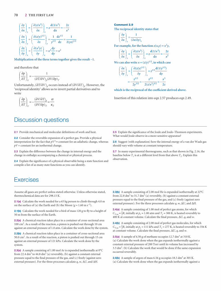
70 2 THE FIRST LAW
z
=z
= z = −
y
=y
= =
x
=x
= x2 = x2
Multiplication of the three terms together gives the result −1.
and therefore that
V
= −
Unfortunately, (∂T/∂V)p occurs instead of (∂V/∂T)p. However, the‘reciprocal identity’ allows us to invert partial derivatives and towrite
V
= − =ακT
(∂V/∂T)p
(∂V/∂p)T
DEF∂p
∂T
ABC
1
(∂T/∂V)p(∂V/∂p)T
DEF∂p
∂T
ABC
dy
dy
DEF∂(x2y)
∂y
ABCDEF
∂z
∂y
ABC
1
2(yz)1/2
dz1/2
dz
1
y1/2
DEF∂(z/y)1/2
∂z
ABCDEF
∂x
∂z
ABC
2z
x3
d(1/x2)
dx
DEF∂(z/x2)
∂x
ABCDEF
∂y
∂x
ABCComment 2.9
The reciprocal identity states that
z
=
For example, for the function z(x,y) = x2y,
z
=z
= z = −
We can also write x = (z/y)1/2, in which case
z
=z
= z1/2
= − = − = −
which is the reciprocal of the coefficient derived above.
Insertion of this relation into eqn 2.57 produces eqn 2.49.
x3
2z
z1/2
2(z/x2)3/2
z1/2
2y 3/2
d(1/y1/2)
dy
DEF∂(z/y)1/2
∂y
ABCDEF
∂x
∂y
ABC
2z
x3
d(1/x 2)
dx
DEF∂(z/x2)
∂x
ABCDEF
∂y
∂x
ABC
1
(∂x/∂y)z
DEF∂y
∂x
ABC
Discussion questions
2.1 Provide mechanical and molecular definitions of work and heat.
2.2 Consider the reversible expansion of a perfect gas. Provide a physicalinterpretation for the fact that pV γ = constant for an adiabatic change, whereaspV = constant for an isothermal change.
2.3 Explain the difference between the change in internal energy and thechange in enthalpy accompanying a chemical or physical process.
2.4 Explain the significance of a physical observable being a state function andcompile a list of as many state functions as you can identify.
2.5 Explain the significance of the Joule and Joule–Thomson experiments.What would Joule observe in a more sensitive apparatus?
2.6 Suggest (with explanation) how the internal energy of a van der Waals gasshould vary with volume at constant temperature.
2.7 In many experimental thermograms, such as that shown in Fig. 2.16, thebaseline below T1 is at a different level from that above T2. Explain thisobservation.
Exercises
Assume all gases are perfect unless stated otherwise. Unless otherwise stated,thermochemical data are for 298.15 K.
2.1(a) Calculate the work needed for a 65 kg person to climb through 4.0 mon the surface of (a) the Earth and (b) the Moon (g = 1.60 m s−2).
2.1(b) Calculate the work needed for a bird of mass 120 g to fly to a height of50 m from the surface of the Earth.
2.2(a) A chemical reaction takes place in a container of cross-sectional area100 cm2. As a result of the reaction, a piston is pushed out through 10 cmagainst an external pressure of 1.0 atm. Calculate the work done by the system.
2.2(b) A chemical reaction takes place in a container of cross-sectional area50.0 cm2. As a result of the reaction, a piston is pushed out through 15 cmagainst an external pressure of 121 kPa. Calculate the work done by thesystem.
2.3(a) A sample consisting of 1.00 mol Ar is expanded isothermally at 0°Cfrom 22.4 dm3 to 44.8 dm3 (a) reversibly, (b) against a constant externalpressure equal to the final pressure of the gas, and (c) freely (against zeroexternal pressure). For the three processes calculate q, w, ∆U, and ∆H.
2.3(b) A sample consisting of 2.00 mol He is expanded isothermally at 22°Cfrom 22.8 dm3 to 31.7 dm3 (a) reversibly, (b) against a constant externalpressure equal to the final pressure of the gas, and (c) freely (against zeroexternal pressure). For the three processes calculate q, w, ∆U, and ∆H.
2.4(a) A sample consisting of 1.00 mol of perfect gas atoms, for which CV,m = 3–
2R, initially at p1 = 1.00 atm and T1 = 300 K, is heated reversibly to 400 K at constant volume. Calculate the final pressure, ∆U, q, and w.
2.4(b) A sample consisting of 2.00 mol of perfect gas molecules, for whichCV,m = 5–
2R, initially at p1 = 111 kPa and T1 = 277 K, is heated reversibly to 356 Kat constant volume. Calculate the final pressure, ∆U, q, and w.
2.5(a) A sample of 4.50 g of methane occupies 12.7 dm3 at 310 K. (a) Calculate the work done when the gas expands isothermally against aconstant external pressure of 200 Torr until its volume has increased by 3.3 dm3. (b) Calculate the work that would be done if the same expansionoccurred reversibly.
2.5(b) A sample of argon of mass 6.56 g occupies 18.5 dm3 at 305 K. (a) Calculate the work done when the gas expands isothermally against a

EXERCISES 71
constant external pressure of 7.7 kPa until its volume has increased by 2.5 dm3.(b) Calculate the work that would be done if the same expansion occurredreversibly.
2.6(a) A sample of 1.00 mol H2O(g) is condensed isothermally and reversiblyto liquid water at 100°C. The standard enthalpy of vaporization of water at100°C is 40.656 kJ mol−1. Find w, q, ∆U, and ∆H for this process.
2.6(b) A sample of 2.00 mol CH3OH(g) is condensed isothermally andreversibly to liquid at 64°C. The standard enthalpy of vaporization ofmethanol at 64°C is 35.3 kJ mol−1. Find w, q, ∆U, and ∆H for this process.
2.7(a) A strip of magnesium of mass 15 g is dropped into a beaker of dilutehydrochloric acid. Calculate the work done by the system as a result of thereaction. The atmospheric pressure is 1.0 atm and the temperature 25°C.
2.7(b) A piece of zinc of mass 5.0 g is dropped into a beaker of dilutehydrochloric acid. Calculate the work done by the system as a result of thereaction. The atmospheric pressure is 1.1 atm and the temperature 23°C.
2.8(a) The constant-pressure heat capacity of a sample of a perfect gas wasfound to vary with temperature according to the expression Cp /(J K−1) = 20.17+ 0.3665(T/K). Calculate q, w, ∆U, and ∆H when the temperature is raisedfrom 25°C to 200°C (a) at constant pressure, (b) at constant volume.
2.8(b) The constant-pressure heat capacity of a sample of a perfect gas wasfound to vary with temperature according to the expression Cp /(J K−1) = 20.17+ 0.4001(T/K). Calculate q, w, ∆U, and ∆H when the temperature is raisedfrom 0°C to 100°C (a) at constant pressure, (b) at constant volume.
2.9(a) Calculate the final temperature of a sample of argon of mass 12.0 g thatis expanded reversibly and adiabatically from 1.0 dm3 at 273.15 K to 3.0 dm3.
2.9(b) Calculate the final temperature of a sample of carbon dioxide of mass16.0 g that is expanded reversibly and adiabatically from 500 cm3 at 298.15 Kto 2.00 dm3.
2.10(a) A sample of carbon dioxide of mass 2.45 g at 27.0°C is allowed toexpand reversibly and adiabatically from 500 cm3 to 3.00 dm3. What is thework done by the gas?
2.10(b) A sample of nitrogen of mass 3.12 g at 23.0°C is allowed to expandreversibly and adiabatically from 400 cm3 to 2.00 dm3. What is the work doneby the gas?
2.11(a) Calculate the final pressure of a sample of carbon dioxide thatexpands reversibly and adiabatically from 57.4 kPa and 1.0 dm3 to a finalvolume of 2.0 dm3. Take γ = 1.4.
2.11(b) Calculate the final pressure of a sample of water vapour that expandsreversibly and adiabatically from 87.3 Torr and 500 cm3 to a final volume of3.0 dm3. Take γ = 1.3.
2.12(a) When 229 J of energy is supplied as heat to 3.0 mol Ar(g), thetemperature of the sample increases by 2.55 K. Calculate the molar heatcapacities at constant volume and constant pressure of the gas.
2.12(b) When 178 J of energy is supplied as heat to 1.9 mol of gas molecules,the temperature of the sample increases by 1.78 K. Calculate the molar heatcapacities at constant volume and constant pressure of the gas.
2.13(a) When 3.0 mol O2 is heated at a constant pressure of 3.25 atm, itstemperature increases from 260 K to 285 K. Given that the molar heat capacityof O2 at constant pressure is 29.4 J K−1 mol−1, calculate q, ∆H, and ∆U.
2.13(b) When 2.0 mol CO2 is heated at a constant pressure of 1.25 atm, itstemperature increases from 250 K to 277 K. Given that the molar heat capacityof CO2 at constant pressure is 37.11 J K−1 mol−1, calculate q, ∆H, and ∆U.
2.14(a) A sample of 4.0 mol O2 is originally confined in 20 dm3 at 270 K andthen undergoes adiabatic expansion against a constant pressure of 600 Torruntil the volume has increased by a factor of 3.0. Calculate q, w, ∆T, ∆U, and∆H. (The final pressure of the gas is not necessarily 600 Torr.)
2.14(b) A sample of 5.0 mol CO2 is originally confined in 15 dm3 at 280 K andthen undergoes adiabatic expansion against a constant pressure of 78.5 kPauntil the volume has increased by a factor of 4.0. Calculate q, w, ∆T, ∆U, and∆H. (The final pressure of the gas is not necessarily 78.5 kPa.)
2.15(a) A sample consisting of 1.0 mol of perfect gas molecules with CV =20.8 J K−1 is initially at 3.25 atm and 310 K. It undergoes reversible adiabaticexpansion until its pressure reaches 2.50 atm. Calculate the final volume andtemperature and the work done.
2.15(b) A sample consisting of 1.5 mol of perfect gas molecules with Cp,m = 20.8 J K−1 mol−1 is initially at 230 kPa and 315 K. It undergoes reversibleadiabatic expansion until its pressure reaches 170 kPa. Calculate the finalvolume and temperature and the work done.
2.16(a) A certain liquid has ∆ vapH 7 = 26.0 kJ mol−1. Calculate q, w, ∆H, and∆U when 0.50 mol is vaporized at 250 K and 750 Torr.
2.16(b) A certain liquid has ∆ vapH 7 = 32.0 kJ mol−1. Calculate q, w, ∆H, and∆U when 0.75 mol is vaporized at 260 K and 765 Torr.
2.17(a) The standard enthalpy of formation of ethylbenzene is −12.5 kJ mol−1.Calculate its standard enthalpy of combustion.
2.17(b) The standard enthalpy of formation of phenol is −165.0 kJ mol−1.Calculate its standard enthalpy of combustion.
2.18(a) The standard enthalpy of combustion of cyclopropane is −2091 kJmol−1 at 25°C. From this information and enthalpy of formation data forCO2(g) and H2O(g), calculate the enthalpy of formation of cyclopropane. Theenthalpy of formation of propene is +20.42 kJ mol−1. Calculate the enthalpy ofisomerization of cyclopropane to propene.
2.18(b) From the following data, determine ∆f H7 for diborane, B2H6(g), at
298 K:
(1) B2H6(g) + 3 O2(g) → B2O3(s) + 3 H2O(g) ∆rH7 = −1941 kJ mol−1
(2) 2 B(s) + 3–2 O2(g) → B2O3(s) ∆rH
7 = −2368 kJ mol−1
(3) H2(g) + 1–2 O2(g) → H2O(g) ∆rH
7 = −241.8 kJ mol−1
2.19(a) When 120 mg of naphthalene, C10H8(s), was burned in a bombcalorimeter the temperature rose by 3.05 K. Calculate the calorimeterconstant. By how much will the temperature rise when 10 mg of phenol,C6H5OH(s), is burned in the calorimeter under the same conditions?
2.19(b) When 2.25 mg of anthracene, C14H10(s), was burned in a bombcalorimeter the temperature rose by 1.35 K. Calculate the calorimeterconstant. By how much will the temperature rise when 135 mg of phenol,C6H5OH(s), is burned in the calorimeter under the same conditions?(∆cH
7(C14H10, s) = −7061 kJ mol−1.)
2.20(a) Calculate the standard enthalpy of solution of AgCl(s) in water fromthe enthalpies of formation of the solid and the aqueous ions.
2.20(b) Calculate the standard enthalpy of solution of AgBr(s) in water fromthe enthalpies of formation of the solid and the aqueous ions.
2.21(a) The standard enthalpy of decomposition of the yellow complexH3NSO2 into NH3 and SO2 is +40 kJ mol−1. Calculate the standard enthalpy offormation of H3NSO2.
2.21(b) Given that the standard enthalpy of combustion of graphite is −393.51 kJ mol−1 and that of diamond is −395.41 kJ mol−1, calculate theenthalpy of the graphite-to-diamond transition.
2.22(a) Given the reactions (1) and (2) below, determine (a) ∆r H 7 and ∆rU7
for reaction (3), (b) ∆fH7 for both HCl(g) and H2O(g) all at 298 K.
(1) H2(g) + Cl2(g) → 2 HCl(g) ∆rH7 = −184.62 kJ mol−1
(2) 2 H2(g) + O2(g) → 2 H2O(g) ∆rH7 = −483.64 kJ mol−1
(3) 4 HCl(g) + O2(g) → Cl2(g) + 2 H2O(g)

72 2 THE FIRST LAW
2.22(b) Given the reactions (1) and (2) below, determine (a) ∆rH7 and
∆rU7 for reaction (3), (b) ∆fH
7 for both HCl(g) and H2O(g) all at 298 K.
(1) H2(g) + I2(s) → 2 HI(g) ∆rH7 = +52.96 kJ mol−1
(2) 2 H2(g) + O2(g) → 2 H2O(g) ∆rH7 = −483.64 kJ mol−1
(3) 4 HI(g) + O2(g) → 2 I2(s) + 2 H2O(g)
2.23(a) For the reaction C2H5OH(l) + 3 O2(g) → 2 CO2(g) + 3 H2O(g),∆rU
7 = −1373 kJ mol−1 at 298 K. Calculate ∆rH7.
2.23(b) For the reaction 2 C6H5COOH(s) + 13 O2(g) → 12 CO2(g) +6 H2O(g), ∆rU
7 = −772.7 kJ mol−1 at 298 K. Calculate ∆rH7.
2.24(a) Calculate the standard enthalpies of formation of (a) KClO3(s) fromthe enthalpy of formation of KCl, (b) NaHCO3(s) from the enthalpies offormation of CO2 and NaOH together with the following information:
2 KClO3(s) → 2 KCl(s) + 3 O2(g) ∆rH7 = −89.4 kJ mol−1
NaOH(s) + CO2(g) → NaHCO3(s) ∆rH7 = −127.5 kJ mol−1
2.24(b) Calculate the standard enthalpy of formation of NOCl(g) from theenthalpy of formation of NO given in Table 2.5, together with the followinginformation:
2 NOCl(g) → 2 NO(g) + Cl2(g) ∆rH7 = +75.5 kJ mol−1
2.25(a) Use the information in Table 2.5 to predict the standard reactionenthalpy of 2 NO2(g) → N2O4(g) at 100°C from its value at 25°C.
2.25(b) Use the information in Table 2.5 to predict the standard reactionenthalpy of 2 H2(g) + O2(g) → 2 H2O(l) at 100°C from its value at 25°C.
2.26(a) From the data in Table 2.5, calculate ∆rH7 and ∆rU
7 at (a) 298 K, (b) 378 K for the reaction C(graphite) + H2O(g) → CO(g) + H2(g). Assume all heat capacities to be constant over the temperature range of interest.
2.26(b) Calculate ∆rH7 and ∆rU
7 at 298 K and ∆rH7 at 348 K for the
hydrogenation of ethyne (acetylene) to ethene (ethylene) from the enthalpy ofcombustion and heat capacity data in Tables 2.5 and 2.7. Assume the heatcapacities to be constant over the temperature range involved.
2.27(a) Calculate ∆rH7 for the reaction Zn(s) + CuSO4(aq) → ZnSO4(aq) +
Cu(s) from the information in Table 2.7 in the Data section.
2.27(b) Calculate ∆rH7 for the reaction NaCl(aq) + AgNO3(aq) → AgCl(s) +
NaNO3(aq) from the information in Table 2.7 in the Data section.
2.28(a) Set up a thermodynamic cycle for determining the enthalpy ofhydration of Mg2+ ions using the following data: enthalpy of sublimation ofMg(s), +167.2 kJ mol−1; first and second ionization enthalpies of Mg(g), 7.646 eV and 15.035 eV; dissociation enthalpy of Cl2(g), +241.6 kJ mol−1;electron gain enthalpy of Cl(g), −3.78 eV; enthalpy of solution of MgCl2(s),−150.5 kJ mol−1; enthalpy of hydration of Cl−(g), −383.7 kJ mol−1.
2.28(b) Set up a thermodynamic cycle for determining the enthalpy ofhydration of Ca2+ ions using the following data: enthalpy of sublimation of Ca(s), +178.2 kJ mol−1; first and second ionization enthalpies of Ca(g),589.7 kJ mol−1 and 1145 kJ mol−1; enthalpy of vaporization of bromine,+30.91 kJ mol−1; dissociation enthalpy of Br2(g), +192.9 kJ mol−1; electrongain enthalpy of Br(g), −331.0 kJ mol−1; enthalpy of solution of CaBr2(s), −103.1 kJ mol−1; enthalpy of hydration of Br−(g), −337 kJ mol−1.
2.29(a) When a certain freon used in refrigeration was expanded adiabaticallyfrom an initial pressure of 32 atm and 0°C to a final pressure of 1.00 atm, thetemperature fell by 22 K. Calculate the Joule–Thomson coefficient, µ, at 0°C,assuming it remains constant over this temperature range.
2.29(b) A vapour at 22 atm and 5°C was allowed to expand adiabatically to afinal pressure of 1.00 atm; the temperature fell by 10 K. Calculate theJoule–Thomson coefficient, µ, at 5°C, assuming it remains constant over thistemperature range.
2.30(a) For a van der Waals gas, πT = a/V 2m. Calculate ∆Um for the isothermal
expansion of nitrogen gas from an initial volume of 1.00 dm3 to 24.8 dm3 at298 K. What are the values of q and w?
2.30(b) Repeat Exercise 2.30(a) for argon, from an initial volume of 1.00 dm3
to 22.1 dm3 at 298 K.
2.31(a) The volume of a certain liquid varies with temperature as
V = V ′{0.75 + 3.9 × 10⁻⁴(T/K) + 1.48 × 10⁻⁶(T/K)2}
where V ′ is its volume at 300 K. Calculate its expansion coefficient, α, at 320 K.
2.31(b) The volume of a certain liquid varies with temperature as
V = V ′{0.77 + 3.7 × 10⁻⁴(T/K) + 1.52 × 10⁻⁶(T/K)2}
where V ′ is its volume at 298 K. Calculate its expansion coefficient, α, at 310 K.
2.32(a) The isothermal compressibility of copper at 293 K is 7.35 ×10⁻⁷ atm−1. Calculate the pressure that must be applied in order to increase itsdensity by 0.08 per cent.
2.32(b) The isothermal compressibility of lead at 293 K is 2.21 × 10⁻⁶ atm−1.Calculate the pressure that must be applied in order to increase its density by0.08 per cent.
2.33(a) Given that µ = 0.25 K atm−1 for nitrogen, calculate the value of itsisothermal Joule–Thomson coefficient. Calculate the energy that must besupplied as heat to maintain constant temperature when 15.0 mol N2 flowsthrough a throttle in an isothermal Joule–Thomson experiment and thepressure drop is 75 atm.
2.33(b) Given that µ = 1.11 K atm−1 for carbon dioxide, calculate the value ofits isothermal Joule–Thomson coefficient. Calculate the energy that must besupplied as heat to maintain constant temperature when 12.0 mol CO2 flowsthrough a throttle in an isothermal Joule–Thomson experiment and thepressure drop is 55 atm.
PROBLEMS 73
Problems*
Assume all gases are perfect unless stated otherwise. Note that 1 atm =1.013 25 bar. Unless otherwise stated, thermochemical data are for 298.15 K.
Numerical problems
2.1 A sample consisting of 1 mol of perfect gas atoms (for which CV,m = 3–
2 R) is taken through the cycle shown in Fig. 2.34. (a) Determine thetemperature at the points 1, 2, and 3. (b) Calculate q, w, ∆U, and ∆H for eachstep and for the overall cycle. If a numerical answer cannot be obtained fromthe information given, then write in +, −, 0, or ? as appropriate.
2.2 A sample consisting of 1.0 mol CaCO3(s) was heated to 800°C, when itdecomposed. The heating was carried out in a container fitted with a pistonthat was initially resting on the solid. Calculate the work done duringcomplete decomposition at 1.0 atm. What work would be done if instead ofhaving a piston the container was open to the atmosphere?
2.3 A sample consisting of 2.0 mol CO2 occupies a fixed volume of 15.0 dm3
at 300 K. When it is supplied with 2.35 kJ of energy as heat its temperatureincreases to 341 K. Assume that CO2 is described by the van der Waalsequation of state, and calculate w, ∆U, and ∆H.
2.4 A sample of 70 mmol Kr(g) expands reversibly and isothermally at 373 Kfrom 5.25 cm3 to 6.29 cm3, and the internal energy of the sample is known toincrease by 83.5 J. Use the virial equation of state up to the second coefficientB = −28.7 cm3 mol−1 to calculate w, q, and ∆H for this change of state.
2.5 A sample of 1.00 mol perfect gas molecules with Cp,m = 7–2R is put through
the following cycle: (a) constant-volume heating to twice its initial volume,(b) reversible, adiabatic expansion back to its initial temperature, (c)reversible isothermal compression back to 1.00 atm. Calculate q, w, ∆U, and∆H for each step and overall.
2.6 Calculate the work done during the isothermal reversible expansion of avan der Waals gas. Account physically for the way in which the coefficients aand b appear in the final expression. Plot on the same graph the indicatordiagrams for the isothermal reversible expansion of (a) a perfect gas, (b) a van der Waals gas in which a = 0 and b = 5.11 × 10⁻² dm3 mol−1, and (c) a = 4.2 dm6 atm mol−2 and b = 0. The values selected exaggerate theimperfections but give rise to significant effects on the indicator diagrams.Take Vi = 1.0 dm3, n = 1.0 mol, and T = 298 K.
2.7 The molar heat capacity of ethane is represented in the temperature range298 K to 400 K by the empirical expression Cp,m /(J K−1 mol−1) = 14.73 +0.1272(T/K). The corresponding expressions for C(s) and H2(g) are given in
Fig. 2.34
Table 2.2. Calculate the standard enthalpy of formation of ethane at 350 Kfrom its value at 298 K.
2.8 A sample of the sugar d-ribose (C5H10O5) of mass 0.727 g was placed in a calorimeter and then ignited in the presence of excess oxygen. Thetemperature rose by 0.910 K. In a separate experiment in the same calorimeter,the combustion of 0.825 g of benzoic acid, for which the internal energy ofcombustion is −3251 kJ mol−1, gave a temperature rise of 1.940 K. Calculatethe internal energy of combustion of d-ribose and its enthalpy of formation.
2.9 The standard enthalpy of formation of the metallocenebis(benzene)chromium was measured in a calorimeter. It was found for thereaction Cr(C6H6)2(s) → Cr(s) + 2 C6H6(g) that ∆rU
7(583 K) = +8.0 kJ mol−1.Find the corresponding reaction enthalpy and estimate the standard enthalpyof formation of the compound at 583 K. The constant-pressure molarheat capacity of benzene is 136.1 J K−1 mol−1 in its liquid range and 81.67 J K−1 mol−1 as a gas.
2.10‡ From the enthalpy of combustion data in Table 2.5 for the alkanes methane through octane, test the extent to which the relation ∆cH
7 = k{(M/(g mol−1)}n holds and find the numerical values for k and n.Predict ∆cH
7 for decane and compare to the known value.
2.11 It is possible to investigate the thermochemical properties ofhydrocarbons with molecular modelling methods. (a) Use electronic structuresoftware to predict ∆cH
7 values for the alkanes methane through pentane. Tocalculate ∆cH
7 values, estimate the standard enthalpy of formation ofCnH2(n+1)(g) by performing semi-empirical calculations (for example, AM1 or PM3 methods) and use experimental standard enthalpy of formationvalues for CO2(g) and H2O(l). (b) Compare your estimated values with theexperimental values of ∆cH
7 (Table 2.5) and comment on the reliability of the molecular modelling method. (c) Test the extent to which the relation∆cH
7 = k{(M/(g mol−1)}n holds and find the numerical values for k and n.
2.12‡ When 1.3584 g of sodium acetate trihydrate was mixed into 100.0 cm3
of 0.2000 m HCl(aq) at 25°C in a solution calorimeter, its temperature fell by0.397°C on account of the reaction:
H3O+(aq) + NaCH3CO2 · 3 H2O(s)→ Na+(aq) + CH3COOH(aq) + 4 H2O(l).
The heat capacity of the calorimeter is 91.0 J K−1 and the heat capacity densityof the acid solution is 4.144 J K−1 cm−3. Determine the standard enthalpy offormation of the aqueous sodium cation. The standard enthalpy of formationof sodium acetate trihydrate is −1064 kJ mol−1.
2.13‡ Since their discovery in 1985, fullerenes have received the attention ofmany chemical researchers. Kolesov et al. reported the standard enthalpy ofcombustion and of formation of crystalline C60 based on calorimetricmeasurements (V.P. Kolesov, S.M. Pimenova, V.K. Pavlovich, N.B. Tamm,and A.A. Kurskaya, J. Chem. Thermodynamics 28, 1121 (1996)). In one of theirruns, they found the standard specific internal energy of combustion to be −36.0334 kJ g−1 at 298.15 K Compute ∆cH7 and ∆fH
7 of C60.
2.14‡ A thermodynamic study of DyCl3 (E.H.P. Cordfunke, A.S. Booji, andM. Yu. Furkaliouk, J. Chem. Thermodynamics 28, 1387 (1996)) determined itsstandard enthalpy of formation from the following information
(1) DyCl3(s) → DyCl3(aq, in 4.0 m HCl) ∆rH7 = −180.06 kJ mol−1
(2) Dy(s) + 3 HCl(aq, 4.0 m) →DyCl3(aq, in 4.0 m HCl(aq)) + 3–
2 H2(g) ∆rH7 = −699.43 kJ mol−1
(3) 1–2 H2(g) + 1–
2 Cl2(g) → HCl(aq, 4.0 m) ∆rH7 = −158.31 kJ mol−1
Determine ∆fH7(DyCl3, s) from these data.
* Problems denoted with the symbol ‡ were supplied by Charles Trapp, Carmen Giunta, and Marshall Cady.
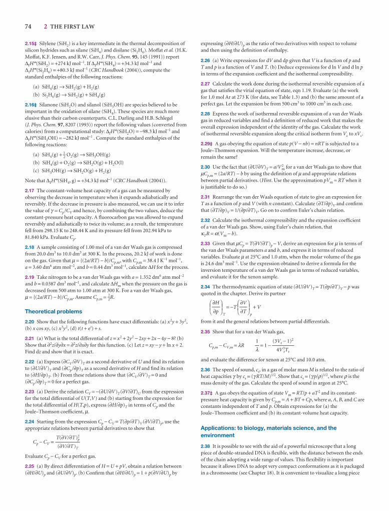
74 2 THE FIRST LAW
2.15‡ Silylene (SiH2) is a key intermediate in the thermal decomposition ofsilicon hydrides such as silane (SiH4) and disilane (Si2H6). Moffat et al. (H.K.Moffat, K.F. Jensen, and R.W. Carr, J. Phys. Chem. 95, 145 (1991)) report∆fH
7(SiH2) = +274 kJ mol−1. If ∆fH7(SiH4) = +34.3 kJ mol−1 and
∆fH7(Si2H6) = +80.3 kJ mol−1 (CRC Handbook (2004)), compute the
standard enthalpies of the following reactions:
(a) SiH4(g) → SiH2(g) + H2(g)
(b) Si2H6(g) → SiH2(g) + SiH4(g)
2.16‡ Silanone (SiH2O) and silanol (SiH3OH) are species believed to beimportant in the oxidation of silane (SiH4). These species are much moreelusive than their carbon counterparts. C.L. Darling and H.B. Schlegel(J. Phys. Chem. 97, 8207 (1993)) report the following values (converted fromcalories) from a computational study: ∆fH
7(SiH2O) = −98.3 kJ mol−1 and∆fH
7(SiH3OH) = −282 kJ mol−1 . Compute the standard enthalpies of thefollowing reactions:
(a) SiH4(g) + 1–2 O2(g) → SiH3OH(g)
(b) SiH4(g) + O2(g) → SiH2O(g) + H2O(l)
(c) SiH3OH(g) → SiH2O(g) + H2(g)
Note that ∆fH7(SiH4, g) = +34.3 kJ mol−1 (CRC Handbook (2004)).
2.17 The constant-volume heat capacity of a gas can be measured byobserving the decrease in temperature when it expands adiabatically andreversibly. If the decrease in pressure is also measured, we can use it to inferthe value of γ = Cp /CV and hence, by combining the two values, deduce theconstant-pressure heat capacity. A fluorocarbon gas was allowed to expandreversibly and adiabatically to twice its volume; as a result, the temperaturefell from 298.15 K to 248.44 K and its pressure fell from 202.94 kPa to81.840 kPa. Evaluate Cp.
2.18 A sample consisting of 1.00 mol of a van der Waals gas is compressedfrom 20.0 dm3 to 10.0 dm3 at 300 K. In the process, 20.2 kJ of work is doneon the gas. Given that µ = {(2a/RT) − b}/Cp,m, with Cp,m = 38.4 J K−1 mol−1,a = 3.60 dm6 atm mol−2, and b = 0.44 dm3 mol−1, calculate ∆H for the process.
2.19 Take nitrogen to be a van der Waals gas with a = 1.352 dm6 atm mol−2
and b = 0.0387 dm3 mol−1, and calculate ∆Hm when the pressure on the gas isdecreased from 500 atm to 1.00 atm at 300 K. For a van der Waals gas, µ = {(2a/RT) − b}/Cp,m. Assume Cp,m = 7–
2R.
Theoretical problems
2.20 Show that the following functions have exact differentials: (a) x2y + 3y2,(b) x cos xy, (c) x3y2, (d) t(t + es) + s.
2.21 (a) What is the total differential of z = x2 + 2y2 − 2xy + 2x − 4y − 8? (b)Show that ∂2z/∂y∂x = ∂2z/∂x∂y for this function. (c) Let z = xy − y + ln x + 2.Find dz and show that it is exact.
2.22 (a) Express (∂CV /∂V)T as a second derivative of U and find its relationto (∂U/∂V)T and (∂Cp /∂p)T as a second derivative of H and find its relation to (∂H/∂p)T. (b) From these relations show that (∂CV /∂V)T = 0 and(∂Cp /∂p)T = 0 for a perfect gas.
2.23 (a) Derive the relation CV = −(∂U/∂V)T (∂V/∂T)U from the expressionfor the total differential of U(T,V) and (b) starting from the expression forthe total differential of H(T,p), express (∂H/∂p)T in terms of Cp and theJoule–Thomson coefficient, µ.
2.24 Starting from the expression Cp − CV = T(∂p/∂T)V (∂V/∂T)p, use theappropriate relations between partial derivatives to show that
Cp − CV =
Evaluate Cp − CV for a perfect gas.
2.25 (a) By direct differentiation of H = U + pV, obtain a relation between(∂H/∂U)p and (∂U/∂V)p. (b) Confirm that (∂H/∂U)p = 1 + p(∂V/∂U)p by
T(∂V/∂T)2p
(∂V/∂T)T
expressing (∂H/∂U)p as the ratio of two derivatives with respect to volumeand then using the definition of enthalpy.
2.26 (a) Write expressions for dV and dp given that V is a function of p andT and p is a function of V and T. (b) Deduce expressions for d ln V and d ln pin terms of the expansion coefficient and the isothermal compressibility.
2.27 Calculate the work done during the isothermal reversible expansion of agas that satisfies the virial equation of state, eqn 1.19. Evaluate (a) the workfor 1.0 mol Ar at 273 K (for data, see Table 1.3) and (b) the same amount of aperfect gas. Let the expansion be from 500 cm3 to 1000 cm3 in each case.
2.28 Express the work of isothermal reversible expansion of a van der Waalsgas in reduced variables and find a definition of reduced work that makes theoverall expression independent of the identity of the gas. Calculate the workof isothermal reversible expansion along the critical isotherm from Vc to xVc.
2.29‡ A gas obeying the equation of state p(V − nb) = nRT is subjected to aJoule–Thomson expansion. Will the temperature increase, decrease, orremain the same?
2.30 Use the fact that (∂U/∂V)T = a/V 2m for a van der Waals gas to show that
µCp,m ≈ (2a/RT) − b by using the definition of µ and appropriate relationsbetween partial derivatives. (Hint. Use the approximation pVm ≈ RT when itis justifiable to do so.)
2.31 Rearrange the van der Waals equation of state to give an expression forT as a function of p and V (with n constant). Calculate (∂T/∂p)V and confirmthat (∂T/∂p)V = 1/(∂p/∂T)V. Go on to confirm Euler’s chain relation.
2.32 Calculate the isothermal compressibility and the expansion coefficientof a van der Waals gas. Show, using Euler’s chain relation, that κTR = α(Vm − b).
2.33 Given that µCp = T(∂V/∂T)p − V, derive an expression for µ in terms ofthe van der Waals parameters a and b, and express it in terms of reducedvariables. Evaluate µ at 25°C and 1.0 atm, when the molar volume of the gasis 24.6 dm3 mol−1. Use the expression obtained to derive a formula for theinversion temperature of a van der Waals gas in terms of reduced variables,and evaluate it for the xenon sample.
2.34 The thermodynamic equation of state (∂U/∂V)T = T(∂p/∂T)V − p wasquoted in the chapter. Derive its partner
T
= −Tp
+ V
from it and the general relations between partial differentials.
2.35 Show that for a van der Waals gas,
Cp,m − CV,m = λR = 1 −
and evaluate the difference for xenon at 25°C and 10.0 atm.
2.36 The speed of sound, cs, in a gas of molar mass M is related to the ratio ofheat capacities γ by cs = (γ RT/M)1/2. Show that cs = (γ p/ρ)1/2, where ρ is themass density of the gas. Calculate the speed of sound in argon at 25°C.
2.37‡ A gas obeys the equation of state Vm = RT/p + aT 2 and its constant-pressure heat capacity is given by Cp,m = A + BT + Cp, where a, A, B, and C areconstants independent of T and p. Obtain expressions for (a) theJoule–Thomson coefficient and (b) its constant-volume heat capacity.
Applications: to biology, materials science, and theenvironment
2.38 It is possible to see with the aid of a powerful microscope that a longpiece of double-stranded DNA is flexible, with the distance between the endsof the chain adopting a wide range of values. This flexibility is importantbecause it allows DNA to adopt very compact conformations as it is packagedin a chromosome (see Chapter 18). It is convenient to visualize a long piece
(3Vr − 1)2
4V 3rTr
1
λ
DEF∂V
∂T
ABCDEF
∂H
∂p
ABC
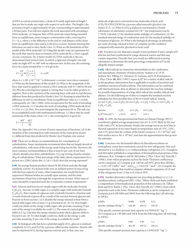
PROBLEMS 75
of DNA as a freely jointed chain, a chain of N small, rigid units of length lthat are free to make any angle with respect to each other. The length l, thepersistence length, is approximately 45 nm, corresponding to approximately130 base pairs. You will now explore the work associated with extending aDNA molecule. (a) Suppose that a DNA molecule resists being extendedfrom an equilibrium, more compact conformation with a restoring forceF = −kF x, where x is the difference in the end-to-end distance of the chainfrom an equilibrium value and kF is the force constant. Systems showing thisbehaviour are said to obey Hooke’s law. (i) What are the limitations of thismodel of the DNA molecule? (ii) Using this model, write an expression forthe work that must be done to extend a DNA molecule by x. Draw a graph of your conclusion. (b) A better model of a DNA molecule is the one-dimensional freely jointed chain, in which a rigid unit of length l can onlymake an angle of 0° or 180° with an adjacent unit. In this case, the restoringforce of a chain extended by x = nl is given by
F = ln ν = n/N
where k = 1.381 × 10⁻²³ J K−1 is Boltzmann’s constant (not a force constant).(i) What are the limitations of this model? (ii) What is the magnitude of theforce that must be applied to extend a DNA molecule with N = 200 by 90 nm?(iii) Plot the restoring force against ν, noting that ν can be either positive ornegative. How is the variation of the restoring force with end-to-end distancedifferent from that predicted by Hooke’s law? (iv) Keeping in mind that thedifference in end-to-end distance from an equilibrium value is x = nl and,consequently, dx = ldn = Nldν, write an expression for the work of extendinga DNA molecule. (v) Calculate the work of extending a DNA molecule fromν = 0 to ν = 1.0. Hint. You must integrate the expression for w. The task canbe accomplished easily with mathematical software. (c) Show that for smallextensions of the chain, when ν << 1, the restoring force is given by
F ≈ =
Hint. See Appendix 2 for a review of series expansions of functions. (d) Is thevariation of the restoring force with extension of the chain given in part (c) different from that predicted by Hooke’s law? Explain your answer.
2.39 There are no dietary recommendations for consumption ofcarbohydrates. Some nutritionists recommend diets that are largely devoid ofcarbohydrates, with most of the energy needs being met by fats. However, themost common recommendation is that at least 65 per cent of our foodcalories should come from carbohydrates. A 3–
4-cup serving of pasta contains40 g of carbohydrates. What percentage of the daily calorie requirement for aperson on a 2200 Calorie diet (1 Cal = 1 kcal) does this serving represent?
2.40 An average human produces about 10 MJ of heat each day throughmetabolic activity. If a human body were an isolated system of mass 65 kgwith the heat capacity of water, what temperature rise would the bodyexperience? Human bodies are actually open systems, and the mainmechanism of heat loss is through the evaporation of water. What mass ofwater should be evaporated each day to maintain constant temperature?
2.41 Glucose and fructose are simple sugars with the molecular formulaC6H12O6. Sucrose, or table sugar, is a complex sugar with molecular formulaC12H22O11 that consists of a glucose unit covalently bound to a fructose unit(a water molecule is given off as a result of the reaction between glucose andfructose to form sucrose). (a) Calculate the energy released as heat when atypical table sugar cube of mass 1.5 g is burned in air. (b) To what heightcould you climb on the energy a table sugar cube provides assuming 25 percent of the energy is available for work? (c) The mass of a typical glucosetablet is 2.5 g. Calculate the energy released as heat when a glucose tablet isburned in air. (d) To what height could you climb on the energy a cubeprovides assuming 25 per cent of the energy is available for work?
2.42 In biological cells that have a plentiful supply of O2, glucose is oxidizedcompletely to CO2 and H2O by a process called aerobic oxidation. Muscle cellsmay be deprived of O2 during vigorous exercise and, in that case, one
nkT
Nl
νkT
l
DEF1 + ν1 − ν
ABCkT
2l
molecule of glucose is converted to two molecules of lactic acid (CH3CH (OH)COOH) by a process called anaerobic glycolysis (seeImpact I7.2). (a) When 0.3212 g of glucose was burned in a bomb calorimeter of calorimeter constant 641 J K−1 the temperature rose by 7.793 K. Calculate (i) the standard molar enthalpy of combustion, (ii) thestandard internal energy of combustion, and (iii) the standard enthalpy offormation of glucose. (b) What is the biological advantage (in kilojoules per mole of energy released as heat) of complete aerobic oxidation compared with anaerobic glycolysis to lactic acid?
2.43 You have at your disposal a sample of pure polymer P and a sample of Pthat has just been synthesized in a large chemical reactor and that maycontain impurities. Describe how you would use differential scanningcalorimetry to determine the mole percentage composition of P in theallegedly impure sample.
2.44‡ Alkyl radicals are important intermediates in the combustion and atmospheric chemistry of hydrocarbons. Seakins et al. (P.W. Seakins, M.J. Pilling, J.T. Niiranen, D. Gutman, and L.N. Krasnoperov, J. Phys. Chem. 96, 9847 (1992)) report ∆fH
7 for a variety of alkyl radicals in the gas phase, information that is applicable to studies of pyrolysis andoxidation reactions of hydrocarbons. This information can be combined with thermodynamic data on alkenes to determine the reaction enthalpy for possible fragmentation of a large alkyl radical into smaller radicals andalkenes. Use the following set of data to compute the standard reactionenthalpies for three possible fates of the tert-butyl radical, namely, (a) tert-C4H9 → sec-C4H9, (b) tert-C4H9 → C3H6 + CH3, (c) tert-C4H9 →C2H4 + C2H5.
Species: C2H5 sec-C4H9 tert-C4H9
∆fH7/(kJ mol−1) +121.0 +67.5 +51.3
2.45‡ In 1995, the Intergovernmental Panel on Climate Change (IPCC)considered a global average temperature rise of 1.0–3.5°C likely by the year2100, with 2.0°C its best estimate. Predict the average rise in sea level due tothermal expansion of sea water based on temperature rises of 1.0°C, 2.0°C,and 3.5°C given that the volume of the Earth’s oceans is 1.37 × 10⁹ km3 andtheir surface area is 361 × 106 km2, and state the approximations that go intothe estimates.
2.46‡ Concerns over the harmful effects of chlorofluorocarbons onstratospheric ozone have motivated a search for new refrigerants. One suchalternative is 2,2-dichloro-1,1,1-trifluoroethane (refrigerant 123). Youngloveand McLinden published a compendium of thermophysical properties of thissubstance (B.A. Younglove and M. McLinden, J. Phys. Chem. Ref. Data 23, 7(1994)), from which properties such as the Joule–Thomson coefficient µcan be computed. (a) Compute µ at 1.00 bar and 50°C given that (∂H/∂p)T
= −3.29 × 10³ J MPa−1 mol−1 and Cp,m = 110.0 J K−1 mol−1 . (b) Compute thetemperature change that would accompany adiabatic expansion of 2.0 mol of this refrigerant from 1.5 bar to 0.5 bar at 50°C.
2.47‡ Another alternative refrigerant (see preceding problem) is 1,1,1,2-tetrafluoroethane (refrigerant HFC-134a). Tillner-Roth and Baehr publisheda compendium of thermophysical properties of this substance (R. Tillner-Roth and H.D. Baehr, J. Phys. Chem. Ref. Data 23, 657 (1994)), from whichproperties such as the Joule–Thomson coefficient µ can be computed. (a)Compute µ at 0.100 MPa and 300 K from the following data (all referring to 300 K):
p/MPa 0.080 0.100 0.12
Specific enthalpy/(kJ kg−1) 426.48 426.12 425.76
(The specific constant-pressure heat capacity is 0.7649 kJ K−1 kg−1.)(b) Compute µ at 1.00 MPa and 350 K from the following data (all referringto 350 K):
p/MPa 0.80 1.00 1.2
Specific enthalpy/(kJ kg−1) 461.93 459.12 456.15
(The specific constant-pressure heat capacity is 1.0392 kJ K−1 kg−1.)
The Second Law
The purpose of this chapter is to explain the origin of the spontaneity of physical and chem-ical change. We examine two simple processes and show how to define, measure, and usea property, the entropy, to discuss spontaneous changes quantitatively. The chapter alsointroduces a major subsidiary thermodynamic property, the Gibbs energy, which lets us ex-press the spontaneity of a process in terms of the properties of a system. The Gibbs energyalso enables us to predict the maximum non-expansion work that a process can do. As webegan to see in Chapter 2, one application of thermodynamics is to find relations betweenproperties that might not be thought to be related. Several relations of this kind can be established by making use of the fact that the Gibbs energy is a state function. We also seehow to derive expressions for the variation of the Gibbs energy with temperature and pres-sure and how to formulate expressions that are valid for real gases. These expressions willprove useful later when we discuss the effect of temperature and pressure on equilibriumconstants.
Some things happen naturally; some things don’t. A gas expands to fill the availablevolume, a hot body cools to the temperature of its surroundings, and a chemical reac-tion runs in one direction rather than another. Some aspect of the world determinesthe spontaneous direction of change, the direction of change that does not requirework to be done to bring it about. A gas can be confined to a smaller volume, an objectcan be cooled by using a refrigerator, and some reactions can be driven in reverse (as in the electrolysis of water). However, none of these processes is spontaneous; each one must be brought about by doing work. An important point, though, is thatthroughout this text ‘spontaneous’ must be interpreted as a natural tendency that mayor may not be realized in practice. Thermodynamics is silent on the rate at which aspontaneous change in fact occurs, and some spontaneous processes (such as the con-version of diamond to graphite) may be so slow that the tendency is never realized in practice whereas others (such as the expansion of a gas into a vacuum) are almost instantaneous.
The recognition of two classes of process, spontaneous and non-spontaneous, issummarized by the Second Law of thermodynamics. This law may be expressed in avariety of equivalent ways. One statement was formulated by Kelvin:
No process is possible in which the sole result is the absorption of heat from a reser-voir and its complete conversion into work.
For example, it has proved impossible to construct an engine like that shown inFig. 3.1, in which heat is drawn from a hot reservoir and completely converted intowork. All real heat engines have both a hot source and a cold sink; some energy is always discarded into the cold sink as heat and not converted into work. The Kelvin
The direction of spontaneouschange
3.1 The dispersal of energy
3.2 Entropy
I3.1 Impact on engineering:Refrigeration
3.3 Entropy changesaccompanying specificprocesses
3.4 The Third Law ofthermodynamics
Concentrating on the system
3.5 The Helmholtz and Gibbsenergies
3.6 Standard reaction Gibbsenergies
Combining the First and Second Laws
3.7 The fundamental equation
3.8 Properties of the internalenergy
3.9 Properties of the Gibbs energy
Checklist of key ideas
Further reading
Further information 3.1: The Bornequation
Further information 3.2: Real gases:the fugacity
Discussion questions
Exercises
Problems
3
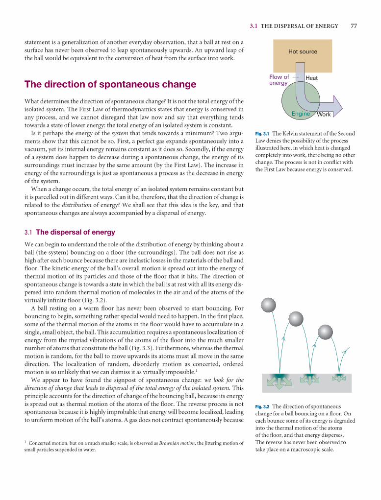
3.1 THE DISPERSAL OF ENERGY 77
statement is a generalization of another everyday observation, that a ball at rest on asurface has never been observed to leap spontaneously upwards. An upward leap ofthe ball would be equivalent to the conversion of heat from the surface into work.
The direction of spontaneous change
What determines the direction of spontaneous change? It is not the total energy of theisolated system. The First Law of thermodynamics states that energy is conserved inany process, and we cannot disregard that law now and say that everything tends towards a state of lower energy: the total energy of an isolated system is constant.
Is it perhaps the energy of the system that tends towards a minimum? Two argu-ments show that this cannot be so. First, a perfect gas expands spontaneously into avacuum, yet its internal energy remains constant as it does so. Secondly, if the energyof a system does happen to decrease during a spontaneous change, the energy of itssurroundings must increase by the same amount (by the First Law). The increase inenergy of the surroundings is just as spontaneous a process as the decrease in energyof the system.
When a change occurs, the total energy of an isolated system remains constant butit is parcelled out in different ways. Can it be, therefore, that the direction of change isrelated to the distribution of energy? We shall see that this idea is the key, and thatspontaneous changes are always accompanied by a dispersal of energy.
3.1 The dispersal of energy
We can begin to understand the role of the distribution of energy by thinking about aball (the system) bouncing on a floor (the surroundings). The ball does not rise ashigh after each bounce because there are inelastic losses in the materials of the ball andfloor. The kinetic energy of the ball’s overall motion is spread out into the energy ofthermal motion of its particles and those of the floor that it hits. The direction ofspontaneous change is towards a state in which the ball is at rest with all its energy dis-persed into random thermal motion of molecules in the air and of the atoms of thevirtually infinite floor (Fig. 3.2).
A ball resting on a warm floor has never been observed to start bouncing. Forbouncing to begin, something rather special would need to happen. In the first place,some of the thermal motion of the atoms in the floor would have to accumulate in asingle, small object, the ball. This accumulation requires a spontaneous localization ofenergy from the myriad vibrations of the atoms of the floor into the much smallernumber of atoms that constitute the ball (Fig. 3.3). Furthermore, whereas the thermalmotion is random, for the ball to move upwards its atoms must all move in the samedirection. The localization of random, disorderly motion as concerted, ordered motion is so unlikely that we can dismiss it as virtually impossible.1
We appear to have found the signpost of spontaneous change: we look for the direction of change that leads to dispersal of the total energy of the isolated system. Thisprinciple accounts for the direction of change of the bouncing ball, because its energyis spread out as thermal motion of the atoms of the floor. The reverse process is notspontaneous because it is highly improbable that energy will become localized, leadingto uniform motion of the ball’s atoms. A gas does not contract spontaneously because
Hot source
Flow ofenergy
Engine
Heat
Work
Fig. 3.1 The Kelvin statement of the SecondLaw denies the possibility of the processillustrated here, in which heat is changedcompletely into work, there being no otherchange. The process is not in conflict withthe First Law because energy is conserved.
Fig. 3.2 The direction of spontaneouschange for a ball bouncing on a floor. Oneach bounce some of its energy is degraded into the thermal motion of the atoms of the floor, and that energy disperses. The reverse has never been observed to take place on a macroscopic scale.
1 Concerted motion, but on a much smaller scale, is observed as Brownian motion, the jittering motion ofsmall particles suspended in water.
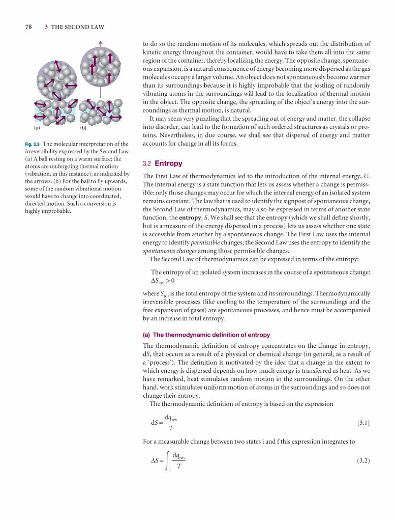
78 3 THE SECOND LAW
to do so the random motion of its molecules, which spreads out the distribution of kinetic energy throughout the container, would have to take them all into the same region of the container, thereby localizing the energy. The opposite change, spontane-ous expansion, is a natural consequence of energy becoming more dispersed as the gasmolecules occupy a larger volume. An object does not spontaneously become warmerthan its surroundings because it is highly improbable that the jostling of randomly vibrating atoms in the surroundings will lead to the localization of thermal motion in the object. The opposite change, the spreading of the object’s energy into the sur-roundings as thermal motion, is natural.
It may seem very puzzling that the spreading out of energy and matter, the collapseinto disorder, can lead to the formation of such ordered structures as crystals or pro-teins. Nevertheless, in due course, we shall see that dispersal of energy and matter accounts for change in all its forms.
3.2 Entropy
The First Law of thermodynamics led to the introduction of the internal energy, U.The internal energy is a state function that lets us assess whether a change is permiss-ible: only those changes may occur for which the internal energy of an isolated systemremains constant. The law that is used to identify the signpost of spontaneous change,the Second Law of thermodynamics, may also be expressed in terms of another statefunction, the entropy, S. We shall see that the entropy (which we shall define shortly,but is a measure of the energy dispersed in a process) lets us assess whether one stateis accessible from another by a spontaneous change. The First Law uses the internalenergy to identify permissible changes; the Second Law uses the entropy to identify thespontaneous changes among those permissible changes.
The Second Law of thermodynamics can be expressed in terms of the entropy:
The entropy of an isolated system increases in the course of a spontaneous change:∆S tot > 0
where Stot is the total entropy of the system and its surroundings. Thermodynamicallyirreversible processes (like cooling to the temperature of the surroundings and thefree expansion of gases) are spontaneous processes, and hence must be accompaniedby an increase in total entropy.
(a) The thermodynamic definition of entropy
The thermodynamic definition of entropy concentrates on the change in entropy, dS, that occurs as a result of a physical or chemical change (in general, as a result of a ‘process’). The definition is motivated by the idea that a change in the extent towhich energy is dispersed depends on how much energy is transferred as heat. As wehave remarked, heat stimulates random motion in the surroundings. On the otherhand, work stimulates uniform motion of atoms in the surroundings and so does notchange their entropy.
The thermodynamic definition of entropy is based on the expression
dS = [3.1]
For a measurable change between two states i and f this expression integrates to
∆S = �f
i
(3.2)dqrev
T
dqrev
T
(a) (b)
Fig. 3.3 The molecular interpretation of theirreversibility expressed by the Second Law.(a) A ball resting on a warm surface; theatoms are undergoing thermal motion(vibration, in this instance), as indicated bythe arrows. (b) For the ball to fly upwards,some of the random vibrational motionwould have to change into coordinated,directed motion. Such a conversion ishighly improbable.
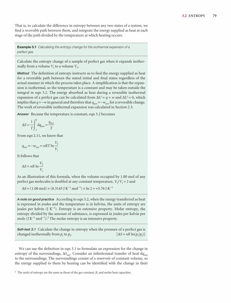
3.2 ENTROPY 79
2 The units of entropy are the same as those of the gas constant, R, and molar heat capacities.
That is, to calculate the difference in entropy between any two states of a system, wefind a reversible path between them, and integrate the energy supplied as heat at eachstage of the path divided by the temperature at which heating occurs.
Example 3.1 Calculating the entropy change for the isothermal expansion of a perfect gas
Calculate the entropy change of a sample of perfect gas when it expands isother-mally from a volume Vi to a volume Vf .
Method The definition of entropy instructs us to find the energy supplied as heatfor a reversible path between the stated initial and final states regardless of the actual manner in which the process takes place. A simplification is that the expan-sion is isothermal, so the temperature is a constant and may be taken outside theintegral in eqn 3.2. The energy absorbed as heat during a reversible isothermal expansion of a perfect gas can be calculated from ∆U = q + w and ∆U = 0, which implies that q = −w in general and therefore that qrev = −wrev for a reversible change.The work of reversible isothermal expansion was calculated in Section 2.3.
Answer Because the temperature is constant, eqn 3.2 becomes
∆S = �f
i
dqrev =
From eqn 2.11, we know that
qrev = −wrev = nRT ln
It follows that
∆S = nR ln
As an illustration of this formula, when the volume occupied by 1.00 mol of anyperfect gas molecules is doubled at any constant temperature, Vf /Vi = 2 and
∆S = (1.00 mol) × (8.3145 J K−1 mol−1) × ln 2 = +5.76 J K−1
A note on good practice According to eqn 3.2, when the energy transferred as heatis expressed in joules and the temperature is in kelvins, the units of entropy arejoules per kelvin (J K−1). Entropy is an extensive property. Molar entropy, the entropy divided by the amount of substance, is expressed in joules per kelvin permole (J K−1 mol−1).2 The molar entropy is an intensive property.
Self-test 3.1 Calculate the change in entropy when the pressure of a perfect gas ischanged isothermally from pi to pf . [∆S = nR ln(pi/pf)]
We can use the definition in eqn 3.1 to formulate an expression for the change inentropy of the surroundings, ∆Ssur. Consider an infinitesimal transfer of heat dqsur
to the surroundings. The surroundings consist of a reservoir of constant volume, sothe energy supplied to them by heating can be identified with the change in their
Vf
Vi
Vf
Vi
qrev
T
1
T
80 3 THE SECOND LAW
3 Alternatively, the surroundings can be regarded as being at constant pressure, in which case we couldequate dqsur to dHsur.
internal energy, dUsur.3 The internal energy is a state function, and dUsur is an exact
differential. As we have seen, these properties imply that dUsur is independent of howthe change is brought about and in particular is independent of whether the process isreversible or irreversible. The same remarks therefore apply to dqsur, to which dUsur isequal. Therefore, we can adapt the definition in eqn 3.1 to write
dSsur = = (3.3a)
Furthermore, because the temperature of the surroundings is constant whatever thechange, for a measurable change
∆Ssur = (3.3b)
That is, regardless of how the change is brought about in the system, reversibly or irreversibly, we can calculate the change of entropy of the surroundings by dividingthe heat transferred by the temperature at which the transfer takes place.
Equation 3.3 makes it very simple to calculate the changes in entropy of the surround-ings that accompany any process. For instance, for any adiabatic change, qsur = 0, so
For an adiabatic change: ∆Ssur = 0 (3.4)
This expression is true however the change takes place, reversibly or irreversibly, pro-vided no local hot spots are formed in the surroundings. That is, it is true so long as thesurroundings remain in internal equilibrium. If hot spots do form, then the localizedenergy may subsequently disperse spontaneously and hence generate more entropy.
Illustration 3.1 Calculating the entropy change in the surroundings
To calculate the entropy change in the surroundings when 1.00 mol H2O(l) isformed from its elements under standard conditions at 298 K, we use ∆H 7 =−286 kJ from Table 2.7. The energy released as heat is supplied to the surroundings,now regarded as being at constant pressure, so qsur = +286 kJ. Therefore,
∆Ssur = = +960 J K−1
This strongly exothermic reaction results in an increase in the entropy of the sur-roundings as energy is released as heat into them.
Self-test 3.2 Calculate the entropy change in the surroundings when 1.00 molN2O4(g) is formed from 2.00 mol NO2(g) under standard conditions at 298 K.
[−192 J K−1]
Molecular interpretation 3.1 The statistical view of entropy
The entry point into the molecular interpretation of the Second Law of thermo-dynamics is the realization that an atom or molecule can possess only certain energies, called its ‘energy levels’. The continuous thermal agitation that molecules
2.86 × 10⁵ J
298 K
qsur
Tsur
dqsur
Tsur
dqsur,rev
Tsur
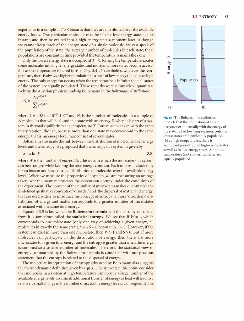
3.2 ENTROPY 81
(a) (b)
En
erg
y
Population
Fig. 3.4 The Boltzmann distributionpredicts that the population of a statedecreases exponentially with the energy ofthe state. (a) At low temperatures, only thelowest states are significantly populated;(b) at high temperatures, there issignificant population in high-energy statesas well as in low-energy states. At infinitetemperature (not shown), all states areequally populated.
experience in a sample at T > 0 ensures that they are distributed over the availableenergy levels. One particular molecule may be in one low energy state at one instant, and then be excited into a high energy state a moment later. Although we cannot keep track of the energy state of a single molecule, we can speak of the population of the state, the average number of molecules in each state; thesepopulations are constant in time provided the temperature remains the same.
Only the lowest energy state is occupied at T = 0. Raising the temperature excitessome molecules into higher energy states, and more and more states become access-ible as the temperature is raised further (Fig. 3.4). Nevertheless, whatever the tem-perature, there is always a higher population in a state of low energy than one of highenergy. The only exception occurs when the temperature is infinite: then all statesof the system are equally populated. These remarks were summarized quantitat-ively by the Austrian physicist Ludwig Boltzmann in the Boltzmann distribution:
Ni =
where k = 1.381 × 10⁻²³ J K−1 and Ni is the number of molecules in a sample of N molecules that will be found in a state with an energy Ei when it is part of a sys-tem in thermal equilibrium at a temperature T. Care must be taken with the exactinterpretation, though, because more than one state may correspond to the sameenergy: that is, an energy level may consist of several states.
Boltzmann also made the link between the distribution of molecules over energylevels and the entropy. He proposed that the entropy of a system is given by
S = k ln W (3.5)
where W is the number of microstates, the ways in which the molecules of a systemcan be arranged while keeping the total energy constant. Each microstate lasts onlyfor an instant and has a distinct distribution of molecules over the available energylevels. When we measure the properties of a system, we are measuring an averagetaken over the many microstates the system can occupy under the conditions of the experiment. The concept of the number of microstates makes quantitative theill-defined qualitative concepts of ‘disorder’ and ‘the dispersal of matter and energy’that are used widely to introduce the concept of entropy: a more ‘disorderly’ dis-tribution of energy and matter corresponds to a greater number of microstates associated with the same total energy.
Equation 3.5 is known as the Boltzmann formula and the entropy calculatedfrom it is sometimes called the statistical entropy. We see that if W = 1, which corresponds to one microstate (only one way of achieving a given energy, allmolecules in exactly the same state), then S = 0 because ln 1 = 0. However, if the system can exist in more than one microstate, then W > 1 and S > 0. But, if moremolecules can participate in the distribution of energy, then there are more microstates for a given total energy and the entropy is greater than when the energyis confined so a smaller number of molecules. Therefore, the statistical view of entropy summarized by the Boltzmann formula is consistent with our previousstatement that the entropy is related to the dispersal of energy.
The molecular interpretation of entropy advanced by Boltzmann also suggeststhe thermodynamic definition given by eqn 3.1. To appreciate this point, considerthat molecules in a system at high temperature can occupy a large number of theavailable energy levels, so a small additional transfer of energy as heat will lead to arelatively small change in the number of accessible energy levels. Consequently, the
Ne−Ei/kT
∑i
e−Ei/kT
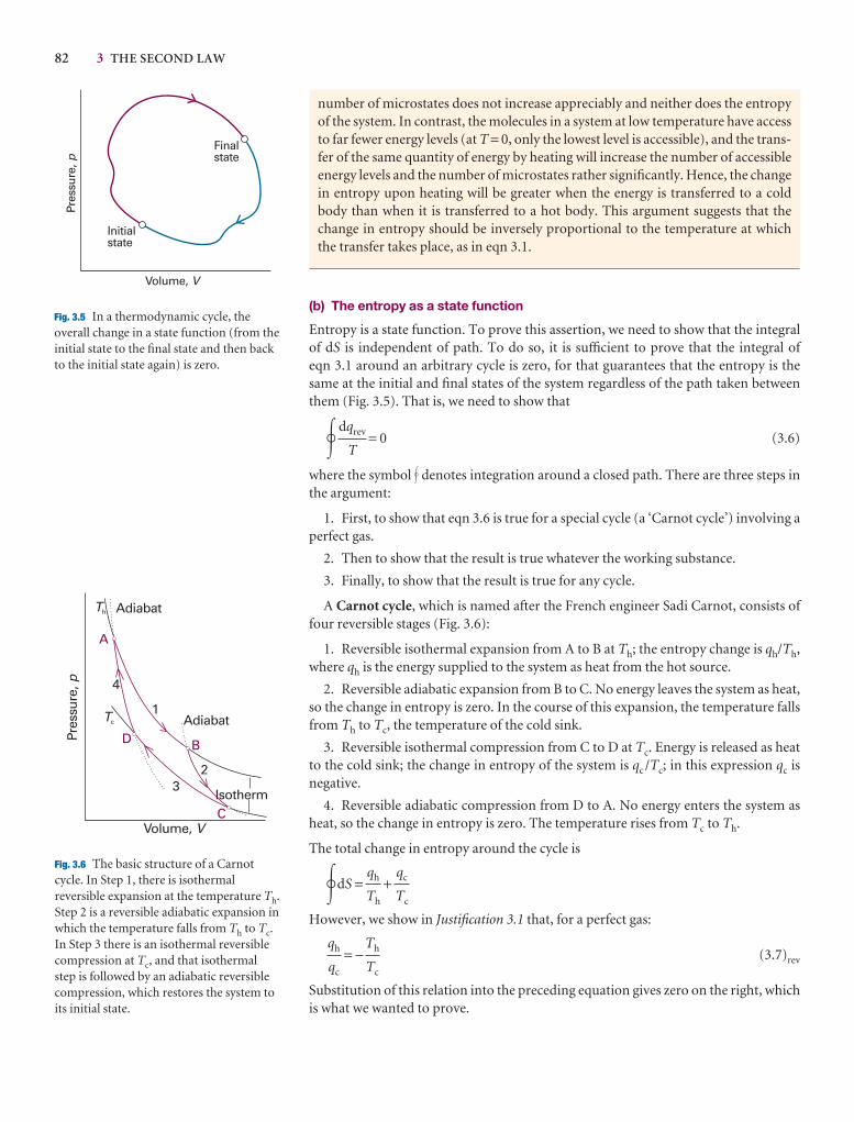
82 3 THE SECOND LAW
Volume, V
Pres
sure
,p
Initialstate
Finalstate
Fig. 3.5 In a thermodynamic cycle, theoverall change in a state function (from theinitial state to the final state and then backto the initial state again) is zero.
Volume, V
Pres
sure
,p
1
23
4
Isotherm
Adiabat
AdiabatTh
Tc
A
B
C
D
Fig. 3.6 The basic structure of a Carnotcycle. In Step 1, there is isothermalreversible expansion at the temperature Th.Step 2 is a reversible adiabatic expansion in which the temperature falls from Th to Tc.In Step 3 there is an isothermal reversiblecompression at Tc, and that isothermal step is followed by an adiabatic reversiblecompression, which restores the system toits initial state.
number of microstates does not increase appreciably and neither does the entropyof the system. In contrast, the molecules in a system at low temperature have accessto far fewer energy levels (at T = 0, only the lowest level is accessible), and the trans-fer of the same quantity of energy by heating will increase the number of accessibleenergy levels and the number of microstates rather significantly. Hence, the changein entropy upon heating will be greater when the energy is transferred to a coldbody than when it is transferred to a hot body. This argument suggests that thechange in entropy should be inversely proportional to the temperature at whichthe transfer takes place, as in eqn 3.1.
(b) The entropy as a state function
Entropy is a state function. To prove this assertion, we need to show that the integralof dS is independent of path. To do so, it is sufficient to prove that the integral of eqn 3.1 around an arbitrary cycle is zero, for that guarantees that the entropy is thesame at the initial and final states of the system regardless of the path taken betweenthem (Fig. 3.5). That is, we need to show that
� = 0 (3.6)
where the symbol � denotes integration around a closed path. There are three steps inthe argument:
1. First, to show that eqn 3.6 is true for a special cycle (a ‘Carnot cycle’) involving aperfect gas.
2. Then to show that the result is true whatever the working substance.
3. Finally, to show that the result is true for any cycle.
A Carnot cycle, which is named after the French engineer Sadi Carnot, consists offour reversible stages (Fig. 3.6):
1. Reversible isothermal expansion from A to B at Th; the entropy change is qh/Th,where qh is the energy supplied to the system as heat from the hot source.
2. Reversible adiabatic expansion from B to C. No energy leaves the system as heat,so the change in entropy is zero. In the course of this expansion, the temperature fallsfrom Th to Tc, the temperature of the cold sink.
3. Reversible isothermal compression from C to D at Tc. Energy is released as heatto the cold sink; the change in entropy of the system is qc /Tc; in this expression qc isnegative.
4. Reversible adiabatic compression from D to A. No energy enters the system asheat, so the change in entropy is zero. The temperature rises from Tc to Th.
The total change in entropy around the cycle is
�dS = +
However, we show in Justification 3.1 that, for a perfect gas:
= − (3.7)rev
Substitution of this relation into the preceding equation gives zero on the right, whichis what we wanted to prove.
Th
Tc
qh
qc
qc
Tc
qh
Th
dqrev
T
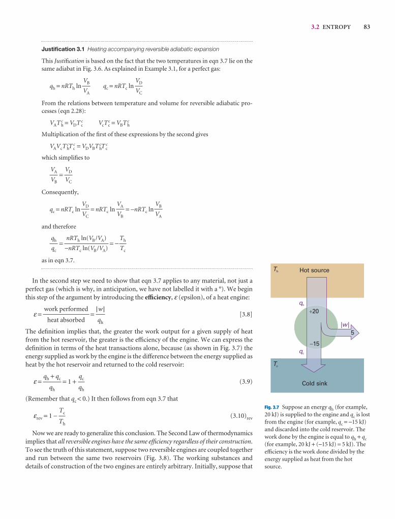
3.2 ENTROPY 83
Justification 3.1 Heating accompanying reversible adiabatic expansion
This Justification is based on the fact that the two temperatures in eqn 3.7 lie on thesame adiabat in Fig. 3.6. As explained in Example 3.1, for a perfect gas:
qh = nRTh ln qc = nRTc ln
From the relations between temperature and volume for reversible adiabatic pro-cesses (eqn 2.28):
VAT hc = VDT c
c VcTcc = VBT h
c
Multiplication of the first of these expressions by the second gives
VAVcT hcT c
c = VDVBT hcT c
c
which simplifies to
=
Consequently,
qc = nRTc ln = nRTc ln = −nRTc ln
and therefore
= = −
as in eqn 3.7.
In the second step we need to show that eqn 3.7 applies to any material, not just aperfect gas (which is why, in anticipation, we have not labelled it with a °). We beginthis step of the argument by introducing the efficiency, ε (epsilon), of a heat engine:
ε = = [3.8]
The definition implies that, the greater the work output for a given supply of heatfrom the hot reservoir, the greater is the efficiency of the engine. We can express thedefinition in terms of the heat transactions alone, because (as shown in Fig. 3.7) theenergy supplied as work by the engine is the difference between the energy supplied asheat by the hot reservoir and returned to the cold reservoir:
ε = = 1 + (3.9)
(Remember that qc < 0.) It then follows from eqn 3.7 that
εrev = 1 − (3.10)rev
Now we are ready to generalize this conclusion. The Second Law of thermodynamicsimplies that all reversible engines have the same efficiency regardless of their construction.To see the truth of this statement, suppose two reversible engines are coupled togetherand run between the same two reservoirs (Fig. 3.8). The working substances and details of construction of the two engines are entirely arbitrary. Initially, suppose that
Tc
Th
qc
qh
qh + qc
qh
|w |qh
work performed
heat absorbed
Th
Tc
nRTh ln(VB /VA)
−nRTc ln(VB /VA)
qh
qc
VB
VA
VA
VB
VD
VC
VD
VC
VA
VB
VD
VC
VB
VA
Tc
Th
qh
qc
| |w
Hot source
Cold sink
�20
�15
5
Fig. 3.7 Suppose an energy qh (for example, 20 kJ) is supplied to the engine and qc is lostfrom the engine (for example, qc = −15 kJ)and discarded into the cold reservoir. Thework done by the engine is equal to qh + qc
(for example, 20 kJ + (−15 kJ) = 5 kJ). Theefficiency is the work done divided by theenergy supplied as heat from the hotsource.
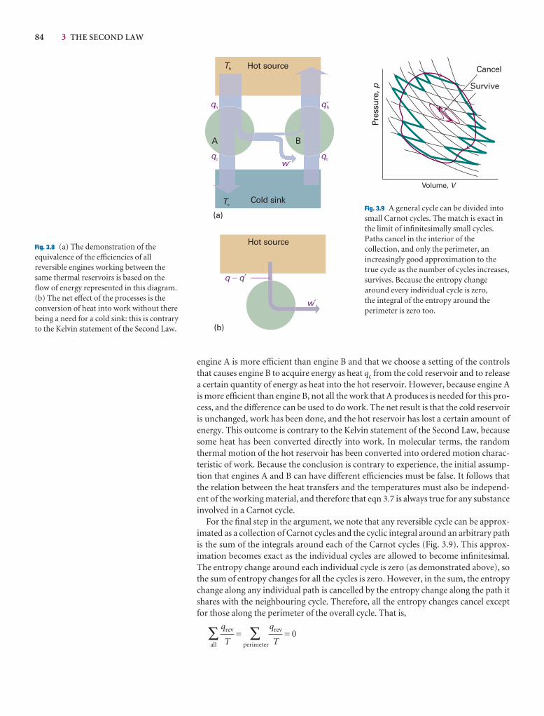
84 3 THE SECOND LAW
engine A is more efficient than engine B and that we choose a setting of the controlsthat causes engine B to acquire energy as heat qc from the cold reservoir and to releasea certain quantity of energy as heat into the hot reservoir. However, because engine Ais more efficient than engine B, not all the work that A produces is needed for this pro-cess, and the difference can be used to do work. The net result is that the cold reservoiris unchanged, work has been done, and the hot reservoir has lost a certain amount ofenergy. This outcome is contrary to the Kelvin statement of the Second Law, becausesome heat has been converted directly into work. In molecular terms, the randomthermal motion of the hot reservoir has been converted into ordered motion charac-teristic of work. Because the conclusion is contrary to experience, the initial assump-tion that engines A and B can have different efficiencies must be false. It follows thatthe relation between the heat transfers and the temperatures must also be independ-ent of the working material, and therefore that eqn 3.7 is always true for any substanceinvolved in a Carnot cycle.
For the final step in the argument, we note that any reversible cycle can be approx-imated as a collection of Carnot cycles and the cyclic integral around an arbitrary pathis the sum of the integrals around each of the Carnot cycles (Fig. 3.9). This approx-imation becomes exact as the individual cycles are allowed to become infinitesimal.The entropy change around each individual cycle is zero (as demonstrated above), sothe sum of entropy changes for all the cycles is zero. However, in the sum, the entropychange along any individual path is cancelled by the entropy change along the path itshares with the neighbouring cycle. Therefore, all the entropy changes cancel exceptfor those along the perimeter of the overall cycle. That is,
∑all
= ∑perimeter
= 0qrev
T
qrev
T
Tc
Th
qh qh́
qc qc
Hot source
Hot source
Cold sink
(a)
(b)
q q´�
w´
w´
A B
Fig. 3.8 (a) The demonstration of theequivalence of the efficiencies of allreversible engines working between thesame thermal reservoirs is based on theflow of energy represented in this diagram.(b) The net effect of the processes is theconversion of heat into work without therebeing a need for a cold sink: this is contraryto the Kelvin statement of the Second Law.
Volume, V
Pres
sure
,p
Cancel
Survive
Fig. 3.9 A general cycle can be divided intosmall Carnot cycles. The match is exact inthe limit of infinitesimally small cycles.Paths cancel in the interior of thecollection, and only the perimeter, anincreasingly good approximation to thetrue cycle as the number of cycles increases,survives. Because the entropy changearound every individual cycle is zero, the integral of the entropy around theperimeter is zero too.
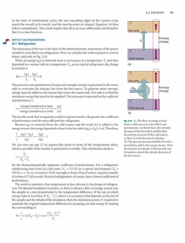
3.2 ENTROPY 85
In the limit of infinitesimal cycles, the non-cancelling edges of the Carnot cyclesmatch the overall cycle exactly, and the sum becomes an integral. Equation 3.6 thenfollows immediately. This result implies that dS is an exact differential and thereforethat S is a state function.
IMPACT ON ENGINEERING
I3.1 Refrigeration
The discussion of the text is the basis of the thermodynamic assessment of the powerneeded to cool objects in refrigerators. First, we consider the work required to cool anobject, and refer to Fig. 3.10.
When an energy |qc | is removed from a cool source at a temperature Tc and thendeposited in a warmer sink at a temperature Th, as in a typical refrigerator, the changein entropy is
∆S = − + < 0
The process is not spontaneous because not enough entropy is generated in the warmsink to overcome the entropy loss from the hot source. To generate more entropy, energy must be added to the stream that enters the warm sink. Our task is to find theminimum energy that needs to be supplied. The outcome is expressed as the coefficientof performance, c:
c = =
The less the work that is required to achieve a given transfer, the greater the coefficientof performance and the more efficient the refrigerator.
Because |qc | is removed from the cold source, and the work |w | is added to the energy stream, the energy deposited as heat in the hot sink is |qh | = |qc | + |w |. Therefore,
= = − − 1
We can now use eqn 3.7 to express this result in terms of the temperatures alone,which is possible if the transfer is performed reversibly. This substitution leads to
c =
for the thermodynamically optimum coefficient of performance. For a refrigeratorwithdrawing heat from ice-cold water (Tc = 273 K) in a typical environment (Th =293 K), c = 14, so, to remove 10 kJ (enough to freeze 30 g of water), requires transferof at least 0.71 kJ as work. Practical refrigerators, of course, have a lower coefficient ofperformance.
The work to maintain a low temperature is also relevant to the design of refrigera-tors. No thermal insulation is perfect, so there is always a flow of energy as heat intothe sample at a rate proportional to the temperature difference. If the rate at which energy leaks in is written A(Th − Tc), where A is a constant that depends on the size ofthe sample and the details of the insulation, then the minimum power, P, required tomaintain the original temperature difference by pumping out that energy by heatingthe surroundings is
P = × A(Th − Tc) = A ×(Th − Tc)
2
Tc
1
c
Tc
Th − Tc
|qh||qc|
|qh | − |qc ||qc |
1
c
|qc ||w |
energy transferred as heat
energy transferred as work
|qc |Th
|qc |Tc
Hot sink
Cold source
Th
Tc
Entropychangeqc
(a)
Cold source
Tc
Hot sink
Th
qc
w
(b)
Entropychange
Fig. 3.10 (a) The flow of energy as heat from a cold source to a hot sink is notspontaneous. As shown here, the entropyincrease of the hot sink is smaller than the entropy increase of the cold source, so there is a net decrease in entropy. (b) The process becomes feasible if work isprovided to add to the energy stream. Thenthe increase in entropy of the hot sink canbe made to cancel the entropy decrease ofthe hot source.
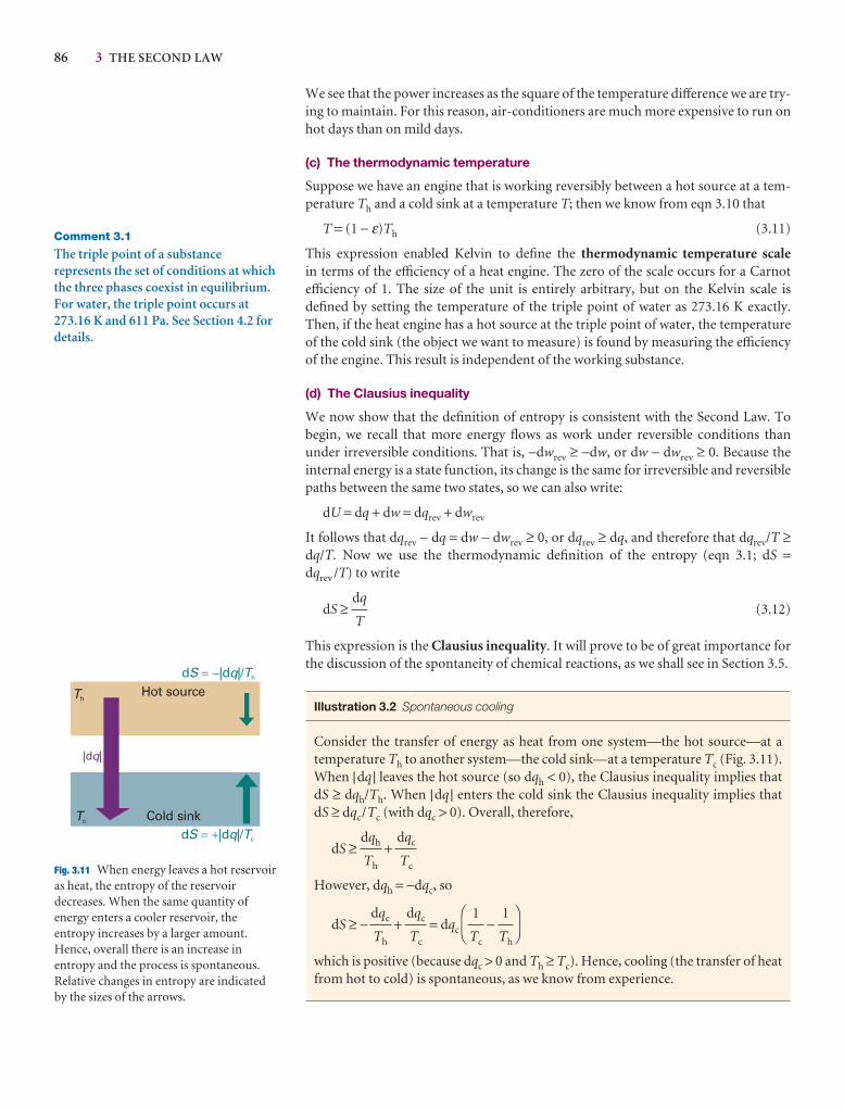
86 3 THE SECOND LAW
Hot sourceTh
Tc Cold sink
|d |q
d |d |/S q T� � h
d |d |/S q T� � c
Fig. 3.11 When energy leaves a hot reservoiras heat, the entropy of the reservoirdecreases. When the same quantity ofenergy enters a cooler reservoir, theentropy increases by a larger amount.Hence, overall there is an increase inentropy and the process is spontaneous.Relative changes in entropy are indicatedby the sizes of the arrows.
We see that the power increases as the square of the temperature difference we are try-ing to maintain. For this reason, air-conditioners are much more expensive to run onhot days than on mild days.
(c) The thermodynamic temperature
Suppose we have an engine that is working reversibly between a hot source at a tem-perature Th and a cold sink at a temperature T; then we know from eqn 3.10 that
T = (1 − ε)Th (3.11)
This expression enabled Kelvin to define the thermodynamic temperature scale in terms of the efficiency of a heat engine. The zero of the scale occurs for a Carnotefficiency of 1. The size of the unit is entirely arbitrary, but on the Kelvin scale isdefined by setting the temperature of the triple point of water as 273.16 K exactly.Then, if the heat engine has a hot source at the triple point of water, the temperatureof the cold sink (the object we want to measure) is found by measuring the efficiencyof the engine. This result is independent of the working substance.
(d) The Clausius inequality
We now show that the definition of entropy is consistent with the Second Law. Tobegin, we recall that more energy flows as work under reversible conditions thanunder irreversible conditions. That is, −dwrev ≥ −dw, or dw − dwrev ≥ 0. Because the internal energy is a state function, its change is the same for irreversible and reversiblepaths between the same two states, so we can also write:
dU = dq + dw = dqrev + dwrev
It follows that dqrev − dq = dw − dwrev ≥ 0, or dqrev ≥ dq, and therefore that dqrev/T ≥dq/T. Now we use the thermodynamic definition of the entropy (eqn 3.1; dS =dqrev /T) to write
dS ≥ (3.12)
This expression is the Clausius inequality. It will prove to be of great importance forthe discussion of the spontaneity of chemical reactions, as we shall see in Section 3.5.
Illustration 3.2 Spontaneous cooling
Consider the transfer of energy as heat from one system—the hot source—at atemperature Th to another system—the cold sink—at a temperature Tc (Fig. 3.11).When |dq | leaves the hot source (so dqh < 0), the Clausius inequality implies thatdS ≥ dqh/Th. When |dq | enters the cold sink the Clausius inequality implies that dS ≥ dqc/Tc (with dqc > 0). Overall, therefore,
dS ≥ +
However, dqh = −dqc, so
dS ≥ − + = dqc −
which is positive (because dqc > 0 and Th ≥ Tc). Hence, cooling (the transfer of heatfrom hot to cold) is spontaneous, as we know from experience.
DF
1
Th
1
Tc
AC
dqc
Tc
dqc
Th
dqc
Tc
dqh
Th
dq
T
Comment 3.1
The triple point of a substancerepresents the set of conditions at whichthe three phases coexist in equilibrium.For water, the triple point occurs at273.16 K and 611 Pa. See Section 4.2 fordetails.
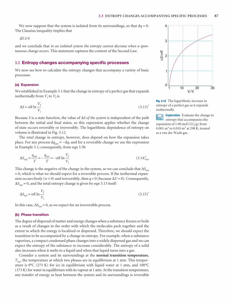
3.3 ENTROPY CHANGES ACCOMPANYING SPECIFIC PROCESSES 87
We now suppose that the system is isolated from its surroundings, so that dq = 0.The Clausius inequality implies that
dS ≥ 0
and we conclude that in an isolated system the entropy cannot decrease when a spon-taneous change occurs. This statement captures the content of the Second Law.
3.3 Entropy changes accompanying specific processes
We now see how to calculate the entropy changes that accompany a variety of basicprocesses.
(a) Expansion
We established in Example 3.1 that the change in entropy of a perfect gas that expandsisothermally from Vi to Vf is
∆S = nR ln (3.13)°
Because S is a state function, the value of ∆S of the system is independent of the pathbetween the initial and final states, so this expression applies whether the change of state occurs reversibly or irreversibly. The logarithmic dependence of entropy onvolume is illustrated in Fig. 3.12.
The total change in entropy, however, does depend on how the expansion takesplace. For any process dqsur = −dq, and for a reversible change we use the expressionin Example 3.1; consequently, from eqn 3.3b
∆Ssur = = − = −nR ln (3.14)°rev
This change is the negative of the change in the system, so we can conclude that ∆Stot
= 0, which is what we should expect for a reversible process. If the isothermal expan-sion occurs freely (w = 0) and irreversibly, then q = 0 (because ∆U = 0). Consequently,∆Ssur = 0, and the total entropy change is given by eqn 3.13 itself:
∆Stot = nR ln (3.15)°
In this case, ∆Stot > 0, as we expect for an irreversible process.
(b) Phase transition
The degree of dispersal of matter and energy changes when a substance freezes or boilsas a result of changes in the order with which the molecules pack together and the extent to which the energy is localized or dispersed. Therefore, we should expect thetransition to be accompanied by a change in entropy. For example, when a substancevaporizes, a compact condensed phase changes into a widely dispersed gas and we canexpect the entropy of the substance to increase considerably. The entropy of a solidalso increases when it melts to a liquid and when that liquid turns into a gas.
Consider a system and its surroundings at the normal transition temperature,Ttrs, the temperature at which two phases are in equilibrium at 1 atm. This temper-ature is 0°C (273 K) for ice in equilibrium with liquid water at 1 atm, and 100°C (373 K) for water in equilibrium with its vapour at 1 atm. At the transition temperature,any transfer of energy as heat between the system and its surroundings is reversible
Vf
Vi
Vf
Vi
qrev
T
qsur
T
Vf
Vi
1
2
3
4
10 20 3010
DS
nR/
V Vf i/
Fig. 3.12 The logarithmic increase inentropy of a perfect gas as it expandsisothermally.
Exploration Evaluate the change inentropy that accompanies the
expansion of 1.00 mol CO2(g) from 0.001 m3 to 0.010 m3 at 298 K, treated as a van der Waals gas.
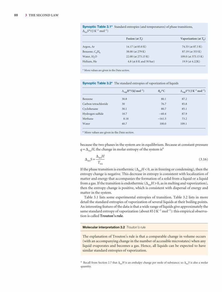
88 3 THE SECOND LAW
4 Recall from Section 2.7 that ∆trsH is an enthalpy change per mole of substance; so ∆trsS is also a molarquantity.
Synoptic Table 3.1* Standard entropies (and temperatures) of phase transitions, ∆trsS
7/(J K−1 mol−1)
Fusion (at Tf) Vaporization (at Tb)
Argon, Ar 14.17 (at 83.8 K) 74.53 (at 87.3 K)
Benzene, C6H6 38.00 (at 279 K) 87.19 (at 353 K)
Water, H2O 22.00 (at 273.15 K) 109.0 (at 373.15 K)
Helium, He 4.8 (at 8 K and 30 bar) 19.9 (at 4.22K)
* More values are given in the Data section.
Synoptic Table 3.2* The standard entropies of vaporization of liquids
∆vapH 7/(kJ mol−1) θb/°C ∆vapS 7/(J K−1 mol−1)
Benzene 30.8 80.1 87.2
Carbon tetrachloride 30 76.7 85.8
Cyclohexane 30.1 80.7 85.1
Hydrogen sulfide 18.7 −60.4 87.9
Methane 8.18 −161.5 73.2
Water 40.7 100.0 109.1
* More values are given in the Data section.
because the two phases in the system are in equilibrium. Because at constant pressureq = ∆ trsH, the change in molar entropy of the system is4
∆ trsS = (3.16)
If the phase transition is exothermic (∆trsH < 0, as in freezing or condensing), then theentropy change is negative. This decrease in entropy is consistent with localization ofmatter and energy that accompanies the formation of a solid from a liquid or a liquidfrom a gas. If the transition is endothermic (∆ trsH > 0, as in melting and vaporization),then the entropy change is positive, which is consistent with dispersal of energy andmatter in the system.
Table 3.1 lists some experimental entropies of transition. Table 3.2 lists in more detail the standard entropies of vaporization of several liquids at their boiling points.An interesting feature of the data is that a wide range of liquids give approximately thesame standard entropy of vaporization (about 85 J K−1 mol−1): this empirical observa-tion is called Trouton’s rule.
Molecular interpretation 3.2 Trouton’s rule
The explanation of Trouton’s rule is that a comparable change in volume occurs(with an accompanying change in the number of accessible microstates) when anyliquid evaporates and becomes a gas. Hence, all liquids can be expected to havesimilar standard entropies of vaporization.
∆ trsH
Ttrs
3.3 ENTROPY CHANGES ACCOMPANYING SPECIFIC PROCESSES 89
Liquids that show significant deviations from Trouton’s rule do so on accountof strong molecular interactions that restrict molecular motion. As a result, thereis a greater dispersal of energy and matter when the liquid turns into a vapour thanwould occur for a liquid in which molcular motion is less restricted. An example is water, where the large entropy of vaporization reflects the presence of structurearising from hydrogen-bonding in the liquid. Hydrogen bonds tend to organize the molecules in the liquid so that they are less random than, for example, themolecules in liquid hydrogen sulfide (in which there is no hydrogen bonding).
Methane has an unusually low entropy of vaporization. A part of the reason is that the entropy of the gas itself is slightly low (186 J K−1 mol−1 at 298 K); the entropy of N2 under the same conditions is 192 J K−1 mol−1. As we shall see inChapter 13, small molecules are difficult to excite into rotation; as a result, only a few rotational states are accessible at room temperature and, consequently, thenumber of rotational energy levels among which energy can be dispersed is low.
Illustration 3.3 Using Trouton’s rule
There is no hydrogen bonding in liquid bromine and Br2 is a heavy molecule thatis unlikely to display unusual behaviour in the gas phase, so it is probably safe touse Trouton’s rule. To predict the standard molar enthalpy of vaporization ofbromine given that it boils at 59.2°C, we use the rule in the form
∆ vapH 7 = Tb × (85 J K−1 mol−1)
Substitution of the data then gives
∆vapH 7 = (332.4 K) × (85 J K−1 mol−1) = +2.8 × 10³ J mol−1 = +28 kJ mol−1
The experimental value is +29.45 kJ mol−1.
Self-test 3.3 Predict the enthalpy of vaporization of ethane from its boiling point,−88.6°C. [16 kJ mol−1]
(c) Heating
We can use eqn 3.2 to calculate the entropy of a system at a temperature Tf from aknowledge of its entropy at a temperature Ti and the heat supplied to change its tem-perature from one value to the other:
S(Tf) = S(Ti) + �Tf
Ti
(3.17)
We shall be particularly interested in the entropy change when the system is subjectedto constant pressure (such as from the atmosphere) during the heating. Then, fromthe definition of constant-pressure heat capacity (eqn 2.22), dqrev = CpdT provided thesystem is doing no non-expansion work. Consequently, at constant pressure:
S(Tf) = S(Ti) + �Tf
Ti
(3.18)
The same expression applies at constant volume, but with Cp replaced by CV . WhenCp is independent of temperature in the temperature range of interest, it can be takenoutside the integral and we obtain
CpdT
T
dqrev
T
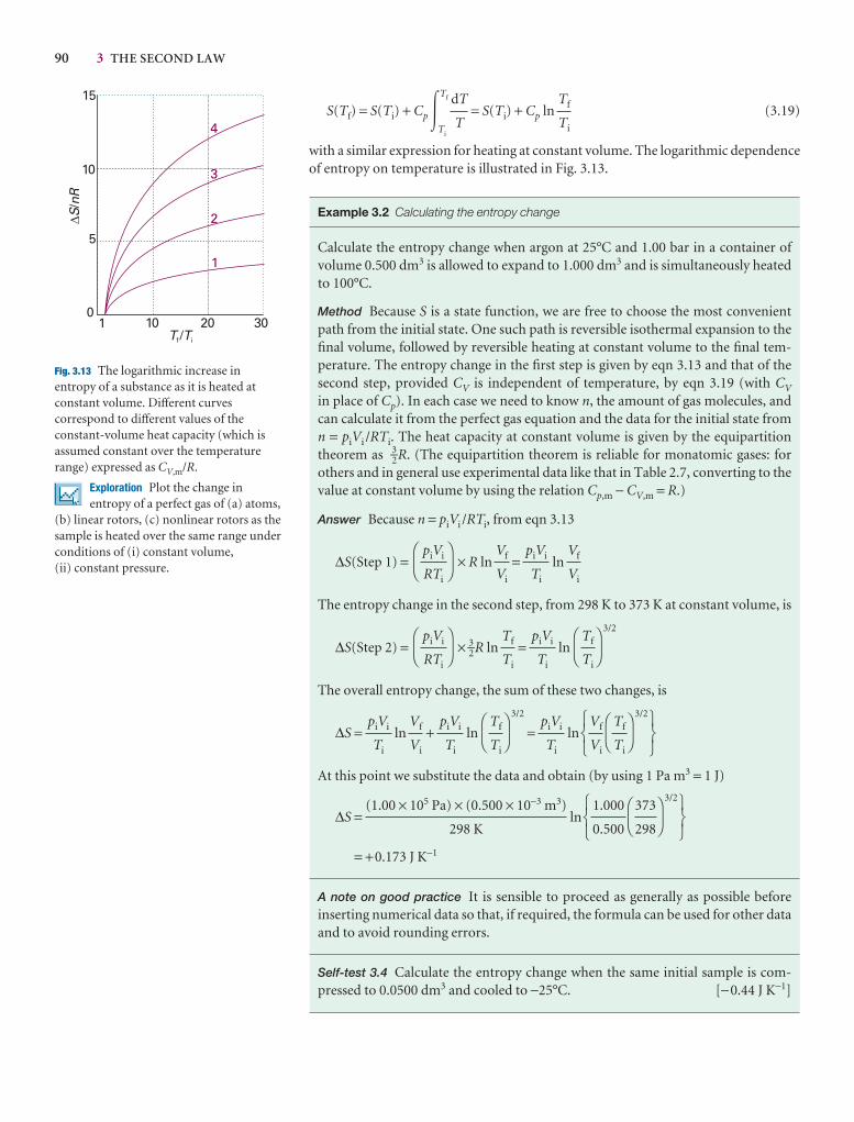
90 3 THE SECOND LAW
10 20 3010
DS
nR/
T Tf i/
5
10
15
1
2
3
4
Fig. 3.13 The logarithmic increase inentropy of a substance as it is heated atconstant volume. Different curvescorrespond to different values of theconstant-volume heat capacity (which isassumed constant over the temperaturerange) expressed as CV,m/R.
Exploration Plot the change inentropy of a perfect gas of (a) atoms,
(b) linear rotors, (c) nonlinear rotors as thesample is heated over the same range underconditions of (i) constant volume, (ii) constant pressure.
S(Tf) = S(Ti) + Cp�Tf
Ti
= S(Ti) + Cp ln (3.19)
with a similar expression for heating at constant volume. The logarithmic dependenceof entropy on temperature is illustrated in Fig. 3.13.
Example 3.2 Calculating the entropy change
Calculate the entropy change when argon at 25°C and 1.00 bar in a container ofvolume 0.500 dm3 is allowed to expand to 1.000 dm3 and is simultaneously heatedto 100°C.
Method Because S is a state function, we are free to choose the most convenientpath from the initial state. One such path is reversible isothermal expansion to thefinal volume, followed by reversible heating at constant volume to the final tem-perature. The entropy change in the first step is given by eqn 3.13 and that of thesecond step, provided CV is independent of temperature, by eqn 3.19 (with CV
in place of Cp). In each case we need to know n, the amount of gas molecules, andcan calculate it from the perfect gas equation and the data for the initial state fromn = piVi /RTi. The heat capacity at constant volume is given by the equipartition theorem as 3–2R. (The equipartition theorem is reliable for monatomic gases: forothers and in general use experimental data like that in Table 2.7, converting to thevalue at constant volume by using the relation Cp,m − CV,m = R.)
Answer Because n = piVi /RTi, from eqn 3.13
∆S(Step 1) = × R ln = ln
The entropy change in the second step, from 298 K to 373 K at constant volume, is
∆S(Step 2) = × 3–2R ln = ln
3/2
The overall entropy change, the sum of these two changes, is
∆S = ln + ln
3/2
= ln
3/2
At this point we substitute the data and obtain (by using 1 Pa m3 = 1 J)
∆S = ln
3/2
= +0.173 J K−1
A note on good practice It is sensible to proceed as generally as possible before inserting numerical data so that, if required, the formula can be used for other dataand to avoid rounding errors.
Self-test 3.4 Calculate the entropy change when the same initial sample is com-pressed to 0.0500 dm3 and cooled to −25°C. [−0.44 J K−1]
567
DF
373
298
AC
1.000
0.500
123
(1.00 × 10⁵ Pa) × (0.500 × 10⁻³ m3)
298 K
567
DF
Tf
Ti
AC
Vf
Vi
123
piVi
Ti
DF
Tf
Ti
AC
piVi
Ti
Vf
Vi
piVi
Ti
DF
Tf
Ti
AC
piVi
Ti
Tf
Ti
DF
piVi
RTi
AC
Vf
Vi
piVi
Ti
Vf
Vi
DF
piVi
RTi
AC
Tf
Ti
dT
T
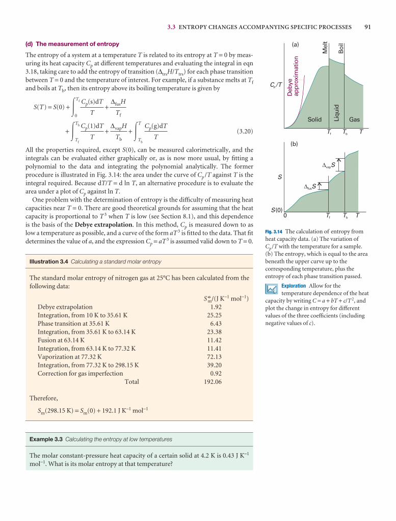
3.3 ENTROPY CHANGES ACCOMPANYING SPECIFIC PROCESSES 91
S
S(0)0 Tf
Tf
Tb
Tb
T
T
vapS
fusS
Mel
t
Boi
l
C /Tp
Solid Liqu
id
Gas
Deb
yeap
prox
imat
ion
(a)
(b)
Fig. 3.14 The calculation of entropy fromheat capacity data. (a) The variation ofCp /T with the temperature for a sample.(b) The entropy, which is equal to the areabeneath the upper curve up to thecorresponding temperature, plus theentropy of each phase transition passed.
Exploration Allow for thetemperature dependence of the heat
capacity by writing C = a + bT + c/T 2, andplot the change in entropy for differentvalues of the three coefficients (includingnegative values of c).
(d) The measurement of entropy
The entropy of a system at a temperature T is related to its entropy at T = 0 by meas-uring its heat capacity Cp at different temperatures and evaluating the integral in eqn3.18, taking care to add the entropy of transition (∆trsH/Ttrs) for each phase transitionbetween T = 0 and the temperature of interest. For example, if a substance melts at Tf
and boils at Tb, then its entropy above its boiling temperature is given by
S(T) = S(0) + �Tf
0
+
+ �Tb
Tf
+ + �T
Tb
(3.20)
All the properties required, except S(0), can be measured calorimetrically, and the integrals can be evaluated either graphically or, as is now more usual, by fitting a polynomial to the data and integrating the polynomial analytically. The former procedure is illustrated in Fig. 3.14: the area under the curve of Cp /T against T is theintegral required. Because dT/T = d ln T, an alternative procedure is to evaluate thearea under a plot of Cp against ln T.
One problem with the determination of entropy is the difficulty of measuring heatcapacities near T = 0. There are good theoretical grounds for assuming that the heatcapacity is proportional to T 3 when T is low (see Section 8.1), and this dependence is the basis of the Debye extrapolation. In this method, Cp is measured down to as low a temperature as possible, and a curve of the form aT 3 is fitted to the data. That fit determines the value of a, and the expression Cp = aT3 is assumed valid down to T = 0.
Illustration 3.4 Calculating a standard molar entropy
The standard molar entropy of nitrogen gas at 25°C has been calculated from thefollowing data:
S 7m/(J K−1 mol−1)
Debye extrapolation 1.92Integration, from 10 K to 35.61 K 25.25Phase transition at 35.61 K 6.43Integration, from 35.61 K to 63.14 K 23.38Fusion at 63.14 K 11.42Integration, from 63.14 K to 77.32 K 11.41Vaporization at 77.32 K 72.13Integration, from 77.32 K to 298.15 K 39.20Correction for gas imperfection 0.92
Total 192.06
Therefore,
Sm(298.15 K) = Sm(0) + 192.1 J K−1 mol−1
Example 3.3 Calculating the entropy at low temperatures
The molar constant-pressure heat capacity of a certain solid at 4.2 K is 0.43 J K−1
mol−1. What is its molar entropy at that temperature?
Cp(g)dT
T
∆vapH
Tb
Cp(1)dT
T
∆fusH
Tf
Cp(s)dT
T
92 3 THE SECOND LAW
Method Because the temperature is so low, we can assume that the heat capacityvaries with temperature as aT 3, in which case we can use eqn 3.18 to calculate theentropy at a temperature T in terms of the entropy at T = 0 and the constant a.When the integration is carried out, it turns out that the result can be expressed interms of the heat capacity at the temperature T, so the data can be used directly tocalculate the entropy.
Answer The integration required is
S(T) = S(0) + �T
0
= S(0) + a�T
0
T 2dT = S(0) + 1–3 aT 3
However, because aT 3 is the heat capacity at the temperature T,
S(T) = S(0) + 1–3 Cp(T)
from which it follows that
Sm(10 K) = Sm(0) + 0.14 J K−1 mol−1
Self-test 3.5 For metals, there is also a contribution to the heat capacity from theelectrons which is linearly proportional to T when the temperature is low. Find itscontribution to the entropy at low temperatures. [S(T) = S(0) + Cp(T)]
3.4 The Third Law of thermodynamics
At T = 0, all energy of thermal motion has been quenched, and in a perfect crystal allthe atoms or ions are in a regular, uniform array. The localization of matter and theabsence of thermal motion suggest that such materials also have zero entropy. Thisconclusion is consistent with the molecular interpretation of entropy, because S = 0 ifthere is only one way of arranging the molecules and only one microstate is accessible(the ground state).
(a) The Nernst heat theorem
The experimental observation that turns out to be consistent with the view that theentropy of a regular array of molecules is zero at T = 0 is summarized by the Nernstheat theorem:
The entropy change accompanying any physical or chemical transformation approaches zero as the temperature approaches zero: ∆S → 0 as T → 0 provided allthe substances involved are perfectly crystalline.
Illustration 3.5 Using the Nernst heat theorem
Consider the entropy of the transition between orthorhombic sulfur, S(α), andmonoclinic sulfur, S(β), which can be calculated from the transition enthalpy (−402 J mol−1) at the transition temperature (369 K):
∆trsS = Sm(α) − Sm(β) = = −1.09 J K−1 mol−1
The two individual entropies can also be determined by measuring the heat capa-cities from T = 0 up to T = 369 K. It is found that Sm(α) = Sm(α,0) + 37 J K−1 mol−1
(−402 J mol−1)
369 K
aT 3dT
T
3.4 THE THIRD LAW OF THEMODYNAMICS 93
Synoptic Table 3.3* StandardThird-Law entropies at 298 K
S 7m/(J K−1 mol−1)
Solids
Graphite, C(s) 5.7
Diamond, C(s) 2.4
Sucrose, C12H22O11(s) 360.2
Iodine, I2(s) 116.1
Liquids
Benzene, C6H6(l) 173.3
Water, H2O(l) 69.9
Mercury, Hg(l) 76.0
Gases
Methane, CH4(g) 186.3
Carbon dioxide, CO2(g) 213.7
Hydrogen, H2(g) 130.7
Helium, He 126.2
Ammonia, NH3(g) 126.2
* More values are given in the Data section.
and Sm(β) = Sm(β,0) + 38 J K−1 mol−1. These two values imply that at the transitiontemperature
∆ trsS = Sm(α,0) − Sm(β,0) = −1 J K−1 mol−1
On comparing this value with the one above, we conclude that Sm(α,0) − Sm(β,0)≈ 0, in accord with the theorem.
It follows from the Nernst theorem that, if we arbitrarily ascribe the value zero to the entropies of elements in their perfect crystalline form at T = 0, then all perfectcrystalline compounds also have zero entropy at T = 0 (because the change in entropythat accompanies the formation of the compounds, like the entropy of all transforma-tions at that temperature, is zero). This conclusion is summarized by the Third Lawof thermodynamics:
The entropy of all perfect crystalline substances is zero at T = 0.
As far as thermodynamics is concerned, choosing this common value as zero is then amatter of convenience. The molecular interpretation of entropy, however, justifiesthe value S = 0 at T = 0.
Molecular interpretation 3.3 The statistical view of the Third Law of thermodynamics
We saw in Molecular interpretation 3.1 that, according to the Boltzmann formula,the entropy is zero if there is only one accessible microstate (W = 1). In most cases,W = 1 at T = 0 because there is only one way of achieving the lowest total energy:put all the molecules into the same, lowest state. Therefore, S = 0 at T = 0, in accordwith the Third Law of thermodynamics. In certain cases, though, W may differfrom 1 at T = 0. This is the case if there is no energy advantage in adopting a par-ticular orientation even at absolute zero. For instance, for a diatomic molecule ABthere may be almost no energy difference between the arrangements . . . AB AB AB. . . and . . . BA AB BA . . . , so W > 1 even at T = 0. If S > 0 at T = 0 we say that thesubstance has a residual entropy. Ice has a residual entropy of 3.4 J K−1 mol−1. Itstems from the arrangement of the hydrogen bonds between neighbouring watermolecules: a given O atom has two short O-H bonds and two long O···H bonds toits neighbours, but there is a degree of randomness in which two bonds are shortand which two are long.
(b) Third-Law entropies
Entropies reported on the basis that S(0) = 0 are called Third-Law entropies (andoften just ‘entropies’). When the substance is in its standard state at the temperatureT, the standard (Third-Law) entropy is denoted S 7(T). A list of values at 298 K isgiven in Table 3.3.
The standard reaction entropy, ∆rS7, is defined, like the standard reaction en-
thalpy, as the difference between the molar entropies of the pure, separated productsand the pure, separated reactants, all substances being in their standard states at thespecified temperature:
∆rS7 =
Products∑νS 7
m −Reactants
∑νS 7m (3.21)
In this expression, each term is weighted by the appropriate stoichiometric coefficient.Standard reaction entropies are likely to be positive if there is a net formation of gas ina reaction, and are likely to be negative if there is a net consumption of gas.

94 3 THE SECOND LAW
5 In terms of the language to be introduced in Section 5.1, the entropies of ions in solution are actually par-tial molar entropies, for their values include the consequences of their presence on the organization of thesolvent molecules around them.
Illustration 3.6 Calculating a standard reaction entropy
To calculate the standard reaction entropy of H2(g) + 1–2 O2(g) → H2O(l) at 25°C,we use the data in Table 2.7 of the Data Section to write
∆rS7 = S 7
m(H2O, l) − {S 7m(H2, g) + 1–2 S 7
m(O2, g)}
= 69.9 J K−1 mol−1 − {130.7 + 1–2 (205.0)} J K−1 mol−1
= −163.4 J K−1 mol−1
The negative value is consistent with the conversion of two gases to a compact liquid.
A note on good practice Do not make the mistake of setting the standard molarentropies of elements equal to zero: they have non-zero values (provided T > 0), aswe have already discussed.
Self-test 3.6 Calculate the standard reaction entropy for the combustion ofmethane to carbon dioxide and liquid water at 25°C. [−243 J K−1 mol−1]
Just as in the discussion of enthalpies in Section 2.8, where we acknowledged thatsolutions of cations cannot be prepared in the absence of anions, the standard molarentropies of ions in solution are reported on a scale in which the standard entropy ofthe H+ ions in water is taken as zero at all temperatures:
S 7(H+, aq) = 0 [3.22]
The values based on this choice are listed in Table 2.7 in the Data section.5 Because theentropies of ions in water are values relative to the hydrogen ion in water, they may beeither positive or negative. A positive entropy means that an ion has a higher molarentropy than H+ in water and a negative entropy means that the ion has a lower molarentropy than H+ in water. For instance, the standard molar entropy of Cl−(aq) is +57J K−1 mol−1 and that of Mg2+(aq) is −128 J K−1 mol−1. Ion entropies vary as expectedon the basis that they are related to the degree to which the ions order the watermolecules around them in the solution. Small, highly charged ions induce local struc-ture in the surrounding water, and the disorder of the solution is decreased more thanin the case of large, singly charged ions. The absolute, Third-Law standard molar entropy of the proton in water can be estimated by proposing a model of the structureit induces, and there is some agreement on the value −21 J K−1 mol−1. The negativevalue indicates that the proton induces order in the solvent.
Concentrating on the system
Entropy is the basic concept for discussing the direction of natural change, but to useit we have to analyse changes in both the system and its surroundings. We have seenthat it is always very simple to calculate the entropy change in the surroundings, andwe shall now see that it is possible to devise a simple method for taking that contribu-tion into account automatically. This approach focuses our attention on the system
3.5 THE HELMHOLTZ AND GIBBS ENERGIES 95
and simplifies discussions. Moreover, it is the foundation of all the applications ofchemical thermodynamics that follow.
3.5 The Helmholtz and Gibbs energies
Consider a system in thermal equilibrium with its surroundings at a temperature T.When a change in the system occurs and there is a transfer of energy as heat betweenthe system and the surroundings, the Clausius inequality, eqn 3.12, reads
dS − ≥ 0 (3.23)
We can develop this inequality in two ways according to the conditions (of constantvolume or constant pressure) under which the process occurs.
(a) Criteria for spontaneity
First, consider heating at constant volume. Then, in the absence of non-expansionwork, we can write dqV = dU; consequently
dS − ≥ 0 (3.24)
The importance of the inequality in this form is that it expresses the criterion forspontaneous change solely in terms of the state functions of the system. The inequal-ity is easily rearranged to
TdS ≥ dU (constant V, no additional work)6 (3.25)
At either constant internal energy (dU = 0) or constant entropy (dS = 0), this expres-sion becomes, respectively,
dSU,V ≥ 0 dUS,V ≤ 0 (3.26)
where the subscripts indicate the constant conditions.Equation 3.26 expresses the criteria for spontaneous change in terms of properties
relating to the system. The first inequality states that, in a system at constant volumeand constant internal energy (such as an isolated system), the entropy increases in aspontaneous change. That statement is essentially the content of the Second Law. Thesecond inequality is less obvious, for it says that, if the entropy and volume of the sys-tem are constant, then the internal energy must decrease in a spontaneous change. Donot interpret this criterion as a tendency of the system to sink to lower energy. It is a disguised statement about entropy, and should be interpreted as implying that, if the entropy of the system is unchanged, then there must be an increase in entropy ofthe surroundings, which can be achieved only if the energy of the system decreases asenergy flows out as heat.
When energy is transferred as heat at constant pressure, and there is no work otherthan expansion work, we can write dqp = dH and obtain
TdS ≥ dH (constant p, no additional work) (3.27)
At either constant enthalpy or constant entropy this inequality becomes, respectively,
dSH,p ≥ 0 dHS,p ≤ 0 (3.28)
The interpretations of these inequalities are similar to those of eqn 3.26. The entropyof the system at constant pressure must increase if its enthalpy remains constant (for
dU
T
dq
T
6 Recall that ‘additional work’ is work other than expansion work.
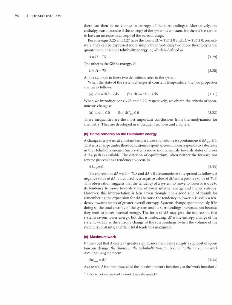
96 3 THE SECOND LAW
there can then be no change in entropy of the surroundings). Alternatively, the enthalpy must decrease if the entropy of the system is constant, for then it is essentialto have an increase in entropy of the surroundings.
Because eqns 3.25 and 3.27 have the forms dU − TdS ≤ 0 and dH − TdS ≤ 0, respect-ively, they can be expressed more simply by introducing two more thermodynamicquantities. One is the Helmholtz energy, A, which is defined as
A = U − TS [3.29]
The other is the Gibbs energy, G:
G = H − TS [3.30]
All the symbols in these two definitions refer to the system.When the state of the system changes at constant temperature, the two properties
change as follows:
(a) dA = dU − TdS (b) dG = dH − TdS (3.31)
When we introduce eqns 3.25 and 3.27, respectively, we obtain the criteria of spon-taneous change as
(a) dAT,V ≤ 0 (b) dGT,p ≤ 0 (3.32)
These inequalities are the most important conclusions from thermodynamics forchemistry. They are developed in subsequent sections and chapters.
(b) Some remarks on the Helmholtz energy
A change in a system at constant temperature and volume is spontaneous if dAT,V ≤ 0.That is, a change under these conditions is spontaneous if it corresponds to a decreasein the Helmholtz energy. Such systems move spontaneously towards states of lower A if a path is available. The criterion of equilibrium, when neither the forward nor reverse process has a tendency to occur, is
dAT,V = 0 (3.33)
The expressions dA = dU − TdS and dA < 0 are sometimes interpreted as follows. Anegative value of dA is favoured by a negative value of dU and a positive value of TdS.This observation suggests that the tendency of a system to move to lower A is due toits tendency to move towards states of lower internal energy and higher entropy.However, this interpretation is false (even though it is a good rule of thumb for remembering the expression for dA) because the tendency to lower A is solely a ten-dency towards states of greater overall entropy. Systems change spontaneously if indoing so the total entropy of the system and its surroundings increases, not becausethey tend to lower internal energy. The form of dA may give the impression that systems favour lower energy, but that is misleading: dS is the entropy change of thesystem, −dU/T is the entropy change of the surroundings (when the volume of thesystem is constant), and their total tends to a maximum.
(c) Maximum work
It turns out that A carries a greater significance than being simply a signpost of spon-taneous change: the change in the Helmholtz function is equal to the maximum work accompanying a process:
dwmax = dA (3.34)
As a result, A is sometimes called the ‘maximum work function’, or the ‘work function’.7
7 Arbeit is the German word for work; hence the symbol A.
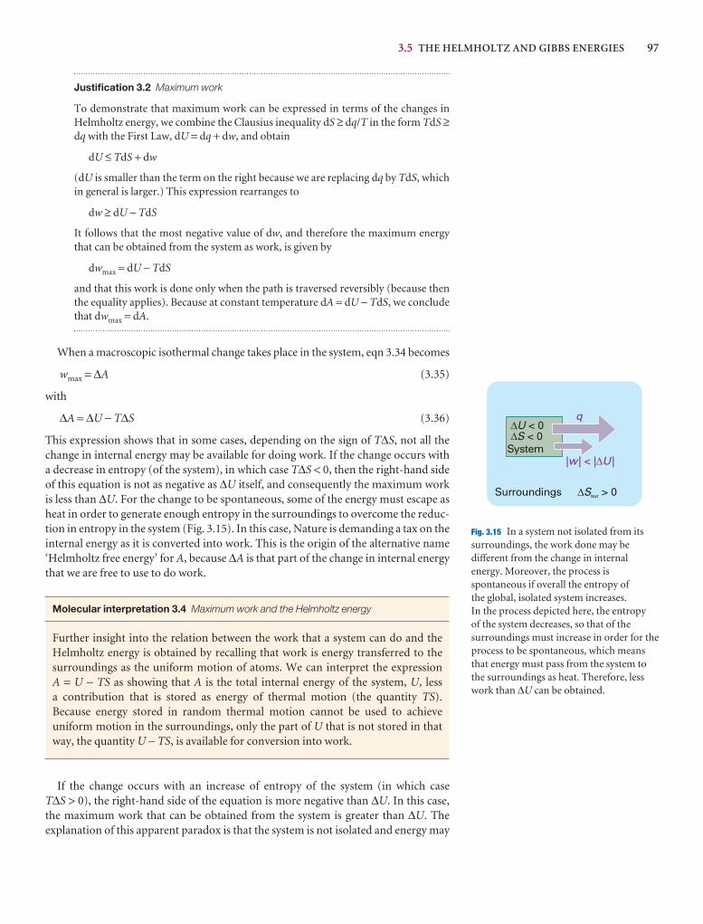
3.5 THE HELMHOLTZ AND GIBBS ENERGIES 97
Surroundings
System
q
| | < | |w UD
D
D
US
< 0< 0
DSsur > 0
Fig. 3.15 In a system not isolated from itssurroundings, the work done may bedifferent from the change in internalenergy. Moreover, the process isspontaneous if overall the entropy of the global, isolated system increases. In the process depicted here, the entropy of the system decreases, so that of thesurroundings must increase in order for theprocess to be spontaneous, which meansthat energy must pass from the system tothe surroundings as heat. Therefore, lesswork than ∆U can be obtained.
Justification 3.2 Maximum work
To demonstrate that maximum work can be expressed in terms of the changes inHelmholtz energy, we combine the Clausius inequality dS ≥ dq/T in the form TdS ≥dq with the First Law, dU = dq + dw, and obtain
dU ≤ TdS + dw
(dU is smaller than the term on the right because we are replacing dq by TdS, whichin general is larger.) This expression rearranges to
dw ≥ dU − TdS
It follows that the most negative value of dw, and therefore the maximum energythat can be obtained from the system as work, is given by
dwmax = dU − TdS
and that this work is done only when the path is traversed reversibly (because thenthe equality applies). Because at constant temperature dA = dU − TdS, we concludethat dwmax = dA.
When a macroscopic isothermal change takes place in the system, eqn 3.34 becomes
wmax = ∆A (3.35)
with
∆A = ∆U − T∆S (3.36)
This expression shows that in some cases, depending on the sign of T∆S, not all thechange in internal energy may be available for doing work. If the change occurs witha decrease in entropy (of the system), in which case T∆S < 0, then the right-hand sideof this equation is not as negative as ∆U itself, and consequently the maximum workis less than ∆U. For the change to be spontaneous, some of the energy must escape asheat in order to generate enough entropy in the surroundings to overcome the reduc-tion in entropy in the system (Fig. 3.15). In this case, Nature is demanding a tax on theinternal energy as it is converted into work. This is the origin of the alternative name‘Helmholtz free energy’ for A, because ∆A is that part of the change in internal energythat we are free to use to do work.
Molecular interpretation 3.4 Maximum work and the Helmholtz energy
Further insight into the relation between the work that a system can do and theHelmholtz energy is obtained by recalling that work is energy transferred to thesurroundings as the uniform motion of atoms. We can interpret the expression A = U − TS as showing that A is the total internal energy of the system, U, less a contribution that is stored as energy of thermal motion (the quantity TS).Because energy stored in random thermal motion cannot be used to achieve uniform motion in the surroundings, only the part of U that is not stored in thatway, the quantity U − TS, is available for conversion into work.
If the change occurs with an increase of entropy of the system (in which case T∆S > 0), the right-hand side of the equation is more negative than ∆U. In this case,the maximum work that can be obtained from the system is greater than ∆U. The explanation of this apparent paradox is that the system is not isolated and energy may
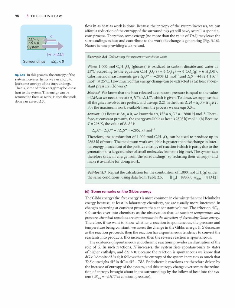
98 3 THE SECOND LAW
Surroundings
System
q
| | > | |w UD
D
D
US
< 0> 0
DSsur < 0
Fig. 3.16 In this process, the entropy of thesystem increases; hence we can afford tolose some entropy of the surroundings.That is, some of their energy may be lost asheat to the system. This energy can bereturned to them as work. Hence the workdone can exceed ∆U.
flow in as heat as work is done. Because the entropy of the system increases, we can afford a reduction of the entropy of the surroundings yet still have, overall, a spontan-eous process. Therefore, some energy (no more than the value of T∆S) may leave thesurroundings as heat and contribute to the work the change is generating (Fig. 3.16).Nature is now providing a tax refund.
Example 3.4 Calculating the maximum available work
When 1.000 mol C6H12O6 (glucose) is oxidized to carbon dioxide and water at25°C according to the equation C6H12O6(s) + 6 O2(g) → 6 CO2(g) + 6 H2O(l),calorimetric measurements give ∆rU
7 = −2808 kJ mol−1 and ∆rS = +182.4 J K−1
mol−1 at 25°C. How much of this energy change can be extracted as (a) heat at con-stant pressure, (b) work?
Method We know that the heat released at constant pressure is equal to the valueof ∆H, so we need to relate ∆rH
7 to ∆rU7, which is given. To do so, we suppose that
all the gases involved are perfect, and use eqn 2.21 in the form ∆r H = ∆rU + ∆νg RT.For the maximum work available from the process we use eqn 3.34.
Answer (a) Because ∆νg = 0, we know that ∆r H 7 = ∆rU7 = −2808 kJ mol−1. There-
fore, at constant pressure, the energy available as heat is 2808 kJ mol−1. (b) BecauseT = 298 K, the value of ∆rA
7 is
∆r A7 = ∆rU7 − T∆rS
7 = −2862 kJ mol−1
Therefore, the combustion of 1.000 mol C6H12O6 can be used to produce up to2862 kJ of work. The maximum work available is greater than the change in inter-nal energy on account of the positive entropy of reaction (which is partly due to thegeneration of a large number of small molecules from one big one). The system cantherefore draw in energy from the surroundings (so reducing their entropy) andmake it available for doing work.
Self-test 3.7 Repeat the calculation for the combustion of 1.000 mol CH4(g) underthe same conditions, using data from Table 2.5. [|qp | = 890 kJ, |wmax | = 813 kJ]
(d) Some remarks on the Gibbs energy
The Gibbs energy (the ‘free energy’) is more common in chemistry than the Helmholtzenergy because, at least in laboratory chemistry, we are usually more interested inchanges occurring at constant pressure than at constant volume. The criterion dGT,p
≤ 0 carries over into chemistry as the observation that, at constant temperature andpressure, chemical reactions are spontaneous in the direction of decreasing Gibbs energy.Therefore, if we want to know whether a reaction is spontaneous, the pressure andtemperature being constant, we assess the change in the Gibbs energy. If G decreasesas the reaction proceeds, then the reaction has a spontaneous tendency to convert thereactants into products. If G increases, then the reverse reaction is spontaneous.
The existence of spontaneous endothermic reactions provides an illustration of therole of G. In such reactions, H increases, the system rises spontaneously to states of higher enthalpy, and dH > 0. Because the reaction is spontaneous we know that dG < 0 despite dH > 0; it follows that the entropy of the system increases so much thatTdS outweighs dH in dG = dH − TdS. Endothermic reactions are therefore driven bythe increase of entropy of the system, and this entropy change overcomes the reduc-tion of entropy brought about in the surroundings by the inflow of heat into the sys-tem (dSsur = −dH/T at constant pressure).
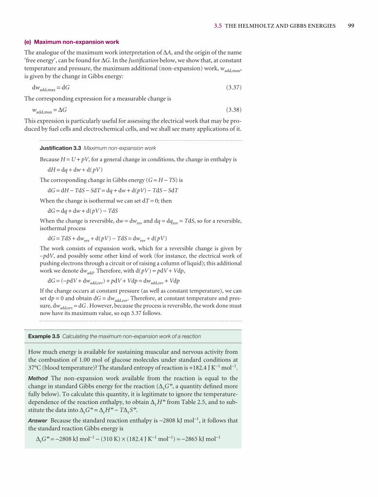
3.5 THE HELMHOLTZ AND GIBBS ENERGIES 99
(e) Maximum non-expansion work
The analogue of the maximum work interpretation of ∆A, and the origin of the name‘free energy’, can be found for ∆G. In the Justification below, we show that, at constanttemperature and pressure, the maximum additional (non-expansion) work, wadd,max,is given by the change in Gibbs energy:
dwadd,max = dG (3.37)
The corresponding expression for a measurable change is
wadd,max = ∆G (3.38)
This expression is particularly useful for assessing the electrical work that may be pro-duced by fuel cells and electrochemical cells, and we shall see many applications of it.
Justification 3.3 Maximum non-expansion work
Because H = U + pV, for a general change in conditions, the change in enthalpy is
dH = dq + dw + d(pV)
The corresponding change in Gibbs energy (G = H − TS) is
dG = dH − TdS − SdT = dq + dw + d(pV) − TdS − SdT
When the change is isothermal we can set dT = 0; then
dG = dq + dw + d(pV) − TdS
When the change is reversible, dw = dwrev and dq = dqrev = TdS, so for a reversible,isothermal process
dG = TdS + dwrev + d(pV) − TdS = dwrev + d(pV)
The work consists of expansion work, which for a reversible change is given by −pdV, and possibly some other kind of work (for instance, the electrical work ofpushing electrons through a circuit or of raising a column of liquid); this additionalwork we denote dwadd. Therefore, with d(pV) = pdV + Vdp,
dG = (−pdV + dwadd,rev) + pdV + Vdp = dwadd,rev + Vdp
If the change occurs at constant pressure (as well as constant temperature), we canset dp = 0 and obtain dG = dwadd,rev. Therefore, at constant temperature and pres-sure, dwadd,rev = dG . However, because the process is reversible, the work done mustnow have its maximum value, so eqn 3.37 follows.
Example 3.5 Calculating the maximum non-expansion work of a reaction
How much energy is available for sustaining muscular and nervous activity fromthe combustion of 1.00 mol of glucose molecules under standard conditions at37°C (blood temperature)? The standard entropy of reaction is +182.4 J K−1 mol−1.
Method The non-expansion work available from the reaction is equal to thechange in standard Gibbs energy for the reaction (∆rG
7, a quantity defined morefully below). To calculate this quantity, it is legitimate to ignore the temperature-dependence of the reaction enthalpy, to obtain ∆r H 7 from Table 2.5, and to sub-stitute the data into ∆rG
7 = ∆rH7 − T∆rS
7.
Answer Because the standard reaction enthalpy is −2808 kJ mol−1, it follows thatthe standard reaction Gibbs energy is
∆rG7 = −2808 kJ mol−1 − (310 K) × (182.4 J K−1 mol−1) = −2865 kJ mol−1
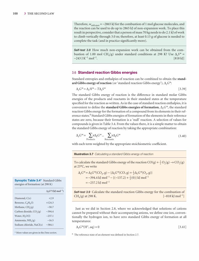
100 3 THE SECOND LAW
8 The reference state of an element was defined in Section 2.7.
Synoptic Table 3.4* Standard Gibbsenergies of formation (at 298 K)
∆fG7/(kJ mol−1)
Diamond, C(s) +2.9
Benzene, C6H6(l) +124.3
Methane, CH4(g) −50.7
Carbon dioxide, CO2(g) −394.4
Water, H2O(l) −237.1
Ammonia, NH3(g) −16.5
Sodium chloride, NaCl(s) −384.1
* More values are given in the Data section.
Therefore, wadd,max = −2865 kJ for the combustion of 1 mol glucose molecules, andthe reaction can be used to do up to 2865 kJ of non-expansion work. To place thisresult in perspective, consider that a person of mass 70 kg needs to do 2.1 kJ of workto climb vertically through 3.0 m; therefore, at least 0.13 g of glucose is needed tocomplete the task (and in practice significantly more).
Self-test 3.8 How much non-expansion work can be obtained from the com-bustion of 1.00 mol CH4(g) under standard conditions at 298 K? Use ∆rS
7 =−243 J K−1 mol−1. [818 kJ]
3.6 Standard reaction Gibbs energies
Standard entropies and enthalpies of reaction can be combined to obtain the stand-ard Gibbs energy of reaction (or ‘standard reaction Gibbs energy’), ∆rG
7:
∆rG7 = ∆rH
7 − T∆rS7 [3.39]
The standard Gibbs energy of reaction is the difference in standard molar Gibbs energies of the products and reactants in their standard states at the temperaturespecified for the reaction as written. As in the case of standard reaction enthalpies, it isconvenient to define the standard Gibbs energies of formation, ∆f G
7, the standardreaction Gibbs energy for the formation of a compound from its elements in their ref-erence states.8 Standard Gibbs energies of formation of the elements in their referencestates are zero, because their formation is a ‘null’ reaction. A selection of values forcompounds is given in Table 3.4. From the values there, it is a simple matter to obtainthe standard Gibbs energy of reaction by taking the appropriate combination:
∆rG7 =
Products∑ν∆fG
7 −Reactants
∑ν∆fG7
(3.40)
with each term weighted by the appropriate stoichiometric coefficient.
Illustration 3.7 Calculating a standard Gibbs energy of reaction
To calculate the standard Gibbs energy of the reaction CO(g) + 1–2 O2(g) → CO2(g)at 25°C, we write
∆rG7 = ∆fG
7(CO2, g) − {∆fG7(CO, g) + 1–2 ∆f G
7(O2, g)}
= −394.4 kJ mol−1 − {(−137.2) + 1–2 (0)} kJ mol−1
= −257.2 kJ mol−1
Self-test 3.9 Calculate the standard reaction Gibbs energy for the combustion ofCH4(g) at 298 K. [−818 kJ mol−1]
Just as we did in Section 2.8, where we acknowledged that solutions of cations cannot be prepared without their accompanying anions, we define one ion, conven-tionally the hydrogen ion, to have zero standard Gibbs energy of formation at all temperatures:
∆fG7(H+, aq) = 0 [3.41]
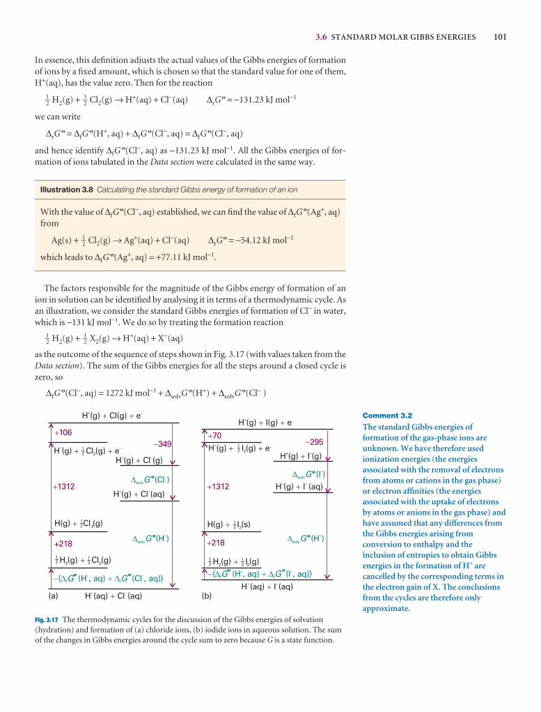
3.6 STANDARD MOLAR GIBBS ENERGIES 101
Comment 3.2
The standard Gibbs energies offormation of the gas-phase ions areunknown. We have therefore usedionization energies (the energiesassociated with the removal of electronsfrom atoms or cations in the gas phase)or electron affinities (the energiesassociated with the uptake of electronsby atoms or anions in the gas phase) andhave assumed that any differences fromthe Gibbs energies arising fromconversion to enthalpy and theinclusion of entropies to obtain Gibbsenergies in the formation of H+ arecancelled by the corresponding terms inthe electron gain of X. The conclusionsfrom the cycles are therefore onlyapproximate.
H (g) Cl(g) e+
_
+ +
H (g) Cl (g) e+ -
+ +2
H(g) Cl (g)+ 2
2 2H (g) Cl (g)+
H (g) Cl (g)+ -
+
H (g) Cl (aq)+ -
+
H (aq) Cl (aq)+ -
+
-349 -295+106
+70
+1312 +1312
+218 +218
(a) (b)
DsolvG (Cl )-
- D + D{ (H , aq) (Cl , aq)}f fG G+ -
H (g) I(g) e+ _
+ +
H (g) I (g) e+
-
+ +2
H (g) I (g)+ –+
H (g) I (aq)+-
+
H(g) I (s)+ 2
DsolvG (H )+
- D + D{ (H , aq) (I , aq)}f fG G+ -
H (aq) I (aq)+
+
-
DsolvG (I )–
DsolvG (H )+
2 2H (g) I (g)+
12-
12- 1
2-
12-
12-
12-
12- 1
2-
°–
°–
°– °– °– °–
°–
°–
Fig. 3.17 The thermodynamic cycles for the discussion of the Gibbs energies of solvation(hydration) and formation of (a) chloride ions, (b) iodide ions in aqueous solution. The sumof the changes in Gibbs energies around the cycle sum to zero because G is a state function.
In essence, this definition adjusts the actual values of the Gibbs energies of formationof ions by a fixed amount, which is chosen so that the standard value for one of them,H+(aq), has the value zero. Then for the reaction
1–2 H2(g) + 1–2 Cl2(g) → H+(aq) + Cl−(aq) ∆rG7 = −131.23 kJ mol−1
we can write
∆rG7 = ∆fG
7(H+, aq) + ∆fG7(Cl−, aq) = ∆fG
7(Cl−, aq)
and hence identify ∆fG7(Cl−, aq) as −131.23 kJ mol−1. All the Gibbs energies of for-
mation of ions tabulated in the Data section were calculated in the same way.
Illustration 3.8 Calculating the standard Gibbs energy of formation of an ion
With the value of ∆fG7(Cl−, aq) established, we can find the value of ∆fG
7(Ag+, aq)from
Ag(s) + 1–2 Cl2(g) → Ag+(aq) + Cl−(aq) ∆rG7 = −54.12 kJ mol−1
which leads to ∆fG7(Ag+, aq) = +77.11 kJ mol−1.
The factors responsible for the magnitude of the Gibbs energy of formation of anion in solution can be identified by analysing it in terms of a thermodynamic cycle. Asan illustration, we consider the standard Gibbs energies of formation of Cl− in water,which is −131 kJ mol−1. We do so by treating the formation reaction
1–2 H2(g) + 1–2 X2(g) → H+(aq) + X−(aq)
as the outcome of the sequence of steps shown in Fig. 3.17 (with values taken from theData section). The sum of the Gibbs energies for all the steps around a closed cycle iszero, so
∆fG7(Cl−, aq) = 1272 kJ mol−1 + ∆solvG
7(H+) + ∆solvG7(Cl− )
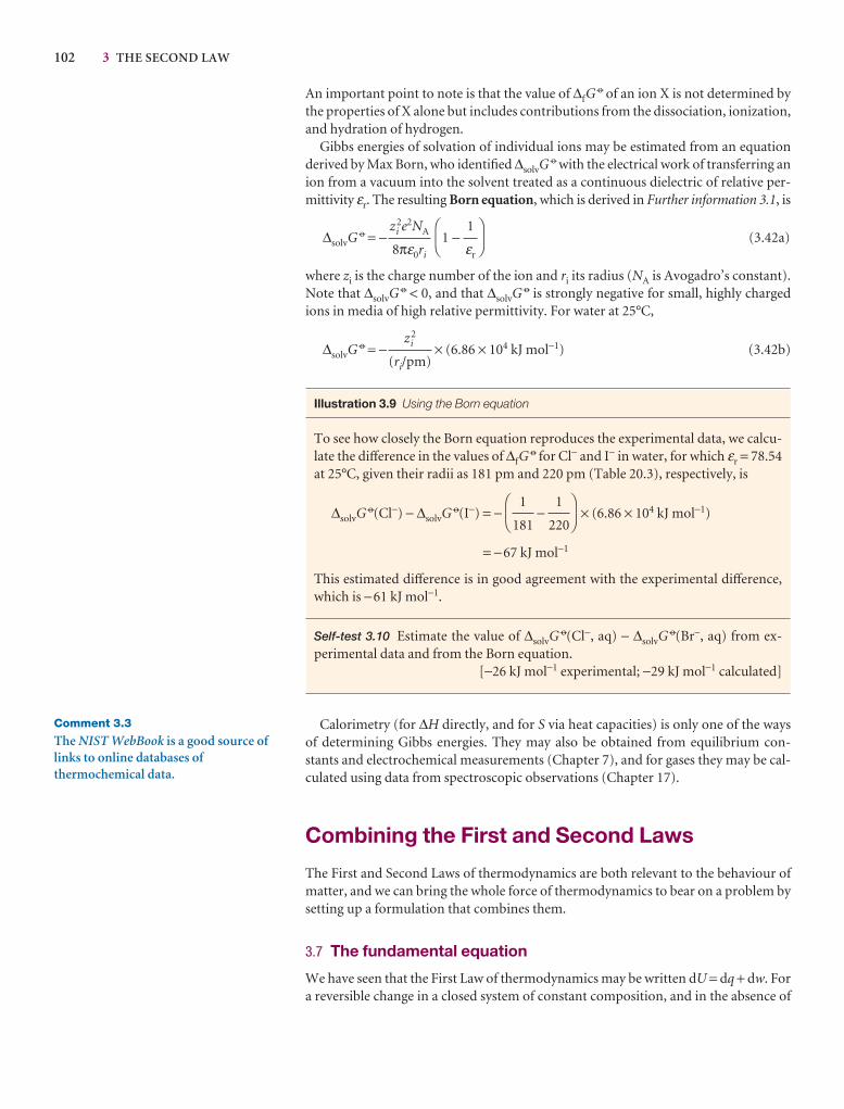
102 3 THE SECOND LAW
Comment 3.3
The NIST WebBook is a good source oflinks to online databases ofthermochemical data.
An important point to note is that the value of ∆fG7 of an ion X is not determined by
the properties of X alone but includes contributions from the dissociation, ionization,and hydration of hydrogen.
Gibbs energies of solvation of individual ions may be estimated from an equationderived by Max Born, who identified ∆solvG
7 with the electrical work of transferring anion from a vacuum into the solvent treated as a continuous dielectric of relative per-mittivity εr. The resulting Born equation, which is derived in Further information 3.1, is
∆solvG7 = − 1 − (3.42a)
where zi is the charge number of the ion and ri its radius (NA is Avogadro’s constant).Note that ∆solvG
7 < 0, and that ∆solvG7 is strongly negative for small, highly charged
ions in media of high relative permittivity. For water at 25°C,
∆solvG7 = − × (6.86 × 10⁴ kJ mol−1) (3.42b)
Illustration 3.9 Using the Born equation
To see how closely the Born equation reproduces the experimental data, we calcu-late the difference in the values of ∆fG
7 for Cl− and I− in water, for which εr = 78.54at 25°C, given their radii as 181 pm and 220 pm (Table 20.3), respectively, is
∆solvG7(Cl−) − ∆solvG
7(I−) = − − × (6.86 × 10⁴ kJ mol−1)
= −67 kJ mol−1
This estimated difference is in good agreement with the experimental difference,which is −61 kJ mol−1.
Self-test 3.10 Estimate the value of ∆solvG7(Cl−, aq) − ∆solvG
7(Br−, aq) from ex-perimental data and from the Born equation.
[−26 kJ mol−1 experimental; −29 kJ mol−1 calculated]
Calorimetry (for ∆H directly, and for S via heat capacities) is only one of the waysof determining Gibbs energies. They may also be obtained from equilibrium con-stants and electrochemical measurements (Chapter 7), and for gases they may be cal-culated using data from spectroscopic observations (Chapter 17).
Combining the First and Second Laws
The First and Second Laws of thermodynamics are both relevant to the behaviour ofmatter, and we can bring the whole force of thermodynamics to bear on a problem bysetting up a formulation that combines them.
3.7 The fundamental equation
We have seen that the First Law of thermodynamics may be written dU = dq + dw. Fora reversible change in a closed system of constant composition, and in the absence of
DF
1
220
1
181
AC
zi2
(ri/pm)
DF
1
εr
AC
zi2e2NA
8πε0ri
3.8 PROPERTIES OF THE INTERNAL ENERGY 103
any additional (non-expansion) work, we may set dwrev = −pdV and (from the defini-tion of entropy) dqrev = TdS, where p is the pressure of the system and T its tempera-ture. Therefore, for a reversible change in a closed system,
dU = TdS − pdV (3.43)
However, because dU is an exact differential, its value is independent of path. There-fore, the same value of dU is obtained whether the change is brought about irreversiblyor reversibly. Consequently, eqn 3.43 applies to any change—reversible or irreversible—of a closed system that does no additional (non-expansion) work. We shall call this com-bination of the First and Second Laws the fundamental equation.
The fact that the fundamental equation applies to both reversible and irreversiblechanges may be puzzling at first sight. The reason is that only in the case of a reversiblechange may TdS be identified with dq and −pdV with dw. When the change is irre-versible, TdS > dq (the Clausius inequality) and −pdV > dw. The sum of dw and dqremains equal to the sum of TdS and −pdV, provided the composition is constant.
3.8 Properties of the internal energy
Equation 3.43 shows that the internal energy of a closed system changes in a simple waywhen either S or V is changed (dU ∝ dS and dU ∝ dV). These simple proportionalitiessuggest that U should be regarded as a function of S and V. We could regard U as afunction of other variables, such as S and p or T and V, because they are all interrelated;but the simplicity of the fundamental equation suggests that U(S,V) is the best choice.
The mathematical consequence of U being a function of S and V is that we can express an infinitesimal change dU in terms of changes dS and dV by
dU =V
dS +S
dV (3.44)
The two partial derivatives are the slopes of the plots of U against S and V, respectively.When this expression is compared to the thermodynamic relation, eqn 3.43, we seethat, for systems of constant composition,
V
= TS
= −p (3.45)
The first of these two equations is a purely thermodynamic definition of temperature(a Zeroth-Law concept) as the ratio of the changes in the internal energy (a First-Lawconcept) and entropy (a Second-Law concept) of a constant-volume, closed, constant-composition system. We are beginning to generate relations between the properties ofa system and to discover the power of thermodynamics for establishing unexpectedrelations.
(a) The Maxwell relations
An infinitesimal change in a function f(x,y) can be written df = gdx + hdy where g andh are functions of x and y. The mathematical criterion for df being an exact differen-tial (in the sense that its integral is independent of path) is that
x
=y
(3.46)
Because the fundamental equation, eqn 3.43, is an expression for an exact differential,the functions multiplying dS and dV (namely T and −p) must pass this test. Therefore,it must be the case that
DF
∂h
∂x
AC
DF
∂g
∂y
AC
DF
∂U
∂V
AC
DF
∂U
∂S
AC
DF
∂U
∂V
AC
DF
∂U
∂S
AC
Comment 3.4
Partial derivatives were introduced inComment 2.5 and are reviewed inAppendix 2. The type of result in eqn3.44 was first obtained in Section 2.11,where we treated U as a function of Tand V.
Comment 3.5
To illustrate the criterion set by eqn3.46, let’s test whether df = 2xydx + x2dyis an exact differential. We identify g = 2xy and h = x2 and form
x
=x
= 2x
y
=y
= 2x
Because these two coefficients are equal,df is exact.
DEF∂x2
∂x
ABCDEF
∂h
∂x
ABC
DEF∂(2xy)
∂y
ABCDEF
∂g
∂y
ABC
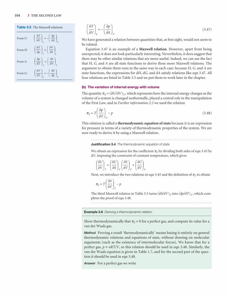
104 3 THE SECOND LAW
Table 3.5 The Maxwell relations
From U:S
= −V
From H:S
=p
From A:V
=T
From G:p
= −T
DEF∂S
∂p
AC
DEF∂V
∂T
ABC
DEF∂S
∂V
AC
DEF∂p
∂T
ABC
DEF∂V
∂S
AC
DEF∂T
∂p
ABC
DEF∂p
∂S
AC
DEF∂T
∂V
ABCS
= −V
(3.47)
We have generated a relation between quantities that, at first sight, would not seem tobe related.
Equation 3.47 is an example of a Maxwell relation. However, apart from being unexpected, it does not look particularly interesting. Nevertheless, it does suggest thatthere may be other similar relations that are more useful. Indeed, we can use the factthat H, G, and A are all state functions to derive three more Maxwell relations. The argument to obtain them runs in the same way in each case: because H, G, and A arestate functions, the expressions for dH, dG, and dA satisfy relations like eqn 3.47. Allfour relations are listed in Table 3.5 and we put them to work later in the chapter.
(b) The variation of internal energy with volume
The quantity πT = (∂U/∂V)T , which represents how the internal energy changes as thevolume of a system is changed isothermally, played a central role in the manipulationof the First Law, and in Further information 2.2 we used the relation
πT = TV
− p (3.48)
This relation is called a thermodynamic equation of state because it is an expressionfor pressure in terms of a variety of thermodynamic properties of the system. We arenow ready to derive it by using a Maxwell relation.
Justification 3.4 The thermodynamic equation of state
We obtain an expression for the coefficient πT by dividing both sides of eqn 3.43 bydV, imposing the constraint of constant temperature, which gives
T
=V T
+S
Next, we introduce the two relations in eqn 3.45 and the definition of πT to obtain
πT = TT
− p
The third Maxwell relation in Table 3.5 turns (∂S/∂V)T into (∂p/∂T)V , which com-pletes the proof of eqn 3.48.
Example 3.6 Deriving a thermodynamic relation
Show thermodynamically that πT = 0 for a perfect gas, and compute its value for avan der Waals gas.
Method Proving a result ‘thermodynamically’ means basing it entirely on generalthermodynamic relations and equations of state, without drawing on moleculararguments (such as the existence of intermolecular forces). We know that for aperfect gas, p = nRT/V, so this relation should be used in eqn 3.48. Similarly, thevan der Waals equation is given in Table 1.7, and for the second part of the ques-tion it should be used in eqn 3.48.
Answer For a perfect gas we write
DEF∂S
∂V
ABC
DEF∂U
∂V
ABCDEF
∂S
∂V
ABCDEF
∂U
∂S
ABCDEF
∂U
∂V
ABC
DF
∂p
∂T
AC
DF
∂p
∂S
AC
DF
∂T
∂V
AC
3.9 PROPERTIES OF THE GIBBS ENERGY 105
V
=V
=
Then, eqn 3.48 becomes
πT = − p = 0
The equation of state of a van der Waals gas is
p = − a
Because a and b are independent of temperature,
V
=
Therefore, from eqn 3.48,
πT = − + a = a
This result for πT implies that the internal energy of a van der Waals gas increaseswhen it expands isothermally (that is, (∂U/∂V)T > 0), and that the increase is related to the parameter a, which models the attractive interactions between theparticles. A larger molar volume, corresponding to a greater average separation between molecules, implies weaker mean intermolecular attractions, so the totalenergy is greater.
Self-test 3.11 Calculate πT for a gas that obeys the virial equation of state (Table 1.7). [πT = RT 2(∂B/∂T)V /V m
2 + · · · ]
3.9 Properties of the Gibbs energy
The same arguments that we have used for U can be used for the Gibbs energy G = H− TS. They lead to expressions showing how G varies with pressure and temperaturethat are important for discussing phase transitions and chemical reactions.
(a) General considerations
When the system undergoes a change of state, G may change because H, T, and S allchange. As in Justification 2.1, we write for infinitesimal changes in each property
dG = dH − d(TS) = dH − TdS − SdT
Because H = U + pV, we know that
dH = dU + d(pV) = dU + pdV + Vdp
and therefore
dG = dU + pdV + Vdp − TdS − SdT
For a closed system doing no non-expansion work, we can replace dU by the funda-mental equation dU = TdS − pdV and obtain
dG = TdS − pdV + pdV + Vdp − TdS − SdT
n2
V 2
n2
V 2
nRT
V − nb
nRT
V − nb
nR
V − nb
DF
∂p
∂T
AC
n2
V 2
nRT
V − nb
nRT
V
nR
V
DF
∂(nRT/V)
∂T
AC
DF
∂p
∂T
AC
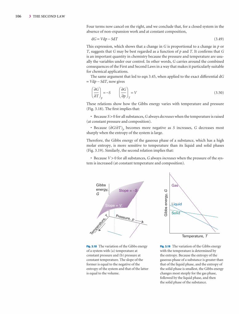
106 3 THE SECOND LAW
Four terms now cancel on the right, and we conclude that, for a closed system in theabsence of non-expansion work and at constant composition,
dG = Vdp − SdT (3.49)
This expression, which shows that a change in G is proportional to a change in p orT, suggests that G may be best regarded as a function of p and T. It confirms that Gis an important quantity in chemistry because the pressure and temperature are usu-ally the variables under our control. In other words, G carries around the combined consequences of the First and Second Laws in a way that makes it particularly suitablefor chemical applications.
The same argument that led to eqn 3.45, when applied to the exact differential dG= Vdp − SdT, now gives
p
= −ST
= V (3.50)
These relations show how the Gibbs energy varies with temperature and pressure (Fig. 3.18). The first implies that:
• Because S > 0 for all substances, G always decreases when the temperature is raised(at constant pressure and composition).
• Because (∂G/∂T)p becomes more negative as S increases, G decreases mostsharply when the entropy of the system is large.
Therefore, the Gibbs energy of the gaseous phase of a substance, which has a highmolar entropy, is more sensitive to temperature than its liquid and solid phases (Fig. 3.19). Similarly, the second relation implies that:
• Because V > 0 for all substances, G always increases when the pressure of the sys-tem is increased (at constant temperature and composition).
DF
∂G
∂p
AC
DF
∂G
∂T
AC
Pressure, p
Tem
pera
ture
, T
Gibbsenergy,G
Slope = V
Slope = �S
Fig. 3.18 The variation of the Gibbs energyof a system with (a) temperature atconstant pressure and (b) pressure atconstant temperature. The slope of theformer is equal to the negative of theentropy of the system and that of the latteris equal to the volume.
Temperature, T
Gib
bsen
ergy
,G
Gas
Liquid
Solid
Fig. 3.19 The variation of the Gibbs energy with the temperature is determined by the entropy. Because the entropy of thegaseous phase of a substance is greater thanthat of the liquid phase, and the entropy ofthe solid phase is smallest, the Gibbs energychanges most steeply for the gas phase,followed by the liquid phase, and then the solid phase of the substance.
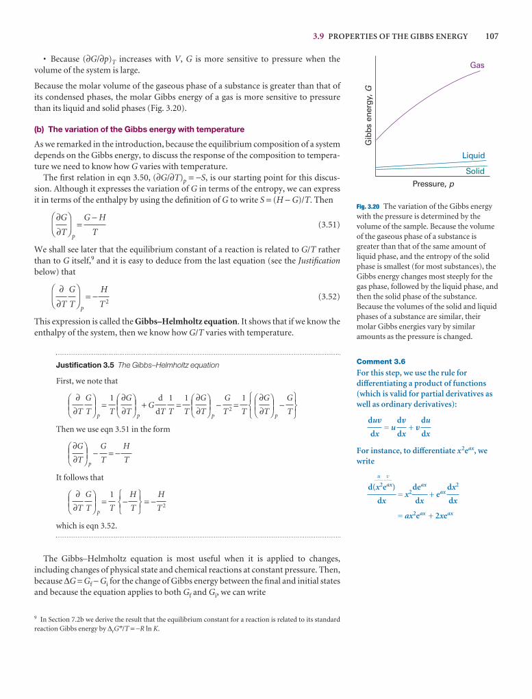
3.9 PROPERTIES OF THE GIBBS ENERGY 107
• Because (∂G/∂p)T increases with V, G is more sensitive to pressure when the volume of the system is large.
Because the molar volume of the gaseous phase of a substance is greater than that ofits condensed phases, the molar Gibbs energy of a gas is more sensitive to pressurethan its liquid and solid phases (Fig. 3.20).
(b) The variation of the Gibbs energy with temperature
As we remarked in the introduction, because the equilibrium composition of a systemdepends on the Gibbs energy, to discuss the response of the composition to tempera-ture we need to know how G varies with temperature.
The first relation in eqn 3.50, (∂G/∂T)p = −S, is our starting point for this discus-sion. Although it expresses the variation of G in terms of the entropy, we can expressit in terms of the enthalpy by using the definition of G to write S = (H − G)/T. Then
p
= (3.51)
We shall see later that the equilibrium constant of a reaction is related to G/T ratherthan to G itself,9 and it is easy to deduce from the last equation (see the Justificationbelow) that
p
= − (3.52)
This expression is called the Gibbs–Helmholtz equation. It shows that if we know theenthalpy of the system, then we know how G/T varies with temperature.
Justification 3.5 The Gibbs–Helmholtz equation
First, we note that
p
=p
+ G =p
− =p
−
Then we use eqn 3.51 in the form
p
− = −
It follows that
p
= − = −
which is eqn 3.52.
The Gibbs–Helmholtz equation is most useful when it is applied to changes, including changes of physical state and chemical reactions at constant pressure. Then,because ∆G = Gf − Gi for the change of Gibbs energy between the final and initial statesand because the equation applies to both Gf and Gi, we can write
H
T 2
567H
T
1231
T
DEFG
T
∂∂T
ABC
H
T
G
T
DEF∂G
∂T
ABC
567
G
T
DEF∂G
∂T
ABC123
1
T
G
T 2
DEF∂G
∂T
ABC1
T
1
T
d
dT
DEF∂G
∂T
ABC1
T
DEFG
T
∂∂T
ABC
H
T 2
DF
G
T
∂∂T
AC
G − H
T
DF
∂G
∂T
AC
Gib
bs e
nerg
y,G
Gas
Liquid
Solid
Pressure, p
Fig. 3.20 The variation of the Gibbs energywith the pressure is determined by thevolume of the sample. Because the volumeof the gaseous phase of a substance isgreater than that of the same amount ofliquid phase, and the entropy of the solidphase is smallest (for most substances), theGibbs energy changes most steeply for thegas phase, followed by the liquid phase, andthen the solid phase of the substance.Because the volumes of the solid and liquidphases of a substance are similar, theirmolar Gibbs energies vary by similaramounts as the pressure is changed.
9 In Section 7.2b we derive the result that the equilibrium constant for a reaction is related to its standardreaction Gibbs energy by ∆rG
7/T = −R ln K.
Comment 3.6
For this step, we use the rule fordifferentiating a product of functions(which is valid for partial derivatives aswell as ordinary derivatives):
= u + V
For instance, to differentiate x2eax, wewrite
u v
= x2 + eax
= ax2eax + 2xeax
dx2
dx
deax
dx
d(x2eax)
dx
# $# $
du
dx
dV
dx
duV
dx
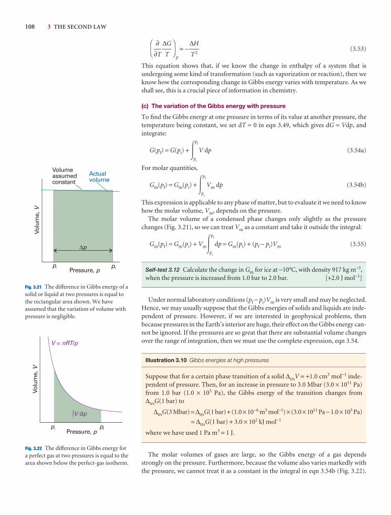
108 3 THE SECOND LAW
Pressure, p
Volu
me,
V
Dp
Volumeassumedconstant
Actualvolume
pfpi
Fig. 3.21 The difference in Gibbs energy of asolid or liquid at two pressures is equal tothe rectangular area shown. We haveassumed that the variation of volume withpressure is negligible.
Pressure, p
Volu
me,
V
V nRT p= /
òV pd
pi pf
Fig. 3.22 The difference in Gibbs energy fora perfect gas at two pressures is equal to thearea shown below the perfect-gas isotherm.
p
= − (3.53)
This equation shows that, if we know the change in enthalpy of a system that is undergoing some kind of transformation (such as vaporization or reaction), then weknow how the corresponding change in Gibbs energy varies with temperature. As weshall see, this is a crucial piece of information in chemistry.
(c) The variation of the Gibbs energy with pressure
To find the Gibbs energy at one pressure in terms of its value at another pressure, thetemperature being constant, we set dT = 0 in eqn 3.49, which gives dG = Vdp, and integrate:
G(pf) = G(pi) + �pf
pi
V dp (3.54a)
For molar quantities,
Gm(pf) = Gm(pi) + �pf
pi
Vm dp (3.54b)
This expression is applicable to any phase of matter, but to evaluate it we need to knowhow the molar volume, Vm, depends on the pressure.
The molar volume of a condensed phase changes only slightly as the pressurechanges (Fig. 3.21), so we can treat Vm as a constant and take it outside the integral:
Gm(pf) = Gm(pi) + Vm�pf
pi
dp = Gm(pi) + (pf − pi)Vm (3.55)
Self-test 3.12 Calculate the change in Gm for ice at −10°C, with density 917 kg m−3,when the pressure is increased from 1.0 bar to 2.0 bar. [+2.0 J mol−1]
Under normal laboratory conditions (pf − pi)Vm is very small and may be neglected.Hence, we may usually suppose that the Gibbs energies of solids and liquids are inde-pendent of pressure. However, if we are interested in geophysical problems, then because pressures in the Earth’s interior are huge, their effect on the Gibbs energy can-not be ignored. If the pressures are so great that there are substantial volume changesover the range of integration, then we must use the complete expression, eqn 3.54.
Illustration 3.10 Gibbs energies at high pressures
Suppose that for a certain phase transition of a solid ∆trsV = +1.0 cm3 mol−1 inde-pendent of pressure. Then, for an increase in pressure to 3.0 Mbar (3.0 × 10¹¹ Pa)from 1.0 bar (1.0 × 10⁵ Pa), the Gibbs energy of the transition changes from ∆trsG(1 bar) to
∆trsG(3 Mbar) = ∆trsG(1 bar) + (1.0 × 10⁻⁶ m3 mol−1) × (3.0 × 1011 Pa − 1.0 × 10⁵ Pa)
= ∆trsG(1 bar) + 3.0 × 10² kJ mol−1
where we have used 1 Pa m3 = 1 J.
The molar volumes of gases are large, so the Gibbs energy of a gas depends strongly on the pressure. Furthermore, because the volume also varies markedly withthe pressure, we cannot treat it as a constant in the integral in eqn 3.54b (Fig. 3.22).
∆H
T 2
DF
∆G
T
∂∂T
AC
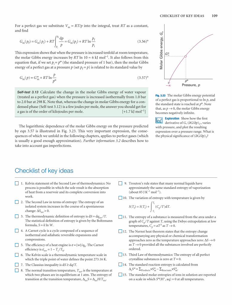
CHECKLIST OF KEY IDEAS 109
For a perfect gas we substitute Vm = RT/p into the integral, treat RT as a constant, and find
Gm(pf) = Gm(pi) + RT�pf
pi
= Gm(pi) + RT ln (3.56)°
This expression shows that when the pressure is increased tenfold at room temperature,the molar Gibbs energy increases by RT ln 10 ≈ 6 kJ mol−1. It also follows from thisequation that, if we set pi = p7 (the standard pressure of 1 bar), then the molar Gibbsenergy of a perfect gas at a pressure p (set pf = p) is related to its standard value by
Gm(p) = G 7m + RT ln (3.57)°
Self-test 3.13 Calculate the change in the molar Gibbs energy of water vapour(treated as a perfect gas) when the pressure is increased isothermally from 1.0 barto 2.0 bar at 298 K. Note that, whereas the change in molar Gibbs energy for a con-densed phase (Self-test 3.12) is a few joules per mole, the answer you should get fora gas is of the order of kilojoules per mole. [+1.7 kJ mol−1]
The logarithmic dependence of the molar Gibbs energy on the pressure predictedby eqn 3.57 is illustrated in Fig. 3.23. This very important expression, the conse-quences of which we unfold in the following chapters, applies to perfect gases (whichis usually a good enough approximation). Further information 3.2 describes how totake into account gas imperfections.
p
p7
pf
pi
dp
p
Checklist of key ideas
1. Kelvin statement of the Second Law of thermodynamics: Noprocess is possible in which the sole result is the absorption of heat from a reservoir and its complete conversion intowork.
2. The Second Law in terms of entropy: The entropy of anisolated system increases in the course of a spontaneouschange: ∆Stot > 0.
3. The thermodynamic definition of entropy is dS = dqrev /T.The statistical definition of entropy is given by the Boltzmannformula, S = k ln W.
4. A Carnot cycle is a cycle composed of a sequence ofisothermal and adiabatic reversible expansions andcompressions.
5. The efficiency of a heat engine is ε = |w | /qh. The Carnotefficiency is εrev = 1 − Tc /Th.
6. The Kelvin scale is a thermodynamic temperature scale inwhich the triple point of water defines the point 273.16 K.
7. The Clausius inequality is dS ≥ dq/T.
8. The normal transition temperature, Ttrs, is the temperature atwhich two phases are in equilibrium at 1 atm. The entropy oftransition at the transition temperature, ∆trsS = ∆trsH/Ttrs.
9. Trouton’s rule states that many normal liquids haveapproximately the same standard entropy of vaporization(about 85 J K−1 mol−1).
10. The variation of entropy with temperature is given by
S(Tf) = S(Ti) + �Tf
Ti
(Cp /T)dT.
11. The entropy of a substance is measured from the area under agraph of Cp /T against T, using the Debye extrapolation at lowtemperatures, Cp = aT 3 as T → 0.
12. The Nernst heat theorem states that the entropy changeaccompanying any physical or chemical transformationapproaches zero as the temperature approaches zero: ∆S → 0as T → 0 provided all the substances involved are perfectlyordered.
13. Third Law of thermodynamics: The entropy of all perfectcrystalline substances is zero at T = 0.
14. The standard reaction entropy is calculated from∆rS
7 = ∑ProductsνS 7m − ∑ReactantsνS 7
m.
15. The standard molar entropies of ions in solution are reportedon a scale in which S 7(H+, aq) = 0 at all temperatures.
Pressure, p-¥
p°
Mol
ar G
ibbs
ene
rgy,
Gm
Gm°
Fig. 3.23 The molar Gibbs energy potentialof a perfect gas is proportional to ln p, andthe standard state is reached at p7. Notethat, as p → 0, the molar Gibbs energybecomes negatively infinite.
Exploration Show how the firstderivative of G, (∂G/∂p)T , varies
with pressure, and plot the resultingexpression over a pressure range. What isthe physical significance of (∂G/∂p)T?

110 3 THE SECOND LAW
16. The Helmholtz energy is A = U − TS. The Gibbs energy is G = H − TS.
17. The criteria of spontaneity may be written as: (a) dSU,V ≥ 0and dUS,V ≤ 0, or (b) dAT,V ≤ 0 and dGT,p ≤ 0.
18. The criterion of equilibrium at constant temperature andvolume, dAT,V = 0. The criterion of equilibrium at constanttemperature and pressure, dGT,p = 0.
19. The maximum work and the Helmholtz energy are related bywmax = ∆A. The maximum additional (non-expansion) workand the Gibbs energy are related by wadd,max = ∆G.
20. The standard Gibbs energy of reaction is given by ∆rG
7 = ∆rH7 − T∆rS
7 = ∑ProductsνG 7m − ∑ReactantsνG 7
m.
21. The standard Gibbs energy of formation (∆fG7) is the
standard reaction Gibbs energy for the formation of acompound from its elements in their reference states.
22. The standard Gibbs energy of reaction may be expressed interms of ∆fG
7, ∆rG7 = ∑Productsν∆fG
7 − ∑Reactantsν∆fG7.
23. The standard Gibbs energies of formation of ions are reportedon a scale in which ∆fG
7(H+, aq) = 0 at all temperatures.
24. The fundamental equation is dU = TdS − pdV.
25. The Maxwell relations are listed in Table 3.5.
26. A thermodynamic equation of state is an expression for pressure in terms of thermodynamic quantities, πT = T(∂p/∂T)V − p.
27. The Gibbs energy is best described as a function of pressureand temperature, dG = Vdp − SdT. The variation of Gibbsenergy with pressure and temperature are, respectively,(∂G/∂p)T = V and (∂G/∂T)p = −S.
28. The temperature dependence of the Gibbs energy is given bythe Gibbs–Helmholtz equation, (∂(G/T)/∂T)p = −H/T 2.
29. For a condensed phase, the Gibbs energy varies with pressureas G(pf) = G(pi) + Vm∆p. For a perfect gas, G(pf) = G(pi) +nRT ln(pf /pi).
Further reading10
Articles and texts
N.C. Craig, Entropy analyses of four familiar processes. J. Chem.Educ. 65, 760 (1988).
J.B. Fenn, Engines, energy, and entropy. W.H. Freeman and Co., New York (1982).
F.J. Hale, Heat engines and refrigerators. In Encyclopedia of appliedphysics (ed. G.L. Trigg), 7, 303. VCH, New York (1993).
D. Kondepudi and I. Prigogine, Modern thermodynamics: from heatengines to dissipative structures. Wiley, New York (1998).
P.G. Nelson, Derivation of the Second Law of thermodynamics fromBoltzmann’s distribution law. J. Chem. Educ. 65, 390 (1988).
Sources of data and information
M.W. Chase, Jr. (ed.), NIST–JANAF thermochemical tables. Publishedas J. Phys. Chem. Ref. Data, Monograph no. 9. American Institute ofPhysics, New York (1998).
R.C. Weast (ed.), Handbook of chemistry and physics, Vol. 81. CRCPress, Boca Raton (2004).
10 See Further reading in Chapter 2 for additional articles, texts, and sources of thermochemical data.
Further information
Further information 3.1 The Born equation
The electrical concepts required in this derivation are reviewed inAppendix 3. The strategy of the calculation is to identify the Gibbsenergy of solvation with the work of transferring an ion from avacuum into the solvent. That work is calculated by taking thedifference of the work of charging an ion when it is in the solutionand the work of charging the same ion when it is in a vacuum.
The Coulomb interaction between two charges q1 and q2 separatedby a distance r is described by the Coulombic potential energy:
V =
where ε is the medium’s permittivity. The permittivity of vacuum isε0 = 8.854 × 10⁻¹² J−1 C2 m−1. The relative permittivity (formerly
q1q2
4πεr
called the ‘dielectric constant’) of a substance is defined as εr = ε /ε0.Ions do not interact as strongly in a solvent of high relativepermittivity (such as water, with εr = 80 at 293 K) as they do in asolvent of lower relative permittivity (such as ethanol, with εr = 25 at293 K). See Chapter 18 for more details. The potential energy of acharge q1 in the presence of a charge q2 can be expressed in terms ofthe Coulomb potential, φ :
V = q1φ φ =
We model an ion as a sphere of radius ri immersed in a medium of permittivity ε. It turns out that, when the charge of the sphere is q, the electric potential, φ, at its surface is the same as the potentialdue to a point charge at its centre, so we can use the last expressionand write
q2
4πεr
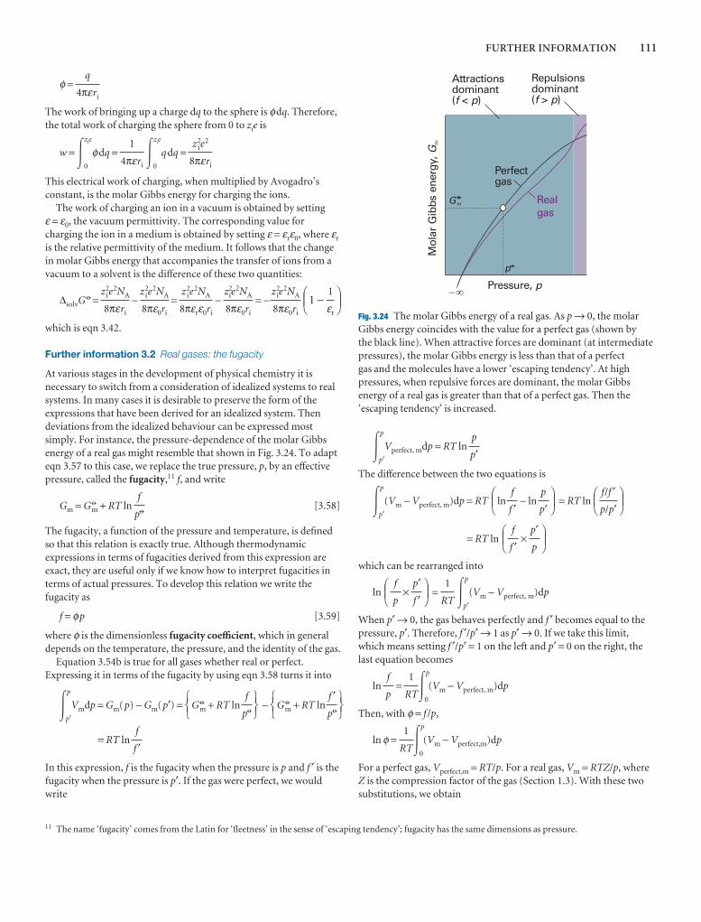
FURTHER INFORMATION 111
φ =
The work of bringing up a charge dq to the sphere is φdq. Therefore,the total work of charging the sphere from 0 to zie is
w = �zie
0
φdq = �zie
0
qdq =
This electrical work of charging, when multiplied by Avogadro’sconstant, is the molar Gibbs energy for charging the ions.
The work of charging an ion in a vacuum is obtained by setting ε = ε0, the vacuum permittivity. The corresponding value forcharging the ion in a medium is obtained by setting ε = εrε0, where εr
is the relative permittivity of the medium. It follows that the changein molar Gibbs energy that accompanies the transfer of ions from avacuum to a solvent is the difference of these two quantities:
∆solvG7 = − = − = − 1 −
which is eqn 3.42.
Further information 3.2 Real gases: the fugacity
At various stages in the development of physical chemistry it isnecessary to switch from a consideration of idealized systems to realsystems. In many cases it is desirable to preserve the form of theexpressions that have been derived for an idealized system. Thendeviations from the idealized behaviour can be expressed mostsimply. For instance, the pressure-dependence of the molar Gibbsenergy of a real gas might resemble that shown in Fig. 3.24. To adapteqn 3.57 to this case, we replace the true pressure, p, by an effectivepressure, called the fugacity,11 f, and write
Gm = G 7m + RT ln [3.58]
The fugacity, a function of the pressure and temperature, is definedso that this relation is exactly true. Although thermodynamicexpressions in terms of fugacities derived from this expression areexact, they are useful only if we know how to interpret fugacities interms of actual pressures. To develop this relation we write thefugacity as
f = φp [3.59]
where φ is the dimensionless fugacity coefficient, which in generaldepends on the temperature, the pressure, and the identity of the gas.
Equation 3.54b is true for all gases whether real or perfect.Expressing it in terms of the fugacity by using eqn 3.58 turns it into
�p
p′
Vmdp = Gm(p) − Gm(p′) = G 7m + RT ln − G 7
m + RT ln
= RT ln
In this expression, f is the fugacity when the pressure is p and f ′ is thefugacity when the pressure is p′. If the gas were perfect, we wouldwrite
f
f ′
567f ′p7
123567
f
p7
123
f
p7
DEF1
εr
ABCz2
ie2NA
8πε0ri
z2ie
2NA
8πε0ri
z2ie
2NA
8πεrε0ri
z2ie
2NA
8πε0ri
z2ie
2NA
8πεri
z2ie
2
8πεri
1
4πεri
q
4πεri
�p
p′
Vperfect, mdp = RT ln
The difference between the two equations is
�p
p′
(Vm − Vperfect, m)dp = RT ln − ln = RT ln
= RT ln ×
which can be rearranged into
ln × = �p
p′
(Vm − Vperfect, m)dp
When p′ → 0, the gas behaves perfectly and f ′ becomes equal to thepressure, p′. Therefore, f ′/p′ → 1 as p′ → 0. If we take this limit,which means setting f ′/p′ = 1 on the left and p′ = 0 on the right, thelast equation becomes
ln = �p
0
(Vm − Vperfect, m)dp
Then, with φ = f /p,
ln φ = �p
0
(Vm − Vperfect,m)dp
For a perfect gas, Vperfect,m = RT/p. For a real gas, Vm = RTZ/p, whereZ is the compression factor of the gas (Section 1.3). With these twosubstitutions, we obtain
1
RT
1
RT
f
p
1
RT
DEFp′f ′
f
p
ABC
DEFp′p
f
f ′ABC
DEFf/f ′p/p′
ABCDEF
p
p′f
f ′ABC
p
p′
Pressure, p-¥
p°
Perfectgas
Repulsionsdominant( > )f p
Attractionsdominant( < )f p
Mol
ar G
ibbs
ene
rgy,
Gm
G m°– Realgas
Fig. 3.24 The molar Gibbs energy of a real gas. As p → 0, the molar Gibbs energy coincides with the value for a perfect gas (shown by the black line). When attractive forces are dominant (at intermediatepressures), the molar Gibbs energy is less than that of a perfect gas and the molecules have a lower ‘escaping tendency’. At highpressures, when repulsive forces are dominant, the molar Gibbsenergy of a real gas is greater than that of a perfect gas. Then the‘escaping tendency’ is increased.
11 The name ‘fugacity’ comes from the Latin for ‘fleetness’ in the sense of ‘escaping tendency’; fugacity has the same dimensions as pressure.
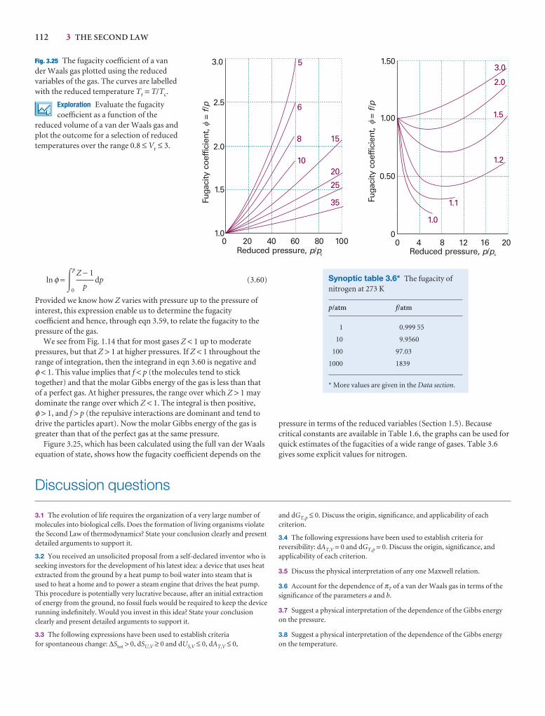
112 3 THE SECOND LAW
ln φ = �p
0
dp (3.60)
Provided we know how Z varies with pressure up to the pressure ofinterest, this expression enable us to determine the fugacitycoefficient and hence, through eqn 3.59, to relate the fugacity to thepressure of the gas.
We see from Fig. 1.14 that for most gases Z < 1 up to moderatepressures, but that Z > 1 at higher pressures. If Z < 1 throughout therange of integration, then the integrand in eqn 3.60 is negative and φ < 1. This value implies that f < p (the molecules tend to sticktogether) and that the molar Gibbs energy of the gas is less than thatof a perfect gas. At higher pressures, the range over which Z > 1 maydominate the range over which Z < 1. The integral is then positive, φ > 1, and f > p (the repulsive interactions are dominant and tend todrive the particles apart). Now the molar Gibbs energy of the gas isgreater than that of the perfect gas at the same pressure.
Figure 3.25, which has been calculated using the full van der Waalsequation of state, shows how the fugacity coefficient depends on the
Z − 1p
pressure in terms of the reduced variables (Section 1.5). Becausecritical constants are available in Table 1.6, the graphs can be used forquick estimates of the fugacities of a wide range of gases. Table 3.6gives some explicit values for nitrogen.
0 20 40 60 80
2.5
2.0
1.5
1.0
Fuga
city
coe
ffici
ent,
=
/fp
5
6
8
10
15
20
25
35
Reduced pressure, /p pc
3.0
1000
0.50
1.00
1.50
0 4 8 12 16 20
Fuga
city
coe
ffici
ent,
=
/fp
Reduced pressure, /p pc
1.0
1.1
1.2
1.5
2.0
3.0
f
f
Fig. 3.25 The fugacity coefficient of a vander Waals gas plotted using the reducedvariables of the gas. The curves are labelledwith the reduced temperature Tr = T/Tc.
Exploration Evaluate the fugacitycoefficient as a function of the
reduced volume of a van der Waals gas andplot the outcome for a selection of reducedtemperatures over the range 0.8 ≤ Vr ≤ 3.
Synoptic table 3.6* The fugacity ofnitrogen at 273 K
p/atm f/atm
1 0.999 55
10 9.9560
100 97.03
1000 1839
* More values are given in the Data section.
Discussion questions
3.1 The evolution of life requires the organization of a very large number ofmolecules into biological cells. Does the formation of living organisms violatethe Second Law of thermodynamics? State your conclusion clearly and presentdetailed arguments to support it.
3.2 You received an unsolicited proposal from a self-declared inventor who isseeking investors for the development of his latest idea: a device that uses heatextracted from the ground by a heat pump to boil water into steam that isused to heat a home and to power a steam engine that drives the heat pump.This procedure is potentially very lucrative because, after an initial extractionof energy from the ground, no fossil fuels would be required to keep the devicerunning indefinitely. Would you invest in this idea? State your conclusionclearly and present detailed arguments to support it.
3.3 The following expressions have been used to establish criteria for spontaneous change: ∆Stot > 0, dSU,V ≥ 0 and dUS,V ≤ 0, dAT,V ≤ 0,
and dGT,p ≤ 0. Discuss the origin, significance, and applicability of eachcriterion.
3.4 The following expressions have been used to establish criteria forreversibility: dAT,V = 0 and dGT,p = 0. Discuss the origin, significance, andapplicability of each criterion.
3.5 Discuss the physical interpretation of any one Maxwell relation.
3.6 Account for the dependence of πT of a van der Waals gas in terms of thesignificance of the parameters a and b.
3.7 Suggest a physical interpretation of the dependence of the Gibbs energyon the pressure.
3.8 Suggest a physical interpretation of the dependence of the Gibbs energyon the temperature.

EXERCISES 113
Exercises
Assume that all gases are perfect and that data refer to 298.15 K unlessotherwise stated.
3.1(a) Calculate the change in entropy when 25 kJ of energy is transferredreversibly and isothermally as heat to a large block of iron at (a) 0°C, (b) 100°C.
3.1(b) Calculate the change in entropy when 50 kJ of energy is transferredreversibly and isothermally as heat to a large block of copper at (a) 0°C, (b) 70°C.
3.2(a) Calculate the molar entropy of a constant-volume sample of neon at500 K given that it is 146.22 J K−1 mol−1 at 298 K.
3.2(b) Calculate the molar entropy of a constant-volume sample of argon at250 K given that it is 154.84 J K−1 mol−1 at 298 K.
3.3(a) Calculate ∆S (for the system) when the state of 3.00 mol of perfect gasatoms, for which Cp,m = 5–
2R, is changed from 25°C and 1.00 atm to 125°C and5.00 atm. How do you rationalize the sign of ∆S?
3.3(b) Calculate ∆S (for the system) when the state of 2.00 mol diatomicperfect gas molecules, for which Cp,m = 7–
2R, is changed from 25°C and 1.50 atm to 135°C and 7.00 atm. How do you rationalize the sign of ∆S?
3.4(a) A sample consisting of 3.00 mol of diatomic perfect gas molecules at200 K is compressed reversibly and adiabatically until its temperature reaches250 K. Given that CV,m = 27.5 J K−1 mol−1, calculate q, w, ∆U, ∆H, and ∆S.
3.4(b) A sample consisting of 2.00 mol of diatomic perfect gas molecules at250 K is compressed reversibly and adiabatically until its temperature reaches300 K. Given that CV,m = 27.5 J K−1 mol−1, calculate q, w, ∆U, ∆H, and ∆S.
3.5(a) Calculate ∆H and ∆Stot when two copper blocks, each of mass 10.0 kg,one at 100°C and the other at 0°C, are placed in contact in an isolatedcontainer. The specific heat capacity of copper is 0.385 J K−1 g−1 and may beassumed constant over the temperature range involved.
3.5(b) Calculate ∆H and ∆Stot when two iron blocks, each of mass 1.00 kg, oneat 200°C and the other at 25°C, are placed in contact in an isolated container.The specific heat capacity of iron is 0.449 J K−1 g−1 and may be assumedconstant over the temperature range involved.
3.6(a) Consider a system consisting of 2.0 mol CO2(g), initially at 25°C and 10 atm and confined to a cylinder of cross-section 10.0 cm2. It is allowed toexpand adiabatically against an external pressure of 1.0 atm until the pistonhas moved outwards through 20 cm. Assume that carbon dioxide may beconsidered a perfect gas with CV,m = 28.8 J K−1 mol−1 and calculate (a) q,(b) w, (c) ∆U, (d) ∆T, (e) ∆S.
3.6(b) Consider a system consisting of 1.5 mol CO2(g), initially at 15°C and9.0 atm and confined to a cylinder of cross-section 100.0 cm2. The sample isallowed to expand adiabatically against an external pressure of 1.5 atm untilthe piston has moved outwards through 15 cm. Assume that carbon dioxidemay be considered a perfect gas with CV,m = 28.8 J K−1 mol−1, and calculate (a) q, (b) w, (c) ∆U, (d) ∆T, (e) ∆S.
3.7(a) The enthalpy of vaporization of chloroform (CHCl3) is 29.4 kJ mol−1 atits normal boiling point of 334.88 K. Calculate (a) the entropy of vaporizationof chloroform at this temperature and (b) the entropy change of thesurroundings.
3.7(b) The enthalpy of vaporization of methanol is 35.27 kJ mol−1 at itsnormal boiling point of 64.1°C. Calculate (a) the entropy of vaporization of methanol at this temperature and (b) the entropy change of thesurroundings.
3.8(a) Calculate the standard reaction entropy at 298 K of
(a) 2 CH3CHO(g) + O2(g) → 2 CH3COOH(l)
(b) 2 AgCl(s) + Br2(l) → 2 AgBr(s) + Cl2(g)
(c) Hg(l) + Cl2(g) → HgCl2(s)
3.8(b) Calculate the standard reaction entropy at 298 K of
(a) Zn(s) + Cu2+(aq) → Zn2+(aq) + Cu(s)
(b) C12H22O11(s) + 12 O2(g) → 12 CO2(g) + 11 H2O(l)
3.9(a) Combine the reaction entropies calculated in Exercise 3.8a with thereaction enthalpies, and calculate the standard reaction Gibbs energies at 298 K.
3.9(b) Combine the reaction entropies calculated in Exercise 3.8b with thereaction enthalpies, and calculate the standard reaction Gibbs energies at 298 K.
3.10(a) Use standard Gibbs energies of formation to calculate the standardreaction Gibbs energies at 298 K of the reactions in Exercise 3.8a.
3.10(b) Use standard Gibbs energies of formation to calculate the standardreaction Gibbs energies at 298 K of the reactions in Exercise 3.8b.
3.11(a) Calculate the standard Gibbs energy of the reaction 4 HCl(g) + O2(g)→ 2 Cl2(g) + 2 H2O(l) at 298 K, from the standard entropies and enthalpies offormation given in the Data section.
3.11(b) Calculate the standard Gibbs energy of the reaction CO(g) +CH3OH(l) → CH3COOH(l) at 298 K, from the standard entropies andenthalpies of formation given in the Data section.
3.12(a) The standard enthalpy of combustion of solid phenol (C6H5OH) is −3054 kJ mol−1 at 298 K and its standard molar entropy is 144.0 J K−1 mol−1.Calculate the standard Gibbs energy of formation of phenol at 298 K.
3.12(b) The standard enthalpy of combustion of solid urea (CO(NH2)2) is −632 kJ mol−1 at 298 K and its standard molar entropy is 104.60 J K−1 mol−1.Calculate the standard Gibbs energy of formation of urea at 298 K.
3.13(a) Calculate the change in the entropies of the system and thesurroundings, and the total change in entropy, when a sample of nitrogen gasof mass 14 g at 298 K and 1.00 bar doubles its volume in (a) an isothermalreversible expansion, (b) an isothermal irreversible expansion against pex = 0,and (c) an adiabatic reversible expansion.
3.13(b) Calculate the change in the entropies of the system and thesurroundings, and the total change in entropy, when the volume of a sampleof argon gas of mass 21 g at 298 K and 1.50 bar increases from 1.20 dm3 to4.60 dm3 in (a) an isothermal reversible expansion, (b) an isothermalirreversible expansion against pex = 0, and (c) an adiabatic reversibleexpansion.
3.14(a) Calculate the maximum non-expansion work per mole that may beobtained from a fuel cell in which the chemical reaction is the combustion ofmethane at 298 K.
3.14(b) Calculate the maximum non-expansion work per mole that may beobtained from a fuel cell in which the chemical reaction is the combustion ofpropane at 298 K.
3.15(a) (a) Calculate the Carnot efficiency of a primitive steam engineoperating on steam at 100°C and discharging at 60°C. (b) Repeat thecalculation for a modern steam turbine that operates with steam at 300°C and discharges at 80°C.

114 3 THE SECOND LAW
3.15(b) A certain heat engine operates between 1000 K and 500 K. (a) What isthe maximum efficiency of the engine? (b) Calculate the maximum work thatcan be done by for each 1.0 kJ of heat supplied by the hot source. (c) Howmuch heat is discharged into the cold sink in a reversible process for each 1.0 kJ supplied by the hot source?
3.16(a) Suppose that 3.0 mmol N2(g) occupies 36 cm3 at 300 K and expandsto 60 cm3. Calculate ∆G for the process.
3.16(b) Suppose that 2.5 mmol Ar(g) occupies 72 dm3 at 298 K and expandsto 100 dm3. Calculate ∆G for the process.
3.17(a) The change in the Gibbs energy of a certain constant-pressure processwas found to fit the expression ∆G/J = −85.40 + 36.5(T/K). Calculate the valueof ∆S for the process.
3.17(b) The change in the Gibbs energy of a certain constant-pressure processwas found to fit the expression ∆G/J = −73.1 + 42.8(T/K). Calculate the valueof ∆S for the process.
3.18(a) Calculate the change in Gibbs energy of 35 g of ethanol (mass density0.789 g cm−3) when the pressure is increased isothermally from 1 atm to 3000 atm.
3.18(b) Calculate the change in Gibbs energy of 25 g of methanol (massdensity 0.791 g cm−3) when the pressure is increased isothermally from 100 kPa to 100 MPa.
3.19(a) Calculate the change in chemical potential of a perfect gas when itspressure is increased isothermally from 1.8 atm to 29.5 atm at 40°C.
3.19(b) Calculate the change in chemical potential of a perfect gas when itspressure is increased isothermally from 92.0 kPa to 252.0 kPa at 50°C.
3.20(a) The fugacity coefficient of a certain gas at 200 K and 50 bar is 0.72.Calculate the difference of its molar Gibbs energy from that of a perfect gas inthe same state.
3.20(b) The fugacity coefficient of a certain gas at 290 K and 2.1 MPa is 0.68.Calculate the difference of its molar Gibbs energy from that of a perfect gas inthe same state.
3.21(a) Estimate the change in the Gibbs energy of 1.0 dm3 of benzene whenthe pressure acting on it is increased from 1.0 atm to 100 atm.
3.21(b) Estimate the change in the Gibbs energy of 1.0 dm3 of water when thepressure acting on it is increased from 100 kPa to 300 kPa.
3.22(a) Calculate the change in the molar Gibbs energy of hydrogen gas when its pressure is increased isothermally from 1.0 atm to 100.0 atm at 298 K.
3.22(b) Calculate the change in the molar Gibbs energy of oxygen when itspressure is increased isothermally from 50.0 kPa to 100.0 kPa at 500 K.
Problems*
Assume that all gases are perfect and that data refer to 298 K unless otherwisestated.
Numerical problems
3.1 Calculate the difference in molar entropy (a) between liquid water and ice at −5°C, (b) between liquid water and its vapour at 95°C and 1.00 atm. The differences in heat capacities on melting and on vaporization are 37.3 J K−1 mol−1 and −41.9 J K−1 mol−1, respectively. Distinguish between the entropy changes of the sample, the surroundings, and the total system, and discuss the spontaneity of the transitions at the two temperatures.
3.2 The heat capacity of chloroform (trichloromethane, CHCl3) in the range240 K to 330 K is given by Cp,m /(J K−1 mol−1) = 91.47 + 7.5 × 10⁻² (T/K). In aparticular experiment, 1.00 mol CHCl3 is heated from 273 K to 300 K.Calculate the change in molar entropy of the sample.
3.3 A block of copper of mass 2.00 kg (Cp,m = 24.44 J K−1 mol−1) andtemperature 0°C is introduced into an insulated container in which there is1.00 mol H2O(g) at 100°C and 1.00 atm. (a) Assuming all the steam iscondensed to water, what will be the final temperature of the system, the heattransferred from water to copper, and the entropy change of the water,copper, and the total system? (b) In fact, some water vapour is present atequilibrium. From the vapour pressure of water at the temperature calculatedin (a), and assuming that the heat capacities of both gaseous and liquid waterare constant and given by their values at that temperature, obtain an improvedvalue of the final temperature, the heat transferred, and the various entropies.(Hint. You will need to make plausible approximations.)
3.4 Consider a perfect gas contained in a cylinder and separated by africtionless adiabatic piston into two sections A and B. All changes in B isisothermal; that is, a thermostat surrounds B to keep its temperature constant.There is 2.00 mol of the gas in each section. Initially, TA = TB = 300 K, VA = VB
= 2.00 dm3. Energy is supplied as heat to Section A and the piston moves tothe right reversibly until the final volume of Section B is 1.00 dm3. Calculate(a) ∆SA and ∆SB, (b) ∆AA and ∆AB, (c) ∆GA and ∆GB, (d) ∆S of the totalsystem and its surroundings. If numerical values cannot be obtained, indicatewhether the values should be positive, negative, or zero or are indeterminatefrom the information given. (Assume CV,m = 20 J K−1 mol−1.)
3.5 A Carnot cycle uses 1.00 mol of a monatomic perfect gas as the workingsubstance from an initial state of 10.0 atm and 600 K. It expands isothermallyto a pressure of 1.00 atm (Step 1), and then adiabatically to a temperature of300 K (Step 2). This expansion is followed by an isothermal compression(Step 3), and then an adiabatic compression (Step 4) back to the initial state.Determine the values of q, w, ∆U, ∆H, ∆S, ∆Stot, and ∆G for each stage of thecycle and for the cycle as a whole. Express your answer as a table of values.
3.6 1.00 mol of perfect gas molecules at 27°C is expanded isothermally froman initial pressure of 3.00 atm to a final pressure of 1.00 atm in two ways: (a) reversibly, and (b) against a constant external pressure of 1.00 atm.Determine the values of q, w, ∆U, ∆H, ∆S, ∆Ssur, ∆Stot for each path.
3.7 The standard molar entropy of NH3(g) is 192.45 J K−1 mol−1 at 298 K, andits heat capacity is given by eqn 2.25 with the coefficients given in Table 2.2.Calculate the standard molar entropy at (a) 100°C and (b) 500°C.
3.8 A block of copper of mass 500 g and initially at 293 K is in thermal contactwith an electric heater of resistance 1.00 kΩ and negligible mass. A current of1.00 A is passed for 15.0 s. Calculate the change in entropy of the copper,taking Cp,m = 24.4 J K−1 mol−1. The experiment is then repeated with thecopper immersed in a stream of water that maintains its temperature at 293 K.Calculate the change in entropy of the copper and the water in this case.
3.9 Find an expression for the change in entropy when two blocks of the samesubstance and of equal mass, one at the temperature Th and the other at Tc, arebrought into thermal contact and allowed to reach equilibrium. Evaluate the
* Problems denoted with the symbol ‡ were supplied by Charles Trapp, Carmen Giunta, and Marshall Cady.
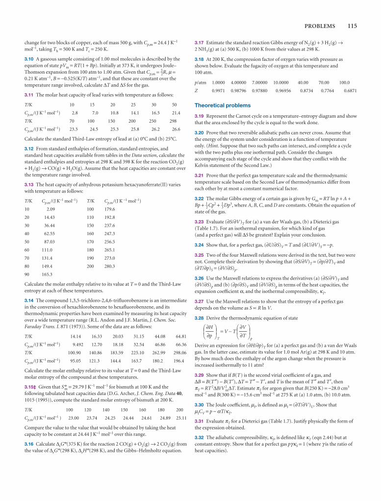
PROBLEMS 115
change for two blocks of copper, each of mass 500 g, with Cp,m = 24.4 J K−1
mol−1, taking Th = 500 K and Tc = 250 K.
3.10 A gaseous sample consisting of 1.00 mol molecules is described by theequation of state pVm = RT(1 + Bp). Initially at 373 K, it undergoes Joule–Thomson expansion from 100 atm to 1.00 atm. Given that Cp,m = 5–
2R, µ =0.21 K atm−1, B = −0.525(K/T) atm−1, and that these are constant over thetemperature range involved, calculate ∆T and ∆S for the gas.
3.11 The molar heat capacity of lead varies with temperature as follows:
T/K 10 15 20 25 30 50
Cp,m /(J K−1 mol−1) 2.8 7.0 10.8 14.1 16.5 21.4
T/K 70 100 150 200 250 298
Cp,m /(J K−1 mol−1) 23.3 24.5 25.3 25.8 26.2 26.6
Calculate the standard Third-Law entropy of lead at (a) 0°C and (b) 25°C.
3.12 From standard enthalpies of formation, standard entropies, andstandard heat capacities available from tables in the Data section, calculate thestandard enthalpies and entropies at 298 K and 398 K for the reaction CO2(g)+ H2(g) → CO(g) + H2O(g). Assume that the heat capacities are constant overthe temperature range involved.
3.13 The heat capacity of anhydrous potassium hexacyanoferrate(II) varieswith temperature as follows:
T/K Cp,m /(J K−1 mol−1) T/K Cp,m /(J K −1 mol−1)
10 2.09 100 179.6
20 14.43 110 192.8
30 36.44 150 237.6
40 62.55 160 247.3
50 87.03 170 256.5
60 111.0 180 265.1
70 131.4 190 273.0
80 149.4 200 280.3
90 165.3
Calculate the molar enthalpy relative to its value at T = 0 and the Third-Lawentropy at each of these temperatures.
3.14 The compound 1,3,5-trichloro-2,4,6-trifluorobenzene is an intermediatein the conversion of hexachlorobenzene to hexafluorobenzene, and itsthermodynamic properties have been examined by measuring its heat capacityover a wide temperature range (R.L. Andon and J.F. Martin, J. Chem. Soc.Faraday Trans. I. 871 (1973)). Some of the data are as follows:
T/K 14.14 16.33 20.03 31.15 44.08 64.81
Cp,m /(J K−1 mol−1) 9.492 12.70 18.18 32.54 46.86 66.36
T/K 100.90 140.86 183.59 225.10 262.99 298.06
Cp,m /(J K−1 mol−1) 95.05 121.3 144.4 163.7 180.2 196.4
Calculate the molar enthalpy relative to its value at T = 0 and the Third-Lawmolar entropy of the compound at these temperatures.
3.15‡ Given that S 7m = 29.79 J K−1 mol−1 for bismuth at 100 K and the
following tabulated heat capacities data (D.G. Archer, J. Chem. Eng. Data 40,1015 (1995)), compute the standard molar entropy of bismuth at 200 K.
T/K 100 120 140 150 160 180 200
Cp,m /(J K−1 mol−1 ) 23.00 23.74 24.25 24.44 24.61 24.89 25.11
Compare the value to the value that would be obtained by taking the heatcapacity to be constant at 24.44 J K−1 mol−1 over this range.
3.16 Calculate ∆rG7(375 K) for the reaction 2 CO(g) + O2(g) → 2 CO2(g) from
the value of ∆rG7(298 K), ∆rH
7(298 K), and the Gibbs–Helmholtz equation.
3.17 Estimate the standard reaction Gibbs energy of N2(g) + 3 H2(g) →2 NH3(g) at (a) 500 K, (b) 1000 K from their values at 298 K.
3.18 At 200 K, the compression factor of oxygen varies with pressure asshown below. Evaluate the fugacity of oxygen at this temperature and 100 atm.
p/atm 1.0000 4.00000 7.00000 10.0000 40.00 70.00 100.0
Z 0.9971 0.98796 0.97880 0.96956 0.8734 0.7764 0.6871
Theoretical problems
3.19 Represent the Carnot cycle on a temperature–entropy diagram and showthat the area enclosed by the cycle is equal to the work done.
3.20 Prove that two reversible adiabatic paths can never cross. Assume thatthe energy of the system under consideration is a function of temperatureonly. (Hint. Suppose that two such paths can intersect, and complete a cyclewith the two paths plus one isothermal path. Consider the changesaccompanying each stage of the cycle and show that they conflict with theKelvin statement of the Second Law.)
3.21 Prove that the perfect gas temperature scale and the thermodynamictemperature scale based on the Second Law of thermodynamics differ fromeach other by at most a constant numerical factor.
3.22 The molar Gibbs energy of a certain gas is given by Gm = RT ln p + A +Bp + 1–
2 Cp2 + 1–3 Dp3, where A, B, C, and D are constants. Obtain the equation of
state of the gas.
3.23 Evaluate (∂S/∂V)T for (a) a van der Waals gas, (b) a Dieterici gas (Table 1.7). For an isothermal expansion, for which kind of gas (and a perfect gas) will ∆S be greatest? Explain your conclusion.
3.24 Show that, for a perfect gas, (∂U/∂S)V = T and (∂U/∂V)S = −p.
3.25 Two of the four Maxwell relations were derived in the text, but two werenot. Complete their derivation by showing that (∂S/∂V)T = (∂p/∂T)V and(∂T/∂p)S = (∂V/∂S)p.
3.26 Use the Maxwell relations to express the derivatives (a) (∂S/∂V)T and(∂V/∂S)p and (b) (∂p/∂S)V and (∂V/∂S)p in terms of the heat capacities, theexpansion coefficient α, and the isothermal compressibility, κT.
3.27 Use the Maxwell relations to show that the entropy of a perfect gasdepends on the volume as S ∝ R ln V.
3.28 Derive the thermodynamic equation of state
T
= V − Tp
Derive an expression for (∂H/∂p)T for (a) a perfect gas and (b) a van der Waalsgas. In the latter case, estimate its value for 1.0 mol Ar(g) at 298 K and 10 atm.By how much does the enthalpy of the argon change when the pressure isincreased isothermally to 11 atm?
3.29 Show that if B(T) is the second virial coefficient of a gas, and ∆B = B(T″) − B(T ′), ∆T = T″ − T ′, and T is the mean of T″ and T ′, then πT ≈ RT 2∆B/V 2
m∆T. Estimate πT for argon given that B(250 K) = −28.0 cm3
mol−1 and B(300 K) = −15.6 cm3 mol−1 at 275 K at (a) 1.0 atm, (b) 10.0 atm.
3.30 The Joule coefficient, µJ, is defined as µJ = (∂T/∂V)U. Show that µJCV = p − αT/κT.
3.31 Evaluate πT for a Dieterici gas (Table 1.7). Justify physically the form ofthe expression obtained.
3.32 The adiabatic compressibility, κS, is defined like κT (eqn 2.44) but atconstant entropy. Show that for a perfect gas pγκS = 1 (where γ is the ratio ofheat capacities).
DEF∂V
∂T
ABCDEF
∂H
∂p
ABC

116 3 THE SECOND LAW
3.33 Suppose that S is regarded as a function of p and T. Show that TdS = CpdT − αTVdp. Hence, show that the energy transferred as heat whenthe pressure on an incompressible liquid or solid is increased by ∆p is equal to−αTV∆p. Evaluate q when the pressure acting on 100 cm3 of mercury at 0°C isincreased by 1.0 kbar. (α = 1.82 × 10⁻⁴ K−1.)
3.34 Suppose that (a) the attractive interactions between gas particles can beneglected, (b) the attractive interaction is dominant in a van der Waals gas,and the pressure is low enough to make the approximation 4ap/(RT)2 << 1.Find expressions for the fugacity of a van der Waals gas in terms of thepressure and estimate its value for ammonia at 10.00 atm and 298.15 K in each case.
3.35 Find an expression for the fugacity coefficient of a gas that obeys theequation of state pVm = RT(1 + B/Vm + C/V 2
m). Use the resulting expression toestimate the fugacity of argon at 1.00 atm and 100 K using B = −21.13 cm3
mol−1 and C = 1054 cm6 mol−2.
Applications: to biology, environmental science, polymerscience, and engineering
3.36 The protein lysozyme unfolds at a transition temperature of 75.5°C andthe standard enthalpy of transition is 509 kJ mol−1. Calculate the entropy ofunfolding of lysozyme at 25.0°C, given that the difference in the constant-pressure heat capacities upon unfolding is 6.28 kJ K−1 mol−1 and can beassumed to be independent of temperature. Hint. Imagine that the transitionat 25.0°C occurs in three steps: (i) heating of the folded protein from 25.0°C tothe transition temperature, (ii) unfolding at the transition temperature, and(iii) cooling of the unfolded protein to 25.0°C. Because the entropy is a statefunction, the entropy change at 25.0°C is equal to the sum of the entropychanges of the steps.
3.37 At 298 K the standard enthalpy of combustion of sucrose is −5797 kJmol−1 and the standard Gibbs energy of the reaction is −6333 kJ mol−1.Estimate the additional non-expansion work that may be obtained by raisingthe temperature to blood temperature, 37°C.
3.38 In biological cells, the energy released by the oxidation of foods (Impacton Biology I2.2) is stored in adenosine triphosphate (ATP or ATP4−). Theessence of ATP’s action is its ability to lose its terminal phosphate group byhydrolysis and to form adenosine diphosphate (ADP or ADP3−):
ATP4−(aq) + H2O(l) → ADP3−(aq) + HPO42− (aq) + H3O+(aq)
At pH = 7.0 and 37°C (310 K, blood temperature) the enthalpy and Gibbsenergy of hydrolysis are ∆rH = −20 kJ mol−1 and ∆rG = −31 kJ mol−1,respectively. Under these conditions, the hydrolysis of 1 mol ATP4−(aq) resultsin the extraction of up to 31 kJ of energy that can be used to do non-expansionwork, such as the synthesis of proteins from amino acids, muscularcontraction, and the activation of neuronal circuits in our brains. (a) Calculateand account for the sign of the entropy of hydrolysis of ATP at pH = 7.0 and310 K. (b) Suppose that the radius of a typical biological cell is 10 µm and thatinside it 106 ATP molecules are hydrolysed each second. What is the powerdensity of the cell in watts per cubic metre (1 W = 1 J s−1)? A computer batterydelivers about 15 W and has a volume of 100 cm3. Which has the greaterpower density, the cell or the battery? (c) The formation of glutamine fromglutamate and ammonium ions requires 14.2 kJ mol−1 of energy input. It isdriven by the hydrolysis of ATP to ADP mediated by the enzyme glutaminesynthetase. How many moles of ATP must be hydrolysed to form 1 molglutamine?
3.39‡ In 1995, the Intergovernmental Panel on Climate Change (IPCC)considered a global average temperature rise of 1.0–3.5°C likely by the year2100, with 2.0°C its best estimate. Because water vapour is itself a greenhousegas, the increase in water vapour content of the atmosphere is of someconcern to climate change experts. Predict the relative increase in water
vapour in the atmosphere based on a temperature rises of 2.0 K, assuming thatthe relative humidity remains constant. (The present global mean temperatureis 290 K, and the equilibrium vapour pressure of water at that temperature is0.0189 bar.)
3.40‡ Nitric acid hydrates have received much attention as possible catalystsfor heterogeneous reactions that bring about the Antarctic ozone hole.Worsnop et al. investigated the thermodynamic stability of these hydratesunder conditions typical of the polar winter stratosphere (D. R. Worsnop, L.E.Fox, M.S. Zahniser, and S.C. Wofsy, Science 259, 71 (1993)). They reportthermodynamic data for the sublimation of mono-, di-, and trihydrates tonitric acid and water vapours, HNO3· nH2O (s) → HNO3(g) + nH2O(g),for n = 1, 2, and 3. Given ∆rG
7 and ∆rH7 for these reactions at 220 K, use the
Gibbs–Helmholtz equation to compute ∆rG7 at 190 K.
n 1 2 3
∆rG7/(kJ mol−1) 46.2 69.4 93.2
∆rH7/(kJ mol−1) 127 188 237
3.41‡ J. Gao and J. H. Weiner in their study of the origin of stress on theatomic level in dense polymer systems (Science 266, 748 (1994)), observe that the tensile force required to maintain the length, l, of a long linear chainof N freely jointed links each of length a, can be interpreted as arising from an entropic spring. For such a chain, S(l) = −3kl2/2Na2 + C, where k is theBoltzmann constant and C is a constant. Using thermodynamic relations ofthis and previous chapters, show that the tensile force obeys Hooke’s law, f = −kf l, if we assume that the energy U is independent of l.
3.42 Suppose that an internal combustion engine runs on octane, for whichthe enthalpy of combustion is −5512 kJ mol−1 and take the mass of 1 gallon offuel as 3 kg. What is the maximum height, neglecting all forms of friction, towhich a car of mass 1000 kg can be driven on 1.00 gallon of fuel given that theengine cylinder temperature is 2000°C and the exit temperature is 800°C?
3.43 The cycle involved in the operation of an internal combustion engine iscalled the Otto cycle. Air can be considered to be the working substance andcan be assumed to be a perfect gas. The cycle consists of the following steps:(1) reversible adiabatic compression from A to B, (2) reversible constant-volume pressure increase from B to C due to the combustion of a smallamount of fuel, (3) reversible adiabatic expansion from C to D, and (4)reversible and constant-volume pressure decrease back to state A. Determinethe change in entropy (of the system and of the surroundings) for each step ofthe cycle and determine an expression for the efficiency of the cycle, assumingthat the heat is supplied in Step 2. Evaluate the efficiency for a compressionratio of 10:1. Assume that, in state A, V = 4.00 dm3, p = 1.00 atm, and T = 300 K, that VA = 10VB, pC /pB = 5, and that Cp,m = 7–
2 R.
3.44 To calculate the work required to lower the temperature of an object, we need to consider how the coefficient of performance changes with thetemperature of the object. (a) Find an expression for the work of cooling anobject from Ti to Tf when the refrigerator is in a room at a temperature Th.Hint. Write dw = dq/c(T), relate dq to dT through the heat capacity Cp,and integrate the resulting expression. Assume that the heat capacity isindependent of temperature in the range of interest. (b) Use the result in part(a) to calculate the work needed to freeze 250 g of water in a refrigerator at 293 K. How long will it take when the refrigerator operates at 100 W?
3.45 The expressions that apply to the treatment of refrigerators also describethe behaviour of heat pumps, where warmth is obtained from the back of arefrigerator while its front is being used to cool the outside world. Heat pumpsare popular home heating devices because they are very efficient. Compareheating of a room at 295 K by each of two methods: (a) direct conversion of1.00 kJ of electrical energy in an electrical heater, and (b) use of 1.00 kJ ofelectrical energy to run a reversible heat pump with the outside at 260 K.Discuss the origin of the difference in the energy delivered to the interior of the house by the two methods.

Physicaltransformations ofpure substancesThe discussion of the phase transitions of pure substances is among the simplest applica-tions of thermodynamics to chemistry. We shall see that a phase diagram is a map of thepressures and temperatures at which each phase of a substance is the most stable. First,we describe the interpretation of empirically determined phase diagrams for a selection ofmaterials. Then we turn to a consideration of the factors that determine the positions andshapes of the boundaries between the regions on a phase diagram. The practical import-ance of the expressions we derive is that they show how the vapour pressure of a sub-stance varies with temperature and how the melting point varies with pressure. We shall seethat the transitions between phases can be classified by noting how various thermodynamicfunctions change when the transition occurs. This chapter also introduces the chemical potential, a property that is at the centre of discussions of phase transitions and chemicalreactions.
Vaporization, melting, and the conversion of graphite to diamond are all examples ofchanges of phase without change of chemical composition. In this chapter we describesuch processes thermodynamically, using as the guiding principle the tendency of sys-tems at constant temperature and pressure to minimize their Gibbs energy.
Phase diagrams
One of the most succinct ways of presenting the physical changes of state that a sub-stance can undergo is in terms of its phase diagram. We present the concept in thissection.
4.1 The stabilities of phases
A phase of a substance is a form of matter that is uniform throughout in chemicalcomposition and physical state. Thus, we speak of solid, liquid, and gas phases of asubstance, and of its various solid phases, such as the white and black allotropes ofphosphorus. A phase transition, the spontaneous conversion of one phase into another phase, occurs at a characteristic temperature for a given pressure. Thus, at 1 atm, ice is the stable phase of water below 0°C, but above 0°C liquid water is morestable. This difference indicates that below 0°C the Gibbs energy decreases as liquidwater changes into ice and that above 0°C the Gibbs energy decreases as ice changesinto liquid water. The transition temperature, Ttrs, is the temperature at which thetwo phases are in equilibrium and the Gibbs energy is minimized at the prevailingpressure.
4Phase diagrams
4.1 The stabilities of phases
4.2 Phase boundaries
I4.1 Impact on engineering andtechnology: Supercritical fluids
4.3 Three typical phase diagrams
Phase stability and phasetransitions
4.4 The thermodynamic criterionof equilibrium
4.5 The dependence of stability onthe conditions
4.6 The location of phaseboundaries
4.7 The Ehrenfest classification ofphase transitions
Checklist of key ideas
Further reading
Discussion questions
Exercises
Problems
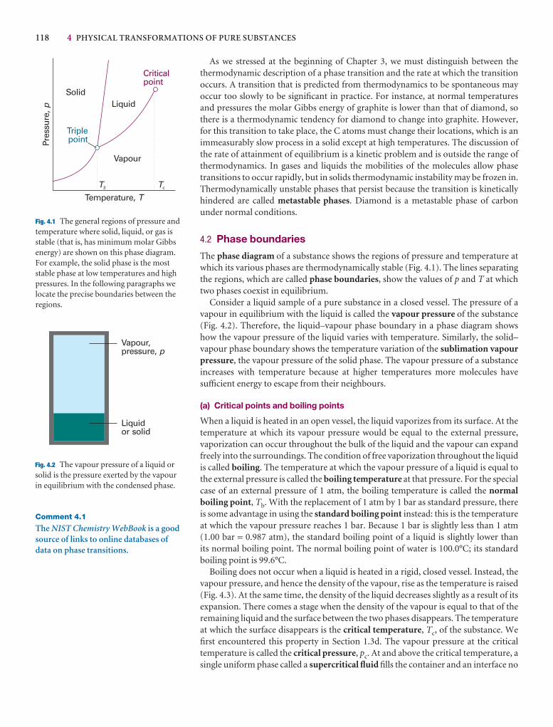
118 4 PHYSICAL TRANSFORMATIONS OF PURE SUBSTANCES
As we stressed at the beginning of Chapter 3, we must distinguish between the thermodynamic description of a phase transition and the rate at which the transition occurs. A transition that is predicted from thermodynamics to be spontaneous mayoccur too slowly to be significant in practice. For instance, at normal temperaturesand pressures the molar Gibbs energy of graphite is lower than that of diamond, sothere is a thermodynamic tendency for diamond to change into graphite. However,for this transition to take place, the C atoms must change their locations, which is animmeasurably slow process in a solid except at high temperatures. The discussion ofthe rate of attainment of equilibrium is a kinetic problem and is outside the range ofthermodynamics. In gases and liquids the mobilities of the molecules allow phasetransitions to occur rapidly, but in solids thermodynamic instability may be frozen in.Thermodynamically unstable phases that persist because the transition is kineticallyhindered are called metastable phases. Diamond is a metastable phase of carbonunder normal conditions.
4.2 Phase boundaries
The phase diagram of a substance shows the regions of pressure and temperature atwhich its various phases are thermodynamically stable (Fig. 4.1). The lines separatingthe regions, which are called phase boundaries, show the values of p and T at whichtwo phases coexist in equilibrium.
Consider a liquid sample of a pure substance in a closed vessel. The pressure of avapour in equilibrium with the liquid is called the vapour pressure of the substance(Fig. 4.2). Therefore, the liquid–vapour phase boundary in a phase diagram showshow the vapour pressure of the liquid varies with temperature. Similarly, the solid–vapour phase boundary shows the temperature variation of the sublimation vapourpressure, the vapour pressure of the solid phase. The vapour pressure of a substanceincreases with temperature because at higher temperatures more molecules havesufficient energy to escape from their neighbours.
(a) Critical points and boiling points
When a liquid is heated in an open vessel, the liquid vaporizes from its surface. At thetemperature at which its vapour pressure would be equal to the external pressure, vaporization can occur throughout the bulk of the liquid and the vapour can expandfreely into the surroundings. The condition of free vaporization throughout the liquidis called boiling. The temperature at which the vapour pressure of a liquid is equal tothe external pressure is called the boiling temperature at that pressure. For the specialcase of an external pressure of 1 atm, the boiling temperature is called the normalboiling point, Tb. With the replacement of 1 atm by 1 bar as standard pressure, thereis some advantage in using the standard boiling point instead: this is the temperatureat which the vapour pressure reaches 1 bar. Because 1 bar is slightly less than 1 atm(1.00 bar = 0.987 atm), the standard boiling point of a liquid is slightly lower than its normal boiling point. The normal boiling point of water is 100.0°C; its standardboiling point is 99.6°C.
Boiling does not occur when a liquid is heated in a rigid, closed vessel. Instead, thevapour pressure, and hence the density of the vapour, rise as the temperature is raised(Fig. 4.3). At the same time, the density of the liquid decreases slightly as a result of itsexpansion. There comes a stage when the density of the vapour is equal to that of theremaining liquid and the surface between the two phases disappears. The temperatureat which the surface disappears is the critical temperature, Tc, of the substance. Wefirst encountered this property in Section 1.3d. The vapour pressure at the criticaltemperature is called the critical pressure, pc. At and above the critical temperature, asingle uniform phase called a supercritical fluid fills the container and an interface no
SolidLiquid
Vapour
TriplepointPr
essu
re,p
Temperature, TTcT3
Criticalpoint
Fig. 4.1 The general regions of pressure andtemperature where solid, liquid, or gas isstable (that is, has minimum molar Gibbsenergy) are shown on this phase diagram.For example, the solid phase is the moststable phase at low temperatures and highpressures. In the following paragraphs welocate the precise boundaries between theregions.
Liquidor solid
Vapour,pressure, p
Fig. 4.2 The vapour pressure of a liquid orsolid is the pressure exerted by the vapourin equilibrium with the condensed phase.
Comment 4.1
The NIST Chemistry WebBook is a goodsource of links to online databases ofdata on phase transitions.
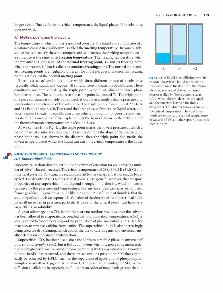
4.2 PHASE BOUNDARIES 119
longer exists. That is, above the critical temperature, the liquid phase of the substancedoes not exist.
(b) Melting points and triple points
The temperature at which, under a specified pressure, the liquid and solid phases of asubstance coexist in equilibrium is called the melting temperature. Because a sub-stance melts at exactly the same temperature as it freezes, the melting temperature ofa substance is the same as its freezing temperature. The freezing temperature whenthe pressure is 1 atm is called the normal freezing point, Tf, and its freezing pointwhen the pressure is 1 bar is called the standard freezing point. The normal and stand-ard freezing points are negligibly different for most purposes. The normal freezingpoint is also called the normal melting point.
There is a set of conditions under which three different phases of a substance (typically solid, liquid, and vapour) all simultaneously coexist in equilibrium. These conditions are represented by the triple point, a point at which the three phaseboundaries meet. The temperature at the triple point is denoted T3. The triple pointof a pure substance is outside our control: it occurs at a single definite pressure andtemperature characteristic of the substance. The triple point of water lies at 273.16 Kand 611 Pa (6.11 mbar, 4.58 Torr), and the three phases of water (ice, liquid water, andwater vapour) coexist in equilibrium at no other combination of pressure and tem-perature. This invariance of the triple point is the basis of its use in the definition ofthe thermodynamic temperature scale (Section 3.2c).
As we can see from Fig. 4.1, the triple point marks the lowest pressure at which a liquid phase of a substance can exist. If (as is common) the slope of the solid–liquidphase boundary is as shown in the diagram, then the triple point also marks the lowest temperature at which the liquid can exist; the critical temperature is the upperlimit.
IMPACT ON CHEMICAL ENGINEERING AND TECHNOLOGY
I4.1 Supercritical fluids
Supercritical carbon dioxide, scCO2, is the centre of attention for an increasing num-ber of solvent-based processes. The critical temperature of CO2, 304.2 K (31.0°C) andits critical pressure, 72.9 atm, are readily accessible, it is cheap, and it can readily be re-cycled. The density of scCO2 at its critical point is 0.45 g cm−3. However, the transportproperties of any supercritical fluid depend strongly on its density, which in turn issensitive to the pressure and temperature. For instance, densities may be adjustedfrom a gas-like 0.1 g cm−3 to a liquid-like 1.2 g cm−3. A useful rule of thumb is that thesolubility of a solute is an exponential function of the density of the supercritical fluid,so small increases in pressure, particularly close to the critical point, can have verylarge effects on solubility.
A great advantage of scCO2 is that there are no noxious residues once the solventhas been allowed to evaporate, so, coupled with its low critical temperature, scCO2 isideally suited to food processing and the production of pharmaceuticals. It is used, forinstance, to remove caffeine from coffee. The supercritical fluid is also increasinglybeing used for dry cleaning, which avoids the use of carcinogenic and environment-ally deleterious chlorinated hydrocarbons.
Supercritical CO2 has been used since the 1960s as a mobile phase in supercriticalfluid chromatography (SFC), but it fell out of favour when the more convenient tech-nique of high-performance liquid chromatography (HPLC) was introduced. However,interest in SFC has returned, and there are separations possible in SFC that cannoteasily be achieved by HPLC, such as the separation of lipids and of phospholipids.Samples as small as 1 pg can be analysed. The essential advantage of SFC is thatdiffusion coefficients in supercritical fluids are an order of magnitude greater than in
(a) (b) (c)
Fig. 4.3 (a) A liquid in equilibrium with itsvapour. (b) When a liquid is heated in asealed container, the density of the vapourphase increases and that of the liquiddecreases slightly. There comes a stage, (c), at which the two densities are equaland the interface between the fluidsdisappears. This disappearance occurs atthe critical temperature. The containerneeds to be strong: the critical temperatureof water is 374°C and the vapour pressure isthen 218 atm.
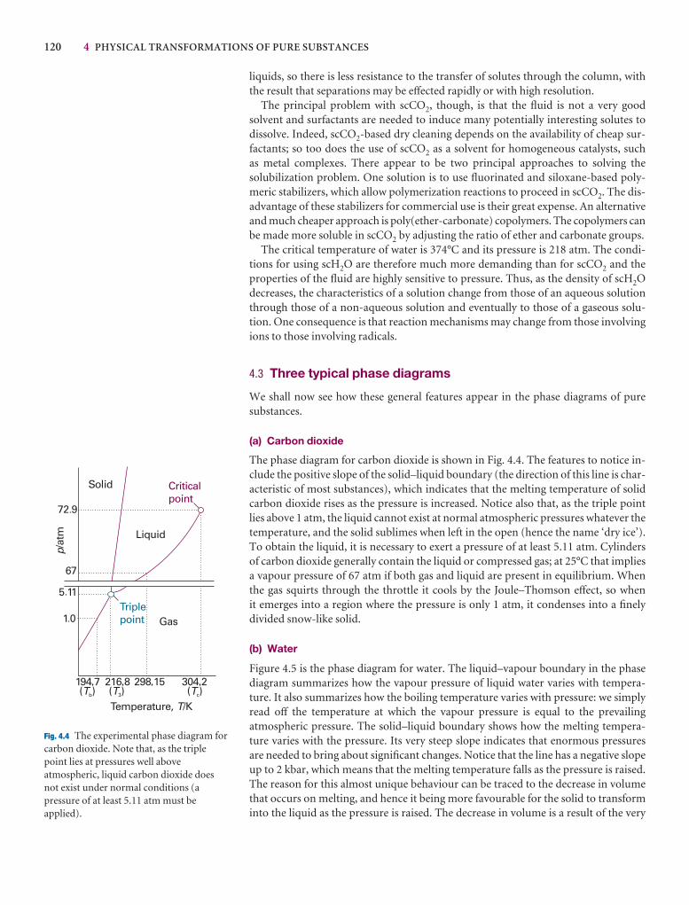
120 4 PHYSICAL TRANSFORMATIONS OF PURE SUBSTANCES
liquids, so there is less resistance to the transfer of solutes through the column, withthe result that separations may be effected rapidly or with high resolution.
The principal problem with scCO2, though, is that the fluid is not a very good solvent and surfactants are needed to induce many potentially interesting solutes to dissolve. Indeed, scCO2-based dry cleaning depends on the availability of cheap sur-factants; so too does the use of scCO2 as a solvent for homogeneous catalysts, such as metal complexes. There appear to be two principal approaches to solving the solubilization problem. One solution is to use fluorinated and siloxane-based poly-meric stabilizers, which allow polymerization reactions to proceed in scCO2. The dis-advantage of these stabilizers for commercial use is their great expense. An alternativeand much cheaper approach is poly(ether-carbonate) copolymers. The copolymers canbe made more soluble in scCO2 by adjusting the ratio of ether and carbonate groups.
The critical temperature of water is 374°C and its pressure is 218 atm. The condi-tions for using scH2O are therefore much more demanding than for scCO2 and theproperties of the fluid are highly sensitive to pressure. Thus, as the density of scH2Odecreases, the characteristics of a solution change from those of an aqueous solutionthrough those of a non-aqueous solution and eventually to those of a gaseous solu-tion. One consequence is that reaction mechanisms may change from those involvingions to those involving radicals.
4.3 Three typical phase diagrams
We shall now see how these general features appear in the phase diagrams of puresubstances.
(a) Carbon dioxide
The phase diagram for carbon dioxide is shown in Fig. 4.4. The features to notice in-clude the positive slope of the solid–liquid boundary (the direction of this line is char-acteristic of most substances), which indicates that the melting temperature of solidcarbon dioxide rises as the pressure is increased. Notice also that, as the triple pointlies above 1 atm, the liquid cannot exist at normal atmospheric pressures whatever thetemperature, and the solid sublimes when left in the open (hence the name ‘dry ice’).To obtain the liquid, it is necessary to exert a pressure of at least 5.11 atm. Cylinders of carbon dioxide generally contain the liquid or compressed gas; at 25°C that impliesa vapour pressure of 67 atm if both gas and liquid are present in equilibrium. Whenthe gas squirts through the throttle it cools by the Joule–Thomson effect, so when it emerges into a region where the pressure is only 1 atm, it condenses into a finely divided snow-like solid.
(b) Water
Figure 4.5 is the phase diagram for water. The liquid–vapour boundary in the phasediagram summarizes how the vapour pressure of liquid water varies with tempera-ture. It also summarizes how the boiling temperature varies with pressure: we simplyread off the temperature at which the vapour pressure is equal to the prevailing atmospheric pressure. The solid–liquid boundary shows how the melting tempera-ture varies with the pressure. Its very steep slope indicates that enormous pressuresare needed to bring about significant changes. Notice that the line has a negative slopeup to 2 kbar, which means that the melting temperature falls as the pressure is raised.The reason for this almost unique behaviour can be traced to the decrease in volumethat occurs on melting, and hence it being more favourable for the solid to transforminto the liquid as the pressure is raised. The decrease in volume is a result of the very
Fig. 4.4 The experimental phase diagram forcarbon dioxide. Note that, as the triplepoint lies at pressures well aboveatmospheric, liquid carbon dioxide doesnot exist under normal conditions (apressure of at least 5.11 atm must beapplied).
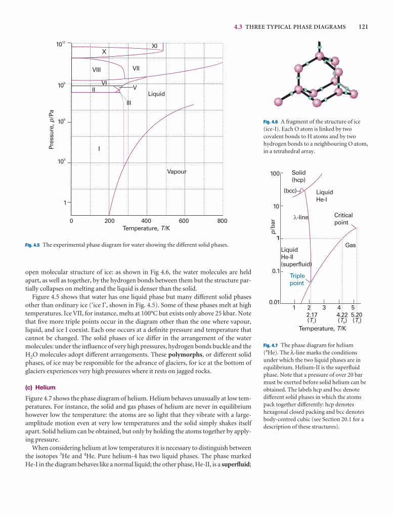
4.3 THREE TYPICAL PHASE DIAGRAMS 121
open molecular structure of ice: as shown in Fig 4.6, the water molecules are heldapart, as well as together, by the hydrogen bonds between them but the structure par-tially collapses on melting and the liquid is denser than the solid.
Figure 4.5 shows that water has one liquid phase but many different solid phasesother than ordinary ice (‘ice I’, shown in Fig. 4.5). Some of these phases melt at hightemperatures. Ice VII, for instance, melts at 100°C but exists only above 25 kbar. Notethat five more triple points occur in the diagram other than the one where vapour, liquid, and ice I coexist. Each one occurs at a definite pressure and temperature thatcannot be changed. The solid phases of ice differ in the arrangement of the watermolecules: under the influence of very high pressures, hydrogen bonds buckle and theH2O molecules adopt different arrangements. These polymorphs, or different solidphases, of ice may be responsible for the advance of glaciers, for ice at the bottom ofglaciers experiences very high pressures where it rests on jagged rocks.
(c) Helium
Figure 4.7 shows the phase diagram of helium. Helium behaves unusually at low tem-peratures. For instance, the solid and gas phases of helium are never in equilibriumhowever low the temperature: the atoms are so light that they vibrate with a large-amplitude motion even at very low temperatures and the solid simply shakes itselfapart. Solid helium can be obtained, but only by holding the atoms together by apply-ing pressure.
When considering helium at low temperatures it is necessary to distinguish betweenthe isotopes 3He and 4He. Pure helium-4 has two liquid phases. The phase markedHe-I in the diagram behaves like a normal liquid; the other phase, He-II, is a superfluid;
0 200 400 600 800
1
103
106
109
1012
XIX
VIII VII
VIVII
I
III
Vapour
Liquid
Pres
sure
,/P
ap
Temperature, /KT
Fig. 4.5 The experimental phase diagram for water showing the different solid phases.
Fig. 4.6 A fragment of the structure of ice(ice-I). Each O atom is linked by twocovalent bonds to H atoms and by twohydrogen bonds to a neighbouring O atom,in a tetrahedral array.
0.1
0.01
1
10
100
p/b
ar
1 2 3 4 52.17 4.22 5.20( )T
l
( )Tb ( )Tc
Temperature, /KT
Triplepoint
Solid(hcp)
(bcc)
LiquidHe-II(superfluid)
LiquidHe-I
Gas
Criticalpoint
l-line
Fig. 4.7 The phase diagram for helium(4He). The λ-line marks the conditionsunder which the two liquid phases are inequilibrium. Helium-II is the superfluidphase. Note that a pressure of over 20 barmust be exerted before solid helium can beobtained. The labels hcp and bcc denotedifferent solid phases in which the atomspack together differently: hcp denoteshexagonal closed packing and bcc denotesbody-centred cubic (see Section 20.1 for adescription of these structures).
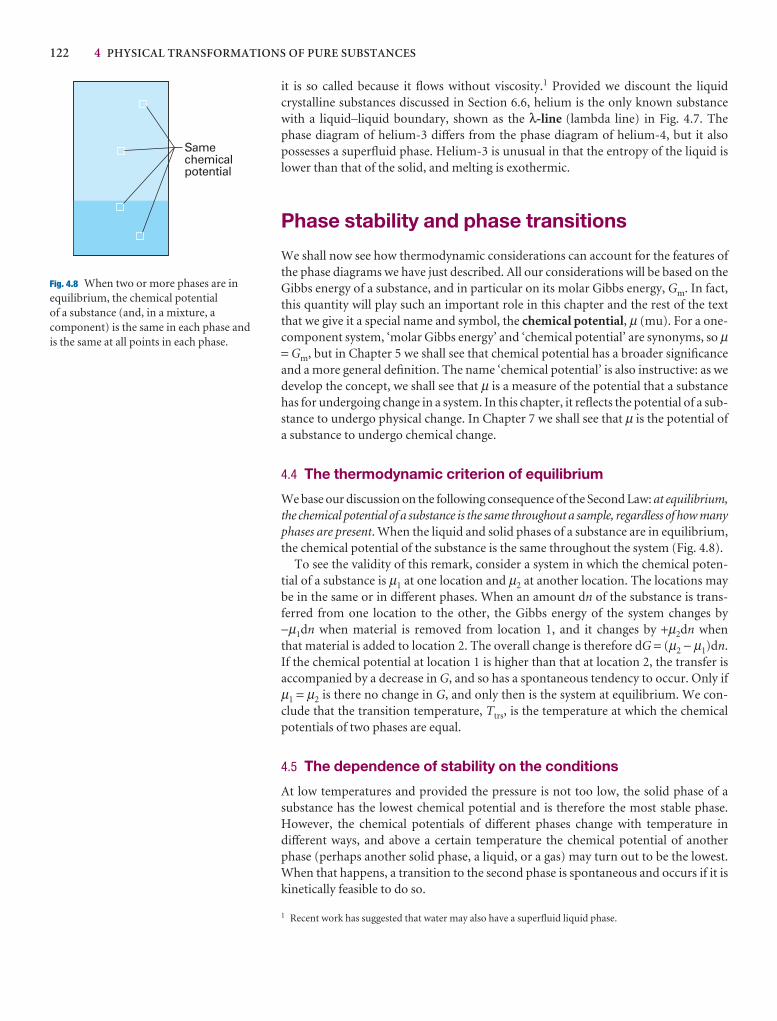
122 4 PHYSICAL TRANSFORMATIONS OF PURE SUBSTANCES
it is so called because it flows without viscosity.1 Provided we discount the liquid crystalline substances discussed in Section 6.6, helium is the only known substancewith a liquid–liquid boundary, shown as the λ-line (lambda line) in Fig. 4.7. Thephase diagram of helium-3 differs from the phase diagram of helium-4, but it alsopossesses a superfluid phase. Helium-3 is unusual in that the entropy of the liquid islower than that of the solid, and melting is exothermic.
Phase stability and phase transitions
We shall now see how thermodynamic considerations can account for the features ofthe phase diagrams we have just described. All our considerations will be based on theGibbs energy of a substance, and in particular on its molar Gibbs energy, Gm. In fact,this quantity will play such an important role in this chapter and the rest of the textthat we give it a special name and symbol, the chemical potential, µ (mu). For a one-component system, ‘molar Gibbs energy’ and ‘chemical potential’ are synonyms, so µ= Gm, but in Chapter 5 we shall see that chemical potential has a broader significanceand a more general definition. The name ‘chemical potential’ is also instructive: as wedevelop the concept, we shall see that µ is a measure of the potential that a substancehas for undergoing change in a system. In this chapter, it reflects the potential of a sub-stance to undergo physical change. In Chapter 7 we shall see that µ is the potential ofa substance to undergo chemical change.
4.4 The thermodynamic criterion of equilibrium
We base our discussion on the following consequence of the Second Law: at equilibrium,the chemical potential of a substance is the same throughout a sample, regardless of how manyphases are present. When the liquid and solid phases of a substance are in equilibrium,the chemical potential of the substance is the same throughout the system (Fig. 4.8).
To see the validity of this remark, consider a system in which the chemical poten-tial of a substance is µ1 at one location and µ2 at another location. The locations maybe in the same or in different phases. When an amount dn of the substance is trans-ferred from one location to the other, the Gibbs energy of the system changes by −µ1dn when material is removed from location 1, and it changes by +µ2dn whenthat material is added to location 2. The overall change is therefore dG = (µ2 − µ1)dn.If the chemical potential at location 1 is higher than that at location 2, the transfer isaccompanied by a decrease in G, and so has a spontaneous tendency to occur. Only ifµ1 = µ2 is there no change in G, and only then is the system at equilibrium. We con-clude that the transition temperature, Ttrs, is the temperature at which the chemicalpotentials of two phases are equal.
4.5 The dependence of stability on the conditions
At low temperatures and provided the pressure is not too low, the solid phase of a substance has the lowest chemical potential and is therefore the most stable phase.However, the chemical potentials of different phases change with temperature indifferent ways, and above a certain temperature the chemical potential of anotherphase (perhaps another solid phase, a liquid, or a gas) may turn out to be the lowest.When that happens, a transition to the second phase is spontaneous and occurs if it iskinetically feasible to do so.
Samechemicalpotential
Fig. 4.8 When two or more phases are inequilibrium, the chemical potential of a substance (and, in a mixture, acomponent) is the same in each phase andis the same at all points in each phase.
1 Recent work has suggested that water may also have a superfluid liquid phase.
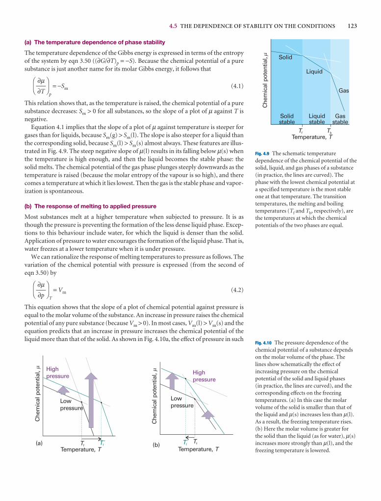
4.5 THE DEPENDENCE OF STABILITY ON THE CONDITIONS 123
Solid
Liquid
Gas
Solidstable
Liquidstable
Gasstable
Temperature, T
Che
mic
al p
oten
tial,
Tf Tb
m
Fig. 4.9 The schematic temperaturedependence of the chemical potential of thesolid, liquid, and gas phases of a substance(in practice, the lines are curved). Thephase with the lowest chemical potential ata specified temperature is the most stableone at that temperature. The transitiontemperatures, the melting and boilingtemperatures (Tf and Tb, respectively), arethe temperatures at which the chemicalpotentials of the two phases are equal.
(a) The temperature dependence of phase stability
The temperature dependence of the Gibbs energy is expressed in terms of the entropyof the system by eqn 3.50 ((∂G/∂T)p = −S). Because the chemical potential of a puresubstance is just another name for its molar Gibbs energy, it follows that
p
= −Sm (4.1)
This relation shows that, as the temperature is raised, the chemical potential of a puresubstance decreases: Sm > 0 for all substances, so the slope of a plot of µ against T isnegative.
Equation 4.1 implies that the slope of a plot of µ against temperature is steeper forgases than for liquids, because Sm(g) > Sm(l). The slope is also steeper for a liquid thanthe corresponding solid, because Sm(l) > Sm(s) almost always. These features are illus-trated in Fig. 4.9. The steep negative slope of µ(l) results in its falling below µ(s) whenthe temperature is high enough, and then the liquid becomes the stable phase: thesolid melts. The chemical potential of the gas phase plunges steeply downwards as thetemperature is raised (because the molar entropy of the vapour is so high), and therecomes a temperature at which it lies lowest. Then the gas is the stable phase and vapor-ization is spontaneous.
(b) The response of melting to applied pressure
Most substances melt at a higher temperature when subjected to pressure. It is asthough the pressure is preventing the formation of the less dense liquid phase. Excep-tions to this behaviour include water, for which the liquid is denser than the solid.Application of pressure to water encourages the formation of the liquid phase. That is,water freezes at a lower temperature when it is under pressure.
We can rationalize the response of melting temperatures to pressure as follows. Thevariation of the chemical potential with pressure is expressed (from the second of eqn 3.50) by
T
= Vm (4.2)
This equation shows that the slope of a plot of chemical potential against pressure isequal to the molar volume of the substance. An increase in pressure raises the chemicalpotential of any pure substance (because Vm > 0). In most cases, Vm(l) > Vm(s) and theequation predicts that an increase in pressure increases the chemical potential of theliquid more than that of the solid. As shown in Fig. 4.10a, the effect of pressure in such
DF
∂µ∂p
AC
DF
∂µ∂T
AC
Che
mic
al p
oten
tial,
Tf Tf´Temperature, T
(a)
Highpressure
Lowpressure
TfTf´Temperature, T
(b)
Highpressure
Lowpressure
Che
mic
al p
oten
tial,
Fig. 4.10 The pressure dependence of thechemical potential of a substance dependson the molar volume of the phase. Thelines show schematically the effect ofincreasing pressure on the chemicalpotential of the solid and liquid phases (in practice, the lines are curved), and thecorresponding effects on the freezingtemperatures. (a) In this case the molarvolume of the solid is smaller than that ofthe liquid and µ(s) increases less than µ(l).As a result, the freezing temperature rises.(b) Here the molar volume is greater forthe solid than the liquid (as for water), µ(s)increases more strongly than µ(l), and thefreezing temperature is lowered.
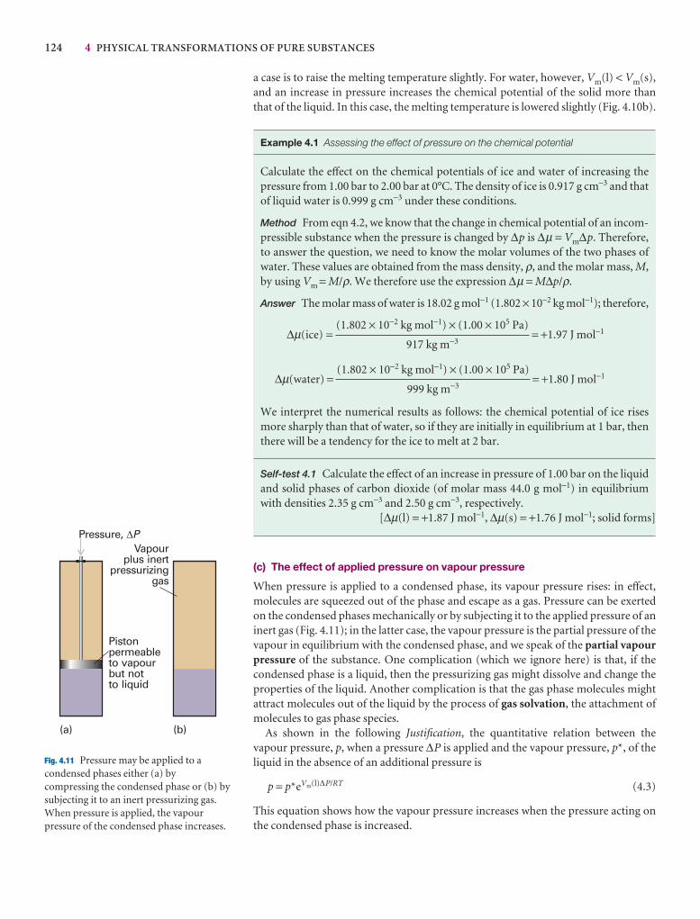
124 4 PHYSICAL TRANSFORMATIONS OF PURE SUBSTANCES
a case is to raise the melting temperature slightly. For water, however, Vm(l) < Vm(s),and an increase in pressure increases the chemical potential of the solid more thanthat of the liquid. In this case, the melting temperature is lowered slightly (Fig. 4.10b).
Example 4.1 Assessing the effect of pressure on the chemical potential
Calculate the effect on the chemical potentials of ice and water of increasing thepressure from 1.00 bar to 2.00 bar at 0°C. The density of ice is 0.917 g cm−3 and thatof liquid water is 0.999 g cm−3 under these conditions.
Method From eqn 4.2, we know that the change in chemical potential of an incom-pressible substance when the pressure is changed by ∆p is ∆µ = Vm∆p. Therefore,to answer the question, we need to know the molar volumes of the two phases ofwater. These values are obtained from the mass density, ρ, and the molar mass, M,by using Vm = M/ρ. We therefore use the expression ∆µ = M∆p/ρ.
Answer The molar mass of water is 18.02 g mol−1 (1.802 × 10⁻² kg mol−1); therefore,
∆µ(ice) = = +1.97 J mol−1
∆µ(water) = = +1.80 J mol−1
We interpret the numerical results as follows: the chemical potential of ice risesmore sharply than that of water, so if they are initially in equilibrium at 1 bar, thenthere will be a tendency for the ice to melt at 2 bar.
Self-test 4.1 Calculate the effect of an increase in pressure of 1.00 bar on the liquidand solid phases of carbon dioxide (of molar mass 44.0 g mol−1) in equilibriumwith densities 2.35 g cm−3 and 2.50 g cm−3, respectively.
[∆µ(l) = +1.87 J mol−1, ∆µ(s) = +1.76 J mol−1; solid forms]
(c) The effect of applied pressure on vapour pressure
When pressure is applied to a condensed phase, its vapour pressure rises: in effect,molecules are squeezed out of the phase and escape as a gas. Pressure can be exertedon the condensed phases mechanically or by subjecting it to the applied pressure of aninert gas (Fig. 4.11); in the latter case, the vapour pressure is the partial pressure of thevapour in equilibrium with the condensed phase, and we speak of the partial vapourpressure of the substance. One complication (which we ignore here) is that, if thecondensed phase is a liquid, then the pressurizing gas might dissolve and change theproperties of the liquid. Another complication is that the gas phase molecules mightattract molecules out of the liquid by the process of gas solvation, the attachment ofmolecules to gas phase species.
As shown in the following Justification, the quantitative relation between thevapour pressure, p, when a pressure ∆P is applied and the vapour pressure, p*, of theliquid in the absence of an additional pressure is
p = p*eVm(l)∆P/RT (4.3)
This equation shows how the vapour pressure increases when the pressure acting onthe condensed phase is increased.
(1.802 × 10⁻² kg mol−1) × (1.00 × 105 Pa)
999 kg m−3
(1.802 × 10⁻² kg mol−1) × (1.00 × 105 Pa)
917 kg m−3
Pistonpermeableto vapourbut notto liquid
Pressure, DP
(a) (b)
Vapourplus inert
pressurizinggas
Fig. 4.11 Pressure may be applied to acondensed phases either (a) bycompressing the condensed phase or (b) bysubjecting it to an inert pressurizing gas.When pressure is applied, the vapourpressure of the condensed phase increases.
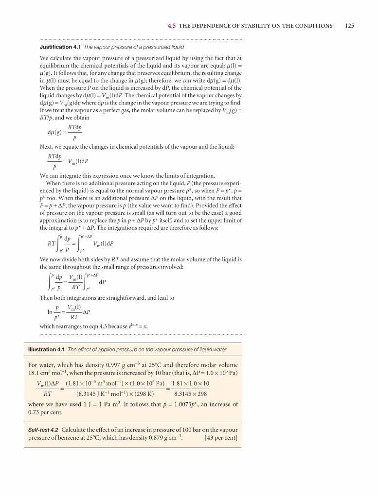
4.5 THE DEPENDENCE OF STABILITY ON THE CONDITIONS 125
Justification 4.1 The vapour pressure of a pressurized liquid
We calculate the vapour pressure of a pressurized liquid by using the fact that atequilibrium the chemical potentials of the liquid and its vapour are equal: µ(l) =µ(g). It follows that, for any change that preserves equilibrium, the resulting changein µ(l) must be equal to the change in µ(g); therefore, we can write dµ(g) = dµ(l).When the pressure P on the liquid is increased by dP, the chemical potential of theliquid changes by dµ(l) = Vm(l)dP. The chemical potential of the vapour changes bydµ(g) = Vm(g)dp where dp is the change in the vapour pressure we are trying to find.If we treat the vapour as a perfect gas, the molar volume can be replaced by Vm(g) =RT/p, and we obtain
dµ(g) =
Next, we equate the changes in chemical potentials of the vapour and the liquid:
= Vm(l)dP
We can integrate this expression once we know the limits of integration.When there is no additional pressure acting on the liquid, P (the pressure experi-
enced by the liquid) is equal to the normal vapour pressure p*, so when P = p*, p =p* too. When there is an additional pressure ∆P on the liquid, with the result that P = p + ∆P, the vapour pressure is p (the value we want to find). Provided the effectof pressure on the vapour pressure is small (as will turn out to be the case) a goodapproximation is to replace the p in p + ∆P by p* itself, and to set the upper limit ofthe integral to p* + ∆P. The integrations required are therefore as follows:
RT�p
p*
= �p*+∆P
p*
Vm(l)dP
We now divide both sides by RT and assume that the molar volume of the liquid isthe same throughout the small range of pressures involved:
�p
p*
= �p*+∆P
p*
dP
Then both integrations are straightforward, and lead to
ln = ∆P
which rearranges to eqn 4.3 because eln x = x.
Illustration 4.1 The effect of applied pressure on the vapour pressure of liquid water
For water, which has density 0.997 g cm−3 at 25°C and therefore molar volume 18.1 cm3 mol−1, when the pressure is increased by 10 bar (that is, ∆P = 1.0 × 10⁵ Pa)
= =
where we have used 1 J = 1 Pa m3. It follows that p = 1.0073p*, an increase of 0.73 per cent.
Self-test 4.2 Calculate the effect of an increase in pressure of 100 bar on the vapourpressure of benzene at 25°C, which has density 0.879 g cm−3. [43 per cent]
1.81 × 1.0 × 10
8.3145 × 298
(1.81 × 10⁻⁵ m3 mol−1) × (1.0 × 106 Pa)
(8.3145 J K−1 mol−1) × (298 K)
Vm(l)∆P
RT
Vm(l)
RT
p
p*
Vm(l)
RT
dp
p
dp
p
RTdp
p
RTdp
p
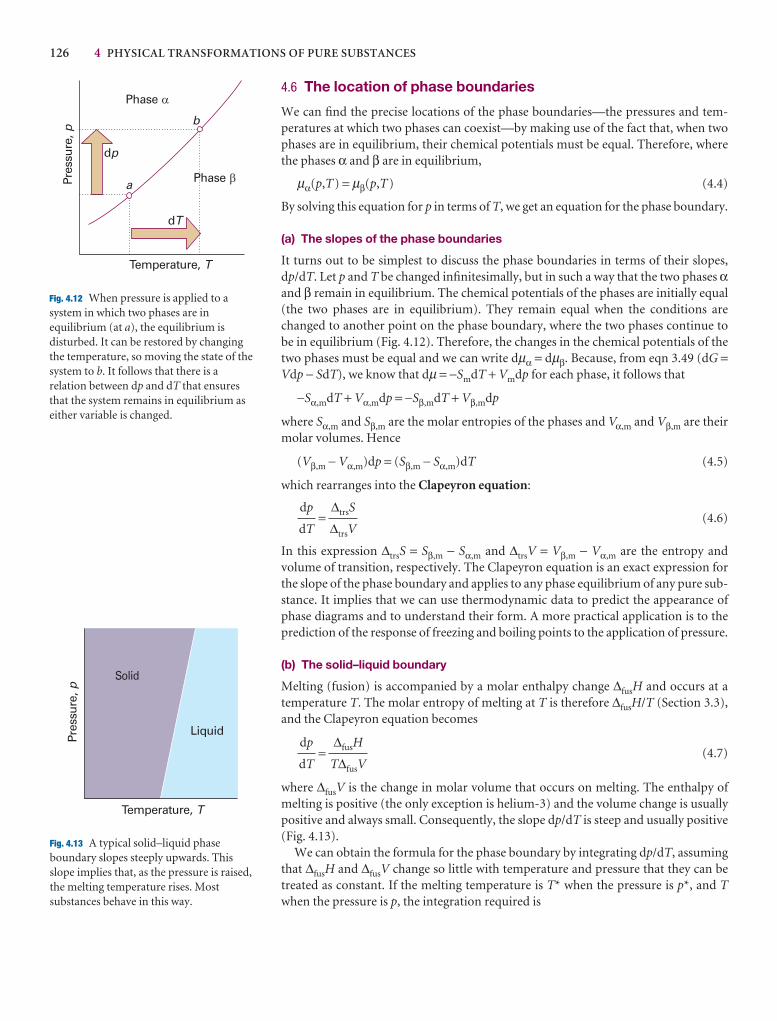
126 4 PHYSICAL TRANSFORMATIONS OF PURE SUBSTANCESPr
essu
re, p
Temperature, T
Phase �
Phase �
dT
dp
a
b
Fig. 4.12 When pressure is applied to asystem in which two phases are inequilibrium (at a), the equilibrium isdisturbed. It can be restored by changingthe temperature, so moving the state of thesystem to b. It follows that there is arelation between dp and dT that ensuresthat the system remains in equilibrium aseither variable is changed.
Pres
sure
, p
Temperature, T
Solid
Liquid
Fig. 4.13 A typical solid–liquid phaseboundary slopes steeply upwards. Thisslope implies that, as the pressure is raised,the melting temperature rises. Mostsubstances behave in this way.
4.6 The location of phase boundaries
We can find the precise locations of the phase boundaries—the pressures and tem-peratures at which two phases can coexist—by making use of the fact that, when twophases are in equilibrium, their chemical potentials must be equal. Therefore, wherethe phases α and β are in equilibrium,
µα(p,T) = µβ(p,T) (4.4)
By solving this equation for p in terms of T, we get an equation for the phase boundary.
(a) The slopes of the phase boundaries
It turns out to be simplest to discuss the phase boundaries in terms of their slopes,dp/dT. Let p and T be changed infinitesimally, but in such a way that the two phases αand β remain in equilibrium. The chemical potentials of the phases are initially equal(the two phases are in equilibrium). They remain equal when the conditions arechanged to another point on the phase boundary, where the two phases continue tobe in equilibrium (Fig. 4.12). Therefore, the changes in the chemical potentials of thetwo phases must be equal and we can write dµα = dµβ. Because, from eqn 3.49 (dG =Vdp − SdT), we know that dµ = −SmdT + Vmdp for each phase, it follows that
−Sα,mdT + Vα,mdp = −Sβ,mdT + Vβ,mdp
where Sα,m and Sβ,m are the molar entropies of the phases and Vα,m and Vβ,m are theirmolar volumes. Hence
(Vβ,m − Vα,m)dp = (Sβ,m − Sα,m)dT (4.5)
which rearranges into the Clapeyron equation:
= (4.6)
In this expression ∆trsS = Sβ,m − Sα,m and ∆trsV = Vβ,m − Vα,m are the entropy and volume of transition, respectively. The Clapeyron equation is an exact expression forthe slope of the phase boundary and applies to any phase equilibrium of any pure sub-stance. It implies that we can use thermodynamic data to predict the appearance ofphase diagrams and to understand their form. A more practical application is to theprediction of the response of freezing and boiling points to the application of pressure.
(b) The solid–liquid boundary
Melting (fusion) is accompanied by a molar enthalpy change ∆fusH and occurs at atemperature T. The molar entropy of melting at T is therefore ∆fusH/T (Section 3.3),and the Clapeyron equation becomes
= (4.7)
where ∆fusV is the change in molar volume that occurs on melting. The enthalpy ofmelting is positive (the only exception is helium-3) and the volume change is usuallypositive and always small. Consequently, the slope dp/dT is steep and usually positive(Fig. 4.13).
We can obtain the formula for the phase boundary by integrating dp/dT, assumingthat ∆fusH and ∆fusV change so little with temperature and pressure that they can betreated as constant. If the melting temperature is T* when the pressure is p*, and Twhen the pressure is p, the integration required is
∆fusH
T∆fusV
dp
dT
∆trsS
∆trsV
dp
dT
4.6 THE LOCATION OF PHASE BOUNDARIES 127
Comment 4.2
Calculations involving naturallogarithms often become simpler if wenote that, provided −1 < x < 1, ln(1 + x)= x − 1–2x2 + 1–3 x3 · · · . If x << 1, a goodapproximation is ln(1 + x) ≈ x.
�p
p*
dp = �T
T*
Therefore, the approximate equation of the solid–liquid boundary is
p ≈ p* + ln (4.8)
This equation was originally obtained by yet another Thomson—James, the brotherof William, Lord Kelvin. When T is close to T*, the logarithm can be approximated byusing
ln = ln 1 + ≈
therefore,
p ≈ p* + (T − T*) (4.9)
This expression is the equation of a steep straight line when p is plotted against T (asin Fig. 4.13).
(c) The liquid–vapour boundary
The entropy of vaporization at a temperature T is equal to ∆vapH/T; the Clapeyronequation for the liquid–vapour boundary is therefore
= (4.10)
The enthalpy of vaporization is positive; ∆vapV is large and positive. Therefore, dp/dTis positive, but it is much smaller than for the solid–liquid boundary. It follows thatdT/dp is large, and hence that the boiling temperature is more responsive to pressurethan the freezing temperature.
Example 4.2 Estimating the effect of pressure on the boiling temperature
Estimate the typical size of the effect of increasing pressure on the boiling point ofa liquid.
Method To use eqn 4.10 we need to estimate the right-hand side. At the boilingpoint, the term ∆vapH/T is Trouton’s constant (Section 3.3b). Because the molarvolume of a gas is so much greater than the molar volume of a liquid, we can write
∆vapV = Vm(g) − Vm(l) ≈ Vm(g)
and take for Vm(g) the molar volume of a perfect gas (at low pressures, at least).
Answer Trouton’s constant has the value 85 J K−1 mol−1. The molar volume of aperfect gas is about 25 dm3 mol−1 at 1 atm and near but above room temperature.Therefore,
≈ = 3.4 × 10³ Pa K−185 J K−1 mol−1
2.5 × 10⁻² m3 mol−1
dp
dT
∆vapH
T∆vapV
dp
dT
∆fusH
T*∆fusV
T − T*
T*
DF
T − T*
T*
AC
T
T*
T
T*
∆fusH
∆fusV
dT
T
∆fusH
∆fusV
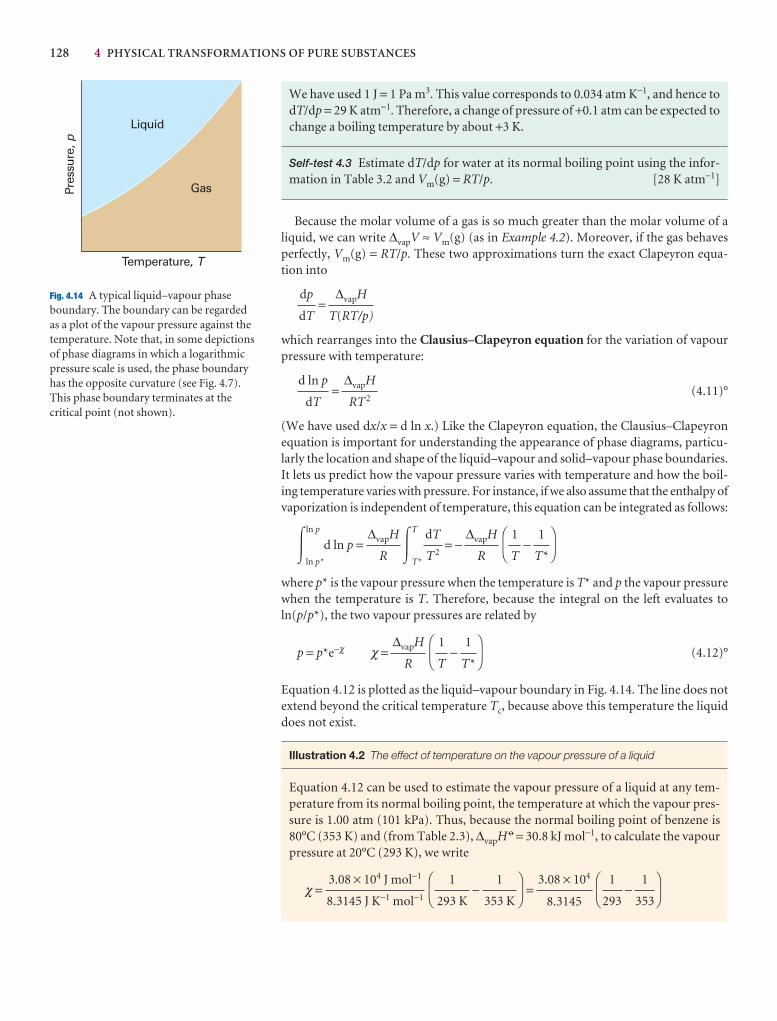
128 4 PHYSICAL TRANSFORMATIONS OF PURE SUBSTANCESPr
essu
re, p
Temperature, T
Liquid
Gas
Fig. 4.14 A typical liquid–vapour phaseboundary. The boundary can be regardedas a plot of the vapour pressure against thetemperature. Note that, in some depictionsof phase diagrams in which a logarithmicpressure scale is used, the phase boundaryhas the opposite curvature (see Fig. 4.7).This phase boundary terminates at thecritical point (not shown).
We have used 1 J = 1 Pa m3. This value corresponds to 0.034 atm K−1, and hence todT/dp = 29 K atm−1. Therefore, a change of pressure of +0.1 atm can be expected tochange a boiling temperature by about +3 K.
Self-test 4.3 Estimate dT/dp for water at its normal boiling point using the infor-mation in Table 3.2 and Vm(g) = RT/p. [28 K atm−1]
Because the molar volume of a gas is so much greater than the molar volume of aliquid, we can write ∆vapV ≈ Vm(g) (as in Example 4.2). Moreover, if the gas behavesperfectly, Vm(g) = RT/p. These two approximations turn the exact Clapeyron equa-tion into
=
which rearranges into the Clausius–Clapeyron equation for the variation of vapourpressure with temperature:
= (4.11)°
(We have used dx/x = d ln x.) Like the Clapeyron equation, the Clausius–Clapeyronequation is important for understanding the appearance of phase diagrams, particu-larly the location and shape of the liquid–vapour and solid–vapour phase boundaries.It lets us predict how the vapour pressure varies with temperature and how the boil-ing temperature varies with pressure. For instance, if we also assume that the enthalpy ofvaporization is independent of temperature, this equation can be integrated as follows:
�ln p
ln p*
d ln p = �T
T*
= − −
where p* is the vapour pressure when the temperature is T* and p the vapour pressurewhen the temperature is T. Therefore, because the integral on the left evaluates toln(p/p*), the two vapour pressures are related by
p = p*e−χ χ = − (4.12)°
Equation 4.12 is plotted as the liquid–vapour boundary in Fig. 4.14. The line does notextend beyond the critical temperature Tc, because above this temperature the liquiddoes not exist.
Illustration 4.2 The effect of temperature on the vapour pressure of a liquid
Equation 4.12 can be used to estimate the vapour pressure of a liquid at any tem-perature from its normal boiling point, the temperature at which the vapour pres-sure is 1.00 atm (101 kPa). Thus, because the normal boiling point of benzene is80°C (353 K) and (from Table 2.3), ∆vapH 7 = 30.8 kJ mol−1, to calculate the vapourpressure at 20°C (293 K), we write
χ = − = −DF
1
353
1
293
AC
3.08 × 10⁴
8.3145
DF
1
353 K
1
293 K
AC
3.08 × 10⁴ J mol−1
8.3145 J K−1 mol−1
DF
1
T*
1
T
AC
∆vapH
R
DF
1
T*
1
T
AC
∆vapH
R
dT
T2
∆vapH
R
∆vapH
RT2
d ln p
dT
∆vapH
T(RT/p)
dp
dT
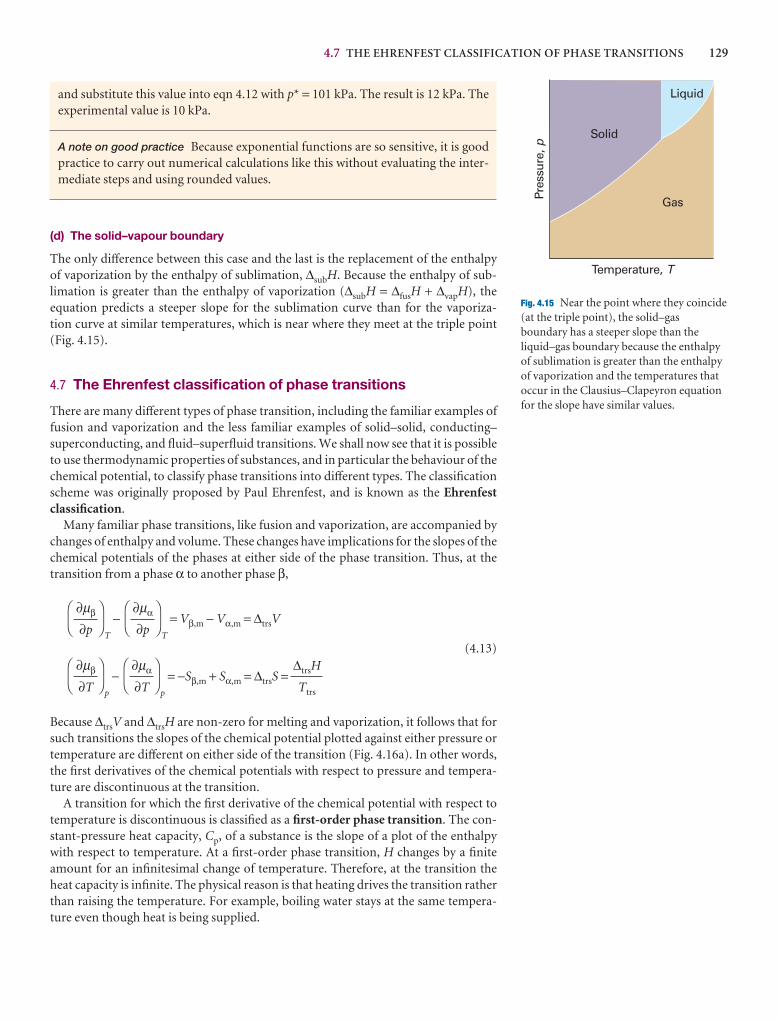
4.7 THE EHRENFEST CLASSIFICATION OF PHASE TRANSITIONS 129
Pres
sure
, p
Temperature, T
Gas
Solid
Liquid
Fig. 4.15 Near the point where they coincide (at the triple point), the solid–gasboundary has a steeper slope than theliquid–gas boundary because the enthalpyof sublimation is greater than the enthalpyof vaporization and the temperatures thatoccur in the Clausius–Clapeyron equationfor the slope have similar values.
and substitute this value into eqn 4.12 with p* = 101 kPa. The result is 12 kPa. Theexperimental value is 10 kPa.
A note on good practice Because exponential functions are so sensitive, it is goodpractice to carry out numerical calculations like this without evaluating the inter-mediate steps and using rounded values.
(d) The solid–vapour boundary
The only difference between this case and the last is the replacement of the enthalpy of vaporization by the enthalpy of sublimation, ∆subH. Because the enthalpy of sub-limation is greater than the enthalpy of vaporization (∆subH = ∆fusH + ∆vapH), theequation predicts a steeper slope for the sublimation curve than for the vaporiza-tion curve at similar temperatures, which is near where they meet at the triple point(Fig. 4.15).
4.7 The Ehrenfest classification of phase transitions
There are many different types of phase transition, including the familiar examples offusion and vaporization and the less familiar examples of solid–solid, conducting–superconducting, and fluid–superfluid transitions. We shall now see that it is possibleto use thermodynamic properties of substances, and in particular the behaviour of thechemical potential, to classify phase transitions into different types. The classificationscheme was originally proposed by Paul Ehrenfest, and is known as the Ehrenfestclassification.
Many familiar phase transitions, like fusion and vaporization, are accompanied bychanges of enthalpy and volume. These changes have implications for the slopes of thechemical potentials of the phases at either side of the phase transition. Thus, at thetransition from a phase α to another phase β,
T
−T
= Vβ,m − Vα,m = ∆trsV
p
−p
= −Sβ,m + Sα,m = ∆trsS =
(4.13)
Because ∆trsV and ∆trsH are non-zero for melting and vaporization, it follows that forsuch transitions the slopes of the chemical potential plotted against either pressure ortemperature are different on either side of the transition (Fig. 4.16a). In other words,the first derivatives of the chemical potentials with respect to pressure and tempera-ture are discontinuous at the transition.
A transition for which the first derivative of the chemical potential with respect totemperature is discontinuous is classified as a first-order phase transition. The con-stant-pressure heat capacity, Cp, of a substance is the slope of a plot of the enthalpywith respect to temperature. At a first-order phase transition, H changes by a finiteamount for an infinitesimal change of temperature. Therefore, at the transition theheat capacity is infinite. The physical reason is that heating drives the transition ratherthan raising the temperature. For example, boiling water stays at the same tempera-ture even though heat is being supplied.
∆trsH
Ttrs
DF
∂µα
∂T
AC
DF
∂µβ
∂T
AC
DF
∂µα
∂p
AC
DF
∂µβ
∂p
AC

130 4 PHYSICAL TRANSFORMATIONS OF PURE SUBSTANCES
2 A metallic conductor is a substance with an electrical conductivity that decreases as the temperature in-creases. A superconductor is a solid that conducts electricity without resistance. See Chapter 20 for moredetails.
A second-order phase transition in the Ehrenfest sense is one in which the firstderivative of µ with respect to temperature is continuous but its second derivative isdiscontinuous. A continuous slope of µ (a graph with the same slope on either side ofthe transition) implies that the volume and entropy (and hence the enthalpy) do notchange at the transition (Fig. 4.16b). The heat capacity is discontinuous at the transi-tion but does not become infinite there. An example of a second-order transition isthe conducting–superconducting transition in metals at low temperatures.2
The term λ-transition is applied to a phase transition that is not first-order yet the heat capacity becomes infinite at the transition temperature. Typically, the heat capacity of a system that shows such a transition begins to increase well before thetransition (Fig. 4.17), and the shape of the heat capacity curve resembles the Greek letter lambda. This type of transition includes order–disorder transitions in alloys, theonset of ferromagnetism, and the fluid–superfluid transition of liquid helium.
Molecular interpretation 4.1 Second-order phase transitions and λ-transitions
One type of second-order transition is associated with a change in symmetry of the crystal structure of a solid. Thus, suppose the arrangement of atoms in a solidis like that represented in Fig. 4.18a, with one dimension (technically, of the unitcell) longer than the other two, which are equal. Such a crystal structure is classifiedas tetragonal (see Section 20.1). Moreover, suppose the two shorter dimensions increase more than the long dimension when the temperature is raised. There maycome a stage when the three dimensions become equal. At that point the crystal hascubic symmetry (Fig. 4.18b), and at higher temperatures it will expand equally inall three directions (because there is no longer any distinction between them). Thetetragonal → cubic phase transition has occurred, but as it has not involved a dis-continuity in the interaction energy between the atoms or the volume they occupy,the transition is not first-order.
Fig. 4.17 The λ-curve for helium, where theheat capacity rises to infinity. The shape ofthis curve is the origin of the name λ-transition.
Volume, V Enthalpy, HChemicalpotential, Entropy, S
Heatcapacity, Cp
Temperature, T
(a)
(b)
Fig. 4.16 The changes in thermodynamic properties accompanying (a) first-order and (b) second-order phase transitions.

CHECKLIST OF KEY IDEAS 131
The order–disorder transition in β-brass (CuZn) is an example of a λ-transition.The low-temperature phase is an orderly array of alternating Cu and Zn atoms.The high-temperature phase is a random array of the atoms (Fig. 4.19). At T = 0 theorder is perfect, but islands of disorder appear as the temperature is raised. The islands form because the transition is cooperative in the sense that, once two atomshave exchanged locations, it is easier for their neighbours to exchange their loca-tions. The islands grow in extent, and merge throughout the crystal at the transitiontemperature (742 K). The heat capacity increases as the transition temperature is approached because the cooperative nature of the transition means that it is increasingly easy for the heat supplied to drive the phase transition rather than tobe stored as thermal motion.
(a)
(b)
(c)
Equalrates
Equalrates
Equalrates
Cubicphase
Phas
etr
ansi
tion
(b)
Fig. 4.18 One version of a second-order phase transition in which (a) a tetragonal phaseexpands more rapidly in two directions than a third, and hence becomes a cubic phase, which (b) expands uniformly in three directions as the temperature is raised. There is norearrangement of atoms at the transition temperature, and hence no enthalpy of transition.
Fig. 4.19 An order–disorder transition.(a) At T = 0, there is perfect order, withdifferent kinds of atoms occupyingalternate sites. (b) As the temperature isincreased, atoms exchange locations andislands of each kind of atom form inregions of the solid. Some of the originalorder survives. (c) At and above thetransition temperature, the islands occur atrandom throughout the sample.
Slow
Fast
Fast
Tetragonalphase
(a)
Checklist of key ideas
1. A phase is a form of matter that is uniform throughout inchemical composition and physical state.
2. A transition temperature is the temperature at which the twophases are in equilibrium.
3. A metastable phase is a thermodynamically unstable phasethat persists because the transition is kinetically hindered.
4. A phase diagram is a diagram showing the regions of pressureand temperature at which its various phases arethermodynamically stable.
5. A phase boundary is a line separating the regions in a phasediagram showing the values of p and T at which two phasescoexist in equilibrium.
6. The vapour pressure is the pressure of a vapour in equilibriumwith the condensed phase.
7. Boiling is the condition of free vaporization throughout theliquid.
8. The boiling temperature is the temperature at which thevapour pressure of a liquid is equal to the external pressure.
9. The critical temperature is the temperature at which a liquidsurface disappears and above which a liquid does not existwhatever the pressure. The critical pressure is the vapourpressure at the critical temperature.
10. A supercritical fluid is a dense fluid phase above the criticaltemperature.
11. The melting temperature (or freezing temperature) is thetemperature at which, under a specified pressure, the liquidand solid phases of a substance coexist in equilibrium.
12. The triple point is a point on a phase diagram at which thethree phase boundaries meet and all three phases are inmutual equilibrium.
13. The chemical potential µ of a pure substance is the molarGibbs energy of the substance.

132 4 PHYSICAL TRANSFORMATIONS OF PURE SUBSTANCES
Discussion questions
4.1 Discuss the implications for phase stability of the variation of chemicalpotential with temperature and pressure.
4.2 Suggest a physical interpretation of the phenomena of superheating andsupercooling.
4.3 Discuss what would be observed as a sample of water is taken along a paththat encircles and is close to its critical point.
4.4 Use the phase diagram in Fig. 4.4 to state what would be observed when a sample of carbon dioxide, initially at 1.0 atm and 298 K, is subjected to thefollowing cycle: (a) isobaric (constant–pressure) heating to 320 K, (b) isothermal compression to 100 atm, (c) isobaric cooling to 210 K, (d) isothermal decompression to 1.0 atm, (e) isobaric heating to 298 K.
4.5 The use of supercritical fluids for the extraction of a component from acomplicated mixture is not confined to the decaffeination of coffee. Consultlibrary and internet resources and prepare a discussion of the principles,advantages, disadvantages, and current uses of supercritical fluid extractiontechnology.
4.6 Explain the significance of the Clapeyron equation and of theClausius–Clapeyron equation.
4.7 Distinguish between a first-order phase transition, a second-order phasetransition, and a λ-transition at both molecular and macroscopic levels.
Exercises
4.1(a) The vapour pressure of dichloromethane at 24.1°C is 53.3 kPa and itsenthalpy of vaporization is 28.7 kJ mol−1. Estimate the temperature at whichits vapour pressure is 70.0 kPa.
4.1(b) The vapour pressure of a substance at 20.0°C is 58.0 kPa and itsenthalpy of vaporization is 32.7 kJ mol−1. Estimate the temperature at whichits vapour pressure is 66.0 kPa.
4.2(a) The molar volume of a certain solid is 161.0 cm3 mol−1 at 1.00 atm and350.75 K, its melting temperature. The molar volume of the liquid at thistemperature and pressure is 163.3 cm3 mol−1. At 100 atm the meltingtemperature changes to 351.26 K. Calculate the enthalpy and entropy offusion of the solid.
4.2(b) The molar volume of a certain solid is 142.0 cm3 mol−1 at 1.00 atm and427.15 K, its melting temperature. The molar volume of the liquid at thistemperature and pressure is 152.6 cm3 mol−1. At 1.2 MPa the meltingtemperature changes to 429.26 K. Calculate the enthalpy and entropy offusion of the solid.
4.3(a) The vapour pressure of a liquid in the temperature range 200 K to 260 K was found to fit the expression ln(p/Torr) = 16.255 – 2501.8/(T/K).Calculate the enthalpy of vaporization of the liquid.
4.3(b) The vapour pressure of a liquid in the temperature range 200 K to 260 K was found to fit the expression ln(p/Torr) = 18.361 – 3036.8/(T/K).Calculate the enthalpy of vaporization of the liquid.
Further reading
Articles and texts
E.K.H. Salje, Phase transitions, structural. In Encyclopedia of appliedphysics (ed. G.L. Trigg), 13, 373. VCH, New York (1995).
J.M. Sanchez, Order–disorder transitions. In Encyclopedia of appliedphysics (ed. G.L. Trigg), 13, 1. VCH, New York (1995).
K.M. Scholsky, Supercritical phase transitions at very high pressure. J.Chem. Educ. 66, 989 (1989).
W.D. Callister, Jr., Materials science and engineering, an introduction.Wiley, New York (2000).
Sources of data and information3
T. Boublik, V. Fried, and E. Hála, The vapor pressures of puresubstances. Elsevier, Amsterdam (1984).
R.C. Weast (ed.), Handbook of chemistry and physics, Vol. 81. CRCPress, Boca Raton (2004).
14. The chemical potential is uniform throughout a system atequilibrium.
15. The chemical potential varies with temperature as (∂µ /∂T)p = −Sm and with pressure as (∂µ /∂p)T = Vm.
16. The vapour pressure in the presence of applied pressure isgiven by p = p*eVm∆P/RT.
17. The temperature dependence of the vapour pressure is givenby the Clapeyron equation, dp/dT = ∆trsS/∆trsV.
18. The temperature dependence of the vapour pressure of acondensed phase is given by the Clausius–Clapeyronequation, d ln p/dT = ∆vapH/RT 2.
19. The Ehrenfest classification is a classification of phasetransitions based on the behaviour of the chemical potential.
3 See Further reading in Chapter 2 for additional sources of thermochemical data.

PROBLEMS 133
Problems*
Numerical problems
4.1 The temperature dependence of the vapour pressure of solid sulfurdioxide can be approximately represented by the relation log(p/Torr) =10.5916 − 1871.2/(T/K) and that of liquid sulfur dioxide by log(p/Torr) =8.3186 − 1425.7/(T/K). Estimate the temperature and pressure of the triplepoint of sulfur dioxide.
4.2 Prior to the discovery that freon-12 (CF2Cl2) was harmful to the Earth’sozone layer, it was frequently used as the dispersing agent in spray cans forhair spray, etc. Its enthalpy of vaporization at its normal boiling point of −29.2°C is 20.25 kJ mol−1. Estimate the pressure that a can of hair spray usingfreon-12 had to withstand at 40°C, the temperature of a can that has beenstanding in sunlight. Assume that ∆vapH is a constant over the temperaturerange involved and equal to its value at −29.2°C.
4.3 The enthalpy of vaporization of a certain liquid is found to be 14.4 kJmol−1 at 180 K, its normal boiling point. The molar volumes of the liquid and the vapour at the boiling point are 115 cm3 mol−1 and 14.5 dm3 mol−1,respectively. (a) Estimate dp/dT from the Clapeyron equation and (b) thepercentage error in its value if the Clausius–Clapeyron equation is usedinstead.
4.4 Calculate the difference in slope of the chemical potential againsttemperature on either side of (a) the normal freezing point of water and(b) the normal boiling point of water. (c) By how much does the chemicalpotential of water supercooled to −5.0°C exceed that of ice at thattemperature?
4.5 Calculate the difference in slope of the chemical potential against pressureon either side of (a) the normal freezing point of water and (b) the normal
boiling point of water. The densities of ice and water at 0°C are 0.917 g cm−3
and 1.000 g cm−3, and those of water and water vapour at 100°C are 0.958 gcm−3 and 0.598 g dm−3, respectively. By how much does the chemical potentialof water vapour exceed that of liquid water at 1.2 atm and 100°C?
4.6 The enthalpy of fusion of mercury is 2.292 kJ mol−1, and its normalfreezing point is 234.3 K with a change in molar volume of +0.517 cm−3 mol−1
on melting. At what temperature will the bottom of a column of mercury(density 13.6 g cm−3) of height 10.0 m be expected to freeze?
4.7 50.0 dm3 of dry air was slowly bubbled through a thermally insulatedbeaker containing 250 g of water initially at 25°C. Calculate the finaltemperature. (The vapour pressure of water is approximately constant at 3.17 kPa throughout, and its heat capacity is 75.5 J K−1 mol−1. Assume that theair is not heated or cooled and that water vapour is a perfect gas.)
4.8 The vapour pressure, p, of nitric acid varies with temperature as follows:
θ/°C 0 20 40 50 70 80 90 100
p/kPa 1.92 6.38 17.7 27.7 62.3 89.3 124.9 170.9
What are (a) the normal boiling point and (b) the enthalpy of vaporization ofnitric acid?
4.9 The vapour pressure of the ketone carvone (M = 150.2 g mol−1), acomponent of oil of spearmint, is as follows:
θ/°C 57.4 100.4 133.0 157.3 203.5 227.5
p/Torr 1.00 10.0 40.0 100 400 760
What are (a) the normal boiling point and (b) the enthalpy of vaporization ofcarvone?
* Problems denoted by the symbol ‡ were supplied by Charles Trapp, Carmen Giunta, and Marshall Cady.
4.4(a) The vapour pressure of benzene between 10°C and 30°C fits theexpression log(p/Torr) = 7.960 – 1780/(T/K). Calculate (a) the enthalpy ofvaporization and (b) the normal boiling point of benzene.
4.4(b) The vapour pressure of a liquid between 15°C and 35°C fits theexpression log(p/Torr) = 8.750 − 1625/(T/K). Calculate (a) the enthalpy ofvaporization and (b) the normal boiling point of the liquid.
4.5(a) When benzene freezes at 5.5°C its density changes from 0.879 g cm−3 to0.891 g cm−3. Its enthalpy of fusion is 10.59 kJ mol−1. Estimate the freezingpoint of benzene at 1000 atm.
4.5(b) When a certain liquid freezes at −3.65°C its density changes from 0.789 g cm−3 to 0.801 g cm−3. Its enthalpy of fusion is 8.68 kJ mol−1. Estimatethe freezing point of the liquid at 100 MPa.
4.6(a) In July in Los Angeles, the incident sunlight at ground level has a powerdensity of 1.2 kW m−2 at noon. A swimming pool of area 50 m2 is directlyexposed to the sun. What is the maximum rate of loss of water? Assume thatall the radiant energy is absorbed.
4.6(b) Suppose the incident sunlight at ground level has a power density of0.87 kW m−2 at noon. What is the maximum rate of loss of water from a lakeof area 1.0 ha? (1 ha = 104 m2.) Assume that all the radiant energy is absorbed.
4.7(a) An open vessel containing (a) water, (b) benzene, (c) mercury stands ina laboratory measuring 5.0 m × 5.0 m × 3.0 m at 25°C. What mass of each
substance will be found in the air if there is no ventilation? (The vapourpressures are (a) 3.2 kPa, (b) 13.1 kPa, (c) 0.23 Pa.)
4.7(b) On a cold, dry morning after a frost, the temperature was −5°C and thepartial pressure of water in the atmosphere fell to 0.30 kPa. Will the frostsublime? What partial pressure of water would ensure that the frost remained?
4.8(a) Naphthalene, C10H8, melts at 80.2°C. If the vapour pressure of theliquid is 1.3 kPa at 85.8°C and 5.3 kPa at 119.3°C, use the Clausius–Clapeyronequation to calculate (a) the enthalpy of vaporization, (b) the normal boilingpoint, and (c) the enthalpy of vaporization at the boiling point.
4.8(b) The normal boiling point of hexane is 69.0°C. Estimate (a) its enthalpyof vaporization and (b) its vapour pressure at 25°C and 60°C.
4.9(a) Calculate the melting point of ice under a pressure of 50 bar. Assumethat the density of ice under these conditions is approximately 0.92 g cm−3 andthat of liquid water is 1.00 g cm−3.
4.9(b) Calculate the melting point of ice under a pressure of 10 MPa. Assumethat the density of ice under these conditions is approximately 0.915 g cm−3
and that of liquid water is 0.998 g cm−3.
4.10(a) What fraction of the enthalpy of vaporization of water is spent onexpanding the water vapour?
4.10(b) What fraction of the enthalpy of vaporization of ethanol is spent onexpanding its vapour?
134 4 PHYSICAL TRANSFORMATIONS OF PURE SUBSTANCES
4.10 Construct the phase diagram for benzene near its triple point at 36 Torrand 5.50°C using the following data: ∆fusH = 10.6 kJ mol−1, ∆vapH = 30.8 kJmol−1, ρ(s) = 0.891 g cm−3, ρ(l) = 0.879 g cm−3.
4.11‡ In an investigation of thermophysical properties of toluene (R.D.Goodwin J. Phys. Chem. Ref. Data 18, 1565 (1989)) presented expressions fortwo coexistence curves (phase boundaries). The solid–liquid coexistence curveis given by
p/bar = p3/bar + 1000 × (5.60 + 11.727x)x
where x = T/T3 − 1 and the triple point pressure and temperature are p3 = 0.4362 µbar and T3 = 178.15 K. The liquid–vapour curve is given by:
ln(p/bar) = −10.418/y + 21.157 − 15.996y + 14.015y2 − 5.0120y3
+ 4.7224(1 − y)1.70
where y = T/Tc = T/(593.95 K). (a) Plot the solid–liquid and liquid–vapourphase boundaries. (b) Estimate the standard melting point of toluene. (c) Estimate the standard boiling point of toluene. (d) Compute the standardenthalpy of vaporization of toluene, given that the molar volumes of the liquid and vapour at the normal boiling point are 0.12 dm3 mol−1 and30.3 dm3 mol−1, respectively.
4.12‡ In a study of the vapour pressure of chloromethane, A. Bah and N.Dupont-Pavlovsky (J. Chem. Eng. Data 40, 869 (1995)) presented data for thevapour pressure over solid chloromethane at low temperatures. Some of thatdata is shown below:
T/K 145.94 147.96 149.93 151.94 153.97 154.94
p/Pa 13.07 18.49 25.99 36.76 50.86 59.56
Estimate the standard enthalpy of sublimation of chloromethane at 150 K.(Take the molar volume of the vapour to be that of a perfect gas, and that ofthe solid to be negligible.)
Theoretical problems
4.13 Show that, for a transition between two incompressible solid phases, ∆G is independent of the pressure.
4.14 The change in enthalpy is given by dH = CpdT + Vdp. The Clapeyronequation relates dp and dT at equilibrium, and so in combination the twoequations can be used to find how the enthalpy changes along a phaseboundary as the temperature changes and the two phases remain inequilibrium. Show that d(∆H/T) = ∆Cp d ln T.
4.15 In the ‘gas saturation method’ for the measurement of vapour pressure,a volume V of gas (as measured at a temperature T and a pressure p) isbubbled slowly through the liquid that is maintained at the temperature T,and a mass loss m is measured. Show that the vapour pressure, p, of the liquidis related to its molar mass, M, by p = AmP/(1 + Am), where A = RT/MPV. Thevapour pressure of geraniol (M = 154.2 g mol−1), which is a component of oilof roses, was measured at 110°C. It was found that, when 5.00 dm3 of nitrogenat 760 Torr was passed slowly through the heated liquid, the loss of mass was0.32 g. Calculate the vapour pressure of geraniol.
4.16 Combine the barometric formula (stated in Impact I1.1) for thedependence of the pressure on altitude with the Clausius–Clapeyron equation, and predict how the boiling temperature of a liquid depends on thealtitude and the ambient temperature. Take the mean ambient temperature as 20°C and predict the boiling temperature of water at 3000 m.
4.17 Figure 4.9 gives a schematic representation of how the chemicalpotentials of the solid, liquid, and gaseous phases of a substance vary withtemperature. All have a negative slope, but it is unlikely that they are trulystraight lines as indicated in the illustration. Derive an expression for thecurvatures (specifically, the second derivatives with respect to temperature) ofthese lines. Is there a restriction on the curvature of these lines? Which state ofmatter shows the greatest curvature?
4.18 The Clapeyron equation does not apply to second-order phasetransitions, but there are two analogous equations, the Ehrenfest equations,that do. They are:
= =
where α is the expansion coefficient, κT the isothermal compressibility, andthe subscripts 1 and 2 refer to two different phases. Derive these twoequations. Why does the Clapeyron equation not apply to second-ordertransitions?
4.19 For a first-order phase transition, to which the Clapeyron equation doesapply, prove the relation
CS = Cp −
where CS = (∂q/∂T)S is the heat capacity along the coexistence curve of twophases.
Applications: to biology and engineering
4.20 Proteins are polypeptides, polymers of amino acids that can exist inordered structures stabilized by a variety of molecular interactions. However,when certain conditions are changed, the compact structure of a polypeptidechain may collapse into a random coil. This structural change may beregarded as a phase transition occurring at a characteristic transitiontemperature, the melting temperature, Tm, which increases with the strengthand number of intermolecular interactions in the chain. A thermodynamictreatment allows predictions to be made of the temperature Tm for theunfolding of a helical polypeptide held together by hydrogen bonds into arandom coil. If a polypeptide has n amino acids, n − 4 hydrogen bonds areformed to form an α-helix, the most common type of helix in naturallyoccurring proteins (see Chapter 19). Because the first and last residues in thechain are free to move, n − 2 residues form the compact helix and haverestricted motion. Based on these ideas, the molar Gibbs energy of unfoldingof a polypeptide with n ≥ 5 may be written as
∆Gm = (n − 4)∆hbHm − (n − 2)T∆hbSm
where ∆hbHm and ∆hbSm are, respectively, the molar enthalpy and entropy ofdissociation of hydrogen bonds in the polypeptide. (a) Justify the form of theequation for the Gibbs energy of unfolding. That is, why are the enthalpy and entropy terms written as (n − 4)∆hbHm and (n − 2)∆hbSm, respectively? (b) Show that Tm may be written as
Tm =
(c) Plot Tm /(∆hbHm /∆hbSm) for 5 ≤ n ≤ 20. At what value of n does Tm changeby less than 1% when n increases by one?
4.21‡ The use of supercritical fluids as mobile phases in SFC depends on theirproperties as nonpolar solvents. The solubility parameter, δ, is defined as(∆Ucohesive /Vm)1/2, where ∆Ucohesive is the cohesive energy of the solvent, theenergy per mole needed to increase the volume isothermally to an infinitevalue. Diethyl ether, carbon tetrachloride, and dioxane have solubilityparameter ranges of 7–8, 8–9, and 10–11, respectively. (a) Derive a practicalequation for the computation of the isotherms for the reduced internal energychange, ∆Ur(Tr,Vr) defined as
∆Ur(Tr,Vr) =
(b) Draw a graph of ∆Ur against pr for the isotherms Tr = 1,1.2, and 1.5 in thereduced pressure range for which 0.7 ≤ Vr ≤ 2. (c) Draw a graph of δ against pr
for the carbon dioxide isotherms Tr = 1 and 1.5 in the reduced pressure rangefor which 1 ≤ Vr ≤ 3. In what pressure range at Tf = 1 will carbon dioxide have
Ur(Tr,Vr) − Ur(Tr,∞)
pcVc
(n − 4)∆hbHm
(n − 2)∆hbSm
αV∆trsH
∆trsV
Cp,m2 − Cp,m1
TVm(α2 − α1)
dp
dT
α2 − α1
κT,2 − κT,1
dp
dT

PROBLEMS 135
solvent properties similar to those of liquid carbon tetrachloride? Hint. Usemathematical software or a spreadsheet.
4.22‡ A substance as well–known as methane still receives research attentionbecause it is an important component of natural gas, a commonly used fossilfuel . Friend et al. have published a review of thermophysical properties ofmethane (D.G. Friend, J.F. Ely, and H. Ingham, J. Phys. Chem. Ref. Data 18,583 (1989)), which included the following data describing the liquid–vapourphase boundary.
T/K 100 108 110 112 114 120 130 140 150 160 170 190
p/MPa 0.034 0.074 0.088 0.104 0.122 0.192 0.368 0.642 1.041 1.593 2.329 4.521
(a) Plot the liquid–vapour phase boundary. (b) Estimate the standard boilingpoint of methane. (c) Compute the standard enthalpy of vaporization ofmethane, given that the molar volumes of the liquid and vapour at thestandard boiling point are 3.80 × 10⁻² and 8.89 dm3 mol−1, respectively.
4.23‡ Diamond, an allotrope of carbon, is the hardest substance and the bestconductor of heat yet characterized. For these reasons, diamond is used widelyin industrial applications that require a strong abrasive. Unfortunately, it isdifficult to synthesize diamond from the more readily available allotropes ofcarbon, such as graphite. To illustrate this point, calculate the pressurerequired to convert graphite into diamond at 25°C. The following data applyto 25°C and 100 kPa. Assume the specific volume, Vs, and κT are constant withrespect to pressure changes.
Graphite Diamond
∆fG7/(kJ mol−1) 0 +2.8678
Vs /(cm3 g−1) 0.444 0.284
κT /kPa 3.04 × 10⁻⁸ 0.187 × 10⁻⁸
Simple mixtures
This chapter begins by developing the concept of chemical potential to show that it is a par-ticular case of a class of properties called partial molar quantities. Then it explores how touse the chemical potential of a substance to describe the physical properties of mixtures.The underlying principle to keep in mind is that at equilibrium the chemical potential of aspecies is the same in every phase. We see, by making use of the experimental observa-tions known as Raoult’s and Henry’s laws, how to express the chemical potential of asubstance in terms of its mole fraction in a mixture. With this result established, we can calculate the effect of a solute on certain thermodynamic properties of a solution. Theseproperties include the lowering of vapour pressure of the solvent, the elevation of its boilingpoint, the depression of its freezing point, and the origin of osmotic pressure. Finally, we seehow to express the chemical potential of a substance in a real mixture in terms of a prop-erty known as the activity. We see how the activity may be measured, and conclude with adiscussion of how the standard states of solutes and solvents are defined and how ion–ioninteractions are taken into account in electrolyte solutions.
Chemistry deals with mixtures, including mixtures of substances that can react together. Therefore, we need to generalize the concepts introduced so far to deal withsubstances that are mingled together. As a first step towards dealing with chemical reactions (which are treated in Chapter 7), here we consider mixtures of substancesthat do not react together. At this stage we deal mainly with binary mixtures, which aremixtures of two components, A and B. We shall therefore often be able to simplifyequations by making use of the relation xA + xB = 1.
The thermodynamic description of mixtures
We have already seen that the partial pressure, which is the contribution of one com-ponent to the total pressure, is used to discuss the properties of mixtures of gases. Fora more general description of the thermodynamics of mixtures we need to introduceother analogous ‘partial’ properties.
5.1 Partial molar quantities
The easiest partial molar property to visualize is the ‘partial molar volume’, the con-tribution that a component of a mixture makes to the total volume of a sample.
(a) Partial molar volume
Imagine a huge volume of pure water at 25°C. When a further 1 mol H2O is added, thevolume increases by 18 cm3 and we can report that 18 cm3 mol−1 is the molar volume
The thermodynamic descriptionof mixtures
5.1 Partial molar quantities
5.2 The thermodynamics of mixing
5.3 The chemical potentials ofliquids
I5.1 Impact on biology: Gassolubility and breathing
The properties of solutions
5.4 Liquid mixtures
5.5 Colligative properties
I5.2 Impact on biology: Osmosis inphysiology and biochemistry
Activities
5.6 The solvent activity
5.7 The solute activity
5.8 The activities of regularsolutions
5.9 The activities of ions insolution
Checklist of key ideas
Further reading
Further information 5.1: The Debye–Hückel theory of ionicsolutions
Discussion questions
Exercises
Problems
5
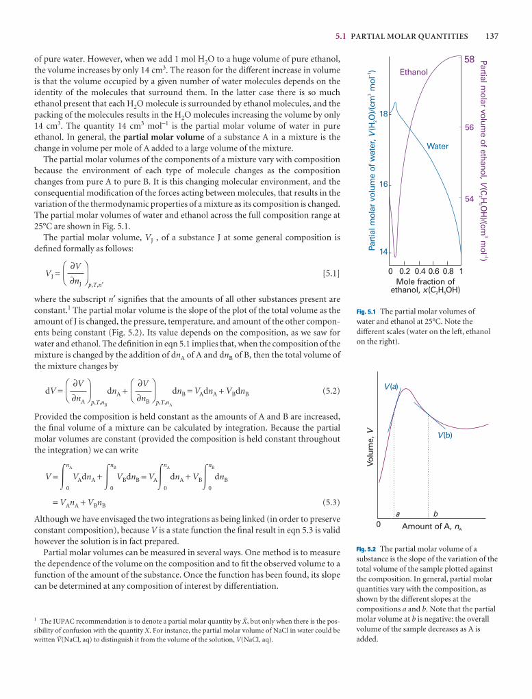
5.1 PARTIAL MOLAR QUANTITIES 137
of pure water. However, when we add 1 mol H2O to a huge volume of pure ethanol,the volume increases by only 14 cm3. The reason for the different increase in volumeis that the volume occupied by a given number of water molecules depends on theidentity of the molecules that surround them. In the latter case there is so muchethanol present that each H2O molecule is surrounded by ethanol molecules, and thepacking of the molecules results in the H2O molecules increasing the volume by only14 cm3. The quantity 14 cm3 mol−1 is the partial molar volume of water in pureethanol. In general, the partial molar volume of a substance A in a mixture is thechange in volume per mole of A added to a large volume of the mixture.
The partial molar volumes of the components of a mixture vary with compositionbecause the environment of each type of molecule changes as the compositionchanges from pure A to pure B. It is this changing molecular environment, and theconsequential modification of the forces acting between molecules, that results in thevariation of the thermodynamic properties of a mixture as its composition is changed.The partial molar volumes of water and ethanol across the full composition range at25°C are shown in Fig. 5.1.
The partial molar volume, VJ , of a substance J at some general composition is defined formally as follows:
VJ =p,T,n′
[5.1]
where the subscript n′ signifies that the amounts of all other substances present areconstant.1 The partial molar volume is the slope of the plot of the total volume as theamount of J is changed, the pressure, temperature, and amount of the other compon-ents being constant (Fig. 5.2). Its value depends on the composition, as we saw forwater and ethanol. The definition in eqn 5.1 implies that, when the composition of themixture is changed by the addition of dnA of A and dnB of B, then the total volume ofthe mixture changes by
dV =p,T,nB
dnA +p,T,nA
dnB = VAdnA + VBdnB (5.2)
Provided the composition is held constant as the amounts of A and B are increased,the final volume of a mixture can be calculated by integration. Because the partialmolar volumes are constant (provided the composition is held constant throughoutthe integration) we can write
V = �nA
0
VAdnA + �nB
0
VBdnB = VA�nA
0
dnA + VB�nB
0
dnB
= VAnA + VBnB (5.3)
Although we have envisaged the two integrations as being linked (in order to preserveconstant composition), because V is a state function the final result in eqn 5.3 is validhowever the solution is in fact prepared.
Partial molar volumes can be measured in several ways. One method is to measurethe dependence of the volume on the composition and to fit the observed volume to afunction of the amount of the substance. Once the function has been found, its slopecan be determined at any composition of interest by differentiation.
DF
∂V
∂nB
AC
DF
∂V
∂nA
AC
DF
∂V
∂nJ
AC
Water
Ethanol
18
16
14
58
56
54
0 0.2 0.4 0.6 0.8 1
Part
ial m
olar
vol
ume
of w
ater
,(H
O)/(
cmm
ol)
V2
3–1
Partial molar volum
e of ethanol,(C
HO
H)/(cm
mol
)V
25
3–1
Mole fraction ofethanol, (C H OH)x 2 5
Fig. 5.1 The partial molar volumes of water and ethanol at 25°C. Note thedifferent scales (water on the left, ethanolon the right).
Volu
me,
V
Amount of A, nA
a b
V( )
V( )
0
a
b
Fig. 5.2 The partial molar volume of asubstance is the slope of the variation of thetotal volume of the sample plotted againstthe composition. In general, partial molarquantities vary with the composition, asshown by the different slopes at thecompositions a and b. Note that the partialmolar volume at b is negative: the overallvolume of the sample decreases as A isadded.
1 The IUPAC recommendation is to denote a partial molar quantity by }, but only when there is the pos-sibility of confusion with the quantity X. For instance, the partial molar volume of NaCl in water could bewritten {(NaCl, aq) to distinguish it from the volume of the solution, V(NaCl, aq).
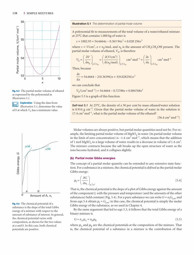
138 5 SIMPLE MIXTURES
0 5 10x
Part
ial m
olar
vol
ume,
/(cm
mol
)V
E3
1
53
54
55
56
Fig. 5.3 The partial molar volume of ethanolas expressed by the polynomial inIllustration 5.1.
Exploration Using the data fromIllustration 5.1, determine the value
of b at which VE has a minimum value.
Amount of A, nA
a b0
Gib
bs e
nerg
y,G
( )a( )b
m
m
Fig. 5.4 The chemical potential of asubstance is the slope of the total Gibbsenergy of a mixture with respect to theamount of substance of interest. In general,the chemical potential varies withcomposition, as shown for the two values at a and b. In this case, both chemicalpotentials are positive.
Illustration 5.1 The determination of partial molar volume
A polynomial fit to measurements of the total volume of a water/ethanol mixtureat 25°C that contains 1.000 kg of water is
v = 1002.93 + 54.6664x − 0.363 94x 2 + 0.028 256x 3
where v = V/cm3, x = nE/mol, and nE is the amount of CH3CH2OH present. Thepartial molar volume of ethanol, VE, is therefore
VE =p,T,nW
=p,T,nW
cm3 mol−1 =p,T,nW
cm3 mol−1
Then, because
= 54.6664 − 2(0.36394)x + 3(0.028256)x 2
we can conclude that
VE/(cm3 mol−1) = 54.6664 − 0.72788x + 0.084768x2
Figure 5.3 is a graph of this function.
Self-test 5.1 At 25°C, the density of a 50 per cent by mass ethanol/water solution is 0.914 g cm−3. Given that the partial molar volume of water in the solution is 17.4 cm3 mol−1, what is the partial molar volume of the ethanol?
[56.4 cm3 mol−1]
Molar volumes are always positive, but partial molar quantities need not be. For ex-ample, the limiting partial molar volume of MgSO4 in water (its partial molar volumein the limit of zero concentration) is −1.4 cm3 mol−1, which means that the additionof 1 mol MgSO4 to a large volume of water results in a decrease in volume of 1.4 cm3.The mixture contracts because the salt breaks up the open structure of water as theions become hydrated, and it collapses slightly.
(b) Partial molar Gibbs energies
The concept of a partial molar quantity can be extended to any extensive state func-tion. For a substance in a mixture, the chemical potential is defined as the partial molarGibbs energy:
µJ =p,T,n′
[5.4]
That is, the chemical potential is the slope of a plot of Gibbs energy against the amountof the component J, with the pressure and temperature (and the amounts of the othersubstances) held constant (Fig. 5.4). For a pure substance we can write G = nJGJ,m, andfrom eqn 5.4 obtain µJ = GJ,m: in this case, the chemical potential is simply the molarGibbs energy of the substance, as we used in Chapter 4.
By the same argument that led to eqn 5.3, it follows that the total Gibbs energy of abinary mixture is
G = nAµA + nBµB (5.5)
where µA and µB are the chemical potentials at the composition of the mixture. Thatis, the chemical potential of a substance in a mixture is the contribution of that
DF
∂G
∂nJ
AC
dv
dx
DF
∂v
∂x
AC
DF
∂(V/cm3)
∂(nE/mol)
AC
DF
∂V
∂nE
AC
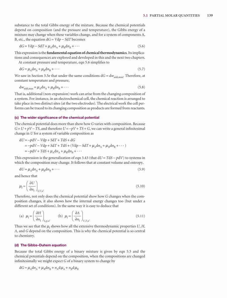
5.1 PARTIAL MOLAR QUANTITIES 139
substance to the total Gibbs energy of the mixture. Because the chemical potentialsdepend on composition (and the pressure and temperature), the Gibbs energy of amixture may change when these variables change, and for a system of components A,B, etc., the equation dG = Vdp − SdT becomes
dG = Vdp − SdT + µAdnA + µBdnB + · · · (5.6)
This expression is the fundamental equation of chemical thermodynamics. Its implica-tions and consequences are explored and developed in this and the next two chapters.
At constant pressure and temperature, eqn 5.6 simplifies to
dG = µAdnA + µBdnB + · · · (5.7)
We saw in Section 3.5e that under the same conditions dG = dwadd,max. Therefore, atconstant temperature and pressure,
dwadd,max = µAdnA + µBdnB + · · · (5.8)
That is, additional (non-expansion) work can arise from the changing composition ofa system. For instance, in an electrochemical cell, the chemical reaction is arranged totake place in two distinct sites (at the two electrodes). The electrical work the cell per-forms can be traced to its changing composition as products are formed from reactants.
(c) The wider significance of the chemical potential
The chemical potential does more than show how G varies with composition. BecauseG = U + pV − TS, and therefore U = −pV + TS + G, we can write a general infinitesimalchange in U for a system of variable composition as
dU = −pdV − Vdp + SdT + TdS + dG
= −pdV − Vdp + SdT + TdS + (Vdp − SdT + µAdnA + µBdnB + · · · )
= −pdV + TdS + µAdnA + µBdnB + · · ·
This expression is the generalization of eqn 3.43 (that dU = TdS − pdV) to systems inwhich the composition may change. It follows that at constant volume and entropy,
dU = µAdnA + µBdnB + · · · (5.9)
and hence that
µJ =S,V,n′
(5.10)
Therefore, not only does the chemical potential show how G changes when the com-position changes, it also shows how the internal energy changes too (but under adifferent set of conditions). In the same way it is easy to deduce that
(a) µJ =S,p,n′
(b) µJ =V,T,n′
(5.11)
Thus we see that the µJ shows how all the extensive thermodynamic properties U, H,A, and G depend on the composition. This is why the chemical potential is so centralto chemistry.
(d) The Gibbs–Duhem equation
Because the total Gibbs energy of a binary mixture is given by eqn 5.5 and thechemical potentials depend on the composition, when the compositions are changed infinitesimally we might expect G of a binary system to change by
dG = µAdnA + µBdnB + nAdµA + nBdµB
DF
∂A
∂nJ
AC
DF
∂H
∂nJ
AC
DF
∂U
∂nJ
AC
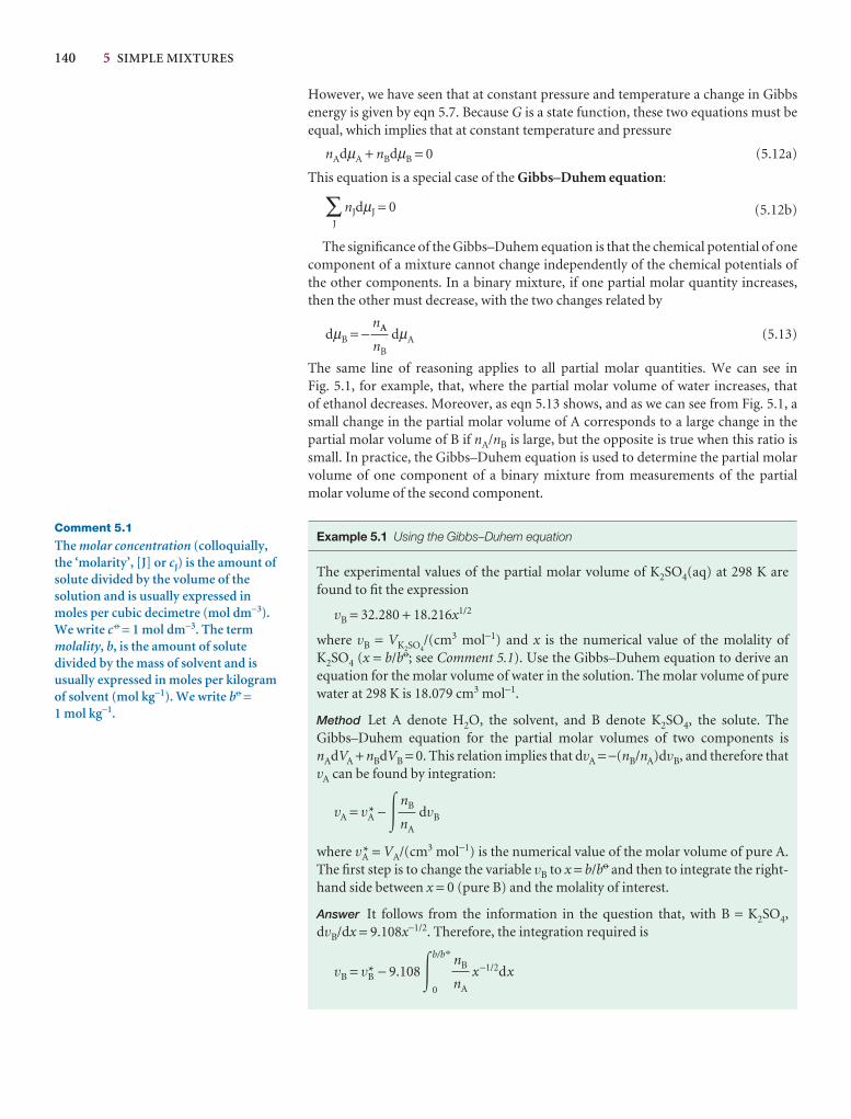
140 5 SIMPLE MIXTURES
Comment 5.1
The molar concentration (colloquially,the ‘molarity’, [J] or cJ) is the amount ofsolute divided by the volume of thesolution and is usually expressed inmoles per cubic decimetre (mol dm−3).We write c 7 = 1 mol dm−3. The termmolality, b, is the amount of solutedivided by the mass of solvent and isusually expressed in moles per kilogramof solvent (mol kg−1). We write b7 =1 mol kg−1.
However, we have seen that at constant pressure and temperature a change in Gibbsenergy is given by eqn 5.7. Because G is a state function, these two equations must beequal, which implies that at constant temperature and pressure
nAdµA + nBdµB = 0 (5.12a)
This equation is a special case of the Gibbs–Duhem equation:
∑J
nJdµJ = 0 (5.12b)
The significance of the Gibbs–Duhem equation is that the chemical potential of onecomponent of a mixture cannot change independently of the chemical potentials ofthe other components. In a binary mixture, if one partial molar quantity increases,then the other must decrease, with the two changes related by
dµB = − dµA (5.13)
The same line of reasoning applies to all partial molar quantities. We can see in Fig. 5.1, for example, that, where the partial molar volume of water increases, that of ethanol decreases. Moreover, as eqn 5.13 shows, and as we can see from Fig. 5.1, asmall change in the partial molar volume of A corresponds to a large change in thepartial molar volume of B if nA/nB is large, but the opposite is true when this ratio issmall. In practice, the Gibbs–Duhem equation is used to determine the partial molarvolume of one component of a binary mixture from measurements of the partialmolar volume of the second component.
Example 5.1 Using the Gibbs–Duhem equation
The experimental values of the partial molar volume of K2SO4(aq) at 298 K arefound to fit the expression
vB = 32.280 + 18.216x1/2
where vB = VK2SO4/(cm3 mol−1) and x is the numerical value of the molality of
K2SO4 (x = b/b7; see Comment 5.1). Use the Gibbs–Duhem equation to derive anequation for the molar volume of water in the solution. The molar volume of purewater at 298 K is 18.079 cm3 mol−1.
Method Let A denote H2O, the solvent, and B denote K2SO4, the solute. TheGibbs–Duhem equation for the partial molar volumes of two components isnAdVA + nBdVB = 0. This relation implies that dvA = −(nB/nA)dvB, and therefore thatvA can be found by integration:
vA = vA* − � dvB
where vA* = VA/(cm3 mol−1) is the numerical value of the molar volume of pure A.The first step is to change the variable vB to x = b/b7 and then to integrate the right-hand side between x = 0 (pure B) and the molality of interest.
Answer It follows from the information in the question that, with B = K2SO4,dvB/dx = 9.108x−1/2. Therefore, the integration required is
vB = vB* − 9.108�0
b/b 7
x−1/2dxnB
nA
nB
nA
nA
nB
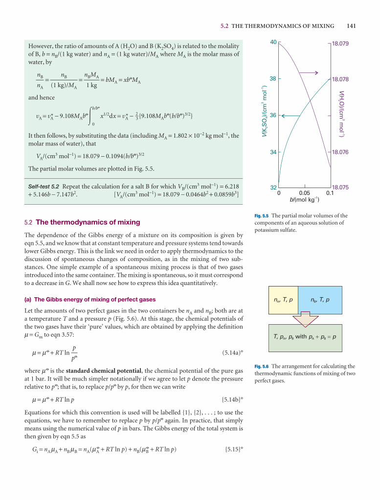
5.2 THE THERMODYNAMICS OF MIXING 141
32
34
36
38
40
V(K
SO
)/(cm
mol
)2
43
–1 V(H
O)/(cm
mol
)2
3–1
18.075
18.076
18.078
18.079
0 0.05 0.1b/(mol kg )–1
Fig. 5.5 The partial molar volumes of thecomponents of an aqueous solution ofpotassium sulfate.
n T pA, , n T pB, ,
T p p p p p, , withA B A B� �
Fig. 5.6 The arrangement for calculating thethermodynamic functions of mixing of twoperfect gases.
However, the ratio of amounts of A (H2O) and B (K2SO4) is related to the molalityof B, b = nB/(1 kg water) and nA = (1 kg water)/MA where MA is the molar mass ofwater, by
= = = bMA = xb7MA
and hence
vA = vA* − 9.108MAb7�0
b/b7
x1/2dx = vA* − 2–3 {9.108MAb7(b/b7)3/2}
It then follows, by substituting the data (including MA = 1.802 × 10⁻² kg mol−1, themolar mass of water), that
VA/(cm3 mol−1) = 18.079 − 0.1094(b/b7)3/2
The partial molar volumes are plotted in Fig. 5.5.
Self-test 5.2 Repeat the calculation for a salt B for which VB/(cm3 mol−1) = 6.218+ 5.146b − 7.147b2. [VA/(cm3 mol−1) = 18.079 − 0.0464b2 + 0.0859b3]
5.2 The thermodynamics of mixing
The dependence of the Gibbs energy of a mixture on its composition is given by eqn 5.5, and we know that at constant temperature and pressure systems tend towardslower Gibbs energy. This is the link we need in order to apply thermodynamics to thediscussion of spontaneous changes of composition, as in the mixing of two sub-stances. One simple example of a spontaneous mixing process is that of two gases introduced into the same container. The mixing is spontaneous, so it must correspondto a decrease in G. We shall now see how to express this idea quantitatively.
(a) The Gibbs energy of mixing of perfect gases
Let the amounts of two perfect gases in the two containers be nA and nB; both are at a temperature T and a pressure p (Fig. 5.6). At this stage, the chemical potentials of the two gases have their ‘pure’ values, which are obtained by applying the definition µ = Gm to eqn 3.57:
µ = µ7 + RT ln (5.14a)°
where µ7 is the standard chemical potential, the chemical potential of the pure gas at 1 bar. It will be much simpler notationally if we agree to let p denote the pressurerelative to p7; that is, to replace p/p7 by p, for then we can write
µ = µ7 + RT ln p {5.14b}°
Equations for which this convention is used will be labelled {1}, {2}, . . . ; to use theequations, we have to remember to replace p by p/p7 again. In practice, that simplymeans using the numerical value of p in bars. The Gibbs energy of the total system isthen given by eqn 5.5 as
Gi = nAµA + nBµB = nA(µA7 + RT ln p) + nB(µB
7 + RT ln p) {5.15}°
p
p7
nBMA
1 kg
nB
(1 kg)/MA
nB
nA
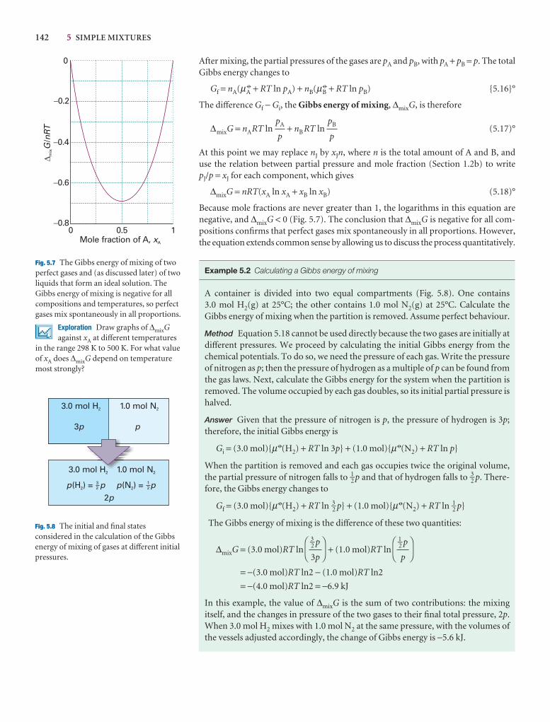
142 5 SIMPLE MIXTURES
3.0 mol H2
3.0 mol H2
1.0 mol N2
1.0 mol N2
3p p
p p(H ) =2 p p(N ) =2
2p
1
0
�0.2
�0.4
�0.6
�0.80 0.5 1
Mole fraction of A, xA
D
mixG
nRT
/
Fig. 5.7 The Gibbs energy of mixing of twoperfect gases and (as discussed later) of twoliquids that form an ideal solution. TheGibbs energy of mixing is negative for allcompositions and temperatures, so perfectgases mix spontaneously in all proportions.
Exploration Draw graphs of ∆mixGagainst xA at different temperatures
in the range 298 K to 500 K. For what valueof xA does ∆mixG depend on temperaturemost strongly?
Fig. 5.8 The initial and final statesconsidered in the calculation of the Gibbsenergy of mixing of gases at different initialpressures.
After mixing, the partial pressures of the gases are pA and pB, with pA + pB = p. The totalGibbs energy changes to
Gf = nA(µA7 + RT ln pA) + nB(µB
7 + RT ln pB) {5.16}°
The difference Gf − Gi, the Gibbs energy of mixing, ∆mixG, is therefore
∆mixG = nART ln + nB RT ln (5.17)°
At this point we may replace nJ by xJn, where n is the total amount of A and B, and use the relation between partial pressure and mole fraction (Section 1.2b) to write pJ/p = xJ for each component, which gives
∆mixG = nRT(xA ln xA + xB ln xB) (5.18)°
Because mole fractions are never greater than 1, the logarithms in this equation arenegative, and ∆mixG < 0 (Fig. 5.7). The conclusion that ∆mixG is negative for all com-positions confirms that perfect gases mix spontaneously in all proportions. However,the equation extends common sense by allowing us to discuss the process quantitatively.
Example 5.2 Calculating a Gibbs energy of mixing
A container is divided into two equal compartments (Fig. 5.8). One contains 3.0 mol H2(g) at 25°C; the other contains 1.0 mol N2(g) at 25°C. Calculate theGibbs energy of mixing when the partition is removed. Assume perfect behaviour.
Method Equation 5.18 cannot be used directly because the two gases are initially atdifferent pressures. We proceed by calculating the initial Gibbs energy from thechemical potentials. To do so, we need the pressure of each gas. Write the pressureof nitrogen as p; then the pressure of hydrogen as a multiple of p can be found fromthe gas laws. Next, calculate the Gibbs energy for the system when the partition isremoved. The volume occupied by each gas doubles, so its initial partial pressure ishalved.
Answer Given that the pressure of nitrogen is p, the pressure of hydrogen is 3p;therefore, the initial Gibbs energy is
Gi = (3.0 mol){µ7(H2) + RT ln 3p} + (1.0 mol){µ7(N2) + RT ln p}
When the partition is removed and each gas occupies twice the original volume,the partial pressure of nitrogen falls to 1–2 p and that of hydrogen falls to 3–2 p. There-fore, the Gibbs energy changes to
Gf = (3.0 mol){µ7(H2) + RT ln 3–2 p} + (1.0 mol){µ7(N2) + RT ln 1–2 p}
The Gibbs energy of mixing is the difference of these two quantities:
∆mixG = (3.0 mol)RT ln + (1.0 mol)RT ln
= −(3.0 mol)RT ln2 − (1.0 mol)RT ln2
= −(4.0 mol)RT ln2 = −6.9 kJ
In this example, the value of ∆mixG is the sum of two contributions: the mixingitself, and the changes in pressure of the two gases to their final total pressure, 2p.When 3.0 mol H2 mixes with 1.0 mol N2 at the same pressure, with the volumes ofthe vessels adjusted accordingly, the change of Gibbs energy is −5.6 kJ.
DF
1–2 p
p
AC
DF
3–2 p
3p
AC
pB
p
pA
p
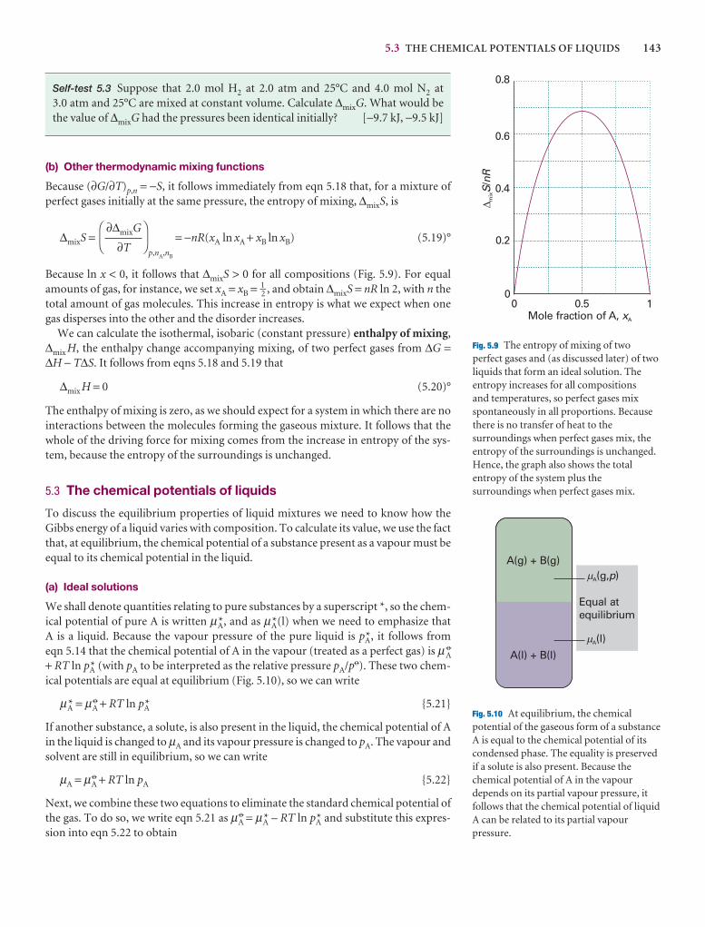
5.3 THE CHEMICAL POTENTIALS OF LIQUIDS 143
0
0.2
0.4
0.6
0.8
0 0.5 1Mole fraction of A, xA
m
ixS
nR/
Fig. 5.9 The entropy of mixing of twoperfect gases and (as discussed later) of twoliquids that form an ideal solution. Theentropy increases for all compositions and temperatures, so perfect gases mixspontaneously in all proportions. Becausethere is no transfer of heat to thesurroundings when perfect gases mix, theentropy of the surroundings is unchanged.Hence, the graph also shows the totalentropy of the system plus thesurroundings when perfect gases mix.
A(g) + B(g)
A(g, )p
A(l)
A(l) + B(l)
Equal atequilibrium
Fig. 5.10 At equilibrium, the chemicalpotential of the gaseous form of a substanceA is equal to the chemical potential of itscondensed phase. The equality is preservedif a solute is also present. Because thechemical potential of A in the vapourdepends on its partial vapour pressure, itfollows that the chemical potential of liquidA can be related to its partial vapourpressure.
Self-test 5.3 Suppose that 2.0 mol H2 at 2.0 atm and 25°C and 4.0 mol N2 at3.0 atm and 25°C are mixed at constant volume. Calculate ∆mixG. What would bethe value of ∆mixG had the pressures been identical initially? [−9.7 kJ, −9.5 kJ]
(b) Other thermodynamic mixing functions
Because (∂G/∂T)p,n = −S, it follows immediately from eqn 5.18 that, for a mixture ofperfect gases initially at the same pressure, the entropy of mixing, ∆mixS, is
∆mixS =p,nA,nB
= −nR(xA ln xA + xB ln xB) (5.19)°
Because ln x < 0, it follows that ∆mixS > 0 for all compositions (Fig. 5.9). For equalamounts of gas, for instance, we set xA = xB = 1–2 , and obtain ∆mixS = nR ln 2, with n thetotal amount of gas molecules. This increase in entropy is what we expect when onegas disperses into the other and the disorder increases.
We can calculate the isothermal, isobaric (constant pressure) enthalpy of mixing,∆mix H, the enthalpy change accompanying mixing, of two perfect gases from ∆G =∆H − T∆S. It follows from eqns 5.18 and 5.19 that
∆mix H = 0 (5.20)°
The enthalpy of mixing is zero, as we should expect for a system in which there are nointeractions between the molecules forming the gaseous mixture. It follows that thewhole of the driving force for mixing comes from the increase in entropy of the sys-tem, because the entropy of the surroundings is unchanged.
5.3 The chemical potentials of liquids
To discuss the equilibrium properties of liquid mixtures we need to know how theGibbs energy of a liquid varies with composition. To calculate its value, we use the factthat, at equilibrium, the chemical potential of a substance present as a vapour must beequal to its chemical potential in the liquid.
(a) Ideal solutions
We shall denote quantities relating to pure substances by a superscript *, so the chem-ical potential of pure A is written µA*, and as µA*(l) when we need to emphasize that A is a liquid. Because the vapour pressure of the pure liquid is pA*, it follows from eqn 5.14 that the chemical potential of A in the vapour (treated as a perfect gas) is µA
7
+ RT ln pA* (with pA to be interpreted as the relative pressure pA/p7). These two chem-ical potentials are equal at equilibrium (Fig. 5.10), so we can write
µA* = µA7 + RT ln pA* {5.21}
If another substance, a solute, is also present in the liquid, the chemical potential of Ain the liquid is changed to µA and its vapour pressure is changed to pA. The vapour andsolvent are still in equilibrium, so we can write
µA = µA7 + RT ln pA {5.22}
Next, we combine these two equations to eliminate the standard chemical potential ofthe gas. To do so, we write eqn 5.21 as µA
7 = µA* – RT ln pA* and substitute this expres-sion into eqn 5.22 to obtain
DF
∂∆mixG
∂T
AC
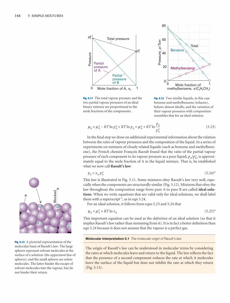
144 5 SIMPLE MIXTURES
0 1Mole fraction of A, xA
Partialpressureof A
Partialpressureof B
Total pressurepB*
pA*
Pres
sure
Fig. 5.11 The total vapour pressure and thetwo partial vapour pressures of an idealbinary mixture are proportional to themole fractions of the components.
60
40
20
0
Pres
sure
,/T
orr
p
0 Mole fraction ofmethylbenzene, (C H CH )x 6 5 3
1
Benzene
Methylbenzene
Total
80
Fig. 5.12 Two similar liquids, in this casebenzene and methylbenzene (toluene),behave almost ideally, and the variation oftheir vapour pressures with compositionresembles that for an ideal solution.
Blo
cked
Fig. 5.13 A pictorial representation of themolecular basis of Raoult’s law. The largespheres represent solvent molecules at thesurface of a solution (the uppermost line ofspheres), and the small spheres are solutemolecules. The latter hinder the escape ofsolvent molecules into the vapour, but donot hinder their return.
µA = µA* − RT ln pA* + RT ln pA = µA* + RT ln (5.23)
In the final step we draw on additional experimental information about the relationbetween the ratio of vapour pressures and the composition of the liquid. In a series ofexperiments on mixtures of closely related liquids (such as benzene and methylbenz-ene), the French chemist François Raoult found that the ratio of the partial vapourpressure of each component to its vapour pressure as a pure liquid, pA/pA*, is approxi-mately equal to the mole fraction of A in the liquid mixture. That is, he establishedwhat we now call Raoult’s law:
pA = xA pA* (5.24)°
This law is illustrated in Fig. 5.11. Some mixtures obey Raoult’s law very well, espe-cially when the components are structurally similar (Fig. 5.12). Mixtures that obey thelaw throughout the composition range from pure A to pure B are called ideal solu-tions. When we write equations that are valid only for ideal solutions, we shall labelthem with a superscript °, as in eqn 5.24.
For an ideal solution, it follows from eqns 5.23 and 5.24 that
µA = µA* + RT ln xA (5.25)°
This important equation can be used as the definition of an ideal solution (so that itimplies Raoult’s law rather than stemming from it). It is in fact a better definition thaneqn 5.24 because it does not assume that the vapour is a perfect gas.
Molecular interpretation 5.1 The molecular origin of Raoult’s law
The origin of Raoult’s law can be understood in molecular terms by consideringthe rates at which molecules leave and return to the liquid. The law reflects the factthat the presence of a second component reduces the rate at which A moleculesleave the surface of the liquid but does not inhibit the rate at which they return(Fig. 5.13).
pA
pA*
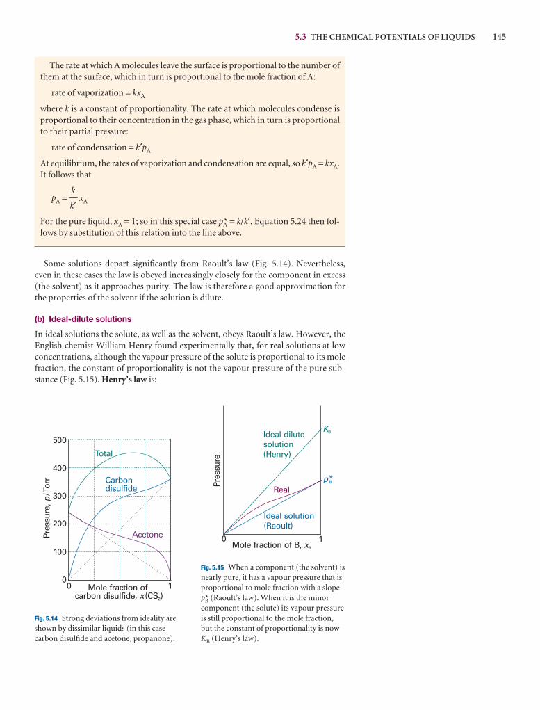
5.3 THE CHEMICAL POTENTIALS OF LIQUIDS 145
Ideal dilutesolution(Henry)
Real
Ideal solution(Raoult)
Mole fraction of B, xB
0 1
Pres
sure
KB
p B*
Fig. 5.15 When a component (the solvent) isnearly pure, it has a vapour pressure that isproportional to mole fraction with a slopepB* (Raoult’s law). When it is the minorcomponent (the solute) its vapour pressureis still proportional to the mole fraction,but the constant of proportionality is nowKB (Henry’s law).
0 1Mole fraction ofcarbon disulfide, (CS )x 2
500
400
300
200
100
0
Total
Carbondisulfide
AcetonePres
sure
,/T
orr
p
Fig. 5.14 Strong deviations from ideality areshown by dissimilar liquids (in this casecarbon disulfide and acetone, propanone).
The rate at which A molecules leave the surface is proportional to the number ofthem at the surface, which in turn is proportional to the mole fraction of A:
rate of vaporization = kxA
where k is a constant of proportionality. The rate at which molecules condense isproportional to their concentration in the gas phase, which in turn is proportionalto their partial pressure:
rate of condensation = k′pA
At equilibrium, the rates of vaporization and condensation are equal, so k′pA = kxA.It follows that
pA = xA
For the pure liquid, xA = 1; so in this special case pA* = k/k′. Equation 5.24 then fol-lows by substitution of this relation into the line above.
Some solutions depart significantly from Raoult’s law (Fig. 5.14). Nevertheless,even in these cases the law is obeyed increasingly closely for the component in excess(the solvent) as it approaches purity. The law is therefore a good approximation forthe properties of the solvent if the solution is dilute.
(b) Ideal-dilute solutions
In ideal solutions the solute, as well as the solvent, obeys Raoult’s law. However, theEnglish chemist William Henry found experimentally that, for real solutions at lowconcentrations, although the vapour pressure of the solute is proportional to its molefraction, the constant of proportionality is not the vapour pressure of the pure sub-stance (Fig. 5.15). Henry’s law is:
k
k′
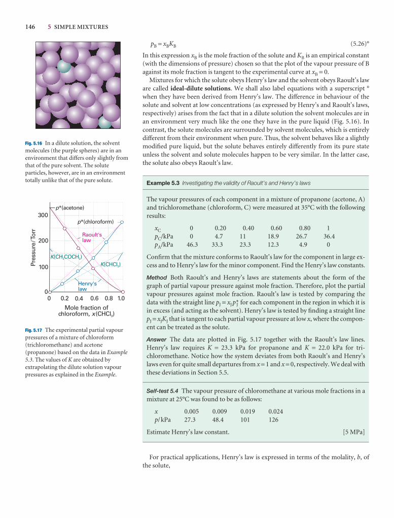
146 5 SIMPLE MIXTURES
200
100
00 0.2 0.4 0.6 0.8 1.0
p*(chloroform)
K(CHCl )3
K(CH COCH )3 3
p*(acetone)
Mole fraction ofchloroform, (CHCl )x 3
Raoult'slaw
Henry'slaw
Pres
sure
/Tor
r
300
Fig. 5.16 In a dilute solution, the solventmolecules (the purple spheres) are in anenvironment that differs only slightly fromthat of the pure solvent. The soluteparticles, however, are in an environmenttotally unlike that of the pure solute.
Fig. 5.17 The experimental partial vapourpressures of a mixture of chloroform(trichloromethane) and acetone(propanone) based on the data in Example5.3. The values of K are obtained byextrapolating the dilute solution vapourpressures as explained in the Example.
pB = xBKB (5.26)°
In this expression xB is the mole fraction of the solute and KB is an empirical constant(with the dimensions of pressure) chosen so that the plot of the vapour pressure of Bagainst its mole fraction is tangent to the experimental curve at xB = 0.
Mixtures for which the solute obeys Henry’s law and the solvent obeys Raoult’s laware called ideal-dilute solutions. We shall also label equations with a superscript °when they have been derived from Henry’s law. The difference in behaviour of the solute and solvent at low concentrations (as expressed by Henry’s and Raoult’s laws,respectively) arises from the fact that in a dilute solution the solvent molecules are inan environment very much like the one they have in the pure liquid (Fig. 5.16). Incontrast, the solute molecules are surrounded by solvent molecules, which is entirelydifferent from their environment when pure. Thus, the solvent behaves like a slightlymodified pure liquid, but the solute behaves entirely differently from its pure state unless the solvent and solute molecules happen to be very similar. In the latter case,the solute also obeys Raoult’s law.
Example 5.3 Investigating the validity of Raoult’s and Henry’s laws
The vapour pressures of each component in a mixture of propanone (acetone, A)and trichloromethane (chloroform, C) were measured at 35°C with the followingresults:
xC 0 0.20 0.40 0.60 0.80 1pC/kPa 0 4.7 11 18.9 26.7 36.4pA/kPa 46.3 33.3 23.3 12.3 4.9 0
Confirm that the mixture conforms to Raoult’s law for the component in large ex-cess and to Henry’s law for the minor component. Find the Henry’s law constants.
Method Both Raoult’s and Henry’s laws are statements about the form of thegraph of partial vapour pressure against mole fraction. Therefore, plot the partialvapour pressures against mole fraction. Raoult’s law is tested by comparing thedata with the straight line pJ = xJ p J* for each component in the region in which it isin excess (and acting as the solvent). Henry’s law is tested by finding a straight linepJ = xJKJ that is tangent to each partial vapour pressure at low x, where the compon-ent can be treated as the solute.
Answer The data are plotted in Fig. 5.17 together with the Raoult’s law lines.Henry’s law requires K = 23.3 kPa for propanone and K = 22.0 kPa for tri-chloromethane. Notice how the system deviates from both Raoult’s and Henry’slaws even for quite small departures from x = 1 and x = 0, respectively. We deal withthese deviations in Section 5.5.
Self-test 5.4 The vapour pressure of chloromethane at various mole fractions in amixture at 25°C was found to be as follows:
x 0.005 0.009 0.019 0.024p/kPa 27.3 48.4 101 126
Estimate Henry’s law constant. [5 MPa]
For practical applications, Henry’s law is expressed in terms of the molality, b, ofthe solute,
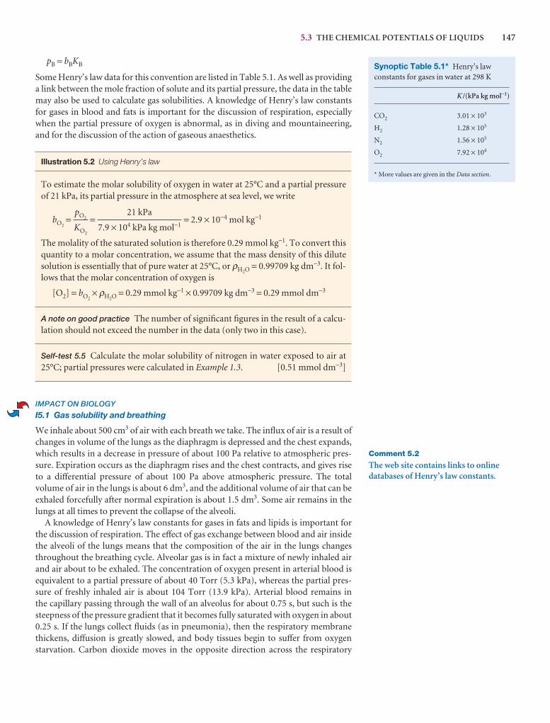
5.3 THE CHEMICAL POTENTIALS OF LIQUIDS 147
Synoptic Table 5.1* Henry’s lawconstants for gases in water at 298 K
K /(kPa kg mol−1)
CO2 3.01 × 10³
H2 1.28 × 10⁵
N2 1.56 × 10⁵
O2 7.92 × 10⁴
* More values are given in the Data section.
Comment 5.2
The web site contains links to onlinedatabases of Henry’s law constants.
pB = bBKB
Some Henry’s law data for this convention are listed in Table 5.1. As well as providinga link between the mole fraction of solute and its partial pressure, the data in the tablemay also be used to calculate gas solubilities. A knowledge of Henry’s law constantsfor gases in blood and fats is important for the discussion of respiration, especiallywhen the partial pressure of oxygen is abnormal, as in diving and mountaineering,and for the discussion of the action of gaseous anaesthetics.
Illustration 5.2 Using Henry’s law
To estimate the molar solubility of oxygen in water at 25°C and a partial pressureof 21 kPa, its partial pressure in the atmosphere at sea level, we write
bO2= = = 2.9 × 10⁻⁴ mol kg−1
The molality of the saturated solution is therefore 0.29 mmol kg−1. To convert thisquantity to a molar concentration, we assume that the mass density of this dilutesolution is essentially that of pure water at 25°C, or ρH2O = 0.99709 kg dm−3. It fol-lows that the molar concentration of oxygen is
[O2] = bO2× ρH2O = 0.29 mmol kg−1 × 0.99709 kg dm−3 = 0.29 mmol dm−3
A note on good practice The number of significant figures in the result of a calcu-lation should not exceed the number in the data (only two in this case).
Self-test 5.5 Calculate the molar solubility of nitrogen in water exposed to air at25°C; partial pressures were calculated in Example 1.3. [0.51 mmol dm−3]
IMPACT ON BIOLOGY
I5.1 Gas solubility and breathing
We inhale about 500 cm3 of air with each breath we take. The influx of air is a result ofchanges in volume of the lungs as the diaphragm is depressed and the chest expands,which results in a decrease in pressure of about 100 Pa relative to atmospheric pres-sure. Expiration occurs as the diaphragm rises and the chest contracts, and gives riseto a differential pressure of about 100 Pa above atmospheric pressure. The total volume of air in the lungs is about 6 dm3, and the additional volume of air that can beexhaled forcefully after normal expiration is about 1.5 dm3. Some air remains in thelungs at all times to prevent the collapse of the alveoli.
A knowledge of Henry’s law constants for gases in fats and lipids is important forthe discussion of respiration. The effect of gas exchange between blood and air insidethe alveoli of the lungs means that the composition of the air in the lungs changesthroughout the breathing cycle. Alveolar gas is in fact a mixture of newly inhaled airand air about to be exhaled. The concentration of oxygen present in arterial blood isequivalent to a partial pressure of about 40 Torr (5.3 kPa), whereas the partial pres-sure of freshly inhaled air is about 104 Torr (13.9 kPa). Arterial blood remains in the capillary passing through the wall of an alveolus for about 0.75 s, but such is thesteepness of the pressure gradient that it becomes fully saturated with oxygen in about0.25 s. If the lungs collect fluids (as in pneumonia), then the respiratory membranethickens, diffusion is greatly slowed, and body tissues begin to suffer from oxygenstarvation. Carbon dioxide moves in the opposite direction across the respiratory
21 kPa
7.9 × 10⁴ kPa kg mol−1
pO2
KO2
148 5 SIMPLE MIXTURES
tissue, but the partial pressure gradient is much less, corresponding to about 5 Torr(0.7 kPa) in blood and 40 Torr (5.3 kPa) in air at equilibrium. However, because carbon dioxide is much more soluble in the alveolar fluid than oxygen is, equalamounts of oxygen and carbon dioxide are exchanged in each breath.
A hyperbaric oxygen chamber, in which oxygen is at an elevated partial pressure, is used to treat certain types of disease. Carbon monoxide poisoning can be treated in this way as can the consequences of shock. Diseases that are caused by anaerobicbacteria, such as gas gangrene and tetanus, can also be treated because the bacteriacannot thrive in high oxygen concentrations.
In scuba diving (where scuba is an acronym formed from ‘self-contained under-water breathing apparatus’), air is supplied at a higher pressure, so that the pressurewithin the diver’s chest matches the pressure exerted by the surrounding water. The latter increases by about 1 atm for each 10 m of descent. One unfortunate con-sequence of breathing air at high pressures is that nitrogen is much more soluble infatty tissues than in water, so it tends to dissolve in the central nervous system, bonemarrow, and fat reserves. The result is nitrogen narcosis, with symptoms like intoxica-tion. If the diver rises too rapidly to the surface, the nitrogen comes out of its lipid solution as bubbles, which causes the painful and sometimes fatal condition known as the bends. Many cases of scuba drowning appear to be consequences of arterial embolisms (obstructions in arteries caused by gas bubbles) and loss of consciousnessas the air bubbles rise into the head.
The properties of solutions
In this section we consider the thermodynamics of mixing of liquids. First, we considerthe simple case of mixtures of liquids that mix to form an ideal solution. In this way,we identify the thermodynamic consequences of molecules of one species minglingrandomly with molecules of the second species. The calculation provides a back-ground for discussing the deviations from ideal behaviour exhibited by real solutions.
5.4 Liquid mixtures
Thermodynamics can provide insight into the properties of liquid mixtures, and a fewsimple ideas can bring the whole field of study together.
(a) Ideal solutions
The Gibbs energy of mixing of two liquids to form an ideal solution is calculated in exactly the same way as for two gases (Section 5.2). The total Gibbs energy before liquids are mixed is
Gi = nAµA* + nBµB*
When they are mixed, the individual chemical potentials are given by eqn 5.25 and thetotal Gibbs energy is
Gf = nA{µA* + RT ln xA} + nB{µB* +RT ln xB}
Consequently, the Gibbs energy of mixing is
∆mixG = nRT{xA ln xA + xB ln xB} (5.27)°
where n = nA + nB. As for gases, it follows that the ideal entropy of mixing of two liquids is
∆mixS = −nR{xA ln xA + xB ln xB} (5.28)°
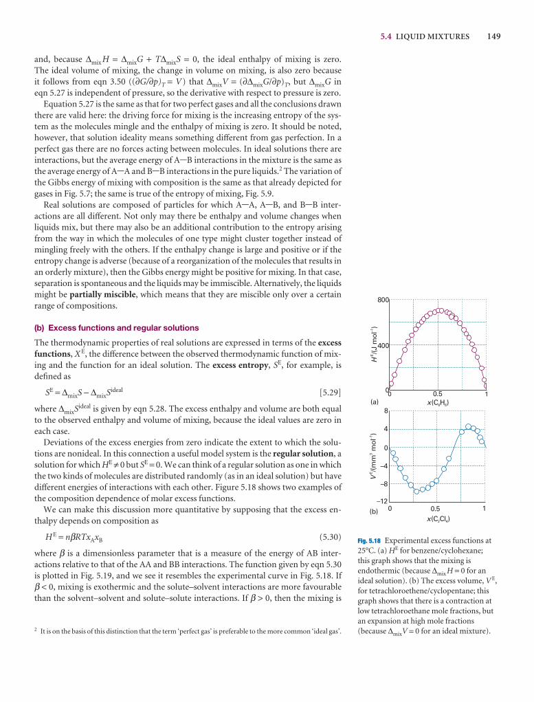
5.4 LIQUID MIXTURES 149
and, because ∆mix H = ∆mixG + T∆mixS = 0, the ideal enthalpy of mixing is zero. The ideal volume of mixing, the change in volume on mixing, is also zero because it follows from eqn 3.50 ((∂G/∂p)T = V) that ∆mixV = (∂∆mixG/∂p)T, but ∆mixG ineqn 5.27 is independent of pressure, so the derivative with respect to pressure is zero.
Equation 5.27 is the same as that for two perfect gases and all the conclusions drawnthere are valid here: the driving force for mixing is the increasing entropy of the sys-tem as the molecules mingle and the enthalpy of mixing is zero. It should be noted,however, that solution ideality means something different from gas perfection. In aperfect gas there are no forces acting between molecules. In ideal solutions there areinteractions, but the average energy of A-B interactions in the mixture is the same asthe average energy of A-A and B-B interactions in the pure liquids.2 The variation ofthe Gibbs energy of mixing with composition is the same as that already depicted forgases in Fig. 5.7; the same is true of the entropy of mixing, Fig. 5.9.
Real solutions are composed of particles for which A-A, A-B, and B-B inter-actions are all different. Not only may there be enthalpy and volume changes whenliquids mix, but there may also be an additional contribution to the entropy arisingfrom the way in which the molecules of one type might cluster together instead ofmingling freely with the others. If the enthalpy change is large and positive or if the entropy change is adverse (because of a reorganization of the molecules that results inan orderly mixture), then the Gibbs energy might be positive for mixing. In that case,separation is spontaneous and the liquids may be immiscible. Alternatively, the liquidsmight be partially miscible, which means that they are miscible only over a certainrange of compositions.
(b) Excess functions and regular solutions
The thermodynamic properties of real solutions are expressed in terms of the excessfunctions, X E, the difference between the observed thermodynamic function of mix-ing and the function for an ideal solution. The excess entropy, SE, for example, isdefined as
SE = ∆mixS − ∆mixSideal [5.29]
where ∆mixSideal is given by eqn 5.28. The excess enthalpy and volume are both equalto the observed enthalpy and volume of mixing, because the ideal values are zero ineach case.
Deviations of the excess energies from zero indicate the extent to which the solu-tions are nonideal. In this connection a useful model system is the regular solution, asolution for which HE ≠ 0 but SE = 0. We can think of a regular solution as one in whichthe two kinds of molecules are distributed randomly (as in an ideal solution) but havedifferent energies of interactions with each other. Figure 5.18 shows two examples ofthe composition dependence of molar excess functions.
We can make this discussion more quantitative by supposing that the excess en-thalpy depends on composition as
H E = nβRTxAxB (5.30)
where β is a dimensionless parameter that is a measure of the energy of AB inter-actions relative to that of the AA and BB interactions. The function given by eqn 5.30 is plotted in Fig. 5.19, and we see it resembles the experimental curve in Fig. 5.18. If β < 0, mixing is exothermic and the solute–solvent interactions are more favourablethan the solvent–solvent and solute–solute interactions. If β > 0, then the mixing is
0
0
0.5
0.5
1
1x(C H )6 6
x(C Cl )2 4
0
400
800
HE
–1/(J
mol
)V
E3
–1/(m
mm
ol)
–12
–4
–8
0
4
8(a)
(b)
Fig. 5.18 Experimental excess functions at25°C. (a) HE for benzene/cyclohexane; this graph shows that the mixing isendothermic (because ∆mix H = 0 for anideal solution). (b) The excess volume, V E,for tetrachloroethene/cyclopentane; thisgraph shows that there is a contraction atlow tetrachloroethane mole fractions, butan expansion at high mole fractions(because ∆mixV = 0 for an ideal mixture).2 It is on the basis of this distinction that the term ‘perfect gas’ is preferable to the more common ‘ideal gas’.
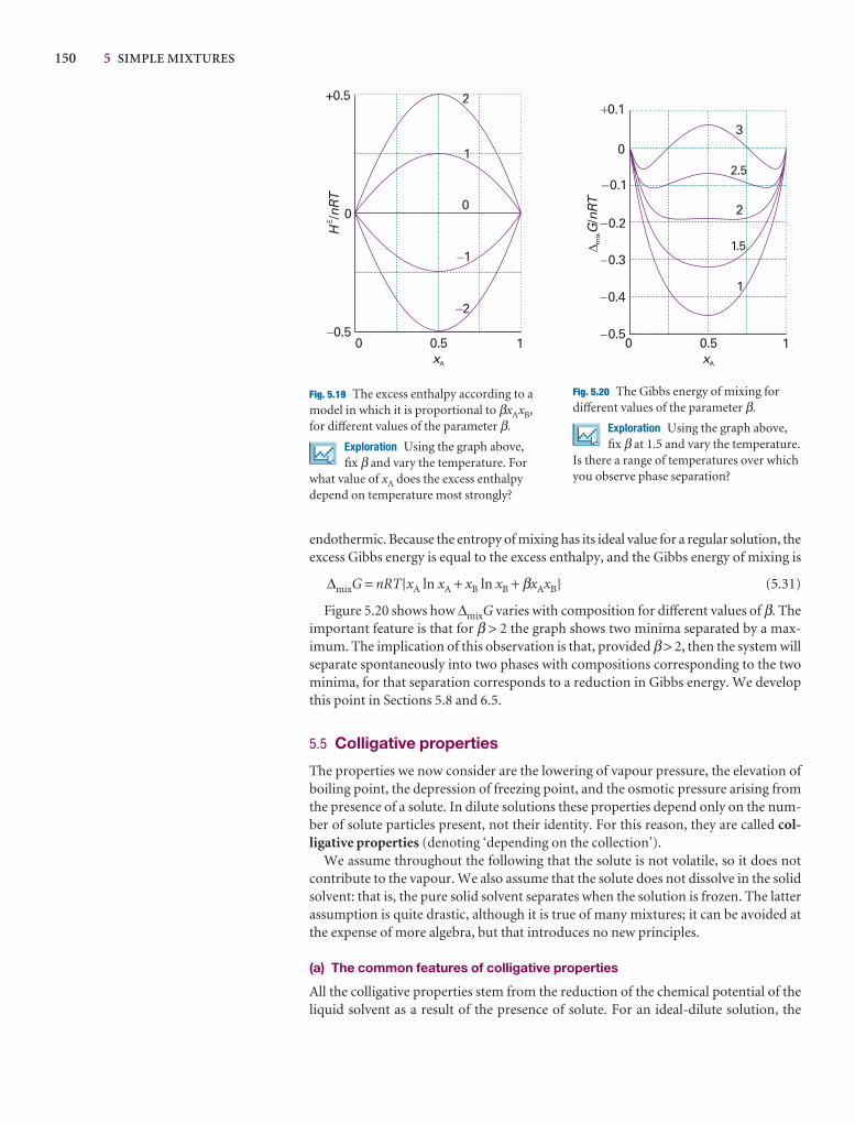
150 5 SIMPLE MIXTURES
endothermic. Because the entropy of mixing has its ideal value for a regular solution, theexcess Gibbs energy is equal to the excess enthalpy, and the Gibbs energy of mixing is
∆mixG = nRT{xA ln xA + xB ln xB + βxAxB} (5.31)
Figure 5.20 shows how ∆mixG varies with composition for different values of β. Theimportant feature is that for β > 2 the graph shows two minima separated by a max-imum. The implication of this observation is that, provided β > 2, then the system willseparate spontaneously into two phases with compositions corresponding to the twominima, for that separation corresponds to a reduction in Gibbs energy. We developthis point in Sections 5.8 and 6.5.
5.5 Colligative properties
The properties we now consider are the lowering of vapour pressure, the elevation ofboiling point, the depression of freezing point, and the osmotic pressure arising fromthe presence of a solute. In dilute solutions these properties depend only on the num-ber of solute particles present, not their identity. For this reason, they are called col-ligative properties (denoting ‘depending on the collection’).
We assume throughout the following that the solute is not volatile, so it does notcontribute to the vapour. We also assume that the solute does not dissolve in the solidsolvent: that is, the pure solid solvent separates when the solution is frozen. The latterassumption is quite drastic, although it is true of many mixtures; it can be avoided atthe expense of more algebra, but that introduces no new principles.
(a) The common features of colligative properties
All the colligative properties stem from the reduction of the chemical potential of theliquid solvent as a result of the presence of solute. For an ideal-dilute solution, the
+0.5
0
�0.5H
nRT
E /0 0.5 1
xA
�2
�1
0
1
2
0
m
ixG
nRT
/
0 0.5 1xA
1
1.5
2
2.5
3
�0.5
�0.4
�0.3
�0.2
�0.1
�0.1
Fig. 5.19 The excess enthalpy according to amodel in which it is proportional to βxAxB,for different values of the parameter β.
Exploration Using the graph above,fix β and vary the temperature. For
what value of xA does the excess enthalpydepend on temperature most strongly?
Fig. 5.20 The Gibbs energy of mixing fordifferent values of the parameter β.
Exploration Using the graph above,fix β at 1.5 and vary the temperature.
Is there a range of temperatures over whichyou observe phase separation?
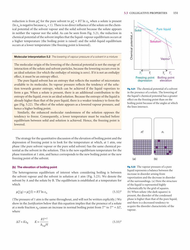
5.5 COLLIGATIVE PROPERTIES 151
Che
mic
al p
oten
tial,
T f Tf Tb Tb
Freezing pointdepression
Boiling pointelevation
Solid Pure liquid
Vapour
Solution
m
´ ´
Fig. 5.21 The chemical potential of a solventin the presence of a solute. The lowering ofthe liquid’s chemical potential has a greatereffect on the freezing point than on theboiling point because of the angles at whichthe lines intersect.
pA* pA
(b)(a)
Fig. 5.22 The vapour pressure of a pureliquid represents a balance between theincrease in disorder arising fromvaporization and the decrease in disorderof the surroundings. (a) Here the structureof the liquid is represented highlyschematically by the grid of squares. (b) When solute (the dark squares) ispresent, the disorder of the condensedphase is higher than that of the pure liquid,and there is a decreased tendency toacquire the disorder characteristic of thevapour.
reduction is from µA* for the pure solvent to µA* + RT ln xA when a solute is present (ln xA is negative because xA < 1). There is no direct influence of the solute on the chem-ical potential of the solvent vapour and the solid solvent because the solute appears in neither the vapour nor the solid. As can be seen from Fig. 5.21, the reduction inchemical potential of the solvent implies that the liquid–vapour equilibrium occurs ata higher temperature (the boiling point is raised) and the solid–liquid equilibrium occurs at a lower temperature (the freezing point is lowered).
Molecular interpretation 5.2 The lowering of vapour pressure of a solvent in a mixture
The molecular origin of the lowering of the chemical potential is not the energy ofinteraction of the solute and solvent particles, because the lowering occurs even inan ideal solution (for which the enthalpy of mixing is zero). If it is not an enthalpyeffect, it must be an entropy effect.
The pure liquid solvent has an entropy that reflects the number of microstatesavailable to its molecules. Its vapour pressure reflects the tendency of the solu-tion towards greater entropy, which can be achieved if the liquid vaporizes to form a gas. When a solute is present, there is an additional contribution to the entropy of the liquid, even in an ideal solution. Because the entropy of the liquid is already higher than that of the pure liquid, there is a weaker tendency to form thegas (Fig. 5.22). The effect of the solute appears as a lowered vapour pressure, andhence a higher boiling point.
Similarly, the enhanced molecular randomness of the solution opposes the tendency to freeze. Consequently, a lower temperature must be reached beforeequilibrium between solid and solution is achieved. Hence, the freezing point islowered.
The strategy for the quantitative discussion of the elevation of boiling point and thedepression of freezing point is to look for the temperature at which, at 1 atm, onephase (the pure solvent vapour or the pure solid solvent) has the same chemical po-tential as the solvent in the solution. This is the new equilibrium temperature for thephase transition at 1 atm, and hence corresponds to the new boiling point or the newfreezing point of the solvent.
(b) The elevation of boiling point
The heterogeneous equilibrium of interest when considering boiling is between the solvent vapour and the solvent in solution at 1 atm (Fig. 5.23). We denote the solvent by A and the solute by B. The equilibrium is established at a temperature forwhich
µA*(g) = µA*(l) + RT ln xA (5.32)°
(The pressure of 1 atm is the same throughout, and will not be written explicitly.) Weshow in the Justification below that this equation implies that the presence of a soluteat a mole fraction xB causes an increase in normal boiling point from T* to T* + ∆T,where
∆T = KxB K = (5.33)°RT*2
∆vapH
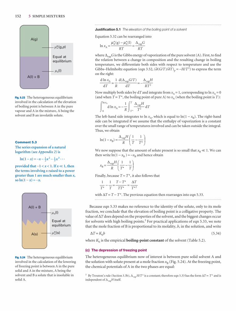
152 5 SIMPLE MIXTURES
Justification 5.1 The elevation of the boiling point of a solvent
Equation 5.32 can be rearranged into
ln xA = =
where ∆vapG is the Gibbs energy of vaporization of the pure solvent (A). First, to findthe relation between a change in composition and the resulting change in boilingtemperature, we differentiate both sides with respect to temperature and use theGibbs–Helmholtz equation (eqn 3.52, (∂(G/T)/∂T)p = −H/T 2) to express the termon the right:
= = −
Now multiply both sides by dT and integrate from xA = 1, corresponding to ln xA = 0(and when T = T*, the boiling point of pure A) to xA (when the boiling point is T):
�0
ln xA
d ln xA = − �T
T *
dT
The left-hand side integrates to ln xA, which is equal to ln(1 − xB). The right-handside can be integrated if we assume that the enthalpy of vaporization is a constantover the small range of temperatures involved and can be taken outside the integral.Thus, we obtain
ln(1 − xB) = −
We now suppose that the amount of solute present is so small that xB << 1. We canthen write ln(1 − xB ) ≈ −xB and hence obtain
xB = −
Finally, because T ≈ T*, it also follows that
− = ≈
with ∆T = T − T*. The previous equation then rearranges into eqn 5.33.
Because eqn 5.33 makes no reference to the identity of the solute, only to its molefraction, we conclude that the elevation of boiling point is a colligative property. Thevalue of ∆T does depend on the properties of the solvent, and the biggest changes occurfor solvents with high boiling points.3 For practical applications of eqn 5.33, we notethat the mole fraction of B is proportional to its molality, b, in the solution, and write
∆T = Kbb (5.34)
where Kb is the empirical boiling-point constant of the solvent (Table 5.2).
(c) The depression of freezing point
The heterogeneous equilibrium now of interest is between pure solid solvent A andthe solution with solute present at a mole fraction xB (Fig. 5.24). At the freezing point,the chemical potentials of A in the two phases are equal:
∆T
T*2
T − T*
TT*
1
T
1
T*
DEF1
T
1
T*
ABC∆ vapH
R
DEF1
T*
1
T
ABC∆ vapH
R
∆ vapH
T 2
1
R
∆ vapH
RT 2
d(∆ vapG/T)
dT
1
R
d ln xA
dT
∆ vapG
RT
µA*(g) − µA*(l)
RT
A(g)
A*(g, )p
A(l)
A(l) + B
Equal atequilibrium
m
m
Fig. 5.23 The heterogeneous equilibriuminvolved in the calculation of the elevationof boiling point is between A in the purevapour and A in the mixture, A being thesolvent and B an involatile solute.
Comment 5.3
The series expansion of a naturallogarithm (see Appendix 2) is
ln(1 − x) = −x − 1–2 x 2 − 1–3 x 3 · · ·
provided that −1 < x < 1. If x << 1, thenthe terms involving x raised to a powergreater than 1 are much smaller than x,so ln(1 − x) ≈ −x.
3 By Trouton’s rule (Section 3.3b), ∆ vap H/T* is a constant; therefore eqn 5.33 has the form ∆T ∝ T* and isindependent of ∆ vapH itself.
A(s) A*(s)
A(l)A(l) + B
Equal atequilibrium
m
m
Fig. 5.24 The heterogeneous equilibriuminvolved in the calculation of the loweringof freezing point is between A in the puresolid and A in the mixture, A being thesolvent and B a solute that is insoluble insolid A.
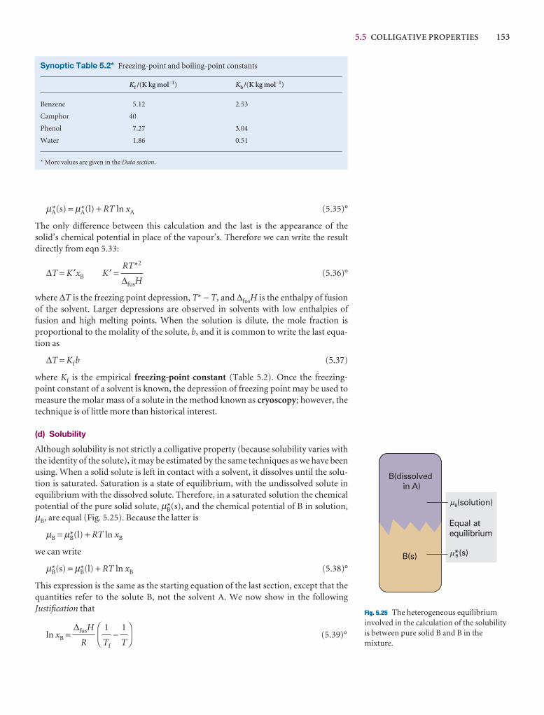
5.5 COLLIGATIVE PROPERTIES 153
µA*(s) = µA*(l) + RT ln xA (5.35)°
The only difference between this calculation and the last is the appearance of thesolid’s chemical potential in place of the vapour’s. Therefore we can write the resultdirectly from eqn 5.33:
∆T = K ′xB K ′ = (5.36)°
where ∆T is the freezing point depression, T* − T, and ∆fusH is the enthalpy of fusionof the solvent. Larger depressions are observed in solvents with low enthalpies of fusion and high melting points. When the solution is dilute, the mole fraction is proportional to the molality of the solute, b, and it is common to write the last equa-tion as
∆T = Kf b (5.37)
where Kf is the empirical freezing-point constant (Table 5.2). Once the freezing-point constant of a solvent is known, the depression of freezing point may be used tomeasure the molar mass of a solute in the method known as cryoscopy; however, thetechnique is of little more than historical interest.
(d) Solubility
Although solubility is not strictly a colligative property (because solubility varies withthe identity of the solute), it may be estimated by the same techniques as we have beenusing. When a solid solute is left in contact with a solvent, it dissolves until the solu-tion is saturated. Saturation is a state of equilibrium, with the undissolved solute inequilibrium with the dissolved solute. Therefore, in a saturated solution the chemicalpotential of the pure solid solute, µB*(s), and the chemical potential of B in solution,µB, are equal (Fig. 5.25). Because the latter is
µB = µB*(l) + RT ln xB
we can write
µB*(s) = µB*(l) + RT ln xB (5.38)°
This expression is the same as the starting equation of the last section, except that thequantities refer to the solute B, not the solvent A. We now show in the followingJustification that
ln xB = − (5.39)°DF
1
T
1
Tf
AC
∆fusH
R
RT*2
∆fusH
Synoptic Table 5.2* Freezing-point and boiling-point constants
Kf /(K kg mol−1) Kb /(K kg mol−1)
Benzene 5.12 2.53
Camphor 40
Phenol 7.27 3.04
Water 1.86 0.51
* More values are given in the Data section.
B(s) B*(s)
B(solution)
Equal atequilibrium
B(dissolvedin A)
Fig. 5.25 The heterogeneous equilibriuminvolved in the calculation of the solubilityis between pure solid B and B in themixture.
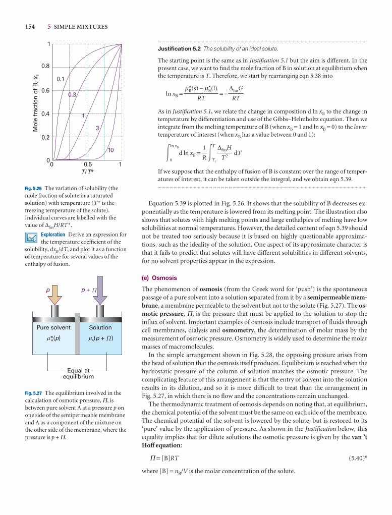
154 5 SIMPLE MIXTURES
Justification 5.2 The solubility of an ideal solute.
The starting point is the same as in Justification 5.1 but the aim is different. In thepresent case, we want to find the mole fraction of B in solution at equilibrium whenthe temperature is T. Therefore, we start by rearranging eqn 5.38 into
ln xB = = −
As in Justification 5.1, we relate the change in composition d ln xB to the change intemperature by differentiation and use of the Gibbs–Helmholtz equation. Then weintegrate from the melting temperature of B (when xB = 1 and ln xB = 0) to the lowertemperature of interest (when xB has a value between 0 and 1):
�0
ln xB
d ln xB = �T
Tf
dT
If we suppose that the enthalpy of fusion of B is constant over the range of temper-atures of interest, it can be taken outside the integral, and we obtain eqn 5.39.
Equation 5.39 is plotted in Fig. 5.26. It shows that the solubility of B decreases ex-ponentially as the temperature is lowered from its melting point. The illustration alsoshows that solutes with high melting points and large enthalpies of melting have lowsolubilities at normal temperatures. However, the detailed content of eqn 5.39 shouldnot be treated too seriously because it is based on highly questionable approxima-tions, such as the ideality of the solution. One aspect of its approximate character isthat it fails to predict that solutes will have different solubilities in different solvents,for no solvent properties appear in the expression.
(e) Osmosis
The phenomenon of osmosis (from the Greek word for ‘push’) is the spontaneouspassage of a pure solvent into a solution separated from it by a semipermeable mem-brane, a membrane permeable to the solvent but not to the solute (Fig. 5.27). The os-motic pressure, Π, is the pressure that must be applied to the solution to stop theinflux of solvent. Important examples of osmosis include transport of fluids throughcell membranes, dialysis and osmometry, the determination of molar mass by themeasurement of osmotic pressure. Osmometry is widely used to determine the molarmasses of macromolecules.
In the simple arrangement shown in Fig. 5.28, the opposing pressure arises fromthe head of solution that the osmosis itself produces. Equilibrium is reached when thehydrostatic pressure of the column of solution matches the osmotic pressure. Thecomplicating feature of this arrangement is that the entry of solvent into the solutionresults in its dilution, and so it is more difficult to treat than the arrangement inFig. 5.27, in which there is no flow and the concentrations remain unchanged.
The thermodynamic treatment of osmosis depends on noting that, at equilibrium,the chemical potential of the solvent must be the same on each side of the membrane.The chemical potential of the solvent is lowered by the solute, but is restored to its‘pure’ value by the application of pressure. As shown in the Justification below, thisequality implies that for dilute solutions the osmotic pressure is given by the van ’tHoff equation:
Π = [B]RT (5.40)°
where [B] = nB/V is the molar concentration of the solute.
∆fusH
T 2
1
R
∆fusG
RT
µB*(s) − µB*(l)
RT
10
3
1
0.3
0.1
0 0.5 1T T/ *
0
0.2
0.4
0.6
0.8
1
Mol
e fr
actio
n o
f B
, xB
Fig. 5.26 The variation of solubility (themole fraction of solute in a saturatedsolution) with temperature (T* is thefreezing temperature of the solute).Individual curves are labelled with thevalue of ∆fusH/RT*.
Exploration Derive an expression forthe temperature coefficient of the
solubility, dxB/dT, and plot it as a functionof temperature for several values of theenthalpy of fusion.
p p +
A*( )p A( + )p
Equal atequilibrium
Pure solvent Solution
Fig. 5.27 The equilibrium involved in thecalculation of osmotic pressure, Π, isbetween pure solvent A at a pressure p onone side of the semipermeable membraneand A as a component of the mixture onthe other side of the membrane, where thepressure is p + Π.
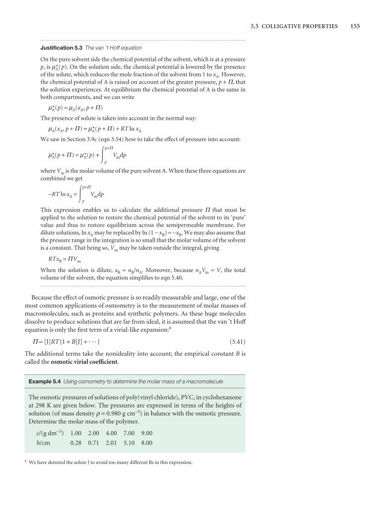
5.5 COLLIGATIVE PROPERTIES 155
4 We have denoted the solute J to avoid too many different Bs in this expression.
Justification 5.3 The van ’t Hoff equation
On the pure solvent side the chemical potential of the solvent, which is at a pressurep, is µA*(p). On the solution side, the chemical potential is lowered by the presenceof the solute, which reduces the mole fraction of the solvent from 1 to xA. However,the chemical potential of A is raised on account of the greater pressure, p + Π, thatthe solution experiences. At equilibrium the chemical potential of A is the same inboth compartments, and we can write
µA*(p) = µA(xA, p + Π)
The presence of solute is taken into account in the normal way:
µA(xA, p + Π) = µA*(p + Π) + RT ln xA
We saw in Section 3.9c (eqn 3.54) how to take the effect of pressure into account:
µA*(p + Π) = µA*(p) + �p
p+Π
Vmdp
where Vm is the molar volume of the pure solvent A. When these three equations arecombined we get
−RT ln xA = �p
p+Π
Vmdp
This expression enables us to calculate the additional pressure Π that must be applied to the solution to restore the chemical potential of the solvent to its ‘pure’value and thus to restore equilibrium across the semipermeable membrane. For dilute solutions, ln xA may be replaced by ln (1 − xB) ≈ −xB. We may also assume thatthe pressure range in the integration is so small that the molar volume of the solventis a constant. That being so, Vm may be taken outside the integral, giving
RTxB = ΠVm
When the solution is dilute, xB ≈ nB/nA. Moreover, because nAVm = V, the total volume of the solvent, the equation simplifies to eqn 5.40.
Because the effect of osmotic pressure is so readily measurable and large, one of themost common applications of osmometry is to the measurement of molar masses ofmacromolecules, such as proteins and synthetic polymers. As these huge moleculesdissolve to produce solutions that are far from ideal, it is assumed that the van ’t Hoff
equation is only the first term of a virial-like expansion:4
Π = [J]RT{1 + B[J] + · · · } (5.41)
The additional terms take the nonideality into account; the empirical constant B iscalled the osmotic virial coefficient.
Example 5.4 Using osmometry to determine the molar mass of a macromolecule
The osmotic pressures of solutions of poly(vinyl chloride), PVC, in cyclohexanoneat 298 K are given below. The pressures are expressed in terms of the heights of solution (of mass density ρ = 0.980 g cm−3) in balance with the osmotic pressure.Determine the molar mass of the polymer.
c/(g dm−3) 1.00 2.00 4.00 7.00 9.00
h/cm 0.28 0.71 2.01 5.10 8.00
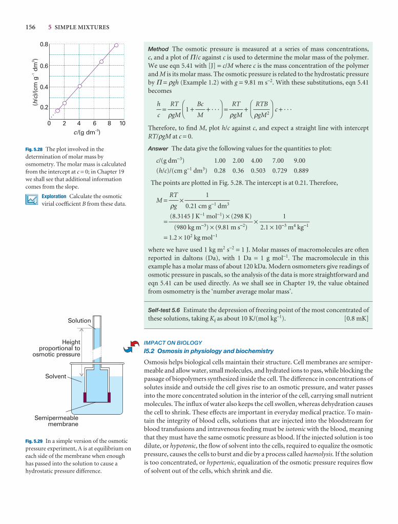
156 5 SIMPLE MIXTURES
Method The osmotic pressure is measured at a series of mass concentrations, c, and a plot of Π /c against c is used to determine the molar mass of the polymer.We use eqn 5.41 with [J] = c/M where c is the mass concentration of the polymerand M is its molar mass. The osmotic pressure is related to the hydrostatic pressureby Π = ρgh (Example 1.2) with g = 9.81 m s−2. With these substitutions, eqn 5.41becomes
= 1 + + · · · = + c + · · ·
Therefore, to find M, plot h/c against c, and expect a straight line with interceptRT/ρgM at c = 0.
Answer The data give the following values for the quantities to plot:
c/(g dm−3) 1.00 2.00 4.00 7.00 9.00
(h/c)/(cm g−1 dm3) 0.28 0.36 0.503 0.729 0.889
The points are plotted in Fig. 5.28. The intercept is at 0.21. Therefore,
M = ×
= ×
= 1.2 × 10² kg mol−1
where we have used 1 kg m2 s−2 = 1 J. Molar masses of macromolecules are often reported in daltons (Da), with 1 Da = 1 g mol−1. The macromolecule in this example has a molar mass of about 120 kDa. Modern osmometers give readings ofosmotic pressure in pascals, so the analysis of the data is more straightforward andeqn 5.41 can be used directly. As we shall see in Chapter 19, the value obtainedfrom osmometry is the ‘number average molar mass’.
Self-test 5.6 Estimate the depression of freezing point of the most concentrated ofthese solutions, taking Kf as about 10 K/(mol kg−1). [0.8 mK]
IMPACT ON BIOLOGY
I5.2 Osmosis in physiology and biochemistry
Osmosis helps biological cells maintain their structure. Cell membranes are semiper-meable and allow water, small molecules, and hydrated ions to pass, while blocking thepassage of biopolymers synthesized inside the cell. The difference in concentrations ofsolutes inside and outside the cell gives rise to an osmotic pressure, and water passesinto the more concentrated solution in the interior of the cell, carrying small nutrientmolecules. The influx of water also keeps the cell swollen, whereas dehydration causesthe cell to shrink. These effects are important in everyday medical practice. To main-tain the integrity of blood cells, solutions that are injected into the bloodstream forblood transfusions and intravenous feeding must be isotonic with the blood, meaningthat they must have the same osmotic pressure as blood. If the injected solution is toodilute, or hypotonic, the flow of solvent into the cells, required to equalize the osmoticpressure, causes the cells to burst and die by a process called haemolysis. If the solutionis too concentrated, or hypertonic, equalization of the osmotic pressure requires flowof solvent out of the cells, which shrink and die.
1
2.1 × 10⁻³ m4 kg−1
(8.3145 J K−1 mol−1) × (298 K)
(980 kg m−3) × (9.81 m s−2)
1
0.21 cm g−1 dm3
RT
ρg
DF
RTB
ρgM2
AC
RT
ρgM
DF
Bc
M
AC
RT
ρgM
h
c0.2
0.4
0.6
0.8
0 2 4 6 8 10
(/
)/(cm
g
dm)
hc
13
c /(g dm )�3
�
Fig. 5.28 The plot involved in thedetermination of molar mass byosmometry. The molar mass is calculatedfrom the intercept at c = 0; in Chapter 19we shall see that additional informationcomes from the slope.
Exploration Calculate the osmoticvirial coefficient B from these data.
Solution
Solvent
Semipermeablemembrane
Heightproportional to
osmotic pressure
Fig. 5.29 In a simple version of the osmoticpressure experiment, A is at equilibrium oneach side of the membrane when enoughhas passed into the solution to cause ahydrostatic pressure difference.
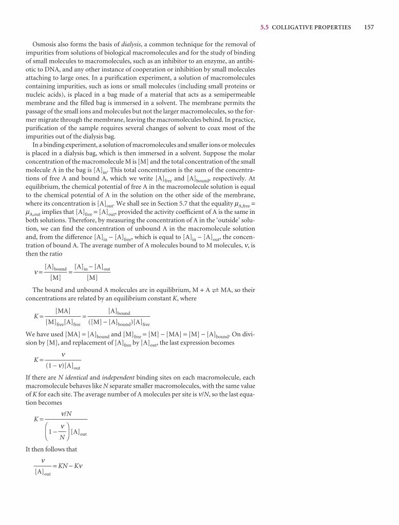
5.5 COLLIGATIVE PROPERTIES 157
Osmosis also forms the basis of dialysis, a common technique for the removal ofimpurities from solutions of biological macromolecules and for the study of bindingof small molecules to macromolecules, such as an inhibitor to an enzyme, an antibi-otic to DNA, and any other instance of cooperation or inhibition by small molecules attaching to large ones. In a purification experiment, a solution of macromoleculescontaining impurities, such as ions or small molecules (including small proteins ornucleic acids), is placed in a bag made of a material that acts as a semipermeablemembrane and the filled bag is immersed in a solvent. The membrane permits thepassage of the small ions and molecules but not the larger macromolecules, so the for-mer migrate through the membrane, leaving the macromolecules behind. In practice,purification of the sample requires several changes of solvent to coax most of theimpurities out of the dialysis bag.
In a binding experiment, a solution of macromolecules and smaller ions or moleculesis placed in a dialysis bag, which is then immersed in a solvent. Suppose the molarconcentration of the macromolecule M is [M] and the total concentration of the smallmolecule A in the bag is [A]in. This total concentration is the sum of the concentra-tions of free A and bound A, which we write [A]free and [A]bound, respectively. At equilibrium, the chemical potential of free A in the macromolecule solution is equalto the chemical potential of A in the solution on the other side of the membrane,where its concentration is [A]out. We shall see in Section 5.7 that the equality µA,free =µA,out implies that [A]free = [A]out, provided the activity coefficient of A is the same inboth solutions. Therefore, by measuring the concentration of A in the ‘outside’ solu-tion, we can find the concentration of unbound A in the macromolecule solution and, from the difference [A]in − [A]free, which is equal to [A]in − [A]out, the concen-tration of bound A. The average number of A molecules bound to M molecules, ν, isthen the ratio
ν = =
The bound and unbound A molecules are in equilibrium, M + A 5 MA, so theirconcentrations are related by an equilibrium constant K, where
K = =
We have used [MA] = [A]bound and [M]free = [M] − [MA] = [M] − [A]bound. On divi-sion by [M], and replacement of [A]free by [A]out, the last expression becomes
K =
If there are N identical and independent binding sites on each macromolecule, eachmacromolecule behaves like N separate smaller macromolecules, with the same valueof K for each site. The average number of A molecules per site is ν/N, so the last equa-tion becomes
K =
1 − [A]out
It then follows that
= KN − Kνν
[A]out
DF
νN
AC
ν/N
ν(1 − ν)[A]out
[A]bound
([M] − [A]bound)[A]free
[MA]
[M]free[A]free
[A]in − [A]out
[M]
[A]bound
[M]
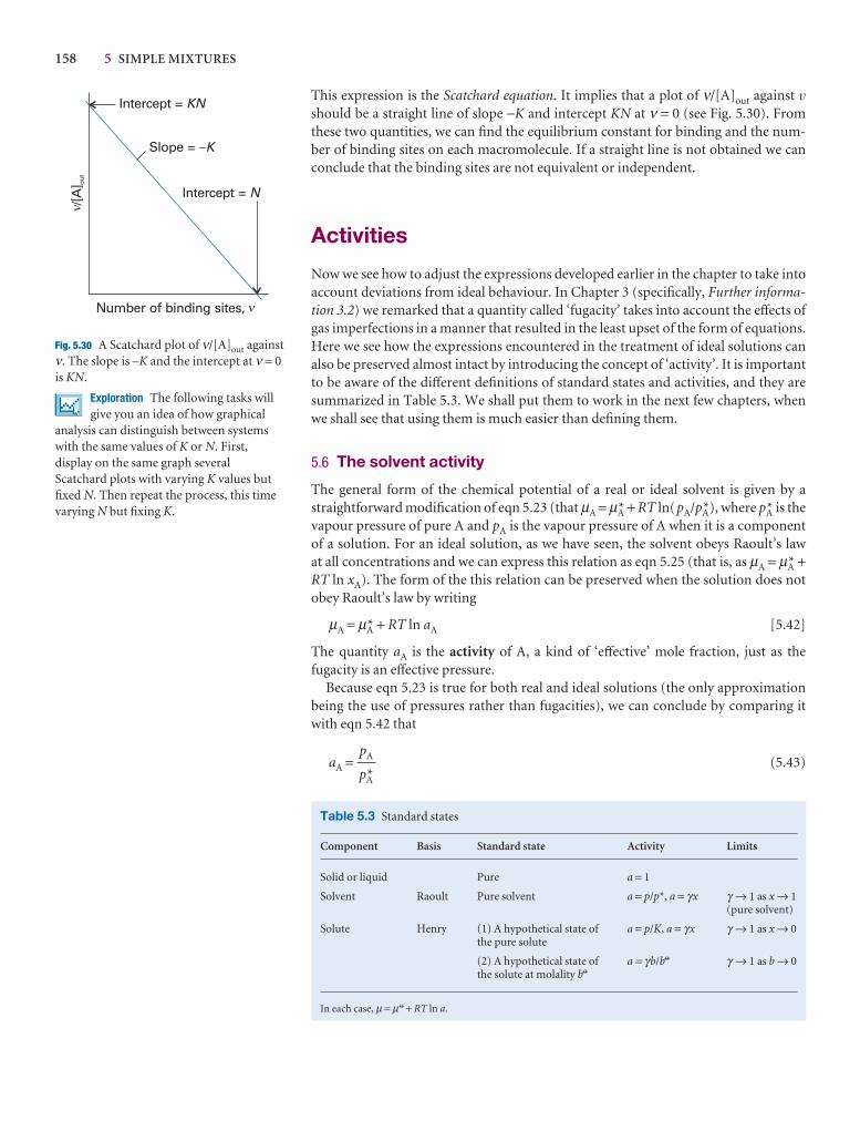
158 5 SIMPLE MIXTURES
Table 5.3 Standard states
Component Basis Standard state Activity Limits
Solid or liquid Pure a = 1
Solvent Raoult Pure solvent a = p/p*, a = γx γ → 1 as x → 1(pure solvent)
Solute Henry (1) A hypothetical state of a = p/K, a = γx γ → 1 as x → 0the pure solute
(2) A hypothetical state of a = γb/b7 γ → 1 as b → 0the solute at molality b7
In each case, µ = µ7 + RT ln a.
This expression is the Scatchard equation. It implies that a plot of ν/[A]out against vshould be a straight line of slope −K and intercept KN at ν = 0 (see Fig. 5.30). Fromthese two quantities, we can find the equilibrium constant for binding and the num-ber of binding sites on each macromolecule. If a straight line is not obtained we canconclude that the binding sites are not equivalent or independent.
Activities
Now we see how to adjust the expressions developed earlier in the chapter to take intoaccount deviations from ideal behaviour. In Chapter 3 (specifically, Further informa-tion 3.2) we remarked that a quantity called ‘fugacity’ takes into account the effects ofgas imperfections in a manner that resulted in the least upset of the form of equations.Here we see how the expressions encountered in the treatment of ideal solutions canalso be preserved almost intact by introducing the concept of ‘activity’. It is importantto be aware of the different definitions of standard states and activities, and they aresummarized in Table 5.3. We shall put them to work in the next few chapters, whenwe shall see that using them is much easier than defining them.
5.6 The solvent activity
The general form of the chemical potential of a real or ideal solvent is given by astraightforward modification of eqn 5.23 (that µA = µA* + RT ln(pA/pA*), where pA* is thevapour pressure of pure A and pA is the vapour pressure of A when it is a componentof a solution. For an ideal solution, as we have seen, the solvent obeys Raoult’s law at all concentrations and we can express this relation as eqn 5.25 (that is, as µA = µA* +RT ln xA). The form of the this relation can be preserved when the solution does notobey Raoult’s law by writing
µA = µA* + RT ln aA [5.42]
The quantity aA is the activity of A, a kind of ‘effective’ mole fraction, just as the fugacity is an effective pressure.
Because eqn 5.23 is true for both real and ideal solutions (the only approximationbeing the use of pressures rather than fugacities), we can conclude by comparing itwith eqn 5.42 that
aA = (5.43)pA
pA*
Number of binding sites,
/[A] ou
t
Intercept = KN
Intercept = N
Slope = �K
�
�
Fig. 5.30 A Scatchard plot of ν/[A]out againstν. The slope is –K and the intercept at ν = 0is KN.
Exploration The following tasks willgive you an idea of how graphical
analysis can distinguish between systemswith the same values of K or N. First,display on the same graph severalScatchard plots with varying K values butfixed N. Then repeat the process, this timevarying N but fixing K.
5.7 THE SOLUTE ACTIVITY 159
We see that there is nothing mysterious about the activity of a solvent: it can be determined experimentally simply by measuring the vapour pressure and then usingeqn 5.43.
Illustration 5.3 Calculating the solvent activity
The vapour pressure of 0.500 M KNO3(aq) at 100°C is 99.95 kPa, so the activity ofwater in the solution at this temperature is
aA = = 0.9864
Because all solvents obey Raoult’s law (that pA/pA* = xA) increasingly closely as theconcentration of solute approaches zero, the activity of the solvent approaches themole fraction as xA → 1:
aA → xA as xA → 1 (5.44)
A convenient way of expressing this convergence is to introduce the activitycoefficient, γ , by the definition
aA = γAxA γA → 1 as xA → 1 [5.45]
at all temperatures and pressures. The chemical potential of the solvent is then
µA = µA* + RT ln xA + RT ln γA (5.46)
The standard state of the solvent, the pure liquid solvent at 1 bar, is established whenxA = 1.
5.7 The solute activity
The problem with defining activity coefficients and standard states for solutes is thatthey approach ideal-dilute (Henry’s law) behaviour as xB → 0, not as xB → 1 (corres-ponding to pure solute). We shall show how to set up the definitions for a solute thatobeys Henry’s law exactly, and then show how to allow for deviations.
(a) Ideal-dilute solutions
A solute B that satisfies Henry’s law has a vapour pressure given by pB = KBxB, whereKB is an empirical constant. In this case, the chemical potential of B is
µB = µB* + RT ln = µB* + RT ln + RT ln xB
Both KB and pB* are characteristics of the solute, so the second term may be combinedwith the first to give a new standard chemical potential:
µB7 = µB* + RT ln [5.47]
It then follows that the chemical potential of a solute in an ideal-dilute solution is related to its mole fraction by
µB = µB7 + RT ln xB (5.48)°
If the solution is ideal, KB = pB* and eqn 5.47 reduces to µB7 = µB*, as we should expect.
KB
pB*
KB
pB*
pB
pB*
99.95 kPa
101.325 kPa
160 5 SIMPLE MIXTURES
(b) Real solutes
We now permit deviations from ideal-dilute, Henry’s law behaviour. For the solute,we introduce aB in place of xB in eqn 5.48, and obtain
µB = µB7 + RT ln aB [5.49]
The standard state remains unchanged in this last stage, and all the deviations fromideality are captured in the activity aB. The value of the activity at any concentrationcan be obtained in the same way as for the solvent, but in place of eqn 5.43 we use
aB = (5.50)
As for the solvent, it is sensible to introduce an activity coefficient through
aB = γBxB [5.51]
Now all the deviations from ideality are captured in the activity coefficient γB. Becausethe solute obeys Henry’s law as its concentration goes to zero, it follows that
aB → xB and γB → 1 as xB → 0 (5.52)
at all temperatures and pressures. Deviations of the solute from ideality disappear aszero concentration is approached.
Example 5.5 Measuring activity
Use the information in Example 5.3 to calculate the activity and activity coefficientof chloroform in acetone at 25°C, treating it first as a solvent and then as a solute.For convenience, the data are repeated here:
xC 0 0.20 0.40 0.60 0.80 1pC/kPa 0 4.7 11 18.9 26.7 36.4pA/kPa 46.3 33.3 23.3 12.3 4.9 0
Method For the activity of chloroform as a solvent (the Raoult’s law activity), formaC = pC /pC* and γC = aC /xC. For its activity as a solute (the Henry’s law activity),form aC = pC /KC and γC = aC /xC.
Answer Because pC* = 36.4 kPa and KC = 22.0 kPa, we can construct the followingtables. For instance, at xC = 0.20, in the Raoult’s law case we find aC = (4.7 kPa)/(36.4 kPa) = 0.13 and γC = 0.13/0.20 = 0.65; likewise, in the Henry’s law case, aC = (4.7 kPa)/(22.0 kPa) = 0.21 and γC = 0.21/0.20 = 1.05.
From Raoult’s law (chloroform regarded as the solvent):
aC 0 0.13 0.30 0.52 0.73 1.00γC 0.65 0.75 0.87 0.91 1.00
From Henry’s law (chloroform regarded as the solute):
aC 0 0.21 0.50 0.86 1.21 1.65γC 1 1.05 1.25 1.43 1.51 1.65
These values are plotted in Fig. 5.31. Notice that γC → 1 as xC → 1 in the Raoult’slaw case, but that γC → 1 as xC → 0 in the Henry’s law case.
Self-test 5.7 Calculate the activities and activity coefficients for acetone accordingto the two conventions.
[At xA = 0.60, for instance aR = 0.50; γR = 0.83; aH = 1.00, γH = 1.67]
pB
KB
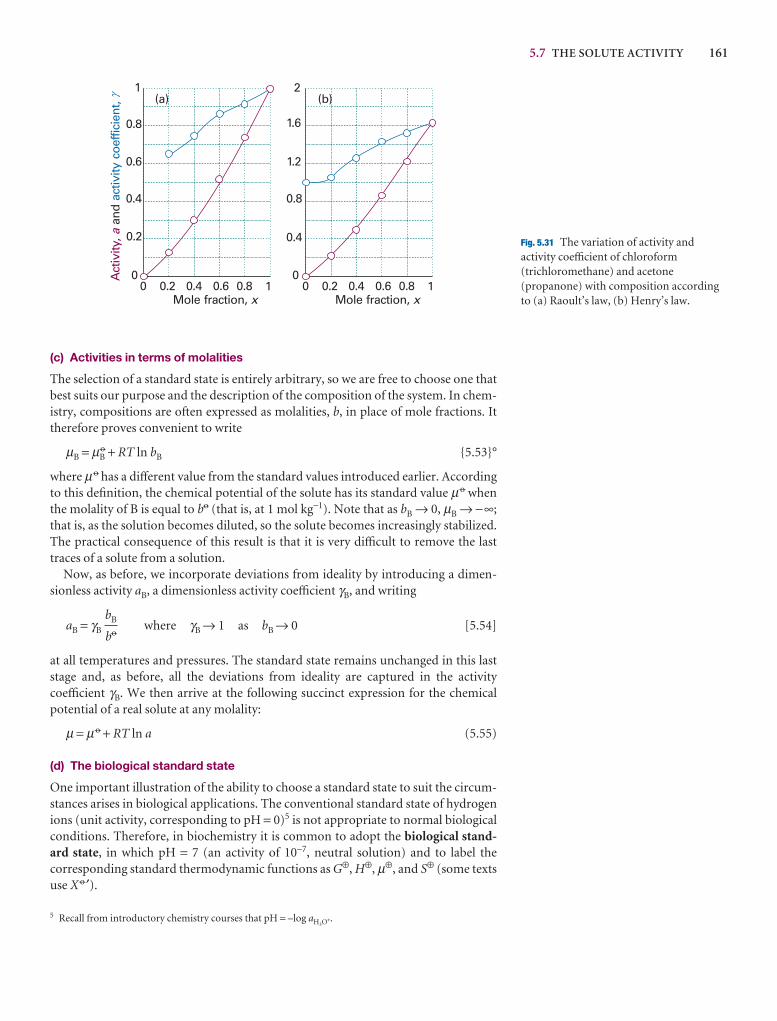
5.7 THE SOLUTE ACTIVITY 161
(c) Activities in terms of molalities
The selection of a standard state is entirely arbitrary, so we are free to choose one thatbest suits our purpose and the description of the composition of the system. In chem-istry, compositions are often expressed as molalities, b, in place of mole fractions. Ittherefore proves convenient to write
µB = µB7 + RT ln bB {5.53}°
where µ7 has a different value from the standard values introduced earlier. Accordingto this definition, the chemical potential of the solute has its standard value µ7 whenthe molality of B is equal to b7 (that is, at 1 mol kg−1). Note that as bB → 0, µB → −∞;that is, as the solution becomes diluted, so the solute becomes increasingly stabilized.The practical consequence of this result is that it is very difficult to remove the lasttraces of a solute from a solution.
Now, as before, we incorporate deviations from ideality by introducing a dimen-sionless activity aB, a dimensionless activity coefficient γB, and writing
aB = γB where γB → 1 as bB → 0 [5.54]
at all temperatures and pressures. The standard state remains unchanged in this laststage and, as before, all the deviations from ideality are captured in the activitycoefficient γB. We then arrive at the following succinct expression for the chemical potential of a real solute at any molality:
µ = µ7 + RT ln a (5.55)
(d) The biological standard state
One important illustration of the ability to choose a standard state to suit the circum-stances arises in biological applications. The conventional standard state of hydrogenions (unit activity, corresponding to pH = 0)5 is not appropriate to normal biologicalconditions. Therefore, in biochemistry it is common to adopt the biological stand-ard state, in which pH = 7 (an activity of 10−7, neutral solution) and to label the corresponding standard thermodynamic functions as G⊕, H⊕, µ⊕, and S⊕ (some textsuse X 7 ′).
bB
b7
0 00 0
0.2
0.2 0.2
0.4
0.4
0.4 0.4
0.6
0.6 0.6
0.8
0.8
0.8 0.8
1
1 1Mole fraction, x Mole fraction, x
Act
ivity
,aan
dac
tivity
coe
ffici
ent,
1.2
1.6
2(a) (b)�
Fig. 5.31 The variation of activity and activity coefficient of chloroform(trichloromethane) and acetone(propanone) with composition accordingto (a) Raoult’s law, (b) Henry’s law.
5 Recall from introductory chemistry courses that pH = –log aH3O+.
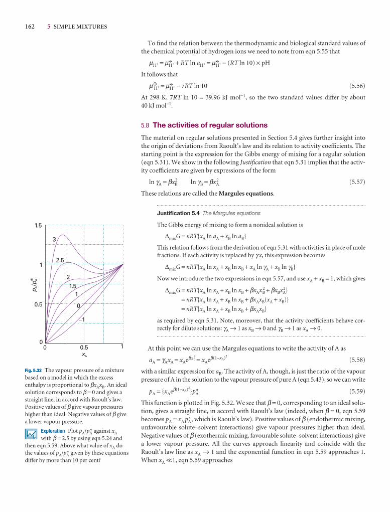
162 5 SIMPLE MIXTURES
To find the relation between the thermodynamic and biological standard values ofthe chemical potential of hydrogen ions we need to note from eqn 5.55 that
µH+ = µ7H+ + RT ln aH+ = µ7
H+ − (RT ln 10) × pH
It follows that
µ⊕H+ = µ7
H+ − 7RT ln 10 (5.56)
At 298 K, 7RT ln 10 = 39.96 kJ mol−1, so the two standard values differ by about 40 kJ mol−1.
5.8 The activities of regular solutions
The material on regular solutions presented in Section 5.4 gives further insight intothe origin of deviations from Raoult’s law and its relation to activity coefficients. Thestarting point is the expression for the Gibbs energy of mixing for a regular solution(eqn 5.31). We show in the following Justification that eqn 5.31 implies that the activ-ity coefficients are given by expressions of the form
ln γA = βxB2 ln γB = βxA
2 (5.57)
These relations are called the Margules equations.
Justification 5.4 The Margules equations
The Gibbs energy of mixing to form a nonideal solution is
∆mixG = nRT{xA ln aA + xB ln aB}
This relation follows from the derivation of eqn 5.31 with activities in place of molefractions. If each activity is replaced by γ x, this expression becomes
∆mixG = nRT{xA ln xA + xB ln xB + xA ln γA + xB ln γB}
Now we introduce the two expressions in eqn 5.57, and use xA + xB = 1, which gives
∆mixG = nRT{xA ln xA + xB ln xB + βxAxB2 + βxBxA
2}
= nRT{xA ln xA + xB ln xB + βxAxB(xA + xB)}
= nRT{xA ln xA + xB ln xB + βxAxB}
as required by eqn 5.31. Note, moreover, that the activity coefficients behave cor-rectly for dilute solutions: γA → 1 as xB → 0 and γB → 1 as xA → 0.
At this point we can use the Margules equations to write the activity of A as
aA = γAxA = xAeβxB2
= xAeβ(1−xA)2
(5.58)
with a similar expression for aB. The activity of A, though, is just the ratio of the vapourpressure of A in the solution to the vapour pressure of pure A (eqn 5.43), so we can write
pA = {xAeβ(1−xA)2
}pA* (5.59)
This function is plotted in Fig. 5.32. We see that β = 0, corresponding to an ideal solu-tion, gives a straight line, in accord with Raoult’s law (indeed, when β = 0, eqn 5.59 becomes pA = xA pA*, which is Raoult’s law). Positive values of β (endothermic mixing,unfavourable solute–solvent interactions) give vapour pressures higher than ideal.Negative values of β (exothermic mixing, favourable solute–solvent interactions) givea lower vapour pressure. All the curves approach linearity and coincide with theRaoult’s law line as xA → 1 and the exponential function in eqn 5.59 approaches 1.When xA <<1, eqn 5.59 approaches
0
0.5
1
1.5
0 0.5 1
0
11.5
2
2.5
3
pp
AA
/
xA
�1
*
Fig. 5.32 The vapour pressure of a mixturebased on a model in which the excessenthalpy is proportional to βxAxB. An idealsolution corresponds to β = 0 and gives astraight line, in accord with Raoult’s law.Positive values of β give vapour pressureshigher than ideal. Negative values of β givea lower vapour pressure.
Exploration Plot pA/pA* against xA
with β = 2.5 by using eqn 5.24 andthen eqn 5.59. Above what value of xA dothe values of pA/pA* given by these equationsdiffer by more than 10 per cent?
5.9 THE ACTIVITIES OF IONS IN SOLUTION 163
pA = xAeβpA* (5.60)
This expression has the form of Henry’s law once we identify K with eβpA*, which isdifferent for each solute–solvent system.
5.9 The activities of ions in solution
Interactions between ions are so strong that the approximation of replacing activitiesby molalities is valid only in very dilute solutions (less than 10−3 mol kg−1 in total ionconcentration) and in precise work activities themselves must be used. We need,therefore, to pay special attention to the activities of ions in solution, especially inpreparation for the discussion of electrochemical phenomena.
(a) Mean activity coefficients
If the chemical potential of a univalent cation M+ is denoted µ+ and that of a univalentanion X− is denoted µ−, the total molar Gibbs energy of the ions in the electrically neu-tral solution is the sum of these partial molar quantities. The molar Gibbs energy of anideal solution is
Gmideal = µ+
ideal + µ−ideal (5.61)°
However, for a real solution of M+ and X− of the same molality,
Gm = µ+ + µ− = µ+ideal + µ−
ideal + RT ln γ+ + RT ln γ− = Gmideal + RT ln γ+γ− (5.62)
All the deviations from ideality are contained in the last term.There is no experimental way of separating the product γ+γ− into contributions
from the cations and the anions. The best we can do experimentally is to assign re-sponsibility for the nonideality equally to both kinds of ion. Therefore, for a 1,1-electrolyte, we introduce the mean activity coefficient as the geometric mean of theindividual coefficients:
γ± = (γ+γ−)1/2 [5.63]
and express the individual chemical potentials of the ions as
µ+ = µ+ideal + RT lnγ± µ− = µ−
ideal + RT ln γ± (5.64)
The sum of these two chemical potentials is the same as before, eqn 5.62, but now thenonideality is shared equally.
We can generalize this approach to the case of a compound Mp Xq that dissolvesto give a solution of p cations and q anions from each formula unit. The molar Gibbsenergy of the ions is the sum of their partial molar Gibbs energies:
Gm = pµ+ + qµ− = Gmideal + pRT lnγ+ + qRT lnγ− (5.65)
If we introduce the mean activity coefficient
γ± = (γ +pγ −
q)1/s s = p + q [5.66]
and write the chemical potential of each ion as
µi = µ iideal + RT lnγ± (5.67)
we get the same expression as in eqn 5.62 for Gm when we write
G = pµ+ + qµ− (5.68)
However, both types of ion now share equal responsibility for the nonideality.
(b) The Debye–Hückel limiting law
The long range and strength of the Coulombic interaction between ions means that itis likely to be primarily responsible for the departures from ideality in ionic solutions
Comment 5.4
The geometric mean of x p and y q is(xpy q)1/(p+q). For example, the geometricmean of x 2 and y−3 is (x 2y−3)−1.
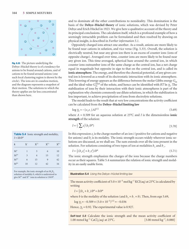
164 5 SIMPLE MIXTURES
Fig. 5.33 The picture underlying theDebye–Hückel theory is of a tendency foranions to be found around cations, and ofcations to be found around anions (onesuch local clustering region is shown by thecircle). The ions are in ceaseless motion,and the diagram represents a snapshot oftheir motion. The solutions to which thetheory applies are far less concentratedthan shown here.
Table 5.4 Ionic strength and molality, I = kb/b7
k X− X2 − X3 − X4 −
M+ 1 3 6 10
M2+ 3 4 15 12
M3+ 6 15 9 42
M4+ 10 12 42 16
For example, the ionic strength of an M2X3
solution of molality b, which is understood togive M3+ and X2− ions in solution is 15b/b7.
and to dominate all the other contributions to nonideality. This domination is thebasis of the Debye–Hückel theory of ionic solutions, which was devised by PeterDebye and Erich Hückel in 1923. We give here a qualitative account of the theory andits principal conclusions. The calculation itself, which is a profound example of how aseemingly intractable problem can be formulated and then resolved by drawing onphysical insight, is described in Further information 5.1.
Oppositely charged ions attract one another. As a result, anions are more likely tobe found near cations in solution, and vice versa (Fig. 5.33). Overall, the solution iselectrically neutral, but near any given ion there is an excess of counter ions (ions ofopposite charge). Averaged over time, counter ions are more likely to be found nearany given ion. This time-averaged, spherical haze around the central ion, in whichcounter ions outnumber ions of the same charge as the central ion, has a net chargeequal in magnitude but opposite in sign to that on the central ion, and is called itsionic atmosphere. The energy, and therefore the chemical potential, of any given cen-tral ion is lowered as a result of its electrostatic interaction with its ionic atmosphere.This lowering of energy appears as the difference between the molar Gibbs energy Gm
and the ideal value Gmideal of the solute, and hence can be identified with RT ln γ±. The
stabilization of ions by their interaction with their ionic atmospheres is part of the explanation why chemists commonly use dilute solutions, in which the stabilization isless important, to achieve precipitation of ions from electrolyte solutions.
The model leads to the result that at very low concentrations the activity coefficientcan be calculated from the Debye–Hückel limiting law
log γ± = − | z+z− | AI1/2 (5.69)
where A = 0.509 for an aqueous solution at 25°C and I is the dimensionless ionicstrength of the solution:
I = 1–2 ∑i
zi2(bi /b
7) [5.70]
In this expression zi is the charge number of an ion i (positive for cations and negativefor anions) and bi is its molality. The ionic strength occurs widely wherever ionic so-lutions are discussed, as we shall see. The sum extends over all the ions present in thesolution. For solutions consisting of two types of ion at molalities b+ and b−,
I = 1–2 (b+z+2 + b−z−
2)/b7 (5.71)
The ionic strength emphasizes the charges of the ions because the charge numbersoccur as their squares. Table 5.4 summarizes the relation of ionic strength and molal-ity in an easily usable form.
Illustration 5.4 Using the Debye–Hückel limiting law
The mean activity coefficient of 5.0 × 10⁻³ mol kg−1 KCl(aq) at 25°C is calculated bywriting
I = 1–2(b+ + b−)/b7 = b/b7
where b is the molality of the solution (and b+ = b− = b). Then, from eqn 5.69,
log γ± = −0.509 × (5.0 × 10−3)1/2 = −0.036
Hence, γ± = 0.92. The experimental value is 0.927.
Self-test 5.8 Calculate the ionic strength and the mean activity coefficient of 1.00 mmol kg−1 CaCl2(aq) at 25°C. [3.00 mmol kg−1, 0.880]
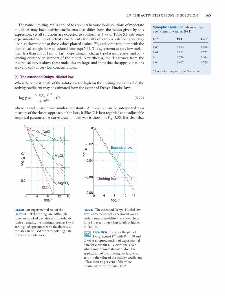
5.9 THE ACTIVITIES OF IONS IN SOLUTION 165
The name ‘limiting law’ is applied to eqn 5.69 because ionic solutions of moderatemolalities may have activity coefficients that differ from the values given by this expression, yet all solutions are expected to conform as b → 0. Table 5.5 lists some experimental values of activity coefficients for salts of various valence types. Fig-ure 5.34 shows some of these values plotted against I1/2, and compares them with thetheoretical straight lines calculated from eqn 5.69. The agreement at very low molal-ities (less than about 1 mmol kg−1, depending on charge type) is impressive, and con-vincing evidence in support of the model. Nevertheless, the departures from the theoretical curves above these molalities are large, and show that the approximationsare valid only at very low concentrations.
(c) The extended Debye–Hückel law
When the ionic strength of the solution is too high for the limiting law to be valid, theactivity coefficient may be estimated from the extended Debye–Hückel law:
log γ± = − + CI (5.72)
where B and C are dimensionless constants. Although B can be interpreted as a measure of the closest approach of the ions, it (like C) is best regarded as an adjustableempirical parameter. A curve drawn in this way is shown in Fig. 5.35. It is clear that
A | z+z− | I1/2
1 + BI1/2
Synoptic Table 5.5* Mean activitycoefficients in water at 298 K
b/b 7 KCl CaCl2
0.001 0.966 0.888
0.01 0.902 0.732
0.1 0.770 0.524
1.0 0.607 0.725
* More values are given in the Data section.
4 8 12
0
�0.1
�0.2
log
±
NaCl
(1,1)
MgCl2
(1,2)
MgSO4
(2,2)
100I1/20 16
�
Fig. 5.34 An experimental test of theDebye–Hückel limiting law. Althoughthere are marked deviations for moderateionic strengths, the limiting slopes as I → 0are in good agreement with the theory, sothe law can be used for extrapolating datato very low molalities.
0
-0.02
-0.04
-0.06
-0.080 4 8 12 16
Extended law
Limiting law
log
±
100I1/2
g
Fig. 5.35 The extended Debye–Hückel lawgives agreement with experiment over awider range of molalities (as shown herefor a 1,1-electrolyte), but it fails at highermolalities.
Exploration Consider the plot of log γ± against I1/2 with B = 1.50 and
C = 0 as a representation of experimentaldata for a certain 1,1-electrolyte. Over what range of ionic strengths does theapplication of the limiting law lead to anerror in the value of the activity coefficientof less than 10 per cent of the valuepredicted by the extended law?

166 5 SIMPLE MIXTURES
Checklist of key ideas
1. The partial molar volume is the change in volume per mole ofA added to a large volume of the mixture: VJ = (∂V/∂n J)p,T,n′.The total volume of a mixture is V = nAVA + nBVB.
2. The chemical potential can be defined in terms of the partialmolar Gibbs energy, µ J = (∂G/∂nJ)p,T,n′. The total Gibbs energyof a mixture is G = nAµA + nBµB.
3. The fundamental equation of chemical thermodynamicsrelates the change in Gibbs energy to changes in pressure,temperature, and composition: dG = Vdp − SdT + µAdnA
+ µBdnB + · · ·.
4. The Gibbs–Duhem equation is ∑J nJdµ J = 0.
5. The chemical potential of a perfect gas is µ = µ7 + RT ln(p/p7),where µ7 is the standard chemical potential, the chemicalpotential of the pure gas at 1 bar.
6. The Gibbs energy of mixing of two perfect gases is given by∆mixG = nRT(xA ln xA + xB ln xB).
7. The entropy of mixing of two perfect gases is given by ∆mix S = –nR(xA ln xA + xB ln xB).
8. The enthalpy of mixing is ∆mix H = 0 for perfect gases.
9. An ideal solution is a solution in which all components obeysRaoult’s law (pA = xA pA*) throughout the composition range.
10. The chemical potential of a component of an ideal solution isgiven by µA = µA* + RT ln xA.
11. An ideal-dilute solution is a solution for which the soluteobeys Henry’s law (pB = xBK B*) and the solvent obeys Raoult’slaw.
12. The Gibbs energy of mixing of two liquids that form an idealsolution is given by ∆mixG = nRT(xA ln xA + xB ln xB).
13. The entropy of mixing of two liquids that form an idealsolution is given by ∆mixS = –nR(xA ln xA + xB ln xB).
14. An excess function (X E) is the difference between the observedthermodynamic function of mixing and the function for anideal solution.
15. A regular solution is a solution for which H E ≠ 0 but SE = 0.
16. A colligative property is a property that depends only on thenumber of solute particles present, not their identity.
17. The elevation of boiling point is given by ∆T = Kbb, where Kb
is the ebullioscopic constant. The depression of freezing pointis given by ∆T = Kf b, where Kf is the cryoscopic constant.
18. Osmosis is the spontaneous passage of a pure solvent into asolution separated from it by a semipermeable membrane, amembrane permeable to the solvent but not to the solute.
19. The osmotic pressure is the pressure that must be applied tothe solution to stop the influx of solvent.
20. The van ’t Hoff equation for the osmotic pressure is Π = [B]RT.
21. The activity is defined as aA = pA/pA*.
22. The solvent activity is related to its chemical potential by µA = µA* + RT ln aA. The activity may be written in terms of theactivity coefficient γA = aA/xA.
23. The chemical potential of a solute in an ideal-dilute solution isgiven by µB = µB
7 + RT ln a B. The activity may be written interms of the activity coefficient γB = aB/xB.
24. The biological standard state (pH = 7) is related to thethermodynamic standard state by µ⊕
H+ = µ7H+ – 7RT ln 10.
25. The mean activity coefficient is the geometric mean of theindividual coefficients: γ± = (γ +
pγ −q)1/(p + q).
26. The Debye–Hückel theory of activity coefficients of electrolytesolutions is based on the assumption that Coulombicinteractions between ions are dominant; a key idea of thetheory is that of an ionic atmosphere.
27. The Debye–Hückel limiting law is log γ± = −| z+z− | AI 1/2 whereI is the ionic strength, I = 1–2 ∑i z
2i (bi /b
7).
28. The extended Debye–Hückel law is ln γ± =−| z+z− | AI 1/2/(1 + BI1/2) + CI.
eqn 5.72 accounts for some activity coefficients over a moderate range of dilute solu-tions (up to about 0.1 mol kg−1); nevertheless it remains very poor near 1 mol kg−1.
Current theories of activity coefficients for ionic solutes take an indirect route.They set up a theory for the dependence of the activity coefficient of the solvent on theconcentration of the solute, and then use the Gibbs–Duhem equation (eqn 5.12) toestimate the activity coefficient of the solute. The results are reasonably reliable for solutions with molalities greater than about 0.1 mol kg−1 and are valuable for the dis-cussion of mixed salt solutions, such as sea water.
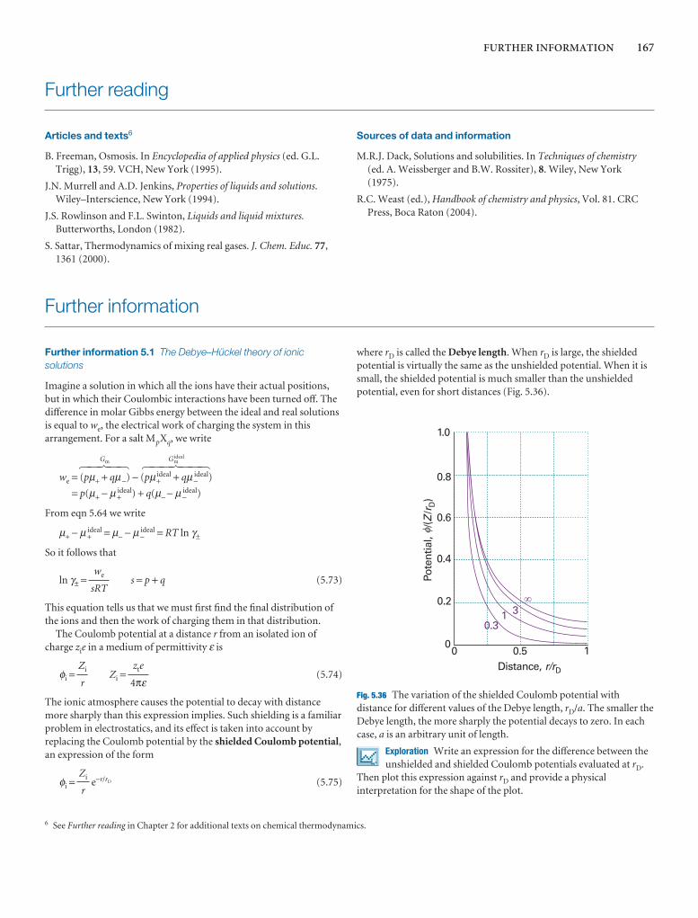
FURTHER INFORMATION 167
Further reading
Articles and texts6
B. Freeman, Osmosis. In Encyclopedia of applied physics (ed. G.L.Trigg), 13, 59. VCH, New York (1995).
J.N. Murrell and A.D. Jenkins, Properties of liquids and solutions.Wiley–Interscience, New York (1994).
J.S. Rowlinson and F.L. Swinton, Liquids and liquid mixtures.Butterworths, London (1982).
S. Sattar, Thermodynamics of mixing real gases. J. Chem. Educ. 77,1361 (2000).
Sources of data and information
M.R.J. Dack, Solutions and solubilities. In Techniques of chemistry(ed. A. Weissberger and B.W. Rossiter), 8. Wiley, New York(1975).
R.C. Weast (ed.), Handbook of chemistry and physics, Vol. 81. CRCPress, Boca Raton (2004).
6 See Further reading in Chapter 2 for additional texts on chemical thermodynamics.
0.2
0.4
0.6
0.8
1.0
0
Pote
ntia
l, /
(/
)Z
r D
0 0.5 1Distance, r/rD
0.31 3
�
�
Fig. 5.36 The variation of the shielded Coulomb potential withdistance for different values of the Debye length, rD/a. The smaller theDebye length, the more sharply the potential decays to zero. In eachcase, a is an arbitrary unit of length.
Exploration Write an expression for the difference between theunshielded and shielded Coulomb potentials evaluated at rD.
Then plot this expression against rD and provide a physicalinterpretation for the shape of the plot.
Further information
Further information 5.1 The Debye–Hückel theory of ionicsolutions
Imagine a solution in which all the ions have their actual positions,but in which their Coulombic interactions have been turned off. Thedifference in molar Gibbs energy between the ideal and real solutionsis equal to we, the electrical work of charging the system in thisarrangement. For a salt MpXq, we write
Gm Gmideal
we = (pµ+ + qµ−) − (pµ+ideal + qµ−
ideal)
= p(µ+ − µ+ideal) + q(µ− − µ−
ideal)
From eqn 5.64 we write
µ+ − µ+ideal = µ− − µ−
ideal = RT ln γ±
So it follows that
ln γ± = s = p + q (5.73)
This equation tells us that we must first find the final distribution ofthe ions and then the work of charging them in that distribution.
The Coulomb potential at a distance r from an isolated ion ofcharge zie in a medium of permittivity ε is
φi = Zi = (5.74)
The ionic atmosphere causes the potential to decay with distancemore sharply than this expression implies. Such shielding is a familiarproblem in electrostatics, and its effect is taken into account byreplacing the Coulomb potential by the shielded Coulomb potential,an expression of the form
φi = e−r/rD (5.75)Zi
r
zte
4πεZi
r
we
sRT
5 4 4 6 4 4 75 4 6 4 7
where rD is called the Debye length. When rD is large, the shieldedpotential is virtually the same as the unshielded potential. When it issmall, the shielded potential is much smaller than the unshieldedpotential, even for short distances (Fig. 5.36).
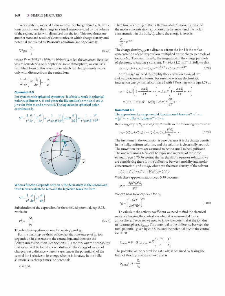
168 5 SIMPLE MIXTURES
To calculate rD, we need to know how the charge density, ρi, of theionic atmosphere, the charge in a small region divided by the volumeof the region, varies with distance from the ion. This step draws onanother standard result of electrostatics, in which charge density andpotential are related by Poisson’s equation (see Appendix 3):
∇2φ = − (5.76)
where ∇2 = (∂2/∂x 2 + ∂2/∂y 2 + ∂2/∂z 2) is called the laplacian. Becausewe are considering only a spherical ionic atmosphere, we can use asimplified form of this equation in which the charge density variesonly with distance from the central ion:
r 2 = −
Comment 5.5
For systems with spherical symmetry, it is best to work in sphericalpolar coordinates r, θ, and φ (see the illustration): x = r sin θ cos φ,y = r sin θ sin φ, and z = r cos θ. The laplacian in spherical polarcoordinates is
∇2 = r 2 + sinθ +
When a function depends only on r, the derivatives in the second andthird terms evaluate to zero and the laplacian takes the form
∇2 = r 2
Substitution of the expression for the shielded potential, eqn 5.75,results in
r 2D = − (5.77)
To solve this equation we need to relate ρi and φi.For the next step we draw on the fact that the energy of an ion
depends on its closeness to the central ion, and then use theBoltzmann distribution (see Section 16.1) to work out the probabilitythat an ion will be found at each distance. The energy of an ion ofcharge zj e at a distance where it experiences the potential φi of thecentral ion i relative to its energy when it is far away in the bulksolution is its charge times the potential:
E = zj eφi
εφi
ρi
DEFd
dr
ABCd
dr
1
r 2
z
x y
r
q
f
∂2
∂θ2
1
r 2 sin2θ
DEF∂
∂θ
ABC∂
∂θ1
r 2 sinθ
DEF∂∂r
ABC∂∂r
1
r 2
ρi
εDEF
dφi
dr
ABCd
dr
1
r 2
ρε
Therefore, according to the Boltzmann distribution, the ratio of the molar concentration, cj , of ions at a distance r and the molarconcentration in the bulk, c j°, where the energy is zero, is:
= e−E/kT
The charge density, ρi, at a distance r from the ion i is the molarconcentration of each type of ion multiplied by the charge per mole ofions, zieNA. The quantity eNA, the magnitude of the charge per moleof electrons, is Faraday’s constant, F = 96.48 kC mol−1. It follows that
ρi = c+z+F + c−z−F = c+°z+Fe−z+eφi/kT + c−° z−Fe−z−eφi/kT (5.78)
At this stage we need to simplify the expression to avoid theawkward exponential terms. Because the average electrostaticinteraction energy is small compared with kT we may write eqn 5.78 as
ρi = c+°z+F 1 − + · · · + c−° z−F 1 − + · · ·
= (c+°z+ + c−° z−)F − (c+°z+2 + c−° z−
2)F + · · ·
Comment 5.6
The expansion of an exponential function used here is e−x = 1 − x+ 1–2x2 − · · · . If x << 1, then e−x ≈ 1 − x.
Replacing e by F/NA and NAk by R results in the following expression:
ρ i = (c+°z+ + c−° z−)F − (c+°z+2 + c−° z−
2) + · · · (5.79)
The first term in the expansion is zero because it is the charge densityin the bulk, uniform solution, and the solution is electrically neutral.The unwritten terms are assumed to be too small to be significant.The one remaining term can be expressed in terms of the ionicstrength, eqn 5.70, by noting that in the dilute aqueous solutions weare considering there is little difference between molality and molarconcentration, and c ≈ bρ, where ρ is the mass density of the solvent
c+°z+2 + c−° z−
2 ≈ (b+°z+2 + b−° z−
2)ρ = 2Ib7ρ
With these approximations, eqn 5.78 becomes
ρi = −
We can now solve eqn 5.77 for rD:
rD =1/2
(5.80)
To calculate the activity coefficient we need to find the electricalwork of charging the central ion when it is surrounded by itsatmosphere. To do so, we need to know the potential at the ion dueto its atmosphere, φatmos. This potential is the difference between thetotal potential, given by eqn 5.75, and the potential due to the centralion itself:
φatmos = φ − φcentral ion = Zi −
The potential at the central ion (at r = 0) is obtained by taking thelimit of this expression as r → 0 and is
φatmos(0) =Zi
rD
DEF1
r
e−r/rD
r
ABC
DEFεRT
2ρF 2Ib7
ABC
2ρF2Ib7φi
RT
F2φi
RT
eφi
kT
DEFz−eφi
kT
ABCDEF
z+eφi
kT
ABC
cj
c j°
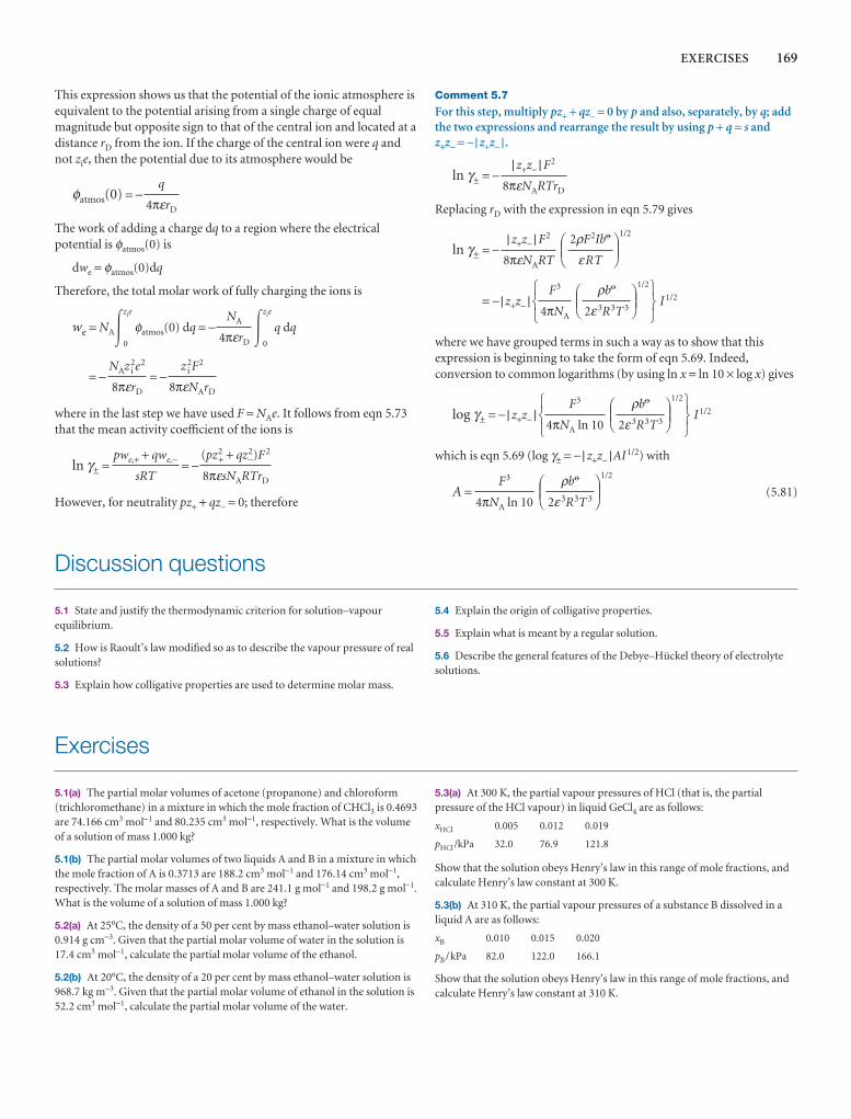
EXERCISES 169
This expression shows us that the potential of the ionic atmosphere isequivalent to the potential arising from a single charge of equalmagnitude but opposite sign to that of the central ion and located at adistance rD from the ion. If the charge of the central ion were q andnot zie, then the potential due to its atmosphere would be
φatmos(0) = −
The work of adding a charge dq to a region where the electricalpotential is φatmos(0) is
dwe = φatmos(0)dq
Therefore, the total molar work of fully charging the ions is
we = NA�0
zie
φatmos(0) dq = − �0
zie
q dq
= − = −
where in the last step we have used F = NAe. It follows from eqn 5.73that the mean activity coefficient of the ions is
ln γ± = = −
However, for neutrality pz+ + qz− = 0; therefore
(pz2+ + qz2
−)F 2
8πεsNARTrD
pwe,+ + qwe,−
sRT
z i2F2
8πεNArD
NAz i2e2
8πεrD
NA
4πεrD
q
4πεrD
Comment 5.7
For this step, multiply pz+ + qz− = 0 by p and also, separately, by q; addthe two expressions and rearrange the result by using p + q = s andz+z− = −| z+z− | .
ln γ± = −
Replacing rD with the expression in eqn 5.79 gives
ln γ± = −1/2
= −| z+z− |1/2
I 1/2
where we have grouped terms in such a way as to show that thisexpression is beginning to take the form of eqn 5.69. Indeed,conversion to common logarithms (by using ln x = ln 10 × log x) gives
log γ± = −| z+z− |1/2
I 1/2
which is eqn 5.69 (log γ± = −| z+z− |AI 1/2) with
A =1/2
(5.81)DEF
ρb7
2ε3R3T 3
ABCF3
4πNA ln 10
567
DEFρb7
2ε3R3T 3
ABCF3
4πNA ln 10
123
567
DEFρb7
2ε3R3T 3
ABCF3
4πNA
123
DEF2ρF2Ib7
εRT
ABC| z+z− | F2
8πεNART
| z+z− | F2
8πεNARTrD
Discussion questions
5.1 State and justify the thermodynamic criterion for solution–vapourequilibrium.
5.2 How is Raoult’s law modified so as to describe the vapour pressure of realsolutions?
5.3 Explain how colligative properties are used to determine molar mass.
5.4 Explain the origin of colligative properties.
5.5 Explain what is meant by a regular solution.
5.6 Describe the general features of the Debye–Hückel theory of electrolytesolutions.
Exercises
5.1(a) The partial molar volumes of acetone (propanone) and chloroform(trichloromethane) in a mixture in which the mole fraction of CHCl3 is 0.4693are 74.166 cm3 mol−1 and 80.235 cm3 mol−1, respectively. What is the volumeof a solution of mass 1.000 kg?
5.1(b) The partial molar volumes of two liquids A and B in a mixture in whichthe mole fraction of A is 0.3713 are 188.2 cm3 mol−1 and 176.14 cm3 mol−1,respectively. The molar masses of A and B are 241.1 g mol−1 and 198.2 g mol−1.What is the volume of a solution of mass 1.000 kg?
5.2(a) At 25°C, the density of a 50 per cent by mass ethanol–water solution is0.914 g cm−3. Given that the partial molar volume of water in the solution is17.4 cm3 mol−1, calculate the partial molar volume of the ethanol.
5.2(b) At 20°C, the density of a 20 per cent by mass ethanol–water solution is968.7 kg m−3. Given that the partial molar volume of ethanol in the solution is52.2 cm3 mol−1, calculate the partial molar volume of the water.
5.3(a) At 300 K, the partial vapour pressures of HCl (that is, the partialpressure of the HCl vapour) in liquid GeCl4 are as follows:
xHCl 0.005 0.012 0.019
pHCl /kPa 32.0 76.9 121.8
Show that the solution obeys Henry’s law in this range of mole fractions, andcalculate Henry’s law constant at 300 K.
5.3(b) At 310 K, the partial vapour pressures of a substance B dissolved in aliquid A are as follows:
xB 0.010 0.015 0.020
pB /kPa 82.0 122.0 166.1
Show that the solution obeys Henry’s law in this range of mole fractions, andcalculate Henry’s law constant at 310 K.

170 5 SIMPLE MIXTURES
5.4(a) Predict the partial vapour pressure of HCl above its solution in liquidgermanium tetrachloride of molality 0.10 mol kg−1. For data, see Exercise 5.3a.
5.4(b) Predict the partial vapour pressure of the component B above itssolution in A in Exercise 5.3b when the molality of B is 0.25 mol kg−1. Themolar mass of A is 74.1 g mol−1.
5.5(a) The vapour pressure of benzene is 53.3 kPa at 60.6°C, but it fell to 51.5 kPa when 19.0 g of an involatile organic compound was dissolved in 500 g of benzene. Calculate the molar mass of the compound.
5.5(b) The vapour pressure of 2-propanol is 50.00 kPa at 338.8°C, but it fell to 49.62 kPa when 8.69 g of an involatile organic compound was dissolved in250 g of 2-propanol. Calculate the molar mass of the compound.
5.6(a) The addition of 100 g of a compound to 750 g of CCl4 lowered thefreezing point of the solvent by 10.5 K. Calculate the molar mass of thecompound.
5.6(b) The addition of 5.00 g of a compound to 250 g of naphthalene loweredthe freezing point of the solvent by 0.780 K. Calculate the molar mass of thecompound.
5.7(a) The osmotic pressure of an aqueous solution at 300 K is 120 kPa.Calculate the freezing point of the solution.
5.7(b) The osmotic pressure of an aqueous solution at 288 K is 99.0 kPa.Calculate the freezing point of the solution.
5.8(a) Consider a container of volume 5.0 dm3 that is divided into twocompartments of equal size. In the left compartment there is nitrogen at 1.0 atm and 25°C; in the right compartment there is hydrogen at the sametemperature and pressure. Calculate the entropy and Gibbs energy of mixingwhen the partition is removed. Assume that the gases are perfect.
5.8(b) Consider a container of volume 250 cm3 that is divided into twocompartments of equal size. In the left compartment there is argon at 100 kPaand 0°C; in the right compartment there is neon at the same temperature andpressure. Calculate the entropy and Gibbs energy of mixing when the partitionis removed. Assume that the gases are perfect.
5.9(a) Air is a mixture with a composition given in Self-test 1.4. Calculate theentropy of mixing when it is prepared from the pure (and perfect) gases.
5.9(b) Calculate the Gibbs energy, entropy, and enthalpy of mixing when1.00 mol C6H14 (hexane) is mixed with 1.00 mol C7H16 (heptane) at 298 K;treat the solution as ideal.
5.10(a) What proportions of hexane and heptane should be mixed (a) by mole fraction, (b) by mass in order to achieve the greatest entropy ofmixing?
5.10(b) What proportions of benzene and ethylbenzene should be mixed (a) by mole fraction, (b) by mass in order to achieve the greatest entropy ofmixing?
5.11(a) Use Henry’s law and the data in Table 5.1 to calculate the solubility (asa molality) of CO2 in water at 25°C when its partial pressure is (a) 0.10 atm,(b) 1.00 atm.
5.11(b) The mole fractions of N2 and O2 in air at sea level are approximately0.78 and 0.21. Calculate the molalities of the solution formed in an open flaskof water at 25°C.
5.12(a) A water carbonating plant is available for use in the home andoperates by providing carbon dioxide at 5.0 atm. Estimate the molarconcentration of the soda water it produces.
5.12(b) After some weeks of use, the pressure in the water carbonating plantmentioned in the previous exercise has fallen to 2.0 atm. Estimate the molarconcentration of the soda water it produces at this stage.
5.13(a) The enthalpy of fusion of anthracene is 28.8 kJ mol−1 and its meltingpoint is 217°C. Calculate its ideal solubility in benzene at 25°C.
5.13(b) Predict the ideal solubility of lead in bismuth at 280°C given that itsmelting point is 327°C and its enthalpy of fusion is 5.2 kJ mol−1.
5.14(a) The osmotic pressure of solutions of polystyrene in toluene weremeasured at 25°C and the pressure was expressed in terms of the height of thesolvent of density 1.004 g cm−3:
c /(g dm−3) 2.042 6.613 9.521 12.602
h/cm 0.592 1.910 2.750 3.600
Calculate the molar mass of the polymer.
5.14(b) The molar mass of an enzyme was determined by dissolving it inwater, measuring the osmotic pressure at 20°C, and extrapolating the data tozero concentration. The following data were obtained:
c /(mg cm−3) 3.221 4.618 5.112 6.722
h/cm 5.746 8.238 9.119 11.990
Calculate the molar mass of the enzyme.
5.15(a) Substances A and B are both volatile liquids with pA* = 300 Torr, pB* = 250 Torr, and KB = 200 Torr (concentration expressed in mole fraction).When xA = 0.9, bB = 2.22 mol kg−1, pA = 250 Torr, and pB = 25 Torr. Calculatethe activities and activity coefficients of A and B. Use the mole fraction,Raoult’s law basis system for A and the Henry’s law basis system (both molefractions and molalities ) for B.
5.15(b) Given that p*(H2O) = 0.02308 atm and p(H2O) = 0.02239 atm in asolution in which 0.122 kg of a non-volatile solute (M = 241 g mol−1) isdissolved in 0.920 kg water at 293 K, calculate the activity and activitycoefficient of water in the solution.
5.16(a) A dilute solution of bromine in carbon tetrachloride behaves as anideal-dilute solution. The vapour pressure of pure CCl4 is 33.85 Torr at 298 K.The Henry’s law constant when the concentration of Br2 is expressed as a molefraction is 122.36 Torr. Calculate the vapour pressure of each component, the total pressure, and the composition of the vapour phase when the molefraction of Br2 is 0.050, on the assumption that the conditions of the ideal-dilute solution are satisfied at this concentration.
5.16(b) Benzene and toluene form nearly ideal solutions. The boiling point ofpure benzene is 80.1°C. Calculate the chemical potential of benzene relative tothat of pure benzene when xbenzene = 0.30 at its boiling point. If the activitycoefficient of benzene in this solution were actually 0.93 rather than 1.00, what would be its vapour pressure?
5.17(a) By measuring the equilibrium between liquid and vapour phases of anacetone (A)–methanol (M) solution at 57.2°C at 1.00 atm, it was found that xA = 0.400 when yA = 0.516. Calculate the activities and activity coefficientsof both components in this solution on the Raoult’s law basis. The vapourpressures of the pure components at this temperature are: pA* = 105 kPa andp*M = 73.5 kPa. (xA is the mole fraction in the liquid and yA the mole fraction inthe vapour.)
5.17(b) By measuring the equilibrium between liquid and vapour phases of a solution at 30°C at 1.00 atm, it was found that xA = 0.220 when yA = 0.314. Calculate the activities and activity coefficients of bothcomponents in this solution on the Raoult’s law basis. The vapour pressures of the pure components at this temperature are: pA* = 73.0 kPa and pB* = 92.1 kPa. (xA is the mole fraction in the liquid and yA the mole fraction in the vapour.)
5.18(a) Calculate the ionic strength of a solution that is 0.10 mol kg−1 inKCl(aq) and 0.20 mol kg−1 in CuSO4(aq).
5.18(b) Calculate the ionic strength of a solution that is 0.040 mol kg−1 inK3[Fe(CN)6](aq), 0.030 mol kg−1 in KCl(aq), and 0.050 mol kg−1 in NaBr(aq).
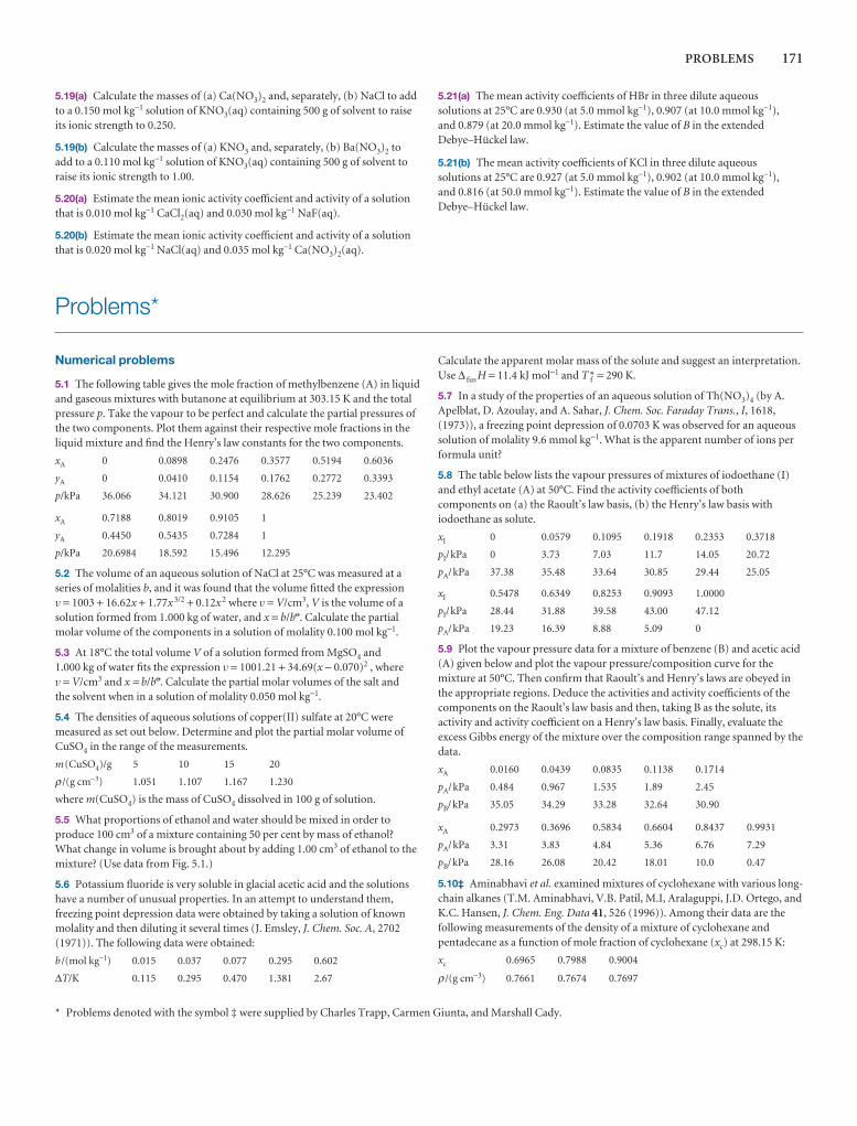
PROBLEMS 171
5.19(a) Calculate the masses of (a) Ca(NO3)2 and, separately, (b) NaCl to addto a 0.150 mol kg−1 solution of KNO3(aq) containing 500 g of solvent to raiseits ionic strength to 0.250.
5.19(b) Calculate the masses of (a) KNO3 and, separately, (b) Ba(NO3)2 toadd to a 0.110 mol kg−1 solution of KNO3(aq) containing 500 g of solvent toraise its ionic strength to 1.00.
5.20(a) Estimate the mean ionic activity coefficient and activity of a solutionthat is 0.010 mol kg−1 CaCl2(aq) and 0.030 mol kg−1 NaF(aq).
5.20(b) Estimate the mean ionic activity coefficient and activity of a solutionthat is 0.020 mol kg−1 NaCl(aq) and 0.035 mol kg−1 Ca(NO3)2(aq).
5.21(a) The mean activity coefficients of HBr in three dilute aqueoussolutions at 25°C are 0.930 (at 5.0 mmol kg−1), 0.907 (at 10.0 mmol kg−1),and 0.879 (at 20.0 mmol kg−1). Estimate the value of B in the extendedDebye–Hückel law.
5.21(b) The mean activity coefficients of KCl in three dilute aqueous solutions at 25°C are 0.927 (at 5.0 mmol kg−1), 0.902 (at 10.0 mmol kg−1),and 0.816 (at 50.0 mmol kg−1). Estimate the value of B in the extendedDebye–Hückel law.
Problems*
Numerical problems
5.1 The following table gives the mole fraction of methylbenzene (A) in liquidand gaseous mixtures with butanone at equilibrium at 303.15 K and the totalpressure p. Take the vapour to be perfect and calculate the partial pressures ofthe two components. Plot them against their respective mole fractions in theliquid mixture and find the Henry’s law constants for the two components.
xA 0 0.0898 0.2476 0.3577 0.5194 0.6036
yA 0 0.0410 0.1154 0.1762 0.2772 0.3393
p/kPa 36.066 34.121 30.900 28.626 25.239 23.402
xA 0.7188 0.8019 0.9105 1
yA 0.4450 0.5435 0.7284 1
p/kPa 20.6984 18.592 15.496 12.295
5.2 The volume of an aqueous solution of NaCl at 25°C was measured at aseries of molalities b, and it was found that the volume fitted the expressionv = 1003 + 16.62x + 1.77x 3/2 + 0.12x 2 where v = V/cm3, V is the volume of asolution formed from 1.000 kg of water, and x = b/b7. Calculate the partialmolar volume of the components in a solution of molality 0.100 mol kg−1.
5.3 At 18°C the total volume V of a solution formed from MgSO4 and1.000 kg of water fits the expression v = 1001.21 + 34.69(x − 0.070)2 , where v = V/cm3 and x = b/b7. Calculate the partial molar volumes of the salt and the solvent when in a solution of molality 0.050 mol kg−1.
5.4 The densities of aqueous solutions of copper(II) sulfate at 20°C weremeasured as set out below. Determine and plot the partial molar volume ofCuSO4 in the range of the measurements.
m(CuSO4)/g 5 10 15 20
ρ /(g cm−3) 1.051 1.107 1.167 1.230
where m(CuSO4) is the mass of CuSO4 dissolved in 100 g of solution.
5.5 What proportions of ethanol and water should be mixed in order toproduce 100 cm3 of a mixture containing 50 per cent by mass of ethanol?What change in volume is brought about by adding 1.00 cm3 of ethanol to themixture? (Use data from Fig. 5.1.)
5.6 Potassium fluoride is very soluble in glacial acetic acid and the solutionshave a number of unusual properties. In an attempt to understand them,freezing point depression data were obtained by taking a solution of knownmolality and then diluting it several times (J. Emsley, J. Chem. Soc. A, 2702(1971)). The following data were obtained:
b /(mol kg−1) 0.015 0.037 0.077 0.295 0.602
∆T/K 0.115 0.295 0.470 1.381 2.67
Calculate the apparent molar mass of the solute and suggest an interpretation.Use ∆ fus H = 11.4 kJ mol−1 and T f* = 290 K.
5.7 In a study of the properties of an aqueous solution of Th(NO3)4 (by A.Apelblat, D. Azoulay, and A. Sahar, J. Chem. Soc. Faraday Trans., I, 1618,(1973)), a freezing point depression of 0.0703 K was observed for an aqueoussolution of molality 9.6 mmol kg−1. What is the apparent number of ions performula unit?
5.8 The table below lists the vapour pressures of mixtures of iodoethane (I)and ethyl acetate (A) at 50°C. Find the activity coefficients of bothcomponents on (a) the Raoult’s law basis, (b) the Henry’s law basis withiodoethane as solute.
xI 0 0.0579 0.1095 0.1918 0.2353 0.3718
pI/kPa 0 3.73 7.03 11.7 14.05 20.72
pA/kPa 37.38 35.48 33.64 30.85 29.44 25.05
xI 0.5478 0.6349 0.8253 0.9093 1.0000
pI/kPa 28.44 31.88 39.58 43.00 47.12
pA/kPa 19.23 16.39 8.88 5.09 0
5.9 Plot the vapour pressure data for a mixture of benzene (B) and acetic acid(A) given below and plot the vapour pressure/composition curve for themixture at 50°C. Then confirm that Raoult’s and Henry’s laws are obeyed inthe appropriate regions. Deduce the activities and activity coefficients of thecomponents on the Raoult’s law basis and then, taking B as the solute, itsactivity and activity coefficient on a Henry’s law basis. Finally, evaluate theexcess Gibbs energy of the mixture over the composition range spanned by thedata.
xA 0.0160 0.0439 0.0835 0.1138 0.1714
pA/kPa 0.484 0.967 1.535 1.89 2.45
pB/kPa 35.05 34.29 33.28 32.64 30.90
xA 0.2973 0.3696 0.5834 0.6604 0.8437 0.9931
pA/kPa 3.31 3.83 4.84 5.36 6.76 7.29
pB/kPa 28.16 26.08 20.42 18.01 10.0 0.47
5.10‡ Aminabhavi et al. examined mixtures of cyclohexane with various long-chain alkanes (T.M. Aminabhavi, V.B. Patil, M.I, Aralaguppi, J.D. Ortego, andK.C. Hansen, J. Chem. Eng. Data 41, 526 (1996)). Among their data are thefollowing measurements of the density of a mixture of cyclohexane andpentadecane as a function of mole fraction of cyclohexane (xc) at 298.15 K:
xc 0.6965 0.7988 0.9004
ρ /(g cm−3) 0.7661 0.7674 0.7697
* Problems denoted with the symbol ‡ were supplied by Charles Trapp, Carmen Giunta, and Marshall Cady.
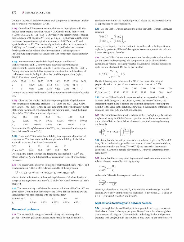
172 5 SIMPLE MIXTURES
Compute the partial molar volume for each component in a mixture that hasa mole fraction cyclohexane of 0.7988.
5.11‡ Comelli and Francesconi examined mixtures of propionic acid withvarious other organic liquids at 313.15 K (F. Comelli and R. Francesconi, J. Chem. Eng. Data 41, 101 (1996)). They report the excess volume of mixingpropionic acid with oxane as V E = x1x2{a0 + a1(x1 − x2)}, where x1 is the molefraction of propionic acid, x2 that of oxane, a0 = −2.4697 cm3 mol−1 anda1 = 0.0608 cm3 mol−1 . The density of propionic acid at this temperature is0.97174 g cm−3; that of oxane is 0.86398 g cm−3. (a) Derive an expression for the partial molar volume of each component at this temperature. (b) Compute the partial molar volume for each component in an equimolarmixture.
5.12‡ Francesconi et al. studied the liquid–vapour equilibria oftrichloromethane and 1,2-epoxybutane at several temperatures (R.Francesconi, B. Lunelli, and F. Comelli, J. Chem. Eng. Data 41, 310 (1996)).Among their data are the following measurements of the mole fractions oftrichloromethane in the liquid phase (x T) and the vapour phase (yT) at 298.15 K as a function of pressure.
p/kPa 23.40 21.75 20.25 18.75 18.15 20.25 22.50 26.30
x 0 0.129 0.228 0.353 0.511 0.700 0.810 1
y 0 0.065 0.145 0.285 0.535 0.805 0.915 1
Compute the activity coefficients of both components on the basis of Raoult’slaw.
5.13‡ Chen and Lee studied the liquid–vapour equilibria of cyclohexanolwith several gases at elevated pressures (J.-T. Chen and M.-J. Lee, J. Chem.Eng. Data 41, 339 (1996)). Among their data are the following measurementsof the mole fractions of cyclohexanol in the vapour phase (y) and the liquidphase (x) at 393.15 K as a function of pressure.
p/bar 10.0 20.0 30.0 40.0 60.0 80.0
ycyc 0.0267 0.0149 0.0112 0.00947 0.00835 0.00921
xcyc 0.9741 0.9464 0.9204 0.892 0.836 0.773
Determine the Henry’s law constant of CO2 in cyclohexanol, and computethe activity coefficient of CO2.
5.14‡ Equation 5.39 indicates that solubility is an exponential function oftemperature. The data in the table below gives the solubility, S, of calciumacetate in water as a function of temperature.
θ /°C 0 20 40 60 80
S/(mol dm−3) 36.4 34.9 33.7 32.7 31.7
Determine the extent to which the data fit the exponential S = S0eτ/T andobtain values for S0 and τ. Express these constants in terms of properties ofthe solute.
5.15 The excess Gibbs energy of solutions of methylcyclohexane (MCH) andtetrahydrofuran (THF) at 303.15 K was found to fit the expression
GE = RTx(1 − x){0.4857 − 0.1077(2x − 1) + 0.0191(2x − 1)2}
where x is the mole fraction of the methylcyclohexane. Calculate the Gibbsenergy of mixing when a mixture of 1.00 mol of MCH and 3.00 mol of THF isprepared.
5.16 The mean activity coefficients for aqueous solutions of NaCl at 25°C aregiven below. Confirm that they support the Debye–Hückel limiting law andthat an improved fit is obtained with the extended law.
b/(mmol kg−1) 1.0 2.0 5.0 10.0 20.0
γ± 0.9649 0.9519 0.9275 0.9024 0.8712
Theoretical problems
5.17 The excess Gibbs energy of a certain binary mixture is equal togRTx(1 − x) where g is a constant and x is the mole fraction of a solute A.
Find an expression for the chemical potential of A in the mixture and sketchits dependence on the composition.
5.18 Use the Gibbs–Duhem equation to derive the Gibbs–Duhem–Margulesequation
p,T
=p,T
where f is the fugacity. Use the relation to show that, when the fugacities arereplaced by pressures, if Raoult’s law applies to one component in a mixtureit must also apply to the other.
5.19 Use the Gibbs–Duhem equation to show that the partial molar volume(or any partial molar property) of a component B can be obtained if thepartial molar volume (or other property) of A is known for all compositionsup to the one of interest. Do this by proving that
VB = V*B −�VA
VA*
dVA
Use the following data (which are for 298 K) to evaluate the integralgraphically to find the partial molar volume of acetone at x = 0.500.
x(CHCl3) 0 0.194 0.385 0.559 0.788 0.889 1.000
Vm/(cm3 mol−1) 73.99 75.29 76.50 77.55 79.08 79.82 80.67
5.20 Use the Gibbs–Helmholtz equation to find an expression for d ln xA
in terms of dT. Integrate d ln xA from xA = 0 to the value of interest, andintegrate the right–hand side from the transition temperature for the pureliquid A to the value in the solution. Show that, if the enthalpy of transition isconstant, then eqns 5.33 and 5.36 are obtained.
5.21 The ‘osmotic coefficient’, φ, is defined as φ = −(xA/xB) ln aA. By writing r= xB/xA, and using the Gibbs–Duhem equation, show that we can calculatethe activity of B from the activities of A over a composition range by usingthe formula
ln = φ − φ(0) +�r
0
dr
5.22 Show that the osmotic pressure of a real solution is given by ΠV = −RTln aA. Go on to show that, provided the concentration of the solution is low,this expression takes the form ΠV = φRT[B] and hence that the osmoticcoefficient, φ, (which is defined in Problem 5.21) may be determined fromosmometry.
5.23 Show that the freezing-point depression of a real solution in which thesolvent of molar mass M has activity aA obeys
= −
and use the Gibbs–Duhem equation to show that
= −
where aB is the solute activity and bB is its molality. Use the Debye–Hückellimiting law to show that the osmotic coefficient (φ, Problem 5.21) is given byφ = 1 − 1–
3 A′I with A′ = 2.303A and I = b/b7.
Applications: to biology and polymer science
5.24 Haemoglobin, the red blood protein responsible for oxygen transport,binds about 1.34 cm3 of oxygen per gram. Normal blood has a haemoglobinconcentration of 150 g dm−3. Haemoglobin in the lungs is about 97 per centsaturated with oxygen, but in the capillary is only about 75 per cent saturated.
1
bBKf
d ln aB
d(∆T)
M
K f
d ln aA
d(∆T)
DEFφ − 1
r
ABCDEF
aB
r
ABC
xA
1 − xA
DEF∂ ln fB
∂ ln xB
ABCDEF
∂ ln fA
∂ ln xA
ABC
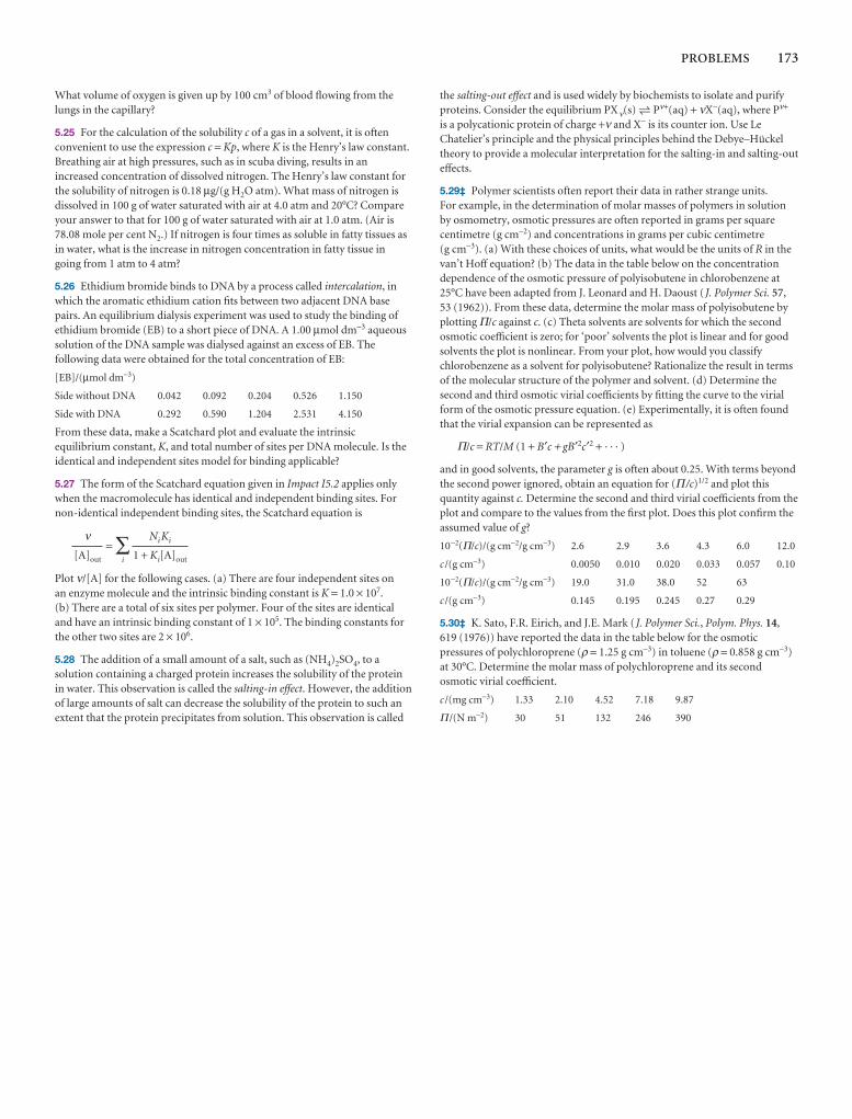
PROBLEMS 173
What volume of oxygen is given up by 100 cm3 of blood flowing from thelungs in the capillary?
5.25 For the calculation of the solubility c of a gas in a solvent, it is oftenconvenient to use the expression c = Kp, where K is the Henry’s law constant.Breathing air at high pressures, such as in scuba diving, results in anincreased concentration of dissolved nitrogen. The Henry’s law constant forthe solubility of nitrogen is 0.18 µg/(g H2O atm). What mass of nitrogen isdissolved in 100 g of water saturated with air at 4.0 atm and 20°C? Compareyour answer to that for 100 g of water saturated with air at 1.0 atm. (Air is78.08 mole per cent N2.) If nitrogen is four times as soluble in fatty tissues asin water, what is the increase in nitrogen concentration in fatty tissue ingoing from 1 atm to 4 atm?
5.26 Ethidium bromide binds to DNA by a process called intercalation, inwhich the aromatic ethidium cation fits between two adjacent DNA basepairs. An equilibrium dialysis experiment was used to study the binding ofethidium bromide (EB) to a short piece of DNA. A 1.00 µmol dm−3 aqueoussolution of the DNA sample was dialysed against an excess of EB. Thefollowing data were obtained for the total concentration of EB:
[EB]/(µmol dm−3)
Side without DNA 0.042 0.092 0.204 0.526 1.150
Side with DNA 0.292 0.590 1.204 2.531 4.150
From these data, make a Scatchard plot and evaluate the intrinsicequilibrium constant, K, and total number of sites per DNA molecule. Is theidentical and independent sites model for binding applicable?
5.27 The form of the Scatchard equation given in Impact I5.2 applies onlywhen the macromolecule has identical and independent binding sites. Fornon-identical independent binding sites, the Scatchard equation is
= ∑i
Plot ν/[A] for the following cases. (a) There are four independent sites on an enzyme molecule and the intrinsic binding constant is K = 1.0 × 10⁷.(b) There are a total of six sites per polymer. Four of the sites are identicaland have an intrinsic binding constant of 1 × 10⁵. The binding constants forthe other two sites are 2 × 10⁶.
5.28 The addition of a small amount of a salt, such as (NH4)2SO4, to asolution containing a charged protein increases the solubility of the proteinin water. This observation is called the salting-in effect. However, the additionof large amounts of salt can decrease the solubility of the protein to such anextent that the protein precipitates from solution. This observation is called
Ni Ki
1 + Ki[A]out
ν[A]out
the salting-out effect and is used widely by biochemists to isolate and purifyproteins. Consider the equilibrium PXν(s) 5 Pν+(aq) + νX−(aq), where Pν+
is a polycationic protein of charge +ν and X− is its counter ion. Use LeChatelier’s principle and the physical principles behind the Debye–Hückeltheory to provide a molecular interpretation for the salting-in and salting-outeffects.
5.29‡ Polymer scientists often report their data in rather strange units. For example, in the determination of molar masses of polymers in solutionby osmometry, osmotic pressures are often reported in grams per squarecentimetre (g cm−2) and concentrations in grams per cubic centimetre(g cm−3). (a) With these choices of units, what would be the units of R in thevan’t Hoff equation? (b) The data in the table below on the concentrationdependence of the osmotic pressure of polyisobutene in chlorobenzene at25°C have been adapted from J. Leonard and H. Daoust (J. Polymer Sci. 57,53 (1962)). From these data, determine the molar mass of polyisobutene byplotting Π/c against c. (c) Theta solvents are solvents for which the secondosmotic coefficient is zero; for ‘poor’ solvents the plot is linear and for goodsolvents the plot is nonlinear. From your plot, how would you classifychlorobenzene as a solvent for polyisobutene? Rationalize the result in termsof the molecular structure of the polymer and solvent. (d) Determine thesecond and third osmotic virial coefficients by fitting the curve to the virialform of the osmotic pressure equation. (e) Experimentally, it is often foundthat the virial expansion can be represented as
Π/c = RT/M (1 + B′c + gB′2c′2 + · · · )
and in good solvents, the parameter g is often about 0.25. With terms beyondthe second power ignored, obtain an equation for (Π /c)1/2 and plot thisquantity against c. Determine the second and third virial coefficients from theplot and compare to the values from the first plot. Does this plot confirm theassumed value of g?
10−2(Π/c)/(g cm−2/g cm−3) 2.6 2.9 3.6 4.3 6.0 12.0
c /(g cm−3) 0.0050 0.010 0.020 0.033 0.057 0.10
10−2(Π/c)/(g cm−2/g cm−3) 19.0 31.0 38.0 52 63
c /(g cm−3) 0.145 0.195 0.245 0.27 0.29
5.30‡ K. Sato, F.R. Eirich, and J.E. Mark (J. Polymer Sci., Polym. Phys. 14,619 (1976)) have reported the data in the table below for the osmoticpressures of polychloroprene (ρ = 1.25 g cm−3) in toluene (ρ = 0.858 g cm−3)at 30°C. Determine the molar mass of polychloroprene and its secondosmotic virial coefficient.
c /(mg cm−3) 1.33 2.10 4.52 7.18 9.87
Π /(N m−2) 30 51 132 246 390
Phase diagrams
Phase diagrams for pure substances were introduced in Chapter 4. Now we develop theiruse systematically and show how they are rich summaries of empirical information about awide range of systems. To set the stage, we introduce the famous phase rule of Gibbs,which shows the extent to which various parameters can be varied yet the equilibrium between phases preserved. With the rule established, we see how it can be used to discussthe phase diagrams that we met in the two preceding chapters. The chapter then intro-duces systems of gradually increasing complexity. In each case we shall see how the phasediagram for the system summarizes empirical observations on the conditions under whichthe various phases of the system are stable.
In this chapter we describe a systematic way of discussing the physical changes mixtures undergo when they are heated or cooled and when their compositions arechanged. In particular, we see how to use phase diagrams to judge whether two sub-stances are mutually miscible, whether an equilibrium can exist over a range of con-ditions, or whether the system must be brought to a definite pressure, temperature,and composition before equilibrium is established. Phase diagrams are of con-siderable commercial and industrial significance, particularly for semiconductors, ceramics, steels, and alloys. They are also the basis of separation procedures in thepetroleum industry and of the formulation of foods and cosmetic preparations.
Phases, components, and degrees of freedom
All phase diagrams can be discussed in terms of a relationship, the phase rule, derivedby J.W. Gibbs. We shall derive this rule first, and then apply it to a wide variety of sys-tems. The phase rule requires a careful use of terms, so we begin by presenting a num-ber of definitions.
6.1 Definitions
The term phase was introduced at the start of Chapter 4, where we saw that it signifiesa state of matter that is uniform throughout, not only in chemical composition butalso in physical state.1 Thus we speak of the solid, liquid, and gas phases of a substance,and of its various solid phases (as for black phosphorus and white phosphorus). Thenumber of phases in a system is denoted P. A gas, or a gaseous mixture, is a singlephase, a crystal is a single phase, and two totally miscible liquids form a single phase.
Phases, components, anddegrees of freedom
6.1 Definitions
6.2 The phase rule
Two-component systems
6.3 Vapour pressure diagrams
6.4 Temperature–compositiondiagrams
6.5 Liquid–liquid phase diagrams
6.6 Liquid–solid phase diagrams
I6.1 Impact on materials science: Liquid crystals
I6.2 Impact on materials science:Ultrapurity and controlledimpurity
Checklist of key ideas
Further reading
Discussion questions
Exercises
Problems
6
1 The words are Gibbs’s.
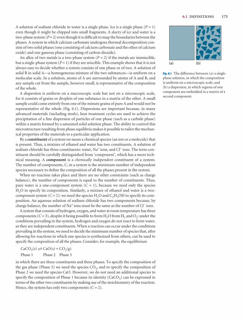
6.1 DEFINITIONS 175
A solution of sodium chloride in water is a single phase. Ice is a single phase (P = 1)even though it might be chipped into small fragments. A slurry of ice and water is atwo-phase system (P = 2) even though it is difficult to map the boundaries between thephases. A system in which calcium carbonate undergoes thermal decomposition con-sists of two solid phases (one consisting of calcium carbonate and the other of calciumoxide) and one gaseous phase (consisting of carbon dioxide).
An alloy of two metals is a two-phase system (P = 2) if the metals are immiscible,but a single-phase system (P = 1) if they are miscible. This example shows that it is notalways easy to decide whether a system consists of one phase or of two. A solution ofsolid B in solid A—a homogeneous mixture of the two substances—is uniform on amolecular scale. In a solution, atoms of A are surrounded by atoms of A and B, andany sample cut from the sample, however small, is representative of the compositionof the whole.
A dispersion is uniform on a macroscopic scale but not on a microscopic scale, for it consists of grains or droplets of one substance in a matrix of the other. A smallsample could come entirely from one of the minute grains of pure A and would not berepresentative of the whole (Fig. 6.1). Dispersions are important because, in many advanced materials (including steels), heat treatment cycles are used to achieve theprecipitation of a fine dispersion of particles of one phase (such as a carbide phase)within a matrix formed by a saturated solid solution phase. The ability to control thismicrostructure resulting from phase equilibria makes it possible to tailor the mechan-ical properties of the materials to a particular application.
By a constituent of a system we mean a chemical species (an ion or a molecule) thatis present. Thus, a mixture of ethanol and water has two constituents. A solution ofsodium chloride has three constituents: water, Na+ ions, and Cl− ions. The term con-stituent should be carefully distinguished from ‘component’, which has a more tech-nical meaning. A component is a chemically independent constituent of a system. The number of components, C, in a system is the minimum number of independentspecies necessary to define the composition of all the phases present in the system.
When no reaction takes place and there are no other constraints (such as chargebalance), the number of components is equal to the number of constituents. Thus,pure water is a one-component system (C = 1), because we need only the species H2O to specify its composition. Similarly, a mixture of ethanol and water is a two-component system (C = 2): we need the species H2O and C2H5OH to specify its com-position. An aqueous solution of sodium chloride has two components because, bycharge balance, the number of Na+ ions must be the same as the number of Cl− ions.
A system that consists of hydrogen, oxygen, and water at room temperature has threecomponents (C = 3), despite it being possible to form H2O from H2 and O2: under theconditions prevailing in the system, hydrogen and oxygen do not react to form water,so they are independent constituents. When a reaction can occur under the conditionsprevailing in the system, we need to decide the minimum number of species that, afterallowing for reactions in which one species is synthesized from others, can be used tospecify the composition of all the phases. Consider, for example, the equilibrium
CaCO3(s) 5 CaO(s) + CO2(g)
Phase 1 Phase 2 Phase 3
in which there are three constituents and three phases. To specify the composition ofthe gas phase (Phase 3) we need the species CO2, and to specify the composition ofPhase 2 we need the species CaO. However, we do not need an additional species tospecify the composition of Phase 1 because its identity (CaCO3) can be expressed interms of the other two constituents by making use of the stoichiometry of the reaction.Hence, the system has only two components (C = 2).
(a) (b)
Fig. 6.1 The difference between (a) a single-phase solution, in which the composition is uniform on a microscopic scale, and (b) a dispersion, in which regions of onecomponent are embedded in a matrix of asecond component.

176 6 PHASE DIAGRAMS
Comment 6.1
Josiah Willard Gibbs spent most of hisworking life at Yale, and may justly beregarded as the originator of chemicalthermodynamics. He reflected for yearsbefore publishing his conclusions, andthen did so in precisely expressed papersin an obscure journal (The Transactionsof the Connecticut Academy of Arts andSciences). He needed interpreters beforethe power of his work was recognizedand before it could be applied toindustrial processes. He is regarded bymany as the first great Americantheoretical scientist.
Example 6.1 Counting components
How many components are present in a system in which ammonium chloride undergoes thermal decomposition?
Method Begin by writing down the chemical equation for the reaction and iden-tifying the constituents of the system (all the species present) and the phases. Thendecide whether, under the conditions prevailing in the system, any of the con-stituents can be prepared from any of the other constituents. The removal of theseconstituents leaves the number of independent constituents. Finally, identify theminimum number of these independent constituents that are needed to specify thecomposition of all the phases.
Answer The chemical reaction is
NH4Cl(s) 5 NH3(g) + HCl(g)
There are three constituents and two phases (one solid, one gas). However, NH3
and HCl are formed in fixed stoichiometric proportions by the reaction. There-fore, the compositions of both phases can be expressed in terms of the singlespecies NH4Cl. It follows that there is only one component in the system (C = 1). Ifadditional HCl (or NH3) were supplied to the system, the decomposition of NH4Clwould not give the correct composition of the gas phase and HCl (or NH3) wouldhave to be invoked as a second component.
Self-test 6.1 Give the number of components in the following systems: (a) water,allowing for its autoprotolysis, (b) aqueous acetic acid, (c) magnesium carbonatein equilibrium with its decomposition products. [(a) 1, (b) 2, (c) 2]
The variance, F, of a system is the number of intensive variables that can bechanged independently without disturbing the number of phases in equilibrium. In asingle-component, single-phase system (C = 1, P = 1), the pressure and temperaturemay be changed independently without changing the number of phases, so F = 2. Wesay that such a system is bivariant, or that it has two degrees of freedom. On the otherhand, if two phases are in equilibrium (a liquid and its vapour, for instance) in a single-component system (C = 1, P = 2), the temperature (or the pressure) can be changed atwill, but the change in temperature (or pressure) demands an accompanying changein pressure (or temperature) to preserve the number of phases in equilibrium. That is,the variance of the system has fallen to 1.
6.2 The phase rule
In one of the most elegant calculations of the whole of chemical thermodynamics,J.W. Gibbs deduced the phase rule, which is a general relation between the variance,F, the number of components, C, and the number of phases at equilibrium, P, for asystem of any composition:
F = C − P + 2 (6.1)
Justification 6.1 The phase rule
Consider first the special case of a one-component system. For two phases in equi-librium, we can write µJ(α) = µJ(β). Each chemical potential is a function of thepressure and temperature, so
µJ(α; p,T) = µJ(β; p,T)
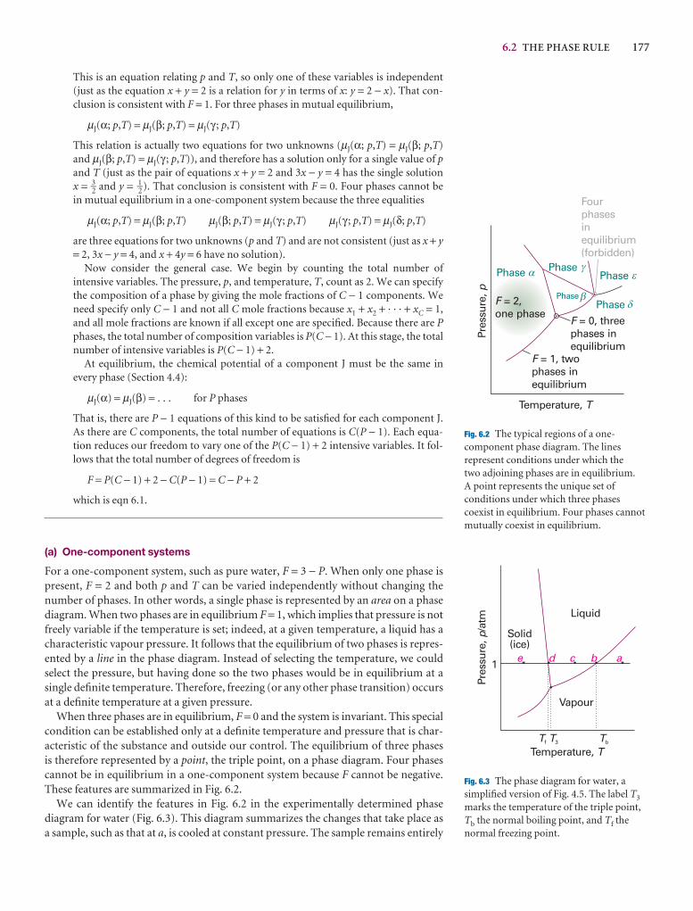
6.2 THE PHASE RULE 177
This is an equation relating p and T, so only one of these variables is independent(just as the equation x + y = 2 is a relation for y in terms of x: y = 2 − x). That con-clusion is consistent with F = 1. For three phases in mutual equilibrium,
µJ(α; p,T) = µJ(β; p,T) = µJ(γ ; p,T)
This relation is actually two equations for two unknowns (µJ(α; p,T) = µJ(β; p,T)and µJ(β; p,T) = µJ(γ ; p,T)), and therefore has a solution only for a single value of pand T (just as the pair of equations x + y = 2 and 3x − y = 4 has the single solution x = 3–2 and y = 1–2). That conclusion is consistent with F = 0. Four phases cannot be in mutual equilibrium in a one-component system because the three equalities
µJ(α; p,T) = µJ(β; p,T) µJ(β; p,T) = µJ(γ ; p,T) µJ(γ ; p,T) = µJ(δ; p,T)
are three equations for two unknowns (p and T) and are not consistent (just as x + y= 2, 3x − y = 4, and x + 4y = 6 have no solution).
Now consider the general case. We begin by counting the total number of intensive variables. The pressure, p, and temperature, T, count as 2. We can specifythe composition of a phase by giving the mole fractions of C − 1 components. Weneed specify only C − 1 and not all C mole fractions because x1 + x2 + · · · + xC = 1,and all mole fractions are known if all except one are specified. Because there are Pphases, the total number of composition variables is P(C − 1). At this stage, the totalnumber of intensive variables is P(C − 1) + 2.
At equilibrium, the chemical potential of a component J must be the same inevery phase (Section 4.4):
µJ(α) = µJ(β) = . . . for P phases
That is, there are P − 1 equations of this kind to be satisfied for each component J.As there are C components, the total number of equations is C(P − 1). Each equa-tion reduces our freedom to vary one of the P(C − 1) + 2 intensive variables. It fol-lows that the total number of degrees of freedom is
F = P(C − 1) + 2 − C(P − 1) = C − P + 2
which is eqn 6.1.
(a) One-component systems
For a one-component system, such as pure water, F = 3 − P. When only one phase ispresent, F = 2 and both p and T can be varied independently without changing thenumber of phases. In other words, a single phase is represented by an area on a phasediagram. When two phases are in equilibrium F = 1, which implies that pressure is notfreely variable if the temperature is set; indeed, at a given temperature, a liquid has acharacteristic vapour pressure. It follows that the equilibrium of two phases is repres-ented by a line in the phase diagram. Instead of selecting the temperature, we couldselect the pressure, but having done so the two phases would be in equilibrium at asingle definite temperature. Therefore, freezing (or any other phase transition) occursat a definite temperature at a given pressure.
When three phases are in equilibrium, F = 0 and the system is invariant. This specialcondition can be established only at a definite temperature and pressure that is char-acteristic of the substance and outside our control. The equilibrium of three phases is therefore represented by a point, the triple point, on a phase diagram. Four phasescannot be in equilibrium in a one-component system because F cannot be negative.These features are summarized in Fig. 6.2.
We can identify the features in Fig. 6.2 in the experimentally determined phase diagram for water (Fig. 6.3). This diagram summarizes the changes that take place asa sample, such as that at a, is cooled at constant pressure. The sample remains entirely
Temperature, T
Pres
sure
,p
F = 1, twophases inequilibrium
Phase PhasePhase
PhasePhaseF = 2,
one phaseF = 0, threephases inequilibrium
Fourphasesinequilibrium(forbidden)�
�
�
�
�
Fig. 6.2 The typical regions of a one-component phase diagram. The linesrepresent conditions under which the two adjoining phases are in equilibrium. A point represents the unique set ofconditions under which three phasescoexist in equilibrium. Four phases cannotmutually coexist in equilibrium.
Solid(ice)
Liquid
Vapour
Tf T3 Tb
Temperature, T
Pres
sure
,/a
tmp
1 d c b ae
Fig. 6.3 The phase diagram for water, asimplified version of Fig. 4.5. The label T3
marks the temperature of the triple point,Tb the normal boiling point, and Tf thenormal freezing point.
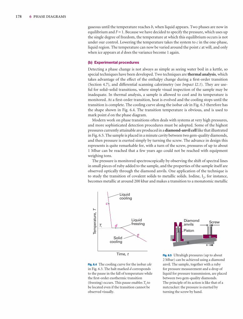
178 6 PHASE DIAGRAMS
Tf
Tem
pera
ture
, T
d
c
e
Time, t
Liquidcooling
Liquidfreezing
Solidcooling
Fig. 6.4 The cooling curve for the isobar cdein Fig. 6.3. The halt marked d correspondsto the pause in the fall of temperature whilethe first-order exothermic transition(freezing) occurs. This pause enables Tf tobe located even if the transition cannot beobserved visually.
Diamondanvils
Piston
Screw
Fig. 6.5 Ultrahigh pressures (up to about 2 Mbar) can be achieved using a diamondanvil. The sample, together with a ruby for pressure measurement and a drop ofliquid for pressure transmission, are placedbetween two gem-quality diamonds. The principle of its action is like that of anutcracker: the pressure is exerted byturning the screw by hand.
gaseous until the temperature reaches b, when liquid appears. Two phases are now inequilibrium and F = 1. Because we have decided to specify the pressure, which uses upthe single degree of freedom, the temperature at which this equilibrium occurs is notunder our control. Lowering the temperature takes the system to c in the one-phase,liquid region. The temperature can now be varied around the point c at will, and onlywhen ice appears at d does the variance become 1 again.
(b) Experimental procedures
Detecting a phase change is not always as simple as seeing water boil in a kettle, so special techniques have been developed. Two techniques are thermal analysis, whichtakes advantage of the effect of the enthalpy change during a first-order transition(Section 4.7), and differential scanning calorimetry (see Impact I2.1). They are use-ful for solid–solid transitions, where simple visual inspection of the sample may be inadequate. In thermal analysis, a sample is allowed to cool and its temperature ismonitored. At a first-order transition, heat is evolved and the cooling stops until thetransition is complete. The cooling curve along the isobar cde in Fig. 6.3 therefore hasthe shape shown in Fig. 6.4. The transition temperature is obvious, and is used tomark point d on the phase diagram.
Modern work on phase transitions often deals with systems at very high pressures,and more sophisticated detection procedures must be adopted. Some of the highestpressures currently attainable are produced in a diamond-anvil cell like that illustratedin Fig. 6.5. The sample is placed in a minute cavity between two gem-quality diamonds,and then pressure is exerted simply by turning the screw. The advance in design thisrepresents is quite remarkable for, with a turn of the screw, pressures of up to about 1 Mbar can be reached that a few years ago could not be reached with equipmentweighing tons.
The pressure is monitored spectroscopically by observing the shift of spectral linesin small pieces of ruby added to the sample, and the properties of the sample itself areobserved optically through the diamond anvils. One application of the technique is to study the transition of covalent solids to metallic solids. Iodine, I2, for instance, becomes metallic at around 200 kbar and makes a transition to a monatomic metallic
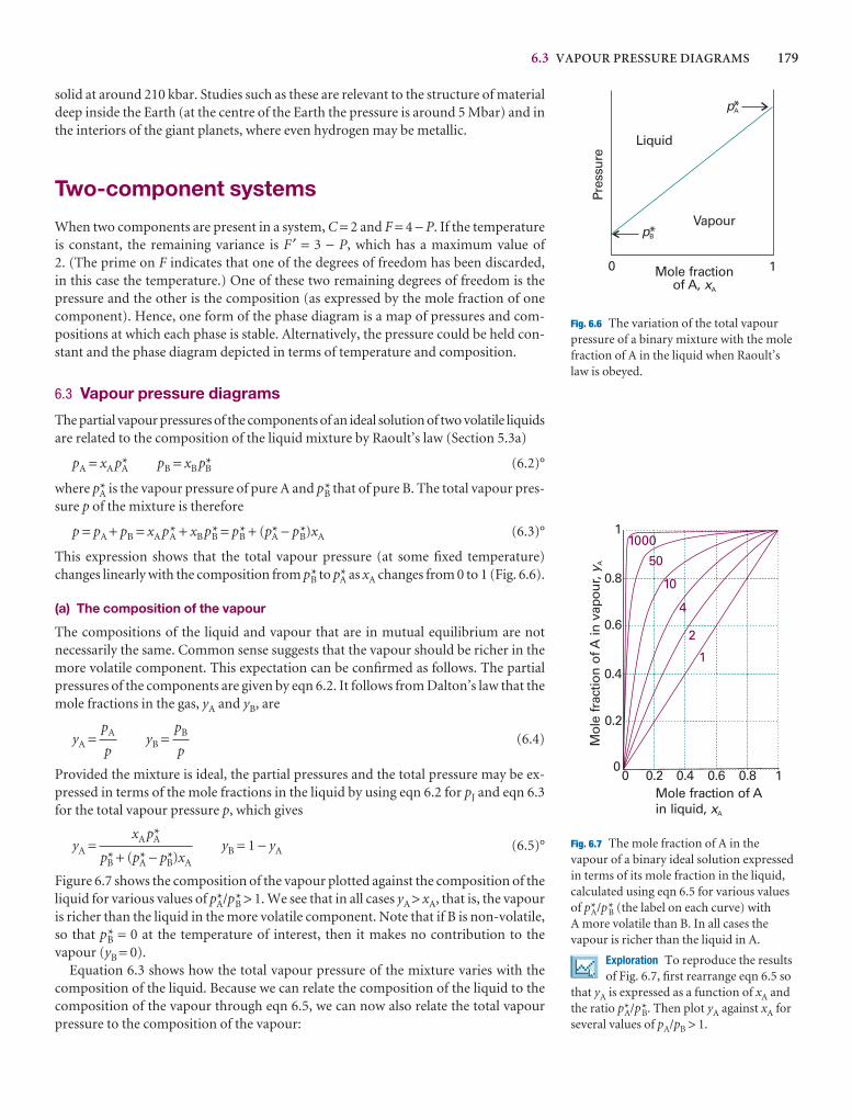
6.3 VAPOUR PRESSURE DIAGRAMS 179
solid at around 210 kbar. Studies such as these are relevant to the structure of materialdeep inside the Earth (at the centre of the Earth the pressure is around 5 Mbar) and inthe interiors of the giant planets, where even hydrogen may be metallic.
Two-component systems
When two components are present in a system, C = 2 and F = 4 − P. If the temperatureis constant, the remaining variance is F ′ = 3 − P, which has a maximum value of 2. (The prime on F indicates that one of the degrees of freedom has been discarded, in this case the temperature.) One of these two remaining degrees of freedom is thepressure and the other is the composition (as expressed by the mole fraction of onecomponent). Hence, one form of the phase diagram is a map of pressures and com-positions at which each phase is stable. Alternatively, the pressure could be held con-stant and the phase diagram depicted in terms of temperature and composition.
6.3 Vapour pressure diagrams
The partial vapour pressures of the components of an ideal solution of two volatile liquidsare related to the composition of the liquid mixture by Raoult’s law (Section 5.3a)
pA = xA p*A pB = xB p*B (6.2)°
where p*A is the vapour pressure of pure A and p*B that of pure B. The total vapour pres-sure p of the mixture is therefore
p = pA + pB = xA p*A + xB p*B = p*B + (p*A − p*B)xA (6.3)°
This expression shows that the total vapour pressure (at some fixed temperature)changes linearly with the composition from p*B to p*A as xA changes from 0 to 1 (Fig. 6.6).
(a) The composition of the vapour
The compositions of the liquid and vapour that are in mutual equilibrium are notnecessarily the same. Common sense suggests that the vapour should be richer in themore volatile component. This expectation can be confirmed as follows. The partialpressures of the components are given by eqn 6.2. It follows from Dalton’s law that themole fractions in the gas, yA and yB, are
yA = yB = (6.4)
Provided the mixture is ideal, the partial pressures and the total pressure may be ex-pressed in terms of the mole fractions in the liquid by using eqn 6.2 for pJ and eqn 6.3for the total vapour pressure p, which gives
yA = yB = 1 − yA (6.5)°
Figure 6.7 shows the composition of the vapour plotted against the composition of theliquid for various values of p*A/p*B > 1. We see that in all cases yA > xA, that is, the vapouris richer than the liquid in the more volatile component. Note that if B is non-volatile,so that p*B = 0 at the temperature of interest, then it makes no contribution to thevapour (yB = 0).
Equation 6.3 shows how the total vapour pressure of the mixture varies with thecomposition of the liquid. Because we can relate the composition of the liquid to thecomposition of the vapour through eqn 6.5, we can now also relate the total vapourpressure to the composition of the vapour:
xA p*A
p*B + (p*A − p*B)xA
pB
p
pA
p
0 1Mole fractionof A, xA
pB*
pA
Liquid
Vapour
Pres
sure
*
Fig. 6.6 The variation of the total vapourpressure of a binary mixture with the molefraction of A in the liquid when Raoult’slaw is obeyed.
0 0.2 0.4 0.6 0.8 1Mole fraction of Ain liquid, xA
Mol
e fr
actio
n o
f A in
vap
our,
y A
0
0.2
0.4
0.6
0.8
1
1
2
4
10
50
1000
Fig. 6.7 The mole fraction of A in thevapour of a binary ideal solution expressedin terms of its mole fraction in the liquid,calculated using eqn 6.5 for various valuesof p*A/p*B (the label on each curve) with A more volatile than B. In all cases thevapour is richer than the liquid in A.
Exploration To reproduce the resultsof Fig. 6.7, first rearrange eqn 6.5 so
that yA is expressed as a function of xA andthe ratio p*A/p*B. Then plot yA against xA forseveral values of pA/pB > 1.
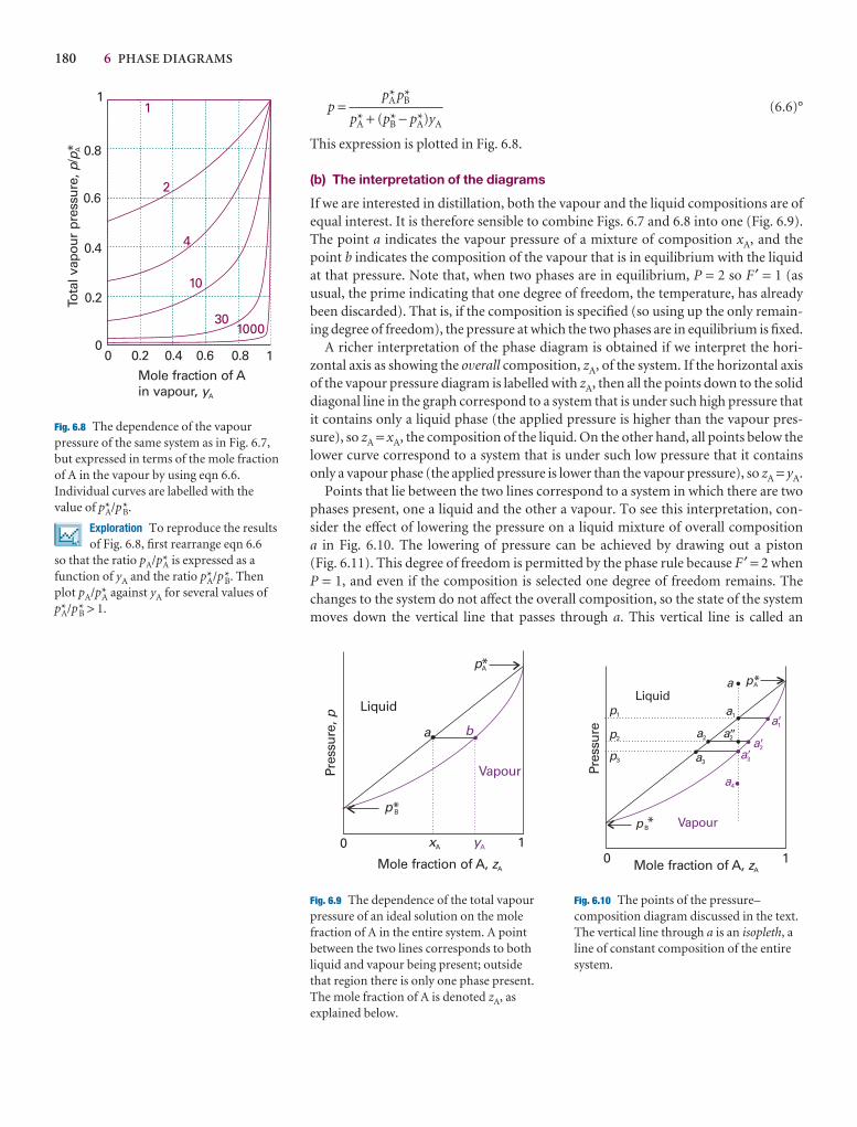
180 6 PHASE DIAGRAMS
0
0.2
0.4
0.6
0.8
1
Tota
l vap
our
pres
sure
,/
*p
p A
0 0.2 0.4 0.6 0.8 1Mole fraction of Ain vapour, yA
1
2
4
10
301000
Fig. 6.8 The dependence of the vapourpressure of the same system as in Fig. 6.7,but expressed in terms of the mole fraction of A in the vapour by using eqn 6.6.Individual curves are labelled with thevalue of p*A/p*B.
Exploration To reproduce the resultsof Fig. 6.8, first rearrange eqn 6.6
so that the ratio pA/p*A is expressed as afunction of yA and the ratio p*A/p*B. Thenplot pA/p*A against yA for several values ofp*A/p*B > 1.
0 1
Mole fraction of A, zA
p B
pA
Liquid
VapourPres
sure
,p
a b
xA yA
*
*
Fig. 6.9 The dependence of the total vapourpressure of an ideal solution on the molefraction of A in the entire system. A pointbetween the two lines corresponds to bothliquid and vapour being present; outsidethat region there is only one phase present.The mole fraction of A is denoted zA, asexplained below.
0 1Mole fraction of A, zA
pB
pA*Liquid
Vapour
Pres
sure
a
a1
a4
a2
a3
a2 a2�a3�
a1�p1
p2
p3
*
��
Fig. 6.10 The points of the pressure–composition diagram discussed in the text.The vertical line through a is an isopleth, aline of constant composition of the entiresystem.
p = (6.6)°
This expression is plotted in Fig. 6.8.
(b) The interpretation of the diagrams
If we are interested in distillation, both the vapour and the liquid compositions are ofequal interest. It is therefore sensible to combine Figs. 6.7 and 6.8 into one (Fig. 6.9).The point a indicates the vapour pressure of a mixture of composition xA, and thepoint b indicates the composition of the vapour that is in equilibrium with the liquidat that pressure. Note that, when two phases are in equilibrium, P = 2 so F ′ = 1 (asusual, the prime indicating that one degree of freedom, the temperature, has alreadybeen discarded). That is, if the composition is specified (so using up the only remain-ing degree of freedom), the pressure at which the two phases are in equilibrium is fixed.
A richer interpretation of the phase diagram is obtained if we interpret the hori-zontal axis as showing the overall composition, zA, of the system. If the horizontal axisof the vapour pressure diagram is labelled with zA, then all the points down to the soliddiagonal line in the graph correspond to a system that is under such high pressure thatit contains only a liquid phase (the applied pressure is higher than the vapour pres-sure), so zA = xA, the composition of the liquid. On the other hand, all points below thelower curve correspond to a system that is under such low pressure that it containsonly a vapour phase (the applied pressure is lower than the vapour pressure), so zA = yA.
Points that lie between the two lines correspond to a system in which there are twophases present, one a liquid and the other a vapour. To see this interpretation, con-sider the effect of lowering the pressure on a liquid mixture of overall composition a in Fig. 6.10. The lowering of pressure can be achieved by drawing out a piston (Fig. 6.11). This degree of freedom is permitted by the phase rule because F ′ = 2 whenP = 1, and even if the composition is selected one degree of freedom remains. Thechanges to the system do not affect the overall composition, so the state of the systemmoves down the vertical line that passes through a. This vertical line is called an
p*A p*B
p*A + (p*B − p*A)yA
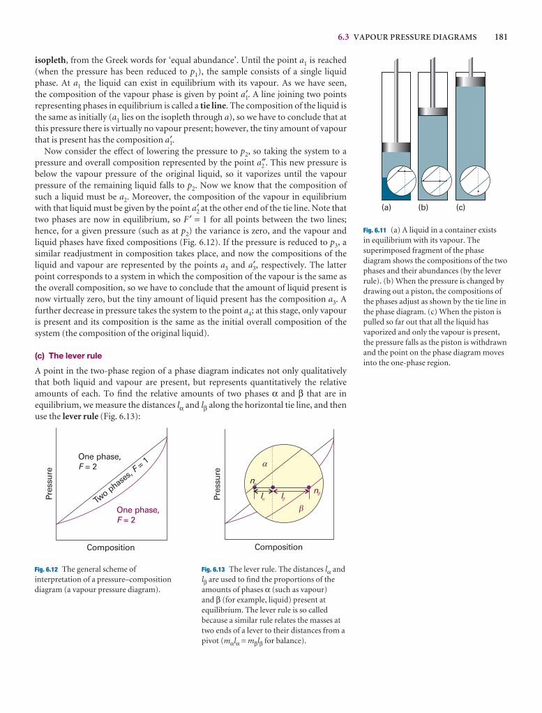
6.3 VAPOUR PRESSURE DIAGRAMS 181
isopleth, from the Greek words for ‘equal abundance’. Until the point a1 is reached(when the pressure has been reduced to p1), the sample consists of a single liquidphase. At a1 the liquid can exist in equilibrium with its vapour. As we have seen, the composition of the vapour phase is given by point a1′. A line joining two pointsrepresenting phases in equilibrium is called a tie line. The composition of the liquid isthe same as initially (a1 lies on the isopleth through a), so we have to conclude that atthis pressure there is virtually no vapour present; however, the tiny amount of vapourthat is present has the composition a1′.
Now consider the effect of lowering the pressure to p2, so taking the system to apressure and overall composition represented by the point a2″. This new pressure isbelow the vapour pressure of the original liquid, so it vaporizes until the vapour pressure of the remaining liquid falls to p2. Now we know that the composition ofsuch a liquid must be a2. Moreover, the composition of the vapour in equilibriumwith that liquid must be given by the point a2′ at the other end of the tie line. Note thattwo phases are now in equilibrium, so F ′ = 1 for all points between the two lines;hence, for a given pressure (such as at p2) the variance is zero, and the vapour and liquid phases have fixed compositions (Fig. 6.12). If the pressure is reduced to p3, asimilar readjustment in composition takes place, and now the compositions of the liquid and vapour are represented by the points a3 and a3′, respectively. The latterpoint corresponds to a system in which the composition of the vapour is the same asthe overall composition, so we have to conclude that the amount of liquid present isnow virtually zero, but the tiny amount of liquid present has the composition a3. Afurther decrease in pressure takes the system to the point a4; at this stage, only vapouris present and its composition is the same as the initial overall composition of the system (the composition of the original liquid).
(c) The lever rule
A point in the two-phase region of a phase diagram indicates not only qualitativelythat both liquid and vapour are present, but represents quantitatively the relativeamounts of each. To find the relative amounts of two phases α and β that are in equilibrium, we measure the distances lα and lβ along the horizontal tie line, and thenuse the lever rule (Fig. 6.13):
(a) (b) (c)
Fig. 6.11 (a) A liquid in a container exists in equilibrium with its vapour. Thesuperimposed fragment of the phasediagram shows the compositions of the twophases and their abundances (by the leverrule). (b) When the pressure is changed bydrawing out a piston, the compositions ofthe phases adjust as shown by the tie line inthe phase diagram. (c) When the piston ispulled so far out that all the liquid hasvaporized and only the vapour is present,the pressure falls as the piston is withdrawnand the point on the phase diagram movesinto the one-phase region.
Pres
sure
Composition
One phase,= 2F
One phase,= 2F
Two phas
es,
= 1F
Fig. 6.12 The general scheme ofinterpretation of a pressure–compositiondiagram (a vapour pressure diagram).
Pres
sure
Composition
na
la
lb
nb
a
b
Fig. 6.13 The lever rule. The distances lα andlβ are used to find the proportions of theamounts of phases α (such as vapour) and β (for example, liquid) present atequilibrium. The lever rule is so calledbecause a similar rule relates the masses attwo ends of a lever to their distances from apivot (mαlα = mβlβ for balance).
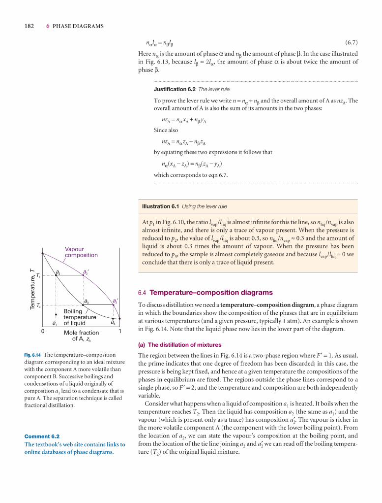
182 6 PHASE DIAGRAMS
Comment 6.2
The textbook’s web site contains links toonline databases of phase diagrams.
Vapourcomposition
Boilingtemperatureof liquid
Tem
pera
ture
,T
0 1Mole fractionof A, zA
T2
T3
a2�
a3�a3
a2
a1a4
Fig. 6.14 The temperature–compositiondiagram corresponding to an ideal mixturewith the component A more volatile thancomponent B. Successive boilings andcondensations of a liquid originally ofcomposition a1 lead to a condensate that ispure A. The separation technique is calledfractional distillation.
nαlα = nβlβ (6.7)
Here nα is the amount of phase α and nβ the amount of phase β. In the case illustratedin Fig. 6.13, because lβ ≈ 2lα, the amount of phase α is about twice the amount of phase β.
Justification 6.2 The lever rule
To prove the lever rule we write n = nα + nβ and the overall amount of A as nzA. Theoverall amount of A is also the sum of its amounts in the two phases:
nzA = nαxA + nβyA
Since also
nzA = nαzA + nβzA
by equating these two expressions it follows that
nα(xA − zA) = nβ(zA − yA)
which corresponds to eqn 6.7.
Illustration 6.1 Using the lever rule
At p1 in Fig. 6.10, the ratio lvap/lliq is almost infinite for this tie line, so nliq/nvap is alsoalmost infinite, and there is only a trace of vapour present. When the pressure is reduced to p2, the value of lvap/lliq is about 0.3, so nliq/nvap ≈ 0.3 and the amount ofliquid is about 0.3 times the amount of vapour. When the pressure has been reduced to p3, the sample is almost completely gaseous and because lvap/lliq ≈ 0 weconclude that there is only a trace of liquid present.
6.4 Temperature–composition diagrams
To discuss distillation we need a temperature–composition diagram, a phase diagramin which the boundaries show the composition of the phases that are in equilibriumat various temperatures (and a given pressure, typically 1 atm). An example is shownin Fig. 6.14. Note that the liquid phase now lies in the lower part of the diagram.
(a) The distillation of mixtures
The region between the lines in Fig. 6.14 is a two-phase region where F ′ = 1. As usual,the prime indicates that one degree of freedom has been discarded; in this case, thepressure is being kept fixed, and hence at a given temperature the compositions of thephases in equilibrium are fixed. The regions outside the phase lines correspond to asingle phase, so F ′ = 2, and the temperature and composition are both independentlyvariable.
Consider what happens when a liquid of composition a1 is heated. It boils when thetemperature reaches T2. Then the liquid has composition a2 (the same as a1) and thevapour (which is present only as a trace) has composition a2′. The vapour is richer inthe more volatile component A (the component with the lower boiling point). Fromthe location of a2, we can state the vapour’s composition at the boiling point, andfrom the location of the tie line joining a2 and a2′ we can read off the boiling tempera-ture (T2) of the original liquid mixture.
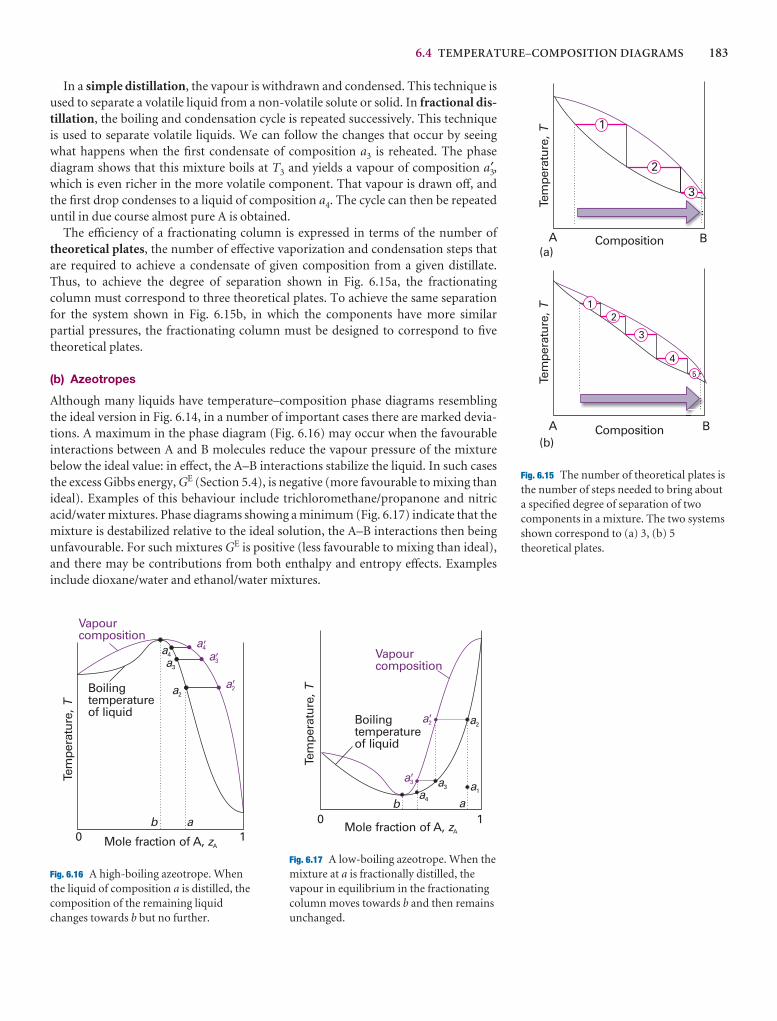
6.4 TEMPERATURE–COMPOSITION DIAGRAMS 183
In a simple distillation, the vapour is withdrawn and condensed. This technique isused to separate a volatile liquid from a non-volatile solute or solid. In fractional dis-tillation, the boiling and condensation cycle is repeated successively. This techniqueis used to separate volatile liquids. We can follow the changes that occur by seeingwhat happens when the first condensate of composition a3 is reheated. The phase diagram shows that this mixture boils at T3 and yields a vapour of composition a3′,which is even richer in the more volatile component. That vapour is drawn off, andthe first drop condenses to a liquid of composition a4. The cycle can then be repeateduntil in due course almost pure A is obtained.
The efficiency of a fractionating column is expressed in terms of the number of theoretical plates, the number of effective vaporization and condensation steps thatare required to achieve a condensate of given composition from a given distillate.Thus, to achieve the degree of separation shown in Fig. 6.15a, the fractionating column must correspond to three theoretical plates. To achieve the same separationfor the system shown in Fig. 6.15b, in which the components have more similar partial pressures, the fractionating column must be designed to correspond to fivetheoretical plates.
(b) Azeotropes
Although many liquids have temperature–composition phase diagrams resemblingthe ideal version in Fig. 6.14, in a number of important cases there are marked devia-tions. A maximum in the phase diagram (Fig. 6.16) may occur when the favourableinteractions between A and B molecules reduce the vapour pressure of the mixturebelow the ideal value: in effect, the A–B interactions stabilize the liquid. In such casesthe excess Gibbs energy, GE (Section 5.4), is negative (more favourable to mixing thanideal). Examples of this behaviour include trichloromethane/propanone and nitricacid/water mixtures. Phase diagrams showing a minimum (Fig. 6.17) indicate that themixture is destabilized relative to the ideal solution, the A–B interactions then beingunfavourable. For such mixtures GE is positive (less favourable to mixing than ideal),and there may be contributions from both enthalpy and entropy effects. Examples include dioxane/water and ethanol/water mixtures.
Tem
pera
ture
,TTe
mpe
ratu
re,T
Composition
Composition
A
A
B
B
(a)
(b)
2
2
3
3
1
1
45
Fig. 6.15 The number of theoretical plates isthe number of steps needed to bring abouta specified degree of separation of twocomponents in a mixture. The two systemsshown correspond to (a) 3, (b) 5theoretical plates.
Vapourcomposition
Boilingtemperatureof liquid
Tem
pera
ture
,T
0 1Mole fraction of A, zA
a
a2a2�
a3
a4 a3�
a4�
b
Vapourcomposition
Boilingtemperatureof liquid
Tem
pera
ture
,T
0 1Mole fraction of A, zA
a2¢ a2
a1a3
a4
a3¢
ab
Fig. 6.16 A high-boiling azeotrope. Whenthe liquid of composition a is distilled, thecomposition of the remaining liquidchanges towards b but no further.
Fig. 6.17 A low-boiling azeotrope. When themixture at a is fractionally distilled, thevapour in equilibrium in the fractionatingcolumn moves towards b and then remainsunchanged.
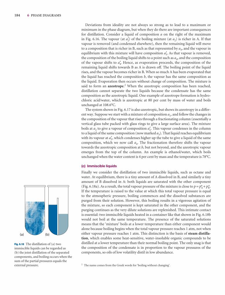
184 6 PHASE DIAGRAMS
Deviations from ideality are not always so strong as to lead to a maximum or minimum in the phase diagram, but when they do there are important consequencesfor distillation. Consider a liquid of composition a on the right of the maximum in Fig. 6.16. The vapour (at a2′) of the boiling mixture (at a2) is richer in A. If thatvapour is removed (and condensed elsewhere), then the remaining liquid will moveto a composition that is richer in B, such as that represented by a3, and the vapour inequilibrium with this mixture will have composition a3′. As that vapour is removed,the composition of the boiling liquid shifts to a point such as a4, and the compositionof the vapour shifts to a4′. Hence, as evaporation proceeds, the composition of the remaining liquid shifts towards B as A is drawn off. The boiling point of the liquidrises, and the vapour becomes richer in B. When so much A has been evaporated thatthe liquid has reached the composition b, the vapour has the same composition as the liquid. Evaporation then occurs without change of composition. The mixture issaid to form an azeotrope.2 When the azeotropic composition has been reached, distillation cannot separate the two liquids because the condensate has the same composition as the azeotropic liquid. One example of azeotrope formation is hydro-chloric acid/water, which is azeotropic at 80 per cent by mass of water and boils unchanged at 108.6°C.
The system shown in Fig. 6.17 is also azeotropic, but shows its azeotropy in a differ-ent way. Suppose we start with a mixture of composition a1, and follow the changes inthe composition of the vapour that rises through a fractionating column (essentially avertical glass tube packed with glass rings to give a large surface area). The mixtureboils at a2 to give a vapour of composition a2′ . This vapour condenses in the columnto a liquid of the same composition (now marked a3). That liquid reaches equilibriumwith its vapour at a3′ , which condenses higher up the tube to give a liquid of the samecomposition, which we now call a4. The fractionation therefore shifts the vapour towards the azeotropic composition at b, but not beyond, and the azeotropic vapouremerges from the top of the column. An example is ethanol/water, which boils unchanged when the water content is 4 per cent by mass and the temperature is 78°C.
(c) Immiscible liquids
Finally we consider the distillation of two immiscible liquids, such as octane andwater. At equilibrium, there is a tiny amount of A dissolved in B, and similarly a tinyamount of B dissolved in A: both liquids are saturated with the other component (Fig. 6.18a). As a result, the total vapour pressure of the mixture is close to p = pA* + pB*.If the temperature is raised to the value at which this total vapour pressure is equal to the atmospheric pressure, boiling commences and the dissolved substances arepurged from their solution. However, this boiling results in a vigorous agitation of the mixture, so each component is kept saturated in the other component, and thepurging continues as the very dilute solutions are replenished. This intimate contactis essential: two immiscible liquids heated in a container like that shown in Fig. 6.18bwould not boil at the same temperature. The presence of the saturated solutionsmeans that the ‘mixture’ boils at a lower temperature than either component wouldalone because boiling begins when the total vapour pressure reaches 1 atm, not wheneither vapour pressure reaches 1 atm. This distinction is the basis of steam distilla-tion, which enables some heat-sensitive, water-insoluble organic compounds to bedistilled at a lower temperature than their normal boiling point. The only snag is thatthe composition of the condensate is in proportion to the vapour pressures of thecomponents, so oils of low volatility distil in low abundance.
2 The name comes from the Greek words for ‘boiling without changing’.
(a) (b)
Fig. 6.18 The distillation of (a) twoimmiscible liquids can be regarded as (b) the joint distillation of the separatedcomponents, and boiling occurs when thesum of the partial pressures equals theexternal pressure.
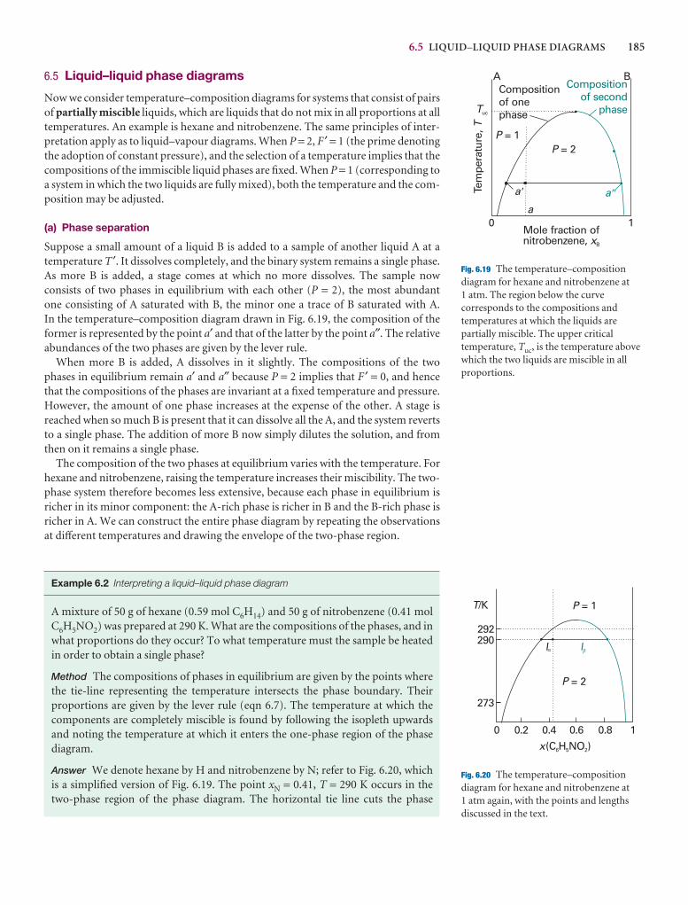
6.5 LIQUID–LIQUID PHASE DIAGRAMS 185
P = 1P = 2
0 1Mole fraction ofnitrobenzene, xB
Tuc
Tem
pera
ture
,T
a ¢
a
a²
A BCompositionof onephase
Compositionof second
phase
Fig. 6.19 The temperature–compositiondiagram for hexane and nitrobenzene at 1 atm. The region below the curvecorresponds to the compositions andtemperatures at which the liquids arepartially miscible. The upper criticaltemperature, Tuc, is the temperature abovewhich the two liquids are miscible in allproportions.
P = 1
P = 2
0 0.2 0.4 0.6 0.8 1
x(C H NO )6 5 2
290292
273
l lb
T/K
a
Fig. 6.20 The temperature–compositiondiagram for hexane and nitrobenzene at 1 atm again, with the points and lengthsdiscussed in the text.
6.5 Liquid–liquid phase diagrams
Now we consider temperature–composition diagrams for systems that consist of pairsof partially miscible liquids, which are liquids that do not mix in all proportions at alltemperatures. An example is hexane and nitrobenzene. The same principles of inter-pretation apply as to liquid–vapour diagrams. When P = 2, F ′ = 1 (the prime denotingthe adoption of constant pressure), and the selection of a temperature implies that thecompositions of the immiscible liquid phases are fixed. When P = 1 (corresponding toa system in which the two liquids are fully mixed), both the temperature and the com-position may be adjusted.
(a) Phase separation
Suppose a small amount of a liquid B is added to a sample of another liquid A at a temperature T ′. It dissolves completely, and the binary system remains a single phase. As more B is added, a stage comes at which no more dissolves. The sample now consists of two phases in equilibrium with each other (P = 2), the most abundant one consisting of A saturated with B, the minor one a trace of B saturated with A. In the temperature–composition diagram drawn in Fig. 6.19, the composition of the former is represented by the point a′ and that of the latter by the point a″. The relativeabundances of the two phases are given by the lever rule.
When more B is added, A dissolves in it slightly. The compositions of the twophases in equilibrium remain a′ and a″ because P = 2 implies that F ′ = 0, and hencethat the compositions of the phases are invariant at a fixed temperature and pressure.However, the amount of one phase increases at the expense of the other. A stage isreached when so much B is present that it can dissolve all the A, and the system revertsto a single phase. The addition of more B now simply dilutes the solution, and fromthen on it remains a single phase.
The composition of the two phases at equilibrium varies with the temperature. Forhexane and nitrobenzene, raising the temperature increases their miscibility. The two-phase system therefore becomes less extensive, because each phase in equilibrium isricher in its minor component: the A-rich phase is richer in B and the B-rich phase isricher in A. We can construct the entire phase diagram by repeating the observationsat different temperatures and drawing the envelope of the two-phase region.
Example 6.2 Interpreting a liquid–liquid phase diagram
A mixture of 50 g of hexane (0.59 mol C6H14) and 50 g of nitrobenzene (0.41 molC6H5NO2) was prepared at 290 K. What are the compositions of the phases, and inwhat proportions do they occur? To what temperature must the sample be heatedin order to obtain a single phase?
Method The compositions of phases in equilibrium are given by the points wherethe tie-line representing the temperature intersects the phase boundary. Their proportions are given by the lever rule (eqn 6.7). The temperature at which thecomponents are completely miscible is found by following the isopleth upwardsand noting the temperature at which it enters the one-phase region of the phase diagram.
Answer We denote hexane by H and nitrobenzene by N; refer to Fig. 6.20, whichis a simplified version of Fig. 6.19. The point xN = 0.41, T = 290 K occurs in the two-phase region of the phase diagram. The horizontal tie line cuts the phase
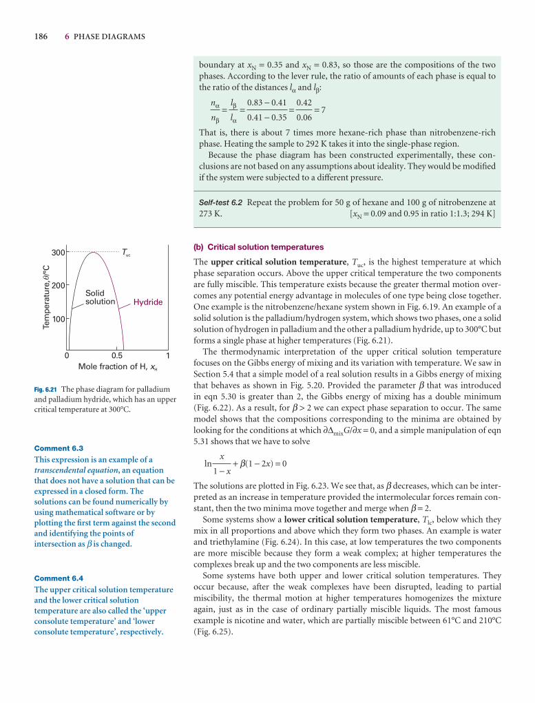
186 6 PHASE DIAGRAMS
300
200
100
Hydride
0 0.5 1
Tem
pera
ture
, /°
C
Solidsolution
Mole fraction of H, xH
Tuc
q
Fig. 6.21 The phase diagram for palladiumand palladium hydride, which has an uppercritical temperature at 300°C.
Comment 6.3
This expression is an example of atranscendental equation, an equationthat does not have a solution that can beexpressed in a closed form. Thesolutions can be found numerically byusing mathematical software or byplotting the first term against the secondand identifying the points ofintersection as β is changed.
Comment 6.4
The upper critical solution temperatureand the lower critical solutiontemperature are also called the ‘upperconsolute temperature’ and ‘lowerconsolute temperature’, respectively.
boundary at xN = 0.35 and xN = 0.83, so those are the compositions of the twophases. According to the lever rule, the ratio of amounts of each phase is equal tothe ratio of the distances lα and lβ:
= = = = 7
That is, there is about 7 times more hexane-rich phase than nitrobenzene-richphase. Heating the sample to 292 K takes it into the single-phase region.
Because the phase diagram has been constructed experimentally, these con-clusions are not based on any assumptions about ideality. They would be modifiedif the system were subjected to a different pressure.
Self-test 6.2 Repeat the problem for 50 g of hexane and 100 g of nitrobenzene at273 K. [xN = 0.09 and 0.95 in ratio 1:1.3; 294 K]
(b) Critical solution temperatures
The upper critical solution temperature, Tuc, is the highest temperature at whichphase separation occurs. Above the upper critical temperature the two componentsare fully miscible. This temperature exists because the greater thermal motion over-comes any potential energy advantage in molecules of one type being close together.One example is the nitrobenzene/hexane system shown in Fig. 6.19. An example of asolid solution is the palladium/hydrogen system, which shows two phases, one a solidsolution of hydrogen in palladium and the other a palladium hydride, up to 300°C butforms a single phase at higher temperatures (Fig. 6.21).
The thermodynamic interpretation of the upper critical solution temperature focuses on the Gibbs energy of mixing and its variation with temperature. We saw inSection 5.4 that a simple model of a real solution results in a Gibbs energy of mixingthat behaves as shown in Fig. 5.20. Provided the parameter β that was introduced in eqn 5.30 is greater than 2, the Gibbs energy of mixing has a double minimum (Fig. 6.22). As a result, for β > 2 we can expect phase separation to occur. The samemodel shows that the compositions corresponding to the minima are obtained bylooking for the conditions at which ∂∆mixG/∂x = 0, and a simple manipulation of eqn5.31 shows that we have to solve
ln + β(1 − 2x) = 0
The solutions are plotted in Fig. 6.23. We see that, as β decreases, which can be inter-preted as an increase in temperature provided the intermolecular forces remain con-stant, then the two minima move together and merge when β = 2.
Some systems show a lower critical solution temperature, Tlc, below which theymix in all proportions and above which they form two phases. An example is waterand triethylamine (Fig. 6.24). In this case, at low temperatures the two componentsare more miscible because they form a weak complex; at higher temperatures thecomplexes break up and the two components are less miscible.
Some systems have both upper and lower critical solution temperatures. Theyoccur because, after the weak complexes have been disrupted, leading to partial miscibility, the thermal motion at higher temperatures homogenizes the mixtureagain, just as in the case of ordinary partially miscible liquids. The most famous example is nicotine and water, which are partially miscible between 61°C and 210°C(Fig. 6.25).
x
1 − x
0.42
0.06
0.83 − 0.41
0.41 − 0.35
lβ
lα
nα
nβ
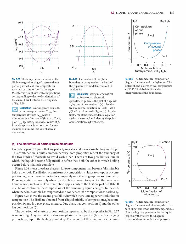
6.5 LIQUID–LIQUID PHASE DIAGRAMS 187
(c) The distillation of partially miscible liquids
Consider a pair of liquids that are partially miscible and form a low-boiling azeotrope.This combination is quite common because both properties reflect the tendency ofthe two kinds of molecule to avoid each other. There are two possibilities: one inwhich the liquids become fully miscible before they boil; the other in which boilingoccurs before mixing is complete.
Figure 6.26 shows the phase diagram for two components that become fully misciblebefore they boil. Distillation of a mixture of composition a1 leads to a vapour of com-position b1, which condenses to the completely miscible single-phase solution at b2.Phase separation occurs only when this distillate is cooled to a point in the two-phaseliquid region, such as b3. This description applies only to the first drop of distillate. Ifdistillation continues, the composition of the remaining liquid changes. In the end,when the whole sample has evaporated and condensed, the composition is back to a1.
Figure 6.27 shows the second possibility, in which there is no upper critical solutiontemperature. The distillate obtained from a liquid initially of composition a1 has com-position b3 and is a two-phase mixture. One phase has composition b3′ and the otherhas composition b3″.
The behaviour of a system of composition represented by the isopleth e in Fig. 6.27is interesting. A system at e1 forms two phases, which persist (but with changing proportions) up to the boiling point at e2. The vapour of this mixture has the same
0
m
ixG
nRT
/
0 0.5 1xA
1
1.5
2
2.5
3
�0.5
�0.4
�0.3
�0.2
�0.1
�0.1
Fig. 6.22 The temperature variation of theGibbs energy of mixing of a system that ispartially miscible at low temperatures. A system of composition in the region P = 2 forms two phases with compositionscorresponding to the two local minima ofthe curve. This illustration is a duplicate of Fig. 5.20.
Exploration Working from eqn 5.31,write an expression for Tmin, the
temperature at which ∆mixG has aminimum, as a function of β and xA. Then,plot Tmin against xA for several values of β.Provide a physical interpretation for anymaxima or minima that you observe inthese plots.
0 0.5 1xA
2
2.5
3
�
Fig. 6.23 The location of the phaseboundary as computed on the basis of the β-parameter model introduced inSection 5.4.
Exploration Using mathematicalsoftware or an electronic
spreadsheet, generate the plot of β againstxA by one of two methods: (a) solve thetranscendental equation ln {(x /(1− x)} +β(1 − 2x) = 0 numerically, or (b) plot thefirst term of the transcendental equationagainst the second and identify the pointsof intersection as β is changed.
P = 1
P = 2
0 0.2 0.4 0.6 0.8 1Mole fraction of
triethylamine, ((C H ) N)x 2 5 3
Tem
pera
ture
,T
Tlc
H O2 (C H ) N2 5 3
Compositionof second
phase
Compositionof onephase
Fig. 6.24 The temperature–compositiondiagram for water and triethylamine. Thissystem shows a lower critical temperatureat 292 K. The labels indicate theinterpretation of the boundaries.
P = 1
P = 2
0 0.2 0.4 0.6 0.8 1Mole fraction of
nicotine, xN
Tem
pera
ture
, /°
C
Tlc
H O2 NicotineTuc
61
210
q
Fig. 6.25 The temperature–compositiondiagram for water and nicotine, which hasboth upper and lower critical temperatures.Note the high temperatures for the liquid(especially the water): the diagramcorresponds to a sample under pressure.
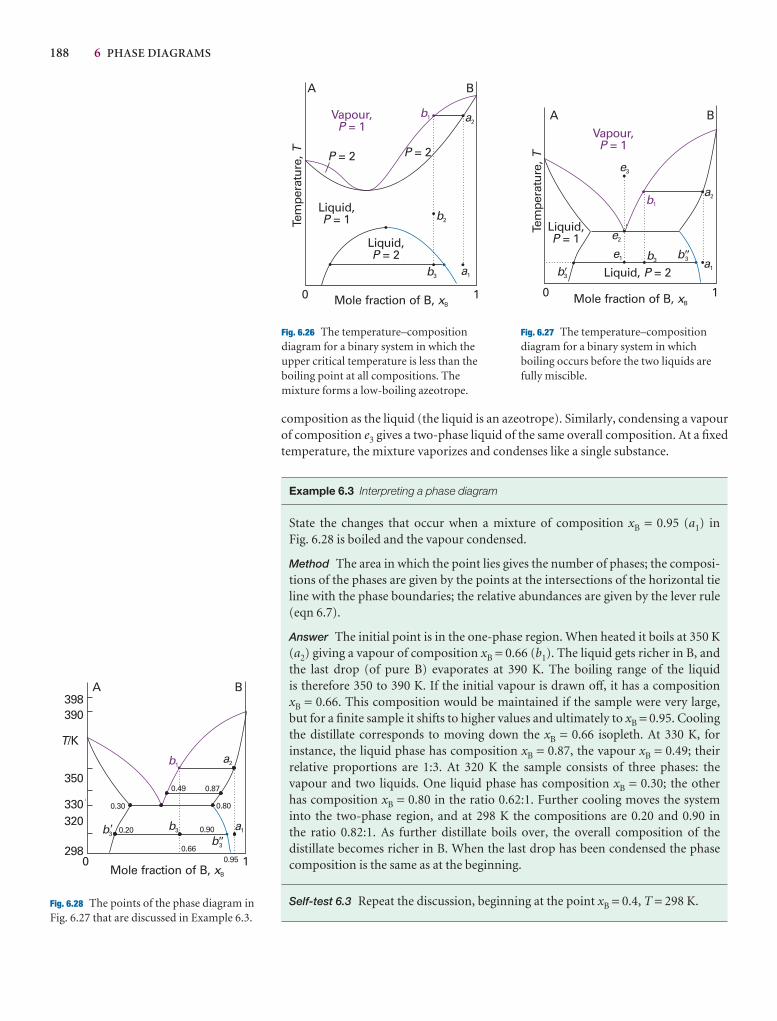
188 6 PHASE DIAGRAMS
0 1Mole fraction of B, xBTe
mpe
ratu
re,T
Vapour,= 1P
Liquid,= 1P
b1
b2
a2
a1b3
Liquid,= 2P
A B
P = 2P = 2
0 1Mole fraction of B, xB
Tem
pera
ture
,T
Vapour,= 1P
Liquid,= 1P
b1
a2
a1
b3
Liquid, = 2P
A B
e3
e2
e1
b3�
b3�
Fig. 6.26 The temperature–compositiondiagram for a binary system in which theupper critical temperature is less than theboiling point at all compositions. Themixture forms a low-boiling azeotrope.
Fig. 6.27 The temperature–compositiondiagram for a binary system in whichboiling occurs before the two liquids arefully miscible.
0 1Mole fraction of B, xB
b1a2
a1b3
A B
b3
b3�
0.95
398390
350
330320
298
T/K
0.20
0.30
0.66
0.80
0.49 0.87
0.90�
Fig. 6.28 The points of the phase diagram inFig. 6.27 that are discussed in Example 6.3.
composition as the liquid (the liquid is an azeotrope). Similarly, condensing a vapourof composition e3 gives a two-phase liquid of the same overall composition. At a fixedtemperature, the mixture vaporizes and condenses like a single substance.
Example 6.3 Interpreting a phase diagram
State the changes that occur when a mixture of composition xB = 0.95 (a1) in Fig. 6.28 is boiled and the vapour condensed.
Method The area in which the point lies gives the number of phases; the composi-tions of the phases are given by the points at the intersections of the horizontal tieline with the phase boundaries; the relative abundances are given by the lever rule(eqn 6.7).
Answer The initial point is in the one-phase region. When heated it boils at 350 K(a2) giving a vapour of composition xB = 0.66 (b1). The liquid gets richer in B, andthe last drop (of pure B) evaporates at 390 K. The boiling range of the liquid is therefore 350 to 390 K. If the initial vapour is drawn off, it has a composition xB = 0.66. This composition would be maintained if the sample were very large, but for a finite sample it shifts to higher values and ultimately to xB = 0.95. Coolingthe distillate corresponds to moving down the xB = 0.66 isopleth. At 330 K, for instance, the liquid phase has composition xB = 0.87, the vapour xB = 0.49; their relative proportions are 1:3. At 320 K the sample consists of three phases: thevapour and two liquids. One liquid phase has composition xB = 0.30; the other has composition xB = 0.80 in the ratio 0.62:1. Further cooling moves the systeminto the two-phase region, and at 298 K the compositions are 0.20 and 0.90 in the ratio 0.82:1. As further distillate boils over, the overall composition of the distillate becomes richer in B. When the last drop has been condensed the phasecomposition is the same as at the beginning.
Self-test 6.3 Repeat the discussion, beginning at the point xB = 0.4, T = 298 K.
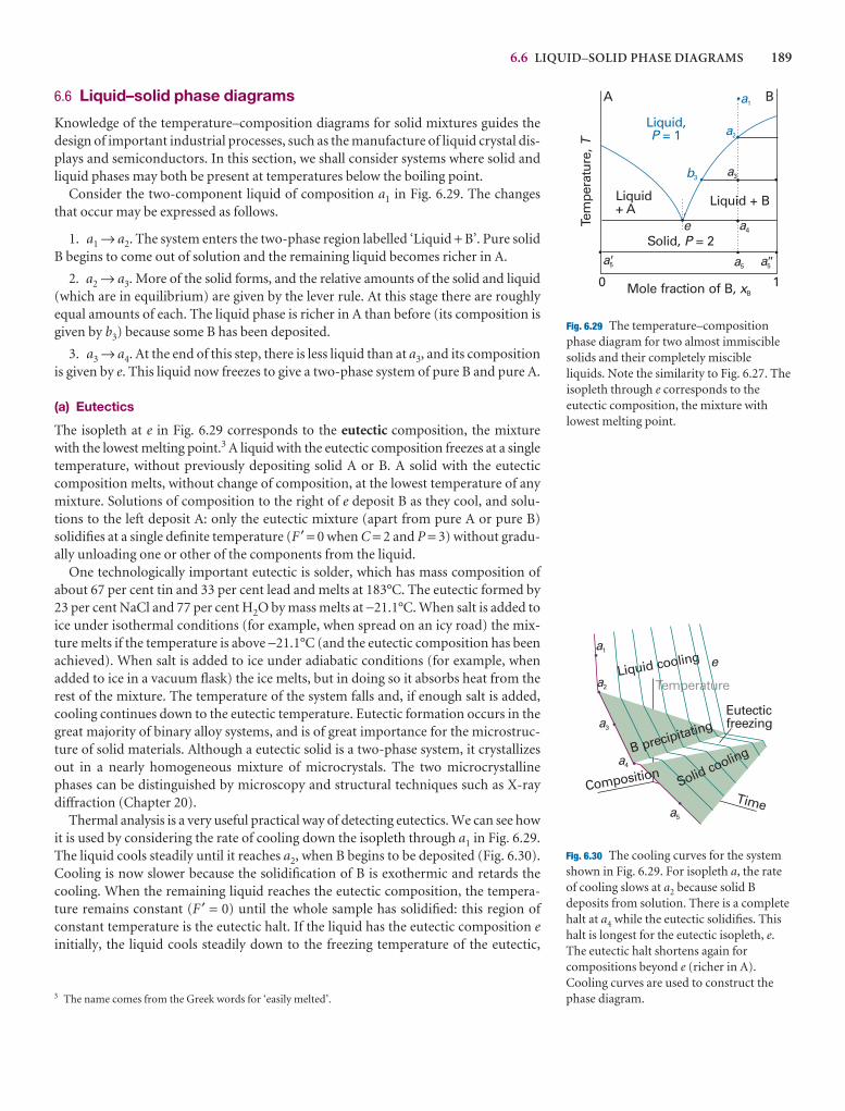
6.6 LIQUID–SOLID PHASE DIAGRAMS 189
6.6 Liquid–solid phase diagrams
Knowledge of the temperature–composition diagrams for solid mixtures guides thedesign of important industrial processes, such as the manufacture of liquid crystal dis-plays and semiconductors. In this section, we shall consider systems where solid andliquid phases may both be present at temperatures below the boiling point.
Consider the two-component liquid of composition a1 in Fig. 6.29. The changesthat occur may be expressed as follows.
1. a1 → a2. The system enters the two-phase region labelled ‘Liquid + B’. Pure solidB begins to come out of solution and the remaining liquid becomes richer in A.
2. a2 → a3. More of the solid forms, and the relative amounts of the solid and liquid(which are in equilibrium) are given by the lever rule. At this stage there are roughlyequal amounts of each. The liquid phase is richer in A than before (its composition isgiven by b3) because some B has been deposited.
3. a3 → a4. At the end of this step, there is less liquid than at a3, and its compositionis given by e. This liquid now freezes to give a two-phase system of pure B and pure A.
(a) Eutectics
The isopleth at e in Fig. 6.29 corresponds to the eutectic composition, the mixture with the lowest melting point.3 A liquid with the eutectic composition freezes at a singletemperature, without previously depositing solid A or B. A solid with the eutecticcomposition melts, without change of composition, at the lowest temperature of any mixture. Solutions of composition to the right of e deposit B as they cool, and solu-tions to the left deposit A: only the eutectic mixture (apart from pure A or pure B) solidifies at a single definite temperature (F ′ = 0 when C = 2 and P = 3) without gradu-ally unloading one or other of the components from the liquid.
One technologically important eutectic is solder, which has mass composition ofabout 67 per cent tin and 33 per cent lead and melts at 183°C. The eutectic formed by23 per cent NaCl and 77 per cent H2O by mass melts at −21.1°C. When salt is added toice under isothermal conditions (for example, when spread on an icy road) the mix-ture melts if the temperature is above −21.1°C (and the eutectic composition has beenachieved). When salt is added to ice under adiabatic conditions (for example, whenadded to ice in a vacuum flask) the ice melts, but in doing so it absorbs heat from therest of the mixture. The temperature of the system falls and, if enough salt is added,cooling continues down to the eutectic temperature. Eutectic formation occurs in thegreat majority of binary alloy systems, and is of great importance for the microstruc-ture of solid materials. Although a eutectic solid is a two-phase system, it crystallizesout in a nearly homogeneous mixture of microcrystals. The two microcrystallinephases can be distinguished by microscopy and structural techniques such as X-raydiffraction (Chapter 20).
Thermal analysis is a very useful practical way of detecting eutectics. We can see howit is used by considering the rate of cooling down the isopleth through a1 in Fig. 6.29.The liquid cools steadily until it reaches a2, when B begins to be deposited (Fig. 6.30).Cooling is now slower because the solidification of B is exothermic and retards thecooling. When the remaining liquid reaches the eutectic composition, the tempera-ture remains constant (F ′ = 0) until the whole sample has solidified: this region ofconstant temperature is the eutectic halt. If the liquid has the eutectic composition einitially, the liquid cools steadily down to the freezing temperature of the eutectic,
0 1Mole fraction of B, xB
Tem
pera
ture
,T
Liquid,= 1P a2
a1
b3
A B
eSolid, = 2P
a3
a4
a5a5� a5�
Liquid+ A
Liquid + B
Fig. 6.29 The temperature–compositionphase diagram for two almost immisciblesolids and their completely miscibleliquids. Note the similarity to Fig. 6.27. Theisopleth through e corresponds to theeutectic composition, the mixture withlowest melting point.
Temperature
TimeComposition
Eutecticfreezing
a1
a2
a3
a4
a5
eLiquid cooling
B precipitating
Solid cooling
Fig. 6.30 The cooling curves for the systemshown in Fig. 6.29. For isopleth a, the rateof cooling slows at a2 because solid Bdeposits from solution. There is a completehalt at a4 while the eutectic solidifies. Thishalt is longest for the eutectic isopleth, e.The eutectic halt shortens again forcompositions beyond e (richer in A).Cooling curves are used to construct thephase diagram.3 The name comes from the Greek words for ‘easily melted’.
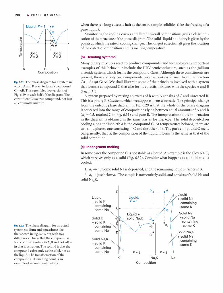
190 6 PHASE DIAGRAMS
Liquid, = 1P
Solid,= 2P
Solid,= 2P
BCA
a1
a2
a3
a4 e
Tem
pera
ture
Composition
Fig. 6.31 The phase diagram for a system inwhich A and B react to form a compound C = AB. This resembles two versions of Fig. 6.29 in each half of the diagram. Theconstituent C is a true compound, not justan equimolar mixture.
Liquid,= 1P
= 2P= 2P
a2
a3
b2
b3
b4
K Na K2 Na
T1
T2
T2
T3
T4
Liquid +solid Na K2
Liquid+ solid Na
containingsome K
Composition
a1b1
Solid Na K+ solid Na
containingsome K
2
Solid Na+solid Na
containingsome K
Liquid+ solid K
containingsome Na
Solid K+ solid K
containingsome Na
Solid Na K+ solid K
containingsome Na
2
�
Fig. 6.32 The phase diagram for an actualsystem (sodium and potassium) like that shown in Fig. 6.35, but with twodifferences. One is that the compound isNa2K, corresponding to A2B and not AB asin that illustration. The second is that thecompound exists only as the solid, not asthe liquid. The transformation of thecompound at its melting point is anexample of incongruent melting.
when there is a long eutectic halt as the entire sample solidifies (like the freezing of apure liquid).
Monitoring the cooling curves at different overall compositions gives a clear indi-cation of the structure of the phase diagram. The solid–liquid boundary is given by thepoints at which the rate of cooling changes. The longest eutectic halt gives the locationof the eutectic composition and its melting temperature.
(b) Reacting systems
Many binary mixtures react to produce compounds, and technologically importantexamples of this behaviour include the III/V semiconductors, such as the gallium arsenide system, which forms the compound GaAs. Although three constituents arepresent, there are only two components because GaAs is formed from the reaction Ga + As 5 GaAs. We shall illustrate some of the principles involved with a systemthat forms a compound C that also forms eutectic mixtures with the species A and B(Fig. 6.31).
A system prepared by mixing an excess of B with A consists of C and unreacted B.This is a binary B, C system, which we suppose forms a eutectic. The principal changefrom the eutectic phase diagram in Fig. 6.29 is that the whole of the phase diagramis squeezed into the range of compositions lying between equal amounts of A and B (xB = 0.5, marked C in Fig. 6.31) and pure B. The interpretation of the information in the diagram is obtained in the same way as for Fig. 6.32. The solid deposited oncooling along the isopleth a is the compound C. At temperatures below a4 there aretwo solid phases, one consisting of C and the other of B. The pure compound C meltscongruently, that is, the composition of the liquid it forms is the same as that of thesolid compound.
(c) Incongruent melting
In some cases the compound C is not stable as a liquid. An example is the alloy Na2K,which survives only as a solid (Fig. 6.32). Consider what happens as a liquid at a1 iscooled:
1. a1 → a2. Some solid Na is deposited, and the remaining liquid is richer in K.
2. a2 → just below a3. The sample is now entirely solid, and consists of solid Na andsolid Na2K.
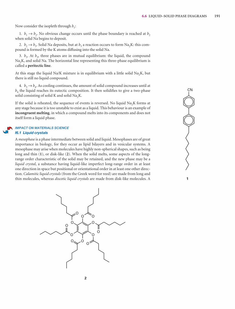
6.6 LIQUID–SOLID PHASE DIAGRAMS 191
Now consider the isopleth through b1:
1. b1 → b2. No obvious change occurs until the phase boundary is reached at b2
when solid Na begins to deposit.
2. b2 → b3. Solid Na deposits, but at b3 a reaction occurs to form Na2K: this com-pound is formed by the K atoms diffusing into the solid Na.
3. b3. At b3, three phases are in mutual equilibrium: the liquid, the compoundNa2K, and solid Na. The horizontal line representing this three-phase equilibrium iscalled a peritectic line.
At this stage the liquid Na/K mixture is in equilibrium with a little solid Na2K, butthere is still no liquid compound.
4. b3 → b4. As cooling continues, the amount of solid compound increases until atb4 the liquid reaches its eutectic composition. It then solidifies to give a two-phasesolid consisting of solid K and solid Na2K.
If the solid is reheated, the sequence of events is reversed. No liquid Na2K forms at any stage because it is too unstable to exist as a liquid. This behaviour is an example ofincongruent melting, in which a compound melts into its components and does notitself form a liquid phase.
IMPACT ON MATERIALS SCIENCE
I6.1 Liquid crystals
A mesophase is a phase intermediate between solid and liquid. Mesophases are of greatimportance in biology, for they occur as lipid bilayers and in vesicular systems. Amesophase may arise when molecules have highly non-spherical shapes, such as beinglong and thin (1), or disk-like (2). When the solid melts, some aspects of the long-range order characteristic of the solid may be retained, and the new phase may be a liquid crystal, a substance having liquid-like imperfect long-range order in at least one direction in space but positional or orientational order in at least one other direc-tion. Calamitic liquid crystals (from the Greek word for reed) are made from long and thin molecules, whereas discotic liquid crystals are made from disk-like molecules. A
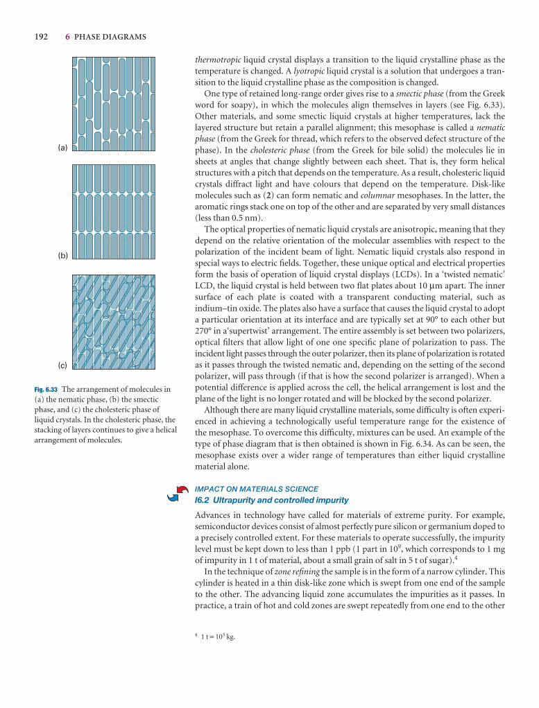
192 6 PHASE DIAGRAMS
thermotropic liquid crystal displays a transition to the liquid crystalline phase as thetemperature is changed. A lyotropic liquid crystal is a solution that undergoes a tran-sition to the liquid crystalline phase as the composition is changed.
One type of retained long-range order gives rise to a smectic phase (from the Greekword for soapy), in which the molecules align themselves in layers (see Fig. 6.33).Other materials, and some smectic liquid crystals at higher temperatures, lack thelayered structure but retain a parallel alignment; this mesophase is called a nematicphase (from the Greek for thread, which refers to the observed defect structure of thephase). In the cholesteric phase (from the Greek for bile solid) the molecules lie insheets at angles that change slightly between each sheet. That is, they form helicalstructures with a pitch that depends on the temperature. As a result, cholesteric liquidcrystals diffract light and have colours that depend on the temperature. Disk-likemolecules such as (2) can form nematic and columnar mesophases. In the latter, thearomatic rings stack one on top of the other and are separated by very small distances(less than 0.5 nm).
The optical properties of nematic liquid crystals are anisotropic, meaning that theydepend on the relative orientation of the molecular assemblies with respect to the polarization of the incident beam of light. Nematic liquid crystals also respond in special ways to electric fields. Together, these unique optical and electrical propertiesform the basis of operation of liquid crystal displays (LCDs). In a ‘twisted nematic’LCD, the liquid crystal is held between two flat plates about 10 µm apart. The innersurface of each plate is coated with a transparent conducting material, such as indium–tin oxide. The plates also have a surface that causes the liquid crystal to adopta particular orientation at its interface and are typically set at 90° to each other but270° in a‘supertwist’ arrangement. The entire assembly is set between two polarizers,optical filters that allow light of one one specific plane of polarization to pass. The incident light passes through the outer polarizer, then its plane of polarization is rotatedas it passes through the twisted nematic and, depending on the setting of the second polarizer, will pass through (if that is how the second polarizer is arranged). When apotential difference is applied across the cell, the helical arrangement is lost and theplane of the light is no longer rotated and will be blocked by the second polarizer.
Although there are many liquid crystalline materials, some difficulty is often experi-enced in achieving a technologically useful temperature range for the existence of the mesophase. To overcome this difficulty, mixtures can be used. An example of thetype of phase diagram that is then obtained is shown in Fig. 6.34. As can be seen, themesophase exists over a wider range of temperatures than either liquid crystallinematerial alone.
IMPACT ON MATERIALS SCIENCE
I6.2 Ultrapurity and controlled impurity
Advances in technology have called for materials of extreme purity. For example,semiconductor devices consist of almost perfectly pure silicon or germanium doped toa precisely controlled extent. For these materials to operate successfully, the impuritylevel must be kept down to less than 1 ppb (1 part in 109, which corresponds to 1 mgof impurity in 1 t of material, about a small grain of salt in 5 t of sugar).4
In the technique of zone refining the sample is in the form of a narrow cylinder. Thiscylinder is heated in a thin disk-like zone which is swept from one end of the sampleto the other. The advancing liquid zone accumulates the impurities as it passes. Inpractice, a train of hot and cold zones are swept repeatedly from one end to the other
4 1 t = 103 kg.
(a)
(b)
(c)
Fig. 6.33 The arrangement of molecules in (a) the nematic phase, (b) the smecticphase, and (c) the cholesteric phase ofliquid crystals. In the cholesteric phase, thestacking of layers continues to give a helicalarrangement of molecules.
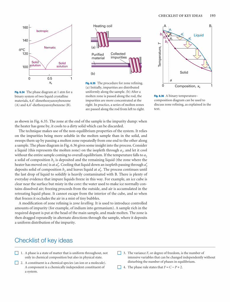
CHECKLIST OF KEY IDEAS 193
as shown in Fig. 6.35. The zone at the end of the sample is the impurity dump: whenthe heater has gone by, it cools to a dirty solid which can be discarded.
The technique makes use of the non-equilibrium properties of the system. It relieson the impurities being more soluble in the molten sample than in the solid, andsweeps them up by passing a molten zone repeatedly from one end to the other alonga sample. The phase diagram in Fig. 6.36 gives some insight into the process. Considera liquid (this represents the molten zone) on the isopleth through a1, and let it coolwithout the entire sample coming to overall equilibrium. If the temperature falls to a2
a solid of composition b2 is deposited and the remaining liquid (the zone where theheater has moved on) is at a2′ . Cooling that liquid down an isopleth passing through a2′deposits solid of composition b3 and leaves liquid at a3′ . The process continues untilthe last drop of liquid to solidify is heavily contaminated with B. There is plenty ofeveryday evidence that impure liquids freeze in this way. For example, an ice cube isclear near the surface but misty in the core: the water used to make ice normally con-tains dissolved air; freezing proceeds from the outside, and air is accumulated in theretreating liquid phase. It cannot escape from the interior of the cube, and so whenthat freezes it occludes the air in a mist of tiny bubbles.
A modification of zone refining is zone levelling. It is used to introduce controlledamounts of impurity (for example, of indium into germanium). A sample rich in therequired dopant is put at the head of the main sample, and made molten. The zone isthen dragged repeatedly in alternate directions through the sample, where it depositsa uniform distribution of the impurity.
Checklist of key ideas
1. A phase is a state of matter that is uniform throughout, notonly in chemical composition but also in physical state.
2. A constituent is a chemical species (an ion or a molecule). A component is a chemically independent constituent of a system.
3. The variance F, or degree of freedom, is the number ofintensive variables that can be changed independently withoutdisturbing the number of phases in equilibrium.
4. The phase rule states that F = C − P + 2.
Liquid
Solid
Tem
pera
ture
,T
Composition, xB
BAa1
a2�
a3�a3
b1b2
b3
a0 1
a2
Fig. 6.36 A binary temperature–composition diagram can be used todiscuss zone refining, as explained in thetext.
160
140
120
100
/°C
0 0.5 1xB
Isotropic
Nematic
Solidsolution
Solidsolution
�
Fig. 6.34 The phase diagram at 1 atm for abinary system of two liquid crystallinematerials, 4,4′-dimethoxyazoxybenzene(A) and 4,4′-diethoxyazoxybenzene (B).
Heating coil
(a)
(b)
Purifiedmaterial
Collectedimpurities
Fig. 6.35 The procedure for zone refining. (a) Initially, impurities are distributeduniformly along the sample. (b) After amolten zone is passed along the rod, theimpurities are more concentrated at theright. In practice, a series of molten zonesare passed along the rod from left to right.

194 6 PHASE DIAGRAMS
Discussion questions
6.1 Define the following terms: phase, constituent, component, and degree offreedom.
6.2 What factors determine the number of theoretical plates required toachieve a desired degree of separation in fractional distillation?
6.3 Draw phase diagrams for the following types of systems. Label the regionsand intersections of the diagrams, stating what materials (possibly compoundsor azeotropes) are present and whether they are solid liquid or gas. (a) One-component, pressure–temperature diagram, liquid density greater than that ofsolid. (b) Two-component, temperature–composition, solid–liquid diagram,one compound AB formed that melts congruently, negligible solid–solidsolubility.
6.4 Draw phase diagrams for the following types of systems. Label the regions and intersections of the diagrams, stating what materials (possibly
Further reading
Articles and texts
J.S. Alper, The Gibbs phase rule revisited: interrelationships betweencomponents and phases. J. Chem. Educ. 76, 1567 (1999).
W.D. Callister, Jr., Materials science and engineering, an introduction.Wiley, New York (2000).
P.J. Collings and M. Hird, Introduction to liquid crystals: chemistryand physics. Taylor & Francis, London (1997).
M. Hillert, Phase equilibria, phase diagrams and phase transformations:a thermodynamic basis. Cambridge University Press (1998).
H.-G. Lee, Chemical thermodynamics for metals and materials.Imperial College Press, London (1999).
R.J. Stead and K. Stead, Phase diagrams for ternary liquid systems. J. Chem. Educ. 67, 385 (1990).
S.I. Sandler, Chemical and engineering thermodynamics. Wiley, New York (1998).
Sources of data and information
A. Alper, Phase diagrams, Vols. 1, 2, and 3. Academic Press, New York(1970).
J. Wisniak, Phase diagrams: a literature source book. Elsevier,Amsterdam (1981–86).
5. Thermal analysis is a technique for detecting phase transitionsthat takes advantage of the effect of the enthalpy changeduring a first-order transition.
6. The vapour pressure of an ideal solution is given by p = p*B + (p*A − p*B)xA. The composition of the vapour, yA = xA p*A/{p*B + (p*A − p*B)xA}, yB = 1 − yA.
7. The total vapour pressure of a mixture is given by p = pA*p*B /{p*A + (p*B − p*A)yA}.
8. An isopleth is a line of constant composition in a phasediagram. A tie line is a line joining two points representingphases in equilibrium.
9. The lever rule allows for the calculation of the relativeamounts of two phases in equilibrium: nαlα = nβlβ.
10. A temperature–composition diagram is a phase diagram inwhich the boundaries show the composition of the phases thatare in equilibrium at various temperatures.
11. An azeotrope is a mixture that boils without change ofcomposition.
12. Partially miscible liquids are liquids that do not mix in allproportions at all temperatures.
13. The upper critical solution temperature is the highesttemperature at which phase separation occurs in a binaryliquid mixture. The lower critical solution temperature is thetemperature below which the components of a binary mixturemix in all proportions and above which they form two phases.
14. A eutectic is the mixture with the lowest melting point; a liquid with the eutectic composition freezes at a singletemperature. A eutectic halt is a delay in cooling while theeutectic freezes.
15. Incongruent melting occurs when a compound melts into itscomponents and does not itself form a liquid phase.
compounds or azeotropes) are present and whether they are solid liquid orgas. (a) Two-component, temperature–composition, solid–liquid diagram,one compound of formula AB2 that melts incongruently, negligiblesolid–solid solubility; (b) two-component, constant temperature–composition, liquid–vapour diagram, formation of an azeotrope at xB = 0.333,complete miscibility.
6.5 Label the regions of the phase diagram in Fig. 6.37. State what substances(if compounds give their formulas) exist in each region. Label each substancein each region as solid, liquid, or gas.
6.6 Label the regions of the phase diagram in Fig. 6.38. State what substances(if compounds give their formulas) exist in each region. Label each substancein each region as solid, liquid, or gas.
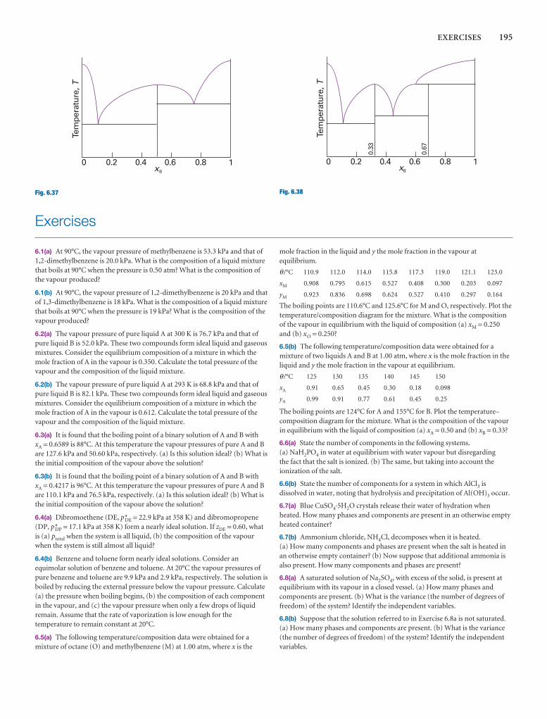
EXERCISES 195
Exercises
6.1(a) At 90°C, the vapour pressure of methylbenzene is 53.3 kPa and that of1,2-dimethylbenzene is 20.0 kPa. What is the composition of a liquid mixturethat boils at 90°C when the pressure is 0.50 atm? What is the composition ofthe vapour produced?
6.1(b) At 90°C, the vapour pressure of 1,2-dimethylbenzene is 20 kPa and thatof 1,3-dimethylbenzene is 18 kPa. What is the composition of a liquid mixturethat boils at 90°C when the pressure is 19 kPa? What is the composition of thevapour produced?
6.2(a) The vapour pressure of pure liquid A at 300 K is 76.7 kPa and that ofpure liquid B is 52.0 kPa. These two compounds form ideal liquid and gaseousmixtures. Consider the equilibrium composition of a mixture in which themole fraction of A in the vapour is 0.350. Calculate the total pressure of thevapour and the composition of the liquid mixture.
6.2(b) The vapour pressure of pure liquid A at 293 K is 68.8 kPa and that ofpure liquid B is 82.1 kPa. These two compounds form ideal liquid and gaseousmixtures. Consider the equilibrium composition of a mixture in which themole fraction of A in the vapour is 0.612. Calculate the total pressure of thevapour and the composition of the liquid mixture.
6.3(a) It is found that the boiling point of a binary solution of A and B with xA = 0.6589 is 88°C. At this temperature the vapour pressures of pure A and Bare 127.6 kPa and 50.60 kPa, respectively. (a) Is this solution ideal? (b) What isthe initial composition of the vapour above the solution?
6.3(b) It is found that the boiling point of a binary solution of A and B with xA = 0.4217 is 96°C. At this temperature the vapour pressures of pure A and Bare 110.1 kPa and 76.5 kPa, respectively. (a) Is this solution ideal? (b) What isthe initial composition of the vapour above the solution?
6.4(a) Dibromoethene (DE, p*DE = 22.9 kPa at 358 K) and dibromopropene(DP, p*DP = 17.1 kPa at 358 K) form a nearly ideal solution. If zDE = 0.60, whatis (a) ptotal when the system is all liquid, (b) the composition of the vapourwhen the system is still almost all liquid?
6.4(b) Benzene and toluene form nearly ideal solutions. Consider anequimolar solution of benzene and toluene. At 20°C the vapour pressures ofpure benzene and toluene are 9.9 kPa and 2.9 kPa, respectively. The solution isboiled by reducing the external pressure below the vapour pressure. Calculate(a) the pressure when boiling begins, (b) the composition of each componentin the vapour, and (c) the vapour pressure when only a few drops of liquidremain. Assume that the rate of vaporization is low enough for thetemperature to remain constant at 20°C.
6.5(a) The following temperature/composition data were obtained for amixture of octane (O) and methylbenzene (M) at 1.00 atm, where x is the
mole fraction in the liquid and y the mole fraction in the vapour at equilibrium.
θ /°C 110.9 112.0 114.0 115.8 117.3 119.0 121.1 123.0
xM 0.908 0.795 0.615 0.527 0.408 0.300 0.203 0.097
yM 0.923 0.836 0.698 0.624 0.527 0.410 0.297 0.164
The boiling points are 110.6°C and 125.6°C for M and O, respectively. Plot thetemperature/composition diagram for the mixture. What is the compositionof the vapour in equilibrium with the liquid of composition (a) xM = 0.250and (b) xO = 0.250?
6.5(b) The following temperature/composition data were obtained for amixture of two liquids A and B at 1.00 atm, where x is the mole fraction in theliquid and y the mole fraction in the vapour at equilibrium.
θ /°C 125 130 135 140 145 150
xA 0.91 0.65 0.45 0.30 0.18 0.098
yA 0.99 0.91 0.77 0.61 0.45 0.25
The boiling points are 124°C for A and 155°C for B. Plot the temperature–composition diagram for the mixture. What is the composition of the vapourin equilibrium with the liquid of composition (a) xA = 0.50 and (b) xB = 0.33?
6.6(a) State the number of components in the following systems. (a) NaH2PO4 in water at equilibrium with water vapour but disregarding the fact that the salt is ionized. (b) The same, but taking into account theionization of the salt.
6.6(b) State the number of components for a system in which AlCl3 isdissolved in water, noting that hydrolysis and precipitation of Al(OH)3 occur.
6.7(a) Blue CuSO4·5H2O crystals release their water of hydration whenheated. How many phases and components are present in an otherwise emptyheated container?
6.7(b) Ammonium chloride, NH4Cl, decomposes when it is heated. (a) How many components and phases are present when the salt is heated inan otherwise empty container? (b) Now suppose that additional ammonia isalso present. How many components and phases are present?
6.8(a) A saturated solution of Na2SO4, with excess of the solid, is present atequilibrium with its vapour in a closed vessel. (a) How many phases andcomponents are present. (b) What is the variance (the number of degrees offreedom) of the system? Identify the independent variables.
6.8(b) Suppose that the solution referred to in Exercise 6.8a is not saturated.(a) How many phases and components are present. (b) What is the variance(the number of degrees of freedom) of the system? Identify the independentvariables.
0 1xB
0.2 0.4 0.6 0.8
Tem
pera
ture
, T
Fig. 6.37
0 1xB
0.2 0.4 0.6 0.8
Tem
pera
ture
,T
0.33
0.67
Fig. 6.38
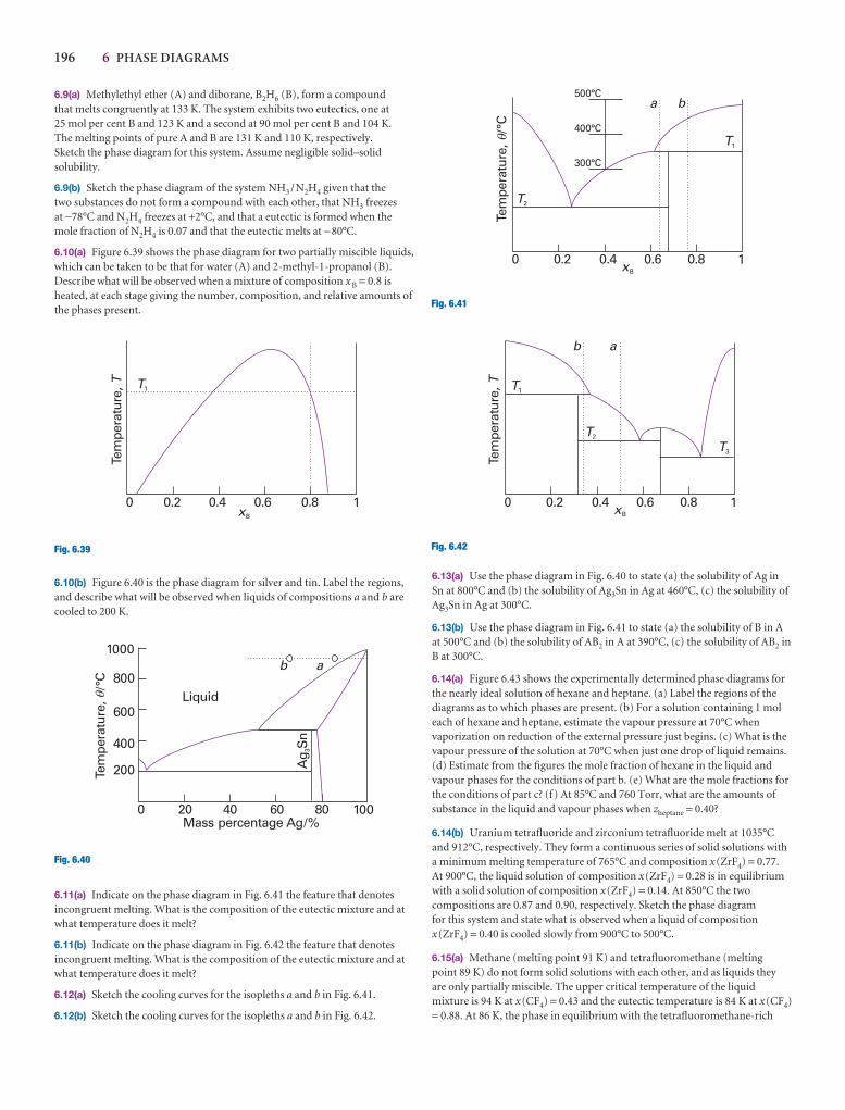
196 6 PHASE DIAGRAMS
6.9(a) Methylethyl ether (A) and diborane, B2H6 (B), form a compound that melts congruently at 133 K. The system exhibits two eutectics, one at 25 mol per cent B and 123 K and a second at 90 mol per cent B and 104 K. The melting points of pure A and B are 131 K and 110 K, respectively. Sketch the phase diagram for this system. Assume negligible solid–solidsolubility.
6.9(b) Sketch the phase diagram of the system NH3 /N2H4 given that the two substances do not form a compound with each other, that NH3 freezesat −78°C and N2H4 freezes at +2°C, and that a eutectic is formed when themole fraction of N2H4 is 0.07 and that the eutectic melts at −80°C.
6.10(a) Figure 6.39 shows the phase diagram for two partially miscible liquids,which can be taken to be that for water (A) and 2-methyl-1-propanol (B).Describe what will be observed when a mixture of composition x B = 0.8 isheated, at each stage giving the number, composition, and relative amounts ofthe phases present.
6.10(b) Figure 6.40 is the phase diagram for silver and tin. Label the regions,and describe what will be observed when liquids of compositions a and b arecooled to 200 K.
6.11(a) Indicate on the phase diagram in Fig. 6.41 the feature that denotesincongruent melting. What is the composition of the eutectic mixture and atwhat temperature does it melt?
6.11(b) Indicate on the phase diagram in Fig. 6.42 the feature that denotesincongruent melting. What is the composition of the eutectic mixture and atwhat temperature does it melt?
6.12(a) Sketch the cooling curves for the isopleths a and b in Fig. 6.41.
6.12(b) Sketch the cooling curves for the isopleths a and b in Fig. 6.42.
Fig. 6.40
0 100
Tem
pera
ture
, /
°C
200
400
600
800
1000
Liquid
ab
Ag
Sn
3
20 40 60 80Mass percentage Ag/%
�
Fig. 6.39
0 1xB
0.2 0.4 0.6 0.8
Tem
pera
ture
, T T1
6.13(a) Use the phase diagram in Fig. 6.40 to state (a) the solubility of Ag inSn at 800°C and (b) the solubility of Ag3Sn in Ag at 460°C, (c) the solubility ofAg3Sn in Ag at 300°C.
6.13(b) Use the phase diagram in Fig. 6.41 to state (a) the solubility of B in Aat 500°C and (b) the solubility of AB2 in A at 390°C, (c) the solubility of AB2 inB at 300°C.
6.14(a) Figure 6.43 shows the experimentally determined phase diagrams forthe nearly ideal solution of hexane and heptane. (a) Label the regions of thediagrams as to which phases are present. (b) For a solution containing 1 moleach of hexane and heptane, estimate the vapour pressure at 70°C whenvaporization on reduction of the external pressure just begins. (c) What is thevapour pressure of the solution at 70°C when just one drop of liquid remains.(d) Estimate from the figures the mole fraction of hexane in the liquid andvapour phases for the conditions of part b. (e) What are the mole fractions forthe conditions of part c? (f) At 85°C and 760 Torr, what are the amounts ofsubstance in the liquid and vapour phases when zheptane = 0.40?
6.14(b) Uranium tetrafluoride and zirconium tetrafluoride melt at 1035°Cand 912°C, respectively. They form a continuous series of solid solutions witha minimum melting temperature of 765°C and composition x(ZrF4) = 0.77.At 900°C, the liquid solution of composition x(ZrF4) = 0.28 is in equilibriumwith a solid solution of composition x(ZrF4) = 0.14. At 850°C the twocompositions are 0.87 and 0.90, respectively. Sketch the phase diagram for this system and state what is observed when a liquid of compositionx(ZrF4) = 0.40 is cooled slowly from 900°C to 500°C.
6.15(a) Methane (melting point 91 K) and tetrafluoromethane (melting point 89 K) do not form solid solutions with each other, and as liquids theyare only partially miscible. The upper critical temperature of the liquidmixture is 94 K at x(CF4) = 0.43 and the eutectic temperature is 84 K at x(CF4)= 0.88. At 86 K, the phase in equilibrium with the tetrafluoromethane-rich
0 1
Tem
pera
ture
, /
°C
0.2 0.4 0.6 0.8xB
a b
300°C
400°C
500°C
T1
T2
�
Fig. 6.41
0 1Te
mpe
ratu
re,T
0.2 0.4 0.6 0.8xB
ab
T1
T2
T3
Fig. 6.42
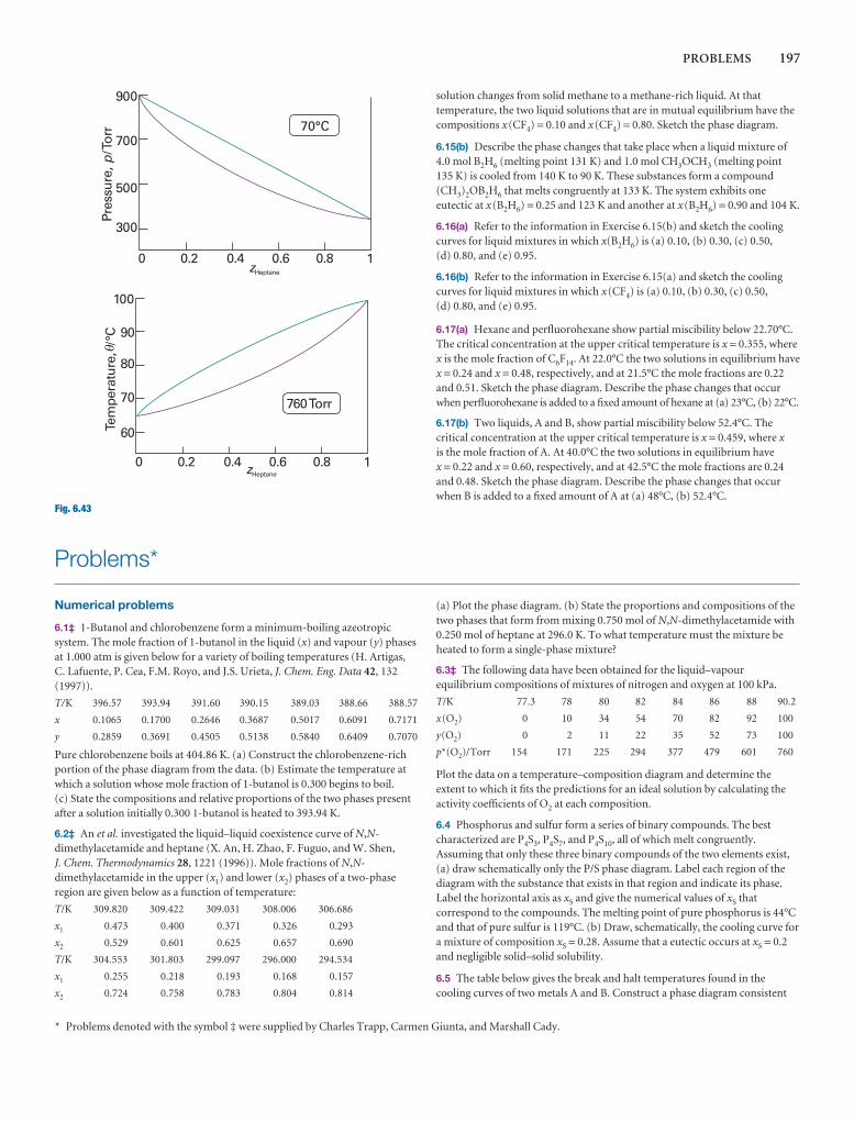
PROBLEMS 197
* Problems denoted with the symbol ‡ were supplied by Charles Trapp, Carmen Giunta, and Marshall Cady.
solution changes from solid methane to a methane-rich liquid. At thattemperature, the two liquid solutions that are in mutual equilibrium have thecompositions x(CF4) = 0.10 and x(CF4) = 0.80. Sketch the phase diagram.
6.15(b) Describe the phase changes that take place when a liquid mixture of4.0 mol B2H6 (melting point 131 K) and 1.0 mol CH3OCH3 (melting point135 K) is cooled from 140 K to 90 K. These substances form a compound(CH3)2OB2H6 that melts congruently at 133 K. The system exhibits oneeutectic at x(B2H6) = 0.25 and 123 K and another at x(B2H6) = 0.90 and 104 K.
6.16(a) Refer to the information in Exercise 6.15(b) and sketch the coolingcurves for liquid mixtures in which x(B2H6) is (a) 0.10, (b) 0.30, (c) 0.50, (d) 0.80, and (e) 0.95.
6.16(b) Refer to the information in Exercise 6.15(a) and sketch the coolingcurves for liquid mixtures in which x(CF4) is (a) 0.10, (b) 0.30, (c) 0.50, (d) 0.80, and (e) 0.95.
6.17(a) Hexane and perfluorohexane show partial miscibility below 22.70°C.The critical concentration at the upper critical temperature is x = 0.355, wherex is the mole fraction of C6F14. At 22.0°C the two solutions in equilibrium havex = 0.24 and x = 0.48, respectively, and at 21.5°C the mole fractions are 0.22and 0.51. Sketch the phase diagram. Describe the phase changes that occurwhen perfluorohexane is added to a fixed amount of hexane at (a) 23°C, (b) 22°C.
6.17(b) Two liquids, A and B, show partial miscibility below 52.4°C. Thecritical concentration at the upper critical temperature is x = 0.459, where xis the mole fraction of A. At 40.0°C the two solutions in equilibrium have x = 0.22 and x = 0.60, respectively, and at 42.5°C the mole fractions are 0.24and 0.48. Sketch the phase diagram. Describe the phase changes that occurwhen B is added to a fixed amount of A at (a) 48°C, (b) 52.4°C.
0 1
Pres
sure
,/T
orr
p
0.2 0.4 0.6 0.8zHeptane
300
500
700
900
70°C
0 10.2 0.4 0.6 0.8zHeptane
760Torr
Tem
pera
ture
, /°
C
60
70
80
90
100
�
Fig. 6.43
Problems*
Numerical problems
6.1‡ 1-Butanol and chlorobenzene form a minimum-boiling azeotropicsystem. The mole fraction of 1-butanol in the liquid (x) and vapour (y) phasesat 1.000 atm is given below for a variety of boiling temperatures (H. Artigas, C. Lafuente, P. Cea, F.M. Royo, and J.S. Urieta, J. Chem. Eng. Data 42, 132(1997)).
T/K 396.57 393.94 391.60 390.15 389.03 388.66 388.57
x 0.1065 0.1700 0.2646 0.3687 0.5017 0.6091 0.7171
y 0.2859 0.3691 0.4505 0.5138 0.5840 0.6409 0.7070
Pure chlorobenzene boils at 404.86 K. (a) Construct the chlorobenzene-richportion of the phase diagram from the data. (b) Estimate the temperature atwhich a solution whose mole fraction of 1-butanol is 0.300 begins to boil. (c) State the compositions and relative proportions of the two phases presentafter a solution initially 0.300 1-butanol is heated to 393.94 K.
6.2‡ An et al. investigated the liquid–liquid coexistence curve of N,N-dimethylacetamide and heptane (X. An, H. Zhao, F. Fuguo, and W. Shen,J. Chem. Thermodynamics 28, 1221 (1996)). Mole fractions of N,N-dimethylacetamide in the upper (x1) and lower (x2) phases of a two-phaseregion are given below as a function of temperature:
T/K 309.820 309.422 309.031 308.006 306.686
x1 0.473 0.400 0.371 0.326 0.293
x2 0.529 0.601 0.625 0.657 0.690
T/K 304.553 301.803 299.097 296.000 294.534
x1 0.255 0.218 0.193 0.168 0.157
x2 0.724 0.758 0.783 0.804 0.814
(a) Plot the phase diagram. (b) State the proportions and compositions of thetwo phases that form from mixing 0.750 mol of N,N-dimethylacetamide with0.250 mol of heptane at 296.0 K. To what temperature must the mixture beheated to form a single-phase mixture?
6.3‡ The following data have been obtained for the liquid–vapourequilibrium compositions of mixtures of nitrogen and oxygen at 100 kPa.
T/K 77.3 78 80 82 84 86 88 90.2
x(O2) 0 10 34 54 70 82 92 100
y(O2) 0 2 11 22 35 52 73 100
p*(O2)/Torr 154 171 225 294 377 479 601 760
Plot the data on a temperature–composition diagram and determine theextent to which it fits the predictions for an ideal solution by calculating theactivity coefficients of O2 at each composition.
6.4 Phosphorus and sulfur form a series of binary compounds. The bestcharacterized are P4S3, P4S7, and P4S10, all of which melt congruently.Assuming that only these three binary compounds of the two elements exist,(a) draw schematically only the P/S phase diagram. Label each region of thediagram with the substance that exists in that region and indicate its phase.Label the horizontal axis as xS and give the numerical values of xS thatcorrespond to the compounds. The melting point of pure phosphorus is 44°Cand that of pure sulfur is 119°C. (b) Draw, schematically, the cooling curve fora mixture of composition xS = 0.28. Assume that a eutectic occurs at xS = 0.2and negligible solid–solid solubility.
6.5 The table below gives the break and halt temperatures found in thecooling curves of two metals A and B. Construct a phase diagram consistent
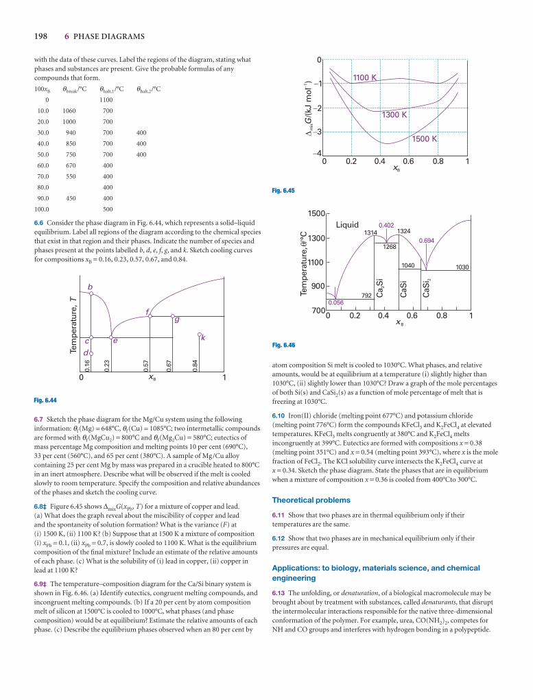
198 6 PHASE DIAGRAMS
with the data of these curves. Label the regions of the diagram, stating whatphases and substances are present. Give the probable formulas of anycompounds that form.
100xB θbreak/°C θhalt,1/°C θhalt,2/°C
0 1100
10.0 1060 700
20.0 1000 700
30.0 940 700 400
40.0 850 700 400
50.0 750 700 400
60.0 670 400
70.0 550 400
80.0 400
90.0 450 400
100.0 500
6.6 Consider the phase diagram in Fig. 6.44, which represents a solid–liquidequilibrium. Label all regions of the diagram according to the chemical speciesthat exist in that region and their phases. Indicate the number of species andphases present at the points labelled b, d, e, f, g, and k. Sketch cooling curvesfor compositions xB = 0.16, 0.23, 0.57, 0.67, and 0.84.
atom composition Si melt is cooled to 1030°C. What phases, and relativeamounts, would be at equilibrium at a temperature (i) slightly higher than1030°C, (ii) slightly lower than 1030°C? Draw a graph of the mole percentagesof both Si(s) and CaSi2(s) as a function of mole percentage of melt that isfreezing at 1030°C.
6.10 Iron(II) chloride (melting point 677°C) and potassium chloride(melting point 776°C) form the compounds KFeCl3 and K2FeCl4 at elevatedtemperatures. KFeCl3 melts congruently at 380°C and K2FeCl4 meltsincongruently at 399°C. Eutectics are formed with compositions x = 0.38(melting point 351°C) and x = 0.54 (melting point 393°C), where x is the molefraction of FeCl2. The KCl solubility curve intersects the K2FeCl4 curve at x = 0.34. Sketch the phase diagram. State the phases that are in equilibriumwhen a mixture of composition x = 0.36 is cooled from 400°Cto 300°C.
Theoretical problems
6.11 Show that two phases are in thermal equilibrium only if theirtemperatures are the same.
6.12 Show that two phases are in mechanical equilibrium only if theirpressures are equal.
Applications: to biology, materials science, and chemicalengineering
6.13 The unfolding, or denaturation, of a biological macromolecule may bebrought about by treatment with substances, called denaturants, that disruptthe intermolecular interactions responsible for the native three-dimensionalconformation of the polymer. For example, urea, CO(NH2)2, competes forNH and CO groups and interferes with hydrogen bonding in a polypeptide.
Tem
pera
ture
, /°
C
0 1xB
700
900
1100
1300
1500
0.2 0.4 0.6 0.8
Liquid
Ca
Si
2
CaS
i
CaS
i 2
1030
0.6941324
1040
1268
0.4021314
7920.056
�
Fig. 6.46
Tem
pera
ture
, T
0.16
0.23
0.57
0.67
0.84
b
cd
e
fg
k
0 1xB
Fig. 6.44
0 1xB
0.2 0.4 0.6 0.8�4
�3
�2
�1
0
m
ixG/(k
J m
ol)1
1100 K
1300 K
1500 K
�
Fig. 6.45
6.7 Sketch the phase diagram for the Mg/Cu system using the followinginformation: θf (Mg) = 648°C, θf (Cu) = 1085°C; two intermetallic compoundsare formed with θf (MgCu2) = 800°C and θf (Mg2Cu) = 580°C; eutectics ofmass percentage Mg composition and melting points 10 per cent (690°C), 33 per cent (560°C), and 65 per cent (380°C). A sample of Mg/Cu alloycontaining 25 per cent Mg by mass was prepared in a crucible heated to 800°Cin an inert atmosphere. Describe what will be observed if the melt is cooledslowly to room temperature. Specify the composition and relative abundancesof the phases and sketch the cooling curve.
6.8‡ Figure 6.45 shows ∆mixG(xPb, T) for a mixture of copper and lead. (a) What does the graph reveal about the miscibility of copper and lead and the spontaneity of solution formation? What is the variance (F) at (i) 1500 K, (ii) 1100 K? (b) Suppose that at 1500 K a mixture of composition(i) xPb = 0.1, (ii) xPb = 0.7, is slowly cooled to 1100 K. What is the equilibriumcomposition of the final mixture? Include an estimate of the relative amountsof each phase. (c) What is the solubility of (i) lead in copper, (ii) copper inlead at 1100 K?
6.9‡ The temperature–composition diagram for the Ca/Si binary system isshown in Fig. 6.46. (a) Identify eutectics, congruent melting compounds, andincongruent melting compounds. (b) If a 20 per cent by atom compositionmelt of silicon at 1500°C is cooled to 1000°C, what phases (and phasecomposition) would be at equilibrium? Estimate the relative amounts of eachphase. (c) Describe the equilibrium phases observed when an 80 per cent by
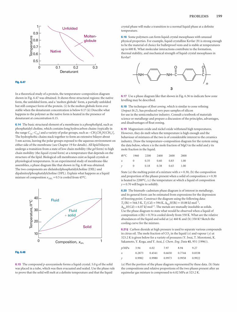
PROBLEMS 199
In a theoretical study of a protein, the temperature–composition diagramshown in Fig. 6.47 was obtained. It shows three structural regions: the nativeform, the unfolded form, and a ‘molten globule’ form, a partially unfolded but still compact form of the protein. (i) Is the molten globule form everstable when the denaturant concentration is below 0.1? (ii) Describe whathappens to the polymer as the native form is heated in the presence ofdenaturant at concentration 0.15.
6.14 The basic structural element of a membrane is a phospholipid, such asphosphatidyl choline, which contains long hydrocarbon chains (typically inthe range C14 –C24) and a variety of polar groups, such as –CH2CH2N(CH3)3
+.The hydrophobic chains stack together to form an extensive bilayer about 5 nm across, leaving the polar groups exposed to the aqueous environment oneither side of the membrane (see Chapter 19 for details). All lipid bilayersundergo a transition from a state of low chain mobility (the gel form) to highchain mobility (the liquid crystal form) at a temperature that depends on thestructure of the lipid. Biological cell membranes exist as liquid crystals atphysiological temperatures. In an experimental study of membrane-likeassemblies, a phase diagram like that shown in Fig. 6.48 was obtained. The two components are dielaidoylphosphatidylcholine (DEL) anddipalmitoylphosphatidylcholine (DPL). Explain what happens as a liquidmixture of composition x DEL = 0.5 is cooled from 45°C.
crystal phase will make a transition to a normal liquid phase at a definitetemperature.
6.16 Some polymers can form liquid crystal mesophases with unusualphysical properties. For example, liquid crystalline Kevlar (3) is strong enoughto be the material of choice for bulletproof vests and is stable at temperaturesup to 600 K. What molecular interactions contribute to the formation,thermal stability, and mechanical strength of liquid crystal mesophases inKevlar?
0 0.1 0.2 0.3Denaturant
0.5
0.6
0.7
0.8
0.9
1Te
mpe
ratu
reUnfolded
Native
Molten-globule
Fig. 6.47
0 1Composition, xDPL
Tem
pera
ture
, /°
C
10
20
30
40Fluid
Solid
Fluidsolid�
�
Fig. 6.48
6.15 The compound p-azoxyanisole forms a liquid crystal. 5.0 g of the solidwas placed in a tube, which was then evacuated and sealed. Use the phase ruleto prove that the solid will melt at a definite temperature and that the liquid
6.17 Use a phase diagram like that shown in Fig. 6.36 to indicate how zonelevelling may be described.
6.18 The technique of float zoning, which is similar to zone refining (Impact I6.2), has produced very pure samples of silicon for use in the semiconductor industry. Consult a textbook of materials science or metallurgy and prepare a discussion of the principles, advantages,and disadvantages of float zoning.
6.19 Magnesium oxide and nickel oxide withstand high temperatures.However, they do melt when the temperature is high enough and thebehaviour of mixtures of the two is of considerable interest to the ceramicsindustry. Draw the temperature–composition diagram for the system usingthe data below, where x is the mole fraction of MgO in the solid and y itsmole fraction in the liquid.
θ /°C 1960 2200 2400 2600 2800
x 0 0.35 0.60 0.83 1.00
y 0 0.18 0.38 0.65 1.00
State (a) the melting point of a mixture with x = 0.30, (b) the composition and proportion of the phases present when a solid of composition x = 0.30is heated to 2200°C, (c) the temperature at which a liquid of composition y = 0.70 will begin to solidify.
6.20 The bismuth–cadmium phase diagram is of interest in metallurgy, and its general form can be estimated from expressions for the depression of freezing point. Construct the diagram using the following data: Tf (Bi) = 544.5 K, Tf (Cd) = 594 K, ∆fusH(Bi) = 10.88 kJ mol−1,∆fusH(Cd) = 6.07 kJ mol−1. The metals are mutually insoluble as solids. Use the phase diagram to state what would be observed when a liquid ofcomposition x(Bi) = 0.70 is cooled slowly from 550 K. What are the relativeabundances of the liquid and solid at (a) 460 K and (b) 350 K? Sketch thecooling curve for the mixture.
6.21‡ Carbon dioxide at high pressure is used to separate various compoundsin citrus oil. The mole fraction of CO2 in the liquid (x) and vapour (y) at 323.2 K is given below for a variety of pressures (Y. Iwai, T. Morotomi, K.Sakamoto, Y. Koga, and Y. Arai, J. Chem. Eng. Data 41, 951 (1996)).
p/MPa 3.94 6.02 7.97 8.94 9.27
x 0.2873 0.4541 0.6650 0.7744 0.8338
y 0.9982 0.9980 0.9973 0.9958 0.9922
(a) Plot the portion of the phase diagram represented by these data. (b) Statethe compositions and relative proportions of the two phases present after anequimolar gas mixture is compressed to 6.02 MPa at 323.2 K.
3
Chemical equilibrium
This chapter develops the concept of chemical potential and shows how it is used to account for the equilibrium composition of chemical reactions. The equilibrium compositioncorresponds to a minimum in the Gibbs energy plotted against the extent of reaction, andby locating this minimum we establish the relation between the equilibrium constant and the standard Gibbs energy of reaction. The thermodynamic formulation of equilibrium enables us to establish the quantitative effects of changes in the conditions. The principlesof thermodynamics established in the preceding chapters can be applied to the descrip-tion of the thermodynamic properties of reactions that take place in electrochemical cells, in which, as the reaction proceeds, it drives electrons through an external circuit.Thermodynamic arguments can be used to derive an expression for the electric potential ofsuch cells and the potential can be related to their composition. There are two major topicsdeveloped in this connection. One is the definition and tabulation of standard potentials; thesecond is the use of these standard potentials to predict the equilibrium constants andother thermodynamic properties of chemical reactions.
Chemical reactions tend to move towards a dynamic equilibrium in which both reac-tants and products are present but have no further tendency to undergo net change.In some cases, the concentration of products in the equilibrium mixture is so muchgreater than that of the unchanged reactants that for all practical purposes the reac-tion is ‘complete’. However, in many important cases the equilibrium mixture hassignificant concentrations of both reactants and products. In this chapter we see howto use thermodynamics to predict the equilibrium composition under any reactionconditions. Because many reactions of ions involve the transfer of electrons, they canbe studied (and utilized) by allowing them to take place in an electrochemical cell.Measurements like those described in this chapter provide data that are very useful fordiscussing the characteristics of electrolyte solutions and of ionic equilibria in solution.
Spontaneous chemical reactions
We have seen that the direction of spontaneous change at constant temperature andpressure is towards lower values of the Gibbs energy, G. The idea is entirely general,and in this chapter we apply it to the discussion of chemical reactions.
7.1 The Gibbs energy minimum
We locate the equilibrium composition of a reaction mixture by calculating the Gibbsenergy of the reaction mixture and identifying the composition that corresponds tominimum G.
Spontaneous chemicalreactions
7.1 The Gibbs energy minimum
7.2 The description of equilibrium
The response of equilibria to the conditions
7.3 How equilibria respond topressure
7.4 The response of equilibria totemperature
I7.1 Impact on engineering: Theextraction of metals from theiroxides
Equilibrium electrochemistry
7.5 Half-reactions and electrodes
7.6 Varieties of cells
7.7 The electromotive force
7.8 Standard potentials
7.9 Applications of standardpotentials
I7.2 Impact on biochemistry:Energy conversion in biologicalcells
Checklist of key ideas
Further reading
Discussion questions
Exercises
Problems
7
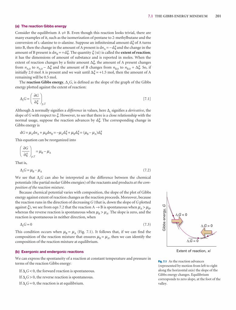
7.1 THE GIBBS ENERGY MINIMUM 201
(a) The reaction Gibbs energy
Consider the equilibrium A 5 B. Even though this reaction looks trivial, there aremany examples of it, such as the isomerization of pentane to 2-methylbutane and theconversion of l-alanine to d-alanine. Suppose an infinitesimal amount dξ of A turnsinto B, then the change in the amount of A present is dnA = −dξ and the change in theamount of B present is dnB = +dξ. The quantity ξ (xi) is called the extent of reaction;it has the dimensions of amount of substance and is reported in moles. When the extent of reaction changes by a finite amount ∆ξ, the amount of A present changesfrom nA,0 to nA,0 − ∆ξ and the amount of B changes from nB,0 to nB,0 + ∆ξ. So, if initially 2.0 mol A is present and we wait until ∆ξ = +1.5 mol, then the amount of A remaining will be 0.5 mol.
The reaction Gibbs energy, ∆ rG, is defined as the slope of the graph of the Gibbsenergy plotted against the extent of reaction:
∆rG =p,T
[7.1]
Although ∆ normally signifies a difference in values, here ∆r signifies a derivative, theslope of G with respect to ξ. However, to see that there is a close relationship with thenormal usage, suppose the reaction advances by dξ. The corresponding change inGibbs energy is
dG = µAdnA + µBdnB = −µAdξ + µBdξ = (µB − µA)dξ
This equation can be reorganized into
p,T
= µB − µA
That is,
∆rG = µB − µA (7.2)
We see that ∆rG can also be interpreted as the difference between the chemical potentials (the partial molar Gibbs energies) of the reactants and products at the com-position of the reaction mixture.
Because chemical potential varies with composition, the slope of the plot of Gibbsenergy against extent of reaction changes as the reaction proceeds. Moreover, becausethe reaction runs in the direction of decreasing G (that is, down the slope of G plottedagainst ξ), we see from eqn 7.2 that the reaction A → B is spontaneous when µA > µB,whereas the reverse reaction is spontaneous when µB > µA. The slope is zero, and thereaction is spontaneous in neither direction, when
∆rG = 0 (7.3)
This condition occurs when µB = µA (Fig. 7.1). It follows that, if we can find the composition of the reaction mixture that ensures µB = µA, then we can identify thecomposition of the reaction mixture at equilibrium.
(b) Exergonic and endergonic reactions
We can express the spontaneity of a reaction at constant temperature and pressure interms of the reaction Gibbs energy:
If ∆rG < 0, the forward reaction is spontaneous.
If ∆rG > 0, the reverse reaction is spontaneous.
If ∆rG = 0, the reaction is at equilibrium.
DF
∂G
∂ξ
AC
DF
∂G
∂ξ
AC
Fig. 7.1 As the reaction advances(represented by motion from left to rightalong the horizontal axis) the slope of theGibbs energy changes. Equilibriumcorresponds to zero slope, at the foot of thevalley.
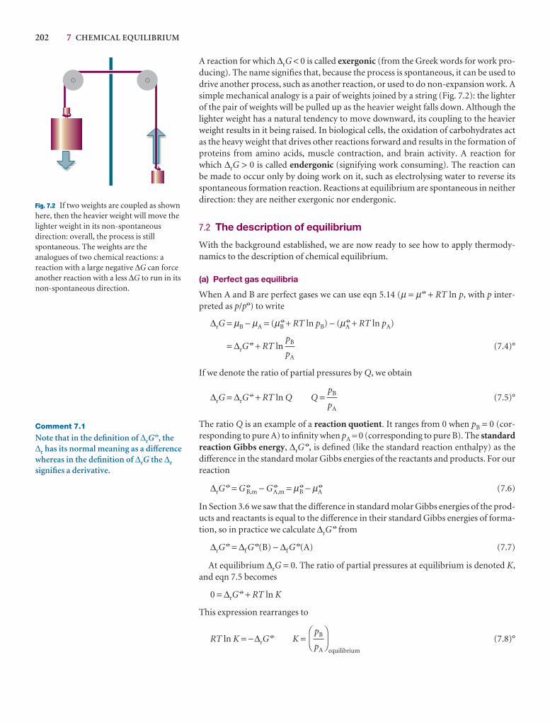
202 7 CHEMICAL EQUILIBRIUM
A reaction for which ∆rG < 0 is called exergonic (from the Greek words for work pro-ducing). The name signifies that, because the process is spontaneous, it can be used todrive another process, such as another reaction, or used to do non-expansion work. Asimple mechanical analogy is a pair of weights joined by a string (Fig. 7.2): the lighterof the pair of weights will be pulled up as the heavier weight falls down. Although thelighter weight has a natural tendency to move downward, its coupling to the heavierweight results in it being raised. In biological cells, the oxidation of carbohydrates actas the heavy weight that drives other reactions forward and results in the formation ofproteins from amino acids, muscle contraction, and brain activity. A reaction forwhich ∆rG > 0 is called endergonic (signifying work consuming). The reaction can be made to occur only by doing work on it, such as electrolysing water to reverse itsspontaneous formation reaction. Reactions at equilibrium are spontaneous in neitherdirection: they are neither exergonic nor endergonic.
7.2 The description of equilibrium
With the background established, we are now ready to see how to apply thermody-namics to the description of chemical equilibrium.
(a) Perfect gas equilibria
When A and B are perfect gases we can use eqn 5.14 (µ = µ7 + RT ln p, with p inter-preted as p/p7) to write
∆rG = µB − µA = (µB7 + RT ln pB) − (µA
7 + RT ln pA)
= ∆rG7 + RT ln (7.4)°
If we denote the ratio of partial pressures by Q, we obtain
∆rG = ∆rG7 + RT ln Q Q = (7.5)°
The ratio Q is an example of a reaction quotient. It ranges from 0 when pB = 0 (cor-responding to pure A) to infinity when pA = 0 (corresponding to pure B). The standardreaction Gibbs energy, ∆rG
7, is defined (like the standard reaction enthalpy) as thedifference in the standard molar Gibbs energies of the reactants and products. For ourreaction
∆rG7 = G 7
B,m − G 7A,m = µB
7 − µA7 (7.6)
In Section 3.6 we saw that the difference in standard molar Gibbs energies of the prod-ucts and reactants is equal to the difference in their standard Gibbs energies of forma-tion, so in practice we calculate ∆rG
7 from
∆rG7 = ∆f G
7(B) − ∆f G7(A) (7.7)
At equilibrium ∆rG = 0. The ratio of partial pressures at equilibrium is denoted K,and eqn 7.5 becomes
0 = ∆rG7 + RT ln K
This expression rearranges to
RT ln K = −∆rG7 K =
equilibrium
(7.8)°DF
pB
pA
AC
pB
pA
pB
pA
Fig. 7.2 If two weights are coupled as shownhere, then the heavier weight will move thelighter weight in its non-spontaneousdirection: overall, the process is stillspontaneous. The weights are theanalogues of two chemical reactions: areaction with a large negative ∆G can forceanother reaction with a less ∆G to run in itsnon-spontaneous direction.
Comment 7.1
Note that in the definition of ∆rG7, the
∆r has its normal meaning as a differencewhereas in the definition of ∆rG the ∆rsignifies a derivative.
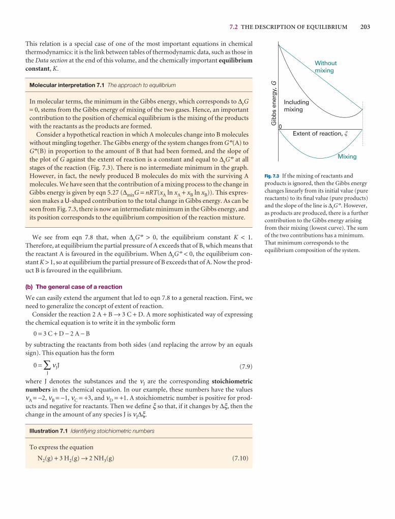
7.2 THE DESCRIPTION OF EQUILIBRIUM 203
Gib
bs e
nerg
y,G
Extent of reaction,0
Withoutmixing
Includingmixing
Mixing
�
Fig. 7.3 If the mixing of reactants andproducts is ignored, then the Gibbs energychanges linearly from its initial value (purereactants) to its final value (pure products)and the slope of the line is ∆rG
7. However,as products are produced, there is a furthercontribution to the Gibbs energy arisingfrom their mixing (lowest curve). The sumof the two contributions has a minimum.That minimum corresponds to theequilibrium composition of the system.
This relation is a special case of one of the most important equations in chemical thermodynamics: it is the link between tables of thermodynamic data, such as those inthe Data section at the end of this volume, and the chemically important equilibriumconstant, K.
Molecular interpretation 7.1 The approach to equilibrium
In molecular terms, the minimum in the Gibbs energy, which corresponds to ∆rG= 0, stems from the Gibbs energy of mixing of the two gases. Hence, an importantcontribution to the position of chemical equilibrium is the mixing of the productswith the reactants as the products are formed.
Consider a hypothetical reaction in which A molecules change into B moleculeswithout mingling together. The Gibbs energy of the system changes from G 7(A) toG 7(B) in proportion to the amount of B that had been formed, and the slope of the plot of G against the extent of reaction is a constant and equal to ∆rG
7 at allstages of the reaction (Fig. 7.3). There is no intermediate minimum in the graph.However, in fact, the newly produced B molecules do mix with the surviving Amolecules. We have seen that the contribution of a mixing process to the change inGibbs energy is given by eqn 5.27 (∆mixG = nRT(xA ln xA + xB ln xB)). This expres-sion makes a U-shaped contribution to the total change in Gibbs energy. As can beseen from Fig. 7.3, there is now an intermediate minimum in the Gibbs energy, andits position corresponds to the equilibrium composition of the reaction mixture.
We see from eqn 7.8 that, when ∆rG7 > 0, the equilibrium constant K < 1.
Therefore, at equilibrium the partial pressure of A exceeds that of B, which means thatthe reactant A is favoured in the equilibrium. When ∆rG
7 < 0, the equilibrium con-stant K > 1, so at equilibrium the partial pressure of B exceeds that of A. Now the prod-uct B is favoured in the equilibrium.
(b) The general case of a reaction
We can easily extend the argument that led to eqn 7.8 to a general reaction. First, weneed to generalize the concept of extent of reaction.
Consider the reaction 2 A + B → 3 C + D. A more sophisticated way of expressingthe chemical equation is to write it in the symbolic form
0 = 3 C + D − 2 A − B
by subtracting the reactants from both sides (and replacing the arrow by an equalssign). This equation has the form
0 = ∑J
νJJ (7.9)
where J denotes the substances and the νJ are the corresponding stoichiometricnumbers in the chemical equation. In our example, these numbers have the values νA = −2, νB = −1, νC = +3, and νD = +1. A stoichiometric number is positive for prod-ucts and negative for reactants. Then we define ξ so that, if it changes by ∆ξ, then thechange in the amount of any species J is νJ∆ξ.
Illustration 7.1 Identifying stoichiometric numbers
To express the equation
N2(g) + 3 H2(g) → 2 NH3(g) (7.10)
204 7 CHEMICAL EQUILIBRIUM
in the notation of eqn 7.9, we rearrange it to
0 = 2 NH3(g) − N2(g) + 3 H2(g)
and then identify the stoichiometric numbers as νN2= −1, νH2
= −3, and νNH3= +2.
Therefore, if initially there is 10 mol N2 present, then when the extent of reactionchanges from ξ = 0 to ξ = 1 mol, implying that ∆ξ = +1 mol, the amount of N2
changes from 10 mol to 9 mol. All the N2 has been consumed when ξ = 10 mol.When ∆ξ = +1 mol, the amount of H2 changes by −3 × (1 mol) = −3 mol and theamount of NH3 changes by +2 × (1 mol) = +2 mol.
A note on good practice Stoichiometric numbers may be positive or negative; stoichiometric coefficients are always positive. Few, however, make the distinctionbetween the two types of quantity.
The reaction Gibbs energy, ∆rG, is defined in the same way as before, eqn 7.1. In theJustification below, we show that the Gibbs energy of reaction can always be written
∆rG = ∆rG7 + RT ln Q (7.11)
with the standard reaction Gibbs energy calculated from
∆rG7 = ∑
Products
ν∆ f G7 − ∑
Reactants
ν∆ f G7
(7.12a)
or, more formally,
∆rG7 = ∑
J
νJ∆ f G7(J) (7.12b)
The reaction quotient, Q, has the form
Q = (7.13a)
with each species raised to the power given by its stoichiometric coefficient. More for-mally, to write the general expression for Q we introduce the symbol Π to denote theproduct of what follows it (just as ∑ denotes the sum), and define Q as
Q = ΠJ
aJνJ [7.13b]
Because reactants have negative stoichiometric numbers, they automatically appearas the denominator when the product is written out explicitly. Recall from Table 5.3that, for pure solids and liquids, the activity is 1, so such substances make no contri-bution to Q even though they may appear in the chemical equation.
Illustration 7.2 Writing a reaction quotient
Consider the reaction 2 A + 3 B → C + 2 D, in which case νA = −2, νB = −3, νC = +1,and νD = +2. The reaction quotient is then
Q = a A−2a B
−3aCa2D =
aCa2D
a2Aa3
B
activities of products
activities of reactants
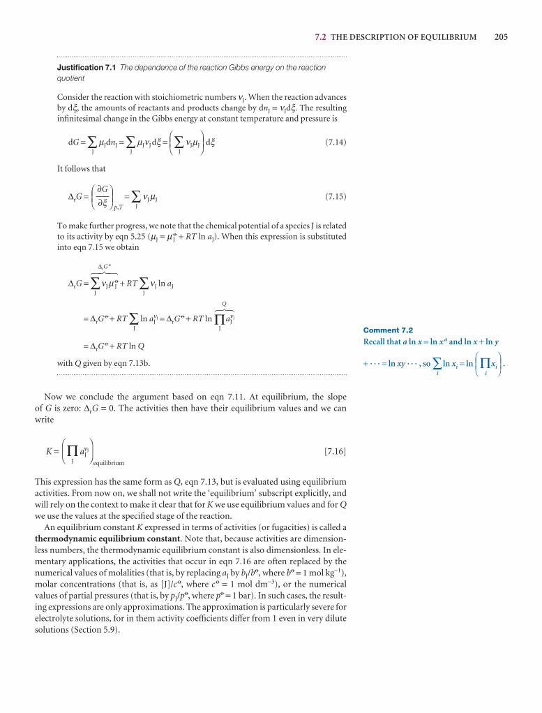
7.2 THE DESCRIPTION OF EQUILIBRIUM 205
Justification 7.1 The dependence of the reaction Gibbs energy on the reactionquotient
Consider the reaction with stoichiometric numbers νJ. When the reaction advancesby dξ, the amounts of reactants and products change by dnJ = νJdξ. The resultinginfinitesimal change in the Gibbs energy at constant temperature and pressure is
dG = ∑J
µJdnJ = ∑J
µJνJ dξ = ∑J
νJµJ dξ (7.14)
It follows that
∆rG =p,T
= ∑J
νJµJ (7.15)
To make further progress, we note that the chemical potential of a species J is relatedto its activity by eqn 5.25 (µJ = µ J
7 + RT ln aJ). When this expression is substitutedinto eqn 7.15 we obtain
∆rG7
∆rG = ∑J
νJµ J7 + RT ∑
J
νJ ln aJ
Q
= ∆rG7 + RT ∑
J
ln aJνJ = ∆rG
7 + RT ln ΠJ
aJνJ
= ∆rG7 + RT ln Q
with Q given by eqn 7.13b.
Now we conclude the argument based on eqn 7.11. At equilibrium, the slope of G is zero: ∆rG = 0. The activities then have their equilibrium values and we can write
K = ΠJ
aJνJ
equilibrium
[7.16]
This expression has the same form as Q, eqn 7.13, but is evaluated using equilibriumactivities. From now on, we shall not write the ‘equilibrium’ subscript explicitly, andwill rely on the context to make it clear that for K we use equilibrium values and for Qwe use the values at the specified stage of the reaction.
An equilibrium constant K expressed in terms of activities (or fugacities) is called athermodynamic equilibrium constant. Note that, because activities are dimension-less numbers, the thermodynamic equilibrium constant is also dimensionless. In ele-mentary applications, the activities that occur in eqn 7.16 are often replaced by thenumerical values of molalities (that is, by replacing aJ by bJ/b
7, where b7 = 1 mol kg−1),molar concentrations (that is, as [J]/c 7, where c 7 = 1 mol dm−3), or the numerical values of partial pressures (that is, by pJ/p
7, where p7 = 1 bar). In such cases, the result-ing expressions are only approximations. The approximation is particularly severe forelectrolyte solutions, for in them activity coefficients differ from 1 even in very dilutesolutions (Section 5.9).
DF
AC
@ $
5 6 7
DEF∂G
∂ξABC
DEFABC
Comment 7.2
Recall that a ln x = ln x a and ln x + ln y
+ · · · = ln xy · · · , so ∑i
ln xi = ln Πi
xi .DEF
ABC
206 7 CHEMICAL EQUILIBRIUM
Comment 7.3
In Chapter 17 we shall see that the right-hand side of eqn 7.17 may be expressedin terms of spectroscopic data for gas-phase species; so this expression alsoprovides a link between spectroscopyand equilibrium composition.
Illustration 7.3 Writing an equilibrium constant.
The equilibrium constant for the heterogeneous equilibrium CaCO3(s) 5 CaO(s)+ CO2(g) is
1
K = a−1CaCO3(s)aCaO(s)aCO2(g) = = aCO2
1
(Table 5.3). Provided the carbon dioxide can be treated as a perfect gas, we can goon to write
K ≈ pCO2/p7
and conclude that in this case the equilibrium constant is the numerical value ofthe decomposition vapour pressure of calcium carbonate.
At this point we set ∆rG = 0 in eqn 7.11 and replace Q by K. We immediately obtain
RT ln K = −∆rG7 (7.17)
This is an exact and highly important thermodynamic relation, for it enables us topredict the equilibrium constant of any reaction from tables of thermodynamic data,and hence to predict the equilibrium composition of the reaction mixture.
Example 7.1 Calculating an equilibrium constant
Calculate the equilibrium constant for the ammonia synthesis reaction, eqn 7.10,at 298 K and show how K is related to the partial pressures of the species at equi-librium when the overall pressure is low enough for the gases to be treated as perfect.
Method Calculate the standard reaction Gibbs energy from eqn 7.12 and convertit to the value of the equilibrium constant by using eqn 7.17. The expression for theequilibrium constant is obtained from eqn 7.16, and because the gases are taken tobe perfect, we replace each activity by the ratio p/p7, where p is a partial pressure.
Answer The standard Gibbs energy of the reaction is
∆rG7 = 2∆f G
7(NH3, g) − {∆f G7(N2, g) + 3∆f G
7(H2, g)}
= 2∆f G7(NH3, g) = 2 × (−16.5 kJ mol−1)
Then,
ln K = − =
Hence, K = 6.1 × 10⁵. This result is thermodynamically exact. The thermodynamicequilibrium constant for the reaction is
K =a2
NH3
aN2a3
H2
2 × 16.5 × 103
8.3145 × 298
2 × (−16.5 × 10³ J mol−1)
(8.3145 J K−1 mol−1) × (298 K)
1 2 3
aCaO(s)aCO2(g)
aCaCO3(s)
5 6 7
7.2 THE DESCRIPTION OF EQUILIBRIUM 207
and this ratio has exactly the value we have just calculated. At low overall pressures,the activities can be replaced by the ratios p/p7, where p is a partial pressure, and anapproximate form of the equilibrium constant is
K = =
Self-test 7.1 Evaluate the equilibrium constant for N2O4(g) 5 2 NO2(g) at 298 K.[K = 0.15]
Example 7.2 Estimating the degree of dissociation at equilibrium
The degree of dissociation, α, is defined as the fraction of reactant that has decom-posed; if the initial amount of reactant is n and the amount at equilibrium is neq,then α = (n − neq)/n. The standard Gibbs energy of reaction for the decompositionH2O(g) → H2(g) + 1–2 O2(g) is +118.08 kJ mol−1 at 2300 K. What is the degree of dis-sociation of H2O at 2300 K and 1.00 bar?
Method The equilibrium constant is obtained from the standard Gibbs energy ofreaction by using eqn 7.17, so the task is to relate the degree of dissociation, α, to Kand then to find its numerical value. Proceed by expressing the equilibrium com-positions in terms of α, and solve for α in terms of K. Because the standard Gibbsenergy of reaction is large and positive, we can anticipate that K will be small, andhence that α << 1, which opens the way to making approximations to obtain its numerical value.
Answer The equilibrium constant is obtained from eqn 7.17 in the form
ln K = − = −
= −
It follows that K = 2.08 × 10⁻³. The equilibrium composition can be expressed interms of α by drawing up the following table:
H2O H2 O2
Initial amount n 0 0
Change to reach equilibrium −αn +αn +1–2αn
Amount at equilibrium (1 − α)n αn 1–2αn Total: (1 + 1–2α)n
Mole fraction, xJ
Partial pressure, pJ
where, for the entries in the last row, we have used pJ = xJ p (eqn 1.13). The equilib-rium constant is therefore
K = =α3/2p1/2
(1 − α)(2 + α)1/2
pH2p1/2
O2
pH2O
1–2αp
1 + 1–2ααp
1 + 1–2α(1 − α)p
1 + 1–2α
1–2α1 + 1–2α
α1 + 1–2α
1 − α1 + 1–2α
118.08 × 10³
8.3145 × 2300
(+118.08 × 10³ J mol−1)
(8.3145 J K−1 mol−1) × (2300 K)
∆rG7
RT
p2NH3
p72
pN2p3
H2
(pNH3/p7)2
(pN2/p7)(pH2
/p7)3
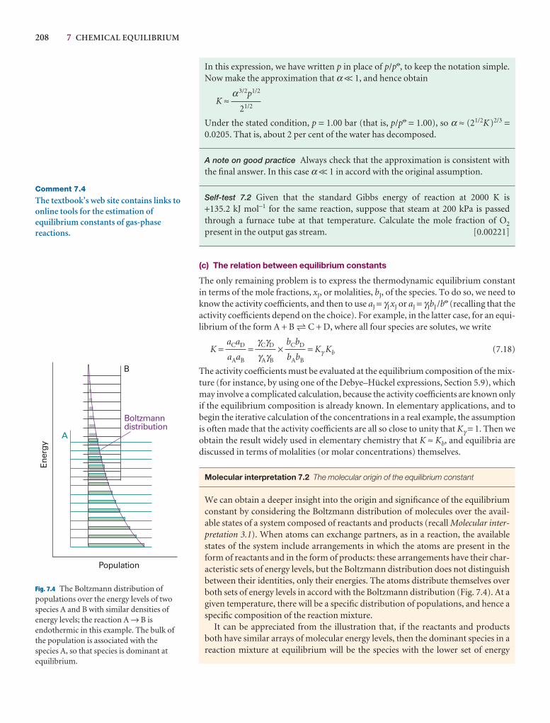
208 7 CHEMICAL EQUILIBRIUM
Comment 7.4
The textbook’s web site contains links toonline tools for the estimation ofequilibrium constants of gas-phasereactions.
Boltzmanndistribution
A
B
Population
Ener
gy
Fig. 7.4 The Boltzmann distribution ofpopulations over the energy levels of twospecies A and B with similar densities ofenergy levels; the reaction A → B isendothermic in this example. The bulk ofthe population is associated with thespecies A, so that species is dominant atequilibrium.
In this expression, we have written p in place of p/p7, to keep the notation simple.Now make the approximation that α << 1, and hence obtain
K ≈
Under the stated condition, p = 1.00 bar (that is, p/p7 = 1.00), so α ≈ (21/2K)2/3 =0.0205. That is, about 2 per cent of the water has decomposed.
A note on good practice Always check that the approximation is consistent withthe final answer. In this case α << 1 in accord with the original assumption.
Self-test 7.2 Given that the standard Gibbs energy of reaction at 2000 K is +135.2 kJ mol−1 for the same reaction, suppose that steam at 200 kPa is passedthrough a furnace tube at that temperature. Calculate the mole fraction of O2
present in the output gas stream. [0.00221]
(c) The relation between equilibrium constants
The only remaining problem is to express the thermodynamic equilibrium constantin terms of the mole fractions, xJ, or molalities, bJ, of the species. To do so, we need toknow the activity coefficients, and then to use aJ = γJ xJ or aJ = γJbJ /b7 (recalling that theactivity coefficients depend on the choice). For example, in the latter case, for an equi-librium of the form A + B 5 C + D, where all four species are solutes, we write
K = = × = Kγ Kb (7.18)
The activity coefficients must be evaluated at the equilibrium composition of the mix-ture (for instance, by using one of the Debye–Hückel expressions, Section 5.9), whichmay involve a complicated calculation, because the activity coefficients are known onlyif the equilibrium composition is already known. In elementary applications, and tobegin the iterative calculation of the concentrations in a real example, the assumptionis often made that the activity coefficients are all so close to unity that Kγ = 1. Then weobtain the result widely used in elementary chemistry that K ≈ Kb, and equilibria arediscussed in terms of molalities (or molar concentrations) themselves.
Molecular interpretation 7.2 The molecular origin of the equilibrium constant
We can obtain a deeper insight into the origin and significance of the equilibriumconstant by considering the Boltzmann distribution of molecules over the avail-able states of a system composed of reactants and products (recall Molecular inter-pretation 3.1). When atoms can exchange partners, as in a reaction, the availablestates of the system include arrangements in which the atoms are present in theform of reactants and in the form of products: these arrangements have their char-acteristic sets of energy levels, but the Boltzmann distribution does not distinguishbetween their identities, only their energies. The atoms distribute themselves overboth sets of energy levels in accord with the Boltzmann distribution (Fig. 7.4). At agiven temperature, there will be a specific distribution of populations, and hence aspecific composition of the reaction mixture.
It can be appreciated from the illustration that, if the reactants and productsboth have similar arrays of molecular energy levels, then the dominant species in areaction mixture at equilibrium will be the species with the lower set of energy
bCbD
bAbB
γCγD
γAγB
aCaD
aAaB
α3/2p1/2
21/2
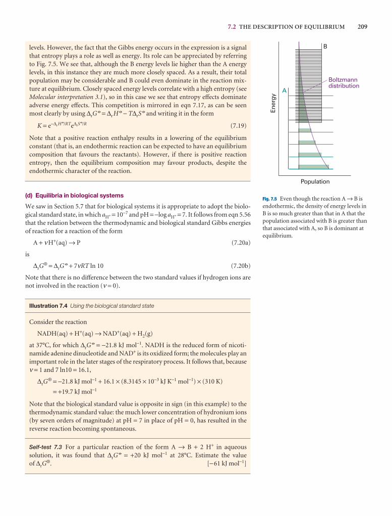
7.2 THE DESCRIPTION OF EQUILIBRIUM 209
Boltzmanndistribution
A
B
Population
Ener
gy
Fig. 7.5 Even though the reaction A → B isendothermic, the density of energy levels inB is so much greater than that in A that thepopulation associated with B is greater thanthat associated with A, so B is dominant atequilibrium.
levels. However, the fact that the Gibbs energy occurs in the expression is a signalthat entropy plays a role as well as energy. Its role can be appreciated by referringto Fig. 7.5. We see that, although the B energy levels lie higher than the A energy levels, in this instance they are much more closely spaced. As a result, their totalpopulation may be considerable and B could even dominate in the reaction mix-ture at equilibrium. Closely spaced energy levels correlate with a high entropy (seeMolecular interpretation 3.1), so in this case we see that entropy effects dominateadverse energy effects. This competition is mirrored in eqn 7.17, as can be seenmost clearly by using ∆rG
7 = ∆r H 7 − T∆rS7 and writing it in the form
K = e−∆rH 7/RTe∆rS7/R (7.19)
Note that a positive reaction enthalpy results in a lowering of the equilibrium constant (that is, an endothermic reaction can be expected to have an equilibriumcomposition that favours the reactants). However, if there is positive reaction entropy, then the equilibrium composition may favour products, despite the endothermic character of the reaction.
(d) Equilibria in biological systems
We saw in Section 5.7 that for biological systems it is appropriate to adopt the biolo-gical standard state, in which aH+ = 10−7 and pH = −log aH+ = 7. It follows from eqn 5.56that the relation between the thermodynamic and biological standard Gibbs energiesof reaction for a reaction of the form
A + νH+(aq) → P (7.20a)
is
∆rG⊕ = ∆rG
7 + 7νRT ln 10 (7.20b)
Note that there is no difference between the two standard values if hydrogen ions arenot involved in the reaction (ν = 0).
Illustration 7.4 Using the biological standard state
Consider the reaction
NADH(aq) + H+(aq) → NAD+(aq) + H2(g)
at 37°C, for which ∆rG7 = −21.8 kJ mol−1. NADH is the reduced form of nicoti-
namide adenine dinucleotide and NAD+ is its oxidized form; the molecules play animportant role in the later stages of the respiratory process. It follows that, becauseν = 1 and 7 ln10 = 16.1,
∆rG⊕ = −21.8 kJ mol−1 + 16.1 × (8.3145 × 10−3 kJ K−1 mol−1) × (310 K)
= +19.7 kJ mol−1
Note that the biological standard value is opposite in sign (in this example) to thethermodynamic standard value: the much lower concentration of hydronium ions(by seven orders of magnitude) at pH = 7 in place of pH = 0, has resulted in the reverse reaction becoming spontaneous.
Self-test 7.3 For a particular reaction of the form A → B + 2 H+ in aqueous solution, it was found that ∆rG
7 = +20 kJ mol−1 at 28°C. Estimate the value of ∆rG
⊕. [−61 kJ mol−1]
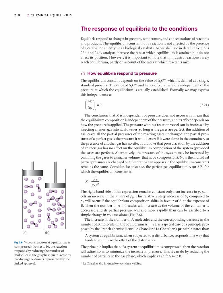
210 7 CHEMICAL EQUILIBRIUM
The response of equilibria to the conditions
Equilibria respond to changes in pressure, temperature, and concentrations of reactantsand products. The equilibrium constant for a reaction is not affected by the presenceof a catalyst or an enzyme (a biological catalyst). As we shall see in detail in Sections22.* and 24.*, catalysts increase the rate at which equilibrium is attained but do notaffect its position. However, it is important to note that in industry reactions rarelyreach equilibrium, partly on account of the rates at which reactants mix.
7.3 How equilibria respond to pressure
The equilibrium constant depends on the value of ∆rG7, which is defined at a single,
standard pressure. The value of ∆rG7, and hence of K, is therefore independent of the
pressure at which the equilibrium is actually established. Formally we may expressthis independence as
T
= 0 (7.21)
The conclusion that K is independent of pressure does not necessarily mean thatthe equilibrium composition is independent of the pressure, and its effect depends onhow the pressure is applied. The pressure within a reaction vessel can be increased byinjecting an inert gas into it. However, so long as the gases are perfect, this addition ofgas leaves all the partial pressures of the reacting gases unchanged: the partial pres-sures of a perfect gas is the pressure it would exert if it were alone in the container, sothe presence of another gas has no effect. It follows that pressurization by the additionof an inert gas has no effect on the equilibrium composition of the system (providedthe gases are perfect). Alternatively, the pressure of the system may be increased byconfining the gases to a smaller volume (that is, by compression). Now the individualpartial pressures are changed but their ratio (as it appears in the equilibrium constant)remains the same. Consider, for instance, the perfect gas equilibrium A 5 2 B, forwhich the equilibrium constant is
K =
The right-hand side of this expression remains constant only if an increase in pA can-cels an increase in the square of pB. This relatively steep increase of pA compared to pB will occur if the equilibrium composition shifts in favour of A at the expense of B. Then the number of A molecules will increase as the volume of the container is decreased and its partial pressure will rise more rapidly than can be ascribed to a simple change in volume alone (Fig. 7.6).
The increase in the number of A molecules and the corresponding decrease in thenumber of B molecules in the equilibrium A 5 2 B is a special case of a principle pro-posed by the French chemist Henri Le Chatelier.1 Le Chatelier’s principle states that:
A system at equilibrium, when subjected to a disturbance, responds in a way thattends to minimize the effect of the disturbance
The principle implies that, if a system at equilibrium is compressed, then the reactionwill adjust so as to minimize the increase in pressure. This it can do by reducing thenumber of particles in the gas phase, which implies a shift A ← 2 B.
p2B
pA p7
DF
∂K
∂p
AC
(a) (b)
Fig. 7.6 When a reaction at equilibrium iscompressed (from a to b), the reactionresponds by reducing the number ofmolecules in the gas phase (in this case byproducing the dimers represented by thelinked spheres). 1 Le Chatelier also invented oxyacetylene welding.
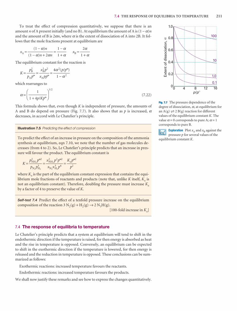
7.4 THE RESPONSE OF EQUILIBRIA TO TEMPERATURE 211
0 4 8 12 160
0.2
0.4
0.6
0.8
1.0
Exte
nt o
f di
ssoc
iatio
n,
0.1
1.0
10
100
p p/ �
�
Fig. 7.7 The pressure dependence of thedegree of dissociation, α, at equilibrium foran A(g) 5 2 B(g) reaction for differentvalues of the equilibrium constant K. Thevalue α = 0 corresponds to pure A; α = 1corresponds to pure B.
Exploration Plot xA and xB against thepressure p for several values of the
equilibrium constant K.
To treat the effect of compression quantitatively, we suppose that there is anamount n of A present initially (and no B). At equilibrium the amount of A is (1 − α)nand the amount of B is 2αn, where α is the extent of dissociation of A into 2B. It fol-lows that the mole fractions present at equilibrium are
xA = = xB =
The equilibrium constant for the reaction is
K = = =
which rearranges to
α =1/2
(7.22)
This formula shows that, even though K is independent of pressure, the amounts of A and B do depend on pressure (Fig. 7.7). It also shows that as p is increased, αdecreases, in accord with Le Chatelier’s principle.
Illustration 7.5 Predicting the effect of compression
To predict the effect of an increase in pressure on the composition of the ammoniasynthesis at equilibrium, eqn 7.10, we note that the number of gas molecules de-creases (from 4 to 2). So, Le Chatelier’s principle predicts that an increase in pres-sure will favour the product. The equilibrium constant is
K = = =
where Kx is the part of the equilibrium constant expression that contains the equi-librium mole fractions of reactants and products (note that, unlike K itself, Kx isnot an equilibrium constant). Therefore, doubling the pressure must increase Kx
by a factor of 4 to preserve the value of K.
Self-test 7.4 Predict the effect of a tenfold pressure increase on the equilibriumcomposition of the reaction 3 N2(g) + H2(g) → 2 N3H(g).
[100-fold increase in Kx]
7.4 The response of equilibria to temperature
Le Chatelier’s principle predicts that a system at equilibrium will tend to shift in theendothermic direction if the temperature is raised, for then energy is absorbed as heatand the rise in temperature is opposed. Conversely, an equilibrium can be expected to shift in the exothermic direction if the temperature is lowered, for then energy isreleased and the reduction in temperature is opposed. These conclusions can be sum-marized as follows:
Exothermic reactions: increased temperature favours the reactants.
Endothermic reactions: increased temperature favours the products.
We shall now justify these remarks and see how to express the changes quantitatively.
Kx p72
p2
x2NH3
p2p72
xN2x 3
H2p4
p2NH3
p72
pN2p3
H2
DF
1
1 + 4p/Kp7
AC
4α2(p/p7)
1 − α2
x2B p2
xA pp7
p2B
pA p7
2α1 + α
1 − α1 + α
(1 − α)n
(1 − α)n + 2αn
212 7 CHEMICAL EQUILIBRIUM
(a) The van ’t Hoff equation
The van ’t Hoff equation, which is derived in the Justification below, is an expressionfor the slope of a plot of the equilibrium constant (specifically, ln K) as a function oftemperature. It may be expressed in either of two ways:
(a) = (b) = − (7.23)
Justification 7.2 The van ’t Hoff equation
From eqn 7.17, we know that
ln K = −
Differentiation of ln K with respect to temperature then gives
= −
The differentials are complete because K and ∆rG7 depend only on temperature, not
on pressure. To develop this equation we use the Gibbs–Helmholtz equation (eqn3.53) in the form
= −
where ∆r H 7 is the standard reaction enthalpy at the temperature T. Combining thetwo equations gives the van ’t Hoff equation, eqn 7.23a. The second form of theequation is obtained by noting that
= − , so dT = −T 2d(1/T)
It follows that eqn 7.23a can be rewritten as
− =
which simplifies into eqn 7.23b.
Equation 7.23a shows that d ln K/dT < 0 (and therefore that dK/dT < 0) for a reac-tion that is exothermic under standard conditions (∆r H 7 < 0). A negative slope meansthat ln K, and therefore K itself, decreases as the temperature rises. Therefore, as asserted above, in the case of an exothermic reaction the equilibrium shifts away fromproducts. The opposite occurs in the case of endothermic reactions.
Some insight into the thermodynamic basis of this behaviour comes from the expression ∆rG
7 = ∆r H 7 − T∆rS7 written in the form −∆rG
7/T = −∆r H 7/T + ∆rS7.
When the reaction is exothermic, −∆r H 7/T corresponds to a positive change of entropy of the surroundings and favours the formation of products. When the tem-perature is raised, −∆r H 7/T decreases, and the increasing entropy of the surroundingshas a less important role. As a result, the equilibrium lies less to the right. When thereaction is endothermic, the principal factor is the increasing entropy of the reactionsystem. The importance of the unfavourable change of entropy of the surroundings isreduced if the temperature is raised (because then ∆r H 7/T is smaller), and the reac-tion is able to shift towards products.
∆r H 7
RT 2
d ln K
T 2d(1/T)
1
T 2
d(1/T)
dT
∆r H 7
T 2
d(∆rG7/T)
dT
d(∆rG7/T)
dT
1
R
d ln K
dT
∆rG7
RT
∆rH7
R
d ln K
d(1/T)
∆rH7
RT 2
d ln K
dT
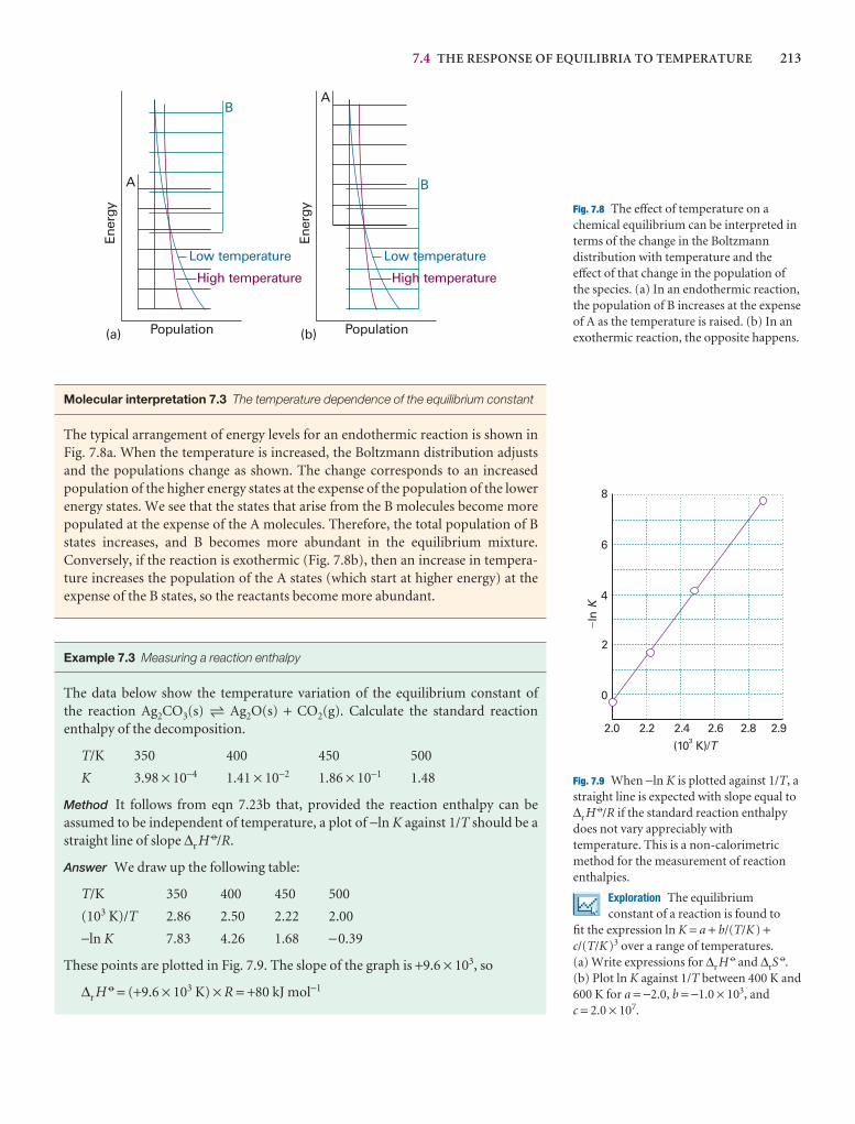
7.4 THE RESPONSE OF EQUILIBRIA TO TEMPERATURE 213
A
AB
B
Population Population
Ener
gy
Ener
gy
Low temperature Low temperature
High temperature High temperature
(a) (b)
Fig. 7.8 The effect of temperature on achemical equilibrium can be interpreted interms of the change in the Boltzmanndistribution with temperature and theeffect of that change in the population ofthe species. (a) In an endothermic reaction,the population of B increases at the expenseof A as the temperature is raised. (b) In anexothermic reaction, the opposite happens.
2.0 2.2 2.4 2.6 2.92.8
0
2
4
6
8
lnK
(10 K)/3 T
�
Fig. 7.9 When −ln K is plotted against 1/T, astraight line is expected with slope equal to∆r H 7/R if the standard reaction enthalpydoes not vary appreciably withtemperature. This is a non-calorimetricmethod for the measurement of reactionenthalpies.
Exploration The equilibriumconstant of a reaction is found to
fit the expression ln K = a + b/(T/K) +c/(T/K)3 over a range of temperatures. (a) Write expressions for ∆r H 7 and ∆rS
7.(b) Plot ln K against 1/T between 400 K and600 K for a = −2.0, b = −1.0 × 10³, and c = 2.0 × 10⁷.
Molecular interpretation 7.3 The temperature dependence of the equilibrium constant
The typical arrangement of energy levels for an endothermic reaction is shown inFig. 7.8a. When the temperature is increased, the Boltzmann distribution adjustsand the populations change as shown. The change corresponds to an increasedpopulation of the higher energy states at the expense of the population of the lowerenergy states. We see that the states that arise from the B molecules become morepopulated at the expense of the A molecules. Therefore, the total population of Bstates increases, and B becomes more abundant in the equilibrium mixture.Conversely, if the reaction is exothermic (Fig. 7.8b), then an increase in tempera-ture increases the population of the A states (which start at higher energy) at theexpense of the B states, so the reactants become more abundant.
Example 7.3 Measuring a reaction enthalpy
The data below show the temperature variation of the equilibrium constant of the reaction Ag2CO3(s) 5 Ag2O(s) + CO2(g). Calculate the standard reaction enthalpy of the decomposition.
T/K 350 400 450 500
K 3.98 × 10⁻⁴ 1.41 × 10⁻² 1.86 × 10⁻¹ 1.48
Method It follows from eqn 7.23b that, provided the reaction enthalpy can be assumed to be independent of temperature, a plot of −ln K against 1/T should be astraight line of slope ∆r H 7/R.
Answer We draw up the following table:
T/K 350 400 450 500
(103 K)/T 2.86 2.50 2.22 2.00
−ln K 7.83 4.26 1.68 −0.39
These points are plotted in Fig. 7.9. The slope of the graph is +9.6 × 10³, so
∆r H 7 = (+9.6 × 10³ K) × R = +80 kJ mol−1
214 7 CHEMICAL EQUILIBRIUM
Self-test 7.5 The equilibrium constant of the reaction 2 SO2(g) + O2(g) 52 SO3(g) is 4.0 × 1024 at 300 K, 2.5 × 10¹⁰ at 500 K, and 3.0 × 10⁴ at 700 K. Estimatethe reaction enthalpy at 500 K. [−200 kJ mol−1]
The temperature dependence of the equilibrium constant provides a non-calorimetric method of determining ∆r H 7. A drawback is that the reaction enthalpyis actually temperature-dependent, so the plot is not expected to be perfectly linear.However, the temperature dependence is weak in many cases, so the plot is reasonablystraight. In practice, the method is not very accurate, but it is often the only methodavailable.
(b) The value of K at different temperatures
To find the value of the equilibrium constant at a temperature T2 in terms of its valueK1 at another temperature T1, we integrate eqn 7.23b between these two temperatures:
ln K2 − ln K1 = − �1/T2
1/T1
∆rH7d(1/T) (7.24)
If we suppose that ∆r H 7 varies only slightly with temperature over the temperaturerange of interest, then we may take it outside the integral. It follows that
ln K2 − ln K1 = − − (7.25)
Illustration 7.6 Estimating an equilibrium constant at a different temperature
To estimate the equilibrium constant for the synthesis of ammonia at 500 K fromits value at 298 K (6.1 × 10⁵ for the reaction as written in eqn 7.10) we use the stand-ard reaction enthalpy, which can be obtained from Table 2.7 in the Data section byusing ∆r H 7 = 2∆f H
7(NH3, g), and assume that its value is constant over the rangeof temperatures. Then, with ∆r H 7 = −92.2 kJ mol−1, from eqn 7.25 we find
ln K2 = ln(6.1 × 10⁵) − −
= −1.71
It follows that K2 = 0.18, a lower value than at 298 K, as expected for this exother-mic reaction.
Self-test 7.6 The equilibrium constant for N2O4(g) 5 2 NO2(g) was calculated inSelf-test 7.1. Estimate its value at 100°C. [15]
Knowledge of the temperature dependence of the equilibrium constant for a reac-tion can be useful in the design of laboratory and industrial processes. For example,synthetic chemists can improve the yield of a reaction by changing the temperature of the reaction mixture. Also, reduction of a metal oxide with carbon or carbonmonoxide results in the extraction of the metal when the process is carried out at a temperature for which the equilibrium constant for the reaction is much greaterthan one.
DF
1
298 K
1
500 K
AC
(−92.2 × 10³ J mol−1)
8.3145 J K−1 mol−1
DF
1
T1
1
T2
AC
∆rH7
R
1
R
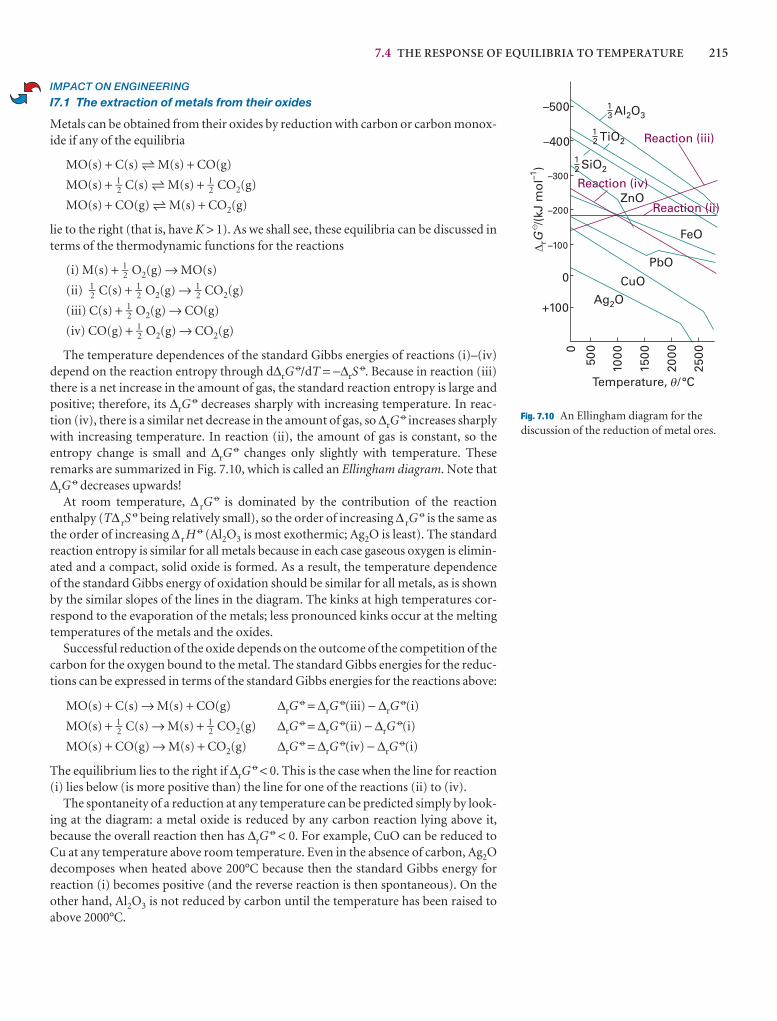
7.4 THE RESPONSE OF EQUILIBRIA TO TEMPERATURE 215
IMPACT ON ENGINEERING
I7.1 The extraction of metals from their oxides
Metals can be obtained from their oxides by reduction with carbon or carbon monox-ide if any of the equilibria
MO(s) + C(s) 5 M(s) + CO(g)
MO(s) + 1–2 C(s) 5 M(s) + 1–2 CO2(g)
MO(s) + CO(g) 5 M(s) + CO2(g)
lie to the right (that is, have K > 1). As we shall see, these equilibria can be discussed interms of the thermodynamic functions for the reactions
(i) M(s) + 1–2 O2(g) → MO(s)
(ii) 1–2 C(s) + 1–2 O2(g) → 1–2 CO2(g)
(iii) C(s) + 1–2 O2(g) → CO(g)
(iv) CO(g) + 1–2 O2(g) → CO2(g)
The temperature dependences of the standard Gibbs energies of reactions (i)–(iv)depend on the reaction entropy through d∆rG
7/dT = −∆rS7. Because in reaction (iii)
there is a net increase in the amount of gas, the standard reaction entropy is large andpositive; therefore, its ∆rG
7 decreases sharply with increasing temperature. In reac-tion (iv), there is a similar net decrease in the amount of gas, so ∆rG
7 increases sharplywith increasing temperature. In reaction (ii), the amount of gas is constant, so the entropy change is small and ∆rG
7 changes only slightly with temperature. These remarks are summarized in Fig. 7.10, which is called an Ellingham diagram. Note that∆rG
7 decreases upwards!At room temperature, ∆ rG
7 is dominated by the contribution of the reaction enthalpy (T∆ rS
7 being relatively small), so the order of increasing ∆ rG7 is the same as
the order of increasing ∆ r H 7 (Al2O3 is most exothermic; Ag2O is least). The standardreaction entropy is similar for all metals because in each case gaseous oxygen is elimin-ated and a compact, solid oxide is formed. As a result, the temperature dependence of the standard Gibbs energy of oxidation should be similar for all metals, as is shownby the similar slopes of the lines in the diagram. The kinks at high temperatures cor-respond to the evaporation of the metals; less pronounced kinks occur at the meltingtemperatures of the metals and the oxides.
Successful reduction of the oxide depends on the outcome of the competition of thecarbon for the oxygen bound to the metal. The standard Gibbs energies for the reduc-tions can be expressed in terms of the standard Gibbs energies for the reactions above:
MO(s) + C(s) → M(s) + CO(g) ∆rG7 = ∆rG
7(iii) − ∆rG7(i)
MO(s) + 1–2 C(s) → M(s) + 1–2 CO2(g) ∆rG7 = ∆rG
7(ii) − ∆rG7(i)
MO(s) + CO(g) → M(s) + CO2(g) ∆rG7 = ∆rG
7(iv) − ∆rG7(i)
The equilibrium lies to the right if ∆rG7 < 0. This is the case when the line for reaction
(i) lies below (is more positive than) the line for one of the reactions (ii) to (iv).The spontaneity of a reduction at any temperature can be predicted simply by look-
ing at the diagram: a metal oxide is reduced by any carbon reaction lying above it, because the overall reaction then has ∆rG
7 < 0. For example, CuO can be reduced toCu at any temperature above room temperature. Even in the absence of carbon, Ag2Odecomposes when heated above 200°C because then the standard Gibbs energy for reaction (i) becomes positive (and the reverse reaction is then spontaneous). On theother hand, Al2O3 is not reduced by carbon until the temperature has been raised toabove 2000°C.
500
1000
1500
2000
2500
–500
–300
–400
–100
–200
+100
0
0
Temperature, /°C
Reaction (iv)
Reaction (ii)
Reaction (iii)
FeO
PbO
CuO
Ag O2
Dr
–1G
/(kJ
mo
l)
Æ
13 2 3Al O
12 2TiO
12 2SiO
ZnO
q
Fig. 7.10 An Ellingham diagram for thediscussion of the reduction of metal ores.
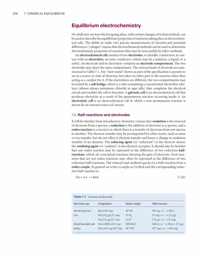
216 7 CHEMICAL EQUILIBRIUM
Equilibrium electrochemistry
We shall now see how the foregoing ideas, with certain changes of technical detail, canbe used to describe the equilibrium properties of reactions taking place in electrochem-ical cells. The ability to make very precise measurements of currents and potentialdifferences (‘voltages’) means that electrochemical methods can be used to determinethermodynamic properties of reactions that may be inaccessible by other methods.
An electrochemical cell consists of two electrodes, or metallic conductors, in con-tact with an electrolyte, an ionic conductor (which may be a solution, a liquid, or asolid). An electrode and its electrolyte comprise an electrode compartment. The twoelectrodes may share the same compartment. The various kinds of electrode are sum-marized in Table 7.1. Any ‘inert metal’ shown as part of the specification is present toact as a source or sink of electrons, but takes no other part in the reaction other thanacting as a catalyst for it. If the electrolytes are different, the two compartments maybe joined by a salt bridge, which is a tube containing a concentrated electrolyte solu-tion (almost always potassium chloride in agar jelly) that completes the electrical circuit and enables the cell to function. A galvanic cell is an electrochemical cell thatproduces electricity as a result of the spontaneous reaction occurring inside it. Anelectrolytic cell is an electrochemical cell in which a non-spontaneous reaction isdriven by an external source of current.
7.5 Half-reactions and electrodes
It will be familiar from introductory chemistry courses that oxidation is the removalof electrons from a species, a reduction is the addition of electrons to a species, and aredox reaction is a reaction in which there is a transfer of electrons from one speciesto another. The electron transfer may be accompanied by other events, such as atomor ion transfer, but the net effect is electron transfer and hence a change in oxidationnumber of an element. The reducing agent (or ‘reductant’) is the electron donor; the oxidizing agent (or ‘oxidant’) is the electron acceptor. It should also be familiarthat any redox reaction may be expressed as the difference of two reduction half-reactions, which are conceptual reactions showing the gain of electrons. Even reac-tions that are not redox reactions may often be expressed as the difference of two reduction half-reactions. The reduced and oxidized species in a half-reaction form aredox couple. In general we write a couple as Ox/Red and the corresponding reduc-tion half-reaction as
Ox + ν e− → Red (7.26)
Table 7.1 Varieties of electrode
Electrode type Designation Redox couple Half-reaction
Metal/metal ion M(s) | M+(aq) M+/M M+(aq) + e− → M(s)
Gas Pt(s) | X2(g) | X+(aq) X+/X2 X+(aq) + e− → 1–2 X2(g)
Pt(s) | X2(g) | X−(aq) X2/X− 1–2 X2(g) + e− → X−(aq)
Metal/insoluble salt M(s) | MX(s) | X−(aq) MX/M,X− MX(s) + e− → M(s) + X−(aq)
Redox Pt(s) | M+(aq),M2+(aq) M2+/M+ M2+(aq) + e− → M+(aq)
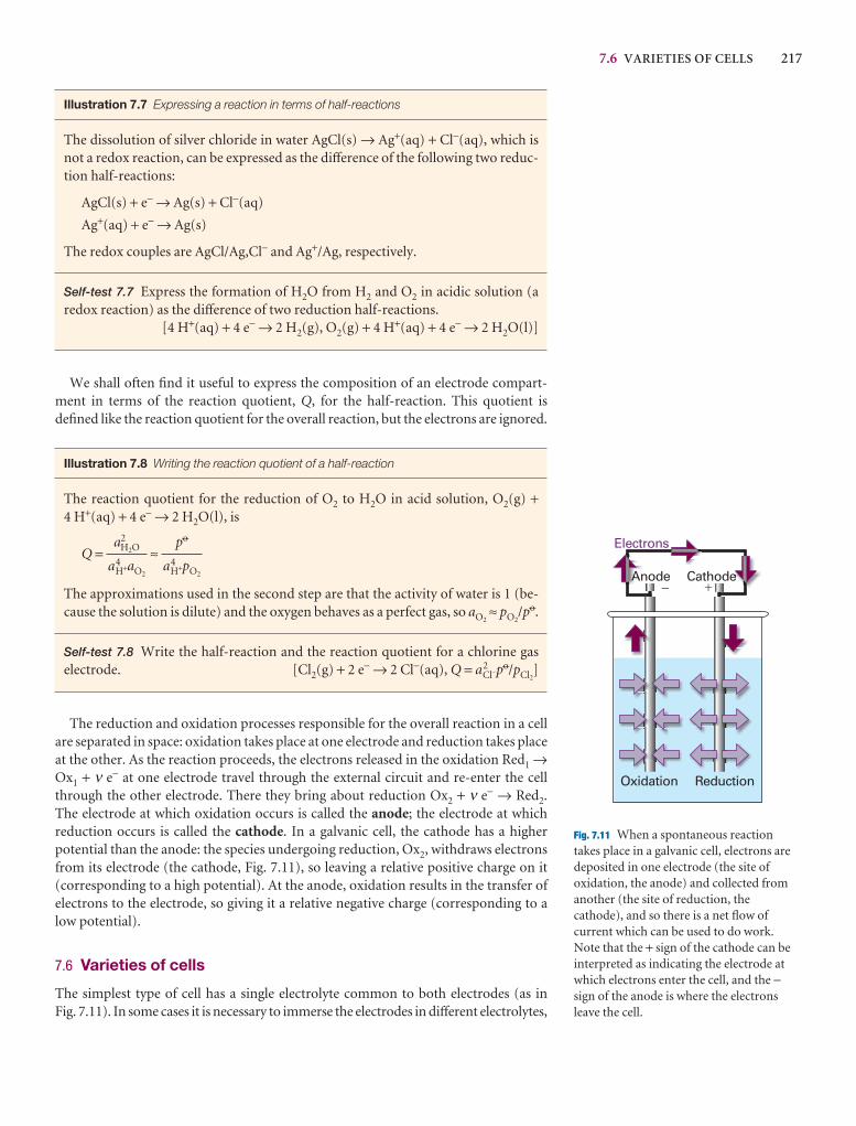
7.6 VARIETIES OF CELLS 217
Reduction
Anode Cathode� �
Electrons
Oxidation
Fig. 7.11 When a spontaneous reactiontakes place in a galvanic cell, electrons aredeposited in one electrode (the site ofoxidation, the anode) and collected fromanother (the site of reduction, thecathode), and so there is a net flow ofcurrent which can be used to do work.Note that the + sign of the cathode can beinterpreted as indicating the electrode atwhich electrons enter the cell, and the −sign of the anode is where the electronsleave the cell.
Illustration 7.7 Expressing a reaction in terms of half-reactions
The dissolution of silver chloride in water AgCl(s) → Ag+(aq) + Cl−(aq), which isnot a redox reaction, can be expressed as the difference of the following two reduc-tion half-reactions:
AgCl(s) + e− → Ag(s) + Cl−(aq)
Ag+(aq) + e− → Ag(s)
The redox couples are AgCl/Ag,Cl− and Ag+/Ag, respectively.
Self-test 7.7 Express the formation of H2O from H2 and O2 in acidic solution (aredox reaction) as the difference of two reduction half-reactions.
[4 H+(aq) + 4 e− → 2 H2(g), O2(g) + 4 H+(aq) + 4 e− → 2 H2O(l)]
We shall often find it useful to express the composition of an electrode compart-ment in terms of the reaction quotient, Q, for the half-reaction. This quotient isdefined like the reaction quotient for the overall reaction, but the electrons are ignored.
Illustration 7.8 Writing the reaction quotient of a half-reaction
The reaction quotient for the reduction of O2 to H2O in acid solution, O2(g) +4 H+(aq) + 4 e− → 2 H2O(l), is
Q = ≈
The approximations used in the second step are that the activity of water is 1 (be-cause the solution is dilute) and the oxygen behaves as a perfect gas, so aO2
≈ pO2/p7.
Self-test 7.8 Write the half-reaction and the reaction quotient for a chlorine gaselectrode. [Cl2(g) + 2 e− → 2 Cl−(aq), Q = a2
Cl−p7/pCl2
]
The reduction and oxidation processes responsible for the overall reaction in a cellare separated in space: oxidation takes place at one electrode and reduction takes placeat the other. As the reaction proceeds, the electrons released in the oxidation Red1 →Ox1 + ν e− at one electrode travel through the external circuit and re-enter the cellthrough the other electrode. There they bring about reduction Ox2 + ν e− → Red2.The electrode at which oxidation occurs is called the anode; the electrode at which reduction occurs is called the cathode. In a galvanic cell, the cathode has a higher potential than the anode: the species undergoing reduction, Ox2, withdraws electronsfrom its electrode (the cathode, Fig. 7.11), so leaving a relative positive charge on it(corresponding to a high potential). At the anode, oxidation results in the transfer ofelectrons to the electrode, so giving it a relative negative charge (corresponding to alow potential).
7.6 Varieties of cells
The simplest type of cell has a single electrolyte common to both electrodes (as in Fig. 7.11). In some cases it is necessary to immerse the electrodes in different electrolytes,
p7
a4H+pO2
a2H2O
a4H+aO2
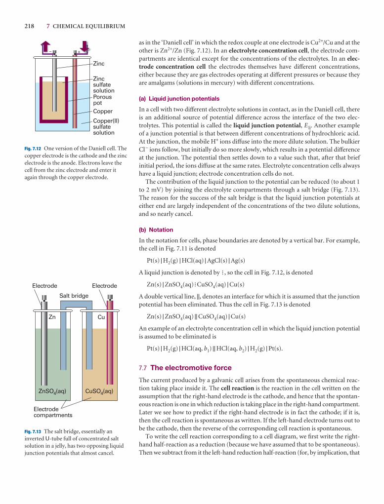
218 7 CHEMICAL EQUILIBRIUM
as in the ‘Daniell cell’ in which the redox couple at one electrode is Cu2+/Cu and at theother is Zn2+/Zn (Fig. 7.12). In an electrolyte concentration cell, the electrode com-partments are identical except for the concentrations of the electrolytes. In an elec-trode concentration cell the electrodes themselves have different concentrations,either because they are gas electrodes operating at different pressures or because theyare amalgams (solutions in mercury) with different concentrations.
(a) Liquid junction potentials
In a cell with two different electrolyte solutions in contact, as in the Daniell cell, thereis an additional source of potential difference across the interface of the two elec-trolytes. This potential is called the liquid junction potential, E lj. Another example of a junction potential is that between different concentrations of hydrochloric acid.At the junction, the mobile H+ ions diffuse into the more dilute solution. The bulkier Cl− ions follow, but initially do so more slowly, which results in a potential differenceat the junction. The potential then settles down to a value such that, after that briefinitial period, the ions diffuse at the same rates. Electrolyte concentration cells alwayshave a liquid junction; electrode concentration cells do not.
The contribution of the liquid junction to the potential can be reduced (to about 1to 2 mV) by joining the electrolyte compartments through a salt bridge (Fig. 7.13).The reason for the success of the salt bridge is that the liquid junction potentials at either end are largely independent of the concentrations of the two dilute solutions,and so nearly cancel.
(b) Notation
In the notation for cells, phase boundaries are denoted by a vertical bar. For example,the cell in Fig. 7.11 is denoted
Pt(s) | H2(g) | HCl(aq) | AgCl(s) | Ag(s)
A liquid junction is denoted by �, so the cell in Fig. 7.12, is denoted
Zn(s) | ZnSO4(aq)�CuSO4(aq) | Cu(s)
A double vertical line, ||, denotes an interface for which it is assumed that the junctionpotential has been eliminated. Thus the cell in Fig. 7.13 is denoted
Zn(s) | ZnSO4(aq) || CuSO4(aq) | Cu(s)
An example of an electrolyte concentration cell in which the liquid junction potentialis assumed to be eliminated is
Pt(s) | H2(g) | HCl(aq, b1) || HCl(aq, b2) | H2(g) | Pt(s).
7.7 The electromotive force
The current produced by a galvanic cell arises from the spontaneous chemical reac-tion taking place inside it. The cell reaction is the reaction in the cell written on the assumption that the right-hand electrode is the cathode, and hence that the spontan-eous reaction is one in which reduction is taking place in the right-hand compartment.Later we see how to predict if the right-hand electrode is in fact the cathode; if it is,then the cell reaction is spontaneous as written. If the left-hand electrode turns out tobe the cathode, then the reverse of the corresponding cell reaction is spontaneous.
To write the cell reaction corresponding to a cell diagram, we first write the right-hand half-reaction as a reduction (because we have assumed that to be spontaneous).Then we subtract from it the left-hand reduction half-reaction (for, by implication, that
Zinc
Copper
Zincsulfatesolution
Copper(II)sulfatesolution
Porouspot
+-
Fig. 7.12 One version of the Daniell cell. Thecopper electrode is the cathode and the zincelectrode is the anode. Electrons leave thecell from the zinc electrode and enter itagain through the copper electrode.
Electrode Electrode
Salt bridge
Electrodecompartments
Zn
ZnSO (aq)4 CuSO (aq)4
Cu
Fig. 7.13 The salt bridge, essentially aninverted U-tube full of concentrated saltsolution in a jelly, has two opposing liquidjunction potentials that almost cancel.
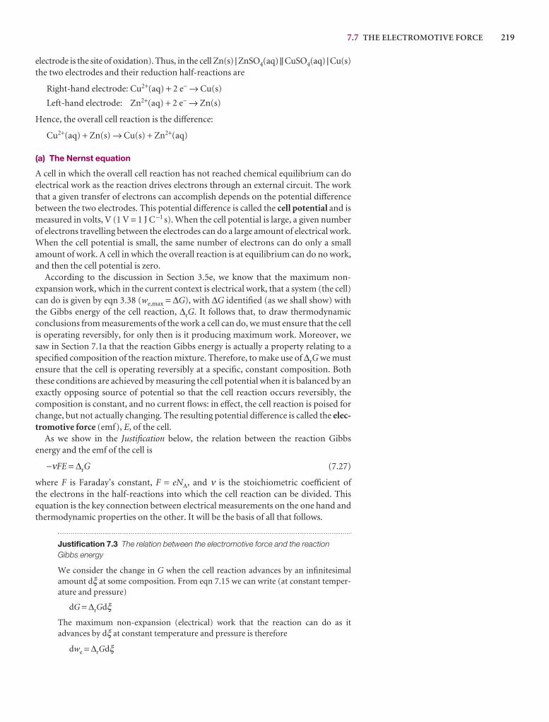
7.7 THE ELECTROMOTIVE FORCE 219
electrode is the site of oxidation). Thus, in the cell Zn(s) | ZnSO4(aq) || CuSO4(aq) | Cu(s)the two electrodes and their reduction half-reactions are
Right-hand electrode: Cu2+(aq) + 2 e− → Cu(s)
Left-hand electrode: Zn2+(aq) + 2 e− → Zn(s)
Hence, the overall cell reaction is the difference:
Cu2+(aq) + Zn(s) → Cu(s) + Zn2+(aq)
(a) The Nernst equation
A cell in which the overall cell reaction has not reached chemical equilibrium can doelectrical work as the reaction drives electrons through an external circuit. The workthat a given transfer of electrons can accomplish depends on the potential differencebetween the two electrodes. This potential difference is called the cell potential and ismeasured in volts, V (1 V = 1 J C−1 s). When the cell potential is large, a given numberof electrons travelling between the electrodes can do a large amount of electrical work.When the cell potential is small, the same number of electrons can do only a smallamount of work. A cell in which the overall reaction is at equilibrium can do no work,and then the cell potential is zero.
According to the discussion in Section 3.5e, we know that the maximum non-expansion work, which in the current context is electrical work, that a system (the cell)can do is given by eqn 3.38 (we,max = ∆G), with ∆G identified (as we shall show) withthe Gibbs energy of the cell reaction, ∆rG. It follows that, to draw thermodynamicconclusions from measurements of the work a cell can do, we must ensure that the cellis operating reversibly, for only then is it producing maximum work. Moreover, wesaw in Section 7.1a that the reaction Gibbs energy is actually a property relating to aspecified composition of the reaction mixture. Therefore, to make use of ∆rG we mustensure that the cell is operating reversibly at a specific, constant composition. Boththese conditions are achieved by measuring the cell potential when it is balanced by anexactly opposing source of potential so that the cell reaction occurs reversibly, thecomposition is constant, and no current flows: in effect, the cell reaction is poised forchange, but not actually changing. The resulting potential difference is called the elec-tromotive force (emf), E, of the cell.
As we show in the Justification below, the relation between the reaction Gibbs energy and the emf of the cell is
−νFE = ∆rG (7.27)
where F is Faraday’s constant, F = eNA, and ν is the stoichiometric coefficient of the electrons in the half-reactions into which the cell reaction can be divided. Thisequation is the key connection between electrical measurements on the one hand andthermodynamic properties on the other. It will be the basis of all that follows.
Justification 7.3 The relation between the electromotive force and the reactionGibbs energy
We consider the change in G when the cell reaction advances by an infinitesimalamount dξ at some composition. From eqn 7.15 we can write (at constant temper-ature and pressure)
dG = ∆rGdξ
The maximum non-expansion (electrical) work that the reaction can do as it advances by dξ at constant temperature and pressure is therefore
dwe = ∆rGdξ
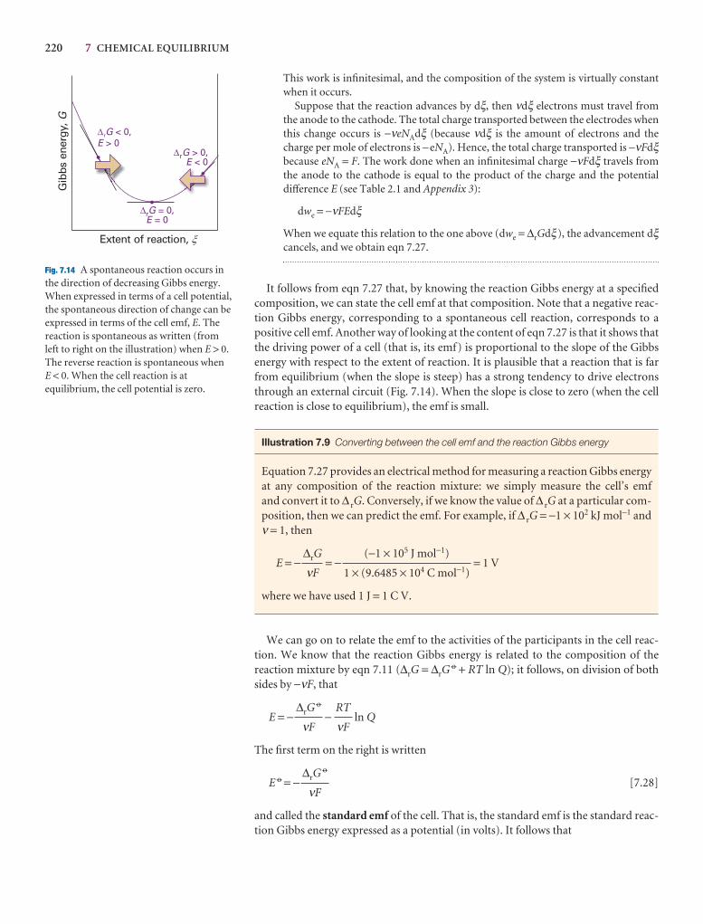
220 7 CHEMICAL EQUILIBRIUM
rGE
< 0,> 0
rGE
= 0,= 0
rGE
> 0,< 0
Extent of reaction,
Gib
bs e
nerg
y,G
�
Fig. 7.14 A spontaneous reaction occurs inthe direction of decreasing Gibbs energy.When expressed in terms of a cell potential,the spontaneous direction of change can beexpressed in terms of the cell emf, E. Thereaction is spontaneous as written (fromleft to right on the illustration) when E > 0.The reverse reaction is spontaneous when E < 0. When the cell reaction is atequilibrium, the cell potential is zero.
This work is infinitesimal, and the composition of the system is virtually constantwhen it occurs.
Suppose that the reaction advances by dξ, then νdξ electrons must travel fromthe anode to the cathode. The total charge transported between the electrodes whenthis change occurs is −νeNAdξ (because νdξ is the amount of electrons and thecharge per mole of electrons is −eNA). Hence, the total charge transported is −νFdξbecause eNA = F. The work done when an infinitesimal charge −νFdξ travels fromthe anode to the cathode is equal to the product of the charge and the potentialdifference E (see Table 2.1 and Appendix 3):
dwe = −νFEdξ
When we equate this relation to the one above (dwe = ∆rGdξ), the advancement dξcancels, and we obtain eqn 7.27.
It follows from eqn 7.27 that, by knowing the reaction Gibbs energy at a specifiedcomposition, we can state the cell emf at that composition. Note that a negative reac-tion Gibbs energy, corresponding to a spontaneous cell reaction, corresponds to apositive cell emf. Another way of looking at the content of eqn 7.27 is that it shows thatthe driving power of a cell (that is, its emf) is proportional to the slope of the Gibbs energy with respect to the extent of reaction. It is plausible that a reaction that is farfrom equilibrium (when the slope is steep) has a strong tendency to drive electronsthrough an external circuit (Fig. 7.14). When the slope is close to zero (when the cellreaction is close to equilibrium), the emf is small.
Illustration 7.9 Converting between the cell emf and the reaction Gibbs energy
Equation 7.27 provides an electrical method for measuring a reaction Gibbs energyat any composition of the reaction mixture: we simply measure the cell’s emf and convert it to ∆ rG. Conversely, if we know the value of ∆ rG at a particular com-position, then we can predict the emf. For example, if ∆ rG = −1 × 10² kJ mol−1 andν = 1, then
E = − = − = 1 V
where we have used 1 J = 1 C V.
We can go on to relate the emf to the activities of the participants in the cell reac-tion. We know that the reaction Gibbs energy is related to the composition of the reaction mixture by eqn 7.11 (∆rG = ∆rG
7 + RT ln Q); it follows, on division of bothsides by −νF, that
E = − − ln Q
The first term on the right is written
E 7 = − [7.28]
and called the standard emf of the cell. That is, the standard emf is the standard reac-tion Gibbs energy expressed as a potential (in volts). It follows that
∆rG7
νF
RT
νF
∆rG7
νF
(−1 × 10⁵ J mol−1)
1 × (9.6485 × 104 C mol−1)
∆rG
νF
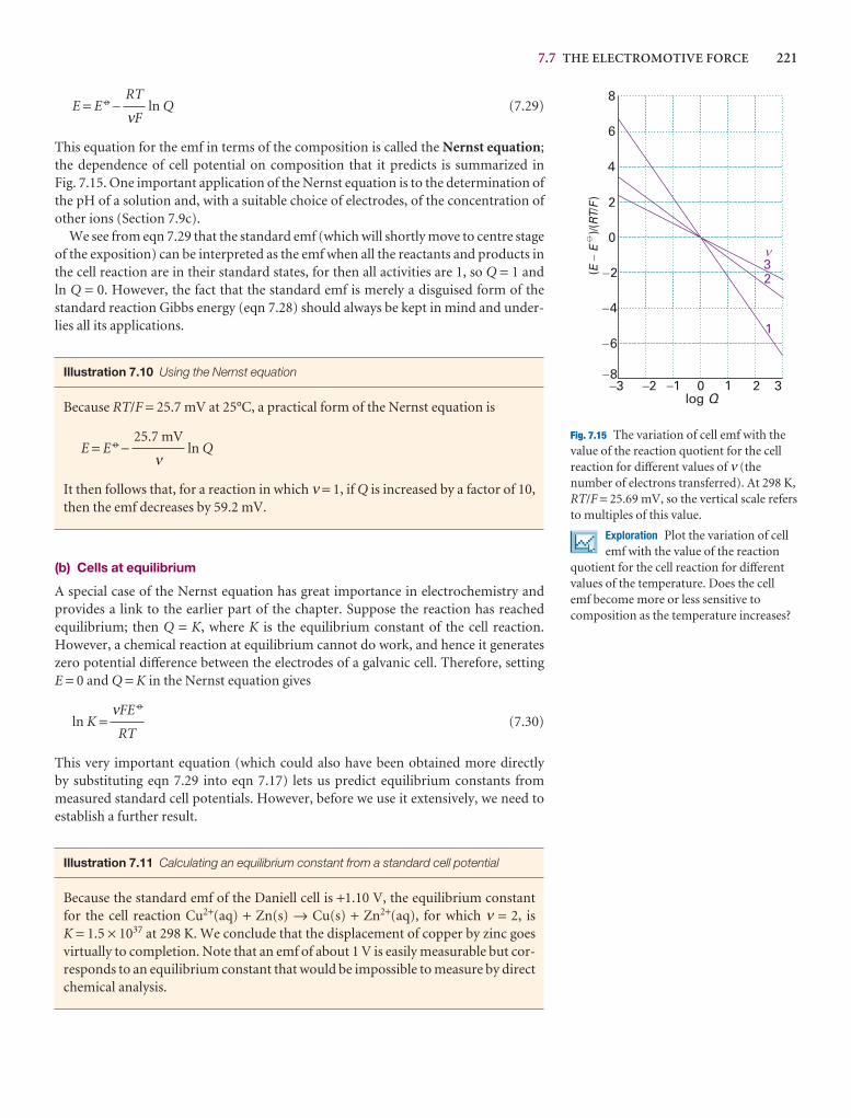
7.7 THE ELECTROMOTIVE FORCE 221
�3 �2 �1 0 1 2 3log Q
8
6
4
2
0
�2
�4
�6
�8
1
23�
()/(
/)
EE
RTF
�
�
Fig. 7.15 The variation of cell emf with thevalue of the reaction quotient for the cellreaction for different values of ν (thenumber of electrons transferred). At 298 K,RT/F = 25.69 mV, so the vertical scale refersto multiples of this value.
Exploration Plot the variation of cellemf with the value of the reaction
quotient for the cell reaction for differentvalues of the temperature. Does the cellemf become more or less sensitive tocomposition as the temperature increases?
E = E 7 − ln Q (7.29)
This equation for the emf in terms of the composition is called the Nernst equation;the dependence of cell potential on composition that it predicts is summarized in Fig. 7.15. One important application of the Nernst equation is to the determination ofthe pH of a solution and, with a suitable choice of electrodes, of the concentration ofother ions (Section 7.9c).
We see from eqn 7.29 that the standard emf (which will shortly move to centre stageof the exposition) can be interpreted as the emf when all the reactants and products inthe cell reaction are in their standard states, for then all activities are 1, so Q = 1 and ln Q = 0. However, the fact that the standard emf is merely a disguised form of thestandard reaction Gibbs energy (eqn 7.28) should always be kept in mind and under-lies all its applications.
Illustration 7.10 Using the Nernst equation
Because RT/F = 25.7 mV at 25°C, a practical form of the Nernst equation is
E = E 7 − ln Q
It then follows that, for a reaction in which ν = 1, if Q is increased by a factor of 10,then the emf decreases by 59.2 mV.
(b) Cells at equilibrium
A special case of the Nernst equation has great importance in electrochemistry andprovides a link to the earlier part of the chapter. Suppose the reaction has reachedequilibrium; then Q = K, where K is the equilibrium constant of the cell reaction.However, a chemical reaction at equilibrium cannot do work, and hence it generateszero potential difference between the electrodes of a galvanic cell. Therefore, setting E = 0 and Q = K in the Nernst equation gives
ln K = (7.30)
This very important equation (which could also have been obtained more directly by substituting eqn 7.29 into eqn 7.17) lets us predict equilibrium constants frommeasured standard cell potentials. However, before we use it extensively, we need toestablish a further result.
Illustration 7.11 Calculating an equilibrium constant from a standard cell potential
Because the standard emf of the Daniell cell is +1.10 V, the equilibrium constantfor the cell reaction Cu2+(aq) + Zn(s) → Cu(s) + Zn2+(aq), for which ν = 2, is K = 1.5 × 1037 at 298 K. We conclude that the displacement of copper by zinc goesvirtually to completion. Note that an emf of about 1 V is easily measurable but cor-responds to an equilibrium constant that would be impossible to measure by directchemical analysis.
νFE 7
RT
25.7 mV
ν
RT
νF
222 7 CHEMICAL EQUILIBRIUM
7.8 Standard potentials
A galvanic cell is a combination of two electrodes, and each one can be considered asmaking a characteristic contribution to the overall cell potential. Although it is notpossible to measure the contribution of a single electrode, we can define the potentialof one of the electrodes as zero and then assign values to others on that basis. The spe-cially selected electrode is the standard hydrogen electrode (SHE):
Pt(s) | H2(g) | H+(aq) E 7 = 0 [7.31]
at all temperatures. To achieve the standard conditions, the activity of the hydrogenions must be 1 (that is, pH = 0) and the pressure (more precisely, the fugacity) of thehydrogen gas must be 1 bar. The standard potential, E 7, of another couple is then assigned by constructing a cell in which it is the right-hand electrode and the standardhydrogen electrode is the left-hand electrode.
The procedure for measuring a standard potential can be illustrated by consideringa specific case, the silver chloride electrode. The measurement is made on the ‘Harnedcell’:
Pt(s) | H2(g) | HCl(aq) | AgCl(s) | Ag(s) 1–2 H2(g) + AgCl(s) → HCl(aq) + Ag(s)
for which the Nernst equation is
E = E 7(AgCl/Ag, Cl−) − ln
We shall set aH2= 1 from now on, and for simplicity write the standard potential as E 7;
then
E = E 7 − ln aH+aCl−
The activities can be expressed in terms of the molality b of HCl(aq) through aH+ =γ±b/b 7 and aCl− = γ±b/b 7 as we saw in Section 5.9), so
E = E 7 − ln b2 − ln γ ±2
where for simplicity we have replaced b/b 7 by b. This expression rearranges to
E + ln b = E 7 − ln γ± {7.32}
From the Debye–Hückel limiting law for a 1,1-electrolyte (Section 5.9; a 1,1-electrolyte is a solution of singly charged M+ and X− ions), we know that ln γ± ∝ −b1/2.The natural logarithm used here is proportional to the common logarithm that appears in eqn 5.69 (because ln x = ln 10 log x = 2.303 log x). Therefore, with the con-stant of proportionality in this relation written as (F/2RT)C, eqn 7.32 becomes
E + ln b = E 7 + Cb1/2 {7.33}
The expression on the left is evaluated at a range of molalities, plotted against b1/2,and extrapolated to b = 0. The intercept at b1/2 = 0 is the value of E 7 for the silver/silver-chloride electrode. In precise work, the b1/2 term is brought to the left, and ahigher-order correction term from the extended Debye–Hückel law is used on theright.
2RT
F
2RT
F
2RT
F
RT
F
RT
F
RT
F
aH+aCl−
a1/2H2
RT
F
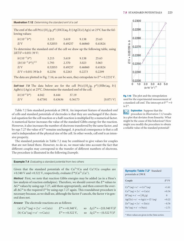
7.8 STANDARD POTENTIALS 223
0 1.0 2.0
Eb
/V +
0.0
5139
ln
( /10 )b b�3 �
3.0 4.0 5.0
0.2250
0.2260
0.2270
0.2280
0.2290
0.2300
0.2240
0.2230
1/2
Fig. 7.16 The plot and the extrapolationused for the experimental measurement ofa standard cell emf. The intercept at b1/2 = 0is E 7.
Exploration Suppose that theprocedure in Illustration 7.12 results
in a plot that deviates from linearity. Whatmight be the cause of this behaviour? Howmight you modify the procedure to obtaina reliable value of the standard potential?
Synoptic Table 7.2* Standardpotentials at 298 K
Couple E 7/V
Ce4+(aq) + e− → Ce3+(aq) +1.61
Cu2+(aq) + 2 e− → Cu(s) +0.34
H+(aq) + e− → 1–2 H2(g) 0
AgCl(s) + e− → Ag(s) + Cl−(aq) +0.22
Zn2+(aq) + 2 e− → Zn(s) −0.76
Na+(aq) + e− → Na(s) −2.71
* More values are given in the Data section.
Illustration 7.12 Determining the standard emf of a cell
The emf of the cell Pt(s) | H2(g, p7) | HCl(aq, b) | AgCl(s) | Ag(s) at 25°C has the fol-lowing values:
b/(10−3 b 7) 3.215 5.619 9.138 25.63
E/V 0.52053 0.49257 0.46860 0.41824
To determine the standard emf of the cell we draw up the following table, using2RT/F = 0.051 39 V:
b/(10−3 b 7) 3.215 5.619 9.138 25.63
{b/(10−3 b 7)}1/2 1.793 2.370 3.023 5.063
E/V 0.52053 0.49257 0.46860 0.41824
E/V + 0.051 39 ln b 0.2256 0.2263 0.2273 0.2299
The data are plotted in Fig. 7.16; as can be seen, they extrapolate to E 7 = 0.2232 V.
Self-test 7.9 The data below are for the cell Pt(s) | H2(g, p 7) | HBr(aq, b) |AgBr(s) | Ag(s) at 25°C. Determine the standard emf of the cell.
b/(10−4 b 7) 4.042 8.444 37.19
E/V 0.47381 0.43636 0.36173 [0.071 V]
Table 7.2 lists standard potentials at 298 K. An important feature of standard emfof cells and standard potentials of electrodes is that they are unchanged if the chem-ical equation for the cell reaction or a half-reaction is multiplied by a numerical factor.A numerical factor increases the value of the standard Gibbs energy for the reaction.However, it also increases the number of electrons transferred by the same factor, andby eqn 7.27 the value of E 7 remains unchanged. A practical consequence is that a cellemf is independent of the physical size of the cell. In other words, cell emf is an inten-sive property.
The standard potentials in Table 7.2 may be combined to give values for couplesthat are not listed there. However, to do so, we must take into account the fact thatdifferent couples may correspond to the transfer of different numbers of electrons.The procedure is illustrated in the following Example.
Example 7.4 Evaluating a standard potential from two others
Given that the standard potentials of the Cu2+/Cu and Cu+/Cu couples are +0.340 V and +0.522 V, respectively, evaluate E 7(Cu2+,Cu+).
Method First, we note that reaction Gibbs energies may be added (as in a Hess’slaw analysis of reaction enthalpies). Therefore, we should convert the E 7 values to∆G 7 values by using eqn 7.27, add them appropriately, and then convert the over-all ∆G 7 to the required E 7 by using eqn 7.27 again. This roundabout procedure isnecessary because, as we shall see, although the factor F cancels, the factor ν in gen-eral does not.
Answer The electrode reactions are as follows:
(a) Cu2+(aq) + 2 e− → Cu(s) E 7 = +0.340 V, so ∆rG7 = −2(0.340 V)F
(b) Cu+(aq) + e− → Cu(s) E 7 = +0.522 V, so ∆rG7 = −(0.522 V)F
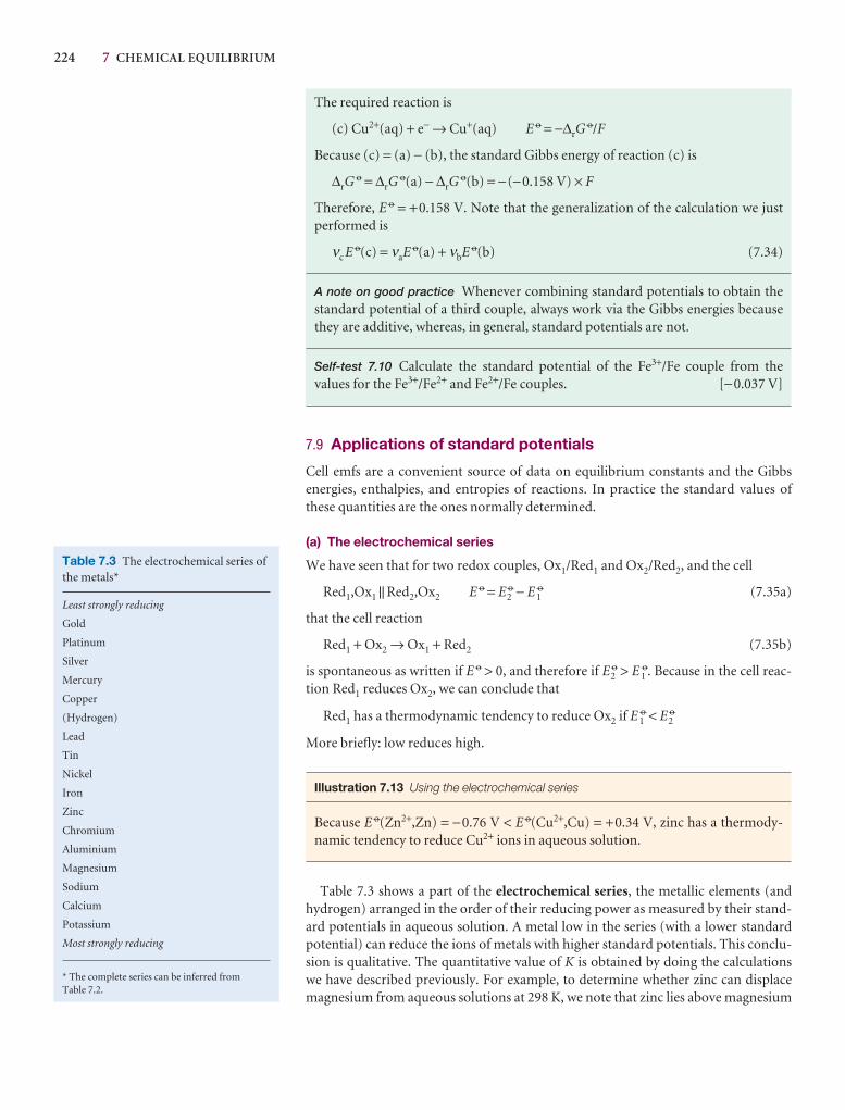
224 7 CHEMICAL EQUILIBRIUM
The required reaction is
(c) Cu2+(aq) + e− → Cu+(aq) E 7 = −∆rG7/F
Because (c) = (a) − (b), the standard Gibbs energy of reaction (c) is
∆rG7 = ∆rG
7(a) − ∆rG7(b) = −(−0.158 V) × F
Therefore, E 7 = +0.158 V. Note that the generalization of the calculation we justperformed is
νc E 7(c) = νaE7(a) + νbE 7(b) (7.34)
A note on good practice Whenever combining standard potentials to obtain thestandard potential of a third couple, always work via the Gibbs energies becausethey are additive, whereas, in general, standard potentials are not.
Self-test 7.10 Calculate the standard potential of the Fe3+/Fe couple from thevalues for the Fe3+/Fe2+ and Fe2+/Fe couples. [−0.037 V]
7.9 Applications of standard potentials
Cell emfs are a convenient source of data on equilibrium constants and the Gibbs energies, enthalpies, and entropies of reactions. In practice the standard values ofthese quantities are the ones normally determined.
(a) The electrochemical series
We have seen that for two redox couples, Ox1/Red1 and Ox2/Red2, and the cell
Red1,Ox1 || Red2,Ox2 E 7 = E27 − E 1
7 (7.35a)
that the cell reaction
Red1 + Ox2 → Ox1 + Red2 (7.35b)
is spontaneous as written if E 7 > 0, and therefore if E27 > E 1
7. Because in the cell reac-tion Red1 reduces Ox2, we can conclude that
Red1 has a thermodynamic tendency to reduce Ox2 if E 17 < E2
7
More briefly: low reduces high.
Illustration 7.13 Using the electrochemical series
Because E 7(Zn2+,Zn) = −0.76 V < E 7(Cu2+,Cu) = +0.34 V, zinc has a thermody-namic tendency to reduce Cu2+ ions in aqueous solution.
Table 7.3 shows a part of the electrochemical series, the metallic elements (and hydrogen) arranged in the order of their reducing power as measured by their stand-ard potentials in aqueous solution. A metal low in the series (with a lower standard potential) can reduce the ions of metals with higher standard potentials. This conclu-sion is qualitative. The quantitative value of K is obtained by doing the calculations we have described previously. For example, to determine whether zinc can displacemagnesium from aqueous solutions at 298 K, we note that zinc lies above magnesium
Table 7.3 The electrochemical series ofthe metals*
Least strongly reducing
Gold
Platinum
Silver
Mercury
Copper
(Hydrogen)
Lead
Tin
Nickel
Iron
Zinc
Chromium
Aluminium
Magnesium
Sodium
Calcium
Potassium
Most strongly reducing
* The complete series can be inferred from Table 7.2.
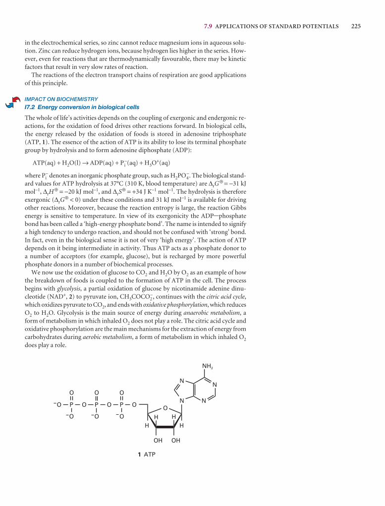
7.9 APPLICATIONS OF STANDARD POTENTIALS 225
in the electrochemical series, so zinc cannot reduce magnesium ions in aqueous solu-tion. Zinc can reduce hydrogen ions, because hydrogen lies higher in the series. How-ever, even for reactions that are thermodynamically favourable, there may be kineticfactors that result in very slow rates of reaction.
The reactions of the electron transport chains of respiration are good applicationsof this principle.
IMPACT ON BIOCHEMISTRY
I7.2 Energy conversion in biological cells
The whole of life’s activities depends on the coupling of exergonic and endergonic re-actions, for the oxidation of food drives other reactions forward. In biological cells,the energy released by the oxidation of foods is stored in adenosine triphosphate(ATP, 1). The essence of the action of ATP is its ability to lose its terminal phosphategroup by hydrolysis and to form adenosine diphosphate (ADP):
ATP(aq) + H2O(l) → ADP(aq) + Pi−(aq) + H3O+(aq)
where Pi− denotes an inorganic phosphate group, such as H2PO4
−. The biological stand-ard values for ATP hydrolysis at 37°C (310 K, blood temperature) are ∆rG
⊕ = −31 kJmol−1, ∆rH
⊕ = −20 kJ mol−1, and ∆rS⊕ = +34 J K−1 mol−1. The hydrolysis is therefore
exergonic (∆rG⊕ < 0) under these conditions and 31 kJ mol−1 is available for driving
other reactions. Moreover, because the reaction entropy is large, the reaction Gibbsenergy is sensitive to temperature. In view of its exergonicity the ADP-phosphatebond has been called a ‘high-energy phosphate bond’. The name is intended to signifya high tendency to undergo reaction, and should not be confused with ‘strong’ bond.In fact, even in the biological sense it is not of very ‘high energy’. The action of ATPdepends on it being intermediate in activity. Thus ATP acts as a phosphate donor toa number of acceptors (for example, glucose), but is recharged by more powerfulphosphate donors in a number of biochemical processes.
We now use the oxidation of glucose to CO2 and H2O by O2 as an example of howthe breakdown of foods is coupled to the formation of ATP in the cell. The process begins with glycolysis, a partial oxidation of glucose by nicotinamide adenine dinu-cleotide (NAD+, 2) to pyruvate ion, CH3COCO2
−, continues with the citric acid cycle,which oxidizes pyruvate to CO2, and ends with oxidative phosphorylation, which reducesO2 to H2O. Glycolysis is the main source of energy during anaerobic metabolism, aform of metabolism in which inhaled O2 does not play a role. The citric acid cycle andoxidative phosphorylation are the main mechanisms for the extraction of energy fromcarbohydrates during aerobic metabolism, a form of metabolism in which inhaled O2
does play a role.
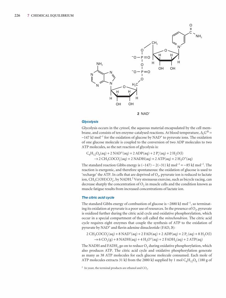
226 7 CHEMICAL EQUILIBRIUM
Glycolysis
Glycolysis occurs in the cytosol, the aqueous material encapsulated by the cell mem-brane, and consists of ten enzyme-catalysed reactions. At blood temperature, ∆rG
⊕ =−147 kJ mol−1 for the oxidation of glucose by NAD+ to pyruvate ions. The oxidationof one glucose molecule is coupled to the conversion of two ADP molecules to twoATP molecules, so the net reaction of glycolysis is:
C6H12O6(aq) + 2 NAD+(aq) + 2 ADP(aq) + 2 Pi−(aq) + 2 H2O(l)
→ 2 CH3COCO2−(aq) + 2 NADH(aq) + 2 ATP(aq) + 2 H3O+(aq)
The standard reaction Gibbs energy is (−147) − 2(−31) kJ mol−1 = −85 kJ mol−1. Thereaction is exergonic, and therefore spontaneous: the oxidation of glucose is used to‘recharge’ the ATP. In cells that are deprived of O2, pyruvate ion is reduced to lactateion, CH3C(OH)CO2
−, by NADH.2 Very strenuous exercise, such as bicycle racing, candecrease sharply the concentration of O2 in muscle cells and the condition known asmuscle fatigue results from increased concentrations of lactate ion.
The citric acid cycle
The standard Gibbs energy of combustion of glucose is −2880 kJ mol−1, so terminat-ing its oxidation at pyruvate is a poor use of resources. In the presence of O2, pyruvateis oxidized further during the citric acid cycle and oxidative phosphorylation, whichoccur in a special compartment of the cell called the mitochondrion. The citric acidcycle requires eight enzymes that couple the synthesis of ATP to the oxidation ofpyruvate by NAD+ and flavin adenine dinucleotide (FAD, 3):
2 CH3COCO2−(aq) + 8 NAD+(aq) + 2 FAD(aq) + 2 ADP(aq) + 2 Pi (aq) + 8 H2O(l)
→ 6 CO2(g) + 8 NADH(aq) + 4 H3O+(aq) + 2 FADH2(aq) + 2 ATP(aq)
The NADH and FADH2 go on to reduce O2 during oxidative phosphorylation, whichalso produces ATP. The citric acid cycle and oxidative phosphorylation generate as many as 38 ATP molecules for each glucose molecule consumed. Each mole of ATP molecules extracts 31 kJ from the 2880 kJ supplied by 1 mol C6H12O6 (180 g of
2 In yeast, the terminal products are ethanol and CO2.
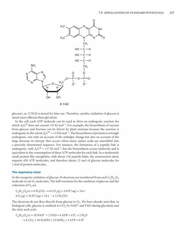
7.9 APPLICATIONS OF STANDARD POTENTIALS 227
glucose), so 1178 kJ is stored for later use. Therefore, aerobic oxidation of glucose ismuch more efficient than glycolysis.
In the cell, each ATP molecule can be used to drive an endergonic reaction forwhich ∆rG
⊕ does not exceed +31 kJ mol−1. For example, the biosynthesis of sucrosefrom glucose and fructose can be driven by plant enzymes because the reaction is endergonic to the extent ∆rG
⊕ = +23 kJ mol−1. The biosynthesis of proteins is stronglyendergonic, not only on account of the enthalpy change but also on account of thelarge decrease in entropy that occurs when many amino acids are assembled into a precisely determined sequence. For instance, the formation of a peptide link is endergonic, with ∆rG
⊕ = +17 kJ mol−1, but the biosynthesis occurs indirectly and isequivalent to the consumption of three ATP molecules for each link. In a moderatelysmall protein like myoglobin, with about 150 peptide links, the construction alone requires 450 ATP molecules, and therefore about 12 mol of glucose molecules for 1 mol of protein molecules.
The respiratory chain
In the exergonic oxidation of glucose 24 electrons are transferred from each C6H12O6
molecule to six O2 molecules. The half-reactions for the oxidation of glucose and thereduction of O2 are
C6H12O6(s) + 6 H2O(l) → 6 CO2(g) + 24 H+(aq) + 24 e−
6 O2(g) + 24 H+(aq) + 24 e− → 12 H2O(l)
The electrons do not flow directly from glucose to O2. We have already seen that, inbiological cells, glucose is oxidized to CO2 by NAD+ and FAD during glycolysis andthe citric acid cycle:
C6H12O6(s) + 10 NAD+ + 2 FAD + 4 ADP + 4 Pi− + 2 H2O
→ 6 CO2 + 10 NADH + 2 FADH2 + 4 ATP + 6 H+
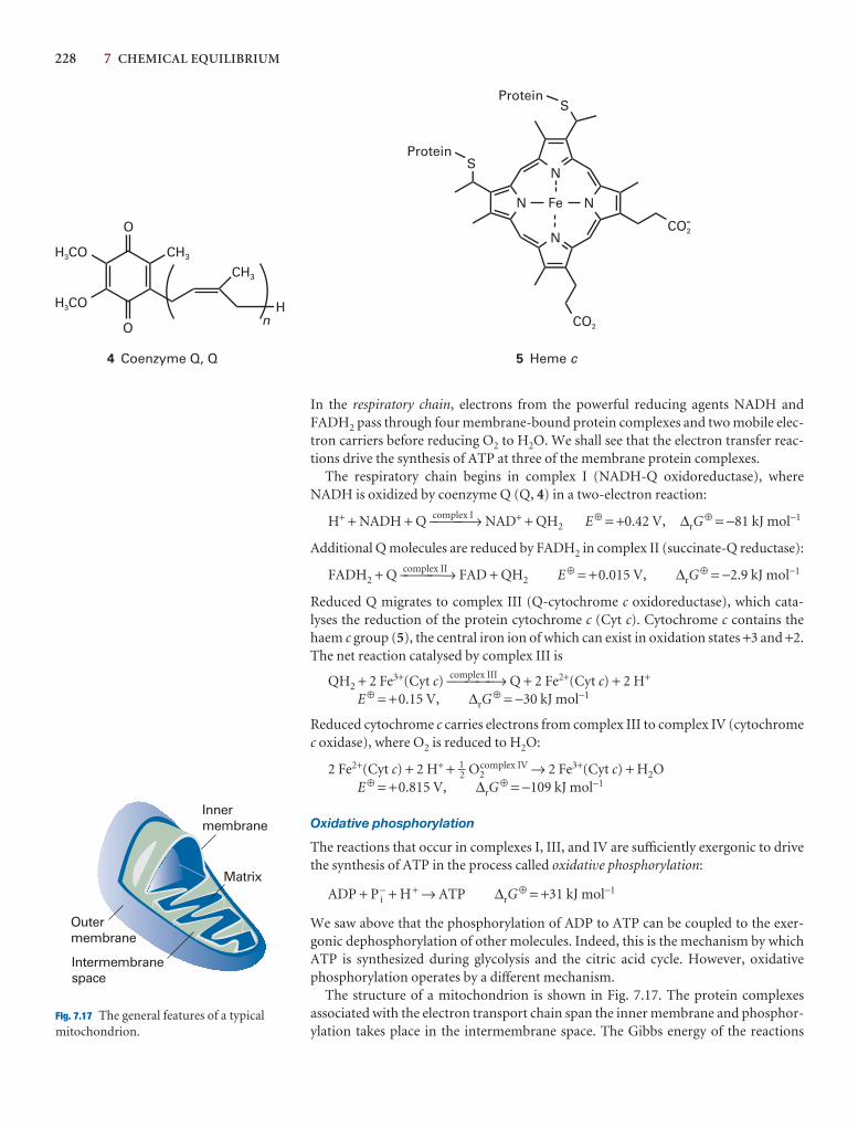
228 7 CHEMICAL EQUILIBRIUM
In the respiratory chain, electrons from the powerful reducing agents NADH andFADH2 pass through four membrane-bound protein complexes and two mobile elec-tron carriers before reducing O2 to H2O. We shall see that the electron transfer reac-tions drive the synthesis of ATP at three of the membrane protein complexes.
The respiratory chain begins in complex I (NADH-Q oxidoreductase), whereNADH is oxidized by coenzyme Q (Q, 4) in a two-electron reaction:
H+ + NADH + Q –co––mp––lex I––→ NAD+ + QH2 E⊕ = +0.42 V, ∆rG⊕ = −81 kJ mol−1
Additional Q molecules are reduced by FADH2 in complex II (succinate-Q reductase):
FADH2 + Q –co––mp––lex II––→ FAD + QH2 E⊕ = +0.015 V, ∆rG⊕ = −2.9 kJ mol−1
Reduced Q migrates to complex III (Q-cytochrome c oxidoreductase), which cata-lyses the reduction of the protein cytochrome c (Cyt c). Cytochrome c contains thehaem c group (5), the central iron ion of which can exist in oxidation states +3 and +2.The net reaction catalysed by complex III is
QH2 + 2 Fe3+(Cyt c) –co––mp––lex III–––→ Q + 2 Fe2+(Cyt c) + 2 H+
E⊕ = +0.15 V, ∆rG⊕ = −30 kJ mol−1
Reduced cytochrome c carries electrons from complex III to complex IV (cytochromec oxidase), where O2 is reduced to H2O:
2 Fe2+(Cyt c) + 2 H+ + 1–2 O2complex IV → 2 Fe3+(Cyt c) + H2O
E⊕ = +0.815 V, ∆rG⊕ = −109 kJ mol−1
Oxidative phosphorylation
The reactions that occur in complexes I, III, and IV are sufficiently exergonic to drivethe synthesis of ATP in the process called oxidative phosphorylation:
ADP + P i− + H+ → ATP ∆rG
⊕ = +31 kJ mol−1
We saw above that the phosphorylation of ADP to ATP can be coupled to the exer-gonic dephosphorylation of other molecules. Indeed, this is the mechanism by whichATP is synthesized during glycolysis and the citric acid cycle. However, oxidativephosphorylation operates by a different mechanism.
The structure of a mitochondrion is shown in Fig. 7.17. The protein complexes associated with the electron transport chain span the inner membrane and phosphor-ylation takes place in the intermembrane space. The Gibbs energy of the reactions
Outermembrane
Innermembrane
Matrix
Intermembranespace
Fig. 7.17 The general features of a typicalmitochondrion.
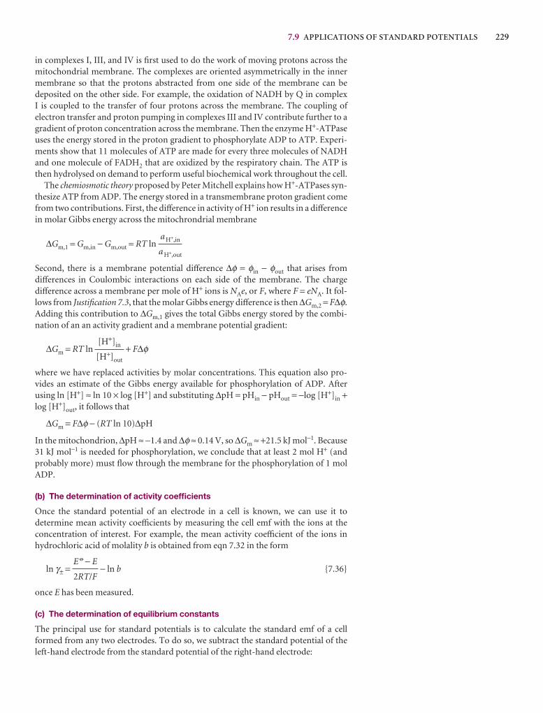
7.9 APPLICATIONS OF STANDARD POTENTIALS 229
in complexes I, III, and IV is first used to do the work of moving protons across themitochondrial membrane. The complexes are oriented asymmetrically in the innermembrane so that the protons abstracted from one side of the membrane can be deposited on the other side. For example, the oxidation of NADH by Q in complex I is coupled to the transfer of four protons across the membrane. The coupling of electron transfer and proton pumping in complexes III and IV contribute further to agradient of proton concentration across the membrane. Then the enzyme H+-ATPaseuses the energy stored in the proton gradient to phosphorylate ADP to ATP. Experi-ments show that 11 molecules of ATP are made for every three molecules of NADHand one molecule of FADH2 that are oxidized by the respiratory chain. The ATP isthen hydrolysed on demand to perform useful biochemical work throughout the cell.
The chemiosmotic theory proposed by Peter Mitchell explains how H+-ATPases syn-thesize ATP from ADP. The energy stored in a transmembrane proton gradient comefrom two contributions. First, the difference in activity of H+ ion results in a differencein molar Gibbs energy across the mitochrondrial membrane
∆Gm,1 = Gm,in − Gm,out = RT ln
Second, there is a membrane potential difference ∆φ = φin − φout that arises fromdifferences in Coulombic interactions on each side of the membrane. The chargedifference across a membrane per mole of H+ ions is NAe, or F, where F = eNA. It fol-lows from Justification 7.3, that the molar Gibbs energy difference is then ∆Gm,2 = F∆φ.Adding this contribution to ∆Gm,1 gives the total Gibbs energy stored by the combi-nation of an an activity gradient and a membrane potential gradient:
∆Gm = RT ln + F∆φ
where we have replaced activities by molar concentrations. This equation also pro-vides an estimate of the Gibbs energy available for phosphorylation of ADP. Afterusing ln [H+] ≈ ln 10 × log [H+] and substituting ∆pH = pHin − pHout = −log [H+]in +log [H+]out, it follows that
∆Gm = F∆φ − (RT ln 10)∆pH
In the mitochondrion, ∆pH ≈ −1.4 and ∆φ ≈ 0.14 V, so ∆Gm ≈ +21.5 kJ mol−1. Because31 kJ mol−1 is needed for phosphorylation, we conclude that at least 2 mol H+ (andprobably more) must flow through the membrane for the phosphorylation of 1 molADP.
(b) The determination of activity coefficients
Once the standard potential of an electrode in a cell is known, we can use it to determine mean activity coefficients by measuring the cell emf with the ions at the concentration of interest. For example, the mean activity coefficient of the ions in hydrochloric acid of molality b is obtained from eqn 7.32 in the form
ln γ± = − ln b {7.36}
once E has been measured.
(c) The determination of equilibrium constants
The principal use for standard potentials is to calculate the standard emf of a cellformed from any two electrodes. To do so, we subtract the standard potential of theleft-hand electrode from the standard potential of the right-hand electrode:
E 7 − E
2RT/F
[H+]in
[H+]out
a H+,in
a H+,out
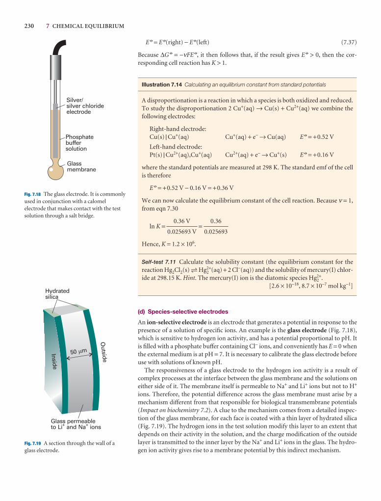
230 7 CHEMICAL EQUILIBRIUM
Silver/silver chlorideelectrode
Phosphatebuffersolution
Glassmembrane
Fig. 7.18 The glass electrode. It is commonlyused in conjunction with a calomelelectrode that makes contact with the testsolution through a salt bridge.
50 m
Glass permeableto Li and Na ions+ +
Hydratedsilica
Inside
Outside
Fig. 7.19 A section through the wall of aglass electrode.
E 7 = E 7(right) − E 7(left) (7.37)
Because ∆G 7 = −νFE 7, it then follows that, if the result gives E 7 > 0, then the cor-responding cell reaction has K > 1.
Illustration 7.14 Calculating an equilibrium constant from standard potentials
A disproportionation is a reaction in which a species is both oxidized and reduced.To study the disproportionation 2 Cu+(aq) → Cu(s) + Cu2+(aq) we combine thefollowing electrodes:
Right-hand electrode:Cu(s) | Cu+(aq) Cu+(aq) + e− → Cu(aq) E 7 = +0.52 V
Left-hand electrode:Pt(s) | Cu2+(aq),Cu+(aq) Cu2+(aq) + e− → Cu+(s) E 7 = +0.16 V
where the standard potentials are measured at 298 K. The standard emf of the cellis therefore
E 7 = +0.52 V − 0.16 V = +0.36 V
We can now calculate the equilibrium constant of the cell reaction. Because ν = 1,from eqn 7.30
ln K = =
Hence, K = 1.2 × 10⁶.
Self-test 7.11 Calculate the solubility constant (the equilibrium constant for thereaction Hg2Cl2(s) 5 Hg2
2+(aq) + 2 Cl−(aq)) and the solubility of mercury(I) chlor-ide at 298.15 K. Hint. The mercury(I) ion is the diatomic species Hg2
2+.[2.6 × 10⁻¹⁸, 8.7 × 10⁻⁷ mol kg−1]
(d) Species-selective electrodes
An ion-selective electrode is an electrode that generates a potential in response to thepresence of a solution of specific ions. An example is the glass electrode (Fig. 7.18),which is sensitive to hydrogen ion activity, and has a potential proportional to pH. Itis filled with a phosphate buffer containing Cl− ions, and conveniently has E = 0 whenthe external medium is at pH = 7. It is necessary to calibrate the glass electrode beforeuse with solutions of known pH.
The responsiveness of a glass electrode to the hydrogen ion activity is a result ofcomplex processes at the interface between the glass membrane and the solutions oneither side of it. The membrane itself is permeable to Na+ and Li+ ions but not to H+
ions. Therefore, the potential difference across the glass membrane must arise by amechanism different from that responsible for biological transmembrane potentials(Impact on biochemistry 7.2). A clue to the mechanism comes from a detailed inspec-tion of the glass membrane, for each face is coated with a thin layer of hydrated silica(Fig. 7.19). The hydrogen ions in the test solution modify this layer to an extent thatdepends on their activity in the solution, and the charge modification of the outsidelayer is transmitted to the inner layer by the Na+ and Li+ ions in the glass. The hydro-gen ion activity gives rise to a membrane potential by this indirect mechanism.
0.36
0.025693
0.36 V
0.025693 V
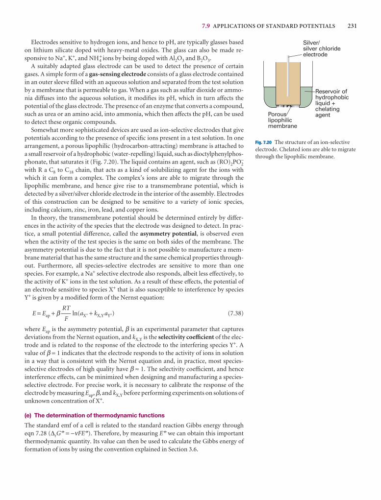
7.9 APPLICATIONS OF STANDARD POTENTIALS 231
Electrodes sensitive to hydrogen ions, and hence to pH, are typically glasses basedon lithium silicate doped with heavy-metal oxides. The glass can also be made re-sponsive to Na+, K+, and NH4
+ ions by being doped with Al2O3 and B2O3.A suitably adapted glass electrode can be used to detect the presence of certain
gases. A simple form of a gas-sensing electrode consists of a glass electrode containedin an outer sleeve filled with an aqueous solution and separated from the test solutionby a membrane that is permeable to gas. When a gas such as sulfur dioxide or ammo-nia diffuses into the aqueous solution, it modifies its pH, which in turn affects the potential of the glass electrode. The presence of an enzyme that converts a compound,such as urea or an amino acid, into ammonia, which then affects the pH, can be usedto detect these organic compounds.
Somewhat more sophisticated devices are used as ion-selective electrodes that givepotentials according to the presence of specific ions present in a test solution. In onearrangement, a porous lipophilic (hydrocarbon-attracting) membrane is attached toa small reservoir of a hydrophobic (water-repelling) liquid, such as dioctylphenylphos-phonate, that saturates it (Fig. 7.20). The liquid contains an agent, such as (RO)2PO2
−
with R a C8 to C18 chain, that acts as a kind of solubilizing agent for the ions withwhich it can form a complex. The complex’s ions are able to migrate through thelipophilic membrane, and hence give rise to a transmembrane potential, which is detected by a silver/silver chloride electrode in the interior of the assembly. Electrodesof this construction can be designed to be sensitive to a variety of ionic species, including calcium, zinc, iron, lead, and copper ions.
In theory, the transmembrane potential should be determined entirely by differ-ences in the activity of the species that the electrode was designed to detect. In prac-tice, a small potential difference, called the asymmetry potential, is observed evenwhen the activity of the test species is the same on both sides of the membrane. Theasymmetry potential is due to the fact that it is not possible to manufacture a mem-brane material that has the same structure and the same chemical properties through-out. Furthermore, all species-selective electrodes are sensitive to more than onespecies. For example, a Na+ selective electrode also responds, albeit less effectively, tothe activity of K+ ions in the test solution. As a result of these effects, the potential ofan electrode sensitive to species X+ that is also susceptible to interference by species Y+ is given by a modified form of the Nernst equation:
E = Eap + β ln(aX+ + kX,Y aY+) (7.38)
where Eap is the asymmetry potential, β is an experimental parameter that capturesdeviations from the Nernst equation, and kX,Y is the selectivity coefficient of the elec-trode and is related to the response of the electrode to the interfering species Y+. Avalue of β = 1 indicates that the electrode responds to the activity of ions in solution in a way that is consistent with the Nernst equation and, in practice, most species-selective electrodes of high quality have β ≈ 1. The selectivity coefficient, and hence interference effects, can be minimized when designing and manufacturing a species-selective electrode. For precise work, it is necessary to calibrate the response of theelectrode by measuring Eap, β, and kX,Y before performing experiments on solutions ofunknown concentration of X+.
(e) The determination of thermodynamic functions
The standard emf of a cell is related to the standard reaction Gibbs energy through eqn 7.28 (∆rG
7 = −νFE 7). Therefore, by measuring E 7 we can obtain this importantthermodynamic quantity. Its value can then be used to calculate the Gibbs energy offormation of ions by using the convention explained in Section 3.6.
RT
F
Porouslipophilicmembrane
Reservoir ofhydrophobicliquid +chelatingagent
Silver/silver chlorideelectrode
Fig. 7.20 The structure of an ion-selectiveelectrode. Chelated ions are able to migratethrough the lipophilic membrane.
232 7 CHEMICAL EQUILIBRIUM
Illustration 7.15 Determining the Gibbs energy of formation of an ion electrochemically
The cell reaction taking place in
Pt(s) | H2 | H+(aq) || Ag+(aq) | Ag(s) E 7 = +0.7996 V
is
Ag+(aq) + 1–2 H2(g) → H+(aq) + Ag(s) ∆rG7 = −∆f G
7(Ag+, aq)
Therefore, with ν = 1, we find
∆f G7(Ag+, aq) = −(−FE 7) = +77.15 kJ mol−1
which is in close agreement with the value in Table 2.6 of the Data section.
The temperature coefficient of the standard cell emf, dE 7/dT, gives the standard en-tropy of the cell reaction. This conclusion follows from the thermodynamic relation(∂G/∂T)p = −S and eqn 7.27, which combine to give
= (7.39)
The derivative is complete because E 7, like ∆rG7, is independent of the pressure. Hence
we have an electrochemical technique for obtaining standard reaction entropies andthrough them the entropies of ions in solution.
Finally, we can combine the results obtained so far and use them to obtain the stand-ard reaction enthalpy:
∆r H 7 = ∆rG7 + T∆rS
7 = −νF E 7 − T (7.40)
This expression provides a non-calorimetric method for measuring ∆r H 7 and,through the convention ∆f H
7(H+, aq) = 0, the standard enthalpies of formation ofions in solution (Section 2.8). Thus, electrical measurements can be used to calculateall the thermodynamic properties with which this chapter began.
Example 7.5 Using the temperature coefficient of the cell potential
The standard emf of the cell Pt(s) | H2(g) | HBr(aq) | AgBr(s) | Ag(s) was measuredover a range of temperatures, and the data were fitted to the following polynomial:
E 7/V = 0.07131 − 4.99 × 10⁻⁴(T/K − 298) − 3.45 × 10⁻⁶(T/K − 298)2
Evaluate the standard reaction Gibbs energy, enthalpy, and entropy at 298 K.
Method The standard Gibbs energy of reaction is obtained by using eqn 7.28 afterevaluating E 7 at 298 K and by using 1 V C = 1 J. The standard entropy of reactionis obtained by using eqn 7.39, which involves differentiating the polynomial withrespect to T and then setting T = 298 K. The reaction enthalpy is obtained by com-bining the values of the standard Gibbs energy and entropy.
Answer At T = 298 K, E 7 = +0.07131 V, so
∆rG7 = −νFE 7 = −(1) × (9.6485 × 104 C mol−1) × (+0.07131 V)
= −6.880 × 10³ V C mol−1 = −6.880 kJ mol−1
DF
dE 7
dT
AC
∆rS7
νF
dE 7
dT
CHECKLIST OF KEY IDEAS 233
Checklist of key ideas
1. The extent of reaction (ξ) is defined such that, when theextent of reaction changes by a finite amount ∆ξ, the amountof A present changes from nA,0 to nA,0 − ∆ξ.
2. The reaction Gibbs energy is the slope of the graph of theGibbs energy plotted against the extent of reaction: ∆rG =(∂G/∂ξ)p,T ; at equilibrium, ∆rG = 0.
3. An exergonic reaction is a reaction for which ∆rG < 0; such areaction can be used to drive another process. An endergonicreaction is a reaction for which ∆rG > 0.
4. The general expression for ∆rG at an arbitrary stage of thereaction is ∆rG = ∆rG
7 + RT ln Q.
5. The equilibrium constant (K) may be written in terms of ∆rG7
as ∆rG7 = −RT ln K.
6. The standard reaction Gibbs energy may be calculated fromstandard Gibbs energies of formation, ∆rG
7 = ∑Productsν∆f G7
− ∑Reactantsν∆f G7 = ∑JνJ∆f G
7(J).
7. Thermodynamic equilibrium constant is an equilibriumconstant K expressed in terms of activities (or fugacities):
K = ΠJ
a Jν J
equilibrium
.DEF
ABC
8. A catalyst does not affect the equilibrium constant.
9. Changes in pressure do not affect the equilibrium constant:(∂K/∂p)T = 0. However, partial pressures and concentrationscan change in response to a change in pressure.
10. Le Chatelier’s principle states that a system at equilibrium,when subjected to a disturbance, responds in a way that tendsto minimize the effect of the disturbance.
11. Increased temperature favours the reactants in exothermicreactions and the products in endothermic reactions.
12. The temperature dependence of the equilibrium constant isgiven by the van ‘t Hoff equation: d ln K/dT = ∆rH
7/RT2. Tocalculate K at one temperature in terms of its value at anothertemperature, and provided ∆rH
7 is independent oftemperature, we use ln K2 − ln K1 = −(∆rH
7/R)(1/T2 − 1/T1).
13. A galvanic cell is an electrochemical cell that produceselectricity as a result of the spontaneous reaction occurringinside it. An electrolytic cell is an electrochemical cell in whicha non-spontaneous reaction is driven by an external source ofcurrent.
14. Oxidation is the removal of electrons from a species;reduction is the addition of electrons to a species; a redox
The temperature coefficient of the cell potential is
= −4.99 × 10⁻⁴ V K−1 − 2(3.45 × 10⁻⁶)(T/K − 298) V K−1
At T = 298 K this expression evaluates to
= −4.99 × 10⁻⁴ V K−1
So, from eqn 7.39, the reaction entropy is
∆rS7 = 1 × (9.6485 × 104 C mol−1) × (−4.99 × 10⁻⁴ V K−1)
= −48.2 J K−1 mol−1
It then follows that
∆r H 7 = ∆rG7 + T∆rS
7 = −6.880 kJ mol−1 + (298 K) × (−0.0482 kJ K−1 mol−1)
= −21.2 kJ mol−1
One difficulty with this procedure lies in the accurate measurement of small tem-perature coefficients of cell potential. Nevertheless, it is another example of thestriking ability of thermodynamics to relate the apparently unrelated, in this caseto relate electrical measurements to thermal properties.
Self-test 7.12 Predict the standard potential of the Harned cell at 303 K from tablesof thermodynamic data. [+0.2222 V]
dE
dT
dE 7
dT

234 7 CHEMICAL EQUILIBRIUM
reaction is a reaction in which there is a transfer of electronsfrom one species to another.
15. The anode is the electrode at which oxidation occurs. Thecathode is the electrode at which reduction occurs.
16. The electromotive force (emf) is the cell potential when it isbalanced by an exactly opposing source of potential so that thecell reaction occurs reversibly, the composition is constant,and no current flows.
17. The cell potential and the reaction Gibbs energy are related by−νFE = ∆rG.
18. The standard emf is the standard reaction Gibbs energyexpressed as a potential: E 7 = ∆rG
7/νF.
19. The Nernst equation is the equation for the emf of a cell interms of the composition: E = E 7 − (RT/νF) ln Q.
20. The equilibrium constant for a cell reaction is related to thestandard emf by ln K = νFE 7/RT.
21. The standard potential of a couple (E 7) is the standard emfof a cell in which a couple forms the right-hand electrode and the standard hydrogen electrode is the left-handelectrode.
22. To calculate the standard emf, form the difference of electrodepotentials: E 7 = E 7(right) − E 7(left).
23. The temperature coefficient of cell potential is given bydE 7/dT = ∆rS
7/νF.
24. The standard reaction entropy and enthalpy are calculatedfrom the temperature dependence of the standard emf by:∆rS
7 = νFdE 7/dT, ∆r H 7 = −ν(FE 7 − TdE 7/dT).
Further reading
Articles and texts
P.W. Atkins and J.C. de Paula, Physical chemistry for the life sciences.W.H. Freeman and Company, New York (2005).
A.J. Bard and L.R. Faulkner, Electrochemical methods. Wiley, New York (2000).
M.J. Blandamer, Chemical equilibria in solution. EllisHorwood/Prentice Hall, Hemel Hempstead (1992).
W.A. Cramer and D.A. Knaff, Energy transduction in biologicalmembranes, a textbook of bioenergetics. Springer–Verlag, New York(1990).
D.R. Crow, Principles and applications of electrochemistry. Blackie,London (1994).
K. Denbigh, The principles of chemical equilibrium, with applicationsin chemistry and chemical engineering. Cambridge University Press(1981).
C.H. Hamann, A. Hamnett, and W. Vielstich, Electrochemistry.Wiley-VCH, Weinheim (1998).
Sources of data and information
M.S. Antelman, The encyclopedia of chemical electrode potentials,Plenum, New York (1982).
A.J. Bard, R. Parsons, and J. Jordan (ed.), Standard potentials inaqueous solution. Marcel Dekker, New York (1985).
R.N. Goldberg and Y.B. Tewari, Thermodynamics of enzyme-catalyzed reactions. J. Phys. Chem. Ref. Data. Part 1: 22, 515 (1993).Part 2: 23, 547 (1994). Part 3: 23, 1035 (1994). Part 4: 24, 1669(1995). Part 5: 24, 1765 (1995).
Discussion questions
7.1 Explain how the mixing of reactants and products affects the position ofchemical equilibrium.
7.2 Suggest how the thermodynamic equilibrium constant may responddifferently to changes in pressure and temperature from the equilibriumconstant expressed in terms of partial pressures.
7.3 Account for Le Chatelier’s principle in terms of thermodynamicquantities.
7.4 Explain the molecular basis of the van ’t Hoff equation for thetemperature dependence of K.
7.5 (a) How may an Ellingham diagram be used to decide whether one metalmay be used to reduce the oxide of another metal? (b) Use the Ellingham
diagram in Fig. 7.10 to identify the lowest temperature at which zinc oxide canbe reduced to zinc metal by carbon.
7.6 Distinguish between cell potential and electromotive force and explainwhy the latter is related to thermodynamic quantities.
7.7 Describe the contributions to the emf of cells formed by combining theelectrodes specified in Table 7.1.
7.8 Describe a method for the determination of a standard potential of aredox couple.
7.9 Devise a method for the determination of the pH of an aqueous solution.

EXERCISES 235
Exercises
7.1(a) At 2257 K and 1.00 atm total pressure, water is 1.77 per cent dissociatedat equilibrium by way of the reaction 2 H2O(g) 5 2 H2(g) + O2(g). Calculate(a) K, (b) ∆rG
7, and (c) ∆rG at this temperature.
7.1(b) For the equilibrium, N2O4(g) 5 2 NO2(g), the degree of dissociation,αe, at 298 K is 0.201 at 1.00 bar total pressure. Calculate (a) ∆rG, (2) K, and (3) ∆rG
7 at 298 K.
7.2(a) Dinitrogen tetroxide is 18.46 per cent dissociated at 25°C and 1.00 barin the equilibrium N2O4(g) 5 2 NO2(g). Calculate (a) K at 25°C, (b) ∆rG
7,(c) K at 100°C given that ∆rH
7 = +57.2 kJ mol−1 over the temperature range.
7.2(b) Molecular bromine is 24 per cent dissociated at 1600 K and 1.00 bar inthe equilibrium Br2(g) 5 2 Br(g). Calculate (a) K at 25°C, (b) ∆rG
7, (c) K at2000°C given that ∆rH
7 = +112 kJ mol−1 over the temperature range.
7.3(a) From information in the Data section, calculate the standard Gibbsenergy and the equilibrium constant at (a) 298 K and (b) 400 K for thereaction PbO(s) + CO(g) 5 Pb(s) + CO2(g). Assume that the reactionenthalpy is independent of temperature.
7.3(b) From information in the Data section, calculate the standard Gibbsenergy and the equilibrium constant at (a) 25°C and (b) 50°C for the reactionCH4(g) + 3 Cl2(g) 5 CHCl3(l) + 3 HCl(g). Assume that the reaction enthalpyis independent of temperature.
7.4(a) In the gas-phase reaction 2 A + B 5 3 C + 2 D, it was found that, when1.00 mol A, 2.00 mol B, and 1.00 mol D were mixed and allowed to come toequilibrium at 25°C, the resulting mixture contained 0.90 mol C at a totalpressure of 1.00 bar. Calculate (a) the mole fractions of each species atequilibrium, (b) Kx, (c) K, and (d) ∆rG
7.
7.4(b) In the gas-phase reaction A + B 5 C + 2 D, it was found that, when2.00 mol A, 1.00 mol B, and 3.00 mol D were mixed and allowed to come toequilibrium at 25°C, the resulting mixture contained 0.79 mol C at a totalpressure of 1.00 bar. Calculate (a) the mole fractions of each species atequilibrium, (b) Kx, (c) K, and (d) ∆rG
7.
7.5(a) The standard reaction enthalpy of Zn(s) + H2O(g) → ZnO(s) + H2(g) isapproximately constant at +224 kJ mol−1 from 920 K up to 1280 K. Thestandard reaction Gibbs energy is +33 kJ mol−1 at 1280 K. Estimate thetemperature at which the equilibrium constant becomes greater than 1.
7.5(b) The standard enthalpy of a certain reaction is approximately constantat +125 kJ mol−1 from 800 K up to 1500 K. The standard reaction Gibbsenergy is +22 kJ mol−1 at 1120 K. Estimate the temperature at which theequilibrium constant becomes greater than 1.
7.6(a) The equilibrium constant of the reaction 2 C3H6(g) 5 C2H4(g) +C4H8(g) is found to fit the expression ln K = A + B/T + C/T 2 between 300 Kand 600 K, with A = −1.04, B = −1088 K, and C = 1.51 × 10⁵ K2. Calculate thestandard reaction enthalpy and standard reaction entropy at 400 K.
7.6(b) The equilibrium constant of a reaction is found to fit the expression ln K = A + B/T + C/T 3 between 400 K and 500 K with A = −2.04, B = −1176 K,and C = 2.1 × 10⁷ K3. Calculate the standard reaction enthalpy and standardreaction entropy at 450 K.
7.7(a) The standard reaction Gibbs energy of the isomerization of borneol(C10H17OH) to isoborneol in the gas phase at 503 K is +9.4 kJ mol−1. Calculatethe reaction Gibbs energy in a mixture consisting of 0.15 mol of borneol and0.30 mol of isoborneol when the total pressure is 600 Torr.
7.7(b) The equilibrium pressure of H2 over solid uranium and uraniumhydride, UH3, at 500 K is 139 Pa. Calculate the standard Gibbs energy offormation of UH3(s) at 500 K.
7.8(a) Calculate the percentage change in Kx for the reaction H2CO(g) 5CO(g) + H2(g) when the total pressure is increased from 1.0 bar to 2.0 bar atconstant temperature.
7.8(b) Calculate the percentage change in Kx for the reaction CH3OH(g) +NOCl(g) 5 HCl(g) + CH3NO2(g) when the total pressure is increased from1.0 bar to 2.0 bar at constant temperature.
7.9(a) The equilibrium constant for the gas-phase isomerization of borneol(C10H17OH) to isoborneol at 503 K is 0.106. A mixture consisting of 7.50 g ofborneol and 14.0 g of isoborneol in a container of volume 5.0 dm3 is heated to503 K and allowed to come to equilibrium. Calculate the mole fractions of thetwo substances at equilibrium.
7.9(b) The equilibrium constant for the reaction N2(g) + O2(g) 5 2 NO(g) is1.69 × 10−3 at 2300 K. A mixture consisting of 5.0 g of nitrogen and 2.0 g ofoxygen in a container of volume 1.0 dm3 is heated to 2300 K and allowed tocome to equilibrium. Calculate the mole fraction of NO at equilibrium.
7.10(a) What is the standard enthalpy of a reaction for which the equilibriumconstant is (a) doubled, (b) halved when the temperature is increased by 10 Kat 298 K?
7.10(b) What is the standard enthalpy of a reaction for which the equilibriumconstant is (a) doubled, (b) halved when the temperature is increased by 15 Kat 310 K?
7.11(a) The standard Gibbs energy of formation of NH3(g) is −16.5 kJ mol−1
at 298 K. What is the reaction Gibbs energy when the partial pressures of theN2, H2, and NH3 (treated as perfect gases) are 3.0 bar, 1.0 bar, and 4.0 bar,respectively? What is the spontaneous direction of the reaction in this case?
7.11(b) The dissociation vapour pressure of NH4Cl at 427°C is 608 kPa but at 459°C it has risen to 1115 kPa. Calculate (a) the equilibrium constant, (b) the standard reaction Gibbs energy, (c) the standard enthalpy, (d) thestandard entropy of dissociation, all at 427°C. Assume that the vapour behavesas a perfect gas and that ∆H 7 and ∆S 7 are independent of temperature in therange given.
7.12(a) Estimate the temperature at which CaCO3(calcite) decomposes.
7.12(b) Estimate the temperature at which CuSO4·5H2O undergoesdehydration.
7.13(a) For CaF2(s) 5 Ca2+(aq) + 2 F−(aq), K = 3.9 ×10⁻¹¹ at 25°C and thestandard Gibbs energy of formation of CaF2(s) is −1167 kJ mol−1. Calculatethe standard Gibbs energy of formation of CaF2(aq).
7.13(b) For PbI2(s) 5 Pb2+(aq) + 2 I−(aq), K = 1.4 × 10⁻⁸ at 25°C and thestandard Gibbs energy of formation of PbI2(s) is −173.64 kJ mol−1. Calculatethe standard Gibbs energy of formation of PbI2(aq).
7.14(a) Write the cell reaction and electrode half-reactions and calculate thestandard emf of each of the following cells:
(a) Zn | ZnSO4(aq) || AgNO3(aq)|Ag
(b) Cd | CdCl2(aq) || HNO3(aq)|H2(g) | Pt
(c) Pt | K3[Fe(CN)6](aq),K4[Fe(CN)6](aq) || CrCl3(aq) | Cr
7.14(b) Write the cell reaction and electrode half-reactions and calculate thestandard emf of each the following cells:
(a) Pt | Cl2(g) | HCl(aq) || K2CrO4(aq) | Ag2CrO4(s) | Ag
(b) Pt | Fe3+(aq),Fe2+(aq) || Sn4+(aq),Sn2+(aq) | Pt
(c) Cu | Cu2+(aq) || Mn2+(aq),H+(aq) | MnO2(s) | Pt
236 7 CHEMICAL EQUILIBRIUM
7.15(a) Devise cells in which the following are the reactions and calculate thestandard emf in each case:
(a) Zn(s) + CuSO4(aq) → ZnSO4(aq) + Cu(s)
(b) 2 AgCl(s) + H2(g) → 2 HCl(aq) + 2 Ag(s)
(c) 2 H2(g) + O2(g) → 2 H2O(l)
7.15(b) Devise cells in which the following are the reactions and calculate thestandard emf in each case:
(a) 2 Na(s) + 2 H2O(l) → 2 NaOH(aq) + H2(g)
(b) H2(g) + I2(g) → 2 HI(aq)
(c) H3O+(aq) + OH−(aq) → 2 H2O(l)
7.16(a) Use the Debye–Hückel limiting law and the Nernst equation toestimate the potential of the cell Ag |AgBr(s) | KBr(aq, 0.050 mol kg−1)|| Cd(NO3)2(aq, 0.010 mol kg−1) | Cd at 25°C.
7.16(b) Consider the cell Pt | H2(g,p7) | HCl(aq) | AgCl(s) | Ag, for which thecell reaction is 2 AgCl(s) + H2(g) → 2 Ag(s) + 2 HCl(aq). At 25°C and amolality of HCl of 0.010 mol kg−1, E = +0.4658 V. (a) Write the Nernst
equation for the cell reaction. (b) Calculate ∆rG for the cell reaction.(c) Assuming that the Debye–Hückel limiting law holds at this concentration,calculate E 7(AgCl, Ag).
7.17(a) Calculate the equilibrium constants of the following reactions at 25°Cfrom standard potential data:
(a) Sn(s) + Sn4+(aq) 5 2 Sn2+(aq)
(b) Sn(s) + 2 AgCl(s) 5 SnCl2(aq) + 2 Ag(s)
7.17(b) Calculate the equilibrium constants of the following reactions at 25°Cfrom standard potential data:
(a) Sn(s) + CuSO4(aq) 5 Cu(s) + SnSO4(aq)
(b) Cu2+(aq) + Cu(s) 5 2 Cu+(aq)
7.18(a) The emf of the cell Ag |AgI(s) |AgI(aq) |Ag is +0.9509 V at 25°C.Calculate (a) the solubility product of AgI and (b) its solubility.
7.18(b) The emf of the cell Bi |Bi2S3(s) |Bi2S3(aq) |Bi is −0.96 V at 25°C.Calculate (a) the solubility product of Bi2S3 and (b) its solubility.
Problems*
Numerical problems
7.1 The equilibrium constant for the reaction, I2(s) + Br2(g) 5 2 IBr(g)is 0.164 at 25°C. (a) Calculate ∆rG
7 for this reaction. (b) Bromine gas isintroduced into a container with excess solid iodine. The pressure andtemperature are held at 0.164 atm and 25°C, respectively. Find the partialpressure of IBr(g) at equilibrium. Assume that all the bromine is in the liquidform and that the vapour pressure of iodine is negligible. (c) In fact, solidiodine has a measurable vapour pressure at 25°C. In this case, how would thecalculation have to be modified?
7.2 Consider the dissociation of methane, CH4(g), into the elements H2(g)and C(s, graphite). (a) Given that ∆ f H
7(CH4, g) = −74.85 kJ mol−1 and that∆f S
7(CH4, g) = −80.67 J K−1 mol−1 at 298 K, calculate the value of theequilibrium constant at 298 K. (b) Assuming that ∆f H
7 is independent oftemperature, calculate K at 50°C. (c) Calculate the degree of dissociation, αe,of methane at 25°C and a total pressure of 0.010 bar. (d) Without doing anynumerical calculations, explain how the degree of dissociation for thisreaction will change as the pressure and temperature are varied.
7.3 The equilibrium pressure of H2 over U(s) and UH3(s) between 450 K and715 K fits the expression ln(p/Pa) = A + B/T + C ln(T/K), with A = 69.32, B =−1.464 × 10⁴ K, and C = −5.65. Find an expression for the standard enthalpy offormation of UH3(s) and from it calculate ∆rC p
7.
7.4 The degree of dissociation, αe, of CO2(g) into CO(g) and O2(g) at hightemperatures was found to vary with temperature as follows:
T/K 1395 1443 1498
αe/10−4 1.44 2.50 4.71
Assuming ∆r H 7 to be constant over this temperature range, calculate K, ∆rG7,
∆r H 7, and ∆rS7. Make any justifiable approximations.
7.5 The standard reaction enthalpy for the decomposition of CaCl2·NH3(s)into CaCl2(s) and NH3(g) is nearly constant at +78 kJ mol−1 between 350 Kand 470 K. The equilibrium pressure of NH3 in the presence of CaCl2·NH3 is
1.71 kPa at 400 K. Find an expression for the temperature dependence of ∆rG7
in the same range.
7.6 Calculate the equilibrium constant of the reaction CO(g) + H2(g) 5H2CO(g) given that, for the production of liquid formaldehyde, ∆rG
7 =+28.95 kJ mol−1 at 298 K and that the vapour pressure of formaldehyde is 1500 Torr at that temperature.
7.7 Acetic acid was evaporated in container of volume 21.45 cm3 at 437 K andat an external pressure of 101.9 kPa, and the container was then sealed. Themass of acid present in the sealed container was 0.0519 g. The experiment wasrepeated with the same container but at 471 K, and it was found that 0.0380 gof acetic acid was present. Calculate the equilibrium constant for thedimerization of the acid in the vapour and the enthalpy of vaporization.
7.8 A sealed container was filled with 0.300 mol H2(g), 0.400 mol I2(g), and0.200 mol HI(g) at 870 K and total pressure 1.00 bar. Calculate the amounts ofthe components in the mixture at equilibrium given that K = 870 for thereaction H2(g) + I2(g) 5 2 HI(g).
7.9 The dissociation of I2 can be monitored by measuring the total pressure,and three sets of results are as follows:
T/K 973 1073 1173
100p/atm 6.244 7.500 9.181
104nI 2.4709 2.4555 2.4366
where nI is the amount of I atoms per mole of I2 molecules in the mixture,which occupied 342.68 cm3. Calculate the equilibrium constants of thedissociation and the standard enthalpy of dissociation at the meantemperature.
7.10‡ Thorn et al. carried out a study of Cl2O(g) by photoelectron ionization(R.P. Thorn, L.J. Stief, S.-C. Kuo, and R.B. Klemm, J. Phys. Chem. 100, 14178(1996)). From their measurements, they report ∆ f H
7(Cl2O) = +77.2 kJ mol−1.They combined this measurement with literature data on the reaction Cl2O (g) + H2O(g)→ 2 HOCl(g), for which K = 8.2 × 10⁻² and ∆rS
7 =
* Problems denoted with the symbol ‡ were supplied by Charles Trapp, Carmen Giunta, and Marshall Cady.
PROBLEMS 237
+16.38 J K−1 mol−1, and with readily available thermodynamic data on watervapour to report a value for ∆f H
7(HOCl). Calculate that value. All quantitiesrefer to 298 K.
7.11‡ The 1980s saw reports of ∆f H7(SiH2) ranging from 243 to 289 kJ mol−1.
For example, the lower value was cited in the review article by R. Walsh (Acc.Chem. Res. 14, 246 (1981)); Walsh later leant towards the upper end of therange (H.M. Frey, R. Walsh, and I.M. Watts, J. Chem. Soc., Chem. Commun.1189 (1986)). The higher value was reported in S.-K. Shin and J.L.Beauchamp, J. Phys. Chem. 90, 1507 (1986). If the standard enthalpy offormation is uncertain by this amount, by what factor is the equilibriumconstant for the formation of SiH2 from its elements uncertain at (a) 298 K,(b) 700 K?
7.12 Fuel cells provide electrical power for spacecraft (as in the NASA space shuttles) and also show promise as power sources for automobiles.Hydrogen and carbon monoxide have been investigated for use in fuel cells, so their solubilities in molten salts are of interest. Their solubilities in a molten NaNO3/KNO3 mixture were examined (E. Desimoni and P.G. Zambonin, J. Chem. Soc. Faraday Trans. 1, 2014 (1973)) with thefollowing results:
log sH2= −5.39 − log sCO = −5.98 −
where s is the solubility in mol cm−3 bar−1. Calculate the standard molarenthalpies of solution of the two gases at 570 K.
7.13 Given that ∆rG7 = −212.7 kJ mol−1 for the reaction in the Daniell cell at
25°C, and b(CuSO4) = 1.0 × 10⁻³ mol kg−1 and b(ZnSO4) = 3.0 × 10⁻³ mol kg−1,calculate (a) the ionic strengths of the solutions, (b) the mean ionic activitycoefficients in the compartments, (c) the reaction quotient, (d) the standardcell potential, and (e) the cell potential. (Take γ+ = γ− = γ± in the respectivecompartments.)
7.14 A fuel cell develops an electric potential from the chemical reactionbetween reagents supplied from an outside source. What is the emf of a cellfuelled by (a) hydrogen and oxygen, (b) the combustion of butane at 1.0 barand 298 K?
7.15 Although the hydrogen electrode may be conceptually the simplestelectrode and is the basis for our reference state of electrical potential inelectrochemical systems, it is cumbersome to use. Therefore, severalsubstitutes for it have been devised. One of these alternatives is thequinhydrone electrode (quinhydrone, Q · QH2, is a complex of quinone,C6H4O2 = Q, and hydroquinone, C6H4O2H2 = QH2). The electrodehalf–reaction is Q(aq) + 2 H+(aq) + 2 e− → QH2(aq), E 7 = +0.6994 V. If thecell Hg | Hg2Cl2(s) | HCl(aq) | Q · QH2 | Au is prepared, and the measured cellpotential is +0.190 V, what is the pH of the HCl solution? Assume that theDebye–Hückel limiting law is applicable.
7.16 Consider the cell, Zn(s) | ZnCl2 (0.0050 mol kg−1) | Hg2Cl2(s) Hg(l), forwhich the cell reaction is Hg2Cl2(s) + Zn(s) → 2 Hg(l) + 2 Cl−(aq) + Zn2+(aq).Given that E 7 (Zn2+,Zn) = −0.7628 V, E 7 (Hg2Cl2, Hg) = +0.2676 V, and thatthe emf is +1.2272 V, (a) write the Nernst equation for the cell. Determine(b) the standard emf, (c) ∆rG, ∆rG
7, and K for the cell reaction, (d) the meanionic activity and activity coefficient of ZnCl2 from the measured cellpotential, and (e) the mean ionic activity coefficient of ZnCl2 from theDebye–Hückel limiting law. (f) Given that (∂E/∂T)p = −4.52 × 10⁻⁴ V K−1.Calculate ∆S and ∆H.
7.17 The emf of the cell Pt | H2(g, p7) | HCl(aq,b) | Hg2Cl2(s) | Hg(l) has beenmeasured with high precision (G.J. Hills and D.J.G. Ives, J. Chem. Soc., 311(1951)) with the following results at 25°C:
b/(mmol kg−1) 1.6077 3.0769 5.0403 7.6938 10.9474
E/V 0.60080 0.56825 0.54366 0.52267 0.50532
980
T/K
980
T/K
Determine the standard emf of the cell and the mean activity coefficient ofHCl at these molalities. (Make a least-squares fit of the data to the best straightline.)
7.18 Careful measurements of the emf of the cell Pt | H2(g, p7) | NaOH(aq,0.0100 mol kg−1), NaCl(aq, 0.01125 mol kg−1) | AgCl(s) | Ag have beenreported (C.P. Bezboruah, M.F.G.F.C. Camoes, A.K. Covington, and J.V.Dobson, J. Chem. Soc. Faraday Trans. I 69, 949 (1973)). Among the data is thefollowing information:
θ/°C 20.0 25.0 30.0
E/V 1.04774 1.04864 1.04942
Calculate pKw at these temperatures and the standard enthalpy and entropy ofthe autoprotolysis of water at 25.0°C.
7.19 Measurements of the emf of cells of the type Ag | AgX(s)MX(b1) | Mx
Hg | MX(b2) | AgX(s) | Ag, where Mx Hg denotes an amalgam and theelectrolyte is an alkali metal halide dissolved in ethylene glycol, have beenreported (U. Sen, J. Chem. Soc. Faraday Trans. I 69, 2006 (1973)) and somevalues for LiCl are given below. Estimate the activity coefficient at theconcentration marked * and then use this value to calculate activitycoefficients from the measured cell potential at the other concentrations. Baseyour answer on the following version of the extended Debye–Hückel law:
log γ = − + kI
with A = 1.461, B = 1.70, k = 0.20, and I = b/b 7. For b2 = 0.09141 mol kg−1:
b1/(mol kg−1) 0.0555 0.09141* 0.1652 0.2171 1.040 1.350
E/V −0.0220 0.0000 0.0263 0.0379 0.1156 0.1336
7.20 The standard potential of the AgCl/Ag,Cl− couple has been measuredvery carefully over a range of temperature (R.G. Bates and V.E. Bowers, J. Res.Nat. Bur. Stand. 53, 283 (1954)) and the results were found to fit the expression
E 7/V = 0.23659 − 4.8564 × 10⁻⁴(θ/°C) − 3.4205 × 10⁻⁶ (θ/°C)2
+ 5.869 × 10⁻⁹(θ/°C)3
Calculate the standard Gibbs energy and enthalpy of formation of Cl−(aq) andits entropy at 298 K.
7.21‡ (a) Derive a general relation for (∂E/∂p)T,n for electrochemical cellsemploying reactants in any state of matter. (b) E. Cohen and K. Piepenbroek(Z. Physik. Chem. 167A, 365 (1933)) calculated the change in volume for thereaction TlCl(s) + CNS−(aq) → TlCNS(s) + Cl−(aq) at 30°C from density dataand obtained ∆rV = −2.666 ± 0.080 cm3 mol−1. They also measured the emf ofthe cell Tl(Hg) | TlCNS(s) | KCNS�KCl | TlCl | Tl(Hg) at pressures up to 1500atm. Their results are given in the following table:
p/atm 1.00 250 500 750 1000 1250 1500
E /mV 8.56 9.27 9.98 10.69 11.39 12.11 12.82
From this information, obtain (∂E/∂p)T,n at 30°C and compare to the valueobtained from ∆ rV. (c) Fit the data to a polynomial for E against p. Howconstant is (∂E/∂p)T,n? (d) From the polynomial, estimate an effectiveisothermal compressibility for the cell as a whole.
7.22‡ The table below summarizes the emf observed for the cell Pd | H2(g, 1 bar) | BH(aq, b), B(aq, b) | AgCl(s) | Ag. Each measurement is madeat equimolar concentrations of 2-aminopyridinium chloride (BH) and 2-aminopyridine (B). The data are for 25°C and it is found that E 7 = 0.22251 V.Use the data to determine pKa for the acid at 25°C and the mean activitycoefficient (γ±) of BH as a function of molality (b) and ionic strength (I). Usethe extended Debye–Hückel equation for the mean activity coefficient in theform
−log γ± = − kbAI1/2
1 + BI1/2
AI1/2
1 − BI1/2
238 7 CHEMICAL EQUILIBRIUM
where A = 0.5091 and B and k are parameters that depend upon the ions.Draw a graph of the mean activity coefficient with b = 0.04 mol kg−1 and0 ≤ I ≤ 0.1.
b/(mol kg−1) 0.01 0.02 0.03 0.04 0.05
E(25°C)/V 0.74452 0.72853 0.71928 0.71314 0.70809
b/(mol kg−1) 0.06 0.07 0.08 0.09 0.10
E(25°C)/V 0.70380 0.70059 0.69790 0.69571 0.69338
Hint. Use mathematical software or a spreadsheet.
7.23 Superheavy elements are now of considerable interest, particularlybecause signs of stability are starting to emerge with element 114, which hasrecently been made. Shortly before it was (falsely) believed that the firstsuperheavy element had been discovered, an attempt was made to predict thechemical properties of ununpentium (Uup, element 115, O.L. Keller, C.W.Nestor, and B. Fricke, J. Phys. Chem. 78, 1945 (1974)). In one part of the paperthe standard enthalpy and entropy of the reaction Uup+(aq) + 1–
2H2(g) →Uup(s) + H+(aq) were estimated from the following data: ∆subH 7(Uup) =+1.5 eV, I(Uup) = 5.52 eV, ∆hydH 7(Uup+, aq) = −3.22 eV, S 7(Uup+, aq) =+1.34 meV K−1, S 7(Uup, s) = 0.69 meV K−1. Estimate the expected standard potential of the Uup+/Uup couple.
7.24 Sodium fluoride is routinely added to public water supplies because it isknown that fluoride ion can prevent tooth decay. In a fluoride-selectiveelectrode used in the analysis of water samples a crystal of LaF3 doped withEu2+, denoted as Eu2+:LaF3, provides a semipermeable barrier between the testsolution and the solution inside the electrode (the filling solution), whichcontains 0.1 mol kg−1 NaF(aq) and 0.1 mol kg−1 NaCl(aq). A silver–silverchloride electrode immersed in the filling solution is connected to apotentiometer and the emf of the cell can be measured against an appropriatereference electrode. It follows that the half-cell for a fluoride-selectiveelectrode is represented by
Ag(s) | AgCl(s) | NaCl(aq, b1), NaF (aq, b1) | Eu2+:LaF3 (s) | F−(aq, b2)
where b1 and b2 are the molalities of fluoride ion in the filling and testsolutions, respectively. (a) Derive an expression for the emf of this half-cell.(b) The fluoride-selective electrode just described is not sensitive to HF(aq).Hydroxide ion is the only interfering species, with kF −,OH − = 0.1. Use thisinformation and the fact that Ka of HF is 3.5 × 10⁻⁴ at 298 K to specify a rangeof pH values in which the electrode responds accurately to the activity of F− inthe test solution at 298 K.
Theoretical problems
7.25 Express the equilibrium constant of a gas-phase reaction A + 3 B 5 2 Cin terms of the equilibrium value of the extent of reaction, ξ, given thatinitially A and B were present in stoichiometric proportions. Find anexpression for ξ as a function of the total pressure, p, of the reaction mixtureand sketch a graph of the expression obtained.
7.26 Find an expression for the standard reaction Gibbs energy at atemperature T ′ in terms of its value at another temperature T and thecoefficients a, b, and c in the expression for the molar heat capacity listed inTable 2.2. Evaluate the standard Gibbs energy of formation of H2O(l) at 372 Kfrom its value at 298 K.
7.27 Show that, if the ionic strength of a solution of the sparingly soluble saltMX and the freely soluble salt NX is dominated by the concentration C of thelatter, and if it is valid to use the Debye–Hückel limiting law, the solubility S′in the mixed solution is given by
S′ =
when Ks is small (in a sense to be specified).
Kse4.606AC1/2
C
Applications: to biology, environmental science, and chemical engineering
7.28 Here we investigate the molecular basis for the observation that thehydrolysis of ATP is exergonic at pH = 7.0 and 310 K. (a) It is thought that theexergonicity of ATP hydrolysis is due in part to the fact that the standardentropies of hydrolysis of polyphosphates are positive. Why would an increasein entropy accompany the hydrolysis of a triphosphate group into adiphosphate and a phosphate group? (b) Under identical conditions, theGibbs energies of hydrolysis of H4ATP and MgATP2−, a complex between theMg2+ ion and ATP4−, are less negative than the Gibbs energy of hydrolysis ofATP4−. This observation has been used to support the hypothesis thatelectrostatic repulsion between adjacent phosphate groups is a factor thatcontrols the exergonicity of ATP hydrolysis. Provide a rationale for thehypothesis and discuss how the experimental evidence supports it. Do theseelectrostatic effects contribute to the ∆r H or ∆rS terms that determine theexergonicity of the reaction? Hint. In the MgATP2−complex, the Mg2+ ion andATP4− anion form two bonds: one that involves a negatively charged oxygenbelonging to the terminal phosphate group of ATP4− and another thatinvolves a negatively charged oxygen belonging to the phosphate groupadjacent to the terminal phosphate group of ATP4−.
7.29 To get a sense of the effect of cellular conditions on the ability of ATP to drive biochemical processes, compare the standard Gibbs energy ofhydrolysis of ATP to ADP with the reaction Gibbs energy in an environmentat 37°C in which pH = 7.0 and the ATP, ADP, and P i
− concentrations are all 1.0 µmol dm−3.
7.30 Under biochemical standard conditions, aerobic respiration produces approximately 38 molecules of ATP per molecule of glucose that is completely oxidized. (a) What is the percentage efficiency of aerobicrespiration under biochemical standard conditions? (b) The followingconditions are more likely to be observed in a living cell: pCO2
= 5.3 × 10⁻² atm,pO2
= 0.132 atm, [glucose] = 5.6 ×10⁻² mol dm−3, [ATP] = [ADP] = [Pi] =1.0 × 10⁻⁴ mol dm−3, pH = 7.4, T = 310 K. Assuming that activities can bereplaced by the numerical values of molar concentrations, calculate theefficiency of aerobic respiration under these physiological conditions. (c) A typical diesel engine operates between Tc = 873 K and Th = 1923 K withan efficiency that is approximately 75 per cent of the theoretical limit of (1 − Tc /Th) (see Section 3.2). Compare the efficiency of a typical diesel enginewith that of aerobic respiration under typical physiological conditions (seepart b). Why is biological energy conversion more or less efficient than energyconversion in a diesel engine?
7.31 In anaerobic bacteria, the source of carbon may be a molecule other thanglucose and the final electron acceptor is some molecule other than O2. Coulda bacterium evolve to use the ethanol/nitrate pair instead of the glucose/O2
pair as a source of metabolic energy?
7.32 If the mitochondrial electric potential between matrix and theintermembrane space were 70 mV, as is common for other membranes, howmuch ATP could be synthesized from the transport of 4 mol H+, assuming thepH difference remains the same?
7.33 The standard potentials of proteins are not commonly measured by the methods described in this chapter because proteins often lose their nativestructure and function when they react on the surfaces of electrodes. In analternative method, the oxidized protein is allowed to react with anappropriate electron donor in solution. The standard potential of the protein is then determined from the Nernst equation, the equilibriumconcentrations of all species in solution, and the known standard potential of the electron donor. We shall illustrate this method with the proteincytochrome c. The one-electron reaction between cytochrome c, cyt, and 2,6-dichloroindophenol, D, can be followed spectrophotometrically becauseeach of the four species in solution has a distinct colour, or absorptionspectrum. We write the reaction as cytox + Dred 5 cytred + Dox, where the

PROBLEMS 239
subscripts ‘ox’ and ‘red’ refer to oxidized and reduced states, respectively. (a) Consider E 7
cyt and E 7D to be the standard potentials of cytochrome c and D,
respectively. Show that, at equilibrium (‘eq’), a plot of ln([Dox]eq/[Dred]eq)versus ln([cytox]eq/[cytred]eq) is linear with slope of 1 and y-intercept F(E 7
cyt −E 7
D)/RT, where equilibrium activities are replaced by the numerical values ofequilibrium molar concentrations. (b) The following data were obtained forthe reaction between oxidized cytochrome c and reduced D in a pH 6.5 bufferat 298 K. The ratios [Dox]eq/[Dred]eq and [cytox]eq/[cytred]eq were adjusted bytitrating a solution containing oxidized cytochrome c and reduced D with asolution of sodium ascorbate, which is a strong reductant. From the data andthe standard potential of D of 0.237 V, determine the standard potentialcytochrome c at pH 6.5 and 298K.
[Dox]eq/[Dred]eq 0.00279 0.00843 0.0257 0.0497 0.0748 0.238 0.534
[cytox]eq/[cytred]eq 0.0106 0.0230 0.0894 0.197 0.335 0.809 1.39
7.34‡ The dimerization of ClO in the Antarctic winter stratosphere is believedto play an important part in that region’s severe seasonal depletion of ozone.The following equilibrium constants are based on measurements by R.A. Coxand C.A. Hayman (Nature 332, 796 (1988)) on the reaction 2ClO (g) →(ClO)2 (g).
T/K 233 248 258 268 273 280
K 4.13 × 10⁸ 5.00 × 10⁷ 1.45 × 10⁷ 5.37 × 10⁶ 3.20 × 10⁶ 9.62 × 10⁵
T/K 288 295 303
K 4.28 × 10⁵ 1.67 × 10⁵ 7.02 × 10⁴
(a) Derive the values of ∆ r H 7 and ∆rS7 for this reaction. (b) Compute the
standard enthalpy of formation and the standard molar entropy of (ClO)2
given ∆ f H7(ClO) = +101.8 kJ mol−1 and S 7
m(ClO) = 226.6 J K−1 mol−1 (CRCHandbook 2004).
7.35‡ Nitric acid hydrates have received much attention as possible catalystsfor heterogeneous reactions that bring about the Antarctic ozone hole.Worsnop et al. investigated the thermodynamic stability of these hydratesunder conditions typical of the polar winter stratosphere (D.R. Worsnop, L.E.Fox, M.S. Zahniser, and S.C. Wofsy, Science 259, 71 (1993)). Standardreaction Gibbs energies can be computed for the following reactions at 190 Kfrom their data:
(i) H2O (g)→ H2O (s) ∆rG7 = −23.6 kJ mol−1
(ii) H2O (g) + HNO3 (g) → HNO3·H2O (s) ∆rG7 = −57.2 kJ mol−1
(iii) 2 H2O (g) + HNO3 (g)→ HNO3·2H2O (s) ∆rG7 = −85.6 kJ mol−1
(iv) 3 H2O (g) + HNO3 (g) →HNO3·3H2O (s) ∆rG7 = −112.8 kJ mol−1
Which solid is thermodynamically most stable at 190 K if pH2O = 1.3×10⁻⁷ barand pHNO3
= 4.1×10⁻¹⁰ bar? Hint. Try computing ∆rG for each reaction underthe prevailing conditions; if more than one solid forms spontaneously,examine ∆rG for the conversion of one solid to another.
7.36‡ Suppose that an iron catalyst at a particular manufacturing plantproduces ammonia in the most cost–effective manner at 450°C when thepressure is such that ∆rG for the reaction 1–
2 N2(g) + 3–2 H2(g) → NH3(g) is equal
to −500 J mol−1. (a) What pressure is needed? (b) Now suppose that a newcatalyst is developed that is most cost-effective at 400°C when the pressuregives the same value of ∆rG. What pressure is needed when the new catalyst isused? What are the advantages of the new catalyst? Assume that (i) all gases are perfect gases or that (ii) all gases are van der Waals gases. Isotherms of∆rG(T, p) in the pressure range 100 atm ≤ p ≤ 400 atm are needed to derive the answer. (c) Do the isotherms you plotted confirm Le Chatelier’s principle concerning the response of equilibrium changes in temperature andpressure?

This page intentionally left blank

PART 2 Structure
In Part 1 we examined the properties of bulk matter from the viewpoint of
thermodynamics. In Part 2 we examine the structures and properties of
individual atoms and molecules from the viewpoint of quantum mechanics.
The two viewpoints merge in Chapters 16 and 17.
8 Quantum theory: introduction and principles
9 Quantum theory: techniques and applications
10 Atomic structure and atomic spectra
11 Molecular structure
12 Molecular symmetry
13 Molecular spectroscopy 1: rotational and vibrational spectra
14 Molecular spectroscopy 2: electronic transitions
15 Molecular spectroscopy 3: magnetic resonance
16 Statistical thermodynamics 1: the concepts
17 Statistical thermodynamics 2: applications
18 Molecular interactions
19 Materials 1: macromolecules and aggregates
20 Materials 2: the solid state

This page intentionally left blank

Quantum theory:introduction andprinciplesThis chapter introduces some of the basic principles of quantum mechanics. First, it reviewsthe experimental results that overthrew the concepts of classical physics. These experi-ments led to the conclusion that particles may not have an arbitrary energy and that the classical concepts of ‘particle’ and ‘wave’ blend together. The overthrow of classicalmechanics inspired the formulation of a new set of concepts and led to the formulation ofquantum mechanics. In quantum mechanics, all the properties of a system are expressedin terms of a wavefunction that is obtained by solving the Schrödinger equation. We seehow to interpret wavefunctions. Finally, we introduce some of the techniques of quantummechanics in terms of operators, and see that they lead to the uncertainty principle, one ofthe most profound departures from classical mechanics.
It was once thought that the motion of atoms and subatomic particles could be expressed using classical mechanics, the laws of motion introduced in the seven-teenth century by Isaac Newton, for these laws were very successful at explaining themotion of everyday objects and planets. However, towards the end of the nineteenthcentury, experimental evidence accumulated showing that classical mechanics failedwhen it was applied to particles as small as electrons, and it took until the 1920s to discover the appropriate concepts and equations for describing them. We describe theconcepts of this new mechanics, which is called quantum mechanics, in this chapter,and apply them throughout the remainder of the text.
The origins of quantum mechanics
The basic principles of classical mechanics are reviewed in Appendix 2. In brief, theyshow that classical physics (1) predicts a precise trajectory for particles, with preciselyspecified locations and momenta at each instant, and (2) allows the translational, rotational, and vibrational modes of motion to be excited to any energy simply bycontrolling the forces that are applied. These conclusions agree with everyday experi-ence. Everyday experience, however, does not extend to individual atoms, and carefulexperiments of the type described below have shown that classical mechanics failswhen applied to the transfers of very small energies and to objects of very small mass.
We shall also investigate the properties of light. In classical physics, light is describedas electromagnetic radiation, which is understood in terms of the electromagneticfield, an oscillating electric and magnetic disturbance that spreads as a harmonic wavethrough empty space, the vacuum. Such waves are generated by the acceleration of electric charge, as in the oscillating motion of electrons in the antenna of a radiotransmitter. The wave travels at a constant speed called the speed of light, c, which
8The origins of quantummechanics
8.1 The failures of classical physics
8.2 Wave–particle duality
I8.1 Impact on biology: Electronmicroscopy
The dynamics of microscopicsystems
8.3 The Schrödinger equation
8.4 The Born interpretation of thewavefunction
Quantum mechanical principles
8.5 The information in awavefunction
8.6 The uncertainty principle
8.7 The postulates of quantummechanics
Checklist of key ideas
Further reading
Discussion questions
Exercises
Problems
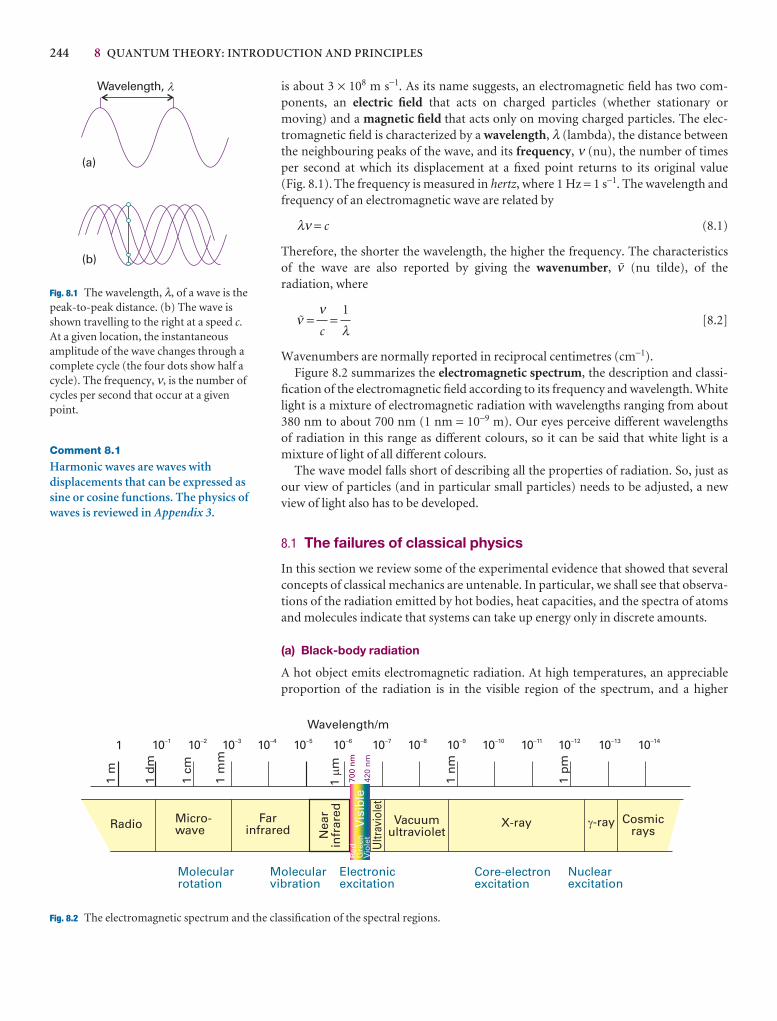
244 8 QUANTUM THEORY: INTRODUCTION AND PRINCIPLES
is about 3 × 10⁸ m s−1. As its name suggests, an electromagnetic field has two com-ponents, an electric field that acts on charged particles (whether stationary or moving) and a magnetic field that acts only on moving charged particles. The elec-tromagnetic field is characterized by a wavelength, λ (lambda), the distance betweenthe neighbouring peaks of the wave, and its frequency, ν (nu), the number of timesper second at which its displacement at a fixed point returns to its original value (Fig. 8.1). The frequency is measured in hertz, where 1 Hz = 1 s−1. The wavelength andfrequency of an electromagnetic wave are related by
λν = c (8.1)
Therefore, the shorter the wavelength, the higher the frequency. The characteristics of the wave are also reported by giving the wavenumber, # (nu tilde), of the radiation, where
# = = [8.2]
Wavenumbers are normally reported in reciprocal centimetres (cm−1).Figure 8.2 summarizes the electromagnetic spectrum, the description and classi-
fication of the electromagnetic field according to its frequency and wavelength. Whitelight is a mixture of electromagnetic radiation with wavelengths ranging from about380 nm to about 700 nm (1 nm = 10−9 m). Our eyes perceive different wavelengths of radiation in this range as different colours, so it can be said that white light is a mixture of light of all different colours.
The wave model falls short of describing all the properties of radiation. So, just asour view of particles (and in particular small particles) needs to be adjusted, a newview of light also has to be developed.
8.1 The failures of classical physics
In this section we review some of the experimental evidence that showed that severalconcepts of classical mechanics are untenable. In particular, we shall see that observa-tions of the radiation emitted by hot bodies, heat capacities, and the spectra of atomsand molecules indicate that systems can take up energy only in discrete amounts.
(a) Black-body radiation
A hot object emits electromagnetic radiation. At high temperatures, an appreciableproportion of the radiation is in the visible region of the spectrum, and a higher
1
λνc
Comment 8.1
Harmonic waves are waves withdisplacements that can be expressed assine or cosine functions. The physics ofwaves is reviewed in Appendix 3.
Wavelength,
(a)
(b)
�
Fig. 8.1 The wavelength, λ, of a wave is thepeak-to-peak distance. (b) The wave isshown travelling to the right at a speed c.At a given location, the instantaneousamplitude of the wave changes through acomplete cycle (the four dots show half acycle). The frequency, ν, is the number ofcycles per second that occur at a givenpoint.
10–1410–1310–1210–1110–1010–910–810–710–610–510–410–310–210–11
1 p
m
1 n
m
1m
1 m
m
1 cm
1 d
m
1 m
Radio Micro-wave
Farinfrared N
ear
infr
ared
Ultr
avio
let
Vacuumultraviolet
X-ray �-ray Cosmicrays
Wavelength/m
Molecularrotation
Molecularvibration
Electronicexcitation
Core-electronexcitation
Nuclearexcitation
Vis
ible
Red
Vio
let
Gre
en70
0 n
m
420
nm
Fig. 8.2 The electromagnetic spectrum and the classification of the spectral regions.
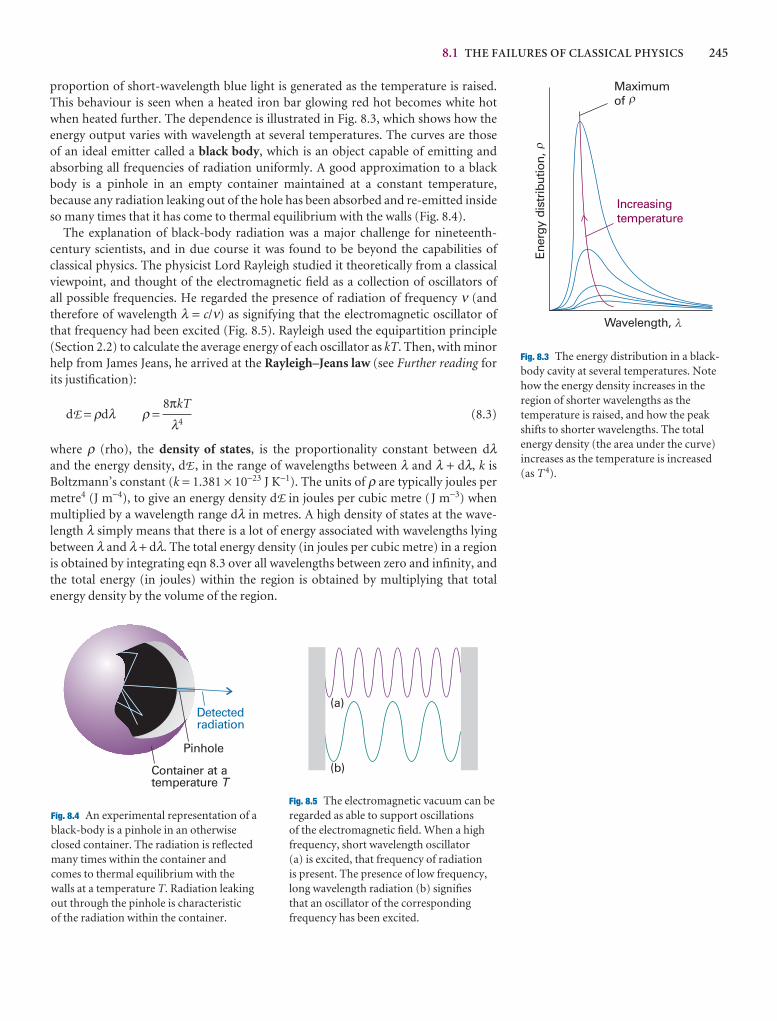
8.1 THE FAILURES OF CLASSICAL PHYSICS 245
proportion of short-wavelength blue light is generated as the temperature is raised.This behaviour is seen when a heated iron bar glowing red hot becomes white hotwhen heated further. The dependence is illustrated in Fig. 8.3, which shows how theenergy output varies with wavelength at several temperatures. The curves are those of an ideal emitter called a black body, which is an object capable of emitting and absorbing all frequencies of radiation uniformly. A good approximation to a blackbody is a pinhole in an empty container maintained at a constant temperature, because any radiation leaking out of the hole has been absorbed and re-emitted insideso many times that it has come to thermal equilibrium with the walls (Fig. 8.4).
The explanation of black-body radiation was a major challenge for nineteenth-century scientists, and in due course it was found to be beyond the capabilities of classical physics. The physicist Lord Rayleigh studied it theoretically from a classicalviewpoint, and thought of the electromagnetic field as a collection of oscillators of all possible frequencies. He regarded the presence of radiation of frequency ν (andtherefore of wavelength λ = c/ν) as signifying that the electromagnetic oscillator ofthat frequency had been excited (Fig. 8.5). Rayleigh used the equipartition principle(Section 2.2) to calculate the average energy of each oscillator as kT. Then, with minorhelp from James Jeans, he arrived at the Rayleigh–Jeans law (see Further reading forits justification):
dE = ρdλ ρ = (8.3)
where ρ (rho), the density of states, is the proportionality constant between dλand the energy density, dE , in the range of wavelengths between λ and λ + dλ, k isBoltzmann’s constant (k = 1.381 × 10⁻²³ J K−1). The units of ρ are typically joules permetre4 (J m−4), to give an energy density dE in joules per cubic metre (J m−3) whenmultiplied by a wavelength range dλ in metres. A high density of states at the wave-length λ simply means that there is a lot of energy associated with wavelengths lyingbetween λ and λ + dλ. The total energy density (in joules per cubic metre) in a regionis obtained by integrating eqn 8.3 over all wavelengths between zero and infinity, andthe total energy (in joules) within the region is obtained by multiplying that total energy density by the volume of the region.
8πkT
λ4
Wavelength,
Ener
gy d
istr
ibut
ion,
Increasingtemperature
Maximumof �
�
�
Fig. 8.3 The energy distribution in a black-body cavity at several temperatures. Notehow the energy density increases in theregion of shorter wavelengths as thetemperature is raised, and how the peakshifts to shorter wavelengths. The totalenergy density (the area under the curve)increases as the temperature is increased(as T 4).
Detectedradiation
Pinhole
Container at atemperature T
Fig. 8.4 An experimental representation of ablack-body is a pinhole in an otherwiseclosed container. The radiation is reflectedmany times within the container andcomes to thermal equilibrium with thewalls at a temperature T. Radiation leakingout through the pinhole is characteristic of the radiation within the container.
(a)
(b)
Fig. 8.5 The electromagnetic vacuum can beregarded as able to support oscillations of the electromagnetic field. When a highfrequency, short wavelength oscillator (a) is excited, that frequency of radiation is present. The presence of low frequency,long wavelength radiation (b) signifies that an oscillator of the correspondingfrequency has been excited.
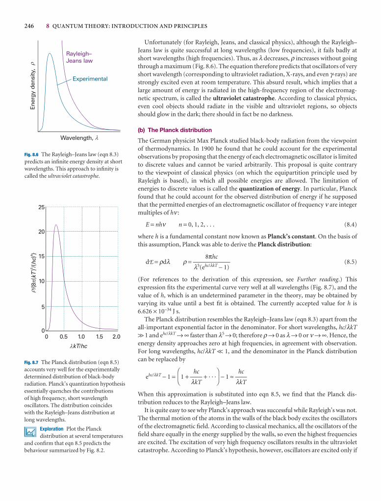
246 8 QUANTUM THEORY: INTRODUCTION AND PRINCIPLES
Unfortunately (for Rayleigh, Jeans, and classical physics), although the Rayleigh–Jeans law is quite successful at long wavelengths (low frequencies), it fails badly atshort wavelengths (high frequencies). Thus, as λ decreases, ρ increases without goingthrough a maximum (Fig. 8.6). The equation therefore predicts that oscillators of veryshort wavelength (corresponding to ultraviolet radiation, X-rays, and even γ-rays) arestrongly excited even at room temperature. This absurd result, which implies that alarge amount of energy is radiated in the high-frequency region of the electromag-netic spectrum, is called the ultraviolet catastrophe. According to classical physics,even cool objects should radiate in the visible and ultraviolet regions, so objectsshould glow in the dark; there should in fact be no darkness.
(b) The Planck distribution
The German physicist Max Planck studied black-body radiation from the viewpointof thermodynamics. In 1900 he found that he could account for the experimental observations by proposing that the energy of each electromagnetic oscillator is limitedto discrete values and cannot be varied arbitrarily. This proposal is quite contrary to the viewpoint of classical physics (on which the equipartition principle used byRayleigh is based), in which all possible energies are allowed. The limitation of energies to discrete values is called the quantization of energy. In particular, Planckfound that he could account for the observed distribution of energy if he supposedthat the permitted energies of an electromagnetic oscillator of frequency ν are integer multiples of hν :
E = nhν n = 0, 1, 2, . . . (8.4)
where h is a fundamental constant now known as Planck’s constant. On the basis ofthis assumption, Planck was able to derive the Planck distribution:
dE = ρdλ ρ = (8.5)
(For references to the derivation of this expression, see Further reading.) This expression fits the experimental curve very well at all wavelengths (Fig. 8.7), and thevalue of h, which is an undetermined parameter in the theory, may be obtained byvarying its value until a best fit is obtained. The currently accepted value for h is6.626 × 10−34 J s.
The Planck distribution resembles the Rayleigh–Jeans law (eqn 8.3) apart from theall-important exponential factor in the denominator. For short wavelengths, hc/λkT>> 1 and ehc/λkT → ∞ faster than λ5 → 0; therefore ρ → 0 as λ → 0 or ν → ∞. Hence, theenergy density approaches zero at high frequencies, in agreement with observation.For long wavelengths, hc/λkT << 1, and the denominator in the Planck distributioncan be replaced by
ehc/λkT − 1 = 1 + + · · · − 1 ≈
When this approximation is substituted into eqn 8.5, we find that the Planck dis-tribution reduces to the Rayleigh–Jeans law.
It is quite easy to see why Planck’s approach was successful while Rayleigh’s was not.The thermal motion of the atoms in the walls of the black body excites the oscillatorsof the electromagnetic field. According to classical mechanics, all the oscillators of thefield share equally in the energy supplied by the walls, so even the highest frequenciesare excited. The excitation of very high frequency oscillators results in the ultravioletcatastrophe. According to Planck’s hypothesis, however, oscillators are excited only if
hc
λkT
DF
hc
λkT
AC
8πhc
λ5(ehc/λkT − 1)
25
20
15
10
5
00 0.5 1.0 1.5 2.0
/{8(
)/(
)}�
kThc
54
kT hc/
�
�
Fig. 8.7 The Planck distribution (eqn 8.5)accounts very well for the experimentallydetermined distribution of black-bodyradiation. Planck’s quantization hypothesisessentially quenches the contributions of high frequency, short wavelengthoscillators. The distribution coincides with the Rayleigh–Jeans distribution atlong wavelengths.
Exploration Plot the Planckdistribution at several temperatures
and confirm that eqn 8.5 predicts thebehaviour summarized by Fig. 8.2.
Rayleigh–Jeans law
Experimental
Ener
gy d
ensi
ty,
Wavelength,
�
�
Fig. 8.6 The Rayleigh–Jeans law (eqn 8.3)predicts an infinite energy density at shortwavelengths. This approach to infinity iscalled the ultraviolet catastrophe.
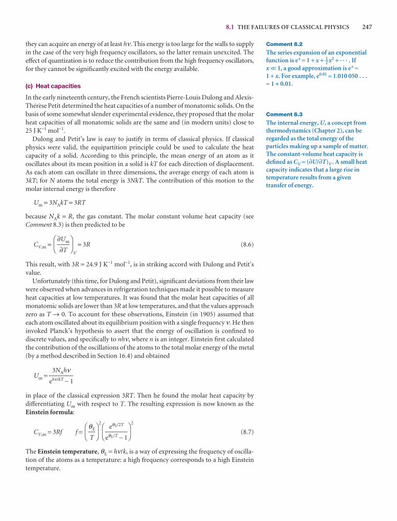
8.1 THE FAILURES OF CLASSICAL PHYSICS 247
they can acquire an energy of at least hν. This energy is too large for the walls to supplyin the case of the very high frequency oscillators, so the latter remain unexcited. Theeffect of quantization is to reduce the contribution from the high frequency oscillators,for they cannot be significantly excited with the energy available.
(c) Heat capacities
In the early nineteenth century, the French scientists Pierre-Louis Dulong and Alexis-Thérèse Petit determined the heat capacities of a number of monatomic solids. On thebasis of some somewhat slender experimental evidence, they proposed that the molarheat capacities of all monatomic solids are the same and (in modern units) close to 25 J K−1 mol−1.
Dulong and Petit’s law is easy to justify in terms of classical physics. If classicalphysics were valid, the equipartition principle could be used to calculate the heat capacity of a solid. According to this principle, the mean energy of an atom as it oscillates about its mean position in a solid is kT for each direction of displacement.As each atom can oscillate in three dimensions, the average energy of each atom is3kT; for N atoms the total energy is 3NkT. The contribution of this motion to themolar internal energy is therefore
Um = 3NAkT = 3RT
because NAk = R, the gas constant. The molar constant volume heat capacity (seeComment 8.3) is then predicted to be
CV,m =V
= 3R (8.6)
This result, with 3R = 24.9 J K−1 mol−1, is in striking accord with Dulong and Petit’svalue.
Unfortunately (this time, for Dulong and Petit), significant deviations from their lawwere observed when advances in refrigeration techniques made it possible to measureheat capacities at low temperatures. It was found that the molar heat capacities of allmonatomic solids are lower than 3R at low temperatures, and that the values approachzero as T → 0. To account for these observations, Einstein (in 1905) assumed thateach atom oscillated about its equilibrium position with a single frequency ν. He theninvoked Planck’s hypothesis to assert that the energy of oscillation is confined to discrete values, and specifically to nhν, where n is an integer. Einstein first calculatedthe contribution of the oscillations of the atoms to the total molar energy of the metal(by a method described in Section 16.4) and obtained
Um =
in place of the classical expression 3RT. Then he found the molar heat capacity by differentiating Um with respect to T. The resulting expression is now known as theEinstein formula:
CV,m = 3Rf f =2 2
(8.7)
The Einstein temperature, θE = hν/k, is a way of expressing the frequency of oscilla-tion of the atoms as a temperature: a high frequency corresponds to a high Einsteintemperature.
DF
eθE/2T
eθE/T − 1
AC
DF
θE
T
AC
3NAhνehν/kT − 1
DF
∂Um
∂T
AC
Comment 8.2
The series expansion of an exponentialfunction is ex = 1 + x + 1–2 x2 + · · · . If x << 1, a good approximation is ex ≈1 + x. For example, e0.01 = 1.010 050 . . .≈ 1 + 0.01.
Comment 8.3
The internal energy, U, a concept fromthermodynamics (Chapter 2), can beregarded as the total energy of theparticles making up a sample of matter.The constant-volume heat capacity isdefined as CV = (∂U/∂T)V . A small heatcapacity indicates that a large rise intemperature results from a giventransfer of energy.
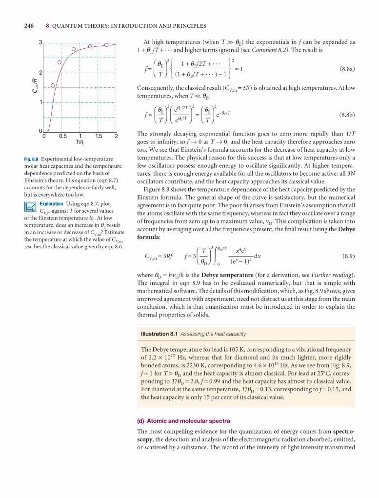
248 8 QUANTUM THEORY: INTRODUCTION AND PRINCIPLES
3
2
1
00 0.5 1 1.5 2
C/R
V,m
T/ E�
Fig. 8.8 Experimental low-temperature molar heat capacities and the temperaturedependence predicted on the basis ofEinstein’s theory. His equation (eqn 8.7)accounts for the dependence fairly well, but is everywhere too low.
Exploration Using eqn 8.7, plot CV,m against T for several values
of the Einstein temperature θE. At lowtemperature, does an increase in θE resultin an increase or decrease of CV,m? Estimatethe temperature at which the value of CV,m
reaches the classical value given by eqn 8.6.
At high temperatures (when T >> θE) the exponentials in f can be expanded as 1 + θE/T + · · · and higher terms ignored (see Comment 8.2). The result is
f =2 2
≈ 1 (8.8a)
Consequently, the classical result (CV,m = 3R) is obtained at high temperatures. At lowtemperatures, when T << θE,
f ≈2 2
=2
e−θE/T (8.8b)
The strongly decaying exponential function goes to zero more rapidly than 1/Tgoes to infinity; so f → 0 as T → 0, and the heat capacity therefore approaches zero too. We see that Einstein’s formula accounts for the decrease of heat capacity at low temperatures. The physical reason for this success is that at low temperatures only afew oscillators possess enough energy to oscillate significantly. At higher tempera-tures, there is enough energy available for all the oscillators to become active: all 3Noscillators contribute, and the heat capacity approaches its classical value.
Figure 8.8 shows the temperature dependence of the heat capacity predicted by theEinstein formula. The general shape of the curve is satisfactory, but the numericalagreement is in fact quite poor. The poor fit arises from Einstein’s assumption that allthe atoms oscillate with the same frequency, whereas in fact they oscillate over a rangeof frequencies from zero up to a maximum value, νD. This complication is taken intoaccount by averaging over all the frequencies present, the final result being the Debyeformula:
CV,m = 3Rf f = 3
3
�0
θD/T
dx (8.9)
where θD = hνD/k is the Debye temperature (for a derivation, see Further reading).The integral in eqn 8.9 has to be evaluated numerically, but that is simple with mathematical software. The details of this modification, which, as Fig. 8.9 shows, gives improved agreement with experiment, need not distract us at this stage from the mainconclusion, which is that quantization must be introduced in order to explain thethermal properties of solids.
Illustration 8.1 Assessing the heat capacity
The Debye temperature for lead is 105 K, corresponding to a vibrational frequencyof 2.2 × 10¹² Hz, whereas that for diamond and its much lighter, more rigidlybonded atoms, is 2230 K, corresponding to 4.6 × 10¹³ Hz. As we see from Fig. 8.9, f ≈ 1 for T > θD and the heat capacity is almost classical. For lead at 25°C, corres-ponding to T/θD = 2.8, f = 0.99 and the heat capacity has almost its classical value.For diamond at the same temperature, T/θD = 0.13, corresponding to f = 0.15, andthe heat capacity is only 15 per cent of its classical value.
(d) Atomic and molecular spectra
The most compelling evidence for the quantization of energy comes from spectro-scopy, the detection and analysis of the electromagnetic radiation absorbed, emitted,or scattered by a substance. The record of the intensity of light intensity transmitted
x4ex
(ex − 1)2
DF
T
θD
AC
DF
θE
T
AC
DF
eθE/2T
eθE /T
AC
DF
θE
T
AC
567
1 + θE/2T + · · ·
(1 + θE/T + · · · ) − 1
123
DF
θE
T
AC
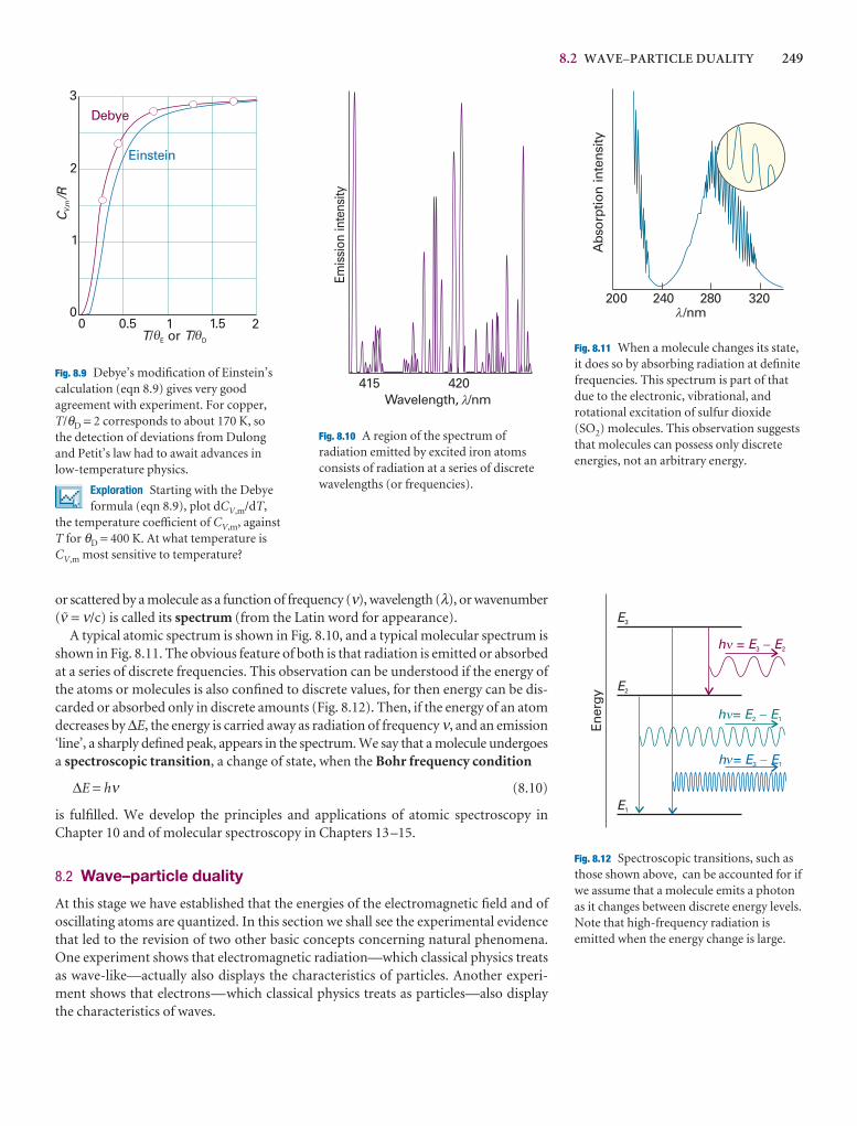
8.2 WAVE–PARTICLE DUALITY 249
or scattered by a molecule as a function of frequency (ν), wavelength (λ), or wavenumber(# = ν/c) is called its spectrum (from the Latin word for appearance).
A typical atomic spectrum is shown in Fig. 8.10, and a typical molecular spectrum isshown in Fig. 8.11. The obvious feature of both is that radiation is emitted or absorbedat a series of discrete frequencies. This observation can be understood if the energy ofthe atoms or molecules is also confined to discrete values, for then energy can be dis-carded or absorbed only in discrete amounts (Fig. 8.12). Then, if the energy of an atomdecreases by ∆E, the energy is carried away as radiation of frequency ν, and an emission‘line’, a sharply defined peak, appears in the spectrum. We say that a molecule undergoesa spectroscopic transition, a change of state, when the Bohr frequency condition
∆E = hν (8.10)
is fulfilled. We develop the principles and applications of atomic spectroscopy inChapter 10 and of molecular spectroscopy in Chapters 13–15.
8.2 Wave–particle duality
At this stage we have established that the energies of the electromagnetic field and ofoscillating atoms are quantized. In this section we shall see the experimental evidencethat led to the revision of two other basic concepts concerning natural phenomena.One experiment shows that electromagnetic radiation—which classical physics treatsas wave-like—actually also displays the characteristics of particles. Another experi-ment shows that electrons—which classical physics treats as particles—also displaythe characteristics of waves.
3
2
1
0
Einstein
0 0.5 1 1.5 2
C/R
V,m
Debye
T T/ or /E D� �
Fig. 8.9 Debye’s modification of Einstein’scalculation (eqn 8.9) gives very goodagreement with experiment. For copper,T/θD = 2 corresponds to about 170 K, sothe detection of deviations from Dulongand Petit’s law had to await advances inlow-temperature physics.
Exploration Starting with the Debyeformula (eqn 8.9), plot dCV,m/dT,
the temperature coefficient of CV,m, againstT for θD = 400 K. At what temperature isCV,m most sensitive to temperature?
415 420
Emis
sion
inte
nsity
Wavelength, /nm�
Fig. 8.10 A region of the spectrum ofradiation emitted by excited iron atomsconsists of radiation at a series of discretewavelengths (or frequencies).
Ener
gy
E1
E2
E3
h E E= 2 1�
h E E= 3 1�
h E E= 3 2��
�
�
Fig. 8.12 Spectroscopic transitions, such asthose shown above, can be accounted for ifwe assume that a molecule emits a photonas it changes between discrete energy levels.Note that high-frequency radiation isemitted when the energy change is large.
200 240 280 320/nm
Abs
orpt
ion
inte
nsity
�
Fig. 8.11 When a molecule changes its state,it does so by absorbing radiation at definitefrequencies. This spectrum is part of thatdue to the electronic, vibrational, androtational excitation of sulfur dioxide(SO2) molecules. This observation suggeststhat molecules can possess only discreteenergies, not an arbitrary energy.
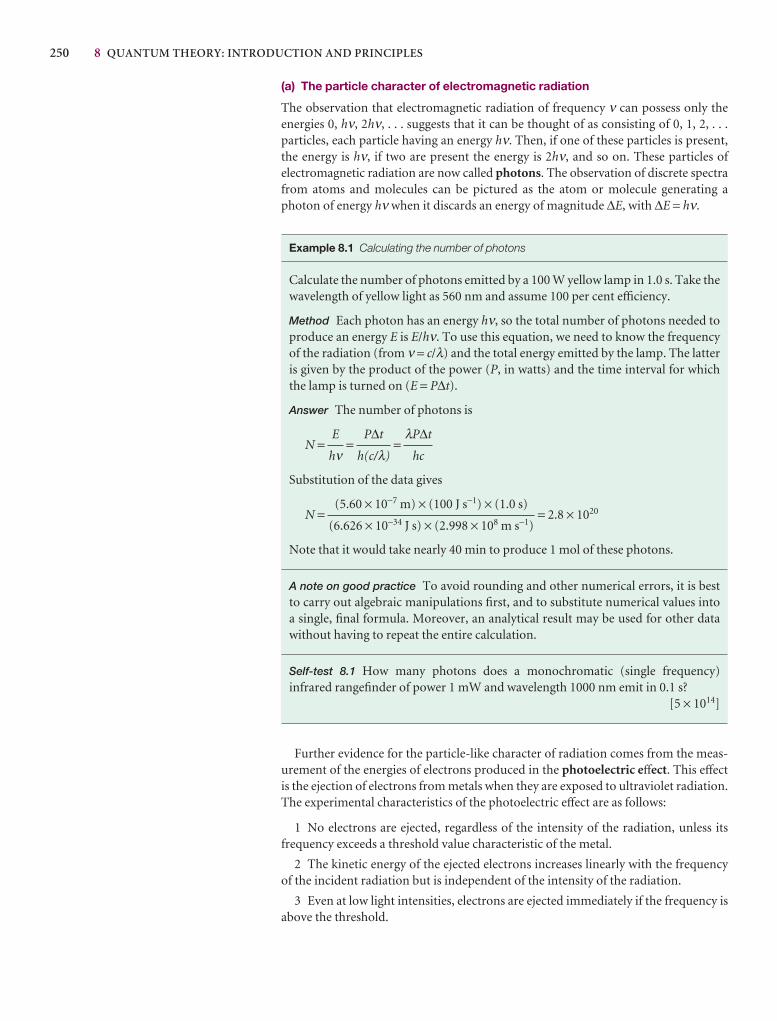
250 8 QUANTUM THEORY: INTRODUCTION AND PRINCIPLES
(a) The particle character of electromagnetic radiation
The observation that electromagnetic radiation of frequency ν can possess only theenergies 0, hν, 2hν, . . . suggests that it can be thought of as consisting of 0, 1, 2, . . .particles, each particle having an energy hν. Then, if one of these particles is present,the energy is hν, if two are present the energy is 2hν, and so on. These particles of electromagnetic radiation are now called photons. The observation of discrete spectrafrom atoms and molecules can be pictured as the atom or molecule generating a photon of energy hν when it discards an energy of magnitude ∆E, with ∆E = hν.
Example 8.1 Calculating the number of photons
Calculate the number of photons emitted by a 100 W yellow lamp in 1.0 s. Take thewavelength of yellow light as 560 nm and assume 100 per cent efficiency.
Method Each photon has an energy hν, so the total number of photons needed toproduce an energy E is E/hν. To use this equation, we need to know the frequencyof the radiation (from ν = c/λ) and the total energy emitted by the lamp. The latteris given by the product of the power (P, in watts) and the time interval for whichthe lamp is turned on (E = P∆t).
Answer The number of photons is
N = = =
Substitution of the data gives
N = = 2.8 × 10²⁰
Note that it would take nearly 40 min to produce 1 mol of these photons.
A note on good practice To avoid rounding and other numerical errors, it is bestto carry out algebraic manipulations first, and to substitute numerical values intoa single, final formula. Moreover, an analytical result may be used for other datawithout having to repeat the entire calculation.
Self-test 8.1 How many photons does a monochromatic (single frequency) infrared rangefinder of power 1 mW and wavelength 1000 nm emit in 0.1 s?
[5 × 10¹⁴]
Further evidence for the particle-like character of radiation comes from the meas-urement of the energies of electrons produced in the photoelectric effect. This effectis the ejection of electrons from metals when they are exposed to ultraviolet radiation.The experimental characteristics of the photoelectric effect are as follows:
1 No electrons are ejected, regardless of the intensity of the radiation, unless its frequency exceeds a threshold value characteristic of the metal.
2 The kinetic energy of the ejected electrons increases linearly with the frequencyof the incident radiation but is independent of the intensity of the radiation.
3 Even at low light intensities, electrons are ejected immediately if the frequency isabove the threshold.
(5.60 × 10⁻⁷ m) × (100 J s−1) × (1.0 s)
(6.626 × 10⁻³⁴ J s) × (2.998 × 10⁸ m s−1)
λP∆t
hc
P∆t
h(c/λ)
E
hν
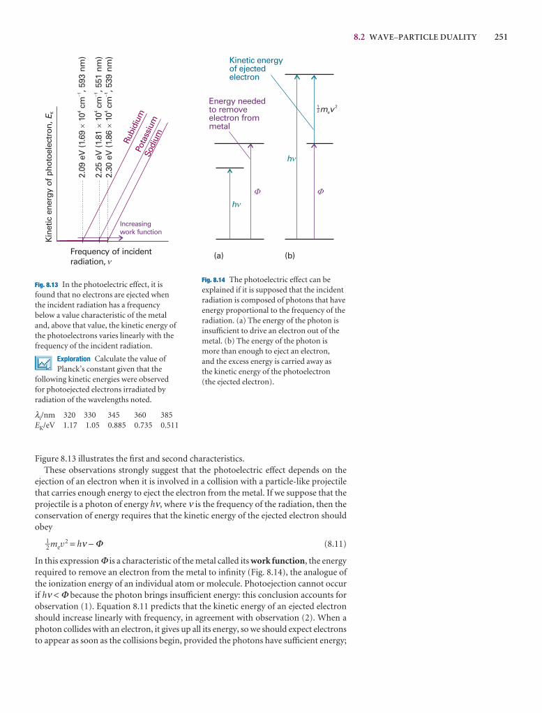
8.2 WAVE–PARTICLE DUALITY 251
Figure 8.13 illustrates the first and second characteristics.These observations strongly suggest that the photoelectric effect depends on the
ejection of an electron when it is involved in a collision with a particle-like projectilethat carries enough energy to eject the electron from the metal. If we suppose that theprojectile is a photon of energy hν, where ν is the frequency of the radiation, then theconservation of energy requires that the kinetic energy of the ejected electron shouldobey
1–2 mev2 = hν − Φ (8.11)
In this expression Φ is a characteristic of the metal called its work function, the energyrequired to remove an electron from the metal to infinity (Fig. 8.14), the analogue ofthe ionization energy of an individual atom or molecule. Photoejection cannot occurif hν < Φ because the photon brings insufficient energy: this conclusion accounts forobservation (1). Equation 8.11 predicts that the kinetic energy of an ejected electronshould increase linearly with frequency, in agreement with observation (2). When aphoton collides with an electron, it gives up all its energy, so we should expect electronsto appear as soon as the collisions begin, provided the photons have sufficient energy;
Kin
etic
ene
rgy
of p
hoto
elec
tron
, EK
Frequency of incidentradiation,
Rubi
dium
Pota
ssiu
mSo
dium
Increasingwork function
2.30
eV
(1.8
610
cm, 5
39 n
m)
�4
12.
25 e
V (1
.81
10cm
, 551
nm
)�
41
2.09
eV
(1.6
910
cm, 5
93 n
m)
�4
1
�
� � �
Fig. 8.13 In the photoelectric effect, it isfound that no electrons are ejected whenthe incident radiation has a frequencybelow a value characteristic of the metaland, above that value, the kinetic energy ofthe photoelectrons varies linearly with thefrequency of the incident radiation.
Exploration Calculate the value ofPlanck’s constant given that the
following kinetic energies were observedfor photoejected electrons irradiated byradiation of the wavelengths noted.
λi/nm 320 330 345 360 385EK/eV 1.17 1.05 0.885 0.735 0.511
Energy neededto removeelectron frommetal
Kinetic energyof ejectedelectron
m ve2
�
(b)(a)
h
�
21
�
h�
Fig. 8.14 The photoelectric effect can beexplained if it is supposed that the incidentradiation is composed of photons that haveenergy proportional to the frequency of theradiation. (a) The energy of the photon isinsufficient to drive an electron out of themetal. (b) The energy of the photon ismore than enough to eject an electron, and the excess energy is carried away as the kinetic energy of the photoelectron (the ejected electron).
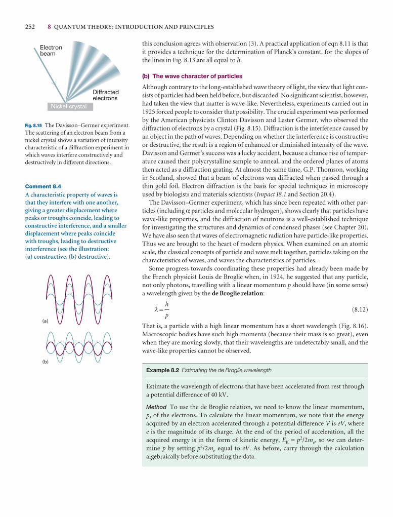
252 8 QUANTUM THEORY: INTRODUCTION AND PRINCIPLES
Comment 8.4
A characteristic property of waves is that they interfere with one another,giving a greater displacement wherepeaks or troughs coincide, leading toconstructive interference, and a smallerdisplacement where peaks coincide with troughs, leading to destructiveinterference (see the illustration: (a) constructive, (b) destructive).
Electronbeam
Nickel crystal
Diffractedelectrons
Fig. 8.15 The Davisson–Germer experiment.The scattering of an electron beam from anickel crystal shows a variation of intensitycharacteristic of a diffraction experiment inwhich waves interfere constructively anddestructively in different directions.
(a)
(b)
this conclusion agrees with observation (3). A practical application of eqn 8.11 is thatit provides a technique for the determination of Planck’s constant, for the slopes of the lines in Fig. 8.13 are all equal to h.
(b) The wave character of particles
Although contrary to the long-established wave theory of light, the view that light con-sists of particles had been held before, but discarded. No significant scientist, however,had taken the view that matter is wave-like. Nevertheless, experiments carried out in1925 forced people to consider that possibility. The crucial experiment was performedby the American physicists Clinton Davisson and Lester Germer, who observed thediffraction of electrons by a crystal (Fig. 8.15). Diffraction is the interference caused byan object in the path of waves. Depending on whether the interference is constructiveor destructive, the result is a region of enhanced or diminished intensity of the wave.Davisson and Germer’s success was a lucky accident, because a chance rise of temper-ature caused their polycrystalline sample to anneal, and the ordered planes of atomsthen acted as a diffraction grating. At almost the same time, G.P. Thomson, workingin Scotland, showed that a beam of electrons was diffracted when passed through athin gold foil. Electron diffraction is the basis for special techniques in microscopyused by biologists and materials scientists (Impact I8.1 and Section 20.4).
The Davisson–Germer experiment, which has since been repeated with other par-ticles (including α particles and molecular hydrogen), shows clearly that particles havewave-like properties, and the diffraction of neutrons is a well-established techniquefor investigating the structures and dynamics of condensed phases (see Chapter 20).We have also seen that waves of electromagnetic radiation have particle-like properties.Thus we are brought to the heart of modern physics. When examined on an atomicscale, the classical concepts of particle and wave melt together, particles taking on thecharacteristics of waves, and waves the characteristics of particles.
Some progress towards coordinating these properties had already been made by the French physicist Louis de Broglie when, in 1924, he suggested that any particle,not only photons, travelling with a linear momentum p should have (in some sense) a wavelength given by the de Broglie relation:
λ = (8.12)
That is, a particle with a high linear momentum has a short wavelength (Fig. 8.16).Macroscopic bodies have such high momenta (because their mass is so great), evenwhen they are moving slowly, that their wavelengths are undetectably small, and thewave-like properties cannot be observed.
Example 8.2 Estimating the de Broglie wavelength
Estimate the wavelength of electrons that have been accelerated from rest througha potential difference of 40 kV.
Method To use the de Broglie relation, we need to know the linear momentum, p, of the electrons. To calculate the linear momentum, we note that the energy acquired by an electron accelerated through a potential difference V is eV, where e is the magnitude of its charge. At the end of the period of acceleration, all the acquired energy is in the form of kinetic energy, EK = p2/2me, so we can deter-mine p by setting p2/2me equal to eV. As before, carry through the calculation algebraically before substituting the data.
h
p
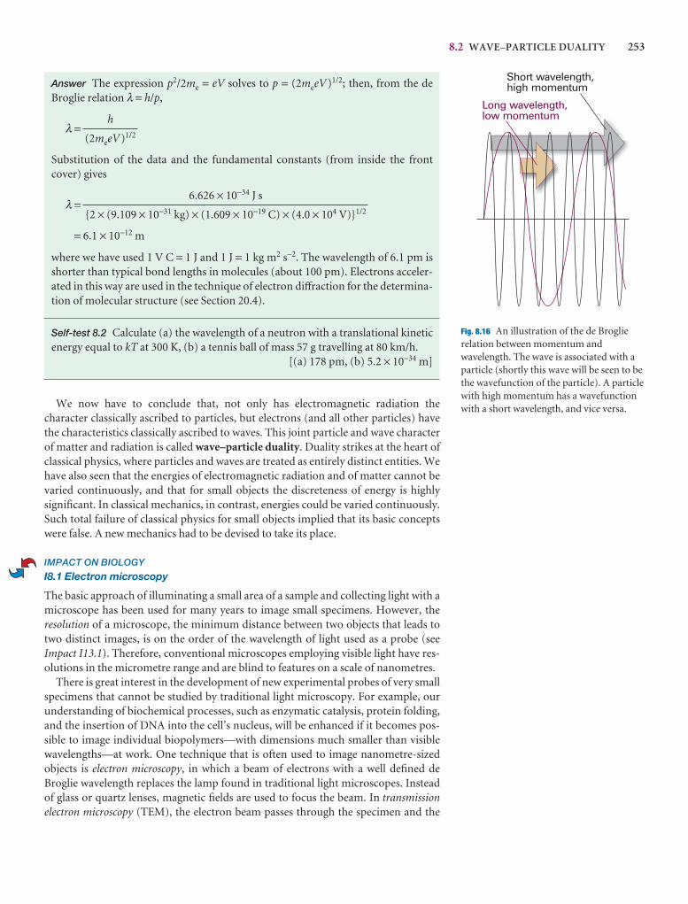
8.2 WAVE–PARTICLE DUALITY 253
Short wavelength,high momentum
Long wavelength,low momentum
Fig. 8.16 An illustration of the de Broglierelation between momentum andwavelength. The wave is associated with aparticle (shortly this wave will be seen to bethe wavefunction of the particle). A particlewith high momentum has a wavefunctionwith a short wavelength, and vice versa.
Answer The expression p2/2me = eV solves to p = (2meeV)1/2; then, from the deBroglie relation λ = h/p,
λ =
Substitution of the data and the fundamental constants (from inside the frontcover) gives
λ =
= 6.1 × 10⁻¹² m
where we have used 1 V C = 1 J and 1 J = 1 kg m2 s−2. The wavelength of 6.1 pm isshorter than typical bond lengths in molecules (about 100 pm). Electrons acceler-ated in this way are used in the technique of electron diffraction for the determina-tion of molecular structure (see Section 20.4).
Self-test 8.2 Calculate (a) the wavelength of a neutron with a translational kineticenergy equal to kT at 300 K, (b) a tennis ball of mass 57 g travelling at 80 km/h.
[(a) 178 pm, (b) 5.2 × 10⁻³⁴ m]
We now have to conclude that, not only has electromagnetic radiation the character classically ascribed to particles, but electrons (and all other particles) havethe characteristics classically ascribed to waves. This joint particle and wave characterof matter and radiation is called wave–particle duality. Duality strikes at the heart ofclassical physics, where particles and waves are treated as entirely distinct entities. Wehave also seen that the energies of electromagnetic radiation and of matter cannot bevaried continuously, and that for small objects the discreteness of energy is highlysignificant. In classical mechanics, in contrast, energies could be varied continuously.Such total failure of classical physics for small objects implied that its basic conceptswere false. A new mechanics had to be devised to take its place.
IMPACT ON BIOLOGY
I8.1 Electron microscopy
The basic approach of illuminating a small area of a sample and collecting light with amicroscope has been used for many years to image small specimens. However, the resolution of a microscope, the minimum distance between two objects that leads totwo distinct images, is on the order of the wavelength of light used as a probe (seeImpact I13.1). Therefore, conventional microscopes employing visible light have res-olutions in the micrometre range and are blind to features on a scale of nanometres.
There is great interest in the development of new experimental probes of very smallspecimens that cannot be studied by traditional light microscopy. For example, ourunderstanding of biochemical processes, such as enzymatic catalysis, protein folding,and the insertion of DNA into the cell’s nucleus, will be enhanced if it becomes pos-sible to image individual biopolymers—with dimensions much smaller than visiblewavelengths—at work. One technique that is often used to image nanometre-sizedobjects is electron microscopy, in which a beam of electrons with a well defined deBroglie wavelength replaces the lamp found in traditional light microscopes. Insteadof glass or quartz lenses, magnetic fields are used to focus the beam. In transmissionelectron microscopy (TEM), the electron beam passes through the specimen and the
6.626 × 10⁻³⁴ J s
{2 × (9.109 × 10−31 kg) × (1.609 × 10⁻¹⁹ C) × (4.0 × 10⁴ V)}1/2
h
(2meeV)1/2
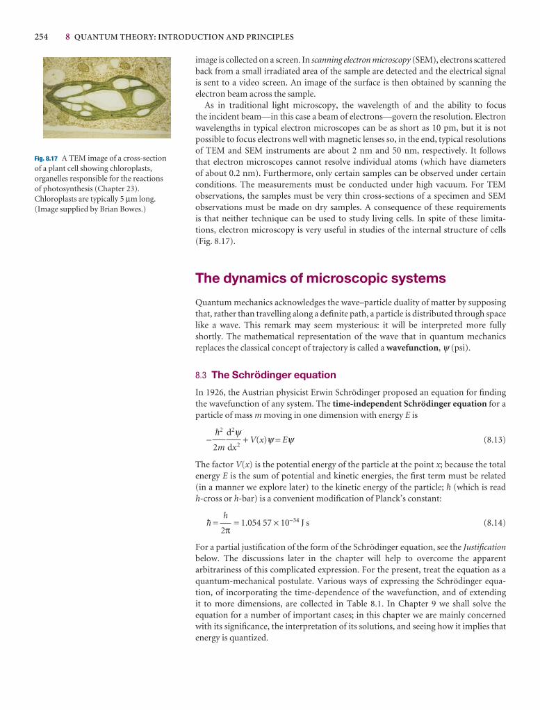
254 8 QUANTUM THEORY: INTRODUCTION AND PRINCIPLES
image is collected on a screen. In scanning electron microscopy (SEM), electrons scatteredback from a small irradiated area of the sample are detected and the electrical signal is sent to a video screen. An image of the surface is then obtained by scanning the electron beam across the sample.
As in traditional light microscopy, the wavelength of and the ability to focus the incident beam—in this case a beam of electrons—govern the resolution. Electronwavelengths in typical electron microscopes can be as short as 10 pm, but it is not possible to focus electrons well with magnetic lenses so, in the end, typical resolutionsof TEM and SEM instruments are about 2 nm and 50 nm, respectively. It follows that electron microscopes cannot resolve individual atoms (which have diameters of about 0.2 nm). Furthermore, only certain samples can be observed under certainconditions. The measurements must be conducted under high vacuum. For TEM observations, the samples must be very thin cross-sections of a specimen and SEM observations must be made on dry samples. A consequence of these requirements is that neither technique can be used to study living cells. In spite of these limita-tions, electron microscopy is very useful in studies of the internal structure of cells(Fig. 8.17).
The dynamics of microscopic systems
Quantum mechanics acknowledges the wave–particle duality of matter by supposingthat, rather than travelling along a definite path, a particle is distributed through spacelike a wave. This remark may seem mysterious: it will be interpreted more fullyshortly. The mathematical representation of the wave that in quantum mechanics replaces the classical concept of trajectory is called a wavefunction, ψ (psi).
8.3 The Schrödinger equation
In 1926, the Austrian physicist Erwin Schrödinger proposed an equation for findingthe wavefunction of any system. The time-independent Schrödinger equation for aparticle of mass m moving in one dimension with energy E is
− + V(x)ψ = Eψ (8.13)
The factor V(x) is the potential energy of the particle at the point x; because the totalenergy E is the sum of potential and kinetic energies, the first term must be related (in a manner we explore later) to the kinetic energy of the particle; $ (which is read h-cross or h-bar) is a convenient modification of Planck’s constant:
$ = = 1.054 57 × 10−34 J s (8.14)
For a partial justification of the form of the Schrödinger equation, see the Justificationbelow. The discussions later in the chapter will help to overcome the apparent arbitrariness of this complicated expression. For the present, treat the equation as aquantum-mechanical postulate. Various ways of expressing the Schrödinger equa-tion, of incorporating the time-dependence of the wavefunction, and of extending it to more dimensions, are collected in Table 8.1. In Chapter 9 we shall solve the equation for a number of important cases; in this chapter we are mainly concernedwith its significance, the interpretation of its solutions, and seeing how it implies thatenergy is quantized.
h
2π
d2ψdx2
$2
2m
Fig. 8.17 A TEM image of a cross-section of a plant cell showing chloroplasts,organelles responsible for the reactions of photosynthesis (Chapter 23).Chloroplasts are typically 5 µm long.(Image supplied by Brian Bowes.)
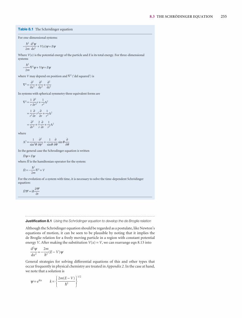
8.3 THE SCHRÖDINGER EQUATION 255
Justification 8.1 Using the Schrödinger equation to develop the de Broglie relation
Although the Schrödinger equation should be regarded as a postulate, like Newton’sequations of motion, it can be seen to be plausible by noting that it implies the de Broglie relation for a freely moving particle in a region with constant potentialenergy V. After making the substitution V(x) = V, we can rearrange eqn 8.13 into
= − (E − V)ψ
General strategies for solving differential equations of this and other types thatoccur frequently in physical chemistry are treated in Appendix 2. In the case at hand,we note that a solution is
ψ = eikx k = 1/2567
2m(E − V)
$2
123
2m
$2
d2ψdx2
Table 8.1 The Schrödinger equation
For one-dimensional systems:
− + V(x)ψ = Eψ
Where V(x) is the potential energy of the particle and E is its total energy. For three-dimensionalsystems
− ∇2ψ + Vψ = Eψ
where V may depend on position and ∇2 (‘del squared’) is
∇2 = + +
In systems with spherical symmetry three equivalent forms are
∇2 = r + Λ2
= r2 + Λ2
= + + Λ2
where
Λ2 = + sin θ
In the general case the Schrodinger equation is written
@ψ = Eψwhere @ is the hamiltonian operator for the system:
@ = − ∇2 + V
For the evolution of a system with time, it is necessary to solve the time-dependent Schrödingerequation:
@Ψ = i$∂Ψ∂t
$2
2m
∂∂θ
∂∂θ
1
sinθ∂2
∂φ2
1
sin2θ
1
r2
∂∂r
2
r
∂2
∂r2
1
r2
∂∂r
∂∂r
1
r2
1
r2
∂2
∂r2
1
r
∂2
∂z2
∂2
∂y2
∂2
∂x2
$2
2m
d2ψdx2
$2
2m
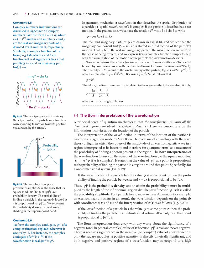
256 8 QUANTUM THEORY: INTRODUCTION AND PRINCIPLES
Comment 8.6
To form the complex conjugate, ψ*, of acomplex function, replace i wherever itoccurs by −i. For instance, the complexconjugate of eikx is e−ikx. If thewavefunction is real, |ψ |2 = ψ2.
In quantum mechanics, a wavefunction that describes the spatial distribution of a particle (a ‘spatial wavefunction’) is complex if the particle it describes has a netmotion. In the present case, we can use the relation eiθ = cos θ + i sin θ to write
ψ = cos kx + i sin kx
The real and imaginary parts of ψ are drawn in Fig. 8.18, and we see that the imaginary component Im(ψ) = sin kx is shifted in the direction of the particle’s motion. That is, both the real and imaginary parts of the wavefunction are ‘real’, inthe sense of being present, and we express ψ as a complex function simply to helpwith the visualization of the motion of the particle the wavefunction desribes.
Now we recognize that cos kx (or sin kx) is a wave of wavelength λ = 2π/k, as canbe seen by comparing cos kx with the standard form of a harmonic wave, cos(2πx/λ).The quantity E − V is equal to the kinetic energy of the particle, EK, so k = (2mEK/$2)1/2,which implies that EK = k2$2/2m. Because EK = p2/2m, it follows that
p = k$
Therefore, the linear momentum is related to the wavelength of the wavefunction by
p = × =
which is the de Broglie relation.
8.4 The Born interpretation of the wavefunction
A principal tenet of quantum mechanics is that the wavefunction contains all the dynamical information about the system it describes. Here we concentrate on the information it carries about the location of the particle.
The interpretation of the wavefunction in terms of the location of the particle isbased on a suggestion made by Max Born. He made use of an analogy with the wavetheory of light, in which the square of the amplitude of an electromagnetic wave in aregion is interpreted as its intensity and therefore (in quantum terms) as a measure ofthe probability of finding a photon present in the region. The Born interpretation ofthe wavefunction focuses on the square of the wavefunction (or the square modulus,|ψ |2 = ψ*ψ, if ψ is complex). It states that the value of |ψ |2 at a point is proportionalto the probability of finding the particle in a region around that point. Specifically, fora one-dimensional system (Fig. 8.19):
If the wavefunction of a particle has the value ψ at some point x, then the prob-ability of finding the particle between x and x + dx is proportional to |ψ |2dx.
Thus, |ψ |2 is the probability density, and to obtain the probability it must be multi-plied by the length of the infinitesimal region dx. The wavefunction ψ itself is calledthe probability amplitude. For a particle free to move in three dimensions (for example,an electron near a nucleus in an atom), the wavefunction depends on the point drwith coordinates x, y, and z, and the interpretation of ψ(r) is as follows (Fig. 8.20):
If the wavefunction of a particle has the value ψ at some point r, then the prob-ability of finding the particle in an infinitesimal volume dτ = dxdydz at that pointis proportional to |ψ |2dτ.
The Born interpretation does away with any worry about the significance of a negative (and, in general, complex) value of ψ because |ψ |2 is real and never negative.There is no direct significance in the negative (or complex) value of a wavefunction:only the square modulus, a positive quantity, is directly physically significant, andboth negative and positive regions of a wavefunction may correspond to a high
h
λh
2π2πλ
Comment 8.5
Complex numbers and functions arediscussed in Appendix 2. Complexnumbers have the form z = x + iy, wherei = (−1)1/2 and the real numbers x and yare the real and imaginary parts of z,denoted Re(z) and Im(z), respectively.Similarly, a complex function of theform f = g + ih, where g and h arefunctions of real arguments, has a realpart Re(f ) = g and an imaginary partIm( f ) = h.
Im e = sinikx kx
Re e = cosikx kx
Wav
efun
ctio
n,�
Fig. 8.18 The real (purple) and imaginary(blue) parts of a free particle wavefunctioncorresponding to motion towards positivex (as shown by the arrow).
dx
x x xd�
Probability= | | d2 x| |2�
�
Fig. 8.19 The wavefunction ψ is aprobability amplitude in the sense that itssquare modulus (ψ*ψ or |ψ |2) is aprobability density. The probability offinding a particle in the region dx located atx is proportional to |ψ |2dx. We representthe probability density by the density ofshading in the superimposed band.
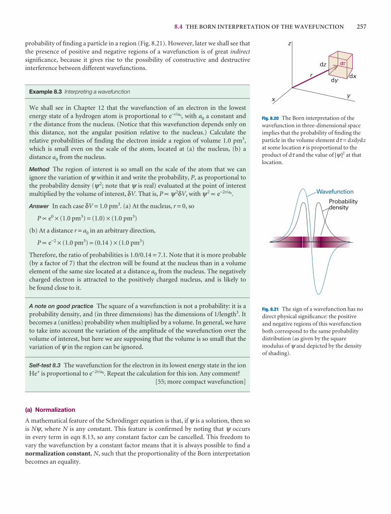
8.4 THE BORN INTERPRETATION OF THE WAVEFUNCTION 257
z
xy
d
r dxdy
dz �
Fig. 8.20 The Born interpretation of thewavefunction in three-dimensional spaceimplies that the probability of finding theparticle in the volume element dτ = dxdydzat some location r is proportional to theproduct of dτ and the value of |ψ |2 at thatlocation.
Fig. 8.21 The sign of a wavefunction has nodirect physical significance: the positiveand negative regions of this wavefunctionboth correspond to the same probabilitydistribution (as given by the squaremodulus of ψ and depicted by the densityof shading).
probability of finding a particle in a region (Fig. 8.21). However, later we shall see thatthe presence of positive and negative regions of a wavefunction is of great indirectsignificance, because it gives rise to the possibility of constructive and destructive interference between different wavefunctions.
Example 8.3 Interpreting a wavefunction
We shall see in Chapter 12 that the wavefunction of an electron in the lowest energy state of a hydrogen atom is proportional to e−r/a0, with a0 a constant and r the distance from the nucleus. (Notice that this wavefunction depends only on this distance, not the angular position relative to the nucleus.) Calculate the relative probabilities of finding the electron inside a region of volume 1.0 pm3,which is small even on the scale of the atom, located at (a) the nucleus, (b) a distance a0 from the nucleus.
Method The region of interest is so small on the scale of the atom that we can ignore the variation of ψ within it and write the probability, P, as proportional tothe probability density (ψ2; note that ψ is real) evaluated at the point of interestmultiplied by the volume of interest, δV. That is, P ∝ ψ2δV, with ψ2 ∝ e−2r/a0.
Answer In each case δV = 1.0 pm3. (a) At the nucleus, r = 0, so
P ∝ e0 × (1.0 pm3) = (1.0) × (1.0 pm3)
(b) At a distance r = a0 in an arbitrary direction,
P ∝ e−2 × (1.0 pm3) = (0.14 ) × (1.0 pm3)
Therefore, the ratio of probabilities is 1.0/0.14 = 7.1. Note that it is more probable(by a factor of 7) that the electron will be found at the nucleus than in a volume element of the same size located at a distance a0 from the nucleus. The negativelycharged electron is attracted to the positively charged nucleus, and is likely to be found close to it.
A note on good practice The square of a wavefunction is not a probability: it is aprobability density, and (in three dimensions) has the dimensions of 1/length3. Itbecomes a (unitless) probability when multiplied by a volume. In general, we haveto take into account the variation of the amplitude of the wavefunction over thevolume of interest, but here we are supposing that the volume is so small that thevariation of ψ in the region can be ignored.
Self-test 8.3 The wavefunction for the electron in its lowest energy state in the ionHe+ is proportional to e−2r/a0. Repeat the calculation for this ion. Any comment?
[55; more compact wavefunction]
(a) Normalization
A mathematical feature of the Schrödinger equation is that, if ψ is a solution, then sois Nψ, where N is any constant. This feature is confirmed by noting that ψ occursin every term in eqn 8.13, so any constant factor can be cancelled. This freedom tovary the wavefunction by a constant factor means that it is always possible to find a normalization constant, N, such that the proportionality of the Born interpretationbecomes an equality.
Probabilitydensity
Wavefunction
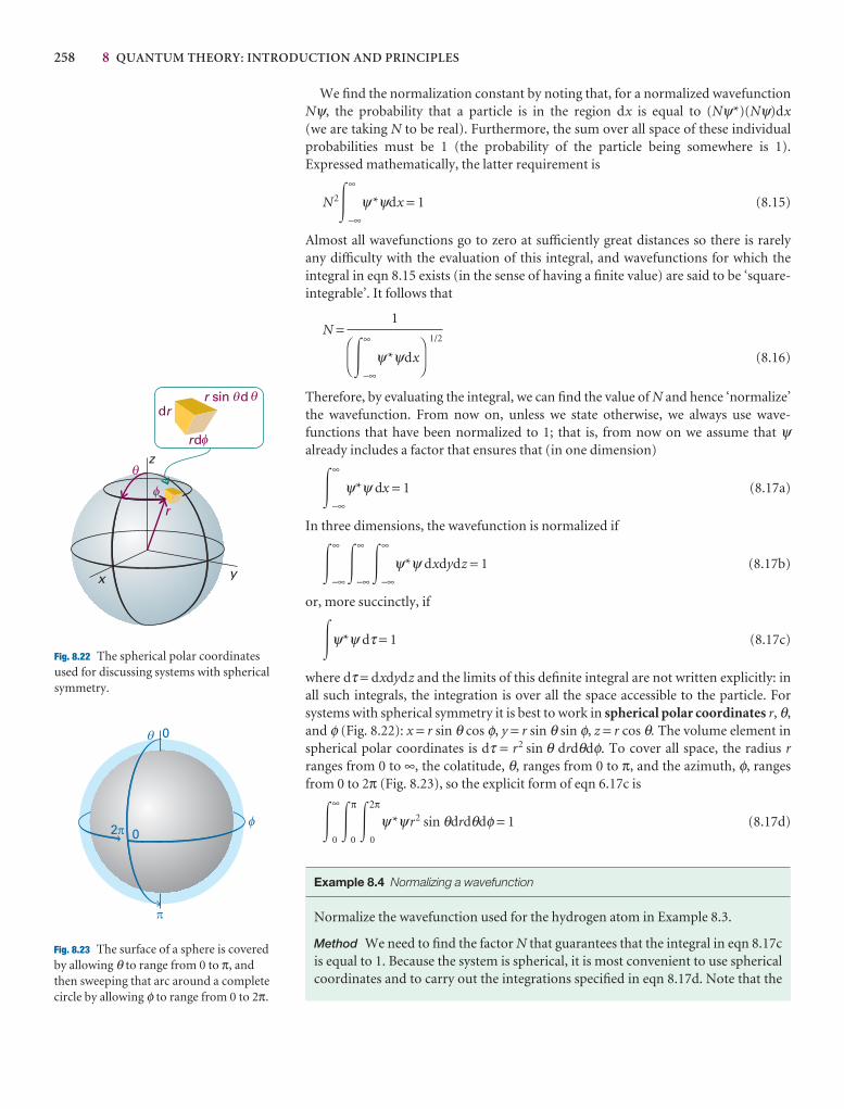
258 8 QUANTUM THEORY: INTRODUCTION AND PRINCIPLES
q
f
02p
0
p
Fig. 8.23 The surface of a sphere is coveredby allowing θ to range from 0 to π, andthen sweeping that arc around a completecircle by allowing φ to range from 0 to 2π.
We find the normalization constant by noting that, for a normalized wavefunctionNψ, the probability that a particle is in the region dx is equal to (Nψ*)(Nψ)dx(we are taking N to be real). Furthermore, the sum over all space of these individualprobabilities must be 1 (the probability of the particle being somewhere is 1).Expressed mathematically, the latter requirement is
N2�∞
−∞
ψ*ψdx = 1 (8.15)
Almost all wavefunctions go to zero at sufficiently great distances so there is rarely any difficulty with the evaluation of this integral, and wavefunctions for which the integral in eqn 8.15 exists (in the sense of having a finite value) are said to be ‘square-integrable’. It follows that
N =
�∞
−∞
ψ*ψdx
1/2
(8.16)
Therefore, by evaluating the integral, we can find the value of N and hence ‘normalize’the wavefunction. From now on, unless we state otherwise, we always use wave-functions that have been normalized to 1; that is, from now on we assume that ψalready includes a factor that ensures that (in one dimension)
�∞
−∞
ψ*ψ dx = 1 (8.17a)
In three dimensions, the wavefunction is normalized if
�∞
−∞ �
∞
−∞ �
∞
−∞
ψ*ψ dxdydz = 1 (8.17b)
or, more succinctly, if
�ψ*ψ dτ = 1 (8.17c)
where dτ = dxdydz and the limits of this definite integral are not written explicitly: inall such integrals, the integration is over all the space accessible to the particle. For systems with spherical symmetry it is best to work in spherical polar coordinates r, θ,and φ (Fig. 8.22): x = r sin θ cos φ, y = r sin θ sin φ, z = r cos θ. The volume element inspherical polar coordinates is dτ = r2 sin θ drdθdφ. To cover all space, the radius rranges from 0 to ∞, the colatitude, θ, ranges from 0 to π, and the azimuth, φ, rangesfrom 0 to 2π (Fig. 8.23), so the explicit form of eqn 6.17c is
�∞
0�
π
0�
2π
0
ψ*ψr2 sin θdrdθdφ = 1 (8.17d)
Example 8.4 Normalizing a wavefunction
Normalize the wavefunction used for the hydrogen atom in Example 8.3.
Method We need to find the factor N that guarantees that the integral in eqn 8.17cis equal to 1. Because the system is spherical, it is most convenient to use sphericalcoordinates and to carry out the integrations specified in eqn 8.17d. Note that the
DF
AC
1
z
x y
r
�
rd
drr sin d� �
�
�
Fig. 8.22 The spherical polar coordinatesused for discussing systems with sphericalsymmetry.
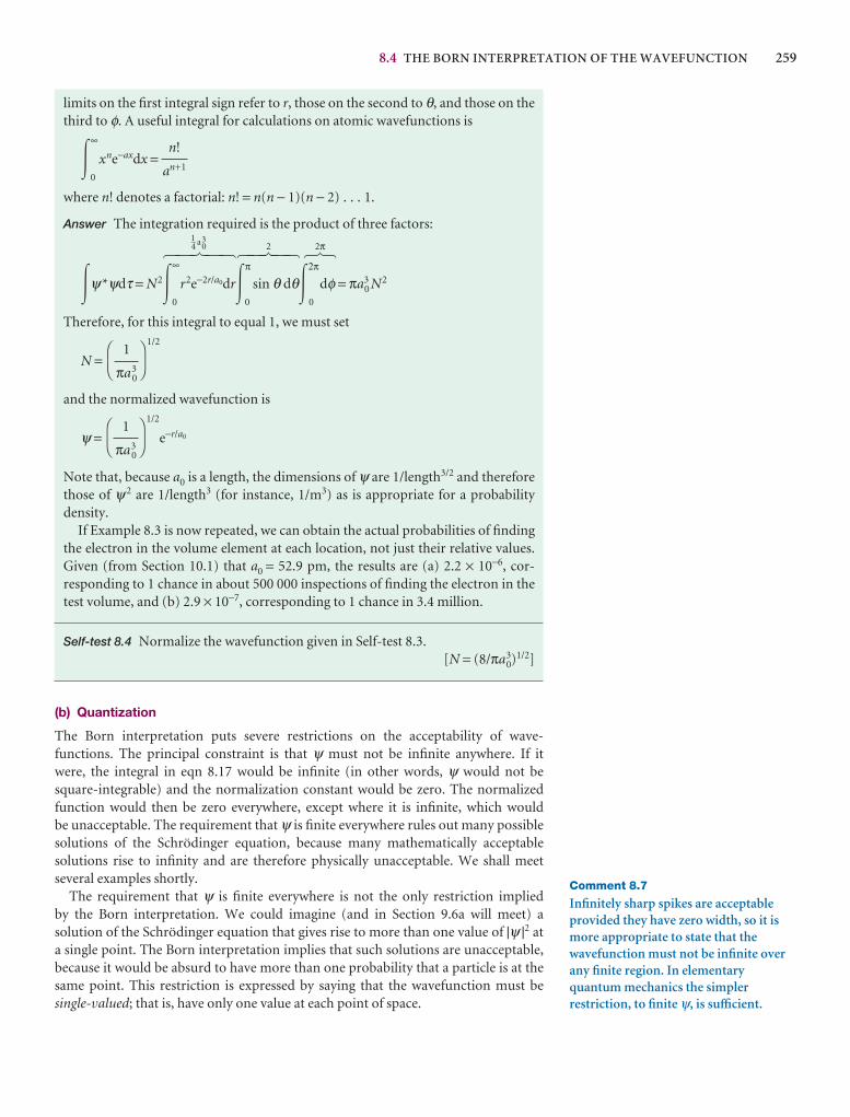
8.4 THE BORN INTERPRETATION OF THE WAVEFUNCTION 259
Comment 8.7
Infinitely sharp spikes are acceptableprovided they have zero width, so it ismore appropriate to state that thewavefunction must not be infinite overany finite region. In elementaryquantum mechanics the simplerrestriction, to finite ψ, is sufficient.
limits on the first integral sign refer to r, those on the second to θ, and those on thethird to φ. A useful integral for calculations on atomic wavefunctions is
�∞
0
xne−axdx =
where n! denotes a factorial: n! = n(n − 1)(n − 2) . . . 1.
Answer The integration required is the product of three factors:1–4 a3
0 2 2π
�ψ*ψdτ = N2�∞
0
r2e−2r/a0dr�π
0
sin θ dθ�2π
0
dφ = πa30 N2
Therefore, for this integral to equal 1, we must set
N =1/2
and the normalized wavefunction is
ψ =1/2
e−r/a0
Note that, because a0 is a length, the dimensions of ψ are 1/length3/2 and thereforethose of ψ2 are 1/length3 (for instance, 1/m3) as is appropriate for a probabilitydensity.
If Example 8.3 is now repeated, we can obtain the actual probabilities of findingthe electron in the volume element at each location, not just their relative values.Given (from Section 10.1) that a0 = 52.9 pm, the results are (a) 2.2 × 10⁻⁶, cor-responding to 1 chance in about 500 000 inspections of finding the electron in thetest volume, and (b) 2.9 × 10⁻⁷, corresponding to 1 chance in 3.4 million.
Self-test 8.4 Normalize the wavefunction given in Self-test 8.3.[N = (8/πa0
3)1/2]
(b) Quantization
The Born interpretation puts severe restrictions on the acceptability of wave-functions. The principal constraint is that ψ must not be infinite anywhere. If it were, the integral in eqn 8.17 would be infinite (in other words, ψ would not besquare-integrable) and the normalization constant would be zero. The normalizedfunction would then be zero everywhere, except where it is infinite, which would be unacceptable. The requirement that ψ is finite everywhere rules out many possiblesolutions of the Schrödinger equation, because many mathematically acceptable solutions rise to infinity and are therefore physically unacceptable. We shall meet several examples shortly.
The requirement that ψ is finite everywhere is not the only restriction implied by the Born interpretation. We could imagine (and in Section 9.6a will meet) a solution of the Schrödinger equation that gives rise to more than one value of |ψ |2 ata single point. The Born interpretation implies that such solutions are unacceptable,because it would be absurd to have more than one probability that a particle is at thesame point. This restriction is expressed by saying that the wavefunction must be single-valued; that is, have only one value at each point of space.
DF
1
πa30
AC
DF
1
πa30
AC
# $5 4 6 4 75 4 6 4 7
n!
an+1
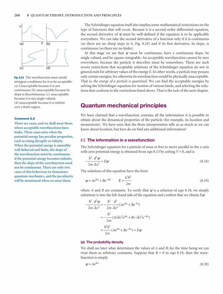
260 8 QUANTUM THEORY: INTRODUCTION AND PRINCIPLES
The Schrödinger equation itself also implies some mathematical restrictions on thetype of functions that will occur. Because it is a second-order differential equation, the second derivative of ψ must be well-defined if the equation is to be applicable everywhere. We can take the second derivative of a function only if it is continuous (so there are no sharp steps in it, Fig. 8.24) and if its first derivative, its slope, is continuous (so there are no kinks).
At this stage we see that ψ must be continuous, have a continuous slope, be single-valued, and be square-integrable. An acceptable wavefunction cannot be zeroeverywhere, because the particle it describes must be somewhere. These are such severe restrictions that acceptable solutions of the Schrödinger equation do not ingeneral exist for arbitrary values of the energy E. In other words, a particle may possessonly certain energies, for otherwise its wavefunction would be physically unacceptable.That is, the energy of a particle is quantized. We can find the acceptable energies bysolving the Schrödinger equation for motion of various kinds, and selecting the solu-tions that conform to the restrictions listed above. That is the task of the next chapter.
Quantum mechanical principles
We have claimed that a wavefunction contains all the information it is possible to obtain about the dynamical properties of the particle (for example, its location andmomentum). We have seen that the Born interpretation tells us as much as we canknow about location, but how do we find any additional information?
8.5 The information in a wavefunction
The Schrödinger equation for a particle of mass m free to move parallel to the x-axiswith zero potential energy is obtained from eqn 8.13 by setting V = 0, and is
− = Eψ (8.18)
The solutions of this equation have the form
ψ = Aeikx + Be−ikx Ε = (8.19)
where A and B are constants. To verify that ψ is a solution of eqn 8.18, we simply substitute it into the left-hand side of the equation and confirm that we obtain Eψ:
− = − (Aeikx + Be−kx)
= − {A(ik)2eikx + B(−ik)2e−ikx}
= (Aeikx + Be−ikx) = Eψ
(a) The probability density
We shall see later what determines the values of A and B; for the time being we cantreat them as arbitrary constants. Suppose that B = 0 in eqn 8.19, then the wave-function is simply
ψ = Aeikx (8.20)
$2k2
2m
$2
2m
d2
dx2
$2
2m
d2ψdx2
$2
2m
k2$2
2m
d2ψdx2
$2
2m
(a) (b)
(c) (d)
�
� �
x
Fig. 8.24 The wavefunction must satisfystringent conditions for it to be acceptable.(a) Unacceptable because it is notcontinuous; (b) unacceptable because itsslope is discontinuous; (c) unacceptablebecause it is not single-valued; (d) unacceptable because it is infinite over a finite region.
Comment 8.8
There are cases, and we shall meet them,where acceptable wavefunctions havekinks. These cases arise when thepotential energy has peculiar properties,such as rising abruptly to infinity. When the potential energy is smoothlywell-behaved and finite, the slope of the wavefunction must be continuous; if the potential energy becomes infinite,then the slope of the wavefunction neednot be continuous. There are only twocases of this behaviour in elementaryquantum mechanics, and the peculiaritywill be mentioned when we meet them.
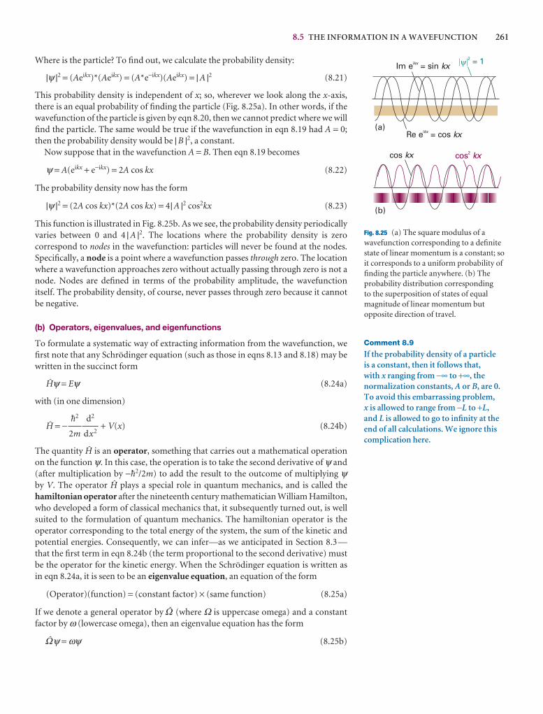
8.5 THE INFORMATION IN A WAVEFUNCTION 261
Im e = sinikx kx
Re e = cosikx kx
� �2 = 1
cos kx cos2 kx
�
(a)
(b)
Fig. 8.25 (a) The square modulus of awavefunction corresponding to a definitestate of linear momentum is a constant; soit corresponds to a uniform probability offinding the particle anywhere. (b) Theprobability distribution corresponding to the superposition of states of equalmagnitude of linear momentum butopposite direction of travel.
Comment 8.9
If the probability density of a particle is a constant, then it follows that, with x ranging from −∞ to +∞, thenormalization constants, A or B, are 0.To avoid this embarrassing problem, x is allowed to range from −L to +L,and L is allowed to go to infinity at theend of all calculations. We ignore thiscomplication here.
Where is the particle? To find out, we calculate the probability density:
|ψ |2 = (Aeikx)*(Aeikx) = (A*e−ikx)(Aeikx) = | A |2 (8.21)
This probability density is independent of x; so, wherever we look along the x-axis,there is an equal probability of finding the particle (Fig. 8.25a). In other words, if thewavefunction of the particle is given by eqn 8.20, then we cannot predict where we willfind the particle. The same would be true if the wavefunction in eqn 8.19 had A = 0;then the probability density would be | B |2, a constant.
Now suppose that in the wavefunction A = B. Then eqn 8.19 becomes
ψ = A(eikx + e−ikx) = 2A cos kx (8.22)
The probability density now has the form
|ψ |2 = (2A cos kx)*(2A cos kx) = 4| A |2 cos2kx (8.23)
This function is illustrated in Fig. 8.25b. As we see, the probability density periodicallyvaries between 0 and 4 | A |2. The locations where the probability density is zero correspond to nodes in the wavefunction: particles will never be found at the nodes.Specifically, a node is a point where a wavefunction passes through zero. The locationwhere a wavefunction approaches zero without actually passing through zero is not anode. Nodes are defined in terms of the probability amplitude, the wavefunction itself. The probability density, of course, never passes through zero because it cannotbe negative.
(b) Operators, eigenvalues, and eigenfunctions
To formulate a systematic way of extracting information from the wavefunction, wefirst note that any Schrödinger equation (such as those in eqns 8.13 and 8.18) may bewritten in the succinct form
@ψ = Eψ (8.24a)
with (in one dimension)
@ = − + V(x) (8.24b)
The quantity @ is an operator, something that carries out a mathematical operationon the function ψ. In this case, the operation is to take the second derivative of ψ and(after multiplication by −$2/2m) to add the result to the outcome of multiplying ψby V. The operator @ plays a special role in quantum mechanics, and is called thehamiltonian operator after the nineteenth century mathematician William Hamilton,who developed a form of classical mechanics that, it subsequently turned out, is wellsuited to the formulation of quantum mechanics. The hamiltonian operator is the operator corresponding to the total energy of the system, the sum of the kinetic andpotential energies. Consequently, we can infer—as we anticipated in Section 8.3—that the first term in eqn 8.24b (the term proportional to the second derivative) mustbe the operator for the kinetic energy. When the Schrödinger equation is written as in eqn 8.24a, it is seen to be an eigenvalue equation, an equation of the form
(Operator)(function) = (constant factor) × (same function) (8.25a)
If we denote a general operator by ) (where Ω is uppercase omega) and a constantfactor by ω (lowercase omega), then an eigenvalue equation has the form
)ψ = ωψ (8.25b)
d2
dx2
$2
2m
262 8 QUANTUM THEORY: INTRODUCTION AND PRINCIPLES
The factor ω is called the eigenvalue of the operator ). The eigenvalue in eqn 8.24a is the energy. The function ψ in an equation of this kind is called an eigenfunctionof the operator ) and is different for each eigenvalue. The eigenfunction in eqn 8.24ais the wavefunction corresponding to the energy E. It follows that another way of saying ‘solve the Schrödinger equation’ is to say ‘find the eigenvalues and eigen-functions of the hamiltonian operator for the system’. The wavefunctions are theeigenfunctions of the hamiltonian operator, and the corresponding eigenvalues arethe allowed energies.
Example 8.5 Identifying an eigenfunction
Show that eax is an eigenfunction of the operator d/dx, and find the correspondingeigenvalue. Show that eax2
is not an eigenfunction of d/dx.
Method We need to operate on the function with the operator and check whetherthe result is a constant factor times the original function.
Answer For ) = d/dx and ψ = eax:
)ψ = eax = aeax = aψ
Therefore eax is indeed an eigenfunction of d/dx, and its eigenvalue is a. For ψ = eax2
,
)ψ = eax2 = 2axeax2 = 2ax × ψ
which is not an eigenvalue equation even though the same function ψ occurson the right, because ψ is now multiplied by a variable factor (2ax), not a constantfactor. Alternatively, if the right-hand side is written 2a(xeax2
), we see that it is aconstant (2a) times a different function.
Self-test 8.5 Is the function cos ax an eigenfunction of (a) d/dx, (b) d2/dx2?[(a) No, (b) yes]
The importance of eigenvalue equations is that the pattern
(Energy operator)ψ = (energy) × ψ
exemplified by the Schrödinger equation is repeated for other observables, or measur-able properties of a system, such as the momentum or the electric dipole moment.Thus, it is often the case that we can write
(Operator corresponding to an observable)ψ = (value of observable) × ψ
The symbol ) in eqn 8.25b is then interpreted as an operator (for example, the hamiltonian, @) corresponding to an observable (for example, the energy), and theeigenvalue ω is the value of that observable (for example, the value of the energy, E).Therefore, if we know both the wavefunction ψ and the operator ) correspondingto the observable Ω of interest, and the wavefunction is an eigenfunction of the operator ), then we can predict the outcome of an observation of the property Ω(for example, an atom’s energy) by picking out the factor ω in the eigenvalue equation, eqn 8.25b.
d
dx
d
dx
8.5 THE INFORMATION IN A WAVEFUNCTION 263
Comment 8.10
The rules summarized by eqn 8.26 applyto observables that depend on spatialvariables; intrinsic properties, such asspin (see Section 9.8) are treateddifferently.
A basic postulate of quantum mechanics tells us how to set up the operator cor-responding to a given observable:
Observables, Ω, are represented by operators, ), built from the following positionand momentum operators:
X = x × Yx = [8.26]
That is, the operator for location along the x-axis is multiplication (of the wavefunction)by x and the operator for linear momentum parallel to the x-axis is proportional totaking the derivative (of the wavefunction) with respect to x.
Example 8.6 Determining the value of an observable
What is the linear momentum of a particle described by the wavefunction in eqn 8.19 with (a) B = 0, (b) A = 0?
Method We operate on ψ with the operator corresponding to linear momentum(eqn 8.26), and inspect the result. If the outcome is the original wavefunction multiplied by a constant (that is, we generate an eigenvalue equation), then theconstant is identified with the value of the observable.
Answer (a) With the wavefunction given in eqn 8.19 with B = 0,
Yxψ = = A = B × ikeikx = k$Be−ikx = k$ψ
This is an eigenvalue equation, and by comparing it with eqn 8.25b we find that px = +k$. (b) For the wavefunction with A = 0,
Yxψ = = B = B × (−ik)e−ikx = −k$Be−ikx = −k$ψ
The magnitude of the linear momentum is the same in each case (k$), but the signsare different: In (a) the particle is travelling to the right (positive x) but in (b) it istravelling to the left (negative x).
Self-test 8.6 The operator for the angular momentum of a particle travelling in acircle in the xy-plane is Zz = ($/i)d/dφ, where φ is its angular position. What is theangular momentum of a particle described by the wavefunction e−2iφ?
[lz = −2$]
We use the definitions in eqn 8.26 to construct operators for other spatial observ-ables. For example, suppose we wanted the operator for a potential energy of the formV = 1–2kx2, with k a constant (later, we shall see that this potential energy describes thevibrations of atoms in molecules). Then it follows from eqn 8.26 that the operatorcorresponding to V is multiplication by x2:
W = 1–2kx2 × (8.27)
In normal practice, the multiplication sign is omitted. To construct the operator forkinetic energy, we make use of the classical relation between kinetic energy and linear
$
i
de−ikx
dx
$
i
dψdx
$
i
$
i
deikx
dx
$
i
dψdx
$
i
d
dx
$
i
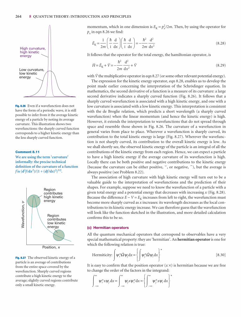
264 8 QUANTUM THEORY: INTRODUCTION AND PRINCIPLES
momentum, which in one dimension is EK = px2 /2m. Then, by using the operator for
px in eqn 8.26 we find:
ÊK = = − (8.28)
It follows that the operator for the total energy, the hamiltonian operator, is
@ = ÊK + W = − + W (8.29)
with W the multiplicative operator in eqn 8.27 (or some other relevant potential energy).The expression for the kinetic energy operator, eqn 8.28, enables us to develop the
point made earlier concerning the interpretation of the Schrödinger equation. Inmathematics, the second derivative of a function is a measure of its curvature: a largesecond derivative indicates a sharply curved function (Fig. 8.26). It follows that asharply curved wavefunction is associated with a high kinetic energy, and one with alow curvature is associated with a low kinetic energy. This interpretation is consistentwith the de Broglie relation, which predicts a short wavelength (a sharply curvedwavefunction) when the linear momentum (and hence the kinetic energy) is high.However, it extends the interpretation to wavefunctions that do not spread throughspace and resemble those shown in Fig. 8.26. The curvature of a wavefunction in general varies from place to place. Wherever a wavefunction is sharply curved, its contribution to the total kinetic energy is large (Fig. 8.27). Wherever the wavefunc-tion is not sharply curved, its contribution to the overall kinetic energy is low. As we shall shortly see, the observed kinetic energy of the particle is an integral of all thecontributions of the kinetic energy from each region. Hence, we can expect a particleto have a high kinetic energy if the average curvature of its wavefunction is high.Locally there can be both positive and negative contributions to the kinetic energy(because the curvature can be either positive, 9, or negative, 8), but the average is always positive (see Problem 8.22).
The association of high curvature with high kinetic energy will turn out to be avaluable guide to the interpretation of wavefunctions and the prediction of theirshapes. For example, suppose we need to know the wavefunction of a particle with agiven total energy and a potential energy that decreases with increasing x (Fig. 8.28).Because the difference E − V = EK increases from left to right, the wavefunction mustbecome more sharply curved as x increases: its wavelength decreases as the local con-tributions to its kinetic energy increase. We can therefore guess that the wavefunctionwill look like the function sketched in the illustration, and more detailed calculationconfirms this to be so.
(c) Hermitian operators
All the quantum mechanical operators that correspond to observables have a veryspecial mathematical property: they are ‘hermitian’. An hermitian operator is one forwhich the following relation is true:
Hermiticity: �ψ i*)ψj dx = �ψj*)ψi dx*
[8.30]
It is easy to confirm that the position operator (x ×) is hermitian because we are freeto change the order of the factors in the integrand:
�∞
−∞
ψ i*xψj dx = �∞
−∞
ψj xψ i*dx = �∞
−∞
ψ j*xψi dx*5
67
123
567
123
d2
dx2
$2
2m
d2
dx2
$2
2m
DF
d
dx
$
i
AC
DF
d
dx
$
i
AC
1
2mHigh curvature,high kineticenergy
Low curvature,low kineticenergy
Fig. 8.26 Even if a wavefunction does nothave the form of a periodic wave, it is stillpossible to infer from it the average kineticenergy of a particle by noting its averagecurvature. This illustration shows twowavefunctions: the sharply curved functioncorresponds to a higher kinetic energy thanthe less sharply curved function.
Regioncontributeshigh kineticenergy
Regioncontributeslow kineticenergyW
avef
unct
ion,
Position, x
�
Fig. 8.27 The observed kinetic energy of aparticle is an average of contributions from the entire space covered by thewavefunction. Sharply curved regionscontribute a high kinetic energy to theaverage; slightly curved regions contributeonly a small kinetic energy.
Comment 8.11
We are using the term ‘curvature’informally: the precise technicaldefinition of the curvature of a functionf is (d2f /dx2)/{1 + (df /dx)2}3/2.
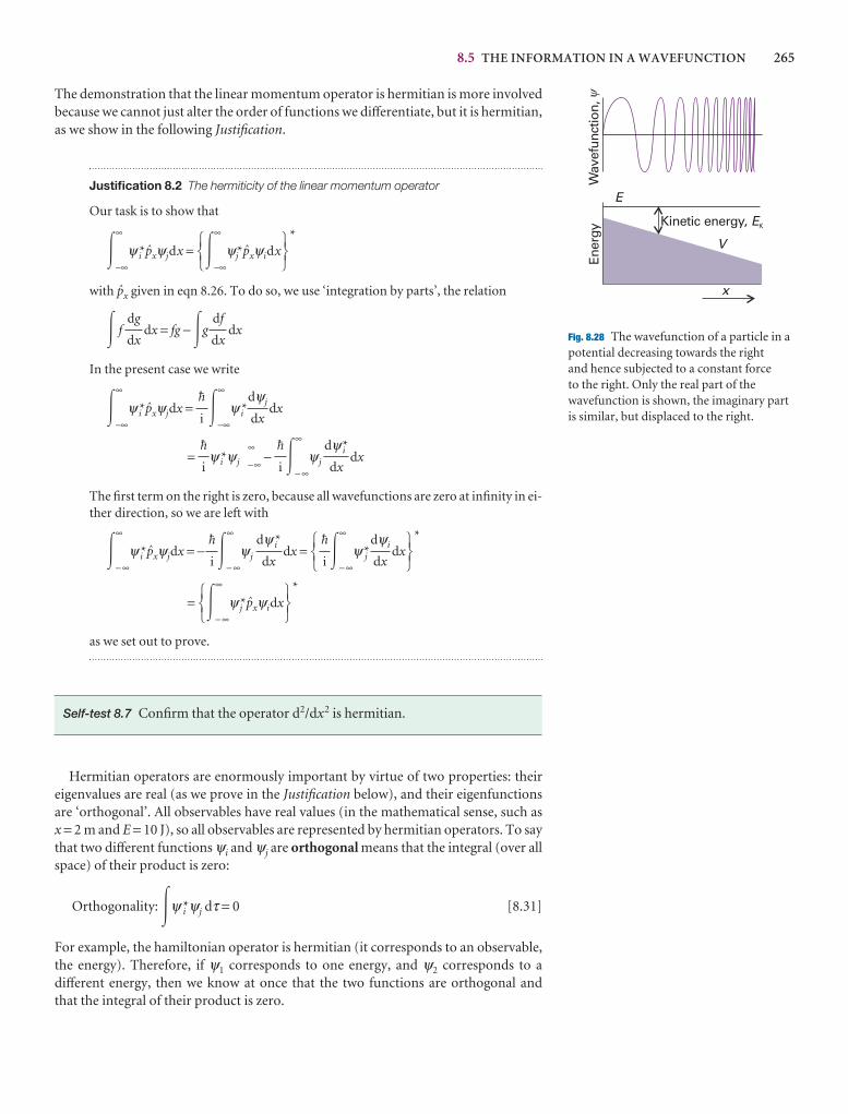
8.5 THE INFORMATION IN A WAVEFUNCTION 265
V
x
E
Kinetic energy, EK
Wav
efun
ctio
n,En
ergy
�
Fig. 8.28 The wavefunction of a particle in apotential decreasing towards the right and hence subjected to a constant force to the right. Only the real part of thewavefunction is shown, the imaginary partis similar, but displaced to the right.
The demonstration that the linear momentum operator is hermitian is more involvedbecause we cannot just alter the order of functions we differentiate, but it is hermitian,as we show in the following Justification.
Justification 8.2 The hermiticity of the linear momentum operator
Our task is to show that
�∞
−∞ψ i*Yxψjdx = �
∞
−∞ψj*Yxψidx
*
with Yx given in eqn 8.26. To do so, we use ‘integration by parts’, the relation
� f dx = fg − �g dx
In the present case we write
�∞
−∞ψ i*Yxψjdx = �
∞
−∞ψ i* dx
= ψ i*ψj
∞
−∞− �
∞
− ∞ψj dx
The first term on the right is zero, because all wavefunctions are zero at infinity in ei-ther direction, so we are left with
�∞
− ∞ψ i*Yxψjdx = − �
∞
− ∞ψj dx = �
∞
− ∞ψ*j dx
*
= �∞
− ∞ψ j*Yxψidx
*
as we set out to prove.
Self-test 8.7 Confirm that the operator d2/dx2 is hermitian.
Hermitian operators are enormously important by virtue of two properties: theireigenvalues are real (as we prove in the Justification below), and their eigenfunctionsare ‘orthogonal’. All observables have real values (in the mathematical sense, such asx = 2 m and E = 10 J), so all observables are represented by hermitian operators. To saythat two different functions ψi and ψj are orthogonal means that the integral (over allspace) of their product is zero:
Orthogonality: �ψ i*ψj dτ = 0 [8.31]
For example, the hamiltonian operator is hermitian (it corresponds to an observable,the energy). Therefore, if ψ1 corresponds to one energy, and ψ2 corresponds to a different energy, then we know at once that the two functions are orthogonal and that the integral of their product is zero.
567123
567dψi
dx
$
i
123dψ i*
dx
$
i
dψ i*
dx
$
i
$
i
dψj
dx
$
i
df
dx
dg
dx
567123
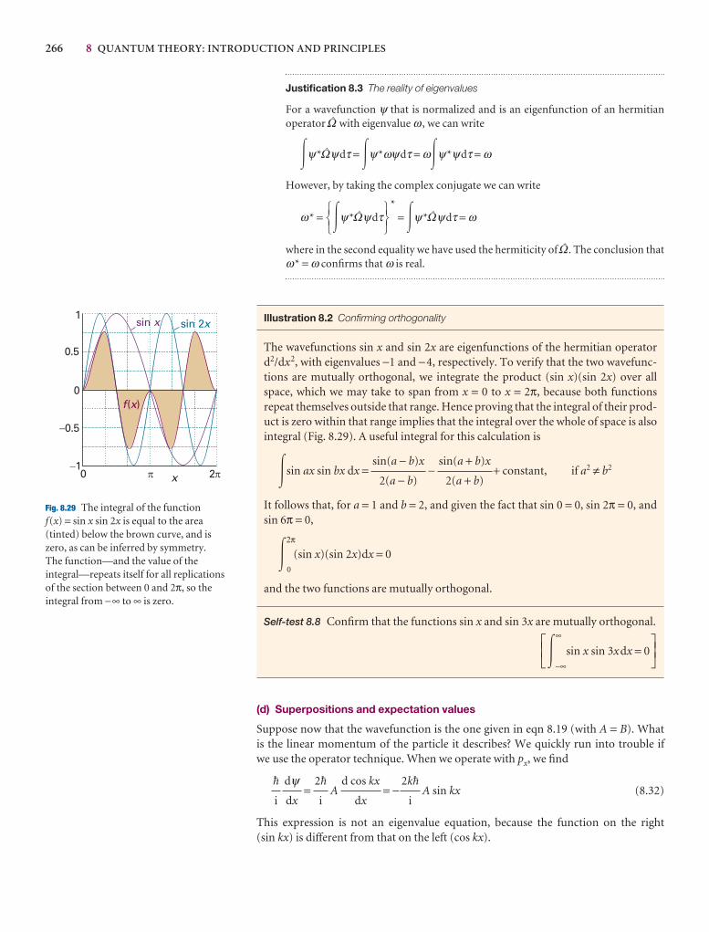
266 8 QUANTUM THEORY: INTRODUCTION AND PRINCIPLES
Justification 8.3 The reality of eigenvalues
For a wavefunction ψ that is normalized and is an eigenfunction of an hermitian operator ) with eigenvalue ω , we can write
�ψ*)ψdτ = �ψ*ωψdτ = ω�ψ*ψdτ = ω
However, by taking the complex conjugate we can write
ω* = �ψ*)ψdτ*
= �ψ*)ψdτ = ω
where in the second equality we have used the hermiticity of ). The conclusion thatω* = ω confirms that ω is real.
Illustration 8.2 Confirming orthogonality
The wavefunctions sin x and sin 2x are eigenfunctions of the hermitian operatord2/dx2, with eigenvalues −1 and −4, respectively. To verify that the two wavefunc-tions are mutually orthogonal, we integrate the product (sin x)(sin 2x) over allspace, which we may take to span from x = 0 to x = 2π, because both functions repeat themselves outside that range. Hence proving that the integral of their prod-uct is zero within that range implies that the integral over the whole of space is also integral (Fig. 8.29). A useful integral for this calculation is
�sin ax sin bx dx = − + constant, if a2 ≠ b2
It follows that, for a = 1 and b = 2, and given the fact that sin 0 = 0, sin 2π = 0, and sin 6π = 0,
�2π
0
(sin x)(sin 2x)dx = 0
and the two functions are mutually orthogonal.
Self-test 8.8 Confirm that the functions sin x and sin 3x are mutually orthogonal.
�∞
−∞
sin x sin 3xdx = 0
(d) Superpositions and expectation values
Suppose now that the wavefunction is the one given in eqn 8.19 (with A = B). What is the linear momentum of the particle it describes? We quickly run into trouble if we use the operator technique. When we operate with px, we find
= A = − A sin kx (8.32)
This expression is not an eigenvalue equation, because the function on the right (sin kx) is different from that on the left (cos kx).
2k$
i
d cos kx
dx
2$
i
dψdx
$
i
JKLGHI
sin(a + b)x
2(a + b)
sin(a − b)x
2(a − b)
567123
1
0.5
0
�0.5
�10 � 2
f x( )
x
sin x sin 2x
�
Fig. 8.29 The integral of the function f(x) = sin x sin 2x is equal to the area(tinted) below the brown curve, and is zero, as can be inferred by symmetry. The function—and the value of theintegral—repeats itself for all replicationsof the section between 0 and 2π, so theintegral from −∞ to ∞ is zero.
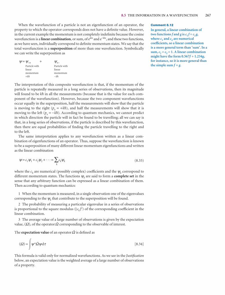
8.5 THE INFORMATION IN A WAVEFUNCTION 267
When the wavefunction of a particle is not an eigenfunction of an operator, theproperty to which the operator corresponds does not have a definite value. However,in the current example the momentum is not completely indefinite because the cosinewavefunction is a linear combination, or sum, of eikx and e−ikx, and these two functions,as we have seen, individually correspond to definite momentum states. We say that thetotal wavefunction is a superposition of more than one wavefunction. Symbolicallywe can write the superposition as
ψ = ψ→ + ψ←Particle with Particle withlinear linearmomentum momentum+k$ −k$
The interpretation of this composite wavefunction is that, if the momentum of theparticle is repeatedly measured in a long series of observations, then its magnitude will found to be k$ in all the measurements (because that is the value for each com-ponent of the wavefunction). However, because the two component wavefunctionsoccur equally in the superposition, half the measurements will show that the particleis moving to the right (px = +k$), and half the measurements will show that it is moving to the left (px = −k$). According to quantum mechanics, we cannot predict in which direction the particle will in fact be found to be travelling; all we can say isthat, in a long series of observations, if the particle is described by this wavefunction,then there are equal probabilities of finding the particle travelling to the right and to the left.
The same interpretation applies to any wavefunction written as a linear com-bination of eigenfunctions of an operator. Thus, suppose the wavefunction is knownto be a superposition of many different linear momentum eigenfunctions and writtenas the linear combination
ψ = c1ψ1 + c2ψ2 + · · · = ∑k
ckψk (8.33)
where the ck are numerical (possibly complex) coefficients and the ψk correspond todifferent momentum states. The functions ψk are said to form a complete set in thesense that any arbitrary function can be expressed as a linear combination of them.Then according to quantum mechanics:
1 When the momentum is measured, in a single observation one of the eigenvaluescorresponding to the ψk that contribute to the superposition will be found.
2 The probability of measuring a particular eigenvalue in a series of observations is proportional to the square modulus (| ck |2) of the corresponding coefficient in thelinear combination.
3 The average value of a large number of observations is given by the expectationvalue, �Ω�, of the operator ) corresponding to the observable of interest.
The expectation value of an operator ) is defined as
�Ω� = �ψ*)ψdτ [8.34]
This formula is valid only for normalized wavefunctions. As we see in the Justificationbelow, an expectation value is the weighted average of a large number of observationsof a property.
Comment 8.12
In general, a linear combination of two functions f and g is c1 f + c2 g,where c1 and c2 are numericalcoefficients, so a linear combination is a more general term than ‘sum’. In asum, c1 = c2 = 1. A linear combinationmight have the form 0.567f + 1.234g,for instance, so it is more general thanthe simple sum f + g.
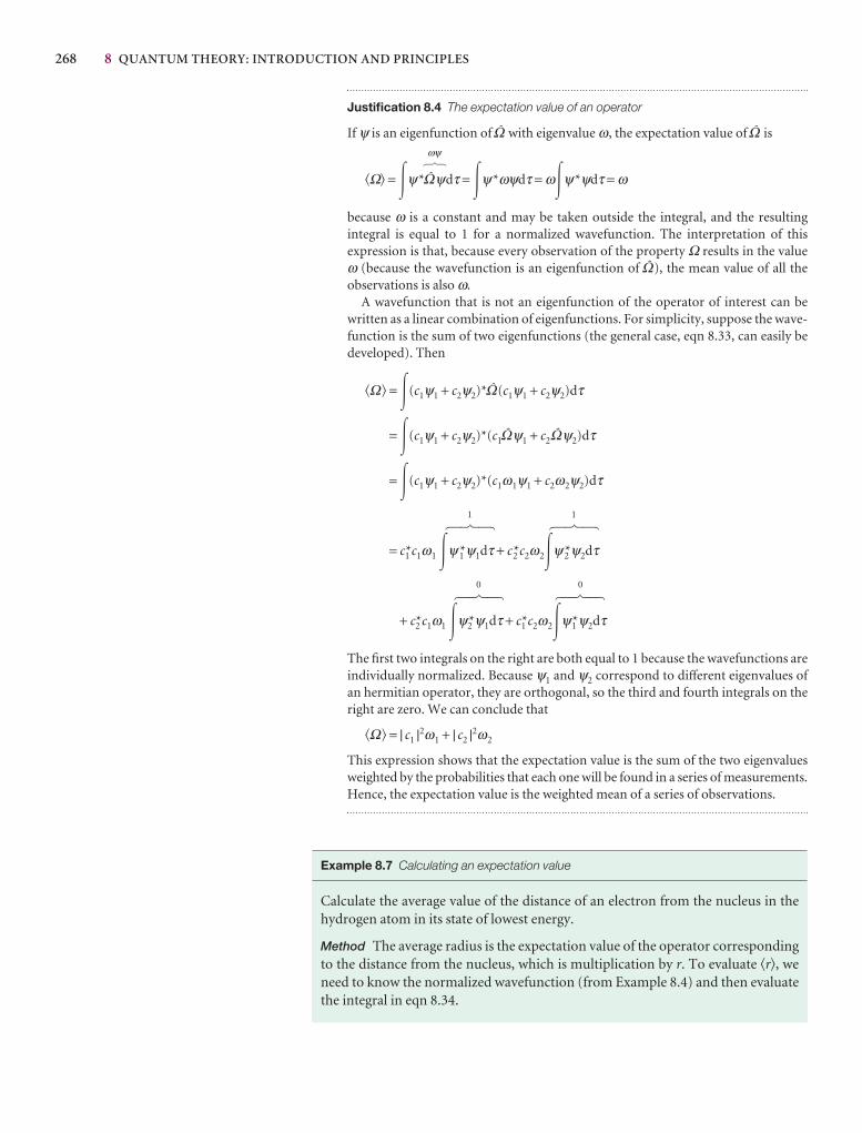
268 8 QUANTUM THEORY: INTRODUCTION AND PRINCIPLES
Justification 8.4 The expectation value of an operator
If ψ is an eigenfunction of ) with eigenvalue ω, the expectation value of ) isωψ
�Ω� = �ψ*)ψdτ = �ψ*ωψdτ = ω�ψ*ψdτ = ω
because ω is a constant and may be taken outside the integral, and the resulting integral is equal to 1 for a normalized wavefunction. The interpretation of this expression is that, because every observation of the property Ω results in the value ω (because the wavefunction is an eigenfunction of )), the mean value of all the observations is also ω.
A wavefunction that is not an eigenfunction of the operator of interest can bewritten as a linear combination of eigenfunctions. For simplicity, suppose the wave-function is the sum of two eigenfunctions (the general case, eqn 8.33, can easily bedeveloped). Then
�Ω� = �(c1ψ1 + c2ψ2)*)(c1ψ1 + c2ψ2)dτ
= �(c1ψ1 + c2ψ2)*(c1)ψ1 + c2 )ψ2)dτ
= �(c1ψ1 + c2ψ2)*(c1ω1ψ1 + c2ω2ψ2)dτ
1 1
= c1*c1ω1 �ψ1*ψ1dτ + c2*c2ω2�ψ2*ψ2dτ
0 0
+ c2*c1ω1 �ψ2*ψ1dτ + c1*c2ω2�ψ1*ψ2dτ
The first two integrals on the right are both equal to 1 because the wavefunctions areindividually normalized. Because ψ1 and ψ2 correspond to different eigenvalues ofan hermitian operator, they are orthogonal, so the third and fourth integrals on theright are zero. We can conclude that
�Ω� = | c1 |2ω1 + | c2 |2ω2
This expression shows that the expectation value is the sum of the two eigenvaluesweighted by the probabilities that each one will be found in a series of measurements.Hence, the expectation value is the weighted mean of a series of observations.
Example 8.7 Calculating an expectation value
Calculate the average value of the distance of an electron from the nucleus in thehydrogen atom in its state of lowest energy.
Method The average radius is the expectation value of the operator correspondingto the distance from the nucleus, which is multiplication by r. To evaluate �r�, weneed to know the normalized wavefunction (from Example 8.4) and then evaluatethe integral in eqn 8.34.
5 6 75 6 7
5 6 75 6 7
# $
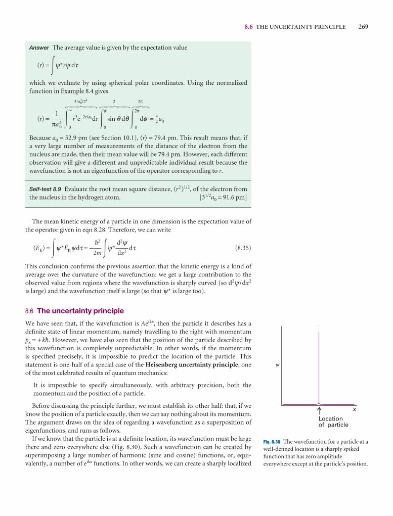
8.6 THE UNCERTAINTY PRINCIPLE 269
Answer The average value is given by the expectation value
�r� = �ψ*rψ dτ
which we evaluate by using spherical polar coordinates. Using the normalizedfunction in Example 8.4 gives
3!a03/24 2 2π
�r� = �∞
0
r3e−2r/a0dr �π
0
sin θ dθ �2π
0
dφ = 3–2 a0
Because a0 = 52.9 pm (see Section 10.1), �r� = 79.4 pm. This result means that, if a very large number of measurements of the distance of the electron from the nucleus are made, then their mean value will be 79.4 pm. However, each differentobservation will give a different and unpredictable individual result because thewavefunction is not an eigenfunction of the operator corresponding to r.
Self-test 8.9 Evaluate the root mean square distance, �r2 �1/2, of the electron fromthe nucleus in the hydrogen atom. [31/2a0 = 91.6 pm]
The mean kinetic energy of a particle in one dimension is the expectation value ofthe operator given in eqn 8.28. Therefore, we can write
�EK� = �ψ*ÊKψdτ = − �ψ* dτ (8.35)
This conclusion confirms the previous assertion that the kinetic energy is a kind of average over the curvature of the wavefunction: we get a large contribution to the observed value from regions where the wavefunction is sharply curved (so d2ψ /dx2
is large) and the wavefunction itself is large (so that ψ* is large too).
8.6 The uncertainty principle
We have seen that, if the wavefunction is Aeikx, then the particle it describes has adefinite state of linear momentum, namely travelling to the right with momentum px = +k$. However, we have also seen that the position of the particle described by this wavefunction is completely unpredictable. In other words, if the momentum is specified precisely, it is impossible to predict the location of the particle. This statement is one-half of a special case of the Heisenberg uncertainty principle, one of the most celebrated results of quantum mechanics:
It is impossible to specify simultaneously, with arbitrary precision, both the momentum and the position of a particle.
Before discussing the principle further, we must establish its other half: that, if weknow the position of a particle exactly, then we can say nothing about its momentum.The argument draws on the idea of regarding a wavefunction as a superposition ofeigenfunctions, and runs as follows.
If we know that the particle is at a definite location, its wavefunction must be largethere and zero everywhere else (Fig. 8.30). Such a wavefunction can be created by superimposing a large number of harmonic (sine and cosine) functions, or, equi-valently, a number of eikx functions. In other words, we can create a sharply localized
d2ψdx2
$2
2m
1
πa30
5 6 75 4 6 4 75 4 6 4 7
y
x
Locationof particle
Fig. 8.30 The wavefunction for a particle at awell-defined location is a sharply spikedfunction that has zero amplitudeeverywhere except at the particle’s position.
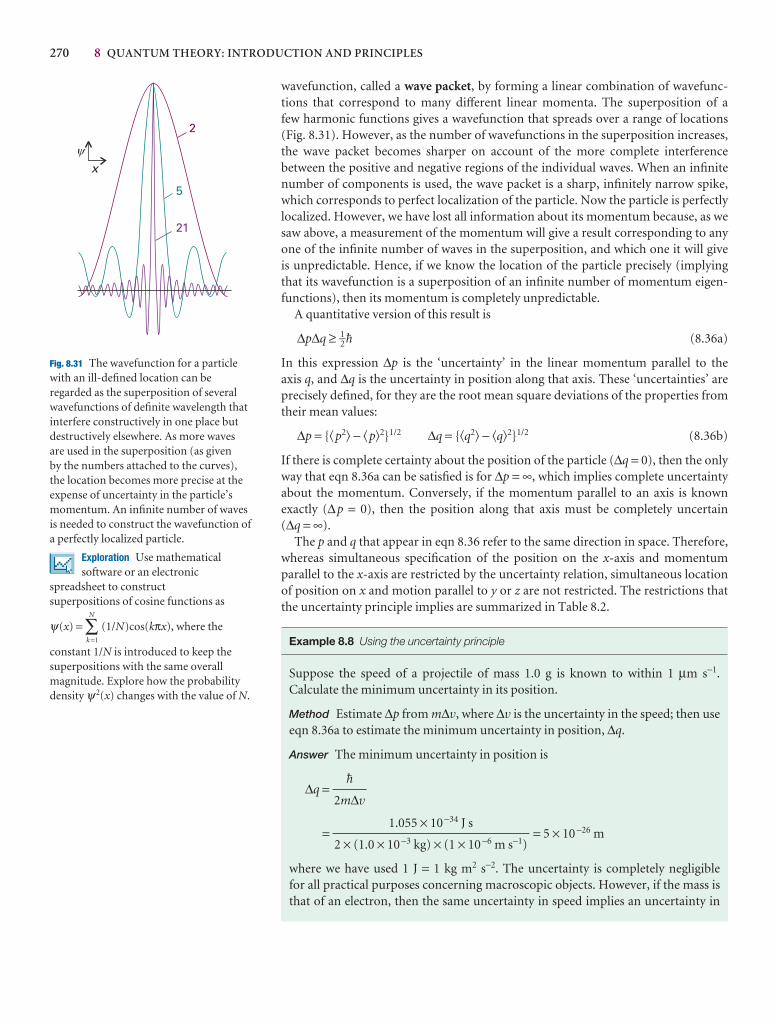
270 8 QUANTUM THEORY: INTRODUCTION AND PRINCIPLES
Fig. 8.31 The wavefunction for a particlewith an ill-defined location can be regarded as the superposition of severalwavefunctions of definite wavelength thatinterfere constructively in one place butdestructively elsewhere. As more waves are used in the superposition (as given by the numbers attached to the curves), the location becomes more precise at theexpense of uncertainty in the particle’smomentum. An infinite number of wavesis needed to construct the wavefunction ofa perfectly localized particle.
Exploration Use mathematicalsoftware or an electronic
spreadsheet to constructsuperpositions of cosine functions as
ψ(x) = ∑N
k =1
(1/N)cos(kπx), where the
constant 1/N is introduced to keep thesuperpositions with the same overallmagnitude. Explore how the probabilitydensity ψ2(x) changes with the value of N.
21
5
2
�
x
wavefunction, called a wave packet, by forming a linear combination of wavefunc-tions that correspond to many different linear momenta. The superposition of a few harmonic functions gives a wavefunction that spreads over a range of locations(Fig. 8.31). However, as the number of wavefunctions in the superposition increases,the wave packet becomes sharper on account of the more complete interference between the positive and negative regions of the individual waves. When an infinitenumber of components is used, the wave packet is a sharp, infinitely narrow spike,which corresponds to perfect localization of the particle. Now the particle is perfectlylocalized. However, we have lost all information about its momentum because, as wesaw above, a measurement of the momentum will give a result corresponding to anyone of the infinite number of waves in the superposition, and which one it will give is unpredictable. Hence, if we know the location of the particle precisely (implying that its wavefunction is a superposition of an infinite number of momentum eigen-functions), then its momentum is completely unpredictable.
A quantitative version of this result is
∆p∆q ≥ 1–2$ (8.36a)
In this expression ∆p is the ‘uncertainty’ in the linear momentum parallel to the axis q, and ∆q is the uncertainty in position along that axis. These ‘uncertainties’ areprecisely defined, for they are the root mean square deviations of the properties fromtheir mean values:
∆p = {�p2� − �p�2}1/2 ∆q = {�q2� − �q�2}1/2 (8.36b)
If there is complete certainty about the position of the particle (∆q = 0), then the onlyway that eqn 8.36a can be satisfied is for ∆p = ∞, which implies complete uncertaintyabout the momentum. Conversely, if the momentum parallel to an axis is known exactly (∆p = 0), then the position along that axis must be completely uncertain (∆q = ∞).
The p and q that appear in eqn 8.36 refer to the same direction in space. Therefore,whereas simultaneous specification of the position on the x-axis and momentum parallel to the x-axis are restricted by the uncertainty relation, simultaneous locationof position on x and motion parallel to y or z are not restricted. The restrictions thatthe uncertainty principle implies are summarized in Table 8.2.
Example 8.8 Using the uncertainty principle
Suppose the speed of a projectile of mass 1.0 g is known to within 1 µm s−1.Calculate the minimum uncertainty in its position.
Method Estimate ∆p from m∆v, where ∆v is the uncertainty in the speed; then useeqn 8.36a to estimate the minimum uncertainty in position, ∆q.
Answer The minimum uncertainty in position is
∆q =
= = 5 × 10⁻²⁶ m
where we have used 1 J = 1 kg m2 s−2. The uncertainty is completely negligible for all practical purposes concerning macroscopic objects. However, if the mass isthat of an electron, then the same uncertainty in speed implies an uncertainty in
1.055 × 10⁻³⁴ J s
2 × (1.0 × 10−3 kg) × (1 × 10⁻⁶ m s−1)
$
2m∆v
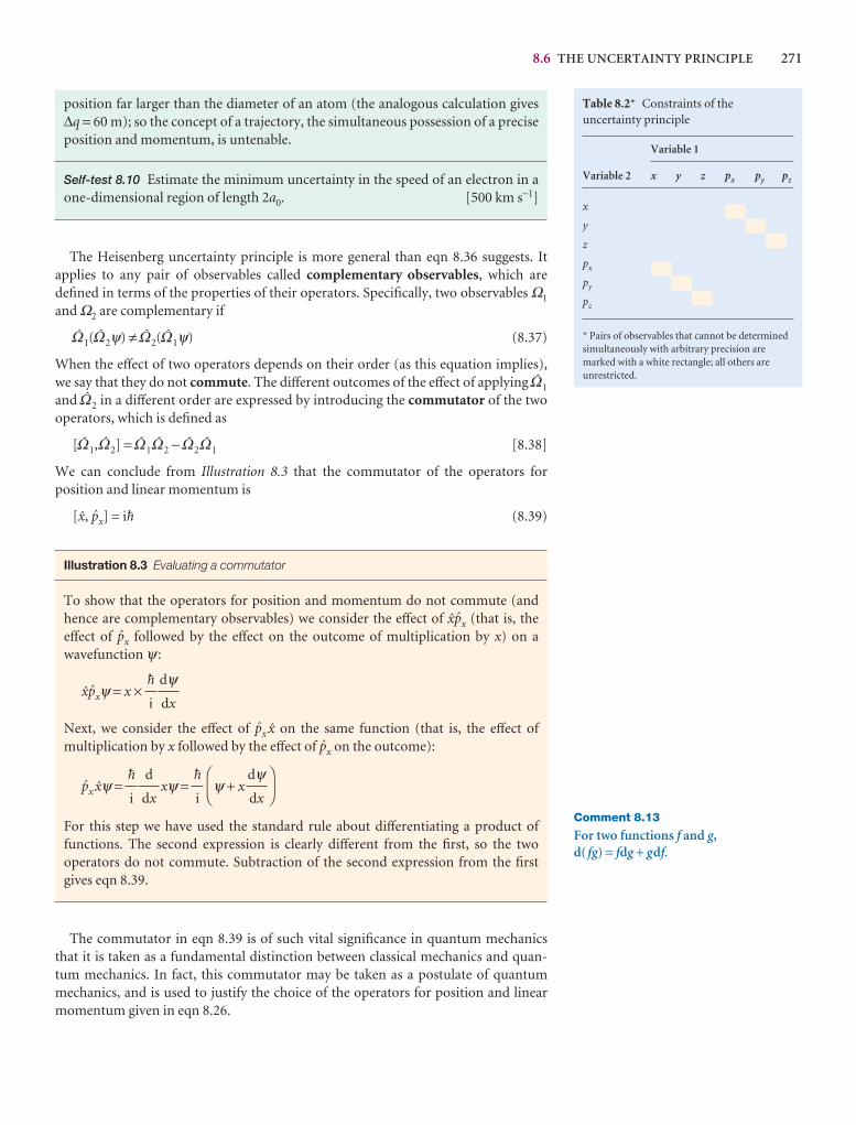
8.6 THE UNCERTAINTY PRINCIPLE 271
Table 8.2* Constraints of theuncertainty principle
Variable 1
Variable 2 x y z px py pz
x
y
z
px
py
pz
* Pairs of observables that cannot be determinedsimultaneously with arbitrary precision aremarked with a white rectangle; all others areunrestricted.
Comment 8.13
For two functions f and g,d( fg) = fdg + gdf.
position far larger than the diameter of an atom (the analogous calculation gives∆q = 60 m); so the concept of a trajectory, the simultaneous possession of a preciseposition and momentum, is untenable.
Self-test 8.10 Estimate the minimum uncertainty in the speed of an electron in aone-dimensional region of length 2a0. [500 km s−1]
The Heisenberg uncertainty principle is more general than eqn 8.36 suggests. It applies to any pair of observables called complementary observables, which aredefined in terms of the properties of their operators. Specifically, two observables Ω1
and Ω2 are complementary if
)1()2ψ) ≠ )2()1ψ) (8.37)
When the effect of two operators depends on their order (as this equation implies), we say that they do not commute. The different outcomes of the effect of applying )1
and )2 in a different order are expressed by introducing the commutator of the twooperators, which is defined as
[)1,)2] = )1 )2 − )2 )1 [8.38]
We can conclude from Illustration 8.3 that the commutator of the operators for position and linear momentum is
[X, Yx] = i$ (8.39)
Illustration 8.3 Evaluating a commutator
To show that the operators for position and momentum do not commute (andhence are complementary observables) we consider the effect of XYx (that is, the effect of Yx followed by the effect on the outcome of multiplication by x) on a wavefunction ψ :
XYxψ = x ×
Next, we consider the effect of Yx X on the same function (that is, the effect of multiplication by x followed by the effect of Yx on the outcome):
Yx Xψ = xψ = ψ + x
For this step we have used the standard rule about differentiating a product offunctions. The second expression is clearly different from the first, so the two operators do not commute. Subtraction of the second expression from the firstgives eqn 8.39.
The commutator in eqn 8.39 is of such vital significance in quantum mechanicsthat it is taken as a fundamental distinction between classical mechanics and quan-tum mechanics. In fact, this commutator may be taken as a postulate of quantum mechanics, and is used to justify the choice of the operators for position and linearmomentum given in eqn 8.26.
DF
dψdx
AC
$
i
d
dx
$
i
dψdx
$
i
272 8 QUANTUM THEORY: INTRODUCTION AND PRINCIPLES
With the concept of commutator established, the Heisenberg uncertainty principlecan be given its most general form. For any two pairs of observables, Ω1 and Ω2, theuncertainties (to be precise, the root mean square deviations of their values from themean) in simultaneous determinations are related by
∆Ω1∆Ω2 ≥ 1–2 | �[)1,)2]� | (8.40)
We obtain the special case of eqn 8.36a when we identify the observables with x and px
and use eqn 8.39 for their commutator.Complementary observables are observables with non-commuting operators.
With the discovery that some pairs of observables are complementary (we meet moreexamples in the next chapter), we are at the heart of the difference between classicaland quantum mechanics. Classical mechanics supposed, falsely as we now know, that the position and momentum of a particle could be specified simultaneously with arbitrary precision. However, quantum mechanics shows that position and momentum are complementary, and that we have to make a choice: we can specifyposition at the expense of momentum, or momentum at the expense of position.
The realization that some observables are complementary allows us to make considerable progress with the calculation of atomic and molecular properties, but it does away with some of the most cherished concepts of classical physics.
8.7 The postulates of quantum mechanics
For convenience, we collect here the postulates on which quantum mechanics is basedand which have been introduced in the course of this chapter.
The wavefunction. All dynamical information is contained in the wavefunction ψfor the system, which is a mathematical function found by solving the Schrödingerequation for the system. In one dimension:
− + V(x)ψ = Eψ
The Born interpretation. If the wavefunction of a particle has the value ψ atsome point r, then the probability of finding the particle in an infinitesimal volume dτ = dxdydz at that point is proportional to |ψ |2dτ.
Acceptable wavefunctions. An acceptable wavefunction must be continuous, have a continuous first derivative, be single-valued, and be square-integrable.
Observables. Observables, Ω, are represented by operators, ), built from positionand momentum operators of the form
X = x × Yx =
or, more generally, from operators that satisfy the commutation relation [X, Yx] = i$.
The Heisenberg uncertainty principle. It is impossible to specify simultaneously,with arbitrary precision, both the momentum and the position of a particle and, more generally, any pair of observable with operators that do not commute.
d
dx
$
i
d2ψdx2
$2
2m
Comment 8.14
The ‘modulus’ notation | . . . | meanstake the magnitude of the term the barsenclose: for a real quantity x, |x | is themagnitude of x (its value without itssign); for an imaginary quantity iy,| iy | is the magnitude of y; and—mostgenerally—for a complex quantity z = x + iy, |z | is the value of (z*z)1/2.For example, |−2 | = 2, |3i | = 3, and |−2 + 3i | = {(−2 − 3i)(−2 + 3i)}1/2 = 131/2.Physically, the modulus on the right ofeqn 8.40 ensures that the product ofuncertainties has a real, non-negativevalue.

FURTHER READING 273
Checklist of key ideas
Further reading
1. In classical physics, radiation is described in terms of anoscillating electromagnetic disturbance that travels throughvacuum at a constant speed c = λν.
2. A black body is an object that emits and absorbs allfrequencies of radiation uniformly.
3. The variation of the energy output of a black body withwavelength is explained by invoking quantization of energy,the limitation of energies to discrete values, which in turnleads to the Planck distribution, eqn 8.5.
4. The variation of the molar heat capacity of a solid withtemperature is explained by invoking quantization of energy,which leads to the Einstein and Debye formulas, eqns 8.7 and 8.9.
5. Spectroscopic transitions are changes in populations ofquantized energy levels of a system involving the absorption,emission, or scattering of electromagnetic radiation, ∆E = hν.
6. The photoelectric effect is the ejection of electrons frommetals when they are exposed to ultraviolet radiation: 1–2 mev
2 = hν − Φ, where Φ is the work function, the energyrequired to remove an electron from the metal to infinity.
7. The photoelectric effect and electron diffraction arephenomena that confirm wave–particle duality, the jointparticle and wave character of matter and radiation.
8. The de Broglie relation, λ = h/p, relates the momentum of aparticle with its wavelength.
9. A wavefunction is a mathematical function obtained bysolving the Schrödinger equation and which contains all thedynamical information about a system.
10. The time-independent Schrödinger equation in onedimension is −($2/2m)(d2ψ /dx2) + V(x)ψ = Eψ.
Articles and texts
P.W. Atkins, Quanta: A handbook of concepts. Oxford UniversityPress (1991).
P.W. Atkins and R.S. Friedman, Molecular quantum mechanics.Oxford University Press (2005).
D. Bohm, Quantum theory. Dover, New York (1989).
11. The Born interpretation of the wavefunction states that thevalue of |ψ |2, the probability density, at a point is proportionalto the probability of finding the particle at that point.
12. Quantization is the confinement of a dynamical observable to discrete values.
13. An acceptable wavefunction must be continuous, have acontinuous first derivative, be single-valued, and be square-integrable.
14. An operator is something that carries out a mathematicaloperation on a function. The position and momentumoperators are X = x × and Yx = ($/i)d/dx, respectively.
15. The hamiltonian operator is the operator for the total energyof a system, @ψ = Eψ and is the sum of the operators forkinetic energy and potential energy.
16. An eigenvalue equation is an equation of the form )ψ = ωψ.The eigenvalue is the constant ω in the eigenvalue equation;the eigenfunction is the function ψ in the eigenvalue equation.
17. The expectation value of an operator is �Ω� = ∫ψ*)ψ dτ.
18. An hermitian operator is one for which ∫ψ i*)ψj dx =(∫ψ j*)ψi dx)*. The eigenvalues of hermitian operators are realand correspond to observables, measurable properties of asystem. The eigenfunctions of hermitian operations areorthogonal, meaning that ∫ψ i*ψj dτ = 0.
19. The Heisenberg uncertainty principle states that it is impossible to specify simultaneously, with arbitrary precision, both themomentum and the position of a particle; ∆p∆q ≥ 1–2 $.
20. Two operators commute when [)1,)2] = )1)2 − )2 )1 = 0.
21. Complementary observables are observables corresponding to non-commuting operators.
22. The general form of the Heisenberg uncertainty principle is∆Ω1∆Ω2 ≥ 1–2 | �[)1,)2]� |.
R.P. Feynman, R.B. Leighton, and M. Sands, The Feynman lectures onphysics. Volume III. Addison–Wesley, Reading (1965).
C.S. Johnson, Jr. and L.G. Pedersen, Problems and solutions inquantum chemistry and physics. Dover, New York, 1986.
L. Pauling and E.B. Wilson, Introduction to quantum mechanics withapplications to chemistry. Dover, New York (1985).

274 8 QUANTUM THEORY: INTRODUCTION AND PRINCIPLES
Exercises
8.1a To what speed must an electron be accelerated for it to have awavelength of 3.0 cm?
8.1b To what speed must a proton be accelerated for it to have a wavelengthof 3.0 cm?
8.2a The fine-structure constant, α, plays a special role in the structure ofmatter; its approximate value is 1/137. What is the wavelength of an electrontravelling at a speed αc, where c is the speed of light? (Note that thecircumference of the first Bohr orbit in the hydrogen atom is 331 pm.)
8.2b Calculate the linear momentum of photons of wavelength 350 nm. What speed does a hydrogen molecule need to travel to have the same linearmomentum?
8.3a The speed of a certain proton is 0.45 Mm s−1. If the uncertainty in itsmomentum is to be reduced to 0.0100 per cent, what uncertainty in itslocation must be tolerated?
8.3b The speed of a certain electron is 995 km s−1. If the uncertainty in itsmomentum is to be reduced to 0.0010 per cent, what uncertainty in itslocation must be tolerated?
8.4a Calculate the energy per photon and the energy per mole of photons for radiation of wavelength (a) 600 nm (red), (b) 550 nm (yellow), (c) 400 nm (blue).
8.4b Calculate the energy per photon and the energy per mole of photons for radiation of wavelength (a) 200 nm (ultraviolet), (b) 150 pm (X-ray), (c) 1.00 cm (microwave).
8.5a Calculate the speed to which a stationary H atom would be accelerated if it absorbed each of the photons used in Exercise 8.4a.
8.5b Calculate the speed to which a stationary 4He atom (mass 4.0026 u)would be accelerated if it absorbed each of the photons used in Exercise 8.4b.
8.6a A glow-worm of mass 5.0 g emits red light (650 nm) with a power of0.10 W entirely in the backward direction. To what speed will it haveaccelerated after 10 y if released into free space and assumed to live?
8.6b A photon-powered spacecraft of mass 10.0 kg emits radiation ofwavelength 225 nm with a power of 1.50 kW entirely in the backwarddirection. To what speed will it have accelerated after 10.0 y if released intofree space?
8.7a A sodium lamp emits yellow light (550 nm). How many photons does it emit each second if its power is (a) 1.0 W, (b) 100 W?
8.7b A laser used to read CDs emits red light of wavelength 700 nm. How many photons does it emit each second if its power is (a) 0.10 W, (b) 1.0 W?
8.8a The work function for metallic caesium is 2.14 eV. Calculate the kinetic energy and the speed of the electrons ejected by light of wavelength (a) 700 nm, (b) 300 nm.
8.8b The work function for metallic rubidium is 2.09 eV. Calculate the kinetic energy and the speed of the electrons ejected by light of wavelength (a) 650 nm, (b) 195 nm.
8.9a Calculate the size of the quantum involved in the excitation of (a) anelectronic oscillation of period 1.0 fs, (b) a molecular vibration of period 10 fs,(c) a pendulum of period 1.0 s. Express the results in joules and kilojoules per mole.
8.9b Calculate the size of the quantum involved in the excitation of (a) anelectronic oscillation of period 2.50 fs, (b) a molecular vibration of period 2.21 fs, (c) a balance wheel of period 1.0 ms. Express the results in joules andkilojoules per mole.
8.10a Calculate the de Broglie wavelength of (a) a mass of 1.0 g travelling at1.0 cm s−1, (b) the same, travelling at 100 km s−1, (c) an He atom travelling at1000 m s−1 (a typical speed at room temperature).
8.10b Calculate the de Broglie wavelength of an electron accelerated from restthrough a potential difference of (a) 100 V, (b) 1.0 kV, (c) 100 kV.
8.11a Confirm that the operator Zz = ($/i)d/dφ, where φ is an angle, ishermitian.
8.11b Show that the linear combinations  + iU and  − iU are not hermitianif  and U are hermitian operators.
8.12a Calculate the minimum uncertainty in the speed of a ball of mass 500 g that is known to be within 1.0 µm of a certain point on a bat. What is theminimum uncertainty in the position of a bullet of mass 5.0 g that is known tohave a speed somewhere between 350.000 01 m s−1 and 350.000 00 m s−1?
8.12b An electron is confined to a linear region with a length of the sameorder as the diameter of an atom (about 100 pm). Calculate the minimumuncertainties in its position and speed.
8.13a In an X-ray photoelectron experiment, a photon of wavelength 150 pmejects an electron from the inner shell of an atom and it emerges with a speedof 21.4 Mm s−1. Calculate the binding energy of the electron.
8.13b In an X-ray photoelectron experiment, a photon of wavelength 121 pmejects an electron from the inner shell of an atom and it emerges with a speedof 56.9 Mm s−1. Calculate the binding energy of the electron.
8.14a Determine the commutators of the operators (a) d/dx and 1/x,(b) d/dx and x2.
8.14b Determine the commutators of the operators a and a†, where a = (X + iY)/21/2 and a† = (X − iY)/21/2.
Discussion questions
8.1 Summarize the evidence that led to the introduction of quantummechanics.
8.2 Explain why Planck’s introduction of quantization accounted for theproperties of black-body radiation.
8.3 Explain why Einstein’s introduction of quantization accounted for theproperties of heat capacities at low temperatures.
8.4 Describe how a wavefunction determines the dynamical properties of asystem and how those properties may be predicted.
8.5 Account for the uncertainty relation between position and linearmomentum in terms of the shape of the wavefunction.
8.6 Suggest how the general shape of a wavefunction can be predicted withoutsolving the Schrödinger equation explicitly.
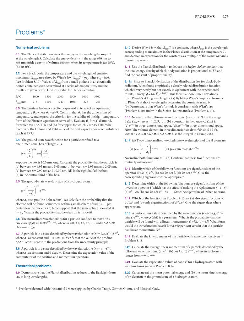
PROBLEMS 275
Problems*
Numerical problems
8.1 The Planck distribution gives the energy in the wavelength range dλat the wavelength λ. Calculate the energy density in the range 650 nm to 655 nm inside a cavity of volume 100 cm3 when its temperature is (a) 25°C,(b) 3000°C.
8.2 For a black body, the temperature and the wavelength of emissionmaximum, λmax, are related by Wien’s law, λmaxT = 1–
5 c2, where c2 = hc/k(see Problem 8.10). Values of λmax from a small pinhole in an electricallyheated container were determined at a series of temperatures, and the results are given below. Deduce a value for Planck’s constant.
θ/°C 1000 1500 2000 2500 3000 3500
λmax/nm 2181 1600 1240 1035 878 763
8.3 The Einstein frequency is often expressed in terms of an equivalenttemperature θE, where θE = hν/k. Confirm that θE has the dimensions oftemperature, and express the criterion for the validity of the high-temperatureform of the Einstein equation in terms of it. Evaluate θE for (a) diamond, for which ν = 46.5 THz and (b) for copper, for which ν = 7.15 THz. Whatfraction of the Dulong and Petit value of the heat capacity does each substancereach at 25°C?
8.4 The ground-state wavefunction for a particle confined to a one-dimensional box of length L is
ψ =1/2
sin
Suppose the box is 10.0 nm long. Calculate the probability that the particle is(a) between x = 4.95 nm and 5.05 nm, (b) between x = 1.95 nm and 2.05 nm,(c) between x = 9.90 nm and 10.00 nm, (d) in the right half of the box, (e) in the central third of the box.
8.5 The ground-state wavefunction of a hydrogen atom is
ψ =1/2
e−r/a0
where a0 = 53 pm (the Bohr radius). (a) Calculate the probability that theelectron will be found somewhere within a small sphere of radius 1.0 pmcentred on the nucleus. (b) Now suppose that the same sphere is located at r = a0. What is the probability that the electron is inside it?
8.6 The normalized wavefunctions for a particle confined to move on a circle are ψ(φ) = (1/2π)1/2e−imφ, where m = 0, ±1, ±2, ±3, . . . and 0 ≤ φ ≤ 2π.Determine �φ�.
8.7 A particle is in a state described by the wavefunction ψ(x) = (2a/π)1/4e−ax2,
where a is a constant and −∞ ≤ x ≤ ∞. Verify that the value of the product∆p∆x is consistent with the predictions from the uncertainty principle.
8.8 A particle is in a state described by the wavefunction ψ(x) = a1/2e−ax,where a is a constant and 0 ≤ x ≤ ∞. Determine the expectation value of thecommutator of the position and momentum operators.
Theoretical problems
8.9 Demonstrate that the Planck distribution reduces to the Rayleigh–Jeanslaw at long wavelengths.
DEF1
πa30
ABC
DEFπx
L
ABCDEF
2
L
ABC
8.10 Derive Wien’s law, that λmaxT is a constant, where λmax is the wavelengthcorresponding to maximum in the Planck distribution at the temperature T,and deduce an expression for the constant as a multiple of the second radiationconstant, c2 = hc/k.
8.11 Use the Planck distribution to deduce the Stefan–Boltzmann law thatthe total energy density of black-body radiation is proportional to T 4, and find the constant of proportionality.
8.12‡ Prior to Planck’s derivation of the distribution law for black-bodyradiation, Wien found empirically a closely related distribution functionwhich is very nearly but not exactly in agreement with the experimentalresults, namely, ρ = (a /λ5)e−b/λkT. This formula shows small deviations from Planck’s at long wavelengths. (a) By fitting Wien’s empirical formula to Planck’s at short wavelengths determine the constants a and b.(b) Demonstrate that Wien’s formula is consistent with Wien’s law (Problem 8.10) and with the Stefan–Boltzmann law (Problem 8.11).
8.13 Normalize the following wavefunctions: (a) sin(nπx/L) in the range 0 ≤ x ≤ L, where n = 1, 2, 3, . . . , (b) a constant in the range −L ≤ x ≤ L,(c) e−r/a in three-dimensional space, (d) xe−r/2a in three-dimensional space.Hint: The volume element in three dimensions is dτ = r2dr sin θ dθ dφ,with 0 ≤ r < ∞, 0 ≤ θ ≤ π, 0 ≤ φ ≤ 2π. Use the integral in Example 8.4.
8.14 (a) Two (unnormalized) excited state wavefunctions of the H atom are
(i) ψ = 2 − e−r/a0 (ii) ψ = r sin θ cos φ e−r/2a0
Normalize both functions to 1. (b) Confirm that these two functions aremutually orthogonal.
8.15 Identify which of the following functions are eigenfunctions of theoperator d/dx: (a) eikx, (b) cos kx, (c) k, (d) kx, (e) e−αx2
. Give thecorresponding eigenvalue where appropriate.
8.16 Determine which of the following functions are eigenfunctions of theinversion operator î (which has the effect of making the replacement x → −x):(a) x3 − kx, (b) cos kx, (c) x2 + 3x − 1. State the eigenvalue of î when relevant.
8.17 Which of the functions in Problem 8.15 are (a) also eigenfunctions ofd2/dx2 and (b) only eigenfunctions of d2/dx2? Give the eigenvalues whereappropriate.
8.18 A particle is in a state described by the wavefunction ψ = (cos χ)eikx +(sin χ)e−ikx, where χ (chi) is a parameter. What is the probability that theparticle will be found with a linear momentum (a) +k$, (b) −k$? What formwould the wavefunction have if it were 90 per cent certain that the particle had linear momentum +k$?
8.19 Evaluate the kinetic energy of the particle with wavefunction given inProblem 8.18.
8.20 Calculate the average linear momentum of a particle described by thefollowing wavefunctions: (a) eikx, (b) cos kx, (c) e−αx2
, where in each one xranges from −∞ to +∞.
8.21 Evaluate the expectation values of r and r2 for a hydrogen atom withwavefunctions given in Problem 8.14.
8.22 Calculate (a) the mean potential energy and (b) the mean kinetic energyof an electron in the ground state of a hydrogenic atom.
DEFr
a0
ABC
* Problems denoted with the symbol ‡ were supplied by Charles Trapp, Carmen Giunta, and Marshall Cady.
276 8 QUANTUM THEORY: INTRODUCTION AND PRINCIPLES
8.23 Use mathematical software to construct superpositions of cosinefunctions and determine the probability that a given momentum will beobserved. If you plot the superposition (which you should), set x = 0 at thecentre of the screen and build the superposition there. Evaluate the root meansquare location of the packet, �x2�1/2.
8.24 Show that the expectation value of an operator that can be written as thesquare of an hermitian operator is positive.
8.25 (a) Given that any operators used to represent observables must satisfythe commutation relation in eqn 8.38, what would be the operator forposition if the choice had been made to represent linear momentum parallelto the x-axis by multiplication by the linear momentum? These differentchoices are all valid ‘representations’ of quantum mechanics. (b) With theidentification of X in this representation, what would be the operator for 1/x?Hint. Think of 1/x as x−1.
Applications: to biology, environmental science, andastrophysics
8.26‡ The temperature of the Sun’s surface is approximately 5800 K. On the assumption that the human eye evolved to be most sensitive at thewavelength of light corresponding to the maximum in the Sun’s radiantenergy distribution, determine the colour of light to which the eye is mostsensitive. Hint: See Problem 8.10.
8.27 We saw in Impact I8.1 that electron microscopes can obtain images with several hundredfold higher resolution than optical microscopes becauseof the short wavelength obtainable from a beam of electrons. For electronsmoving at speeds close to c, the speed of light, the expression for the de Broglie wavelength (eqn 8.12) needs to be corrected for relativistic effects:
λ =
2meeV 1 +1/2
where c is the speed of light in vacuum and V is the potential differencethrough which the electrons are accelerated. (a) Use the expression above tocalculate the de Broglie wavelength of electrons accelerated through 50 kV. (b) Is the relativistic correction important?
8.28‡ Solar energy strikes the top of the Earth’s atmosphere at a rate of 343 W m−2. About 30 per cent of this energy is reflected directly back intospace by the Earth or the atmosphere. The Earth–atmosphere system absorbsthe remaining energy and re-radiates it into space as black-body radiation.What is the average black-body temperature of the Earth? What is thewavelength of the most plentiful of the Earth’s black-body radiation? Hint. Use Wien’s law, Problem 8.10.
8.29‡ A star too small and cold to shine has been found by S. Kulkarni, K.Matthews, B.R. Oppenheimer, and T. Nakajima (Science 270, 1478 (1995)).The spectrum of the object shows the presence of methane, which, accordingto the authors, would not exist at temperatures much above 1000 K. The massof the star, as determined from its gravitational effect on a companion star, is roughly 20 times the mass of Jupiter. The star is considered to be a browndwarf, the coolest ever found. (a) From available thermodynamic data, test the stability of methane at temperatures above 1000 K. (b) What is λmax forthis star? (c) What is the energy density of the star relative to that of the Sun(6000 K)? (d) To determine whether the star will shine, estimate the fractionof the energy density of the star in the visible region of the spectrum.
567
DEFeV
2mec2
ABC123
h
Quantum theory:techniques andapplicationsTo find the properties of systems according to quantum mechanics we need to solve theappropriate Schrödinger equation. This chapter presents the essentials of the solutions forthree basic types of motion: translation, vibration, and rotation. We shall see that only certainwavefunctions and their corresponding energies are acceptable. Hence, quantizationemerges as a natural consequence of the equation and the conditions imposed on it. Thesolutions bring to light a number of highly nonclassical, and therefore surprising, features ofparticles, especially their ability to tunnel into and through regions where classical physicswould forbid them to be found. We also encounter a property of the electron, its spin, thathas no classical counterpart. The chapter concludes with an introduction to the experi-mental techniques used to probe the quantization of energy in molecules.
The three basic modes of motion—translation (motion through space), vibration,and rotation—all play an important role in chemistry because they are ways in whichmolecules store energy. Gas-phase molecules, for instance, undergo translational motion and their kinetic energy is a contribution to the total internal energy of a sample. Molecules can also store energy as rotational kinetic energy and transitionsbetween their rotational energy states can be observed spectroscopically. Energy isalso stored as molecular vibration and transitions between vibrational states are responsible for the appearance of infrared and Raman spectra.
Translational motion
Section 8.5 introduced the quantum mechanical description of free motion in one dimension. We saw there that the Schrödinger equation is
− = Eψ (9.1a)
or more succinctly
@ψ = Eψ @ = − (9.1b)
The general solutions of eqn 9.1 are
ψk = Aeikx + Be−ikx Ek = (9.2)
Note that we are now labelling both the wavefunctions and the energies (that is, the eigenfunctions and eigenvalues of @) with the index k. We can verify that these
k2$2
2m
d2
dx 2
$2
2m
d2ψdx 2
$2
2m
9Translational motion
9.1 A particle in a box
9.2 Motion in two and moredimensions
9.3 Tunnelling
I9.1 Impact on nanoscience:Scanning probe microscopy
Vibrational motion
9.4 The energy levels
9.5 The wavefunctions
Rotational motion
9.6 Rotation in two dimensions: aparticle on a ring
9.7 Rotation in three dimensions:the particle on a sphere
I9.2 Impact on nanoscience:Quantum dots
9.8 Spin
Techniques of approximation
9.9 Time-independentperturbation theory
9.10 Time-dependent perturbationtheory
Checklist of key ideas
Further reading
Further information 9.1: Dirac notation
Further information 9.2: Perturbationtheory
Discussion questions
Exercises
Problems
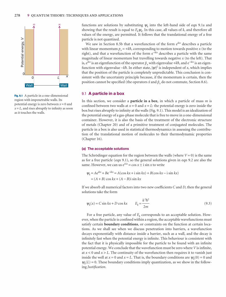
278 9 QUANTUM THEORY: TECHNIQUES AND APPLICATIONS
functions are solutions by substituting ψk into the left-hand side of eqn 9.1a andshowing that the result is equal to Ekψk. In this case, all values of k, and therefore allvalues of the energy, are permitted. It follows that the translational energy of a freeparticle is not quantized.
We saw in Section 8.5b that a wavefunction of the form eikx describes a particle with linear momentum px = +k$, corresponding to motion towards positive x (to theright), and that a wavefunction of the form e−ikx describes a particle with the samemagnitude of linear momentum but travelling towards negative x (to the left). That is, eikx is an eigenfunction of the operator Yx with eigenvalue +k$, and e−ikx is an eigen-function with eigenvalue −k$. In either state, |ψ |2 is independent of x, which impliesthat the position of the particle is completely unpredictable. This conclusion is con-sistent with the uncertainty principle because, if the momentum is certain, then theposition cannot be specified (the operators X and Yx do not commute, Section 8.6).
9.1 A particle in a box
In this section, we consider a particle in a box, in which a particle of mass m isconfined between two walls at x = 0 and x = L: the potential energy is zero inside thebox but rises abruptly to infinity at the walls (Fig. 9.1). This model is an idealization ofthe potential energy of a gas-phase molecule that is free to move in a one-dimensionalcontainer. However, it is also the basis of the treatment of the electronic structure of metals (Chapter 20) and of a primitive treatment of conjugated molecules. The particle in a box is also used in statistical thermodynamics in assessing the contribu-tion of the translational motion of molecules to their thermodynamic properties(Chapter 16).
(a) The acceptable solutions
The Schrödinger equation for the region between the walls (where V = 0) is the sameas for a free particle (eqn 9.1), so the general solutions given in eqn 9.2 are also thesame. However, we can us e±ix = cos x ± i sin x to write
ψk = Aeikx + Be−ikx = A(cos kx + i sin kx) + B(cos kx − i sin kx)
= (A + B) cos kx + (A − B)i sin kx
If we absorb all numerical factors into two new coefficients C and D, then the generalsolutions take the form
ψk(x) = C sin kx + D cos kx Ek = (9.3)
For a free particle, any value of Ek corresponds to an acceptable solution. How-ever, when the particle is confined within a region, the acceptable wavefunctions mustsatisfy certain boundary conditions, or constraints on the function at certain loca-tions. As we shall see when we discuss penetration into barriers, a wavefunction decays exponentially with distance inside a barrier, such as a wall, and the decay isinfinitely fast when the potential energy is infinite. This behaviour is consistent withthe fact that it is physically impossible for the particle to be found with an infinite potential energy. We conclude that the wavefunction must be zero where V is infinite,at x < 0 and x > L. The continuity of the wavefunction then requires it to vanish just inside the well at x = 0 and x = L. That is, the boundary conditions are ψk(0) = 0 andψk(L) = 0. These boundary conditions imply quantization, as we show in the follow-ing Justification.
k 2$2
2m
Pote
ntia
l ene
rgy,
V
0 L x
��
0
Wall Wall
Fig. 9.1 A particle in a one-dimensionalregion with impenetrable walls. Itspotential energy is zero between x = 0 and x = L, and rises abruptly to infinity as soonas it touches the walls.
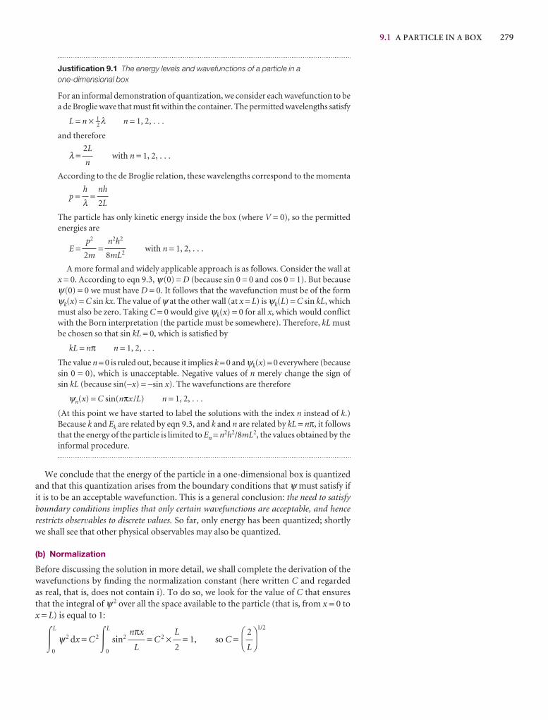
9.1 A PARTICLE IN A BOX 279
Justification 9.1 The energy levels and wavefunctions of a particle in a one-dimensional box
For an informal demonstration of quantization, we consider each wavefunction to bea de Broglie wave that must fit within the container. The permitted wavelengths satisfy
L = n × 1–2 λ n = 1, 2, . . .
and therefore
λ = with n = 1, 2, . . .
According to the de Broglie relation, these wavelengths correspond to the momenta
p = =
The particle has only kinetic energy inside the box (where V = 0), so the permittedenergies are
E = = with n = 1, 2, . . .
A more formal and widely applicable approach is as follows. Consider the wall atx = 0. According to eqn 9.3, ψ(0) = D (because sin 0 = 0 and cos 0 = 1). But becauseψ(0) = 0 we must have D = 0. It follows that the wavefunction must be of the formψk(x) = C sin kx. The value of ψ at the other wall (at x = L) is ψk(L) = C sin kL, whichmust also be zero. Taking C = 0 would give ψk(x) = 0 for all x, which would conflictwith the Born interpretation (the particle must be somewhere). Therefore, kL mustbe chosen so that sin kL = 0, which is satisfied by
kL = nπ n = 1, 2, . . .
The value n = 0 is ruled out, because it implies k = 0 and ψk(x) = 0 everywhere (becausesin 0 = 0), which is unacceptable. Negative values of n merely change the sign of sin kL (because sin(−x) = −sin x). The wavefunctions are therefore
ψn(x) = C sin(nπx /L) n = 1, 2, . . .
(At this point we have started to label the solutions with the index n instead of k.)Because k and Ek are related by eqn 9.3, and k and n are related by kL = nπ, it followsthat the energy of the particle is limited to En = n2h2/8mL2, the values obtained by theinformal procedure.
We conclude that the energy of the particle in a one-dimensional box is quantizedand that this quantization arises from the boundary conditions that ψ must satisfy ifit is to be an acceptable wavefunction. This is a general conclusion: the need to satisfyboundary conditions implies that only certain wavefunctions are acceptable, and hencerestricts observables to discrete values. So far, only energy has been quantized; shortlywe shall see that other physical observables may also be quantized.
(b) Normalization
Before discussing the solution in more detail, we shall complete the derivation of thewavefunctions by finding the normalization constant (here written C and regarded as real, that is, does not contain i). To do so, we look for the value of C that ensuresthat the integral of ψ2 over all the space available to the particle (that is, from x = 0 tox = L) is equal to 1:
�L
0
ψ2 dx = C 2�L
0
sin2 = C 2 × = 1, so C =1/2D
F2
L
AC
L
2
nπx
L
n2h2
8mL2
p2
2m
nh
2L
h
λ
2L
n
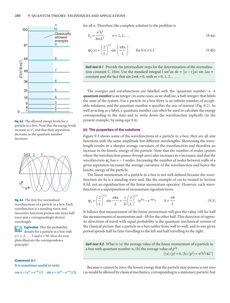
280 9 QUANTUM THEORY: TECHNIQUES AND APPLICATIONS
149
16
25
36
49
64
81
100
123
4
5
6
7
8
9
10
Eh
mL
/(/ 8
)2
2
n
0
Classicallyallowedenergies
Fig. 9.2 The allowed energy levels for aparticle in a box. Note that the energy levelsincrease as n2, and that their separationincreases as the quantum numberincreases.
Fig. 9.3 The first five normalizedwavefunctions of a particle in a box. Eachwavefunction is a standing wave, andsuccessive functions possess one more halfwave and a correspondingly shorterwavelength.
Exploration Plot the probabilitydensity for a particle in a box with
n = 1, 2, . . . 5 and n = 50. How do yourplots illustrate the correspondenceprinciple?
12345
�
x
Comment 9.1
It is sometimes useful to write
cos x = (eix + e−ix)/2 sin x = (eix − e−ix )/2i
for all n. Therefore, the complete solution to the problem is
En = n = 1, 2, . . . (9.4a)
ψn(x) =1/2
sin for 0 ≤ x ≤ L (9.4b)
Self-test 9.1 Provide the intermediate steps for the determination of the normaliza-tion constant C. Hint. Use the standard integral ∫ sin2ax dx = 1–2x − (1–4a) sin 2ax +constant and the fact that sin 2mπ = 0, with m = 0, 1, 2, . . . .
The energies and wavefunctions are labelled with the ‘quantum number’ n. Aquantum number is an integer (in some cases, as we shall see, a half-integer) that labelsthe state of the system. For a particle in a box there is an infinite number of accept-able solutions, and the quantum number n specifies the one of interest (Fig. 9.2). Aswell as acting as a label, a quantum number can often be used to calculate the energy corresponding to the state and to write down the wavefunction explicitly (in the present example, by using eqn 9.4).
(c) The properties of the solutions
Figure 9.3 shows some of the wavefunctions of a particle in a box: they are all sinefunctions with the same amplitude but different wavelengths. Shortening the wave-length results in a sharper average curvature of the wavefunction and therefore an increase in the kinetic energy of the particle. Note that the number of nodes (pointswhere the wavefunction passes through zero) also increases as n increases, and that thewavefunction ψn has n − 1 nodes. Increasing the number of nodes between walls of agiven separation increases the average curvature of the wavefunction and hence thekinetic energy of the particle.
The linear momentum of a particle in a box is not well defined because the wave-function sin kx is a standing wave and, like the example of cos kx treated in Section8.5d, not an eigenfunction of the linear momentum operator. However, each wave-function is a superposition of momentum eigenfunctions:
ψn =1/2
sin =1/2
(eikx − e−ikx) k = (9.5)
It follows that measurement of the linear momentum will give the value +k$ for halfthe measurements of momentum and −k$ for the other half. This detection of oppos-ite directions of travel with equal probability is the quantum mechanical version ofthe classical picture that a particle in a box rattles from wall to wall, and in any givenperiod spends half its time travelling to the left and half travelling to the right.
Self-test 9.2 What is (a) the average value of the linear momentum of a particle ina box with quantum number n, (b) the average value of p2?
[(a) �p� = 0, (b) �p2� = n2h2/4L2]
Because n cannot be zero, the lowest energy that the particle may possess is not zero(as would be allowed by classical mechanics, corresponding to a stationary particle) but
nπL
DF
2
L
AC
1
2i
nπx
L
DF
2
L
AC
DF
nπx
L
AC
DF
2
L
AC
n2h2
8mL2
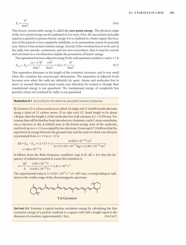
9.1 A PARTICLE IN A BOX 281
E1 = (9.6)
This lowest, irremovable energy is called the zero-point energy. The physical origin of the zero-point energy can be explained in two ways. First, the uncertainty principlerequires a particle to possess kinetic energy if it is confined to a finite region: the loca-tion of the particle is not completely indefinite, so its momentum cannot be preciselyzero. Hence it has nonzero kinetic energy. Second, if the wavefunction is to be zero atthe walls, but smooth, continuous, and not zero everywhere, then it must be curved,and curvature in a wavefunction implies the possession of kinetic energy.
The separation between adjacent energy levels with quantum numbers n and n + 1 is
En+1 − En = − = (2n + 1) (9.7)
This separation decreases as the length of the container increases, and is very smallwhen the container has macroscopic dimensions. The separation of adjacent levelsbecomes zero when the walls are infinitely far apart. Atoms and molecules free tomove in normal laboratory-sized vessels may therefore be treated as though theirtranslational energy is not quantized. The translational energy of completely free particles (those not confined by walls) is not quantized.
Illustration 9.1 Accounting for the electronic absorption spectra of polyenes
β-Carotene (1) is a linear polyene in which 10 single and 11 double bonds alternatealong a chain of 22 carbon atoms. If we take each CC bond length to be about 140 pm, then the length L of the molecular box in β-carotene is L = 0.294 nm. Forreasons that will be familiar from introductory chemistry, each C atom contributesone p-electron to the π orbitals and, in the lowest energy state of the molecule, each level up to n = 11 is occupied by two electrons. From eqn 9.7 it follows that theseparation in energy between the ground state and the state in which one electronis promoted from n = 11 to n = 12 is
∆E = E12 − E11 = (2 × 11 + 1)
= 1.60 × 10⁻¹⁹ J
It follows from the Bohr frequency condition (eqn 8.10, ∆E = hν) that the fre-quency of radiation required to cause this transition is
ν = = = 2.41 × 10¹⁴ s−1
The experimental value is ν = 6.03 × 10¹⁴ s−1 (λ = 497 nm), corresponding to radi-ation in the visible range of the electromagnetic spectrum.
Self-test 9.3 Estimate a typical nuclear excitation energy by calculating the first excitation energy of a proton confined to a square well with a length equal to thediameter of a nucleus (approximately 1 fm). [0.6 GeV]
1.60 × 10⁻¹⁹ J
6.626 × 10⁻³⁴ J s
∆E
h
(6.626 × 10⁻³⁴ J s)2
8 × (9.110 × 10−31 kg) × (2.94 × 10⁻¹⁰ m)2
h2
8mL2
n2h2
8mL2
(n + 1)2h2
8mL2
h2
8mL2
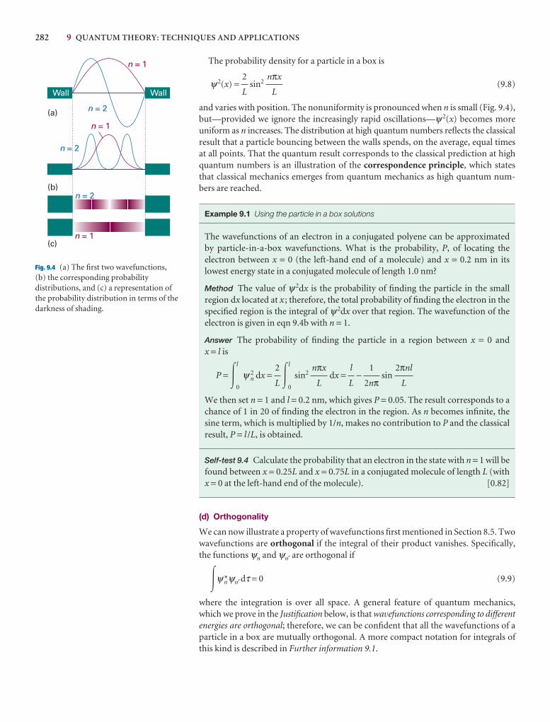
282 9 QUANTUM THEORY: TECHNIQUES AND APPLICATIONS
n = 1
n = 1
n = 1
n = 2
n = 2
n = 2
(a)
(c)
(b)
Wall Wall
Fig. 9.4 (a) The first two wavefunctions, (b) the corresponding probabilitydistributions, and (c) a representation ofthe probability distribution in terms of thedarkness of shading.
The probability density for a particle in a box is
ψ2(x) = sin2 (9.8)
and varies with position. The nonuniformity is pronounced when n is small (Fig. 9.4),but—provided we ignore the increasingly rapid oscillations—ψ2(x) becomes moreuniform as n increases. The distribution at high quantum numbers reflects the classicalresult that a particle bouncing between the walls spends, on the average, equal timesat all points. That the quantum result corresponds to the classical prediction at highquantum numbers is an illustration of the correspondence principle, which statesthat classical mechanics emerges from quantum mechanics as high quantum num-bers are reached.
Example 9.1 Using the particle in a box solutions
The wavefunctions of an electron in a conjugated polyene can be approximated by particle-in-a-box wavefunctions. What is the probability, P, of locating the electron between x = 0 (the left-hand end of a molecule) and x = 0.2 nm in its lowest energy state in a conjugated molecule of length 1.0 nm?
Method The value of ψ2dx is the probability of finding the particle in the small region dx located at x ; therefore, the total probability of finding the electron in thespecified region is the integral of ψ2dx over that region. The wavefunction of theelectron is given in eqn 9.4b with n = 1.
Answer The probability of finding the particle in a region between x = 0 and x = l is
P = �l
0
ψ 2n dx = �
l
0
sin2 dx = − sin
We then set n = 1 and l = 0.2 nm, which gives P = 0.05. The result corresponds to achance of 1 in 20 of finding the electron in the region. As n becomes infinite, thesine term, which is multiplied by 1/n, makes no contribution to P and the classicalresult, P = l /L, is obtained.
Self-test 9.4 Calculate the probability that an electron in the state with n = 1 will befound between x = 0.25L and x = 0.75L in a conjugated molecule of length L (withx = 0 at the left-hand end of the molecule). [0.82]
(d) Orthogonality
We can now illustrate a property of wavefunctions first mentioned in Section 8.5. Twowavefunctions are orthogonal if the integral of their product vanishes. Specifically,the functions ψn and ψn′ are orthogonal if
�ψn*ψn′dτ = 0 (9.9)
where the integration is over all space. A general feature of quantum mechanics,which we prove in the Justification below, is that wavefunctions corresponding to differentenergies are orthogonal; therefore, we can be confident that all the wavefunctions of aparticle in a box are mutually orthogonal. A more compact notation for integrals ofthis kind is described in Further information 9.1.
2πnl
L
1
2nπl
L
nπx
L
2
L
nπx
L
2
L
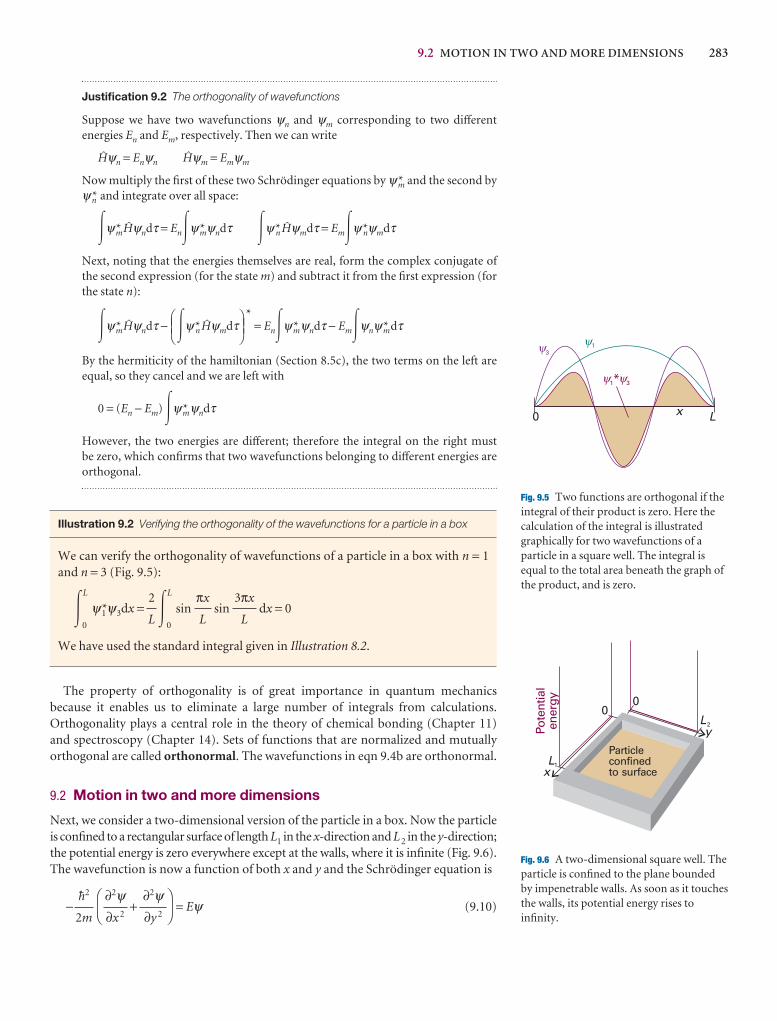
9.2 MOTION IN TWO AND MORE DIMENSIONS 283
13
1 3*
x L0
��
� �
Fig. 9.5 Two functions are orthogonal if theintegral of their product is zero. Here thecalculation of the integral is illustratedgraphically for two wavefunctions of aparticle in a square well. The integral isequal to the total area beneath the graph ofthe product, and is zero.
Justification 9.2 The orthogonality of wavefunctions
Suppose we have two wavefunctions ψn and ψm corresponding to two differentenergies En and Em, respectively. Then we can write
@ψn = Enψn @ψm = Emψm
Now multiply the first of these two Schrödinger equations by ψ*m and the second byψn* and integrate over all space:
�ψ*m@ψndτ = En�ψ*mψndτ �ψ*n @ψmdτ = Em�ψ*nψmdτ
Next, noting that the energies themselves are real, form the complex conjugate ofthe second expression (for the state m) and subtract it from the first expression (forthe state n):
�ψ*m@ψndτ − �ψ*n @ψmdτ*
= En�ψ*mψndτ − Em�ψnψ*mdτ
By the hermiticity of the hamiltonian (Section 8.5c), the two terms on the left areequal, so they cancel and we are left with
0 = (En − Em)�ψ*mψndτ
However, the two energies are different; therefore the integral on the right must be zero, which confirms that two wavefunctions belonging to different energies areorthogonal.
Illustration 9.2 Verifying the orthogonality of the wavefunctions for a particle in a box
We can verify the orthogonality of wavefunctions of a particle in a box with n = 1and n = 3 (Fig. 9.5):
�L
0
ψ*1ψ3dx = �L
0
sin sin dx = 0
We have used the standard integral given in Illustration 8.2.
The property of orthogonality is of great importance in quantum mechanics because it enables us to eliminate a large number of integrals from calculations.Orthogonality plays a central role in the theory of chemical bonding (Chapter 11) and spectroscopy (Chapter 14). Sets of functions that are normalized and mutuallyorthogonal are called orthonormal. The wavefunctions in eqn 9.4b are orthonormal.
9.2 Motion in two and more dimensions
Next, we consider a two-dimensional version of the particle in a box. Now the particleis confined to a rectangular surface of length L1 in the x-direction and L2 in the y-direction;the potential energy is zero everywhere except at the walls, where it is infinite (Fig. 9.6).The wavefunction is now a function of both x and y and the Schrödinger equation is
− + = Eψ (9.10)DF
∂2ψ∂y 2
∂2ψ∂x 2
AC
$2
2m
3πx
L
πx
L
2
L
DEFABC
x
y
L1
L2
00
Pote
ntia
len
ergy
Particleconfinedto surface
Fig. 9.6 A two-dimensional square well. Theparticle is confined to the plane boundedby impenetrable walls. As soon as it touchesthe walls, its potential energy rises toinfinity.
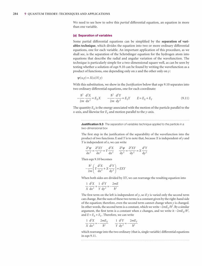
284 9 QUANTUM THEORY: TECHNIQUES AND APPLICATIONS
We need to see how to solve this partial differential equation, an equation in morethan one variable.
(a) Separation of variables
Some partial differential equations can be simplified by the separation of vari-ables technique, which divides the equation into two or more ordinary differentialequations, one for each variable. An important application of this procedure, as weshall see, is the separation of the Schrödinger equation for the hydrogen atom intoequations that describe the radial and angular variation of the wavefunction. Thetechnique is particularly simple for a two-dimensional square well, as can be seen bytesting whether a solution of eqn 9.10 can be found by writing the wavefunction as aproduct of functions, one depending only on x and the other only on y :
ψ(x,y) = X(x)Y(y)
With this substitution, we show in the Justification below that eqn 9.10 separates intotwo ordinary differential equations, one for each coordinate:
− = EX X − = EYY E = EX + EY (9.11)
The quantity EX is the energy associated with the motion of the particle parallel to thex-axis, and likewise for EY and motion parallel to the y-axis.
Justification 9.3 The separation of variables technique applied to the particle in atwo-dimensional box
The first step in the justification of the separability of the wavefunction into theproduct of two functions X and Y is to note that, because X is independent of y andY is independent of x, we can write
= = Y = = X
Then eqn 9.10 becomes
− Y + X = EXY
When both sides are divided by XY, we can rearrange the resulting equation into
+ = −
The first term on the left is independent of y, so if y is varied only the second termcan change. But the sum of these two terms is a constant given by the right-hand sideof the equation; therefore, even the second term cannot change when y is changed.In other words, the second term is a constant, which we write −2mEY/$2. By a similarargument, the first term is a constant when x changes, and we write it −2mEX /$2,and E = EX + EY . Therefore, we can write
= − = −
which rearrange into the two ordinary (that is, single variable) differential equationsin eqn 9.11.
2mEY
$2
d2Y
dy 2
1
Y
2mEX
$2
d2X
dx 2
1
X
2mE
$2
d2Y
dy 2
1
Y
d2X
dx 2
1
X
DEFd2Y
dy 2
d2X
dx 2
ABC$2
2m
d2Y
dy 2
∂2XY
∂y 2
∂2ψ∂y 2
d2X
dx 2
∂2XY
∂x 2
∂2ψ∂x 2
d2Y
dy 2
$2
2m
d2X
dx 2
$2
2m
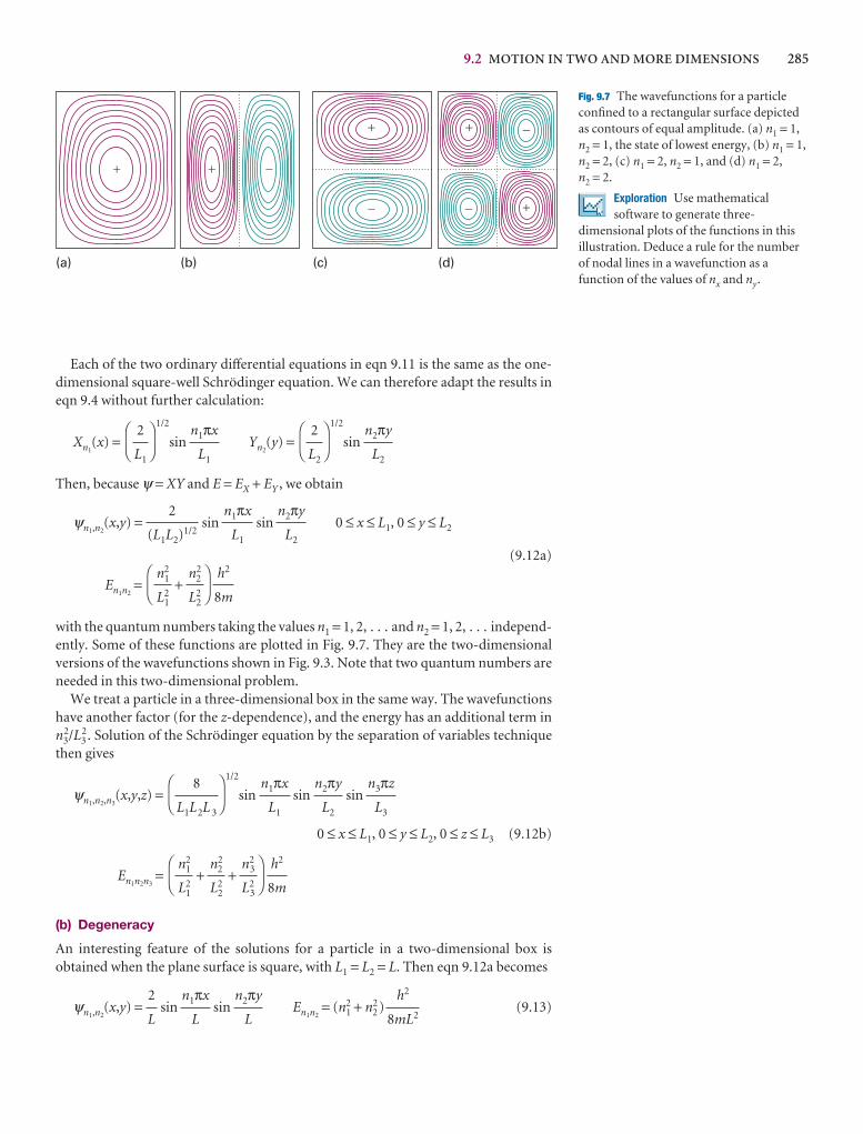
9.2 MOTION IN TWO AND MORE DIMENSIONS 285
Each of the two ordinary differential equations in eqn 9.11 is the same as the one-dimensional square-well Schrödinger equation. We can therefore adapt the results ineqn 9.4 without further calculation:
Xn1(x) =
1/2
sin Yn2(y) =
1/2
sin
Then, because ψ = XY and E = EX + EY , we obtain
ψn1,n2(x,y) = sin sin 0 ≤ x ≤ L1, 0 ≤ y ≤ L2
En1n2= +
(9.12a)
with the quantum numbers taking the values n1 = 1, 2, . . . and n2 = 1, 2, . . . independ-ently. Some of these functions are plotted in Fig. 9.7. They are the two-dimensionalversions of the wavefunctions shown in Fig. 9.3. Note that two quantum numbers areneeded in this two-dimensional problem.
We treat a particle in a three-dimensional box in the same way. The wavefunctionshave another factor (for the z-dependence), and the energy has an additional term inn3
2/L32. Solution of the Schrödinger equation by the separation of variables technique
then gives
ψn1,n2,n3(x,y,z) =
1/2
sin sin sin
0 ≤ x ≤ L1, 0 ≤ y ≤ L2, 0 ≤ z ≤ L3 (9.12b)
En1n2n3= + +
(b) Degeneracy
An interesting feature of the solutions for a particle in a two-dimensional box is obtained when the plane surface is square, with L1 = L2 = L. Then eqn 9.12a becomes
ψn1,n2(x,y) = sin sin En1n2
= (n12 + n2
2 ) (9.13)h2
8mL2
n2πy
L
n1πx
L
2
L
h2
8m
DF
n23
L23
n22
L22
n12
L12
AC
n3πz
L3
n2πy
L2
n1πx
L1
DF
8
L1L2L 3
AC
h2
8m
DF
n22
L22
n12
L12
AC
n2πy
L2
n1πx
L1
2
(L1L2)1/2
n2πy
L2
DF
2
L2
AC
n1πx
L1
DF
2
L1
AC
(a) (b) (c) (d)
� ��
� �
�� �
�
Fig. 9.7 The wavefunctions for a particleconfined to a rectangular surface depictedas contours of equal amplitude. (a) n1 = 1,n2 = 1, the state of lowest energy, (b) n1 = 1,n2 = 2, (c) n1 = 2, n2 = 1, and (d) n1 = 2,n2 = 2.
Exploration Use mathematicalsoftware to generate three-
dimensional plots of the functions in thisillustration. Deduce a rule for the numberof nodal lines in a wavefunction as afunction of the values of nx and ny.
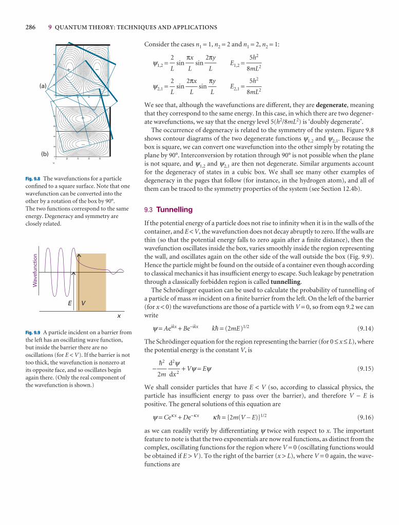
286 9 QUANTUM THEORY: TECHNIQUES AND APPLICATIONS
Consider the cases n1 = 1, n2 = 2 and n1 = 2, n2 = 1:
ψ1,2 = sin sin E1,2 =
ψ2,1 = sin sin E2,1 =
We see that, although the wavefunctions are different, they are degenerate, meaningthat they correspond to the same energy. In this case, in which there are two degener-ate wavefunctions, we say that the energy level 5(h2/8mL2) is ‘doubly degenerate’.
The occurrence of degeneracy is related to the symmetry of the system. Figure 9.8shows contour diagrams of the two degenerate functions ψ1,2 and ψ2,1. Because thebox is square, we can convert one wavefunction into the other simply by rotating theplane by 90°. Interconversion by rotation through 90° is not possible when the planeis not square, and ψ1,2 and ψ2,1 are then not degenerate. Similar arguments accountfor the degeneracy of states in a cubic box. We shall see many other examples of degeneracy in the pages that follow (for instance, in the hydrogen atom), and all ofthem can be traced to the symmetry properties of the system (see Section 12.4b).
9.3 Tunnelling
If the potential energy of a particle does not rise to infinity when it is in the walls of thecontainer, and E < V, the wavefunction does not decay abruptly to zero. If the walls arethin (so that the potential energy falls to zero again after a finite distance), then thewavefunction oscillates inside the box, varies smoothly inside the region representingthe wall, and oscillates again on the other side of the wall outside the box (Fig. 9.9).Hence the particle might be found on the outside of a container even though accordingto classical mechanics it has insufficient energy to escape. Such leakage by penetrationthrough a classically forbidden region is called tunnelling.
The Schrödinger equation can be used to calculate the probability of tunnelling ofa particle of mass m incident on a finite barrier from the left. On the left of the barrier(for x < 0) the wavefunctions are those of a particle with V = 0, so from eqn 9.2 we canwrite
ψ = Aeikx + Be−ikx k$ = (2mE)1/2 (9.14)
The Schrödinger equation for the region representing the barrier (for 0 ≤ x ≤ L), wherethe potential energy is the constant V, is
− + Vψ = Eψ (9.15)
We shall consider particles that have E < V (so, according to classical physics, the particle has insufficient energy to pass over the barrier), and therefore V − E ispositive. The general solutions of this equation are
ψ = Ceκ x + De−κ x κ$ = {2m(V − E)}1/2 (9.16)
as we can readily verify by differentiating ψ twice with respect to x. The important feature to note is that the two exponentials are now real functions, as distinct from thecomplex, oscillating functions for the region where V = 0 (oscillating functions wouldbe obtained if E > V). To the right of the barrier (x > L), where V = 0 again, the wave-functions are
d2ψdx 2
$2
2m
5h2
8mL2
πy
L
2πx
L
2
L
5h2
8mL2
2πy
L
πx
L
2
L
M
M
(a)
(b)
� �
�
�
Fig. 9.8 The wavefunctions for a particleconfined to a square surface. Note that onewavefunction can be converted into theother by a rotation of the box by 90°. The two functions correspond to the sameenergy. Degeneracy and symmetry areclosely related.
Wav
efun
ctio
n
E V
x
Fig. 9.9 A particle incident on a barrier fromthe left has an oscillating wave function,but inside the barrier there are nooscillations (for E < V). If the barrier is nottoo thick, the wavefunction is nonzero atits opposite face, and so oscillates beginagain there. (Only the real component ofthe wavefunction is shown.)
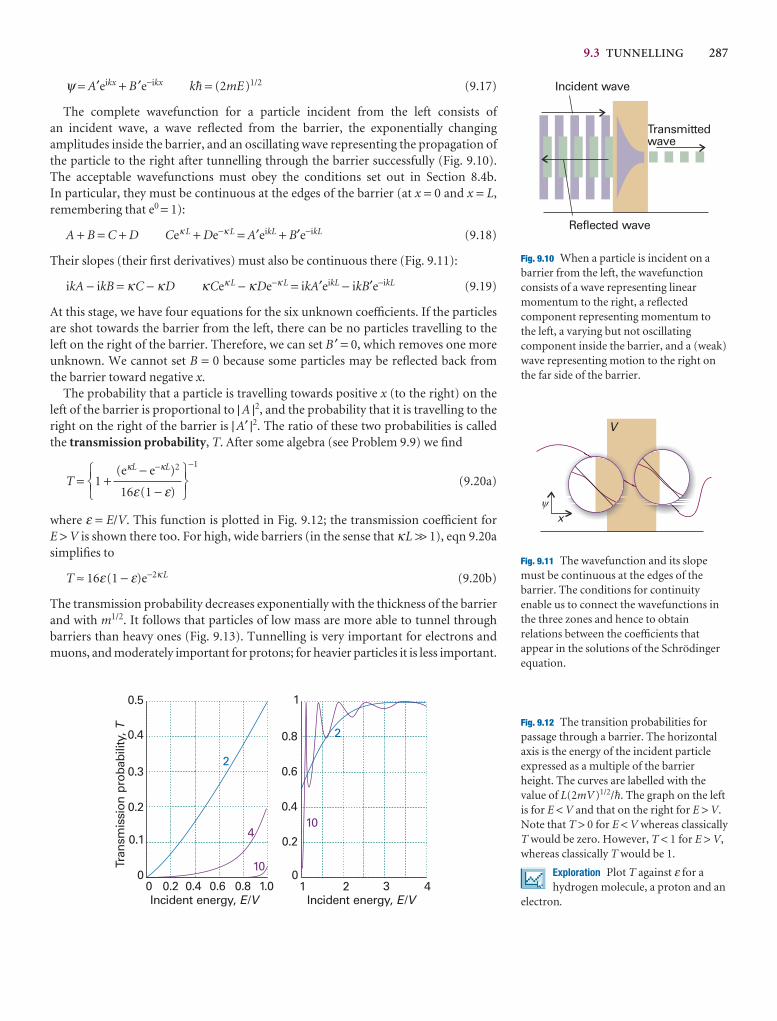
9.3 TUNNELLING 287
ψ = A′eikx + B ′e−ikx k$ = (2mE)1/2 (9.17)
The complete wavefunction for a particle incident from the left consists of an incident wave, a wave reflected from the barrier, the exponentially changing amplitudes inside the barrier, and an oscillating wave representing the propagation ofthe particle to the right after tunnelling through the barrier successfully (Fig. 9.10).The acceptable wavefunctions must obey the conditions set out in Section 8.4b. In particular, they must be continuous at the edges of the barrier (at x = 0 and x = L,remembering that e0 = 1):
A + B = C + D Ceκ L + De−κ L = A′eikL + B′e−ikL (9.18)
Their slopes (their first derivatives) must also be continuous there (Fig. 9.11):
ikA − ikB = κC − κD κCeκ L − κDe−κ L = ikA′eikL − ikB′e−ikL (9.19)
At this stage, we have four equations for the six unknown coefficients. If the particlesare shot towards the barrier from the left, there can be no particles travelling to the left on the right of the barrier. Therefore, we can set B ′ = 0, which removes one moreunknown. We cannot set B = 0 because some particles may be reflected back from the barrier toward negative x.
The probability that a particle is travelling towards positive x (to the right) on theleft of the barrier is proportional to | A |2, and the probability that it is travelling to theright on the right of the barrier is | A′ |2. The ratio of these two probabilities is called the transmission probability, T. After some algebra (see Problem 9.9) we find
T = 1 +−1
(9.20a)
where ε = E/V. This function is plotted in Fig. 9.12; the transmission coefficient for E > V is shown there too. For high, wide barriers (in the sense that κL >> 1), eqn 9.20asimplifies to
T ≈ 16ε(1 − ε)e−2κ L (9.20b)
The transmission probability decreases exponentially with the thickness of the barrierand with m1/2. It follows that particles of low mass are more able to tunnel throughbarriers than heavy ones (Fig. 9.13). Tunnelling is very important for electrons andmuons, and moderately important for protons; for heavier particles it is less important.
567(eκL − e−κL)2
16ε(1 − ε)
123
Incident wave
Reflected wave
Transmittedwave
Fig. 9.10 When a particle is incident on abarrier from the left, the wavefunctionconsists of a wave representing linearmomentum to the right, a reflectedcomponent representing momentum tothe left, a varying but not oscillatingcomponent inside the barrier, and a (weak)wave representing motion to the right onthe far side of the barrier.
�
x
Fig. 9.11 The wavefunction and its slopemust be continuous at the edges of thebarrier. The conditions for continuityenable us to connect the wavefunctions inthe three zones and hence to obtainrelations between the coefficients thatappear in the solutions of the Schrödingerequation.
0.5
0.4
0.3
0.2
0.1
00 0.2 0.4 0.6 0.8 1.0
2
410
1 2 3 4
1
0.8
0.6
0.4
0.2
0
2
Tran
smis
sion
pro
babi
lity,
T
Incident energy, /E V Incident energy, /E V
10
Fig. 9.12 The transition probabilities forpassage through a barrier. The horizontalaxis is the energy of the incident particleexpressed as a multiple of the barrierheight. The curves are labelled with thevalue of L(2mV)1/2/$. The graph on the leftis for E < V and that on the right for E > V.Note that T > 0 for E < V whereas classicallyT would be zero. However, T < 1 for E > V,whereas classically T would be 1.
Exploration Plot T against ε for ahydrogen molecule, a proton and an
electron.
V
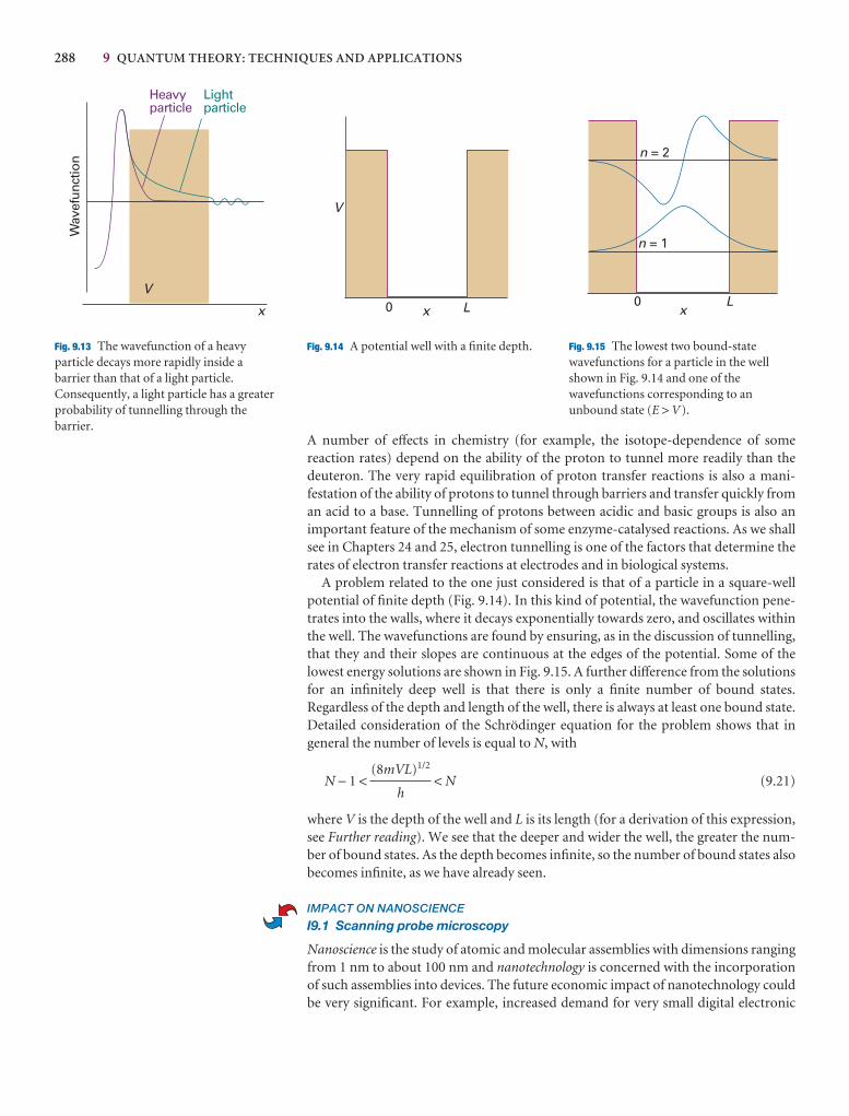
288 9 QUANTUM THEORY: TECHNIQUES AND APPLICATIONS
A number of effects in chemistry (for example, the isotope-dependence of some reaction rates) depend on the ability of the proton to tunnel more readily than thedeuteron. The very rapid equilibration of proton transfer reactions is also a mani-festation of the ability of protons to tunnel through barriers and transfer quickly froman acid to a base. Tunnelling of protons between acidic and basic groups is also an important feature of the mechanism of some enzyme-catalysed reactions. As we shallsee in Chapters 24 and 25, electron tunnelling is one of the factors that determine therates of electron transfer reactions at electrodes and in biological systems.
A problem related to the one just considered is that of a particle in a square-well potential of finite depth (Fig. 9.14). In this kind of potential, the wavefunction pene-trates into the walls, where it decays exponentially towards zero, and oscillates withinthe well. The wavefunctions are found by ensuring, as in the discussion of tunnelling,that they and their slopes are continuous at the edges of the potential. Some of thelowest energy solutions are shown in Fig. 9.15. A further difference from the solutionsfor an infinitely deep well is that there is only a finite number of bound states.Regardless of the depth and length of the well, there is always at least one bound state.Detailed consideration of the Schrödinger equation for the problem shows that ingeneral the number of levels is equal to N, with
N − 1 < < N (9.21)
where V is the depth of the well and L is its length (for a derivation of this expression,see Further reading). We see that the deeper and wider the well, the greater the num-ber of bound states. As the depth becomes infinite, so the number of bound states alsobecomes infinite, as we have already seen.
IMPACT ON NANOSCIENCE
I9.1 Scanning probe microscopy
Nanoscience is the study of atomic and molecular assemblies with dimensions rangingfrom 1 nm to about 100 nm and nanotechnology is concerned with the incorporationof such assemblies into devices. The future economic impact of nanotechnology couldbe very significant. For example, increased demand for very small digital electronic
(8mVL)1/2
h
Wav
efun
ctio
n
x
Lightparticle
Heavyparticle
V
Fig. 9.13 The wavefunction of a heavyparticle decays more rapidly inside abarrier than that of a light particle.Consequently, a light particle has a greaterprobability of tunnelling through thebarrier.
V
0 Lx
Fig. 9.14 A potential well with a finite depth.
0 Lx
n = 1
n = 2
Fig. 9.15 The lowest two bound-statewavefunctions for a particle in the wellshown in Fig. 9.14 and one of thewavefunctions corresponding to anunbound state (E > V).
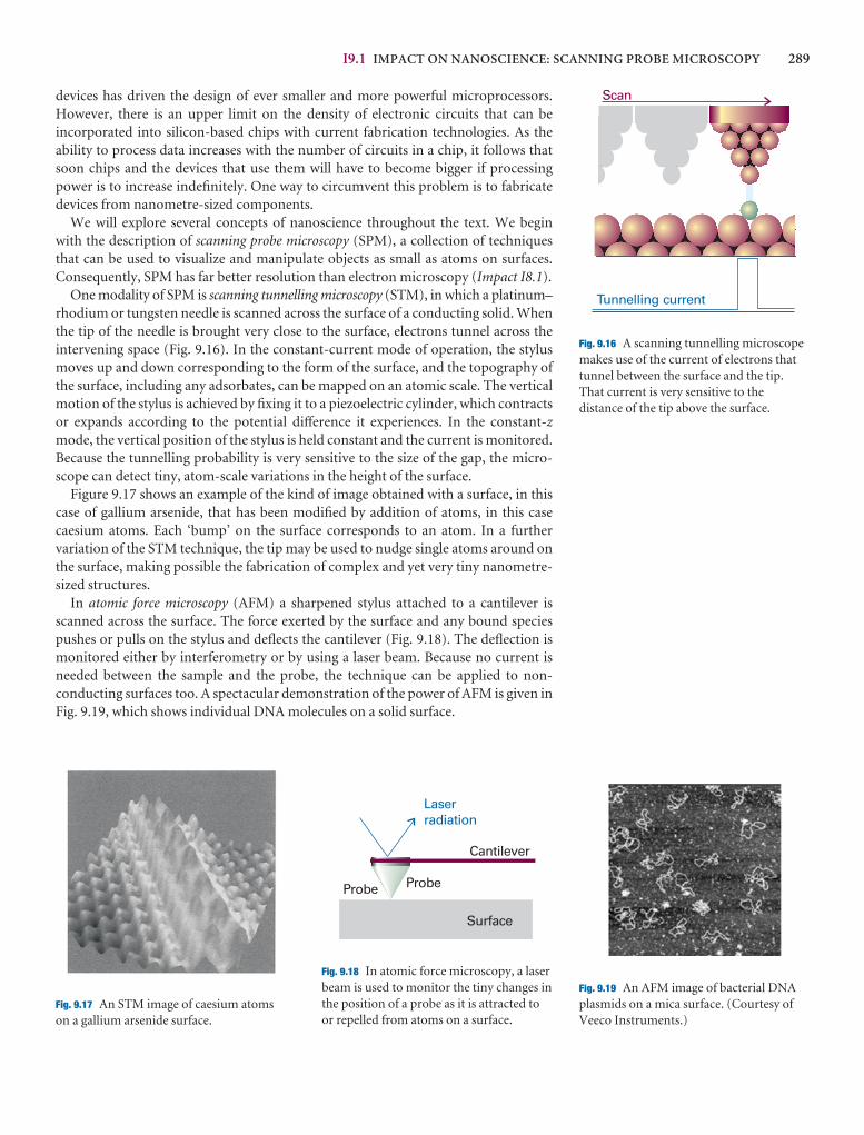
I9.1 IMPACT ON NANOSCIENCE: SCANNING PROBE MICROSCOPY 289
devices has driven the design of ever smaller and more powerful microprocessors.However, there is an upper limit on the density of electronic circuits that can be incorporated into silicon-based chips with current fabrication technologies. As theability to process data increases with the number of circuits in a chip, it follows thatsoon chips and the devices that use them will have to become bigger if processingpower is to increase indefinitely. One way to circumvent this problem is to fabricatedevices from nanometre-sized components.
We will explore several concepts of nanoscience throughout the text. We beginwith the description of scanning probe microscopy (SPM), a collection of techniquesthat can be used to visualize and manipulate objects as small as atoms on surfaces.Consequently, SPM has far better resolution than electron microscopy (Impact I8.1).
One modality of SPM is scanning tunnelling microscopy (STM), in which a platinum–rhodium or tungsten needle is scanned across the surface of a conducting solid. Whenthe tip of the needle is brought very close to the surface, electrons tunnel across the intervening space (Fig. 9.16). In the constant-current mode of operation, the stylusmoves up and down corresponding to the form of the surface, and the topography ofthe surface, including any adsorbates, can be mapped on an atomic scale. The verticalmotion of the stylus is achieved by fixing it to a piezoelectric cylinder, which contractsor expands according to the potential difference it experiences. In the constant-zmode, the vertical position of the stylus is held constant and the current is monitored.Because the tunnelling probability is very sensitive to the size of the gap, the micro-scope can detect tiny, atom-scale variations in the height of the surface.
Figure 9.17 shows an example of the kind of image obtained with a surface, in thiscase of gallium arsenide, that has been modified by addition of atoms, in this case caesium atoms. Each ‘bump’ on the surface corresponds to an atom. In a further variation of the STM technique, the tip may be used to nudge single atoms around onthe surface, making possible the fabrication of complex and yet very tiny nanometre-sized structures.
In atomic force microscopy (AFM) a sharpened stylus attached to a cantilever isscanned across the surface. The force exerted by the surface and any bound speciespushes or pulls on the stylus and deflects the cantilever (Fig. 9.18). The deflection is monitored either by interferometry or by using a laser beam. Because no current isneeded between the sample and the probe, the technique can be applied to non-conducting surfaces too. A spectacular demonstration of the power of AFM is given inFig. 9.19, which shows individual DNA molecules on a solid surface.
Scan
Tunnelling current
Fig. 9.16 A scanning tunnelling microscopemakes use of the current of electrons thattunnel between the surface and the tip.That current is very sensitive to thedistance of the tip above the surface.
Fig. 9.17 An STM image of caesium atomson a gallium arsenide surface.
Surface
Probe
Cantilever
Laserradiation
Probe
Fig. 9.18 In atomic force microscopy, a laserbeam is used to monitor the tiny changes inthe position of a probe as it is attracted toor repelled from atoms on a surface.
Fig. 9.19 An AFM image of bacterial DNAplasmids on a mica surface. (Courtesy ofVeeco Instruments.)
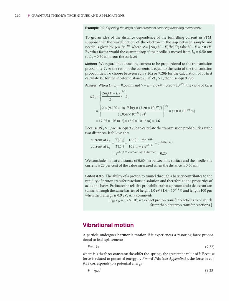
290 9 QUANTUM THEORY: TECHNIQUES AND APPLICATIONS
Example 9.2 Exploring the origin of the current in scanning tunnelling microscopy
To get an idea of the distance dependence of the tunnelling current in STM, suppose that the wavefunction of the electron in the gap between sample and needle is given by ψ = Be−κx, where κ = {2me(V − E)/$2}1/2; take V − E = 2.0 eV. By what factor would the current drop if the needle is moved from L1 = 0.50 nm to L 2 = 0.60 nm from the surface?
Method We regard the tunnelling current to be proportional to the transmissionprobability T, so the ratio of the currents is equal to the ratio of the transmissionprobabilities. To choose between eqn 9.20a or 9.20b for the calculation of T, firstcalculate κL for the shortest distance L1: if κL1 > 1, then use eqn 9.20b.
Answer When L = L1 = 0.50 nm and V − E = 2.0 eV = 3.20 × 10⁻¹⁹ J the value of κL is
κL1 =1/2
L1
=1/2
× (5.0 × 10−10 m)
= (7.25 × 10⁹ m−1) × (5.0 × 10−10 m) = 3.6
Because κL1 > 1, we use eqn 9.20b to calculate the transmission probabilities at thetwo distances. It follows that
= = = e−2κ (L2−L1)
= e−2×(7.25 ×10−9 m−1)×(1.0×10−10 m) = 0.23
We conclude that, at a distance of 0.60 nm between the surface and the needle, thecurrent is 23 per cent of the value measured when the distance is 0.50 nm.
Self-test 9.5 The ability of a proton to tunnel through a barrier contributes to therapidity of proton transfer reactions in solution and therefore to the properties ofacids and bases. Estimate the relative probabilities that a proton and a deuteron cantunnel through the same barrier of height 1.0 eV (1.6 × 10⁻¹⁹ J) and length 100 pmwhen their energy is 0.9 eV. Any comment?
[TH/TD = 3.7 × 10²; we expect proton transfer reactions to be much faster than deuteron transfer reactions.]
Vibrational motion
A particle undergoes harmonic motion if it experiences a restoring force propor-tional to its displacement:
F = −kx (9.22)
where k is the force constant: the stiffer the ‘spring’, the greater the value of k. Becauseforce is related to potential energy by F = −dV/dx (see Appendix 3), the force in eqn9.22 corresponds to a potential energy
V = 1–2 kx 2 (9.23)
16ε(1 − ε)e−2κ L2
16ε(1 − ε)e−2κ L1
T(L 2)
T(L1)
current at L2
current at L1
5672 × (9.109 × 10−31 kg) × (3.20 × 10⁻¹⁹ J)
(1.054 × 10⁻³⁴ J s)2
123
5672me(V − E)
$2
123
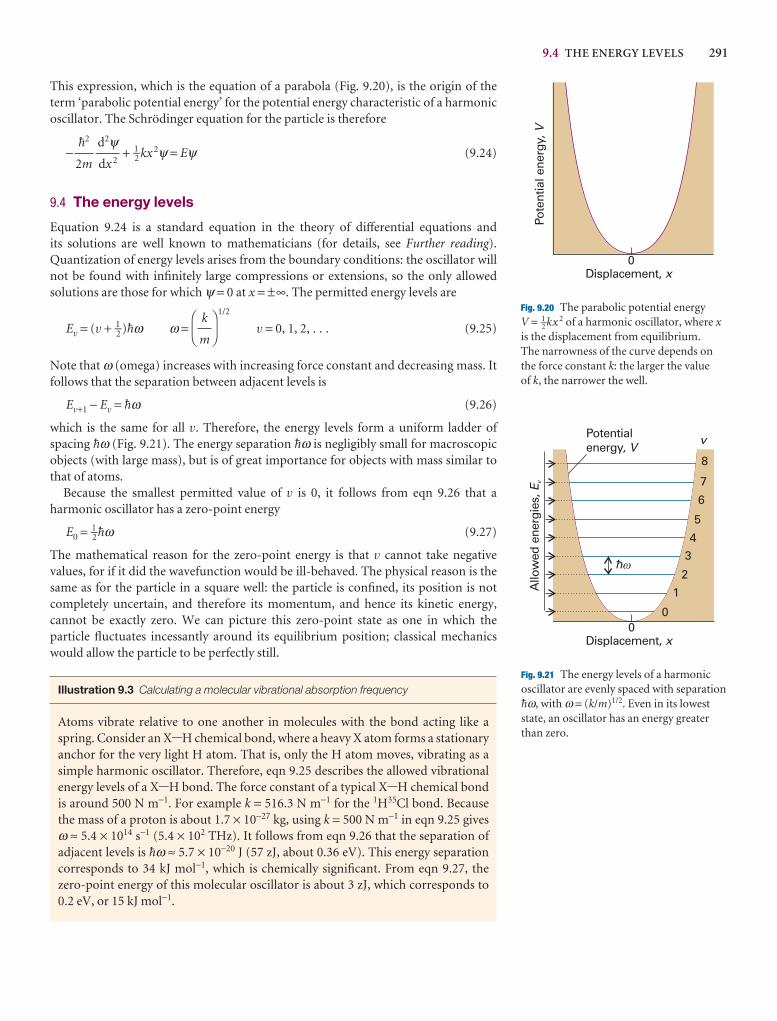
9.4 THE ENERGY LEVELS 291
Displacement, x
Pote
ntia
l ene
rgy,
V
0
Fig. 9.20 The parabolic potential energy V = 1–2 kx 2 of a harmonic oscillator, where xis the displacement from equilibrium. The narrowness of the curve depends onthe force constant k: the larger the value of k, the narrower the well.
Displacement, x
Allo
wed
ene
rgie
s,E v
0
v
0
1
2
34
5
6
7
8
Potentialenergy, V
�
Fig. 9.21 The energy levels of a harmonicoscillator are evenly spaced with separation$ω, with ω = (k/m)1/2. Even in its loweststate, an oscillator has an energy greaterthan zero.
This expression, which is the equation of a parabola (Fig. 9.20), is the origin of theterm ‘parabolic potential energy’ for the potential energy characteristic of a harmonicoscillator. The Schrödinger equation for the particle is therefore
− + 1–2 kx 2ψ = Eψ (9.24)
9.4 The energy levels
Equation 9.24 is a standard equation in the theory of differential equations and its solutions are well known to mathematicians (for details, see Further reading).Quantization of energy levels arises from the boundary conditions: the oscillator willnot be found with infinitely large compressions or extensions, so the only allowed solutions are those for which ψ = 0 at x = ±∞. The permitted energy levels are
Ev = (v + 1–2 )$ω ω =1/2
v = 0, 1, 2, . . . (9.25)
Note that ω (omega) increases with increasing force constant and decreasing mass. Itfollows that the separation between adjacent levels is
Ev+1 − Ev = $ω (9.26)
which is the same for all v. Therefore, the energy levels form a uniform ladder of spacing $ω (Fig. 9.21). The energy separation $ω is negligibly small for macroscopicobjects (with large mass), but is of great importance for objects with mass similar tothat of atoms.
Because the smallest permitted value of v is 0, it follows from eqn 9.26 that a harmonic oscillator has a zero-point energy
E0 = 1–2$ω (9.27)
The mathematical reason for the zero-point energy is that v cannot take negative values, for if it did the wavefunction would be ill-behaved. The physical reason is thesame as for the particle in a square well: the particle is confined, its position is notcompletely uncertain, and therefore its momentum, and hence its kinetic energy, cannot be exactly zero. We can picture this zero-point state as one in which the particle fluctuates incessantly around its equilibrium position; classical mechanicswould allow the particle to be perfectly still.
Illustration 9.3 Calculating a molecular vibrational absorption frequency
Atoms vibrate relative to one another in molecules with the bond acting like aspring. Consider an X-H chemical bond, where a heavy X atom forms a stationaryanchor for the very light H atom. That is, only the H atom moves, vibrating as asimple harmonic oscillator. Therefore, eqn 9.25 describes the allowed vibrationalenergy levels of a X-H bond. The force constant of a typical X-H chemical bond is around 500 N m−1. For example k = 516.3 N m−1 for the 1H35Cl bond. Because the mass of a proton is about 1.7 × 10⁻²⁷ kg, using k = 500 N m−1 in eqn 9.25 givesω ≈ 5.4 × 10¹⁴ s−1 (5.4 × 10² THz). It follows from eqn 9.26 that the separation ofadjacent levels is $ω ≈ 5.7 × 10⁻²⁰ J (57 zJ, about 0.36 eV). This energy separationcorresponds to 34 kJ mol−1, which is chemically significant. From eqn 9.27, thezero-point energy of this molecular oscillator is about 3 zJ, which corresponds to0.2 eV, or 15 kJ mol−1.
DF
k
m
AC
d2ψdx 2
$2
2m
h
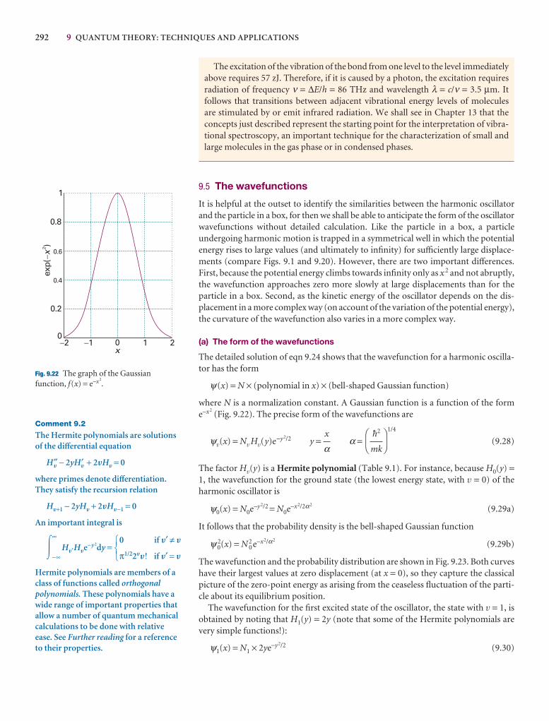
292 9 QUANTUM THEORY: TECHNIQUES AND APPLICATIONS
�2 �1 0 1 2x
exp(
)x
2
0
1
0.2
0.4
0.6
0.8
�
Fig. 9.22 The graph of the Gaussian function, f(x) = e−x2
.
Comment 9.2
The Hermite polynomials are solutionsof the differential equation
HV″ − 2yHV′ + 2VHV = 0
where primes denote differentiation.They satisfy the recursion relation
HV+1 − 2yHV + 2VHV−1 = 0
An important integral is
�∞
−∞HV′HVe−y2dy =
Hermite polynomials are members of aclass of functions called orthogonalpolynomials. These polynomials have awide range of important properties thatallow a number of quantum mechanicalcalculations to be done with relativeease. See Further reading for a referenceto their properties.
0 if V′ ≠ V
π1/22VV! if V′ = V
123
The excitation of the vibration of the bond from one level to the level immediatelyabove requires 57 zJ. Therefore, if it is caused by a photon, the excitation requiresradiation of frequency ν = ∆E/h = 86 THz and wavelength λ = c/ν = 3.5 µm. It follows that transitions between adjacent vibrational energy levels of molecules are stimulated by or emit infrared radiation. We shall see in Chapter 13 that theconcepts just described represent the starting point for the interpretation of vibra-tional spectroscopy, an important technique for the characterization of small andlarge molecules in the gas phase or in condensed phases.
9.5 The wavefunctions
It is helpful at the outset to identify the similarities between the harmonic oscillatorand the particle in a box, for then we shall be able to anticipate the form of the oscillatorwavefunctions without detailed calculation. Like the particle in a box, a particle undergoing harmonic motion is trapped in a symmetrical well in which the potentialenergy rises to large values (and ultimately to infinity) for sufficiently large displace-ments (compare Figs. 9.1 and 9.20). However, there are two important differences.First, because the potential energy climbs towards infinity only as x 2 and not abruptly,the wavefunction approaches zero more slowly at large displacements than for theparticle in a box. Second, as the kinetic energy of the oscillator depends on the dis-placement in a more complex way (on account of the variation of the potential energy),the curvature of the wavefunction also varies in a more complex way.
(a) The form of the wavefunctions
The detailed solution of eqn 9.24 shows that the wavefunction for a harmonic oscilla-tor has the form
ψ(x) = N × (polynomial in x) × (bell-shaped Gaussian function)
where N is a normalization constant. A Gaussian function is a function of the form e−x2
(Fig. 9.22). The precise form of the wavefunctions are
ψv(x) = Nv Hv(y)e−y2/2 y = α =1/4
(9.28)
The factor Hv(y) is a Hermite polynomial (Table 9.1). For instance, because H0(y) =1, the wavefunction for the ground state (the lowest energy state, with v = 0) of theharmonic oscillator is
ψ0(x) = N0e−y2/2 = N0e−x2/2α2(9.29a)
It follows that the probability density is the bell-shaped Gaussian function
ψ02(x) = N 0
2 e−x2/α2(9.29b)
The wavefunction and the probability distribution are shown in Fig. 9.23. Both curveshave their largest values at zero displacement (at x = 0), so they capture the classicalpicture of the zero-point energy as arising from the ceaseless fluctuation of the parti-cle about its equilibrium position.
The wavefunction for the first excited state of the oscillator, the state with v = 1, isobtained by noting that H1(y) = 2y (note that some of the Hermite polynomials arevery simple functions!):
ψ1(x) = N1 × 2ye−y2/2 (9.30)
DF
$2
mk
AC
x
α
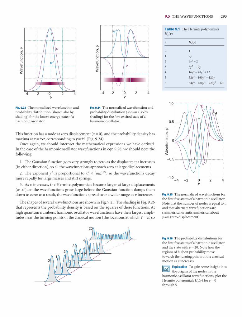
9.5 THE WAVEFUNCTIONS 293
This function has a node at zero displacement (x = 0), and the probability density hasmaxima at x = ±α, corresponding to y = ±1 (Fig. 9.24).
Once again, we should interpret the mathematical expressions we have derived. In the case of the harmonic oscillator wavefunctions in eqn 9.28, we should note thefollowing:
1. The Gaussian function goes very strongly to zero as the displacement increases(in either direction), so all the wavefunctions approach zero at large displacements.
2. The exponent y 2 is proportional to x 2 × (mk)1/2, so the wavefunctions decaymore rapidly for large masses and stiff springs.
3. As v increases, the Hermite polynomials become larger at large displacements(as xv), so the wavefunctions grow large before the Gaussian function damps themdown to zero: as a result, the wavefunctions spread over a wider range as v increases.
The shapes of several wavefunctions are shown in Fig. 9.25. The shading in Fig. 9.26that represents the probability density is based on the squares of these functions. Athigh quantum numbers, harmonic oscillator wavefunctions have their largest ampli-tudes near the turning points of the classical motion (the locations at which V = E, so
Table 9.1 The Hermite polynomialsHv(y)
V H1(y)
0 1
1 2y
2 4y2 − 2
3 8y3 − 12y
4 16y4 − 48y2 + 12
5 32y5 − 160y 3 + 120y
6 64y6 − 480y 4 + 720y 2 − 120
-4 -2 0 2 4y
Wav
efun
ctio
n,
y
2�
�
Fig. 9.23 The normalized wavefunction andprobability distribution (shown also byshading) for the lowest energy state of aharmonic oscillator.
�4 �2 0 2 4y
Wav
efun
ctio
n,
�
�
�
2
Fig. 9.24 The normalized wavefunction andprobability distribution (shown also byshading) for the first excited state of aharmonic oscillator.
1.0
0.5
0
�0.5
�1.0�4 �2 0 2 4
y
03
Wav
efun
ctio
n,
4
1 2
�
Fig. 9.25 The normalized wavefunctions forthe first five states of a harmonic oscillator.Note that the number of nodes is equal to vand that alternate wavefunctions aresymmetrical or antisymmetrical about y = 0 (zero displacement).
01
2
34
20
Fig. 9.26 The probability distributions forthe first five states of a harmonic oscillatorand the state with v = 20. Note how theregions of highest probability movetowards the turning points of the classicalmotion as v increases.
Exploration To gain some insight intothe origins of the nodes in the
harmonic oscillator wavefunctions, plot theHermite polynomials Hv(y) for v = 0through 5.
294 9 QUANTUM THEORY: TECHNIQUES AND APPLICATIONS
the kinetic energy is zero). We see classical properties emerging in the correspondencelimit of high quantum numbers, for a classical particle is most likely to be found at theturning points (where it travels most slowly) and is least likely to be found at zero dis-placement (where it travels most rapidly).
Example 9.3 Normalizing a harmonic oscillator wavefunction
Find the normalization constant for the harmonic oscillator wavefunctions.
Method Normalization is always carried out by evaluating the integral of |ψ |2 overall space and then finding the normalization factor from eqn 8.16. The normalizedwavefunction is then equal to Nψ. In this one-dimensional problem, the volumeelement is dx and the integration is from −∞ to +∞. The wavefunctions areexpressed in terms of the dimensionless variable y = x/α, so begin by expressing the integral in terms of y by using dx = αdy. The integrals required are given inComment 9.2.
Answer The unnormalized wavefunction is
ψv(x) = Hv(y)e−y2/2
It follows from the integrals given in Comment 9.2 that
�∞
−∞
ψ v*ψvdx = α�∞
−∞
ψ v*ψvdy = α�∞
−∞
Hv2(y)e−y2
dy = απ1/22vv!
where v! = v(v − 1)(v − 2) . . . 1. Therefore,
Nv =1/2
Note that for a harmonic oscillator Nv is different for each value of v.
Self-test 9.6 Confirm, by explicit evaluation of the integral, that ψ0 and ψ1 areorthogonal.
[Evaluate the integral ∫ ∞−∞ψ0*ψ1 dx by using the information in Comment 9.2.]
(b) The properties of oscillators
With the wavefunctions that are available, we can start calculating the properties of a harmonic oscillator. For instance, we can calculate the expectation values of an observable Ω by evaluating integrals of the type
�Ω� = �∞
−∞
ψ v*)ψvdx (9.31)
(Here and henceforth, the wavefunctions are all taken to be normalized to 1.) Whenthe explicit wavefunctions are substituted, the integrals look fearsome, but theHermite polynomials have many simplifying features. For instance, we show in thefollowing example that the mean displacement, �x�, and the mean square displace-ment, �x 2�, of the oscillator when it is in the state with quantum number v are
�x� = 0 �x 2� = (v + 1–2) (9.32)$
(mk)1/2
DF
1
απ1/22vv!
AC
9.5 THE WAVEFUNCTIONS 295
Comment 9.3
An even function is one for which f(−x) = f(x); an odd function is one forwhich f(−x) = −f(x). The product of anodd and even function is itself odd, andthe integral of an odd function over asymmetrical range about x = 0 is zero.
The result for �x� shows that the oscillator is equally likely to be found on either sideof x = 0 (like a classical oscillator). The result for �x 2� shows that the mean square dis-placement increases with v. This increase is apparent from the probability densities inFig. 9.26, and corresponds to the classical amplitude of swing increasing as the oscil-lator becomes more highly excited.
Example 9.4 Calculating properties of a harmonic oscillator
We can imagine the bending motion of a CO2 molecule as a harmonic oscillationrelative to the linear conformation of the molecule. We may be interested in the extent to which the molecule bends. Calculate the mean displacement of the oscillator when it is in a quantum state v.
Method Normalized wavefunctions must be used to calculate the expectation value.The operator for position along x is multiplication by the value of x (Section 8.5b).The resulting integral can be evaluated either by inspection (the integrand is theproduct of an odd and an even function), or by explicit evaluation using the formulas in Comment 9.2. To give practice in this type of calculation, we illustratethe latter procedure. We shall need the relation x = αy, which implies that dx = αdy.
Answer The integral we require is
�x� = �∞
−∞
ψ v*xψvdx = N v2�
∞
−∞
(Hve−y2/2)x(Hve−y2/2)dx
= α2N v2�
∞
−∞
(Hve−y2/2)y(Hve−y2/2)dy
= α2N v2�
∞
−∞
Hv yHve−y2dy
Now use the recursion relation (see Comment 9.2) to form
yHv = vHv−1 + 1–2Hv+1
which turns the integral into
�∞
−∞
HvyHve−y2dy = v�
∞
−∞
Hv−1Hve−y2dy + 1–2�
∞
−∞
Hv+1Hve−y2dy
Both integrals are zero, so �x� = 0. As remarked in the text, the mean displacementis zero because the displacement occurs equally on either side of the equilibriumposition. The following Self-test extends this calculation by examining the meansquare displacement, which we can expect to be non-zero and to increase with increasing v.
Self-test 9.7 Calculate the mean square displacement �x 2� of the particle from itsequilibrium position. (Use the recursion relation twice.) [eqn 9.32]
The mean potential energy of an oscillator, the expectation value of V = 1–2kx 2, cannow be calculated very easily:
�V� = �1–2kx 2� = 1–2(v + 1–2)$1/2
= 1–2(v + 1–2)$ω (9.33)DF
k
m
AC
296 9 QUANTUM THEORY: TECHNIQUES AND APPLICATIONS
Because the total energy in the state with quantum number v is (v + 1–2)$ω, it followsthat
�V� = 1–2Ev (9.34a)
The total energy is the sum of the potential and kinetic energies, so it follows at oncethat the mean kinetic energy of the oscillator is
�EK� = 1–2Ev (9.34b)
The result that the mean potential and kinetic energies of a harmonic oscillator areequal (and therefore that both are equal to half the total energy) is a special case of thevirial theorem:
If the potential energy of a particle has the form V = ax b, then its mean potentialand kinetic energies are related by
2�EK� = b�V� (9.35)
For a harmonic oscillator b = 2, so �EK� = �V�, as we have found. The virial theorem isa short cut to the establishment of a number of useful results, and we shall use it again.
An oscillator may be found at extensions with V > E that are forbidden by classicalphysics, for they correspond to negative kinetic energy. For example, it follows fromthe shape of the wavefunction (see the Justification below) that in its lowest energystate there is about an 8 per cent chance of finding an oscillator stretched beyond itsclassical limit and an 8 per cent chance of finding it with a classically forbidden com-pression. These tunnelling probabilities are independent of the force constant andmass of the oscillator. The probability of being found in classically forbidden regionsdecreases quickly with increasing v, and vanishes entirely as v approaches infinity, aswe would expect from the correspondence principle. Macroscopic oscillators (such aspendulums) are in states with very high quantum numbers, so the probability thatthey will be found in a classically forbidden region is wholly negligible. Molecules,however, are normally in their vibrational ground states, and for them the probabilityis very significant.
Justification 9.4 Tunnelling in the quantum mechanical harmonic oscillator
According to classical mechanics, the turning point, xtp, of an oscillator occurs whenits kinetic energy is zero, which is when its potential energy 1–2 kx 2 is equal to its totalenergy E. This equality occurs when
x 2tp = or, xtp = ±
1/2
with E given by eqn 9.25. The probability of finding the oscillator stretched beyonda displacement xtp is the sum of the probabilities ψ2dx of finding it in any of the intervals dx lying between xtp and infinity:
P = �∞
xtp
ψ v2dx
The variable of integration is best expressed in terms of y = x /α with α = ($2/mk)1/2,and then the turning point on the right lies at
ytp = =1/2
= (2v + 1)1/2
For the state of lowest energy (v = 0), ytp = 1 and the probability is
567
2(v + 1–2 )$ωα2k
123
xtp
α
DEF2E
k
ABC2E
k
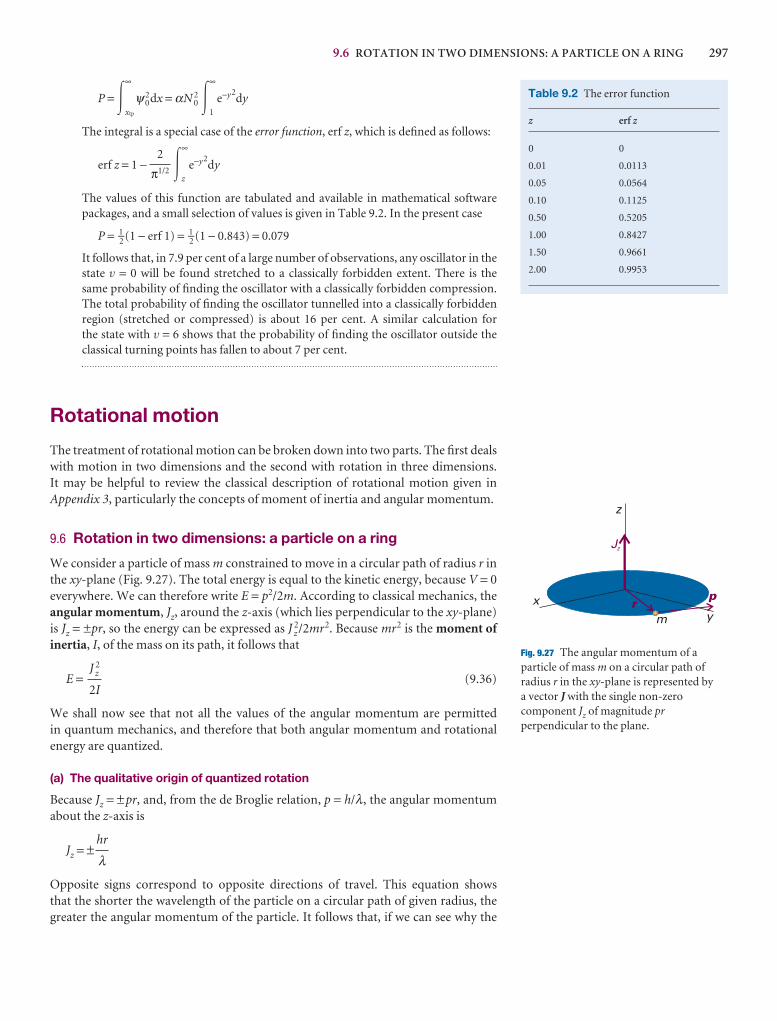
9.6 ROTATION IN TWO DIMENSIONS: A PARTICLE ON A RING 297
P = �∞
xtp
ψ02dx = αN 0
2 �1
∞
e−y2dy
The integral is a special case of the error function, erf z, which is defined as follows:
erf z = 1 − �∞
z
e−y2dy
The values of this function are tabulated and available in mathematical softwarepackages, and a small selection of values is given in Table 9.2. In the present case
P = 1–2 (1 − erf 1) = 1–2 (1 − 0.843) = 0.079
It follows that, in 7.9 per cent of a large number of observations, any oscillator in thestate v = 0 will be found stretched to a classically forbidden extent. There is the same probability of finding the oscillator with a classically forbidden compression.The total probability of finding the oscillator tunnelled into a classically forbidden region (stretched or compressed) is about 16 per cent. A similar calculation for the state with v = 6 shows that the probability of finding the oscillator outside theclassical turning points has fallen to about 7 per cent.
Rotational motion
The treatment of rotational motion can be broken down into two parts. The first dealswith motion in two dimensions and the second with rotation in three dimensions. It may be helpful to review the classical description of rotational motion given inAppendix 3, particularly the concepts of moment of inertia and angular momentum.
9.6 Rotation in two dimensions: a particle on a ring
We consider a particle of mass m constrained to move in a circular path of radius r inthe xy-plane (Fig. 9.27). The total energy is equal to the kinetic energy, because V = 0everywhere. We can therefore write E = p2/2m. According to classical mechanics, theangular momentum, Jz, around the z-axis (which lies perpendicular to the xy-plane)is Jz = ±pr, so the energy can be expressed as J z
2/2mr2. Because mr2 is the moment of inertia, I, of the mass on its path, it follows that
E = (9.36)
We shall now see that not all the values of the angular momentum are permitted in quantum mechanics, and therefore that both angular momentum and rotational energy are quantized.
(a) The qualitative origin of quantized rotation
Because Jz = ±pr, and, from the de Broglie relation, p = h/λ, the angular momentumabout the z-axis is
Jz = ±
Opposite signs correspond to opposite directions of travel. This equation shows that the shorter the wavelength of the particle on a circular path of given radius, thegreater the angular momentum of the particle. It follows that, if we can see why the
hr
λ
J z2
2I
2
π1/2
rm
xy
z
p
Jz
Fig. 9.27 The angular momentum of aparticle of mass m on a circular path ofradius r in the xy-plane is represented by a vector J with the single non-zerocomponent Jz of magnitude prperpendicular to the plane.
Table 9.2 The error function
z erf z
0 0
0.01 0.0113
0.05 0.0564
0.10 0.1125
0.50 0.5205
1.00 0.8427
1.50 0.9661
2.00 0.9953
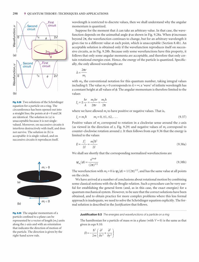
298 9 QUANTUM THEORY: TECHNIQUES AND APPLICATIONS
wavelength is restricted to discrete values, then we shall understand why the angularmomentum is quantized.
Suppose for the moment that λ can take an arbitrary value. In that case, the wave-function depends on the azimuthal angle φ as shown in Fig. 9.28a. When φ increasesbeyond 2π, the wavefunction continues to change, but for an arbitrary wavelength itgives rise to a different value at each point, which is unacceptable (Section 8.4b). Anacceptable solution is obtained only if the wavefunction reproduces itself on succes-sive circuits, as in Fig. 9.28b. Because only some wavefunctions have this property, itfollows that only some angular momenta are acceptable, and therefore that only cer-tain rotational energies exist. Hence, the energy of the particle is quantized. Specific-ally, the only allowed wavelengths are
λ =
with ml, the conventional notation for this quantum number, taking integral valuesincluding 0. The value ml = 0 corresponds to λ = ∞; a ‘wave’ of infinite wavelength hasa constant height at all values of φ. The angular momentum is therefore limited to thevalues
Jz = ± = =
where we have allowed ml to have positive or negative values. That is,
Jz = ml $ ml = 0, ±1, ±2, . . . (9.37)
Positive values of ml correspond to rotation in a clockwise sense around the z-axis(as viewed in the direction of z, Fig. 9.29) and negative values of ml correspond tocounter-clockwise rotation around z. It then follows from eqn 9.36 that the energy islimited to the values
E = = (9.38a)
We shall see shortly that the corresponding normalized wavefunctions are
ψml(φ) = (9.38b)
The wavefunction with ml = 0 is ψ0(φ) = 1/(2π)1/2, and has the same value at all pointson the circle.
We have arrived at a number of conclusions about rotational motion by combiningsome classical notions with the de Broglie relation. Such a procedure can be very use-ful for establishing the general form (and, as in this case, the exact energies) for aquantum mechanical system. However, to be sure that the correct solutions have beenobtained, and to obtain practice for more complex problems where this less formalapproach is inadequate, we need to solve the Schrödinger equation explicitly. The for-mal solution is described in the Justification that follows.
Justification 9.5 The energies and wavefunctions of a particle on a ring
The hamiltonian for a particle of mass m in a plane (with V = 0) is the same as thatgiven in eqn 9.10:
@ = − +DEF
∂2
∂y 2
∂2
∂x 2
ABC$2
2m
eimlφ
(2π)1/2
ml2$2
2I
J z2
2I
ml h
2πml hr
2πr
hr
λ
2πr
ml
Secondcircuit
Secondcircuit
Firstcircuit
Firstcircuit
p
p
2p
2p
0
0
(a)
(b)
f
f
Wav
efun
ctio
n,W
avef
unct
ion,
yy
ml 0�
ml 0�
(a)
(b)
Fig. 9.28 Two solutions of the Schrödingerequation for a particle on a ring. Thecircumference has been opened out into a straight line; the points at φ = 0 and 2πare identical. The solution in (a) isunacceptable because it is not single-valued. Moreover, on successive circuits itinterferes destructively with itself, and doesnot survive. The solution in (b) isacceptable: it is single-valued, and onsuccessive circuits it reproduces itself.
Fig. 9.29 The angular momentum of aparticle confined to a plane can berepresented by a vector of length |ml | unitsalong the z-axis and with an orientationthat indicates the direction of motion ofthe particle. The direction is given by theright-hand screw rule.
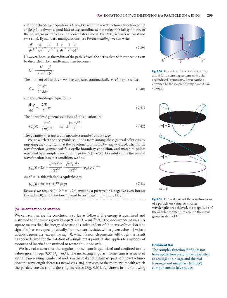
9.6 ROTATION IN TWO DIMENSIONS: A PARTICLE ON A RING 299
and the Schrödinger equation is Hψ = Eψ, with the wavefunction a function of theangle φ. It is always a good idea to use coordinates that reflect the full symmetry ofthe system, so we introduce the coordinates r and φ (Fig. 9.30), where x = r cos φ andy = r sin φ. By standard manipulations (see Further reading) we can write
+ = + + (9.39)
However, because the radius of the path is fixed, the derivatives with respect to r canbe discarded. The hamiltonian then becomes
@ = −
The moment of inertia I = mr 2 has appeared automatically, so H may be written
@ = − (9.40)
and the Schrödinger equation is
= − ψ (9.41)
The normalized general solutions of the equation are
ψml(φ) = ml = ± (9.42)
The quantity ml is just a dimensionless number at this stage.We now select the acceptable solutions from among these general solutions by
imposing the condition that the wavefunction should be single-valued. That is, thewavefunction ψ must satisfy a cyclic boundary condition, and match at points separated by a complete revolution: ψ(φ + 2π) = ψ(φ). On substituting the generalwavefunction into this condition, we find
ψml(φ + 2π) = = = ψml
(φ)e2πiml
As eiπ = −1, this relation is equivalent to
ψml(φ + 2π) = (−1)2mlψ(φ) (9.43)
Because we require (−1)2ml = 1, 2ml must be a positive or a negative even integer (including 0), and therefore ml must be an integer: ml = 0, ±1, ±2, . . . .
(b) Quantization of rotation
We can summarize the conclusions so far as follows. The energy is quantized and restricted to the values given in eqn 9.38a (E = ml
2$2/2I). The occurrence of ml as itssquare means that the energy of rotation is independent of the sense of rotation (thesign of ml), as we expect physically. In other words, states with a given value of | ml | aredoubly degenerate, except for ml = 0, which is non-degenerate. Although the resulthas been derived for the rotation of a single mass point, it also applies to any body ofmoment of inertia I constrained to rotate about one axis.
We have also seen that the angular momentum is quantized and confined to the values given in eqn 9.37 ( Jz = ml$). The increasing angular momentum is associatedwith the increasing number of nodes in the real and imaginary parts of the wavefunc-tion: the wavelength decreases stepwise as | ml | increases, so the momentum with whichthe particle travels round the ring increases (Fig. 9.31). As shown in the following
eimlφe2πiml
(2π)1/2
eiml(φ +2π)
(2π)1/2
(2IE)1/2
$
eimlφ
(2π)1/2
2IE
$2
d2ψdφ2
d2
dφ2
$2
2I
d2
dφ2
$2
2mr 2
∂2
∂φ2
1
r 2
∂∂r
1
r
∂2
∂r 2
∂2
∂y 2
∂2
∂x 2
x y�
r
z
Fig. 9.30 The cylindrical coordinates z, r,and φ for discussing systems with axial(cylindrical) symmetry. For a particleconfined to the xy-plane, only r and φ canchange.
ml = 0
| | = 1ml
| | = 2ml
Fig. 9.31 The real parts of the wavefunctionsof a particle on a ring. As shorterwavelengths are achieved, the magnitude ofthe angular momentum around the z-axisgrows in steps of $.
Comment 9.4
The complex function eimlφ does nothave nodes; however, it may be writtenas cos mlφ + i sin mlφ, and the real (cos mlφ) and imaginary (sin mlφ)components do have nodes.
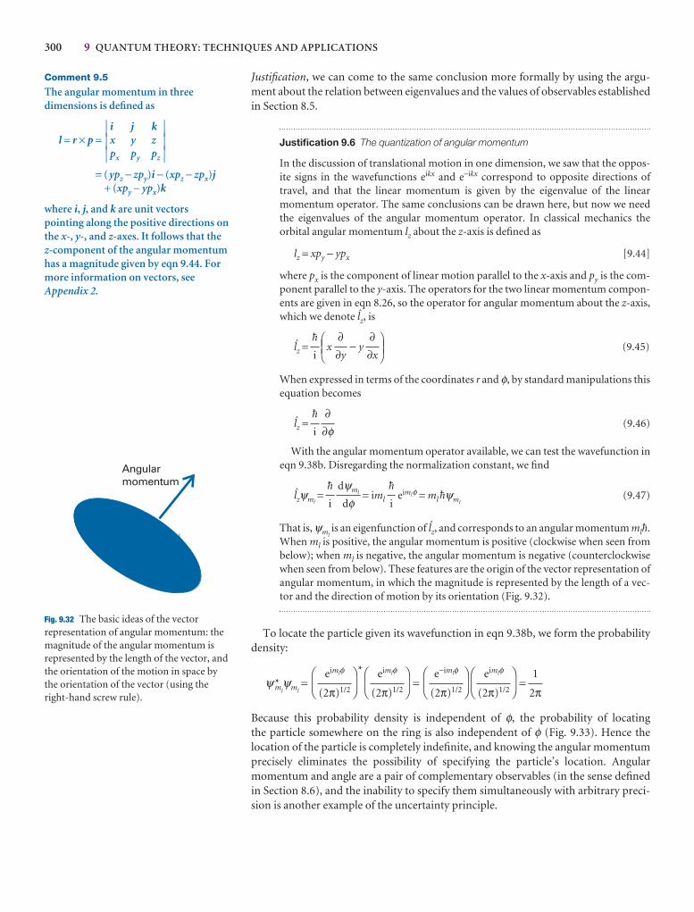
300 9 QUANTUM THEORY: TECHNIQUES AND APPLICATIONS
Justification, we can come to the same conclusion more formally by using the argu-ment about the relation between eigenvalues and the values of observables establishedin Section 8.5.
Justification 9.6 The quantization of angular momentum
In the discussion of translational motion in one dimension, we saw that the oppos-ite signs in the wavefunctions eikx and e−ikx correspond to opposite directions oftravel, and that the linear momentum is given by the eigenvalue of the linear momentum operator. The same conclusions can be drawn here, but now we needthe eigenvalues of the angular momentum operator. In classical mechanics the orbital angular momentum lz about the z-axis is defined as
lz = xpy − ypx [9.44]
where px is the component of linear motion parallel to the x-axis and py is the com-ponent parallel to the y-axis. The operators for the two linear momentum compon-ents are given in eqn 8.26, so the operator for angular momentum about the z-axis,which we denote Zz, is
Zz = x − y (9.45)
When expressed in terms of the coordinates r and φ, by standard manipulations thisequation becomes
Zz = (9.46)
With the angular momentum operator available, we can test the wavefunction ineqn 9.38b. Disregarding the normalization constant, we find
Zzψml= = iml eimlφ = ml $ψml
(9.47)
That is, ψmlis an eigenfunction of Zz, and corresponds to an angular momentum ml$.
When ml is positive, the angular momentum is positive (clockwise when seen frombelow); when ml is negative, the angular momentum is negative (counterclockwisewhen seen from below). These features are the origin of the vector representation ofangular momentum, in which the magnitude is represented by the length of a vec-tor and the direction of motion by its orientation (Fig. 9.32).
To locate the particle given its wavefunction in eqn 9.38b, we form the probabilitydensity:
ψ*mlψml
=*
= =
Because this probability density is independent of φ, the probability of locating the particle somewhere on the ring is also independent of φ (Fig. 9.33). Hence the location of the particle is completely indefinite, and knowing the angular momentumprecisely eliminates the possibility of specifying the particle’s location. Angular momentum and angle are a pair of complementary observables (in the sense definedin Section 8.6), and the inability to specify them simultaneously with arbitrary preci-sion is another example of the uncertainty principle.
1
2π
DF
eimlφ
(2π)1/2
AC
DF
e−imlφ
(2π)1/2
AC
DF
eimlφ
(2π)1/2
AC
DF
eimlφ
(2π)1/2
AC
$
i
dψml
dφ$
i
∂∂φ
$
i
DEF∂∂x
∂∂y
ABC$
i
Comment 9.5
The angular momentum in threedimensions is defined as
l = r × p =
= (ypz − zpy)i − (xpz − zpx)j+ (xpy − ypx)k
where i, j, and k are unit vectorspointing along the positive directions onthe x-, y-, and z-axes. It follows that thez-component of the angular momentumhas a magnitude given by eqn 9.44. Formore information on vectors, seeAppendix 2.
iii
i j kx y zpx py pz
iii
Angularmomentum
Fig. 9.32 The basic ideas of the vectorrepresentation of angular momentum: themagnitude of the angular momentum isrepresented by the length of the vector, andthe orientation of the motion in space bythe orientation of the vector (using theright-hand screw rule).
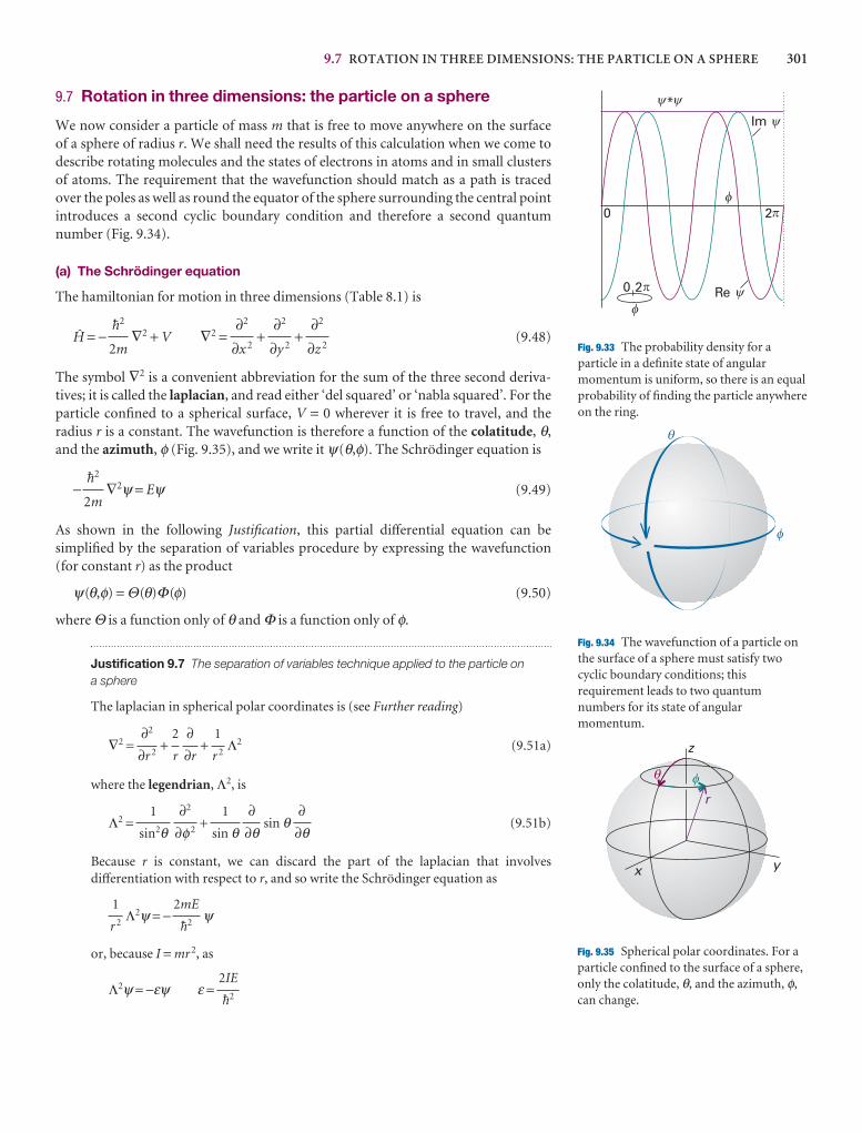
9.7 ROTATION IN THREE DIMENSIONS: THE PARTICLE ON A SPHERE 301
9.7 Rotation in three dimensions: the particle on a sphere
We now consider a particle of mass m that is free to move anywhere on the surface of a sphere of radius r. We shall need the results of this calculation when we come todescribe rotating molecules and the states of electrons in atoms and in small clustersof atoms. The requirement that the wavefunction should match as a path is tracedover the poles as well as round the equator of the sphere surrounding the central pointintroduces a second cyclic boundary condition and therefore a second quantumnumber (Fig. 9.34).
(a) The Schrödinger equation
The hamiltonian for motion in three dimensions (Table 8.1) is
@ = − ∇2 + V ∇2 = + + (9.48)
The symbol ∇2 is a convenient abbreviation for the sum of the three second deriva-tives; it is called the laplacian, and read either ‘del squared’ or ‘nabla squared’. For theparticle confined to a spherical surface, V = 0 wherever it is free to travel, and the radius r is a constant. The wavefunction is therefore a function of the colatitude, θ,and the azimuth, φ (Fig. 9.35), and we write it ψ(θ,φ). The Schrödinger equation is
− ∇2ψ = Eψ (9.49)
As shown in the following Justification, this partial differential equation can be simplified by the separation of variables procedure by expressing the wavefunction(for constant r) as the product
ψ(θ,φ) = Θ(θ)Φ(φ) (9.50)
where Θ is a function only of θ and Φ is a function only of φ.
Justification 9.7 The separation of variables technique applied to the particle on a sphere
The laplacian in spherical polar coordinates is (see Further reading)
∇2 = + + Λ2 (9.51a)
where the legendrian, Λ2, is
Λ2 = + sin θ (9.51b)
Because r is constant, we can discard the part of the laplacian that involvesdifferentiation with respect to r, and so write the Schrödinger equation as
Λ2ψ = − ψ
or, because I = mr 2, as
Λ2ψ = −εψ ε =2IE
$2
2mE
$2
1
r 2
∂∂θ
∂∂θ
1
sin θ∂2
∂φ2
1
sin2θ
1
r 2
∂∂r
2
r
∂2
∂r 2
$2
2m
∂2
∂z 2
∂2
∂y 2
∂2
∂x 2
$2
2m
Re
Im
�
*
0
2�
2
0
� �
�
�
�
�
q
f
Fig. 9.33 The probability density for aparticle in a definite state of angularmomentum is uniform, so there is an equalprobability of finding the particle anywhereon the ring.
Fig. 9.34 The wavefunction of a particle onthe surface of a sphere must satisfy twocyclic boundary conditions; thisrequirement leads to two quantumnumbers for its state of angularmomentum.
z
x y
r
q
f
Fig. 9.35 Spherical polar coordinates. For aparticle confined to the surface of a sphere,only the colatitude, θ, and the azimuth, φ,can change.
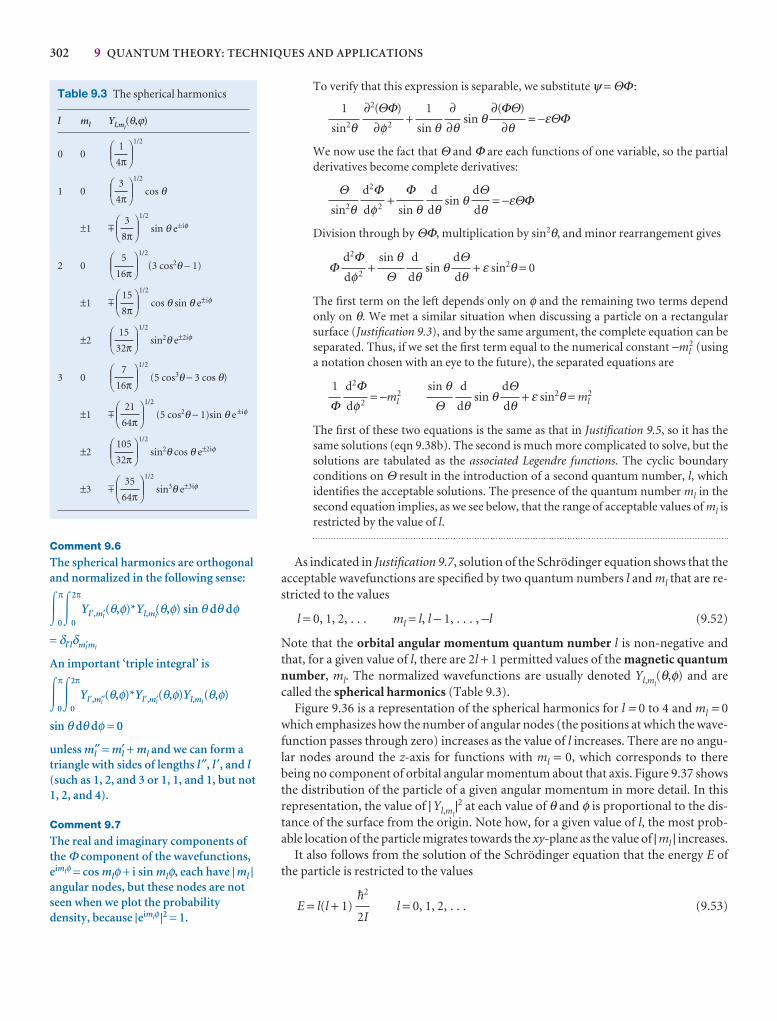
302 9 QUANTUM THEORY: TECHNIQUES AND APPLICATIONS
To verify that this expression is separable, we substitute ψ = ΘΦ :
+ sin θ = −εΘΦ
We now use the fact that Θ and Φ are each functions of one variable, so the partialderivatives become complete derivatives:
+ sin θ = −εΘΦ
Division through by ΘΦ, multiplication by sin2θ, and minor rearrangement gives
Φ + sin θ + ε sin2θ = 0
The first term on the left depends only on φ and the remaining two terms dependonly on θ. We met a similar situation when discussing a particle on a rectangularsurface (Justification 9.3), and by the same argument, the complete equation can beseparated. Thus, if we set the first term equal to the numerical constant −ml
2 (usinga notation chosen with an eye to the future), the separated equations are
= −ml2 sin θ + ε sin2θ = ml
2
The first of these two equations is the same as that in Justification 9.5, so it has thesame solutions (eqn 9.38b). The second is much more complicated to solve, but thesolutions are tabulated as the associated Legendre functions. The cyclic boundaryconditions on Θ result in the introduction of a second quantum number, l, whichidentifies the acceptable solutions. The presence of the quantum number ml in thesecond equation implies, as we see below, that the range of acceptable values of ml isrestricted by the value of l.
As indicated in Justification 9.7, solution of the Schrödinger equation shows that theacceptable wavefunctions are specified by two quantum numbers l and ml that are re-stricted to the values
l = 0, 1, 2, . . . ml = l, l − 1, . . . , −l (9.52)
Note that the orbital angular momentum quantum number l is non-negative andthat, for a given value of l, there are 2l + 1 permitted values of the magnetic quantumnumber, ml. The normalized wavefunctions are usually denoted Yl,ml
(θ,φ) and arecalled the spherical harmonics (Table 9.3).
Figure 9.36 is a representation of the spherical harmonics for l = 0 to 4 and ml = 0which emphasizes how the number of angular nodes (the positions at which the wave-function passes through zero) increases as the value of l increases. There are no angu-lar nodes around the z-axis for functions with ml = 0, which corresponds to therebeing no component of orbital angular momentum about that axis. Figure 9.37 showsthe distribution of the particle of a given angular momentum in more detail. In thisrepresentation, the value of | Yl,ml
|2 at each value of θ and φ is proportional to the dis-tance of the surface from the origin. Note how, for a given value of l, the most prob-able location of the particle migrates towards the xy-plane as the value of | ml | increases.
It also follows from the solution of the Schrödinger equation that the energy E ofthe particle is restricted to the values
E = l(l + 1) l = 0, 1, 2, . . . (9.53)$2
2I
dΘdθ
d
dθsin θ
Θd2Φdφ2
1
Φ
dΘdθ
d
dθsin θ
Θd2Φdφ2
dΘdθ
d
dθΦ
sin θd2Φdφ2
Θsin2θ
∂(ΦΘ)
∂θ∂
∂θ1
sin θ∂2(ΘΦ)
∂φ2
1
sin2θ
Table 9.3 The spherical harmonics
l ml Yl,ml(θ,ϕ)
0 01/2
1 01/2
cos θ
±1 ,1/2
sin θ e±iφ
2 01/2
(3 cos2θ − 1)
±1 ,1/2
cos θ sin θ e±iφ
±21/2
sin2θ e±2iφ
3 01/2
(5 cos3θ − 3 cos θ)
±1 ,1/2
(5 cos2θ − 1)sin θ e±iφ
±21/2
sin2θ cos θ e±2iφ
±3 ,1/2
sin3θ e±3iφDEF35
64πABC
DEF105
32πABC
DEF21
64πABC
DEF7
16πABC
DEF15
32πABC
DEF15
8πABC
DEF5
16πABC
DEF3
8πABC
DEF3
4πABC
DEF1
4πABC
Comment 9.6
The spherical harmonics are orthogonaland normalized in the following sense:
�0
π
�0
2π
Yl′,ml′(θ,φ)*Yl,ml(θ,φ) sin θ dθ dφ
= δl′lδml′ml
An important ‘triple integral’ is
�0
π
�0
2π
Yl′,ml″(θ,φ)*Yl′,ml′(θ,φ)Yl,ml(θ,φ)
sin θ dθ dφ = 0
unless ml″ = ml′ + ml and we can form atriangle with sides of lengths l″, l ′, and l(such as 1, 2, and 3 or 1, 1, and 1, but not1, 2, and 4).
Comment 9.7
The real and imaginary components ofthe Φ component of the wavefunctions,eimlφ = cos mlφ + i sin mlφ, each have | ml |angular nodes, but these nodes are notseen when we plot the probabilitydensity, because |eimlφ |2 = 1.
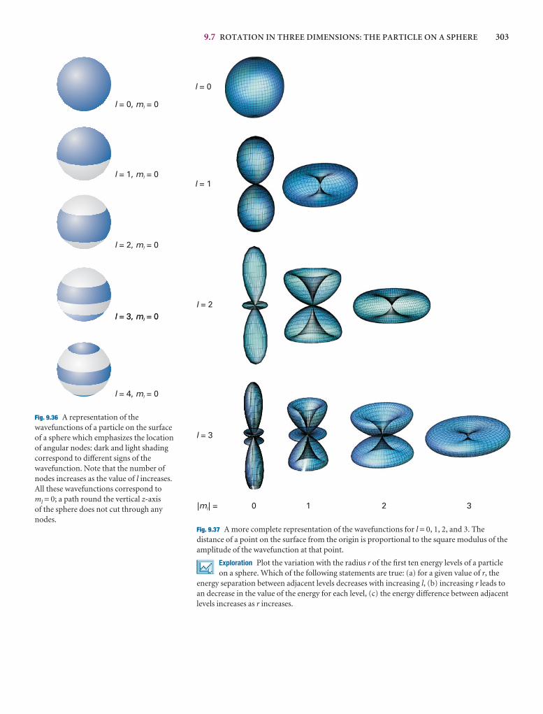
9.7 ROTATION IN THREE DIMENSIONS: THE PARTICLE ON A SPHERE 303
l = 0
l = 1
l = 2
l = 3
1 2 3| | =ml 0
Fig. 9.37 A more complete representation of the wavefunctions for l = 0, 1, 2, and 3. Thedistance of a point on the surface from the origin is proportional to the square modulus of theamplitude of the wavefunction at that point.
Exploration Plot the variation with the radius r of the first ten energy levels of a particleon a sphere. Which of the following statements are true: (a) for a given value of r, the
energy separation between adjacent levels decreases with increasing l, (b) increasing r leads toan decrease in the value of the energy for each level, (c) the energy difference between adjacentlevels increases as r increases.
l m= 0, = 0l
l m= 4, = 0l
l m= 3, = 0l
l m= 2, = 0l
l m= 1, = 0l
l m= 3, = 0l
Fig. 9.36 A representation of thewavefunctions of a particle on the surfaceof a sphere which emphasizes the locationof angular nodes: dark and light shadingcorrespond to different signs of thewavefunction. Note that the number ofnodes increases as the value of l increases.All these wavefunctions correspond to ml = 0; a path round the vertical z-axisof the sphere does not cut through anynodes.
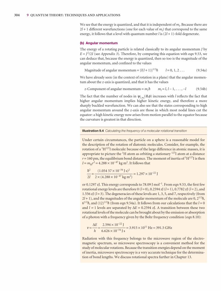
304 9 QUANTUM THEORY: TECHNIQUES AND APPLICATIONS
We see that the energy is quantized, and that it is independent of ml. Because there are2l + 1 different wavefunctions (one for each value of ml) that correspond to the sameenergy, it follows that a level with quantum number l is (2l + 1)-fold degenerate.
(b) Angular momentum
The energy of a rotating particle is related classically to its angular momentum J byE = J 2/2I (see Appendix 3). Therefore, by comparing this equation with eqn 9.53, wecan deduce that, because the energy is quantized, then so too is the magnitude of the angular momentum, and confined to the values
Magnitude of angular momentum = {l(l + 1)}1/2$ l = 0, 1, 2 . . . (9.54a)
We have already seen (in the context of rotation in a plane) that the angular momen-tum about the z-axis is quantized, and that it has the values
z-Component of angular momentum = ml $ ml = l, l − 1, . . . , −l (9.54b)
The fact that the number of nodes in ψl,ml(θ,φ) increases with l reflects the fact that
higher angular momentum implies higher kinetic energy, and therefore a moresharply buckled wavefunction. We can also see that the states corresponding to highangular momentum around the z-axis are those in which most nodal lines cut theequator: a high kinetic energy now arises from motion parallel to the equator becausethe curvature is greatest in that direction.
Illustration 9.4 Calculating the frequency of a molecular rotational transition
Under certain circumstances, the particle on a sphere is a reasonable model for the description of the rotation of diatomic molecules. Consider, for example, therotation of a 1H127I molecule: because of the large difference in atomic masses, it isappropriate to picture the 1H atom as orbiting a stationary 127I atom at a distancer = 160 pm, the equilibrium bond distance. The moment of inertia of 1H127I is thenI = mHr2 = 4.288 × 10−47 kg m2. It follows that
= = 1.297 × 10⁻²² J
or 0.1297 zJ. This energy corresponds to 78.09 J mol−1. From eqn 9.53, the first fewrotational energy levels are therefore 0 (l = 0), 0.2594 zJ (l = 1), 0.7782 zJ (l = 2), and1.556 zJ (l = 3). The degeneracies of these levels are 1, 3, 5, and 7, respectively (from2l + 1), and the magnitudes of the angular momentum of the molecule are 0, 21/2$,61/2$, and (12)1/2$ (from eqn 9.54a). It follows from our calculations that the l = 0and l = 1 levels are separated by ∆E = 0.2594 zJ. A transition between these two rotational levels of the molecule can be brought about by the emission or absorptionof a photon with a frequency given by the Bohr frequency condition (eqn 8.10):
ν = = = 3.915 × 10¹¹ Hz = 391.5 GHz
Radiation with this frequency belongs to the microwave region of the electro-magnetic spectrum, so microwave spectroscopy is a convenient method for thestudy of molecular rotations. Because the transition energies depend on the momentof inertia, microwave spectroscopy is a very accurate technique for the determina-tion of bond lengths. We discuss rotational spectra further in Chapter 13.
2.594 × 10⁻²² J
6.626 × 10⁻³⁴ J s
∆E
h
(1.054 57 × 10−34 J s)2
2 × (4.288 × 10−47 kg m2)
$2
2I
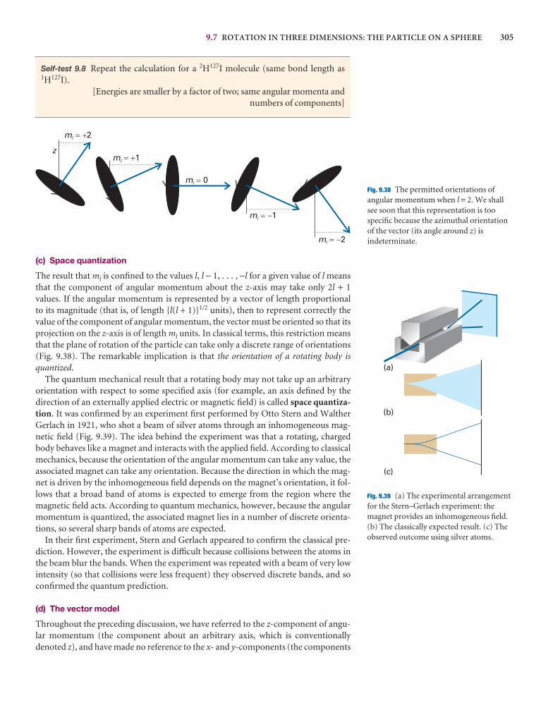
9.7 ROTATION IN THREE DIMENSIONS: THE PARTICLE ON A SPHERE 305
Self-test 9.8 Repeat the calculation for a 2H127I molecule (same bond length as1H127I).
[Energies are smaller by a factor of two; same angular momenta and numbers of components]
ml 1� �
ml 0�
ml 1� �
ml 2� �
ml 2� �
z
Fig. 9.38 The permitted orientations ofangular momentum when l = 2. We shallsee soon that this representation is toospecific because the azimuthal orientationof the vector (its angle around z) isindeterminate.
(a)
(b)
(c)
Fig. 9.39 (a) The experimental arrangementfor the Stern–Gerlach experiment: themagnet provides an inhomogeneous field.(b) The classically expected result. (c) Theobserved outcome using silver atoms.
(c) Space quantization
The result that ml is confined to the values l, l − 1, . . . , −l for a given value of l meansthat the component of angular momentum about the z-axis may take only 2l + 1values. If the angular momentum is represented by a vector of length proportional to its magnitude (that is, of length {l(l + 1)}1/2 units), then to represent correctly thevalue of the component of angular momentum, the vector must be oriented so that itsprojection on the z-axis is of length ml units. In classical terms, this restriction meansthat the plane of rotation of the particle can take only a discrete range of orientations(Fig. 9.38). The remarkable implication is that the orientation of a rotating body isquantized.
The quantum mechanical result that a rotating body may not take up an arbitraryorientation with respect to some specified axis (for example, an axis defined by the direction of an externally applied electric or magnetic field) is called space quantiza-tion. It was confirmed by an experiment first performed by Otto Stern and WaltherGerlach in 1921, who shot a beam of silver atoms through an inhomogeneous mag-netic field (Fig. 9.39). The idea behind the experiment was that a rotating, chargedbody behaves like a magnet and interacts with the applied field. According to classicalmechanics, because the orientation of the angular momentum can take any value, theassociated magnet can take any orientation. Because the direction in which the mag-net is driven by the inhomogeneous field depends on the magnet’s orientation, it fol-lows that a broad band of atoms is expected to emerge from the region where themagnetic field acts. According to quantum mechanics, however, because the angularmomentum is quantized, the associated magnet lies in a number of discrete orienta-tions, so several sharp bands of atoms are expected.
In their first experiment, Stern and Gerlach appeared to confirm the classical pre-diction. However, the experiment is difficult because collisions between the atoms inthe beam blur the bands. When the experiment was repeated with a beam of very lowintensity (so that collisions were less frequent) they observed discrete bands, and soconfirmed the quantum prediction.
(d) The vector model
Throughout the preceding discussion, we have referred to the z-component of angu-lar momentum (the component about an arbitrary axis, which is conventionally denoted z), and have made no reference to the x- and y-components (the components
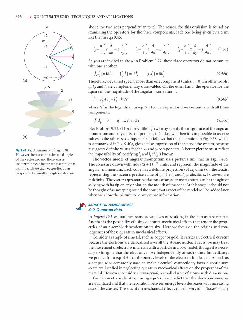
306 9 QUANTUM THEORY: TECHNIQUES AND APPLICATIONS
about the two axes perpendicular to z). The reason for this omission is found by examining the operators for the three components, each one being given by a termlike that in eqn 9.45:
Zx = y − z Zy = z − x Zz = x − y (9.55)
As you are invited to show in Problem 9.27, these three operators do not commutewith one another:
[Zx,Zy] = i$Zz [Zy,Zz] = i$Zx [Zz,Zx] = i$Zy (9.56a)
Therefore, we cannot specify more than one component (unless l = 0). In other words,lx, ly, and lz are complementary observables. On the other hand, the operator for thesquare of the magnitude of the angular momentum is
Z 2 = Z 2x + Z 2
y + Z 2z = $2Λ2 (9.56b)
where Λ2 is the legendrian in eqn 9.51b. This operator does commute with all threecomponents:
[Z 2,Zq] = 0 q = x, y, and z (9.56c)
(See Problem 9.29.) Therefore, although we may specify the magnitude of the angularmomentum and any of its components, if lz is known, then it is impossible to ascribevalues to the other two components. It follows that the illustration in Fig. 9.38, whichis summarized in Fig. 9.40a, gives a false impression of the state of the system, becauseit suggests definite values for the x- and y-components. A better picture must reflectthe impossibility of specifying lx and ly if lz is known.
The vector model of angular momentum uses pictures like that in Fig. 9.40b. The cones are drawn with side {l(l + 1)}1/2 units, and represent the magnitude of theangular momentum. Each cone has a definite projection (of ml units) on the z-axis,representing the system’s precise value of lz. The lx and ly projections, however, areindefinite. The vector representing the state of angular momentum can be thought ofas lying with its tip on any point on the mouth of the cone. At this stage it should notbe thought of as sweeping round the cone; that aspect of the model will be added laterwhen we allow the picture to convey more information.
IMPACT ON NANOSCIENCE
I9.2 Quantum dots
In Impact I9.1 we outlined some advantages of working in the nanometre regime.Another is the possibility of using quantum mechanical effects that render the prop-erties of an assembly dependent on its size. Here we focus on the origins and con-sequences of these quantum mechanical effects.
Consider a sample of a metal, such as copper or gold. It carries an electrical currentbecause the electrons are delocalized over all the atomic nuclei. That is, we may treatthe movement of electrons in metals with a particle in a box model, though it is neces-sary to imagine that the electrons move independently of each other. Immediately, we predict from eqn 9.6 that the energy levels of the electrons in a large box, such as a copper wire commonly used to make electrical connections, form a continuum so we are justified in neglecting quantum mechanical effects on the properties of thematerial. However, consider a nanocrystal, a small cluster of atoms with dimensions in the nanometre scale. Again using eqn 9.6, we predict that the electronic energies are quantized and that the separation between energy levels decreases with increasingsize of the cluster. This quantum mechanical effect can be observed in ‘boxes’ of any
DF
∂∂x
∂∂y
AC
$
i
DF
∂∂z
∂∂x
AC
$
i
DF
∂∂y
∂∂z
AC
$
i
�2
�1
0
�1
�2
z
ml
(a)
�1
�2
z�2
�1
0
(b)
Fig. 9.40 (a) A summary of Fig. 9.38.However, because the azimuthal angle of the vector around the z-axis isindeterminate, a better representation is as in (b), where each vector lies at anunspecified azimuthal angle on its cone.
I9.2 IMPACT ON NANOSCIENCE: QUANTUM DOTS 307
shape. For example, you are invited to show in Problem 9.39 that the energy levels ofan electron in a sphere of radius R are given by
En = (9.57)
The quantization of energy in nanocrystals has important technological implica-tions when the material is a semiconductor, in which the electrical conductivity increases with increasing temperature or upon excitation by light (see Chapter 20 for a more detailed discussion). Transfer of energy to a semiconductor increases the mobility of electrons in the material. However, for every electron that moves to adifferent site in the sample, a unit of positive charge, called a hole, is left behind. Theholes are also mobile, so to describe electrical conductivity in semiconductors we needto consider the movement of electron–hole pairs, also called excitons, in the material.
The electrons and holes may be regarded as particles trapped in a box, so eqn 9.6can give us qualitative insight into the origins of conductivity in semiconductors. Weconclude as before that only in nanocrystals are the energies of the charge carriersquantized. Now we explore the impact of energy quantization on the optical and elec-tronic properties of semiconducting nanocrystals.
Three-dimensional nanocrystals of semiconducting materials containing 103 to 105
atoms are called quantum dots. They can be made in solution or by depositing atomson a surface, with the size of the nanocrystal being determined by the details of thesynthesis (see, for example, Impact I20.2). A quantitative but approximate treatmentthat leads to the energy of the exciton begins with the following hamiltonian for aspherical quantum dot of radius R:
@ = − ∇2e − ∇2
h + V(re,rh) (9.58)
where the first two terms are the kinetic energy operators for the electron and hole(with masses me and mh, respectively), and the third term is the potential energy of interaction between electron and hole, which are located at positions re and rh fromthe centre of the sphere. Taking into account only the Coulomb attraction betweenthe hole, with charge +e, and the electron, with charge −e, we write (see Chapter 9 andAppendix 3 for details):
V(re,rh) = − (9.59)
where | re − rh | is the distance between the electron and hole and ε is the permittivityof the medium (we are ignoring the effect of polarization of the medium due to thepresence of charges). Solving the Schrödinger equation in this case is not a trivial task,but the final expression for the energy of the exciton, Eex, is relatively simple (seeFurther reading for details):
Eex = + − (9.60)
As expected, we see that the energy of the exciton decreases with increasing radius of the quantum dot. Moreover, for small R, the second term on the right of the pre-ceding equation is smaller than the first term and the energy of the exciton is largelykinetic, with the resulting expression resembling the case for a particle in a sphere.
The expression for Eex has important consequences for the optical properties ofquantum dots. First, we see that the energy required to create mobile charge carriersand to induce electrical conductivity depends on the size of the quantum dot. The
1.8e2
4πεR
DF
1
mh
1
me
AC
h2
8R2
e2
4πε | re − rh |
$2
2mh
$2
2me
n2h2
8me R2
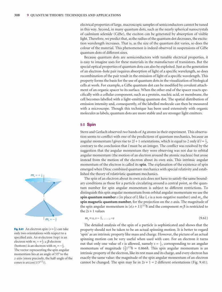
308 9 QUANTUM THEORY: TECHNIQUES AND APPLICATIONS
electrical properties of large, macroscopic samples of semiconductors cannot be tunedin this way. Second, in many quantum dots, such as the nearly spherical nanocrystalsof cadmium selenide (CdSe), the exciton can be generated by absorption of visiblelight. Therefore, we predict that, as the radius of the quantum dot decreases, the excita-tion wavelength increases. That is, as the size of the quantum dot varies, so does thecolour of the material. This phenomenon is indeed observed in suspensions of CdSequantum dots of different sizes.
Because quantum dots are semiconductors with tunable electrical properties, it is easy to imagine uses for these materials in the manufacture of transistors. But thespecial optical properties of quantum dots can also be exploited. Just as the generationof an electron–hole pair requires absorption of light of a specific wavelength, so doesrecombination of the pair result in the emission of light of a specific wavelength. Thisproperty forms the basis for the use of quantum dots in the visualization of biologicalcells at work. For example, a CdSe quantum dot can be modified by covalent attach-ment of an organic spacer to its surface. When the other end of the spacer reacts spe-cifically with a cellular component, such as a protein, nucleic acid, or membrane, thecell becomes labelled with a light-emitting quantum dot. The spatial distribution ofemission intensity and, consequently, of the labelled molecule can then be measuredwith a microscope. Though this technique has been used extensively with organicmolecules as labels, quantum dots are more stable and are stronger light emitters.
9.8 Spin
Stern and Gerlach observed two bands of Ag atoms in their experiment. This observa-tion seems to conflict with one of the predictions of quantum mechanics, because anangular momentum l gives rise to 2l + 1 orientations, which is equal to 2 only if l = 1–2 ,contrary to the conclusion that l must be an integer. The conflict was resolved by thesuggestion that the angular momentum they were observing was not due to orbitalangular momentum (the motion of an electron around the atomic nucleus) but aroseinstead from the motion of the electron about its own axis. This intrinsic angularmomentum of the electron is called its spin. The explanation of the existence of spinemerged when Dirac combined quantum mechanics with special relativity and estab-lished the theory of relativistic quantum mechanics.
The spin of an electron about its own axis does not have to satisfy the same bound-ary conditions as those for a particle circulating around a central point, so the quan-tum number for spin angular momentum is subject to different restrictions. Todistinguish this spin angular momentum from orbital angular momentum we use thespin quantum number s (in place of l; like l, s is a non-negative number) and ms, thespin magnetic quantum number, for the projection on the z-axis. The magnitude ofthe spin angular momentum is {s(s + 1)}1/2$ and the component ms$ is restricted tothe 2s + 1 values
ms = s, s − 1, . . . , −s (9.61)
The detailed analysis of the spin of a particle is sophisticated and shows that theproperty should not be taken to be an actual spinning motion. It is better to regard‘spin’ as an intrinsic property like mass and charge. However, the picture of an actualspinning motion can be very useful when used with care. For an electron it turns out that only one value of s is allowed, namely s = 1–2 , corresponding to an angular momentum of magnitude (3–4)1/2$ = 0.866$. This spin angular momentum is an intrinsic property of the electron, like its rest mass and its charge, and every electron hasexactly the same value: the magnitude of the spin angular momentum of an electroncannot be changed. The spin may lie in 2s + 1 = 2 different orientations (Fig. 9.41).
ms � �
ms � � 21�
21�
Fig. 9.41 An electron spin (s = 1–2) can takeonly two orientations with respect to aspecified axis. An α electron (top) is anelectron with ms = + 1–2 ; a β electron(bottom) is an electron with ms = − 1–2.The vector representing the spin angularmomentum lies at an angle of 55° to the z-axis (more precisely, the half-angle of thecones is arccos(1/31/2)).
9.8 SPIN 309
One orientation corresponds to ms = +1–2 (this state is often denoted α or ↑); the otherorientation corresponds to ms = − 1–2 (this state is denoted β or ↓).
The outcome of the Stern–Gerlach experiment can now be explained if we supposethat each Ag atom possesses an angular momentum due to the spin of a single elec-tron, because the two bands of atoms then correspond to the two spin orientations.Why the atoms behave like this is explained in Chapter 10 (but it is already probablyfamiliar from introductory chemistry that the ground-state configuration of a silveratom is [Kr]4d105s1, a single unpaired electron outside a closed shell).
Like the electron, other elementary particles have characteristic spin. For example,protons and neutrons are spin-1–2 particles (that is, s = 1–2 ) and invariably spin with angular momentum (3–4)1/2$ = 0.866$. Because the masses of a proton and a neutronare so much greater than the mass of an electron, yet they all have the same spin angular momentum, the classical picture would be of these two particles spinningmuch more slowly than an electron. Some elementary particles have s = 1, and so havean intrinsic angular momentum of magnitude 21/2$. Some mesons are spin-1 particles(as are some atomic nuclei), but for our purposes the most important spin-1 particleis the photon. From the discussion in this chapter, we see that the photon has zero restmass, zero charge, an energy hν, a linear momentum h/λ or hν/c, an intrinsic angularmomentum of 21/2$, and travels at the speed c. We shall see the importance of photonspin in the next chapter.
Particles with half-integral spin are called fermions and those with integral spin(including 0) are called bosons. Thus, electrons and protons are fermions and pho-tons are bosons. It is a very deep feature of nature that all the elementary particles thatconstitute matter are fermions whereas the elementary particles that are responsiblefor the forces that bind fermions together are all bosons. Photons, for example, trans-mit the electromagnetic force that binds together electrically charged particles. Matter,therefore, is an assembly of fermions held together by forces conveyed by bosons.
The properties of angular momentum that we have developed are set out in Table 9.4. As mentioned there, when we use the quantum numbers l and ml we shallmean orbital angular momentum (circulation in space). When we use s and ms weshall mean spin angular momentum (intrinsic angular momentum). When we use jand mj we shall mean either (or, in some contexts to be described in Chapter 10, acombination of orbital and spin momenta).
Table 9.4 Properties of angular momentum
Quantum number Symbol Values* Specifies
Orbital angular momentum l 0, 1, 2, . . . Magnitude, {l(l + 1)}1/2$
Magnetic ml l, l − 1, . . . , −l Component on z-axis, ml $
Spin s 1–2 Magnitude, {s(s + 1)}1/2$
Spin magnetic ms ± 1–2 Component on z-axis, ms $
Total j l + s, l + s − 1, . . . , | l − s | Magnitude, {j( j + 1)}1/2$
Total magnetic mj j, j − 1, . . . , −j Component on z-axis, mj $
To combine two angular momenta, use the Clebsch–Gordan series:
j = j1 + j2, j1 + j2 − 1, . . . , | j1 − j2 |
For many-electron systems, the quantum numbers are designated by uppercase letters (L, ML, S, MS, etc.).
*Note that the quantum numbers for magnitude (l, s, j, etc.) are never negative.
310 9 QUANTUM THEORY: TECHNIQUES AND APPLICATIONS
Techniques of approximation
All the applications treated so far have had exact solutions. However, many problems—and almost all the problems of interest in chemistry—do not have exact solutions.To make progress with these problems we need to develop techniques of approxima-tion. There are two major approaches, variation theory and perturbation theory.Variation theory is most commonly encountered in the context of molecular orbitaltheory, and we consider it there (Chapter 11). Here, we concentrate on perturbationtheory.
9.9 Time-independent perturbation theory
In perturbation theory, we suppose that the hamiltonian for the problem we are try-ing to solve, @, can be expressed as the sum of a simple hamiltonian, @ (0), which hasknown eigenvalues and eigenfunctions, and a contribution, @ (1), which representsthe extent to which the true hamiltonian differs from the ‘model’ hamiltonian:
@ = @ (0) + @ (1) (9.62)
In time-independent perturbation theory, the perturbation is always present andunvarying. For example, it might represent a dip in the potential energy of a particlein a box in some region along the length of the box.
In time-independent perturbation theory, we suppose that the true energy of thesystem differs from the energy of the simple system, and that we can write
E = E (0) + E (1) + E (2) + . . . (9.63)
where E (1) is the ‘first-order correction’ to the energy, a contribution proportional to@ (1), and E (2) is the ‘second-order correction’ to the energy, a contribution propor-tional to @ (1)2, and so on. The true wavefunction also differs from the ‘simple’ wave-function, and we write
ψ = ψ (0) + ψ (1) + ψ (2) + . . . (9.64)
In practice, we need to consider only the ‘first-order correction’ to the wavefunction,ψ (1). As we show in Further information 9.2, the first- and second-order corrections tothe energy of the ground state (with the wavefunction ψ0 and energy E0), are
E0(1) = �ψ 0
(0)*@ (1)ψ 0(0)dτ = H00
(1) (9.65a)
and
E0(2) = ∑
n≠0
2
= ∑n≠0
(9.65b)
where we have introduced the matrix element
Ωnm = �ψn*)ψmdτ [9.65c]
in a convenient compact notation for integrals that we shall use frequently.As usual, it is important to be able to interpret these equations physically. We can
interpret E (1) as the average value of the perturbation, calculated by using the unper-turbed wavefunction. An analogy is the shift in energy of vibration of a violin string
| H n0(1) |2
E0(0) − En
(0)
�ψ 0(0)*@ (1)ψ 0
(0)dτ
E0(0) − En
(0)
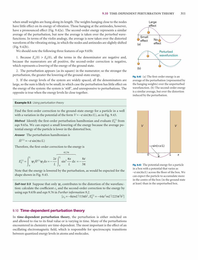
9.10 TIME-DEPENDENT PERTURBATION THEORY 311
Largeeffect
Noeffect
Smalleffect
(a)
(b)
Perturbedwavefunction
Fig. 9.42 (a) The first-order energy is anaverage of the perturbation (represented bythe hanging weights) over the unperturbedwavefunction. (b) The second-order energyis a similar average, but over the distortioninduced by the perturbation.
V
0 L x
– sin( / )x L
V
e p
Fig. 9.43 The potential energy for a particle in a box with a potential that varies as −ε sin(πx/L) across the floor of the box. Wecan expect the particle to accumulate morein the centre of the box (in the ground stateat least) than in the unperturbed box.
when small weights are hung along its length. The weights hanging close to the nodeshave little effect on its energy of vibration. Those hanging at the antinodes, however,have a pronounced effect (Fig. 9.42a). The second-order energy represents a similaraverage of the perturbation, but now the average is taken over the perturbed wave-functions. In terms of the violin analogy, the average is now taken over the distortedwaveform of the vibrating string, in which the nodes and antinodes are slightly shifted(Fig. 9.42b).
We should note the following three features of eqn 9.65b:
1. Because En(0) > E0(0), all the terms in the denominator are negative and, because the numerators are all positive, the second-order correction is negative,which represents a lowering of the energy of the ground state.
2. The perturbation appears (as its square) in the numerator; so the stronger theperturbation, the greater the lowering of the ground-state energy.
3. If the energy levels of the system are widely spaced, all the denominators arelarge, so the sum is likely to be small; in which case the perturbation has little effect onthe energy of the system: the system is ‘stiff ’, and unresponsive to perturbations. Theopposite is true when the energy levels lie close together.
Example 9.5 Using perturbation theory
Find the first-order correction to the ground-state energy for a particle in a wellwith a variation in the potential of the form V = −ε sin(πx /L), as in Fig. 9.43.
Method Identify the first-order perturbation hamiltonian and evaluate E0(1) from
eqn 9.65a. We can expect a small lowering of the energy because the average po-tential energy of the particle is lower in the distorted box.
Answer The perturbation hamiltonian is
@ (1) = −ε sin(πx /L)
Therefore, the first-order correction to the energy is
4L/3π
E0(1) = �
L
0
ψ1@(1)ψ1dx = − �L
0
sin3 dx = −
Note that the energy is lowered by the perturbation, as would be expected for theshape shown in Fig. 9.43.
Self-test 9.9 Suppose that only ψ3 contributes to the distortion of the wavefunc-tion: calculate the coefficient c3 and the second-order correction to the energy byusing eqn 9.65b and eqn 9.76 in Further information 9.2.
[c3 = −8εmL2/15πh2, E0(2) = −64ε2mL2/225π2h2]
9.10 Time-dependent perturbation theory
In time-dependent perturbation theory, the perturbation is either switched on and allowed to rise to its final value or is varying in time. Many of the perturbations encountered in chemistry are time-dependent. The most important is the effect of anoscillating electromagnetic field, which is responsible for spectroscopic transitionsbetween quantized energy levels in atoms and molecules.
8ε3π
πx
L
2εL
5 4 6 4 7
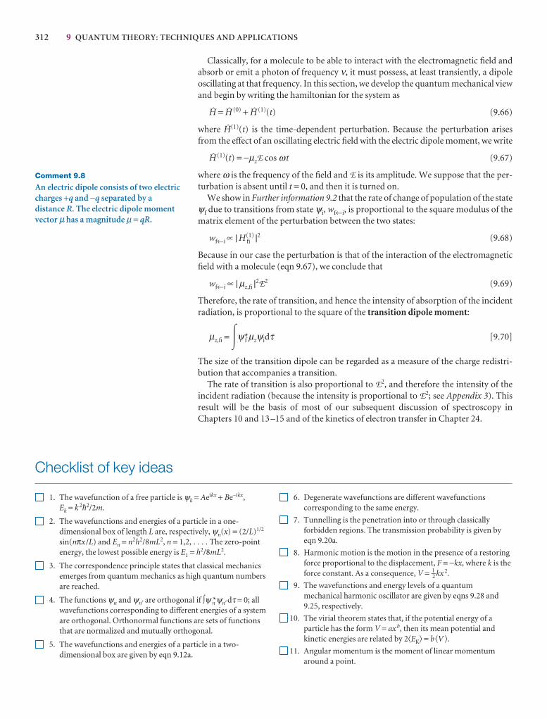
312 9 QUANTUM THEORY: TECHNIQUES AND APPLICATIONS
Classically, for a molecule to be able to interact with the electromagnetic field andabsorb or emit a photon of frequency ν, it must possess, at least transiently, a dipoleoscillating at that frequency. In this section, we develop the quantum mechanical viewand begin by writing the hamiltonian for the system as
@ = @ (0) + @ (1)(t) (9.66)
where @(1)(t) is the time-dependent perturbation. Because the perturbation arisesfrom the effect of an oscillating electric field with the electric dipole moment, we write
@ (1)(t) = −µzE cos ω t (9.67)
where ω is the frequency of the field and E is its amplitude. We suppose that the per-turbation is absent until t = 0, and then it is turned on.
We show in Further information 9.2 that the rate of change of population of the stateψf due to transitions from state ψi, wf←i, is proportional to the square modulus of thematrix element of the perturbation between the two states:
wf←i ∝ | H fi(1) |2 (9.68)
Because in our case the perturbation is that of the interaction of the electromagneticfield with a molecule (eqn 9.67), we conclude that
wf←i ∝ | µz,fi |2E2 (9.69)
Therefore, the rate of transition, and hence the intensity of absorption of the incidentradiation, is proportional to the square of the transition dipole moment:
µz,fi = �ψ f*µzψidτ [9.70]
The size of the transition dipole can be regarded as a measure of the charge redistri-bution that accompanies a transition.
The rate of transition is also proportional to E2, and therefore the intensity of theincident radiation (because the intensity is proportional to E2; see Appendix 3). Thisresult will be the basis of most of our subsequent discussion of spectroscopy inChapters 10 and 13–15 and of the kinetics of electron transfer in Chapter 24.
Comment 9.8
An electric dipole consists of two electriccharges +q and −q separated by adistance R. The electric dipole momentvector µ has a magnitude µ = qR.
Checklist of key ideas
1. The wavefunction of a free particle is ψk = Aeikx + Be−ikx,Ek = k 2$2/2m.
2. The wavefunctions and energies of a particle in a one-dimensional box of length L are, respectively, ψn(x) = (2/L)1/2
sin(nπx /L) and En = n2h2/8mL2, n = 1,2, . . . . The zero-pointenergy, the lowest possible energy is E1 = h2/8mL2.
3. The correspondence principle states that classical mechanicsemerges from quantum mechanics as high quantum numbersare reached.
4. The functions ψn and ψn′ are orthogonal if ∫ψ n*ψn′dτ = 0; allwavefunctions corresponding to different energies of a systemare orthogonal. Orthonormal functions are sets of functionsthat are normalized and mutually orthogonal.
5. The wavefunctions and energies of a particle in a two-dimensional box are given by eqn 9.12a.
6. Degenerate wavefunctions are different wavefunctionscorresponding to the same energy.
7. Tunnelling is the penetration into or through classicallyforbidden regions. The transmission probability is given byeqn 9.20a.
8. Harmonic motion is the motion in the presence of a restoringforce proportional to the displacement, F = −kx, where k is theforce constant. As a consequence, V = 1–2 kx 2.
9. The wavefunctions and energy levels of a quantummechanical harmonic oscillator are given by eqns 9.28 and9.25, respectively.
10. The virial theorem states that, if the potential energy of aparticle has the form V = ax b, then its mean potential andkinetic energies are related by 2�EK� = b�V �.
11. Angular momentum is the moment of linear momentumaround a point.
FURTHER INFORMATION 313
12. The wavefunctions and energies of a particle on a ring are,respectively, ψml
(φ) = (1/2π)1/2eimlφ and E = ml2$2/2I, with
I = mr 2 and ml = 0, ±1, ±2, . . . .
13. The wavefunctions of a particle on a sphere are the sphericalharmonics, the functions Yl,ml
(θ,φ) (Table 9.3). The energiesare E = l(l + 1)$2/2I, l = 0, 1, 2, . . . .
14. For a particle on a sphere, the magnitude of the angularmomentum is {l(l + 1)}1/2$ and the z-component of theangular momentum is ml $, ml = l, l − 1, . . . , −l.
15. Space quantization is the restriction of the component ofangular momentum around an axis to discrete values.
16. Spin is an intrinsic angular momentum of a fundamentalparticle. A fermion is a particle with a half-integral spinquantum number; a boson is a particle with an integral spinquantum number.
17. For an electron, the spin quantum number is s = 1–2 .
18. The spin magnetic quantum number is ms = s, s − 1, . . . , −s;for an electron, ms = +1–2 , −1–2 .
19. Perturbation theory is a technique that supplies approximatesolutions to the Schrödinger equation and in which thehamiltonian for the problem is expressed as a sum of simplerhamiltonians.
20. In time-independent perturbation theory, the perturbation isalways present and unvarying. The first- and second-ordercorrections to the energy are given by eqns 9.65a and 9.65b,respectively. In time-dependent perturbation theory, theperturbation is either switched on and allowed to rise to itsfinal value or is varying in time.
21. The rate of change of population of the state ψf due totransitions from state ψi is wf←i ∝ | µz,fi |2E 2, where µz,fi = ∫ψ f*µzψidτ is the transition dipole moment.
Further reading
Articles and texts
P.W. Atkins and R.S. Friedman, Molecular quantum mechanics.Oxford University Press (2005).
C.S. Johnson, Jr. and L.G. Pedersen, Problems and solutions inquantum chemistry and physics. Dover, New York (1986).
I.N. Levine, Quantum chemistry. Prentice–Hall, Upper Saddle River(2000).
D.A. McQuarrie, Mathematical methods for scientists and engineers.University Science Books, Mill Valley (2003).
J.J.C. Mulder, Closed-form spherical harmonics: explicit polynomialexpression for the associated legendre functions. J. Chem. Educ. 77,244 (2000).
L. Pauling and E.B. Wilson, Introduction to quantum mechanics withapplications to chemistry. Dover, New York (1985).
Further information
Further information 9.1 Dirac notation
The integral in eqn 9.9 is often written
�n | n′� = 0 (n′ ≠ n)
This Dirac bracket notation is much more succinct than writing outthe integral in full. It also introduces the words ‘bra’ and ‘ket’ into thelanguage of quantum mechanics. Thus, the bra �n | corresponds toψ n* and the ket | n′� corresponds to the wavefunction ψn′. When thebra and ket are put together as in this expression, the integration overall space is understood. Similarly, the normalization condition in eqn8.17c becomes simply
�n | n� = 1
in bracket notation. These two expressions can be combined intoone:
�n | n′� = δnn′ (9.71)
Here δnn′, which is called the Kronecker delta, is 1 when n′ = n and 0when n′ ≠ n.
Integrals of the form ∫ψ n*)ψmdτ, which we first encounter inconnection with perturbation theory (Section 9.9) and which are
commonly called ‘matrix elements’, are incorporated into the bracketnotation by writing
�n | ) | m � = �ψ n*)ψmdτ [9.72]
Note how the operator stands between the bra and the ket (whichmay denote different states), in the place of the c in �bra | c | ket�. Anintegration is implied whenever a complete bracket is written. In thisnotation, an expectation value is
�Ω� = �n | ) | n� (9.73)
with the bra and the ket corresponding to the same state (withquantum number n and wavefunction ψn). In this notation, anoperator is hermitian (eqn 8.30) if
�n | ) | m � = �m | ) | n�* (9.74)
Further information 9.2 Perturbation theory
Here we treat perturbation theory in detail. Our first task is todevelop the results of time-independent perturbation theory, inwhich a system is subjected to a perturbation that does not vary with
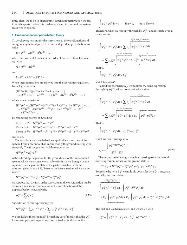
314 9 QUANTUM THEORY: TECHNIQUES AND APPLICATIONS
�ψ 0(0)*ψ n
(0)dτ = 0 if n ≠ 0, but 1 if n = 0
Therefore, when we multiply through by ψ 0(0)* and integrate over all
space, we get
E0(0) if n=0, 0 otherwise
�ψ 0(0)*@ (1)ψ 0
(0)dτ + ∑n
cn�ψ 0(0)*@ (0)ψ n
(0)dτ
1 if n=0, 0 otherwise 1
= ∑n
cnE 0(0)�ψ 0
(0)*ψ n(0) dτ + E 0
(1)�ψ 0(0)*ψ 0
(0)dτ
That is,
�ψ 0(0)*@ (1)ψ 0
(0)dτ = E 0(1)
which is eqn 9.65a.To find the coefficients cn, we multiply the same expression
through by ψ k(0)*, where now k ≠ 0, which gives
Ek(0)δkn
�ψ k(0)*@ (1)ψ 0
(0)dτ + ∑n
cn�ψ k(0)*@ (0)ψ n
(0)dτ
1 if n=k, 0 otherwise 0
= ∑n
cnE 0(0)�ψ k
(0)*ψ n(0)dτ + E 0
(1)�ψ k(0)*ψ 0
(0)dτ
That is,
�ψ k(0)*@ (1)ψ 0
(0)dτ + ckE k(0) = ckE 0
(0)
which we can rearrange into
ck = − (9.76)
The second-order energy is obtained starting from the second-order expression, which for the ground state is
@ (0)ψ 0(2) + @ (1)ψ 0
(1) = E 0(2)ψ 0
(0) + E 0(1)ψ 0
(1) + E 0(0)ψ 0
(2)
To isolate the term E 0(2) we multiply both sides by ψ 0
(0)*, integrateover all space, and obtain
E0(0)∫ψ 0
(0)*ψ 0(2)dτ
�ψ 0(0)*@ (0)ψ 0
(2)dτ + �ψ 0(0)*@ (1)ψ 0
(1)dτ
= E 0(2)�ψ 0
(0)*ψ 0(0)dτ + E 0
(1)�ψ 0(0)*ψ 0
(1)dτ + E 0(0)�ψ 0
(0)*ψ 0(2) dτ
1
The first and last terms cancel, and we are left with
E 0(2) = �ψ 0
(0)*@ (1)ψ 0(1)dτ − E 0
(1)�ψ 0(0)*ψ 0
(1)dτ
1 4 2 4 3
5 4 4 6 4 4 7
�ψ k(0)*@ (1)ψ 0
(0)dτ
E k(0) − E 0
(0)
5 4 6 4 75 4 6 4 75 4 4 6 4 4 7
5 4 6 4 75 4 6 4 75 4 4 6 4 4 7
time. Then, we go on to discuss time-dependent perturbation theory,in which a perturbation is turned on at a specific time and the systemis allowed to evolve.
1 Time-independent perturbation theory
To develop expressions for the corrections to the wavefunction andenergy of a system subjected to a time-independent perturbation, wewrite
ψ = ψ (0) + λψ (1) + λ2ψ (2) + . . .
where the power of λ indicates the order of the correction. Likewise,we write
@ = @ (0) + λ@ (1)
and
E = E(0) + λE(1) + λ2E(2) + . . .
When these expressions are inserted into the Schrödinger equation,@ψ = Eψ, we obtain
(@ (0) + λ@ (1))(ψ (0) + λψ (1) + λ2ψ (2) + . . . ) = (E(0) + λE(1) + λ2E(2) + . . . )(ψ (0) + λψ (1) + λ2ψ (2) + . . . )
which we can rewrite as
@ (0)ψ (0) + λ(@ (1)ψ (0) + @ (0)ψ (1)) + λ2(@ (0)ψ (2) + @ (1)ψ (1)) + . . .= E(0)ψ (0) + λ(E(0)ψ (1) + E(1)ψ (0)) + λ2(E(2)ψ (0) + E(1)ψ (1)
+ E(0)ψ (2)) + . . .
By comparing powers of λ, we find
Terms in λ0: @ (0)ψ (0) = E(0)ψ (0)
Terms in λ: @ (1)ψ (0) + @ (0)ψ (1) = E(0)ψ (1) + E(1)ψ (0)
Terms in λ2: @ (0)ψ (2) + @ (1)ψ (1) = E(2)ψ (0) + E(1)ψ (1) + E(0)ψ (2)
and so on.The equations we have derived are applicable to any state of the
system. From now on we shall consider only the ground state ψ0 withenergy E0. The first equation, which we now write
@ (0)ψ 0(0) = E0
(0)ψ 0(0)
is the Schrödinger equation for the ground state of the unperturbedsystem, which we assume we can solve (for instance, it might be theequation for the ground state of the particle in a box, with thesolutions given in eqn 9.7). To solve the next equation, which is nowwritten
@ (1)ψ 0(0) + @ (0)ψ 0
(1) = E 0(0)ψ (1) + E 0
(1)ψ 0(0)
we suppose that the first-order correction to the wavefunction can beexpressed as a linear combination of the wavefunctions of theunperturbed system, and write
ψ 0(1) = ∑
n
cnψ n(0) (9.75)
Substitution of this expression gives
@ (1)ψ 0(0) + ∑
n
cn @ (0)ψ n(0) = ∑
n
cn E 0(0)ψ n
(0) + E 0(1)ψ 0
(0)
We can isolate the term in E 0(1) by making use of the fact that the ψ n
(0)
form a complete orthogonal and normalized set in the sense that
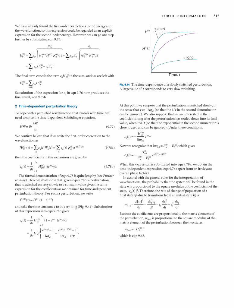
FURTHER INFORMATION 315
We have already found the first-order corrections to the energy andthe wavefunction, so this expression could be regarded as an explicitexpression for the second-order energy. However, we can go one stepfurther by substituting eqn 9.75:
H 0n(1) δ0n
E 0(2) = ∑
n
cn�ψ 0(0)*@ (1)ψ n
(0)dτ − ∑n
cn E 0(1)�ψ 0
(0)*ψ n(0)dτ
= ∑n
cn H(1)0n − c0E(1)
0
The final term cancels the term c0H 00(1) in the sum, and we are left with
E 0(2) = ∑
n≠0
cn H(1)0n
Substitution of the expression for cn in eqn 9.76 now produces thefinal result, eqn 9.65b.
2 Time-dependent perturbation theory
To cope with a perturbed wavefunction that evolves with time, weneed to solve the time-dependent Schrödinger equation,
@Ψ = i$ (9.77)
We confirm below, that if we write the first-order correction to thewavefunction as
Ψ 0(1)(t) = ∑
n
cn(t)Ψn(t) = ∑n
cn(t)ψ n(0)e−iEn
(0)t/$ (9.78a)
then the coefficients in this expansion are given by
cn(t) = �0
t
H(1)n0 (t)eiωn0tdt (9.78b)
The formal demonstration of eqn 9.78 is quite lengthy (see Furtherreading). Here we shall show that, given eqn 9.78b, a perturbationthat is switched on very slowly to a constant value gives the sameexpression for the coefficients as we obtained for time-independentperturbation theory. For such a perturbation, we write
@ (1)(t) = @ (1)(1 − e−t/τ)
and take the time constant τ to be very long (Fig. 9.44). Substitutionof this expression into eqn 9.78b gives
cn(t) = H(1)n0�
0
t
(1 − e−t/τ)eiωn0tdt
= H(1)n0 −
567
e(iωn0 − 1/τ)t − 1
iωn0 − 1/τeiωn0t − 1
iωn0
123
1
i$
1
i$
1
i$
∂Ψ∂t
5 4 6 4 75 4 4 6 4 4 7
At this point we suppose that the perturbation is switched slowly, inthe sense that τ >> 1/ωn0 (so that the 1/τ in the second denominatorcan be ignored). We also suppose that we are interested in thecoefficients long after the perturbation has settled down into its finalvalue, when t >> τ (so that the exponential in the second numerator isclose to zero and can be ignored). Under these conditions,
cn(t) = − eiωn0t
Now we recognize that $ωn0 = En(0) − E0
(0), which gives
cn(t) = − eiEn(0)t
e−iE0(0)t
When this expression is substituted into eqn 9.78a, we obtain thetime-independent expression, eqn 9.76 (apart from an irrelevantoverall phase factor).
In accord with the general rules for the interpretation ofwavefunctions, the probability that the system will be found in thestate n is proportional to the square modulus of the coefficient of thestate, | cn(t) |2. Therefore, the rate of change of population of a final state ψf due to transitions from an initial state ψi is
wf←i = = = cf + cf*
Because the coefficients are proportional to the matrix elements ofthe perturbation, wf←i is proportional to the square modulus of thematrix element of the perturbation between the two states:
wf←i ∝ | H fi(1) |2
which is eqn 9.68.
dcf
dt
dcf*
dt
dcf*cf
dt
d | cf |2
dt
H(0)n0
En(0) − E0
(0)
H(0)n0
$ωn0
Time, t
H(1)
long
short
H t(1)( )
�
�
Fig. 9.44 The time-dependence of a slowly switched perturbation. A large value of τ corresponds to very slow switching.

316 9 QUANTUM THEORY: TECHNIQUES AND APPLICATIONS
Discussion questions
9.1 Discuss the physical origin of quantization energy for a particle confinedto moving inside a one-dimensional box or on a ring.
9.2 Discuss the correspondence principle and provide two examples.
9.3 Define, justify, and provide examples of zero-point energy.
9.4 Discuss the physical origins of quantum mechanical tunnelling. Why istunnelling more likely to contribute to the mechanisms of electron transfer
and proton transfer processes than to mechanisms of group transfer reactions,such as AB + C → A + BC (where A, B, and C are large molecular groups)?
9.5 Distinguish between a fermion and a boson. Provide examples of eachtype of particle.
9.6 Describe the features that stem from nanometre-scale dimensions that arenot found in macroscopic objects.
Exercises
9.1a Calculate the energy separations in joules, kilojoules per mole,electronvolts, and reciprocal centimetres between the levels (a) n = 2 andn = 1, (b) n = 6 and n = 5 of an electron in a box of length 1.0 nm.
9.1b Calculate the energy separations in joules, kilojoules per mole,electronvolts, and reciprocal centimetres between the levels (a) n = 3 and n = 1, (b) n = 7 and n = 6 of an electron in a box of length 1.50 nm.
9.2a Calculate the probability that a particle will be found between 0.49Land 0.51L in a box of length L when it has (a) n = 1, (b) n = 2. Take thewavefunction to be a constant in this range.
9.2b Calculate the probability that a particle will be found between 0.65Land 0.67L in a box of length L when it has (a) n = 1, (b) n = 2. Take thewavefunction to be a constant in this range.
9.3a Calculate the expectation values of p and p2 for a particle in the state n = 1 in a square-well potential.
9.3b Calculate the expectation values of p and p2 for a particle in the state n = 2 in a square-well potential.
9.4a An electron is confined to a a square well of length L. What would be thelength of the box such that the zero-point energy of the electron is equal to itsrest mass energy, mec
2? Express your answer in terms of the parameter λC = h/mec, the ‘Compton wavelength’ of the electron.
9.4b Repeat Exercise 9.4a for a general particle of mass m in a cubic box.
9.5a What are the most likely locations of a particle in a box of length L in thestate n = 3?
9.5b What are the most likely locations of a particle in a box of length L in thestate n = 5?
9.6a Consider a particle in a cubic box. What is the degeneracy of the levelthat has an energy three times that of the lowest level?
9.6b Consider a particle in a cubic box. What is the degeneracy of the levelthat has an energy 14––
3 times that of the lowest level?
9.7a Calculate the percentage change in a given energy level of a particle in acubic box when the length of the edge of the cube is decreased by 10 per centin each direction.
9.7b A nitrogen molecule is confined in a cubic box of volume 1.00 m3.Assuming that the molecule has an energy equal to 3–
2 kT at T = 300 K, what isthe value of n = (nx
2 + ny2 + nz
2)1/2 for this molecule? What is the energyseparation between the levels n and n + 1? What is its de Broglie wavelength?Would it be appropriate to describe this particle as behaving classically?
9.8a Calculate the zero-point energy of a harmonic oscillator consisting of aparticle of mass 2.33 × 10⁻²⁶ kg and force constant 155 N m−1.
9.8b Calculate the zero-point energy of a harmonic oscillator consisting of aparticle of mass 5.16 × 10⁻²⁶ kg and force constant 285 N m−1.
9.9a For a harmonic oscillator of effective mass 1.33 × 10⁻²⁵ kg, the differencein adjacent energy levels is 4.82 zJ. Calculate the force constant of theoscillator.
9.9b For a harmonic oscillator of effective mass 2.88 × 10⁻²⁵ kg, the differencein adjacent energy levels is 3.17 zJ. Calculate the force constant of theoscillator.
9.10a Calculate the wavelength of a photon needed to excite a transitionbetween neighbouring energy levels of a harmonic oscillator of effective massequal to that of a proton (1.0078 u) and force constant 855 N m−1.
9.10b Calculate the wavelength of a photon needed to excite a transitionbetween neighbouring energy levels of a harmonic oscillator of effective massequal to that of an oxygen atom (15.9949 u) and force constant 544 N m−1.
9.11a Refer to Exercise 9.10a and calculate the wavelength that would resultfrom doubling the effective mass of the oscillator.
9.11b Refer to Exercise 9.10b and calculate the wavelength that would resultfrom doubling the effective mass of the oscillator.
9.12a Calculate the minimum excitation energies of (a) a pendulum of length1.0 m on the surface of the Earth, (b) the balance-wheel of a clockwork watch(ν = 5 Hz).
9.12b Calculate the minimum excitation energies of (a) the 33 kHz quartzcrystal of a watch, (b) the bond between two O atoms in O2, for which k = 1177 N m−1.
9.13a Confirm that the wavefunction for the ground state of a one-dimensional linear harmonic oscillator given in Table 9.1 is a solution of theSchrödinger equation for the oscillator and that its energy is 1–
2 $ω.
9.13b Confirm that the wavefunction for the first excited state of a one-dimensional linear harmonic oscillator given in Table 9.1 is a solution of theSchrödinger equation for the oscillator and that its energy is 3–
2 $ω.
9.14a Locate the nodes of the harmonic oscillator wavefunction with v = 4.
9.14b Locate the nodes of the harmonic oscillator wavefunction with v = 5.
9.15a Assuming that the vibrations of a 35Cl2 molecule are equivalent to thoseof a harmonic oscillator with a force constant k = 329 N m−1, what is the zero-point energy of vibration of this molecule? The mass of a 35Cl atom is 34.9688 u.
9.15b Assuming that the vibrations of a 14N2 molecule are equivalent to thoseof a harmonic oscillator with a force constant k = 2293.8 N m−1, what is thezero-point energy of vibration of this molecule? The mass of a 14N atom is14.0031 u.
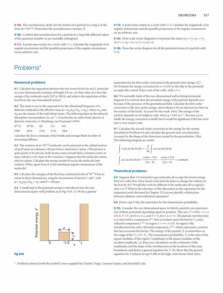
PROBLEMS 317
9.16a The wavefunction, ψ(φ), for the motion of a particle in a ring is of theform ψ = Neimlφ. Determine the normalization constant, N.
9.16b Confirm that wavefunctions for a particle in a ring with different valuesof the quantum number ml are mutually orthogonal.
9.17a A point mass rotates in a circle with l = 1, Calculate the magnitude of itsangular momentum and the possible projections of the angular momentumon an arbitrary axis.
9.17b A point mass rotates in a circle with l = 2, Calculate the magnitude of itsangular momentum and the possible projections of the angular momentumon an arbitrary axis.
9.18a Draw scale vector diagrams to represent the states (a) s = 1–2 , ms = + 1–
2 ,(b) l = 1, ml = +1, (c) l = 2, ml = 0.
9.18b Draw the vector diagram for all the permitted states of a particle with l = 6.
Problems*
Numerical problems
9.1 Calculate the separation between the two lowest levels for an O2 moleculein a one-dimensional container of length 5.0 cm. At what value of n does theenergy of the molecule reach 1–
2 kT at 300 K, and what is the separation of thislevel from the one immediately below?
9.2 The mass to use in the expression for the vibrational frequency of adiatomic molecule is the effective mass µ = mAmB /(mA + mB), where mA andmB are the masses of the individual atoms. The following data on the infraredabsorption wavenumbers (in cm−1) of molecules are taken from Spectra ofdiatomic molecules, G. Herzberg, van Nostrand (1950):
H35Cl H81Br HI CO NO
2990 2650 2310 2170 1904
Calculate the force constants of the bonds and arrange them in order ofincreasing stiffness.
9.3 The rotation of an 1H127I molecule can be pictured as the orbital motionof an H atom at a distance 160 pm from a stationary I atom. (This picture isquite good; to be precise, both atoms rotate around their common centre ofmass, which is very close to the I nucleus.) Suppose that the molecule rotatesonly in a plane. Calculate the energy needed to excite the molecule intorotation. What, apart from 0, is the minimum angular momentum of themolecule?
9.4 Calculate the energies of the first four rotational levels of 1H127I free torotate in three dimensions, using for its moment of inertia I = µR2, with µ = mHmI /(mH + mI) and R = 160 pm.
9.5 A small step in the potential energy is introduced into the one-dimensional square-well problem as in Fig. 9.45. (a) Write a general
expression for the first-order correction to the ground-state energy, E 0(1).
(b) Evaluate the energy correction for a = L/10 (so the blip in the potentialoccupies the central 10 per cent of the well), with n = 1.
9.6 We normally think of the one-dimensional well as being horizontal.Suppose it is vertical; then the potential energy of the particle depends on xbecause of the presence of the gravitational field. Calculate the first-ordercorrection to the zero-point energy, and evaluate it for an electron in a box onthe surface of the Earth. Account for the result. Hint. The energy of theparticle depends on its height as mgh, where g = 9.81 m s−2. Because g is sosmall, the energy correction is small; but it would be significant if the box werenear a very massive star.
9.7 Calculate the second-order correction to the energy for the systemdescribed in Problem 9.6 and calculate the ground-state wavefunction.Account for the shape of the distortion caused by the perturbation. Hint.The following integrals are useful
� x sin ax sin bx dx = − � cos ax sin bx dx
� cos ax sin bx dx = − + constant
Theoretical problems
9.8 Suppose that 1.0 mol perfect gas molecules all occupy the lowest energylevel of a cubic box. How much work must be done to change the volume ofthe box by ∆V? Would the work be different if the molecules all occupied astate n ≠ 1? What is the relevance of this discussion to the expression for theexpansion work discussed in Chapter 2? Can you identify a distinctionbetween adiabatic and isothermal expansion?
9.9 Derive eqn 9.20a, the expression for the transmission probability.
9.10‡ Consider the one-dimensional space in which a particle can experienceone of three potentials depending upon its position. They are: V = 0 for −∞ < x≤ 0, 0, V = V2 for 0 ≤ x ≤ L, and V = V3 for L ≤ x < ∞. The particle wavefunctionis to have both a component eik1x that is incident upon the barrier V2 and areflected component e−ik1x in region 1 (−∞ < x ≤ 0). In region 3 thewavefunction has only a forward component, eik3x, which represents a particlethat has traversed the barrier. The energy of the particle, E, is somewhere inthe range of the V2 > E > V3. The transmission probability, T, is the ratio of thesquare modulus of the region 3 amplitude to the square modulus of theincident amplitude. (a) Base your calculation on the continuity of theamplitudes and the slope of the wavefunction at the locations of the zoneboundaries and derive a general equation for T. (b) Show that the generalequation for T reduces to eqn 9.20b in the high, wide barrier limit when
cos(a + b)x
2(a + b)
cos(a − b)x
2(a − b)
d
da
* Problems denoted with the symbol ‡ were supplied by Charles Trapp, Carmen Giunta, and Marshall Cady.
x
a
0 L/2 L
�Pote
ntia
l ene
rgy,
V
Fig. 9.45

318 9 QUANTUM THEORY: TECHNIQUES AND APPLICATIONS
V1 = V3 = 0. (c) Draw a graph of the probability of proton tunnelling when V3 = 0, L = 50 pm, and E = 10 kJ mol−1 in the barrier range E < V2 < 2E.
9.11 The wavefunction inside a long barrier of height V is ψ = Ne−κ x.Calculate (a) the probability that the particle is inside the barrier and (b) theaverage penetration depth of the particle into the barrier.
9.12 Confirm that a function of the form e−gx2is a solution of the Schrödinger
equation for the ground state of a harmonic oscillator and find an expressionfor g in terms of the mass and force constant of the oscillator.
9.13 Calculate the mean kinetic energy of a harmonic oscillator by using therelations in Table 9.1.
9.14 Calculate the values of �x3� and �x4� for a harmonic oscillator by usingthe relations in Table 9.1.
9.15 Determine the values of δx = (�x2� − �x�2)1/2 and δp = (�p2� − �p�2)1/2 for(a) a particle in a box of length L and (b) a harmonic oscillator. Discuss thesequantities with reference to the uncertainty principle.
9.16 We shall see in Chapter 13 that the intensities of spectroscopictransitions between the vibrational states of a molecule are proportional to thesquare of the integral ∫ψv′xψvdx over all space. Use the relations betweenHermite polynomials given in Table 9.1 to show that the only permittedtransitions are those for which v′ = v ± 1 and evaluate the integral in thesecases.
9.17 The potential energy of the rotation of one CH3 group relative to itsneighbour in ethane can be expressed as V(ϕ) = V0 cos 3ϕ. Show that for smalldisplacements the motion of the group is harmonic and calculate the energy ofexcitation from v = 0 to v = 1. What do you expect to happen to the energylevels and wavefunctions as the excitation increases?
9.18 Show that, whatever superposition of harmonic oscillator states is usedto construct a wavepacket, it is localized at the same place at the times 0, T,2T, . . . , where T is the classical period of the oscillator.
9.19 Use the virial theorem to obtain an expression for the relation betweenthe mean kinetic and potential energies of an electron in a hydrogen atom.
9.20 Evaluate the z-component of the angular momentum and the kineticenergy of a particle on a ring that is described by the (unnormalized)wavefunctions (a) eiφ, (b) e−2iφ, (c) cos φ, and (d) (cos χ)eiφ + (sin χ)e−iφ.
9.21 Is the Schrödinger equation for a particle on an elliptical ring ofsemimajor axes a and b separable? Hint. Although r varies with angle ϕ, thetwo are related by r 2 = a2 sin2φ + b2 cos2φ.
9.22 Use mathematical software to construct a wavepacket of the form
Ψ(φ,t) = ∑ml= 0
ml,max
cmlei(mlφ −Eml
t/$) Eml= ml
2$2/2I
with coefficients c of your choice (for example, all equal). Explore how thewavepacket migrates on the ring but spreads with time.
9.23 Confirm that the spherical harmonics (a) Y0,0, (b) Y2,−1, and (c) Y3,+3
satisfy the Schrödinger equation for a particle free to rotate in threedimensions, and find its energy and angular momentum in each case.
9.24 Confirm that Y3,+3 is normalized to 1. (The integration required is overthe surface of a sphere.)
9.25 Derive an expression in terms of l and ml for the half-angle of the apex ofthe cone used to represent an angular momentum according to the vectormodel. Evaluate the expression for an α spin. Show that the minimumpossible angle approaches 0 as l → ∞.
9.26 Show that the function f = cos ax cos cos cz is an eigenfunction of ∇2,and determine its eigenvalue.
9.27 Derive (in Cartesian coordinates) the quantum mechanical operators forthe three components of angular momentum starting from the classicaldefinition of angular momentum, l = r × p. Show that any two of thecomponents do not mutually commute, and find their commutator.
9.28 Starting from the operator lz = xpy − ypx , prove that in spherical polarcoordinates lz = −i$∂/∂φ.
9.29 Show that the commutator [l2,lz] = 0, and then, without furthercalculation, justify the remark that [l2,lq] = 0 for all q = x, y, and z.
9.30‡ A particle is confined to move in a one-dimensional box of length L.(a) If the particle is classical, show that the average value of x is 1–
2 L and that the root-mean square value is L/31/2. (b) Show that for large values of n, aquantum particle approaches the classical values. This result is an example ofthe correspondence principle, which states that, for very large values of thequantum numbers, the predictions of quantum mechanics approach those ofclassical mechanics.
Applications: to biology and nanotechnology
9.31 When β-carotene is oxidized in vivo, it breaks in half and forms twomolecules of retinal (vitamin A), which is a precursor to the pigment in theretina responsible for vision (Impact I14.1). The conjugated system of retinalconsists of 11 C atoms and one O atom. In the ground state of retinal, eachlevel up to n = 6 is occupied by two electrons. Assuming an averageinternuclear distance of 140 pm, calculate (a) the separation in energybetween the ground state and the first excited state in which one electronoccupies the state with n = 7, and (b) the frequency of the radiation requiredto produce a transition between these two states. (c) Using your results andIllustration 9.1, choose among the words in parentheses to generate a rule forthe prediction of frequency shifts in the absorption spectra of linear polyenes:
The absorption spectrum of a linear polyene shifts to (higher/lower)frequency as the number of conjugated atoms (increases/decreases).
9.32 Many biological electron transfer reactions, such as those associated withbiological energy conversion, may be visualized as arising from electrontunnelling between protein-bound co-factors, such as cytochromes, quinones,flavins, and chlorophylls. This tunnelling occurs over distances that are oftengreater than 1.0 nm, with sections of protein separating electron donor fromacceptor. For a specific combination of donor and acceptor, the rate ofelectron tunnelling is proportional to the transmission probability, withκ ≈ 7 nm−1 (eqn 9.20). By what factor does the rate of electron tunnellingbetween two co-factors increase as the distance between them changes from2.0 nm to 1.0 nm?
9.33 Carbon monoxide binds strongly to the Fe2+ ion of the haem group ofthe protein myoglobin. Estimate the vibrational frequency of CO bound tomyoglobin by using the data in Problem 9.2 and by making the followingassumptions: the atom that binds to the haem group is immobilized, theprotein is infinitely more massive than either the C or O atom, the C atombinds to the Fe2+ ion, and binding of CO to the protein does not alter the forceconstant of the C.O bond.
9.34 Of the four assumptions made in Problem 9.33, the last two arequestionable. Suppose that the first two assumptions are still reasonable and that you have at your disposal a supply of myoglobin, a suitable buffer inwhich to suspend the protein, 12C16O, 13C16O, 12C18O, 13C18O, and an infraredspectrometer. Assuming that isotopic substitution does not affect the forceconstant of the C.O bond, describe a set of experiments that: (a) proveswhich atom, C or O, binds to the haem group of myoglobin, and (b) allows for the determination of the force constant of the C.O bond for myoglobin-bound carbon monoxide.
9.35 The particle on a ring is a useful model for the motion of electronsaround the porphine ring (2), the conjugated macrocycle that forms the
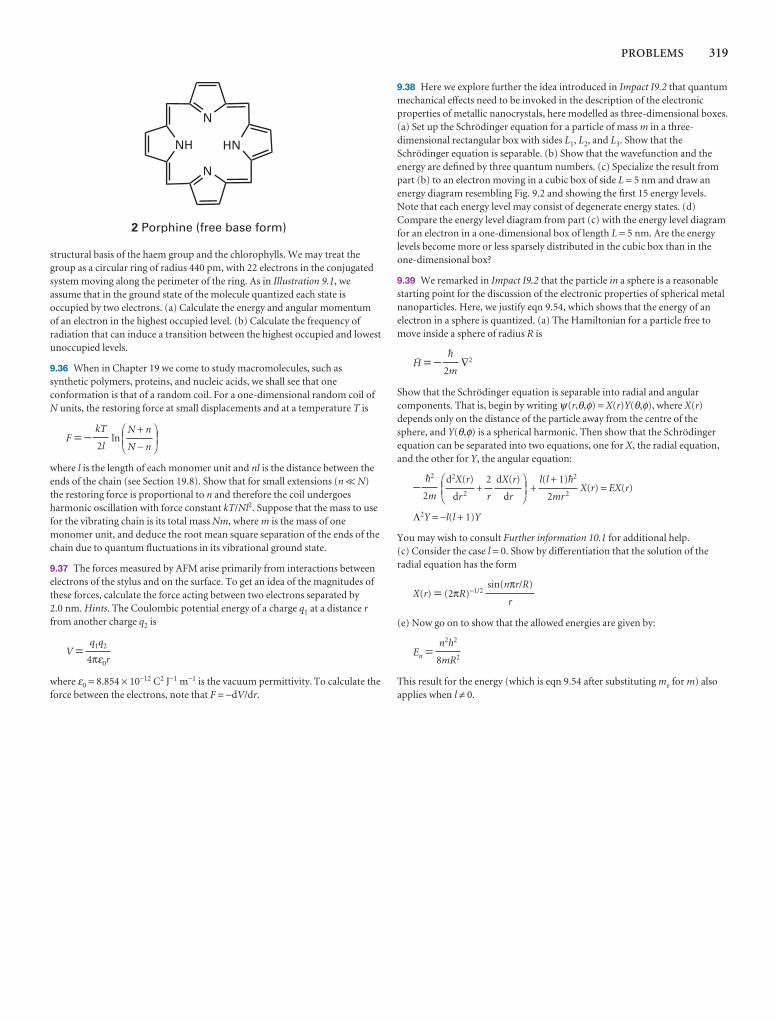
PROBLEMS 319
structural basis of the haem group and the chlorophylls. We may treat thegroup as a circular ring of radius 440 pm, with 22 electrons in the conjugatedsystem moving along the perimeter of the ring. As in Illustration 9.1, weassume that in the ground state of the molecule quantized each state isoccupied by two electrons. (a) Calculate the energy and angular momentumof an electron in the highest occupied level. (b) Calculate the frequency ofradiation that can induce a transition between the highest occupied and lowestunoccupied levels.
9.36 When in Chapter 19 we come to study macromolecules, such assynthetic polymers, proteins, and nucleic acids, we shall see that oneconformation is that of a random coil. For a one-dimensional random coil ofN units, the restoring force at small displacements and at a temperature T is
F = − ln
where l is the length of each monomer unit and nl is the distance between theends of the chain (see Section 19.8). Show that for small extensions (n << N)the restoring force is proportional to n and therefore the coil undergoesharmonic oscillation with force constant kT/Nl2. Suppose that the mass to usefor the vibrating chain is its total mass Nm, where m is the mass of onemonomer unit, and deduce the root mean square separation of the ends of thechain due to quantum fluctuations in its vibrational ground state.
9.37 The forces measured by AFM arise primarily from interactions betweenelectrons of the stylus and on the surface. To get an idea of the magnitudes ofthese forces, calculate the force acting between two electrons separated by 2.0 nm. Hints. The Coulombic potential energy of a charge q1 at a distance rfrom another charge q2 is
V =
where ε0 = 8.854 × 10⁻¹² C2 J−1 m−1 is the vacuum permittivity. To calculate theforce between the electrons, note that F = −dV/dr.
q1q2
4πε0r
DEFN + n
N − n
ABCkT
2l
9.38 Here we explore further the idea introduced in Impact I9.2 that quantummechanical effects need to be invoked in the description of the electronicproperties of metallic nanocrystals, here modelled as three-dimensional boxes.(a) Set up the Schrödinger equation for a particle of mass m in a three-dimensional rectangular box with sides L1, L2, and L3. Show that theSchrödinger equation is separable. (b) Show that the wavefunction and theenergy are defined by three quantum numbers. (c) Specialize the result frompart (b) to an electron moving in a cubic box of side L = 5 nm and draw anenergy diagram resembling Fig. 9.2 and showing the first 15 energy levels.Note that each energy level may consist of degenerate energy states. (d)Compare the energy level diagram from part (c) with the energy level diagramfor an electron in a one-dimensional box of length L = 5 nm. Are the energylevels become more or less sparsely distributed in the cubic box than in theone-dimensional box?
9.39 We remarked in Impact I9.2 that the particle in a sphere is a reasonablestarting point for the discussion of the electronic properties of spherical metalnanoparticles. Here, we justify eqn 9.54, which shows that the energy of anelectron in a sphere is quantized. (a) The Hamiltonian for a particle free tomove inside a sphere of radius R is
@ = − ∇2
Show that the Schrödinger equation is separable into radial and angularcomponents. That is, begin by writing ψ(r,θ,φ) = X(r)Y(θ,φ), where X(r)depends only on the distance of the particle away from the centre of thesphere, and Y(θ,φ) is a spherical harmonic. Then show that the Schrödingerequation can be separated into two equations, one for X, the radial equation,and the other for Y, the angular equation:
− + + X(r) = EX(r)
Λ2Y = −l(l + 1)Y
You may wish to consult Further information 10.1 for additional help. (c) Consider the case l = 0. Show by differentiation that the solution of theradial equation has the form
X(r) = (2πR)−1/2
(e) Now go on to show that the allowed energies are given by:
En =
This result for the energy (which is eqn 9.54 after substituting me for m) alsoapplies when l ≠ 0.
n2h2
8mR2
sin(nπr/R)
r
l(l + 1)$2
2mr 2
DEFdX(r)
dr
2
r
d2X(r)
dr 2
ABC$2
2m
$
2m
Atomic structure andatomic spectra
We now use the principles of quantum mechanics introduced in the preceding two chap-ters to describe the internal structures of atoms. We see what experimental information isavailable from a study of the spectrum of atomic hydrogen. Then we set up the Schrödingerequation for an electron in an atom and separate it into angular and radial parts. The wave-functions obtained are the ‘atomic orbitals’ of hydrogenic atoms. Next, we use thesehydrogenic atomic orbitals to describe the structures of many-electron atoms. In conjunc-tion with the Pauli exclusion principle, we account for the periodicity of atomic properties.The spectra of many-electron atoms are more complicated than those of hydrogen, but thesame principles apply. We see in the closing sections of the chapter how such spectra aredescribed by using term symbols, and the origin of the finer details of their appearance.
In this chapter we see how to use quantum mechanics to describe the electronic struc-ture of an atom, the arrangement of electrons around a nucleus. The concepts wemeet are of central importance for understanding the structures and reactions ofatoms and molecules, and hence have extensive chemical applications. We need todistinguish between two types of atoms. A hydrogenic atom is a one-electron atom orion of general atomic number Z; examples of hydrogenic atoms are H, He+, Li2+, O7+,and even U91+. A many-electron atom (or polyelectronic atom) is an atom or ion withmore than one electron; examples include all neutral atoms other than H. So even He,with only two electrons, is a many-electron atom. Hydrogenic atoms are importantbecause their Schrödinger equations can be solved exactly. They also provide a set ofconcepts that are used to describe the structures of many-electron atoms and, as weshall see in the next chapter, the structures of molecules too.
The structure and spectra of hydrogenic atoms
When an electric discharge is passed through gaseous hydrogen, the H2 molecules aredissociated and the energetically excited H atoms that are produced emit light of dis-crete frequencies, producting a spectrum of a series of ‘lines’ (Fig. 10.1). The Swedishspectroscopist Johannes Rydberg noted (in 1890) that all of them are described by theexpression
# = RH − RH = 109 677 cm−1 (10.1)
with n1 = 1 (the Lyman series), 2 (the Balmer series), and 3 (the Paschen series), and thatin each case n2 = n1 + 1, n1 + 2, . . . . The constant RH is now called the Rydberg con-stant for the hydrogen atom.
DF
1
n22
1
n12
AC
The structure and spectra ofhydrogenic atoms
10.1 The structure of hydrogenicatoms
10.2 Atomic orbitals and theirenergies
10.3 Spectroscopic transitions andselection rules
The structures of many-electronatoms
10.4 The orbital approximation
10.5 Self-consistent field orbitals
The spectra of complex atoms
I10.1 Impact on astrophysics:Spectroscopy of stars
10.6 Quantum defects andionization limits
10.7 Singlet and triplet states
10.8 Spin–orbit coupling
10.9 Term symbols and selectionrules
Checklist of key ideas
Further reading
Further information 10.1: The separation of motion
Discussion questions
Exercises
Problems
10
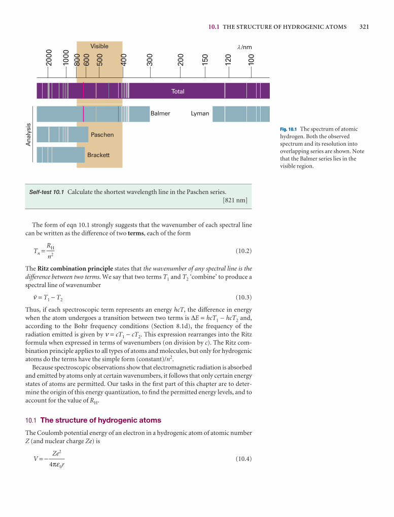
10.1 THE STRUCTURE OF HYDROGENIC ATOMS 321
Self-test 10.1 Calculate the shortest wavelength line in the Paschen series. [821 nm]
The form of eqn 10.1 strongly suggests that the wavenumber of each spectral linecan be written as the difference of two terms, each of the form
Tn = (10.2)
The Ritz combination principle states that the wavenumber of any spectral line is thedifference between two terms. We say that two terms T1 and T2 ‘combine’ to produce aspectral line of wavenumber
# = T1 − T2 (10.3)
Thus, if each spectroscopic term represents an energy hcT, the difference in energywhen the atom undergoes a transition between two terms is ∆E = hcT1 − hcT2 and,according to the Bohr frequency conditions (Section 8.1d), the frequency of the radiation emitted is given by ν = cT1 − cT2. This expression rearranges into the Ritzformula when expressed in terms of wavenumbers (on division by c). The Ritz com-bination principle applies to all types of atoms and molecules, but only for hydrogenicatoms do the terms have the simple form (constant)/n2.
Because spectroscopic observations show that electromagnetic radiation is absorbedand emitted by atoms only at certain wavenumbers, it follows that only certain energystates of atoms are permitted. Our tasks in the first part of this chapter are to deter-mine the origin of this energy quantization, to find the permitted energy levels, and toaccount for the value of RH.
10.1 The structure of hydrogenic atoms
The Coulomb potential energy of an electron in a hydrogenic atom of atomic numberZ (and nuclear charge Ze) is
V = − (10.4)Ze2
4πε0r
RH
n2
2000
1000
800
600
500
400
300
200
150
120
100
/nmVisible
Balmer Lyman
Paschen
Brackett
Total
Ana
lysi
s
�
Fig. 10.1 The spectrum of atomichydrogen. Both the observedspectrum and its resolution intooverlapping series are shown. Notethat the Balmer series lies in thevisible region.
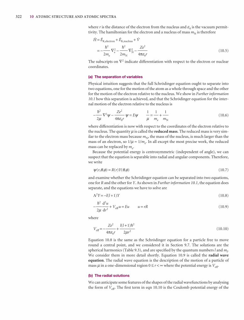
322 10 ATOMIC STRUCTURE AND ATOMIC SPECTRA
where r is the distance of the electron from the nucleus and ε0 is the vacuum permit-tivity. The hamiltonian for the electron and a nucleus of mass mN is therefore
@ = ÊK,electron + ÊK,nucleus + W
= − ∇e2 − ∇N
2 − (10.5)
The subscripts on ∇2 indicate differentiation with respect to the electron or nuclearcoordinates.
(a) The separation of variables
Physical intuition suggests that the full Schrödinger equation ought to separate intotwo equations, one for the motion of the atom as a whole through space and the otherfor the motion of the electron relative to the nucleus. We show in Further information10.1 how this separation is achieved, and that the Schrödinger equation for the inter-nal motion of the electron relative to the nucleus is
− ∇2ψ − ψ = Eψ = + (10.6)
where differentiation is now with respect to the coordinates of the electron relative tothe nucleus. The quantity µ is called the reduced mass. The reduced mass is very sim-ilar to the electron mass because mN, the mass of the nucleus, is much larger than themass of an electron, so 1/µ ≈ 1/me. In all except the most precise work, the reducedmass can be replaced by me.
Because the potential energy is centrosymmetric (independent of angle), we cansuspect that the equation is separable into radial and angular components. Therefore,we write
ψ(r,θ,φ) = R(r)Y(θ,φ) (10.7)
and examine whether the Schrödinger equation can be separated into two equations,one for R and the other for Y. As shown in Further information 10.1, the equation doesseparate, and the equations we have to solve are
Λ2Y = −l(l +1)Y (10.8)
− + Veff u = Eu u = rR (10.9)
where
Veff = − + (10.10)
Equation 10.8 is the same as the Schrödinger equation for a particle free to moveround a central point, and we considered it in Section 9.7. The solutions are the spherical harmonics (Table 9.3), and are specified by the quantum numbers l and ml.We consider them in more detail shortly. Equation 10.9 is called the radial waveequation. The radial wave equation is the description of the motion of a particle ofmass µ in a one-dimensional region 0 ≤ r < ∞ where the potential energy is Veff.
(b) The radial solutions
We can anticipate some features of the shapes of the radial wavefunctions by analysingthe form of Veff. The first term in eqn 10.10 is the Coulomb potential energy of the
l(l +1)$2
2µr2
Ze2
4πε0r
d2u
dr2
$2
2µ
1
mN
1
me
1
µZe2
4πε0r
$2
2µ
Ze2
4πε0r
$2
2mN
$2
2me
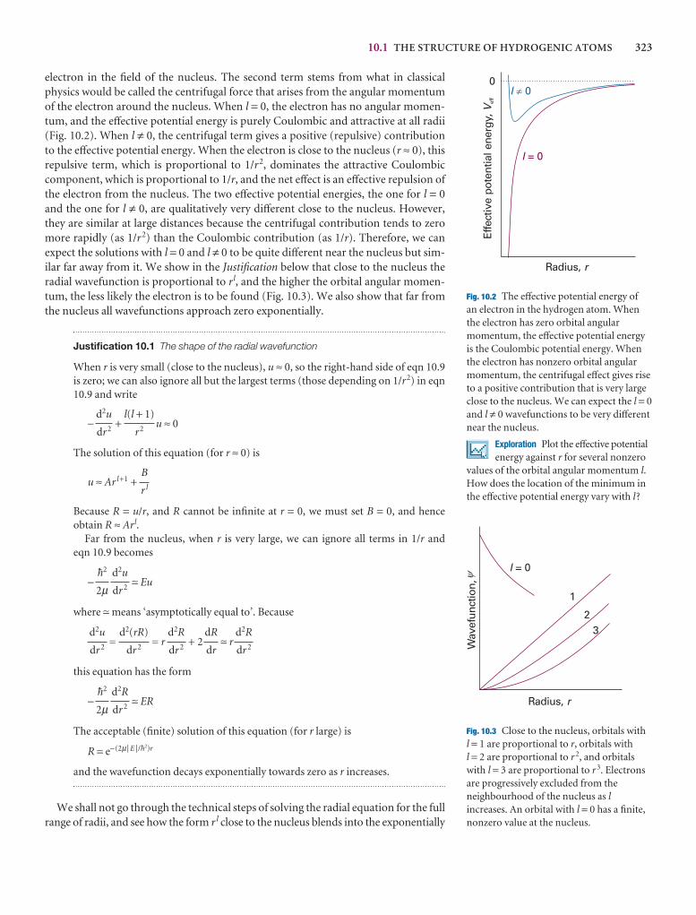
10.1 THE STRUCTURE OF HYDROGENIC ATOMS 323
electron in the field of the nucleus. The second term stems from what in classicalphysics would be called the centrifugal force that arises from the angular momentumof the electron around the nucleus. When l = 0, the electron has no angular momen-tum, and the effective potential energy is purely Coulombic and attractive at all radii(Fig. 10.2). When l ≠ 0, the centrifugal term gives a positive (repulsive) contributionto the effective potential energy. When the electron is close to the nucleus (r ≈ 0), thisrepulsive term, which is proportional to 1/r2, dominates the attractive Coulombiccomponent, which is proportional to 1/r, and the net effect is an effective repulsion ofthe electron from the nucleus. The two effective potential energies, the one for l = 0and the one for l ≠ 0, are qualitatively very different close to the nucleus. However,they are similar at large distances because the centrifugal contribution tends to zeromore rapidly (as 1/r2) than the Coulombic contribution (as 1/r). Therefore, we canexpect the solutions with l = 0 and l ≠ 0 to be quite different near the nucleus but sim-ilar far away from it. We show in the Justification below that close to the nucleus theradial wavefunction is proportional to rl, and the higher the orbital angular momen-tum, the less likely the electron is to be found (Fig. 10.3). We also show that far fromthe nucleus all wavefunctions approach zero exponentially.
Justification 10.1 The shape of the radial wavefunction
When r is very small (close to the nucleus), u ≈ 0, so the right-hand side of eqn 10.9is zero; we can also ignore all but the largest terms (those depending on 1/r2) in eqn10.9 and write
− + u ≈ 0
The solution of this equation (for r ≈ 0) is
u ≈ Ar l+1 +
Because R = u/r, and R cannot be infinite at r = 0, we must set B = 0, and hence obtain R ≈ Arl.
Far from the nucleus, when r is very large, we can ignore all terms in 1/r andeqn 10.9 becomes
− t Eu
where t means ‘asymptotically equal to’. Because
= = r + 2 t r
this equation has the form
− t ER
The acceptable (finite) solution of this equation (for r large) is
R t e−(2µ| E |/$2)r
and the wavefunction decays exponentially towards zero as r increases.
We shall not go through the technical steps of solving the radial equation for the fullrange of radii, and see how the form r l close to the nucleus blends into the exponentially
d2R
dr 2
$2
2µ
d2R
dr 2
dR
dr
d2R
dr 2
d2(rR)
dr 2
d2u
dr 2
d2u
dr 2
$2
2µ
B
r l
l(l + 1)
r2
d2u
dr2
Effe
ctiv
e po
tent
ial e
nerg
y,V
eff
l = 0
l 0!
Radius, r
0
Fig. 10.2 The effective potential energy of an electron in the hydrogen atom. Whenthe electron has zero orbital angularmomentum, the effective potential energyis the Coulombic potential energy. Whenthe electron has nonzero orbital angularmomentum, the centrifugal effect gives riseto a positive contribution that is very largeclose to the nucleus. We can expect the l = 0and l ≠ 0 wavefunctions to be very differentnear the nucleus.
Exploration Plot the effective potentialenergy against r for several nonzero
values of the orbital angular momentum l.How does the location of the minimum inthe effective potential energy vary with l?
Radius, r
Wav
efun
ctio
n,
l = 0
1
23
�
Fig. 10.3 Close to the nucleus, orbitals with l = 1 are proportional to r, orbitals with l = 2 are proportional to r 2, and orbitalswith l = 3 are proportional to r 3. Electronsare progressively excluded from theneighbourhood of the nucleus as lincreases. An orbital with l = 0 has a finite,nonzero value at the nucleus.
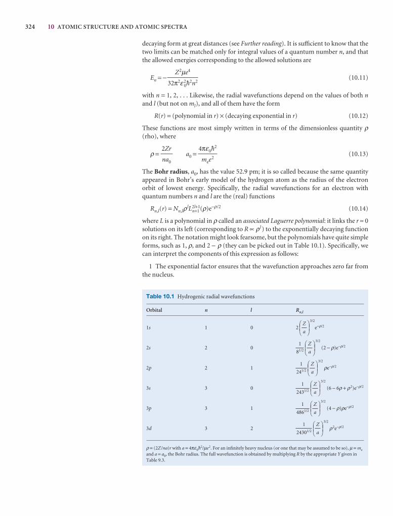
324 10 ATOMIC STRUCTURE AND ATOMIC SPECTRA
decaying form at great distances (see Further reading). It is sufficient to know that thetwo limits can be matched only for integral values of a quantum number n, and thatthe allowed energies corresponding to the allowed solutions are
En = − (10.11)
with n = 1, 2, . . . Likewise, the radial wavefunctions depend on the values of both nand l (but not on ml), and all of them have the form
R(r) = (polynomial in r) × (decaying exponential in r) (10.12)
These functions are most simply written in terms of the dimensionless quantity ρ(rho), where
ρ = a0 = (10.13)
The Bohr radius, a0, has the value 52.9 pm; it is so called because the same quantityappeared in Bohr’s early model of the hydrogen atom as the radius of the electronorbit of lowest energy. Specifically, the radial wavefunctions for an electron withquantum numbers n and l are the (real) functions
Rn,l(r) = Nn,lρlL2l+1n+1 (ρ)e−ρ/2 (10.14)
where L is a polynomial in ρ called an associated Laguerre polynomial: it links the r ≈ 0solutions on its left (corresponding to R ∝ ρl ) to the exponentially decaying functionon its right. The notation might look fearsome, but the polynomials have quite simpleforms, such as 1, ρ, and 2 − ρ (they can be picked out in Table 10.1). Specifically, wecan interpret the components of this expression as follows:
1 The exponential factor ensures that the wavefunction approaches zero far fromthe nucleus.
4πε0$2
mee2
2Zr
na0
Z2µe4
32π2ε20$2n2
Table 10.1 Hydrogenic radial wavefunctions
Orbital n l Rn,l
1s 1 0 2
3/2
e−ρ/2
2s 2 0
3/2
(2 − ρ)e−ρ/2
2p 2 1
3/2
ρe−ρ/2
3s 3 0
3/2
(6 − 6ρ + ρ2)e−ρ/2
3p 3 1
3/2
(4 − ρ)ρe−ρ/2
3d 3 2
3/2
ρ2e−ρ/2
ρ = (2Z /na)r with a = 4πε0$2/µe2. For an infinitely heavy nucleus (or one that may be assumed to be so), µ = me
and a = a0, the Bohr radius. The full wavefunction is obtained by multiplying R by the appropriate Y given inTable 9.3.
DEFZ
a
ABC1
24301/2
DEFZ
a
ABC1
4861/2
DEFZ
a
ABC1
2431/2
DEFZ
a
ABC1
241/2
DEFZ
a
ABC1
81/2
DEFZ
a
ABC
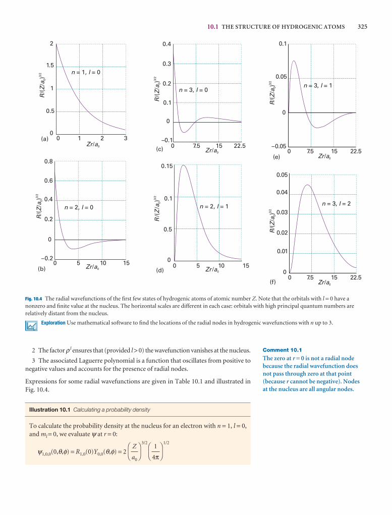
10.1 THE STRUCTURE OF HYDROGENIC ATOMS 325
RZ
a/(
/) 03/
2
0.05
0.04
0.03
0.02
0.01
0
(f)
Zr a/ 0
0 22.57.5 15Zr a/ 0
RZ
a/(
/) 03/
2
0.1
0.05
0
–0.05
(e)0 22.57.5 15
n l= 3, = 1
n l= 3, = 2
Fig. 10.4 The radial wavefunctions of the first few states of hydrogenic atoms of atomic number Z. Note that the orbitals with l = 0 have anonzero and finite value at the nucleus. The horizontal scales are different in each case: orbitals with high principal quantum numbers arerelatively distant from the nucleus.
Exploration Use mathematical software to find the locations of the radial nodes in hydrogenic wavefunctions with n up to 3.
Comment 10.1
The zero at r = 0 is not a radial nodebecause the radial wavefunction doesnot pass through zero at that point(because r cannot be negative). Nodes at the nucleus are all angular nodes.
2
1.5
1
0.5
00 2
RZ
a/(
/ ) 0
3/2
RZ
a/(
/ ) 0
3/2
–0.2
0
0.2
0.4
0.6
0.8
0 5 10 15
(a)
(b)
Zr a/ 0
Zr a/ 0
1 3
n l= 1, = 0
n l= 2, = 0
RZ
a/(
/ ) 0
3/2
0 5 10 15
0.15
0.1
0.5
0
(d)
0 22.57.5 15
0.4
0.3
0.2
0.1
0
–0.1
RZ
a/(
/ ) 0
3/2
(c) Zr a/ 0
Zr a/ 0
n l= 3, = 0
n l= 2, = 1
2 The factor ρ l ensures that (provided l > 0) the wavefunction vanishes at the nucleus.
3 The associated Laguerre polynomial is a function that oscillates from positive tonegative values and accounts for the presence of radial nodes.
Expressions for some radial wavefunctions are given in Table 10.1 and illustrated inFig. 10.4.
Illustration 10.1 Calculating a probability density
To calculate the probability density at the nucleus for an electron with n = 1, l = 0,and ml = 0, we evaluate ψ at r = 0:
ψ1,0,0(0,θ,φ) = R1,0(0)Y0,0(θ,φ) = 2
3/2 1/2DF
1
4π
AC
DF
Z
a0
AC
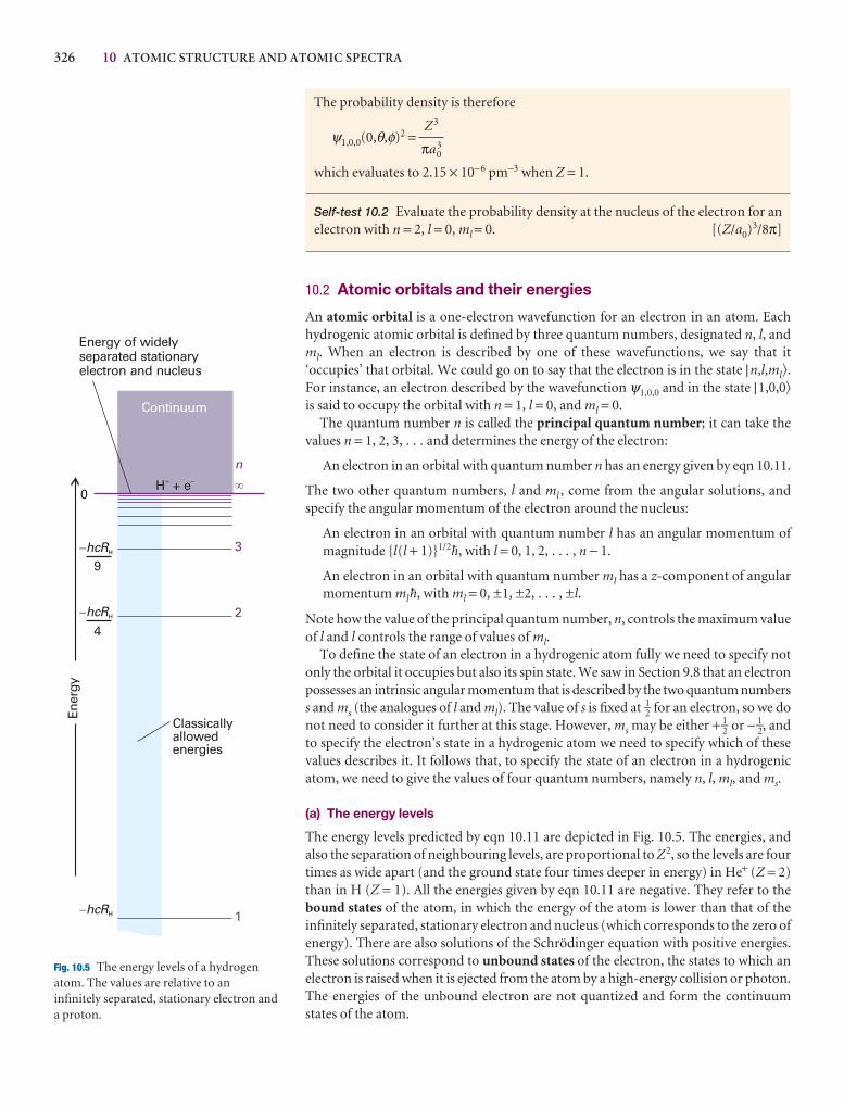
326 10 ATOMIC STRUCTURE AND ATOMIC SPECTRAEn
ergy
1
2
3
�
n
Energy of widelyseparated stationaryelectron and nucleus
Classicallyallowedenergies
0
�hcRH
�hcRH
�hcRH
9
4
Continuum
H + e� �
Fig. 10.5 The energy levels of a hydrogenatom. The values are relative to aninfinitely separated, stationary electron anda proton.
The probability density is therefore
ψ1,0,0(0,θ,φ)2 =
which evaluates to 2.15 × 10⁻⁶ pm−3 when Z = 1.
Self-test 10.2 Evaluate the probability density at the nucleus of the electron for anelectron with n = 2, l = 0, ml = 0. [(Z/a0)3/8π]
10.2 Atomic orbitals and their energies
An atomic orbital is a one-electron wavefunction for an electron in an atom. Each hydrogenic atomic orbital is defined by three quantum numbers, designated n, l, andml. When an electron is described by one of these wavefunctions, we say that it ‘occupies’ that orbital. We could go on to say that the electron is in the state |n,l,ml�.For instance, an electron described by the wavefunction ψ1,0,0 and in the state |1,0,0�is said to occupy the orbital with n = 1, l = 0, and ml = 0.
The quantum number n is called the principal quantum number; it can take thevalues n = 1, 2, 3, . . . and determines the energy of the electron:
An electron in an orbital with quantum number n has an energy given by eqn 10.11.
The two other quantum numbers, l and ml , come from the angular solutions, andspecify the angular momentum of the electron around the nucleus:
An electron in an orbital with quantum number l has an angular momentum ofmagnitude {l(l + 1)}1/2$, with l = 0, 1, 2, . . . , n − 1.
An electron in an orbital with quantum number ml has a z-component of angularmomentum ml$, with ml = 0, ±1, ±2, . . . , ±l.
Note how the value of the principal quantum number, n, controls the maximum valueof l and l controls the range of values of ml.
To define the state of an electron in a hydrogenic atom fully we need to specify notonly the orbital it occupies but also its spin state. We saw in Section 9.8 that an electronpossesses an intrinsic angular momentum that is described by the two quantum numberss and ms (the analogues of l and ml). The value of s is fixed at 1–2 for an electron, so we donot need to consider it further at this stage. However, ms may be either + 1–2 or − 1–2, andto specify the electron’s state in a hydrogenic atom we need to specify which of thesevalues describes it. It follows that, to specify the state of an electron in a hydrogenicatom, we need to give the values of four quantum numbers, namely n, l, ml, and ms.
(a) The energy levels
The energy levels predicted by eqn 10.11 are depicted in Fig. 10.5. The energies, andalso the separation of neighbouring levels, are proportional to Z2, so the levels are fourtimes as wide apart (and the ground state four times deeper in energy) in He+ (Z = 2)than in H (Z = 1). All the energies given by eqn 10.11 are negative. They refer to thebound states of the atom, in which the energy of the atom is lower than that of theinfinitely separated, stationary electron and nucleus (which corresponds to the zero ofenergy). There are also solutions of the Schrödinger equation with positive energies.These solutions correspond to unbound states of the electron, the states to which anelectron is raised when it is ejected from the atom by a high-energy collision or photon.The energies of the unbound electron are not quantized and form the continuumstates of the atom.
Z3
πa30
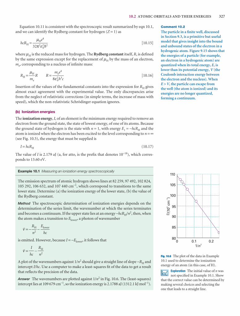
10.2 ATOMIC ORBITALS AND THEIR ENERGIES 327
Comment 10.2
The particle in a finite well, discussed in Section 9.3, is a primitive but usefulmodel that gives insight into the boundand unbound states of the electron in ahydrogenic atom. Figure 9.15 shows thatthe energies of a particle (for example,an electron in a hydrogenic atom) arequantized when its total energy, E, islower than its potential energy, V (theCoulomb interaction energy betweenthe electron and the nucleus). When E > V, the particle can escape from the well (the atom is ionized) and itsenergies are no longer quantized,forming a continuum.
0 0.1 0.21/n2
80
85
90
95
100
105
110
/(10
cm)
31
�̃�
Fig. 10.6 The plot of the data in Example10.1 used to determine the ionizationenergy of an atom (in this case, of H).
Exploration The initial value of n wasnot specified in Example 10.1. Show
that the correct value can be determined bymaking several choices and selecting theone that leads to a straight line.
Equation 10.11 is consistent with the spectroscopic result summarized by eqn 10.1,and we can identify the Rydberg constant for hydrogen (Z = 1) as
hcRH = [10.15]
where µH is the reduced mass for hydrogen. The Rydberg constant itself, R, is definedby the same expression except for the replacement of µH by the mass of an electron,me, corresponding to a nucleus of infinite mass:
RH = R R = [10.16]
Insertion of the values of the fundamental constants into the expression for RH givesalmost exact agreement with the experimental value. The only discrepancies arisefrom the neglect of relativistic corrections (in simple terms, the increase of mass withspeed), which the non-relativistic Schrödinger equation ignores.
(b) Ionization energies
The ionization energy, I, of an element is the minimum energy required to remove anelectron from the ground state, the state of lowest energy, of one of its atoms. Becausethe ground state of hydrogen is the state with n = 1, with energy E1 = −hcRH and theatom is ionized when the electron has been excited to the level corresponding to n = ∞(see Fig. 10.5), the energy that must be supplied is
I = hcRH (10.17)
The value of I is 2.179 aJ (a, for atto, is the prefix that denotes 10−18), which corres-ponds to 13.60 eV.
Example 10.1 Measuring an ionization energy spectroscopically
The emission spectrum of atomic hydrogen shows lines at 82 259, 97 492, 102 824,105 292, 106 632, and 107 440 cm−1, which correspond to transitions to the samelower state. Determine (a) the ionization energy of the lower state, (b) the value ofthe Rydberg constant.
Method The spectroscopic determination of ionization energies depends on thedetermination of the series limit, the wavenumber at which the series terminatesand becomes a continuum. If the upper state lies at an energy −hcRH/n2, then, whenthe atom makes a transition to Elower, a photon of wavenumber
# = − −
is emitted. However, because I = −Elower, it follows that
# = −
A plot of the wavenumbers against 1/n2 should give a straight line of slope −RH andintercept I/hc. Use a computer to make a least-squares fit of the data to get a resultthat reflects the precision of the data.
Answer The wavenumbers are plotted against 1/n2 in Fig. 10.6. The (least-squares)intercept lies at 109 679 cm−1, so the ionization energy is 2.1788 aJ (1312.1 kJ mol−1).
RH
n2
I
hc
Elower
hc
RH
n2
mee4
8ε20h3c
µH
me
µHe4
32π2ε20$2
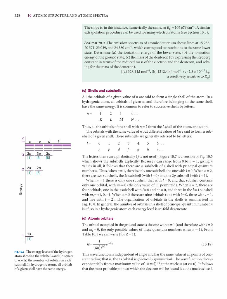
328 10 ATOMIC STRUCTURE AND ATOMIC SPECTRA
Ener
gy
1
2
3
�n
1s
2s 2p
3s 3p 3d
s p d f
[3]
[3]
[5][1]
[1]
[1]
Fig. 10.7 The energy levels of the hydrogenatom showing the subshells and (in squarebrackets) the numbers of orbitals in eachsubshell. In hydrogenic atoms, all orbitalsof a given shell have the same energy.
The slope is, in this instance, numerically the same, so RH = 109 679 cm−1. A similarextrapolation procedure can be used for many-electron atoms (see Section 10.5).
Self-test 10.3 The emission spectrum of atomic deuterium shows lines at 15 238,20 571, 23 039, and 24 380 cm−1, which correspond to transitions to the same lowerstate. Determine (a) the ionization energy of the lower state, (b) the ionization energy of the ground state, (c) the mass of the deuteron (by expressing the Rydbergconstant in terms of the reduced mass of the electron and the deuteron, and solv-ing for the mass of the deuteron).
[(a) 328.1 kJ mol−1, (b) 1312.4 kJ mol−1, (c) 2.8 × 10⁻²⁷ kg,a result very sensitive to RD]
(c) Shells and subshells
All the orbitals of a given value of n are said to form a single shell of the atom. In a hydrogenic atom, all orbitals of given n, and therefore belonging to the same shell,have the same energy. It is common to refer to successive shells by letters:
n = 1 2 3 4 . . .
K L M N . . .
Thus, all the orbitals of the shell with n = 2 form the L shell of the atom, and so on.The orbitals with the same value of n but different values of l are said to form a sub-
shell of a given shell. These subshells are generally referred to by letters:
l = 0 1 2 3 4 5 6 . . .
s p d f g h i . . .
The letters then run alphabetically ( j is not used). Figure 10.7 is a version of Fig. 10.5which shows the subshells explicitly. Because l can range from 0 to n − 1, giving nvalues in all, it follows that there are n subshells of a shell with principal quantumnumber n. Thus, when n = 1, there is only one subshell, the one with l = 0. When n = 2,there are two subshells, the 2s subshell (with l = 0) and the 2p subshell (with l = 1).
When n = 1 there is only one subshell, that with l = 0, and that subshell containsonly one orbital, with ml = 0 (the only value of ml permitted). When n = 2, there arefour orbitals, one in the s subshell with l = 0 and ml = 0, and three in the l = 1 subshellwith ml = +1, 0, −1. When n = 3 there are nine orbitals (one with l = 0, three with l = 1,and five with l = 2). The organization of orbitals in the shells is summarized in Fig. 10.8. In general, the number of orbitals in a shell of principal quantum number nis n2, so in a hydrogenic atom each energy level is n2-fold degenerate.
(d) Atomic orbitals
The orbital occupied in the ground state is the one with n = 1 (and therefore with l = 0and ml = 0, the only possible values of these quantum numbers when n = 1). FromTable 10.1 we can write (for Z = 1):
ψ = e−r/a0 (10.18)
This wavefunction is independent of angle and has the same value at all points of con-stant radius; that is, the 1s orbital is spherically symmetrical. The wavefunction decaysexponentially from a maximum value of 1/(πa0
3)1/2 at the nucleus (at r = 0). It followsthat the most probable point at which the electron will be found is at the nucleus itself.
1
(πa30)1/2
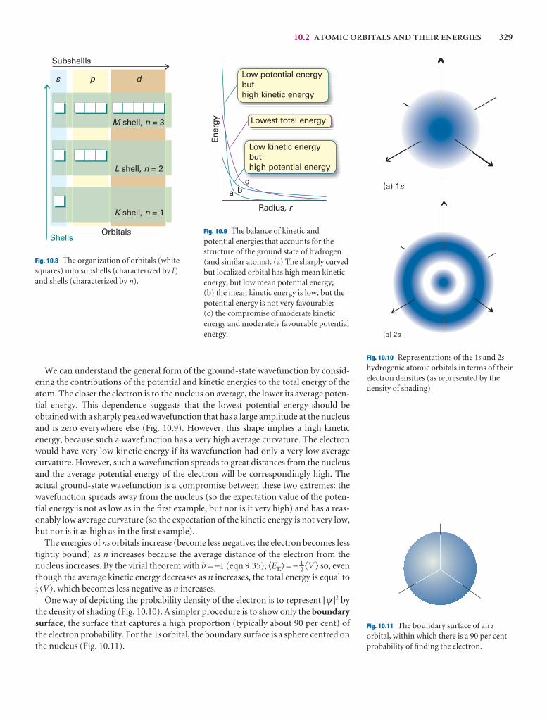
10.2 ATOMIC ORBITALS AND THEIR ENERGIES 329
We can understand the general form of the ground-state wavefunction by consid-ering the contributions of the potential and kinetic energies to the total energy of theatom. The closer the electron is to the nucleus on average, the lower its average poten-tial energy. This dependence suggests that the lowest potential energy should be obtained with a sharply peaked wavefunction that has a large amplitude at the nucleusand is zero everywhere else (Fig. 10.9). However, this shape implies a high kinetic energy, because such a wavefunction has a very high average curvature. The electronwould have very low kinetic energy if its wavefunction had only a very low averagecurvature. However, such a wavefunction spreads to great distances from the nucleusand the average potential energy of the electron will be correspondingly high. The actual ground-state wavefunction is a compromise between these two extremes: thewavefunction spreads away from the nucleus (so the expectation value of the poten-tial energy is not as low as in the first example, but nor is it very high) and has a reas-onably low average curvature (so the expectation of the kinetic energy is not very low,but nor is it as high as in the first example).
The energies of ns orbitals increase (become less negative; the electron becomes lesstightly bound) as n increases because the average distance of the electron from the nucleus increases. By the virial theorem with b = −1 (eqn 9.35), �EK� = − 1–2 �V � so, eventhough the average kinetic energy decreases as n increases, the total energy is equal to1–2 �V�, which becomes less negative as n increases.
One way of depicting the probability density of the electron is to represent |ψ |2 bythe density of shading (Fig. 10.10). A simpler procedure is to show only the boundarysurface, the surface that captures a high proportion (typically about 90 per cent) ofthe electron probability. For the 1s orbital, the boundary surface is a sphere centred onthe nucleus (Fig. 10.11).
Radius, rEn
ergy
Low potential energybuthigh kinetic energy
Low kinetic energybuthigh potential energy
Lowest total energy
a bc
Fig. 10.9 The balance of kinetic andpotential energies that accounts for thestructure of the ground state of hydrogen(and similar atoms). (a) The sharply curvedbut localized orbital has high mean kineticenergy, but low mean potential energy; (b) the mean kinetic energy is low, but thepotential energy is not very favourable; (c) the compromise of moderate kineticenergy and moderately favourable potentialenergy.
Fig. 10.11 The boundary surface of an sorbital, within which there is a 90 per centprobability of finding the electron.
(a) 1s
(b) 2s
Fig. 10.10 Representations of the 1s and 2shydrogenic atomic orbitals in terms of theirelectron densities (as represented by thedensity of shading)
K nshell, = 1
L nshell, = 2
M nshell, = 3
s p d
Subshellls
OrbitalsShells
Fig. 10.8 The organization of orbitals (whitesquares) into subshells (characterized by l)and shells (characterized by n).
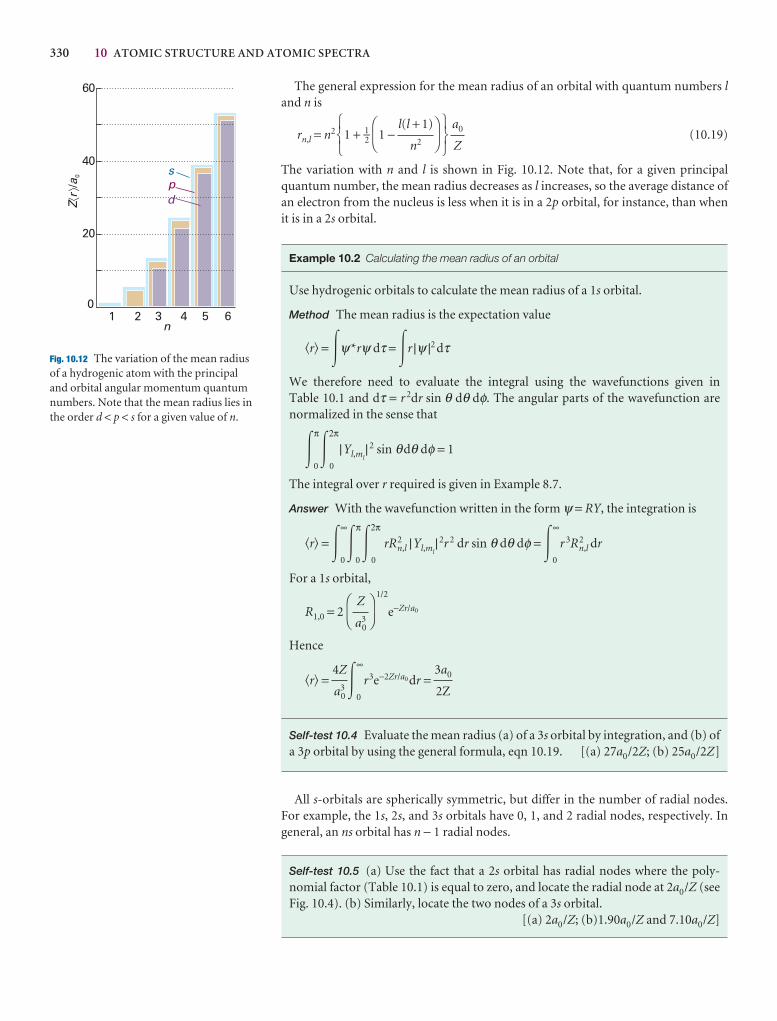
330 10 ATOMIC STRUCTURE AND ATOMIC SPECTRA
1 2 3 4 5 6n
Zr
a"
#/0
0
20
40
60
spd
Fig. 10.12 The variation of the mean radiusof a hydrogenic atom with the principaland orbital angular momentum quantumnumbers. Note that the mean radius lies inthe order d < p < s for a given value of n.
The general expression for the mean radius of an orbital with quantum numbers land n is
rn,l = n2 1 + 1–2 1 − (10.19)
The variation with n and l is shown in Fig. 10.12. Note that, for a given principal quantum number, the mean radius decreases as l increases, so the average distance ofan electron from the nucleus is less when it is in a 2p orbital, for instance, than whenit is in a 2s orbital.
Example 10.2 Calculating the mean radius of an orbital
Use hydrogenic orbitals to calculate the mean radius of a 1s orbital.
Method The mean radius is the expectation value
�r� = �ψ*rψ dτ = �r |ψ |2 dτ
We therefore need to evaluate the integral using the wavefunctions given in Table 10.1 and dτ = r 2dr sin θ dθ dφ. The angular parts of the wavefunction are normalized in the sense that
�π
0�
2π
0
|Yl,ml|2 sin θdθ dφ = 1
The integral over r required is given in Example 8.7.
Answer With the wavefunction written in the form ψ = RY, the integration is
�r� = �∞
0�
π
0�
2π
0
rR2n,l |Yl,ml
|2r 2 dr sin θ dθ dφ = �∞
0
r 3R2n,l dr
For a 1s orbital,
R1,0 = 2
1/2
e−Zr/a0
Hence
�r� = �∞
0
r3e−2Zr/a0dr =
Self-test 10.4 Evaluate the mean radius (a) of a 3s orbital by integration, and (b) ofa 3p orbital by using the general formula, eqn 10.19. [(a) 27a0/2Z; (b) 25a0/2Z]
All s-orbitals are spherically symmetric, but differ in the number of radial nodes.For example, the 1s, 2s, and 3s orbitals have 0, 1, and 2 radial nodes, respectively. Ingeneral, an ns orbital has n − 1 radial nodes.
Self-test 10.5 (a) Use the fact that a 2s orbital has radial nodes where the poly-nomial factor (Table 10.1) is equal to zero, and locate the radial node at 2a0/Z (seeFig. 10.4). (b) Similarly, locate the two nodes of a 3s orbital.
[(a) 2a0/Z; (b)1.90a0/Z and 7.10a0/Z]
3a0
2Z
4Z
a30
DF
Z
a30
AC
a0
Z
567
DF
l(l + 1)
n2
AC
123
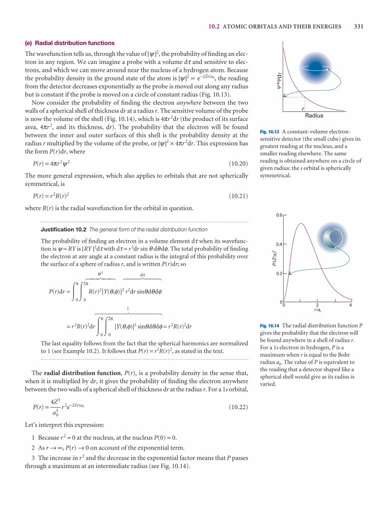
10.2 ATOMIC ORBITALS AND THEIR ENERGIES 331
(e) Radial distribution functions
The wavefunction tells us, through the value of |ψ |2, the probability of finding an elec-tron in any region. We can imagine a probe with a volume dτ and sensitive to elec-trons, and which we can move around near the nucleus of a hydrogen atom. Becausethe probability density in the ground state of the atom is |ψ |2 ∝ e−2Zr/a0, the readingfrom the detector decreases exponentially as the probe is moved out along any radiusbut is constant if the probe is moved on a circle of constant radius (Fig. 10.13).
Now consider the probability of finding the electron anywhere between the twowalls of a spherical shell of thickness dr at a radius r. The sensitive volume of the probeis now the volume of the shell (Fig. 10.14), which is 4πr 2dr (the product of its surfacearea, 4πr 2, and its thickness, dr). The probability that the electron will be found between the inner and outer surfaces of this shell is the probability density at the radius r multiplied by the volume of the probe, or |ψ |2 × 4πr 2dr. This expression hasthe form P(r)dr, where
P(r) = 4πr 2ψ2 (10.20)
The more general expression, which also applies to orbitals that are not sphericallysymmetrical, is
P(r) = r 2R(r)2 (10.21)
where R(r) is the radial wavefunction for the orbital in question.
Justification 10.2 The general form of the radial distribution function
The probability of finding an electron in a volume element dτ when its wavefunc-tion is ψ = RY is |RY |2dτ with dτ = r 2dr sin θ dθdφ. The total probability of findingthe electron at any angle at a constant radius is the integral of this probability overthe surface of a sphere of radius r, and is written P(r)dr; so
ψ 2dτ
P(r)dr =�π
0�
2π
0
R(r)2|Y(θ,φ)|2 r2dr sinθdθdφ
1
= r 2R(r)2dr�π
0�
2π
0
|Y(θ,φ)|2 sinθdθdφ = r 2R(r)2dr
The last equality follows from the fact that the spherical harmonics are normalizedto 1 (see Example 10.2). It follows that P(r) = r2R(r)2, as stated in the text.
The radial distribution function, P(r), is a probability density in the sense that,when it is multiplied by dr, it gives the probability of finding the electron anywherebetween the two walls of a spherical shell of thickness dr at the radius r. For a 1s orbital,
P(r) = r 2e−2Zr/a0 (10.22)
Let’s interpret this expression:
1 Because r 2 = 0 at the nucleus, at the nucleus P(0) = 0.
2 As r → ∞, P(r) → 0 on account of the exponential term.
3 The increase in r 2 and the decrease in the exponential factor means that P passesthrough a maximum at an intermediate radius (see Fig. 10.14).
4Z3
a30
5 4 4 4 6 4 4 4 7
5 4 6 4 75 4 6 4 7
* d
Radiusr
��
�
Fig. 10.13 A constant-volume electron-sensitive detector (the small cube) gives itsgreatest reading at the nucleus, and asmaller reading elsewhere. The samereading is obtained anywhere on a circle ofgiven radius: the s orbital is sphericallysymmetrical.
00 2 4
r a/ 0
PZ
a/(
/) 03
0.6
0.4
0.2
Fig. 10.14 The radial distribution function Pgives the probability that the electron willbe found anywhere in a shell of radius r.For a 1s electron in hydrogen, P is amaximum when r is equal to the Bohrradius a0. The value of P is equivalent to the reading that a detector shaped like aspherical shell would give as its radius isvaried.
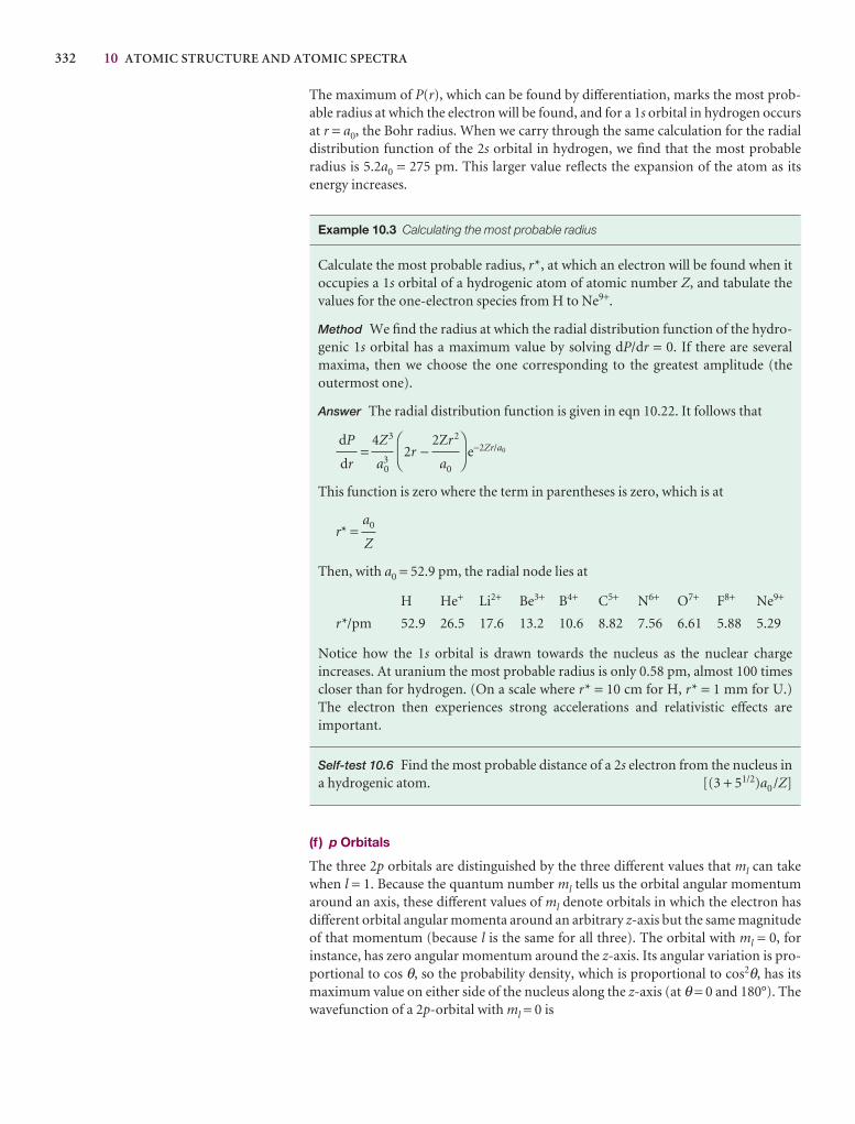
332 10 ATOMIC STRUCTURE AND ATOMIC SPECTRA
The maximum of P(r), which can be found by differentiation, marks the most prob-able radius at which the electron will be found, and for a 1s orbital in hydrogen occursat r = a0, the Bohr radius. When we carry through the same calculation for the radialdistribution function of the 2s orbital in hydrogen, we find that the most probable radius is 5.2a0 = 275 pm. This larger value reflects the expansion of the atom as its energy increases.
Example 10.3 Calculating the most probable radius
Calculate the most probable radius, r*, at which an electron will be found when itoccupies a 1s orbital of a hydrogenic atom of atomic number Z, and tabulate thevalues for the one-electron species from H to Ne9+.
Method We find the radius at which the radial distribution function of the hydro-genic 1s orbital has a maximum value by solving dP/dr = 0. If there are several maxima, then we choose the one corresponding to the greatest amplitude (the outermost one).
Answer The radial distribution function is given in eqn 10.22. It follows that
= 2r − e−2Zr/a0
This function is zero where the term in parentheses is zero, which is at
r* =
Then, with a0 = 52.9 pm, the radial node lies at
H He+ Li2+ Be3+ B4+ C5+ N6+ O7+ F8+ Ne9+
r*/pm 52.9 26.5 17.6 13.2 10.6 8.82 7.56 6.61 5.88 5.29
Notice how the 1s orbital is drawn towards the nucleus as the nuclear charge increases. At uranium the most probable radius is only 0.58 pm, almost 100 timescloser than for hydrogen. (On a scale where r* = 10 cm for H, r* = 1 mm for U.) The electron then experiences strong accelerations and relativistic effects are important.
Self-test 10.6 Find the most probable distance of a 2s electron from the nucleus ina hydrogenic atom. [(3 + 51/2)a0 /Z]
(f ) p Orbitals
The three 2p orbitals are distinguished by the three different values that ml can takewhen l = 1. Because the quantum number ml tells us the orbital angular momentumaround an axis, these different values of ml denote orbitals in which the electron hasdifferent orbital angular momenta around an arbitrary z-axis but the same magnitudeof that momentum (because l is the same for all three). The orbital with ml = 0, for instance, has zero angular momentum around the z-axis. Its angular variation is pro-portional to cos θ, so the probability density, which is proportional to cos2θ, has itsmaximum value on either side of the nucleus along the z-axis (at θ = 0 and 180°). Thewavefunction of a 2p-orbital with ml = 0 is
a0
Z
DF
2Zr2
a0
AC
4Z3
a30
dP
dr
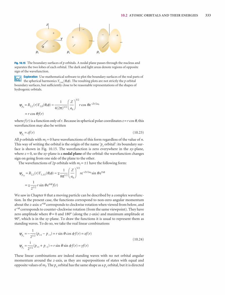
10.2 ATOMIC ORBITALS AND THEIR ENERGIES 333
ψp0= R2,1(r)Y1,0(θ,φ) =
5/2
r cos θe−Zr/2a0
= r cos θ f(r)
where f(r) is a function only of r. Because in spherical polar coordinates z = r cos θ, thiswavefunction may also be written
ψpz= zf(r) (10.23)
All p orbitals with ml = 0 have wavefunctions of this form regardless of the value of n.This way of writing the orbital is the origin of the name ‘pz orbital’: its boundary sur-face is shown in Fig. 10.15. The wavefunction is zero everywhere in the xy-plane,where z = 0, so the xy-plane is a nodal plane of the orbital: the wavefunction changessign on going from one side of the plane to the other.
The wavefunctions of 2p orbitals with ml = ±1 have the following form:
ψp±1= R2,1(r)Y1, ±1(θ,φ) = ,
5/2
re−Zr/2a0 sin θ e±iφ
= , r sin θ e±iφ f(r)
We saw in Chapter 8 that a moving particle can be described by a complex wavefunc-tion. In the present case, the functions correspond to non-zero angular momentumabout the z-axis: e+iφ corresponds to clockwise rotation when viewed from below, ande−iφ corresponds to counter-clockwise rotation (from the same viewpoint). They havezero amplitude where θ = 0 and 180° (along the z-axis) and maximum amplitude at90°, which is in the xy-plane. To draw the functions it is usual to represent them asstanding waves. To do so, we take the real linear combinations
ψpx= − (p+1 − p−1) = r sin θ cos φ f(r) = xf(r)
(10.24)
ψpy= (p+1 + p−1) = r sin θ sin φ f(r) = yf(r)
These linear combinations are indeed standing waves with no net orbital angular momentum around the z-axis, as they are superpositions of states with equal and opposite values of ml. The px orbital has the same shape as a pz orbital, but it is directed
i
21/2
1
21/2
1
21/2
DF
Z
a0
AC
1
8π1/2
DF
Z
a0
AC
1
4(2π)1/2
x
y
z
pxpz py
��
��
�
�
Fig. 10.15 The boundary surfaces of p orbitals. A nodal plane passes through the nucleus andseparates the two lobes of each orbital. The dark and light areas denote regions of oppositesign of the wavefunction.
Exploration Use mathematical software to plot the boundary surfaces of the real parts ofthe spherical harmonics Y1,ml
(θ,φ). The resulting plots are not strictly the p orbitalboundary surfaces, but sufficiently close to be reasonable representations of the shapes ofhydrogenic orbitals.
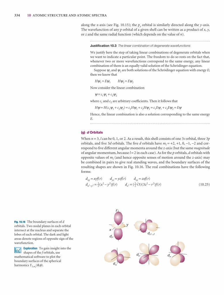
334 10 ATOMIC STRUCTURE AND ATOMIC SPECTRA
along the x-axis (see Fig. 10.15); the py orbital is similarly directed along the y-axis.The wavefunction of any p orbital of a given shell can be written as a product of x, y,or z and the same radial function (which depends on the value of n).
Justification 10.3 The linear combination of degenerate wavefunctions
We justify here the step of taking linear combinations of degenerate orbitals whenwe want to indicate a particular point. The freedom to do so rests on the fact that,whenever two or more wavefunctions correspond to the same energy, any linearcombination of them is an equally valid solution of the Schrödinger equation.
Suppose ψ1 and ψ2 are both solutions of the Schrödinger equation with energy E;then we know that
Hψ1 = Eψ1 Hψ2 = Eψ2
Now consider the linear combination
ψ = c1ψ1 + c2ψ2
where c1 and c2 are arbitrary coefficients. Then it follows that
Hψ = H(c1ψ1 + c2ψ2) = c1Hψ1 + c2Hψ2 = c1Eψ1 + c2Eψ2 = Eψ
Hence, the linear combination is also a solution corresponding to the same energyE.
(g) d Orbitals
When n = 3, l can be 0, 1, or 2. As a result, this shell consists of one 3s orbital, three 3porbitals, and five 3d orbitals. The five d orbitals have ml = +2, +1, 0, −1, −2 and cor-respond to five different angular momenta around the z-axis (but the same magnitudeof angular momentum, because l = 2 in each case). As for the p orbitals, d orbitals withopposite values of ml (and hence opposite senses of motion around the z-axis) may be combined in pairs to give real standing waves, and the boundary surfaces of the resulting shapes are shown in Fig. 10.16. The real combinations have the followingforms:
dxy = xyf(r) dyz = yzf(r) dzx = zxf(r)
dx2−y2 = 1–2(x2 − y2)f(r) dz2 = ( 1–2√3)(3z2 − r 2)f(r) (10.25)
z
xy
dz2
dx y2 2�
dxy
dyz dzx
Fig. 10.16 The boundary surfaces of dorbitals. Two nodal planes in each orbitalintersect at the nucleus and separate thelobes of each orbital. The dark and lightareas denote regions of opposite sign of thewavefunction.
Exploration To gain insight into theshapes of the f orbitals, use
mathematical software to plot theboundary surfaces of the sphericalharmonics Y3,ml
(θ,φ).
10.3 SPECTROSCOPIC TRANSITIONS AND SELECTION RULES 335
10.3 Spectroscopic transitions and selection rules
The energies of the hydrogenic atoms are given by eqn 10.11. When the electron undergoes a transition, a change of state, from an orbital with quantum numbers n1, l1,ml1 to another (lower energy) orbital with quantum numbers n2, l2, ml2, it undergoesa change of energy ∆E and discards the excess energy as a photon of electromagneticradiation with a frequency ν given by the Bohr frequency condition (eqn 8.10).
It is tempting to think that all possible transitions are permissible, and that a spec-trum arises from the transition of an electron from any initial orbital to any other orbital. However, this is not so, because a photon has an intrinsic spin angular momentum corresponding to s = 1 (Section 9.8). The change in angular momentumof the electron must compensate for the angular momentum carried away by the photon. Thus, an electron in a d orbital (l = 2) cannot make a transition into an sorbital (l = 0) because the photon cannot carry away enough angular momentum.Similarly, an s electron cannot make a transition to another s orbital, because therewould then be no change in the electron’s angular momentum to make up for the angular momentum carried away by the photon. It follows that some spectroscopictransitions are allowed, meaning that they can occur, whereas others are forbidden,meaning that they cannot occur.
A selection rule is a statement about which transitions are allowed. They are derived (for atoms) by identifying the transitions that conserve angular momentumwhen a photon is emitted or absorbed. The selection rules for hydrogenic atoms are
∆l = ±1 ∆ml = 0, ±1 (10.26)
The principal quantum number n can change by any amount consistent with the ∆lfor the transition, because it does not relate directly to the angular momentum.
Justification 10.4 The identification of selection rules
We saw in Section 9.10 that the rate of transition between two states is proportionalto the square of the transition dipole moment, µfi, between the initial and finalstates, where (using the notation introduced in Further information 9.1)
µfi = �f | µ |i� [10.27]
and µ is the electric dipole moment operator. For a one-electron atom µ is multi-plication by −er with components µx = −ex, µy = −ey, and µz = −ez. If the transitiondipole moment is zero, the transition is forbidden; the transition is allowed if thetransition moment is non-zero. Physically, the transition dipole moment is a measureof the dipolar ‘kick’ that the electron gives to or receives from the electromagnetic field.
To evaluate a transition dipole moment, we consider each component in turn.For example, for the z-component,
µz,fi = −e�f |z |i� = −e�ψ f*zψi dτ (10.28)
To evaluate the integral, we note from Table 9.3 that z = (4π/3)1/2rY1,0, so
ψf
zψi dτ
�ψ f*zψidτ = �∞
0�
π
0�
2π
0Rnf ,lf
Y*lf ,ml,f
1/2
rY1,0 Rni,liYli,ml,i
r 2dr sin θdθdφ
This multiple integral is the product of three factors, an integral over r and two integrals over the angles, so the factors on the right can be grouped as follows:
�ψ f*zψidτ =1/2
�∞
0Rnf,lf
rRni,lir 2dr�
π
0�
2π
0Y*lf,ml,f
Y1,0Yli,ml,isin θdθdφ
DEF4π3
ABC
DEF4π3
ABC
5 4 4 6 4 4 75 4 6 4 7
5 4 6 4 7
5 4 6 4 7
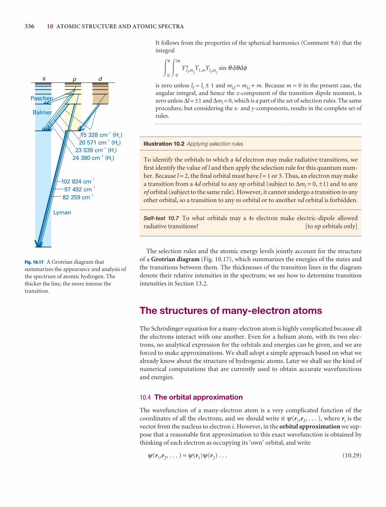
336 10 ATOMIC STRUCTURE AND ATOMIC SPECTRA
s p d
Lyman
Balmer
Paschen
20 571 cm (H )-1b
15 328 cm (H )-1a
23 039 cm (H )-1g
24 380 cm (H )-1d
102 824 cm-1
97 492 cm-1
82 259 cm-1
Fig. 10.17 A Grotrian diagram thatsummarizes the appearance and analysis ofthe spectrum of atomic hydrogen. Thethicker the line, the more intense thetransition.
It follows from the properties of the spherical harmonics (Comment 9.6) that theintegral
�π
0�
2π
0Y*lf,mlf
Y1,mYli,mlisin θ dθdφ
is zero unless lf = li ± 1 and ml,f = ml,i + m. Because m = 0 in the present case, the angular integral, and hence the z-component of the transition dipole moment, iszero unless ∆l = ±1 and ∆ml = 0, which is a part of the set of selection rules. The sameprocedure, but considering the x- and y-components, results in the complete set ofrules.
Illustration 10.2 Applying selection rules
To identify the orbitals to which a 4d electron may make radiative transitions, wefirst identify the value of l and then apply the selection rule for this quantum num-ber. Because l = 2, the final orbital must have l = 1 or 3. Thus, an electron may makea transition from a 4d orbital to any np orbital (subject to ∆ml = 0, ±1) and to anynf orbital (subject to the same rule). However, it cannot undergo a transition to anyother orbital, so a transition to any ns orbital or to another nd orbital is forbidden.
Self-test 10.7 To what orbitals may a 4s electron make electric-dipole allowed radiative transitions? [to np orbitals only]
The selection rules and the atomic energy levels jointly account for the structure of a Grotrian diagram (Fig. 10.17), which summarizes the energies of the states and the transitions between them. The thicknesses of the transition lines in the diagram denote their relative intensities in the spectrum; we see how to determine transitionintensities in Section 13.2.
The structures of many-electron atoms
The Schrödinger equation for a many-electron atom is highly complicated because allthe electrons interact with one another. Even for a helium atom, with its two elec-trons, no analytical expression for the orbitals and energies can be given, and we areforced to make approximations. We shall adopt a simple approach based on what wealready know about the structure of hydrogenic atoms. Later we shall see the kind ofnumerical computations that are currently used to obtain accurate wavefunctionsand energies.
10.4 The orbital approximation
The wavefunction of a many-electron atom is a very complicated function of the coordinates of all the electrons, and we should write it ψ(r1,r2, . . . ), where ri is the vector from the nucleus to electron i. However, in the orbital approximation we sup-pose that a reasonable first approximation to this exact wavefunction is obtained bythinking of each electron as occupying its ‘own’ orbital, and write
ψ(r1,r2, . . . ) = ψ(r1)ψ(r2) . . . (10.29)
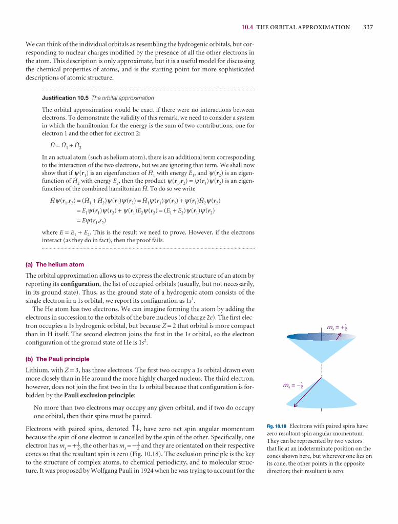
10.4 THE ORBITAL APPROXIMATION 337
We can think of the individual orbitals as resembling the hydrogenic orbitals, but cor-responding to nuclear charges modified by the presence of all the other electrons inthe atom. This description is only approximate, but it is a useful model for discussingthe chemical properties of atoms, and is the starting point for more sophisticated descriptions of atomic structure.
Justification 10.5 The orbital approximation
The orbital approximation would be exact if there were no interactions betweenelectrons. To demonstrate the validity of this remark, we need to consider a systemin which the hamiltonian for the energy is the sum of two contributions, one forelectron 1 and the other for electron 2:
@ = @1 + @2
In an actual atom (such as helium atom), there is an additional term correspondingto the interaction of the two electrons, but we are ignoring that term. We shall nowshow that if ψ(r1) is an eigenfunction of @1 with energy E1, and ψ(r2) is an eigen-function of @2 with energy E2, then the product ψ(r1,r2) = ψ(r1)ψ(r2) is an eigen-function of the combined hamiltonian @. To do so we write
@ψ(r1,r2) = (@1 + @2)ψ(r1)ψ(r2) = @1ψ(r1)ψ(r2) + ψ(r1)@2ψ(r2)
= E1ψ(r1)ψ(r2) + ψ(r1)E2ψ(r2) = (E1 + E2)ψ(r1)ψ(r2)
= Eψ(r1,r2)
where E = E1 + E2. This is the result we need to prove. However, if the electrons interact (as they do in fact), then the proof fails.
(a) The helium atom
The orbital approximation allows us to express the electronic structure of an atom byreporting its configuration, the list of occupied orbitals (usually, but not necessarily,in its ground state). Thus, as the ground state of a hydrogenic atom consists of the single electron in a 1s orbital, we report its configuration as 1s1.
The He atom has two electrons. We can imagine forming the atom by adding theelectrons in succession to the orbitals of the bare nucleus (of charge 2e). The first elec-tron occupies a 1s hydrogenic orbital, but because Z = 2 that orbital is more compactthan in H itself. The second electron joins the first in the 1s orbital, so the electronconfiguration of the ground state of He is 1s2.
(b) The Pauli principle
Lithium, with Z = 3, has three electrons. The first two occupy a 1s orbital drawn evenmore closely than in He around the more highly charged nucleus. The third electron,however, does not join the first two in the 1s orbital because that configuration is for-bidden by the Pauli exclusion principle:
No more than two electrons may occupy any given orbital, and if two do occupyone orbital, then their spins must be paired.
Electrons with paired spins, denoted ↑↓, have zero net spin angular momentum because the spin of one electron is cancelled by the spin of the other. Specifically, oneelectron has ms = + 1–2, the other has ms = − 1–2 and they are orientated on their respectivecones so that the resultant spin is zero (Fig. 10.18). The exclusion principle is the keyto the structure of complex atoms, to chemical periodicity, and to molecular struc-ture. It was proposed by Wolfgang Pauli in 1924 when he was trying to account for the
ms = �
ms = �
12-
12-
Fig. 10.18 Electrons with paired spins havezero resultant spin angular momentum.They can be represented by two vectorsthat lie at an indeterminate position on thecones shown here, but wherever one lies onits cone, the other points in the oppositedirection; their resultant is zero.
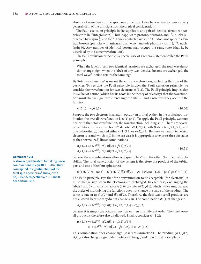
338 10 ATOMIC STRUCTURE AND ATOMIC SPECTRA
absence of some lines in the spectrum of helium. Later he was able to derive a verygeneral form of the principle from theoretical considerations.
The Pauli exclusion principle in fact applies to any pair of identical fermions (par-ticles with half integral spin). Thus it applies to protons, neutrons, and 13C nuclei (allof which have spin 1–2) and to 35Cl nuclei (which have spin 3–2). It does not apply to iden-tical bosons (particles with integral spin), which include photons (spin 1), 12C nuclei(spin 0). Any number of identical bosons may occupy the same state (that is, be described by the same wavefunction).
The Pauli exclusion principle is a special case of a general statement called the Pauliprinciple:
When the labels of any two identical fermions are exchanged, the total wavefunc-tion changes sign; when the labels of any two identical bosons are exchanged, thetotal wavefunction retains the same sign.
By ‘total wavefunction’ is meant the entire wavefunction, including the spin of theparticles. To see that the Pauli principle implies the Pauli exclusion principle, we consider the wavefunction for two electrons ψ(1,2). The Pauli principle implies that it is a fact of nature (which has its roots in the theory of relativity) that the wavefunc-tion must change sign if we interchange the labels 1 and 2 wherever they occur in thefunction:
ψ(2,1) = −ψ(1,2) (10.30)
Suppose the two electrons in an atom occupy an orbital ψ, then in the orbital approx-imation the overall wavefunction is ψ(1)ψ(2). To apply the Pauli principle, we mustdeal with the total wavefunction, the wavefunction including spin. There are severalpossibilities for two spins: both α, denoted α(1)α(2), both β, denoted β(1)β(2), andone α the other β, denoted either α(1)β(2) or α(2)β(1). Because we cannot tell whichelectron is α and which is β, in the last case it is appropriate to express the spin statesas the (normalized) linear combinations
σ+(1,2) = (1/21/2){α(1)β(2) + β(1)α(2)}
σ−(1,2) = (1/21/2){α(1)β(2) − β(1)α(2)}(10.31)
because these combinations allow one spin to be α and the other β with equal prob-ability. The total wavefunction of the system is therefore the product of the orbitalpart and one of the four spin states:
ψ(1)ψ(2)α(1)α(2) ψ(1)ψ(2)β(1)β(2) ψ(1)ψ(2)σ+(1,2) ψ(1)ψ(2)σ−(1,2)
The Pauli principle says that for a wavefunction to be acceptable (for electrons), itmust change sign when the electrons are exchanged. In each case, exchanging the labels 1 and 2 converts the factor ψ(1)ψ(2) into ψ(2)ψ(1), which is the same, becausethe order of multiplying the functions does not change the value of the product. Thesame is true of α(1)α(2) and β(1)β(2). Therefore, the first two overall products arenot allowed, because they do not change sign. The combination σ+(1,2) changes to
σ+(2,1) = (1/21/2){α(2)β(1) + β(2)α(1)} = σ+(1,2)
because it is simply the original function written in a different order. The third over-all product is therefore also disallowed. Finally, consider σ−(1,2):
σ−(2,1) = (1/21/2){α(2)β(1) − β(2)α(1)}
= −(1/21/2){α(1)β(2) − β(1)α(2)} = −σ−(1,2)
This combination does change sign (it is ‘antisymmetric’). The product ψ(1)ψ(2)σ−(1,2) also changes sign under particle exchange, and therefore it is acceptable.
Comment 10.3
A stronger justification for taking linearcombinations in eqn 10.31 is that theycorrespond to eigenfunctions of thetotal spin operators S2 and Sz, with MS = 0 and, respectively, S = 1 and 0. See Section 10.7.
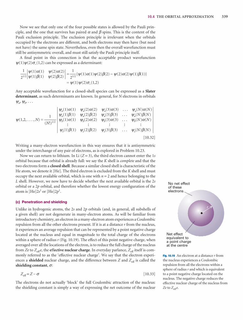
10.4 THE ORBITAL APPROXIMATION 339
Now we see that only one of the four possible states is allowed by the Pauli prin-ciple, and the one that survives has paired α and β spins. This is the content of thePauli exclusion principle. The exclusion principle is irrelevant when the orbitals occupied by the electrons are different, and both electrons may then have (but neednot have) the same spin state. Nevertheless, even then the overall wavefunction muststill be antisymmetric overall, and must still satisfy the Pauli principle itself.
A final point in this connection is that the acceptable product wavefunctionψ(1)ψ(2)σ−(1,2) can be expressed as a determinant:
ψ(1)α(1) ψ(2)α(2)ψ(1)β(1) ψ(2)β(2)
= {ψ(1)α(1)ψ(2)β(2) − ψ(2)α(2)ψ(1)β(1)}
= ψ(1)ψ(2)σ−(1,2)
Any acceptable wavefunction for a closed-shell species can be expressed as a Slaterdeterminant, as such determinants are known. In general, for N electrons in orbitalsψa, ψb, . . .
ψa(1)α(1) ψa(2)α(2) ψa(3)α(3) . . . ψa(N)α(N)ψa(1)β(1) ψa(2)β(2) ψa(3)β(3) . . . ψa(N)β(N)
ψ(1,2, . . . , N) = ψb(1)α(1) ψb(2)α(2) ψb(3)α(3) . . . ψb(N)α(N)� � � � �
ψz(1)β(1) ψz(2)β(2) ψz(3)β(3) . . . ψz(N)β(N)
[10.32]
Writing a many-electron wavefunction in this way ensures that it is antisymmetricunder the interchange of any pair of electrons, as is explored in Problem 10.23.
Now we can return to lithium. In Li (Z = 3), the third electron cannot enter the 1sorbital because that orbital is already full: we say the K shell is complete and that thetwo electrons form a closed shell. Because a similar closed shell is characteristic of theHe atom, we denote it [He]. The third electron is excluded from the K shell and mustoccupy the next available orbital, which is one with n = 2 and hence belonging to theL shell. However, we now have to decide whether the next available orbital is the 2sorbital or a 2p orbital, and therefore whether the lowest energy configuration of theatom is [He]2s1 or [He]2p1.
(c) Penetration and shielding
Unlike in hydrogenic atoms, the 2s and 2p orbitals (and, in general, all subshells of a given shell) are not degenerate in many-electron atoms. As will be familiar from introductory chemistry, an electron in a many-electron atom experiences a Coulombicrepulsion from all the other electrons present. If it is at a distance r from the nucleus,it experiences an average repulsion that can be represented by a point negative chargelocated at the nucleus and equal in magnitude to the total charge of the electronswithin a sphere of radius r (Fig. 10.19). The effect of this point negative charge, whenaveraged over all the locations of the electron, is to reduce the full charge of the nucleusfrom Ze to Zeff e, the effective nuclear charge. In everyday parlance, Zeff itself is com-monly referred to as the ‘effective nuclear charge’. We say that the electron experi-ences a shielded nuclear charge, and the difference between Z and Zeff is called theshielding constant, σ :
Zeff = Z − σ [10.33]
The electrons do not actually ‘block’ the full Coulombic attraction of the nucleus: the shielding constant is simply a way of expressing the net outcome of the nuclear
1
(N!)1/2
1
21/2
1
21/2
Fig. 10.19 An electron at a distance r fromthe nucleus experiences a Coulombicrepulsion from all the electrons within asphere of radius r and which is equivalentto a point negative charge located on thenucleus. The negative charge reduces theeffective nuclear charge of the nucleus fromZe to Zeff e.
r
No net effectof theseelectrons
Net effectequivalent toa point chargeat the centre
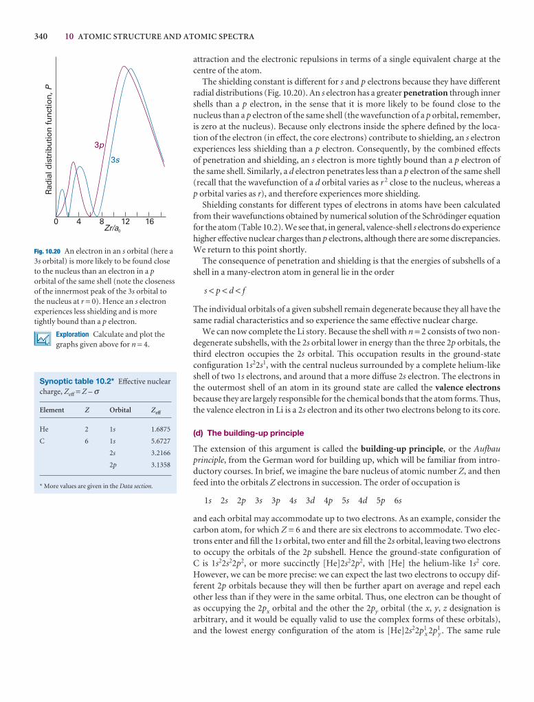
340 10 ATOMIC STRUCTURE AND ATOMIC SPECTRA
attraction and the electronic repulsions in terms of a single equivalent charge at thecentre of the atom.
The shielding constant is different for s and p electrons because they have differentradial distributions (Fig. 10.20). An s electron has a greater penetration through innershells than a p electron, in the sense that it is more likely to be found close to the nucleus than a p electron of the same shell (the wavefunction of a p orbital, remember,is zero at the nucleus). Because only electrons inside the sphere defined by the loca-tion of the electron (in effect, the core electrons) contribute to shielding, an s electronexperiences less shielding than a p electron. Consequently, by the combined effectsof penetration and shielding, an s electron is more tightly bound than a p electron ofthe same shell. Similarly, a d electron penetrates less than a p electron of the same shell(recall that the wavefunction of a d orbital varies as r 2 close to the nucleus, whereas ap orbital varies as r), and therefore experiences more shielding.
Shielding constants for different types of electrons in atoms have been calculatedfrom their wavefunctions obtained by numerical solution of the Schrödinger equationfor the atom (Table 10.2). We see that, in general, valence-shell s electrons do experiencehigher effective nuclear charges than p electrons, although there are some discrepancies.We return to this point shortly.
The consequence of penetration and shielding is that the energies of subshells of ashell in a many-electron atom in general lie in the order
s < p < d < f
The individual orbitals of a given subshell remain degenerate because they all have thesame radial characteristics and so experience the same effective nuclear charge.
We can now complete the Li story. Because the shell with n = 2 consists of two non-degenerate subshells, with the 2s orbital lower in energy than the three 2p orbitals, thethird electron occupies the 2s orbital. This occupation results in the ground-stateconfiguration 1s22s1, with the central nucleus surrounded by a complete helium-likeshell of two 1s electrons, and around that a more diffuse 2s electron. The electrons inthe outermost shell of an atom in its ground state are called the valence electronsbecause they are largely responsible for the chemical bonds that the atom forms. Thus,the valence electron in Li is a 2s electron and its other two electrons belong to its core.
(d) The building-up principle
The extension of this argument is called the building-up principle, or the Aufbauprinciple, from the German word for building up, which will be familiar from intro-ductory courses. In brief, we imagine the bare nucleus of atomic number Z, and thenfeed into the orbitals Z electrons in succession. The order of occupation is
1s 2s 2p 3s 3p 4s 3d 4p 5s 4d 5p 6s
and each orbital may accommodate up to two electrons. As an example, consider thecarbon atom, for which Z = 6 and there are six electrons to accommodate. Two elec-trons enter and fill the 1s orbital, two enter and fill the 2s orbital, leaving two electronsto occupy the orbitals of the 2p subshell. Hence the ground-state configuration of C is 1s22s22p2, or more succinctly [He]2s22p2, with [He] the helium-like 1s2 core.However, we can be more precise: we can expect the last two electrons to occupy dif-ferent 2p orbitals because they will then be further apart on average and repel eachother less than if they were in the same orbital. Thus, one electron can be thought ofas occupying the 2px orbital and the other the 2py orbital (the x, y, z designation is arbitrary, and it would be equally valid to use the complex forms of these orbitals),and the lowest energy configuration of the atom is [He]2s22p1
x 2p1y . The same rule
0 4 8 12 16
3p
3s
Zr/a0
Rad
ial d
istr
ibut
ion
func
tion,
P
Synoptic table 10.2* Effective nuclearcharge, Zeff = Z – σ
Element Z Orbital Zeff
He 2 1s 1.6875
C 6 1s 5.6727
2s 3.2166
2p 3.1358
* More values are given in the Data section.
Fig. 10.20 An electron in an s orbital (here a3s orbital) is more likely to be found closeto the nucleus than an electron in a porbital of the same shell (note the closenessof the innermost peak of the 3s orbital tothe nucleus at r = 0). Hence an s electronexperiences less shielding and is moretightly bound than a p electron.
Exploration Calculate and plot thegraphs given above for n = 4.

10.4 THE ORBITAL APPROXIMATION 341
applies whenever degenerate orbitals of a subshell are available for occupation. Thus,another rule of the building-up principle is:
Electrons occupy different orbitals of a given subshell before doubly occupying anyone of them.
For instance, nitrogen (Z = 7) has the configuration [He]2s22p1x2p1
y2p1z , and only when
we get to oxygen (Z = 8) is a 2p orbital doubly occupied, giving [He]2s22p2x2p1
y 2p1z .
When electrons occupy orbitals singly we invoke Hund’s maximum multiplicity rule:
An atom in its ground state adopts a configuration with the greatest number of unpaired electrons.
The explanation of Hund’s rule is subtle, but it reflects the quantum mechanical prop-erty of spin correlation, that electrons with parallel spins behave as if they have a tendency to stay well apart, and hence repel each other less. In essence, the effect of spincorrelation is to allow the atom to shrink slightly, so the electron–nucleus interactionis improved when the spins are parallel. We can now conclude that, in the ground stateof the carbon atom, the two 2p electrons have the same spin, that all three 2p electronsin the N atoms have the same spin, and that the two 2p electrons in different orbitalsin the O atom have the same spin (the two in the 2px orbital are necessarily paired).
Justification 10.6 Spin correlation
Suppose electron 1 is described by a wavefunction ψa(r1) and electron 2 is describedby a wavefunction ψb(r2); then, in the orbital approximation, the joint wavefunc-tion of the electrons is the product ψ = ψa(r1)ψb(r2). However, this wavefunction isnot acceptable, because it suggests that we know which electron is in which orbital,whereas we cannot keep track of electrons. According to quantum mechanics, thecorrect description is either of the two following wavefunctions:
ψ± = (1/21/2){ψa(r1)ψb(r2) ± ψb(r1)ψa(r2)}
According to the Pauli principle, because ψ+ is symmetrical under particle inter-change, it must be multiplied by an antisymmetric spin function (the one denotedσ−). That combination corresponds to a spin-paired state. Conversely, ψ− is anti-symmetric, so it must be multiplied by one of the three symmetric spin states. Thesethree symmetric states correspond to electrons with parallel spins (see Section 10.7for an explanation).
Now consider the values of the two combinations when one electron approachesanother, and r1 = r2. We see that ψ− vanishes, which means that there is zero prob-ability of finding the two electrons at the same point in space when they have parallelspins. The other combination does not vanish when the two electrons are at the samepoint in space. Because the two electrons have different relative spatial distributionsdepending on whether their spins are parallel or not, it follows that their Coulombicinteraction is different, and hence that the two states have different energies.
Neon, with Z = 10, has the configuration [He]2s22p6, which completes the L shell.This closed-shell configuration is denoted [Ne], and acts as a core for subsequent ele-ments. The next electron must enter the 3s orbital and begin a new shell, so an Naatom, with Z = 11, has the configuration [Ne]3s1. Like lithium with the configuration[He]2s1, sodium has a single s electron outside a complete core. This analysis hasbrought us to the origin of chemical periodicity. The L shell is completed by eight elec-trons, so the element with Z = 3 (Li) should have similar properties to the elementwith Z = 11 (Na). Likewise, Be (Z = 4) should be similar to Z = 12 (Mg), and so on, upto the noble gases He (Z = 2), Ne (Z = 10), and Ar (Z = 18).
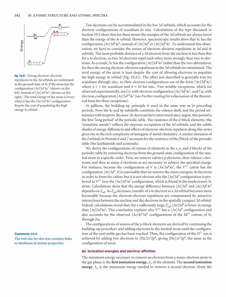
342 10 ATOMIC STRUCTURE AND ATOMIC SPECTRA
Ten electrons can be accommodated in the five 3d orbitals, which accounts for theelectron configurations of scandium to zinc. Calculations of the type discussed inSection 10.5 show that for these atoms the energies of the 3d orbitals are always lowerthan the energy of the 4s orbital. However, spectroscopic results show that Sc has theconfiguration [Ar]3d14s2, instead of [Ar]3d3 or [Ar]3d24s1. To understand this obser-vation, we have to consider the nature of electron–electron repulsions in 3d and 4sorbitals. The most probable distance of a 3d electron from the nucleus is less than thatfor a 4s electron, so two 3d electrons repel each other more strongly than two 4s elec-trons. As a result, Sc has the configuration [Ar]3d14s2 rather than the two alternatives,for then the strong electron–electron repulsions in the 3d orbitals are minimized. Thetotal energy of the atom is least despite the cost of allowing electrons to populate the high energy 4s orbital (Fig. 10.21). The effect just described is generally true forscandium through zinc, so their electron configurations are of the form [Ar]3dn4s2,where n = 1 for scandium and n = 10 for zinc. Two notable exceptions, which are observed experimentally, are Cr, with electron configuration [Ar]3d54s1, and Cu, withelectron configuration [Ar]3d104s1 (see Further reading for a discussion of the theoret-ical basis for these exceptions).
At gallium, the building-up principle is used in the same way as in preceding periods. Now the 4s and 4p subshells constitute the valence shell, and the period ter-minates with krypton. Because 18 electrons have intervened since argon, this period isthe first ‘long period’ of the periodic table. The existence of the d-block elements (the‘transition metals’) reflects the stepwise occupation of the 3d orbitals, and the subtleshades of energy differences and effects of electron–electron repulsion along this seriesgives rise to the rich complexity of inorganic d-metal chemistry. A similar intrusion ofthe f orbitals in Periods 6 and 7 accounts for the existence of the f block of the periodictable (the lanthanoids and actinoids).
We derive the configurations of cations of elements in the s, p, and d blocks of theperiodic table by removing electrons from the ground-state configuration of the neu-tral atom in a specific order. First, we remove valence p electrons, then valence s elec-trons, and then as many d electrons as are necessary to achieve the specified charge.For instance, because the configuration of V is [Ar]3d34s2, the V2+ cation has theconfiguration [Ar]3d3. It is reasonable that we remove the more energetic 4s electronsin order to form the cation, but it is not obvious why the [Ar]3d3 configuration is pre-ferred in V2+ over the [Ar]3d14s2 configuration, which is found in the isoelectronic Scatom. Calculations show that the energy difference between [Ar]3d3 and [Ar]3d14s2
depends on Zeff. As Zeff increases, transfer of a 4s electron to a 3d orbital becomes morefavourable because the electron–electron repulsions are compensated by attractive interactions between the nucleus and the electrons in the spatially compact 3d orbital.Indeed, calculations reveal that, for a sufficiently large Zeff, [Ar]3d3 is lower in energythan [Ar]3d14s2. This conclusion explains why V2+ has a [Ar]3d3 configuration andalso accounts for the observed [Ar]4s03dn configurations of the M2+ cations of Scthrough Zn.
The configurations of anions of the p-block elements are derived by continuing thebuilding-up procedure and adding electrons to the neutral atom until the configura-tion of the next noble gas has been reached. Thus, the configuration of the O2− ion isachieved by adding two electrons to [He]2s22p4, giving [He]2s22p6, the same as theconfiguration of neon.
(e) Ionization energies and electron affinities
The minimum energy necessary to remove an electron from a many-electron atom inthe gas phase is the first ionization energy, I1, of the element. The second ionizationenergy, I2, is the minimum energy needed to remove a second electron (from the
En
erg
y
Fig. 10.21 Strong electron–electronrepulsions in the 3d orbitals are minimizedin the ground state of Sc if the atom has theconfiguration [Ar]3d14s2 (shown on theleft) instead of [Ar]3d24s1 (shown on theright). The total energy of the atom is lowerwhen it has the [Ar]3d14s2 configurationdespite the cost of populating the highenergy 4s orbital.
Comment 10.4
The web site for this text contains linksto databases of atomic properties.
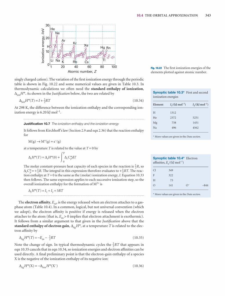
10.4 THE ORBITAL APPROXIMATION 343
singly charged cation). The variation of the first ionization energy through the periodictable is shown in Fig. 10.22 and some numerical values are given in Table 10.3. In thermodynamic calculations we often need the standard enthalpy of ionization,∆ionH 7. As shown in the Justification below, the two are related by
∆ionH 7(T) = I + 5–2RT (10.34)
At 298 K, the difference between the ionization enthalpy and the corresponding ion-ization energy is 6.20 kJ mol−1.
Justification 10.7 The ionization enthalpy and the ionization energy
It follows from Kirchhoff’s law (Section 2.9 and eqn 2.36) that the reaction enthalpyfor
M(g) → M+(g) + e−(g)
at a temperature T is related to the value at T = 0 by
∆rH7(T) = ∆rH
7(0) + �Τ
0∆rC p
7dT
The molar constant-pressure heat capacity of each species in the reaction is 5–2 R, so∆rC
7p = + 5–2 R. The integral in this expression therefore evaluates to + 5–2 RT. The reac-
tion enthalpy at T = 0 is the same as the (molar) ionization energy, I. Equation 10.33then follows. The same expression applies to each successive ionization step, so theoverall ionization enthalpy for the formation of M2+ is
∆rH7(T) = I1 + I2 + 5RT
The electron affinity, Eea, is the energy released when an electron attaches to a gas-phase atom (Table 10.4). In a common, logical, but not universal convention (whichwe adopt), the electron affinity is positive if energy is released when the electron attaches to the atom (that is, Eea > 0 implies that electron attachment is exothermic).It follows from a similar argument to that given in the Justification above that the standard enthalpy of electron gain, ∆eg H 7, at a temperature T is related to the elec-tron affinity by
∆eg H 7(T) = −Eea − 5–2RT (10.35)
Note the change of sign. In typical thermodynamic cycles the 5–2 RT that appears in eqn 10.35 cancels that in eqn 10.34, so ionization energies and electron affinities can beused directly. A final preliminary point is that the electron-gain enthalpy of a speciesX is the negative of the ionization enthalpy of its negative ion:
∆eg H 7(X) = −∆ion H 7(X−) (10.36)
Ioni
zatio
n e
nerg
y,/e
VI
0
10
20
30
1 20 40 60 80 100Atomic number, Z
HeNe
ArKr
Hg RnXe
Li Na K Rb Cs Tl
H
Fig. 10.22 The first ionization energies of theelements plotted against atomic number.
Synoptic table 10.3* First and secondionization energies
Element I1/(kJ mol−1) I2/(kJ mol−1)
H 1312
He 2372 5251
Mg 738 1451
Na 496 4562
* More values are given in the Data section.
Synoptic table 10.4* Electronaffinities, Ea /(kJ mol−1)
Cl 349
F 322
H 73
O 141 O− –844
* More values are given in the Data section.
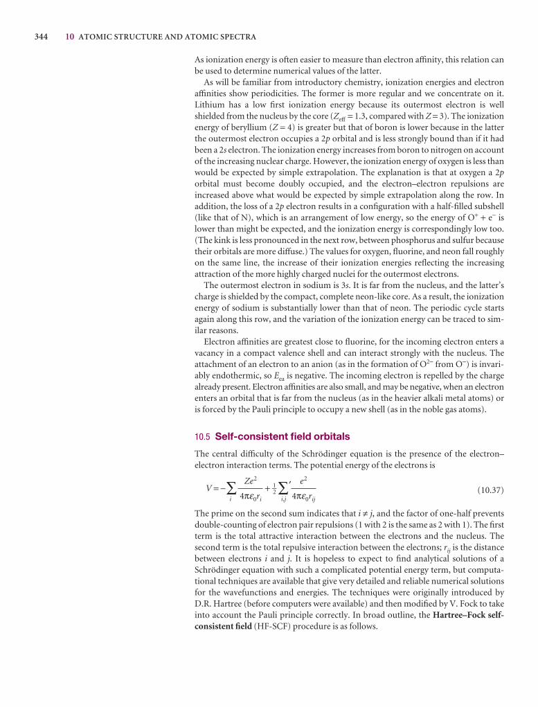
344 10 ATOMIC STRUCTURE AND ATOMIC SPECTRA
As ionization energy is often easier to measure than electron affinity, this relation canbe used to determine numerical values of the latter.
As will be familiar from introductory chemistry, ionization energies and electronaffinities show periodicities. The former is more regular and we concentrate on it.Lithium has a low first ionization energy because its outermost electron is wellshielded from the nucleus by the core (Zeff = 1.3, compared with Z = 3). The ionizationenergy of beryllium (Z = 4) is greater but that of boron is lower because in the latterthe outermost electron occupies a 2p orbital and is less strongly bound than if it hadbeen a 2s electron. The ionization energy increases from boron to nitrogen on accountof the increasing nuclear charge. However, the ionization energy of oxygen is less thanwould be expected by simple extrapolation. The explanation is that at oxygen a 2porbital must become doubly occupied, and the electron–electron repulsions are increased above what would be expected by simple extrapolation along the row. In addition, the loss of a 2p electron results in a configuration with a half-filled subshell(like that of N), which is an arrangement of low energy, so the energy of O+ + e− islower than might be expected, and the ionization energy is correspondingly low too.(The kink is less pronounced in the next row, between phosphorus and sulfur becausetheir orbitals are more diffuse.) The values for oxygen, fluorine, and neon fall roughlyon the same line, the increase of their ionization energies reflecting the increasing attraction of the more highly charged nuclei for the outermost electrons.
The outermost electron in sodium is 3s. It is far from the nucleus, and the latter’scharge is shielded by the compact, complete neon-like core. As a result, the ionizationenergy of sodium is substantially lower than that of neon. The periodic cycle startsagain along this row, and the variation of the ionization energy can be traced to sim-ilar reasons.
Electron affinities are greatest close to fluorine, for the incoming electron enters avacancy in a compact valence shell and can interact strongly with the nucleus. The attachment of an electron to an anion (as in the formation of O2− from O−) is invari-ably endothermic, so Eea is negative. The incoming electron is repelled by the chargealready present. Electron affinities are also small, and may be negative, when an electronenters an orbital that is far from the nucleus (as in the heavier alkali metal atoms) oris forced by the Pauli principle to occupy a new shell (as in the noble gas atoms).
10.5 Self-consistent field orbitals
The central difficulty of the Schrödinger equation is the presence of the electron–electron interaction terms. The potential energy of the electrons is
V = −i∑ + 1–2 ∑
i,j
′(10.37)
The prime on the second sum indicates that i ≠ j, and the factor of one-half preventsdouble-counting of electron pair repulsions (1 with 2 is the same as 2 with 1). The firstterm is the total attractive interaction between the electrons and the nucleus. The second term is the total repulsive interaction between the electrons; rij is the distancebetween electrons i and j. It is hopeless to expect to find analytical solutions of aSchrödinger equation with such a complicated potential energy term, but computa-tional techniques are available that give very detailed and reliable numerical solutionsfor the wavefunctions and energies. The techniques were originally introduced byD.R. Hartree (before computers were available) and then modified by V. Fock to takeinto account the Pauli principle correctly. In broad outline, the Hartree–Fock self-consistent field (HF-SCF) procedure is as follows.
e2
4πε0rij
Ze2
4πε0ri
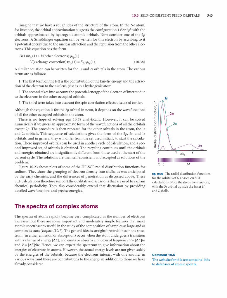
10.5 SELF-CONSISTENT FIELD ORBITALS 345
Imagine that we have a rough idea of the structure of the atom. In the Ne atom, for instance, the orbital approximation suggests the configuration 1s22s22p6 with theorbitals approximated by hydrogenic atomic orbitals. Now consider one of the 2pelectrons. A Schrödinger equation can be written for this electron by ascribing to it a potential energy due to the nuclear attraction and the repulsion from the other elec-trons. This equation has the form
H(1)ψ2p(1) + V(other electrons)ψ2p(1)
− V(exchange correction)ψ2p(1) = E2pψ2p(1) (10.38)
A similar equation can be written for the 1s and 2s orbitals in the atom. The variousterms are as follows:
1 The first term on the left is the contribution of the kinetic energy and the attrac-tion of the electron to the nucleus, just as in a hydrogenic atom.
2 The second takes into account the potential energy of the electron of interest dueto the electrons in the other occupied orbitals.
3 The third term takes into account the spin correlation effects discussed earlier.
Although the equation is for the 2p orbital in neon, it depends on the wavefunctionsof all the other occupied orbitals in the atom.
There is no hope of solving eqn 10.38 analytically. However, it can be solved numerically if we guess an approximate form of the wavefunctions of all the orbitals except 2p. The procedure is then repeated for the other orbitals in the atom, the 1sand 2s orbitals. This sequence of calculations gives the form of the 2p, 2s, and 1sorbitals, and in general they will differ from the set used initially to start the calcula-tion. These improved orbitals can be used in another cycle of calculation, and a sec-ond improved set of orbitals is obtained. The recycling continues until the orbitalsand energies obtained are insignificantly different from those used at the start of thecurrent cycle. The solutions are then self-consistent and accepted as solutions of theproblem.
Figure 10.23 shows plots of some of the HF-SCF radial distribution functions forsodium. They show the grouping of electron density into shells, as was anticipated by the early chemists, and the differences of penetration as discussed above. TheseSCF calculations therefore support the qualitative discussions that are used to explainchemical periodicity. They also considerably extend that discussion by providing detailed wavefunctions and precise energies.
The spectra of complex atoms
The spectra of atoms rapidly become very complicated as the number of electrons increases, but there are some important and moderately simple features that makeatomic spectroscopy useful in the study of the composition of samples as large and ascomplex as stars (Impact I10.1). The general idea is straightforward: lines in the spec-trum (in either emission or absorption) occur when the atom undergoes a transitionwith a change of energy |∆E |, and emits or absorbs a photon of frequency ν = |∆E |/hand # = |∆E |/hc. Hence, we can expect the spectrum to give information about the energies of electrons in atoms. However, the actual energy levels are not given solelyby the energies of the orbitals, because the electrons interact with one another in various ways, and there are contributions to the energy in addition to those we have already considered.
0 1 2R
adia
l dis
trib
utio
n fu
nctio
n,P
2p
2s
3s
1s
r/a0
K L M
Fig. 10.23 The radial distribution functions for the orbitals of Na based on SCFcalculations. Note the shell-like structure,with the 3s orbital outside the inner Kand L shells.
Comment 10.5
The web site for this text contains linksto databases of atomic spectra.
346 10 ATOMIC STRUCTURE AND ATOMIC SPECTRA
IMPACT ON ASTROPHYSICS
I10.1 Spectroscopy of stars
The bulk of stellar material consists of neutral and ionized forms of hydrogen and helium atoms, with helium being the product of ‘hydrogen burning’ by nuclear fusion.However, nuclear fusion also makes heavier elements. It is generally accepted that theouter layers of stars are composed of lighter elements, such as H, He, C, N, O, and Nein both neutral and ionized forms. Heavier elements, including neutral and ionizedforms of Si, Mg, Ca, S, and Ar, are found closer to the stellar core. The core itself con-tains the heaviest elements and 56Fe is particularly abundant because it is a very stablenuclide. All these elements are in the gas phase on account of the very high temper-atures in stellar interiors. For example, the temperature is estimated to be 3.6 MK halfway to the centre of the Sun.
Astronomers use spectroscopic techniques to determine the chemical compositionof stars because each element, and indeed each isotope of an element, has a charac-teristic spectral signature that is transmitted through space by the star’s light. To understand the spectra of stars, we must first know why they shine. Nuclear reactionsin the dense stellar interior generate radiation that travels to less dense outer layers.Absorption and re-emission of photons by the atoms and ions in the interior give riseto a quasi-continuum of radiation energy that is emitted into space by a thin layer of gascalled the photosphere. To a good approximation, the distribution of energy emittedfrom a star’s photosphere resembles the Planck distribution for a very hot black body (Section 8.1). For example, the energy distribution of our Sun’s photospheremay be modelled by a Planck distribution with an effective temperature of 5.8 kK.Superimposed on the black-body radiation continuum are sharp absorption and emis-sion lines from neutral atoms and ions present in the photosphere. Analysis of stellarradiation with a spectrometer mounted on to a telescope yields the chemical composi-tion of the star’s photosphere by comparison with known spectra of the elements. Thedata can also reveal the presence of small molecules, such as CN, C2, TiO, and ZrO, incertain ‘cold’ stars, which are stars with relatively low effective temperatures.
The two outermost layers of a star are the chromosphere, a region just above thephotosphere, and the corona, a region above the chromosphere that can be seen (withproper care) during eclipses. The photosphere, chromosphere, and corona comprise astar’s ‘atmosphere’. Our Sun’s chromosphere is much less dense than its photosphereand its temperature is much higher, rising to about 10 kK. The reasons for this increasein temperature are not fully understood. The temperature of our Sun’s corona is veryhigh, rising up to 1.5 MK, so black-body emission is strong from the X-ray to the radio-frequency region of the spectrum. The spectrum of the Sun’s corona is dominated byemission lines from electronically excited species, such as neutral atoms and a num-ber of highly ionized species . The most intense emission lines in the visible range arefrom the Fe13+ ion at 530.3 nm, the Fe9+ ion at 637.4 nm, and the Ca4+ ion at 569.4 nm.
Because only light from the photosphere reaches our telescopes, the overall chem-ical composition of a star must be inferred from theoretical work on its interior andfrom spectral analysis of its atmosphere. Data on the Sun indicate that it is 92 per centhydrogen and 7.8 per cent helium. The remaining 0.2 per cent is due to heavier ele-ments, among which C, N, O, Ne, and Fe are the most abundant. More advancedanalysis of spectra also permit the determination of other properties of stars, such astheir relative speeds (Problem 10.27) and their effective temperatures (Problem 13.29).
10.6 Quantum defects and ionization limits
One application of atomic spectroscopy is to the determination of ionization energies.However, we cannot use the procedure illustrated in Example 10.1 indiscriminately
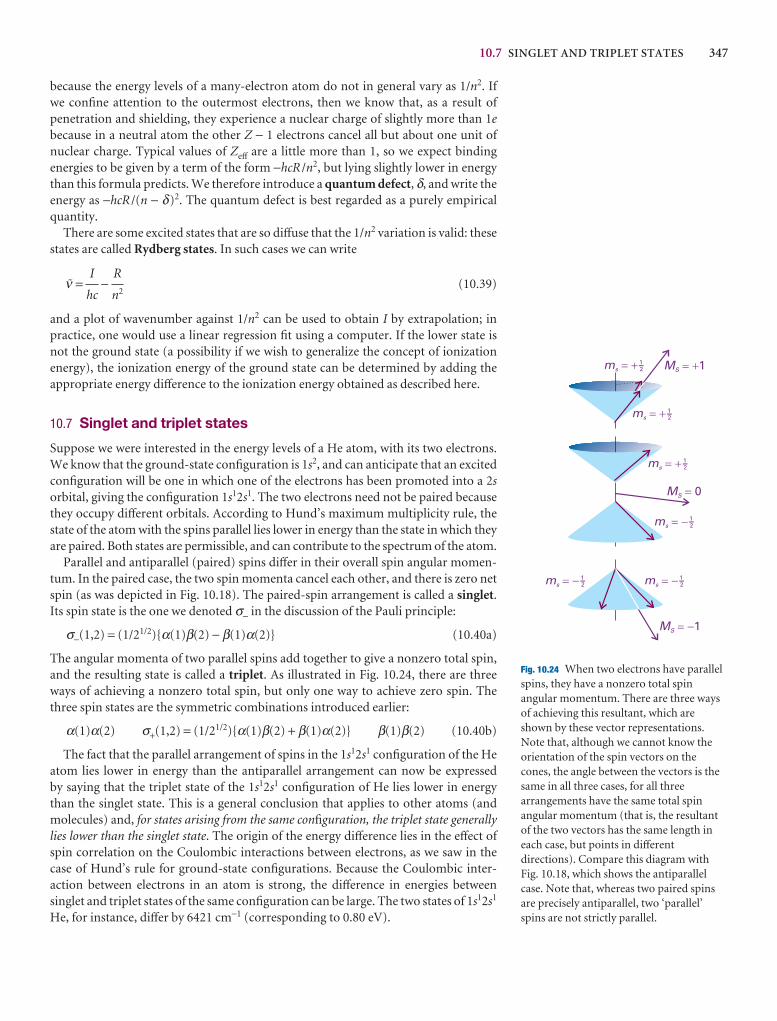
10.7 SINGLET AND TRIPLET STATES 347
because the energy levels of a many-electron atom do not in general vary as 1/n2. If we confine attention to the outermost electrons, then we know that, as a result of penetration and shielding, they experience a nuclear charge of slightly more than 1ebecause in a neutral atom the other Z − 1 electrons cancel all but about one unit of nuclear charge. Typical values of Zeff are a little more than 1, so we expect binding energies to be given by a term of the form −hcR /n2, but lying slightly lower in energythan this formula predicts. We therefore introduce a quantum defect, δ, and write theenergy as −hcR /(n − δ)2. The quantum defect is best regarded as a purely empiricalquantity.
There are some excited states that are so diffuse that the 1/n2 variation is valid: thesestates are called Rydberg states. In such cases we can write
# = − (10.39)
and a plot of wavenumber against 1/n2 can be used to obtain I by extrapolation; inpractice, one would use a linear regression fit using a computer. If the lower state isnot the ground state (a possibility if we wish to generalize the concept of ionizationenergy), the ionization energy of the ground state can be determined by adding theappropriate energy difference to the ionization energy obtained as described here.
10.7 Singlet and triplet states
Suppose we were interested in the energy levels of a He atom, with its two electrons.We know that the ground-state configuration is 1s2, and can anticipate that an excitedconfiguration will be one in which one of the electrons has been promoted into a 2sorbital, giving the configuration 1s12s1. The two electrons need not be paired becausethey occupy different orbitals. According to Hund’s maximum multiplicity rule, thestate of the atom with the spins parallel lies lower in energy than the state in which theyare paired. Both states are permissible, and can contribute to the spectrum of the atom.
Parallel and antiparallel (paired) spins differ in their overall spin angular momen-tum. In the paired case, the two spin momenta cancel each other, and there is zero netspin (as was depicted in Fig. 10.18). The paired-spin arrangement is called a singlet.Its spin state is the one we denoted σ− in the discussion of the Pauli principle:
σ−(1,2) = (1/21/2){α(1)β(2) − β(1)α(2)} (10.40a)
The angular momenta of two parallel spins add together to give a nonzero total spin,and the resulting state is called a triplet. As illustrated in Fig. 10.24, there are threeways of achieving a nonzero total spin, but only one way to achieve zero spin. Thethree spin states are the symmetric combinations introduced earlier:
α(1)α(2) σ+(1,2) = (1/21/2){α(1)β(2) + β(1)α(2)} β(1)β(2) (10.40b)
The fact that the parallel arrangement of spins in the 1s12s1 configuration of the Heatom lies lower in energy than the antiparallel arrangement can now be expressed by saying that the triplet state of the 1s12s1 configuration of He lies lower in energythan the singlet state. This is a general conclusion that applies to other atoms (andmolecules) and, for states arising from the same configuration, the triplet state generallylies lower than the singlet state. The origin of the energy difference lies in the effect ofspin correlation on the Coulombic interactions between electrons, as we saw in thecase of Hund’s rule for ground-state configurations. Because the Coulombic inter-action between electrons in an atom is strong, the difference in energies between singlet and triplet states of the same configuration can be large. The two states of 1s12s1
He, for instance, differ by 6421 cm−1 (corresponding to 0.80 eV).
R
n2
I
hc
MS 0�
ms � �
ms � �
MS 1� �ms � �
ms � �
MS 1� �
ms � �ms � �
21-
21-
21-
21-
21-2
1-
Fig. 10.24 When two electrons have parallelspins, they have a nonzero total spinangular momentum. There are three waysof achieving this resultant, which areshown by these vector representations.Note that, although we cannot know theorientation of the spin vectors on thecones, the angle between the vectors is thesame in all three cases, for all threearrangements have the same total spinangular momentum (that is, the resultantof the two vectors has the same length ineach case, but points in differentdirections). Compare this diagram withFig. 10.18, which shows the antiparallelcase. Note that, whereas two paired spinsare precisely antiparallel, two ‘parallel’spins are not strictly parallel.
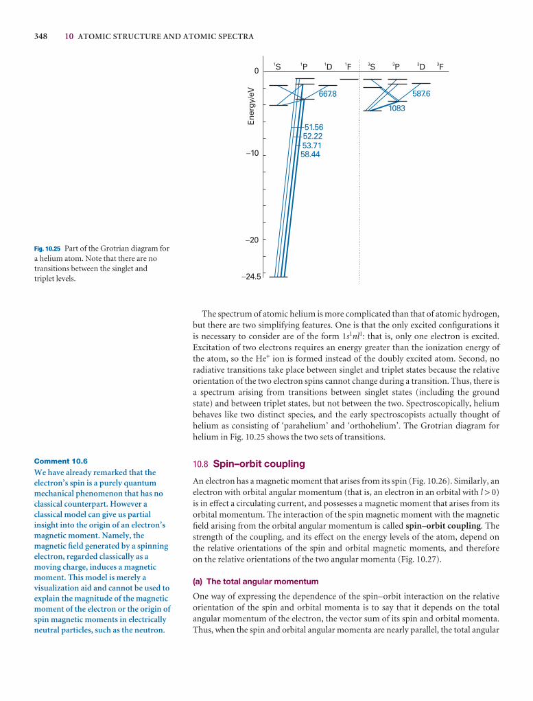
348 10 ATOMIC STRUCTURE AND ATOMIC SPECTRA
The spectrum of atomic helium is more complicated than that of atomic hydrogen,but there are two simplifying features. One is that the only excited configurations it is necessary to consider are of the form 1s1nl1: that is, only one electron is excited.Excitation of two electrons requires an energy greater than the ionization energy ofthe atom, so the He+ ion is formed instead of the doubly excited atom. Second, no radiative transitions take place between singlet and triplet states because the relativeorientation of the two electron spins cannot change during a transition. Thus, there isa spectrum arising from transitions between singlet states (including the groundstate) and between triplet states, but not between the two. Spectroscopically, heliumbehaves like two distinct species, and the early spectroscopists actually thought of helium as consisting of ‘parahelium’ and ‘orthohelium’. The Grotrian diagram for helium in Fig. 10.25 shows the two sets of transitions.
10.8 Spin–orbit coupling
An electron has a magnetic moment that arises from its spin (Fig. 10.26). Similarly, anelectron with orbital angular momentum (that is, an electron in an orbital with l > 0)is in effect a circulating current, and possesses a magnetic moment that arises from itsorbital momentum. The interaction of the spin magnetic moment with the magneticfield arising from the orbital angular momentum is called spin–orbit coupling. Thestrength of the coupling, and its effect on the energy levels of the atom, depend on the relative orientations of the spin and orbital magnetic moments, and therefore on the relative orientations of the two angular momenta (Fig. 10.27).
(a) The total angular momentum
One way of expressing the dependence of the spin–orbit interaction on the relativeorientation of the spin and orbital momenta is to say that it depends on the total angular momentum of the electron, the vector sum of its spin and orbital momenta.Thus, when the spin and orbital angular momenta are nearly parallel, the total angular
1S 1P 1D 1F 3S 3P 3D 3F
�24.5
0
�10
�20En
ergy
/eV
1083
587.6667.8
58.4453.7152.2251.56
Fig. 10.25 Part of the Grotrian diagram for a helium atom. Note that there are notransitions between the singlet and triplet levels.
Comment 10.6
We have already remarked that theelectron’s spin is a purely quantummechanical phenomenon that has noclassical counterpart. However aclassical model can give us partialinsight into the origin of an electron’smagnetic moment. Namely, themagnetic field generated by a spinningelectron, regarded classically as amoving charge, induces a magneticmoment. This model is merely avisualization aid and cannot be used toexplain the magnitude of the magneticmoment of the electron or the origin ofspin magnetic moments in electricallyneutral particles, such as the neutron.
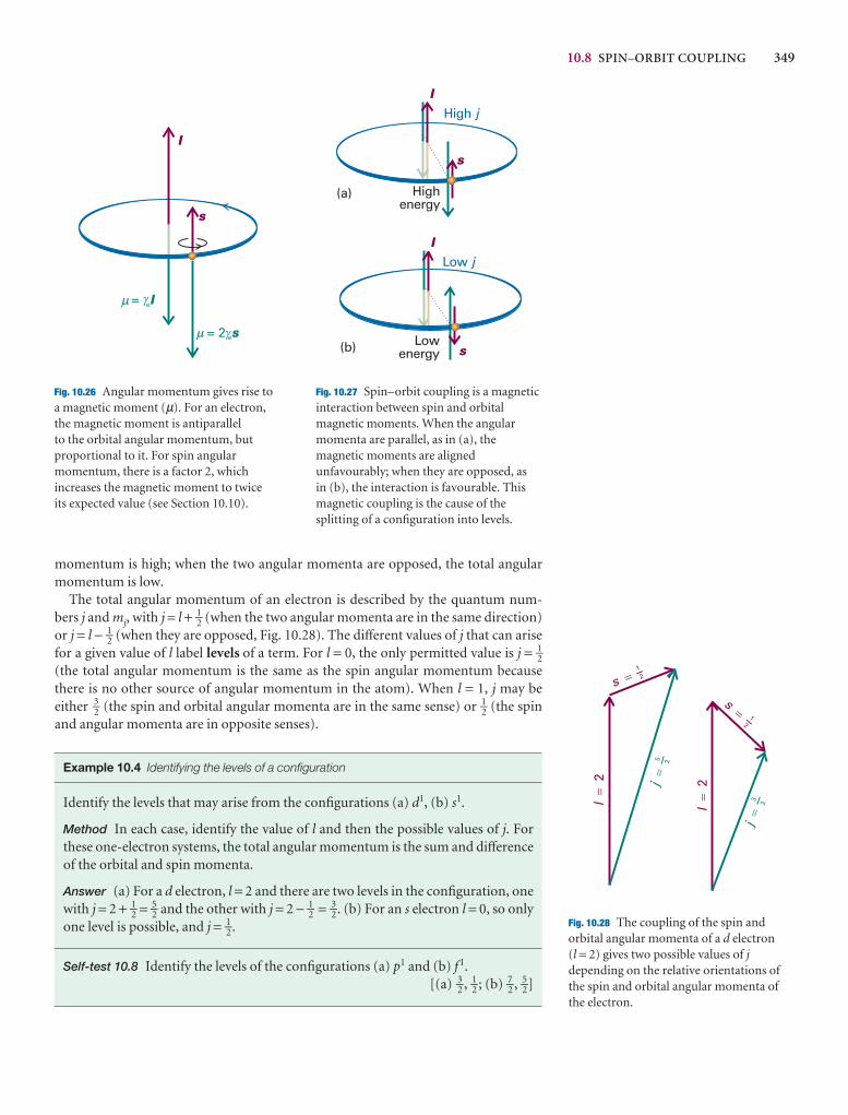
10.8 SPIN–ORBIT COUPLING 349
l
= el
= 2 es
s
�
�
Fig. 10.26 Angular momentum gives rise toa magnetic moment (µ). For an electron, the magnetic moment is antiparallel to the orbital angular momentum, butproportional to it. For spin angularmomentum, there is a factor 2, whichincreases the magnetic moment to twice its expected value (see Section 10.10).
l
l
s
s
Highenergy
High j
Low j
Lowenergy
(a)
(b)
Fig. 10.27 Spin–orbit coupling is a magneticinteraction between spin and orbitalmagnetic moments. When the angularmomenta are parallel, as in (a), themagnetic moments are alignedunfavourably; when they are opposed, as in (b), the interaction is favourable. Thismagnetic coupling is the cause of thesplitting of a configuration into levels.
s �1
s�
1
l2
�
l2
�
j�
5
j�
3
– 2
2–
2–
– 2
Fig. 10.28 The coupling of the spin andorbital angular momenta of a d electron(l = 2) gives two possible values of jdepending on the relative orientations ofthe spin and orbital angular momenta ofthe electron.
momentum is high; when the two angular momenta are opposed, the total angularmomentum is low.
The total angular momentum of an electron is described by the quantum num-bers j and mj, with j = l + 1–2 (when the two angular momenta are in the same direction)or j = l − 1–2 (when they are opposed, Fig. 10.28). The different values of j that can arisefor a given value of l label levels of a term. For l = 0, the only permitted value is j = 1–2(the total angular momentum is the same as the spin angular momentum becausethere is no other source of angular momentum in the atom). When l = 1, j may be either 3–2 (the spin and orbital angular momenta are in the same sense) or 1–2 (the spinand angular momenta are in opposite senses).
Example 10.4 Identifying the levels of a configuration
Identify the levels that may arise from the configurations (a) d1, (b) s1.
Method In each case, identify the value of l and then the possible values of j. Forthese one-electron systems, the total angular momentum is the sum and differenceof the orbital and spin momenta.
Answer (a) For a d electron, l = 2 and there are two levels in the configuration, onewith j = 2 + 1–2 = 5–2 and the other with j = 2 − 1–2 = 3–2. (b) For an s electron l = 0, so onlyone level is possible, and j = 1–2.
Self-test 10.8 Identify the levels of the configurations (a) p1 and (b) f 1.[(a) 3–2 , 1–2 ; (b) 7–2 , 5–2]
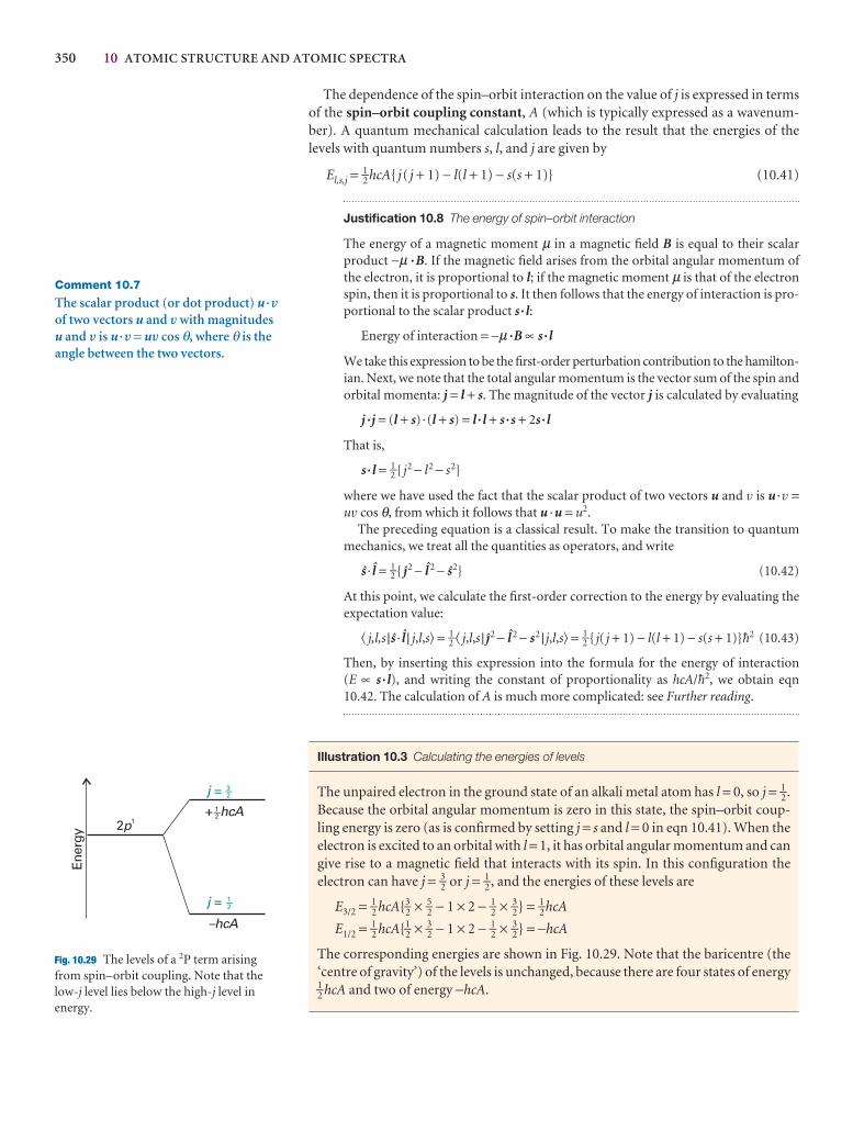
350 10 ATOMIC STRUCTURE AND ATOMIC SPECTRA
Comment 10.7
The scalar product (or dot product) u ·1of two vectors u and 1 with magnitudesu and 1 is u ·1 = u1 cos θ, where θ is theangle between the two vectors.
2p1
j =
j =
+ hcA
–hcA
Ener
gy
23�
21�
21�
Fig. 10.29 The levels of a 2P term arisingfrom spin–orbit coupling. Note that thelow-j level lies below the high-j level inenergy.
The dependence of the spin–orbit interaction on the value of j is expressed in termsof the spin–orbit coupling constant, A (which is typically expressed as a wavenum-ber). A quantum mechanical calculation leads to the result that the energies of the levels with quantum numbers s, l, and j are given by
El,s,j = 1–2hcA{ j( j + 1) − l(l + 1) − s(s + 1)} (10.41)
Justification 10.8 The energy of spin–orbit interaction
The energy of a magnetic moment µ in a magnetic field B is equal to their scalarproduct −µ ·B. If the magnetic field arises from the orbital angular momentum ofthe electron, it is proportional to l; if the magnetic moment µ is that of the electronspin, then it is proportional to s. It then follows that the energy of interaction is pro-portional to the scalar product s · l:
Energy of interaction = −µ ·B ∝ s · l
We take this expression to be the first-order perturbation contribution to the hamilton-ian. Next, we note that the total angular momentum is the vector sum of the spin andorbital momenta: j = l + s. The magnitude of the vector j is calculated by evaluating
j ·j = (l + s) ·(l + s) = l · l + s ·s + 2s · l
That is,
s · l = 1–2 { j2 − l2 − s2}
where we have used the fact that the scalar product of two vectors u and v is u ·v =uv cos θ, from which it follows that u ·u = u2.
The preceding equation is a classical result. To make the transition to quantummechanics, we treat all the quantities as operators, and write
£ · ™ = 1–2 { ¡2 − ™ 2 − £2} (10.42)
At this point, we calculate the first-order correction to the energy by evaluating theexpectation value:
� j,l,s |£ · ™ | j,l,s� = 1–2 � j,l,s | ¡2 − ™ 2 − s2 | j,l,s� = 1–2 { j( j + 1) − l(l + 1) − s(s + 1)}$2 (10.43)
Then, by inserting this expression into the formula for the energy of interaction (E ∝ s · l), and writing the constant of proportionality as hcA/$2, we obtain eqn10.42. The calculation of A is much more complicated: see Further reading.
Illustration 10.3 Calculating the energies of levels
The unpaired electron in the ground state of an alkali metal atom has l = 0, so j = 1–2.Because the orbital angular momentum is zero in this state, the spin–orbit coup-ling energy is zero (as is confirmed by setting j = s and l = 0 in eqn 10.41). When theelectron is excited to an orbital with l = 1, it has orbital angular momentum and cangive rise to a magnetic field that interacts with its spin. In this configuration theelectron can have j = 3–2 or j = 1–2, and the energies of these levels are
E3/2 = 1–2 hcA{3–2 × 5–2 − 1 × 2 − 1–2 × 3–2} = 1–2hcA
E1/2 = 1–2 hcA{1–2 × 3–2 − 1 × 2 − 1–2 × 3–2} = −hcA
The corresponding energies are shown in Fig. 10.29. Note that the baricentre (the‘centre of gravity’) of the levels is unchanged, because there are four states of energy1–2 hcA and two of energy −hcA.
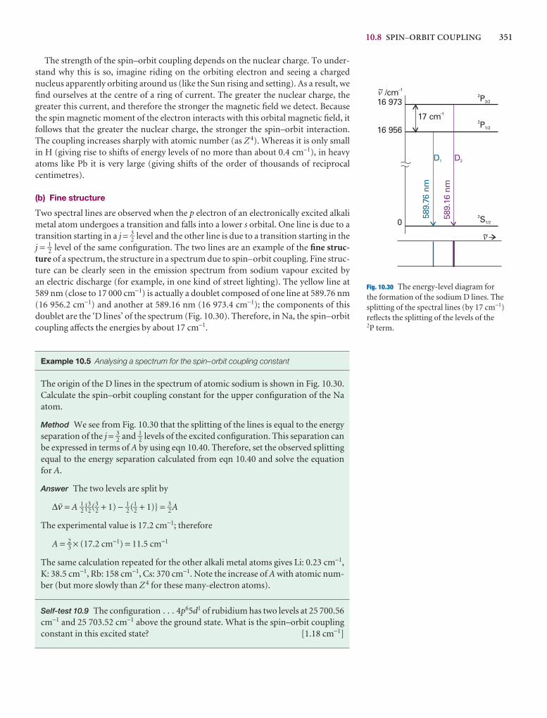
10.8 SPIN–ORBIT COUPLING 351
D1 D2
2P1/2
2P3/2
17 cm1
2S1/2
16 973
16 956
0
589.
76 n
m
589.
16 n
m
�~
/cm 1~� �
�
Fig. 10.30 The energy-level diagram for the formation of the sodium D lines. Thesplitting of the spectral lines (by 17 cm−1)reflects the splitting of the levels of the 2P term.
The strength of the spin–orbit coupling depends on the nuclear charge. To under-stand why this is so, imagine riding on the orbiting electron and seeing a charged nucleus apparently orbiting around us (like the Sun rising and setting). As a result, wefind ourselves at the centre of a ring of current. The greater the nuclear charge, thegreater this current, and therefore the stronger the magnetic field we detect. Becausethe spin magnetic moment of the electron interacts with this orbital magnetic field, itfollows that the greater the nuclear charge, the stronger the spin–orbit interaction.The coupling increases sharply with atomic number (as Z 4). Whereas it is only smallin H (giving rise to shifts of energy levels of no more than about 0.4 cm−1), in heavyatoms like Pb it is very large (giving shifts of the order of thousands of reciprocal centimetres).
(b) Fine structure
Two spectral lines are observed when the p electron of an electronically excited alkalimetal atom undergoes a transition and falls into a lower s orbital. One line is due to atransition starting in a j = 3–2 level and the other line is due to a transition starting in thej = 1–2 level of the same configuration. The two lines are an example of the fine struc-ture of a spectrum, the structure in a spectrum due to spin–orbit coupling. Fine struc-ture can be clearly seen in the emission spectrum from sodium vapour excited by an electric discharge (for example, in one kind of street lighting). The yellow line at589 nm (close to 17 000 cm−1) is actually a doublet composed of one line at 589.76 nm (16 956.2 cm−1) and another at 589.16 nm (16 973.4 cm−1); the components of thisdoublet are the ‘D lines’ of the spectrum (Fig. 10.30). Therefore, in Na, the spin–orbitcoupling affects the energies by about 17 cm−1.
Example 10.5 Analysing a spectrum for the spin–orbit coupling constant
The origin of the D lines in the spectrum of atomic sodium is shown in Fig. 10.30.Calculate the spin–orbit coupling constant for the upper configuration of the Naatom.
Method We see from Fig. 10.30 that the splitting of the lines is equal to the energyseparation of the j = 3–2 and 1–2 levels of the excited configuration. This separation canbe expressed in terms of A by using eqn 10.40. Therefore, set the observed splittingequal to the energy separation calculated from eqn 10.40 and solve the equation for A.
Answer The two levels are split by
∆# = A 1–2{3–2(3–2 + 1) − 1–2 (1–2 + 1)} = 3–2A
The experimental value is 17.2 cm−1; therefore
A = 2–3 × (17.2 cm−1) = 11.5 cm−1
The same calculation repeated for the other alkali metal atoms gives Li: 0.23 cm−1,K: 38.5 cm−1, Rb: 158 cm−1, Cs: 370 cm−1. Note the increase of A with atomic num-ber (but more slowly than Z 4 for these many-electron atoms).
Self-test 10.9 The configuration . . . 4p65d1 of rubidium has two levels at 25 700.56cm−1 and 25 703.52 cm−1 above the ground state. What is the spin–orbit couplingconstant in this excited state? [1.18 cm−1]
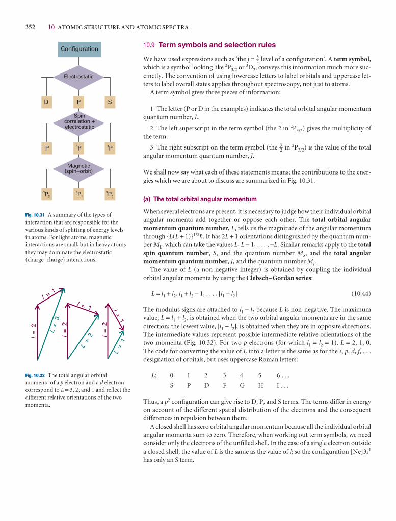
352 10 ATOMIC STRUCTURE AND ATOMIC SPECTRA
10.9 Term symbols and selection rules
We have used expressions such as ‘the j = 3–2 level of a configuration’. A term symbol,which is a symbol looking like 2P3/2 or 3D2, conveys this information much more suc-cinctly. The convention of using lowercase letters to label orbitals and uppercase let-ters to label overall states applies throughout spectroscopy, not just to atoms.
A term symbol gives three pieces of information:
1 The letter (P or D in the examples) indicates the total orbital angular momentumquantum number, L.
2 The left superscript in the term symbol (the 2 in 2P3/2) gives the multiplicity ofthe term.
3 The right subscript on the term symbol (the 3–2 in 2P3/2) is the value of the total angular momentum quantum number, J.
We shall now say what each of these statements means; the contributions to the ener-gies which we are about to discuss are summarized in Fig. 10.31.
(a) The total orbital angular momentum
When several electrons are present, it is necessary to judge how their individual orbitalangular momenta add together or oppose each other. The total orbital angular momentum quantum number, L, tells us the magnitude of the angular momentumthrough {L(L + 1)}1/2$. It has 2L + 1 orientations distinguished by the quantum num-ber ML, which can take the values L, L − 1, . . . , −L. Similar remarks apply to the totalspin quantum number, S, and the quantum number MS, and the total angular momentum quantum number, J, and the quantum number MJ.
The value of L (a non-negative integer) is obtained by coupling the individual orbital angular momenta by using the Clebsch–Gordan series:
L = l1 + l2, l1 + l2 − 1, . . . , | l1 − l2 | (10.44)
The modulus signs are attached to l1 − l2 because L is non-negative. The maximumvalue, L = l1 + l2, is obtained when the two orbital angular momenta are in the same direction; the lowest value, | l1 − l2 |, is obtained when they are in opposite directions.The intermediate values represent possible intermediate relative orientations of thetwo momenta (Fig. 10.32). For two p electrons (for which l1 = l2 = 1), L = 2, 1, 0. The code for converting the value of L into a letter is the same as for the s, p, d, f, . . .designation of orbitals, but uses uppercase Roman letters:
L: 0 1 2 3 4 5 6 . . .
S P D F G H I . . .
Thus, a p2 configuration can give rise to D, P, and S terms. The terms differ in energyon account of the different spatial distribution of the electrons and the consequentdifferences in repulsion between them.
A closed shell has zero orbital angular momentum because all the individual orbitalangular momenta sum to zero. Therefore, when working out term symbols, we needconsider only the electrons of the unfilled shell. In the case of a single electron outsidea closed shell, the value of L is the same as the value of l; so the configuration [Ne]3s1
has only an S term.
D P S
5P 3P 1P
3P23P1
3P0
Configuration
Electrostatic
Spincorrelation +electrostatic
Magnetic(spin orbit)�
Fig. 10.31 A summary of the types ofinteraction that are responsible for thevarious kinds of splitting of energy levels in atoms. For light atoms, magneticinteractions are small, but in heavy atomsthey may dominate the electrostatic(charge–charge) interactions.
l = 1
l = 1 l=
1
l=
2
l=
2
l=
2
L=
3
L
=2
L=
1
Fig. 10.32 The total angular orbitalmomenta of a p electron and a d electroncorrespond to L = 3, 2, and 1 and reflect thedifferent relative orientations of the twomomenta.
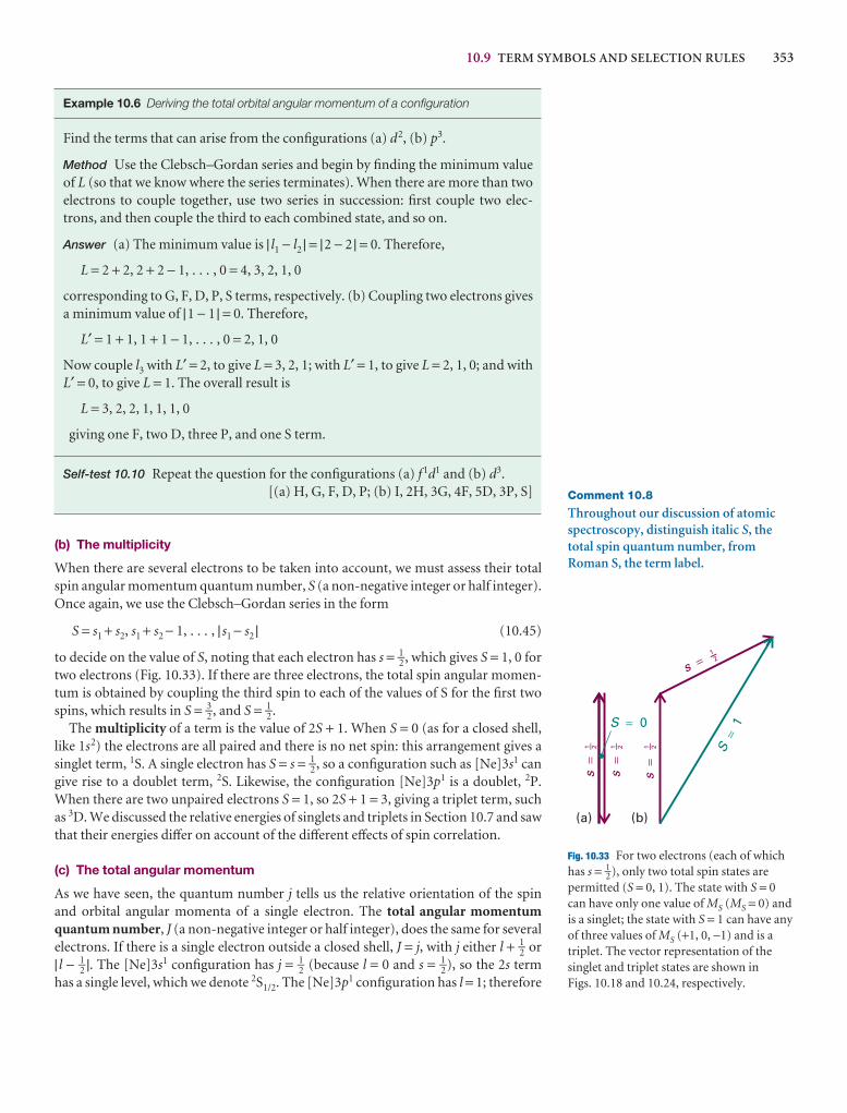
10.9 TERM SYMBOLS AND SELECTION RULES 353
Comment 10.8
Throughout our discussion of atomicspectroscopy, distinguish italic S, thetotal spin quantum number, fromRoman S, the term label.
s�
s�
s�
s �
S1
�S 0�
(a) (b)
21–
21 �21 � 21 �
Fig. 10.33 For two electrons (each of whichhas s = 1–2), only two total spin states arepermitted (S = 0, 1). The state with S = 0can have only one value of MS (MS = 0) andis a singlet; the state with S = 1 can have anyof three values of MS (+1, 0, −1) and is atriplet. The vector representation of thesinglet and triplet states are shown in Figs. 10.18 and 10.24, respectively.
Example 10.6 Deriving the total orbital angular momentum of a configuration
Find the terms that can arise from the configurations (a) d2, (b) p3.
Method Use the Clebsch–Gordan series and begin by finding the minimum valueof L (so that we know where the series terminates). When there are more than twoelectrons to couple together, use two series in succession: first couple two elec-trons, and then couple the third to each combined state, and so on.
Answer (a) The minimum value is | l1 − l2 | = |2 − 2 | = 0. Therefore,
L = 2 + 2, 2 + 2 − 1, . . . , 0 = 4, 3, 2, 1, 0
corresponding to G, F, D, P, S terms, respectively. (b) Coupling two electrons givesa minimum value of |1 − 1 | = 0. Therefore,
L′ = 1 + 1, 1 + 1 − 1, . . . , 0 = 2, 1, 0
Now couple l3 with L′ = 2, to give L = 3, 2, 1; with L′ = 1, to give L = 2, 1, 0; and withL′ = 0, to give L = 1. The overall result is
L = 3, 2, 2, 1, 1, 1, 0
giving one F, two D, three P, and one S term.
Self-test 10.10 Repeat the question for the configurations (a) f 1d1 and (b) d3.[(a) H, G, F, D, P; (b) I, 2H, 3G, 4F, 5D, 3P, S]
(b) The multiplicity
When there are several electrons to be taken into account, we must assess their totalspin angular momentum quantum number, S (a non-negative integer or half integer).Once again, we use the Clebsch–Gordan series in the form
S = s1 + s2, s1 + s2 − 1, . . . , | s1 − s2 | (10.45)
to decide on the value of S, noting that each electron has s = 1–2, which gives S = 1, 0 fortwo electrons (Fig. 10.33). If there are three electrons, the total spin angular momen-tum is obtained by coupling the third spin to each of the values of S for the first twospins, which results in S = 3–2, and S = 1–2.
The multiplicity of a term is the value of 2S + 1. When S = 0 (as for a closed shell,like 1s2) the electrons are all paired and there is no net spin: this arrangement gives asinglet term, 1S. A single electron has S = s = 1–2, so a configuration such as [Ne]3s1 cangive rise to a doublet term, 2S. Likewise, the configuration [Ne]3p1 is a doublet, 2P.When there are two unpaired electrons S = 1, so 2S + 1 = 3, giving a triplet term, suchas 3D. We discussed the relative energies of singlets and triplets in Section 10.7 and sawthat their energies differ on account of the different effects of spin correlation.
(c) The total angular momentum
As we have seen, the quantum number j tells us the relative orientation of the spin and orbital angular momenta of a single electron. The total angular momentumquantum number, J (a non-negative integer or half integer), does the same for severalelectrons. If there is a single electron outside a closed shell, J = j, with j either l + 1–2 or| l − 1–2 |. The [Ne]3s1 configuration has j = 1–2 (because l = 0 and s = 1–2), so the 2s termhas a single level, which we denote 2S1/2. The [Ne]3p1 configuration has l = 1; therefore
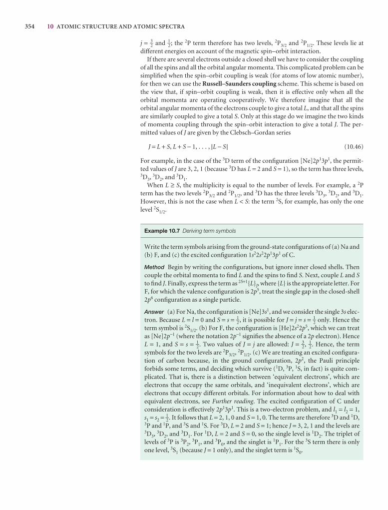
354 10 ATOMIC STRUCTURE AND ATOMIC SPECTRA
j = 3–2 and 1–2; the 2P term therefore has two levels, 2P3/2 and 2P1/2. These levels lie at different energies on account of the magnetic spin–orbit interaction.
If there are several electrons outside a closed shell we have to consider the couplingof all the spins and all the orbital angular momenta. This complicated problem can besimplified when the spin–orbit coupling is weak (for atoms of low atomic number),for then we can use the Russell–Saunders coupling scheme. This scheme is based onthe view that, if spin–orbit coupling is weak, then it is effective only when all the orbital momenta are operating cooperatively. We therefore imagine that all the orbital angular momenta of the electrons couple to give a total L, and that all the spinsare similarly coupled to give a total S. Only at this stage do we imagine the two kindsof momenta coupling through the spin–orbit interaction to give a total J. The per-mitted values of J are given by the Clebsch–Gordan series
J = L + S, L + S − 1, . . . , |L − S | (10.46)
For example, in the case of the 3D term of the configuration [Ne]2p13p1, the permit-ted values of J are 3, 2, 1 (because 3D has L = 2 and S = 1), so the term has three levels,3D3, 3D2, and 3D1.
When L ≥ S, the multiplicity is equal to the number of levels. For example, a 2Pterm has the two levels 2P3/2 and 2P1/2, and 3D has the three levels 3D3, 3D2, and 3D1.However, this is not the case when L < S: the term 2S, for example, has only the one level 2S1/2.
Example 10.7 Deriving term symbols
Write the term symbols arising from the ground-state configurations of (a) Na and(b) F, and (c) the excited configuration 1s22s22p13p1 of C.
Method Begin by writing the configurations, but ignore inner closed shells. Thencouple the orbital momenta to find L and the spins to find S. Next, couple L and Sto find J. Finally, express the term as 2S+1{L}J, where {L} is the appropriate letter. ForF, for which the valence configuration is 2p5, treat the single gap in the closed-shell2p6 configuration as a single particle.
Answer (a) For Na, the configuration is [Ne]3s1, and we consider the single 3s elec-tron. Because L = l = 0 and S = s = 1–2, it is possible for J = j = s = 1–2 only. Hence theterm symbol is 2S1/2. (b) For F, the configuration is [He]2s22p5, which we can treatas [Ne]2p−1 (where the notation 2p−1 signifies the absence of a 2p electron). HenceL = 1, and S = s = 1–2. Two values of J = j are allowed: J = 3–2, 1–2. Hence, the term symbols for the two levels are 2P3/2, 2P1/2. (c) We are treating an excited configura-tion of carbon because, in the ground configuration, 2p2, the Pauli principle forbids some terms, and deciding which survive (1D, 3P, 1S, in fact) is quite com-plicated. That is, there is a distinction between ‘equivalent electrons’, which areelectrons that occupy the same orbitals, and ‘inequivalent electrons’, which areelectrons that occupy different orbitals. For information about how to deal withequivalent electrons, see Further reading. The excited configuration of C underconsideration is effectively 2p13p1. This is a two-electron problem, and l1 = l2 = 1,s1 = s2 = 1–2. It follows that L = 2, 1, 0 and S = 1, 0. The terms are therefore 3D and 1D,3P and 1P, and 3S and 1S. For 3D, L = 2 and S = 1; hence J = 3, 2, 1 and the levels are3D3, 3D2, and 3D1. For 1D, L = 2 and S = 0, so the single level is 1D2. The triplet oflevels of 3P is 3P2, 3P1, and 3P0, and the singlet is 1P1. For the 3S term there is onlyone level, 3S1 (because J = 1 only), and the singlet term is 1S0.
10.9 TERM SYMBOLS AND SELECTION RULES 355
Si Ge Sn Pb
1S0
1D2
3P23P13P0
PureRussell–Saunderscoupling
Pure-couplingjj
C
Fig. 10.34 The correlation diagram for someof the states of a two-electron system. Allatoms lie between the two extremes, butthe heavier the atom, the closer it lies to thepure jj-coupling case.
Self-test 10.11 Write down the terms arising from the configurations (a) 2s12p1,(b) 2p13d1.
[(a) 3P2, 3P1, 3P0, 1P1;(b) 3F4, 3F3, 3F2, 1F3, 3D3, 3D2, 3D1, 1D2, 3P1, 3P0, 1P1]
Russell–Saunders coupling fails when the spin–orbit coupling is large (in heavyatoms). In that case, the individual spin and orbital momenta of the electrons are coupled into individual j values; then these momenta are combined into a grand total,J. This scheme is called jj-coupling. For example, in a p2 configuration, the individualvalues of j are 3–2 and 1–2 for each electron. If the spin and the orbital angular momentumof each electron are coupled together strongly, it is best to consider each electron as aparticle with angular momentum j = 3–2 or 1–2. These individual total momenta thencouple as follows:
j1 = 3–2 and j2 = 3–2 J = 3, 2, 1, 0
j1 = 3–2 and j2 = 1–2 J = 2, 1
j1 = 1–2 and j2 = 3–2 J = 2, 1
j1 = 1–2 and j2 = 1–2 J = 1, 0
For heavy atoms, in which jj-coupling is appropriate, it is best to discuss their energiesusing these quantum numbers.
Although jj-coupling should be used for assessing the energies of heavy atoms, theterm symbols derived from Russell–Saunders coupling can still be used as labels. Tosee why this procedure is valid, we need to examine how the energies of the atomicstates change as the spin–orbit coupling increases in strength. Such a correlationdiagram is shown in Fig. 10.34. It shows that there is a correspondence between thelow spin–orbit coupling (Russell–Saunders coupling) and high spin–orbit coupling( jj-coupling) schemes, so the labels derived by using the Russell–Saunders schemecan be used to label the states of the jj-coupling scheme.
(d) Selection rules
Any state of the atom, and any spectral transition, can be specified by using term sym-bols. For example, the transitions giving rise to the yellow sodium doublet (whichwere shown in Fig. 10.30) are
3p1 2P3/2 → 3s1 2S1/2 3p1 2P1/2 → 3s1 2S1/2
By convention, the upper term precedes the lower. The corresponding absorptionsare therefore denoted
2P3/2 ← 2S1/22P1/2 ← 2S1/2
(The configurations have been omitted.)We have seen that selection rules arise from the conservation of angular momen-
tum during a transition and from the fact that a photon has a spin of 1. They cantherefore be expressed in terms of the term symbols, because the latter carry informa-tion about angular momentum. A detailed analysis leads to the following rules:
∆S = 0 ∆L = 0, ±1 ∆l = ±1 ∆J = 0, ±1, but J = 0 ←|→ J = 0 (10.47)
where the symbol ←|→ denotes a forbidden transition. The rule about ∆S (no changeof overall spin) stems from the fact that the light does not affect the spin directly. The rules about ∆L and ∆l express the fact that the orbital angular momentum of an

356 10 ATOMIC STRUCTURE AND ATOMIC SPECTRA
individual electron must change (so ∆l = ±1), but whether or not this results in anoverall change of orbital momentum depends on the coupling.
The selection rules given above apply when Russell–Saunders coupling is valid (inlight atoms). If we insist on labelling the terms of heavy atoms with symbols like 3D,then we shall find that the selection rules progressively fail as the atomic number increases because the quantum numbers S and L become ill defined as jj-couplingbecomes more appropriate. As explained above, Russell–Saunders term symbols areonly a convenient way of labelling the terms of heavy atoms: they do not bear any direct relation to the actual angular momenta of the electrons in a heavy atom. Forthis reason, transitions between singlet and triplet states (for which ∆S = ±1), whileforbidden in light atoms, are allowed in heavy atoms.
Checklist of key ideas
1. A hydrogenic atom is a one-electron atom or ion of generalatomic number Z. A many-electron (polyelectronic) atom isan atom or ion with more than one electron.
2. The Lyman, Balmer, and Paschen series in the spectrum ofatomic hydrogen arise, respectively, from the transitions n → 1, n → 2, and n → 3.
3. The wavenumbers of all the spectral lines of a hydrogen atomcan be expressed as # = RH(1/n1
2 − 1/n22), where RH is the
Rydberg constant for hydrogen.
4. The Ritz combination principle states that the wavenumber ofany spectral line is the difference between two spectroscopicenergy levels, or terms: # = T1 − T2.
5. The wavefunction of the hydrogen atom is the product of a radial wavefunction and a radial wavefunction: ψ(r,θ,φ) = R(r)Y(θ,φ).
6. An atomic orbital is a one-electron wavefunction for anelectron in an atom.
7. The energies of an electron in a hydrogen atom are given by En = −Z 2µe 4/32π2ε2
0$2n2, where n is the principal quantumnumber, n = 1, 2, . . . .
8. All the orbitals of a given value of n belong to a given shell;orbitals with the same value of n but different values of lbelong to different subshells.
9. The radial distribution function is a probability density that,when it is multiplied by dr, gives the probability of finding theelectron anywhere in a shell of thickness dr at the radius r;P(r) = r2R(r)2.
10. A selection rule is a statement about which spectroscopictransitions are allowed; a Grotrian diagram is a diagramsummarizing the energies of the states and atom and thetransitions between them.
11. In the orbital approximation it is supposed that each electronoccupies its ‘own’ orbital, ψ(r1,r2, . . . ) = ψ(r1)ψ(r2) . . . .
12. The Pauli exclusion principle states that no more than twoelectrons may occupy any given orbital and, if two do occupyone orbital, then their spins must be paired.
13. The Pauli principle states that, when the labels of any twoidentical fermions are exchanged, the total wavefunctionchanges sign; when the labels of any two identical bosons are exchanged, the total wavefunction retains the same sign.
14. The effective nuclear charge Zeff is the net charge experiencedby an electron allowing for electron–electron repulsions.
15. Shielding is the effective reduction in charge of a nucleus bysurrounding electrons; the shielding constant σ is given by Zeff = Z − σ.
16. Penetration is the ability of an electron to be found insideinner shells and close to the nucleus.
17. The building-up (Aufbau) principle is the procedure for fillingatomic orbitals that leads to the ground-state configuration ofan atom.
18. Hund’s maximum multiplicity rule states that an atom in itsground state adopts a configuration with the greatest numberof unpaired electrons.
19. The first ionization energy I1 is the minimum energynecessary to remove an electron from a many-electron atomin the gas phase; the second ionization energy I2 is theminimum energy necessary to remove an electron from anionized many-electron atom in the gas phase.
20. The electron affinity Eea is the energy released when anelectron attaches to a gas-phase atom.
21. A singlet term has S = 0; a triplet term has S = 1.
22. Spin–orbit coupling is the interaction of the spin magneticmoment with the magnetic field arising from the orbitalangular momentum.
23. Fine structure is the structure in a spectrum due to spin–orbitcoupling.
24. A term symbol is a symbolic specification of the state of anatom, 2S+1{L}J.
25. The allowed values of a combined angular momenta areobtained by using the Clebsch–Gordan series: J = j1 + j2,j1 + j2 − 1, . . . | j1 − j2|.
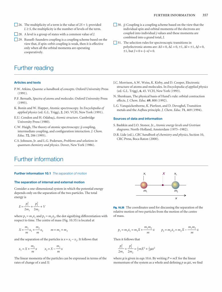
FURTHER INFORMATION 357
26. The multiplicity of a term is the value of 2S + 1; provided L ≥ S, the multiplicity is the number of levels of the term.
28. A level is a group of states with a common value of J.
29. Russell–Saunders coupling is a coupling scheme based on theview that, if spin–orbit coupling is weak, then it is effectiveonly when all the orbital momenta are operatingcooperatively.
30. jj-Coupling is a coupling scheme based on the view that theindividual spin and orbital momenta of the electrons arecoupled into individual j values and these momenta arecombined into a grand total, J.
31. The selection rules for spectroscopic transitions inpolyelectronic atoms are: ∆S = 0, ∆L = 0, ±1, ∆l = ±1, ∆J = 0,±1, but J = 0 ←|→J = 0.
Further reading
Articles and texts
P.W. Atkins, Quanta: a handbook of concepts. Oxford University Press(1991).
P.F. Bernath, Spectra of atoms and molecules. Oxford University Press(1995).
K. Bonin and W. Happer, Atomic spectroscopy. In Encyclopedia ofapplied physics (ed. G.L. Trigg), 2, 245. VCH, New York (1991).
E.U. Condon and H. Odabaçi, Atomic structure. CambridgeUniversity Press (1980).
C.W. Haigh, The theory of atomic spectroscopy: jj coupling,intermediate coupling, and configuration interaction. J. Chem.Educ. 72, 206 (1995).
C.S. Johnson, Jr. and L.G. Pedersen, Problems and solutions inquantum chemistry and physics. Dover, New York (1986).
J.C. Morrison, A.W. Weiss, K. Kirby, and D. Cooper, Electronicstructure of atoms and molecules. In Encyclopedia of applied physics(ed. G.L. Trigg), 6, 45. VCH, New York (1993).
N. Shenkuan, The physical basis of Hund’s rule: orbital contractioneffects. J. Chem. Educ. 69, 800 (1992).
L.G. Vanquickenborne, K. Pierloot, and D. Devoghel, Transitionmetals and the Aufbau principle. J. Chem. Educ. 71, 469 (1994).
Sources of data and information
S. Bashkin and J.O. Stonor, Jr., Atomic energy levels and Grotriandiagrams. North-Holland, Amsterdam (1975–1982).
D.R. Lide (ed.), CRC handbook of chemistry and physics, Section 10,CRC Press, Boca Raton (2000).
Further information
Further information 10.1 The separation of motion
The separation of internal and external motion
Consider a one-dimensional system in which the potential energydepends only on the separation of the two particles. The total energy is
E = + + V
where p1 = m1R1 and p2 = m2R2, the dot signifying differentiation withrespect to time. The centre of mass (Fig. 10.35) is located at
X = x1 + x2 m = m1 + m2
and the separation of the particles is x = x1 − x2. It follows that
x1 = X + x x2 = X − x
The linear momenta of the particles can be expressed in terms of therates of change of x and X:
m1
m
m2
m
m2
m
m1
m
p22
2m2
p21
2m1
p1 = m1R1 = m1| + R p2 = m2R2 = m2 | − R
Then it follows that
+ = 1–2 m|2 + 1–2 µR2
where µ is given in eqn 10.6. By writing P = m| for the linearmomentum of the system as a whole and defining p as µR, we find
p22
2m2
p21
2m1
m1m2
m
m1m2
m
x1
m1
x2
m2
X
x
Fig. 10.35 The coordinates used for discussing the separation of therelative motion of two particles from the motion of the centre of mass.
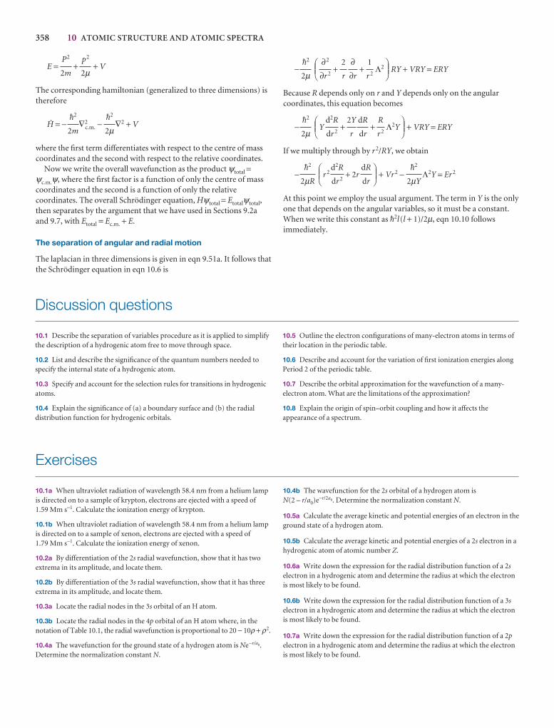
358 10 ATOMIC STRUCTURE AND ATOMIC SPECTRA
E = + + V
The corresponding hamiltonian (generalized to three dimensions) istherefore
@ = − ∇2c.m. − ∇2 + V
where the first term differentiates with respect to the centre of masscoordinates and the second with respect to the relative coordinates.
Now we write the overall wavefunction as the product ψtotal =ψc.m.ψ, where the first factor is a function of only the centre of masscoordinates and the second is a function of only the relativecoordinates. The overall Schrödinger equation, Hψtotal = Etotalψtotal,then separates by the argument that we have used in Sections 9.2aand 9.7, with Etotal = Ec.m. + E.
The separation of angular and radial motion
The laplacian in three dimensions is given in eqn 9.51a. It follows thatthe Schrödinger equation in eqn 10.6 is
$2
2µ$2
2m
p2
2µP2
2m − + + Λ2 RY + VRY = ERY
Because R depends only on r and Y depends only on the angularcoordinates, this equation becomes
− Y + + Λ2Y + VRY = ERY
If we multiply through by r 2/RY, we obtain
− r 2 + 2r + Vr 2 − Λ2Y = Er 2
At this point we employ the usual argument. The term in Y is the onlyone that depends on the angular variables, so it must be a constant.When we write this constant as $2l(l + 1)/2µ, eqn 10.10 followsimmediately.
$2
2µY
DEFdR
dr
d2R
dr 2
ABC$2
2µR
DEFR
r 2
dR
dr
2Y
r
d2R
dr 2
ABC$2
2µ
DEF1
r 2
∂∂r
2
r
∂2
∂r 2
ABC$2
2µ
Discussion questions
10.1 Describe the separation of variables procedure as it is applied to simplifythe description of a hydrogenic atom free to move through space.
10.2 List and describe the significance of the quantum numbers needed tospecify the internal state of a hydrogenic atom.
10.3 Specify and account for the selection rules for transitions in hydrogenicatoms.
10.4 Explain the significance of (a) a boundary surface and (b) the radialdistribution function for hydrogenic orbitals.
10.5 Outline the electron configurations of many-electron atoms in terms oftheir location in the periodic table.
10.6 Describe and account for the variation of first ionization energies alongPeriod 2 of the periodic table.
10.7 Describe the orbital approximation for the wavefunction of a many-electron atom. What are the limitations of the approximation?
10.8 Explain the origin of spin–orbit coupling and how it affects theappearance of a spectrum.
Exercises
10.1a When ultraviolet radiation of wavelength 58.4 nm from a helium lampis directed on to a sample of krypton, electrons are ejected with a speed of 1.59 Mm s−1. Calculate the ionization energy of krypton.
10.1b When ultraviolet radiation of wavelength 58.4 nm from a helium lampis directed on to a sample of xenon, electrons are ejected with a speed of 1.79 Mm s−1. Calculate the ionization energy of xenon.
10.2a By differentiation of the 2s radial wavefunction, show that it has twoextrema in its amplitude, and locate them.
10.2b By differentiation of the 3s radial wavefunction, show that it has threeextrema in its amplitude, and locate them.
10.3a Locate the radial nodes in the 3s orbital of an H atom.
10.3b Locate the radial nodes in the 4p orbital of an H atom where, in thenotation of Table 10.1, the radial wavefunction is proportional to 20 − 10ρ + ρ2.
10.4a The wavefunction for the ground state of a hydrogen atom is Ne−r/a0.Determine the normalization constant N.
10.4b The wavefunction for the 2s orbital of a hydrogen atom is N(2 – r/a0)e−r/2a0. Determine the normalization constant N.
10.5a Calculate the average kinetic and potential energies of an electron in theground state of a hydrogen atom.
10.5b Calculate the average kinetic and potential energies of a 2s electron in ahydrogenic atom of atomic number Z.
10.6a Write down the expression for the radial distribution function of a 2selectron in a hydrogenic atom and determine the radius at which the electronis most likely to be found.
10.6b Write down the expression for the radial distribution function of a 3selectron in a hydrogenic atom and determine the radius at which the electronis most likely to be found.
10.7a Write down the expression for the radial distribution function of a 2pelectron in a hydrogenic atom and determine the radius at which the electronis most likely to be found.

PROBLEMS 359
10.7b Write down the expression for the radial distribution function of a 3pelectron in a hydrogenic atom and determine the radius at which the electronis most likely to be found.
10.8a What is the orbital angular momentum of an electron in the orbitals (a) 1s, (b) 3s, (c) 3d? Give the numbers of angular and radial nodes in each case.
10.8b What is the orbital angular momentum of an electron in the orbitals(a) 4d, (b) 2p, (c) 3p? Give the numbers of angular and radial nodes in eachcase.
10.9a Calculate the permitted values of j for (a) a d electron, (b) an f electron.
10.9b Calculate the permitted values of j for (a) a p electron, (b) an h electron.
10.10a An electron in two different states of an atom is known to have j = 3–2
and 1–2. What is its orbital angular momentum quantum number in each case?
10.10b What are the allowed total angular momentum quantum numbers ofa composite system in which j1 = 5 and j2 = 3?
10.11a State the orbital degeneracy of the levels in a hydrogen atom that haveenergy (a) –hcRH; (b) – 1–
9hcRH; (c) – 1–25hcRH.
10.11b State the orbital degeneracy of the levels in a hydrogenic atom (Z inparentheses) that have energy (a) –4hcRatom (2); (b) −1–
4hcRatom (4), and (c) –hcRatom (5).
10.12a What information does the term symbol 1D2 provide about theangular momentum of an atom?
10.12b What information does the term symbol 3F4 provide about theangular momentum of an atom?
10.13a At what radius does the probability of finding an electron at a point inthe H atom fall to 50 per cent of its maximum value?
10.13b At what radius in the H atom does the radial distribution function ofthe ground state have (a) 50 per cent, (b) 75 per cent of its maximum value?
10.14a Which of the following transitions are allowed in the normalelectronic emission spectrum of an atom: (a) 2s → 1s, (b) 2p → 1s,(c) 3d → 2p?
10.14b Which of the following transitions are allowed in the normalelectronic emission spectrum of an atom: (a) 5d → 2s, (b) 5p → 3s,(c) 6p → 4f?
10.15a (a) Write the electronic configuration of the Ni2+ ion. (b) What arethe possible values of the total spin quantum numbers S and MS for this ion?
10.15b (a) Write the electronic configuration of the V2+ ion. (b) What are thepossible values of the total spin quantum numbers S and MS for this ion?
10.16a Suppose that an atom has (a) 2, (b) 3 electrons in different orbitals.What are the possible values of the total spin quantum number S? What is themultiplicity in each case?
10.16b Suppose that an atom has (a) 4, (b) 5 electrons in different orbitals.What are the possible values of the total spin quantum number S? What is themultiplicity in each case?
10.17a What atomic terms are possible for the electron configuration ns1nd1?Which term is likely to lie lowest in energy?
10.17b What atomic terms are possible for the electron configuration np1nd1?Which term is likely to lie lowest in energy?
10.18a What values of J may occur in the terms (a) 1S, (b) 2P, (c) 3P? Howmany states (distinguished by the quantum number MJ) belong to each level?
10.18b What values of J may occur in the terms (a) 3D, (b) 4D, (c) 2G? Howmany states (distinguished by the quantum number MJ) belong to each level?
10.19a Give the possible term symbols for (a) Li [He]2s1, (b) Na [Ne]3p1.
10.19b Give the possible term symbols for (a) Sc [Ar]3d14s2,(b) Br [Ar]3d 104s24p5.
Problems*
Numerical problems
10.1 The Humphreys series is a group of lines in the spectrum of atomichydrogen. It begins at 12 368 nm and has been traced to 3281.4 nm. What arethe transitions involved? What are the wavelengths of the intermediatetransitions?
10.2 A series of lines in the spectrum of atomic hydrogen lies at 656.46 nm,486.27 nm, 434.17 nm, and 410.29 nm. What is the wavelength of the next linein the series? What is the ionization energy of the atom when it is in the lowerstate of the transitions?
10.3 The Li2+ ion is hydrogenic and has a Lyman series at 740 747 cm−1,877 924 cm−1, 925 933 cm−1, and beyond. Show that the energy levels are ofthe form –hcR/n2 and find the value of R for this ion. Go on to predict thewavenumbers of the two longest-wavelength transitions of the Balmer seriesof the ion and find the ionization energy of the ion.
10.4 A series of lines in the spectrum of neutral Li atoms rise fromcombinations of 1s22p1 2P with 1s2nd1 2D and occur at 610.36 nm, 460.29 nm,and 413.23 nm. The d orbitals are hydrogenic. It is known that the 2P term liesat 670.78 nm above the ground state, which is 1s22s1 2S. Calculate theionization energy of the ground-state atom.
10.5‡ W.P. Wijesundera, S.H. Vosko, and F.A. Parpia (Phys. Rev. A 51, 278(1995)) attempted to determine the electron configuration of the ground state of lawrencium, element 103. The two contending configurations are[Rn]5f 147s27p1 and [Rn]5f 146d7s2. Write down the term symbols for each of theseconfigurations, and identify the lowest level within each configuration. Whichlevel would be lowest according to a simple estimate of spin–orbit coupling?
10.6 The characteristic emission from K atoms when heated is purple and liesat 770 nm. On close inspection, the line is found to have two closely spacedcomponents, one at 766.70 nm and the other at 770.11 nm. Account for thisobservation, and deduce what information you can.
10.7 Calculate the mass of the deuteron given that the first line in the Lymanseries of H lies at 82 259.098 cm−1 whereas that of D lies at 82 281.476 cm−1.Calculate the ratio of the ionization energies of H and D.
10.8 Positronium consists of an electron and a positron (same mass, oppositecharge) orbiting round their common centre of mass. The broad features ofthe spectrum are therefore expected to be hydrogen-like, the differencesarising largely from the mass differences. Predict the wavenumbers of the firstthree lines of the Balmer series of positronium. What is the binding energy ofthe ground state of positronium?
* Problems denoted with the symbol ‡ were supplied by Charles Trapp, Carmen Giunta, and Marshall Cady.

360 10 ATOMIC STRUCTURE AND ATOMIC SPECTRA
10.9 The Zeeman effect is the modification of an atomic spectrum by theapplication of a strong magnetic field. It arises from the interaction betweenapplied magnetic fields and the magnetic moments due to orbital and spinangular momenta (recall the evidence provided for electron spin by theStern–Gerlach experiment, Section 9.8). To gain some appreciation for the so-called normal Zeeman effect, which is observed in transitions involving singletstates, consider a p electron, with l = 1 and ml = 0, ±1. In the absence of amagnetic field, these three states are degenerate. When a field of magnitude Bis present, the degeneracy is removed and it is observed that the state with ml = +1 moves up in energy by µBB, the state with ml = 0 is unchanged, andthe state with ml = –1 moves down in energy by µBB, where µB = e$/2me =9.274 × 10⁻²⁴ J T−1 is the Bohr magneton (see Section 15.1). Therefore, atransition between a 1S0 term and a 1P1 term consists of three spectral lines inthe presence of a magnetic field where, in the absence of the magnetic field,there is only one. (a) Calculate the splitting in reciprocal centimetres betweenthe three spectral lines of a transition between a 1S0 term and a 1P1 term in thepresence of a magnetic field of 2 T (where 1 T = 1 kg s−2 A−1). (b) Compare thevalue you calculated in (a) with typical optical transition wavenumbers, suchas those for the Balmer series of the H atom. Is the line splitting caused by thenormal Zeeman effect relatively small or relatively large?
10.10 In 1976 it was mistakenly believed that the first of the ‘superheavy’elements had been discovered in a sample of mica. Its atomic number wasbelieved to be 126. What is the most probable distance of the innermostelectrons from the nucleus of an atom of this element? (In such elements,relativistic effects are very important, but ignore them here.)
Theoretical problems
10.11 What is the most probable point (not radius) at which a 2p electron willbe found in the hydrogen atom?
10.12 Show by explicit integration that (a) hydrogenic 1s and 2s orbitals,(b) 2px and 2py orbitals are mutually orthogonal.
10.13‡ Explicit expressions for hydrogenic orbitals are given in Tables 10.1and 9.3. (a) Verify both that the 3px orbital is normalized (to 1) and that 3px
and 3dxy are mutually orthogonal. (b) Determine the positions of both theradial nodes and nodal planes of the 3s, 3px, and 3dxy orbitals. (c) Determinethe mean radius of the 3s orbital. (d) Draw a graph of the radial distributionfunction for the three orbitals (of part (b)) and discuss the significance of thegraphs for interpreting the properties of many-electron atoms. (e) Create bothxy-plane polar plots and boundary surface plots for these orbitals. Constructthe boundary plots so that the distance from the origin to the surface is theabsolute value of the angular part of the wavefunction. Compare the s, p, andd boundary surface plots with that of an f-orbital; e.g. ψf ∝ x(5z2 – r2) ∝ sin θ(5 cos2θ – 1)cos φ.
10.14 Determine whether the px and py orbitals are eigenfunctions of lz. If not,does a linear combination exist that is an eigenfunction of lz?
10.15 Show that lz and l2 both commute with the hamiltonian for a hydrogenatom. What is the significance of this result?
10.16 The ‘size’ of an atom is sometimes considered to be measured by theradius of a sphere that contains 90 per cent of the charge density of theelectrons in the outermost occupied orbital. Calculate the ‘size’ of a hydrogenatom in its ground state according to this definition. Go on to explore how the‘size’ varies as the definition is changed to other percentages, and plot yourconclusion.
10.17 Some atomic properties depend on the average value of 1/r rather thanthe average value of r itself. Evaluate the expectation value of 1/r for (a) ahydrogen 1s orbital, (b) a hydrogenic 2s orbital, (c) a hydrogenic 2p orbital.
10.18 One of the most famous of the obsolete theories of the hydrogen atomwas proposed by Bohr. It has been replaced by quantum mechanics but, by aremarkable coincidence (not the only one where the Coulomb potential is
concerned), the energies it predicts agree exactly with those obtained from theSchrödinger equation. In the Bohr atom, an electron travels in a circle aroundthe nucleus. The Coulombic force of attraction (Ze2/4πε0r2) is balanced by the centrifugal effect of the orbital motion. Bohr proposed that the angularmomentum is limited to integral values of $. When the two forces arebalanced, the atom remains in a stationary state until it makes a spectraltransition. Calculate the energies of a hydrogenic atom using the Bohr model.
10.19 The Bohr model of the atom is specified in Problem 10.18. Whatfeatures of it are untenable according to quantum mechanics? How does theBohr ground state differ from the actual ground state? Is there anexperimental distinction between the Bohr and quantum mechanical modelsof the ground state?
10.20 Atomic units of length and energy may be based on the properties of aparticular atom. The usual choice is that of a hydrogen atom, with the unit oflength being the Bohr radius, a0, and the unit of energy being the (negative ofthe) energy of the 1s orbital. If the positronium atom (e+,e−) were usedinstead, with analogous definitions of units of length and energy, what wouldbe the relation between these two sets of atomic units?
10.21 Some of the selection rules for hydrogenic atoms were derived inJustification 10.4. Complete the derivation by considering the x- and y-components of the electric dipole moment operator.
10.22‡ Stern–Gerlach splittings of atomic beams are small and require eitherlarge magnetic field gradients or long magnets for their observation. For abeam of atoms with zero orbital angular momentum, such as H or Ag, thedeflection is given by x = ±(µBL2/4EK)dB/dz, where µB is the Bohr magneton(Problem 10.9), L is the length of the magnet, EK is the average kinetic energyof the atoms in the beam, and dB/dz is the magnetic field gradient across thebeam. (a) Use the Maxwell–Boltzmann velocity distribution to show that theaverage translational kinetic energy of the atoms emerging as a beam from apinhole in an oven at temperature T is 2kT. (b) Calculate the magnetic fieldgradient required to produce a splitting of 1.00 mm in a beam of Ag atomsfrom an oven at 1000 K with a magnet of length 50 cm.
10.23 The wavefunction of a many-electron closed-shell atom can expressedas a Slater determinant (Section 10.4b). A useful property of determinants isthat interchanging any two rows or columns changes their sign and therefore,if any two rows or columns are identical, then the determinant vanishes. Use this property to show that (a) the wavefunction is antisymmetric underparticle exchange, (b) no two electrons can occupy the same orbital with thesame spin.
Applications: to astrophysics and biochemistry
10.24 Hydrogen is the most abundant element in all stars. However, neitherabsorption nor emission lines due to neutral hydrogen are found in thespectra of stars with effective temperatures higher than 25 000 K. Account forthis observation.
10.25 The distribution of isotopes of an element may yield clues about thenuclear reactions that occur in the interior of a star. Show that it is possible touse spectroscopy to confirm the presence of both 4He+ and 3He+ in a star bycalculating the wavenumbers of the n = 3 → n = 2 and of the n = 2 → n = 1transitions for each isotope.
10.26‡ Highly excited atoms have electrons with large principal quantumnumbers. Such Rydberg atoms have unique properties and are of interest toastrophysicists . For hydrogen atoms with large n, derive a relation for theseparation of energy levels. Calculate this separation for n = 100; also calculatethe average radius, the geometric cross-section, and the ionization energy.Could a thermal collision with another hydrogen atom ionize this Rydbergatom? What minimum velocity of the second atom is required? Could anormal-sized neutral H atom simply pass through the Rydberg atom leaving itundisturbed? What might the radial wavefunction for a 100s orbital be like?

PROBLEMS 361
10.27 The spectrum of a star is used to measure its radial velocity with respectto the Sun, the component of the star’s velocity vector that is parallel to avector connecting the star’s centre to the centre of the Sun. The measurementrelies on the Doppler effect, in which radiation is shifted in frequency when thesource is moving towards or away from the observer. When a star emittingelectromagnetic radiation of frequency ν moves with a speed s relative to anobserver, the observer detects radiation of frequency νreceding = ν f or νapproaching
= ν/f, where f = {(1 – s/c)/(1 + s/c)}1/2 and c is the speed of light. It is easy to seethat νreceding < ν and a receding star is characterized by a red shift of itsspectrum with respect to the spectrum of an identical, but stationary source.Furthermore, νapproaching > ν and an approaching star is characterized by a blueshift of its spectrum with respect to the spectrum of an identical, but stationarysource. In a typical experiment, ν is the frequency of a spectral line of anelement measured in a stationary Earth-bound laboratory from a calibrationsource, such as an arc lamp. Measurement of the same spectral line in a stargives νstar and the speed of recession or approach may be calculated from thevalue of ν and the equations above. (a) Three Fe I lines of the star HDE 271 182, which belongs to the Large Magellanic Cloud, occur at 438.882 nm,441.000 nm, and 442.020 nm. The same lines occur at 438.392 nm, 440.510 nm,and 441.510 nm in the spectrum of an Earth-bound iron arc. Determine
whether HDE 271 182 is receding from or approaching the Earth and estimatethe star’s radial speed with respect to the Earth. (b) What additionalinformation would you need to calculate the radial velocity of HDE 271 182with respect to the Sun?
10.28 The d-metals iron, copper, and manganese form cations with differentoxidation states. For this reason, they are found in many oxidoreductases andin several proteins of oxidative phosphorylation and photosynthesis (ImpactI7.2 and I23.2). Explain why many d-metals form cations with differentoxidation states.
10.29 Thallium, a neurotoxin, is the heaviest member of Group 13 of theperiodic table and is found most usually in the +1 oxidation state. Aluminium,which causes anaemia and dementia, is also a member of the group but itschemical properties are dominated by the +3 oxidation state. Examine thisissue by plotting the first, second, and third ionization energies for the Group13 elements against atomic number. Explain the trends you observe. Hints.The third ionization energy, I3, is the minimum energy needed to remove anelectron from the doubly charged cation: E2+(g) → E3+(g) + e−(g), I3 = E(E3+)− E(E2+). For data, see the links to databases of atomic properties provided inthe text’s web site.

Molecular structure
The concepts developed in Chapter 10, particularly those of orbitals, can be extended toa description of the electronic structures of molecules. There are two principal quantum mechanical theories of molecular electronic structure. In valence-bond theory, the startingpoint is the concept of the shared electron pair. We see how to write the wavefunction forsuch a pair, and how it may be extended to account for the structures of a wide variety of molecules. The theory introduces the concepts of σ and π bonds, promotion, and hybridization that are used widely in chemistry. In molecular orbital theory (with which thebulk of the chapter is concerned), the concept of atomic orbital is extended to that of molecular orbital, which is a wavefunction that spreads over all the atoms in a molecule.
In this chapter we consider the origin of the strengths, numbers, and three-dimensionalarrangement of chemical bonds between atoms. The quantum mechanical descrip-tion of chemical bonding has become highly developed through the use of computers,and it is now possible to consider the structures of molecules of almost any complex-ity. We shall concentrate on the quantum mechanical description of the covalentbond, which was identified by G.N. Lewis (in 1916, before quantum mechanics wasfully established) as an electron pair shared between two neighbouring atoms. Weshall see, however, that the other principal type of bond, an ionic bond, in which thecohesion arises from the Coulombic attraction between ions of opposite charge, isalso captured as a limiting case of a covalent bond between dissimilar atoms. In fact,although the Schrödinger equation might shroud the fact in mystery, all chemicalbonding can be traced to the interplay between the attraction of opposite charges, therepulsion of like charges, and the effect of changing kinetic energy as the electrons areconfined to various regions when bonds form.
There are two major approaches to the calculation of molecular structure, valence-bond theory (VB theory) and molecular orbital theory (MO theory). Almost allmodern computational work makes use of MO theory, and we concentrate on thattheory in this chapter. Valence-bond theory, though, has left its imprint on the lan-guage of chemistry, and it is important to know the significance of terms that chemistsuse every day. Therefore, our discussion is organized as follows. First, we set out theconcepts common to all levels of description. Then we present VB theory, which givesus a simple qualitative understanding of bond formation. Next, we present the basicideas of MO theory. Finally, we see how computational techniques pervade all currentdiscussions of molecular structure, including the prediction of chemical reactivity.
The Born–Oppenheimer approximationAll theories of molecular structure make the same simplification at the outset. Whereasthe Schrödinger equation for a hydrogen atom can be solved exactly, an exact solution
The Born–Oppenheimerapproximation
Valence-bond theory
11.1 Homonuclear diatomicmolecules
11.2 Polyatomic molecules
Molecular orbital theory
11.3 The hydrogen molecule-ion
11.4 Homonuclear diatomicmolecules
11.5 Heteronuclear diatomicmolecules
I11.1 Impact on biochemistry: The biochemical reactivity of O2, N2, and NO
Molecular orbitals forpolyatomic systems
11.6 The Hückel approximation
11.7 Computational chemistry
11.8 The prediction of molecularproperties
Checklist of key ideas
Further reading
Discussion questions
Exercises
Problems
11
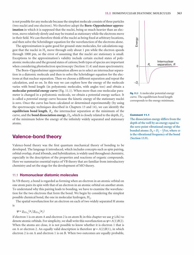
11.1 HOMONUCLEAR DIATOMIC MOLECULES 363
is not possible for any molecule because the simplest molecule consists of three particles(two nuclei and one electron). We therefore adopt the Born–Oppenheimer approx-imation in which it is supposed that the nuclei, being so much heavier than an elec-tron, move relatively slowly and may be treated as stationary while the electrons movein their field. We can therefore think of the nuclei as being fixed at arbitrary locations,and then solve the Schrödinger equation for the wavefunction of the electrons alone.
The approximation is quite good for ground-state molecules, for calculations sug-gest that the nuclei in H2 move through only about 1 pm while the electron speedsthrough 1000 pm, so the error of assuming that the nuclei are stationary is small.Exceptions to the approximation’s validity include certain excited states of poly-atomic molecules and the ground states of cations; both types of species are importantwhen considering photoelectron spectroscopy (Section 11.4) and mass spectrometry.
The Born–Oppenheimer approximation allows us to select an internuclear separa-tion in a diatomic molecule and then to solve the Schrödinger equation for the elec-trons at that nuclear separation. Then we choose a different separation and repeat thecalculation, and so on. In this way we can explore how the energy of the moleculevaries with bond length (in polyatomic molecules, with angles too) and obtain amolecular potential energy curve (Fig. 11.1). When more than one molecular para-meter is changed in a polyatomic molecule, we obtain a potential energy surface. It is called a potential energy curve because the kinetic energy of the stationary nuclei is zero. Once the curve has been calculated or determined experimentally (by usingthe spectroscopic techniques described in Chapters 13 and 14), we can identify theequilibrium bond length, Re, the internuclear separation at the minimum of thecurve, and the bond dissociation energy, D0, which is closely related to the depth, De,of the minimum below the energy of the infinitely widely separated and stationaryatoms.
Valence-bond theory
Valence-bond theory was the first quantum mechanical theory of bonding to be developed. The language it introduced, which includes concepts such as spin pairing,orbital overlap, σ and π bonds, and hybridization, is widely used throughout chemistry,especially in the description of the properties and reactions of organic compounds.Here we summarize essential topics of VB theory that are familiar from introductorychemistry and set the stage for the development of MO theory.
11.1 Homonuclear diatomic molecules
In VB theory, a bond is regarded as forming when an electron in an atomic orbital onone atom pairs its spin with that of an electron in an atomic orbital on another atom.To understand why this pairing leads to bonding, we have to examine the wavefunc-tion for the two electrons that form the bond. We begin by considering the simplestpossible chemical bond, the one in molecular hydrogen, H2.
The spatial wavefunction for an electron on each of two widely separated H atomsis
ψ = χH1sA(r1)χH1sB
(r2)
if electron 1 is on atom A and electron 2 is on atom B; in this chapter we use χ (chi) todenote atomic orbitals. For simplicity, we shall write this wavefunction as ψ = A(1)B(2).When the atoms are close, it is not possible to know whether it is electron 1 that is on A or electron 2. An equally valid description is therefore ψ = A(2)B(1), in whichelectron 2 is on A and electron 1 is on B. When two outcomes are equally probable,
Comment 11.1
The dissociation energy differs from thedepth of the well by an energy equal tothe zero-point vibrational energy of thebonded atoms: D0 = De − 1–2 $ω , where ωis the vibrational frequency of the bond(Section 13.9).
Ener
gy
Internuclearseparation, RRe
�De
0
Fig. 11.1 A molecular potential energycurve. The equilibrium bond lengthcorresponds to the energy minimum.
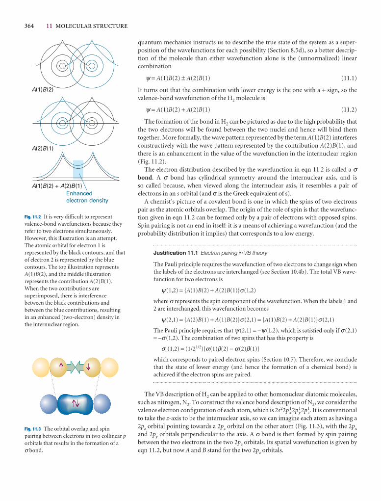
364 11 MOLECULAR STRUCTURE
quantum mechanics instructs us to describe the true state of the system as a super-position of the wavefunctions for each possibility (Section 8.5d), so a better descrip-tion of the molecule than either wavefunction alone is the (unnormalized) linearcombination
ψ = A(1)B(2) ± A(2)B(1) (11.1)
It turns out that the combination with lower energy is the one with a + sign, so the valence-bond wavefunction of the H2 molecule is
ψ = A(1)B(2) + A(2)B(1) (11.2)
The formation of the bond in H2 can be pictured as due to the high probability thatthe two electrons will be found between the two nuclei and hence will bind them together. More formally, the wave pattern represented by the term A(1)B(2) interferesconstructively with the wave pattern represented by the contribution A(2)B(1), andthere is an enhancement in the value of the wavefunction in the internuclear region(Fig. 11.2).
The electron distribution described by the wavefunction in eqn 11.2 is called a σbond. A σ bond has cylindrical symmetry around the internuclear axis, and is so called because, when viewed along the internuclear axis, it resembles a pair of electrons in an s orbital (and σ is the Greek equivalent of s).
A chemist’s picture of a covalent bond is one in which the spins of two electronspair as the atomic orbitals overlap. The origin of the role of spin is that the wavefunc-tion given in eqn 11.2 can be formed only by a pair of electrons with opposed spins.Spin pairing is not an end in itself: it is a means of achieving a wavefunction (and theprobability distribution it implies) that corresponds to a low energy.
Justification 11.1 Electron pairing in VB theory
The Pauli principle requires the wavefunction of two electrons to change sign whenthe labels of the electrons are interchanged (see Section 10.4b). The total VB wave-function for two electrons is
ψ(1,2) = {A(1)B(2) + A(2)B(1)}σ(1,2)
where σ represents the spin component of the wavefunction. When the labels 1 and2 are interchanged, this wavefunction becomes
ψ(2,1) = {A(2)B(1) + A(1)B(2)}σ(2,1) = {A(1)B(2) + A(2)B(1)}σ(2,1)
The Pauli principle requires that ψ(2,1) = −ψ(1,2), which is satisfied only if σ(2,1)= −σ(1,2). The combination of two spins that has this property is
σ−(1,2) = (1/21/2){α(1)β(2) − α(2)β(1)}
which corresponds to paired electron spins (Section 10.7). Therefore, we concludethat the state of lower energy (and hence the formation of a chemical bond) isachieved if the electron spins are paired.
The VB description of H2 can be applied to other homonuclear diatomic molecules,such as nitrogen, N2. To construct the valence bond description of N2, we consider thevalence electron configuration of each atom, which is 2s22px
12py12pz
1. It is conventionalto take the z-axis to be the internuclear axis, so we can imagine each atom as having a2pz orbital pointing towards a 2pz orbital on the other atom (Fig. 11.3), with the 2px
and 2py orbitals perpendicular to the axis. A σ bond is then formed by spin pairing between the two electrons in the two 2pz orbitals. Its spatial wavefunction is given byeqn 11.2, but now A and B stand for the two 2pz orbitals.
A B(1) (2)
A B(2) (1)
A B A B(1) (2) + (2) (1)Enhancedelectron density
Fig. 11.2 It is very difficult to representvalence-bond wavefunctions because theyrefer to two electrons simultaneously.However, this illustration is an attempt.The atomic orbital for electron 1 isrepresented by the black contours, and thatof electron 2 is represented by the bluecontours. The top illustration representsA(1)B(2), and the middle illustrationrepresents the contribution A(2)B(1).When the two contributions aresuperimposed, there is interferencebetween the black contributions andbetween the blue contributions, resultingin an enhanced (two-electron) density inthe internuclear region.
Fig. 11.3 The orbital overlap and spinpairing between electrons in two collinear porbitals that results in the formation of a σ bond.
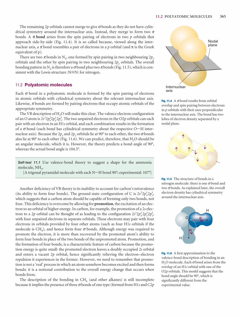
11.2 POLYATOMIC MOLECULES 365
The remaining 2p orbitals cannot merge to give σ bonds as they do not have cylin-drical symmetry around the internuclear axis. Instead, they merge to form two πbonds. A π bond arises from the spin pairing of electrons in two p orbitals that approach side-by-side (Fig. 11.4). It is so called because, viewed along the inter-nuclear axis, a π bond resembles a pair of electrons in a p orbital (and π is the Greekequivalent of p).
There are two π bonds in N2, one formed by spin pairing in two neighbouring 2px
orbitals and the other by spin pairing in two neighbouring 2py orbitals. The overallbonding pattern in N2 is therefore a σ bond plus two π bonds (Fig. 11.5), which is con-sistent with the Lewis structure :N.N: for nitrogen.
11.2 Polyatomic molecules
Each σ bond in a polyatomic molecule is formed by the spin pairing of electrons in atomic orbitals with cylindrical symmetry about the relevant internuclear axis.Likewise, π bonds are formed by pairing electrons that occupy atomic orbitals of theappropriate symmetry.
The VB description of H2O will make this clear. The valence electron configurationof an O atom is 2s22p2
x2p1y 2p1
z. The two unpaired electrons in the O2p orbitals can eachpair with an electron in an H1s orbital, and each combination results in the formationof a σ bond (each bond has cylindrical symmetry about the respective O-H inter-nuclear axis). Because the 2py and 2pz orbitals lie at 90° to each other, the two σ bondsalso lie at 90° to each other (Fig. 11.6). We can predict, therefore, that H2O should bean angular molecule, which it is. However, the theory predicts a bond angle of 90°,whereas the actual bond angle is 104.5°.
Self-test 11.1 Use valence-bond theory to suggest a shape for the ammoniamolecule, NH3.
[A trigonal pyramidal molecule with each N-H bond 90°; experimental: 107°]
Another deficiency of VB theory is its inability to account for carbon’s tetravalence(its ability to form four bonds). The ground-state configuration of C is 2s22p1
x2p1y,
which suggests that a carbon atom should be capable of forming only two bonds, notfour. This deficiency is overcome by allowing for promotion, the excitation of an elec-tron to an orbital of higher energy. In carbon, for example, the promotion of a 2s elec-tron to a 2p orbital can be thought of as leading to the configuration 2s12p1
x 2p1y2p1
z,with four unpaired electrons in separate orbitals. These electrons may pair with fourelectrons in orbitals provided by four other atoms (such as four H1s orbitals if themolecule is CH4), and hence form four σ bonds. Although energy was required topromote the electron, it is more than recovered by the promoted atom’s ability toform four bonds in place of the two bonds of the unpromoted atom. Promotion, andthe formation of four bonds, is a characteristic feature of carbon because the promo-tion energy is quite small: the promoted electron leaves a doubly occupied 2s orbitaland enters a vacant 2p orbital, hence significantly relieving the electron–electron repulsion it experiences in the former. However, we need to remember that promo-tion is not a ‘real’ process in which an atom somehow becomes excited and then formsbonds: it is a notional contribution to the overall energy change that occurs whenbonds form.
The description of the bonding in CH4 (and other alkanes) is still incomplete because it implies the presence of three σ bonds of one type (formed from H1s and C2p
Internuclearaxis
Nodalplane
Fig. 11.4 A π bond results from orbitaloverlap and spin pairing between electronsin p orbitals with their axes perpendicularto the internuclear axis. The bond has twolobes of electron density separated by anodal plane.
Fig. 11.5 The structure of bonds in anitrogen molecule: there is one σ bond andtwo π bonds. As explained later, the overallelectron density has cylindrical symmetryaround the internuclear axis.
O
H
H
Fig. 11.6 A first approximation to thevalence-bond description of bonding in anH2O molecule. Each σ bond arises from theoverlap of an H1s orbital with one of theO2p orbitals. This model suggests that thebond angle should be 90°, which issignificantly different from theexperimental value.
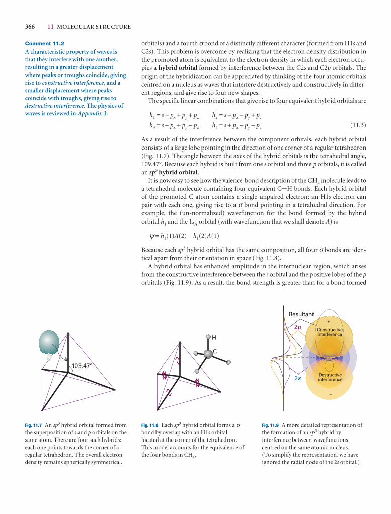
366 11 MOLECULAR STRUCTURE
orbitals) and a fourth σ bond of a distinctly different character (formed from H1s andC2s). This problem is overcome by realizing that the electron density distribution inthe promoted atom is equivalent to the electron density in which each electron occu-pies a hybrid orbital formed by interference between the C2s and C2p orbitals. Theorigin of the hybridization can be appreciated by thinking of the four atomic orbitalscentred on a nucleus as waves that interfere destructively and constructively in differ-ent regions, and give rise to four new shapes.
The specific linear combinations that give rise to four equivalent hybrid orbitals are
h1 = s + px + py + pz h2 = s − px − py + pz
h3 = s − px + py − pz h4 = s + px − py − pz (11.3)
As a result of the interference between the component orbitals, each hybrid orbitalconsists of a large lobe pointing in the direction of one corner of a regular tetrahedron(Fig. 11.7). The angle between the axes of the hybrid orbitals is the tetrahedral angle,109.47°. Because each hybrid is built from one s orbital and three p orbitals, it is calledan sp3 hybrid orbital.
It is now easy to see how the valence-bond description of the CH4 molecule leads toa tetrahedral molecule containing four equivalent C-H bonds. Each hybrid orbital of the promoted C atom contains a single unpaired electron; an H1s electron can pair with each one, giving rise to a σ bond pointing in a tetrahedral direction. For example, the (un-normalized) wavefunction for the bond formed by the hybrid orbital h1 and the 1sA orbital (with wavefunction that we shall denote A) is
ψ = h1(1)A(2) + h1(2)A(1)
Because each sp3 hybrid orbital has the same composition, all four σ bonds are iden-tical apart from their orientation in space (Fig. 11.8).
A hybrid orbital has enhanced amplitude in the internuclear region, which arisesfrom the constructive interference between the s orbital and the positive lobes of the porbitals (Fig. 11.9). As a result, the bond strength is greater than for a bond formed
Comment 11.2
A characteristic property of waves is that they interfere with one another,resulting in a greater displacementwhere peaks or troughs coincide, givingrise to constructive interference, and asmaller displacement where peakscoincide with troughs, giving rise todestructive interference. The physics ofwaves is reviewed in Appendix 3.
109.47°
Fig. 11.7 An sp3 hybrid orbital formed fromthe superposition of s and p orbitals on thesame atom. There are four such hybrids:each one points towards the corner of aregular tetrahedron. The overall electrondensity remains spherically symmetrical.
C
H
Fig. 11.8 Each sp3 hybrid orbital forms a σbond by overlap with an H1s orbitallocated at the corner of the tetrahedron.This model accounts for the equivalence ofthe four bonds in CH4.
Constructiveinterference
+
–
+
Resultant
2p
2s Destructiveinterference
Fig. 11.9 A more detailed representation ofthe formation of an sp3 hybrid byinterference between wavefunctionscentred on the same atomic nucleus. (To simplify the representation, we haveignored the radial node of the 2s orbital.)
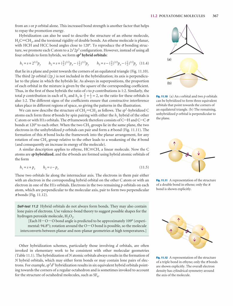
11.2 POLYATOMIC MOLECULES 367
from an s or p orbital alone. This increased bond strength is another factor that helpsto repay the promotion energy.
Hybridization can also be used to describe the structure of an ethene molecule,H2C=CH2, and the torsional rigidity of double bonds. An ethene molecule is planar,with HCH and HCC bond angles close to 120°. To reproduce the σ bonding struc-ture, we promote each C atom to a 2s12p3 configuration. However, instead of using allfour orbitals to form hybrids, we form sp2 hybrid orbitals:
h1 = s + 21/2py h2 = s + ( 3–2 )1/2px − ( 1–2 )1/2py h3 = s − ( 3–2 )1/2px − ( 1–2 )1/2py (11.4)
that lie in a plane and point towards the corners of an equilateral triangle (Fig. 11.10).The third 2p orbital (2pz) is not included in the hybridization; its axis is perpendicu-lar to the plane in which the hybrids lie. As always in superpositions, the proportionof each orbital in the mixture is given by the square of the corresponding coefficient.Thus, in the first of these hybrids the ratio of s to p contributions is 1:2. Similarly, thetotal p contribution in each of h2 and h3 is 3–2 + 1–2 = 2, so the ratio for these orbitals isalso 1:2. The different signs of the coefficients ensure that constructive interferencetakes place in different regions of space, so giving the patterns in the illustration.
We can now describe the structure of CH2=CH2 as follows. The sp2-hybridized Catoms each form three σ bonds by spin pairing with either the h1 hybrid of the otherC atom or with H1s orbitals. The σ framework therefore consists of C-H and C-C σbonds at 120° to each other. When the two CH2 groups lie in the same plane, the twoelectrons in the unhybridized p orbitals can pair and form a π bond (Fig. 11.11). Theformation of this π bond locks the framework into the planar arrangement, for anyrotation of one CH2 group relative to the other leads to a weakening of the π bond(and consequently an increase in energy of the molecule).
A similar description applies to ethyne, HC.CH, a linear molecule. Now the Catoms are sp hybridized, and the σ bonds are formed using hybrid atomic orbitals ofthe form
h1 = s + pz h2 = s − pz (11.5)
These two orbitals lie along the internuclear axis. The electrons in them pair eitherwith an electron in the corresponding hybrid orbital on the other C atom or with anelectron in one of the H1s orbitals. Electrons in the two remaining p orbitals on eachatom, which are perpendicular to the molecular axis, pair to form two perpendicularπ bonds (Fig. 11.12).
Self-test 11.2 Hybrid orbitals do not always form bonds. They may also containlone pairs of electrons. Use valence-bond theory to suggest possible shapes for thehydrogen peroxide molecule, H2O2.
[Each H-O-O bond angle is predicted to be approximately 109° (experi-mental: 94.8°); rotation around the O-O bond is possible, so the molecule
interconverts between planar and non-planar geometries at high temperatures.]
Other hybridization schemes, particularly those involving d orbitals, are ofteninvoked in elementary work to be consistent with other molecular geometries (Table 11.1). The hybridization of N atomic orbitals always results in the formation ofN hybrid orbitals, which may either form bonds or may contain lone pairs of elec-trons. For example, sp3d2 hybridization results in six equivalent hybrid orbitals point-ing towards the corners of a regular octahedron and is sometimes invoked to accountfor the structure of octahedral molecules, such as SF6.
(a)
(b)
Fig. 11.10 (a) An s orbital and two p orbitalscan be hybridized to form three equivalentorbitals that point towards the corners ofan equilateral triangle. (b) The remaining,unhybridized p orbital is perpendicular tothe plane.
Fig. 11.11 A representation of the structureof a double bond in ethene; only the πbond is shown explicitly.
Fig. 11.12 A representation of the structureof a triple bond in ethyne; only the π bondsare shown explicitly. The overall electrondensity has cylindrical symmetry aroundthe axis of the molecule.
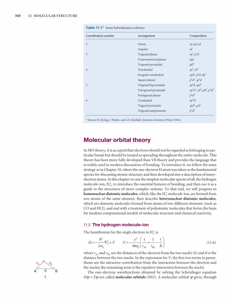
368 11 MOLECULAR STRUCTURE
Molecular orbital theory
In MO theory, it is accepted that electrons should not be regarded as belonging to par-ticular bonds but should be treated as spreading throughout the entire molecule. Thistheory has been more fully developed than VB theory and provides the language thatis widely used in modern discussions of bonding. To introduce it, we follow the samestrategy as in Chapter 10, where the one-electron H atom was taken as the fundamentalspecies for discussing atomic structure and then developed into a description of many-electron atoms. In this chapter we use the simplest molecular species of all, the hydrogenmolecule-ion, H2
+, to introduce the essential features of bonding, and then use it as aguide to the structures of more complex systems. To that end, we will progress tohomonuclear diatomic molecules, which, like the H2
+ molecule-ion, are formed fromtwo atoms of the same element, then describe heteronuclear diatomic molecules,which are diatomic molecules formed from atoms of two different elements (such asCO and HCl), and end with a treatment of polyatomic molecules that forms the basisfor modern computational models of molecular structure and chemical reactivity.
11.3 The hydrogen molecule-ion
The hamiltonian for the single electron in H2+ is
H = − ∇21 + V V = − + − (11.6)
where rA1 and rB1 are the distances of the electron from the two nuclei (1) and R is thedistance between the two nuclei. In the expression for V, the first two terms in paren-theses are the attractive contribution from the interaction between the electron andthe nuclei; the remaining term is the repulsive interaction between the nuclei.
The one-electron wavefunctions obtained by solving the Schrödinger equation Hψ = Eψ are called molecular orbitals (MO). A molecular orbital ψ gives, through
DF
1
R
1
rB1
1
rA1
AC
e2
4πε0
$2
2me
Table 11.1* Some hybridization schemes
Coordination number Arrangement Composition
2 Linear sp, pd, sd
Angular sd
3 Trigonal planar sp2, p2d
Unsymmetrical planar spd
Trigonal pyramidal pd 2
4 Tetrahedral sp3, sd 3
Irregular tetrahedral spd2, p3d, dp3
Square planar p2d2, sp2d
5 Trigonal bipyramidal sp3d, spd2
Tetragonal pyramidal sp2d2, sd4, pd4, p3d2
Pentagonal planar p2d3
6 Octahedral sp3d2
Trigonal prismatic spd4, pd5
Trigonal antiprismatic p3d2
* Source: H. Eyring, J. Walter, and G.E. Kimball, Quantum chemistry, Wiley (1944).
rA1 rB1
RA B
1
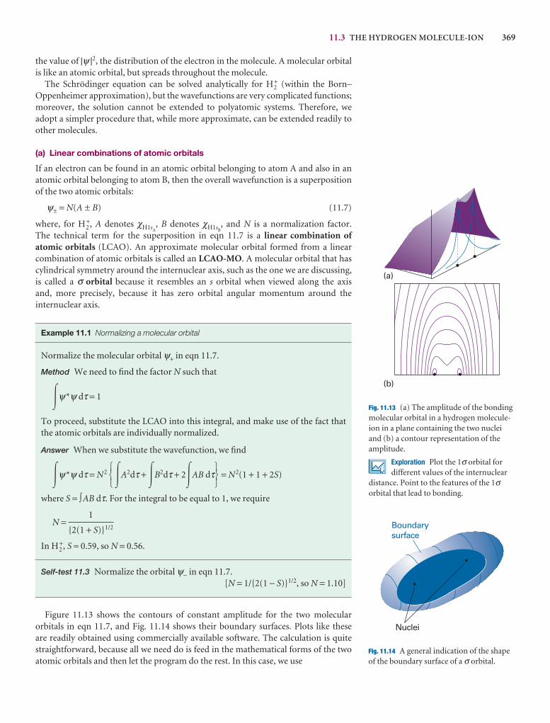
11.3 THE HYDROGEN MOLECULE-ION 369
(a)
(b)
Fig. 11.13 (a) The amplitude of the bondingmolecular orbital in a hydrogen molecule-ion in a plane containing the two nucleiand (b) a contour representation of theamplitude.
Exploration Plot the 1σ orbital fordifferent values of the internuclear
distance. Point to the features of the 1σorbital that lead to bonding.
Boundarysurface
Nuclei
Fig. 11.14 A general indication of the shapeof the boundary surface of a σ orbital.
the value of |ψ |2, the distribution of the electron in the molecule. A molecular orbitalis like an atomic orbital, but spreads throughout the molecule.
The Schrödinger equation can be solved analytically for H2+ (within the Born–
Oppenheimer approximation), but the wavefunctions are very complicated functions;moreover, the solution cannot be extended to polyatomic systems. Therefore, weadopt a simpler procedure that, while more approximate, can be extended readily toother molecules.
(a) Linear combinations of atomic orbitals
If an electron can be found in an atomic orbital belonging to atom A and also in anatomic orbital belonging to atom B, then the overall wavefunction is a superpositionof the two atomic orbitals:
ψ± = N(A ± B) (11.7)
where, for H2+, A denotes χH1sA
, B denotes χH1sB, and N is a normalization factor.
The technical term for the superposition in eqn 11.7 is a linear combination ofatomic orbitals (LCAO). An approximate molecular orbital formed from a linearcombination of atomic orbitals is called an LCAO-MO. A molecular orbital that hascylindrical symmetry around the internuclear axis, such as the one we are discussing,is called a σ orbital because it resembles an s orbital when viewed along the axis and, more precisely, because it has zero orbital angular momentum around the internuclear axis.
Example 11.1 Normalizing a molecular orbital
Normalize the molecular orbital ψ+ in eqn 11.7.
Method We need to find the factor N such that
�ψ*ψ dτ = 1
To proceed, substitute the LCAO into this integral, and make use of the fact thatthe atomic orbitals are individually normalized.
Answer When we substitute the wavefunction, we find
�ψ*ψ dτ = N2 �A2dτ + �B2dτ + 2�AB dτ = N2(1 + 1 + 2S)
where S = ∫AB dτ. For the integral to be equal to 1, we require
N =
In H2+, S ≈ 0.59, so N = 0.56.
Self-test 11.3 Normalize the orbital ψ− in eqn 11.7.[N = 1/{2(1 − S)}1/2, so N = 1.10]
Figure 11.13 shows the contours of constant amplitude for the two molecular orbitals in eqn 11.7, and Fig. 11.14 shows their boundary surfaces. Plots like these are readily obtained using commercially available software. The calculation is quitestraightforward, because all we need do is feed in the mathematical forms of the twoatomic orbitals and then let the program do the rest. In this case, we use
1
{2(1 + S)}1/2
567
123
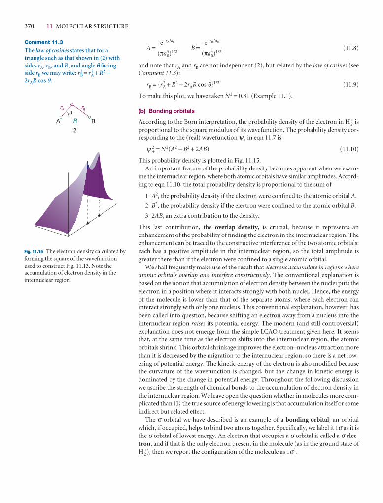
370 11 MOLECULAR STRUCTURE
A = B = (11.8)
and note that rA and rB are not independent (2), but related by the law of cosines (seeComment 11.3):
rB = {rA2 + R2 − 2rAR cos θ}1/2 (11.9)
To make this plot, we have taken N2 = 0.31 (Example 11.1).
(b) Bonding orbitals
According to the Born interpretation, the probability density of the electron in H2+ is
proportional to the square modulus of its wavefunction. The probability density cor-responding to the (real) wavefunction ψ+ in eqn 11.7 is
ψ 2+ = N2(A2 + B2 + 2AB) (11.10)
This probability density is plotted in Fig. 11.15.An important feature of the probability density becomes apparent when we exam-
ine the internuclear region, where both atomic orbitals have similar amplitudes. Accord-ing to eqn 11.10, the total probability density is proportional to the sum of
1 A2, the probability density if the electron were confined to the atomic orbital A.
2 B2, the probability density if the electron were confined to the atomic orbital B.
3 2AB, an extra contribution to the density.
This last contribution, the overlap density, is crucial, because it represents an enhancement of the probability of finding the electron in the internuclear region. Theenhancement can be traced to the constructive interference of the two atomic orbitals:each has a positive amplitude in the internuclear region, so the total amplitude isgreater there than if the electron were confined to a single atomic orbital.
We shall frequently make use of the result that electrons accumulate in regions whereatomic orbitals overlap and interfere constructively. The conventional explanation isbased on the notion that accumulation of electron density between the nuclei puts theelectron in a position where it interacts strongly with both nuclei. Hence, the energyof the molecule is lower than that of the separate atoms, where each electron can interact strongly with only one nucleus. This conventional explanation, however, hasbeen called into question, because shifting an electron away from a nucleus into theinternuclear region raises its potential energy. The modern (and still controversial)explanation does not emerge from the simple LCAO treatment given here. It seemsthat, at the same time as the electron shifts into the internuclear region, the atomic orbitals shrink. This orbital shrinkage improves the electron–nucleus attraction morethan it is decreased by the migration to the internuclear region, so there is a net low-ering of potential energy. The kinetic energy of the electron is also modified becausethe curvature of the wavefunction is changed, but the change in kinetic energy is dominated by the change in potential energy. Throughout the following discussionwe ascribe the strength of chemical bonds to the accumulation of electron density inthe internuclear region. We leave open the question whether in molecules more com-plicated than H2
+ the true source of energy lowering is that accumulation itself or someindirect but related effect.
The σ orbital we have described is an example of a bonding orbital, an orbitalwhich, if occupied, helps to bind two atoms together. Specifically, we label it 1σ as it isthe σ orbital of lowest energy. An electron that occupies a σ orbital is called a σ elec-tron, and if that is the only electron present in the molecule (as in the ground state ofH2
+), then we report the configuration of the molecule as 1σ1.
e−rB/a0
(πa30)1/2
e−rA/a0
(πa30)1/2
Comment 11.3
The law of cosines states that for atriangle such as that shown in (2) withsides rA, rB, and R, and angle θ facingside rB we may write: rB
2 = rA2 + R2 −
2rAR cos θ.
rA rB
RA B�
2
Fig. 11.15 The electron density calculated byforming the square of the wavefunctionused to construct Fig. 11.13. Note theaccumulation of electron density in theinternuclear region.
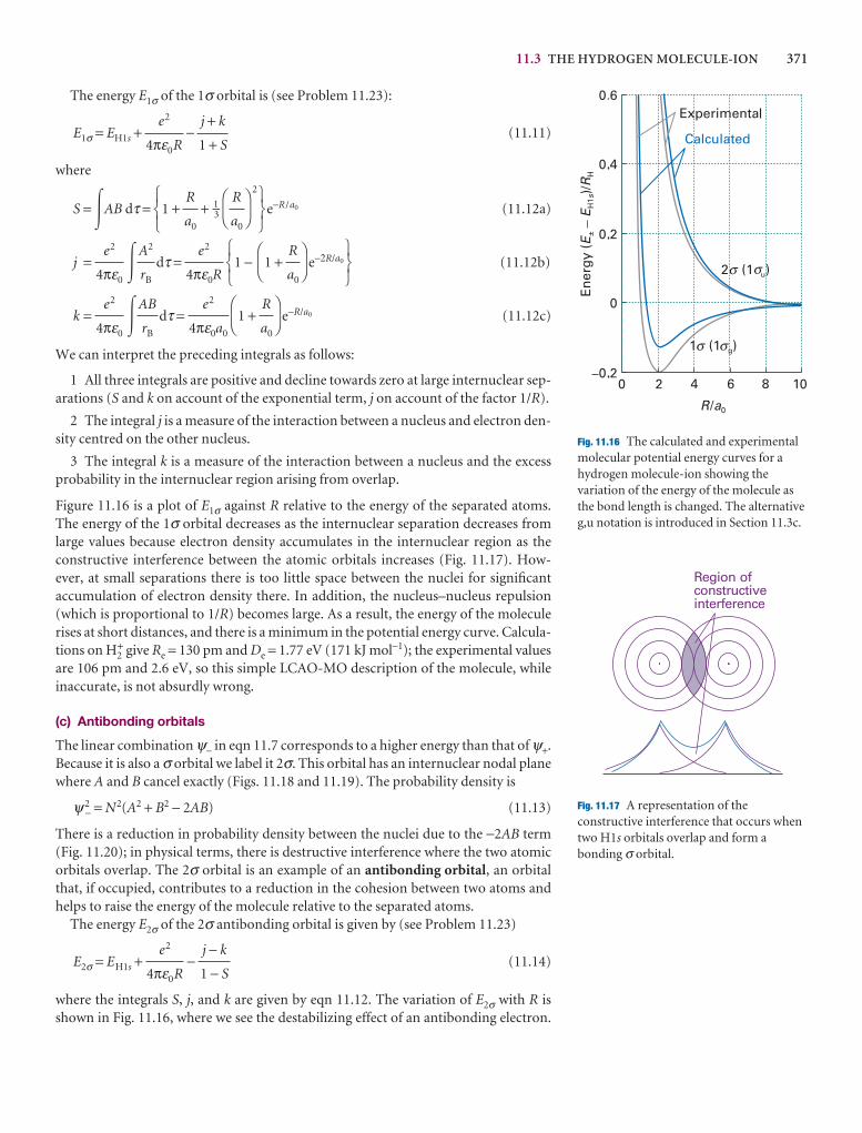
11.3 THE HYDROGEN MOLECULE-ION 371
The energy E1σ of the 1σ orbital is (see Problem 11.23):
E1σ = EH1s + − (11.11)
where
S = �AB dτ = 1 + + 1–3
2
e−R/a0 (11.12a)
j = � dτ = 1 − 1 + e−2R/a0 (11.12b)
k = � dτ = 1 + e−R/a0 (11.12c)
We can interpret the preceding integrals as follows:
1 All three integrals are positive and decline towards zero at large internuclear sep-arations (S and k on account of the exponential term, j on account of the factor 1/R).
2 The integral j is a measure of the interaction between a nucleus and electron den-sity centred on the other nucleus.
3 The integral k is a measure of the interaction between a nucleus and the excessprobability in the internuclear region arising from overlap.
Figure 11.16 is a plot of E1σ against R relative to the energy of the separated atoms. The energy of the 1σ orbital decreases as the internuclear separation decreases fromlarge values because electron density accumulates in the internuclear region as theconstructive interference between the atomic orbitals increases (Fig. 11.17). How-ever, at small separations there is too little space between the nuclei for significant accumulation of electron density there. In addition, the nucleus–nucleus repulsion(which is proportional to 1/R) becomes large. As a result, the energy of the moleculerises at short distances, and there is a minimum in the potential energy curve. Calcula-tions on H2
+ give Re = 130 pm and De = 1.77 eV (171 kJ mol−1); the experimental valuesare 106 pm and 2.6 eV, so this simple LCAO-MO description of the molecule, whileinaccurate, is not absurdly wrong.
(c) Antibonding orbitals
The linear combination ψ− in eqn 11.7 corresponds to a higher energy than that of ψ+.Because it is also a σ orbital we label it 2σ. This orbital has an internuclear nodal planewhere A and B cancel exactly (Figs. 11.18 and 11.19). The probability density is
ψ2− = N2(A2 + B2 − 2AB) (11.13)
There is a reduction in probability density between the nuclei due to the −2AB term(Fig. 11.20); in physical terms, there is destructive interference where the two atomicorbitals overlap. The 2σ orbital is an example of an antibonding orbital, an orbitalthat, if occupied, contributes to a reduction in the cohesion between two atoms andhelps to raise the energy of the molecule relative to the separated atoms.
The energy E2σ of the 2σ antibonding orbital is given by (see Problem 11.23)
E2σ = EH1s + − (11.14)
where the integrals S, j, and k are given by eqn 11.12. The variation of E2σ with R isshown in Fig. 11.16, where we see the destabilizing effect of an antibonding electron.
j − k
1 − S
e2
4πε0R
DF
R
a0
AC
e2
4πε0a0
AB
rB
e2
4πε0
567
DF
R
a0
AC
123
e2
4πε0R
A2
rB
e2
4πε0
567
DF
R
a0
AC
R
a0
123
j + k
1 + S
e2
4πε0R
Fig. 11.16 The calculated and experimentalmolecular potential energy curves for ahydrogen molecule-ion showing thevariation of the energy of the molecule asthe bond length is changed. The alternativeg,u notation is introduced in Section 11.3c.
Region ofconstructiveinterference
Fig. 11.17 A representation of theconstructive interference that occurs whentwo H1s orbitals overlap and form abonding σ orbital.
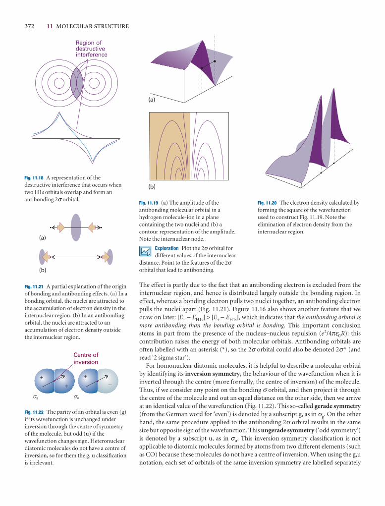
372 11 MOLECULAR STRUCTURE
The effect is partly due to the fact that an antibonding electron is excluded from theinternuclear region, and hence is distributed largely outside the bonding region. In effect, whereas a bonding electron pulls two nuclei together, an antibonding electronpulls the nuclei apart (Fig. 11.21). Figure 11.16 also shows another feature that wedraw on later: |E− − EH1s | > |E+ − EH1s |, which indicates that the antibonding orbital ismore antibonding than the bonding orbital is bonding. This important conclusionstems in part from the presence of the nucleus–nucleus repulsion (e2/4πε0R): thiscontribution raises the energy of both molecular orbitals. Antibonding orbitals areoften labelled with an asterisk (*), so the 2σ orbital could also be denoted 2σ * (andread ‘2 sigma star’).
For homonuclear diatomic molecules, it is helpful to describe a molecular orbitalby identifying its inversion symmetry, the behaviour of the wavefunction when it isinverted through the centre (more formally, the centre of inversion) of the molecule.Thus, if we consider any point on the bonding σ orbital, and then project it throughthe centre of the molecule and out an equal distance on the other side, then we arriveat an identical value of the wavefunction (Fig. 11.22). This so-called gerade symmetry(from the German word for ‘even’) is denoted by a subscript g, as in σg. On the otherhand, the same procedure applied to the antibonding 2σ orbital results in the samesize but opposite sign of the wavefunction. This ungerade symmetry (‘odd symmetry’)is denoted by a subscript u, as in σu. This inversion symmetry classification is not applicable to diatomic molecules formed by atoms from two different elements (suchas CO) because these molecules do not have a centre of inversion. When using the g,unotation, each set of orbitals of the same inversion symmetry are labelled separately
Region ofdestructiveinterference
Fig. 11.18 A representation of thedestructive interference that occurs whentwo H1s orbitals overlap and form anantibonding 2σ orbital.
(b)
(a)
Fig. 11.19 (a) The amplitude of theantibonding molecular orbital in ahydrogen molecule-ion in a planecontaining the two nuclei and (b) acontour representation of the amplitude.Note the internuclear node.
Exploration Plot the 2σ orbital fordifferent values of the internuclear
distance. Point to the features of the 2σorbital that lead to antibonding.
Fig. 11.20 The electron density calculated byforming the square of the wavefunctionused to construct Fig. 11.19. Note theelimination of electron density from theinternuclear region.
Fig. 11.22 The parity of an orbital is even (g)if its wavefunction is unchanged underinversion through the centre of symmetryof the molecule, but odd (u) if thewavefunction changes sign. Heteronucleardiatomic molecules do not have a centre ofinversion, so for them the g, u classificationis irrelevant.
(a)
(b)
Fig. 11.21 A partial explanation of the originof bonding and antibonding effects. (a) In abonding orbital, the nuclei are attracted tothe accumulation of electron density in theinternuclear region. (b) In an antibondingorbital, the nuclei are attracted to anaccumulation of electron density outsidethe internuclear region.
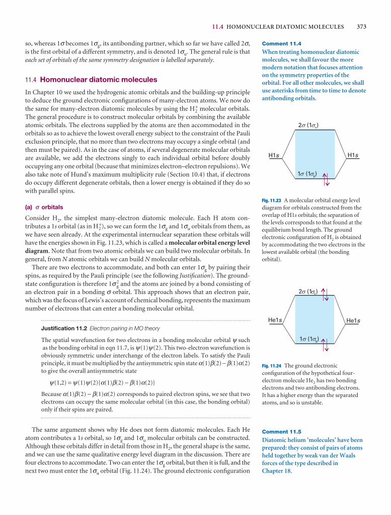
11.4 HOMONUCLEAR DIATOMIC MOLECULES 373
so, whereas 1σ becomes 1σg, its antibonding partner, which so far we have called 2σ,is the first orbital of a different symmetry, and is denoted 1σu. The general rule is thateach set of orbitals of the same symmetry designation is labelled separately.
11.4 Homonuclear diatomic molecules
In Chapter 10 we used the hydrogenic atomic orbitals and the building-up principleto deduce the ground electronic configurations of many-electron atoms. We now dothe same for many-electron diatomic molecules by using the H2
+ molecular orbitals.The general procedure is to construct molecular orbitals by combining the availableatomic orbitals. The electrons supplied by the atoms are then accommodated in theorbitals so as to achieve the lowest overall energy subject to the constraint of the Pauliexclusion principle, that no more than two electrons may occupy a single orbital (andthen must be paired). As in the case of atoms, if several degenerate molecular orbitalsare available, we add the electrons singly to each individual orbital before doubly occupying any one orbital (because that minimizes electron–electron repulsions). Wealso take note of Hund’s maximum multiplicity rule (Section 10.4) that, if electronsdo occupy different degenerate orbitals, then a lower energy is obtained if they do sowith parallel spins.
(a) σ orbitals
Consider H2, the simplest many-electron diatomic molecule. Each H atom con-tributes a 1s orbital (as in H2
+), so we can form the 1σg and 1σu orbitals from them, aswe have seen already. At the experimental internuclear separation these orbitals willhave the energies shown in Fig. 11.23, which is called a molecular orbital energy leveldiagram. Note that from two atomic orbitals we can build two molecular orbitals. Ingeneral, from N atomic orbitals we can build N molecular orbitals.
There are two electrons to accommodate, and both can enter 1σg by pairing theirspins, as required by the Pauli principle (see the following Justification). The ground-state configuration is therefore 1σ g
2 and the atoms are joined by a bond consisting ofan electron pair in a bonding σ orbital. This approach shows that an electron pair,which was the focus of Lewis’s account of chemical bonding, represents the maximumnumber of electrons that can enter a bonding molecular orbital.
Justification 11.2 Electron pairing in MO theory
The spatial wavefunction for two electrons in a bonding molecular orbital ψ suchas the bonding orbital in eqn 11.7, is ψ(1)ψ(2). This two-electron wavefunction isobviously symmetric under interchange of the electron labels. To satisfy the Pauliprinciple, it must be multiplied by the antisymmetric spin state α(1)β(2) − β(1)α(2)to give the overall antisymmetric state
ψ(1,2) = ψ(1)ψ(2){α(1)β(2) − β(1)α(2)}
Because α(1)β(2) − β(1)α(2) corresponds to paired electron spins, we see that twoelectrons can occupy the same molecular orbital (in this case, the bonding orbital)only if their spins are paired.
The same argument shows why He does not form diatomic molecules. Each Heatom contributes a 1s orbital, so 1σg and 1σu molecular orbitals can be constructed.Although these orbitals differ in detail from those in H2, the general shape is the same,and we can use the same qualitative energy level diagram in the discussion. There arefour electrons to accommodate. Two can enter the 1σg orbital, but then it is full, and thenext two must enter the 1σu orbital (Fig. 11.24). The ground electronic configuration
Comment 11.4
When treating homonuclear diatomicmolecules, we shall favour the moremodern notation that focuses attentionon the symmetry properties of theorbital. For all other molecules, we shalluse asterisks from time to time to denoteantibonding orbitals.
Fig. 11.23 A molecular orbital energy leveldiagram for orbitals constructed from theoverlap of H1s orbitals; the separation ofthe levels corresponds to that found at theequilibrium bond length. The groundelectronic configuration of H2 is obtainedby accommodating the two electrons in thelowest available orbital (the bondingorbital).
He1s He1s
2 (1 )u
1 (1 )g
s s
s s
Fig. 11.24 The ground electronicconfiguration of the hypothetical four-electron molecule He2 has two bondingelectrons and two antibonding electrons. It has a higher energy than the separatedatoms, and so is unstable.
Comment 11.5
Diatomic helium ‘molecules’ have beenprepared: they consist of pairs of atomsheld together by weak van der Waalsforces of the type described in Chapter 18.
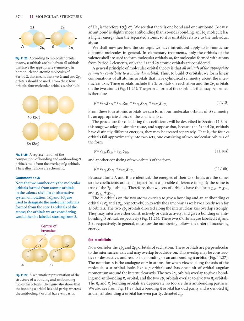
374 11 MOLECULAR STRUCTURE
of He2 is therefore 1σ g21σu
2. We see that there is one bond and one antibond. Becausean antibond is slightly more antibonding than a bond is bonding, an He2 molecule hasa higher energy than the separated atoms, so it is unstable relative to the individualatoms.
We shall now see how the concepts we have introduced apply to homonuclear diatomic molecules in general. In elementary treatments, only the orbitals of the valence shell are used to form molecular orbitals so, for molecules formed with atomsfrom Period 2 elements, only the 2s and 2p atomic orbitals are considered.
A general principle of molecular orbital theory is that all orbitals of the appropriatesymmetry contribute to a molecular orbital. Thus, to build σ orbitals, we form linearcombinations of all atomic orbitals that have cylindrical symmetry about the inter-nuclear axis. These orbitals include the 2s orbitals on each atom and the 2pz orbitalson the two atoms (Fig. 11.25). The general form of the σ orbitals that may be formedis therefore
ψ = cA2sχA2s + cB2sχB2s + cA2pzχA2pz
+ cB2pzχB2pz
(11.15)
From these four atomic orbitals we can form four molecular orbitals of σ symmetryby an appropriate choice of the coefficients c.
The procedure for calculating the coefficients will be described in Section 11.6. Atthis stage we adopt a simpler route, and suppose that, because the 2s and 2pz orbitalshave distinctly different energies, they may be treated separately. That is, the four σorbitals fall approximately into two sets, one consisting of two molecular orbitals ofthe form
ψ = cA2sχA2s + cB2sχB2s (11.16a)
and another consisting of two orbitals of the form
ψ = cA2pzχA2pz
+ cB2pzχB2pz
(11.16b)
Because atoms A and B are identical, the energies of their 2s orbitals are the same, so the coefficients are equal (apart from a possible difference in sign); the same is true of the 2pz orbitals. Therefore, the two sets of orbitals have the form χA2s ± χB2s
and χA2pz± χB2pz
.The 2s orbitals on the two atoms overlap to give a bonding and an antibonding σ
orbital (1σg and 1σu, respectively) in exactly the same way as we have already seen for1s orbitals. The two 2pz orbitals directed along the internuclear axis overlap strongly.They may interfere either constructively or destructively, and give a bonding or anti-bonding σ orbital, respectively (Fig. 11.26). These two σ orbitals are labelled 2σg and2σu, respectively. In general, note how the numbering follows the order of increasingenergy.
(b) π orbitals
Now consider the 2px and 2py orbitals of each atom. These orbitals are perpendicularto the internuclear axis and may overlap broadside-on. This overlap may be construc-tive or destructive, and results in a bonding or an antibonding π orbital (Fig. 11.27).The notation π is the analogue of p in atoms, for when viewed along the axis of themolecule, a π orbital looks like a p orbital, and has one unit of orbital angular momentum around the internuclear axis. The two 2px orbitals overlap to give a bond-ing and antibonding πx orbital, and the two 2py orbitals overlap to give two πy orbitals.The πx and πy bonding orbitals are degenerate; so too are their antibonding partners.We also see from Fig. 11.27 that a bonding π orbital has odd parity and is denoted πu
and an antibonding π orbital has even parity, denoted πg.
u g
Centre ofinversion
�
�
� �
�� �
�
� �
2s 2s
2pz 2pzA B
Fig. 11.25 According to molecular orbitaltheory, σ orbitals are built from all orbitalsthat have the appropriate symmetry. Inhomonuclear diatomic molecules of Period 2, that means that two 2s and two 2pz
orbitals should be used. From these fourorbitals, four molecular orbitals can be built.
3 (2 )g
4 (2 )u$ $
$ $
Fig. 11.26 A representation of thecomposition of bonding and antibonding σorbitals built from the overlap of p orbitals.These illustrations are schematic.
Fig. 11.27 A schematic representation of thestructure of π bonding and antibondingmolecular orbitals. The figure also shows thatthe bonding π orbital has odd parity, whereasthe antiboding π orbital has even parity.
Comment 11.6
Note that we number only the molecularorbitals formed from atomic orbitals in the valence shell. In an alternativesystem of notation, 1σg and 1σu areused to designate the molecular orbitalsformed from the core 1s orbitals of theatoms; the orbitals we are consideringwould then be labelled starting from 2.
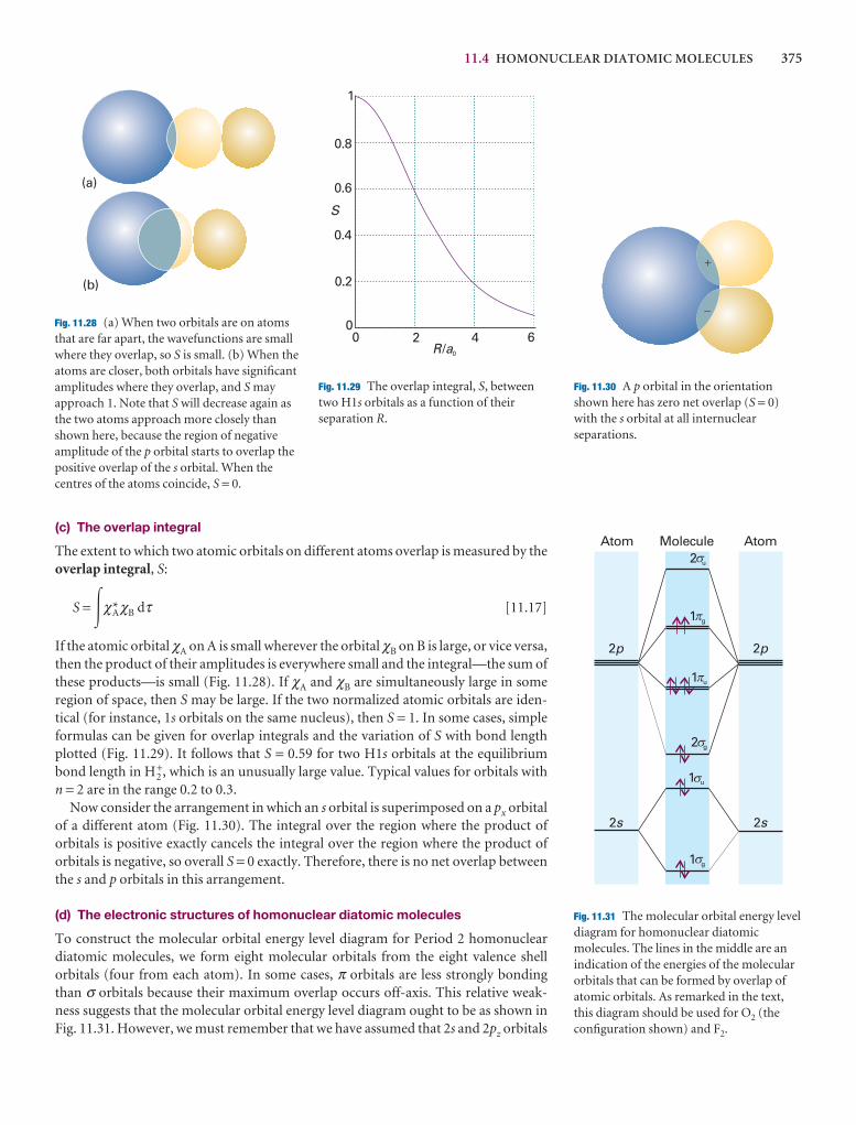
11.4 HOMONUCLEAR DIATOMIC MOLECULES 375
(c) The overlap integral
The extent to which two atomic orbitals on different atoms overlap is measured by theoverlap integral, S:
S = �χA*χB dτ [11.17]
If the atomic orbital χA on A is small wherever the orbital χB on B is large, or vice versa,then the product of their amplitudes is everywhere small and the integral—the sum ofthese products—is small (Fig. 11.28). If χA and χB are simultaneously large in some region of space, then S may be large. If the two normalized atomic orbitals are iden-tical (for instance, 1s orbitals on the same nucleus), then S = 1. In some cases, simpleformulas can be given for overlap integrals and the variation of S with bond lengthplotted (Fig. 11.29). It follows that S = 0.59 for two H1s orbitals at the equilibriumbond length in H2
+, which is an unusually large value. Typical values for orbitals withn = 2 are in the range 0.2 to 0.3.
Now consider the arrangement in which an s orbital is superimposed on a px orbitalof a different atom (Fig. 11.30). The integral over the region where the product of orbitals is positive exactly cancels the integral over the region where the product of orbitals is negative, so overall S = 0 exactly. Therefore, there is no net overlap betweenthe s and p orbitals in this arrangement.
(d) The electronic structures of homonuclear diatomic molecules
To construct the molecular orbital energy level diagram for Period 2 homonuclear diatomic molecules, we form eight molecular orbitals from the eight valence shell orbitals (four from each atom). In some cases, π orbitals are less strongly bondingthan σ orbitals because their maximum overlap occurs off-axis. This relative weak-ness suggests that the molecular orbital energy level diagram ought to be as shown inFig. 11.31. However, we must remember that we have assumed that 2s and 2pz orbitals
(a)
(b)
Fig. 11.28 (a) When two orbitals are on atomsthat are far apart, the wavefunctions are smallwhere they overlap, so S is small. (b) When theatoms are closer, both orbitals have significantamplitudes where they overlap, and S mayapproach 1. Note that S will decrease again asthe two atoms approach more closely thanshown here, because the region of negativeamplitude of the p orbital starts to overlap thepositive overlap of the s orbital. When thecentres of the atoms coincide, S = 0.
00
2 4 6
0.2
0.4
0.6
0.8
1
S
R a/ 0
Fig. 11.29 The overlap integral, S, betweentwo H1s orbitals as a function of theirseparation R.
�
�
Fig. 11.30 A p orbital in the orientationshown here has zero net overlap (S = 0)with the s orbital at all internuclearseparations.
2p 2p
2s 2s
1 g
1 u
2 g
2 u
1 u
1 g
Atom Molecule Atom$
$
$
$
�
�
Fig. 11.31 The molecular orbital energy leveldiagram for homonuclear diatomicmolecules. The lines in the middle are anindication of the energies of the molecularorbitals that can be formed by overlap ofatomic orbitals. As remarked in the text,this diagram should be used for O2 (theconfiguration shown) and F2.
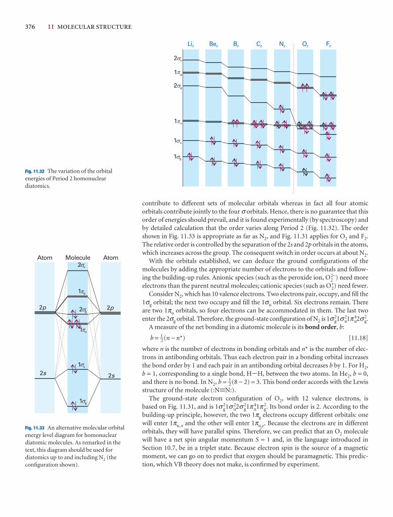
376 11 MOLECULAR STRUCTURE
Li2 Be2 B2 C2 N2 O2 F2
1 g
1 u
2 g
2 u
1 u
1 g
$
$
�
$
�
$
Fig. 11.32 The variation of the orbitalenergies of Period 2 homonucleardiatomics.
2p 2p
2s 2s
Atom Molecule Atom
1 g
1 u
2 g
2 u
1 u
1 g
$
�
$
�
$
$
Fig. 11.33 An alternative molecular orbitalenergy level diagram for homonucleardiatomic molecules. As remarked in thetext, this diagram should be used fordiatomics up to and including N2 (theconfiguration shown).
contribute to different sets of molecular orbitals whereas in fact all four atomic orbitals contribute jointly to the four σ orbitals. Hence, there is no guarantee that thisorder of energies should prevail, and it is found experimentally (by spectroscopy) andby detailed calculation that the order varies along Period 2 (Fig. 11.32). The ordershown in Fig. 11.33 is appropriate as far as N2, and Fig. 11.31 applies for O2 and F2.The relative order is controlled by the separation of the 2s and 2p orbitals in the atoms,which increases across the group. The consequent switch in order occurs at about N2.
With the orbitals established, we can deduce the ground configurations of themolecules by adding the appropriate number of electrons to the orbitals and follow-ing the building-up rules. Anionic species (such as the peroxide ion, O2
2−) need moreelectrons than the parent neutral molecules; cationic species (such as O2
+) need fewer.Consider N2, which has 10 valence electrons. Two electrons pair, occupy, and fill the
1σg orbital; the next two occupy and fill the 1σu orbital. Six electrons remain. Thereare two 1πu orbitals, so four electrons can be accommodated in them. The last twoenter the 2σg orbital. Therefore, the ground-state configuration of N2 is 1σg
21σu21πu
42σg2.
A measure of the net bonding in a diatomic molecule is its bond order, b:
b = 1–2 (n − n*) [11.18]
where n is the number of electrons in bonding orbitals and n* is the number of elec-trons in antibonding orbitals. Thus each electron pair in a bonding orbital increasesthe bond order by 1 and each pair in an antibonding orbital decreases b by 1. For H2,b = 1, corresponding to a single bond, H-H, between the two atoms. In He2, b = 0,and there is no bond. In N2, b = 1–2 (8 − 2) = 3. This bond order accords with the Lewisstructure of the molecule (:N.N:).
The ground-state electron configuration of O2, with 12 valence electrons, is based on Fig. 11.31, and is 1σ g
21σu22σ g
21πu41π g
2. Its bond order is 2. According to thebuilding-up principle, however, the two 1πg electrons occupy different orbitals: onewill enter 1πu,x and the other will enter 1πu,y. Because the electrons are in different orbitals, they will have parallel spins. Therefore, we can predict that an O2 moleculewill have a net spin angular momentum S = 1 and, in the language introduced inSection 10.7, be in a triplet state. Because electron spin is the source of a magnetic moment, we can go on to predict that oxygen should be paramagnetic. This predic-tion, which VB theory does not make, is confirmed by experiment.
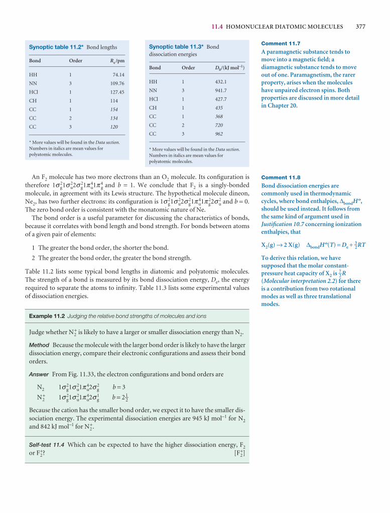
11.4 HOMONUCLEAR DIATOMIC MOLECULES 377
Comment 11.7
A paramagnetic substance tends tomove into a magnetic field; adiamagnetic substance tends to moveout of one. Paramagnetism, the rarerproperty, arises when the moleculeshave unpaired electron spins. Bothproperties are discussed in more detailin Chapter 20.
Synoptic table 11.2* Bond lengths
Bond Order Re /pm
HH 1 74.14
NN 3 109.76
HCl 1 127.45
CH 1 114
CC 1 154
CC 2 134
CC 3 120
* More values will be found in the Data section.Numbers in italics are mean values forpolyatomic molecules.
Synoptic table 11.3* Bonddissociation energies
Bond Order D0/(kJ mol−1)
HH 1 432.1
NN 3 941.7
HCl 1 427.7
CH 1 435
CC 1 368
CC 2 720
CC 3 962
* More values will be found in the Data section.Numbers in italics are mean values forpolyatomic molecules.
Comment 11.8
Bond dissociation energies arecommonly used in thermodynamiccycles, where bond enthalpies, ∆bondH 7,should be used instead. It follows fromthe same kind of argument used inJustification 10.7 concerning ionizationenthalpies, that
X2(g) → 2 X(g) ∆bondH 7(T) = De + 3–2RT
To derive this relation, we havesupposed that the molar constant-pressure heat capacity of X2 is 7–2 R(Molecular interpretation 2.2) for thereis a contribution from two rotationalmodes as well as three translationalmodes.
An F2 molecule has two more electrons than an O2 molecule. Its configuration istherefore 1σ g
21σu22σ g
21πu41π g
4 and b = 1. We conclude that F2 is a singly-bondedmolecule, in agreement with its Lewis structure. The hypothetical molecule dineon,Ne2, has two further electrons: its configuration is 1σ g
21σu22σ g
21πu41π g
22σu2 and b = 0.
The zero bond order is consistent with the monatomic nature of Ne.The bond order is a useful parameter for discussing the characteristics of bonds,
because it correlates with bond length and bond strength. For bonds between atomsof a given pair of elements:
1 The greater the bond order, the shorter the bond.
2 The greater the bond order, the greater the bond strength.
Table 11.2 lists some typical bond lengths in diatomic and polyatomic molecules. The strength of a bond is measured by its bond dissociation energy, De, the energy required to separate the atoms to infinity. Table 11.3 lists some experimental values of dissociation energies.
Example 11.2 Judging the relative bond strengths of molecules and ions
Judge whether N2+ is likely to have a larger or smaller dissociation energy than N2.
Method Because the molecule with the larger bond order is likely to have the largerdissociation energy, compare their electronic configurations and assess their bondorders.
Answer From Fig. 11.33, the electron configurations and bond orders are
N2 1σ g21σu
21πu42σ g
2 b = 3
N2+ 1σ g
21σu21πu
42σ g1 b = 2 1–2
Because the cation has the smaller bond order, we expect it to have the smaller dis-sociation energy. The experimental dissociation energies are 945 kJ mol−1 for N2
and 842 kJ mol−1 for N2+.
Self-test 11.4 Which can be expected to have the higher dissociation energy, F2
or F2+? [F2
+]
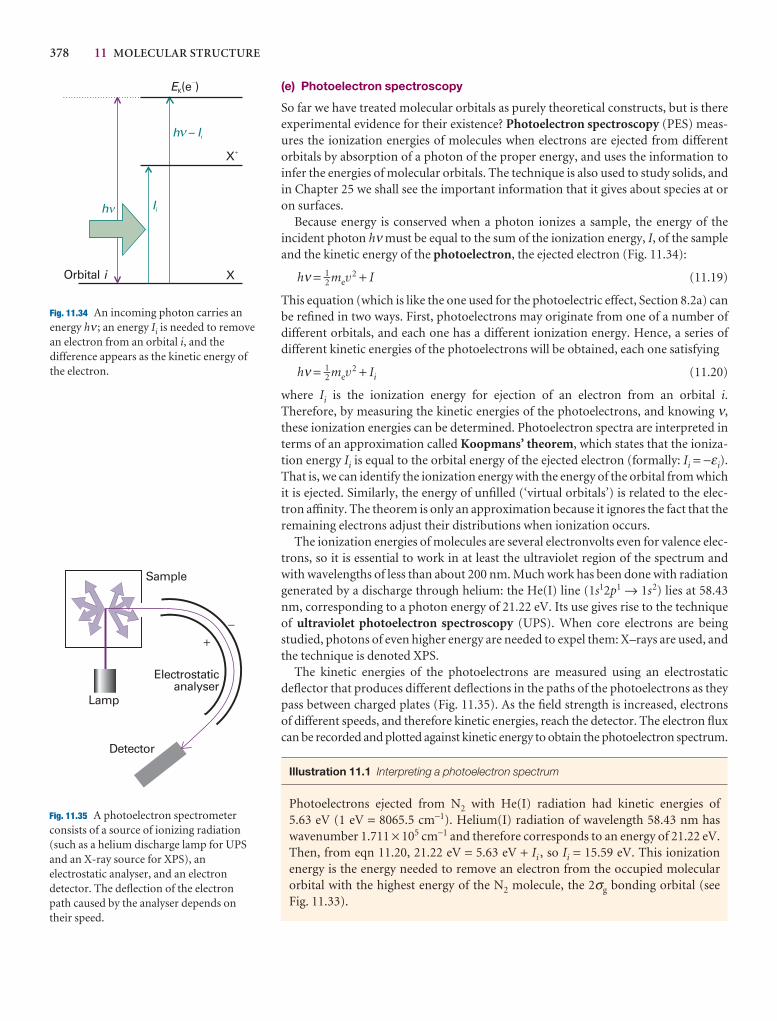
378 11 MOLECULAR STRUCTURE
X
X�
h�
Orbital i
Ii
h – Ii
EK(e )
�
�
Fig. 11.34 An incoming photon carries anenergy hν ; an energy Ii is needed to removean electron from an orbital i, and thedifference appears as the kinetic energy ofthe electron.
Detector
Electrostaticanalyser
�
�
Sample
Lamp
Fig. 11.35 A photoelectron spectrometerconsists of a source of ionizing radiation(such as a helium discharge lamp for UPSand an X-ray source for XPS), anelectrostatic analyser, and an electrondetector. The deflection of the electronpath caused by the analyser depends ontheir speed.
(e) Photoelectron spectroscopy
So far we have treated molecular orbitals as purely theoretical constructs, but is thereexperimental evidence for their existence? Photoelectron spectroscopy (PES) meas-ures the ionization energies of molecules when electrons are ejected from different orbitals by absorption of a photon of the proper energy, and uses the information toinfer the energies of molecular orbitals. The technique is also used to study solids, andin Chapter 25 we shall see the important information that it gives about species at oron surfaces.
Because energy is conserved when a photon ionizes a sample, the energy of the incident photon hν must be equal to the sum of the ionization energy, I, of the sampleand the kinetic energy of the photoelectron, the ejected electron (Fig. 11.34):
hν = 1–2 mev2 + I (11.19)
This equation (which is like the one used for the photoelectric effect, Section 8.2a) canbe refined in two ways. First, photoelectrons may originate from one of a number ofdifferent orbitals, and each one has a different ionization energy. Hence, a series ofdifferent kinetic energies of the photoelectrons will be obtained, each one satisfying
hν = 1–2 mev2 + Ii (11.20)
where Ii is the ionization energy for ejection of an electron from an orbital i.Therefore, by measuring the kinetic energies of the photoelectrons, and knowing ν,these ionization energies can be determined. Photoelectron spectra are interpreted interms of an approximation called Koopmans’ theorem, which states that the ioniza-tion energy Ii is equal to the orbital energy of the ejected electron (formally: Ii = −εi).That is, we can identify the ionization energy with the energy of the orbital from whichit is ejected. Similarly, the energy of unfilled (‘virtual orbitals’) is related to the elec-tron affinity. The theorem is only an approximation because it ignores the fact that theremaining electrons adjust their distributions when ionization occurs.
The ionization energies of molecules are several electronvolts even for valence elec-trons, so it is essential to work in at least the ultraviolet region of the spectrum andwith wavelengths of less than about 200 nm. Much work has been done with radiationgenerated by a discharge through helium: the He(I) line (1s12p1 → 1s2) lies at 58.43nm, corresponding to a photon energy of 21.22 eV. Its use gives rise to the techniqueof ultraviolet photoelectron spectroscopy (UPS). When core electrons are beingstudied, photons of even higher energy are needed to expel them: X–rays are used, andthe technique is denoted XPS.
The kinetic energies of the photoelectrons are measured using an electrostaticdeflector that produces different deflections in the paths of the photoelectrons as theypass between charged plates (Fig. 11.35). As the field strength is increased, electrons of different speeds, and therefore kinetic energies, reach the detector. The electron fluxcan be recorded and plotted against kinetic energy to obtain the photoelectron spectrum.
Illustration 11.1 Interpreting a photoelectron spectrum
Photoelectrons ejected from N2 with He(I) radiation had kinetic energies of 5.63 eV (1 eV = 8065.5 cm−1). Helium(I) radiation of wavelength 58.43 nm haswavenumber 1.711 × 105 cm−1 and therefore corresponds to an energy of 21.22 eV.Then, from eqn 11.20, 21.22 eV = 5.63 eV + Ii , so Ii = 15.59 eV. This ionization energy is the energy needed to remove an electron from the occupied molecular orbital with the highest energy of the N2 molecule, the 2σg bonding orbital (see Fig. 11.33).
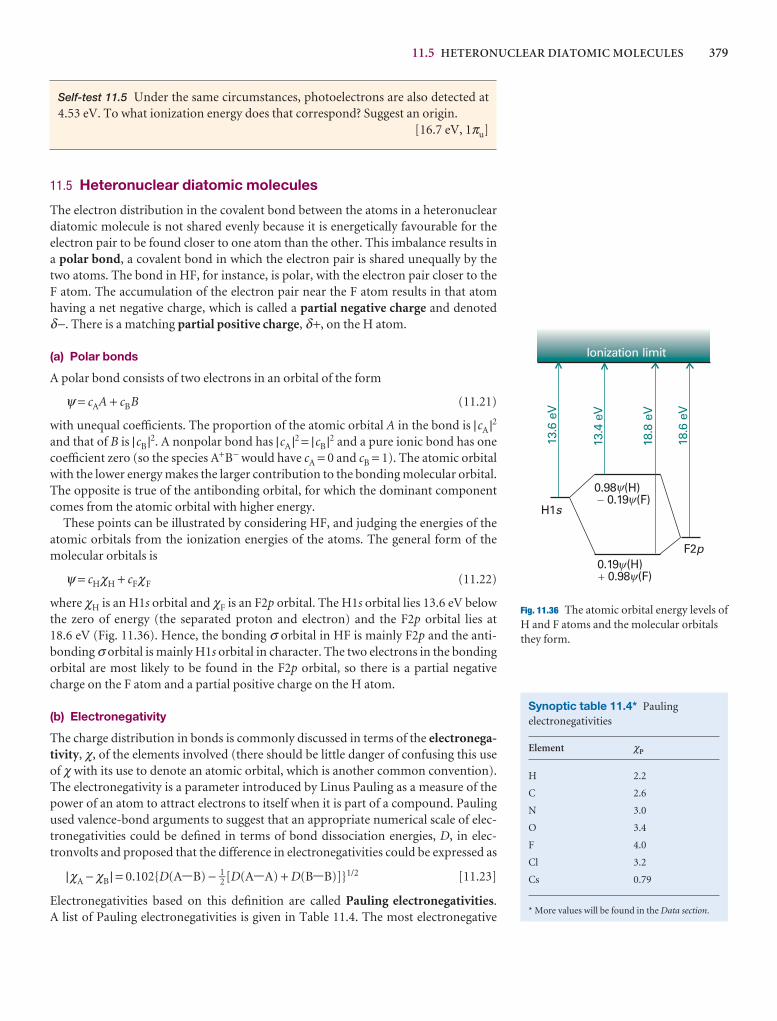
11.5 HETERONUCLEAR DIATOMIC MOLECULES 379
H1s
F2p
0.98 (H)0.19 (F)�
0.19 (H)0.98 (F)�
Ionization limit
13.6
eV
13.4
eV
18.8
eV
18.6
eV
��
��
Fig. 11.36 The atomic orbital energy levels ofH and F atoms and the molecular orbitalsthey form.
Synoptic table 11.4* Paulingelectronegativities
Element χP
H 2.2
C 2.6
N 3.0
O 3.4
F 4.0
Cl 3.2
Cs 0.79
* More values will be found in the Data section.
Self-test 11.5 Under the same circumstances, photoelectrons are also detected at4.53 eV. To what ionization energy does that correspond? Suggest an origin.
[16.7 eV, 1πu]
11.5 Heteronuclear diatomic molecules
The electron distribution in the covalent bond between the atoms in a heteronucleardiatomic molecule is not shared evenly because it is energetically favourable for theelectron pair to be found closer to one atom than the other. This imbalance results ina polar bond, a covalent bond in which the electron pair is shared unequally by thetwo atoms. The bond in HF, for instance, is polar, with the electron pair closer to theF atom. The accumulation of the electron pair near the F atom results in that atomhaving a net negative charge, which is called a partial negative charge and denoted δ−. There is a matching partial positive charge, δ+, on the H atom.
(a) Polar bonds
A polar bond consists of two electrons in an orbital of the form
ψ = cAA + cBB (11.21)
with unequal coefficients. The proportion of the atomic orbital A in the bond is |cA |2and that of B is |cB |2. A nonpolar bond has |cA |2 = |cB |2 and a pure ionic bond has onecoefficient zero (so the species A+B− would have cA = 0 and cB = 1). The atomic orbitalwith the lower energy makes the larger contribution to the bonding molecular orbital.The opposite is true of the antibonding orbital, for which the dominant componentcomes from the atomic orbital with higher energy.
These points can be illustrated by considering HF, and judging the energies of theatomic orbitals from the ionization energies of the atoms. The general form of themolecular orbitals is
ψ = cHχH + cFχF (11.22)
where χH is an H1s orbital and χF is an F2p orbital. The H1s orbital lies 13.6 eV belowthe zero of energy (the separated proton and electron) and the F2p orbital lies at 18.6 eV (Fig. 11.36). Hence, the bonding σ orbital in HF is mainly F2p and the anti-bonding σ orbital is mainly H1s orbital in character. The two electrons in the bonding orbital are most likely to be found in the F2p orbital, so there is a partial negativecharge on the F atom and a partial positive charge on the H atom.
(b) Electronegativity
The charge distribution in bonds is commonly discussed in terms of the electronega-tivity, χ, of the elements involved (there should be little danger of confusing this useof χ with its use to denote an atomic orbital, which is another common convention).The electronegativity is a parameter introduced by Linus Pauling as a measure of thepower of an atom to attract electrons to itself when it is part of a compound. Paulingused valence-bond arguments to suggest that an appropriate numerical scale of elec-tronegativities could be defined in terms of bond dissociation energies, D, in elec-tronvolts and proposed that the difference in electronegativities could be expressed as
|χA − χB | = 0.102{D(A-B) − 1–2 [D(A-A) + D(B-B)]}1/2 [11.23]
Electronegativities based on this definition are called Pauling electronegativities.A list of Pauling electronegativities is given in Table 11.4. The most electronegative
380 11 MOLECULAR STRUCTURE
elements are those close to fluorine; the least are those close to caesium. It is foundthat the greater the difference in electronegativities, the greater the polar character ofthe bond. The difference for HF, for instance, is 1.78; a C-H bond, which is com-monly regarded as almost nonpolar, has an electronegativity difference of 0.51.
The spectroscopist Robert Mulliken proposed an alternative definition of elec-tronegativity. He argued that an element is likely to be highly electronegative if it hasa high ionization energy (so it will not release electrons readily) and a high electronaffinity (so it is energetically favorable to acquire electrons). The Mulliken elec-tronegativity scale is therefore based on the definition
χM = 1–2 (I + Eea) [11.24]
where I is the ionization energy of the element and Eea is its electron affinity (both in electronvolts, Section 10.4e). The Mulliken and Pauling scales are approxim-ately in line with each other. A reasonably reliable conversion between the two is χP = 1.35χM
1/2 − 1.37.
(c) The variation principle
A more systematic way of discussing bond polarity and finding the coefficients in thelinear combinations used to build molecular orbitals is provided by the variationprinciple:
If an arbitrary wavefunction is used to calculate the energy, the value calculated isnever less than the true energy.
This principle is the basis of all modern molecular structure calculations (Section 11.7).The arbitrary wavefunction is called the trial wavefunction. The principle impliesthat, if we vary the coefficients in the trial wavefunction until the lowest energy isachieved (by evaluating the expectation value of the hamiltonian for each wavefunc-tion), then those coefficients will be the best. We might get a lower energy if we use amore complicated wavefunction (for example, by taking a linear combination of sev-eral atomic orbitals on each atom), but we shall have the optimum (minimum energy)molecular orbital that can be built from the chosen basis set, the given set of atomicorbitals.
The method can be illustrated by the trial wavefunction in eqn 11.21. We showin the Justification below that the coefficients are given by the solutions of the two secular equations
(αA − E)cA + (β − ES)cB = 0 (11.25a)
(β − ES)cA + (αB − E)cB = 0 (11.25b)
The parameter α is called a Coulomb integral. It is negative and can be interpreted as the energy of the electron when it occupies A (for αA) or B (for αB). In a homo-nuclear diatomic molecule, αA = αB. The parameter β is called a resonance integral(for classical reasons). It vanishes when the orbitals do not overlap, and at equilibriumbond lengths it is normally negative.
Justification 11.3 The variation principle applied to a heteronuclear diatomicmolecule
The trial wavefunction in eqn 11.21 is real but not normalized because at this stagethe coefficients can take arbitrary values. Therefore, we can write ψ* = ψ but do notassume that ∫ψ2dτ = 1. The energy of the trial wavefunction is the expectation valueof the energy operator (the hamiltonian, @, Section 8.5):
Comment 11.9
The name ‘secular’ is derived from theLatin word for age or generation. Theterm comes via astronomy, where thesame equations appear in connectionwith slowly accumulating modificationsof planetary orbits.
11.5 HETERONUCLEAR DIATOMIC MOLECULES 381
E = (11.26)
We must search for values of the coefficients in the trial function that minimize thevalue of E. This is a standard problem in calculus, and is solved by finding thecoefficients for which
= 0 = 0
The first step is to express the two integrals in terms of the coefficients. The denom-inator is
�ψ2 dτ =�(cAA + cBB)2 dτ
= cA2�A2 dτ + cB
2�B2 dτ + 2cAcB�AB dτ
= cA2 + cB
2 + 2cAcBS
because the individual atomic orbitals are normalized and the third integral is theoverlap integral S (eqn 11.17). The numerator is
�ψ@ψ dτ =�(cAA + cBB)@(cAA + cBB) dτ
= cA2�A@A dτ + c B
2�B@B dτ + cAcB�A@B dτ + cAcB�B@A dτ
There are some complicated integrals in this expression, but we can combine themall into the parameters
αA =�A@A dτ αB =�B@B dτ [11.27]
β =�A@B dτ =�B@A dτ (by the hermiticity of @)
Then
�ψ@ψ dτ = cA2αA + cB
2αB + 2cAcBβ
The complete expression for E is
E = (11.28)
Its minimum is found by differentiation with respect to the two coefficients and set-ting the results equal to 0. After a bit of work, we obtain
= = 0
= = 02 × (cBαB − cBE + cAβ − cASE)
cA2 + cB
2 + 2cAcBS
∂E
∂cB
2 × (cAαA − cAE + cBβ − cBSE)
cA2 + cB
2 + 2cAcBS
∂E
∂cA
cA2αA + cB
2αB + 2cAcBβcA
2 + cB2 + 2cAcBS
∂E
∂cB
∂E
∂cA
�ψ*@ψdτ
�ψ*ψdτ
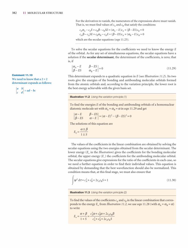
382 11 MOLECULAR STRUCTURE
Comment 11.10
We need to know that a 2 × 2determinant expands as follows:
a bc d
= ad − bc
For the derivatives to vanish, the numerators of the expressions above must vanish.That is, we must find values of cA and cB that satisfy the conditions
cAαA − cAE + cBβ − cBSE = (αA − E)cA + (β − ES)cB = 0
cAβ − cASE + cBαB − cBE = (β − ES)cA + (αB − E)cB = 0
which are the secular equations (eqn 11.25).
To solve the secular equations for the coefficients we need to know the energy Eof the orbital. As for any set of simultaneous equations, the secular equations have asolution if the secular determinant, the determinant of the coefficients, is zero; that is, if
αA − E β − ES(11.29)β − ES αB − E
= 0
This determinant expands to a quadratic equation in E (see Illustration 11.2). Its tworoots give the energies of the bonding and antibonding molecular orbitals formedfrom the atomic orbitals and, according to the variation principle, the lower root isthe best energy achievable with the given basis set.
Illustration 11.2 Using the variation principle (1)
To find the energies E of the bonding and antibonding orbitals of a homonucleardiatomic molecule set with αA = αB = α in eqn 11.29 and get
α − E β − ESβ − ES α − E
= (α − E)2 − (β − ES)2 = 0
The solutions of this equation are
E± =
The values of the coefficients in the linear combination are obtained by solving thesecular equations using the two energies obtained from the secular determinant. Thelower energy (E+ in the Illustration) gives the coefficients for the bonding molecularorbital, the upper energy (E−) the coefficients for the antibonding molecular orbital.The secular equations give expressions for the ratio of the coefficients in each case, sowe need a further equation in order to find their individual values. This equation isobtained by demanding that the best wavefunction should also be normalized. Thiscondition means that, at this final stage, we must also ensure that
�ψ2 dτ = cA2 + cB
2 + 2cAcBS = 1 (11.30)
Illustration 11.3 Using the variation principle (2)
To find the values of the coefficients cA and cB in the linear combination that corres-ponds to the energy E+ from Illustration 11.2, we use eqn 11.28 (with αA = αB = α)to write
E+ = =cA
2α + cB2α + 2cAcBβ
cA2 + cB
2 + 2cAcBS
α + β1 + S
α ± β1 ± S
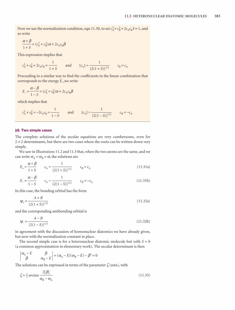
11.5 HETERONUCLEAR DIATOMIC MOLECULES 383
Now we use the normalization condition, eqn 11.30, to set cA2 + cB
2 + 2cAcBS = 1, andso write
= (c2A + c 2
B)α + 2cAcBβ
This expression implies that
c2A + c2
B = 2cAcB = and |cA | = cB = cA
Proceeding in a similar way to find the coefficients in the linear combination thatcorresponds to the energy E−,we write
E− = = (c2A + c2
B)α + 2cAcBβ
which implies that
c2A + c2
B = −2cAcB = and |cA | = cB = −cA
(d) Two simple cases
The complete solutions of the secular equations are very cumbersome, even for 2 × 2 determinants, but there are two cases where the roots can be written down verysimply.
We saw in Illustrations 11.2 and 11.3 that, when the two atoms are the same, and wecan write αA = αB = α, the solutions are
E+ = cA = cB = cA (11.31a)
E− = cA = cB = −cA (11.31b)
In this case, the bonding orbital has the form
ψ+ = (11.32a)
and the corresponding antibonding orbital is
ψ− = (11.32b)
in agreement with the discussion of homonuclear diatomics we have already given,but now with the normalization constant in place.
The second simple case is for a heteronuclear diatomic molecule but with S = 0(a common approximation in elementary work). The secular determinant is then
= (αA − E)(αB − E) − β2 = 0
The solutions can be expressed in terms of the parameter ζ (zeta), with
ζ = 1–2 arctan (11.33)2|β |
αB − αA
βαB − E
αA − Eβ
A − B
{2(1 − S)}1/2
A + B
{2(1 + S)}1/2
1
{2(1 − S)}1/2
α − β1 − S
1
{2(1 + S)}1/2
α + β1 + S
1
{2(1 − S)}1/2
1
1 − S
α − β1 − S
1
{2(1 + S)}1/2
1
1 + S
α + β1 + S
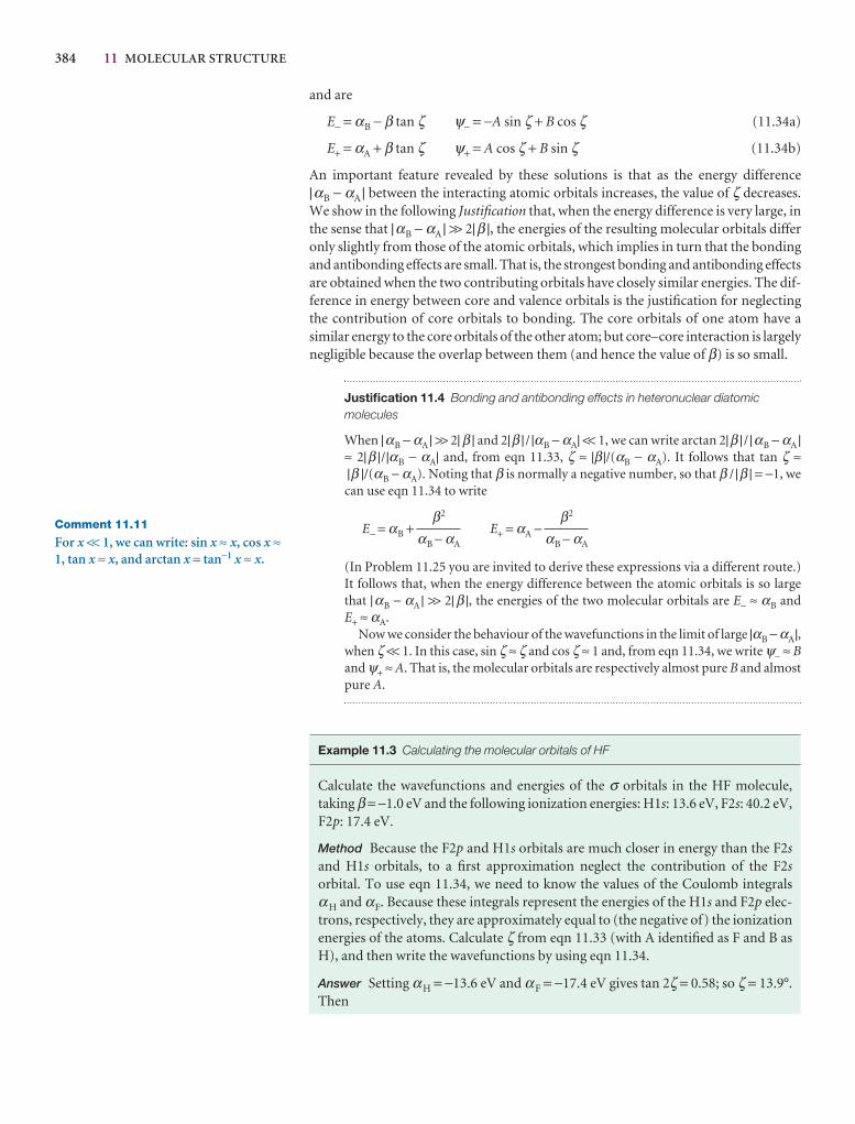
384 11 MOLECULAR STRUCTURE
Comment 11.11
For x << 1, we can write: sin x ≈ x, cos x ≈1, tan x ≈ x, and arctan x = tan−1 x ≈ x.
and are
E− = αB − β tan ζ ψ− = −A sin ζ + B cos ζ (11.34a)
E+ = αA + β tan ζ ψ+ = A cos ζ + B sin ζ (11.34b)
An important feature revealed by these solutions is that as the energy difference|αB − αA | between the interacting atomic orbitals increases, the value of ζ decreases.We show in the following Justification that, when the energy difference is very large, inthe sense that |αB − αA | >> 2|β |, the energies of the resulting molecular orbitals differonly slightly from those of the atomic orbitals, which implies in turn that the bondingand antibonding effects are small. That is, the strongest bonding and antibonding effectsare obtained when the two contributing orbitals have closely similar energies. The dif-ference in energy between core and valence orbitals is the justification for neglectingthe contribution of core orbitals to bonding. The core orbitals of one atom have a similar energy to the core orbitals of the other atom; but core–core interaction is largelynegligible because the overlap between them (and hence the value of β) is so small.
Justification 11.4 Bonding and antibonding effects in heteronuclear diatomicmolecules
When |αB − αA | >> 2| β | and 2|β | / |αB − αA| << 1, we can write arctan 2|β | / |αB − αA |≈ 2|β |/|αB − αA| and, from eqn 11.33, ζ ≈ |β |/(αB − αA). It follows that tan ζ ≈|β |/(αB − αA). Noting that β is normally a negative number, so that β / |β | = −1, wecan use eqn 11.34 to write
E− = αB + E+ = αA −
(In Problem 11.25 you are invited to derive these expressions via a different route.)It follows that, when the energy difference between the atomic orbitals is so largethat |αB − αA | >> 2| β |, the energies of the two molecular orbitals are E− ≈ αB andE+ ≈ αA.
Now we consider the behaviour of the wavefunctions in the limit of large |αB − αA|,when ζ << 1. In this case, sin ζ ≈ ζ and cos ζ ≈ 1 and, from eqn 11.34, we write ψ− ≈ Band ψ+ ≈ A. That is, the molecular orbitals are respectively almost pure B and almostpure A.
Example 11.3 Calculating the molecular orbitals of HF
Calculate the wavefunctions and energies of the σ orbitals in the HF molecule, taking β = −1.0 eV and the following ionization energies: H1s: 13.6 eV, F2s: 40.2 eV,F2p: 17.4 eV.
Method Because the F2p and H1s orbitals are much closer in energy than the F2sand H1s orbitals, to a first approximation neglect the contribution of the F2sorbital. To use eqn 11.34, we need to know the values of the Coulomb integrals αH and αF. Because these integrals represent the energies of the H1s and F2p elec-trons, respectively, they are approximately equal to (the negative of) the ionizationenergies of the atoms. Calculate ζ from eqn 11.33 (with A identified as F and B asH), and then write the wavefunctions by using eqn 11.34.
Answer Setting αH = −13.6 eV and αF = −17.4 eV gives tan 2ζ = 0.58; so ζ = 13.9°.Then
β2
αB − αA
β2
αB − αA
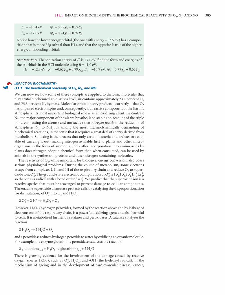
I11.1 IMPACT ON BIOCHEMISTRY: THE BIOCHEMICAL REACTIVITY OF O2, N2, AND NO 385
E− = −13.4 eV ψ− = 0.97χH − 0.24χF
E+ = −17.6 eV ψ+ = 0.24χH + 0.97χF
Notice how the lower energy orbital (the one with energy −17.6 eV) has a compo-sition that is more F2p orbital than H1s, and that the opposite is true of the higherenergy, antibonding orbital.
Self-test 11.6 The ionization energy of Cl is 13.1 eV; find the form and energies ofthe σ orbitals in the HCl molecule using β = −1.0 eV.
[E− = −12.8 eV, ψ− = −0.62χH + 0.79χCl; E+ = −13.9 eV, ψ+ = 0.79χH + 0.62χCl]
IMPACT ON BIOCHEMISTRY
I11.1 The biochemical reactivity of O2, N2, and NO
We can now see how some of these concepts are applied to diatomic molecules thatplay a vital biochemical role. At sea level, air contains approximately 23.1 per cent O2
and 75.5 per cent N2 by mass. Molecular orbital theory predicts—correctly—that O2
has unpaired electron spins and, consequently, is a reactive component of the Earth’satmosphere; its most important biological role is as an oxidizing agent. By contrastN2, the major component of the air we breathe, is so stable (on account of the triplebond connecting the atoms) and unreactive that nitrogen fixation, the reduction of atmospheric N2 to NH3, is among the most thermodynamically demanding of biochemical reactions, in the sense that it requires a great deal of energy derived frommetabolism. So taxing is the process that only certain bacteria and archaea are cap-able of carrying it out, making nitrogen available first to plants and other micro-organisms in the form of ammonia. Only after incorporation into amino acids byplants does nitrogen adopt a chemical form that, when consumed, can be used by animals in the synthesis of proteins and other nitrogen-containing molecules.
The reactivity of O2, while important for biological energy conversion, also posesserious physiological problems. During the course of metabolism, some electrons escape from complexes I, II, and III of the respiratory chain and reduce O2 to super-oxide ion, O2
−. The ground-state electronic configuration of O2− is 1σ g
21σu22σ g
21πu41π g
3,so the ion is a radical with a bond order b = 3–2 . We predict that the superoxide ion is areactive species that must be scavenged to prevent damage to cellular components.The enzyme superoxide dismutase protects cells by catalysing the disproportionation(or dismutation) of O2
− into O2 and H2O2:
2 O2− + 2 H+ → H2O2 + O2
However, H2O2 (hydrogen peroxide), formed by the reaction above and by leakage ofelectrons out of the respiratory chain, is a powerful oxidizing agent and also harmfulto cells. It is metabolized further by catalases and peroxidases. A catalase catalyses thereaction
2 H2O2 → 2 H2O + O2
and a peroxidase reduces hydrogen peroxide to water by oxidizing an organic molecule.For example, the enzyme glutathione peroxidase catalyses the reaction
2 glutathionered + H2O2 → glutathioneox + 2 H2O
There is growing evidence for the involvement of the damage caused by reactive oxygen species (ROS), such as O2
−, H2O2, and ·OH (the hydroxyl radical), in the mechanism of ageing and in the development of cardiovascular disease, cancer,
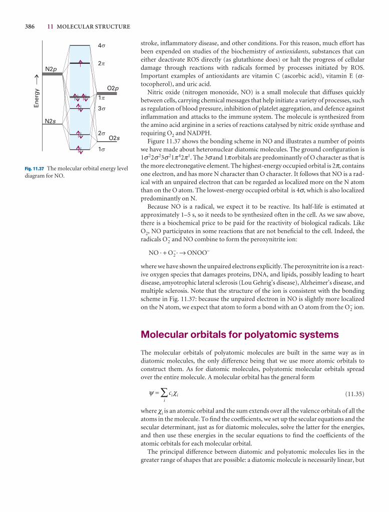
386 11 MOLECULAR STRUCTURE
stroke, inflammatory disease, and other conditions. For this reason, much effort hasbeen expended on studies of the biochemistry of antioxidants, substances that can either deactivate ROS directly (as glutathione does) or halt the progress of cellulardamage through reactions with radicals formed by processes initiated by ROS.Important examples of antioxidants are vitamin C (ascorbic acid), vitamin E (α-tocopherol), and uric acid.
Nitric oxide (nitrogen monoxide, NO) is a small molecule that diffuses quickly between cells, carrying chemical messages that help initiate a variety of processes, suchas regulation of blood pressure, inhibition of platelet aggregation, and defence againstinflammation and attacks to the immune system. The molecule is synthesized fromthe amino acid arginine in a series of reactions catalysed by nitric oxide synthase andrequiring O2 and NADPH.
Figure 11.37 shows the bonding scheme in NO and illustrates a number of pointswe have made about heteronuclear diatomic molecules. The ground configuration is1σ22σ23σ21π42π1. The 3σ and 1π orbitals are predominantly of O character as that isthe more electronegative element. The highest-energy occupied orbital is 2π, containsone electron, and has more N character than O character. It follows that NO is a rad-ical with an unpaired electron that can be regarded as localized more on the N atomthan on the O atom. The lowest-energy occupied orbital is 4σ, which is also localizedpredominantly on N.
Because NO is a radical, we expect it to be reactive. Its half-life is estimated at approximately 1–5 s, so it needs to be synthesized often in the cell. As we saw above,there is a biochemical price to be paid for the reactivity of biological radicals. LikeO2, NO participates in some reactions that are not beneficial to the cell. Indeed, theradicals O2
− and NO combine to form the peroxynitrite ion:
NO · + O2−· → ONOO−
where we have shown the unpaired electrons explicitly. The peroxynitrite ion is a react-ive oxygen species that damages proteins, DNA, and lipids, possibly leading to heartdisease, amyotrophic lateral sclerosis (Lou Gehrig’s disease), Alzheimer’s disease, andmultiple sclerosis. Note that the structure of the ion is consistent with the bondingscheme in Fig. 11.37: because the unpaired electron in NO is slightly more localizedon the N atom, we expect that atom to form a bond with an O atom from the O2
− ion.
Molecular orbitals for polyatomic systems
The molecular orbitals of polyatomic molecules are built in the same way as in diatomic molecules, the only difference being that we use more atomic orbitals toconstruct them. As for diatomic molecules, polyatomic molecular orbitals spreadover the entire molecule. A molecular orbital has the general form
ψ = ∑i
ciχi (11.35)
where χi is an atomic orbital and the sum extends over all the valence orbitals of all theatoms in the molecule. To find the coefficients, we set up the secular equations and thesecular determinant, just as for diatomic molecules, solve the latter for the energies,and then use these energies in the secular equations to find the coefficients of theatomic orbitals for each molecular orbital.
The principal difference between diatomic and polyatomic molecules lies in thegreater range of shapes that are possible: a diatomic molecule is necessarily linear, but
O2s
O2p
N2s
N2p
1
2
3
4
1
2
Ener
gy
$
�
�
$
$
$
Fig. 11.37 The molecular orbital energy leveldiagram for NO.
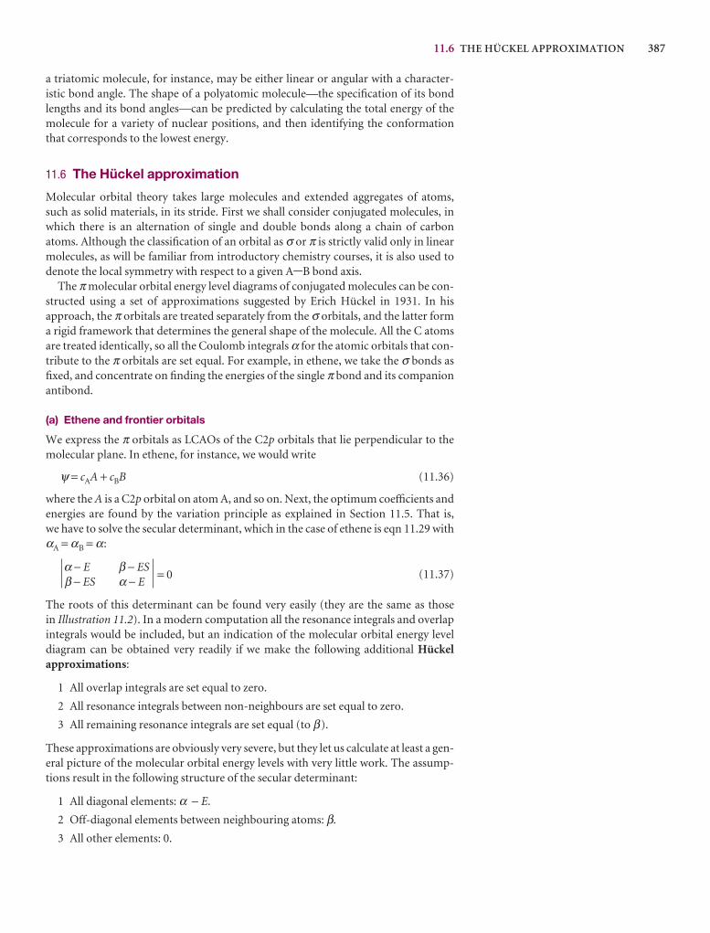
11.6 THE HÜCKEL APPROXIMATION 387
a triatomic molecule, for instance, may be either linear or angular with a character-istic bond angle. The shape of a polyatomic molecule—the specification of its bondlengths and its bond angles—can be predicted by calculating the total energy of themolecule for a variety of nuclear positions, and then identifying the conformationthat corresponds to the lowest energy.
11.6 The Hückel approximation
Molecular orbital theory takes large molecules and extended aggregates of atoms,such as solid materials, in its stride. First we shall consider conjugated molecules, inwhich there is an alternation of single and double bonds along a chain of carbonatoms. Although the classification of an orbital as σ or π is strictly valid only in linearmolecules, as will be familiar from introductory chemistry courses, it is also used todenote the local symmetry with respect to a given A-B bond axis.
The π molecular orbital energy level diagrams of conjugated molecules can be con-structed using a set of approximations suggested by Erich Hückel in 1931. In his approach, the π orbitals are treated separately from the σ orbitals, and the latter forma rigid framework that determines the general shape of the molecule. All the C atomsare treated identically, so all the Coulomb integrals α for the atomic orbitals that con-tribute to the π orbitals are set equal. For example, in ethene, we take the σ bonds asfixed, and concentrate on finding the energies of the single π bond and its companionantibond.
(a) Ethene and frontier orbitals
We express the π orbitals as LCAOs of the C2p orbitals that lie perpendicular to themolecular plane. In ethene, for instance, we would write
ψ = cAA + cBB (11.36)
where the A is a C2p orbital on atom A, and so on. Next, the optimum coefficients andenergies are found by the variation principle as explained in Section 11.5. That is, we have to solve the secular determinant, which in the case of ethene is eqn 11.29 withαA = αB = α:
α − E β − ES(11.37)β − ES α − E
= 0
The roots of this determinant can be found very easily (they are the same as those in Illustration 11.2). In a modern computation all the resonance integrals and overlapintegrals would be included, but an indication of the molecular orbital energy level diagram can be obtained very readily if we make the following additional Hückelapproximations:
1 All overlap integrals are set equal to zero.
2 All resonance integrals between non-neighbours are set equal to zero.
3 All remaining resonance integrals are set equal (to β).
These approximations are obviously very severe, but they let us calculate at least a gen-eral picture of the molecular orbital energy levels with very little work. The assump-tions result in the following structure of the secular determinant:
1 All diagonal elements: α − E.
2 Off-diagonal elements between neighbouring atoms: β.
3 All other elements: 0.
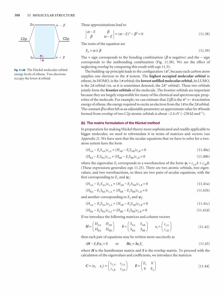
388 11 MOLECULAR STRUCTURE
These approximations lead to
= (α − E)2 − β2 = 0 (11.38)
The roots of the equation are
E± = α ± β (11.39)
The + sign corresponds to the bonding combination (β is negative) and the − signcorresponds to the antibonding combination (Fig. 11.38). We see the effect of neglecting overlap by comparing this result with eqn 11.31.
The building-up principle leads to the configuration 1π2, because each carbon atomsupplies one electron to the π system. The highest occupied molecular orbital inethene, its HOMO, is the 1π orbital; the lowest unfilled molecular orbital, its LUMO,is the 2π orbital (or, as it is sometimes denoted, the 2π* orbital). These two orbitalsjointly form the frontier orbitals of the molecule. The frontier orbitals are importantbecause they are largely responsible for many of the chemical and spectroscopic prop-erties of the molecule. For example, we can estimate that 2 |β | is the π* ← π excitationenergy of ethene, the energy required to excite an electron from the 1π to the 2π orbital.The constant β is often left as an adjustable parameter; an approximate value for π bondsformed from overlap of two C2p atomic orbitals is about −2.4 eV (−230 kJ mol−1).
(b) The matrix formulation of the Hückel method
In preparation for making Hückel theory more sophisticated and readily applicable tobigger molecules, we need to reformulate it in terms of matrices and vectors (seeAppendix 2). We have seen that the secular equations that we have to solve for a two-atom system have the form
(HAA − EiSAA)ci,A + (HAB − EiSAB)ci,B = 0 (11.40a)
(HBA − EiSBA)ci,A + (HBB − EiSBB)ci,B = 0 (11.40b)
where the eigenvalue Ei corresponds to a wavefunction of the form ψi = ci,AA + ci,BB.(These expressions generalize eqn 11.25). There are two atomic orbitals, two eigen-values, and two wavefunctions, so there are two pairs of secular equations, with thefirst corresponding to E1 and ψ1:
(HAA − E1SAA)c1,A + (HAB − E1SAB)c1,B = 0 (11.41a)
(HBA − E1SBA)c1,A + (HBB − E1SBB)c1,B = 0 (11.41b)
and another corresponding to E2 and ψ2:
(HAA − E2SAA)c2,A + (HAB − E2SAB)c2,B = 0 (11.41c)
(HBA − E2SBA)c2,A + (HBB − E2SBB)c2,B = 0 (11.41d)
If we introduce the following matrices and column vectors
H = S = ci = (11.42)
then each pair of equations may be written more succinctly as
(H − EiS)ci = 0 or Hci = SciEi (11.43)
where H is the hamiltonian matrix and S is the overlap matrix. To proceed with thecalculation of the eigenvalues and coefficients, we introduce the matrices
C = (c1 c2) = E = [11.44]DF
0
E2
E1
0
AC
DF
c2,A
c2,B
c1,A
c1,B
AC
DF
ci,A
ci,B
AC
DF
SAB
SBB
SAA
SBA
AC
DF
HAB
HBB
HAA
HBA
AC
βα − E
α − Eβ
Fig. 11.38 The Hückel molecular orbitalenergy levels of ethene. Two electronsoccupy the lower π orbital.
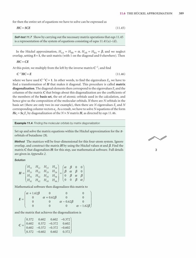
11.6 THE HÜCKEL APPROXIMATION 389
for then the entire set of equations we have to solve can be expressed as
HC = SCE (11.45)
Self-test 11.7 Show by carrying out the necessary matrix operations that eqn 11.45is a representation of the system of equations consisting of eqns 11.41(a)–(d).
In the Hückel approximation, HAA = HBB = α, HAB = HBA = β, and we neglect overlap, setting S = 1, the unit matrix (with 1 on the diagonal and 0 elsewhere). Then
HC = CE
At this point, we multiply from the left by the inverse matrix C −1, and find
C −1HC = E (11.46)
where we have used C −1C = 1. In other words, to find the eigenvalues Ei, we have tofind a transformation of H that makes it diagonal. This procedure is called matrixdiagonalization. The diagonal elements then correspond to the eigenvalues Ei and thecolumns of the matrix C that brings about this diagonalization are the coefficients ofthe members of the basis set, the set of atomic orbitals used in the calculation, andhence give us the composition of the molecular orbitals. If there are N orbitals in thebasis set (there are only two in our example), then there are N eigenvalues Ei and Ncorresponding column vectors ci. As a result, we have to solve N equations of the formHci = SciEi by diagonalization of the N × N matrix H, as directed by eqn 11.46.
Example 11.4 Finding the molecular orbitals by matrix diagonalization
Set up and solve the matrix equations within the Hückel approximation for the π-orbitals of butadiene (3).
Method The matrices will be four-dimensional for this four-atom system. Ignoreoverlap, and construct the matrix H by using the Hückel values α and β. Find thematrix C that diagonalizes H: for this step, use mathematical software. Full detailsare given in Appendix 2.
Solution
Mathematical software then diagonalizes this matrix to
and the matrix that achieves the diagonalization is
C
. . . .
. . . .
. . . .
. . . .
=
−−
− − −−
⎛
⎝
⎜⎜⎜
⎞
⎠
⎟⎟⎟
0 372 0 602 0 602 0 3720 602 0 372 0 372 0 6020 602 0 372 0 372 0 6020 372 0 602 0 602 0 372
E
. .
. .
=
++
−−
⎛
⎝
⎜⎜⎜
⎞
⎠
⎟⎟⎟
α βα β
α βα β
1 62 0 0 00 0 62 0 00 0 0 62 00 0 0 1 62
H =
⎛
⎝
⎜⎜⎜⎜
⎞
⎠
⎟⎟⎟⎟
=
⎛
⎝
⎜⎜⎜
⎞
⎠
⎟⎟⎟
H H H HH H H HH H H HH H H H
11 12 13 14
21 22 23 24
31 32 33 34
41 42 43 44
0 00
00 0
α ββ α β
β α ββ α
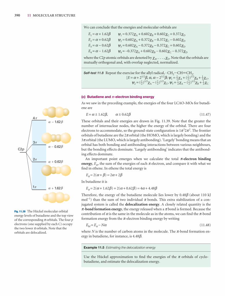
390 11 MOLECULAR STRUCTURE
1.62�
0.62�
0.62�
1.62�
4
3
2
1
C2p
�
�
�
�
�
�
�
�
�
�
�
�
Fig. 11.39 The Hückel molecular orbitalenergy levels of butadiene and the top viewof the corresponding π orbitals. The four pelectrons (one supplied by each C) occupythe two lower π orbitals. Note that theorbitals are delocalized.
We can conclude that the energies and molecular orbitals are
E1 = α + 1.62β ψ1 = 0.372χA + 0.602χB + 0.602χC + 0.372χD
E2 = α + 0.62β ψ2 = 0.602χA + 0.372χB − 0.372χC − 0.602χD
E3 = α − 0.62β ψ3 = 0.602χA − 0.372χB − 0.372χC + 0.602χD
E4 = α − 1.62β ψ4 = −0.372χA + 0.602χB − 0.602χC − 0.372χD
where the C2p atomic orbitals are denoted by χA, . . . , χD. Note that the orbitals aremutually orthogonal and, with overlap neglected, normalized.
Self-test 11.8 Repeat the exercise for the allyl radical, · CH2-CH=CH2.[E = α + 21/2β, α, α − 21/2β; ψ1 = 1–2 χA + ( 1–2 )1/2χB + 1–2 χC,
ψ2 = ( 1–2 )1/2χA − ( 1–2 )1/2χC, ψ3 = 1–2 χA − ( 1–2 )1/2χB + 1–2 χC
(c) Butadiene and π-electron binding energy
As we saw in the preceding example, the energies of the four LCAO-MOs for butadi-ene are
E = α ± 1.62β, α ± 0.62β (11.47)
These orbitals and their energies are drawn in Fig. 11.39. Note that the greater thenumber of internuclear nodes, the higher the energy of the orbital. There are fourelectrons to accommodate, so the ground-state configuration is 1π22π2. The frontierorbitals of butadiene are the 2π orbital (the HOMO, which is largely bonding) and the3π orbital (the LUMO, which is largely antibonding). ‘Largely’ bonding means that anorbital has both bonding and antibonding interactions between various neighbours,but the bonding effects dominate. ‘Largely antibonding’ indicates that the antibond-ing effects dominate.
An important point emerges when we calculate the total π-electron binding energy, Eπ, the sum of the energies of each π electron, and compare it with what wefind in ethene. In ethene the total energy is
Eπ = 2(α + β) = 2α + 2β
In butadiene it is
Eπ = 2(α + 1.62β) + 2(α + 0.62β) = 4α + 4.48β
Therefore, the energy of the butadiene molecule lies lower by 0.48β (about 110 kJmol−1) than the sum of two individual π bonds. This extra stabilization of a con-jugated system is called the delocalization energy. A closely related quantity is the π-bond formation energy, the energy released when a π bond is formed. Because thecontribution of α is the same in the molecule as in the atoms, we can find the π-bondformation energy from the π-electron binding energy by writing
Ebf = Eπ − Nα (11.48)
where N is the number of carbon atoms in the molecule. The π-bond formation en-ergy in butadiene, for instance, is 4.48β.
Example 11.5 Estimating the delocalization energy
Use the Hückel approximation to find the energies of the π orbitals of cyclo-butadiene, and estimate the delocalization energy.
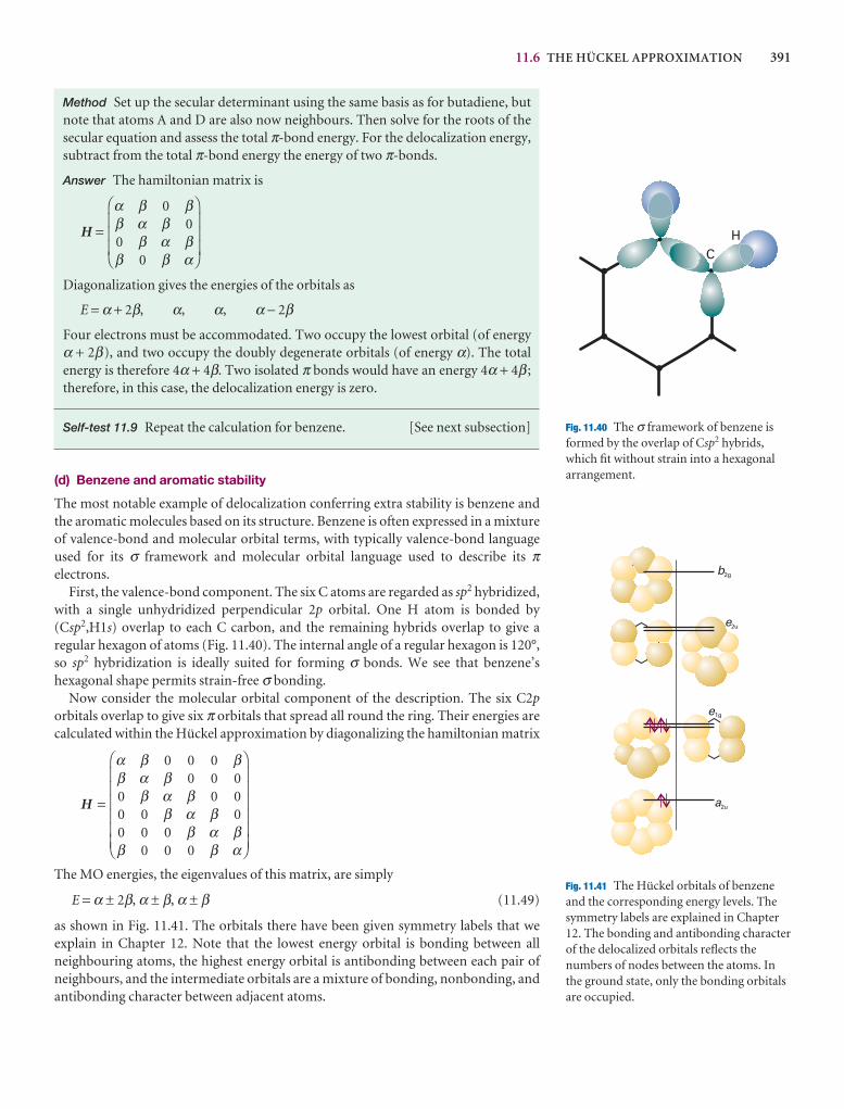
11.6 THE HÜCKEL APPROXIMATION 391
CH
Fig. 11.40 The σ framework of benzene isformed by the overlap of Csp2 hybrids,which fit without strain into a hexagonalarrangement.
b2g
e2u
e1g
a2u
Fig. 11.41 The Hückel orbitals of benzeneand the corresponding energy levels. Thesymmetry labels are explained in Chapter12. The bonding and antibonding characterof the delocalized orbitals reflects thenumbers of nodes between the atoms. Inthe ground state, only the bonding orbitalsare occupied.
Method Set up the secular determinant using the same basis as for butadiene, butnote that atoms A and D are also now neighbours. Then solve for the roots of thesecular equation and assess the total π-bond energy. For the delocalization energy,subtract from the total π-bond energy the energy of two π-bonds.
Answer The hamiltonian matrix is
Diagonalization gives the energies of the orbitals as
E = α + 2β, α, α, α − 2β
Four electrons must be accommodated. Two occupy the lowest orbital (of energyα + 2β), and two occupy the doubly degenerate orbitals (of energy α). The total energy is therefore 4α + 4β. Two isolated π bonds would have an energy 4α + 4β ;therefore, in this case, the delocalization energy is zero.
Self-test 11.9 Repeat the calculation for benzene. [See next subsection]
(d) Benzene and aromatic stability
The most notable example of delocalization conferring extra stability is benzene andthe aromatic molecules based on its structure. Benzene is often expressed in a mixtureof valence-bond and molecular orbital terms, with typically valence-bond languageused for its σ framework and molecular orbital language used to describe its πelectrons.
First, the valence-bond component. The six C atoms are regarded as sp2 hybridized,with a single unhydridized perpendicular 2p orbital. One H atom is bonded by(Csp2,H1s) overlap to each C carbon, and the remaining hybrids overlap to give a regular hexagon of atoms (Fig. 11.40). The internal angle of a regular hexagon is 120°,so sp2 hybridization is ideally suited for forming σ bonds. We see that benzene’shexagonal shape permits strain-free σ bonding.
Now consider the molecular orbital component of the description. The six C2porbitals overlap to give six π orbitals that spread all round the ring. Their energies arecalculated within the Hückel approximation by diagonalizing the hamiltonian matrix
The MO energies, the eigenvalues of this matrix, are simply
E = α ± 2β, α ± β, α ± β (11.49)
as shown in Fig. 11.41. The orbitals there have been given symmetry labels that we explain in Chapter 12. Note that the lowest energy orbital is bonding between allneighbouring atoms, the highest energy orbital is antibonding between each pair ofneighbours, and the intermediate orbitals are a mixture of bonding, nonbonding, andantibonding character between adjacent atoms.
H =
⎛
⎝
⎜⎜⎜⎜⎜⎜
⎞
⎠
⎟⎟⎟⎟⎟⎟
α β ββ α β
β α ββ α β
β α ββ β α
0 0 00 0 0
0 0 00 0 00 0 0
0 0 0
H =
⎛
⎝
⎜⎜⎜
⎞
⎠
⎟⎟⎟
α β ββ α β
β α ββ β α
00
00
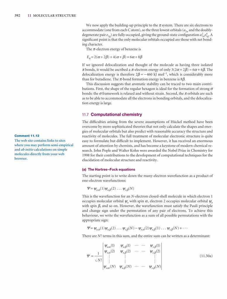
392 11 MOLECULAR STRUCTURE
We now apply the building-up principle to the π system. There are six electrons toaccommodate (one from each C atom), so the three lowest orbitals (a2u and the doubly-degenerate pair e1g) are fully occupied, giving the ground-state configuration a2
2ue41g. A
significant point is that the only molecular orbitals occupied are those with net bond-ing character.
The π-electron energy of benzene is
Eπ = 2(α + 2β) + 4(α + β) = 6α + 8β
If we ignored delocalization and thought of the molecule as having three isolated π bonds, it would be ascribed a π-electron energy of only 3(2α + 2β) = 6α + 6β. The delocalization energy is therefore 2β ≈ −460 kJ mol−1, which is considerably morethan for butadiene. The π-bond formation energy in benzene is 8β.
This discussion suggests that aromatic stability can be traced to two main contri-butions. First, the shape of the regular hexagon is ideal for the formation of strong σbonds: the σ framework is relaxed and without strain. Second, the π orbitals are suchas to be able to accommodate all the electrons in bonding orbitals, and the delocaliza-tion energy is large.
11.7 Computational chemistry
The difficulties arising from the severe assumptions of Hückel method have beenovercome by more sophisticated theories that not only calculate the shapes and ener-gies of molecular orbitals but also predict with reasonable accuracy the structure andreactivity of molecules. The full treatment of molecular electronic structure is quiteeasy to formulate but difficult to implement. However, it has received an enormousamount of attention by chemists, and has become a keystone of modern chemical re-search. John Pople and Walter Kohn were awarded the Nobel Prize in Chemistry for1998 for their contributions to the development of computational techniques for theelucidation of molecular structure and reactivity.
(a) The Hartree–Fock equations
The starting point is to write down the many-electron wavefunction as a product ofone-electron wavefunctions:
Ψ = ψa,α(1)ψa,β(2) . . . ψz,β(N)
This is the wavefunction for an N-electron closed-shell molecule in which electron 1occupies molecular orbital ψa with spin α , electron 2 occupies molecular orbital ψa
with spin β, and so on. However, the wavefunction must satisfy the Pauli principleand change sign under the permutation of any pair of electrons. To achieve this behaviour, we write the wavefunction as a sum of all possible permutations with theappropriate sign:
Ψ = ψa,α(1)ψa,β(2) . . . ψz,β(N) − ψa,α(2)ψa,β(1) . . . ψz,β(N) + · · ·
There are N ! terms in this sum, and the entire sum can be written as a determinant:
(11.50a)Ψ!
( ) ( ) ( )
( ) ( ) ( )
( ) ( ) ( )
, , ,
, , ,
, , ,
=1
1 1 1
2 2 2
N
N N N
a a z
a a z
a a z
ψ ψ ψψ ψ ψ
ψ ψ ψ
α β β
α β β
α β β
L L
L L
M M MM M M
L L
Comment 11.12
The web site contains links to siteswhere you may perform semi-empiricaland ab initio calculations on simplemolecules directly from your webbrowser.
11.7 COMPUTATIONAL CHEMISTRY 393
The initial factor ensures that the wavefunction is normalized if the componentmolecular orbitals are normalized. To save the tedium of writing out large deter-minants, the wavefunction is normally written simply as
Ψ = (1/N!)1/2det |ψa,α(1)ψa,β(2) . . . ψz,β(N) | (11.50b)
When the determinantal wavefunction is combined with the variation principle(Section 11.5c), the optimum wavefunctions, in the sense of corresponding to thelowest total energy, must satisfy the Hartree–Fock equations:
f1ψa,σ(1) = εψa,σ(1) (11.51)
where σ is either α or β. The Fock operator f1 is
f1 = h1 + ∑j{2Jj(1) − Kj(1)} (11.52)
The three terms in this expression are the core hamiltonian
h1 = − ∇21 − ∑
n[11.53a]
the Coulomb operator J, where
Jj(1)ψa(1) = �ψ j*(2)ψj(2) ψa(1)dτ2 [11.53b]
and the exchange operator, K, where
Kj(1)ψa(1) = �ψ j*(2)ψa(2) ψj(1)dτ2 [11.53c]
Although the Hartree–Fock equations look deceptively simple, with the Fock opera-tor looking like a hamiltonian, we see from these definitions that f actually depends onthe wavefunctions of all the electrons. To proceed, we have to guess the initial form ofthe wavefunctions, use them in the definition of the Coulomb and exchange opera-tors, and solve the Hartree–Fock equations. That process is then continued using thenewly found wavefunctions until each cycle of calculation leaves the energies andwavefunctions unchanged to within a chosen criterion. This is the origin of the termself-consistent field (SCF) for this type of procedure.
The difficulty in this procedure is in the solution of the Hartree–Fock equations. Tomake progress, we have to express the wavefunctions as linear combinations of Matomic orbitals χi, and write
ψa =M
∑i=1
ciaχi
As we show in the Justification below, the use of a linear combination like this leads toa set of equations that can be expressed in a matrix form known as the Roothaanequations:
FC = SCε (11.54)
where F is the matrix formed from the Fock operator:
Fij = �χi*(1)f1χj(1)dτ (11.55a)
and S is the matrix of overlap integrals
Sij = �χi*(1)χj(1)dτ (11.55b)
DF
e2
4πε0r12
AC
DF
e2
4πε0r12
AC
Zne2
4πε0rni
$2
2me
394 11 MOLECULAR STRUCTURE
Justification 11.5 The Roothaan equations
To construct the Roothaan equations we substitute the linear combination ofatomic orbitals into eqn 11.51, which gives
f1
M
∑i=1
ciαχi(1) = εα
M
∑i=1
ciαχi(1)
Now multiply from the left by χ j*(1) and integrate over the coordinates of electron 1:
Fji Sji
M
∑i=1
ciα �χj(1)* f(1)χi(1)dr1 = εα
M
∑i=1
ciα �χj(1)*χi(1)dr1
That is,
M
∑i=1
Fji ciα = εα
M
∑i=1
Sji ciα
This expression has the form of the matrix equation in eqn 11.54.
(b) Semi-empirical and ab initio methods
There are two main strategies for continuing the calculation from this point. In thesemi-empirical methods, many of the integrals are estimated by appealing to spec-troscopic data or physical properties such as ionization energies, and using a series ofrules to set certain integrals equal to zero. In the ab initio methods, an attempt ismade to calculate all the integrals that appear in the Fock and overlap matrices. Bothprocedures employ a great deal of computational effort and, along with cryptanalystsand meteorologists, theoretical chemists are among the heaviest users of the fastestcomputers.
The Fock matrix has elements that consist of integrals of the form
(AB |CD) = �A(1)B(1) C(2)D(2)dτ1dτ2 (11.56)
where A, B, C, and D are atomic orbitals that in general may be centred on differentnuclei. It can be appreciated that, if there are several dozen atomic orbitals used tobuild the molecular orbitals, then there will be tens of thousands of integrals of thisform to evaluate (the number of integrals increases as the fourth power of the numberof atomic orbitals in the basis). One severe approximation is called complete neglectof differential overlap (CNDO), in which all integrals are set to zero unless A and Bare the same orbitals centred on the same nucleus, and likewise for C and D. The sur-viving integrals are then adjusted until the energy levels are in good agreement withexperiment. The more recent semi-empirical methods make less draconian decisionsabout which integrals are to be ignored, but they are all descendants of the earlyCNDO technique. These procedures are now readily available in commercial softwarepackages and can be used with very little detailed knowledge of their mode of calcula-tion. The packages also have sophisticated graphical output procedures, which enableone to analyse the shapes of orbitals and the distribution of electric charge inmolecules. The latter is important when assessing, for instance, the likelihood that agiven molecule will bind to an active site in an enzyme.
Commercial packages are also available for ab initio calculations. Here the problemis to evaluate as efficiently as possible thousands of integrals. This task is greatly facil-itated by expressing the atomic orbitals used in the LCAOs as linear combinations of
DF
e 2
4πε0r12
AC
5 4 6 4 75 4 4 6 4 4 7
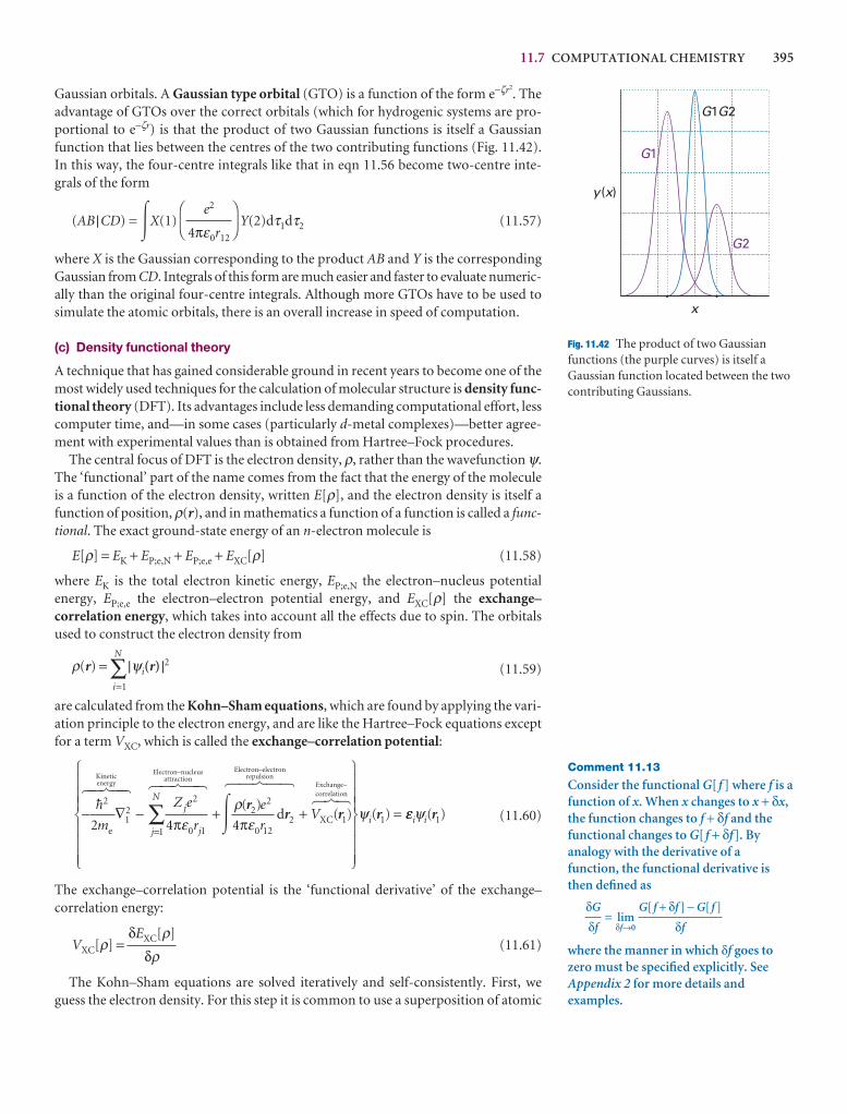
11.7 COMPUTATIONAL CHEMISTRY 395
Gaussian orbitals. A Gaussian type orbital (GTO) is a function of the form e−ζr2. The
advantage of GTOs over the correct orbitals (which for hydrogenic systems are pro-portional to e−ζr) is that the product of two Gaussian functions is itself a Gaussianfunction that lies between the centres of the two contributing functions (Fig. 11.42).In this way, the four-centre integrals like that in eqn 11.56 become two-centre inte-grals of the form
(AB |CD) = �X(1) Y(2)dτ1dτ2 (11.57)
where X is the Gaussian corresponding to the product AB and Y is the correspondingGaussian from CD. Integrals of this form are much easier and faster to evaluate numeric-ally than the original four-centre integrals. Although more GTOs have to be used tosimulate the atomic orbitals, there is an overall increase in speed of computation.
(c) Density functional theory
A technique that has gained considerable ground in recent years to become one of themost widely used techniques for the calculation of molecular structure is density func-tional theory (DFT). Its advantages include less demanding computational effort, lesscomputer time, and—in some cases (particularly d-metal complexes)—better agree-ment with experimental values than is obtained from Hartree–Fock procedures.
The central focus of DFT is the electron density, ρ, rather than the wavefunction ψ.The ‘functional’ part of the name comes from the fact that the energy of the moleculeis a function of the electron density, written E[ρ], and the electron density is itself afunction of position, ρ(r), and in mathematics a function of a function is called a func-tional. The exact ground-state energy of an n-electron molecule is
E[ρ] = EK + EP;e,N + EP;e,e + EXC[ρ] (11.58)
where EK is the total electron kinetic energy, EP;e,N the electron–nucleus potential energy, EP;e,e the electron–electron potential energy, and EXC[ρ] the exchange–correlation energy, which takes into account all the effects due to spin. The orbitalsused to construct the electron density from
ρ(r) =N
∑i=1
|ψi(r) |2 (11.59)
are calculated from the Kohn–Sham equations, which are found by applying the vari-ation principle to the electron energy, and are like the Hartree–Fock equations exceptfor a term VXC, which is called the exchange–correlation potential:
(11.60)
The exchange–correlation potential is the ‘functional derivative’ of the exchange–correlation energy:
VXC[ρ] = (11.61)
The Kohn–Sham equations are solved iteratively and self-consistently. First, weguess the electron density. For this step it is common to use a superposition of atomic
δEXC[ρ]
δρ
− ∇ − + +
⎧
⎨
⎪⎪⎪
⎩
⎪⎪⎪
⎫
⎬
⎪⎪⎪
⎭
⎪⎪⎪
==∑$2
12
2
0 11
22
0 122 1 12 4 4m
Z e
r
e
rVj
jj
N
ie
XC
Kineticenergy
Electron–nucleusattraction
Electron–electronrepulsion
Exchange–correlation
d
6 74 84 6 74 84 6 74 84678
( )
( ) ( ) π πε
ρε
ψ� rr r r εε ψi i( )r1
DF
e2
4πε0r12
AC
G1
G2
G G1 23
y x( )
x
Fig. 11.42 The product of two Gaussianfunctions (the purple curves) is itself aGaussian function located between the twocontributing Gaussians.
Comment 11.13
Consider the functional G[ f ] where f is afunction of x. When x changes to x + δx,the function changes to f + δf and thefunctional changes to G[ f + δf]. Byanalogy with the derivative of afunction, the functional derivative isthen defined as
= limδf→0
where the manner in which δf goes tozero must be specified explicitly. SeeAppendix 2 for more details andexamples.
G[ f + δf ] − G[ f ]
δf
δG
δf
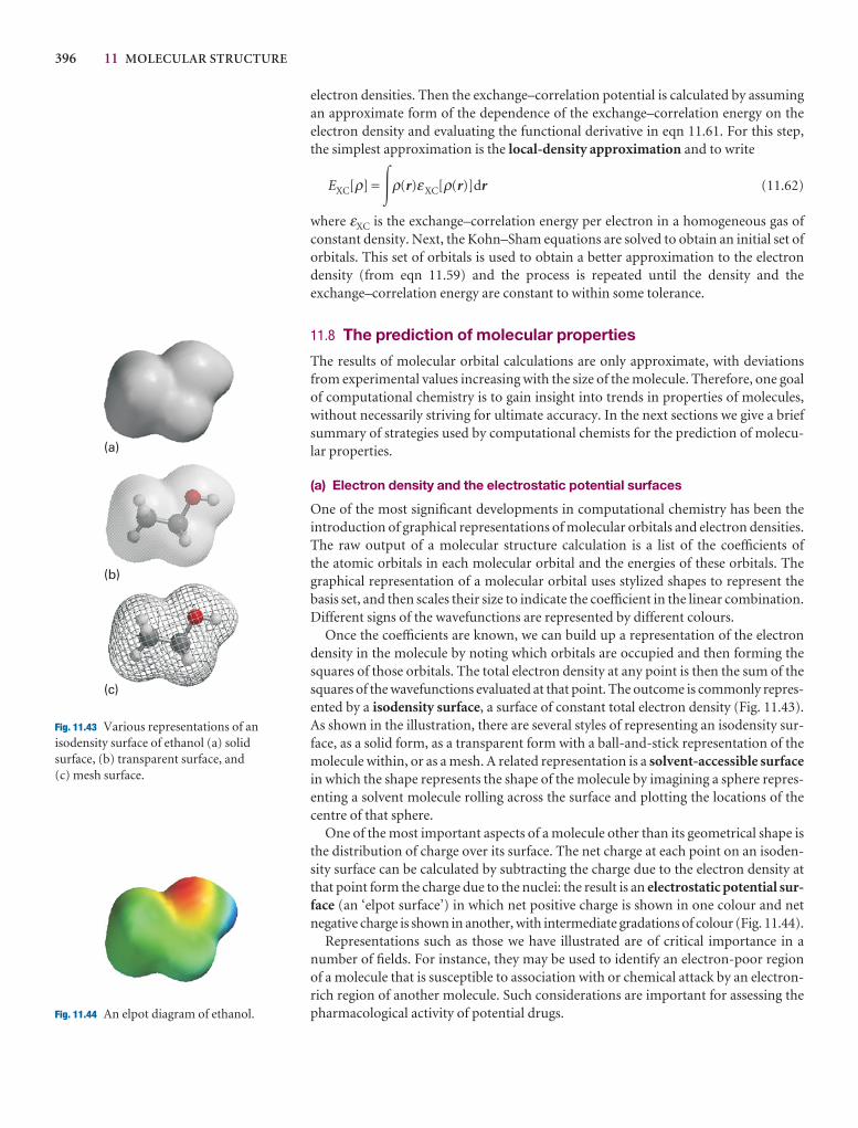
396 11 MOLECULAR STRUCTURE
electron densities. Then the exchange–correlation potential is calculated by assumingan approximate form of the dependence of the exchange–correlation energy on theelectron density and evaluating the functional derivative in eqn 11.61. For this step,the simplest approximation is the local-density approximation and to write
EXC[ρ] = �ρ(r)εXC[ρ(r)]dr (11.62)
where εXC is the exchange–correlation energy per electron in a homogeneous gas ofconstant density. Next, the Kohn–Sham equations are solved to obtain an initial set oforbitals. This set of orbitals is used to obtain a better approximation to the electrondensity (from eqn 11.59) and the process is repeated until the density and the exchange–correlation energy are constant to within some tolerance.
11.8 The prediction of molecular properties
The results of molecular orbital calculations are only approximate, with deviationsfrom experimental values increasing with the size of the molecule. Therefore, one goalof computational chemistry is to gain insight into trends in properties of molecules,without necessarily striving for ultimate accuracy. In the next sections we give a briefsummary of strategies used by computational chemists for the prediction of molecu-lar properties.
(a) Electron density and the electrostatic potential surfaces
One of the most significant developments in computational chemistry has been theintroduction of graphical representations of molecular orbitals and electron densities.The raw output of a molecular structure calculation is a list of the coefficients of the atomic orbitals in each molecular orbital and the energies of these orbitals. Thegraphical representation of a molecular orbital uses stylized shapes to represent thebasis set, and then scales their size to indicate the coefficient in the linear combination.Different signs of the wavefunctions are represented by different colours.
Once the coefficients are known, we can build up a representation of the electrondensity in the molecule by noting which orbitals are occupied and then forming thesquares of those orbitals. The total electron density at any point is then the sum of thesquares of the wavefunctions evaluated at that point. The outcome is commonly repres-ented by a isodensity surface, a surface of constant total electron density (Fig. 11.43).As shown in the illustration, there are several styles of representing an isodensity sur-face, as a solid form, as a transparent form with a ball-and-stick representation of themolecule within, or as a mesh. A related representation is a solvent-accessible surfacein which the shape represents the shape of the molecule by imagining a sphere repres-enting a solvent molecule rolling across the surface and plotting the locations of thecentre of that sphere.
One of the most important aspects of a molecule other than its geometrical shape isthe distribution of charge over its surface. The net charge at each point on an isoden-sity surface can be calculated by subtracting the charge due to the electron density atthat point form the charge due to the nuclei: the result is an electrostatic potential sur-face (an ‘elpot surface’) in which net positive charge is shown in one colour and netnegative charge is shown in another, with intermediate gradations of colour (Fig. 11.44).
Representations such as those we have illustrated are of critical importance in anumber of fields. For instance, they may be used to identify an electron-poor regionof a molecule that is susceptible to association with or chemical attack by an electron-rich region of another molecule. Such considerations are important for assessing thepharmacological activity of potential drugs.
(a)
(b)
(c)
Fig. 11.43 Various representations of anisodensity surface of ethanol (a) solidsurface, (b) transparent surface, and (c) mesh surface.
Fig. 11.44 An elpot diagram of ethanol.
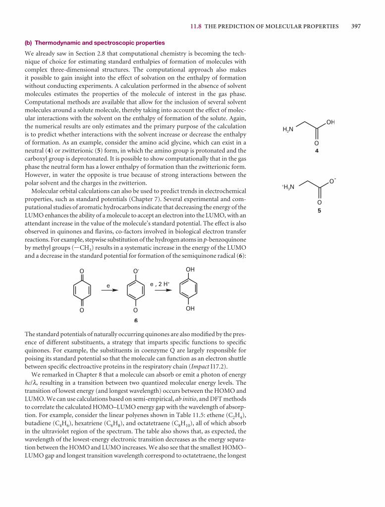
11.8 THE PREDICTION OF MOLECULAR PROPERTIES 397
(b) Thermodynamic and spectroscopic properties
We already saw in Section 2.8 that computational chemistry is becoming the tech-nique of choice for estimating standard enthalpies of formation of molecules withcomplex three-dimensional structures. The computational approach also makes it possible to gain insight into the effect of solvation on the enthalpy of formationwithout conducting experiments. A calculation performed in the absence of solventmolecules estimates the properties of the molecule of interest in the gas phase.Computational methods are available that allow for the inclusion of several solventmolecules around a solute molecule, thereby taking into account the effect of molec-ular interactions with the solvent on the enthalpy of formation of the solute. Again,the numerical results are only estimates and the primary purpose of the calculation is to predict whether interactions with the solvent increase or decrease the enthalpy of formation. As an example, consider the amino acid glycine, which can exist in aneutral (4) or zwitterionic (5) form, in which the amino group is protonated and thecarboxyl group is deprotonated. It is possible to show computationally that in the gasphase the neutral form has a lower enthalpy of formation than the zwitterionic form.However, in water the opposite is true because of strong interactions between thepolar solvent and the charges in the zwitterion.
Molecular orbital calculations can also be used to predict trends in electrochemicalproperties, such as standard potentials (Chapter 7). Several experimental and com-putational studies of aromatic hydrocarbons indicate that decreasing the energy of theLUMO enhances the ability of a molecule to accept an electron into the LUMO, with anattendant increase in the value of the molecule’s standard potential. The effect is alsoobserved in quinones and flavins, co-factors involved in biological electron transferreactions. For example, stepwise substitution of the hydrogen atoms in p-benzoquinoneby methyl groups (-CH3) results in a systematic increase in the energy of the LUMOand a decrease in the standard potential for formation of the semiquinone radical (6):
The standard potentials of naturally occurring quinones are also modified by the pres-ence of different substituents, a strategy that imparts specific functions to specificquinones. For example, the substituents in coenzyme Q are largely responsible forpoising its standard potential so that the molecule can function as an electron shuttlebetween specific electroactive proteins in the respiratory chain (Impact I17.2).
We remarked in Chapter 8 that a molecule can absorb or emit a photon of energyhc/λ, resulting in a transition between two quantized molecular energy levels. Thetransition of lowest energy (and longest wavelength) occurs between the HOMO andLUMO. We can use calculations based on semi-empirical, ab initio, and DFT methodsto correlate the calculated HOMO–LUMO energy gap with the wavelength of absorp-tion. For example, consider the linear polyenes shown in Table 11.5: ethene (C2H4),butadiene (C4H6), hexatriene (C6H8), and octatetraene (C8H10), all of which absorbin the ultraviolet region of the spectrum. The table also shows that, as expected, thewavelength of the lowest-energy electronic transition decreases as the energy separa-tion between the HOMO and LUMO increases. We also see that the smallest HOMO–LUMO gap and longest transition wavelength correspond to octatetraene, the longest
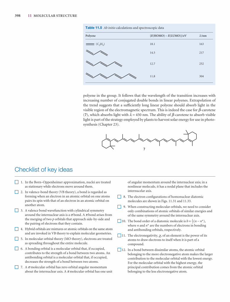
398 11 MOLECULAR STRUCTURE
polyene in the group. It follows that the wavelength of the transition increases withincreasing number of conjugated double bonds in linear polyenes. Extrapolation ofthe trend suggests that a sufficiently long linear polyene should absorb light in the visible region of the electromagnetic spectrum. This is indeed the case for β-carotene(7), which absorbs light with λ ≈ 450 nm. The ability of β-carotene to absorb visiblelight is part of the strategy employed by plants to harvest solar energy for use in photo-synthesis (Chapter 23).
Checklist of key ideas
1. In the Born–Oppenheimer approximation, nuclei are treatedas stationary while electrons move around them.
2. In valence-bond theory (VB theory), a bond is regarded asforming when an electron in an atomic orbital on one atomspairs its spin with that of an electron in an atomic orbital onanother atom.
3. A valence bond wavefunction with cylindrical symmetryaround the internuclear axis is a σ bond. A π bond arises fromthe merging of two p orbitals that approach side-by-side andthe pairing of electrons that they contain.
4. Hybrid orbitals are mixtures or atomic orbitals on the same atomand are invoked in VB theory to explain molecular geometries.
5. In molecular orbital theory (MO theory), electrons are treatedas spreading throughout the entire molecule.
6. A bonding orbital is a molecular orbital that, if occupied,contributes to the strength of a bond between two atoms. Anantibonding orbital is a molecular orbital that, if occupied,decreases the strength of a bond between two atoms.
7. A σ molecular orbital has zero orbital angular momentumabout the internuclear axis. A π molecular orbital has one unit
of angular momentum around the internuclear axis; in anonlinear molecule, it has a nodal plane that includes theinternucelar axis.
8. The electron configurations of homonuclear diatomicmolecules are shown in Figs. 11.31 and 11.33.
9. When constructing molecular orbitals, we need to consideronly combinations of atomic orbitals of similar energies andof the same symmetry around the internuclear axis.
10. The bond order of a diatomic molecule is b = 1–2(n − n*),where n and n* are the numbers of electrons in bonding and antibonding orbitals, respectively.
11. The electronegativity, χ, of an element is the power of itsatoms to draw electrons to itself when it is part of acompound.
12. In a bond between dissimilar atoms, the atomic orbitalbelonging to the more electronegative atom makes the largercontribution to the molecular orbital with the lowest energy.For the molecular orbital with the highest energy, theprincipal contribution comes from the atomic orbitalbelonging to the less electronegative atom.
Table 11.5 Ab initio calculations and spectroscopic data
Polyene {E(HOMO) − E(LUMO)}/eV λ /nm
(C2H4) 18.1 163
14.5 217
12.7 252
11.8 304

EXERCISES 399
13. The hamiltonian matrix, H, is formed of all integrals Hij = ∫ψ i*@ψjdτ. The overlap matrix, S, is formed of all Sij = ∫ψ i*ψjdτ.
14. The variation principle states that if an arbitrary wavefunctionis used to calculate the energy, the value calculated is neverless than the true energy.
15. In the Hückel method, all Coulomb integrals Hii are set equal(to α), all overlap integrals are set equal to zero, all resonanceintegrals Hij between non-neighbours are set equal to zero,and all remaining resonance integrals are set equal (to β).
16. The π-electron binding energy is the sum of the energies ofeach π electron. The π-bond formation energy is the energy
released when a π bond is formed. The delocalization energy isthe extra stabilization of a conjugated system.
17. In the self-consistent field procedure, an initial guess aboutthe composition of the molecular orbitals is successivelyrefined until the solution remains unchanged in a cycle ofcalculations.
18. In semi-empirical methods for the determination of electronicstructure, the Schrödinger equation is written in terms ofparameters chosen to agree with selected experimentalquantities. In ab initio and density functional methods, theSchrödinger equation is solved numerically, without the needof parameters that appeal to experimental data.
Further reading
Articles and texts
T.A. Albright and J.K. Burdett, Problems in molecular orbital theory.Oxford University Press (1992).
P.W. Atkins and R.S. Friedman, Molecular quantum mechanics.Oxford University Press (2005).
I.N. Levine, Quantum chemistry. Prentice–Hall, Upper Saddle River(2000).
D.A. McQuarrie, Mathematical methods for scientists and engineers.University Science Books, Mill Valley (2003).
R.C. Mebane, S.A. Schanley, T.R. Rybolt, and C.D. Bruce, Thecorrelation of physical properties of organic molecules withcomputed molecular surface areas. J. Chem. Educ. 76, 688 (1999).
L. Pauling, The nature of the chemical bond. Cornell University Press,Ithaca (1960).
C.M. Quinn, Computational quantum chemistry: an interactive guideto basis set theory. Academic Press, San Diego (2002).
Sources of data and information
D.R. Lide (ed.), CRC handbook of chemistry and physics, Section 9,CRC Press, Boca Raton (2000).
P.R. Scott and W.G. Richards, Energy levels in atoms and molecules.Oxford Chemistry Primers, Oxford University Press (1994).
Discussion questions
11.1 Compare the approximations built into valence-bond theory andmolecular-orbital theory.
11.2 Discuss the steps involved in the construction of sp3, sp2, and sp hybridorbitals.
11.3 Distinguish between the Pauling and Mulliken electronegativity scales.
11.4 Discuss the steps involved in the calculation of the energy of a system byusing the variation principle.
11.5 Discuss the approximations built into the Hückel method.
11.6 Distinguish between delocalization energy, π-electron binding energy,and π-bond formation energy.
11.7 Use concepts of molecular orbital theory to describe the biochemicalreactivity of O2, N2, and NO.
11.8 Distinguish between semi-empirical, ab initio, and density functionaltheory methods of electronic structure determination.
Exercises
11.1a Give the ground-state electron configurations and bond orders of (a) Li2, (b) Be2, and (c) C2.
11.1b Give the ground-state electron configurations of (a) H2−, (b) N2, and
(c) O2.
11.2a Give the ground-state electron configurations of (a) CO, (b) NO, and(c) CN−.
11.2b Give the ground-state electron configurations of (a) ClF, (b) CS, and(c) O2
−.
400 11 MOLECULAR STRUCTURE
11.3a From the ground-state electron configurations of B2 and C2, predictwhich molecule should have the greater bond dissociation energy.
11.3b Which of the molecules N2, NO, O2, C2, F2, and CN would you expectto be stabilized by (a) the addition of an electron to form AB−, (b) the removalof an electron to form AB+?
11.4a Sketch the molecular orbital energy level diagram for XeF and deduceits ground-state electron configurations. Is XeF likely to have a shorter bondlength than XeF+?
11.4b Sketch the molecular orbital energy level diagrams for BrCl and deduceits ground-state electron configurations. Is BrCl likely to have a shorter bondlength than BrCl−?
11.5a Use the electron configurations of NO and N2 to predict which is likelyto have the shorter bond length.
11.5b Arrange the species O2+, O2, O2
−, O22− in order of increasing bond length.
11.6a Show that the sp2 hybrid orbital (s + 21/2p)/31/2 is normalized to 1 if the sand p orbitals are normalized to 1.
11.6b Normalize the molecular orbital ψA + λψB in terms of the parameter λand the overlap integral S.
11.7a Confirm that the bonding and antibonding combinations ψA ± ψB aremutually orthogonal in the sense that their mutual overlap is zero.
11.7b Suppose that a molecular orbital has the form N(0.145A + 0.844B).Find a linear combination of the orbitals A and B that is orthogonal to thiscombination.
11.8a Can the function ψ = x(L − x) be used as a trial wavefunction for the n =1 state of a particle with mass m in a one-dimensional box of length L? If theanswer is yes, then express the energy of this trial wavefunction in terms of h,m, and L and compare it with the exact result (eqn 9.4). If the answer is no,explain why this is not a suitable trial wavefunction.
11.8b Can the function ψ = x2(L − 2x) be used as a trial wavefunction for then = 1 state of a particle with mass m in a one-dimensional box of length L? Ifthe answer is yes, then express the energy of this trial wavefunction in terms ofh, m, and L and compare it with the exact result (eqn 9.4). If the answer is no,explain why this is not a suitable trial wavefunction.
11.9a Suppose that the function ψ = Ae−ar2, with A being the normalization
constant and a being an adjustable parameter, is used as a trial wavefunctionfor the 1s orbital of the hydrogen atom. Express the energy of this trial
wavefunction as a function of the h, a, e, the electron charge, and µ, theeffective mass of the H atom.
11.9b Suppose that the function ψ = Ae−ar2, with A being the normalization
constant and a being an adjustable parameter, is used as a trial wavefunctionfor the 1s orbital of the hydrogen atom. The energy of this trial wavefunction is
E = −1/2
where e is the electron charge, and µ is the effective mass of the H atom. Whatis the minimum energy associated with this trial wavefunction?
11.10a What is the energy of an electron that has been ejected from an orbitalof ionization energy 11.0 eV by a photon of radiation of wavelength 100 nm?
11.10b What is the energy of an electron that has been ejected from an orbitalof ionization energy 4.69 eV by a photon of radiation of wavelength 584 pm?
11.11a Construct the molecular orbital energy level diagrams of ethene onthe basis that the molecule is formed from the appropriately hybridized CH2
or CH fragments.
11.11b Construct the molecular orbital energy level diagrams of ethyne(acetylene) on the basis that the molecule is formed from the appropriatelyhybridized CH2 or CH fragments.
11.12a Write down the secular determinants for (a) linear H3, (b) cyclic H3
within the Hückel approximation.
11.12b Predict the electronic configurations of (a) the benzene anion, (b) the benzene cation. Estimate the π-electron binding energy in each case.
11.13a Write down the secular determinants (a) anthracene (8),(b) phenanthrene (9) within the Hückel approximation and using the C2porbitals as the basis set.
11.13b Use mathematical software to estimate the π-electron binding energyof (a) anthracene (7), (b) phenanthrene (8) within the Hückel approximation.
DEFa
2π3
ABCe2
ε0
3a$2
2µ
Problems*
Numerical problems
11.1 Show that, if a wave cos kx centred on A (so that x is measured from A)interferes with a similar wave cos k′x centred on B (with x measured from B) a distance R away, then constructive interference occurs in the intermediateregion when k = k′ = π/2R and destructive interference if kR = 1–
2π and k′R = 3–2π.
11.2 The overlap integral between two H1s orbitals on nuclei separated by adistance R is S = {1 + (R /a0) + 1–
3 (R /a0)2}e−R/a0. Plot this function for 0 ≤ R < ∞.
11.3 Before doing the calculation below, sketch how the overlap between a 1sorbital and a 2p orbital can be expected to depend on their separation. Theoverlap integral between an H1s orbital and an H2p orbital on nuclei
separated by a distance R and forming a σ orbital is S = (R /a0){1 + (R /a0) +1–3 (R/a0)2}e−R/a0. Plot this function, and find the separation for which theoverlap is a maximum.
11.4 Calculate the total amplitude of the normalized bonding andantibonding LCAO-MOs that may be formed from two H1s orbitals at aseparation of 106 pm. Plot the two amplitudes for positions along themolecular axis both inside and outside the internuclear region.
11.5 Repeat the calculation in Problem 11.4 but plot the probability densitiesof the two orbitals. Then form the difference density, the difference betweenψ2 and 1–
2 {ψA2 + ψB
2}.
* Problems denoted with the symbol ‡ were supplied by Charles Trapp, Carmen Giunta, and Marshall Cady.
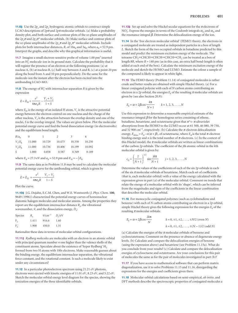
PROBLEMS 401
11.6‡ Use the 2px and 2pz hydrogenic atomic orbitals to construct simpleLCAO descriptions of 2pσ and 2pπ molecular orbitals. (a) Make a probabilitydensity plot, and both surface and contour plots of the xz-plane amplitudes ofthe 2pzσ and 2pzσ* molecular orbitals. (b) Make surface and contour plots ofthe xz-plane amplitudes of the 2pxπ and 2pxπ* molecular orbitals. Includeplots for both internuclear distances, R, of 10a0 and 3a0, where a0 = 52.9 pm.Interpret the graphs, and describe why this graphical information is useful.
11.7 Imagine a small electron-sensitive probe of volume 1.00 pm3 insertedinto an H2
+ molecule-ion in its ground state. Calculate the probability that itwill register the presence of an electron at the following positions: (a) atnucleus A, (b) at nucleus B, (c) half-way between A and B, (c) at a point 20 pmalong the bond from A and 10 pm perpendicularly. Do the same for themolecule-ion the instant after the electron has been excited into theantibonding LCAO-MO.
11.8 The energy of H2+ with internuclear separation R is given by the
expression
E = EH + −
where EH is the energy of an isolated H atom, V1 is the attractive potentialenergy between the electron centred on one nucleus and the charge of theother nucleus, V2 is the attraction between the overlap density and one of thenuclei, S is the overlap integral. The values are given below. Plot the molecularpotential energy curve and find the bond dissociation energy (in electronvolts)and the equilibrium bond length.
R/a0 0 1 2 3 4
V1/Eh 11.000 10.729 10.473 10.330 10.250
V2/Eh 11.000 10.736 10.406 10.199 10.092
S 1.000 0.858 0.587 0.349 0.189
where Eh = 27.3 eV and a0 = 52.9 pm and EH = − 1–2 Eh.
11.9 The same data as in Problem 11.8 may be used to calculate the molecularpotential energy curve for the antibonding orbital, which is given by
E = EH + −
Plot the curve.
11.10‡ J.G. Dojahn, E.C.M. Chen, and W.E. Wentworth (J. Phys. Chem. 100,9649 (1996)) characterized the potential energy curves of homonucleardiatomic halogen molecules and molecular anions. Among the properties theyreport are the equilibrium internuclear distance Re, the vibrationalwavenumber, #, and the dissociation energy, De:
Species Re #/cm−1 De /eV
F2 1.411 916.6 1.60
F2− 1.900 450.0 1.31
Rationalize these data in terms of molecular orbital configurations.
11.11‡ Rydberg molecules are molecules with an electron in an atomic orbitalwith principal quantum number n one higher than the valence shells of theconstituent atoms. Speculate about the existence of ‘hyper Rydberg’ H2
formed from two H atoms with 100s electrons. Make reasonable guesses aboutthe binding energy, the equilibrium internuclear separation, the vibrationalforce constant, and the rotational constant. Is such a molecule likely to existunder any circumstances?
11.12 In a particular photoelectron spectrum using 21.21 eV photons,electrons were ejected with kinetic energies of 11.01 eV, 8.23 eV, and 5.22 eV.Sketch the molecular orbital energy level diagram for the species, showing theionization energies of the three identifiable orbitals.
V1 − V2
1 − Se2
4πε0R
V1 + V2
1 + Se2
4πε0R
11.13‡ Set up and solve the Hückel secular equations for the π electrons ofNO3
−. Express the energies in terms of the Coulomb integrals αO and αN andthe resonance integral β. Determine the delocalization energy of the ion.
11.14 In the ‘free electron molecular orbital’ (FEMO) theory, the electrons ina conjugated molecule are treated as independent particles in a box of lengthL. Sketch the form of the two occupied orbitals in butadiene predicted by thismodel and predict the minimum excitation energy of the molecule. Thetetraene CH2=CHCH=CHCH=CHCH=CH2 can be treated as a box oflength 8R, where R ≈ 140 pm (as in this case, an extra half bond-length is oftenadded at each end of the box). Calculate the minimum excitation energy of themolecule and sketch the HOMO and LUMO. Estimate the colour a sample ofthe compound is likely to appear in white light.
11.15 The FEMO theory (Problem 11.14) of conjugated molecules is rathercrude and better results are obtained with simple Hückel theory. (a) For alinear conjugated polyene with each of N carbon atoms contributing anelectron in a 2p orbital, the energies Ek of the resulting π molecular orbitals aregiven by (see also Section 20.9):
Ek = α + 2βcos k = 1, 2, 3, . . . , N
Use this expression to determine a reasonable empirical estimate of theresonance integral β for the homologous series consisting of ethene,butadiene, hexatriene, and octatetraene given that π*←π ultravioletabsorptions from the HOMO to the LUMO occur at 61 500, 46 080, 39 750,and 32 900 cm−1, respectively. (b) Calculate the π-electron delocalizationenergy, Edeloc = Eπ −n(α + β), of octatetraene, where Eπ is the total π-electronbinding energy and n is the total number of π-electrons. (c) In the context ofthis Hückel model, the π molecular orbitals are written as linear combinationsof the carbon 2p orbitals. The coefficient of the jth atomic orbital in the kthmolecular orbital is given by:
ckj = 1/2
sin j = 1, 2, 3, . . . , N
Determine the values of the coefficients of each of the six 2p orbitals in each of the six π molecular orbitals of hexatriene. Match each set of coefficients(that is, each molecular orbital) with a value of the energy calculated with theexpression given in part (a) of the molecular orbital. Comment on trends thatrelate the energy of a molecular orbital with its ‘shape’, which can be inferredfrom the magnitudes and signs of the coefficients in the linear combinationthat describes the molecular orbital.
11.16 For monocyclic conjugated polyenes (such as cyclobutadiene andbenzene) with each of N carbon atoms contributing an electron in a 2p orbital,simple Hückel theory gives the following expression for the energies Ek of theresulting π molecular orbitals:
Ek = α + 2βcos k = 0, ±1, ±2, . . . , ±N/2 (even N)
k = 0, ±1, ±2, . . . , ±(N − 1)/2 (odd N)
(a) Calculate the energies of the π molecular orbitals of benzene andcyclooctatetraene. Comment on the presence or absence of degenerate energylevels. (b) Calculate and compare the delocalization energies of benzene(using the expression above) and hexatriene (see Problem 11.15a). What doyou conclude from your results? (c) Calculate and compare the delocalizationenergies of cyclooctaene and octatetraene. Are your conclusions for this pairof molecules the same as for the pair of molecules investigated in part (b)?
11.17 If you have access to mathematical software that can perform matrixdiagonalization, use it to solve Problems 11.15 and 11.16, disregarding theexpressions for the energies and coefficients given there.
11.18 Molecular orbital calculations based on semi-empirical, ab initio, andDFT methods describe the spectroscopic properties of conjugated molecules a
2kπN
jkπN + 1
DEF2
N + 1
ABC
kπN + 1
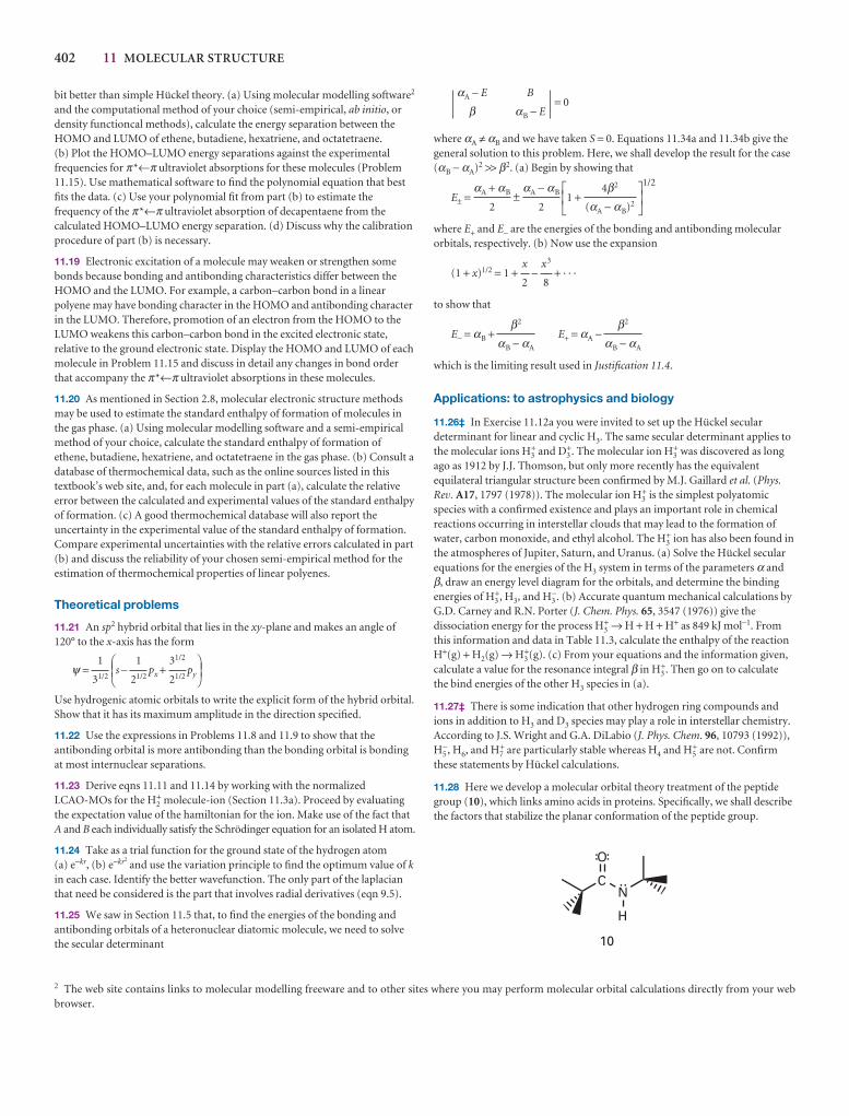
402 11 MOLECULAR STRUCTURE
bit better than simple Hückel theory. (a) Using molecular modelling software2
and the computational method of your choice (semi-empirical, ab initio, ordensity functioncal methods), calculate the energy separation between theHOMO and LUMO of ethene, butadiene, hexatriene, and octatetraene. (b) Plot the HOMO–LUMO energy separations against the experimentalfrequencies for π*←π ultraviolet absorptions for these molecules (Problem11.15). Use mathematical software to find the polynomial equation that bestfits the data. (c) Use your polynomial fit from part (b) to estimate thefrequency of the π*←π ultraviolet absorption of decapentaene from thecalculated HOMO–LUMO energy separation. (d) Discuss why the calibrationprocedure of part (b) is necessary.
11.19 Electronic excitation of a molecule may weaken or strengthen somebonds because bonding and antibonding characteristics differ between theHOMO and the LUMO. For example, a carbon–carbon bond in a linearpolyene may have bonding character in the HOMO and antibonding characterin the LUMO. Therefore, promotion of an electron from the HOMO to theLUMO weakens this carbon–carbon bond in the excited electronic state,relative to the ground electronic state. Display the HOMO and LUMO of eachmolecule in Problem 11.15 and discuss in detail any changes in bond orderthat accompany the π*←π ultraviolet absorptions in these molecules.
11.20 As mentioned in Section 2.8, molecular electronic structure methodsmay be used to estimate the standard enthalpy of formation of molecules inthe gas phase. (a) Using molecular modelling software and a semi-empiricalmethod of your choice, calculate the standard enthalpy of formation ofethene, butadiene, hexatriene, and octatetraene in the gas phase. (b) Consult adatabase of thermochemical data, such as the online sources listed in thistextbook’s web site, and, for each molecule in part (a), calculate the relativeerror between the calculated and experimental values of the standard enthalpyof formation. (c) A good thermochemical database will also report theuncertainty in the experimental value of the standard enthalpy of formation.Compare experimental uncertainties with the relative errors calculated in part(b) and discuss the reliability of your chosen semi-empirical method for theestimation of thermochemical properties of linear polyenes.
Theoretical problems
11.21 An sp2 hybrid orbital that lies in the xy-plane and makes an angle of120° to the x-axis has the form
ψ = s − px + py
Use hydrogenic atomic orbitals to write the explicit form of the hybrid orbital.Show that it has its maximum amplitude in the direction specified.
11.22 Use the expressions in Problems 11.8 and 11.9 to show that theantibonding orbital is more antibonding than the bonding orbital is bondingat most internuclear separations.
11.23 Derive eqns 11.11 and 11.14 by working with the normalized LCAO-MOs for the H2
+ molecule-ion (Section 11.3a). Proceed by evaluatingthe expectation value of the hamiltonian for the ion. Make use of the fact thatA and B each individually satisfy the Schrödinger equation for an isolated H atom.
11.24 Take as a trial function for the ground state of the hydrogen atom (a) e−kr, (b) e−kr2
and use the variation principle to find the optimum value of kin each case. Identify the better wavefunction. The only part of the laplacianthat need be considered is the part that involves radial derivatives (eqn 9.5).
11.25 We saw in Section 11.5 that, to find the energies of the bonding andantibonding orbitals of a heteronuclear diatomic molecule, we need to solvethe secular determinant
DEF31/2
21/2
1
21/2
ABC1
31/2
2 The web site contains links to molecular modelling freeware and to other sites where you may perform molecular orbital calculations directly from your webbrowser.
= 0
where αA ≠ αB and we have taken S = 0. Equations 11.34a and 11.34b give thegeneral solution to this problem. Here, we shall develop the result for the case(αB − αA)2 >> β2. (a) Begin by showing that
E± = ± 1 + 1/2
where E+ and E− are the energies of the bonding and antibonding molecularorbitals, respectively. (b) Now use the expansion
(1 + x)1/2 = 1 + − + · · ·
to show that
E− = αB + E+ = αA −
which is the limiting result used in Justification 11.4.
Applications: to astrophysics and biology
11.26‡ In Exercise 11.12a you were invited to set up the Hückel seculardeterminant for linear and cyclic H3. The same secular determinant applies tothe molecular ions H3
+ and D3+. The molecular ion H3
+ was discovered as longago as 1912 by J.J. Thomson, but only more recently has the equivalentequilateral triangular structure been confirmed by M.J. Gaillard et al. (Phys.Rev. A17, 1797 (1978)). The molecular ion H3
+ is the simplest polyatomicspecies with a confirmed existence and plays an important role in chemicalreactions occurring in interstellar clouds that may lead to the formation ofwater, carbon monoxide, and ethyl alcohol. The H3
+ ion has also been found inthe atmospheres of Jupiter, Saturn, and Uranus. (a) Solve the Hückel secularequations for the energies of the H3 system in terms of the parameters α andβ, draw an energy level diagram for the orbitals, and determine the bindingenergies of H3
+, H3, and H3−. (b) Accurate quantum mechanical calculations by
G.D. Carney and R.N. Porter (J. Chem. Phys. 65, 3547 (1976)) give thedissociation energy for the process H3
+ → H + H + H+ as 849 kJ mol−1. Fromthis information and data in Table 11.3, calculate the enthalpy of the reactionH+(g) + H2(g) → H3
+(g). (c) From your equations and the information given,calculate a value for the resonance integral β in H3
+. Then go on to calculatethe bind energies of the other H3 species in (a).
11.27‡ There is some indication that other hydrogen ring compounds andions in addition to H3 and D3 species may play a role in interstellar chemistry.According to J.S. Wright and G.A. DiLabio (J. Phys. Chem. 96, 10793 (1992)),H5
−, H6, and H7+ are particularly stable whereas H4 and H5
+ are not. Confirmthese statements by Hückel calculations.
11.28 Here we develop a molecular orbital theory treatment of the peptidegroup (10), which links amino acids in proteins. Specifically, we shall describethe factors that stabilize the planar conformation of the peptide group.
β2
αB − αA
β2
αB − αA
x3
8
x
2
JKL4β2
(αA − αB)2
GHIαA − αB
2
αA + αB
2
B
αB − E
αA − E
β
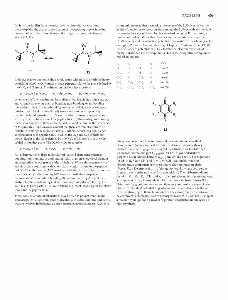
PROBLEMS 403
(a) It will be familiar from introductory chemistry that valence bond theory explains the planar conformation of the peptide group by invokingdelocalization of the π bond between the oxygen, carbon, and nitrogen atoms (11, 11):
It follows that we can model the peptide group with molecular orbital theoryby making LCAO-MOs from 2p orbitals perpendicular to the plane defined bythe O, C, and N atoms. The three combinations have the form:
ψ1 = aψO + bψC + cψN ψ2 = dψO − eψN ψ3 = fψO − gψC + hψN
where the coefficients a through h are all positive. Sketch the orbitals ψ1, ψ2,and ψ3 and characterize them as bonding, non-bonding, or antibondingmolecular orbitals. In a non-bonding molecular orbital, a pair of electronsresides in an orbital confined largely to one atom and not appreciablyinvolved in bond formation. (b) Show that this treatment is consistent onlywith a planar conformation of the peptide link. (c) Draw a diagram showingthe relative energies of these molecular orbitals and determine the occupancyof the orbitals. Hint. Convince yourself that there are four electrons to bedistributed among the molecular orbitals. (d) Now consider a non-planarconformation of the peptide link, in which the O2p and C2p orbitals areperpendicular to the plane defined by the O, C, and N atoms, but the N2porbital lies on that plane. The LCAO-MOs are given by
ψ4 = aψO + bψC ψ5 = eψN ψ6 = fψO − gψC
Just as before, sketch these molecular orbitals and characterize them asbonding, non-bonding, or antibonding. Also, draw an energy level diagramand determine the occupancy of the orbitals. (e) Why is this arrangement ofatomic orbitals consistent with a non-planar conformation for the peptidelink? (f) Does the bonding MO associated with the planar conformation havethe same energy as the bonding MO associated with the non-planarconformation? If not, which bonding MO is lower in energy? Repeat theanalysis for the non-bonding and anti-bonding molecular orbitals. (g) Useyour results from parts (a)–(f) to construct arguments that support the planarmodel for the peptide link.
11.29 Molecular orbital calculations may be used to predict trends in thestandard potentials of conjugated molecules, such as the quinones and flavins,that are involved in biological electron transfer reactions (Impact I17.2). It is
commonly assumed that decreasing the energy of the LUMO enhances theability of a molecule to accept an electron into the LUMO, with an attendantincrease in the value of the molecule’s standard potential. Furthermore, anumber of studies indicate that there is a linear correlation between theLUMO energy and the reduction potential of aromatic hydrocarbons (see, forexample, J.P. Lowe, Quantum chemistry, Chapter 8, Academic Press (1993)).(a) The standard potentials at pH = 7 for the one-electron reduction ofmethyl-substituted 1,4-benzoquinones (13) to their respective semiquinoneradical anions are:
R2 R3 R5 R6 E 7/V
H H H H 0.078
CH3 H H H 0.023
CH3 H CH3 H −0.067
CH3 CH3 CH3 H −0.165
CH3 CH3 CH3 CH3 −0.260
Using molecular modelling software and the computational method of your choice (semi-empirical, ab initio, or density functional theorymethods), calculate ELUMO, the energy of the LUMO of each substituted1,4-benzoquinone, and plot ELUMO against E 7. Do your calculations support a linear relation between ELUMO and E 7? (b) The 1,4-benzoquinonefor which R2 = R3 = CH3 and R5 = R6 = OCH3 is a suitable model ofubiquinone, a component of the respiratory electron transport chain (Impact I7.2). Determine ELUMO of this quinone and then use your results from part (a) to estimate its standard potential. (c) The 1,4-benzoquinone for which R2 = R3 = R5 = CH3 and R6 = H is a suitable model of plastoquinone,a component of the photosynthetic electron transport chain (Impact I7.2).Determine ELUMO of this quinone and then use your results from part (a) toestimate its standard potential. Is plastoquinone expected to be a better orworse oxidizing agent than ubiquinone? (d) Based on your predictions and onbasic concepts of biological electron transport (Impact I7.2 and I23.2), suggesta reason why ubiquinone is used in respiration and plastoquinone is used inphotosynthesis.
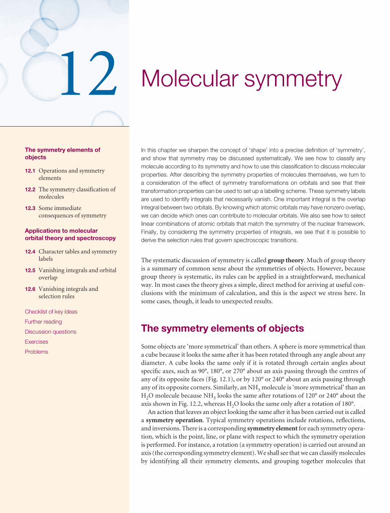
Molecular symmetry
In this chapter we sharpen the concept of ‘shape’ into a precise definition of ‘symmetry’,and show that symmetry may be discussed systematically. We see how to classify anymolecule according to its symmetry and how to use this classification to discuss molecularproperties. After describing the symmetry properties of molecules themselves, we turn to a consideration of the effect of symmetry transformations on orbitals and see that theirtransformation properties can be used to set up a labelling scheme. These symmetry labelsare used to identify integrals that necessarily vanish. One important integral is the overlap integral between two orbitals. By knowing which atomic orbitals may have nonzero overlap,we can decide which ones can contribute to molecular orbitals. We also see how to selectlinear combinations of atomic orbitals that match the symmetry of the nuclear framework.Finally, by considering the symmetry properties of integrals, we see that it is possible to derive the selection rules that govern spectroscopic transitions.
The systematic discussion of symmetry is called group theory. Much of group theoryis a summary of common sense about the symmetries of objects. However, becausegroup theory is systematic, its rules can be applied in a straightforward, mechanicalway. In most cases the theory gives a simple, direct method for arriving at useful con-clusions with the minimum of calculation, and this is the aspect we stress here. Insome cases, though, it leads to unexpected results.
The symmetry elements of objects
Some objects are ‘more symmetrical’ than others. A sphere is more symmetrical thana cube because it looks the same after it has been rotated through any angle about anydiameter. A cube looks the same only if it is rotated through certain angles aboutspecific axes, such as 90°, 180°, or 270° about an axis passing through the centres ofany of its opposite faces (Fig. 12.1), or by 120° or 240° about an axis passing throughany of its opposite corners. Similarly, an NH3 molecule is ‘more symmetrical’ than anH2O molecule because NH3 looks the same after rotations of 120° or 240° about theaxis shown in Fig. 12.2, whereas H2O looks the same only after a rotation of 180°.
An action that leaves an object looking the same after it has been carried out is calleda symmetry operation. Typical symmetry operations include rotations, reflections,and inversions. There is a corresponding symmetry element for each symmetry opera-tion, which is the point, line, or plane with respect to which the symmetry operationis performed. For instance, a rotation (a symmetry operation) is carried out around anaxis (the corresponding symmetry element). We shall see that we can classify moleculesby identifying all their symmetry elements, and grouping together molecules that
The symmetry elements ofobjects
12.1 Operations and symmetryelements
12.2 The symmetry classification ofmolecules
12.3 Some immediateconsequences of symmetry
Applications to molecularorbital theory and spectroscopy
12.4 Character tables and symmetrylabels
12.5 Vanishing integrals and orbitaloverlap
12.6 Vanishing integrals andselection rules
Checklist of key ideas
Further reading
Discussion questions
Exercises
Problems
12
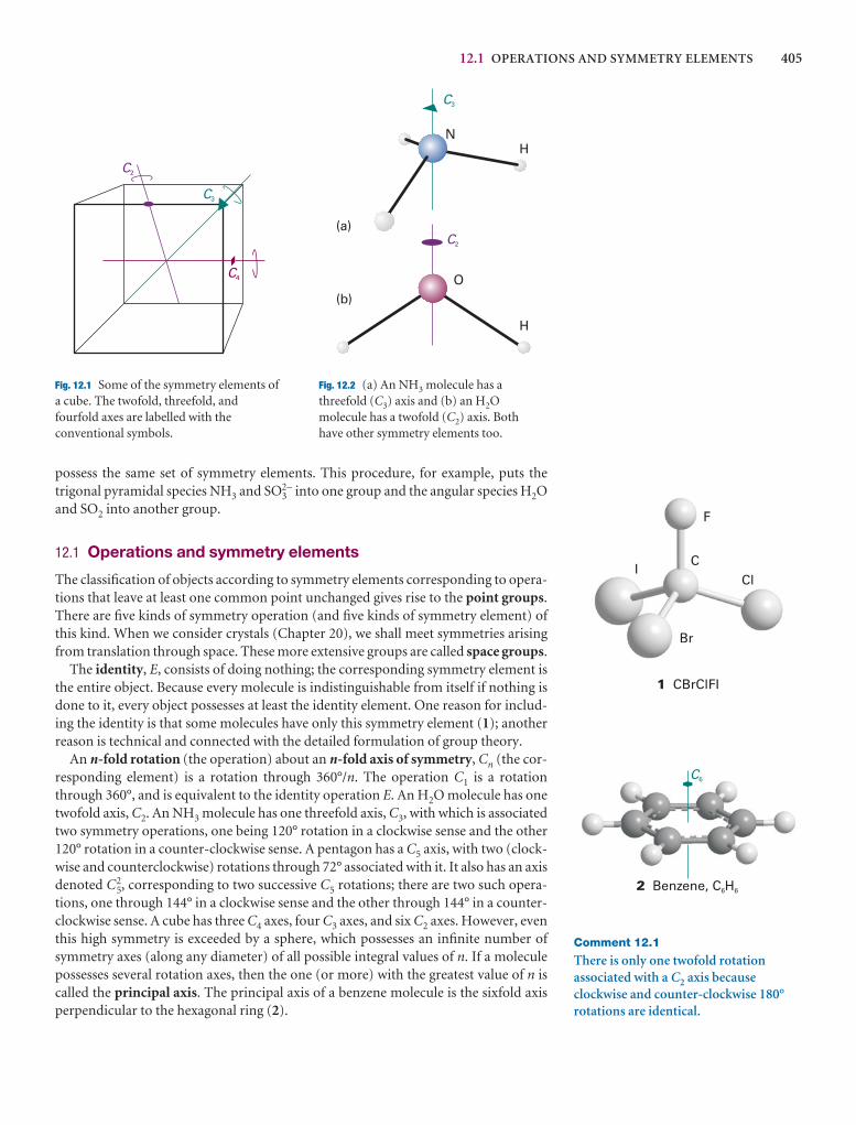
12.1 OPERATIONS AND SYMMETRY ELEMENTS 405
possess the same set of symmetry elements. This procedure, for example, puts the trigonal pyramidal species NH3 and SO3
2− into one group and the angular species H2Oand SO2 into another group.
12.1 Operations and symmetry elements
The classification of objects according to symmetry elements corresponding to opera-tions that leave at least one common point unchanged gives rise to the point groups.There are five kinds of symmetry operation (and five kinds of symmetry element) ofthis kind. When we consider crystals (Chapter 20), we shall meet symmetries arisingfrom translation through space. These more extensive groups are called space groups.
The identity, E, consists of doing nothing; the corresponding symmetry element isthe entire object. Because every molecule is indistinguishable from itself if nothing isdone to it, every object possesses at least the identity element. One reason for includ-ing the identity is that some molecules have only this symmetry element (1); anotherreason is technical and connected with the detailed formulation of group theory.
An n-fold rotation (the operation) about an n-fold axis of symmetry, Cn (the cor-responding element) is a rotation through 360°/n. The operation C1 is a rotationthrough 360°, and is equivalent to the identity operation E. An H2O molecule has onetwofold axis, C2. An NH3 molecule has one threefold axis, C3, with which is associatedtwo symmetry operations, one being 120° rotation in a clockwise sense and the other120° rotation in a counter-clockwise sense. A pentagon has a C5 axis, with two (clock-wise and counterclockwise) rotations through 72° associated with it. It also has an axisdenoted C5
2, corresponding to two successive C5 rotations; there are two such opera-tions, one through 144° in a clockwise sense and the other through 144° in a counter-clockwise sense. A cube has three C4 axes, four C3 axes, and six C2 axes. However, eventhis high symmetry is exceeded by a sphere, which possesses an infinite number ofsymmetry axes (along any diameter) of all possible integral values of n. If a moleculepossesses several rotation axes, then the one (or more) with the greatest value of n iscalled the principal axis. The principal axis of a benzene molecule is the sixfold axisperpendicular to the hexagonal ring (2).
C2
C3
C4
Fig. 12.1 Some of the symmetry elements ofa cube. The twofold, threefold, andfourfold axes are labelled with theconventional symbols.
C2
C3
NH
O
H
(a)
(b)
Fig. 12.2 (a) An NH3 molecule has athreefold (C3) axis and (b) an H2Omolecule has a twofold (C2) axis. Both have other symmetry elements too.
F
Cl
Br
IC
1 CBrClFI
C6
2 Benzene, C H6 6
Comment 12.1
There is only one twofold rotationassociated with a C2 axis becauseclockwise and counter-clockwise 180°rotations are identical.
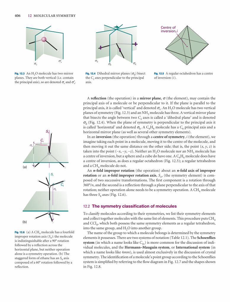
406 12 MOLECULAR SYMMETRY
A reflection (the operation) in a mirror plane, σ (the element), may contain theprincipal axis of a molecule or be perpendicular to it. If the plane is parallel to theprincipal axis, it is called ‘vertical’ and denoted σv. An H2O molecule has two verticalplanes of symmetry (Fig. 12.3) and an NH3 molecule has three. A vertical mirror planethat bisects the angle between two C2 axes is called a ‘dihedral plane’ and is denoted σd (Fig. 12.4). When the plane of symmetry is perpendicular to the principal axis it is called ‘horizontal’ and denoted σh. A C6H6 molecule has a C6 principal axis and ahorizontal mirror plane (as well as several other symmetry elements).
In an inversion (the operation) through a centre of symmetry, i (the element), weimagine taking each point in a molecule, moving it to the centre of the molecule, andthen moving it out the same distance on the other side; that is, the point (x, y, z) istaken into the point (−x, −y, −z). Neither an H2O molecule nor an NH3 molecule hasa centre of inversion, but a sphere and a cube do have one. A C6H6 molecule does havea centre of inversion, as does a regular octahedron (Fig. 12.5); a regular tetrahedronand a CH4 molecule do not.
An n-fold improper rotation (the operation) about an n-fold axis of improperrotation or an n-fold improper rotation axis, Sn, (the symmetry element) is com-posed of two successive transformations. The first component is a rotation through360°/n, and the second is a reflection through a plane perpendicular to the axis of thatrotation; neither operation alone needs to be a symmetry operation. A CH4 moleculehas three S4 axes (Fig. 12.6).
12.2 The symmetry classification of molecules
To classify molecules according to their symmetries, we list their symmetry elementsand collect together molecules with the same list of elements. This procedure puts CH4
and CCl4, which both possess the same symmetry elements as a regular tetrahedron,into the same group, and H2O into another group.
The name of the group to which a molecule belongs is determined by the symmetryelements it possesses. There are two systems of notation (Table 12.1). The Schoenfliessystem (in which a name looks like C4v) is more common for the discussion of indi-vidual molecules, and the Hermann–Mauguin system, or International system (inwhich a name looks like 4mm), is used almost exclusively in the discussion of crystalsymmetry. The identification of a molecule’s point group according to the Schoenfliessystem is simplified by referring to the flow diagram in Fig. 12.7 and the shapes shownin Fig. 12.8.
vv́
s
s
d
dd
s
s
s
Fig. 12.3 An H2O molecule has two mirrorplanes. They are both vertical (i.e. containthe principal axis), so are denoted σv and σv′ .
Fig. 12.4 Dihedral mirror planes (σd) bisectthe C2 axes perpendicular to the principalaxis.
Centre ofinversion,i
Fig. 12.5 A regular octahedron has a centreof inversion (i).
h
h
C4
S4
C6
S6
(a)
(b)
s
s
Fig. 12.6 (a) A CH4 molecule has a fourfoldimproper rotation axis (S4): the molecule is indistinguishable after a 90° rotationfollowed by a reflection across thehorizontal plane, but neither operationalone is a symmetry operation. (b) Thestaggered form of ethane has an S6 axiscomposed of a 60° rotation followed by areflection.
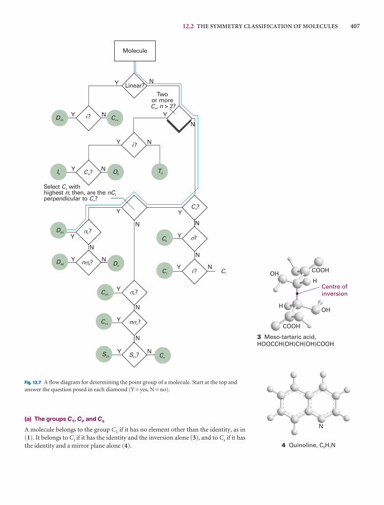
12.2 THE SYMMETRY CLASSIFICATION OF MOLECULES 407
Cnv
S2n
Molecule
Linear?Y N
i?Y N Y
N
Twoor more
, > 2?C nn
Y Ni?
C 5?Y NIh
Td
YY
Y
N
?Cs
Nh?
Y
N
n d?Dnd Dn
Y N
h?Y
N
N
Cnh
Y n v?
S2n?Y N
Cn
N
Y Ni?C i
Select withhighest ; then, are theperpendicular to ?
Cn nC
C
n
n
2
Dnh
Cn?
D¥h C
¥v
Oh
C1
s
s
s
s
s
Fig. 12.7 A flow diagram for determining the point group of a molecule. Start at the top andanswer the question posed in each diamond (Y = yes, N = no).
(a) The groups C1, Ci, and Cs
A molecule belongs to the group C1 if it has no element other than the identity, as in(1). It belongs to Ci if it has the identity and the inversion alone (3), and to Cs if it hasthe identity and a mirror plane alone (4).
COOHOHH
COOH
HOH
Centre ofinversion
3 Meso-tartaric acid,HOOCCH(OH)CH(OH)COOH
N
4 Quinoline, C H N9 7
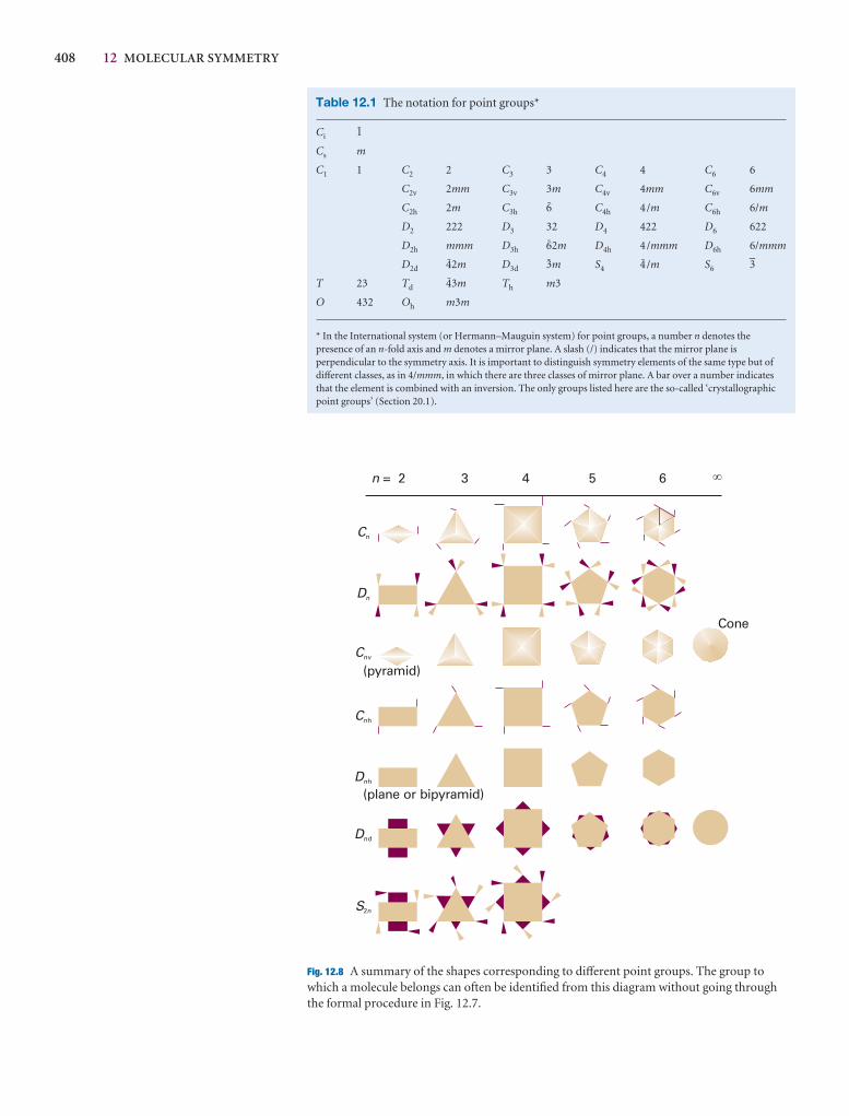
408 12 MOLECULAR SYMMETRY
Cone
2 3 4 5 6 ¥
Cn
Dn
Cnv
Dnh
Dnd
Cnh
S2n
(plane or bipyramid)
(pyramid)
n =
Fig. 12.8 A summary of the shapes corresponding to different point groups. The group towhich a molecule belongs can often be identified from this diagram without going throughthe formal procedure in Fig. 12.7.
Table 12.1 The notation for point groups*
Ci ⁄
Cs m
C1 1 C2 2 C3 3 C4 4 C6 6
C2v 2mm C3v 3m C4v 4mm C6v 6mm
C2h 2m C3h fl C4h 4/m C6h 6/m
D2 222 D3 32 D4 422 D6 622
D2h mmm D3h fl2m D4h 4/mmm D6h 6/mmm
D2d ›2m D3d ‹m S4 › /m S6 3–
T 23 Td ›3m Th m3
O 432 Oh m3m
* In the International system (or Hermann–Mauguin system) for point groups, a number n denotes thepresence of an n-fold axis and m denotes a mirror plane. A slash (/) indicates that the mirror plane isperpendicular to the symmetry axis. It is important to distinguish symmetry elements of the same type but ofdifferent classes, as in 4/mmm, in which there are three classes of mirror plane. A bar over a number indicatesthat the element is combined with an inversion. The only groups listed here are the so-called ‘crystallographicpoint groups’ (Section 20.1).
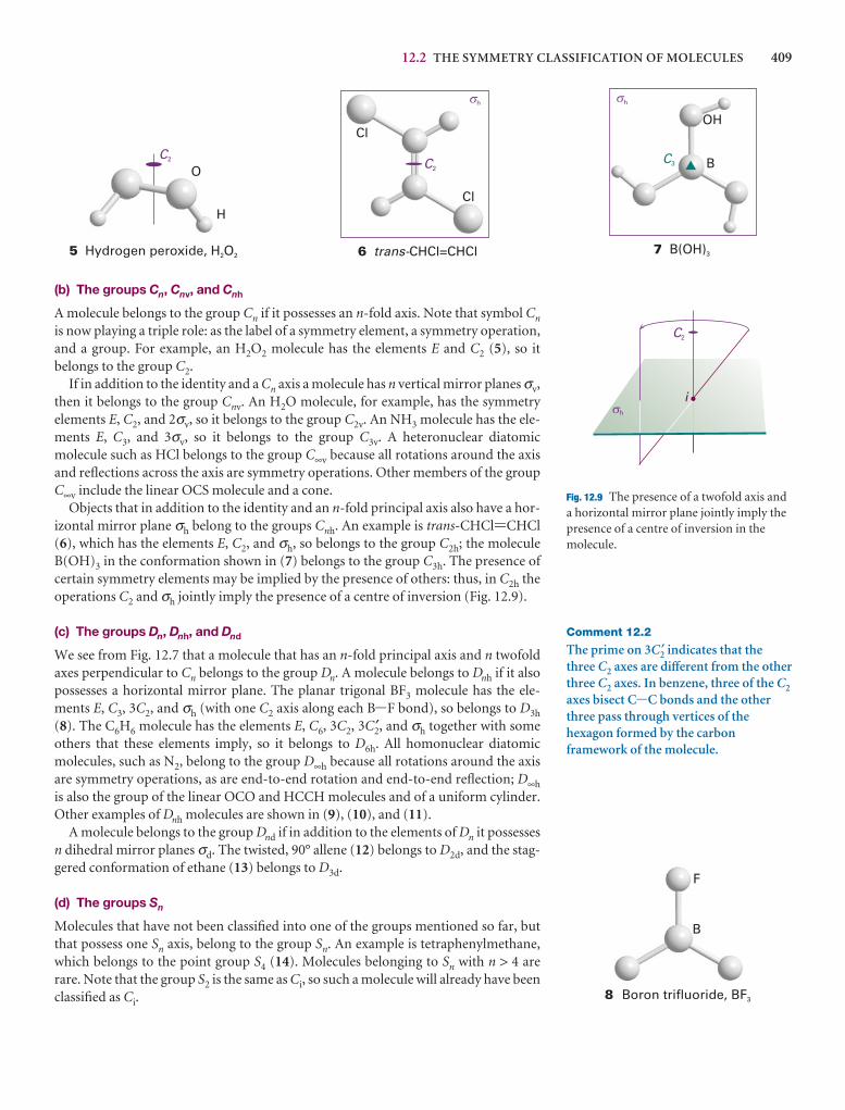
12.2 THE SYMMETRY CLASSIFICATION OF MOLECULES 409
(b) The groups Cn, Cnv, and Cnh
A molecule belongs to the group Cn if it possesses an n-fold axis. Note that symbol Cn
is now playing a triple role: as the label of a symmetry element, a symmetry operation,and a group. For example, an H2O2 molecule has the elements E and C2 (5), so it belongs to the group C2.
If in addition to the identity and a Cn axis a molecule has n vertical mirror planes σv,then it belongs to the group Cnv. An H2O molecule, for example, has the symmetryelements E, C2, and 2σv, so it belongs to the group C2v. An NH3 molecule has the ele-ments E, C3, and 3σv, so it belongs to the group C3v. A heteronuclear diatomicmolecule such as HCl belongs to the group C∞v because all rotations around the axisand reflections across the axis are symmetry operations. Other members of the groupC∞v include the linear OCS molecule and a cone.
Objects that in addition to the identity and an n-fold principal axis also have a hor-izontal mirror plane σh belong to the groups Cnh. An example is trans-CHCl=CHCl(6), which has the elements E, C2, and σh, so belongs to the group C2h; the moleculeB(OH)3 in the conformation shown in (7) belongs to the group C3h. The presence ofcertain symmetry elements may be implied by the presence of others: thus, in C2h theoperations C2 and σh jointly imply the presence of a centre of inversion (Fig. 12.9).
(c) The groups Dn, Dnh, and Dnd
We see from Fig. 12.7 that a molecule that has an n-fold principal axis and n twofoldaxes perpendicular to Cn belongs to the group Dn. A molecule belongs to Dnh if it alsopossesses a horizontal mirror plane. The planar trigonal BF3 molecule has the ele-ments E, C3, 3C2, and σh (with one C2 axis along each B-F bond), so belongs to D3h
(8). The C6H6 molecule has the elements E, C6, 3C2, 3C2′, and σh together with someothers that these elements imply, so it belongs to D6h. All homonuclear diatomicmolecules, such as N2, belong to the group D∞h because all rotations around the axisare symmetry operations, as are end-to-end rotation and end-to-end reflection; D∞h
is also the group of the linear OCO and HCCH molecules and of a uniform cylinder.Other examples of Dnh molecules are shown in (9), (10), and (11).
A molecule belongs to the group Dnd if in addition to the elements of Dn it possessesn dihedral mirror planes σd. The twisted, 90° allene (12) belongs to D2d, and the stag-gered conformation of ethane (13) belongs to D3d.
(d) The groups Sn
Molecules that have not been classified into one of the groups mentioned so far, butthat possess one Sn axis, belong to the group Sn. An example is tetraphenylmethane,which belongs to the point group S4 (14). Molecules belonging to Sn with n > 4 arerare. Note that the group S2 is the same as Ci, so such a molecule will already have beenclassified as Ci.
O
H
C2
5 Hydrogen peroxide, H O2 2
h
C2
is
Fig. 12.9 The presence of a twofold axis anda horizontal mirror plane jointly imply thepresence of a centre of inversion in themolecule.
Cl
Cl
C2
6 CHCl=CHCltrans-
h$
B
OH
7 B(OH)3
C3
h$
B
F
8 Boron trifluoride, BF3
Comment 12.2
The prime on 3C2′ indicates that thethree C2 axes are different from the otherthree C2 axes. In benzene, three of the C2axes bisect C-C bonds and the otherthree pass through vertices of thehexagon formed by the carbonframework of the molecule.
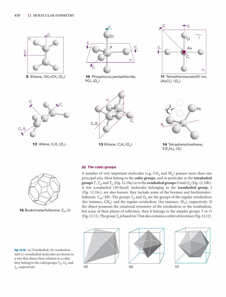
410 12 MOLECULAR SYMMETRY
(e) The cubic groups
A number of very important molecules (e.g. CH4 and SF6) possess more than oneprincipal axis. Most belong to the cubic groups, and in particular to the tetrahedralgroups T, Td, and Th (Fig. 12.10a) or to the octahedral groups O and Oh (Fig. 12.10b).A few icosahedral (20-faced) molecules belonging to the icosahedral group, I(Fig. 12.10c), are also known: they include some of the boranes and buckminster-fullerene, C60 (15). The groups Td and Oh are the groups of the regular tetrahedron(for instance, CH4) and the regular octahedron (for instance, SF6), respectively. If the object possesses the rotational symmetry of the tetrahedron or the octahedron,but none of their planes of reflection, then it belongs to the simpler groups T or O(Fig. 12.11). The group Th is based on T but also contains a centre of inversion (Fig. 12.12).
P
Cl
C3
C2
C2
C2
h
10 Phosphorus pentachloride,PCl ( )5 3hD
$
h
C4
C2
C2 C2
–Cl
Au
11 Tetrachloroaurate(III) ion,[AuCl ] ( )4 4h
� D
$
h
C2
C2
9 Ethene, CH =CH ( )2 2 2hD
$
C2C2
C S2 4,
12 Allene, C H ( )3 4 2dD
d
C2C S3 3,
13 Ethane, C H ( )2 6 3dD
$
S4
Ph
14 Tetraphenylmethane,C(C H ) ( )6 5 4 4S
(a) (b) (c)
15 Buckminsterfullerene, C ( )60 I
Fig. 12.10 (a) Tetrahedral, (b) octahedral,and (c) icosahedral molecules are drawn ina way that shows their relation to a cube:they belong to the cubicgroups Td, Oh, andIh, respectively.
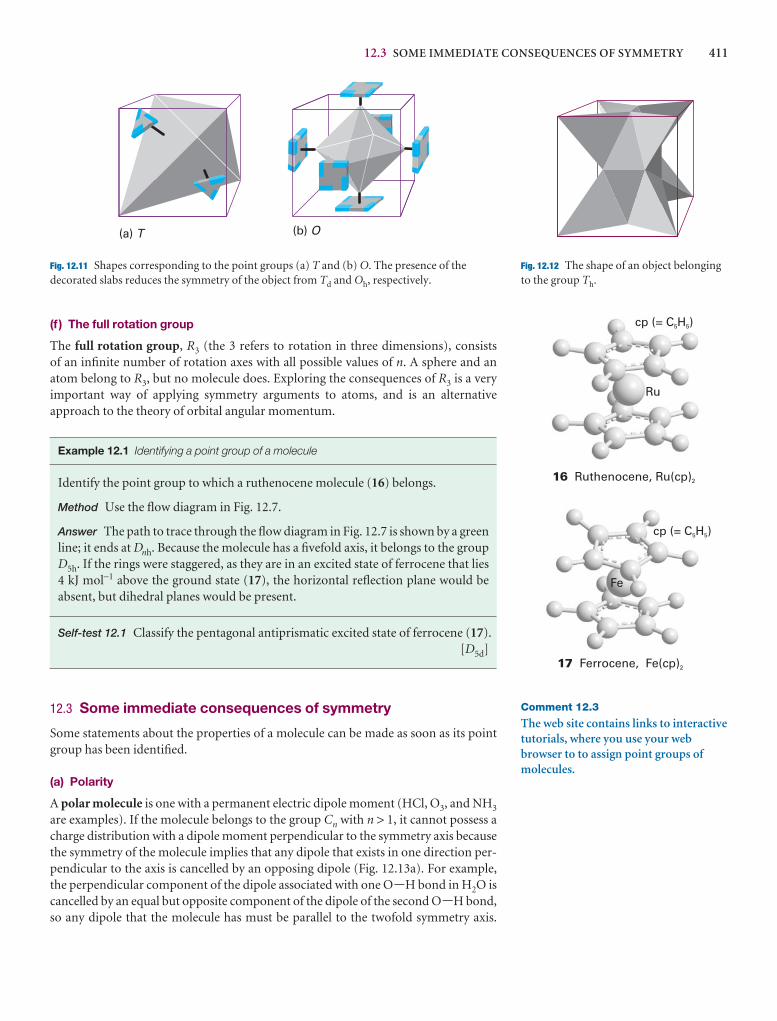
12.3 SOME IMMEDIATE CONSEQUENCES OF SYMMETRY 411
(a) T (b) O
Fig. 12.11 Shapes corresponding to the point groups (a) T and (b) O. The presence of thedecorated slabs reduces the symmetry of the object from Td and Oh, respectively.
Fig. 12.12 The shape of an object belongingto the group Th.
cp (= C H )5 5
Ru
16 Ruthenocene, Ru(cp)2
Comment 12.3
The web site contains links to interactivetutorials, where you use your webbrowser to to assign point groups ofmolecules.
cp (= C H )5 5
Fe
17 Ferrocene, Fe(cp)2
(f ) The full rotation group
The full rotation group, R3 (the 3 refers to rotation in three dimensions), consists of an infinite number of rotation axes with all possible values of n. A sphere and anatom belong to R3, but no molecule does. Exploring the consequences of R3 is a very important way of applying symmetry arguments to atoms, and is an alternative approach to the theory of orbital angular momentum.
Example 12.1 Identifying a point group of a molecule
Identify the point group to which a ruthenocene molecule (16) belongs.
Method Use the flow diagram in Fig. 12.7.
Answer The path to trace through the flow diagram in Fig. 12.7 is shown by a greenline; it ends at Dnh. Because the molecule has a fivefold axis, it belongs to the groupD5h. If the rings were staggered, as they are in an excited state of ferrocene that lies4 kJ mol−1 above the ground state (17), the horizontal reflection plane would beabsent, but dihedral planes would be present.
Self-test 12.1 Classify the pentagonal antiprismatic excited state of ferrocene (17).[D5d]
12.3 Some immediate consequences of symmetry
Some statements about the properties of a molecule can be made as soon as its pointgroup has been identified.
(a) Polarity
A polar molecule is one with a permanent electric dipole moment (HCl, O3, and NH3
are examples). If the molecule belongs to the group Cn with n > 1, it cannot possess acharge distribution with a dipole moment perpendicular to the symmetry axis becausethe symmetry of the molecule implies that any dipole that exists in one direction per-pendicular to the axis is cancelled by an opposing dipole (Fig. 12.13a). For example,the perpendicular component of the dipole associated with one O-H bond in H2O iscancelled by an equal but opposite component of the dipole of the second O-H bond,so any dipole that the molecule has must be parallel to the twofold symmetry axis.
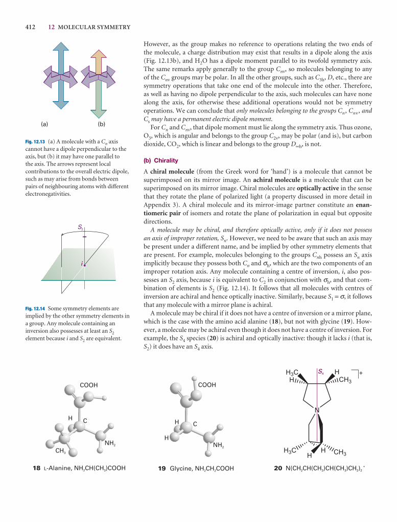
412 12 MOLECULAR SYMMETRY
However, as the group makes no reference to operations relating the two ends of the molecule, a charge distribution may exist that results in a dipole along the axis (Fig. 12.13b), and H2O has a dipole moment parallel to its twofold symmetry axis. The same remarks apply generally to the group Cnv, so molecules belonging to any of the Cnv groups may be polar. In all the other groups, such as C3h, D, etc., there are symmetry operations that take one end of the molecule into the other. Therefore, as well as having no dipole perpendicular to the axis, such molecules can have nonealong the axis, for otherwise these additional operations would not be symmetry operations. We can conclude that only molecules belonging to the groups Cn , Cnv , andCs may have a permanent electric dipole moment.
For Cn and Cnv, that dipole moment must lie along the symmetry axis. Thus ozone,O3, which is angular and belongs to the group C2v, may be polar (and is), but carbondioxide, CO2, which is linear and belongs to the group D∞h, is not.
(b) Chirality
A chiral molecule (from the Greek word for ‘hand’) is a molecule that cannot be superimposed on its mirror image. An achiral molecule is a molecule that can be superimposed on its mirror image. Chiral molecules are optically active in the sensethat they rotate the plane of polarized light (a property discussed in more detail inAppendix 3). A chiral molecule and its mirror-image partner constitute an enan-tiomeric pair of isomers and rotate the plane of polarization in equal but opposite directions.
A molecule may be chiral, and therefore optically active, only if it does not possess an axis of improper rotation, Sn. However, we need to be aware that such an axis maybe present under a different name, and be implied by other symmetry elements thatare present. For example, molecules belonging to the groups Cnh possess an Sn axisimplicitly because they possess both Cn and σh, which are the two components of an improper rotation axis. Any molecule containing a centre of inversion, i, also pos-sesses an S2 axis, because i is equivalent to C2 in conjunction with σh, and that com-bination of elements is S2 (Fig. 12.14). It follows that all molecules with centres of inversion are achiral and hence optically inactive. Similarly, because S1 = σ, it followsthat any molecule with a mirror plane is achiral.
A molecule may be chiral if it does not have a centre of inversion or a mirror plane,which is the case with the amino acid alanine (18), but not with glycine (19). How-ever, a molecule may be achiral even though it does not have a centre of inversion. Forexample, the S4 species (20) is achiral and optically inactive: though it lacks i (that is,S2) it does have an S4 axis.
(a) (b)
Fig. 12.13 (a) A molecule with a Cn axiscannot have a dipole perpendicular to theaxis, but (b) it may have one parallel to the axis. The arrows represent localcontributions to the overall electric dipole,such as may arise from bonds betweenpairs of neighbouring atoms with differentelectronegativities.
i
S2
Fig. 12.14 Some symmetry elements areimplied by the other symmetry elements ina group. Any molecule containing aninversion also possesses at least an S2
element because i and S2 are equivalent.
COOH
C
NH2
CH3
H
18 -Alanine, NH CH(CH )COOHL 2 3
NH2
C
COOH
H
H
19 Glycine, NH CH COOH2 2
H
N
HH3C
H
H CH3
CH3H3C
S4
20 N(CH CH(CH )CH(CH )CH )2 3 3 2 2
+
+
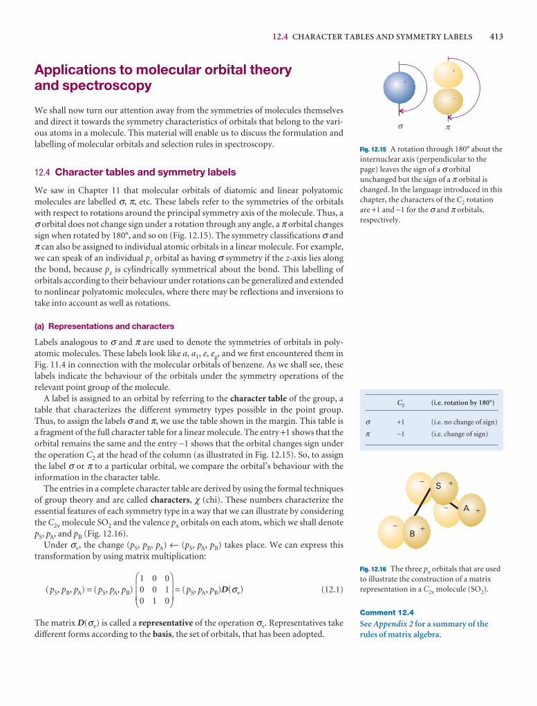
12.4 CHARACTER TABLES AND SYMMETRY LABELS 413
Applications to molecular orbital theory and spectroscopy
We shall now turn our attention away from the symmetries of molecules themselvesand direct it towards the symmetry characteristics of orbitals that belong to the vari-ous atoms in a molecule. This material will enable us to discuss the formulation andlabelling of molecular orbitals and selection rules in spectroscopy.
12.4 Character tables and symmetry labels
We saw in Chapter 11 that molecular orbitals of diatomic and linear polyatomicmolecules are labelled σ, π, etc. These labels refer to the symmetries of the orbitalswith respect to rotations around the principal symmetry axis of the molecule. Thus, aσ orbital does not change sign under a rotation through any angle, a π orbital changessign when rotated by 180°, and so on (Fig. 12.15). The symmetry classifications σ andπ can also be assigned to individual atomic orbitals in a linear molecule. For example,we can speak of an individual pz orbital as having σ symmetry if the z-axis lies alongthe bond, because pz is cylindrically symmetrical about the bond. This labelling of orbitals according to their behaviour under rotations can be generalized and extendedto nonlinear polyatomic molecules, where there may be reflections and inversions totake into account as well as rotations.
(a) Representations and characters
Labels analogous to σ and π are used to denote the symmetries of orbitals in poly-atomic molecules. These labels look like a, a1, e, eg, and we first encountered them inFig. 11.4 in connection with the molecular orbitals of benzene. As we shall see, theselabels indicate the behaviour of the orbitals under the symmetry operations of the relevant point group of the molecule.
A label is assigned to an orbital by referring to the character table of the group, atable that characterizes the different symmetry types possible in the point group.Thus, to assign the labels σ and π, we use the table shown in the margin. This table isa fragment of the full character table for a linear molecule. The entry +1 shows that theorbital remains the same and the entry −1 shows that the orbital changes sign underthe operation C2 at the head of the column (as illustrated in Fig. 12.15). So, to assignthe label σ or π to a particular orbital, we compare the orbital’s behaviour with theinformation in the character table.
The entries in a complete character table are derived by using the formal techniquesof group theory and are called characters, χ (chi). These numbers characterize the essential features of each symmetry type in a way that we can illustrate by consideringthe C2v molecule SO2 and the valence px orbitals on each atom, which we shall denotepS, pA, and pB (Fig. 12.16).
Under σv, the change (pS, pB, pA) ← (pS, pA, pB) takes place. We can express thistransformation by using matrix multiplication:
(pS, pB, pA) = (pS, pA, pB) = (pS, pA, pB)D(σv) (12.1)
The matrix D(σv) is called a representative of the operation σv. Representatives takedifferent forms according to the basis, the set of orbitals, that has been adopted.
1 0 00 0 10 1 0
⎛
⎝⎜⎜
⎞
⎠⎟⎟
s
p
+
+
-
Fig. 12.15 A rotation through 180° about theinternuclear axis (perpendicular to thepage) leaves the sign of a σ orbitalunchanged but the sign of a π orbital ischanged. In the language introduced in thischapter, the characters of the C2 rotationare +1 and −1 for the σ and π orbitals,respectively.
C2 (i.e. rotation by 180°)
σ +1 (i.e. no change of sign)
π −1 (i.e. change of sign)
Comment 12.4
See Appendix 2 for a summary of therules of matrix algebra.
�
�
�
B�
S �
A �
Fig. 12.16 The three px orbitals that are usedto illustrate the construction of a matrixrepresentation in a C2v molecule (SO2).
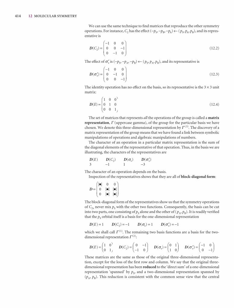
414 12 MOLECULAR SYMMETRY
We can use the same technique to find matrices that reproduce the other symmetryoperations. For instance, C2 has the effect (−pS, −pB, −pA) ← (pS, pA, pB), and its repres-entative is
D(C2) = (12.2)
The effect of σ ′v is (−pS, −pA, −pB) ← (pS, pA, pB), and its representative is
D(σ ′v) = (12.3)
The identity operation has no effect on the basis, so its representative is the 3 × 3 unitmatrix:
D(E) = (12.4)
The set of matrices that represents all the operations of the group is called a matrixrepresentation, Γ (uppercase gamma), of the group for the particular basis we havechosen. We denote this three-dimensional representation by Γ (3). The discovery of amatrix representation of the group means that we have found a link between symbolicmanipulations of operations and algebraic manipulations of numbers.
The character of an operation in a particular matrix representation is the sum of the diagonal elements of the representative of that operation. Thus, in the basis we areillustrating, the characters of the representatives are
D(E) D(C2) D(σv) D(σ ′v)3 −1 1 −3
The character of an operation depends on the basis.Inspection of the representatives shows that they are all of block-diagonal form:
D =
The block-diagonal form of the representatives show us that the symmetry operationsof C2v never mix pS with the other two functions. Consequently, the basis can be cutinto two parts, one consisting of pS alone and the other of (pA, pB). It is readily verifiedthat the pS orbital itself is a basis for the one-dimensional representation
D(E) = 1 D(C2) = −1 D(σv) = 1 D(σ ′v) = −1
which we shall call Γ (1). The remaining two basis functions are a basis for the two-dimensional representation Γ (2):
D(E) = D(C2) = D(σv) = D(σ v′) =
These matrices are the same as those of the original three-dimensional representa-tion, except for the loss of the first row and column. We say that the original three-dimensional representation has been reduced to the ‘direct sum’ of a one-dimensionalrepresentation ‘spanned’ by pS, and a two-dimensional representation spanned by(pA, pB). This reduction is consistent with the common sense view that the central
−−
⎛⎝⎜
⎞⎠⎟
1 00 1
0 11 0
⎛⎝⎜
⎞⎠⎟
0 11 0
−−
⎛⎝⎜
⎞⎠⎟
1 00 1
⎛⎝⎜
⎞⎠⎟
[ ][ ] [ ][ ] [ ]
n
n n
n n
0 000
⎛
⎝⎜⎜
⎞
⎠⎟⎟
1 0 00 1 00 0 1
⎛
⎝⎜⎜
⎞
⎠⎟⎟
−−
−
⎛
⎝⎜⎜
⎞
⎠⎟⎟
1 0 00 1 00 0 1
−−
−
⎛
⎝⎜⎜
⎞
⎠⎟⎟
1 0 00 0 10 1 0
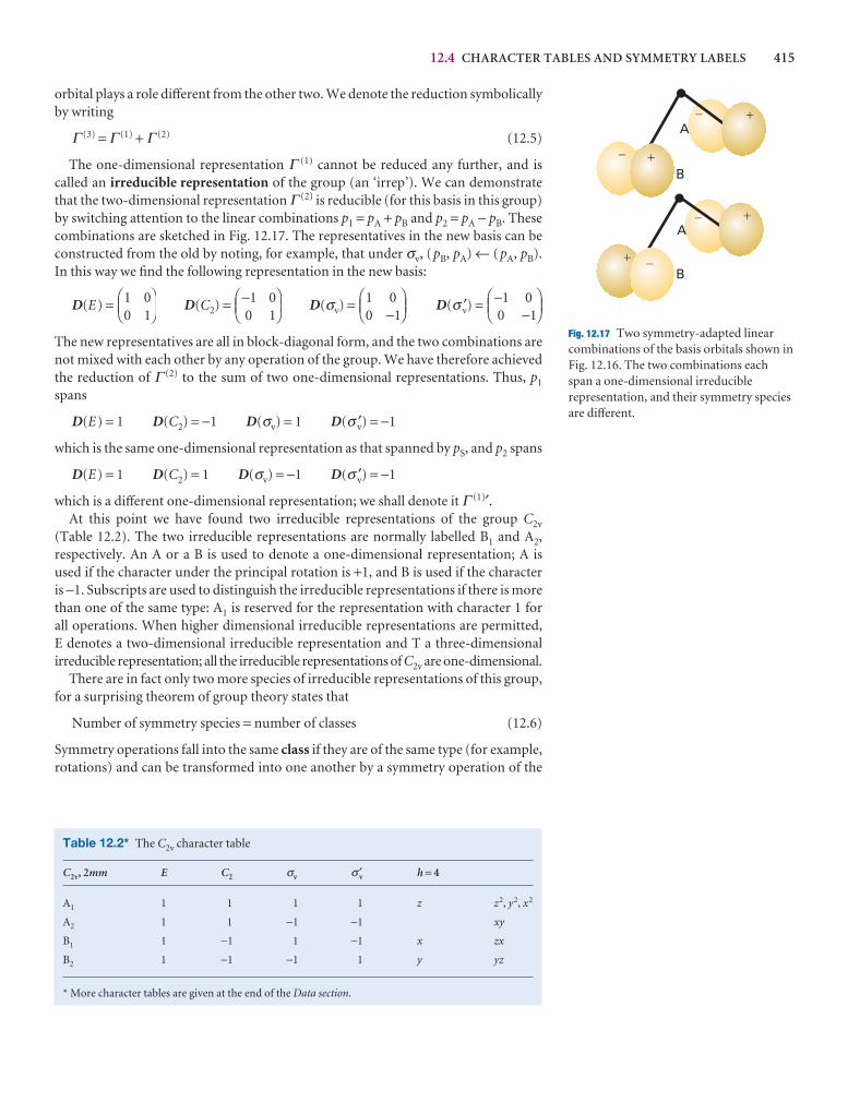
12.4 CHARACTER TABLES AND SYMMETRY LABELS 415
orbital plays a role different from the other two. We denote the reduction symbolicallyby writing
Γ (3) = Γ (1) + Γ (2) (12.5)
The one-dimensional representation Γ (1) cannot be reduced any further, and iscalled an irreducible representation of the group (an ‘irrep’). We can demonstratethat the two-dimensional representation Γ (2) is reducible (for this basis in this group)by switching attention to the linear combinations p1 = pA + pB and p2 = pA − pB. Thesecombinations are sketched in Fig. 12.17. The representatives in the new basis can beconstructed from the old by noting, for example, that under σv, (pB, pA) ← (pA, pB).In this way we find the following representation in the new basis:
D(E) = D(C2) = D(σv) = D(σ v′) =
The new representatives are all in block-diagonal form, and the two combinations arenot mixed with each other by any operation of the group. We have therefore achievedthe reduction of Γ (2) to the sum of two one-dimensional representations. Thus, p1
spans
D(E) = 1 D(C2) = −1 D(σv) = 1 D(σ v′) = −1
which is the same one-dimensional representation as that spanned by pS, and p2 spans
D(E) = 1 D(C2) = 1 D(σv) = −1 D(σ v′) = −1
which is a different one-dimensional representation; we shall denote it Γ (1)′.At this point we have found two irreducible representations of the group C2v
(Table 12.2). The two irreducible representations are normally labelled B1 and A2,respectively. An A or a B is used to denote a one-dimensional representation; A is used if the character under the principal rotation is +1, and B is used if the character is −1. Subscripts are used to distinguish the irreducible representations if there is morethan one of the same type: A1 is reserved for the representation with character 1 for all operations. When higher dimensional irreducible representations are permitted, E denotes a two-dimensional irreducible representation and T a three-dimensional irreducible representation; all the irreducible representations of C2v are one-dimensional.
There are in fact only two more species of irreducible representations of this group,for a surprising theorem of group theory states that
Number of symmetry species = number of classes (12.6)
Symmetry operations fall into the same class if they are of the same type (for example,rotations) and can be transformed into one another by a symmetry operation of the
−−
⎛⎝⎜
⎞⎠⎟
1 00 1
1 00 1−
⎛⎝⎜
⎞⎠⎟
−⎛⎝⎜
⎞⎠⎟
1 00 1
1 00 1
⎛⎝⎜
⎞⎠⎟
�
�
�
�
A�
B�
A�
B�
Fig. 12.17 Two symmetry-adapted linearcombinations of the basis orbitals shown inFig. 12.16. The two combinations eachspan a one-dimensional irreduciblerepresentation, and their symmetry speciesare different.
Table 12.2* The C2v character table
C2v, 2mm E C2 σv σ′v h = 4
A1 1 1 1 1 z z2, y2, x2
A2 1 1 −1 −1 xy
B1 1 −1 1 −1 x zx
B2 1 −1 −1 1 y yz
* More character tables are given at the end of the Data section.
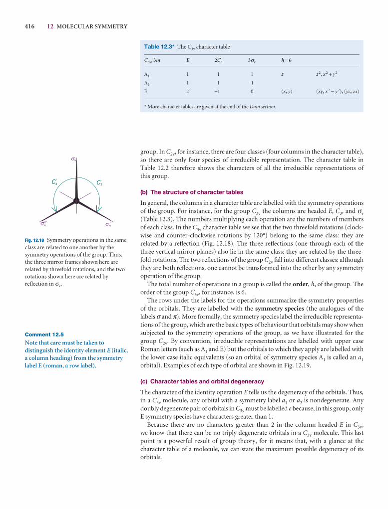
416 12 MOLECULAR SYMMETRY
group. In C2v, for instance, there are four classes (four columns in the character table),so there are only four species of irreducible representation. The character table inTable 12.2 therefore shows the characters of all the irreducible representations of this group.
(b) The structure of character tables
In general, the columns in a character table are labelled with the symmetry operationsof the group. For instance, for the group C3v the columns are headed E, C3, and σv
(Table 12.3). The numbers multiplying each operation are the numbers of membersof each class. In the C3v character table we see that the two threefold rotations (clock-wise and counter-clockwise rotations by 120°) belong to the same class: they are related by a reflection (Fig. 12.18). The three reflections (one through each of thethree vertical mirror planes) also lie in the same class: they are related by the three-fold rotations. The two reflections of the group C2v fall into different classes: althoughthey are both reflections, one cannot be transformed into the other by any symmetryoperation of the group.
The total number of operations in a group is called the order, h, of the group. Theorder of the group C3v, for instance, is 6.
The rows under the labels for the operations summarize the symmetry propertiesof the orbitals. They are labelled with the symmetry species (the analogues of the labels σ and π). More formally, the symmetry species label the irreducible representa-tions of the group, which are the basic types of behaviour that orbitals may show whensubjected to the symmetry operations of the group, as we have illustrated for thegroup C2v. By convention, irreducible representations are labelled with upper caseRoman letters (such as A1 and E) but the orbitals to which they apply are labelled withthe lower case italic equivalents (so an orbital of symmetry species A1 is called an a1
orbital). Examples of each type of orbital are shown in Fig. 12.19.
(c) Character tables and orbital degeneracy
The character of the identity operation E tells us the degeneracy of the orbitals. Thus,in a C3v molecule, any orbital with a symmetry label a1 or a2 is nondegenerate. Anydoubly degenerate pair of orbitals in C3v must be labelled e because, in this group, onlyE symmetry species have characters greater than 1.
Because there are no characters greater than 2 in the column headed E in C3v,we know that there can be no triply degenerate orbitals in a C3v molecule. This lastpoint is a powerful result of group theory, for it means that, with a glance at the character table of a molecule, we can state the maximum possible degeneracy of its orbitals.
Table 12.3* The C3v character table
C3v, 3m E 2C3 3σv h = 6
A1 1 1 1 z z 2, x 2 + y2
A2 1 1 −1
E 2 −1 0 (x, y) (xy, x 2 − y 2), (yz, zx)
* More character tables are given at the end of the Data section.
C3C3
v
v¢v²
s
s
s
+
-
Fig. 12.18 Symmetry operations in the sameclass are related to one another by thesymmetry operations of the group. Thus,the three mirror frames shown here arerelated by threefold rotations, and the tworotations shown here are related byreflection in σv.
Comment 12.5
Note that care must be taken todistinguish the identity element E (italic,a column heading) from the symmetrylabel E (roman, a row label).
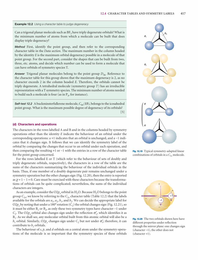
12.4 CHARACTER TABLES AND SYMMETRY LABELS 417
a1
a2
e
e
sN
Fig. 12.19 Typical symmetry-adapted linearcombinations of orbitals in a C3v molecule.
�
�
�
��1�1
�1
Fig. 12.20 The two orbitals shown here havedifferent properties under reflectionthrough the mirror plane: one changes sign(character −1), the other does not(character +1).
Example 12.2 Using a character table to judge degeneracy
Can a trigonal planar molecule such as BF3 have triply degenerate orbitals? What isthe minimum number of atoms from which a molecule can be built that does display triple degeneracy?
Method First, identify the point group, and then refer to the corresponding character table in the Data section. The maximum number in the column headedby the identity E is the maximum orbital degeneracy possible in a molecule of thatpoint group. For the second part, consider the shapes that can be built from two,three, etc. atoms, and decide which number can be used to form a molecule thatcan have orbitals of symmetry species T.
Answer Trigonal planar molecules belong to the point group D3h. Reference to the character table for this group shows that the maximum degeneracy is 2, as nocharacter exceeds 2 in the column headed E. Therefore, the orbitals cannot betriply degenerate. A tetrahedral molecule (symmetry group T) has an irreduciblerepresentation with a T symmetry species. The minimum number of atoms neededto build such a molecule is four (as in P4, for instance).
Self-test 12.2 A buckminsterfullerene molecule, C60 (15), belongs to the icosahedralpoint group. What is the maximum possible degree of degeneracy of its orbitals?
[5]
(d) Characters and operations
The characters in the rows labelled A and B and in the columns headed by symmetryoperations other than the identity E indicate the behaviour of an orbital under thecorresponding operations: a +1 indicates that an orbital is unchanged, and a −1 indi-cates that it changes sign. It follows that we can identify the symmetry label of the orbital by comparing the changes that occur to an orbital under each operation, andthen comparing the resulting +1 or −1 with the entries in a row of the character tablefor the point group concerned.
For the rows labelled E or T (which refer to the behaviour of sets of doubly andtriply degenerate orbitals, respectively), the characters in a row of the table are thesums of the characters summarizing the behaviour of the individual orbitals in thebasis. Thus, if one member of a doubly degenerate pair remains unchanged under asymmetry operation but the other changes sign (Fig. 12.20), then the entry is reportedas χ = 1 − 1 = 0. Care must be exercised with these characters because the transforma-tions of orbitals can be quite complicated; nevertheless, the sums of the individualcharacters are integers.
As an example, consider the O2px orbital in H2O. Because H2O belongs to the pointgroup C2v, we know by referring to the C2v character table (Table 12.2) that the labelsavailable for the orbitals are a1, a2, b1, and b2. We can decide the appropriate label forO2px by noting that under a 180° rotation (C2) the orbital changes sign (Fig. 12.21), soit must be either B1 or B2, as only these two symmetry types have character −1 underC2. The O2px orbital also changes sign under the reflection σ v′ , which identifies it asB1. As we shall see, any molecular orbital built from this atomic orbital will also be a b1 orbital. Similarly, O2py changes sign under C2 but not under σv′; therefore, it cancontribute to b2 orbitals.
The behaviour of s, p, and d orbitals on a central atom under the symmetry opera-tions of the molecule is so important that the symmetry species of these orbitals
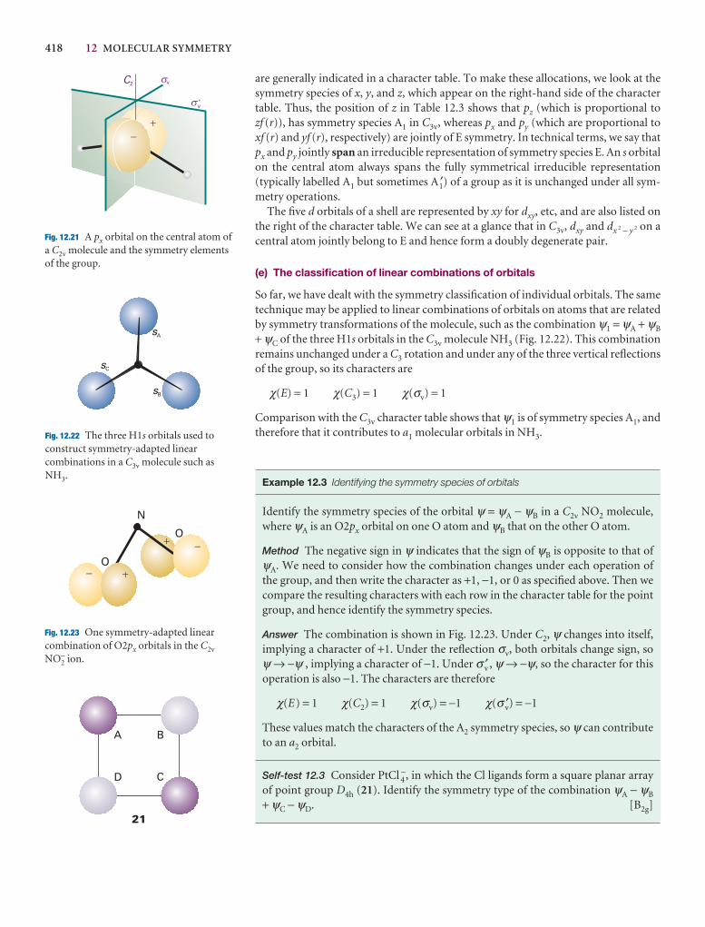
418 12 MOLECULAR SYMMETRY
v
v́
C2
+
-
s
s
Fig. 12.21 A px orbital on the central atom ofa C2v molecule and the symmetry elementsof the group.
sA
sB
sC
Fig. 12.22 The three H1s orbitals used toconstruct symmetry-adapted linearcombinations in a C3v molecule such asNH3.
N
�
�O
�
O�
Fig. 12.23 One symmetry-adapted linearcombination of O2px orbitals in the C2v
NO2− ion.
A B
CD
21
are generally indicated in a character table. To make these allocations, we look at the symmetry species of x, y, and z, which appear on the right-hand side of the charactertable. Thus, the position of z in Table 12.3 shows that pz (which is proportional tozf (r)), has symmetry species A1 in C3v, whereas px and py (which are proportional toxf (r) and yf (r), respectively) are jointly of E symmetry. In technical terms, we say thatpx and py jointly span an irreducible representation of symmetry species E. An s orbitalon the central atom always spans the fully symmetrical irreducible representation(typically labelled A1 but sometimes A1′) of a group as it is unchanged under all sym-metry operations.
The five d orbitals of a shell are represented by xy for dxy, etc, and are also listed onthe right of the character table. We can see at a glance that in C3v, dxy and dx 2 − y 2 on acentral atom jointly belong to E and hence form a doubly degenerate pair.
(e) The classification of linear combinations of orbitals
So far, we have dealt with the symmetry classification of individual orbitals. The sametechnique may be applied to linear combinations of orbitals on atoms that are relatedby symmetry transformations of the molecule, such as the combination ψ1 = ψA + ψB
+ ψC of the three H1s orbitals in the C3v molecule NH3 (Fig. 12.22). This combinationremains unchanged under a C3 rotation and under any of the three vertical reflectionsof the group, so its characters are
χ(E) = 1 χ(C3) = 1 χ(σv) = 1
Comparison with the C3v character table shows that ψ1 is of symmetry species A1, andtherefore that it contributes to a1 molecular orbitals in NH3.
Example 12.3 Identifying the symmetry species of orbitals
Identify the symmetry species of the orbital ψ = ψA − ψB in a C2v NO2 molecule,where ψA is an O2px orbital on one O atom and ψB that on the other O atom.
Method The negative sign in ψ indicates that the sign of ψB is opposite to that ofψA. We need to consider how the combination changes under each operation ofthe group, and then write the character as +1, −1, or 0 as specified above. Then wecompare the resulting characters with each row in the character table for the pointgroup, and hence identify the symmetry species.
Answer The combination is shown in Fig. 12.23. Under C2, ψ changes into itself,implying a character of +1. Under the reflection σv, both orbitals change sign, so ψ → −ψ , implying a character of −1. Under σ v′ , ψ → −ψ, so the character for thisoperation is also −1. The characters are therefore
χ(E) = 1 χ(C2) = 1 χ(σv) = −1 χ(σ v′) = −1
These values match the characters of the A2 symmetry species, so ψ can contributeto an a2 orbital.
Self-test 12.3 Consider PtCl 4−, in which the Cl ligands form a square planar array
of point group D4h (21). Identify the symmetry type of the combination ψA − ψB
+ ψC − ψD. [B2g]
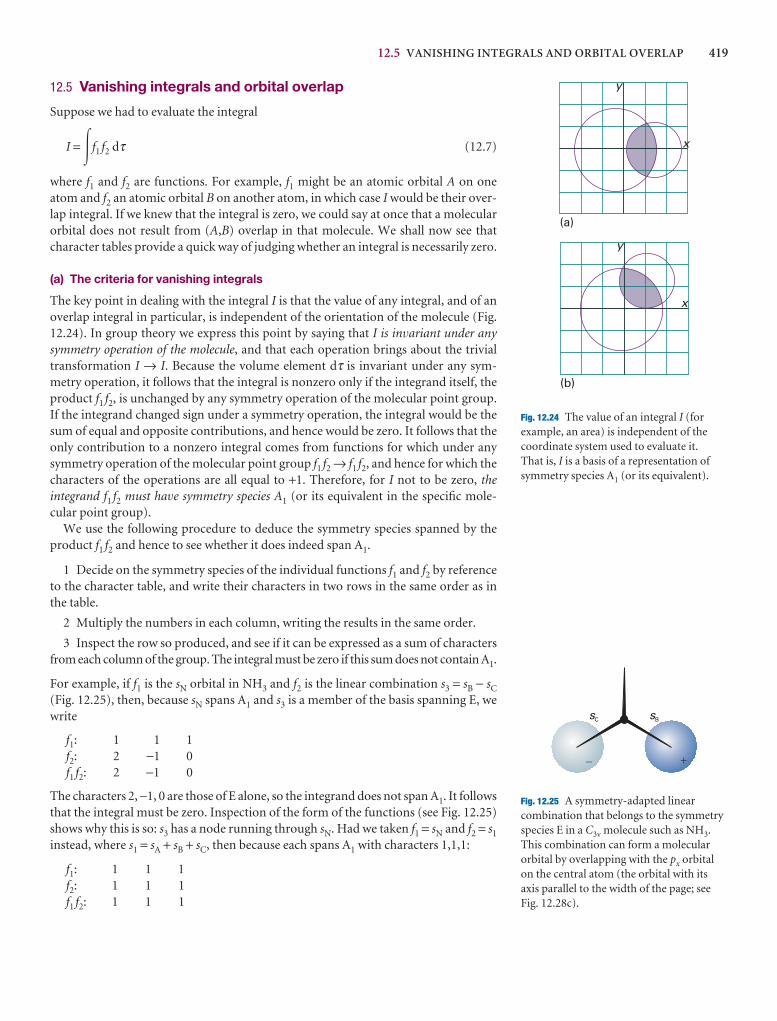
12.5 VANISHING INTEGRALS AND ORBITAL OVERLAP 419
12.5 Vanishing integrals and orbital overlap
Suppose we had to evaluate the integral
I = �f1 f2 dτ (12.7)
where f1 and f2 are functions. For example, f1 might be an atomic orbital A on oneatom and f2 an atomic orbital B on another atom, in which case I would be their over-lap integral. If we knew that the integral is zero, we could say at once that a molecularorbital does not result from (A,B) overlap in that molecule. We shall now see thatcharacter tables provide a quick way of judging whether an integral is necessarily zero.
(a) The criteria for vanishing integrals
The key point in dealing with the integral I is that the value of any integral, and of anoverlap integral in particular, is independent of the orientation of the molecule (Fig.12.24). In group theory we express this point by saying that I is invariant under anysymmetry operation of the molecule, and that each operation brings about the trivialtransformation I → I. Because the volume element dτ is invariant under any sym-metry operation, it follows that the integral is nonzero only if the integrand itself, theproduct f1 f2, is unchanged by any symmetry operation of the molecular point group.If the integrand changed sign under a symmetry operation, the integral would be thesum of equal and opposite contributions, and hence would be zero. It follows that theonly contribution to a nonzero integral comes from functions for which under anysymmetry operation of the molecular point group f1 f2 → f1 f2, and hence for which thecharacters of the operations are all equal to +1. Therefore, for I not to be zero, theintegrand f1 f2 must have symmetry species A1 (or its equivalent in the specific mole-cular point group).
We use the following procedure to deduce the symmetry species spanned by theproduct f1 f2 and hence to see whether it does indeed span A1.
1 Decide on the symmetry species of the individual functions f1 and f2 by referenceto the character table, and write their characters in two rows in the same order as inthe table.
2 Multiply the numbers in each column, writing the results in the same order.
3 Inspect the row so produced, and see if it can be expressed as a sum of charactersfrom each column of the group. The integral must be zero if this sum does not contain A1.
For example, if f1 is the sN orbital in NH3 and f2 is the linear combination s3 = sB − sC
(Fig. 12.25), then, because sN spans A1 and s3 is a member of the basis spanning E, wewrite
f1: 1 1 1f2: 2 −1 0f1 f2: 2 −1 0
The characters 2, −1, 0 are those of E alone, so the integrand does not span A1. It followsthat the integral must be zero. Inspection of the form of the functions (see Fig. 12.25)shows why this is so: s3 has a node running through sN. Had we taken f1 = sN and f2 = s1
instead, where s1 = sA + sB + sC, then because each spans A1 with characters 1,1,1:
f1: 1 1 1f2: 1 1 1f1 f2: 1 1 1
x
y
y
x
(a)
(b)
Fig. 12.24 The value of an integral I (forexample, an area) is independent of thecoordinate system used to evaluate it. That is, I is a basis of a representation ofsymmetry species A1 (or its equivalent).
sBsC
��
Fig. 12.25 A symmetry-adapted linearcombination that belongs to the symmetryspecies E in a C3v molecule such as NH3.This combination can form a molecularorbital by overlapping with the px orbitalon the central atom (the orbital with itsaxis parallel to the width of the page; seeFig. 12.28c).
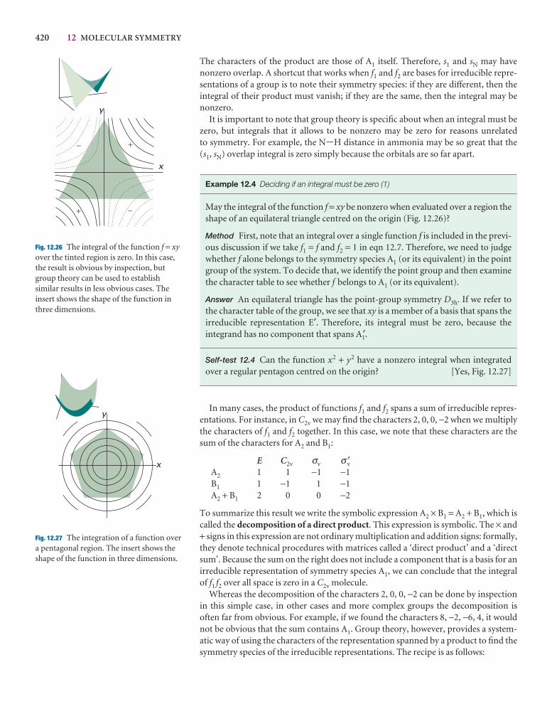
420 12 MOLECULAR SYMMETRY
x
y
�
�
�
�
Fig. 12.26 The integral of the function f = xyover the tinted region is zero. In this case,the result is obvious by inspection, butgroup theory can be used to establishsimilar results in less obvious cases. Theinsert shows the shape of the function inthree dimensions.
x
y
�
Fig. 12.27 The integration of a function overa pentagonal region. The insert shows theshape of the function in three dimensions.
The characters of the product are those of A1 itself. Therefore, s1 and sN may havenonzero overlap. A shortcut that works when f1 and f2 are bases for irreducible repre-sentations of a group is to note their symmetry species: if they are different, then theintegral of their product must vanish; if they are the same, then the integral may benonzero.
It is important to note that group theory is specific about when an integral must bezero, but integrals that it allows to be nonzero may be zero for reasons unrelated to symmetry. For example, the N-H distance in ammonia may be so great that the(s1, sN) overlap integral is zero simply because the orbitals are so far apart.
Example 12.4 Deciding if an integral must be zero (1)
May the integral of the function f = xy be nonzero when evaluated over a region theshape of an equilateral triangle centred on the origin (Fig. 12.26)?
Method First, note that an integral over a single function f is included in the previ-ous discussion if we take f1 = f and f2 = 1 in eqn 12.7. Therefore, we need to judgewhether f alone belongs to the symmetry species A1 (or its equivalent) in the pointgroup of the system. To decide that, we identify the point group and then examinethe character table to see whether f belongs to A1 (or its equivalent).
Answer An equilateral triangle has the point-group symmetry D3h. If we refer tothe character table of the group, we see that xy is a member of a basis that spans theirreducible representation E′. Therefore, its integral must be zero, because theintegrand has no component that spans A1′.
Self-test 12.4 Can the function x2 + y2 have a nonzero integral when integratedover a regular pentagon centred on the origin? [Yes, Fig. 12.27]
In many cases, the product of functions f1 and f2 spans a sum of irreducible repres-entations. For instance, in C2v we may find the characters 2, 0, 0, −2 when we multiplythe characters of f1 and f2 together. In this case, we note that these characters are thesum of the characters for A2 and B1:
E C2v σv σ ′vA2 1 1 −1 −1B1 1 −1 1 −1A2 + B1 2 0 0 −2
To summarize this result we write the symbolic expression A2 × B1 = A2 + B1, which iscalled the decomposition of a direct product. This expression is symbolic. The × and+ signs in this expression are not ordinary multiplication and addition signs: formally,they denote technical procedures with matrices called a ‘direct product’ and a ‘directsum’. Because the sum on the right does not include a component that is a basis for anirreducible representation of symmetry species A1, we can conclude that the integralof f1 f2 over all space is zero in a C2v molecule.
Whereas the decomposition of the characters 2, 0, 0, −2 can be done by inspectionin this simple case, in other cases and more complex groups the decomposition isoften far from obvious. For example, if we found the characters 8, −2, −6, 4, it wouldnot be obvious that the sum contains A1. Group theory, however, provides a system-atic way of using the characters of the representation spanned by a product to find thesymmetry species of the irreducible representations. The recipe is as follows:
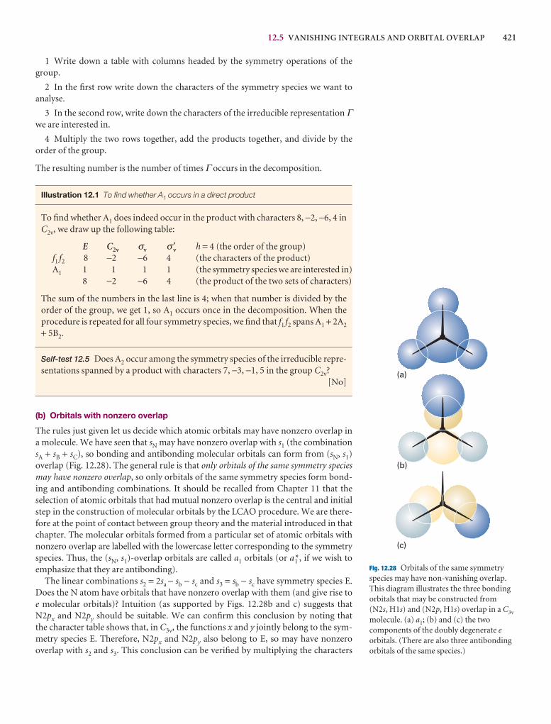
12.5 VANISHING INTEGRALS AND ORBITAL OVERLAP 421
(a)
(b)
(c)
Fig. 12.28 Orbitals of the same symmetryspecies may have non-vanishing overlap.This diagram illustrates the three bondingorbitals that may be constructed from(N2s, H1s) and (N2p, H1s) overlap in a C3v
molecule. (a) a1; (b) and (c) the twocomponents of the doubly degenerate eorbitals. (There are also three antibondingorbitals of the same species.)
1 Write down a table with columns headed by the symmetry operations of thegroup.
2 In the first row write down the characters of the symmetry species we want toanalyse.
3 In the second row, write down the characters of the irreducible representation Γwe are interested in.
4 Multiply the two rows together, add the products together, and divide by theorder of the group.
The resulting number is the number of times Γ occurs in the decomposition.
Illustration 12.1 To find whether A1 occurs in a direct product
To find whether A1 does indeed occur in the product with characters 8, −2, −6, 4 inC2v, we draw up the following table:
E C2v σv σ′v h = 4 (the order of the group)f1 f2 8 −2 −6 4 (the characters of the product)A1 1 1 1 1 (the symmetry species we are interested in)
8 −2 −6 4 (the product of the two sets of characters)
The sum of the numbers in the last line is 4; when that number is divided by theorder of the group, we get 1, so A1 occurs once in the decomposition. When theprocedure is repeated for all four symmetry species, we find that f1 f2 spans A1 + 2A2
+ 5B2.
Self-test 12.5 Does A2 occur among the symmetry species of the irreducible repre-sentations spanned by a product with characters 7, −3, −1, 5 in the group C2v?
[No]
(b) Orbitals with nonzero overlap
The rules just given let us decide which atomic orbitals may have nonzero overlap ina molecule. We have seen that sN may have nonzero overlap with s1 (the combinationsA + sB + sC), so bonding and antibonding molecular orbitals can form from (sN, s1)overlap (Fig. 12.28). The general rule is that only orbitals of the same symmetry speciesmay have nonzero overlap, so only orbitals of the same symmetry species form bond-ing and antibonding combinations. It should be recalled from Chapter 11 that theselection of atomic orbitals that had mutual nonzero overlap is the central and initialstep in the construction of molecular orbitals by the LCAO procedure. We are there-fore at the point of contact between group theory and the material introduced in thatchapter. The molecular orbitals formed from a particular set of atomic orbitals withnonzero overlap are labelled with the lowercase letter corresponding to the symmetryspecies. Thus, the (sN, s1)-overlap orbitals are called a1 orbitals (or a1*, if we wish toemphasize that they are antibonding).
The linear combinations s2 = 2sa − sb − sc and s3 = sb − sc have symmetry species E.Does the N atom have orbitals that have nonzero overlap with them (and give rise toe molecular orbitals)? Intuition (as supported by Figs. 12.28b and c) suggests thatN2px and N2py should be suitable. We can confirm this conclusion by noting that the character table shows that, in C3v, the functions x and y jointly belong to the sym-metry species E. Therefore, N2px and N2py also belong to E, so may have nonzerooverlap with s2 and s3. This conclusion can be verified by multiplying the characters
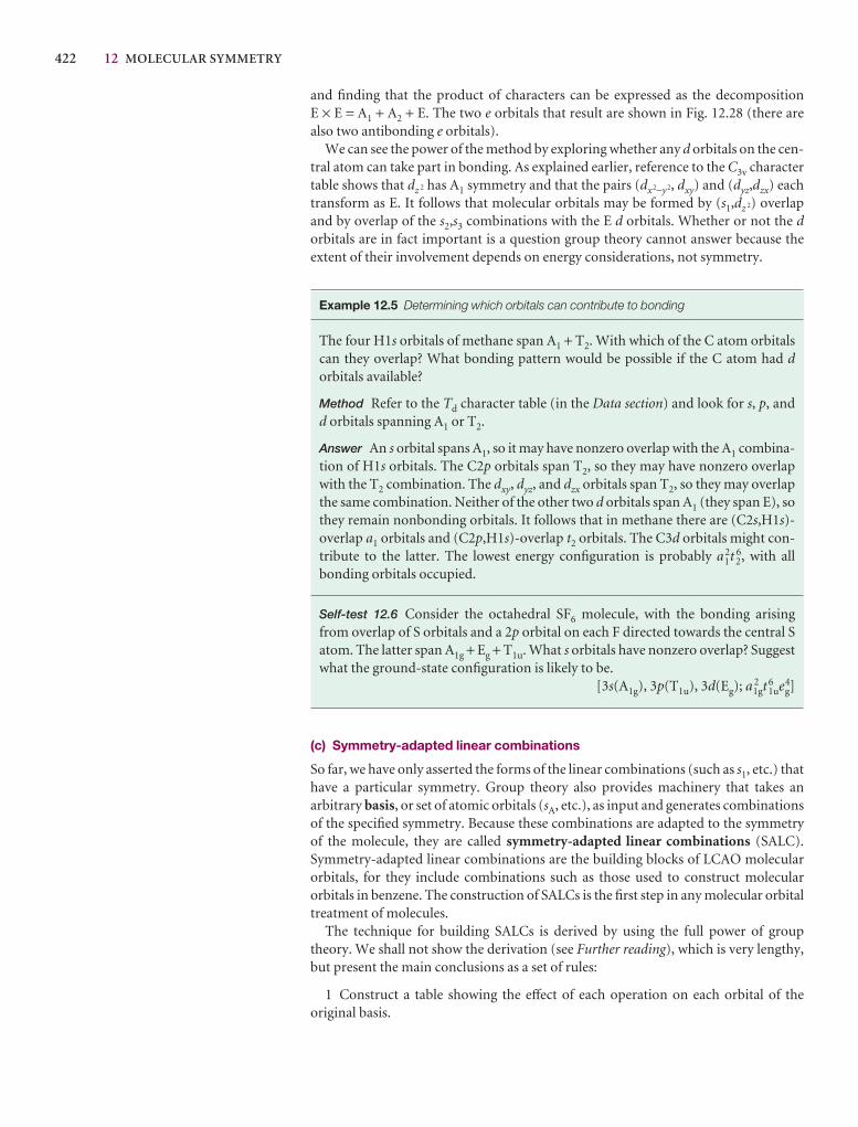
422 12 MOLECULAR SYMMETRY
and finding that the product of characters can be expressed as the decomposition E × E = A1 + A2 + E. The two e orbitals that result are shown in Fig. 12.28 (there are also two antibonding e orbitals).
We can see the power of the method by exploring whether any d orbitals on the cen-tral atom can take part in bonding. As explained earlier, reference to the C3v charactertable shows that dz 2 has A1 symmetry and that the pairs (dx2−y2, dxy) and (dyz,dzx) eachtransform as E. It follows that molecular orbitals may be formed by (s1,dz 2) overlapand by overlap of the s2,s3 combinations with the E d orbitals. Whether or not the dorbitals are in fact important is a question group theory cannot answer because the extent of their involvement depends on energy considerations, not symmetry.
Example 12.5 Determining which orbitals can contribute to bonding
The four H1s orbitals of methane span A1 + T2. With which of the C atom orbitalscan they overlap? What bonding pattern would be possible if the C atom had dorbitals available?
Method Refer to the Td character table (in the Data section) and look for s, p, andd orbitals spanning A1 or T2.
Answer An s orbital spans A1, so it may have nonzero overlap with the A1 combina-tion of H1s orbitals. The C2p orbitals span T2, so they may have nonzero overlapwith the T2 combination. The dxy, dyz, and dzx orbitals span T2, so they may overlapthe same combination. Neither of the other two d orbitals span A1 (they span E), sothey remain nonbonding orbitals. It follows that in methane there are (C2s,H1s)-overlap a1 orbitals and (C2p,H1s)-overlap t2 orbitals. The C3d orbitals might con-tribute to the latter. The lowest energy configuration is probably a1
2t 26, with all
bonding orbitals occupied.
Self-test 12.6 Consider the octahedral SF6 molecule, with the bonding arisingfrom overlap of S orbitals and a 2p orbital on each F directed towards the central Satom. The latter span A1g + Eg + T1u. What s orbitals have nonzero overlap? Suggestwhat the ground-state configuration is likely to be.
[3s(A1g), 3p(T1u), 3d(Eg); a 21gt
61ue4
g]
(c) Symmetry-adapted linear combinations
So far, we have only asserted the forms of the linear combinations (such as s1, etc.) thathave a particular symmetry. Group theory also provides machinery that takes an arbitrary basis, or set of atomic orbitals (sA, etc.), as input and generates combinationsof the specified symmetry. Because these combinations are adapted to the symmetryof the molecule, they are called symmetry-adapted linear combinations (SALC).Symmetry-adapted linear combinations are the building blocks of LCAO molecularorbitals, for they include combinations such as those used to construct molecular orbitals in benzene. The construction of SALCs is the first step in any molecular orbitaltreatment of molecules.
The technique for building SALCs is derived by using the full power of group theory. We shall not show the derivation (see Further reading), which is very lengthy,but present the main conclusions as a set of rules:
1 Construct a table showing the effect of each operation on each orbital of the original basis.
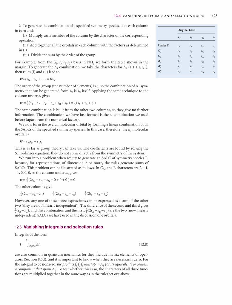
12.6 VANISHING INTEGRALS AND SELECTION RULES 423
2 To generate the combination of a specified symmetry species, take each columnin turn and:
(i) Multiply each member of the column by the character of the correspondingoperation.
(ii) Add together all the orbitals in each column with the factors as determinedin (i).
(iii) Divide the sum by the order of the group.
For example, from the (sN,sA,sB,sC) basis in NH3 we form the table shown in the margin. To generate the A1 combination, we take the characters for A1 (1,1,1,1,1,1);then rules (i) and (ii) lead to
ψ ∝ sN + sN + · · · = 6sN
The order of the group (the number of elements) is 6, so the combination of A1 sym-metry that can be generated from sN is sN itself. Applying the same technique to thecolumn under sA gives
ψ = 1–6(sA + sB + sC + sA + sB + sC ) = 1–3 (sA + sB + sC)
The same combination is built from the other two columns, so they give no further information. The combination we have just formed is the s1 combination we used before (apart from the numerical factor).
We now form the overall molecular orbital by forming a linear combination of allthe SALCs of the specified symmetry species. In this case, therefore, the a1 molecularorbital is
ψ = cNsN + c1s1
This is as far as group theory can take us. The coefficients are found by solving theSchrödinger equation; they do not come directly from the symmetry of the system.
We run into a problem when we try to generate an SALC of symmetry species E, because, for representations of dimension 2 or more, the rules generate sums ofSALCs. This problem can be illustrated as follows. In C3v, the E characters are 2, −1,−1, 0, 0, 0, so the column under sN gives
ψ = 1–6 (2sN − sN − sN + 0 + 0 + 0 ) = 0
The other columns give1–6(2sA − sB − sC) 1–6 (2sB − sA − sC) 1–6(2sC − sB − sA)
However, any one of these three expressions can be expressed as a sum of the othertwo (they are not ‘linearly independent’). The difference of the second and third gives1–2(sB − sC), and this combination and the first, 1–6(2sA − sB − sC) are the two (now linearlyindependent) SALCs we have used in the discussion of e orbitals.
12.6 Vanishing integrals and selection rules
Integrals of the form
I = �f1 f2 f3dτ (12.8)
are also common in quantum mechanics for they include matrix elements of oper-ators (Section 8.5d), and it is important to know when they are necessarily zero. Forthe integral to be nonzero, the product f1 f2 f3 must span A1 (or its equivalent) or containa component that spans A1. To test whether this is so, the characters of all three func-tions are multiplied together in the same way as in the rules set out above.
Original basis
sN sA sB sC
Under E sN sA sB sC
C 3+ sN sB sC sA
C3− sN sC sA sB
σv sN sA sC sB
σ v′ sN sB sA sC
σ v″ sN sC sB sA
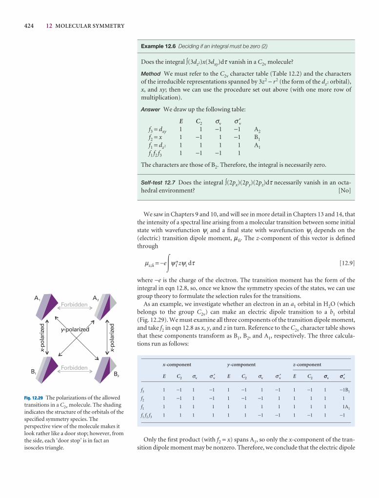
424 12 MOLECULAR SYMMETRY
Forbidden
Forbidden
x-po
lari
zed
x-po
lari
zed
A1 A2
B1 B2
y-polarized
Fig. 12.29 The polarizations of the allowedtransitions in a C2v molecule. The shadingindicates the structure of the orbitals of thespecified symmetry species. Theperspective view of the molecule makes itlook rather like a door stop; however, fromthe side, each ‘door stop’ is in fact anisosceles triangle.
Example 12.6 Deciding if an integral must be zero (2)
Does the integral ∫(3dz2)x(3dxy)dτ vanish in a C2v molecule?
Method We must refer to the C2v character table (Table 12.2) and the characters of the irreducible representations spanned by 3z2 − r2 (the form of the dz2 orbital),x, and xy; then we can use the procedure set out above (with one more row of multiplication).
Answer We draw up the following table:
E C2 σv σ ′vf3 = dxy 1 1 −1 −1 A2
f2 = x 1 −1 1 −1 B1
f1 = dz2 1 1 1 1 A1
f1 f2 f3 1 −1 −1 1
The characters are those of B2. Therefore, the integral is necessarily zero.
Self-test 12.7 Does the integral ∫(2px)(2py)(2pz)dτ necessarily vanish in an octa-hedral environment? [No]
We saw in Chapters 9 and 10, and will see in more detail in Chapters 13 and 14, thatthe intensity of a spectral line arising from a molecular transition between some initialstate with wavefunction ψi and a final state with wavefunction ψf depends on the(electric) transition dipole moment, µfi. The z-component of this vector is definedthrough
µz,fi = −e�ψ f*zψi dτ [12.9]
where −e is the charge of the electron. The transition moment has the form of the integral in eqn 12.8, so, once we know the symmetry species of the states, we can usegroup theory to formulate the selection rules for the transitions.
As an example, we investigate whether an electron in an a1 orbital in H2O (whichbelongs to the group C2v) can make an electric dipole transition to a b1 orbital(Fig. 12.29). We must examine all three components of the transition dipole moment,and take f2 in eqn 12.8 as x, y, and z in turn. Reference to the C2v character table showsthat these components transform as B1, B2, and A1, respectively. The three calcula-tions run as follows:
x-component y-component z-component
E C2 σv σ′v E C2 σv σ′v E C2 sv s′v
f3 1 −1 1 −1 1 −1 1 −1 1 −1 1 −1B1
f2 1 −1 1 −1 1 −1 −1 1 1 1 1 1
f1 1 1 1 1 1 1 1 1 1 1 1 1A1
f1 f2 f3 1 1 1 1 1 1 −1 −1 1 −1 1 −1
Only the first product (with f2 = x) spans A1, so only the x-component of the tran-sition dipole moment may be nonzero. Therefore, we conclude that the electric dipole
CHECKLIST OF KEY IDEAS 425
Checklist of key ideas
1. A symmetry operation is an action that leaves an objectlooking the same after it has been carried out.
2. A symmetry element is a point, line, or plane with respect towhich a symmetry operation is performed.
3. A point group is a group of symmetry operations that leaves atleast one common point unchanged. A space group, a groupof symmetry operations that includes translation throughspace.
4. The notation for point groups commonly used for moleculesand solids is summarized in Table 12.1.
5. To be polar, a molecule must belong to Cn, Cnv, or Cs (andhave no higher symmetry).
6. A molecule may be chiral only if it does not possess an axis ofimproper rotation, Sn.
7. A representative D(X) is a matrix that brings about thetransformation of the basis under the operation X. The basis isthe set of functions on which the representative acts.
8. A character, χ, is the sum of the diagonal elements of a matrixrepresentative.
9. A character table characterizes the different symmetry typespossible in the point group.
10. In a reduced representation all the matrices have block-diagonal form. An irreducible representation cannot bereduced further.
11. Symmetry species are the labels for the irreduciblerepresentations of a group.
12. Decomposition of the direct product is the reduction of aproduct of symmetry species to a sum of symmetry species, Γ × Γ ′ = Γ (1) + Γ (2) + · · ·
transitions between a1 and b1 are allowed. We can go on to state that the radiationemitted (or absorbed) is x-polarized and has its electric field vector in the x-direction,because that form of radiation couples with the x–component of a transition dipole.
Example 12.7 Deducing a selection rule
Is px → py an allowed transition in a tetrahedral environment?
Method We must decide whether the product py qpx , with q = x, y, or z, spans A1 byusing the Td character table.
Answer The procedure works out as follows:
E 8C3 3C2 6σd 6S4
f3(py) 3 0 −1 −1 1 T2
f2(q) 3 0 −1 −1 1 T2
f1(px) 3 0 −1 −1 1 T2
f1 f2 f3 27 0 −1 −1 1
We can use the decomposition procedure described in Section 12.5a to deduce thatA1 occurs (once) in this set of characters, so px → py is allowed.
A more detailed analysis (using the matrix representatives rather than the char-acters) shows that only q = z gives an integral that may be nonzero, so the transitionis z-polarized. That is, the electromagnetic radiation involved in the transition hasits electric vector aligned in the z-direction.
Self-test 12.8 What are the allowed transitions, and their polarizations, of a b1
electron in a C4v molecule? [b1 → b1(z); b1 → e(x,y)]
The following chapters will show many more examples of the systematic use ofsymmetry. We shall see that the techniques of group theory greatly simplify the ana-lysis of molecular structure and spectra.

426 12 MOLECULAR SYMMETRY
13. For an integral ∫f1 f2 dτ to be nonzero, the integrand f1 f2 musthave the symmetry species A1 (or its equivalent in the specificmolecular point group).
14. A symmetry-adapted linear combination (SALC) is acombination of atomic orbitals adapted to the symmetry ofthe molecule and used as the building blocks for LCAOmolecular orbitals.
15. Allowed and forbidden spectroscopic transitions can beidentified by considering the symmetry criteria for the non-vanishing of the transition moment between the initial andfinal states.
Further reading
Articles and texts
P.W. Atkins and R.S. Friedman, Molecular quantum mechanics.Oxford University Press (2005).
F.A. Cotton, Chemical applications of group theory. Wiley, New York(1990).
R. Drago, Physical methods for chemists. Saunders, Philadelphia(1992).
D.C. Harris and M.D. Bertollucci, Symmetry and spectroscopy: anintroduction to vibrational and electronic spectroscopy. Dover, New York (1989).
S.F.A. Kettle, Symmetry and structure: readable group theory forchemists. Wiley, New York (1995).
Sources of data and information
G.L. Breneman, Crystallographic symmetry point group notationflow chart. J. Chem. Educ. 64, 216 (1987).
P.W. Atkins, M.S. Child, and C.S.G. Phillips, Tables for group theory.Oxford University Press (1970).
Discussion questions
12.1 Explain how a molecule is assigned to a point group.
12.2 List the symmetry operations and the corresponding symmetry elementsof the point groups.
12.3 Explain the symmetry criteria that allow a molecule to be polar.
12.4 Explain the symmetry criteria that allow a molecule to be optically active.
12.5 Explain what is meant by (a) a representative and (b) a representation inthe context of group theory.
12.6 Explain the construction and content of a character table.
12.7 Explain how spectroscopic selection rules arise and how they areformulated by using group theory.
12.8 Outline how a direct product is expressed as a direct sum and how todecide whether the totally symmetric irreducible representation is present inthe direct product.
Exercises
12.1a The CH3Cl molecule belongs to the point group C3v. List the symmetryelements of the group and locate them in the molecule.
12.1b The CCl4 molecule belongs to the point group Td. List the symmetryelements of the group and locate them in the molecule.
12.2a Which of the following molecules may be polar? (a) pyridine (C2v),(b) nitroethane (Cs), (c) gas-phase HgBr2 (D∞h), (d) B3N3N6 (D3h).
12.2b Which of the following molecules may be polar? (a) CH3Cl (C3v),(b) HW2(CO)10 (D4h), (c) SnCl4 (Td).
12.3a Use symmetry properties to determine whether or not the integral∫px zpzdτ is necessarily zero in a molecule with symmetry C4v.
12.3b Use symmetry properties to determine whether or not the integral∫px zpzdτ is necessarily zero in a molecule with symmetry D6h.
12.4a Show that the transition A1 → A2 is forbidden for electric dipoletransitions in a C3v molecule.
12.4b Is the transition A1g → E2u forbidden for electric dipole transitions in aD6h molecule?
12.5a Show that the function xy has symmetry species B2 in the group C4v.
12.5b Show that the function xyz has symmetry species A1 in the group D2.
12.6a Molecules belonging to the point groups D2h or C3h cannot be chiral.Which elements of these groups rule out chirality?
12.6b Molecules belonging to the point groups Th or Td cannot be chiral.Which elements of these groups rule out chirality?
12.7a The group D2 consists of the elements E, C2, C2′, and C2″, where thethree twofold rotations are around mutually perpendicular axes. Constructthe group multiplication table.
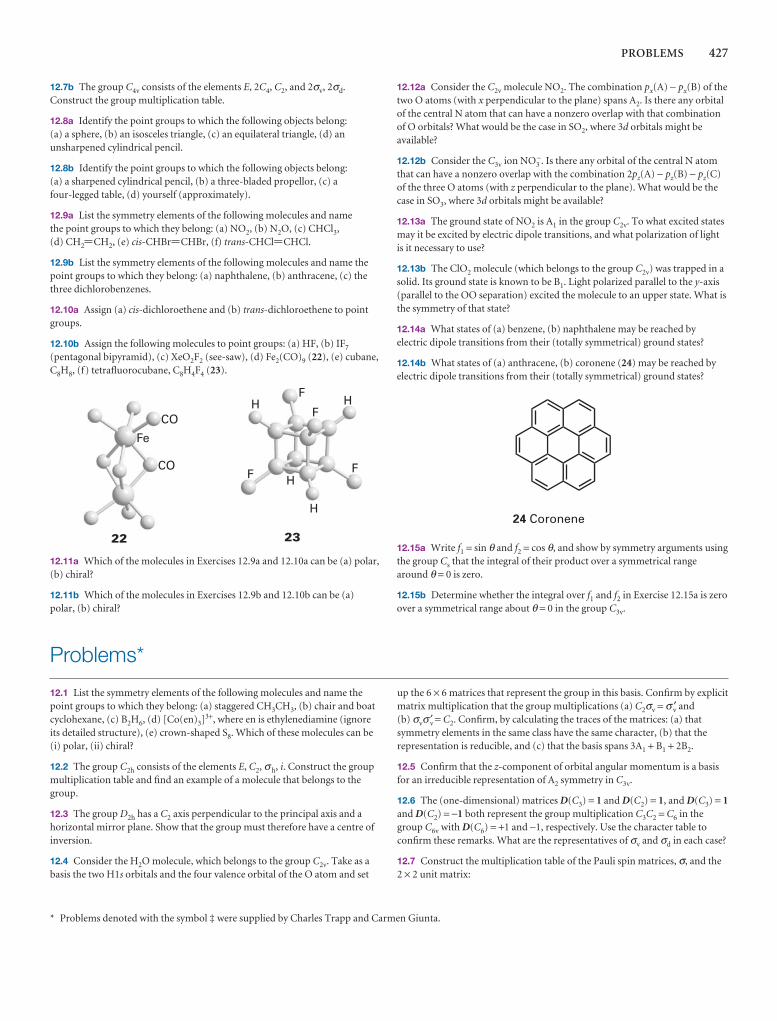
PROBLEMS 427
12.7b The group C4v consists of the elements E, 2C4, C2, and 2σv, 2σd.Construct the group multiplication table.
12.8a Identify the point groups to which the following objects belong: (a) a sphere, (b) an isosceles triangle, (c) an equilateral triangle, (d) anunsharpened cylindrical pencil.
12.8b Identify the point groups to which the following objects belong: (a) a sharpened cylindrical pencil, (b) a three-bladed propellor, (c) a four-legged table, (d) yourself (approximately).
12.9a List the symmetry elements of the following molecules and name the point groups to which they belong: (a) NO2, (b) N2O, (c) CHCl3,(d) CH2=CH2, (e) cis-CHBr=CHBr, (f) trans-CHCl=CHCl.
12.9b List the symmetry elements of the following molecules and name thepoint groups to which they belong: (a) naphthalene, (b) anthracene, (c) thethree dichlorobenzenes.
12.10a Assign (a) cis-dichloroethene and (b) trans-dichloroethene to pointgroups.
12.10b Assign the following molecules to point groups: (a) HF, (b) IF7
(pentagonal bipyramid), (c) XeO2F2 (see-saw), (d) Fe2(CO)9 (22), (e) cubane,C8H8, (f) tetrafluorocubane, C8H4F4 (23).
12.11a Which of the molecules in Exercises 12.9a and 12.10a can be (a) polar,(b) chiral?
12.11b Which of the molecules in Exercises 12.9b and 12.10b can be (a)polar, (b) chiral?
12.12a Consider the C2v molecule NO2. The combination px(A) − px(B) of thetwo O atoms (with x perpendicular to the plane) spans A2. Is there any orbitalof the central N atom that can have a nonzero overlap with that combinationof O orbitals? What would be the case in SO2, where 3d orbitals might beavailable?
12.12b Consider the C3v ion NO3−. Is there any orbital of the central N atom
that can have a nonzero overlap with the combination 2pz(A) − pz(B) − pz(C)of the three O atoms (with z perpendicular to the plane). What would be thecase in SO3, where 3d orbitals might be available?
12.13a The ground state of NO2 is A1 in the group C2v. To what excited statesmay it be excited by electric dipole transitions, and what polarization of lightis it necessary to use?
12.13b The ClO2 molecule (which belongs to the group C2v) was trapped in asolid. Its ground state is known to be B1. Light polarized parallel to the y-axis(parallel to the OO separation) excited the molecule to an upper state. What isthe symmetry of that state?
12.14a What states of (a) benzene, (b) naphthalene may be reached byelectric dipole transitions from their (totally symmetrical) ground states?
12.14b What states of (a) anthracene, (b) coronene (24) may be reached byelectric dipole transitions from their (totally symmetrical) ground states?
12.15a Write f1 = sin θ and f2 = cos θ, and show by symmetry arguments usingthe group Cs that the integral of their product over a symmetrical rangearound θ = 0 is zero.
12.15b Determine whether the integral over f1 and f2 in Exercise 12.15a is zeroover a symmetrical range about θ = 0 in the group C3v.
Problems*
12.1 List the symmetry elements of the following molecules and name thepoint groups to which they belong: (a) staggered CH3CH3, (b) chair and boatcyclohexane, (c) B2H6, (d) [Co(en)3]3+, where en is ethylenediamine (ignoreits detailed structure), (e) crown-shaped S8. Which of these molecules can be(i) polar, (ii) chiral?
12.2 The group C2h consists of the elements E, C2, σh, i. Construct the groupmultiplication table and find an example of a molecule that belongs to thegroup.
12.3 The group D2h has a C2 axis perpendicular to the principal axis and ahorizontal mirror plane. Show that the group must therefore have a centre ofinversion.
12.4 Consider the H2O molecule, which belongs to the group C2v. Take as abasis the two H1s orbitals and the four valence orbital of the O atom and set
up the 6 × 6 matrices that represent the group in this basis. Confirm by explicitmatrix multiplication that the group multiplications (a) C2σv = σ v′ and(b) σvσ v′ = C2. Confirm, by calculating the traces of the matrices: (a) thatsymmetry elements in the same class have the same character, (b) that therepresentation is reducible, and (c) that the basis spans 3A1 + B1 + 2B2.
12.5 Confirm that the z-component of orbital angular momentum is a basisfor an irreducible representation of A2 symmetry in C3v.
12.6 The (one-dimensional) matrices D(C3) = 1 and D(C2) = 1, and D(C3) = 1and D(C2) = −1 both represent the group multiplication C3C2 = C6 in thegroup C6v with D(C6) = +1 and −1, respectively. Use the character table toconfirm these remarks. What are the representatives of σv and σd in each case?
12.7 Construct the multiplication table of the Pauli spin matrices, σ, and the2 × 2 unit matrix:
* Problems denoted with the symbol ‡ were supplied by Charles Trapp and Carmen Giunta.
CO
Fe
CO
22
F
F
F F
H H
H
H
23
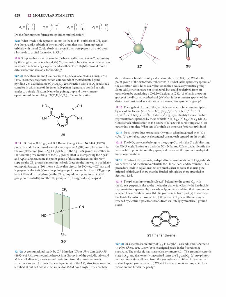
428 12 MOLECULAR SYMMETRY
σx = σy = σz = σ0 =
Do the four matrices form a group under multiplication?
12.8 What irreducible representations do the four H1s orbitals of CH4 span?Are there s and p orbitals of the central C atom that may form molecularorbitals with them? Could d orbitals, even if they were present on the C atom,play a role in orbital formation in CH4?
12.9 Suppose that a methane molecule became distorted to (a) C3v symmetryby the lengthening of one bond, (b) C2v symmetry, by a kind of scissors actionin which one bond angle opened and another closed slightly. Would more dorbitals become available for bonding?
12.10‡ B.A. Bovenzi and G.A. Pearse, Jr. (J. Chem. Soc. Dalton Trans., 2763(1997)) synthesized coordination compounds of the tridentate ligandpyridine-2,6-diamidoxime (C7H9N5O2, 25). Reaction with NiSO4 produced acomplex in which two of the essentially planar ligands are bonded at rightangles to a single Ni atom. Name the point group and the symmetryoperations of the resulting [Ni(C7H9N5O2)2]2+ complex cation.
12.11‡ R. Eujen, B. Hoge, and D.J. Brauer (Inorg. Chem. 36, 1464 (1997))prepared and characterized several square-planar Ag(III) complex anions. Inthe complex anion [trans-Ag(CF3)2(CN)2]−, the Ag-CN groups are collinear.(a) Assuming free rotation of the CF3 groups (that is, disregarding the AgCFand AgCH angles), name the point group of this complex anion. (b) Nowsuppose the CF3 groups cannot rotate freely (because the ion was in a solid, forexample). Structure (26) shows a plane that bisects the NC-Ag-CN axis andis perpendicular to it. Name the point group of the complex if each CF3 grouphas a CF bond in that plane (so the CF3 groups do not point to either CNgroup preferentially) and the CF3 groups are (i) staggered, (ii) eclipsed.
12.12‡ A computational study by C.J. Marsden (Chem. Phys. Lett. 245, 475(1995)) of AMx compounds, where A is in Group 14 of the periodic table andM is an alkali metal, shows several deviations from the most symmetricstructures for each formula. For example, most of the AM4 structures were nottetrahedral but had two distinct values for MAM bond angles. They could be
NC
CN
CF3
CF3
Ag
26
1 00 1
⎛⎝⎜
⎞⎠⎟
1 00 1−
⎛⎝⎜
⎞⎠⎟
00−⎛
⎝⎜⎞⎠⎟
ii
0 11 0
⎛⎝⎜
⎞⎠⎟
derived from a tetrahedron by a distortion shown in (27). (a) What is thepoint group of the distorted tetrahedron? (b) What is the symmetry species ofthe distortion considered as a vibration in the new, less symmetric group?Some AM6 structures are not octahedral, but could be derived from anoctahedron by translating a C-M-C axis as in (28). (c) What is the pointgroup of the distorted octahedron? (d) What is the symmetry species of thedistortion considered as a vibration in the new, less symmetric group?
12.13 The algebraic forms of the f orbitals are a radial function multiplied by one of the factors (a) z(5z2 − 3r2), (b) y(5y2 − 3r2), (c) x(5x2 − 3r2),(d) z(x2 − y2), (e) y(x2 − z2), (f ) x(z2 − y2), (g) xyz. Identify the irreduciblerepresentations spanned by these orbitals in (a) C2v, (b) C3v, (c) Td, (d) Oh.Consider a lanthanide ion at the centre of (a) a tetrahedral complex, (b) anoctahedral complex. What sets of orbitals do the seven f orbitals split into?
12.14 Does the product xyz necessarily vanish when integrated over (a) acube, (b) a tetrahedron, (c) a hexagonal prism, each centred on the origin?
12.15 The NO2 molecule belongs to the group C2v, with the C2 axis bisectingthe ONO angle. Taking as a basis the N2s, N2p, and O2p orbitals, identify theirreducible representations they span, and construct the symmetry-adaptedlinear combinations.
12.16 Construct the symmetry-adapted linear combinations of C2pz orbitalsfor benzene, and use them to calculate the Hückel secular determinant. Thisprocedure leads to equations that are much easier to solve than using theoriginal orbitals, and show that the Hückel orbitals are those specified inSection 11.6d.
12.17 The phenanthrene molecule (29) belongs to the group C2v withthe C2 axis perpendicular to the molecular plane. (a) Classify the irreduciblerepresentations spanned by the carbon 2pz orbitals and find their symmetry-adapted linear combinations. (b) Use your results from part (a) to calculatethe Hückel secular determinant. (c) What states of phenanthrene may bereached by electric dipole transitions from its (totally symmetrical) groundstate?
12.18‡ In a spectroscopic study of C60, F. Negri, G. Orlandi, and F. Zerbetto(J. Phys. Chem. 100, 10849 (1996)) assigned peaks in the fluorescencespectrum. The molecule has icosahedral symmetry (Ih). The ground electronicstate is A1g, and the lowest-lying excited states are T1g and Gg. (a) Are photon-induced transitions allowed from the ground state to either of these excitedstates? Explain your answer. (b) What if the transition is accompanied by avibration that breaks the parity?
27 28
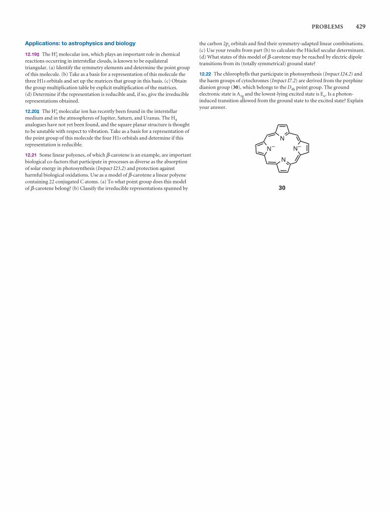
PROBLEMS 429
Applications: to astrophysics and biology
12.19‡ The H3+ molecular ion, which plays an important role in chemical
reactions occurring in interstellar clouds, is known to be equilateraltriangular. (a) Identify the symmetry elements and determine the point groupof this molecule. (b) Take as a basis for a representation of this molecule thethree H1s orbitals and set up the matrices that group in this basis. (c) Obtainthe group multiplication table by explicit multiplication of the matrices.(d) Determine if the representation is reducible and, if so, give the irreduciblerepresentations obtained.
12.20‡ The H3+ molecular ion has recently been found in the interstellar
medium and in the atmospheres of Jupiter, Saturn, and Uranus. The H4
analogues have not yet been found, and the square planar structure is thoughtto be unstable with respect to vibration. Take as a basis for a representation ofthe point group of this molecule the four H1s orbitals and determine if thisrepresentation is reducible.
12.21 Some linear polyenes, of which β-carotene is an example, are importantbiological co-factors that participate in processes as diverse as the absorptionof solar energy in photosynthesis (Impact I23.2) and protection againstharmful biological oxidations. Use as a model of β-carotene a linear polyenecontaining 22 conjugated C atoms. (a) To what point group does this modelof β-carotene belong? (b) Classify the irreducible representations spanned by
the carbon 2pz orbitals and find their symmetry-adapted linear combinations.(c) Use your results from part (b) to calculate the Hückel secular determinant.(d) What states of this model of β-carotene may be reached by electric dipoletransitions from its (totally symmetrical) ground state?
12.22 The chlorophylls that participate in photosynthesis (Impact I24.2) and the haem groups of cytochromes (Impact I7.2) are derived from the porphinedianion group (30), which belongs to the D4h point group. The groundelectronic state is A1g and the lowest-lying excited state is Eu. Is a photon-induced transition allowed from the ground state to the excited state? Explainyour answer.

Molecularspectroscopy 1:rotational andvibrational spectraThe general strategy we adopt in the chapter is to set up expressions for the energy levelsof molecules and then apply selection rules and considerations of populations to infer theform of spectra. Rotational energy levels are considered first, and we see how to derive expressions for their values and how to interpret rotational spectra in terms of molecular dimensions. Not all molecules can occupy all rotational states: we see the experimental evidence for this restriction and its explanation in terms of nuclear spin and the Pauli prin-ciple. Next, we consider the vibrational energy levels of diatomic molecules, and see that wecan use the properties of harmonic oscillators developed in Chapter 9. Then we considerpolyatomic molecules and find that their vibrations may be discussed as though they consisted of a set of independent harmonic oscillators, so the same approach as employedfor diatomic molecules may be used. We also see that the symmetry properties of the vibrations of polyatomic molecules are helpful for deciding which modes of vibration can be studied spectroscopically.
The origin of spectral lines in molecular spectroscopy is the absorption, emission, orscattering of a photon when the energy of a molecule changes. The difference fromatomic spectroscopy is that the energy of a molecule can change not only as a result of electronic transitions but also because it can undergo changes of rotational and vibrational state. Molecular spectra are therefore more complex than atomic spectra.However, they also contain information relating to more properties, and their ana-lysis leads to values of bond strengths, lengths, and angles. They also provide a way ofdetermining a variety of molecular properties, particularly molecular dimensions,shapes, and dipole moments. Molecular spectroscopy is also useful to astrophysicistsand environmental scientists, for the chemical composition of interstellar space andof planetary atmospheres can be inferred from their rotational, vibrational, and elec-tronic spectra.
Pure rotational spectra, in which only the rotational state of a molecule changes,can be observed in the gas phase. Vibrational spectra of gaseous samples show featuresthat arise from rotational transitions that accompany the excitation of vibration.Electronic spectra, which are described in Chapter 14, show features arising fromsimultaneous vibrational and rotational transitions. The simplest way of dealing withthese complexities is to tackle each type of transition in turn, and then to see how simultaneous changes affect the appearance of spectra.
General features of spectroscopy
13.1 Experimental techniques
13.2 The intensities of spectral lines
13.3 Linewidths
I13.1 Impact on astrophysics:Rotational and vibrationalspectroscopy of interstellar space
Pure rotation spectra
13.4 Moments of inertia
13.5 The rotational energy levels
13.6 Rotational transitions
13.7 Rotational Raman spectra
13.8 Nuclear statistics and rotationalstates
The vibrations of diatomicmolecules
13.9 Molecular vibrations
13.10 Selection rules
13.11 Anharmonicity
13.12 Vibration–rotation spectra
13.13 Vibrational Raman spectra ofdiatomic molecules
The vibrations of polyatomicmolecules
13.14 Normal modes
13.15 Infrared absorption spectra ofpolyatomic molecules
I13.2 Impact on environmentalscience: Global warming
13.16 Vibrational Raman spectra ofpolyatomic molecules
I13.3 Impact on biochemistry:Vibrational microscopy
13.17 Symmetry aspects of molecularvibrations
Checklist of key ideasFurther readingFurther information 13.1: SpectrometersFurther information 13.2: Selection rulesfor rotational and vibrationalspectroscopyDiscussion questionsExercisesProblems
13
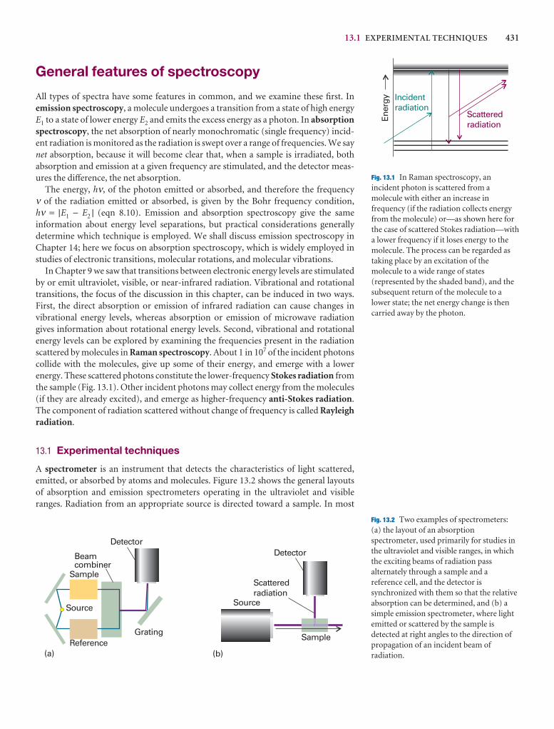
13.1 EXPERIMENTAL TECHNIQUES 431
General features of spectroscopy
All types of spectra have some features in common, and we examine these first. Inemission spectroscopy, a molecule undergoes a transition from a state of high energyE1 to a state of lower energy E2 and emits the excess energy as a photon. In absorptionspectroscopy, the net absorption of nearly monochromatic (single frequency) incid-ent radiation is monitored as the radiation is swept over a range of frequencies. We saynet absorption, because it will become clear that, when a sample is irradiated, bothabsorption and emission at a given frequency are stimulated, and the detector meas-ures the difference, the net absorption.
The energy, hν, of the photon emitted or absorbed, and therefore the frequency ν of the radiation emitted or absorbed, is given by the Bohr frequency condition, hν = |E1 − E2 | (eqn 8.10). Emission and absorption spectroscopy give the sameinformation about energy level separations, but practical considerations generally determine which technique is employed. We shall discuss emission spectroscopy inChapter 14; here we focus on absorption spectroscopy, which is widely employed instudies of electronic transitions, molecular rotations, and molecular vibrations.
In Chapter 9 we saw that transitions between electronic energy levels are stimulatedby or emit ultraviolet, visible, or near-infrared radiation. Vibrational and rotationaltransitions, the focus of the discussion in this chapter, can be induced in two ways.First, the direct absorption or emission of infrared radiation can cause changes in vibrational energy levels, whereas absorption or emission of microwave radiationgives information about rotational energy levels. Second, vibrational and rotationalenergy levels can be explored by examining the frequencies present in the radiationscattered by molecules in Raman spectroscopy. About 1 in 107 of the incident photonscollide with the molecules, give up some of their energy, and emerge with a lower energy. These scattered photons constitute the lower-frequency Stokes radiation fromthe sample (Fig. 13.1). Other incident photons may collect energy from the molecules(if they are already excited), and emerge as higher-frequency anti-Stokes radiation.The component of radiation scattered without change of frequency is called Rayleighradiation.
13.1 Experimental techniques
A spectrometer is an instrument that detects the characteristics of light scattered,emitted, or absorbed by atoms and molecules. Figure 13.2 shows the general layoutsof absorption and emission spectrometers operating in the ultraviolet and visibleranges. Radiation from an appropriate source is directed toward a sample. In most
Ener
gy Incidentradiation
Scatteredradiation
Fig. 13.1 In Raman spectroscopy, anincident photon is scattered from amolecule with either an increase infrequency (if the radiation collects energyfrom the molecule) or—as shown here forthe case of scattered Stokes radiation—witha lower frequency if it loses energy to themolecule. The process can be regarded astaking place by an excitation of themolecule to a wide range of states(represented by the shaded band), and thesubsequent return of the molecule to alower state; the net energy change is thencarried away by the photon.
Sample
Reference
Source
Detector
Grating
Beamcombiner
Source
Detector
Sample
Scatteredradiation
(a) (b)
Fig. 13.2 Two examples of spectrometers:(a) the layout of an absorptionspectrometer, used primarily for studies inthe ultraviolet and visible ranges, in whichthe exciting beams of radiation passalternately through a sample and areference cell, and the detector issynchronized with them so that the relativeabsorption can be determined, and (b) asimple emission spectrometer, where lightemitted or scattered by the sample isdetected at right angles to the direction ofpropagation of an incident beam ofradiation.
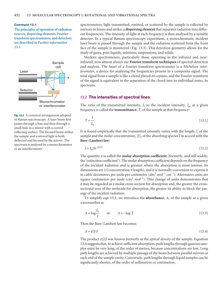
432 13 MOLECULAR SPECTROSCOPY 1: ROTATIONAL AND VIBRATIONAL SPECTRA
spectrometers, light transmitted, emitted, or scattered by the sample is collected bymirrors or lenses and strikes a dispersing element that separates radiation into differ-ent frequencies. The intensity of light at each frequency is then analysed by a suitabledetector. In a typical Raman spectroscopy experiment, a monochromatic incidentlaser beam is passed through the sample and the radiation scattered from the frontface of the sample is monitored (Fig. 13.3). This detection geometry allows for thestudy of gases, pure liquids, solutions, suspensions, and solids.
Modern spectrometers, particularly those operating in the infrared and near-infrared, now almost always use Fourier transform techniques of spectral detectionand analysis. The heart of a Fourier transform spectrometer is a Michelson inter-ferometer, a device for analysing the frequencies present in a composite signal. Thetotal signal from a sample is like a chord played on a piano, and the Fourier transformof the signal is equivalent to the separation of the chord into its individual notes, itsspectrum.
13.2 The intensities of spectral lines
The ratio of the transmitted intensity, I, to the incident intensity, I0, at a given frequency is called the transmittance, T, of the sample at that frequency:
T = [13.1]
It is found empirically that the transmitted intensity varies with the length, l, of thesample and the molar concentration, [J], of the absorbing species J in accord with theBeer–Lambert law:
I = I010−ε[J]l (13.2)
The quantity ε is called the molar absorption coefficient (formerly, and still widely,the ‘extinction coefficient’). The molar absorption coefficient depends on the frequencyof the incident radiation and is greatest where the absorption is most intense. Its dimensions are 1/(concentration × length), and it is normally convenient to express itin cubic decimetres per mole per centimetre (dm3 mol−1 cm−1). Alternative units aresquare centimetres per mole (cm2 mol−1). This change of units demonstrates that ε may be regarded as a molar cross-section for absorption and, the greater the cross-sectional area of the molecule for absorption, the greater its ability to block the pas-sage of the incident radiation.
To simplify eqn 13.2, we introduce the absorbance, A, of the sample at a givenwavenumber as
A = log or A = −log T [13.3]
Then the Beer–Lambert law becomes
A = ε[J]l (13.4)
The product ε[J]l was known formerly as the optical density of the sample. Equation13.4 suggests that, to achieve sufficient absorption, path lengths through gaseous sam-ples must be very long, of the order of metres, because concentrations are low. Longpath lengths are achieved by multiple passage of the beam between parallel mirrors ateach end of the sample cavity. Conversely, path lengths through liquid samples can besignificantly shorter, of the order of millimetres or centimetres.
I0
I
I
I0
Laser
Samplecell
Monochromatoror interferometer
Detector
Fig. 13.3 A common arrangement adoptedin Raman spectroscopy. A laser beam firstpasses through a lens and then through asmall hole in a mirror with a curvedreflecting surface. The focused beam strikesthe sample and scattered light is bothdeflected and focused by the mirror. Thespectrum is analysed by a monochromatoror an interferometer.
Comment 13.1
The principles of operation of radiationsources, dispersing elements, Fouriertransform spectrometers, and detectorsare described in Further information13.1.
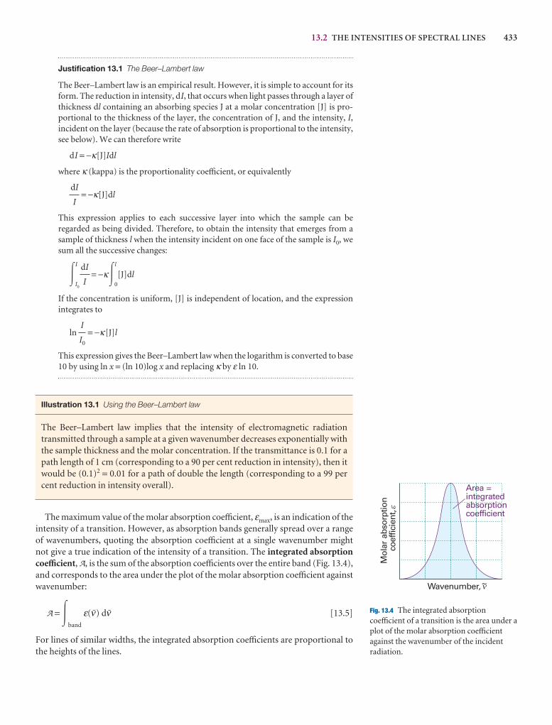
13.2 THE INTENSITIES OF SPECTRAL LINES 433
Mol
arab
sorp
tion
coef
ficie
nt,
Area =integratedabsorptioncoefficient
Wavenumber,~n
e
Fig. 13.4 The integrated absorptioncoefficient of a transition is the area under aplot of the molar absorption coefficientagainst the wavenumber of the incidentradiation.
Justification 13.1 The Beer–Lambert law
The Beer–Lambert law is an empirical result. However, it is simple to account for itsform. The reduction in intensity, dI, that occurs when light passes through a layer ofthickness dl containing an absorbing species J at a molar concentration [J] is pro-portional to the thickness of the layer, the concentration of J, and the intensity, I,incident on the layer (because the rate of absorption is proportional to the intensity,see below). We can therefore write
dI = −κ[J]Idl
where κ (kappa) is the proportionality coefficient, or equivalently
= −κ[J]dl
This expression applies to each successive layer into which the sample can be regarded as being divided. Therefore, to obtain the intensity that emerges from asample of thickness l when the intensity incident on one face of the sample is I0, wesum all the successive changes:
�I
I0
= −κ�l
0
[J]dl
If the concentration is uniform, [J] is independent of location, and the expressionintegrates to
ln = −κ[J]l
This expression gives the Beer–Lambert law when the logarithm is converted to base10 by using ln x = (ln 10)log x and replacing κ by ε ln 10.
Illustration 13.1 Using the Beer–Lambert law
The Beer–Lambert law implies that the intensity of electromagnetic radiationtransmitted through a sample at a given wavenumber decreases exponentially withthe sample thickness and the molar concentration. If the transmittance is 0.1 for apath length of 1 cm (corresponding to a 90 per cent reduction in intensity), then itwould be (0.1)2 = 0.01 for a path of double the length (corresponding to a 99 percent reduction in intensity overall).
The maximum value of the molar absorption coefficient, εmax, is an indication of theintensity of a transition. However, as absorption bands generally spread over a rangeof wavenumbers, quoting the absorption coefficient at a single wavenumber mightnot give a true indication of the intensity of a transition. The integrated absorptioncoefficient, A, is the sum of the absorption coefficients over the entire band (Fig. 13.4),and corresponds to the area under the plot of the molar absorption coefficient againstwavenumber:
A = �band
ε(#) d# [13.5]
For lines of similar widths, the integrated absorption coefficients are proportional tothe heights of the lines.
I
I0
dI
I
dI
I
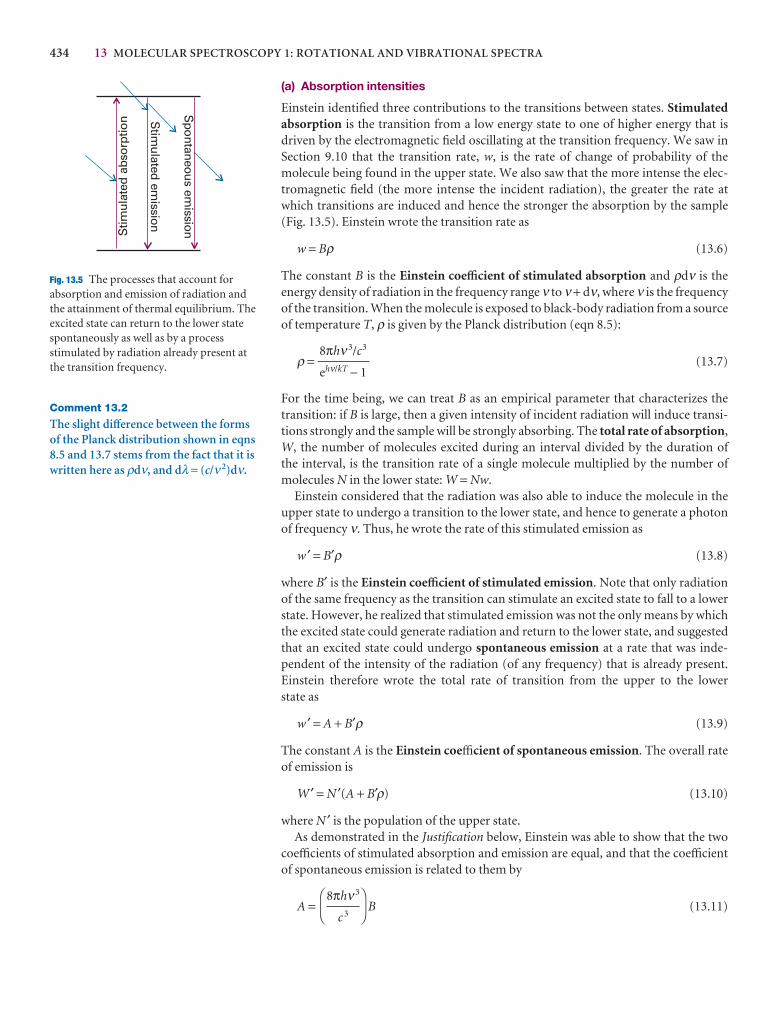
434 13 MOLECULAR SPECTROSCOPY 1: ROTATIONAL AND VIBRATIONAL SPECTRA
(a) Absorption intensities
Einstein identified three contributions to the transitions between states. Stimulatedabsorption is the transition from a low energy state to one of higher energy that isdriven by the electromagnetic field oscillating at the transition frequency. We saw inSection 9.10 that the transition rate, w, is the rate of change of probability of themolecule being found in the upper state. We also saw that the more intense the elec-tromagnetic field (the more intense the incident radiation), the greater the rate atwhich transitions are induced and hence the stronger the absorption by the sample(Fig. 13.5). Einstein wrote the transition rate as
w = Bρ (13.6)
The constant B is the Einstein coefficient of stimulated absorption and ρdν is the energy density of radiation in the frequency range ν to ν + dν, where ν is the frequencyof the transition. When the molecule is exposed to black-body radiation from a sourceof temperature T, ρ is given by the Planck distribution (eqn 8.5):
ρ = (13.7)
For the time being, we can treat B as an empirical parameter that characterizes thetransition: if B is large, then a given intensity of incident radiation will induce transi-tions strongly and the sample will be strongly absorbing. The total rate of absorption,W, the number of molecules excited during an interval divided by the duration of the interval, is the transition rate of a single molecule multiplied by the number ofmolecules N in the lower state: W = Nw.
Einstein considered that the radiation was also able to induce the molecule in theupper state to undergo a transition to the lower state, and hence to generate a photonof frequency ν. Thus, he wrote the rate of this stimulated emission as
w ′ = B′ρ (13.8)
where B′ is the Einstein coefficient of stimulated emission. Note that only radiationof the same frequency as the transition can stimulate an excited state to fall to a lowerstate. However, he realized that stimulated emission was not the only means by whichthe excited state could generate radiation and return to the lower state, and suggestedthat an excited state could undergo spontaneous emission at a rate that was inde-pendent of the intensity of the radiation (of any frequency) that is already present.Einstein therefore wrote the total rate of transition from the upper to the lower state as
w ′ = A + B′ρ (13.9)
The constant A is the Einstein coefficient of spontaneous emission. The overall rateof emission is
W ′ = N ′(A + B′ρ) (13.10)
where N ′ is the population of the upper state.As demonstrated in the Justification below, Einstein was able to show that the two
coefficients of stimulated absorption and emission are equal, and that the coefficientof spontaneous emission is related to them by
A = B (13.11)DF
8πhν3
c 3
AC
8πhν3/c3
ehν/kT − 1
Stim
ulat
ed a
bsor
ptio
n Stim
ulated em
ission
Spontaneous em
ission
Fig. 13.5 The processes that account forabsorption and emission of radiation andthe attainment of thermal equilibrium. Theexcited state can return to the lower statespontaneously as well as by a processstimulated by radiation already present atthe transition frequency.
Comment 13.2
The slight difference between the formsof the Planck distribution shown in eqns8.5 and 13.7 stems from the fact that it iswritten here as ρdν, and dλ = (c/ν2)dν.
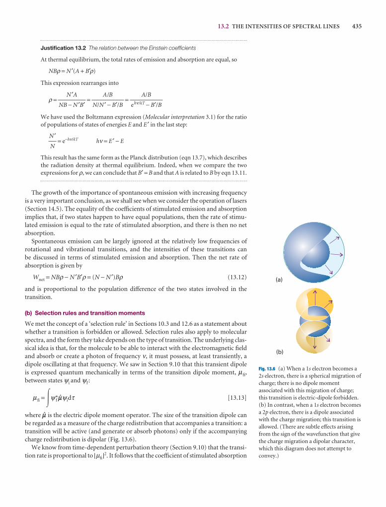
13.2 THE INTENSITIES OF SPECTRAL LINES 435
Justification 13.2 The relation between the Einstein coefficients
At thermal equilibrium, the total rates of emission and absorption are equal, so
NBρ = N ′(A + B′ρ)
This expression rearranges into
ρ = = =
We have used the Boltzmann expression (Molecular interpretation 3.1) for the ratioof populations of states of energies E and E ′ in the last step:
= e−hν/kT hν = E ′ − E
This result has the same form as the Planck distribution (eqn 13.7), which describesthe radiation density at thermal equilibrium. Indeed, when we compare the two expressions for ρ, we can conclude that B′ = B and that A is related to B by eqn 13.11.
The growth of the importance of spontaneous emission with increasing frequencyis a very important conclusion, as we shall see when we consider the operation of lasers(Section 14.5). The equality of the coefficients of stimulated emission and absorptionimplies that, if two states happen to have equal populations, then the rate of stimu-lated emission is equal to the rate of stimulated absorption, and there is then no net absorption.
Spontaneous emission can be largely ignored at the relatively low frequencies of rotational and vibrational transitions, and the intensities of these transitions can be discussed in terms of stimulated emission and absorption. Then the net rate of absorption is given by
Wnet = NBρ − N ′B′ρ = (N − N ′)Bρ (13.12)
and is proportional to the population difference of the two states involved in the transition.
(b) Selection rules and transition moments
We met the concept of a ‘selection rule’ in Sections 10.3 and 12.6 as a statement aboutwhether a transition is forbidden or allowed. Selection rules also apply to molecularspectra, and the form they take depends on the type of transition. The underlying clas-sical idea is that, for the molecule to be able to interact with the electromagnetic fieldand absorb or create a photon of frequency ν, it must possess, at least transiently, adipole oscillating at that frequency. We saw in Section 9.10 that this transient dipole is expressed quantum mechanically in terms of the transition dipole moment, µfi,between states ψi and ψf :
µfi = �ψ f*¢ψidτ [13.13]
where ¢ is the electric dipole moment operator. The size of the transition dipole canbe regarded as a measure of the charge redistribution that accompanies a transition: atransition will be active (and generate or absorb photons) only if the accompanyingcharge redistribution is dipolar (Fig. 13.6).
We know from time-dependent perturbation theory (Section 9.10) that the transi-tion rate is proportional to |µfi |2. It follows that the coefficient of stimulated absorption
N ′
N
A/B
ehν/kT − B′/B
A/B
N/N ′ − B′/B
N ′A
NB − N ′B′
(a)
(b)
Fig. 13.6 (a) When a 1s electron becomes a2s electron, there is a spherical migration ofcharge; there is no dipole momentassociated with this migration of charge;this transition is electric-dipole forbidden.(b) In contrast, when a 1s electron becomesa 2p electron, there is a dipole associatedwith the charge migration; this transition isallowed. (There are subtle effects arisingfrom the sign of the wavefunction that givethe charge migration a dipolar character,which this diagram does not attempt toconvey.)
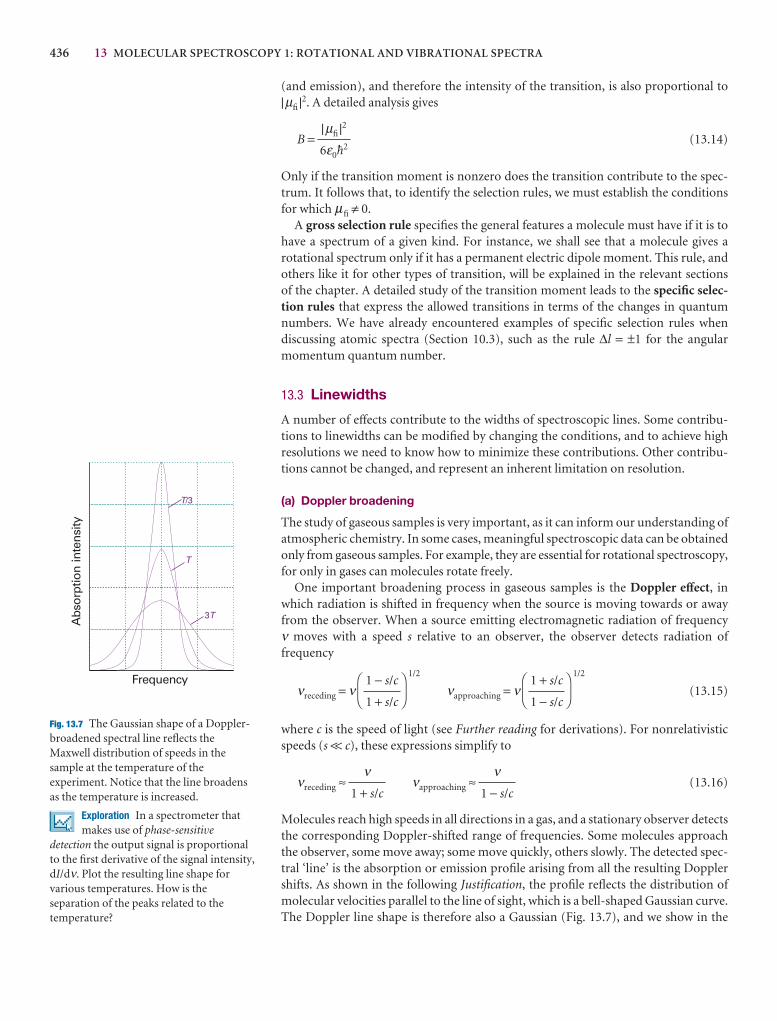
436 13 MOLECULAR SPECTROSCOPY 1: ROTATIONAL AND VIBRATIONAL SPECTRA
(and emission), and therefore the intensity of the transition, is also proportional to|µfi |2. A detailed analysis gives
B = (13.14)
Only if the transition moment is nonzero does the transition contribute to the spec-trum. It follows that, to identify the selection rules, we must establish the conditionsfor which µfi ≠ 0.
A gross selection rule specifies the general features a molecule must have if it is tohave a spectrum of a given kind. For instance, we shall see that a molecule gives a rotational spectrum only if it has a permanent electric dipole moment. This rule, andothers like it for other types of transition, will be explained in the relevant sections of the chapter. A detailed study of the transition moment leads to the specific selec-tion rules that express the allowed transitions in terms of the changes in quantumnumbers. We have already encountered examples of specific selection rules when discussing atomic spectra (Section 10.3), such as the rule ∆l = ±1 for the angularmomentum quantum number.
13.3 Linewidths
A number of effects contribute to the widths of spectroscopic lines. Some contribu-tions to linewidths can be modified by changing the conditions, and to achieve highresolutions we need to know how to minimize these contributions. Other contribu-tions cannot be changed, and represent an inherent limitation on resolution.
(a) Doppler broadening
The study of gaseous samples is very important, as it can inform our understanding ofatmospheric chemistry. In some cases, meaningful spectroscopic data can be obtainedonly from gaseous samples. For example, they are essential for rotational spectroscopy,for only in gases can molecules rotate freely.
One important broadening process in gaseous samples is the Doppler effect, inwhich radiation is shifted in frequency when the source is moving towards or awayfrom the observer. When a source emitting electromagnetic radiation of frequency ν moves with a speed s relative to an observer, the observer detects radiation of frequency
νreceding = ν1/2
νapproaching = ν1/2
(13.15)
where c is the speed of light (see Further reading for derivations). For nonrelativisticspeeds (s << c), these expressions simplify to
νreceding ≈ νapproaching ≈ (13.16)
Molecules reach high speeds in all directions in a gas, and a stationary observer detectsthe corresponding Doppler-shifted range of frequencies. Some molecules approachthe observer, some move away; some move quickly, others slowly. The detected spec-tral ‘line’ is the absorption or emission profile arising from all the resulting Dopplershifts. As shown in the following Justification, the profile reflects the distribution ofmolecular velocities parallel to the line of sight, which is a bell-shaped Gaussian curve.The Doppler line shape is therefore also a Gaussian (Fig. 13.7), and we show in the
ν1 − s/c
ν1 + s/c
DF
1 + s/c
1 − s/c
AC
DF
1 − s/c
1 + s/c
AC
|µfi |2
6ε0$2
T/3
T
3T
Frequency
Abs
orpt
ion
inte
nsity
Fig. 13.7 The Gaussian shape of a Doppler-broadened spectral line reflects theMaxwell distribution of speeds in thesample at the temperature of theexperiment. Notice that the line broadensas the temperature is increased.
Exploration In a spectrometer thatmakes use of phase-sensitive
detection the output signal is proportionalto the first derivative of the signal intensity,dI/dν. Plot the resulting line shape forvarious temperatures. How is theseparation of the peaks related to thetemperature?
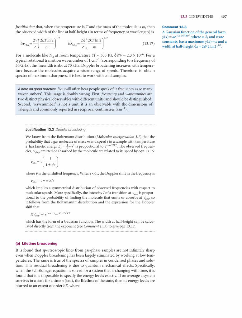
13.3 LINEWIDTHS 437
Justification that, when the temperature is T and the mass of the molecule is m, thenthe observed width of the line at half-height (in terms of frequency or wavelength) is
δνobs =1/2
δλobs =1/2
(13.17)
For a molecule like N2 at room temperature (T ≈ 300 K), δν/ν ≈ 2.3 × 10⁻⁶. For a typical rotational transition wavenumber of 1 cm−1 (corresponding to a frequency of 30 GHz), the linewidth is about 70 kHz. Doppler broadening increases with tempera-ture because the molecules acquire a wider range of speeds. Therefore, to obtain spectra of maximum sharpness, it is best to work with cold samples.
A note on good practice You will often hear people speak of ‘a frequency as so manywavenumbers’. This usage is doubly wrong. First, frequency and wavenumber aretwo distinct physical observables with different units, and should be distinguished.Second, ‘wavenumber’ is not a unit, it is an observable with the dimensions of1/length and commonly reported in reciprocal centimetres (cm−1).
Justification 13.3 Doppler broadening
We know from the Boltzmann distribution (Molecular interpretation 3.1) that theprobability that a gas molecule of mass m and speed s in a sample with temperatureT has kinetic energy EK = 1–2 ms2 is proportional to e−ms2/2kT. The observed frequen-cies, νobs, emitted or absorbed by the molecule are related to its speed by eqn 13.16:
νobs = ν
where ν is the unshifted frequency. When s << c, the Doppler shift in the frequency is
νobs − ν ≈ ±νs/c
which implies a symmetrical distribution of observed frequencies with respect tomolecular speeds. More specifically, the intensity I of a transition at νobs is propor-tional to the probability of finding the molecule that emits or absorbs at νobs, so it follows from the Boltzmannm distribution and the expression for the Dopplershift that
I(νobs) ∝ e−mc2(νobs−ν)2/2ν2kT
which has the form of a Gaussian function. The width at half-height can be calcu-lated directly from the exponent (see Comment 13.3) to give eqn 13.17.
(b) Lifetime broadening
It is found that spectroscopic lines from gas-phase samples are not infinitely sharpeven when Doppler broadening has been largely eliminated by working at low tem-peratures. The same is true of the spectra of samples in condensed phases and solu-tion. This residual broadening is due to quantum mechanical effects. Specifically,when the Schrödinger equation is solved for a system that is changing with time, it isfound that it is impossible to specify the energy levels exactly. If on average a systemsurvives in a state for a time τ (tau), the lifetime of the state, then its energy levels areblurred to an extent of order δE, where
DEF1
1 ± s/c
ABC
DF
2kT ln 2
m
AC
2λc
DF
2kT ln 2
m
AC
2νc
Comment 13.3
A Gaussian function of the general formy(x) = ae−(x−b)2/2σ2
, where a, b, and σ areconstants, has a maximum y(b) = a and awidth at half-height δx = 2σ(2 ln 2)1/2.
438 13 MOLECULAR SPECTROSCOPY 1: ROTATIONAL AND VIBRATIONAL SPECTRA
δE ≈ (13.18)
This expression is reminiscent of the Heisenberg uncertainty principle (eqn 8.40), andconsequently this lifetime broadening is often called ‘uncertainty broadening’. Whenthe energy spread is expressed as a wavenumber through δE = hcδ#, and the values ofthe fundamental constants introduced, this relation becomes
δ# ≈ (13.19)
No excited state has an infinite lifetime; therefore, all states are subject to some life-time broadening and, the shorter the lifetimes of the states involved in a transition, thebroader the corresponding spectral lines.
Two processes are responsible for the finite lifetimes of excited states. The domin-ant one for low frequency transitions is collisional deactivation, which arises fromcollisions between molecules or with the walls of the container. If the collisional life-time, the mean time between collisions, is τcol, the resulting collisional linewidth isδEcol ≈ $/τcol. Because τcol = 1/z, where z is the collision frequency, and from the kineticmodel of gases (Section 1.3) we know that z is proportional to the pressure, we see thatthe collisional linewidth is proportional to the pressure. The collisional linewidth cantherefore be minimized by working at low pressures.
The rate of spontaneous emission cannot be changed. Hence it is a natural limit tothe lifetime of an excited state, and the resulting lifetime broadening is the naturallinewidth of the transition. The natural linewidth is an intrinsic property of the transition, and cannot be changed by modifying the conditions. Natural linewidths depend strongly on the transition frequency (they increase with the coefficient ofspontaneous emission A and therefore as ν3), so low frequency transitions (such as themicrowave transitions of rotational spectroscopy) have very small natural linewidths,and collisional and Doppler line-broadening processes are dominant. The naturallifetimes of electronic transitions are very much shorter than for vibrational and rota-tional transitions, so the natural linewidths of electronic transitions are much greaterthan those of vibrational and rotational transitions. For example, a typical electronicexcited state natural lifetime is about 10−8 s (10 ns), corresponding to a natural widthof about 5 × 10⁻⁴ cm−1 (15 MHz). A typical rotational state natural lifetime is about 103 s, corresponding to a natural linewidth of only 5 × 10⁻¹⁵ cm−1 (of the order of 10−4 Hz).
IMPACT ON ASTROPHYSICS
I13.1 Rotational and vibrational spectroscopy of interstellar space
Observations by the Cosmic Background Explorer (COBE) satellite support the long-held hypothesis that the distribution of energy in the current Universe can bemodelled by a Planck distribution (eqn. 8.5) with T = 2.726 ± 0.001 K, the bulk of theradiation spanning the microwave region of the spectrum. This cosmic microwavebackground radiation is the residue of energy released during the Big Bang, the eventthat brought the Universe into existence. Very small fluctuations in the backgroundtemperature are believed to account for the large-scale structure of the Universe.
The interstellar space in our galaxy is a little warmer than the cosmic backgroundand consists largely of dust grains and gas clouds. The dust grains are carbon-basedcompounds and silicates of aluminium, magnesium, and iron, in which are embeddedtrace amounts of methane, water, and ammonia. Interstellar clouds are significant because it is from them that new stars, and consequently new planets, are formed. Thehottest clouds are plasmas with temperatures of up to 106 K and densities of onlyabout 3 × 10³ particles m−3. Colder clouds range from 0.1 to 1000 solar masses (1 solar
5.3 cm−1
τ /ps
$
τ
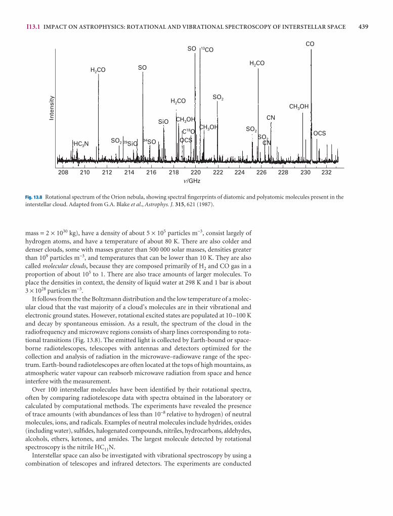
I13.1 IMPACT ON ASTROPHYSICS: ROTATIONAL AND VIBRATIONAL SPECTROSCOPY OF INTERSTELLAR SPACE 439
mass = 2 × 1030 kg), have a density of about 5 × 10⁵ particles m−3, consist largely of hydrogen atoms, and have a temperature of about 80 K. There are also colder anddenser clouds, some with masses greater than 500 000 solar masses, densities greaterthan 109 particles m−3, and temperatures that can be lower than 10 K. They are alsocalled molecular clouds, because they are composed primarily of H2 and CO gas in aproportion of about 105 to 1. There are also trace amounts of larger molecules. Toplace the densities in context, the density of liquid water at 298 K and 1 bar is about 3 × 1028 particles m−3.
It follows from the the Boltzmann distribution and the low temperature of a molec-ular cloud that the vast majority of a cloud’s molecules are in their vibrational andelectronic ground states. However, rotational excited states are populated at 10–100 Kand decay by spontaneous emission. As a result, the spectrum of the cloud in the radiofrequency and microwave regions consists of sharp lines corresponding to rota-tional transitions (Fig. 13.8). The emitted light is collected by Earth-bound or space-borne radiotelescopes, telescopes with antennas and detectors optimized for thecollection and analysis of radiation in the microwave–radiowave range of the spec-trum. Earth-bound radiotelescopes are often located at the tops of high mountains, asatmospheric water vapour can reabsorb microwave radiation from space and henceinterfere with the measurement.
Over 100 interstellar molecules have been identified by their rotational spectra,often by comparing radiotelescope data with spectra obtained in the laboratory or calculated by computational methods. The experiments have revealed the presence of trace amounts (with abundances of less than 10−8 relative to hydrogen) of neutralmolecules, ions, and radicals. Examples of neutral molecules include hydrides, oxides(including water), sulfides, halogenated compounds, nitriles, hydrocarbons, aldehydes,alcohols, ethers, ketones, and amides. The largest molecule detected by rotationalspectroscopy is the nitrile HC11N.
Interstellar space can also be investigated with vibrational spectroscopy by using acombination of telescopes and infrared detectors. The experiments are conducted
Fig. 13.8 Rotational spectrum of the Orion nebula, showing spectral fingerprints of diatomic and polyatomic molecules present in theinterstellar cloud. Adapted from G.A. Blake et al., Astrophys. J. 315, 621 (1987).
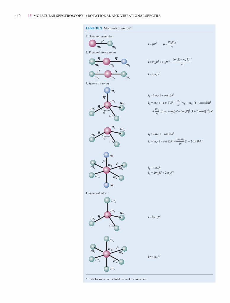
440 13 MOLECULAR SPECTROSCOPY 1: ROTATIONAL AND VIBRATIONAL SPECTRA
RmA mB
R �
mA mB mC
R
mA mB
R R
mA
mC
mB mA
mA
mAR
R �
�
mB
mC
mC
mA mA
mA mA
RR �
mB mA
mA
mAR
�
mB mA
mA
mAR
mA
mB
mA mA
mA mA
R
mA
mA
Table 13.1 Moments of inertia*
1. Diatomic molecules
I = µR2 µ =
2. Triatomic linear rotors
I = mAR2 + mCR′2 −
I = 2mAR2
3. Symmetric rotors
I|| = 2mA(1 − cosθ)R2
I⊥ = mA(1 − cosθ)R2 + (mB + mC)(1 + 2cosθ)R2
+ {(3mA + mB)R′+ 6mAR[1–3 (1 + 2cosθ)]1/2}R′
I|| = 2mA(1 − cosθ)R2
I⊥ = mA(1 − cosθ)R2 + (1 + 2cosθ)R2
I|| = 4mAR2
I⊥ = 2mAR2 + 2mCR′2
4. Spherical rotors
I = 8–3 mAR2
I = 4mAR2
* In each case, m is the total mass of the molecule.
mAmB
m
mC
m
mA
m
(mAR − mCR′)2
m
mAmB
m
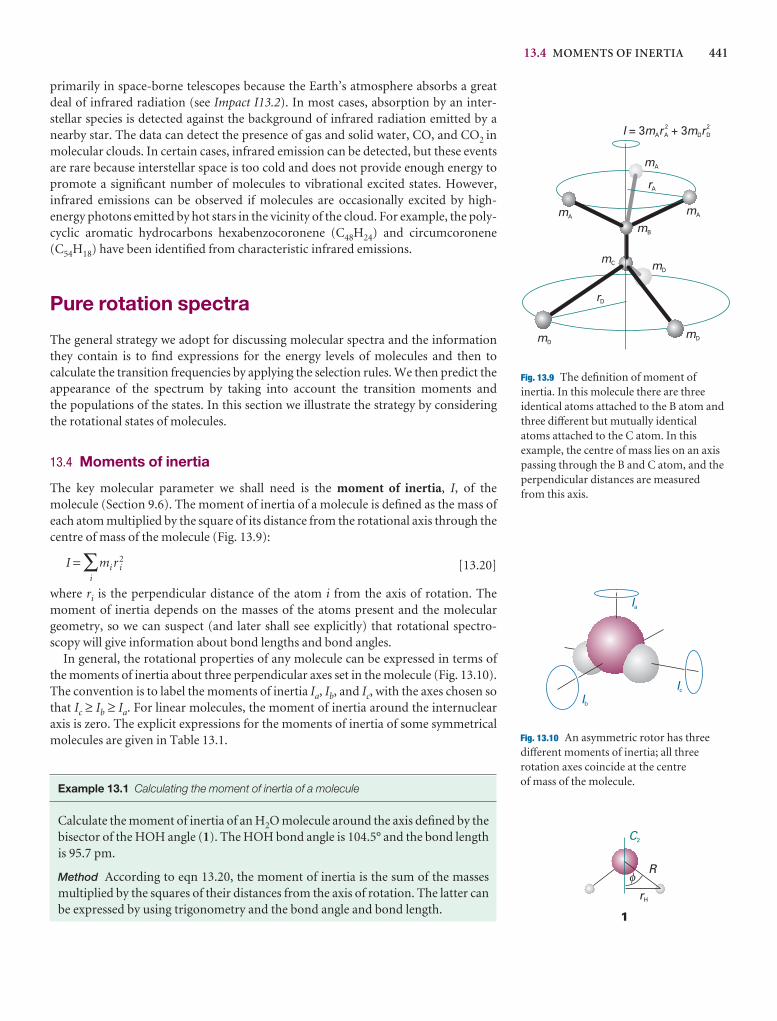
13.4 MOMENTS OF INERTIA 441
mC
mDmD
mD
rD
mA
mA
mA
mB
rA
I m r m r= 3 + 3A A D D2 2
Fig. 13.9 The definition of moment ofinertia. In this molecule there are threeidentical atoms attached to the B atom andthree different but mutually identicalatoms attached to the C atom. In thisexample, the centre of mass lies on an axispassing through the B and C atom, and theperpendicular distances are measured from this axis.
Ia
Ib
Ic
Fig. 13.10 An asymmetric rotor has threedifferent moments of inertia; all threerotation axes coincide at the centre of mass of the molecule.
rH
R�
1
C2
primarily in space-borne telescopes because the Earth’s atmosphere absorbs a greatdeal of infrared radiation (see Impact I13.2). In most cases, absorption by an inter-stellar species is detected against the background of infrared radiation emitted by anearby star. The data can detect the presence of gas and solid water, CO, and CO2 inmolecular clouds. In certain cases, infrared emission can be detected, but these eventsare rare because interstellar space is too cold and does not provide enough energy topromote a significant number of molecules to vibrational excited states. However, infrared emissions can be observed if molecules are occasionally excited by high-energy photons emitted by hot stars in the vicinity of the cloud. For example, the poly-cyclic aromatic hydrocarbons hexabenzocoronene (C48H24) and circumcoronene(C54H18) have been identified from characteristic infrared emissions.
Pure rotation spectra
The general strategy we adopt for discussing molecular spectra and the informationthey contain is to find expressions for the energy levels of molecules and then to calculate the transition frequencies by applying the selection rules. We then predict theappearance of the spectrum by taking into account the transition moments and the populations of the states. In this section we illustrate the strategy by considering the rotational states of molecules.
13.4 Moments of inertia
The key molecular parameter we shall need is the moment of inertia, I, of themolecule (Section 9.6). The moment of inertia of a molecule is defined as the mass ofeach atom multiplied by the square of its distance from the rotational axis through thecentre of mass of the molecule (Fig. 13.9):
I = ∑i
mi r i2
[13.20]
where ri is the perpendicular distance of the atom i from the axis of rotation. The moment of inertia depends on the masses of the atoms present and the molecular geometry, so we can suspect (and later shall see explicitly) that rotational spectro-scopy will give information about bond lengths and bond angles.
In general, the rotational properties of any molecule can be expressed in terms ofthe moments of inertia about three perpendicular axes set in the molecule (Fig. 13.10).The convention is to label the moments of inertia Ia, Ib, and Ic, with the axes chosen sothat Ic ≥ Ib ≥ Ia. For linear molecules, the moment of inertia around the internuclearaxis is zero. The explicit expressions for the moments of inertia of some symmetricalmolecules are given in Table 13.1.
Example 13.1 Calculating the moment of inertia of a molecule
Calculate the moment of inertia of an H2O molecule around the axis defined by thebisector of the HOH angle (1). The HOH bond angle is 104.5° and the bond lengthis 95.7 pm.
Method According to eqn 13.20, the moment of inertia is the sum of the massesmultiplied by the squares of their distances from the axis of rotation. The latter canbe expressed by using trigonometry and the bond angle and bond length.
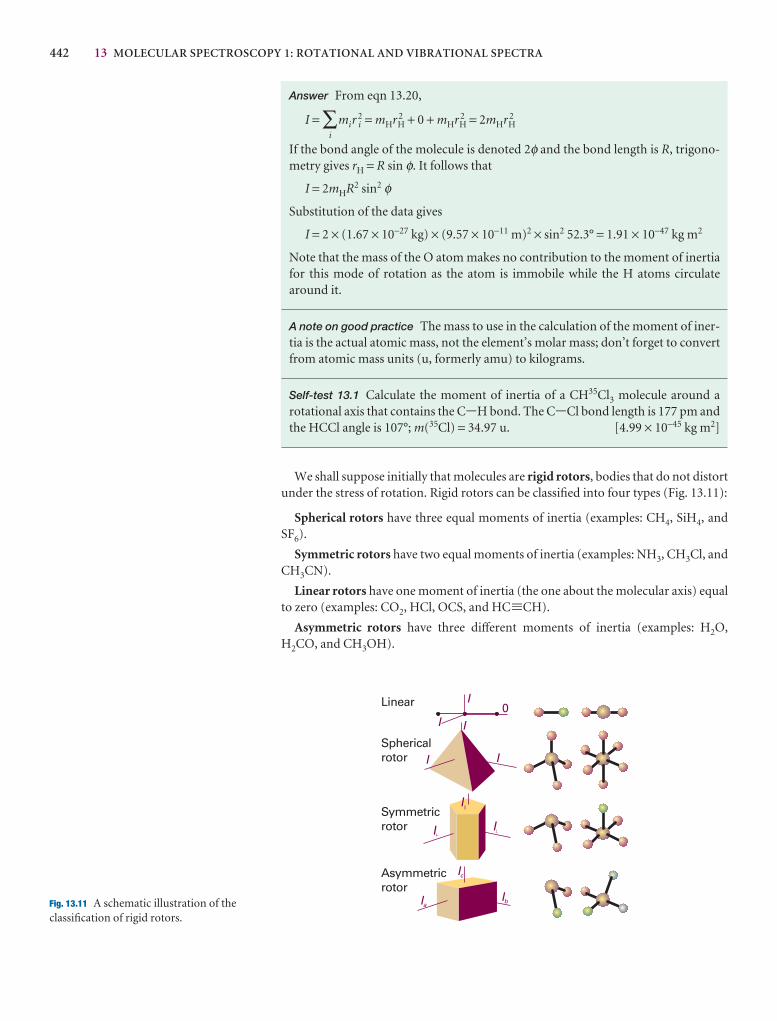
442 13 MOLECULAR SPECTROSCOPY 1: ROTATIONAL AND VIBRATIONAL SPECTRA
I
I I
II
Ia
Ic
Ib
0Linear
Sphericalrotor
Symmetricrotor
I
I I
Asymmetricrotor
Fig. 13.11 A schematic illustration of theclassification of rigid rotors.
Answer From eqn 13.20,
I = ∑i
mir2i = mHr 2
H + 0 + mHr 2H = 2mHr 2
H
If the bond angle of the molecule is denoted 2φ and the bond length is R, trigono-metry gives rH = R sin φ. It follows that
I = 2mHR2 sin2 φ
Substitution of the data gives
I = 2 × (1.67 × 10−27 kg) × (9.57 × 10⁻¹¹ m)2 × sin2 52.3° = 1.91 × 10−47 kg m2
Note that the mass of the O atom makes no contribution to the moment of inertiafor this mode of rotation as the atom is immobile while the H atoms circulatearound it.
A note on good practice The mass to use in the calculation of the moment of iner-tia is the actual atomic mass, not the element’s molar mass; don’t forget to convertfrom atomic mass units (u, formerly amu) to kilograms.
Self-test 13.1 Calculate the moment of inertia of a CH35Cl3 molecule around a rotational axis that contains the C-H bond. The C-Cl bond length is 177 pm andthe HCCl angle is 107°; m(35Cl) = 34.97 u. [4.99 × 10−45 kg m2]
We shall suppose initially that molecules are rigid rotors, bodies that do not distortunder the stress of rotation. Rigid rotors can be classified into four types (Fig. 13.11):
Spherical rotors have three equal moments of inertia (examples: CH4, SiH4, andSF6).
Symmetric rotors have two equal moments of inertia (examples: NH3, CH3Cl, andCH3CN).
Linear rotors have one moment of inertia (the one about the molecular axis) equalto zero (examples: CO2, HCl, OCS, and HC.CH).
Asymmetric rotors have three different moments of inertia (examples: H2O,H2CO, and CH3OH).
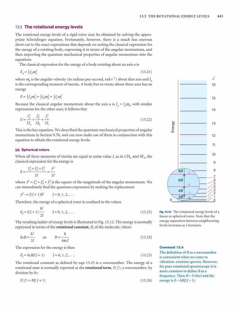
13.5 THE ROTATIONAL ENERGY LEVELS 443
13.5 The rotational energy levels
The rotational energy levels of a rigid rotor may be obtained by solving the appro-priate Schrödinger equation. Fortunately, however, there is a much less onerous short cut to the exact expressions that depends on noting the classical expression forthe energy of a rotating body, expressing it in terms of the angular momentum, andthen importing the quantum mechanical properties of angular momentum into the equations.
The classical expression for the energy of a body rotating about an axis a is
Ea = 1–2Iaω a2 (13.21)
where ωa is the angular velocity (in radians per second, rad s−1) about that axis and Ia
is the corresponding moment of inertia. A body free to rotate about three axes has anenergy
E = 1–2Iaω a2 + 1–2Ibω b
2 + 1–2Icω c2
Because the classical angular momentum about the axis a is Ja = Iaωa, with similar expressions for the other axes, it follows that
E = + + (13.22)
This is the key equation. We described the quantum mechanical properties of angularmomentum in Section 9.7b, and can now make use of them in conjunction with thisequation to obtain the rotational energy levels.
(a) Spherical rotors
When all three moments of inertia are equal to some value I, as in CH4 and SF6, theclassical expression for the energy is
E = =
where J 2 = Ja2 + Jb
2 + J c2 is the square of the magnitude of the angular momentum. We
can immediately find the quantum expression by making the replacement
J 2 → J(J + 1)$2 J = 0, 1, 2, . . .
Therefore, the energy of a spherical rotor is confined to the values
EJ = J(J + 1) J = 0, 1, 2, . . . (13.23)
The resulting ladder of energy levels is illustrated in Fig. 13.12. The energy is normallyexpressed in terms of the rotational constant, B, of the molecule, where
hcB = so B = [13.24]
The expression for the energy is then
EJ = hcBJ(J + 1) J = 0, 1, 2, . . . (13.25)
The rotational constant as defined by eqn 13.25 is a wavenumber. The energy of a rotational state is normally reported as the rotational term, F( J), a wavenumber, bydivision by hc:
F( J) = BJ( J + 1) (13.26)
$
4πcI
$2
2I
$2
2I
J 2
2I
Ja2 + Jb
2 + J c2
2I
J c2
2Ic
J b2
2Ib
J a2
2Ia
01234567
8
9
10
11
12
13
14
15
16
0
Ener
gy
J
2B
4B
6B
8B
0
1
2
3
Fig. 13.12 The rotational energy levels of alinear or spherical rotor. Note that theenergy separation between neighbouringlevels increases as J increases.
Comment 13.4
The definition of B as a wavenumber is convenient when we come tovibration–rotation spectra. However,for pure rotational spectroscopy it ismore common to define B as afrequency. Then B = $/4πcI and theenergy is E = hBJ(J + 1).
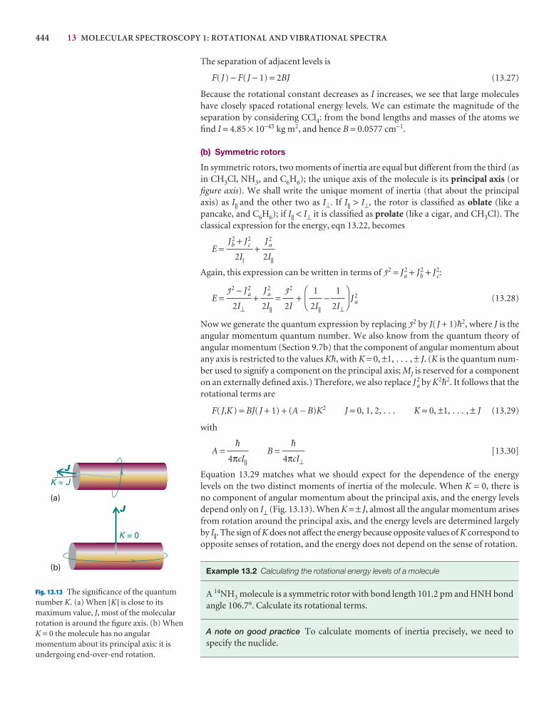
444 13 MOLECULAR SPECTROSCOPY 1: ROTATIONAL AND VIBRATIONAL SPECTRA
K = 0
K J»
J
J(a)
(b)
Fig. 13.13 The significance of the quantumnumber K. (a) When |K | is close to itsmaximum value, J, most of the molecularrotation is around the figure axis. (b) WhenK = 0 the molecule has no angularmomentum about its principal axis: it isundergoing end-over-end rotation.
The separation of adjacent levels is
F( J) − F( J − 1) = 2BJ (13.27)
Because the rotational constant decreases as I increases, we see that large moleculeshave closely spaced rotational energy levels. We can estimate the magnitude of theseparation by considering CCl4: from the bond lengths and masses of the atoms wefind I = 4.85 × 10−45 kg m2, and hence B = 0.0577 cm−1.
(b) Symmetric rotors
In symmetric rotors, two moments of inertia are equal but different from the third (asin CH3Cl, NH3, and C6H6); the unique axis of the molecule is its principal axis (orfigure axis). We shall write the unique moment of inertia (that about the principalaxis) as I|| and the other two as I⊥. If I|| > I⊥, the rotor is classified as oblate (like a pancake, and C6H6); if I|| < I⊥ it is classified as prolate (like a cigar, and CH3Cl). Theclassical expression for the energy, eqn 13.22, becomes
E = +
Again, this expression can be written in terms of J 2 = Ja2 + Jb
2 + J c2:
E = + = + − J a2 (13.28)
Now we generate the quantum expression by replacing J 2 by J( J + 1)$2, where J is theangular momentum quantum number. We also know from the quantum theory ofangular momentum (Section 9.7b) that the component of angular momentum aboutany axis is restricted to the values K$, with K = 0, ±1, . . . , ± J. (K is the quantum num-ber used to signify a component on the principal axis; MJ is reserved for a componenton an externally defined axis.) Therefore, we also replace J a
2 by K2$2. It follows that therotational terms are
F( J,K) = BJ( J + 1) + (A − B)K2 J = 0, 1, 2, . . . K = 0, ±1, . . . , ± J (13.29)
with
A = B = [13.30]
Equation 13.29 matches what we should expect for the dependence of the energylevels on the two distinct moments of inertia of the molecule. When K = 0, there is no component of angular momentum about the principal axis, and the energy levelsdepend only on I⊥ (Fig. 13.13). When K = ± J, almost all the angular momentum arisesfrom rotation around the principal axis, and the energy levels are determined largelyby I||. The sign of K does not affect the energy because opposite values of K correspond toopposite senses of rotation, and the energy does not depend on the sense of rotation.
Example 13.2 Calculating the rotational energy levels of a molecule
A 14NH3 molecule is a symmetric rotor with bond length 101.2 pm and HNH bondangle 106.7°. Calculate its rotational terms.
A note on good practice To calculate moments of inertia precisely, we need tospecify the nuclide.
$
4πcI⊥
$
4πcI||
DF
1
2I⊥
1
2I||
AC
J 2
2I
J a2
2I||
J 2 − J a2
2I⊥
J a2
2I||
Jb2 + J c
2
2I|
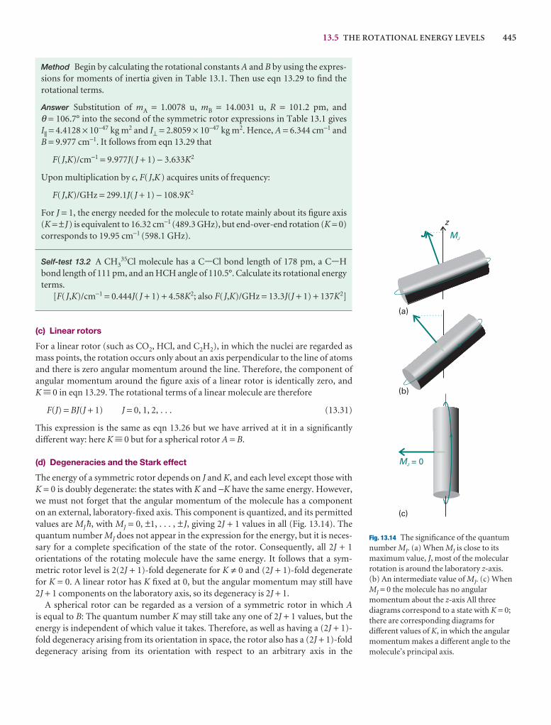
13.5 THE ROTATIONAL ENERGY LEVELS 445
J MJ
MJ = 0
z
(a)
(b)
(c)
Fig. 13.14 The significance of the quantumnumber MJ. (a) When MJ is close to itsmaximum value, J, most of the molecularrotation is around the laboratory z-axis.(b) An intermediate value of MJ. (c) WhenMJ = 0 the molecule has no angularmomentum about the z-axis All threediagrams correspond to a state with K = 0;there are corresponding diagrams fordifferent values of K, in which the angularmomentum makes a different angle to themolecule’s principal axis.
Method Begin by calculating the rotational constants A and B by using the expres-sions for moments of inertia given in Table 13.1. Then use eqn 13.29 to find the rotational terms.
Answer Substitution of mA = 1.0078 u, mB = 14.0031 u, R = 101.2 pm, and θ = 106.7° into the second of the symmetric rotor expressions in Table 13.1 gives I|| = 4.4128 × 10−47 kg m2 and I⊥ = 2.8059 × 10−47 kg m2. Hence, A = 6.344 cm−1 andB = 9.977 cm−1. It follows from eqn 13.29 that
F( J,K)/cm−1 = 9.977J( J + 1) − 3.633K2
Upon multiplication by c, F( J,K) acquires units of frequency:
F( J,K)/GHz = 299.1J( J + 1) − 108.9K2
For J = 1, the energy needed for the molecule to rotate mainly about its figure axis(K = ±J) is equivalent to 16.32 cm−1 (489.3 GHz), but end-over-end rotation (K = 0)corresponds to 19.95 cm−1 (598.1 GHz).
Self-test 13.2 A CH335Cl molecule has a C-Cl bond length of 178 pm, a C-H
bond length of 111 pm, and an HCH angle of 110.5°. Calculate its rotational energyterms.
[F( J,K)/cm−1 = 0.444J( J + 1) + 4.58K2; also F( J,K)/GHz = 13.3J(J + 1) + 137K2]
(c) Linear rotors
For a linear rotor (such as CO2, HCl, and C2H2), in which the nuclei are regarded asmass points, the rotation occurs only about an axis perpendicular to the line of atomsand there is zero angular momentum around the line. Therefore, the component ofangular momentum around the figure axis of a linear rotor is identically zero, and K . 0 in eqn 13.29. The rotational terms of a linear molecule are therefore
F(J) = BJ(J + 1) J = 0, 1, 2, . . . (13.31)
This expression is the same as eqn 13.26 but we have arrived at it in a significantlydifferent way: here K . 0 but for a spherical rotor A = B.
(d) Degeneracies and the Stark effect
The energy of a symmetric rotor depends on J and K, and each level except those withK = 0 is doubly degenerate: the states with K and −K have the same energy. However,we must not forget that the angular momentum of the molecule has a component on an external, laboratory-fixed axis. This component is quantized, and its permitted values are MJ $, with MJ = 0, ±1, . . . , ± J, giving 2J + 1 values in all (Fig. 13.14). Thequantum number MJ does not appear in the expression for the energy, but it is neces-sary for a complete specification of the state of the rotor. Consequently, all 2J + 1orientations of the rotating molecule have the same energy. It follows that a sym-metric rotor level is 2(2J + 1)-fold degenerate for K ≠ 0 and (2J + 1)-fold degeneratefor K = 0. A linear rotor has K fixed at 0, but the angular momentum may still have 2J + 1 components on the laboratory axis, so its degeneracy is 2J + 1.
A spherical rotor can be regarded as a version of a symmetric rotor in which Ais equal to B: The quantum number K may still take any one of 2J + 1 values, but the energy is independent of which value it takes. Therefore, as well as having a (2J + 1)-fold degeneracy arising from its orientation in space, the rotor also has a (2J + 1)-folddegeneracy arising from its orientation with respect to an arbitrary axis in the
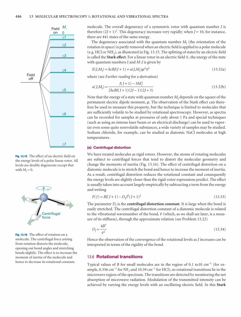
446 13 MOLECULAR SPECTROSCOPY 1: ROTATIONAL AND VIBRATIONAL SPECTRA
molecule. The overall degeneracy of a symmetric rotor with quantum number J istherefore (2J + 1)2. This degeneracy increases very rapidly: when J = 10, for instance,there are 441 states of the same energy.
The degeneracy associated with the quantum number MJ (the orientation of the rotation in space) is partly removed when an electric field is applied to a polar molecule(e.g. HCl or NH3), as illustrated in Fig. 13.15. The splitting of states by an electric fieldis called the Stark effect. For a linear rotor in an electric field E , the energy of the statewith quantum numbers J and M-J is given by
E(J,MJ) = hcBJ(J + 1) + a(J,MJ)µ2E2 (13.32a)
where (see Further reading for a derivation)
a( J,MJ) = (13.32b)
Note that the energy of a state with quantum number MJ depends on the square of thepermanent electric dipole moment, µ. The observation of the Stark effect can there-fore be used to measure this property, but the technique is limited to molecules thatare sufficiently volatile to be studied by rotational spectroscopy. However, as spectracan be recorded for samples at pressures of only about 1 Pa and special techniques(such as using an intense laser beam or an electrical discharge) can be used to vapor-ize even some quite nonvolatile substances, a wide variety of samples may be studied.Sodium chloride, for example, can be studied as diatomic NaCl molecules at hightemperatures.
(e) Centrifugal distortion
We have treated molecules as rigid rotors. However, the atoms of rotating moleculesare subject to centrifugal forces that tend to distort the molecular geometry andchange the moments of inertia (Fig. 13.16). The effect of centrifugal distortion on adiatomic molecule is to stretch the bond and hence to increase the moment of inertia.As a result, centrifugal distortion reduces the rotational constant and consequentlythe energy levels are slightly closer than the rigid-rotor expressions predict. The effectis usually taken into account largely empirically by subtracting a term from the energyand writing
F( J) = BJ( J + 1) − DJ J2( J + 1)2 (13.33)
The parameter DJ is the centrifugal distortion constant. It is large when the bond iseasily stretched. The centrifugal distortion constant of a diatomic molecule is relatedto the vibrational wavenumber of the bond, # (which, as we shall see later, is a meas-ure of its stiffness), through the approximate relation (see Problem 13.22)
DJ = (13.34)
Hence the observation of the convergence of the rotational levels as J increases can beinterpreted in terms of the rigidity of the bond.
13.6 Rotational transitions
Typical values of B for small molecules are in the region of 0.1 to10 cm−1 (for ex-ample, 0.356 cm−1 for NF3 and 10.59 cm−1 for HCl), so rotational transitions lie in the microwave region of the spectrum. The transitions are detected by monitoring the netabsorption of microwave radiation. Modulation of the transmitted intensity can beachieved by varying the energy levels with an oscillating electric field. In this Stark
4B3
#2
J( J + 1) − 3M2J
2hcBJ( J + 1)(2J − 1)(2J + 3)
0%1
%2
%3
%4
%5
%6
%7
MJFieldon
Fieldoff
Fig. 13.15 The effect of an electric field onthe energy levels of a polar linear rotor. Alllevels are doubly degenerate except thatwith MJ = 0.
Centrifugalforce
Fig. 13.16 The effect of rotation on amolecule. The centrifugal force arisingfrom rotation distorts the molecule,opening out bond angles and stretchingbonds slightly. The effect is to increase themoment of inertia of the molecule andhence to decrease its rotational constant.
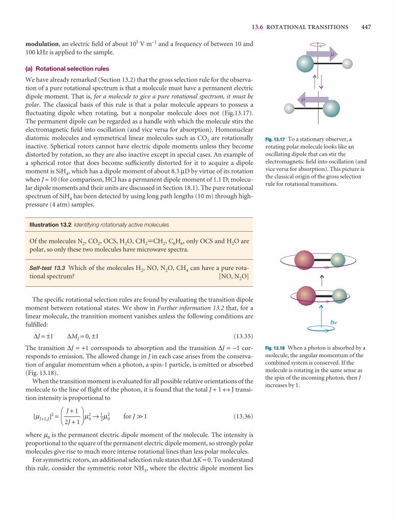
13.6 ROTATIONAL TRANSITIONS 447
m
m
Fig. 13.17 To a stationary observer, arotating polar molecule looks like anoscillating dipole that can stir theelectromagnetic field into oscillation (andvice versa for absorption). This picture isthe classical origin of the gross selectionrule for rotational transitions.
hn
Fig. 13.18 When a photon is absorbed by amolecule, the angular momentum of thecombined system is conserved. If themolecule is rotating in the same sense asthe spin of the incoming photon, then Jincreases by 1.
modulation, an electric field of about 105 V m−1 and a frequency of between 10 and100 kHz is applied to the sample.
(a) Rotational selection rules
We have already remarked (Section 13.2) that the gross selection rule for the observa-tion of a pure rotational spectrum is that a molecule must have a permanent electricdipole moment. That is, for a molecule to give a pure rotational spectrum, it must bepolar. The classical basis of this rule is that a polar molecule appears to possess a fluctuating dipole when rotating, but a nonpolar molecule does not (Fig.13.17). The permanent dipole can be regarded as a handle with which the molecule stirs theelectromagnetic field into oscillation (and vice versa for absorption). Homonuclear diatomic molecules and symmetrical linear molecules such as CO2 are rotationally inactive. Spherical rotors cannot have electric dipole moments unless they becomedistorted by rotation, so they are also inactive except in special cases. An example ofa spherical rotor that does become sufficiently distorted for it to acquire a dipole moment is SiH4, which has a dipole moment of about 8.3 µD by virtue of its rotationwhen J ≈ 10 (for comparison, HCl has a permanent dipole moment of 1.1 D; molecu-lar dipole moments and their units are discussed in Section 18.1). The pure rotationalspectrum of SiH4 has been detected by using long path lengths (10 m) through high-pressure (4 atm) samples.
Illustration 13.2 Identifying rotationally active molecules
Of the molecules N2, CO2, OCS, H2O, CH2=CH2, C6H6, only OCS and H2O arepolar, so only these two molecules have microwave spectra.
Self-test 13.3 Which of the molecules H2, NO, N2O, CH4 can have a pure rota-tional spectrum? [NO, N2O]
The specific rotational selection rules are found by evaluating the transition dipolemoment between rotational states. We show in Further information 13.2 that, for a linear molecule, the transition moment vanishes unless the following conditions arefulfilled:
∆J = ±1 ∆MJ = 0, ±1 (13.35)
The transition ∆J = +1 corresponds to absorption and the transition ∆J = −1 cor-responds to emission. The allowed change in J in each case arises from the conserva-tion of angular momentum when a photon, a spin-1 particle, is emitted or absorbed(Fig. 13.18).
When the transition moment is evaluated for all possible relative orientations of themolecule to the line of flight of the photon, it is found that the total J + 1 ↔ J transi-tion intensity is proportional to
|µJ+1,J |2 = µ02 → 1–2µ0
2 for J >> 1 (13.36)
where µ0 is the permanent electric dipole moment of the molecule. The intensity isproportional to the square of the permanent electric dipole moment, so strongly polarmolecules give rise to much more intense rotational lines than less polar molecules.
For symmetric rotors, an additional selection rule states that ∆K = 0. To understandthis rule, consider the symmetric rotor NH3, where the electric dipole moment lies
DF
J + 1
2J + 1
AC
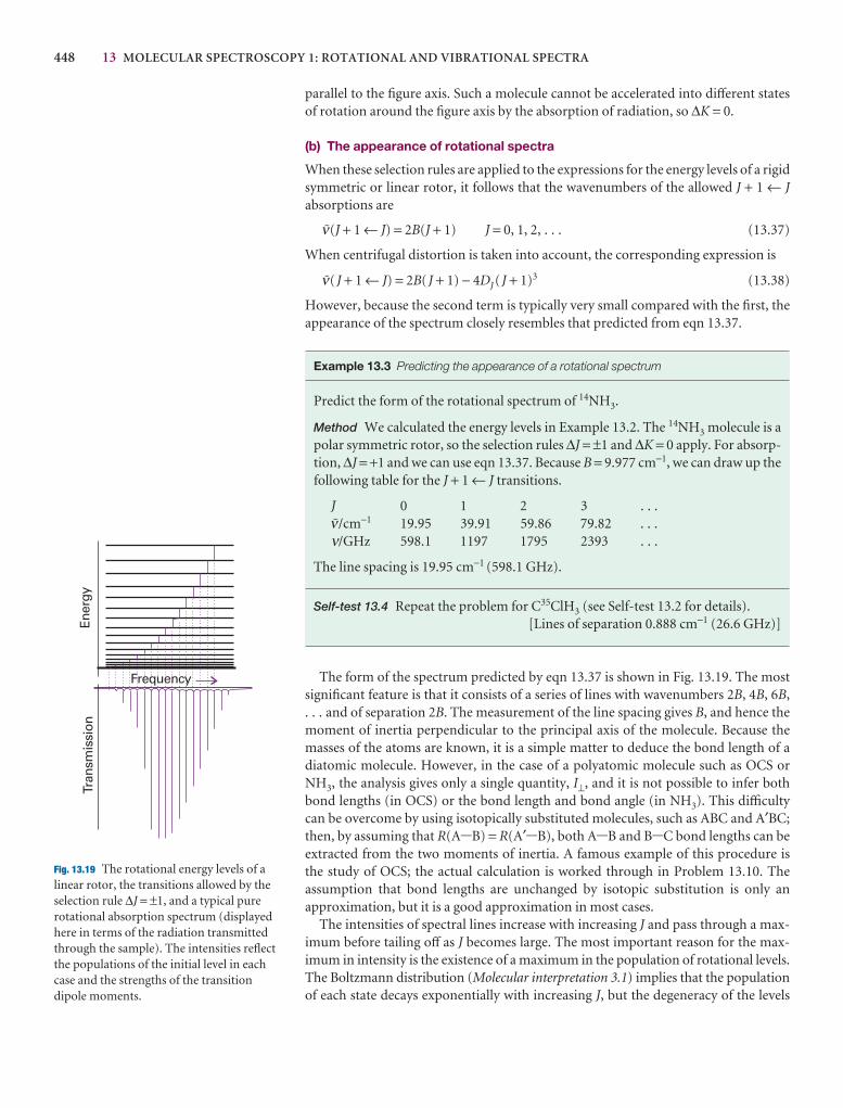
448 13 MOLECULAR SPECTROSCOPY 1: ROTATIONAL AND VIBRATIONAL SPECTRA
Ener
gy
Frequency
Tran
smis
sion
Fig. 13.19 The rotational energy levels of alinear rotor, the transitions allowed by theselection rule ∆J = ±1, and a typical purerotational absorption spectrum (displayedhere in terms of the radiation transmittedthrough the sample). The intensities reflectthe populations of the initial level in eachcase and the strengths of the transitiondipole moments.
parallel to the figure axis. Such a molecule cannot be accelerated into different statesof rotation around the figure axis by the absorption of radiation, so ∆K = 0.
(b) The appearance of rotational spectra
When these selection rules are applied to the expressions for the energy levels of a rigidsymmetric or linear rotor, it follows that the wavenumbers of the allowed J + 1 ← Jabsorptions are
#(J + 1 ← J) = 2B(J + 1) J = 0, 1, 2, . . . (13.37)
When centrifugal distortion is taken into account, the corresponding expression is
#( J + 1 ← J) = 2B( J + 1) − 4DJ ( J + 1)3 (13.38)
However, because the second term is typically very small compared with the first, theappearance of the spectrum closely resembles that predicted from eqn 13.37.
Example 13.3 Predicting the appearance of a rotational spectrum
Predict the form of the rotational spectrum of 14NH3.
Method We calculated the energy levels in Example 13.2. The 14NH3 molecule is apolar symmetric rotor, so the selection rules ∆J = ±1 and ∆K = 0 apply. For absorp-tion, ∆J = +1 and we can use eqn 13.37. Because B = 9.977 cm−1, we can draw up thefollowing table for the J + 1 ← J transitions.
J 0 1 2 3 . . .#/cm−1 19.95 39.91 59.86 79.82 . . .ν/GHz 598.1 1197 1795 2393 . . .
The line spacing is 19.95 cm−1 (598.1 GHz).
Self-test 13.4 Repeat the problem for C35ClH3 (see Self-test 13.2 for details).[Lines of separation 0.888 cm−1 (26.6 GHz)]
The form of the spectrum predicted by eqn 13.37 is shown in Fig. 13.19. The mostsignificant feature is that it consists of a series of lines with wavenumbers 2B, 4B, 6B,. . . and of separation 2B. The measurement of the line spacing gives B, and hence themoment of inertia perpendicular to the principal axis of the molecule. Because themasses of the atoms are known, it is a simple matter to deduce the bond length of a diatomic molecule. However, in the case of a polyatomic molecule such as OCS orNH3, the analysis gives only a single quantity, I⊥, and it is not possible to infer bothbond lengths (in OCS) or the bond length and bond angle (in NH3). This difficultycan be overcome by using isotopically substituted molecules, such as ABC and A′BC;then, by assuming that R(A-B) = R(A′-B), both A-B and B-C bond lengths can be extracted from the two moments of inertia. A famous example of this procedure is the study of OCS; the actual calculation is worked through in Problem 13.10. The assumption that bond lengths are unchanged by isotopic substitution is only an approximation, but it is a good approximation in most cases.
The intensities of spectral lines increase with increasing J and pass through a max-imum before tailing off as J becomes large. The most important reason for the max-imum in intensity is the existence of a maximum in the population of rotational levels.The Boltzmann distribution (Molecular interpretation 3.1) implies that the populationof each state decays exponentially with increasing J, but the degeneracy of the levels
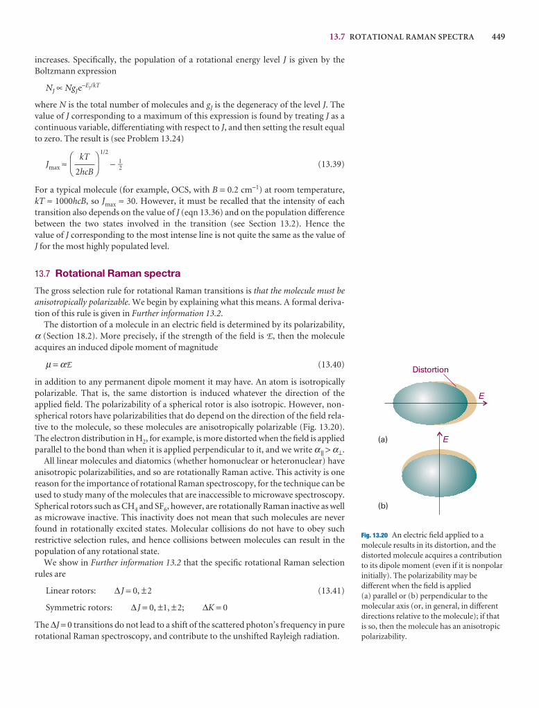
13.7 ROTATIONAL RAMAN SPECTRA 449
increases. Specifically, the population of a rotational energy level J is given by theBoltzmann expression
NJ ∝ NgJe−EJ/kT
where N is the total number of molecules and gJ is the degeneracy of the level J. Thevalue of J corresponding to a maximum of this expression is found by treating J as acontinuous variable, differentiating with respect to J, and then setting the result equalto zero. The result is (see Problem 13.24)
Jmax ≈1/2
− 1–2 (13.39)
For a typical molecule (for example, OCS, with B = 0.2 cm−1) at room temperature, kT ≈ 1000hcB, so Jmax ≈ 30. However, it must be recalled that the intensity of each transition also depends on the value of J (eqn 13.36) and on the population differencebetween the two states involved in the transition (see Section 13.2). Hence the value of J corresponding to the most intense line is not quite the same as the value of J for the most highly populated level.
13.7 Rotational Raman spectra
The gross selection rule for rotational Raman transitions is that the molecule must beanisotropically polarizable. We begin by explaining what this means. A formal deriva-tion of this rule is given in Further information 13.2.
The distortion of a molecule in an electric field is determined by its polarizability,α (Section 18.2). More precisely, if the strength of the field is E, then the molecule acquires an induced dipole moment of magnitude
µ = αE (13.40)
in addition to any permanent dipole moment it may have. An atom is isotropicallypolarizable. That is, the same distortion is induced whatever the direction of the applied field. The polarizability of a spherical rotor is also isotropic. However, non-spherical rotors have polarizabilities that do depend on the direction of the field rela-tive to the molecule, so these molecules are anisotropically polarizable (Fig. 13.20).The electron distribution in H2, for example, is more distorted when the field is appliedparallel to the bond than when it is applied perpendicular to it, and we write α|| > α⊥.
All linear molecules and diatomics (whether homonuclear or heteronuclear) haveanisotropic polarizabilities, and so are rotationally Raman active. This activity is onereason for the importance of rotational Raman spectroscopy, for the technique can beused to study many of the molecules that are inaccessible to microwave spectroscopy.Spherical rotors such as CH4 and SF6, however, are rotationally Raman inactive as wellas microwave inactive. This inactivity does not mean that such molecules are neverfound in rotationally excited states. Molecular collisions do not have to obey such restrictive selection rules, and hence collisions between molecules can result in thepopulation of any rotational state.
We show in Further information 13.2 that the specific rotational Raman selectionrules are
Linear rotors: ∆ J = 0, ±2 (13.41)
Symmetric rotors: ∆ J = 0, ±1, ±2; ∆K = 0
The ∆J = 0 transitions do not lead to a shift of the scattered photon’s frequency in purerotational Raman spectroscopy, and contribute to the unshifted Rayleigh radiation.
DF
kT
2hcB
AC
E
E
(a)
(b)
Distortion
Fig. 13.20 An electric field applied to amolecule results in its distortion, and thedistorted molecule acquires a contributionto its dipole moment (even if it is nonpolarinitially). The polarizability may bedifferent when the field is applied (a) parallel or (b) perpendicular to themolecular axis (or, in general, in differentdirections relative to the molecule); if thatis so, then the molecule has an anisotropicpolarizability.
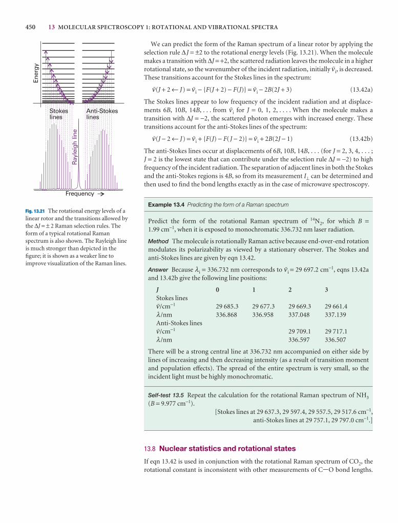
450 13 MOLECULAR SPECTROSCOPY 1: ROTATIONAL AND VIBRATIONAL SPECTRAEn
ergy
Stokeslines
Anti-Stokeslines
Ray
leig
h li
ne
Frequency
Fig. 13.21 The rotational energy levels of alinear rotor and the transitions allowed bythe ∆J = ± 2 Raman selection rules. Theform of a typical rotational Ramanspectrum is also shown. The Rayleigh lineis much stronger than depicted in thefigure; it is shown as a weaker line toimprove visualization of the Raman lines.
We can predict the form of the Raman spectrum of a linear rotor by applying theselection rule ∆ J = ±2 to the rotational energy levels (Fig. 13.21). When the moleculemakes a transition with ∆J = +2, the scattered radiation leaves the molecule in a higherrotational state, so the wavenumber of the incident radiation, initially #i, is decreased.These transitions account for the Stokes lines in the spectrum:
#(J + 2 ← J) = #i − {F(J + 2) − F(J)} = #i − 2B(2J + 3) (13.42a)
The Stokes lines appear to low frequency of the incident radiation and at displace-ments 6B, 10B, 14B, . . . from #i for J = 0, 1, 2, . . . . When the molecule makes a transition with ∆J = −2, the scattered photon emerges with increased energy. Thesetransitions account for the anti-Stokes lines of the spectrum:
#(J − 2 ← J) = #i + {F(J) − F( J − 2)} = #i + 2B(2J − 1) (13.42b)
The anti-Stokes lines occur at displacements of 6B, 10B, 14B, . . . (for J = 2, 3, 4, . . . ; J = 2 is the lowest state that can contribute under the selection rule ∆J = −2) to high frequency of the incident radiation. The separation of adjacent lines in both the Stokesand the anti-Stokes regions is 4B, so from its measurement I⊥ can be determined andthen used to find the bond lengths exactly as in the case of microwave spectroscopy.
Example 13.4 Predicting the form of a Raman spectrum
Predict the form of the rotational Raman spectrum of 14N2, for which B =1.99 cm−1, when it is exposed to monochromatic 336.732 nm laser radiation.
Method The molecule is rotationally Raman active because end-over-end rotationmodulates its polarizability as viewed by a stationary observer. The Stokes andanti-Stokes lines are given by eqn 13.42.
Answer Because λi = 336.732 nm corresponds to #i = 29 697.2 cm−1, eqns 13.42aand 13.42b give the following line positions:
J 0 1 2 3Stokes lines#/cm−1 29 685.3 29 677.3 29 669.3 29 661.4λ /nm 336.868 336.958 337.048 337.139Anti-Stokes lines#/cm−1 29 709.1 29 717.1λ /nm 336.597 336.507
There will be a strong central line at 336.732 nm accompanied on either side bylines of increasing and then decreasing intensity (as a result of transition momentand population effects). The spread of the entire spectrum is very small, so the incident light must be highly monochromatic.
Self-test 13.5 Repeat the calculation for the rotational Raman spectrum of NH3
(B = 9.977 cm−1).[Stokes lines at 29 637.3, 29 597.4, 29 557.5, 29 517.6 cm−1,
anti-Stokes lines at 29 757.1, 29 797.0 cm−1.]
13.8 Nuclear statistics and rotational states
If eqn 13.42 is used in conjunction with the rotational Raman spectrum of CO2, therotational constant is inconsistent with other measurements of C-O bond lengths.
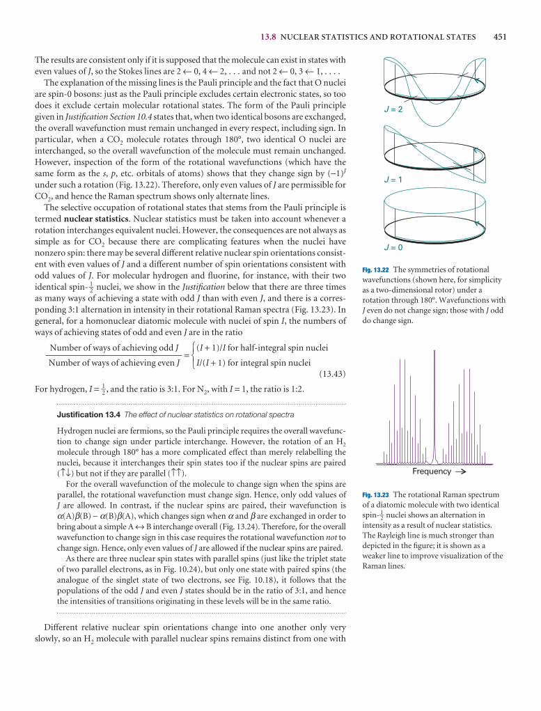
13.8 NUCLEAR STATISTICS AND ROTATIONAL STATES 451
The results are consistent only if it is supposed that the molecule can exist in states witheven values of J, so the Stokes lines are 2 ← 0, 4 ← 2, . . . and not 2 ← 0, 3 ← 1, . . . .
The explanation of the missing lines is the Pauli principle and the fact that O nucleiare spin-0 bosons: just as the Pauli principle excludes certain electronic states, so toodoes it exclude certain molecular rotational states. The form of the Pauli principlegiven in Justification Section 10.4 states that, when two identical bosons are exchanged,the overall wavefunction must remain unchanged in every respect, including sign. In particular, when a CO2 molecule rotates through 180°, two identical O nuclei are interchanged, so the overall wavefunction of the molecule must remain unchanged.However, inspection of the form of the rotational wavefunctions (which have thesame form as the s, p, etc. orbitals of atoms) shows that they change sign by (−1)J
under such a rotation (Fig. 13.22). Therefore, only even values of J are permissible forCO2, and hence the Raman spectrum shows only alternate lines.
The selective occupation of rotational states that stems from the Pauli principle istermed nuclear statistics. Nuclear statistics must be taken into account whenever arotation interchanges equivalent nuclei. However, the consequences are not always assimple as for CO2 because there are complicating features when the nuclei havenonzero spin: there may be several different relative nuclear spin orientations consist-ent with even values of J and a different number of spin orientations consistent withodd values of J. For molecular hydrogen and fluorine, for instance, with their twoidentical spin- 1–2 nuclei, we show in the Justification below that there are three times as many ways of achieving a state with odd J than with even J, and there is a corres-ponding 3:1 alternation in intensity in their rotational Raman spectra (Fig. 13.23). Ingeneral, for a homonuclear diatomic molecule with nuclei of spin I, the numbers ofways of achieving states of odd and even J are in the ratio
=
(13.43)
For hydrogen, I = 1–2 , and the ratio is 3:1. For N2, with I = 1, the ratio is 1:2.
Justification 13.4 The effect of nuclear statistics on rotational spectra
Hydrogen nuclei are fermions, so the Pauli principle requires the overall wavefunc-tion to change sign under particle interchange. However, the rotation of an H2
molecule through 180° has a more complicated effect than merely relabelling thenuclei, because it interchanges their spin states too if the nuclear spins are paired(↑↓) but not if they are parallel (↑↑).
For the overall wavefunction of the molecule to change sign when the spins areparallel, the rotational wavefunction must change sign. Hence, only odd values of J are allowed. In contrast, if the nuclear spins are paired, their wavefunction isα(A)β(B) − α(B)β(A), which changes sign when α and β are exchanged in order tobring about a simple A ↔ B interchange overall (Fig. 13.24). Therefore, for the overallwavefunction to change sign in this case requires the rotational wavefunction not tochange sign. Hence, only even values of J are allowed if the nuclear spins are paired.
As there are three nuclear spin states with parallel spins (just like the triplet stateof two parallel electrons, as in Fig. 10.24), but only one state with paired spins (theanalogue of the singlet state of two electrons, see Fig. 10.18), it follows that the populations of the odd J and even J states should be in the ratio of 3:1, and hence the intensities of transitions originating in these levels will be in the same ratio.
Different relative nuclear spin orientations change into one another only veryslowly, so an H2 molecule with parallel nuclear spins remains distinct from one with
(I + 1)/I for half-integral spin nuclei
I/(I + 1) for integral spin nuclei
123
Number of ways of achieving odd J
Number of ways of achieving even J
J = 2
J = 1
J = 0
Fig. 13.22 The symmetries of rotationalwavefunctions (shown here, for simplicityas a two-dimensional rotor) under arotation through 180°. Wavefunctions withJ even do not change sign; those with J odddo change sign.
Frequency
Fig. 13.23 The rotational Raman spectrumof a diatomic molecule with two identicalspin- 1–2 nuclei shows an alternation inintensity as a result of nuclear statistics.The Rayleigh line is much stronger thandepicted in the figure; it is shown as aweaker line to improve visualization of theRaman lines.
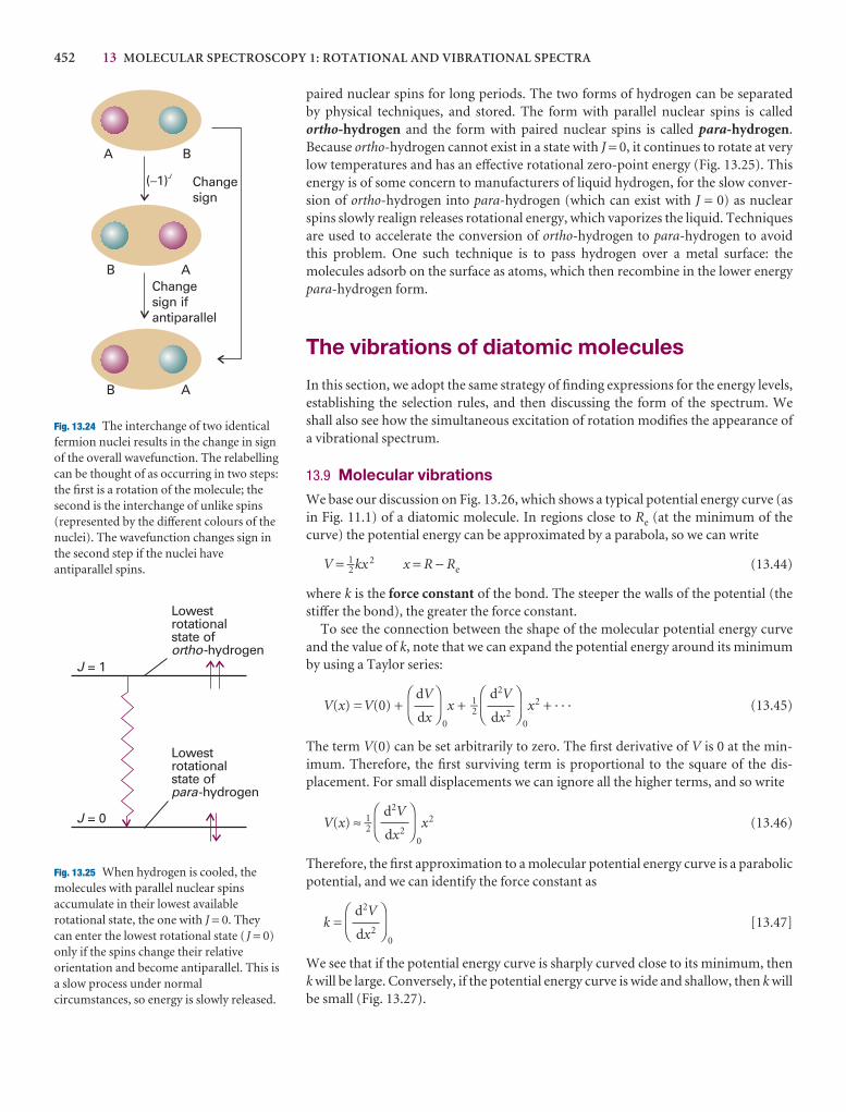
452 13 MOLECULAR SPECTROSCOPY 1: ROTATIONAL AND VIBRATIONAL SPECTRA
paired nuclear spins for long periods. The two forms of hydrogen can be separated by physical techniques, and stored. The form with parallel nuclear spins is calledortho-hydrogen and the form with paired nuclear spins is called para-hydrogen.Because ortho-hydrogen cannot exist in a state with J = 0, it continues to rotate at verylow temperatures and has an effective rotational zero-point energy (Fig. 13.25). Thisenergy is of some concern to manufacturers of liquid hydrogen, for the slow conver-sion of ortho-hydrogen into para-hydrogen (which can exist with J = 0) as nuclearspins slowly realign releases rotational energy, which vaporizes the liquid. Techniquesare used to accelerate the conversion of ortho-hydrogen to para-hydrogen to avoidthis problem. One such technique is to pass hydrogen over a metal surface: themolecules adsorb on the surface as atoms, which then recombine in the lower energypara-hydrogen form.
The vibrations of diatomic molecules
In this section, we adopt the same strategy of finding expressions for the energy levels,establishing the selection rules, and then discussing the form of the spectrum. Weshall also see how the simultaneous excitation of rotation modifies the appearance ofa vibrational spectrum.
13.9 Molecular vibrationsWe base our discussion on Fig. 13.26, which shows a typical potential energy curve (asin Fig. 11.1) of a diatomic molecule. In regions close to Re (at the minimum of thecurve) the potential energy can be approximated by a parabola, so we can write
V = 1–2 kx 2 x = R − Re (13.44)
where k is the force constant of the bond. The steeper the walls of the potential (thestiffer the bond), the greater the force constant.
To see the connection between the shape of the molecular potential energy curveand the value of k, note that we can expand the potential energy around its minimumby using a Taylor series:
V(x) =V(0) +0
x + 1–20
x2 + · · · (13.45)
The term V(0) can be set arbitrarily to zero. The first derivative of V is 0 at the min-imum. Therefore, the first surviving term is proportional to the square of the dis-placement. For small displacements we can ignore all the higher terms, and so write
V(x) ≈ 1–20
x2 (13.46)
Therefore, the first approximation to a molecular potential energy curve is a parabolicpotential, and we can identify the force constant as
k =0
[13.47]
We see that if the potential energy curve is sharply curved close to its minimum, thenk will be large. Conversely, if the potential energy curve is wide and shallow, then k willbe small (Fig. 13.27).
DF
d2V
dx2
AC
DF
d2V
dx2
AC
DF
d2V
dx2
AC
DF
dV
dx
AC
A
A
A
B
B
B
( 1)�J
Changesign ifantiparallel
Changesign
Fig. 13.24 The interchange of two identicalfermion nuclei results in the change in signof the overall wavefunction. The relabellingcan be thought of as occurring in two steps:the first is a rotation of the molecule; thesecond is the interchange of unlike spins(represented by the different colours of thenuclei). The wavefunction changes sign inthe second step if the nuclei haveantiparallel spins.
J = 1
J = 0
Lowestrotationalstate of
-hydrogenpara
Lowestrotationalstate of
-hydrogenortho
Fig. 13.25 When hydrogen is cooled, themolecules with parallel nuclear spinsaccumulate in their lowest availablerotational state, the one with J = 0. Theycan enter the lowest rotational state (J = 0)only if the spins change their relativeorientation and become antiparallel. This isa slow process under normalcircumstances, so energy is slowly released.
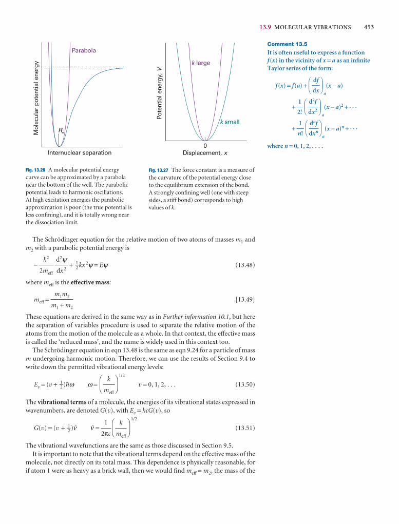
13.9 MOLECULAR VIBRATIONS 453
The Schrödinger equation for the relative motion of two atoms of masses m1 andm2 with a parabolic potential energy is
− + 1–2 kx 2ψ = Eψ (13.48)
where meff is the effective mass:
meff = [13.49]
These equations are derived in the same way as in Further information 10.1, but herethe separation of variables procedure is used to separate the relative motion of theatoms from the motion of the molecule as a whole. In that context, the effective massis called the ‘reduced mass’, and the name is widely used in this context too.
The Schrödinger equation in eqn 13.48 is the same as eqn 9.24 for a particle of massm undergoing harmonic motion. Therefore, we can use the results of Section 9.4 towrite down the permitted vibrational energy levels:
Ev = (v + 1–2 )$ω ω =1/2
v = 0, 1, 2, . . . (13.50)
The vibrational terms of a molecule, the energies of its vibrational states expressed inwavenumbers, are denoted G(v), with Ev = hcG(v), so
G(v) = (v + 1–2 )# # =1/2
(13.51)
The vibrational wavefunctions are the same as those discussed in Section 9.5.It is important to note that the vibrational terms depend on the effective mass of the
molecule, not directly on its total mass. This dependence is physically reasonable, forif atom 1 were as heavy as a brick wall, then we would find meff ≈ m2, the mass of the
DF
k
meff
AC
1
2πc
DF
k
meff
AC
m1m2
m1 + m2
d2ψdx 2
$2
2meff
Parabola
Mol
ecul
ar p
oten
tial e
nerg
y
Internuclear separation
Re
Fig. 13.26 A molecular potential energycurve can be approximated by a parabolanear the bottom of the well. The parabolicpotential leads to harmonic oscillations. At high excitation energies the parabolicapproximation is poor (the true potential isless confining), and it is totally wrong nearthe dissociation limit.
Comment 13.5
It is often useful to express a functionf(x) in the vicinity of x = a as an infiniteTaylor series of the form:
f(x) = f(a) +a
(x − a)
+a
(x − a)2 + · · ·
+a
(x − a)n + · · ·
where n = 0, 1, 2, . . . .
DEFdnf
dxn
ABC1
n!
DEFd2f
dx2
ABC1
2!
DEFdf
dx
ABC
k large
k small
Displacement, x0
Pote
ntia
l ene
rgy,
V
Fig. 13.27 The force constant is a measure ofthe curvature of the potential energy closeto the equilibrium extension of the bond. A strongly confining well (one with steepsides, a stiff bond) corresponds to highvalues of k.
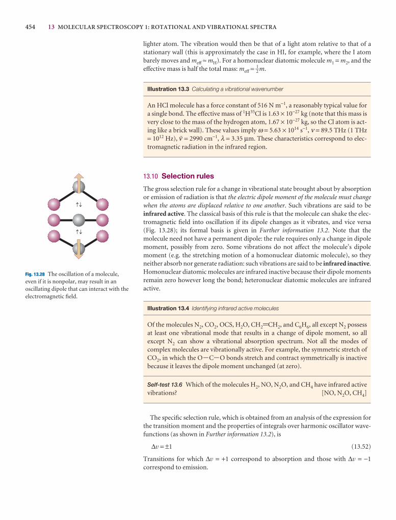
454 13 MOLECULAR SPECTROSCOPY 1: ROTATIONAL AND VIBRATIONAL SPECTRA
¯
¯
¯
¯
Fig. 13.28 The oscillation of a molecule,even if it is nonpolar, may result in anoscillating dipole that can interact with theelectromagnetic field.
lighter atom. The vibration would then be that of a light atom relative to that of a stationary wall (this is approximately the case in HI, for example, where the I atombarely moves and meff ≈ mH). For a homonuclear diatomic molecule m1 = m2, and theeffective mass is half the total mass: meff = 1–2 m.
Illustration 13.3 Calculating a vibrational wavenumber
An HCl molecule has a force constant of 516 N m−1, a reasonably typical value fora single bond. The effective mass of 1H35Cl is 1.63 × 10⁻²⁷ kg (note that this mass isvery close to the mass of the hydrogen atom, 1.67 × 10⁻²⁷ kg, so the Cl atom is act-ing like a brick wall). These values imply ω = 5.63 × 10¹⁴ s−1, ν = 89.5 THz (1 THz= 1012 Hz), # = 2990 cm−1, λ = 3.35 µm. These characteristics correspond to elec-tromagnetic radiation in the infrared region.
13.10 Selection rules
The gross selection rule for a change in vibrational state brought about by absorptionor emission of radiation is that the electric dipole moment of the molecule must changewhen the atoms are displaced relative to one another. Such vibrations are said to be infrared active. The classical basis of this rule is that the molecule can shake the elec-tromagnetic field into oscillation if its dipole changes as it vibrates, and vice versa (Fig. 13.28); its formal basis is given in Further information 13.2. Note that themolecule need not have a permanent dipole: the rule requires only a change in dipolemoment, possibly from zero. Some vibrations do not affect the molecule’s dipole moment (e.g. the stretching motion of a homonuclear diatomic molecule), so theyneither absorb nor generate radiation: such vibrations are said to be infrared inactive.Homonuclear diatomic molecules are infrared inactive because their dipole momentsremain zero however long the bond; heteronuclear diatomic molecules are infraredactive.
Illustration 13.4 Identifying infrared active molecules
Of the molecules N2, CO2, OCS, H2O, CH2=CH2, and C6H6, all except N2 possessat least one vibrational mode that results in a change of dipole moment, so all except N2 can show a vibrational absorption spectrum. Not all the modes of complex molecules are vibrationally active. For example, the symmetric stretch of CO2, in which the O-C-O bonds stretch and contract symmetrically is inactivebecause it leaves the dipole moment unchanged (at zero).
Self-test 13.6 Which of the molecules H2, NO, N2O, and CH4 have infrared activevibrations? [NO, N2O, CH4]
The specific selection rule, which is obtained from an analysis of the expression forthe transition moment and the properties of integrals over harmonic oscillator wave-functions (as shown in Further information 13.2), is
∆v = ±1 (13.52)
Transitions for which ∆v = +1 correspond to absorption and those with ∆v = −1correspond to emission.
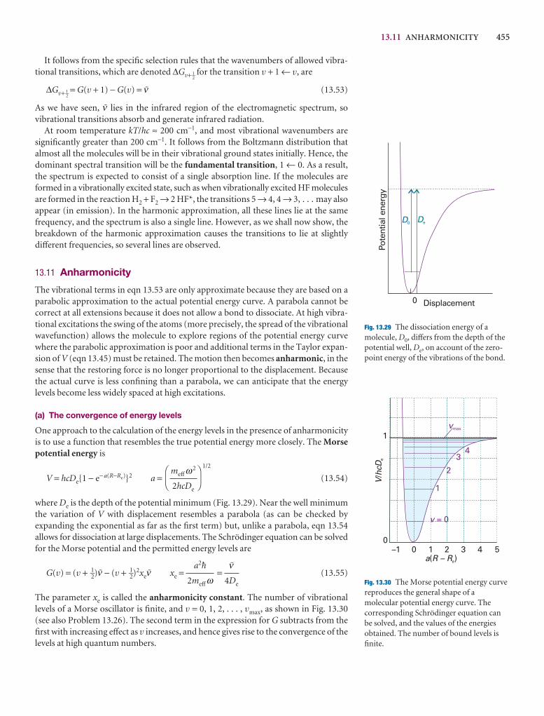
13.11 ANHARMONICITY 455
It follows from the specific selection rules that the wavenumbers of allowed vibra-tional transitions, which are denoted ∆Gv+ 1––
2for the transition v + 1 ← v, are
∆Gv+ 1––2= G(v + 1) − G(v) = # (13.53)
As we have seen, # lies in the infrared region of the electromagnetic spectrum, so vibrational transitions absorb and generate infrared radiation.
At room temperature kT/hc ≈ 200 cm−1, and most vibrational wavenumbers aresignificantly greater than 200 cm−1. It follows from the Boltzmann distribution thatalmost all the molecules will be in their vibrational ground states initially. Hence, thedominant spectral transition will be the fundamental transition, 1 ← 0. As a result,the spectrum is expected to consist of a single absorption line. If the molecules areformed in a vibrationally excited state, such as when vibrationally excited HF moleculesare formed in the reaction H2 + F2 → 2 HF*, the transitions 5 → 4, 4 → 3, . . . may alsoappear (in emission). In the harmonic approximation, all these lines lie at the samefrequency, and the spectrum is also a single line. However, as we shall now show, thebreakdown of the harmonic approximation causes the transitions to lie at slightlydifferent frequencies, so several lines are observed.
13.11 Anharmonicity
The vibrational terms in eqn 13.53 are only approximate because they are based on aparabolic approximation to the actual potential energy curve. A parabola cannot becorrect at all extensions because it does not allow a bond to dissociate. At high vibra-tional excitations the swing of the atoms (more precisely, the spread of the vibrationalwavefunction) allows the molecule to explore regions of the potential energy curvewhere the parabolic approximation is poor and additional terms in the Taylor expan-sion of V (eqn 13.45) must be retained. The motion then becomes anharmonic, in thesense that the restoring force is no longer proportional to the displacement. Becausethe actual curve is less confining than a parabola, we can anticipate that the energy levels become less widely spaced at high excitations.
(a) The convergence of energy levels
One approach to the calculation of the energy levels in the presence of anharmonicityis to use a function that resembles the true potential energy more closely. The Morsepotential energy is
V = hcDe{1 − e− a(R−Re)}2 a =1/2
(13.54)
where De is the depth of the potential minimum (Fig. 13.29). Near the well minimumthe variation of V with displacement resembles a parabola (as can be checked by expanding the exponential as far as the first term) but, unlike a parabola, eqn 13.54 allows for dissociation at large displacements. The Schrödinger equation can be solvedfor the Morse potential and the permitted energy levels are
G(v) = (v + 1–2)# − (v + 1–2)2xe# xe = = (13.55)
The parameter xe is called the anharmonicity constant. The number of vibrationallevels of a Morse oscillator is finite, and v = 0, 1, 2, . . . , vmax, as shown in Fig. 13.30(see also Problem 13.26). The second term in the expression for G subtracts from thefirst with increasing effect as v increases, and hence gives rise to the convergence of thelevels at high quantum numbers.
#
4De
a2$
2meffω
DF
meffω2
2hcDe
AC
D0 De
Displacement
Pote
ntia
l ene
rgy
0
Fig. 13.29 The dissociation energy of amolecule, D0, differs from the depth of thepotential well, De, on account of the zero-point energy of the vibrations of the bond.
–1 0 1 2 3 4 5
1
0
v = 0
1
2
34
vmax
a R – R( )e
Vhc
D/
e
Fig. 13.30 The Morse potential energy curvereproduces the general shape of amolecular potential energy curve. Thecorresponding Schrödinger equation canbe solved, and the values of the energiesobtained. The number of bound levels isfinite.
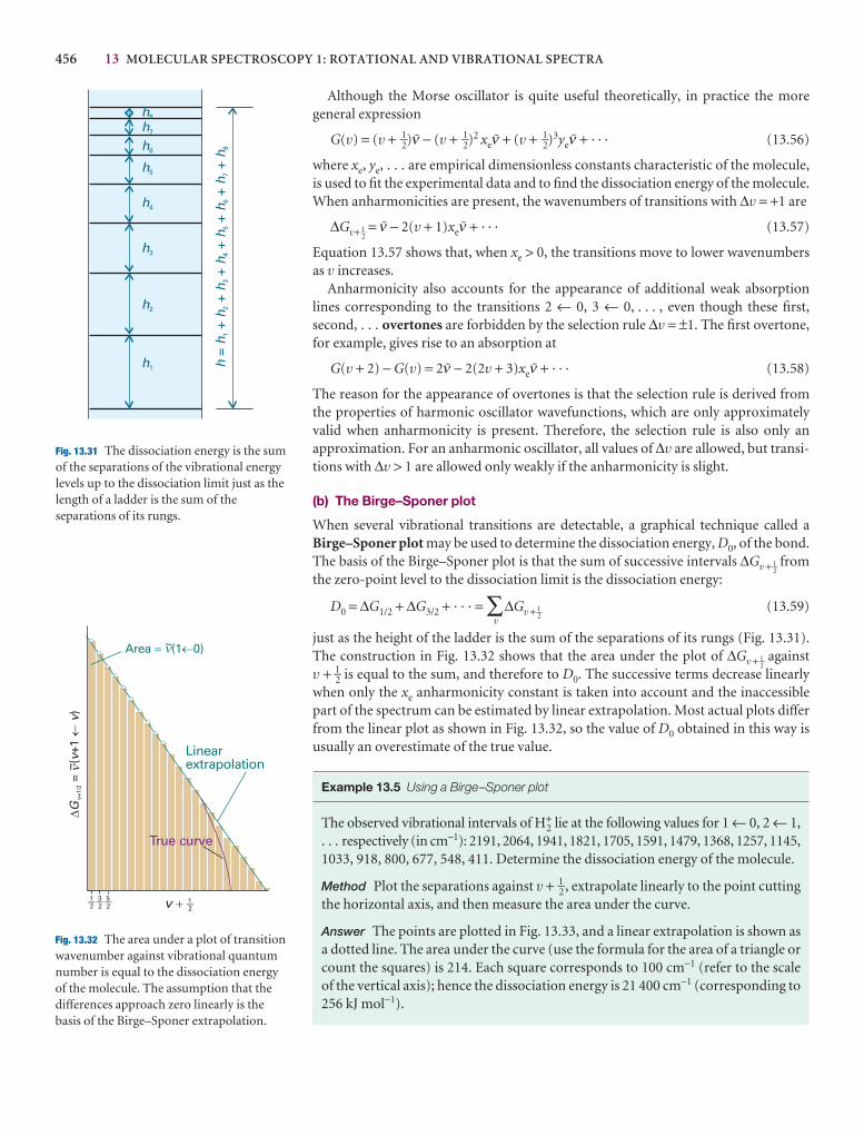
456 13 MOLECULAR SPECTROSCOPY 1: ROTATIONAL AND VIBRATIONAL SPECTRA
h1
h5
h2
h6
h3
h7
h4
h8
hh
hh
hh
hh
h=
++
++
++
+1
23
45
67
8
Fig. 13.31 The dissociation energy is the sumof the separations of the vibrational energylevels up to the dissociation limit just as thelength of a ladder is the sum of theseparations of its rungs.
D¬
Gv
vv+
1/2
=(
+1)
~
Area (1 0)� ¬~
Linearextrapolation
True curve
v �
n
n
21-2
1- 23- 2
5-
Fig. 13.32 The area under a plot of transitionwavenumber against vibrational quantumnumber is equal to the dissociation energyof the molecule. The assumption that thedifferences approach zero linearly is thebasis of the Birge–Sponer extrapolation.
Although the Morse oscillator is quite useful theoretically, in practice the moregeneral expression
G(v) = (v + 1–2)# − (v + 1–2)2 xe# + (v + 1–2)3ye# + · · · (13.56)
where xe, ye, . . . are empirical dimensionless constants characteristic of the molecule,is used to fit the experimental data and to find the dissociation energy of the molecule.When anharmonicities are present, the wavenumbers of transitions with ∆v = +1 are
∆Gv+ 1––2= # − 2(v + 1)xe# + · · · (13.57)
Equation 13.57 shows that, when xe > 0, the transitions move to lower wavenumbersas v increases.
Anharmonicity also accounts for the appearance of additional weak absorptionlines corresponding to the transitions 2 ← 0, 3 ← 0, . . . , even though these first, second, . . . overtones are forbidden by the selection rule ∆v = ±1. The first overtone,for example, gives rise to an absorption at
G(v + 2) − G(v) = 2# − 2(2v + 3)xe# + · · · (13.58)
The reason for the appearance of overtones is that the selection rule is derived fromthe properties of harmonic oscillator wavefunctions, which are only approximatelyvalid when anharmonicity is present. Therefore, the selection rule is also only an approximation. For an anharmonic oscillator, all values of ∆v are allowed, but transi-tions with ∆v > 1 are allowed only weakly if the anharmonicity is slight.
(b) The Birge–Sponer plot
When several vibrational transitions are detectable, a graphical technique called aBirge–Sponer plot may be used to determine the dissociation energy, D0, of the bond.The basis of the Birge–Sponer plot is that the sum of successive intervals ∆Gv + 1––
2from
the zero-point level to the dissociation limit is the dissociation energy:
D0 = ∆G1/2 + ∆G3/2 + · · · = ∑v
∆Gv + 1––2
(13.59)
just as the height of the ladder is the sum of the separations of its rungs (Fig. 13.31).The construction in Fig. 13.32 shows that the area under the plot of ∆Gv + 1––
2against
v + 1–2 is equal to the sum, and therefore to D0. The successive terms decrease linearlywhen only the xe anharmonicity constant is taken into account and the inaccessiblepart of the spectrum can be estimated by linear extrapolation. Most actual plots differfrom the linear plot as shown in Fig. 13.32, so the value of D0 obtained in this way isusually an overestimate of the true value.
Example 13.5 Using a Birge–Sponer plot
The observed vibrational intervals of H2+ lie at the following values for 1 ← 0, 2 ← 1,
. . . respectively (in cm−1): 2191, 2064, 1941, 1821, 1705, 1591, 1479, 1368, 1257, 1145,1033, 918, 800, 677, 548, 411. Determine the dissociation energy of the molecule.
Method Plot the separations against v + 1–2, extrapolate linearly to the point cuttingthe horizontal axis, and then measure the area under the curve.
Answer The points are plotted in Fig. 13.33, and a linear extrapolation is shown asa dotted line. The area under the curve (use the formula for the area of a triangle orcount the squares) is 214. Each square corresponds to 100 cm−1 (refer to the scaleof the vertical axis); hence the dissociation energy is 21 400 cm−1 (corresponding to256 kJ mol−1).
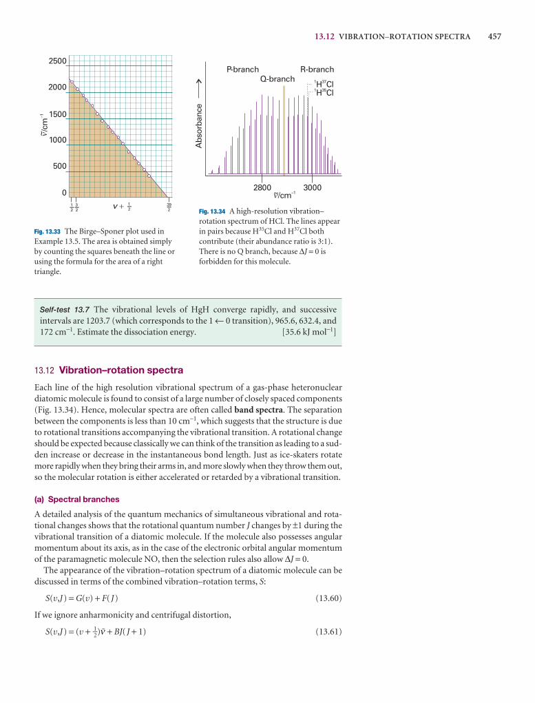
13.12 VIBRATION–ROTATION SPECTRA 457
2500
2000
1500
1000
500
0
v �
/cm
-1
~
21–
21– 2
3– 239–
n
Fig. 13.33 The Birge–Sponer plot used inExample 13.5. The area is obtained simplyby counting the squares beneath the line orusing the formula for the area of a righttriangle.
2800 3000
P-branch R-branchQ-branch
1 35H Cl
1 37H Cl
/cm–1~A
bsor
banc
en
Fig. 13.34 A high-resolution vibration–rotation spectrum of HCl. The lines appearin pairs because H35Cl and H37Cl bothcontribute (their abundance ratio is 3:1).There is no Q branch, because ∆J = 0 isforbidden for this molecule.
Self-test 13.7 The vibrational levels of HgH converge rapidly, and successive intervals are 1203.7 (which corresponds to the 1 ← 0 transition), 965.6, 632.4, and172 cm−1. Estimate the dissociation energy. [35.6 kJ mol−1]
13.12 Vibration–rotation spectra
Each line of the high resolution vibrational spectrum of a gas-phase heteronuclear diatomic molecule is found to consist of a large number of closely spaced components(Fig. 13.34). Hence, molecular spectra are often called band spectra. The separationbetween the components is less than 10 cm−1, which suggests that the structure is dueto rotational transitions accompanying the vibrational transition. A rotational changeshould be expected because classically we can think of the transition as leading to a sud-den increase or decrease in the instantaneous bond length. Just as ice-skaters rotatemore rapidly when they bring their arms in, and more slowly when they throw them out,so the molecular rotation is either accelerated or retarded by a vibrational transition.
(a) Spectral branches
A detailed analysis of the quantum mechanics of simultaneous vibrational and rota-tional changes shows that the rotational quantum number J changes by ±1 during thevibrational transition of a diatomic molecule. If the molecule also possesses angularmomentum about its axis, as in the case of the electronic orbital angular momentumof the paramagnetic molecule NO, then the selection rules also allow ∆J = 0.
The appearance of the vibration–rotation spectrum of a diatomic molecule can bediscussed in terms of the combined vibration–rotation terms, S:
S(v,J) = G(v) + F( J) (13.60)
If we ignore anharmonicity and centrifugal distortion,
S(v,J) = (v + 1–2)# + BJ( J + 1) (13.61)
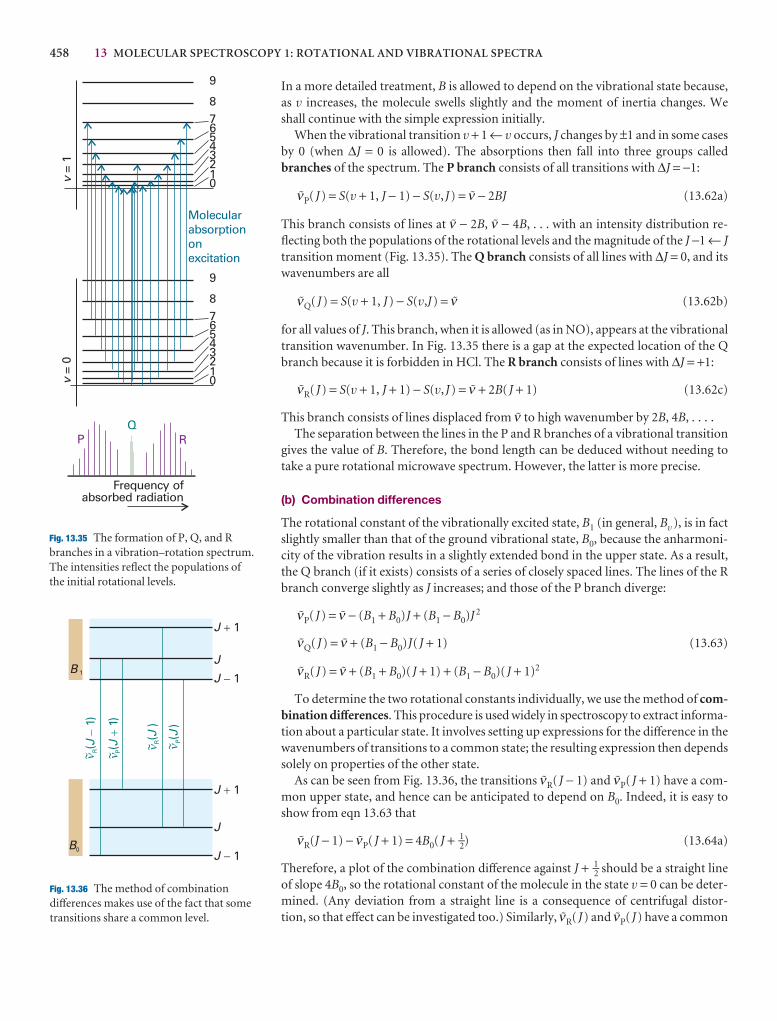
458 13 MOLECULAR SPECTROSCOPY 1: ROTATIONAL AND VIBRATIONAL SPECTRA
In a more detailed treatment, B is allowed to depend on the vibrational state because,as v increases, the molecule swells slightly and the moment of inertia changes. Weshall continue with the simple expression initially.
When the vibrational transition v + 1 ← v occurs, J changes by ±1 and in some casesby 0 (when ∆J = 0 is allowed). The absorptions then fall into three groups calledbranches of the spectrum. The P branch consists of all transitions with ∆J = −1:
#P( J) = S(v + 1, J − 1) − S(v, J) = # − 2BJ (13.62a)
This branch consists of lines at # − 2B, # − 4B, . . . with an intensity distribution re-flecting both the populations of the rotational levels and the magnitude of the J −1 ← Jtransition moment (Fig. 13.35). The Q branch consists of all lines with ∆J = 0, and itswavenumbers are all
#Q( J) = S(v + 1, J) − S(v,J) = # (13.62b)
for all values of J. This branch, when it is allowed (as in NO), appears at the vibrationaltransition wavenumber. In Fig. 13.35 there is a gap at the expected location of the Qbranch because it is forbidden in HCl. The R branch consists of lines with ∆J = +1:
#R( J) = S(v + 1, J + 1) − S(v, J) = # + 2B( J + 1) (13.62c)
This branch consists of lines displaced from # to high wavenumber by 2B, 4B, . . . .The separation between the lines in the P and R branches of a vibrational transition
gives the value of B. Therefore, the bond length can be deduced without needing totake a pure rotational microwave spectrum. However, the latter is more precise.
(b) Combination differences
The rotational constant of the vibrationally excited state, B1 (in general, Bv ), is in factslightly smaller than that of the ground vibrational state, B0, because the anharmoni-city of the vibration results in a slightly extended bond in the upper state. As a result,the Q branch (if it exists) consists of a series of closely spaced lines. The lines of the Rbranch converge slightly as J increases; and those of the P branch diverge:
#P( J) = # − (B1 + B0)J + (B1 − B0)J 2
#Q( J) = # + (B1 − B0)J( J + 1) (13.63)
#R( J) = # + (B1 + B0)( J + 1) + (B1 − B0)( J + 1)2
To determine the two rotational constants individually, we use the method of com-bination differences. This procedure is used widely in spectroscopy to extract informa-tion about a particular state. It involves setting up expressions for the difference in thewavenumbers of transitions to a common state; the resulting expression then dependssolely on properties of the other state.
As can be seen from Fig. 13.36, the transitions #R( J − 1) and #P( J + 1) have a com-mon upper state, and hence can be anticipated to depend on B0. Indeed, it is easy toshow from eqn 13.63 that
#R(J − 1) − #P( J + 1) = 4B0( J + 1–2) (13.64a)
Therefore, a plot of the combination difference against J + 1–2 should be a straight lineof slope 4B0, so the rotational constant of the molecule in the state v = 0 can be deter-mined. (Any deviation from a straight line is a consequence of centrifugal distor-tion, so that effect can be investigated too.) Similarly, #R( J) and #P( J) have a common
J 1+
J 1+
J
J
J 1-
J 1-
R(
1 )J
-
P(1)
J+
R(
)J
P()
J
B 1
B0
n
~ n
~
n
~ n
~
Fig. 13.36 The method of combinationdifferences makes use of the fact that sometransitions share a common level.
0
0
1
1
2
2
3
3
4
4
5
5
6
6
7
7
8
8
9
9
v=
1v
= 0
Frequency ofabsorbed radiation
PQ
R
Molecularabsorptiononexcitation
Fig. 13.35 The formation of P, Q, and Rbranches in a vibration–rotation spectrum.The intensities reflect the populations ofthe initial rotational levels.
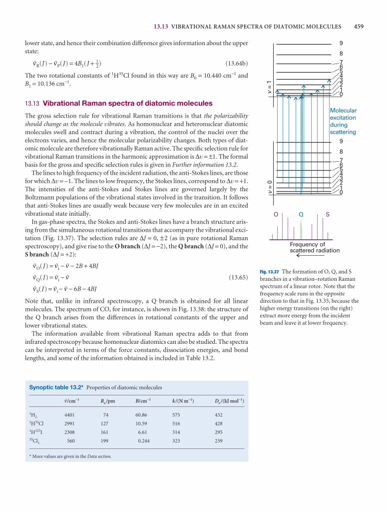
13.13 VIBRATIONAL RAMAN SPECTRA OF DIATOMIC MOLECULES 459
lower state, and hence their combination difference gives information about the upperstate:
#R(J) − #P( J) = 4B1( J + 1–2) (13.64b)
The two rotational constants of 1H35Cl found in this way are B0 = 10.440 cm−1 andB1 = 10.136 cm−1.
13.13 Vibrational Raman spectra of diatomic molecules
The gross selection rule for vibrational Raman transitions is that the polarizabilityshould change as the molecule vibrates. As homonuclear and heteronuclear diatomicmolecules swell and contract during a vibration, the control of the nuclei over theelectrons varies, and hence the molecular polarizability changes. Both types of diat-omic molecule are therefore vibrationally Raman active. The specific selection rule forvibrational Raman transitions in the harmonic approximation is ∆v = ±1. The formalbasis for the gross and specific selection rules is given in Further information 13.2.
The lines to high frequency of the incident radiation, the anti-Stokes lines, are thosefor which ∆v = −1. The lines to low frequency, the Stokes lines, correspond to ∆v = +1.The intensities of the anti-Stokes and Stokes lines are governed largely by theBoltzmann populations of the vibrational states involved in the transition. It followsthat anti-Stokes lines are usually weak because very few molecules are in an excited vibrational state initially.
In gas-phase spectra, the Stokes and anti-Stokes lines have a branch structure aris-ing from the simultaneous rotational transitions that accompany the vibrational exci-tation (Fig. 13.37). The selection rules are ∆J = 0, ±2 (as in pure rotational Ramanspectroscopy), and give rise to the O branch (∆J = −2), the Q branch (∆J = 0), and theS branch (∆J = +2):
#O( J) = #i − # − 2B + 4BJ
#Q( J) = #i − # (13.65)
#S( J) = #i − # − 6B − 4BJ
Note that, unlike in infrared spectroscopy, a Q branch is obtained for all linearmolecules. The spectrum of CO, for instance, is shown in Fig. 13.38: the structure ofthe Q branch arises from the differences in rotational constants of the upper andlower vibrational states.
The information available from vibrational Raman spectra adds to that from infrared spectroscopy because homonuclear diatomics can also be studied. The spectracan be interpreted in terms of the force constants, dissociation energies, and bondlengths, and some of the information obtained is included in Table 13.2.
0
0
1
1
2
2
3
3
4
4
5
5
6
6
7
7
8
8
9
9
v=
1v
= 0
Frequency ofscattered radiation
QO S
Molecularexcitationduringscattering
Fig. 13.37 The formation of O, Q, and Sbranches in a vibration–rotation Ramanspectrum of a linear rotor. Note that thefrequency scale runs in the oppositedirection to that in Fig. 13.35, because thehigher energy transitions (on the right)extract more energy from the incidentbeam and leave it at lower frequency.
Synoptic table 13.2* Properties of diatomic molecules
#/cm−1 Re /pm B/cm−1 k /(N m−1) De /(kJ mol−1)
1H2 4401 74 60.86 575 4321H35Cl 2991 127 10.59 516 4281H127I 2308 161 6.61 314 29535Cl2 560 199 0.244 323 239
* More values are given in the Data section.
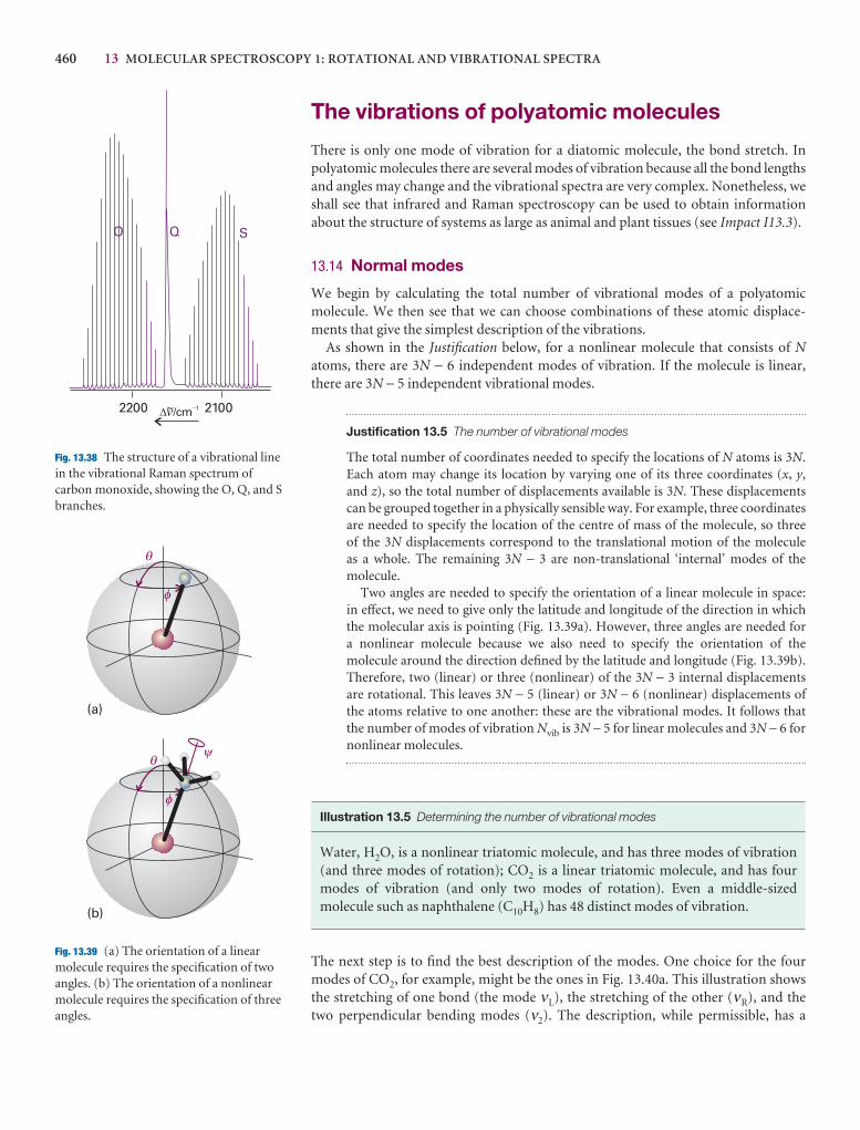
460 13 MOLECULAR SPECTROSCOPY 1: ROTATIONAL AND VIBRATIONAL SPECTRA
O Q S
21002200D /cm 1~n
-
Fig. 13.38 The structure of a vibrational linein the vibrational Raman spectrum ofcarbon monoxide, showing the O, Q, and Sbranches.
q
q
f
f
y
(a)
(b)
Fig. 13.39 (a) The orientation of a linearmolecule requires the specification of twoangles. (b) The orientation of a nonlinearmolecule requires the specification of threeangles.
The vibrations of polyatomic molecules
There is only one mode of vibration for a diatomic molecule, the bond stretch. Inpolyatomic molecules there are several modes of vibration because all the bond lengthsand angles may change and the vibrational spectra are very complex. Nonetheless, weshall see that infrared and Raman spectroscopy can be used to obtain informationabout the structure of systems as large as animal and plant tissues (see Impact I13.3).
13.14 Normal modes
We begin by calculating the total number of vibrational modes of a polyatomicmolecule. We then see that we can choose combinations of these atomic displace-ments that give the simplest description of the vibrations.
As shown in the Justification below, for a nonlinear molecule that consists of Natoms, there are 3N − 6 independent modes of vibration. If the molecule is linear,there are 3N − 5 independent vibrational modes.
Justification 13.5 The number of vibrational modes
The total number of coordinates needed to specify the locations of N atoms is 3N.Each atom may change its location by varying one of its three coordinates (x, y,and z), so the total number of displacements available is 3N. These displacementscan be grouped together in a physically sensible way. For example, three coordinatesare needed to specify the location of the centre of mass of the molecule, so three of the 3N displacements correspond to the translational motion of the molecule as a whole. The remaining 3N − 3 are non-translational ‘internal’ modes of themolecule.
Two angles are needed to specify the orientation of a linear molecule in space: in effect, we need to give only the latitude and longitude of the direction in which the molecular axis is pointing (Fig. 13.39a). However, three angles are needed for a nonlinear molecule because we also need to specify the orientation of the molecule around the direction defined by the latitude and longitude (Fig. 13.39b).Therefore, two (linear) or three (nonlinear) of the 3N − 3 internal displacements are rotational. This leaves 3N − 5 (linear) or 3N − 6 (nonlinear) displacements of the atoms relative to one another: these are the vibrational modes. It follows that the number of modes of vibration Nvib is 3N − 5 for linear molecules and 3N − 6 fornonlinear molecules.
Illustration 13.5 Determining the number of vibrational modes
Water, H2O, is a nonlinear triatomic molecule, and has three modes of vibration(and three modes of rotation); CO2 is a linear triatomic molecule, and has fourmodes of vibration (and only two modes of rotation). Even a middle-sizedmolecule such as naphthalene (C10H8) has 48 distinct modes of vibration.
The next step is to find the best description of the modes. One choice for the fourmodes of CO2, for example, might be the ones in Fig. 13.40a. This illustration showsthe stretching of one bond (the mode νL), the stretching of the other (νR), and the two perpendicular bending modes (ν2). The description, while permissible, has a
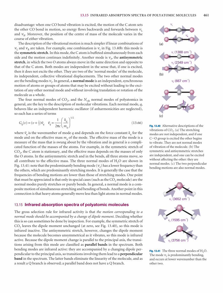
13.15 INFRARED ABSORPTION SPECTRA OF POLYATOMIC MOLECULES 461
disadvantage: when one CO bond vibration is excited, the motion of the C atom setsthe other CO bond in motion, so energy flows backwards and forwards between νL
and νR. Moreover, the position of the centre of mass of the molecule varies in thecourse of either vibration.
The description of the vibrational motion is much simpler if linear combinations ofνL and νR are taken. For example, one combination is ν1 in Fig. 13.40b: this mode isthe symmetric stretch. In this mode, the C atom is buffeted simultaneously from eachside and the motion continues indefinitely. Another mode is ν3, the antisymmetricstretch, in which the two O atoms always move in the same direction and opposite tothat of the C atom. Both modes are independent in the sense that, if one is excited,then it does not excite the other. They are two of the ‘normal modes’ of the molecule,its independent, collective vibrational displacements. The two other normal modesare the bending modes ν2. In general, a normal mode is an independent, synchronousmotion of atoms or groups of atoms that may be excited without leading to the exci-tation of any other normal mode and without involving translation or rotation of themolecule as a whole.
The four normal modes of CO2, and the Nvib normal modes of polyatomics in general, are the key to the description of molecular vibrations. Each normal mode, q,behaves like an independent harmonic oscillator (if anharmonicities are neglected),so each has a series of terms
Gq(v) = (v + 1–2)#q #q =1/2
(13.66)
where #q is the wavenumber of mode q and depends on the force constant kq for themode and on the effective mass mq of the mode. The effective mass of the mode is ameasure of the mass that is swung about by the vibration and in general is a compli-cated function of the masses of the atoms. For example, in the symmetric stretch ofCO2, the C atom is stationary, and the effective mass depends on the masses of onlythe O atoms. In the antisymmetric stretch and in the bends, all three atoms move, soall contribute to the effective mass. The three normal modes of H2O are shown in Fig. 13.41: note that the predominantly bending mode (ν2) has a lower frequency thanthe others, which are predominantly stretching modes. It is generally the case that the frequencies of bending motions are lower than those of stretching modes. One pointthat must be appreciated is that only in special cases (such as the CO2 molecule) are thenormal modes purely stretches or purely bends. In general, a normal mode is a com-posite motion of simultaneous stretching and bending of bonds. Another point in thisconnection is that heavy atoms generally move less than light atoms in normal modes.
13.15 Infrared absorption spectra of polyatomic molecules
The gross selection rule for infrared activity is that the motion corresponding to a normal mode should be accompanied by a change of dipole moment. Deciding whetherthis is so can sometimes be done by inspection. For example, the symmetric stretch ofCO2 leaves the dipole moment unchanged (at zero, see Fig. 13.40), so this mode is infrared inactive. The antisymmetric stretch, however, changes the dipole momentbecause the molecule becomes unsymmetrical as it vibrates, so this mode is infraredactive. Because the dipole moment change is parallel to the principal axis, the transi-tions arising from this mode are classified as parallel bands in the spectrum. Bothbending modes are infrared active: they are accompanied by a changing dipole per-pendicular to the principal axis, so transitions involving them lead to a perpendicularband in the spectrum. The latter bands eliminate the linearity of the molecule, and asa result a Q branch is observed; a parallel band does not have a Q branch.
DF
kq
mq
AC
1
2πc
L
R
1 (1388 cm )�1
3 (2349 cm )�1
2 (667 cm )1
(c)
(b)
(a)
�
�
�
�
��
Fig. 13.40 Alternative descriptions of thevibrations of CO2. (a) The stretchingmodes are not independent, and if one C-O group is excited the other begins to vibrate. They are not normal modes of vibration of the molecule. (b) Thesymmetric and antisymmetric stretches are independent, and one can be excitedwithout affecting the other: they arenormal modes. (c) The two perpendicularbending motions are also normal modes.
1 (3652 cm )�1
2 (1595 cm )1
3 (3756 cm )�1
�
�
�
�
Fig. 13.41 The three normal modes of H2O.The mode ν2 is predominantly bending,and occurs at lower wavenumber than theother two.
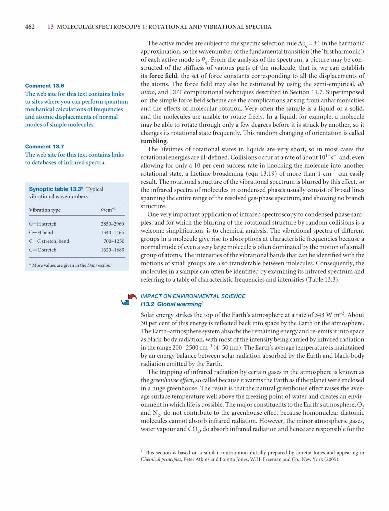
462 13 MOLECULAR SPECTROSCOPY 1: ROTATIONAL AND VIBRATIONAL SPECTRA
The active modes are subject to the specific selection rule ∆vq = ±1 in the harmonicapproximation, so the wavenumber of the fundamental transition (the ‘first harmonic’)of each active mode is #q. From the analysis of the spectrum, a picture may be con-structed of the stiffness of various parts of the molecule, that is, we can establish its force field, the set of force constants corresponding to all the displacements of the atoms. The force field may also be estimated by using the semi-empirical, abinitio, and DFT computational techniques described in Section 11.7. Superimposedon the simple force field scheme are the complications arising from anharmonicitiesand the effects of molecular rotation. Very often the sample is a liquid or a solid, and the molecules are unable to rotate freely. In a liquid, for example, a molecule may be able to rotate through only a few degrees before it is struck by another, so itchanges its rotational state frequently. This random changing of orientation is calledtumbling.
The lifetimes of rotational states in liquids are very short, so in most cases the rotational energies are ill-defined. Collisions occur at a rate of about 1013 s−1 and, evenallowing for only a 10 per cent success rate in knocking the molecule into another rotational state, a lifetime broadening (eqn 13.19) of more than 1 cm−1 can easily result. The rotational structure of the vibrational spectrum is blurred by this effect, sothe infrared spectra of molecules in condensed phases usually consist of broad linesspanning the entire range of the resolved gas-phase spectrum, and showing no branchstructure.
One very important application of infrared spectroscopy to condensed phase sam-ples, and for which the blurring of the rotational structure by random collisions is awelcome simplification, is to chemical analysis. The vibrational spectra of differentgroups in a molecule give rise to absorptions at characteristic frequencies because anormal mode of even a very large molecule is often dominated by the motion of a smallgroup of atoms. The intensities of the vibrational bands that can be identified with themotions of small groups are also transferable between molecules. Consequently, themolecules in a sample can often be identified by examining its infrared spectrum andreferring to a table of characteristic frequencies and intensities (Table 13.3).
IMPACT ON ENVIRONMENTAL SCIENCE
I13.2 Global warming1
Solar energy strikes the top of the Earth’s atmosphere at a rate of 343 W m−2. About 30 per cent of this energy is reflected back into space by the Earth or the atmosphere.The Earth–atmosphere system absorbs the remaining energy and re-emits it into spaceas black-body radiation, with most of the intensity being carried by infrared radiationin the range 200–2500 cm−1 (4–50 µm). The Earth’s average temperature is maintainedby an energy balance between solar radiation absorbed by the Earth and black-bodyradiation emitted by the Earth.
The trapping of infrared radiation by certain gases in the atmosphere is known asthe greenhouse effect, so called because it warms the Earth as if the planet were enclosedin a huge greenhouse. The result is that the natural greenhouse effect raises the aver-age surface temperature well above the freezing point of water and creates an envir-onment in which life is possible. The major constituents to the Earth’s atmosphere, O2
and N2, do not contribute to the greenhouse effect because homonuclear diatomicmolecules cannot absorb infrared radiation. However, the minor atmospheric gases,water vapour and CO2, do absorb infrared radiation and hence are responsible for the
Comment 13.6
The web site for this text contains linksto sites where you can perform quantummechanical calculations of frequenciesand atomic displacements of normalmodes of simple molecules.
Comment 13.7
The web site for this text contains linksto databases of infrared spectra.
Synoptic table 13.3* Typicalvibrational wavenumbers
Vibration type #/cm−1
C-H stretch 2850–2960
C-H bend 1340–1465
C-C stretch, bend 700–1250
C=C stretch 1620–1680
* More values are given in the Data section.
1 This section is based on a similar contribution initially prepared by Loretta Jones and appearing inChemical principles, Peter Atkins and Loretta Jones, W.H. Freeman and Co., New York (2005).
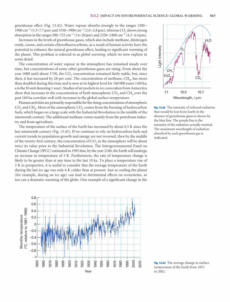
I13.2 IMPACT ON ENVIRONMENTAL SCIENCE: GLOBAL WARMING 463
greenhouse effect (Fig. 13.42). Water vapour absorbs strongly in the ranges 1300–1900 cm−1 (5.3–7.7 µm) and 3550–3900 cm−1 (2.6–2.8 µm), whereas CO2 shows strongabsorption in the ranges 500–725 cm−1 (14–20 µm) and 2250–2400 cm−1 (4.2–4.4 µm).
Increases in the levels of greenhouse gases, which also include methane, dinitrogenoxide, ozone, and certain chlorofluorocarbons, as a result of human activity have thepotential to enhance the natural greenhouse effect, leading to significant warming ofthe planet. This problem is referred to as global warming, which we now explore insome detail.
The concentration of water vapour in the atmosphere has remained steady overtime, but concentrations of some other greenhouse gases are rising. From about theyear 1000 until about 1750, the CO2 concentration remained fairly stable, but, sincethen, it has increased by 28 per cent. The concentration of methane, CH4, has morethan doubled during this time and is now at its highest level for 160 000 years (160 ka;a is the SI unit denoting 1 year). Studies of air pockets in ice cores taken from Antarcticashow that increases in the concentration of both atmospheric CO2 and CH4 over thepast 160 ka correlate well with increases in the global surface temperature.
Human activities are primarily responsible for the rising concentrations of atmosphericCO2 and CH4. Most of the atmospheric CO2 comes from the burning of hydrocarbonfuels, which began on a large scale with the Industrial Revolution in the middle of thenineteenth century. The additional methane comes mainly from the petroleum indus-try and from agriculture.
The temperature of the surface of the Earth has increased by about 0.5 K since thelate nineteenth century (Fig. 13.43). If we continue to rely on hydrocarbon fuels andcurrent trends in population growth and energy are not reversed, then by the middleof the twenty-first century, the concentration of CO2 in the atmosphere will be abouttwice its value prior to the Industrial Revolution. The Intergovernmental Panel onClimate Change (IPCC) estimated in 1995 that, by the year 2100, the Earth will undergoan increase in temperature of 3 K. Furthermore, the rate of temperature change islikely to be greater than at any time in the last 10 ka. To place a temperature rise of 3 K in perspective, it is useful to consider that the average temperature of the Earthduring the last ice age was only 6 K colder than at present. Just as cooling the planet(for example, during an ice age) can lead to detrimental effects on ecosystems, so too can a dramatic warming of the globe. One example of a significant change in the
Ligh
t in
tens
ity
H O2
CH4
O3
CO2
H O2
7.1 10.0 16.7
Wavelength, m�
Fig. 13.42 The intensity of infrared radiationthat would be lost from Earth in theabsence of greenhouse gases is shown bythe blue line. The purple line is theintensity of the radiation actually emitted.The maximum wavelength of radiationabsorbed by each greenhouse gas isindicated.
0.8
0.6
0.4
0.2
0
�0.2
�0.4
�0.6
�0.8
�1
Mon
thly
tem
pera
ture
(°C
, rel
ativ
e to
196
119
90)
�
1850
1860
1870
1880
1890
1900
1910
1920
1930
1940
1950
1960
1970
1980
1990
2000
2010
Year
Fig. 13.43 The average change in surfacetemperature of the Earth from 1855 to 2002.
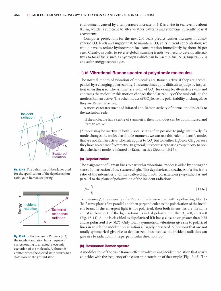
464 13 MOLECULAR SPECTROSCOPY 1: ROTATIONAL AND VIBRATIONAL SPECTRA
environment caused by a temperature increase of 3 K is a rise in sea level by about 0.5 m, which is sufficient to alter weather patterns and submerge currently coastalecosystems.
Computer projections for the next 200 years predict further increases in atmo-spheric CO2 levels and suggest that, to maintain CO2 at its current concentration, wewould have to reduce hydrocarbon fuel consumption immediately by about 50 percent. Clearly, in order to reverse global warming trends, we need to develop alterna-tives to fossil fuels, such as hydrogen (which can be used in fuel cells, Impact I25.3)and solar energy technologies.
13.16 Vibrational Raman spectra of polyatomic molecules
The normal modes of vibration of molecules are Raman active if they are accom-panied by a changing polarizability. It is sometimes quite difficult to judge by inspec-tion when this is so. The symmetric stretch of CO2, for example, alternately swells andcontracts the molecule: this motion changes the polarizability of the molecule, so themode is Raman active. The other modes of CO2 leave the polarizability unchanged, sothey are Raman inactive.
A more exact treatment of infrared and Raman activity of normal modes leads tothe exclusion rule:
If the molecule has a centre of symmetry, then no modes can be both infrared andRaman active.
(A mode may be inactive in both.) Because it is often possible to judge intuitively if amode changes the molecular dipole moment, we can use this rule to identify modesthat are not Raman active. The rule applies to CO2 but to neither H2O nor CH4 becausethey have no centre of symmetry. In general, it is necessary to use group theory to pre-dict whether a mode is infrared or Raman active (Section 13.17).
(a) Depolarization
The assignment of Raman lines to particular vibrational modes is aided by noting thestate of polarization of the scattered light. The depolarization ratio, ρ, of a line is theratio of the intensities, I, of the scattered light with polarizations perpendicular andparallel to the plane of polarization of the incident radiation:
ρ = [13.67]
To measure ρ, the intensity of a Raman line is measured with a polarizing filter (a‘half-wave plate’) first parallel and then perpendicular to the polarization of the incid-ent beam. If the emergent light is not polarized, then both intensities are the same and ρ is close to 1; if the light retains its initial polarization, then I⊥ = 0, so ρ = 0(Fig. 13.44). A line is classified as depolarized if it has ρ close to or greater than 0.75and as polarized if ρ < 0.75. Only totally symmetrical vibrations give rise to polarizedlines in which the incident polarization is largely preserved. Vibrations that are not totally symmetrical give rise to depolarized lines because the incident radiation cangive rise to radiation in the perpendicular direction too.
(b) Resonance Raman spectra
A modification of the basic Raman effect involves using incident radiation that nearlycoincides with the frequency of an electronic transition of the sample (Fig. 13.45). The
I⊥
I||
Incidentradiation
Scatteredradiation
I��
I&
Fig. 13.44 The definition of the planes usedfor the specification of the depolarizationratio, ρ, in Raman scattering.
Ener
gy Incidentradiation Scattered
resonanceradiation
Fig. 13.45 In the resonance Raman effect,the incident radiation has a frequencycorresponding to an actual electronicexcitation of the molecule. A photon isemitted when the excited state returns to astate close to the ground state.
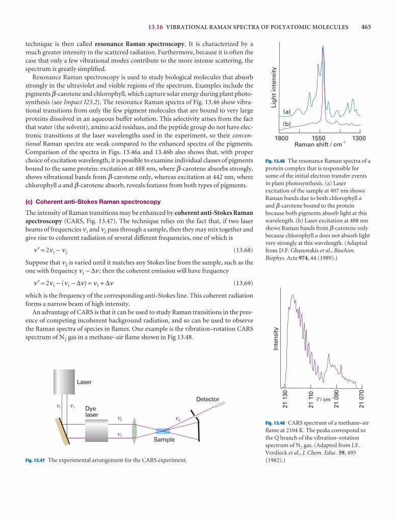
13.16 VIBRATIONAL RAMAN SPECTRA OF POLYATOMIC MOLECULES 465
technique is then called resonance Raman spectroscopy. It is characterized by amuch greater intensity in the scattered radiation. Furthermore, because it is often thecase that only a few vibrational modes contribute to the more intense scattering, thespectrum is greatly simplified.
Resonance Raman spectroscopy is used to study biological molecules that absorbstrongly in the ultraviolet and visible regions of the spectrum. Examples include thepigments β-carotene and chlorophyll, which capture solar energy during plant photo-synthesis (see Impact I23.2). The resonance Raman spectra of Fig. 13.46 show vibra-tional transitions from only the few pigment molecules that are bound to very largeproteins dissolved in an aqueous buffer solution. This selectivity arises from the factthat water (the solvent), amino acid residues, and the peptide group do not have elec-tronic transitions at the laser wavelengths used in the experiment, so their conven-tional Raman spectra are weak compared to the enhanced spectra of the pigments.Comparison of the spectra in Figs. 13.46a and 13.46b also shows that, with properchoice of excitation wavelength, it is possible to examine individual classes of pigmentsbound to the same protein: excitation at 488 nm, where β-carotene absorbs strongly,shows vibrational bands from β-carotene only, whereas excitation at 442 nm, wherechlorophyll a and β-carotene absorb, reveals features from both types of pigments.
(c) Coherent anti-Stokes Raman spectroscopy
The intensity of Raman transitions may be enhanced by coherent anti-Stokes Ramanspectroscopy (CARS, Fig. 13.47). The technique relies on the fact that, if two laserbeams of frequencies ν1 and ν2 pass through a sample, then they may mix together andgive rise to coherent radiation of several different frequencies, one of which is
ν′ = 2ν1 − ν2 (13.68)
Suppose that ν2 is varied until it matches any Stokes line from the sample, such as theone with frequency ν1 − ∆ν ; then the coherent emission will have frequency
ν′ = 2ν1 − (ν1 − ∆ν) = ν1 + ∆ν (13.69)
which is the frequency of the corresponding anti-Stokes line. This coherent radiationforms a narrow beam of high intensity.
An advantage of CARS is that it can be used to study Raman transitions in the pres-ence of competing incoherent background radiation, and so can be used to observethe Raman spectra of species in flames. One example is the vibration–rotation CARSspectrum of N2 gas in a methane–air flame shown in Fig 13.48.
Raman shift / cm�1130015501800
(a)
(b)
Lig
ht
inte
nsi
ty
Fig. 13.46 The resonance Raman spectra of aprotein complex that is responsible forsome of the initial electron transfer eventsin plant photosynthesis. (a) Laserexcitation of the sample at 407 nm showsRaman bands due to both chlorophyll aand β-carotene bound to the proteinbecause both pigments absorb light at thiswavelength. (b) Laser excitation at 488 nmshows Raman bands from β-carotene onlybecause chlorophyll a does not absorb lightvery strongly at this wavelength. (Adaptedfrom D.F. Ghanotakis et al., Biochim.Biophys. Acta 974, 44 (1989).)
Laser
1
11
2 3
Dyelaser
Detector
Sample
� �
�
�
�
Inte
nsity
/ cm�1~
21 0
70
21 0
90
21 1
10
21 1
30
�
Fig. 13.47 The experimental arrangement for the CARS experiment.
Fig. 13.48 CARS spectrum of a methane–airflame at 2104 K. The peaks correspond tothe Q branch of the vibration–rotationspectrum of N2 gas. (Adapted from J.F.Verdieck et al., J. Chem. Educ. 59, 495(1982).)
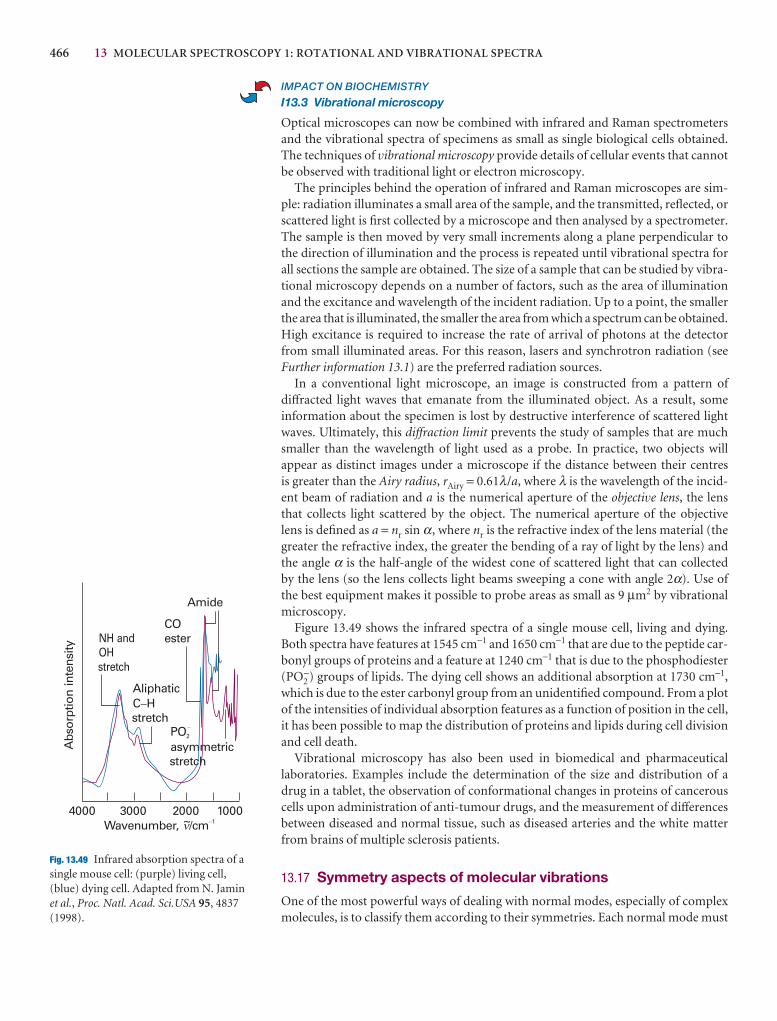
466 13 MOLECULAR SPECTROSCOPY 1: ROTATIONAL AND VIBRATIONAL SPECTRA
IMPACT ON BIOCHEMISTRY
I13.3 Vibrational microscopy
Optical microscopes can now be combined with infrared and Raman spectrometersand the vibrational spectra of specimens as small as single biological cells obtained.The techniques of vibrational microscopy provide details of cellular events that cannotbe observed with traditional light or electron microscopy.
The principles behind the operation of infrared and Raman microscopes are sim-ple: radiation illuminates a small area of the sample, and the transmitted, reflected, orscattered light is first collected by a microscope and then analysed by a spectrometer.The sample is then moved by very small increments along a plane perpendicular to the direction of illumination and the process is repeated until vibrational spectra forall sections the sample are obtained. The size of a sample that can be studied by vibra-tional microscopy depends on a number of factors, such as the area of illuminationand the excitance and wavelength of the incident radiation. Up to a point, the smallerthe area that is illuminated, the smaller the area from which a spectrum can be obtained.High excitance is required to increase the rate of arrival of photons at the detectorfrom small illuminated areas. For this reason, lasers and synchrotron radiation (seeFurther information 13.1) are the preferred radiation sources.
In a conventional light microscope, an image is constructed from a pattern ofdiffracted light waves that emanate from the illuminated object. As a result, some information about the specimen is lost by destructive interference of scattered lightwaves. Ultimately, this diffraction limit prevents the study of samples that are muchsmaller than the wavelength of light used as a probe. In practice, two objects will appear as distinct images under a microscope if the distance between their centresis greater than the Airy radius, rAiry = 0.61λ/a, where λ is the wavelength of the incid-ent beam of radiation and a is the numerical aperture of the objective lens, the lens that collects light scattered by the object. The numerical aperture of the objective lens is defined as a = nr sin α, where nr is the refractive index of the lens material (thegreater the refractive index, the greater the bending of a ray of light by the lens) andthe angle α is the half-angle of the widest cone of scattered light that can collected by the lens (so the lens collects light beams sweeping a cone with angle 2α). Use of the best equipment makes it possible to probe areas as small as 9 µm2 by vibrationalmicroscopy.
Figure 13.49 shows the infrared spectra of a single mouse cell, living and dying.Both spectra have features at 1545 cm−1 and 1650 cm−1 that are due to the peptide car-bonyl groups of proteins and a feature at 1240 cm−1 that is due to the phosphodiester(PO2
−) groups of lipids. The dying cell shows an additional absorption at 1730 cm−1,which is due to the ester carbonyl group from an unidentified compound. From a plotof the intensities of individual absorption features as a function of position in the cell,it has been possible to map the distribution of proteins and lipids during cell divisionand cell death.
Vibrational microscopy has also been used in biomedical and pharmaceutical laboratories. Examples include the determination of the size and distribution of adrug in a tablet, the observation of conformational changes in proteins of cancerouscells upon administration of anti-tumour drugs, and the measurement of differencesbetween diseased and normal tissue, such as diseased arteries and the white matterfrom brains of multiple sclerosis patients.
13.17 Symmetry aspects of molecular vibrations
One of the most powerful ways of dealing with normal modes, especially of complexmolecules, is to classify them according to their symmetries. Each normal mode must
NH andOHstretch
AliphaticC Hstretch
�
Amide
POasymmetricstretch
2
4000 3000 2000 1000
Abs
orpt
ion
inte
nsity
COester
Wavenumber, /cm�1~
�
�
Fig. 13.49 Infrared absorption spectra of asingle mouse cell: (purple) living cell,(blue) dying cell. Adapted from N. Jamin et al., Proc. Natl. Acad. Sci.USA 95, 4837(1998).
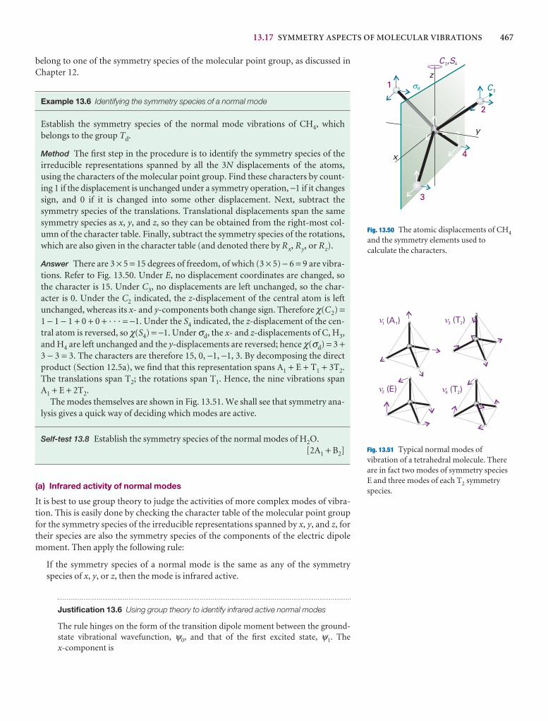
13.17 SYMMETRY ASPECTS OF MOLECULAR VIBRATIONS 467
x
y
z
C ,S2 4
d1
4
C3
2
3
$
1 1(A )
2 (E)
3 2(T )
4 2(T )
� �
� �
Fig. 13.50 The atomic displacements of CH4
and the symmetry elements used tocalculate the characters.
Fig. 13.51 Typical normal modes ofvibration of a tetrahedral molecule. Thereare in fact two modes of symmetry speciesE and three modes of each T2 symmetryspecies.
belong to one of the symmetry species of the molecular point group, as discussed inChapter 12.
Example 13.6 Identifying the symmetry species of a normal mode
Establish the symmetry species of the normal mode vibrations of CH4, which belongs to the group Td.
Method The first step in the procedure is to identify the symmetry species of the irreducible representations spanned by all the 3N displacements of the atoms,using the characters of the molecular point group. Find these characters by count-ing 1 if the displacement is unchanged under a symmetry operation, −1 if it changessign, and 0 if it is changed into some other displacement. Next, subtract the symmetry species of the translations. Translational displacements span the samesymmetry species as x, y, and z, so they can be obtained from the right-most col-umn of the character table. Finally, subtract the symmetry species of the rotations,which are also given in the character table (and denoted there by Rx, Ry, or Rz).
Answer There are 3 × 5 = 15 degrees of freedom, of which (3 × 5) − 6 = 9 are vibra-tions. Refer to Fig. 13.50. Under E, no displacement coordinates are changed, sothe character is 15. Under C3, no displacements are left unchanged, so the char-acter is 0. Under the C2 indicated, the z-displacement of the central atom is left unchanged, whereas its x- and y-components both change sign. Therefore χ(C2) =1 − 1 − 1 + 0 + 0 + · · · = −1. Under the S4 indicated, the z-displacement of the cen-tral atom is reversed, so χ(S4) = −1. Under σd, the x- and z-displacements of C, H3,and H4 are left unchanged and the y-displacements are reversed; hence χ(σd) = 3 +3 − 3 = 3. The characters are therefore 15, 0, −1, −1, 3. By decomposing the directproduct (Section 12.5a), we find that this representation spans A1 + E + T1 + 3T2.The translations span T2; the rotations span T1. Hence, the nine vibrations span A1 + E + 2T2.
The modes themselves are shown in Fig. 13.51. We shall see that symmetry ana-lysis gives a quick way of deciding which modes are active.
Self-test 13.8 Establish the symmetry species of the normal modes of H2O.[2A1 + B2]
(a) Infrared activity of normal modes
It is best to use group theory to judge the activities of more complex modes of vibra-tion. This is easily done by checking the character table of the molecular point groupfor the symmetry species of the irreducible representations spanned by x, y, and z, fortheir species are also the symmetry species of the components of the electric dipolemoment. Then apply the following rule:
If the symmetry species of a normal mode is the same as any of the symmetryspecies of x, y, or z, then the mode is infrared active.
Justification 13.6 Using group theory to identify infrared active normal modes
The rule hinges on the form of the transition dipole moment between the ground-state vibrational wavefunction, ψ0, and that of the first excited state, ψ1. The x-component is
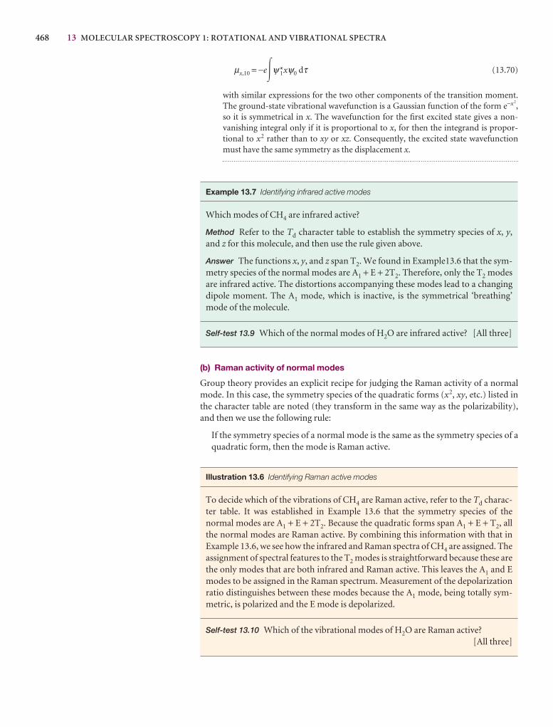
468 13 MOLECULAR SPECTROSCOPY 1: ROTATIONAL AND VIBRATIONAL SPECTRA
µx,10 = −e�ψ*1xψ0 dτ (13.70)
with similar expressions for the two other components of the transition moment.The ground-state vibrational wavefunction is a Gaussian function of the form e−x2
,so it is symmetrical in x. The wavefunction for the first excited state gives a non-vanishing integral only if it is proportional to x, for then the integrand is propor-tional to x2 rather than to xy or xz. Consequently, the excited state wavefunctionmust have the same symmetry as the displacement x.
Example 13.7 Identifying infrared active modes
Which modes of CH4 are infrared active?
Method Refer to the Td character table to establish the symmetry species of x, y,and z for this molecule, and then use the rule given above.
Answer The functions x, y, and z span T2. We found in Example13.6 that the sym-metry species of the normal modes are A1 + E + 2T2. Therefore, only the T2 modesare infrared active. The distortions accompanying these modes lead to a changingdipole moment. The A1 mode, which is inactive, is the symmetrical ‘breathing’mode of the molecule.
Self-test 13.9 Which of the normal modes of H2O are infrared active? [All three]
(b) Raman activity of normal modes
Group theory provides an explicit recipe for judging the Raman activity of a normalmode. In this case, the symmetry species of the quadratic forms (x2, xy, etc.) listed inthe character table are noted (they transform in the same way as the polarizability),and then we use the following rule:
If the symmetry species of a normal mode is the same as the symmetry species of aquadratic form, then the mode is Raman active.
Illustration 13.6 Identifying Raman active modes
To decide which of the vibrations of CH4 are Raman active, refer to the Td charac-ter table. It was established in Example 13.6 that the symmetry species of the normal modes are A1 + E + 2T2. Because the quadratic forms span A1 + E + T2, allthe normal modes are Raman active. By combining this information with that inExample 13.6, we see how the infrared and Raman spectra of CH4 are assigned. Theassignment of spectral features to the T2 modes is straightforward because these arethe only modes that are both infrared and Raman active. This leaves the A1 and Emodes to be assigned in the Raman spectrum. Measurement of the depolarizationratio distinguishes between these modes because the A1 mode, being totally sym-metric, is polarized and the E mode is depolarized.
Self-test 13.10 Which of the vibrational modes of H2O are Raman active?[All three]

CHECKLIST OF KEY IDEAS 469
Checklist of key ideas
1. Emission spectroscopy is based on the detection of atransition from a state of high energy to a state of lowerenergy; absorption spectroscopy is based on the detection ofthe net absorption of nearly monochromatic incidentradiation as the radiation is swept over a range of frequencies.
2. In Raman spectroscopy molecular energy levels are exploredby examining the frequencies present in scattered radiation.Stokes and anti-Stokes radiation are scattered radiation at alower and higher frequency, respectively, than the incidentradiation. Rayleigh radiation is the component of radiationscattered into the forward direction without change offrequency.
3. The Beer–Lambert law is I(#) = I0(#)10−ε(#)[J]l, where I(#) isthe transmitted intensity, I0(#) is the incident intensity, andε(#) is the molar absorption coefficient.
4. The transmittance, T = I/I0, and the absorbance, A, of asample at a given wavenumber are related by A = − log T.
5. The integrated absorption coefficient, A , is the sum of theabsorption coefficients over the entire band, A = ∫band ε(#)d#.
6. Stimulated absorption is the radiation-driven transition froma low energy state to one of higher energy. Stimulatedemission is the radiation-driven transition from a high energystate to one of lower energy. Spontaneous emission isradiative emission independent of the intensity of theradiation (of any frequency) that is already present.
7. The natural linewidth of a spectral line is due to spontaneousemission. Spectral lines are affected by Doppler broadening,lifetime broadening, and collisional deactivation of excitedstates.
8. A rigid rotor is a body that does not distort under the stress of rotation. A spherical rotor is a rigid rotor with three equal moments of inertia. A symmetric rotor is a rigid rotorwith two equal moments of inertia. A linear rotor is a rigidrotor with one moment of inertia equal to zero. Anasymmetric rotor is a rigid rotor with three differentmoments of inertia.
9. The rotational terms of a spherical rotor are F( J) = BJ( J + 1)with B = $/4πcI, J = 0, 1, 2, . . . , and are (2J + 1)2-folddegenerate.
10. The principal axis (figure axis) is the unique axis of asymmetric top. In an oblate top, I|| > I⊥. In a prolate top, I|| < I⊥.
11. The rotational terms of a symmetric rotor are F( J,K) =BJ( J + 1) + (A − B)K2, J = 0, 1, 2, . . . , K = 0, ±1, . . . , ± J.
12. The rotational terms of a linear rotor are F( J) = BJ( J + 1),J = 0, 1, 2, . . . and are (2J + 1)-fold degenerate.
13. The centrifugal distortion constant, DJ , is the empiricalconstant in the expression F( J) = BJ( J + 1) − DJ J
2( J + 1)2 thattakes into account centrifugal distortion, DJ ≈ 4B3/#2.
14. The gross rotational selection rule for microwave spectra is:for a molecule to give a pure rotational spectrum, it must be
polar. The specific rotational selection rule is: ∆J = ±1,∆MJ = 0, ±1, ∆K = 0. The rotational wavenumbers in theabsence and presence of centrifugal distortion are given byeqns 13.37 and 13.38, respectively.
15. The gross selection rule for rotational Raman spectra is: themolecule must be anisotropically polarizable. The specificselection rules are: (i) linear rotors, ∆J = 0, ±2; (ii) symmetricrotors, ∆J = 0, ±1, ±2; ∆K = 0.
16. The appearance of rotational spectra is affected by nuclearstatistics, the selective occupation of rotational states thatstems from the Pauli principle.
17. The vibrational energy levels of a diatomic molecule modelledas a harmonic oscillator are Ev = (v + 1–2)$ω, ω = (k /meff)1/2; the
vibrational terms are G(v) = (v + 1–2)#, # =(1/2πc)(k/meff)1/2.
18. The gross selection rule for infrared spectra is: the electricdipole moment of the molecule must change when the atomsare displaced relative to one another. The specific selectionrule is: ∆v = ±1.
19. Morse potential energy, eqn 13.54, describes anharmonicmotion, oscillatory motion in which the restoring force is notproportional to the displacement; the vibrational terms of aMorse oscillator are given by eqn 13.55.
20. A Birge–Sponer plot is a graphical procedure for determiningthe dissociation energy of a bond.
21. The P branch consists of vibration–rotation infraredtransitions with ∆J = −1; the Q branch has transitions with ∆J = 0; the R branch has transitions with ∆J = +1.
22. The gross selection rule for vibrational Raman spectra is: thepolarizability must change as the molecule vibrates. Thespecific selection rule is: ∆v = ±1.
23. A normal mode is an independent, synchronous motion ofatoms or groups of atoms that may be excited without leadingto the excitation of any other normal mode. The number ofnormal modes is 3N − 6 (for nonlinear molecules) or 3N − 5(linear molecules).
24. A symmetric stretch is a symmetrically stretching vibrationalmode. An antisymmetric stretch is a stretching mode, one halfof which is the mirror image of the other half.
25. The exclusion rule states that, if the molecule has a centre ofsymmetry, then no modes can be both infrared and Ramanactive.
26. The depolarization ratio, ρ, the ratio of the intensities, I, of thescattered light with polarizations perpendicular and parallel tothe plane of polarization of the incident radiation, ρ = I⊥/I||. Adepolarized line is a line with ρ close to or greater than 0.75. Apolarized line is a line with ρ < 0.75.
27. Resonance Raman spectroscopy is a Raman technique inwhich the frequency of the incident radiation nearly coincideswith the frequency of an electronic transition of the sample.Coherent anti-Stokes Raman spectroscopy (CARS) is a

470 13 MOLECULAR SPECTROSCOPY 1: ROTATIONAL AND VIBRATIONAL SPECTRA
Raman technique that relies on the use of two incident beamsof radiation.
28. A normal mode is infrared active if its symmetry species is thesame as any of the symmetry species of x, y, or z, then the
mode is infrared active. A normal mode is Raman active if itssymmetry species is the same as the symmetry species of aquadratic form.
Further reading
Articles and texts
L. Glasser, Fourier transforms for chemists. Part I. Introduction tothe Fourier transform. J. Chem. Educ. 64, A228 (1987). Part II.Fourier transforms in chemistry and spectroscopy. J. Chem. Educ.64, A260 (1987).
H.-U. Gremlich and B. Yan, Infrared and Raman spectroscopy ofbiological materials. Marcel Dekker, New York (2001).
G. Herzberg, Molecular spectra and molecular structure I. Spectra ofdiatomic molecules. Krieger, Malabar (1989).
G. Herzberg, Molecular spectra and molecular structure II. Infrared andRaman spectra of polyatomic molecules. Van Nostrand–Reinhold,New York (1945).
J.C. Lindon, G.E. Tranter, and J.L. Holmes (ed.), Encyclopedia ofspectroscopy and spectrometry. Academic Press, San Diego (2000).
D.P. Strommen, Specific values of the depolarization ratio in Ramanspectroscopy: Their origins and significance. J. Chem. Educ. 69, 803(1992).
E.B. Wilson, J.C. Decius, and P.C. Cross, Molecular vibrations. Dover,New York (1980).
J.M. Brown and A. Carrington, Rotational spectroscopy of diatomicmolecules. Cambridge University Press (2003).
Sources of data and information
M.E. Jacox, Vibrational and electronic energy levels of polyatomictransient molecules. Journal of Physical and Chemical ReferenceData, Monograph No. 3 (1994).
K.P. Huber and G. Herzberg, Molecular spectra and molecularstructure IV. Constants of diatomic molecules. Van Nostrand-Reinhold, New York (1979).
B. Schrader, Raman/IR atlas of organic compounds. VCH, New York(1989).
G. Socrates, Infrared and Raman characteristic group frequencies: tablesand charts. Wiley, New York (2000).
Further information
Further information 13.1 Spectrometers
Here we provide additional detail on the principles of operation ofspectrometers, describing radiation sources, dispersing elements,detectors, and Fourier transform techniques.
Sources of radiation
Sources of radiation are either monochromatic, those spanning a verynarrow range of frequencies around a central value, or polychromatic,those spanning a wide range of frequencies. Monochromatic sourcesthat can be tuned over a range of frequencies include the klystron andthe Gunn diode, which operate in the microwave range, and lasers,which are discussed in Chapter 14.
Polychromatic sources that take advantage of black-body radiation from hot materials. For far infrared radiation with 35 cm−1
< # < 200 cm−1, a typical source is a mercury arc inside a quartzenvelope, most of the radiation being generated by the hot quartz.Either a Nernst filament or a globar is used as a source of mid-infraredradiation with 200 cm−1 < # < 4000 cm−1. The Nernst filamentconsists of a ceramic filament of lanthanoid oxides that is heated totemperatures ranging from 1200 to 2000 K. The globar consists of arod of silicon carbide, which is heated electrically to about 1500 K.
A quartz–tungsten–halogen lamp consists of a tungsten filamentthat, when heated to about 3000 K, emits light in the range 320 nm <λ < 2500 nm. Near the surface of the lamp’s quartz envelope, iodineatoms and tungsten atoms ejected from the filament combine tomake a variety of tungsten–iodine compounds that decompose at thehot filament, replenishing it with tungsten atoms.
A gas discharge lamp is a common source of ultraviolet and visibleradiation. In a xenon discharge lamp, an electrical discharge excitesxenon atoms to excited states, which then emit ultraviolet radiation.At pressures exceeding 1 kPa, the output consists of sharp lines on a broad, intense background due to emission from a mixture of ionsformed by the electrical discharge. These high-pressure xenon lampshave emission profiles similar to that of a black body heated to 6000 K. In a deuterium lamp, excited D2 molecules dissociate intoelectronically excited D atoms, which emit intense radiation between200–400 nm.
For certain applications, synchrotron radiation is generated in asynchrotron storage ring, which consists of an electron beam travellingin a circular path with circumferences of up to several hunderdmetres. As electrons travelling in a circle are constantly accelerated bythe forces that constrain them to their path, they generate radiation(Fig. 13.52). Synchrotron radiation spans a wide range of frequencies,
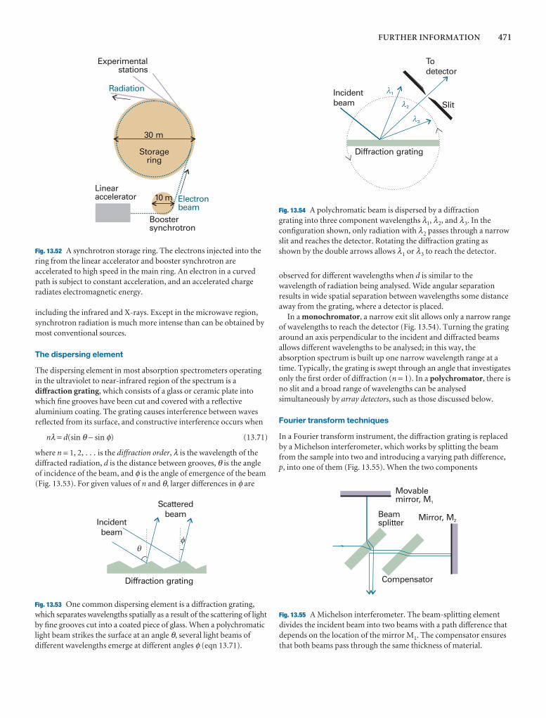
FURTHER INFORMATION 471
observed for different wavelengths when d is similar to thewavelength of radiation being analysed. Wide angular separationresults in wide spatial separation between wavelengths some distanceaway from the grating, where a detector is placed.
In a monochromator, a narrow exit slit allows only a narrow rangeof wavelengths to reach the detector (Fig. 13.54). Turning the gratingaround an axis perpendicular to the incident and diffracted beamsallows different wavelengths to be analysed; in this way, theabsorption spectrum is built up one narrow wavelength range at atime. Typically, the grating is swept through an angle that investigatesonly the first order of diffraction (n = 1). In a polychromator, there isno slit and a broad range of wavelengths can be analysedsimultaneously by array detectors, such as those discussed below.
Fourier transform techniques
In a Fourier transform instrument, the diffraction grating is replacedby a Michelson interferometer, which works by splitting the beamfrom the sample into two and introducing a varying path difference,p, into one of them (Fig. 13.55). When the two components
Linearaccelerator
Boostersynchrotron
Storagering
10 m
30 m
Experimentalstations
Radiation
Electronbeam
Fig. 13.52 A synchrotron storage ring. The electrons injected into thering from the linear accelerator and booster synchrotron areaccelerated to high speed in the main ring. An electron in a curvedpath is subject to constant acceleration, and an accelerated chargeradiates electromagnetic energy.
��
Incidentbeam
Scatteredbeam
Diffraction grating
Fig. 13.53 One common dispersing element is a diffraction grating,which separates wavelengths spatially as a result of the scattering of lightby fine grooves cut into a coated piece of glass. When a polychromaticlight beam strikes the surface at an angle θ, several light beams ofdifferent wavelengths emerge at different angles φ (eqn 13.71).
including the infrared and X-rays. Except in the microwave region,synchrotron radiation is much more intense than can be obtained bymost conventional sources.
The dispersing element
The dispersing element in most absorption spectrometers operatingin the ultraviolet to near-infrared region of the spectrum is adiffraction grating, which consists of a glass or ceramic plate intowhich fine grooves have been cut and covered with a reflectivealuminium coating. The grating causes interference between wavesreflected from its surface, and constructive interference occurs when
nλ = d(sin θ − sin φ) (13.71)
where n = 1, 2, . . . is the diffraction order, λ is the wavelength of thediffracted radiation, d is the distance between grooves, θ is the angleof incidence of the beam, and φ is the angle of emergence of the beam(Fig. 13.53). For given values of n and θ, larger differences in φ are
Incidentbeam
1
2
3
Slit
Todetector
Diffraction grating
�
�
�
Fig. 13.54 A polychromatic beam is dispersed by a diffractiongrating into three component wavelengths λ1, λ2, and λ3. In theconfiguration shown, only radiation with λ2 passes through a narrowslit and reaches the detector. Rotating the diffraction grating asshown by the double arrows allows λ1 or λ3 to reach the detector.
Beamsplitter
Compensator
Mirror, M2
Movablemirror, M1
Fig. 13.55 A Michelson interferometer. The beam-splitting elementdivides the incident beam into two beams with a path difference thatdepends on the location of the mirror M1. The compensator ensuresthat both beams pass through the same thickness of material.
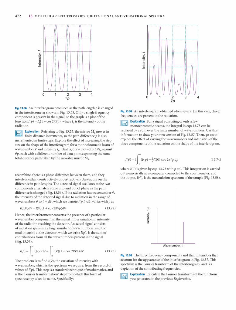
472 13 MOLECULAR SPECTROSCOPY 1: ROTATIONAL AND VIBRATIONAL SPECTRA
recombine, there is a phase difference between them, and theyinterfere either constructively or destructively depending on thedifference in path lengths. The detected signal oscillates as the twocomponents alternately come into and out of phase as the pathdifference is changed (Fig. 13.56). If the radiation has wavenumber #,the intensity of the detected signal due to radiation in the range ofwavenumbers # to # + d#, which we denote I(p,#)d#, varies with p as
I(p,#)d# = I(#)(1 + cos 2π#p)d# (13.72)
Hence, the interferometer converts the presence of a particularwavenumber component in the signal into a variation in intensity of the radiation reaching the detector. An actual signal consists of radiation spanning a large number of wavenumbers, and the total intensity at the detector, which we write I(p), is the sum ofcontributions from all the wavenumbers present in the signal (Fig. 13.57):
I(p) = �0
∞
I(p,#)d# = �0
∞
I(#)(1 + cos 2π#p)d# (13.73)
The problem is to find I(#), the variation of intensity withwavenumber, which is the spectrum we require, from the record ofvalues of I(p). This step is a standard technique of mathematics, andis the ‘Fourier transformation’ step from which this form ofspectroscopy takes its name. Specifically:
1 2 30p~
Inte
nsity
, I
4�
Fig. 13.56 An interferogram produced as the path length p is changedin the interferometer shown in Fig. 13.55. Only a single frequencycomponent is present in the signal, so the graph is a plot of thefunction I(p) = I0(1 + cos 2π#p), where I0 is the intensity of theradiation.
Exploration Referring to Fig. 13.55, the mirror M1 moves infinite distance increments, so the path difference p is also
incremented in finite steps. Explore the effect of increasing the stepsize on the shape of the interferogram for a monochromatic beam ofwavenumber # and intensity I0. That is, draw plots of I(p)/I0 against#p, each with a different number of data points spanning the sametotal distance path taken by the movable mirror M1.
1 2 30p~
Inte
nsity
, I
4�
Fig. 13.57 An interferogram obtained when several (in this case, three)frequencies are present in the radiation.
Exploration For a signal consisting of only a fewmonochromatic beams, the integral in eqn 13.73 can be
replaced by a sum over the finite number of wavenumbers. Use thisinformation to draw your own version of Fig. 13.57. Then, go on toexplore the effect of varying the wavenumbers and intensities of thethree components of the radiation on the shape of the interferogram.
Inte
nsity
,(
)I
~
Wavenumber, ~�
�
Fig. 13.58 The three frequency components and their intensities thataccount for the appearance of the interferogram in Fig. 13.57. Thisspectrum is the Fourier transform of the interferogram, and is adepiction of the contributing frequencies.
Exploration Calculate the Fourier transforms of the functionsyou generated in the previous Exploration.
I(#) = 4�0
∞
{I(p) − 1–2I(0)} cos 2π#p dp (13.74)
where I(0) is given by eqn 13.73 with p = 0. This integration is carriedout numerically in a computer connected to the spectrometer, andthe output, I(#), is the transmission spectrum of the sample (Fig. 13.58).
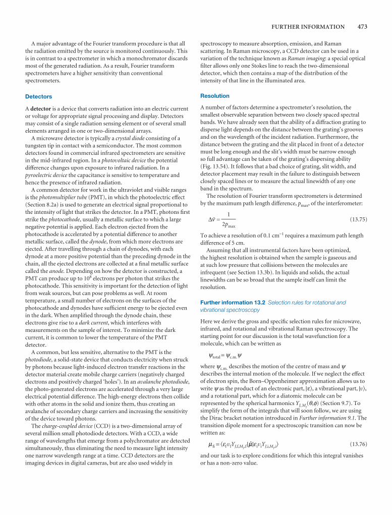
FURTHER INFORMATION 473
A major advantage of the Fourier transform procedure is that allthe radiation emitted by the source is monitored continuously. Thisis in contrast to a spectrometer in which a monochromator discardsmost of the generated radiation. As a result, Fourier transformspectrometers have a higher sensitivity than conventionalspectrometers.
Detectors
A detector is a device that converts radiation into an electric currentor voltage for appropriate signal processing and display. Detectorsmay consist of a single radiation sensing element or of several smallelements arranged in one or two-dimensional arrays.
A microwave detector is typically a crystal diode consisting of atungsten tip in contact with a semiconductor. The most commondetectors found in commercial infrared spectrometers are sensitive in the mid-infrared region. In a photovoltaic device the potentialdifference changes upon exposure to infrared radiation. In apyroelectric device the capacitance is sensitive to temperature andhence the presence of infrared radiation.
A common detector for work in the ultraviolet and visible ranges is the photomultiplier tube (PMT), in which the photoelectric effect(Section 8.2a) is used to generate an electrical signal proportional tothe intensity of light that strikes the detector. In a PMT, photons firststrike the photocathode, usually a metallic surface to which a largenegative potential is applied. Each electron ejected from thephotocathode is accelerated by a potential difference to anothermetallic surface, called the dynode, from which more electrons areejected. After travelling through a chain of dynodes, with eachdynode at a more positive potential than the preceding dynode in thechain, all the ejected electrons are collected at a final metallic surfacecalled the anode. Depending on how the detector is constructed, aPMT can produce up to 108 electrons per photon that strikes thephotocathode. This sensitivity is important for the detection of lightfrom weak sources, but can pose problems as well. At roomtemperature, a small number of electrons on the surfaces of thephotocathode and dynodes have sufficient energy to be ejected evenin the dark. When amplified through the dynode chain, theseelectrons give rise to a dark current, which interferes withmeasurements on the sample of interest. To minimize the darkcurrent, it is common to lower the temperature of the PMT detector.
A common, but less sensitive, alternative to the PMT is thephotodiode, a solid-state device that conducts electricity when struckby photons because light-induced electron transfer reactions in thedetector material create mobile charge carriers (negatively chargedelectrons and positively charged ‘holes’). In an avalanche photodiode,the photo-generated electrons are accelerated through a very largeelectrical potential difference. The high-energy electrons then collidewith other atoms in the solid and ionize them, thus creating anavalanche of secondary charge carriers and increasing the sensitivityof the device toward photons.
The charge-coupled device (CCD) is a two-dimensional array ofseveral million small photodiode detectors. With a CCD, a widerange of wavelengths that emerge from a polychromator are detectedsimultaneously, thus eliminating the need to measure light intensityone narrow wavelength range at a time. CCD detectors are theimaging devices in digital cameras, but are also used widely in
spectroscopy to measure absorption, emission, and Ramanscattering. In Raman microscopy, a CCD detector can be used in avariation of the technique known as Raman imaging: a special opticalfilter allows only one Stokes line to reach the two-dimensionaldetector, which then contains a map of the distribution of theintensity of that line in the illuminated area.
Resolution
A number of factors determine a spectrometer’s resolution, thesmallest observable separation between two closely spaced spectralbands. We have already seen that the ability of a diffraction grating todisperse light depends on the distance between the grating’s groovesand on the wavelength of the incident radiation. Furthermore, thedistance between the grating and the slit placed in front of a detectormust be long enough and the slit’s width must be narrow enough so full advantage can be taken of the grating’s dispersing ability (Fig. 13.54). It follows that a bad choice of grating, slit width, anddetector placement may result in the failure to distinguish betweenclosely spaced lines or to measure the actual linewidth of any oneband in the spectrum.
The resolution of Fourier transform spectrometers is determinedby the maximum path length difference, pmax, of the interferometer:
∆# = (13.75)
To achieve a resolution of 0.1 cm−1 requires a maximum path lengthdifference of 5 cm.
Assuming that all instrumental factors have been optimized, the highest resolution is obtained when the sample is gaseous and at such low pressure that collisions between the molecules areinfrequent (see Section 13.3b). In liquids and solids, the actuallinewidths can be so broad that the sample itself can limit theresolution.
Further information 13.2 Selection rules for rotational andvibrational spectroscopy
Here we derive the gross and specific selection rules for microwave,infrared, and rotational and vibrational Raman spectroscopy. Thestarting point for our discussion is the total wavefunction for amolecule, which can be written as
ψtotal = ψc.m.ψ
where ψc.m. describes the motion of the centre of mass and ψdescribes the internal motion of the molecule. If we neglect the effectof electron spin, the Born–Oppenheimer approximation allows us towrite ψ as the product of an electronic part, | ε�, a vibrational part, |v�,and a rotational part, which for a diatomic molecule can berepresented by the spherical harmonics YJ, MJ
(θ,φ) (Section 9.7). Tosimplify the form of the integrals that will soon follow, we are usingthe Dirac bracket notation introduced in Further information 9.1. Thetransition dipole moment for a spectroscopic transition can now bewritten as:
µfi = �εf vfYJ,f,MJ,f|¢|εiviYJ,i,MJ,i
� (13.76)
and our task is to explore conditions for which this integral vanishesor has a non-zero value.
1
2pmax
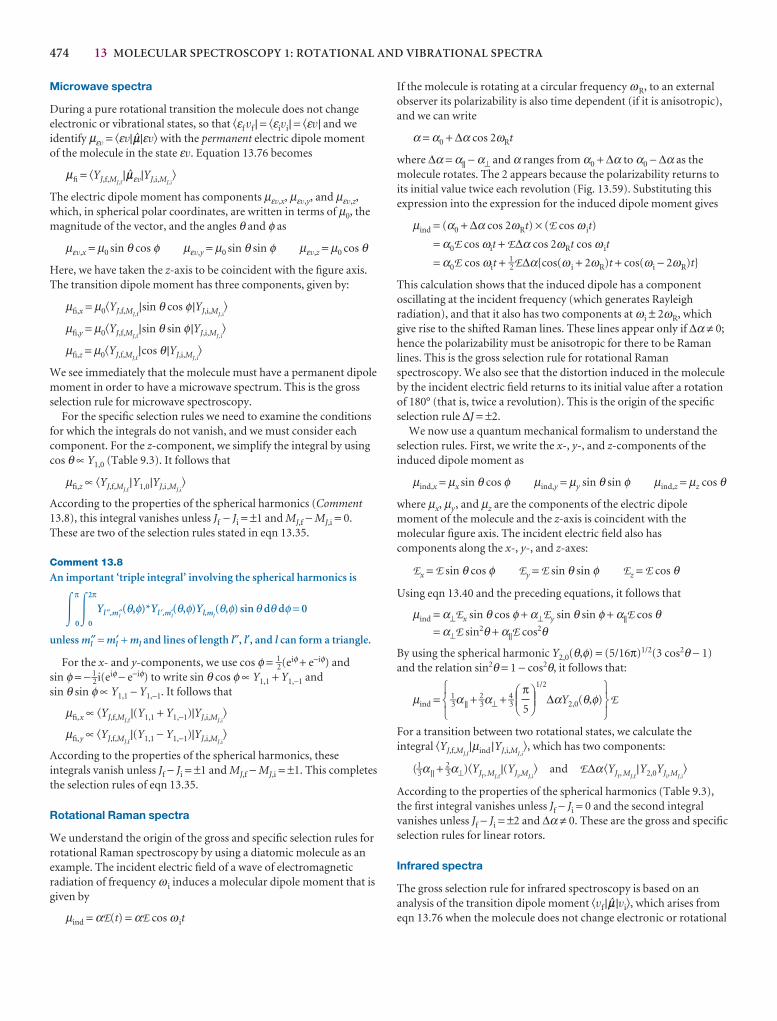
474 13 MOLECULAR SPECTROSCOPY 1: ROTATIONAL AND VIBRATIONAL SPECTRA
Microwave spectra
During a pure rotational transition the molecule does not changeelectronic or vibrational states, so that �εf vf | = �εivi| = �εv| and weidentify µεv = �εv|¢|εv� with the permanent electric dipole moment of the molecule in the state εv. Equation 13.76 becomes
µfi = �YJ,f,MJ,f|¢εv|YJ,i,MJ,i
�
The electric dipole moment has components µεv,x, µεv,y, and µεv,z,which, in spherical polar coordinates, are written in terms of µ0, themagnitude of the vector, and the angles θ and φ as
µεv,x = µ0 sin θ cos φ µεv,y = µ0 sin θ sin φ µεv,z = µ0 cos θ
Here, we have taken the z-axis to be coincident with the figure axis.The transition dipole moment has three components, given by:
µfi,x = µ0�YJ,f,MJ,f|sin θ cos φ|YJ,i,MJ,i
�
µfi,y = µ0�YJ,f,MJ,f|sin θ sin φ|YJ,i,MJ,i
�
µfi,z = µ0�YJ,f,MJ,f|cos θ|YJ,i,MJ,i
�
We see immediately that the molecule must have a permanent dipolemoment in order to have a microwave spectrum. This is the grossselection rule for microwave spectroscopy.
For the specific selection rules we need to examine the conditionsfor which the integrals do not vanish, and we must consider eachcomponent. For the z-component, we simplify the integral by usingcos θ ∝ Y1,0 (Table 9.3). It follows that
µfi,z ∝ �YJ,f,MJ,f|Y1,0|YJ,i,MJ,i
�
According to the properties of the spherical harmonics (Comment13.8), this integral vanishes unless Jf − Ji = ±1 and MJ,f − MJ,i = 0.These are two of the selection rules stated in eqn 13.35.
Comment 13.8
An important ‘triple integral’ involving the spherical harmonics is
�0
π
�0
2π
Yl ″,ml″(θ,φ)*Yl ′,m′l
(θ,φ)Yl,ml(θ,φ) sin θ dθ dφ = 0
unless ml″ = ml′ + ml and lines of length l″, l′, and l can form a triangle.
For the x- and y-components, we use cos φ = 1–2(eiφ + e−iφ) and sin φ = − 1–2i(eiφ − e−iφ) to write sin θ cos φ ∝ Y1,1 + Y1,−1 andsin θ sin φ ∝ Y1,1 − Y1,−1. It follows that
µfi,x ∝ �YJ,f,MJ,f|(Y1,1 + Y1,−1)|YJ,i,MJ,i
�
µfi,y ∝ �YJ,f,MJ,f|(Y1,1 − Y1,−1)|YJ,i,MJ,i
�
According to the properties of the spherical harmonics, theseintegrals vanish unless Jf − Ji = ±1 and MJ,f − MJ,i = ±1. This completesthe selection rules of eqn 13.35.
Rotational Raman spectra
We understand the origin of the gross and specific selection rules forrotational Raman spectroscopy by using a diatomic molecule as anexample. The incident electric field of a wave of electromagneticradiation of frequency ω i induces a molecular dipole moment that isgiven by
µind = αE(t) = αE cos ω it
If the molecule is rotating at a circular frequency ωR, to an externalobserver its polarizability is also time dependent (if it is anisotropic),and we can write
α = α0 + ∆α cos 2ωRt
where ∆α = α|| − α⊥ and α ranges from α0 + ∆α to α0 − ∆α as themolecule rotates. The 2 appears because the polarizability returns toits initial value twice each revolution (Fig. 13.59). Substituting thisexpression into the expression for the induced dipole moment gives
µind = (α0 + ∆α cos 2ωRt) × (E cos ω it)
= α0E cos ωit + E∆α cos 2ωRt cos ω it
= α0E cos ωit + 1–2E∆α{cos(ω i + 2ωR)t + cos(ωi − 2ωR)t}
This calculation shows that the induced dipole has a componentoscillating at the incident frequency (which generates Rayleighradiation), and that it also has two components at ωi ± 2ωR, whichgive rise to the shifted Raman lines. These lines appear only if ∆α ≠ 0;hence the polarizability must be anisotropic for there to be Ramanlines. This is the gross selection rule for rotational Ramanspectroscopy. We also see that the distortion induced in the moleculeby the incident electric field returns to its initial value after a rotationof 180° (that is, twice a revolution). This is the origin of the specificselection rule ∆J = ±2.
We now use a quantum mechanical formalism to understand theselection rules. First, we write the x-, y-, and z-components of theinduced dipole moment as
µind,x = µx sin θ cos φ µind,y = µy sin θ sin φ µind,z = µz cos θ
where µx, µy, and µz are the components of the electric dipolemoment of the molecule and the z-axis is coincident with themolecular figure axis. The incident electric field also has components along the x-, y-, and z-axes:
Ex = E sin θ cos φ Ey = E sin θ sin φ Ez = E cos θ
Using eqn 13.40 and the preceding equations, it follows that
µind = α⊥Ex sin θ cos φ + α⊥Ey sin θ sin φ + α||E cos θ= α⊥E sin2θ + α||E cos2θ
By using the spherical harmonic Y2,0(θ,φ) = (5/16π)1/2(3 cos2θ − 1)and the relation sin2θ = 1 − cos2θ, it follows that:
µind = 1–3α|| +2–3α⊥ + 4–3
1/2
∆αY2,0(θ,φ) E
For a transition between two rotational states, we calculate theintegral �YJ,f,MJ,f
|µind |YJ,i,MJ,i�, which has two components:
(1–3α|| +2–3α⊥)�YJf , MJ,f
|(YJi,MJ,i� and E∆α�YJf , MJ,f
|Y2,0YJi,MJ,i�
According to the properties of the spherical harmonics (Table 9.3),the first integral vanishes unless Jf − Ji = 0 and the second integralvanishes unless Jf − Ji = ±2 and ∆α ≠ 0. These are the gross and specificselection rules for linear rotors.
Infrared spectra
The gross selection rule for infrared spectroscopy is based on ananalysis of the transition dipole moment �vf |¢|vi�, which arises fromeqn 13.76 when the molecule does not change electronic or rotational
567
DEFπ5
ABC123
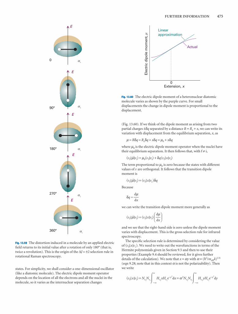
FURTHER INFORMATION 475
states. For simplicity, we shall consider a one-dimensional oscillator(like a diatomic molecule). The electric dipole moment operatordepends on the location of all the electrons and all the nuclei in themolecule, so it varies as the internuclear separation changes
(Fig. 13.60). If we think of the dipole moment as arising from twopartial charges ±δq separated by a distance R = Re + x, we can write itsvariation with displacement from the equilibrium separation, x, as
µ = Rδq = Reδq + xδq = µ0 + xδq
where µ0 is the electric dipole moment operator when the nuclei havetheir equilibrium separation. It then follows that, with f ≠ i,
�vf | N|vi� = µ0�vf |vi� + δq�vf |x |vi�
The term proportional to µ0 is zero because the states with differentvalues of v are orthogonal. It follows that the transition dipolemoment is
�vf | N|vi� = �vf |x |vi �δq
Because
δq =
we can write the transition dipole moment more generally as
�vf | N|vi� = �vf |x |vi�
and we see that the right-hand side is zero unless the dipole momentvaries with displacement. This is the gross selection rule for infraredspectroscopy.
The specific selection rule is determined by considering the valueof �vf |x |vi �. We need to write out the wavefunctions in terms of theHermite polynomials given in Section 9.5 and then to use theirproperties (Example 9.4 should be reviewed, for it gives furtherdetails of the calculation). We note that x = αy with α = ($2/meff k)1/4
(eqn 9.28; note that in this context α is not the polarizability). Thenwe write
�vf | x |vi� = NvfNvi�
∞
−∞
HvfxHvi
e−y2
dx = α2NvfNvi�
∞
−∞
HvfyHvi
e−y2
dy
DEFdµdx
ABC
dµdx
E
E
E
E
E
0
90°
180°
270°
360°
^
^
^
||
||
�
�
�
�
�
Fig. 13.59 The distortion induced in a molecule by an applied electricfield returns to its initial value after a rotation of only 180° (that is,twice a revolution). This is the origin of the ∆J = ±2 selection rule inrotational Raman spectroscopy.
Elec
tric
dip
ole
mom
ent,
Extension, x0
Linearapproximation
Actual
Fig. 13.60 The electric dipole moment of a heteronuclear diatomicmolecule varies as shown by the purple curve. For smalldisplacements the change in dipole moment is proportional to thedisplacement.
476 13 MOLECULAR SPECTROSCOPY 1: ROTATIONAL AND VIBRATIONAL SPECTRA
To evaluate the integral we use the recursion relation
yHv = vHv−1 + 1–2Hv+1
which turns the matrix element into
�vf | x |vi� = α2NvfNvi
vi�∞
−∞
HvfHvi−1e−y2
dy + 1–2�∞
−∞
HvfHvi+1e−y2
dy
The first integral is zero unless vf = vi − 1 and that the second is zerounless vf = vi + 1. It follows that the transition dipole moment is zerounless ∆v = ±1.
Comment 13.9
An important integral involving Hermite polynomials is
�∞
−∞
Hv′Hve−y 2
dy =0 if v′ ≠ vπ1/22vv! if v′ = v
Vibrational Raman spectra
The gross selection rule for vibrational Raman spectroscopy is basedon an analysis of the transition dipole moment �εvf | ¢|εvi�, which iswritten from eqn 13.76 by using the Born–Oppenheimer
123
567
123
approximation and neglecting the effect of rotation and electron spin.For simplicity, we consider a one-dimensional harmonic oscillator(like a diatomic molecule).
First, we use eqn 13.40 to write the transition dipole moment as
µfi = �εvf | N|εvi� = �εvf |α |εvi�E = �vf |α(x)|vi�E
where α(x) = �ε |α|ε� is the polarizability of the molecule, which weexpect to be a function of small displacements x from the equilibriumbond length of the molecule (Section 13.13). Next, we expand α(x) asa Taylor series, so the transition dipole moment becomes
µfi = vf α(0) +0
x + · · · vi E
= �vf |vi�α(0)E +0
�vf |x |vi�E + · · ·
The term containing �vf |vi� vanishes for f ≠ i because the harmonicoscillator wavefunctions are orthogonal. Therefore, the vibration isRaman active if (dα /dx)0 ≠ 0 and �vf |x |vi� ≠ 0. Therefore, thepolarizability of the molecule must change during the vibration; thisis the gross selection rule of Raman spectroscopy. Also, we alreadyknow that �vf |x |vi� ≠ 0 if vf − vi = ±1; this is the specific selection ruleof Raman spectroscopy.
DEFdαdx
ABC
DEFdαdx
ABC
Discussion questions
13.1 Describe the physical origins of linewidths in the absorption andemission spectra of gases, liquids, and solids.
13.2 Discuss the physical origins of the gross selection rules for microwaveand infrared spectroscopy.
13.3 Discuss the physical origins of the gross selection rules for rotational andvibrational Raman spectroscopy.
13.4 Consider a diatomic molecule that is highly susceptible to centrifugaldistortion in its ground vibrational state. Do you expect excitation to highrotational energy levels to change the equilibrium bond length of thismolecule? Justify your answer.
13.5 Suppose that you wish to characterize the normal modes of benzene inthe gas phase. Why is it important to obtain both infrared absorption andRaman spectra of your sample?
Exercises
13.1a Calculate the ratio of the Einstein coefficients of spontaneous andstimulated emission, A and B, for transitions with the following characteristics:(a) 70.8 pm X-rays, (b) 500 nm visible light, (c) 3000 cm−1 infrared radiation.
13.1b Calculate the ratio of the Einstein coefficients of spontaneous andstimulated emission, A and B, for transitions with the following characteristics:(a) 500 MHz radiofrequency radiation, (e) 3.0 cm microwave radiation.
13.2a What is the Doppler-shifted wavelength of a red (660 nm) traffic lightapproached at 80 km h−1?
13.2b At what speed of approach would a red (660 nm) traffic light appeargreen (520 nm)?
13.3a Estimate the lifetime of a state that gives rise to a line of width (a) 0.10 cm−1, (b) 1.0 cm−1.
13.3b Estimate the lifetime of a state that gives rise to a line of width (a) 100 MHZ, (b) 2.14 cm−1.
13.4a A molecule in a liquid undergoes about 1.0 × 10¹³ collisions in eachsecond. Suppose that (a) every collision is effective in deactivating the
molecule vibrationally and (b) that one collision in 100 is effective. Calculatethe width (in cm−1) of vibrational transitions in the molecule.
13.4b A molecule in a gas undergoes about 1.0 × 10⁹ collisions in each second.Suppose that (a) every collision is effective in deactivating the moleculerotationally and (b) that one collision in 10 is effective. Calculate the width (in hertz) of rotational transitions in the molecule.
13.5a Calculate the frequency of the J = 4 ← 3 transition in the purerotational spectrum of 14N16O. The equilibrium bond length is 115 pm.
13.5b Calculate the frequency of the J = 3 ← 2 transition in the purerotational spectrum of 12C16O. The equilibrium bond length is 112.81 pm.
13.6a If the wavenumber of the J = 3 ← 2 rotational transition of 1H35Clconsidered as a rigid rotator is 63.56 cm−1, what is (a) the moment of inertia of the molecule, (b) the bond length?
13.6b If the wavenumber of the J = 1 ← 0 rotational transition of 1H81Brconsidered as a rigid rotator is 16.93 cm−1, what is (a) the moment of inertia of the molecule, (b) the bond length?

EXERCISES 477
13.7a Given that the spacing of lines in the microwave spectrum of 27Al1H isconstant at 12.604 cm−1, calculate the moment of inertia and bond length ofthe molecule (m(27Al) = 26.9815 u).
13.7b Given that the spacing of lines in the microwave spectrum of 35Cl19F isconstant at 1.033 cm−1, calculate the moment of inertia and bond length of themolecule (m(35Cl) = 34.9688 u, m(19F) = 18.9984 u).
13.8a The rotational constant of 127I35Cl is 0.1142 cm−1. Calculate the IClbond length (m(35Cl) = 34.9688 u, m(127I) = 126.9045 u).
13.8b The rotational constant of 12C16O2 is 0.39021 cm−1. Calculate the bondlength of the molecule (m(12C) = 12 u exactly, m(16O) = 15.9949 u).
13.9a Determine the HC and CN bond lengths in HCN from the rotationalconstants B(1H12C14N) = 44.316 GHz and B(2H12C14N) = 36.208 GHz.
13.9b Determine the CO and CS bond lengths in OCS from the rotationalconstants B(16O12C32S) = 6081.5 MHz, B(16O12C34S) = 5932.8 MHz.
13.10a The wavenumber of the incident radiation in a Raman spectrometer is20 487 cm−1. What is the wavenumber of the scattered Stokes radiation for theJ = 2 ← 0 transition of 14N2?
13.10b The wavenumber of the incident radiation in a Raman spectrometer is20 623 cm−1. What is the wavenumber of the scattered Stokes radiation for theJ = 4 ← 2 transition of 16O2?
13.11a The rotational Raman spectrum of 35Cl2 (m(35Cl) = 34.9688 u) showsa series of Stokes lines separated by 0.9752 cm−1 and a similar series of anti-Stokes lines. Calculate the bond length of the molecule.
13.11b The rotational Raman spectrum of 19F2 (m(19F) = 18.9984 u) shows aseries of Stokes lines separated by 3.5312 cm−1 and a similar series of anti-Stokes lines. Calculate the bond length of the molecule.
13.12a Which of the following molecules may show a pure rotationalmicrowave absorption spectrum: (a) H2, (b) HCl, (c) CH4, (d) CH3Cl,(e) CH2Cl2?
13.12b Which of the following molecules may show a pure rotationalmicrowave absorption spectrum: (a) H2O, (b) H2O2, (c) NH3, (d) N2O?
13.13a Which of the following molecules may show a pure rotational Ramanspectrum: (a) H2, (b) HCl, (c) CH4, (d) CH3Cl?
13.13b Which of the following molecules may show a pure rotational Ramanspectrum: (a) CH2Cl2, (b) CH3CH3, (c) SF6, (d) N2O?
13.14a An object of mass 1.0 kg suspended from the end of a rubber band hasa vibrational frequency of 2.0 Hz. Calculate the force constant of the rubberband.
13.14b An object of mass 2.0 g suspended from the end of a spring has avibrational frequency of 3.0 Hz. Calculate the force constant of the spring.
13.15a Calculate the percentage difference in the fundamental vibrationwavenumber of 23Na35Cl and 23Na37Cl on the assumption that their forceconstants are the same.
13.15b Calculate the percentage difference in the fundamental vibrationwavenumber of 1H35Cl and 2H37Cl on the assumption that their forceconstants are the same.
13.16a The wavenumber of the fundamental vibrational transition of 35Cl2 is564.9 cm−1. Calculate the force constant of the bond (m(35Cl) = 34.9688 u).
13.16b The wavenumber of the fundamental vibrational transition of79Br81Br is 323.2 cm−1. Calculate the force constant of the bond (m(79Br) =78.9183 u, m(81Br) = 80.9163 u).
13.17a Calculate the relative numbers of Cl2 molecules (# = 559.7 cm−1) inthe ground and first excited vibrational states at (a) 298 K, (b) 500 K.
13.17b Calculate the relative numbers of Br2 molecules (# = 321 cm−1) in thesecond and first excited vibrational states at (a) 298 K, (b) 800 K.
13.18a The hydrogen halides have the following fundamental vibrationalwavenumbers: 4141.3 cm−1 (HF); 2988.9 cm−1 (H35Cl); 2649.7 cm−1 (H81Br);2309.5 cm−1 (H127I). Calculate the force constants of the hydrogen–halogenbonds.
13.18b From the data in Exercise 13.18a, predict the fundamental vibrationalwavenumbers of the deuterium halides.
13.19a For 16O2, ∆G values for the transitions v = 1 ← 0, 2 ← 0, and 3 ← 0are, respectively, 1556.22, 3088.28, and 4596.21 cm−1. Calculate # and xe.Assume ye to be zero.
13.19b For 14N2, ∆G values for the transitions v = 1 ← 0, 2 ← 0, and 3 ← 0are, respectively, 2345.15, 4661.40, and 6983.73 cm−1. Calculate # and xe.Assume ye to be zero.
13.20a The first five vibrational energy levels of HCl are at 1481.86, 4367.50,7149.04, 9826.48, and 12 399.8 cm−1. Calculate the dissociation energy of themolecule in reciprocal centimetres and electronvolts.
13.20b The first five vibrational energy levels of HI are at 1144.83, 3374.90,5525.51, 7596.66, and 9588.35 cm−1. Calculate the dissociation energy of themolecule in reciprocal centimetres and electronvolts.
13.21a Infrared absorption by 1H81Br gives rise to an R branch from v = 0.What is the wavenumber of the line originating from the rotational state withJ = 2? Use the information in Table 13.2.
13.21b Infrared absorption by 1H127I gives rise to an R branch from v = 0.What is the wavenumber of the line originating from the rotational state withJ = 2? Use the information in Table 13.2.
13.22a Which of the following molecules may show infrared absorptionspectra: (a) H2, (b) HCl, (c) CO2, (d) H2O?
13.22b Which of the following molecules may show infrared absorptionspectra: (a) CH3CH3, (b) CH4, (c) CH3Cl, (d) N2?
13.23a How many normal modes of vibration are there for the followingmolecules: (a) H2O, (b) H2O2, (c) C2H4?
13.23b How many normal modes of vibration are there for the followingmolecules: (a) C6H6, (b) C6H6CH3, (c) HC.C-C.CH.
13.24a Which of the three vibrations of an AB2 molecule are infrared orRaman active when it is (a) angular, (b) linear?
13.24b Which of the vibrations of an AB3 molecule are infrared or Ramanactive when it is (a) trigonal planar, (b) trigonal pyramidal?
13.25a Consider the vibrational mode that corresponds to the uniformexpansion of the benzene ring. Is it (a) Raman, (b) infrared active?
13.25b Consider the vibrational mode that corresponds to the boat-likebending of a benzene ring. Is it (a) Raman, (b) infrared active?
13.26a The molecule CH2Cl2 belongs to the point group C2v. Thedisplacements of the atoms span 5A1 + 2A2 + 4B1 + 4B2. What are thesymmetries of the normal modes of vibration?
13.26b A carbon disulfide molecule belongs to the point group D∞h. The ninedisplacements of the three atoms span A1g + A1u + A2g + 2E1u + E1g. What arethe symmetries of the normal modes of vibration?

478 13 MOLECULAR SPECTROSCOPY 1: ROTATIONAL AND VIBRATIONAL SPECTRA
Problems*
Numerical problems
13.1 Use mathematical software to evaluate the Planck distribution at anytemperature and wavelength or frequency, and evaluate integrals for theenergy density of the radiation between any two wavelengths. Calculate thetotal energy density in the visible region (700 nm to 400 nm) for a black bodyat (a) 1500 K, a typical operating temperature for globars, (b) 2500 K, a typicaloperating temperature for tungsten filament lamps, (c) 5800 K, the surfacetemperature of the Sun. What are the classical values at these temperatures?
13.2 Calculate the Doppler width (as a fraction of the transition wavelength)for any kind of transition in (a) HCl, (b) ICl at 25°C. What would be thewidths of the rotational and vibrational transitions in these molecules (in MHz and cm−1, respectively), given B(ICl) = 0.1142 cm−1 and #(ICl)= 384 cm−1 and additional information in Table 13.2.
13.3 The collision frequency z of a molecule of mass m in a gas at a pressure p is z = 4σ(kT/πm)1/2p/kT, where σ is the collision cross-section. Find anexpression for the collision-limited lifetime of an excited state assuming thatevery collision is effective. Estimate the width of rotational transition in HCl(σ = 0.30 nm2) at 25°C and 1.0 atm. To what value must the pressure of thegas be reduced in order to ensure that collision broadening is less importantthan Doppler broadening?
13.4 The rotational constant of NH3 is equivalent to 298 GHz. Compute theseparation of the pure rotational spectrum lines in GHz, cm−1, and mm, andshow that the value of B is consistent with an N-H bond length of 101.4 pmand a bond angle of 106.78°.
13.5 The rotational constant for CO is 1.9314 cm−1 and 1.6116 cm−1 in theground and first excited vibrational states, respectively. By how much does theinternuclear distance change as a result of this transition?
13.6 Pure rotational Raman spectra of gaseous C6H6 and C6D6 yield thefollowing rotational constants: B(C6H6) = 0.189 60 cm−1, B(C6D6) =0.156 81 cm−1. The moments of inertia of the molecules about any axisperpendicular to the C6 axis were calculated from these data as I(C6H6) =1.4759 × 10−45 kg m2, I(C6D6) = 1.7845 × 10−45 kg m2. Calculate the CC, CH,and CD bond lengths.
13.7 Rotational absorption lines from 1H35Cl gas were found at the followingwavenumbers (R.L. Hausler and R.A. Oetjen, J. Chem. Phys. 21, 1340 (1953)):83.32, 104.13, 124.73, 145.37, 165.89, 186.23, 206.60, 226.86 cm−1. Calculatethe moment of inertia and the bond length of the molecule. Predict thepositions of the corresponding lines in 2H35Cl.
13.8 Is the bond length in HCl the same as that in DCl? The wavenumbers ofthe J = 1 ← 0 rotational transitions for H35Cl and 2H35Cl are 20.8784 and10.7840 cm−1, respectively. Accurate atomic masses are 1.007825 u and 2.0140 u for 1H and 2H, respectively. The mass of 35Cl is 34.96885 u. Based on this information alone, can you conclude that the bond lengths are thesame or different in the two molecules?
13.9 Thermodynamic considerations suggest that the copper monohalidesCuX should exist mainly as polymers in the gas phase, and indeed it proveddifficult to obtain the monomers in sufficient abundance to detectspectroscopically. This problem was overcome by flowing the halogen gas overcopper heated to 1100 K (E.L. Manson, F.C. de Lucia, and W. Gordy, J. Chem.Phys. 63, 2724 (1975)). For CuBr the J = 13–14, 14–15, and 15–16 transitions
occurred at 84 421.34, 90 449.25, and 96 476.72 MHz, respectively. Calculatethe rotational constant and bond length of CuBr.
13.10 The microwave spectrum of 16O12CS (C.H. Townes, A.N. Holden, andF.R. Merritt, Phys. Rev. 74, 1113 (1948)) gave absorption lines (in GHz) asfollows:
J 1 2 3 432S 24.325 92 36.488 82 48.651 64 60.814 0834S 23.732 33 47.462 40
Use the expressions for moments of inertia in Table 13.1 and assume that thebond lengths are unchanged by substitution; calculate the CO and CS bondlengths in OCS.
13.11‡ In a study of the rotational spectrum of the linear FeCO radical, K.Tanaka, M. Shirasaka, and T. Tanaka (J. Chem. Phys. 106, 6820 (1997)) reportthe following J + 1 ← J transitions:
J 24 25 26 27 28 29
#/m−1 214 777.7 223 379.0 231 981.2 240 584.4 249 188.5 257 793.5
Evaluate the rotational constant of the molecule. Also, estimate the value of Jfor the most highly populated rotational energy level at 298 K and at 100 K.
13.12 The vibrational energy levels of NaI lie at the wavenumbers 142.81,427.31, 710.31, and 991.81 cm−1. Show that they fit the expression (v + 1–
2)# −(v + 1–
2)2x#, and deduce the force constant, zero-point energy, and dissociationenergy of the molecule.
13.13 Predict the shape of the nitronium ion, NO2+, from its Lewis structure
and the VSEPR model. It has one Raman active vibrational mode at 1400 cm−1,two strong IR active modes at 2360 and 540 cm−1, and one weak IR mode at3735 cm−1. Are these data consistent with the predicted shape of the molecule?Assign the vibrational wavenumbers to the modes from which they arise.
13.14 At low resolution, the strongest absorption band in the infraredabsorption spectrum of 12C16O is centred at 2150 cm−1. Upon closerexamination at higher resolution, this band is observed to be split into two setsof closely spaced peaks, one on each side of the centre of the spectrum at2143.26 cm−1. The separation between the peaks immediately to the right andleft of the centre is 7.655 cm−1. Make the harmonic oscillator and rigid rotorapproximations and calculate from these data: (a) the vibrationalwavenumber of a CO molecule, (b) its molar zero-point vibrational energy,(c) the force constant of the CO bond, (d) the rotational constant B, and (e)the bond length of CO.
13.15 The HCl molecule is quite well described by the Morse potential withDe = 5.33 eV, # = 2989.7 cm−1, and x# = 52.05 cm−1. Assuming that thepotential is unchanged on deuteration, predict the dissociation energies (D0)of (a) HCl, (b) DCl.
13.16 The Morse potential (eqn 13.54) is very useful as a simplerepresentation of the actual molecular potential energy. When RbH wasstudied, it was found that # = 936.8 cm−1 and x# = 14.15 cm−1. Plot thepotential energy curve from 50 pm to 800 pm around Re = 236.7 pm. Then go on to explore how the rotation of a molecule may weaken its bond byallowing for the kinetic energy of rotation of a molecule and plotting V* =V + hcBJ(J + 1) with B = $/4πcµR2. Plot these curves on the same diagram for J = 40, 80, and 100, and observe how the dissociation energy is affected by the
* Problems denoted with the symbol ‡ were supplied by Charles Trapp, Carmen Giunta, and Marshall Cady.
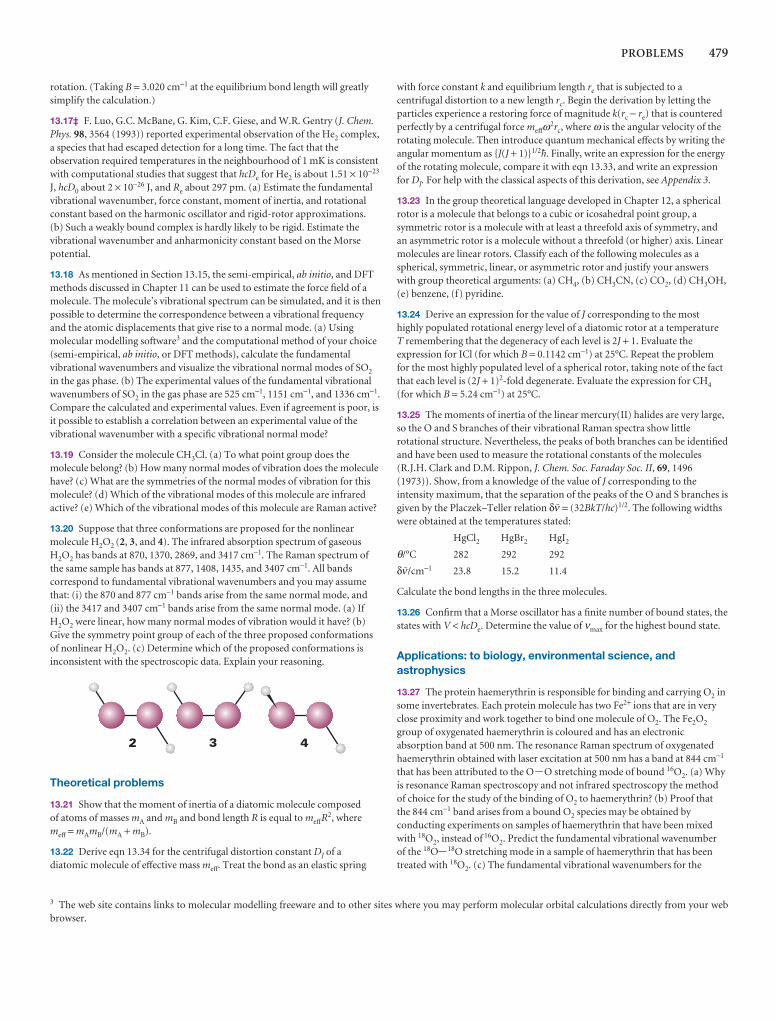
PROBLEMS 479
rotation. (Taking B = 3.020 cm−1 at the equilibrium bond length will greatlysimplify the calculation.)
13.17‡ F. Luo, G.C. McBane, G. Kim, C.F. Giese, and W.R. Gentry (J. Chem.Phys. 98, 3564 (1993)) reported experimental observation of the He2 complex,a species that had escaped detection for a long time. The fact that theobservation required temperatures in the neighbourhood of 1 mK is consistentwith computational studies that suggest that hcDe for He2 is about 1.51 × 10⁻²³
J, hcD0 about 2 × 10⁻²⁶ J, and Re about 297 pm. (a) Estimate the fundamentalvibrational wavenumber, force constant, moment of inertia, and rotationalconstant based on the harmonic oscillator and rigid-rotor approximations.(b) Such a weakly bound complex is hardly likely to be rigid. Estimate thevibrational wavenumber and anharmonicity constant based on the Morsepotential.
13.18 As mentioned in Section 13.15, the semi-empirical, ab initio, and DFTmethods discussed in Chapter 11 can be used to estimate the force field of amolecule. The molecule’s vibrational spectrum can be simulated, and it is thenpossible to determine the correspondence between a vibrational frequencyand the atomic displacements that give rise to a normal mode. (a) Usingmolecular modelling software3 and the computational method of your choice(semi-empirical, ab initio, or DFT methods), calculate the fundamentalvibrational wavenumbers and visualize the vibrational normal modes of SO2
in the gas phase. (b) The experimental values of the fundamental vibrationalwavenumbers of SO2 in the gas phase are 525 cm−1, 1151 cm−1, and 1336 cm−1.Compare the calculated and experimental values. Even if agreement is poor, isit possible to establish a correlation between an experimental value of thevibrational wavenumber with a specific vibrational normal mode?
13.19 Consider the molecule CH3Cl. (a) To what point group does themolecule belong? (b) How many normal modes of vibration does the molecule have? (c) What are the symmetries of the normal modes of vibration for thismolecule? (d) Which of the vibrational modes of this molecule are infraredactive? (e) Which of the vibrational modes of this molecule are Raman active?
13.20 Suppose that three conformations are proposed for the nonlinearmolecule H2O2 (2, 3, and 4). The infrared absorption spectrum of gaseousH2O2 has bands at 870, 1370, 2869, and 3417 cm−1. The Raman spectrum ofthe same sample has bands at 877, 1408, 1435, and 3407 cm−1. All bandscorrespond to fundamental vibrational wavenumbers and you may assumethat: (i) the 870 and 877 cm−1 bands arise from the same normal mode, and(ii) the 3417 and 3407 cm−1 bands arise from the same normal mode. (a) IfH2O2 were linear, how many normal modes of vibration would it have? (b)Give the symmetry point group of each of the three proposed conformationsof nonlinear H2O2. (c) Determine which of the proposed conformations isinconsistent with the spectroscopic data. Explain your reasoning.
Theoretical problems
13.21 Show that the moment of inertia of a diatomic molecule composed of atoms of masses mA and mB and bond length R is equal to meffR2, where meff = mAmB/(mA + mB).
13.22 Derive eqn 13.34 for the centrifugal distortion constant DJ of adiatomic molecule of effective mass meff. Treat the bond as an elastic spring
2 3 4
with force constant k and equilibrium length re that is subjected to acentrifugal distortion to a new length rc. Begin the derivation by letting theparticles experience a restoring force of magnitude k(rc − re) that is counteredperfectly by a centrifugal force meffω2rc, where ω is the angular velocity of therotating molecule. Then introduce quantum mechanical effects by writing theangular momentum as {J(J + 1)}1/2$. Finally, write an expression for the energyof the rotating molecule, compare it with eqn 13.33, and write an expressionfor DJ. For help with the classical aspects of this derivation, see Appendix 3.
13.23 In the group theoretical language developed in Chapter 12, a sphericalrotor is a molecule that belongs to a cubic or icosahedral point group, asymmetric rotor is a molecule with at least a threefold axis of symmetry, andan asymmetric rotor is a molecule without a threefold (or higher) axis. Linearmolecules are linear rotors. Classify each of the following molecules as aspherical, symmetric, linear, or asymmetric rotor and justify your answerswith group theoretical arguments: (a) CH4, (b) CH3CN, (c) CO2, (d) CH3OH,(e) benzene, (f) pyridine.
13.24 Derive an expression for the value of J corresponding to the mosthighly populated rotational energy level of a diatomic rotor at a temperature T remembering that the degeneracy of each level is 2J + 1. Evaluate theexpression for ICl (for which B = 0.1142 cm−1) at 25°C. Repeat the problemfor the most highly populated level of a spherical rotor, taking note of the factthat each level is (2J + 1)2-fold degenerate. Evaluate the expression for CH4
(for which B = 5.24 cm−1) at 25°C.
13.25 The moments of inertia of the linear mercury(II) halides are very large,so the O and S branches of their vibrational Raman spectra show littlerotational structure. Nevertheless, the peaks of both branches can be identifiedand have been used to measure the rotational constants of the molecules(R.J.H. Clark and D.M. Rippon, J. Chem. Soc. Faraday Soc. II, 69, 1496(1973)). Show, from a knowledge of the value of J corresponding to theintensity maximum, that the separation of the peaks of the O and S branches isgiven by the Placzek–Teller relation δ# = (32BkT/hc)1/2. The following widthswere obtained at the temperatures stated:
HgCl2 HgBr2 HgI2
θ/°C 282 292 292
δ#/cm−1 23.8 15.2 11.4
Calculate the bond lengths in the three molecules.
13.26 Confirm that a Morse oscillator has a finite number of bound states, thestates with V < hcDe. Determine the value of νmax for the highest bound state.
Applications: to biology, environmental science, andastrophysics
13.27 The protein haemerythrin is responsible for binding and carrying O2 insome invertebrates. Each protein molecule has two Fe2+ ions that are in veryclose proximity and work together to bind one molecule of O2. The Fe2O2
group of oxygenated haemerythrin is coloured and has an electronicabsorption band at 500 nm. The resonance Raman spectrum of oxygenatedhaemerythrin obtained with laser excitation at 500 nm has a band at 844 cm−1
that has been attributed to the O-O stretching mode of bound 16O2. (a) Whyis resonance Raman spectroscopy and not infrared spectroscopy the methodof choice for the study of the binding of O2 to haemerythrin? (b) Proof thatthe 844 cm−1 band arises from a bound O2 species may be obtained byconducting experiments on samples of haemerythrin that have been mixedwith 18O2, instead of 16O2. Predict the fundamental vibrational wavenumber of the 18O- 18O stretching mode in a sample of haemerythrin that has beentreated with 18O2. (c) The fundamental vibrational wavenumbers for the
3 The web site contains links to molecular modelling freeware and to other sites where you may perform molecular orbital calculations directly from your webbrowser.
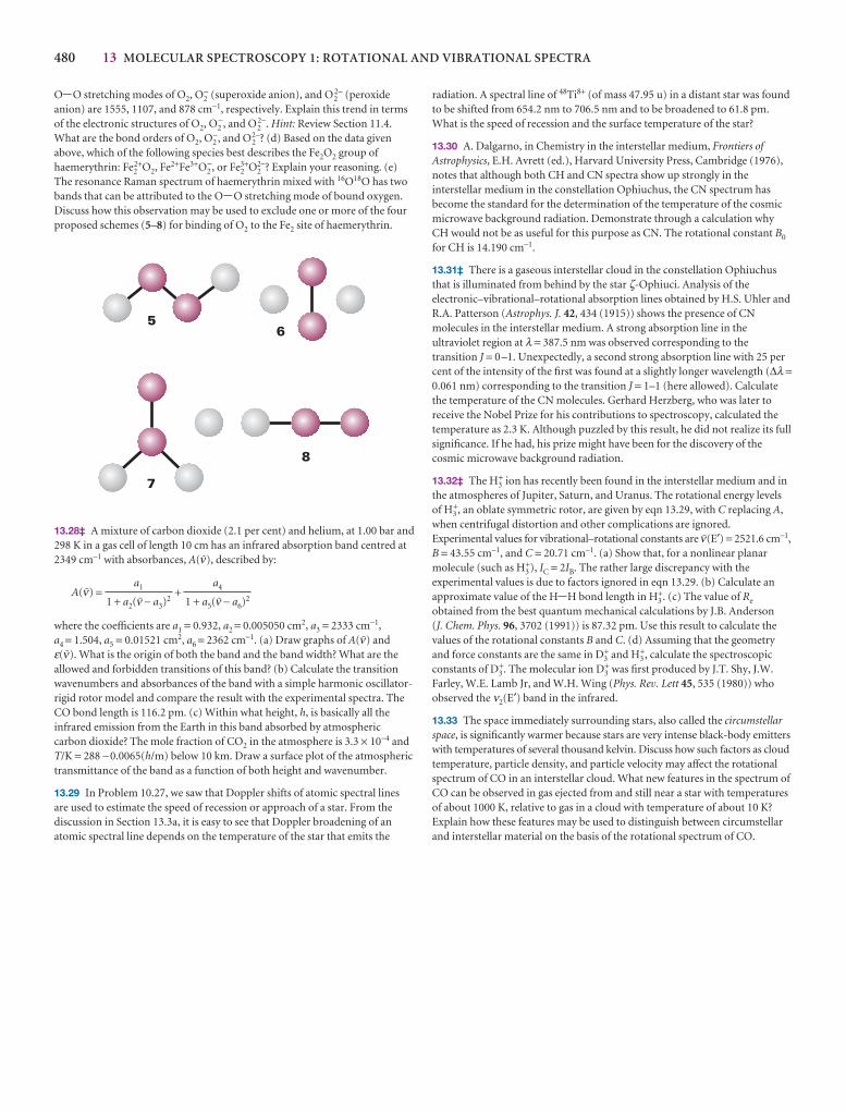
480 13 MOLECULAR SPECTROSCOPY 1: ROTATIONAL AND VIBRATIONAL SPECTRA
O-O stretching modes of O2, O2− (superoxide anion), and O2
2− (peroxideanion) are 1555, 1107, and 878 cm−1, respectively. Explain this trend in termsof the electronic structures of O2, O2
−, and O22−. Hint: Review Section 11.4.
What are the bond orders of O2, O2−, and O2
2−? (d) Based on the data givenabove, which of the following species best describes the Fe2O2 group ofhaemerythrin: Fe2
2+O2, Fe2+Fe3+O2−, or Fe2
3+O22−? Explain your reasoning. (e)
The resonance Raman spectrum of haemerythrin mixed with 16O18O has twobands that can be attributed to the O-O stretching mode of bound oxygen.Discuss how this observation may be used to exclude one or more of the fourproposed schemes (5–8) for binding of O2 to the Fe2 site of haemerythrin.
13.28‡ A mixture of carbon dioxide (2.1 per cent) and helium, at 1.00 bar and298 K in a gas cell of length 10 cm has an infrared absorption band centred at2349 cm−1 with absorbances, A(#), described by:
A(#) = +
where the coefficients are a1 = 0.932, a2 = 0.005050 cm2, a3 = 2333 cm−1,a4 = 1.504, a5 = 0.01521 cm2, a6 = 2362 cm−1. (a) Draw graphs of A(#) and ε(#). What is the origin of both the band and the band width? What are theallowed and forbidden transitions of this band? (b) Calculate the transitionwavenumbers and absorbances of the band with a simple harmonic oscillator-rigid rotor model and compare the result with the experimental spectra. TheCO bond length is 116.2 pm. (c) Within what height, h, is basically all theinfrared emission from the Earth in this band absorbed by atmosphericcarbon dioxide? The mole fraction of CO2 in the atmosphere is 3.3 × 10⁻⁴ andT/K = 288 −0.0065(h/m) below 10 km. Draw a surface plot of the atmospherictransmittance of the band as a function of both height and wavenumber.
13.29 In Problem 10.27, we saw that Doppler shifts of atomic spectral linesare used to estimate the speed of recession or approach of a star. From thediscussion in Section 13.3a, it is easy to see that Doppler broadening of anatomic spectral line depends on the temperature of the star that emits the
a4
1 + a5(# − a6)2
a1
1 + a2(# − a3)2
7
8
56
radiation. A spectral line of 48Ti8+ (of mass 47.95 u) in a distant star was foundto be shifted from 654.2 nm to 706.5 nm and to be broadened to 61.8 pm.What is the speed of recession and the surface temperature of the star?
13.30 A. Dalgarno, in Chemistry in the interstellar medium, Frontiers ofAstrophysics, E.H. Avrett (ed.), Harvard University Press, Cambridge (1976),notes that although both CH and CN spectra show up strongly in theinterstellar medium in the constellation Ophiuchus, the CN spectrum hasbecome the standard for the determination of the temperature of the cosmicmicrowave background radiation. Demonstrate through a calculation whyCH would not be as useful for this purpose as CN. The rotational constant B0
for CH is 14.190 cm−1.
13.31‡ There is a gaseous interstellar cloud in the constellation Ophiuchusthat is illuminated from behind by the star ζ-Ophiuci. Analysis of theelectronic–vibrational–rotational absorption lines obtained by H.S. Uhler andR.A. Patterson (Astrophys. J. 42, 434 (1915)) shows the presence of CNmolecules in the interstellar medium. A strong absorption line in theultraviolet region at λ = 387.5 nm was observed corresponding to thetransition J = 0–1. Unexpectedly, a second strong absorption line with 25 percent of the intensity of the first was found at a slightly longer wavelength (∆λ =0.061 nm) corresponding to the transition J = 1–1 (here allowed). Calculatethe temperature of the CN molecules. Gerhard Herzberg, who was later toreceive the Nobel Prize for his contributions to spectroscopy, calculated thetemperature as 2.3 K. Although puzzled by this result, he did not realize its fullsignificance. If he had, his prize might have been for the discovery of thecosmic microwave background radiation.
13.32‡ The H3+ ion has recently been found in the interstellar medium and in
the atmospheres of Jupiter, Saturn, and Uranus. The rotational energy levelsof H3
+, an oblate symmetric rotor, are given by eqn 13.29, with C replacing A,when centrifugal distortion and other complications are ignored.Experimental values for vibrational–rotational constants are #(E′) = 2521.6 cm−1,B = 43.55 cm−1, and C = 20.71 cm−1. (a) Show that, for a nonlinear planarmolecule (such as H3
+), IC = 2IB. The rather large discrepancy with theexperimental values is due to factors ignored in eqn 13.29. (b) Calculate anapproximate value of the H-H bond length in H3
+. (c) The value of Re
obtained from the best quantum mechanical calculations by J.B. Anderson (J. Chem. Phys. 96, 3702 (1991)) is 87.32 pm. Use this result to calculate thevalues of the rotational constants B and C. (d) Assuming that the geometryand force constants are the same in D3
+ and H3+, calculate the spectroscopic
constants of D3+. The molecular ion D3
+ was first produced by J.T. Shy, J.W.Farley, W.E. Lamb Jr, and W.H. Wing (Phys. Rev. Lett 45, 535 (1980)) whoobserved the ν2(E′) band in the infrared.
13.33 The space immediately surrounding stars, also called the circumstellarspace, is significantly warmer because stars are very intense black-body emitterswith temperatures of several thousand kelvin. Discuss how such factors as cloudtemperature, particle density, and particle velocity may affect the rotationalspectrum of CO in an interstellar cloud. What new features in the spectrum ofCO can be observed in gas ejected from and still near a star with temperaturesof about 1000 K, relative to gas in a cloud with temperature of about 10 K?Explain how these features may be used to distinguish between circumstellarand interstellar material on the basis of the rotational spectrum of CO.

Molecularspectroscopy 2:electronic transitionsSimple analytical expressions for the electronic energy levels of molecules cannot be given,so this chapter concentrates on the qualitative features of electronic transitions. A commontheme throughout the chapter is that electronic transitions occur within a stationary nuclearframework. We pay particular attention to spontaneous radiative decay processes, whichinclude fluorescence and phosphorescence. A specially important example of stimulatedradiative decay is that responsible for the action of lasers, and we see how this stimulatedemission may be achieved and employed.
The energies needed to change the electron distributions of molecules are of the orderof several electronvolts (1 eV is equivalent to about 8000 cm−1 or 100 kJ mol−1). Con-sequently, the photons emitted or absorbed when such changes occur lie in the visibleand ultraviolet regions of the spectrum (Table 14.1).
One of the revolutions that has occurred in physical chemistry in recent years is theapplication of lasers to spectroscopy and kinetics. Lasers have brought unprecedentedprecision to spectroscopy, made Raman spectroscopy a widely useful technique, andhave made it possible to study chemical reactions on a femtosecond time scale. Weshall see the principles of their action in this chapter and their applications through-out the rest of the book.
The characteristics of electronic transitions
In the ground state of a molecule the nuclei are at equilibrium in the sense that they experience no net force from the electrons and other nuclei in the molecule.Immediately after an electronic transition they are subjected to different forces and
14The characteristics ofelectronic transitions
14.1 The electronic spectra ofdiatomic molecules
14.2 The electronic spectra ofpolyatomic molecules
I14.1 Impact on biochemistry:Vision
The fates of electronicallyexcited states
14.3 Fluorescence andphosphorescence
I14.2 Impact on biochemistry:Fluorescence microscopy
14.4 Dissociation andpredissociation
Lasers
14.5 General principles of laseraction
14.6 Applications of lasers inchemistry
Checklist of key ideas
Further reading
Further information 14.1: Examples ofpractical lasers
Discussion questions
Exercises
Problems
Synoptic table 14.1* Colour, frequency, and energy of light
Colour λ /nm ν /(1014 Hz) E/(kJ mol−1)
Infrared >1000 <3.0 <120
Red 700 4.3 170
Yellow 580 5.2 210
Blue 470 6.4 250
Ultraviolet <300 >10 >400
* More values are given in the Data section.
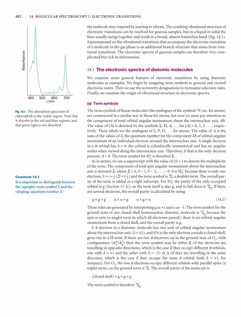
482 14 MOLECULAR SPECTROSCOPY 2: ELECTRONIC TRANSITIONS
the molecule may respond by starting to vibrate. The resulting vibrational structure ofelectronic transitions can be resolved for gaseous samples, but in a liquid or solid thelines usually merge together and result in a broad, almost featureless band (Fig. 14.1).Superimposed on the vibrational transitions that accompany the electronic transitionof a molecule in the gas phase is an additional branch structure that arises from rota-tional transitions. The electronic spectra of gaseous samples are therefore very com-plicated but rich in information.
14.1 The electronic spectra of diatomic molecules
We examine some general features of electronic transitions by using diatomicmolecules as examples. We begin by assigning term symbols to ground and excitedelectronic states. Then we use the symmetry designations to formulate selection rules.Finally, we examine the origin of vibrational structure in electronic spectra.
(a) Term symbols
The term symbols of linear molecules (the analogues of the symbols 2P, etc. for atoms)are constructed in a similar way to those for atoms, but now we must pay attention tothe component of total orbital angular momentum about the internuclear axis, Λ$.The value of |Λ | is denoted by the symbols Σ, Π, ∆, . . . for |Λ | = 0, 1, 2 . . . , respec-tively. These labels are the analogues of S, P, D, . . . for atoms. The value of Λ is thesum of the values of λ, the quantum number for the component λ$ of orbital angular momentum of an individual electron around the internuclear axis. A single electronin a σ orbital has λ = 0: the orbital is cylindrically symmetrical and has no angularnodes when viewed along the internuclear axis. Therefore, if that is the only electronpresent, Λ = 0. The term symbol for H2
+ is therefore Σ.As in atoms, we use a superscript with the value of 2S + 1 to denote the multiplicity
of the term. The component of total spin angular momentum about the internuclearaxis is denoted Σ, where Σ = S, S − 1, S − 2, . . . , −S. For H2
+, because there is only oneelectron, S = s = 1–2 (Σ = ± 1–2) and the term symbol is 2Σ, a doublet term. The overall par-ity of the term is added as a right subscript. For H2
+, the parity of the only occupied orbital is g (Section 11.3c), so the term itself is also g, and in full dress is 2Σg. If thereare several electrons, the overall parity is calculated by using
g × g = g u × u = g u × g = u (14.1)
These rules are generated by interpreting g as +1 and u as −1. The term symbol for theground state of any closed-shell homonuclear diatomic molecule is 1Σg because thespin is zero (a singlet term in which all electrons paired), there is no orbital angularmomentum from a closed shell, and the overall parity is g.
A π electron in a diatomic molecule has one unit of orbital angular momentumabout the internuclear axis (λ = ±1), and if it is the only electron outside a closed shell,gives rise to a Π term. If there are two π electrons (as in the ground state of O2, withconfiguration 1πu
41πg2) then the term symbol may be either Σ (if the electrons are
travelling in opposite directions, which is the case if they occupy different π orbitals,one with λ = +1 and the other with λ = −1) or ∆ (if they are travelling in the same direction, which is the case if they occupy the same π orbital, both λ = +1, for instance). For O2, the two π electrons occupy different orbitals with parallel spins (atriplet term), so the ground term is 3Σ. The overall parity of the molecule is
(closed shell) × g × g = g
The term symbol is therefore 3Σg.
400 500 600 700/nm
Abs
orba
nce
�
Fig. 14.1 The absorption spectrum ofchlorophyll in the visible region. Note thatit absorbs in the red and blue regions, andthat green light is not absorbed.
Comment 14.1
It is important to distinguish betweenthe (upright) term symbol Σ and the(sloping) quantum number Σ.
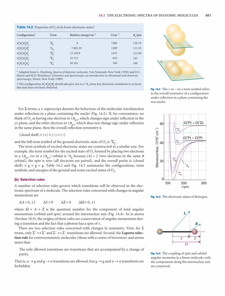
14.1 THE ELECTRONIC SPECTRA OF DIATOMIC MOLECULES 483
For Σ terms, a ± superscript denotes the behaviour of the molecular wavefunctionunder reflection in a plane containing the nuclei (Fig. 14.2). If, for convenience, wethink of O2 as having one electron in 1πg,x, which changes sign under reflection in theyz-plane, and the other electron in 1πg,y, which does not change sign under reflectionin the same plane, then the overall reflection symmetry is
(closed shell) × (+) × (−) = (−)
and the full term symbol of the ground electronic state of O2 is 3Σg−.
The term symbols of excited electronic states are constructed in a similar way. Forexample, the term symbol for the excited state of O2 formed by placing two electronsin a 1πg,x (or in a 1πg,y) orbital is 1∆g because |Λ | = 2 (two electrons in the same πorbital), the spin is zero (all electrons are paired), and the overall parity is (closedshell) × g × g = g. Table 14.2 and Fig. 14.3 summarize the configurations, term symbols, and energies of the ground and some excited states of O2.
(b) Selection rules
A number of selection rules govern which transitions will be observed in the elec-tronic spectrum of a molecule. The selection rules concerned with changes in angularmomentum are
∆Λ = 0, ±1 ∆S = 0 ∆Σ = 0 ∆Ω = 0, ±1
where Ω = Λ + Σ is the quantum number for the component of total angular momentum (orbital and spin) around the internuclear axis (Fig. 14.4). As in atoms(Section 10.9), the origins of these rules are conservation of angular momentum dur-ing a transition and the fact that a photon has a spin of 1.
There are two selection rules concerned with changes in symmetry. First, for Σterms, only Σ+ ↔ Σ+ and Σ− ↔ Σ− transitions are allowed. Second, the Laporte selec-tion rule for centrosymmetric molecules (those with a centre of inversion) and atomsstates that:
The only allowed transitions are transitions that are accompanied by a change ofparity.
That is, u → g and g → u transitions are allowed, but g → g and u → u transitions areforbidden.
�
�
Fig. 14.2 The + or – on a term symbol refersto the overall symmetry of a configurationunder reflection in a plane containing thetwo nuclei.
Table 14.2 Properties of O2 in its lower electronic states*
Configuration† Term Relative energy/cm−1 #/cm−1 Re /pm
πu2πu
2π g1π g
1 3Σg− 0 1580 120.74
πu2πu
2π g2πg
0 1∆g 7 882.39 1509 121.55
πu2πu
2πg1πg
1 1Σg+ 13 120.9 1433 122.68
πu2πu
1π g2πg
1 3Σu+ 35 713 819 142
πu2πu
1π g2πg
1 3Σu− 49 363 700 160
* Adapted from G. Herzberg, Spectra of diatomic molecules, Van Nostrand, New York (1950) and D.C.Harris and M.D. Bertolucci, Symmetry and spectroscopy: an introduction to vibrational and electronicspectroscopy, Dover, New York (1989).
† The configuration πu2 πu
1π g2πg
1 should also give rise to a 3∆u term, but electronic transitions to or fromthis state have not been observed.
0
20
40
60
Wav
enum
ber,
/(1
0cm
)3
1~
100 200 300r/pm
O( P) O( P)3 3�
O( P) O( D)3 1�
3'g
1g
1'g
3'u
3'u
�
�
�
�
�
�
L
S
( '
)
Fig. 14.3 The electronic states of dioxygen.
Fig. 14.4 The coupling of spin and orbitalangular momenta in a linear molecule: onlythe components along the internuclear axisare conserved.
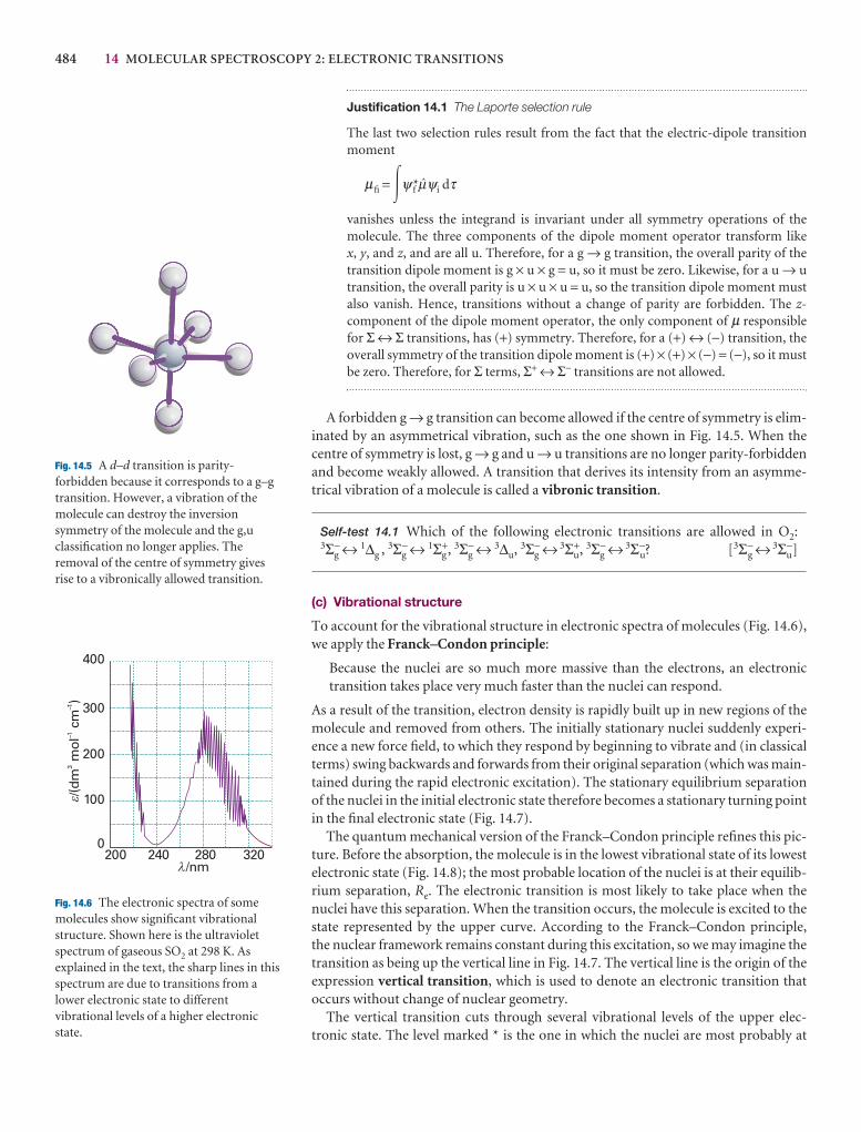
484 14 MOLECULAR SPECTROSCOPY 2: ELECTRONIC TRANSITIONS
Justification 14.1 The Laporte selection rule
The last two selection rules result from the fact that the electric-dipole transitionmoment
µfi = �ψ f*Nψi dτ
vanishes unless the integrand is invariant under all symmetry operations of themolecule. The three components of the dipole moment operator transform like x, y, and z, and are all u. Therefore, for a g → g transition, the overall parity of thetransition dipole moment is g × u × g = u, so it must be zero. Likewise, for a u → utransition, the overall parity is u × u × u = u, so the transition dipole moment mustalso vanish. Hence, transitions without a change of parity are forbidden. The z-component of the dipole moment operator, the only component of µ responsiblefor Σ ↔ Σ transitions, has (+) symmetry. Therefore, for a (+) ↔ (−) transition, theoverall symmetry of the transition dipole moment is (+) × (+) × (−) = (−), so it mustbe zero. Therefore, for Σ terms, Σ+ ↔ Σ− transitions are not allowed.
A forbidden g → g transition can become allowed if the centre of symmetry is elim-inated by an asymmetrical vibration, such as the one shown in Fig. 14.5. When thecentre of symmetry is lost, g → g and u → u transitions are no longer parity-forbiddenand become weakly allowed. A transition that derives its intensity from an asymme-trical vibration of a molecule is called a vibronic transition.
Self-test 14.1 Which of the following electronic transitions are allowed in O2:3Σg
− ↔ 1∆g , 3Σg− ↔ 1Σg
+, 3Σg− ↔ 3∆u, 3Σg
− ↔ 3Σu+, 3Σg
− ↔ 3Σu−? [3Σg
− ↔ 3Σu−]
(c) Vibrational structure
To account for the vibrational structure in electronic spectra of molecules (Fig. 14.6),we apply the Franck–Condon principle:
Because the nuclei are so much more massive than the electrons, an electronictransition takes place very much faster than the nuclei can respond.
As a result of the transition, electron density is rapidly built up in new regions of themolecule and removed from others. The initially stationary nuclei suddenly experi-ence a new force field, to which they respond by beginning to vibrate and (in classicalterms) swing backwards and forwards from their original separation (which was main-tained during the rapid electronic excitation). The stationary equilibrium separationof the nuclei in the initial electronic state therefore becomes a stationary turning pointin the final electronic state (Fig. 14.7).
The quantum mechanical version of the Franck–Condon principle refines this pic-ture. Before the absorption, the molecule is in the lowest vibrational state of its lowestelectronic state (Fig. 14.8); the most probable location of the nuclei is at their equilib-rium separation, Re. The electronic transition is most likely to take place when the nuclei have this separation. When the transition occurs, the molecule is excited to thestate represented by the upper curve. According to the Franck–Condon principle, the nuclear framework remains constant during this excitation, so we may imagine thetransition as being up the vertical line in Fig. 14.7. The vertical line is the origin of theexpression vertical transition, which is used to denote an electronic transition thatoccurs without change of nuclear geometry.
The vertical transition cuts through several vibrational levels of the upper elec-tronic state. The level marked * is the one in which the nuclei are most probably at
Fig. 14.5 A d–d transition is parity-forbidden because it corresponds to a g–gtransition. However, a vibration of themolecule can destroy the inversionsymmetry of the molecule and the g,uclassification no longer applies. Theremoval of the centre of symmetry givesrise to a vibronically allowed transition.
400
300
200
100
0200 240 280 320
/(dm
mol
cm)
31
1
/nm�
�–
–
Fig. 14.6 The electronic spectra of somemolecules show significant vibrationalstructure. Shown here is the ultravioletspectrum of gaseous SO2 at 298 K. Asexplained in the text, the sharp lines in thisspectrum are due to transitions from alower electronic state to differentvibrational levels of a higher electronicstate.

14.1 THE ELECTRONIC SPECTRA OF DIATOMIC MOLECULES 485
the same initial separation Re (because the vibrational wavefunction has maximumamplitude there), so this vibrational state is the most probable state for the termina-tion of the transition. However, it is not the only accessible vibrational state becauseseveral nearby states have an appreciable probability of the nuclei being at the separa-tion Re. Therefore, transitions occur to all the vibrational states in this region, but mostintensely to the state with a vibrational wavefunction that peaks most strongly near Re.
The vibrational structure of the spectrum depends on the relative horizontal posi-tion of the two potential energy curves, and a long vibrational progression, a lot of vibrational structure, is stimulated if the upper potential energy curve is appreciablydisplaced horizontally from the lower. The upper curve is usually displaced to greaterequilibrium bond lengths because electronically excited states usually have more antibonding character than electronic ground states.
The separation of the vibrational lines of an electronic absorption spectrum dependson the vibrational energies of the upper electronic state. Hence, electronic absorptionspectra may be used to assess the force fields and dissociation energies of electronicallyexcited molecules (for example, by using a Birge–Sponer plot, as in Problem 14.2).
(d) Franck–Condon factors
The quantitative form of the Franck–Condon principle is derived from the expressionfor the transition dipole moment, µfi = �f | µ| i�. The dipole moment operator is a sumover all nuclei and electrons in the molecule:
¢ = −e∑i
ri + e∑I
ZI RI (14.2)
where the vectors are the distances from the centre of charge of the molecule. The intensity of the transition is proportional to the square modulus, |µfi|2, of the magnitudeof the transition dipole moment (eqn 9.70), and we show in the Justification below thatthis intensity is proportional to the square modulus of the overlap integral, S(vf ,vi),between the vibrational states of the initial and final electronic states. This overlap integral is a measure of the match between the vibrational wavefunctions in the upperand lower electronic states: S = 1 for a perfect match and S = 0 when there is no similarity.
Justification 14.2 The Franck–Condon approximation
The overall state of the molecule consists of an electronic part, | ε�, and a vibrationalpart, |v�. Therefore, within the Born–Oppenheimer approximation, the transitiondipole moment factorizes as follows:
µfi = �εf vf |{−e∑i
ri + e∑I
ZI RI}| εivi�
= −e∑i
�εf |ri|εi��vf |vi� + e∑i
Zi�εf | εi��vf | RI |vi�
The second term on the right of the second row is zero, because �εf | εi� = 0 for twodifferent electronic states (they are orthogonal). Therefore,
µfi = −e∑i
�εf |ri | εi��vf |vi� = µε f,εiS(vf ,vi) (14.3)
where
µε f,ε i= −e∑
i
�εf |ri|εi� S(vf ,vi) = �vf |vi� (14.4)
The matrix element µε f,εiis the electric-dipole transition moment arising from the
redistribution of electrons (and a measure of the ‘kick’ this redistribution gives tothe electromagnetic field, and vice versa for absorption). The factor S(vf ,vi), is theoverlap integral between the vibrational state |vi� in the initial electronic state of themolecule, and the vibrational state |vf� in the final electronic state of the molecule.
Turningpoint(stationarynuclei)
Electronicexcited state
Electronicground state
Nuclei stationary
Mol
ecul
ar p
oten
tial e
nerg
y
Internuclear separation
Electronicexcited state
Electronicground state
Mol
ecul
ar p
oten
tial e
nerg
y
Internuclear separation
*
Fig. 14.7 According to the Franck–Condonprinciple, the most intense vibronictransition is from the ground vibrationalstate to the vibrational state lying verticallyabove it. Transitions to other vibrationallevels also occur, but with lower intensity.
Fig. 14.8 In the quantum mechanicalversion of the Franck–Condon principle,the molecule undergoes a transition to theupper vibrational state that most closelyresembles the vibrational wavefunction ofthe vibrational ground state of the lowerelectronic state. The two wavefunctionsshown here have the greatest overlapintegral of all the vibrational states of theupper electronic state and hence are mostclosely similar.
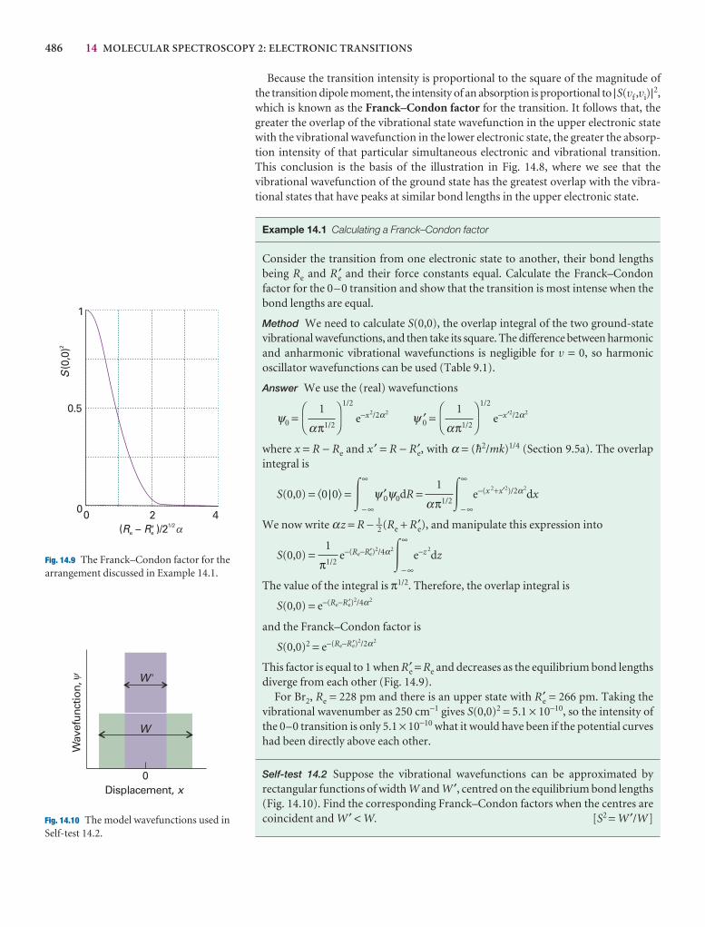
486 14 MOLECULAR SPECTROSCOPY 2: ELECTRONIC TRANSITIONS
0.5
1
00 2 4
S(0
,0)2
( – )/2R Re e�1/2
�
Fig. 14.9 The Franck–Condon factor for thearrangement discussed in Example 14.1.
Fig. 14.10 The model wavefunctions used inSelf-test 14.2.
Because the transition intensity is proportional to the square of the magnitude ofthe transition dipole moment, the intensity of an absorption is proportional to |S(vf ,vi)|2,which is known as the Franck–Condon factor for the transition. It follows that, thegreater the overlap of the vibrational state wavefunction in the upper electronic statewith the vibrational wavefunction in the lower electronic state, the greater the absorp-tion intensity of that particular simultaneous electronic and vibrational transition.This conclusion is the basis of the illustration in Fig. 14.8, where we see that the vibrational wavefunction of the ground state has the greatest overlap with the vibra-tional states that have peaks at similar bond lengths in the upper electronic state.
Example 14.1 Calculating a Franck–Condon factor
Consider the transition from one electronic state to another, their bond lengthsbeing Re and Re′ and their force constants equal. Calculate the Franck–Condon factor for the 0–0 transition and show that the transition is most intense when thebond lengths are equal.
Method We need to calculate S(0,0), the overlap integral of the two ground-statevibrational wavefunctions, and then take its square. The difference between harmonicand anharmonic vibrational wavefunctions is negligible for v = 0, so harmonic oscillator wavefunctions can be used (Table 9.1).
Answer We use the (real) wavefunctions
ψ0 =1/2
e−x2/2α2 ψ ′0 =1/2
e−x′2/2α2
where x = R − Re and x ′ = R − R′e, with α = ($2/mk)1/4 (Section 9.5a). The overlap integral is
S(0,0) = �0 |0� = �∞
− ∞
ψ ′0ψ0dR = �∞
− ∞
e−(x 2+x′2)/2α2dx
We now write αz = R − 1–2 (Re + R′e), and manipulate this expression into
S(0,0) = e−(Re−R′e)2/4α2�∞
− ∞
e−z 2dz
The value of the integral is π1/2. Therefore, the overlap integral is
S(0,0) = e−(Re−R′e)2/4α2
and the Franck–Condon factor is
S(0,0)2 = e−(Re−R′e)2/2α2
This factor is equal to 1 when R′e = Re and decreases as the equilibrium bond lengthsdiverge from each other (Fig. 14.9).
For Br2, Re = 228 pm and there is an upper state with R′e = 266 pm. Taking the vibrational wavenumber as 250 cm−1 gives S(0,0)2 = 5.1 × 10⁻¹⁰, so the intensity ofthe 0–0 transition is only 5.1 × 10⁻¹⁰ what it would have been if the potential curveshad been directly above each other.
Self-test 14.2 Suppose the vibrational wavefunctions can be approximated byrectangular functions of width W and W ′, centred on the equilibrium bond lengths(Fig. 14.10). Find the corresponding Franck–Condon factors when the centres arecoincident and W ′ < W. [S2 = W ′/W]
1
π1/2
1
απ1/2
DF
1
απ1/2
AC
DF
1
απ1/2
AC
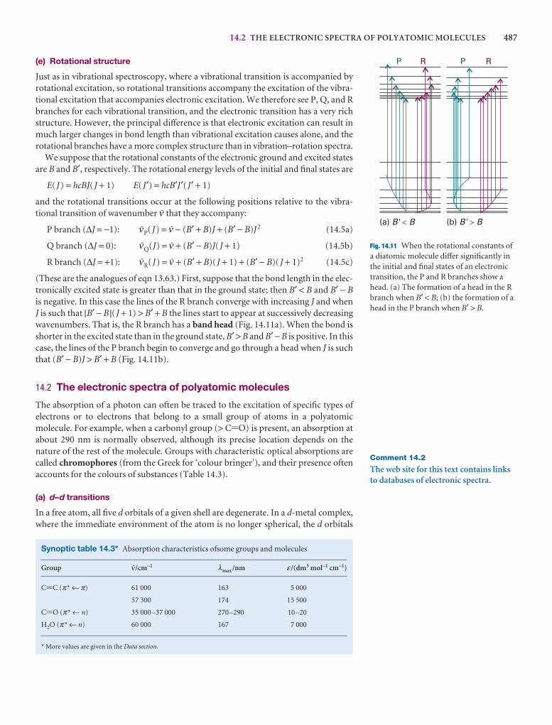
14.2 THE ELECTRONIC SPECTRA OF POLYATOMIC MOLECULES 487
(e) Rotational structure
Just as in vibrational spectroscopy, where a vibrational transition is accompanied byrotational excitation, so rotational transitions accompany the excitation of the vibra-tional excitation that accompanies electronic excitation. We therefore see P, Q, and Rbranches for each vibrational transition, and the electronic transition has a very richstructure. However, the principal difference is that electronic excitation can result inmuch larger changes in bond length than vibrational excitation causes alone, and therotational branches have a more complex structure than in vibration–rotation spectra.
We suppose that the rotational constants of the electronic ground and excited statesare B and B′, respectively. The rotational energy levels of the initial and final states are
E( J) = hcBJ( J + 1) E( J′) = hcB′J′( J′ + 1)
and the rotational transitions occur at the following positions relative to the vibra-tional transition of wavenumber # that they accompany:
P branch (∆J = −1): #P( J) = # − (B′ + B)J + (B′ − B)J 2 (14.5a)
Q branch (∆J = 0): #Q(J) = # + (B′ − B)J( J + 1) (14.5b)
R branch (∆J = +1): #R( J) = # + (B′ + B)( J + 1) + (B′ − B)( J + 1)2 (14.5c)
(These are the analogues of eqn 13.63.) First, suppose that the bond length in the elec-tronically excited state is greater than that in the ground state; then B′ < B and B′ − Bis negative. In this case the lines of the R branch converge with increasing J and whenJ is such that |B′ − B |( J + 1) > B′ + B the lines start to appear at successively decreasingwavenumbers. That is, the R branch has a band head (Fig. 14.11a). When the bond isshorter in the excited state than in the ground state, B′ > B and B′ − B is positive. In thiscase, the lines of the P branch begin to converge and go through a head when J is suchthat (B′ − B)J > B′ + B (Fig. 14.11b).
14.2 The electronic spectra of polyatomic molecules
The absorption of a photon can often be traced to the excitation of specific types ofelectrons or to electrons that belong to a small group of atoms in a polyatomicmolecule. For example, when a carbonyl group (> C=O) is present, an absorption atabout 290 nm is normally observed, although its precise location depends on the nature of the rest of the molecule. Groups with characteristic optical absorptions arecalled chromophores (from the Greek for ‘colour bringer’), and their presence oftenaccounts for the colours of substances (Table 14.3).
(a) d–d transitions
In a free atom, all five d orbitals of a given shell are degenerate. In a d-metal complex,where the immediate environment of the atom is no longer spherical, the d orbitals
P R P R
(a) B' B� (b) B' B�
Fig. 14.11 When the rotational constants ofa diatomic molecule differ significantly inthe initial and final states of an electronictransition, the P and R branches show ahead. (a) The formation of a head in the Rbranch when B′ < B; (b) the formation of ahead in the P branch when B′ > B.
Comment 14.2
The web site for this text contains linksto databases of electronic spectra.
Synoptic table 14.3* Absorption characteristics ofsome groups and molecules
Group #/cm−1 λmax /nm ε /(dm3 mol−1 cm−1)
C=C (π* ← π) 61 000 163 5 000
57 300 174 15 500
C=O (π* ← n) 35 000–37 000 270–290 10–20
H2O (π* ← n) 60 000 167 7 000
* More values are given in the Data section.
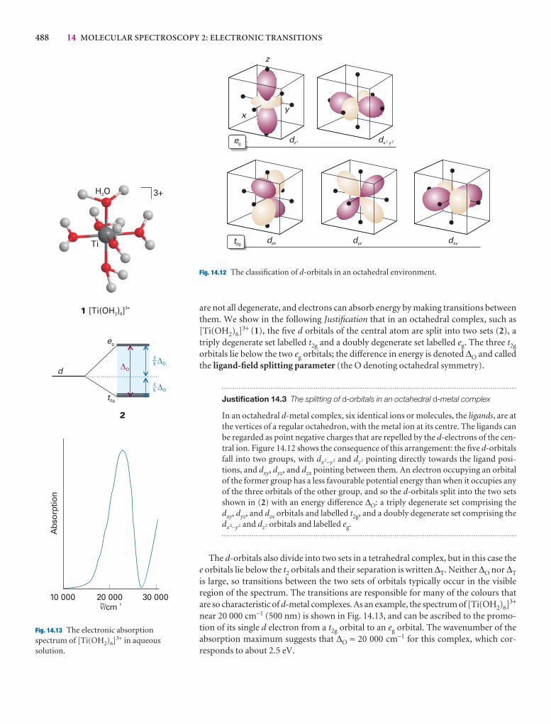
488 14 MOLECULAR SPECTROSCOPY 2: ELECTRONIC TRANSITIONS
are not all degenerate, and electrons can absorb energy by making transitions betweenthem. We show in the following Justification that in an octahedral complex, such as[Ti(OH2)6]3+ (1), the five d orbitals of the central atom are split into two sets (2), atriply degenerate set labelled t2g and a doubly degenerate set labelled eg. The three t2g
orbitals lie below the two eg orbitals; the difference in energy is denoted ∆O and calledthe ligand-field splitting parameter (the O denoting octahedral symmetry).
Justification 14.3 The splitting of d-orbitals in an octahedral d-metal complex
In an octahedral d-metal complex, six identical ions or molecules, the ligands, are atthe vertices of a regular octahedron, with the metal ion at its centre. The ligands canbe regarded as point negative charges that are repelled by the d-electrons of the cen-tral ion. Figure 14.12 shows the consequence of this arrangement: the five d-orbitalsfall into two groups, with dx2−y2 and dz2 pointing directly towards the ligand posi-tions, and dxy, dyz, and dzx pointing between them. An electron occupying an orbitalof the former group has a less favourable potential energy than when it occupies anyof the three orbitals of the other group, and so the d-orbitals split into the two setsshown in (2) with an energy difference ∆O: a triply degenerate set comprising thedxy, dyz, and dzx orbitals and labelled t2g, and a doubly degenerate set comprising thedx2−y2 and dz2 orbitals and labelled eg.
The d-orbitals also divide into two sets in a tetrahedral complex, but in this case thee orbitals lie below the t2 orbitals and their separation is written ∆T. Neither ∆O nor ∆T
is large, so transitions between the two sets of orbitals typically occur in the visible region of the spectrum. The transitions are responsible for many of the colours thatare so characteristic of d-metal complexes. As an example, the spectrum of [Ti(OH2)6]
3+
near 20 000 cm−1 (500 nm) is shown in Fig. 14.13, and can be ascribed to the promo-tion of its single d electron from a t2g orbital to an eg orbital. The wavenumber of theabsorption maximum suggests that ∆O ≈ 20 000 cm−1 for this complex, which cor-responds to about 2.5 eV.
Ti
H O2 3+
1 [Ti(OH ) ]2 63+
d
eg
t2g
O
O
O
�53
�52
2
dz 2 dx y2 2�
dzx dyz dxy
xy
z
eg
t2g
Fig. 14.12 The classification of d-orbitals in an octahedral environment.
Fig. 14.13 The electronic absorptionspectrum of [Ti(OH2)6]3+ in aqueoussolution.
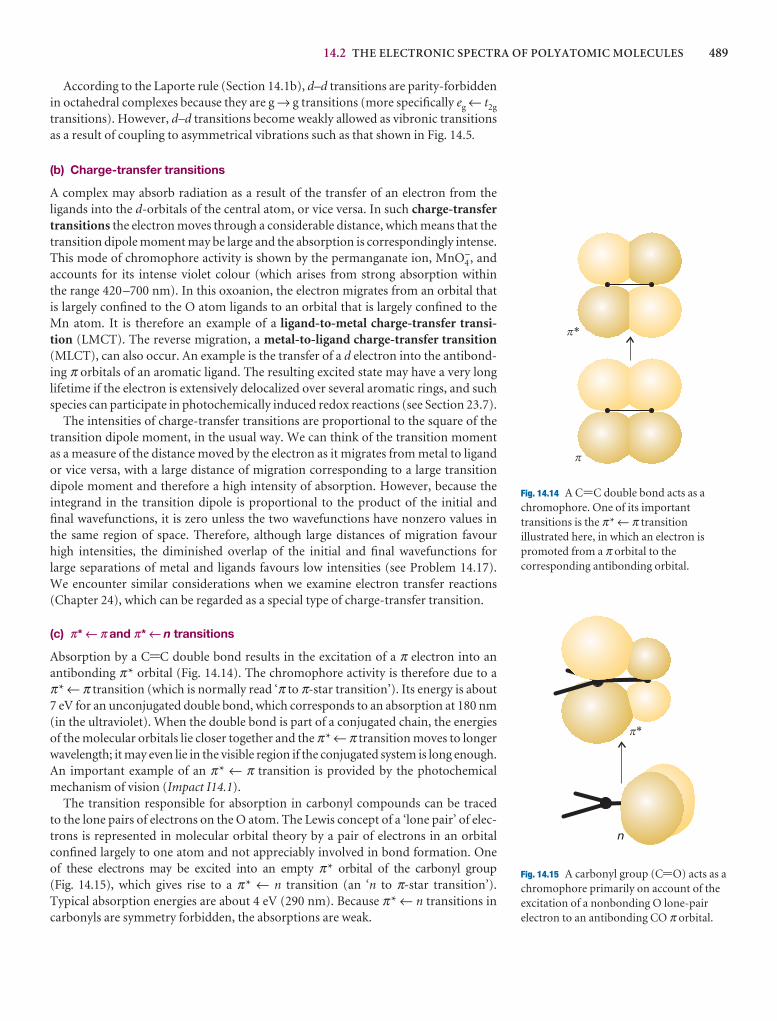
14.2 THE ELECTRONIC SPECTRA OF POLYATOMIC MOLECULES 489
According to the Laporte rule (Section 14.1b), d–d transitions are parity-forbiddenin octahedral complexes because they are g → g transitions (more specifically eg ← t2g
transitions). However, d–d transitions become weakly allowed as vibronic transitionsas a result of coupling to asymmetrical vibrations such as that shown in Fig. 14.5.
(b) Charge-transfer transitions
A complex may absorb radiation as a result of the transfer of an electron from theligands into the d-orbitals of the central atom, or vice versa. In such charge-transfertransitions the electron moves through a considerable distance, which means that thetransition dipole moment may be large and the absorption is correspondingly intense.This mode of chromophore activity is shown by the permanganate ion, MnO4
−, andaccounts for its intense violet colour (which arises from strong absorption within the range 420–700 nm). In this oxoanion, the electron migrates from an orbital thatis largely confined to the O atom ligands to an orbital that is largely confined to theMn atom. It is therefore an example of a ligand-to-metal charge-transfer transi-tion (LMCT). The reverse migration, a metal-to-ligand charge-transfer transition(MLCT), can also occur. An example is the transfer of a d electron into the antibond-ing π orbitals of an aromatic ligand. The resulting excited state may have a very longlifetime if the electron is extensively delocalized over several aromatic rings, and suchspecies can participate in photochemically induced redox reactions (see Section 23.7).
The intensities of charge-transfer transitions are proportional to the square of thetransition dipole moment, in the usual way. We can think of the transition momentas a measure of the distance moved by the electron as it migrates from metal to ligandor vice versa, with a large distance of migration corresponding to a large transitiondipole moment and therefore a high intensity of absorption. However, because the integrand in the transition dipole is proportional to the product of the initial and final wavefunctions, it is zero unless the two wavefunctions have nonzero values in the same region of space. Therefore, although large distances of migration favour high intensities, the diminished overlap of the initial and final wavefunctions for large separations of metal and ligands favours low intensities (see Problem 14.17). We encounter similar considerations when we examine electron transfer reactions(Chapter 24), which can be regarded as a special type of charge-transfer transition.
(c) π* ← π and π* ← n transitions
Absorption by a C=C double bond results in the excitation of a π electron into an antibonding π* orbital (Fig. 14.14). The chromophore activity is therefore due to a π* ← π transition (which is normally read ‘π to π-star transition’). Its energy is about7 eV for an unconjugated double bond, which corresponds to an absorption at 180 nm(in the ultraviolet). When the double bond is part of a conjugated chain, the energiesof the molecular orbitals lie closer together and the π* ← π transition moves to longerwavelength; it may even lie in the visible region if the conjugated system is long enough.An important example of an π* ← π transition is provided by the photochemicalmechanism of vision (Impact I14.1).
The transition responsible for absorption in carbonyl compounds can be traced to the lone pairs of electrons on the O atom. The Lewis concept of a ‘lone pair’ of elec-trons is represented in molecular orbital theory by a pair of electrons in an orbitalconfined largely to one atom and not appreciably involved in bond formation. One of these electrons may be excited into an empty π* orbital of the carbonyl group (Fig. 14.15), which gives rise to a π* ← n transition (an ‘n to π-star transition’).Typical absorption energies are about 4 eV (290 nm). Because π* ← n transitions incarbonyls are symmetry forbidden, the absorptions are weak.
p
*
p
Fig. 14.14 A C=C double bond acts as achromophore. One of its importanttransitions is the π* ← π transitionillustrated here, in which an electron ispromoted from a π orbital to thecorresponding antibonding orbital.
*
n
�
Fig. 14.15 A carbonyl group (C=O) acts as achromophore primarily on account of theexcitation of a nonbonding O lone-pairelectron to an antibonding CO π orbital.
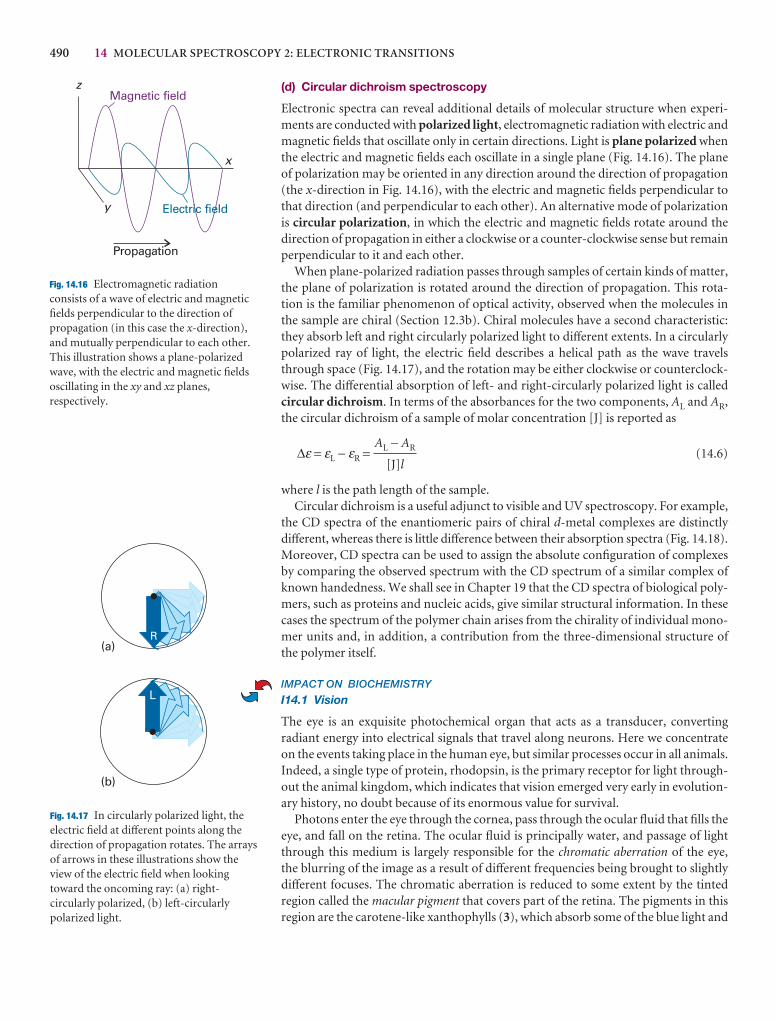
490 14 MOLECULAR SPECTROSCOPY 2: ELECTRONIC TRANSITIONS
(d) Circular dichroism spectroscopy
Electronic spectra can reveal additional details of molecular structure when experi-ments are conducted with polarized light, electromagnetic radiation with electric andmagnetic fields that oscillate only in certain directions. Light is plane polarized whenthe electric and magnetic fields each oscillate in a single plane (Fig. 14.16). The planeof polarization may be oriented in any direction around the direction of propagation(the x-direction in Fig. 14.16), with the electric and magnetic fields perpendicular tothat direction (and perpendicular to each other). An alternative mode of polarizationis circular polarization, in which the electric and magnetic fields rotate around thedirection of propagation in either a clockwise or a counter-clockwise sense but remainperpendicular to it and each other.
When plane-polarized radiation passes through samples of certain kinds of matter,the plane of polarization is rotated around the direction of propagation. This rota-tion is the familiar phenomenon of optical activity, observed when the molecules inthe sample are chiral (Section 12.3b). Chiral molecules have a second characteristic: they absorb left and right circularly polarized light to different extents. In a circularlypolarized ray of light, the electric field describes a helical path as the wave travelsthrough space (Fig. 14.17), and the rotation may be either clockwise or counterclock-wise. The differential absorption of left- and right-circularly polarized light is calledcircular dichroism. In terms of the absorbances for the two components, AL and AR,the circular dichroism of a sample of molar concentration [J] is reported as
∆ε = εL − εR = (14.6)
where l is the path length of the sample.Circular dichroism is a useful adjunct to visible and UV spectroscopy. For example,
the CD spectra of the enantiomeric pairs of chiral d-metal complexes are distinctlydifferent, whereas there is little difference between their absorption spectra (Fig. 14.18).Moreover, CD spectra can be used to assign the absolute configuration of complexesby comparing the observed spectrum with the CD spectrum of a similar complex ofknown handedness. We shall see in Chapter 19 that the CD spectra of biological poly-mers, such as proteins and nucleic acids, give similar structural information. In thesecases the spectrum of the polymer chain arises from the chirality of individual mono-mer units and, in addition, a contribution from the three-dimensional structure ofthe polymer itself.
IMPACT ON BIOCHEMISTRY
I14.1 Vision
The eye is an exquisite photochemical organ that acts as a transducer, converting radiant energy into electrical signals that travel along neurons. Here we concentrateon the events taking place in the human eye, but similar processes occur in all animals.Indeed, a single type of protein, rhodopsin, is the primary receptor for light through-out the animal kingdom, which indicates that vision emerged very early in evolution-ary history, no doubt because of its enormous value for survival.
Photons enter the eye through the cornea, pass through the ocular fluid that fills theeye, and fall on the retina. The ocular fluid is principally water, and passage of lightthrough this medium is largely responsible for the chromatic aberration of the eye, the blurring of the image as a result of different frequencies being brought to slightly different focuses. The chromatic aberration is reduced to some extent by the tinted region called the macular pigment that covers part of the retina. The pigments in thisregion are the carotene-like xanthophylls (3), which absorb some of the blue light and
AL − AR
[J]l
x
y
Magnetic field
Electric field
z
Propagation
Fig. 14.16 Electromagnetic radiationconsists of a wave of electric and magneticfields perpendicular to the direction ofpropagation (in this case the x-direction),and mutually perpendicular to each other.This illustration shows a plane-polarizedwave, with the electric and magnetic fieldsoscillating in the xy and xz planes,respectively.
R
L
(a)
(b)
Fig. 14.17 In circularly polarized light, theelectric field at different points along thedirection of propagation rotates. The arraysof arrows in these illustrations show theview of the electric field when lookingtoward the oncoming ray: (a) right-circularly polarized, (b) left-circularlypolarized light.
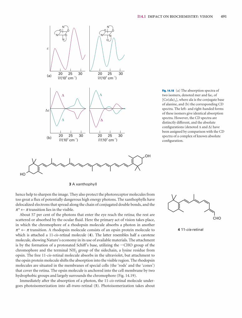
I14.1 IMPACT ON BIOCHEMISTRY: VISION 491
hence help to sharpen the image. They also protect the photoreceptor molecules fromtoo great a flux of potentially dangerous high energy photons. The xanthophylls havedelocalized electrons that spread along the chain of conjugated double bonds, and theπ* ← π transition lies in the visible.
About 57 per cent of the photons that enter the eye reach the retina; the rest arescattered or absorbed by the ocular fluid. Here the primary act of vision takes place, in which the chromophore of a rhodopsin molecule absorbs a photon in another π* ← π transition. A rhodopsin molecule consists of an opsin protein molecule towhich is attached a 11-cis-retinal molecule (4). The latter resembles half a carotenemolecule, showing Nature’s economy in its use of available materials. The attachmentis by the formation of a protonated Schiff ’s base, utilizing the -CHO group of the chromophore and the terminal NH2 group of the sidechain, a lysine residue fromopsin. The free 11-cis-retinal molecule absorbs in the ultraviolet, but attachment tothe opsin protein molecule shifts the absorption into the visible region. The rhodopsinmolecules are situated in the membranes of special cells (the ‘rods’ and the ‘cones’)that cover the retina. The opsin molecule is anchored into the cell membrane by twohydrophobic groups and largely surrounds the chromophore (Fig. 14.19).
Immediately after the absorption of a photon, the 11-cis-retinal molecule under-goes photoisomerization into all-trans-retinal (5). Photoisomerization takes about
Fig. 14.18 (a) The absorption spectra of two isomers, denoted mer and fac, of[Co(ala)3], where ala is the conjugate baseof alanine, and (b) the corresponding CDspectra. The left- and right-handed formsof these isomers give identical absorptionspectra. However, the CD spectra aredistinctly different, and the absoluteconfigurations (denoted Λ and ∆) havebeen assigned by comparison with the CDspectra of a complex of known absoluteconfiguration.
�
20 25 30/(10 cm )3 1�~
20 25 30/(10 cm )3 1�~
20 25 30/(10 cm )3 1�~
20 25 30/(10 cm )3 1�~
(
(
N
N
N
O
OON
N N
O
OO
(a)
(b)
� �
� �
�
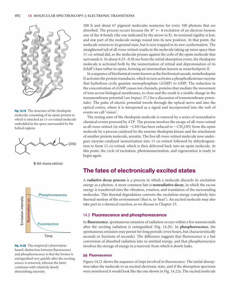
492 14 MOLECULAR SPECTROSCOPY 2: ELECTRONIC TRANSITIONS
200 fs and about 67 pigment molecules isomerize for every 100 photons that are absorbed. The process occurs because the π* ← π excitation of an electron loosensone of the π-bonds (the one indicated by the arrow in 5), its torsional rigidity is lost,and one part of the molecule swings round into its new position. At that point, themolecule returns to its ground state, but is now trapped in its new conformation. Thestraightened tail of all-trans-retinal results in the molecule taking up more space than11-cis-retinal did, so the molecule presses against the coils of the opsin molecule thatsurrounds it. In about 0.25–0.50 ms from the initial absorption event, the rhodopsinmolecule is activated both by the isomerization of retinal and deprotonation of itsSchiff ’s base tether to opsin, forming an intermediate known as metarhodopsin II.
In a sequence of biochemical events known as the biochemical cascade, metarhodopsinII activates the protein transducin, which in turn activates a phosphodiesterase enzymethat hydrolyses cyclic guanine monophosphate (cGMP) to GMP. The reduction inthe concentration of cGMP causes ion channels, proteins that mediate the movementof ions across biological membranes, to close and the result is a sizable change in thetransmembrane potential (see Impact I7.2 for a discussion of transmembrane poten-tials). The pulse of electric potential travels through the optical nerve and into the optical cortex, where it is interpreted as a signal and incorporated into the web ofevents we call ‘vision’.
The resting state of the rhodopsin molecule is restored by a series of nonradiativechemical events powered by ATP. The process involves the escape of all-trans-retinalas all-trans-retinol (in which -CHO has been reduced to -CH2OH) from the opsinmolecule by a process catalysed by the enzyme rhodopsin kinase and the attachmentof another protein molecule, arrestin. The free all-trans-retinol molecule now under-goes enzyme-catalysed isomerization into 11-cis-retinol followed by dehydrogena-tion to form 11-cis-retinal, which is then delivered back into an opsin molecule. Atthis point, the cycle of excitation, photoisomerization, and regeneration is ready tobegin again.
The fates of electronically excited statesA radiative decay process is a process in which a molecule discards its excitation energy as a photon. A more common fate is nonradiative decay, in which the excess energy is transferred into the vibration, rotation, and translation of the surroundingmolecules. This thermal degradation converts the excitation energy completely intothermal motion of the environment (that is, to ‘heat’). An excited molecule may alsotake part in a chemical reaction, as we discuss in Chapter 23.
14.3 Fluorescence and phosphorescence
In fluorescence, spontaneous emission of radiation occurs within a few nanosecondsafter the exciting radiation is extinguished (Fig. 14.20). In phosphorescence, thespontaneous emission may persist for long periods (even hours, but characteristicallyseconds or fractions of seconds). The difference suggests that fluorescence is a fastconversion of absorbed radiation into re-emitted energy, and that phosphorescenceinvolves the storage of energy in a reservoir from which it slowly leaks.
(a) Fluorescence
Figure 14.21 shows the sequence of steps involved in fluorescence. The initial absorp-tion takes the molecule to an excited electronic state, and if the absorption spectrumwere monitored it would look like the one shown in Fig. 14.22a. The excited molecule
Time
Emis
sion
inte
nsity
Fluorescence
Phosphorescence
Illum
inat
ion
on
Fig. 14.20 The empirical (observation-based) distinction between fluorescenceand phosphorescence is that the former isextinguished very quickly after the excitingsource is removed, whereas the lattercontinues with relatively slowlydiminishing intensity.
Fig. 14.19 The structure of the rhodopsinmolecule, consisting of an opsin protein towhich is attached an 11-cis-retinal moleculeembedded in the space surrounded by thehelical regions.
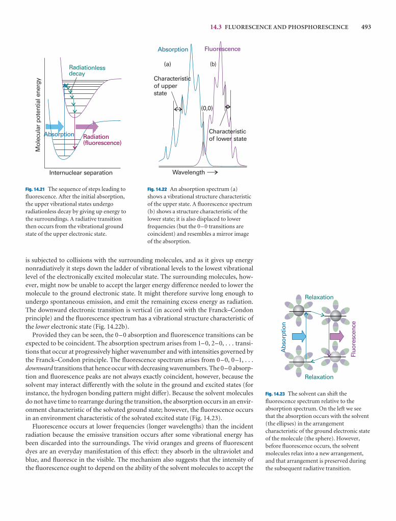
14.3 FLUORESCENCE AND PHOSPHORESCENCE 493
is subjected to collisions with the surrounding molecules, and as it gives up energynonradiatively it steps down the ladder of vibrational levels to the lowest vibrationallevel of the electronically excited molecular state. The surrounding molecules, how-ever, might now be unable to accept the larger energy difference needed to lower themolecule to the ground electronic state. It might therefore survive long enough to undergo spontaneous emission, and emit the remaining excess energy as radiation.The downward electronic transition is vertical (in accord with the Franck–Condonprinciple) and the fluorescence spectrum has a vibrational structure characteristic ofthe lower electronic state (Fig. 14.22b).
Provided they can be seen, the 0–0 absorption and fluorescence transitions can beexpected to be coincident. The absorption spectrum arises from 1–0, 2–0, . . . transi-tions that occur at progressively higher wavenumber and with intensities governed bythe Franck–Condon principle. The fluorescence spectrum arises from 0–0, 0–1, . . .downward transitions that hence occur with decreasing wavenumbers. The 0–0 absorp-tion and fluorescence peaks are not always exactly coincident, however, because thesolvent may interact differently with the solute in the ground and excited states (forinstance, the hydrogen bonding pattern might differ). Because the solvent moleculesdo not have time to rearrange during the transition, the absorption occurs in an envir-onment characteristic of the solvated ground state; however, the fluorescence occursin an environment characteristic of the solvated excited state (Fig. 14.23).
Fluorescence occurs at lower frequencies (longer wavelengths) than the incidentradiation because the emissive transition occurs after some vibrational energy hasbeen discarded into the surroundings. The vivid oranges and greens of fluorescentdyes are an everyday manifestation of this effect: they absorb in the ultraviolet andblue, and fluoresce in the visible. The mechanism also suggests that the intensity of the fluorescence ought to depend on the ability of the solvent molecules to accept the
Radiation(fluorescence)
Radiationlessdecay
Absorption
Mol
ecul
ar p
oten
tial e
nerg
y
Internuclear separation
(a) (b)
Absorption Fluorescence
Wavelength
Characteristicof upperstate
Characteristicof lower state
(0,0)
Fig. 14.21 The sequence of steps leading tofluorescence. After the initial absorption,the upper vibrational states undergoradiationless decay by giving up energy tothe surroundings. A radiative transitionthen occurs from the vibrational groundstate of the upper electronic state.
Fig. 14.22 An absorption spectrum (a)shows a vibrational structure characteristicof the upper state. A fluorescence spectrum(b) shows a structure characteristic of thelower state; it is also displaced to lowerfrequencies (but the 0–0 transitions arecoincident) and resembles a mirror imageof the absorption.
Abs
orpt
ion
Fluo
resc
ence
Relaxation
Relaxation
Fig. 14.23 The solvent can shift thefluorescence spectrum relative to theabsorption spectrum. On the left we seethat the absorption occurs with the solvent(the ellipses) in the arrangementcharacteristic of the ground electronic stateof the molecule (the sphere). However,before fluorescence occurs, the solventmolecules relax into a new arrangement,and that arrangement is preserved duringthe subsequent radiative transition.
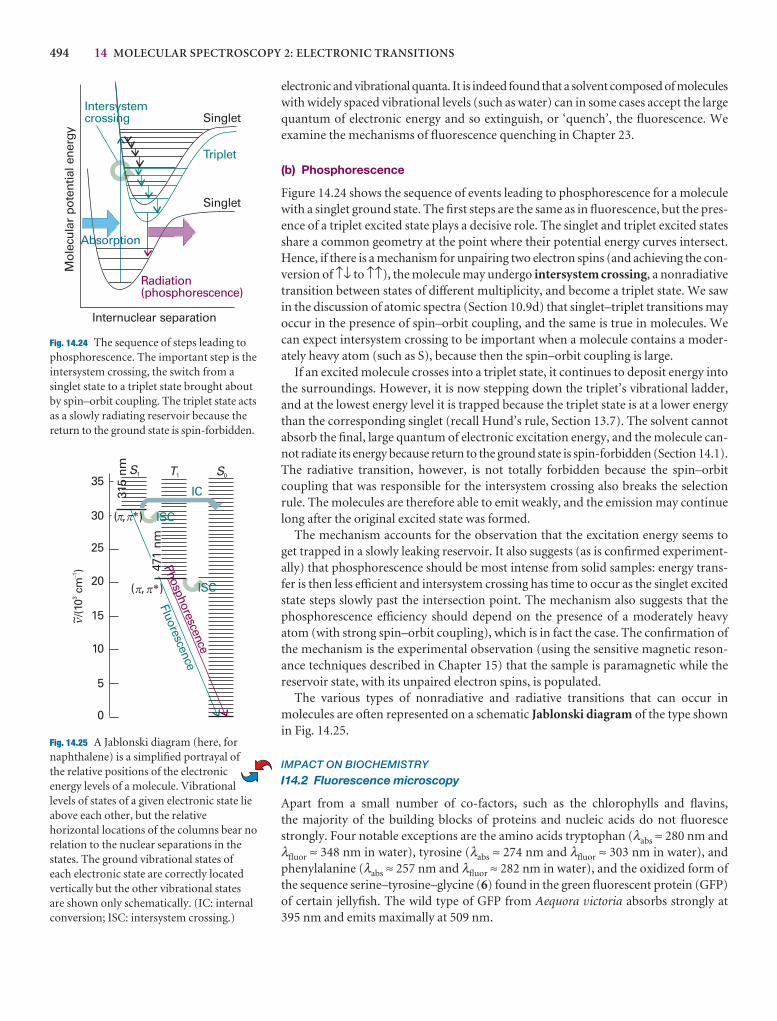
494 14 MOLECULAR SPECTROSCOPY 2: ELECTRONIC TRANSITIONS
electronic and vibrational quanta. It is indeed found that a solvent composed of moleculeswith widely spaced vibrational levels (such as water) can in some cases accept the largequantum of electronic energy and so extinguish, or ‘quench’, the fluorescence. We examine the mechanisms of fluorescence quenching in Chapter 23.
(b) Phosphorescence
Figure 14.24 shows the sequence of events leading to phosphorescence for a moleculewith a singlet ground state. The first steps are the same as in fluorescence, but the pres-ence of a triplet excited state plays a decisive role. The singlet and triplet excited statesshare a common geometry at the point where their potential energy curves intersect.Hence, if there is a mechanism for unpairing two electron spins (and achieving the con-version of ↑↓ to ↑↑), the molecule may undergo intersystem crossing, a nonradiativetransition between states of different multiplicity, and become a triplet state. We sawin the discussion of atomic spectra (Section 10.9d) that singlet–triplet transitions mayoccur in the presence of spin–orbit coupling, and the same is true in molecules. Wecan expect intersystem crossing to be important when a molecule contains a moder-ately heavy atom (such as S), because then the spin–orbit coupling is large.
If an excited molecule crosses into a triplet state, it continues to deposit energy intothe surroundings. However, it is now stepping down the triplet’s vibrational ladder,and at the lowest energy level it is trapped because the triplet state is at a lower energythan the corresponding singlet (recall Hund’s rule, Section 13.7). The solvent cannotabsorb the final, large quantum of electronic excitation energy, and the molecule can-not radiate its energy because return to the ground state is spin-forbidden (Section 14.1).The radiative transition, however, is not totally forbidden because the spin–orbit coupling that was responsible for the intersystem crossing also breaks the selectionrule. The molecules are therefore able to emit weakly, and the emission may continuelong after the original excited state was formed.
The mechanism accounts for the observation that the excitation energy seems toget trapped in a slowly leaking reservoir. It also suggests (as is confirmed experiment-ally) that phosphorescence should be most intense from solid samples: energy trans-fer is then less efficient and intersystem crossing has time to occur as the singlet excitedstate steps slowly past the intersection point. The mechanism also suggests that thephosphorescence efficiency should depend on the presence of a moderately heavyatom (with strong spin–orbit coupling), which is in fact the case. The confirmation ofthe mechanism is the experimental observation (using the sensitive magnetic reson-ance techniques described in Chapter 15) that the sample is paramagnetic while thereservoir state, with its unpaired electron spins, is populated.
The various types of nonradiative and radiative transitions that can occur inmolecules are often represented on a schematic Jablonski diagram of the type shownin Fig. 14.25.
IMPACT ON BIOCHEMISTRY
I14.2 Fluorescence microscopy
Apart from a small number of co-factors, such as the chlorophylls and flavins, the majority of the building blocks of proteins and nucleic acids do not fluorescestrongly. Four notable exceptions are the amino acids tryptophan (λabs ≈ 280 nm andλfluor ≈ 348 nm in water), tyrosine (λabs ≈ 274 nm and λfluor ≈ 303 nm in water), andphenylalanine (λabs ≈ 257 nm and λfluor ≈ 282 nm in water), and the oxidized form ofthe sequence serine–tyrosine–glycine (6) found in the green fluorescent protein (GFP)of certain jellyfish. The wild type of GFP from Aequora victoria absorbs strongly at395 nm and emits maximally at 509 nm.
Radiation(phosphorescence)
Absorption
Mol
ecul
arpo
tent
ial e
nerg
y
Internuclear separation
SingletIntersystemcrossing
Singlet
Triplet
35
30
25
20
15
10
5
0
S0T1S1
( , )*
315
nm
471
nm
IC
/(10
cm)
31
~
Phosphorescence
Fluorescence
ISC
ISC
( , )*� �
�
� �
�
Fig. 14.25 A Jablonski diagram (here, fornaphthalene) is a simplified portrayal ofthe relative positions of the electronicenergy levels of a molecule. Vibrationallevels of states of a given electronic state lieabove each other, but the relativehorizontal locations of the columns bear norelation to the nuclear separations in thestates. The ground vibrational states ofeach electronic state are correctly locatedvertically but the other vibrational statesare shown only schematically. (IC: internalconversion; ISC: intersystem crossing.)
Fig. 14.24 The sequence of steps leading tophosphorescence. The important step is theintersystem crossing, the switch from asinglet state to a triplet state brought aboutby spin–orbit coupling. The triplet state actsas a slowly radiating reservoir because thereturn to the ground state is spin-forbidden.
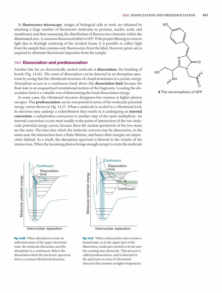
14.4 DISSOCIATION AND PREDISSOCIATION 495
In fluorescence microscopy, images of biological cells at work are obtained byattaching a large number of fluorescent molecules to proteins, nucleic acids, andmembranes and then measuring the distribution of fluorescence intensity within theilluminated area. A common fluorescent label is GFP. With proper filtering to removelight due to Rayleigh scattering of the incident beam, it is possible to collect light from the sample that contains only fluorescence from the label. However, great care isrequired to eliminate fluorescent impurities from the sample.
14.4 Dissociation and predissociation
Another fate for an electronically excited molecule is dissociation, the breaking ofbonds (Fig. 14.26). The onset of dissociation can be detected in an absorption spec-trum by seeing that the vibrational structure of a band terminates at a certain energy.Absorption occurs in a continuous band above this dissociation limit because thefinal state is an unquantized translational motion of the fragments. Locating the dis-sociation limit is a valuable way of determining the bond dissociation energy.
In some cases, the vibrational structure disappears but resumes at higher photonenergies. This predissociation can be interpreted in terms of the molecular potentialenergy curves shown in Fig. 14.27. When a molecule is excited to a vibrational level,its electrons may undergo a redistribution that results in it undergoing an internalconversion, a radiationless conversion to another state of the same multiplicity. Aninternal conversion occurs most readily at the point of intersection of the two mole-cular potential energy curves, because there the nuclear geometries of the two statesare the same. The state into which the molecule converts may be dissociative, so thestates near the intersection have a finite lifetime, and hence their energies are impre-cisely defined. As a result, the absorption spectrum is blurred in the vicinity of the intersection. When the incoming photon brings enough energy to excite the molecule
Dissociationlimit
Continuum
Mol
ecul
ar p
oten
tial e
nerg
y
Internuclear separation
Continuum
Dissociationlimit
Continuum
Mol
ecul
ar p
oten
tial e
nerg
y
Internuclear separation
Fig. 14.26 When absorption occurs tounbound states of the upper electronicstate, the molecule dissociates and theabsorption is a continuum. Below thedissociation limit the electronic spectrumshows a normal vibrational structure.
Fig. 14.27 When a dissociative state crosses abound state, as in the upper part of theillustration, molecules excited to levels nearthe crossing may dissociate. This process iscalled predissociation, and is detected inthe spectrum as a loss of vibrationalstructure that resumes at higher frequencies.
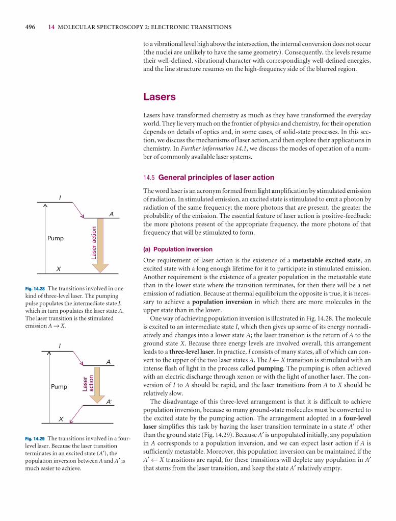
496 14 MOLECULAR SPECTROSCOPY 2: ELECTRONIC TRANSITIONS
to a vibrational level high above the intersection, the internal conversion does not occur(the nuclei are unlikely to have the same geometry). Consequently, the levels resumetheir well-defined, vibrational character with correspondingly well-defined energies,and the line structure resumes on the high-frequency side of the blurred region.
Lasers
Lasers have transformed chemistry as much as they have transformed the everydayworld. They lie very much on the frontier of physics and chemistry, for their operationdepends on details of optics and, in some cases, of solid-state processes. In this sec-tion, we discuss the mechanisms of laser action, and then explore their applications inchemistry. In Further information 14.1, we discuss the modes of operation of a num-ber of commonly available laser systems.
14.5 General principles of laser action
The word laser is an acronym formed from light amplification by stimulated emissionof radiation. In stimulated emission, an excited state is stimulated to emit a photon byradiation of the same frequency; the more photons that are present, the greater theprobability of the emission. The essential feature of laser action is positive-feedback:the more photons present of the appropriate frequency, the more photons of that frequency that will be stimulated to form.
(a) Population inversion
One requirement of laser action is the existence of a metastable excited state, an excited state with a long enough lifetime for it to participate in stimulated emission.Another requirement is the existence of a greater population in the metastable statethan in the lower state where the transition terminates, for then there will be a netemission of radiation. Because at thermal equilibrium the opposite is true, it is neces-sary to achieve a population inversion in which there are more molecules in theupper state than in the lower.
One way of achieving population inversion is illustrated in Fig. 14.28. The moleculeis excited to an intermediate state I, which then gives up some of its energy nonradi-atively and changes into a lower state A; the laser transition is the return of A to theground state X. Because three energy levels are involved overall, this arrangementleads to a three-level laser. In practice, I consists of many states, all of which can con-vert to the upper of the two laser states A. The I ← X transition is stimulated with an intense flash of light in the process called pumping. The pumping is often achievedwith an electric discharge through xenon or with the light of another laser. The con-version of I to A should be rapid, and the laser transitions from A to X should be relatively slow.
The disadvantage of this three-level arrangement is that it is difficult to achievepopulation inversion, because so many ground-state molecules must be converted tothe excited state by the pumping action. The arrangement adopted in a four-levellaser simplifies this task by having the laser transition terminate in a state A′ otherthan the ground state (Fig. 14.29). Because A′ is unpopulated initially, any populationin A corresponds to a population inversion, and we can expect laser action if A issufficiently metastable. Moreover, this population inversion can be maintained if theA′ ← X transitions are rapid, for these transitions will deplete any population in A′that stems from the laser transition, and keep the state A′ relatively empty.
I
A
X
Pump
Lase
r ac
tion
I
A
A�
X
Pump Lase
rac
tion
Fig. 14.28 The transitions involved in onekind of three-level laser. The pumpingpulse populates the intermediate state I,which in turn populates the laser state A.The laser transition is the stimulatedemission A → X.
Fig. 14.29 The transitions involved in a four-level laser. Because the laser transitionterminates in an excited state (A′), thepopulation inversion between A and A′ ismuch easier to achieve.
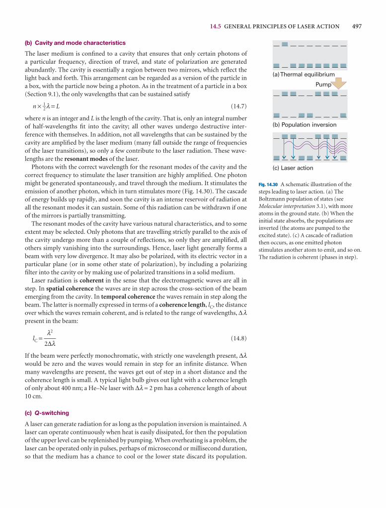
14.5 GENERAL PRINCIPLES OF LASER ACTION 497
(b) Cavity and mode characteristics
The laser medium is confined to a cavity that ensures that only certain photons of a particular frequency, direction of travel, and state of polarization are generatedabundantly. The cavity is essentially a region between two mirrors, which reflect thelight back and forth. This arrangement can be regarded as a version of the particle ina box, with the particle now being a photon. As in the treatment of a particle in a box(Section 9.1), the only wavelengths that can be sustained satisfy
n × 1–2 λ = L (14.7)
where n is an integer and L is the length of the cavity. That is, only an integral numberof half-wavelengths fit into the cavity; all other waves undergo destructive inter-ference with themselves. In addition, not all wavelengths that can be sustained by thecavity are amplified by the laser medium (many fall outside the range of frequenciesof the laser transitions), so only a few contribute to the laser radiation. These wave-lengths are the resonant modes of the laser.
Photons with the correct wavelength for the resonant modes of the cavity and thecorrect frequency to stimulate the laser transition are highly amplified. One photonmight be generated spontaneously, and travel through the medium. It stimulates theemission of another photon, which in turn stimulates more (Fig. 14.30). The cascadeof energy builds up rapidly, and soon the cavity is an intense reservoir of radiation atall the resonant modes it can sustain. Some of this radiation can be withdrawn if oneof the mirrors is partially transmitting.
The resonant modes of the cavity have various natural characteristics, and to someextent may be selected. Only photons that are travelling strictly parallel to the axis ofthe cavity undergo more than a couple of reflections, so only they are amplified, allothers simply vanishing into the surroundings. Hence, laser light generally forms abeam with very low divergence. It may also be polarized, with its electric vector in aparticular plane (or in some other state of polarization), by including a polarizingfilter into the cavity or by making use of polarized transitions in a solid medium.
Laser radiation is coherent in the sense that the electromagnetic waves are all instep. In spatial coherence the waves are in step across the cross-section of the beamemerging from the cavity. In temporal coherence the waves remain in step along thebeam. The latter is normally expressed in terms of a coherence length, lC, the distanceover which the waves remain coherent, and is related to the range of wavelengths, ∆λpresent in the beam:
lC = (14.8)
If the beam were perfectly monochromatic, with strictly one wavelength present, ∆λwould be zero and the waves would remain in step for an infinite distance. Whenmany wavelengths are present, the waves get out of step in a short distance and the coherence length is small. A typical light bulb gives out light with a coherence lengthof only about 400 nm; a He–Ne laser with ∆λ ≈ 2 pm has a coherence length of about10 cm.
(c) Q-switching
A laser can generate radiation for as long as the population inversion is maintained. Alaser can operate continuously when heat is easily dissipated, for then the populationof the upper level can be replenished by pumping. When overheating is a problem, thelaser can be operated only in pulses, perhaps of microsecond or millisecond duration,so that the medium has a chance to cool or the lower state discard its population.
λ2
2∆λ
Pump
(a)Thermal equilibrium
(b) Population inversion
(c) Laser action
Fig. 14.30 A schematic illustration of thesteps leading to laser action. (a) TheBoltzmann population of states (seeMolecular interpretation 3.1), with moreatoms in the ground state. (b) When theinitial state absorbs, the populations areinverted (the atoms are pumped to theexcited state). (c) A cascade of radiationthen occurs, as one emitted photonstimulates another atom to emit, and so on.The radiation is coherent (phases in step).
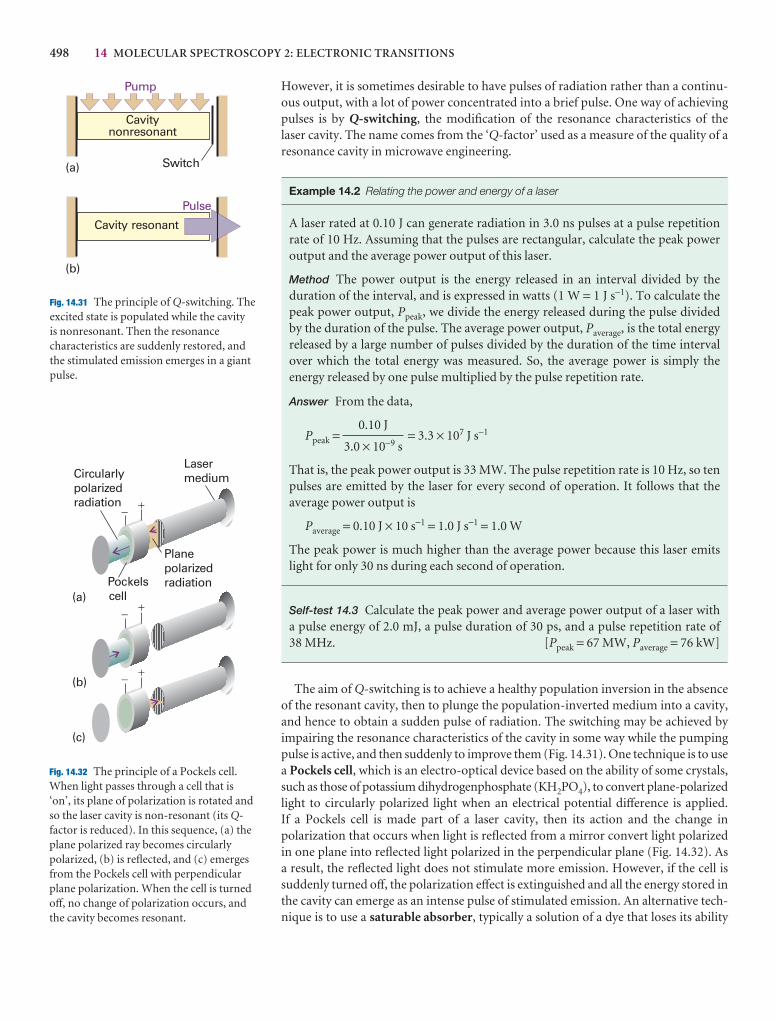
498 14 MOLECULAR SPECTROSCOPY 2: ELECTRONIC TRANSITIONS
Pump
Switch
Pulse
Cavity resonant
Cavitynonresonant
(a)
(b)
��
��
��
LasermediumCircularly
polarizedradiation
PlanepolarizedradiationPockels
cell(a)
(b)
(c)
Fig. 14.31 The principle of Q-switching. Theexcited state is populated while the cavity is nonresonant. Then the resonancecharacteristics are suddenly restored, andthe stimulated emission emerges in a giantpulse.
Fig. 14.32 The principle of a Pockels cell.When light passes through a cell that is‘on’, its plane of polarization is rotated andso the laser cavity is non-resonant (its Q-factor is reduced). In this sequence, (a) theplane polarized ray becomes circularlypolarized, (b) is reflected, and (c) emergesfrom the Pockels cell with perpendicularplane polarization. When the cell is turnedoff, no change of polarization occurs, andthe cavity becomes resonant.
However, it is sometimes desirable to have pulses of radiation rather than a continu-ous output, with a lot of power concentrated into a brief pulse. One way of achievingpulses is by Q-switching, the modification of the resonance characteristics of the laser cavity. The name comes from the ‘Q-factor’ used as a measure of the quality of aresonance cavity in microwave engineering.
Example 14.2 Relating the power and energy of a laser
A laser rated at 0.10 J can generate radiation in 3.0 ns pulses at a pulse repetitionrate of 10 Hz. Assuming that the pulses are rectangular, calculate the peak poweroutput and the average power output of this laser.
Method The power output is the energy released in an interval divided by the duration of the interval, and is expressed in watts (1 W = 1 J s−1). To calculate thepeak power output, Ppeak, we divide the energy released during the pulse divided by the duration of the pulse. The average power output, Paverage, is the total energyreleased by a large number of pulses divided by the duration of the time intervalover which the total energy was measured. So, the average power is simply the energy released by one pulse multiplied by the pulse repetition rate.
Answer From the data,
Ppeak = = 3.3 × 10⁷ J s−1
That is, the peak power output is 33 MW. The pulse repetition rate is 10 Hz, so tenpulses are emitted by the laser for every second of operation. It follows that the average power output is
Paverage = 0.10 J × 10 s−1 = 1.0 J s−1 = 1.0 W
The peak power is much higher than the average power because this laser emitslight for only 30 ns during each second of operation.
Self-test 14.3 Calculate the peak power and average power output of a laser with a pulse energy of 2.0 mJ, a pulse duration of 30 ps, and a pulse repetition rate of 38 MHz. [Ppeak = 67 MW, Paverage = 76 kW]
The aim of Q-switching is to achieve a healthy population inversion in the absenceof the resonant cavity, then to plunge the population-inverted medium into a cavity,and hence to obtain a sudden pulse of radiation. The switching may be achieved byimpairing the resonance characteristics of the cavity in some way while the pumpingpulse is active, and then suddenly to improve them (Fig. 14.31). One technique is to usea Pockels cell, which is an electro-optical device based on the ability of some crystals,such as those of potassium dihydrogenphosphate (KH2PO4), to convert plane-polarizedlight to circularly polarized light when an electrical potential difference is applied. If a Pockels cell is made part of a laser cavity, then its action and the change in polarization that occurs when light is reflected from a mirror convert light polarizedin one plane into reflected light polarized in the perpendicular plane (Fig. 14.32). As a result, the reflected light does not stimulate more emission. However, if the cell issuddenly turned off, the polarization effect is extinguished and all the energy stored inthe cavity can emerge as an intense pulse of stimulated emission. An alternative tech-nique is to use a saturable absorber, typically a solution of a dye that loses its ability
0.10 J
3.0 × 10⁻⁹ s
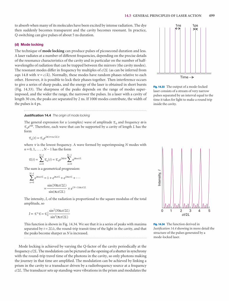
14.5 GENERAL PRINCIPLES OF LASER ACTION 499
to absorb when many of its molecules have been excited by intense radiation. The dyethen suddenly becomes transparent and the cavity becomes resonant. In practice, Q-switching can give pulses of about 5 ns duration.
(d) Mode locking
The technique of mode locking can produce pulses of picosecond duration and less.A laser radiates at a number of different frequencies, depending on the precise detailsof the resonance characteristics of the cavity and in particular on the number of half-wavelengths of radiation that can be trapped between the mirrors (the cavity modes).The resonant modes differ in frequency by multiples of c/2L (as can be inferred fromeqn 14.8 with ν = c /λ). Normally, these modes have random phases relative to eachother. However, it is possible to lock their phases together. Then interference occursto give a series of sharp peaks, and the energy of the laser is obtained in short bursts(Fig. 14.33). The sharpness of the peaks depends on the range of modes super-imposed, and the wider the range, the narrower the pulses. In a laser with a cavity oflength 30 cm, the peaks are separated by 2 ns. If 1000 modes contribute, the width ofthe pulses is 4 ps.
Justification 14.4 The origin of mode locking
The general expression for a (complex) wave of amplitude E 0 and frequency ω isE 0eiωt. Therefore, each wave that can be supported by a cavity of length L has theform
En(t) = E 0e2π(ν+nc/2L)t
where ν is the lowest frequency. A wave formed by superimposing N modes with n = 0, 1, . . . , N − 1 has the form
E(t) =N−1
∑n=0
En(t) = E 0e2πiνtN−1
∑n=0
eiπnct/L
The sum is a geometrical progression:N−1
∑n=0
eiπnct/L = 1 + eiπct/L + e2iπct/L + · · ·
= × e(N−1)iπct/2L
The intensity, I, of the radiation is proportional to the square modulus of the totalamplitude, so
I ∝ E*E = E 02
This function is shown in Fig. 14.34. We see that it is a series of peaks with maximaseparated by t = 2L/c, the round-trip transit time of the light in the cavity, and thatthe peaks become sharper as N is increased.
Mode locking is achieved by varying the Q-factor of the cavity periodically at thefrequency c/2L. The modulation can be pictured as the opening of a shutter in synchronywith the round-trip travel time of the photons in the cavity, so only photons makingthe journey in that time are amplified. The modulation can be achieved by linking aprism in the cavity to a transducer driven by a radiofrequency source at a frequencyc/2L. The transducer sets up standing-wave vibrations in the prism and modulates the
sin2(Nπct/2L)
sin2(πct/2L)
sin(Nπct/2L)
sin(πct/2L)
1ps1ns
Time
Fig. 14.33 The output of a mode-lockedlaser consists of a stream of very narrowpulses separated by an interval equal to thetime it takes for light to make a round tripinside the cavity.
0 1 2 3 4 5ct L/2
Inte
nsity
,I
Fig. 14.34 The function derived inJustification 14.4 showing in more detail thestructure of the pulses generated by amode-locked laser.
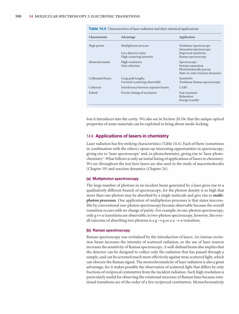
500 14 MOLECULAR SPECTROSCOPY 2: ELECTRONIC TRANSITIONS
loss it introduces into the cavity. We also see in Section 20.10c that the unique opticalproperties of some materials can be exploited to bring about mode-locking.
14.6 Applications of lasers in chemistry
Laser radiation has five striking characteristics (Table 14.4). Each of them (sometimesin combination with the others) opens up interesting opportunities in spectroscopy,giving rise to ‘laser spectroscopy’ and, in photochemistry, giving rise to ‘laser photo-chemistry’. What follows is only an initial listing of applications of lasers to chemistry.We see throughout the text how lasers are also used in the study of macromolecules(Chapter 19) and reaction dynamics (Chapter 24).
(a) Multiphoton spectroscopy
The large number of photons in an incident beam generated by a laser gives rise to aqualitatively different branch of spectroscopy, for the photon density is so high thatmore than one photon may be absorbed by a single molecule and give rise to multi-photon processes. One application of multiphoton processes is that states inaccess-ible by conventional one-photon spectroscopy become observable because the overalltransition occurs with no change of parity. For example, in one-photon spectroscopy,only g ↔ u transitions are observable; in two-photon spectroscopy, however, the over-all outcome of absorbing two photons is a g → g or a u → u transition.
(b) Raman spectroscopy
Raman spectroscopy was revitalized by the introduction of lasers. An intense excita-tion beam increases the intensity of scattered radiation, so the use of laser sources increases the sensitivity of Raman spectroscopy. A well-defined beam also implies thatthe detector can be designed to collect only the radiation that has passed through asample, and can be screened much more effectively against stray scattered light, whichcan obscure the Raman signal. The monochromaticity of laser radiation is also a greatadvantage, for it makes possible the observation of scattered light that differs by onlyfractions of reciprocal centimetres from the incident radiation. Such high resolution isparticularly useful for observing the rotational structure of Raman lines because rota-tional transitions are of the order of a few reciprocal centimetres. Monochromaticity
Table 14.4 Characteristics of laser radiation and their chemical applications
Characteristic Advantage Application
High power Multiphoton process Nonlinear spectroscopySaturation spectroscopy
Low detector noise Improved sensitivityHigh scattering intensity Raman spectroscopy
Monochromatic High resolution SpectroscopyState selection Isotope separation
Photochemically preciseState-to-state reaction dynamics
Collimated beam Long path lengths SensitivitvForward-scattering observable Nonlinear Raman spectroscopy
Coherent Interference between separate beams CARS
Pulsed Precise timing of excitation Fast reactionsRelaxationEnergy transfer
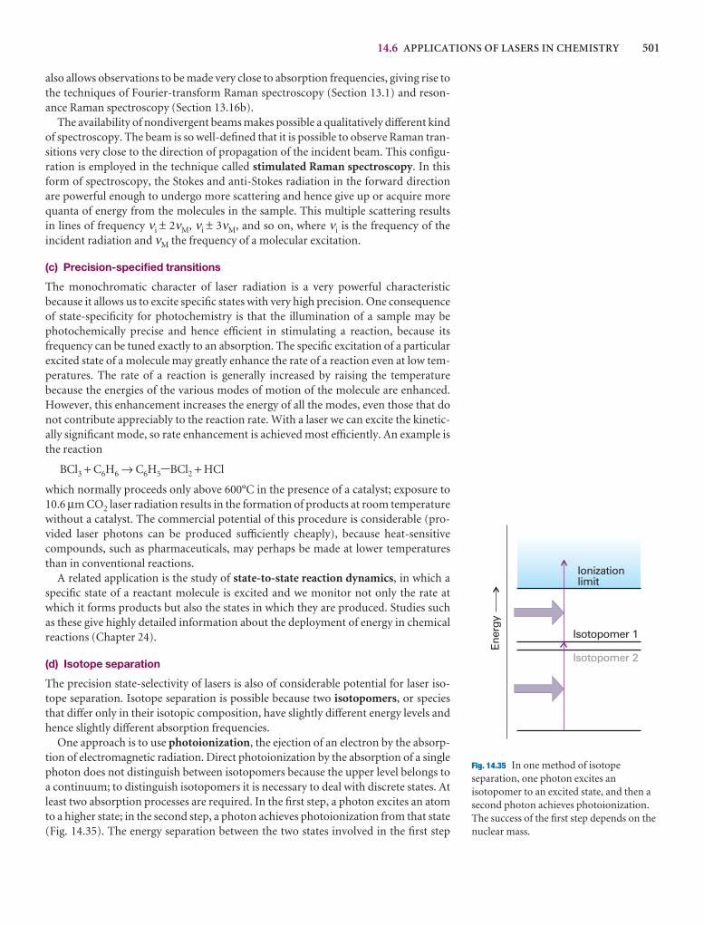
14.6 APPLICATIONS OF LASERS IN CHEMISTRY 501
also allows observations to be made very close to absorption frequencies, giving rise tothe techniques of Fourier-transform Raman spectroscopy (Section 13.1) and reson-ance Raman spectroscopy (Section 13.16b).
The availability of nondivergent beams makes possible a qualitatively different kindof spectroscopy. The beam is so well-defined that it is possible to observe Raman tran-sitions very close to the direction of propagation of the incident beam. This configu-ration is employed in the technique called stimulated Raman spectroscopy. In thisform of spectroscopy, the Stokes and anti-Stokes radiation in the forward directionare powerful enough to undergo more scattering and hence give up or acquire morequanta of energy from the molecules in the sample. This multiple scattering results in lines of frequency νi ± 2νM, νi ± 3νM, and so on, where νi is the frequency of the incident radiation and νM the frequency of a molecular excitation.
(c) Precision-specified transitions
The monochromatic character of laser radiation is a very powerful characteristic because it allows us to excite specific states with very high precision. One consequenceof state-specificity for photochemistry is that the illumination of a sample may bephotochemically precise and hence efficient in stimulating a reaction, because its frequency can be tuned exactly to an absorption. The specific excitation of a particularexcited state of a molecule may greatly enhance the rate of a reaction even at low tem-peratures. The rate of a reaction is generally increased by raising the temperature because the energies of the various modes of motion of the molecule are enhanced.However, this enhancement increases the energy of all the modes, even those that donot contribute appreciably to the reaction rate. With a laser we can excite the kinetic-ally significant mode, so rate enhancement is achieved most efficiently. An example isthe reaction
BCl3 + C6H6 → C6H5-BCl2 + HCl
which normally proceeds only above 600°C in the presence of a catalyst; exposure to10.6 µm CO2 laser radiation results in the formation of products at room temperaturewithout a catalyst. The commercial potential of this procedure is considerable (pro-vided laser photons can be produced sufficiently cheaply), because heat-sensitivecompounds, such as pharmaceuticals, may perhaps be made at lower temperaturesthan in conventional reactions.
A related application is the study of state-to-state reaction dynamics, in which aspecific state of a reactant molecule is excited and we monitor not only the rate atwhich it forms products but also the states in which they are produced. Studies suchas these give highly detailed information about the deployment of energy in chemicalreactions (Chapter 24).
(d) Isotope separation
The precision state-selectivity of lasers is also of considerable potential for laser iso-tope separation. Isotope separation is possible because two isotopomers, or speciesthat differ only in their isotopic composition, have slightly different energy levels andhence slightly different absorption frequencies.
One approach is to use photoionization, the ejection of an electron by the absorp-tion of electromagnetic radiation. Direct photoionization by the absorption of a singlephoton does not distinguish between isotopomers because the upper level belongs toa continuum; to distinguish isotopomers it is necessary to deal with discrete states. Atleast two absorption processes are required. In the first step, a photon excites an atomto a higher state; in the second step, a photon achieves photoionization from that state(Fig. 14.35). The energy separation between the two states involved in the first step
Isotopomer 1
Isotopomer 2
Ener
gy
Ionizationlimit
Fig. 14.35 In one method of isotopeseparation, one photon excites anisotopomer to an excited state, and then asecond photon achieves photoionization.The success of the first step depends on thenuclear mass.
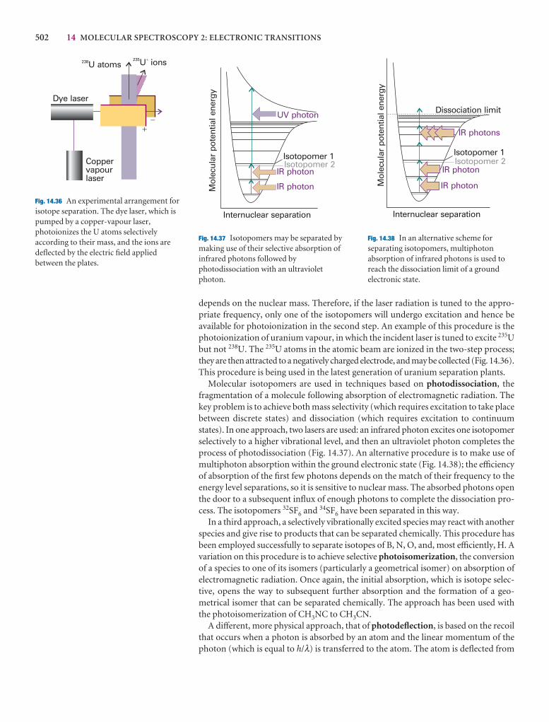
502 14 MOLECULAR SPECTROSCOPY 2: ELECTRONIC TRANSITIONS
depends on the nuclear mass. Therefore, if the laser radiation is tuned to the appro-priate frequency, only one of the isotopomers will undergo excitation and hence beavailable for photoionization in the second step. An example of this procedure is thephotoionization of uranium vapour, in which the incident laser is tuned to excite 235Ubut not 238U. The 235U atoms in the atomic beam are ionized in the two-step process;they are then attracted to a negatively charged electrode, and may be collected (Fig. 14.36).This procedure is being used in the latest generation of uranium separation plants.
Molecular isotopomers are used in techniques based on photodissociation, thefragmentation of a molecule following absorption of electromagnetic radiation. Thekey problem is to achieve both mass selectivity (which requires excitation to take placebetween discrete states) and dissociation (which requires excitation to continuumstates). In one approach, two lasers are used: an infrared photon excites one isotopomerselectively to a higher vibrational level, and then an ultraviolet photon completes theprocess of photodissociation (Fig. 14.37). An alternative procedure is to make use ofmultiphoton absorption within the ground electronic state (Fig. 14.38); the efficiencyof absorption of the first few photons depends on the match of their frequency to theenergy level separations, so it is sensitive to nuclear mass. The absorbed photons openthe door to a subsequent influx of enough photons to complete the dissociation pro-cess. The isotopomers 32SF6 and 34SF6 have been separated in this way.
In a third approach, a selectively vibrationally excited species may react with anotherspecies and give rise to products that can be separated chemically. This procedure hasbeen employed successfully to separate isotopes of B, N, O, and, most efficiently, H. Avariation on this procedure is to achieve selective photoisomerization, the conversionof a species to one of its isomers (particularly a geometrical isomer) on absorption ofelectromagnetic radiation. Once again, the initial absorption, which is isotope selec-tive, opens the way to subsequent further absorption and the formation of a geo-metrical isomer that can be separated chemically. The approach has been used withthe photoisomerization of CH3NC to CH3CN.
A different, more physical approach, that of photodeflection, is based on the recoilthat occurs when a photon is absorbed by an atom and the linear momentum of thephoton (which is equal to h/λ) is transferred to the atom. The atom is deflected from
238U atoms235U ions�
�
Dye laser
Coppervapourlaser
�
Fig. 14.36 An experimental arrangement forisotope separation. The dye laser, which ispumped by a copper-vapour laser,photoionizes the U atoms selectivelyaccording to their mass, and the ions aredeflected by the electric field appliedbetween the plates.
Mol
ecul
ar p
oten
tial e
nerg
yInternuclear separation
UV photon
Isotopomer 1Isotopomer 2
IR photon
IR photon
Fig. 14.37 Isotopomers may be separated bymaking use of their selective absorption ofinfrared photons followed byphotodissociation with an ultravioletphoton.
Mol
ecul
ar p
oten
tial e
nerg
y
Internuclear separation
Isotopomer 1Isotopomer 2
IR photon
IR photon
IR photons
Dissociation limit
Fig. 14.38 In an alternative scheme forseparating isotopomers, multiphotonabsorption of infrared photons is used toreach the dissociation limit of a groundelectronic state.
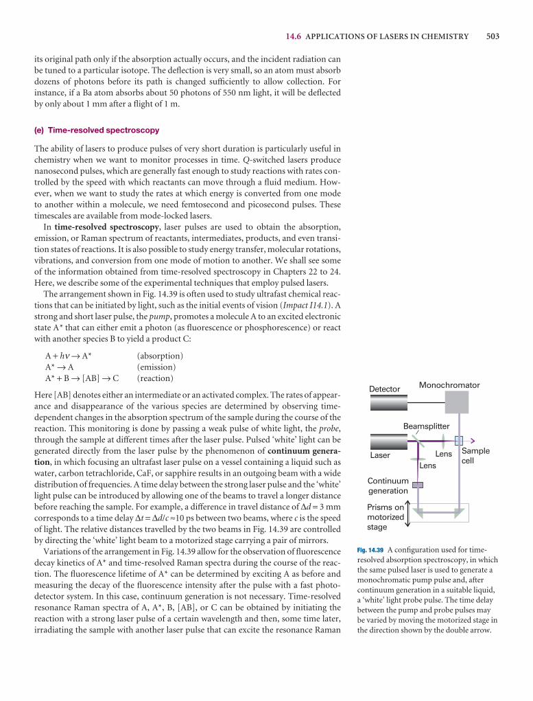
14.6 APPLICATIONS OF LASERS IN CHEMISTRY 503
its original path only if the absorption actually occurs, and the incident radiation canbe tuned to a particular isotope. The deflection is very small, so an atom must absorbdozens of photons before its path is changed sufficiently to allow collection. For instance, if a Ba atom absorbs about 50 photons of 550 nm light, it will be deflected by only about 1 mm after a flight of 1 m.
(e) Time-resolved spectroscopy
The ability of lasers to produce pulses of very short duration is particularly useful inchemistry when we want to monitor processes in time. Q-switched lasers producenanosecond pulses, which are generally fast enough to study reactions with rates con-trolled by the speed with which reactants can move through a fluid medium. How-ever, when we want to study the rates at which energy is converted from one mode to another within a molecule, we need femtosecond and picosecond pulses. Thesetimescales are available from mode-locked lasers.
In time-resolved spectroscopy, laser pulses are used to obtain the absorption,emission, or Raman spectrum of reactants, intermediates, products, and even transi-tion states of reactions. It is also possible to study energy transfer, molecular rotations,vibrations, and conversion from one mode of motion to another. We shall see someof the information obtained from time-resolved spectroscopy in Chapters 22 to 24.Here, we describe some of the experimental techniques that employ pulsed lasers.
The arrangement shown in Fig. 14.39 is often used to study ultrafast chemical reac-tions that can be initiated by light, such as the initial events of vision (Impact I14.1). Astrong and short laser pulse, the pump, promotes a molecule A to an excited electronicstate A* that can either emit a photon (as fluorescence or phosphorescence) or reactwith another species B to yield a product C:
A + hν → A* (absorption)A* → A (emission)A* + B → [AB] → C (reaction)
Here [AB] denotes either an intermediate or an activated complex. The rates of appear-ance and disappearance of the various species are determined by observing time-dependent changes in the absorption spectrum of the sample during the course of thereaction. This monitoring is done by passing a weak pulse of white light, the probe,through the sample at different times after the laser pulse. Pulsed ‘white’ light can begenerated directly from the laser pulse by the phenomenon of continuum genera-tion, in which focusing an ultrafast laser pulse on a vessel containing a liquid such aswater, carbon tetrachloride, CaF, or sapphire results in an outgoing beam with a widedistribution of frequencies. A time delay between the strong laser pulse and the ‘white’light pulse can be introduced by allowing one of the beams to travel a longer distancebefore reaching the sample. For example, a difference in travel distance of ∆d = 3 mmcorresponds to a time delay ∆t = ∆d/c ≈10 ps between two beams, where c is the speedof light. The relative distances travelled by the two beams in Fig. 14.39 are controlledby directing the ‘white’ light beam to a motorized stage carrying a pair of mirrors.
Variations of the arrangement in Fig. 14.39 allow for the observation of fluorescencedecay kinetics of A* and time-resolved Raman spectra during the course of the reac-tion. The fluorescence lifetime of A* can be determined by exciting A as before andmeasuring the decay of the fluorescence intensity after the pulse with a fast photo-detector system. In this case, continuum generation is not necessary. Time-resolvedresonance Raman spectra of A, A*, B, [AB], or C can be obtained by initiating the reaction with a strong laser pulse of a certain wavelength and then, some time later, irradiating the sample with another laser pulse that can excite the resonance Raman
Laser Samplecell
MonochromatorDetector
Prisms onmotorizedstage
Continuumgeneration
Beamsplitter
LensLens
Fig. 14.39 A configuration used for time-resolved absorption spectroscopy, in whichthe same pulsed laser is used to generate amonochromatic pump pulse and, aftercontinuum generation in a suitable liquid,a ‘white’ light probe pulse. The time delaybetween the pump and probe pulses maybe varied by moving the motorized stage inthe direction shown by the double arrow.
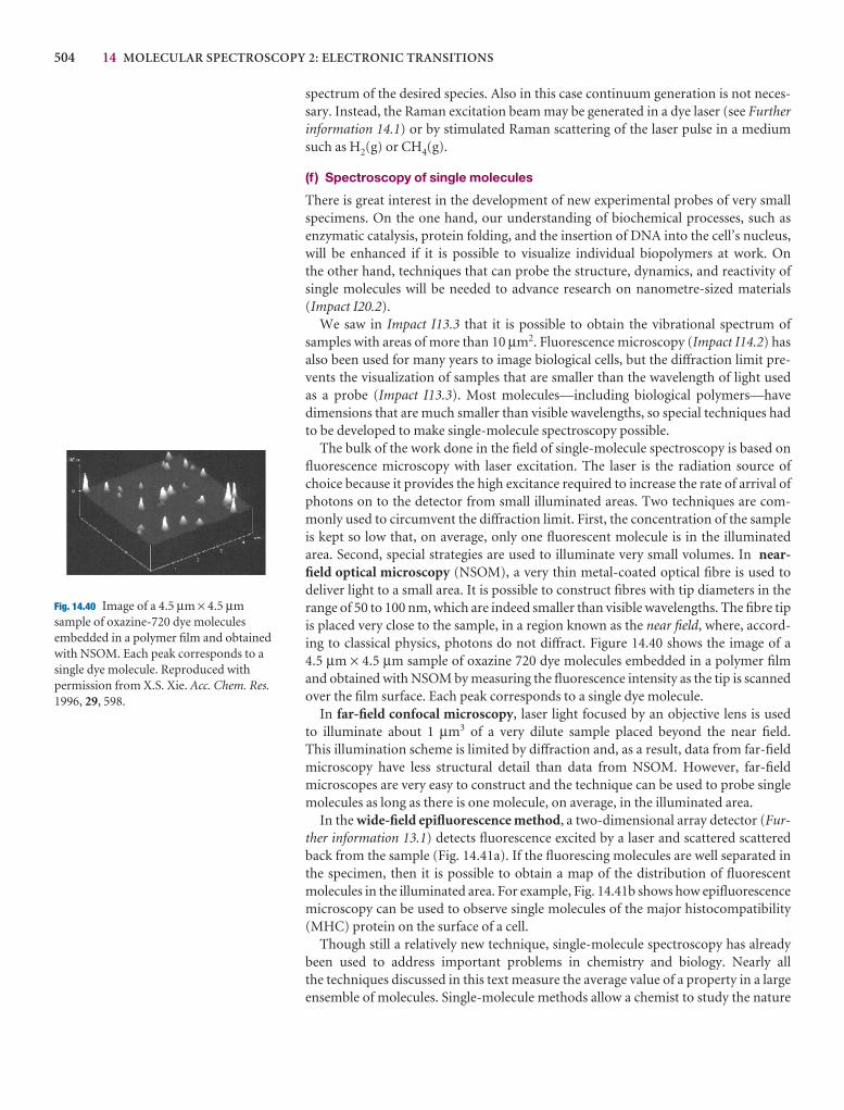
504 14 MOLECULAR SPECTROSCOPY 2: ELECTRONIC TRANSITIONS
spectrum of the desired species. Also in this case continuum generation is not neces-sary. Instead, the Raman excitation beam may be generated in a dye laser (see Furtherinformation 14.1) or by stimulated Raman scattering of the laser pulse in a mediumsuch as H2(g) or CH4(g).
(f ) Spectroscopy of single molecules
There is great interest in the development of new experimental probes of very smallspecimens. On the one hand, our understanding of biochemical processes, such as enzymatic catalysis, protein folding, and the insertion of DNA into the cell’s nucleus,will be enhanced if it is possible to visualize individual biopolymers at work. On the other hand, techniques that can probe the structure, dynamics, and reactivity of single molecules will be needed to advance research on nanometre-sized materials(Impact I20.2).
We saw in Impact I13.3 that it is possible to obtain the vibrational spectrum of samples with areas of more than 10 µm2. Fluorescence microscopy (Impact I14.2) hasalso been used for many years to image biological cells, but the diffraction limit pre-vents the visualization of samples that are smaller than the wavelength of light used as a probe (Impact I13.3). Most molecules—including biological polymers—have dimensions that are much smaller than visible wavelengths, so special techniques hadto be developed to make single-molecule spectroscopy possible.
The bulk of the work done in the field of single-molecule spectroscopy is based onfluorescence microscopy with laser excitation. The laser is the radiation source ofchoice because it provides the high excitance required to increase the rate of arrival ofphotons on to the detector from small illuminated areas. Two techniques are com-monly used to circumvent the diffraction limit. First, the concentration of the sampleis kept so low that, on average, only one fluorescent molecule is in the illuminatedarea. Second, special strategies are used to illuminate very small volumes. In near-field optical microscopy (NSOM), a very thin metal-coated optical fibre is used to deliver light to a small area. It is possible to construct fibres with tip diameters in therange of 50 to 100 nm, which are indeed smaller than visible wavelengths. The fibre tipis placed very close to the sample, in a region known as the near field, where, accord-ing to classical physics, photons do not diffract. Figure 14.40 shows the image of a 4.5 µm × 4.5 µm sample of oxazine 720 dye molecules embedded in a polymer filmand obtained with NSOM by measuring the fluorescence intensity as the tip is scannedover the film surface. Each peak corresponds to a single dye molecule.
In far-field confocal microscopy, laser light focused by an objective lens is used to illuminate about 1 µm3 of a very dilute sample placed beyond the near field. This illumination scheme is limited by diffraction and, as a result, data from far-field microscopy have less structural detail than data from NSOM. However, far-field microscopes are very easy to construct and the technique can be used to probe singlemolecules as long as there is one molecule, on average, in the illuminated area.
In the wide-field epifluorescence method, a two-dimensional array detector (Fur-ther information 13.1) detects fluorescence excited by a laser and scattered scatteredback from the sample (Fig. 14.41a). If the fluorescing molecules are well separated inthe specimen, then it is possible to obtain a map of the distribution of fluorescentmolecules in the illuminated area. For example, Fig. 14.41b shows how epifluorescencemicroscopy can be used to observe single molecules of the major histocompatibility(MHC) protein on the surface of a cell.
Though still a relatively new technique, single-molecule spectroscopy has alreadybeen used to address important problems in chemistry and biology. Nearly all the techniques discussed in this text measure the average value of a property in a large ensemble of molecules. Single-molecule methods allow a chemist to study the nature
Fig. 14.40 Image of a 4.5 µm × 4.5 µmsample of oxazine-720 dye moleculesembedded in a polymer film and obtainedwith NSOM. Each peak corresponds to asingle dye molecule. Reproduced withpermission from X.S. Xie. Acc. Chem. Res.1996, 29, 598.

CHECKLIST OF KEY IDEAS 505
of distributions of physical and chemical properties in an ensemble of molecules. Forexample, it is possible to measure the fluorescence lifetime of a molecule by moving thelaser focus to a location on the sample that contains a molecule and then measuringthe decay of fluorescence intensity after excitation with a pulsed laser. Such studieshave shown that not every molecule in a sample has the same fluorescence lifetime,probably because each molecule interacts with its immediate environment in a slightlydifferent way. These details are not apparent from conventional measurements offluorescence lifetimes, in which many molecules are excited electronically and only anaverage lifetime for the ensemble can be measured.
Lens
(a) (b)
CCD
Fromlaser
Opticalfilter
Fig. 14.41 (a) Layout of an epifluorescencemicroscope. Laser radiation is diverted to a sample by a special optical filter thatreflects radiation with a specifiedwavelength (in this case the laser excitationwavelength) but transmits radiation withother wavelengths (in this case,wavelengths at which the fluorescent labelemits). A CCD detector (see Furtherinformation 13.1) analyses the spatialdistribution of the fluorescence signal fromthe illuminated area. (b) Observation offluorescence from single MHC proteinsthat have been labelled with a fluorescentmarker and are bound to the surface of acell (the area shown has dimensions of 12 µm × 12 µm). Image provided byProfessor W.E. Moerner, StanfordUniversity, USA.
Checklist of key ideas
1. The selection rules for electronic transitions that areconcerned with changes in angular momentum are: ∆Λ = 0, ±1, ∆S = 0, ∆Σ = 0, ∆Ω = 0, ±1.
2. The Laporte selection rule (for centrosymmetric molecules)states that the only allowed transitions are transitions that areaccompanied by a change of parity.
3. The Franck–Condon principle states that, because the nucleiare so much more massive than the electrons, an electronictransition takes place very much faster than the nuclei canrespond.
4. The intensity of an electronic transition is proportional to the Franck–Condon factor, the quantity |S(vf ,vi) |2, withS(vf,vi) = �vf |vi�.
5. Examples of electronic transitions include d–d transitions ind-metal complexes, charge-transfer transitions (a transition inwhich an electron moves from metal to ligand or from ligandto metal in a complex), π* ← π, and π* ← n transitions.
6. A Jablonski diagram is a schematic diagram of the varioustypes of nonradiative and radiative transitions that can occurin molecules.
7. Fluorescence is the spontaneous emission of radiation arisingfrom a transition between states of the same multiplicity.
8. Phosphorescence is the spontaneous emission of radiationarising from a transition between states of differentmultiplicity.
9. Intersystem crossing is a nonradiative transition betweenstates of different multiplicity.
10. Internal conversion is a nonradiative transition between statesof the same multiplicity.
11. Laser action depends on the achievement of populationinversion, an arrangement in which there are more moleculesin an upper state than in a lower state, and the stimulatedemission of radiation.
12. Resonant modes are the wavelengths that can be sustained byan optical cavity and contribute to the laser action. Q-switching is the modification of the resonance characteristicsof the laser cavity and, consequently, of the laser output.
13. Mode locking is a technique for producing pulses ofpicosecond duration and less by matching the phases of manyresonant cavity modes.
14. Applications of lasers in chemistry include multiphotonspectroscopy, Raman spectroscopy, precision-specifiedtransitions, isotope separation, time-resolved spectroscopy,and single-molecule spectroscopy.

506 14 MOLECULAR SPECTROSCOPY 2: ELECTRONIC TRANSITIONS
Further reading
Articles and texts
G. Herzberg, Molecular spectra and molecular structure I. Spectra ofdiatomic molecules. Krieger, Malabar (1989).
G. Herzberg, Molecular spectra and molecular structure III. Electronicspectra and electronic structure of polyatomic molecules. VanNostrand–Reinhold, New York (1966).
J.R. Lakowicz, Principles of fluorescence spectroscopy. Kluwer/Plenum,New York (1999).
J.C. Lindon, G.E. Tranter, and J.L. Holmes (ed.), Encyclopedia ofspectroscopy and spectrometry. Academic Press, San Diego (2000).
G.R. van Hecke and K.K. Karukstis, A guide to lasers in chemistry.Jones and Bartlett, Boston (1998).
G. Steinmeyer, D.H. Sutter, L. Gallmann, N. Matuschek, and U.Keller, Frontiers in ultrashort pulse generation: pushing the limitsin linear and nonlinear optics. Science 1999, 286, 1507.
Sources of data and information
M.E. Jacox, Vibrational and electronic energy levels of polyatomictransient molecules. Journal of Physical and Chemical ReferenceData , Monograph No. 3 (1994).
D.R. Lide (ed.), CRC Handbook of Chemistry and Physics, Sections 9and 10, CRC Press, Boca Raton (2000).
Further information
Further information 14.1 Examples of practical lasers
Figure 14.42 summarizes the requirements for an efficient laser. In practice, the requirements can be satisfied by using a variety ofdifferent systems, and this section reviews some that are commonlyavailable. We also include some lasers that operate by using otherthan electronic transitions. Noticeably absent from this discussion aresolid state lasers (including the ubiquitous diode lasers), which wediscuss in Chapter 20.
Comment 14.3
The web site for this text contains links to databases on the opticalproperties of laser materials.
Effic
ient
pum
ping
Slo
w r
elax
atio
n
Slo
w
Popu
latio
n in
vers
ion
Fast
Fastrelaxation
Metastablestate
Fig. 14.42 A summary of the features needed for efficient laser action.
1.2
m
632.8
nm
3.4 m
1 2 Ss s1 1 31 2 Ss s1 1 1
1 Ss2 1
Helium Neon
Fig. 14.43 The transitions involved in a helium–neon laser. Thepumping (of the neon) depends on a coincidental matching of thehelium and neon energy separations, so excited He atoms cantransfer their excess energy to Ne atoms during a collision.
Gas lasers
Because gas lasers can be cooled by a rapid flow of the gas through thecavity, they can be used to generate high powers. The pumping isnormally achieved using a gas that is different from the gasresponsible for the laser emission itself.
In the helium–neon laser the active medium is a mixture ofhelium and neon in a mole ratio of about 5:1 (Fig. 14.43). The initialstep is the excitation of an He atom to the metastable 1s12s1
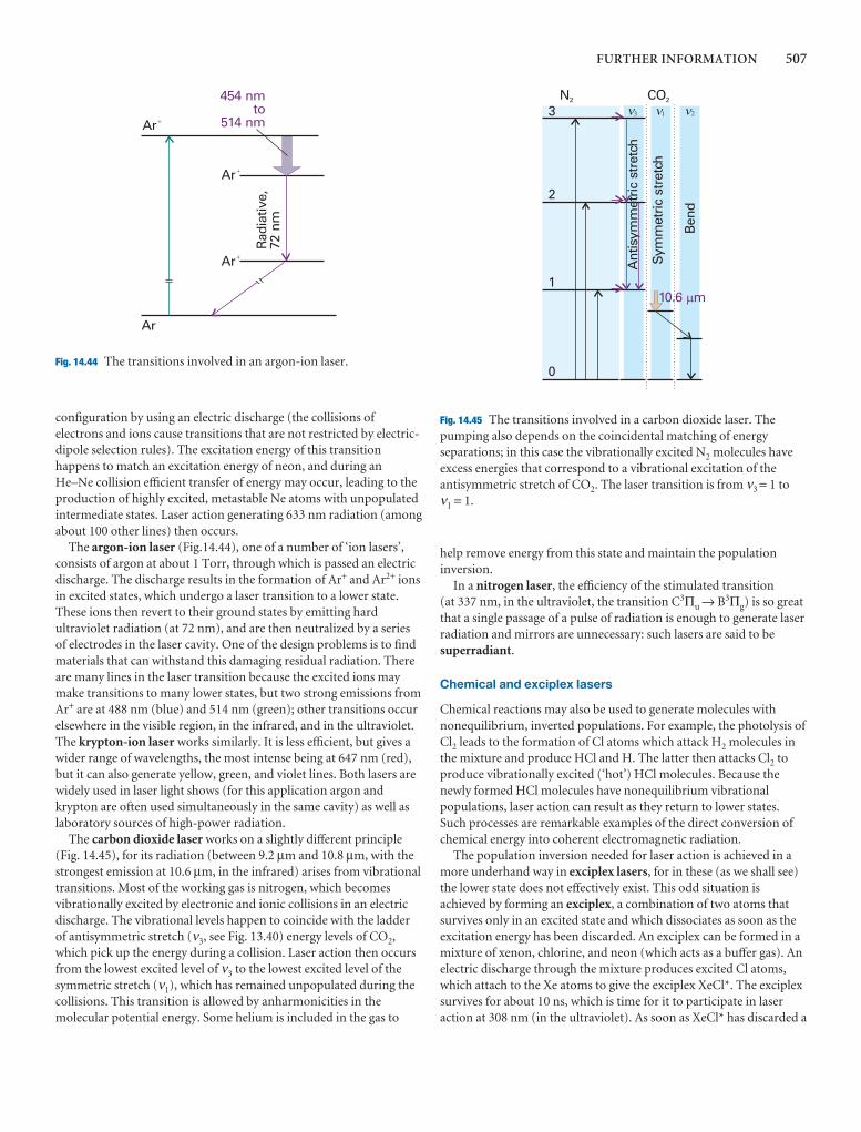
FURTHER INFORMATION 507
configuration by using an electric discharge (the collisions ofelectrons and ions cause transitions that are not restricted by electric-dipole selection rules). The excitation energy of this transitionhappens to match an excitation energy of neon, and during anHe–Ne collision efficient transfer of energy may occur, leading to theproduction of highly excited, metastable Ne atoms with unpopulatedintermediate states. Laser action generating 633 nm radiation (amongabout 100 other lines) then occurs.
The argon-ion laser (Fig.14.44), one of a number of ‘ion lasers’,consists of argon at about 1 Torr, through which is passed an electricdischarge. The discharge results in the formation of Ar+ and Ar2+ ionsin excited states, which undergo a laser transition to a lower state.These ions then revert to their ground states by emitting hardultraviolet radiation (at 72 nm), and are then neutralized by a seriesof electrodes in the laser cavity. One of the design problems is to findmaterials that can withstand this damaging residual radiation. Thereare many lines in the laser transition because the excited ions maymake transitions to many lower states, but two strong emissions fromAr+ are at 488 nm (blue) and 514 nm (green); other transitions occurelsewhere in the visible region, in the infrared, and in the ultraviolet.The krypton-ion laser works similarly. It is less efficient, but gives awider range of wavelengths, the most intense being at 647 nm (red),but it can also generate yellow, green, and violet lines. Both lasers arewidely used in laser light shows (for this application argon andkrypton are often used simultaneously in the same cavity) as well aslaboratory sources of high-power radiation.
The carbon dioxide laser works on a slightly different principle(Fig. 14.45), for its radiation (between 9.2 µm and 10.8 µm, with thestrongest emission at 10.6 µm, in the infrared) arises from vibrationaltransitions. Most of the working gas is nitrogen, which becomesvibrationally excited by electronic and ionic collisions in an electricdischarge. The vibrational levels happen to coincide with the ladderof antisymmetric stretch (ν3, see Fig. 13.40) energy levels of CO2,which pick up the energy during a collision. Laser action then occursfrom the lowest excited level of ν3 to the lowest excited level of thesymmetric stretch (ν1), which has remained unpopulated during thecollisions. This transition is allowed by anharmonicities in themolecular potential energy. Some helium is included in the gas to
help remove energy from this state and maintain the populationinversion.
In a nitrogen laser, the efficiency of the stimulated transition (at 337 nm, in the ultraviolet, the transition C3Πu → B3Πg) is so greatthat a single passage of a pulse of radiation is enough to generate laserradiation and mirrors are unnecessary: such lasers are said to besuperradiant.
Chemical and exciplex lasers
Chemical reactions may also be used to generate molecules withnonequilibrium, inverted populations. For example, the photolysis ofCl2 leads to the formation of Cl atoms which attack H2 molecules inthe mixture and produce HCl and H. The latter then attacks Cl2 toproduce vibrationally excited (‘hot’) HCl molecules. Because thenewly formed HCl molecules have nonequilibrium vibrationalpopulations, laser action can result as they return to lower states.Such processes are remarkable examples of the direct conversion ofchemical energy into coherent electromagnetic radiation.
The population inversion needed for laser action is achieved in amore underhand way in exciplex lasers, for in these (as we shall see)the lower state does not effectively exist. This odd situation isachieved by forming an exciplex, a combination of two atoms thatsurvives only in an excited state and which dissociates as soon as theexcitation energy has been discarded. An exciplex can be formed in amixture of xenon, chlorine, and neon (which acts as a buffer gas). Anelectric discharge through the mixture produces excited Cl atoms,which attach to the Xe atoms to give the exciplex XeCl*. The exciplexsurvives for about 10 ns, which is time for it to participate in laseraction at 308 nm (in the ultraviolet). As soon as XeCl* has discarded a
454 nmto
514 nm
Ar�
Ar�
Ar�R
adia
tive,
72 n
m
Ar
Fig. 14.44 The transitions involved in an argon-ion laser.
Ant
isym
met
ric
stre
tch
Sym
met
ric
stre
tch
Ben
d
N2 CO2
+ , .3
2
1
0
10.6 mm
� � �
Fig. 14.45 The transitions involved in a carbon dioxide laser. Thepumping also depends on the coincidental matching of energyseparations; in this case the vibrationally excited N2 molecules haveexcess energies that correspond to a vibrational excitation of theantisymmetric stretch of CO2. The laser transition is from ν3 = 1 to ν1 = 1.
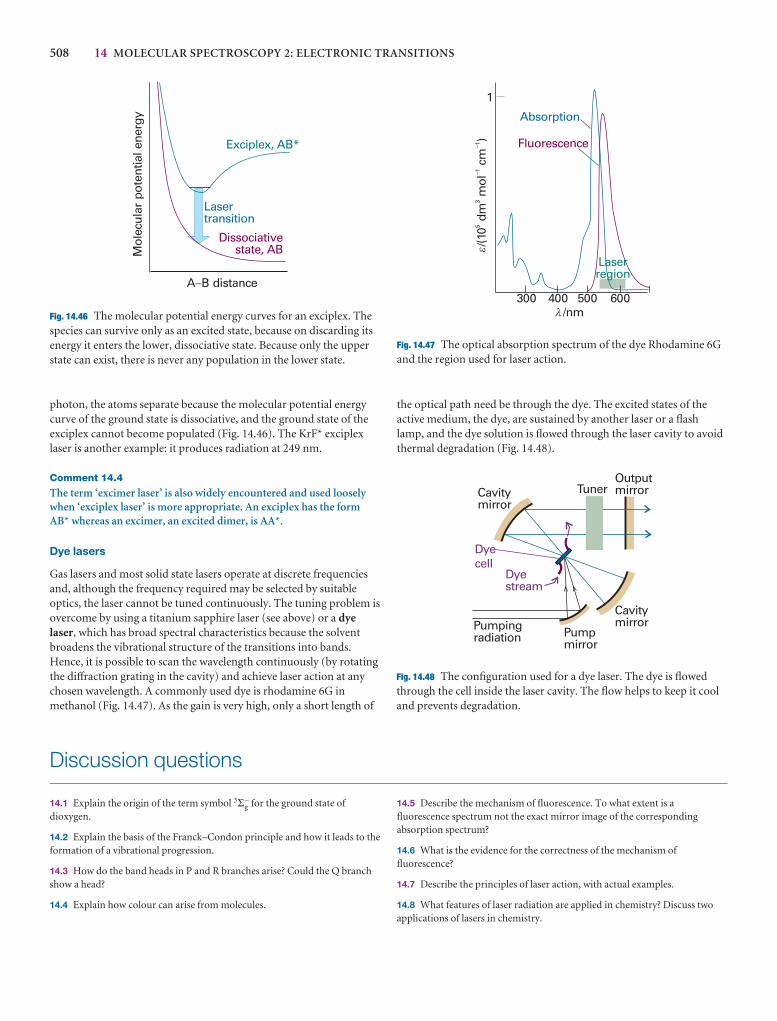
508 14 MOLECULAR SPECTROSCOPY 2: ELECTRONIC TRANSITIONS
photon, the atoms separate because the molecular potential energycurve of the ground state is dissociative, and the ground state of theexciplex cannot become populated (Fig. 14.46). The KrF* exciplexlaser is another example: it produces radiation at 249 nm.
Comment 14.4
The term ‘excimer laser’ is also widely encountered and used looselywhen ‘exciplex laser’ is more appropriate. An exciplex has the formAB* whereas an excimer, an excited dimer, is AA*.
Dye lasers
Gas lasers and most solid state lasers operate at discrete frequenciesand, although the frequency required may be selected by suitableoptics, the laser cannot be tuned continuously. The tuning problem isovercome by using a titanium sapphire laser (see above) or a dyelaser, which has broad spectral characteristics because the solventbroadens the vibrational structure of the transitions into bands.Hence, it is possible to scan the wavelength continuously (by rotatingthe diffraction grating in the cavity) and achieve laser action at anychosen wavelength. A commonly used dye is rhodamine 6G inmethanol (Fig. 14.47). As the gain is very high, only a short length of
Exciplex, AB*
Dissociativestate, AB
Lasertransition
Mol
ecul
ar p
oten
tial e
nerg
y
A B distance�
Fig. 14.46 The molecular potential energy curves for an exciplex. Thespecies can survive only as an excited state, because on discarding itsenergy it enters the lower, dissociative state. Because only the upperstate can exist, there is never any population in the lower state.
300 400 500 600/nm
Absorption
Fluorescence
1
/(10
dmm
ol
cm)
53
11
Laserregion
�
��
�
Fig. 14.47 The optical absorption spectrum of the dye Rhodamine 6Gand the region used for laser action.
Pumpingradiation
Cavitymirror
Cavitymirror
Pumpmirror
TunerOutputmirror
Dyestream
Dyecell
Fig. 14.48 The configuration used for a dye laser. The dye is flowedthrough the cell inside the laser cavity. The flow helps to keep it cooland prevents degradation.
Discussion questions
14.1 Explain the origin of the term symbol 3Σg− for the ground state of
dioxygen.
14.2 Explain the basis of the Franck–Condon principle and how it leads to theformation of a vibrational progression.
14.3 How do the band heads in P and R branches arise? Could the Q branchshow a head?
14.4 Explain how colour can arise from molecules.
14.5 Describe the mechanism of fluorescence. To what extent is afluorescence spectrum not the exact mirror image of the correspondingabsorption spectrum?
14.6 What is the evidence for the correctness of the mechanism offluorescence?
14.7 Describe the principles of laser action, with actual examples.
14.8 What features of laser radiation are applied in chemistry? Discuss twoapplications of lasers in chemistry.
the optical path need be through the dye. The excited states of theactive medium, the dye, are sustained by another laser or a flashlamp, and the dye solution is flowed through the laser cavity to avoidthermal degradation (Fig. 14.48).
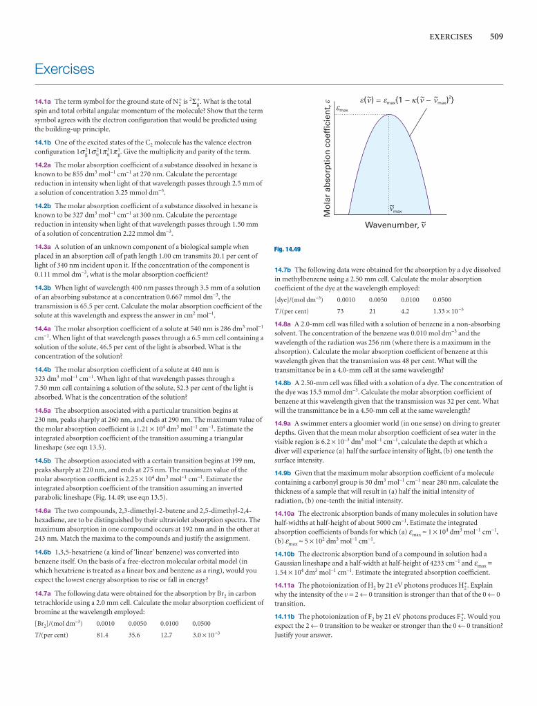
EXERCISES 509
max
Mo
lar
abso
rpti
on
co
effi
cien
t,
Wavenumber, ~
( ) {1 ( ) }� � �max max2� � �
max~
� � �� � /�
�
�
�
Exercises
14.1a The term symbol for the ground state of N2+ is 2Σg
+. What is the totalspin and total orbital angular momentum of the molecule? Show that the termsymbol agrees with the electron configuration that would be predicted usingthe building-up principle.
14.1b One of the excited states of the C2 molecule has the valence electronconfiguration 1σ g
21σu21πu
31π g1. Give the multiplicity and parity of the term.
14.2a The molar absorption coefficient of a substance dissolved in hexane isknown to be 855 dm3 mol−1 cm−1 at 270 nm. Calculate the percentagereduction in intensity when light of that wavelength passes through 2.5 mm ofa solution of concentration 3.25 mmol dm−3.
14.2b The molar absorption coefficient of a substance dissolved in hexane isknown to be 327 dm3 mol−1 cm−1 at 300 nm. Calculate the percentagereduction in intensity when light of that wavelength passes through 1.50 mmof a solution of concentration 2.22 mmol dm−3.
14.3a A solution of an unknown component of a biological sample whenplaced in an absorption cell of path length 1.00 cm transmits 20.1 per cent oflight of 340 nm incident upon it. If the concentration of the component is0.111 mmol dm−3, what is the molar absorption coefficient?
14.3b When light of wavelength 400 nm passes through 3.5 mm of a solutionof an absorbing substance at a concentration 0.667 mmol dm−3, thetransmission is 65.5 per cent. Calculate the molar absorption coefficient of thesolute at this wavelength and express the answer in cm2 mol−1.
14.4a The molar absorption coefficient of a solute at 540 nm is 286 dm3 mol−1
cm−1. When light of that wavelength passes through a 6.5 mm cell containing asolution of the solute, 46.5 per cent of the light is absorbed. What is theconcentration of the solution?
14.4b The molar absorption coefficient of a solute at 440 nm is 323 dm3 mol−1 cm−1. When light of that wavelength passes through a 7.50 mm cell containing a solution of the solute, 52.3 per cent of the light isabsorbed. What is the concentration of the solution?
14.5a The absorption associated with a particular transition begins at 230 nm, peaks sharply at 260 nm, and ends at 290 nm. The maximum value ofthe molar absorption coefficient is 1.21 × 10⁴ dm3 mol−1 cm−1. Estimate theintegrated absorption coefficient of the transition assuming a triangularlineshape (see eqn 13.5).
14.5b The absorption associated with a certain transition begins at 199 nm,peaks sharply at 220 nm, and ends at 275 nm. The maximum value of themolar absorption coefficient is 2.25 × 10⁴ dm3 mol−1 cm−1. Estimate theintegrated absorption coefficient of the transition assuming an invertedparabolic lineshape (Fig. 14.49; use eqn 13.5).
14.6a The two compounds, 2,3-dimethyl-2-butene and 2,5-dimethyl-2,4-hexadiene, are to be distinguished by their ultraviolet absorption spectra. Themaximum absorption in one compound occurs at 192 nm and in the other at243 nm. Match the maxima to the compounds and justify the assignment.
14.6b 1,3,5-hexatriene (a kind of ‘linear’ benzene) was converted intobenzene itself. On the basis of a free-electron molecular orbital model (inwhich hexatriene is treated as a linear box and benzene as a ring), would youexpect the lowest energy absorption to rise or fall in energy?
14.7a The following data were obtained for the absorption by Br2 in carbontetrachloride using a 2.0 mm cell. Calculate the molar absorption coefficient ofbromine at the wavelength employed:
[Br2]/(mol dm−3) 0.0010 0.0050 0.0100 0.0500
T/(per cent) 81.4 35.6 12.7 3.0 × 10⁻³
14.7b The following data were obtained for the absorption by a dye dissolvedin methylbenzene using a 2.50 mm cell. Calculate the molar absorptioncoefficient of the dye at the wavelength employed:
[dye]/(mol dm−3) 0.0010 0.0050 0.0100 0.0500
T /(per cent) 73 21 4.2 1.33 × 10⁻⁵
14.8a A 2.0-mm cell was filled with a solution of benzene in a non-absorbingsolvent. The concentration of the benzene was 0.010 mol dm−3 and thewavelength of the radiation was 256 nm (where there is a maximum in theabsorption). Calculate the molar absorption coefficient of benzene at thiswavelength given that the transmission was 48 per cent. What will thetransmittance be in a 4.0-mm cell at the same wavelength?
14.8b A 2.50-mm cell was filled with a solution of a dye. The concentration ofthe dye was 15.5 mmol dm−3. Calculate the molar absorption coefficient ofbenzene at this wavelength given that the transmission was 32 per cent. Whatwill the transmittance be in a 4.50-mm cell at the same wavelength?
14.9a A swimmer enters a gloomier world (in one sense) on diving to greaterdepths. Given that the mean molar absorption coefficient of sea water in thevisible region is 6.2 × 10⁻³ dm3 mol−1 cm−1, calculate the depth at which adiver will experience (a) half the surface intensity of light, (b) one tenth thesurface intensity.
14.9b Given that the maximum molar absorption coefficient of a moleculecontaining a carbonyl group is 30 dm3 mol−1 cm−1 near 280 nm, calculate thethickness of a sample that will result in (a) half the initial intensity ofradiation, (b) one-tenth the initial intensity.
14.10a The electronic absorption bands of many molecules in solution havehalf-widths at half-height of about 5000 cm−1. Estimate the integratedabsorption coefficients of bands for which (a) εmax ≈ 1 × 10⁴ dm3 mol−1 cm−1,(b) εmax ≈ 5 × 10² dm3 mol−1 cm−1.
14.10b The electronic absorption band of a compound in solution had aGaussian lineshape and a half-width at half-height of 4233 cm−1 and εmax =1.54 × 10⁴ dm3 mol−1 cm−1. Estimate the integrated absorption coefficient.
14.11a The photoionization of H2 by 21 eV photons produces H2+. Explain
why the intensity of the v = 2 ← 0 transition is stronger than that of the 0 ← 0transition.
14.11b The photoionization of F2 by 21 eV photons produces F2+. Would you
expect the 2 ← 0 transition to be weaker or stronger than the 0 ← 0 transition?Justify your answer.
Fig. 14.49
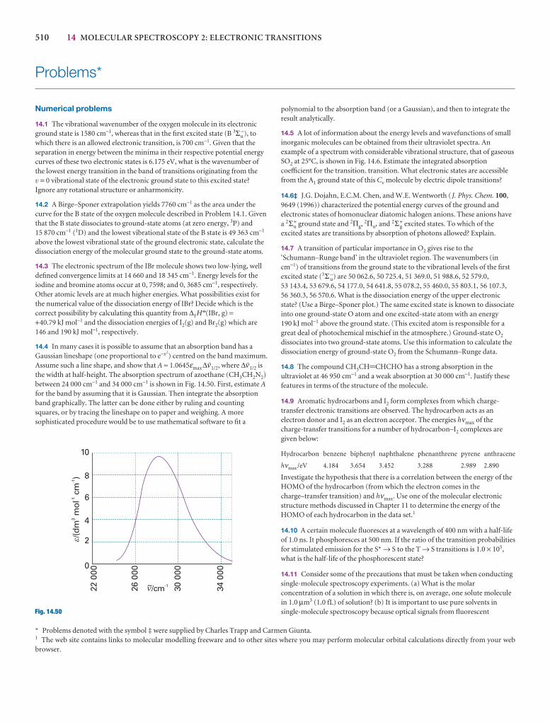
510 14 MOLECULAR SPECTROSCOPY 2: ELECTRONIC TRANSITIONS
Problems*
Numerical problems
14.1 The vibrational wavenumber of the oxygen molecule in its electronicground state is 1580 cm−1, whereas that in the first excited state (B 3Σu
−), towhich there is an allowed electronic transition, is 700 cm−1. Given that theseparation in energy between the minima in their respective potential energycurves of these two electronic states is 6.175 eV, what is the wavenumber ofthe lowest energy transition in the band of transitions originating from the v = 0 vibrational state of the electronic ground state to this excited state?Ignore any rotational structure or anharmonicity.
14.2 A Birge–Sponer extrapolation yields 7760 cm−1 as the area under thecurve for the B state of the oxygen molecule described in Problem 14.1. Giventhat the B state dissociates to ground-state atoms (at zero energy, 3P) and 15 870 cm−1 (1D) and the lowest vibrational state of the B state is 49 363 cm−1
above the lowest vibrational state of the ground electronic state, calculate thedissociation energy of the molecular ground state to the ground-state atoms.
14.3 The electronic spectrum of the IBr molecule shows two low-lying, welldefined convergence limits at 14 660 and 18 345 cm−1. Energy levels for theiodine and bromine atoms occur at 0, 7598; and 0, 3685 cm−1, respectively.Other atomic levels are at much higher energies. What possibilities exist forthe numerical value of the dissociation energy of IBr? Decide which is thecorrect possibility by calculating this quantity from ∆f H
7(IBr, g) =+40.79 kJ mol−1 and the dissociation energies of I2(g) and Br2(g) which are146 and 190 kJ mol−1, respectively.
14.4 In many cases it is possible to assume that an absorption band has aGaussian lineshape (one proportional to e−x2
) centred on the band maximum.Assume such a line shape, and show that A ≈ 1.0645εmax∆#1/2, where ∆#1/2 isthe width at half-height. The absorption spectrum of azoethane (CH3CH2N2)between 24 000 cm−1 and 34 000 cm−1 is shown in Fig. 14.50. First, estimate Afor the band by assuming that it is Gaussian. Then integrate the absorptionband graphically. The latter can be done either by ruling and countingsquares, or by tracing the lineshape on to paper and weighing. A moresophisticated procedure would be to use mathematical software to fit a
polynomial to the absorption band (or a Gaussian), and then to integrate theresult analytically.
14.5 A lot of information about the energy levels and wavefunctions of smallinorganic molecules can be obtained from their ultraviolet spectra. Anexample of a spectrum with considerable vibrational structure, that of gaseousSO2 at 25°C, is shown in Fig. 14.6. Estimate the integrated absorptioncoefficient for the transition. transition. What electronic states are accessiblefrom the A1 ground state of this Cv molecule by electric dipole transitions?
14.6‡ J.G. Dojahn, E.C.M. Chen, and W.E. Wentworth (J. Phys. Chem. 100,9649 (1996)) characterized the potential energy curves of the ground andelectronic states of homonuclear diatomic halogen anions. These anions havea 2Σu
+ ground state and 2Πg,2Πu, and 2Σ g
+ excited states. To which of theexcited states are transitions by absorption of photons allowed? Explain.
14.7 A transition of particular importance in O2 gives rise to the‘Schumann–Runge band’ in the ultraviolet region. The wavenumbers (in cm−1) of transitions from the ground state to the vibrational levels of the firstexcited state (3Σu
−) are 50 062.6, 50 725.4, 51 369.0, 51 988.6, 52 579.0, 53 143.4, 53 679.6, 54 177.0, 54 641.8, 55 078.2, 55 460.0, 55 803.1, 56 107.3,56 360.3, 56 570.6. What is the dissociation energy of the upper electronicstate? (Use a Birge–Sponer plot.) The same excited state is known to dissociateinto one ground-state O atom and one excited-state atom with an energy 190 kJ mol−1 above the ground state. (This excited atom is responsible for agreat deal of photochemical mischief in the atmosphere.) Ground-state O2
dissociates into two ground-state atoms. Use this information to calculate thedissociation energy of ground-state O2 from the Schumann–Runge data.
14.8 The compound CH3CH=CHCHO has a strong absorption in theultraviolet at 46 950 cm−1 and a weak absorption at 30 000 cm−1. Justify thesefeatures in terms of the structure of the molecule.
14.9 Aromatic hydrocarbons and I2 form complexes from which charge-transfer electronic transitions are observed. The hydrocarbon acts as anelectron donor and I2 as an electron acceptor. The energies hνmax of thecharge-transfer transitions for a number of hydrocarbon–I2 complexes aregiven below:
Hydrocarbon benzene biphenyl naphthalene phenanthrene pyrene anthracene
hνmax /eV 4.184 3.654 3.452 3.288 2.989 2.890
Investigate the hypothesis that there is a correlation between the energy of theHOMO of the hydrocarbon (from which the electron comes in thecharge–transfer transition) and hνmax. Use one of the molecular electronicstructure methods discussed in Chapter 11 to determine the energy of theHOMO of each hydrocarbon in the data set.1
14.10 A certain molecule fluoresces at a wavelength of 400 nm with a half-lifeof 1.0 ns. It phosphoresces at 500 nm. If the ratio of the transition probabilitiesfor stimulated emission for the S* → S to the T → S transitions is 1.0 × 10⁵,what is the half-life of the phosphorescent state?
14.11 Consider some of the precautions that must be taken when conductingsingle-molecule spectroscopy experiments. (a) What is the molarconcentration of a solution in which there is, on average, one solute moleculein 1.0 µm3 (1.0 fL) of solution? (b) It is important to use pure solvents insingle-molecule spectroscopy because optical signals from fluorescent
* Problems denoted with the symbol ‡ were supplied by Charles Trapp and Carmen Giunta.1 The web site contains links to molecular modelling freeware and to other sites where you may perform molecular orbital calculations directly from your webbrowser.
22 0
00
26 0
00
30 0
00
34 0
00
10
8
6
4
2
0
/(dm
mol
cm)
31
1
/cm 1~�
��
�
�
Fig. 14.50
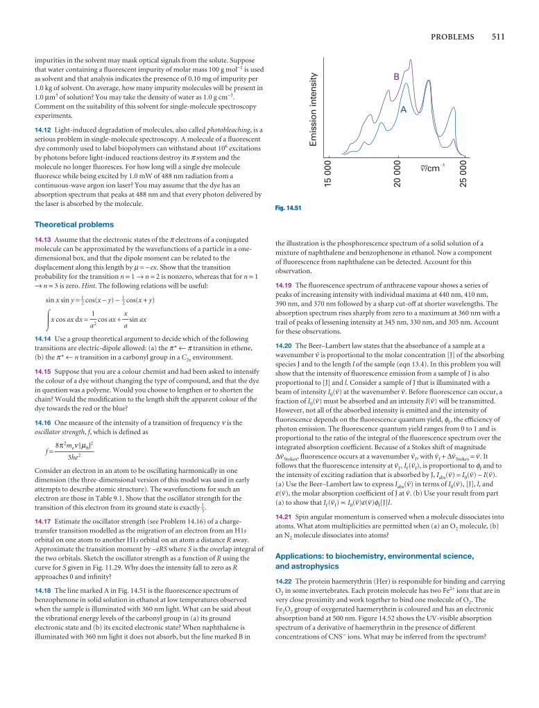
PROBLEMS 511
impurities in the solvent may mask optical signals from the solute. Supposethat water containing a fluorescent impurity of molar mass 100 g mol−1 is usedas solvent and that analysis indicates the presence of 0.10 mg of impurity per1.0 kg of solvent. On average, how many impurity molecules will be present in1.0 µm3 of solution? You may take the density of water as 1.0 g cm−3.Comment on the suitability of this solvent for single-molecule spectroscopyexperiments.
14.12 Light-induced degradation of molecules, also called photobleaching, is aserious problem in single-molecule spectroscopy. A molecule of a fluorescentdye commonly used to label biopolymers can withstand about 106 excitationsby photons before light-induced reactions destroy its π system and themolecule no longer fluoresces. For how long will a single dye moleculefluoresce while being excited by 1.0 mW of 488 nm radiation from acontinuous-wave argon ion laser? You may assume that the dye has anabsorption spectrum that peaks at 488 nm and that every photon delivered bythe laser is absorbed by the molecule.
Theoretical problems
14.13 Assume that the electronic states of the π electrons of a conjugatedmolecule can be approximated by the wavefunctions of a particle in a one-dimensional box, and that the dipole moment can be related to thedisplacement along this length by µ = −ex. Show that the transitionprobability for the transition n = 1 → n = 2 is nonzero, whereas that for n = 1→ n = 3 is zero. Hint. The following relations will be useful:
sin x sin y = 1–2 cos(x − y) − 1–
2 cos(x + y)
�x cos ax dx = cos ax + sin ax
14.14 Use a group theoretical argument to decide which of the followingtransitions are electric-dipole allowed: (a) the π* ← π transition in ethene, (b) the π* ← n transition in a carbonyl group in a C2v environment.
14.15 Suppose that you are a colour chemist and had been asked to intensifythe colour of a dye without changing the type of compound, and that the dyein question was a polyene. Would you choose to lengthen or to shorten thechain? Would the modification to the length shift the apparent colour of thedye towards the red or the blue?
14.16 One measure of the intensity of a transition of frequency ν is theoscillator strength, f, which is defined as
f =
Consider an electron in an atom to be oscillating harmonically in onedimension (the three-dimensional version of this model was used in earlyattempts to describe atomic structure). The wavefunctions for such anelectron are those in Table 9.1. Show that the oscillator strength for thetransition of this electron from its ground state is exactly 1–3.
14.17 Estimate the oscillator strength (see Problem 14.16) of a charge-transfer transition modelled as the migration of an electron from an H1sorbital on one atom to another H1s orbital on an atom a distance R away.Approximate the transition moment by −eRS where S is the overlap integral ofthe two orbitals. Sketch the oscillator strength as a function of R using thecurve for S given in Fig. 11.29. Why does the intensity fall to zero as Rapproaches 0 and infinity?
14.18 The line marked A in Fig. 14.51 is the fluorescence spectrum ofbenzophenone in solid solution in ethanol at low temperatures observed when the sample is illuminated with 360 nm light. What can be said about the vibrational energy levels of the carbonyl group in (a) its ground electronic state and (b) its excited electronic state? When naphthalene isilluminated with 360 nm light it does not absorb, but the line marked B in
8π2meν |µfi|2
3he2
x
a
1
a2
the illustration is the phosphorescence spectrum of a solid solution of amixture of naphthalene and benzophenone in ethanol. Now a component of fluorescence from naphthalene can be detected. Account for thisobservation.
14.19 The fluorescence spectrum of anthracene vapour shows a series ofpeaks of increasing intensity with individual maxima at 440 nm, 410 nm, 390 nm, and 370 nm followed by a sharp cut-off at shorter wavelengths. Theabsorption spectrum rises sharply from zero to a maximum at 360 nm with atrail of peaks of lessening intensity at 345 nm, 330 nm, and 305 nm. Accountfor these observations.
14.20 The Beer–Lambert law states that the absorbance of a sample at awavenumber # is proportional to the molar concentration [J] of the absorbingspecies J and to the length l of the sample (eqn 13.4). In this problem you willshow that the intensity of fluorescence emission from a sample of J is alsoproportional to [J] and l. Consider a sample of J that is illuminated with abeam of intensity I0(#) at the wavenumber #. Before fluorescence can occur, afraction of I0(#) must be absorbed and an intensity I(#) will be transmitted.However, not all of the absorbed intensity is emitted and the intensity offluorescence depends on the fluorescence quantum yield, φf , the efficiency ofphoton emission. The fluorescence quantum yield ranges from 0 to 1 and isproportional to the ratio of the integral of the fluorescence spectrum over theintegrated absorption coefficient. Because of a Stokes shift of magnitude∆#Stokes, fluorescence occurs at a wavenumber #f, with #f + ∆#Stokes = #. Itfollows that the fluorescence intensity at #f , If (#f), is proportional to φf and tothe intensity of exciting radiation that is absorbed by J, Iabs(#) = I0(#) − I(#).(a) Use the Beer–Lambert law to express Iabs(#) in terms of I0(#), [J], l, andε(#), the molar absorption coefficient of J at #. (b) Use your result from part(a) to show that If (#f) ∝ I0(#)ε(#)φf[J]l.
14.21 Spin angular momentum is conserved when a molecule dissociates intoatoms. What atom multiplicities are permitted when (a) an O2 molecule, (b)an N2 molecule dissociates into atoms?
Applications: to biochemistry, environmental science, and astrophysics
14.22 The protein haemerythrin (Her) is responsible for binding and carryingO2 in some invertebrates. Each protein molecule has two Fe2+ ions that are invery close proximity and work together to bind one molecule of O2. The Fe2O2 group of oxygenated haemerythrin is coloured and has an electronicabsorption band at 500 nm. Figure 14.52 shows the UV-visible absorptionspectrum of a derivative of haemerythrin in the presence of differentconcentrations of CNS− ions. What may be inferred from the spectrum?
Emis
sion
inte
nsity
A
B
15 0
00
20 0
00
25 0
00/cm 1~� �
Fig. 14.51
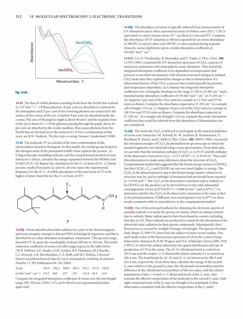
14.26‡ The abundance of ozone is typically inferred from measurements ofUV absorption and is often expressed in terms of Dobson units (DU): 1 DU isequivalent to a layer of pure ozone 10−3 cm thick at 1 atm and 0°C. Computethe absorbance of UV radiation at 300 nm expected for an ozone abundanceof 300 DU (a typical value) and 100 DU (a value reached during seasonalAntarctic ozone depletions) given a molar absorption coefficient of 476 dm3 mol−1 cm−1.
14.27‡ G.C.G. Wachewsky, R. Horansky, and V. Vaida (J. Phys. Chem. 100,11559 (1996)) examined the UV absorption spectrum of CH3I, a species ofinterest in connection with stratospheric ozone chemistry. They found theintegrated absorption coefficient to be dependent on temperature andpressure to an extent inconsistent with internal structural changes in isolatedCH3I molecules; they explained the changes as due to dimerization of asubstantial fraction of the CH3I, a process that would naturally be pressureand temperature dependent. (a) Compute the integrated absorptioncoefficient over a triangular lineshape in the range 31 250 to 34 483 cm−1 and amaximal molar absorption coefficient of 150 dm3 mol−1 cm−1 at 31 250 cm−1.(b) Suppose 1 per cent of the CH3I units in a sample at 2.4 Torr and 373 Kexists as dimers. Compute the absorbance expected at 31 250 cm−1 in a samplecell of length 12.0 cm. (c) Suppose 18 per cent of the CH3I units in a sample at100 Torr and 373 K exists as dimers. Compute the absorbance expected at 31 250 cm−1 in a sample cell of length 12.0 cm; compute the molar absorptioncoefficient that would be inferred from this absorbance if dimerization wasnot considered.
14.28‡ The molecule Cl2O2 is believed to participate in the seasonal depletionof ozone over Antarctica. M. Schwell, H.-W. Jochims, B. Wassermann, U.Rockland, R. Flesch, and E. Rühl ( J. Phys. Chem. 100, 10070 (1996)) measuredthe ionization energies of Cl2O2 by photoelectron spectroscopy in which theionized fragments were detected using a mass spectrometer. From their data,we can infer that the ionization enthalpy of Cl2O2 is 11.05 eV and the enthalpyof the dissociative ionization Cl2O2 → Cl + OClO+ + e− is 10.95 eV. They usedthis information to make some inferences about the structure of Cl2O2.Computational studies had suggested that the lowest energy isomer is ClOOCl,but that ClClO2 (C2v) and ClOClO are not very much higher in energy. TheCl2O2 in the photoionization step is the lowest energy isomer, whatever itsstructure may be, and its enthalpy of formation had previously been reportedas +133 kJ mol−1. The Cl2O2 in the dissociative ionization step is unlikely to be ClOOCl, for the product can be derived from it only with substantialrearrangement. Given ∆ f H
7(OClO+) = +1096 kJ mol−1 and ∆ f H7(e−) = 0,
determine whether the Cl2O2 in the dissociative ionization is the same as thatin the photoionization. If different, how much greater is its ∆ f H
7? Are theseresults consistent with or contradictory to the computational studies?
14.29‡ One of the principal methods for obtaining the electronic spectra ofunstable radicals is to study the spectra of comets, which are almost entirelydue to radicals. Many radical spectra have been found in comets, includingthat due to CN. These radicals are produced in comets by the absorption of farultraviolet solar radiation by their parent compounds. Subsequently, theirfluorescence is excited by sunlight of longer wavelength. The spectra of cometHale–Bopp (C/1995 O1) have been the subject of many recent studies. Onesuch study is that of the fluorescence spectrum of CN in the comet at largeheliocentric distances by R.M. Wagner and D.G. Schleicher (Science 275, 1918(1997)), in which the authors determine the spatial distribution and rate ofproduction of CN in the coma. The (0–0) vibrational band is centred on 387.6 nm and the weaker (1–1) band with relative intensity 0.1 is centred on386.4 nm. The band heads for (0–0) and (0–1) are known to be 388.3 and421.6 nm, respectively. From these data, calculate the energy of the excited S1 state relative to the ground S0 state, the vibrational wavenumbers and thedifference in the vibrational wavenumbers of the two states, and the relativepopulations of the v = 0 and v = 1 vibrational levels of the S1 state. Alsoestimate the effective temperature of the molecule in the excited S1 state. Onlyeight rotational levels of the S1 state are thought to be populated. Is thatobservation consistent with the effective temperature of the S1 state?
512 14 MOLECULAR SPECTROSCOPY 2: ELECTRONIC TRANSITIONS
14.23 The flux of visible photons reaching Earth from the North Star is about4 × 103 mm−2 s−1. Of these photons, 30 per cent are absorbed or scattered bythe atmosphere and 25 per cent of the surviving photons are scattered by thesurface of the cornea of the eye. A further 9 per cent are absorbed inside thecornea. The area of the pupil at night is about 40 mm2 and the response timeof the eye is about 0.1 s. Of the photons passing through the pupil, about 43per cent are absorbed in the ocular medium. How many photons from theNorth Star are focused on to the retina in 0.1 s? For a continuation of thisstory, see R.W. Rodieck, The first steps in seeing, Sinauer, Sunderland (1998).
14.24 Use molecule (7) as a model of the trans conformation of thechromophore found in rhodopsin. In this model, the methyl group bound tothe nitrogen atom of the protonated Schiff ’s base replaces the protein. (a)Using molecular modelling software and the computational method of yourinstructor’s choice, calculate the energy separation between the HOMO andLUMO of (7). (b) Repeat the calculation for the 11-cis form of (7). (c) Basedon your results from parts (a) and (b), do you expect the experimentalfrequency for the π* ← π visible absorption of the trans form of (7) to behigher or lower than that for the 11-cis form of (7)?
14.25‡ Ozone absorbs ultraviolet radiation in a part of the electromagneticspectrum energetic enough to disrupt DNA in biological organisms and that isabsorbed by no other abundant atmospheric constituent. This spectral range,denoted UV-B, spans the wavelengths of about 290 nm to 320 nm. The molarextinction coefficient of ozone over this range is given in the table below (W.B. DeMore, S.P. Sander, D.M. Golden, R.F. Hampson, M.J. Kurylo, C.J. Howard, A.R. Ravishankara, C.E. Kolb, and M.J. Molina, Chemicalkinetics and photochemical data for use in stratospheric modeling: EvaluationNumber 11, JPL Publication 94–26 (1994).
λ /nm 292.0 296.3 300.8 305.4 310.1 315.0 320.0
ε /(dm3 mol−1 cm−1) 1512 865 477 257 135.9 69.5 34.5
Compute the integrated absorption coefficient of ozone over the wavelengthrange 290–320 nm. (Hint. ε(#) can be fitted to an exponential function quite well.)
Her(OH)8
Her(CNS)8
Abs
orba
nce
Wavenumber, ~�
Fig. 14.52

Molecularspectroscopy 3:magnetic resonanceOne of the most widely used spectroscopic procedures in chemistry makes use of the classical concept of resonance. The chapter begins with an account of conventional nuclearmagnetic resonance, which shows how the resonance frequency of a magnetic nucleus isaffected by its electronic environment and the presence of magnetic nuclei in its vicinity.Then we turn to the modern versions of NMR, which are based on the use of pulses of elec-tromagnetic radiation and the processing of the resulting signal by Fourier transform tech-niques. The experimental techniques for electron paramagnetic resonance resemble thoseused in the early days of NMR. The information obtained is very useful for the determinationof the properties of species with unpaired electrons.
When two pendulums share a slightly flexible support and one is set in motion, theother is forced into oscillation by the motion of the common axle. As a result, energyflows between the two pendulums. The energy transfer occurs most efficiently whenthe frequencies of the two pendulums are identical. The condition of strong effectivecoupling when the frequencies of two oscillators are identical is called resonance.Resonance is the basis of a number of everyday phenomena, including the response of radios to the weak oscillations of the electromagnetic field generated by a distanttransmitter. In this chapter we explore some spectroscopic applications that, as origin-ally developed (and in some cases still), depend on matching a set of energy levels to asource of monochromatic radiation and observing the strong absorption that occursat resonance.
The effect of magnetic fields on electrons and nuclei
The Stern–Gerlach experiment (Section 9.8) provided evidence for electron spin. It turns out that many nuclei also possess spin angular momentum. Orbital and spinangular momenta give rise to magnetic moments, and to say that electrons and nucleihave magnetic moments means that, to some extent, they behave like small bar mag-nets. First, we establish how the energies of electrons and nuclei depend on thestrength of an external field. Then we see how to use this dependence to study thestructure and dynamics of complex molecules.
15.1 The energies of electrons in magnetic fields
Classically, the energy of a magnetic moment m in a magnetic field ; is equal to thescalar product
15The effect of magnetic fields onelectrons and nuclei
15.1 The energies of electrons inmagnetic fields
15.2 The energies of nuclei inmagnetic fields
15.3 Magnetic resonancespectroscopy
Nuclear magnetic resonance
15.4 The NMR spectrometer15.5 The chemical shift15.6 The fine structure15.7 Conformational conversion
and exchange processes
Pulse techniques in NMR
15.8 The magnetization vector15.9 Spin relaxationI15.1 Impact on medicine:
Magnetic resonance imaging15.10 Spin decoupling15.11 The nuclear Overhauser effect15.12 Two-dimensional NMR15.13 Solid-state NMR
Electron paramagneticresonance
15.14 The EPR spectrometer15.15 The g-value15.16 Hyperfine structureI15.2 Impact on biochemistry:
Spin probes
Checklist of key ideasFurther readingFurther information 15.1: Fouriertransformation of the FID curveDiscussion questionsExercisesProblems
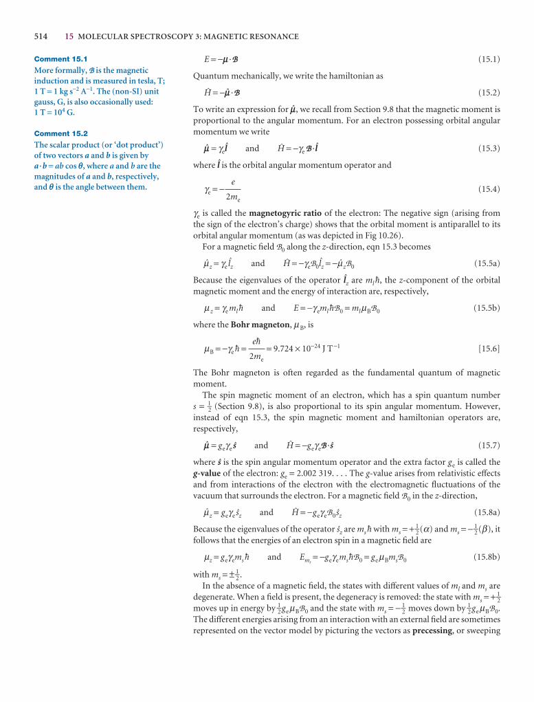
514 15 MOLECULAR SPECTROSCOPY 3: MAGNETIC RESONANCE
E = −m ·; (15.1)
Quantum mechanically, we write the hamiltonian as
@ = −¢ ·; (15.2)
To write an expression for ¢, we recall from Section 9.8 that the magnetic moment isproportional to the angular momentum. For an electron possessing orbital angularmomentum we write
¢ = γe™ and @ = −γe ; ·™ (15.3)
where ™ is the orbital angular momentum operator and
γe = − (15.4)
γe is called the magnetogyric ratio of the electron: The negative sign (arising from the sign of the electron’s charge) shows that the orbital moment is antiparallel to itsorbital angular momentum (as was depicted in Fig 10.26).
For a magnetic field B0 along the z-direction, eqn 15.3 becomes
Nz = γe Zz and @ = −γeB0Zz = −NzB0 (15.5a)
Because the eigenvalues of the operator ™z are ml $, the z-component of the orbitalmagnetic moment and the energy of interaction are, respectively,
µ z = γe ml $ and E = −γ eml $B0 = mlµBB0 (15.5b)
where the Bohr magneton, µB, is
µB = −γe $ = = 9.724 × 10⁻²⁴ J T−1 [15.6]
The Bohr magneton is often regarded as the fundamental quantum of magnetic moment.
The spin magnetic moment of an electron, which has a spin quantum number s = 1–2 (Section 9.8), is also proportional to its spin angular momentum. However, instead of eqn 15.3, the spin magnetic moment and hamiltonian operators are, respectively,
¢ = geγe £ and @ = −geγe; ·£ (15.7)
where £ is the spin angular momentum operator and the extra factor ge is called the g-value of the electron: ge = 2.002 319. . . . The g-value arises from relativistic effectsand from interactions of the electron with the electromagnetic fluctuations of the vacuum that surrounds the electron. For a magnetic field B0 in the z-direction,
Nz = geγe Sz and @ = −geγeB0Sz (15.8a)
Because the eigenvalues of the operator Sz are ms $ with ms = + 1–2 (α) and ms = − 1–2 (β), itfollows that the energies of an electron spin in a magnetic field are
µz = geγems $ and Ems= −geγems$B0 = geµBmsB0 (15.8b)
with ms = ± 1–2 .In the absence of a magnetic field, the states with different values of ml and ms are
degenerate. When a field is present, the degeneracy is removed: the state with ms = + 1–2moves up in energy by 1–2 geµBB0 and the state with ms = − 1–2 moves down by 1–2 geµBB0.The different energies arising from an interaction with an external field are sometimesrepresented on the vector model by picturing the vectors as precessing, or sweeping
e$
2me
e
2me
Comment 15.1
More formally, ; is the magneticinduction and is measured in tesla, T; 1 T = 1 kg s−2 A−1. The (non-SI) unitgauss, G, is also occasionally used: 1 T = 104 G.
Comment 15.2
The scalar product (or ‘dot product’) of two vectors a and b is given by a ·b = ab cos q, where a and b are themagnitudes of a and b, respectively, and q is the angle between them.
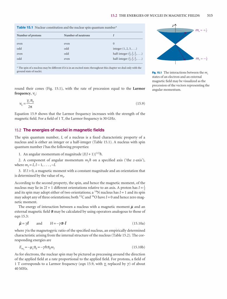
15.2 THE ENERGIES OF NUCLEI IN MAGNETIC FIELDS 515
round their cones (Fig. 15.1), with the rate of precession equal to the Larmorfrequency, νL:
νL = (15.9)
Equation 15.9 shows that the Larmor frequency increases with the strength of themagnetic field. For a field of 1 T, the Larmor frequency is 30 GHz.
15.2 The energies of nuclei in magnetic fields
The spin quantum number, I, of a nucleus is a fixed characteristic property of a nucleus and is either an integer or a half-integer (Table 15.1). A nucleus with spinquantum number I has the following properties:
1. An angular momentum of magnitude {I(I + 1)}1/2$.
2. A component of angular momentum mI $ on a specified axis (‘the z-axis’),where mI = I, I − 1, . . . , −I.
3. If I > 0, a magnetic moment with a constant magnitude and an orientation thatis determined by the value of mI.
According to the second property, the spin, and hence the magnetic moment, of thenucleus may lie in 2I + 1 different orientations relative to an axis. A proton has I = 1–2and its spin may adopt either of two orientations; a 14N nucleus has I = 1 and its spinmay adopt any of three orientations; both 12C and 16O have I = 0 and hence zero mag-netic moment.
The energy of interaction between a nucleus with a magnetic moment m and an external magnetic field ; may be calculated by using operators analogous to those ofeqn 15.3:
¢ = γÎ and H = −γ ; ·Î (15.10a)
where γ is the magnetogyric ratio of the specified nucleus, an empirically determinedcharacteristic arising from the internal structure of the nucleus (Table 15.2). The cor-responding energies are
EmI= −µzB0 = −γ $B0mI (15.10b)
As for electrons, the nuclear spin may be pictured as precessing around the directionof the applied field at a rate proportional to the applied field. For protons, a field of 1 T corresponds to a Larmor frequency (eqn 15.9, with γe replaced by γ ) of about 40 MHz.
γe B0
2π
ms � �
ms � �
z�21
�21
Fig. 15.1 The interactions between the ms
states of an electron and an externalmagnetic field may be visualized as theprecession of the vectors representing theangular momentum.
Table 15.1 Nuclear constitution and the nuclear spin quantum number*
Number of protons Number of neutrons I
even even 0
odd odd integer (1, 2, 3, . . .)
even odd half-integer (1–2, 3–
2 , 5–2 , . . .)
odd even half-integer (1–2, 3–
2 , 5–2 , . . .)
* The spin of a nucleus may be different if it is in an excited state; throughout this chapter we deal only with theground state of nuclei.
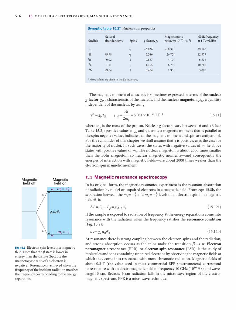
516 15 MOLECULAR SPECTROSCOPY 3: MAGNETIC RESONANCE
The magnetic moment of a nucleus is sometimes expressed in terms of the nuclearg-factor, gI, a characteristic of the nucleus, and the nuclear magneton, µN, a quantityindependent of the nucleus, by using
γ $ = gIµN µN = = 5.051 × 10⁻²⁷ J T−1 [15.11]
where mp is the mass of the proton. Nuclear g-factors vary between −6 and +6 (seeTable 15.2): positive values of gI and γ denote a magnetic moment that is parallel tothe spin; negative values indicate that the magnetic moment and spin are antiparallel. For the remainder of this chapter we shall assume that γ is positive, as is the case forthe majority of nuclei. In such cases, the states with negative values of mI lie abovestates with positive values of mI. The nuclear magneton is about 2000 times smallerthan the Bohr magneton, so nuclear magnetic moments—and consequently the energies of interaction with magnetic fields—are about 2000 times weaker than theelectron spin magnetic moment.
15.3 Magnetic resonance spectroscopy
In its original form, the magnetic resonance experiment is the resonant absorption of radiation by nuclei or unpaired electrons in a magnetic field. From eqn 15.8b, the separation between the ms = − 1–2 and ms = + 1–2 levels of an electron spin in a magneticfield B0 is
∆E = Eα − Eβ = geµBB0 (15.12a)
If the sample is exposed to radiation of frequency ν, the energy separations come intoresonance with the radiation when the frequency satisfies the resonance condition(Fig. 15.2):
hν = geµBB0 (15.12b)
At resonance there is strong coupling between the electron spins and the radiation,and strong absorption occurs as the spins make the transition β → α. Electronparamagnetic resonance (EPR), or electron spin resonance (ESR), is the study ofmolecules and ions containing unpaired electrons by observing the magnetic fields atwhich they come into resonance with monochromatic radiation. Magnetic fields ofabout 0.3 T (the value used in most commercial EPR spectrometers) correspond to resonance with an electromagnetic field of frequency 10 GHz (1010 Hz) and wave-length 3 cm. Because 3 cm radiation falls in the microwave region of the electro-magnetic spectrum, EPR is a microwave technique.
e$
2mp
Synoptic table 15.2* Nuclear spin properties
Natural Magnetogyric NMR frequency Nuclide abundance/% Spin I g-factor, gI ratio, g /(107 T −1 s−1) at 1 T, n/MHz
1n 1–2 −3.826 −18.32 29.165
1H 99.98 1–2 5.586 26.75 42.577
2H 0.02 1 0.857 4.10 6.53613C 1.11 1–
2 1.405 6.73 10.70514N 99.64 1 0.404 1.93 3.076
* More values are given in the Data section.
�
�
ms � �
ms � �
Magneticfield off
Magneticfield on
ge B 0B
�21
�21
Fig. 15.2 Electron spin levels in a magneticfield. Note that the β state is lower inenergy than the α state (because themagnetogyric ratio of an electron isnegative). Resonance is achieved when thefrequency of the incident radiation matchesthe frequency corresponding to the energyseparation.
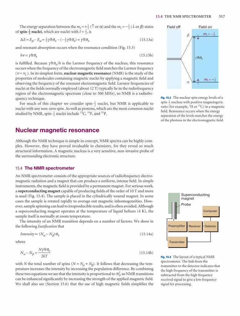
15.4 THE NMR SPECTROMETER 517
The energy separation between the mI = + 1–2 (↑ or α) and the mI = − 1–2 (↓ or β) statesof spin- 1–2 nuclei, which are nuclei with I = 1–2 , is
∆E = Eβ − Eα = 1–2 γ $B0 − (− 1–2 γ $B0) = γ $B0 (15.13a)
and resonant absorption occurs when the resonance condition (Fig. 15.3)
hν = γ $B0 (15.13b)
is fulfilled. Because γ $B0 /h is the Larmor frequency of the nucleus, this resonance occurs when the frequency of the electromagnetic field matches the Larmor frequency(ν = νL ). In its simplest form, nuclear magnetic resonance (NMR) is the study of theproperties of molecules containing magnetic nuclei by applying a magnetic field andobserving the frequency of the resonant electromagnetic field. Larmor frequencies ofnuclei at the fields normally employed (about 12 T) typically lie in the radiofrequencyregion of the electromagnetic spectrum (close to 500 MHz), so NMR is a radiofre-quency technique.
For much of this chapter we consider spin- 1–2 nuclei, but NMR is applicable to nuclei with any non-zero spin. As well as protons, which are the most common nucleistudied by NMR, spin- 1–2 nuclei include 13C, 19F, and 31P.
Nuclear magnetic resonance
Although the NMR technique is simple in concept, NMR spectra can be highly com-plex. However, they have proved invaluable in chemistry, for they reveal so muchstructural information. A magnetic nucleus is a very sensitive, non-invasive probe ofthe surrounding electronic structure.
15.4 The NMR spectrometer
An NMR spectrometer consists of the appropriate sources of radiofrequency electro-magnetic radiation and a magnet that can produce a uniform, intense field. In simpleinstruments, the magnetic field is provided by a permanent magnet. For serious work,a superconducting magnet capable of producing fields of the order of 10 T and moreis used (Fig. 15.4). The sample is placed in the cylindrically wound magnet. In somecases the sample is rotated rapidly to average out magnetic inhomogeneities. How-ever, sample spinning can lead to irreproducible results, and is often avoided. Althougha superconducting magnet operates at the temperature of liquid helium (4 K), thesample itself is normally at room temperature.
The intensity of an NMR transition depends on a number of factors. We show inthe following Justification that
Intensity ∝ (Nα − Nβ)B0 (15.14a)
where
Nα − Nβ ≈ (15.14b)
with N the total number of spins (N = Nα + Nβ). It follows that decreasing the tem-perature increases the intensity by increasing the population difference. By combiningthese two equations we see that the intensity is proportional to B 0
2, so NMR transitionscan be enhanced significantly by increasing the strength of the applied magnetic field.We shall also see (Section 15.6) that the use of high magnetic fields simplifies the
Nγ $B0
2kT
�
�
mI � �
mI � �
Field off Field on
hB0
�21
�21
�
Fig. 15.3 The nuclear spin energy levels of aspin- 1–2 nucleus with positive magnetogyricratio (for example, 1H or 13C) in a magneticfield. Resonance occurs when the energyseparation of the levels matches the energyof the photons in the electromagnetic field.
Superconductingmagnet
Probe
Preamplifier Receiver Detector
Computer
Transmitter
Fig. 15.4 The layout of a typical NMRspectrometer. The link from thetransmitter to the detector indicates thatthe high frequency of the transmitter issubtracted from the high frequencyreceived signal to give a low frequencysignal for processing.
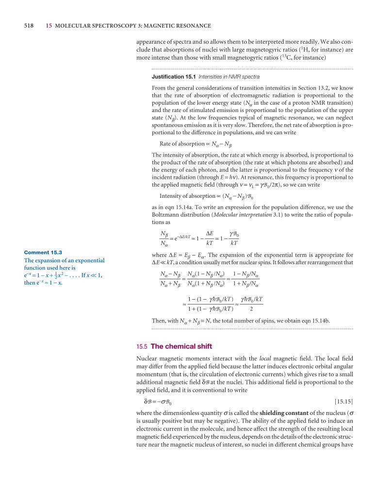
518 15 MOLECULAR SPECTROSCOPY 3: MAGNETIC RESONANCE
appearance of spectra and so allows them to be interpreted more readily. We also con-clude that absorptions of nuclei with large magnetogyric ratios (1H, for instance) aremore intense than those with small magnetogyric ratios (13C, for instance)
Justification 15.1 Intensities in NMR spectra
From the general considerations of transition intensities in Section 13.2, we knowthat the rate of absorption of electromagnetic radiation is proportional to the population of the lower energy state (Nα in the case of a proton NMR transition)and the rate of stimulated emission is proportional to the population of the upperstate (Nβ). At the low frequencies typical of magnetic resonance, we can neglectspontaneous emission as it is very slow. Therefore, the net rate of absorption is pro-portional to the difference in populations, and we can write
Rate of absorption ∝ Nα − Nβ
The intensity of absorption, the rate at which energy is absorbed, is proportional tothe product of the rate of absorption (the rate at which photons are absorbed) andthe energy of each photon, and the latter is proportional to the frequency ν of theincident radiation (through E = hν). At resonance, this frequency is proportional tothe applied magnetic field (through ν = νL = γB 0/2π), so we can write
Intensity of absorption ∝ (Nα − Nβ)B0
as in eqn 15.14a. To write an expression for the population difference, we use theBoltzmann distribution (Molecular interpretation 3.1) to write the ratio of popula-tions as
= e−∆E/kT ≈ 1 − = 1 −
where ∆E = Eβ − Eα . The expansion of the exponential term is appropriate for ∆E << kT, a condition usually met for nuclear spins. It follows after rearrangement that
= =
≈ ≈
Then, with Nα + Nβ = N, the total number of spins, we obtain eqn 15.14b.
15.5 The chemical shift
Nuclear magnetic moments interact with the local magnetic field. The local field may differ from the applied field because the latter induces electronic orbital angular momentum (that is, the circulation of electronic currents) which gives rise to a smalladditional magnetic field δB at the nuclei. This additional field is proportional to theapplied field, and it is conventional to write
δB = −σB0 [15.15]
where the dimensionless quantity σ is called the shielding constant of the nucleus (σis usually positive but may be negative). The ability of the applied field to induce anelectronic current in the molecule, and hence affect the strength of the resulting localmagnetic field experienced by the nucleus, depends on the details of the electronic struc-ture near the magnetic nucleus of interest, so nuclei in different chemical groups have
γ $B0 /kT
2
1 − (1 − γ $B0 /kT)
1 + (1 − γ $B0 /kT)
1 − Nβ /Nα
1 + Nβ /Nα
Nα(1 − Nβ /Nα)
Nα(1 + Nβ /Nα)
Nα − Nβ
Nα + Nβ
γ B0
kT
∆E
kT
Nβ
Nα
Comment 15.3
The expansion of an exponentialfunction used here is e−x = 1 − x + 1–2 x 2 − . . . . If x << 1,then e−x ≈ 1 − x.
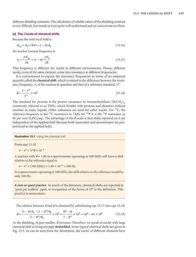
15.5 THE CHEMICAL SHIFT 519
different shielding constants. The calculation of reliable values of the shielding constantis very difficult, but trends in it are quite well understood and we concentrate on them.
(a) The δ scale of chemical shifts
Because the total local field is
B loc = B0 + δB = (1 − σ)B0 (15.16)
the nuclear Larmor frequency is
νL = = (1 − σ) (15.17)
This frequency is different for nuclei in different environments. Hence, differentnuclei, even of the same element, come into resonance at different frequencies.
It is conventional to express the resonance frequencies in terms of an empiricalquantity called the chemical shift, which is related to the difference between the reson-ance frequency, ν, of the nucleus in question and that of a reference standard, ν°:
δ = × 106 [15.18]
The standard for protons is the proton resonance in tetramethylsilane (Si(CH3)4,commonly referred to as TMS), which bristles with protons and dissolves without reaction in many liquids. Other references are used for other nuclei. For 13C, the reference frequency is the 13C resonance in TMS; for 31P it is the 31P resonance in 85 per cent H3PO4(aq). The advantage of the δ-scale is that shifts reported on it are independent of the applied field (because both numerator and denominator are pro-portional to the applied field).
Illustration 15.1 Using the chemical shift
From eqn 15.18,
ν − ν° = ν°δ × 10−6
A nucleus with δ = 1.00 in a spectrometer operating at 500 MHz will have a shiftrelative to the reference equal to
ν − ν° = (500 MHz) × 1.00 × 10−6 = 500 Hz
In a spectrometer operating at 100 MHz, the shift relative to the reference would beonly 100 Hz.
A note on good practice In much of the literature, chemical shifts are reported in‘parts per million’, ppm, in recognition of the factor of 106 in the definition. Thispractice is unnecessary.
The relation between δ and σ is obtained by substituting eqn 15.17 into eqn 15.18:
δ = × 106 = × 106 ≈ (σ° − σ) × 106 (15.19)
As the shielding, σ, gets smaller, δ increases. Therefore, we speak of nuclei with largechemical shift as being strongly deshielded. Some typical chemical shifts are given inFig. 15.5. As can be seen from the illustration, the nuclei of different elements have
σ° − σ1 − σ°
(1 − σ)B0 − (1 − σ°)B0
(1 − σ°)B0
ν − ν°
ν°
γ B 0
2πγ B loc
2π
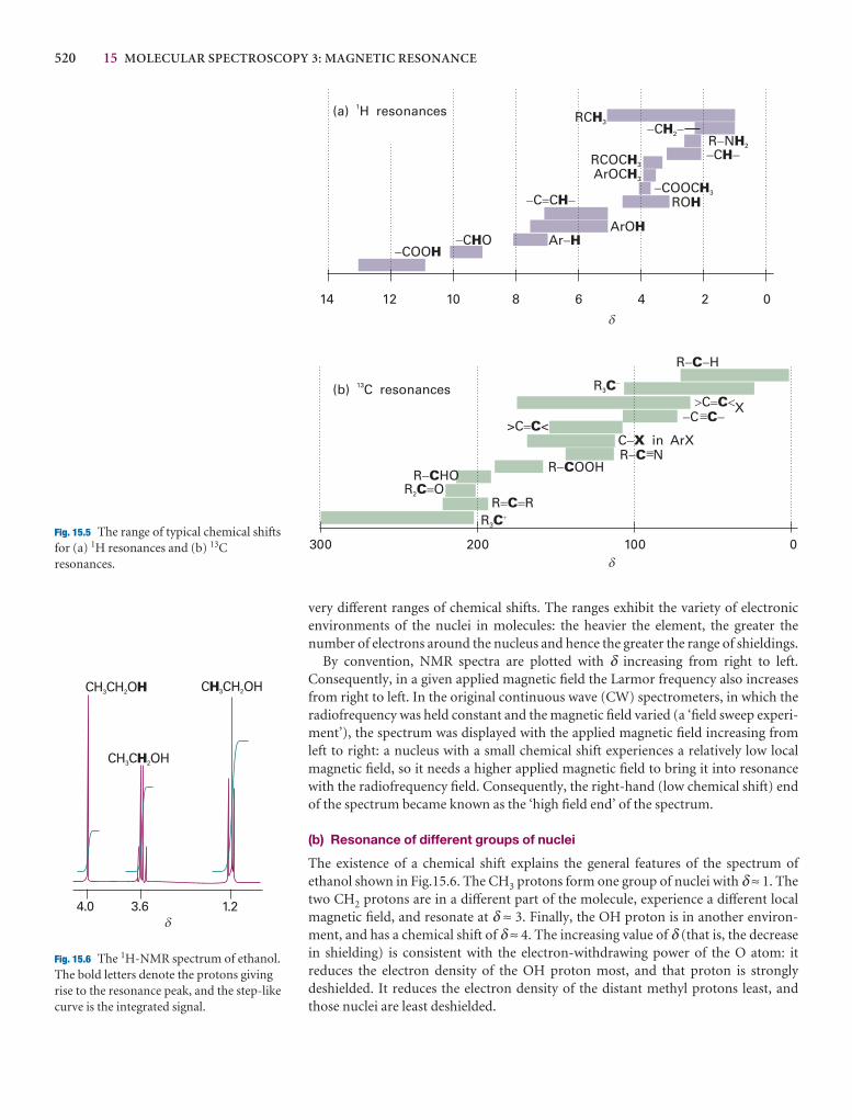
520 15 MOLECULAR SPECTROSCOPY 3: MAGNETIC RESONANCE
14 12 10 8 6 4 2 0
�
�
300 200 100 0
RCH3� �CH2
R N� H2
� �CHRCOCH3
ArOCH3
�COOCH3
ROH� � �C CH
ArOHAr�H
�COOH�C OH
R H� �C
R3C�
� � �C XC
>C <�CC in ArX�XR N� 0C
R OOH�CR HO�C
R O2C�R R� �C
R3C�
� 0 �C C
(a) H resonances1
(b) C resonances13
Fig. 15.5 The range of typical chemical shiftsfor (a) 1H resonances and (b) 13Cresonances.
very different ranges of chemical shifts. The ranges exhibit the variety of electronic environments of the nuclei in molecules: the heavier the element, the greater thenumber of electrons around the nucleus and hence the greater the range of shieldings.
By convention, NMR spectra are plotted with δ increasing from right to left.Consequently, in a given applied magnetic field the Larmor frequency also increasesfrom right to left. In the original continuous wave (CW) spectrometers, in which theradiofrequency was held constant and the magnetic field varied (a ‘field sweep experi-ment’), the spectrum was displayed with the applied magnetic field increasing fromleft to right: a nucleus with a small chemical shift experiences a relatively low localmagnetic field, so it needs a higher applied magnetic field to bring it into resonancewith the radiofrequency field. Consequently, the right-hand (low chemical shift) endof the spectrum became known as the ‘high field end’ of the spectrum.
(b) Resonance of different groups of nuclei
The existence of a chemical shift explains the general features of the spectrum ofethanol shown in Fig.15.6. The CH3 protons form one group of nuclei with δ ≈ 1. Thetwo CH2 protons are in a different part of the molecule, experience a different localmagnetic field, and resonate at δ ≈ 3. Finally, the OH proton is in another environ-ment, and has a chemical shift of δ ≈ 4. The increasing value of δ (that is, the decreasein shielding) is consistent with the electron-withdrawing power of the O atom: it reduces the electron density of the OH proton most, and that proton is stronglydeshielded. It reduces the electron density of the distant methyl protons least, andthose nuclei are least deshielded.
�
CH CH O3 2 H
CH C OH3 2H
C CH OHH3 2
3.64.0 1.2
Fig. 15.6 The 1H-NMR spectrum of ethanol.The bold letters denote the protons givingrise to the resonance peak, and the step-likecurve is the integrated signal.
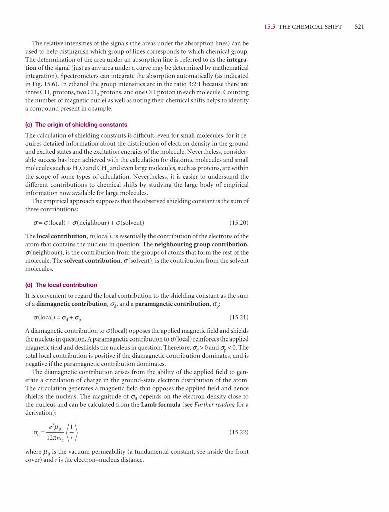
15.5 THE CHEMICAL SHIFT 521
The relative intensities of the signals (the areas under the absorption lines) can beused to help distinguish which group of lines corresponds to which chemical group.The determination of the area under an absorption line is referred to as the integra-tion of the signal (just as any area under a curve may be determined by mathematicalintegration). Spectrometers can integrate the absorption automatically (as indicatedin Fig. 15.6). In ethanol the group intensities are in the ratio 3:2:1 because there arethree CH3 protons, two CH2 protons, and one OH proton in each molecule. Countingthe number of magnetic nuclei as well as noting their chemical shifts helps to identifya compound present in a sample.
(c) The origin of shielding constants
The calculation of shielding constants is difficult, even for small molecules, for it re-quires detailed information about the distribution of electron density in the groundand excited states and the excitation energies of the molecule. Nevertheless, consider-able success has been achieved with the calculation for diatomic molecules and smallmolecules such as H2O and CH4 and even large molecules, such as proteins, are withinthe scope of some types of calculation. Nevertheless, it is easier to understand thedifferent contributions to chemical shifts by studying the large body of empirical information now available for large molecules.
The empirical approach supposes that the observed shielding constant is the sum ofthree contributions:
σ = σ(local) + σ(neighbour) + σ(solvent) (15.20)
The local contribution, σ(local), is essentially the contribution of the electrons of theatom that contains the nucleus in question. The neighbouring group contribution,σ(neighbour), is the contribution from the groups of atoms that form the rest of themolecule. The solvent contribution, σ(solvent), is the contribution from the solventmolecules.
(d) The local contribution
It is convenient to regard the local contribution to the shielding constant as the sumof a diamagnetic contribution, σd, and a paramagnetic contribution, σp:
σ(local) = σd + σp (15.21)
A diamagnetic contribution to σ(local) opposes the applied magnetic field and shieldsthe nucleus in question. A paramagnetic contribution to σ(local) reinforces the appliedmagnetic field and deshields the nucleus in question. Therefore, σd > 0 and σp < 0. Thetotal local contribution is positive if the diamagnetic contribution dominates, and isnegative if the paramagnetic contribution dominates.
The diamagnetic contribution arises from the ability of the applied field to gen-erate a circulation of charge in the ground-state electron distribution of the atom. The circulation generates a magnetic field that opposes the applied field and henceshields the nucleus. The magnitude of σd depends on the electron density close to the nucleus and can be calculated from the Lamb formula (see Further reading for aderivation):
σd = (15.22)
where µ0 is the vacuum permeability (a fundamental constant, see inside the frontcover) and r is the electron–nucleus distance.
1
r
e2µ0
12πme
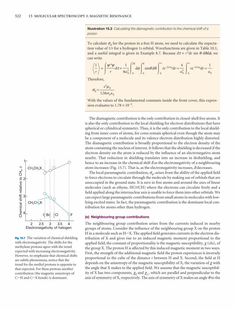
522 15 MOLECULAR SPECTROSCOPY 3: MAGNETIC RESONANCE
4
3
2
1
2 2.5 3 3.5 4
Che
mic
al s
hift
rel
ativ
e to
CH
, 4
Electronegativity of halogen
FClBrI
CH C X3 2H
C CH X3 2H�
Fig. 15.7 The variation of chemical shieldingwith electronegativity. The shifts for themethylene protons agree with the trendexpected with increasing electronegativity.However, to emphasize that chemical shiftsare subtle phenomena, notice that thetrend for the methyl protons is opposite tothat expected. For these protons anothercontribution (the magnetic anisotropy ofC-H and C-X bonds) is dominant.
Illustration 15.2 Calculating the diamagnetic contribution to the chemical shift of aproton
To calculate σd for the proton in a free H atom, we need to calculate the expecta-tion value of 1/r for a hydrogen 1s orbital. Wavefunctions are given in Table 10.1,and a useful integral is given in Example 8.7. Because dτ = r 2dr sin θ dθdφ, we can write
= � dτ = �2π
0
dφ�π
0
sinθ dθ �∞
0
re−2r/a0dr = �∞
0
re−2r/a0dr =
Therefore,
σd =
With the values of the fundamental constants inside the front cover, this expres-sion evaluates to 1.78 × 10⁻⁵.
The diamagnetic contribution is the only contribution in closed-shell free atoms. Itis also the only contribution to the local shielding for electron distributions that havespherical or cylindrical symmetry. Thus, it is the only contribution to the local shield-ing from inner cores of atoms, for cores remain spherical even though the atom maybe a component of a molecule and its valence electron distribution highly distorted.The diamagnetic contribution is broadly proportional to the electron density of theatom containing the nucleus of interest. It follows that the shielding is decreased if theelectron density on the atom is reduced by the influence of an electronegative atomnearby. That reduction in shielding translates into an increase in deshielding, andhence to an increase in the chemical shift δ as the electronegativity of a neighbouringatom increases (Fig. 15.7). That is, as the electronegativity increases, δ decreases.
The local paramagnetic contribution, σp, arises from the ability of the applied fieldto force electrons to circulate through the molecule by making use of orbitals that areunoccupied in the ground state. It is zero in free atoms and around the axes of linearmolecules (such as ethyne, HC.CH) where the electrons can circulate freely and afield applied along the internuclear axis is unable to force them into other orbitals. Wecan expect large paramagnetic contributions from small atoms in molecules with low-lying excited states. In fact, the paramagnetic contribution is the dominant local con-tribution for atoms other than hydrogen.
(e) Neighbouring group contributions
The neighbouring group contribution arises from the currents induced in nearbygroups of atoms. Consider the influence of the neighbouring group X on the protonH in a molecule such as H-X. The applied field generates currents in the electron dis-tribution of X and gives rise to an induced magnetic moment proportional to the applied field; the constant of proportionality is the magnetic susceptibility, χ (chi), ofthe group X. The proton H is affected by this induced magnetic moment in two ways.First, the strength of the additional magnetic field the proton experiences is inverselyproportional to the cube of the distance r between H and X. Second, the field at H depends on the anisotropy of the magnetic susceptibility of X, the variation of χ withthe angle that X makes to the applied field. We assume that the magnetic susceptibil-ity of X has two components, χ|| and χ⊥, which are parallel and perpendicular to theaxis of symmetry of X, respectively. The axis of symmetry of X makes an angle θ to the
e2µ0
12πmea 0
1
a0
4
a30
1
πa30
ψ*ψr
1
r
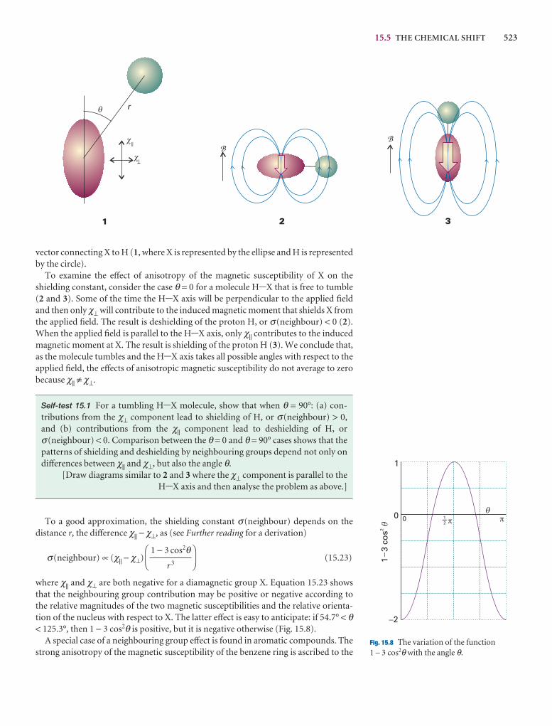
15.5 THE CHEMICAL SHIFT 523
rq
||
|
1
1
1
B
2
B
3
�2
0
1
13
cos2
0 � ��
–21
��
Fig. 15.8 The variation of the function 1 – 3 cos2θ with the angle θ.
vector connecting X to H (1, where X is represented by the ellipse and H is representedby the circle).
To examine the effect of anisotropy of the magnetic susceptibility of X on theshielding constant, consider the case θ = 0 for a molecule H-X that is free to tumble(2 and 3). Some of the time the H-X axis will be perpendicular to the applied fieldand then only χ⊥ will contribute to the induced magnetic moment that shields X fromthe applied field. The result is deshielding of the proton H, or σ(neighbour) < 0 (2).When the applied field is parallel to the H-X axis, only χ|| contributes to the inducedmagnetic moment at X. The result is shielding of the proton H (3). We conclude that,as the molecule tumbles and the H-X axis takes all possible angles with respect to theapplied field, the effects of anisotropic magnetic susceptibility do not average to zerobecause χ|| ≠ χ⊥.
Self-test 15.1 For a tumbling H-X molecule, show that when θ = 90°: (a) con-tributions from the χ⊥ component lead to shielding of H, or σ(neighbour) > 0,and (b) contributions from the χ|| component lead to deshielding of H, orσ(neighbour) < 0. Comparison between the θ = 0 and θ = 90° cases shows that thepatterns of shielding and deshielding by neighbouring groups depend not only ondifferences between χ|| and χ⊥, but also the angle θ.
[Draw diagrams similar to 2 and 3 where the χ⊥ component is parallel to the H-X axis and then analyse the problem as above.]
To a good approximation, the shielding constant σ(neighbour) depends on thedistance r, the difference χ|| − χ⊥, as (see Further reading for a derivation)
σ(neighbour) ∝ (χ|| − χ⊥) (15.23)
where χ|| and χ⊥ are both negative for a diamagnetic group X. Equation 15.23 showsthat the neighbouring group contribution may be positive or negative according tothe relative magnitudes of the two magnetic susceptibilities and the relative orienta-tion of the nucleus with respect to X. The latter effect is easy to anticipate: if 54.7° < θ< 125.3°, then 1 − 3 cos2θ is positive, but it is negative otherwise (Fig. 15.8).
A special case of a neighbouring group effect is found in aromatic compounds. Thestrong anisotropy of the magnetic susceptibility of the benzene ring is ascribed to the
DF
1 − 3 cos2θr 3
AC
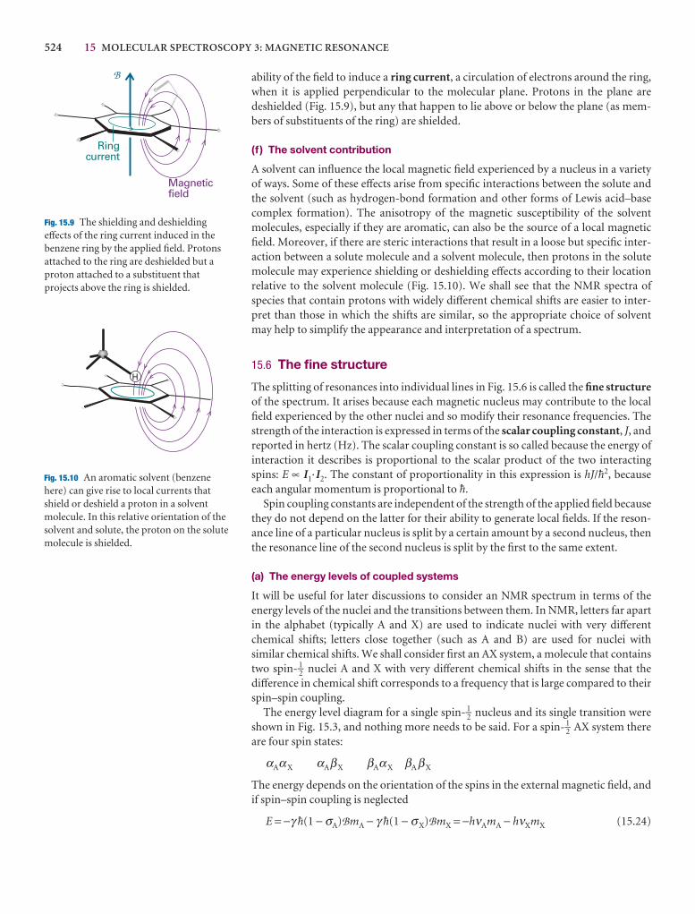
524 15 MOLECULAR SPECTROSCOPY 3: MAGNETIC RESONANCE
ability of the field to induce a ring current, a circulation of electrons around the ring,when it is applied perpendicular to the molecular plane. Protons in the plane aredeshielded (Fig. 15.9), but any that happen to lie above or below the plane (as mem-bers of substituents of the ring) are shielded.
(f ) The solvent contribution
A solvent can influence the local magnetic field experienced by a nucleus in a varietyof ways. Some of these effects arise from specific interactions between the solute andthe solvent (such as hydrogen-bond formation and other forms of Lewis acid–basecomplex formation). The anisotropy of the magnetic susceptibility of the solventmolecules, especially if they are aromatic, can also be the source of a local magneticfield. Moreover, if there are steric interactions that result in a loose but specific inter-action between a solute molecule and a solvent molecule, then protons in the solutemolecule may experience shielding or deshielding effects according to their locationrelative to the solvent molecule (Fig. 15.10). We shall see that the NMR spectra ofspecies that contain protons with widely different chemical shifts are easier to inter-pret than those in which the shifts are similar, so the appropriate choice of solventmay help to simplify the appearance and interpretation of a spectrum.
15.6 The fine structure
The splitting of resonances into individual lines in Fig. 15.6 is called the fine structureof the spectrum. It arises because each magnetic nucleus may contribute to the localfield experienced by the other nuclei and so modify their resonance frequencies. Thestrength of the interaction is expressed in terms of the scalar coupling constant, J, andreported in hertz (Hz). The scalar coupling constant is so called because the energy ofinteraction it describes is proportional to the scalar product of the two interactingspins: E ∝ I1·I2. The constant of proportionality in this expression is hJ/$2, becauseeach angular momentum is proportional to $.
Spin coupling constants are independent of the strength of the applied field becausethey do not depend on the latter for their ability to generate local fields. If the reson-ance line of a particular nucleus is split by a certain amount by a second nucleus, thenthe resonance line of the second nucleus is split by the first to the same extent.
(a) The energy levels of coupled systems
It will be useful for later discussions to consider an NMR spectrum in terms of the energy levels of the nuclei and the transitions between them. In NMR, letters far apartin the alphabet (typically A and X) are used to indicate nuclei with very differentchemical shifts; letters close together (such as A and B) are used for nuclei with similar chemical shifts. We shall consider first an AX system, a molecule that containstwo spin- 1–2 nuclei A and X with very different chemical shifts in the sense that thedifference in chemical shift corresponds to a frequency that is large compared to theirspin–spin coupling.
The energy level diagram for a single spin-1–2 nucleus and its single transition wereshown in Fig. 15.3, and nothing more needs to be said. For a spin-1–2 AX system thereare four spin states:
αAαX αAβX βAαX βAβX
The energy depends on the orientation of the spins in the external magnetic field, andif spin–spin coupling is neglected
E = −γ $(1 − σA)BmA − γ $(1 − σX)BmX = −hνAmA − hνXmX (15.24)
B
Ringcurrent
Magneticfield
Fig. 15.9 The shielding and deshieldingeffects of the ring current induced in thebenzene ring by the applied field. Protonsattached to the ring are deshielded but aproton attached to a substituent thatprojects above the ring is shielded.
H
Fig. 15.10 An aromatic solvent (benzenehere) can give rise to local currents thatshield or deshield a proton in a solventmolecule. In this relative orientation of thesolvent and solute, the proton on the solutemolecule is shielded.
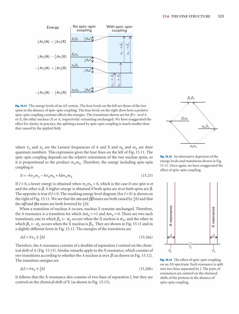
15.6 THE FINE STRUCTURE 525
where νA and νX are the Larmor frequencies of A and X and mA and mX are their quantum numbers. This expression gives the four lines on the left of Fig. 15.11. Thespin–spin coupling depends on the relative orientation of the two nuclear spins, so it is proportional to the product mAmX. Therefore, the energy including spin–spincoupling is
E = −hνAmA − hνXmX + hJmAmX (15.25)
If J > 0, a lower energy is obtained when mAmX < 0, which is the case if one spin is αand the other is β. A higher energy is obtained if both spins are α or both spins are β.The opposite is true if J < 0. The resulting energy level diagram (for J > 0) is shown onthe right of Fig. 15.11. We see that the αα and ββ states are both raised by 1–4 hJ and thatthe αβ and βα states are both lowered by 1–4 hJ.
When a transition of nucleus A occurs, nucleus X remains unchanged. Therefore,the A resonance is a transition for which ∆mA = +1 and ∆mX = 0. There are two suchtransitions, one in which βA ← αA occurs when the X nucleus is αX, and the other inwhich βA ← αA occurs when the X nucleus is βX. They are shown in Fig. 15.11 and ina slightly different form in Fig. 15.12. The energies of the transitions are
∆E = hνA ± 1–2hJ (15.26a)
Therefore, the A resonance consists of a doublet of separation J centred on the chem-ical shift of A (Fig. 15.13). Similar remarks apply to the X resonance, which consists oftwo transitions according to whether the A nucleus is α or β (as shown in Fig. 15.12).The transition energies are
∆E = hνX ± 1–2hJ (15.26b)
It follows that the X resonance also consists of two lines of separation J, but they arecentred on the chemical shift of X (as shown in Fig. 15.13).
Energy
hJ
hJ
hJ
hJ
No spin spincoupling
� With spin spincoupling
�
h hL L(A) (X)��21 �2
1� �
h hL L(A) (X)��21 �2
1� �
h hL L(A) (X)��21 �2
1� �
h hL L(A) (X)��21 �2
1� �
�
�
1
1�41
�41
�41
�41
A X� �
A X� �
A X� �
A X� �
XX
2�
�
AA
2�
�X
X2
��
AA
2�
�
A X� �
A X� �
A X� �
A X� �
Fig. 15.12 An alternative depiction of theenergy levels and transitions shown in Fig.15.11. Once again, we have exaggerated theeffect of spin–spin coupling.
J J
A r
eson
ance
X r
eson
ance
A X� �
Fig. 15.13 The effect of spin–spin couplingon an AX spectrum. Each resonance is splitinto two lines separated by J. The pairs ofresonances are centred on the chemicalshifts of the protons in the absence ofspin–spin coupling.
Fig. 15.11 The energy levels of an AX system. The four levels on the left are those of the twospins in the absence of spin–spin coupling. The four levels on the right show how a positivespin–spin coupling constant affects the energies. The transitions shown are for β ← α of A or X, the other nucleus (X or A, respectively) remaining unchanged. We have exaggerated theeffect for clarity; in practice, the splitting caused by spin–spin coupling is much smaller thanthat caused by the applied field.
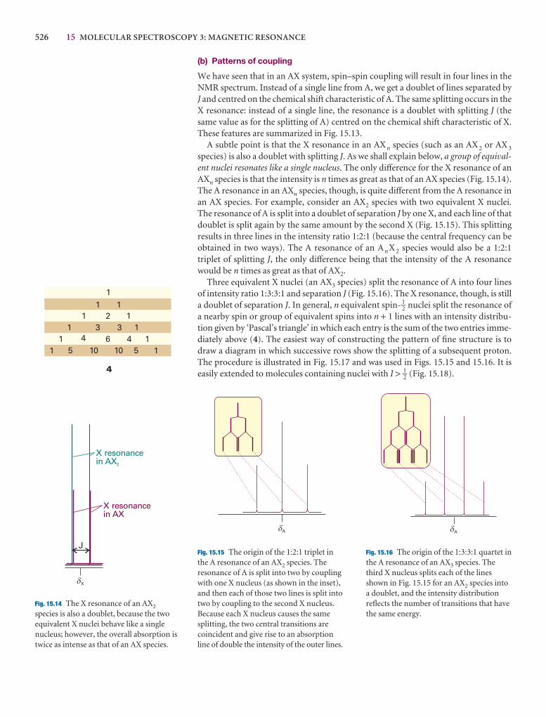
526 15 MOLECULAR SPECTROSCOPY 3: MAGNETIC RESONANCE
(b) Patterns of coupling
We have seen that in an AX system, spin–spin coupling will result in four lines in theNMR spectrum. Instead of a single line from A, we get a doublet of lines separated byJ and centred on the chemical shift characteristic of A. The same splitting occurs in theX resonance: instead of a single line, the resonance is a doublet with splitting J (thesame value as for the splitting of A) centred on the chemical shift characteristic of X.These features are summarized in Fig. 15.13.
A subtle point is that the X resonance in an AXn species (such as an AX 2 or AX 3
species) is also a doublet with splitting J. As we shall explain below, a group of equival-ent nuclei resonates like a single nucleus. The only difference for the X resonance of anAXn species is that the intensity is n times as great as that of an AX species (Fig. 15.14).The A resonance in an AXn species, though, is quite different from the A resonance inan AX species. For example, consider an AX2 species with two equivalent X nuclei.The resonance of A is split into a doublet of separation J by one X, and each line of thatdoublet is split again by the same amount by the second X (Fig. 15.15). This splittingresults in three lines in the intensity ratio 1:2:1 (because the central frequency can beobtained in two ways). The A resonance of an An X 2 species would also be a 1:2:1triplet of splitting J, the only difference being that the intensity of the A resonancewould be n times as great as that of AX2.
Three equivalent X nuclei (an AX3 species) split the resonance of A into four linesof intensity ratio 1:3:3:1 and separation J (Fig. 15.16). The X resonance, though, is stilla doublet of separation J. In general, n equivalent spin- 1–2 nuclei split the resonance ofa nearby spin or group of equivalent spins into n + 1 lines with an intensity distribu-tion given by ‘Pascal’s triangle’ in which each entry is the sum of the two entries imme-diately above (4). The easiest way of constructing the pattern of fine structure is todraw a diagram in which successive rows show the splitting of a subsequent proton.The procedure is illustrated in Fig. 15.17 and was used in Figs. 15.15 and 15.16. It iseasily extended to molecules containing nuclei with I > 1–2 (Fig. 15.18).
J
X resonancein AX
X resonancein AX2
X�
A�
Fig. 15.14 The X resonance of an AX2
species is also a doublet, because the twoequivalent X nuclei behave like a singlenucleus; however, the overall absorption istwice as intense as that of an AX species.
Fig. 15.15 The origin of the 1:2:1 triplet inthe A resonance of an AX2 species. Theresonance of A is split into two by couplingwith one X nucleus (as shown in the inset),and then each of those two lines is split intotwo by coupling to the second X nucleus.Because each X nucleus causes the samesplitting, the two central transitions arecoincident and give rise to an absorptionline of double the intensity of the outer lines.
A�
Fig. 15.16 The origin of the 1:3:3:1 quartet inthe A resonance of an AX3 species. Thethird X nucleus splits each of the linesshown in Fig. 15.15 for an AX2 species intoa doublet, and the intensity distributionreflects the number of transitions that havethe same energy.
11 1
1 2 11 3 3 1
1 4 6 4 11 5 10 10 5 1
4
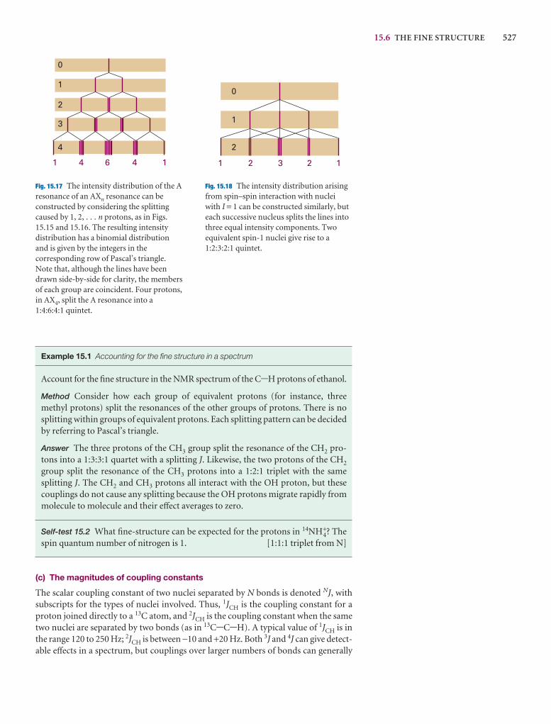
15.6 THE FINE STRUCTURE 527
0
1
2
3
4
1 4 6 4 1
1
2
1 2 3 2 1
0
Fig. 15.17 The intensity distribution of the Aresonance of an AXn resonance can beconstructed by considering the splittingcaused by 1, 2, . . . n protons, as in Figs.15.15 and 15.16. The resulting intensitydistribution has a binomial distributionand is given by the integers in thecorresponding row of Pascal’s triangle.Note that, although the lines have beendrawn side-by-side for clarity, the membersof each group are coincident. Four protons,in AX4, split the A resonance into a1:4:6:4:1 quintet.
Fig. 15.18 The intensity distribution arisingfrom spin–spin interaction with nucleiwith I = 1 can be constructed similarly, buteach successive nucleus splits the lines intothree equal intensity components. Twoequivalent spin-1 nuclei give rise to a1:2:3:2:1 quintet.
Example 15.1 Accounting for the fine structure in a spectrum
Account for the fine structure in the NMR spectrum of the C-H protons of ethanol.
Method Consider how each group of equivalent protons (for instance, threemethyl protons) split the resonances of the other groups of protons. There is nosplitting within groups of equivalent protons. Each splitting pattern can be decidedby referring to Pascal’s triangle.
Answer The three protons of the CH3 group split the resonance of the CH2 pro-tons into a 1:3:3:1 quartet with a splitting J. Likewise, the two protons of the CH2
group split the resonance of the CH3 protons into a 1:2:1 triplet with the same splitting J. The CH2 and CH3 protons all interact with the OH proton, but these couplings do not cause any splitting because the OH protons migrate rapidly frommolecule to molecule and their effect averages to zero.
Self-test 15.2 What fine-structure can be expected for the protons in 14NH4+? The
spin quantum number of nitrogen is 1. [1:1:1 triplet from N]
(c) The magnitudes of coupling constants
The scalar coupling constant of two nuclei separated by N bonds is denoted NJ, withsubscripts for the types of nuclei involved. Thus, 1JCH is the coupling constant for aproton joined directly to a 13C atom, and 2JCH is the coupling constant when the sametwo nuclei are separated by two bonds (as in 13C-C-H). A typical value of 1JCH is inthe range 120 to 250 Hz; 2JCH is between −10 and +20 Hz. Both 3J and 4J can give detect-able effects in a spectrum, but couplings over larger numbers of bonds can generally
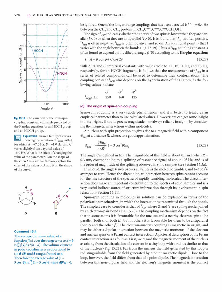
528 15 MOLECULAR SPECTROSCOPY 3: MAGNETIC RESONANCE
be ignored. One of the longest range couplings that has been detected is 9JHH = 0.4 Hzbetween the CH3 and CH2 protons in CH3C.CC.CC.CCH2OH.
The sign of JXY indicates whether the energy of two spins is lower when they are par-allel (J < 0) or when they are antiparallel (J > 0). It is found that 1JCH is often positive,2JHH is often negative, 3JHH is often positive, and so on. An additional point is that Jvaries with the angle between the bonds (Fig. 15.19). Thus, a 3JHH coupling constant isoften found to depend on the dihedral angle φ (5) according to the Karplus equation:
J = A + B cos φ + C cos 2φ (15.27)
with A, B, and C empirical constants with values close to +7 Hz, −1 Hz, and +5 Hz, respectively, for an HCCH fragment. It follows that the measurement of 3JHH in a series of related compounds can be used to determine their conformations. The coupling constant 1JCH also depends on the hybridization of the C atom, as the fol-lowing values indicate:
sp sp2 sp3
1JCH/Hz: 250 160 125
(d) The origin of spin–spin coupling
Spin–spin coupling is a very subtle phenomenon, and it is better to treat J as an empirical parameter than to use calculated values. However, we can get some insightinto its origins, if not its precise magnitude—or always reliably its sign—by consider-ing the magnetic interactions within molecules.
A nucleus with spin projection mI gives rise to a magnetic field with z-componentBnuc at a distance R, where, to a good approximation,
Bnuc = − (1 − 3 cos2θ)mI (15.28)
The angle θ is defined in (6). The magnitude of this field is about 0.1 mT when R =0.3 nm, corresponding to a splitting of resonance signal of about 104 Hz, and is ofthe order of magnitude of the splitting observed in solid samples (see Section 15.3a).
In a liquid, the angle θ sweeps over all values as the molecule tumbles, and 1–3 cos2θaverages to zero. Hence the direct dipolar interaction between spins cannot accountfor the fine structure of the spectra of rapidly tumbling molecules. The direct inter-action does make an important contribution to the spectra of solid samples and is avery useful indirect source of structure information through its involvement in spinrelaxation (Section 15.11).
Spin–spin coupling in molecules in solution can be explained in terms of the polarization mechanism, in which the interaction is transmitted through the bonds.The simplest case to consider is that of 1JXY where X and Y are spin- 1–2 nuclei joined by an electron-pair bond (Fig. 15.20). The coupling mechanism depends on the factthat in some atoms it is favourable for the nucleus and a nearby electron spin to be parallel (both α or both β), but in others it is favourable for them to be antiparallel(one α and the other β). The electron–nucleus coupling is magnetic in origin, andmay be either a dipolar interaction between the magnetic moments of the electronand nuclear spins or a Fermi contact interaction. A pictorial description of the Fermicontact interaction is as follows. First, we regard the magnetic moment of the nucleusas arising from the circulation of a current in a tiny loop with a radius similar to thatof the nucleus (Fig. 15.21). Far from the nucleus the field generated by this loop is indistinguishable from the field generated by a point magnetic dipole. Close to theloop, however, the field differs from that of a point dipole. The magnetic interactionbetween this non-dipolar field and the electron’s magnetic moment is the contact
γ $µ0
4πR3
14
12
10
8
6
4
2
00 90° 180°
Angle,
Spi
n–sp
in c
oupl
ing,
/Hz
J HCCH
HNCH
�
Fig. 15.19 The variation of the spin–spincoupling constant with angle predicted bythe Karplus equation for an HCCH groupand an HNCH group.
Exploration Draw a family of curvesshowing the variation of 3JHH with φ
for which A = +7.0 Hz, B = −1.0 Hz, and Cvaries slightly from a typical value of +5.0 Hz. What is the effect of changing thevalue of the parameter C on the shape ofthe curve? In a similar fashion, explore theeffect of the values of A and B on the shapeof the curve.
�H
H
5
� R
6
Comment 15.4
The average (or mean value) of afunction f(x) over the range x = a to x = bis Úb
a f(x)dx /(b − a). The volume elementin polar coordinates is proportional tosin q dq, and q ranges from 0 to p.Therefore the average value of (1 –3 cos2q) is Úp
0 (1 – 3 cos2q) sin q dq/p = 0.
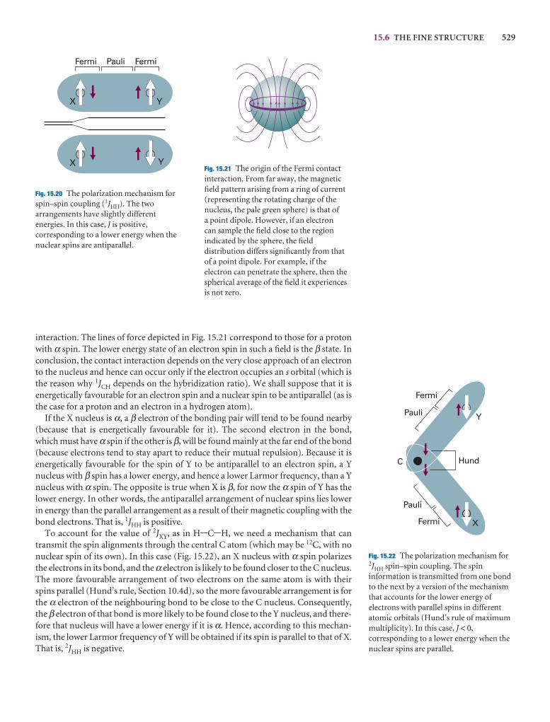
15.6 THE FINE STRUCTURE 529
interaction. The lines of force depicted in Fig. 15.21 correspond to those for a protonwith α spin. The lower energy state of an electron spin in such a field is the β state. Inconclusion, the contact interaction depends on the very close approach of an electronto the nucleus and hence can occur only if the electron occupies an s orbital (which isthe reason why 1JCH depends on the hybridization ratio). We shall suppose that it isenergetically favourable for an electron spin and a nuclear spin to be antiparallel (as isthe case for a proton and an electron in a hydrogen atom).
If the X nucleus is α, a β electron of the bonding pair will tend to be found nearby(because that is energetically favourable for it). The second electron in the bond,which must have α spin if the other is β, will be found mainly at the far end of the bond(because electrons tend to stay apart to reduce their mutual repulsion). Because it isenergetically favourable for the spin of Y to be antiparallel to an electron spin, a Y nucleus with β spin has a lower energy, and hence a lower Larmor frequency, than a Ynucleus with α spin. The opposite is true when X is β, for now the α spin of Y has thelower energy. In other words, the antiparallel arrangement of nuclear spins lies lowerin energy than the parallel arrangement as a result of their magnetic coupling with thebond electrons. That is, 1JHH is positive.
To account for the value of 2JXY, as in H-C-H, we need a mechanism that cantransmit the spin alignments through the central C atom (which may be 12C, with nonuclear spin of its own). In this case (Fig. 15.22), an X nucleus with α spin polarizesthe electrons in its bond, and the α electron is likely to be found closer to the C nucleus.The more favourable arrangement of two electrons on the same atom is with theirspins parallel (Hund’s rule, Section 10.4d), so the more favourable arrangement is forthe α electron of the neighbouring bond to be close to the C nucleus. Consequently,the β electron of that bond is more likely to be found close to the Y nucleus, and there-fore that nucleus will have a lower energy if it is α. Hence, according to this mechan-ism, the lower Larmor frequency of Y will be obtained if its spin is parallel to that of X.That is, 2JHH is negative.
X Y
X Y
Fermi FermiPauli
Fig. 15.20 The polarization mechanism forspin–spin coupling (1JHH). The twoarrangements have slightly differentenergies. In this case, J is positive,corresponding to a lower energy when thenuclear spins are antiparallel.
Fig. 15.21 The origin of the Fermi contactinteraction. From far away, the magneticfield pattern arising from a ring of current(representing the rotating charge of thenucleus, the pale green sphere) is that of a point dipole. However, if an electron can sample the field close to the regionindicated by the sphere, the fielddistribution differs significantly from thatof a point dipole. For example, if theelectron can penetrate the sphere, then thespherical average of the field it experiencesis not zero.
X
Fermi
Fermi
Pauli
Pauli
Hund
Y
C
Fig. 15.22 The polarization mechanism for2JHH spin–spin coupling. The spininformation is transmitted from one bondto the next by a version of the mechanismthat accounts for the lower energy ofelectrons with parallel spins in differentatomic orbitals (Hund’s rule of maximummultiplicity). In this case, J < 0,corresponding to a lower energy when thenuclear spins are parallel.
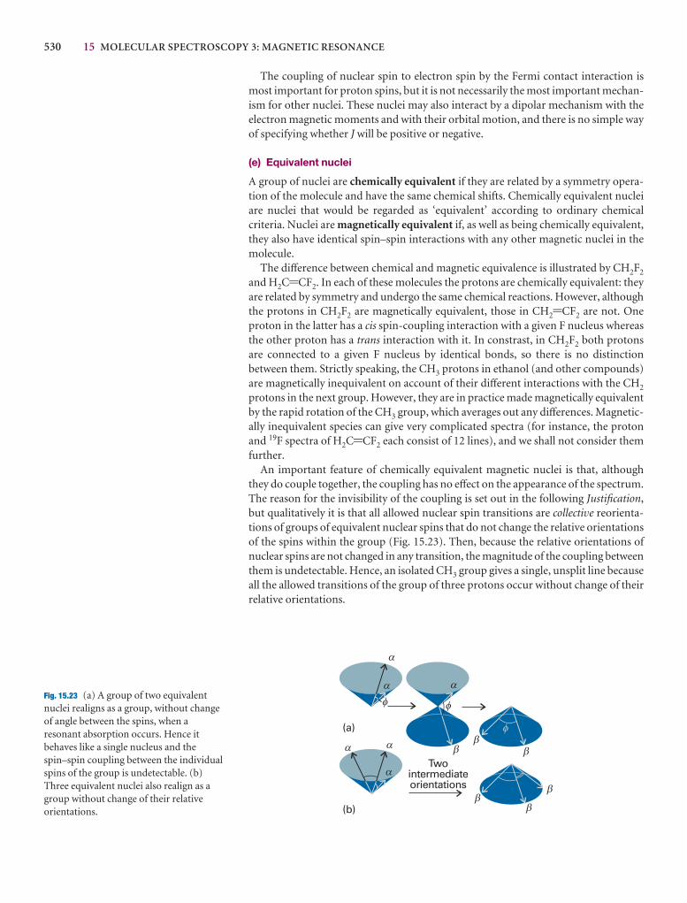
530 15 MOLECULAR SPECTROSCOPY 3: MAGNETIC RESONANCE
The coupling of nuclear spin to electron spin by the Fermi contact interaction ismost important for proton spins, but it is not necessarily the most important mechan-ism for other nuclei. These nuclei may also interact by a dipolar mechanism with theelectron magnetic moments and with their orbital motion, and there is no simple wayof specifying whether J will be positive or negative.
(e) Equivalent nuclei
A group of nuclei are chemically equivalent if they are related by a symmetry opera-tion of the molecule and have the same chemical shifts. Chemically equivalent nucleiare nuclei that would be regarded as ‘equivalent’ according to ordinary chemical criteria. Nuclei are magnetically equivalent if, as well as being chemically equivalent,they also have identical spin–spin interactions with any other magnetic nuclei in themolecule.
The difference between chemical and magnetic equivalence is illustrated by CH2F2
and H2C=CF2. In each of these molecules the protons are chemically equivalent: theyare related by symmetry and undergo the same chemical reactions. However, althoughthe protons in CH2F2 are magnetically equivalent, those in CH2=CF2 are not. Oneproton in the latter has a cis spin-coupling interaction with a given F nucleus whereasthe other proton has a trans interaction with it. In constrast, in CH2F2 both protonsare connected to a given F nucleus by identical bonds, so there is no distinction between them. Strictly speaking, the CH3 protons in ethanol (and other compounds)are magnetically inequivalent on account of their different interactions with the CH2
protons in the next group. However, they are in practice made magnetically equivalentby the rapid rotation of the CH3 group, which averages out any differences. Magnetic-ally inequivalent species can give very complicated spectra (for instance, the protonand 19F spectra of H2C=CF2 each consist of 12 lines), and we shall not consider themfurther.
An important feature of chemically equivalent magnetic nuclei is that, althoughthey do couple together, the coupling has no effect on the appearance of the spectrum.The reason for the invisibility of the coupling is set out in the following Justification,but qualitatively it is that all allowed nuclear spin transitions are collective reorienta-tions of groups of equivalent nuclear spins that do not change the relative orientationsof the spins within the group (Fig. 15.23). Then, because the relative orientations ofnuclear spins are not changed in any transition, the magnitude of the coupling betweenthem is undetectable. Hence, an isolated CH3 group gives a single, unsplit line becauseall the allowed transitions of the group of three protons occur without change of theirrelative orientations.
f
f
f
Twointermediateorientations
a
a
a
a
a
a
b
b
b
b
b
b
(a)
(b)
Fig. 15.23 (a) A group of two equivalentnuclei realigns as a group, without changeof angle between the spins, when aresonant absorption occurs. Hence itbehaves like a single nucleus and thespin–spin coupling between the individualspins of the group is undetectable. (b)Three equivalent nuclei also realign as agroup without change of their relativeorientations.
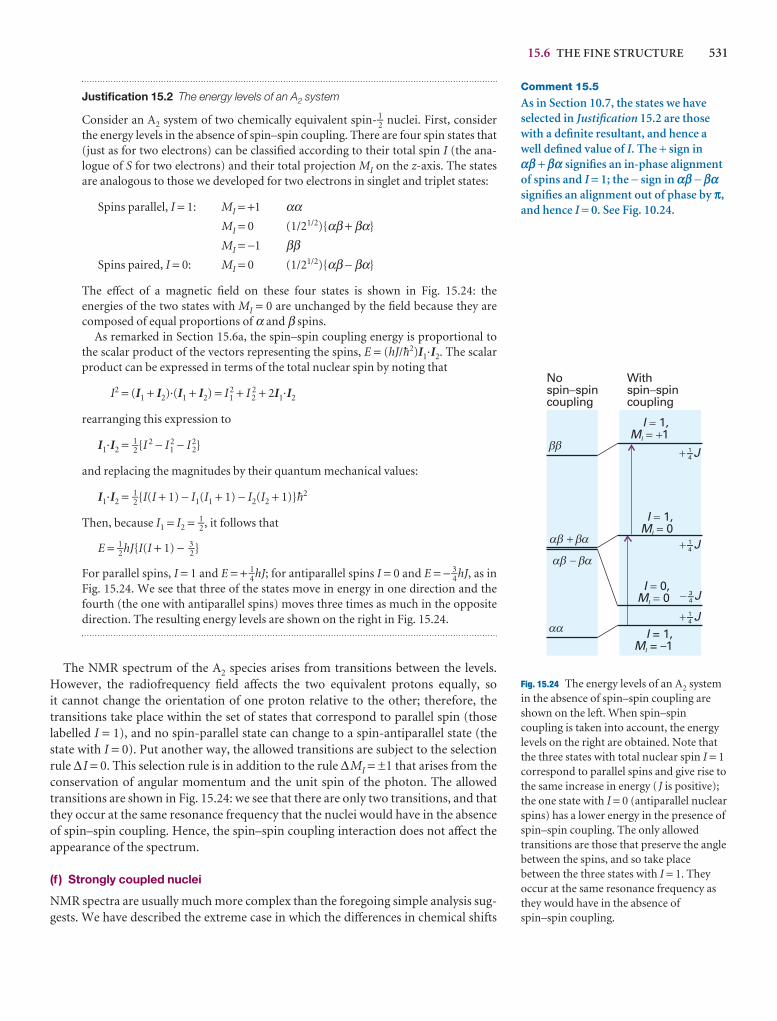
15.6 THE FINE STRUCTURE 531
Justification 15.2 The energy levels of an A2 system
Consider an A2 system of two chemically equivalent spin-1–2 nuclei. First, considerthe energy levels in the absence of spin–spin coupling. There are four spin states that(just as for two electrons) can be classified according to their total spin I (the ana-logue of S for two electrons) and their total projection MI on the z-axis. The statesare analogous to those we developed for two electrons in singlet and triplet states:
Spins parallel, I = 1: MI = +1 ααMI = 0 (1/21/2){αβ + βα}
MI = −1 ββSpins paired, I = 0: MI = 0 (1/21/2){αβ − βα}
The effect of a magnetic field on these four states is shown in Fig. 15.24: the energies of the two states with MI = 0 are unchanged by the field because they arecomposed of equal proportions of α and β spins.
As remarked in Section 15.6a, the spin–spin coupling energy is proportional tothe scalar product of the vectors representing the spins, E = (hJ/$2)I1·I2. The scalarproduct can be expressed in terms of the total nuclear spin by noting that
I2 = (I1 + I2)·(I1 + I2) = I12 + I 2
2 + 2I1·I2
rearranging this expression to
I1·I2 = 1–2{I 2 − I12 − I 2
2}
and replacing the magnitudes by their quantum mechanical values:
I1·I2 = 1–2{I(I + 1) − I1(I1 + 1) − I2(I2 + 1)}$2
Then, because I1 = I2 = 1–2, it follows that
E = 1–2hJ{I(I + 1) − 3–2}
For parallel spins, I = 1 and E = + 1–4hJ; for antiparallel spins I = 0 and E = − 3–4hJ, as inFig. 15.24. We see that three of the states move in energy in one direction and thefourth (the one with antiparallel spins) moves three times as much in the oppositedirection. The resulting energy levels are shown on the right in Fig. 15.24.
The NMR spectrum of the A2 species arises from transitions between the levels.However, the radiofrequency field affects the two equivalent protons equally, so it cannot change the orientation of one proton relative to the other; therefore, the transitions take place within the set of states that correspond to parallel spin (those labelled I = 1), and no spin-parallel state can change to a spin-antiparallel state (thestate with I = 0). Put another way, the allowed transitions are subject to the selectionrule ∆ I = 0. This selection rule is in addition to the rule ∆MI = ±1 that arises from theconservation of angular momentum and the unit spin of the photon. The allowedtransitions are shown in Fig. 15.24: we see that there are only two transitions, and thatthey occur at the same resonance frequency that the nuclei would have in the absenceof spin–spin coupling. Hence, the spin–spin coupling interaction does not affect theappearance of the spectrum.
(f ) Strongly coupled nuclei
NMR spectra are usually much more complex than the foregoing simple analysis sug-gests. We have described the extreme case in which the differences in chemical shifts
Comment 15.5
As in Section 10.7, the states we haveselected in Justification 15.2 are thosewith a definite resultant, and hence awell defined value of I. The + sign in ab + ba signifies an in-phase alignmentof spins and I = 1; the − sign in ab − basignifies an alignment out of phase by p,and hence I = 0. See Fig. 10.24.
��
�� ��
�� ��
��
IM
1,1
�� �I
IM
1,0
��I
IM
0,0
��I
IM
= 1,= –1I
� J
� J
� J
� J
Nospin spincoupling
�Withspin spincoupling
�
�
�
–41
–41
–43
–41
Fig. 15.24 The energy levels of an A2 systemin the absence of spin–spin coupling areshown on the left. When spin–spincoupling is taken into account, the energylevels on the right are obtained. Note thatthe three states with total nuclear spin I = 1correspond to parallel spins and give rise tothe same increase in energy ( J is positive);the one state with I = 0 (antiparallel nuclearspins) has a lower energy in the presence ofspin–spin coupling. The only allowedtransitions are those that preserve the anglebetween the spins, and so take placebetween the three states with I = 1. Theyoccur at the same resonance frequency asthey would have in the absence ofspin–spin coupling.
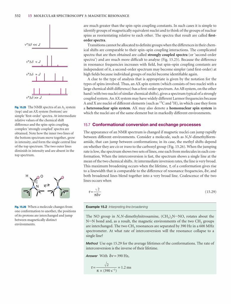
532 15 MOLECULAR SPECTROSCOPY 3: MAGNETIC RESONANCE
° <<D J
°D » J
°D » J
° >>D J
n d
n d
n d
n d
Fig. 15.25 The NMR spectra of an A2 system(top) and an AX system (bottom) aresimple ‘first-order’ spectra. At intermediaterelative values of the chemical shiftdifference and the spin–spin coupling,complex ‘strongly coupled’ spectra areobtained. Note how the inner two lines ofthe bottom spectrum move together, growin intensity, and form the single central lineof the top spectrum. The two outer linesdiminish in intensity and are absent in thetop spectrum.
CN
OH
Fig. 15.26 When a molecule changes fromone conformation to another, the positionsof its protons are interchanged and jumpbetween magnetically distinctenvironments.
are much greater than the spin–spin coupling constants. In such cases it is simple toidentify groups of magnetically equivalent nuclei and to think of the groups of nuclearspins as reorientating relative to each other. The spectra that result are called first-order spectra.
Transitions cannot be allocated to definite groups when the differences in their chem-ical shifts are comparable to their spin–spin coupling interactions. The complicatedspectra that are then obtained are called strongly coupled spectra (or ‘second-orderspectra’) and are much more difficult to analyse (Fig. 15.25). Because the differencein resonance frequencies increases with field, but spin–spin coupling constants are independent of it, a second-order spectrum may become simpler (and first-order) athigh fields because individual groups of nuclei become identifiable again.
A clue to the type of analysis that is appropriate is given by the notation for the types of spins involved. Thus, an AX spin system (which consists of two nuclei with alarge chemical shift difference) has a first-order spectrum. An AB system, on the otherhand (with two nuclei of similar chemical shifts), gives a spectrum typical of a strongly coupled system. An AX system may have widely different Larmor frequencies becauseA and X are nuclei of different elements (such as 13C and 1H), in which case they forma heteronuclear spin system. AX may also denote a homonuclear spin system inwhich the nuclei are of the same element but in markedly different environments.
15.7 Conformational conversion and exchange processes
The appearance of an NMR spectrum is changed if magnetic nuclei can jump rapidlybetween different environments. Consider a molecule, such as N,N-dimethylform-amide, that can jump between conformations; in its case, the methyl shifts depend on whether they are cis or trans to the carbonyl group (Fig. 15.26). When the jumpingrate is low, the spectrum shows two sets of lines, one each from molecules in each con-formation. When the interconversion is fast, the spectrum shows a single line at themean of the two chemical shifts. At intermediate inversion rates, the line is very broad.This maximum broadening occurs when the lifetime, τ, of a conformation gives riseto a linewidth that is comparable to the difference of resonance frequencies, δν, andboth broadened lines blend together into a very broad line. Coalescence of the twolines occurs when
τ = (15.29)
Example 15.2 Interpreting line broadening
The NO group in N,N-dimethylnitrosamine, (CH3)2N-NO, rotates about the N-N bond and, as a result, the magnetic environments of the two CH3 groupsare interchanged. The two CH3 resonances are separated by 390 Hz in a 600 MHz spectrometer. At what rate of interconversion will the resonance collapse to a single line?
Method Use eqn 15.29 for the average lifetimes of the conformations. The rate ofinterconversion is the inverse of their lifetime.
Answer With δν = 390 Hz,
τ = = 1.2 ms2
390 1π ( )× −s
2
πδν

15.8 THE MAGNETIZATION VECTOR 533
It follows that the signal will collapse to a single line when the interconversion rateexceeds about 830 s−1. The dependence of the rate of exchange on the temperatureis used to determine the energy barrier to interconversion.
Self-test 15.3 What would you deduce from the observation of a single line fromthe same molecule in a 300 MHz spectrometer?
[Conformation lifetime less than 2.3 ms]
A similar explanation accounts for the loss of fine structure in solvents able to ex-change protons with the sample. For example, hydroxyl protons are able to exchangewith water protons. When this chemical exchange occurs, a molecule ROH with an α-spin proton (we write this ROHα) rapidly converts to ROHβ and then perhaps to ROHα again because the protons provided by the solvent molecules in successive exchanges have random spin orientations. Therefore, instead of seeing a spectrumcomposed of contributions from both ROHα and ROHβ molecules (that is, a spec-trum showing a doublet structure due to the OH proton) we see a spectrum thatshows no splitting caused by coupling of the OH proton (as in Fig. 15.6). The effect isobserved when the lifetime of a molecule due to this chemical exchange is so short thatthe lifetime broadening is greater than the doublet splitting. Because this splitting isoften very small (a few hertz), a proton must remain attached to the same molecule forlonger than about 0.1 s for the splitting to be observable. In water, the exchange rate ismuch faster than that, so alcohols show no splitting from the OH protons. In drydimethylsulfoxide (DMSO), the exchange rate may be slow enough for the splitting tobe detected.
Pulse techniques in NMR
Modern methods of detecting the energy separation between nuclear spin states aremore sophisticated than simply looking for the frequency at which resonance occurs.One of the best analogies that has been suggested to illustrate the difference betweenthe old and new ways of observing an NMR spectrum is that of detecting the spectrumof vibrations of a bell. We could stimulate the bell with a gentle vibration at a gradu-ally increasing frequency, and note the frequencies at which it resonated with thestimulation. A lot of time would be spent getting zero response when the stimulat-ing frequency was between the bell’s vibrational modes. However, if we were simplyto hit the bell with a hammer, we would immediately obtain a clang composed of allthe frequencies that the bell can produce. The equivalent in NMR is to monitor the radiation nuclear spins emit as they return to equilibrium after the appropriate stimu-lation. The resulting Fourier-transform NMR gives greatly increased sensitivity, soopening up the entire periodic table to the technique. Moreover, multiple-pulse FT-NMR gives chemists unparalleled control over the information content and display ofspectra. We need to understand how the equivalent of the hammer blow is deliveredand how the signal is monitored and interpreted. These features are generally expressedin terms of the vector model of angular momentum introduced in Section 9.7d.
15.8 The magnetization vector
Consider a sample composed of many identical spin- 1–2 nuclei. As we saw in Section9.7d, an angular momentum can be represented by a vector of length {I(I + 1)}1/2 units
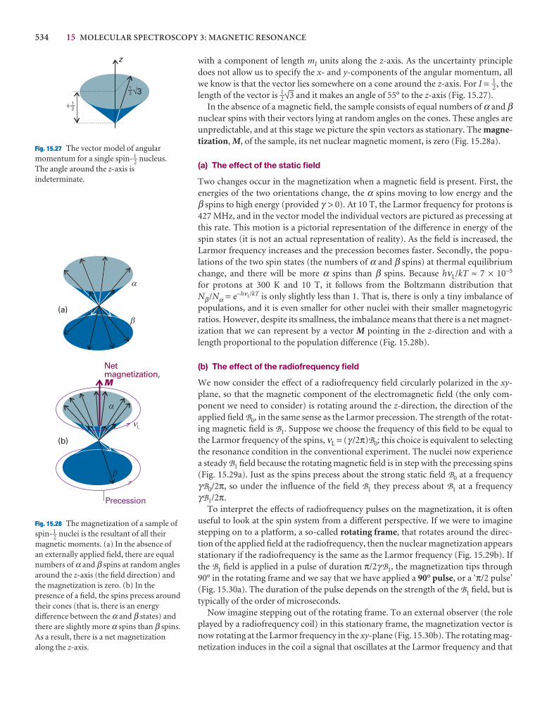
534 15 MOLECULAR SPECTROSCOPY 3: MAGNETIC RESONANCE
with a component of length mI units along the z-axis. As the uncertainty principledoes not allow us to specify the x- and y-components of the angular momentum, allwe know is that the vector lies somewhere on a cone around the z-axis. For I = 1–2, thelength of the vector is 1–2 3 and it makes an angle of 55° to the z-axis (Fig. 15.27).
In the absence of a magnetic field, the sample consists of equal numbers of α and βnuclear spins with their vectors lying at random angles on the cones. These angles areunpredictable, and at this stage we picture the spin vectors as stationary. The magne-tization, M, of the sample, its net nuclear magnetic moment, is zero (Fig. 15.28a).
(a) The effect of the static field
Two changes occur in the magnetization when a magnetic field is present. First, theenergies of the two orientations change, the α spins moving to low energy and the β spins to high energy (provided γ > 0). At 10 T, the Larmor frequency for protons is427 MHz, and in the vector model the individual vectors are pictured as precessing atthis rate. This motion is a pictorial representation of the difference in energy of thespin states (it is not an actual representation of reality). As the field is increased, theLarmor frequency increases and the precession becomes faster. Secondly, the popu-lations of the two spin states (the numbers of α and β spins) at thermal equilibriumchange, and there will be more α spins than β spins. Because hνL/kT ≈ 7 × 10⁻⁵
for protons at 300 K and 10 T, it follows from the Boltzmann distribution that Nβ /Nα = e−hνL/kT is only slightly less than 1. That is, there is only a tiny imbalance ofpopulations, and it is even smaller for other nuclei with their smaller magnetogyric ratios. However, despite its smallness, the imbalance means that there is a net magnet-ization that we can represent by a vector M pointing in the z-direction and with alength proportional to the population difference (Fig. 15.28b).
(b) The effect of the radiofrequency field
We now consider the effect of a radiofrequency field circularly polarized in the xy-plane, so that the magnetic component of the electromagnetic field (the only com-ponent we need to consider) is rotating around the z-direction, the direction of theapplied field B0, in the same sense as the Larmor precession. The strength of the rotat-ing magnetic field is B1. Suppose we choose the frequency of this field to be equal tothe Larmor frequency of the spins, νL = (γ /2π)B0; this choice is equivalent to selectingthe resonance condition in the conventional experiment. The nuclei now experiencea steady B1 field because the rotating magnetic field is in step with the precessing spins(Fig. 15.29a). Just as the spins precess about the strong static field B0 at a frequencyγB0/2π, so under the influence of the field B1 they precess about B1 at a frequencyγB1/2π.
To interpret the effects of radiofrequency pulses on the magnetization, it is oftenuseful to look at the spin system from a different perspective. If we were to imaginestepping on to a platform, a so-called rotating frame, that rotates around the direc-tion of the applied field at the radiofrequency, then the nuclear magnetization appearsstationary if the radiofrequency is the same as the Larmor frequency (Fig. 15.29b). Ifthe B1 field is applied in a pulse of duration π/2γ B1, the magnetization tips through 90° in the rotating frame and we say that we have applied a 90° pulse, or a ‘π/2 pulse’(Fig. 15.30a). The duration of the pulse depends on the strength of the B1 field, but istypically of the order of microseconds.
Now imagine stepping out of the rotating frame. To an external observer (the roleplayed by a radiofrequency coil) in this stationary frame, the magnetization vector isnow rotating at the Larmor frequency in the xy-plane (Fig. 15.30b). The rotating mag-netization induces in the coil a signal that oscillates at the Larmor frequency and that
�
33
z
–21
–21
Fig. 15.27 The vector model of angularmomentum for a single spin- 1–2 nucleus.The angle around the z-axis isindeterminate.
a
a
b
b
L
Precession
Netmagnetization,M
(a)
(b)
�
Fig. 15.28 The magnetization of a sample ofspin- 1–2 nuclei is the resultant of all theirmagnetic moments. (a) In the absence ofan externally applied field, there are equalnumbers of α and β spins at random anglesaround the z-axis (the field direction) andthe magnetization is zero. (b) In thepresence of a field, the spins precess aroundtheir cones (that is, there is an energydifference between the α and β states) andthere are slightly more α spins than β spins.As a result, there is a net magnetizationalong the z-axis.
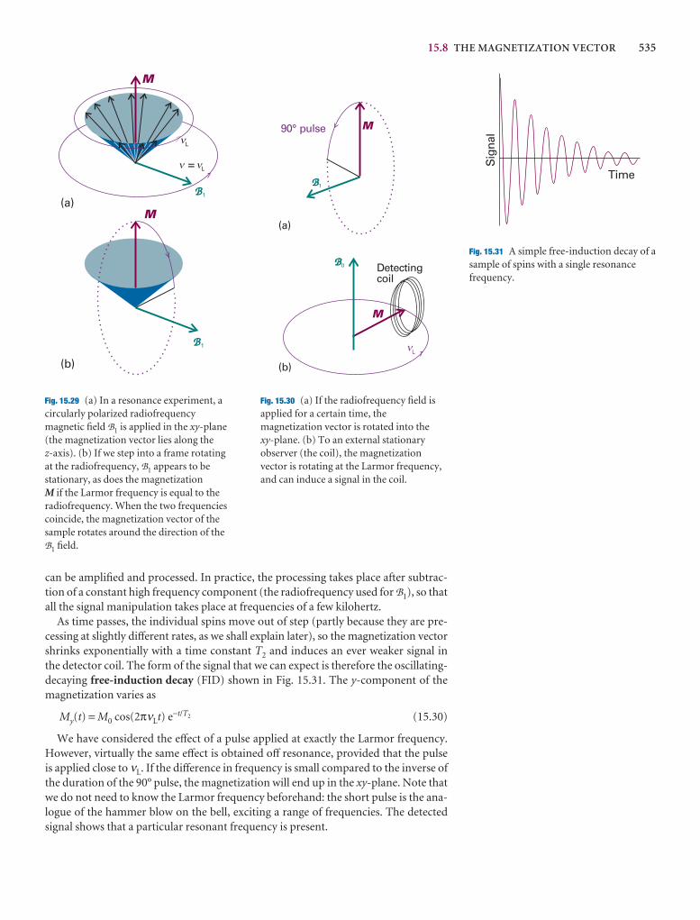
15.8 THE MAGNETIZATION VECTOR 535
can be amplified and processed. In practice, the processing takes place after subtrac-tion of a constant high frequency component (the radiofrequency used for B1), so thatall the signal manipulation takes place at frequencies of a few kilohertz.
As time passes, the individual spins move out of step (partly because they are pre-cessing at slightly different rates, as we shall explain later), so the magnetization vectorshrinks exponentially with a time constant T2 and induces an ever weaker signal in the detector coil. The form of the signal that we can expect is therefore the oscillating-decaying free-induction decay (FID) shown in Fig. 15.31. The y-component of themagnetization varies as
My(t) = M0 cos(2πνLt) e−t/T2 (15.30)
We have considered the effect of a pulse applied at exactly the Larmor frequency.However, virtually the same effect is obtained off resonance, provided that the pulse is applied close to νL. If the difference in frequency is small compared to the inverse ofthe duration of the 90° pulse, the magnetization will end up in the xy-plane. Note thatwe do not need to know the Larmor frequency beforehand: the short pulse is the ana-logue of the hammer blow on the bell, exciting a range of frequencies. The detectedsignal shows that a particular resonant frequency is present.
L
= L
B1B
M
M(a)
(b)
�
� �
B1BB1B
M
M
(a)
(b)
90° pulse
Detectingcoil
L�
B0B
Fig. 15.30 (a) If the radiofrequency field isapplied for a certain time, themagnetization vector is rotated into the xy-plane. (b) To an external stationaryobserver (the coil), the magnetizationvector is rotating at the Larmor frequency,and can induce a signal in the coil.
Time
Sig
nal
Fig. 15.31 A simple free-induction decay of asample of spins with a single resonancefrequency.
Fig. 15.29 (a) In a resonance experiment, acircularly polarized radiofrequencymagnetic field B1 is applied in the xy-plane(the magnetization vector lies along the z-axis). (b) If we step into a frame rotatingat the radiofrequency, B1 appears to bestationary, as does the magnetizationM if the Larmor frequency is equal to theradiofrequency. When the two frequenciescoincide, the magnetization vector of thesample rotates around the direction of theB1 field.
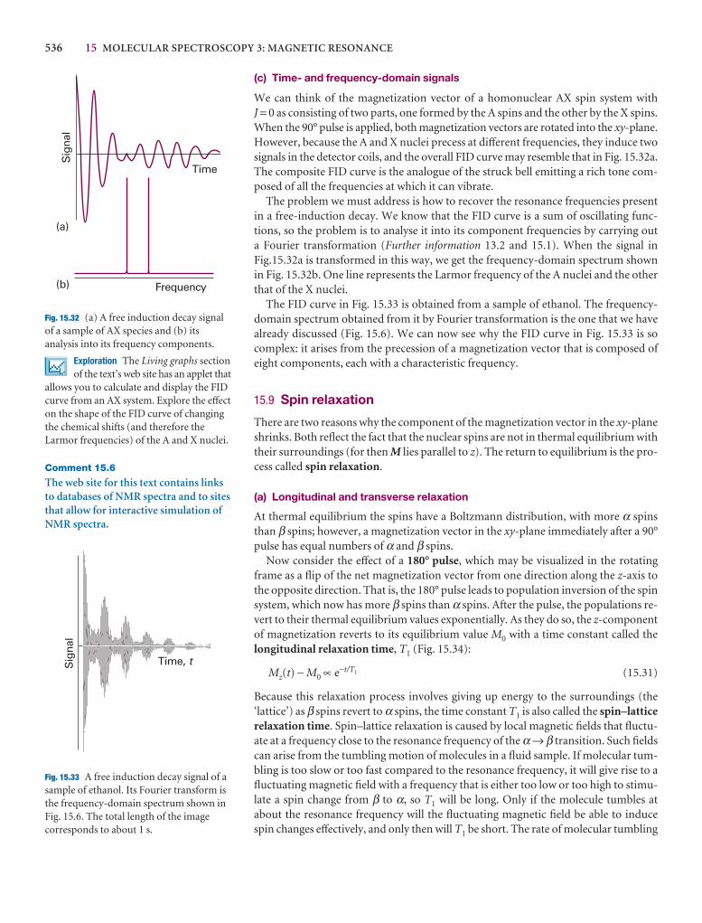
536 15 MOLECULAR SPECTROSCOPY 3: MAGNETIC RESONANCE
(c) Time- and frequency-domain signals
We can think of the magnetization vector of a homonuclear AX spin system with J = 0 as consisting of two parts, one formed by the A spins and the other by the X spins.When the 90° pulse is applied, both magnetization vectors are rotated into the xy-plane.However, because the A and X nuclei precess at different frequencies, they induce twosignals in the detector coils, and the overall FID curve may resemble that in Fig. 15.32a.The composite FID curve is the analogue of the struck bell emitting a rich tone com-posed of all the frequencies at which it can vibrate.
The problem we must address is how to recover the resonance frequencies presentin a free-induction decay. We know that the FID curve is a sum of oscillating func-tions, so the problem is to analyse it into its component frequencies by carrying outa Fourier transformation (Further information 13.2 and 15.1). When the signal inFig.15.32a is transformed in this way, we get the frequency-domain spectrum shownin Fig. 15.32b. One line represents the Larmor frequency of the A nuclei and the otherthat of the X nuclei.
The FID curve in Fig. 15.33 is obtained from a sample of ethanol. The frequency-domain spectrum obtained from it by Fourier transformation is the one that we havealready discussed (Fig. 15.6). We can now see why the FID curve in Fig. 15.33 is socomplex: it arises from the precession of a magnetization vector that is composed ofeight components, each with a characteristic frequency.
15.9 Spin relaxation
There are two reasons why the component of the magnetization vector in the xy-planeshrinks. Both reflect the fact that the nuclear spins are not in thermal equilibrium withtheir surroundings (for then M lies parallel to z). The return to equilibrium is the pro-cess called spin relaxation.
(a) Longitudinal and transverse relaxation
At thermal equilibrium the spins have a Boltzmann distribution, with more α spinsthan β spins; however, a magnetization vector in the xy-plane immediately after a 90°pulse has equal numbers of α and β spins.
Now consider the effect of a 180° pulse, which may be visualized in the rotatingframe as a flip of the net magnetization vector from one direction along the z-axis tothe opposite direction. That is, the 180° pulse leads to population inversion of the spinsystem, which now has more β spins than α spins. After the pulse, the populations re-vert to their thermal equilibrium values exponentially. As they do so, the z-componentof magnetization reverts to its equilibrium value M0 with a time constant called thelongitudinal relaxation time, T1 (Fig. 15.34):
Mz(t) − M0 ∝ e−t/T1 (15.31)
Because this relaxation process involves giving up energy to the surroundings (the‘lattice’) as β spins revert to α spins, the time constant T1 is also called the spin–latticerelaxation time. Spin–lattice relaxation is caused by local magnetic fields that fluctu-ate at a frequency close to the resonance frequency of the α → β transition. Such fieldscan arise from the tumbling motion of molecules in a fluid sample. If molecular tum-bling is too slow or too fast compared to the resonance frequency, it will give rise to afluctuating magnetic field with a frequency that is either too low or too high to stimu-late a spin change from β to α, so T1 will be long. Only if the molecule tumbles at about the resonance frequency will the fluctuating magnetic field be able to inducespin changes effectively, and only then will T1 be short. The rate of molecular tumbling
Sig
nal
Time
Frequency
(a)
(b)
Fig. 15.32 (a) A free induction decay signalof a sample of AX species and (b) itsanalysis into its frequency components.
Exploration The Living graphs sectionof the text’s web site has an applet that
allows you to calculate and display the FIDcurve from an AX system. Explore the effecton the shape of the FID curve of changingthe chemical shifts (and therefore theLarmor frequencies) of the A and X nuclei.
Comment 15.6
The web site for this text contains linksto databases of NMR spectra and to sitesthat allow for interactive simulation ofNMR spectra.
Sig
nal
Time, t
Fig. 15.33 A free induction decay signal of asample of ethanol. Its Fourier transform isthe frequency-domain spectrum shown inFig. 15.6. The total length of the imagecorresponds to about 1 s.
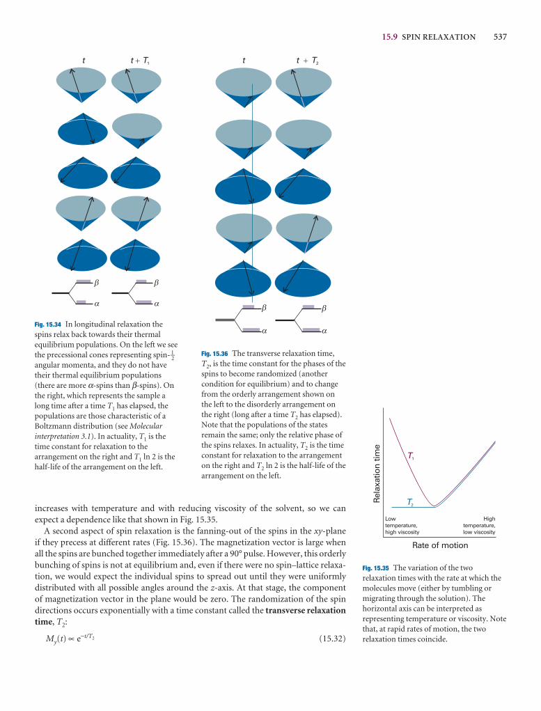
15.9 SPIN RELAXATION 537
increases with temperature and with reducing viscosity of the solvent, so we canexpect a dependence like that shown in Fig. 15.35.
A second aspect of spin relaxation is the fanning-out of the spins in the xy-planeif they precess at different rates (Fig. 15.36). The magnetization vector is large when all the spins are bunched together immediately after a 90° pulse. However, this orderlybunching of spins is not at equilibrium and, even if there were no spin–lattice relaxa-tion, we would expect the individual spins to spread out until they were uniformly distributed with all possible angles around the z-axis. At that stage, the component of magnetization vector in the plane would be zero. The randomization of the spin directions occurs exponentially with a time constant called the transverse relaxationtime, T2:
My(t) ∝ e−t/T2 (15.32)
t t T� 1
� �
� �
Fig. 15.34 In longitudinal relaxation thespins relax back towards their thermalequilibrium populations. On the left we seethe precessional cones representing spin-1–2angular momenta, and they do not havetheir thermal equilibrium populations(there are more α-spins than β-spins). Onthe right, which represents the sample along time after a time T1 has elapsed, thepopulations are those characteristic of aBoltzmann distribution (see Molecularinterpretation 3.1). In actuality, T1 is thetime constant for relaxation to thearrangement on the right and T1 ln 2 is thehalf-life of the arrangement on the left.
Rel
axat
ion
tim
e
Rate of motion
Lowtemperature,high viscosity
Hightemperature,low viscosity
T1
T2
Fig. 15.35 The variation of the tworelaxation times with the rate at which themolecules move (either by tumbling ormigrating through the solution). Thehorizontal axis can be interpreted asrepresenting temperature or viscosity. Notethat, at rapid rates of motion, the tworelaxation times coincide.
Fig. 15.36 The transverse relaxation time,T2, is the time constant for the phases of thespins to become randomized (anothercondition for equilibrium) and to changefrom the orderly arrangement shown onthe left to the disorderly arrangement onthe right (long after a time T2 has elapsed).Note that the populations of the statesremain the same; only the relative phase ofthe spins relaxes. In actuality, T2 is the timeconstant for relaxation to the arrangementon the right and T2 ln 2 is the half-life of thearrangement on the left.
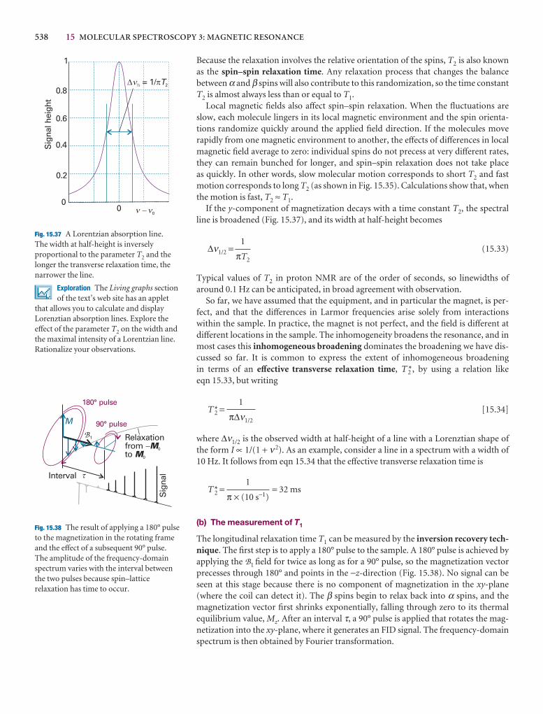
538 15 MOLECULAR SPECTROSCOPY 3: MAGNETIC RESONANCE
Because the relaxation involves the relative orientation of the spins, T2 is also knownas the spin–spin relaxation time. Any relaxation process that changes the balance between α and β spins will also contribute to this randomization, so the time constantT2 is almost always less than or equal to T1.
Local magnetic fields also affect spin–spin relaxation. When the fluctuations areslow, each molecule lingers in its local magnetic environment and the spin orienta-tions randomize quickly around the applied field direction. If the molecules moverapidly from one magnetic environment to another, the effects of differences in localmagnetic field average to zero: individual spins do not precess at very different rates,they can remain bunched for longer, and spin–spin relaxation does not take place as quickly. In other words, slow molecular motion corresponds to short T2 and fastmotion corresponds to long T2 (as shown in Fig. 15.35). Calculations show that, whenthe motion is fast, T2 ≈ T1.
If the y-component of magnetization decays with a time constant T2, the spectralline is broadened (Fig. 15.37), and its width at half-height becomes
∆ν1/2 = (15.33)
Typical values of T2 in proton NMR are of the order of seconds, so linewidths ofaround 0.1 Hz can be anticipated, in broad agreement with observation.
So far, we have assumed that the equipment, and in particular the magnet, is per-fect, and that the differences in Larmor frequencies arise solely from interactionswithin the sample. In practice, the magnet is not perfect, and the field is different atdifferent locations in the sample. The inhomogeneity broadens the resonance, and inmost cases this inhomogeneous broadening dominates the broadening we have dis-cussed so far. It is common to express the extent of inhomogeneous broadening in terms of an effective transverse relaxation time, T 2*, by using a relation like eqn 15.33, but writing
T*2 = [15.34]
where ∆ν1/2 is the observed width at half-height of a line with a Lorenztian shape of the form I ∝ 1/(1 + ν2). As an example, consider a line in a spectrum with a width of10 Hz. It follows from eqn 15.34 that the effective transverse relaxation time is
T*2 = = 32 ms
(b) The measurement of T1
The longitudinal relaxation time T1 can be measured by the inversion recovery tech-nique. The first step is to apply a 180° pulse to the sample. A 180° pulse is achieved byapplying the B1 field for twice as long as for a 90° pulse, so the magnetization vectorprecesses through 180° and points in the −z-direction (Fig. 15.38). No signal can beseen at this stage because there is no component of magnetization in the xy-plane(where the coil can detect it). The β spins begin to relax back into α spins, and themagnetization vector first shrinks exponentially, falling through zero to its thermalequilibrium value, Mz. After an interval τ, a 90° pulse is applied that rotates the mag-netization into the xy-plane, where it generates an FID signal. The frequency-domainspectrum is then obtained by Fourier transformation.
1
π × (10 s−1)
1
π∆ν1/2
1
πT2
1
0.8
0.6
0.4
0.2
00
Sig
nal h
eigh
t
� 0
�½ 2= 1/ T
� �
�
Fig. 15.37 A Lorentzian absorption line. The width at half-height is inverselyproportional to the parameter T2 and thelonger the transverse relaxation time, thenarrower the line.
Exploration The Living graphs sectionof the text’s web site has an applet
that allows you to calculate and displayLorenztian absorption lines. Explore theeffect of the parameter T2 on the width andthe maximal intensity of a Lorentzian line.Rationalize your observations.
M
B1
180° pulse
90° pulse
Interval
Relaxationfromto
�MM
0
0
Sig
nal�
Fig. 15.38 The result of applying a 180° pulseto the magnetization in the rotating frameand the effect of a subsequent 90° pulse.The amplitude of the frequency-domainspectrum varies with the interval betweenthe two pulses because spin–latticerelaxation has time to occur.
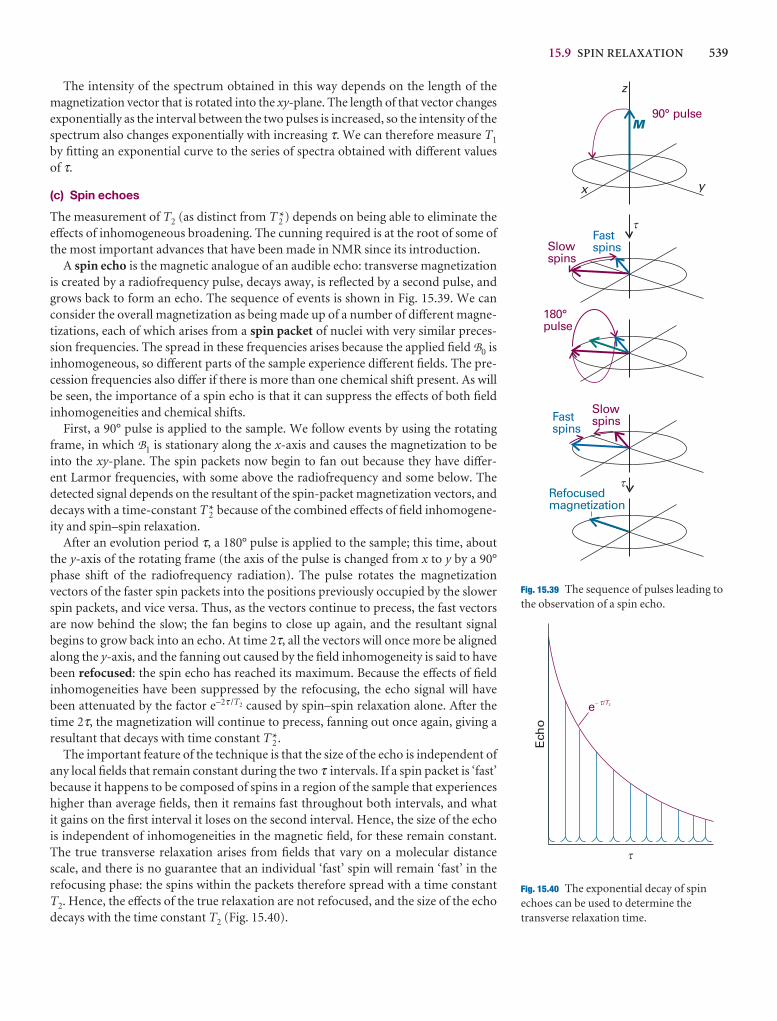
15.9 SPIN RELAXATION 539
The intensity of the spectrum obtained in this way depends on the length of themagnetization vector that is rotated into the xy-plane. The length of that vector changesexponentially as the interval between the two pulses is increased, so the intensity of thespectrum also changes exponentially with increasing τ. We can therefore measure T1
by fitting an exponential curve to the series of spectra obtained with different values of τ.
(c) Spin echoes
The measurement of T2 (as distinct from T 2*) depends on being able to eliminate theeffects of inhomogeneous broadening. The cunning required is at the root of some ofthe most important advances that have been made in NMR since its introduction.
A spin echo is the magnetic analogue of an audible echo: transverse magnetizationis created by a radiofrequency pulse, decays away, is reflected by a second pulse, andgrows back to form an echo. The sequence of events is shown in Fig. 15.39. We canconsider the overall magnetization as being made up of a number of different magne-tizations, each of which arises from a spin packet of nuclei with very similar preces-sion frequencies. The spread in these frequencies arises because the applied field B0 isinhomogeneous, so different parts of the sample experience different fields. The pre-cession frequencies also differ if there is more than one chemical shift present. As willbe seen, the importance of a spin echo is that it can suppress the effects of both fieldinhomogeneities and chemical shifts.
First, a 90° pulse is applied to the sample. We follow events by using the rotatingframe, in which B1 is stationary along the x-axis and causes the magnetization to beinto the xy-plane. The spin packets now begin to fan out because they have differ-ent Larmor frequencies, with some above the radiofrequency and some below. Thedetected signal depends on the resultant of the spin-packet magnetization vectors, anddecays with a time-constant T 2* because of the combined effects of field inhomogene-ity and spin–spin relaxation.
After an evolution period τ, a 180° pulse is applied to the sample; this time, aboutthe y-axis of the rotating frame (the axis of the pulse is changed from x to y by a 90°phase shift of the radiofrequency radiation). The pulse rotates the magnetization vectors of the faster spin packets into the positions previously occupied by the slowerspin packets, and vice versa. Thus, as the vectors continue to precess, the fast vectorsare now behind the slow; the fan begins to close up again, and the resultant signal begins to grow back into an echo. At time 2τ, all the vectors will once more be alignedalong the y-axis, and the fanning out caused by the field inhomogeneity is said to havebeen refocused: the spin echo has reached its maximum. Because the effects of fieldinhomogeneities have been suppressed by the refocusing, the echo signal will havebeen attenuated by the factor e−2τ /T2 caused by spin–spin relaxation alone. After thetime 2τ, the magnetization will continue to precess, fanning out once again, giving aresultant that decays with time constant T 2*.
The important feature of the technique is that the size of the echo is independent ofany local fields that remain constant during the two τ intervals. If a spin packet is ‘fast’because it happens to be composed of spins in a region of the sample that experienceshigher than average fields, then it remains fast throughout both intervals, and whatit gains on the first interval it loses on the second interval. Hence, the size of the echois independent of inhomogeneities in the magnetic field, for these remain constant.The true transverse relaxation arises from fields that vary on a molecular distancescale, and there is no guarantee that an individual ‘fast’ spin will remain ‘fast’ in the refocusing phase: the spins within the packets therefore spread with a time constantT2. Hence, the effects of the true relaxation are not refocused, and the size of the echodecays with the time constant T2 (Fig. 15.40).
90° pulseM
x y
z
FastspinsSlow
spins
180°pulse
Refocusedmagnetization
�
�
Fastspins
Slowspins
Fig. 15.39 The sequence of pulses leading tothe observation of a spin echo.
e- /T
t
Ech
o
t 2
Fig. 15.40 The exponential decay of spinechoes can be used to determine thetransverse relaxation time.
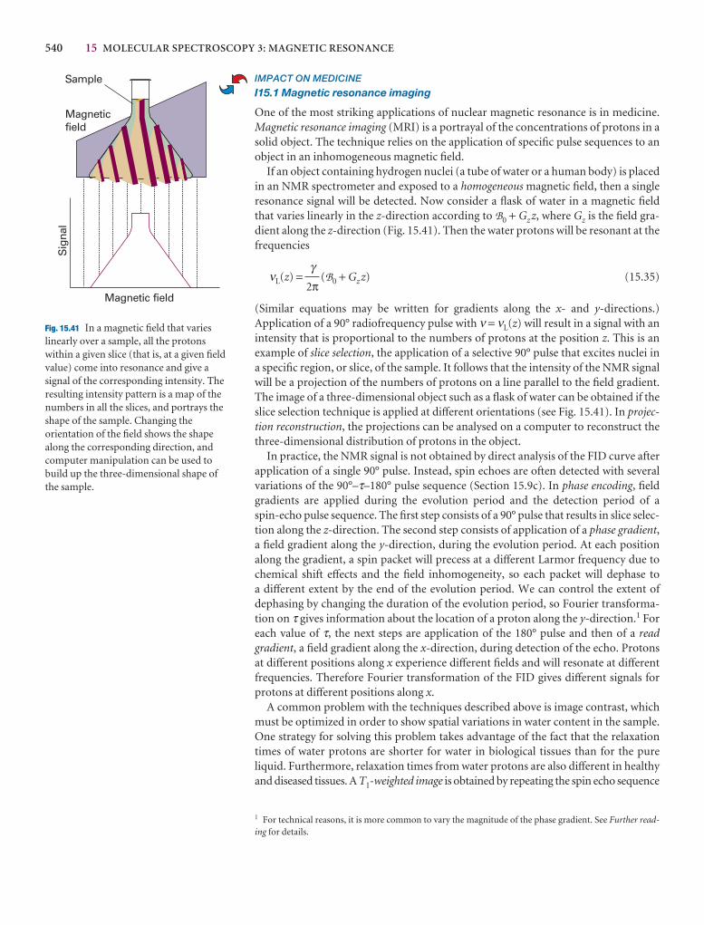
540 15 MOLECULAR SPECTROSCOPY 3: MAGNETIC RESONANCE
IMPACT ON MEDICINE
I15.1 Magnetic resonance imaging
One of the most striking applications of nuclear magnetic resonance is in medicine.Magnetic resonance imaging (MRI) is a portrayal of the concentrations of protons in asolid object. The technique relies on the application of specific pulse sequences to anobject in an inhomogeneous magnetic field.
If an object containing hydrogen nuclei (a tube of water or a human body) is placedin an NMR spectrometer and exposed to a homogeneous magnetic field, then a singleresonance signal will be detected. Now consider a flask of water in a magnetic fieldthat varies linearly in the z-direction according to B0 + Gz z, where Gz is the field gra-dient along the z-direction (Fig. 15.41). Then the water protons will be resonant at thefrequencies
νL(z) = (B0 + Gz z) (15.35)
(Similar equations may be written for gradients along the x- and y-directions.)Application of a 90° radiofrequency pulse with ν = νL(z) will result in a signal with anintensity that is proportional to the numbers of protons at the position z. This is an example of slice selection, the application of a selective 90° pulse that excites nuclei ina specific region, or slice, of the sample. It follows that the intensity of the NMR signalwill be a projection of the numbers of protons on a line parallel to the field gradient.The image of a three-dimensional object such as a flask of water can be obtained if theslice selection technique is applied at different orientations (see Fig. 15.41). In projec-tion reconstruction, the projections can be analysed on a computer to reconstruct thethree-dimensional distribution of protons in the object.
In practice, the NMR signal is not obtained by direct analysis of the FID curve afterapplication of a single 90° pulse. Instead, spin echoes are often detected with severalvariations of the 90°–τ–180° pulse sequence (Section 15.9c). In phase encoding, fieldgradients are applied during the evolution period and the detection period of a spin-echo pulse sequence. The first step consists of a 90° pulse that results in slice selec-tion along the z-direction. The second step consists of application of a phase gradient,a field gradient along the y-direction, during the evolution period. At each positionalong the gradient, a spin packet will precess at a different Larmor frequency due tochemical shift effects and the field inhomogeneity, so each packet will dephase to a different extent by the end of the evolution period. We can control the extent of dephasing by changing the duration of the evolution period, so Fourier transforma-tion on τ gives information about the location of a proton along the y-direction.1 Foreach value of τ, the next steps are application of the 180° pulse and then of a readgradient, a field gradient along the x-direction, during detection of the echo. Protons at different positions along x experience different fields and will resonate at differentfrequencies. Therefore Fourier transformation of the FID gives different signals forprotons at different positions along x.
A common problem with the techniques described above is image contrast, whichmust be optimized in order to show spatial variations in water content in the sample.One strategy for solving this problem takes advantage of the fact that the relaxationtimes of water protons are shorter for water in biological tissues than for the pure liquid. Furthermore, relaxation times from water protons are also different in healthyand diseased tissues. A T1-weighted image is obtained by repeating the spin echo sequence
γ2π
Magnetic field
Magneticfield
Sig
nal
Sample
Fig. 15.41 In a magnetic field that varieslinearly over a sample, all the protonswithin a given slice (that is, at a given fieldvalue) come into resonance and give asignal of the corresponding intensity. Theresulting intensity pattern is a map of thenumbers in all the slices, and portrays theshape of the sample. Changing theorientation of the field shows the shapealong the corresponding direction, andcomputer manipulation can be used tobuild up the three-dimensional shape ofthe sample.
1 For technical reasons, it is more common to vary the magnitude of the phase gradient. See Further read-ing for details.
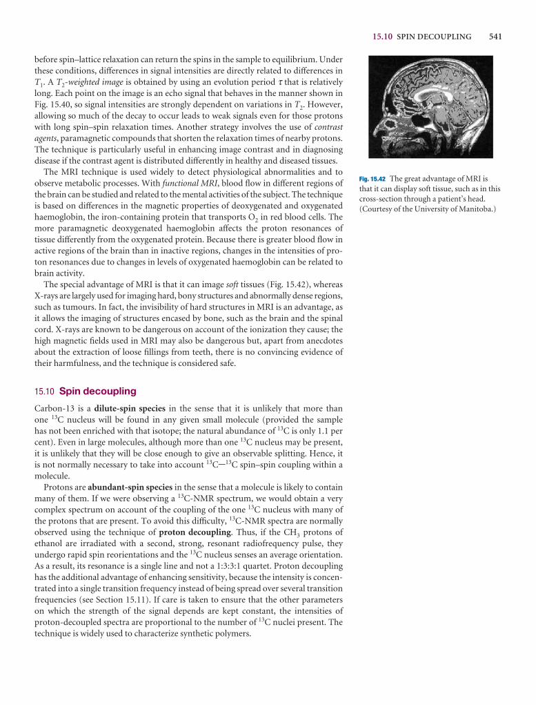
15.10 SPIN DECOUPLING 541
before spin–lattice relaxation can return the spins in the sample to equilibrium. Underthese conditions, differences in signal intensities are directly related to differences inT1. A T2-weighted image is obtained by using an evolution period τ that is relativelylong. Each point on the image is an echo signal that behaves in the manner shown inFig. 15.40, so signal intensities are strongly dependent on variations in T2. However,allowing so much of the decay to occur leads to weak signals even for those protonswith long spin–spin relaxation times. Another strategy involves the use of contrastagents, paramagnetic compounds that shorten the relaxation times of nearby protons.The technique is particularly useful in enhancing image contrast and in diagnosingdisease if the contrast agent is distributed differently in healthy and diseased tissues.
The MRI technique is used widely to detect physiological abnormalities and to observe metabolic processes. With functional MRI, blood flow in different regions ofthe brain can be studied and related to the mental activities of the subject. The techniqueis based on differences in the magnetic properties of deoxygenated and oxygenatedhaemoglobin, the iron-containing protein that transports O2 in red blood cells. Themore paramagnetic deoxygenated haemoglobin affects the proton resonances of tissue differently from the oxygenated protein. Because there is greater blood flow inactive regions of the brain than in inactive regions, changes in the intensities of pro-ton resonances due to changes in levels of oxygenated haemoglobin can be related tobrain activity.
The special advantage of MRI is that it can image soft tissues (Fig. 15.42), whereasX-rays are largely used for imaging hard, bony structures and abnormally dense regions,such as tumours. In fact, the invisibility of hard structures in MRI is an advantage, asit allows the imaging of structures encased by bone, such as the brain and the spinalcord. X-rays are known to be dangerous on account of the ionization they cause; thehigh magnetic fields used in MRI may also be dangerous but, apart from anecdotesabout the extraction of loose fillings from teeth, there is no convincing evidence oftheir harmfulness, and the technique is considered safe.
15.10 Spin decoupling
Carbon-13 is a dilute-spin species in the sense that it is unlikely that more than one 13C nucleus will be found in any given small molecule (provided the sample has not been enriched with that isotope; the natural abundance of 13C is only 1.1 percent). Even in large molecules, although more than one 13C nucleus may be present, it is unlikely that they will be close enough to give an observable splitting. Hence, it is not normally necessary to take into account 13C-13C spin–spin coupling within amolecule.
Protons are abundant-spin species in the sense that a molecule is likely to containmany of them. If we were observing a 13C-NMR spectrum, we would obtain a verycomplex spectrum on account of the coupling of the one 13C nucleus with many of the protons that are present. To avoid this difficulty, 13C-NMR spectra are normallyobserved using the technique of proton decoupling. Thus, if the CH3 protons ofethanol are irradiated with a second, strong, resonant radiofrequency pulse, they undergo rapid spin reorientations and the 13C nucleus senses an average orientation.As a result, its resonance is a single line and not a 1:3:3:1 quartet. Proton decouplinghas the additional advantage of enhancing sensitivity, because the intensity is concen-trated into a single transition frequency instead of being spread over several transitionfrequencies (see Section 15.11). If care is taken to ensure that the other parameters on which the strength of the signal depends are kept constant, the intensities of proton-decoupled spectra are proportional to the number of 13C nuclei present. Thetechnique is widely used to characterize synthetic polymers.
Fig. 15.42 The great advantage of MRI isthat it can display soft tissue, such as in thiscross-section through a patient’s head.(Courtesy of the University of Manitoba.)
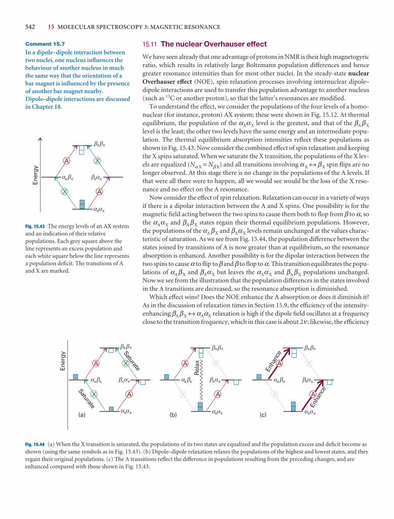
542 15 MOLECULAR SPECTROSCOPY 3: MAGNETIC RESONANCE
15.11 The nuclear Overhauser effect
We have seen already that one advantage of protons in NMR is their high magnetogyricratio, which results in relatively large Boltzmann population differences and hencegreater resonance intensities than for most other nuclei. In the steady-state nuclearOverhauser effect (NOE), spin relaxation processes involving internuclear dipole–dipole interactions are used to transfer this population advantage to another nucleus(such as 13C or another proton), so that the latter’s resonances are modified.
To understand the effect, we consider the populations of the four levels of a homo-nuclear (for instance, proton) AX system; these were shown in Fig. 15.12. At thermalequilibrium, the population of the αAαX level is the greatest, and that of the βAβX
level is the least; the other two levels have the same energy and an intermediate popu-lation. The thermal equilibrium absorption intensities reflect these populations asshown in Fig. 15.43. Now consider the combined effect of spin relaxation and keepingthe X spins saturated. When we saturate the X transition, the populations of the X lev-els are equalized (Nα X = Nβ X) and all transitions involving αX ↔ βX spin flips are nolonger observed. At this stage there is no change in the populations of the A levels. Ifthat were all there were to happen, all we would see would be the loss of the X reso-nance and no effect on the A resonance.
Now consider the effect of spin relaxation. Relaxation can occur in a variety of waysif there is a dipolar interaction between the A and X spins. One possibility is for themagnetic field acting between the two spins to cause them both to flop from β to α, sothe αAαX and βAβX states regain their thermal equilibrium populations. However,the populations of the αAβX and βAαX levels remain unchanged at the values charac-teristic of saturation. As we see from Fig. 15.44, the population difference between thestates joined by transitions of A is now greater than at equilibrium, so the resonanceabsorption is enhanced. Another possibility is for the dipolar interaction between thetwo spins to cause α to flip to β and β to flop to α. This transition equilibrates the popu-lations of αAβX and βAαX but leaves the αAαX and βAβX populations unchanged.Now we see from the illustration that the population differences in the states involvedin the A transitions are decreased, so the resonance absorption is diminished.
Which effect wins? Does the NOE enhance the A absorption or does it diminish it?As in the discussion of relaxation times in Section 15.9, the efficiency of the intensity-enhancing βAβX ↔ αAαX relaxation is high if the dipole field oscillates at a frequencyclose to the transition frequency, which in this case is about 2ν ; likewise, the efficiency
Comment 15.7
In a dipole–dipole interaction betweentwo nuclei, one nucleus influences thebehaviour of another nucleus in muchthe same way that the orientation of abar magnet is influenced by the presenceof another bar magnet nearby.Dipole–dipole interactions are discussedin Chapter 18.
Ener
gy
A X
A
A
X
X
� � A X� �
A X� �
A X� �
Fig. 15.43 The energy levels of an AX systemand an indication of their relativepopulations. Each grey square above theline represents an excess population andeach white square below the line representsa population deficit. The transitions of Aand X are marked.
Ener
gy
A X
A A A
A A A
X XX
X XX
Saturate
Saturate
Rel
ax
Enha
nce
Enha
nce
(a) (b) (c)
� �
A X� �
A X� �A X� �
A X� �
A X� �
A X� �A X� �
A X� �
A X� �
A X� �A X� �
Fig. 15.44 (a) When the X transition is saturated, the populations of its two states are equalized and the population excess and deficit become asshown (using the same symbols as in Fig. 15.43). (b) Dipole–dipole relaxation relaxes the populations of the highest and lowest states, and theyregain their original populations. (c) The A transitions reflect the difference in populations resulting from the preceding changes, and areenhanced compared with those shown in Fig. 15.43.
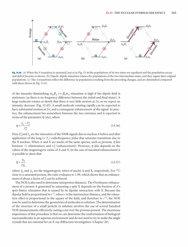
15.11 THE NUCLEAR OVERHAUSER EFFECT 543
of the intensity-diminishing αAβX ↔ βAαX relaxation is high if the dipole field is stationary (as there is no frequency difference between the initial and final states). Alarge molecule rotates so slowly that there is very little motion at 2ν, so we expect anintensity decrease (Fig. 15.45). A small molecule rotating rapidly can be expected tohave substantial motion at 2ν, and a consequent enhancement of the signal. In prac-tice, the enhancement lies somewhere between the two extremes and is reported interms of the parameter η (eta), where
η = [15.36]
Here IA° and IA are the intensities of the NMR signals due to nucleus A before and afterapplication of the long (> T1) radiofrequency pulse that saturates transitions due tothe X nucleus. When A and X are nuclei of the same species, such as protons, η liesbetween −1 (diminution) and + 1–2 (enhancement). However, η also depends on thevalues of the magnetogyric ratios of A and X. In the case of maximal enhancement itis possible to show that
η = (15.37)
where γA and γX are the magnetogyric ratios of nuclei A and X, respectively. For 13Cclose to a saturated proton, the ratio evaluates to 1.99, which shows that an enhance-ment of about a factor of 2 can be achieved.
The NOE is also used to determine interproton distances. The Overhauser enhance-ment of a proton A generated by saturating a spin X depends on the fraction of A’sspin–lattice relaxation that is caused by its dipolar interaction with X. Because thedipolar field is proportional to r−3, where r is the internuclear distance, and the relaxa-tion effect is proportional to the square of the field, and therefore to r−6, the NOE may be used to determine the geometries of molecules in solution. The determinationof the structure of a small protein in solution involves the use of several hundred NOE measurements, effectively casting a net over the protons present. The enormous importance of this procedure is that we can determine the conformation of biologicalmacromolecules in an aqueous environment and do not need to try to make the singlecrystals that are essential for an X-ray diffraction investigation (Chapter 20).
γX
2γA
IA − IA°
IA°
Ener
gyA A A
A A A
X XX
X XX
Saturate
Saturate
Relax
(a) (b) (c)
Dim
inis
h
Dim
inis
h
A X� �
A X� �
A X� �A X� �
A X� �
A X� �
A X� �
A X� �
A X� �
A X� �
A X� �
A X� �
Fig. 15.45 (a) When the X transition is saturated, just as in Fig. 15.44 the populations of its two states are equalized and the population excessand deficit become as shown. (b) Dipole–dipole relaxation relaxes the populations of the two intermediate states, and they regain their originalpopulations. (c) The A transitions reflect the difference in populations resulting from the preceding changes, and are diminished comparedwith those shown in Fig. 15.41.
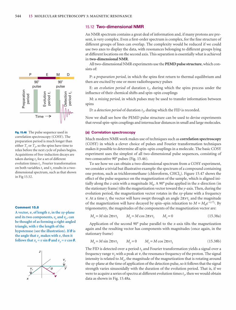
544 15 MOLECULAR SPECTROSCOPY 3: MAGNETIC RESONANCE
15.12 Two-dimensional NMR
An NMR spectrum contains a great deal of information and, if many protons are pre-sent, is very complex. Even a first-order spectrum is complex, for the fine structure ofdifferent groups of lines can overlap. The complexity would be reduced if we coulduse two axes to display the data, with resonances belonging to different groups lyingat different locations on the second axis. This separation is essentially what is achievedin two-dimensional NMR.
All two-dimensional NMR experiments use the PEMD pulse structure, which con-sists of:
P: a preparation period, in which the spins first return to thermal equilibrium andthen are excited by one or more radiofrequency pulses
E: an evolution period of duration t1, during which the spins precess under theinfluence of their chemical shifts and spin–spin couplings
M: a mixing period, in which pulses may be used to transfer information betweenspins
D: a detection period of duration t2, during which the FID is recorded.
Now we shall see how the PEMD pulse structure can be used to devise experimentsthat reveal spin–spin couplings and internuclear distances in small and large molecules.
(a) Correlation spectroscopy
Much modern NMR work makes use of techniques such as correlation spectroscopy(COSY) in which a clever choice of pulses and Fourier transformation techniquesmakes it possible to determine all spin–spin couplings in a molecule. The basic COSYexperiment uses the simplest of all two-dimensional pulse sequences, consisting oftwo consecutive 90° pulses (Fig. 15.46).
To see how we can obtain a two-dimensional spectrum from a COSY experiment,we consider a trivial but illustrative example: the spectrum of a compound containingone proton, such as trichloromethane (chloroform, CHCl3). Figure 15.47 shows theeffect of the pulse sequence on the magnetization of the sample, which is aligned ini-tially along the z-axis with a magnitude M0. A 90° pulse applied in the x-direction (inthe stationary frame) tilts the magnetization vector toward the y-axis. Then, during theevolution period, the magnetization vector rotates in the xy-plane with a frequency ν. At a time t1 the vector will have swept through an angle 2πν t1 and the magnitude of the magnetization will have decayed by spin–spin relaxation to M = M0e−t1/T2. Bytrigonometry, the magnitudes of the components of the magnetization vector are:
Mx = M sin 2πν t1 My = M cos 2πν t1 Mz = 0 (15.38a)
Application of the second 90° pulse parallel to the x-axis tilts the magnetizationagain and the resulting vector has components with magnitudes (once again, in thestationary frame)
Mx = M sin 2πν t1 My = 0 Mz = M cos 2πν t1 (15.38b)
The FID is detected over a period t2 and Fourier transformation yields a signal over afrequency range ν2 with a peak at ν, the resonance frequency of the proton. The signalintensity is related to Mx, the magnitude of the magnetization that is rotating aroundthe xy-plane at the time of application of the detection pulse, so it follows that the signalstrength varies sinusoidally with the duration of the evolution period. That is, if wewere to acquire a series of spectra at different evolution times t1, then we would obtaindata as shown in Fig. 15.48a.
Time
Prep
arat
ion
peri
od
Evol
utio
npe
riod
t 1
Det
ectio
npe
riod
t 2
90pulse
o90pulse
o
P E M D
Fig. 15.46 The pulse sequence used incorrelation spectroscopy (COSY). Thepreparation period is much longer thaneither T1 or T2, so the spins have time torelax before the next cycle of pulses begins.Acquisitions of free-induction decays aretaken during t2 for a set of differentevolution times t1. Fourier transformationon both variables t1 and t2 results in a two-dimensional spectrum, such as that shownin Fig 15.52.
Comment 15.8
A vector, V, of length 1, in the xy-planeand its two components, 1x and 1y , canbe thought of as forming a right-angledtriangle, with 1 the length of thehypotenuse (see the illustration). If q isthe angle that 1y makes with 1, then itfollows that 1x = 1 sin q and 1y = 1 cos q.
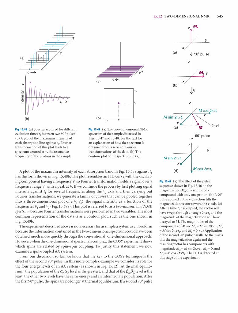
15.12 TWO-DIMENSIONAL NMR 545
A plot of the maximum intensity of each absorption band in Fig. 15.48a against t1
has the form shown in Fig. 15.48b. The plot resembles an FID curve with the oscillat-ing component having a frequency ν, so Fourier transformation yields a signal over afrequency range ν1 with a peak at ν. If we continue the process by first plotting signalintensity against t1 for several frequencies along the ν2 axis and then carrying outFourier transformations, we generate a family of curves that can be pooled togetherinto a three-dimensional plot of I(ν1,ν2), the signal intensity as a function of the frequencies ν1 and ν2 (Fig. 15.49a). This plot is referred to as a two-dimensional NMRspectrum because Fourier transformations were performed in two variables. The mostcommon representation of the data is as a contour plot, such as the one shown in Fig. 15.49b.
The experiment described above is not necessary for as simple a system as chloroformbecause the information contained in the two-dimensional spectrum could have beenobtained much more quickly through the conventional, one-dimensional approach.However, when the one-dimensional spectrum is complex, the COSY experiment showswhich spins are related by spin–spin coupling. To justify this statement, we now examine a spin-coupled AX system.
From our discussion so far, we know that the key to the COSY technique is theeffect of the second 90° pulse. In this more complex example we consider its role forthe four energy levels of an AX system (as shown in Fig. 15.12). At thermal equilib-rium, the population of the αAαX level is the greatest, and that of the βAβX level is theleast; the other two levels have the same energy and an intermediate population. Afterthe first 90° pulse, the spins are no longer at thermal equilibrium. If a second 90° pulse
M0
(a)x
y
z
(b)x
y
z
90 pulseo
M0
(c)x
y
z
t1
M tcos 2� 1
M 2� t1
(d)
x
yz
90 pulseo
M tsin 2� 1
M tcos 2� 1
M tsin 2� 1�
�
�
�
�
2
t1
(b)
t1Inte
nsity
(a)
�
2
1
(a)
(b)
2
1
n
nn
n
n
n
Fig. 15.47 (a) The effect of the pulsesequence shown in Fig. 15.46 on themagnetization M0 of a sample of acompound with only one proton. (b) A 90°pulse applied in the x-direction tilts themagnetization vector toward the y-axis. (c)After a time t1 has elapsed, the vector willhave swept through an angle 2πν t1 and themagnitude of the magnetization will havedecayed to M. The magnitudes of thecomponents of M are Mx = M sin 2πν t1, My
= M cos 2πν t1, and Mz = 0. (d) Applicationof the second 90° pulse parallel to the x-axistilts the magnetization again and theresulting vector has components withmagnitude Mx = M sin 2πν t1, My = 0, andMz = M cos 2πν t1. The FID is detected at this stage of the experiment.
Fig. 15.48 (a) Spectra acquired for differentevolution times t1 between two 90° pulses.(b) A plot of the maximum intensity ofeach absorption line against t1. Fouriertransformation of this plot leads to aspectrum centred at ν, the resonancefrequency of the protons in the sample.
Fig. 15.49 (a) The two-dimensional NMRspectrum of the sample discussed in Figs. 15.47 and 15.48. See the text for an explanation of how the spectrum isobtained from a series of Fouriertransformations of the data. (b) Thecontour plot of the spectrum in (a).
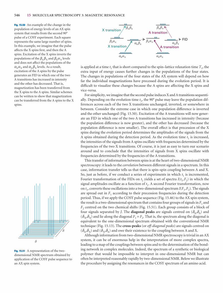
546 15 MOLECULAR SPECTROSCOPY 3: MAGNETIC RESONANCE
is applied at a time t1 that is short compared to the spin–lattice relaxation time T1, theextra input of energy causes further changes in the populations of the four states.The changes in populations of the four states of the AX system will depend on how far the individual magnetizations have precessed during the evolution period. It isdifficult to visualize these changes because the A spins are affecting the X spins andvice-versa.
For simplicity, we imagine that the second pulse induces X and A transitions sequenti-ally. Depending on the evolution time t1, the 90° pulse may leave the population dif-ferences across each of the two X transitions unchanged, inverted, or somewhere inbetween. Consider the extreme case in which one population difference is invertedand the other unchanged (Fig. 15.50). Excitation of the A transitions will now gener-ate an FID in which one of the two A transitions has increased in intensity (becausethe population difference is now greater), and the other has decreased (because thepopulation difference is now smaller). The overall effect is that precession of the Xspins during the evolution period determines the amplitudes of the signals from the A spins obtained during the detection period. As the evolution time t1 is increased, the intensities of the signals from A spins oscillate with frequencies determined by thefrequencies of the two X transitions. Of course, it is just as easy to turn our scenarioaround and to conclude that the intensities of signals from X spins oscillate with frequencies determined by the frequencies of the A transitions.
This transfer of information between spins is at the heart of two-dimensional NMRspectroscopy: it leads to the correlation between different signals in a spectrum. In thiscase, information transfer tells us that there is spin–spin coupling between A and X.So, just as before, if we conduct a series of experiments in which t1 is incremented,Fourier transformation of the FIDs on t2 yields a set of spectra I(t1,F2) in which thesignal amplitudes oscillate as a function of t1. A second Fourier transformation, nowon t1, converts these oscillations into a two-dimensional spectrum I(F1,F2). The signalsare spread out in F1 according to their precession frequencies during the detection period. Thus, if we apply the COSY pulse sequence (Fig. 15.46) to the AX spin system,the result is a two-dimensional spectrum that contains four groups of signals in F1 andF2 centred on the two chemical shifts (Fig. 15.51). Each group consists of a block offour signals separated by J. The diagonal peaks are signals centred on (δA,δA) and(δX,δX) and lie along the diagonal F1 = F2. That is, the spectrum along the diagonal isequivalent to the one-dimensional spectrum obtained with the conventional NMRtechnique (Fig. 15.13). The cross-peaks (or off-diagonal peaks) are signals centred on(δA,δX) and (δX,δA) and owe their existence to the coupling between A and X.
Although information from two-dimensional NMR spectroscopy is trivial in an AXsystem, it can be of enormous help in the interpretation of more complex spectra,leading to a map of the couplings between spins and to the determination of the bond-ing network in complex molecules. Indeed, the spectrum of a synthetic or biologicalpolymer that would be impossible to interpret in one-dimensional NMR but canoften be interpreted reasonably rapidly by two-dimensional NMR. Below we illustratethe procedure by assigning the resonances in the COSY spectrum of an amino acid.
X transitionA transition
A transition
FID
A Xb b
A Xb a A Xb a
A Xba
A Xb b
A XaaA Xaa
A XbaX transition
Fig. 15.50 An example of the change in thepopulation of energy levels of an AX spinsystem that results from the second 90°pulse of a COSY experiment. Each squarerepresents the same large number of spins.In this example, we imagine that the pulseaffects the X spins first, and then the Aspins. Excitation of the X spins inverts thepopulations of the βAβX and βAα X levelsand does not affect the populations of theαAαX and αAβX levels. As a result,excitation of the A spins by the pulsegenerates an FID in which one of the two A transitions has increased in intensity and the other has decreased. That is,magnetization has been transferred fromthe X spins to the A spins. Similar schemescan be written to show that magnetizationcan be transferred from the A spins to the Xspins.
d
d
Fig. 15.51 A representation of the two-dimensional NMR spectrum obtained byapplication of the COSY pulse sequence toan AX spin system.
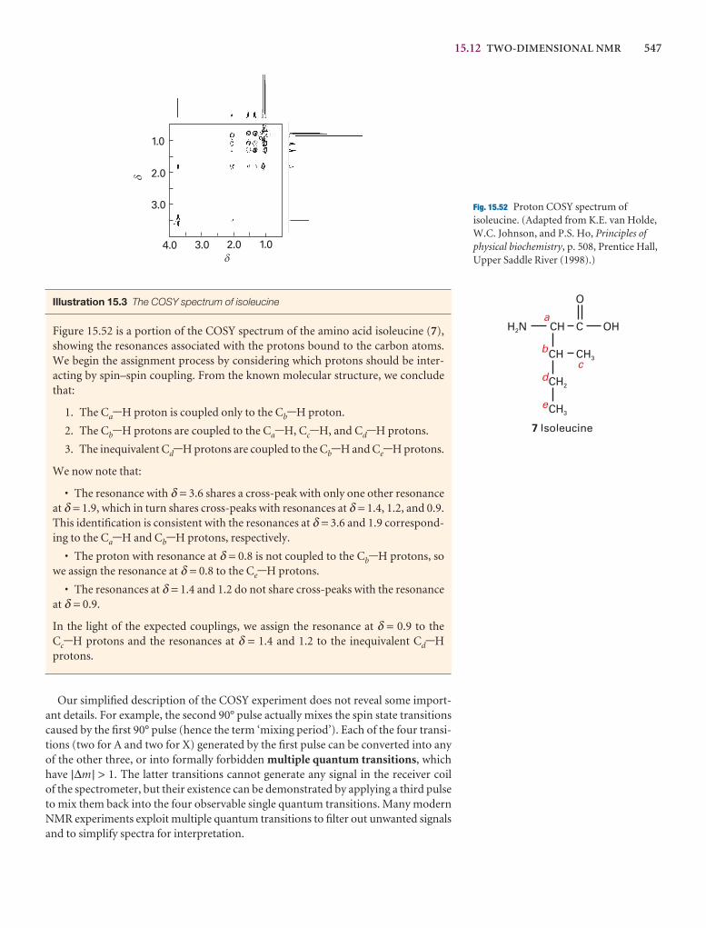
15.12 TWO-DIMENSIONAL NMR 547
�
4.0
�
3.0 2.0 1.0
3.0
2.0
1.0
Fig. 15.52 Proton COSY spectrum ofisoleucine. (Adapted from K.E. van Holde,W.C. Johnson, and P.S. Ho, Principles ofphysical biochemistry, p. 508, Prentice Hall,Upper Saddle River (1998).)
Illustration 15.3 The COSY spectrum of isoleucine
Figure 15.52 is a portion of the COSY spectrum of the amino acid isoleucine (7),showing the resonances associated with the protons bound to the carbon atoms.We begin the assignment process by considering which protons should be inter-acting by spin–spin coupling. From the known molecular structure, we concludethat:
1. The Ca-H proton is coupled only to the Cb-H proton.
2. The Cb-H protons are coupled to the Ca-H, Cc-H, and Cd-H protons.
3. The inequivalent Cd-H protons are coupled to the Cb-H and Ce-H protons.
We now note that:
• The resonance with δ = 3.6 shares a cross-peak with only one other resonanceat δ = 1.9, which in turn shares cross-peaks with resonances at δ = 1.4, 1.2, and 0.9.This identification is consistent with the resonances at δ = 3.6 and 1.9 correspond-ing to the Ca-H and Cb-H protons, respectively.
• The proton with resonance at δ = 0.8 is not coupled to the Cb-H protons, sowe assign the resonance at δ = 0.8 to the Ce-H protons.
• The resonances at δ = 1.4 and 1.2 do not share cross-peaks with the resonanceat δ = 0.9.
In the light of the expected couplings, we assign the resonance at δ = 0.9 to the Cc-H protons and the resonances at δ = 1.4 and 1.2 to the inequivalent Cd-Hprotons.
Our simplified description of the COSY experiment does not reveal some import-ant details. For example, the second 90° pulse actually mixes the spin state transitionscaused by the first 90° pulse (hence the term ‘mixing period’). Each of the four transi-tions (two for A and two for X) generated by the first pulse can be converted into anyof the other three, or into formally forbidden multiple quantum transitions, whichhave |∆m | > 1. The latter transitions cannot generate any signal in the receiver coil of the spectrometer, but their existence can be demonstrated by applying a third pulse to mix them back into the four observable single quantum transitions. Many modernNMR experiments exploit multiple quantum transitions to filter out unwanted signalsand to simplify spectra for interpretation.
548 15 MOLECULAR SPECTROSCOPY 3: MAGNETIC RESONANCE
(b) Nuclear Overhauser effect spectroscopy
Many different two-dimensional NMR experiments are based on the PEMD pulsestructure. We have seen that the steady-state nuclear Overhauser effect can provideinformation about internuclear distances through analysis of enhancement patternsin the NMR spectrum before and after saturation of selected resonances. In its dynamicanalogue, nuclear Overhauser effect spectroscopy (NOESY), the second 90° pulse of the COSY experiment is replaced by two 90° pulses separated by a time delay dur-ing which dipole–dipole interactions cause magnetization to be exchanged betweenneighbouring spins (Fig. 15.50). The results of double Fourier transformation is aspectrum in which the cross-peaks form a map of all the NOE interactions in amolecule. Because the nuclear Overhauser effect depends on the inverse sixth powerof the separation between nuclei (see Section 15.11), NOESY data reveal internucleardistances up to about 0.5 nm.
15.13 Solid-state NMR
The principal difficulty with the application of NMR to solids is the low resolutioncharacteristic of solid samples. Nevertheless, there are good reasons for seeking toovercome these difficulties. They include the possibility that a compound of interestis unstable in solution or that it is insoluble, so conventional solution NMR cannot be employed. Moreover, many species are intrinsically interesting as solids, and it isimportant to determine their structures and dynamics. Synthetic polymers are particu-larly interesting in this regard, and information can be obtained about the arrange-ment of molecules, their conformations, and the motion of different parts of thechain. This kind of information is crucial to an interpretation of the bulk properties ofthe polymer in terms of its molecular characteristics. Similarly, inorganic substances,such as the zeolites that are used as molecular sieves and shape-selective catalysts, canbe studied using solid-state NMR, and structural problems can be resolved that can-not be tackled by X-ray diffraction.
Problems of resolution and linewidth are not the only features that plague NMRstudies of solids, but the rewards are so great that considerable efforts have been madeto overcome them and have achieved notable success. Because molecular rotation hasalmost ceased (except in special cases, including ‘plastic crystals’ in which the moleculescontinue to tumble), spin–lattice relaxation times are very long but spin–spin relaxa-tion times are very short. Hence, in a pulse experiment, there is a need for lengthy delays—of several seconds—between successive pulses so that the spin system hastime to revert to equilibrium. Even gathering the murky information may thereforebe a lengthy process. Moreover, because lines are so broad, very high powers of radio-frequency radiation may be required to achieve saturation. Whereas solution pulseNMR uses transmitters of a few tens of watts, solid-state NMR may require trans-mitters rated at several hundreds of watts.
(a) The origins of linewidths in solids
There are two principal contributions to the linewidths of solids. One is the directmagnetic dipolar interaction between nuclear spins. As we saw in the discussion ofspin–spin coupling, a nuclear magnetic moment will give rise to a local magnetic field,which points in different directions at different locations around the nucleus. If we areinterested only in the component parallel to the direction of the applied magneticfield (because only this component has a significant effect), then we can use a classicalexpression to write the magnitude of the local magnetic field as
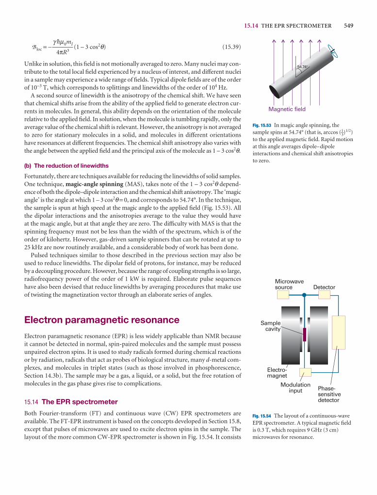
15.14 THE EPR SPECTROMETER 549
B loc = − (1 – 3 cos2θ) (15.39)
Unlike in solution, this field is not motionally averaged to zero. Many nuclei may con-tribute to the total local field experienced by a nucleus of interest, and different nucleiin a sample may experience a wide range of fields. Typical dipole fields are of the orderof 10−3 T, which corresponds to splittings and linewidths of the order of 104 Hz.
A second source of linewidth is the anisotropy of the chemical shift. We have seenthat chemical shifts arise from the ability of the applied field to generate electron cur-rents in molecules. In general, this ability depends on the orientation of the moleculerelative to the applied field. In solution, when the molecule is tumbling rapidly, only theaverage value of the chemical shift is relevant. However, the anisotropy is not averagedto zero for stationary molecules in a solid, and molecules in different orientationshave resonances at different frequencies. The chemical shift anisotropy also varies withthe angle between the applied field and the principal axis of the molecule as 1 – 3 cos2θ.
(b) The reduction of linewidths
Fortunately, there are techniques available for reducing the linewidths of solid samples.One technique, magic-angle spinning (MAS), takes note of the 1 – 3 cos2θ depend-ence of both the dipole–dipole interaction and the chemical shift anisotropy. The ‘magicangle’ is the angle at which 1 – 3 cos2θ = 0, and corresponds to 54.74°. In the technique,the sample is spun at high speed at the magic angle to the applied field (Fig. 15.53). Allthe dipolar interactions and the anisotropies average to the value they would have at the magic angle, but at that angle they are zero. The difficulty with MAS is that thespinning frequency must not be less than the width of the spectrum, which is of theorder of kilohertz. However, gas-driven sample spinners that can be rotated at up to25 kHz are now routinely available, and a considerable body of work has been done.
Pulsed techniques similar to those described in the previous section may also beused to reduce linewidths. The dipolar field of protons, for instance, may be reducedby a decoupling procedure. However, because the range of coupling strengths is so large,radiofrequency power of the order of 1 kW is required. Elaborate pulse sequenceshave also been devised that reduce linewidths by averaging procedures that make useof twisting the magnetization vector through an elaborate series of angles.
Electron paramagnetic resonance
Electron paramagnetic resonance (EPR) is less widely applicable than NMR because it cannot be detected in normal, spin-paired molecules and the sample must possessunpaired electron spins. It is used to study radicals formed during chemical reactionsor by radiation, radicals that act as probes of biological structure, many d-metal com-plexes, and molecules in triplet states (such as those involved in phosphorescence,Section 14.3b). The sample may be a gas, a liquid, or a solid, but the free rotation ofmolecules in the gas phase gives rise to complications.
15.14 The EPR spectrometer
Both Fourier-transform (FT) and continuous wave (CW) EPR spectrometers areavailable. The FT-EPR instrument is based on the concepts developed in Section 15.8,except that pulses of microwaves are used to excite electron spins in the sample. Thelayout of the more common CW-EPR spectrometer is shown in Fig. 15.54. It consists
γ $µ0mI
4πR3
54.74°
Magnetic field
54.744
Fig. 15.53 In magic angle spinning, thesample spins at 54.74° (that is, arccos (1–3)1/2)to the applied magnetic field. Rapid motion at this angle averages dipole–dipoleinteractions and chemical shift anisotropiesto zero.
Microwavesource Detector
Modulationinput
Electro-magnet
Phase-sensitivedetector
Samplecavity
Fig. 15.54 The layout of a continuous-waveEPR spectrometer. A typical magnetic fieldis 0.3 T, which requires 9 GHz (3 cm)microwaves for resonance.
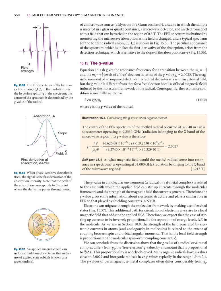
550 15 MOLECULAR SPECTROSCOPY 3: MAGNETIC RESONANCE
Fieldstrength
a
Absorption, A
First derivative ofabsorption, d /dA B
Slope
Field, B
Fig. 15.55 The EPR spectrum of the benzeneradical anion, C6H6
−, in fluid solution. a isthe hyperfine splitting of the spectrum; thecentre of the spectrum is determined by theg-value of the radical.
Fig. 15.56 When phase-sensitive detection isused, the signal is the first derivative of theabsorption intensity. Note that the peak ofthe absorption corresponds to the pointwhere the derivative passes through zero.
Fig. 15.57 An applied magnetic field caninduce circulation of electrons that makesuse of excited state orbitals (shown as agreen outline).
of a microwave source (a klystron or a Gunn oscillator), a cavity in which the sampleis inserted in a glass or quartz container, a microwave detector, and an electromagnetwith a field that can be varied in the region of 0.3 T. The EPR spectrum is obtained bymonitoring the microwave absorption as the field is changed, and a typical spectrum(of the benzene radical anion, C6H6
−) is shown in Fig. 15.55. The peculiar appearanceof the spectrum, which is in fact the first-derivative of the absorption, arises from thedetection technique, which is sensitive to the slope of the absorption curve (Fig. 15.56).
15.15 The g-value
Equation 15.13b gives the resonance frequency for a transition between the ms = − 1–2and the ms = + 1–2 levels of a ‘free’ electron in terms of the g-value ge ≈ 2.0023. The mag-netic moment of an unpaired electron in a radical also interacts with an external field,but the g-value is different from that for a free electron because of local magnetic fieldsinduced by the molecular framework of the radical. Consequently, the resonance con-dition is normally written as
hν = gµBB0 (15.40)
where g is the g-value of the radical.
Illustration 15.4 Calculating the g-value of an organic radical
The centre of the EPR spectrum of the methyl radical occurred at 329.40 mT in aspectrometer operating at 9.2330 GHz (radiation belonging to the X band of themicrowave region). Its g-value is therefore
g = = = 2.0027
Self-test 15.4 At what magnetic field would the methyl radical come into reson-ance in a spectrometer operating at 34.000 GHz (radiation belonging to the Q bandof the microwave region)? [1.213 T]
The g-value in a molecular environment (a radical or a d-metal complex) is relatedto the ease with which the applied field can stir up currents through the molecularframework and the strength of the magnetic field the currents generate. Therefore, theg-value gives some information about electronic structure and plays a similar role inEPR to that played by shielding constants in NMR.
Electrons can migrate through the molecular framework by making use of excitedstates (Fig. 15.57). This additional path for circulation of electrons gives rise to a localmagnetic field that adds to the applied field. Therefore, we expect that the ease of stir-ring up currents to be inversely proportional to the separation of energy levels, ∆E, inthe molecule. As we saw in Section 10.8, the strength of the field generated by elec-tronic currents in atoms (and analogously in molecules) is related to the extent ofcoupling between spin and orbital angular momenta. That is, the local field strengthis proportional to the molecular spin–orbit coupling constant, ξ.
We can conclude from the discussion above that the g-value of a radical or d-metalcomplex differs from ge, the ‘free-electron’ g-value, by an amount that is proportionalto ξ /∆E. This proportionality is widely observed. Many organic radicals have g-valuesclose to 2.0027 and inorganic radicals have g-values typically in the range 1.9 to 2.1.The g-values of paramagnetic d-metal complexes often differ considerably from ge,
(6.626 08 × 10−34 J s) × (9.2330 × 10⁹ s−1)
(9.2740 × 10⁻²⁴ J T−1) × (0.329 40 T)
hνµBB
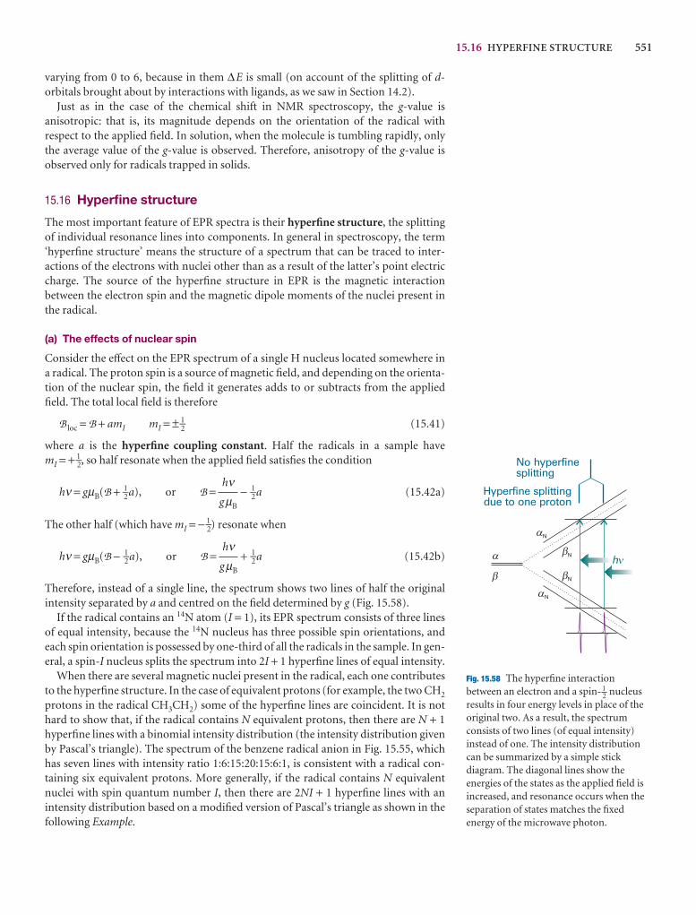
15.16 HYPERFINE STRUCTURE 551
varying from 0 to 6, because in them ∆E is small (on account of the splitting of d-orbitals brought about by interactions with ligands, as we saw in Section 14.2).
Just as in the case of the chemical shift in NMR spectroscopy, the g-value isanisotropic: that is, its magnitude depends on the orientation of the radical withrespect to the applied field. In solution, when the molecule is tumbling rapidly, onlythe average value of the g-value is observed. Therefore, anisotropy of the g-value is observed only for radicals trapped in solids.
15.16 Hyperfine structure
The most important feature of EPR spectra is their hyperfine structure, the splittingof individual resonance lines into components. In general in spectroscopy, the term‘hyperfine structure’ means the structure of a spectrum that can be traced to inter-actions of the electrons with nuclei other than as a result of the latter’s point electriccharge. The source of the hyperfine structure in EPR is the magnetic interaction between the electron spin and the magnetic dipole moments of the nuclei present inthe radical.
(a) The effects of nuclear spin
Consider the effect on the EPR spectrum of a single H nucleus located somewhere ina radical. The proton spin is a source of magnetic field, and depending on the orienta-tion of the nuclear spin, the field it generates adds to or subtracts from the appliedfield. The total local field is therefore
B loc = B + amI mI = ± 1–2 (15.41)
where a is the hyperfine coupling constant. Half the radicals in a sample have mI = + 1–2, so half resonate when the applied field satisfies the condition
hν = gµB(B + 1–2a), or B = − 1–2a (15.42a)
The other half (which have mI = − 1–2) resonate when
hν = gµB(B − 1–2a), or B = + 1–2a (15.42b)
Therefore, instead of a single line, the spectrum shows two lines of half the original intensity separated by a and centred on the field determined by g (Fig. 15.58).
If the radical contains an 14N atom (I = 1), its EPR spectrum consists of three linesof equal intensity, because the 14N nucleus has three possible spin orientations, andeach spin orientation is possessed by one-third of all the radicals in the sample. In gen-eral, a spin-I nucleus splits the spectrum into 2I + 1 hyperfine lines of equal intensity.
When there are several magnetic nuclei present in the radical, each one contributesto the hyperfine structure. In the case of equivalent protons (for example, the two CH2
protons in the radical CH3CH2) some of the hyperfine lines are coincident. It is nothard to show that, if the radical contains N equivalent protons, then there are N + 1hyperfine lines with a binomial intensity distribution (the intensity distribution givenby Pascal’s triangle). The spectrum of the benzene radical anion in Fig. 15.55, whichhas seven lines with intensity ratio 1:6:15:20:15:6:1, is consistent with a radical con-taining six equivalent protons. More generally, if the radical contains N equivalentnuclei with spin quantum number I, then there are 2NI + 1 hyperfine lines with an intensity distribution based on a modified version of Pascal’s triangle as shown in thefollowing Example.
hνgµB
hνgµB
N
N
N
N
ha
b
No hyperfinesplitting
Hyperfine splittingdue to one proton
a
a
b
b
�
Fig. 15.58 The hyperfine interactionbetween an electron and a spin-1–2 nucleusresults in four energy levels in place of theoriginal two. As a result, the spectrumconsists of two lines (of equal intensity)instead of one. The intensity distributioncan be summarized by a simple stickdiagram. The diagonal lines show theenergies of the states as the applied field isincreased, and resonance occurs when theseparation of states matches the fixedenergy of the microwave photon.
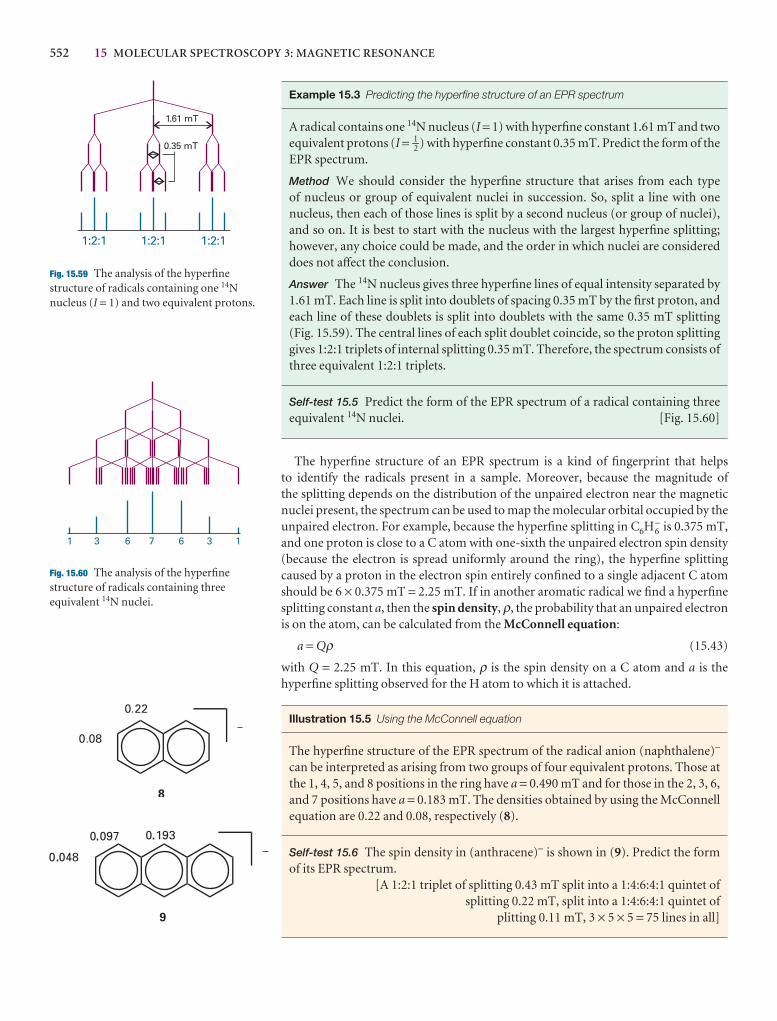
552 15 MOLECULAR SPECTROSCOPY 3: MAGNETIC RESONANCE
1:2:1 1:2:1 1:2:1
1.61 mT
0.35 mT
Fig. 15.59 The analysis of the hyperfinestructure of radicals containing one 14Nnucleus (I = 1) and two equivalent protons.
1 3 6 7 6 3 1
Fig. 15.60 The analysis of the hyperfinestructure of radicals containing threeequivalent 14N nuclei.
Example 15.3 Predicting the hyperfine structure of an EPR spectrum
A radical contains one 14N nucleus (I = 1) with hyperfine constant 1.61 mT and twoequivalent protons (I = 1–2 ) with hyperfine constant 0.35 mT. Predict the form of theEPR spectrum.
Method We should consider the hyperfine structure that arises from each type of nucleus or group of equivalent nuclei in succession. So, split a line with one nucleus, then each of those lines is split by a second nucleus (or group of nuclei),and so on. It is best to start with the nucleus with the largest hyperfine splitting;however, any choice could be made, and the order in which nuclei are considereddoes not affect the conclusion.
Answer The 14N nucleus gives three hyperfine lines of equal intensity separated by1.61 mT. Each line is split into doublets of spacing 0.35 mT by the first proton, andeach line of these doublets is split into doublets with the same 0.35 mT splitting(Fig. 15.59). The central lines of each split doublet coincide, so the proton splittinggives 1:2:1 triplets of internal splitting 0.35 mT. Therefore, the spectrum consists ofthree equivalent 1:2:1 triplets.
Self-test 15.5 Predict the form of the EPR spectrum of a radical containing threeequivalent 14N nuclei. [Fig. 15.60]
The hyperfine structure of an EPR spectrum is a kind of fingerprint that helps to identify the radicals present in a sample. Moreover, because the magnitude of the splitting depends on the distribution of the unpaired electron near the magneticnuclei present, the spectrum can be used to map the molecular orbital occupied by theunpaired electron. For example, because the hyperfine splitting in C6H6
− is 0.375 mT,and one proton is close to a C atom with one-sixth the unpaired electron spin density(because the electron is spread uniformly around the ring), the hyperfine splittingcaused by a proton in the electron spin entirely confined to a single adjacent C atomshould be 6 × 0.375 mT = 2.25 mT. If in another aromatic radical we find a hyperfinesplitting constant a, then the spin density, ρ, the probability that an unpaired electronis on the atom, can be calculated from the McConnell equation:
a = Qρ (15.43)
with Q = 2.25 mT. In this equation, ρ is the spin density on a C atom and a is thehyperfine splitting observed for the H atom to which it is attached.
Illustration 15.5 Using the McConnell equation
The hyperfine structure of the EPR spectrum of the radical anion (naphthalene)−
can be interpreted as arising from two groups of four equivalent protons. Those atthe 1, 4, 5, and 8 positions in the ring have a = 0.490 mT and for those in the 2, 3, 6,and 7 positions have a = 0.183 mT. The densities obtained by using the McConnellequation are 0.22 and 0.08, respectively (8).
Self-test 15.6 The spin density in (anthracene)− is shown in (9). Predict the formof its EPR spectrum.
[A 1:2:1 triplet of splitting 0.43 mT split into a 1:4:6:4:1 quintet of splitting 0.22 mT, split into a 1:4:6:4:1 quintet of
plitting 0.11 mT, 3 × 5 × 5 = 75 lines in all]
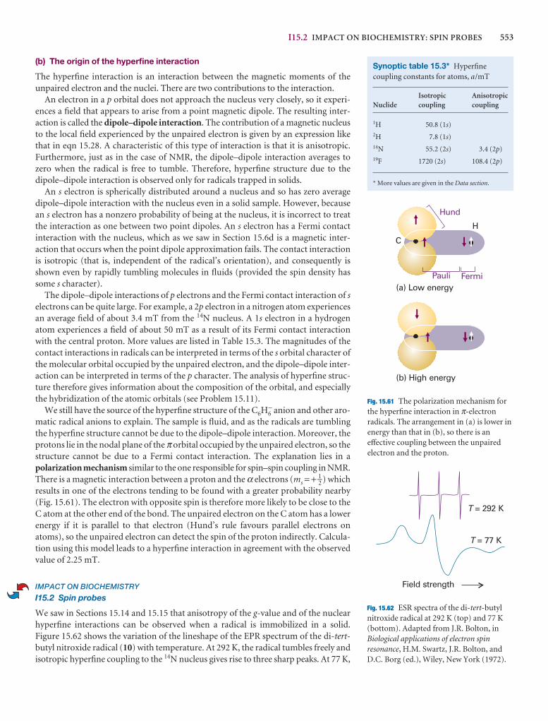
I15.2 IMPACT ON BIOCHEMISTRY: SPIN PROBES 553
(b) The origin of the hyperfine interaction
The hyperfine interaction is an interaction between the magnetic moments of the unpaired electron and the nuclei. There are two contributions to the interaction.
An electron in a p orbital does not approach the nucleus very closely, so it experi-ences a field that appears to arise from a point magnetic dipole. The resulting inter-action is called the dipole–dipole interaction. The contribution of a magnetic nucleusto the local field experienced by the unpaired electron is given by an expression likethat in eqn 15.28. A characteristic of this type of interaction is that it is anisotropic.Furthermore, just as in the case of NMR, the dipole–dipole interaction averages tozero when the radical is free to tumble. Therefore, hyperfine structure due to thedipole–dipole interaction is observed only for radicals trapped in solids.
An s electron is spherically distributed around a nucleus and so has zero averagedipole–dipole interaction with the nucleus even in a solid sample. However, becausean s electron has a nonzero probability of being at the nucleus, it is incorrect to treatthe interaction as one between two point dipoles. An s electron has a Fermi contact interaction with the nucleus, which as we saw in Section 15.6d is a magnetic inter-action that occurs when the point dipole approximation fails. The contact interactionis isotropic (that is, independent of the radical’s orientation), and consequently isshown even by rapidly tumbling molecules in fluids (provided the spin density hassome s character).
The dipole–dipole interactions of p electrons and the Fermi contact interaction of selectrons can be quite large. For example, a 2p electron in a nitrogen atom experiencesan average field of about 3.4 mT from the 14N nucleus. A 1s electron in a hydrogenatom experiences a field of about 50 mT as a result of its Fermi contact interactionwith the central proton. More values are listed in Table 15.3. The magnitudes of thecontact interactions in radicals can be interpreted in terms of the s orbital character ofthe molecular orbital occupied by the unpaired electron, and the dipole–dipole inter-action can be interpreted in terms of the p character. The analysis of hyperfine struc-ture therefore gives information about the composition of the orbital, and especiallythe hybridization of the atomic orbitals (see Problem 15.11).
We still have the source of the hyperfine structure of the C6H6− anion and other aro-
matic radical anions to explain. The sample is fluid, and as the radicals are tumblingthe hyperfine structure cannot be due to the dipole–dipole interaction. Moreover, theprotons lie in the nodal plane of the π orbital occupied by the unpaired electron, so thestructure cannot be due to a Fermi contact interaction. The explanation lies in a polarization mechanism similar to the one responsible for spin–spin coupling in NMR.There is a magnetic interaction between a proton and the α electrons (ms = + 1–2 ) whichresults in one of the electrons tending to be found with a greater probability nearby(Fig. 15.61). The electron with opposite spin is therefore more likely to be close to theC atom at the other end of the bond. The unpaired electron on the C atom has a lowerenergy if it is parallel to that electron (Hund’s rule favours parallel electrons onatoms), so the unpaired electron can detect the spin of the proton indirectly. Calcula-tion using this model leads to a hyperfine interaction in agreement with the observedvalue of 2.25 mT.
IMPACT ON BIOCHEMISTRY
I15.2 Spin probes
We saw in Sections 15.14 and 15.15 that anisotropy of the g-value and of the nuclearhyperfine interactions can be observed when a radical is immobilized in a solid. Figure 15.62 shows the variation of the lineshape of the EPR spectrum of the di-tert-butyl nitroxide radical (10) with temperature. At 292 K, the radical tumbles freely andisotropic hyperfine coupling to the 14N nucleus gives rise to three sharp peaks. At 77 K,
Synoptic table 15.3* Hyperfinecoupling constants for atoms, a/mT
Isotropic Anisotropic Nuclide coupling coupling
1H 50.8 (1s)2H 7.8 (1s)14N 55.2 (2s) 3.4 (2p)19F 1720 (2s) 108.4 (2p)
* More values are given in the Data section.
Hund
FermiPauli
C
H
(b) High energy
(a) Low energy
Fig. 15.61 The polarization mechanism forthe hyperfine interaction in π-electronradicals. The arrangement in (a) is lower inenergy than that in (b), so there is aneffective coupling between the unpairedelectron and the proton.
T = 77 K
T = 292 K
Field strength
Fig. 15.62 ESR spectra of the di-tert-butylnitroxide radical at 292 K (top) and 77 K(bottom). Adapted from J.R. Bolton, inBiological applications of electron spinresonance, H.M. Swartz, J.R. Bolton, andD.C. Borg (ed.), Wiley, New York (1972).
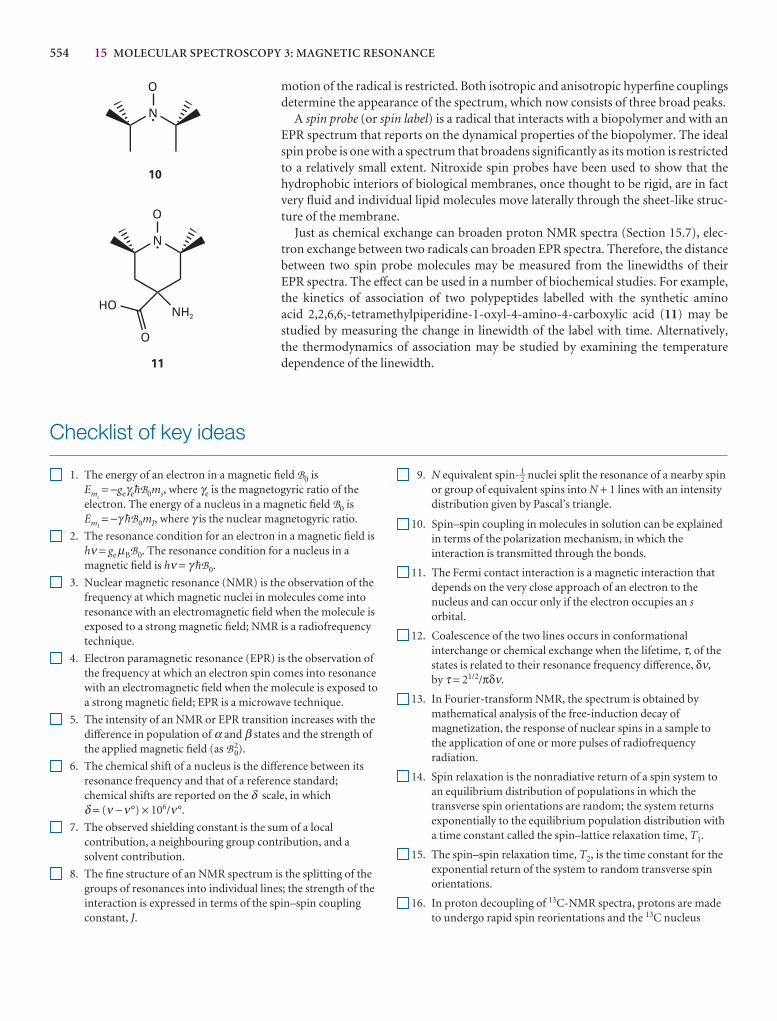
554 15 MOLECULAR SPECTROSCOPY 3: MAGNETIC RESONANCE
motion of the radical is restricted. Both isotropic and anisotropic hyperfine couplingsdetermine the appearance of the spectrum, which now consists of three broad peaks.
A spin probe (or spin label) is a radical that interacts with a biopolymer and with anEPR spectrum that reports on the dynamical properties of the biopolymer. The idealspin probe is one with a spectrum that broadens significantly as its motion is restrictedto a relatively small extent. Nitroxide spin probes have been used to show that the hydrophobic interiors of biological membranes, once thought to be rigid, are in factvery fluid and individual lipid molecules move laterally through the sheet-like struc-ture of the membrane.
Just as chemical exchange can broaden proton NMR spectra (Section 15.7), elec-tron exchange between two radicals can broaden EPR spectra. Therefore, the distancebetween two spin probe molecules may be measured from the linewidths of their EPR spectra. The effect can be used in a number of biochemical studies. For example,the kinetics of association of two polypeptides labelled with the synthetic amino acid 2,2,6,6,-tetramethylpiperidine-1-oxyl-4-amino-4-carboxylic acid (11) may bestudied by measuring the change in linewidth of the label with time. Alternatively, the thermodynamics of association may be studied by examining the temperature dependence of the linewidth.
Checklist of key ideas
1. The energy of an electron in a magnetic field B0 isEms
= −geγe$B0ms, where γe is the magnetogyric ratio of theelectron. The energy of a nucleus in a magnetic field B0 isEmI
= −γ $B0mI, where γ is the nuclear magnetogyric ratio.
2. The resonance condition for an electron in a magnetic field ishν = geµBB0. The resonance condition for a nucleus in amagnetic field is hν = γ $B0.
3. Nuclear magnetic resonance (NMR) is the observation of thefrequency at which magnetic nuclei in molecules come intoresonance with an electromagnetic field when the molecule isexposed to a strong magnetic field; NMR is a radiofrequencytechnique.
4. Electron paramagnetic resonance (EPR) is the observation ofthe frequency at which an electron spin comes into resonancewith an electromagnetic field when the molecule is exposed toa strong magnetic field; EPR is a microwave technique.
5. The intensity of an NMR or EPR transition increases with thedifference in population of α and β states and the strength ofthe applied magnetic field (as B 0
2).
6. The chemical shift of a nucleus is the difference between itsresonance frequency and that of a reference standard;chemical shifts are reported on the δ scale, in which δ = (ν −ν°) × 106/ν°.
7. The observed shielding constant is the sum of a localcontribution, a neighbouring group contribution, and asolvent contribution.
8. The fine structure of an NMR spectrum is the splitting of thegroups of resonances into individual lines; the strength of theinteraction is expressed in terms of the spin–spin couplingconstant, J.
9. N equivalent spin- 1–2 nuclei split the resonance of a nearby spin
or group of equivalent spins into N + 1 lines with an intensitydistribution given by Pascal’s triangle.
10. Spin–spin coupling in molecules in solution can be explainedin terms of the polarization mechanism, in which theinteraction is transmitted through the bonds.
11. The Fermi contact interaction is a magnetic interaction thatdepends on the very close approach of an electron to thenucleus and can occur only if the electron occupies an sorbital.
12. Coalescence of the two lines occurs in conformationalinterchange or chemical exchange when the lifetime, τ, of thestates is related to their resonance frequency difference, δν,by τ = 21/2/πδν.
13. In Fourier-transform NMR, the spectrum is obtained bymathematical analysis of the free-induction decay ofmagnetization, the response of nuclear spins in a sample tothe application of one or more pulses of radiofrequencyradiation.
14. Spin relaxation is the nonradiative return of a spin system toan equilibrium distribution of populations in which thetransverse spin orientations are random; the system returnsexponentially to the equilibrium population distribution witha time constant called the spin–lattice relaxation time, T1.
15. The spin–spin relaxation time, T2, is the time constant for theexponential return of the system to random transverse spinorientations.
16. In proton decoupling of 13C-NMR spectra, protons are madeto undergo rapid spin reorientations and the 13C nucleus

FURTHER INFORMATION 555
senses an average orientation. As a result, its resonance is asingle line and not a group of lines.
17. The nuclear Overhauser effect (NOE) is the modification ofone resonance by the saturation of another.
18. In two-dimensional NMR, spectra are displayed in two axes,with resonances belonging to different groups lying atdifferent locations on the second axis. An example of a two-dimensional NMR technique is correlation spectroscopy(COSY), in which all spin–spin couplings in a molecule aredetermined. Another example is nuclear Overhauser effectspectroscopy (NOESY), in which internuclear distances up toabout 0.5 nm are determined.
19. Magic-angle spinning (MAS) is technique in which the NMRlinewidths in a solid sample are reduced by spinning at anangle of 54.74° to the applied magnetic field.
20. The EPR resonance condition is written hν = gµBB, where g isthe g-value of the radical; the deviation of g from ge = 2.0023depends on the ability of the applied field to induce localelectron currents in the radical.
21. The hyperfine structure of an EPR spectrum is its splitting ofindividual resonance lines into components by the magneticinteraction between the electron and nuclei with spin.
22. If a radical contains N equivalent nuclei with spin quantumnumber I, then there are 2NI + 1 hyperfine lines with anintensity distribution given by a modified version of Pascal’striangle.
23. The hyperfine structure due to a hydrogen attached to anaromatic ring is converted to spin density, ρ, on theneighbouring carbon atom by using the McConnell equation:a = Qρ with Q = 2.25 mT.
Further reading
Articles and texts
N.M. Atherton, Principles of electron spin resonance. EllisHorwood/Prentice Hall, Hemel Hempstead (1993).
E.D. Becker, High resolution NMR: theory and chemical applications.Academic Press, San Diego (2000).
R. Freeman, Spin choreography: basic steps in high resolution NMR.Oxford University Press (1998).
J.C. Lindon, G.E. Tranter, and J.L. Holmes (ed.), Encyclopedia ofspectroscopy and spectrometry. Academic Press, San Diego (2000).
R.W. King and K.R. Williams. The Fourier transform in chemistry.Part 1. Nuclear magnetic resonance: Introduction. J. Chem. Educ.66, A213 (1989); Part 2. Nuclear magnetic resonance: The singlepulse experiment. Ibid. A243; Part 3. Multiple-pulse experiments.
J. Chem. Educ. 67, A93 (1990); Part 4. NMR: Two-dimensionalmethods. Ibid. A125; A glossary of NMR terms. Ibid. A100.
M.T. Vlaardingerbroek and J.A. de Boer, Magnetic resonance imaging:theory and practice. Springer, Berlin (1999).
M.H. Levitt, Spin dynamics. Wiley (2001).
Sources of data and information
D.R. Lide (ed.), CRC Handbook of Chemistry and Physics, Section 9,CRC Press, Boca Raton (2000).
C.P. Poole, Jr. and H.A. Farach (ed.), Handbook of electron spinresonance: data sources, computer technology, relaxation, andENDOR. Vols. 1–2. Springer, Berlin (1997, 1999).
Further information
Further information 15.1 Fourier transformation of the FID curve
The analysis of the FID curve is achieved by the standardmathematical technique of Fourier transformation, which weexplored in the context of FT infrared spectroscopy (Furtherinformation 13.2). We start by noting that the signal S(t) in the timedomain, the total FID curve, is the sum (more precisely, the integral)over all the contributing frequencies
S(t) = �∞
−∞
I(ν)e−2πiνtdν (15.44)
Because e2πiνt = cos(2πνt) + i sin(2πνt), the expression above is a sumover harmonically oscillating functions, with each one weighted bythe intensity I(ν).
We need I(ν), the spectrum in the frequency domain; it is obtainedby evaluating the integral
I(ν) = 2 Re�∞
0
S(t)e2πiνtdt (15.45)
where Re means take the real part of the following expression. Thisintegral is very much like an overlap integral: it gives a nonzero valueif S(t) contains a component that matches the oscillating functione2iπνt. The integration is carried out at a series of frequencies ν on acomputer that is built into the spectrometer.

556 15 MOLECULAR SPECTROSCOPY 3: MAGNETIC RESONANCE
Discussion questions
15.1 Discuss in detail the origins of the local, neighbouring group, andsolvent contributions to the shielding constant.
15.2 Discuss in detail the effects of a 90° pulse and of a 180° pulse on a systemof spin- 1–2 nuclei in a static magnetic field.
15.3 Suggest a reason why the relaxation times of 13C nuclei are typicallymuch longer than those of 1H nuclei.
15.4 Discuss the origins of diagonal and cross peaks in the COSY spectrum ofan AX system.
15.5 Discuss how the Fermi contact interaction and the polarizationmechanism contribute to spin–spin couplings in NMR and hyperfineinteractions in EPR.
15.6 Suggest how spin probes could be used to estimate the depth of a crevicein a biopolymer, such as the active site of an enzyme.
Exercises
15.1a What is the resonance frequency of a proton in a magnetic field of 14.1 T?
15.1b What is the resonance frequency of a 19F nucleus in a magnetic field of 16.2 T?
15.2a 33S has a nuclear spin of 3–2 and a nuclear g-factor of 0.4289. Calculate theenergies of the nuclear spin states in a magnetic field of 7.500 T.
15.2b 14N has a nuclear spin of 1 and a nuclear g-factor of 0.404. Calculate theenergies of the nuclear spin states in a magnetic field of 11.50 T.
15.3a Calculate the frequency separation of the nuclear spin levels of a 13Cnucleus in a magnetic field of 14.4 T given that the magnetogyric ratio is 6.73 × 10⁷ T−1 s−1.
15.3b Calculate the frequency separation of the nuclear spin levels of a 14Nnucleus in a magnetic field of 15.4 T given that the magnetogyric ratio is 1.93 × 10⁷ T−1 s−1.
15.4a In which of the following systems is the energy level separation thelargest? (a) A proton in a 600 MHz NMR spectrometer, (b) a deuteron in thesame spectrometer.
15.4b In which of the following systems is the energy level separation thelargest? (a) A 14N nucleus in (for protons) a 600 MHz NMR spectrometer, (b) an electron in a radical in a field of 0.300 T.
15.5a Calculate the energy difference between the lowest and highest nuclearspin states of a 14N nucleus in a 15.00 T magnetic field.
15.5b Calculate the magnetic field needed to satisfy the resonance conditionfor unshielded protons in a 150.0 MHz radiofrequency field.
15.6a Use Table 15.2 to predict the magnetic fields at which (a) 1H, (b) 2H,(c) 13C come into resonance at (i) 250 MHz, (ii) 500 MHz.
15.6b Use Table 15.2 to predict the magnetic fields at which (a) 14N, (b) 19F,and (c) 31P come into resonance at (i) 300 MHz, (ii) 750 MHz.
15.7a Calculate the relative population differences (δN/N) for protons infields of (a) 0.30 T, (b) 1.5 T, and (c) 10 T at 25°C.
15.7b Calculate the relative population differences (δN/N) for 13C nuclei infields of (a) 0.50 T, (b) 2.5 T, and (c) 15.5 T at 25°C.
15.8a The first generally available NMR spectrometers operated at afrequency of 60 MHz; today it is not uncommon to use a spectrometer thatoperates at 800 MHz. What are the relative population differences of 13C spinstates in these two spectrometers at 25°C?
15.8b What are the relative values of the chemical shifts observed for nuclei in the spectrometers mentioned in Exercise 15.8a in terms of (a) δ values,(b) frequencies?
15.9a The chemical shift of the CH3 protons in acetaldehyde (ethanal) is δ = 2.20 and that of the CHO proton is 9.80. What is the difference in localmagnetic field between the two regions of the molecule when the applied fieldis (a) 1.5 T, (b) 15 T?
15.9b The chemical shift of the CH3 protons in diethyl ether is δ = 1.16 andthat of the CH2 protons is 3.36. What is the difference in local magnetic fieldbetween the two regions of the molecule when the applied field is (a) 1.9 T, (b) 16.5 T?
15.10a Sketch the appearance of the 1H-NMR spectrum of acetaldehyde(ethanal) using J = 2.90 Hz and the data in Exercise 15.9a in a spectrometeroperating at (a) 250 MHz, (b) 500 MHz.
15.10b Sketch the appearance of the 1H-NMR spectrum of diethyl ether usingJ = 6.97 Hz and the data in Exercise 15.9b in a spectrometer operating at (a) 350 MHz, (b) 650 MHz.
15.11a Two groups of protons are made equivalent by the isomerization of a fluxional molecule. At low temperatures, where the interconversion is slow, one group has δ = 4.0 and the other has δ = 5.2. At what rate ofinterconversion will the two signals merge in a spectrometer operating at 250 MHz?
15.11b Two groups of protons are made equivalent by the isomerization of afluxional molecule. At low temperatures, where the interconversion is slow,one group has δ = 5.5 and the other has δ = 6.8. At what rate ofinterconversion will the two signals merge in a spectrometer operating at 350 MHz?
15.12a Sketch the form of the 19F-NMR spectra of a natural sample oftetrafluoroborate ions, BF−
4, allowing for the relative abundances of 10BF4−
and 11BF4−.
15.12b From the data in Table 15.2, predict the frequency needed for 31P-NMR in an NMR spectrometer designed to observe proton resonance at 500 MHz. Sketch the proton and 31P resonances in the NMR spectrum of PH4
+.
15.13a Sketch the form of an A3M2X4 spectrum, where A, M, and X areprotons with distinctly different chemical shifts and JAM > JAX > JMX.
15.13b Sketch the form of an A2M2X5 spectrum, where A, M, and X areprotons with distinctly different chemical shifts and JAM > JAX > JMX.
15.14a Which of the following molecules have sets of nuclei that arechemically but not magnetically equivalent? (a) CH3CH3, (b) CH2=CH2.
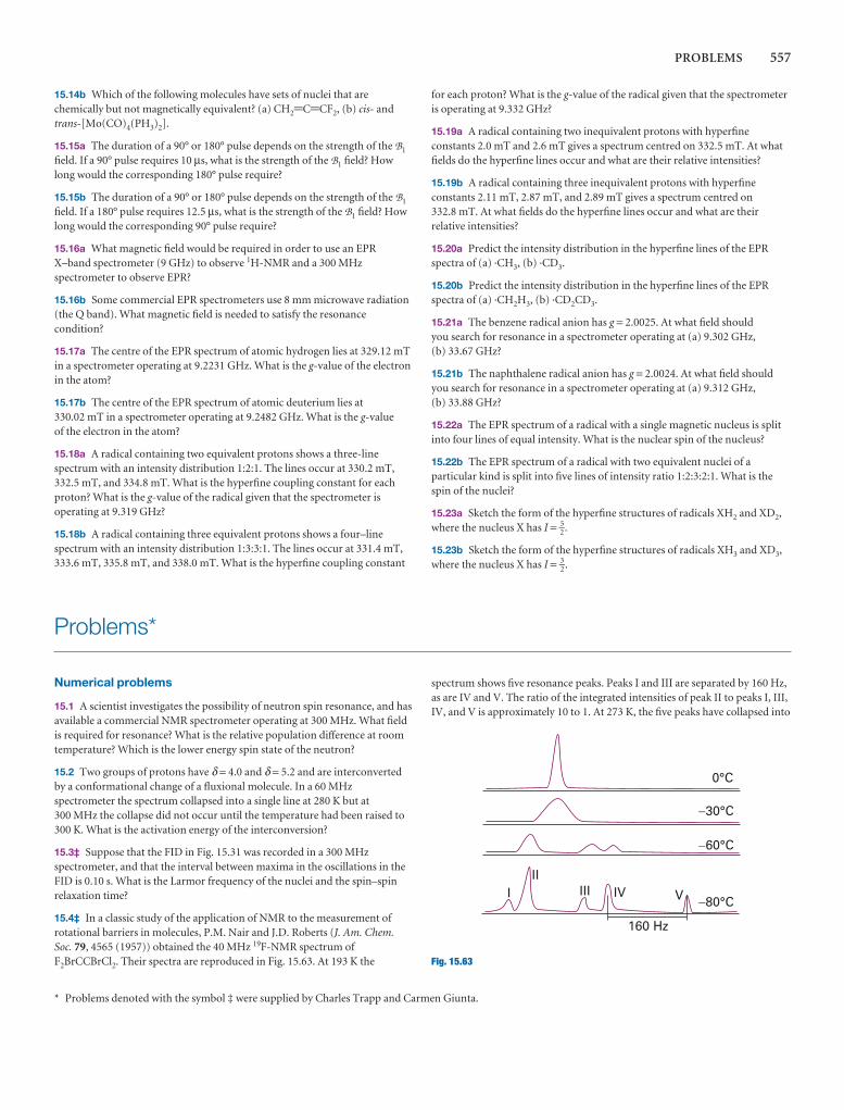
PROBLEMS 557
15.14b Which of the following molecules have sets of nuclei that arechemically but not magnetically equivalent? (a) CH2=C=CF2, (b) cis- andtrans-[Mo(CO)4(PH3)2].
15.15a The duration of a 90° or 180° pulse depends on the strength of the B1
field. If a 90° pulse requires 10 µs, what is the strength of the B1 field? Howlong would the corresponding 180° pulse require?
15.15b The duration of a 90° or 180° pulse depends on the strength of the B1
field. If a 180° pulse requires 12.5 µs, what is the strength of the B1 field? Howlong would the corresponding 90° pulse require?
15.16a What magnetic field would be required in order to use an EPRX–band spectrometer (9 GHz) to observe 1H-NMR and a 300 MHzspectrometer to observe EPR?
15.16b Some commercial EPR spectrometers use 8 mm microwave radiation(the Q band). What magnetic field is needed to satisfy the resonancecondition?
15.17a The centre of the EPR spectrum of atomic hydrogen lies at 329.12 mTin a spectrometer operating at 9.2231 GHz. What is the g-value of the electronin the atom?
15.17b The centre of the EPR spectrum of atomic deuterium lies at 330.02 mT in a spectrometer operating at 9.2482 GHz. What is the g-valueof the electron in the atom?
15.18a A radical containing two equivalent protons shows a three-linespectrum with an intensity distribution 1:2:1. The lines occur at 330.2 mT,332.5 mT, and 334.8 mT. What is the hyperfine coupling constant for eachproton? What is the g-value of the radical given that the spectrometer isoperating at 9.319 GHz?
15.18b A radical containing three equivalent protons shows a four–linespectrum with an intensity distribution 1:3:3:1. The lines occur at 331.4 mT,333.6 mT, 335.8 mT, and 338.0 mT. What is the hyperfine coupling constant
for each proton? What is the g-value of the radical given that the spectrometeris operating at 9.332 GHz?
15.19a A radical containing two inequivalent protons with hyperfineconstants 2.0 mT and 2.6 mT gives a spectrum centred on 332.5 mT. At whatfields do the hyperfine lines occur and what are their relative intensities?
15.19b A radical containing three inequivalent protons with hyperfineconstants 2.11 mT, 2.87 mT, and 2.89 mT gives a spectrum centred on 332.8 mT. At what fields do the hyperfine lines occur and what are theirrelative intensities?
15.20a Predict the intensity distribution in the hyperfine lines of the EPRspectra of (a) ·CH3, (b) ·CD3.
15.20b Predict the intensity distribution in the hyperfine lines of the EPRspectra of (a) ·CH2H3, (b) ·CD2CD3.
15.21a The benzene radical anion has g = 2.0025. At what field should you search for resonance in a spectrometer operating at (a) 9.302 GHz, (b) 33.67 GHz?
15.21b The naphthalene radical anion has g = 2.0024. At what field shouldyou search for resonance in a spectrometer operating at (a) 9.312 GHz, (b) 33.88 GHz?
15.22a The EPR spectrum of a radical with a single magnetic nucleus is splitinto four lines of equal intensity. What is the nuclear spin of the nucleus?
15.22b The EPR spectrum of a radical with two equivalent nuclei of aparticular kind is split into five lines of intensity ratio 1:2:3:2:1. What is thespin of the nuclei?
15.23a Sketch the form of the hyperfine structures of radicals XH2 and XD2,where the nucleus X has I = 5–
2.
15.23b Sketch the form of the hyperfine structures of radicals XH3 and XD3,where the nucleus X has I = 3–
2.
Problems*
Numerical problems
15.1 A scientist investigates the possibility of neutron spin resonance, and hasavailable a commercial NMR spectrometer operating at 300 MHz. What fieldis required for resonance? What is the relative population difference at roomtemperature? Which is the lower energy spin state of the neutron?
15.2 Two groups of protons have δ = 4.0 and δ = 5.2 and are interconvertedby a conformational change of a fluxional molecule. In a 60 MHzspectrometer the spectrum collapsed into a single line at 280 K but at 300 MHz the collapse did not occur until the temperature had been raised to300 K. What is the activation energy of the interconversion?
15.3‡ Suppose that the FID in Fig. 15.31 was recorded in a 300 MHzspectrometer, and that the interval between maxima in the oscillations in theFID is 0.10 s. What is the Larmor frequency of the nuclei and the spin–spinrelaxation time?
15.4‡ In a classic study of the application of NMR to the measurement ofrotational barriers in molecules, P.M. Nair and J.D. Roberts (J. Am. Chem.Soc. 79, 4565 (1957)) obtained the 40 MHz 19F-NMR spectrum ofF2BrCCBrCl2. Their spectra are reproduced in Fig. 15.63. At 193 K the
spectrum shows five resonance peaks. Peaks I and III are separated by 160 Hz,as are IV and V. The ratio of the integrated intensities of peak II to peaks I, III,IV, and V is approximately 10 to 1. At 273 K, the five peaks have collapsed into
* Problems denoted with the symbol ‡ were supplied by Charles Trapp and Carmen Giunta.
Fig. 15.63
0°C
�30°C
�60°C
�80°CI
IIIII IV V
160 Hz
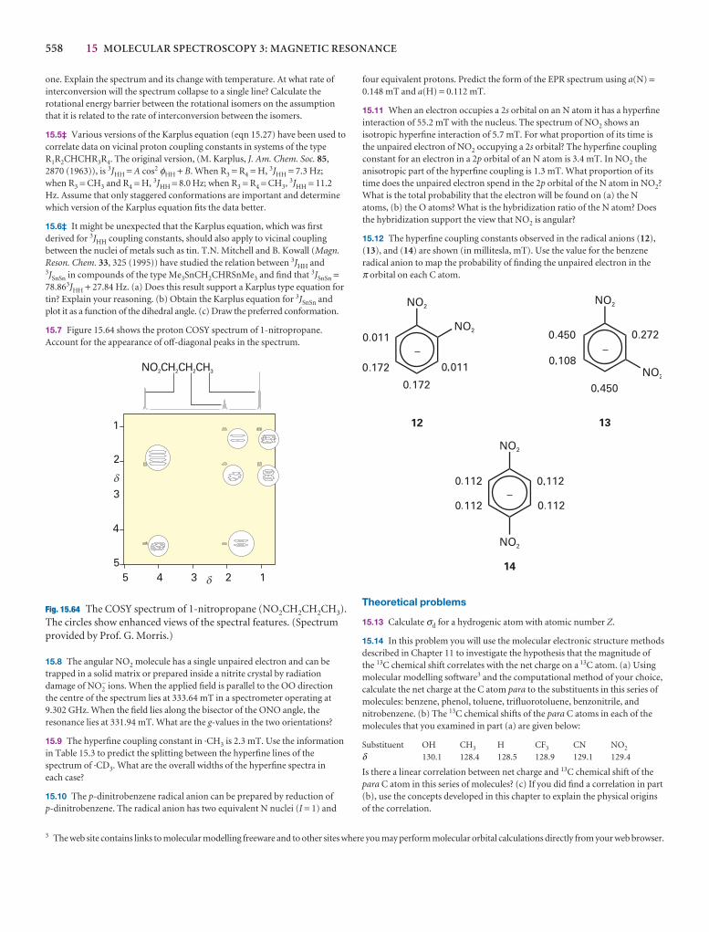
558 15 MOLECULAR SPECTROSCOPY 3: MAGNETIC RESONANCE
four equivalent protons. Predict the form of the EPR spectrum using a(N) =0.148 mT and a(H) = 0.112 mT.
15.11 When an electron occupies a 2s orbital on an N atom it has a hyperfineinteraction of 55.2 mT with the nucleus. The spectrum of NO2 shows anisotropic hyperfine interaction of 5.7 mT. For what proportion of its time isthe unpaired electron of NO2 occupying a 2s orbital? The hyperfine couplingconstant for an electron in a 2p orbital of an N atom is 3.4 mT. In NO2 theanisotropic part of the hyperfine coupling is 1.3 mT. What proportion of itstime does the unpaired electron spend in the 2p orbital of the N atom in NO2?What is the total probability that the electron will be found on (a) the Natoms, (b) the O atoms? What is the hybridization ratio of the N atom? Doesthe hybridization support the view that NO2 is angular?
15.12 The hyperfine coupling constants observed in the radical anions (12),(13), and (14) are shown (in millitesla, mT). Use the value for the benzeneradical anion to map the probability of finding the unpaired electron in the π orbital on each C atom.
12345
2
3
5
NO CH CH CH2 2 2 3
1
4
�
�
one. Explain the spectrum and its change with temperature. At what rate ofinterconversion will the spectrum collapse to a single line? Calculate therotational energy barrier between the rotational isomers on the assumptionthat it is related to the rate of interconversion between the isomers.
15.5‡ Various versions of the Karplus equation (eqn 15.27) have been used tocorrelate data on vicinal proton coupling constants in systems of the typeR1R2CHCHR3R4. The original version, (M. Karplus, J. Am. Chem. Soc. 85,2870 (1963)), is 3JHH = A cos2 φHH + B. When R3 = R4 = H, 3JHH = 7.3 Hz; when R3 = CH3 and R4 = H, 3JHH = 8.0 Hz; when R3 = R4 = CH3, 3JHH = 11.2Hz. Assume that only staggered conformations are important and determinewhich version of the Karplus equation fits the data better.
15.6‡ It might be unexpected that the Karplus equation, which was firstderived for 3JHH coupling constants, should also apply to vicinal couplingbetween the nuclei of metals such as tin. T.N. Mitchell and B. Kowall (Magn.Reson. Chem. 33, 325 (1995)) have studied the relation between 3JHH and3JSnSn in compounds of the type Me3SnCH2CHRSnMe3 and find that 3JSnSn =78.863JHH + 27.84 Hz. (a) Does this result support a Karplus type equation fortin? Explain your reasoning. (b) Obtain the Karplus equation for 3JSnSn andplot it as a function of the dihedral angle. (c) Draw the preferred conformation.
15.7 Figure 15.64 shows the proton COSY spectrum of 1-nitropropane.Account for the appearance of off-diagonal peaks in the spectrum.
Theoretical problems
15.13 Calculate σd for a hydrogenic atom with atomic number Z.
15.14 In this problem you will use the molecular electronic structure methodsdescribed in Chapter 11 to investigate the hypothesis that the magnitude ofthe 13C chemical shift correlates with the net charge on a 13C atom. (a) Usingmolecular modelling software3 and the computational method of your choice,calculate the net charge at the C atom para to the substituents in this series ofmolecules: benzene, phenol, toluene, trifluorotoluene, benzonitrile, andnitrobenzene. (b) The 13C chemical shifts of the para C atoms in each of themolecules that you examined in part (a) are given below:
Substituent OH CH3 H CF3 CN NO2
δ 130.1 128.4 128.5 128.9 129.1 129.4
Is there a linear correlation between net charge and 13C chemical shift of thepara C atom in this series of molecules? (c) If you did find a correlation in part(b), use the concepts developed in this chapter to explain the physical originsof the correlation.
3 The web site contains links to molecular modelling freeware and to other sites where you may perform molecular orbital calculations directly from your web browser.
Fig. 15.64 The COSY spectrum of 1-nitropropane (NO2CH2CH2CH3).The circles show enhanced views of the spectral features. (Spectrumprovided by Prof. G. Morris.)
15.8 The angular NO2 molecule has a single unpaired electron and can betrapped in a solid matrix or prepared inside a nitrite crystal by radiationdamage of NO2
− ions. When the applied field is parallel to the OO direction the centre of the spectrum lies at 333.64 mT in a spectrometer operating at9.302 GHz. When the field lies along the bisector of the ONO angle, theresonance lies at 331.94 mT. What are the g-values in the two orientations?
15.9 The hyperfine coupling constant in ·CH3 is 2.3 mT. Use the informationin Table 15.3 to predict the splitting between the hyperfine lines of thespectrum of ·CD3. What are the overall widths of the hyperfine spectra in each case?
15.10 The p-dinitrobenzene radical anion can be prepared by reduction of p-dinitrobenzene. The radical anion has two equivalent N nuclei (I = 1) and
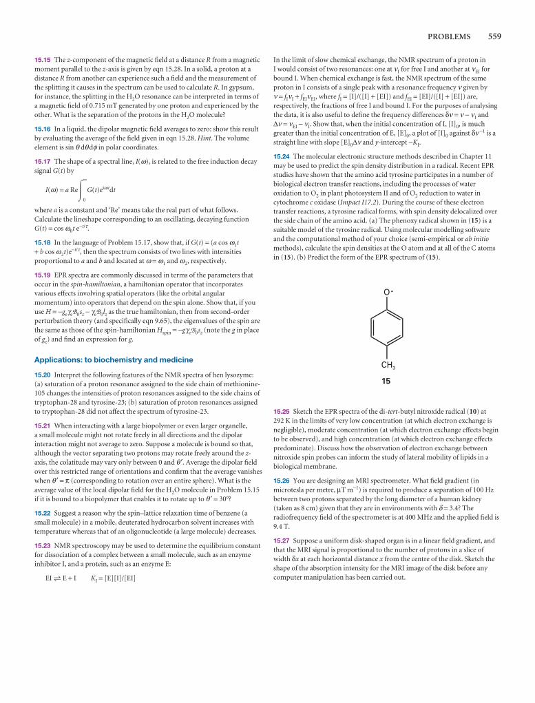
PROBLEMS 559
15.15 The z-component of the magnetic field at a distance R from a magneticmoment parallel to the z-axis is given by eqn 15.28. In a solid, a proton at adistance R from another can experience such a field and the measurement ofthe splitting it causes in the spectrum can be used to calculate R. In gypsum,for instance, the splitting in the H2O resonance can be interpreted in terms ofa magnetic field of 0.715 mT generated by one proton and experienced by theother. What is the separation of the protons in the H2O molecule?
15.16 In a liquid, the dipolar magnetic field averages to zero: show this resultby evaluating the average of the field given in eqn 15.28. Hint. The volumeelement is sin θ dθdφ in polar coordinates.
15.17 The shape of a spectral line, I(ω), is related to the free induction decaysignal G(t) by
I(ω) = a Re�∞
0
G(t)eiωtdt
where a is a constant and ‘Re’ means take the real part of what follows.Calculate the lineshape corresponding to an oscillating, decaying functionG(t) = cos ω0t e−t/τ.
15.18 In the language of Problem 15.17, show that, if G(t) = (a cos ω1t+ b cos ω2t)e−t/τ, then the spectrum consists of two lines with intensitiesproportional to a and b and located at ω = ω1 and ω2, respectively.
15.19 EPR spectra are commonly discussed in terms of the parameters thatoccur in the spin-hamiltonian, a hamiltonian operator that incorporatesvarious effects involving spatial operators (like the orbital angularmomentum) into operators that depend on the spin alone. Show that, if youuse H = −geγeB0sz − γeB0lz as the true hamiltonian, then from second-orderperturbation theory (and specifically eqn 9.65), the eigenvalues of the spin arethe same as those of the spin-hamiltonian Hspin = −gγeB0sz (note the g in placeof ge) and find an expression for g.
Applications: to biochemistry and medicine
15.20 Interpret the following features of the NMR spectra of hen lysozyme:(a) saturation of a proton resonance assigned to the side chain of methionine-105 changes the intensities of proton resonances assigned to the side chains oftryptophan-28 and tyrosine-23; (b) saturation of proton resonances assignedto tryptophan-28 did not affect the spectrum of tyrosine-23.
15.21 When interacting with a large biopolymer or even larger organelle, a small molecule might not rotate freely in all directions and the dipolarinteraction might not average to zero. Suppose a molecule is bound so that,although the vector separating two protons may rotate freely around the z-axis, the colatitude may vary only between 0 and θ′. Average the dipolar fieldover this restricted range of orientations and confirm that the average vanisheswhen θ′ = π (corresponding to rotation over an entire sphere). What is theaverage value of the local dipolar field for the H2O molecule in Problem 15.15if it is bound to a biopolymer that enables it to rotate up to θ′ = 30°?
15.22 Suggest a reason why the spin–lattice relaxation time of benzene (asmall molecule) in a mobile, deuterated hydrocarbon solvent increases withtemperature whereas that of an oligonucleotide (a large molecule) decreases.
15.23 NMR spectroscopy may be used to determine the equilibrium constantfor dissociation of a complex between a small molecule, such as an enzymeinhibitor I, and a protein, such as an enzyme E:
EI 5 E + I KI = [E][I]/[EI]
In the limit of slow chemical exchange, the NMR spectrum of a proton in I would consist of two resonances: one at νI for free I and another at νEI forbound I. When chemical exchange is fast, the NMR spectrum of the sameproton in I consists of a single peak with a resonance frequency ν given by ν = fIνI + fEIνEI, where fI = [I]/([I] + [EI]) and fEI = [EI]/([I] + [EI]) are,respectively, the fractions of free I and bound I. For the purposes of analysingthe data, it is also useful to define the frequency differences δν = ν − νI and∆ν = νEI − νI. Show that, when the initial concentration of I, [I]0, is muchgreater than the initial concentration of E, [E]0, a plot of [I]0 against δν−1 is astraight line with slope [E]0∆ν and y-intercept −KI.
15.24 The molecular electronic structure methods described in Chapter 11may be used to predict the spin density distribution in a radical. Recent EPRstudies have shown that the amino acid tyrosine participates in a number ofbiological electron transfer reactions, including the processes of wateroxidation to O2 in plant photosystem II and of O2 reduction to water incytochrome c oxidase (Impact I17.2). During the course of these electrontransfer reactions, a tyrosine radical forms, with spin density delocalized overthe side chain of the amino acid. (a) The phenoxy radical shown in (15) is asuitable model of the tyrosine radical. Using molecular modelling softwareand the computational method of your choice (semi-empirical or ab initiomethods), calculate the spin densities at the O atom and at all of the C atomsin (15). (b) Predict the form of the EPR spectrum of (15).
15.25 Sketch the EPR spectra of the di-tert-butyl nitroxide radical (10) at 292 K in the limits of very low concentration (at which electron exchange isnegligible), moderate concentration (at which electron exchange effects beginto be observed), and high concentration (at which electron exchange effectspredominate). Discuss how the observation of electron exchange betweennitroxide spin probes can inform the study of lateral mobility of lipids in abiological membrane.
15.26 You are designing an MRI spectrometer. What field gradient (inmicrotesla per metre, µT m−1) is required to produce a separation of 100 Hzbetween two protons separated by the long diameter of a human kidney(taken as 8 cm) given that they are in environments with δ = 3.4? Theradiofrequency field of the spectrometer is at 400 MHz and the applied field is9.4 T.
15.27 Suppose a uniform disk-shaped organ is in a linear field gradient, andthat the MRI signal is proportional to the number of protons in a slice ofwidth δx at each horizontal distance x from the centre of the disk. Sketch theshape of the absorption intensity for the MRI image of the disk before anycomputer manipulation has been carried out.
Statisticalthermodynamics 1:the conceptsStatistical thermodynamics provides the link between the microscopic properties of matterand its bulk properties. Two key ideas are introduced in this chapter. The first is the Boltzmanndistribution, which is used to predict the populations of states in systems at thermal equilibrium. In this chapter we see its derivation in terms of the distribution of particles overavailable states. The derivation leads naturally to the introduction of the partition function,which is the central mathematical concept of this and the next chapter. We see how to interpret the partition function and how to calculate it in a number of simple cases. We thensee how to extract thermodynamic information from the partition function. In the final part of the chapter, we generalize the discussion to include systems that are composed of assemblies of interacting particles. Very similar equations are developed to those in the firstpart of the chapter, but they are much more widely applicable.
The preceding chapters of this part of the text have shown how the energy levels of molecules can be calculated, determined spectroscopically, and related to theirstructures. The next major step is to see how a knowledge of these energy levels can be used to account for the properties of matter in bulk. To do so, we now introducethe concepts of statistical thermodynamics, the link between individual molecularproperties and bulk thermodynamic properties.
The crucial step in going from the quantum mechanics of individual molecules to the thermodynamics of bulk samples is to recognize that the latter deals with the average behaviour of large numbers of molecules. For example, the pressure of a gasdepends on the average force exerted by its molecules, and there is no need to specifywhich molecules happen to be striking the wall at any instant. Nor is it necessary toconsider the fluctuations in the pressure as different numbers of molecules collidewith the wall at different moments. The fluctuations in pressure are very small com-pared with the steady pressure: it is highly improbable that there will be a sudden lullin the number of collisions, or a sudden surge. Fluctuations in other thermodynamicproperties also occur, but for large numbers of particles they are negligible comparedto the mean values.
This chapter introduces statistical thermodynamics in two stages. The first, thederivation of the Boltzmann distribution for individual particles, is of restricted applicability, but it has the advantage of taking us directly to a result of central import-ance in a straightforward and elementary way. We can use statistical thermodynamicsonce we have deduced the Boltzmann distribution. Then (in Section 16.5) we extendthe arguments to systems composed of interacting particles.
The distribution of molecularstates
16.1 Configurations and weights
16.2 The molecular partitionfunction
I16.1 Impact on biochemistry: The helix–coil transition inpolypeptides
The internal energy and the entropy
16.3 The internal energy
16.4 The statistical entropy
The canonical partition function
16.5 The canonical ensemble
16.6 The thermodynamicinformation in the partitionfunction
16.7 Independent molecules
Checklist of key ideas
Further reading
Further information 16.1: The Boltzmann distribution
Further information 16.2: The Boltzmann formula
Further information 16.3:Temperatures below zero
Discussion questions
Exercises
Problems
16
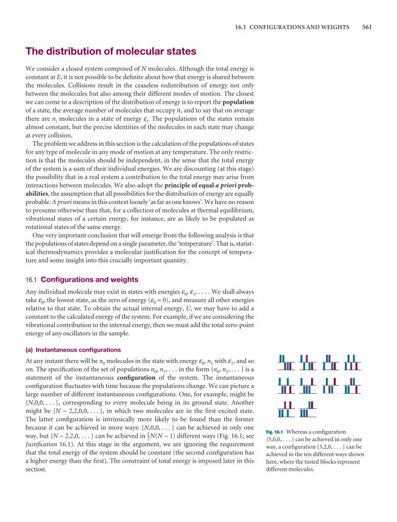
16.1 CONFIGURATIONS AND WEIGHTS 561
The distribution of molecular states
We consider a closed system composed of N molecules. Although the total energy isconstant at E, it is not possible to be definite about how that energy is shared betweenthe molecules. Collisions result in the ceaseless redistribution of energy not only between the molecules but also among their different modes of motion. The closestwe can come to a description of the distribution of energy is to report the populationof a state, the average number of molecules that occupy it, and to say that on averagethere are ni molecules in a state of energy εi. The populations of the states remainalmost constant, but the precise identities of the molecules in each state may changeat every collision.
The problem we address in this section is the calculation of the populations of statesfor any type of molecule in any mode of motion at any temperature. The only restric-tion is that the molecules should be independent, in the sense that the total energy of the system is a sum of their individual energies. We are discounting (at this stage)the possibility that in a real system a contribution to the total energy may arise frominteractions between molecules. We also adopt the principle of equal a priori prob-abilities, the assumption that all possibilities for the distribution of energy are equallyprobable. A priori means in this context loosely ‘as far as one knows’. We have no reasonto presume otherwise than that, for a collection of molecules at thermal equilibrium,vibrational states of a certain energy, for instance, are as likely to be populated as rotational states of the same energy.
One very important conclusion that will emerge from the following analysis is thatthe populations of states depend on a single parameter, the ‘temperature’. That is, statist-ical thermodynamics provides a molecular justification for the concept of tempera-ture and some insight into this crucially important quantity.
16.1 Configurations and weights
Any individual molecule may exist in states with energies ε0, ε1, . . . . We shall alwaystake ε0, the lowest state, as the zero of energy (ε0 = 0), and measure all other energiesrelative to that state. To obtain the actual internal energy, U, we may have to add aconstant to the calculated energy of the system. For example, if we are considering thevibrational contribution to the internal energy, then we must add the total zero-pointenergy of any oscillators in the sample.
(a) Instantaneous configurations
At any instant there will be n0 molecules in the state with energy ε0, n1 with ε1, and soon. The specification of the set of populations n0, n1, . . . in the form {n0, n1, . . . } is astatement of the instantaneous configuration of the system. The instantaneousconfiguration fluctuates with time because the populations change. We can picture alarge number of different instantaneous configurations. One, for example, might be{N,0,0, . . . }, corresponding to every molecule being in its ground state. Anothermight be {N − 2,2,0,0, . . . }, in which two molecules are in the first excited state. The latter configuration is intrinsically more likely to be found than the former because it can be achieved in more ways: {N,0,0, . . . } can be achieved in only one way, but {N − 2,2,0, . . . } can be achieved in 1–2N(N − 1) different ways (Fig. 16.1; seeJustification 16.1). At this stage in the argument, we are ignoring the requirement that the total energy of the system should be constant (the second configuration has a higher energy than the first). The constraint of total energy is imposed later in this section.
Fig. 16.1 Whereas a configuration {5,0,0, . . . } can be achieved in only oneway, a configuration {3,2,0, . . . } can beachieved in the ten different ways shownhere, where the tinted blocks representdifferent molecules.
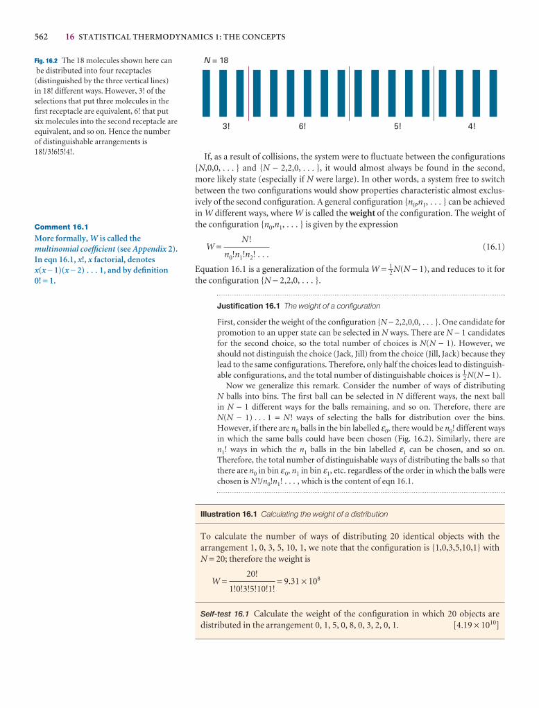
562 16 STATISTICAL THERMODYNAMICS 1: THE CONCEPTS
Comment 16.1
More formally, W is called themultinomial coefficient (see Appendix 2).In eqn 16.1, x!, x factorial, denotes x(x − 1)(x − 2) . . . 1, and by definition 0! = 1.
3! 6! 5! 4!
N = 18Fig. 16.2 The 18 molecules shown here canbe distributed into four receptacles(distinguished by the three vertical lines) in 18! different ways. However, 3! of theselections that put three molecules in thefirst receptacle are equivalent, 6! that putsix molecules into the second receptacle areequivalent, and so on. Hence the numberof distinguishable arrangements is18!/3!6!5!4!.
If, as a result of collisions, the system were to fluctuate between the configurations{N,0,0, . . . } and {N − 2,2,0, . . . }, it would almost always be found in the second,more likely state (especially if N were large). In other words, a system free to switch between the two configurations would show properties characteristic almost exclus-ively of the second configuration. A general configuration {n0,n1, . . . } can be achievedin W different ways, where W is called the weight of the configuration. The weight ofthe configuration {n0,n1, . . . } is given by the expression
W = (16.1)
Equation 16.1 is a generalization of the formula W = 1–2 N(N − 1), and reduces to it forthe configuration {N − 2,2,0, . . . }.
Justification 16.1 The weight of a configuration
First, consider the weight of the configuration {N − 2,2,0,0, . . . }. One candidate forpromotion to an upper state can be selected in N ways. There are N − 1 candidatesfor the second choice, so the total number of choices is N(N − 1). However, weshould not distinguish the choice (Jack, Jill) from the choice (Jill, Jack) because theylead to the same configurations. Therefore, only half the choices lead to distinguish-able configurations, and the total number of distinguishable choices is 1–2 N(N − 1).
Now we generalize this remark. Consider the number of ways of distributing N balls into bins. The first ball can be selected in N different ways, the next ball in N − 1 different ways for the balls remaining, and so on. Therefore, there are N(N − 1) . . . 1 = N! ways of selecting the balls for distribution over the bins.However, if there are n0 balls in the bin labelled ε0, there would be n0! different waysin which the same balls could have been chosen (Fig. 16.2). Similarly, there are n1! ways in which the n1 balls in the bin labelled ε1 can be chosen, and so on.Therefore, the total number of distinguishable ways of distributing the balls so thatthere are n0 in bin ε0, n1 in bin ε1, etc. regardless of the order in which the balls werechosen is N!/n0!n1! . . . , which is the content of eqn 16.1.
Illustration 16.1 Calculating the weight of a distribution
To calculate the number of ways of distributing 20 identical objects with the arrangement 1, 0, 3, 5, 10, 1, we note that the configuration is {1,0,3,5,10,1} with N = 20; therefore the weight is
W = = 9.31 × 10⁸
Self-test 16.1 Calculate the weight of the configuration in which 20 objects are distributed in the arrangement 0, 1, 5, 0, 8, 0, 3, 2, 0, 1. [4.19 × 10¹⁰]
20!
1!0!3!5!10!1!
N!
n0!n1!n2! . . .
16.1 CONFIGURATIONS AND WEIGHTS 563
It will turn out to be more convenient to deal with the natural logarithm of theweight, ln W, rather than with the weight itself. We shall therefore need the expression
ln W = ln = ln N! − ln(n0!n1!n2! · · · )
= ln N! − (ln n0! + ln n1! + ln n2! + · · · )
= ln N! − ∑i
ln ni!
where in the first line we have used ln(x/y) = ln x − ln y and in the second ln xy = ln x+ ln y. One reason for introducing ln W is that it is easier to make approximations. Inparticular, we can simplify the factorials by using Stirling’s approximation in the form
ln x! ≈ x ln x − x (16.2)
Then the approximate expression for the weight is
ln W = (N ln N − N) − ∑i
(ni ln ni − ni) = N ln N − ∑i
ni ln ni (16.3)
The final form of eqn 16.3 is derived by noting that the sum of ni is equal to N, so thesecond and fourth terms in the second expression cancel.
(b) The Boltzmann distribution
We have seen that the configuration {N − 2,2,0, . . . } dominates {N,0,0, . . . }, and itshould be easy to believe that there may be other configurations that have a muchgreater weight than both. We shall see, in fact, that there is a configuration with sogreat a weight that it overwhelms all the rest in importance to such an extent that thesystem will almost always be found in it. The properties of the system will therefore becharacteristic of that particular dominating configuration. This dominating config-uration can be found by looking for the values of ni that lead to a maximum value of W.Because W is a function of all the ni, we can do this search by varying the ni and look-ing for the values that correspond to dW = 0 (just as in the search for the maximum ofany function), or equivalently a maximum value of ln W. However, there are twodifficulties with this procedure.
The first difficulty is that the only permitted configurations are those correspond-ing to the specified, constant, total energy of the system. This requirement rules outmany configurations; {N,0,0, . . . } and {N − 2,2,0, . . . }, for instance, have differentenergies, so both cannot occur in the same isolated system. It follows that, in lookingfor the configuration with the greatest weight, we must ensure that the configurationalso satisfies the condition
Constant total energy: ∑i
ni εi = E (16.4)
where E is the total energy of the system.The second constraint is that, because the total number of molecules present is
also fixed (at N), we cannot arbitrarily vary all the populations simultaneously. Thus, increasing the population of one state by 1 demands that the population of anotherstate must be reduced by 1. Therefore, the search for the maximum value of W is alsosubject to the condition
Constant total number of molecules: ∑i
ni = N (16.5)
We show in Further information 16.1 that the populations in the configuration ofgreatest weight, subject to the two constraints in eqns 16.4 and 16.5, depend on the energy of the state according to the Boltzmann distribution:
N!
n0!n1!n2! . . .
Comment 16.2
A more accurate form of Stirling’sapproximation is
x! ≈ (2π)1/2xx+ 1–2 e−x
and is in error by less than 1 per centwhen x is greater than about 10. We dealwith far larger values of x, and thesimplified version in eqn 16.2 isadequate.
564 16 STATISTICAL THERMODYNAMICS 1: THE CONCEPTS
= (16.6a)
where ε0 ≤ ε1 ≤ ε2 . . . . Equation 16.6a is the justification of the remark that a single parameter, here denoted β, determines the most probable populations of the states ofthe system. We shall see in Section 16.3b that
β = (16.6b)
where T is the thermodynamic temperature and k is Boltzmann’s constant. In otherwords, the thermodynamic temperature is the unique parameter that governs the mostprobable populations of states of a system at thermal equilibrium. In Further information16.3, moreover, we see that β is a more natural measure of temperature than T itself.
16.2 The molecular partition function
From now on we write the Boltzmann distribution as
pi = (16.7)
where pi is the fraction of molecules in the state i, pi = ni /N, and q is the molecularpartition function:
q = ∑i
e−βεi [16.8]
The sum in q is sometimes expressed slightly differently. It may happen that several stateshave the same energy, and so give the same contribution to the sum. If, for example,gi states have the same energy εi (so the level is gi-fold degenerate), we could write
q = ∑levels i
gi e−βεi (16.9)
where the sum is now over energy levels (sets of states with the same energy), not individual states.
Example 16.1 Writing a partition function
Write an expression for the partition function of a linear molecule (such as HCl)treated as a rigid rotor.
Method To use eqn 16.9 we need to know (a) the energies of the levels, (b) the degeneracies, the number of states that belong to each level. Whenever calculatinga partition function, the energies of the levels are expressed relative to 0 for the stateof lowest energy. The energy levels of a rigid linear rotor were derived in Section 13.5c.
Answer From eqn 13.31, the energy levels of a linear rotor are hcBJ( J + 1), with J = 0, 1, 2, . . . . The state of lowest energy has zero energy, so no adjustment needbe made to the energies given by this expression. Each level consists of 2J + 1degenerate states. Therefore,
gJ εJ
q =∞
∑J=0
(2J + 1)e−βhcBJ(J+1)
The sum can be evaluated numerically by supplying the value of B (from spectro-scopy or calculation) and the temperature. For reasons explained in Section 17.2b,
5 6 75 6 7e−βεi
q
1
kT
e−βεi
∑i
e−βεi
ni
N
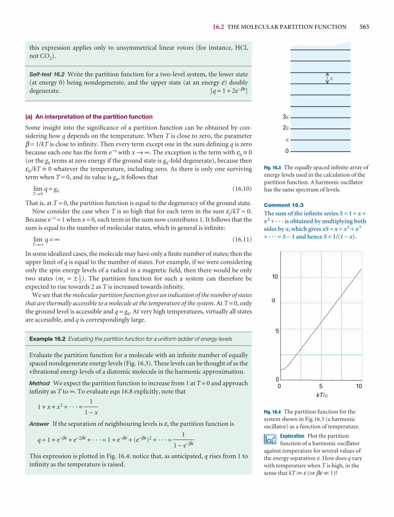
16.2 THE MOLECULAR PARTITION FUNCTION 565
0
e
2
3
e
e
e
Fig. 16.3 The equally spaced infinite array ofenergy levels used in the calculation of thepartition function. A harmonic oscillatorhas the same spectrum of levels.
0 5 10
10
5
0
q
kT/�
Fig. 16.4 The partition function for thesystem shown in Fig.16.3 (a harmonicoscillator) as a function of temperature.
Exploration Plot the partitionfunction of a harmonic oscillator
against temperature for several values ofthe energy separation ε. How does q varywith temperature when T is high, in thesense that kT >> ε (or βε << 1)?
Comment 16.3
The sum of the infinite series S = 1 + x +x2 + · · · is obtained by multiplying bothsides by x, which gives xS = x + x2 + x3
+ · · · = S − 1 and hence S = 1/(1 − x).
this expression applies only to unsymmetrical linear rotors (for instance, HCl, not CO2).
Self-test 16.2 Write the partition function for a two-level system, the lower state(at energy 0) being nondegenerate, and the upper state (at an energy ε) doubly degenerate. [q = 1 + 2e−βε]
(a) An interpretation of the partition function
Some insight into the significance of a partition function can be obtained by con-sidering how q depends on the temperature. When T is close to zero, the parameter β = 1/kT is close to infinity. Then every term except one in the sum defining q is zerobecause each one has the form e−x with x → ∞. The exception is the term with ε0 ≡ 0(or the g0 terms at zero energy if the ground state is g0-fold degenerate), because thenε0 /kT ≡ 0 whatever the temperature, including zero. As there is only one survivingterm when T = 0, and its value is g0, it follows that
limT→0
q = g0 (16.10)
That is, at T = 0, the partition function is equal to the degeneracy of the ground state.Now consider the case when T is so high that for each term in the sum εj/kT ≈ 0.
Because e−x = 1 when x = 0, each term in the sum now contributes 1. It follows that thesum is equal to the number of molecular states, which in general is infinite:
limT→∞
q = ∞ (16.11)
In some idealized cases, the molecule may have only a finite number of states; then theupper limit of q is equal to the number of states. For example, if we were consideringonly the spin energy levels of a radical in a magnetic field, then there would be onlytwo states (ms = ± 1–2 ). The partition function for such a system can therefore be expected to rise towards 2 as T is increased towards infinity.
We see that the molecular partition function gives an indication of the number of statesthat are thermally accessible to a molecule at the temperature of the system. At T = 0, onlythe ground level is accessible and q = g0. At very high temperatures, virtually all statesare accessible, and q is correspondingly large.
Example 16.2 Evaluating the partition function for a uniform ladder of energy levels
Evaluate the partition function for a molecule with an infinite number of equallyspaced nondegenerate energy levels (Fig. 16.3). These levels can be thought of as thevibrational energy levels of a diatomic molecule in the harmonic approximation.
Method We expect the partition function to increase from 1 at T = 0 and approachinfinity as T to ∞. To evaluate eqn 16.8 explicitly, note that
1 + x + x2 + · · · =
Answer If the separation of neighbouring levels is ε, the partition function is
q = 1 + e−βε + e−2βε + · · · = 1 + e−βε + (e−βε)2 + · · · =
This expression is plotted in Fig. 16.4: notice that, as anticipated, q rises from 1 toinfinity as the temperature is raised.
1
1 − e−βε
1
1 − x
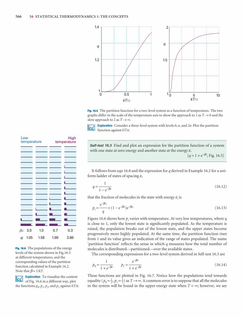
566 16 STATISTICAL THERMODYNAMICS 1: THE CONCEPTS
q
2
10 5 10
1.5
1.4
1.2
10 0.5 1
q
kT/ kT/� �
Fig. 16.5 The partition function for a two-level system as a function of temperature. The twographs differ in the scale of the temperature axis to show the approach to 1 as T → 0 and theslow approach to 2 as T → ∞.
Exploration Consider a three-level system with levels 0, ε, and 2ε. Plot the partitionfunction against kT/ε.
Lowtemperature
Hightemperature
�� 3.0 1.0 0.7 0.3
q: 1.05 1.58 1.99 3.86
5
Fig. 16.6 The populations of the energylevels of the system shown in Fig.16.3 at different temperatures, and thecorresponding values of the partitionfunction calculated in Example 16.2. Note that β = 1/kT.
Exploration To visualize the contentof Fig. 16.6 in a different way, plot
the functions p0, p1, p2, and p3 against kT/ε.
Self-test 16.3 Find and plot an expression for the partition function of a systemwith one state at zero energy and another state at the energy ε.
[q = 1 + e−βε, Fig. 16.5]
It follows from eqn 16.8 and the expression for q derived in Example 16.2 for a uni-form ladder of states of spacing ε,
q = (16.12)
that the fraction of molecules in the state with energy εi is
pi = = (1 − e−βε)e−βεi (16.13)
Figure 16.6 shows how pi varies with temperature. At very low temperatures, where qis close to 1, only the lowest state is significantly populated. As the temperature israised, the population breaks out of the lowest state, and the upper states become progressively more highly populated. At the same time, the partition function risesfrom 1 and its value gives an indication of the range of states populated. The name‘partition function’ reflects the sense in which q measures how the total number ofmolecules is distributed—partitioned—over the available states.
The corresponding expressions for a two-level system derived in Self-test 16.3 are
p0 = p1 = (16.14)
These functions are plotted in Fig. 16.7. Notice how the populations tend towardsequality (p0 = 1–2 , p1 = 1–2 ) as T → ∞. A common error is to suppose that all the moleculesin the system will be found in the upper energy state when T = ∞; however, we see
e−βε
1 + e−βε
1
1 + e−βε
e−βεi
q
1
1 − e−βε
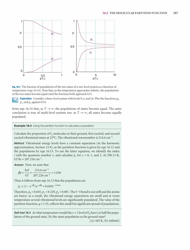
16.2 THE MOLECULAR PARTITION FUNCTION 567
00 0.5
0.5
1
1
p p0
p1
0
0.5
1
0 5 10
p
p0
p1
kT/ kT/� �
Fig. 16.7 The fraction of populations of the two states of a two-level system as a function oftemperature (eqn 16.14). Note that, as the temperature approaches infinity, the populationsof the two states become equal (and the fractions both approach 0.5).
Exploration Consider a three-level system with levels 0, ε, and 2ε. Plot the functions p0,p1, and p2 against kT/ε.
from eqn 16.14 that, as T → ∞, the populations of states become equal. The same conclusion is true of multi-level systems too: as T → ∞, all states become equally populated.
Example 16.3 Using the partition function to calculate a population
Calculate the proportion of I2 molecules in their ground, first excited, and secondexcited vibrational states at 25°C. The vibrational wavenumber is 214.6 cm−1.
Method Vibrational energy levels have a constant separation (in the harmonic approximation, Section 13.9), so the partition function is given by eqn 16.12 andthe populations by eqn 16.13. To use the latter equation, we identify the index i with the quantum number v, and calculate pv for v = 0, 1, and 2. At 298.15 K, kT/hc = 207.226 cm−1.
Answer First, we note that
βε = = = 1.036
Then it follows from eqn 16.13 that the populations are
pv = (1 − e−βε)e−vβε = 0.645e−1.036v
Therefore, p0 = 0.645, p1 = 0.229, p2 = 0.081. The I-I bond is not stiff and the atomsare heavy: as a result, the vibrational energy separations are small and at room temperature several vibrational levels are significantly populated. The value of thepartition function, q = 1.55, reflects this small but significant spread of populations.
Self-test 16.4 At what temperature would the v = 1 level of I2 have (a) half the popu-lation of the ground state, (b) the same population as the ground state?
[(a) 445 K, (b) infinite]
214.6 cm−1
207.226 cm−1
hc#
kT
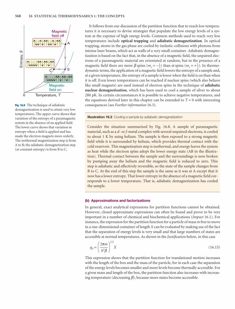
568 16 STATISTICAL THERMODYNAMICS 1: THE CONCEPTS
Magneticfield on
Magneticfield off
Entr
opy,
S
A
BC
Temperature, T0
Fig. 16.8 The technique of adiabaticdemagnetization is used to attain very lowtemperatures. The upper curve shows thatvariation of the entropy of a paramagneticsystem in the absence of an applied field.The lower curve shows that variation inentropy when a field is applied and hasmade the electron magnets more orderly.The isothermal magnetization step is fromA to B; the adiabatic demagnetization step(at constant entropy) is from B to C.
It follows from our discussion of the partition function that to reach low tempera-tures it is necessary to devise strategies that populate the low energy levels of a sys-tem at the expense of high energy levels. Common methods used to reach very low temperatures include optical trapping and adiabatic demagnetization. In opticaltrapping, atoms in the gas phase are cooled by inelastic collisions with photons fromintense laser beams, which act as walls of a very small container. Adiabatic demagne-tization is based on the fact that, in the absence of a magnetic field, the unpaired elec-trons of a paramagnetic material are orientated at random, but in the presence of amagnetic field there are more β spins (ms = − 1–2) than α spins (ms = + 1–2). In thermo-dynamic terms, the application of a magnetic field lowers the entropy of a sample and,at a given temperature, the entropy of a sample is lower when the field is on than whenit is off. Even lower temperatures can be reached if nuclear spins (which also behavelike small magnets) are used instead of electron spins in the technique of adiabaticnuclear demagnetization, which has been used to cool a sample of silver to about 280 pK. In certain circumstances it is possible to achieve negative temperatures, andthe equations derived later in this chapter can be extended to T < 0 with interestingconsequences (see Further information 16.3).
Illustration 16.2 Cooling a sample by adiabatic demagnetization
Consider the situation summarized by Fig. 16.8. A sample of paramagnetic material, such as a d- or f-metal complex with several unpaired electrons, is cooledto about 1 K by using helium. The sample is then exposed to a strong magnetic field while it is surrounded by helium, which provides thermal contact with thecold reservoir. This magnetization step is isothermal, and energy leaves the systemas heat while the electron spins adopt the lower energy state (AB in the illustra-tion). Thermal contact between the sample and the surroundings is now broken by pumping away the helium and the magnetic field is reduced to zero. This step is adiabatic and effectively reversible, so the state of the sample changes fromB to C. At the end of this step the sample is the same as it was at A except that it now has a lower entropy. That lower entropy in the absence of a magnetic field cor-responds to a lower temperature. That is, adiabatic demagnetization has cooled the sample.
(b) Approximations and factorizations
In general, exact analytical expressions for partition functions cannot be obtained.However, closed approximate expressions can often be found and prove to be veryimportant in a number of chemical and biochemical applications (Impact 16.1). Forinstance, the expression for the partition function for a particle of mass m free to movein a one-dimensional container of length X can be evaluated by making use of the factthat the separation of energy levels is very small and that large numbers of states areaccessible at normal temperatures. As shown in the Justification below, in this case
qX = 1/2
X (16.15)
This expression shows that the partition function for translational motion increaseswith the length of the box and the mass of the particle, for in each case the separationof the energy levels becomes smaller and more levels become thermally accessible. Fora given mass and length of the box, the partition function also increases with increas-ing temperature (decreasing β), because more states become accessible.
DF
2πm
h2β
AC
16.2 THE MOLECULAR PARTITION FUNCTION 569
Justification 16.2 The partition function for a particle in a one-dimensional box
The energy levels of a molecule of mass m in a container of length X are given by eqn 9.4a with L = X:
En = n = 1, 2, . . .
The lowest level (n = 1) has energy h2/8mX 2, so the energies relative to that level are
εn = (n2 − 1)ε ε = h2/8mX 2
The sum to evaluate is therefore
qX = ∞
∑n=1
e−(n2−1)βε
The translational energy levels are very close together in a container the size of a typ-ical laboratory vessel; therefore, the sum can be approximated by an integral:
qX = �∞
1
e−(n2−1)βεdn ≈ �∞
0
e−n2βεdn
The extension of the lower limit to n = 0 and the replacement of n2 − 1 by n2 intro-duces negligible error but turns the integral into standard form. We make thesubstitution x 2 = n2βε, implying dn = dx /(βε)1/2, and therefore that
π1/2/2
qX =1/2
�∞
0
e−x2dx =
1/2
=1/2
X
Another useful feature of partition functions is used to derive expressions when theenergy of a molecule arises from several different, independent sources: if the energyis a sum of contributions from independent modes of motion, then the partitionfunction is a product of partition functions for each mode of motion. For instance,suppose the molecule we are considering is free to move in three dimensions. We takethe length of the container in the y-direction to be Y and that in the z-direction to beZ. The total energy of a molecule ε is the sum of its translational energies in all threedirections:
εn1n2n3= εn1
(X) + εn2
(Y) + εn3
(Z) (16.16)
where n1, n2, and n3 are the quantum numbers for motion in the x-, y-, and z-directions,respectively. Therefore, because ea+b+c = eaebec, the partition function factorizes as follows:
q = ∑all n
e−βε n1
(X)−βε n2
(Y)−βε n3
(Z ) = ∑all n
e−βε n1
(X)e−βε n2
(Y)e−βε n3
(Z)
= ∑∑n1
e−βε n1
(X) ∑n2
e−βε n2
(Y) ∑n3
e−βε n3
(Z)(16.17)
= qX qY qZ
It is generally true that, if the energy of a molecule can be written as the sum of inde-pendent terms, then the partition function is the corresponding product of individualcontributions.
DF
AC
DF
AC
DF
AC
DEF2πm
h2βABC
DEFπ1/2
2
ABCDEF
1
βεABC
DEF1
βεABC
5 6 7
n2h2
8mX 2
570 16 STATISTICAL THERMODYNAMICS 1: THE CONCEPTS
Equation 16.15 gives the partition function for translational motion in the x-direction. The only change for the other two directions is to replace the length X by thelengths Y or Z. Hence the partition function for motion in three dimensions is
q =3/2
XYZ (16.18)
The product of lengths XYZ is the volume, V, of the container, so we can write
q = Λ = h
1/2
= (16.19)
The quantity Λ has the dimensions of length and is called the thermal wavelength(sometimes the thermal de Broglie wavelength) of the molecule. The thermal wave-length decreases with increasing mass and temperature. As in the one-dimensionalcase, the partition function increases with the mass of the particle (as m3/2) and thevolume of the container (as V); for a given mass and volume, the partition functionincreases with temperature (as T3/2).
Illustration 16.3 Calculating the translational partition function
To calculate the translational partition function of an H2 molecule confined to a100 cm3 vessel at 25°C we use m = 2.016 u; then
Λ =
= 7.12 × 10⁻¹¹ m
where we have used 1 J = 1 kg m2 s−2. Therefore,
q = = 2.77 × 1026
About 1026 quantum states are thermally accessible, even at room temperature andfor this light molecule. Many states are occupied if the thermal wavelength (whichin this case is 71.2 pm) is small compared with the linear dimensions of the container.
Self-test 16.5 Calculate the translational partition function for a D2 moleculeunder the same conditions. [q = 7.8 × 1026, 23/2 times larger]
The validity of the approximations that led to eqn 16.19 can be expressed in termsof the average separation of the particles in the container, d. We do not have to worryabout the role of the Pauli principle on the occupation of states if there are many statesavailable for each molecule. Because q is the total number of accessible states, theaverage number of states per molecule is q/N. For this quantity to be large, we requireV/NΛ3 >> 1. However, V/N is the volume occupied by a single particle, and there-fore the average separation of the particles is d = (V/N)1/3. The condition for therebeing many states available per molecule is therefore d3/Λ3 >> 1, and therefore d >> Λ.That is, for eqn 16.19 to be valid, the average separation of the particles must be muchgreater than their thermal wavelength. For H2 molecules at 1 bar and 298 K, the aver-age separation is 3 nm, which is significantly larger than their thermal wavelength(71.2 pm, Illustration 16.3).
1.00 × 10⁻⁴ m3
(7.12 × 10⁻¹¹ m)3
6.626 × 10⁻³⁴ J s
{2π × (2.016 × 1.6605 × 10−27 kg) × (1.38 × 10⁻²³ J K−1) × (298 K)}1/2
h
(2πmkT)1/2
DF
β2πm
AC
V
Λ3
DF
2πm
h2β
AC
I16.1 IMPACT ON BIOCHEMISTRY: THE HELIX–COIL TRANSITION IN POLYPEPTIDES 571
IMPACT ON BIOCHEMISTRY
I16.1 The helix–coil transition in polypeptides
Proteins are polymers that attain well defined three-dimensional structures both insolution and in biological cells. They are polypeptides formed from different aminoacids strung together by the peptide link, -CONH-. Hydrogen bonds between aminoacids of a polypeptide give rise to stable helical or sheet structures, which may collapseinto a random coil when certain conditions are changed. The unwinding of a helixinto a random coil is a cooperative transition, in which the polymer becomes increas-ingly more susceptible to structural changes once the process has begun. We examinehere a model grounded in the principles of statistical thermodynamics that accountsfor the cooperativity of the helix–coil transition in polypeptides.
To calculate the fraction of polypeptide molecules present as helix or coil we needto set up the partition function for the various states of the molecule. To illustrate theapproach, consider a short polypeptide with four amino acid residues, each labelled hif it contributes to a helical region and c if it contributes to a random coil region. Wesuppose that conformations hhhh and cccc contribute terms q0 and q4, respectively, tothe partition function q. Then we assume that each of the four conformations withone c amino acid (such as hchh) contributes q1. Similarly, each of the six states withtwo c amino acids contributes a term q2, and each of the four states with three c aminoacids contributes a term q3. The partition function is then
q = q0 + 4q1 + 6q2 + 4q3 + q4 = q0 1 + + + +
We shall now suppose that each partition function differs from q0 only by the energyof each conformation relative to hhhh, and write
= e−(εi−ε0)/kT
Next, we suppose that the conformational transformations are non-cooperative, inthe sense that the energy associated with changing one h amino acid into one c aminoacid has the same value regardless of how many h or c amino acid residues are in thereactant or product state and regardless of where in the chain the conversion occurs.That is, we suppose that the difference in energy between cih4−i and ci+1h3−i has thesame value γ for all i. This assumption implies that εi − ε0 = iγ and therefore that
q = q0(1 + 4s + 6s2 + 4s3 + s4) s = e−Γ/RT (16.20)
where Γ = NAγ and s is called the stability parameter. The term in parentheses has theform of the binomial expansion of (1 + s)4.
=4
∑i=0
C(4,i)si with C(4,i) = (16.21)
which we interpret as the number of ways in which a state with i c amino acids can beformed.
The extension of this treatment to take into account a longer chain of residues isnow straightforward: we simply replace the upper limit of 4 in the sum by n:
=n
∑i=0
C(n,i)si(16.22)
A cooperative transformation is more difficult to accommodate, and depends onbuilding a model of how neighbours facilitate each other’s conformational change. In
q
q0
4!
(4 − i)!i!
q
q0
qi
q0
DF
q4
q0
4q3
q0
6q2
q0
4q1
q0
AC
Comment 16.4
The binomial expansion of (1 + x)n is
(1 + x)n =n
∑i=0
C(n,i)xi,
with C(n,i) =n!
(n − i)!i!
572 16 STATISTICAL THERMODYNAMICS 1: THE CONCEPTS
the simple zipper model, conversion from h to c is allowed only if a residue adjacent tothe one undergoing the conversion is already a c residue. Thus, the zipper model allowsa transition of the type . . .hhhch. . . → . . .hhhcc. . . , but not a transition of the type. . .hhhch. . . → . . .hchch. . . . The only exception to this rule is, of course, the very first conversion from h to c in a fully helical chain. Cooperativity is included in the zipper model by assuming that the first conversion from h to c, called the nucleationstep, is less favourable than the remaining conversions and replacing s for that step byσs, where σ << 1. Each subsequent step is called a propagation step and has a stabilityparameter s. In Problem 16.24, you are invited to show that the partition function is:
q = 1 +n
∑i=1
Z(n,i)σsi(16.23)
where Z(n,i) is the number of ways in which a state with a number i of c amino acidscan be formed under the strictures of the zipper model. Because Z(n,i) = n − i + 1 (seeProblem 16.24),
q = 1 + σ(n + 1)n
∑i=1
si − σn
∑i=1
isi(16.24)
After evaluating both geometric series by using the two relationsn
∑i=1
xi =n
∑i=1
ixi = [nxn+1 − (n + 1)xn + 1]
we find
q = 1 +
The fraction pi = qi /q of molecules that has a number i of c amino acids is pi =[(n − i + 1)σsi]/q and the mean value of i is then �i� = ∑iipi. Figure 16.9 shows the dis-tribution of pi for various values of s with σ = 5.0 × 10⁻³. We see that most of thepolypeptide chains remain largely helical when s < 1 and that most of the chains existlargely as random coils when s > 1. When s = 1, there is a more widespread distribu-tion of length of random coil segments. Because the degree of conversion, θ, of apolypeptide with n amino acids to a random coil is defined as θ = �i�/n, it is possible toshow (see Problem 16.24) that
θ = ln q (16.25)
This is a general result that applies to any model of the helix–coil transition in whichthe partition function q is expressed as a function of the stability parameter s.
A more sophisticated model for the helix–coil transition must allow for helical seg-ments to form in different regions of a long polypeptide chain, with the nascent helicesbeing separated by shrinking coil segments. Calculations based on this more completeZimm–Bragg model give
θ = 1–2 1 + (16.26)
Figure 16.10 shows plots of θ against s for several values of σ. The curves show the sigmoidal shape characteristic of cooperative behaviour. There is a sudden surge oftransition to a random coil as s passes through 1 and, the smaller the parameter σ, thegreater the sharpness and hence the greater the cooperativity of the transition. That is,the harder it is to get coil formation started, the sharper the transition from helix to coil.
DF
(s − 1) + 2σ[(s − 1)2 + 4sσ]1/2
AC
d
d(ln s)
1
n
σs[sn+1 − (n + 1)sn + 1]
(s − 1)2
x
(x − 1)2
xn+1 − x
x − 105 10 15 20
0.05
0.1
0.15
pi
1
0.82
1.5
s
i0
Fig. 16.9 The distribution of pi, the fractionof molecules that has a number i of c aminoacids for s = 0.8 (�i� = 1.1), 1.0 (�i� = 3.8),and 1.5 (�i� = 15.9), with σ = 5.0 × 10⁻³.
( ,
)s
0 0.5 1 1.5 20
0.5
1
0.01
0.001
0.0001
s
�$
Fig. 16.10 Plots of the degree of conversionθ, against s for several values of σ. Thecurves show the sigmoidal shapecharacteristics of cooperative behaviour.
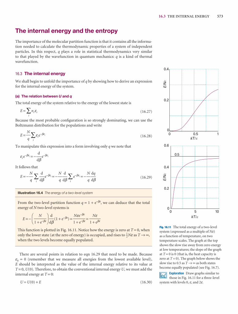
16.3 THE INTERNAL ENERGY 573
0 0.5 1
0.2
0.4
0
0 5 10
E/N
E/N
0
0.2
0.4
0.6
0.5
kT/
kT/
�
�
��
Fig. 16.11 The total energy of a two-level system (expressed as a multiple of Nε)as a function of temperature, on twotemperature scales. The graph at the topshows the slow rise away from zero energyat low temperatures; the slope of the graphat T = 0 is 0 (that is, the heat capacity is zero at T = 0). The graph below shows theslow rise to 0.5 as T → ∞ as both statesbecome equally populated (see Fig. 16.7).
Exploration Draw graphs similar tothose in Fig. 16.11 for a three-level
system with levels 0, ε, and 2ε.
The internal energy and the entropy
The importance of the molecular partition function is that it contains all the informa-tion needed to calculate the thermodynamic properties of a system of independentparticles. In this respect, q plays a role in statistical thermodynamics very similar to that played by the wavefunction in quantum mechanics: q is a kind of thermalwavefunction.
16.3 The internal energy
We shall begin to unfold the importance of q by showing how to derive an expressionfor the internal energy of the system.
(a) The relation between U and q
The total energy of the system relative to the energy of the lowest state is
E = ∑i
niεi (16.27)
Because the most probable configuration is so strongly dominating, we can use theBoltzmann distribution for the populations and write
E = ∑i
εie−βεi (16.28)
To manipulate this expression into a form involving only q we note that
εi e−βεi = − e−βεi
It follows that
E = − ∑i
e−βεi = − ∑i
e−βεi = − (16.29)
Illustration 16.4 The energy of a two-level system
From the two-level partition function q = 1 + e−βε, we can deduce that the total energy of N two-level systems is
E = − (1 + e−βε) = =
This function is plotted in Fig. 16.11. Notice how the energy is zero at T = 0, whenonly the lower state (at the zero of energy) is occupied, and rises to 1–2 Nε as T → ∞,when the two levels become equally populated.
There are several points in relation to eqn 16.29 that need to be made. Because ε0 = 0 (remember that we measure all energies from the lowest available level), E should be interpreted as the value of the internal energy relative to its value at T = 0, U(0). Therefore, to obtain the conventional internal energy U, we must add the internal energy at T = 0:
U = U(0) + E (16.30)
Nε1 + eβε
Nεe−βε
1 + e−βε
d
dβ
DF
N
1 + e−βε
AC
dq
dβN
q
d
dβN
q
d
dβN
q
d
dβ
N
q
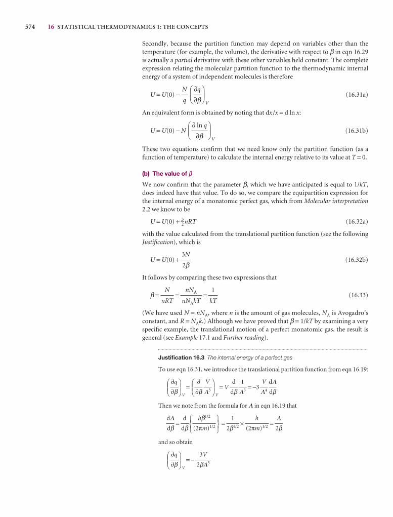
574 16 STATISTICAL THERMODYNAMICS 1: THE CONCEPTS
Secondly, because the partition function may depend on variables other than the temperature (for example, the volume), the derivative with respect to β in eqn 16.29is actually a partial derivative with these other variables held constant. The completeexpression relating the molecular partition function to the thermodynamic internalenergy of a system of independent molecules is therefore
U = U(0) −V
(16.31a)
An equivalent form is obtained by noting that dx /x = d ln x:
U = U(0) − NV
(16.31b)
These two equations confirm that we need know only the partition function (as afunction of temperature) to calculate the internal energy relative to its value at T = 0.
(b) The value of β
We now confirm that the parameter β, which we have anticipated is equal to 1/kT,does indeed have that value. To do so, we compare the equipartition expression forthe internal energy of a monatomic perfect gas, which from Molecular interpretation2.2 we know to be
U = U(0) + 3–2 nRT (16.32a)
with the value calculated from the translational partition function (see the followingJustification), which is
U = U(0) + (16.32b)
It follows by comparing these two expressions that
β = = = (16.33)
(We have used N = nNA, where n is the amount of gas molecules, NA is Avogadro’sconstant, and R = NAk.) Although we have proved that β = 1/kT by examining a veryspecific example, the translational motion of a perfect monatomic gas, the result isgeneral (see Example 17.1 and Further reading).
Justification 16.3 The internal energy of a perfect gas
To use eqn 16.31, we introduce the translational partition function from eqn 16.19:
V
=V
= V = −3
Then we note from the formula for Λ in eqn 16.19 that
= = × =
and so obtain
V
= −3V
2βΛ3
DEF∂q
∂βABC
Λ2β
h
(2πm)1/2
1
2β1/2
567hβ1/2
(2πm)1/2
123d
dβdΛdβ
dΛdβ
V
Λ4
1
Λ3
d
dβDEF
V
Λ3
∂∂β
ABCDEF
∂q
∂βABC
1
kT
nNA
nNAkT
N
nRT
3N
2β
DF
∂ ln q
∂β
AC
DF
∂q
∂β
AC
N
q
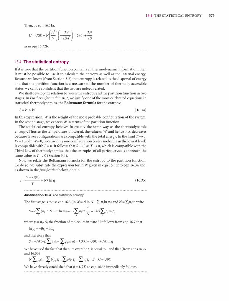
16.4 THE STATISTICAL ENTROPY 575
Then, by eqn 16.31a,
U = U(0) − N − = U(0) +
as in eqn 16.32b.
16.4 The statistical entropy
If it is true that the partition function contains all thermodynamic information, thenit must be possible to use it to calculate the entropy as well as the internal energy.Because we know (from Section 3.2) that entropy is related to the dispersal of energyand that the partition function is a measure of the number of thermally accessiblestates, we can be confident that the two are indeed related.
We shall develop the relation between the entropy and the partition function in twostages. In Further information 16.2, we justify one of the most celebrated equations instatistical thermodynamics, the Boltzmann formula for the entropy:
S = k ln W [16.34]
In this expression, W is the weight of the most probable configuration of the system.In the second stage, we express W in terms of the partition function.
The statistical entropy behaves in exactly the same way as the thermodynamic entropy. Thus, as the temperature is lowered, the value of W, and hence of S, decreasesbecause fewer configurations are compatible with the total energy. In the limit T → 0,W = 1, so ln W = 0, because only one configuration (every molecule in the lowest level)is compatible with E = 0. It follows that S → 0 as T → 0, which is compatible with theThird Law of thermodynamics, that the entropies of all perfect crystals approach thesame value as T → 0 (Section 3.4).
Now we relate the Boltzmann formula for the entropy to the partition function. To do so, we substitute the expression for ln W given in eqn 16.3 into eqn 16.34 and,as shown in the Justification below, obtain
S = + Nk ln q (16.35)
Justification 16.4 The statistical entropy
The first stage is to use eqn 16.3 (ln W = N ln N − ∑i ni ln ni) and N = ∑ini to write
S = k∑i
(ni ln N − ni ln ni) = −k∑i
ni ln = −Nk∑i
pi ln pi
where pi = ni /N, the fraction of molecules in state i. It follows from eqn 16.7 that
ln pi = −βεi − ln q
and therefore that
S = −Nk(−β∑i
piεi − ∑i
pi ln q) = kβ{U − U(0)} + Nk ln q
We have used the fact that the sum over the pi is equal to 1 and that (from eqns 16.27and 16.30)
N ∑i
piεi = ∑i
Npiεi = ∑i
Npiεi = ∑i
niεi = E = U − U(0)
We have already established that β = 1/kT, so eqn 16.35 immediately follows.
ni
N
U − U(0)
T
3N
2βDEF
3V
2βΛ3
ABCDEF
Λ3
V
ABC
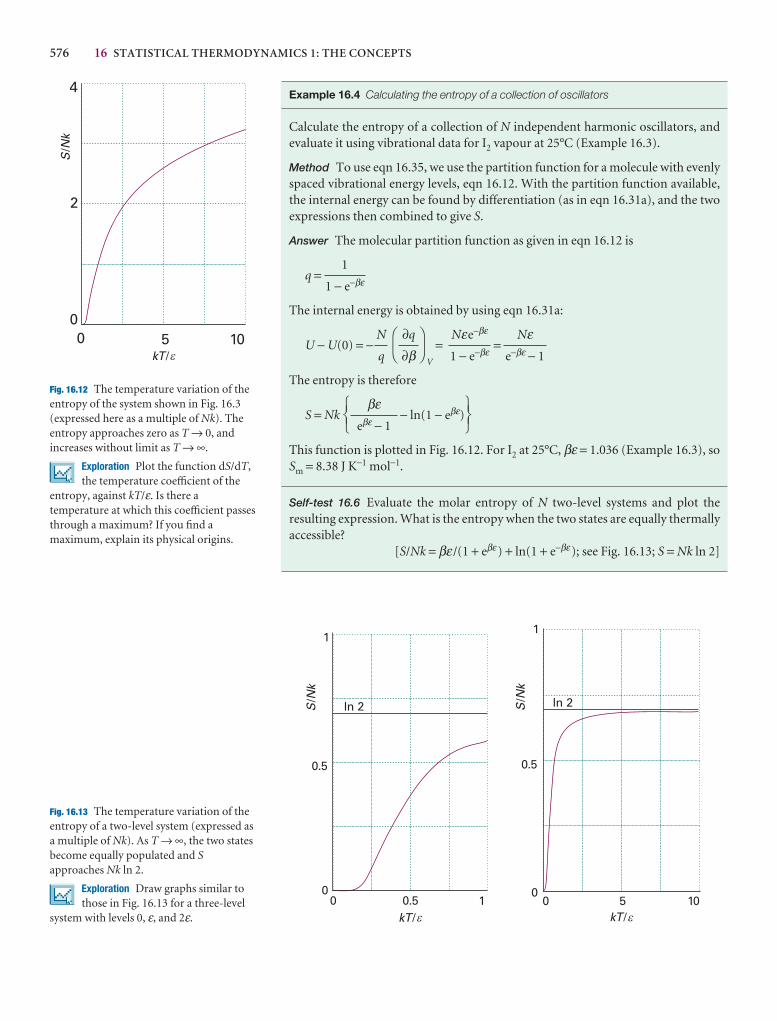
576 16 STATISTICAL THERMODYNAMICS 1: THE CONCEPTS
0 5 10
4
2
0
SN
k/
kT/�
Fig. 16.12 The temperature variation of theentropy of the system shown in Fig. 16.3(expressed here as a multiple of Nk). Theentropy approaches zero as T → 0, andincreases without limit as T → ∞.
Exploration Plot the function dS/dT,the temperature coefficient of the
entropy, against kT/ε. Is there atemperature at which this coefficient passesthrough a maximum? If you find amaximum, explain its physical origins.
00
0.5
0.5
1
1
SN
k/
0
0.5
1
0 5 10
SN
k/ ln 2ln 2
kT/ kT/� �
Fig. 16.13 The temperature variation of theentropy of a two-level system (expressed asa multiple of Nk). As T → ∞, the two statesbecome equally populated and Sapproaches Nk ln 2.
Exploration Draw graphs similar tothose in Fig. 16.13 for a three-level
system with levels 0, ε, and 2ε.
Example 16.4 Calculating the entropy of a collection of oscillators
Calculate the entropy of a collection of N independent harmonic oscillators, andevaluate it using vibrational data for I2 vapour at 25°C (Example 16.3).
Method To use eqn 16.35, we use the partition function for a molecule with evenlyspaced vibrational energy levels, eqn 16.12. With the partition function available,the internal energy can be found by differentiation (as in eqn 16.31a), and the twoexpressions then combined to give S.
Answer The molecular partition function as given in eqn 16.12 is
q =
The internal energy is obtained by using eqn 16.31a:
U − U(0) = −V
= =
The entropy is therefore
S = Nk − ln(1 − eβε)
This function is plotted in Fig. 16.12. For I2 at 25°C, βε = 1.036 (Example 16.3), soSm = 8.38 J K−1 mol−1.
Self-test 16.6 Evaluate the molar entropy of N two-level systems and plot the resulting expression. What is the entropy when the two states are equally thermallyaccessible?
[S/Nk = βε /(1 + eβε) + ln(1 + e−βε); see Fig. 16.13; S = Nk ln 2]
567βε
eβε − 1
123
Nεe−βε − 1
Nεe−βε
1 − e−βε
DF
∂q
∂β
AC
N
q
1
1 − e−βε
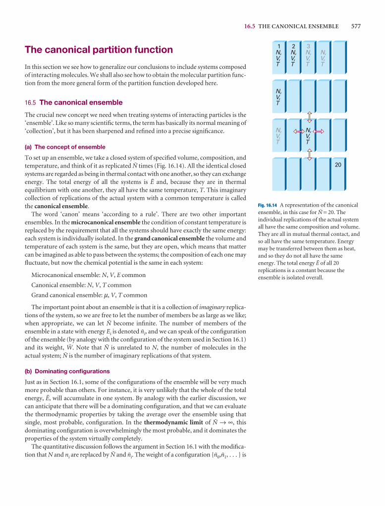
16.5 THE CANONICAL ENSEMBLE 577
The canonical partition function
In this section we see how to generalize our conclusions to include systems composedof interacting molecules. We shall also see how to obtain the molecular partition func-tion from the more general form of the partition function developed here.
16.5 The canonical ensemble
The crucial new concept we need when treating systems of interacting particles is the‘ensemble’. Like so many scientific terms, the term has basically its normal meaning of‘collection’, but it has been sharpened and refined into a precise significance.
(a) The concept of ensemble
To set up an ensemble, we take a closed system of specified volume, composition, andtemperature, and think of it as replicated Ñ times (Fig. 16.14). All the identical closedsystems are regarded as being in thermal contact with one another, so they can exchangeenergy. The total energy of all the systems is L and, because they are in thermal equilibrium with one another, they all have the same temperature, T. This imaginary collection of replications of the actual system with a common temperature is calledthe canonical ensemble.
The word ‘canon’ means ‘according to a rule’. There are two other important ensembles. In the microcanonical ensemble the condition of constant temperature isreplaced by the requirement that all the systems should have exactly the same energy:each system is individually isolated. In the grand canonical ensemble the volume andtemperature of each system is the same, but they are open, which means that mattercan be imagined as able to pass between the systems; the composition of each one mayfluctuate, but now the chemical potential is the same in each system:
Microcanonical ensemble: N, V, E common
Canonical ensemble: N, V, T common
Grand canonical ensemble: µ, V, T common
The important point about an ensemble is that it is a collection of imaginary replica-tions of the system, so we are free to let the number of members be as large as we like;when appropriate, we can let Ñ become infinite. The number of members of the ensemble in a state with energy Ei is denoted ñi, and we can speak of the configurationof the ensemble (by analogy with the configuration of the system used in Section 16.1)and its weight, M. Note that Ñ is unrelated to N, the number of molecules in the actual system; Ñ is the number of imaginary replications of that system.
(b) Dominating configurations
Just as in Section 16.1, some of the configurations of the ensemble will be very muchmore probable than others. For instance, it is very unlikely that the whole of the totalenergy, L, will accumulate in one system. By analogy with the earlier discussion, wecan anticipate that there will be a dominating configuration, and that we can evaluatethe thermodynamic properties by taking the average over the ensemble using that single, most probable, configuration. In the thermodynamic limit of Ñ → ∞, thisdominating configuration is overwhelmingly the most probable, and it dominates theproperties of the system virtually completely.
The quantitative discussion follows the argument in Section 16.1 with the modifica-tion that N and ni are replaced by Ñ and ñi. The weight of a configuration {ñ0,ñ1, . . . } is
N,V,T
N,V,T
20
N,V,T
N,V,T
N,V,T
N,V,T
N,V,T
1 2 3
Fig. 16.14 A representation of the canonicalensemble, in this case for Ñ = 20. Theindividual replications of the actual systemall have the same composition and volume.They are all in mutual thermal contact, andso all have the same temperature. Energymay be transferred between them as heat,and so they do not all have the sameenergy. The total energy L of all 20replications is a constant because theensemble is isolated overall.
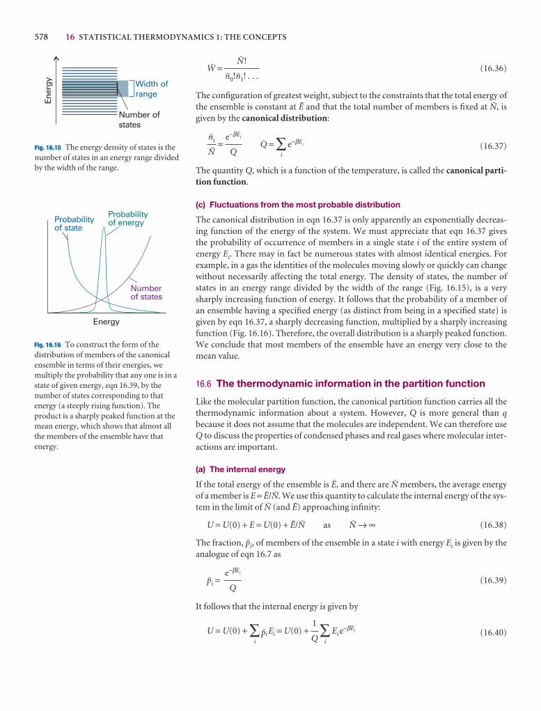
578 16 STATISTICAL THERMODYNAMICS 1: THE CONCEPTS
M = (16.36)
The configuration of greatest weight, subject to the constraints that the total energy ofthe ensemble is constant at L and that the total number of members is fixed at Ñ, isgiven by the canonical distribution:
= Q = ∑i
e−βEi (16.37)
The quantity Q, which is a function of the temperature, is called the canonical parti-tion function.
(c) Fluctuations from the most probable distribution
The canonical distribution in eqn 16.37 is only apparently an exponentially decreas-ing function of the energy of the system. We must appreciate that eqn 16.37 gives the probability of occurrence of members in a single state i of the entire system of energy Ei. There may in fact be numerous states with almost identical energies. For example, in a gas the identities of the molecules moving slowly or quickly can changewithout necessarily affecting the total energy. The density of states, the number ofstates in an energy range divided by the width of the range (Fig. 16.15), is a verysharply increasing function of energy. It follows that the probability of a member ofan ensemble having a specified energy (as distinct from being in a specified state) isgiven by eqn 16.37, a sharply decreasing function, multiplied by a sharply increasingfunction (Fig. 16.16). Therefore, the overall distribution is a sharply peaked function.We conclude that most members of the ensemble have an energy very close to themean value.
16.6 The thermodynamic information in the partition function
Like the molecular partition function, the canonical partition function carries all thethermodynamic information about a system. However, Q is more general than qbecause it does not assume that the molecules are independent. We can therefore useQ to discuss the properties of condensed phases and real gases where molecular inter-actions are important.
(a) The internal energy
If the total energy of the ensemble is L, and there are Ñ members, the average energyof a member is E = L/Ñ. We use this quantity to calculate the internal energy of the sys-tem in the limit of Ñ (and L) approaching infinity:
U = U(0) + E = U(0) + L/Ñ as Ñ → ∞ (16.38)
The fraction, "i, of members of the ensemble in a state i with energy Ei is given by theanalogue of eqn 16.7 as
"i = (16.39)
It follows that the internal energy is given by
U = U(0) + ∑i
"i Ei = U(0) + ∑i
Ei e−βEi (16.40)
1
Q
e−βEi
Q
e−βEi
Q
ñi
Ñ
Ñ!
ñ0!ñ1! . . .
Ener
gy
Number ofstates
Width ofrange
Fig. 16.15 The energy density of states is thenumber of states in an energy range dividedby the width of the range.
Probabilityof state
Numberof states
Probabilityof energy
Energy
Fig. 16.16 To construct the form of thedistribution of members of the canonicalensemble in terms of their energies, wemultiply the probability that any one is in astate of given energy, eqn 16.39, by thenumber of states corresponding to thatenergy (a steeply rising function). Theproduct is a sharply peaked function at themean energy, which shows that almost allthe members of the ensemble have thatenergy.
16.7 INDEPENDENT MOLECULES 579
By the same argument that led to eqn 16.31,
U = U(0) −V
= U(0) −V
(16.41)
(b) The entropy
The total weight, M, of a configuration of the ensemble is the product of the averageweight W of each member of the ensemble, M = W Ñ. Hence, we can calculate S from
S = k lnW = k lnM 1/Ñ = lnM (16.42)
It follows, by the same argument used in Section 16.4, that
S = + k ln Q (16.43)
16.7 Independent molecules
We shall now see how to recover the molecular partition function from the more general canonical partition function when the molecules are independent. When the molecules are independent and distinguishable (in the sense to be described), therelation between Q and q is
Q = q N (16.44)
Justification 16.5 The relation between Q and q
The total energy of a collection of N independent molecules is the sum of the ener-gies of the molecules. Therefore, we can write the total energy of a state i of the system as
Ei = εi(1) + εi(2) + · · · + εi(N)
In this expression, εi(1) is the energy of molecule 1 when the system is in the state i,εi(2) the energy of molecule 2 when the system is in the same state i, and so on. Thecanonical partition function is then
Q = ∑i
e−βεi(1)−βεi(2)− · · · −βεi(N )
The sum over the states of the system can be reproduced by letting each moleculeenter all its own individual states (although we meet an important proviso shortly).Therefore, instead of summing over the states i of the system, we can sum over allthe individual states i of molecule 1, all the states i of molecule 2, and so on. Thisrewriting of the original expression leads to
Q = ∑i
e−βεi ∑i
e−βεi · · · ∑i
e−βεi = ∑i
e−βεi
N
= q N
(a) Distinguishable and indistinguishable molecules
If all the molecules are identical and free to move through space, we cannot distin-guish them and the relation Q = q N is not valid. Suppose that molecule 1 is in somestate a, molecule 2 is in b, and molecule 3 is in c, then one member of the ensemble has an energy E = εa + εb + εc. This member, however, is indistinguishable from one formed by putting molecule 1 in state b, molecule 2 in state c, and molecule 3 instate a, or some other permutation. There are six such permutations in all, and N! in
DEFABC
DEFABC
DEFABC
DEFABC
U − U(0)
T
k
Ñ
DF
∂ ln Q
∂β
AC
DF
∂Q
∂β
AC
1
Q
580 16 STATISTICAL THERMODYNAMICS 1: THE CONCEPTS
general. In the case of indistinguishable molecules, it follows that we have counted too many states in going from the sum over system states to the sum over molecularstates, so writing Q = q N overestimates the value of Q. The detailed argument is quite involved, but at all except very low temperatures it turns out that the correction factoris 1/N!. Therefore:
• For distinguishable independent molecules: Q = q N (16.45a)
• For indistinguishable independent molecules: Q = q N/N! (16.45b)
For molecules to be indistinguishable, they must be of the same kind: an Ar atom is never indistinguishable from a Ne atom. Their identity, however, is not the only criterion. Each identical molecule in a crystal lattice, for instance, can be ‘named’ witha set of coordinates. Identical molecules in a lattice can therefore be treated as dis-tinguishable because their sites are distinguishable, and we use eqn 16.45a. On theother hand, identical molecules in a gas are free to move to different locations, andthere is no way of keeping track of the identity of a given molecule; we therefore use eqn 16.45b.
(b) The entropy of a monatomic gas
An important application of the previous material is the derivation (as shown in theJustification below) of the Sackur–Tetrode equation for the entropy of a monatomicgas:
S = nR ln Λ = (16.46a)
This equation implies that the molar entropy of a perfect gas of high molar mass isgreater than one of low molar mass under the same conditions (because the formerhas more thermally accessible translational states). Because the gas is perfect, we canuse the relation V = nRT/p to express the entropy in terms of the pressure as
S = nR ln (16.46b)
Justification 16.6 The Sackur–Tetrode equation
For a gas of independent molecules, Q may be replaced by q N/N!, with the resultthat eqn 16.43 becomes
S = + Nk ln q − k ln N!
Because the number of molecules (N = nNA) in a typical sample is large, we can useStirling’s approximation (eqn 16.2) to write
S = + nR ln q − nR ln N + nR
The only mode of motion for a gas of atoms is translation, and the partition func-tion is q = V/Λ3 (eqn 16.19), where Λ is the thermal wavelength. The internal energyis given by eqn 16.32, so the entropy is
S = 3–2 nR + nR ln − ln nNA + 1 = nR ln e3/2 + ln − ln nNA + ln e
which rearranges into eqn 16.46.
DEFV
Λ3
ABCDEF
V
Λ3
ABC
U − U(0)
T
U − U(0)
T
DF
e5/2kT
pΛ3
AC
h
(2πmkT)1/2
DF
e5/2V
nNAΛ3
AC
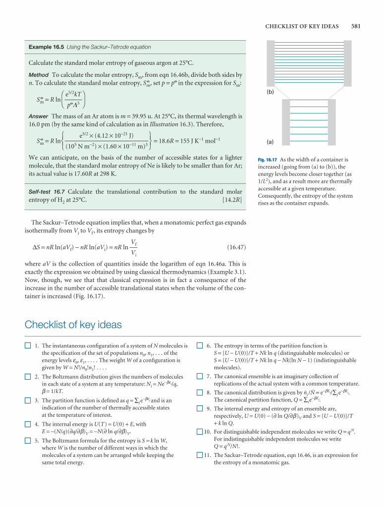
CHECKLIST OF KEY IDEAS 581
(a)
(b)
Fig. 16.17 As the width of a container isincreased (going from (a) to (b)), theenergy levels become closer together (as1/L2), and as a result more are thermallyaccessible at a given temperature.Consequently, the entropy of the systemrises as the container expands.
Checklist of key ideas
1. The instantaneous configuration of a system of N molecules isthe specification of the set of populations n0, n1, . . . of theenergy levels ε0, ε1, . . . . The weight W of a configuration isgiven by W = N!/n0!n1! . . . .
2. The Boltzmann distribution gives the numbers of moleculesin each state of a system at any temperature: Ni = Ne−βεi/q,β = 1/kT.
3. The partition function is defined as q = ∑j e−βεj and is an
indication of the number of thermally accessible states at the temperature of interest.
4. The internal energy is U(T) = U(0) + E, withE = −(N/q)(∂q/∂β)V = −N(∂ ln q/∂β)V.
5. The Boltzmann formula for the entropy is S = k ln W,where W is the number of different ways in which themolecules of a system can be arranged while keeping the same total energy.
6. The entropy in terms of the partition function is S = {U − U(0)}/T + Nk ln q (distinguishable molecules) or S = {U − U(0)}/T + Nk ln q − Nk(ln N − 1) (indistinguishablemolecules).
7. The canonical ensemble is an imaginary collection ofreplications of the actual system with a common temperature.
8. The canonical distribution is given by ñi /Ñ = e−βEi/∑j e−βEj.
The canonical partition function, Q = ∑ie−βEi.
9. The internal energy and entropy of an ensemble are,respectively, U = U(0) − (∂ ln Q/∂β)V and S = {U − U(0)}/T+ k ln Q.
10. For distinguishable independent molecules we write Q = q N.For indistinguishable independent molecules we write Q = q N/N!.
11. The Sackur–Tetrode equation, eqn 16.46, is an expression forthe entropy of a monatomic gas.
Example 16.5 Using the Sackur–Tetrode equation
Calculate the standard molar entropy of gaseous argon at 25°C.
Method To calculate the molar entropy, Sm, from eqn 16.46b, divide both sides byn. To calculate the standard molar entropy, S 7
m, set p = p7 in the expression for Sm:
S 7m = R ln
Answer The mass of an Ar atom is m = 39.95 u. At 25°C, its thermal wavelength is16.0 pm (by the same kind of calculation as in Illustration 16.3). Therefore,
S 7m = R ln = 18.6R = 155 J K−1 mol−1
We can anticipate, on the basis of the number of accessible states for a lightermolecule, that the standard molar entropy of Ne is likely to be smaller than for Ar;its actual value is 17.60R at 298 K.
Self-test 16.7 Calculate the translational contribution to the standard molar entropy of H2 at 25°C. [14.2R]
The Sackur–Tetrode equation implies that, when a monatomic perfect gas expandsisothermally from Vi to Vf , its entropy changes by
∆S = nR ln(aVf) − nR ln(aVi) = nR ln (16.47)
where aV is the collection of quantities inside the logarithm of eqn 16.46a. This is exactly the expression we obtained by using classical thermodynamics (Example 3.1).Now, though, we see that that classical expression is in fact a consequence of the increase in the number of accessible translational states when the volume of the con-tainer is increased (Fig. 16.17).
Vf
Vi
567e5/2 × (4.12 × 10−21 J)
(105 N m−2) × (1.60 × 10−11 m)3
123
DF
e5/2kT
p7Λ3
AC
582 16 STATISTICAL THERMODYNAMICS 1: THE CONCEPTS
Further reading
Articles and texts
D. Chandler, Introduction to modern statistical mechanics. OxfordUniversity Press (1987).
D.A. McQuarrie and J.D. Simon, Molecular thermodynamics.University Science Books, Sausalito (1999).
K.E. van Holde, W.C. Johnson, and P.S. Ho, Principles of physicalbiochemistry. Prentice Hall, Upper Saddle River (1998).
J. Wisniak, Negative absolute temperatures, a novelty. J. Chem. Educ.77, 518 (2000).
Further information
Further information 16.1 The Boltzmann distribution
We remarked in Section 16.1 that ln W is easier to handle than W.Therefore, to find the form of the Boltzmann distribution, we lookfor the condition for ln W being a maximum rather than dealingdirectly with W. Because ln W depends on all the ni, when aconfiguration changes and the ni change to ni + dni, the function ln W changes to ln W + d ln W, where
d ln W = ∑i
dni
All this expression states is that a change in ln W is the sum ofcontributions arising from changes in each value of ni. At amaximum, d ln W = 0. However, when the ni change, they do sosubject to the two constraints
∑i
εidni = 0 ∑i
dni = 0 (16.48)
The first constraint recognizes that the total energy must not change,and the second recognizes that the total number of molecules mustnot change. These two constraints prevent us from solving d ln W = 0simply by setting all (∂ ln W/∂ni) = 0 because the dni are not allindependent.
The way to take constraints into account was devised by the Frenchmathematician Lagrange, and is called the method of undeterminedmultipliers. The technique is described in Appendix 2. All we needhere is the rule that a constraint should be multiplied by a constantand then added to the main variation equation. The variables arethen treated as though they were all independent, and the constantsare evaluated at the end of the calculation.
We employ the technique as follows. The two constraints in eqn16.48 are multiplied by the constants −β and α, respectively (theminus sign in −β has been included for future convenience), and thenadded to the expression for d ln W:
d ln W = ∑i
dni + α∑i
dni − β∑i
εi dni
= ∑i
+ α − βεi dni
567
DEF∂ ln W
∂ni
ABC123
DEF∂ ln W
∂ni
ABC
DEF∂ lnW
∂ni
ABC
All the dni are now treated as independent. Hence the only way ofsatisfying d ln W = 0 is to require that, for each i,
+ α − βεi = 0 (16.49)
when the ni have their most probable values.Differentiation of ln W as given in eqn 16.3 with respect to ni gives
= − ∑j
The derivative of the first term is obtained as follows:
= ln N + N
= ln N + = ln N + 1
The ln N in the first term on the right in the second line arises becauseN = n1 + n2 + · · · and so the derivative of N with respect to any of theni is 1: that is, ∂N/∂ni = 1. The second term on the right in the secondline arises because ∂(ln N)/∂ni = (1/N)∂N/∂ni. The final 1 is thenobtained in the same way as in the preceding remark, by using ∂N/∂ni = 1.
For the derivative of the second term we first note that
=
Morever, if i ≠ j, nj is independent of ni, so ∂nj /∂ni = 0. However, if i = j,
= = 1
Therefore,
= δij
∂nj
∂ni
∂nj
∂nj
∂nj
∂ni
DEF∂nj
∂ni
ABC1
nj
∂ ln nj
∂ni
∂N
∂ni
DEF∂ ln N
∂ni
ABCDEF
∂N
∂ni
ABC∂(N ln N)
∂ni
∂(nj ln nj)
∂ni
∂(N ln N)
∂ni
∂ ln W
∂ni
∂ ln W
∂ni
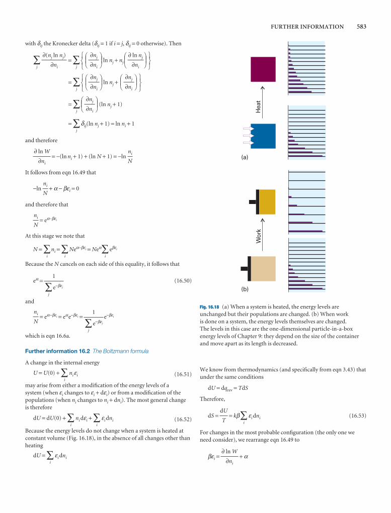
FURTHER INFORMATION 583
with δij the Kronecker delta (δij = 1 if i = j, δij = 0 otherwise). Then
∑j
= ∑j
ln nj + nj
= ∑j
ln nj +
= ∑j
(ln nj + 1)
= ∑j
δij(ln nj + 1) = ln ni + 1
and therefore
= −(ln ni + 1) + (ln N + 1) = −ln
It follows from eqn 16.49 that
−ln + α − βεi = 0
and therefore that
= eα−βεi
At this stage we note that
N = ∑i
ni = ∑i
Neα−βεi = Neα∑i
eβεi
Because the N cancels on each side of this equality, it follows that
eα = (16.50)
and
= eα−βεi = eαe−βεi = e−βεi
which is eqn 16.6a.
Further information 16.2 The Boltzmann formula
A change in the internal energy
U = U(0) + ∑i
niεi (16.51)
may arise from either a modification of the energy levels of a system (when εi changes to εi + dεi) or from a modification of thepopulations (when ni changes to ni + dni). The most general change is therefore
dU = dU(0) + ∑i
ni dεi + ∑i
εi dni (16.52)
Because the energy levels do not change when a system is heated atconstant volume (Fig. 16.18), in the absence of all changes other thanheating
dU = ∑i
εi dni
1
∑j
e−βεj
ni
N
1
∑j
e−βεj
ni
N
ni
N
ni
N
∂ ln W
∂ni
DEF∂nj
∂ni
ABC
567
DEF∂nj
∂ni
ABCDEF
∂nj
∂ni
ABC123
567
DEF∂ ln nj
∂ni
ABCDEF
∂nj
∂ni
ABC123
∂(nj ln nj)
∂ni
We know from thermodynamics (and specifically from eqn 3.43) thatunder the same conditions
dU = dqrev = TdS
Therefore,
dS = = kβ∑i
εi dni (16.53)
For changes in the most probable configuration (the only one weneed consider), we rearrange eqn 16.49 to
βεi = + α∂ ln W
∂ni
dU
T
Hea
tW
ork
(a)
(b)
Fig. 16.18 (a) When a system is heated, the energy levels areunchanged but their populations are changed. (b) When work is done on a system, the energy levels themselves are changed. The levels in this case are the one-dimensional particle-in-a-boxenergy levels of Chapter 9: they depend on the size of the containerand move apart as its length is decreased.
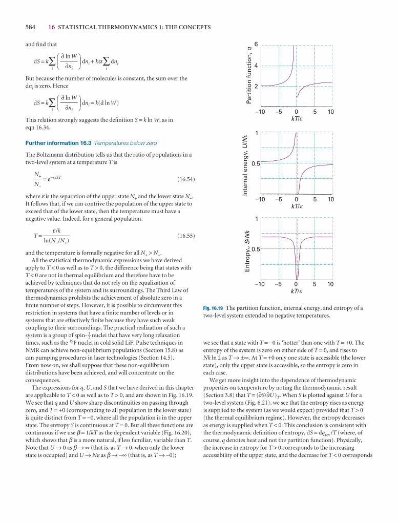
584 16 STATISTICAL THERMODYNAMICS 1: THE CONCEPTS
and find that
dS = k∑i
dni + kα∑i
dni
But because the number of molecules is constant, the sum over thedni is zero. Hence
dS = k∑i
dni = k(d lnW)
This relation strongly suggests the definition S = k ln W, as in eqn 16.34.
Further information 16.3 Temperatures below zero
The Boltzmann distribution tells us that the ratio of populations in atwo-level system at a temperature T is
= e−ε /kT (16.54)
where ε is the separation of the upper state N+ and the lower state N−.It follows that, if we can contrive the population of the upper state toexceed that of the lower state, then the temperature must have anegative value. Indeed, for a general population,
T = (16.55)
and the temperature is formally negative for all N+ > N−.All the statistical thermodynamic expressions we have derived
apply to T < 0 as well as to T > 0, the difference being that states withT < 0 are not in thermal equilibrium and therefore have to beachieved by techniques that do not rely on the equalization oftemperatures of the system and its surroundings. The Third Law ofthermodynamics prohibits the achievement of absolute zero in afinite number of steps. However, it is possible to circumvent thisrestriction in systems that have a finite number of levels or in systems that are effectively finite because they have such weakcoupling to their surroundings. The practical realization of such asystem is a group of spin- 1–2 nuclei that have very long relaxationtimes, such as the 19F nuclei in cold solid LiF. Pulse techniques inNMR can achieve non-equilibrium populations (Section 15.8) as can pumping procedures in laser technologies (Section 14.5). From now on, we shall suppose that these non-equilibriumdistributions have been achieved, and will concentrate on theconsequences.
The expressions for q, U, and S that we have derived in this chapterare applicable to T < 0 as well as to T > 0, and are shown in Fig. 16.19.We see that q and U show sharp discontinuities on passing throughzero, and T = +0 (corresponding to all population in the lower state)is quite distinct from T = −0, where all the population is in the upperstate. The entropy S is continuous at T = 0. But all these functions arecontinuous if we use β = 1/kT as the dependent variable (Fig. 16.20),which shows that β is a more natural, if less familiar, variable than T.Note that U → 0 as β → ∞ (that is, as T → 0, when only the lowerstate is occupied) and U → Nε as β → −∞ (that is, as T → −0);
ε /k
ln(N−/N+)
N+
N−
DEF∂ lnW
∂ni
ABC
DEF∂ lnW
∂ni
ABC
we see that a state with T = −0 is ‘hotter’ than one with T = +0. Theentropy of the system is zero on either side of T = 0, and rises to Nk ln 2 as T → ±∞. At T = +0 only one state is accessible (the lowerstate), only the upper state is accessible, so the entropy is zero in each case.
We get more insight into the dependence of thermodynamicproperties on temperature by noting the thermodynamic result(Section 3.8) that T = (∂S/∂U)T. When S is plotted against U for atwo-level system (Fig. 6.21), we see that the entropy rises as energy is supplied to the system (as we would expect) provided that T > 0(the thermal equilibrium regime). However, the entropy decreases as energy is supplied when T < 0. This conclusion is consistent withthe thermodynamic definition of entropy, dS = dqrev /T (where, ofcourse, q denotes heat and not the partition function). Physically, the increase in entropy for T > 0 corresponds to the increasingaccessibility of the upper state, and the decrease for T < 0 corresponds
Inte
rnal
en
erg
y,/
U N
0.5
1
En
tro
py.
,/
S N
k0.5
1
Part
itio
n f
un
ctio
n, q
0�5�10kT/
5 10
6
2
4
0�5�10kT/
5 10
0�5�10kT/
5 10
�
�
�
�
Fig. 16.19 The partition function, internal energy, and entropy of atwo-level system extended to negative temperatures.
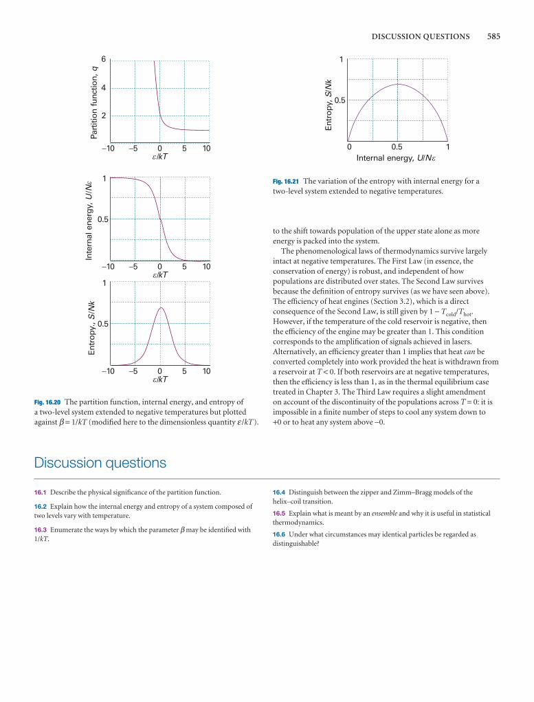
DISCUSSION QUESTIONS 585
to the shift towards population of the upper state alone as moreenergy is packed into the system.
The phenomenological laws of thermodynamics survive largelyintact at negative temperatures. The First Law (in essence, theconservation of energy) is robust, and independent of howpopulations are distributed over states. The Second Law survivesbecause the definition of entropy survives (as we have seen above).The efficiency of heat engines (Section 3.2), which is a directconsequence of the Second Law, is still given by 1 − Tcold/Thot.However, if the temperature of the cold reservoir is negative, then the efficiency of the engine may be greater than 1. This conditioncorresponds to the amplification of signals achieved in lasers.Alternatively, an efficiency greater than 1 implies that heat can beconverted completely into work provided the heat is withdrawn froma reservoir at T < 0. If both reservoirs are at negative temperatures,then the efficiency is less than 1, as in the thermal equilibrium casetreated in Chapter 3. The Third Law requires a slight amendment on account of the discontinuity of the populations across T = 0: it isimpossible in a finite number of steps to cool any system down to +0 or to heat any system above −0.
Inte
rnal
ene
rgy,
/U
N
0.5
1
Entr
opy.
,/
SN
k
0.5
1
Part
ition
func
tion,
q
0�5�10/kT
5 10
6
2
4
0
0
�5
�5
�10
�10
/kT
/kT
5
5
10
10
�
�
�
�
Fig. 16.20 The partition function, internal energy, and entropy of a two-level system extended to negative temperatures but plottedagainst β = 1/kT (modified here to the dimensionless quantity ε /kT).
Internal energy, /U N
Entr
opy,
/S
Nk
0.5
1
0 0.5 1�
Fig. 16.21 The variation of the entropy with internal energy for a two-level system extended to negative temperatures.
Discussion questions
16.1 Describe the physical significance of the partition function.
16.2 Explain how the internal energy and entropy of a system composed oftwo levels vary with temperature.
16.3 Enumerate the ways by which the parameter β may be identified with1/kT.
16.4 Distinguish between the zipper and Zimm–Bragg models of thehelix–coil transition.
16.5 Explain what is meant by an ensemble and why it is useful in statisticalthermodynamics.
16.6 Under what circumstances may identical particles be regarded asdistinguishable?

586 16 STATISTICAL THERMODYNAMICS 1: THE CONCEPTS
Exercises
16.1a What are the relative populations of the states of a two-level systemwhen the temperature is infinite?
16.1b What is the temperature of a two-level system of energy separationequivalent to 300 cm−1 when the population of the upper state is one-half thatof the lower state?
16.2a Calculate the translational partition function at (a) 300 K and (b) 600 Kof a molecule of molar mass 120 g mol−1 in a container of volume 2.00 cm3.
16.2b Calculate (a) the thermal wavelength, (b) the translational partitionfunction of an Ar atom in a cubic box of side 1.00 cm at (i) 300 K and (ii) 3000 K.
16.3a Calculate the ratio of the translational partition functions of D2 and H2
at the same temperature and volume.
16.3b Calculate the ratio of the translational partition functions of xenon andhelium at the same temperature and volume.
16.4a A certain atom has a threefold degenerate ground level, a non-degenerate electronically excited level at 3500 cm−1, and a threefold degeneratelevel at 4700 cm−1. Calculate the partition function of these electronic states at1900 K.
16.4b A certain atom has a doubly degenerate ground level, a triply degenerate electronically excited level at 1250 cm−1, and a doubly degenerate level at 1300 cm−1. Calculate the partition function of these electronic states at 2000 K.
16.5a Calculate the electronic contribution to the molar internal energy at1900 K for a sample composed of the atoms specified in Exercise 16.4a.
16.5b Calculate the electronic contribution to the molar internal energy at2000 K for a sample composed of the atoms specified in Exercise 16.4b.
16.6a A certain molecule has a non-degenerate excited state lying at 540 cm−1
above the non-degenerate ground state. At what temperature will 10 per centof the molecules be in the upper state?
16.6b A certain molecule has a doubly degenerate excited state lying at 360 cm−1 above the non-degenerate ground state. At what temperature will 15 per cent of the molecules be in the upper state?
16.7a An electron spin can adopt either of two orientations in a magneticfield, and its energies are ±µBB, where µB is the Bohr magneton. Deduce anexpression for the partition function and mean energy of the electron andsketch the variation of the functions with B. Calculate the relative populationsof the spin states at (a) 4.0 K, (b) 298 K when B = 1.0 T.
16.7b A nitrogen nucleus spin can adopt any of three orientations in amagnetic field, and its energies are 0, ±γN$B, where γN is the magnetogyricratio of the nucleus. Deduce an expression for the partition function andmean energy of the nucleus and sketch the variation of the functions with B.Calculate the relative populations of the spin states at (a) 1.0 K, (b) 298 Kwhen B = 20.0 T.
16.8a Consider a system of distinguishable particles having only two non-degenerate energy levels separated by an energy that is equal to the value of kT at 10 K. Calculate (a) the ratio of populations in the two states at (1) 1.0 K,(2) 10 K, and (3) 100 K, (b) the molecular partition function at 10 K, (c) themolar energy at 10 K, (d) the molar heat capacity at 10 K, (e) the molarentropy at 10 K.
16.8b Consider a system of distinguishable particles having only three non-degenerate energy levels separated by an energy which is equal to the value ofkT at 25.0 K. Calculate (a) the ratio of populations in the states at (1) 1.00 K,(2) 25.0 K, and (3) 100 K, (b) the molecular partition function at 25.0 K, (c) the molar energy at 25.0 K, (d) the molar heat capacity at 25.0 K, (e) themolar entropy at 25.0 K.
16.9a At what temperature would the population of the first excitedvibrational state of HCl be 1/e times its population of the ground state?
16.9b At what temperature would the population of the first excitedrotational level of HCl be 1/e times its population of the ground state?
16.10a Calculate the standard molar entropy of neon gas at (a) 200 K, (b) 298.15 K.
16.10b Calculate the standard molar entropy of xenon gas at (a) 100 K, (b) 298.15 K.
16.11a Calculate the vibrational contribution to the entropy of Cl2 at 500 Kgiven that the wavenumber of the vibration is 560 cm−1.
16.11b Calculate the vibrational contribution to the entropy of Br2 at 600 Kgiven that the wavenumber of the vibration is 321 cm−1.
16.12a Identify the systems for which it is essential to include a factor of 1/N!on going from Q to q: (a) a sample of helium gas, (b) a sample of carbonmonoxide gas, (c) a solid sample of carbon monoxide, (d) water vapour.
16.12b Identify the systems for which it is essential to include a factor of 1/N!on going from Q to q: (a) a sample of carbon dioxide gas, (b) a sample ofgraphite, (c) a sample of diamond, (d) ice.
Problems*
Numerical problems
16.1‡ Consider a system A consisting of subsystems A1 and A2, for which W1 = 1 × 10²⁰ and W2 = 2 × 10²⁰. What is the number of configurationsavailable to the combined system? Also, compute the entropies S, S1, and S2.What is the significance of this result?
16.2‡ Consider 1.00 × 10²² 4He atoms in a box of dimensions 1.0 cm × 1.0 cm× 1.0 cm. Calculate the occupancy of the first excited level at 1.0 mK, 2.0 K,and 4.0 K. Do the same for 3He. What conclusions might you draw from theresults of your calculations?
* Problems denoted with the symbol ‡ were supplied by Charles Trapp and Carmen Giunta.
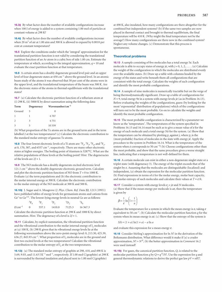
PROBLEMS 587
16.3‡ By what factor does the number of available configurations increasewhen 100 J of energy is added to a system containing 1.00 mol of particles atconstant volume at 298 K?
16.4‡ By what factor does the number of available configurations increasewhen 20 m3 of air at 1.00 atm and 300 K is allowed to expand by 0.0010 percent at constant temperature?
16.5 Explore the conditions under which the ‘integral’ approximation for thetranslational partition function is not valid by considering the translationalpartition function of an Ar atom in a cubic box of side 1.00 cm. Estimate thetemperature at which, according to the integral approximation, q = 10 andevaluate the exact partition function at that temperature.
16.6 A certain atom has a doubly degenerate ground level pair and an upperlevel of four degenerate states at 450 cm−1 above the ground level. In an atomicbeam study of the atoms it was observed that 30 per cent of the atoms were inthe upper level, and the translational temperature of the beam was 300 K. Arethe electronic states of the atoms in thermal equilibrium with the translationalstates?
16.7 (a) Calculate the electronic partition function of a tellurium atom at (i) 298 K, (ii) 5000 K by direct summation using the following data:
Term Degeneracy Wavenumber/cm−1
Ground 5 0
1 1 4 707
2 3 4 751
3 5 10 559
(b) What proportion of the Te atoms are in the ground term and in the termlabelled 2 at the two temperatures? (c) Calculate the electronic contribution tothe standard molar entropy of gaseous Te atoms.
16.8 The four lowest electronic levels of a Ti atom are: 3F2, 3F3, 3F4, and 5F1,at 0, 170, 387, and 6557 cm−1, respectively. There are many other electronicstates at higher energies. The boiling point of titanium is 3287°C. What are therelative populations of these levels at the boiling point? Hint. The degeneraciesof the levels are 2J + 1.
16.9 The NO molecule has a doubly degenerate excited electronic level 121.1 cm−1 above the doubly degenerate electronic ground term. Calculateand plot the electronic partition function of NO from T = 0 to 1000 K.Evaluate (a) the term populations and (b) the electronic contribution to the molar internal energy at 300 K. Calculate the electronic contribution to the molar entropy of the NO molecule at 300 K and 500 K.
16.10‡ J. Sugar and A. Musgrove (J. Phys. Chem. Ref. Data 22, 1213 (1993))have published tables of energy levels for germanium atoms and cations fromGe+ to Ge+31. The lowest-lying energy levels in neutral Ge are as follows:
3P03P1
3P21D2
1S0
E/cm−1 0 557.1 1410.0 7125.3 16 367.3
Calculate the electronic partition function at 298 K and 1000 K by directsummation. Hint. The degeneracy of a level is 2J + 1.
16.11 Calculate, by explicit summation, the vibrational partition functionand the vibrational contribution to the molar internal energy of I2 moleculesat (a) 100 K, (b) 298 K given that its vibrational energy levels lie at thefollowing wavenumbers above the zero-point energy level: 0, 213.30, 425.39,636.27, 845.93 cm−1. What proportion of I2 molecules are in the ground andfirst two excited levels at the two temperatures? Calculate the vibrationalcontribution to the molar entropy of I2 at the two temperatures.
16.12‡ (a) The standard molar entropy of graphite at 298, 410, and 498 K is5.69, 9.03, and 11.63 J K−1 mol−1, respectively. If 1.00 mol C(graphite) at 298 Kis surrounded by thermal insulation and placed next to 1.00 mol C(graphite)
at 498 K, also insulated, how many configurations are there altogether for thecombined but independent systems? (b) If the same two samples are nowplaced in thermal contact and brought to thermal equilibrium, the finaltemperature will be 410 K. (Why might the final temperature not be theaverage?) How many configurations are there now in the combined system?Neglect any volume changes. (c) Demonstrate that this process isspontaneous.
Theoretical problems
16.13 A sample consisting of five molecules has a total energy 5ε. Eachmolecule is able to occupy states of energy jε, with j = 0, 1, 2, . . . . (a) Calculatethe weight of the configuration in which the molecules are distributed evenlyover the available states. (b) Draw up a table with columns headed by theenergy of the states and write beneath them all configurations that areconsistent with the total energy. Calculate the weights of each configurationand identify the most probable configurations.
16.14 A sample of nine molecules is numerically tractable but on the verge ofbeing thermodynamically significant. Draw up a table of configurations for N = 9, total energy 9ε in a system with energy levels jε (as in Problem 16.13).Before evaluating the weights of the configurations, guess (by looking for themost ‘exponential’ distribution of populations) which of the configurationswill turn out to be the most probable. Go on to calculate the weights andidentify the most probable configuration.
16.15 The most probable configuration is characterized by a parameter weknow as the ‘temperature’. The temperatures of the system specified inProblems 16.13 and 16.14 must be such as to give a mean value of ε for theenergy of each molecule and a total energy Nε for the system. (a) Show thatthe temperature can be obtained by plotting pj against j, where pj is the (most probable) fraction of molecules in the state with energy jε. Apply theprocedure to the system in Problem 16.14. What is the temperature of thesystem when ε corresponds to 50 cm−1? (b) Choose configurations other thanthe most probable, and show that the same procedure gives a worse straightline, indicating that a temperature is not well-defined for them.
16.16 A certain molecule can exist in either a non-degenerate singlet state or atriplet state (with degeneracy 3). The energy of the triplet exceeds that of thesinglet by ε. Assuming that the molecules are distinguishable (localized) andindependent, (a) obtain the expression for the molecular partition function.(b) Find expressions in terms of ε for the molar energy, molar heat capacity,and molar entropy of such molecules and calculate their values at T = ε /k.
16.17 Consider a system with energy levels εj = jε and N molecules.(a) Show that if the mean energy per molecule is aε, then the temperature is given by
β = ln l +
Evaluate the temperature for a system in which the mean energy is ε, taking εequivalent to 50 cm−1. (b) Calculate the molecular partition function q for thesystem when its mean energy is aε. (c) Show that the entropy of the system is
S/k = (1 + a) ln(1 + a) − a ln a
and evaluate this expression for a mean energy ε.
16.18 Consider Stirling’s approximation for ln N! in the derivation of theBoltzmann distribution. What difference would it make if (a) a cruderapproximation, N! = N N, (b) the better approximation in Comment 16.2were used instead?
16.19‡ For gases, the canonical partition function, Q, is related to themolecular partition function q by Q = q N/N!. Use the expression for q andgeneral thermodynamic relations to derive the perfect gas law pV = nRT.
DEF1
a
ABC1
ε
588 16 STATISTICAL THERMODYNAMICS 1: THE CONCEPTS
Applications: to atmospheric science, astrophysics, and biochemistry
16.20‡ Obtain the barometric formula (Problem 1.27) from the Boltzmanndistribution. Recall that the potential energy of a particle at height h above thesurface of the Earth is mgh. Convert the barometric formula from pressure tonumber density, N . Compare the relative number densities, N (h)/N (0), forO2 and H2O at h = 8.0 km, a typical cruising altitude for commercial aircraft.
16.21‡ Planets lose their atmospheres over time unless they are replenished. Acomplete analysis of the overall process is very complicated and depends uponthe radius of the planet, temperature, atmospheric composition, and otherfactors. Prove that the atmosphere of planets cannot be in an equilibrium stateby demonstrating that the Boltzmann distribution leads to a uniform finitenumber density as r → ∞. Hint. Recall that in a gravitational field the potentialenergy is V(r) = −GMm/r, where G is the gravitational constant, M is the massof the planet, and m the mass of the particle.
16.22‡ Consider the electronic partition function of a perfect atomichydrogen gas at a density of 1.99 × 10⁻⁴ kg m−3 and 5780 K. These are themean conditions within the Sun’s photosphere, the surface layer of the Sunthat is about 190 km thick. (a) Show that this partition function, whichinvolves a sum over an infinite number of quantum states that are solutions tothe Schrödinger equation for an isolated atomic hydrogen atom, is infinite.(b) Develop a theoretical argument for truncating the sum and estimate themaximum number of quantum states that contribute to the sum. (c) Calculatethe equilibrium probability that an atomic hydrogen electron is in each
quantum state. Are there any general implications concerning electronic statesthat will be observed for other atoms and molecules? Is it wise to apply thesecalculations in the study of the Sun’s photosphere?
16.23 Consider a protein P with four distinct sites, with each site capable ofbinding one ligand L. Show that the possible varieties (configurations) of thespecies PL i (with PL0 denoting P) are given by the binomial coefficients C(4,i).
16.24 Complete some of the derivations in the discussion of the helix–coiltransition in polypeptides (Impact I16.1). (a) Show that, within the tenets ofthe zipper model,
q = 1 +n
∑i=1
Z(n,i)σsi
and that Z(n,i) = n − i + 1 is the number of ways in which an allowed state witha number i of c amino acids can be formed. (b) Using the zipper model, showthat θ = (1/n)d(ln q)/d(ln s). Hint. As a first step, show that ∑i i(n − i + 1)σsi =s(dq/ds).
16.25 Here you will use the zipper model discussed in Impact I16.1 to explorethe helix–coil transition in polypeptides.(a) Investigate the effect of theparameter s on the distribution of random coil segments in a polypeptide withn = 20 by plotting pi, the fraction of molecules with a number i of amino acidsin a coil region, against i for s = 0.8, 1.0, and 1.5, with σ = 5.0 × 10⁻². Discussthe significance of any effects you discover. (b) The average value of i given by�i� = ∑iipi. Use the results of the zipper model to calculate �i� for all thecombinations of s and σ used in Fig. 16.10 and part (a).
Statisticalthermodynamics 2:applicationsIn this chapter we apply the concepts of statistical thermodynamics to the calculation ofchemically significant quantities. First, we establish the relations between thermodynamicfunctions and partition functions. Next, we show that the molecular partition function can befactorized into contributions from each mode of motion and establish the formulas for thepartition functions for translational, rotational, and vibrational modes of motion and the con-tribution of electronic excitation. These contributions can be calculated from spectroscopicdata. Finally, we turn to specific applications, which include the mean energies of modes ofmotion, the heat capacities of substances, and residual entropies. In the final section, wesee how to calculate the equilibrium constant of a reaction and through that calculation understand some of the molecular features that determine the magnitudes of equilibriumconstants and their variation with temperature.
A partition function is the bridge between thermodynamics, spectroscopy, and quantum mechanics. Once it is known, a partition function can be used to calculatethermodynamic functions, heat capacities, entropies, and equilibrium constants. Italso sheds light on the significance of these properties.
Fundamental relations
In this section we see how to obtain any thermodynamic function once we know thepartition function. Then we see how to calculate the molecular partition function, andthrough that the thermodynamic functions, from spectroscopic data.
17.1 The thermodynamic functions
We have already derived (in Chapter 16) the two expressions for calculating the internal energy and the entropy of a system from its canonical partition function, Q:
U − U(0) = −V
S = + k ln Q (17.1)
where β = 1/kT. If the molecules are independent, we can go on to make the substitu-tions Q = q N (for distinguishable molecules, as in a solid) or Q = q N/N ! (for indistin-guishable molecules, as in a gas). All the thermodynamic functions introduced in Part 1are related to U and S, so we have a route to their calculation from Q.
U − U(0)
T
DF
∂ ln Q
∂β
AC
17Fundamental relations
17.1 The thermodynamic functions
17.2 The molecular partitionfunction
Using statisticalthermodynamics
17.3 Mean energies
17.4 Heat capacities
17.5 Equations of state
17.6 Molecular interactions inliquids
17.7 Residual entropies
17.8 Equilibrium constants
Checklist of key ideas
Further reading
Discussion questions
Exercises
Problems
590 17 STATISTICAL THERMODYNAMICS 2: APPLICATIONS
(a) The Helmholtz energy
The Helmholtz energy, A, is defined as A = U − TS. This relation implies that A(0) =U(0), so substitution for U and S by using eqn 17.1 leads to the very simple expression
A − A(0) = −kT ln Q (17.2)
(b) The pressure
By an argument like that leading to eqn 3.31, it follows from A = U − TS thatdA = −pdV − SdT. Therefore, on imposing constant temperature, the pressure and theHelmholtz energy are related by p = −(∂A/∂V)T. It then follows from eqn 17.2 that
p = kTT
(17.3)
This relation is entirely general, and may be used for any type of substance, includingperfect gases, real gases, and liquids. Because Q is in general a function of the volume,temperature, and amount of substance, eqn 17.3 is an equation of state.
Example 17.1 Deriving an equation of state
Derive an expression for the pressure of a gas of independent particles.
Method We should suspect that the pressure is that given by the perfect gas law. Toproceed systematically, substitute the explicit formula for Q for a gas of independ-ent, indistinguishable molecules (see eqn 16.45 and Table 17.3 at the end of thechapter) into eqn 17.3.
Answer For a gas of independent molecules, Q = q N/N! with q = V/Λ3:
p = kTT
=T
=T
= × = =
To derive this relation, we have used
T
=T
=
and NkT = nNAkT = nRT. The calculation shows that the equation of state of a gasof independent particles is indeed the perfect gas law.
Self-test 17.1 Derive the equation of state of a sample for which Q = q Nf /N!, with q = V/Λ3, where f depends on the volume. [p = nRT/V + kT(∂ ln f /∂V)T]
(c) The enthalpy
At this stage we can use the expressions for U and p in the definition H = U + pV toobtain an expression for the enthalpy, H, of any substance:
H − H(0) = −V
+ kTVT
(17.4)DF
∂ ln Q
∂V
AC
DF
∂ ln Q
∂β
AC
1
Λ3
DF
∂(V/Λ3)
∂V
AC
DF
∂q
∂V
AC
nRT
V
NkT
V
1
Λ3
NkTΛ3
V
DF
∂q
∂V
AC
NkT
q
DF
∂Q
∂V
AC
kT
Q
DF
∂ ln Q
∂V
AC
DF
∂ ln Q
∂V
AC
17.2 THE MOLECULAR PARTITION FUNCTION 591
We have already seen that U − U(0) = 3–2 nRT for a gas of independent particles (eqn16.32a), and have just shown that pV = nRT. Therefore, for such a gas,
H − H(0) = 5–2 nRT (17.5)°
(d) The Gibbs energy
One of the most important thermodynamic functions for chemistry is the Gibbs energy, G = H − TS = A + pV. We can now express this function in terms of the parti-tion function by combining the expressions for A and p:
G − G(0) = −kT ln Q + kTVT
(17.6)
This expression takes a simple form for a gas of independent molecules because pV inthe expression G = A + pV can be replaced by nRT:
G − G(0) = −kT ln Q + nRT (17.7)°
Furthermore, because Q = q N/N!, and therefore ln Q = N ln q − ln N!, it follows byusing Stirling’s approximation (ln N! ≈ N ln N −N) that we can write
G − G(0) = −NkT ln q + kT ln N ! + nRT
= −nRT ln q + kT(N ln N − N) + nRT
= −nRT ln (17.8)°
with N = nNA. Now we see another interpretation of the Gibbs energy: it is pro-portional to the logarithm of the average number of thermally accessible states permolecule.
It will turn out to be convenient to define the molar partition function, qm = q/n(with units mol−1), for then
G − G(0) = −nRT ln (17.9)°
17.2 The molecular partition function
The energy of a molecule is the sum of contributions from its different modes of motion:
εi = ε iT + εi
R + ε iV + ε i
E (17.10)
where T denotes translation, R rotation, V vibration, and E the electronic contribu-tion. The electronic contribution is not actually a ‘mode of motion’, but it is con-venient to include it here. The separation of terms in eqn 17.10 is only approximate(except for translation) because the modes are not completely independent, but inmost cases it is satisfactory. The separation of the electronic and vibrational motionsis justified provided only the ground electronic state is occupied (for otherwise the vibrational characteristics depend on the electronic state) and, for the electronicground state, that the Born–Oppenheimer approximation is valid (Chapter 11). Theseparation of the vibrational and rotational modes is justified to the extent that the rotational constant is independent of the vibrational state.
Given that the energy is a sum of independent contributions, the partition functionfactorizes into a product of contributions (recall Section 16.2b):
qm
NA
q
N
DF
∂ ln Q
∂V
AC
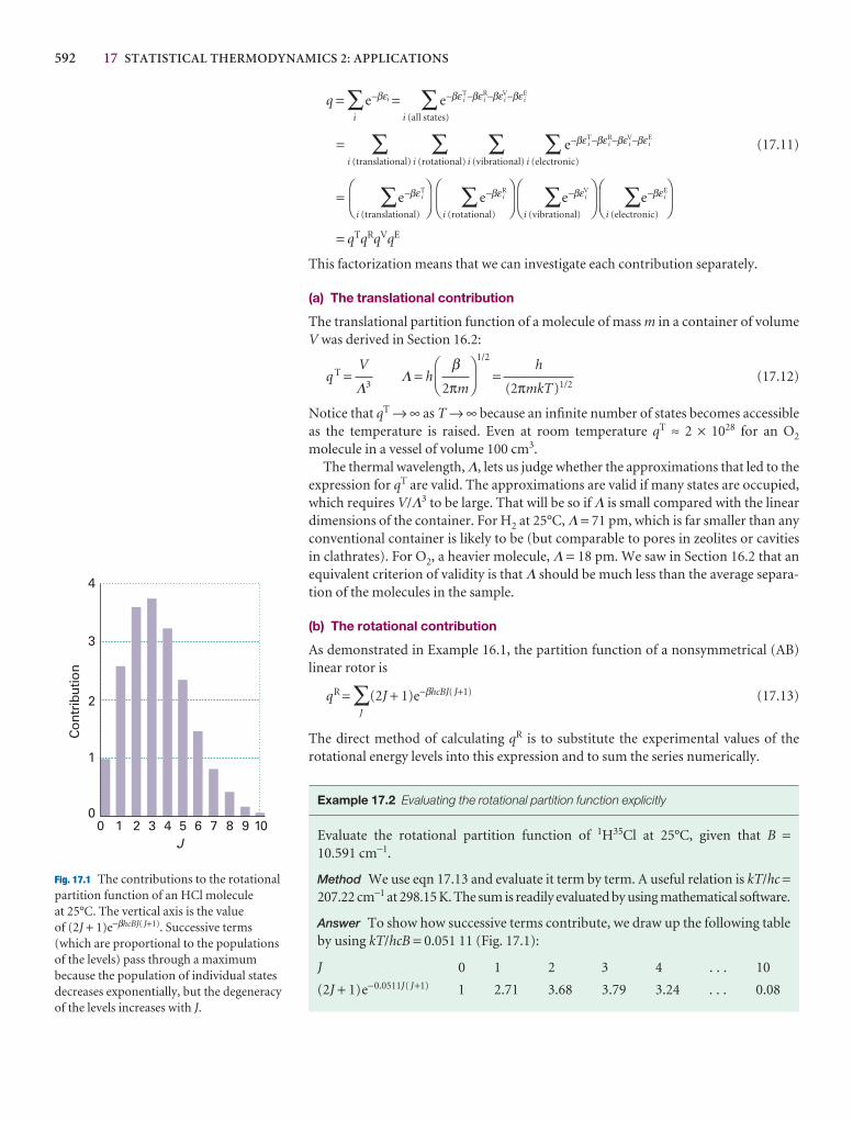
592 17 STATISTICAL THERMODYNAMICS 2: APPLICATIONS
1 2 3 4 5 6 7 8 9 1000
1
2
3
4
J
Con
trib
utio
n
Fig. 17.1 The contributions to the rotationalpartition function of an HCl molecule at 25°C. The vertical axis is the value of (2J + 1)e−βhcBJ( J+1). Successive terms(which are proportional to the populationsof the levels) pass through a maximumbecause the population of individual statesdecreases exponentially, but the degeneracyof the levels increases with J.
q = ∑i
e−βεi = ∑i (all states)
e−βεTi −βεR
i −βεVi −βεE
i
= ∑i (translational)
∑i (rotational)
∑i (vibrational)
∑i (electronic)
e−βεTi −βεR
i −βεVi −βεE
i (17.11)
= ∑i (translational)
e−βεTi ∑
i (rotational)
e−βεRi ∑
i (vibrational)
e−βεVi ∑
i (electronic)
e−βεEi
= qTqRqVqE
This factorization means that we can investigate each contribution separately.
(a) The translational contribution
The translational partition function of a molecule of mass m in a container of volumeV was derived in Section 16.2:
q T = Λ = h
1/2
= (17.12)
Notice that qT → ∞ as T → ∞ because an infinite number of states becomes accessibleas the temperature is raised. Even at room temperature qT ≈ 2 × 1028 for an O2
molecule in a vessel of volume 100 cm3.The thermal wavelength, Λ, lets us judge whether the approximations that led to the
expression for qT are valid. The approximations are valid if many states are occupied,which requires V/Λ3 to be large. That will be so if Λ is small compared with the lineardimensions of the container. For H2 at 25°C, Λ = 71 pm, which is far smaller than anyconventional container is likely to be (but comparable to pores in zeolites or cavitiesin clathrates). For O2, a heavier molecule, Λ = 18 pm. We saw in Section 16.2 that anequivalent criterion of validity is that Λ should be much less than the average separa-tion of the molecules in the sample.
(b) The rotational contribution
As demonstrated in Example 16.1, the partition function of a nonsymmetrical (AB)linear rotor is
qR = ∑J
(2J + 1)e−βhcBJ( J+1) (17.13)
The direct method of calculating qR is to substitute the experimental values of the rotational energy levels into this expression and to sum the series numerically.
Example 17.2 Evaluating the rotational partition function explicitly
Evaluate the rotational partition function of 1H35Cl at 25°C, given that B =10.591 cm−1.
Method We use eqn 17.13 and evaluate it term by term. A useful relation is kT/hc =207.22 cm−1 at 298.15 K. The sum is readily evaluated by using mathematical software.
Answer To show how successive terms contribute, we draw up the following tableby using kT/hcB = 0.051 11 (Fig. 17.1):
J 0 1 2 3 4 . . . 10
(2J + 1)e−0.0511J( J+1) 1 2.71 3.68 3.79 3.24 . . . 0.08
h
(2πmkT)1/2
DF
β2πm
AC
V
Λ3
DF
AC
DF
AC
DF
AC
DF
AC
17.2 THE MOLECULAR PARTITION FUNCTION 593
The sum required by eqn 17.13 (the sum of the numbers in the second row of thetable) is 19.9, hence qR = 19.9 at this temperature. Taking J up to 50 gives qR =19.902. Notice that about ten J-levels are significantly populated but the number ofpopulated states is larger on account of the (2J + 1)-fold degeneracy of each level.We shall shortly encounter the approximation that qR ≈ kT/hcB, which in the pre-sent case gives qR = 19.6, in good agreement with the exact value and with much lesswork.
Self-test 17.2 Evaluate the rotational partition function for HCl at 0°C. [18.26]
At room temperature kT/hc ≈ 200 cm−1. The rotational constants of many moleculesare close to 1 cm−1 (Table 13.2) and often smaller (though the very light H2 molecule,for which B = 60.9 cm−1, is one exception). It follows that many rotational levels arepopulated at normal temperatures. When this is the case, the partition function maybe approximated by
Linear rotors: qR = (17.14a)
Nonlinear rotors: qR =3/2 1/2
(17.14b)
where A, B, and C are the rotational constants of the molecule. However, before usingthese expressions, read on (to eqns 17.15 and 17.16).
Justification 17.1 The rotational contribution to the molecular partition function
When many rotational states are occupied and kT is much larger than the separationbetween neighbouring states, the sum in the partition function can be approxim-ated by an integral, much as we did for translational motion in Justification 16.2:
qR = �∞
0
(2J + 1)e−βhcBJ( J+1)dJ
Although this integral looks complicated, it can be evaluated without much effort bynoticing that because
eaJ( J+1) = aJ( J + 1) eaJ( J+1) = a(2J + 1)eaJ( J+1)
it can also be written as
qR = �∞
0
e−βhcBJ( J+1) dJ
Then, because the integral of a derivative of a function is the function itself, we obtain
qR = − e−βhcBJ( J+1)
0
∞
=
which (because β = 1/kT) is eqn 17.14a.The calculation for a nonlinear molecule is along the same lines, but slightly
trickier. First, we note that the energies of a symmetric rotor are
EJ,K,MJ= hcBJ( J + 1) + hc(A − B)K2
1
βhcB
1
βhcB
DEFd
dJ
ABC1
βhcB
567d
dJ
123d
dJ
DF
πABC
AC
DF
kT
hc
AC
kT
hcB
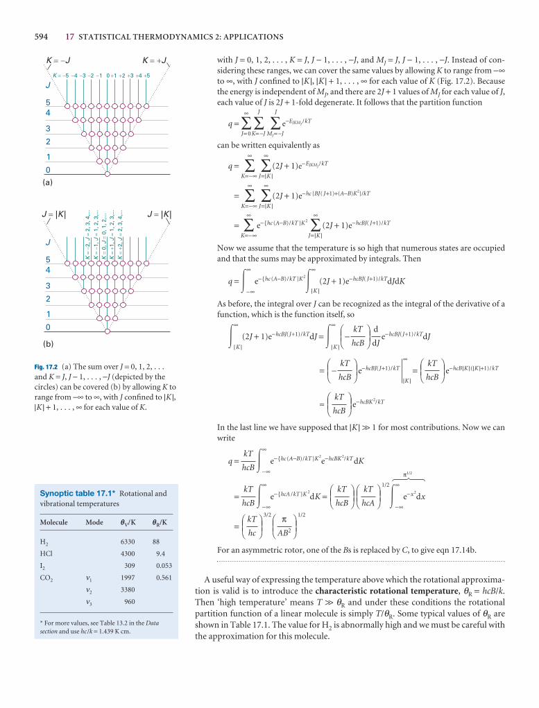
594 17 STATISTICAL THERMODYNAMICS 2: APPLICATIONS
with J = 0, 1, 2, . . . , K = J, J − 1, . . . , −J, and MJ = J, J − 1, . . . , −J. Instead of con-sidering these ranges, we can cover the same values by allowing K to range from −∞to ∞, with J confined to |K |, |K | + 1, . . . , ∞ for each value of K (Fig. 17.2). Becausethe energy is independent of MJ, and there are 2J + 1 values of MJ for each value of J,each value of J is 2J + 1-fold degenerate. It follows that the partition function
q =∞
∑J= 0
J
∑K= −J
J
∑MJ= −J
e−EJKMJ/kT
can be written equivalently as
q =∞
∑K=−∞
∞
∑J=|K |
(2J + 1)e−EJKMJ/kT
=∞
∑K=−∞
∞
∑J=|K |
(2J + 1)e−hc {BJ( J+1)+(A−B)K2}/kT
=∞
∑K=−∞
e−{hc (A−B)/kT }K2∞
∑J=|K |
(2J + 1)e−hcBJ( J+1)/kT
Now we assume that the temperature is so high that numerous states are occupiedand that the sums may be approximated by integrals. Then
q = �∞
−∞e−{hc (A−B)/kT }K2�
∞
| K |(2J + 1)e−hcBJ( J+1)/kTdJdK
As before, the integral over J can be recognized as the integral of the derivative of afunction, which is the function itself, so
�∞
| K |(2J + 1)e−hcBJ(J+1)/kTdJ = �
∞
| K |− e−hcBJ(J+1)/kTdJ
= − e−hcBJ(J+1)/kT
∞
|K |= e−hcB |K |(|K |+1)/kT
≈ e−hcBK2/kT
In the last line we have supposed that |K | >> 1 for most contributions. Now we canwrite
q = �∞
−∞e−{hc (A−B)/kT }K2
e−hcBK2/kT dK
π1/2
= �∞
−∞e−{hcA /kT }K 2
dK =1/2
�∞
−∞e−x2
dx
=3/2 1/2
For an asymmetric rotor, one of the Bs is replaced by C, to give eqn 17.14b.
A useful way of expressing the temperature above which the rotational approxima-tion is valid is to introduce the characteristic rotational temperature, θR = hcB/k.Then ‘high temperature’ means T >> θR and under these conditions the rotationalpartition function of a linear molecule is simply T/θR. Some typical values of θR areshown in Table 17.1. The value for H2 is abnormally high and we must be careful withthe approximation for this molecule.
DEFπ
AB2
ABCDEF
kT
hc
ABC
DEFkT
hcA
ABCDEF
kT
hcB
ABCkT
hcB
5 6 7
kT
hcB
DEFkT
hcB
ABC
DEFkT
hcB
ABCDEF
kT
hcB
ABC
d
dJ
DEFkT
hcB
ABC
Synoptic table 17.1* Rotational andvibrational temperatures
Molecule Mode qV/K qR/K
H2 6330 88
HCl 4300 9.4
I2 309 0.053
CO2 ν1 1997 0.561
ν2 3380
ν3 960
* For more values, see Table 13.2 in the Datasection and use hc /k = 1.439 K cm.
J
0
1
2
3
45
K J� � K J� �
0 �1 �2 �3 �4 �5�1�2�3�4�5
J
0
1
2
3
45
J K� | | J K� | |
KJ
0,0,
1, 2
,...
��
KJ
1,1,
2, 3
,...
��
�
KJ
2,2,
3, 4
,...
��
�
KJ
1,1,
2, 3
,...
��
�
KJ
2,2,
3, 4
,...
��
�
K �
(a)
(b)
Fig. 17.2 (a) The sum over J = 0, 1, 2, . . .and K = J, J − 1, . . . , −J (depicted by thecircles) can be covered (b) by allowing K torange from −∞ to ∞, with J confined to |K |,|K | + 1, . . . , ∞ for each value of K.
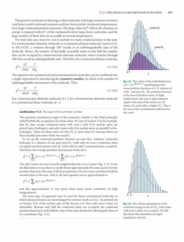
17.2 THE MOLECULAR PARTITION FUNCTION 595
The general conclusion at this stage is that molecules with large moments of inertia(and hence small rotational constants and low characteristic rotational temperatures)have large rotational partition functions. The large value of qR reflects the closeness inenergy (compared with kT) of the rotational levels in large, heavy molecules, and thelarge number of them that are accessible at normal temperatures.
We must take care, however, not to include too many rotational states in the sum.For a homonuclear diatomic molecule or a symmetrical linear molecule (such as CO2
or HC.CH), a rotation through 180° results in an indistinguishable state of themolecule. Hence, the number of thermally accessible states is only half the numberthat can be occupied by a heteronuclear diatomic molecule, where rotation through180° does result in a distinguishable state. Therefore, for a symmetrical linear molecule,
qR = = (17.15a)
The equations for symmetrical and nonsymmetrical molecules can be combined intoa single expression by introducing the symmetry number, σ, which is the number ofindistinguishable orientations of the molecule. Then
qR = = (17.15b)
For a heteronuclear diatomic molecule σ = 1; for a homonuclear diatomic moleculeor a symmetrical linear molecule, σ = 2.
Justification 17.2 The origin of the symmetry number
The quantum mechanical origin of the symmetry number is the Pauli principle,which forbids the occupation of certain states. We saw in Section 13.8, for example,that H2 may occupy rotational states with even J only if its nuclear spins are paired (para-hydrogen), and odd J states only if its nuclear spins are parallel (ortho-hydrogen). There are three states of ortho-H2 to each value of J (because there arethree parallel spin states of the two nuclei).
To set up the rotational partition function we note that ‘ordinary’ molecular hydrogen is a mixture of one part para-H2 (with only its even-J rotational states occupied) and three parts ortho-H2 (with only its odd-J rotational states occupied).Therefore, the average partition function per molecule is
qR = 1–4 ∑even J
(2J + 1)e−βhcBJ(J+1) + 3–4 ∑odd J
(2J + 1)e−βhcBJ( J+1)
The odd-J states are more heavily weighted than the even-J states (Fig. 17.3). Fromthe illustration we see that we would obtain approximately the same answer for thepartition function (the sum of all the populations) if each J term contributed half itsnormal value to the sum. That is, the last equation can be approximated as
qR = 1–2 ∑J
(2J + 1)e−βhcBJ(J+1)
and this approximation is very good when many terms contribute (at high temperatures).
The same type of argument may be used for linear symmetrical molecules inwhich identical bosons are interchanged by rotation (such as CO2). As pointed outin Section 13.8, if the nuclear spin of the bosons is 0, then only even-J states are admissible. Because only half the rotational states are occupied, the rotational partition function is only half the value of the sum obtained by allowing all values ofJ to contribute (Fig. 17.4).
T
σθR
kT
σhcB
T
2θR
kT
2hcB
ortho-H2
para-H2
0 1 J
Fig. 17.3 The values of the individual terms(2J + 1)e−βhcBJ( J+1) contributing to the mean partition function of a 3:1 mixture ofortho- and para-H2. The partition functionis the sum of all these terms. At hightemperatures, the sum is approximatelyequal to the sum of the terms over allvalues of J, each with a weight of 1–2. This isthe sum of the contributions indicated bythe curve.
0 2 J
Fig. 17.4 The relative populations of therotational energy levels of CO2. Only stateswith even J values are occupied. The fullline shows the smoothed, averagedpopulation of levels.
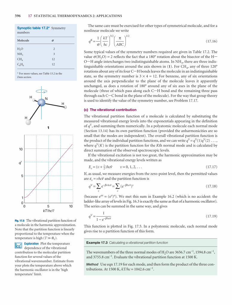
596 17 STATISTICAL THERMODYNAMICS 2: APPLICATIONS
Synoptic table 17.2* Symmetrynumbers
Molecule s
H2O 2
NH3 3
CH4 12
C6H6 12
* For more values, see Table 13.2 in the Data section.
NH
H
H
1
0 5 10
10
5
0
qV
kT hc/ ~
1
�
Fig. 17.5 The vibrational partition function ofa molecule in the harmonic approximation.Note that the partition function is linearlyproportional to the temperature when thetemperature is high (T >> θV).
Exploration Plot the temperaturedependence of the vibrational
contribution to the molecular partitionfunction for several values of thevibrational wavennumber. Estimate fromyour plots the temperature above which the harmonic oscillator is in the ‘hightemperature’ limit.
The same care must be exercised for other types of symmetrical molecule, and for anonlinear molecule we write
qR =3/2 1/2
(17.16)
Some typical values of the symmetry numbers required are given in Table 17.2. Thevalue σ(H2O) = 2 reflects the fact that a 180° rotation about the bisector of the H-O-H angle interchanges two indistinguishable atoms. In NH3, there are three indis-tinguishable orientations around the axis shown in (1). For CH4, any of three 120°rotations about any of its four C-H bonds leaves the molecule in an indistinguishablestate, so the symmetry number is 3 × 4 = 12. For benzene, any of six orientationsaround the axis perpendicular to the plane of the molecule leaves it apparently unchanged, as does a rotation of 180° around any of six axes in the plane of themolecule (three of which pass along each C-H bond and the remaining three passthrough each C-C bond in the plane of the molecule). For the way that group theoryis used to identify the value of the symmetry number, see Problem 17.17.
(c) The vibrational contribution
The vibrational partition function of a molecule is calculated by substituting the measured vibrational energy levels into the exponentials appearing in the definitionof qV, and summing them numerically. In a polyatomic molecule each normal mode(Section 13.14) has its own partition function (provided the anharmonicities are sosmall that the modes are independent). The overall vibrational partition function isthe product of the individual partition functions, and we can write qV = qV(1)qV(2) . . . ,where qV(K) is the partition function for the Kth normal mode and is calculated by direct summation of the observed spectroscopic levels.
If the vibrational excitation is not too great, the harmonic approximation may bemade, and the vibrational energy levels written as
Ev = (v + 1–2)hc# v = 0, 1, 2, . . . (17.17)
If, as usual, we measure energies from the zero-point level, then the permitted valuesare εv = vhc# and the partition function is
qV = ∑v
e−βvhc# = ∑v
(e−βhc#)v (17.18)
(because eax = (ex)a). We met this sum in Example 16.2 (which is no accident: the ladder-like array of levels in Fig. 16.3 is exactly the same as that of a harmonic oscillator).The series can be summed in the same way, and gives
qV = (17.19)
This function is plotted in Fig. 17.5. In a polyatomic molecule, each normal modegives rise to a partition function of this form.
Example 17.3 Calculating a vibrational partition function
The wavenumbers of the three normal modes of H2O are 3656.7 cm−1, 1594.8 cm−1,and 3755.8 cm−1. Evaluate the vibrational partition function at 1500 K.
Method Use eqn 17.19 for each mode, and then form the product of the three con-tributions. At 1500 K, kT/hc = 1042.6 cm−1.
1
1 − e−β hc#
DF
πABC
AC
DF
kT
hc
AC
1
σ
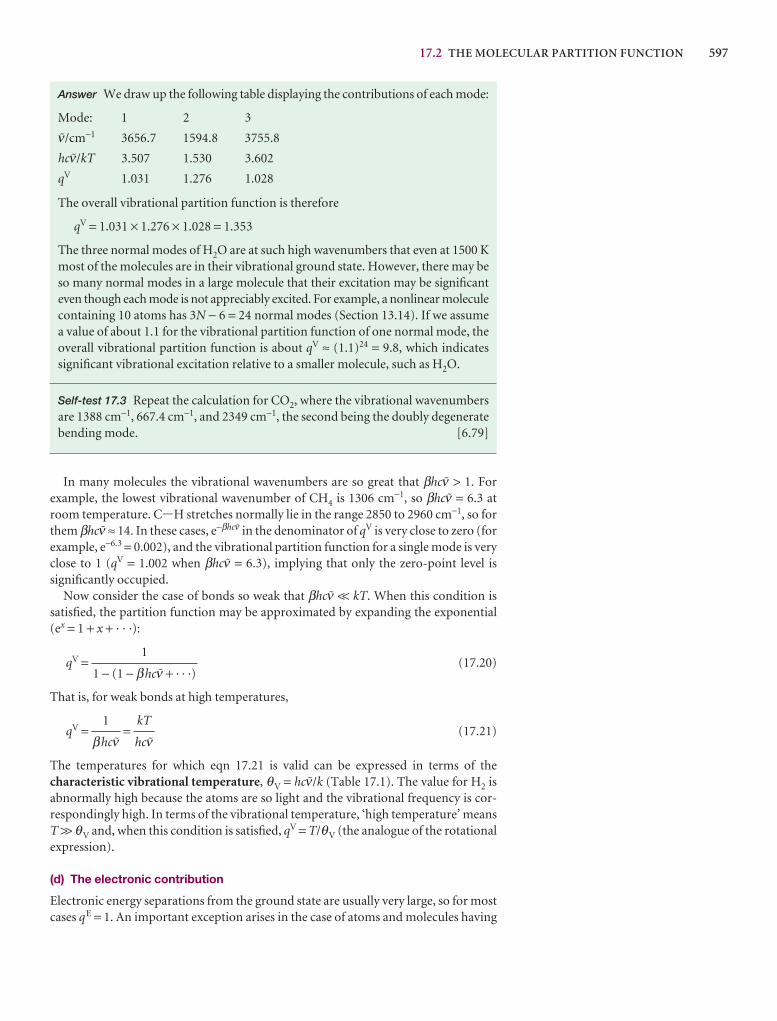
17.2 THE MOLECULAR PARTITION FUNCTION 597
Answer We draw up the following table displaying the contributions of each mode:
Mode: 1 2 3
#/cm−1 3656.7 1594.8 3755.8
hc#/kT 3.507 1.530 3.602
qV 1.031 1.276 1.028
The overall vibrational partition function is therefore
qV = 1.031 × 1.276 × 1.028 = 1.353
The three normal modes of H2O are at such high wavenumbers that even at 1500 Kmost of the molecules are in their vibrational ground state. However, there may beso many normal modes in a large molecule that their excitation may be significanteven though each mode is not appreciably excited. For example, a nonlinear moleculecontaining 10 atoms has 3N − 6 = 24 normal modes (Section 13.14). If we assumea value of about 1.1 for the vibrational partition function of one normal mode, theoverall vibrational partition function is about qV ≈ (1.1)24 = 9.8, which indicatessignificant vibrational excitation relative to a smaller molecule, such as H2O.
Self-test 17.3 Repeat the calculation for CO2, where the vibrational wavenumbersare 1388 cm−1, 667.4 cm−1, and 2349 cm−1, the second being the doubly degeneratebending mode. [6.79]
In many molecules the vibrational wavenumbers are so great that βhc# > 1. For example, the lowest vibrational wavenumber of CH4 is 1306 cm−1, so βhc# = 6.3 atroom temperature. C-H stretches normally lie in the range 2850 to 2960 cm−1, so forthem βhc# ≈ 14. In these cases, e−βhc# in the denominator of qV is very close to zero (forexample, e−6.3 = 0.002), and the vibrational partition function for a single mode is veryclose to 1 (qV = 1.002 when βhc# = 6.3), implying that only the zero-point level issignificantly occupied.
Now consider the case of bonds so weak that βhc# << kT. When this condition issatisfied, the partition function may be approximated by expanding the exponential(ex = 1 + x + · · ·):
qV = (17.20)
That is, for weak bonds at high temperatures,
qV = = (17.21)
The temperatures for which eqn 17.21 is valid can be expressed in terms of the characteristic vibrational temperature, θV = hc#/k (Table 17.1). The value for H2 isabnormally high because the atoms are so light and the vibrational frequency is cor-respondingly high. In terms of the vibrational temperature, ‘high temperature’ meansT >> θV and, when this condition is satisfied, qV = T/θV (the analogue of the rotationalexpression).
(d) The electronic contribution
Electronic energy separations from the ground state are usually very large, so for mostcases qE = 1. An important exception arises in the case of atoms and molecules having
kT
hc#
1
βhc#
1
1 − (1 − βhc# + · · ·)
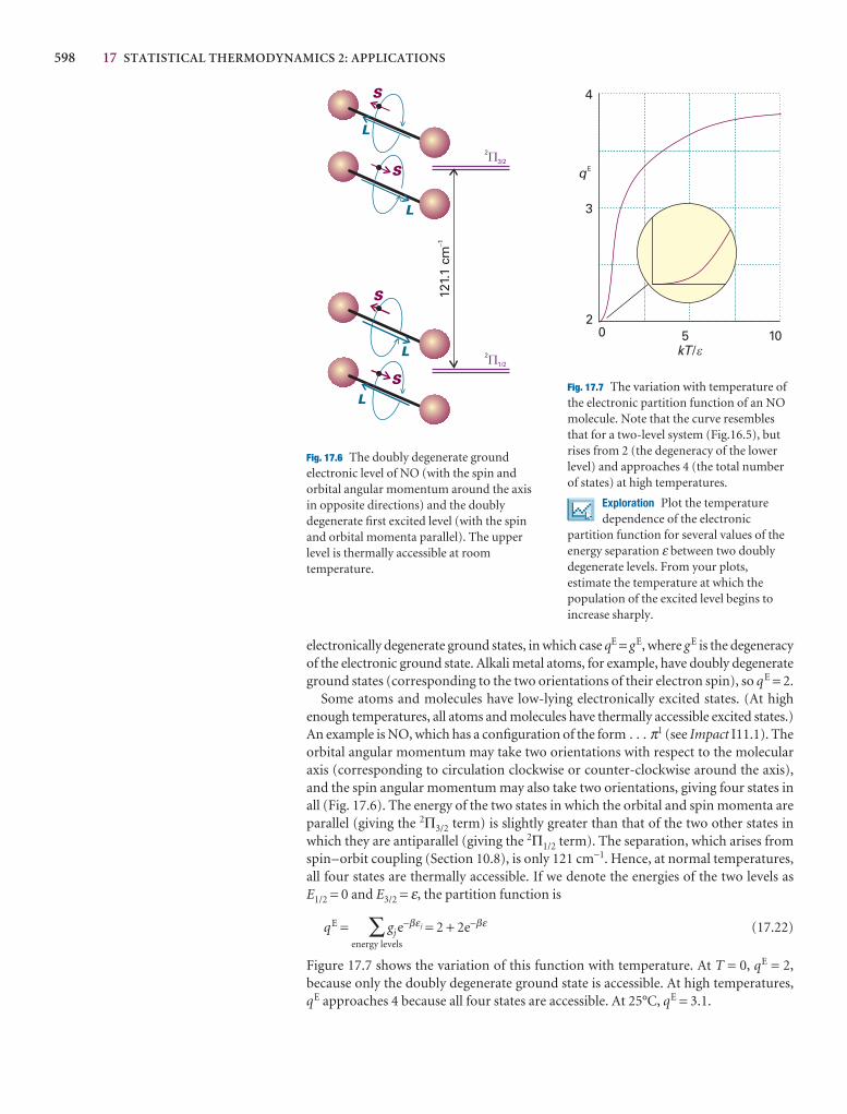
598 17 STATISTICAL THERMODYNAMICS 2: APPLICATIONS
electronically degenerate ground states, in which case qE = gE, where gE is the degeneracyof the electronic ground state. Alkali metal atoms, for example, have doubly degenerateground states (corresponding to the two orientations of their electron spin), so qE = 2.
Some atoms and molecules have low-lying electronically excited states. (At highenough temperatures, all atoms and molecules have thermally accessible excited states.)An example is NO, which has a configuration of the form . . . π1 (see Impact I11.1). Theorbital angular momentum may take two orientations with respect to the molecularaxis (corresponding to circulation clockwise or counter-clockwise around the axis),and the spin angular momentum may also take two orientations, giving four states inall (Fig. 17.6). The energy of the two states in which the orbital and spin momenta areparallel (giving the 2Π3/2 term) is slightly greater than that of the two other states inwhich they are antiparallel (giving the 2Π1/2 term). The separation, which arises fromspin–orbit coupling (Section 10.8), is only 121 cm−1. Hence, at normal temperatures,all four states are thermally accessible. If we denote the energies of the two levels as E1/2 = 0 and E3/2 = ε, the partition function is
qE = ∑energy levels
gj e−βε j = 2 + 2e−βε (17.22)
Figure 17.7 shows the variation of this function with temperature. At T = 0, qE = 2,because only the doubly degenerate ground state is accessible. At high temperatures,qE approaches 4 because all four states are accessible. At 25°C, qE = 3.1.
S
S
S
S
L
L
L
L
2 3/2
2 1/2
121.
1 cm
1�
Fig. 17.6 The doubly degenerate groundelectronic level of NO (with the spin andorbital angular momentum around the axisin opposite directions) and the doublydegenerate first excited level (with the spinand orbital momenta parallel). The upperlevel is thermally accessible at roomtemperature.
qE
4
20 5 10
3
kT/�
Fig. 17.7 The variation with temperature ofthe electronic partition function of an NOmolecule. Note that the curve resemblesthat for a two-level system (Fig.16.5), butrises from 2 (the degeneracy of the lowerlevel) and approaches 4 (the total numberof states) at high temperatures.
Exploration Plot the temperaturedependence of the electronic
partition function for several values of theenergy separation ε between two doublydegenerate levels. From your plots,estimate the temperature at which thepopulation of the excited level begins toincrease sharply.
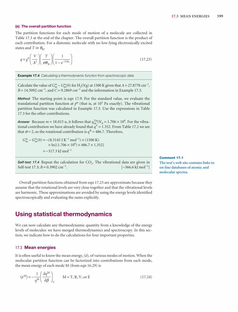
17.3 MEAN ENERGIES 599
Comment 17.1
The text’s web site contains links to on-line databases of atomic andmolecular spectra.
(e) The overall partition function
The partition functions for each mode of motion of a molecule are collected in Table 17.3 at the end of the chapter. The overall partition function is the product ofeach contribution. For a diatomic molecule with no low-lying electronically excitedstates and T >> θR,
q = gE (17.23)
Example 17.4 Calculating a thermodynamic function from spectroscopic data
Calculate the value of G 7m − G 7
m(0) for H2O(g) at 1500 K given that A = 27.8778 cm−1,B = 14.5092 cm−1, and C = 9.2869 cm−1 and the information in Example 17.3.
Method The starting point is eqn 17.9. For the standard value, we evaluate thetranslational partition function at p7 (that is, at 105 Pa exactly). The vibrationalpartition function was calculated in Example 17.3. Use the expressions in Table17.3 for the other contributions.
Answer Because m = 18.015 u, it follows that qmT7/NA = 1.706 × 10⁸. For the vibra-
tional contribution we have already found that qV = 1.352. From Table 17.2 we seethat σ = 2, so the rotational contribution is qR = 486.7. Therefore,
G 7m − G 7
m(0) = −(8.3145 J K−1 mol−1) × (1500 K) × ln{(1.706 × 108) × 486.7 × 1.352}
= −317.3 kJ mol−1
Self-test 17.4 Repeat the calculation for CO2. The vibrational data are given inSelf-test 17.3; B = 0.3902 cm−1. [−366.6 kJ mol−1]
Overall partition functions obtained from eqn 17.23 are approximate because theyassume that the rotational levels are very close together and that the vibrational levelsare harmonic. These approximations are avoided by using the energy levels identifiedspectroscopically and evaluating the sums explicitly.
Using statistical thermodynamics
We can now calculate any thermodynamic quantity from a knowledge of the energylevels of molecules: we have merged thermodynamics and spectroscopy. In this sec-tion, we indicate how to do the calculations for four important properties.
17.3 Mean energies
It is often useful to know the mean energy, �ε�, of various modes of motion. When themolecular partition function can be factorized into contributions from each mode,the mean energy of each mode M (from eqn 16.29) is
�εM� = −V
M = T, R, V, or E (17.24)DF
∂qM
∂β
AC
1
qM
DF
1
1 − e−T/θ v
AC
DF
T
σθR
AC
DF
V
Λ3
AC
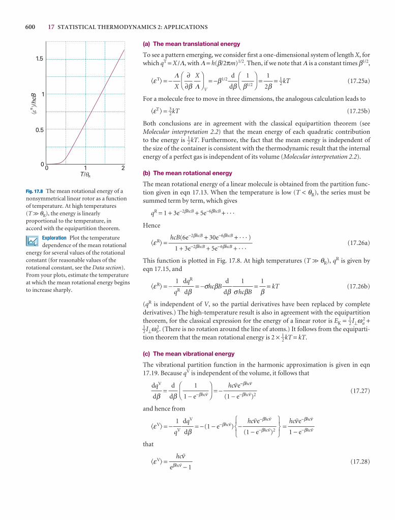
600 17 STATISTICAL THERMODYNAMICS 2: APPLICATIONS
(a) The mean translational energy
To see a pattern emerging, we consider first a one-dimensional system of length X, forwhich qT = X /Λ, with Λ = h(β/2πm)1/2. Then, if we note that Λ is a constant times β1/2,
�εT� = −V
= −β1/2 = = 1–2 kT (17.25a)
For a molecule free to move in three dimensions, the analogous calculation leads to
�εT � = 3–2kT (17.25b)
Both conclusions are in agreement with the classical equipartition theorem (seeMolecular interpretation 2.2) that the mean energy of each quadratic contribution to the energy is 1–2 kT. Furthermore, the fact that the mean energy is independent of the size of the container is consistent with the thermodynamic result that the internalenergy of a perfect gas is independent of its volume (Molecular interpretation 2.2).
(b) The mean rotational energy
The mean rotational energy of a linear molecule is obtained from the partition func-tion given in eqn 17.13. When the temperature is low (T < θR), the series must besummed term by term, which gives
qR = 1 + 3e−2βhcB + 5e−6βhcB + · · ·
Hence
�εR� = (17.26a)
This function is plotted in Fig. 17.8. At high temperatures (T >> θR), qR is given by eqn 17.15, and
�εR� = − = −σhcβB = = kT (17.26b)
(qR is independent of V, so the partial derivatives have been replaced by completederivatives.) The high-temperature result is also in agreement with the equipartitiontheorem, for the classical expression for the energy of a linear rotor is EK = 1–2 I⊥ωa
2 +1–2 I⊥ωb
2. (There is no rotation around the line of atoms.) It follows from the equiparti-tion theorem that the mean rotational energy is 2 × 1–2 kT = kT.
(c) The mean vibrational energy
The vibrational partition function in the harmonic approximation is given in eqn17.19. Because qV is independent of the volume, it follows that
= = − (17.27)
and hence from
�εV� = − = −(1 − e−βhc#) − =
that
�εV� = (17.28)hc#
eβhc# − 1
hc#e−βhc#
1 − e−βhc#
567
hc#e−βhc#
(1 − e−βhc#)2
123
dqV
dβ1
qV
hc#e−βhc#
(1 − e−βhc#)2
DF
1
1 − e−βhc#
AC
d
dβdqV
dβ
1
β1
σhcβB
d
dβdqR
dβ1
qR
hcB(6e−2βhcB + 30e−6βhcB + · · · )
1 + 3e−2βhcB + 5e−6βhcB + · · ·
1
2β
DF
1
β1/2
AC
d
dβ
DF
X
Λ∂
∂β
AC
ΛX
001 2
T/ R
0.5
1
1.5
"#
R/h
cB
�
�
Fig. 17.8 The mean rotational energy of anonsymmetrical linear rotor as a functionof temperature. At high temperatures (T >> θR), the energy is linearlyproportional to the temperature, in accord with the equipartition theorem.
Exploration Plot the temperaturedependence of the mean rotational
energy for several values of the rotationalconstant (for reasonable values of therotational constant, see the Data section).From your plots, estimate the temperatureat which the mean rotational energy beginsto increase sharply.
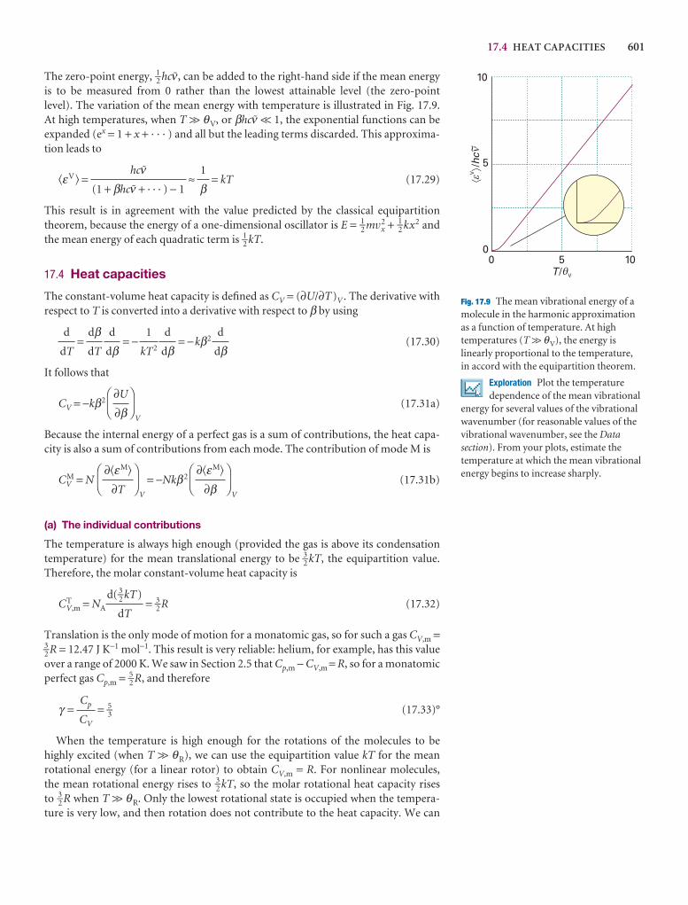
17.4 HEAT CAPACITIES 601
The zero-point energy, 1–2 hc#, can be added to the right-hand side if the mean energyis to be measured from 0 rather than the lowest attainable level (the zero-point level). The variation of the mean energy with temperature is illustrated in Fig. 17.9. At high temperatures, when T >> θV, or βhc# << 1, the exponential functions can be expanded (ex = 1 + x + · · · ) and all but the leading terms discarded. This approxima-tion leads to
�εV � = ≈ = kT (17.29)
This result is in agreement with the value predicted by the classical equipartition theorem, because the energy of a one-dimensional oscillator is E = 1–2 mv2
x + 1–2 kx2 andthe mean energy of each quadratic term is 1–2 kT.
17.4 Heat capacities
The constant-volume heat capacity is defined as CV = (∂U/∂T)V . The derivative withrespect to T is converted into a derivative with respect to β by using
= = − = −kβ2 (17.30)
It follows that
CV = −kβ2
V
(17.31a)
Because the internal energy of a perfect gas is a sum of contributions, the heat capa-city is also a sum of contributions from each mode. The contribution of mode M is
CVM = N
V
= −Nkβ2
V
(17.31b)
(a) The individual contributions
The temperature is always high enough (provided the gas is above its condensationtemperature) for the mean translational energy to be 3–2 kT, the equipartition value.Therefore, the molar constant-volume heat capacity is
CTV,m = NA = 3–2 R (17.32)
Translation is the only mode of motion for a monatomic gas, so for such a gas CV,m =3–2 R = 12.47 J K−1 mol−1. This result is very reliable: helium, for example, has this valueover a range of 2000 K. We saw in Section 2.5 that Cp,m − CV,m = R, so for a monatomicperfect gas Cp,m = 5–2 R, and therefore
γ = = 5–3 (17.33)°
When the temperature is high enough for the rotations of the molecules to behighly excited (when T >> θR), we can use the equipartition value kT for the mean rotational energy (for a linear rotor) to obtain CV,m = R. For nonlinear molecules, the mean rotational energy rises to 3–2 kT, so the molar rotational heat capacity rises to 3–2 R when T >> θR. Only the lowest rotational state is occupied when the tempera-ture is very low, and then rotation does not contribute to the heat capacity. We can
Cp
CV
d( 3–2 kT)
dT
DF
∂�εM�
∂β
AC
DF
∂�εM�
∂T
AC
DF
∂U
∂β
AC
d
dβd
dβ1
kT2
d
dβdβdT
d
dT
1
βhc#
(1 + βhc# + · · · ) − 1
0 5 10
10
5
0
T/ V
áñ
V/h
c~
�
��
Fig. 17.9 The mean vibrational energy of amolecule in the harmonic approximationas a function of temperature. At hightemperatures (T >> θV), the energy islinearly proportional to the temperature, in accord with the equipartition theorem.
Exploration Plot the temperaturedependence of the mean vibrational
energy for several values of the vibrationalwavenumber (for reasonable values of thevibrational wavenumber, see the Datasection). From your plots, estimate thetemperature at which the mean vibrationalenergy begins to increase sharply.
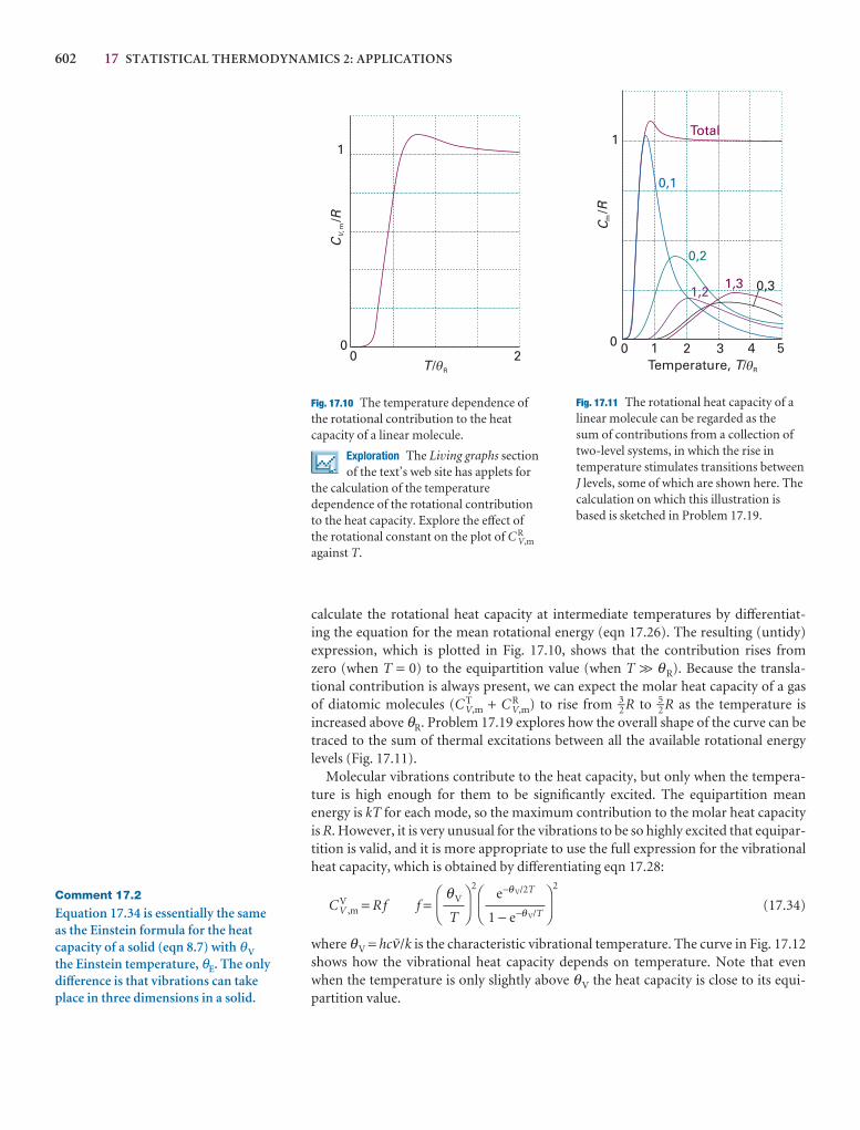
602 17 STATISTICAL THERMODYNAMICS 2: APPLICATIONS
calculate the rotational heat capacity at intermediate temperatures by differentiat-ing the equation for the mean rotational energy (eqn 17.26). The resulting (untidy)expression, which is plotted in Fig. 17.10, shows that the contribution rises from zero (when T = 0) to the equipartition value (when T >> θR). Because the transla-tional contribution is always present, we can expect the molar heat capacity of a gas of diatomic molecules (C T
V,m + C RV,m) to rise from 3–2 R to 5–2 R as the temperature is
increased above θR. Problem 17.19 explores how the overall shape of the curve can betraced to the sum of thermal excitations between all the available rotational energylevels (Fig. 17.11).
Molecular vibrations contribute to the heat capacity, but only when the tempera-ture is high enough for them to be significantly excited. The equipartition mean energy is kT for each mode, so the maximum contribution to the molar heat capacityis R. However, it is very unusual for the vibrations to be so highly excited that equipar-tition is valid, and it is more appropriate to use the full expression for the vibrationalheat capacity, which is obtained by differentiating eqn 17.28:
C VV ,m = Rf f =
2 2
(17.34)
where θV = hc#/k is the characteristic vibrational temperature. The curve in Fig. 17.12shows how the vibrational heat capacity depends on temperature. Note that evenwhen the temperature is only slightly above θV the heat capacity is close to its equi-partition value.
DF
e−θ V/2T
1 − e−θ V/T
AC
DF
θV
T
AC
1
0C
RV
,m/
T/ R
0 2�
Fig. 17.10 The temperature dependence ofthe rotational contribution to the heatcapacity of a linear molecule.
Exploration The Living graphs sectionof the text’s web site has applets for
the calculation of the temperaturedependence of the rotational contributionto the heat capacity. Explore the effect ofthe rotational constant on the plot of C R
V,m
against T.
Comment 17.2
Equation 17.34 is essentially the same as the Einstein formula for the heatcapacity of a solid (eqn 8.7) with θVthe Einstein temperature, θE. The onlydifference is that vibrations can takeplace in three dimensions in a solid.
0,1
0,2
1,2 0,31,3
0 1 2 3 4 50
1Total
Temperature, /T R
CR
m/
�
Fig. 17.11 The rotational heat capacity of alinear molecule can be regarded as the sum of contributions from a collection oftwo-level systems, in which the rise intemperature stimulates transitions betweenJ levels, some of which are shown here. Thecalculation on which this illustration isbased is sketched in Problem 17.19.
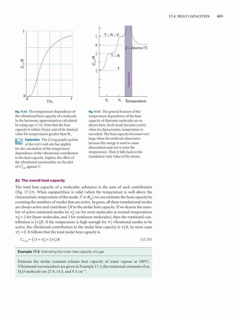
17.4 HEAT CAPACITIES 603
1
0
CR
V,m
/
0 1T/ V�
T
T R�
T R V� �
2 Atoms (T)�
Dis
soci
atio
n
3
2
CR
V,m
/
R V Temperature
3�
25�
27�
� �
Fig. 17.12 The temperature dependence ofthe vibrational heat capacity of a moleculein the harmonic approximation calculatedby using eqn 17.34. Note that the heatcapacity is within 10 per cent of its classicalvalue for temperatures greater than θV.
Exploration The Living graphs sectionof the text’s web site has applets
for the calculation of the temperaturedependence of the vibrational contributionto the heat capacity. Explore the effect ofthe vibrational wavenumber on the plot of CV
V,m against T.
Fig. 17.13 The general features of thetemperature dependence of the heatcapacity of diatomic molecules are asshown here. Each mode becomes activewhen its characteristic temperature isexceeded. The heat capacity becomes verylarge when the molecule dissociatesbecause the energy is used to causedissociation and not to raise thetemperature. Then it falls back to thetranslation-only value of the atoms.
(b) The overall heat capacity
The total heat capacity of a molecular substance is the sum of each contribution (Fig. 17.13). When equipartition is valid (when the temperature is well above thecharacteristic temperature of the mode, T >> θM) we can estimate the heat capacity bycounting the numbers of modes that are active. In gases, all three translational modesare always active and contribute 3–2 R to the molar heat capacity. If we denote the num-ber of active rotational modes by ν*R (so for most molecules at normal temperaturesν*R = 2 for linear molecules, and 3 for nonlinear molecules), then the rotational con-tribution is 1–2 ν*RR. If the temperature is high enough for ν*V vibrational modes to be active, the vibrational contribution to the molar heat capacity is ν*VR. In most cases ν*V ≈ 0. It follows that the total molar heat capacity is
CV,m = 1–2 (3 + ν*R + 2ν*V)R (17.35)
Example 17.5 Estimating the molar heat capacity of a gas
Estimate the molar constant-volume heat capacity of water vapour at 100°C.Vibrational wavenumbers are given in Example 17.3; the rotational constants of anH2O molecule are 27.9, 14.5, and 9.3 cm−1.
604 17 STATISTICAL THERMODYNAMICS 2: APPLICATIONS
Method We need to assess whether the rotational and vibrational modes are activeby computing their characteristic temperatures from the data (to do so, use hc/k =1.439 cm K).
Answer The characteristic temperatures (in round numbers) of the vibrations are 5300 K, 2300 K, and 5400 K; the vibrations are therefore not excited at 373 K.The three rotational modes have characteristic temperatures 40 K, 21 K, and 13 K,so they are fully excited, like the three translational modes. The translational con-tribution is 3–2 R = 12.5 J K−1 mol−1. Fully excited rotations contribute a further 12.5 J K−1 mol−1. Therefore, a value close to 25 J K−1 mol−1 is predicted. The experi-mental value is 26.1 J K−1 mol−1. The discrepancy is probably due to deviationsfrom perfect gas behaviour.
Self-test 17.5 Estimate the molar constant-volume heat capacity of gaseous I2 at25°C (B = 0.037 cm−1; see Table 13.2 for more data). [29 J K−1 mol−1]
17.5 Equations of state
The relation between p and Q in eqn 17.3 is a very important route to the equations of state of real gases in terms of intermolecular forces, for the latter can be built into Q. We have already seen (Example 17.1) that the partition function for a gas of inde-pendent particles leads to the perfect gas equation of state, pV = nRT. Real gases differfrom perfect gases in their equations of state and we saw in Section 1.3 that their equa-tions of state may be written
= 1 + + + · · · (17.36)
where B is the second virial coefficient and C is the third virial coefficient.The total kinetic energy of a gas is the sum of the kinetic energies of the individual
molecules. Therefore, even in a real gas the canonical partition function factorizesinto a part arising from the kinetic energy, which is the same as for the perfect gas, anda factor called the configuration integral, Z, which depends on the intermolecularpotentials. We therefore write
Q = (17.37)
By comparing this equation with eqn 16.45 (Q = qN/N!, with q = V/Λ3), we see that fora perfect gas of atoms (with no contributions from rotational or vibrational modes)
Z = (17.38)
For a real gas of atoms (for which the intermolecular interactions are isotropic), Z isrelated to the total potential energy EP of interaction of all the particles by
Z = �e−βEPdτ1dτ2 · · · dτN (17.39)
where dτi is the volume element for atom i. The physical origin of this term is that theprobability of occurrence of each arrangement of molecules possible in the sample is given by a Boltzmann distribution in which the exponent is given by the potentialenergy corresponding to that arrangement.
1
N !
V N
N !
Z
Λ3N
C
V 2m
B
Vm
pVm
RT
17.5 EQUATIONS OF STATE 605
Illustration 17.1 Calculating a configuration integral
When the molecules do not interact with one another, EP = 0 and hence e−βEP = 1.Then
Z = �dτ1dτ2 · · · dτN =
because ∫dτ = V, where V is the volume of the container. This result coincides witheqn 17.39.
When we consider only interactions between pairs of particles the configuration integral simplifies to
Z = 1–2�e−βEPdτ1dτ2 (17.40)
The second virial coefficient then turns out to be
B = − �f dτ1dτ2 (17.41)
The quantity f is the Mayer f-function: it goes to zero when the two particles are so far apart that EP = 0. When the intermolecular interaction depends only on the separation r of the particles and not on their relative orientation or their absolute position in space, as in the interaction of closed-shell atoms in a uniform sample, thevolume element simplifies to 4πr 2dr (because the integrals over the angular variablesin dτ = r 2dr sin θ dθdφ give a factor of 4π) and eqn 17.41 becomes
B = −2πNA�∞
0
fr 2dr f = e−βEP − 1 (17.42)
The integral can be evaluated (usually numerically) by substituting an expression forthe intermolecular potential energy.
Intermolecular potential energies are discussed in more detail in Chapter 18, where several expressions are developed for them. At this stage, we can illustrate how eqn 17.42 is used by considering the hard-sphere potential, which is infinitewhen the separation of the two molecules, r, is less than or equal to a certain value σ,and is zero for greater separations. Then
e−βEP = 0 f = −1 when r ≤ σ (and EP = ∞) (17.43a)
e−βEP = 1 f = 0 when r > σ (and EP = 0) (17.43b)
It follows from eqn 17.42 that the second virial coefficient is
B = 2πNA�σ
0
r 2dr = 2–3 πNAσ3 (17.44)
This calculation of B raises the question as to whether a potential can be found that,when the virial coefficients are evaluated, gives the van der Waals equation of state.Such a potential can be found for weak attractive interactions (a << RT): it consists ofa hard-sphere repulsive core and a long-range, shallow attractive region (see Problem17.15). A further point is that, once a second virial coefficient has been calculated fora given intermolecular potential, it is possible to calculate other thermodynamicproperties that depend on the form of the potential. For example, it is possible to
NA
2V
V N
N!
1
N!
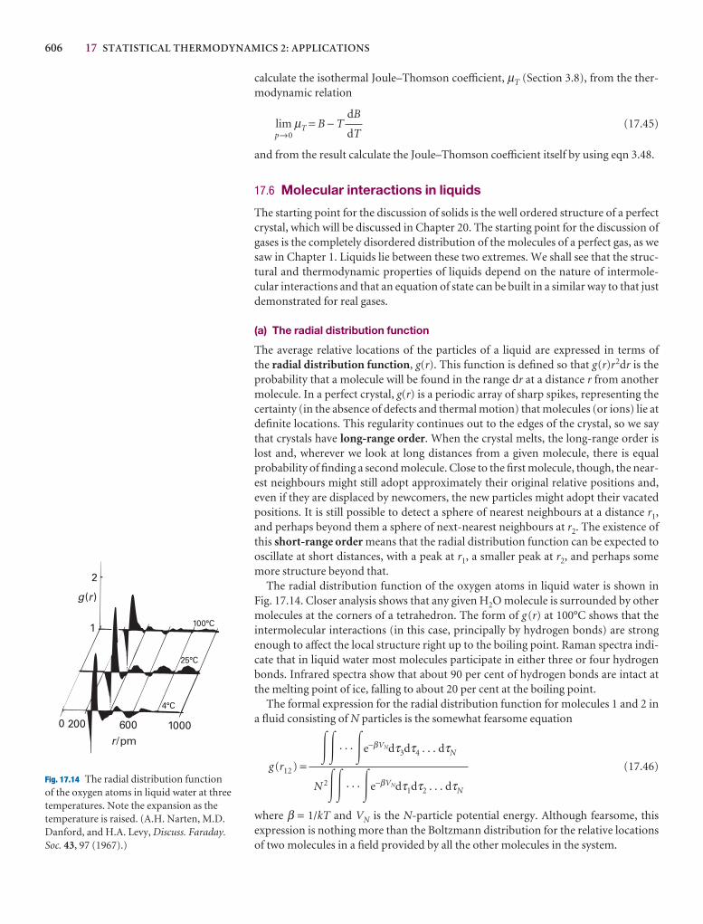
606 17 STATISTICAL THERMODYNAMICS 2: APPLICATIONS
calculate the isothermal Joule–Thomson coefficient, µT (Section 3.8), from the ther-modynamic relation
p→0lim µT = B − T (17.45)
and from the result calculate the Joule–Thomson coefficient itself by using eqn 3.48.
17.6 Molecular interactions in liquids
The starting point for the discussion of solids is the well ordered structure of a perfectcrystal, which will be discussed in Chapter 20. The starting point for the discussion ofgases is the completely disordered distribution of the molecules of a perfect gas, as wesaw in Chapter 1. Liquids lie between these two extremes. We shall see that the struc-tural and thermodynamic properties of liquids depend on the nature of intermole-cular interactions and that an equation of state can be built in a similar way to that justdemonstrated for real gases.
(a) The radial distribution function
The average relative locations of the particles of a liquid are expressed in terms of the radial distribution function, g(r). This function is defined so that g(r)r2dr is theprobability that a molecule will be found in the range dr at a distance r from anothermolecule. In a perfect crystal, g(r) is a periodic array of sharp spikes, representing thecertainty (in the absence of defects and thermal motion) that molecules (or ions) lie atdefinite locations. This regularity continues out to the edges of the crystal, so we saythat crystals have long-range order. When the crystal melts, the long-range order islost and, wherever we look at long distances from a given molecule, there is equalprobability of finding a second molecule. Close to the first molecule, though, the near-est neighbours might still adopt approximately their original relative positions and,even if they are displaced by newcomers, the new particles might adopt their vacatedpositions. It is still possible to detect a sphere of nearest neighbours at a distance r1,and perhaps beyond them a sphere of next-nearest neighbours at r2. The existence ofthis short-range order means that the radial distribution function can be expected tooscillate at short distances, with a peak at r1, a smaller peak at r2, and perhaps somemore structure beyond that.
The radial distribution function of the oxygen atoms in liquid water is shown inFig. 17.14. Closer analysis shows that any given H2O molecule is surrounded by othermolecules at the corners of a tetrahedron. The form of g(r) at 100°C shows that the intermolecular interactions (in this case, principally by hydrogen bonds) are strongenough to affect the local structure right up to the boiling point. Raman spectra indi-cate that in liquid water most molecules participate in either three or four hydrogenbonds. Infrared spectra show that about 90 per cent of hydrogen bonds are intact atthe melting point of ice, falling to about 20 per cent at the boiling point.
The formal expression for the radial distribution function for molecules 1 and 2 ina fluid consisting of N particles is the somewhat fearsome equation
g(r12 ) = (17.46)
where β = 1/kT and VN is the N-particle potential energy. Although fearsome, this expression is nothing more than the Boltzmann distribution for the relative locationsof two molecules in a field provided by all the other molecules in the system.
�� · · · �e−βVNdτ3dτ4 . . . dτN
N 2�� · · · �e−βVNdτ1dτ2 . . . dτN
dB
dT
g r( )
2
1 100°C
25°C
4°C
10000 200 600r/pm
Fig. 17.14 The radial distribution functionof the oxygen atoms in liquid water at threetemperatures. Note the expansion as thetemperature is raised. (A.H. Narten, M.D.Danford, and H.A. Levy, Discuss. Faraday.Soc. 43, 97 (1967).)
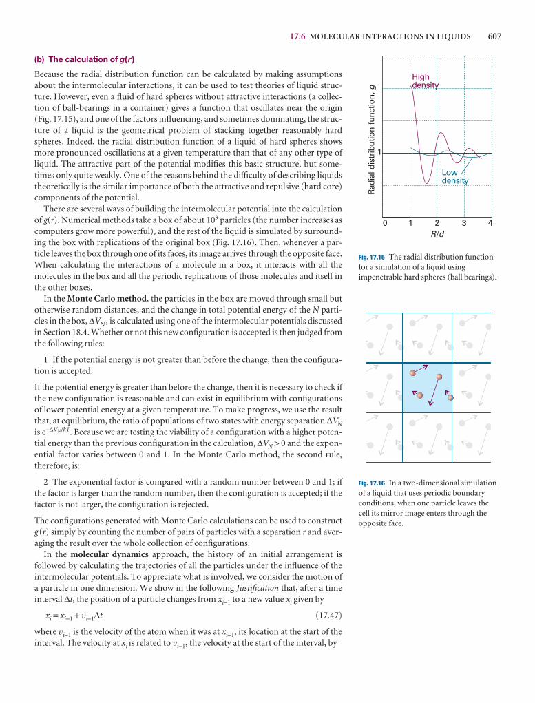
17.6 MOLECULAR INTERACTIONS IN LIQUIDS 607
(b) The calculation of g(r )
Because the radial distribution function can be calculated by making assumptionsabout the intermolecular interactions, it can be used to test theories of liquid struc-ture. However, even a fluid of hard spheres without attractive interactions (a collec-tion of ball-bearings in a container) gives a function that oscillates near the origin(Fig. 17.15), and one of the factors influencing, and sometimes dominating, the struc-ture of a liquid is the geometrical problem of stacking together reasonably hardspheres. Indeed, the radial distribution function of a liquid of hard spheres showsmore pronounced oscillations at a given temperature than that of any other type ofliquid. The attractive part of the potential modifies this basic structure, but some-times only quite weakly. One of the reasons behind the difficulty of describing liquids theoretically is the similar importance of both the attractive and repulsive (hard core)components of the potential.
There are several ways of building the intermolecular potential into the calculationof g(r). Numerical methods take a box of about 103 particles (the number increases ascomputers grow more powerful), and the rest of the liquid is simulated by surround-ing the box with replications of the original box (Fig. 17.16). Then, whenever a par-ticle leaves the box through one of its faces, its image arrives through the opposite face.When calculating the interactions of a molecule in a box, it interacts with all themolecules in the box and all the periodic replications of those molecules and itself inthe other boxes.
In the Monte Carlo method, the particles in the box are moved through small butotherwise random distances, and the change in total potential energy of the N parti-cles in the box, ∆VN , is calculated using one of the intermolecular potentials discussedin Section 18.4. Whether or not this new configuration is accepted is then judged fromthe following rules:
1 If the potential energy is not greater than before the change, then the configura-tion is accepted.
If the potential energy is greater than before the change, then it is necessary to check ifthe new configuration is reasonable and can exist in equilibrium with configurationsof lower potential energy at a given temperature. To make progress, we use the resultthat, at equilibrium, the ratio of populations of two states with energy separation ∆VN
is e−∆VN/kT. Because we are testing the viability of a configuration with a higher poten-tial energy than the previous configuration in the calculation, ∆VN > 0 and the expon-ential factor varies between 0 and 1. In the Monte Carlo method, the second rule,therefore, is:
2 The exponential factor is compared with a random number between 0 and 1; ifthe factor is larger than the random number, then the configuration is accepted; if thefactor is not larger, the configuration is rejected.
The configurations generated with Monte Carlo calculations can be used to constructg(r) simply by counting the number of pairs of particles with a separation r and aver-aging the result over the whole collection of configurations.
In the molecular dynamics approach, the history of an initial arrangement is followed by calculating the trajectories of all the particles under the influence of theintermolecular potentials. To appreciate what is involved, we consider the motion ofa particle in one dimension. We show in the following Justification that, after a timeinterval ∆t, the position of a particle changes from xi−1 to a new value xi given by
xi = xi−1 + vi−1∆t (17.47)
where vi−1 is the velocity of the atom when it was at xi−1, its location at the start of theinterval. The velocity at xi is related to vi−1, the velocity at the start of the interval, by
Highdensity
Lowdensity
1 2 3 40
1
Rad
ial d
istr
ibut
ion
func
tion,
g
R d/
Fig. 17.15 The radial distribution functionfor a simulation of a liquid usingimpenetrable hard spheres (ball bearings).
Fig. 17.16 In a two-dimensional simulationof a liquid that uses periodic boundaryconditions, when one particle leaves thecell its mirror image enters through theopposite face.
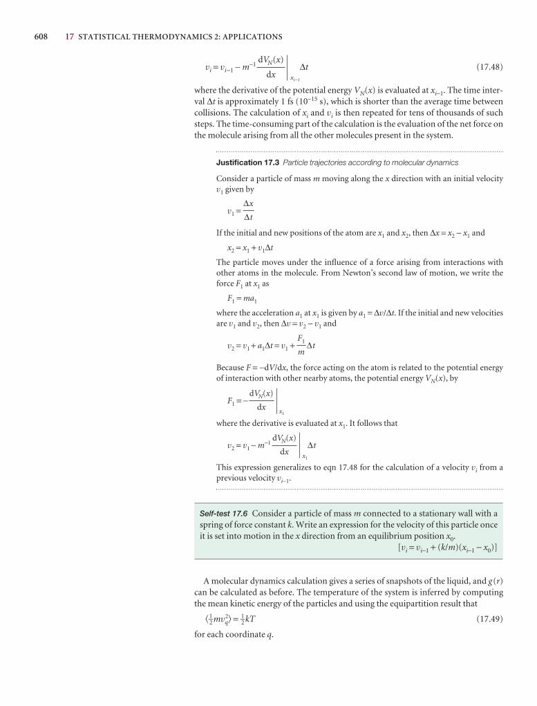
608 17 STATISTICAL THERMODYNAMICS 2: APPLICATIONS
vi = vi−1 − m−1
xi−1
∆t (17.48)
where the derivative of the potential energy VN(x) is evaluated at xi−1. The time inter-val ∆t is approximately 1 fs (10−15 s), which is shorter than the average time betweencollisions. The calculation of xi and vi is then repeated for tens of thousands of suchsteps. The time-consuming part of the calculation is the evaluation of the net force onthe molecule arising from all the other molecules present in the system.
Justification 17.3 Particle trajectories according to molecular dynamics
Consider a particle of mass m moving along the x direction with an initial velocityv1 given by
v1 =
If the initial and new positions of the atom are x1 and x2, then ∆x = x2 − x1 and
x2 = x1 + v1∆t
The particle moves under the influence of a force arising from interactions withother atoms in the molecule. From Newton’s second law of motion, we write theforce F1 at x1 as
F1 = ma1
where the acceleration a1 at x1 is given by a1 = ∆v/∆t. If the initial and new velocitiesare v1 and v2, then ∆v = v2 − v1 and
v2 = v1 + a1∆t = v1 + ∆t
Because F = −dV/dx, the force acting on the atom is related to the potential energyof interaction with other nearby atoms, the potential energy VN(x), by
F1 = −x1
where the derivative is evaluated at x1. It follows that
v2 = v1 − m−1
x1
∆t
This expression generalizes to eqn 17.48 for the calculation of a velocity vi from aprevious velocity vi−1.
Self-test 17.6 Consider a particle of mass m connected to a stationary wall with aspring of force constant k. Write an expression for the velocity of this particle onceit is set into motion in the x direction from an equilibrium position x0.
[vi = vi−1 + (k/m)(xi−1 − x0)]
A molecular dynamics calculation gives a series of snapshots of the liquid, and g(r)can be calculated as before. The temperature of the system is inferred by computingthe mean kinetic energy of the particles and using the equipartition result that
�1–2 mvq2� = 1–2 kT (17.49)
for each coordinate q.
dVN(x)
dx
dVN(x)
dx
F1
m
∆x
∆t
dVN(x)
dx
17.7 RESIDUAL ENTROPIES 609
(c) The thermodynamic properties of liquids
Once g(r) is known it can be used to calculate the thermodynamic properties of liquids. For example, the contribution of the pairwise additive intermolecular poten-tial, V2, to the internal energy is given by the integral
U = �∞
0
g(r)V2r2dr (17.50)
That is, U is essentially the average two-particle potential energy weighted by g(r)r 2dr,which is the probability that the pair of particles have a separation between r and r + dr.Likewise, the contribution that pairwise interactions make to the pressure is
= 1 − �∞
0
g(r)v2r 2dr v2 = r (17.51a)
The quantity v2 is called the virial (hence the term ‘virial equation of state’). To under-stand the physical content of this expression, we rewrite it as
p = − 2π2
�∞
0
g(r)v2r 2dr (17.51b)
The first term on the right is the kinetic pressure, the contribution to the pressurefrom the impact of the molecules in free flight. The second term is essentially the internal pressure, πT = (∂U/∂V)T , introduced in Section 2.11, representing the con-tribution to the pressure from the intermolecular forces. To see the connection, weshould recognize −dV2/dr (in v2) as the force required to move two molecules apart,and therefore −r(dV2/dr) as the work required to separate the molecules through adistance r. The second term is therefore the average of this work over the range of pairwise separations in the liquid as represented by the probability of finding twomolecules at separations between r and r + dr, which is g(r)r 2dr. In brief, the integral,when multiplied by the square of the number density, is the change in internal energyof the system as it expands, and therefore is equal to the internal pressure.
17.7 Residual entropies
Entropies may be calculated from spectroscopic data; they may also be measured experimentally (Section 3.3). In many cases there is good agreement, but in some the experimental entropy is less than the calculated value. One possibility is that theexperimental determination failed to take a phase transition into account (and a con-tribution of the form ∆trsH/Ttrs incorrectly omitted from the sum). Another possibilityis that some disorder is present in the solid even at T = 0. The entropy at T = 0 is thengreater than zero and is called the residual entropy.
The origin and magnitude of the residual entropy can be explained by consideringa crystal composed of AB molecules, where A and B are similar atoms (such as CO,with its very small electric dipole moment). There may be so little energy differencebetween . . .AB AB AB AB. . . , . . .AB BA BA AB. . . , and other arrangements that themolecules adopt the orientations AB and BA at random in the solid. We can readilycalculate the entropy arising from residual disorder by using the Boltzmann formulaS = k ln W. To do so, we suppose that two orientations are equally probable, and thatthe sample consists of N molecules. Because the same energy can be achieved in 2N
different ways (because each molecule can take either of two orientations), the totalnumber of ways of achieving the same energy is W = 2N. It follows that
S = k ln 2N = Nk ln 2 = nR ln 2 (17.52a)
DF
N
V
AC
nRT
V
dV2
dr
2πN
kTV
pV
nRT
2πN2
V
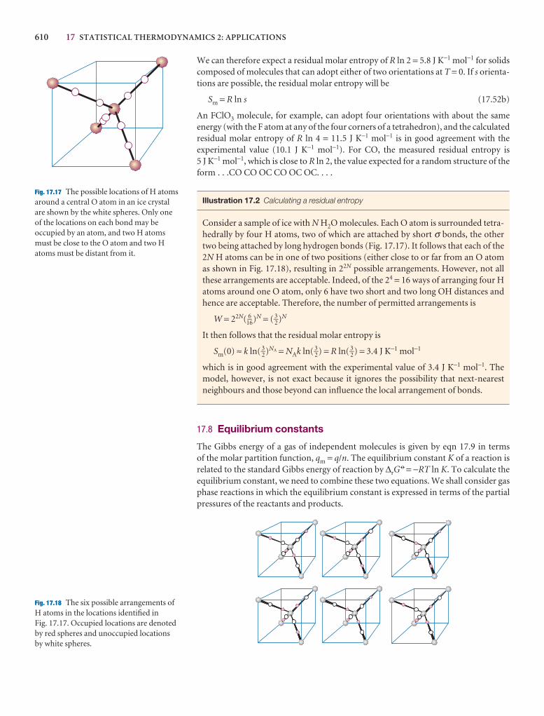
610 17 STATISTICAL THERMODYNAMICS 2: APPLICATIONS
Fig. 17.17 The possible locations of H atomsaround a central O atom in an ice crystalare shown by the white spheres. Only oneof the locations on each bond may beoccupied by an atom, and two H atomsmust be close to the O atom and two Hatoms must be distant from it.
Fig. 17.18 The six possible arrangements of H atoms in the locations identified in Fig. 17.17. Occupied locations are denotedby red spheres and unoccupied locations by white spheres.
We can therefore expect a residual molar entropy of R ln 2 = 5.8 J K−1 mol−1 for solidscomposed of molecules that can adopt either of two orientations at T = 0. If s orienta-tions are possible, the residual molar entropy will be
Sm = R ln s (17.52b)
An FClO3 molecule, for example, can adopt four orientations with about the same energy (with the F atom at any of the four corners of a tetrahedron), and the calculatedresidual molar entropy of R ln 4 = 11.5 J K−1 mol−1 is in good agreement with the experimental value (10.1 J K−1 mol−1). For CO, the measured residual entropy is 5 J K−1 mol−1, which is close to R ln 2, the value expected for a random structure of theform . . .CO CO OC CO OC OC. . . .
Illustration 17.2 Calculating a residual entropy
Consider a sample of ice with N H2O molecules. Each O atom is surrounded tetra-hedrally by four H atoms, two of which are attached by short σ bonds, the othertwo being attached by long hydrogen bonds (Fig. 17.17). It follows that each of the2N H atoms can be in one of two positions (either close to or far from an O atomas shown in Fig. 17.18), resulting in 22N possible arrangements. However, not allthese arrangements are acceptable. Indeed, of the 24 = 16 ways of arranging four Hatoms around one O atom, only 6 have two short and two long OH distances andhence are acceptable. Therefore, the number of permitted arrangements is
W = 22N( 6–16)N = ( 3–2)N
It then follows that the residual molar entropy is
Sm(0) ≈ k ln( 3–2)NA = NAk ln( 3–2) = R ln( 3–2) = 3.4 J K−1 mol−1
which is in good agreement with the experimental value of 3.4 J K−1 mol−1. Themodel, however, is not exact because it ignores the possibility that next-nearestneighbours and those beyond can influence the local arrangement of bonds.
17.8 Equilibrium constants
The Gibbs energy of a gas of independent molecules is given by eqn 17.9 in terms of the molar partition function, qm = q/n. The equilibrium constant K of a reaction isrelated to the standard Gibbs energy of reaction by ∆rG
7 = −RT ln K. To calculate theequilibrium constant, we need to combine these two equations. We shall consider gasphase reactions in which the equilibrium constant is expressed in terms of the partialpressures of the reactants and products.
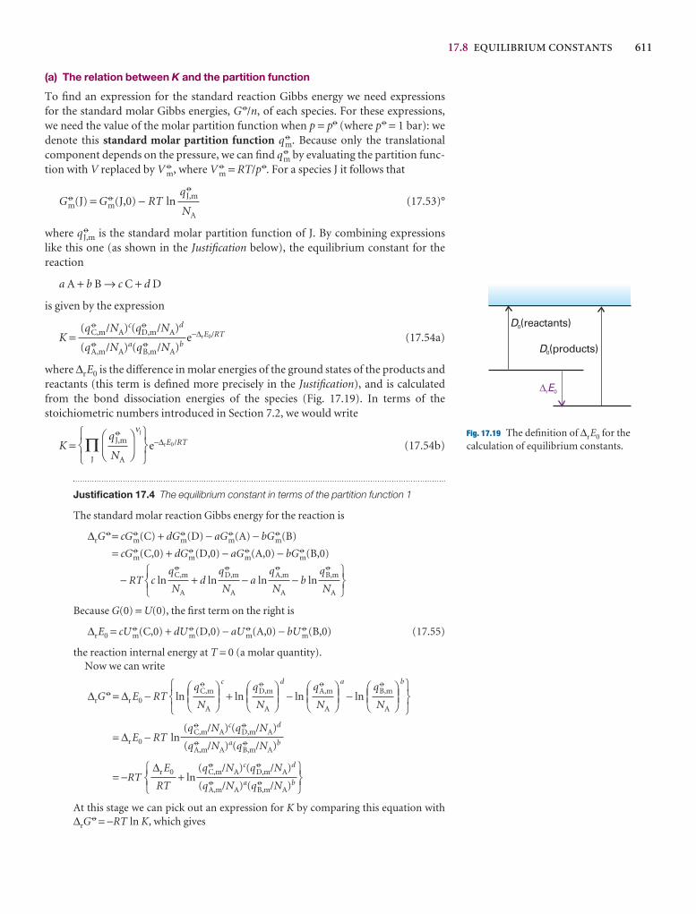
17.8 EQUILIBRIUM CONSTANTS 611
(a) The relation between K and the partition function
To find an expression for the standard reaction Gibbs energy we need expressions for the standard molar Gibbs energies, G 7/n, of each species. For these expressions, we need the value of the molar partition function when p = p7 (where p7 = 1 bar): wedenote this standard molar partition function q 7
m. Because only the translationalcomponent depends on the pressure, we can find q 7
m by evaluating the partition func-tion with V replaced by V 7
m, where V 7m = RT/p7. For a species J it follows that
G 7m(J) = G 7
m(J,0) − RT ln (17.53)°
where q 7J,m is the standard molar partition function of J. By combining expressions
like this one (as shown in the Justification below), the equilibrium constant for the reaction
a A + b B → c C + d D
is given by the expression
K = e−∆rE0/RT (17.54a)
where ∆rE0 is the difference in molar energies of the ground states of the products andreactants (this term is defined more precisely in the Justification), and is calculatedfrom the bond dissociation energies of the species (Fig. 17.19). In terms of the stoichiometric numbers introduced in Section 7.2, we would write
K = ΠJ
νJ
e−∆rE0/RT (17.54b)
Justification 17.4 The equilibrium constant in terms of the partition function 1
The standard molar reaction Gibbs energy for the reaction is
∆rG7 = cG 7
m(C) + dG 7m(D) − aG 7
m(A) − bG 7m(B)
= cG 7m(C,0) + dG 7
m(D,0) − aG 7m(A,0) − bG 7
m(B,0)
− RT c ln + d ln − a ln − b ln
Because G(0) = U(0), the first term on the right is
∆rE0 = cU 7m(C,0) + dU 7
m(D,0) − aU 7m(A,0) − bU 7
m(B,0) (17.55)
the reaction internal energy at T = 0 (a molar quantity).Now we can write
∆rG7 = ∆r E0 − RT ln
c
+ ln
d
− ln
a
− ln
b
= ∆r E0 − RT ln
= −RT + ln
At this stage we can pick out an expression for K by comparing this equation with∆rG
7 = −RT ln K, which gives
567(q 7
C,m/NA)c(q 7D,m/NA)d
(q 7A,m/NA)a(q 7
B,m/NA)b
∆r E0
RT
123
(q 7C,m/NA)c(q 7
D,m/NA)d
(q 7A,m/NA)a(q 7
B,m/NA)b
567
DEFq 7
B,m
NA
ABCDEF
q 7A,m
NA
ABCDEF
q 7D,m
NA
ABCDEF
q 7C,m
NA
ABC123
567q 7
B,m
NA
q 7A,m
NA
q 7D,m
NA
q 7C,m
NA
123
567
DF
q 7J,m
NA
AC
123
(q 7C,m/NA)c(q7
D,m/NA)d
(q 7A,m/NA)a(q 7
B,m/NA)b
q 7J,m
NA
D0(reactants)
D0(products)
r 0E
Fig. 17.19 The definition of ∆rE0 for thecalculation of equilibrium constants.
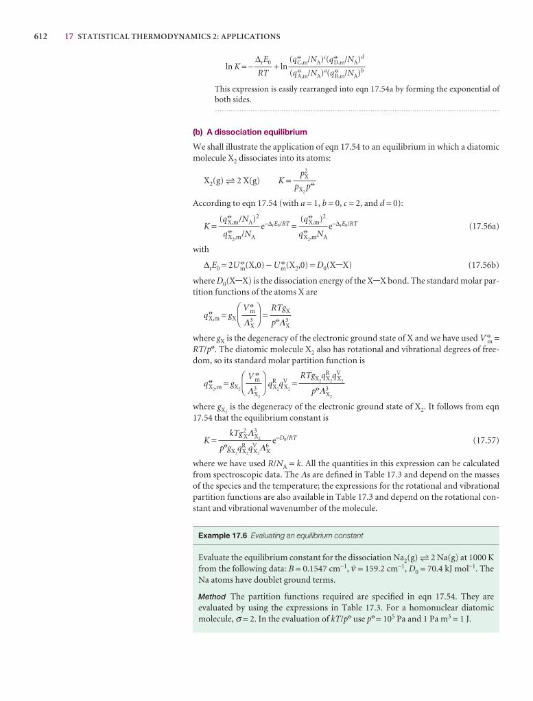
612 17 STATISTICAL THERMODYNAMICS 2: APPLICATIONS
ln K = − + ln
This expression is easily rearranged into eqn 17.54a by forming the exponential ofboth sides.
(b) A dissociation equilibrium
We shall illustrate the application of eqn 17.54 to an equilibrium in which a diatomicmolecule X2 dissociates into its atoms:
X2(g) 5 2 X(g) K =
According to eqn 17.54 (with a = 1, b = 0, c = 2, and d = 0):
K = e−∆rE0/RT = e−∆rE0/RT (17.56a)
with
∆rE0 = 2U 7m(X,0) − U 7
m(X2,0) = D0(X-X) (17.56b)
where D0(X-X) is the dissociation energy of the X-X bond. The standard molar par-tition functions of the atoms X are
q 7X,m = gX =
where gX is the degeneracy of the electronic ground state of X and we have used V 7m =
RT/p7. The diatomic molecule X2 also has rotational and vibrational degrees of free-dom, so its standard molar partition function is
q 7X2,m = gX2
qRX2
qVX2
=
where gX2is the degeneracy of the electronic ground state of X2. It follows from eqn
17.54 that the equilibrium constant is
K = e−D0/RT (17.57)
where we have used R/NA = k. All the quantities in this expression can be calculatedfrom spectroscopic data. The Λs are defined in Table 17.3 and depend on the massesof the species and the temperature; the expressions for the rotational and vibrationalpartition functions are also available in Table 17.3 and depend on the rotational con-stant and vibrational wavenumber of the molecule.
Example 17.6 Evaluating an equilibrium constant
Evaluate the equilibrium constant for the dissociation Na2(g) 5 2 Na(g) at 1000 Kfrom the following data: B = 0.1547 cm−1, # = 159.2 cm−1, D0 = 70.4 kJ mol−1. TheNa atoms have doublet ground terms.
Method The partition functions required are specified in eqn 17.54. They are evaluated by using the expressions in Table 17.3. For a homonuclear diatomicmolecule, σ = 2. In the evaluation of kT/p7 use p7 = 105 Pa and 1 Pa m3 = 1 J.
kTg2XΛ3
X2
p7gX2qR
X2qV
X2Λ6
X
RTgX2qR
X2qV
X2
p7Λ3X2
DF
V 7m
Λ3X2
AC
RTgX
p7Λ3X
DF
V 7m
Λ3X
AC
(q 7X,m)2
q 7X2,mNA
(q 7X,m/NA)2
q 7X2,m/NA
p2X
pX2p7
(q 7C,m/NA)c(q 7
D,m/NA)d
(q 7A,m/NA)a(q 7
B,m/NA)b
∆rE0
RT
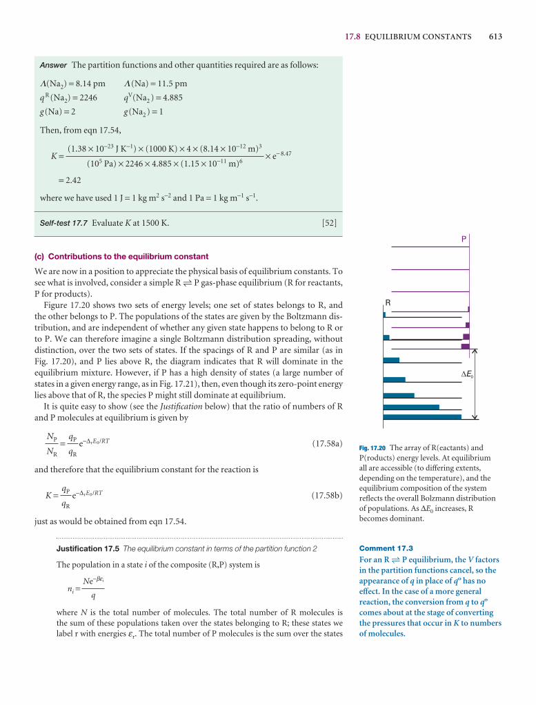
17.8 EQUILIBRIUM CONSTANTS 613
E0
R
P
Fig. 17.20 The array of R(eactants) andP(roducts) energy levels. At equilibrium all are accessible (to differing extents,depending on the temperature), and theequilibrium composition of the systemreflects the overall Bolzmann distributionof populations. As ∆E0 increases, Rbecomes dominant.
Comment 17.3
For an R 5 P equilibrium, the V factorsin the partition functions cancel, so theappearance of q in place of q7 has noeffect. In the case of a more generalreaction, the conversion from q to q7
comes about at the stage of convertingthe pressures that occur in K to numbersof molecules.
Answer The partition functions and other quantities required are as follows:
Λ(Na2) = 8.14 pm Λ(Na) = 11.5 pm
q R (Na2) = 2246 qV(Na2 ) = 4.885
g(Na) = 2 g(Na2 ) = 1
Then, from eqn 17.54,
K = × e− 8.47
= 2.42
where we have used 1 J = 1 kg m2 s−2 and 1 Pa = 1 kg m−1 s−1.
Self-test 17.7 Evaluate K at 1500 K. [52]
(c) Contributions to the equilibrium constant
We are now in a position to appreciate the physical basis of equilibrium constants. Tosee what is involved, consider a simple R 5 P gas-phase equilibrium (R for reactants,P for products).
Figure 17.20 shows two sets of energy levels; one set of states belongs to R, and the other belongs to P. The populations of the states are given by the Boltzmann dis-tribution, and are independent of whether any given state happens to belong to R orto P. We can therefore imagine a single Boltzmann distribution spreading, without distinction, over the two sets of states. If the spacings of R and P are similar (as in Fig. 17.20), and P lies above R, the diagram indicates that R will dominate in the equilibrium mixture. However, if P has a high density of states (a large number ofstates in a given energy range, as in Fig. 17.21), then, even though its zero-point energylies above that of R, the species P might still dominate at equilibrium.
It is quite easy to show (see the Justification below) that the ratio of numbers of Rand P molecules at equilibrium is given by
= e−∆rE0/RT (17.58a)
and therefore that the equilibrium constant for the reaction is
K = e−∆rE0/RT (17.58b)
just as would be obtained from eqn 17.54.
Justification 17.5 The equilibrium constant in terms of the partition function 2
The population in a state i of the composite (R,P) system is
ni =
where N is the total number of molecules. The total number of R molecules is the sum of these populations taken over the states belonging to R; these states welabel r with energies εr. The total number of P molecules is the sum over the states
Ne−βεi
q
qP
qR
qP
qR
NP
NR
(1.38 × 10⁻²³ J K−1) × (1000 K) × 4 × (8.14 × 10−12 m)3
(105 Pa) × 2246 × 4.885 × (1.15 × 10−11 m)6
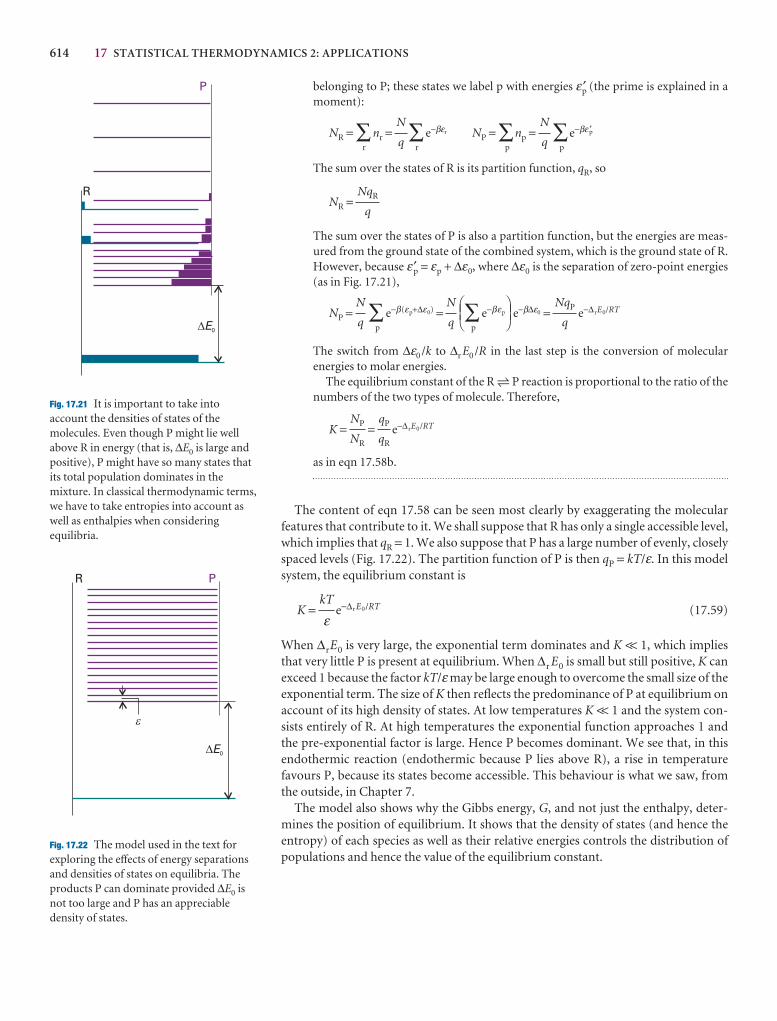
614 17 STATISTICAL THERMODYNAMICS 2: APPLICATIONS
belonging to P; these states we label p with energies εp′ (the prime is explained in amoment):
NR = ∑r
nr = ∑r
e−βεr NP = ∑p
np = ∑p
e−βε ′p
The sum over the states of R is its partition function, qR, so
NR =
The sum over the states of P is also a partition function, but the energies are meas-ured from the ground state of the combined system, which is the ground state of R.However, because ε′p = εp + ∆ε0, where ∆ε0 is the separation of zero-point energies(as in Fig. 17.21),
NP = ∑p
e−β(εp+∆ε0) = ∑p
e−βεp e−β∆ε0 = e−∆rE0/RT
The switch from ∆ε0 /k to ∆r E0 /R in the last step is the conversion of molecular energies to molar energies.
The equilibrium constant of the R 5 P reaction is proportional to the ratio of thenumbers of the two types of molecule. Therefore,
K = = e−∆rE0/RT
as in eqn 17.58b.
The content of eqn 17.58 can be seen most clearly by exaggerating the molecularfeatures that contribute to it. We shall suppose that R has only a single accessible level,which implies that qR = 1. We also suppose that P has a large number of evenly, closelyspaced levels (Fig. 17.22). The partition function of P is then qP = kT/ε. In this modelsystem, the equilibrium constant is
K = e−∆rE0/RT (17.59)
When ∆rE0 is very large, the exponential term dominates and K << 1, which impliesthat very little P is present at equilibrium. When ∆r E0 is small but still positive, K canexceed 1 because the factor kT/ε may be large enough to overcome the small size of theexponential term. The size of K then reflects the predominance of P at equilibrium onaccount of its high density of states. At low temperatures K << 1 and the system con-sists entirely of R. At high temperatures the exponential function approaches 1 andthe pre-exponential factor is large. Hence P becomes dominant. We see that, in thisendothermic reaction (endothermic because P lies above R), a rise in temperaturefavours P, because its states become accessible. This behaviour is what we saw, fromthe outside, in Chapter 7.
The model also shows why the Gibbs energy, G, and not just the enthalpy, deter-mines the position of equilibrium. It shows that the density of states (and hence theentropy) of each species as well as their relative energies controls the distribution ofpopulations and hence the value of the equilibrium constant.
kT
ε
qP
qR
NP
NR
NqP
q
DEFABC
N
q
N
q
NqR
q
N
q
N
q
E0
R
P
Fig. 17.21 It is important to take intoaccount the densities of states of themolecules. Even though P might lie wellabove R in energy (that is, ∆E0 is large andpositive), P might have so many states thatits total population dominates in themixture. In classical thermodynamic terms,we have to take entropies into account aswell as enthalpies when consideringequilibria.
E0
R P
�
Fig. 17.22 The model used in the text forexploring the effects of energy separationsand densities of states on equilibria. Theproducts P can dominate provided ∆E0 isnot too large and P has an appreciabledensity of states.
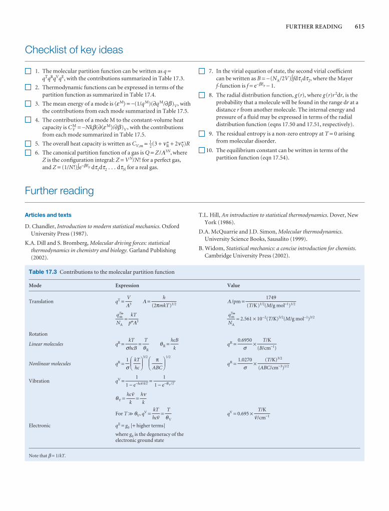
FURTHER READING 615
Checklist of key ideas
1. The molecular partition function can be written as q =qTqRqVqE, with the contributions summarized in Table 17.3.
2. Thermodynamic functions can be expressed in terms of thepartition function as summarized in Table 17.4.
3. The mean energy of a mode is �εM� = −(1/q M)(∂q M/∂β)V, withthe contributions from each mode summarized in Table 17.5.
4. The contribution of a mode M to the constant-volume heatcapacity is C M
V = −Nkβ(∂�ε M�/∂β)V , with the contributionsfrom each mode summarized in Table 17.5.
5. The overall heat capacity is written as CV,m = 1–2(3 + νR* + 2νV*)R
6. The canonical partition function of a gas is Q = Z /Λ3N, whereZ is the configuration integral: Z = V N/N! for a perfect gas,and Z = (1/N!)∫e−βEP dτ1dτ2 . . . dτN for a real gas.
7. In the virial equation of state, the second virial coefficientcan be written as B = −(NA/2V)∫fdτ1dτ2, where the Mayer f-function is f = e−βEP − 1.
8. The radial distribution function, g(r), where g(r)r 2dr, is theprobability that a molecule will be found in the range dr at adistance r from another molecule. The internal energy andpressure of a fluid may be expressed in terms of the radialdistribution function (eqns 17.50 and 17.51, respectively).
9. The residual entropy is a non-zero entropy at T = 0 arisingfrom molecular disorder.
10. The equilibrium constant can be written in terms of thepartition function (eqn 17.54).
Further reading
Articles and texts
D. Chandler, Introduction to modern statistical mechanics. OxfordUniversity Press (1987).
K.A. Dill and S. Bromberg, Molecular driving forces: statisticalthermodynamics in chemistry and biology. Garland Publishing(2002).
T.L. Hill, An introduction to statistical thermodynamics. Dover, NewYork (1986).
D.A. McQuarrie and J.D. Simon, Molecular thermodynamics.University Science Books, Sausalito (1999).
B. Widom, Statistical mechanics: a concise introduction for chemists.Cambridge University Press (2002).
Table 17.3 Contributions to the molecular partition function
Mode Expression Value
Translation qT = Λ = Λ /pm =
= = 2.561 × 10⁻²(T/K)5/2(M/g mol−1)3/2
Rotation
Linear molecules qR = = θR = qR = ×
Nonlinear molecules qR =3/2 1/2
qR = ×
Vibration qV = =
θV = =
For T >> θV, qV = = qV = 0.695 ×
Electronic qE = g0 [+ higher terms]
where g0 is the degeneracy of the electronic ground state
Note that β = 1/kT.
T/K
#/cm−1
T
θV
kT
hc#
hνk
hc#k
1
1 − e−θ V/T
1
1 − e−hc#/kT
(T/K)3/2
(ABC/cm−3)1/2
1.0270
σDEF
πABC
ABCDEF
kT
hc
ABC1
σ
T/K
(B/cm−1)
0.6950
σhcB
k
T
θR
kT
σhcB
qT7m
NA
kT
p7Λ3
qT7m
NA
1749
(T/K)1/2(M/g mol−1)1/2
h
(2πmkT)1/2
V
Λ3
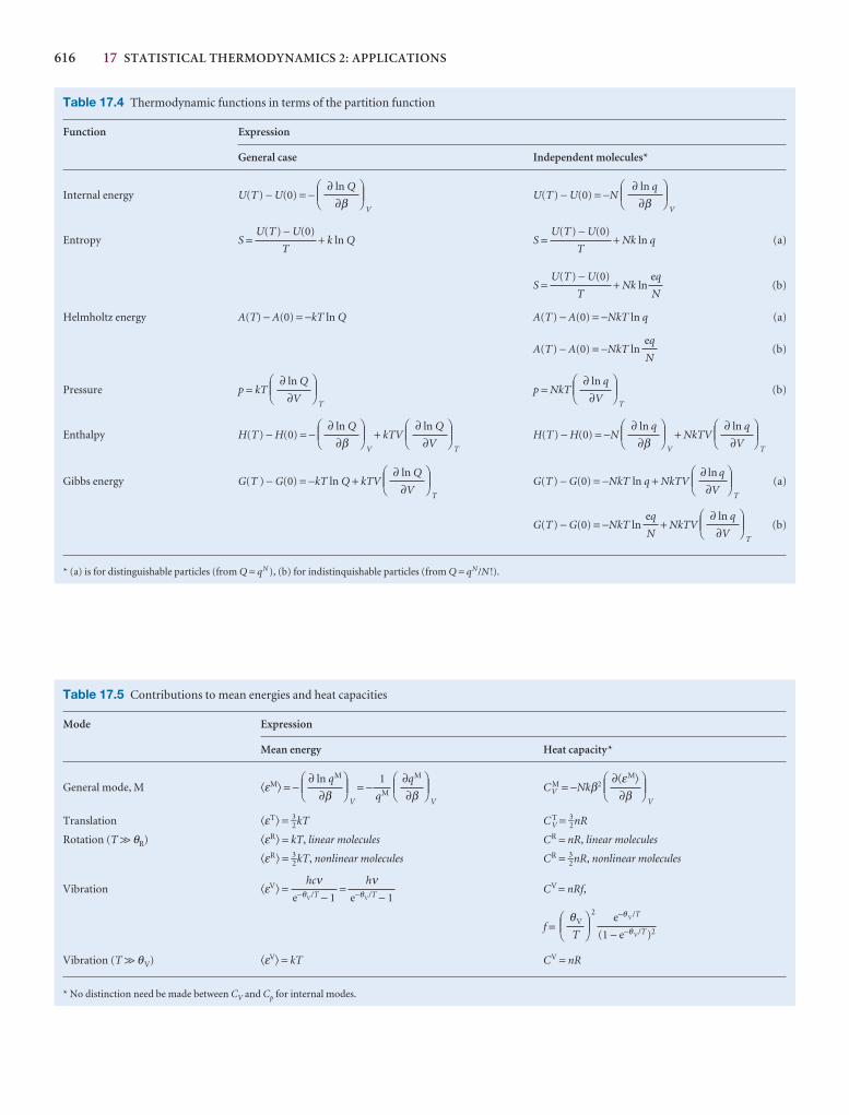
616 17 STATISTICAL THERMODYNAMICS 2: APPLICATIONS
Table 17.5 Contributions to mean energies and heat capacities
Mode Expression
Mean energy Heat capacity*
General mode, M �εM� = −V
= −V
CVM = −Nkβ2
V
Translation �εT� = 3–2kT C T
V = 3–2nR
Rotation (T >> θR) �εR� = kT, linear molecules CR = nR, linear molecules
�εR� = 3–2kT, nonlinear molecules CR = 3–
2nR, nonlinear molecules
Vibration �εV� = = CV = nRf,
f =2
Vibration (T >> θV) �εV� = kT CV = nR
* No distinction need be made between CV and Cp for internal modes.
e−θ V/T
(1 − e−θ V/T )2
DEFθV
T
ABC
hνe−θV/T − 1
hcνe−θV/T − 1
DEF∂�εM�
∂βABC
DEF∂qM
∂βABC
1
qM
DEF∂ ln qM
∂βABC
Table 17.4 Thermodynamic functions in terms of the partition function
Function Expression
General case Independent molecules*
Internal energy U(T) − U(0) = −V
U(T) − U(0) = −NV
Entropy S = + k ln Q S = + Nk ln q (a)
S = + Nk ln (b)
Helmholtz energy A(T) − A(0) = −kT ln Q A(T) − A(0) = −NkT ln q (a)
A(T) − A(0) = −NkT ln (b)
Pressure p = kTT
p = NkTT
(b)
Enthalpy H(T) − H(0) = −V
+ kTVT
H(T) − H(0) = −NV
+ NkTVT
Gibbs energy G(T ) − G(0) = −kT ln Q + kTVT
G(T) − G(0) = −NkT ln q + NkTVT
(a)
G(T) − G(0) = −NkT ln + NkTVT
(b)
* (a) is for distinguishable particles (from Q = qN ), (b) for indistinquishable particles (from Q = qN/N !).
DEF∂ ln q
∂V
ABCeq
N
DEF∂ ln q
∂V
ABCDEF
∂ ln Q
∂V
ABC
DEF∂ ln q
∂V
ABCDEF
∂ ln q
∂βABC
DEF∂ ln Q
∂V
ABCDEF
∂ ln Q
∂βABC
DEF∂ ln q
∂V
ABCDEF
∂ ln Q
∂V
ABC
eq
N
eq
N
U(T) − U(0)
T
U(T) − U(0)
T
U(T) − U(0)
T
DEF∂ ln q
∂βABC
DEF∂ ln Q
∂βABC

EXERCISES 617
Discussion questions
17.1 Discuss the limitations of the expressions qR = kT/hcB, qV = kT/hc#, andqE = g E.
17.2 Explain the origin of the symmetry number.
17.3 Explain the origin of residual entropy.
17.4 Use concepts of statistical thermodynamics to describe the molecularfeatures that determine the magnitudes of the constant-volume molar heatcapacity of a molecular substance.
17.5 Use concepts of statistical thermodynamics to describe the molecularfeatures that lead to the equations of state of perfect and real gases.
17.6 Describe how liquids are investigated by using concepts of statisticalthermodynamics.
17.7 Use concepts of statistical thermodynamics to describe the molecularfeatures that determine the magnitudes of equilibrium constants and theirvariation with temperature.
Exercises
17.1a Use the equipartition theorem to estimate the constant-volume molarheat capacity of (a) I2, (b) CH4, (c) C6H6 in the gas phase at 25°C.
17.1b Use the equipartition theorem to estimate the constant-volume molarheat capacity of (a) O3, (b) C2H6, (c) CO2 in the gas phase at 25°C.
17.2a Estimate the values of γ = Cp /CV for gaseous ammonia and methane.Do this calculation with and without the vibrational contribution to theenergy. Which is closer to the expected experimental value at 25°C?
17.2b Estimate the value of γ = Cp /CV for carbon dioxide. Do this calculationwith and without the vibrational contribution to the energy. Which is closer tothe expected experimental value at 25°C?
17.3a Estimate the rotational partition function of HCl at (a) 25°C and (b) 250°C.
17.3b Estimate the rotational partition function of O2 at (a) 25°C and (b) 250°C.
17.4a Give the symmetry number for each of the following molecules: (a) CO, (b) O2, (c) H2S, and (d) SiH4, (e) CHCl3.
17.4b Give the symmetry number for each of the following molecules: (a) CO2, (b) O3, (c) SO3, (d) SF6, and (e) Al2Cl6.
17.5a Calculate the rotational partition function of H2O at 298 K from itsrotational constants 27.878 cm−1, 14.509 cm−1, and 9.287 cm−1. Above what temperature is the high-temperature approximation valid to within 10 per cent of the true value?
17.5b Calculate the rotational partition function of SO2 at 298 K from itsrotational constants 2.027 36 cm−1, 0.344 17 cm−1, and 0.293 535 cm−1. Abovewhat temperature is the high-temperature approximation valid to within 10 per cent of the true value?
17.6a From the results of Exercise 17.5a, calculate the rotational contributionto the molar entropy of gaseous water at 25°C.
17.6b From the results of Exercise 17.5b, calculate the rotational contributionto the molar entropy of sulfur dioxide at 25°C.
17.7a Calculate the rotational partition function of CH4 (a) by directsummation of the energy levels at 298 K and 500 K, and (b) by the high-temperature approximation. Take B = 5.2412 cm−1.
17.7b Calculate the rotational partition function of CH3CN (a) by directsummation of the energy levels at 298 K and 500 K, and (b) by the high-temperature approximation. Take A = 5.28 cm−1 and B = 0.307 cm−1.
17.8a The bond length of O2 is 120.75 pm. Use the high-temperatureapproximation to calculate the rotational partition function of the molecule at 300 K.
17.8b The NOF molecule is an asymmetric rotor with rotational constants3.1752 cm−1, 0.3951 cm−1, and 0.3505 cm−1. Calculate the rotational partitionfunction of the molecule at (a) 25°C, (b) 100°C.
17.9a Plot the molar heat capacity of a collection of harmonic oscillators as a function of T/θV, and predict the vibrational heat capacity of ethyne at (a) 298 K, (b) 500 K. The normal modes (and their degeneracies in parentheses)occur at wavenumbers 612(2), 729(2), 1974, 3287, and 3374 cm−1.
17.9b Plot the molar entropy of a collection of harmonic oscillators as afunction of T/θV, and predict the standard molar entropy of ethyne at (a) 298 K, (b) 500 K. For data, see the preceding exercise.
17.10a A CO2 molecule is linear, and its vibrational wavenumbers are 1388.2cm−1, 667.4 cm−1, and 2349.2 cm−1, the last being doubly degenerate and theothers non-degenerate. The rotational constant of the molecule is 0.3902 cm−1.Calculate the rotational and vibrational contributions to the molar Gibbsenergy at 298 K.
17.10b An O3 molecule is angular, and its vibrational wavenumbers are 1110 cm−1, 705 cm−1, and 1042 cm−1. The rotational constants of the moleculeare 3.553 cm−1, 0.4452 cm−1, and 0.3948 cm−1. Calculate the rotational andvibrational contributions to the molar Gibbs energy at 298 K.
17.11a The ground level of Cl is 2P3/2 and a 2P1/2 level lies 881 cm−1 above it.Calculate the electronic contribution to the heat capacity of Cl atoms at (a) 500 K and (b) 900 K.
17.11b The first electronically excited state of O2 is 1∆ g and lies 7918.1 cm−1
above the ground state, which is 3Σg−. Calculate the electronic contribution to
the molar Gibbs energy of O2 at 400 K.
17.12a The ground state of the Co2+ ion in CoSO4·7H2O may be regarded as4 T9/2. The entropy of the solid at temperatures below 1 K is derived almostentirely from the electron spin. Estimate the molar entropy of the solid atthese temperatures.
17.12b Estimate the contribution of the spin to the molar entropy of a solidsample of a d-metal complex with S = 5–
2 .
17.13a Calculate the residual molar entropy of a solid in which the moleculescan adopt (a) three, (b) five, (c) six orientations of equal energy at T = 0.
17.13b Suppose that the hexagonal molecule C6HnF6 −n has a residual entropyon account of the similarity of the H and F atoms. Calculate the residual foreach value of n.
17.14a Calculate the equilibrium constant of the reaction I2(g) 5 2 I(g) at1000 K from the following data for I2: # = 214.36 cm−1, B = 0.0373 cm−1,De = 1.5422 eV. The ground state of the I atoms is 2P3/2, implying fourfolddegeneracy.
17.14b Calculate the value of K at 298 K for the gas-phase isotopic exchangereaction 2 79Br81Br 79Br79 5 Br + 81Br81Br. The Br2 molecule has a non-degenerate ground state, with no other electronic states nearby. Base thecalculation on the wavenumber of the vibration of 79Br81Br, which is 323.33 cm−1.

618 17 STATISTICAL THERMODYNAMICS 2: APPLICATIONS
Problems*
Numerical problems
17.1 The NO molecule has a doubly degenerate electronic ground state and a doubly degenerate excited state at 121.1 cm−1. Calculate the electroniccontribution to the molar heat capacity of the molecule at (a) 50 K, (b) 298 K,and (c) 500 K.
17.2 Explore whether a magnetic field can influence the heat capacity of aparamagnetic molecule by calculating the electronic contribution to the heatcapacity of an NO2 molecule in a magnetic field. Estimate the total constant-volume heat capacity using equipartition, and calculate the percentage changein heat capacity brought about by a 5.0 T magnetic field at (a) 50 K, (b) 298 K.
17.3 The energy levels of a CH3 group attached to a larger fragment are givenby the expression for a particle on a ring, provided the group is rotating freely.What is the high-temperature contribution to the heat capacity and entropy of such a freely rotating group at 25°C? The moment of inertia of CH3 aboutits three-fold rotation axis (the axis that passes through the C atom and the centre of the equilateral triangle formed by the H atoms) is 5.341 ×10−47 kg m2).
17.4 Calculate the temperature dependence of the heat capacity of p-H2
(in which only rotational states with even values of J are populated) at lowtemperatures on the basis that its rotational levels J = 0 and J = 2 constitute asystem that resembles a two-level system except for the degeneracy of theupper level. Use B = 60.864 cm−1 and sketch the heat capacity curve. Theexperimental heat capacity of p-H2 does in fact show a peak at lowtemperatures.
17.5 The pure rotational microwave spectrum of HCl has absorption lines at the following wavenumbers (in cm−1): 21.19, 42.37, 63.56, 84.75, 105.93,127.12 148.31 169.49, 190.68, 211.87, 233.06, 254.24, 275.43, 296.62, 317.80,338.99, 360.18, 381.36, 402.55, 423.74, 444.92, 466.11, 487.30, 508.48.Calculate the rotational partition function at 25°C by direct summation.
17.6 Calculate the standard molar entropy of N2(g) at 298 K from itsrotational constant B = 1.9987 cm−1 and its vibrational wavenumber # = 2358 cm−1. The thermochemical value is 192.1 J K−1 mol−1. What does this suggest about the solid at T = 0?
17.7‡ J.G. Dojahn, E.C.M. Chen, and W.E. Wentworth (J. Phys. Chem. 100,9649 (1996)) characterized the potential energy curves of the ground andelectronic states of homonuclear diatomic halogen anions. The ground stateof F2
− is 2Σu+ with a fundamental vibrational wavenumber of 450.0 cm−1 and
equilibrium internuclear distance of 190.0 pm. The first two excited states areat 1.609 and 1.702 eV above the ground state. Compute the standard molarentropy of F2
− at 298 K.
17.8‡ In a spectroscopic study of buckminsterfullerene C60, F. Negri, G. Orlandi, and F. Zerbetto ( J. Phys. Chem. 100, 10849 (1996)) reviewed thewavenumbers of all the vibrational modes of the molecule. The wavenumberfor the single Au mode is 976 cm−1; wavenumbers for the four threefolddegenerate T1u modes are 525, 578, 1180, and 1430 cm−1; wavenumbers for the five threefold degenerate T2u modes are 354, 715, 1037, 1190, and 1540 cm−1; wavenumbers for the six fourfold degenerate Gu modes are 345,757, 776, 963, 1315, and 1410 cm−1; and wavenumbers for the seven fivefolddegenerate Hu modes are 403, 525, 667, 738, 1215, 1342, and 1566 cm−1. Howmany modes have a vibrational temperature θV below 1000 K? Estimate themolar constant-volume heat capacity of C60 at 1000 K, counting as active allmodes with θV below this temperature.
17.9‡ Treat carbon monoxide as a perfect gas and apply equilibriumstatistical thermodynamics to the study of its properties, as specified below, inthe temperature range 100–1000 K at 1 bar. # = 2169.8 cm−1, B =1.931 cm−1,and D0 = 11.09 eV; neglect anharmonicity and centrifugal distortion. (a) Examine the probability distribution of molecules over available rotationaland vibrational states. (b) Explore numerically the differences, if any, betweenthe rotational molecular partition function as calculated with the discreteenergy distribution and that calculated with the classical, continuous energydistribution. (c) Calculate the individual contributions to Um(T) − Um
(100 K), CV,m(T), and Sm(T) − Sm(100 K) made by the translational,rotational, and vibrational degrees of freedom.
17.10 Calculate and plot as a function of temperature, in the range 300 K to 1000 K, the equilibrium constant for the reaction CD4(g) + HCl(g) 5CHD3(g) + DCl(g) using the following data (numbers in parentheses aredegeneracies): #(CHD3)/cm−1 = 2993(1), 2142(1), 1003(3), 1291(2), 1036(2);#(CD4)/cm−1 = 2109(1), 1092(2), 2259(3), 996(3); #(HCl)/cm−1 = 2991;#(DCl)/cm−1 = 2145; B(HCl)/cm−1 = 10.59; B(DCl)/cm−1 = 5.445;B(CHD3)/cm−1 = 3.28; A(CHD3)/cm−1 = 2.63, B(CD4)/cm−1 = 2.63.
17.11 The exchange of deuterium between acid and water is an importanttype of equilibrium, and we can examine it using spectroscopic data on themolecules. Calculate the equilibrium constant at (a) 298 K and (b) 800 K for the gas-phase exchange reaction H2O + DCl 5 HDO + HCl from thefollowing data: #(H2O)/cm−1 = 3656.7, 1594.8, 3755.8; #(HDO)/cm−1 =2726.7, 1402.2, 3707.5; A(H2O)/cm−1 = 27.88; B(H2O)/cm−1 = 14.51;C(H2O)/cm−1 = 9.29; A(HDO)/cm−1 = 23.38; B(HDO)/cm−1 = 9.102;C(HDO)/cm−1 = 6.417; B(HCl)/cm−1 = 10.59; B(DCl)/cm−1 = 5.449;#(HCl)/cm−1 = 2991; #(DCl)/cm−1 = 2145.
Theoretical problems
17.12 Derive the Sackur–Tetrode equation for a monatomic gas confined to a two-dimensional surface, and hence derive an expression for the standardmolar entropy of condensation to form a mobile surface film.
17.13‡ For H2 at very low temperatures, only translational motioncontributes to the heat capacity. At temperatures above θR = hcB/k, therotational contribution to the heat capacity becomes significant. At still highertemperatures, above θV = hν/k, the vibrations contribute. But at this lattertemperature, dissociation of the molecule into the atoms must be considered.(a) Explain the origin of the expressions for θR and θV, and calculate theirvalues for hydrogen. (b) Obtain an expression for the molar constant-pressureheat capacity of hydrogen at all temperatures taking into account thedissociation of hydrogen. (c) Make a plot of the molar constant-pressure heatcapacity as a function of temperature in the high-temperature region wheredissociation of the molecule is significant.
17.14 Derive expressions for the internal energy, heat capacity, entropy,Helmholtz energy, and Gibbs energy of a harmonic oscillator. Express theresults in terms of the vibrational temperature, θV and plot graphs of eachproperty against T/θV.
17.15 Suppose that an intermolecular potential has a hard-sphere core ofradius r1 and a shallow attractive well of uniform depth ε out to a distance r2.Show, by using eqn 17.42 and the condition ε << kT, that such a model isapproximately consistent with a van der Waals equation of state when b << Vm, and relate the van der Waals parameters and the Joule–Thomsoncoefficient to the parameters in this model.
* Problems denoted with the symbol ‡ were supplied by Charles Trapp, Carmen Giunta, and Marshall Cady.
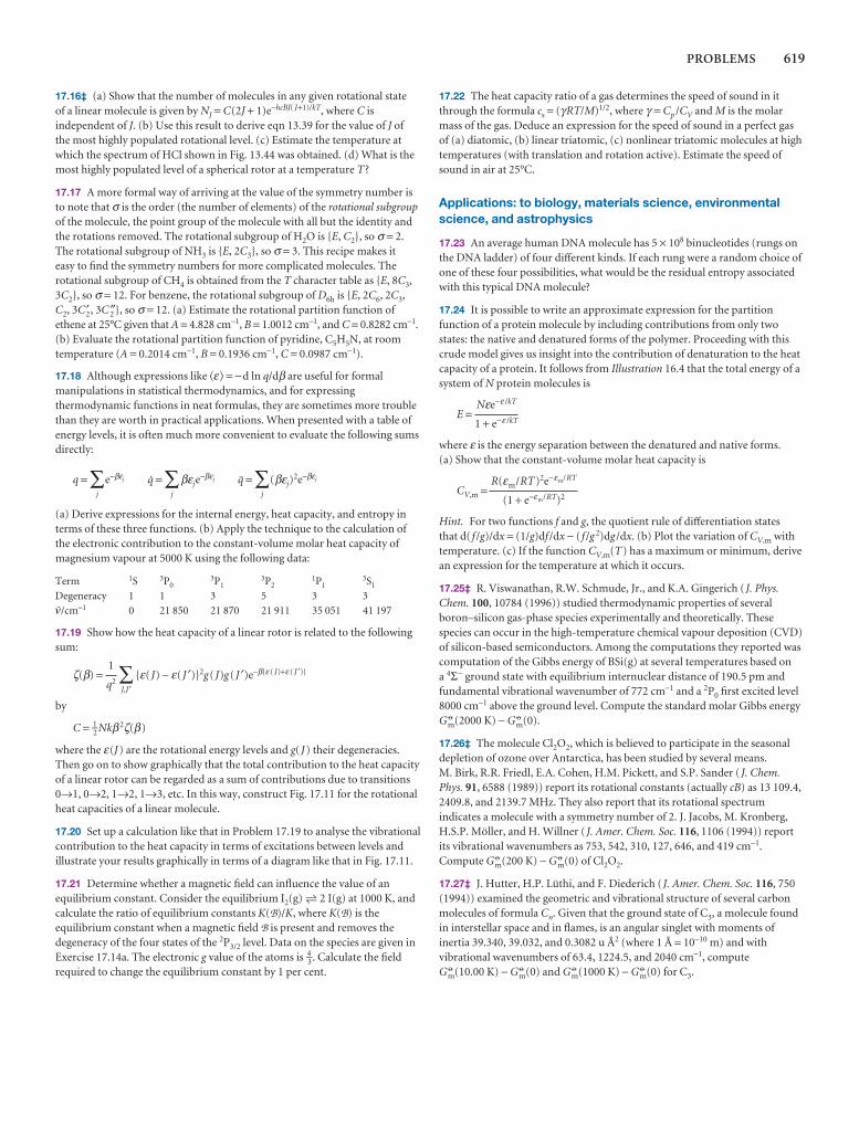
PROBLEMS 619
17.16‡ (a) Show that the number of molecules in any given rotational state of a linear molecule is given by NJ = C(2J + 1)e−hcBJ( J+1)/kT, where C isindependent of J. (b) Use this result to derive eqn 13.39 for the value of J ofthe most highly populated rotational level. (c) Estimate the temperature atwhich the spectrum of HCl shown in Fig. 13.44 was obtained. (d) What is themost highly populated level of a spherical rotor at a temperature T?
17.17 A more formal way of arriving at the value of the symmetry number isto note that σ is the order (the number of elements) of the rotational subgroupof the molecule, the point group of the molecule with all but the identity andthe rotations removed. The rotational subgroup of H2O is {E, C2}, so σ = 2.The rotational subgroup of NH3 is {E, 2C3}, so σ = 3. This recipe makes it easy to find the symmetry numbers for more complicated molecules. Therotational subgroup of CH4 is obtained from the T character table as {E, 8C3,3C2}, so σ = 12. For benzene, the rotational subgroup of D6h is {E, 2C6, 2C3,C2, 3C2′ , 3C 2″}, so σ = 12. (a) Estimate the rotational partition function ofethene at 25°C given that A = 4.828 cm−1, B = 1.0012 cm−1, and C = 0.8282 cm−1.(b) Evaluate the rotational partition function of pyridine, C5H5N, at roomtemperature (A = 0.2014 cm−1, B = 0.1936 cm−1, C = 0.0987 cm−1).
17.18 Although expressions like �ε � = −d ln q/dβ are useful for formalmanipulations in statistical thermodynamics, and for expressingthermodynamic functions in neat formulas, they are sometimes more troublethan they are worth in practical applications. When presented with a table ofenergy levels, it is often much more convenient to evaluate the following sumsdirectly:
q = ∑j
e−βεj ≥ = ∑j
βεje−βεj ” = ∑
j
(βεj)2e−βεj
(a) Derive expressions for the internal energy, heat capacity, and entropy interms of these three functions. (b) Apply the technique to the calculation ofthe electronic contribution to the constant-volume molar heat capacity ofmagnesium vapour at 5000 K using the following data:
Term 1S 3P03P1
3P21P1
3S1
Degeneracy 1 1 3 5 3 3
#/cm−1 0 21 850 21 870 21 911 35 051 41 197
17.19 Show how the heat capacity of a linear rotor is related to the followingsum:
ζ(β) = ∑J,J′
{ε( J) − ε( J′ )}2g( J)g( J′ )e−β{ε ( J)+ε ( J′ )}
by
C = 1–2 Nkβ2ζ(β)
where the ε(J) are the rotational energy levels and g( J) their degeneracies.Then go on to show graphically that the total contribution to the heat capacityof a linear rotor can be regarded as a sum of contributions due to transitions0→1, 0→2, 1→2, 1→3, etc. In this way, construct Fig. 17.11 for the rotationalheat capacities of a linear molecule.
17.20 Set up a calculation like that in Problem 17.19 to analyse the vibrationalcontribution to the heat capacity in terms of excitations between levels andillustrate your results graphically in terms of a diagram like that in Fig. 17.11.
17.21 Determine whether a magnetic field can influence the value of anequilibrium constant. Consider the equilibrium I2(g) 5 2 I(g) at 1000 K, andcalculate the ratio of equilibrium constants K(B)/K, where K(B) is theequilibrium constant when a magnetic field B is present and removes thedegeneracy of the four states of the 2P3/2 level. Data on the species are given inExercise 17.14a. The electronic g value of the atoms is 4–
3. Calculate the fieldrequired to change the equilibrium constant by 1 per cent.
1
q2
17.22 The heat capacity ratio of a gas determines the speed of sound in itthrough the formula cs = (γRT/M)1/2, where γ = Cp /CV and M is the molarmass of the gas. Deduce an expression for the speed of sound in a perfect gasof (a) diatomic, (b) linear triatomic, (c) nonlinear triatomic molecules at hightemperatures (with translation and rotation active). Estimate the speed ofsound in air at 25°C.
Applications: to biology, materials science, environmentalscience, and astrophysics
17.23 An average human DNA molecule has 5 × 10⁸ binucleotides (rungs onthe DNA ladder) of four different kinds. If each rung were a random choice ofone of these four possibilities, what would be the residual entropy associatedwith this typical DNA molecule?
17.24 It is possible to write an approximate expression for the partitionfunction of a protein molecule by including contributions from only twostates: the native and denatured forms of the polymer. Proceeding with thiscrude model gives us insight into the contribution of denaturation to the heatcapacity of a protein. It follows from Illustration 16.4 that the total energy of asystem of N protein molecules is
E =
where ε is the energy separation between the denatured and native forms. (a) Show that the constant-volume molar heat capacity is
CV,m =
Hint. For two functions f and g, the quotient rule of differentiation states that d( f /g)/dx = (1/g)df /dx − ( f /g 2)dg /dx. (b) Plot the variation of CV,m withtemperature. (c) If the function CV,m(T) has a maximum or minimum, derivean expression for the temperature at which it occurs.
17.25‡ R. Viswanathan, R.W. Schmude, Jr., and K.A. Gingerich (J. Phys.Chem. 100, 10784 (1996)) studied thermodynamic properties of severalboron–silicon gas-phase species experimentally and theoretically. Thesespecies can occur in the high-temperature chemical vapour deposition (CVD)of silicon-based semiconductors. Among the computations they reported wascomputation of the Gibbs energy of BSi(g) at several temperatures based on a 4Σ− ground state with equilibrium internuclear distance of 190.5 pm andfundamental vibrational wavenumber of 772 cm−1 and a 2P0 first excited level8000 cm−1 above the ground level. Compute the standard molar Gibbs energyG 7
m(2000 K) − G 7m(0).
17.26‡ The molecule Cl2O2, which is believed to participate in the seasonaldepletion of ozone over Antarctica, has been studied by several means. M. Birk, R.R. Friedl, E.A. Cohen, H.M. Pickett, and S.P. Sander (J. Chem.Phys. 91, 6588 (1989)) report its rotational constants (actually cB) as 13 109.4,2409.8, and 2139.7 MHz. They also report that its rotational spectrumindicates a molecule with a symmetry number of 2. J. Jacobs, M. Kronberg,H.S.P. Möller, and H. Willner (J. Amer. Chem. Soc. 116, 1106 (1994)) reportits vibrational wavenumbers as 753, 542, 310, 127, 646, and 419 cm−1.Compute G 7
m(200 K) − G 7m(0) of Cl2O2.
17.27‡ J. Hutter, H.P. Lüthi, and F. Diederich (J. Amer. Chem. Soc. 116, 750(1994)) examined the geometric and vibrational structure of several carbonmolecules of formula Cn. Given that the ground state of C3, a molecule foundin interstellar space and in flames, is an angular singlet with moments ofinertia 39.340, 39.032, and 0.3082 u Å2 (where 1 Å = 10−10 m) and withvibrational wavenumbers of 63.4, 1224.5, and 2040 cm−1, compute G 7
m(10.00 K) − G 7m(0) and G 7
m(1000 K) − G 7m(0) for C3.
R(εm/RT)2e−εm/RT
(1 + e−εm/RT)2
Nεe−ε /kT
1 + e−ε /kT
Molecular interactions
In this chapter we examine molecular interactions in gases and liquids and interpret them interms of electric properties of molecules, such as electric dipole moments and polarizabilit-ies. All these properties reflect the degree to which the nuclei of atoms exert control over theelectrons in a molecule, either by causing electrons to accumulate in particular regions, orby permitting them to respond more or less strongly to the effects of external electric fields.
Molecular interactions are responsible for the unique properties of substances as simple as water and as complex as polymers. We begin our examination of molecularinteractions by describing the electric properties of molecules, which may be inter-preted in terms of concepts in electronic structure introduced in Chapter 11. We shallsee that small imbalances of charge distributions in molecules allow them to interactwith one another and with externally applied fields. One result of this interaction isthe cohesion of molecules to form the bulk phases of matter. These interactions arealso important for understanding the shapes adopted by biological and syntheticmacromolecules, as we shall see in Chapter 19. The interaction between ions is treatedin Chapter 5 (for solutions) and Chapter 20 (for solids).
Electric properties of molecules
Many of the electric properties of molecules can be traced to the competing influencesof nuclei with different charges or the competition between the control exercised by a nucleus and the influence of an externally applied field. The former competitionmay result in an electric dipole moment. The latter may result in properties such as refractive index and optical activity.
18.1 Electric dipole moments
An electric dipole consists of two electric charges +q and −q separated by a distance R.This arrangement of charges is represented by a vector m (1). The magnitude of m isµ = qR and, although the SI unit of dipole moment is coulomb metre (C m), it is stillcommonly reported in the non-SI unit debye, D, named after Peter Debye, a pioneerin the study of dipole moments of molecules, where
1 D = 3.335 64 × 10−30 C m (18.1)
The dipole moment of a pair of charges +e and −e separated by 100 pm is 1.6 ×10⁻²⁹ C m, corresponding to 4.8 D. Dipole moments of small molecules are typicallyabout 1 D. The conversion factor in eqn 18.1 stems from the original definition of thedebye in terms of c.g.s. units: 1 D is the dipole moment of two equal and oppositecharges of magnitude 1 e.s.u. separated by 1 Å.
Electric properties of molecules
18.1 Electric dipole moments
18.2 Polarizabilities
18.3 Relative permittivities
Interactions between molecules
18.4 Interactions between dipoles
18.5 Repulsive and totalinteractions
I18.1 Impact on medicine:Molecular recognition anddrug design
Gases and liquids
18.6 Molecular interactions in gases
18.7 The liquid–vapour interface
18.8 Condensation
Checklist of key ideas
Further reading
Further information 18.1: Thedipole–dipole interaction
Further information 18.2: The basicprinciples of molecular beams
Discussion questions
Exercises
Problems
18
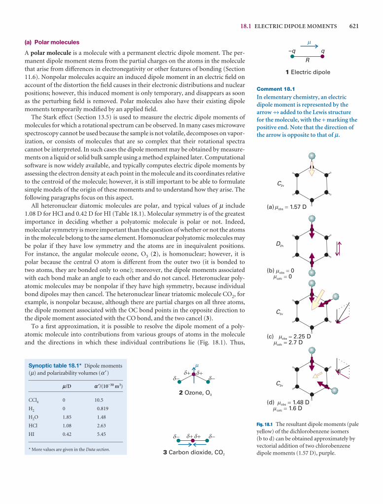
18.1 ELECTRIC DIPOLE MOMENTS 621
(a) Polar molecules
A polar molecule is a molecule with a permanent electric dipole moment. The per-manent dipole moment stems from the partial charges on the atoms in the moleculethat arise from differences in electronegativity or other features of bonding (Section11.6). Nonpolar molecules acquire an induced dipole moment in an electric field onaccount of the distortion the field causes in their electronic distributions and nuclearpositions; however, this induced moment is only temporary, and disappears as soonas the perturbing field is removed. Polar molecules also have their existing dipole moments temporarily modified by an applied field.
The Stark effect (Section 13.5) is used to measure the electric dipole moments ofmolecules for which a rotational spectrum can be observed. In many cases microwavespectroscopy cannot be used because the sample is not volatile, decomposes on vapor-ization, or consists of molecules that are so complex that their rotational spectracannot be interpreted. In such cases the dipole moment may be obtained by measure-ments on a liquid or solid bulk sample using a method explained later. Computationalsoftware is now widely available, and typically computes electric dipole moments byassessing the electron density at each point in the molecule and its coordinates relativeto the centroid of the molecule; however, it is still important to be able to formulatesimple models of the origin of these moments and to understand how they arise. Thefollowing paragraphs focus on this aspect.
All heteronuclear diatomic molecules are polar, and typical values of µ include1.08 D for HCl and 0.42 D for HI (Table 18.1). Molecular symmetry is of the greatest importance in deciding whether a polyatomic molecule is polar or not. Indeed,molecular symmetry is more important than the question of whether or not the atomsin the molecule belong to the same element. Homonuclear polyatomic molecules maybe polar if they have low symmetry and the atoms are in inequivalent positions. For instance, the angular molecule ozone, O3 (2), is homonuclear; however, it is polar because the central O atom is different from the outer two (it is bonded to two atoms, they are bonded only to one); moreover, the dipole moments associatedwith each bond make an angle to each other and do not cancel. Heteronuclear poly-atomic molecules may be nonpolar if they have high symmetry, because individualbond dipoles may then cancel. The heteronuclear linear triatomic molecule CO2, forexample, is nonpolar because, although there are partial charges on all three atoms,the dipole moment associated with the OC bond points in the opposite direction tothe dipole moment associated with the CO bond, and the two cancel (3).
To a first approximation, it is possible to resolve the dipole moment of a poly-atomic molecule into contributions from various groups of atoms in the moleculeand the directions in which these individual contributions lie (Fig. 18.1). Thus,
Comment 18.1
In elementary chemistry, an electricdipole moment is represented by thearrow ( added to the Lewis structurefor the molecule, with the + marking thepositive end. Note that the direction ofthe arrow is opposite to that of µ.
–q q
R
1 Electric dipole
Synoptic table 18.1* Dipole moments(µ) and polarizability volumes (α′)
m/D a¢/(10−30 m3)
CCl4 0 10.5
H2 0 0.819
H2O 1.85 1.48
HCl 1.08 2.63
HI 0.42 5.45
* More values are given in the Data section.
(a) 1.57 Dobs �
(b) 00
obs
calc
��
(c) 2.25 D2.7 D
obs
calc
��
(d) 1.48 D1.6 D
obs
calc
��
C2v
C2v
C2v
D2h
Fig. 18.1 The resultant dipole moments (paleyellow) of the dichlorobenzene isomers (b to d) can be obtained approximately byvectorial addition of two chlorobenzenedipole moments (1.57 D), purple.
�
2 Ozone, O3
� ������
3 Carbon dioxide, CO2
�� ���� ��
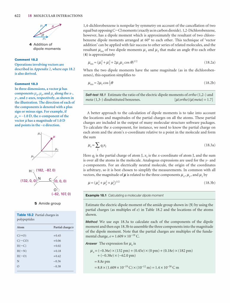
622 18 MOLECULAR INTERACTIONS
Comment 18.3
In three dimensions, a vector m hascomponents µx, µy, and µz along the x-,y-, and z-axes, respectively, as shown inthe illustration. The direction of each ofthe components is denoted with a plussign or minus sign. For example, if µx = −1.0 D, the x-component of thevector µ has a magnitude of 1.0 D and points in the −x direction.
z
x
y
�
1
4 Addition ofdipole moments
2
Comment 18.2
Operations involving vectors aredescribed in Appendix 2, where eqn 18.2is also derived.
Table 18.2 Partial charges inpolypeptides
Atom Partial charge/e
C(=O) +0.45
C(-CO) +0.06
H(-C) +0.02
H(-N) +0.18
H(-O) +0.42
N –0.36
O –0.38
H
N C
O
(182, 87, 0)�
(132, 0, 0) (0, 0, 0)
( 62, 107, 0)�
5 Amide group
1,4-dichlorobenzene is nonpolar by symmetry on account of the cancellation of twoequal but opposing C-Cl moments (exactly as in carbon dioxide). 1,2-Dichlorobenzene,however, has a dipole moment which is approximately the resultant of two chloro-benzene dipole moments arranged at 60° to each other. This technique of ‘vector addition’ can be applied with fair success to other series of related molecules, and theresultant µres of two dipole moments µ1 and µ2 that make an angle θ to each other (4) is approximately
µres ≈ (µ12 + µ2
2 + 2µ1µ2 cos θ)1/2 (18.2a)
When the two dipole moments have the same magnitude (as in the dichloroben-zenes), this equation simplifies to
µres ≈ 2µ1 cos 1–2θ (18.2b)
Self-test 18.1 Estimate the ratio of the electric dipole moments of ortho (1,2-) andmeta (1,3-) disubstituted benzenes. [µ(ortho)/µ(meta) = 1.7]
A better approach to the calculation of dipole moments is to take into account the locations and magnitudes of the partial charges on all the atoms. These partialcharges are included in the output of many molecular structure software packages. To calculate the x-component, for instance, we need to know the partial charge oneach atom and the atom’s x-coordinate relative to a point in the molecule and formthe sum
µx = ∑J
qJxJ (18.3a)
Here qJ is the partial charge of atom J, xJ is the x-coordinate of atom J, and the sum is over all the atoms in the molecule. Analogous expressions are used for the y- and z-components. For an electrically neutral molecule, the origin of the coordinates is arbitrary, so it is best chosen to simplify the measurements. In common with all vectors, the magnitude of m is related to the three components µx , µy , and µz by
µ = (µx2 + µy
2 + µz2)1/2 (18.3b)
Example 18.1 Calculating a molecular dipole moment
Estimate the electric dipole moment of the amide group shown in (5) by using thepartial charges (as multiples of e) in Table 18.2 and the locations of the atomsshown.
Method We use eqn 18.3a to calculate each of the components of the dipole moment and then eqn 18.3b to assemble the three components into the magnitudeof the dipole moment. Note that the partial charges are multiples of the funda-mental charge, e = 1.609 × 10⁻¹⁹ C.
Answer The expression for µx is
µ x = (−0.36e) × (132 pm) + (0.45e) × (0 pm) + (0.18e) × (182 pm)+ (−0.38e) × (−62.0 pm)
= 8.8e pm
= 8.8 × (1.609 × 10−19 C) × (10−12 m) = 1.4 × 10⁻³⁰ C m
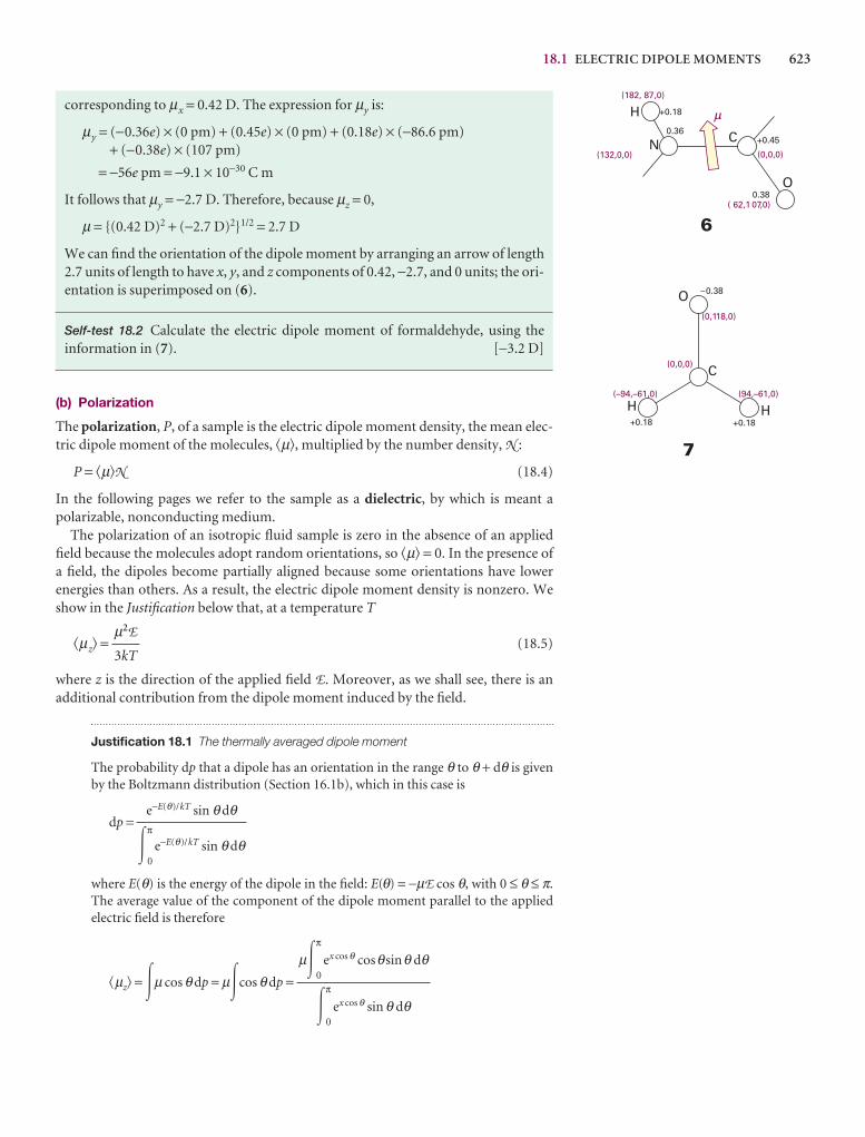
18.1 ELECTRIC DIPOLE MOMENTS 623
(182, 87,0)
(132,0,0)
H
N C
O
(0,0,0)
( 62,1 07,0)
+0.18
0.36+0.45
0.38
6
7
C
H H
O –0.38
+0.18+0.18
(0,118,0)
(0,0,0)
(–94,–61,0) (94,–61,0)
corresponding to µx = 0.42 D. The expression for µy is:
µy = (−0.36e) × (0 pm) + (0.45e) × (0 pm) + (0.18e) × (−86.6 pm)+ (−0.38e) × (107 pm)
= −56e pm = −9.1 × 10⁻³⁰ C m
It follows that µy = −2.7 D. Therefore, because µz = 0,
µ = {(0.42 D)2 + (−2.7 D)2}1/2 = 2.7 D
We can find the orientation of the dipole moment by arranging an arrow of length2.7 units of length to have x, y, and z components of 0.42, −2.7, and 0 units; the ori-entation is superimposed on (6).
Self-test 18.2 Calculate the electric dipole moment of formaldehyde, using the information in (7). [−3.2 D]
(b) Polarization
The polarization, P, of a sample is the electric dipole moment density, the mean elec-tric dipole moment of the molecules, �µ�, multiplied by the number density, N :
P = �µ�N (18.4)
In the following pages we refer to the sample as a dielectric, by which is meant a polarizable, nonconducting medium.
The polarization of an isotropic fluid sample is zero in the absence of an appliedfield because the molecules adopt random orientations, so �µ� = 0. In the presence ofa field, the dipoles become partially aligned because some orientations have lower energies than others. As a result, the electric dipole moment density is nonzero. Weshow in the Justification below that, at a temperature T
�µz� = (18.5)
where z is the direction of the applied field E. Moreover, as we shall see, there is an additional contribution from the dipole moment induced by the field.
Justification 18.1 The thermally averaged dipole moment
The probability dp that a dipole has an orientation in the range θ to θ + dθ is givenby the Boltzmann distribution (Section 16.1b), which in this case is
dp =
where E(θ) is the energy of the dipole in the field: E(θ) = −µE cos θ, with 0 ≤ θ ≤ π.The average value of the component of the dipole moment parallel to the appliedelectric field is therefore
�µz� = �µ cos θ dp = µ�cos θ dp =µ�
π
0ex cos θ cosθsinθ dθ
�π
0ex cos θ sin θ dθ
e−E(θ)/kT sin θ dθ
�π
0e−E(θ)/kT sin θ dθ
µ2E
3kT
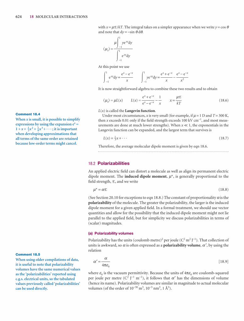
624 18 MOLECULAR INTERACTIONS
with x = µE /kT. The integral takes on a simpler appearance when we write y = cos θand note that dy = −sin θ dθ.
�µz� =
At this point we use
�1
−1
e xydy = �1
−1
ye xydy = −
It is now straightforward algebra to combine these two results and to obtain
�µz� = µL(x) L(x) = − x = (18.6)
L(x) is called the Langevin function.Under most circumstances, x is very small (for example, if µ = 1 D and T = 300 K,
then x exceeds 0.01 only if the field strength exceeds 100 kV cm−1, and most meas-urements are done at much lower strengths). When x << 1, the exponentials in theLangevin function can be expanded, and the largest term that survives is
L(x) = 1–3 x + · · · (18.7)
Therefore, the average molecular dipole moment is given by eqn 18.6.
18.2 Polarizabilities
An applied electric field can distort a molecule as well as align its permanent electricdipole moment. The induced dipole moment, µ*, is generally proportional to thefield strength, E , and we write
µ* = αE (18.8)
(See Section 20.10 for exceptions to eqn 18.8.) The constant of proportionality α is thepolarizability of the molecule. The greater the polarizability, the larger is the induceddipole moment for a given applied field. In a formal treatment, we should use vectorquantities and allow for the possibility that the induced dipole moment might not lieparallel to the applied field, but for simplicity we discuss polarizabilities in terms of(scalar) magnitudes.
(a) Polarizability volumes
Polarizability has the units (coulomb metre)2 per joule (C2 m2 J−1). That collection ofunits is awkward, so α is often expressed as a polarizability volume, α ′, by using therelation
α′ = [18.9]
where ε0 is the vacuum permittivity. Because the units of 4πε0 are coulomb-squaredper joule per metre (C2 J−1 m−1), it follows that α′ has the dimensions of volume(hence its name). Polarizability volumes are similar in magnitude to actual molecularvolumes (of the order of 10−30 m3, 10−3 nm3, 1 Å3).
α4πε0
µE
kT
1
x
ex + e−x
ex − e−x
ex − e−x
x2
ex + e−x
x
ex − e−x
x
µ�1
−1
ye xydy
�1
−1
e xydy
Comment 18.4
When x is small, it is possible to simplifyexpressions by using the expansion ex =1 + x + 1–2x 2 + 1–6x 3 + · · · ; it is importantwhen developing approximations thatall terms of the same order are retainedbecause low-order terms might cancel.
Comment 18.5
When using older compilations of data,it is useful to note that polarizabilityvolumes have the same numerical valuesas the ‘polarizabilities’ reported usingc.g.s. electrical units, so the tabulatedvalues previously called ‘polarizabilities’can be used directly.
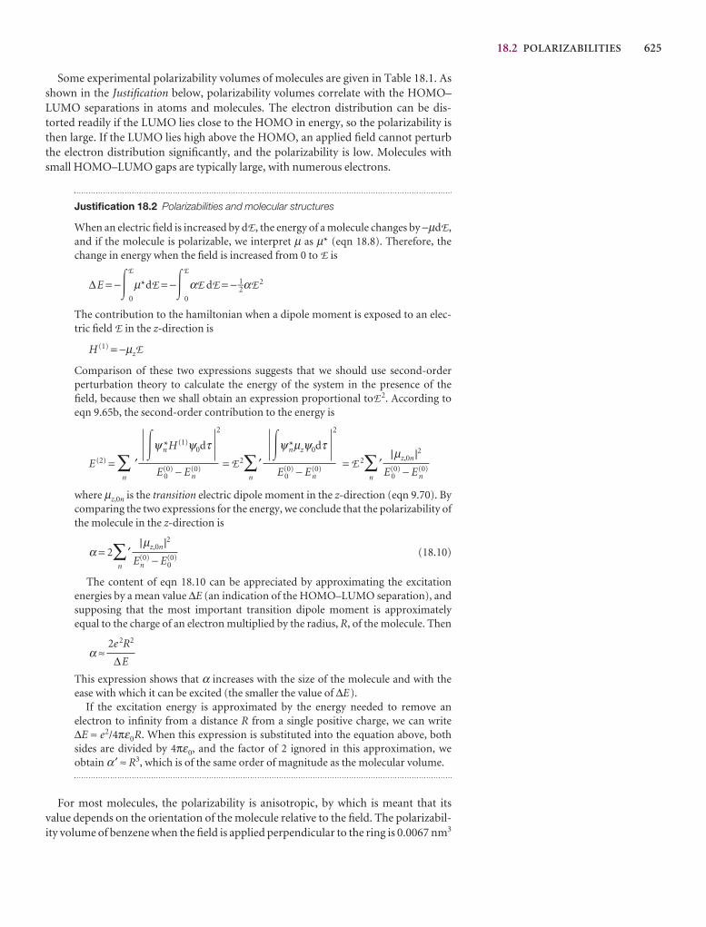
18.2 POLARIZABILITIES 625
Some experimental polarizability volumes of molecules are given in Table 18.1. Asshown in the Justification below, polarizability volumes correlate with the HOMO–LUMO separations in atoms and molecules. The electron distribution can be dis-torted readily if the LUMO lies close to the HOMO in energy, so the polarizability isthen large. If the LUMO lies high above the HOMO, an applied field cannot perturbthe electron distribution significantly, and the polarizability is low. Molecules withsmall HOMO–LUMO gaps are typically large, with numerous electrons.
Justification 18.2 Polarizabilities and molecular structures
When an electric field is increased by dE, the energy of a molecule changes by −µdE,and if the molecule is polarizable, we interpret µ as µ* (eqn 18.8). Therefore, thechange in energy when the field is increased from 0 to E is
∆E = −�E
0
µ*dE = −�E
0
αE dE = − 1–2αE 2
The contribution to the hamiltonian when a dipole moment is exposed to an elec-tric field E in the z-direction is
H (1) = −µzE
Comparison of these two expressions suggests that we should use second-order perturbation theory to calculate the energy of the system in the presence of the field, because then we shall obtain an expression proportional toE 2. According toeqn 9.65b, the second-order contribution to the energy is
E (2) = ∑n
′
2
= E 2∑n
′
2
b= E 2∑n
′
where µz,0n is the transition electric dipole moment in the z-direction (eqn 9.70). Bycomparing the two expressions for the energy, we conclude that the polarizability ofthe molecule in the z-direction is
α = 2∑n
′ (18.10)
The content of eqn 18.10 can be appreciated by approximating the excitation energies by a mean value ∆E (an indication of the HOMO–LUMO separation), andsupposing that the most important transition dipole moment is approximatelyequal to the charge of an electron multiplied by the radius, R, of the molecule. Then
α ≈
This expression shows that α increases with the size of the molecule and with theease with which it can be excited (the smaller the value of ∆E).
If the excitation energy is approximated by the energy needed to remove an electron to infinity from a distance R from a single positive charge, we can write ∆E ≈ e2/4πε0R. When this expression is substituted into the equation above, bothsides are divided by 4πε0, and the factor of 2 ignored in this approximation, we obtain α′ ≈ R3, which is of the same order of magnitude as the molecular volume.
For most molecules, the polarizability is anisotropic, by which is meant that itsvalue depends on the orientation of the molecule relative to the field. The polarizabil-ity volume of benzene when the field is applied perpendicular to the ring is 0.0067 nm3
2e 2R2
∆E
|µz,0n |2
En(0) − E0
(0)
|µz,0n |2
E 0(0) − E n
(0)
�ψn*µzψ0dτ
E 0(0) − E n
(0)
�ψn*H (1)ψ0dτ
E 0(0) − E n
(0)
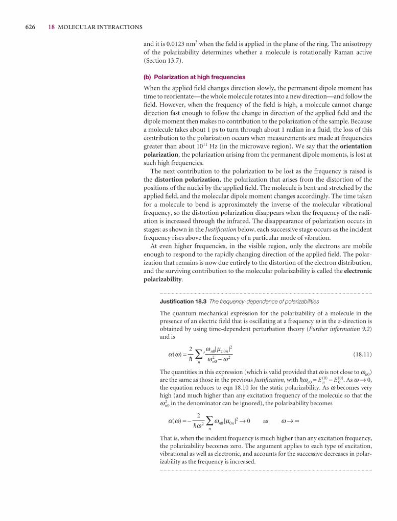
626 18 MOLECULAR INTERACTIONS
and it is 0.0123 nm3 when the field is applied in the plane of the ring. The anisotropyof the polarizability determines whether a molecule is rotationally Raman active(Section 13.7).
(b) Polarization at high frequencies
When the applied field changes direction slowly, the permanent dipole moment hastime to reorientate—the whole molecule rotates into a new direction—and follow thefield. However, when the frequency of the field is high, a molecule cannot change direction fast enough to follow the change in direction of the applied field and thedipole moment then makes no contribution to the polarization of the sample. Becausea molecule takes about 1 ps to turn through about 1 radian in a fluid, the loss of thiscontribution to the polarization occurs when measurements are made at frequenciesgreater than about 1011 Hz (in the microwave region). We say that the orientationpolarization, the polarization arising from the permanent dipole moments, is lost atsuch high frequencies.
The next contribution to the polarization to be lost as the frequency is raised isthe distortion polarization, the polarization that arises from the distortion of the positions of the nuclei by the applied field. The molecule is bent and stretched by theapplied field, and the molecular dipole moment changes accordingly. The time takenfor a molecule to bend is approximately the inverse of the molecular vibrational frequency, so the distortion polarization disappears when the frequency of the radi-ation is increased through the infrared. The disappearance of polarization occurs instages: as shown in the Justification below, each successive stage occurs as the incidentfrequency rises above the frequency of a particular mode of vibration.
At even higher frequencies, in the visible region, only the electrons are mobileenough to respond to the rapidly changing direction of the applied field. The polar-ization that remains is now due entirely to the distortion of the electron distribution,and the surviving contribution to the molecular polarizability is called the electronicpolarizability.
Justification 18.3 The frequency-dependence of polarizabilities
The quantum mechanical expression for the polarizability of a molecule in the presence of an electric field that is oscillating at a frequency ω in the z-direction isobtained by using time-dependent perturbation theory (Further information 9.2)and is
α(ω) = ∑n
′ (18.11)
The quantities in this expression (which is valid provided that ω is not close to ωn0)are the same as those in the previous Justification, with $ωn0 = E n
(0) − E 0(0). As ω → 0,
the equation reduces to eqn 18.10 for the static polarizability. As ω becomes veryhigh (and much higher than any excitation frequency of the molecule so that theω2
n0 in the denominator can be ignored), the polarizability becomes
α(ω) = − ∑n
ωn0 |µ0n |2 → 0 as ω → ∞
That is, when the incident frequency is much higher than any excitation frequency,the polarizability becomes zero. The argument applies to each type of excitation, vibrational as well as electronic, and accounts for the successive decreases in polar-izability as the frequency is increased.
2
$ω2
ωn0|µz,0n |2
ω2n0 − ω2
2
$
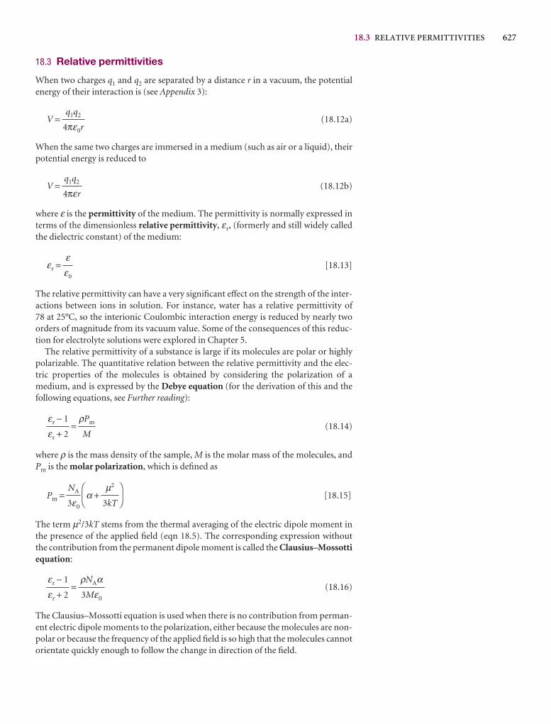
18.3 RELATIVE PERMITTIVITIES 627
18.3 Relative permittivities
When two charges q1 and q2 are separated by a distance r in a vacuum, the potentialenergy of their interaction is (see Appendix 3):
V = (18.12a)
When the same two charges are immersed in a medium (such as air or a liquid), theirpotential energy is reduced to
V = (18.12b)
where ε is the permittivity of the medium. The permittivity is normally expressed interms of the dimensionless relative permittivity, εr, (formerly and still widely calledthe dielectric constant) of the medium:
εr = [18.13]
The relative permittivity can have a very significant effect on the strength of the inter-actions between ions in solution. For instance, water has a relative permittivity of 78 at 25°C, so the interionic Coulombic interaction energy is reduced by nearly twoorders of magnitude from its vacuum value. Some of the consequences of this reduc-tion for electrolyte solutions were explored in Chapter 5.
The relative permittivity of a substance is large if its molecules are polar or highlypolarizable. The quantitative relation between the relative permittivity and the elec-tric properties of the molecules is obtained by considering the polarization of amedium, and is expressed by the Debye equation (for the derivation of this and thefollowing equations, see Further reading):
= (18.14)
where ρ is the mass density of the sample, M is the molar mass of the molecules, andPm is the molar polarization, which is defined as
Pm = α + [18.15]
The term µ2/3kT stems from the thermal averaging of the electric dipole moment inthe presence of the applied field (eqn 18.5). The corresponding expression withoutthe contribution from the permanent dipole moment is called the Clausius–Mossottiequation:
= (18.16)
The Clausius–Mossotti equation is used when there is no contribution from perman-ent electric dipole moments to the polarization, either because the molecules are non-polar or because the frequency of the applied field is so high that the molecules cannotorientate quickly enough to follow the change in direction of the field.
ρNAα3Mε0
εr − 1
εr + 2
DF
µ2
3kT
AC
NA
3ε0
ρPm
M
εr − 1
εr + 2
εε0
q1q2
4πεr
q1q2
4πε0r
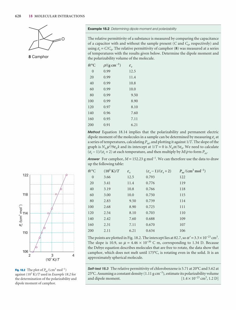
628 18 MOLECULAR INTERACTIONS
O
8 Camphor
2 3 4(10 K)/3 T
P m/(c
mm
ol)
31
106
110
114
118
122
�
Fig. 18.2 The plot of Pm /(cm3 mol−1)against (103 K)/T used in Example 18.2 forthe determination of the polarizability anddipole moment of camphor.
Example 18.2 Determining dipole moment and polarizability
The relative permittivity of a substance is measured by comparing the capacitanceof a capacitor with and without the sample present (C and C0, respectively) andusing εr = C/C0. The relative permittivity of camphor (8) was measured at a seriesof temperatures with the results given below. Determine the dipole moment andthe polarizability volume of the molecule.
θ/°C ρ/(g cm−3) ε r
0 0.99 12.5
20 0.99 11.4
40 0.99 10.8
60 0.99 10.0
80 0.99 9.50
100 0.99 8.90
120 0.97 8.10
140 0.96 7.60
160 0.95 7.11
200 0.91 6.21
Method Equation 18.14 implies that the polarizability and permanent electricdipole moment of the molecules in a sample can be determined by measuring εr ata series of temperatures, calculating Pm, and plotting it against 1/T. The slope of thegraph is NAµ2/9ε0 k and its intercept at 1/T = 0 is NAα /3ε0. We need to calculate (εr − 1)/(εr + 2) at each temperature, and then multiply by M/ρ to form Pm.
Answer For camphor, M = 152.23 g mol−1. We can therefore use the data to drawup the following table:
θ/°C (103 K)/T ε r (ε r − 1)/(ε r + 2) Pm /(cm3 mol−1)
0 3.66 12.5 0.793 122
20 3.41 11.4 0.776 119
40 3.19 10.8 0.766 118
60 3.00 10.0 0.750 115
80 2.83 9.50 0.739 114
100 2.68 8.90 0.725 111
120 2.54 8.10 0.703 110
140 2.42 7.60 0.688 109
160 2.31 7.11 0.670 107
200 2.11 6.21 0.634 106
The points are plotted in Fig. 18.2. The intercept lies at 82.7, so α′ = 3.3 × 10⁻²³ cm3.The slope is 10.9, so µ = 4.46 × 10⁻³⁰ C m, corresponding to 1.34 D. Because the Debye equation describes molecules that are free to rotate, the data show thatcamphor, which does not melt until 175°C, is rotating even in the solid. It is an approximately spherical molecule.
Self-test 18.3 The relative permittivity of chlorobenzene is 5.71 at 20°C and 5.62 at25°C. Assuming a constant density (1.11 g cm−3), estimate its polarizability volumeand dipole moment. [1.4 × 10⁻²³ cm3, 1.2 D]
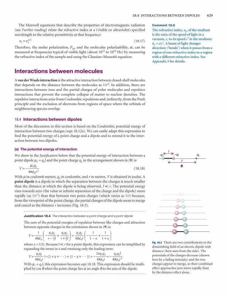
18.4 INTERACTIONS BETWEEN DIPOLES 629
The Maxwell equations that describe the properties of electromagnetic radiation(see Further reading) relate the refractive index at a (visible or ultraviolet) specifiedwavelength to the relative permittivity at that frequency:
nr = ε r1/2 (18.17)
Therefore, the molar polarization, Pm, and the molecular polarizability, α, can bemeasured at frequencies typical of visible light (about 1015 to 1016 Hz) by measuringthe refractive index of the sample and using the Clausius–Mossotti equation.
Interactions between moleculesA van der Waals interaction is the attractive interaction between closed-shell moleculesthat depends on the distance between the molecules as 1/r 6. In addition, there areinteractions between ions and the partial charges of polar molecules and repulsive interactions that prevent the complete collapse of matter to nuclear densities. The repulsive interactions arise from Coulombic repulsions and, indirectly, from the Pauliprinciple and the exclusion of electrons from regions of space where the orbitals ofneighbouring species overlap.
18.4 Interactions between dipoles
Most of the discussion in this section is based on the Coulombic potential energy ofinteraction between two charges (eqn 18.12a). We can easily adapt this expression tofind the potential energy of a point charge and a dipole and to extend it to the inter-action between two dipoles.
(a) The potential energy of interaction
We show in the Justification below that the potential energy of interaction between apoint dipole µ1 = q1l and the point charge q2 in the arrangement shown in (9) is
V = − (18.18)
With µ in coulomb metres, q2 in coulombs, and r in metres, V is obtained in joules. Apoint dipole is a dipole in which the separation between the charges is much smallerthan the distance at which the dipole is being observed, l << r. The potential energyrises towards zero (the value at infinite separation of the charge and the dipole) morerapidly (as 1/r 2) than that between two point charges (which varies as 1/r) because,from the viewpoint of the point charge, the partial charges of the dipole seem to mergeand cancel as the distance r increases (Fig. 18.3).
Justification 18.4 The interaction between a point charge and a point dipole
The sum of the potential energies of repulsion between like charges and attractionbetween opposite charges in the orientation shown in (9) is
V = − + = − +
where x = l /2r. Because l << r for a point dipole, this expression can be simplified byexpanding the terms in x and retaining only the leading term:
V = {−(1 + x + · · · ) + (1 − x + · · · )} ≈ − = −
With µ1 = q1l, this expression becomes eqn 18.18. This expression should be multi-plied by cos θ when the point charge lies at an angle θ to the axis of the dipole.
q1q2l
4πε0r 2
2xq1q2
4πε0r
q1q2
4πε0r
DEF1
1 + x
1
1 − x
ABCq1q2
4πε0r
DEFq1q2
r + 1–2l
q1q2
r − 1–2l
ABC1
4πε0
µ1q2
4πε0r 2
Comment 18.6
The refractive index, nr, of the mediumis the ratio of the speed of light in avacuum, c, to its speed c¢ in the medium:nr = c/c′. A beam of light changesdirection (‘bends’) when it passes from aregion of one refractive index to a regionwith a different refractive index. SeeAppendix 3 for details.
l
r
q1 –q1 q2
9
Fig. 18.3 There are two contributions to thediminishing field of an electric dipole withdistance (here seen from the side). Thepotentials of the charges decrease (shownhere by a fading intensity) and the twocharges appear to merge, so their combinedeffect approaches zero more rapidly thanby the distance effect alone.
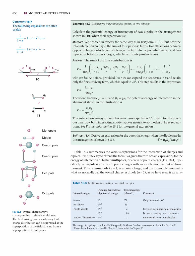
630 18 MOLECULAR INTERACTIONS
Comment 18.7
The following expansions are oftenuseful:
= 1 − x + x 2 − · · ·
= 1 + x + x 2 + · · ·1
1 − x
1
1 + x
l l
r
q1 �q1 �q2q2
10
Table 18.3 Multipole interaction potential energies
Distance dependence Typical energy/Interaction type of potential energy (kJ mol−1) Comment
Ion–ion 1/r 250 Only between ions*
Ion–dipole 1/r 2 15
Dipole–dipole 1/r 3 2 Between stationary polar molecules
1/r 6 0.6 Between rotating polar molecules
London (dispersion) 1/r 6 2 Between all types of molecules
The energy of a hydrogen bond A-H···B is typically 20 kJ mol−l and occurs on contact for A, B = O, N, or F.* Electrolyte solutions are treated in Chapter 5, ionic solids in Chapter 20.
r
q1 �q1
�q2q2
11
Monopole
Dipole
Quadrupole
Quadrupole
Octupole
Octupole
Fig. 18.4 Typical charge arrayscorresponding to electric multipoles. The field arising from an arbitrary finitecharge distribution can be expressed as thesuperposition of the fields arising from asuperposition of multipoles.
Example 18.3 Calculating the interaction energy of two dipoles
Calculate the potential energy of interaction of two dipoles in the arrangementshown in (10) when their separation is r.
Method We proceed in exactly the same way as in Justification 18.4, but now thetotal interaction energy is the sum of four pairwise terms, two attractions betweenopposite charges, which contribute negative terms to the potential energy, and tworepulsions between like charges, which contribute positive terms.
Answer The sum of the four contributions is
V = − + + − = − − 2 +
with x = l /r. As before, provided l << r we can expand the two terms in x and retainonly the first surviving term, which is equal to 2x2. This step results in the expression
V = −
Therefore, because µ1 = q1l and µ2 = q2l, the potential energy of interaction in thealignment shown in the illustration is
V = −
This interaction energy approaches zero more rapidly (as 1/r 3) than for the previ-ous case: now both interacting entities appear neutral to each other at large separa-tions. See Further information 18.1 for the general expression.
Self-test 18.4 Derive an expression for the potential energy when the dipoles are inthe arrangement shown in (11). [V = µ1µ2/4πε0r 3]
Table 18.3 summarizes the various expressions for the interaction of charges anddipoles. It is quite easy to extend the formulas given there to obtain expressions for theenergy of interaction of higher multipoles, or arrays of point charges (Fig. 18.4). Spe-cifically, an n-pole is an array of point charges with an n-pole moment but no lowermoment. Thus, a monopole (n = 1) is a point charge, and the monopole moment iswhat we normally call the overall charge. A dipole (n = 2), as we have seen, is an array
µ1µ2
2πε0r 3
2xq1q2
4πε0r
DF
1
1 − x
1
1 + x
AC
q1q2
4πε0r
DF
q1q2
r − l
q1q2
r
q1q2
r
q1q2
r + l
AC
1
4πε0
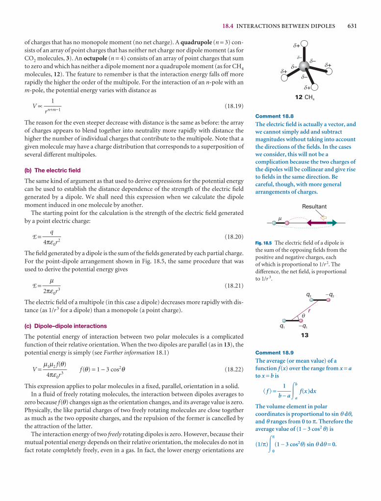
18.4 INTERACTIONS BETWEEN DIPOLES 631
of charges that has no monopole moment (no net charge). A quadrupole (n = 3) con-sists of an array of point charges that has neither net charge nor dipole moment (as forCO2 molecules, 3). An octupole (n = 4) consists of an array of point charges that sumto zero and which has neither a dipole moment nor a quadrupole moment (as for CH4
molecules, 12). The feature to remember is that the interaction energy falls off morerapidly the higher the order of the multipole. For the interaction of an n-pole with anm-pole, the potential energy varies with distance as
V ∝ (18.19)
The reason for the even steeper decrease with distance is the same as before: the arrayof charges appears to blend together into neutrality more rapidly with distance thehigher the number of individual charges that contribute to the multipole. Note that agiven molecule may have a charge distribution that corresponds to a superposition ofseveral different multipoles.
(b) The electric field
The same kind of argument as that used to derive expressions for the potential energycan be used to establish the distance dependence of the strength of the electric fieldgenerated by a dipole. We shall need this expression when we calculate the dipole moment induced in one molecule by another.
The starting point for the calculation is the strength of the electric field generatedby a point electric charge:
E = (18.20)
The field generated by a dipole is the sum of the fields generated by each partial charge.For the point-dipole arrangement shown in Fig. 18.5, the same procedure that wasused to derive the potential energy gives
E = (18.21)
The electric field of a multipole (in this case a dipole) decreases more rapidly with dis-tance (as 1/r 3 for a dipole) than a monopole (a point charge).
(c) Dipole–dipole interactions
The potential energy of interaction between two polar molecules is a complicatedfunction of their relative orientation. When the two dipoles are parallel (as in 13), thepotential energy is simply (see Further information 18.1)
V = f (θ) = 1 − 3 cos2θ (18.22)
This expression applies to polar molecules in a fixed, parallel, orientation in a solid.In a fluid of freely rotating molecules, the interaction between dipoles averages to
zero because f(θ) changes sign as the orientation changes, and its average value is zero.Physically, the like partial charges of two freely rotating molecules are close togetheras much as the two opposite charges, and the repulsion of the former is cancelled bythe attraction of the latter.
The interaction energy of two freely rotating dipoles is zero. However, because theirmutual potential energy depends on their relative orientation, the molecules do not infact rotate completely freely, even in a gas. In fact, the lower energy orientations are
µ1µ2 f(θ)
4πε0r3
µ2πε0r3
q
4πε0r2
1
rn+m−1
+�
+�
+�
+�–�
–�–�
–�
12 CH4
Comment 18.8
The electric field is actually a vector, andwe cannot simply add and subtractmagnitudes without taking into accountthe directions of the fields. In the caseswe consider, this will not be acomplication because the two charges ofthe dipoles will be collinear and give riseto fields in the same direction. Becareful, though, with more generalarrangements of charges.
Resultant
Fig. 18.5 The electric field of a dipole is the sum of the opposing fields from thepositive and negative charges, each of which is proportional to 1/r 2. Thedifference, the net field, is proportional to 1/r 3.
r
q1 �q1
�q2q2
�
13
Comment 18.9
The average (or mean value) of afunction f(x) over the range from x = ato x = b is
� f � = �b
a
f(x)dx
The volume element in polarcoordinates is proportional to sin θ dθ,and θ ranges from 0 to π. Therefore theaverage value of (1 − 3 cos2 θ) is
(1/π)�π
0
(1 − 3 cos2θ) sin θ dθ = 0.
1
b − a
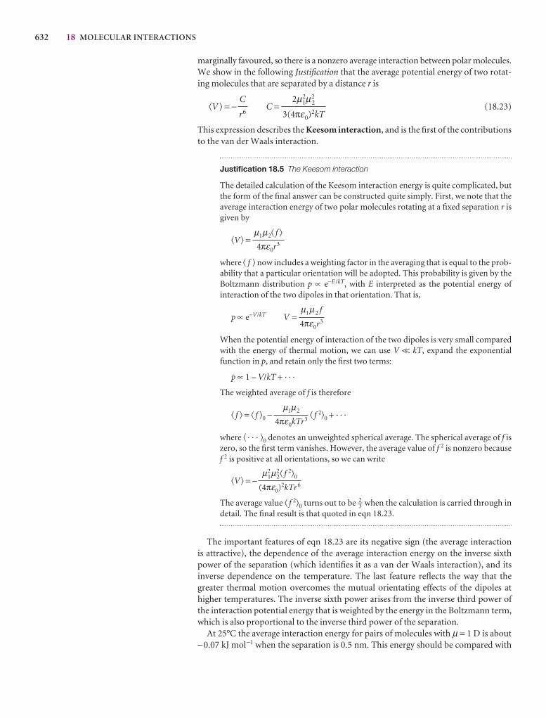
632 18 MOLECULAR INTERACTIONS
marginally favoured, so there is a nonzero average interaction between polar molecules.We show in the following Justification that the average potential energy of two rotat-ing molecules that are separated by a distance r is
�V � = − C = (18.23)
This expression describes the Keesom interaction, and is the first of the contributionsto the van der Waals interaction.
Justification 18.5 The Keesom interaction
The detailed calculation of the Keesom interaction energy is quite complicated, butthe form of the final answer can be constructed quite simply. First, we note that theaverage interaction energy of two polar molecules rotating at a fixed separation r isgiven by
�V� =
where � f � now includes a weighting factor in the averaging that is equal to the prob-ability that a particular orientation will be adopted. This probability is given by theBoltzmann distribution p ∝ e−E /kT, with E interpreted as the potential energy of interaction of the two dipoles in that orientation. That is,
p ∝ e−V/kT V =
When the potential energy of interaction of the two dipoles is very small comparedwith the energy of thermal motion, we can use V << kT, expand the exponentialfunction in p, and retain only the first two terms:
p ∝ 1 – V/kT + · · ·
The weighted average of f is therefore
� f � = � f �0 − � f 2�0 + · · ·
where � · · · �0 denotes an unweighted spherical average. The spherical average of f iszero, so the first term vanishes. However, the average value of f 2 is nonzero becausef 2 is positive at all orientations, so we can write
�V� = −
The average value � f 2�0 turns out to be 2–3 when the calculation is carried through indetail. The final result is that quoted in eqn 18.23.
The important features of eqn 18.23 are its negative sign (the average interaction is attractive), the dependence of the average interaction energy on the inverse sixthpower of the separation (which identifies it as a van der Waals interaction), and its inverse dependence on the temperature. The last feature reflects the way that thegreater thermal motion overcomes the mutual orientating effects of the dipoles athigher temperatures. The inverse sixth power arises from the inverse third power ofthe interaction potential energy that is weighted by the energy in the Boltzmann term,which is also proportional to the inverse third power of the separation.
At 25°C the average interaction energy for pairs of molecules with µ = 1 D is about−0.07 kJ mol−1 when the separation is 0.5 nm. This energy should be compared with
µ12µ2
2� f 2�0
(4πε0)2kTr 6
µ1µ2
4πε0kTr3
µ1µ2 f
4πε0r3
µ1µ2� f �4πε0r3
2µ21µ2
2
3(4πε0)2kT
C
r6
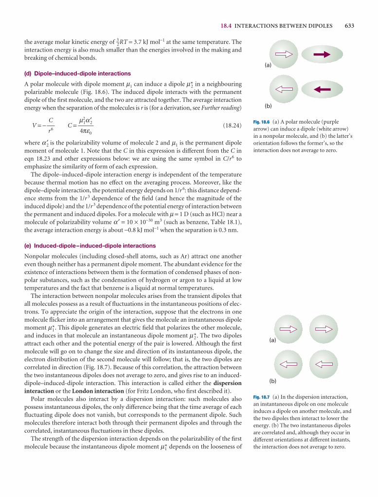
18.4 INTERACTIONS BETWEEN DIPOLES 633
the average molar kinetic energy of 3–2RT = 3.7 kJ mol−1 at the same temperature. Theinteraction energy is also much smaller than the energies involved in the making andbreaking of chemical bonds.
(d) Dipole–induced-dipole interactions
A polar molecule with dipole moment µ1 can induce a dipole µ2* in a neighbouringpolarizable molecule (Fig. 18.6). The induced dipole interacts with the permanentdipole of the first molecule, and the two are attracted together. The average interactionenergy when the separation of the molecules is r is (for a derivation, see Further reading)
V = − C = (18.24)
where α2′ is the polarizability volume of molecule 2 and µ1 is the permanent dipolemoment of molecule 1. Note that the C in this expression is different from the C ineqn 18.23 and other expressions below: we are using the same symbol in C/r6 toemphasize the similarity of form of each expression.
The dipole–induced-dipole interaction energy is independent of the temperaturebecause thermal motion has no effect on the averaging process. Moreover, like thedipole–dipole interaction, the potential energy depends on 1/r 6: this distance depend-ence stems from the 1/r 3 dependence of the field (and hence the magnitude of the induced dipole) and the 1/r3 dependence of the potential energy of interaction betweenthe permanent and induced dipoles. For a molecule with µ = 1 D (such as HCl) near amolecule of polarizability volume α′ = 10 × 10−30 m3 (such as benzene, Table 18.1), the average interaction energy is about −0.8 kJ mol−1 when the separation is 0.3 nm.
(e) Induced-dipole–induced-dipole interactions
Nonpolar molecules (including closed-shell atoms, such as Ar) attract one anothereven though neither has a permanent dipole moment. The abundant evidence for theexistence of interactions between them is the formation of condensed phases of non-polar substances, such as the condensation of hydrogen or argon to a liquid at lowtemperatures and the fact that benzene is a liquid at normal temperatures.
The interaction between nonpolar molecules arises from the transient dipoles thatall molecules possess as a result of fluctuations in the instantaneous positions of elec-trons. To appreciate the origin of the interaction, suppose that the electrons in onemolecule flicker into an arrangement that gives the molecule an instantaneous dipolemoment µ1*. This dipole generates an electric field that polarizes the other molecule,and induces in that molecule an instantaneous dipole moment µ2*. The two dipoles attract each other and the potential energy of the pair is lowered. Although the firstmolecule will go on to change the size and direction of its instantaneous dipole, theelectron distribution of the second molecule will follow; that is, the two dipoles arecorrelated in direction (Fig. 18.7). Because of this correlation, the attraction betweenthe two instantaneous dipoles does not average to zero, and gives rise to an induced-dipole–induced-dipole interaction. This interaction is called either the dispersioninteraction or the London interaction (for Fritz London, who first described it).
Polar molecules also interact by a dispersion interaction: such molecules also possess instantaneous dipoles, the only difference being that the time average of eachfluctuating dipole does not vanish, but corresponds to the permanent dipole. Suchmolecules therefore interact both through their permanent dipoles and through thecorrelated, instantaneous fluctuations in these dipoles.
The strength of the dispersion interaction depends on the polarizability of the firstmolecule because the instantaneous dipole moment µ1* depends on the looseness of
µ21α′2
4πε0
C
r6
(a)
(b)
Fig. 18.7 (a) In the dispersion interaction,an instantaneous dipole on one moleculeinduces a dipole on another molecule, andthe two dipoles then interact to lower theenergy. (b) The two instantaneous dipolesare correlated and, although they occur indifferent orientations at different instants,the interaction does not average to zero.
Fig. 18.6 (a) A polar molecule (purplearrow) can induce a dipole (white arrow)in a nonpolar molecule, and (b) the latter’sorientation follows the former’s, so theinteraction does not average to zero.
(a)
(b)
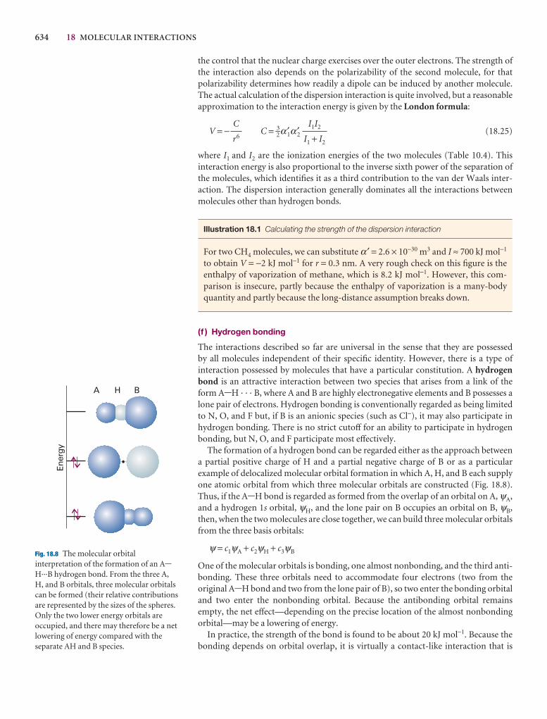
634 18 MOLECULAR INTERACTIONS
Ener
gy
A H B
Fig. 18.8 The molecular orbitalinterpretation of the formation of an A-H···B hydrogen bond. From the three A, H, and B orbitals, three molecular orbitalscan be formed (their relative contributionsare represented by the sizes of the spheres.Only the two lower energy orbitals areoccupied, and there may therefore be a netlowering of energy compared with theseparate AH and B species.
the control that the nuclear charge exercises over the outer electrons. The strength ofthe interaction also depends on the polarizability of the second molecule, for that polarizability determines how readily a dipole can be induced by another molecule.The actual calculation of the dispersion interaction is quite involved, but a reasonableapproximation to the interaction energy is given by the London formula:
V = − C = 3–2α′1α′2 (18.25)
where I1 and I2 are the ionization energies of the two molecules (Table 10.4). This interaction energy is also proportional to the inverse sixth power of the separation ofthe molecules, which identifies it as a third contribution to the van der Waals inter-action. The dispersion interaction generally dominates all the interactions betweenmolecules other than hydrogen bonds.
Illustration 18.1 Calculating the strength of the dispersion interaction
For two CH4 molecules, we can substitute α′ = 2.6 × 10⁻³⁰ m3 and I ≈ 700 kJ mol−1
to obtain V = −2 kJ mol−1 for r = 0.3 nm. A very rough check on this figure is the enthalpy of vaporization of methane, which is 8.2 kJ mol−1. However, this com-parison is insecure, partly because the enthalpy of vaporization is a many-bodyquantity and partly because the long-distance assumption breaks down.
(f ) Hydrogen bonding
The interactions described so far are universal in the sense that they are possessed by all molecules independent of their specific identity. However, there is a type of interaction possessed by molecules that have a particular constitution. A hydrogenbond is an attractive interaction between two species that arises from a link of theform A-H · · · B, where A and B are highly electronegative elements and B possesses alone pair of electrons. Hydrogen bonding is conventionally regarded as being limitedto N, O, and F but, if B is an anionic species (such as Cl−), it may also participate in hydrogen bonding. There is no strict cutoff for an ability to participate in hydrogenbonding, but N, O, and F participate most effectively.
The formation of a hydrogen bond can be regarded either as the approach betweena partial positive charge of H and a partial negative charge of B or as a particularexample of delocalized molecular orbital formation in which A, H, and B each supplyone atomic orbital from which three molecular orbitals are constructed (Fig. 18.8).Thus, if the A-H bond is regarded as formed from the overlap of an orbital on A, ψA,and a hydrogen 1s orbital, ψH, and the lone pair on B occupies an orbital on B, ψB,then, when the two molecules are close together, we can build three molecular orbitalsfrom the three basis orbitals:
ψ = c1ψA + c2ψH + c3ψB
One of the molecular orbitals is bonding, one almost nonbonding, and the third anti-bonding. These three orbitals need to accommodate four electrons (two from theoriginal A-H bond and two from the lone pair of B), so two enter the bonding orbitaland two enter the nonbonding orbital. Because the antibonding orbital remainsempty, the net effect—depending on the precise location of the almost nonbondingorbital—may be a lowering of energy.
In practice, the strength of the bond is found to be about 20 kJ mol−1. Because thebonding depends on orbital overlap, it is virtually a contact-like interaction that is
I1I2
I1 + I2
C
r6
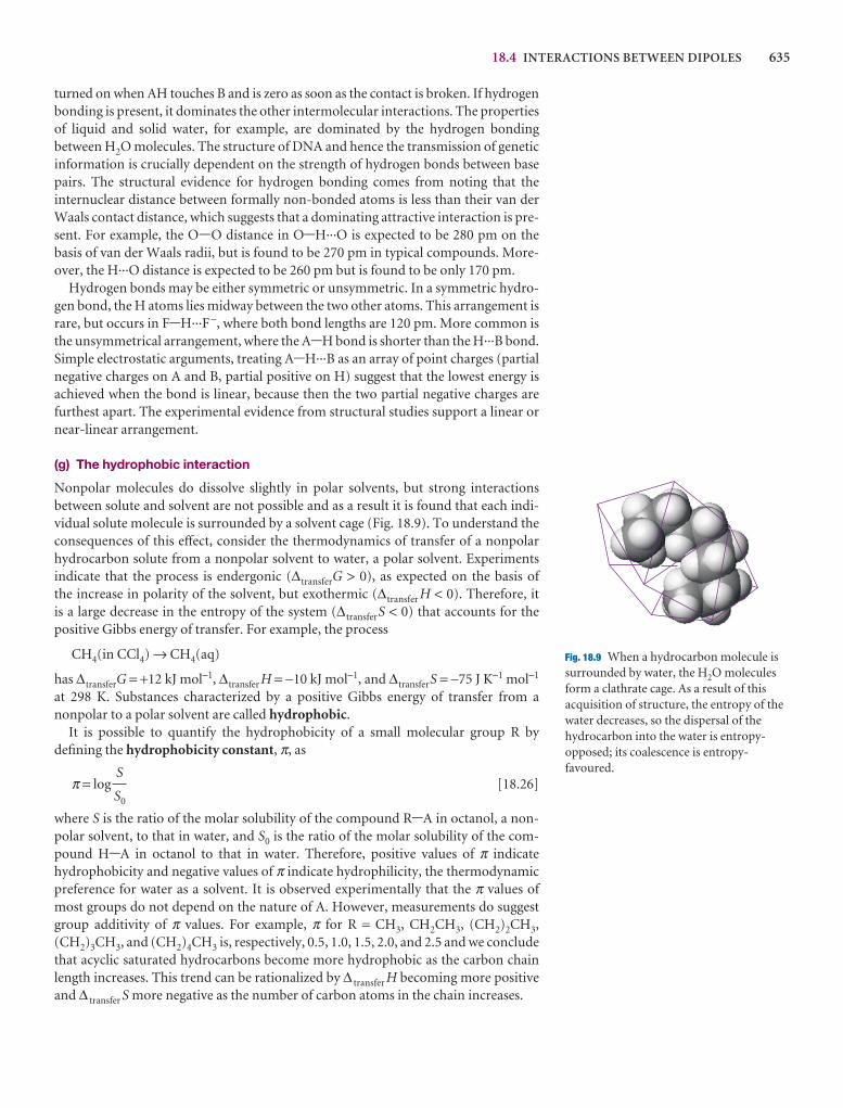
18.4 INTERACTIONS BETWEEN DIPOLES 635
turned on when AH touches B and is zero as soon as the contact is broken. If hydrogenbonding is present, it dominates the other intermolecular interactions. The propertiesof liquid and solid water, for example, are dominated by the hydrogen bonding between H2O molecules. The structure of DNA and hence the transmission of geneticinformation is crucially dependent on the strength of hydrogen bonds between basepairs. The structural evidence for hydrogen bonding comes from noting that the internuclear distance between formally non-bonded atoms is less than their van derWaals contact distance, which suggests that a dominating attractive interaction is pre-sent. For example, the O-O distance in O-H···O is expected to be 280 pm on thebasis of van der Waals radii, but is found to be 270 pm in typical compounds. More-over, the H···O distance is expected to be 260 pm but is found to be only 170 pm.
Hydrogen bonds may be either symmetric or unsymmetric. In a symmetric hydro-gen bond, the H atoms lies midway between the two other atoms. This arrangement israre, but occurs in F-H···F−, where both bond lengths are 120 pm. More common isthe unsymmetrical arrangement, where the A-H bond is shorter than the H···B bond.Simple electrostatic arguments, treating A-H···B as an array of point charges (partialnegative charges on A and B, partial positive on H) suggest that the lowest energy isachieved when the bond is linear, because then the two partial negative charges arefurthest apart. The experimental evidence from structural studies support a linear ornear-linear arrangement.
(g) The hydrophobic interaction
Nonpolar molecules do dissolve slightly in polar solvents, but strong interactions between solute and solvent are not possible and as a result it is found that each indi-vidual solute molecule is surrounded by a solvent cage (Fig. 18.9). To understand theconsequences of this effect, consider the thermodynamics of transfer of a nonpolarhydrocarbon solute from a nonpolar solvent to water, a polar solvent. Experimentsindicate that the process is endergonic (∆transferG > 0), as expected on the basis of the increase in polarity of the solvent, but exothermic (∆transfer H < 0). Therefore, it is a large decrease in the entropy of the system (∆transferS < 0) that accounts for the positive Gibbs energy of transfer. For example, the process
CH4(in CCl4) → CH4(aq)
has ∆transferG = +12 kJ mol−1, ∆transferH = −10 kJ mol−1, and ∆transferS = −75 J K−1 mol−1
at 298 K. Substances characterized by a positive Gibbs energy of transfer from a nonpolar to a polar solvent are called hydrophobic.
It is possible to quantify the hydrophobicity of a small molecular group R bydefining the hydrophobicity constant, π, as
π = log [18.26]
where S is the ratio of the molar solubility of the compound R-A in octanol, a non-polar solvent, to that in water, and S0 is the ratio of the molar solubility of the com-pound H-A in octanol to that in water. Therefore, positive values of π indicatehydrophobicity and negative values of π indicate hydrophilicity, the thermodynamicpreference for water as a solvent. It is observed experimentally that the π values ofmost groups do not depend on the nature of A. However, measurements do suggestgroup additivity of π values. For example, π for R = CH3, CH2CH3, (CH2)2CH3,(CH2)3CH3, and (CH2)4CH3 is, respectively, 0.5, 1.0, 1.5, 2.0, and 2.5 and we concludethat acyclic saturated hydrocarbons become more hydrophobic as the carbon chainlength increases. This trend can be rationalized by ∆ transfer H becoming more positiveand ∆ transfer S more negative as the number of carbon atoms in the chain increases.
S
S0
Fig. 18.9 When a hydrocarbon molecule issurrounded by water, the H2O moleculesform a clathrate cage. As a result of thisacquisition of structure, the entropy of thewater decreases, so the dispersal of thehydrocarbon into the water is entropy-opposed; its coalescence is entropy-favoured.
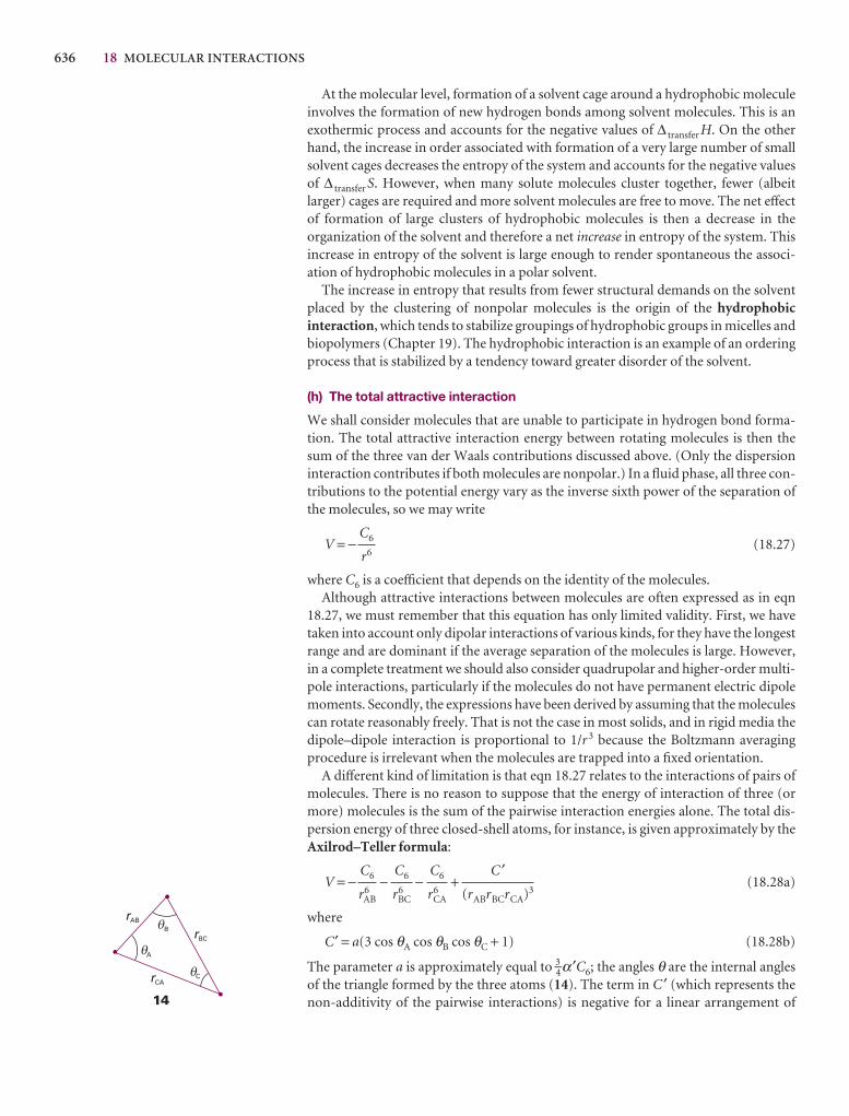
636 18 MOLECULAR INTERACTIONS
At the molecular level, formation of a solvent cage around a hydrophobic moleculeinvolves the formation of new hydrogen bonds among solvent molecules. This is anexothermic process and accounts for the negative values of ∆ transfer H. On the otherhand, the increase in order associated with formation of a very large number of smallsolvent cages decreases the entropy of the system and accounts for the negative valuesof ∆ transfer S. However, when many solute molecules cluster together, fewer (albeitlarger) cages are required and more solvent molecules are free to move. The net effectof formation of large clusters of hydrophobic molecules is then a decrease in the organization of the solvent and therefore a net increase in entropy of the system. Thisincrease in entropy of the solvent is large enough to render spontaneous the associ-ation of hydrophobic molecules in a polar solvent.
The increase in entropy that results from fewer structural demands on the solventplaced by the clustering of nonpolar molecules is the origin of the hydrophobicinteraction, which tends to stabilize groupings of hydrophobic groups in micelles andbiopolymers (Chapter 19). The hydrophobic interaction is an example of an orderingprocess that is stabilized by a tendency toward greater disorder of the solvent.
(h) The total attractive interaction
We shall consider molecules that are unable to participate in hydrogen bond forma-tion. The total attractive interaction energy between rotating molecules is then thesum of the three van der Waals contributions discussed above. (Only the dispersioninteraction contributes if both molecules are nonpolar.) In a fluid phase, all three con-tributions to the potential energy vary as the inverse sixth power of the separation ofthe molecules, so we may write
V = − (18.27)
where C6 is a coefficient that depends on the identity of the molecules.Although attractive interactions between molecules are often expressed as in eqn
18.27, we must remember that this equation has only limited validity. First, we havetaken into account only dipolar interactions of various kinds, for they have the longestrange and are dominant if the average separation of the molecules is large. However,in a complete treatment we should also consider quadrupolar and higher-order multi-pole interactions, particularly if the molecules do not have permanent electric dipolemoments. Secondly, the expressions have been derived by assuming that the moleculescan rotate reasonably freely. That is not the case in most solids, and in rigid media thedipole–dipole interaction is proportional to 1/r 3 because the Boltzmann averagingprocedure is irrelevant when the molecules are trapped into a fixed orientation.
A different kind of limitation is that eqn 18.27 relates to the interactions of pairs ofmolecules. There is no reason to suppose that the energy of interaction of three (ormore) molecules is the sum of the pairwise interaction energies alone. The total dis-persion energy of three closed-shell atoms, for instance, is given approximately by theAxilrod–Teller formula:
V = − − − + (18.28a)
where
C′ = a(3 cos θA cos θB cos θC + 1) (18.28b)
The parameter a is approximately equal to 3–4α′C6; the angles θ are the internal anglesof the triangle formed by the three atoms (14). The term in C ′ (which represents thenon-additivity of the pairwise interactions) is negative for a linear arrangement of
C ′(rABrBCrCA)3
C6
r6CA
C6
r6BC
C6
r6AB
C6
r6
B
rAB
rBC
rCA
14
�
A�
C�
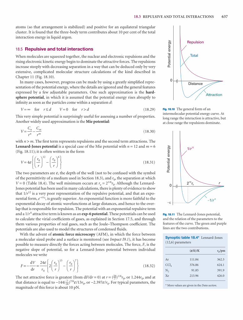
18.5 REPULSIVE AND TOTAL INTERACTIONS 637
atoms (so that arrangement is stabilized) and positive for an equilateral triangularcluster. It is found that the three-body term contributes about 10 per cent of the totalinteraction energy in liquid argon.
18.5 Repulsive and total interactions
When molecules are squeezed together, the nuclear and electronic repulsions and therising electronic kinetic energy begin to dominate the attractive forces. The repulsionsincrease steeply with decreasing separation in a way that can be deduced only by veryextensive, complicated molecular structure calculations of the kind described inChapter 11 (Fig. 18.10).
In many cases, however, progress can be made by using a greatly simplified repre-sentation of the potential energy, where the details are ignored and the general featuresexpressed by a few adjustable parameters. One such approximation is the hard-sphere potential, in which it is assumed that the potential energy rises abruptly toinfinity as soon as the particles come within a separation d:
V = ∞ for r ≤ d V = 0 for r > d (18.29)
This very simple potential is surprisingly useful for assessing a number of properties.Another widely used approximation is the Mie potential:
V = − (18.30)
with n > m. The first term represents repulsions and the second term attractions. TheLennard-Jones potential is a special case of the Mie potential with n = 12 and m = 6(Fig. 18.11); it is often written in the form
V = 4ε12
−6
(18.31)
The two parameters are ε, the depth of the well (not to be confused with the symbol of the permittivity of a medium used in Section 18.3), and r0, the separation at whichV = 0 (Table 18.4). The well minimum occurs at re = 21/6r0. Although the Lennard-Jones potential has been used in many calculations, there is plenty of evidence to showthat 1/r12 is a very poor representation of the repulsive potential, and that an expo-nential form, e−r/r0, is greatly superior. An exponential function is more faithful to theexponential decay of atomic wavefunctions at large distances, and hence to the over-lap that is responsible for repulsion. The potential with an exponential repulsive termand a 1/r 6 attractive term is known as an exp-6 potential. These potentials can be usedto calculate the virial coefficients of gases, as explained in Section 17.5, and throughthem various properties of real gases, such as the Joule–Thompson coefficient. Thepotentials are also used to model the structures of condensed fluids.
With the advent of atomic force microscopy (AFM), in which the force between a molecular sized probe and a surface is monitored (see Impact I9.1), it has becomepossible to measure directly the forces acting between molecules. The force, F, is thenegative slope of potential, so for a Lennard-Jones potential between individualmolecules we write
F = − = 2
13
−7
(18.32)
The net attractive force is greatest (from dF/dr = 0) at r = (26––7 )1/6r0, or 1.244r0, and atthat distance is equal to −144( 7––26)7/6ε /13r0, or −2.397ε /r0. For typical parameters, themagnitude of this force is about 10 pN.
567
DF
r0
r
AC
DF
r0
r
AC
123
24εr0
dV
dr
567
DF
r0
r
AC
DF
r0
r
AC
123
Cm
rm
Cn
rn
Pote
ntia
l ene
rgy
0
�1/r 6
21/6r0
1/r12
r
��
Fig. 18.11 The Lennard-Jones potential, and the relation of the parameters to thefeatures of the curve. The green and purplelines are the two contributions.
Synoptic table 18.4* Lennard-Jones(12,6) parameters
(e/k)/K r0/pm
Ar 111.84 362.3
CCl4 376.86 624.1
N2 91.85 391.9
Xe 213.96 426.0
* More values are given in the Data section.
Repulsion
Attraction
Total
Pote
ntia
l ene
rgy
Distance0
Fig. 18.10 The general form of anintermolecular potential energy curve. Atlong range the interaction is attractive, butat close range the repulsions dominate.
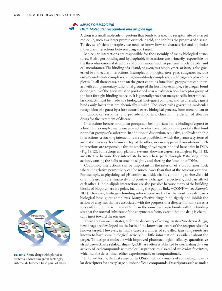
638 18 MOLECULAR INTERACTIONS
IMPACT ON MEDICINE
I18.1 Molecular recognition and drug design
A drug is a small molecule or protein that binds to a specific receptor site of a targetmolecule, such as a larger protein or nucleic acid, and inhibits the progress of disease.To devise efficient therapies, we need to know how to characterize and optimizemolecular interactions between drug and target.
Molecular interactions are responsible for the assembly of many biological struc-tures. Hydrogen bonding and hydrophobic interactions are primarily responsible forthe three-dimensional structures of biopolymers, such as proteins, nucleic acids, andcell membranes. The binding of a ligand, or guest, to a biopolymer, or host, is also gov-erned by molecular interactions. Examples of biological host–guest complexes includeenzyme–substrate complexes, antigen–antibody complexes, and drug–receptor com-plexes. In all these cases, a site on the guest contains functional groups that can inter-act with complementary functional groups of the host. For example, a hydrogen bonddonor group of the guest must be positioned near a hydrogen bond acceptor group ofthe host for tight binding to occur. It is generally true that many specific intermolecu-lar contacts must be made in a biological host–guest complex and, as a result, a guestbinds only hosts that are chemically similar. The strict rules governing molecularrecognition of a guest by a host control every biological process, from metabolism toimmunological response, and provide important clues for the design of effectivedrugs for the treatment of disease.
Interactions between nonpolar groups can be important in the binding of a guest toa host. For example, many enzyme active sites have hydrophobic pockets that bindnonpolar groups of a substrate. In addition to dispersion, repulsive, and hydrophobicinteractions, π stacking interactions are also possible, in which the planar π systems ofaromatic macrocycles lie one on top of the other, in a nearly parallel orientation. Suchinteractions are responsible for the stacking of hydrogen-bonded base pairs in DNA(Fig. 18.12). Some drugs with planar π systems, shown as a green rectangle in Fig. 18.12,are effective because they intercalate between base pairs through π stacking inter-actions, causing the helix to unwind slightly and altering the function of DNA.
Coulombic interactions can be important in the interior of a biopolymer host,where the relative permittivity can be much lower than that of the aqueous exterior.For example, at physiological pH, amino acid side chains containing carboxylic acidor amine groups are negatively and positively charged, respectively, and can attracteach other. Dipole–dipole interactions are also possible because many of the buildingblocks of biopolymers are polar, including the peptide link, -CONH- (see Example18.1). However, hydrogen bonding interactions are by far the most prevalent in a biological host–guest complexes. Many effective drugs bind tightly and inhibit the action of enzymes that are associated with the progress of a disease. In many cases, asuccessful inhibitor will be able to form the same hydrogen bonds with the bindingsite that the normal substrate of the enzyme can form, except that the drug is chemi-cally inert toward the enzyme.
There are two main strategies for the discovery of a drug. In structure-based design,new drugs are developed on the basis of the known structure of the receptor site of aknown target. However, in many cases a number of so-called lead compounds areknown to have some biological activity but little information is available about thetarget. To design a molecule with improved pharmacological efficacy, quantitativestructure–activity relationships (QSAR) are often established by correlating data onactivity of lead compounds with molecular properties, also called molecular descriptors,which can be determined either experimentally or computationally.
In broad terms, the first stage of the QSAR method consists of compiling molecu-lar descriptors for a very large number of lead compounds. Descriptors such as molar
T A
C G
T A
G C
T A
C G
G C
Intercalation
T A
Fig. 18.12 Some drugs with planar πsystems, shown as a green rectangle,intercalate between base pairs of DNA.
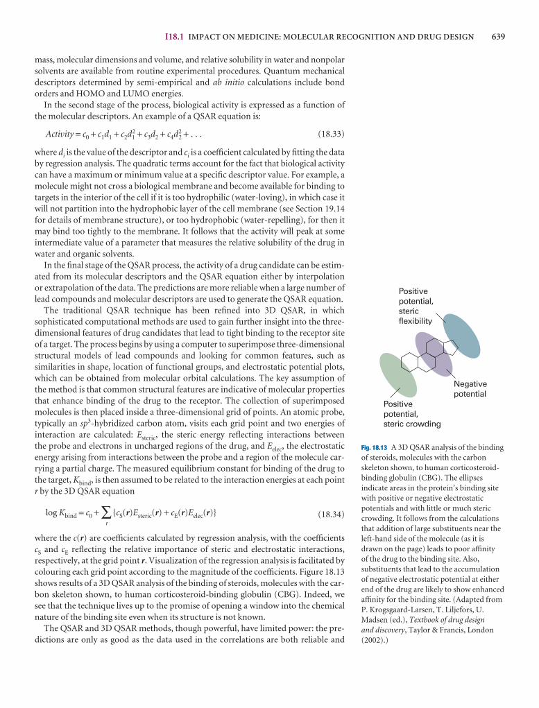
I18.1 IMPACT ON MEDICINE: MOLECULAR RECOGNITION AND DRUG DESIGN 639
mass, molecular dimensions and volume, and relative solubility in water and nonpolarsolvents are available from routine experimental procedures. Quantum mechanicaldescriptors determined by semi-empirical and ab initio calculations include bond orders and HOMO and LUMO energies.
In the second stage of the process, biological activity is expressed as a function ofthe molecular descriptors. An example of a QSAR equation is:
Activity = c0 + c1d1 + c2d12 + c3d2 + c4d2
2 + . . . (18.33)
where di is the value of the descriptor and ci is a coefficient calculated by fitting the databy regression analysis. The quadratic terms account for the fact that biological activity can have a maximum or minimum value at a specific descriptor value. For example, amolecule might not cross a biological membrane and become available for binding totargets in the interior of the cell if it is too hydrophilic (water-loving), in which case itwill not partition into the hydrophobic layer of the cell membrane (see Section 19.14for details of membrane structure), or too hydrophobic (water-repelling), for then itmay bind too tightly to the membrane. It follows that the activity will peak at some intermediate value of a parameter that measures the relative solubility of the drug inwater and organic solvents.
In the final stage of the QSAR process, the activity of a drug candidate can be estim-ated from its molecular descriptors and the QSAR equation either by interpolation or extrapolation of the data. The predictions are more reliable when a large number oflead compounds and molecular descriptors are used to generate the QSAR equation.
The traditional QSAR technique has been refined into 3D QSAR, in which sophisticated computational methods are used to gain further insight into the three-dimensional features of drug candidates that lead to tight binding to the receptor siteof a target. The process begins by using a computer to superimpose three-dimensionalstructural models of lead compounds and looking for common features, such as similarities in shape, location of functional groups, and electrostatic potential plots,which can be obtained from molecular orbital calculations. The key assumption of the method is that common structural features are indicative of molecular propertiesthat enhance binding of the drug to the receptor. The collection of superimposedmolecules is then placed inside a three-dimensional grid of points. An atomic probe,typically an sp3-hybridized carbon atom, visits each grid point and two energies of interaction are calculated: Esteric, the steric energy reflecting interactions between the probe and electrons in uncharged regions of the drug, and Eelec, the electrostatic energy arising from interactions between the probe and a region of the molecule car-rying a partial charge. The measured equilibrium constant for binding of the drug tothe target, Kbind, is then assumed to be related to the interaction energies at each pointr by the 3D QSAR equation
log Kbind = c0 + ∑r
{cS(r)Esteric(r) + cE(r)Eelec(r)} (18.34)
where the c(r) are coefficients calculated by regression analysis, with the coefficientscS and cE reflecting the relative importance of steric and electrostatic interactions, respectively, at the grid point r. Visualization of the regression analysis is facilitated bycolouring each grid point according to the magnitude of the coefficients. Figure 18.13shows results of a 3D QSAR analysis of the binding of steroids, molecules with the car-bon skeleton shown, to human corticosteroid-binding globulin (CBG). Indeed, wesee that the technique lives up to the promise of opening a window into the chemicalnature of the binding site even when its structure is not known.
The QSAR and 3D QSAR methods, though powerful, have limited power: the pre-dictions are only as good as the data used in the correlations are both reliable and
Positivepotential,stericflexibility
Negativepotential
Positivepotential,steric crowding
Fig. 18.13 A 3D QSAR analysis of the binding of steroids, molecules with the carbonskeleton shown, to human corticosteroid-binding globulin (CBG). The ellipsesindicate areas in the protein’s binding sitewith positive or negative electrostaticpotentials and with little or much stericcrowding. It follows from the calculationsthat addition of large substituents near theleft-hand side of the molecule (as it isdrawn on the page) leads to poor affinityof the drug to the binding site. Also,substituents that lead to the accumulationof negative electrostatic potential at eitherend of the drug are likely to show enhancedaffinity for the binding site. (Adapted fromP. Krogsgaard-Larsen, T. Liljefors, U.Madsen (ed.), Textbook of drug design and discovery, Taylor & Francis, London(2002).)
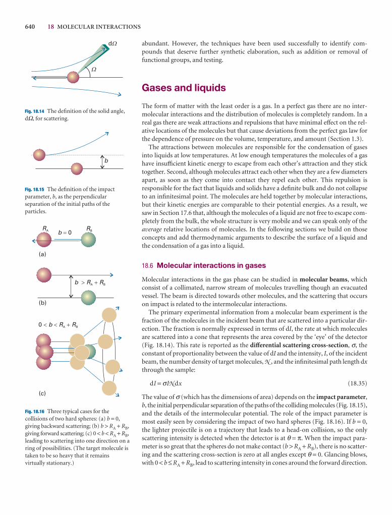
640 18 MOLECULAR INTERACTIONS
abundant. However, the techniques have been used successfully to identify com-pounds that deserve further synthetic elaboration, such as addition or removal offunctional groups, and testing.
Gases and liquids
The form of matter with the least order is a gas. In a perfect gas there are no inter-molecular interactions and the distribution of molecules is completely random. In areal gas there are weak attractions and repulsions that have minimal effect on the rel-ative locations of the molecules but that cause deviations from the perfect gas law forthe dependence of pressure on the volume, temperature, and amount (Section 1.3).
The attractions between molecules are responsible for the condensation of gasesinto liquids at low temperatures. At low enough temperatures the molecules of a gashave insufficient kinetic energy to escape from each other’s attraction and they sticktogether. Second, although molecules attract each other when they are a few diametersapart, as soon as they come into contact they repel each other. This repulsion is responsible for the fact that liquids and solids have a definite bulk and do not collapseto an infinitesimal point. The molecules are held together by molecular interactions,but their kinetic energies are comparable to their potential energies. As a result, wesaw in Section 17.6 that, although the molecules of a liquid are not free to escape com-pletely from the bulk, the whole structure is very mobile and we can speak only of theaverage relative locations of molecules. In the following sections we build on thoseconcepts and add thermodynamic arguments to describe the surface of a liquid andthe condensation of a gas into a liquid.
18.6 Molecular interactions in gases
Molecular interactions in the gas phase can be studied in molecular beams, whichconsist of a collimated, narrow stream of molecules travelling though an evacuatedvessel. The beam is directed towards other molecules, and the scattering that occurson impact is related to the intermolecular interactions.
The primary experimental information from a molecular beam experiment is thefraction of the molecules in the incident beam that are scattered into a particular dir-ection. The fraction is normally expressed in terms of dI, the rate at which moleculesare scattered into a cone that represents the area covered by the ‘eye’ of the detector(Fig. 18.14). This rate is reported as the differential scattering cross-section, σ, theconstant of proportionality between the value of dI and the intensity, I, of the incidentbeam, the number density of target molecules, N , and the infinitesimal path length dxthrough the sample:
dI = σIN dx (18.35)
The value of σ (which has the dimensions of area) depends on the impact parameter,b, the initial perpendicular separation of the paths of the colliding molecules (Fig. 18.15),and the details of the intermolecular potential. The role of the impact parameter ismost easily seen by considering the impact of two hard spheres (Fig. 18.16). If b = 0,the lighter projectile is on a trajectory that leads to a head-on collision, so the onlyscattering intensity is detected when the detector is at θ = π. When the impact para-meter is so great that the spheres do not make contact (b > RA + RB), there is no scatter-ing and the scattering cross-section is zero at all angles except θ = 0. Glancing blows,with 0 < b ≤ RA + RB, lead to scattering intensity in cones around the forward direction.
W
dW
b
Fig. 18.14 The definition of the solid angle,dΩ, for scattering.
Fig. 18.15 The definition of the impactparameter, b, as the perpendicularseparation of the initial paths of theparticles.
0 � � �b R RA B
b R R� �A B
b 0�
(a)
(b)
(c)
RA RB
Fig. 18.16 Three typical cases for thecollisions of two hard spheres: (a) b = 0,giving backward scattering; (b) b > RA + RB,giving forward scattering; (c) 0 < b < RA + RB,leading to scattering into one direction on aring of possibilities. (The target molecule istaken to be so heavy that it remainsvirtually stationary.)
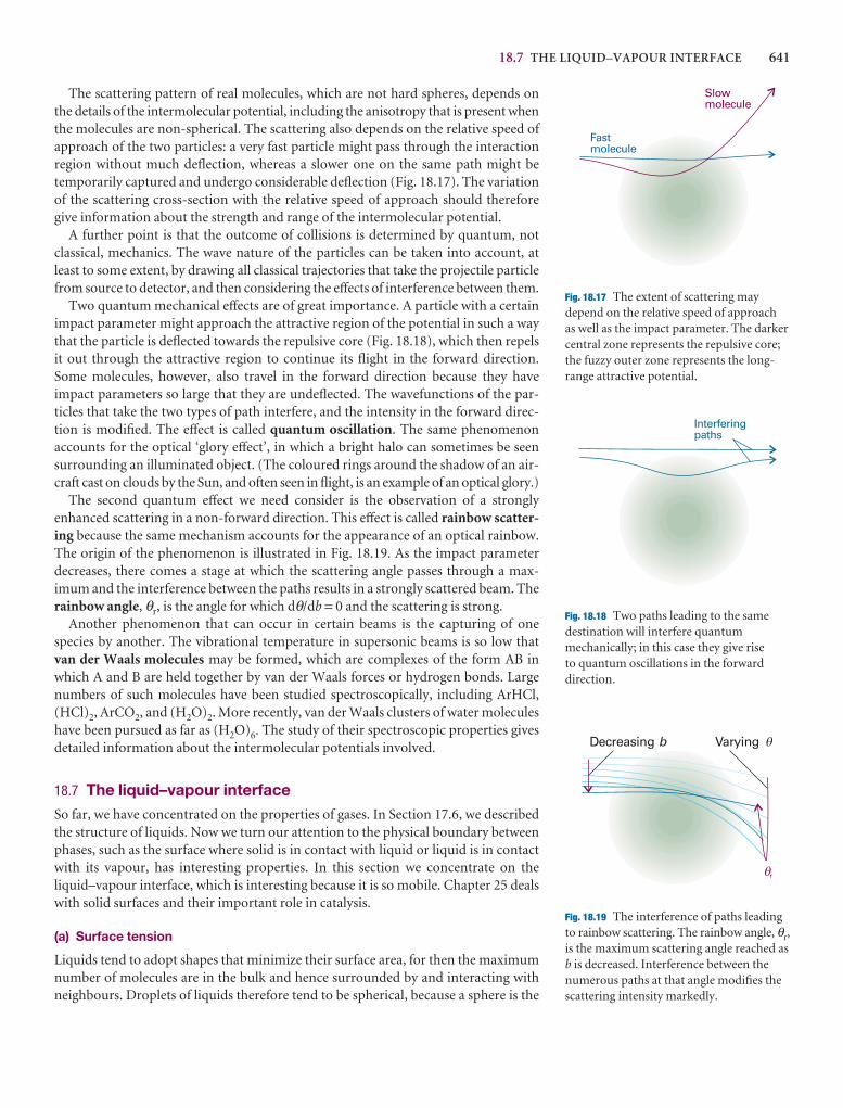
18.7 THE LIQUID–VAPOUR INTERFACE 641
The scattering pattern of real molecules, which are not hard spheres, depends onthe details of the intermolecular potential, including the anisotropy that is present whenthe molecules are non-spherical. The scattering also depends on the relative speed ofapproach of the two particles: a very fast particle might pass through the interactionregion without much deflection, whereas a slower one on the same path might betemporarily captured and undergo considerable deflection (Fig. 18.17). The variationof the scattering cross-section with the relative speed of approach should thereforegive information about the strength and range of the intermolecular potential.
A further point is that the outcome of collisions is determined by quantum, notclassical, mechanics. The wave nature of the particles can be taken into account, atleast to some extent, by drawing all classical trajectories that take the projectile particlefrom source to detector, and then considering the effects of interference between them.
Two quantum mechanical effects are of great importance. A particle with a certainimpact parameter might approach the attractive region of the potential in such a waythat the particle is deflected towards the repulsive core (Fig. 18.18), which then repelsit out through the attractive region to continue its flight in the forward direction.Some molecules, however, also travel in the forward direction because they have impact parameters so large that they are undeflected. The wavefunctions of the par-ticles that take the two types of path interfere, and the intensity in the forward direc-tion is modified. The effect is called quantum oscillation. The same phenomenonaccounts for the optical ‘glory effect’, in which a bright halo can sometimes be seensurrounding an illuminated object. (The coloured rings around the shadow of an air-craft cast on clouds by the Sun, and often seen in flight, is an example of an optical glory.)
The second quantum effect we need consider is the observation of a strongly enhanced scattering in a non-forward direction. This effect is called rainbow scatter-ing because the same mechanism accounts for the appearance of an optical rainbow.The origin of the phenomenon is illustrated in Fig. 18.19. As the impact parameter decreases, there comes a stage at which the scattering angle passes through a max-imum and the interference between the paths results in a strongly scattered beam. Therainbow angle, θr, is the angle for which dθ/db = 0 and the scattering is strong.
Another phenomenon that can occur in certain beams is the capturing of onespecies by another. The vibrational temperature in supersonic beams is so low thatvan der Waals molecules may be formed, which are complexes of the form AB inwhich A and B are held together by van der Waals forces or hydrogen bonds. Largenumbers of such molecules have been studied spectroscopically, including ArHCl,(HCl)2, ArCO2, and (H2O)2. More recently, van der Waals clusters of water moleculeshave been pursued as far as (H2O)6. The study of their spectroscopic properties givesdetailed information about the intermolecular potentials involved.
18.7 The liquid–vapour interfaceSo far, we have concentrated on the properties of gases. In Section 17.6, we describedthe structure of liquids. Now we turn our attention to the physical boundary betweenphases, such as the surface where solid is in contact with liquid or liquid is in contactwith its vapour, has interesting properties. In this section we concentrate on the liquid–vapour interface, which is interesting because it is so mobile. Chapter 25 dealswith solid surfaces and their important role in catalysis.
(a) Surface tension
Liquids tend to adopt shapes that minimize their surface area, for then the maximumnumber of molecules are in the bulk and hence surrounded by and interacting withneighbours. Droplets of liquids therefore tend to be spherical, because a sphere is the
Slowmolecule
Fastmolecule
Fig. 18.17 The extent of scattering maydepend on the relative speed of approach as well as the impact parameter. The darkercentral zone represents the repulsive core;the fuzzy outer zone represents the long-range attractive potential.
Interferingpaths
Fig. 18.18 Two paths leading to the samedestination will interfere quantummechanically; in this case they give rise to quantum oscillations in the forwarddirection.
Decreasing b Varying
r�
�
Fig. 18.19 The interference of paths leadingto rainbow scattering. The rainbow angle, θr,is the maximum scattering angle reached asb is decreased. Interference between thenumerous paths at that angle modifies thescattering intensity markedly.
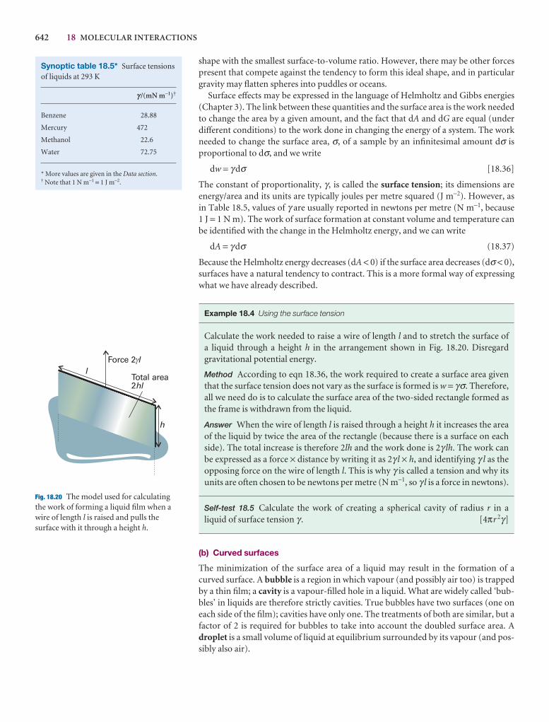
642 18 MOLECULAR INTERACTIONS
Synoptic table 18.5* Surface tensionsof liquids at 293 K
g /(mN m−1)†
Benzene 28.88
Mercury 472
Methanol 22.6
Water 72.75
* More values are given in the Data section.† Note that 1 N m−1 = 1 J m−2.
Force 2 ll
h
Total area2hl
�
Fig. 18.20 The model used for calculatingthe work of forming a liquid film when awire of length l is raised and pulls thesurface with it through a height h.
shape with the smallest surface-to-volume ratio. However, there may be other forcespresent that compete against the tendency to form this ideal shape, and in particulargravity may flatten spheres into puddles or oceans.
Surface effects may be expressed in the language of Helmholtz and Gibbs energies(Chapter 3). The link between these quantities and the surface area is the work neededto change the area by a given amount, and the fact that dA and dG are equal (underdifferent conditions) to the work done in changing the energy of a system. The workneeded to change the surface area, σ, of a sample by an infinitesimal amount dσ isproportional to dσ, and we write
dw = γ dσ [18.36]
The constant of proportionality, γ, is called the surface tension; its dimensions are energy/area and its units are typically joules per metre squared (J m−2). However, as in Table 18.5, values of γ are usually reported in newtons per metre (N m−1, because 1 J = 1 N m). The work of surface formation at constant volume and temperature canbe identified with the change in the Helmholtz energy, and we can write
dA = γ dσ (18.37)
Because the Helmholtz energy decreases (dA < 0) if the surface area decreases (dσ < 0),surfaces have a natural tendency to contract. This is a more formal way of expressingwhat we have already described.
Example 18.4 Using the surface tension
Calculate the work needed to raise a wire of length l and to stretch the surface of a liquid through a height h in the arrangement shown in Fig. 18.20. Disregard gravitational potential energy.
Method According to eqn 18.36, the work required to create a surface area giventhat the surface tension does not vary as the surface is formed is w = γσ. Therefore,all we need do is to calculate the surface area of the two-sided rectangle formed asthe frame is withdrawn from the liquid.
Answer When the wire of length l is raised through a height h it increases the areaof the liquid by twice the area of the rectangle (because there is a surface on eachside). The total increase is therefore 2lh and the work done is 2γ lh. The work can be expressed as a force × distance by writing it as 2γ l × h, and identifying γ l as theopposing force on the wire of length l. This is why γ is called a tension and why itsunits are often chosen to be newtons per metre (N m−1, so γ l is a force in newtons).
Self-test 18.5 Calculate the work of creating a spherical cavity of radius r in a liquid of surface tension γ . [4πr 2γ]
(b) Curved surfaces
The minimization of the surface area of a liquid may result in the formation of acurved surface. A bubble is a region in which vapour (and possibly air too) is trappedby a thin film; a cavity is a vapour-filled hole in a liquid. What are widely called ‘bub-bles’ in liquids are therefore strictly cavities. True bubbles have two surfaces (one oneach side of the film); cavities have only one. The treatments of both are similar, but afactor of 2 is required for bubbles to take into account the doubled surface area. Adroplet is a small volume of liquid at equilibrium surrounded by its vapour (and pos-sibly also air).
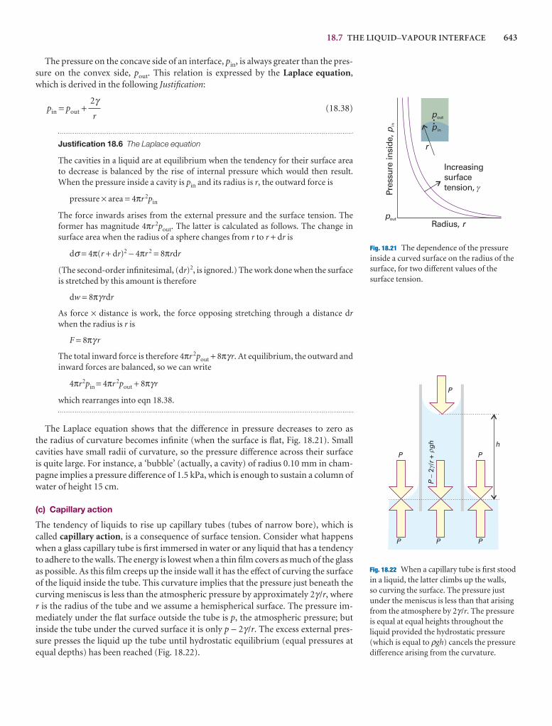
18.7 THE LIQUID–VAPOUR INTERFACE 643
The pressure on the concave side of an interface, pin, is always greater than the pres-sure on the convex side, pout. This relation is expressed by the Laplace equation,which is derived in the following Justification:
pin = pout + (18.38)
Justification 18.6 The Laplace equation
The cavities in a liquid are at equilibrium when the tendency for their surface areato decrease is balanced by the rise of internal pressure which would then result.When the pressure inside a cavity is pin and its radius is r, the outward force is
pressure × area = 4πr 2pin
The force inwards arises from the external pressure and the surface tension. The former has magnitude 4πr 2pout. The latter is calculated as follows. The change insurface area when the radius of a sphere changes from r to r + dr is
dσ = 4π(r + dr)2 − 4πr 2 = 8πrdr
(The second-order infinitesimal, (dr)2, is ignored.) The work done when the surfaceis stretched by this amount is therefore
dw = 8πγrdr
As force × distance is work, the force opposing stretching through a distance drwhen the radius is r is
F = 8πγ r
The total inward force is therefore 4πr 2pout + 8πγr. At equilibrium, the outward andinward forces are balanced, so we can write
4πr2pin = 4πr 2pout + 8πγr
which rearranges into eqn 18.38.
The Laplace equation shows that the difference in pressure decreases to zero as the radius of curvature becomes infinite (when the surface is flat, Fig. 18.21). Smallcavities have small radii of curvature, so the pressure difference across their surface is quite large. For instance, a ‘bubble’ (actually, a cavity) of radius 0.10 mm in cham-pagne implies a pressure difference of 1.5 kPa, which is enough to sustain a column ofwater of height 15 cm.
(c) Capillary action
The tendency of liquids to rise up capillary tubes (tubes of narrow bore), which iscalled capillary action, is a consequence of surface tension. Consider what happenswhen a glass capillary tube is first immersed in water or any liquid that has a tendencyto adhere to the walls. The energy is lowest when a thin film covers as much of the glassas possible. As this film creeps up the inside wall it has the effect of curving the surfaceof the liquid inside the tube. This curvature implies that the pressure just beneath thecurving meniscus is less than the atmospheric pressure by approximately 2γ /r, wherer is the radius of the tube and we assume a hemispherical surface. The pressure im-mediately under the flat surface outside the tube is p, the atmospheric pressure; but inside the tube under the curved surface it is only p − 2γ /r. The excess external pres-sure presses the liquid up the tube until hydrostatic equilibrium (equal pressures atequal depths) has been reached (Fig. 18.22).
2γr
Pres
sure
insi
de, p
in
Radius, r
r
pin
pout
pout
Increasingsurfacetension, �
Fig. 18.21 The dependence of the pressureinside a curved surface on the radius of thesurface, for two different values of thesurface tension.
P
P
P
PPP
Pr
gh�
2/
+
h
��
Fig. 18.22 When a capillary tube is first stoodin a liquid, the latter climbs up the walls, so curving the surface. The pressure justunder the meniscus is less than that arisingfrom the atmosphere by 2γ /r. The pressureis equal at equal heights throughout theliquid provided the hydrostatic pressure(which is equal to ρgh) cancels the pressuredifference arising from the curvature.
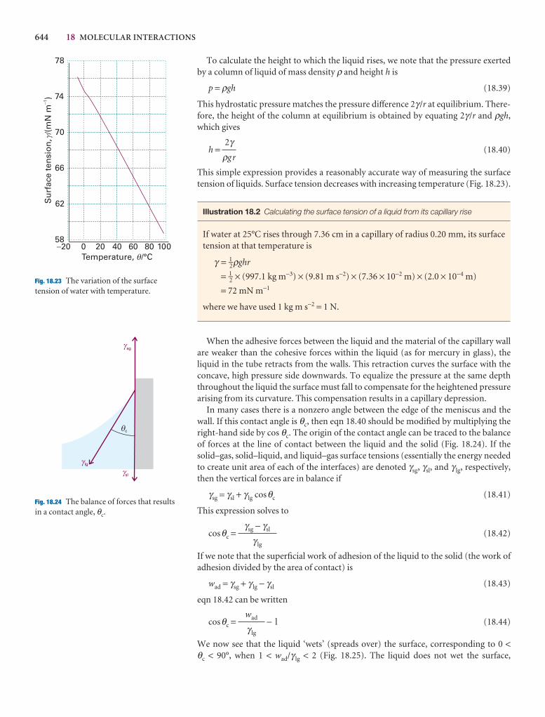
644 18 MOLECULAR INTERACTIONS
�20 0 20 40 60 80 10058
62
66
70
74
78
Temperature, /°C
Su
rfac
e te
nsi
on
, /(
mN
m)
�1
�
�
Fig. 18.23 The variation of the surfacetension of water with temperature.
lg
sl
sg
c
�
�
�
�
Fig. 18.24 The balance of forces that resultsin a contact angle, θc.
To calculate the height to which the liquid rises, we note that the pressure exertedby a column of liquid of mass density ρ and height h is
p = ρgh (18.39)
This hydrostatic pressure matches the pressure difference 2γ /r at equilibrium. There-fore, the height of the column at equilibrium is obtained by equating 2γ /r and ρgh,which gives
h = (18.40)
This simple expression provides a reasonably accurate way of measuring the surfacetension of liquids. Surface tension decreases with increasing temperature (Fig. 18.23).
Illustration 18.2 Calculating the surface tension of a liquid from its capillary rise
If water at 25°C rises through 7.36 cm in a capillary of radius 0.20 mm, its surfacetension at that temperature is
γ = 1–2ρghr
= 1–2 × (997.1 kg m−3) × (9.81 m s−2) × (7.36 × 10−2 m) × (2.0 × 10⁻⁴ m)
= 72 mN m−1
where we have used 1 kg m s−2 = 1 N.
When the adhesive forces between the liquid and the material of the capillary wallare weaker than the cohesive forces within the liquid (as for mercury in glass), the liquid in the tube retracts from the walls. This retraction curves the surface with the concave, high pressure side downwards. To equalize the pressure at the same depththroughout the liquid the surface must fall to compensate for the heightened pressurearising from its curvature. This compensation results in a capillary depression.
In many cases there is a nonzero angle between the edge of the meniscus and thewall. If this contact angle is θc, then eqn 18.40 should be modified by multiplying theright-hand side by cos θc. The origin of the contact angle can be traced to the balanceof forces at the line of contact between the liquid and the solid (Fig. 18.24). If thesolid–gas, solid–liquid, and liquid–gas surface tensions (essentially the energy neededto create unit area of each of the interfaces) are denoted γsg, γsl, and γ lg, respectively,then the vertical forces are in balance if
γsg = γsl + γ lg cosθc (18.41)
This expression solves to
cosθc = (18.42)
If we note that the superficial work of adhesion of the liquid to the solid (the work ofadhesion divided by the area of contact) is
wad = γsg + γ lg − γsl (18.43)
eqn 18.42 can be written
cosθc = − l (18.44)
We now see that the liquid ‘wets’ (spreads over) the surface, corresponding to 0 <θc < 90°, when 1 < wad/γ lg < 2 (Fig. 18.25). The liquid does not wet the surface,
wad
γ lg
γsg − γsl
γ lg
2γρgr
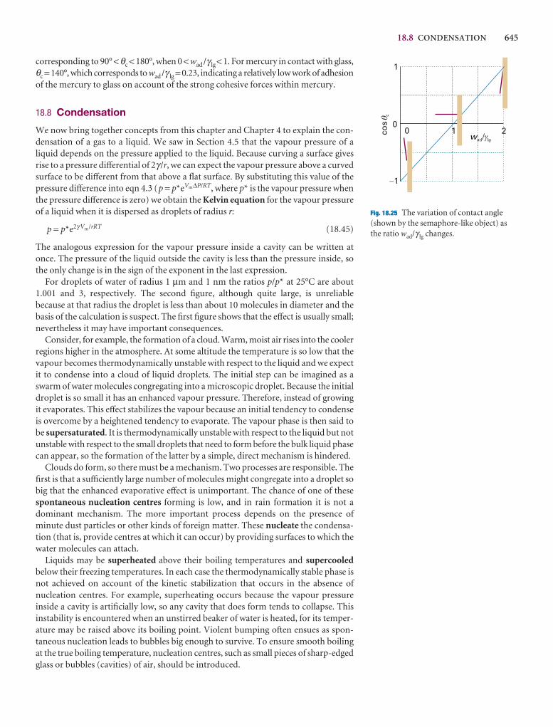
18.8 CONDENSATION 645
corresponding to 90° < θc < 180°, when 0 < wad/γ lg< 1. For mercury in contact with glass,θc = 140°, which corresponds to wad/γ lg = 0.23, indicating a relatively low work of adhesionof the mercury to glass on account of the strong cohesive forces within mercury.
18.8 Condensation
We now bring together concepts from this chapter and Chapter 4 to explain the con-densation of a gas to a liquid. We saw in Section 4.5 that the vapour pressure of a liquid depends on the pressure applied to the liquid. Because curving a surface givesrise to a pressure differential of 2γ /r, we can expect the vapour pressure above a curvedsurface to be different from that above a flat surface. By substituting this value of thepressure difference into eqn 4.3 (p = p*eVm∆P/RT, where p* is the vapour pressure whenthe pressure difference is zero) we obtain the Kelvin equation for the vapour pressureof a liquid when it is dispersed as droplets of radius r:
p = p*e2γ Vm/rRT (18.45)
The analogous expression for the vapour pressure inside a cavity can be written atonce. The pressure of the liquid outside the cavity is less than the pressure inside, sothe only change is in the sign of the exponent in the last expression.
For droplets of water of radius 1 µm and 1 nm the ratios p/p* at 25°C are about1.001 and 3, respectively. The second figure, although quite large, is unreliable because at that radius the droplet is less than about 10 molecules in diameter and thebasis of the calculation is suspect. The first figure shows that the effect is usually small;nevertheless it may have important consequences.
Consider, for example, the formation of a cloud. Warm, moist air rises into the coolerregions higher in the atmosphere. At some altitude the temperature is so low that thevapour becomes thermodynamically unstable with respect to the liquid and we expectit to condense into a cloud of liquid droplets. The initial step can be imagined as aswarm of water molecules congregating into a microscopic droplet. Because the initialdroplet is so small it has an enhanced vapour pressure. Therefore, instead of growingit evaporates. This effect stabilizes the vapour because an initial tendency to condenseis overcome by a heightened tendency to evaporate. The vapour phase is then said tobe supersaturated. It is thermodynamically unstable with respect to the liquid but notunstable with respect to the small droplets that need to form before the bulk liquid phasecan appear, so the formation of the latter by a simple, direct mechanism is hindered.
Clouds do form, so there must be a mechanism. Two processes are responsible. Thefirst is that a sufficiently large number of molecules might congregate into a droplet sobig that the enhanced evaporative effect is unimportant. The chance of one of thesespontaneous nucleation centres forming is low, and in rain formation it is not adominant mechanism. The more important process depends on the presence ofminute dust particles or other kinds of foreign matter. These nucleate the condensa-tion (that is, provide centres at which it can occur) by providing surfaces to which thewater molecules can attach.
Liquids may be superheated above their boiling temperatures and supercooledbelow their freezing temperatures. In each case the thermodynamically stable phase isnot achieved on account of the kinetic stabilization that occurs in the absence of nucleation centres. For example, superheating occurs because the vapour pressure inside a cavity is artificially low, so any cavity that does form tends to collapse. This instability is encountered when an unstirred beaker of water is heated, for its temper-ature may be raised above its boiling point. Violent bumping often ensues as spon-taneous nucleation leads to bubbles big enough to survive. To ensure smooth boilingat the true boiling temperature, nucleation centres, such as small pieces of sharp-edgedglass or bubbles (cavities) of air, should be introduced.
wad lg/0 1 2co
sc
0
1
-1
q
g
Fig. 18.25 The variation of contact angle(shown by the semaphore-like object) asthe ratio wad/γ lg changes.

646 18 MOLECULAR INTERACTIONS
Checklist of key ideas
1. A polar molecule is a molecule with a permanent electricdipole moment; the magnitude of a dipole moment is theproduct of the partial charge and the separation.
2. The polarization is the electric dipole moment density, P = �µ �N . Orientation polarization is the polarization arisingfrom the permanent dipole moments. Distortion polarizationis the polarization arising from the distortion of the positionsof the nuclei by the applied field.
3. The polarizability is a measure of the ability of an electric fieldto induce a dipole moment in a molecule (µ = αE). Electronicpolarizability is the polarizability due to the distortion of theelectron distribution.
4. The permittivity is the quantity ε in the Coulomb potentialenergy, V = q1q2/4πεr.
5. The relative permittivity is given by εr = ε /ε0 and may becalculated from electric properties by using the Debyeequation (eqn 18.14) or the Clausius–Mossotti equation (eqn 18.16).
6. A van der Waals interaction between closed-shell molecules isinversely proportional to the sixth power of their separation.
7. The potential energy of the dipole–dipole interaction betweentwo fixed (non-rotating) molecules is proportional to µ1µ2/r 3
and that between molecules that are free to rotate isproportional to µ1
2µ22/kTr 6.
8. The dipole–induced-dipole interaction between two moleculesis proportional to µ1
2α2/r 6, where α is the polarizability.
9. The potential energy of the dispersion (or London)interaction is proportional to α1α2/r 6.
10. A hydrogen bond is an interaction of the form A-H···B,where A and B are N, O, or F.
11. A hydrophobic interaction is an interaction that favoursformation of clusters of hydrophobic groups in aqueousenvironments and that stems from changes in entropy ofwater molecules.
12. The Lennard-Jones (12,6) potential, V = 4ε{(r0 /r)12 −(r0 /r)6},is a model of the total intermolecular potential energy.
13. A molecular beam is a collimated, narrow stream of moleculestravelling though an evacuated vessel. Molecular beamtechniques are used to investigate molecular interactions ingases.
14. The work of forming a liquid surface is dw = γ dσ, where γ isthe surface tension.
15. The Laplace equation for the vapour pressure at a curvedsurface is pin = pout + 2γ /r.
16. The Kelvin equation for the vapour pressure of droplets is p = p*e2γ Vm/rRT.
17. Capillary action is the tendency of liquids to rise up capillarytubes.
18. Nucleation provides surfaces to which molecules can attachand thereby induce condensation.
Further reading
Articles and texts
P.W. Atkins and R.S. Friedman, Molecular quantum mechanics.Oxford University Press (2005).
M.A.D. Fluendy and K.P. Lawley, Chemical applications of molecularbeam scattering. Chapman and Hall, London (1973).
J.N. Israelachvili, Intermolecular and surface forces. Academic Press,New York (1998).
G.A. Jeffrey, An introduction to hydrogen bonding. Oxford UniversityPress (1997).
H.-J. Schneider and A. Yatsimirsky, Principles and methods insupramolecular chemistry. Wiley, Chichester (1999).
Sources of data and information
J.J. Jasper, The surface tension of pure liquid compounds. J. Phys.Chem. Ref. Data 1, 841 (1972).
D.R. Lide (ed.), CRC Handbook of Chemistry and Physics, Sections 3,4, 6, 9, 10, 12, and 13. CRC Press, Boca Raton (2000).
Further information
Further information 18.1 The dipole–dipole interaction
An important problem in physical chemistry is the calculation of thepotential energy of interaction between two point dipoles withmoments m1 and m2, separated by a vector r. From classical
electromagnetic theory, the potential energy of m2 in the electric field/ 1 generated by m1 is given by the dot (scalar) product
V = −/ 1 · m2 (18.46)
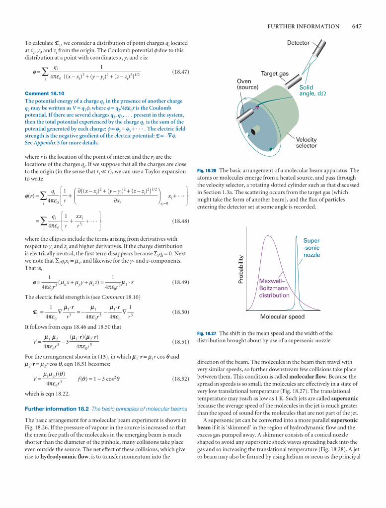
FURTHER INFORMATION 647
To calculate / 1, we consider a distribution of point charges qi locatedat xi, yi, and zi from the origin. The Coulomb potential φ due to thisdistribution at a point with coordinates x, y, and z is:
φ = ∑i
(18.47)
Comment 18.10
The potential energy of a charge q1 in the presence of another charge q2 may be written as V = q1φ, where φ = q2/4pe0r is the Coulombpotential. If there are several charges q2, q3, . . . present in the system,then the total potential experienced by the charge q1 is the sum of thepotential generated by each charge: φ = φ2 + φ3 + · · · . The electric fieldstrength is the negative gradient of the electric potential: / = −—φ.See Appendix 3 for more details.
where r is the location of the point of interest and the ri are thelocations of the charges qi. If we suppose that all the charges are closeto the origin (in the sense that ri << r), we can use a Taylor expansionto write
φ(r) = ∑i
+xi=0
xi + · · ·
= ∑i
+ + · · · (18.48)
where the ellipses include the terms arising from derivatives withrespect to yi and zi and higher derivatives. If the charge distribution is electrically neutral, the first term disappears because Σi qi = 0. Nextwe note that ∑i qixi = µx, and likewise for the y- and z-components.That is,
φ = (µx x + µy y + µz z) = m1 · r (18.49)
The electric field strength is (see Comment 18.10)
/ 1 = ∇ = − − ∇ (18.50)
It follows from eqns 18.46 and 18.50 that
V = − 3 (18.51)
For the arrangement shown in (13), in which m1·r = µ1r cos θ andm2·r = µ2r cos θ, eqn 18.51 becomes:
V = f(θ) = 1 − 3 cos2θ (18.52)
which is eqn 18.22.
Further information 18.2 The basic principles of molecular beams
The basic arrangement for a molecular beam experiment is shown inFig. 18.26. If the pressure of vapour in the source is increased so thatthe mean free path of the molecules in the emerging beam is muchshorter than the diameter of the pinhole, many collisions take placeeven outside the source. The net effect of these collisions, which giverise to hydrodynamic flow, is to transfer momentum into the
µ1µ2 f(θ)
4πε0r 3
(m1·r)(m2·r)
4πε0r 5
m1·m2
4πε0r 3
1
r 3
m1·r
4πε0
m1
4πε0r 3
m1·r
r 3
1
4πε0
1
4πε0r 3
1
4πε0r 3
567
xxi
r 3
1
r
123
qi
4πε0
567
DEF∂{(x − xi)
2 + (y − yi)2 + (z − zi)
2}1/2
∂xi
ABC1
r
123
qi
4πε0
1
{(x − xi)2 + (y − yi)
2 + (z − zi)2}1/2
qi
4πε0
direction of the beam. The molecules in the beam then travel withvery similar speeds, so further downstream few collisions take placebetween them. This condition is called molecular flow. Because thespread in speeds is so small, the molecules are effectively in a state ofvery low translational temperature (Fig. 18.27). The translationaltemperature may reach as low as 1 K. Such jets are called supersonicbecause the average speed of the molecules in the jet is much greaterthan the speed of sound for the molecules that are not part of the jet.
A supersonic jet can be converted into a more parallel supersonicbeam if it is ‘skimmed’ in the region of hydrodynamic flow and theexcess gas pumped away. A skimmer consists of a conical nozzleshaped to avoid any supersonic shock waves spreading back into thegas and so increasing the translational temperature (Fig. 18.28). A jetor beam may also be formed by using helium or neon as the principal
Solidangle, d
Detector
Target gas
Velocityselector
Oven(source)
)
Fig. 18.26 The basic arrangement of a molecular beam apparatus. Theatoms or molecules emerge from a heated source, and pass throughthe velocity selector, a rotating slotted cylinder such as that discussedin Section 1.3a. The scattering occurs from the target gas (whichmight take the form of another beam), and the flux of particlesentering the detector set at some angle is recorded.
Molecular speed
Prob
abili
ty
Maxwell–Boltzmanndistribution
Super-sonicnozzle
Fig. 18.27 The shift in the mean speed and the width of thedistribution brought about by use of a supersonic nozzle.

648 18 MOLECULAR INTERACTIONS
gas, and injecting molecules of interest into it in the hydrodynamicregion of flow.
The low translational temperature of the molecules is reflected inthe low rotational and vibrational temperatures of the molecules. In
this context, a rotational or vibrational temperature means thetemperature that should be used in the Boltzmann distribution toreproduce the observed populations of the states. However, asrotational modes equilibrate more slowly, and vibrational modesequilibrate even more slowly, the rotational and vibrational populationsof the species correspond to somewhat higher temperatures, of theorder of 10 K for rotation and 100 K for vibrations.
The target gas may be either a bulk sample or another molecularbeam. The latter crossed beam technique gives a lot of informationbecause the states of both the target and projectile molecules may becontrolled. The intensity of the incident beam is measured by theincident beam flux, I, which is the number of particles passingthrough a given area in a given interval divided by the area and theduration of the interval.
The detectors may consist of a chamber fitted with a sensitivepressure gauge, a bolometer (a detector that responds to the incidentenergy by making use of the temperature-dependence of resistance),or an ionization detector, in which the incoming molecule is firstionized and then detected electronically. The state of the scatteredmolecules may also be determined spectroscopically, and is of interestwhen the collisions change their vibrational or rotational states.
Oven
Gasflow
Skimmer
Collimator
Pinhole
Fig. 18.28 A supersonic nozzle skims off some of the molecules of thebeam and leads to a beam with well defined velocity.
Discussion questions
18.1 Explain how the permanent dipole moment and the polarizability of amolecule arise.
18.2 Explain why the polarizability of a molecule decreases at highfrequencies.
18.3 Describe the experimental procedures available for determining theelectric dipole moment of a molecule.
18.4 Account for the theoretical conclusion that many attractive interactionsbetween molecules vary with their separation as 1/r 6.
18.5 Describe the formation of a hydrogen bond in terms of molecular orbitals.
18.6 Account for the hydrophobic interaction and discuss its manifestations.
18.7 Describe how molecular beams are used to investigate intermolecularpotentials.
Exercises
18.1a Which of the following molecules may be polar: CIF3, O3, H2O2?
18.1b Which of the following molecules may be polar: SO3, XeF4, SF4?
18.2a The electric dipole moment of toluene (methylbenzene) is 0.4 D.Estimate the dipole moments of the three xylenes (dimethylbenzene). Whichanswer can you be sure about?
18.2b Calculate the resultant of two dipole moments of magnitude 1.5 D and0.80 D that make an angle of 109.5° to each other.
18.3a Calculate the magnitude and direction of the dipole moment of thefollowing arrangement of charges in the xy-plane: 3e at (0,0), −e at (0.32 nm,0), and −2e at an angle of 20° from the x-axis and a distance of 0.23 nm fromthe origin.
18.3b Calculate the magnitude and direction of the dipole moment of thefollowing arrangement of charges in the xy-plane: 4e at (0, 0), −2e at (162 pm,0), and −2e at an angle of 30° from the x-axis and a distance of 143 pm fromthe origin.
18.4a The molar polarization of fluorobenzene vapour varies linearly with T −1, and is 70.62 cm3 mol−1 at 351.0 K and 62.47 cm3 mol−1 at 423.2 K.Calculate the polarizability and dipole moment of the molecule.
18.4b The molar polarization of the vapour of a compound was found to varylinearly with T−1, and is 75.74 cm3 mol−1 at 320.0 K and 71.43 cm3 mol−1 at421.7 K. Calculate the polarizability and dipole moment of the molecule.
18.5a At 0°C, the molar polarization of liquid chlorine trifluoride is 27.18 cm3 mol−1 and its density is 1.89 g cm−3. Calculate the relativepermittivity of the liquid.
18.5b At 0°C, the molar polarization of a liquid is 32.l6 cm3 mol−1 and itsdensity is 1.92 g cm−3. Calculate the relative permittivity of the liquid. Take M = 55.0 g mol−1.
18.6a The polarizability volume of H2O is 1.48 × 10⁻²⁴ cm3; calculate thedipole moment of the molecule (in addition to the permanent dipolemoment) induced by an applied electric field of strength 1.0 kV cm−1.
18.6b The polarizability volume of NH3 is 2.22 × 10⁻³⁰ m3; calculate thedipole moment of the molecule (in addition to the permanent dipolemoment) induced by an applied electric field of strength 15.0 kV m−1.
18.7a The refractive index of CH2I2 is 1.732 for 656 nm light. Its density at20°C is 3.32 g cm−3. Calculate the polarizability of the molecule at thiswavelength.
PROBLEMS 649
18.7b The refractive index of a compound is 1.622 for 643 nm light. Itsdensity at 20°C is 2.99 g cm−3. Calculate the polarizability of the molecule atthis wavelength. Take M = 65.5 g mol−1.
18.8a The polarizability volume of H2O at optical frequencies is 1.5 × 10⁻²⁴ cm3:estimate the refractive index of water. The experimental value is 1.33; whatmay be the origin of the discrepancy?
18.8b The polarizability volume of a liquid of molar mass 72.3 g mol−1 anddensity 865 kg mol−1 at optical frequencies is 2.2 × 10⁻³⁰ m3: estimate therefractive index of the liquid.
18.9a The dipole moment of chlorobenzene is 1.57 D and its polarizabilityvolume is 1.23 × 10⁻²³ cm3. Estimate its relative permittivity at 25°C, when itsdensity is 1.173 g cm−3.
18.9b The dipole moment of bromobenzene is 5. 17 × 10−30 C m and itspolarizability volume is approximately 1.5 × 10⁻²⁹ m3. Estimate its relativepermittivity at 25°C, when its density is 1491 kg m−3.
18.10a Calculate the vapour pressure of a spherical droplet of water of radius10 nm at 20°C. The vapour pressure of bulk water at that temperature is 2.3 kPa and its density is 0.9982 g cm−3.
18.10b Calculate the vapour pressure of a spherical droplet of water of radius20.0 nm at 35.0°C. The vapour pressure of bulk water at that temperature is5.623 kPa and its density is 994.0 kg m−3.
18.11a The contact angle for water on clean glass is close to zero. Calculatethe surface tension of water at 20°C given that at that temperature waterclimbs to a height of 4.96 cm in a clean glass capillary tube of internal radius0.300 mm. The density of water at 20°C is 998.2 kg m−3.
18.11b The contact angle for water on clean glass is close to zero. Calculatethe surface tension of water at 30°C given that at that temperature waterclimbs to a height of 9.11 cm in a clean glass capillary tube of internal radius0.320 mm. The density of water at 30°C is 0.9956 g cm−3.
18.12a Calculate the pressure differential of water across the surface of aspherical droplet of radius 200 nm at 20°C.
18.12b Calculate the pressure differential of ethanol across the surface of aspherical droplet of radius 220 nm at 20°C. The surface tension of ethanol atthat temperature is 22.39 mN m−1.
Problems*
Numerical problems
18.1 Suppose an H2O molecule (µ = 1.85 D) approaches an anion. What isthe favourable orientation of the molecule? Calculate the electric field (in voltsper metre) experienced by the anion when the water dipole is (a) 1.0 nm, (b) 0.3 nm, (c) 30 nm from the ion.
18.2 An H2O molecule is aligned by an external electric field of strength 1.0 kV m−1 and an Ar atom (α′ = 1.66 × 10⁻²⁴ cm3) is brought up slowly fromone side. At what separation is it energetically favourable for the H2Omolecule to flip over and point towards the approaching Ar atom?
18.3 The relative permittivity of chloroform was measured over a range oftemperatures with the following results:
θ /°C −80 −70 −60 −40 −20 0 20
εr 3.1 3.1 7.0 6.5 6.0 5.5 5.0
ρ/(g cm−3) 1.65 1.64 1.64 1.61 1.57 1.53 1.50
The freezing point of chloroform is −64°C. Account for these results andcalculate the dipole moment and polarizability volume of the molecule.
18.4 The relative permittivities of methanol (m.p. −95°C) corrected for density
variation are given below. What molecular information can be deduced from these
values? Take ρ = 0.791 g cm−3 at 20°C.
θ /°C −185 −170 −150 −140 −110 −80 −50 −20 0 20
ε r 3.2 3.6 4.0 5.1 67 57 4 43 38 34
18.5 In his classic book Polar molecules, Debye reports some earlymeasurements of the polarizability of ammonia. From the selection below,determine the dipole moment and the polarizability volume of the molecule.
T /K 292.2 309.0 333.0 387.0 413.0 446.0
Pm /(cm3 mol−1) 57.57 55.01 51.22 44.99 42.51 39.59
The refractive index of ammonia at 273 K and 100 kPa is 1.000 379 (for yellowsodium light). Calculate the molar polarizability of the gas at this temperature
and at 292.2 K. Combine the value calculated with the static molarpolarizability at 292.2 K and deduce from this information alone themolecular dipole moment.
18.6 Values of the molar polarization of gaseous water at 100 kPa asdetermined from capacitance measurements are given below as a function oftemperature.
T/K 384.3 420.1 444.7 484.1 522.0
Pm /(cm3 mol−1) 57.4 53.5 50.1 46.8 43.1
Calculate the dipole moment of H2O and its polarizability volume.
18.7‡ F. Luo, G.C. MeBane, O. Kim, C.F. Giese, and W.R. Gentry (J. Chem.Phys. 98, 3564 (1993)) reported experimental observation of the He2 complex,a species that had escaped detection for a long time. The fact that theobservation required temperatures in the neighbourhood of 1 mK isconsistent with computational studies which suggest that hcDe, for He2 isabout 1.51 × 10⁻²³ J, hcD0 about 2 × 10⁻²⁶ J, and R about 297 pm. (a)Determine the Lennard-Jones parameters r0, and ε and plot the Lennard-Jones potential for He–He interactions. (b) Plot the Morse potential given thata = 5.79 × 10¹⁰ m−1.
18.8‡ D.D. Nelson, G.T. Fraser, and W. Klemperer (Science 238, 1670 (1987))examined several weakly bound gas-phase complexes of ammonia in search of examples in which the H atoms in NH3 formed hydrogen bonds, but foundnone. For example, they found that the complex of NH3 and CO2 has thecarbon atom nearest the nitrogen (299 pm away): the CO2 molecule is at rightangles to the C-N ‘bond’, and the H atoms of NH3 are pointing away fromthe CO2. The permanent dipole moment of this complex is reported as 1.77 D. If the N and C atoms are the centres of the negative and positivecharge distributions, respectively, what is the magnitude of those partialcharges (as multiples of e)?
18.9‡ From data in Table 18.1 calculate the molar polarization, relativepermittivity, and refractive index of methanol at 20°C. Its density at thattemperature is 0.7914 g cm−3.
* Problems denoted with the symbol‡ were supplied by Charles Trapp and Carmen Giunta.
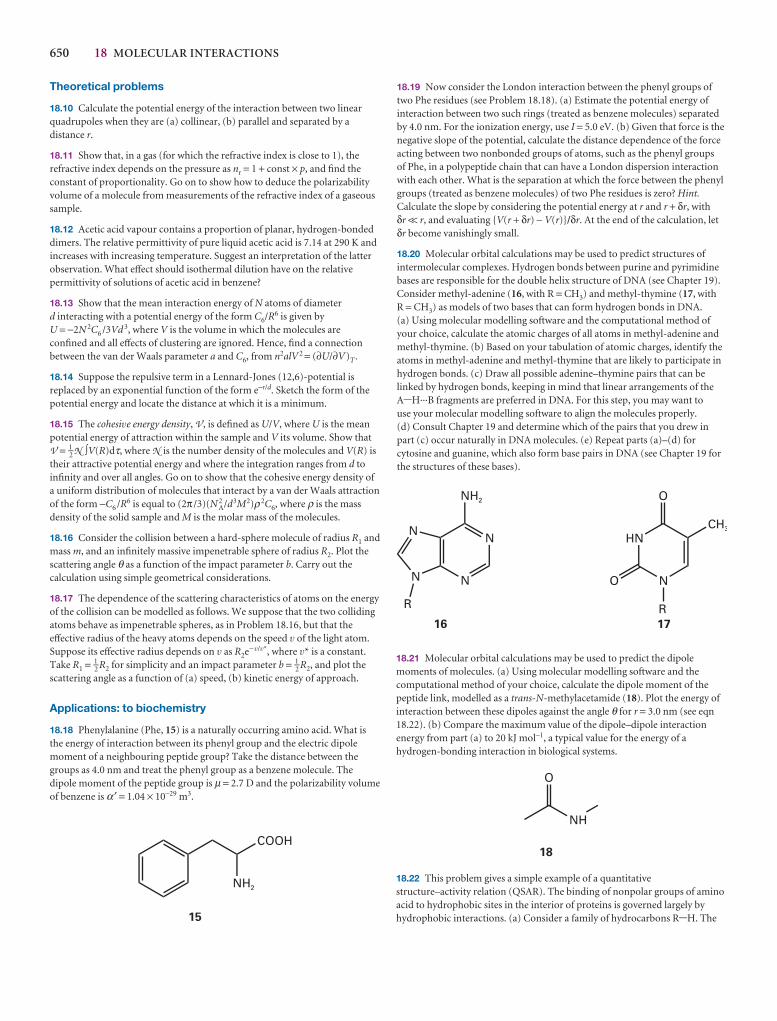
650 18 MOLECULAR INTERACTIONS
Theoretical problems
18.10 Calculate the potential energy of the interaction between two linearquadrupoles when they are (a) collinear, (b) parallel and separated by adistance r.
18.11 Show that, in a gas (for which the refractive index is close to 1), therefractive index depends on the pressure as nr = 1 + const × p, and find theconstant of proportionality. Go on to show how to deduce the polarizabilityvolume of a molecule from measurements of the refractive index of a gaseoussample.
18.12 Acetic acid vapour contains a proportion of planar, hydrogen-bondeddimers. The relative permittivity of pure liquid acetic acid is 7.14 at 290 K andincreases with increasing temperature. Suggest an interpretation of the latterobservation. What effect should isothermal dilution have on the relativepermittivity of solutions of acetic acid in benzene?
18.13 Show that the mean interaction energy of N atoms of diameter d interacting with a potential energy of the form C6/R6 is given by U = −2N 2C6 /3Vd 3, where V is the volume in which the molecules are confined and all effects of clustering are ignored. Hence, find a connectionbetween the van der Waals parameter a and C6, from n2alV 2 = (∂U/∂V)T .
18.14 Suppose the repulsive term in a Lennard-Jones (12,6)-potential isreplaced by an exponential function of the form e−r/d. Sketch the form of thepotential energy and locate the distance at which it is a minimum.
18.15 The cohesive energy density, V , is defined as U/V, where U is the meanpotential energy of attraction within the sample and V its volume. Show that V = 1–
2 N ∫V(R)dτ, where N is the number density of the molecules and V(R) istheir attractive potential energy and where the integration ranges from d toinfinity and over all angles. Go on to show that the cohesive energy density ofa uniform distribution of molecules that interact by a van der Waals attractionof the form −C6 /R6 is equal to (2π /3)(N A
2 /d3M2)ρ2C6, where ρ is the massdensity of the solid sample and M is the molar mass of the molecules.
18.16 Consider the collision between a hard-sphere molecule of radius R1 andmass m, and an infinitely massive impenetrable sphere of radius R2. Plot thescattering angle θ as a function of the impact parameter b. Carry out thecalculation using simple geometrical considerations.
18.17 The dependence of the scattering characteristics of atoms on the energyof the collision can be modelled as follows. We suppose that the two collidingatoms behave as impenetrable spheres, as in Problem 18.16, but that theeffective radius of the heavy atoms depends on the speed v of the light atom.Suppose its effective radius depends on v as R2e− v/v*, where v* is a constant.Take R1 = 1–
2 R2 for simplicity and an impact parameter b = 1–2 R2, and plot the
scattering angle as a function of (a) speed, (b) kinetic energy of approach.
Applications: to biochemistry
18.18 Phenylalanine (Phe, 15) is a naturally occurring amino acid. What isthe energy of interaction between its phenyl group and the electric dipolemoment of a neighbouring peptide group? Take the distance between thegroups as 4.0 nm and treat the phenyl group as a benzene molecule. Thedipole moment of the peptide group is µ = 2.7 D and the polarizability volumeof benzene is α′ = 1.04 × 10⁻²⁹ m3.
18.19 Now consider the London interaction between the phenyl groups oftwo Phe residues (see Problem 18.18). (a) Estimate the potential energy ofinteraction between two such rings (treated as benzene molecules) separatedby 4.0 nm. For the ionization energy, use I = 5.0 eV. (b) Given that force is thenegative slope of the potential, calculate the distance dependence of the forceacting between two nonbonded groups of atoms, such as the phenyl groups of Phe, in a polypeptide chain that can have a London dispersion interactionwith each other. What is the separation at which the force between the phenylgroups (treated as benzene molecules) of two Phe residues is zero? Hint.Calculate the slope by considering the potential energy at r and r + δr, with δr << r, and evaluating {V(r + δr) − V(r)}/δr. At the end of the calculation, letδr become vanishingly small.
18.20 Molecular orbital calculations may be used to predict structures ofintermolecular complexes. Hydrogen bonds between purine and pyrimidinebases are responsible for the double helix structure of DNA (see Chapter 19).Consider methyl-adenine (16, with R = CH3) and methyl-thymine (17, with R = CH3) as models of two bases that can form hydrogen bonds in DNA. (a) Using molecular modelling software and the computational method ofyour choice, calculate the atomic charges of all atoms in methyl-adenine andmethyl-thymine. (b) Based on your tabulation of atomic charges, identify theatoms in methyl-adenine and methyl-thymine that are likely to participate inhydrogen bonds. (c) Draw all possible adenine–thymine pairs that can belinked by hydrogen bonds, keeping in mind that linear arrangements of the A-H···B fragments are preferred in DNA. For this step, you may want to use your molecular modelling software to align the molecules properly. (d) Consult Chapter 19 and determine which of the pairs that you drew inpart (c) occur naturally in DNA molecules. (e) Repeat parts (a)–(d) forcytosine and guanine, which also form base pairs in DNA (see Chapter 19 forthe structures of these bases).
18.21 Molecular orbital calculations may be used to predict the dipolemoments of molecules. (a) Using molecular modelling software and thecomputational method of your choice, calculate the dipole moment of thepeptide link, modelled as a trans-N-methylacetamide (18). Plot the energy ofinteraction between these dipoles against the angle θ for r = 3.0 nm (see eqn18.22). (b) Compare the maximum value of the dipole–dipole interactionenergy from part (a) to 20 kJ mol−1, a typical value for the energy of ahydrogen-bonding interaction in biological systems.
18.22 This problem gives a simple example of a quantitativestructure–activity relation (QSAR). The binding of nonpolar groups of aminoacid to hydrophobic sites in the interior of proteins is governed largely byhydrophobic interactions. (a) Consider a family of hydrocarbons R-H. The
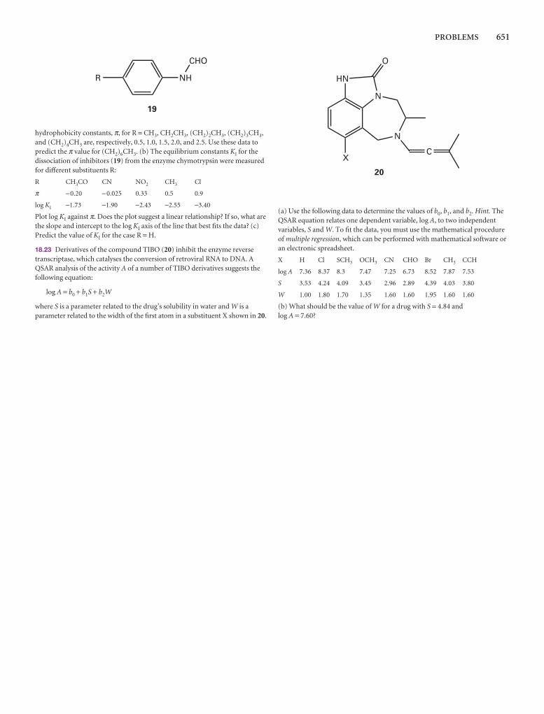
PROBLEMS 651
hydrophobicity constants, π, for R = CH3, CH2CH3, (CH2)2CH3, (CH2)3CH3,and (CH2)4CH3 are, respectively, 0.5, 1.0, 1.5, 2.0, and 2.5. Use these data topredict the π value for (CH2)6CH3. (b) The equilibrium constants KI for thedissociation of inhibitors (19) from the enzyme chymotrypsin were measuredfor different substituents R:
R CH3CO CN NO2 CH3 Cl
π −0.20 −0.025 0.33 0.5 0.9
log KI −1.73 −1.90 −2.43 −2.55 −3.40
Plot log KI against π. Does the plot suggest a linear relationship? If so, what arethe slope and intercept to the log KI axis of the line that best fits the data? (c)Predict the value of KI for the case R = H.
18.23 Derivatives of the compound TIBO (20) inhibit the enzyme reversetranscriptase, which catalyses the conversion of retroviral RNA to DNA. AQSAR analysis of the activity A of a number of TIBO derivatives suggests thefollowing equation:
log A = b0 + b1S + b2W
where S is a parameter related to the drug’s solubility in water and W is aparameter related to the width of the first atom in a substituent X shown in 20.
(a) Use the following data to determine the values of b0, b1, and b2. Hint. TheQSAR equation relates one dependent variable, log A, to two independentvariables, S and W. To fit the data, you must use the mathematical procedureof multiple regression, which can be performed with mathematical software oran electronic spreadsheet.
X H Cl SCH3 OCH3 CN CHO Br CH3 CCH
log A 7.36 8.37 8.3 7.47 7.25 6.73 8.52 7.87 7.53
S 3.53 4.24 4.09 3.45 2.96 2.89 4.39 4.03 3.80
W 1.00 1.80 1.70 1.35 1.60 1.60 1.95 1.60 1.60
(b) What should be the value of W for a drug with S = 4.84 and log A = 7.60?

Materials 1:macromolecules and aggregatesMacromolecules exhibit a range of properties and problems that illustrate a wide variety ofphysical chemical principles. They need to be characterized in terms of their molar mass,their size, and their shape. However, the molecules are so large and the solutions they formdepart so strongly from ideality, that techniques for accommodating these departures fromideality need to be developed. Another major problem concerns the influences that deter-mine the shapes of the molecules. We consider a range of influences in this chapter, begin-ning with a structureless random coil and ending with the structurally precise forces thatoperate in polypeptides and nucleic acids. Atoms, small molecules, and macromolecules canform large assemblies that are held together by one or more of the molecular interactionsdescribed in Chapter 18. These assemblies, which include colloids and biological membranes,exhibit some of the typical properties of molecules but have their own characteristic features.
There are macromolecules everywhere, inside us and outside us. Some are natural:they include polysaccharides such as cellulose, polypeptides such as protein enzymes,and polynucleotides such as deoxyribonucleic acid (DNA). Others are synthetic: theyinclude polymers such as nylon and polystyrene that are manufactured by stringingtogether and (in some cases) cross-linking smaller units known as monomers. Life inall its forms, from its intrinsic nature to its technological interaction with its environ-ment, is the chemistry of macromolecules.
Macromolecules give rise to special problems that include the shapes and the lengthsof polymer chains, the determination of their sizes, and the large deviations from ideality of their solutions. Natural macromolecules differ in certain respects from syn-thetic macromolecules, particularly in their composition and the resulting structure,but the two share a number of common properties. We concentrate on these commonproperties here. Another level of complexity arises when small molecules aggregateinto large particles in a process that is called ‘self-assembly’ and give rise to aggregates.One example is the assembly of haemoglobin from four myoglobin-like polypeptides.A similar type of aggregation gives rise to a variety of disperse phases, which includecolloids. The properties of these disperse phases resemble to a certain extent the prop-erties of solutions of macromolecules, and we describe their common attributes in thefinal part of this chapter.
Determination of size and shape
X-ray diffraction techniques (Chapter 20) can reveal the position of almost everyheavy atom (that is, every atom other than hydrogen) even in very large molecules.However, there are several reasons why other techniques must also be used. In the first
Determination of size and shape
19.1 Mean molar masses
19.2 Mass spectrometry
19.3 Laser light scattering
19.4 Ultracentrifugation
19.5 Electrophoresis
I19.1 Impact on biochemistry: Gelelectrophoresis in genomicsand proteomics
19.6 Viscosity
Structure and dynamics
19.7 The different levels ofstructure
19.8 Random coils
19.9 The structure and stability ofsynthetic polymers
I19.2 Impact on technology:Conducting polymers
19.10 The structure of proteins
19.11 The structure of nucleic acids
19.12 The stability of proteins andnucleic acids
Self-assembly
19.13 Colloids
19.14 Micelles and biologicalmembranes
19.15 Surface films
I19.3 Impact on nanoscience:Nanofabrication with self-assembled monolayers
Checklist of key ideas
Further reading
Further information 19.1: TheRayleigh ratio
Discussion questions
Exercises
Problems
19
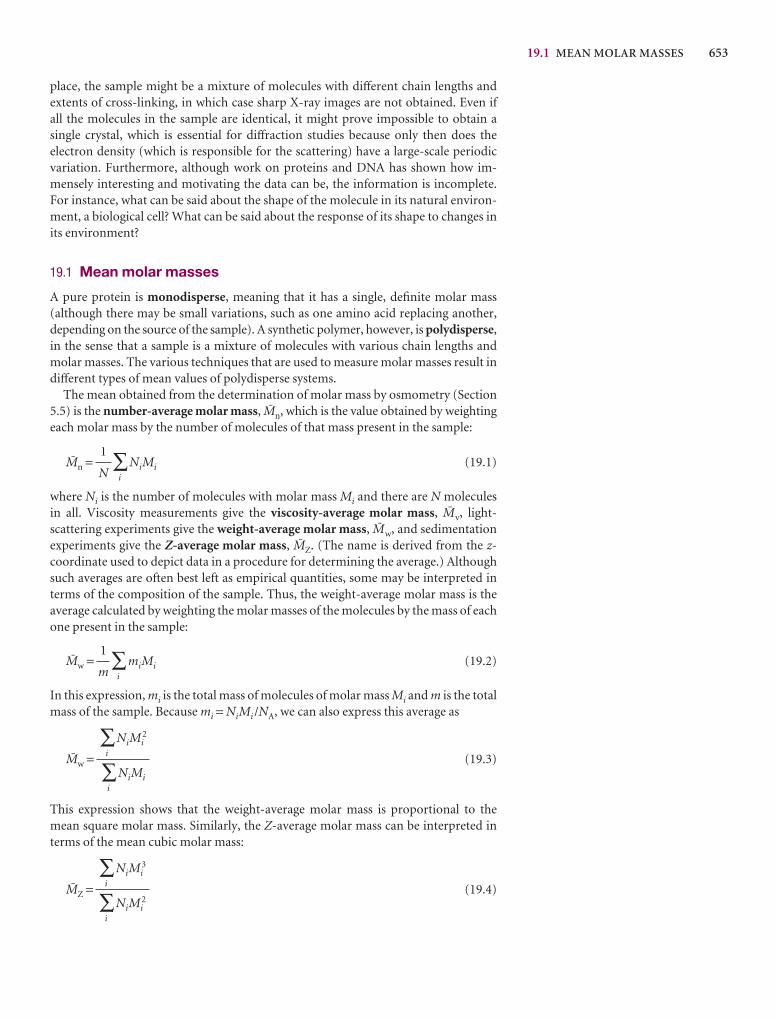
19.1 MEAN MOLAR MASSES 653
place, the sample might be a mixture of molecules with different chain lengths and extents of cross-linking, in which case sharp X-ray images are not obtained. Even if all the molecules in the sample are identical, it might prove impossible to obtain a single crystal, which is essential for diffraction studies because only then does the electron density (which is responsible for the scattering) have a large-scale periodicvariation. Furthermore, although work on proteins and DNA has shown how im-mensely interesting and motivating the data can be, the information is incomplete.For instance, what can be said about the shape of the molecule in its natural environ-ment, a biological cell? What can be said about the response of its shape to changes inits environment?
19.1 Mean molar masses
A pure protein is monodisperse, meaning that it has a single, definite molar mass (although there may be small variations, such as one amino acid replacing another,depending on the source of the sample). A synthetic polymer, however, is polydisperse,in the sense that a sample is a mixture of molecules with various chain lengths andmolar masses. The various techniques that are used to measure molar masses result indifferent types of mean values of polydisperse systems.
The mean obtained from the determination of molar mass by osmometry (Section5.5) is the number-average molar mass, Jn, which is the value obtained by weightingeach molar mass by the number of molecules of that mass present in the sample:
Jn = ∑i
NiMi (19.1)
where Ni is the number of molecules with molar mass Mi and there are N moleculesin all. Viscosity measurements give the viscosity-average molar mass, Jv, light-scattering experiments give the weight-average molar mass, Jw, and sedimentationexperiments give the Z-average molar mass, JZ. (The name is derived from the z-coordinate used to depict data in a procedure for determining the average.) Althoughsuch averages are often best left as empirical quantities, some may be interpreted interms of the composition of the sample. Thus, the weight-average molar mass is theaverage calculated by weighting the molar masses of the molecules by the mass of eachone present in the sample:
Jw = ∑i
miMi (19.2)
In this expression, mi is the total mass of molecules of molar mass Mi and m is the totalmass of the sample. Because mi = NiMi /NA, we can also express this average as
Jw = (19.3)
This expression shows that the weight-average molar mass is proportional to themean square molar mass. Similarly, the Z-average molar mass can be interpreted interms of the mean cubic molar mass:
JZ = (19.4)
∑i
NiMi3
∑i
NiMi2
∑i
NiMi2
∑i
NiMi
1
m
1
N
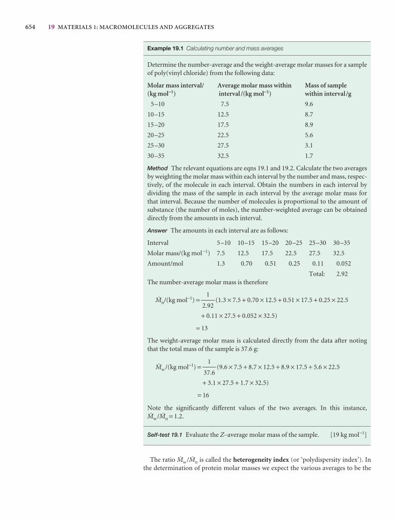
654 19 MATERIALS 1: MACROMOLECULES AND AGGREGATES
Example 19.1 Calculating number and mass averages
Determine the number-average and the weight-average molar masses for a sampleof poly(vinyl chloride) from the following data:
Molar mass interval/ Average molar mass within Mass of sample (kg mol−1) interval/(kg mol−1) within interval/g
5–10 7.5 9.6
10–15 12.5 8.7
15–20 17.5 8.9
20–25 22.5 5.6
25–30 27.5 3.1
30–35 32.5 1.7
Method The relevant equations are eqns 19.1 and 19.2. Calculate the two averagesby weighting the molar mass within each interval by the number and mass, respec-tively, of the molecule in each interval. Obtain the numbers in each interval by dividing the mass of the sample in each interval by the average molar mass for that interval. Because the number of molecules is proportional to the amount ofsubstance (the number of moles), the number-weighted average can be obtaineddirectly from the amounts in each interval.
Answer The amounts in each interval are as follows:
Interval 5–10 10–15 15–20 20–25 25–30 30–35
Molar mass/(kg mol−1) 7.5 12.5 17.5 22.5 27.5 32.5
Amount/mol 1.3 0.70 0.51 0.25 0.11 0.052
Total: 2.92The number-average molar mass is therefore
Jn/(kg mol−1) = (1.3 × 7.5 + 0.70 × 12.5 + 0.51 × 17.5 + 0.25 × 22.5
+ 0.11 × 27.5 + 0.052 × 32.5)
= 13
The weight-average molar mass is calculated directly from the data after notingthat the total mass of the sample is 37.6 g:
Jw /(kg mol−1) = (9.6 × 7.5 + 8.7 × 12.5 + 8.9 × 17.5 + 5.6 × 22.5
+ 3.1 × 27.5 + 1.7 × 32.5)
= 16
Note the significantly different values of the two averages. In this instance, Jw /Jn = 1.2.
Self-test 19.1 Evaluate the Z–average molar mass of the sample. [19 kg mol−1]
The ratio Jw /Jn is called the heterogeneity index (or ‘polydispersity index’). Inthe determination of protein molar masses we expect the various averages to be the
1
37.6
1
2.92
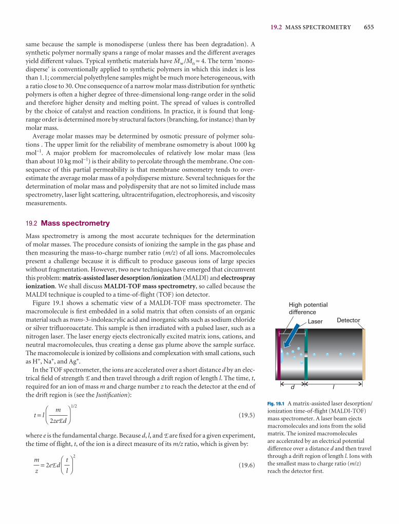
19.2 MASS SPECTROMETRY 655
same because the sample is monodisperse (unless there has been degradation). A synthetic polymer normally spans a range of molar masses and the different averagesyield different values. Typical synthetic materials have Jw /Jn ≈ 4. The term ‘mono-disperse’ is conventionally applied to synthetic polymers in which this index is lessthan 1.1; commercial polyethylene samples might be much more heterogeneous, witha ratio close to 30. One consequence of a narrow molar mass distribution for syntheticpolymers is often a higher degree of three-dimensional long-range order in the solidand therefore higher density and melting point. The spread of values is controlled by the choice of catalyst and reaction conditions. In practice, it is found that long-range order is determined more by structural factors (branching, for instance) than bymolar mass.
Average molar masses may be determined by osmotic pressure of polymer solu-tions . The upper limit for the reliability of membrane osmometry is about 1000 kgmol−1. A major problem for macromolecules of relatively low molar mass (less than about 10 kg mol−1) is their ability to percolate through the membrane. One con-sequence of this partial permeability is that membrane osmometry tends to over-estimate the average molar mass of a polydisperse mixture. Several techniques for thedetermination of molar mass and polydispersity that are not so limited include massspectrometry, laser light scattering, ultracentrifugation, electrophoresis, and viscositymeasurements.
19.2 Mass spectrometry
Mass spectrometry is among the most accurate techniques for the determination of molar masses. The procedure consists of ionizing the sample in the gas phase andthen measuring the mass-to-charge number ratio (m/z) of all ions. Macromoleculespresent a challenge because it is difficult to produce gaseous ions of large species without fragmentation. However, two new techniques have emerged that circumvent this problem: matrix-assisted laser desorption/ionization (MALDI) and electrosprayionization. We shall discuss MALDI-TOF mass spectrometry, so called because theMALDI technique is coupled to a time-of-flight (TOF) ion detector.
Figure 19.1 shows a schematic view of a MALDI-TOF mass spectrometer. Themacromolecule is first embedded in a solid matrix that often consists of an organicmaterial such as trans-3-indoleacrylic acid and inorganic salts such as sodium chlorideor silver trifluoroacetate. This sample is then irradiated with a pulsed laser, such as anitrogen laser. The laser energy ejects electronically excited matrix ions, cations, andneutral macromolecules, thus creating a dense gas plume above the sample surface.The macromolecule is ionized by collisions and complexation with small cations, suchas H+, Na+, and Ag+.
In the TOF spectrometer, the ions are accelerated over a short distance d by an elec-trical field of strength E and then travel through a drift region of length l. The time, t,required for an ion of mass m and charge number z to reach the detector at the end ofthe drift region is (see the Justification):
t = l
1/2
(19.5)
where e is the fundamental charge. Because d, l, and E are fixed for a given experiment,the time of flight, t, of the ion is a direct measure of its m/z ratio, which is given by:
= 2eEd
2
(19.6)DF
t
l
AC
m
z
DF
m
2zeEd
AC
Laser
High potentialdifference
Detector
d l
Fig. 19.1 A matrix-assisted laser desorption/ionization time-of-flight (MALDI-TOF)mass spectrometer. A laser beam ejectsmacromolecules and ions from the solidmatrix. The ionized macromolecules are accelerated by an electrical potentialdifference over a distance d and then travelthrough a drift region of length l. Ions withthe smallest mass to charge ratio (m/z)reach the detector first.
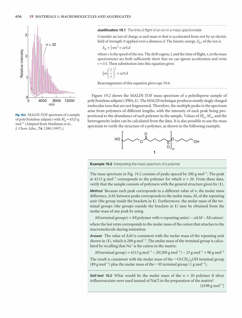
656 19 MATERIALS 1: MACROMOLECULES AND AGGREGATESR
elat
ive
inte
nsity
0
1
2
3
4000 8000 12000m z/
n = 20
0
Fig. 19.2 MALDI-TOF spectrum of a sampleof poly(butylene adipate) with Jn = 4525 gmol−1 (Adapted from Mudiman et al.,J. Chem. Educ., 74, 1288 (1997).)
Justification 19.1 The time of flight of an ion in a mass spectrometer
Consider an ion of charge ze and mass m that is accelerated from rest by an electricfield of strength E applied over a distance d. The kinetic energy, EK, of the ion is
EK = 1–2 mv2 = zeEd
where v is the speed of the ion. The drift region, l, and the time of flight, t, in the massspectrometer are both sufficiently short that we can ignore acceleration and write v = l /t. Then substitution into this equation gives
1–2m
2
= zeEd
Rearrangement of this equation gives eqn 19.6.
Figure 19.2 shows the MALDI-TOF mass spectrum of a polydisperse sample ofpoly(butylene adipate) (PBA, 1). The MALDI technique produces mostly singly chargedmolecular ions that are not fragmented. Therefore, the multiple peaks in the spectrumarise from polymers of different lengths, with the intensity of each peak being pro-portional to the abundance of each polymer in the sample. Values of Jn, Jw, and theheterogeneity index can be calculated from the data. It is also possible to use the massspectrum to verify the structure of a polymer, as shown in the following example.
Example 19.2 Interpreting the mass spectrum of a polymer
The mass spectrum in Fig. 19.2 consists of peaks spaced by 200 g mol−1. The peakat 4113 g mol−1 corresponds to the polymer for which n = 20. From these data, verify that the sample consists of polymers with the general structure given by (1).
Method Because each peak corresponds to a different value of n, the molar massdifference, ∆M, between peaks corresponds to the molar mass, M, of the repeatingunit (the group inside the brackets in 1). Furthermore, the molar mass of the ter-minal groups (the groups outside the brackets in 1) may be obtained from themolar mass of any peak by using
M(terminal groups) = M(polymer with n repeating units) − n∆M − M(cation)
where the last term corresponds to the molar mass of the cation that attaches to themacromolecule during ionization.
Answer The value of ∆M is consistent with the molar mass of the repeating unitshown in (1), which is 200 g mol−1. The molar mass of the terminal group is calcu-lated by recalling that Na+ is the cation in the matrix:
M(terminal group) = 4113 g mol−1 − 20(200 g mol−1) − 23 g mol−1 = 90 g mol−1
The result is consistent with the molar mass of the -O(CH2)4OH terminal group(89 g mol−1) plus the molar mass of the -H terminal group (1 g mol−1).
Self-test 19.2 What would be the molar mass of the n = 20 polymer if silvertrifluoroacetate were used instead of NaCl in the preparation of the matrix?
[4198 g mol−1]
DEFl
t
ABC
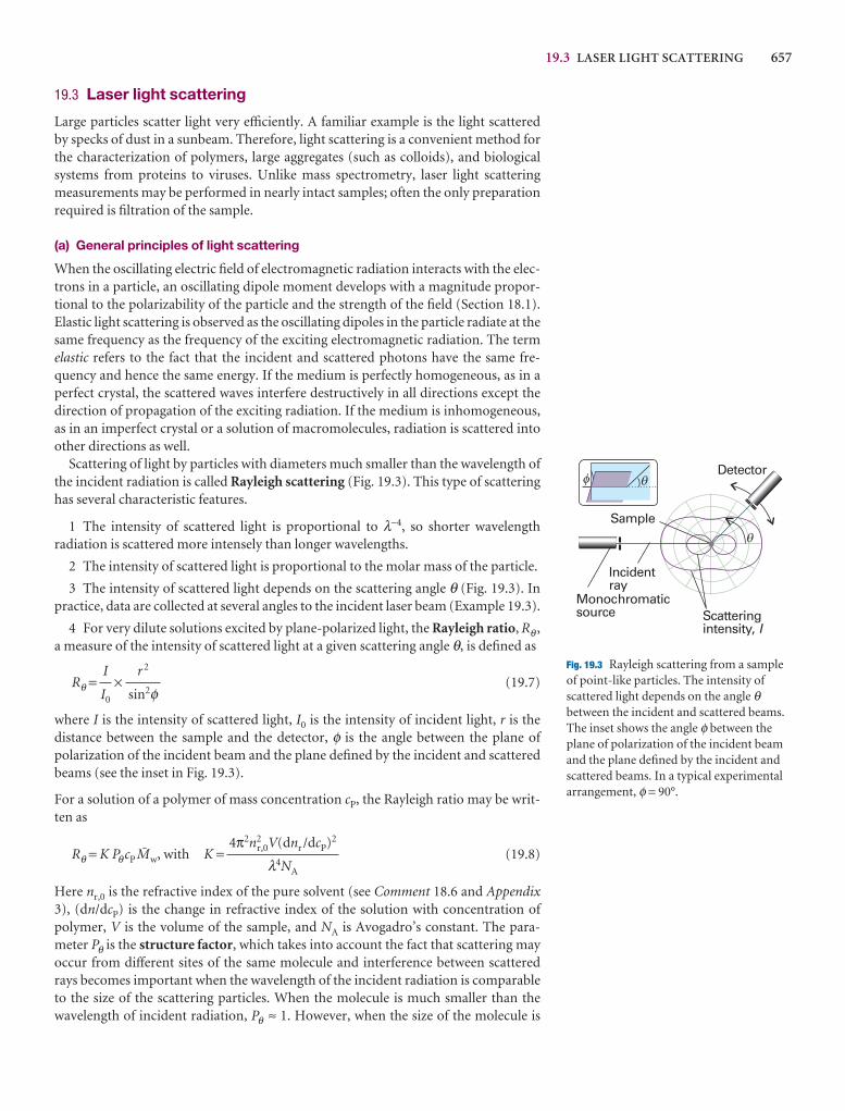
19.3 LASER LIGHT SCATTERING 657
19.3 Laser light scattering
Large particles scatter light very efficiently. A familiar example is the light scattered by specks of dust in a sunbeam. Therefore, light scattering is a convenient method for the characterization of polymers, large aggregates (such as colloids), and biologicalsystems from proteins to viruses. Unlike mass spectrometry, laser light scatteringmeasurements may be performed in nearly intact samples; often the only preparationrequired is filtration of the sample.
(a) General principles of light scattering
When the oscillating electric field of electromagnetic radiation interacts with the elec-trons in a particle, an oscillating dipole moment develops with a magnitude propor-tional to the polarizability of the particle and the strength of the field (Section 18.1).Elastic light scattering is observed as the oscillating dipoles in the particle radiate at thesame frequency as the frequency of the exciting electromagnetic radiation. The termelastic refers to the fact that the incident and scattered photons have the same fre-quency and hence the same energy. If the medium is perfectly homogeneous, as in aperfect crystal, the scattered waves interfere destructively in all directions except thedirection of propagation of the exciting radiation. If the medium is inhomogeneous,as in an imperfect crystal or a solution of macromolecules, radiation is scattered intoother directions as well.
Scattering of light by particles with diameters much smaller than the wavelength ofthe incident radiation is called Rayleigh scattering (Fig. 19.3). This type of scatteringhas several characteristic features.
1 The intensity of scattered light is proportional to λ−4, so shorter wavelength radiation is scattered more intensely than longer wavelengths.
2 The intensity of scattered light is proportional to the molar mass of the particle.
3 The intensity of scattered light depends on the scattering angle θ (Fig. 19.3). Inpractice, data are collected at several angles to the incident laser beam (Example 19.3).
4 For very dilute solutions excited by plane-polarized light, the Rayleigh ratio, Rθ ,a measure of the intensity of scattered light at a given scattering angle θ, is defined as
Rθ = × (19.7)
where I is the intensity of scattered light, I0 is the intensity of incident light, r is the distance between the sample and the detector, φ is the angle between the plane of polarization of the incident beam and the plane defined by the incident and scatteredbeams (see the inset in Fig. 19.3).
For a solution of a polymer of mass concentration cP, the Rayleigh ratio may be writ-ten as
Rθ = K PθcP Jw, with K = (19.8)
Here nr,0 is the refractive index of the pure solvent (see Comment 18.6 and Appendix3), (dn/dcP) is the change in refractive index of the solution with concentration ofpolymer, V is the volume of the sample, and NA is Avogadro’s constant. The para-meter Pθ is the structure factor, which takes into account the fact that scattering mayoccur from different sites of the same molecule and interference between scatteredrays becomes important when the wavelength of the incident radiation is comparableto the size of the scattering particles. When the molecule is much smaller than thewavelength of incident radiation, Pθ ≈ 1. However, when the size of the molecule is
4π2n2r,0V(dnr /dcP)2
λ4NA
r 2
sin2φI
I0
q
Incidentray
Monochromaticsource
Detector
Scatteringintensity, I
Sample
qf
Fig. 19.3 Rayleigh scattering from a sampleof point-like particles. The intensity ofscattered light depends on the angle θbetween the incident and scattered beams.The inset shows the angle φ between theplane of polarization of the incident beamand the plane defined by the incident andscattered beams. In a typical experimentalarrangement, φ = 90°.
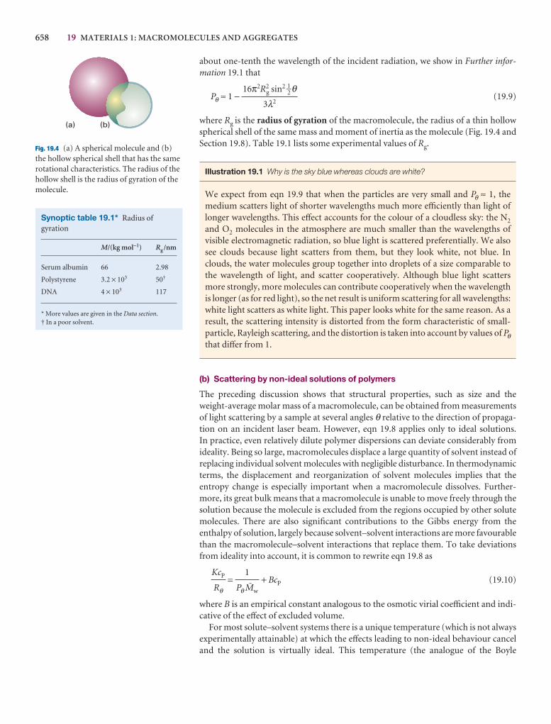
658 19 MATERIALS 1: MACROMOLECULES AND AGGREGATES
(a) (b)
Fig. 19.4 (a) A spherical molecule and (b)the hollow spherical shell that has the samerotational characteristics. The radius of thehollow shell is the radius of gyration of themolecule.
Synoptic table 19.1* Radius ofgyration
M/(kg mol−1) Rg /nm
Serum albumin 66 2.98
Polystyrene 3.2 × 10³ 50†
DNA 4 × 10³ 117
* More values are given in the Data section.† In a poor solvent.
about one-tenth the wavelength of the incident radiation, we show in Further infor-mation 19.1 that
Pθ ≈ 1 − (19.9)
where Rg is the radius of gyration of the macromolecule, the radius of a thin hollowspherical shell of the same mass and moment of inertia as the molecule (Fig. 19.4 andSection 19.8). Table 19.1 lists some experimental values of Rg.
Illustration 19.1 Why is the sky blue whereas clouds are white?
We expect from eqn 19.9 that when the particles are very small and Pθ ≈ 1, themedium scatters light of shorter wavelengths much more efficiently than light oflonger wavelengths. This effect accounts for the colour of a cloudless sky: the N2
and O2 molecules in the atmosphere are much smaller than the wavelengths of visible electromagnetic radiation, so blue light is scattered preferentially. We alsosee clouds because light scatters from them, but they look white, not blue. Inclouds, the water molecules group together into droplets of a size comparable tothe wavelength of light, and scatter cooperatively. Although blue light scattersmore strongly, more molecules can contribute cooperatively when the wavelengthis longer (as for red light), so the net result is uniform scattering for all wavelengths:white light scatters as white light. This paper looks white for the same reason. As aresult, the scattering intensity is distorted from the form characteristic of small-particle, Rayleigh scattering, and the distortion is taken into account by values of Pθthat differ from 1.
(b) Scattering by non-ideal solutions of polymers
The preceding discussion shows that structural properties, such as size and theweight-average molar mass of a macromolecule, can be obtained from measurementsof light scattering by a sample at several angles θ relative to the direction of propaga-tion on an incident laser beam. However, eqn 19.8 applies only to ideal solutions. In practice, even relatively dilute polymer dispersions can deviate considerably fromideality. Being so large, macromolecules displace a large quantity of solvent instead ofreplacing individual solvent molecules with negligible disturbance. In thermodynamicterms, the displacement and reorganization of solvent molecules implies that the entropy change is especially important when a macromolecule dissolves. Further-more, its great bulk means that a macromolecule is unable to move freely through thesolution because the molecule is excluded from the regions occupied by other solutemolecules. There are also significant contributions to the Gibbs energy from the enthalpy of solution, largely because solvent–solvent interactions are more favourablethan the macromolecule–solvent interactions that replace them. To take deviationsfrom ideality into account, it is common to rewrite eqn 19.8 as
= + BcP (19.10)
where B is an empirical constant analogous to the osmotic virial coefficient and indi-cative of the effect of excluded volume.
For most solute–solvent systems there is a unique temperature (which is not alwaysexperimentally attainable) at which the effects leading to non-ideal behaviour canceland the solution is virtually ideal. This temperature (the analogue of the Boyle
1
Pθ Jw
KcP
Rθ
16π2R2g sin2 1–2 θ
3λ2
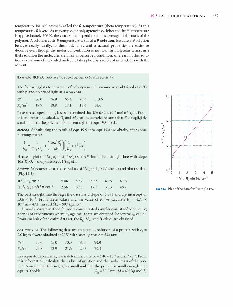
19.3 LASER LIGHT SCATTERING 659
0 1 2 3 4 54.5
5.5
6.5
7.5
10/m
21
´R
--
2
10 sin ( )/m3 1 2´ R - -2
q
q�21q
Fig. 19.5 Plot of the data for Example 19.3.
temperature for real gases) is called the q-temperature (theta temperature). At thistemperature, B is zero. As an example, for polystyrene in cyclohexane the θ-temperatureis approximately 306 K, the exact value depending on the average molar mass of thepolymer. A solution at its θ-temperature is called a q-solution. Because a θ-solutionbehaves nearly ideally, its thermodynamic and structural properties are easier to describe even though the molar concentration is not low. In molecular terms, in atheta solution the molecules are in an unperturbed condition, whereas in other solu-tions expansion of the coiled molecule takes place as a result of interactions with thesolvent.
Example 19.3 Determining the size of a polymer by light scattering
The following data for a sample of polystyrene in butanone were obtained at 20°Cwith plane-polarized light at λ = 546 nm.
θ/° 26.0 36.9 66.4 90.0 113.6
Rθ /m2 19.7 18.8 17.1 16.0 14.4
In separate experiments, it was determined that K = 6.42 × 10⁻⁵ mol m5 kg−2. Fromthis information, calculate Rg and Jw for the sample. Assume that B is negligiblysmall and that the polymer is small enough that eqn 19.9 holds.
Method Substituting the result of eqn 19.9 into eqn 19.8 we obtain, after some rearrangement:
= + sin2 1–2θ
Hence, a plot of 1/Rθ against (1/Rθ) sin2 1–2θ should be a straight line with slope16π2Rg
2 /3λ2 and y-intercept 1/KcP Jw.
Answer We construct a table of values of 1/Rθ and (1/Rθ) sin2 1–2θ and plot the data(Fig. 19.5).
102 × Rθ−1/m−2 5.06 5.32 5.83 6.25 6.96
(103/Rθ ) sin2( 1–2θ )/m−2 2.56 5.33 17.5 31.3 48.7
The best straight line through the data has a slope of 0.391 and a y-intercept of 5.06 × 10⁻². From these values and the value of K, we calculate Rg = 4.71 ×10⁻⁸ m = 47.1 nm and Jw = 987 kg mol−1.
A more accurate method for more concentrated samples consists of conductinga series of experiments where Rθ against θ data are obtained for several cP values.From analysis of the entire data set, the Rg, Jw, and B values are obtained.
Self-test 19.3 The following data for an aqueous solution of a protein with cP =2.0 kg m−3 were obtained at 20°C with laser light at λ = 532 nm:
θ / ° 15.0 45.0 70.0 85.0 90.0
Rθ /m2 23.8 22.9 21.6 20.7 20.4
In a separate experiment, it was determined that K = 2.40 × 10⁻² mol m5 kg−2. Fromthis information, calculate the radius of gyration and the molar mass of the pro-tein. Assume that B is negligibly small and that the protein is small enough that eqn 19.9 holds. [Rg = 39.8 nm; M = 498 kg mol−1]
DF
1
Rθ
AC
DF
16π2R2g
3λ2
AC
1
KcP Jw
1
Rθ
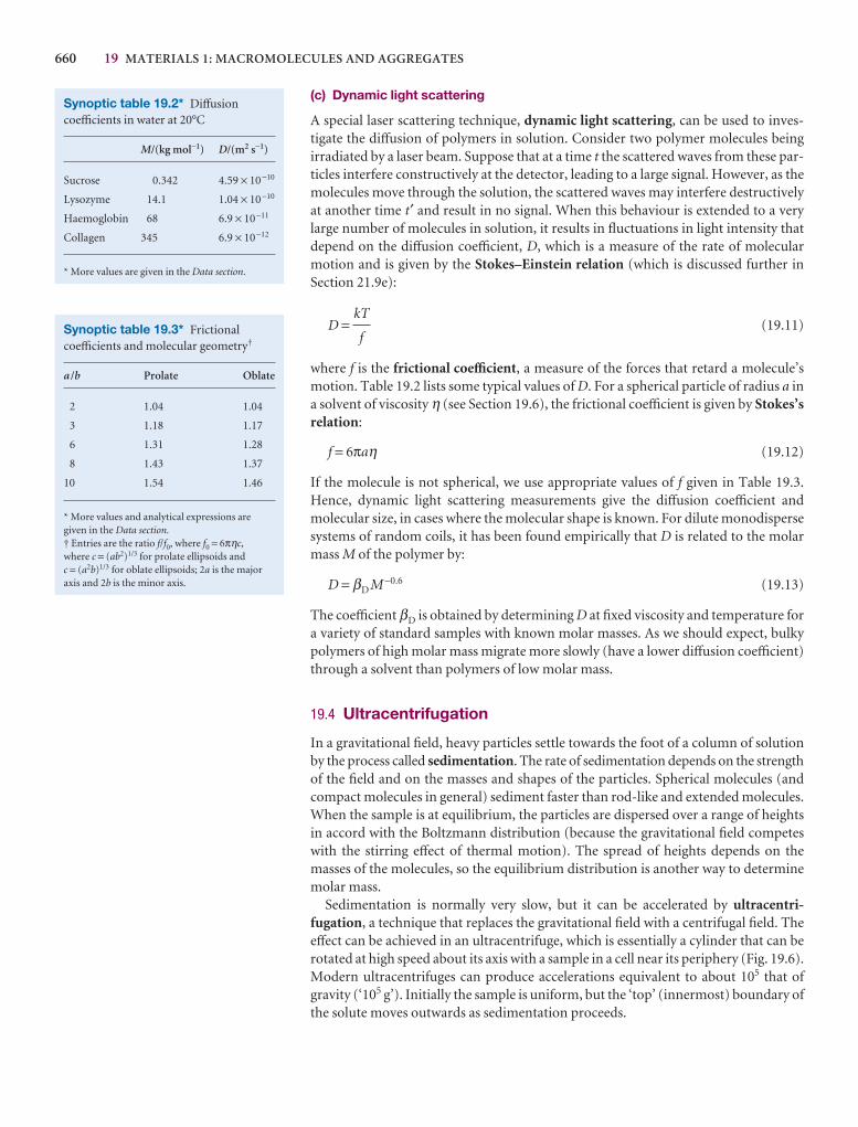
660 19 MATERIALS 1: MACROMOLECULES AND AGGREGATES
(c) Dynamic light scattering
A special laser scattering technique, dynamic light scattering, can be used to inves-tigate the diffusion of polymers in solution. Consider two polymer molecules being irradiated by a laser beam. Suppose that at a time t the scattered waves from these par-ticles interfere constructively at the detector, leading to a large signal. However, as themolecules move through the solution, the scattered waves may interfere destructivelyat another time t′ and result in no signal. When this behaviour is extended to a verylarge number of molecules in solution, it results in fluctuations in light intensity thatdepend on the diffusion coefficient, D, which is a measure of the rate of molecularmotion and is given by the Stokes–Einstein relation (which is discussed further inSection 21.9e):
D = (19.11)
where f is the frictional coefficient, a measure of the forces that retard a molecule’smotion. Table 19.2 lists some typical values of D. For a spherical particle of radius a ina solvent of viscosity η (see Section 19.6), the frictional coefficient is given by Stokes’srelation:
f = 6πaη (19.12)
If the molecule is not spherical, we use appropriate values of f given in Table 19.3.Hence, dynamic light scattering measurements give the diffusion coefficient andmolecular size, in cases where the molecular shape is known. For dilute monodispersesystems of random coils, it has been found empirically that D is related to the molarmass M of the polymer by:
D = βD M−0.6 (19.13)
The coefficient βD is obtained by determining D at fixed viscosity and temperature fora variety of standard samples with known molar masses. As we should expect, bulkypolymers of high molar mass migrate more slowly (have a lower diffusion coefficient)through a solvent than polymers of low molar mass.
19.4 Ultracentrifugation
In a gravitational field, heavy particles settle towards the foot of a column of solutionby the process called sedimentation. The rate of sedimentation depends on the strengthof the field and on the masses and shapes of the particles. Spherical molecules (andcompact molecules in general) sediment faster than rod-like and extended molecules.When the sample is at equilibrium, the particles are dispersed over a range of heightsin accord with the Boltzmann distribution (because the gravitational field competeswith the stirring effect of thermal motion). The spread of heights depends on themasses of the molecules, so the equilibrium distribution is another way to determinemolar mass.
Sedimentation is normally very slow, but it can be accelerated by ultracentri-fugation, a technique that replaces the gravitational field with a centrifugal field. Theeffect can be achieved in an ultracentrifuge, which is essentially a cylinder that can berotated at high speed about its axis with a sample in a cell near its periphery (Fig. 19.6).Modern ultracentrifuges can produce accelerations equivalent to about 105 that ofgravity (‘105 g’). Initially the sample is uniform, but the ‘top’ (innermost) boundary ofthe solute moves outwards as sedimentation proceeds.
kT
f
Synoptic table 19.2* Diffusioncoefficients in water at 20°C
M/(kg mol−1) D/(m2 s−1)
Sucrose 0.342 4.59 × 10⁻¹⁰
Lysozyme 14.1 1.04 × 10⁻¹⁰
Haemoglobin 68 6.9 × 10⁻¹¹
Collagen 345 6.9 × 10⁻¹²
* More values are given in the Data section.
Synoptic table 19.3* Frictionalcoefficients and molecular geometry†
a /b Prolate Oblate
2 1.04 1.04
3 1.18 1.17
6 1.31 1.28
8 1.43 1.37
10 1.54 1.46
* More values and analytical expressions aregiven in the Data section.† Entries are the ratio f/f0, where f0 = 6πηc,where c = (ab2)1/3 for prolate ellipsoids and c = (a2b)1/3 for oblate ellipsoids; 2a is the majoraxis and 2b is the minor axis.
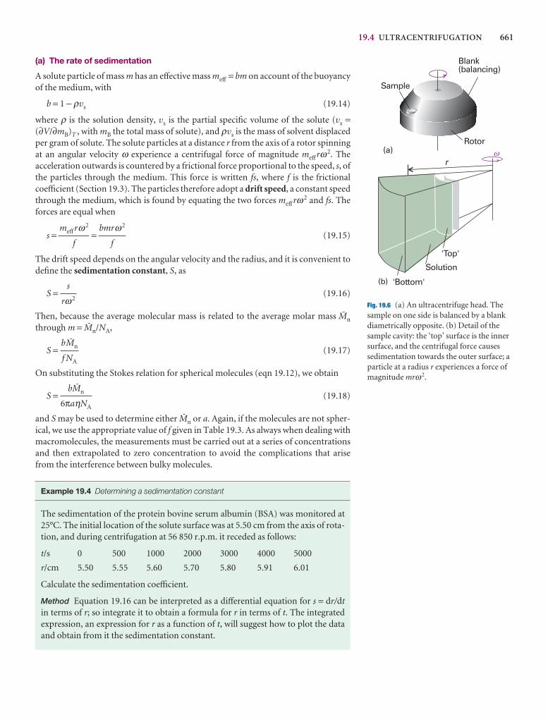
19.4 ULTRACENTRIFUGATION 661
Sample
Blank(balancing)
Rotor
r�
'Top'
Solution
'Bottom'
(a)
(b)
Fig. 19.6 (a) An ultracentrifuge head. Thesample on one side is balanced by a blankdiametrically opposite. (b) Detail of thesample cavity: the ‘top’ surface is the innersurface, and the centrifugal force causessedimentation towards the outer surface; aparticle at a radius r experiences a force ofmagnitude mrω2.
(a) The rate of sedimentation
A solute particle of mass m has an effective mass meff = bm on account of the buoyancyof the medium, with
b = 1 − ρvs (19.14)
where ρ is the solution density, vs is the partial specific volume of the solute (vs =(∂V/∂mB)T , with mB the total mass of solute), and ρvs is the mass of solvent displacedper gram of solute. The solute particles at a distance r from the axis of a rotor spinningat an angular velocity ω experience a centrifugal force of magnitude meff rω2. The acceleration outwards is countered by a frictional force proportional to the speed, s, ofthe particles through the medium. This force is written fs, where f is the frictionalcoefficient (Section 19.3). The particles therefore adopt a drift speed, a constant speedthrough the medium, which is found by equating the two forces meff rω2 and fs. Theforces are equal when
s = = (19.15)
The drift speed depends on the angular velocity and the radius, and it is convenient todefine the sedimentation constant, S, as
S = (19.16)
Then, because the average molecular mass is related to the average molar mass Jn
through m = Jn/NA,
S = (19.17)
On substituting the Stokes relation for spherical molecules (eqn 19.12), we obtain
S = (19.18)
and S may be used to determine either Jn or a. Again, if the molecules are not spher-ical, we use the appropriate value of f given in Table 19.3. As always when dealing withmacromolecules, the measurements must be carried out at a series of concentrationsand then extrapolated to zero concentration to avoid the complications that arisefrom the interference between bulky molecules.
Example 19.4 Determining a sedimentation constant
The sedimentation of the protein bovine serum albumin (BSA) was monitored at25°C. The initial location of the solute surface was at 5.50 cm from the axis of rota-tion, and during centrifugation at 56 850 r.p.m. it receded as follows:
t/s 0 500 1000 2000 3000 4000 5000
r/cm 5.50 5.55 5.60 5.70 5.80 5.91 6.01
Calculate the sedimentation coefficient.
Method Equation 19.16 can be interpreted as a differential equation for s = dr/dtin terms of r; so integrate it to obtain a formula for r in terms of t. The integratedexpression, an expression for r as a function of t, will suggest how to plot the dataand obtain from it the sedimentation constant.
bJn
6πaηNA
bJn
f NA
s
rω2
bmrω2
f
meff rω2
f
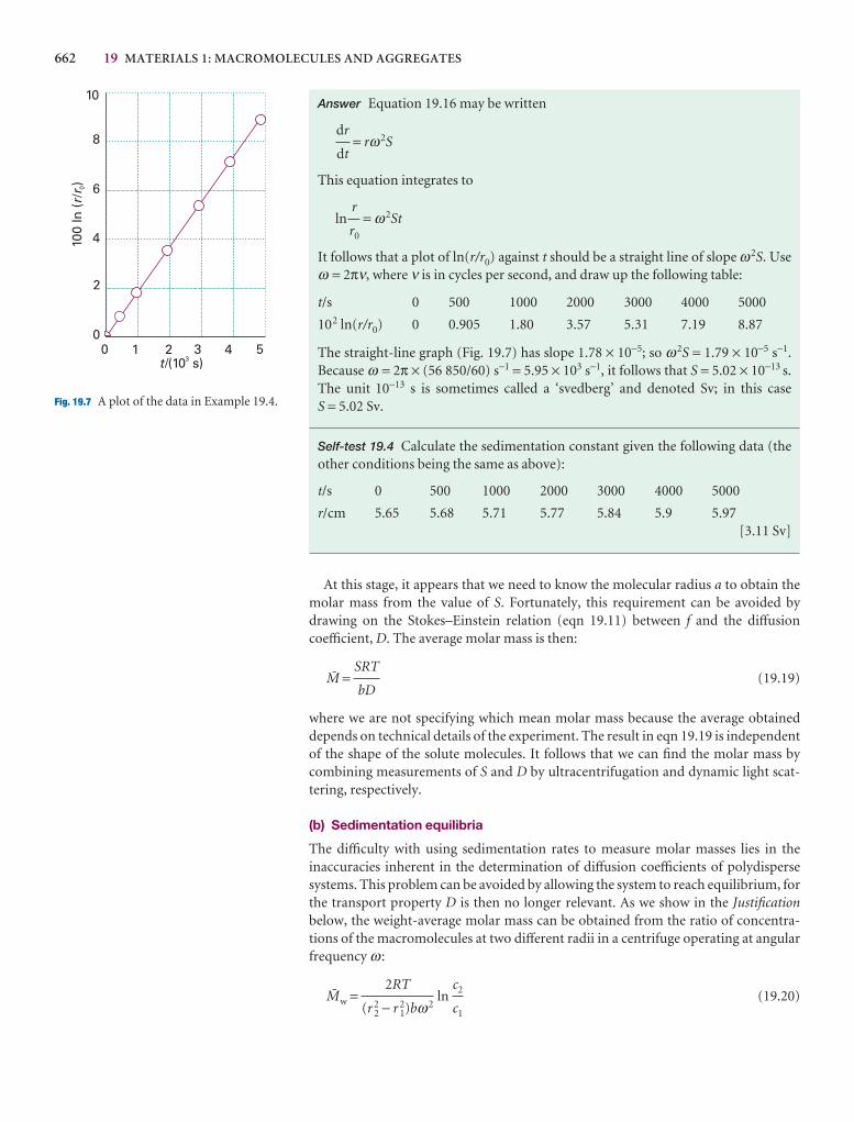
662 19 MATERIALS 1: MACROMOLECULES AND AGGREGATES
0 1 2 3 4 5t/(10 s)3
0
2
4
6
8
1010
0 ln
(/
)r
r 0
Fig. 19.7 A plot of the data in Example 19.4.
Answer Equation 19.16 may be written
= rω2S
This equation integrates to
ln = ω2St
It follows that a plot of ln(r/r0) against t should be a straight line of slope ω2S. Useω = 2πν, where ν is in cycles per second, and draw up the following table:
t/s 0 500 1000 2000 3000 4000 5000
102 ln(r/r0) 0 0.905 1.80 3.57 5.31 7.19 8.87
The straight-line graph (Fig. 19.7) has slope 1.78 × 10⁻⁵; so ω2S = 1.79 × 10⁻⁵ s−1.Because ω = 2π × (56 850/60) s−1 = 5.95 × 10³ s−1, it follows that S = 5.02 × 10⁻¹³ s.The unit 10−13 s is sometimes called a ‘svedberg’ and denoted Sv; in this case S = 5.02 Sv.
Self-test 19.4 Calculate the sedimentation constant given the following data (theother conditions being the same as above):
t/s 0 500 1000 2000 3000 4000 5000
r/cm 5.65 5.68 5.71 5.77 5.84 5.9 5.97[3.11 Sv]
At this stage, it appears that we need to know the molecular radius a to obtain themolar mass from the value of S. Fortunately, this requirement can be avoided bydrawing on the Stokes–Einstein relation (eqn 19.11) between f and the diffusioncoefficient, D. The average molar mass is then:
J = (19.19)
where we are not specifying which mean molar mass because the average obtained depends on technical details of the experiment. The result in eqn 19.19 is independentof the shape of the solute molecules. It follows that we can find the molar mass bycombining measurements of S and D by ultracentrifugation and dynamic light scat-tering, respectively.
(b) Sedimentation equilibria
The difficulty with using sedimentation rates to measure molar masses lies in the inaccuracies inherent in the determination of diffusion coefficients of polydispersesystems. This problem can be avoided by allowing the system to reach equilibrium, forthe transport property D is then no longer relevant. As we show in the Justificationbelow, the weight-average molar mass can be obtained from the ratio of concentra-tions of the macromolecules at two different radii in a centrifuge operating at angularfrequency ω :
Jw = ln (19.20)c2
c1
2RT
(r 22 − r 2
1)bω2
SRT
bD
r
r0
dr
dt
19.5 ELECTROPHORESIS 663
An alternative treatment of the data leads to the Z–average molar mass. The centrifugeis run more slowly in this technique than in the sedimentation rate method to avoidhaving all the solute pressed in a thin film against the bottom of the cell. At theseslower speeds, several days may be needed for equilibrium to be reached.
Justification 19.2 The weight-average molar mass from sedimentation experiments
The distribution of particles is the outcome of the balance between the effect of the centrifugal force and the dispersing effect of diffusion down a concentrationgradient. The kinetic energy of a particle of effective mass m at a radius r in a rotorspinning at a frequency ω is 1–2mω2r 2, so the total chemical potential at a radius r isG(r) = µ(r) − 1–2mω2r 2, where µ(r) is the contribution that depends on the con-centration of solute. The condition for equilibrium is that the chemical potential isuniform, so
T
=T
− Mω2r = 0
To evaluate the partial derivative of µ, we write
T
=T,c T,c
+T,p T,p
= Mvω2rρ + RTT,p
The first result follows from the fact that (∂µ /∂p)T = Vm, the partial molar volume,and Vm = Mv. It also makes use of the fact that the hydrostatic pressure at r is p(r) =p(r0) + 1–2ρω2(r 2 − r 2
0), where r0 is the radius of the surface of the liquid in the sample holder (that is, the location of its meniscus), with ρ the mass density of the solution. The concentration term stems from the expression µ = µ7 + RT ln c.The condition for equilibrium is therefore
Mrω2(1 − vρ) − RTT,p
= 0
and therefore, at constant temperature,
d ln c =
This expression integrates to eqn 19.20.
19.5 Electrophoresis
Many macromolecules, such as DNA, are charged and move in response to an electricfield. This motion is called electrophoresis. Electrophoretic mobility is a result of aconstant drift speed, s, reached by an ion when the driving force zeE (where, as usual,ze is the net charge and E is the field strength) is matched by the frictional force fs. Thedrift speed (which is treated in detail in Section 21.7) is then:
s = (19.21)
Therefore, the mobility of a macromolecule in an electric field depends on its netcharge, size (and hence molar mass), and shape. The latter two factors are implied bythe dependence of s on f.
The drift speeds attained by polymers in traditional electrophoresis methods arerather low; as a result, several hours are often necessary to effect good separation of
zeE
f
Mrω2(1 − vρ)dr
RT
DEF∂ ln c
∂r
ABC
DEF∂ ln c
∂r
ABCDEF
∂c
∂r
ABCDEF
∂µ∂c
ABCDEF
∂p
∂r
ABCDEF
∂µ∂p
ABCDEF
∂µ∂r
ABC
DEF∂µ∂r
ABCDEF
∂G
∂r
ABC
664 19 MATERIALS 1: MACROMOLECULES AND AGGREGATES
complex mixtures. According to eqn 19.21, one way to increase the drift speed is to increase the electric field strength. However, there are limits to this strategy becausevery large electric fields can heat the large surfaces of an electrophoresis apparatus unevenly, leading to a non-uniform distribution of electrophoretic mobilities andpoor separation.
In capillary electrophoresis, the sample is dispersed in a medium (such as methyl-cellulose) and held in a thin glass or plastic tube with diameters ranging from 20 to100 µm. The small size of the apparatus makes it easy to dissipate heat when large elec-tric fields are applied. Excellent separations may be effected in minutes rather thanhours. Each polymer fraction emerging from the capillary can be characterized fur-ther by other techniques, such as MALDI-TOF.
IMPACT ON BIOCHEMISTRY
I19.1 Gel electrophoresis in genomics and proteomics
Advances in biotechnology are linked strongly to the development of physical tech-niques. The ongoing effort to characterize the entire genetic material, or genome, oforganisms as simple as bacteria and as complex as Homo sapiens will lead to importantnew insights into the molecular mechanisms of disease, primarily through the discov-ery of previously unknown proteins encoded by the deoxyribonucleic acid (DNA) ingenes. However, decoding genomic DNA will not always lead to accurate predictionsof the amino acids present in biologically active proteins. Many proteins undergochemical modification, such as cleavage into smaller proteins, after being synthesizedin the cell. Moreover, it is known that one piece of DNA may encode more than oneactive protein. It follows that it is also important to describe the proteome, the fullcomplement of functional proteins of an organism, by characterizing directly the pro-teins after they have been synthesized and processed in the cell.
The procedures of genomics and proteomics, the analysis of the genome and pro-teome, of complex organisms are time-consuming because of the very large numberof molecules that must be characterized. For example, the human genome containsabout 30 000 genes and the number of active proteins is likely to be much larger.Success in the characterization of the genome and proteome of any organism will depend on the deployment of very rapid techniques for the determination of the orderin which molecular building blocks are linked covalently in DNA and proteins.
An important tool in genomics and proteomics is gel electrophoresis, in whichbiopolymers are separated on a slab of a porous gel, a semirigid dispersion of a solidin a liquid. Because the molecules must pass through the pores in the gel, the larger themacromolecule the less mobile it is in the electric field and, conversely, the smaller themacromolecule the more swiftly it moves through the pores. In this way, gel elec-trophoresis allows for the separation of components of a mixture according to theirmolar masses. Two common gel materials for the study of proteins and nucleic acidsare agarose and cross-linked polyacrylamide. Agarose has large pores and is bettersuited for the study of large macromolecules, such as DNA and enzyme complexes.Polyacrylamide gels with varying pore sizes can be made by changing the concentra-tion of acrylamide in the polymerization solution. In general, smaller pores form asthe concentration of acrylamide is increased, making possible the separation of rela-tively small macromolecules by polyacrylamide gel electrophoresis (PAGE).
The separation of very large pieces of DNA, such as chromosomes, by conventionalgel electrophoresis is not effective, making the analysis of genomic material ratherdifficult. Double-stranded DNA molecules are thin enough to pass through gel pores,but long and flexible DNA coils can become trapped in the pores and the result is impaired mobility along the direction of the applied electric field. This problem canbe avoided with pulsed-field electrophoresis, in which a brief burst of the electric
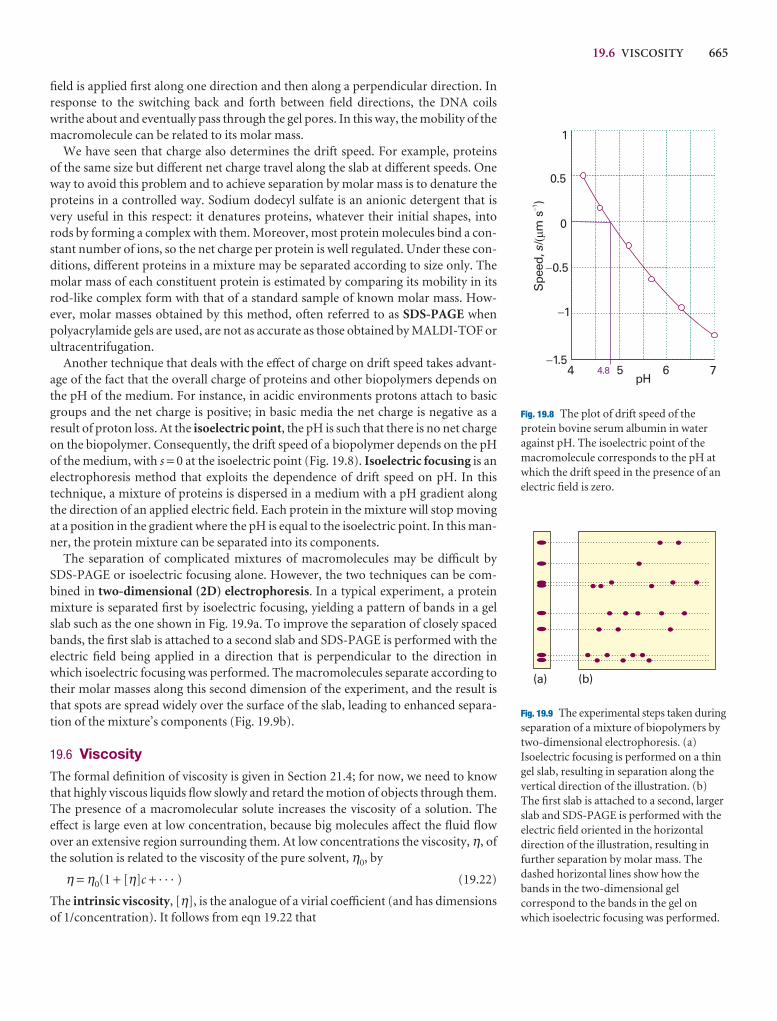
19.6 VISCOSITY 665
field is applied first along one direction and then along a perpendicular direction. Inresponse to the switching back and forth between field directions, the DNA coilswrithe about and eventually pass through the gel pores. In this way, the mobility of themacromolecule can be related to its molar mass.
We have seen that charge also determines the drift speed. For example, proteins of the same size but different net charge travel along the slab at different speeds. Oneway to avoid this problem and to achieve separation by molar mass is to denature theproteins in a controlled way. Sodium dodecyl sulfate is an anionic detergent that isvery useful in this respect: it denatures proteins, whatever their initial shapes, intorods by forming a complex with them. Moreover, most protein molecules bind a con-stant number of ions, so the net charge per protein is well regulated. Under these con-ditions, different proteins in a mixture may be separated according to size only. Themolar mass of each constituent protein is estimated by comparing its mobility in itsrod-like complex form with that of a standard sample of known molar mass. How-ever, molar masses obtained by this method, often referred to as SDS-PAGE whenpolyacrylamide gels are used, are not as accurate as those obtained by MALDI-TOF orultracentrifugation.
Another technique that deals with the effect of charge on drift speed takes advant-age of the fact that the overall charge of proteins and other biopolymers depends onthe pH of the medium. For instance, in acidic environments protons attach to basicgroups and the net charge is positive; in basic media the net charge is negative as a result of proton loss. At the isoelectric point, the pH is such that there is no net chargeon the biopolymer. Consequently, the drift speed of a biopolymer depends on the pHof the medium, with s = 0 at the isoelectric point (Fig. 19.8). Isoelectric focusing is anelectrophoresis method that exploits the dependence of drift speed on pH. In thistechnique, a mixture of proteins is dispersed in a medium with a pH gradient alongthe direction of an applied electric field. Each protein in the mixture will stop movingat a position in the gradient where the pH is equal to the isoelectric point. In this man-ner, the protein mixture can be separated into its components.
The separation of complicated mixtures of macromolecules may be difficult bySDS-PAGE or isoelectric focusing alone. However, the two techniques can be com-bined in two-dimensional (2D) electrophoresis. In a typical experiment, a proteinmixture is separated first by isoelectric focusing, yielding a pattern of bands in a gelslab such as the one shown in Fig. 19.9a. To improve the separation of closely spacedbands, the first slab is attached to a second slab and SDS-PAGE is performed with theelectric field being applied in a direction that is perpendicular to the direction inwhich isoelectric focusing was performed. The macromolecules separate according totheir molar masses along this second dimension of the experiment, and the result isthat spots are spread widely over the surface of the slab, leading to enhanced separa-tion of the mixture’s components (Fig. 19.9b).
19.6 ViscosityThe formal definition of viscosity is given in Section 21.4; for now, we need to knowthat highly viscous liquids flow slowly and retard the motion of objects through them.The presence of a macromolecular solute increases the viscosity of a solution. Theeffect is large even at low concentration, because big molecules affect the fluid flowover an extensive region surrounding them. At low concentrations the viscosity, η, ofthe solution is related to the viscosity of the pure solvent, η0, by
η = η0(1 + [η]c + · · · ) (19.22)
The intrinsic viscosity, [η], is the analogue of a virial coefficient (and has dimensionsof 1/concentration). It follows from eqn 19.22 that
4 5 6 7pH
�1.5
�1
�0.5
0
0.5
1
4.8
Spe
ed,
/m
s)
s6
�1
Fig. 19.8 The plot of drift speed of theprotein bovine serum albumin in wateragainst pH. The isoelectric point of themacromolecule corresponds to the pH atwhich the drift speed in the presence of anelectric field is zero.
(a) (b)
Fig. 19.9 The experimental steps taken duringseparation of a mixture of biopolymers bytwo-dimensional electrophoresis. (a)Isoelectric focusing is performed on a thingel slab, resulting in separation along thevertical direction of the illustration. (b)The first slab is attached to a second, largerslab and SDS-PAGE is performed with theelectric field oriented in the horizontaldirection of the illustration, resulting infurther separation by molar mass. Thedashed horizontal lines show how thebands in the two-dimensional gelcorrespond to the bands in the gel onwhich isoelectric focusing was performed.
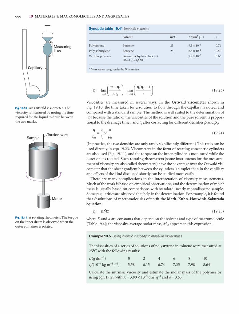
666 19 MATERIALS 1: MACROMOLECULES AND AGGREGATES
Measuringlines
Capillary
Fig. 19.10 An Ostwald viscometer. Theviscosity is measured by noting the timerequired for the liquid to drain between the two marks.
Torsion wireSample
Motor
Fig. 19.11 A rotating rheometer. The torqueon the inner drum is observed when theouter container is rotated.
Synoptic table 19.4* Intrinsic viscosity
Solvent q/°C K/(cm3 g−1) a
Polystyrene Benzene 25 9.5 × 10⁻³ 0.74
Polyisobutylene Benzene 23 8.3 × 10⁻² 0.50
Various proteins Guanidine hydrochloride + 7.2 × 10⁻³ 0.66HSCH2CH2OH
* More values are given in the Data section.
[η] = limc→0
= limc→0
(19.23)
Viscosities are measured in several ways. In the Ostwald viscometer shown in Fig. 19.10, the time taken for a solution to flow through the capillary is noted, andcompared with a standard sample. The method is well suited to the determination of[η] because the ratio of the viscosities of the solution and the pure solvent is propor-tional to the drainage time t and t0 after correcting for different densities ρ and ρ0:
= × (19.24)
(In practice, the two densities are only rarely significantly different.) This ratio can beused directly in eqn 19.23. Viscometers in the form of rotating concentric cylindersare also used (Fig. 19.11), and the torque on the inner cylinder is monitored while theouter one is rotated. Such rotating rheometers (some instruments for the measure-ment of viscosity are also called rheometers) have the advantage over the Ostwald vis-cometer that the shear gradient between the cylinders is simpler than in the capillaryand effects of the kind discussed shortly can be studied more easily.
There are many complications in the interpretation of viscosity measurements.Much of the work is based on empirical observations, and the determination of molarmass is usually based on comparisons with standard, nearly monodisperse sample.Some regularities are observed that help in the determination. For example, it is foundthat θ solutions of macromolecules often fit the Mark–Kuhn–Houwink–Sakuradaequation:
[η] = KJva (19.25)
where K and a are constants that depend on the solvent and type of macromolecule(Table 19.4); the viscosity-average molar mass, Jv, appears in this expression.
Example 19.5 Using intrinsic viscosity to measure molar mass
The viscosities of a series of solutions of polystyrene in toluene were measured at25°C with the following results:
c/(g dm−3) 0 2 4 6 8 10
η/(10−4 kg m−1 s−1) 5.58 6.15 6.74 7.35 7.98 8.64
Calculate the intrinsic viscosity and estimate the molar mass of the polymer byusing eqn 19.25 with K = 3.80 × 10⁻⁵ dm3 g−1 and a = 0.63.
ρρ0
t
t0
ηη0
DF
η/η0 − 1
c
AC
DF
η − η0
cη0
AC
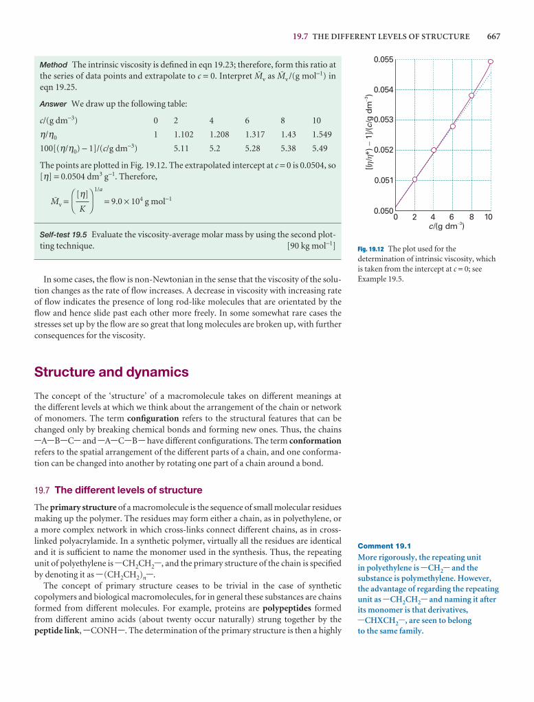
19.7 THE DIFFERENT LEVELS OF STRUCTURE 667
Comment 19.1
More rigorously, the repeating unit in polyethylene is -CH2- and thesubstance is polymethylene. However,the advantage of regarding the repeatingunit as -CH2CH2- and naming it afterits monomer is that derivatives, -CHXCH2-, are seen to belong to the same family.
0.055
0.054
0.053
0.052
0.051
0.050
[(/
*)1]
/(/g
dm
)-
c-
3
0 2 4 6 8 10c/(g dm )-3
hh
Fig. 19.12 The plot used for thedetermination of intrinsic viscosity, whichis taken from the intercept at c = 0; seeExample 19.5.
Method The intrinsic viscosity is defined in eqn 19.23; therefore, form this ratio atthe series of data points and extrapolate to c = 0. Interpret Jv as Jv /(g mol−1) ineqn 19.25.
Answer We draw up the following table:
c/(g dm−3) 0 2 4 6 8 10
η/η0 1 1.102 1.208 1.317 1.43 1.549
100[(η/η0) − 1]/(c/g dm−3) 5.11 5.2 5.28 5.38 5.49
The points are plotted in Fig. 19.12. The extrapolated intercept at c = 0 is 0.0504, so[η] = 0.0504 dm3 g−1. Therefore,
Jv =1/a
= 9.0 × 10⁴ g mol−1
Self-test 19.5 Evaluate the viscosity-average molar mass by using the second plot-ting technique. [90 kg mol−1]
In some cases, the flow is non-Newtonian in the sense that the viscosity of the solu-tion changes as the rate of flow increases. A decrease in viscosity with increasing rateof flow indicates the presence of long rod-like molecules that are orientated by theflow and hence slide past each other more freely. In some somewhat rare cases thestresses set up by the flow are so great that long molecules are broken up, with furtherconsequences for the viscosity.
Structure and dynamics
The concept of the ‘structure’ of a macromolecule takes on different meanings at the different levels at which we think about the arrangement of the chain or networkof monomers. The term configuration refers to the structural features that can bechanged only by breaking chemical bonds and forming new ones. Thus, the chains -A-B-C- and -A-C-B- have different configurations. The term conformationrefers to the spatial arrangement of the different parts of a chain, and one conforma-tion can be changed into another by rotating one part of a chain around a bond.
19.7 The different levels of structure
The primary structure of a macromolecule is the sequence of small molecular residuesmaking up the polymer. The residues may form either a chain, as in polyethylene, ora more complex network in which cross-links connect different chains, as in cross-linked polyacrylamide. In a synthetic polymer, virtually all the residues are identicaland it is sufficient to name the monomer used in the synthesis. Thus, the repeatingunit of polyethylene is -CH2CH2-, and the primary structure of the chain is specifiedby denoting it as -(CH2CH2)n-.
The concept of primary structure ceases to be trivial in the case of synthetic copolymers and biological macromolecules, for in general these substances are chainsformed from different molecules. For example, proteins are polypeptides formedfrom different amino acids (about twenty occur naturally) strung together by the peptide link, -CONH-. The determination of the primary structure is then a highly
DF
[η]
K
AC
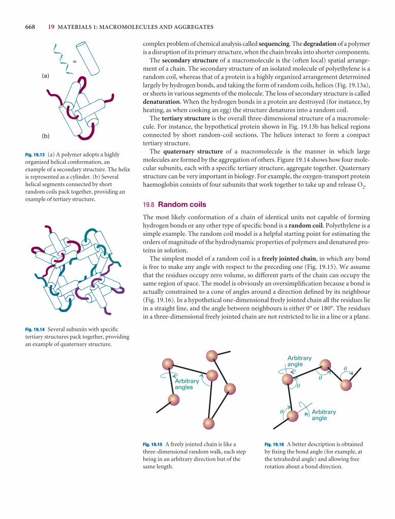
668 19 MATERIALS 1: MACROMOLECULES AND AGGREGATES
complex problem of chemical analysis called sequencing. The degradation of a polymeris a disruption of its primary structure, when the chain breaks into shorter components.
The secondary structure of a macromolecule is the (often local) spatial arrange-ment of a chain. The secondary structure of an isolated molecule of polyethylene is arandom coil, whereas that of a protein is a highly organized arrangement determinedlargely by hydrogen bonds, and taking the form of random coils, helices (Fig. 19.13a),or sheets in various segments of the molecule. The loss of secondary structure is calleddenaturation. When the hydrogen bonds in a protein are destroyed (for instance, byheating, as when cooking an egg) the structure denatures into a random coil.
The tertiary structure is the overall three-dimensional structure of a macromole-cule. For instance, the hypothetical protein shown in Fig. 19.13b has helical regionsconnected by short random-coil sections. The helices interact to form a compact tertiary structure.
The quaternary structure of a macromolecule is the manner in which largemolecules are formed by the aggregation of others. Figure 19.14 shows how four mole-cular subunits, each with a specific tertiary structure, aggregate together. Quaternarystructure can be very important in biology. For example, the oxygen-transport proteinhaemoglobin consists of four subunits that work together to take up and release O2.
19.8 Random coils
The most likely conformation of a chain of identical units not capable of forming hydrogen bonds or any other type of specific bond is a random coil. Polyethylene is asimple example. The random coil model is a helpful starting point for estimating theorders of magnitude of the hydrodynamic properties of polymers and denatured pro-teins in solution.
The simplest model of a random coil is a freely jointed chain, in which any bond is free to make any angle with respect to the preceding one (Fig. 19.15). We assumethat the residues occupy zero volume, so different parts of the chain can occupy thesame region of space. The model is obviously an oversimplification because a bond is actually constrained to a cone of angles around a direction defined by its neighbour(Fig. 19.16). In a hypothetical one-dimensional freely jointed chain all the residues liein a straight line, and the angle between neighbours is either 0° or 180°. The residuesin a three-dimensional freely jointed chain are not restricted to lie in a line or a plane.
=
(a)
(b)
Fig. 19.13 (a) A polymer adopts a highlyorganized helical conformation, anexample of a secondary structure. The helixis represented as a cylinder. (b) Severalhelical segments connected by shortrandom coils pack together, providing anexample of tertiary structure.
Fig. 19.14 Several subunits with specifictertiary structures pack together, providingan example of quaternary structure.
Arbitraryangles
Fig. 19.15 A freely jointed chain is like a three-dimensional random walk, each stepbeing in an arbitrary direction but of thesame length.
Arbitraryangle
Arbitraryangle
q
q
q
q
Fig. 19.16 A better description is obtainedby fixing the bond angle (for example, atthe tetrahedral angle) and allowing freerotation about a bond direction.
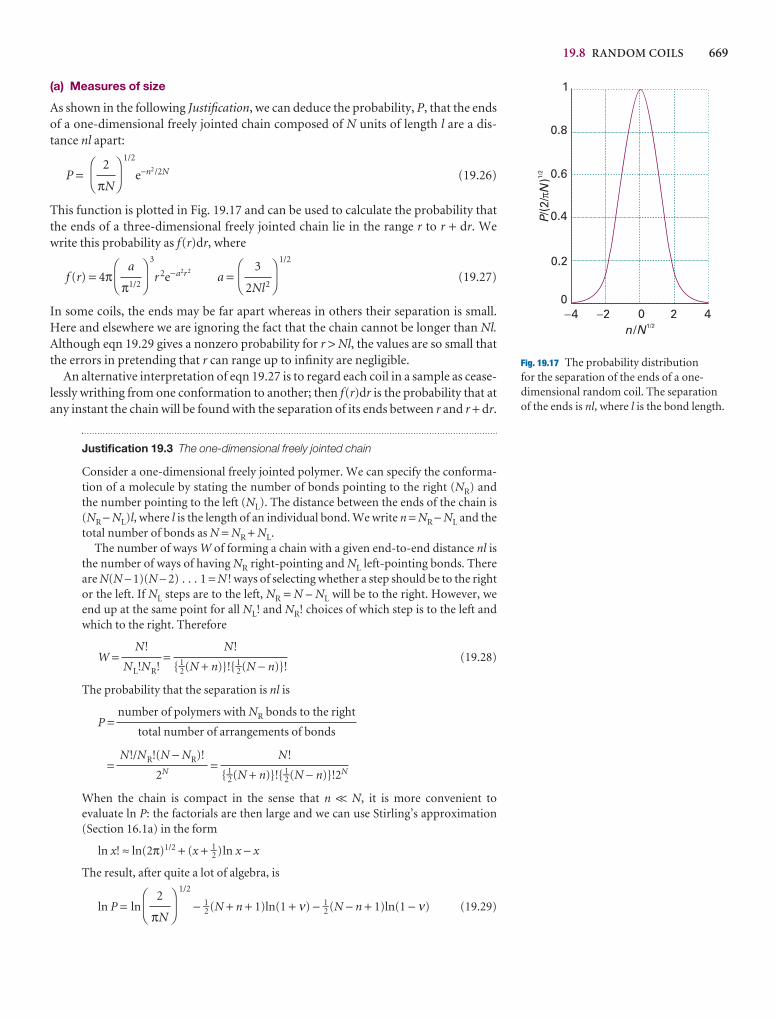
19.8 RANDOM COILS 669
(a) Measures of size
As shown in the following Justification, we can deduce the probability, P, that the endsof a one-dimensional freely jointed chain composed of N units of length l are a dis-tance nl apart:
P =1/2
e−n2/2N (19.26)
This function is plotted in Fig. 19.17 and can be used to calculate the probability thatthe ends of a three-dimensional freely jointed chain lie in the range r to r + dr. Wewrite this probability as f(r)dr, where
f (r) = 4π3
r 2e−a2r2a =
1/2
(19.27)
In some coils, the ends may be far apart whereas in others their separation is small.Here and elsewhere we are ignoring the fact that the chain cannot be longer than Nl.Although eqn 19.29 gives a nonzero probability for r > Nl, the values are so small thatthe errors in pretending that r can range up to infinity are negligible.
An alternative interpretation of eqn 19.27 is to regard each coil in a sample as cease-lessly writhing from one conformation to another; then f(r)dr is the probability that atany instant the chain will be found with the separation of its ends between r and r + dr.
Justification 19.3 The one-dimensional freely jointed chain
Consider a one-dimensional freely jointed polymer. We can specify the conforma-tion of a molecule by stating the number of bonds pointing to the right (NR) and the number pointing to the left (NL). The distance between the ends of the chain is(NR − NL)l, where l is the length of an individual bond. We write n = NR − NL and thetotal number of bonds as N = NR + NL.
The number of ways W of forming a chain with a given end-to-end distance nl isthe number of ways of having NR right-pointing and NL left-pointing bonds. Thereare N(N – 1)(N – 2) . . . 1 = N ! ways of selecting whether a step should be to the rightor the left. If NL steps are to the left, NR = N – NL will be to the right. However, weend up at the same point for all NL! and NR! choices of which step is to the left andwhich to the right. Therefore
W = = (19.28)
The probability that the separation is nl is
P =
= =
When the chain is compact in the sense that n << N, it is more convenient to evaluate ln P: the factorials are then large and we can use Stirling’s approximation(Section 16.1a) in the form
ln x! ≈ ln(2π)1/2 + (x + 1–2 )ln x − x
The result, after quite a lot of algebra, is
ln P = ln
1/2
− 1–2 (N + n + 1)ln(1 + ν) − 1–2 (N − n + 1)ln(1 − ν) (19.29)DF
2
πN
AC
N!
{ 1–2(N + n)}!{ 1–2(N − n)}!2N
N!/NR!(N − NR)!
2N
number of polymers with NR bonds to the right
total number of arrangements of bonds
N!
{ 1–2(N + n)}!{ 1–2(N − n)}!
N!
NL!NR!
DF
3
2Nl2
AC
DF
a
π1/2
AC
DF
2
πN
AC
0 2 4-4 -20
0.2
0.4
0.6
0.8
1
PN
/(2/
)1/2
n N/ 1/2
p
Fig. 19.17 The probability distribution for the separation of the ends of a one-dimensional random coil. The separationof the ends is nl, where l is the bond length.
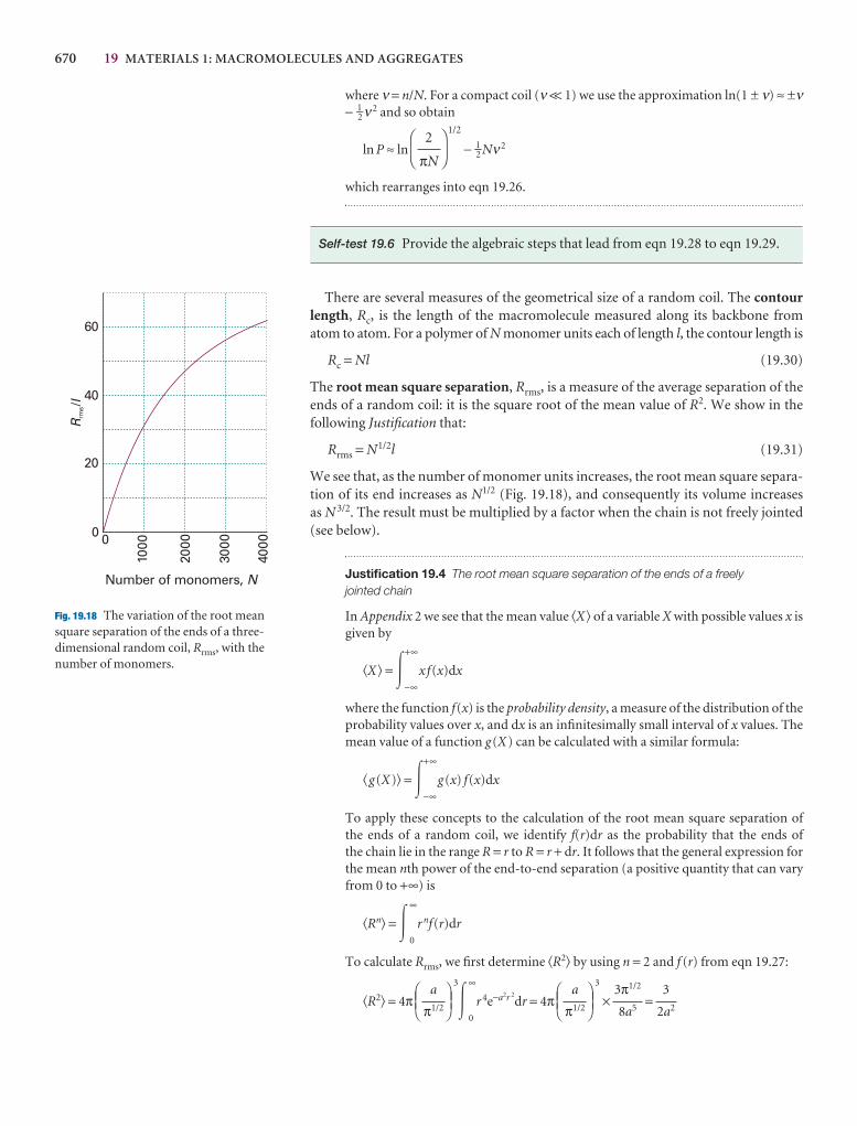
670 19 MATERIALS 1: MACROMOLECULES AND AGGREGATES
0
1000
2000
3000
4000
Number of monomers, N
0
20
40
60
Rl
rms/
Fig. 19.18 The variation of the root meansquare separation of the ends of a three-dimensional random coil, Rrms, with thenumber of monomers.
where ν = n/N. For a compact coil (ν << 1) we use the approximation ln(1 ± ν) ≈ ±ν− 1–2 ν2 and so obtain
ln P ≈ ln
1/2
− 1–2 Nν2
which rearranges into eqn 19.26.
Self-test 19.6 Provide the algebraic steps that lead from eqn 19.28 to eqn 19.29.
There are several measures of the geometrical size of a random coil. The contourlength, Rc, is the length of the macromolecule measured along its backbone fromatom to atom. For a polymer of N monomer units each of length l, the contour length is
Rc = Nl (19.30)
The root mean square separation, Rrms, is a measure of the average separation of theends of a random coil: it is the square root of the mean value of R2. We show in the following Justification that:
Rrms = N1/2l (19.31)
We see that, as the number of monomer units increases, the root mean square separa-tion of its end increases as N1/2 (Fig. 19.18), and consequently its volume increases as N 3/2. The result must be multiplied by a factor when the chain is not freely jointed(see below).
Justification 19.4 The root mean square separation of the ends of a freely jointed chain
In Appendix 2 we see that the mean value �X� of a variable X with possible values x isgiven by
�X� = �+∞
−∞xf(x)dx
where the function f(x) is the probability density, a measure of the distribution of theprobability values over x, and dx is an infinitesimally small interval of x values. Themean value of a function g(X) can be calculated with a similar formula:
�g(X)� = �+∞
−∞g(x) f(x)dx
To apply these concepts to the calculation of the root mean square separation of the ends of a random coil, we identify f(r)dr as the probability that the ends of the chain lie in the range R = r to R = r + dr. It follows that the general expression forthe mean nth power of the end-to-end separation (a positive quantity that can varyfrom 0 to +∞) is
�Rn� = �∞
0
r nf(r)dr
To calculate Rrms, we first determine �R2� by using n = 2 and f (r) from eqn 19.27:
�R2� = 4π3
�∞
0
r 4e−a2r 2dr = 4π
3
× =3
2a2
3π1/2
8a5
DEFa
π1/2
ABCDEF
a
π1/2
ABC
DF
2
πN
AC
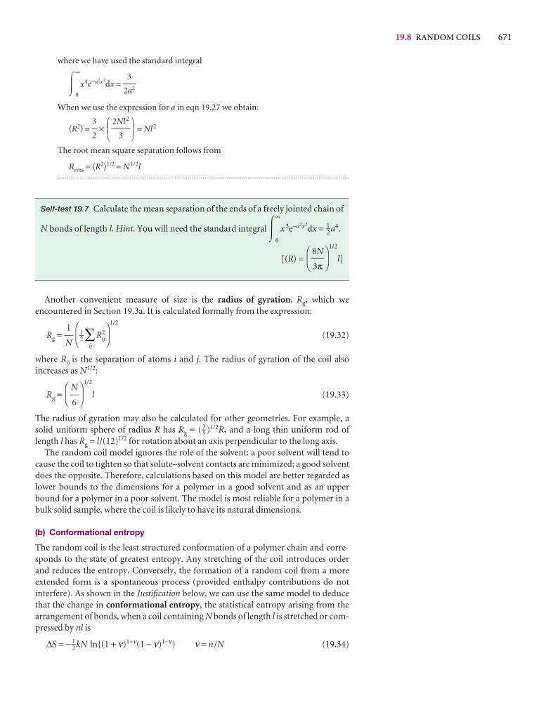
19.8 RANDOM COILS 671
where we have used the standard integral
�∞
0
x4e−a2x2dx =
When we use the expression for a in eqn 19.27 we obtain:
�R2� = × = Nl 2
The root mean square separation follows from
Rrms = �R2�1/2 = N 1/2l
Self-test 19.7 Calculate the mean separation of the ends of a freely jointed chain of
N bonds of length l. Hint. You will need the standard integral �∞
0
x 3e−a2x2dx = 1–2 a4.
[�R� =1/2
l]
Another convenient measure of size is the radius of gyration, Rg, which we encountered in Section 19.3a. It is calculated formally from the expression:
Rg = 1–2∑ij
R2ij
1/2
(19.32)
where Rij is the separation of atoms i and j. The radius of gyration of the coil also increases as N1/2:
Rg =1/2
l (19.33)
The radius of gyration may also be calculated for other geometries. For example, asolid uniform sphere of radius R has Rg = ( 3–5 )1/2R, and a long thin uniform rod oflength l has Rg = l/(12)1/2 for rotation about an axis perpendicular to the long axis.
The random coil model ignores the role of the solvent: a poor solvent will tend tocause the coil to tighten so that solute–solvent contacts are minimized; a good solventdoes the opposite. Therefore, calculations based on this model are better regarded aslower bounds to the dimensions for a polymer in a good solvent and as an upperbound for a polymer in a poor solvent. The model is most reliable for a polymer in abulk solid sample, where the coil is likely to have its natural dimensions.
(b) Conformational entropy
The random coil is the least structured conformation of a polymer chain and corre-sponds to the state of greatest entropy. Any stretching of the coil introduces order and reduces the entropy. Conversely, the formation of a random coil from a more extended form is a spontaneous process (provided enthalpy contributions do not interfere). As shown in the Justification below, we can use the same model to deducethat the change in conformational entropy, the statistical entropy arising from thearrangement of bonds, when a coil containing N bonds of length l is stretched or com-pressed by nl is
∆S = − 1–2 kN ln{(1 + ν)1+ν(1 − ν)1−ν} ν = n /N (19.34)
DF
N
6
AC
DF
AC
1
N
DF
8N
3π
AC
DEF2Nl 2
3
ABC3
2
3
2a2
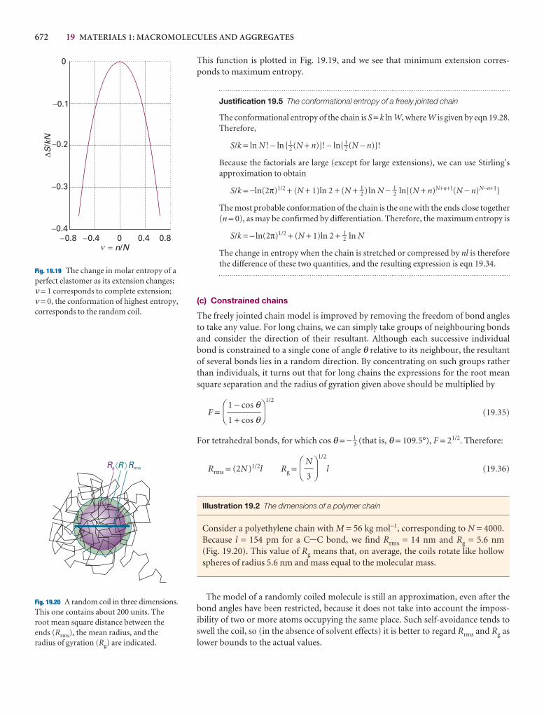
672 19 MATERIALS 1: MACROMOLECULES AND AGGREGATES
0
-0.1
-0.2
-0.3
-0.4
DS
kN
/
-0.8 -0.4 0 0.4 0.8/= n Nn
Fig. 19.19 The change in molar entropy of aperfect elastomer as its extension changes;ν = 1 corresponds to complete extension; ν = 0, the conformation of highest entropy,corresponds to the random coil.
RrmsRg" #R
Fig. 19.20 A random coil in three dimensions.This one contains about 200 units. Theroot mean square distance between theends (Rrms), the mean radius, and theradius of gyration (Rg) are indicated.
This function is plotted in Fig. 19.19, and we see that minimum extension corres-ponds to maximum entropy.
Justification 19.5 The conformational entropy of a freely jointed chain
The conformational entropy of the chain is S = k ln W, where W is given by eqn 19.28.Therefore,
S/k = ln N ! − ln{ 1–2 (N + n)}! − ln{ 1–2 (N − n)}!
Because the factorials are large (except for large extensions), we can use Stirling’sapproximation to obtain
S/k = −ln(2π)1/2 + (N + 1)ln 2 + (N + 1–2 ) ln N − 1–2 ln{(N + n)N+n+1(N − n)N−n+1}
The most probable conformation of the chain is the one with the ends close together(n = 0), as may be confirmed by differentiation. Therefore, the maximum entropy is
S/k = − ln(2π)1/2 + (N + 1)ln 2 + 1–2 ln N
The change in entropy when the chain is stretched or compressed by nl is thereforethe difference of these two quantities, and the resulting expression is eqn 19.34.
(c) Constrained chains
The freely jointed chain model is improved by removing the freedom of bond anglesto take any value. For long chains, we can simply take groups of neighbouring bondsand consider the direction of their resultant. Although each successive individualbond is constrained to a single cone of angle θ relative to its neighbour, the resultantof several bonds lies in a random direction. By concentrating on such groups ratherthan individuals, it turns out that for long chains the expressions for the root meansquare separation and the radius of gyration given above should be multiplied by
F =1/2
(19.35)
For tetrahedral bonds, for which cos θ = − 1–3 (that is, θ = 109.5°), F = 21/2. Therefore:
Rrms = (2N)1/2l Rg =1/2
l (19.36)
Illustration 19.2 The dimensions of a polymer chain
Consider a polyethylene chain with M = 56 kg mol−1, corresponding to N = 4000.Because l = 154 pm for a C-C bond, we find Rrms = 14 nm and Rg = 5.6 nm (Fig. 19.20). This value of Rg means that, on average, the coils rotate like hollowspheres of radius 5.6 nm and mass equal to the molecular mass.
The model of a randomly coiled molecule is still an approximation, even after thebond angles have been restricted, because it does not take into account the imposs-ibility of two or more atoms occupying the same place. Such self-avoidance tends toswell the coil, so (in the absence of solvent effects) it is better to regard Rrms and Rg aslower bounds to the actual values.
DF
N
3
AC
DF
1 − cos θ1 + cos θ
AC
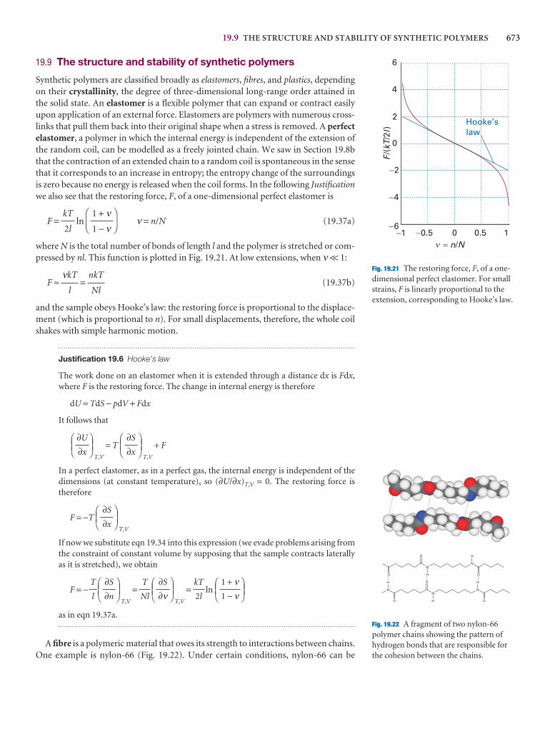
19.9 THE STRUCTURE AND STABILITY OF SYNTHETIC POLYMERS 673
19.9 The structure and stability of synthetic polymers
Synthetic polymers are classified broadly as elastomers, fibres, and plastics, dependingon their crystallinity, the degree of three-dimensional long-range order attained inthe solid state. An elastomer is a flexible polymer that can expand or contract easilyupon application of an external force. Elastomers are polymers with numerous cross-links that pull them back into their original shape when a stress is removed. A perfectelastomer, a polymer in which the internal energy is independent of the extension ofthe random coil, can be modelled as a freely jointed chain. We saw in Section 19.8bthat the contraction of an extended chain to a random coil is spontaneous in the sensethat it corresponds to an increase in entropy; the entropy change of the surroundingsis zero because no energy is released when the coil forms. In the following Justificationwe also see that the restoring force, F, of a one-dimensional perfect elastomer is
F = ln ν = n/N (19.37a)
where N is the total number of bonds of length l and the polymer is stretched or com-pressed by nl. This function is plotted in Fig. 19.21. At low extensions, when ν << 1:
F ≈ = (19.37b)
and the sample obeys Hooke’s law: the restoring force is proportional to the displace-ment (which is proportional to n). For small displacements, therefore, the whole coilshakes with simple harmonic motion.
Justification 19.6 Hooke’s law
The work done on an elastomer when it is extended through a distance dx is Fdx,where F is the restoring force. The change in internal energy is therefore
dU = TdS − pdV + Fdx
It follows that
T,V
= TT,V
+ F
In a perfect elastomer, as in a perfect gas, the internal energy is independent of thedimensions (at constant temperature), so (∂U/∂x)T,V = 0. The restoring force istherefore
F = −TT,V
If now we substitute eqn 19.34 into this expression (we evade problems arising fromthe constraint of constant volume by supposing that the sample contracts laterallyas it is stretched), we obtain
F = −T,V
=T,V
= ln
as in eqn 19.37a.
A fibre is a polymeric material that owes its strength to interactions between chains.One example is nylon-66 (Fig. 19.22). Under certain conditions, nylon-66 can be
DEF1 + ν1 − ν
ABCkT
2l
DEF∂S
∂νABC
T
Nl
DEF∂S
∂n
ABCT
l
DEF∂S
∂x
ABC
DEF∂S
∂x
ABCDEF
∂U
∂x
ABC
nkT
Nl
νkT
l
DF
1 + ν1 − ν
AC
kT
2l �6
�4
�2
0
2
4
6
�1 �0.5 0 0.5 1/� n N
FkT
l/(
/2) Hooke’s
law
�
Fig. 19.21 The restoring force, F, of a one-dimensional perfect elastomer. For smallstrains, F is linearly proportional to theextension, corresponding to Hooke’s law.
N
N
O H
H
O
O
N
N
N
O H
H
O
OH
Fig. 19.22 A fragment of two nylon-66polymer chains showing the pattern ofhydrogen bonds that are responsible for the cohesion between the chains.
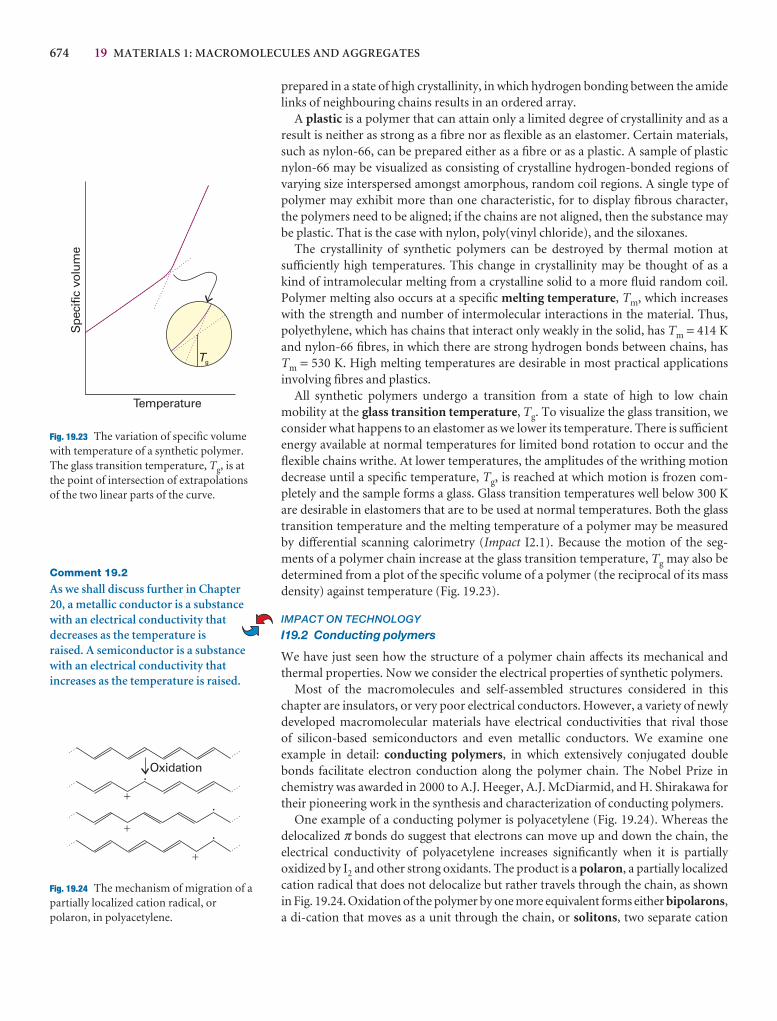
674 19 MATERIALS 1: MACROMOLECULES AND AGGREGATES
prepared in a state of high crystallinity, in which hydrogen bonding between the amidelinks of neighbouring chains results in an ordered array.
A plastic is a polymer that can attain only a limited degree of crystallinity and as aresult is neither as strong as a fibre nor as flexible as an elastomer. Certain materials,such as nylon-66, can be prepared either as a fibre or as a plastic. A sample of plasticnylon-66 may be visualized as consisting of crystalline hydrogen-bonded regions ofvarying size interspersed amongst amorphous, random coil regions. A single type ofpolymer may exhibit more than one characteristic, for to display fibrous character,the polymers need to be aligned; if the chains are not aligned, then the substance maybe plastic. That is the case with nylon, poly(vinyl chloride), and the siloxanes.
The crystallinity of synthetic polymers can be destroyed by thermal motion atsufficiently high temperatures. This change in crystallinity may be thought of as a kind of intramolecular melting from a crystalline solid to a more fluid random coil.Polymer melting also occurs at a specific melting temperature, Tm, which increaseswith the strength and number of intermolecular interactions in the material. Thus,polyethylene, which has chains that interact only weakly in the solid, has Tm = 414 Kand nylon-66 fibres, in which there are strong hydrogen bonds between chains, hasTm = 530 K. High melting temperatures are desirable in most practical applicationsinvolving fibres and plastics.
All synthetic polymers undergo a transition from a state of high to low chain mobility at the glass transition temperature, Tg. To visualize the glass transition, weconsider what happens to an elastomer as we lower its temperature. There is sufficientenergy available at normal temperatures for limited bond rotation to occur and theflexible chains writhe. At lower temperatures, the amplitudes of the writhing motiondecrease until a specific temperature, Tg, is reached at which motion is frozen com-pletely and the sample forms a glass. Glass transition temperatures well below 300 Kare desirable in elastomers that are to be used at normal temperatures. Both the glasstransition temperature and the melting temperature of a polymer may be measuredby differential scanning calorimetry (Impact I2.1). Because the motion of the seg-ments of a polymer chain increase at the glass transition temperature, Tg may also bedetermined from a plot of the specific volume of a polymer (the reciprocal of its massdensity) against temperature (Fig. 19.23).
IMPACT ON TECHNOLOGY
I19.2 Conducting polymers
We have just seen how the structure of a polymer chain affects its mechanical andthermal properties. Now we consider the electrical properties of synthetic polymers.
Most of the macromolecules and self-assembled structures considered in this chapter are insulators, or very poor electrical conductors. However, a variety of newlydeveloped macromolecular materials have electrical conductivities that rival those of silicon-based semiconductors and even metallic conductors. We examine one example in detail: conducting polymers, in which extensively conjugated doublebonds facilitate electron conduction along the polymer chain. The Nobel Prize inchemistry was awarded in 2000 to A.J. Heeger, A.J. McDiarmid, and H. Shirakawa fortheir pioneering work in the synthesis and characterization of conducting polymers.
One example of a conducting polymer is polyacetylene (Fig. 19.24). Whereas thedelocalized π bonds do suggest that electrons can move up and down the chain, theelectrical conductivity of polyacetylene increases significantly when it is partially oxidized by I2 and other strong oxidants. The product is a polaron, a partially localizedcation radical that does not delocalize but rather travels through the chain, as shownin Fig. 19.24. Oxidation of the polymer by one more equivalent forms either bipolarons,a di-cation that moves as a unit through the chain, or solitons, two separate cation
Spe
cific
vol
ume
Temperature
Tg
Fig. 19.23 The variation of specific volumewith temperature of a synthetic polymer.The glass transition temperature, Tg, is atthe point of intersection of extrapolationsof the two linear parts of the curve.
�
.
�
.
�
.
Oxidation
Fig. 19.24 The mechanism of migration of apartially localized cation radical, orpolaron, in polyacetylene.
Comment 19.2
As we shall discuss further in Chapter20, a metallic conductor is a substancewith an electrical conductivity thatdecreases as the temperature is raised. A semiconductor is a substancewith an electrical conductivity thatincreases as the temperature is raised.
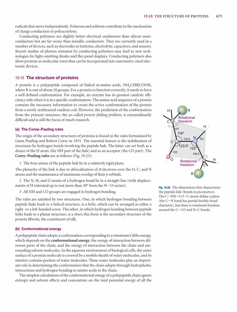
19.10 THE STRUCTURE OF PROTEINS 675
radicals that move independently. Polarons and solitons contribute to the mechanismof charge conduction in polyacetylene.
Conducting polymers are slightly better electrical conductors than silicon semi-conductors but are far worse than metallic conductors. They are currently used in anumber of devices, such as electrodes in batteries, electrolytic capacitors, and sensors.Recent studies of photon emission by conducting polymers may lead to new tech-nologies for light-emitting diodes and flat-panel displays. Conducting polymers alsoshow promise as molecular wires that can be incorporated into nanometre-sized elec-tronic devices.
19.10 The structure of proteins
A protein is a polypeptide composed of linked α-amino acids, NH2CHRCOOH,where R is one of about 20 groups. For a protein to function correctly, it needs to havea well defined conformation. For example, an enzyme has its greatest catalytic effi-
ciency only when it is in a specific conformation. The amino acid sequence of a proteincontains the necessary information to create the active conformation of the proteinfrom a newly synthesized random coil. However, the prediction of the conformationfrom the primary structure, the so-called protein folding problem, is extraordinarilydifficult and is still the focus of much research.
(a) The Corey–Pauling rules
The origin of the secondary structures of proteins is found in the rules formulated byLinus Pauling and Robert Corey in 1951. The essential feature is the stabilization ofstructures by hydrogen bonds involving the peptide link. The latter can act both as adonor of the H atom (the NH part of the link) and as an acceptor (the CO part). TheCorey–Pauling rules are as follows (Fig. 19.25):
1 The four atoms of the peptide link lie in a relatively rigid plane.
The planarity of the link is due to delocalization of π electrons over the O, C, and Natoms and the maintenance of maximum overlap of their p orbitals.
2 The N, H, and O atoms of a hydrogen bond lie in a straight line (with displace-ments of H tolerated up to not more than 30° from the N-O vector).
3 All NH and CO groups are engaged in hydrogen bonding.
The rules are satisfied by two structures. One, in which hydrogen bonding betweenpeptide links leads to a helical structure, is a helix, which can be arranged as either aright- or a left-handed screw. The other, in which hydrogen bonding between peptidelinks leads to a planar structure, is a sheet; this form is the secondary structure of theprotein fibroin, the constituent of silk.
(b) Conformational energy
A polypeptide chain adopts a conformation corresponding to a minimum Gibbs energy,which depends on the conformational energy, the energy of interaction between dif-ferent parts of the chain, and the energy of interaction between the chain and sur-rounding solvent molecules. In the aqueous environment of biological cells, the outersurface of a protein molecule is covered by a mobile sheath of water molecules, and itsinterior contains pockets of water molecules. These water molecules play an import-ant role in determining the conformation that the chain adopts through hydrophobicinteractions and hydrogen bonding to amino acids in the chain.
The simplest calculations of the conformational energy of a polypeptide chain ignoreentropy and solvent effects and concentrate on the total potential energy of all the
H
H
H
R
R
C
C
C
N
O
122°
116°
123.5°
102
145.5
132.5
124
151
Rotationalfreedom
Rotationalfreedom
Fig. 19.25 The dimensions that characterizethe peptide link (bonds in picometres). The C-NH-CO-C atoms define a plane (the C-N bond has partial double-bondcharacter), but there is rotational freedomaround the C-CO and N–C bonds.
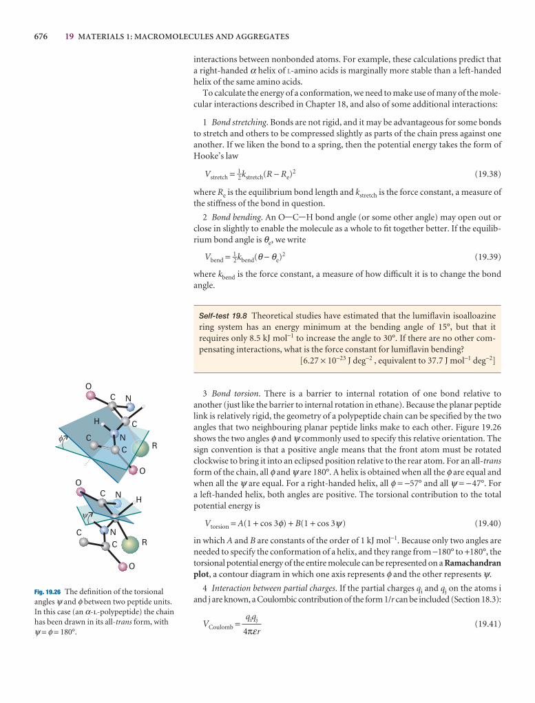
676 19 MATERIALS 1: MACROMOLECULES AND AGGREGATES
N
O
C
Cf
RN
H
C
CH
y
R
O
NCO
O
CNC
Fig. 19.26 The definition of the torsionalangles ψ and φ between two peptide units.In this case (an α-l-polypeptide) the chainhas been drawn in its all-trans form, with ψ = φ = 180°.
interactions between nonbonded atoms. For example, these calculations predict thata right-handed α helix of L-amino acids is marginally more stable than a left-handedhelix of the same amino acids.
To calculate the energy of a conformation, we need to make use of many of the mole-cular interactions described in Chapter 18, and also of some additional interactions:
1 Bond stretching. Bonds are not rigid, and it may be advantageous for some bondsto stretch and others to be compressed slightly as parts of the chain press against oneanother. If we liken the bond to a spring, then the potential energy takes the form ofHooke’s law
Vstretch = 1–2kstretch(R − Re)2 (19.38)
where Re is the equilibrium bond length and kstretch is the force constant, a measure ofthe stiffness of the bond in question.
2 Bond bending. An O-C-H bond angle (or some other angle) may open out orclose in slightly to enable the molecule as a whole to fit together better. If the equilib-rium bond angle is θe, we write
Vbend = 1–2kbend(θ − θe)2 (19.39)
where kbend is the force constant, a measure of how difficult it is to change the bondangle.
Self-test 19.8 Theoretical studies have estimated that the lumiflavin isoalloazinering system has an energy minimum at the bending angle of 15°, but that it requires only 8.5 kJ mol−1 to increase the angle to 30°. If there are no other com-pensating interactions, what is the force constant for lumiflavin bending?
[6.27 × 10⁻²³ J deg−2 , equivalent to 37.7 J mol−1 deg−2]
3 Bond torsion. There is a barrier to internal rotation of one bond relative to another (just like the barrier to internal rotation in ethane). Because the planar peptidelink is relatively rigid, the geometry of a polypeptide chain can be specified by the twoangles that two neighbouring planar peptide links make to each other. Figure 19.26shows the two angles φ and ψ commonly used to specify this relative orientation. Thesign convention is that a positive angle means that the front atom must be rotatedclockwise to bring it into an eclipsed position relative to the rear atom. For an all-transform of the chain, all φ and ψ are 180°. A helix is obtained when all the φ are equal andwhen all the ψ are equal. For a right-handed helix, all φ = −57° and all ψ = −47°. For a left-handed helix, both angles are positive. The torsional contribution to the totalpotential energy is
Vtorsion = A(1 + cos 3φ) + B(1 + cos 3ψ) (19.40)
in which A and B are constants of the order of 1 kJ mol−1. Because only two angles areneeded to specify the conformation of a helix, and they range from −180° to +180°, thetorsional potential energy of the entire molecule can be represented on a Ramachandranplot, a contour diagram in which one axis represents φ and the other represents ψ.
4 Interaction between partial charges. If the partial charges qi and qj on the atoms iand j are known, a Coulombic contribution of the form 1/r can be included (Section 18.3):
VCoulomb = (19.41)qiqj
4πεr
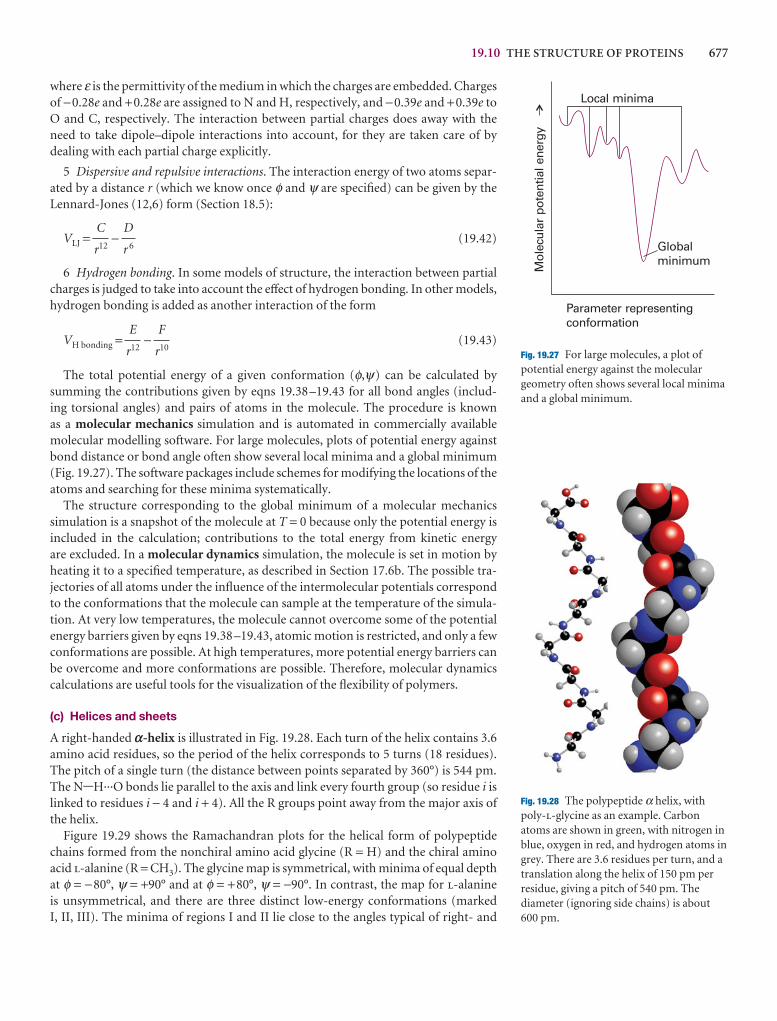
19.10 THE STRUCTURE OF PROTEINS 677
where ε is the permittivity of the medium in which the charges are embedded. Chargesof −0.28e and +0.28e are assigned to N and H, respectively, and −0.39e and +0.39e toO and C, respectively. The interaction between partial charges does away with theneed to take dipole–dipole interactions into account, for they are taken care of bydealing with each partial charge explicitly.
5 Dispersive and repulsive interactions. The interaction energy of two atoms separ-ated by a distance r (which we know once φ and ψ are specified) can be given by theLennard-Jones (12,6) form (Section 18.5):
VLJ = − (19.42)
6 Hydrogen bonding. In some models of structure, the interaction between partialcharges is judged to take into account the effect of hydrogen bonding. In other models,hydrogen bonding is added as another interaction of the form
VH bonding = − (19.43)
The total potential energy of a given conformation (φ,ψ) can be calculated by summing the contributions given by eqns 19.38–19.43 for all bond angles (includ-ing torsional angles) and pairs of atoms in the molecule. The procedure is known as a molecular mechanics simulation and is automated in commercially available molecular modelling software. For large molecules, plots of potential energy against bond distance or bond angle often show several local minima and a global minimum (Fig. 19.27). The software packages include schemes for modifying the locations of theatoms and searching for these minima systematically.
The structure corresponding to the global minimum of a molecular mechanicssimulation is a snapshot of the molecule at T = 0 because only the potential energy isincluded in the calculation; contributions to the total energy from kinetic energy are excluded. In a molecular dynamics simulation, the molecule is set in motion byheating it to a specified temperature, as described in Section 17.6b. The possible tra-jectories of all atoms under the influence of the intermolecular potentials correspondto the conformations that the molecule can sample at the temperature of the simula-tion. At very low temperatures, the molecule cannot overcome some of the potentialenergy barriers given by eqns 19.38–19.43, atomic motion is restricted, and only a fewconformations are possible. At high temperatures, more potential energy barriers canbe overcome and more conformations are possible. Therefore, molecular dynamicscalculations are useful tools for the visualization of the flexibility of polymers.
(c) Helices and sheets
A right-handed a-helix is illustrated in Fig. 19.28. Each turn of the helix contains 3.6amino acid residues, so the period of the helix corresponds to 5 turns (18 residues).The pitch of a single turn (the distance between points separated by 360°) is 544 pm.The N-H···O bonds lie parallel to the axis and link every fourth group (so residue i islinked to residues i − 4 and i + 4). All the R groups point away from the major axis ofthe helix.
Figure 19.29 shows the Ramachandran plots for the helical form of polypeptidechains formed from the nonchiral amino acid glycine (R = H) and the chiral aminoacid l-alanine (R = CH3). The glycine map is symmetrical, with minima of equal depthat φ = −80°, ψ = +90° and at φ = +80°, ψ = −90°. In contrast, the map for l-alanineis unsymmetrical, and there are three distinct low-energy conformations (marked I, II, III). The minima of regions I and II lie close to the angles typical of right- and
F
r10
E
r12
D
r 6
C
r12
Parameter representingconformation
Mol
ecul
ar p
oten
tial e
nerg
y
Local minima
Globalminimum
Fig. 19.27 For large molecules, a plot ofpotential energy against the moleculargeometry often shows several local minimaand a global minimum.
Fig. 19.28 The polypeptide α helix, withpoly-l-glycine as an example. Carbonatoms are shown in green, with nitrogen inblue, oxygen in red, and hydrogen atoms ingrey. There are 3.6 residues per turn, and atranslation along the helix of 150 pm perresidue, giving a pitch of 540 pm. Thediameter (ignoring side chains) is about600 pm.
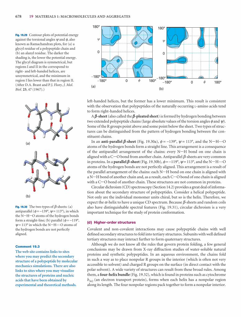
678 19 MATERIALS 1: MACROMOLECULES AND AGGREGATES
left-handed helices, but the former has a lower minimum. This result is consistentwith the observation that polypeptides of the naturally occurring L-amino acids tendto form right-handed helices.
A b-sheet (also called the b-pleated sheet) is formed by hydrogen bonding betweentwo extended polypeptide chains (large absolute values of the torsion angles φ and ψ).Some of the R groups point above and some point below the sheet. Two types of struc-tures can be distinguished from the pattern of hydrogen bonding between the con-stituent chains.
In an anti-parallel b-sheet (Fig. 19.30a), φ = −139°, ψ = 113°, and the N-H····Oatoms of the hydrogen bonds form a straight line. This arrangement is a consequenceof the antiparallel arrangement of the chains: every N-H bond on one chain isaligned with a C-O bond from another chain. Antiparallel β-sheets are very commonin proteins. In a parallel b-sheet (Fig. 19.30b), φ = −119°, ψ = 113°, and the N-H····Oatoms of the hydrogen bonds are not perfectly aligned. This arrangement is a result ofthe parallel arrangement of the chains: each N-H bond on one chain is aligned witha N-H bond of another chain and, as a result, each C-O bond of one chain is alignedwith a C-O bond of another chain. These structures are not common in proteins.
Circular dichroism (CD) spectroscopy (Section 14.2) provides a great deal of informa-tion about the secondary structure of polypeptides. Consider a helical polypeptide.Not only are the individual monomer units chiral, but so is the helix. Therefore, weexpect the α-helix to have a unique CD spectrum. Because β-sheets and random coilsalso have distinguishable spectral features (Fig. 19.31), circular dichroism is a veryimportant technique for the study of protein conformation.
(d) Higher-order structures
Covalent and non-covalent interactions may cause polypeptide chains with welldefined secondary structures to fold into tertiary structures. Subunits with well definedtertiary structures may interact further to form quaternary structures.
Although we do not know all the rules that govern protein folding, a few generalconclusions may be drawn from X-ray diffraction studies of water-soluble naturalproteins and synthetic polypeptides. In an aqueous environment, the chains fold in such a way as to place nonpolar R groups in the interior (which is often not very accessible to solvent) and charged R groups on the surface (in direct contact with thepolar solvent). A wide variety of structures can result from these broad rules. Amongthem, a four-helix bundle (Fig. 19.32), which is found in proteins such as cytochromeb562 (an electron transport protein), forms when each helix has a nonpolar regionalong its length. The four nonpolar regions pack together to form a nonpolar interior.
(a)(b)
�180° 180°0
�
�
180°
�180°
0
�180° 180°0
�
�
180°
�180°
0
Fig. 19.29 Contour plots of potential energyagainst the torsional angles ψ and φ, alsoknown as Ramachandran plots, for (a) aglycyl residue of a polypeptide chain and(b) an alanyl residue. The darker theshading is, the lower the potential energy.The glycyl diagram is symmetrical, butregions I and II in the correspond to right- and left-handed helices, areunsymmetrical, and the minimum inregion I lies lower than that in region II.(After D.A. Brant and P.J. Flory, J. Mol.Biol. 23, 47 (1967).)
Comment 19.3
The web site contains links to siteswhere you may predict the secondarystructure of a polypeptide by molecularmechanics simulations. There are alsolinks to sites where you may visualizethe structures of proteins and nucleicacids that have been obtained byexperimental and theoretical methods.
(a)
(b)
Fig. 19.30 The two types of β-sheets: (a)antiparallel (φ = −139°, ψ = 113°), in whichthe N-H-O atoms of the hydrogen bondsform a straight-line; (b) parallel (φ = −119°,ψ = 113° in which the N-H····O atoms ofthe hydrogen bonds are not perfectlyaligned.
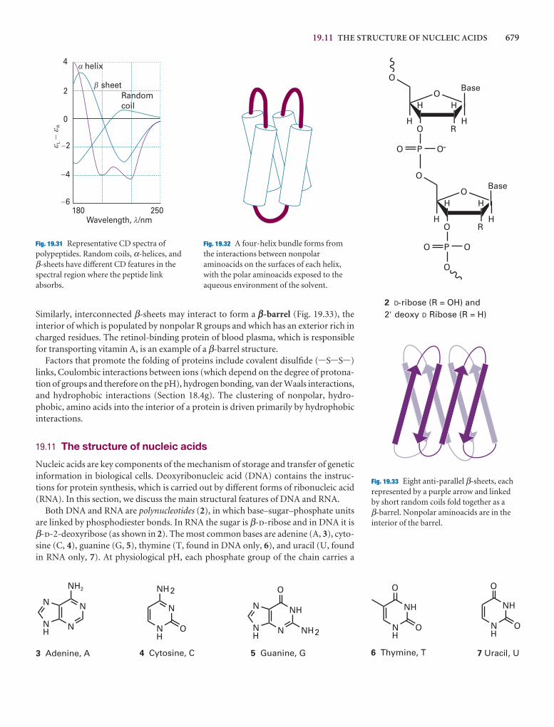
19.11 THE STRUCTURE OF NUCLEIC ACIDS 679
Similarly, interconnected β-sheets may interact to form a b-barrel (Fig. 19.33), the interior of which is populated by nonpolar R groups and which has an exterior rich incharged residues. The retinol-binding protein of blood plasma, which is responsiblefor transporting vitamin A, is an example of a β-barrel structure.
Factors that promote the folding of proteins include covalent disulfide (-S-S-)links, Coulombic interactions between ions (which depend on the degree of protona-tion of groups and therefore on the pH), hydrogen bonding, van der Waals interactions,and hydrophobic interactions (Section 18.4g). The clustering of nonpolar, hydro-phobic, amino acids into the interior of a protein is driven primarily by hydrophobic interactions.
19.11 The structure of nucleic acids
Nucleic acids are key components of the mechanism of storage and transfer of geneticinformation in biological cells. Deoxyribonucleic acid (DNA) contains the instruc-tions for protein synthesis, which is carried out by different forms of ribonucleic acid(RNA). In this section, we discuss the main structural features of DNA and RNA.
Both DNA and RNA are polynucleotides (2), in which base–sugar–phosphate unitsare linked by phosphodiester bonds. In RNA the sugar is β-d-ribose and in DNA it isβ-d-2-deoxyribose (as shown in 2). The most common bases are adenine (A, 3), cyto-sine (C, 4), guanine (G, 5), thymine (T, found in DNA only, 6), and uracil (U, foundin RNA only, 7). At physiological pH, each phosphate group of the chain carries a
Wavelength, /nm
helix
sheetRandomcoil
180 250
LR
-
0
4
2
-2
-4
-6
a
b
ee
l
Fig. 19.31 Representative CD spectra ofpolypeptides. Random coils, α-helices, andβ-sheets have different CD features in thespectral region where the peptide linkabsorbs.
Fig. 19.32 A four-helix bundle forms fromthe interactions between nonpolaraminoacids on the surfaces of each helix,with the polar aminoacids exposed to theaqueous environment of the solvent.
Fig. 19.33 Eight anti-parallel β-sheets, eachrepresented by a purple arrow and linkedby short random coils fold together as a β-barrel. Nonpolar aminoacids are in theinterior of the barrel.
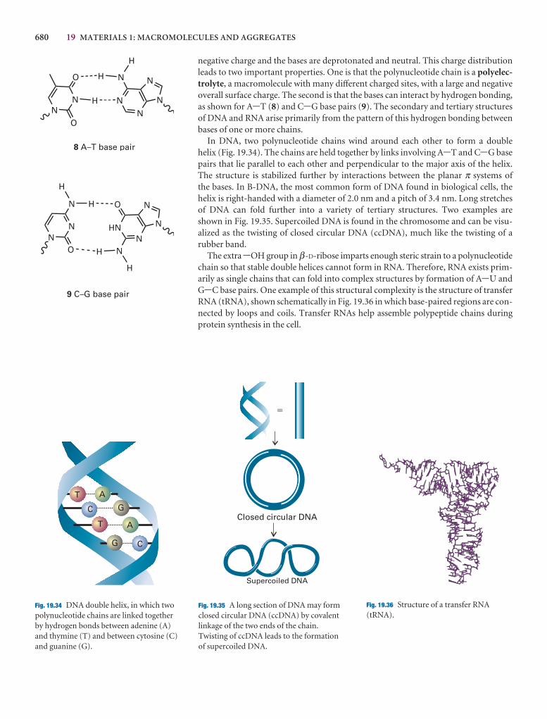
680 19 MATERIALS 1: MACROMOLECULES AND AGGREGATES
negative charge and the bases are deprotonated and neutral. This charge distributionleads to two important properties. One is that the polynucleotide chain is a polyelec-trolyte, a macromolecule with many different charged sites, with a large and negativeoverall surface charge. The second is that the bases can interact by hydrogen bonding,as shown for A-T (8) and C-G base pairs (9). The secondary and tertiary structuresof DNA and RNA arise primarily from the pattern of this hydrogen bonding betweenbases of one or more chains.
In DNA, two polynucleotide chains wind around each other to form a double helix (Fig. 19.34). The chains are held together by links involving A-T and C-G basepairs that lie parallel to each other and perpendicular to the major axis of the helix. The structure is stabilized further by interactions between the planar π systems of the bases. In B-DNA, the most common form of DNA found in biological cells, the helix is right-handed with a diameter of 2.0 nm and a pitch of 3.4 nm. Long stretches of DNA can fold further into a variety of tertiary structures. Two examples are shown in Fig. 19.35. Supercoiled DNA is found in the chromosome and can be visu-alized as the twisting of closed circular DNA (ccDNA), much like the twisting of a rubber band.
The extra -OH group in β-D-ribose imparts enough steric strain to a polynucleotidechain so that stable double helices cannot form in RNA. Therefore, RNA exists prim-arily as single chains that can fold into complex structures by formation of A-U andG-C base pairs. One example of this structural complexity is the structure of transferRNA (tRNA), shown schematically in Fig. 19.36 in which base-paired regions are con-nected by loops and coils. Transfer RNAs help assemble polypeptide chains duringprotein synthesis in the cell.
T A
C G
T A
G C
Fig. 19.34 DNA double helix, in which twopolynucleotide chains are linked togetherby hydrogen bonds between adenine (A)and thymine (T) and between cytosine (C)and guanine (G).
Closed circular DNA
Supercoiled DNA
�
Fig. 19.35 A long section of DNA may formclosed circular DNA (ccDNA) by covalentlinkage of the two ends of the chain.Twisting of ccDNA leads to the formationof supercoiled DNA.
Fig. 19.36 Structure of a transfer RNA(tRNA).
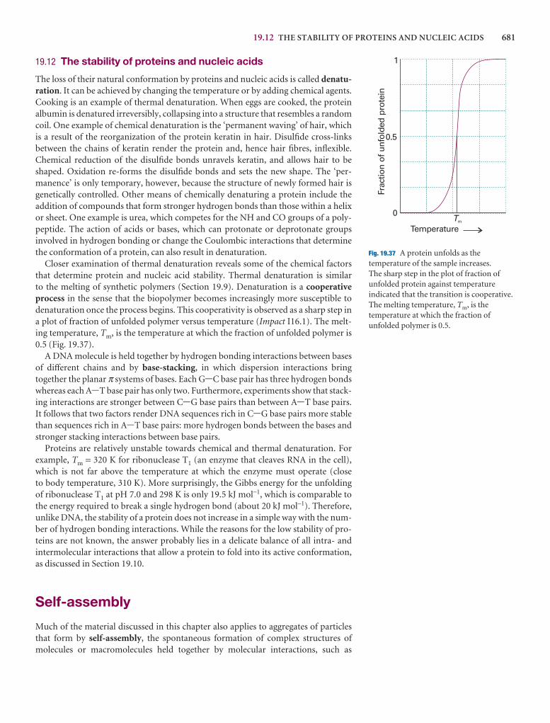
19.12 THE STABILITY OF PROTEINS AND NUCLEIC ACIDS 681
19.12 The stability of proteins and nucleic acids
The loss of their natural conformation by proteins and nucleic acids is called denatu-ration. It can be achieved by changing the temperature or by adding chemical agents.Cooking is an example of thermal denaturation. When eggs are cooked, the proteinalbumin is denatured irreversibly, collapsing into a structure that resembles a randomcoil. One example of chemical denaturation is the ‘permanent waving’ of hair, whichis a result of the reorganization of the protein keratin in hair. Disulfide cross-links between the chains of keratin render the protein and, hence hair fibres, inflexible.Chemical reduction of the disulfide bonds unravels keratin, and allows hair to beshaped. Oxidation re-forms the disulfide bonds and sets the new shape. The ‘per-manence’ is only temporary, however, because the structure of newly formed hair isgenetically controlled. Other means of chemically denaturing a protein include theaddition of compounds that form stronger hydrogen bonds than those within a helixor sheet. One example is urea, which competes for the NH and CO groups of a poly-peptide. The action of acids or bases, which can protonate or deprotonate groups involved in hydrogen bonding or change the Coulombic interactions that determinethe conformation of a protein, can also result in denaturation.
Closer examination of thermal denaturation reveals some of the chemical factorsthat determine protein and nucleic acid stability. Thermal denaturation is similar to the melting of synthetic polymers (Section 19.9). Denaturation is a cooperativeprocess in the sense that the biopolymer becomes increasingly more susceptible to denaturation once the process begins. This cooperativity is observed as a sharp step ina plot of fraction of unfolded polymer versus temperature (Impact I16.1). The melt-ing temperature, Tm, is the temperature at which the fraction of unfolded polymer is0.5 (Fig. 19.37).
A DNA molecule is held together by hydrogen bonding interactions between basesof different chains and by base-stacking, in which dispersion interactions bring together the planar π systems of bases. Each G-C base pair has three hydrogen bondswhereas each A-T base pair has only two. Furthermore, experiments show that stack-ing interactions are stronger between C-G base pairs than between A-T base pairs.It follows that two factors render DNA sequences rich in C-G base pairs more stablethan sequences rich in A-T base pairs: more hydrogen bonds between the bases andstronger stacking interactions between base pairs.
Proteins are relatively unstable towards chemical and thermal denaturation. Forexample, Tm = 320 K for ribonuclease T1 (an enzyme that cleaves RNA in the cell),which is not far above the temperature at which the enzyme must operate (close to body temperature, 310 K). More surprisingly, the Gibbs energy for the unfolding of ribonuclease T1 at pH 7.0 and 298 K is only 19.5 kJ mol−1, which is comparable tothe energy required to break a single hydrogen bond (about 20 kJ mol−1). Therefore,unlike DNA, the stability of a protein does not increase in a simple way with the num-ber of hydrogen bonding interactions. While the reasons for the low stability of pro-teins are not known, the answer probably lies in a delicate balance of all intra- andintermolecular interactions that allow a protein to fold into its active conformation,as discussed in Section 19.10.
Self-assembly
Much of the material discussed in this chapter also applies to aggregates of particlesthat form by self-assembly, the spontaneous formation of complex structures ofmolecules or macromolecules held together by molecular interactions, such as
Temperature
Frac
tion
of
unfo
lded
pro
tein
Tm
0
0.5
1
Fig. 19.37 A protein unfolds as thetemperature of the sample increases. The sharp step in the plot of fraction ofunfolded protein against temperatureindicated that the transition is cooperative.The melting temperature, Tm, is thetemperature at which the fraction ofunfolded polymer is 0.5.
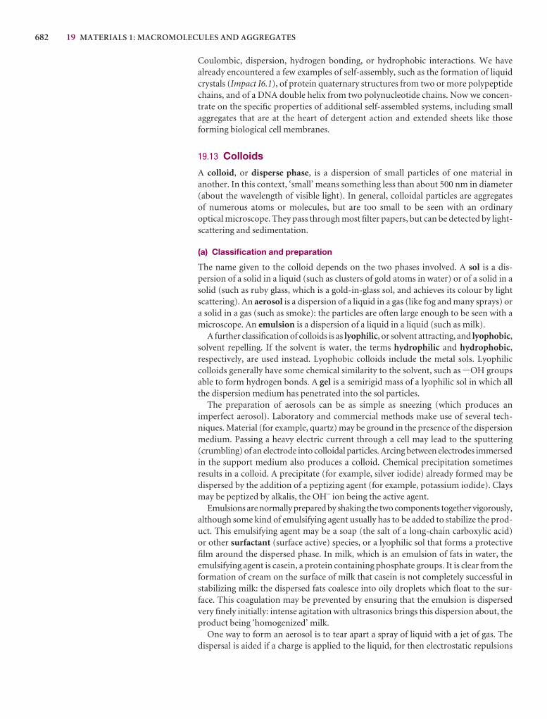
682 19 MATERIALS 1: MACROMOLECULES AND AGGREGATES
Coulombic, dispersion, hydrogen bonding, or hydrophobic interactions. We have already encountered a few examples of self-assembly, such as the formation of liquidcrystals (Impact I6.1), of protein quaternary structures from two or more polypeptidechains, and of a DNA double helix from two polynucleotide chains. Now we concen-trate on the specific properties of additional self-assembled systems, including smallaggregates that are at the heart of detergent action and extended sheets like thoseforming biological cell membranes.
19.13 Colloids
A colloid, or disperse phase, is a dispersion of small particles of one material in another. In this context, ‘small’ means something less than about 500 nm in diameter(about the wavelength of visible light). In general, colloidal particles are aggregates of numerous atoms or molecules, but are too small to be seen with an ordinary optical microscope. They pass through most filter papers, but can be detected by light-scattering and sedimentation.
(a) Classification and preparation
The name given to the colloid depends on the two phases involved. A sol is a dis-persion of a solid in a liquid (such as clusters of gold atoms in water) or of a solid in asolid (such as ruby glass, which is a gold-in-glass sol, and achieves its colour by lightscattering). An aerosol is a dispersion of a liquid in a gas (like fog and many sprays) ora solid in a gas (such as smoke): the particles are often large enough to be seen with amicroscope. An emulsion is a dispersion of a liquid in a liquid (such as milk).
A further classification of colloids is as lyophilic, or solvent attracting, and lyophobic,solvent repelling. If the solvent is water, the terms hydrophilic and hydrophobic,respectively, are used instead. Lyophobic colloids include the metal sols. Lyophiliccolloids generally have some chemical similarity to the solvent, such as -OH groupsable to form hydrogen bonds. A gel is a semirigid mass of a lyophilic sol in which allthe dispersion medium has penetrated into the sol particles.
The preparation of aerosols can be as simple as sneezing (which produces an imperfect aerosol). Laboratory and commercial methods make use of several tech-niques. Material (for example, quartz) may be ground in the presence of the dispersionmedium. Passing a heavy electric current through a cell may lead to the sputtering(crumbling) of an electrode into colloidal particles. Arcing between electrodes immersedin the support medium also produces a colloid. Chemical precipitation sometimes results in a colloid. A precipitate (for example, silver iodide) already formed may bedispersed by the addition of a peptizing agent (for example, potassium iodide). Claysmay be peptized by alkalis, the OH− ion being the active agent.
Emulsions are normally prepared by shaking the two components together vigorously,although some kind of emulsifying agent usually has to be added to stabilize the prod-uct. This emulsifying agent may be a soap (the salt of a long-chain carboxylic acid) or other surfactant (surface active) species, or a lyophilic sol that forms a protectivefilm around the dispersed phase. In milk, which is an emulsion of fats in water, theemulsifying agent is casein, a protein containing phosphate groups. It is clear from theformation of cream on the surface of milk that casein is not completely successful instabilizing milk: the dispersed fats coalesce into oily droplets which float to the sur-face. This coagulation may be prevented by ensuring that the emulsion is dispersedvery finely initially: intense agitation with ultrasonics brings this dispersion about, theproduct being ‘homogenized’ milk.
One way to form an aerosol is to tear apart a spray of liquid with a jet of gas. Thedispersal is aided if a charge is applied to the liquid, for then electrostatic repulsions

19.13 COLLOIDS 683
help to blast it apart into droplets. This procedure may also be used to produce emul-sions, for the charged liquid phase may be directed into another liquid.
Colloids are often purified by dialysis (Impact I5.2). The aim is to remove much (butnot all, for reasons explained later) of the ionic material that may have accompaniedtheir formation. A membrane (for example, cellulose) is selected that is permeable tosolvent and ions, but not to the colloid particles. Dialysis is very slow, and is normallyaccelerated by applying an electric field and making use of the charges carried bymany colloidal particles; the technique is then called electrodialysis.
(b) Structure and stability
Colloids are thermodynamically unstable with respect to the bulk. This instability canbe expressed thermodynamically by noting that because the change in Gibbs energy,dG, when the surface area of the sample changes by dσ at constant temperature andpressure is dG = γdσ, where γ is the interfacial surface tension (Section 18.7a), it follows that dG < 0 if dσ < 0. The survival of colloids must therefore be a consequence of the kinetics of collapse: colloids are thermodynamically unstable but kineticallynonlabile.
At first sight, even the kinetic argument seems to fail: colloidal particles attract eachother over large distances, so there is a long-range force that tends to condense theminto a single blob. The reasoning behind this remark is as follows. The energy of attraction between two individual atoms i and j separated by a distance Rij, one in eachcolloidal particle, varies with their separation as 1/R6
ij (Section 18.4). The sum of allthese pairwise interactions, however, decreases only as approximately 1/R2 (the pre-cise variation depending on the shape of the particles and their closeness), where R isthe separation of the centres of the particles. The sum has a much longer range thanthe 1/R6 dependence characteristic of individual particles and small molecules.
Several factors oppose the long-range dispersion attraction. For example, theremay be a protective film at the surface of the colloid particles that stabilizes the inter-face and cannot be penetrated when two particles touch. Thus the surface atoms of aplatinum sol in water react chemically and are turned into -Pt(OH)3H3, and thislayer encases the particle like a shell. A fat can be emulsified by a soap because the longhydrocarbon tails penetrate the oil droplet but the carboxylate head groups (or otherhydrophilic groups in synthetic detergents) surround the surface, form hydrogenbonds with water, and give rise to a shell of negative charge that repels a possible approach from another similarly charged particle.
(c) The electrical double layer
A major source of kinetic nonlability of colloids is the existence of an electric chargeon the surfaces of the particles. On account of this charge, ions of opposite charge tendto cluster nearby, and an ionic atmosphere is formed, just as for ions (Section 5.9).
We need to distinguish two regions of charge. First, there is a fairly immobile layerof ions that adhere tightly to the surface of the colloidal particle, and which may include water molecules (if that is the support medium). The radius of the sphere thatcaptures this rigid layer is called the radius of shear and is the major factor determin-ing the mobility of the particles. The electric potential at the radius of shear relative toits value in the distant, bulk medium is called the zeta potential, ζ, or the electro-kinetic potential. Second, the charged unit attracts an oppositely charged atmosphereof mobile ions. The inner shell of charge and the outer ionic atmosphere is called theelectrical double layer.
The theory of the stability of lyophobic dispersions was developed by B. Derjaguinand L. Landau and independently by E. Verwey and J.T.G. Overbeek, and is known as
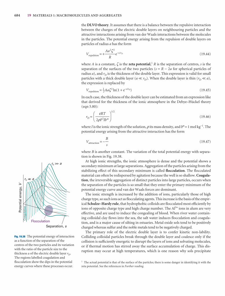
684 19 MATERIALS 1: MACROMOLECULES AND AGGREGATES
the DLVO theory. It assumes that there is a balance between the repulsive interactionbetween the charges of the electric double layers on neighbouring particles and the attractive interactions arising from van der Waals interactions between the moleculesin the particles. The potential energy arising from the repulsion of double layers onparticles of radius a has the form
Vrepulsion = + e−s/rD (19.44)
where A is a constant, ζ is the zeta potential,1 R is the separation of centres, s is the separation of the surfaces of the two particles (s = R − 2a for spherical particles of radius a), and rD is the thickness of the double layer. This expression is valid for smallparticles with a thick double layer (a << rD). When the double layer is thin (rD << a),the expression is replaced by
Vrepulsion = 1–2 Aaζ2 ln(1 + e−s/rD) (19.45)
In each case, the thickness of the double layer can be estimated from an expression likethat derived for the thickness of the ionic atmosphere in the Debye–Hückel theory(eqn 5.80):
rD =1/2
(19.46)
where I is the ionic strength of the solution, ρ its mass density, and b7 = 1 mol kg−1. Thepotential energy arising from the attractive interaction has the form
Vattraction = − (19.47)
where B is another constant. The variation of the total potential energy with separa-tion is shown in Fig. 19.38.
At high ionic strengths, the ionic atmosphere is dense and the potential shows a secondary minimum at large separations. Aggregation of the particles arising from thestabilizing effect of this secondary minimum is called flocculation. The flocculatedmaterial can often be redispersed by agitation because the well is so shallow. Coagula-tion, the irreversible aggregation of distinct particles into large particles, occurs whenthe separation of the particles is so small that they enter the primary minimum of thepotential energy curve and van der Waals forces are dominant.
The ionic strength is increased by the addition of ions, particularly those of highcharge type, so such ions act as flocculating agents. This increase is the basis of the empir-ical Schulze–Hardy rule, that hydrophobic colloids are flocculated most efficiently byions of opposite charge type and high charge number. The Al3+ ions in alum are veryeffective, and are used to induce the congealing of blood. When river water contain-ing colloidal clay flows into the sea, the salt water induces flocculation and coagula-tion, and is a major cause of silting in estuaries. Metal oxide sols tend to be positivelycharged whereas sulfur and the noble metals tend to be negatively charged.
The primary role of the electric double layer is to confer kinetic non-lability.Colliding colloidal particles break through the double layer and coalesce only if thecollision is sufficiently energetic to disrupt the layers of ions and solvating molecules,or if thermal motion has stirred away the surface accumulation of charge. This dis-ruption may occur at high temperatures, which is one reason why sols precipitate
B
s
DF
εRT
2ρF2Ib 7
AC
Aa2ζ2
R
1 The actual potential is that of the surface of the particles; there is some danger in identifying it with thezeta potential. See the references in Further reading.
r aD <<
r aD >>
Pote
ntia
l ene
rgy,
VC
oagu
latio
n
FlocculationSeparation, s
Fig. 19.38 The potential energy of interactionas a function of the separation of thecentres of the two particles and its variationwith the ratio of the particle size to thethickness a of the electric double layer rD.The regions labelled coagulation andflocculation show the dips in the potentialenergy curves where these processes occur.
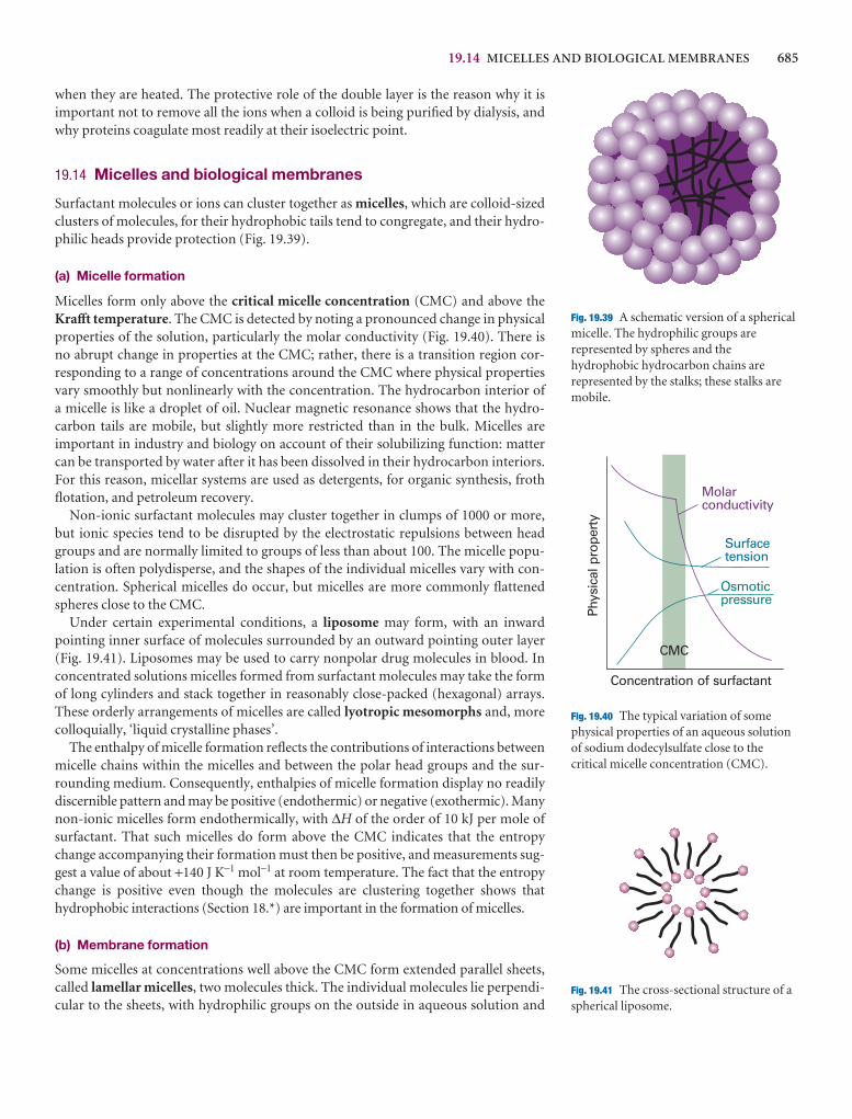
19.14 MICELLES AND BIOLOGICAL MEMBRANES 685
when they are heated. The protective role of the double layer is the reason why it is important not to remove all the ions when a colloid is being purified by dialysis, andwhy proteins coagulate most readily at their isoelectric point.
19.14 Micelles and biological membranes
Surfactant molecules or ions can cluster together as micelles, which are colloid-sizedclusters of molecules, for their hydrophobic tails tend to congregate, and their hydro-philic heads provide protection (Fig. 19.39).
(a) Micelle formation
Micelles form only above the critical micelle concentration (CMC) and above theKrafft temperature. The CMC is detected by noting a pronounced change in physicalproperties of the solution, particularly the molar conductivity (Fig. 19.40). There is no abrupt change in properties at the CMC; rather, there is a transition region cor-responding to a range of concentrations around the CMC where physical propertiesvary smoothly but nonlinearly with the concentration. The hydrocarbon interior of a micelle is like a droplet of oil. Nuclear magnetic resonance shows that the hydro-carbon tails are mobile, but slightly more restricted than in the bulk. Micelles are important in industry and biology on account of their solubilizing function: mattercan be transported by water after it has been dissolved in their hydrocarbon interiors.For this reason, micellar systems are used as detergents, for organic synthesis, frothflotation, and petroleum recovery.
Non-ionic surfactant molecules may cluster together in clumps of 1000 or more,but ionic species tend to be disrupted by the electrostatic repulsions between headgroups and are normally limited to groups of less than about 100. The micelle popu-lation is often polydisperse, and the shapes of the individual micelles vary with con-centration. Spherical micelles do occur, but micelles are more commonly flattenedspheres close to the CMC.
Under certain experimental conditions, a liposome may form, with an inwardpointing inner surface of molecules surrounded by an outward pointing outer layer(Fig. 19.41). Liposomes may be used to carry nonpolar drug molecules in blood. Inconcentrated solutions micelles formed from surfactant molecules may take the formof long cylinders and stack together in reasonably close-packed (hexagonal) arrays.These orderly arrangements of micelles are called lyotropic mesomorphs and, morecolloquially, ‘liquid crystalline phases’.
The enthalpy of micelle formation reflects the contributions of interactions betweenmicelle chains within the micelles and between the polar head groups and the sur-rounding medium. Consequently, enthalpies of micelle formation display no readilydiscernible pattern and may be positive (endothermic) or negative (exothermic). Manynon-ionic micelles form endothermically, with ∆H of the order of 10 kJ per mole ofsurfactant. That such micelles do form above the CMC indicates that the entropychange accompanying their formation must then be positive, and measurements sug-gest a value of about +140 J K−1 mol−1 at room temperature. The fact that the entropychange is positive even though the molecules are clustering together shows thathydrophobic interactions (Section 18.*) are important in the formation of micelles.
(b) Membrane formation
Some micelles at concentrations well above the CMC form extended parallel sheets,called lamellar micelles, two molecules thick. The individual molecules lie perpendi-cular to the sheets, with hydrophilic groups on the outside in aqueous solution and
Fig. 19.39 A schematic version of a sphericalmicelle. The hydrophilic groups arerepresented by spheres and thehydrophobic hydrocarbon chains arerepresented by the stalks; these stalks aremobile.
Concentration of surfactant
CMC
Molarconductivity
Surfacetension
Osmoticpressure
Phys
ical
pro
pert
y
Fig. 19.40 The typical variation of somephysical properties of an aqueous solutionof sodium dodecylsulfate close to thecritical micelle concentration (CMC).
Fig. 19.41 The cross-sectional structure of aspherical liposome.
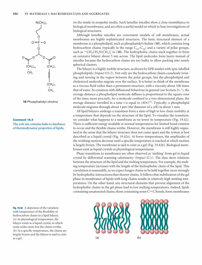
686 19 MATERIALS 1: MACROMOLECULES AND AGGREGATES
on the inside in nonpolar media. Such lamellar micelles show a close resemblance tobiological membranes, and are often a useful model on which to base investigations ofbiological structures.
Although lamellar micelles are convenient models of cell membranes, actual membranes are highly sophisticated structures. The basic structural element of amembrane is a phospholipid, such as phosphatidyl choline (10), which contains longhydrocarbon chains (typically in the range C14–C24) and a variety of polar groups,such as -CH2CH2N(CH3)3
+ in (10). The hydrophobic chains stack together to forman extensive bilayer about 5 nm across. The lipid molecules form layers instead of micelles because the hydrocarbon chains are too bulky to allow packing into nearlyspherical clusters.
The bilayer is a highly mobile structure, as shown by EPR studies with spin-labelledphospholipids (Impact I15.2). Not only are the hydrocarbon chains ceaselessly twist-ing and turning in the region between the polar groups, but the phospholipid andcholesterol molecules migrate over the surface. It is better to think of the membraneas a viscous fluid rather than a permanent structure, with a viscosity about 100 timesthat of water. In common with diffusional behaviour in general (see Section 21.*), theaverage distance a phospholipid molecule diffuses is proportional to the square-rootof the time; more precisely, for a molecule confined to a two-dimensional plane, theaverage distance travelled in a time t is equal to (4Dt)1/2. Typically, a phospholipidmolecule migrates through about 1 µm (the diameter of a cell) in about 1 min.
All lipid bilayers undergo a transition from a state of high to low chain mobility ata temperature that depends on the structure of the lipid. To visualize the transition,we consider what happens to a membrane as we lower its temperature (Fig. 19.42).There is sufficient energy available at normal temperatures for limited bond rotationto occur and the flexible chains writhe. However, the membrane is still highly organ-ized in the sense that the bilayer structure does not come apart and the system is bestdescribed as a liquid crystal (Fig. 19.42a). At lower temperatures, the amplitudes ofthe writhing motion decrease until a specific temperature is reached at which motionis largely frozen. The membrane is said to exist as a gel (Fig. 19.42b). Biological mem-branes exist as liquid crystals at physiological temperatures.
Phase transitions in membranes are often observed as ‘melting’ from gel to liquidcrystal by differential scanning calorimetry (Impact I2.1). The data show relations between the structure of the lipid and the melting temperature. For example, the melt-ing temperature increases with the length of the hydrophobic chain of the lipid. Thiscorrelation is reasonable, as we expect longer chains to be held together more stronglyby hydrophobic interactions than shorter chains. It follows that stabilization of the gelphase in membranes of lipids with long chains results in relatively high melting tem-peratures. On the other hand, any structural elements that prevent alignment of thehydrophobic chains in the gel phase lead to low melting temperatures. Indeed, lipidscontaining unsaturated chains, those containing some C=C bonds, form membranes
Comment 19.4
The web site contains links to databasesof thermodynamic properties of lipids.
(b)(a)
Fig. 19.42 A depiction of the variation with temperature of the flexibility ofhydrocarbon chains in a lipid bilayer. (a) At physiological temperature, thebilayer exists as a liquid crystal, in whichsome order exists but the chains writhe. (b) At a specific temperature, the chains arelargely frozen and the bilayer is said to existas a gel.
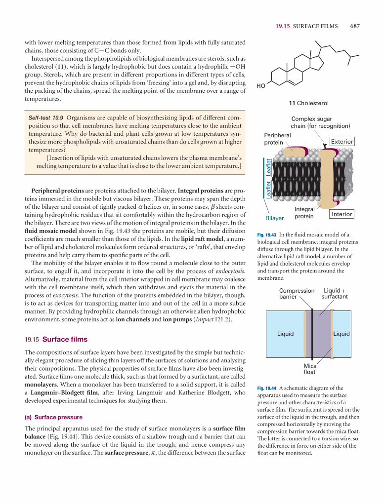
19.15 SURFACE FILMS 687
Bilayer
Leaf
let
Leaf
let
Complex sugarchain (for recognition)
Peripheralprotein
Integralprotein
Exterior
Interior
Fig. 19.43 In the fluid mosaic model of abiological cell membrane, integral proteinsdiffuse through the lipid bilayer. In thealternative lipid raft model, a number oflipid and cholesterol molecules envelopand transport the protein around themembrane.
Compressionbarrier
Micafloat
Liquid +surfactant
Liquid Liquid
Fig. 19.44 A schematic diagram of theapparatus used to measure the surfacepressure and other characteristics of asurface film. The surfactant is spread on thesurface of the liquid in the trough, and thencompressed horizontally by moving thecompression barrier towards the mica float.The latter is connected to a torsion wire, sothe difference in force on either side of thefloat can be monitored.
with lower melting temperatures than those formed from lipids with fully saturatedchains, those consisting of C-C bonds only.
Interspersed among the phospholipids of biological membranes are sterols, such ascholesterol (11), which is largely hydrophobic but does contain a hydrophilic -OHgroup. Sterols, which are present in different proportions in different types of cells,prevent the hydrophobic chains of lipids from ‘freezing’ into a gel and, by disruptingthe packing of the chains, spread the melting point of the membrane over a range oftemperatures.
Self-test 19.9 Organisms are capable of biosynthesizing lipids of different com-position so that cell membranes have melting temperatures close to the ambienttemperature. Why do bacterial and plant cells grown at low temperatures syn-thesize more phospholipids with unsaturated chains than do cells grown at highertemperatures?
[Insertion of lipids with unsaturated chains lowers the plasma membrane’s melting temperature to a value that is close to the lower ambient temperature.]
Peripheral proteins are proteins attached to the bilayer. Integral proteins are pro-teins immersed in the mobile but viscous bilayer. These proteins may span the depthof the bilayer and consist of tightly packed α helices or, in some cases, β sheets con-taining hydrophobic residues that sit comfortably within the hydrocarbon region ofthe bilayer. There are two views of the motion of integral proteins in the bilayer. In thefluid mosaic model shown in Fig. 19.43 the proteins are mobile, but their diffusioncoefficients are much smaller than those of the lipids. In the lipid raft model, a num-ber of lipid and cholesterol molecules form ordered structures, or ‘rafts’, that envelopproteins and help carry them to specific parts of the cell.
The mobility of the bilayer enables it to flow round a molecule close to the outersurface, to engulf it, and incorporate it into the cell by the process of endocytosis.Alternatively, material from the cell interior wrapped in cell membrane may coalescewith the cell membrane itself, which then withdraws and ejects the material in theprocess of exocytosis. The function of the proteins embedded in the bilayer, though, is to act as devices for transporting matter into and out of the cell in a more subtlemanner. By providing hydrophilic channels through an otherwise alien hydrophobic environment, some proteins act as ion channels and ion pumps (Impact I21.2).
19.15 Surface films
The compositions of surface layers have been investigated by the simple but technic-ally elegant procedure of slicing thin layers off the surfaces of solutions and analysingtheir compositions. The physical properties of surface films have also been investig-ated. Surface films one molecule thick, such as that formed by a surfactant, are calledmonolayers. When a monolayer has been transferred to a solid support, it is called a Langmuir–Blodgett film, after Irving Langmuir and Katherine Blodgett, who developed experimental techniques for studying them.
(a) Surface pressure
The principal apparatus used for the study of surface monolayers is a surface film balance (Fig. 19.44). This device consists of a shallow trough and a barrier that can be moved along the surface of the liquid in the trough, and hence compress anymonolayer on the surface. The surface pressure, π , the difference between the surface
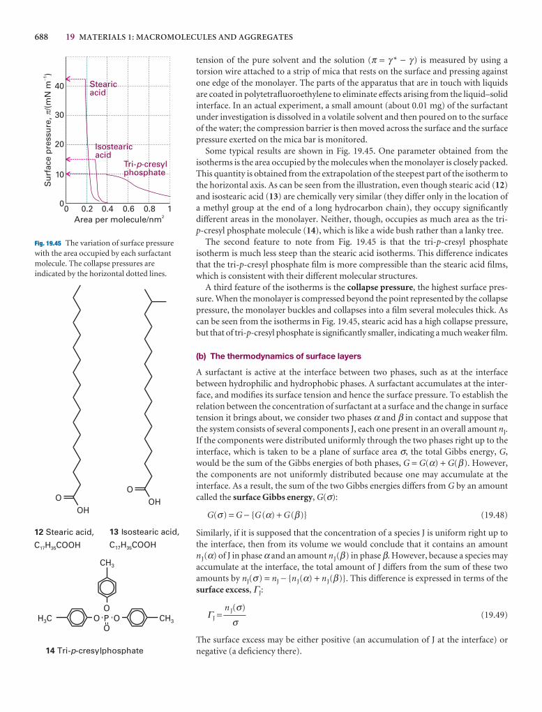
688 19 MATERIALS 1: MACROMOLECULES AND AGGREGATES
40
30
20
10
00 0.2 0.4 0.6 0.8 1
Su
rfac
e p
ress
ure
, /(
mN
m)
-1
Area per molecule/nm2
Stearicacid
Isostearicacid
Tri- -cresylphosphate
p
p
tension of the pure solvent and the solution (π = γ * − γ ) is measured by using a torsion wire attached to a strip of mica that rests on the surface and pressing againstone edge of the monolayer. The parts of the apparatus that are in touch with liquidsare coated in polytetrafluoroethylene to eliminate effects arising from the liquid–solidinterface. In an actual experiment, a small amount (about 0.01 mg) of the surfactantunder investigation is dissolved in a volatile solvent and then poured on to the surfaceof the water; the compression barrier is then moved across the surface and the surfacepressure exerted on the mica bar is monitored.
Some typical results are shown in Fig. 19.45. One parameter obtained from theisotherms is the area occupied by the molecules when the monolayer is closely packed.This quantity is obtained from the extrapolation of the steepest part of the isotherm tothe horizontal axis. As can be seen from the illustration, even though stearic acid (12)and isostearic acid (13) are chemically very similar (they differ only in the location ofa methyl group at the end of a long hydrocarbon chain), they occupy significantlydifferent areas in the monolayer. Neither, though, occupies as much area as the tri-p-cresyl phosphate molecule (14), which is like a wide bush rather than a lanky tree.
The second feature to note from Fig. 19.45 is that the tri-p-cresyl phosphateisotherm is much less steep than the stearic acid isotherms. This difference indicatesthat the tri-p-cresyl phosphate film is more compressible than the stearic acid films,which is consistent with their different molecular structures.
A third feature of the isotherms is the collapse pressure, the highest surface pres-sure. When the monolayer is compressed beyond the point represented by the collapsepressure, the monolayer buckles and collapses into a film several molecules thick. Ascan be seen from the isotherms in Fig. 19.45, stearic acid has a high collapse pressure,but that of tri-p-cresyl phosphate is significantly smaller, indicating a much weaker film.
(b) The thermodynamics of surface layers
A surfactant is active at the interface between two phases, such as at the interface between hydrophilic and hydrophobic phases. A surfactant accumulates at the inter-face, and modifies its surface tension and hence the surface pressure. To establish therelation between the concentration of surfactant at a surface and the change in surfacetension it brings about, we consider two phases α and β in contact and suppose thatthe system consists of several components J, each one present in an overall amount nJ.If the components were distributed uniformly through the two phases right up to theinterface, which is taken to be a plane of surface area σ, the total Gibbs energy, G,would be the sum of the Gibbs energies of both phases, G = G(α) + G(β). However,the components are not uniformly distributed because one may accumulate at the interface. As a result, the sum of the two Gibbs energies differs from G by an amountcalled the surface Gibbs energy, G(σ):
G(σ) = G − {G(α) + G(β)} (19.48)
Similarly, if it is supposed that the concentration of a species J is uniform right up tothe interface, then from its volume we would conclude that it contains an amountnJ(α) of J in phase α and an amount nJ(β) in phase β. However, because a species mayaccumulate at the interface, the total amount of J differs from the sum of these twoamounts by nJ(σ) = nJ − {nJ(α) + nJ(β)}. This difference is expressed in terms of thesurface excess, ΓJ:
ΓJ = (19.49)
The surface excess may be either positive (an accumulation of J at the interface) ornegative (a deficiency there).
n J(σ)
σ
Fig. 19.45 The variation of surface pressurewith the area occupied by each surfactantmolecule. The collapse pressures areindicated by the horizontal dotted lines.
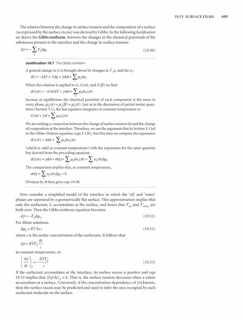
19.15 SURFACE FILMS 689
The relation between the change in surface tension and the composition of a surface(as expressed by the surface excess) was derived by Gibbs. In the following Justificationwe derive the Gibbs isotherm, between the changes in the chemical potentials of thesubstances present in the interface and the change in surface tension:
dγ = − ∑J
ΓJdµJ (19.50)
Justification 19.7 The Gibbs isotherm
A general change in G is brought about by changes in T, p, and the nJ:
dG = −SdT + Vdp + γ dσ + ∑J
µJdnJ
When this relation is applied to G, G(α), and G(β) we find
dG(σ) = −S(σ)dT + γ dσ + ∑J
µJdnJ(σ)
because at equilibrium the chemical potential of each component is the same inevery phase, µJ(α) = µJ(β) = µJ(σ). Just as in the discussion of partial molar quan-tities (Section 5.1), the last equation integrates at constant temperature to
G(σ) = γ σ + ∑J
µJnJ(σ)
We are seeking a connection between the change of surface tension dγ and the changeof composition at the interface. Therefore, we use the argument that in Section 5.1 ledto the Gibbs–Duhem equation (eqn 5.12b), but this time we compare the expression
dG(σ) = γdσ + ∑J
µJdnJ(σ)
(which is valid at constant temperature) with the expression for the same quantitybut derived from the preceding equation:
dG(σ) = γdσ + σdγ + ∑J
µJdnJ(σ) + ∑J
nJ(σ)dµJ
The comparison implies that, at constant temperature,
σdγ + ∑J
nJ(σ)dµJ = 0
Division by σ then gives eqn 19.50.
Now consider a simplified model of the interface in which the ‘oil’ and ‘water’phases are separated by a geometrically flat surface. This approximation implies thatonly the surfactant, S, accumulates at the surface, and hence that Γoil and Γwater areboth zero. Then the Gibbs isotherm equation becomes
dγ = −ΓSdµS (19.51)
For dilute solutions,
dµS = RT ln c (19.52)
where c is the molar concentration of the surfactant. It follows that
dγ = RTΓS
at constant temperature, or
T
= − (19.53)
If the surfactant accumulates at the interface, its surface excess is positive and eqn19.53 implies that (∂γ /∂c)T < 0. That is, the surface tension decreases when a solute accumulates at a surface. Conversely, if the concentration dependence of γ is known,then the surface excess may be predicted and used to infer the area occupied by eachsurfactant molecule on the surface.
RTΓS
c
DF
∂γ∂c
AC
dc
c
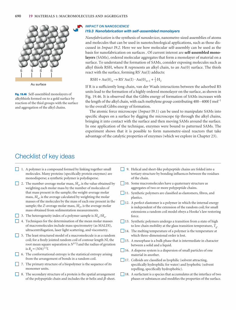
690 19 MATERIALS 1: MACROMOLECULES AND AGGREGATES
IMPACT ON NANOSCIENCE
I19.3 Nanofabrication with self-assembled monolayers
Nanofabrication is the synthesis of nanodevices, nanometre-sized assemblies of atomsand molecules that can be used in nanotechnological applications, such as those dis-cussed in Impact I9.2. Here we see how molecular self-assembly can be used as thebasis for nanofabrication on surfaces . Of current interest are self-assembled mono-layers (SAMs), ordered molecular aggregates that form a monolayer of material on asurface. To understand the formation of SAMs, consider exposing molecules such asalkyl thiols RSH, where R represents an alkyl chain, to an Au(0) surface. The thiolsreact with the surface, forming RS−Au(I) adducts:
RSH + Au(0)n → RS−Au(I) · Au(0)n−1 + 1–2 H2
If R is a sufficiently long chain, van der Waals interactions between the adsorbed RSunits lead to the formation of a highly ordered monolayer on the surface, as shown inFig. 19.46. It is observed that the Gibbs energy of formation of SAMs increases withthe length of the alkyl chain, with each methylene group contributing 400–4000 J mol−1
to the overall Gibbs energy of formation.The atomic force microscope (Impact I9.1) can be used to manipulate SAMs into
specific shapes on a surface by digging the microscope tip through the alkyl chains,bringing it into contact with the surface and then moving SAMs around the surface.In one application of the technique, enzymes were bound to patterned SAMs. The experiment shows that it is possible to form nanometre-sized reactors that take advantage of the catalytic properties of enzymes (which we explore in Chapter 23).
S S S S
Au surface
Fig. 19.46 Self-assembled monolayers ofalkylthiols formed on to a gold surface byreaction of the thiol groups with the surfaceand aggregation of the alkyl chains.
Checklist of key ideas
1. A polymer is a compound formed by linking together smallmolecules. Many proteins (specifically protein enzymes) aremonodisperse; a synthetic polymer is polydisperse.
2. The number-average molar mass, Jn, is the value obtained byweighting each molar mass by the number of molecules ofthat mass present in the sample; the weight-average molarmass, Jw, is the average calculated by weighting the molarmasses of the molecules by the mass of each one present in thesample; the Z-average molar mass, JZ, is the average molarmass obtained from sedimentation measurements.
3. The heterogeneity index of a polymer sample is Jw /Jn.
4. Techniques for the determination of the mean molar massesof macromolecules include mass spectrometry (as MALDI),ultracentrifugation, laser light scattering, and viscometry.
5. The least structured model of a macromolecule is as a randomcoil; for a freely jointed random coil of contour length Nl, theroot mean square separation is N1/2l and the radius of gyrationis Rg = (N/6)1/2l.
6. The conformational entropy is the statistical entropy arisingfrom the arrangement of bonds in a random coil.
7. The primary structure of a biopolymer is the sequence of itsmonomer units.
8. The secondary structure of a protein is the spatial arrangementof the polypeptide chain and includes the α-helix and β-sheet.
9. Helical and sheet-like polypeptide chains are folded into atertiary structure by bonding influences between the residuesof the chain.
10. Some macromolecules have a quaternary structure asaggregates of two or more polypeptide chains.
11. Synthetic polymers are classified as elastomers, fibres, andplastics.
12. A perfect elastomer is a polymer in which the internal energyis independent of the extension of the random coil; for smallextensions a random coil model obeys a Hooke’s law restoringforce.
13. Synthetic polymers undergo a transition from a state of highto low chain mobility at the glass transition temperature, Tg.
14. The melting temperature of a polymer is the temperature atwhich three-dimensional order is lost.
15. A mesophase is a bulk phase that is intermediate in characterbetween a solid and a liquid.
16. A disperse system is a dispersion of small particles of onematerial in another.
17. Colloids are classified as lyophilic (solvent attracting,specifically hydrophilic for water) and lyophobic (solventrepelling, specifically hydrophobic).
18. A surfactant is a species that accumulates at the interface of twophases or substances and modifies the properties of the surface.

FURTHER INFORMATION 691
19. The radius of shear is the radius of the sphere that captures therigid layer of charge attached to a colloid particle.
20. The zeta potential is the electric potential at the radius of shearrelative to its value in the distant, bulk medium.
21. The inner shell of charge and the outer atmosphere jointlyconstitute the electric double layer.
22. Many colloid particles are thermodynamically unstable butkinetically non-labile.
23. Flocculation is the reversible aggregation of colloidal particles;coagulation is the irreversible aggregation of colloidalparticles.
24. The Schultze–Hardy rule states that hydrophobic colloids areflocculated most efficiently by ions of opposite charge typeand high charge number.
25. A micelle is a colloid-sized cluster of molecules that forms atthe critical micelle concentration (CMC) and at the Kraffttemperature.
26. A liposome is a vesicle with an inward pointing inner surfaceof molecules surrounded by an outward pointing outer layer.
27. A lamellar micelle is an extended layer of molecules twomolecules thick.
28. A monolayer, a single layer of molecules on a surface. ALangmuir–Blodgett film is a monolayer that has beentransferred to a solid support.
29. Surface pressure is the difference between the surface tensionof the pure solvent and the solution: π = γ * − γ.
30. The collapse pressure is the highest surface pressure sustainedby a surface film.
Further reading
Articles and texts
A.W. Adamson and A.P. Gast, Physical chemistry of surfaces. Wiley,New York (1997).
J. Barker, Mass spectrometry. Wiley, New York (1999).
C.E. Carraher, Jr., Seymour/Carraher’s polymer chemistry, MarcelDekker (2000).
D.F. Evans and H. Wennerström, The colloidal domain : wherephysics, chemistry, biology, and technology meet. Wiley-VCH, New York (1999).
P. Flory, Principles of polymer chemistry. Cornell University Press,Ithaca (1953).
C.S. Johnson and D.A. Gabriel, Laser light scattering. Dover, New York (1995).
A.R. Leach, Molecular modelling: principles and applications.Longman, Harlow (1997).
K.E. van Holde, W.C. Johnson, and P.S. Ho, Principles of physicalbiochemistry. Prentice Hall, Upper Saddle River (1998).
P.C. Heimenz and R. Rajagopalan, Principles of colloid and surfacechemistry. Marcel Dekker, New York (1997).
Sources of data and information
D.R. Lide (ed.), CRC Handbook of Chemistry and Physics, Sections 7and 13. CRC Press, Boca Raton (2000).
Further information
Further information 19.1 The Rayleigh ratio
Here we outline the key steps in the derivation of eqn 19.8 for theRayleigh ratio. You are encouraged to consult sources in the Furtherreading section for additional details.
The ratio of the intensity of the light scattered by a sample to theintensity of the incident light is (see Further reading):
= (19.54)
where r is the distance between the sample and the detector and φ isthe angle of observation relative to the z-axis (φ = 90° in Fig. 19.3). It follows from eqn 19.7 that
Rθ =π2α2
ε2rλ4
sin2φr 2
π2α2
ε2rλ4
I
I0
The relation between the polarizability and the refractive index, nr,of a solution is (see Appendix 3 for a qualitative explanation andFurther reading for quantitative details)
n2r − n2
r,0 = (19.55)
where nr,0 is the refractive index of the solvent and N is the numberdensity of polymer molecules. Because N = cP NA/M (where cP is themass concentration of the polymer and M is its molar mass), we have:
α = (n2r − n2
r,0)
For a dilute solution, nr differs little from nr,0 and we can write:
nr = nr,0 + cP + · · ·DEF
dnr
dcP
ABC
εr M
cP NA
N αεr
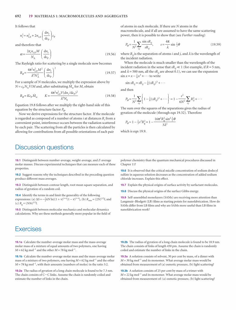
692 19 MATERIALS 1: MACROMOLECULES AND AGGREGATES
It follows that
n2r ≈ n2
r,0 + 2nr,0 cP
and therefore that
α = (19.56)
The Rayleigh ratio for scattering by a single molecule now becomes
Rθ =2
(19.57)
For a sample of N molecules, we multiply the expression above by N = cP NAV/M and, after substituting Jw for M, obtain
Rθ = KcP Jw K = (19.58)
Equation 19.8 follows after we multiply the right-hand side of thisequation by the structure factor Pθ .
Now we derive expressions for the structure factor. If the moleculeis regarded as composed of a number of atoms i at distances Ri from aconvenient point, interference occurs between the radiation scatteredby each pair. The scattering from all the particles is then calculated byallowing for contributions from all possible orientations of each pair
4π2n2r,0V(dnr /dcP)2
λ4NA
DEFdnr
dcP
ABC4π2n2
r,0 M 2
λ4N 2A
DEFdnr
dcP
ABC2εrnr,0 M
NA
DEFdnr
dcP
ABC
of atoms in each molecule. If there are N atoms in themacromolecule, and if all are assumed to have the same scatteringpower, then it is possible to show that (see Further reading)
Pθ = ∑i,j
, s = sin 1–2θ (19.59)
where Rij is the separation of atoms i and j, and λ is the wavelength ofthe incident radiation.
When the molecule is much smaller than the wavelength of theincident radiation in the sense that sRij << 1 (for example, if R = 5 nm,and λ = 500 nm, all the sRij are about 0.1), we can use the expansionsin x = x − 1–6 x3 + · · · to write
sin sRij = sRij − 1–6 (sRij)3 + · · ·
and then
Pθ = ∑i,j
1 − 1–6 (sRij)2 + · · · = 1 − ∑
i,j
R2ij + · · ·
The sum over the squares of the separations gives the radius ofgyration of the molecule (through eqn 19.32). Therefore
Pθ ≈ 1 − 1–3 s2R2g = 1 −
which is eqn 19.9.
16π2R2g sin2 1–2 θ
3λ2
s2
6N2
567123
1
N2
4πλ
sin sRij
sRij
1
N2
Discussion questions
19.1 Distinguish between number-average, weight-average, and Z-averagemolar masses. Discuss experimental techniques that can measure each of theseproperties.
19.2 Suggest reasons why the techniques described in the preceding questionproduce different mass averages.
19.3 Distinguish between contour length, root mean square separation, andradius of gyration of a random coil.
19.4 Identify the terms in and limit the generality of the followingexpressions: (a) ∆S = − 1–
2 kN ln{(1 + ν)1+ν(1 − ν)1−ν}, (b) Rrms = (2N)1/2l, and (c) Rg = (N/6)1/2l.
19.5 Distinguish between molecular mechanics and molecular dynamicscalculations. Why are these methods generally more popular in the field of
polymer chemistry than the quantum mechanical procedures discussed inChapter 11?
19.6 It is observed that the critical micelle concentration of sodium dodecylsulfate in aqueous solution decreases as the concentration of added sodiumchloride increases. Explain this effect.
19.7 Explain the physical origins of surface activity by surfactant molecules.
19.8 Discuss the physical origins of the surface Gibbs energy.
19.9 Self-assembled monolayers (SAMs) are receiving more attention thanLangmuir–Blodgett (LB) films as starting points for nanofabrication. How doSAMs differ from LB films and why are SAMs more useful than LB films innanofabrication work?
Exercises
19.1a Calculate the number-average molar mass and the mass-average molar mass of a mixture of equal amounts of two polymers, one having M = 62 kg mol−1 and the other M = 78 kg mol−1.
19.1b Calculate the number-average molar mass and the mass-average molarmass of a mixture of two polymers, one having M = 62 kg mol−1 and the otherM = 78 kg mol−1, with their amounts (numbers of moles) in the ratio 3:2.
19.2a The radius of gyration of a long chain molecule is found to be 7.3 nm.The chain consists of C-C links. Assume the chain is randomly coiled andestimate the number of links in the chain.
19.2b The radius of gyration of a long chain molecule is found to be 18.9 nm.The chain consists of links of length 450 pm. Assume the chain is randomlycoiled and estimate the number of links in the chain.
19.3a A solution consists of solvent, 30 per cent by mass, of a dimer with M = 30 kg mol−1 and its monomer. What average molar mass would beobtained from measurement of (a) osmotic pressure, (b) light scattering?
19.3b A solution consists of 25 per cent by mass of a trimer with M = 22 kg mol−1 and its monomer. What average molar mass would beobtained from measurement of: (a) osmotic pressure, (b) light scattering?

PROBLEMS 693
19.4a Evaluate the rotational correlation time, τR = 4πa3η/3kT, for serumalbumin in water at 25°C on the basis that it is a sphere of radius 3.0 nm. What is the value for a CCl4 molecule in carbon tetrachloride at 25°C?(Viscosity data in Table 21.4 in the Data section at the end of this volume; take a(CCl4) = 250 pm.)
19.4b Evaluate the rotational correlation time, τR = 4πa3η/3kT, for a syntheticpolymer in water at 20°C on the basis that it is a sphere of radius 4.5 nm.
19.5a What is the relative rate of sedimentation for two spherical particles ofthe same density, but which differ in radius by a factor of 10?
19.5b What is the relative rate of sedimentation for two spherical particleswith densities 1.10 g cm−3 and 1.18 g cm−3 and which differ in radius by afactor of 8.4, the former being the larger? Use ρ = 0.794 g cm−3 for the densityof the solution.
19.6a Human haemoglobin has a specific volume of 0.749 × 10⁻³ m3 kg−1,a sedimentation constant of 4.48 Sv, and a diffusion coefficient of 6.9 × 10⁻¹¹ m2 s−1. Determine its molar mass from this information.
19.6b A synthetic polymer has a specific volume of 8.01 × 10⁻⁴ m3 kg−1,a sedimentation constant of 7.46 Sv, and a diffusion coefficient of 7.72 × 10⁻¹¹ m2 s−1. Determine its molar mass from this information.
19.7a Find the drift speed of a particle of radius 20 µm and density 1750 kg m−3 which is settling from suspension in water (density 1000 kg m−3) under the influence of gravity alone. The viscosity of water is 8.9 × 10⁻⁴ kg m−1 s−1.
19.7b Find the drift speed of a particle of radius 15.5 µm and density 1250 kg m−3 which is settling from suspension in water (density 1000 kg m−3) under the influence of gravity alone. The viscosity of water is 8.9 × 10⁻⁴ kg m−1 s−1.
19.8a At 20°C the diffusion coefficient of a macromolecule is found to be 8.3 × 10⁻¹¹ m2 s−1. Its sedimentation constant is 3.2 Sv in a solution of density1.06 g cm−3. The specific volume of the macromolecule is 0.656 cm3 g−1.Determine the molar mass of the macromolecule.
19.8b At 20°C the diffusion coefficient of a macromolecule is found to be7.9 × 10−11 m2 s−1. Its sedimentation constant is 5.1 Sv in a solution of density997 kg m−3. The specific volume of the macromolecule is 0.721 cm3 g−1.Determine the molar mass of the macromolecule.
19.9a The data from a sedimentation equilibrium experiment performed at300 K on a macromolecular solute in aqueous solution show that a graph of ln c against r 2 is a straight line with a slope of 729 cm−2. The rotational rate of the centrifuge was 50 000 r.p.m. The specific volume of the solute is 0.61 cm3 g−1. Calculate the molar mass of the solute.
19.9b The data from a sedimentation equilibrium experiment performed at293 K on a macromolecular solute in aqueous solution show that a graph of ln c against (r/cm)2 is a straight line with a slope of 821. The rotation rate ofthe centrifuge was 1080 Hz. The specific volume of the solute is 7.2 ×10⁻⁴ m3 kg−1. Calculate the molar mass of the solute.
19.10a Calculate the radial acceleration (as so many g) in a cell placed at 6.0 cm from the centre of rotation in an ultracentrifuge operating at 80 000 r.p.m.
19.10b Calculate the radial acceleration (as so many g) in a cell placed at 5.50 cmfrom the centre of rotation in an ultracentrifuge operating at 1.32 kHz.
19.11a A polymer chain consists of 700 segments, each 0.90 nm long. If thechain were ideally flexible, what would be the r.m.s. separation of the ends ofthe chain?
19.11b A polymer chain consists of 1200 segments, each 1.125 nm long. If thechain were ideally flexible, what would be the r.m.s. separation of the ends ofthe chain?
19.12a Calculate the contour length (the length of the extended chain) andthe root mean square separation (the end-to-end distance) for polyethylenewith a molar mass of 280 kg mol−1.
19.12b Calculate the contour length (the length of the extended chain) andthe root mean square separation (the end-to-end distance) for polypropyleneof molar mass 174 kg mol−1.
Problems*
Numerical problems
19.1 In a sedimentation experiment the position of the boundary as afunction of time was found to be as follows:
t /min 15.5 29.1 36.4 58.2
r/cm 5.05 5.09 5.12 5.19
The rotation rate of the centrifuge was 45 000 r.p.m. Calculate thesedimentation constant of the solute.
19.2 Calculate the speed of operation (in r.p.m.) of an ultracentrifuge neededto obtain a readily measurable concentration gradient in a sedimentationequilibrium experiment. Take that gradient to be a concentration at thebottom of the cell about five times greater than at the top. Use rtop = 5.0 cm,rbott = 7.0 cm, M ≈ 105 g mol−1, ρvs ≈ 0.75, T = 298 K.
19.3 The concentration dependence of the viscosity of a polymer solution isfound to be as follows:
c /(g dm−3) 1.32 2.89 5.73 9.17
η /(g m−1 s−1) 1.08 1.20 1.42 1.73
The viscosity of the solvent is 0.985 g m−1 s−1. What is the intrinsic viscosity ofthe polymer?
19.4 The times of flow of dilute solutions of polystyrene in benzene through aviscometer at 25°C are given in the table below. From these data, calculate themolar mass of the polystyrene samples. Since the solutions are dilute, assumethat the densities of the solutions are the same as those of pure benzene.η(benzene) = 0.601 × 10⁻³ kg m−1 s−1 (0.601 cP) at 25°C.
c /(g dm−3) 0 2.22 5.00 8.00 10.00
t/s 208.2 248.1 303.4 371.8 421.3
19.5 The viscosities of solutions of polyisobutylene in benzene were measuredat 24°C (the θ temperature for the system) with the following results:
c/(g/102 cm3) 0 0.2 0.4 0.6 0.8 1.0
η /(10−3 kg m−1 s−1) 0.647 0.690 0.733 0.777 0.821 0.865
Use the information in Table 19.4 to deduce the molar mass of the polymer.
19.6‡ Polystyrene in cyclohexane at 34.5°C forms a θ solution, with anintrinsic viscosity related to the molar mass by [η] = KM a. The following data
* Problems denoted with the symbol ‡ were supplied by Charles Trapp and Carmen Giunta.
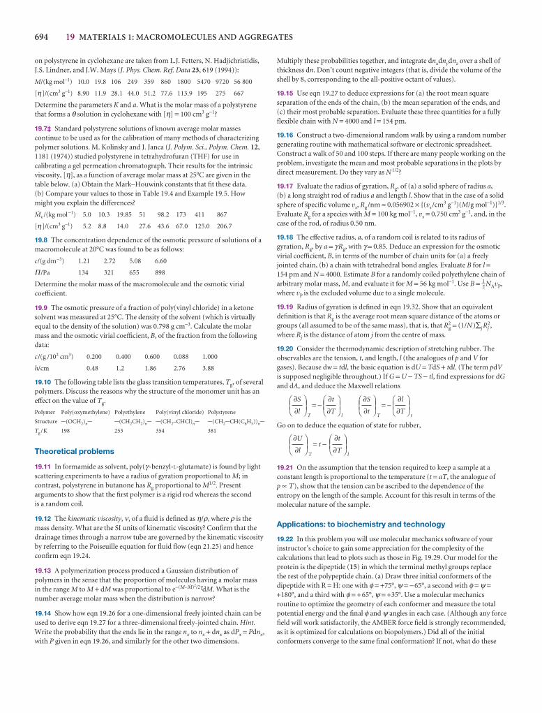
694 19 MATERIALS 1: MACROMOLECULES AND AGGREGATES
on polystyrene in cyclohexane are taken from L.J. Fetters, N. Hadjichristidis,J.S. Lindner, and J.W. Mays (J. Phys. Chem. Ref. Data 23, 619 (1994)):
M/(kg mol−1) 10.0 19.8 106 249 359 860 1800 5470 9720 56 800
[η]/(cm3 g−1) 8.90 11.9 28.1 44.0 51.2 77.6 113.9 195 275 667
Determine the parameters K and a. What is the molar mass of a polystyrenethat forms a θ solution in cyclohexane with [η] = 100 cm3 g−1?
19.7‡ Standard polystyrene solutions of known average molar massescontinue to be used as for the calibration of many methods of characterizingpolymer solutions. M. Kolinsky and J. Janca (J. Polym. Sci., Polym. Chem. 12,1181 (1974)) studied polystyrene in tetrahydrofuran (THF) for use incalibrating a gel permeation chromatograph. Their results for the intrinsicviscosity, [η], as a function of average molar mass at 25°C are given in thetable below. (a) Obtain the Mark–Houwink constants that fit these data. (b) Compare your values to those in Table 19.4 and Example 19.5. How might you explain the differences?
Jv /(kg mol−1) 5.0 10.3 19.85 51 98.2 173 411 867
[η]/(cm3 g−1) 5.2 8.8 14.0 27.6 43.6 67.0 125.0 206.7
19.8 The concentration dependence of the osmotic pressure of solutions of amacromolecule at 20°C was found to be as follows:
c/(g dm−3) 1.21 2.72 5.08 6.60
Π /Pa 134 321 655 898
Determine the molar mass of the macromolecule and the osmotic virialcoefficient.
19.9 The osmotic pressure of a fraction of poly(vinyl chloride) in a ketonesolvent was measured at 25°C. The density of the solvent (which is virtuallyequal to the density of the solution) was 0.798 g cm−3. Calculate the molarmass and the osmotic virial coefficient, B, of the fraction from the followingdata:
c /(g /102 cm3) 0.200 0.400 0.600 0.088 1.000
h/cm 0.48 1.2 1.86 2.76 3.88
19.10 The following table lists the glass transition temperatures, Tg, of severalpolymers. Discuss the reasons why the structure of the monomer unit has aneffect on the value of Tg.
Polymer Poly(oxymethylene) Polyethylene Poly(vinyl chloride) Polystyrene
Structure -(OCH2)n- -(CH2CH2)n- -(CH2–CHCl)n- -(CH2-CH(C6H5))n-
Tg /K 198 253 354 381
Theoretical problems
19.11 In formamide as solvent, poly(γ-benzyl-L-glutamate) is found by lightscattering experiments to have a radius of gyration proportional to M; incontrast, polystyrene in butanone has Rg proportional to M1/2. Presentarguments to show that the first polymer is a rigid rod whereas the second is a random coil.
19.12 The kinematic viscosity, ν, of a fluid is defined as η/ρ, where ρ is themass density. What are the SI units of kinematic viscosity? Confirm that thedrainage times through a narrow tube are governed by the kinematic viscosityby referring to the Poiseuille equation for fluid flow (eqn 21.25) and henceconfirm eqn 19.24.
19.13 A polymerization process produced a Gaussian distribution ofpolymers in the sense that the proportion of molecules having a molar mass in the range M to M + dM was proportional to e−(M−J)2/2γdM. What is thenumber average molar mass when the distribution is narrow?
19.14 Show how eqn 19.26 for a one-dimensional freely jointed chain can beused to derive eqn 19.27 for a three-dimensional freely-jointed chain. Hint.Write the probability that the ends lie in the range nx to nx + dnx as dPx = Pdnx,with P given in eqn 19.26, and similarly for the other two dimensions.
Multiply these probabilities together, and integrate dnxdnydnz over a shell ofthickness dn. Don’t count negative integers (that is, divide the volume of theshell by 8, corresponding to the all-positive octant of values).
19.15 Use eqn 19.27 to deduce expressions for (a) the root mean squareseparation of the ends of the chain, (b) the mean separation of the ends, and(c) their most probable separation. Evaluate these three quantities for a fullyflexible chain with N = 4000 and l = 154 pm.
19.16 Construct a two-dimensional random walk by using a random numbergenerating routine with mathematical software or electronic spreadsheet.Construct a walk of 50 and 100 steps. If there are many people working on theproblem, investigate the mean and most probable separations in the plots bydirect measurement. Do they vary as N 1/2?
19.17 Evaluate the radius of gyration, Rg, of (a) a solid sphere of radius a,(b) a long straight rod of radius a and length l. Show that in the case of a solidsphere of specific volume vs, Rg/nm ≈ 0.056902 × {(vs /cm3 g−1)(M/g mol−1)}1/3.Evaluate Rg for a species with M = 100 kg mol−1, vs = 0.750 cm3 g−1, and, in thecase of the rod, of radius 0.50 nm.
19.18 The effective radius, a, of a random coil is related to its radius ofgyration, Rg, by a = γRg, with γ = 0.85. Deduce an expression for the osmoticvirial coefficient, B, in terms of the number of chain units for (a) a freelyjointed chain, (b) a chain with tetrahedral bond angles. Evaluate B for l =154 pm and N = 4000. Estimate B for a randomly coiled polyethylene chain ofarbitrary molar mass, M, and evaluate it for M = 56 kg mol−1. Use B = 1–
2 NAvP,where vP is the excluded volume due to a single molecule.
19.19 Radius of gyration is defined in eqn 19.32. Show that an equivalentdefinition is that Rg is the average root mean square distance of the atoms orgroups (all assumed to be of the same mass), that is, that R2
g = (1/N)∑j Rj2,
where Rj is the distance of atom j from the centre of mass.
19.20 Consider the thermodynamic description of stretching rubber. Theobservables are the tension, t, and length, l (the analogues of p and V forgases). Because dw = tdl, the basic equation is dU = TdS + tdl. (The term pdVis supposed negligible throughout.) If G = U − TS − tl, find expressions for dGand dA, and deduce the Maxwell relations
T
= −l T
= −t
Go on to deduce the equation of state for rubber,
T
= t −l
19.21 On the assumption that the tension required to keep a sample at aconstant length is proportional to the temperature (t = aT, the analogue of p ∝ T), show that the tension can be ascribed to the dependence of theentropy on the length of the sample. Account for this result in terms of themolecular nature of the sample.
Applications: to biochemistry and technology
19.22 In this problem you will use molecular mechanics software of yourinstructor’s choice to gain some appreciation for the complexity of thecalculations that lead to plots such as those in Fig. 19.29. Our model for theprotein is the dipeptide (15) in which the terminal methyl groups replace the rest of the polypeptide chain. (a) Draw three initial conformers of thedipeptide with R = H: one with φ = +75°, ψ = −65°, a second with φ = ψ =+180°, and a third with φ = +65°, ψ = +35°. Use a molecular mechanicsroutine to optimize the geometry of each conformer and measure the totalpotential energy and the final φ and ψ angles in each case. (Although any forcefield will work satisfactorily, the AMBER force field is strongly recommended,as it is optimized for calculations on biopolymers.) Did all of the initialconformers converge to the same final conformation? If not, what do these
DEF∂t
∂T
ABCDEF
∂U
∂l
ABC
DEF∂l
∂T
ABCDEF
∂S
∂t
ABCDEF
∂t
∂T
ABCDEF
∂S
∂l
ABC
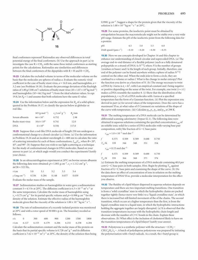
PROBLEMS 695
final conformers represent? Rationalize any observed differences in totalpotential energy of the final conformers. (b) Use the approach in part (a) toinvestigate the case R = CH3, with the same three initial conformers as startingpoints for the calculations. Rationalize any similarities and differencesbetween the final conformers of the dipeptides with R = H and R = CH3.
19.23 Calculate the excluded volume in terms of the molecular volume on thebasis that the molecules are spheres of radius a. Evaluate the osmotic virialcoefficient in the case of bushy stunt virus, a = 14.0 nm, and haemoglobin, a =3.2 nm (see Problem 19.18). Evaluate the percentage deviation of the Rayleighratios of 1.00 g/(100 cm3) solutions of bushy stunt virus (M = 1.07 × 10⁴ kg mol−1)and haemoglobin (M = 66.5 kg mol−1) from the ideal solution values. In eqn19.8, let Pθ = 1 and assume that both solutions have the same K value.
19.24 Use the information below and the expression for Rg of a solid spherequoted in the Problem 19.17, to classify the species below as globular or rod-like.
M /(g mol−1) vs/(cm3 g−1) Rg /nm
Serum albumin 66 × 103 0.752 2.98
Bushy stunt virus 10.6 × 10⁶ 0.741 12.0
DNA 4 × 10⁶ 0.556 117.0
19.25 Suppose that a rod-like DNA molecule of length 250 nm undergoes aconformational change to a closed-circular (cc) form. (a) Use the informationin Problem 19.24 and an incident wavelength λ = 488 nm to calculate the ratioof scattering intensities by each of these conformations, Irod/Icc, when θ = 20°,45°, and 90°. (b) Suppose that you wish to use light scattering as a techniquefor the study of conformational changes in DNA molecules. Based on youranswer to part (a), at which angle would you conduct the experiments? Justifyyour choice.
19.26 In an ultracentrifugation experiment at 20°C on bovine serum albuminthe following data were obtained: ρ = 1.001 g cm−3, vs = 1.112 cm3 g−1,ω /2π = 322 Hz,
r /cm 5.0 5.1 5.2 5.3 5.4
c /(mg cm−3) 0.536 0.284 0.148 0.077 0.039
Evaluate the molar mass of the sample.
19.27 Sedimentation studies on haemoglobin in water gave a sedimentationconstant S = 4.5 Sv at 20°C. The diffusion coefficient is 6.3 × 10⁻¹¹ m2 s−1 atthe same temperature. Calculate the molar mass of haemoglobin using vs = 0.75 cm3 g−1 for its partial specific volume and ρ = 0.998 g cm−3 for thedensity of the solution. Estimate the effective radius of the haemoglobinmolecule given that the viscosity of the solution is 1.00 × 10⁻³ kg m−1 s−1.
19.28 The rate of sedimentation of a recently isolated protein was monitoredat 20°C and with a rotor speed of 50 000 r.p.m. The boundary receded asfollows:
t /s 0 300 600 900 1200 1500 1800
r /cm 6.127 6.153 6.179 6.206 6.232 6.258 6.284
Calculate the sedimentation constant and the molar mass of the protein onthe basis that its partial specific volume is 0.728 cm3 g−1 and its diffusioncoefficient is 7.62 × 10⁻¹¹ m2 s−1 at 20°C, the density of the solution then being
0.9981 g cm−3. Suggest a shape for the protein given that the viscosity of thesolution is 1.00 × 10⁻³ kg m−1 s−1 at 20°C.
19.29 For some proteins, the isoelectric point must be obtained byextrapolation because the macromolecule might not be stable over a very widepH range. Estimate the pH of the isoelectric point from the following data fora protein:
pH 4.5 5.0 5.5 6.0
Drift speed/(µm s−1) −0.10 −0.20 −0.30 −0.35
19.30 Here we use concepts developed in Chapter 16 and this chapter toenhance our understanding of closed-circular and supercoiled DNA. (a) Theaverage end-to-end distance of a flexible polymer (such as a fully denaturedpolypeptide or a strand of DNA) is N 1/2l, where N is the number of groups(residues or bases) and l is the length of each group. Initially, therefore, oneend of the polymer can be found anywhere within a sphere of radius N 1/2lcentred on the other end. When the ends join to form a circle, they areconfined to a volume or radius l. What is the change in molar entropy? Plotthe function you derive as a function of N. (b) The energy necessary to twistccDNA by i turns is εi = ki2, with k an empirical constant and i being negativeor positive depending on the sense of the twist. For example, one twist (i = ±1)makes ccDNA resemble the number 8. (i) Show that the distribution of thepopulations pi = ni /N of ccDNA molecules with i turns at a specifiedtemperature has the form of a Gaussian function. (ii) Plot the expression youderived in part (a) for several values of the temperature. Does the curve has amaximum? If so, at what value of i? Comment on variations of the shape ofthe curve with temperature. (iii) Calculate p0, p1, p5, and p10 at 298 K.
19.31 The melting temperature of a DNA molecule can be determined bydifferential scanning calorimetry (Impact I2.1). The following data wereobtained in aqueous solutions containing the specified concentration csalt ofan soluble ionic solid for a series of DNA molecules with varying base paircomposition, with f the fraction of G-C base pairs:
csalt = 1.0 × 10⁻² mol dm−3
f 0.375 0.509 0.589 0.688 0.750
Tm /K 339 344 348 351 354
csalt = 0.15 mol dm−3
f 0.375 0.509 0.589 0.688 0.750
Tm /K 359 364 368 371 374
(a) Estimate the melting temperature of a DNA molecule containing 40.0 percent G-C base pairs in both samples. Hint. Begin by plotting Tm againstfraction of G-C base pairs and examining the shape of the curve. (b) Do the data show an effect of concentration of ions in solution on the meltingtemperature of DNA? If so, provide a molecular interpretation for the effectyou observe.
19.32 The fluidity of a lipid bilayer dispersed in aqueous solution depends ontemperature and there are two important melting transitions. One transitionis from a ‘solid crystalline’ state in which the hydrophobic chains are packedtogether tightly (hence move very little) to a ‘liquid crystalline state’, in whichthere is increased but still limited movement of the of the chains. The secondtransition, which occurs at a higher temperature than the first, is from theliquid crystalline state to a liquid state, in which the hydrophobic interactionsholding the aggregate together are largely disrupted. (a) It is observed that thetransition temperatures increase with the hydrophobic chain length anddecrease with the number of C=C bonds in the chain. Explain theseobservations. (b) What effect is the inclusion of cholesterol likely to have onthe transition temperatures of a lipid bilayer? Justify your answer.
19.33 Polystyrene is a synthetic polymer with the structure -(CH2-CH(C6H5))n-. A batch of polydisperse polystyrene was prepared by initiatingthe polymerization with t-butyl radicals. As a result, the t-butyl group is

696 19 MATERIALS 1: MACROMOLECULES AND AGGREGATES
expected to be covalently attached to the end of the final products. A samplefrom this batch was embedded in an organic matrix containing silvertrifluoroacetate and the resulting MALDI-TOF spectrum consisted of a largenumber of peaks separated by 104 g mol−1, with the most intense peak at 25 578 g mol−1. Comment on the purity of this sample and determine thenumber of (CH2-CH(C6H5)) units in the species that gives rise to the mostintense peak in the spectrum .
19.34 A manufacturer of polystyrene beads claims that they have an averagemolar mass of 250 kg mol−1. Solutions of these beads are studied by a physicalchemistry student by dilute solution viscometry with an Ostwald viscometerin both the ‘good’ solvent toluene and the theta solvent cyclohexane. Thedrainage times, tD, as a function of concentration for the two solvents aregiven in the table below. (a) Fit the data to the virial equation for viscosity,
η = η*(1 + [η]c + k′[η]2c2 + · · · )
where k′ is called the Huggins constant and is typically in the range 0.35–0.40.From the fit, determine the intrinsic viscosity and the Huggins constant. (b) Use the empirical Mark–Kuhn–Houwink–Sakurada equation (eqn 19.25)to determine the molar mass of polystyrene in the two solvents. For thetasolvents, a = 0.5 and K = 8.2 × 10⁻⁵ dm3 g−1 for cyclohexane; for the goodsolvent toluene a = 0.72 and K = 1.15 × 10⁻⁵ dm3 g−1. (c) According to ageneral theory proposed by Kirkwood and Riseman, the root mean squareend-to-end distance of a polymer chain in solution is related to [η] by [η] =Φ �r 2�3/2/M, where Φ is a universal constant with the value 2.84 × 1026 when[η] is expressed in cubic decimetres per gram and the distance is in metres.Calculate this quantity for each solvent. (d) From the molar masses calculate
the average number of styrene (C6H5CH=CH2) monomer units, �n�, (e)Calculate the length of a fully stretched, planar zigzag configuration, takingthe C-C distance as 154 pm and the CCC bond angle to be 109°. (f) Use eqn 19.33 to calculate the radius of gyration, Rg. Also calculate �r 2�1/2 = n1/2.Compare this result with that predicted by the Kirkwood–Riseman theory:which gives the better fit? (g) Compare your values for M to the results ofProblem 19.33. Is there any reason why they should or should not agree? Is themanufacturer’s claim valid?
c /(g dm−3 toluene) 0 1.0 3.0 5.0
t D /s 8.37 9.11 10.72 12.52
c/(g dm−3 cyclohexane) 0 1.0 1.5 2.0
t D /s 8.32 8.67 8.85 9.03
19.35‡ The determination of the average molar masses of conductingpolymers is an important part of their characterization. S. Holdcroft ( J. Polym. Sci., Polym. Phys. 29, 1585 (1991)) has determined the molar masesand Mark–Houwink constants for the electronically conducting polymer,poly(3-hexylthiophene) (P3HT) in tetrahydrofuran (THF) at 25°C bymethods similar to those used for nonconducting polymers. The values formolar mass and intrinsic viscosity in the table below are adapted from theirdata. Determine the constants in the Mark–Kuhn–Houwink–Sakuradaequation from these results and compare to the values obtained in yoursolution to Problem 19.7 .
J v /(kg mol−1) 3.8 11.1 15.3 58.8
[η]/(cm3 g−1) 6.23 17.44 23.73 85.28

Materials 2: the solid state
First, we see how to describe the regular arrangement of atoms in crystals and the sym-metry of their arrangement. Then we consider the basic principles of X-ray diffraction andsee how the diffraction pattern can be interpreted in terms of the distribution of electrondensity in a unit cell. X-ray diffraction leads to information about the structures of metallic,ionic, and molecular solids, and we review some typical results and their rationalization interms of atomic and ionic radii. With structures established, we move on to the propertiesof solids, and see how their mechanical, electrical, optical, and magnetic properties stemfrom the properties of their constituent atoms and molecules.
The solid state includes most of the materials that make modern technology possible.It includes the wide varieties of steel that are used in architecture and engineering, thesemiconductors and metallic conductors that are used in information technology andpower distribution, the ceramics that increasingly are replacing metals, and the syn-thetic and natural polymers that are used in the textile industry and in the fabricationof many of the common objects of the modern world. The properties of solids stem,of course, from the arrangement and properties of the constituent atoms, and one ofthe challenges of this chapter is to see how a wide range of bulk properties, includingrigidity, electrical conductivity, and optical and magnetic properties stem from theproperties of atoms. One crucial aspect of this link is the pattern in which the atoms(and molecules) are stacked together, and we start this chapter with an examinationof how the structures of solids are described and determined.
Crystal lattices
Early in the history of modern science it was suggested that the regular external formof crystals implied an internal regularity of their constituents. In this section we seehow to describe the arrangement of atoms inside crystals.
20.1 Lattices and unit cells
A crystal is built up from regularly repeating ‘structural motifs’, which may be atoms,molecules, or groups of atoms, molecules, or ions. A space lattice is the patternformed by points representing the locations of these motifs (Fig. 20.1). The space lattice is, in effect, an abstract scaffolding for the crystal structure. More formally, aspace lattice is a three-dimensional, infinite array of points, each of which is sur-rounded in an identical way by its neighbours, and which defines the basic structureof the crystal. In some cases there may be a structural motif centred on each lattice
20Crystal lattices
20.1 Lattices and unit cells
20.2 The identification of latticeplanes
20.3 The investigation of structure
I20.1 Impact on biochemistry: X-ray crystallography ofbiological macromolecules
20.4 Neutron and electrondiffraction
Crystal structure
20.5 Metallic solids
20.6 Ionic solids
20.7 Molecular solids and covalentnetworks
The properties of solids
20.8 Mechanical properties
20.9 Electrical properties
I20.2 Impact on nanoscience:Nanowires
20.10 Optical properties
20.11 Magnetic properties
20.12 Superconductors
Checklist of key ideas
Further reading
Discussion questions
Exercises
Problems
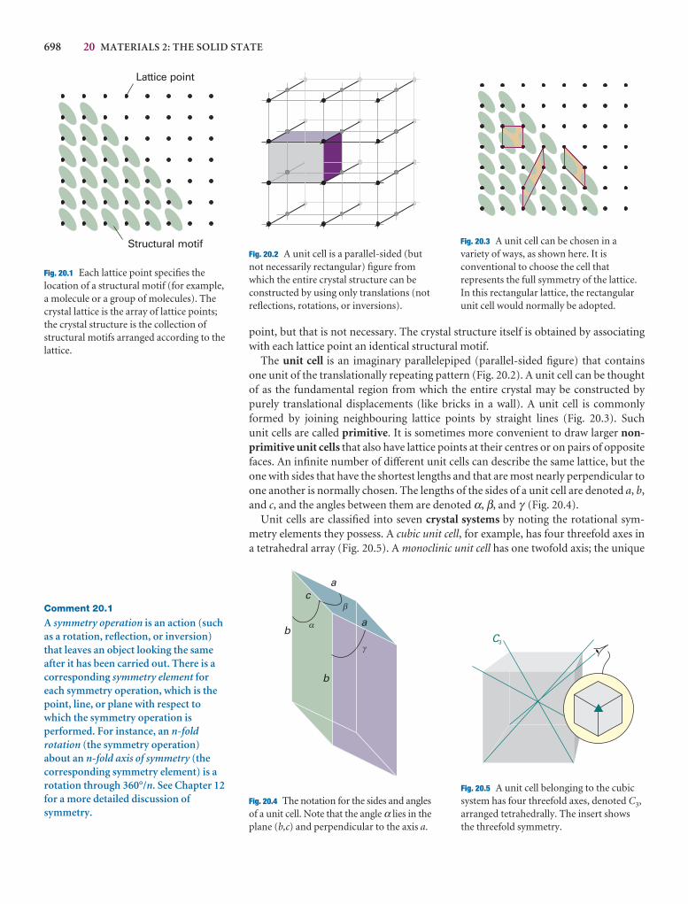
698 20 MATERIALS 2: THE SOLID STATE
Fig. 20.1 Each lattice point specifies thelocation of a structural motif (for example,a molecule or a group of molecules). Thecrystal lattice is the array of lattice points;the crystal structure is the collection ofstructural motifs arranged according to thelattice.
Comment 20.1
A symmetry operation is an action (suchas a rotation, reflection, or inversion)that leaves an object looking the sameafter it has been carried out. There is acorresponding symmetry element foreach symmetry operation, which is thepoint, line, or plane with respect towhich the symmetry operation isperformed. For instance, an n-foldrotation (the symmetry operation)about an n-fold axis of symmetry (thecorresponding symmetry element) is arotation through 360°/n. See Chapter 12for a more detailed discussion ofsymmetry.
Fig. 20.2 A unit cell is a parallel-sided (butnot necessarily rectangular) figure fromwhich the entire crystal structure can beconstructed by using only translations (notreflections, rotations, or inversions).
Fig. 20.3 A unit cell can be chosen in avariety of ways, as shown here. It isconventional to choose the cell thatrepresents the full symmetry of the lattice.In this rectangular lattice, the rectangularunit cell would normally be adopted.
C3
Fig. 20.4 The notation for the sides and anglesof a unit cell. Note that the angle α lies in theplane (b,c) and perpendicular to the axis a.
Fig. 20.5 A unit cell belonging to the cubicsystem has four threefold axes, denoted C3,arranged tetrahedrally. The insert showsthe threefold symmetry.
point, but that is not necessary. The crystal structure itself is obtained by associatingwith each lattice point an identical structural motif.
The unit cell is an imaginary parallelepiped (parallel-sided figure) that containsone unit of the translationally repeating pattern (Fig. 20.2). A unit cell can be thoughtof as the fundamental region from which the entire crystal may be constructed bypurely translational displacements (like bricks in a wall). A unit cell is commonlyformed by joining neighbouring lattice points by straight lines (Fig. 20.3). Such unit cells are called primitive. It is sometimes more convenient to draw larger non-primitive unit cells that also have lattice points at their centres or on pairs of oppositefaces. An infinite number of different unit cells can describe the same lattice, but theone with sides that have the shortest lengths and that are most nearly perpendicular toone another is normally chosen. The lengths of the sides of a unit cell are denoted a, b,and c, and the angles between them are denoted α, β, and γ (Fig. 20.4).
Unit cells are classified into seven crystal systems by noting the rotational sym-metry elements they possess. A cubic unit cell, for example, has four threefold axes ina tetrahedral array (Fig. 20.5). A monoclinic unit cell has one twofold axis; the unique
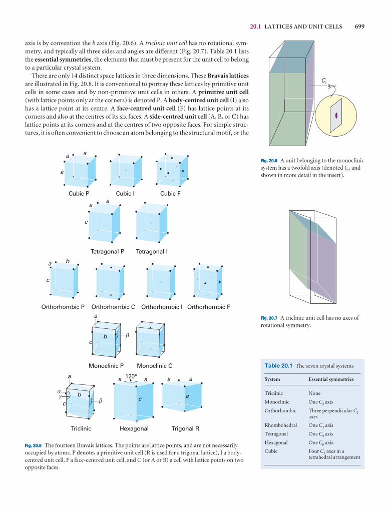
20.1 LATTICES AND UNIT CELLS 699
C2
Fig. 20.6 A unit belonging to the monoclinicsystem has a twofold axis (denoted C2 andshown in more detail in the insert).
Fig. 20.7 A triclinic unit cell has no axes ofrotational symmetry.
Fig. 20.8 The fourteen Bravais lattices. The points are lattice points, and are not necessarilyoccupied by atoms. P denotes a primitive unit cell (R is used for a trigonal lattice), I a body-centred unit cell, F a face-centred unit cell, and C (or A or B) a cell with lattice points on twoopposite faces.
Table 20.1 The seven crystal systems
System Essential symmetries
Triclinic None
Monoclinic One C2 axis
Orthorhombic Three perpendicular C2axes
Rhombohedral One C3 axis
Tetragonal One C4 axis
Hexagonal One C6 axis
Cubic Four C3 axes in atetrahedral arrangement
Cubic P Cubic I Cubic F
Tetragonal P Tetragonal I
Orthorhombic P Orthorhombic C Orthorhombic I Orthorhombic F
Monoclinic P Monoclinic C
Triclinic Hexagonal Trigonal R
a
a a
aa
c
a b
c
a
a
�
b
b
c
c�
�
�
a a a a
ac
120°
axis is by convention the b axis (Fig. 20.6). A triclinic unit cell has no rotational sym-metry, and typically all three sides and angles are different (Fig. 20.7). Table 20.1 liststhe essential symmetries, the elements that must be present for the unit cell to belongto a particular crystal system.
There are only 14 distinct space lattices in three dimensions. These Bravais latticesare illustrated in Fig. 20.8. It is conventional to portray these lattices by primitive unitcells in some cases and by non-primitive unit cells in others. A primitive unit cell(with lattice points only at the corners) is denoted P. A body-centred unit cell (I) alsohas a lattice point at its centre. A face-centred unit cell (F) has lattice points at its corners and also at the centres of its six faces. A side-centred unit cell (A, B, or C) haslattice points at its corners and at the centres of two opposite faces. For simple struc-tures, it is often convenient to choose an atom belonging to the structural motif, or the
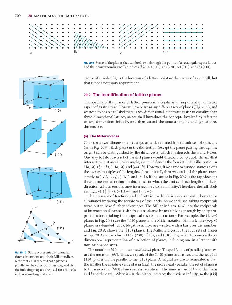
700 20 MATERIALS 2: THE SOLID STATE
20.9 Some of the planes that can be drawnthrough the points of a rectangular spacelattice and their corresponding Millerindices (hkl): (a) (110), (b) (230), (c) (⁄10),and (d) (010).
centre of a molecule, as the location of a lattice point or the vertex of a unit cell, butthat is not a necessary requirement.
20.2 The identification of lattice planes
The spacing of the planes of lattice points in a crystal is an important quantitative aspect of its structure. However, there are many different sets of planes (Fig. 20.9), andwe need to be able to label them. Two-dimensional lattices are easier to visualize thanthree-dimensional lattices, so we shall introduce the concepts involved by referring to two dimensions initially, and then extend the conclusions by analogy to three dimensions.
(a) The Miller indices
Consider a two-dimensional rectangular lattice formed from a unit cell of sides a, b(as in Fig. 20.9). Each plane in the illustration (except the plane passing through the origin) can be distinguished by the distances at which it intersects the a and b axes.One way to label each set of parallel planes would therefore be to quote the smallestintersection distances. For example, we could denote the four sets in the illustration as(1a,1b), ( 1–2 a, 1–3b), (−1a,1b), and (∞a,1b). However, if we agree to quote distances alongthe axes as multiples of the lengths of the unit cell, then we can label the planes moresimply as (1,1), ( 1–2 , 1–3), (−1,1), and (∞,1). If the lattice in Fig. 20.9 is the top view of athree-dimensional orthorhombic lattice in which the unit cell has a length c in the z-direction, all four sets of planes intersect the z-axis at infinity. Therefore, the full labelsare (1,1,∞), ( 1–2 , 1–3,∞), (−1,1,∞), and (∞,1,∞).
The presence of fractions and infinity in the labels is inconvenient. They can beeliminated by taking the reciprocals of the labels. As we shall see, taking reciprocalsturns out to have further advantages. The Miller indices, (hkl), are the reciprocals of intersection distances (with fractions cleared by multiplying through by an appro-priate factor, if taking the reciprocal results in a fraction). For example, the (1,1,∞)planes in Fig. 20.9a are the (110) planes in the Miller notation. Similarly, the (1–2 , 1–3,∞)planes are denoted (230). Negative indices are written with a bar over the number,and Fig. 20.9c shows the (⁄10) planes. The Miller indices for the four sets of planes in Fig. 20.9 are therefore (110), (230), (⁄10), and (010). Figure 20.10 shows a three-dimensional representation of a selection of planes, including one in a lattice withnon-orthogonal axes.
The notation (hkl) denotes an individual plane. To specify a set of parallel planes weuse the notation {hkl}. Thus, we speak of the (110) plane in a lattice, and the set of all{110} planes that lie parallel to the (110) plane. A helpful feature to remember is that,the smaller the absolute value of h in {hkl}, the more nearly parallel the set of planes isto the a axis (the {h00} planes are an exception). The same is true of k and the b axisand l and the c axis. When h = 0, the planes intersect the a axis at infinity, so the {0kl}
a
b
c
(110)
(111)
(100)
(111)
b
c
a
Fig. 20.10 Some representative planes inthree dimensions and their Miller indices.Note that a 0 indicates that a plane isparallel to the corresponding axis, and thatthe indexing may also be used for unit cellswith non-orthogonal axes.
Fig. 20.9 Some of the planes that can be drawn through the points of a rectangular space latticeand their corresponding Miller indices (hkl): (a) (110), (b) (230), (c) (⁄10), and (d) (010).
(a) (b) (c) (d)
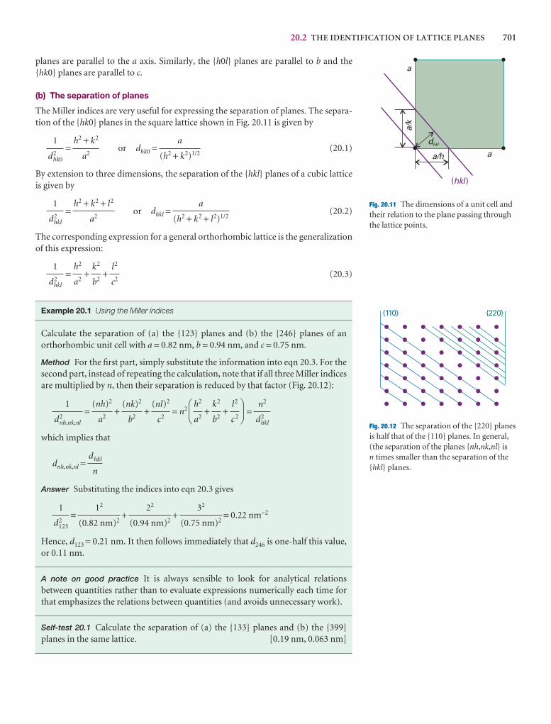
20.2 THE IDENTIFICATION OF LATTICE PLANES 701
a
a
a/k
a/h
( )hkl
dhkl
Fig. 20.11 The dimensions of a unit cell andtheir relation to the plane passing throughthe lattice points.
{110} {220}
Fig. 20.12 The separation of the {220} planes is half that of the {110} planes. In general,(the separation of the planes {nh,nk,nl} is n times smaller than the separation of the{hkl} planes.
planes are parallel to the a axis. Similarly, the {h0l} planes are parallel to b and the{hk0} planes are parallel to c.
(b) The separation of planes
The Miller indices are very useful for expressing the separation of planes. The separa-tion of the {hk0} planes in the square lattice shown in Fig. 20.11 is given by
= or dhk0 = (20.1)
By extension to three dimensions, the separation of the {hkl} planes of a cubic latticeis given by
= or dhkl = (20.2)
The corresponding expression for a general orthorhombic lattice is the generalizationof this expression:
= + + (20.3)
Example 20.1 Using the Miller indices
Calculate the separation of (a) the {123} planes and (b) the {246} planes of an orthorhombic unit cell with a = 0.82 nm, b = 0.94 nm, and c = 0.75 nm.
Method For the first part, simply substitute the information into eqn 20.3. For thesecond part, instead of repeating the calculation, note that if all three Miller indicesare multiplied by n, then their separation is reduced by that factor (Fig. 20.12):
= + + = n2 + + =
which implies that
dnh,nk,nl =
Answer Substituting the indices into eqn 20.3 gives
= + + = 0.22 nm−2
Hence, d123 = 0.21 nm. It then follows immediately that d246 is one-half this value,or 0.11 nm.
A note on good practice It is always sensible to look for analytical relations between quantities rather than to evaluate expressions numerically each time forthat emphasizes the relations between quantities (and avoids unnecessary work).
Self-test 20.1 Calculate the separation of (a) the {133} planes and (b) the {399}planes in the same lattice. [0.19 nm, 0.063 nm]
32
(0.75 nm)2
22
(0.94 nm)2
12
(0.82 nm)2
1
d2123
dhkl
n
n2
d2hkl
DF
l2
c 2
k2
b2
h2
a2
AC
(nl)2
c2
(nk)2
b2
(nh)2
a2
1
d2nh,nk,nl
l2
c2
k2
b2
h2
a2
1
d2hkl
a
(h2 + k2 + l2)1/2
h2 + k2 + l2
a2
1
d2hkl
a
(h2 + k2)1/2
h2 + k2
a2
1
d2hk0
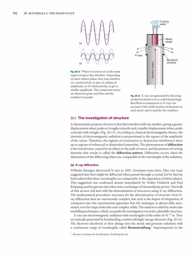
702 20 MATERIALS 2: THE SOLID STATE
20.3 The investigation of structure
A characteristic property of waves is that they interfere with one another, giving a greaterdisplacement where peaks or troughs coincide and a smaller displacement where peakscoincide with troughs (Fig. 20.13). According to classical electromagnetic theory, theintensity of electromagnetic radiation is proportional to the square of the amplitudeof the waves. Therefore, the regions of constructive or destructive interference showup as regions of enhanced or diminished intensities. The phenomenon of diffractionis the interference caused by an object in the path of waves, and the pattern of varyingintensity that results is called the diffraction pattern. Diffraction occurs when the dimensions of the diffracting object are comparable to the wavelength of the radiation.
(a) X-ray diffraction
Wilhelm Röntgen discovered X-rays in 1895. Seventeen years later, Max von Lauesuggested that they might be diffracted when passed through a crystal, for by then hehad realized that their wavelengths are comparable to the separation of lattice planes.This suggestion was confirmed almost immediately by Walter Friedrich and PaulKnipping and has grown since then into a technique of extraordinary power. The bulkof this section will deal with the determination of structures using X-ray diffraction.The mathematical procedures necessary for the determination of structure from X-ray diffraction data are enormously complex, but such is the degree of integration ofcomputers into the experimental apparatus that the technique is almost fully auto-mated, even for large molecules and complex solids. The analysis is aided by molecularmodelling techniques, which can guide the investigation towards a plausible structure.
X-rays are electromagnetic radiation with wavelengths of the order of 10−10 m. Theyare typically generated by bombarding a metal with high-energy electrons (Fig. 20.14).The electrons decelerate as they plunge into the metal and generate radiation with a continuous range of wavelengths called Bremsstrahlung.1 Superimposed on the
(a)
(b)
Fig. 20.13 When two waves are in the sameregion of space they interfere. Dependingon their relative phase, they may interfere(a) constructively, to give an enhancedamplitude, or (b) destructively, to give asmaller amplitude. The component wavesare shown in green and blue and theresultant in purple.
Coolingwater
X-rays
Berylliumwindow
Elec
tron
bea
m
Metaltarget
Fig. 20.14 X-rays are generated by directingan electron beam on to a cooled metal target.Beryllium is transparent to X-rays (onaccount of the small number of electrons ineach atom) and is used for the windows.
1 Bremse is German for deceleration, Strahlung for ray.
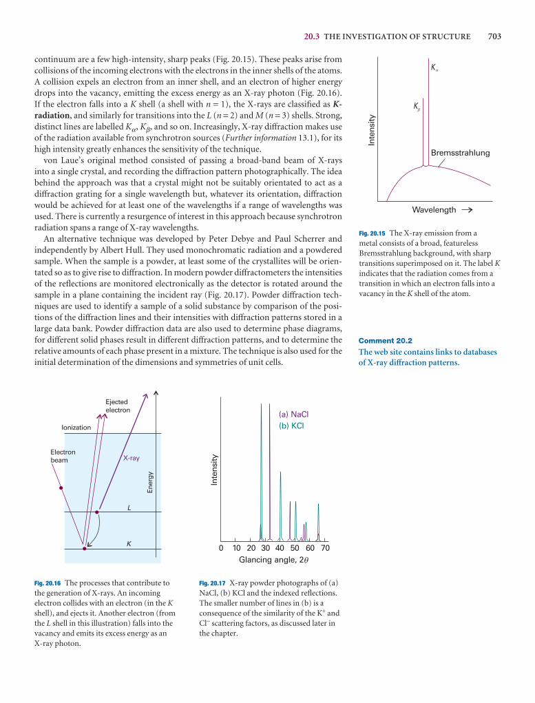
20.3 THE INVESTIGATION OF STRUCTURE 703
K
K
Wavelength
Inte
nsity
Bremsstrahlung
�
�
K
L
Ionization
X-rayElectronbeam
Ejectedelectron
Ener
gy
Fig. 20.15 The X-ray emission from a metal consists of a broad, featurelessBremsstrahlung background, with sharptransitions superimposed on it. The label Kindicates that the radiation comes from atransition in which an electron falls into avacancy in the K shell of the atom.
Fig. 20.16 The processes that contribute tothe generation of X-rays. An incomingelectron collides with an electron (in the Kshell), and ejects it. Another electron (fromthe L shell in this illustration) falls into thevacancy and emits its excess energy as an X-ray photon.
0 10 20 30 40 50 60 70Glancing angle, 2
Inte
nsity
(a) NaCl(b) KCl
�
Fig. 20.17 X-ray powder photographs of (a)NaCl, (b) KCl and the indexed reflections.The smaller number of lines in (b) is aconsequence of the similarity of the K+ andCl− scattering factors, as discussed later inthe chapter.
continuum are a few high-intensity, sharp peaks (Fig. 20.15). These peaks arise fromcollisions of the incoming electrons with the electrons in the inner shells of the atoms.A collision expels an electron from an inner shell, and an electron of higher energydrops into the vacancy, emitting the excess energy as an X-ray photon (Fig. 20.16). If the electron falls into a K shell (a shell with n = 1), the X-rays are classified as K-radiation, and similarly for transitions into the L (n = 2) and M (n = 3) shells. Strong,distinct lines are labelled Kα, Kβ, and so on. Increasingly, X-ray diffraction makes useof the radiation available from synchrotron sources (Further information 13.1), for itshigh intensity greatly enhances the sensitivity of the technique.
von Laue’s original method consisted of passing a broad-band beam of X-rays into a single crystal, and recording the diffraction pattern photographically. The idea behind the approach was that a crystal might not be suitably orientated to act as adiffraction grating for a single wavelength but, whatever its orientation, diffractionwould be achieved for at least one of the wavelengths if a range of wavelengths wasused. There is currently a resurgence of interest in this approach because synchrotronradiation spans a range of X-ray wavelengths.
An alternative technique was developed by Peter Debye and Paul Scherrer and independently by Albert Hull. They used monochromatic radiation and a powderedsample. When the sample is a powder, at least some of the crystallites will be orien-tated so as to give rise to diffraction. In modern powder diffractometers the intensitiesof the reflections are monitored electronically as the detector is rotated around thesample in a plane containing the incident ray (Fig. 20.17). Powder diffraction tech-niques are used to identify a sample of a solid substance by comparison of the posi-tions of the diffraction lines and their intensities with diffraction patterns stored in alarge data bank. Powder diffraction data are also used to determine phase diagrams,for different solid phases result in different diffraction patterns, and to determine therelative amounts of each phase present in a mixture. The technique is also used for theinitial determination of the dimensions and symmetries of unit cells.
Comment 20.2
The web site contains links to databasesof X-ray diffraction patterns.
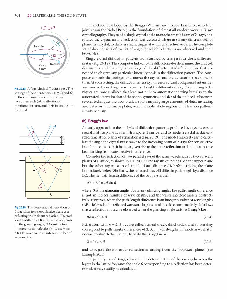
704 20 MATERIALS 2: THE SOLID STATE
The method developed by the Braggs (William and his son Lawrence, who laterjointly won the Nobel Prize) is the foundation of almost all modern work in X-raycrystallography. They used a single crystal and a monochromatic beam of X-rays, androtated the crystal until a reflection was detected. There are many different sets ofplanes in a crystal, so there are many angles at which a reflection occurs. The completeset of data consists of the list of angles at which reflections are observed and their intensities.
Single-crystal diffraction patterns are measured by using a four-circle diffracto-meter (Fig. 20.18). The computer linked to the diffractometer determines the unit cell dimensions and the angular settings of the diffractometer’s four circles that areneeded to observe any particular intensity peak in the diffraction pattern. The com-puter controls the settings, and moves the crystal and the detector for each one inturn. At each setting, the diffraction intensity is measured, and background intensitiesare assessed by making measurements at slightly different settings. Computing tech-niques are now available that lead not only to automatic indexing but also to the automated determination of the shape, symmetry, and size of the unit cell. Moreover,several techniques are now available for sampling large amounts of data, includingarea detectors and image plates, which sample whole regions of diffraction patternssimultaneously.
(b) Bragg’s law
An early approach to the analysis of diffraction patterns produced by crystals was toregard a lattice plane as a semi-transparent mirror, and to model a crystal as stacks ofreflecting lattice planes of separation d (Fig. 20.19). The model makes it easy to calcu-late the angle the crystal must make to the incoming beam of X-rays for constructiveinterference to occur. It has also given rise to the name reflection to denote an intensebeam arising from constructive interference.
Consider the reflection of two parallel rays of the same wavelength by two adjacentplanes of a lattice, as shown in Fig. 20.19. One ray strikes point D on the upper planebut the other ray must travel an additional distance AB before striking the plane immediately below. Similarly, the reflected rays will differ in path length by a distanceBC. The net path length difference of the two rays is then
AB + BC = 2d sin θ
where θ is the glancing angle. For many glancing angles the path-length differenceis not an integer number of wavelengths, and the waves interfere largely destruct-ively. However, when the path-length difference is an integer number of wavelengths (AB + BC = nλ), the reflected waves are in phase and interfere constructively. It followsthat a reflection should be observed when the glancing angle satisfies Bragg’s law:
nλ = 2d sin θ (20.4)
Reflections with n = 2, 3, . . . are called second-order, third-order, and so on; they correspond to path-length differences of 2, 3, . . . wavelengths. In modern work it isnormal to absorb the n into d, to write the Bragg law as
λ = 2d sin θ (20.5)
and to regard the nth-order reflection as arising from the {nh,nk,nl} planes (seeExample 20.1).
The primary use of Bragg’s law is in the determination of the spacing between thelayers in the lattice for, once the angle θ corresponding to a reflection has been deter-mined, d may readily be calculated.
�
2
1
Detector
)
Sample
X-raybeam
�
Fig. 20.18 A four-circle diffractometer. Thesettings of the orientations (φ, χ, θ, and Ω)of the components is controlled bycomputer; each (hkl) reflection ismonitored in turn, and their intensities arerecorded.
�
d
A C
B
q
q
Fig. 20.19 The conventional derivation ofBragg’s law treats each lattice plane as areflecting the incident radiation. The pathlengths differ by AB + BC, which dependson the glancing angle, θ. Constructiveinterference (a ‘reflection’) occurs when AB + BC is equal to an integer number ofwavelengths.
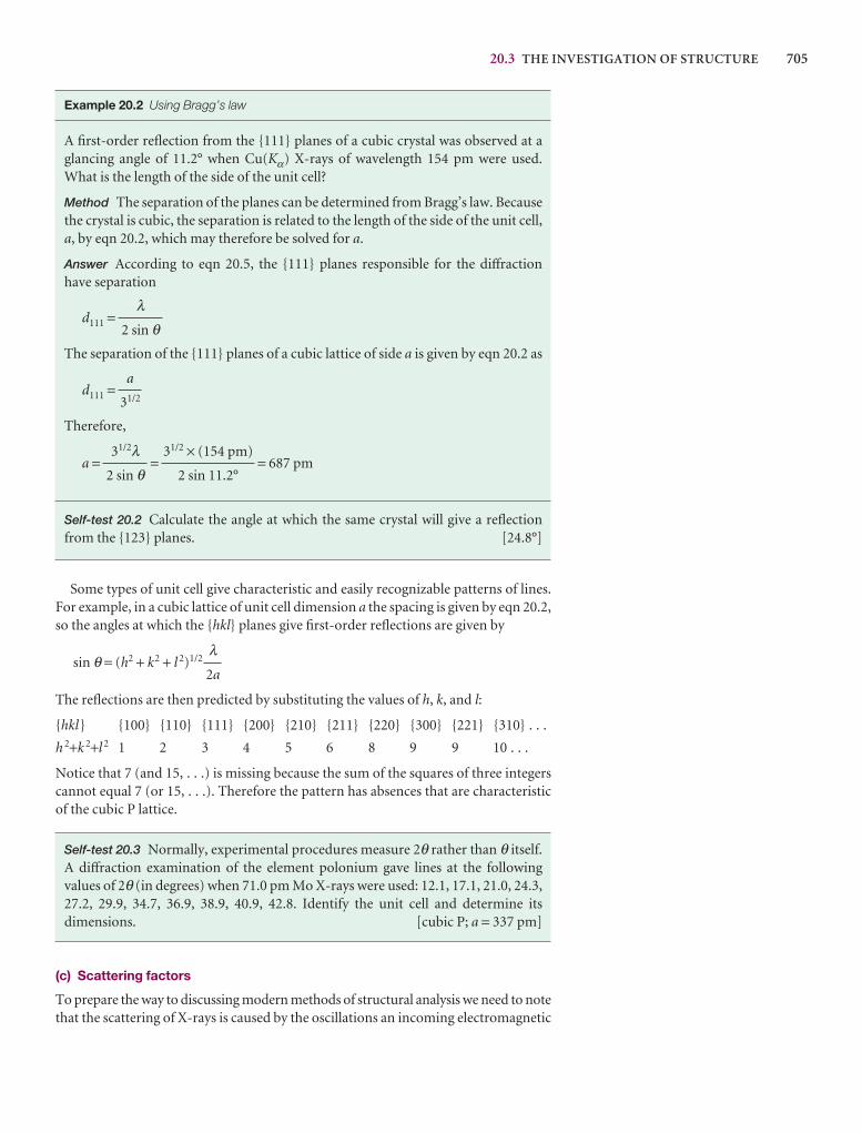
20.3 THE INVESTIGATION OF STRUCTURE 705
Example 20.2 Using Bragg’s law
A first-order reflection from the {111} planes of a cubic crystal was observed at aglancing angle of 11.2° when Cu(Kα) X-rays of wavelength 154 pm were used.What is the length of the side of the unit cell?
Method The separation of the planes can be determined from Bragg’s law. Becausethe crystal is cubic, the separation is related to the length of the side of the unit cell,a, by eqn 20.2, which may therefore be solved for a.
Answer According to eqn 20.5, the {111} planes responsible for the diffractionhave separation
d111 =
The separation of the {111} planes of a cubic lattice of side a is given by eqn 20.2 as
d111 =
Therefore,
a = = = 687 pm
Self-test 20.2 Calculate the angle at which the same crystal will give a reflectionfrom the {123} planes. [24.8°]
Some types of unit cell give characteristic and easily recognizable patterns of lines.For example, in a cubic lattice of unit cell dimension a the spacing is given by eqn 20.2,so the angles at which the {hkl} planes give first-order reflections are given by
sin θ = (h2 + k2 + l 2)1/2
The reflections are then predicted by substituting the values of h, k, and l:
{hkl} {100} {110} {111} {200} {210} {211} {220} {300} {221} {310} . . .
h 2+k 2+l 2 1 2 3 4 5 6 8 9 9 10 . . .
Notice that 7 (and 15, . . .) is missing because the sum of the squares of three integerscannot equal 7 (or 15, . . .). Therefore the pattern has absences that are characteristicof the cubic P lattice.
Self-test 20.3 Normally, experimental procedures measure 2θ rather than θ itself.A diffraction examination of the element polonium gave lines at the following values of 2θ (in degrees) when 71.0 pm Mo X-rays were used: 12.1, 17.1, 21.0, 24.3,27.2, 29.9, 34.7, 36.9, 38.9, 40.9, 42.8. Identify the unit cell and determine its dimensions. [cubic P; a = 337 pm]
(c) Scattering factors
To prepare the way to discussing modern methods of structural analysis we need to notethat the scattering of X-rays is caused by the oscillations an incoming electromagnetic
λ2a
31/2 × (154 pm)
2 sin 11.2°
31/2λ2 sin θ
a
31/2
λ2 sin θ
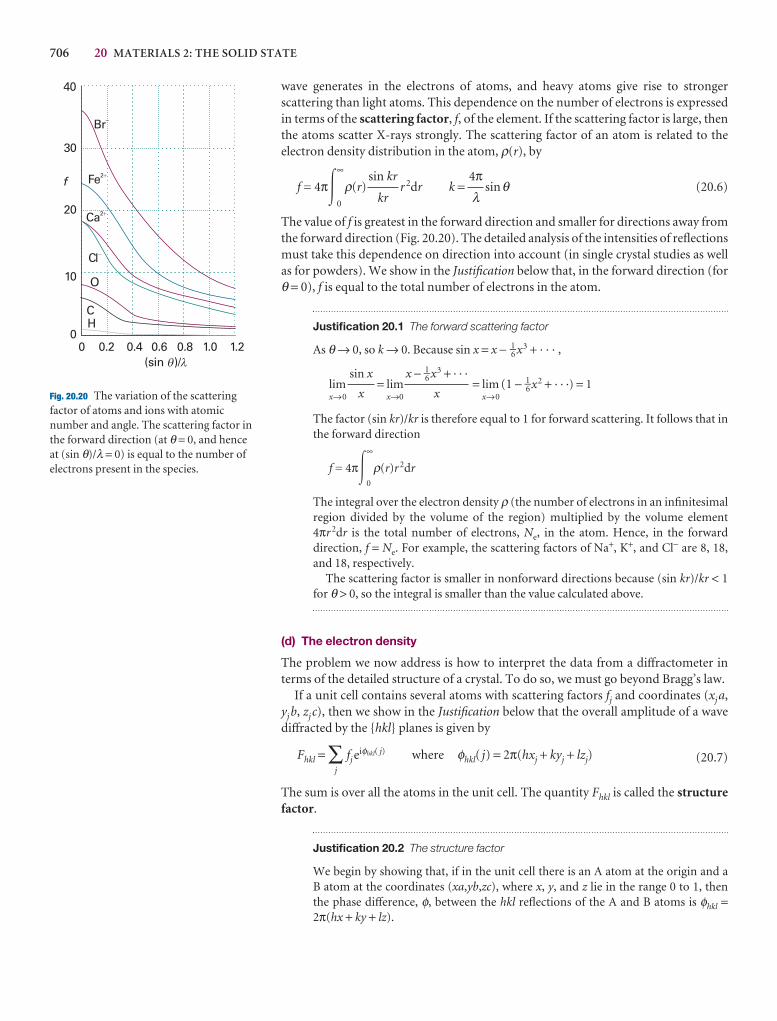
706 20 MATERIALS 2: THE SOLID STATE
wave generates in the electrons of atoms, and heavy atoms give rise to stronger scattering than light atoms. This dependence on the number of electrons is expressedin terms of the scattering factor, f, of the element. If the scattering factor is large, thenthe atoms scatter X-rays strongly. The scattering factor of an atom is related to theelectron density distribution in the atom, ρ(r), by
f = 4π�∞
0
ρ(r) r 2dr k = sinθ (20.6)
The value of f is greatest in the forward direction and smaller for directions away fromthe forward direction (Fig. 20.20). The detailed analysis of the intensities of reflectionsmust take this dependence on direction into account (in single crystal studies as wellas for powders). We show in the Justification below that, in the forward direction (forθ = 0), f is equal to the total number of electrons in the atom.
Justification 20.1 The forward scattering factor
As θ → 0, so k → 0. Because sin x = x − 1–6 x3 + · · · ,
limx→0
= limx→0
= limx→0
(1 − 1–6 x2 + · · ·) = 1
The factor (sin kr)/kr is therefore equal to 1 for forward scattering. It follows that inthe forward direction
f = 4π�∞
0
ρ(r)r 2dr
The integral over the electron density ρ (the number of electrons in an infinitesimalregion divided by the volume of the region) multiplied by the volume element4πr 2dr is the total number of electrons, Ne, in the atom. Hence, in the forward direction, f = Ne. For example, the scattering factors of Na+, K+, and Cl− are 8, 18,and 18, respectively.
The scattering factor is smaller in nonforward directions because (sin kr)/kr < 1for θ > 0, so the integral is smaller than the value calculated above.
(d) The electron density
The problem we now address is how to interpret the data from a diffractometer interms of the detailed structure of a crystal. To do so, we must go beyond Bragg’s law.
If a unit cell contains several atoms with scattering factors fj and coordinates (xj a,yj b, zj c), then we show in the Justification below that the overall amplitude of a wavediffracted by the {hkl} planes is given by
Fhkl = ∑j
fj eiφhkl( j) where φhkl( j) = 2π(hxj + kyj + lzj) (20.7)
The sum is over all the atoms in the unit cell. The quantity Fhkl is called the structurefactor.
Justification 20.2 The structure factor
We begin by showing that, if in the unit cell there is an A atom at the origin and a B atom at the coordinates (xa,yb,zc), where x, y, and z lie in the range 0 to 1, then the phase difference, φ, between the hkl reflections of the A and B atoms is φhkl =2π(hx + ky + lz).
x − 1–6 x3 + · · ·
x
sin x
x
4πλ
sin kr
kr
10
30
20
Br�
Fe2�
Ca2�
Cl�
O
CH
f
0 0.4 0.6 0.8 1.0 1.20.2(sin )/
40
0
��
Fig. 20.20 The variation of the scatteringfactor of atoms and ions with atomicnumber and angle. The scattering factor inthe forward direction (at θ = 0, and henceat (sin θ)/λ = 0) is equal to the number ofelectrons present in the species.
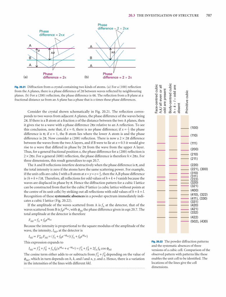
20.3 THE INVESTIGATION OF STRUCTURE 707
B B
A A
A A
(a) (b)
xaa xa
Phasedifference = 2�x
Phasedifference 2 2� � �x
Phasedifference = 2�
Phasedifference = 2 2� �
(100)
(110)
(111)
(200)(210)(211)
(220)
(222)
(310)
(320)(321)(400)
(331)
(332)
(420)(421)
(422)(502), (430)
(410), (322)(411), (330)
(311)
(221), (300)
Face
-cen
tred
cub
ic,
,al
l eve
n o
r al
lod
d a
re p
rese
nth
kl
Bod
y-ce
ntre
d c
ubic
odd
are
abse
nth
kl
��
�
Prim
itive
cub
ic
Fig. 20.22 The powder diffraction patternsand the systematic absences of threeversions of a cubic cell. Comparison of theobserved pattern with patterns like theseenables the unit cell to be identified. Thelocations of the lines give the celldimensions.
Consider the crystal shown schematically in Fig. 20.21. The reflection corres-ponds to two waves from adjacent A planes, the phase difference of the waves being2π. If there is a B atom at a fraction x of the distance between the two A planes, thenit gives rise to a wave with a phase difference 2πx relative to an A reflection. To seethis conclusion, note that, if x = 0, there is no phase difference; if x = 1–2 the phasedifference is π; if x = 1, the B atom lies where the lower A atom is and the phasedifference is 2π. Now consider a (200) reflection. There is now a 2 × 2π differencebetween the waves from the two A layers, and if B were to lie at x = 0.5 it would giverise to a wave that differed in phase by 2π from the wave from the upper A layer.Thus, for a general fractional position x, the phase difference for a (200) reflection is2 × 2πx. For a general (h00) reflection, the phase difference is therefore h × 2πx. Forthree dimensions, this result generalizes to eqn 20.7.
The A and B reflections interfere destructively when the phase difference is π, andthe total intensity is zero if the atoms have the same scattering power. For example,if the unit cells are cubic I with a B atom at x = y = z = 1–2, then the A,B phase differenceis (h + k + l)π. Therefore, all reflections for odd values of h + k + l vanish because thewaves are displaced in phase by π. Hence the diffraction pattern for a cubic I latticecan be constructed from that for the cubic P lattice (a cubic lattice without points atthe centre of its unit cells) by striking out all reflections with odd values of h + k + l.Recognition of these systematic absences in a powder spectrum immediately indi-cates a cubic I lattice (Fig. 20.22).
If the amplitude of the waves scattered from A is fA at the detector, that of thewaves scattered from B is fBeiφhkl, with φhkl the phase difference given in eqn 20.7. Thetotal amplitude at the detector is therefore
Fhkl = fA + fBeiφhkl
Because the intensity is proportional to the square modulus of the amplitude of thewave, the intensity, Ihkl, at the detector is
Ihkl ∝ F*hkl Fhkl = ( fA + fBe−iφhkl)( fA + fBeiφhkl)
This expression expands to
Ihkl ∝ f 2A + f 2
B + fA fB(eiφhkl + e−iφhkl) = f 2A + f 2
B + 2fA fB cos φhkl
The cosine term either adds to or subtracts from f 2A + f 2
B depending on the value ofφhkl , which in turn depends on h, k, and l and x, y, and z. Hence, there is a variationin the intensities of the lines with different hkl.
Fig. 20.21 Diffraction from a crystal containing two kinds of atoms. (a) For a (100) reflectionfrom the A planes, there is a phase difference of 2π between waves reflected by neighbouringplanes. (b) For a (200) reflection, the phase difference is 4π. The reflection from a B plane at afractional distance xa from an A plane has a phase that is x times these phase differences.
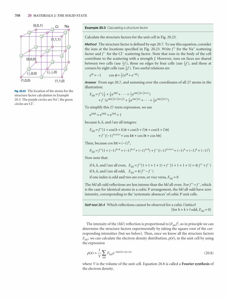
708 20 MATERIALS 2: THE SOLID STATE
Cl Na(0,0,1)
(1,1,0)(1,0,0)
(1,1,1)
(0,0,0)
( ,0,0) ( , ,0)�21 �2
1 �21
Fig. 20.23 The location of the atoms for thestructure factor calculation in Example20.3. The purple circles are Na+; the greencircles are Cl−.
Example 20.3 Calculating a structure factor
Calculate the structure factors for the unit cell in Fig. 20.23.
Method The structure factor is defined by eqn 20.7. To use this equation, considerthe ions at the locations specified in Fig. 20.23. Write f + for the Na+ scatteringfactor and f − for the Cl− scattering factor. Note that ions in the body of the cell contribute to the scattering with a strength f. However, ions on faces are shared between two cells (use 1–2 f ), those on edges by four cells (use 1–4 f ), and those at corners by eight cells (use 1–8 f ). Two useful relations are
eiπ = −1 cos φ = 1–2(eiφ + e−iφ)
Answer From eqn 20.7, and summing over the coordinates of all 27 atoms in theillustration:
Fhkl = f +( 1–8 + 1–8 e2πil + · · · + 1–2 e2πi(1––2 h+ 1––
2 k+l ))
+ f −(e2πi(1––2 h+ 1––
2 k+ 1––2 l) + 1–4 e2πi(1––
2 h) + · · · + 1–4 e2πi(1––2 h+l))
To simplify this 27-term expression, we use
e2πih = e2πik = e2πil = 1
because h, k, and l are all integers:
Fhkl = f +{1 + cos(h + k)π + cos(h + l)π + cos(k + l)π}
+ f −{(−1)h+k+l + cos kπ + cos lπ + cos hπ}
Then, because cos hπ = (−1)h,
Fhkl = f +{1 + (−1)h+k + (−1)h+l + (−1)l+k} + f −{(−1)h+k+l + (−1)h + (−1)k + (−1)l}
Now note that:
if h, k, and l are all even, Fhkl = f +{1 + 1 + 1 + 1} + f −{1 + 1 + 1 + 1} = 4( f + + f −)
if h, k, and l are all odd, Fhkl = 4( f + − f −)
if one index is odd and two are even, or vice versa, Fhkl = 0
The hkl all-odd reflections are less intense than the hkl all-even. For f + = f −, whichis the case for identical atoms in a cubic P arrangement, the hkl all-odd have zerointensity, corresponding to the ‘systematic absences’ of cubic P unit cells.
Self-test 20.4 Which reflections cannot be observed for a cubic I lattice?[for h + k + l odd, Fhkl = 0]
The intensity of the (hkl) reflection is proportional to |Fhkl |2, so in principle we candetermine the structure factors experimentally by taking the square root of the cor-responding intensities (but see below). Then, once we know all the structure factorsFhkl , we can calculate the electron density distribution, ρ(r), in the unit cell by usingthe expression
ρ(r) = ∑hkl
Fhkle−2πi(hx+ky+lz) (20.8)
where V is the volume of the unit cell. Equation 20.8 is called a Fourier synthesis ofthe electron density.
1
V
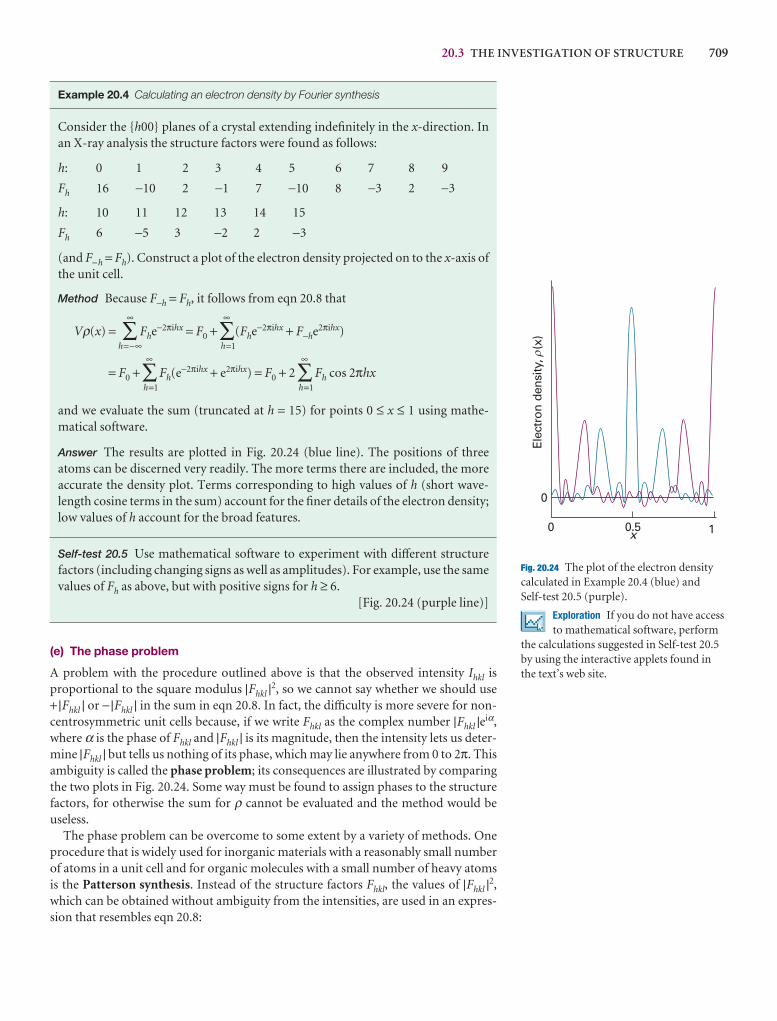
20.3 THE INVESTIGATION OF STRUCTURE 709
Elec
tron
den
sity
, (x
)0 0.5 1x
0
�
Fig. 20.24 The plot of the electron densitycalculated in Example 20.4 (blue) and Self-test 20.5 (purple).
Exploration If you do not have accessto mathematical software, perform
the calculations suggested in Self-test 20.5by using the interactive applets found inthe text’s web site.
Example 20.4 Calculating an electron density by Fourier synthesis
Consider the {h00} planes of a crystal extending indefinitely in the x-direction. Inan X-ray analysis the structure factors were found as follows:
h: 0 1 2 3 4 5 6 7 8 9
Fh 16 −10 2 −1 7 −10 8 −3 2 −3
h: 10 11 12 13 14 15
Fh 6 −5 3 −2 2 −3
(and F−h = Fh). Construct a plot of the electron density projected on to the x-axis ofthe unit cell.
Method Because F−h = Fh, it follows from eqn 20.8 that
Vρ(x) =∞
∑h=−∞
Fhe−2πihx = F0 +∞
∑h=1
(Fhe−2πihx + F−he2πihx)
= F0 +∞
∑h=1
Fh(e−2πihx + e2πihx) = F0 + 2∞
∑h=1
Fh cos 2πhx
and we evaluate the sum (truncated at h = 15) for points 0 ≤ x ≤ 1 using mathe-matical software.
Answer The results are plotted in Fig. 20.24 (blue line). The positions of threeatoms can be discerned very readily. The more terms there are included, the moreaccurate the density plot. Terms corresponding to high values of h (short wave-length cosine terms in the sum) account for the finer details of the electron density;low values of h account for the broad features.
Self-test 20.5 Use mathematical software to experiment with different structurefactors (including changing signs as well as amplitudes). For example, use the samevalues of Fh as above, but with positive signs for h ≥ 6.
[Fig. 20.24 (purple line)]
(e) The phase problem
A problem with the procedure outlined above is that the observed intensity Ihkl isproportional to the square modulus |Fhkl |2, so we cannot say whether we should use+|Fhkl | or −|Fhkl | in the sum in eqn 20.8. In fact, the difficulty is more severe for non-centrosymmetric unit cells because, if we write Fhkl as the complex number |Fhkl |eiα,where α is the phase of Fhkl and |Fhkl | is its magnitude, then the intensity lets us deter-mine |Fhkl | but tells us nothing of its phase, which may lie anywhere from 0 to 2π. Thisambiguity is called the phase problem; its consequences are illustrated by comparingthe two plots in Fig. 20.24. Some way must be found to assign phases to the structurefactors, for otherwise the sum for ρ cannot be evaluated and the method would beuseless.
The phase problem can be overcome to some extent by a variety of methods. Oneprocedure that is widely used for inorganic materials with a reasonably small numberof atoms in a unit cell and for organic molecules with a small number of heavy atomsis the Patterson synthesis. Instead of the structure factors Fhkl, the values of |Fhkl |2,which can be obtained without ambiguity from the intensities, are used in an expres-sion that resembles eqn 20.8:
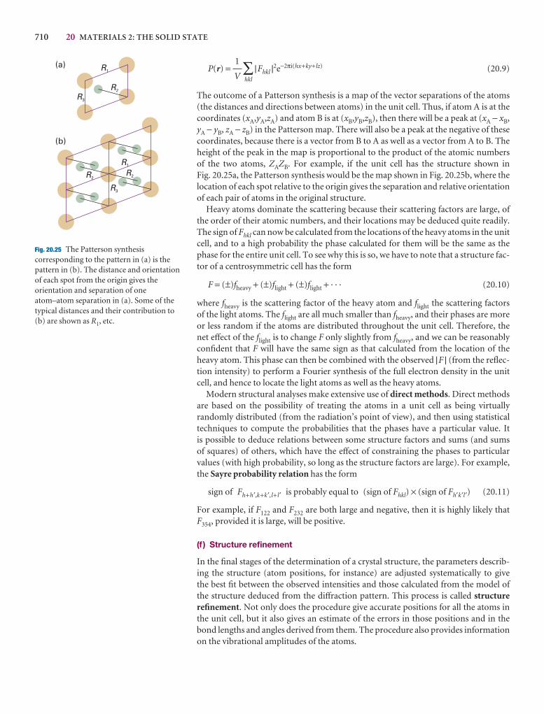
710 20 MATERIALS 2: THE SOLID STATE
P(r) = ∑hkl
|Fhkl |2e−2πi(hx+ky+lz) (20.9)
The outcome of a Patterson synthesis is a map of the vector separations of the atoms(the distances and directions between atoms) in the unit cell. Thus, if atom A is at thecoordinates (xA,yA,zA) and atom B is at (xB,yB,zB), then there will be a peak at (xA − xB,yA − yB, zA − zB) in the Patterson map. There will also be a peak at the negative of thesecoordinates, because there is a vector from B to A as well as a vector from A to B. Theheight of the peak in the map is proportional to the product of the atomic numbers of the two atoms, ZAZB. For example, if the unit cell has the structure shown in Fig. 20.25a, the Patterson synthesis would be the map shown in Fig. 20.25b, where thelocation of each spot relative to the origin gives the separation and relative orientationof each pair of atoms in the original structure.
Heavy atoms dominate the scattering because their scattering factors are large, ofthe order of their atomic numbers, and their locations may be deduced quite readily.The sign of Fhkl can now be calculated from the locations of the heavy atoms in the unitcell, and to a high probability the phase calculated for them will be the same as thephase for the entire unit cell. To see why this is so, we have to note that a structure fac-tor of a centrosymmetric cell has the form
F = (±)fheavy + (±)flight + (±)flight + · · · (20.10)
where fheavy is the scattering factor of the heavy atom and flight the scattering factors of the light atoms. The flight are all much smaller than fheavy, and their phases are more or less random if the atoms are distributed throughout the unit cell. Therefore, the net effect of the flight is to change F only slightly from fheavy, and we can be reasonablyconfident that F will have the same sign as that calculated from the location of theheavy atom. This phase can then be combined with the observed |F | (from the reflec-tion intensity) to perform a Fourier synthesis of the full electron density in the unitcell, and hence to locate the light atoms as well as the heavy atoms.
Modern structural analyses make extensive use of direct methods. Direct methodsare based on the possibility of treating the atoms in a unit cell as being virtually randomly distributed (from the radiation’s point of view), and then using statisticaltechniques to compute the probabilities that the phases have a particular value. It is possible to deduce relations between some structure factors and sums (and sums of squares) of others, which have the effect of constraining the phases to particularvalues (with high probability, so long as the structure factors are large). For example,the Sayre probability relation has the form
sign of Fh+h′,k+k′,l+l′ is probably equal to (sign of Fhkl) × (sign of Fh′k′l′) (20.11)
For example, if F122 and F232 are both large and negative, then it is highly likely thatF354, provided it is large, will be positive.
(f ) Structure refinement
In the final stages of the determination of a crystal structure, the parameters describ-ing the structure (atom positions, for instance) are adjusted systematically to give the best fit between the observed intensities and those calculated from the model ofthe structure deduced from the diffraction pattern. This process is called structurerefinement. Not only does the procedure give accurate positions for all the atoms inthe unit cell, but it also gives an estimate of the errors in those positions and in thebond lengths and angles derived from them. The procedure also provides informationon the vibrational amplitudes of the atoms.
1
VR1
R1
R2
R2R2
R3
R3
(a)
(b)
Fig. 20.25 The Patterson synthesiscorresponding to the pattern in (a) is thepattern in (b). The distance and orientationof each spot from the origin gives theorientation and separation of oneatom–atom separation in (a). Some of thetypical distances and their contribution to(b) are shown as R1, etc.
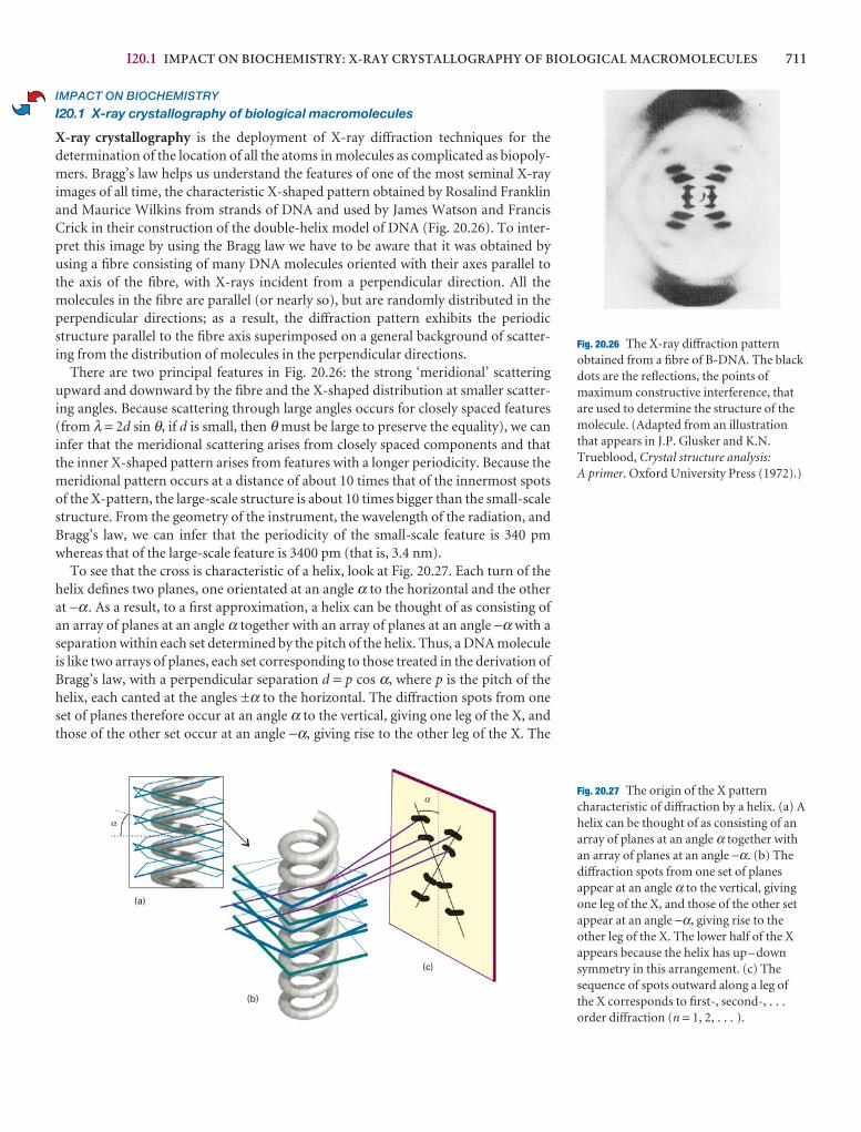
I20.1 IMPACT ON BIOCHEMISTRY: X-RAY CRYSTALLOGRAPHY OF BIOLOGICAL MACROMOLECULES 711
IMPACT ON BIOCHEMISTRY
I20.1 X-ray crystallography of biological macromolecules
X-ray crystallography is the deployment of X-ray diffraction techniques for the determination of the location of all the atoms in molecules as complicated as biopoly-mers. Bragg’s law helps us understand the features of one of the most seminal X-rayimages of all time, the characteristic X-shaped pattern obtained by Rosalind Franklinand Maurice Wilkins from strands of DNA and used by James Watson and FrancisCrick in their construction of the double-helix model of DNA (Fig. 20.26). To inter-pret this image by using the Bragg law we have to be aware that it was obtained byusing a fibre consisting of many DNA molecules oriented with their axes parallel tothe axis of the fibre, with X-rays incident from a perpendicular direction. All themolecules in the fibre are parallel (or nearly so), but are randomly distributed in theperpendicular directions; as a result, the diffraction pattern exhibits the periodicstructure parallel to the fibre axis superimposed on a general background of scatter-ing from the distribution of molecules in the perpendicular directions.
There are two principal features in Fig. 20.26: the strong ‘meridional’ scattering upward and downward by the fibre and the X-shaped distribution at smaller scatter-ing angles. Because scattering through large angles occurs for closely spaced features(from λ = 2d sin θ, if d is small, then θ must be large to preserve the equality), we caninfer that the meridional scattering arises from closely spaced components and thatthe inner X-shaped pattern arises from features with a longer periodicity. Because themeridional pattern occurs at a distance of about 10 times that of the innermost spotsof the X-pattern, the large-scale structure is about 10 times bigger than the small-scalestructure. From the geometry of the instrument, the wavelength of the radiation, andBragg’s law, we can infer that the periodicity of the small-scale feature is 340 pmwhereas that of the large-scale feature is 3400 pm (that is, 3.4 nm).
To see that the cross is characteristic of a helix, look at Fig. 20.27. Each turn of thehelix defines two planes, one orientated at an angle α to the horizontal and the otherat −α . As a result, to a first approximation, a helix can be thought of as consisting ofan array of planes at an angle α together with an array of planes at an angle −α with aseparation within each set determined by the pitch of the helix. Thus, a DNA moleculeis like two arrays of planes, each set corresponding to those treated in the derivation ofBragg’s law, with a perpendicular separation d = p cos α, where p is the pitch of thehelix, each canted at the angles ±α to the horizontal. The diffraction spots from oneset of planes therefore occur at an angle α to the vertical, giving one leg of the X, andthose of the other set occur at an angle −α, giving rise to the other leg of the X. The
Fig. 20.26 The X-ray diffraction patternobtained from a fibre of B-DNA. The blackdots are the reflections, the points ofmaximum constructive interference, thatare used to determine the structure of themolecule. (Adapted from an illustrationthat appears in J.P. Glusker and K.N.Trueblood, Crystal structure analysis: A primer. Oxford University Press (1972).)
(a)
(b)
(c)
�
�Fig. 20.27 The origin of the X patterncharacteristic of diffraction by a helix. (a) Ahelix can be thought of as consisting of anarray of planes at an angle α together withan array of planes at an angle −α. (b) Thediffraction spots from one set of planesappear at an angle α to the vertical, givingone leg of the X, and those of the other setappear at an angle −α, giving rise to theother leg of the X. The lower half of the Xappears because the helix has up–downsymmetry in this arrangement. (c) Thesequence of spots outward along a leg ofthe X corresponds to first-, second-, . . .order diffraction (n = 1, 2, . . . ).
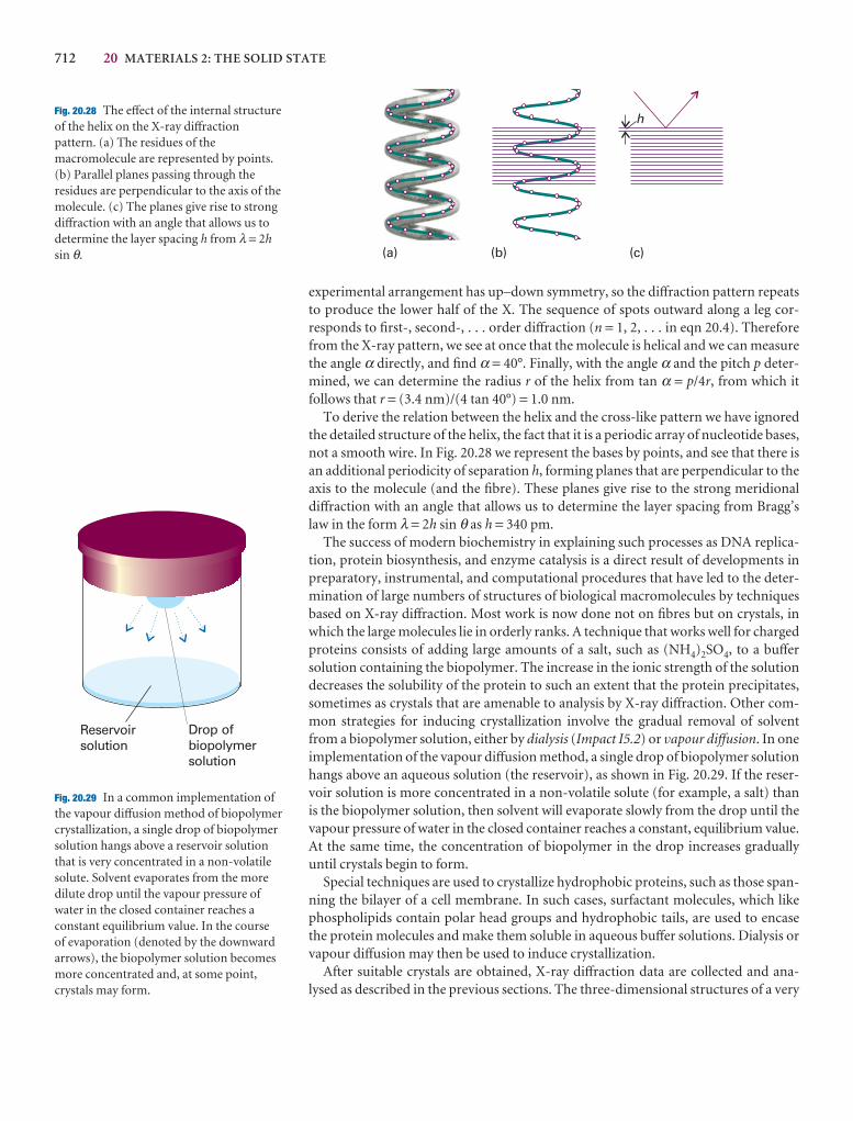
712 20 MATERIALS 2: THE SOLID STATE
experimental arrangement has up–down symmetry, so the diffraction pattern repeats to produce the lower half of the X. The sequence of spots outward along a leg cor-responds to first-, second-, . . . order diffraction (n = 1, 2, . . . in eqn 20.4). Thereforefrom the X-ray pattern, we see at once that the molecule is helical and we can measurethe angle α directly, and find α = 40°. Finally, with the angle α and the pitch p deter-mined, we can determine the radius r of the helix from tan α = p/4r, from which itfollows that r = (3.4 nm)/(4 tan 40°) = 1.0 nm.
To derive the relation between the helix and the cross-like pattern we have ignoredthe detailed structure of the helix, the fact that it is a periodic array of nucleotide bases,not a smooth wire. In Fig. 20.28 we represent the bases by points, and see that there isan additional periodicity of separation h, forming planes that are perpendicular to theaxis to the molecule (and the fibre). These planes give rise to the strong meridionaldiffraction with an angle that allows us to determine the layer spacing from Bragg’slaw in the form λ = 2h sin θ as h = 340 pm.
The success of modern biochemistry in explaining such processes as DNA replica-tion, protein biosynthesis, and enzyme catalysis is a direct result of developments inpreparatory, instrumental, and computational procedures that have led to the deter-mination of large numbers of structures of biological macromolecules by techniquesbased on X-ray diffraction. Most work is now done not on fibres but on crystals, inwhich the large molecules lie in orderly ranks. A technique that works well for chargedproteins consists of adding large amounts of a salt, such as (NH4)2SO4, to a buffersolution containing the biopolymer. The increase in the ionic strength of the solutiondecreases the solubility of the protein to such an extent that the protein precipitates,sometimes as crystals that are amenable to analysis by X-ray diffraction. Other com-mon strategies for inducing crystallization involve the gradual removal of solventfrom a biopolymer solution, either by dialysis (Impact I5.2) or vapour diffusion. In oneimplementation of the vapour diffusion method, a single drop of biopolymer solutionhangs above an aqueous solution (the reservoir), as shown in Fig. 20.29. If the reser-voir solution is more concentrated in a non-volatile solute (for example, a salt) thanis the biopolymer solution, then solvent will evaporate slowly from the drop until thevapour pressure of water in the closed container reaches a constant, equilibrium value.At the same time, the concentration of biopolymer in the drop increases graduallyuntil crystals begin to form.
Special techniques are used to crystallize hydrophobic proteins, such as those span-ning the bilayer of a cell membrane. In such cases, surfactant molecules, which likephospholipids contain polar head groups and hydrophobic tails, are used to encasethe protein molecules and make them soluble in aqueous buffer solutions. Dialysis orvapour diffusion may then be used to induce crystallization.
After suitable crystals are obtained, X-ray diffraction data are collected and ana-lysed as described in the previous sections. The three-dimensional structures of a very
h
(a) (b) (c)
Fig. 20.28 The effect of the internal structureof the helix on the X-ray diffractionpattern. (a) The residues of themacromolecule are represented by points.(b) Parallel planes passing through theresidues are perpendicular to the axis of themolecule. (c) The planes give rise to strongdiffraction with an angle that allows us todetermine the layer spacing h from λ = 2hsin θ.
Drop ofbiopolymersolution
Reservoirsolution
Fig. 20.29 In a common implementation ofthe vapour diffusion method of biopolymercrystallization, a single drop of biopolymersolution hangs above a reservoir solutionthat is very concentrated in a non-volatilesolute. Solvent evaporates from the moredilute drop until the vapour pressure ofwater in the closed container reaches aconstant equilibrium value. In the courseof evaporation (denoted by the downwardarrows), the biopolymer solution becomesmore concentrated and, at some point,crystals may form.
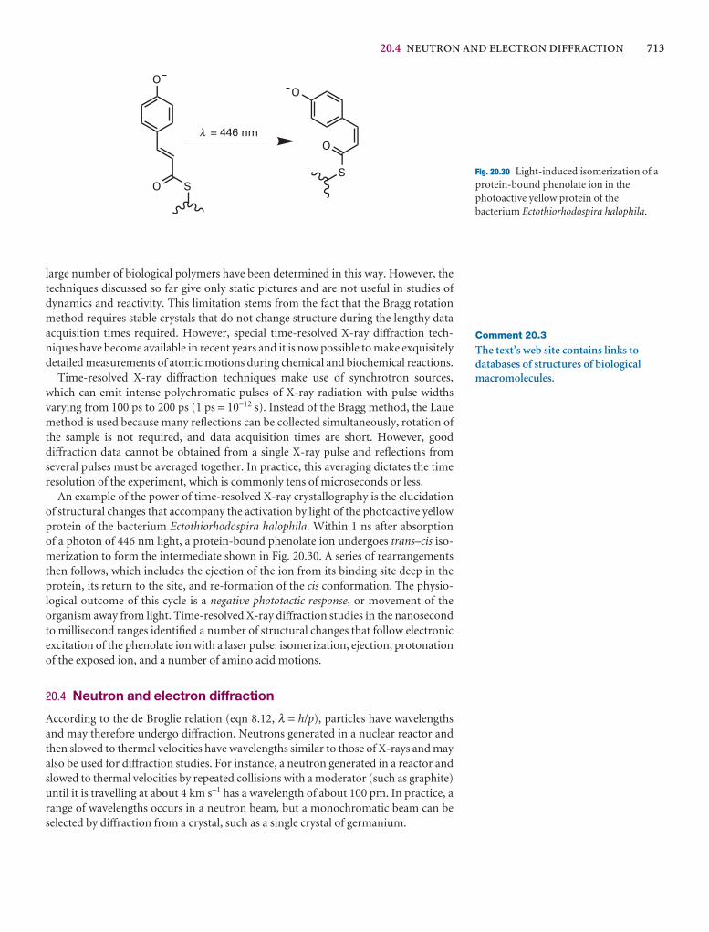
20.4 NEUTRON AND ELECTRON DIFFRACTION 713
large number of biological polymers have been determined in this way. However, thetechniques discussed so far give only static pictures and are not useful in studies of dynamics and reactivity. This limitation stems from the fact that the Bragg rotationmethod requires stable crystals that do not change structure during the lengthy dataacquisition times required. However, special time-resolved X-ray diffraction tech-niques have become available in recent years and it is now possible to make exquisitelydetailed measurements of atomic motions during chemical and biochemical reactions.
Time-resolved X-ray diffraction techniques make use of synchrotron sources,which can emit intense polychromatic pulses of X-ray radiation with pulse widthsvarying from 100 ps to 200 ps (1 ps = 10−12 s). Instead of the Bragg method, the Lauemethod is used because many reflections can be collected simultaneously, rotation ofthe sample is not required, and data acquisition times are short. However, gooddiffraction data cannot be obtained from a single X-ray pulse and reflections fromseveral pulses must be averaged together. In practice, this averaging dictates the timeresolution of the experiment, which is commonly tens of microseconds or less.
An example of the power of time-resolved X-ray crystallography is the elucidationof structural changes that accompany the activation by light of the photoactive yellowprotein of the bacterium Ectothiorhodospira halophila. Within 1 ns after absorption of a photon of 446 nm light, a protein-bound phenolate ion undergoes trans–cis iso-merization to form the intermediate shown in Fig. 20.30. A series of rearrangementsthen follows, which includes the ejection of the ion from its binding site deep in theprotein, its return to the site, and re-formation of the cis conformation. The physio-logical outcome of this cycle is a negative phototactic response, or movement of the organism away from light. Time-resolved X-ray diffraction studies in the nanosecondto millisecond ranges identified a number of structural changes that follow electronicexcitation of the phenolate ion with a laser pulse: isomerization, ejection, protonationof the exposed ion, and a number of amino acid motions.
20.4 Neutron and electron diffraction
According to the de Broglie relation (eqn 8.12, λ = h/p), particles have wavelengthsand may therefore undergo diffraction. Neutrons generated in a nuclear reactor andthen slowed to thermal velocities have wavelengths similar to those of X-rays and mayalso be used for diffraction studies. For instance, a neutron generated in a reactor andslowed to thermal velocities by repeated collisions with a moderator (such as graphite)until it is travelling at about 4 km s−1 has a wavelength of about 100 pm. In practice, arange of wavelengths occurs in a neutron beam, but a monochromatic beam can beselected by diffraction from a crystal, such as a single crystal of germanium.
Comment 20.3
The text’s web site contains links todatabases of structures of biologicalmacromolecules.
Fig. 20.30 Light-induced isomerization of aprotein-bound phenolate ion in thephotoactive yellow protein of thebacterium Ectothiorhodospira halophila.
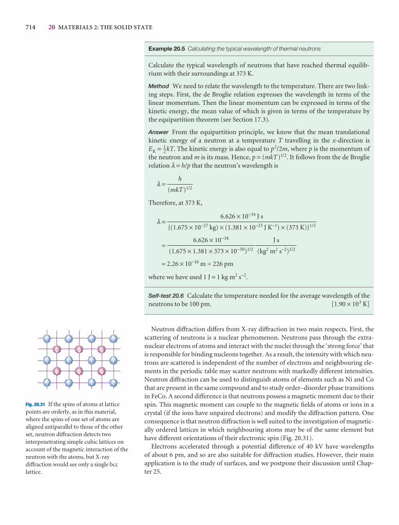
714 20 MATERIALS 2: THE SOLID STATE
Fig. 20.31 If the spins of atoms at latticepoints are orderly, as in this material,where the spins of one set of atoms arealigned antiparallel to those of the otherset, neutron diffraction detects twointerpenetrating simple cubic lattices onaccount of the magnetic interaction of theneutron with the atoms, but X-raydiffraction would see only a single bcclattice.
Example 20.5 Calculating the typical wavelength of thermal neutrons
Calculate the typical wavelength of neutrons that have reached thermal equilib-rium with their surroundings at 373 K.
Method We need to relate the wavelength to the temperature. There are two link-ing steps. First, the de Broglie relation expresses the wavelength in terms of the linear momentum. Then the linear momentum can be expressed in terms of the kinetic energy, the mean value of which is given in terms of the temperature by the equipartition theorem (see Section 17.3).
Answer From the equipartition principle, we know that the mean translational kinetic energy of a neutron at a temperature T travelling in the x-direction is EK = 1–2 kT. The kinetic energy is also equal to p2/2m, where p is the momentum ofthe neutron and m is its mass. Hence, p = (mkT)1/2. It follows from the de Broglierelation λ = h/p that the neutron’s wavelength is
λ =
Therefore, at 373 K,
λ =
=
= 2.26 × 10⁻¹⁰ m = 226 pm
where we have used 1 J = 1 kg m2 s−2.
Self-test 20.6 Calculate the temperature needed for the average wavelength of theneutrons to be 100 pm. [1.90 × 10³ K]
Neutron diffraction differs from X-ray diffraction in two main respects. First, thescattering of neutrons is a nuclear phenomenon. Neutrons pass through the extra-nuclear electrons of atoms and interact with the nuclei through the ‘strong force’ thatis responsible for binding nucleons together. As a result, the intensity with which neu-trons are scattered is independent of the number of electrons and neighbouring ele-ments in the periodic table may scatter neutrons with markedly different intensities.Neutron diffraction can be used to distinguish atoms of elements such as Ni and Cothat are present in the same compound and to study order–disorder phase transitionsin FeCo. A second difference is that neutrons possess a magnetic moment due to theirspin. This magnetic moment can couple to the magnetic fields of atoms or ions in acrystal (if the ions have unpaired electrons) and modify the diffraction pattern. Oneconsequence is that neutron diffraction is well suited to the investigation of magnetic-ally ordered lattices in which neighbouring atoms may be of the same element buthave different orientations of their electronic spin (Fig. 20.31).
Electrons accelerated through a potential difference of 40 kV have wavelengths of about 6 pm, and so are also suitable for diffraction studies. However, their main application is to the study of surfaces, and we postpone their discussion until Chap-ter 25.
J s
(kg2 m2 s−2)1/2
6.626 × 10⁻³⁴
(1.675 × 1.381 × 373 × 10−50)1/2
6.626 × 10⁻³⁴ J s
{(1.675 × 10⁻²⁷ kg) × (1.381 × 10⁻²³ J K−1) × (373 K)}1/2
h
(mkT)1/2
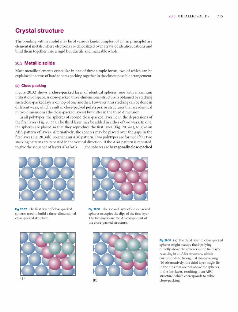
20.5 METALLIC SOLIDS 715
Crystal structure
The bonding within a solid may be of various kinds. Simplest of all (in principle) areelemental metals, where electrons are delocalized over arrays of identical cations andbind them together into a rigid but ductile and malleable whole.
20.5 Metallic solids
Most metallic elements crystallize in one of three simple forms, two of which can beexplained in terms of hard spheres packing together in the closest possible arrangement.
(a) Close packing
Figure 20.32 shows a close-packed layer of identical spheres, one with maximum utilization of space. A close-packed three-dimensional structure is obtained by stackingsuch close-packed layers on top of one another. However, this stacking can be done indifferent ways, which result in close-packed polytypes, or structures that are identicalin two dimensions (the close-packed layers) but differ in the third dimension.
In all polytypes, the spheres of second close-packed layer lie in the depressions ofthe first layer (Fig. 20.33). The third layer may be added in either of two ways. In one,the spheres are placed so that they reproduce the first layer (Fig. 20.34a), to give anABA pattern of layers. Alternatively, the spheres may be placed over the gaps in thefirst layer (Fig. 20.34b), so giving an ABC pattern. Two polytypes are formed if the twostacking patterns are repeated in the vertical direction. If the ABA pattern is repeated,to give the sequence of layers ABABAB . . . , the spheres are hexagonally close-packed
Fig. 20.34 (a) The third layer of close-packedspheres might occupy the dips lyingdirectly above the spheres in the first layer,resulting in an ABA structure, whichcorresponds to hexagonal close-packing.(b) Alternatively, the third layer might liein the dips that are not above the spheres in the first layer, resulting in an ABCstructure, which corresponds to cubicclose-packing
Fig. 20.32 The first layer of close-packedspheres used to build a three-dimensionalclose-packed structure.
Fig. 20.33 The second layer of close-packedspheres occupies the dips of the first layer.The two layers are the AB component ofthe close-packed structure.
(a) (b)
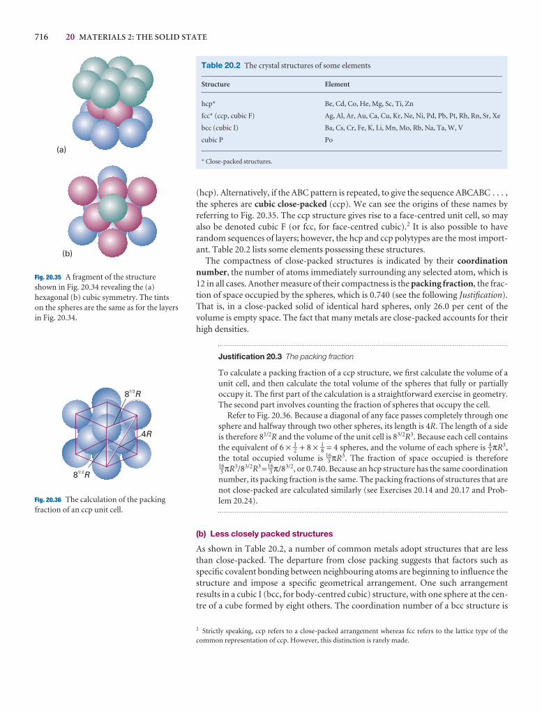
716 20 MATERIALS 2: THE SOLID STATE
(hcp). Alternatively, if the ABC pattern is repeated, to give the sequence ABCABC . . . ,the spheres are cubic close-packed (ccp). We can see the origins of these names by referring to Fig. 20.35. The ccp structure gives rise to a face-centred unit cell, so mayalso be denoted cubic F (or fcc, for face-centred cubic).2 It is also possible to have random sequences of layers; however, the hcp and ccp polytypes are the most import-ant. Table 20.2 lists some elements possessing these structures.
The compactness of close-packed structures is indicated by their coordinationnumber, the number of atoms immediately surrounding any selected atom, which is12 in all cases. Another measure of their compactness is the packing fraction, the frac-tion of space occupied by the spheres, which is 0.740 (see the following Justification).That is, in a close-packed solid of identical hard spheres, only 26.0 per cent of the volume is empty space. The fact that many metals are close-packed accounts for theirhigh densities.
Justification 20.3 The packing fraction
To calculate a packing fraction of a ccp structure, we first calculate the volume of aunit cell, and then calculate the total volume of the spheres that fully or partially occupy it. The first part of the calculation is a straightforward exercise in geometry.The second part involves counting the fraction of spheres that occupy the cell.
Refer to Fig. 20.36. Because a diagonal of any face passes completely through onesphere and halfway through two other spheres, its length is 4R. The length of a sideis therefore 81/2R and the volume of the unit cell is 83/2R3. Because each cell containsthe equivalent of 6 × 1–2 + 8 × 1–8 = 4 spheres, and the volume of each sphere is 4–3 πR3,the total occupied volume is 16–3 πR3. The fraction of space occupied is therefore16–3 πR3/83/2R3 =16–3 π/83/2, or 0.740. Because an hcp structure has the same coordinationnumber, its packing fraction is the same. The packing fractions of structures that arenot close-packed are calculated similarly (see Exercises 20.14 and 20.17 and Prob-lem 20.24).
(b) Less closely packed structures
As shown in Table 20.2, a number of common metals adopt structures that are lessthan close-packed. The departure from close packing suggests that factors such asspecific covalent bonding between neighbouring atoms are beginning to influence thestructure and impose a specific geometrical arrangement. One such arrangement results in a cubic I (bcc, for body-centred cubic) structure, with one sphere at the cen-tre of a cube formed by eight others. The coordination number of a bcc structure is
Table 20.2 The crystal structures of some elements
Structure Element
hcp* Be, Cd, Co, He, Mg, Sc, Ti, Zn
fcc* (ccp, cubic F) Ag, Al, Ar, Au, Ca, Cu, Kr, Ne, Ni, Pd, Pb, Pt, Rh, Rn, Sr, Xe
bcc (cubic I) Ba, Cs, Cr, Fe, K, Li, Mn, Mo, Rb, Na, Ta, W, V
cubic P Po
* Close-packed structures.
(a)
(b)
Fig. 20.35 A fragment of the structureshown in Fig. 20.34 revealing the (a)hexagonal (b) cubic symmetry. The tintson the spheres are the same as for the layersin Fig. 20.34.
2 Strictly speaking, ccp refers to a close-packed arrangement whereas fcc refers to the lattice type of thecommon representation of ccp. However, this distinction is rarely made.
4R
81/2R
81/ 2R
Fig. 20.36 The calculation of the packingfraction of an ccp unit cell.
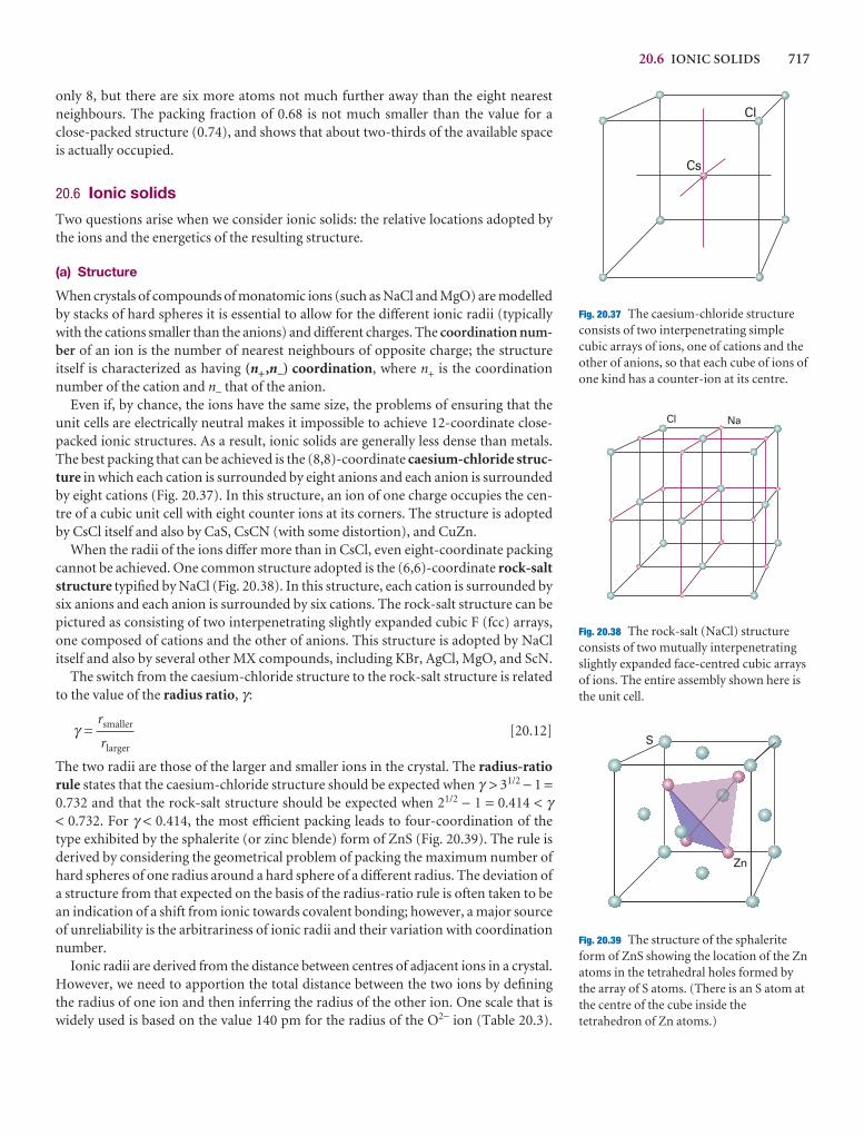
20.6 IONIC SOLIDS 717
only 8, but there are six more atoms not much further away than the eight nearestneighbours. The packing fraction of 0.68 is not much smaller than the value for aclose-packed structure (0.74), and shows that about two-thirds of the available spaceis actually occupied.
20.6 Ionic solids
Two questions arise when we consider ionic solids: the relative locations adopted bythe ions and the energetics of the resulting structure.
(a) Structure
When crystals of compounds of monatomic ions (such as NaCl and MgO) are modelledby stacks of hard spheres it is essential to allow for the different ionic radii (typicallywith the cations smaller than the anions) and different charges. The coordination num-ber of an ion is the number of nearest neighbours of opposite charge; the structureitself is characterized as having (n+ ,n−) coordination, where n+ is the coordinationnumber of the cation and n− that of the anion.
Even if, by chance, the ions have the same size, the problems of ensuring that theunit cells are electrically neutral makes it impossible to achieve 12-coordinate close-packed ionic structures. As a result, ionic solids are generally less dense than metals.The best packing that can be achieved is the (8,8)-coordinate caesium-chloride struc-ture in which each cation is surrounded by eight anions and each anion is surroundedby eight cations (Fig. 20.37). In this structure, an ion of one charge occupies the cen-tre of a cubic unit cell with eight counter ions at its corners. The structure is adoptedby CsCl itself and also by CaS, CsCN (with some distortion), and CuZn.
When the radii of the ions differ more than in CsCl, even eight-coordinate packingcannot be achieved. One common structure adopted is the (6,6)-coordinate rock-saltstructure typified by NaCl (Fig. 20.38). In this structure, each cation is surrounded bysix anions and each anion is surrounded by six cations. The rock-salt structure can bepictured as consisting of two interpenetrating slightly expanded cubic F (fcc) arrays,one composed of cations and the other of anions. This structure is adopted by NaClitself and also by several other MX compounds, including KBr, AgCl, MgO, and ScN.
The switch from the caesium-chloride structure to the rock-salt structure is relatedto the value of the radius ratio, γ :
γ = [20.12]
The two radii are those of the larger and smaller ions in the crystal. The radius-ratiorule states that the caesium-chloride structure should be expected when γ > 31/2 − 1 =0.732 and that the rock-salt structure should be expected when 21/2 − 1 = 0.414 < γ< 0.732. For γ < 0.414, the most efficient packing leads to four-coordination of thetype exhibited by the sphalerite (or zinc blende) form of ZnS (Fig. 20.39). The rule isderived by considering the geometrical problem of packing the maximum number ofhard spheres of one radius around a hard sphere of a different radius. The deviation ofa structure from that expected on the basis of the radius-ratio rule is often taken to bean indication of a shift from ionic towards covalent bonding; however, a major sourceof unreliability is the arbitrariness of ionic radii and their variation with coordinationnumber.
Ionic radii are derived from the distance between centres of adjacent ions in a crystal.However, we need to apportion the total distance between the two ions by definingthe radius of one ion and then inferring the radius of the other ion. One scale that iswidely used is based on the value 140 pm for the radius of the O2− ion (Table 20.3).
rsmaller
rlarger
Cs
Cl
Fig. 20.37 The caesium-chloride structureconsists of two interpenetrating simplecubic arrays of ions, one of cations and theother of anions, so that each cube of ions ofone kind has a counter-ion at its centre.
S
Zn
Fig. 20.39 The structure of the sphaleriteform of ZnS showing the location of the Znatoms in the tetrahedral holes formed bythe array of S atoms. (There is an S atom atthe centre of the cube inside thetetrahedron of Zn atoms.)
Cl Na
Fig. 20.38 The rock-salt (NaCl) structureconsists of two mutually interpenetratingslightly expanded face-centred cubic arraysof ions. The entire assembly shown here isthe unit cell.
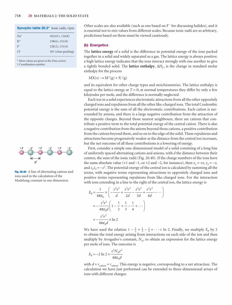
718 20 MATERIALS 2: THE SOLID STATE
Other scales are also available (such as one based on F− for discussing halides), and itis essential not to mix values from different scales. Because ionic radii are so arbitrary,predictions based on them must be viewed cautiously.
(b) Energetics
The lattice energy of a solid is the difference in potential energy of the ions packed together in a solid and widely separated as a gas. The lattice energy is always positive;a high lattice energy indicates that the ions interact strongly with one another to givea tightly bonded solid. The lattice enthalpy, ∆HL, is the change in standard molar enthalpy for the process
MX(s) → M+(g) + X−(g)
and its equivalent for other charge types and stoichiometries. The lattice enthalpy isequal to the lattice energy at T = 0; at normal temperatures they differ by only a fewkilojoules per mole, and the difference is normally neglected.
Each ion in a solid experiences electrostatic attractions from all the other oppositelycharged ions and repulsions from all the other like-charged ions. The total Coulombicpotential energy is the sum of all the electrostatic contributions. Each cation is sur-rounded by anions, and there is a large negative contribution from the attraction ofthe opposite charges. Beyond those nearest neighbours, there are cations that con-tribute a positive term to the total potential energy of the central cation. There is alsoa negative contribution from the anions beyond those cations, a positive contributionfrom the cations beyond them, and so on to the edge of the solid. These repulsions andattractions become progressively weaker as the distance from the central ion increases,but the net outcome of all these contributions is a lowering of energy.
First, consider a simple one-dimensional model of a solid consisting of a long lineof uniformly spaced alternating cations and anions, with d the distance between theircentres, the sum of the ionic radii (Fig. 20.40). If the charge numbers of the ions havethe same absolute value (+1 and −1, or +2 and −2, for instance), then z1 = +z, z2 = −z,and z1z2 = −z2. The potential energy of the central ion is calculated by summing all theterms, with negative terms representing attractions to oppositely charged ions andpositive terms representing repulsions from like-charged ions. For the interactionwith ions extending in a line to the right of the central ion, the lattice energy is
EP = × − + − + − · · ·
= − 1 − + − + · · ·
= − × ln 2
We have used the relation 1 − 1–2 + 1–3 − 1–4 + · · · = ln 2. Finally, we multiply EP by 2 to obtain the total energy arising from interactions on each side of the ion and thenmultiply by Avogadro’s constant, NA, to obtain an expression for the lattice energy per mole of ions. The outcome is
EP = −2 ln 2 ×
with d = rcation + ranion. This energy is negative, corresponding to a net attraction. Thecalculation we have just performed can be extended to three-dimensional arrays ofions with different charges:
z2NAe2
4πε0d
z2e2
4πε0d
DF
1
4
1
3
1
2
AC
z2e2
4πε0d
DF
z2e2
4d
z2e2
3d
z2e2
2d
z2e2
d
AC
1
4πε0
d
�z �z �z �z�z �z
Fig. 20.40 A line of alternating cations andions used in the calculation of theMadelung constant in one dimension.
Synoptic table 20.3* Ionic radii, r/pm
Na+ 102(6†), 116(8)
K+ 138(6), 151(8)
F− 128(2), 131(4)
Cl− 181 (close packing)
* More values are given in the Data section.† Coordination number.
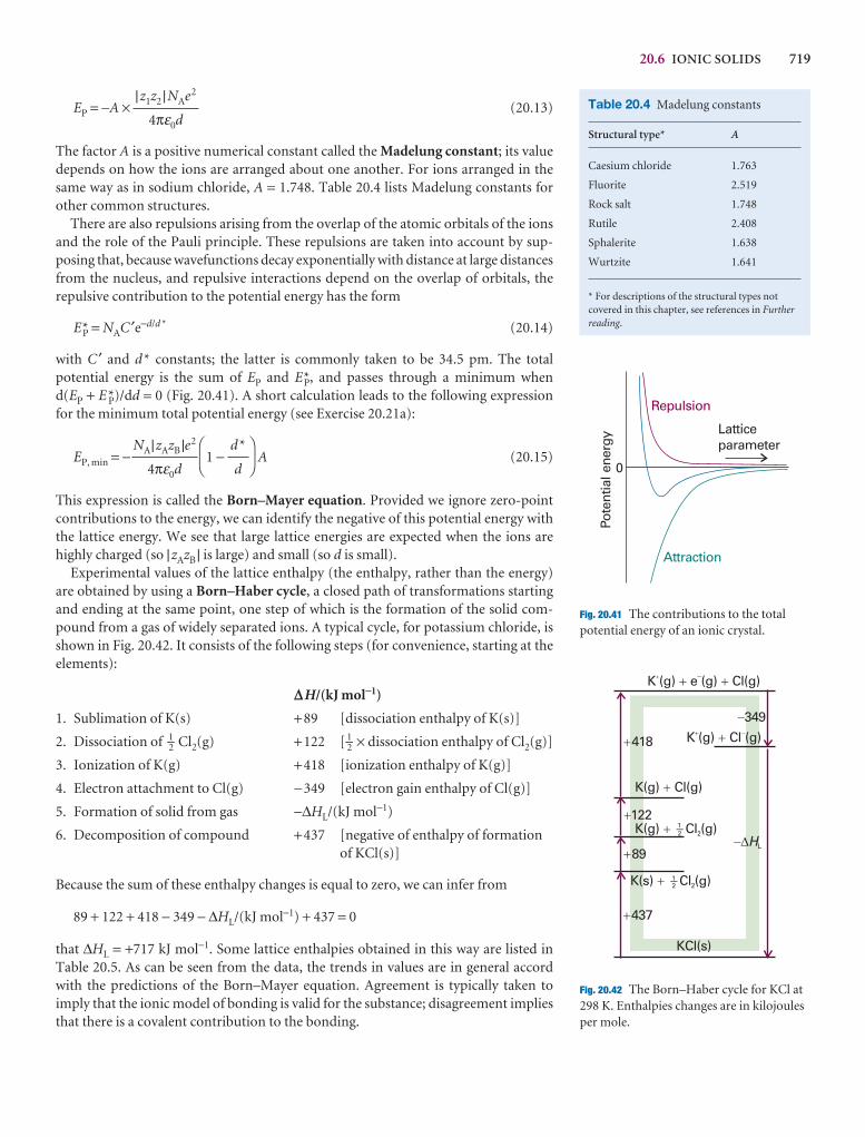
20.6 IONIC SOLIDS 719
EP = −A × (20.13)
The factor A is a positive numerical constant called the Madelung constant; its valuedepends on how the ions are arranged about one another. For ions arranged in thesame way as in sodium chloride, A = 1.748. Table 20.4 lists Madelung constants forother common structures.
There are also repulsions arising from the overlap of the atomic orbitals of the ionsand the role of the Pauli principle. These repulsions are taken into account by sup-posing that, because wavefunctions decay exponentially with distance at large distancesfrom the nucleus, and repulsive interactions depend on the overlap of orbitals, the repulsive contribution to the potential energy has the form
E*P = NAC ′e−d/d * (20.14)
with C ′ and d* constants; the latter is commonly taken to be 34.5 pm. The total potential energy is the sum of EP and E*P, and passes through a minimum when d(EP + E*P)/dd = 0 (Fig. 20.41). A short calculation leads to the following expressionfor the minimum total potential energy (see Exercise 20.21a):
EP, min = − 1 − A (20.15)
This expression is called the Born–Mayer equation. Provided we ignore zero-pointcontributions to the energy, we can identify the negative of this potential energy withthe lattice energy. We see that large lattice energies are expected when the ions arehighly charged (so |zAzB | is large) and small (so d is small).
Experimental values of the lattice enthalpy (the enthalpy, rather than the energy)are obtained by using a Born–Haber cycle, a closed path of transformations startingand ending at the same point, one step of which is the formation of the solid com-pound from a gas of widely separated ions. A typical cycle, for potassium chloride, isshown in Fig. 20.42. It consists of the following steps (for convenience, starting at theelements):
DH/(kJ mol−1)
1. Sublimation of K(s) +89 [dissociation enthalpy of K(s)]
2. Dissociation of 1–2 Cl2(g) +122 [ 1–2 × dissociation enthalpy of Cl2(g)]
3. Ionization of K(g) +418 [ionization enthalpy of K(g)]
4. Electron attachment to Cl(g) −349 [electron gain enthalpy of Cl(g)]
5. Formation of solid from gas −∆HL/(kJ mol−1)
6. Decomposition of compound +437 [negative of enthalpy of formation of KCl(s)]
Because the sum of these enthalpy changes is equal to zero, we can infer from
89 + 122 + 418 − 349 − ∆HL/(kJ mol−1) + 437 = 0
that ∆HL = +717 kJ mol−1. Some lattice enthalpies obtained in this way are listed inTable 20.5. As can be seen from the data, the trends in values are in general accordwith the predictions of the Born–Mayer equation. Agreement is typically taken toimply that the ionic model of bonding is valid for the substance; disagreement impliesthat there is a covalent contribution to the bonding.
DF
d*
d
AC
NA|zAzB |e2
4πε0d
|z1z2 |NAe2
4πε0dTable 20.4 Madelung constants
Structural type* A
Caesium chloride 1.763
Fluorite 2.519
Rock salt 1.748
Rutile 2.408
Sphalerite 1.638
Wurtzite 1.641
* For descriptions of the structural types notcovered in this chapter, see references in Furtherreading.
Repulsion
Attraction
Latticeparameter
Pote
ntia
l ene
rgy
0
Fig. 20.42 The Born–Haber cycle for KCl at 298 K. Enthalpies changes are in kilojoulesper mole.
KCl(s)
K(s) Cl (g)� 2
K(g) Cl (g)� 2
K(g) Cl(g)�
K (g) e (g) Cl(g)�� �
�
K (g) Cl (g)��
�
�437
�89
�122
�418
�349
�HL
12�
12�
Fig. 20.41 The contributions to the totalpotential energy of an ionic crystal.
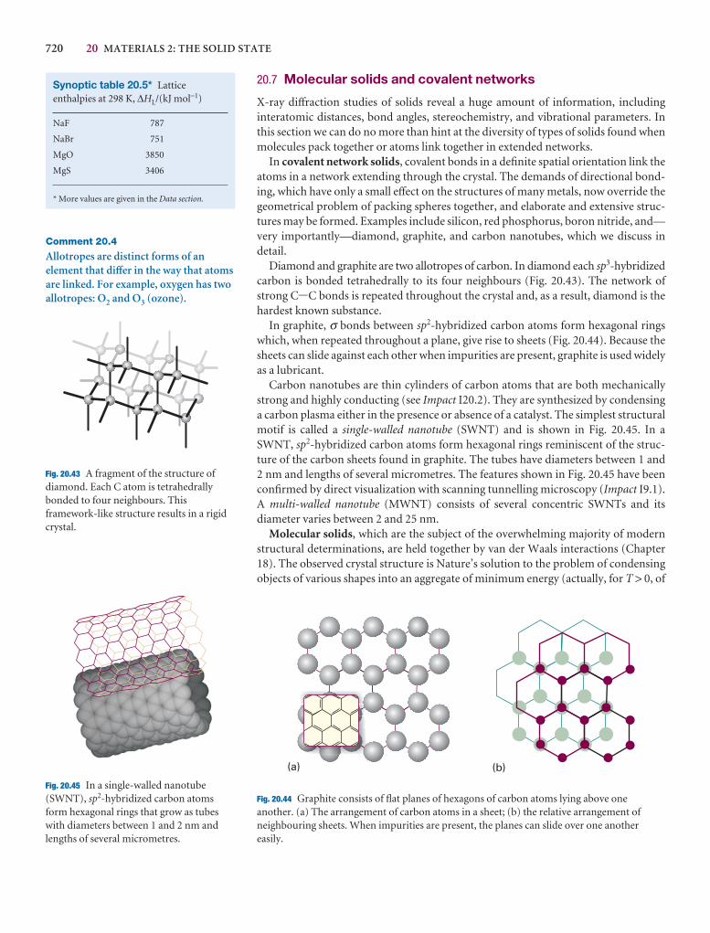
720 20 MATERIALS 2: THE SOLID STATE
20.7 Molecular solids and covalent networks
X-ray diffraction studies of solids reveal a huge amount of information, including interatomic distances, bond angles, stereochemistry, and vibrational parameters. Inthis section we can do no more than hint at the diversity of types of solids found whenmolecules pack together or atoms link together in extended networks.
In covalent network solids, covalent bonds in a definite spatial orientation link theatoms in a network extending through the crystal. The demands of directional bond-ing, which have only a small effect on the structures of many metals, now override thegeometrical problem of packing spheres together, and elaborate and extensive struc-tures may be formed. Examples include silicon, red phosphorus, boron nitride, and—very importantly—diamond, graphite, and carbon nanotubes, which we discuss indetail.
Diamond and graphite are two allotropes of carbon. In diamond each sp3-hybridizedcarbon is bonded tetrahedrally to its four neighbours (Fig. 20.43). The network ofstrong C-C bonds is repeated throughout the crystal and, as a result, diamond is thehardest known substance.
In graphite, σ bonds between sp2-hybridized carbon atoms form hexagonal ringswhich, when repeated throughout a plane, give rise to sheets (Fig. 20.44). Because thesheets can slide against each other when impurities are present, graphite is used widelyas a lubricant.
Carbon nanotubes are thin cylinders of carbon atoms that are both mechanicallystrong and highly conducting (see Impact I20.2). They are synthesized by condensinga carbon plasma either in the presence or absence of a catalyst. The simplest structuralmotif is called a single-walled nanotube (SWNT) and is shown in Fig. 20.45. In aSWNT, sp2-hybridized carbon atoms form hexagonal rings reminiscent of the struc-ture of the carbon sheets found in graphite. The tubes have diameters between 1 and2 nm and lengths of several micrometres. The features shown in Fig. 20.45 have beenconfirmed by direct visualization with scanning tunnelling microscopy (Impact I9.1).A multi-walled nanotube (MWNT) consists of several concentric SWNTs and its diameter varies between 2 and 25 nm.
Molecular solids, which are the subject of the overwhelming majority of modernstructural determinations, are held together by van der Waals interactions (Chapter18). The observed crystal structure is Nature’s solution to the problem of condensingobjects of various shapes into an aggregate of minimum energy (actually, for T > 0, of
Synoptic table 20.5* Latticeenthalpies at 298 K, ∆HL/(kJ mol−1)
NaF 787
NaBr 751
MgO 3850
MgS 3406
* More values are given in the Data section.
Comment 20.4
Allotropes are distinct forms of anelement that differ in the way that atomsare linked. For example, oxygen has twoallotropes: O2 and O3 (ozone).
(a) (b)
Fig. 20.43 A fragment of the structure ofdiamond. Each C atom is tetrahedrallybonded to four neighbours. Thisframework-like structure results in a rigidcrystal.
Fig. 20.44 Graphite consists of flat planes of hexagons of carbon atoms lying above oneanother. (a) The arrangement of carbon atoms in a sheet; (b) the relative arrangement ofneighbouring sheets. When impurities are present, the planes can slide over one anothereasily.
Fig. 20.45 In a single-walled nanotube(SWNT), sp2-hybridized carbon atomsform hexagonal rings that grow as tubeswith diameters between 1 and 2 nm andlengths of several micrometres.
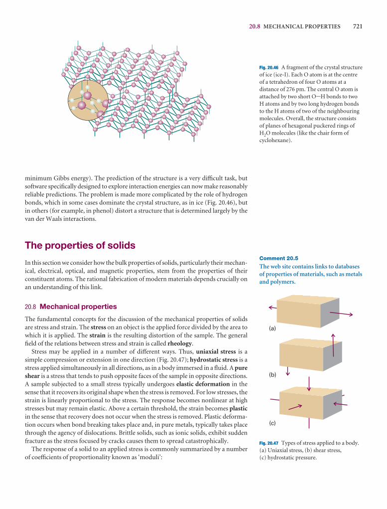
20.8 MECHANICAL PROPERTIES 721
minimum Gibbs energy). The prediction of the structure is a very difficult task, butsoftware specifically designed to explore interaction energies can now make reasonablyreliable predictions. The problem is made more complicated by the role of hydrogenbonds, which in some cases dominate the crystal structure, as in ice (Fig. 20.46), butin others (for example, in phenol) distort a structure that is determined largely by thevan der Waals interactions.
The properties of solids
In this section we consider how the bulk properties of solids, particularly their mechan-ical, electrical, optical, and magnetic properties, stem from the properties of their constituent atoms. The rational fabrication of modern materials depends crucially onan understanding of this link.
20.8 Mechanical properties
The fundamental concepts for the discussion of the mechanical properties of solidsare stress and strain. The stress on an object is the applied force divided by the area towhich it is applied. The strain is the resulting distortion of the sample. The generalfield of the relations between stress and strain is called rheology.
Stress may be applied in a number of different ways. Thus, uniaxial stress is a simple compression or extension in one direction (Fig. 20.47); hydrostatic stress is astress applied simultaneously in all directions, as in a body immersed in a fluid. A pureshear is a stress that tends to push opposite faces of the sample in opposite directions.A sample subjected to a small stress typically undergoes elastic deformation in thesense that it recovers its original shape when the stress is removed. For low stresses, thestrain is linearly proportional to the stress. The response becomes nonlinear at highstresses but may remain elastic. Above a certain threshold, the strain becomes plasticin the sense that recovery does not occur when the stress is removed. Plastic deforma-tion occurs when bond breaking takes place and, in pure metals, typically takes placethrough the agency of dislocations. Brittle solids, such as ionic solids, exhibit suddenfracture as the stress focused by cracks causes them to spread catastrophically.
The response of a solid to an applied stress is commonly summarized by a numberof coefficients of proportionality known as ‘moduli’:
Fig. 20.46 A fragment of the crystal structureof ice (ice-I). Each O atom is at the centreof a tetrahedron of four O atoms at adistance of 276 pm. The central O atom isattached by two short O-H bonds to twoH atoms and by two long hydrogen bondsto the H atoms of two of the neighbouringmolecules. Overall, the structure consists of planes of hexagonal puckered rings ofH2O molecules (like the chair form ofcyclohexane).
Comment 20.5
The web site contains links to databasesof properties of materials, such as metalsand polymers.
(a)
(b)
(c)
Fig. 20.47 Types of stress applied to a body. (a) Uniaxial stress, (b) shear stress, (c) hydrostatic pressure.
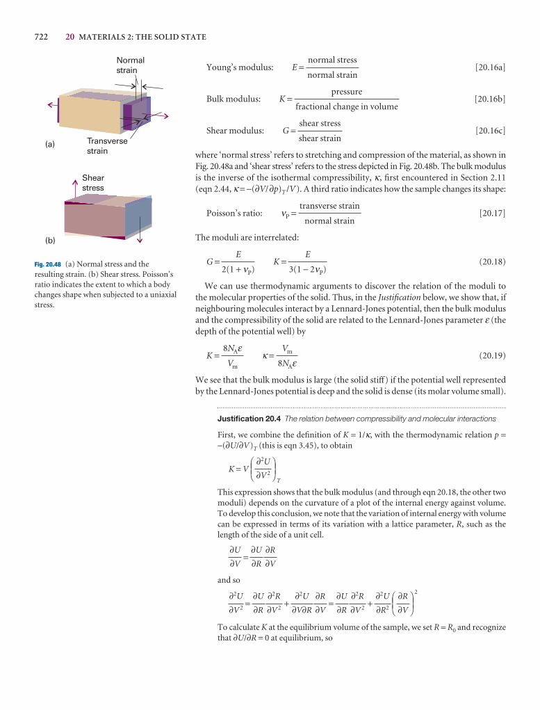
722 20 MATERIALS 2: THE SOLID STATE
Young’s modulus: E = [20.16a]
Bulk modulus: K = [20.16b]
Shear modulus: G = [20.16c]
where ‘normal stress’ refers to stretching and compression of the material, as shown inFig. 20.48a and ‘shear stress’ refers to the stress depicted in Fig. 20.48b. The bulk modulusis the inverse of the isothermal compressibility, κ, first encountered in Section 2.11(eqn 2.44, κ = −(∂V/∂p)T/V). A third ratio indicates how the sample changes its shape:
Poisson’s ratio: νP = [20.17]
The moduli are interrelated:
G = K = (20.18)
We can use thermodynamic arguments to discover the relation of the moduli to the molecular properties of the solid. Thus, in the Justification below, we show that, ifneighbouring molecules interact by a Lennard-Jones potential, then the bulk modulusand the compressibility of the solid are related to the Lennard-Jones parameter ε (thedepth of the potential well) by
K = κ = (20.19)
We see that the bulk modulus is large (the solid stiff) if the potential well representedby the Lennard-Jones potential is deep and the solid is dense (its molar volume small).
Justification 20.4 The relation between compressibility and molecular interactions
First, we combine the definition of K = 1/κ, with the thermodynamic relation p =−(∂U/∂V)T (this is eqn 3.45), to obtain
K = VT
This expression shows that the bulk modulus (and through eqn 20.18, the other twomoduli) depends on the curvature of a plot of the internal energy against volume.To develop this conclusion, we note that the variation of internal energy with volumecan be expressed in terms of its variation with a lattice parameter, R, such as thelength of the side of a unit cell.
=
and so
= + = +2
To calculate K at the equilibrium volume of the sample, we set R = R0 and recognizethat ∂U/∂R = 0 at equilibrium, so
DEF∂R
∂V
ABC∂2U
∂R2
∂2R
∂V 2
∂U
∂R
∂R
∂V
∂2U
∂V∂R
∂2R
∂V 2
∂U
∂R
∂2U
∂V 2
∂R
∂V
∂U
∂R
∂U
∂V
DEF∂2U
∂V 2
ABC
Vm
8NAε8NAεVm
E
3(1 − 2νP)
E
2(1 + νP)
transverse strain
normal strain
shear stress
shear strain
pressure
fractional change in volume
normal stress
normal strain
Normalstrain
Transversestrain
Shearstress
(a)
(b)
Fig. 20.48 (a) Normal stress and theresulting strain. (b) Shear stress. Poisson’sratio indicates the extent to which a bodychanges shape when subjected to a uniaxialstress.
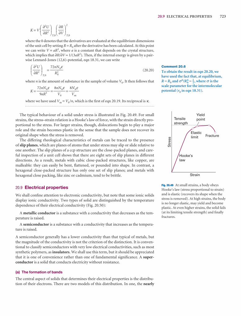
20.9 ELECTRICAL PROPERTIES 723
K = VT,0
2
T,0
where the 0 denotes that the derivatives are evaluated at the equilibrium dimensionsof the unit cell by setting R = R0 after the derivative has been calculated. At this pointwe can write V = aR3, where a is a constant that depends on the crystal structure,which implies that ∂R/∂V = 1/(3aR2). Then, if the internal energy is given by a pair-wise Lennard-Jones (12,6)-potential, eqn 18.31, we can write
T,0
= (20.20)
where n is the amount of substance in the sample of volume V0. It then follows that
K = = =
where we have used Vm = V0 /n, which is the first of eqn 20.19. Its reciprocal is κ.
The typical behaviour of a solid under stress is illustrated in Fig. 20.49. For smallstrains, the stress–strain relation is a Hooke’s law of force, with the strain directly pro-portional to the stress. For larger strains, though, dislocations begin to play a majorrole and the strain becomes plastic in the sense that the sample does not recover itsoriginal shape when the stress is removed.
The differing rheological characteristics of metals can be traced to the presence of slip planes, which are planes of atoms that under stress may slip or slide relative toone another. The slip planes of a ccp structure are the close-packed planes, and care-ful inspection of a unit cell shows that there are eight sets of slip planes in differentdirections. As a result, metals with cubic close-packed structures, like copper, are malleable: they can easily be bent, flattened, or pounded into shape. In contrast, ahexagonal close-packed structure has only one set of slip planes; and metals withhexagonal close packing, like zinc or cadmium, tend to be brittle.
20.9 Electrical properties
We shall confine attention to electronic conductivity, but note that some ionic solidsdisplay ionic conductivity. Two types of solid are distinguished by the temperaturedependence of their electrical conductivity (Fig. 20.50):
A metallic conductor is a substance with a conductivity that decreases as the tem-perature is raised.
A semiconductor is a substance with a conductivity that increases as the tempera-ture is raised.
A semiconductor generally has a lower conductivity than that typical of metals, butthe magnitude of the conductivity is not the criterion of the distinction. It is conven-tional to classify semiconductors with very low electrical conductivities, such as mostsynthetic polymers, as insulators. We shall use this term, but it should be appreciatedthat it is one of convenience rather than one of fundamental significance. A super-conductor is a solid that conducts electricity without resistance.
(a) The formation of bands
The central aspect of solids that determines their electrical properties is the distribu-tion of their electrons. There are two models of this distribution. In one, the nearly
8NAεVm
8nNAεV0
72nNAε9aR3
72nNAεR2
0
DEF∂2U
∂R2
ABC
DEF∂R
∂V
ABCDEF
∂2U
∂R2
ABC
Comment 20.6
To obtain the result in eqn 20.20, wehave used the fact that, at equilibrium, R = R0 and σ6/R0
6 = 1–2 , where σ is thescale parameter for the intermolecularpotential (r0 in eqn 18.31).
Str
ess
Strain
Hooke’slaw
Elasticlimit
YieldpointTensile
strength
Fracture
Fig. 20.49 At small strains, a body obeysHooke’s law (stress proportional to strain)and is elastic (recovers its shape when thestress is removed). At high strains, the bodyis no longer elastic, may yield and becomeplastic. At even higher strains, the solid fails(at its limiting tensile strength) and finallyfractures.
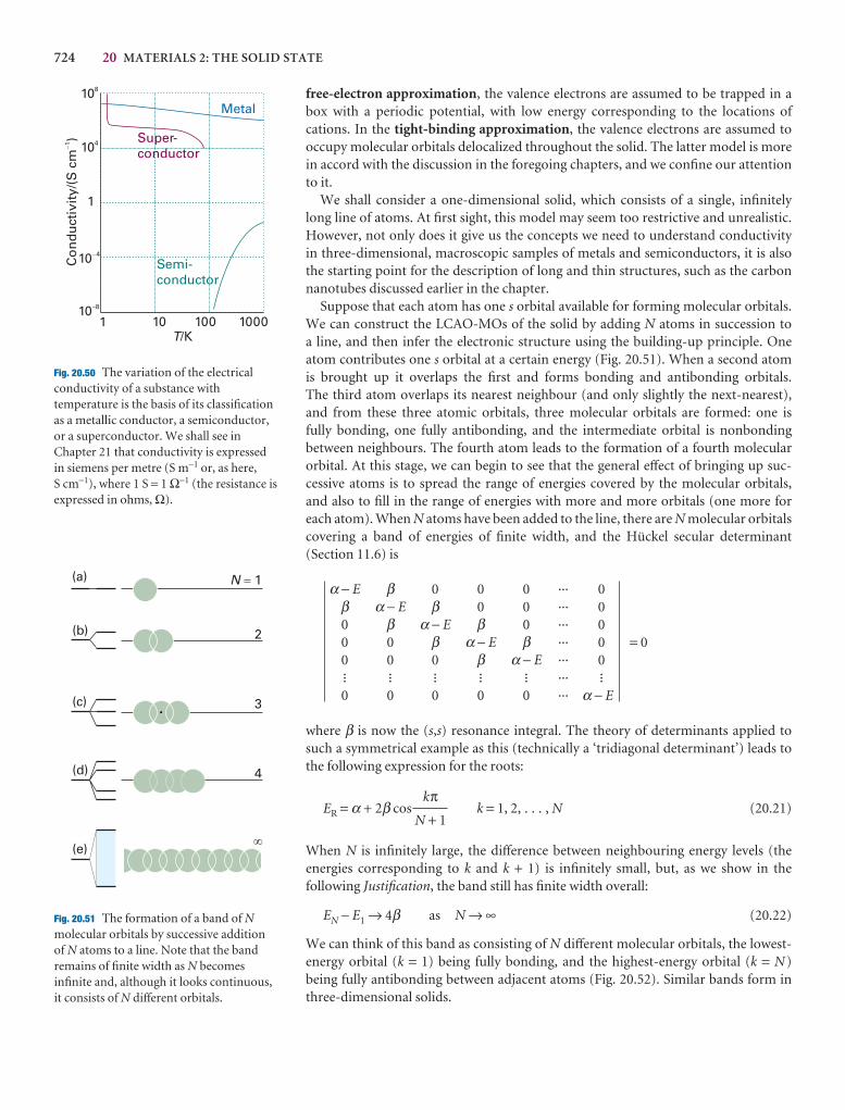
724 20 MATERIALS 2: THE SOLID STATE
free-electron approximation, the valence electrons are assumed to be trapped in abox with a periodic potential, with low energy corresponding to the locations ofcations. In the tight-binding approximation, the valence electrons are assumed tooccupy molecular orbitals delocalized throughout the solid. The latter model is morein accord with the discussion in the foregoing chapters, and we confine our attentionto it.
We shall consider a one-dimensional solid, which consists of a single, infinitelylong line of atoms. At first sight, this model may seem too restrictive and unrealistic.However, not only does it give us the concepts we need to understand conductivity in three-dimensional, macroscopic samples of metals and semiconductors, it is alsothe starting point for the description of long and thin structures, such as the carbonnanotubes discussed earlier in the chapter.
Suppose that each atom has one s orbital available for forming molecular orbitals.We can construct the LCAO-MOs of the solid by adding N atoms in succession to a line, and then infer the electronic structure using the building-up principle. Oneatom contributes one s orbital at a certain energy (Fig. 20.51). When a second atom is brought up it overlaps the first and forms bonding and antibonding orbitals. The third atom overlaps its nearest neighbour (and only slightly the next-nearest),and from these three atomic orbitals, three molecular orbitals are formed: one is fully bonding, one fully antibonding, and the intermediate orbital is nonbonding between neighbours. The fourth atom leads to the formation of a fourth molecular orbital. At this stage, we can begin to see that the general effect of bringing up suc-cessive atoms is to spread the range of energies covered by the molecular orbitals, and also to fill in the range of energies with more and more orbitals (one more for each atom). When N atoms have been added to the line, there are N molecular orbitalscovering a band of energies of finite width, and the Hückel secular determinant(Section 11.6) is
α − E β 0 0 0 ··· 0β α − E β 0 0 ··· 00 β α − E β 0 ··· 00 0 β α − E β ··· 0 = 00 0 0 β α − E ··· 0� � � � � ··· �0 0 0 0 0 ··· α − E
where β is now the (s,s) resonance integral. The theory of determinants applied tosuch a symmetrical example as this (technically a ‘tridiagonal determinant’) leads tothe following expression for the roots:
ER = α + 2β cos k = 1, 2, . . . , N (20.21)
When N is infinitely large, the difference between neighbouring energy levels (the energies corresponding to k and k + 1) is infinitely small, but, as we show in the following Justification, the band still has finite width overall:
EN − E1 → 4β as N → ∞ (20.22)
We can think of this band as consisting of N different molecular orbitals, the lowest-energy orbital (k = 1) being fully bonding, and the highest-energy orbital (k = N)being fully antibonding between adjacent atoms (Fig. 20.52). Similar bands form inthree-dimensional solids.
kπN + 1
1 10 100 1000T/K
10�4
10�8
1
104
108
Co
nd
uct
ivit
y/(S
cm
)�
1
Semi-conductor
Super-conductor
Metal
Fig. 20.50 The variation of the electricalconductivity of a substance withtemperature is the basis of its classificationas a metallic conductor, a semiconductor,or a superconductor. We shall see inChapter 21 that conductivity is expressedin siemens per metre (S m−1 or, as here, S cm−1), where 1 S = 1 Ω−1 (the resistance isexpressed in ohms, Ω).
N 1�
2
3
4
(a)
(b)
(c)
(d)
(e)�
Fig. 20.51 The formation of a band of Nmolecular orbitals by successive addition of N atoms to a line. Note that the bandremains of finite width as N becomesinfinite and, although it looks continuous,it consists of N different orbitals.
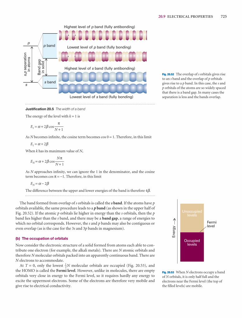
20.9 ELECTRICAL PROPERTIES 725
Highest level of band (fully antibonding)p
Highest level of band (fully antibonding)s
Lowest level of band (fully bonding)p
Lowest level of band (fully bonding)s
p
s
p band
s band
s,p
sepa
ratio
nin
ato
ms
Ban
d g
apin
sol
id
Fig. 20.52 The overlap of s orbitals gives riseto an s band and the overlap of p orbitalsgives rise to a p band. In this case, the s andp orbitals of the atoms are so widely spacedthat there is a band gap. In many cases theseparation is less and the bands overlap.
Ener
gy
Fermilevel
Occupiedlevels
Unoccupiedlevels
Fig. 20.53 When N electrons occupy a bandof N orbitals, it is only half full and theelectrons near the Fermi level (the top ofthe filled levels) are mobile.
Justification 20.5 The width of a band
The energy of the level with k = 1 is
E1 = α + 2β cos
As N becomes infinite, the cosine term becomes cos 0 = 1. Therefore, in this limit
E1 = α + 2β
When k has its maximum value of N,
EN = α + 2β cos
As N approaches infinity, we can ignore the 1 in the denominator, and the cosineterm becomes cos π = −1. Therefore, in this limit
EN = α − 2β
The difference between the upper and lower energies of the band is therefore 4β.
The band formed from overlap of s orbitals is called the s band. If the atoms have porbitals available, the same procedure leads to a p band (as shown in the upper half ofFig. 20.52). If the atomic p orbitals lie higher in energy than the s orbitals, then the pband lies higher than the s band, and there may be a band gap, a range of energies towhich no orbital corresponds. However, the s and p bands may also be contiguous oreven overlap (as is the case for the 3s and 3p bands in magnesium).
(b) The occupation of orbitals
Now consider the electronic structure of a solid formed from atoms each able to con-tribute one electron (for example, the alkali metals). There are N atomic orbitals andtherefore N molecular orbitals packed into an apparently continuous band. There areN electrons to accommodate.
At T = 0, only the lowest 1–2 N molecular orbitals are occupied (Fig. 20.53), and the HOMO is called the Fermi level. However, unlike in molecules, there are emptyorbitals very close in energy to the Fermi level, so it requires hardly any energy to excite the uppermost electrons. Some of the electrons are therefore very mobile andgive rise to electrical conductivity.
NπN + 1
πN + 1
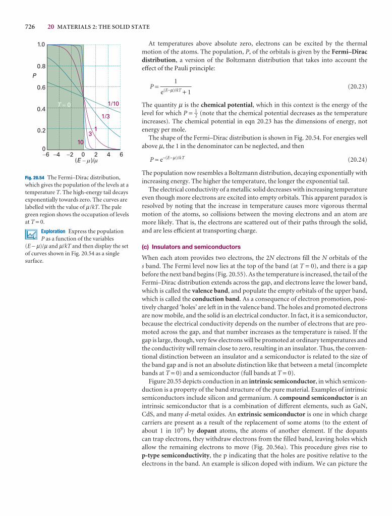
726 20 MATERIALS 2: THE SOLID STATE
At temperatures above absolute zero, electrons can be excited by the thermal motion of the atoms. The population, P, of the orbitals is given by the Fermi–Diracdistribution, a version of the Boltzmann distribution that takes into account theeffect of the Pauli principle:
P = (20.23)
The quantity µ is the chemical potential, which in this context is the energy of thelevel for which P = 1–2 (note that the chemical potential decreases as the temperature increases). The chemical potential in eqn 20.23 has the dimensions of energy, not energy per mole.
The shape of the Fermi–Dirac distribution is shown in Fig. 20.54. For energies wellabove µ, the 1 in the denominator can be neglected, and then
P ≈ e−(E−µ)/kT (20.24)
The population now resembles a Boltzmann distribution, decaying exponentially withincreasing energy. The higher the temperature, the longer the exponential tail.
The electrical conductivity of a metallic solid decreases with increasing temperatureeven though more electrons are excited into empty orbitals. This apparent paradox isresolved by noting that the increase in temperature causes more vigorous thermalmotion of the atoms, so collisions between the moving electrons and an atom aremore likely. That is, the electrons are scattered out of their paths through the solid,and are less efficient at transporting charge.
(c) Insulators and semiconductors
When each atom provides two electrons, the 2N electrons fill the N orbitals of the s band. The Fermi level now lies at the top of the band (at T = 0), and there is a gap before the next band begins (Fig. 20.55). As the temperature is increased, the tail of theFermi–Dirac distribution extends across the gap, and electrons leave the lower band,which is called the valence band, and populate the empty orbitals of the upper band,which is called the conduction band. As a consequence of electron promotion, posi-tively charged ‘holes’ are left in in the valence band. The holes and promoted electronsare now mobile, and the solid is an electrical conductor. In fact, it is a semiconductor,because the electrical conductivity depends on the number of electrons that are pro-moted across the gap, and that number increases as the temperature is raised. If thegap is large, though, very few electrons will be promoted at ordinary temperatures andthe conductivity will remain close to zero, resulting in an insulator. Thus, the conven-tional distinction between an insulator and a semiconductor is related to the size ofthe band gap and is not an absolute distinction like that between a metal (incompletebands at T = 0) and a semiconductor (full bands at T = 0).
Figure 20.55 depicts conduction in an intrinsic semiconductor, in which semicon-duction is a property of the band structure of the pure material. Examples of intrinsicsemiconductors include silicon and germanium. A compound semiconductor is anintrinsic semiconductor that is a combination of different elements, such as GaN,CdS, and many d-metal oxides. An extrinsic semiconductor is one in which chargecarriers are present as a result of the replacement of some atoms (to the extent ofabout 1 in 109) by dopant atoms, the atoms of another element. If the dopants can trap electrons, they withdraw electrons from the filled band, leaving holes whichallow the remaining electrons to move (Fig. 20.56a). This procedure gives rise to p-type semiconductivity, the p indicating that the holes are positive relative to theelectrons in the band. An example is silicon doped with indium. We can picture the
1
e(E−µ)/kT + 1
0
0.2
0.4
0.6
0.8
1.0
�6 �4 �2 0 2 4 6( )/E �
P
103
1
1/3
1/10T 0�
Fig. 20.54 The Fermi–Dirac distribution,which gives the population of the levels at atemperature T. The high-energy tail decaysexponentially towards zero. The curves arelabelled with the value of µ /kT. The palegreen region shows the occupation of levelsat T = 0.
Exploration Express the population P as a function of the variables
(E − µ)/µ and µ/kT and then display the setof curves shown in Fig. 20.54 as a singlesurface.
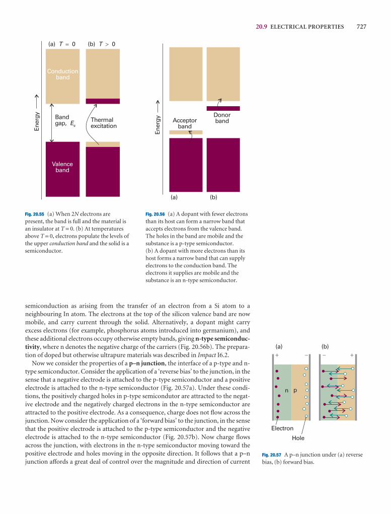
20.9 ELECTRICAL PROPERTIES 727
semiconduction as arising from the transfer of an electron from a Si atom to a neighbouring In atom. The electrons at the top of the silicon valence band are nowmobile, and carry current through the solid. Alternatively, a dopant might carry excess electrons (for example, phosphorus atoms introduced into germanium), andthese additional electrons occupy otherwise empty bands, giving n-type semiconduc-tivity, where n denotes the negative charge of the carriers (Fig. 20.56b). The prepara-tion of doped but otherwise ultrapure materials was described in Impact I6.2.
Now we consider the properties of a p–n junction, the interface of a p-type and n-type semiconductor. Consider the application of a ‘reverse bias’ to the junction, in thesense that a negative electrode is attached to the p-type semiconductor and a positiveelectrode is attached to the n-type semiconductor (Fig. 20.57a). Under these condi-tions, the positively charged holes in p-type semicondutor are attracted to the negat-ive electrode and the negatively charged electrons in the n-type semiconductor are attracted to the positive electrode. As a consequence, charge does not flow across thejunction. Now consider the application of a ‘forward bias’ to the junction, in the sensethat the positive electrode is attached to the p-type semiconductor and the negativeelectrode is attached to the n-type semiconductor (Fig. 20.57b). Now charge flowsacross the junction, with electrons in the n-type semiconductor moving toward thepositive electrode and holes moving in the opposite direction. It follows that a p–njunction affords a great deal of control over the magnitude and direction of current
Ener
gy Acceptorband
Donorband
(a) (b)
Ener
gy(a) 0T � (b) 0T �
Conductionband
Valenceband
Bandgap, gE Thermal
excitation
Fig. 20.55 (a) When 2N electrons arepresent, the band is full and the material isan insulator at T = 0. (b) At temperaturesabove T = 0, electrons populate the levels ofthe upper conduction band and the solid is asemiconductor.
Fig. 20.56 (a) A dopant with fewer electronsthan its host can form a narrow band thataccepts electrons from the valence band.The holes in the band are mobile and thesubstance is a p-type semiconductor.(b) A dopant with more electrons than itshost forms a narrow band that can supplyelectrons to the conduction band. Theelectrons it supplies are mobile and thesubstance is an n-type semiconductor.
� � ��
n p
Electron
Hole
(a) (b)
Fig. 20.57 A p–n junction under (a) reversebias, (b) forward bias.

728 20 MATERIALS 2: THE SOLID STATE
through a material. This control is essential for the operation of transistors and diodes,which are key components of modern electronic devices.
As electrons and holes move across a p–n junction under forward bias, they recom-bine and release energy. However, as long as the forward bias continues to be applied,the flow of charge from the electrodes to the semiconductors will replenish them withelectrons and holes, so the junction will sustain a current. In some solids, the energyof electron–hole recombination is released as heat and the device becomes warm. Thisis the case for silicon semiconductors, and is one reason why computers need efficientcooling systems.
IMPACT ON NANOSCIENCE
I20.2 Nanowires
We have already remarked (Impacts I9.1, I9.2, and I19.3) that research on nano-metre-sized materials is motivated by the possibility that they will form the basis forcheaper and smaller electronic devices. The synthesis of nanowires, nanometre-sizedatomic assemblies that conduct electricity, is a major step in the fabrication of nanodevices. An important type of nanowire is based on carbon nanotubes, which,like graphite, can conduct electrons through delocalized π molecular orbitals thatform from unhybridized 2p orbitals on carbon. Recent studies have shown a cor-relation between structure and conductivity in single-walled nanotubes (SWNTs)that does not occur in graphite. The SWNT in Fig. 20.45 is a semiconductor. If thehexagons are rotated by 90° about their sixfold axis, the resulting SWNT is a metallicconductor.
Carbon nanotubes are promising building blocks not only because they have usefulelectrical properties but also because they have unusual mechanical properties. Forexample, an SWNT has a Young’s modulus that is approximately five times larger anda tensile strength that is approximately 375 times larger than that of steel.
Silicon nanowires can be made by focusing a pulsed laser beam on to a solid targetcomposed of silicon and iron. The laser ejects Fe and Si atoms from the surface of thetarget, forming a vapour that can condense into liquid FeSin nanoclusters at suffi-
ciently low temperatures. The phase diagram for this complex mixture shows thatsolid silicon and liquid FeSin coexist at temperatures higher than 1473 K. Hence, it ispossible to precipitate solid silicon from the mixture if the experimental conditionsare controlled to maintain the FeSin nanoclusters in a liquid state that is supersatur-ated with silicon. It is observed that the silicon precipitate consists of nanowires withdiameters of about 10 nm and lengths greater than 1 µm.
Nanowires are also fabricated by molecular beam epitaxy (MBE), in which gaseousatoms or molecules are sprayed onto a crystalline surface in an ultra-high vacuumchamber. The result is formation of highly ordered structures. Through careful con-trol of the chamber temperature and of the spraying process, it is possible to depositthin films on to a surface or to create nanometre-sized assemblies with specific shapes.For example, Fig. 20.58 shows an AFM image of germanium nanowires on a siliconsurface. The wires are about 2 nm high, 10–32 nm wide, and 10–600 nm long.
Direct manipulation of atoms on a surface also leads to the formation of nanowires.The Coulomb attraction between an atom and the tip of an STM can be exploited tomove atoms along a surface, arranging them into patterns, such as wires.
20.10 Optical properties
In this section, we explore the consequences of interactions between electromagneticradiation and solids. Our focus will be on the origins of phenomena that inform thedesign of useful devices, such as lasers and light-emitting diodes.
Fig. 20.58 Germanium nanowires fabricatedon to a silicon surface by molecular beamepitaxy. (Reproduced with permissionfrom T. Ogino et al. Acc. Chem. Res. 32, 447(1999).)
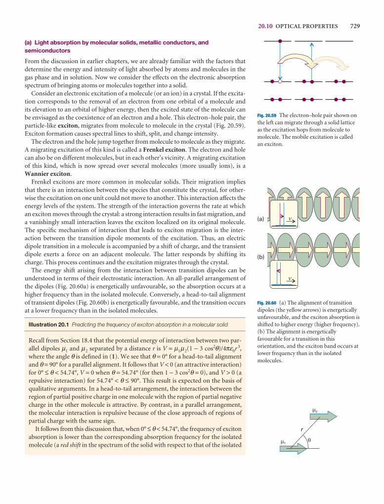
20.10 OPTICAL PROPERTIES 729
Fig. 20.59 The electron–hole pair shown onthe left can migrate through a solid latticeas the excitation hops from molecule tomolecule. The mobile excitation is calledan exciton.
�(a)
(b)
�
Fig. 20.60 (a) The alignment of transitiondipoles (the yellow arrows) is energeticallyunfavourable, and the exciton absorption isshifted to higher energy (higher frequency).(b) The alignment is energeticallyfavourable for a transition in thisorientation, and the exciton band occurs atlower frequency than in the isolatedmolecules.
r
�1
2
(a) Light absorption by molecular solids, metallic conductors, andsemiconductors
From the discussion in earlier chapters, we are already familiar with the factors thatdetermine the energy and intensity of light absorbed by atoms and molecules in thegas phase and in solution. Now we consider the effects on the electronic absorptionspectrum of bringing atoms or molecules together into a solid.
Consider an electronic excitation of a molecule (or an ion) in a crystal. If the excita-tion corresponds to the removal of an electron from one orbital of a molecule and its elevation to an orbital of higher energy, then the excited state of the molecule canbe envisaged as the coexistence of an electron and a hole. This electron–hole pair, theparticle-like exciton, migrates from molecule to molecule in the crystal (Fig. 20.59).Exciton formation causes spectral lines to shift, split, and change intensity.
The electron and the hole jump together from molecule to molecule as they migrate.A migrating excitation of this kind is called a Frenkel exciton. The electron and holecan also be on different molecules, but in each other’s vicinity. A migrating excitationof this kind, which is now spread over several molecules (more usually ions), is aWannier exciton.
Frenkel excitons are more common in molecular solids. Their migration impliesthat there is an interaction between the species that constitute the crystal, for other-wise the excitation on one unit could not move to another. This interaction affects theenergy levels of the system. The strength of the interaction governs the rate at whichan exciton moves through the crystal: a strong interaction results in fast migration, anda vanishingly small interaction leaves the exciton localized on its original molecule.The specific mechanism of interaction that leads to exciton migration is the inter-action between the transition dipole moments of the excitation. Thus, an electricdipole transition in a molecule is accompanied by a shift of charge, and the transientdipole exerts a force on an adjacent molecule. The latter responds by shifting itscharge. This process continues and the excitation migrates through the crystal.
The energy shift arising from the interaction between transition dipoles can be understood in terms of their electrostatic interaction. An all-parallel arrangement ofthe dipoles (Fig. 20.60a) is energetically unfavourable, so the absorption occurs at ahigher frequency than in the isolated molecule. Conversely, a head-to-tail alignmentof transient dipoles (Fig. 20.60b) is energetically favourable, and the transition occursat a lower frequency than in the isolated molecules.
Illustration 20.1 Predicting the frequency of exciton absorption in a molecular solid
Recall from Section 18.4 that the potential energy of interaction between two par-allel dipoles µ1 and µ2 separated by a distance r is V = µ1µ2(1 − 3 cos2θ)/4πε0r 3,where the angle θ is defined in (1). We see that θ = 0° for a head-to-tail alignmentand θ = 90° for a parallel alignment. It follows that V < 0 (an attractive interaction)for 0° ≤ θ < 54.74°, V = 0 when θ = 54.74° (for then 1 − 3 cos2θ = 0), and V > 0 (a repulsive interaction) for 54.74° < θ ≤ 90°. This result is expected on the basis ofqualitative arguments. In a head-to-tail arrangement, the interaction between theregion of partial positive charge in one molecule with the region of partial negativecharge in the other molecule is attractive. By contrast, in a parallel arrangement,the molecular interaction is repulsive because of the close approach of regions ofpartial charge with the same sign.
It follows from this discussion that, when 0° ≤ θ < 54.74°, the frequency of excitonabsorption is lower than the corresponding absorption frequency for the isolatedmolecule (a red shift in the spectrum of the solid with respect to that of the isolated
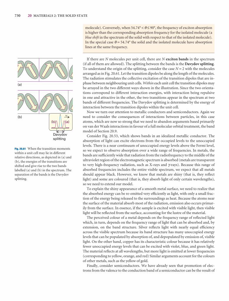
730 20 MATERIALS 2: THE SOLID STATE
(b)
(a)
(a)(b)
Davydovsplitting
�
Fig. 20.61 When the transition momentswithin a unit cell may lie in differentrelative directions, as depicted in (a) and(b), the energies of the transitions areshifted and give rise to the two bandslabelled (a) and (b) in the spectrum. Theseparation of the bands is the Davydovsplitting.
molecule). Conversely, when 54.74° < θ ≤ 90°, the frequency of exciton absorptionis higher than the corresponding absorption frequency for the isolated molecule (ablue shift in the spectrum of the solid with respect to that of the isolated molecule).In the special case θ = 54.74° the solid and the isolated molecule have absorptionlines at the same frequency.
If there are N molecules per unit cell, there are N exciton bands in the spectrum (if all of them are allowed). The splitting between the bands is the Davydov splitting.To understand the origin of the splitting, consider the case N = 2 with the molecules arranged as in Fig. 20.61. Let the transition dipoles be along the length of the molecules.The radiation stimulates the collective excitation of the transition dipoles that are in-phase between neighbouring unit cells. Within each unit cell the transition dipoles maybe arrayed in the two different ways shown in the illustration. Since the two orienta-tions correspond to different interaction energies, with interaction being repulsive in one and attractive in the other, the two transitions appear in the spectrum at twobands of different frequencies. The Davydov splitting is determined by the energy ofinteraction between the transition dipoles within the unit cell.
Now we turn our attention to metallic conductors and semiconductors. Again weneed to consider the consequences of interactions between particles, in this caseatoms, which are now so strong that we need to abandon arguments based primarilyon van der Waals interactions in favour of a full molecular orbital treatment, the bandmodel of Section 20.9.
Consider Fig. 20.53, which shows bands in an idealized metallic conductor. The absorption of light can excite electrons from the occupied levels to the unoccupiedlevels. There is a near continuum of unoccupied energy levels above the Fermi level,so we expect to observe absorption over a wide range of frequencies. In metals, thebands are sufficiently wide that radiation from the radiofrequency to the middle of theultraviolet region of the electromagnetic spectrum is absorbed (metals are transparentto very high-frequency radiation, such as X-rays and γ-rays). Because this range of absorbed frequencies includes the entire visible spectrum, we expect that all metalsshould appear black. However, we know that metals are shiny (that is, they reflectlight) and some are coloured (that is, they absorb light of only certain wavelengths),so we need to extend our model.
To explain the shiny appearance of a smooth metal surface, we need to realize thatthe absorbed energy can be re-emitted very efficiently as light, with only a small frac-tion of the energy being released to the surroundings as heat. Because the atoms nearthe surface of the material absorb most of the radiation, emission also occurs primar-ily from the surface. In essence, if the sample is excited with visible light, then visiblelight will be reflected from the surface, accounting for the lustre of the material.
The perceived colour of a metal depends on the frequency range of reflected lightwhich, in turn, depends on the frequency range of light that can be absorbed and, byextension, on the band structure. Silver reflects light with nearly equal efficiencyacross the visible spectrum because its band structure has many unoccupied energylevels that can be populated by absorption of, and depopulated by emission of, visiblelight. On the other hand, copper has its characteristic colour because it has relativelyfewer unoccupied energy levels that can be excited with violet, blue, and green light.The material reflects at all wavelengths, but more light is emitted at lower frequencies(corresponding to yellow, orange, and red) Similar arguments account for the coloursof other metals, such as the yellow of gold.
Finally, consider semiconductors. We have already seen that promotion of elec-trons from the valence to the conduction band of a semiconductor can be the result of
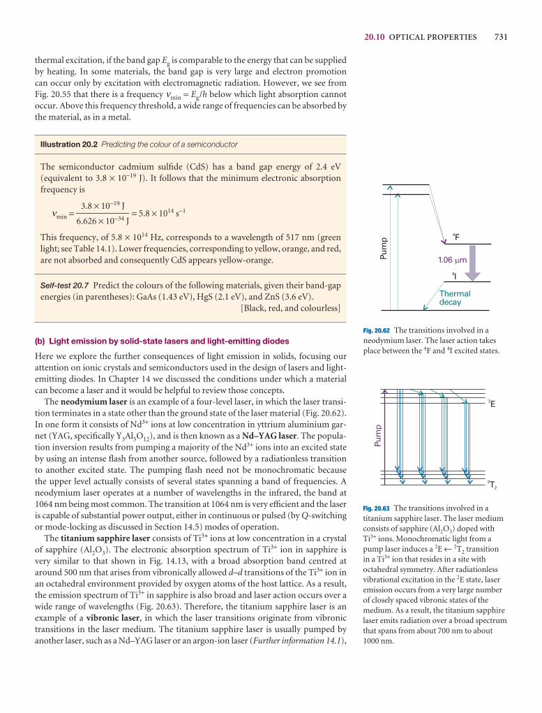
20.10 OPTICAL PROPERTIES 731
4F
Pum
p
4I
1.06 m
Thermaldecay
Fig. 20.62 The transitions involved in aneodymium laser. The laser action takesplace between the 4F and 4I excited states.
2E
2T2
Pum
p
Fig. 20.63 The transitions involved in atitanium sapphire laser. The laser mediumconsists of sapphire (Al2O3) doped withTi3+ ions. Monochromatic light from apump laser induces a 2E ← 2T2 transitionin a Ti3+ ion that resides in a site withoctahedral symmetry. After radiationlessvibrational excitation in the 2E state, laseremission occurs from a very large numberof closely spaced vibronic states of themedium. As a result, the titanium sapphirelaser emits radiation over a broad spectrumthat spans from about 700 nm to about1000 nm.
thermal excitation, if the band gap Eg is comparable to the energy that can be suppliedby heating. In some materials, the band gap is very large and electron promotion can occur only by excitation with electromagnetic radiation. However, we see from Fig. 20.55 that there is a frequency νmin = Eg/h below which light absorption cannotoccur. Above this frequency threshold, a wide range of frequencies can be absorbed bythe material, as in a metal.
Illustration 20.2 Predicting the colour of a semiconductor
The semiconductor cadmium sulfide (CdS) has a band gap energy of 2.4 eV(equivalent to 3.8 × 10⁻¹⁹ J). It follows that the minimum electronic absorption frequency is
νmin = = 5.8 × 10¹⁴ s−1
This frequency, of 5.8 × 10¹⁴ Hz, corresponds to a wavelength of 517 nm (greenlight; see Table 14.1). Lower frequencies, corresponding to yellow, orange, and red,are not absorbed and consequently CdS appears yellow-orange.
Self-test 20.7 Predict the colours of the following materials, given their band-gapenergies (in parentheses): GaAs (1.43 eV), HgS (2.1 eV), and ZnS (3.6 eV).
[Black, red, and colourless]
(b) Light emission by solid-state lasers and light-emitting diodes
Here we explore the further consequences of light emission in solids, focusing our attention on ionic crystals and semiconductors used in the design of lasers and light-emitting diodes. In Chapter 14 we discussed the conditions under which a materialcan become a laser and it would be helpful to review those concepts.
The neodymium laser is an example of a four-level laser, in which the laser transi-tion terminates in a state other than the ground state of the laser material (Fig. 20.62).In one form it consists of Nd3+ ions at low concentration in yttrium aluminium gar-net (YAG, specifically Y3Al5O12), and is then known as a Nd–YAG laser. The popula-tion inversion results from pumping a majority of the Nd3+ ions into an excited stateby using an intense flash from another source, followed by a radiationless transitionto another excited state. The pumping flash need not be monochromatic because the upper level actually consists of several states spanning a band of frequencies. Aneodymium laser operates at a number of wavelengths in the infrared, the band at1064 nm being most common. The transition at 1064 nm is very efficient and the laseris capable of substantial power output, either in continuous or pulsed (by Q-switchingor mode-locking as discussed in Section 14.5) modes of operation.
The titanium sapphire laser consists of Ti3+ ions at low concentration in a crystalof sapphire (Al2O3). The electronic absorption spectrum of Ti3+ ion in sapphire is very similar to that shown in Fig. 14.13, with a broad absorption band centred ataround 500 nm that arises from vibronically allowed d–d transitions of the Ti3+ ion inan octahedral environment provided by oxygen atoms of the host lattice. As a result,the emission spectrum of Ti3+ in sapphire is also broad and laser action occurs over awide range of wavelengths (Fig. 20.63). Therefore, the titanium sapphire laser is an example of a vibronic laser, in which the laser transitions originate from vibronictransitions in the laser medium. The titanium sapphire laser is usually pumped by another laser, such as a Nd–YAG laser or an argon-ion laser (Further information 14.1),
3.8 × 10⁻¹⁹ J
6.626 × 10⁻³⁴ J
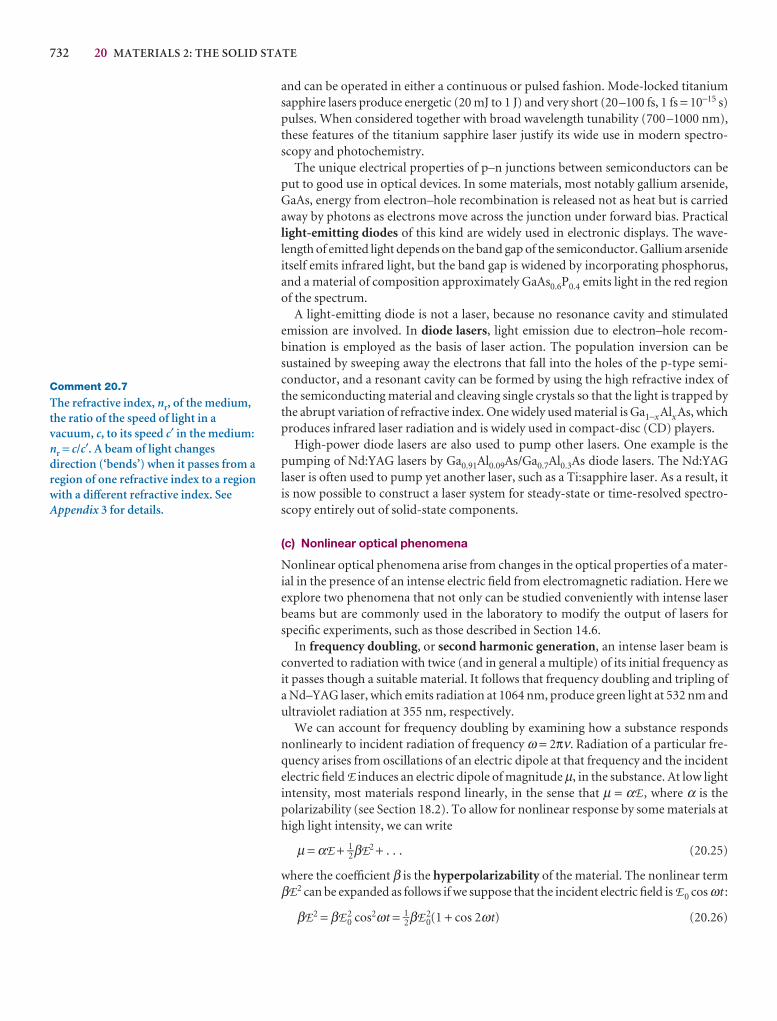
732 20 MATERIALS 2: THE SOLID STATE
and can be operated in either a continuous or pulsed fashion. Mode-locked titaniumsapphire lasers produce energetic (20 mJ to 1 J) and very short (20–100 fs, 1 fs = 10−15 s)pulses. When considered together with broad wavelength tunability (700–1000 nm),these features of the titanium sapphire laser justify its wide use in modern spectro-scopy and photochemistry.
The unique electrical properties of p–n junctions between semiconductors can beput to good use in optical devices. In some materials, most notably gallium arsenide,GaAs, energy from electron–hole recombination is released not as heat but is carriedaway by photons as electrons move across the junction under forward bias. Practicallight-emitting diodes of this kind are widely used in electronic displays. The wave-length of emitted light depends on the band gap of the semiconductor. Gallium arsenideitself emits infrared light, but the band gap is widened by incorporating phosphorus,and a material of composition approximately GaAs0.6P0.4 emits light in the red regionof the spectrum.
A light-emitting diode is not a laser, because no resonance cavity and stimulatedemission are involved. In diode lasers, light emission due to electron–hole recom-bination is employed as the basis of laser action. The population inversion can be sustained by sweeping away the electrons that fall into the holes of the p-type semi-conductor, and a resonant cavity can be formed by using the high refractive index ofthe semiconducting material and cleaving single crystals so that the light is trapped bythe abrupt variation of refractive index. One widely used material is Ga1−xAlxAs, whichproduces infrared laser radiation and is widely used in compact-disc (CD) players.
High-power diode lasers are also used to pump other lasers. One example is thepumping of Nd:YAG lasers by Ga0.91Al0.09As/Ga0.7Al0.3As diode lasers. The Nd:YAGlaser is often used to pump yet another laser, such as a Ti:sapphire laser. As a result, itis now possible to construct a laser system for steady-state or time-resolved spectro-scopy entirely out of solid-state components.
(c) Nonlinear optical phenomena
Nonlinear optical phenomena arise from changes in the optical properties of a mater-ial in the presence of an intense electric field from electromagnetic radiation. Here weexplore two phenomena that not only can be studied conveniently with intense laserbeams but are commonly used in the laboratory to modify the output of lasers forspecific experiments, such as those described in Section 14.6.
In frequency doubling, or second harmonic generation, an intense laser beam isconverted to radiation with twice (and in general a multiple) of its initial frequency asit passes though a suitable material. It follows that frequency doubling and tripling ofa Nd–YAG laser, which emits radiation at 1064 nm, produce green light at 532 nm andultraviolet radiation at 355 nm, respectively.
We can account for frequency doubling by examining how a substance respondsnonlinearly to incident radiation of frequency ω = 2πν. Radiation of a particular fre-quency arises from oscillations of an electric dipole at that frequency and the incidentelectric field E induces an electric dipole of magnitude µ, in the substance. At low lightintensity, most materials respond linearly, in the sense that µ = αE , where α is the polarizability (see Section 18.2). To allow for nonlinear response by some materials athigh light intensity, we can write
µ = αE + 1–2βE2 + . . . (20.25)
where the coefficient β is the hyperpolarizability of the material. The nonlinear termβE2 can be expanded as follows if we suppose that the incident electric field is E0 cos ωt :
βE2 = βE 20 cos2ωt = 1–2βE 2
0(1 + cos 2ωt) (20.26)
Comment 20.7
The refractive index, nr, of the medium,the ratio of the speed of light in avacuum, c, to its speed c′ in the medium:nr = c/c′. A beam of light changesdirection (‘bends’) when it passes from aregion of one refractive index to a regionwith a different refractive index. SeeAppendix 3 for details.
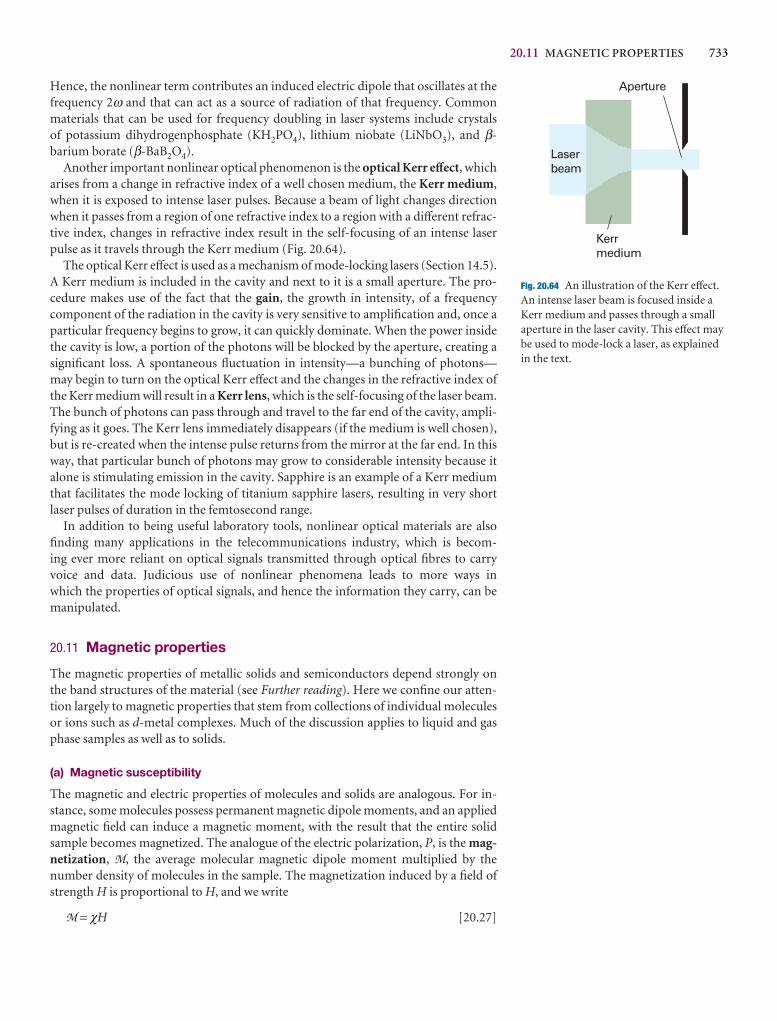
20.11 MAGNETIC PROPERTIES 733
Hence, the nonlinear term contributes an induced electric dipole that oscillates at thefrequency 2ω and that can act as a source of radiation of that frequency. Commonmaterials that can be used for frequency doubling in laser systems include crystals of potassium dihydrogenphosphate (KH2PO4), lithium niobate (LiNbO3), and β-barium borate (β-BaB2O4).
Another important nonlinear optical phenomenon is the optical Kerr effect, whicharises from a change in refractive index of a well chosen medium, the Kerr medium,when it is exposed to intense laser pulses. Because a beam of light changes directionwhen it passes from a region of one refractive index to a region with a different refrac-tive index, changes in refractive index result in the self-focusing of an intense laserpulse as it travels through the Kerr medium (Fig. 20.64).
The optical Kerr effect is used as a mechanism of mode-locking lasers (Section 14.5).A Kerr medium is included in the cavity and next to it is a small aperture. The pro-cedure makes use of the fact that the gain, the growth in intensity, of a frequency component of the radiation in the cavity is very sensitive to amplification and, once aparticular frequency begins to grow, it can quickly dominate. When the power insidethe cavity is low, a portion of the photons will be blocked by the aperture, creating asignificant loss. A spontaneous fluctuation in intensity—a bunching of photons—may begin to turn on the optical Kerr effect and the changes in the refractive index ofthe Kerr medium will result in a Kerr lens, which is the self-focusing of the laser beam.The bunch of photons can pass through and travel to the far end of the cavity, ampli-fying as it goes. The Kerr lens immediately disappears (if the medium is well chosen),but is re-created when the intense pulse returns from the mirror at the far end. In thisway, that particular bunch of photons may grow to considerable intensity because italone is stimulating emission in the cavity. Sapphire is an example of a Kerr mediumthat facilitates the mode locking of titanium sapphire lasers, resulting in very shortlaser pulses of duration in the femtosecond range.
In addition to being useful laboratory tools, nonlinear optical materials are alsofinding many applications in the telecommunications industry, which is becom-ing ever more reliant on optical signals transmitted through optical fibres to carryvoice and data. Judicious use of nonlinear phenomena leads to more ways in which the properties of optical signals, and hence the information they carry, can bemanipulated.
20.11 Magnetic properties
The magnetic properties of metallic solids and semiconductors depend strongly onthe band structures of the material (see Further reading). Here we confine our atten-tion largely to magnetic properties that stem from collections of individual moleculesor ions such as d-metal complexes. Much of the discussion applies to liquid and gasphase samples as well as to solids.
(a) Magnetic susceptibility
The magnetic and electric properties of molecules and solids are analogous. For in-stance, some molecules possess permanent magnetic dipole moments, and an appliedmagnetic field can induce a magnetic moment, with the result that the entire solidsample becomes magnetized. The analogue of the electric polarization, P, is the mag-netization, M, the average molecular magnetic dipole moment multiplied by thenumber density of molecules in the sample. The magnetization induced by a field ofstrength H is proportional to H, and we write
M = χH [20.27]
Kerrmedium
Laserbeam
Aperture
Fig. 20.64 An illustration of the Kerr effect.An intense laser beam is focused inside aKerr medium and passes through a smallaperture in the laser cavity. This effect maybe used to mode-lock a laser, as explainedin the text.
734 20 MATERIALS 2: THE SOLID STATE
where χ is the dimensionless volume magnetic susceptibility. A closely related quan-tity is the molar magnetic susceptibility, χm:
χm = χVm [20.28]
where Vm is the molar volume of the substance (we shall soon see why it is sensible tointroduce this quantity). The magnetic flux density, B, is related to the applied fieldstrength and the magnetization by
B = µ0(H + M) = µ0(1 + χ)H [20.29]
where µ0 is the vacuum permeability, µ0 = 4π × 10−7 J C−2 m−1 s2. The magnetic fluxdensity can be thought of as the density of magnetic lines of force permeating themedium. This density is increased if M adds to H (when χ > 0), but the density is decreased if M opposes H (when χ < 0). Materials for which χ is positive are calledparamagnetic. Those for which χ is negative are called diamagnetic.
Just as polar molecules in fluid phases contribute a term proportional to µ2/3kT tothe electric polarization of a medium (eqn 18.15), so molecules with a permanentmagnetic dipole moment of magnitude m contribute to the magnetization an amountproportional to m2/3kT. However, unlike for polar molecules, this contribution to themagnetization is obtained even for paramagnetic species trapped in solids, becausethe direction of the spin of the electrons is typically not coupled to the orientation ofthe molecular framework and so contributes even when the nuclei are stationary. Anapplied field can also induce a magnetic moment by stirring up currents in the elec-tron distribution like those responsible for the chemical shift in NMR (Section 15.5).The constant of proportionality between the induced moment and the applied field iscalled the magnetizability, ξ (xi), and the magnetic analogue of eqn 18.15 is
χ = N µ0 ξ + (20.30)
We can now see why it is convenient to introduce χm, because the product of the num-ber density N and the molar volume is Avogadro’s constant, NA:
NVm = = = NA (20.31)
Hence
χm = NAµ0 ξ + (20.32)
and the density dependence of the susceptibility (which occurs in eqn 20.30 via N = NAρ/M) has been eliminated. The expression for χm is in agreement with the empirical Curie law:
χm = A + (20.33)
with A = NAµ0ξ and C = NAµ0m2/3k. As indicated above, and in contrast to electricmoments, this expression applies to solids as well as fluid phases.
The magnetic susceptibility is traditionally measured with a Gouy balance. This instrument consists of a sensitive balance from which the sample hangs in the form of anarrow cylinder and lies between the poles of a magnet. If the sample is paramagnetic,it is drawn into the field, and its apparent weight is greater than when the field is off.A diamagnetic sample tends to be expelled from the field and appears to weigh lesswhen the field is turned on. The balance is normally calibrated against a sample of
C
T
DF
m2
3kT
AC
nNAVm
nVm
NVm
V
DF
m2
3kT
AC
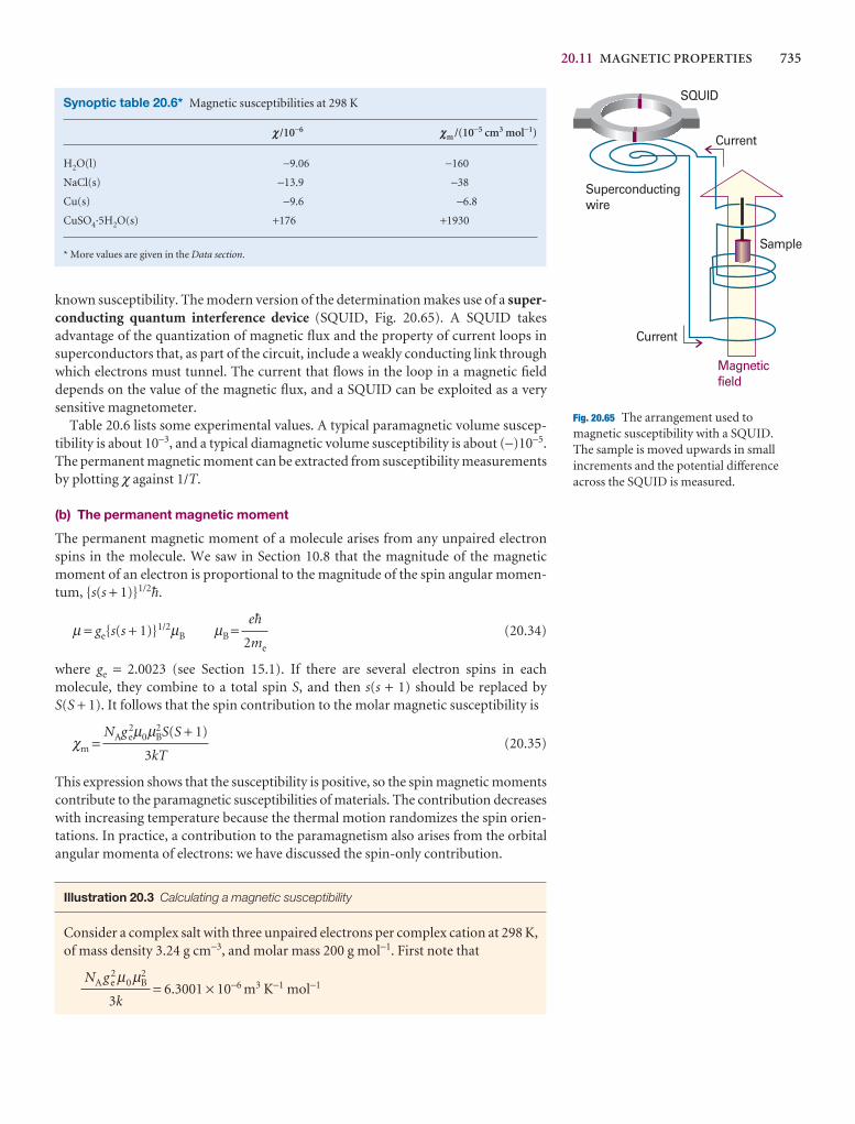
20.11 MAGNETIC PROPERTIES 735
SQUID
Superconductingwire
Current
Current
Magneticfield
Sample
Fig. 20.65 The arrangement used tomagnetic susceptibility with a SQUID. The sample is moved upwards in smallincrements and the potential differenceacross the SQUID is measured.
Synoptic table 20.6* Magnetic susceptibilities at 298 K
c/10−6 cm /(10−5 cm3 mol−1)
H2O(l) −9.06 −160
NaCl(s) −13.9 −38
Cu(s) −9.6 −6.8
CuSO4·5H2O(s) +176 +1930
* More values are given in the Data section.
known susceptibility. The modern version of the determination makes use of a super-conducting quantum interference device (SQUID, Fig. 20.65). A SQUID takes advantage of the quantization of magnetic flux and the property of current loops insuperconductors that, as part of the circuit, include a weakly conducting link throughwhich electrons must tunnel. The current that flows in the loop in a magnetic field depends on the value of the magnetic flux, and a SQUID can be exploited as a verysensitive magnetometer.
Table 20.6 lists some experimental values. A typical paramagnetic volume suscep-tibility is about 10−3, and a typical diamagnetic volume susceptibility is about (−)10−5.The permanent magnetic moment can be extracted from susceptibility measurementsby plotting χ against 1/T.
(b) The permanent magnetic moment
The permanent magnetic moment of a molecule arises from any unpaired electronspins in the molecule. We saw in Section 10.8 that the magnitude of the magnetic moment of an electron is proportional to the magnitude of the spin angular momen-tum, {s(s + 1)}1/2$.
µ = ge{s(s + 1)}1/2µB µB = (20.34)
where ge = 2.0023 (see Section 15.1). If there are several electron spins in eachmolecule, they combine to a total spin S, and then s(s + 1) should be replaced by S(S + 1). It follows that the spin contribution to the molar magnetic susceptibility is
χm = (20.35)
This expression shows that the susceptibility is positive, so the spin magnetic momentscontribute to the paramagnetic susceptibilities of materials. The contribution decreaseswith increasing temperature because the thermal motion randomizes the spin orien-tations. In practice, a contribution to the paramagnetism also arises from the orbitalangular momenta of electrons: we have discussed the spin-only contribution.
Illustration 20.3 Calculating a magnetic susceptibility
Consider a complex salt with three unpaired electrons per complex cation at 298 K,of mass density 3.24 g cm−3, and molar mass 200 g mol−1. First note that
= 6.3001 × 10⁻⁶ m3 K−1 mol−1NA g 2
e µ0µ2B
3k
NAg 2eµ0µ2
BS(S + 1)
3kT
e$
2me
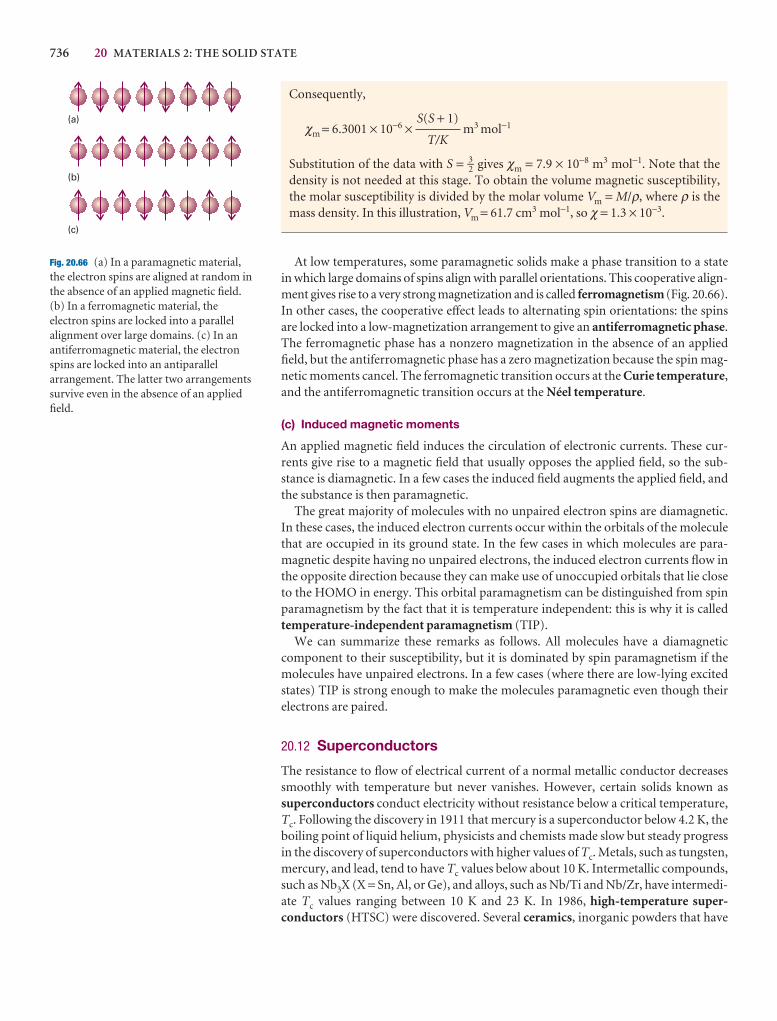
736 20 MATERIALS 2: THE SOLID STATE
(a)
(b)
(c)
Fig. 20.66 (a) In a paramagnetic material,the electron spins are aligned at random inthe absence of an applied magnetic field.(b) In a ferromagnetic material, theelectron spins are locked into a parallelalignment over large domains. (c) In anantiferromagnetic material, the electronspins are locked into an antiparallelarrangement. The latter two arrangementssurvive even in the absence of an appliedfield.
Consequently,
χm = 6.3001 × 10⁻⁶ × m3 mol−1
Substitution of the data with S = 3–2 gives χm = 7.9 × 10⁻⁸ m3 mol−1. Note that thedensity is not needed at this stage. To obtain the volume magnetic susceptibility,the molar susceptibility is divided by the molar volume Vm = M/ρ, where ρ is themass density. In this illustration, Vm = 61.7 cm3 mol−1, so χ = 1.3 × 10⁻³.
At low temperatures, some paramagnetic solids make a phase transition to a statein which large domains of spins align with parallel orientations. This cooperative align-ment gives rise to a very strong magnetization and is called ferromagnetism (Fig. 20.66).In other cases, the cooperative effect leads to alternating spin orientations: the spinsare locked into a low-magnetization arrangement to give an antiferromagnetic phase.The ferromagnetic phase has a nonzero magnetization in the absence of an appliedfield, but the antiferromagnetic phase has a zero magnetization because the spin mag-netic moments cancel. The ferromagnetic transition occurs at the Curie temperature,and the antiferromagnetic transition occurs at the Néel temperature.
(c) Induced magnetic moments
An applied magnetic field induces the circulation of electronic currents. These cur-rents give rise to a magnetic field that usually opposes the applied field, so the sub-stance is diamagnetic. In a few cases the induced field augments the applied field, andthe substance is then paramagnetic.
The great majority of molecules with no unpaired electron spins are diamagnetic.In these cases, the induced electron currents occur within the orbitals of the moleculethat are occupied in its ground state. In the few cases in which molecules are para-magnetic despite having no unpaired electrons, the induced electron currents flow inthe opposite direction because they can make use of unoccupied orbitals that lie closeto the HOMO in energy. This orbital paramagnetism can be distinguished from spinparamagnetism by the fact that it is temperature independent: this is why it is calledtemperature-independent paramagnetism (TIP).
We can summarize these remarks as follows. All molecules have a diamagneticcomponent to their susceptibility, but it is dominated by spin paramagnetism if themolecules have unpaired electrons. In a few cases (where there are low-lying excitedstates) TIP is strong enough to make the molecules paramagnetic even though theirelectrons are paired.
20.12 Superconductors
The resistance to flow of electrical current of a normal metallic conductor decreasessmoothly with temperature but never vanishes. However, certain solids known as superconductors conduct electricity without resistance below a critical temperature,Tc. Following the discovery in 1911 that mercury is a superconductor below 4.2 K, theboiling point of liquid helium, physicists and chemists made slow but steady progressin the discovery of superconductors with higher values of Tc. Metals, such as tungsten,mercury, and lead, tend to have Tc values below about 10 K. Intermetallic compounds,such as Nb3X (X = Sn, Al, or Ge), and alloys, such as Nb/Ti and Nb/Zr, have intermedi-ate Tc values ranging between 10 K and 23 K. In 1986, high-temperature super-conductors (HTSC) were discovered. Several ceramics, inorganic powders that have
S(S + 1)
T/K
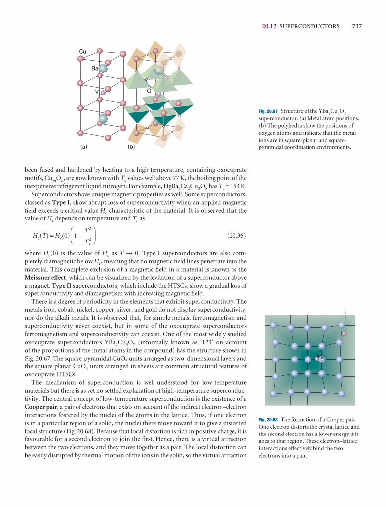
20.12 SUPERCONDUCTORS 737
been fused and hardened by heating to a high temperature, containing oxocupratemotifs, CumOn, are now known with Tc values well above 77 K, the boiling point of theinexpensive refrigerant liquid nitrogen. For example, HgBa2Ca2Cu2O8 has Tc = 153 K.
Superconductors have unique magnetic properties as well. Some superconductors,classed as Type I, show abrupt loss of superconductivity when an applied magneticfield exceeds a critical value Hc characteristic of the material. It is observed that thevalue of Hc depends on temperature and Tc as
Hc(T) = Hc(0) 1 − (20.36)
where Hc(0) is the value of Hc as T → 0. Type I superconductors are also com-pletely diamagnetic below Hc, meaning that no magnetic field lines penetrate into thematerial. This complete exclusion of a magnetic field in a material is known as theMeissner effect, which can be visualized by the levitation of a superconductor abovea magnet. Type II superconductors, which include the HTSCs, show a gradual loss ofsuperconductivity and diamagnetism with increasing magnetic field.
There is a degree of periodicity in the elements that exhibit superconductivity. Themetals iron, cobalt, nickel, copper, silver, and gold do not display superconductivity,nor do the alkali metals. It is observed that, for simple metals, ferromagnetism and superconductivity never coexist, but in some of the oxocuprate superconductors ferromagnetism and superconductivity can coexist. One of the most widely studiedoxocuprate superconductors YBa2Cu3O7 (informally known as ‘123’ on account of the proportions of the metal atoms in the compound) has the structure shown inFig. 20.67. The square-pyramidal CuO5 units arranged as two-dimensional layers andthe square planar CuO4 units arranged in sheets are common structural features ofoxocuprate HTSCs.
The mechanism of superconduction is well-understood for low-temperature materials but there is as yet no settled explanation of high-temperature superconduc-tivity. The central concept of low-temperature superconduction is the existence of aCooper pair, a pair of electrons that exists on account of the indirect electron–electroninteractions fostered by the nuclei of the atoms in the lattice. Thus, if one electron is in a particular region of a solid, the nuclei there move toward it to give a distortedlocal structure (Fig. 20.68). Because that local distortion is rich in positive charge, it isfavourable for a second electron to join the first. Hence, there is a virtual attraction between the two electrons, and they move together as a pair. The local distortion canbe easily disrupted by thermal motion of the ions in the solid, so the virtual attraction
DF
T 2
T 2c
AC
Cu
Ba
Y O
(a) (b)
Fig. 20.67 Structure of the YBa2Cu3O7
superconductor. (a) Metal atom positions.(b) The polyhedra show the positions ofoxygen atoms and indicate that the metalions are in square-planar and square-pyramidal coordination environments.
e�
Fig. 20.68 The formation of a Cooper pair.One electron distorts the crystal lattice andthe second electron has a lower energy if itgoes to that region. These electron–latticeinteractions effectively bind the twoelectrons into a pair.

738 20 MATERIALS 2: THE SOLID STATE
occurs only at very low temperatures. A Cooper pair undergoes less scattering than anindividual electron as it travels through the solid because the distortion caused by oneelectron can attract back the other electron should it be scattered out of its path in acollision. Because the Cooper pair is stable against scattering, it can carry charge freelythrough the solid, and hence give rise to superconduction.
The Cooper pairs responsible for low-temperature superconductivity are likely to be important in HTSCs, but the mechanism for pairing is hotly debated. There isevidence implicating the arrangement of CuO5 layers and CuO4 sheets in the mechan-ism of high-temperature superconduction. It is believed that movement of electronsalong the linked CuO4 units accounts for superconductivity, whereas the linked CuO5
units act as ‘charge reservoirs’ that maintain an appropriate number of electrons inthe superconducting layers.
Superconductors can sustain large currents and, consequently, are excellent materialsfor the high-field magnets used in modern NMR spectroscopy (Chapter 15). However,the potential uses of superconducting materials are not limited to the field to chem-ical instrumentation. For example, HTSCs with Tc values near ambient temperaturewould be very efficient components of an electrical power transmission system, inwhich energy loss due to electrical resistance would be minimized. The appropriatetechnology is not yet available, but research in this area of materials science is active.
Checklist of key ideas
1. Solids are classified as metallic, ionic, covalent, and molecular.
2. A space lattice is the pattern formed by points representing thelocations of structural motifs (atoms, molecules, or groups ofatoms, molecules, or ions). The Bravais lattices are the 14distinct space lattices in three dimensions (Fig. 20.8).
3. A unit cell is an imaginary parallelepiped that contains oneunit of a translationally repeating pattern. Unit cells areclassified into seven crystal systems according to theirrotational symmetries.
4. Crystal planes are specified by a set of Miller indices (hkl) andthe separation of neighbouring planes in a rectangular latticeis given by 1/d2
hkl = h2/a2 + k2/b2 + l 2/c2.
5. Bragg’s law relating the glancing angle θ to the separation oflattice planes is λ = 2d sin θ, where λ is the wavelength of theradiation.
6. The scattering factor is a measure of the ability of an atom todiffract radiation (eqn 20.6).
7. The structure factor is the overall amplitude of a wavediffracted by the {hkl} planes (eqn 20.7). Fourier synthesis isthe construction of the electron density distribution fromstructure factors (eqn 20.8).
8. A Patterson synthesis is a map of interatomic vectors obtained by Fourier analysis of diffraction intensities (eqn 20.9).
9. Structure refinement is the adjustment of structuralparameters to give the best fit between the observed intensitiesand those calculated from the model of the structure deducedfrom the diffraction pattern.
10. Many elemental metals have close-packed structures withcoordination number 12; close-packed structures may beeither cubic (ccp) or hexagonal (hcp).
11. Representative ionic structures include the caesium-chloride,rock-salt, and zinc-blende structures.
12. The radius-ratio rule may be used cautiously to predict whichof these three structures is likely (eqn 20.12).
13. The lattice enthalpy is the change in enthalpy (per mole offormula units) accompanying the complete separation of thecomponents of the solid. The electrostatic contribution to thelattice enthalpy is expressed by the Born–Mayer equation (eqn 20.15).
14. A covalent network solid is a solid in which covalent bonds ina definite spatial orientation link the atoms in a networkextending through the crystal. A molecular solid is a solidconsisting of discrete molecules held together by van derWaals interactions.
15. The mechanical properties of a solid are discussed in terms ofthe relationship between stress, the applied force divided bythe area to which it is applied, and strain, the distortion of asample resulting from an applied stress.
16. The response of a solid to an applied stress is summarized by the Young’s modulus (eqn 20.16a), the bulk modulus (eqn 20.16b), the shear modulus (eqn 20.16c), and Poisson’sratio (eqn 20.17).
17. Electronic conductors are classified as metallic conductors orsemiconductors according to the temperature dependence oftheir conductivities. An insulator is a semiconductor with avery low electrical conductivity.

DISCUSSION QUESTIONS 739
18. According to the band theory, electrons occupy molecularorbitals formed from the overlap of atomic orbitals: full bands are called valence bands and empty bands are calledconduction bands. The occupation of the orbitals in a solid isgiven by the Fermi–Dirac distribution (eqn 20.23).
19. Semiconductors are classified as p-type or n-type according to whether conduction is due to holes in the valence band orelectrons in the conduction band.
20. The spectroscopic properties of molecular solids can beunderstood in terms of the formation and migration ofexcitons, electron–hole pairs, from molecule to molecule.
21. The spectroscopic properties of metallic conductors andsemiconductors can be understood in terms of the light-induced promotion of electrons from valence bands toconduction bands.
22. Examples of solid state lasers include the neodymium laser,the titanium sapphire laser, and diode lasers.
23. Nonlinear optical phenomena arise from changes in theoptical properties of a material in the presence of an intensefield from electromagnetic radiation. Examples includesecond harmonic generation, and the optical Kerr effect.
24. A bulk sample exposed to a magnetic field of strength Hacquires a magnetization, M = χH, where χ is the
dimensionless volume magnetic susceptibility. When χ < 0,the material is diamagnetic and moves out of a magnetic field.When χ > 0, the material is paramagnetic and moves into amagnetic field.
25. The temperature dependence of χm is given by the Curie lawχm = A + C/T, where A = NAµ0ξ, C = NAµ0m2/3k, and ξ is themagnetizability, a measure of the extent to which a magneticdipole moment may be induced in a molecule.
26. Ferromagnetism is the cooperative alignment of electron spins in a material and gives rise to strong magnetization.Antiferromagnetism results from alternating spin orientationsin a material and leads to weak magnetization.
27. Temperature-independent paramagnetism arises frominduced electron currents within the orbitals of a moleculethat are occupied in its ground state.
28. Superconductors conduct electricity without resistance belowa critical temperature Tc. Type I superconductors show abruptloss of superconductivity when an applied magnetic fieldexceeds a critical value Hc characteristic of the material. They are also completely diamagnetic below Hc. Type IIsuperconductors show a gradual loss of superconductivity and diamagnetism with increasing magnetic field.
Further reading
Articles and texts
C.D. Graham, Jr., Magnetic materials. In Encyclopedia of appliedphysics, G.L. Trigg (ed.), 9, 1 VCH, New York (1994).
W.B. Pearson and C. Chieh, Crystallography. In Encyclopedia ofapplied physics, G.L. Trigg (ed.), 4, 385 VCH, New York (1992).
W.D. Callister, Jr., Materials science and engineering: an introduction.Wiley, New York (2000).
P.A. Cox, The electronic structure and chemistry of solids. OxfordUniversity Press (1987).
O. Svelto, Principles of lasers. Plenum, New York (1998).
M.A. White, Properties of materials. Oxford University Press (2000).
Sources of data and information
D.R. Lide (ed.), CRC Handbook of Chemistry and Physics, Sections 3,12, 13, and 15, CRC Press, Boca Raton (2000).
D. Sangeeta and J.R. LaGraff, Inorganic materials chemistry deskreference, CRC Press, Boca Raton (2004).
Discussion questions
20.1 Explain how planes of lattice points are labelled.
20.2 Describe the procedure for identifying the type and size of a cubic unitcell.
20.3 What is meant by a systematic absence? How do they arise?
20.4 Describe the phase problem and explain how it may be overcome.
20.5 Describe the structures of elemental metallic solids in terms of thepacking of hard spheres. To what extent is the hard-sphere model inaccurate?
20.6 Describe the caesium-chloride and rock-salt structures in terms of theoccupation of holes in expanded close-packed lattices.
20.7 Explain how X-ray diffraction can be used to determine the absoluteconfiguration of molecules.
20.8 Explain how metallic conductors and semiconductors are identified andexplain their electrical and optical properties in terms of band theory.
20.9 Describe the characteristics of the Fermi–Dirac distribution. Why is itappropriate to call the parameter µ a chemical potential?
20.10 To what extent are the electric and magnetic properties of moleculesanalogous? How do they differ?

740 20 MATERIALS 2: THE SOLID STATE
Exercises
20.1a Equivalent lattice points within the unit cell of a Bravais lattice haveidentical surroundings. What points within a face-centred cubic unit cell areequivalent to the point (1–
2 , 0, 0)?
20.1b Equivalent lattice points within the unit cell of a Bravais lattice haveidentical surroundings. What points within a body-centred cubic unit cell areequivalent to the point (1–
2 , 0, 1–2 )?
20.2a Find the Miller indices of the planes that intersect the crystallographicaxes at the distances (2a, 3b, 2c) and (2a, 2b, ∞c).
20.2b Find the Miller indices of the planes that intersect the crystallographicaxes at the distances (1a, 3b, −c) and (2a, 3b, 4c).
20.3a Calculate the separations of the planes {111}, {211}, and {100} in acrystal in which the cubic unit cell has side 432 pm.
20.3b Calculate the separations of the planes {121}, {221}, and {244} in acrystal in which the cubic unit cell has side 523 pm.
20.4a The glancing angle of a Bragg reflection from a set of crystal planesseparated by 99.3 pm is 20.85°. Calculate the wavelength of the X-rays.
20.4b The glancing angle of a Bragg reflection from a set of crystal planesseparated by 128.2 pm is 19.76°. Calculate the wavelength of the X-rays.
20.5a What are the values of 2θ of the first three diffraction lines of bcc iron(atomic radius 126 pm) when the X-ray wavelength is 58 pm?
20.5b What are the values of 2θ of the first three diffraction lines of fcc gold{atomic radius 144 pm) when the X-ray wavelength is 154 pm?
20.6a Copper Kα radiation consists of two components of wavelengths154.433 pm and 154.051 pm. Calculate the separation of the diffraction linesarising from the two components in a powder diffraction pattern recorded ina circular camera of radius 5.74 cm (with the sample at the centre) fromplanes of separation 77.8 pm.
20.6b A synchrotron source produces X-radiation at a range of wavelengths.Consider two components of wavelengths 95.401 and 96.035 pm. Calculatethe separation of the diffraction lines arising from the two components in apowder diffraction pattern recorded in a circular camera of radius 5.74 cm(with the sample at the centre) from planes of separation 82.3 pm.
20.7a The compound Rb3TlF6 has a tetragonal unit cell with dimensions a = 651 pm and c = 934 pm. Calculate the volume of the unit cell.
20.7b Calculate the volume of the hexagonal unit cell of sodium nitrate, forwhich the dimensions are a = 1692.9 pm and c = 506.96 pm.
20.8a The orthorhombic unit cell of NiSO4 has the dimensions a = 634 pm, b = 784 pm, and c = 516 pm, and the density of the solid is estimated as 3.9 g cm−3. Determine the number of formula units per unit cell and calculate a more precise value of the density.
20.8b An orthorhombic unit cell of a compound of molar mass 135.01 g mol−1
has the dimensions a = 589 pm, b = 822 pm, and c = 798 pm. The density ofthe solid is estimated as 2.9 g cm−3. Determine the number of formula unitsper unit cell and calculate a more precise value of the density.
20.9a The unit cells of SbCl3 are orthorhombic with dimensions a = 812 pm,b = 947 pm, and c = 637 pm. Calculate the spacing, d, of the (411) planes.
20.9b An orthorhombic unit cell has dimensions a = 679 pm, b = 879 pm, andc = 860 pm. Calculate the spacing, d, of the (322) planes.
20.10a A substance known to have a cubic unit cell gives reflections with CuKα radiation (wavelength 154 pm) at glancing angles 19.4°, 22.5°, 32.6°, and
39.4°. The reflection at 32.6° is known to be due to the (220) planes. Index theother reflections.
20.10b A substance known to have a cubic unit cell gives reflections withradiation of wavelength 137 pm at the glancing angles 10.7°, 13.6°, 17.7°, and21.9°. The reflection at 17.7° is known to be due to the (111) planes. Index theother reflections.
20.11a Potassium nitrate crystals have orthorhombic unit cells of dimensionsa = 542 pm, b = 917 pm, and c = 645 pm. Calculate the glancing angles for the(100), (010), and (111) reflections using CuKα radiation (154 pm).
20.11b Calcium carbonate crystals in the form of aragonite haveorthorhombic unit cells of dimensions a = 574.1 pm, b = 796.8 pm, and c = 495.9 pm. Calculate the glancing angles for the (100), (010), and (111)reflections using radiation of wavelength 83.42 pm (from aluminium).
20.12a Copper(I) chloride forms cubic crystals with four formula units perunit cell. The only reflections present in a powder photograph are those witheither all even indices or all odd indices. What is the (Bravais) lattice type ofthe unit cell?
20.12b A powder diffraction photograph from tungsten shows lines thatindex as (110), (200), (211), (220), (310), (222), (321), (400), . . . Identify the(Bravais) lattice type of the unit cell.
20.13a The coordinates, in units of a, of the atoms in a body-centred cubiclattice are (0,0,0), (0,1,0), (0,0,1), (0,1,1), (1,0,0), (1,1,0), (1,0,1), and (1,1,1).Calculate the structure factors Fhkl when all the atoms are identical.
20.13b The coordinates, in units of a, of the atoms in a body-centred cubiclattice are (0,0,0), (0,1,0), (0,0,1), (0,1,1), (1,0,0), (1,1,0), (1,0,1), (1,1,1), and( 1–
2 , 1–2 , 1–
2 ). Calculate the structure factors Fhkl when all the atoms are identical.
20.14a Calculate the packing fraction for close-packed cylinders.
20.14b Calculate the packing fraction for equilateral triangular rods stackedas shown in 2.
20.15a Verify that the radius ratios for sixfold coordination is 0.414.
20.15b Verify that the radius ratios for eightfold coordination is 0.732.
20.16a From the data in Table 20.3 determine the radius of the smallestcation that can have (a) sixfold and (b) eightfold coordination with the O2− ion.
20.16b From the data in Table 20.3 determine the radius of the smallestcation that can have (a) sixfold and (b) eightfold coordination with the K+ ion.
20.17a Calculate the atomic packing factor for diamond.
20.17b Calculate the atomic packing factor for a side-centred (C) cubic unitcell.
2

PROBLEMS 741
20.18a Is there an expansion or a contraction as titanium transforms fromhcp to body-centred cubic? The atomic radius of titanium is 145.8 pm in hcpbut 142.5 pm in bcc.
20.18b Is there an expansion or a contraction as iron transforms from hcp tobcc? The atomic radius of iron is 126 pm in hcp but 122 pm in bcc.
20.19a In a Patterson synthesis, the spots correspond to the lengths anddirections of the vectors joining the atoms in a unit cell. Sketch the patternthat would be obtained for a planar, triangular isolated BF3 molecule.
20.19b In a Patterson synthesis, the spots correspond to the lengths anddirections of the vectors joining the atoms in a unit cell. Sketch the patternthat would be obtained from the C atoms in an isolated benzene molecule.
20.20a What velocity should neutrons have if they are to have wavelength 50 pm?
20.20b Calculate the wavelength of neutrons that have reached thermalequilibrium by collision with a moderator at 300 K.
20.21a Derive the Born–Mayer equation (eqn 20.15) by calculating theenergy at which d(EP + E*P)/dd = 0, with EP and E*P given by eqns 20.13 and20.14, respectively.
20.21b Calculate the lattice enthalpy of MgBr2 from the following data:
∆H/(kJ mol−1)
Sublimation of Mg(s) +148
Ionization of Mg(g) to Mg2+(g) +2187
Vaporization of Br2(l) +31
Dissociation of Br2(g) +193
Electron attachment to Br(g) −331
Formation of MgBr2(s) from Mg(s) and Br2(l) −524
20.22a Cotton consists of the polymer cellulose, which is a linear chain ofglucose molecules. The chains are held together by hydrogen bonding. Whena cotton shirt is ironed, it is first moistened, then heated under pressure.Explain this process.
20.22b Sections of the solid fuel rocket boosters of the space shuttleChallenger were sealed together with O-ring rubber seals of circumference 11 m. These seals failed at 0°C, a temperature well above the crystallizationtemperature of the rubber. Speculate on why the failure occurred.
20.23a Young’s modulus for polyethylene at room temperature is 1.2 GPa.What strain will be produced when a mass of 1.0 kg is suspended from apolyethylene thread of diameter 1.0 mm?
20.23b Young’s modulus for iron at room temperature is 215 GPa. Whatstrain will be produced when a mass of 10.0 kg is suspended from an iron wireof diameter 0.10 mm?
20.24a Poisson’s ratio for polyethylene is 0.45. What change in volume takesplace when a cube of polyethylene of volume 1.0 cm3 is subjected to a uniaxialstress that produces a strain of 1.0 per cent?
20.24b Poisson’s ratio for lead is 0.41. What change in volume takes placewhen a cube of lead of volume 1.0 dm3 is subjected to a uniaxial stress thatproduces a strain of 2.0 per cent?
20.25a Is arsenic-doped germanium a p-type or n-type semiconductor?
20.25b Is gallium-doped germanium a p-type or n-type semiconductor?
20.26a The promotion of an electron from the valence band into theconduction band in pure TIO2 by light absorption requires a wavelength ofless than 350 nm. Calculate the energy gap in electronvolts between thevalence and conduction bands.
20.26b The band gap in silicon is 1.12 eV. Calculate the minimum frequencyof electromagnetic radiation that results in promotion of electrons from thevalence to the conduction band.
20.27a The magnetic moment of CrCl3 is 3.81µB. How many unpairedelectrons does the Cr possess?
20.27b The magnetic moment of Mn2+ in its complexes is typically 5.3µB.How many unpaired electrons does the ion possess?
20.28a Calculate the molar susceptibility of benzene given that its volumesusceptibility is −7.2 × 10⁻⁷ and its density 0.879 g cm−3 at 25°C.
20.28b Calculate the molar susceptibility of cyclohexane given that its volumesusceptibility is −7.9 × 10⁻⁷ and its density 811 kg m−3 at 25°C.
20.29a According to Lewis theory, an O2 molecule should be diamagnetic.However, experimentally it is found that χm /(m3 mol−1) = (1.22 × 10⁻⁵ K)/T.Determine the number of unpaired spins in O2. How is the problem of theLewis structure resolved?
20.29b Predict the molar susceptibility of nitrogen dioxide at 298 K. Whydoes the molar susceptibility of a sample of nitrogen dioxide gas decrease as itis compressed?
20.30a Data on a single crystal of MnF2 give χm = 0.1463 cm3 mol−1 at294.53 K. Determine the effective number of unpaired electrons in thiscompound and compare your result with the theoretical value.
20.30b Data on a single crystal of NiSO4·7H2O give χm = 6.00 × 10⁻⁸ m3 mol−1
at 298 K. Determine the effective number of unpaired electrons in thiscompound and compare your result with the theoretical value.
20.31a Estimate the spin-only molar susceptibility of CuSO4·5H2O at 25°C.
20.31b Estimate the spin-only molar susceptibility of MnSO4·4H2O at 298 K.
20.32a Approximately how large must the magnetic induction, B, be for theorientational energy of an S = 1 system to be comparable to kT at 298 K?
20.32b Estimate the ratio of populations of the MS states of a system with S = 1 in 15.0 T at 298 K.
Problems*
Numerical problems
20.1 In the early days of X-ray crystallography there was an urgent need toknow the wavelengths of X-rays. One technique was to measure the diffractionangle from a mechanically ruled grating. Another method was to estimate theseparation of lattice planes from the measured density of a crystal. The density
of NaCl is 2.17 g cm−3 and the (100) reflection using PdKα radiation occurredat 6.0°. Calculate the wavelength of the X-rays.
20.2 The element polonium crystallizes in a cubic system. Bragg reflections,with X-rays of wavelength 154 pm, occur at sin θ = 0.225, 0.316, and 0.388from the (100), (110), and (111) sets of planes. The separation between the
* Problems denoted with the symbol ‡ were supplied by Charles Trapp and Carmen Giunta.
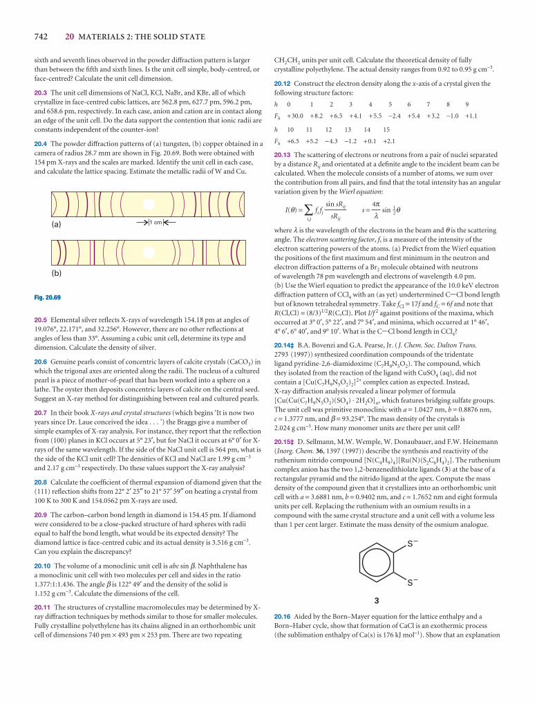
742 20 MATERIALS 2: THE SOLID STATE
sixth and seventh lines observed in the powder diffraction pattern is largerthan between the fifth and sixth lines. Is the unit cell simple, body-centred, orface-centred? Calculate the unit cell dimension.
20.3 The unit cell dimensions of NaCl, KCl, NaBr, and KBr, all of whichcrystallize in face-centred cubic lattices, are 562.8 pm, 627.7 pm, 596.2 pm,and 658.6 pm, respectively. In each case, anion and cation are in contact alongan edge of the unit cell. Do the data support the contention that ionic radii areconstants independent of the counter-ion?
20.4 The powder diffraction patterns of (a) tungsten, (b) copper obtained in acamera of radius 28.7 mm are shown in Fig. 20.69. Both were obtained with154 pm X-rays and the scales are marked. Identify the unit cell in each case,and calculate the lattice spacing. Estimate the metallic radii of W and Cu.
20.5 Elemental silver reflects X-rays of wavelength 154.18 pm at angles of19.076°, 22.171°, and 32.256°. However, there are no other reflections atangles of less than 33°. Assuming a cubic unit cell, determine its type anddimension. Calculate the density of silver.
20.6 Genuine pearls consist of concentric layers of calcite crystals (CaCO3) inwhich the trigonal axes are oriented along the radii. The nucleus of a culturedpearl is a piece of mother-of-pearl that has been worked into a sphere on alathe. The oyster then deposits concentric layers of calcite on the central seed.Suggest an X-ray method for distinguishing between real and cultured pearls.
20.7 In their book X-rays and crystal structures (which begins ‘It is now twoyears since Dr. Laue conceived the idea . . . ’) the Braggs give a number ofsimple examples of X-ray analysis. For instance, they report that the reflectionfrom (100) planes in KCl occurs at 5° 23′, but for NaCl it occurs at 6° 0′ for X-rays of the same wavelength. If the side of the NaCl unit cell is 564 pm, what isthe side of the KCl unit cell? The densities of KCl and NaCl are 1.99 g cm−3
and 2.17 g cm−3 respectively. Do these values support the X-ray analysis?
20.8 Calculate the coefficient of thermal expansion of diamond given that the(111) reflection shifts from 22° 2′ 25″ to 21° 57′ 59″ on heating a crystal from100 K to 300 K and 154.0562 pm X-rays are used.
20.9 The carbon–carbon bond length in diamond is 154.45 pm. If diamondwere considered to be a close-packed structure of hard spheres with radiiequal to half the bond length, what would be its expected density? Thediamond lattice is face-centred cubic and its actual density is 3.516 g cm−3.Can you explain the discrepancy?
20.10 The volume of a monoclinic unit cell is abc sin β. Naphthalene has a monoclinic unit cell with two molecules per cell and sides in the ratio1.377:1:1.436. The angle β is 122° 49′ and the density of the solid is 1.152 g cm−3. Calculate the dimensions of the cell.
20.11 The structures of crystalline macromolecules may be determined by X-ray diffraction techniques by methods similar to those for smaller molecules.Fully crystalline polyethylene has its chains aligned in an orthorhombic unitcell of dimensions 740 pm × 493 pm × 253 pm. There are two repeating
Fig. 20.69
1 cm(a)
(b)
CH2CH2 units per unit cell. Calculate the theoretical density of fullycrystalline polyethylene. The actual density ranges from 0.92 to 0.95 g cm−3.
20.12 Construct the electron density along the x-axis of a crystal given thefollowing structure factors:
h 0 1 2 3 4 5 6 7 8 9
Fh +30.0 +8.2 +6.5 +4.1 +5.5 −2.4 +5.4 +3.2 −1.0 +1.1
h 10 11 12 13 14 15
Fh +6.5 +5.2 −4.3 −1.2 +0.1 +2.1
20.13 The scattering of electrons or neutrons from a pair of nuclei separatedby a distance Rij and orientated at a definite angle to the incident beam can becalculated. When the molecule consists of a number of atoms, we sum overthe contribution from all pairs, and find that the total intensity has an angularvariation given by the Wierl equation:
I(θ) = ∑i,j
fi fj s = sin 1–2θ
where λ is the wavelength of the electrons in the beam and θ is the scatteringangle. The electron scattering factor, f, is a measure of the intensity of theelectron scattering powers of the atoms. (a) Predict from the Wierl equationthe positions of the first maximum and first minimum in the neutron andelectron diffraction patterns of a Br2 molecule obtained with neutrons of wavelength 78 pm wavelength and electrons of wavelength 4.0 pm. (b) Use the Wierl equation to predict the appearance of the 10.0 keV electrondiffraction pattern of CCl4 with an (as yet) undertermined C-Cl bond lengthbut of known tetrahedral symmetry. Take fCl = 17f and fC = 6f and note thatR(Cl,Cl) = (8/3)1/2R(C,Cl). Plot I/f 2 against positions of the maxima, whichoccurred at 3° 0′, 5° 22′, and 7° 54′, and minima, which occurred at 1° 46′,4° 6′, 6° 40′, and 9° 10′. What is the C-Cl bond length in CCl4?
20.14‡ B.A. Bovenzi and G.A. Pearse, Jr. (J. Chem. Soc. Dalton Trans.2793 (1997)) synthesized coordination compounds of the tridentateligand pyridine-2,6-diamidoxime (C7H9N5O2). The compound, which they isolated from the reaction of the ligand with CuSO4 (aq), did not contain a [Cu(C7H9N5O2)2]2+ complex cation as expected. Instead, X-ray diffraction analysis revealed a linear polymer of formula[Cu(Cu(C7H9N5O2)(SO4) · 2H2O]n, which features bridging sulfate groups.The unit cell was primitive monoclinic with a = 1.0427 nm, b = 0.8876 nm, c = 1.3777 nm, and β = 93.254°. The mass density of the crystals is 2.024 g cm−3. How many monomer units are there per unit cell?
20.15‡ D. Sellmann, M.W. Wemple, W. Donaubauer, and F.W. Heinemann(Inorg. Chem. 36, 1397 (1997)) describe the synthesis and reactivity of theruthenium nitrido compound [N(C4H9)4][Ru(N)(S2C6H4)2]. The rutheniumcomplex anion has the two 1,2-benzenedithiolate ligands (3) at the base of arectangular pyramid and the nitrido ligand at the apex. Compute the massdensity of the compound given that it crystallizes into an orthorhombic unitcell with a = 3.6881 nm, b = 0.9402 nm, and c = 1.7652 nm and eight formulaunits per cell. Replacing the ruthenium with an osmium results in acompound with the same crystal structure and a unit cell with a volume lessthan 1 per cent larger. Estimate the mass density of the osmium analogue.
20.16 Aided by the Born–Mayer equation for the lattice enthalpy and aBorn–Haber cycle, show that formation of CaCl is an exothermic process (the sublimation enthalpy of Ca(s) is 176 kJ mol−1). Show that an explanation
4πλ
sin sRij
sRij
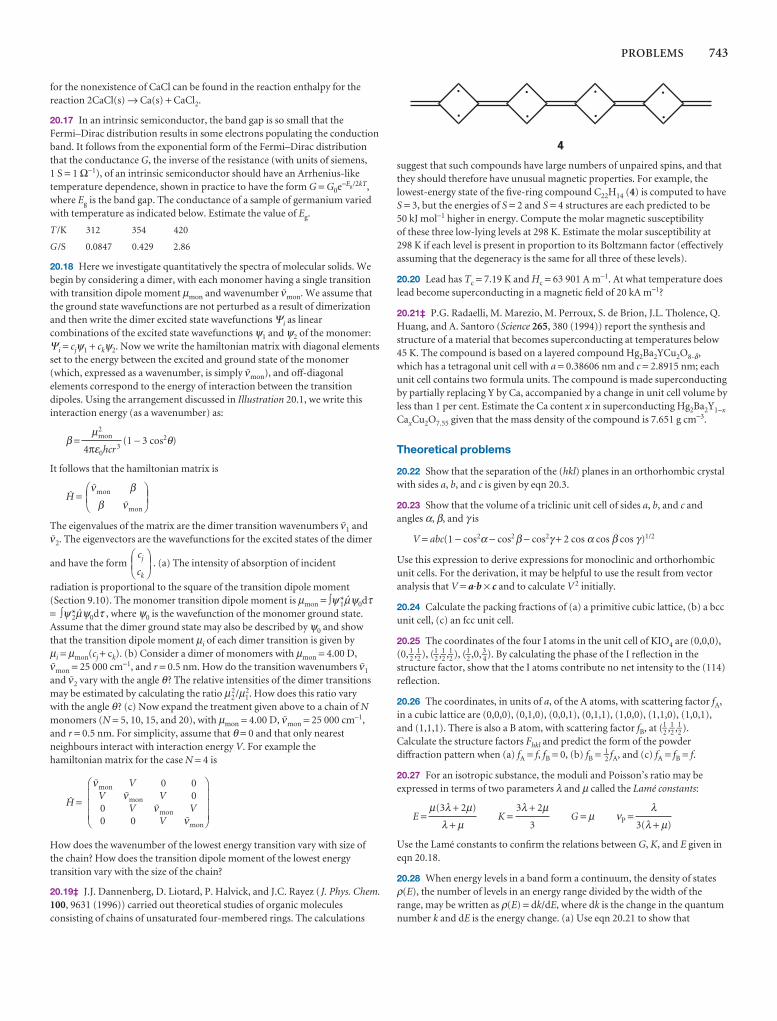
PROBLEMS 743
for the nonexistence of CaCl can be found in the reaction enthalpy for thereaction 2CaCl(s) → Ca(s) + CaCl2.
20.17 In an intrinsic semiconductor, the band gap is so small that theFermi–Dirac distribution results in some electrons populating the conductionband. It follows from the exponential form of the Fermi–Dirac distributionthat the conductance G, the inverse of the resistance (with units of siemens, 1 S = 1 Ω−1), of an intrinsic semiconductor should have an Arrhenius-liketemperature dependence, shown in practice to have the form G = G0e−Eg/2kT,where Eg is the band gap. The conductance of a sample of germanium variedwith temperature as indicated below. Estimate the value of Eg.
T /K 312 354 420
G /S 0.0847 0.429 2.86
20.18 Here we investigate quantitatively the spectra of molecular solids. Webegin by considering a dimer, with each monomer having a single transitionwith transition dipole moment µmon and wavenumber #mon. We assume thatthe ground state wavefunctions are not perturbed as a result of dimerizationand then write the dimer excited state wavefunctions Ψi as linearcombinations of the excited state wavefunctions ψ1 and ψ2 of the monomer:Ψi = cjψ1 + ckψ2. Now we write the hamiltonian matrix with diagonal elementsset to the energy between the excited and ground state of the monomer(which, expressed as a wavenumber, is simply #mon), and off-diagonalelements correspond to the energy of interaction between the transitiondipoles. Using the arrangement discussed in Illustration 20.1, we write thisinteraction energy (as a wavenumber) as:
β = (1 − 3 cos2θ)
It follows that the hamiltonian matrix is
@ =
The eigenvalues of the matrix are the dimer transition wavenumbers #1 and#2. The eigenvectors are the wavefunctions for the excited states of the dimer
and have the form . (a) The intensity of absorption of incident
radiation is proportional to the square of the transition dipole moment(Section 9.10). The monomer transition dipole moment is µmon = ∫ψ*1 Nψ0dτ= ∫ψ*2 Nψ0dτ , where ψ0 is the wavefunction of the monomer ground state.Assume that the dimer ground state may also be described by ψ0 and showthat the transition dipole moment µi of each dimer transition is given by µi = µmon(cj + ck). (b) Consider a dimer of monomers with µmon = 4.00 D, #mon = 25 000 cm−1, and r = 0.5 nm. How do the transition wavenumbers #1
and #2 vary with the angle θ? The relative intensities of the dimer transitionsmay be estimated by calculating the ratio µ2
2/µ12. How does this ratio vary
with the angle θ? (c) Now expand the treatment given above to a chain of Nmonomers (N = 5, 10, 15, and 20), with µmon = 4.00 D, #mon = 25 000 cm−1,and r = 0.5 nm. For simplicity, assume that θ = 0 and that only nearestneighbours interact with interaction energy V. For example the hamiltonian matrix for the case N = 4 is
@ =
How does the wavenumber of the lowest energy transition vary with size ofthe chain? How does the transition dipole moment of the lowest energytransition vary with the size of the chain?
20.19‡ J.J. Dannenberg, D. Liotard, P. Halvick, and J.C. Rayez (J. Phys. Chem.100, 9631 (1996)) carried out theoretical studies of organic moleculesconsisting of chains of unsaturated four-membered rings. The calculations
##
##
mon
mon
mon
mon
VV V
V VV
0 00
00 0
⎛
⎝
⎜⎜⎜
⎞
⎠
⎟⎟⎟
DEFcj
ck
ABC
DEFβ
#mon
#mon
β
ABC
µ2mon
4πε0hcr 3
suggest that such compounds have large numbers of unpaired spins, and thatthey should therefore have unusual magnetic properties. For example, thelowest-energy state of the five-ring compound C22H14 (4) is computed to haveS = 3, but the energies of S = 2 and S = 4 structures are each predicted to be 50 kJ mol−1 higher in energy. Compute the molar magnetic susceptibility of these three low-lying levels at 298 K. Estimate the molar susceptibility at298 K if each level is present in proportion to its Boltzmann factor (effectivelyassuming that the degeneracy is the same for all three of these levels).
20.20 Lead has Tc = 7.19 K and Hc = 63 901 A m−1. At what temperature doeslead become superconducting in a magnetic field of 20 kA m−1?
20.21‡ P.G. Radaelli, M. Marezio, M. Perroux, S. de Brion, J.L. Tholence, Q.Huang, and A. Santoro (Science 265, 380 (1994)) report the synthesis andstructure of a material that becomes superconducting at temperatures below45 K. The compound is based on a layered compound Hg2Ba2YCu2O8-δ,which has a tetragonal unit cell with a = 0.38606 nm and c = 2.8915 nm; eachunit cell contains two formula units. The compound is made superconductingby partially replacing Y by Ca, accompanied by a change in unit cell volume byless than 1 per cent. Estimate the Ca content x in superconducting Hg2Ba2Y1−x
CaxCu2O7.55 given that the mass density of the compound is 7.651 g cm−3.
Theoretical problems
20.22 Show that the separation of the (hkl) planes in an orthorhombic crystalwith sides a, b, and c is given by eqn 20.3.
20.23 Show that the volume of a triclinic unit cell of sides a, b, and c andangles α, β, and γ is
V = abc(1 − cos2α − cos2β − cos2γ + 2 cos α cos β cos γ)1/2
Use this expression to derive expressions for monoclinic and orthorhombicunit cells. For the derivation, it may be helpful to use the result from vectoranalysis that V = a·b × c and to calculate V 2 initially.
20.24 Calculate the packing fractions of (a) a primitive cubic lattice, (b) a bccunit cell, (c) an fcc unit cell.
20.25 The coordinates of the four I atoms in the unit cell of KIO4 are (0,0,0),(0, 1–
2 ,1–2 ), (1–2 ,1–2 ,1–2 ), (1–
2 ,0, 3–4). By calculating the phase of the I reflection in the
structure factor, show that the I atoms contribute no net intensity to the (114)reflection.
20.26 The coordinates, in units of a, of the A atoms, with scattering factor fA,in a cubic lattice are (0,0,0), (0,1,0), (0,0,1), (0,1,1), (1,0,0), (1,1,0), (1,0,1),and (1,1,1). There is also a B atom, with scattering factor fB, at (1–
2 ,1–2 ,1–2 ).Calculate the structure factors Fhkl and predict the form of the powderdiffraction pattern when (a) fA = f, fB = 0, (b) fB = 1–
2 fA, and (c) fA = fB = f.
20.27 For an isotropic substance, the moduli and Poisson’s ratio may beexpressed in terms of two parameters λ and µ called the Lamé constants:
E = K = G = µ νP =
Use the Lamé constants to confirm the relations between G, K, and E given ineqn 20.18.
20.28 When energy levels in a band form a continuum, the density of statesρ(E), the number of levels in an energy range divided by the width of therange, may be written as ρ(E) = dk/dE, where dk is the change in the quantumnumber k and dE is the energy change. (a) Use eqn 20.21 to show that
λ3(λ + µ)
3λ + 2µ3
µ(3λ + 2µ)
λ + µ
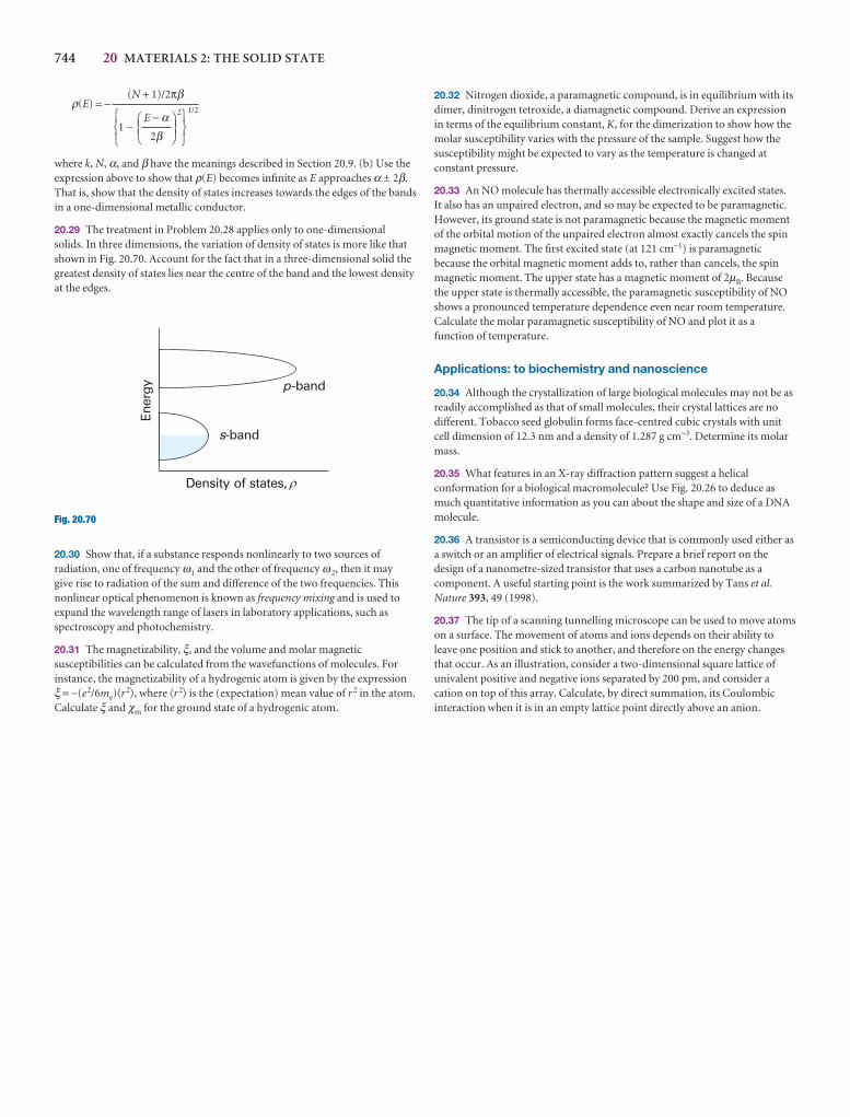
744 20 MATERIALS 2: THE SOLID STATE
ρ(E) = −
1 −2 1/2
where k, N, α, and β have the meanings described in Section 20.9. (b) Use theexpression above to show that ρ(E) becomes infinite as E approaches α ± 2β.That is, show that the density of states increases towards the edges of the bandsin a one-dimensional metallic conductor.
20.29 The treatment in Problem 20.28 applies only to one-dimensionalsolids. In three dimensions, the variation of density of states is more like thatshown in Fig. 20.70. Account for the fact that in a three-dimensional solid thegreatest density of states lies near the centre of the band and the lowest densityat the edges.
20.30 Show that, if a substance responds nonlinearly to two sources ofradiation, one of frequency ω1 and the other of frequency ω2, then it may give rise to radiation of the sum and difference of the two frequencies. Thisnonlinear optical phenomenon is known as frequency mixing and is used toexpand the wavelength range of lasers in laboratory applications, such asspectroscopy and photochemistry.
20.31 The magnetizability, ξ, and the volume and molar magneticsusceptibilities can be calculated from the wavefunctions of molecules. Forinstance, the magnetizability of a hydrogenic atom is given by the expression ξ = −(e2/6me)�r
2�, where �r 2� is the (expectation) mean value of r 2 in the atom.Calculate ξ and χm for the ground state of a hydrogenic atom.
Fig. 20.70
Density of states,
Ener
gy
s-band
p-band
�
567
DEFE − α
2β
ABC123
(N + 1)/2πβ 20.32 Nitrogen dioxide, a paramagnetic compound, is in equilibrium with itsdimer, dinitrogen tetroxide, a diamagnetic compound. Derive an expressionin terms of the equilibrium constant, K, for the dimerization to show how themolar susceptibility varies with the pressure of the sample. Suggest how thesusceptibility might be expected to vary as the temperature is changed atconstant pressure.
20.33 An NO molecule has thermally accessible electronically excited states. It also has an unpaired electron, and so may be expected to be paramagnetic.However, its ground state is not paramagnetic because the magnetic momentof the orbital motion of the unpaired electron almost exactly cancels the spinmagnetic moment. The first excited state (at 121 cm−1) is paramagneticbecause the orbital magnetic moment adds to, rather than cancels, the spinmagnetic moment. The upper state has a magnetic moment of 2µB. Becausethe upper state is thermally accessible, the paramagnetic susceptibility of NOshows a pronounced temperature dependence even near room temperature.Calculate the molar paramagnetic susceptibility of NO and plot it as afunction of temperature.
Applications: to biochemistry and nanoscience
20.34 Although the crystallization of large biological molecules may not be asreadily accomplished as that of small molecules, their crystal lattices are nodifferent. Tobacco seed globulin forms face-centred cubic crystals with unitcell dimension of 12.3 nm and a density of 1.287 g cm−3. Determine its molarmass.
20.35 What features in an X-ray diffraction pattern suggest a helicalconformation for a biological macromolecule? Use Fig. 20.26 to deduce asmuch quantitative information as you can about the shape and size of a DNAmolecule.
20.36 A transistor is a semiconducting device that is commonly used either asa switch or an amplifier of electrical signals. Prepare a brief report on thedesign of a nanometre-sized transistor that uses a carbon nanotube as acomponent. A useful starting point is the work summarized by Tans et al.Nature 393, 49 (1998).
20.37 The tip of a scanning tunnelling microscope can be used to move atomson a surface. The movement of atoms and ions depends on their ability toleave one position and stick to another, and therefore on the energy changesthat occur. As an illustration, consider a two-dimensional square lattice ofunivalent positive and negative ions separated by 200 pm, and consider acation on top of this array. Calculate, by direct summation, its Coulombicinteraction when it is in an empty lattice point directly above an anion.

PART 3 Change
Part 3 considers the processes by which change occurs. We prepare the
ground for a discussion of the rates of reactions by considering the motion of
molecules in gases and in liquids. Then we establish the precise meaning of
reaction rate, and see how the overall rate, and the complex behaviour of some
reactions, may be expressed in terms of elementary steps and the atomic events
that take place when molecules meet. Characteristic physical and chemical
events take place at surfaces, including catalysis, and we see how to describe
them. A special type of surface is that of an electrode, and we shall see how to
describe and understand the rate at which electrons are transferred between an
electrode and species in solution.
21 Molecules in motion
22 The rates of chemical reactions
23 The kinetics of complex reactions
24 Molecular reaction dynamics
25 Processes at solid surfaces

This page intentionally left blank
Molecules in motion
One of the simplest types of molecular motion to describe is the random motion ofmolecules of a perfect gas. We see that a simple theory accounts for the pressure of a gasand the rates at which molecules and energy migrate through gases. Molecular mobility isparticularly important in liquids. Another simple kind of motion is the largely uniform motionof ions in solution in the presence of an electric field. Molecular and ionic motion have com-mon features and, by considering them from a more general viewpoint, we derive expres-sions that govern the migration of properties through matter. One of the most usefulconsequences of this general approach is the formulation of the diffusion equation, which isan equation that shows how matter and energy spread through media of various kinds.Finally, we build a simple model for all types of molecular motion, in which the molecules migrate in a series of small steps, and see that it accounts for many of the properties of migrating molecules in both gases and condensed phases.
The general approach we describe in this chapter provides techniques for discussingthe motion of all kinds of particles in all kinds of fluids. We set the scene by consider-ing a simple type of motion, that of molecules in a perfect gas, and go on to see thatmolecular motion in liquids shows a number of similarities. We shall concentrate onthe transport properties of a substance, its ability to transfer matter, energy, or someother property from one place to another. Four examples of transport properties are
Diffusion, the migration of matter down a concentration gradient.
Thermal conduction, the migration of energy down a temperature gradient.
Electric conduction, the migration of electric charge along an electrical potentialgradient.
Viscosity, the migration of linear momentum down a velocity gradient.
It is convenient to include in the discussion effusion, the emergence of a gas from acontainer through a small hole.
Molecular motion in gases
Here we present the kinetic model of a perfect gas as a starting point for the discussionof its transport properties. In the kinetic model of gases we assume that the only con-tribution to the energy of the gas is from the kinetic energies of the molecules. The kinetic model is one of the most remarkable—and arguably most beautiful—modelsin physical chemistry for, from a set of very slender assumptions, powerful quantitativeconclusions can be deduced.
21Molecular motion in gases
21.1 The kinetic model of gases
I21.1 Impact on astrophysics: TheSun as a ball of perfect gas
21.2 Collision with walls andsurfaces
21.3 The rate of effusion
21.4 Transport properties of aperfect gas
Molecular motion in liquids
21.5 Experimental results
21.6 The conductivities ofelectrolyte solutions
21.7 The mobilities of ions
21.8 Conductivities and ion–ioninteractions
I21.2 Impact on biochemistry: Ionchannels and ion pumps
Diffusion
21.9 The thermodynamic view
21.10 The diffusion equation
I21.3 Impact on biochemistry:Transport of non-electrolytesacross biological membranes
21.11 Diffusion probabilities
21.12 The statistical view
Checklist of key ideas
Further reading
Further information 21.1: Thetransport characteristics of a perfect gas
Discussion questions
Exercises
Problems
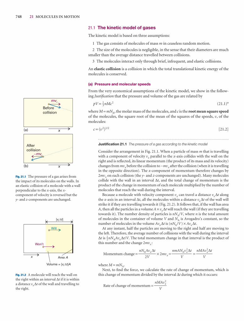
748 21 MOLECULES IN MOTION
21.1 The kinetic model of gases
The kinetic model is based on three assumptions:
1 The gas consists of molecules of mass m in ceaseless random motion.
2 The size of the molecules is negligible, in the sense that their diameters are muchsmaller than the average distance travelled between collisions.
3 The molecules interact only through brief, infrequent, and elastic collisions.
An elastic collision is a collision in which the total translational kinetic energy of themolecules is conserved.
(a) Pressure and molecular speeds
From the very economical assumptions of the kinetic model, we show in the follow-ing Justification that the pressure and volume of the gas are related by
pV = 1–3 nMc2 (21.1)°
where M = mNA, the molar mass of the molecules, and c is the root mean square speedof the molecules, the square root of the mean of the squares of the speeds, v, of themolecules:
c = �v2�1/2 [21.2]
Justification 21.1 The pressure of a gas according to the kinetic model
Consider the arrangement in Fig. 21.1. When a particle of mass m that is travellingwith a component of velocity vx parallel to the x-axis collides with the wall on theright and is reflected, its linear momentum (the product of its mass and its velocity)changes from mvx before the collision to −mvx after the collision (when it is travellingin the opposite direction). The x-component of momentum therefore changes by2mvx on each collision (the y- and z-components are unchanged). Many moleculescollide with the wall in an interval ∆t, and the total change of momentum is theproduct of the change in momentum of each molecule multiplied by the number ofmolecules that reach the wall during the interval.
Because a molecule with velocity component vx can travel a distance vx∆t alongthe x-axis in an interval ∆t, all the molecules within a distance vx∆t of the wall willstrike it if they are travelling towards it (Fig. 21.2). It follows that, if the wall has areaA, then all the particles in a volume A × vx∆t will reach the wall (if they are travellingtowards it). The number density of particles is nNA/V, where n is the total amountof molecules in the container of volume V and NA is Avogadro’s constant, so thenumber of molecules in the volume Avx∆t is (nNA/V) × Avx∆t.
At any instant, half the particles are moving to the right and half are moving to the left. Therefore, the average number of collisions with the wall during the interval∆t is 1–2 nNAAvx∆t/V. The total momentum change in that interval is the product ofthis number and the change 2mvx :
Momentum change = × 2mvx = =
where M = mNA.Next, to find the force, we calculate the rate of change of momentum, which is
this change of momentum divided by the interval ∆t during which it occurs:
Rate of change of momentum =nMAv2
x
V
nMAv2x∆t
V
nmANAv2x∆t
V
nNAAvx∆t
2V
mvx
�mvx
x
x
Beforecollision
Aftercollision
(a)
(b)
Fig. 21.1 The pressure of a gas arises fromthe impact of its molecules on the walls. Inan elastic collision of a molecule with a wallperpendicular to the x-axis, the x-component of velocity is reversed but they- and z-components are unchanged.
x
| |v tx
Volume = | |v t Ax
Area A
Will
Won’t
Fig. 21.2 A molecule will reach the wall onthe right within an interval ∆t if it is withina distance vx∆t of the wall and travelling tothe right.
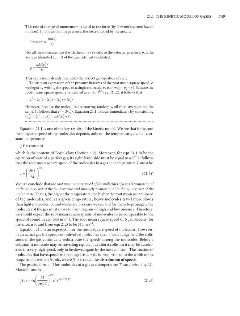
21.1 THE KINETIC MODEL OF GASES 749
This rate of change of momentum is equal to the force (by Newton’s second law ofmotion). It follows that the pressure, the force divided by the area, is
Pressure =
Not all the molecules travel with the same velocity, so the detected pressure, p, is theaverage (denoted � . . . �) of the quantity just calculated:
p =
This expression already resembles the perfect gas equation of state.To write an expression of the pressure in terms of the root mean square speed, c,
we begin by writing the speed of a single molecule, v, as v2 = v2x + v2
y + v2z. Because the
root-mean-square speed, c, is defined as c = �v2�1/2 (eqn 21.2), it follows that
c2 = �v2� = �v2x � + �v2
y � + �v2z�
However, because the molecules are moving randomly, all three averages are thesame. It follows that c 2 = 3�v2
x�. Equation 21.1 follows immediately by substituting�v2
x � = 1–3 c 2 into p = nM�v2x � /V.
Equation 21.1 is one of the key results of the kinetic model. We see that if the rootmean square speed of the molecules depends only on the temperature, then at con-stant temperature
pV = constant
which is the content of Boyle’s law (Section 1.2). Moreover, for eqn 21.1 to be theequation of state of a perfect gas, its right-hand side must be equal to nRT. It followsthat the root mean square speed of the molecules in a gas at a temperature T must be
c =1/2
(21.3)°
We can conclude that the root mean square speed of the molecules of a gas is proportionalto the square root of the temperature and inversely proportional to the square root of themolar mass. That is, the higher the temperature, the higher the root mean square speedof the molecules, and, at a given temperature, heavy molecules travel more slowlythan light molecules. Sound waves are pressure waves, and for them to propagate themolecules of the gas must move to form regions of high and low pressure. Therefore,we should expect the root mean square speeds of molecules to be comparable to thespeed of sound in air (340 m s−1). The root mean square speed of N2 molecules, for instance, is found from eqn 21.3 to be 515 m s−1.
Equation 21.3 is an expression for the mean square speed of molecules. However,in an actual gas the speeds of individual molecules span a wide range, and the colli-sions in the gas continually redistribute the speeds among the molecules. Before a collision, a molecule may be travelling rapidly, but after a collision it may be acceler-ated to a very high speed, only to be slowed again by the next collision. The fraction ofmolecules that have speeds in the range v to v + dv is proportional to the width of therange, and is written f(v)dv, where f(v) is called the distribution of speeds.
The precise form of f for molecules of a gas at a temperature T was derived by J.C.Maxwell, and is
f(v) = 4π3/2
v2e−Mv2/2RT (21.4)DF
M
2πRT
AC
DF
3RT
M
AC
nM�v2x �
V
nMv2x
V
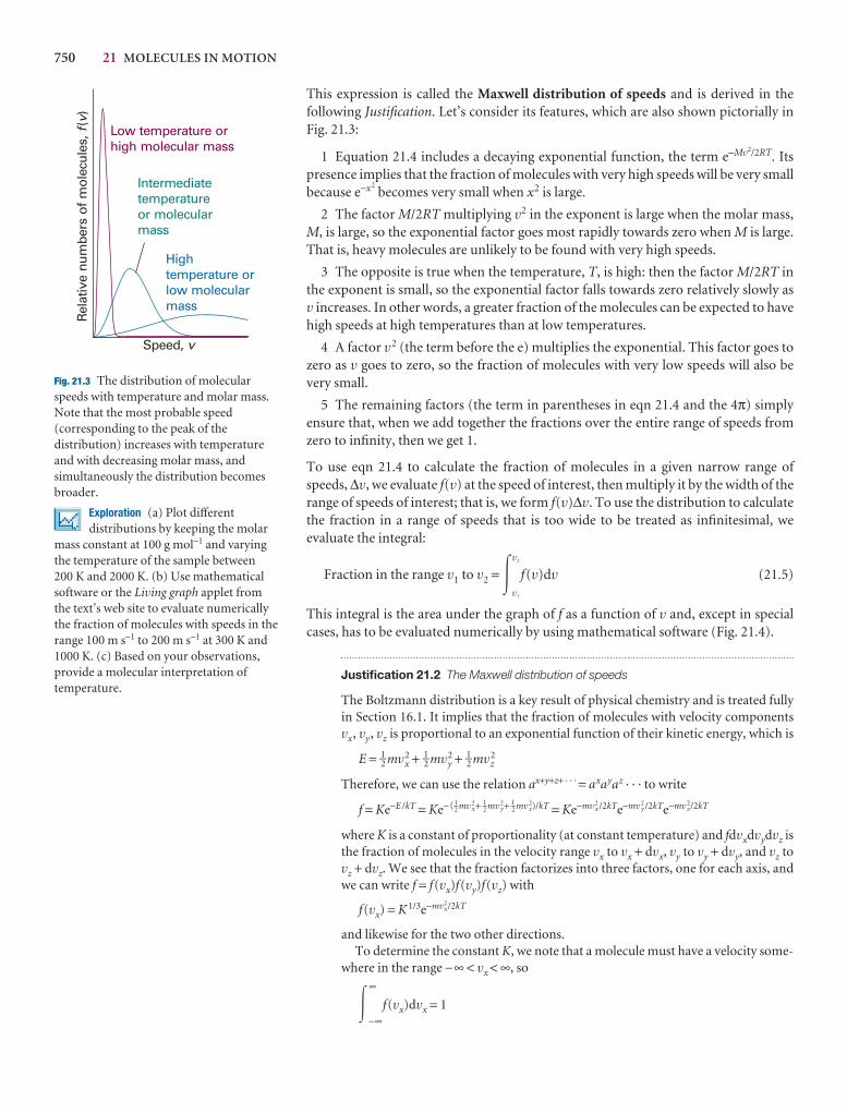
750 21 MOLECULES IN MOTION
This expression is called the Maxwell distribution of speeds and is derived in the following Justification. Let’s consider its features, which are also shown pictorially inFig. 21.3:
1 Equation 21.4 includes a decaying exponential function, the term e−Mv2/2RT. Itspresence implies that the fraction of molecules with very high speeds will be very smallbecause e−x2
becomes very small when x2 is large.
2 The factor M/2RT multiplying v2 in the exponent is large when the molar mass,M, is large, so the exponential factor goes most rapidly towards zero when M is large.That is, heavy molecules are unlikely to be found with very high speeds.
3 The opposite is true when the temperature, T, is high: then the factor M/2RT inthe exponent is small, so the exponential factor falls towards zero relatively slowly asv increases. In other words, a greater fraction of the molecules can be expected to havehigh speeds at high temperatures than at low temperatures.
4 A factor v2 (the term before the e) multiplies the exponential. This factor goes tozero as v goes to zero, so the fraction of molecules with very low speeds will also bevery small.
5 The remaining factors (the term in parentheses in eqn 21.4 and the 4π) simply ensure that, when we add together the fractions over the entire range of speeds fromzero to infinity, then we get 1.
To use eqn 21.4 to calculate the fraction of molecules in a given narrow range ofspeeds, ∆v, we evaluate f(v) at the speed of interest, then multiply it by the width of therange of speeds of interest; that is, we form f(v)∆v. To use the distribution to calculatethe fraction in a range of speeds that is too wide to be treated as infinitesimal, we evaluate the integral:
Fraction in the range v1 to v2 = �v2
v1
f(v)dv (21.5)
This integral is the area under the graph of f as a function of v and, except in specialcases, has to be evaluated numerically by using mathematical software (Fig. 21.4).
Justification 21.2 The Maxwell distribution of speeds
The Boltzmann distribution is a key result of physical chemistry and is treated fullyin Section 16.1. It implies that the fraction of molecules with velocity componentsvx, vy, vz is proportional to an exponential function of their kinetic energy, which is
E = 1–2 mv2x + 1–2 mv2
y + 1–2 mv2z
Therefore, we can use the relation ax+y+z+ · · · = axayaz · · · to write
f = Ke−E /kT = Ke− (1––2 mv2
x+ 1––2 mv2
y+ 1––2 mv2
z)/kT = Ke−mv2x /2kTe−mv2
y /2kTe−mv2z/2kT
where K is a constant of proportionality (at constant temperature) and fdvxdvydvz isthe fraction of molecules in the velocity range vx to vx + dvx, vy to vy + dvy, and vz tovz + dvz. We see that the fraction factorizes into three factors, one for each axis, andwe can write f = f(vx)f(vy)f(vz) with
f(vx) = K 1/3e−mv2x/2kT
and likewise for the two other directions.To determine the constant K, we note that a molecule must have a velocity some-
where in the range −∞ < vx < ∞, so
�∞
−∞f(vx)dvx = 1
Speed, v
Low temperature orhigh molecular mass
Hightemperature orlow molecularmass
Intermediatetemperatureor molecularmass
Rel
ativ
e nu
mbe
rs o
f m
olec
ules
,(
)f
v
Fig. 21.3 The distribution of molecularspeeds with temperature and molar mass. Note that the most probable speed(corresponding to the peak of thedistribution) increases with temperatureand with decreasing molar mass, andsimultaneously the distribution becomesbroader.
Exploration (a) Plot differentdistributions by keeping the molar
mass constant at 100 g mol−1 and varyingthe temperature of the sample between 200 K and 2000 K. (b) Use mathematicalsoftware or the Living graph applet fromthe text’s web site to evaluate numericallythe fraction of molecules with speeds in therange 100 m s−1 to 200 m s−1 at 300 K and1000 K. (c) Based on your observations,provide a molecular interpretation oftemperature.
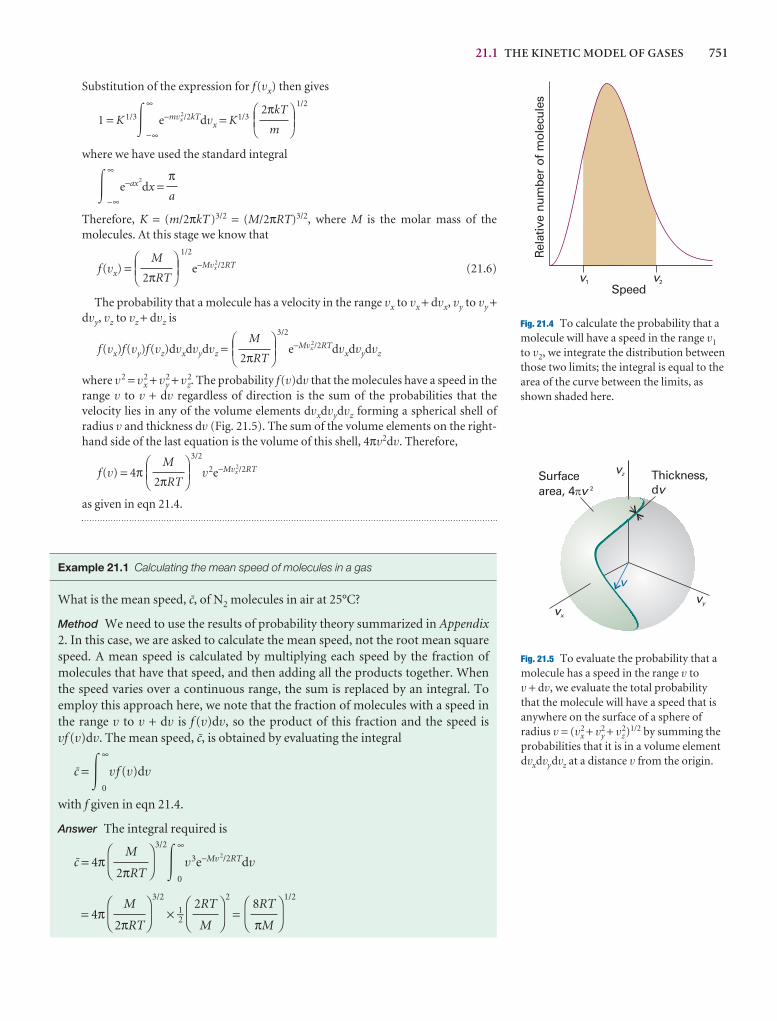
21.1 THE KINETIC MODEL OF GASES 751
vx
vy
vz
v
Surfacearea, 4�v 2
Thickness,dv
Fig. 21.5 To evaluate the probability that amolecule has a speed in the range v tov + dv, we evaluate the total probabilitythat the molecule will have a speed that isanywhere on the surface of a sphere ofradius v = (vx
2 + vy2 + vz
2)1/2 by summing theprobabilities that it is in a volume elementdvxdvydvz at a distance v from the origin.
Speed
Rel
ativ
e nu
mbe
r of
mol
ecul
es
v2v1
Fig. 21.4 To calculate the probability that amolecule will have a speed in the range v1
to v2, we integrate the distribution betweenthose two limits; the integral is equal to thearea of the curve between the limits, asshown shaded here.
Substitution of the expression for f(vx) then gives
1 = K 1/3�∞
−∞e−mv2
x /2kTdvx = K1/3
1/2
where we have used the standard integral
�∞
−∞e−ax2
dx =
Therefore, K = (m/2πkT)3/2 = (M/2πRT)3/2, where M is the molar mass of themolecules. At this stage we know that
f(vx) =1/2
e−Mv2x /2RT (21.6)
The probability that a molecule has a velocity in the range vx to vx + dvx, vy to vy +dvy, vz to vz + dvz is
f(vx)f(vy)f(vz)dvxdvydvz =3/2
e−Mv2x /2RTdvxdvydvz
where v2 = v2x + v2
y + v2z. The probability f(v)dv that the molecules have a speed in the
range v to v + dv regardless of direction is the sum of the probabilities that the velocity lies in any of the volume elements dvxdvydvz forming a spherical shell of radius v and thickness dv (Fig. 21.5). The sum of the volume elements on the right-hand side of the last equation is the volume of this shell, 4πv2dv. Therefore,
f(v) = 4π3/2
v2e−Mv2x /2RT
as given in eqn 21.4.
Example 21.1 Calculating the mean speed of molecules in a gas
What is the mean speed, K, of N2 molecules in air at 25°C?
Method We need to use the results of probability theory summarized in Appendix2. In this case, we are asked to calculate the mean speed, not the root mean squarespeed. A mean speed is calculated by multiplying each speed by the fraction ofmolecules that have that speed, and then adding all the products together. Whenthe speed varies over a continuous range, the sum is replaced by an integral. To employ this approach here, we note that the fraction of molecules with a speed inthe range v to v + dv is f (v)dv, so the product of this fraction and the speed isvf (v)dv. The mean speed, K, is obtained by evaluating the integral
K = �∞
0
vf (v)dv
with f given in eqn 21.4.
Answer The integral required is
K = 4π3/2
�∞
0
v3e−Mv2/2RTdv
= 4π3/2
× 1–2
2
=1/2D
F8RT
πM
AC
DF
2RT
M
AC
DF
M
2πRT
AC
DF
M
2πRT
AC
DEFM
2πRT
ABC
DEFM
2πRT
ABC
DEFM
2πRT
ABC
πa
DEF2πkT
m
ABC
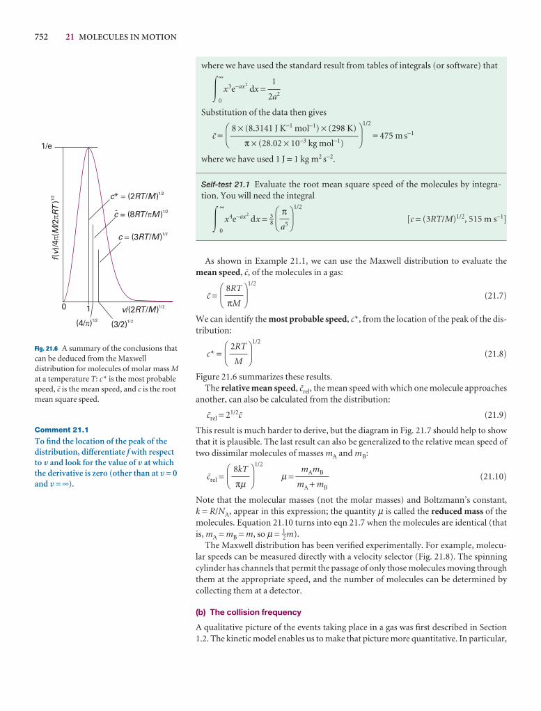
752 21 MOLECULES IN MOTION
Comment 21.1
To find the location of the peak of thedistribution, differentiate f with respectto V and look for the value of V at whichthe derivative is zero (other than at 1 = 0and 1 = ∞).
fv
MR
T(
)/4
(/2
)p
p1/
2
v RT M/(2 / )1/2
1/e
10
(4/ )p1/2
c RT M= (3 / )1/2
c RT M* (2 / )=1/2
(3/2)1/2
c RT M= (8 / )p1/2
Fig. 21.6 A summary of the conclusions thatcan be deduced from the Maxwelldistribution for molecules of molar mass Mat a temperature T: c* is the most probablespeed, K is the mean speed, and c is the rootmean square speed.
where we have used the standard result from tables of integrals (or software) that
�∞
0
x3e−ax2dx =
Substitution of the data then gives
K =1/2
= 475 m s−1
where we have used 1 J = 1 kg m2 s−2.
Self-test 21.1 Evaluate the root mean square speed of the molecules by integra-tion. You will need the integral
�∞
0
x4e−ax2dx = 3–8
1/2
[c = (3RT/M)1/2, 515 m s−1]
As shown in Example 21.1, we can use the Maxwell distribution to evaluate themean speed, K, of the molecules in a gas:
K =1/2
(21.7)
We can identify the most probable speed, c*, from the location of the peak of the dis-tribution:
c* =1/2
(21.8)
Figure 21.6 summarizes these results.The relative mean speed, Krel, the mean speed with which one molecule approaches
another, can also be calculated from the distribution:
Krel = 21/2K (21.9)
This result is much harder to derive, but the diagram in Fig. 21.7 should help to showthat it is plausible. The last result can also be generalized to the relative mean speed oftwo dissimilar molecules of masses mA and mB:
Krel =1/2
µ = (21.10)
Note that the molecular masses (not the molar masses) and Boltzmann’s constant, k = R/NA, appear in this expression; the quantity µ is called the reduced mass of themolecules. Equation 21.10 turns into eqn 21.7 when the molecules are identical (thatis, mA = mB = m, so µ = 1–2m).
The Maxwell distribution has been verified experimentally. For example, molecu-lar speeds can be measured directly with a velocity selector (Fig. 21.8). The spinningcylinder has channels that permit the passage of only those molecules moving throughthem at the appropriate speed, and the number of molecules can be determined bycollecting them at a detector.
(b) The collision frequency
A qualitative picture of the events taking place in a gas was first described in Section1.2. The kinetic model enables us to make that picture more quantitative. In particular,
mAmB
mA + mB
DF
8kT
πµ
AC
DF
2RT
M
AC
DF
8RT
πM
AC
DF
πa5
AC
DF
8 × (8.3141 J K−1 mol−1) × (298 K)
π × (28.02 × 10⁻³ kg mol−1)
AC
1
2a2
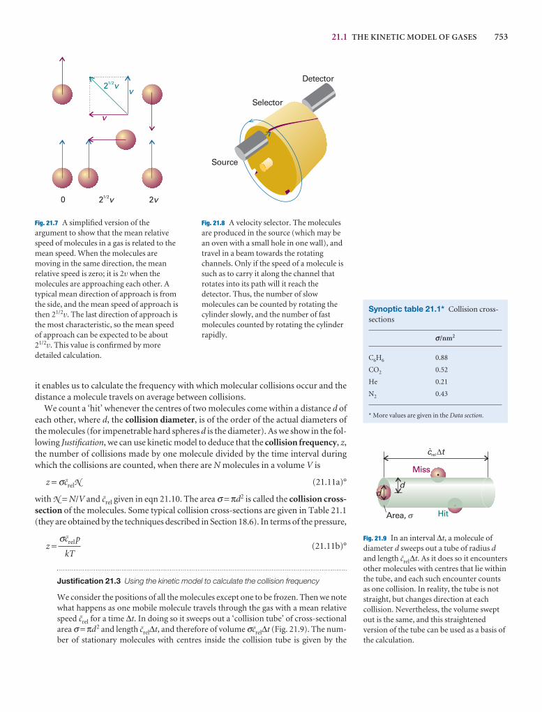
21.1 THE KINETIC MODEL OF GASES 753
it enables us to calculate the frequency with which molecular collisions occur and thedistance a molecule travels on average between collisions.
We count a ‘hit’ whenever the centres of two molecules come within a distance d ofeach other, where d, the collision diameter, is of the order of the actual diameters ofthe molecules (for impenetrable hard spheres d is the diameter). As we show in the fol-lowing Justification, we can use kinetic model to deduce that the collision frequency, z,the number of collisions made by one molecule divided by the time interval duringwhich the collisions are counted, when there are N molecules in a volume V is
z = σKrelN (21.11a)°
with N = N/V and Krel given in eqn 21.10. The area σ = πd2 is called the collision cross-section of the molecules. Some typical collision cross-sections are given in Table 21.1(they are obtained by the techniques described in Section 18.6). In terms of the pressure,
z = (21.11b)°
Justification 21.3 Using the kinetic model to calculate the collision frequency
We consider the positions of all the molecules except one to be frozen. Then we notewhat happens as one mobile molecule travels through the gas with a mean relativespeed Krel for a time ∆t. In doing so it sweeps out a ‘collision tube’ of cross-sectionalarea σ = πd2 and length Krel∆t, and therefore of volume σKrel∆t (Fig. 21.9). The num-ber of stationary molecules with centres inside the collision tube is given by the
σKrel p
kT
Fig. 21.7 A simplified version of theargument to show that the mean relativespeed of molecules in a gas is related to themean speed. When the molecules aremoving in the same direction, the meanrelative speed is zero; it is 2v when themolecules are approaching each other. Atypical mean direction of approach is fromthe side, and the mean speed of approach isthen 21/2v. The last direction of approach isthe most characteristic, so the mean speedof approach can be expected to be about21/2v. This value is confirmed by moredetailed calculation.
v
v
21/2v
21/2v0 2v
Source
Selector
Detector
Fig. 21.8 A velocity selector. The moleculesare produced in the source (which may bean oven with a small hole in one wall), andtravel in a beam towards the rotatingchannels. Only if the speed of a molecule issuch as to carry it along the channel thatrotates into its path will it reach thedetector. Thus, the number of slowmolecules can be counted by rotating thecylinder slowly, and the number of fastmolecules counted by rotating the cylinderrapidly.
Synoptic table 21.1* Collision cross-sections
s/nm2
C6H6 0.88
CO2 0.52
He 0.21
N2 0.43
* More values are given in the Data section.
Miss
Hit
dd
c trelD
Area, s
Fig. 21.9 In an interval ∆t, a molecule ofdiameter d sweeps out a tube of radius dand length Krel∆t. As it does so it encountersother molecules with centres that lie withinthe tube, and each such encounter countsas one collision. In reality, the tube is notstraight, but changes direction at eachcollision. Nevertheless, the volume sweptout is the same, and this straightenedversion of the tube can be used as a basis ofthe calculation.
754 21 MOLECULES IN MOTION
volume of the tube multiplied by the number density N = N/V, and is NσKrel∆t. Thenumber of hits scored in the interval ∆t is equal to this number, so the number ofcollisions divided by the time interval, is NσKrel. The expression in terms of the pres-sure of the gas is obtained by using the perfect gas equation to write
N = = = =
Equation 21.11a shows that, at constant volume, the collision frequency increaseswith increasing temperature. The reason for this increase is that the relative meanspeed increases with temperature (eqns 21.9 and 21.10). Equation 21.11b shows that,at constant temperature, the collision frequency is proportional to the pressure. Sucha proportionality is plausible, for the greater the pressure, the greater the number density of molecules in the sample, and the rate at which they encounter one anotheris greater even though their average speed remains the same. For an N2 molecule in asample at 1 atm and 25°C, z ≈ 5 × 10⁹ s−1, so a given molecule collides about 5 × 10⁹
times each second. We are beginning to appreciate the timescale of events in gases.
(c) The mean free path
Once we have the collision frequency, we can calculate the mean free path, λ(lambda), the average distance a molecule travels between collisions. If a moleculecollides with a frequency z, it spends a time 1/z in free flight between collisions, andtherefore travels a distance (1/z)K. It follows that the mean free path is
λ = (21.12)
Substitution of the expression for z in eqn 21.11b gives
λ = (21.13)
Doubling the pressure reduces the mean free path by half. A typical mean free path innitrogen gas at 1 atm is 70 nm, or about 103 molecular diameters. Although the tem-perature appears in eqn 21.13, in a sample of constant volume, the pressure is pro-portional to T, so T/p remains constant when the temperature is increased. Therefore,the mean free path is independent of the temperature in a sample of gas in a containerof fixed volume. The distance between collisions is determined by the number ofmolecules present in the given volume, not by the speed at which they travel.
In summary, a typical gas (N2 or O2) at 1 atm and 25°C can be thought of as a col-lection of molecules travelling with a mean speed of about 500 m s−1. Each moleculemakes a collision within about 1 ns, and between collisions it travels about 103 molecu-lar diameters. The kinetic model of gases is valid (and the gas behaves nearly perfectly)if the diameter of the molecules is much smaller than the mean free path (d << λ), forthen the molecules spend most of their time far from one another.
IMPACT ON ASTROPHYSICS
I21.1 The Sun as a ball of perfect gas
The kinetic model of gases is valid when the size of the particles is negligible comparedwith their mean free path. It may seem absurd, therefore, to expect the kinetic modeland, as a consequence, the perfect gas law, to be applicable to the dense matter of stellar interiors. In the Sun, for instance, the density at its centre is 1.50 times that ofliquid water and comparable to that of water about half way to its surface. However,
kT
21/2σp
K
z
p
kT
pNA
RT
nNA
V
N
V
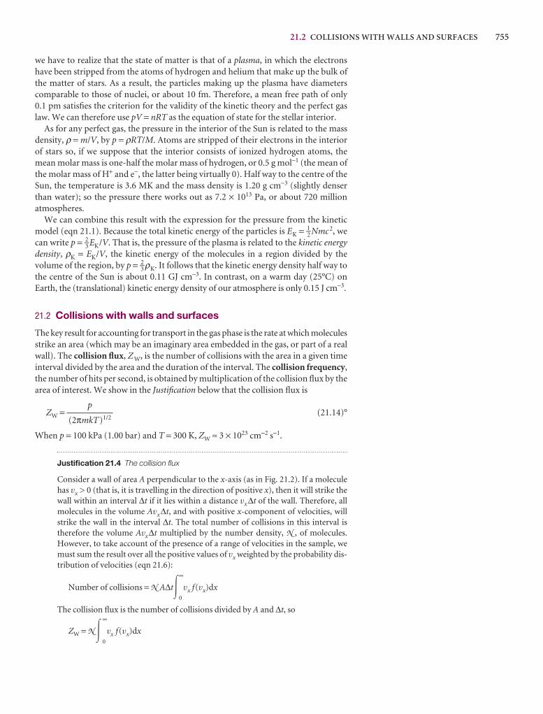
21.2 COLLISIONS WITH WALLS AND SURFACES 755
we have to realize that the state of matter is that of a plasma, in which the electronshave been stripped from the atoms of hydrogen and helium that make up the bulk ofthe matter of stars. As a result, the particles making up the plasma have diameterscomparable to those of nuclei, or about 10 fm. Therefore, a mean free path of only0.1 pm satisfies the criterion for the validity of the kinetic theory and the perfect gaslaw. We can therefore use pV = nRT as the equation of state for the stellar interior.
As for any perfect gas, the pressure in the interior of the Sun is related to the massdensity, ρ = m/V, by p = ρRT/M. Atoms are stripped of their electrons in the interiorof stars so, if we suppose that the interior consists of ionized hydrogen atoms, themean molar mass is one-half the molar mass of hydrogen, or 0.5 g mol−1 (the mean ofthe molar mass of H+ and e−, the latter being virtually 0). Half way to the centre of theSun, the temperature is 3.6 MK and the mass density is 1.20 g cm−3 (slightly denserthan water); so the pressure there works out as 7.2 × 10¹³ Pa, or about 720 million atmospheres.
We can combine this result with the expression for the pressure from the kineticmodel (eqn 21.1). Because the total kinetic energy of the particles is EK = 1–2 Nmc 2, wecan write p = 2–3 EK/V. That is, the pressure of the plasma is related to the kinetic energydensity, ρK = EK/V, the kinetic energy of the molecules in a region divided by the volume of the region, by p = 2–3 ρK. It follows that the kinetic energy density half way tothe centre of the Sun is about 0.11 GJ cm−3. In contrast, on a warm day (25°C) onEarth, the (translational) kinetic energy density of our atmosphere is only 0.15 J cm−3.
21.2 Collisions with walls and surfaces
The key result for accounting for transport in the gas phase is the rate at which moleculesstrike an area (which may be an imaginary area embedded in the gas, or part of a realwall). The collision flux, Z W, is the number of collisions with the area in a given timeinterval divided by the area and the duration of the interval. The collision frequency,the number of hits per second, is obtained by multiplication of the collision flux by thearea of interest. We show in the Justification below that the collision flux is
ZW = (21.14)°
When p = 100 kPa (1.00 bar) and T = 300 K, ZW ≈ 3 × 1023 cm−2 s−1.
Justification 21.4 The collision flux
Consider a wall of area A perpendicular to the x-axis (as in Fig. 21.2). If a moleculehas vx > 0 (that is, it is travelling in the direction of positive x), then it will strike thewall within an interval ∆t if it lies within a distance vx∆t of the wall. Therefore, allmolecules in the volume Avx∆t, and with positive x-component of velocities, willstrike the wall in the interval ∆t. The total number of collisions in this interval istherefore the volume Avx∆t multiplied by the number density, N , of molecules.However, to take account of the presence of a range of velocities in the sample, wemust sum the result over all the positive values of vx weighted by the probability dis-tribution of velocities (eqn 21.6):
Number of collisions = N A∆t�∞
0
vx f(vx)dx
The collision flux is the number of collisions divided by A and ∆t, so
ZW = N �∞
0
vx f(vx)dx
p
(2πmkT)1/2
756 21 MOLECULES IN MOTION
Then, using the velocity distribution in eqn 21.6,
�∞
0
vx f(vx)dvx =1/2
�∞
0
vxe−mv2
x/2kTdvx =1/2
where we have used the standard integral
�∞
0
xe−ax 2dx =
Therefore,
ZW = N
1/2
= 1–4 KN (21.15)°
where we have used eqn 21.7 in the form K = (8kT/πm)1/2, which implies that 1–4 K =(kT/2πm)1/2. Substitution of N = nNA/V = p/kT gives eqn 21.14.
21.3 The rate of effusion
The essential empirical observations on effusion are summarized by Graham’s law ofeffusion, which states that the rate of effusion is inversely proportional to the squareroot of the molar mass. The basis of this result is that, as remarked above, the meanspeed of molecules is inversely proportional to M1/2, so the rate at which they strikethe area of the hole is also inversely proportional to M1/2. However, by using the expression for the rate of collisions, we can obtain a more detailed expression for therate of effusion and hence use effusion data more effectively.
When a gas at a pressure p and temperature T is separated from a vacuum by a smallhole, the rate of escape of its molecules is equal to the rate at which they strike the areaof the hole (which is given by eqn 21.14). Therefore, for a hole of area A0,
Rate of effusion = ZW A = = (21.16)°
where, in the last step, we have used R = NAk and M = mNA. This rate is inversely pro-portional to M1/2, in accord with Graham’s law.
Equation 21.16 is the basis of the Knudsen method for the determination of thevapour pressures of liquids and solids, particularly of substances with very low vapourpressures. Thus, if the vapour pressure of a sample is p, and it is enclosed in a cavitywith a small hole, then the rate of loss of mass from the container is proportional to p.
Example 21.2 Calculating the vapour pressure from a mass loss
Caesium (m.p. 29°C, b.p. 686°C) was introduced into a container and heated to500°C. When a hole of diameter 0.50 mm was opened in the container for 100 s, amass loss of 385 mg was measured. Calculate the vapour pressure of liquid caesiumat 500 K.
Method The pressure of vapour is constant inside the container despite the effusionof atoms because the hot liquid metal replenishes the vapour. The rate of effusionis therefore constant, and given by eqn 21.16. To express the rate in terms of mass,multiply the number of atoms that escape by the mass of each atom.
Answer The mass loss ∆m in an interval ∆t is related to the collision flux by
∆m = ZW A0m∆t
pA0NA
(2πMRT)1/2
pA0
(2πmkT)1/2
DF
kT
2πm
AC
1
2a
DF
kT
2πm
AC
DF
m
2πkT
AC
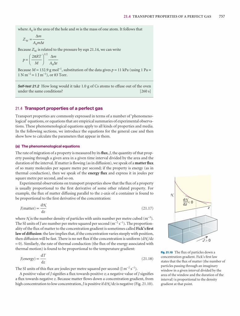
21.4 TRANSPORT PROPERTIES OF A PERFECT GAS 757
z
NdNdz � 0
J 0�
Fig. 21.10 The flux of particles down aconcentration gradient. Fick’s first lawstates that the flux of matter (the number ofparticles passing through an imaginarywindow in a given interval divided by thearea of the window and the duration of theinterval) is proportional to the densitygradient at that point.
where A0 is the area of the hole and m is the mass of one atom. It follows that
Z W =
Because ZW is related to the pressure by eqn 21.14, we can write
p =1/2
Because M = 132.9 g mol−1, substitution of the data gives p = 11 kPa (using 1 Pa =1 N m−2 = 1 J m−1), or 83 Torr.
Self-test 21.2 How long would it take 1.0 g of Cs atoms to effuse out of the ovenunder the same conditions? [260 s]
21.4 Transport properties of a perfect gas
Transport properties are commonly expressed in terms of a number of ‘phenomeno-logical’ equations, or equations that are empirical summaries of experimental observa-tions. These phenomenological equations apply to all kinds of properties and media.In the following sections, we introduce the equations for the general case and thenshow how to calculate the parameters that appear in them.
(a) The phenomenological equations
The rate of migration of a property is measured by its flux, J, the quantity of that prop-erty passing through a given area in a given time interval divided by the area and theduration of the interval. If matter is flowing (as in diffusion), we speak of a matter fluxof so many molecules per square metre per second; if the property is energy (as inthermal conduction), then we speak of the energy flux and express it in joules persquare metre per second, and so on.
Experimental observations on transport properties show that the flux of a propertyis usually proportional to the first derivative of some other related property. For example, the flux of matter diffusing parallel to the z-axis of a container is found to be proportional to the first derivative of the concentration:
J(matter) ∝ (21.17)
where N is the number density of particles with units number per metre cubed (m−3).The SI units of J are number per metre squared per second (m−2 s−1). The proportion-ality of the flux of matter to the concentration gradient is sometimes called Fick’s firstlaw of diffusion: the law implies that, if the concentration varies steeply with position,then diffusion will be fast. There is no net flux if the concentration is uniform (dN /dz= 0). Similarly, the rate of thermal conduction (the flux of the energy associated withthermal motion) is found to be proportional to the temperature gradient:
J(energy) ∝ (21.18)
The SI units of this flux are joules per metre squared per second (J m−2 s−1).A positive value of J signifies a flux towards positive z; a negative value of J signifies
a flux towards negative z. Because matter flows down a concentration gradient, fromhigh concentration to low concentration, J is positive if dN /dz is negative (Fig. 21.10).
dT
dz
dN
dz
∆m
A0∆t
DF
2πRT
M
AC
∆m
A0m∆t
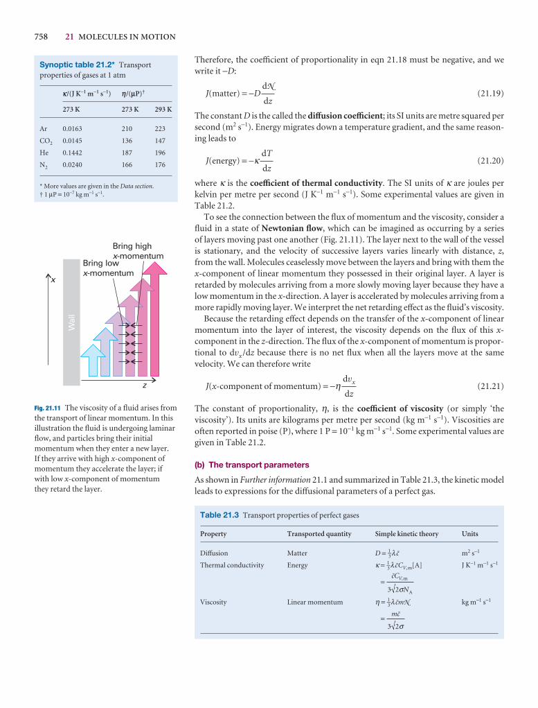
758 21 MOLECULES IN MOTION
Therefore, the coefficient of proportionality in eqn 21.18 must be negative, and wewrite it −D:
J(matter) = −D (21.19)
The constant D is the called the diffusion coefficient; its SI units are metre squared persecond (m2 s−1). Energy migrates down a temperature gradient, and the same reason-ing leads to
J(energy) = −κ (21.20)
where κ is the coefficient of thermal conductivity. The SI units of κ are joules perkelvin per metre per second (J K−1 m−1 s−1). Some experimental values are given inTable 21.2.
To see the connection between the flux of momentum and the viscosity, consider afluid in a state of Newtonian flow, which can be imagined as occurring by a series of layers moving past one another (Fig. 21.11). The layer next to the wall of the vesselis stationary, and the velocity of successive layers varies linearly with distance, z,from the wall. Molecules ceaselessly move between the layers and bring with them the x-component of linear momentum they possessed in their original layer. A layer is retarded by molecules arriving from a more slowly moving layer because they have alow momentum in the x-direction. A layer is accelerated by molecules arriving from amore rapidly moving layer. We interpret the net retarding effect as the fluid’s viscosity.
Because the retarding effect depends on the transfer of the x-component of linearmomentum into the layer of interest, the viscosity depends on the flux of this x-component in the z-direction. The flux of the x-component of momentum is propor-tional to dvx /dz because there is no net flux when all the layers move at the same velocity. We can therefore write
J(x-component of momentum) = −η (21.21)
The constant of proportionality, η, is the coefficient of viscosity (or simply ‘the viscosity’). Its units are kilograms per metre per second (kg m−1 s−1). Viscosities areoften reported in poise (P), where 1 P = 10−1 kg m−1 s−1. Some experimental values aregiven in Table 21.2.
(b) The transport parameters
As shown in Further information 21.1 and summarized in Table 21.3, the kinetic modelleads to expressions for the diffusional parameters of a perfect gas.
dvx
dz
dT
dz
dN
dz
Synoptic table 21.2* Transportproperties of gases at 1 atm
k/(J K−1 m−1 s−1) h/(mP)†
273 K 273 K 293 K
Ar 0.0163 210 223
CO2 0.0145 136 147
He 0.1442 187 196
N2 0.0240 166 176
* More values are given in the Data section.† 1 µP = 10−7 kg m−1 s−1.
Wal
l
Bring high-momentumx
Bring low-momentumx
x
z
Fig. 21.11 The viscosity of a fluid arises from the transport of linear momentum. In thisillustration the fluid is undergoing laminarflow, and particles bring their initialmomentum when they enter a new layer. If they arrive with high x-component ofmomentum they accelerate the layer; ifwith low x-component of momentum they retard the layer.
Table 21.3 Transport properties of perfect gases
Property Transported quantity Simple kinetic theory Units
Diffusion Matter D = 1–3λK m2 s−1
Thermal conductivity Energy κ = 1–3λKCV,m[A] J K−1 m−1 s−1
=
Viscosity Linear momentum η = 1–3λKmN kg m−1 s−1
=mK
3 2σ
KC
N
V, m
A3 2σ
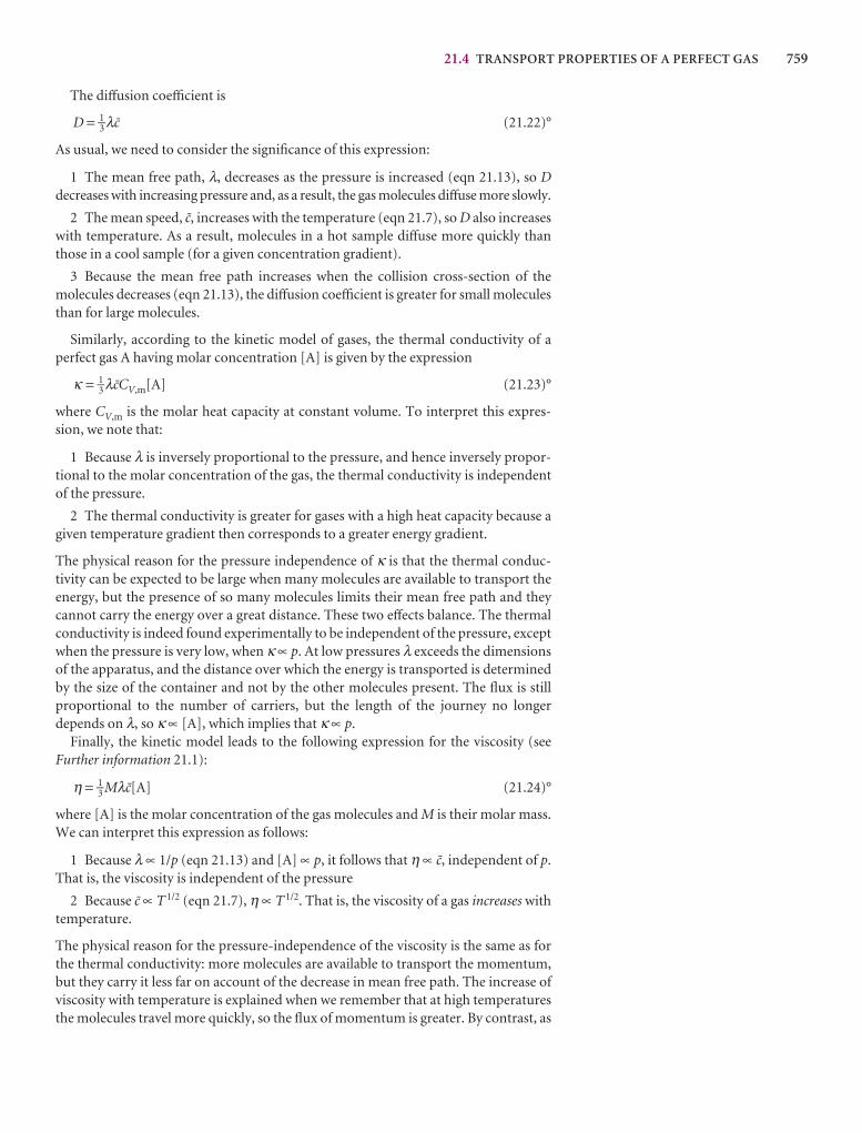
21.4 TRANSPORT PROPERTIES OF A PERFECT GAS 759
The diffusion coefficient is
D = 1–3 λK (21.22)°
As usual, we need to consider the significance of this expression:
1 The mean free path, λ, decreases as the pressure is increased (eqn 21.13), so Ddecreases with increasing pressure and, as a result, the gas molecules diffuse more slowly.
2 The mean speed, K, increases with the temperature (eqn 21.7), so D also increaseswith temperature. As a result, molecules in a hot sample diffuse more quickly thanthose in a cool sample (for a given concentration gradient).
3 Because the mean free path increases when the collision cross-section of themolecules decreases (eqn 21.13), the diffusion coefficient is greater for small moleculesthan for large molecules.
Similarly, according to the kinetic model of gases, the thermal conductivity of aperfect gas A having molar concentration [A] is given by the expression
κ = 1–3 λKCV,m[A] (21.23)°
where CV,m is the molar heat capacity at constant volume. To interpret this expres-sion, we note that:
1 Because λ is inversely proportional to the pressure, and hence inversely propor-tional to the molar concentration of the gas, the thermal conductivity is independentof the pressure.
2 The thermal conductivity is greater for gases with a high heat capacity because agiven temperature gradient then corresponds to a greater energy gradient.
The physical reason for the pressure independence of κ is that the thermal conduc-tivity can be expected to be large when many molecules are available to transport the energy, but the presence of so many molecules limits their mean free path and theycannot carry the energy over a great distance. These two effects balance. The thermalconductivity is indeed found experimentally to be independent of the pressure, exceptwhen the pressure is very low, when κ ∝ p. At low pressures λ exceeds the dimensionsof the apparatus, and the distance over which the energy is transported is determinedby the size of the container and not by the other molecules present. The flux is stillproportional to the number of carriers, but the length of the journey no longer depends on λ, so κ ∝ [A], which implies that κ ∝ p.
Finally, the kinetic model leads to the following expression for the viscosity (seeFurther information 21.1):
η = 1–3 MλK[A] (21.24)°
where [A] is the molar concentration of the gas molecules and M is their molar mass.We can interpret this expression as follows:
1 Because λ ∝ 1/p (eqn 21.13) and [A] ∝ p, it follows that η ∝ K, independent of p.That is, the viscosity is independent of the pressure
2 Because K ∝ T 1/2 (eqn 21.7), η ∝ T 1/2. That is, the viscosity of a gas increases withtemperature.
The physical reason for the pressure-independence of the viscosity is the same as forthe thermal conductivity: more molecules are available to transport the momentum,but they carry it less far on account of the decrease in mean free path. The increase ofviscosity with temperature is explained when we remember that at high temperaturesthe molecules travel more quickly, so the flux of momentum is greater. By contrast, as
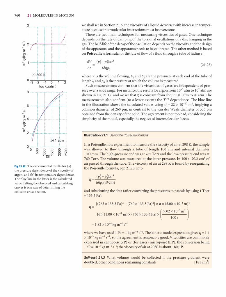
760 21 MOLECULES IN MOTION
10/(k
g m
s)
51
1-
-
h
0
1
2
3
-3 -2 -1 0 1 2log ( /atm)p
0
2
4
6
8
0
500
1000
1500
2000
T/K
(b) 1 atm
(a) 300 K
10/(k
g m
s)
51
1-
-
h
2500
hh
Fig. 21.12 The experimental results for (a)the pressure dependence of the viscosity ofargon, and (b) its temperature dependence.The blue line in the latter is the calculatedvalue. Fitting the observed and calculatingcurves is one way of determining thecollision cross-section.
we shall see in Section 21.6, the viscosity of a liquid decreases with increase in temper-ature because intermolecular interactions must be overcome.
There are two main techniques for measuring viscosities of gases. One techniquedepends on the rate of damping of the torsional oscillations of a disc hanging in thegas. The half-life of the decay of the oscillation depends on the viscosity and the designof the apparatus, and the apparatus needs to be calibrated. The other method is basedon Poiseuille’s formula for the rate of flow of a fluid through a tube of radius r:
= (21.25)
where V is the volume flowing, p1 and p2 are the pressures at each end of the tube oflength l, and p0 is the pressure at which the volume is measured.
Such measurements confirm that the viscosities of gases are independent of pres-sure over a wide range. For instance, the results for argon from 10−3 atm to 102 atm areshown in Fig. 21.12, and we see that η is constant from about 0.01 atm to 20 atm. Themeasurements also confirm (to a lesser extent) the T1/2 dependence. The blue line in the illustration shows the calculated values using σ = 22 × 10−20 m2, implying a collision diameter of 260 pm, in contrast to the van der Waals diameter of 335 pm obtained from the density of the solid. The agreement is not too bad, considering thesimplicity of the model, especially the neglect of intermolecular forces.
Illustration 21.1 Using the Poiseuille formula
In a Poiseuille flow experiment to measure the viscosity of air at 298 K, the samplewas allowed to flow through a tube of length 100 cm and internal diameter 1.00 mm. The high-pressure end was at 765 Torr and the low-pressure end was at760 Torr. The volume was measured at the latter pressure. In 100 s, 90.2 cm3 ofair passed through the tube. The viscosity of air at 298 K is found by reorganizingthe Poiseuille formula, eqn 21.25, into
η =
and substituting the data (after converting the pressures to pascals by using 1 Torr= 133.3 Pa):
η =
= 1.82 × 10⁻⁴ kg m−1 s−1
where we have used 1 Pa = 1 kg m−1 s−2. The kinetic model expression gives η = 1.4× 10⁻⁵ kg m−1 s−1, so the agreement is reasonably good. Viscosities are commonlyexpressed in centipoise (cP) or (for gases) micropoise (µP), the conversion being 1 cP = 10−3 kg m−1 s−1; the viscosity of air at 20°C is about 180 µP.
Self-test 21.3 What volume would be collected if the pressure gradient were doubled, other conditions remaining constant? [181 cm3]
DF
9.02 × 10⁻⁵ m3
100 s
AC
{(765 × 133.3 Pa)2 − (760 × 133.3 Pa)2} × π × (5.00 × 10⁻⁴ m)4
16 × (1.00 × 10−1 m) × (760 × 133.3 Pa) ×
(p21 − p2
2)πr4
16lp0(dV/dt)
(p21 − p2
2)πr4
16lηp0
dV
dt
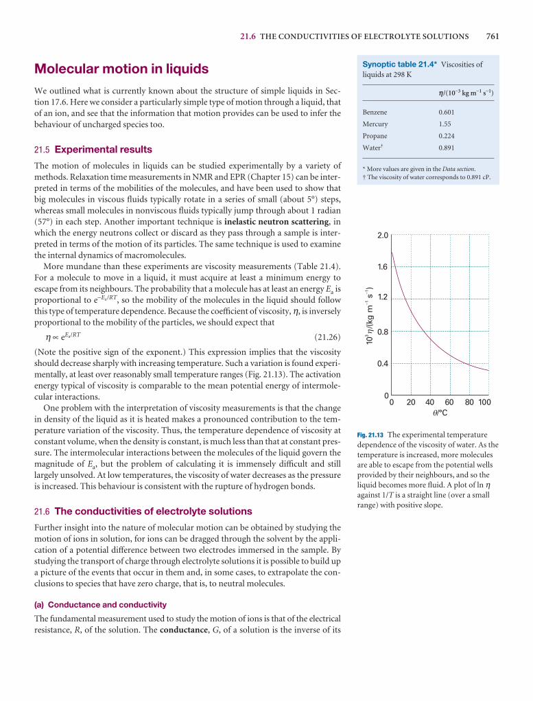
21.6 THE CONDUCTIVITIES OF ELECTROLYTE SOLUTIONS 761
Molecular motion in liquidsWe outlined what is currently known about the structure of simple liquids in Sec-tion 17.6. Here we consider a particularly simple type of motion through a liquid, thatof an ion, and see that the information that motion provides can be used to infer thebehaviour of uncharged species too.
21.5 Experimental results
The motion of molecules in liquids can be studied experimentally by a variety ofmethods. Relaxation time measurements in NMR and EPR (Chapter 15) can be inter-preted in terms of the mobilities of the molecules, and have been used to show that big molecules in viscous fluids typically rotate in a series of small (about 5°) steps,whereas small molecules in nonviscous fluids typically jump through about 1 radian(57°) in each step. Another important technique is inelastic neutron scattering, inwhich the energy neutrons collect or discard as they pass through a sample is inter-preted in terms of the motion of its particles. The same technique is used to examinethe internal dynamics of macromolecules.
More mundane than these experiments are viscosity measurements (Table 21.4).For a molecule to move in a liquid, it must acquire at least a minimum energy to escape from its neighbours. The probability that a molecule has at least an energy Ea isproportional to e−Ea/RT, so the mobility of the molecules in the liquid should followthis type of temperature dependence. Because the coefficient of viscosity, η, is inverselyproportional to the mobility of the particles, we should expect that
η ∝ eEa/RT (21.26)
(Note the positive sign of the exponent.) This expression implies that the viscosityshould decrease sharply with increasing temperature. Such a variation is found experi-mentally, at least over reasonably small temperature ranges (Fig. 21.13). The activationenergy typical of viscosity is comparable to the mean potential energy of intermole-cular interactions.
One problem with the interpretation of viscosity measurements is that the changein density of the liquid as it is heated makes a pronounced contribution to the tem-perature variation of the viscosity. Thus, the temperature dependence of viscosity atconstant volume, when the density is constant, is much less than that at constant pres-sure. The intermolecular interactions between the molecules of the liquid govern themagnitude of Ea, but the problem of calculating it is immensely difficult and stilllargely unsolved. At low temperatures, the viscosity of water decreases as the pressureis increased. This behaviour is consistent with the rupture of hydrogen bonds.
21.6 The conductivities of electrolyte solutions
Further insight into the nature of molecular motion can be obtained by studying themotion of ions in solution, for ions can be dragged through the solvent by the appli-cation of a potential difference between two electrodes immersed in the sample. Bystudying the transport of charge through electrolyte solutions it is possible to build upa picture of the events that occur in them and, in some cases, to extrapolate the con-clusions to species that have zero charge, that is, to neutral molecules.
(a) Conductance and conductivity
The fundamental measurement used to study the motion of ions is that of the electricalresistance, R, of the solution. The conductance, G, of a solution is the inverse of its
Synoptic table 21.4* Viscosities ofliquids at 298 K
h/(10−3 kg m−1 s−1)
Benzene 0.601
Mercury 1.55
Propane 0.224
Water† 0.891
* More values are given in the Data section.† The viscosity of water corresponds to 0.891 cP.
0
0.4
0.8
1.2
1.6
10/(k
g m
s)
31
1-
-h
0 20 40 60 80 100q/°C
2.0
h
q
Fig. 21.13 The experimental temperaturedependence of the viscosity of water. As thetemperature is increased, more moleculesare able to escape from the potential wellsprovided by their neighbours, and so theliquid becomes more fluid. A plot of ln ηagainst 1/T is a straight line (over a smallrange) with positive slope.
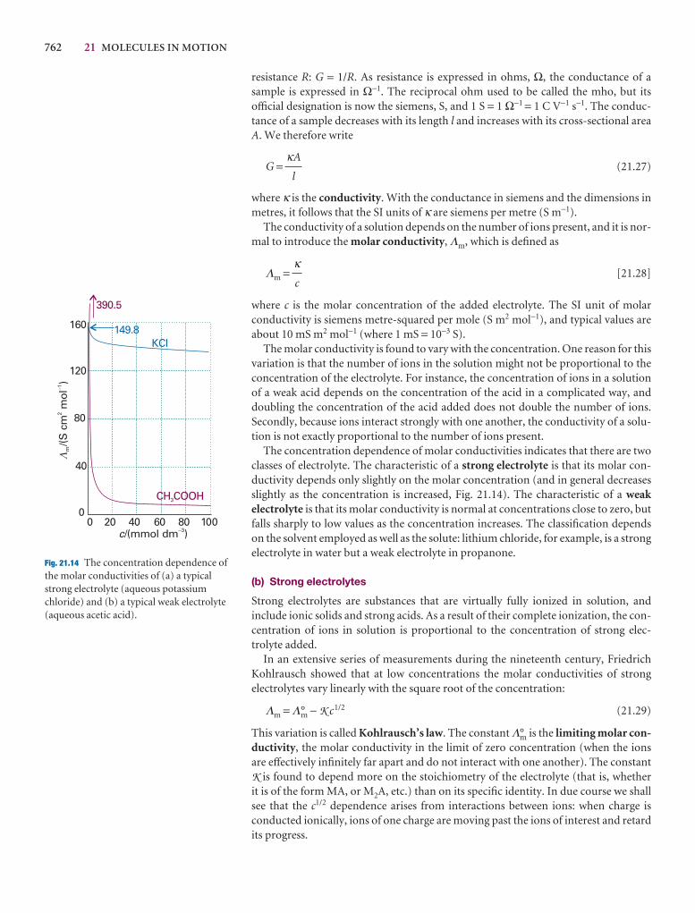
762 21 MOLECULES IN MOTION
resistance R: G = 1/R. As resistance is expressed in ohms, Ω, the conductance of a sample is expressed in Ω−1. The reciprocal ohm used to be called the mho, but itsofficial designation is now the siemens, S, and 1 S = 1 Ω−1 = 1 C V−1 s−1. The conduc-tance of a sample decreases with its length l and increases with its cross-sectional areaA. We therefore write
G = (21.27)
where κ is the conductivity. With the conductance in siemens and the dimensions inmetres, it follows that the SI units of κ are siemens per metre (S m−1).
The conductivity of a solution depends on the number of ions present, and it is nor-mal to introduce the molar conductivity, Λm, which is defined as
Λm = [21.28]
where c is the molar concentration of the added electrolyte. The SI unit of molar conductivity is siemens metre-squared per mole (S m2 mol−1), and typical values areabout 10 mS m2 mol−1 (where 1 mS = 10−3 S).
The molar conductivity is found to vary with the concentration. One reason for thisvariation is that the number of ions in the solution might not be proportional to theconcentration of the electrolyte. For instance, the concentration of ions in a solutionof a weak acid depends on the concentration of the acid in a complicated way, anddoubling the concentration of the acid added does not double the number of ions.Secondly, because ions interact strongly with one another, the conductivity of a solu-tion is not exactly proportional to the number of ions present.
The concentration dependence of molar conductivities indicates that there are twoclasses of electrolyte. The characteristic of a strong electrolyte is that its molar con-ductivity depends only slightly on the molar concentration (and in general decreasesslightly as the concentration is increased, Fig. 21.14). The characteristic of a weakelectrolyte is that its molar conductivity is normal at concentrations close to zero, butfalls sharply to low values as the concentration increases. The classification dependson the solvent employed as well as the solute: lithium chloride, for example, is a strongelectrolyte in water but a weak electrolyte in propanone.
(b) Strong electrolytes
Strong electrolytes are substances that are virtually fully ionized in solution, and include ionic solids and strong acids. As a result of their complete ionization, the con-centration of ions in solution is proportional to the concentration of strong elec-trolyte added.
In an extensive series of measurements during the nineteenth century, FriedrichKohlrausch showed that at low concentrations the molar conductivities of strongelectrolytes vary linearly with the square root of the concentration:
Λm = Λ°m − K c1/2 (21.29)
This variation is called Kohlrausch’s law. The constant Λ°m is the limiting molar con-ductivity, the molar conductivity in the limit of zero concentration (when the ions are effectively infinitely far apart and do not interact with one another). The constantK is found to depend more on the stoichiometry of the electrolyte (that is, whether it is of the form MA, or M2A, etc.) than on its specific identity. In due course we shall see that the c1/2 dependence arises from interactions between ions: when charge isconducted ionically, ions of one charge are moving past the ions of interest and retardits progress.
κc
κA
l
(m/(S
cm
mol
)2
1�
0
40
80
120
160
390.5
KCl
CH COOH3
149.8
0 20 40 60 80 100c/(mmol dm )�3
(
Fig. 21.14 The concentration dependence ofthe molar conductivities of (a) a typicalstrong electrolyte (aqueous potassiumchloride) and (b) a typical weak electrolyte(aqueous acetic acid).
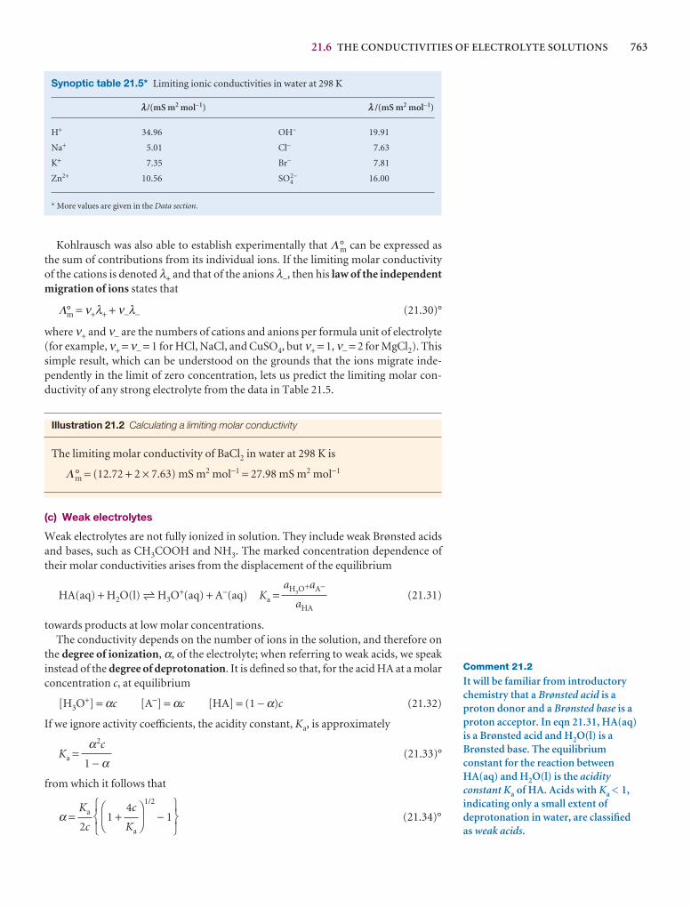
21.6 THE CONDUCTIVITIES OF ELECTROLYTE SOLUTIONS 763
Synoptic table 21.5* Limiting ionic conductivities in water at 298 K
l/(mS m2 mol−1) l /(mS m2 mol−1)
H+ 34.96 OH− 19.91
Na+ 5.01 Cl− 7.63
K+ 7.35 Br− 7.81
Zn2+ 10.56 SO42− 16.00
* More values are given in the Data section.
Comment 21.2
It will be familiar from introductorychemistry that a Brønsted acid is aproton donor and a Brønsted base is aproton acceptor. In eqn 21.31, HA(aq) is a Brønsted acid and H2O(l) is aBrønsted base. The equilibriumconstant for the reaction betweenHA(aq) and H2O(l) is the acidityconstant Ka of HA. Acids with Ka < 1,indicating only a small extent ofdeprotonation in water, are classified as weak acids.
Kohlrausch was also able to establish experimentally that Λ°m can be expressed asthe sum of contributions from its individual ions. If the limiting molar conductivityof the cations is denoted λ+ and that of the anions λ−, then his law of the independentmigration of ions states that
Λ°m = ν+λ+ + ν−λ− (21.30)°
where ν+ and ν− are the numbers of cations and anions per formula unit of electrolyte(for example, ν+ = ν− = 1 for HCl, NaCl, and CuSO4, but ν+ = 1, ν− = 2 for MgCl2). Thissimple result, which can be understood on the grounds that the ions migrate inde-pendently in the limit of zero concentration, lets us predict the limiting molar con-ductivity of any strong electrolyte from the data in Table 21.5.
Illustration 21.2 Calculating a limiting molar conductivity
The limiting molar conductivity of BaCl2 in water at 298 K is
Λm° = (12.72 + 2 × 7.63) mS m2 mol−1 = 27.98 mS m2 mol−1
(c) Weak electrolytes
Weak electrolytes are not fully ionized in solution. They include weak Brønsted acidsand bases, such as CH3COOH and NH3. The marked concentration dependence oftheir molar conductivities arises from the displacement of the equilibrium
HA(aq) + H2O(l) 5 H3O+(aq) + A−(aq) Ka = (21.31)
towards products at low molar concentrations.The conductivity depends on the number of ions in the solution, and therefore on
the degree of ionization, α, of the electrolyte; when referring to weak acids, we speakinstead of the degree of deprotonation. It is defined so that, for the acid HA at a molarconcentration c, at equilibrium
[H3O+] = αc [A−] = αc [HA] = (1 − α)c (21.32)
If we ignore activity coefficients, the acidity constant, Ka, is approximately
Ka = (21.33)°
from which it follows that
α = 1 +1/2
− 1 (21.34)°567
DF
4c
Ka
AC
123
Ka
2c
α2c
1 − α
aH3O+aA−
aHA
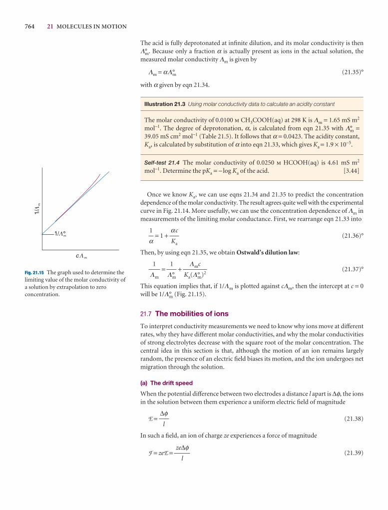
764 21 MOLECULES IN MOTION
1/m
(
1/ °m(
c m((
(
(
Fig. 21.15 The graph used to determine thelimiting value of the molar conductivity ofa solution by extrapolation to zeroconcentration.
The acid is fully deprotonated at infinite dilution, and its molar conductivity is thenΛ°m. Because only a fraction α is actually present as ions in the actual solution, themeasured molar conductivity Λm is given by
Λm = αΛ°m (21.35)°
with α given by eqn 21.34.
Illustration 21.3 Using molar conductivity data to calculate an acidity constant
The molar conductivity of 0.0100 m CH3COOH(aq) at 298 K is Λm = 1.65 mS m2
mol−1. The degree of deprotonation, α, is calculated from eqn 21.35 with Λ°m =39.05 mS cm2 mol−1 (Table 21.5). It follows that α = 0.0423. The acidity constant,Ka, is calculated by substitution of α into eqn 21.33, which gives Ka = 1.9 × 10⁻⁵.
Self-test 21.4 The molar conductivity of 0.0250 m HCOOH(aq) is 4.61 mS m2
mol−1. Determine the pKa = − log Ka of the acid. [3.44]
Once we know Ka, we can use eqns 21.34 and 21.35 to predict the concentration dependence of the molar conductivity. The result agrees quite well with the experimentalcurve in Fig. 21.14. More usefully, we can use the concentration dependence of Λm inmeasurements of the limiting molar conductance. First, we rearrange eqn 21.33 into
= 1 + (21.36)°
Then, by using eqn 21.35, we obtain Ostwald’s dilution law:
= + (21.37)°
This equation implies that, if 1/Λm is plotted against cΛm, then the intercept at c = 0will be 1/Λ°m (Fig. 21.15).
21.7 The mobilities of ions
To interpret conductivity measurements we need to know why ions move at differentrates, why they have different molar conductivities, and why the molar conductivitiesof strong electrolytes decrease with the square root of the molar concentration. Thecentral idea in this section is that, although the motion of an ion remains largely random, the presence of an electric field biases its motion, and the ion undergoes netmigration through the solution.
(a) The drift speed
When the potential difference between two electrodes a distance l apart is ∆φ, the ionsin the solution between them experience a uniform electric field of magnitude
E = (21.38)
In such a field, an ion of charge ze experiences a force of magnitude
F = zeE = (21.39)ze∆φ
l
∆φl
Λmc
Ka(Λ°m)2
1
Λ°m
1
Λm
αc
Ka
1
α
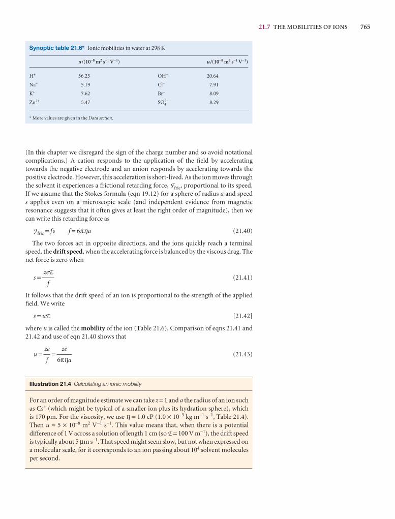
21.7 THE MOBILITIES OF IONS 765
(In this chapter we disregard the sign of the charge number and so avoid notationalcomplications.) A cation responds to the application of the field by accelerating towards the negative electrode and an anion responds by accelerating towards thepositive electrode. However, this acceleration is short-lived. As the ion moves throughthe solvent it experiences a frictional retarding force, Ffric, proportional to its speed. If we assume that the Stokes formula (eqn 19.12) for a sphere of radius a and speed s applies even on a microscopic scale (and independent evidence from magnetic resonance suggests that it often gives at least the right order of magnitude), then wecan write this retarding force as
Ffric = f s f = 6πηa (21.40)
The two forces act in opposite directions, and the ions quickly reach a terminalspeed, the drift speed, when the accelerating force is balanced by the viscous drag. Thenet force is zero when
s = (21.41)
It follows that the drift speed of an ion is proportional to the strength of the appliedfield. We write
s = uE [21.42]
where u is called the mobility of the ion (Table 21.6). Comparison of eqns 21.41 and21.42 and use of eqn 21.40 shows that
u = = (21.43)
Illustration 21.4 Calculating an ionic mobility
For an order of magnitude estimate we can take z = 1 and a the radius of an ion suchas Cs+ (which might be typical of a smaller ion plus its hydration sphere), which is 170 pm. For the viscosity, we use η = 1.0 cP (1.0 × 10⁻³ kg m−1 s−1, Table 21.4).Then u ≈ 5 × 10⁻⁸ m2 V−1 s−1. This value means that, when there is a potentialdifference of 1 V across a solution of length 1 cm (so E = 100 V m−1), the drift speedis typically about 5 µm s−1. That speed might seem slow, but not when expressed ona molecular scale, for it corresponds to an ion passing about 104 solvent moleculesper second.
ze
6πηa
ze
f
zeE
f
Synoptic table 21.6* Ionic mobilities in water at 298 K
u /(10−8 m2 s−1 V−1) u /(10−8 m2 s−1 V−1)
H+ 36.23 OH− 20.64
Na+ 5.19 Cl− 7.91
K+ 7.62 Br− 8.09
Zn2+ 5.47 SO42− 8.29
* More values are given in the Data section.
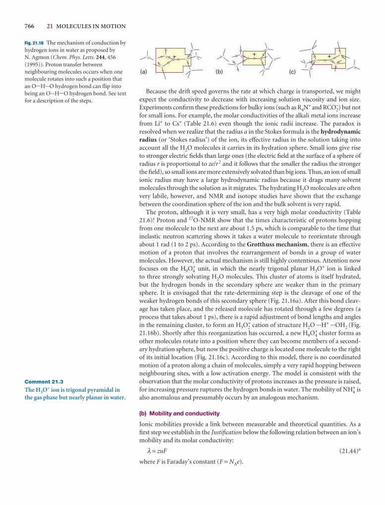
766 21 MOLECULES IN MOTION
Because the drift speed governs the rate at which charge is transported, we mightexpect the conductivity to decrease with increasing solution viscosity and ion size.Experiments confirm these predictions for bulky ions (such as R4N
+ and RCO2−) but not
for small ions. For example, the molar conductivities of the alkali metal ions increasefrom Li+ to Cs+ (Table 21.6) even though the ionic radii increase. The paradox isresolved when we realize that the radius a in the Stokes formula is the hydrodynamicradius (or ‘Stokes radius’) of the ion, its effective radius in the solution taking into account all the H2O molecules it carries in its hydration sphere. Small ions give rise to stronger electric fields than large ones (the electric field at the surface of a sphere ofradius r is proportional to ze/r2 and it follows that the smaller the radius the strongerthe field), so small ions are more extensively solvated than big ions. Thus, an ion of smallionic radius may have a large hydrodynamic radius because it drags many solventmolecules through the solution as it migrates. The hydrating H2O molecules are oftenvery labile, however, and NMR and isotope studies have shown that the exchangebetween the coordination sphere of the ion and the bulk solvent is very rapid.
The proton, although it is very small, has a very high molar conductivity (Table21.6)! Proton and 17O-NMR show that the times characteristic of protons hoppingfrom one molecule to the next are about 1.5 ps, which is comparable to the time thatinelastic neutron scattering shows it takes a water molecule to reorientate throughabout 1 rad (1 to 2 ps). According to the Grotthuss mechanism, there is an effectivemotion of a proton that involves the rearrangement of bonds in a group of watermolecules. However, the actual mechanism is still highly contentious. Attention nowfocuses on the H9O4
+ unit, in which the nearly trigonal planar H3O+ ion is linked to three strongly solvating H2O molecules. This cluster of atoms is itself hydrated, but the hydrogen bonds in the secondary sphere are weaker than in the primarysphere. It is envisaged that the rate-determining step is the cleavage of one of theweaker hydrogen bonds of this secondary sphere (Fig. 21.16a). After this bond cleav-age has taken place, and the released molecule has rotated through a few degrees (aprocess that takes about 1 ps), there is a rapid adjustment of bond lengths and anglesin the remaining cluster, to form an H5O2
+ cation of structure H2O ···H+ ···OH2 (Fig.21.16b). Shortly after this reorganization has occurred, a new H9O4
+ cluster forms asother molecules rotate into a position where they can become members of a second-ary hydration sphere, but now the positive charge is located one molecule to the rightof its initial location (Fig. 21.16c). According to this model, there is no coordinatedmotion of a proton along a chain of molecules, simply a very rapid hopping betweenneighbouring sites, with a low activation energy. The model is consistent with the observation that the molar conductivity of protons increases as the pressure is raised,for increasing pressure ruptures the hydrogen bonds in water. The mobility of NH4
+ isalso anomalous and presumably occurs by an analogous mechanism.
(b) Mobility and conductivity
Ionic mobilities provide a link between measurable and theoretical quantities. As afirst step we establish in the Justification below the following relation between an ion’smobility and its molar conductivity:
λ = zuF (21.44)°
where F is Faraday’s constant (F = NAe).
Comment 21.3
The H3O+ ion is trigonal pyramidal inthe gas phase but nearly planar in water.
(a) (b) (c)
+ + +
Fig. 21.16 The mechanism of conduction byhydrogen ions in water as proposed by N. Agmon (Chem. Phys. Letts. 244, 456(1995)). Proton transfer betweenneighbouring molecules occurs when onemolecule rotates into such a position thatan O-H···O hydrogen bond can flip intobeing an O···H-O hydrogen bond. See textfor a description of the steps.
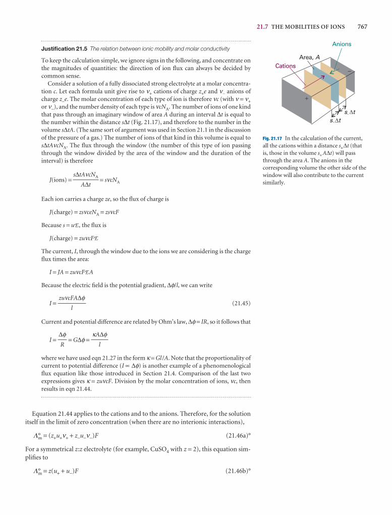
21.7 THE MOBILITIES OF IONS 767
Justification 21.5 The relation between ionic mobility and molar conductivity
To keep the calculation simple, we ignore signs in the following, and concentrate onthe magnitudes of quantities: the direction of ion flux can always be decided bycommon sense.
Consider a solution of a fully dissociated strong electrolyte at a molar concentra-tion c. Let each formula unit give rise to ν+ cations of charge z+e and ν− anions ofcharge z−e. The molar concentration of each type of ion is therefore νc (with ν = ν+or ν−), and the number density of each type is νcNA. The number of ions of one kindthat pass through an imaginary window of area A during an interval ∆t is equal tothe number within the distance s∆t (Fig. 21.17), and therefore to the number in thevolume s∆tA. (The same sort of argument was used in Section 21.1 in the discussionof the pressure of a gas.) The number of ions of that kind in this volume is equal tos∆tAνcNA. The flux through the window (the number of this type of ion passingthrough the window divided by the area of the window and the duration of the interval) is therefore
J(ions) = = sνcNA
Each ion carries a charge ze, so the flux of charge is
J(charge) = zsνceNA = zsνcF
Because s = uE , the flux is
J(charge) = zuνcFE
The current, I, through the window due to the ions we are considering is the chargeflux times the area:
I = JA = zuνcFEA
Because the electric field is the potential gradient, ∆φ/l, we can write
I = (21.45)
Current and potential difference are related by Ohm’s law, ∆φ = IR, so it follows that
I = = G∆φ =
where we have used eqn 21.27 in the form κ = Gl /A. Note that the proportionality ofcurrent to potential difference (I ∝ ∆φ) is another example of a phenomenologicalflux equation like those introduced in Section 21.4. Comparison of the last two expressions gives κ = zuνcF. Division by the molar concentration of ions, νc, thenresults in eqn 21.44.
Equation 21.44 applies to the cations and to the anions. Therefore, for the solutionitself in the limit of zero concentration (when there are no interionic interactions),
Λ°m = (z+u+ν+ + z−u−ν−)F (21.46a)°
For a symmetrical z:z electrolyte (for example, CuSO4 with z = 2), this equation sim-plifies to
Λ°m = z(u+ + u−)F (21.46b)°
κA∆φl
∆φR
zuνcFA∆φl
s∆tAνcNA
A∆t
Area, A
+
-
s t+D
s t-D
Cations
Anions
Fig. 21.17 In the calculation of the current,all the cations within a distance s+∆t (thatis, those in the volume s+A∆t) will passthrough the area A. The anions in thecorresponding volume the other side of thewindow will also contribute to the currentsimilarly.
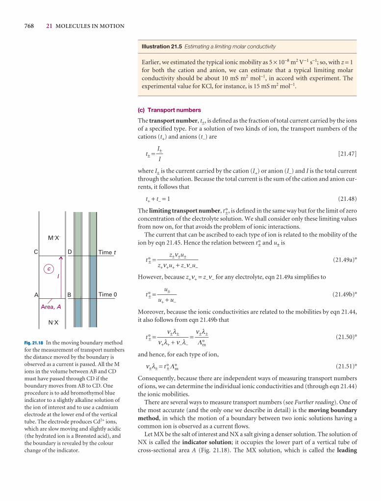
768 21 MOLECULES IN MOTION
M X� �
N X� �
A B
C D Time t
Time 0
l
Area, A
c
Fig. 21.18 In the moving boundary methodfor the measurement of transport numbers the distance moved by the boundary isobserved as a current is passed. All the Mions in the volume between AB and CDmust have passed through CD if theboundary moves from AB to CD. Oneprocedure is to add bromothymol blueindicator to a slightly alkaline solution ofthe ion of interest and to use a cadmiumelectrode at the lower end of the verticaltube. The electrode produces Cd2+ ions,which are slow moving and slightly acidic(the hydrated ion is a Brønsted acid), andthe boundary is revealed by the colourchange of the indicator.
Illustration 21.5 Estimating a limiting molar conductivity
Earlier, we estimated the typical ionic mobility as 5 × 10⁻⁸ m2 V−1 s−1; so, with z = 1for both the cation and anion, we can estimate that a typical limiting molar conductivity should be about 10 mS m2 mol−1, in accord with experiment. The experimental value for KCl, for instance, is 15 mS m2 mol−1.
(c) Transport numbers
The transport number, t±, is defined as the fraction of total current carried by the ionsof a specified type. For a solution of two kinds of ion, the transport numbers of thecations (t+) and anions (t−) are
t± = [21.47]
where I± is the current carried by the cation (I+) or anion (I−) and I is the total currentthrough the solution. Because the total current is the sum of the cation and anion cur-rents, it follows that
t+ + t− = 1 (21.48)
The limiting transport number, t°±, is defined in the same way but for the limit of zeroconcentration of the electrolyte solution. We shall consider only these limiting valuesfrom now on, for that avoids the problem of ionic interactions.
The current that can be ascribed to each type of ion is related to the mobility of theion by eqn 21.45. Hence the relation between t°± and u± is
t°± = (21.49a)°
However, because z+ν+ = z−ν− for any electrolyte, eqn 21.49a simplifies to
t°± = (21.49b)°
Moreover, because the ionic conductivities are related to the mobilities by eqn 21.44,it also follows from eqn 21.49b that
t°± = = (21.50)°
and hence, for each type of ion,
ν±λ± = t°±Λ°m (21.51)°
Consequently, because there are independent ways of measuring transport numbersof ions, we can determine the individual ionic conductivities and (through eqn 21.44)the ionic mobilities.
There are several ways to measure transport numbers (see Further reading). One ofthe most accurate (and the only one we describe in detail) is the moving boundarymethod, in which the motion of a boundary between two ionic solutions having acommon ion is observed as a current flows.
Let MX be the salt of interest and NX a salt giving a denser solution. The solution ofNX is called the indicator solution; it occupies the lower part of a vertical tube ofcross-sectional area A (Fig. 21.18). The MX solution, which is called the leading
ν±λ±
Λ°m
ν±λ±
ν+λ+ + ν−λ−
u±
u+ + u−
z±ν±u±
z+ν+u+ + z−ν−u−
I±
I
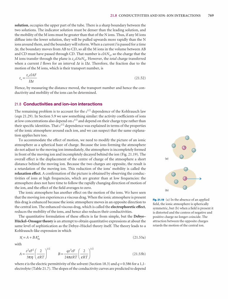
21.8 CONDUCTIVITIES AND ION–ION INTERACTIONS 769
solution, occupies the upper part of the tube. There is a sharp boundary between thetwo solutions. The indicator solution must be denser than the leading solution, andthe mobility of the M ions must be greater than that of the N ions. Thus, if any M ionsdiffuse into the lower solution, they will be pulled upwards more rapidly than the Nions around them, and the boundary will reform. When a current I is passed for a time∆t, the boundary moves from AB to CD, so all the M ions in the volume between ABand CD must have passed through CD. That number is clANA, so the charge that theM ions transfer through the plane is z+clAeNA. However, the total charge transferredwhen a current I flows for an interval ∆t is I∆t. Therefore, the fraction due to the motion of the M ions, which is their transport number, is
t+ = (21.52)
Hence, by measuring the distance moved, the transport number and hence the con-ductivity and mobility of the ions can be determined.
21.8 Conductivities and ion–ion interactions
The remaining problem is to account for the c1/2 dependence of the Kohlrausch law(eqn 21.29). In Section 5.9 we saw something similar: the activity coefficients of ionsat low concentrations also depend on c1/2 and depend on their charge type rather thantheir specific identities. That c1/2 dependence was explained in terms of the propertiesof the ionic atmosphere around each ion, and we can suspect that the same explana-tion applies here too.
To accommodate the effect of motion, we need to modify the picture of an ionic atmosphere as a spherical haze of charge. Because the ions forming the atmosphere do not adjust to the moving ion immediately, the atmosphere is incompletely formedin front of the moving ion and incompletely decayed behind the ion (Fig. 21.19). Theoverall effect is the displacement of the centre of charge of the atmosphere a short distance behind the moving ion. Because the two charges are opposite, the result is a retardation of the moving ion. This reduction of the ions’ mobility is called the relaxation effect. A confirmation of the picture is obtained by observing the conduc-tivities of ions at high frequencies, which are greater than at low frequencies: the atmosphere does not have time to follow the rapidly changing direction of motion ofthe ion, and the effect of the field averages to zero.
The ionic atmosphere has another effect on the motion of the ions. We have seenthat the moving ion experiences a viscous drag. When the ionic atmosphere is presentthis drag is enhanced because the ionic atmosphere moves in an opposite direction tothe central ion. The enhanced viscous drag, which is called the electrophoretic effect,reduces the mobility of the ions, and hence also reduces their conductivities.
The quantitative formulation of these effects is far from simple, but the Debye–Hückel–Onsager theory is an attempt to obtain quantitative expressions at about thesame level of sophistication as the Debye–Hückel theory itself. The theory leads to aKohlrausch-like expression in which
K = A + BΛ°m (21.53a)
with
A =1/2
B =1/2
(21.53b)
where ε is the electric permittivity of the solvent (Section 18.3) and q = 0.586 for a 1,1-electrolyte (Table 21.7). The slopes of the conductivity curves are predicted to depend
DF
2
εRT
AC
qz3eF
24πεRT
DF
2
εRT
AC
z2eF2
3πη
z+clAF
I∆t
(a)
(b)
�
�
�
�
�
�
�
�
�
�
Fig. 21.19 (a) In the absence of an appliedfield, the ionic atmosphere is sphericallysymmetric, but (b) when a field is present itis distorted and the centres of negative andpositive charge no longer coincide. Theattraction between the opposite chargesretards the motion of the central ion.
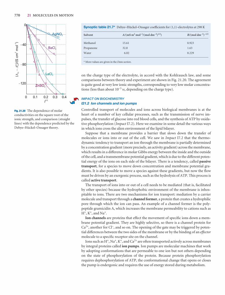
770 21 MOLECULES IN MOTION
on the charge type of the electrolyte, in accord with the Kohlrausch law, and somecomparisons between theory and experiment are shown in Fig. 21.20. The agreementis quite good at very low ionic strengths, corresponding to very low molar concentra-tions (less than about 10−3 M, depending on the charge type).
IMPACT ON BIOCHEMISTRY
I21.2 Ion channels and ion pumps
Controlled transport of molecules and ions across biological membranes is at theheart of a number of key cellular processes, such as the transmission of nerve im-pulses, the transfer of glucose into red blood cells, and the synthesis of ATP by oxida-tive phosphorylation (Impact I7.2). Here we examine in some detail the various waysin which ions cross the alien environment of the lipid bilayer.
Suppose that a membrane provides a barrier that slows down the transfer ofmolecules or ions into or out of the cell. We saw in Impact I7.2 that the thermo-dynamic tendency to transport an ion through the membrane is partially determinedby a concentration gradient (more precisely, an activity gradient) across the membrane,which results in a difference in molar Gibbs energy between the inside and the outsideof the cell, and a transmembrane potential gradient, which is due to the different poten-tial energy of the ions on each side of the bilayer. There is a tendency, called passivetransport, for a species to move down concentration and membrane potential gra-dients. It is also possible to move a species against these gradients, but now the flowmust be driven by an exergonic process, such as the hydrolysis of ATP. This process iscalled active transport.
The transport of ions into or out of a cell needs to be mediated (that is, facilitatedby other species) because the hydrophobic environment of the membrane is inhos-pitable to ions. There are two mechanisms for ion transport: mediation by a carriermolecule and transport through a channel former, a protein that creates a hydrophilicpore through which the ion can pass. An example of a channel former is the poly-peptide gramicidin A, which increases the membrane permeability to cations such asH+, K+, and Na+.
Ion channels are proteins that effect the movement of specific ions down a mem-brane potential gradient. They are highly selective, so there is a channel protein forCa2+, another for Cl−, and so on. The opening of the gate may be triggered by poten-tial differences between the two sides of the membrane or by the binding of an effectormolecule to a specific receptor site on the channel.
Ions such as H+, Na+, K+, and Ca2+ are often transported actively across membranesby integral proteins called ion pumps. Ion pumps are molecular machines that workby adopting conformations that are permeable to one ion but not others dependingon the state of phosphorylation of the protein. Because protein phosphorylation requires dephosphorylation of ATP, the conformational change that opens or closesthe pump is endergonic and requires the use of energy stored during metabolism.
Synoptic table 21.7* Debye–Hückel–Onsager coefficients for (1,1)-electrolytes at 298 K
Solvent A/(mS m2 mol−1/(mol dm−3)1/2) B/(mol dm−3)−1/2
Methanol 15.61 0.923
Propanone 32.8 1.63
Water 6.02 0.229
* More values are given in the Data section.
Fig. 21.20 The dependence of molarconductivities on the square root of theionic strength, and comparison (straightlines) with the dependence predicted by theDebye–Hückel–Onsager theory.
(°)
/(S c
mm
ol)
mm
�2
1�
((
0
�40
�80
�120
I1/2
0 0.1 0.2 0.3 0.4
AgNO3
BaCl2
LaCl3
ZnSO4
((
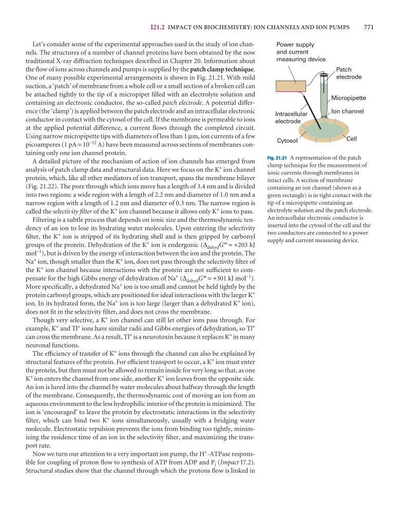
I21.2 IMPACT ON BIOCHEMISTRY: ION CHANNELS AND ION PUMPS 771
Let’s consider some of the experimental approaches used in the study of ion chan-nels. The structures of a number of channel proteins have been obtained by the nowtraditional X-ray diffraction techniques described in Chapter 20. Information aboutthe flow of ions across channels and pumps is supplied by the patch clamp technique.One of many possible experimental arrangements is shown in Fig. 21.21. With mildsuction, a ‘patch’ of membrane from a whole cell or a small section of a broken cell canbe attached tightly to the tip of a micropipet filled with an electrolyte solution andcontaining an electronic conductor, the so-called patch electrode. A potential differ-ence (the ‘clamp’) is applied between the patch electrode and an intracellular electronicconductor in contact with the cytosol of the cell. If the membrane is permeable to ionsat the applied potential difference, a current flows through the completed circuit.Using narrow micropipette tips with diameters of less than 1 µm, ion currents of a fewpicoamperes (1 pA = 10−12 A) have been measured across sections of membranes con-taining only one ion channel protein.
A detailed picture of the mechanism of action of ion channels has emerged fromanalysis of patch clamp data and structural data. Here we focus on the K+ ion channelprotein, which, like all other mediators of ion transport, spans the membrane bilayer(Fig. 21.22). The pore through which ions move has a length of 3.4 nm and is dividedinto two regions: a wide region with a length of 2.2 nm and diameter of 1.0 nm and anarrow region with a length of 1.2 nm and diameter of 0.3 nm. The narrow region iscalled the selectivity filter of the K+ ion channel because it allows only K+ ions to pass.
Filtering is a subtle process that depends on ionic size and the thermodynamic ten-dency of an ion to lose its hydrating water molecules. Upon entering the selectivityfilter, the K+ ion is stripped of its hydrating shell and is then gripped by carbonylgroups of the protein. Dehydration of the K+ ion is endergonic (∆dehydG 7 = +203 kJmol−1), but is driven by the energy of interaction between the ion and the protein. TheNa+ ion, though smaller than the K+ ion, does not pass through the selectivity filter ofthe K+ ion channel because interactions with the protein are not sufficient to com-pensate for the high Gibbs energy of dehydration of Na+ (∆dehydG 7 = +301 kJ mol−1).More specifically, a dehydrated Na+ ion is too small and cannot be held tightly by theprotein carbonyl groups, which are positioned for ideal interactions with the larger K+
ion. In its hydrated form, the Na+ ion is too large (larger than a dehydrated K+ ion),does not fit in the selectivity filter, and does not cross the membrane.
Though very selective, a K+ ion channel can still let other ions pass through. For example, K+ and Tl+ ions have similar radii and Gibbs energies of dehydration, so Tl+
can cross the membrane. As a result, Tl+ is a neurotoxin because it replaces K+ in manyneuronal functions.
The efficiency of transfer of K+ ions through the channel can also be explained bystructural features of the protein. For efficient transport to occur, a K+ ion must enterthe protein, but then must not be allowed to remain inside for very long so that, as oneK+ ion enters the channel from one side, another K+ ion leaves from the opposite side.An ion is lured into the channel by water molecules about halfway through the lengthof the membrane. Consequently, the thermodynamic cost of moving an ion from anaqueous environment to the less hydrophilic interior of the protein is minimized. Theion is ‘encouraged’ to leave the protein by electrostatic interactions in the selectivityfilter, which can bind two K+ ions simultaneously, usually with a bridging watermolecule. Electrostatic repulsion prevents the ions from binding too tightly, minim-izing the residence time of an ion in the selectivity filter, and maximizing the trans-port rate.
Now we turn our attention to a very important ion pump, the H+-ATPase respons-ible for coupling of proton flow to synthesis of ATP from ADP and Pi (Impact I7.2).Structural studies show that the channel through which the protons flow is linked in
Micropipette
Power supplyand currentmeasuring device
Intracellularelectrode
Patchelectrode
Cytosol
Ion channel
Cell
Fig. 21.21 A representation of the patchclamp technique for the measurement ofionic currents through membranes inintact cells. A section of membranecontaining an ion channel (shown as agreen rectangle) is in tight contact with thetip of a micropipette containing anelectrolyte solution and the patch electrode.An intracellular electronic conductor isinserted into the cytosol of the cell and thetwo conductors are connected to a powersupply and current measuring device.
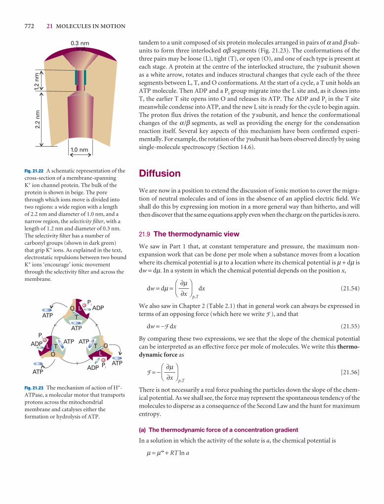
772 21 MOLECULES IN MOTION
tandem to a unit composed of six protein molecules arranged in pairs of α and β sub-units to form three interlocked αβ segments (Fig. 21.23). The conformations of thethree pairs may be loose (L), tight (T), or open (O), and one of each type is present ateach stage. A protein at the centre of the interlocked structure, the γ subunit shown as a white arrow, rotates and induces structural changes that cycle each of the three segments between L, T, and O conformations. At the start of a cycle, a T unit holds anATP molecule. Then ADP and a Pi group migrate into the L site and, as it closes intoT, the earlier T site opens into O and releases its ATP. The ADP and Pi in the T sitemeanwhile condense into ATP, and the new L site is ready for the cycle to begin again.The proton flux drives the rotation of the γ subunit, and hence the conformationalchanges of the α /β segments, as well as providing the energy for the condensation reaction itself. Several key aspects of this mechanism have been confirmed experi-mentally. For example, the rotation of the γ subunit has been observed directly by usingsingle-molecule spectroscopy (Section 14.6).
Diffusion
We are now in a position to extend the discussion of ionic motion to cover the migra-tion of neutral molecules and of ions in the absence of an applied electric field. Weshall do this by expressing ion motion in a more general way than hitherto, and willthen discover that the same equations apply even when the charge on the particles is zero.
21.9 The thermodynamic view
We saw in Part 1 that, at constant temperature and pressure, the maximum non-expansion work that can be done per mole when a substance moves from a locationwhere its chemical potential is µ to a location where its chemical potential is µ + dµ isdw = dµ. In a system in which the chemical potential depends on the position x,
dw = dµ = p,T
dx (21.54)
We also saw in Chapter 2 (Table 2.1) that in general work can always be expressed interms of an opposing force (which here we write F ), and that
dw = −F dx (21.55)
By comparing these two expressions, we see that the slope of the chemical potentialcan be interpreted as an effective force per mole of molecules. We write this thermo-dynamic force as
F = −p,T
[21.56]
There is not necessarily a real force pushing the particles down the slope of the chem-ical potential. As we shall see, the force may represent the spontaneous tendency of themolecules to disperse as a consequence of the Second Law and the hunt for maximumentropy.
(a) The thermodynamic force of a concentration gradient
In a solution in which the activity of the solute is a, the chemical potential is
µ = µ7 + RT ln a
DF
∂µ∂x
AC
DF
∂µ∂x
AC
L
LL
T
TT
O
OO
ATP
ATP
ATPATP
ATP
ADP
ADP
Pi
Pi
LADP
Pi
ATP
L
Fig. 21.23 The mechanism of action of H+-ATPase, a molecular motor that transportsprotons across the mitochondrialmembrane and catalyses either theformation or hydrolysis of ATP.
2.2
nm1.
2 nm
1.0 nm
0.3 nm
Fig. 21.22 A schematic representation of thecross-section of a membrane-spanning K+ ion channel protein. The bulk of theprotein is shown in beige. The porethrough which ions move is divided intotwo regions: a wide region with a length of 2.2 nm and diameter of 1.0 nm, and anarrow region, the selectivity filter, with alength of 1.2 nm and diameter of 0.3 nm.The selectivity filter has a number ofcarbonyl groups (shown in dark green) that grip K+ ions. As explained in the text,electrostatic repulsions between two boundK+ ions ‘encourage’ ionic movementthrough the selectivity filter and across themembrane.
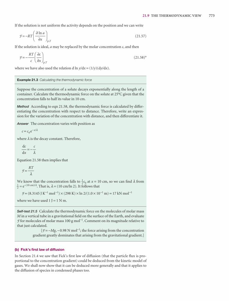
21.9 THE THERMODYNAMIC VIEW 773
If the solution is not uniform the activity depends on the position and we can write
F = −RTp,T
(21.57)
If the solution is ideal, a may be replaced by the molar concentration c, and then
F = −p,T
(21.58)°
where we have also used the relation d ln y/dx = (1/y)(dy/dx).
Example 21.3 Calculating the thermodynamic force
Suppose the concentration of a solute decays exponentially along the length of acontainer. Calculate the thermodynamic force on the solute at 25°C given that theconcentration falls to half its value in 10 cm.
Method According to eqn 21.58, the thermodynamic force is calculated by differ-entiating the concentration with respect to distance. Therefore, write an expres-sion for the variation of the concentration with distance, and then differentiate it.
Answer The concentration varies with position as
c = c0 e− x/λ
where λ is the decay constant. Therefore,
= −
Equation 21.58 then implies that
F =
We know that the concentration falls to 1–2 c0 at x = 10 cm, so we can find λ from1–2 = e−(10 cm)/λ. That is, λ = (10 cm/ln 2). It follows that
F = (8.3145 J K−1 mol−1) × (298 K) × ln 2/(1.0 × 10−1 m) = 17 kN mol−1
where we have used 1 J = 1 N m.
Self-test 21.5 Calculate the thermodynamic force on the molecules of molar massM in a vertical tube in a gravitational field on the surface of the Earth, and evaluateF for molecules of molar mass 100 g mol−1. Comment on its magnitude relative tothat just calculated.
[F = −Mg, −0.98 N mol−1; the force arising from the concentration gradient greatly dominates that arising from the gravitational gradient.]
(b) Fick’s first law of diffusion
In Section 21.4 we saw that Fick’s first law of diffusion (that the particle flux is pro-portional to the concentration gradient) could be deduced from the kinetic model ofgases. We shall now show that it can be deduced more generally and that it applies tothe diffusion of species in condensed phases too.
RT
λ
c
λdc
dx
DF
∂c
∂x
AC
RT
c
DF
∂ ln a
∂x
AC
774 21 MOLECULES IN MOTION
We suppose that the flux of diffusing particles is motion in response to a thermo-dynamic force arising from a concentration gradient. The particles reach a steady driftspeed, s, when the thermodynamic force, F, is matched by the viscous drag. This driftspeed is proportional to the thermodynamic force, and we write s ∝ F. However, theparticle flux, J, is proportional to the drift speed, and the thermodynamic force is pro-portional to the concentration gradient, dc/dx. The chain of proportionalities (J ∝ s,s ∝ F , and F ∝ dc/dx) implies that J ∝ dc/dx, which is the content of Fick’s law.
(c) The Einstein relation
If we divide both sides of eqn 21.19 by Avogadro’s constant, thereby converting num-bers into amounts (numbers of moles), then Fick’s law becomes
J = −D (21.59)
In this expression, D is the diffusion coefficient and dc/dx is the slope of the molarconcentration. The flux is related to the drift speed by
J = sc (21.60)
This relation follows from the argument that we have used several times before. Thus,all particles within a distance s∆t, and therefore in a volume s∆tA, can pass through awindow of area A in an interval ∆t. Hence, the amount of substance that can passthrough the window in that interval is s∆tAc. Therefore,
sc = −D
If now we express dc/dx in terms of F by using eqn 21.58, we find
s = − = (21.61)
Therefore, once we know the effective force and the diffusion coefficient, D, we cancalculate the drift speed of the particles (and vice versa) whatever the origin of theforce.
There is one case where we already know the drift speed and the effective force act-ing on a particle: an ion in solution has a drift speed s = uE when it experiences a forceezE from an electric field of strength E (so F = NAezE = zFE). Therefore, substitutingthese known values into eqn 21.61 gives
uE =
and hence
u = (21.62)
This equation rearranges into the very important result known as the Einstein rela-tion between the diffusion coefficient and the ionic mobility:
D = (21.63)°
On inserting the typical value u = 5 × 10⁻⁸ m2 s−1 V−1, we find D ≈ 1 × 10⁻⁹ m2 s−1 at25°C as a typical value of the diffusion coefficient of an ion in water.
uRT
zF
zFD
RT
zFED
RT
DF
RT
dc
dx
D
c
dc
dx
dc
dx
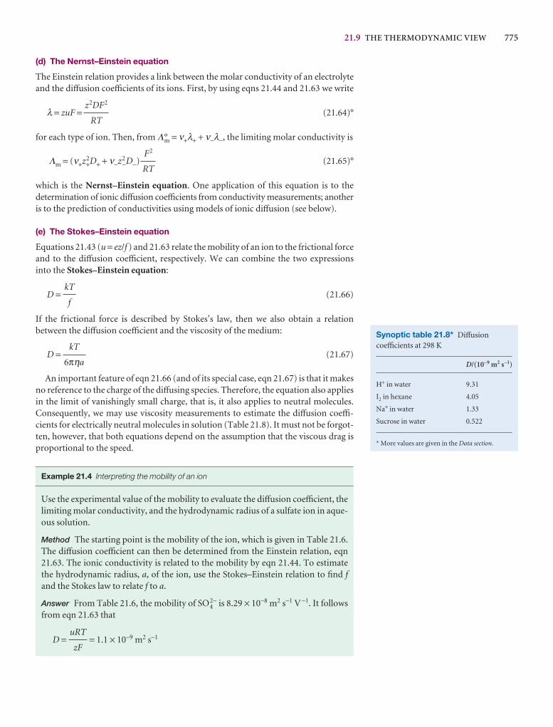
21.9 THE THERMODYNAMIC VIEW 775
Synoptic table 21.8* Diffusioncoefficients at 298 K
D/(10−9 m2 s−1)
H+ in water 9.31
I2 in hexane 4.05
Na+ in water 1.33
Sucrose in water 0.522
* More values are given in the Data section.
(d) The Nernst–Einstein equation
The Einstein relation provides a link between the molar conductivity of an electrolyteand the diffusion coefficients of its ions. First, by using eqns 21.44 and 21.63 we write
λ = zuF = (21.64)°
for each type of ion. Then, from Λ°m = ν+λ+ + ν−λ−, the limiting molar conductivity is
Λm = (ν+z2+D+ + ν−z2
−D−) (21.65)°
which is the Nernst–Einstein equation. One application of this equation is to the determination of ionic diffusion coefficients from conductivity measurements; anotheris to the prediction of conductivities using models of ionic diffusion (see below).
(e) The Stokes–Einstein equation
Equations 21.43 (u = ez/f ) and 21.63 relate the mobility of an ion to the frictional forceand to the diffusion coefficient, respectively. We can combine the two expressionsinto the Stokes–Einstein equation:
D = (21.66)
If the frictional force is described by Stokes’s law, then we also obtain a relation between the diffusion coefficient and the viscosity of the medium:
D = (21.67)
An important feature of eqn 21.66 (and of its special case, eqn 21.67) is that it makesno reference to the charge of the diffusing species. Therefore, the equation also appliesin the limit of vanishingly small charge, that is, it also applies to neutral molecules.Consequently, we may use viscosity measurements to estimate the diffusion coeffi-
cients for electrically neutral molecules in solution (Table 21.8). It must not be forgot-ten, however, that both equations depend on the assumption that the viscous drag isproportional to the speed.
Example 21.4 Interpreting the mobility of an ion
Use the experimental value of the mobility to evaluate the diffusion coefficient, thelimiting molar conductivity, and the hydrodynamic radius of a sulfate ion in aque-ous solution.
Method The starting point is the mobility of the ion, which is given in Table 21.6.The diffusion coefficient can then be determined from the Einstein relation, eqn21.63. The ionic conductivity is related to the mobility by eqn 21.44. To estimatethe hydrodynamic radius, a, of the ion, use the Stokes–Einstein relation to find fand the Stokes law to relate f to a.
Answer From Table 21.6, the mobility of SO42− is 8.29 × 10⁻⁸ m2 s−1 V−1. It follows
from eqn 21.63 that
D = = 1.1 × 10⁻⁹ m2 s−1uRT
zF
kT
6πηa
kT
f
F2
RT
z2DF2
RT
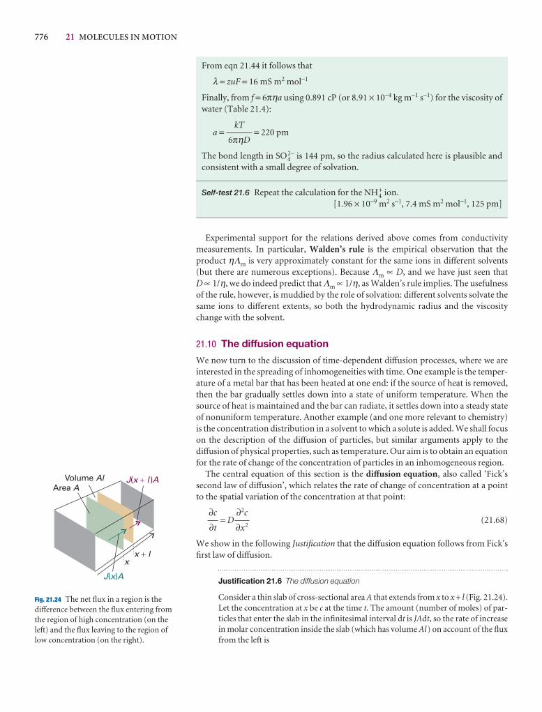
776 21 MOLECULES IN MOTION
x l�x
Area A
J x A( )
J x l A( )�Volume Al
Fig. 21.24 The net flux in a region is thedifference between the flux entering fromthe region of high concentration (on theleft) and the flux leaving to the region oflow concentration (on the right).
From eqn 21.44 it follows that
λ = zuF = 16 mS m2 mol−1
Finally, from f = 6πηa using 0.891 cP (or 8.91 × 10⁻⁴ kg m−1 s−1) for the viscosity ofwater (Table 21.4):
a = = 220 pm
The bond length in SO42− is 144 pm, so the radius calculated here is plausible and
consistent with a small degree of solvation.
Self-test 21.6 Repeat the calculation for the NH4+ ion.
[1.96 × 10⁻⁹ m2 s−1, 7.4 mS m2 mol−1, 125 pm]
Experimental support for the relations derived above comes from conductivitymeasurements. In particular, Walden’s rule is the empirical observation that theproduct ηΛm is very approximately constant for the same ions in different solvents(but there are numerous exceptions). Because Λm ∝ D, and we have just seen that D ∝ 1/η, we do indeed predict that Λm ∝ 1/η, as Walden’s rule implies. The usefulnessof the rule, however, is muddied by the role of solvation: different solvents solvate thesame ions to different extents, so both the hydrodynamic radius and the viscositychange with the solvent.
21.10 The diffusion equation
We now turn to the discussion of time-dependent diffusion processes, where we areinterested in the spreading of inhomogeneities with time. One example is the temper-ature of a metal bar that has been heated at one end: if the source of heat is removed,then the bar gradually settles down into a state of uniform temperature. When thesource of heat is maintained and the bar can radiate, it settles down into a steady stateof nonuniform temperature. Another example (and one more relevant to chemistry)is the concentration distribution in a solvent to which a solute is added. We shall focuson the description of the diffusion of particles, but similar arguments apply to thediffusion of physical properties, such as temperature. Our aim is to obtain an equationfor the rate of change of the concentration of particles in an inhomogeneous region.
The central equation of this section is the diffusion equation, also called ‘Fick’s second law of diffusion’, which relates the rate of change of concentration at a point to the spatial variation of the concentration at that point:
= D (21.68)
We show in the following Justification that the diffusion equation follows from Fick’sfirst law of diffusion.
Justification 21.6 The diffusion equation
Consider a thin slab of cross-sectional area A that extends from x to x + l (Fig. 21.24).Let the concentration at x be c at the time t. The amount (number of moles) of par-ticles that enter the slab in the infinitesimal interval dt is JAdt, so the rate of increasein molar concentration inside the slab (which has volume Al) on account of the fluxfrom the left is
∂2c
∂x2
∂c
∂t
kT
6πηD
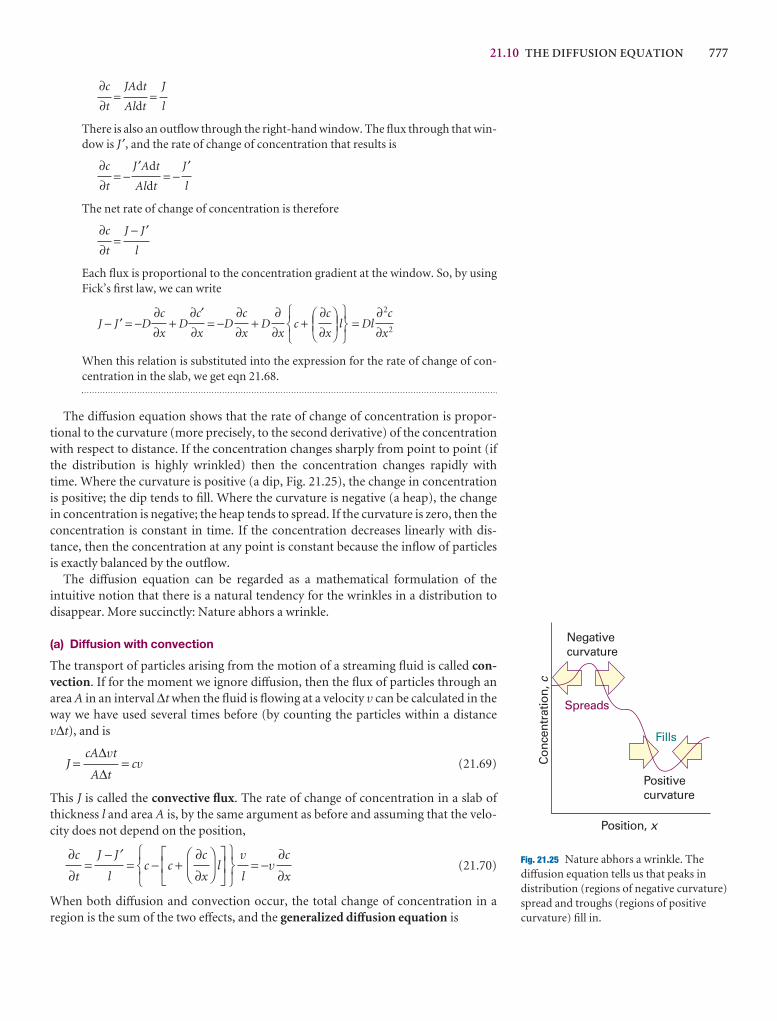
21.10 THE DIFFUSION EQUATION 777
= =
There is also an outflow through the right-hand window. The flux through that win-dow is J ′, and the rate of change of concentration that results is
= − = −
The net rate of change of concentration is therefore
=
Each flux is proportional to the concentration gradient at the window. So, by usingFick’s first law, we can write
J − J ′ = −D + D = −D + D c + l = Dl
When this relation is substituted into the expression for the rate of change of con-centration in the slab, we get eqn 21.68.
The diffusion equation shows that the rate of change of concentration is propor-tional to the curvature (more precisely, to the second derivative) of the concentrationwith respect to distance. If the concentration changes sharply from point to point (ifthe distribution is highly wrinkled) then the concentration changes rapidly with time. Where the curvature is positive (a dip, Fig. 21.25), the change in concentrationis positive; the dip tends to fill. Where the curvature is negative (a heap), the change in concentration is negative; the heap tends to spread. If the curvature is zero, then theconcentration is constant in time. If the concentration decreases linearly with dis-tance, then the concentration at any point is constant because the inflow of particlesis exactly balanced by the outflow.
The diffusion equation can be regarded as a mathematical formulation of the intuitive notion that there is a natural tendency for the wrinkles in a distribution todisappear. More succinctly: Nature abhors a wrinkle.
(a) Diffusion with convection
The transport of particles arising from the motion of a streaming fluid is called con-vection. If for the moment we ignore diffusion, then the flux of particles through anarea A in an interval ∆t when the fluid is flowing at a velocity v can be calculated in theway we have used several times before (by counting the particles within a distancev∆t), and is
J = = cv (21.69)
This J is called the convective flux. The rate of change of concentration in a slab ofthickness l and area A is, by the same argument as before and assuming that the velo-city does not depend on the position,
= = c − c + l = −v (21.70)
When both diffusion and convection occur, the total change of concentration in a region is the sum of the two effects, and the generalized diffusion equation is
∂c
∂x
v
l
567
JKLDF
∂c
∂x
AC
GHI123
J − J′l
∂c
∂t
cA∆vt
A∆t
∂2c
∂x2
567
DEF∂c
∂x
ABC123
∂∂x
∂c
∂x
∂c′∂x
∂c
∂x
J − J ′l
∂c
∂t
J ′l
J ′Adt
Aldt
∂c
∂t
J
l
JAdt
Aldt
∂c
∂t
Position, x
Con
cent
ratio
n,c
Negativecurvature
Positivecurvature
Spreads
Fills
Fig. 21.25 Nature abhors a wrinkle. Thediffusion equation tells us that peaks indistribution (regions of negative curvature)spread and troughs (regions of positivecurvature) fill in.
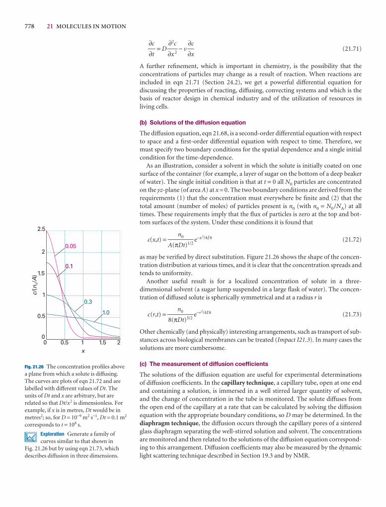
778 21 MOLECULES IN MOTION
= D − v (21.71)
A further refinement, which is important in chemistry, is the possibility that the concentrations of particles may change as a result of reaction. When reactions are included in eqn 21.71 (Section 24.2), we get a powerful differential equation for discussing the properties of reacting, diffusing, convecting systems and which is thebasis of reactor design in chemical industry and of the utilization of resources in living cells.
(b) Solutions of the diffusion equation
The diffusion equation, eqn 21.68, is a second-order differential equation with respectto space and a first-order differential equation with respect to time. Therefore, wemust specify two boundary conditions for the spatial dependence and a single initialcondition for the time-dependence.
As an illustration, consider a solvent in which the solute is initially coated on onesurface of the container (for example, a layer of sugar on the bottom of a deep beakerof water). The single initial condition is that at t = 0 all N0 particles are concentratedon the yz-plane (of area A) at x = 0. The two boundary conditions are derived from therequirements (1) that the concentration must everywhere be finite and (2) that thetotal amount (number of moles) of particles present is n0 (with n0 = N0 /NA) at alltimes. These requirements imply that the flux of particles is zero at the top and bot-tom surfaces of the system. Under these conditions it is found that
c(x,t) = e−x2/4Dt (21.72)
as may be verified by direct substitution. Figure 21.26 shows the shape of the concen-tration distribution at various times, and it is clear that the concentration spreads andtends to uniformity.
Another useful result is for a localized concentration of solute in a three-dimensional solvent (a sugar lump suspended in a large flask of water). The concen-tration of diffused solute is spherically symmetrical and at a radius r is
c(r,t) = e−r2/4Dt (21.73)
Other chemically (and physically) interesting arrangements, such as transport of sub-stances across biological membranes can be treated (Impact I21.3). In many cases thesolutions are more cumbersome.
(c) The measurement of diffusion coefficients
The solutions of the diffusion equation are useful for experimental determinations of diffusion coefficients. In the capillary technique, a capillary tube, open at one endand containing a solution, is immersed in a well stirred larger quantity of solvent, and the change of concentration in the tube is monitored. The solute diffuses from the open end of the capillary at a rate that can be calculated by solving the diffusionequation with the appropriate boundary conditions, so D may be determined. In thediaphragm technique, the diffusion occurs through the capillary pores of a sinteredglass diaphragm separating the well-stirred solution and solvent. The concentrationsare monitored and then related to the solutions of the diffusion equation correspond-ing to this arrangement. Diffusion coefficients may also be measured by the dynamiclight scattering technique described in Section 19.3 and by NMR.
n0
8(πDt)3/2
n0
A(πDt)1/2
∂c
∂x
∂2c
∂x 2
∂c
∂t
cn
A/(
/)
0
0
0.5
1
1.5
2
2.5
0 0.5 1 1.5 2x
1.0
0.3
0.1
0.05
Fig. 21.26 The concentration profiles abovea plane from which a solute is diffusing.The curves are plots of eqn 21.72 and arelabelled with different values of Dt. Theunits of Dt and x are arbitrary, but arerelated so that Dt/x2 is dimensionless. Forexample, if x is in metres, Dt would be inmetres2; so, for D = 10−9 m2 s−1, Dt = 0.1 m2
corresponds to t = 108 s.
Exploration Generate a family ofcurves similar to that shown in
Fig. 21.26 but by using eqn 21.73, whichdescribes diffusion in three dimensions.
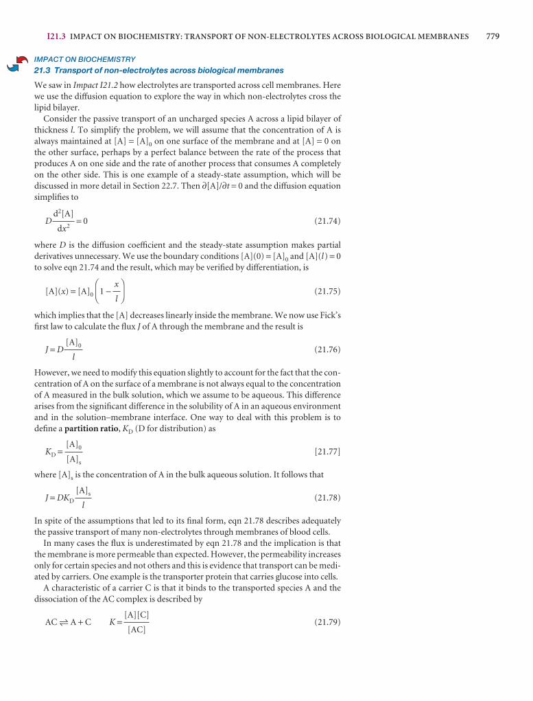
I21.3 IMPACT ON BIOCHEMISTRY: TRANSPORT OF NON-ELECTROLYTES ACROSS BIOLOGICAL MEMBRANES 779
IMPACT ON BIOCHEMISTRY
21.3 Transport of non-electrolytes across biological membranes
We saw in Impact I21.2 how electrolytes are transported across cell membranes. Herewe use the diffusion equation to explore the way in which non-electrolytes cross thelipid bilayer.
Consider the passive transport of an uncharged species A across a lipid bilayer ofthickness l. To simplify the problem, we will assume that the concentration of A is always maintained at [A] = [A]0 on one surface of the membrane and at [A] = 0 on the other surface, perhaps by a perfect balance between the rate of the process thatproduces A on one side and the rate of another process that consumes A completelyon the other side. This is one example of a steady-state assumption, which will be discussed in more detail in Section 22.7. Then ∂[A]/∂t = 0 and the diffusion equationsimplifies to
D = 0 (21.74)
where D is the diffusion coefficient and the steady-state assumption makes partialderivatives unnecessary. We use the boundary conditions [A](0) = [A]0 and [A](l) = 0to solve eqn 21.74 and the result, which may be verified by differentiation, is
[A](x) = [A]0 1 − (21.75)
which implies that the [A] decreases linearly inside the membrane. We now use Fick’sfirst law to calculate the flux J of A through the membrane and the result is
J = D (21.76)
However, we need to modify this equation slightly to account for the fact that the con-centration of A on the surface of a membrane is not always equal to the concentrationof A measured in the bulk solution, which we assume to be aqueous. This differencearises from the significant difference in the solubility of A in an aqueous environmentand in the solution–membrane interface. One way to deal with this problem is todefine a partition ratio, KD (D for distribution) as
KD = [21.77]
where [A]s is the concentration of A in the bulk aqueous solution. It follows that
J = DKD (21.78)
In spite of the assumptions that led to its final form, eqn 21.78 describes adequatelythe passive transport of many non-electrolytes through membranes of blood cells.
In many cases the flux is underestimated by eqn 21.78 and the implication is thatthe membrane is more permeable than expected. However, the permeability increasesonly for certain species and not others and this is evidence that transport can be medi-ated by carriers. One example is the transporter protein that carries glucose into cells.
A characteristic of a carrier C is that it binds to the transported species A and thedissociation of the AC complex is described by
AC 5 A + C K = (21.79)[A][C]
[AC]
[A]s
l
[A]0
[A]s
[A]0
l
DF
x
l
AC
d2[A]
dx2
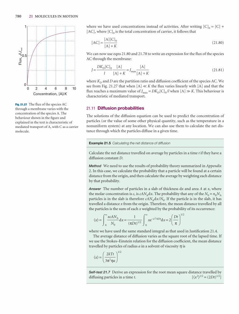
780 21 MOLECULES IN MOTION
0 2 4 6 8 100
0.5
1
Concentration, [A]/K
Flux
,/JJ m
ax
Fig. 21.27 The flux of the species ACthrough a membrane varies with theconcentration of the species A. Thebehaviour shown in the figure andexplained in the text is characteristic ofmediated transport of A, with C as a carriermolecule.
where we have used concentrations instead of activities. After writing [C]0 = [C] +[AC], where [C]0 is the total concentration of carrier, it follows that
[AC] = (21.80)
We can now use eqns 21.80 and 21.78 to write an expression for the flux of the speciesAC through the membrane:
J = = Jmax (21.81)
where KD and D are the partition ratio and diffusion coefficient of the species AC. Wesee from Fig. 21.27 that when [A] << K the flux varies linearly with [A] and that theflux reaches a maximum value of Jmax = DKD[C]0 /l when [A] >> K. This behaviour ischaracteristic of mediated transport.
21.11 Diffusion probabilities
The solutions of the diffusion equation can be used to predict the concentration ofparticles (or the value of some other physical quantity, such as the temperature in anonuniform system) at any location. We can also use them to calculate the net dis-tance through which the particles diffuse in a given time.
Example 21.5 Calculating the net distance of diffusion
Calculate the net distance travelled on average by particles in a time t if they have adiffusion constant D.
Method We need to use the results of probability theory summarized in Appendix2. In this case, we calculate the probability that a particle will be found at a certaindistance from the origin, and then calculate the average by weighting each distanceby that probability.
Answer The number of particles in a slab of thickness dx and area A at x, where the molar concentration is c, is cANAdx. The probability that any of the N0 = n0NA
particles is in the slab is therefore cANAdx /N0. If the particle is in the slab, it hastravelled a distance x from the origin. Therefore, the mean distance travelled by allthe particles is the sum of each x weighted by the probability of its occurrence:
�x� = �∞
0
dx = �∞
0
xe−x2/4Dtdx = 2
1/2
where we have used the same standard integral as that used in Justification 21.4.The average distance of diffusion varies as the square root of the lapsed time. If
we use the Stokes–Einstein relation for the diffusion coefficient, the mean distancetravelled by particles of radius a in a solvent of viscosity η is
�x� =1/2
Self-test 21.7 Derive an expression for the root mean square distance travelled bydiffusing particles in a time t. [�x2�1/2 = (2Dt)1/2]
DF
2kTt
3π2ηa
AC
DF
Dt
π
AC
1
(πDt)1/2
xcANA
N0
[A]
[A] + K
[A]
[A] + K
DKD[C]0
l
[A][C]0
[A] + K
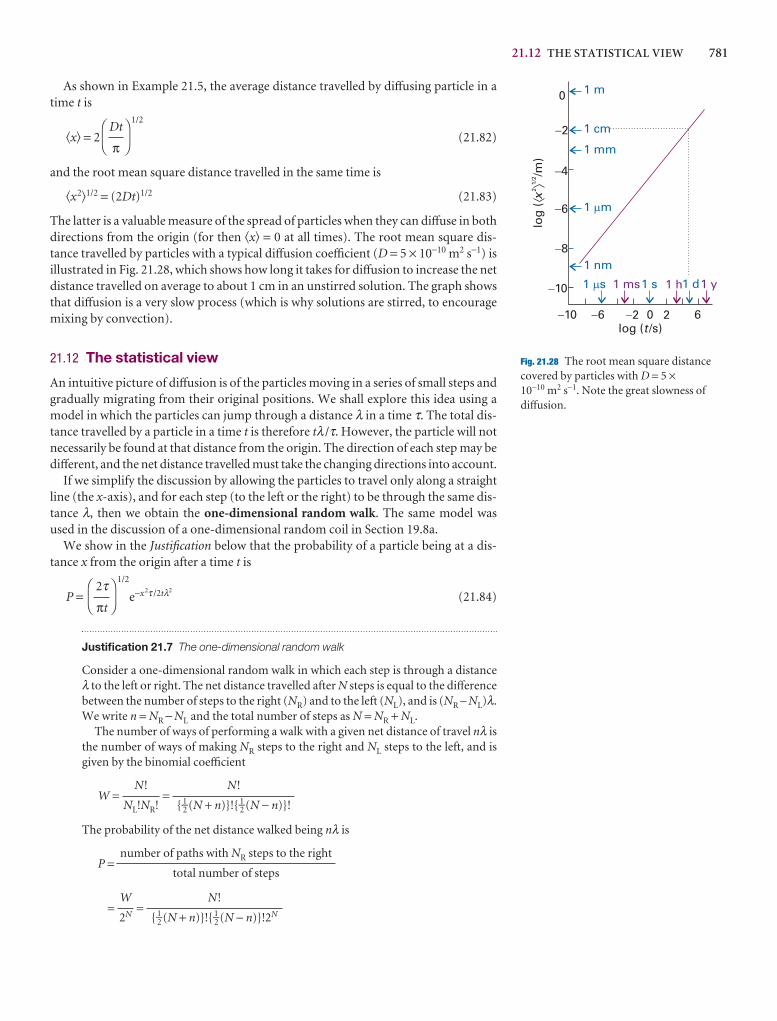
21.12 THE STATISTICAL VIEW 781
As shown in Example 21.5, the average distance travelled by diffusing particle in atime t is
�x� = 2
1/2
(21.82)
and the root mean square distance travelled in the same time is
�x2�1/2 = (2Dt)1/2 (21.83)
The latter is a valuable measure of the spread of particles when they can diffuse in bothdirections from the origin (for then �x� = 0 at all times). The root mean square dis-tance travelled by particles with a typical diffusion coefficient (D = 5 × 10⁻¹⁰ m2 s−1) isillustrated in Fig. 21.28, which shows how long it takes for diffusion to increase the netdistance travelled on average to about 1 cm in an unstirred solution. The graph showsthat diffusion is a very slow process (which is why solutions are stirred, to encouragemixing by convection).
21.12 The statistical view
An intuitive picture of diffusion is of the particles moving in a series of small steps andgradually migrating from their original positions. We shall explore this idea using amodel in which the particles can jump through a distance λ in a time τ. The total dis-tance travelled by a particle in a time t is therefore tλ /τ. However, the particle will notnecessarily be found at that distance from the origin. The direction of each step may bedifferent, and the net distance travelled must take the changing directions into account.
If we simplify the discussion by allowing the particles to travel only along a straightline (the x-axis), and for each step (to the left or the right) to be through the same dis-tance λ, then we obtain the one-dimensional random walk. The same model wasused in the discussion of a one-dimensional random coil in Section 19.8a.
We show in the Justification below that the probability of a particle being at a dis-tance x from the origin after a time t is
P =1/2
e−x2τ /2tλ2(21.84)
Justification 21.7 The one-dimensional random walk
Consider a one-dimensional random walk in which each step is through a distanceλ to the left or right. The net distance travelled after N steps is equal to the differencebetween the number of steps to the right (NR) and to the left (NL), and is (NR −NL)λ.We write n = NR − NL and the total number of steps as N = NR + NL.
The number of ways of performing a walk with a given net distance of travel nλ isthe number of ways of making NR steps to the right and NL steps to the left, and isgiven by the binomial coefficient
W = =
The probability of the net distance walked being nλ is
P =
= = N!
{ 1–2 (N + n)}!{ 1–2 (N − n)}!2N
W
2N
number of paths with NR steps to the right
total number of steps
N!
{ 1–2 (N + n)}!{ 1–2 (N − n)}!
N!
NL!NR!
DF
2τπt
AC
DF
Dt
π
AC
0
�2
�4
�6
�8
�10
log
(/m
)x
2 1
/2
�10 �6 �2 0 2 6log ( /s)t
1 m
1 cm
1 mm
1 m
1 nm
1 s 1 ms1 s 1 d1 y1 h
Fig. 21.28 The root mean square distancecovered by particles with D = 5 ×10⁻¹⁰ m2 s−1. Note the great slowness ofdiffusion.
782 21 MOLECULES IN MOTION
The use of Stirling’s approximation (Section 16.1a) in the form
ln x! ≈ ln(2π)1/2 + (x + 1–2 ) ln x − x
gives (after quite a lot of algebra; see Problem 21.33)
ln P = ln
1/2
− 1–2 (N + n + 1)ln 1 + − 1–2 (N − n + 1)ln 1 −
For small net distances (n << N ) we can use the approximation ln(1 ± x) ≈ ±x − 1–2 x2,and so obtain
ln P ≈ ln
1/2
−
At this point, we note that the number of steps taken in a time t is N = t/τ and the netdistance travelled from the origin is x = nλ. Substitution of these quantities into theexpression for ln P gives
ln P ≈ ln
1/2
−
which, upon using eln x = x and ex+y = exey, rearranges into eqn 21.84.
The differences of detail between eqns 21.72 and 21.84 arise from the fact that in thepresent calculation the particles can migrate in either direction from the origin.Moreover, they can be found only at discrete points separated by λ instead of beinganywhere on a continuous line. The fact that the two expressions are so similar sug-gests that diffusion can indeed be interpreted as the outcome of a large number ofsteps in random directions.
We can now relate the coefficient D to the step length λ and the rate at which thejumps occur. Thus, by comparing the two exponents in eqns 21.72 and 21.84 we canimmediately write down the Einstein–Smoluchowski equation:
D = (21.85)
Illustration 21.6 Using the Einstein–Smoluchowski equation
Suppose that a SO42− ion jumps through its own diameter each time it makes a
move in an aqueous solution; then, because D = 1.1 × 10⁻⁹ m2 s−1 and a = 210 pm(as deduced from mobility measurements), it follows from λ = 2a that τ = 80 ps.Because τ is the time for one jump, the ion makes 1 × 10¹⁰ jumps per second.
The Einstein–Smoluchowski equation is the central connection between the micro-scopic details of particle motion and the macroscopic parameters relating to diffusion(for example, the diffusion coefficient and, through the Stokes–Einstein relation, theviscosity). It also brings us back full circle to the properties of the perfect gas. For if weinterpret λ /τ as K, the mean speed of the molecules, and interpret λ as a mean freepath, then we can recognize in the Einstein–Smoluchowski equation exactly the sameexpression as we obtained from the kinetic model of gases, eqn 21.22. That is, thediffusion of a perfect gas is a random walk with an average step size equal to the meanfree path.
λ2
2τ
x2τ2tλ2
DEF2τπt
ABC
n2
2N
DEF2
πN
ABC
DEFn
N
ABCDEF
n
N
ABCDEF
2
πN
ABC

FURTHER READING 783
Checklist of key ideas
1. Diffusion is the migration of matter down a concentrationgradient; thermal conduction is the migration of energy downa temperature gradient; electric conduction is the migration ofelectric charge along an electrical potential gradient; viscosityis the migration of linear momentum down a velocitygradient.
2. The kinetic model of a gas considers only the contribution to the energy from the kinetic energies of the molecules.Important results from the model include expressions for the pressure (pV = 1–3nMc 2) and the root mean square speed (c = �v2�1/2 = (3RT/M)1/2).
3. The Maxwell distribution of speeds is the function which,through f(v)dv, gives the fraction of molecules that havespeeds in the range v to v + dv.
4. The collision frequency is the number of collisions made by amolecule in an interval divided by the length of the interval: z = σKrelN , where the collision cross-section is σ = πd2.
5. The mean free path is the average distance a molecule travelsbetween collisions: λ = K/z.
6. The collision flux, ZW, is the number of collisions with an areain a given time interval divided by the area and the duration ofthe interval: Zw = p/(2πmkT)1/2.
7. Effusion is the emergence of a gas from a container through asmall hole. Graham’s law of effusion states that the rate ofeffusion is inversely proportional to the square root of themolar mass.
8. Flux J is the quantity of a property passing through a givenarea in a given time interval divided by the area and theduration of the interval.
9. Fick’s first law of diffusion states that the flux of matter is proportional to the concentration gradient, J(matter)= −DdN /dz, where D is the diffusion coefficient.
10. The conductance, G, is the inverse of resistance. Theconductivity is the constant κ in G = κA/l and the molarconductivity is written as Λm = κ /c.
11. A strong electrolyte is an electrolyte with a molar conductivitythat varies only slightly with concentration. A weak electrolyte
is an electrolyte with a molar conductivity that is normal atconcentrations close to zero, but falls sharply to low values asthe concentration increases.
12. Kohlrausch’s law for the concentration dependence of themolar conductivity of a strong electrolyte is written as Λm =Λ°m − K c1/2, where the limiting molar conductivity, Λ°m, is themolar conductivity at zero concentration (Λ°m = ν+λ+ + ν−λ−).
13. The drift speed s is the terminal speed when an acceleratingforce is balanced by the viscous drag: s = uE , where u =ze/6πηa is the ionic mobility and a is the hydrodynamic radius(Stokes radius), the effective radius of a particle in solution.
14. The ionic conductivity is the contribution of ions of one typeto the molar conductivity: λ = zuF.
15. The transport number is the fraction of total current I carriedby the ions of a specified type: t± = I±/I.
16. The Debye–Hückel–Onsager theory explains theconcentration dependence of the molar conductivity of astrong electrolyte in terms of ionic interactions.
17. The Einstein relation between the diffusion coefficient and theionic mobility is D = uRT/zF.
18. The Nernst–Einstein relation between the molar conductivityof an electrolyte and the diffusion coefficients of its ions is Λm = (ν+z 2
+D+ + ν −z2−D−)(F 2/RT).
19. The Stokes–Einstein equation relates the diffusion coefficientto the frictional force: D = kT/f.
20. Walden’s rule states that the product ηΛm is veryapproximately constant for the same ions in different solvents.
21. The diffusion equation is a relation between the rate of changeof concentration at a point and the spatial variation of theconcentration at that point: ∂c/∂t = D∂2c/∂x2.
22. In a one-dimensional random walk, the probability Pthat a molecule moves a distance x from the origin for aperiod t by taking small steps with size λ and time τ is: P =(2τ /π t)1/2e−x 2τ/2tλ2
.
23. The Einstein–Smoluchowski equation relates the diffusioncoefficient to the parameters used in the formulation of therandom walk model, D = λ2/2τ.
Further reading
Articles and texts
D.G. Leaist, Diffusion and ionic conduction in liquids. InEncyclopedia of applied physics (ed. G.L. Trigg), 5, 661 VCH, New York (1993).
A.J. Bard and L.R. Faulkner, Electrochemical methods: fundamentalsand applications. Wiley, New York (2000).
R.B. Bird, W.E. Stewart, and E.N. Lightfoot, Transport phenomena.Wiley, New-York (1960).
J.N. Murrell and A.D. Jenkins, Properties of liquids and solutions.Wiley-Interscience, New York (1994).
K.E. van Holde, W.C. Johnson, and P.S. Ho, Principles of physicalbiochemistry. Prentice Hall, Upper Saddle River (1998).
A.J. Walton, Three phases of matter. Oxford University Press (1983).
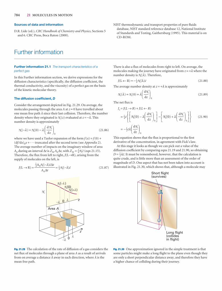
784 21 MOLECULES IN MOTION
Sources of data and information
D.R. Lide (ed.), CRC Handbook of Chemistry and Physics, Sections 5and 6. CRC Press, Boca Raton (2000).
NIST thermodynamic and transport properties of pure fluidsdatabase, NIST standard reference database 12, National Instituteof Standards and Testing, Gaithersburg (1995). This material is onCD-ROM.
N ( )�N (0)
N ( )�N
�
�
0
0
�
�
z
z
Area A
�
�
�
�
Fig. 21.29 The calculation of the rate of diffusion of a gas considers thenet flux of molecules through a plane of area A as a result of arrivalsfrom on average a distance λ away in each direction, where λ is themean free path.
Short flight(survives)
Long flight(collidesin flight)
Fig. 21.30 One approximation ignored in the simple treatment is thatsome particles might make a long flight to the plane even though theyare only a short perpendicular distance away, and therefore they havea higher chance of colliding during their journey.
Further information
Further information 21.1 The transport characteristics of a perfect gas
In this Further information section, we derive expressions for thediffusion characteristics (specifically, the diffusion coefficient, thethermal conductivity, and the viscosity) of a perfect gas on the basisof the kinetic molecular theory.
The diffusion coefficient, D
Consider the arrangement depicted in Fig. 21.29. On average, themolecules passing through the area A at z = 0 have travelled aboutone mean free path λ since their last collision. Therefore, the numberdensity where they originated is N (z) evaluated at z = −λ. Thisnumber density is approximately
N (−λ) = N (0) − λ0
(21.86)
where we have used a Taylor expansion of the form f (x) = f (0) +(df /dx)0x + · · · truncated after the second term (see Appendix 2).The average number of impacts on the imaginary window of area A0 during an interval ∆t is ZW A0∆t, with ZW = 1–4N K (eqn 21.15).Therefore, the flux from left to right, J(L→R), arising from the supply of molecules on the left, is
J(L → R) = = 1–4 N (−λ)K (21.87)1–4A0N (−λ)K∆t
A0∆t
DEFdN
dz
ABC
There is also a flux of molecules from right to left. On average, themolecules making the journey have originated from z = +λ where thenumber density is N (λ). Therefore,
J(L ← R) = − 1–4 N (λ)K (21.88)
The average number density at z = +λ is approximately
N (λ) = N (0) + λ0
(21.89)
The net flux is
Jz = J(L → R) + J(L ← R)
= 1–4K N (0) − λ0
− N (0) + λ0
(21.90)
= − 1–2Kλ0
This equation shows that the flux is proportional to the firstderivative of the concentration, in agreement with Fick’s law.
At this stage it looks as though we can pick out a value of thediffusion coefficient by comparing eqns 21.19 and 21.90, so obtainingD = 1–2λK. It must be remembered, however, that the calculation isquite crude, and is little more than an assessment of the order ofmagnitude of D. One aspect that has not been taken into account isillustrated in Fig. 21.30, which shows that, although a molecule may
DEFdN
dz
ABC
567
JKLDEF
dN
dz
ABCGHI
JKLDEF
dN
dz
ABCGHI
123
DEFdN
dz
ABC
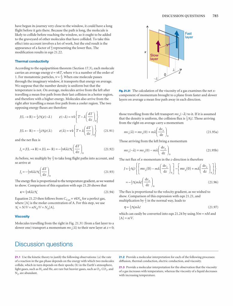
DISCUSSION QUESTIONS 785
have begun its journey very close to the window, it could have a longflight before it gets there. Because the path is long, the molecule islikely to collide before reaching the window, so it ought to be addedto the graveyard of other molecules that have collided. To take thiseffect into account involves a lot of work, but the end result is theappearance of a factor of 2–3 representing the lower flux. Themodification results in eqn 21.22.
Thermal conductivity
According to the equipartition theorem (Section 17.3), each moleculecarries an average energy ε = νkT, where ν is a number of the order of1. For monatomic particles, ν = 3–2. When one molecule passesthrough the imaginary window, it transports that energy on average.We suppose that the number density is uniform but that thetemperature is not. On average, molecules arrive from the left aftertravelling a mean free path from their last collision in a hotter region,and therefore with a higher energy. Molecules also arrive from theright after travelling a mean free path from a cooler region. The twoopposing energy fluxes are therefore
J(L → R) = 1–4 KN ε(−λ ) ε(−λ) = ν k T − λ0
J(L ← R) = − 1–4 KN ε(λ) ε(λ) = ν k T + λ0
(21.91)
and the net flux is
Jz = J(L → R) + J(L ← R) = − 1–2νkλKN0
(21.92)
As before, we multiply by 2–3 to take long flight paths into account, andso arrive at
Jz = − 1–3νkλKN0
(21.93)
The energy flux is proportional to the temperature gradient, as we wantedto show. Comparison of this equation with eqn 21.20 shows that
κ = 1–3νkλKN (21.94)
Equation 21.23 then follows from CV,m = νkNA for a perfect gas,where [A] is the molar concentration of A. For this step, we use N = N/V = nNA/V = NA[A].
Viscosity
Molecules travelling from the right in Fig. 21.31 (from a fast layer to aslower one) transport a momentum mvx(λ) to their new layer at z = 0;
DEFdT
dz
ABC
DEFdT
dz
ABC
567
DEFdT
dz
ABC123
567
DEFdT
dz
ABC123
those travelling from the left transport mvx(−λ) to it. If it is assumedthat the density is uniform, the collision flux is 1–4 N K. Those arrivingfrom the right on average carry a momentum
mvx(λ) = mvx(0) + mλ0
(21.95a)
Those arriving from the left bring a momentum
mvx(−λ) = mvx(0) − mλ0
(21.95b)
The net flux of x-momentum in the z-direction is therefore
J = 1–4 N K mvx(0) − mλ0
− mvx(0) + mλ0
= − 1–2N mλK0
(21.96)
The flux is proportional to the velocity gradient, as we wished toshow. Comparison of this expression with eqn 21.21, andmultiplication by 2–3 in the normal way, leads to
η = 1–3NmλK (21.97)
which can easily be converted into eqn 21.24 by using Nm = nM and[A] = n/V.
DEFdvx
dz
ABC
567
JKLDEF
dvx
dz
ABCGHI
JKLDEF
dvx
dz
ABCGHI
123
DEFdvx
dz
ABC
DEFdvx
dz
ABC
Slowlayer
Fastlayer
0�
�
z
x
�
Fig. 21.31 The calculation of the viscosity of a gas examines the net x-component of momentum brought to a plane from faster and slowerlayers on average a mean free path away in each direction.
Discussion questions
21.1 Use the kinetic theory to justify the following observations: (a) the rateof a reaction in the gas phase depends on the energy with which two moleculescollide, which in turn depends on their speeds; (b) in the Earth’s atmosphere,light gases, such as H2 and He, are rare but heavier gases, such as O2, CO2, andN2, are abundant.
21.2 Provide a molecular interpretation for each of the following processes:diffusion, thermal conduction, electric conduction, and viscosity.
21.3 Provide a molecular interpretation for the observation that the viscosityof a gas increases with temperature, whereas the viscosity of a liquid decreaseswith increasing temperature.

786 21 MOLECULES IN MOTION
21.4 Discuss the mechanism of proton conduction in liquid water.
21.5 Limit the generality of the following expressions: (a) J = −D(dc/dx),(b) D = kT/f, and (c) D = kT/6πηa.
21.6 Provide a molecular interpretation for the observation that mediatedtransport across a biological membrane leads to a maximum flux Jmax whenthe concentration of the transported species becomes very large.
21.7 Discuss how nuclear magnetic resonance spectroscopy, inelastic neutronscattering, and dynamic light scattering may be used to measure the mobilityof molecules in liquids.
Exercises
21.1a Determine the ratios of (a) the mean speeds, (b) the mean kineticenergies of H2 molecules and Hg atoms at 20°C.
21.1b Determine the ratios of (a) the mean speeds, (b) the mean kineticenergies of He atoms and Hg atoms at 25°C.
21.2a A 1.0 dm3 glass bulb contains 1.0 × 10²³ H2 molecules. If the pressureexerted by the gas is 100 kPa, what are (a) the temperature of the gas, (b) theroot mean square speeds of the molecules? (c) Would the temperature bedifferent if they were O2 molecules?
21.2b The best laboratory vacuum pump can generate a vacuum of about 1 nTorr. At 25°C and assuming that air consists of N2 molecules with acollision diameter of 395 pm, calculate (a) the mean speed of the molecules,(b) the mean free path, (c) the collision frequency in the gas.
21.3a At what pressure does the mean free path of argon at 25°C becomecomparable to the size of a 1 dm3 vessel that contains it? Take σ = 0.36 nm2.
21.3b At what pressure does the mean free path of argon at 25°C becomecomparable to the diameters of the atoms themselves?
21.4a At an altitude of 20 km the temperature is 217 K and the pressure 0.050 atm. What is the mean free path of N2 molecules? (σ = 0.43 nm2.)
21.4b At an altitude of 15 km the temperature is 217 K and the pressure 12.1 kPa. What is the mean free path of N2 molecules? (σ = 0.43 nm2.)
21.5a How many collisions does a single Ar atom make in 1.0 s when thetemperature is 25°C and the pressure is (a) 10 atm, (b) 1.0 atm, (c) 1.0 µatm?
21.5b How many collisions per second does an N2 molecule make at analtitude of 15 km? (See Exercise 21.4b for data.)
21.6a Calculate the mean free path of molecules in air using σ = 0.43 nm2 at25°C and (a) 10 atm, (b) 1.0 atm, (c) 1.0 µatm.
21.6b Calculate the mean free path of carbon dioxide molecules using σ = 0.52 nm2 at 25°C and (a) 15 atm, (b) 1.0 bar, (c) 1.0 Torr.
21.7a Use the Maxwell distribution of speeds to estimate the fraction of N2
molecules at 500 K that have speeds in the range 290 to 300 m s−1.
21.7b Use the Maxwell distribution of speeds to estimate the fraction of CO2
molecules at 300 K that have speeds in the range 200 to 250 m s−1.
21.8a A solid surface with dimensions 2.5 mm × 3.0 mm is exposed to argongas at 90 Pa and 500 K. How many collisions do the Ar atoms make with thissurface in 15 s?
21.8b A solid surface with dimensions 3.5 mm × 4.0 cm is exposed to heliumgas at 111 Pa and 1500 K. How many collisions do the He atoms make withthis surface in 10 s?
21.9a An effusion cell has a circular hole of diameter 2.50 mm. If the molarmass of the solid in the cell is 260 g mol−1 and its vapour pressure is 0.835 Pa at400 K, by how much will the mass of the solid decrease in a period of 2.00 h?
21.9b An effusion cell has a circular hole of diameter 3.00 mm. If the molarmass of the solid in the cell is 300 g mol−1 and its vapour pressure is 0.224 Pa at450 K, by how much will the mass of the solid decrease in a period of 24.00 h?
21.10a A manometer was connected to a bulb containing carbon dioxideunder slight pressure. The gas was allowed to escape through a small pinhole,and the time for the manometer reading to drop from 75 cm to 50 cm was 52 s. When the experiment was repeated using nitrogen (for which M = 28.02 g mol−1) the same fall took place in 42 s. Calculate the molar mass of carbon dioxide.
21.10b A manometer was connected to a bulb containing nitrogen underslight pressure. The gas was allowed to escape through a small pinhole, and thetime for the manometer reading to drop from 65.1 cm to 42.1 cm was 18.5 s.When the experiment was repeated using a fluorocarbon gas, the same falltook place in 82.3 s. Calculate the molar mass of the fluorocarbon.
21.11a A space vehicle of internal volume 3.0 m3 is struck by a meteor and ahole of radius 0.10 mm is formed. If the oxygen pressure within the vehicle isinitially 80 kPa and its temperature 298 K, how long will the pressure take tofall to 70 kPa?
21.11b A container of internal volume 22.0 m3 was punctured, and a hole ofradius 0.050 mm was formed. If the nitrogen pressure within the vehicle isinitially 122 kPa and its temperature 293 K, how long will the pressure take tofall to 105 kPa?
21.12a Calculate the flux of energy arising from a temperature gradient of 2.5 K m−1 in a sample of argon in which the mean temperature is 273 K.
21.12b Calculate the flux of energy arising from a temperature gradient of 3.5 K m−1 in a sample of hydrogen in which the mean temperature is 260 K.
21.13a Use the experimental value of the thermal conductivity of neon (Table 21.2) to estimate the collision cross-section of Ne atoms at 273 K.
21.13b Use the experimental value of the thermal conductivity of nitrogen(Table 21.2) to estimate the collision cross-section of N2 molecules at 298 K.
21.14a In a double-glazed window, the panes of glass are separated by 5.0 cm.What is the rate of transfer of heat by conduction from the warm room (25°C)to the cold exterior (−10°C) through a window of area 1.0 m2? What power ofheater is required to make good the loss of heat?
21.14b Two sheets of copper of area 1.50 m2 are separated by 10.0 cm. Whatis the rate of transfer of heat by conduction from the warm sheet (50°C) to thecold sheet (−10°C). What is the rate of loss of heat?
21.15a Use the experimental value of the coefficient of viscosity for neon(Table 21.2) to estimate the collision cross-section of Ne atoms at 273 K.
21.15b Use the experimental value of the coefficient of viscosity for nitrogen(Table 21.2) to estimate the collision cross-section of the molecules at 273 K.
21.16a Calculate the inlet pressure required to maintain a flow rate of 9.5 × 10⁵ dm3 h−1 of nitrogen at 293 K flowing through a pipe of length 8.50 m

EXERCISES 787
and diameter 1.00 cm. The pressure of gas as it leaves the tube is 1.00 bar. The volume of the gas is measured at that pressure.
21.16b Calculate the inlet pressure required to maintain a flow rate of 8.70 cm3 s−1 of nitrogen at 300 K flowing through a pipe of length 10.5 m and diameter 15 mm. The pressure of gas as it leaves the tube is 1.00 bar. The volume of the gas is measured at that pressure.
21.17a Calculate the viscosity of air at (a) 273 K, (b) 298 K, (c) 1000 K. Takeσ ≈ 0.40 nm2. (The experimental values are 173 µP at 273 K, 182 µP at 20°C,and 394 µP at 600°C.)
21.17b Calculate the viscosity of benzene vapour at (a) 273 K, (b) 298 K, (c) 1000 K. Take σ ≈ 0.88 nm2.
21.18a Calculate the thermal conductivities of (a) argon, (b) helium at 300 Kand 1.0 mbar. Each gas is confined in a cubic vessel of side 10 cm, one wallbeing at 310 K and the one opposite at 295 K. What is the rate of flow ofenergy as heat from one wall to the other in each case?
21.18b Calculate the thermal conductivities of (a) neon, (b) nitrogen at 300 Kand 15 mbar. Each gas is confined in a cubic vessel of side 15 cm, one wallbeing at 305 K and the one opposite at 295 K. What is the rate of flow ofenergy as heat from one wall to the other in each case?
21.19a The viscosity of carbon dioxide was measured by comparing its rate offlow through a long narrow tube (using Poiseuille’s formula) with that ofargon. For the same pressure differential, the same volume of carbon dioxidepassed through the tube in 55 s as argon in 83 s. The viscosity of argon at 25°Cis 208 µP; what is the viscosity of carbon dioxide? Estimate the moleculardiameter of carbon dioxide.
21.19b The viscosity of a chlorofluorocarbon (CFC) was measured bycomparing its rate of flow through a long narrow tube (using Poiseuille’sformula) with that of argon. For the same pressure differential, the samevolume of the CFC passed through the tube in 72.0 s as argon in 18.0 s. Theviscosity of argon at 25°C is 208 µP; what is the viscosity of the CFC? Estimatethe molecular diameter of the CFC. Take M = 200 g mol−1.
21.20a Calculate the thermal conductivity of argon (CV,m = 12.5 J K−1 mol−1,σ = 0.36 nm2) at room temperature (20°C).
21.20b Calculate the thermal conductivity of nitrogen (CV,m = 20.8 J K−1
mol−1, σ = 0.43 nm2) at room temperature (20°C).
21.21a Calculate the diffusion constant of argon at 25°C and (a) 1.00 Pa, (b) 100 kPa, (c) 10.0 MPa. If a pressure gradient of 0.10 atm cm−1 isestablished in a pipe, what is the flow of gas due to diffusion?
21.21b Calculate the diffusion constant of nitrogen at 25°C and (a) 10.0 Pa,(b) 100 kPa, (c) 15.0 MPa. If a pressure gradient of 0.20 bar m−1 is establishedin a pipe, what is the flow of gas due to diffusion?
21.22a The mobility of a chloride ion in aqueous solution at 25°C is 7.91 × 10⁻⁸ m2 s−1 V−1. Calculate the molar ionic conductivity.
21.22b The mobility of an acetate ion in aqueous solution at 25°C is 4.24 × 10⁻⁸ m2 s−1 V−1. Calculate the molar ionic conductivity.
21.23a The mobility of a Rb+ ion in aqueous solution is 7.92 × 10⁻⁸ m2 s−1 V−1
at 25°C. The potential difference between two electrodes placed in the solutionis 35.0 V. If the electrodes are 8.00 mm apart, what is the drift speed of the Rb+ ion?
21.23b The mobility of a Li+ ion in aqueous solution is 4.01 × 10⁻⁸ m2 s−1 V−1
at 25°C. The potential difference between two electrodes placed in the solutionis 12.0 V. If the electrodes are 1.00 cm apart, what is the drift speed of the ion?
21.24a What fraction of the total current is carried by Li+ when current flowsthrough an aqueous solution of LiBr at 25°C?
21.24b What fraction of the total current is carried by Cl− when current flowsthrough an aqueous solution of NaCl at 25°C?
21.25a The limiting molar conductivities of KCl, KNO3, and AgNO3 are14.99 mS m2 mol−1, 14.50 mS m2 mol−1, and 13.34 mS m2 mol−1, respectively(all at 25°C). What is the limiting molar conductivity of AgCl at thistemperature?
21.25b The limiting molar conductivities of NaI, NaCH3CO2, andMg(CH3CO2)2 are 12.69 mS m2 mol−1, 9.10 mS m2 mol−1, and 18.78 mS m2
mol−1, respectively (all at 25°C). What is the limiting molar conductivity ofMgI2 at this temperature?
21.26a At 25°C the molar ionic conductivities of Li+, Na+, and K+ are3.87 mS m2 mol−1, 5.01 mS m2 mol−1, and 7.35 mS m2 mol−1, respectively.What are their mobilities?
21.26b At 25°C the molar ionic conductivities of F−, Cl−, and Br− are 5.54 mSm2 mol−1, 7.635 mS m2 mol−1, and 7.81 mS m2 mol−1, respectively. What aretheir mobilities?
21.27a The mobility of a NO3− ion in aqueous solution at 25°C is 7.40 ×
10−8 m2 s−1 V−1. Calculate its diffusion coefficient in water at 25°C.
21.27b The mobility of a CH3CO2− ion in aqueous solution at 25°C is
4.24 × 10⁻⁸ m2 s−1 V−1. Calculate its diffusion coefficient in water at 25°C.
21.28a The diffusion coefficient of CCl4 in heptane at 25°C is 3.17 × 10⁻⁹ m2
s−1. Estimate the time required for a CCl4 molecule to have a root mean squaredisplacement of 5.0 mm.
21.28b The diffusion coefficient of I2 in hexane at 25°C is 4.05 × 10⁻⁹ m2 s−1.Estimate the time required for an iodine molecule to have a root mean squaredisplacement of 1.0 cm.
21.29a Estimate the effective radius of a sucrose molecule in water 25°C giventhat its diffusion coefficient is 5.2 × 10⁻¹⁰ m2 s−1 and that the viscosity of wateris 1.00 cP.
21.29b Estimate the effective radius of a glycine molecule in water at 25°Cgiven that its diffusion coefficient is 1.055 × 10⁻⁹ m2 s−1 and that the viscosityof water is 1.00 cP.
21.30a The diffusion coefficient for molecular iodine in benzene is 2.13 × 10⁻⁹ m2 s−1. How long does a molecule take to jump through about one molecular diameter (approximately the fundamental jump length fortranslational motion)?
21.30b The diffusion coefficient for CCl4 in heptane is 3.17 × 10⁻⁹ m2 s−1.How long does a molecule take to jump through about one moleculardiameter (approximately the fundamental jump length for translationalmotion)?
21.31a What are the root mean square distances travelled by an iodinemolecule in benzene and by a sucrose molecule in water at 25°C in 1.0 s?
21.31b About how long, on average, does it take for the molecules in Exercise21.31a to drift to a point (a) 1.0 mm, (b) 1.0 cm from their starting points?
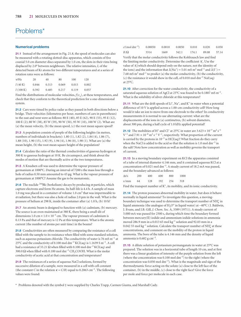
788 21 MOLECULES IN MOTION
Problems*
Numerical problems
21.1 Instead of the arrangement in Fig. 21.8, the speed of molecules can alsobe measured with a rotating slotted-disc apparatus, which consists of fivecoaxial 5.0 cm diameter discs separated by 1.0 cm, the slots in their rims beingdisplaced by 2.0° between neighbours. The relative intensities, I, of thedetected beam of Kr atoms for two different temperatures and at a series ofrotation rates were as follows:
ν/Hz 20 40 80 100 120
I (40 K) 0.846 0.513 0.069 0.015 0.002
I (100 K) 0.592 0.485 0.217 0.119 0.057
Find the distributions of molecular velocities, f(vx), at these temperatures, andcheck that they conform to the theoretical prediction for a one-dimensionalsystem.
21.2 Cars were timed by police radar as they passed in both directions below abridge. Their velocities (kilometres per hour, numbers of cars in parentheses)to the east and west were as follows: 80 E (40), 85 E (62), 90 E (53), 95 E (12),100 E (2); 80 W (38), 85 W (59), 90 W (50), 95 W (10), 100 W (2). What are(a) the mean velocity, (b) the mean speed, (c) the root mean square speed?
21.3 A population consists of people of the following heights (in metres,numbers of individuals in brackets): 1.80 (1), 1.82 (2), 1.84 (4), 1.86 (7), 1.88 (10), 1.90 (15), 1.92 (9), 1.94 (4), 1.96 (0), 1.98 (1). What are (a) themean height, (b) the root mean square height of the population?
21.4 Calculate the ratio of the thermal conductivities of gaseous hydrogen at300 K to gaseous hydrogen at 10 K. Be circumspect, and think about themodes of motion that are thermally active at the two temperatures.
21.5 A Knudsen cell was used to determine the vapour pressure ofgermanium at 1000°C. During an interval of 7200 s the mass loss through ahole of radius 0.50 mm amounted to 43 µg. What is the vapour pressure ofgermanium at 1000°C? Assume the gas to be monatomic.
21.6 The nuclide 244Bk (berkelium) decays by producing α particles, whichcapture electrons and form He atoms. Its half-life is 4.4 h. A sample of mass1.0 mg was placed in a container of volume 1.0 cm3 that was impermeable to α radiation, but there was also a hole of radius 2.0 µm in the wall. What is thepressure of helium at 298 K, inside the container after (a) 1.0 h, (b) 10 h?
21.7 An atomic beam is designed to function with (a) cadmium, (b) mercury.The source is an oven maintained at 380 K, there being a small slit ofdimensions 1.0 cm × 1.0 × 10−3 cm. The vapour pressure of cadmium is 0.13 Pa and that of mercury is 12 Pa at this temperature. What is the atomiccurrent (the number of atoms per unit time) in the beams?
21.8 Conductivities are often measured by comparing the resistance of a cellfilled with the sample to its resistance when filled with some standard solution,such as aqueous potassium chloride. The conductivity of water is 76 mS m−1 at25°C and the conductivity of 0.100 mol dm−3 KCl(aq) is 1.1639 S m−1. A cellhad a resistance of 33.21 Ω when filled with 0.100 mol dm−3 KCl(aq) and300.0 Ω when filled with 0.100 mol dm−3 CH3COOH. What is the molarconductivity of acetic acid at that concentration and temperature?
21.9 The resistances of a series of aqueous NaCl solutions, formed bysuccessive dilution of a sample, were measured in a cell with cell constant (the constant C in the relation κ = C/R) equal to 0.2063 cm−1. The followingvalues were found:
c/(mol dm−3) 0.00050 0.0010 0.0050 0.010 0.020 0.050
R /Ω 3314 1669 342.1 174.1 89.08 37.14
Verify that the molar conductivity follows the Kohlrausch law and find the limiting molar conductivity. Determine the coefficient K . Use the value of K (which should depend only on the nature, not the identity of the ions) and the information that λ(Na+) = 5.01 mS m2 mol−1 and λ(I−) =7.68 mS m2 mol−1 to predict (a) the molar conductivity, (b) the conductivity, (c) the resistance it would show in the cell, of 0.010 mol dm−3 NaI(aq)at 25°C.
21.10 After correction for the water conductivity, the conductivity of asaturated aqueous solution of AgCl at 25°C was found to be 0.1887 mS m−1.What is the solubility of silver chloride at this temperature?
21.11 What are the drift speeds of Li+, Na+, and K+ in water when a potentialdifference of 10 V is applied across a 1.00-cm conductivity cell? How longwould it take an ion to move from one electrode to the other? In conductivitymeasurements it is normal to use alternating current: what are thedisplacements of the ions in (a) centimetres, (b) solvent diameters, about 300 pm, during a half cycle of 1.0 kHz applied potential?
21.12 The mobilities of H+ and Cl− at 25°C in water are 3.623 × 10⁻⁷ m2 s−1
V−1 and 7.91 × 10⁻⁸ m2 s−1 V−1, respectively. What proportion of the current is carried by the protons in 10−3 m HCl(aq)? What fraction do they carry when the NaCl is added to the acid so that the solution is 1.0 mol dm−3 inthe salt? Note how concentration as well as mobility governs the transport of current.
21.13 In a moving boundary experiment on KCl the apparatus consisted of a tube of internal diameter 4.146 mm, and it contained aqueous KCl at aconcentration of 0.021 mol dm−3. A steady current of 18.2 mA was passed, and the boundary advanced as follows:
∆t/s 200 400 600 800 1000
x /mm 64 128 192 254 318
Find the transport number of K+, its mobility, and its ionic conductivity.
21.14 The proton possesses abnormal mobility in water, but does it behavenormally in liquid ammonia? To investigate this question, a moving-boundary technique was used to determine the transport number of NH4
+ inliquid ammonia (the analogue of H3O+ in liquid water) at −40°C (J. Baldwin,J. Evans, and J.B. Gill, J. Chem. Soc. A, 3389 (1971)). A steady current of 5.000 mA was passed for 2500 s, during which time the boundary formedbetween mercury(II) iodide and ammonium iodide solutions in ammoniamoved 286.9 mm in a 0.013 65 mol kg−1 solution and 92.03 mm in a 0.042 55 mol kg−1 solution. Calculate the transport number of NH4
+ at theseconcentrations, and comment on the mobility of the proton in liquidammonia. The bore of the tube is 4.146 mm and the density of liquidammonia is 0.682 g cm−3.
21.15 A dilute solution of potassium permanganate in water at 25°C wasprepared. The solution was in a horizontal tube of length 10 cm, and at firstthere was a linear gradation of intensity of the purple solution from the left(where the concentration was 0.100 mol dm−3) to the right (where theconcentration was 0.050 mol dm−3). What is the magnitude and sign of thethermodynamic force acting on the solute (a) close to the left face of thecontainer, (b) in the middle, (c) close to the right face? Give the force per mole and force per molecule in each case.
* Problems denoted with the symbol ‡ were supplied by Charles Trapp, Carmen Giunta, and Marshall Cady.
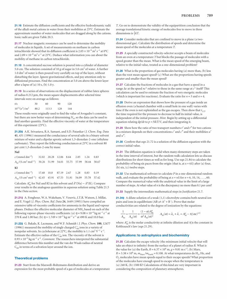
PROBLEMS 789
21.16 Estimate the diffusion coefficients and the effective hydrodynamic radiiof the alkali metal cations in water from their mobilities at 25°C. Estimate theapproximate number of water molecules that are dragged along by the cations.Ionic radii are given Table 20.3.
21.17 Nuclear magnetic resonance can be used to determine the mobility of molecules in liquids. A set of measurements on methane in carbontetrachloride showed that its diffusion coefficient is 2.05 × 10⁻⁹ m2 s−1 at 0°Cand 2.89 × 10⁻⁹ m2 s−1 at 25°C. Deduce what information you can about themobility of methane in carbon tetrachloride.
21.18 A concentrated sucrose solution is poured into a cylinder of diameter5.0 cm. The solution consisted of 10 g of sugar in 5.0 cm3 of water. A further1.0 dm3 of water is then poured very carefully on top of the layer, withoutdisturbing the layer. Ignore gravitational effects, and pay attention only todiffusional processes. Find the concentration at 5.0 cm above the lower layerafter a lapse of (a) 10 s, (b) 1.0 y.
21.19 In a series of observations on the displacement of rubber latex spheresof radius 0.212 µm, the mean square displacements after selected timeintervals were on average as follows:
t/s 30 60 90 120
1012�x2 � /m2 88.2 113.5 128 144
These results were originally used to find the value of Avogadro’s constant,but there are now better ways of determining NA, so the data can be used tofind another quantity. Find the effective viscosity of water at the temperatureof this experiment (25°C).
21.20‡ A.K. Srivastava, R.A. Samant, and S.D. Patankar (J. Chem. Eng. Data41, 431 (1996)) measured the conductance of several salts in a binary solventmixture of water and a dipolar aprotic solvent 1,3-dioxolan-2-one (ethylenecarbonate). They report the following conductances at 25°C in a solvent 80per cent 1,3-dioxolan-2-one by mass:
NaI
c /(mmol dm−3) 32.02 20.28 12.06 8.64 2.85 1.24 0.83
Λm /(S cm2 mol−1) 50.26 51.99 54.01 55.75 57.99 58.44 58.67
KI
c /(mmol dm−3) 17.68 10.8 87.19 2.67 1.28 0.83 0.19
Λm /(S cm2 mol−1) 42.45 45.91 47.53 51.81 54.09 55.78 57.42
Calculate Λ°m for NaI and KI in this solvent and λ°(Na) − λ°(K). Compareyour results to the analogous quantities in aqueous solution using Table 21.5in the Data section.
21.21‡ A. Fenghour, W.A. Wakeham, V. Vesovic, J.T.R. Watson, J. Millat,and E. Vogel ( J. Phys. Chem. Ref. Data 24, 1649 (1995)) have compiled anextensive table of viscosity coefficients for ammonia in the liquid and vapourphases. Deduce the effective molecular diameter of NH3 based on each of thefollowing vapour-phase viscosity coefficients: (a) η = 9.08 × 10⁻⁶ kg m−1 s−1 at270 K and 1.00 bar; (b) η = 1.749 × 10⁻⁵ kg m−1 s−1 at 490 K and 10.0 bar.
21.22‡ G. Bakale, K. Lacmann, and W.F. Schmidt ( J. Phys. Chem. 100, 12477(1996)) measured the mobility of singly charged C−
60 ions in a variety ofnonpolar solvents. In cyclohexane at 22°C, the mobility is 1.1 cm2 V−1 s−1.Estimate the effective radius of the C−
60 ion. The viscosity of the solvent is 0.93 × 10⁻³ kg m−1 s−1. Comment. The researchers interpreted the substantialdifference between this number and the van der Waals radius of neutral C60 in terms of a solvation layer around the ion.
Theoretical problems
21.23 Start from the Maxwell–Boltzmann distribution and derive anexpression for the most probable speed of a gas of molecules at a temperature
T. Go on to demonstrate the validity of the equipartition conclusion that theaverage translational kinetic energy of molecules free to move in threedimensions is 3–
2kT.
21.24 Consider molecules that are confined to move in a plane (a two-dimensional gas). Calculate the distribution of speeds and determine themean speed of the molecules at a temperature T.
21.25 A specially constructed velocity-selector accepts a beam of moleculesfrom an oven at a temperature T but blocks the passage of molecules with aspeed greater than the mean. What is the mean speed of the emerging beam,relative to the initial value, treated as a one-dimensional problem?
21.26 What is the proportion of gas molecules having (a) more than, (b) lessthan the root mean square speed? (c) What are the proportions having speedsgreater and smaller than the mean speed?
21.27 Calculate the fractions of molecules in a gas that have a speed in a range ∆v at the speed nc* relative to those in the same range at c* itself? Thiscalculation can be used to estimate the fraction of very energetic molecules(which is important for reactions). Evaluate the ratio for n = 3 and n = 4.
21.28 Derive an expression that shows how the pressure of a gas inside aneffusion oven (a heated chamber with a small hole in one wall) varies withtime if the oven is not replenished as the gas escapes. Then show that t1/2,the time required for the pressure to decrease to half its initial value, isindependent of the initial pressure. Hint. Begin by setting up a differentialequation relating dp/dt to p = NkT/V, and then integrating it.
21.29 Show how the ratio of two transport numbers t ′ and t″ for two cationsin a mixture depends on their concentrations c′ and c″ and their mobilities u′and u″.
21.30 Confirm that eqn 21.72 is a solution of the diffusion equation with thecorrect initial value.
21.31 The diffusion equation is valid when many elementary steps are takenin the time interval of interest, but the random walk calculation lets us discussdistributions for short times as well as for long. Use eqn 21.84 to calculate theprobability of being six paces from the origin (that is, at x = 6λ) after (a) four,(b) six, (c) twelve steps.
21.32 Use mathematical software to calculate P in a one-dimensional randomwalk, and evaluate the probability of being at x = nλ for n = 6, 10, 14, . . . , 60.Compare the numerical value with the analytical value in the limit of a largenumber of steps. At what value of n is the discrepancy no more than 0.1 per cent?
21.33 Supply the intermediate mathematical steps in Justification 21.7.
21.34‡ A dilute solution of a weak (1,1)-electrolyte contains both neutral ionpairs and ions in equilibrium (AB 5 A+ + B−). Prove that molarconductivities are related to the degree of ionization by the equations:
= + Λm(α) = λ+ + λ− = Λ°m − K (αc)1/2
where Λ°m is the molar conductivity at infinite dilution and K is the constant inKohlrausch’s law (eqn 21.29).
Applications: to astrophysics and biochemistry
21.35 Calculate the escape velocity (the minimum initial velocity that willtake an object to infinity) from the surface of a planet of radius R. What is the value for (a) the Earth, R = 6.37 × 10⁶ m, g = 9.81 m s−2, (b) Mars, R = 3.38 × 10⁶ m, mMars /mEarth = 0.108. At what temperatures do H2, He, andO2 molecules have mean speeds equal to their escape speeds? What proportionof the molecules have enough speed to escape when the temperature is (a) 240 K, (b) 1500 K? Calculations of this kind are very important inconsidering the composition of planetary atmospheres.
(1 − α)Λ°m
α2Λm(α)2
1
Λm(α)
1
Λm
790 21 MOLECULES IN MOTION
21.36‡ Interstellar space is a medium quite different from the gaseousenvironments we commonly encounter on Earth. For instance, a typicaldensity of the medium is about 1 atom cm−3 and that atom is typically H; theeffective temperature due to stellar background radiation is about 10 000 K.Estimate the diffusion coefficient and thermal conductivity of H under theseconditions. Comment. Energy is in fact transferred much more effectively byradiation.
21.37 The principal components of the atmosphere of the Earth are diatomicmolecules, which can rotate as well as translate. Given that the translationalkinetic energy density of the atmosphere is 0.15 J cm−3, what is the total kineticenergy density, including rotation?
21.38‡ In the standard model of stellar structure (I. Nicholson, The sun. RandMcNally, New York (1982)), the interior of the Sun is thought to consist of 36per cent H and 64 per cent He by mass, at a density of 158 g cm−3. Both atomsare completely ionized. The approximate dimensions of the nuclei can becalculated from the formula rnucleus = 1.4 × 10⁻¹⁵ A1/3 m, where A is the massnumber. The size of the free electron, re ≈ 10−18 m, is negligible compared tothe size of the nuclei. (a) Calculate the excluded volume in 1.0 cm3 of thestellar interior and on that basis decide upon the applicability of the perfectgas law to this system. (b) The standard model suggests that the pressure in the stellar interior is 2.5 × 10¹¹ atm. Calculate the temperature of the Sun’sinterior based on the perfect gas model. The generally accepted standardmodel value is 16 MK. (c) Would a van der Waals type of equation (with a = 0) give a better value for T?
21.39 Enrico Fermi, the great Italian scientist, was a master at making goodapproximate calculations based on little or no actual data. Hence, suchcalculations are often called ‘Fermi calculations’. Do a Fermi calculation on how long it would take for a gaseous air-borne cold virus of molar mass 100 kg mol−1 to travel the distance between two conversing people 1.0 m apart by diffusion in still air.
21.40 The diffusion coefficient of a particular kind of t-RNA molecule is D = 1.0 × 10⁻¹¹ m2 s−1 in the medium of a cell interior. How long does it takemolecules produced in the cell nucleus to reach the walls of the cell at adistance 1.0 µm, corresponding to the radius of the cell?
21.41‡ In this problem, we examine a model for the transport of oxygen fromair in the lungs to blood. First, show that, for the initial and boundaryconditions c(x,t) = c(x,0) = c0, (0 < x < ∞) and c(0,t) = cs, (0 ≤ t ≤ ∞ ) where c0 and cs are constants, the concentration, c(x,t), of a species is given by
c(x,t) = c0 + (cs − c0){1 − erfξ} ξ(x,t) =
where erfξ is the error function (Justification 9.4) and the concentration c(x,t)evolves by diffusion from the yz-plane of constant concentration, such asmight occur if a condensed phase is absorbing a species from a gas phase. Nowdraw graphs of concentration profiles at several different times of your choicefor the diffusion of oxygen into water at 298 K (when D = 2.10 × 10⁻⁹ m2 s−1)on a spatial scale comparable to passage of oxygen from lungs through alveoliinto the blood. Use c0 = 0 and set cs equal to the solubility of oxygen in water.Hint. Use mathematical software.
x
(4Dt)1/2
The rates of chemicalreactions
This chapter is the first of a sequence that explores the rates of chemical reactions. Thechapter begins with a discussion of the definition of reaction rate and outlines the tech-niques for its measurement. The results of such measurements show that reaction rates depend on the concentration of reactants (and products) in characteristic ways that can beexpressed in terms of differential equations known as rate laws. The solutions of theseequations are used to predict the concentrations of species at any time after the start of thereaction. The form of the rate law also provides insight into the series of elementary stepsby which a reaction takes place. The key task in this connection is the construction of a ratelaw from a proposed mechanism and its comparison with experiment. Simple elementarysteps have simple rate laws, and these rate laws can be combined together by invoking one or more approximations. These approximations include the concept of the rate-determining stage of a reaction, the steady-state concentration of a reaction intermediate,and the existence of a pre-equilibrium.
This chapter introduces the principles of chemical kinetics, the study of reaction rates,by showing how the rates of reactions may be measured and interpreted. The remain-ing chapters of this part of the text then develop this material in more detail and applyit to more complicated or more specialized cases. The rate of a chemical reactionmight depend on variables under our control, such as the pressure, the temperature,and the presence of a catalyst, and we may be able to optimize the rate by the appro-priate choice of conditions. The study of reaction rates also leads to an understandingof the mechanisms of reactions, their analysis into a sequence of elementary steps.
Empirical chemical kinetics
The first steps in the kinetic analysis of reactions are to establish the stoichiometry ofthe reaction and identify any side reactions. The basic data of chemical kinetics arethen the concentrations of the reactants and products at different times after a reac-tion has been initiated. The rates of most chemical reactions are sensitive to the tem-perature, so in conventional experiments the temperature of the reaction mixturemust be held constant throughout the course of the reaction. This requirement putssevere demands on the design of an experiment. Gas-phase reactions, for instance, are often carried out in a vessel held in contact with a substantial block of metal.Liquid-phase reactions, including flow reactions, must be carried out in an efficientthermostat. Special efforts have to be made to study reactions at low temperatures, as in the study of the kinds of reactions that take place in interstellar clouds. Thus, supersonic expansion of the reaction gas can be used to attain temperatures as low as
22Empirical chemical kinetics
22.1 Experimental techniques
22.2 The rates of reactions
22.3 Integrated rate laws
22.4 Reactions approachingequilibrium
22.5 The temperature dependenceof reaction rates
Accounting for the rate laws
22.6 Elementary reactions
22.7 Consecutive elementaryreactions
I22.1 Impact on biochemistry: Thekinetics of the helix–coiltransition in polypeptides
22.8 Unimolecular reactions
Checklist of key ideas
Further reading
Further information 22.1: The RRKmodel of unimolecular reactions
Discussion questions
Exercises
Problems
792 22 THE RATES OF CHEMICAL REACTIONS
10 K. For work in the liquid phase and the solid phase, very low temperatures are oftenreached by flowing cold liquid or cold gas around the reaction vessel. Alternatively,the entire reaction vessel is immersed in a thermally insulated container filled with acryogenic liquid, such as liquid helium (for work at around 4 K) or liquid nitrogen(for work at around 77 K). Non-isothermal conditions are sometimes employed. For instance, the shelf-life of an expensive pharmaceutical may be explored by slowlyraising the temperature of a single sample.
22.1 Experimental techniques
The method used to monitor concentrations depends on the species involved and therapidity with which their concentrations change. Many reactions reach equilibriumover periods of minutes or hours, and several techniques may then be used to followthe changing concentrations.
(a) Monitoring the progress of a reaction
A reaction in which at least one component is a gas might result in an overall changein pressure in a system of constant volume, so its progress may be followed by record-ing the variation of pressure with time.
Example 22.1 Monitoring the variation in pressure
Predict how the total pressure varies during the gas-phase decomposition 2 N2O5(g)→ 4 NO2(g) + O2(g) in a constant-volume container.
Method The total pressure (at constant volume and temperature and assumingperfect gas behaviour) is proportional to the number of gas-phase molecules.Therefore, because each mole of N2O5 gives rise to 5–2 mol of gas molecules, we canexpect the pressure to rise to 5–2 times its initial value. To confirm this conclusion,express the progress of the reaction in terms of the fraction, α, of N2O5 moleculesthat have reacted.
Answer Let the initial pressure be p0 and the initial amount of N2O5 moleculespresent be n. When a fraction α of the N2O5 molecules has decomposed, theamounts of the components in the reaction mixture are:
N2O5 NO2 O2 Total
Amount: n(1 − α) 2αn 1–2αn n(1 + 3–2α)
When α = 0 the pressure is p0, so at any stage the total pressure is
p = (1 + 3–2α)p0
When the reaction is complete, the pressure will have risen to 5–2 times its initialvalue.
Self-test 22.1 Repeat the calculation for 2 NOBr(g) → 2 NO(g) + Br2(g).[p = (1 + 1–2α)p0]
Spectrophotometry, the measurement of absorption of radiation in a particularspectral region, is widely applicable, and is especially useful when one substance in thereaction mixture has a strong characteristic absorption in a conveniently accessibleregion of the electromagnetic spectrum. For example, the progress of the reaction
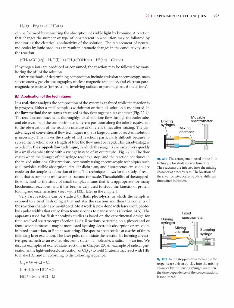
22.1 EXPERIMENTAL TECHNIQUES 793
H2(g) + Br2(g) → 2 HBr(g)
can be followed by measuring the absorption of visible light by bromine. A reactionthat changes the number or type of ions present in a solution may be followed bymonitoring the electrical conductivity of the solution. The replacement of neutralmolecules by ionic products can result in dramatic changes in the conductivity, as inthe reaction
(CH3)3CCl(aq) + H2O(l) → (CH3)3COH(aq) + H+(aq) + Cl−(aq)
If hydrogen ions are produced or consumed, the reaction may be followed by mon-itoring the pH of the solution.
Other methods of determining composition include emission spectroscopy, massspectrometry, gas chromatography, nuclear magnetic resonance, and electron para-magnetic resonance (for reactions involving radicals or paramagnetic d-metal ions).
(b) Application of the techniques
In a real-time analysis the composition of the system is analysed while the reaction isin progress. Either a small sample is withdrawn or the bulk solution is monitored. Inthe flow method the reactants are mixed as they flow together in a chamber (Fig. 22.1).The reaction continues as the thoroughly mixed solutions flow through the outlet tube,and observation of the composition at different positions along the tube is equivalentto the observation of the reaction mixture at different times after mixing. The dis-advantage of conventional flow techniques is that a large volume of reactant solutionis necessary. This makes the study of fast reactions particularly difficult because tospread the reaction over a length of tube the flow must be rapid. This disadvantage isavoided by the stopped-flow technique, in which the reagents are mixed very quicklyin a small chamber fitted with a syringe instead of an outlet tube (Fig. 22.2). The flowceases when the plunger of the syringe reaches a stop, and the reaction continues inthe mixed solutions. Observations, commonly using spectroscopic techniques such as ultraviolet–visible absorption, circular dichroism, and fluorescence emission, aremade on the sample as a function of time. The technique allows for the study of reac-tions that occur on the millisecond to second timescale. The suitability of the stopped-flow method to the study of small samples means that it is appropriate for manybiochemical reactions, and it has been widely used to study the kinetics of proteinfolding and enzyme action (see Impact I22.1 later in the chapter).
Very fast reactions can be studied by flash photolysis, in which the sample is exposed to a brief flash of light that initiates the reaction and then the contents of the reaction chamber are monitored. Most work is now done with lasers with photo-lysis pulse widths that range from femtoseconds to nanoseconds (Section 14.5). The apparatus used for flash photolysis studies is based on the experimental design fortime-resolved spectroscopy (Section 14.6). Reactions occurring on a picosecond orfemtosecond timescale may be monitored by using electronic absorption or emission,infrared absorption, or Raman scattering. The spectra are recorded at a series of timesfollowing laser excitation. The laser pulse can initiate the reaction by forming a react-ive species, such as an excited electronic state of a molecule, a radical, or an ion. Wediscuss examples of excited state reactions in Chapter 23. An example of radical gen-eration is the light-induced dissociation of Cl2(g) to yield Cl atoms that react with HBrto make HCl and Br according to the following sequence:
Cl2 + hν → Cl + Cl
Cl + HBr → HCl* + Br
HCl* + M → HCl + M
Mixingchamber
Drivingsyringes
Movablespectrometer
Mixingchamber
Drivingsyringes
Fixedspectrometer
Stoppingsyringe
Fig. 22.1 The arrangement used in the flowtechnique for studying reaction rates. The reactants are injected into the mixingchamber at a steady rate. The location ofthe spectrometer corresponds to differenttimes after initiation.
Fig. 22.2 In the stopped-flow technique thereagents are driven quickly into the mixingchamber by the driving syringes and thenthe time dependence of the concentrationsis monitored.
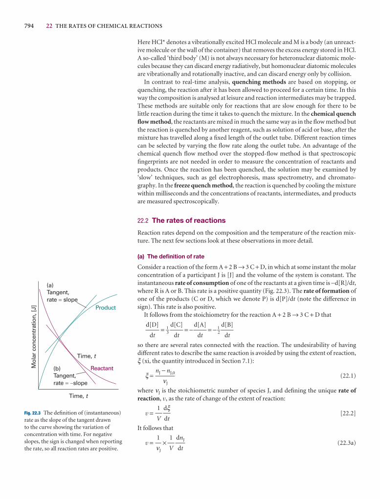
794 22 THE RATES OF CHEMICAL REACTIONS
Here HCl* denotes a vibrationally excited HCl molecule and M is a body (an unreact-ive molecule or the wall of the container) that removes the excess energy stored in HCl.A so-called ‘third body’ (M) is not always necessary for heteronuclear diatomic mole-cules because they can discard energy radiatively, but homonuclear diatomic moleculesare vibrationally and rotationally inactive, and can discard energy only by collision.
In contrast to real-time analysis, quenching methods are based on stopping, orquenching, the reaction after it has been allowed to proceed for a certain time. In thisway the composition is analysed at leisure and reaction intermediates may be trapped.These methods are suitable only for reactions that are slow enough for there to be little reaction during the time it takes to quench the mixture. In the chemical quenchflow method, the reactants are mixed in much the same way as in the flow method butthe reaction is quenched by another reagent, such as solution of acid or base, after themixture has travelled along a fixed length of the outlet tube. Different reaction timescan be selected by varying the flow rate along the outlet tube. An advantage of thechemical quench flow method over the stopped-flow method is that spectroscopicfingerprints are not needed in order to measure the concentration of reactants andproducts. Once the reaction has been quenched, the solution may be examined by‘slow’ techniques, such as gel electrophoresis, mass spectrometry, and chromato-graphy. In the freeze quench method, the reaction is quenched by cooling the mixturewithin milliseconds and the concentrations of reactants, intermediates, and productsare measured spectroscopically.
22.2 The rates of reactions
Reaction rates depend on the composition and the temperature of the reaction mix-ture. The next few sections look at these observations in more detail.
(a) The definition of rate
Consider a reaction of the form A + 2 B → 3 C + D, in which at some instant the molarconcentration of a participant J is [J] and the volume of the system is constant. The instantaneous rate of consumption of one of the reactants at a given time is −d[R]/dt,where R is A or B. This rate is a positive quantity (Fig. 22.3). The rate of formation ofone of the products (C or D, which we denote P) is d[P]/dt (note the difference insign). This rate is also positive.
It follows from the stoichiometry for the reaction A + 2 B → 3 C + D that
= 1–3 = − = − 1–2
so there are several rates connected with the reaction. The undesirability of havingdifferent rates to describe the same reaction is avoided by using the extent of reaction,ξ (xi, the quantity introduced in Section 7.1):
ξ = (22.1)
where νJ is the stoichiometric number of species J, and defining the unique rate of reaction, v, as the rate of change of the extent of reaction:
v = [22.2]
It follows that
v = × (22.3a)dnJ
dt
1
V
1
νJ
dξdt
1
V
nJ − nJ,0
νJ
d[B]
dt
d[A]
dt
d[C]
dt
d[D]
dt
Mol
ar c
once
ntra
tion,
[J]
Time, t
(b)Tangent,rate slope� �
(a)Tangent,rate slope�
Reactant
Product
Time, t
Fig. 22.3 The definition of (instantaneous) rate as the slope of the tangent drawn to the curve showing the variation ofconcentration with time. For negativeslopes, the sign is changed when reportingthe rate, so all reaction rates are positive.
22.2 THE RATES OF REACTIONS 795
(Remember that νJ is negative for reactants and positive for products.) For a homo-geneous reaction in a constant-volume system the volume V can be taken inside thedifferential and we use [J] = nJ /V to write
v = (22.3b)
For a heterogeneous reaction, we use the (constant) surface area, A, occupied by thespecies in place of V and use σJ = nJ /A to write
v = (22.3c)
In each case there is now a single rate for the entire reaction (for the chemical equa-tion as written). With molar concentrations in moles per cubic decimetre and time inseconds, reaction rates of homogeneous reactions are reported in moles per cubicdecimetre per second (mol dm−3 s−1) or related units. For gas-phase reactions, such asthose taking place in the atmosphere, concentrations are often expressed in moleculesper cubic centimetre (molecules cm−3) and rates in molecules per cubic centimetreper second (molecules cm−3 s−1). For heterogeneous reactions, rates are expressed inmoles per square metre per second (mol m−2 s−1) or related units.
Illustration 22.1 Rates of formation and consumption
If the rate of formation of NO in the reaction 2 NOBr(g) → 2 NO(g) + Br2(g) is reported as 0.16 mmol dm−3 s−1, we use νNO = +2 to report that v = 0.080 mmoldm−3 s−1. Because νNOBr = −2 it follows that d[NOBr]/dt = −0.16 mmol dm−3 s−1.The rate of consumption of NOBr is therefore 0.16 mmol dm−3 s−1, or 9.6 × 10¹⁶
molecules cm−3 s−1.
Self-test 22.2 The rate of change of molar concentration of CH3 radicals in the reaction 2 CH3(g) → CH3CH3(g) was reported as d[CH3]/dt = −1.2 mol dm−3 s−1
under particular conditions. What is (a) the rate of reaction and (b) the rate of formation of CH3CH3? [(a) 0.60 mol dm−3 s−1, (b) 0.60 mol dm−3 s−1]
(b) Rate laws and rate constants
The rate of reaction is often found to be proportional to the concentrations of the reactants raised to a power. For example, the rate of a reaction may be proportional tothe molar concentrations of two reactants A and B, so we write
v = k[A][B] (22.4)
with each concentration raised to the first power. The coefficient k is called the rateconstant for the reaction. The rate constant is independent of the concentrations but depends on the temperature. An experimentally determined equation of this kindis called the rate law of the reaction. More formally, a rate law is an equation that expresses the rate of reaction as a function of the concentrations of all the species pre-sent in the overall chemical equation for the reaction at some time:
v = f([A],[B], . . . ) [22.5a]
For homogeneous gas-phase reactions, it is often more convenient to express the rate law in terms of partial pressures, which are related to molar concentrations by pJ = RT[J]. In this case, we write
dσJ
dt
1
νJ
d[J]
dt
1
νJ
796 22 THE RATES OF CHEMICAL REACTIONS
v = f(pA,pB, . . . ) [22.5b]
The rate law of a reaction is determined experimentally, and cannot in general beinferred from the chemical equation for the reaction. The reaction of hydrogen andbromine, for example, has a very simple stoichiometry, H2(g) + Br2(g) → 2 HBr(g),but its rate law is complicated:
v = (22.6)
In certain cases the rate law does reflect the stoichiometry of the reaction, but that iseither a coincidence or reflects a feature of the underlying reaction mechanism (seelater).
A practical application of a rate law is that, once we know the law and the value of the rate constant, we can predict the rate of reaction from the composition of themixture. Moreover, as we shall see later, by knowing the rate law, we can go on to pre-dict the composition of the reaction mixture at a later stage of the reaction. Moreover,a rate law is a guide to the mechanism of the reaction, for any proposed mechanismmust be consistent with the observed rate law.
(c) Reaction order
Many reactions are found to have rate laws of the form
v = k[A]a[B]b · · · (22.7)
The power to which the concentration of a species (a product or a reactant) is raisedin a rate law of this kind is the order of the reaction with respect to that species. A reaction with the rate law in eqn 22.4 is first-order in A and first-order in B. The over-all order of a reaction with a rate law like that in eqn 22.7 is the sum of the individualorders, a + b + · · · . The rate law in eqn 22.4 is therefore second-order overall.
A reaction need not have an integral order, and many gas-phase reactions do not.For example, a reaction having the rate law
v = k[A]1/2[B] (22.8)
is half-order in A, first-order in B, and three-halves-order overall. Some reactionsobey a zero-order rate law, and therefore have a rate that is independent of the con-centration of the reactant (so long as some is present). Thus, the catalytic decomposi-tion of phosphine (PH3) on hot tungsten at high pressures has the rate law
v = k (22.9)
The PH3 decomposes at a constant rate until it has almost entirely disappeared. Zero-order reactions typically occur when there is a bottle-neck of some kind in the mechanism, as in heterogeneous reactions when the surface is saturated and thesubsequent reaction slow and in a number of enzyme reactions when there is a large excess of substrate relative to the enzyme.
When a rate law is not of the form in eqn 22.7, the reaction does not have an over-all order and may not even have definite orders with respect to each participant. Thus,although eqn 22.6 shows that the reaction of hydrogen and bromine is first-order inH2, the reaction has an indefinite order with respect to both Br2 and HBr and has nooverall order.
These remarks point to three problems. First, we must see how to identify the ratelaw and obtain the rate constant from the experimental data. We concentrate on thisaspect in this chapter. Second, we must see how to construct reaction mechanismsthat are consistent with the rate law. We shall introduce the techniques of doing so in
k[H2][Br2]3/2
[Br2] + k′[HBr]
22.2 THE RATES OF REACTIONS 797
this chapter and develop them further in Chapter 23. Third, we must account for thevalues of the rate constants and explain their temperature dependence. We shall see alittle of what is involved in this chapter, but leave the details until Chapter 24.
(d) The determination of the rate law
The determination of a rate law is simplified by the isolation method in which theconcentrations of all the reactants except one are in large excess. If B is in large excess,for example, then to a good approximation its concentration is constant throughoutthe reaction. Although the true rate law might be v = k[A][B], we can approximate [B]by [B]0, its initial value, and write
v = k′[A] k′ = k[B]0 (22.10)
which has the form of a first-order rate law. Because the true rate law has been forcedinto first-order form by assuming that the concentration of B is constant, eqn 22.10 iscalled a pseudofirst-order rate law. The dependence of the rate on the concentrationof each of the reactants may be found by isolating them in turn (by having all the othersubstances present in large excess), and so constructing a picture of the overall rate law.
In the method of initial rates, which is often used in conjunction with the isolationmethod, the rate is measured at the beginning of the reaction for several differentinitial concentrations of reactants. We shall suppose that the rate law for a reactionwith A isolated is v = k[A]a; then its initial rate, v0, is given by the initial values of theconcentration of A, and we write v0 = k[A]0
a. Taking logarithms gives:
log v0 = log k + a log [A]0 (22.11)
For a series of initial concentrations, a plot of the logarithms of the initial rates againstthe logarithms of the initial concentrations of A should be a straight line with slope a.
Example 22.2 Using the method of initial rates
The recombination of iodine atoms in the gas phase in the presence of argon wasinvestigated and the order of the reaction was determined by the method of initialrates. The initial rates of reaction of 2 I(g) + Ar(g) → I2(g) + Ar(g) were as follows:
[I]0 /(10−5 mol dm−3) 1.0 2.0 4.0 6.0
v0 /(mol dm−3 s−1) (a) 8.70 × 10− 4 3.48 × 10⁻³ 1.39 × 10⁻² 3.13 × 10⁻²
(b) 4.35 × 10⁻³ 1.74 × 10⁻² 6.96 × 10⁻² 1.57 × 10⁻¹
(c) 8.69 × 10⁻³ 3.47 × 10⁻² 1.38 × 10⁻¹ 3.13 × 10⁻¹
The Ar concentrations are (a) 1.0 mmol dm−3, (b) 5.0 mmol dm−3, and (c) 10.0mmol dm−3. Determine the orders of reaction with respect to the I and Ar atomconcentrations and the rate constant.
Method Plot the logarithm of the initial rate, log v0, against log [I]0 for a given concentration of Ar, and, separately, against log [Ar]0 for a given concentration ofI. The slopes of the two lines are the orders of reaction with respect to I and Ar, respectively. The intercepts with the vertical axis give log k.
Answer The plots are shown in Fig. 22.4. The slopes are 2 and 1, respectively, so the(initial) rate law is
v0 = k[I]20[Ar]0
This rate law signifies that the reaction is second-order in [I], first-order in [Ar],and third-order overall. The intercept corresponds to k = 9 × 10⁹ mol−2 dm6 s−1.
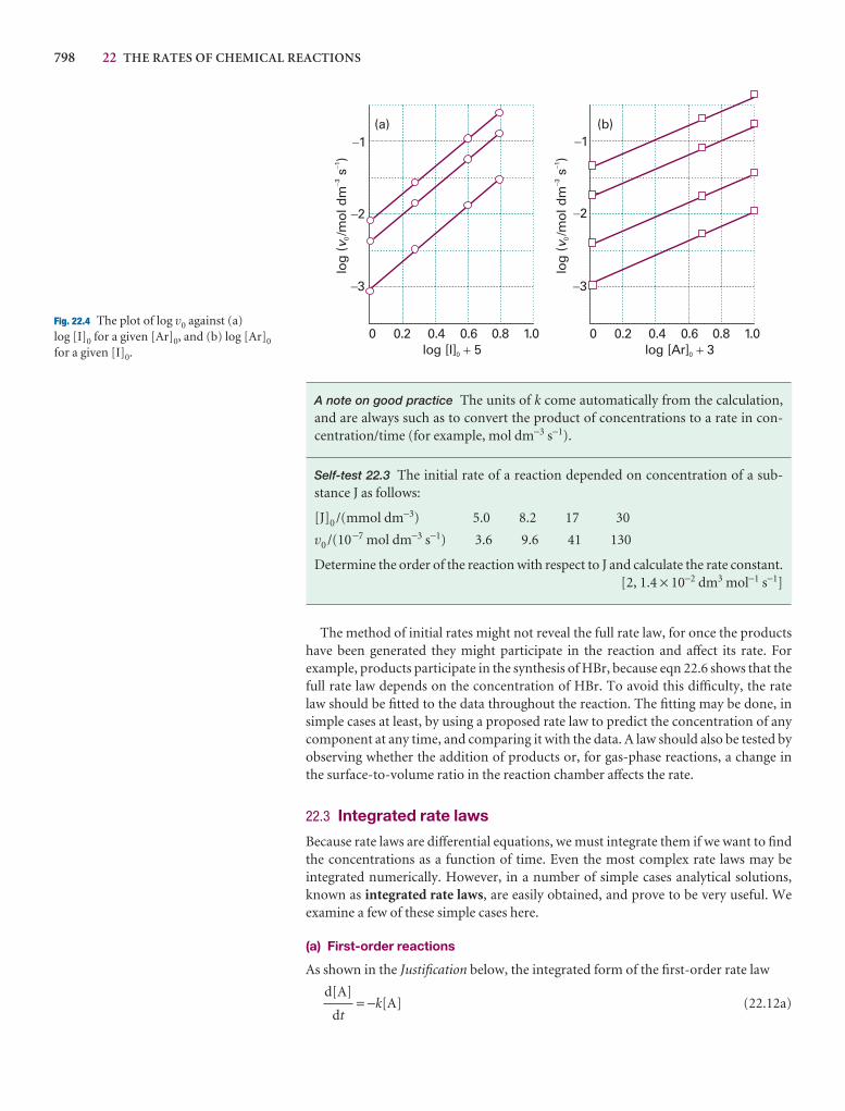
798 22 THE RATES OF CHEMICAL REACTIONS
�1
�2
�3
log
(/m
ol d
ms
)v 0
��
31
�1
�2
�3
0 00.2 0.20.4 0.40.6 0.60.8 0.81.0 1.0log [I] 50 � log [Ar] 30 �
(a)
log
(/m
ol d
ms
)v 0
��
31
(b)
Fig. 22.4 The plot of log v0 against (a) log [I]0 for a given [Ar]0, and (b) log [Ar]0
for a given [I]0.
A note on good practice The units of k come automatically from the calculation,and are always such as to convert the product of concentrations to a rate in con-centration/time (for example, mol dm−3 s−1).
Self-test 22.3 The initial rate of a reaction depended on concentration of a sub-stance J as follows:
[J]0 /(mmol dm−3) 5.0 8.2 17 30
v0 /(10−7 mol dm−3 s−1) 3.6 9.6 41 130
Determine the order of the reaction with respect to J and calculate the rate constant.[2, 1.4 × 10⁻² dm3 mol−1 s−1]
The method of initial rates might not reveal the full rate law, for once the productshave been generated they might participate in the reaction and affect its rate. For example, products participate in the synthesis of HBr, because eqn 22.6 shows that thefull rate law depends on the concentration of HBr. To avoid this difficulty, the rate law should be fitted to the data throughout the reaction. The fitting may be done, insimple cases at least, by using a proposed rate law to predict the concentration of anycomponent at any time, and comparing it with the data. A law should also be tested byobserving whether the addition of products or, for gas-phase reactions, a change inthe surface-to-volume ratio in the reaction chamber affects the rate.
22.3 Integrated rate laws
Because rate laws are differential equations, we must integrate them if we want to findthe concentrations as a function of time. Even the most complex rate laws may be integrated numerically. However, in a number of simple cases analytical solutions,known as integrated rate laws, are easily obtained, and prove to be very useful. We examine a few of these simple cases here.
(a) First-order reactions
As shown in the Justification below, the integrated form of the first-order rate law
= −k[A] (22.12a)d[A]
dt
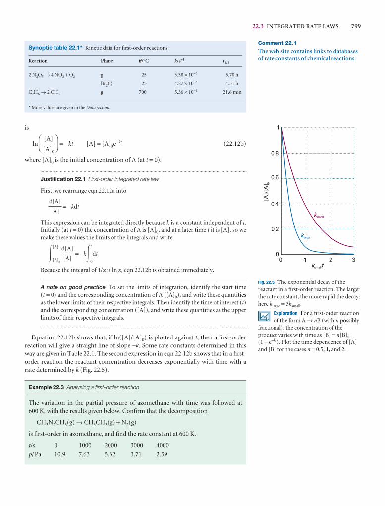
22.3 INTEGRATED RATE LAWS 799
is
ln = −kt [A] = [A]0e−kt (22.12b)
where [A]0 is the initial concentration of A (at t = 0).
Justification 22.1 First-order integrated rate law
First, we rearrange eqn 22.12a into
= −kdt
This expression can be integrated directly because k is a constant independent of t.Initially (at t = 0) the concentration of A is [A]0, and at a later time t it is [A], so wemake these values the limits of the integrals and write
�[A]
[A]0
= −k�t
0
dt
Because the integral of 1/x is ln x, eqn 22.12b is obtained immediately.
A note on good practice To set the limits of integration, identify the start time(t = 0) and the corresponding concentration of A ([A]0), and write these quantitiesas the lower limits of their respective integrals. Then identify the time of interest (t)and the corresponding concentration ([A]), and write these quantities as the upperlimits of their respective integrals.
Equation 22.12b shows that, if ln([A]/[A]0) is plotted against t, then a first-order reaction will give a straight line of slope −k. Some rate constants determined in thisway are given in Table 22.1. The second expression in eqn 22.12b shows that in a first-order reaction the reactant concentration decreases exponentially with time with arate determined by k (Fig. 22.5).
d[A]
[A]
d[A]
[A]
DF
[A]
[A]0
AC
Synoptic table 22.1* Kinetic data for first-order reactions
Reaction Phase q/°C k/s−1 t1/2
2 N2O5 → 4 NO2 + O2 g 25 3.38 × 10⁻⁵ 5.70 h
Br2(l) 25 4.27 × 10⁻⁵ 4.51 h
C2H6 → 2 CH3 g 700 5.36 × 10⁻⁴ 21.6 min
* More values are given in the Data section.
Comment 22.1
The web site contains links to databasesof rate constants of chemical reactions.
0
0.2
0.4
0.6
0.8
1
0 1 2 3k tsmall
[A]/[
A] 0
ksmall
klarge
Fig. 22.5 The exponential decay of thereactant in a first-order reaction. The largerthe rate constant, the more rapid the decay:here klarge = 3ksmall.
Exploration For a first-order reactionof the form A → nB (with n possibly
fractional), the concentration of theproduct varies with time as [B] = n[B]0
(1 − e−kt). Plot the time dependence of [A]and [B] for the cases n = 0.5, 1, and 2.
Example 22.3 Analysing a first-order reaction
The variation in the partial pressure of azomethane with time was followed at 600 K, with the results given below. Confirm that the decomposition
CH3N2CH3(g) → CH3CH3(g) + N2(g)
is first-order in azomethane, and find the rate constant at 600 K.
t/s 0 1000 2000 3000 4000
p/Pa 10.9 7.63 5.32 3.71 2.59
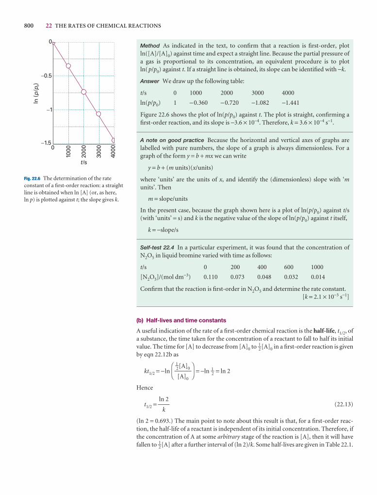
800 22 THE RATES OF CHEMICAL REACTIONS
0
1000
2000
3000
4000
t /s
�1.5
�1
�0.5
0ln
(/
)p
p 0
Fig. 22.6 The determination of the rateconstant of a first-order reaction: a straightline is obtained when ln [A] (or, as here, ln p) is plotted against t; the slope gives k.
Method As indicated in the text, to confirm that a reaction is first-order, plotln([A]/[A]0) against time and expect a straight line. Because the partial pressure ofa gas is proportional to its concentration, an equivalent procedure is to plotln(p/p0) against t. If a straight line is obtained, its slope can be identified with −k.
Answer We draw up the following table:
t/s 0 1000 2000 3000 4000
ln(p/p0) 1 −0.360 −0.720 −1.082 −1.441
Figure 22.6 shows the plot of ln(p/p0) against t. The plot is straight, confirming afirst-order reaction, and its slope is −3.6 × 10⁻⁴. Therefore, k = 3.6 × 10⁻⁴ s−1.
A note on good practice Because the horizontal and vertical axes of graphs arelabelled with pure numbers, the slope of a graph is always dimensionless. For agraph of the form y = b + mx we can write
y = b + (m units)(x/units)
where ‘units’ are the units of x, and identify the (dimensionless) slope with ‘munits’. Then
m = slope/units
In the present case, because the graph shown here is a plot of ln(p/p0) against t/s(with ‘units’ = s) and k is the negative value of the slope of ln(p/p0) against t itself,
k = −slope/s
Self-test 22.4 In a particular experiment, it was found that the concentration ofN2O5 in liquid bromine varied with time as follows:
t/s 0 200 400 600 1000
[N2O5]/(mol dm−3) 0.110 0.073 0.048 0.032 0.014
Confirm that the reaction is first-order in N2O5 and determine the rate constant.[k = 2.1 × 10⁻³ s−1]
(b) Half-lives and time constants
A useful indication of the rate of a first-order chemical reaction is the half-life, t1/2, ofa substance, the time taken for the concentration of a reactant to fall to half its initialvalue. The time for [A] to decrease from [A]0 to 1–2 [A]0 in a first-order reaction is givenby eqn 22.12b as
kt1/2 = −ln = −ln 1−2 = ln 2
Hence
t1/2 = (22.13)
(ln 2 = 0.693.) The main point to note about this result is that, for a first-order reac-tion, the half-life of a reactant is independent of its initial concentration. Therefore, ifthe concentration of A at some arbitrary stage of the reaction is [A], then it will havefallen to 1–2 [A] after a further interval of (ln 2)/k. Some half-lives are given in Table 22.1.
ln 2
k
DF
1−2[A]0
[A]0
AC
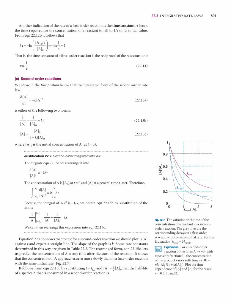
22.3 INTEGRATED RATE LAWS 801
Another indication of the rate of a first-order reaction is the time constant, τ (tau),the time required for the concentration of a reactant to fall to 1/e of its initial value.From eqn 22.12b it follows that
kτ = −ln = −ln = 1
That is, the time constant of a first-order reaction is the reciprocal of the rate constant:
τ = (22.14)
(c) Second-order reactions
We show in the Justification below that the integrated form of the second-order ratelaw
= −k[A]2 (22.15a)
is either of the following two forms:
− = kt (22.15b)
[A] = (22.15c)
where [A]0 is the initial concentration of A (at t = 0).
Justification 22.2 Second-order integrated rate law
To integrate eqn 22.15a we rearrange it into
= −kdt
The concentration of A is [A0] at t = 0 and [A] at a general time t later. Therefore,
−�[A]
[A]0
= k�t
0
dt
Because the integral of 1/x 2 is −1/x, we obtain eqn 22.15b by substitution of the limits
[A]
[A]0
= − = kt
We can then rearrange this expression into eqn 22.15c.
Equation 22.15b shows that to test for a second-order reaction we should plot 1/[A]against t and expect a straight line. The slope of the graph is k. Some rate constants determined in this way are given in Table 22.2. The rearranged form, eqn 22.15c, letsus predict the concentration of A at any time after the start of the reaction. It showsthat the concentration of A approaches zero more slowly than in a first-order reactionwith the same initial rate (Fig. 22.7).
It follows from eqn 22.15b by substituting t = t1/2 and [A] = 1–2 [A]0 that the half-lifeof a species A that is consumed in a second-order reaction is
1
[A]0
1
[A]
1
[A]
d[A]
[A]2
d[A]
[A]2
[A]0
1 + kt[A]0
1
[A]0
1
[A]
d[A]
dt
1
k
1
e
DF
[A]0 /e
[A]0
AC
1
0.8
0.6
0.4
0.2
00 1 2 3
[A]/[
A] 0
k tsmall 0[A]
ksmall
klarge
Fig. 22.7 The variation with time of theconcentration of a reactant in a second-order reaction. The grey lines are thecorresponding decays in a first-orderreaction with the same initial rate. For thisillustration, klarge = 3ksmall.
Exploration For a second-orderreaction of the form A → nB (with
n possibly fractional), the concentration of the product varies with time as [B] =nkt[A]2
0 /(1 + kt[A]0). Plot the timedependence of [A] and [B] for the cases n = 0.5, 1, and 2.
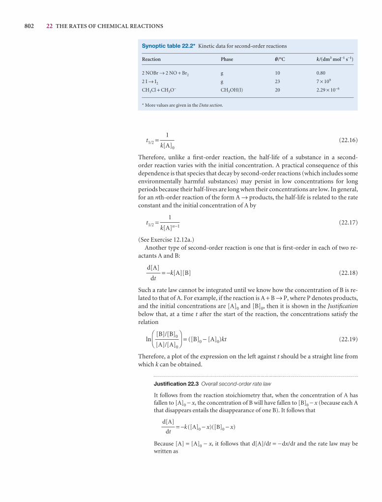
802 22 THE RATES OF CHEMICAL REACTIONS
t1/2 = (22.16)
Therefore, unlike a first-order reaction, the half-life of a substance in a second-order reaction varies with the initial concentration. A practical consequence of thisdependence is that species that decay by second-order reactions (which includes someenvironmentally harmful substances) may persist in low concentrations for long periods because their half-lives are long when their concentrations are low. In general,for an nth-order reaction of the form A → products, the half-life is related to the rateconstant and the initial concentration of A by
t1/2 = (22.17)
(See Exercise 12.12a.)Another type of second-order reaction is one that is first-order in each of two re-
actants A and B:
= −k[A][B] (22.18)
Such a rate law cannot be integrated until we know how the concentration of B is re-lated to that of A. For example, if the reaction is A + B → P, where P denotes products,and the initial concentrations are [A]0 and [B]0, then it is shown in the Justificationbelow that, at a time t after the start of the reaction, the concentrations satisfy the relation
ln = ([B]0 − [A]0)kt (22.19)
Therefore, a plot of the expression on the left against t should be a straight line fromwhich k can be obtained.
Justification 22.3 Overall second-order rate law
It follows from the reaction stoichiometry that, when the concentration of A hasfallen to [A]0 − x, the concentration of B will have fallen to [B]0 − x (because each Athat disappears entails the disappearance of one B). It follows that
= −k([A]0 − x)([B]0 − x)
Because [A] = [A]0 − x, it follows that d[A]/dt = −dx/dt and the rate law may bewritten as
d[A]
dt
DF
[B]/[B]0
[A]/[A]0
AC
d[A]
dt
1
k[A]n−1
1
k[A]0
Synoptic table 22.2* Kinetic data for second-order reactions
Reaction Phase q/°C k/(dm3 mol−1 s−1)
2 NOBr → 2 NO + Br2 g 10 0.80
2 I → I2 g 23 7 × 10⁹
CH3Cl + CH3O− CH3OH(l) 20 2.29 × 10⁻⁶
* More values are given in the Data section.
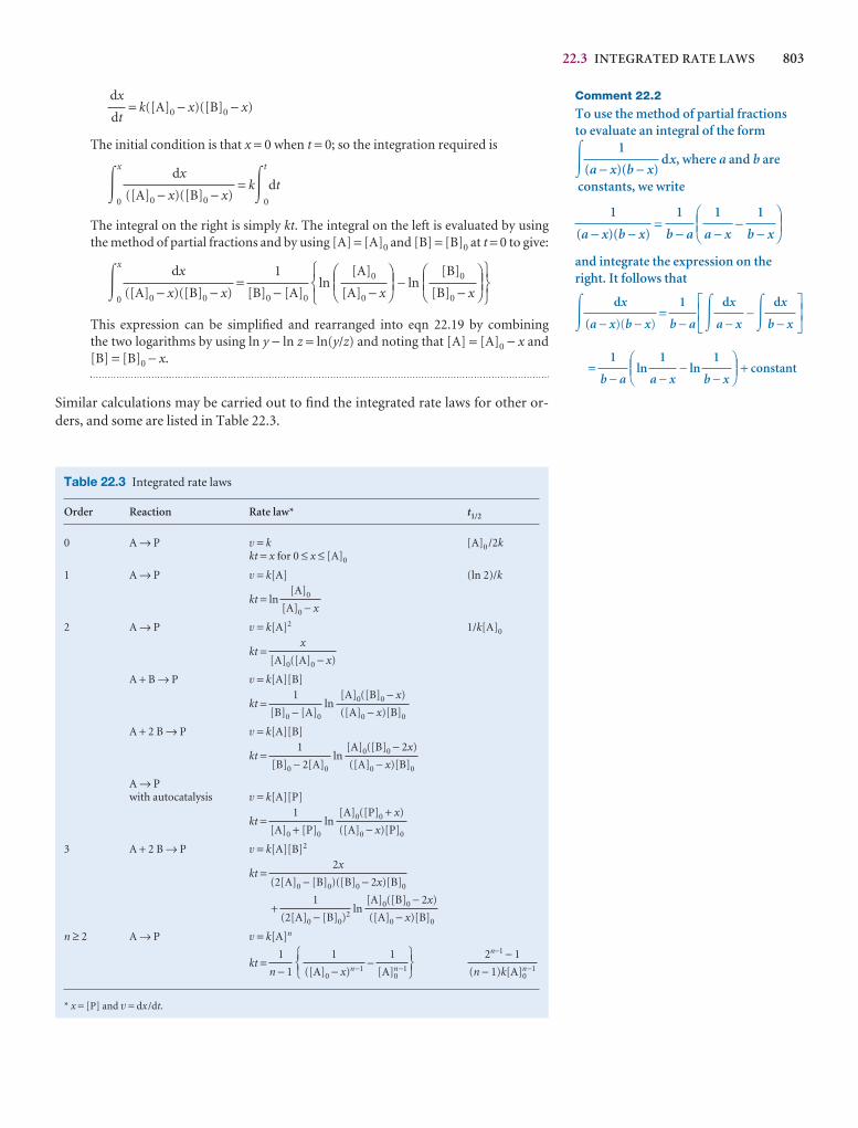
22.3 INTEGRATED RATE LAWS 803
= k([A]0 − x)([B]0 − x)
The initial condition is that x = 0 when t = 0; so the integration required is
�x
0
= k�t
0
dt
The integral on the right is simply kt. The integral on the left is evaluated by usingthe method of partial fractions and by using [A] = [A]0 and [B] = [B]0 at t = 0 to give:
�x
0
= ln − ln
This expression can be simplified and rearranged into eqn 22.19 by combining the two logarithms by using ln y − ln z = ln(y/z) and noting that [A] = [A]0 − x and[B] = [B]0 − x.
Similar calculations may be carried out to find the integrated rate laws for other or-ders, and some are listed in Table 22.3.
567
DEF[B]0
[B]0 − x
ABCDEF
[A]0
[A]0 − x
ABC123
1
[B]0 − [A]0
dx
([A]0 − x)([B]0 − x)
dx
([A]0 − x)([B]0 − x)
dx
dt
Comment 22.2
To use the method of partial fractions to evaluate an integral of the form
� dx, where a and b are
constants, we write
= −
and integrate the expression on theright. It follows that
� = � −�= ln − ln + constant
DEF1
b − x
1
a − x
ABC1
b − a
JKLdx
b − x
dx
a − x
GHI1
b − a
dx
(a − x)(b − x)
DEF1
b − x
1
a − x
ABC1
b − a
1
(a − x)(b − x)
1
(a − x)(b − x)
Table 22.3 Integrated rate laws
Order Reaction Rate law* t1/2
0 A → P v = k [A]0 /2kkt = x for 0 ≤ x ≤ [A]0
1 A → P v = k[A] (ln 2)/k
kt = ln
2 A → P v = k[A]2 1/k[A]0
kt =
A + B → P v = k[A][B]
kt = ln
A + 2 B → P v = k[A][B]
kt = ln
A → Pwith autocatalysis v = k[A][P]
kt = ln
3 A + 2 B → P v = k[A][B]2
kt =
+ ln
n ≥ 2 A → P v = k[A]n
kt = −
* x = [P] and v = dx /dt.
2n−1 − 1
(n − 1)k[A]0n−1
5671
[A]0n−1
1
([A]0 − x)n−1
1231
n − 1
[A]0([B]0 − 2x)
([A]0 − x)[B]0
1
(2[A]0 − [B]0)2
2x
(2[A]0 − [B]0)([B]0 − 2x)[B]0
[A]0([P]0 + x)
([A]0 − x)[P]0
1
[A]0 + [P]0
[A]0([B]0 − 2x)
([A]0 − x)[B]0
1
[B]0 − 2[A]0
[A]0([B]0 − x)
([A]0 − x)[B]0
1
[B]0 − [A]0
x
[A]0([A]0 − x)
[A]0
[A]0 − x
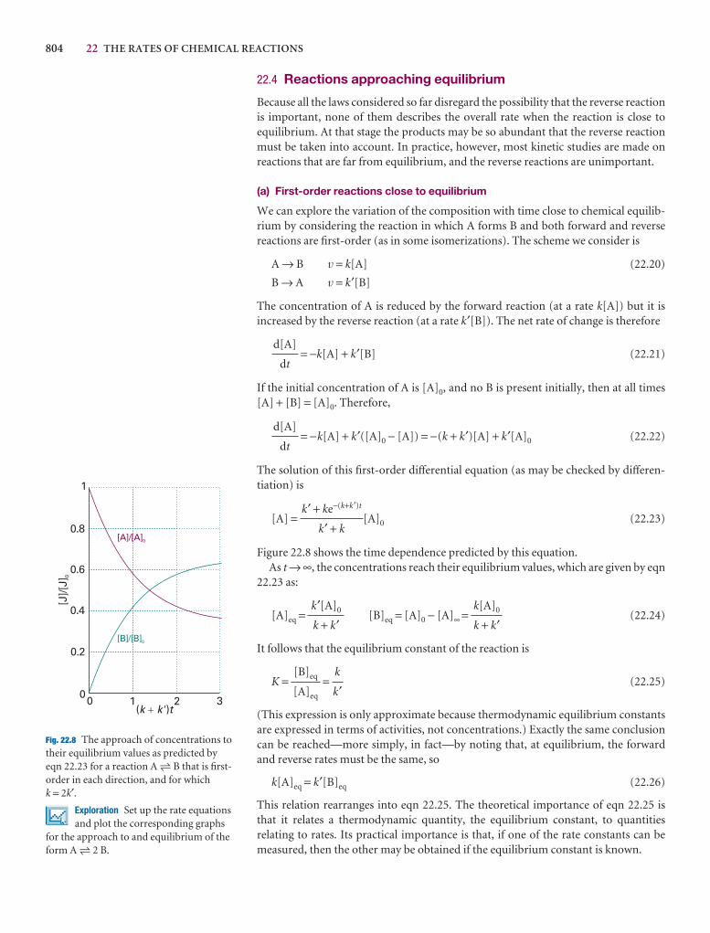
804 22 THE RATES OF CHEMICAL REACTIONS
22.4 Reactions approaching equilibrium
Because all the laws considered so far disregard the possibility that the reverse reactionis important, none of them describes the overall rate when the reaction is close toequilibrium. At that stage the products may be so abundant that the reverse reactionmust be taken into account. In practice, however, most kinetic studies are made on reactions that are far from equilibrium, and the reverse reactions are unimportant.
(a) First-order reactions close to equilibrium
We can explore the variation of the composition with time close to chemical equilib-rium by considering the reaction in which A forms B and both forward and reverse reactions are first-order (as in some isomerizations). The scheme we consider is
A → B v = k[A] (22.20)
B → A v = k′[B]
The concentration of A is reduced by the forward reaction (at a rate k[A]) but it is increased by the reverse reaction (at a rate k′[B]). The net rate of change is therefore
= −k[A] + k′[B] (22.21)
If the initial concentration of A is [A]0, and no B is present initially, then at all times[A] + [B] = [A]0. Therefore,
= −k[A] + k′([A]0 − [A]) = −(k + k′)[A] + k′[A]0 (22.22)
The solution of this first-order differential equation (as may be checked by differen-tiation) is
[A] = [A]0 (22.23)
Figure 22.8 shows the time dependence predicted by this equation.As t → ∞, the concentrations reach their equilibrium values, which are given by eqn
22.23 as:
[A]eq = [B]eq = [A]0 − [A]∞ = (22.24)
It follows that the equilibrium constant of the reaction is
K = = (22.25)
(This expression is only approximate because thermodynamic equilibrium constantsare expressed in terms of activities, not concentrations.) Exactly the same conclusioncan be reached—more simply, in fact—by noting that, at equilibrium, the forwardand reverse rates must be the same, so
k[A]eq = k′[B]eq (22.26)
This relation rearranges into eqn 22.25. The theoretical importance of eqn 22.25 isthat it relates a thermodynamic quantity, the equilibrium constant, to quantities relating to rates. Its practical importance is that, if one of the rate constants can bemeasured, then the other may be obtained if the equilibrium constant is known.
k
k′[B]eq
[A]eq
k[A]0
k + k′k′[A]0
k + k′
k′ + ke−(k+k′)t
k′ + k
d[A]
dt
d[A]
dt
0
0.2
0.4
0.6
0.8
1
0 1 2 3( )k k' t�
[J]/[
J]0
[A]/[A]0
[B]/[B]0
Fig. 22.8 The approach of concentrations totheir equilibrium values as predicted byeqn 22.23 for a reaction A 5 B that is first-order in each direction, and for which k = 2k′.
Exploration Set up the rate equationsand plot the corresponding graphs
for the approach to and equilibrium of theform A 5 2 B.
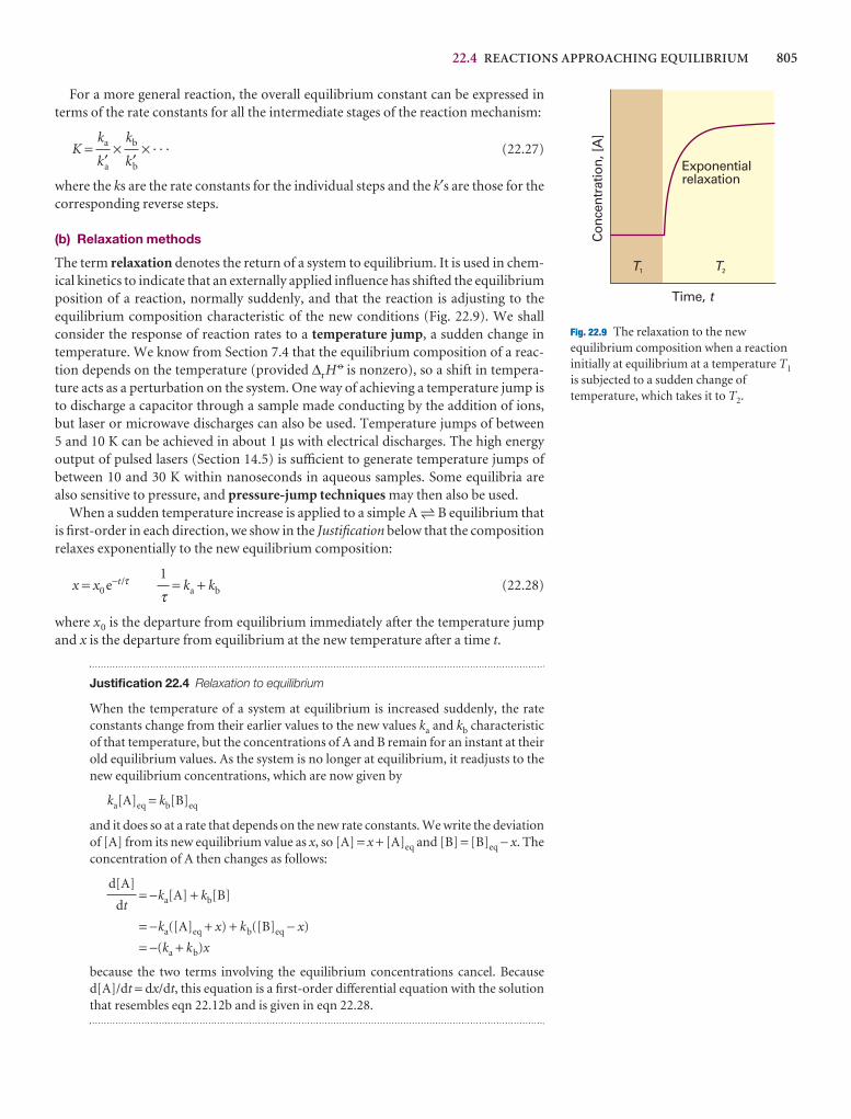
22.4 REACTIONS APPROACHING EQUILIBRIUM 805
For a more general reaction, the overall equilibrium constant can be expressed interms of the rate constants for all the intermediate stages of the reaction mechanism:
K = × × · · · (22.27)
where the ks are the rate constants for the individual steps and the k′s are those for thecorresponding reverse steps.
(b) Relaxation methods
The term relaxation denotes the return of a system to equilibrium. It is used in chem-ical kinetics to indicate that an externally applied influence has shifted the equilibriumposition of a reaction, normally suddenly, and that the reaction is adjusting to theequilibrium composition characteristic of the new conditions (Fig. 22.9). We shallconsider the response of reaction rates to a temperature jump, a sudden change intemperature. We know from Section 7.4 that the equilibrium composition of a reac-tion depends on the temperature (provided ∆rH
7 is nonzero), so a shift in tempera-ture acts as a perturbation on the system. One way of achieving a temperature jump isto discharge a capacitor through a sample made conducting by the addition of ions,but laser or microwave discharges can also be used. Temperature jumps of between 5 and 10 K can be achieved in about 1 µs with electrical discharges. The high energyoutput of pulsed lasers (Section 14.5) is sufficient to generate temperature jumps ofbetween 10 and 30 K within nanoseconds in aqueous samples. Some equilibria arealso sensitive to pressure, and pressure-jump techniques may then also be used.
When a sudden temperature increase is applied to a simple A 5 B equilibrium thatis first-order in each direction, we show in the Justification below that the compositionrelaxes exponentially to the new equilibrium composition:
x = x0 e−t/τ = ka + kb (22.28)
where x0 is the departure from equilibrium immediately after the temperature jumpand x is the departure from equilibrium at the new temperature after a time t.
Justification 22.4 Relaxation to equilibrium
When the temperature of a system at equilibrium is increased suddenly, the rateconstants change from their earlier values to the new values ka and kb characteristicof that temperature, but the concentrations of A and B remain for an instant at theirold equilibrium values. As the system is no longer at equilibrium, it readjusts to thenew equilibrium concentrations, which are now given by
ka[A]eq = kb[B]eq
and it does so at a rate that depends on the new rate constants. We write the deviationof [A] from its new equilibrium value as x, so [A] = x + [A]eq and [B] = [B]eq − x. Theconcentration of A then changes as follows:
= −ka[A] + kb[B]
= −ka([A]eq + x) + kb([B]eq − x)
= −(ka + kb)x
because the two terms involving the equilibrium concentrations cancel. Becaused[A]/dt = dx/dt, this equation is a first-order differential equation with the solutionthat resembles eqn 22.12b and is given in eqn 22.28.
d[A]
dt
1
τ
kb
k′b
ka
k′a
T1
Con
cent
ratio
n, [A
]
Time, t
T2
Exponentialrelaxation
Fig. 22.9 The relaxation to the newequilibrium composition when a reactioninitially at equilibrium at a temperature T1
is subjected to a sudden change oftemperature, which takes it to T2.
806 22 THE RATES OF CHEMICAL REACTIONS
Equation 22.28 shows that the concentrations of A and B relax into the new equi-librium at a rate determined by the sum of the two new rate constants. Because theequilibrium constant under the new conditions is K ≈ ka /kb, its value may be com-bined with the relaxation time measurement to find the individual ka and kb.
Example 22.4 Analysing a temperature-jump experiment
The equilibrium constant for the autoprotolysis of water, H2O(l) 5 H+(aq) +OH−(aq), is Kw = a(H+)a(OH−) = 1.008 × 10⁻¹⁴ at 298 K. After a temperature-jump,the reaction returns to equilibrium with a relaxation time of 37 µs at 298 K and pH ≈ 7. Given that the forward reaction is first-order and the reverse is second-order overall, calculate the rate constants for the forward and reverse reactions.
Method We need to derive an expression for the relaxation time, τ (the time con-stant for return to equilibrium), in terms of k1 (forward, first-order reaction) andk2 (reverse, second-order reaction). We can proceed as above, but it will be neces-sary to make the assumption that the deviation from equilibrium (x) is so smallthat terms in x2 can be neglected. Relate k1 and k2 through the equilibrium con-stant, but be careful with units because Kw is dimensionless.
Answer The forward rate at the final temperature is k1[H2O] and the reverse rateis k2[H+][OH−]. The net rate of deprotonation of H2O is
= −k1[H2O] + k2[H+][OH−]
We write [H2O] = [H2O]eq+ x, [H+] = [H+]eq − x, and [OH−] = [OH−]eq − x, and obtain
= −{k1 + k2([H+]eq + [OH−]eq)}x − k1[H2O]eq + k2[H+]eq[OH−]eq + k2x2
≈ −{k1 + k2([H+]eq + [OH−]eq)}x
where we have neglected the term in x2 and used the equilibrium condition
k1[H2O]eq = k2[H+]eq[OH−]eq
to eliminate the terms that are independent of x. It follows that
= k1 + k2([H+]eq + [OH−]eq)
At this point we note that
Kw = a(H+)a(OH−) ≈ ([H+]eq /c 7)([OH−]eq)/c 7) = [H+]eq[OH−]eq/c 72
with c 7 = 1 mol dm−3. For this electrically neutral system, [H+] = [OH−], so theconcentration of each type of ion is K w
1/2c 7, and hence
= k1 + k2(K w1/2c 7 + K w
1/2c 7) = k2 + 2Kw1/2c 7
At this point we note that
= =
The molar concentration of pure water is 55.6 mol dm−3, so [H2O]eq /c 7 = 55.6. Ifwe write K = Kw /55.6 = 1.81 × 10⁻¹⁶, we obtain
= k2{K + 2Kw1/2}c 7
1
τ
Kw c 72
[H2O]eq
[H+]eq[OH−]eq
[H2O]eq
k1
k2
567
k1
k2
123
1
τ
1
τ
dx
dt
d[H2O]
dt
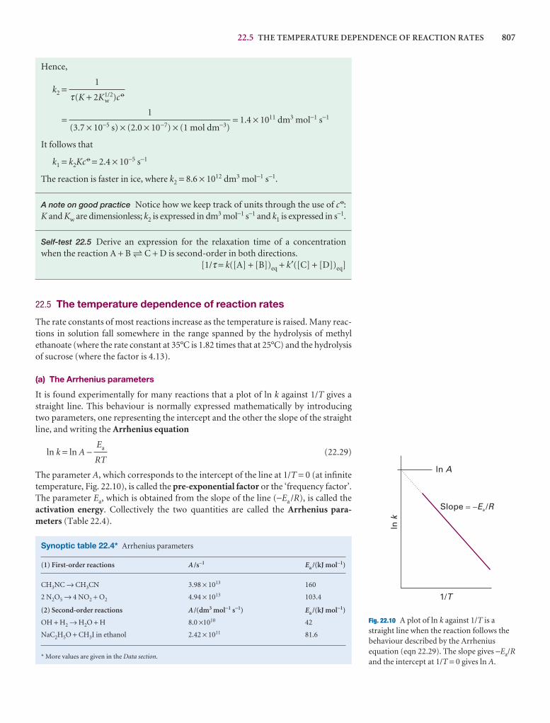
22.5 THE TEMPERATURE DEPENDENCE OF REACTION RATES 807
lnk
ln A
1/T
Slope /� �E Ra
Fig. 22.10 A plot of ln k against 1/T is astraight line when the reaction follows thebehaviour described by the Arrheniusequation (eqn 22.29). The slope gives −Ea/Rand the intercept at 1/T = 0 gives ln A.
Synoptic table 22.4* Arrhenius parameters
(1) First-order reactions A /s−1 Ea /(kJ mol−1)
CH3NC → CH3CN 3.98 × 10¹³ 160
2 N2O5 → 4 NO2 + O2 4.94 × 10¹³ 103.4
(2) Second-order reactions A /(dm3 mol−1 s−1) Ea /(kJ mol−1)
OH + H2 → H2O + H 8.0 ×10¹⁰ 42
NaC2H5O + CH3I in ethanol 2.42 × 10¹¹ 81.6
* More values are given in the Data section.
Hence,
k2 =
= = 1.4 × 10¹¹ dm3 mol−1 s−1
It follows that
k1 = k2Kc 7 = 2.4 × 10⁻⁵ s−1
The reaction is faster in ice, where k2 = 8.6 × 10¹² dm3 mol−1 s−1.
A note on good practice Notice how we keep track of units through the use of c 7:K and Kw are dimensionless; k2 is expressed in dm3 mol−1 s−1 and k1 is expressed in s−1.
Self-test 22.5 Derive an expression for the relaxation time of a concentrationwhen the reaction A + B 5 C + D is second-order in both directions.
[1/τ = k([A] + [B])eq + k′([C] + [D])eq]
22.5 The temperature dependence of reaction rates
The rate constants of most reactions increase as the temperature is raised. Many reac-tions in solution fall somewhere in the range spanned by the hydrolysis of methylethanoate (where the rate constant at 35°C is 1.82 times that at 25°C) and the hydrolysisof sucrose (where the factor is 4.13).
(a) The Arrhenius parameters
It is found experimentally for many reactions that a plot of ln k against 1/T gives astraight line. This behaviour is normally expressed mathematically by introducingtwo parameters, one representing the intercept and the other the slope of the straightline, and writing the Arrhenius equation
ln k = ln A − (22.29)
The parameter A, which corresponds to the intercept of the line at 1/T = 0 (at infinitetemperature, Fig. 22.10), is called the pre-exponential factor or the ‘frequency factor’.The parameter Ea, which is obtained from the slope of the line (−Ea /R), is called the activation energy. Collectively the two quantities are called the Arrhenius para-meters (Table 22.4).
Ea
RT
1
(3.7 × 10⁻⁵ s) × (2.0 × 10−7) × (1 mol dm−3)
1
τ(K + 2Kw1/2)c 7
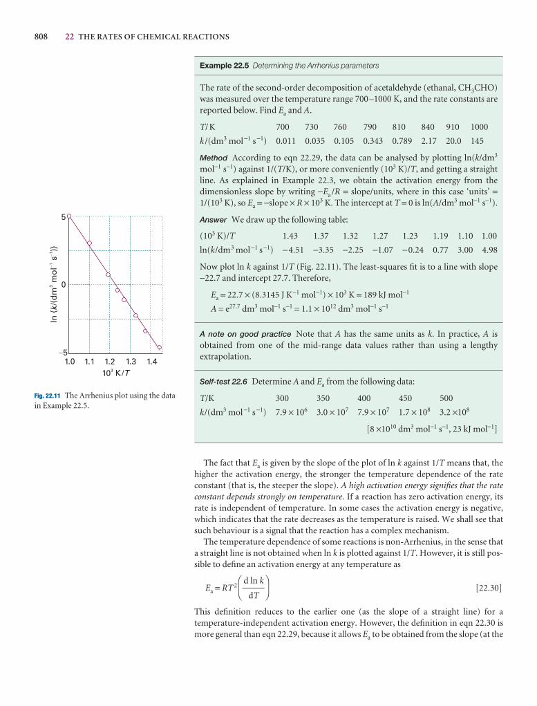
808 22 THE RATES OF CHEMICAL REACTIONS
1.0 1.1 1.2 1.3 1.410 K/3 T
�5
0
5
ln {
/(d
m m
ol
s)}
k3
11
��
Fig. 22.11 The Arrhenius plot using the datain Example 22.5.
Example 22.5 Determining the Arrhenius parameters
The rate of the second-order decomposition of acetaldehyde (ethanal, CH3CHO)was measured over the temperature range 700–1000 K, and the rate constants arereported below. Find Ea and A.
T/K 700 730 760 790 810 840 910 1000
k /(dm3 mol−1 s−1) 0.011 0.035 0.105 0.343 0.789 2.17 20.0 145
Method According to eqn 22.29, the data can be analysed by plotting ln(k/dm3
mol−1 s−1) against 1/(T/K), or more conveniently (103 K)/T, and getting a straightline. As explained in Example 22.3, we obtain the activation energy from the dimensionless slope by writing −Ea /R = slope/units, where in this case ‘units’ =1/(103 K), so Ea = −slope × R × 103 K. The intercept at T = 0 is ln(A/dm3 mol−1 s−1).
Answer We draw up the following table:
(103 K)/T 1.43 1.37 1.32 1.27 1.23 1.19 1.10 1.00
ln(k/dm3 mol−1 s−1) −4.51 −3.35 −2.25 −1.07 −0.24 0.77 3.00 4.98
Now plot ln k against 1/T (Fig. 22.11). The least-squares fit is to a line with slope −22.7 and intercept 27.7. Therefore,
Ea = 22.7 × (8.3145 J K−1 mol−1) × 103 K = 189 kJ mol−1
A = e27.7 dm3 mol−1 s−1 = 1.1 × 10¹² dm3 mol−1 s−1
A note on good practice Note that A has the same units as k. In practice, A isobtained from one of the mid-range data values rather than using a lengthy extrapolation.
Self-test 22.6 Determine A and Ea from the following data:
T/K 300 350 400 450 500
k/(dm3 mol−1 s−1) 7.9 × 10⁶ 3.0 × 10⁷ 7.9 × 10⁷ 1.7 × 10⁸ 3.2 ×10⁸
[8 ×10¹⁰ dm3 mol−1 s−1, 23 kJ mol−1]
The fact that Ea is given by the slope of the plot of ln k against 1/T means that, thehigher the activation energy, the stronger the temperature dependence of the rateconstant (that is, the steeper the slope). A high activation energy signifies that the rateconstant depends strongly on temperature. If a reaction has zero activation energy, itsrate is independent of temperature. In some cases the activation energy is negative,which indicates that the rate decreases as the temperature is raised. We shall see thatsuch behaviour is a signal that the reaction has a complex mechanism.
The temperature dependence of some reactions is non-Arrhenius, in the sense thata straight line is not obtained when ln k is plotted against 1/T. However, it is still pos-sible to define an activation energy at any temperature as
Ea = RT 2 [22.30]
This definition reduces to the earlier one (as the slope of a straight line) for a temperature-independent activation energy. However, the definition in eqn 22.30 ismore general than eqn 22.29, because it allows Ea to be obtained from the slope (at the
DF
d ln k
dT
AC
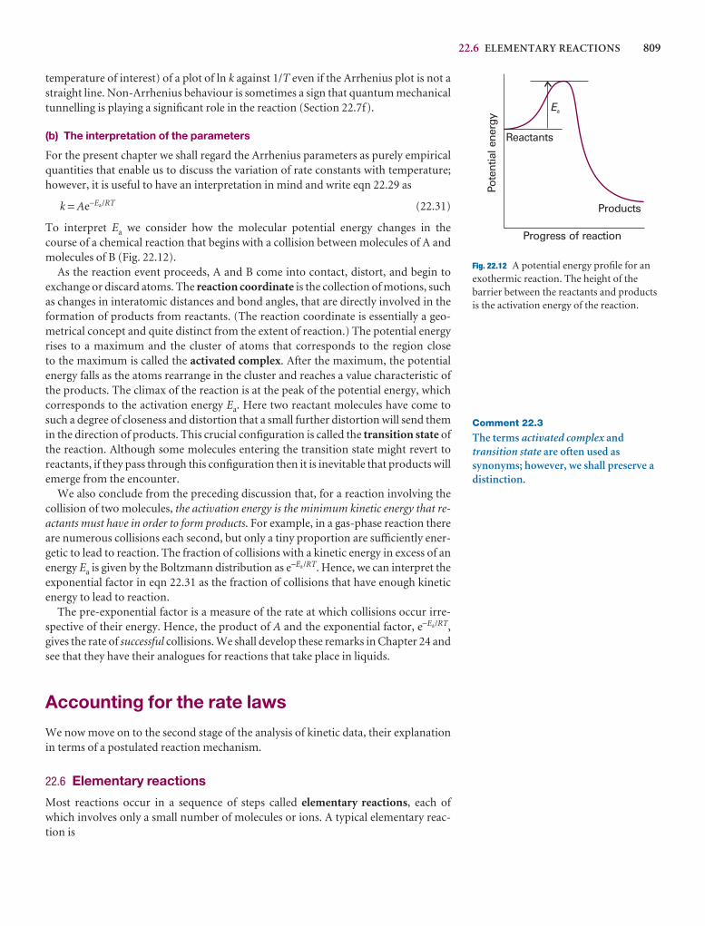
22.6 ELEMENTARY REACTIONS 809
temperature of interest) of a plot of ln k against 1/T even if the Arrhenius plot is not astraight line. Non-Arrhenius behaviour is sometimes a sign that quantum mechanicaltunnelling is playing a significant role in the reaction (Section 22.7f).
(b) The interpretation of the parameters
For the present chapter we shall regard the Arrhenius parameters as purely empiricalquantities that enable us to discuss the variation of rate constants with temperature;however, it is useful to have an interpretation in mind and write eqn 22.29 as
k = Ae−Ea/RT (22.31)
To interpret Ea we consider how the molecular potential energy changes in the course of a chemical reaction that begins with a collision between molecules of A andmolecules of B (Fig. 22.12).
As the reaction event proceeds, A and B come into contact, distort, and begin to exchange or discard atoms. The reaction coordinate is the collection of motions, suchas changes in interatomic distances and bond angles, that are directly involved in theformation of products from reactants. (The reaction coordinate is essentially a geo-metrical concept and quite distinct from the extent of reaction.) The potential energyrises to a maximum and the cluster of atoms that corresponds to the region close to the maximum is called the activated complex. After the maximum, the potential energy falls as the atoms rearrange in the cluster and reaches a value characteristic ofthe products. The climax of the reaction is at the peak of the potential energy, whichcorresponds to the activation energy Ea. Here two reactant molecules have come tosuch a degree of closeness and distortion that a small further distortion will send themin the direction of products. This crucial configuration is called the transition state ofthe reaction. Although some molecules entering the transition state might revert toreactants, if they pass through this configuration then it is inevitable that products willemerge from the encounter.
We also conclude from the preceding discussion that, for a reaction involving thecollision of two molecules, the activation energy is the minimum kinetic energy that re-actants must have in order to form products. For example, in a gas-phase reaction thereare numerous collisions each second, but only a tiny proportion are sufficiently ener-getic to lead to reaction. The fraction of collisions with a kinetic energy in excess of anenergy Ea is given by the Boltzmann distribution as e−Ea/RT. Hence, we can interpret theexponential factor in eqn 22.31 as the fraction of collisions that have enough kineticenergy to lead to reaction.
The pre-exponential factor is a measure of the rate at which collisions occur irre-spective of their energy. Hence, the product of A and the exponential factor, e−Ea/RT,gives the rate of successful collisions. We shall develop these remarks in Chapter 24 andsee that they have their analogues for reactions that take place in liquids.
Accounting for the rate laws
We now move on to the second stage of the analysis of kinetic data, their explanationin terms of a postulated reaction mechanism.
22.6 Elementary reactions
Most reactions occur in a sequence of steps called elementary reactions, each ofwhich involves only a small number of molecules or ions. A typical elementary reac-tion is
Comment 22.3
The terms actiVated complex andtransition state are often used assynonyms; however, we shall preserve adistinction.
Ea
Reactants
Products
Pote
ntia
l ene
rgy
Progress of reaction
Fig. 22.12 A potential energy profile for anexothermic reaction. The height of thebarrier between the reactants and productsis the activation energy of the reaction.
810 22 THE RATES OF CHEMICAL REACTIONS
H + Br2 → HBr + Br
Note that the phase of the species is not specified in the chemical equation for an elementary reaction, and the equation represents the specific process occurring to individual molecules. This equation, for instance, signifies that an H atom attacks a Br2 molecule to produce an HBr molecule and a Br atom. The molecularity of an elementary reaction is the number of molecules coming together to react in an ele-mentary reaction. In a unimolecular reaction, a single molecule shakes itself apart orits atoms into a new arrangement, as in the isomerization of cyclopropane to propene.In a bimolecular reaction, a pair of molecules collide and exchange energy, atoms, or groups of atoms, or undergo some other kind of change. It is most important to distinguish molecularity from order: reaction order is an empirical quantity, andobtained from the experimental rate law; molecularity refers to an elementary reac-tion proposed as an individual step in a mechanism.
The rate law of a unimolecular elementary reaction is first-order in the reactant:
A → P = −k[A] (22.32)
where P denotes products (several different species may be formed). A unimolecularreaction is first-order because the number of A molecules that decay in a short inter-val is proportional to the number available to decay. (Ten times as many decay in the same interval when there are initially 1000 A molecules as when there are only 100 present.) Therefore, the rate of decomposition of A is proportional to its molarconcentration.
An elementary bimolecular reaction has a second-order rate law:
A + B → P = −k[A][B] (22.33)
A bimolecular reaction is second-order because its rate is proportional to the rate atwhich the reactant species meet, which in turn is proportional to their concentrations.Therefore, if we have evidence that a reaction is a single-step, bimolecular process, wecan write down the rate law (and then go on to test it). Bimolecular elementary reac-tions are believed to account for many homogeneous reactions, such as the dimeriza-tions of alkenes and dienes and reactions such as
CH3I(alc) + CH3CH2O−(alc) → CH3OCH2CH3(alc) + I−(alc)
(where ‘alc’ signifies alcohol solution). There is evidence that the mechanism of thisreaction is a single elementary step
CH3I + CH3CH2O− → CH3OCH2CH3 + I−
This mechanism is consistent with the observed rate law
v = k[CH3I][CH3CH2O−] (22.34)
We shall see below how to combine a series of simple steps together into a mechan-ism and how to arrive at the corresponding rate law. For the present we emphasizethat, if the reaction is an elementary bimolecular process, then it has second-order kinetics,but if the kinetics are second-order, then the reaction might be complex. The postulatedmechanism can be explored only by detailed detective work on the system, and by investigating whether side products or intermediates appear during the course of thereaction. Detailed analysis of this kind was one of the ways, for example, in which thereaction H2(g) + I2(g) → 2 HI(g) was shown to proceed by a complex mechanism. For
d[A]
dt
d[A]
dt
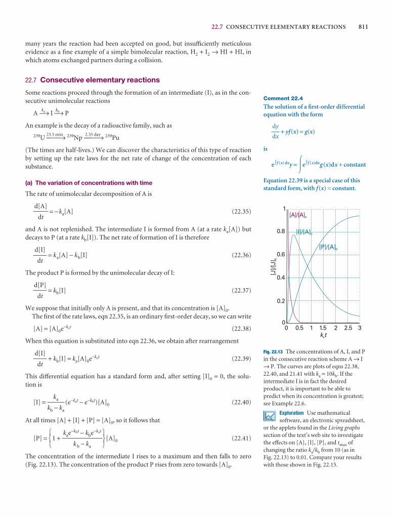
22.7 CONSECUTIVE ELEMENTARY REACTIONS 811
many years the reaction had been accepted on good, but insufficiently meticulous evidence as a fine example of a simple bimolecular reaction, H2 + I2 → HI + HI, inwhich atoms exchanged partners during a collision.
22.7 Consecutive elementary reactions
Some reactions proceed through the formation of an intermediate (I), as in the con-secutive unimolecular reactions
Aka−→ I
kb−→ P
An example is the decay of a radioactive family, such as
239U23.5 min−−−−−→ 239Np
2.35 day−−−−−−→ 239Pu
(The times are half-lives.) We can discover the characteristics of this type of reactionby setting up the rate laws for the net rate of change of the concentration of each substance.
(a) The variation of concentrations with time
The rate of unimolecular decomposition of A is
= −ka[A] (22.35)
and A is not replenished. The intermediate I is formed from A (at a rate ka[A]) but decays to P (at a rate kb[I]). The net rate of formation of I is therefore
= ka[A] − kb[I] (22.36)
The product P is formed by the unimolecular decay of I:
= kb[I] (22.37)
We suppose that initially only A is present, and that its concentration is [A]0.The first of the rate laws, eqn 22.35, is an ordinary first-order decay, so we can write
[A] = [A]0e−kat (22.38)
When this equation is substituted into eqn 22.36, we obtain after rearrangement
+ kb[I] = ka[A]0e−kat (22.39)
This differential equation has a standard form and, after setting [I]0 = 0, the solu-tion is
[I] = (e−kat − e−kbt)[A]0 (22.40)
At all times [A] + [I] + [P] = [A]0, so it follows that
[P] = 1 + [A]0 (22.41)
The concentration of the intermediate I rises to a maximum and then falls to zero(Fig. 22.13). The concentration of the product P rises from zero towards [A]0.
567
kae−kbt − kbe−kat
k b − ka
123
ka
kb − ka
d[I]
dt
d[P]
dt
d[I]
dt
d[A]
dt
Comment 22.4
The solution of a first-order differentialequation with the form
+ yf(x) = g(x)
is
e ∫ f (x) dxy = �e ∫ f (x)dxg(x)dx + constant
Equation 22.39 is a special case of thisstandard form, with f(x) = constant.
dy
dx
0 0.5 1 1.5 2 2.5 3k ta
0
0.2
0.4
0.6
0.8
1
[J]/[
J]0
[A]/[A]0
[I]/[A]0
[P]/[A]0
Fig. 22.13 The concentrations of A, I, and Pin the consecutive reaction scheme A → I→ P. The curves are plots of eqns 22.38, 22.40, and 21.41 with ka = 10kb. If theintermediate I is in fact the desiredproduct, it is important to be able topredict when its concentration is greatest;see Example 22.6.
Exploration Use mathematicalsoftware, an electronic spreadsheet,
or the applets found in the Living graphssection of the text’s web site to investigatethe effects on [A], [I], [P], and tmax ofchanging the ratio ka/kb from 10 (as in Fig. 22.13) to 0.01. Compare your resultswith those shown in Fig. 22.15.
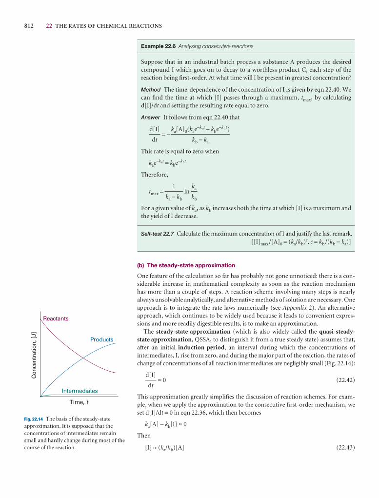
812 22 THE RATES OF CHEMICAL REACTIONS
Reactants
Products
Intermediates
Con
cent
ratio
n, [J
]
Time, t
Fig. 22.14 The basis of the steady-stateapproximation. It is supposed that theconcentrations of intermediates remainsmall and hardly change during most of thecourse of the reaction.
Example 22.6 Analysing consecutive reactions
Suppose that in an industrial batch process a substance A produces the desiredcompound I which goes on to decay to a worthless product C, each step of the reaction being first-order. At what time will I be present in greatest concentration?
Method The time-dependence of the concentration of I is given by eqn 22.40. Wecan find the time at which [I] passes through a maximum, tmax, by calculatingd[I]/dt and setting the resulting rate equal to zero.
Answer It follows from eqn 22.40 that
= −
This rate is equal to zero when
kae−kat = kbe−kbt
Therefore,
tmax = ln
For a given value of ka, as kb increases both the time at which [I] is a maximum andthe yield of I decrease.
Self-test 22.7 Calculate the maximum concentration of I and justify the last remark.[[I]max /[A]0 = (ka/kb)c, c = kb /(kb − ka)]
(b) The steady-state approximation
One feature of the calculation so far has probably not gone unnoticed: there is a con-siderable increase in mathematical complexity as soon as the reaction mechanism has more than a couple of steps. A reaction scheme involving many steps is nearly always unsolvable analytically, and alternative methods of solution are necessary. Oneapproach is to integrate the rate laws numerically (see Appendix 2). An alternative approach, which continues to be widely used because it leads to convenient expres-sions and more readily digestible results, is to make an approximation.
The steady-state approximation (which is also widely called the quasi-steady-state approximation, QSSA, to distinguish it from a true steady state) assumes that,after an initial induction period, an interval during which the concentrations of intermediates, I, rise from zero, and during the major part of the reaction, the rates ofchange of concentrations of all reaction intermediates are negligibly small (Fig. 22.14):
≈ 0 (22.42)
This approximation greatly simplifies the discussion of reaction schemes. For exam-ple, when we apply the approximation to the consecutive first-order mechanism, weset d[I]/dt = 0 in eqn 22.36, which then becomes
ka[A] − kb[I] ≈ 0
Then
[I] ≈ (ka/kb)[A] (22.43)
d[I]
dt
ka
kb
1
ka − kb
ka[A]0(kae−kat − kbe−kbt)
kb − ka
d[I]
dt
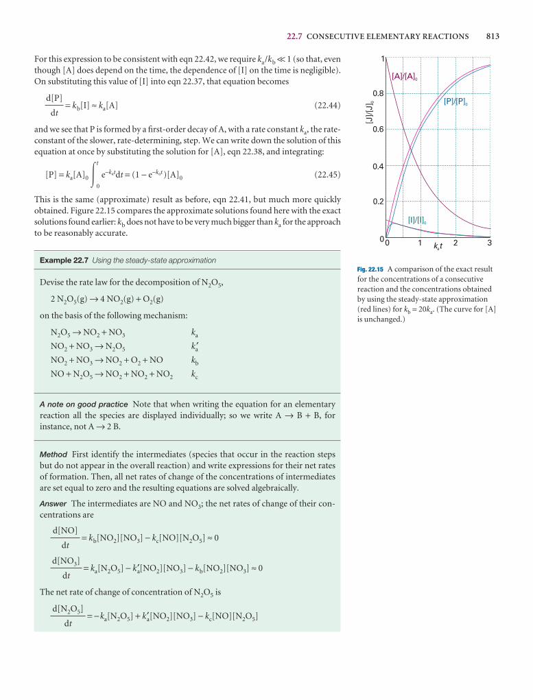
22.7 CONSECUTIVE ELEMENTARY REACTIONS 813
0 1 2 30
0.2
0.4
0.6
0.8
1
[J]/[
J]0
k ta
[A]/[A]0
[I]/[I]0
[P]/[P]0
Fig. 22.15 A comparison of the exact resultfor the concentrations of a consecutivereaction and the concentrations obtainedby using the steady-state approximation(red lines) for kb = 20ka. (The curve for [A]is unchanged.)
For this expression to be consistent with eqn 22.42, we require ka/kb << 1 (so that, eventhough [A] does depend on the time, the dependence of [I] on the time is negligible).On substituting this value of [I] into eqn 22.37, that equation becomes
= kb[I] ≈ ka[A] (22.44)
and we see that P is formed by a first-order decay of A, with a rate constant ka, the rate-constant of the slower, rate-determining, step. We can write down the solution of thisequation at once by substituting the solution for [A], eqn 22.38, and integrating:
[P] = ka[A]0 �t
0
e−katdt = (1 − e−kat )[A]0 (22.45)
This is the same (approximate) result as before, eqn 22.41, but much more quickly obtained. Figure 22.15 compares the approximate solutions found here with the exactsolutions found earlier: kb does not have to be very much bigger than ka for the approachto be reasonably accurate.
Example 22.7 Using the steady-state approximation
Devise the rate law for the decomposition of N2O5,
2 N2O5(g) → 4 NO2(g) + O2(g)
on the basis of the following mechanism:
N2O5 → NO2 + NO3 ka
NO2 + NO3 → N2O5 ka′NO2 + NO3 → NO2 + O2 + NO kb
NO + N2O5 → NO2 + NO2 + NO2 kc
A note on good practice Note that when writing the equation for an elementary reaction all the species are displayed individually; so we write A → B + B, for instance, not A → 2 B.
Method First identify the intermediates (species that occur in the reaction stepsbut do not appear in the overall reaction) and write expressions for their net ratesof formation. Then, all net rates of change of the concentrations of intermediatesare set equal to zero and the resulting equations are solved algebraically.
Answer The intermediates are NO and NO3; the net rates of change of their con-centrations are
= kb[NO2][NO3] − kc[NO][N2O5] ≈ 0
= ka[N2O5] − ka′[NO2][NO3] − kb[NO2][NO3] ≈ 0
The net rate of change of concentration of N2O5 is
= −ka[N2O5] + k′a[NO2][NO3] − kc[NO][N2O5]d[N2O5]
dt
d[NO3]
dt
d[NO]
dt
d[P]
dt
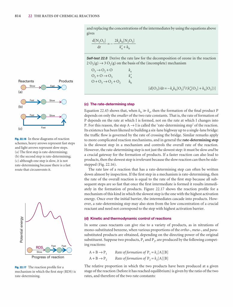
814 22 THE RATES OF CHEMICAL REACTIONS
Reactants Products
(a)
(b)
(c)
Slow Fast
Fast Slow
Slow
Fast
Fast
Fig. 22.16 In these diagrams of reactionschemes, heavy arrows represent fast stepsand light arrows represent slow steps. (a) The first step is rate-determining; (b) the second step is rate-determining; (c) although one step is slow, it is not rate-determining because there is a fastroute that circumvents it.
Pote
ntia
l ene
rgy
Progress of reaction
Fast
Slow
FastRDS
Fig. 22.17 The reaction profile for amechanism in which the first step (RDS) israte-determining.
and replacing the concentrations of the intermediates by using the equations abovegives
= −
Self-test 22.8 Derive the rate law for the decomposition of ozone in the reaction 2 O3(g) → 3 O2(g) on the basis of the (incomplete) mechanism
O3 → O2 + O ka
O2 + O → O3 k′aO + O3 → O2 + O2 kb
[d[O3]/dt = −kakb[O3]2/(k′a[O2] + kb[O3])]
(c) The rate-determining step
Equation 22.45 shows that, when kb >> ka, then the formation of the final product Pdepends on only the smaller of the two rate constants. That is, the rate of formation ofP depends on the rate at which I is formed, not on the rate at which I changes into P. For this reason, the step A → I is called the ‘rate-determining step’ of the reaction.Its existence has been likened to building a six-lane highway up to a single-lane bridge:the traffic flow is governed by the rate of crossing the bridge. Similar remarks apply to more complicated reaction mechanisms, and in general the rate-determining stepis the slowest step in a mechanism and controls the overall rate of the reaction.However, the rate-determining step is not just the slowest step: it must be slow and bea crucial gateway for the formation of products. If a faster reaction can also lead toproducts, then the slowest step is irrelevant because the slow reaction can then be side-stepped (Fig. 22.16).
The rate law of a reaction that has a rate-determining step can often be writtendown almost by inspection. If the first step in a mechanism is rate-determining, thenthe rate of the overall reaction is equal to the rate of the first step because all sub-sequent steps are so fast that once the first intermediate is formed it results immedi-ately in the formation of products. Figure 22.17 shows the reaction profile for a mechanism of this kind in which the slowest step is the one with the highest activationenergy. Once over the initial barrier, the intermediates cascade into products. How-ever, a rate-determining step may also stem from the low concentration of a crucialreactant and need not correspond to the step with highest activation barrier.
(d) Kinetic and thermodynamic control of reactions
In some cases reactants can give rise to a variety of products, as in nitrations of mono-substituted benzene, when various proportions of the ortho-, meta-, and para-substituted products are obtained, depending on the directing power of the originalsubstituent. Suppose two products, P1 and P2, are produced by the following compet-ing reactions:
A + B → P1 Rate of formation of P1 = k1[A][B]
A + B → P2 Rate of formation of P2 = k2[A][B]
The relative proportion in which the two products have been produced at a givenstage of the reaction (before it has reached equilibrium) is given by the ratio of the tworates, and therefore of the two rate constants:
2kakb[N2O5]
k′a + kb
d[N2O5]
dt
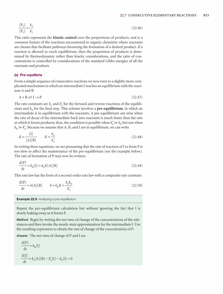
22.7 CONSECUTIVE ELEMENTARY REACTIONS 815
= (22.46)
This ratio represents the kinetic control over the proportions of products, and is acommon feature of the reactions encountered in organic chemistry where reactantsare chosen that facilitate pathways favouring the formation of a desired product. If areaction is allowed to reach equilibrium, then the proportion of products is deter-mined by thermodynamic rather than kinetic considerations, and the ratio of con-centrations is controlled by considerations of the standard Gibbs energies of all thereactants and products.
(e) Pre-equilibria
From a simple sequence of consecutive reactions we now turn to a slightly more com-plicated mechanism in which an intermediate I reaches an equilibrium with the react-ants A and B:
A + B 5 I → P (22.47)
The rate constants are ka and k′a for the forward and reverse reactions of the equilib-rium and kb for the final step. This scheme involves a pre-equilibrium, in which an intermediate is in equilibrium with the reactants. A pre-equilibrium can arise whenthe rate of decay of the intermediate back into reactants is much faster than the rate at which it forms products; thus, the condition is possible when k′a >> kb but not whenkb >> k′a. Because we assume that A, B, and I are in equilibrium, we can write
K = K = (22.48)
In writing these equations, we are presuming that the rate of reaction of I to form P istoo slow to affect the maintenance of the pre-equilibrium (see the example below).The rate of formation of P may now be written:
= kb[I] = kbK[A][B] (22.49)
This rate law has the form of a second-order rate law with a composite rate constant:
= k[A][B] k = kbK = (22.50)
Example 22.8 Analysing a pre-equilibrium
Repeat the pre-equilibrium calculation but without ignoring the fact that I isslowly leaking away as it forms P.
Method Begin by writing the net rates of change of the concentrations of the sub-stances and then invoke the steady-state approximation for the intermediate I. Usethe resulting expression to obtain the rate of change of the concentration of P.
Answer The net rates of change of P and I are
= kb[I]
= ka[A][B] − k′a[I] − kb[I] ≈ 0d[I]
dt
d[P]
dt
kakb
k′a
d[P]
dt
d[P]
dt
ka
k′a
[I]
[A][B]
k2
k1
[P2]
[P1]
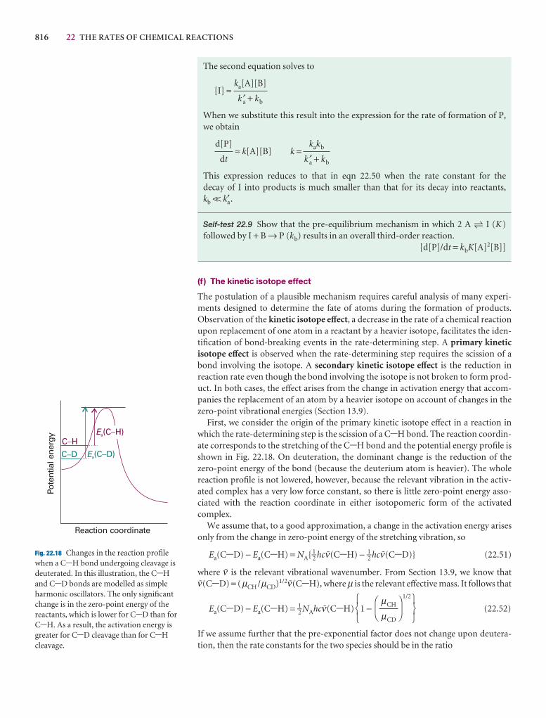
816 22 THE RATES OF CHEMICAL REACTIONS
Ea(C H)�
Pote
ntia
l ene
rgy
Reaction coordinate
C D�
C H�
Ea(C D)�
Fig. 22.18 Changes in the reaction profilewhen a C-H bond undergoing cleavage isdeuterated. In this illustration, the C-Hand C-D bonds are modelled as simpleharmonic oscillators. The only significantchange is in the zero-point energy of thereactants, which is lower for C-D than forC-H. As a result, the activation energy isgreater for C-D cleavage than for C-Hcleavage.
The second equation solves to
[I] ≈
When we substitute this result into the expression for the rate of formation of P, we obtain
≈ k[A][B] k =
This expression reduces to that in eqn 22.50 when the rate constant for the decay of I into products is much smaller than that for its decay into reactants, kb << ka′ .
Self-test 22.9 Show that the pre-equilibrium mechanism in which 2 A 5 I (K)followed by I + B → P (kb) results in an overall third-order reaction.
[d[P]/dt = kbK[A]2[B]]
(f ) The kinetic isotope effect
The postulation of a plausible mechanism requires careful analysis of many experi-ments designed to determine the fate of atoms during the formation of products.Observation of the kinetic isotope effect, a decrease in the rate of a chemical reactionupon replacement of one atom in a reactant by a heavier isotope, facilitates the iden-tification of bond-breaking events in the rate-determining step. A primary kinetic isotope effect is observed when the rate-determining step requires the scission of abond involving the isotope. A secondary kinetic isotope effect is the reduction in reaction rate even though the bond involving the isotope is not broken to form prod-uct. In both cases, the effect arises from the change in activation energy that accom-panies the replacement of an atom by a heavier isotope on account of changes in thezero-point vibrational energies (Section 13.9).
First, we consider the origin of the primary kinetic isotope effect in a reaction inwhich the rate-determining step is the scission of a C-H bond. The reaction coordin-ate corresponds to the stretching of the C-H bond and the potential energy profile isshown in Fig. 22.18. On deuteration, the dominant change is the reduction of thezero-point energy of the bond (because the deuterium atom is heavier). The whole reaction profile is not lowered, however, because the relevant vibration in the activ-ated complex has a very low force constant, so there is little zero-point energy asso-ciated with the reaction coordinate in either isotopomeric form of the activated complex.
We assume that, to a good approximation, a change in the activation energy arisesonly from the change in zero-point energy of the stretching vibration, so
Ea(C-D) − Ea(C-H) = NA{ 1–2 hc#(C-H) − 1–2 hc#(C-D)} (22.51)
where # is the relevant vibrational wavenumber. From Section 13.9, we know that#(C-D) = (µCH /µCD)1/2#(C-H), where µ is the relevant effective mass. It follows that
Ea(C-D) − Ea(C-H) = 1–2 NAhc#(C-H) 1 −1/2
(22.52)
If we assume further that the pre-exponential factor does not change upon deutera-tion, then the rate constants for the two species should be in the ratio
567
DF
µCH
µCD
AC
123
kakb
k′a + kb
d[P]
dt
ka[A][B]
k′a + kb
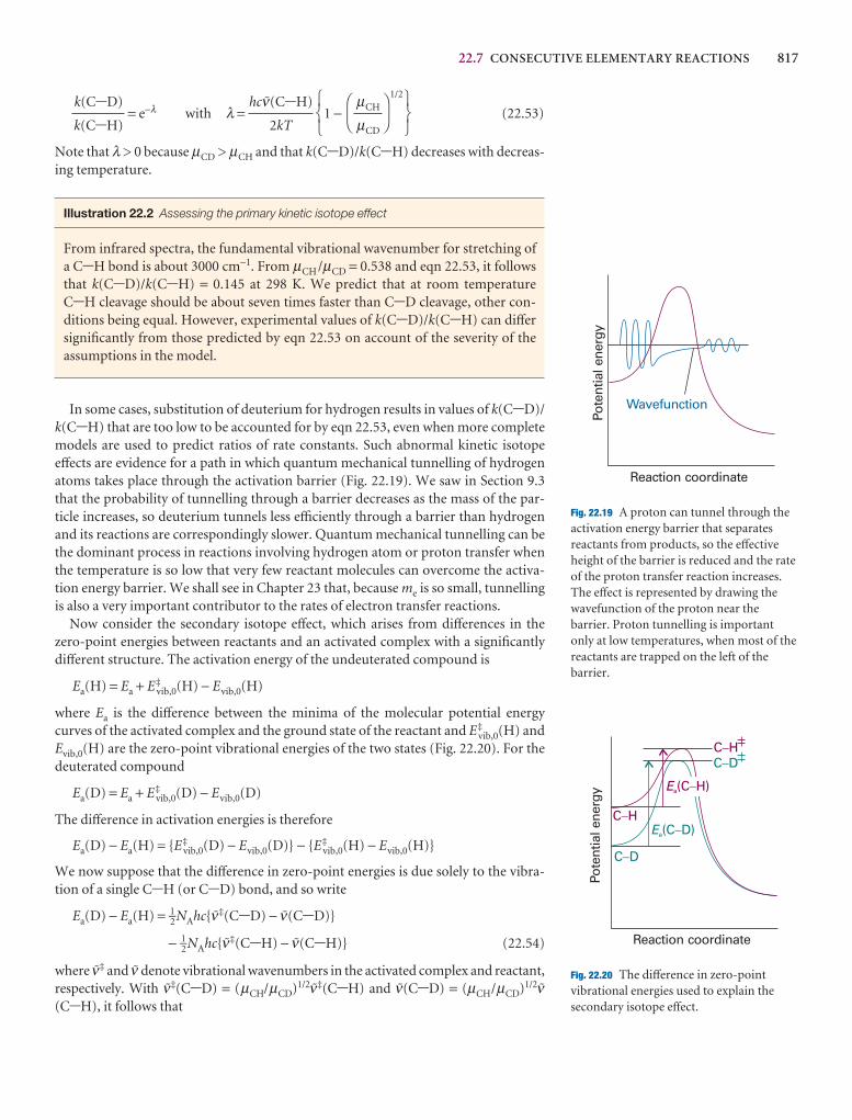
22.7 CONSECUTIVE ELEMENTARY REACTIONS 817
Pote
ntia
l ene
rgy
Reaction coordinate
Wavefunction
Fig. 22.19 A proton can tunnel through theactivation energy barrier that separatesreactants from products, so the effectiveheight of the barrier is reduced and the rateof the proton transfer reaction increases.The effect is represented by drawing thewavefunction of the proton near thebarrier. Proton tunnelling is importantonly at low temperatures, when most of thereactants are trapped on the left of thebarrier.
Ea(C H)�
Pote
ntia
l ene
rgy
Reaction coordinate
C D�
C H�Ea(C D)�
C H�
C D�
Fig. 22.20 The difference in zero-pointvibrational energies used to explain thesecondary isotope effect.
= e−λ with λ = 1 −1/2
(22.53)
Note that λ > 0 because µCD > µCH and that k(C-D)/k(C-H) decreases with decreas-ing temperature.
Illustration 22.2 Assessing the primary kinetic isotope effect
From infrared spectra, the fundamental vibrational wavenumber for stretching ofa C-H bond is about 3000 cm−1. From µCH /µCD = 0.538 and eqn 22.53, it followsthat k(C-D)/k(C-H) = 0.145 at 298 K. We predict that at room temperature C-H cleavage should be about seven times faster than C-D cleavage, other con-ditions being equal. However, experimental values of k(C-D)/k(C-H) can differsignificantly from those predicted by eqn 22.53 on account of the severity of the assumptions in the model.
In some cases, substitution of deuterium for hydrogen results in values of k(C-D)/k(C-H) that are too low to be accounted for by eqn 22.53, even when more completemodels are used to predict ratios of rate constants. Such abnormal kinetic isotopeeffects are evidence for a path in which quantum mechanical tunnelling of hydrogenatoms takes place through the activation barrier (Fig. 22.19). We saw in Section 9.3that the probability of tunnelling through a barrier decreases as the mass of the par-ticle increases, so deuterium tunnels less efficiently through a barrier than hydrogenand its reactions are correspondingly slower. Quantum mechanical tunnelling can bethe dominant process in reactions involving hydrogen atom or proton transfer whenthe temperature is so low that very few reactant molecules can overcome the activa-tion energy barrier. We shall see in Chapter 23 that, because me is so small, tunnellingis also a very important contributor to the rates of electron transfer reactions.
Now consider the secondary isotope effect, which arises from differences in thezero-point energies between reactants and an activated complex with a significantlydifferent structure. The activation energy of the undeuterated compound is
Ea(H) = Ea + E‡vib,0(H) − Evib,0(H)
where Ea is the difference between the minima of the molecular potential energycurves of the activated complex and the ground state of the reactant and E‡
vib,0(H) andEvib,0(H) are the zero-point vibrational energies of the two states (Fig. 22.20). For thedeuterated compound
Ea(D) = Ea + E‡vib,0(D) − Evib,0(D)
The difference in activation energies is therefore
Ea(D) − Ea(H) = {E‡vib,0(D) − Evib,0(D)} − {E‡
vib,0(H) − Evib,0(H)}
We now suppose that the difference in zero-point energies is due solely to the vibra-tion of a single C-H (or C-D) bond, and so write
Ea(D) − Ea(H) = 1–2NAhc{#‡(C-D) − #(C-D)}
− 1–2NAhc{#‡(C-H) − #(C-H)} (22.54)
where #‡ and # denote vibrational wavenumbers in the activated complex and reactant,respectively. With #‡(C-D) = (µCH/µCD)1/2#‡(C-H) and #(C-D) = (µCH/µCD)1/2#(C-H), it follows that
567
DF
µCH
µCD
AC
123
hc#(C-H)
2kT
k(C-D)
k(C-H)
818 22 THE RATES OF CHEMICAL REACTIONS
Ea(D) − Ea(H) = 1–2 NAhc{#‡(C-H) − #(C-H)}
1/2
− 1 (22.55)
and
= e−λ with λ =
1/2
− 1 (22.56)
Because µCH/µCD < 1, provided the vibrational wavenumber of the activated complexis less than that of the reactant, λ > 1 and the deuterated form reacts more slowly thanthe undeuterated compound.
Illustration 22.3 Assessing the secondary kinetic isotope effect
In the heterolytic dissociation CHCl3 → CHCl2+ + Cl− the activated complex
resembles the product CHCl2+. From infrared spectra, the fundamental vibrational
wavenumber for a bending motion involving the C-H group is about 1350 cm−1
in CHCl3 and about 800 cm−1 in CHCl2+. Assuming that #‡(C-H) = 800 cm−1 on
account of the structural similarity between CHCl2+ and the activated complex,
it follows from µCH/µCD = 0.538 and eqn 22.56 that k(D)/k(H) = 0.709 at 298 K. We predict that at room temperature the dissociation of CHCl3 should be about 40 per cent faster than dissociation of CDCl3. Comparison with the result fromIllustration 22.2 shows that the secondary kinetic isotope effect leads to higher values of k(D)/k(H) than does the primary kinetic isotope effect. This conclusionis supported by a number of experimental observations.
IMPACT ON BIOCHEMISTRY
I22.1 Kinetics of the helix–coil transition in polypeptides
We saw in Impact I16.1 that a simple statistical model accounts for the thermodynamicaspects of the helix–coil transition in polypeptides. The unfolding of a helix beginssomewhere in the middle of the chain with a nucleation step, which is less favourablethan the remaining helix-to-coil conversions, and continues in a cooperative fashion,in which the polymer becomes increasingly more susceptible to structural changes as more conversions occur. Here we examine the kinetics of the helix–coil transition,focusing primarily on experimental strategies and some recent results.
Earlier work on folding and unfolding of small polypeptides and large proteins reliedprimarily on rapid mixing and stopped-flow techniques. In a typical stopped-flowexperiment, a sample of the protein with a high concentration of a chemical denatur-ant, such as urea or guanidinium hydrochloride, is mixed with a solution containinga much lower concentration of the same denaturant. Upon entering the mixingchamber, the denaturant is diluted and the protein re-folds. Unfolding is observed bymixing a sample of folded protein with a solution containing a high concentration ofdenaturant. These experiments are ideal for sorting out events in the millisecondtimescale, such as the formation of contacts between helical segments in a large pro-tein. However, the available data also indicate that, in a number of proteins, a signific-ant portion of the folding process occurs in less than 1 ms, a time range not accessibleby the stopped-flow technique. More recent temperature-jump and flash photolysisexperiments have uncovered faster events. For example, at ambient temperature theformation of a loop between helical or sheet segments may be as fast as 1 µs and the formation of tightly packed cores with significant tertiary structure occurs in the
567
DF
µCH
µCD
AC
123
hc{#‡(C-H) − #(C-H)}
2kT
k(D)
k(H)
567
DF
µCH
µCD
AC
123
I22.1 IMPACT ON BIOCHEMISTRY: KINETICS OF THE HELIX–COIL TRANSITION IN POLYPEPTIDES 819
10–100 µs range. Among the fastest events are the formation and denaturation of helices and sheets from fully unfolded peptide chains and we examine how the laser-induced temperature-jump technique has been used in the study of the helix–coiltransition.
The laser-induced temperature-jump technique takes advantage of the fact thatproteins unfold, or melt, at high temperatures and each protein has a characteristicmelting temperature (Section 19.10). Proteins also lose their native structures at verylow temperatures, a process known as cold denaturation, and re-fold when the tem-perature is increased but kept significantly below the melting temperature. Hence, atemperature-jump experiment can be configured to monitor either folding or unfold-ing of a polypeptide, depending on the initial and final temperatures of the sample.The challenge of using melting or cold denaturation as the basis of kinetic measure-ments lies in increasing the temperature of the sample very quickly so fast relaxationproccess can be monitored. A number of clever strategies have been employed. In oneexample, a pulsed laser excites dissolved dye molecules that decay largely by internalconversion, or heat transfer to the solution. Another variation makes use of direct excitation of overtones of the O-H or O-D stretching modes of H2O or D2O, respect-ively, with a pulsed infrared laser. The latter strategy leads to temperature jumps in a small irradiated volume of about 20 K in less than 100 ps. Relaxation of the samplecan then be probed by a variety of spectroscopic techniques, including absorption,emission, or Raman scattering. For example, the infrared absorption spectrum of apolypeptide is sensitive to polypeptide conformation, as the N-H stretching vibra-tions in the range 1630–1670 cm−1 are significantly different in the helix and coil forms.
Much of the kinetic work on the helix–coil transition has been conducted in smallsynthetic polypeptides rich in alanine, an aminoacid that is known to stabilize helicalstructures. Both experimental results and statistical mechanical calculations suggestthat the mechanism of unfolding consists of at least two steps: a very fast step in whichaminoacids at either end of a helical segment undergo transitions to coil regions anda slower rate-determining step that corresponds to the cooperative melting of the restof the chain and loss of helical content. Using h and c to denote an aminoacid residuebelonging to a helical and coil region, respectively, the mechanism may be sum-marized as follows:
hhhh... → chhh... very fast
chhh... → cccc... rate-determining step
The rate-determining step is thought to account for the relaxation time of 160 ns measured with a laser-induced temperature jump between 282.5 K and 300.6 K in an alanine-rich polypeptide containing 21 amino acids. It is thought that the limitationon the rate of the helix–coil transition in this peptide arises from an activation energybarrier of 1.7 kJ mol−1 associated with nucleation events of the form ...hhhh...→ ...hhch... in the middle of the chain. Therefore, nucleation is not only thermody-namically unfavourable but also kinetically slow. Models that use concepts of statistical thermodynamics also suggest that a hhhh... → chhh... transition at eitherend of a helical segment has a significantly lower activation energy on account of theconverting aminoacid not being flanked by h regions.
The time constant for the helix–coil transition has also been measured in proteins.In apomyoglobin (myoglobin lacking the haem cofactor), the unfolding of the helicesappears to have a relaxation time of about 50 ns, even shorter than in synthetic peptides.It is difficult to interpret these results because we do not yet know how the amino acidsequence or interactions between helices in a folded protein affect the helix–coil relaxation time.
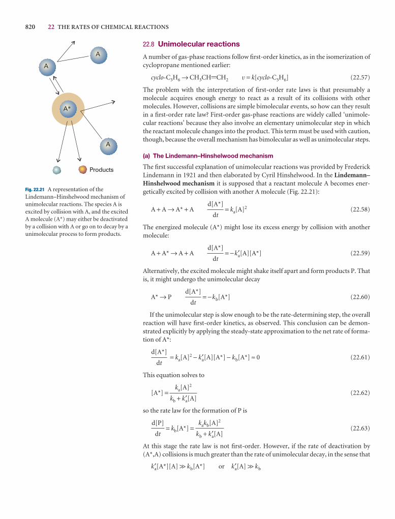
820 22 THE RATES OF CHEMICAL REACTIONS
22.8 Unimolecular reactions
A number of gas-phase reactions follow first-order kinetics, as in the isomerization ofcyclopropane mentioned earlier:
cyclo-C3H6 → CH3CH=CH2 v = k[cyclo-C3H6] (22.57)
The problem with the interpretation of first-order rate laws is that presumably amolecule acquires enough energy to react as a result of its collisions with othermolecules. However, collisions are simple bimolecular events, so how can they resultin a first-order rate law? First-order gas-phase reactions are widely called ‘unimole-cular reactions’ because they also involve an elementary unimolecular step in whichthe reactant molecule changes into the product. This term must be used with caution,though, because the overall mechanism has bimolecular as well as unimolecular steps.
(a) The Lindemann–Hinshelwood mechanism
The first successful explanation of unimolecular reactions was provided by FrederickLindemann in 1921 and then elaborated by Cyril Hinshelwood. In the Lindemann–Hinshelwood mechanism it is supposed that a reactant molecule A becomes ener-getically excited by collision with another A molecule (Fig. 22.21):
A + A → A* + A = ka[A]2 (22.58)
The energized molecule (A*) might lose its excess energy by collision with anothermolecule:
A + A* → A + A = −k′a[A][A*] (22.59)
Alternatively, the excited molecule might shake itself apart and form products P. Thatis, it might undergo the unimolecular decay
A* → P = −kb[A*] (22.60)
If the unimolecular step is slow enough to be the rate-determining step, the overallreaction will have first-order kinetics, as observed. This conclusion can be demon-strated explicitly by applying the steady-state approximation to the net rate of forma-tion of A*:
= ka[A]2 − k′a[A][A*] − kb[A*] ≈ 0 (22.61)
This equation solves to
[A*] = (22.62)
so the rate law for the formation of P is
= kb[A*] = (22.63)
At this stage the rate law is not first-order. However, if the rate of deactivation by(A*,A) collisions is much greater than the rate of unimolecular decay, in the sense that
k′a[A*][A] >> kb[A*] or k′a[A] >> kb
kakb[A]2
kb + k′a[A]
d[P]
dt
ka[A]2
kb + k′a[A]
d[A*]
dt
d[A*]
dt
d[A*]
dt
d[A*]
dt
Products
A*
A
A
A
Fig. 22.21 A representation of theLindemann–Hinshelwood mechanism ofunimolecular reactions. The species A isexcited by collision with A, and the excitedA molecule (A*) may either be deactivatedby a collision with A or go on to decay by aunimolecular process to form products.
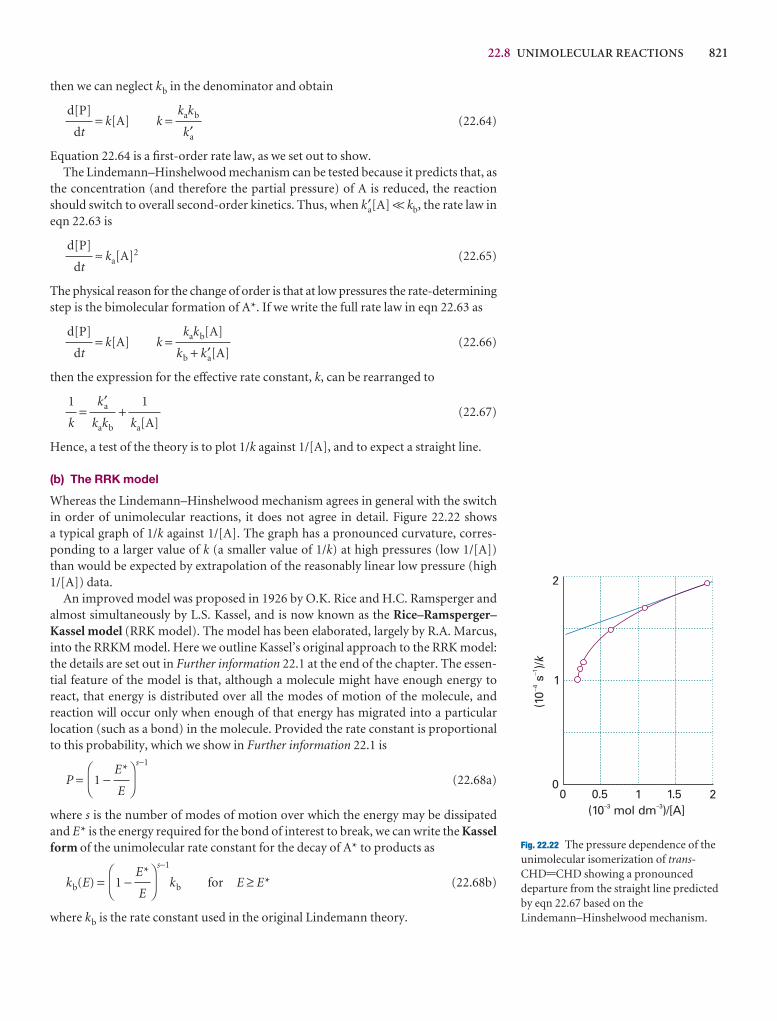
22.8 UNIMOLECULAR REACTIONS 821
then we can neglect kb in the denominator and obtain
= k[A] k = (22.64)
Equation 22.64 is a first-order rate law, as we set out to show.The Lindemann–Hinshelwood mechanism can be tested because it predicts that, as
the concentration (and therefore the partial pressure) of A is reduced, the reactionshould switch to overall second-order kinetics. Thus, when k′a[A] << kb, the rate law ineqn 22.63 is
≈ ka[A]2 (22.65)
The physical reason for the change of order is that at low pressures the rate-determiningstep is the bimolecular formation of A*. If we write the full rate law in eqn 22.63 as
= k[A] k = (22.66)
then the expression for the effective rate constant, k, can be rearranged to
= + (22.67)
Hence, a test of the theory is to plot 1/k against 1/[A], and to expect a straight line.
(b) The RRK model
Whereas the Lindemann–Hinshelwood mechanism agrees in general with the switchin order of unimolecular reactions, it does not agree in detail. Figure 22.22 shows a typical graph of 1/k against 1/[A]. The graph has a pronounced curvature, corres-ponding to a larger value of k (a smaller value of 1/k) at high pressures (low 1/[A])than would be expected by extrapolation of the reasonably linear low pressure (high1/[A]) data.
An improved model was proposed in 1926 by O.K. Rice and H.C. Ramsperger andalmost simultaneously by L.S. Kassel, and is now known as the Rice–Ramsperger–Kassel model (RRK model). The model has been elaborated, largely by R.A. Marcus,into the RRKM model. Here we outline Kassel’s original approach to the RRK model:the details are set out in Further information 22.1 at the end of the chapter. The essen-tial feature of the model is that, although a molecule might have enough energy toreact, that energy is distributed over all the modes of motion of the molecule, and reaction will occur only when enough of that energy has migrated into a particular location (such as a bond) in the molecule. Provided the rate constant is proportionalto this probability, which we show in Further information 22.1 is
P = 1 −s−1
(22.68a)
where s is the number of modes of motion over which the energy may be dissipatedand E* is the energy required for the bond of interest to break, we can write the Kasselform of the unimolecular rate constant for the decay of A* to products as
kb(E) = 1 −s−1
kb for E ≥ E* (22.68b)
where kb is the rate constant used in the original Lindemann theory.
DF
E*
E
AC
DF
E*
E
AC
1
ka[A]
k′akakb
1
k
kakb[A]
kb + k′a[A]
d[P]
dt
d[P]
dt
kakb
k′a
d[P]
dt
(10
s)/
��
41
k
0
1
2
0 0.5 1 1.5 2(10 mol dm )/[A]� �3 3
Fig. 22.22 The pressure dependence of theunimolecular isomerization of trans-CHD=CHD showing a pronounceddeparture from the straight line predictedby eqn 22.67 based on theLindemann–Hinshelwood mechanism.
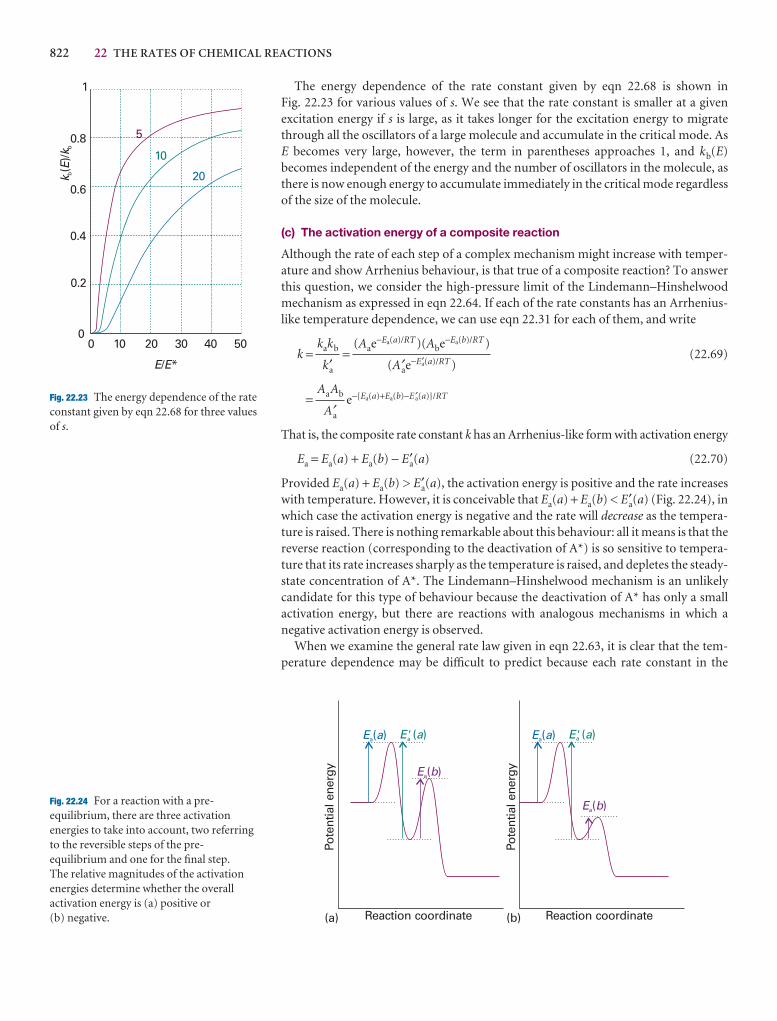
822 22 THE RATES OF CHEMICAL REACTIONS
The energy dependence of the rate constant given by eqn 22.68 is shown inFig. 22.23 for various values of s. We see that the rate constant is smaller at a given excitation energy if s is large, as it takes longer for the excitation energy to migratethrough all the oscillators of a large molecule and accumulate in the critical mode. AsE becomes very large, however, the term in parentheses approaches 1, and kb(E)becomes independent of the energy and the number of oscillators in the molecule, asthere is now enough energy to accumulate immediately in the critical mode regardlessof the size of the molecule.
(c) The activation energy of a composite reaction
Although the rate of each step of a complex mechanism might increase with temper-ature and show Arrhenius behaviour, is that true of a composite reaction? To answerthis question, we consider the high-pressure limit of the Lindemann–Hinshelwoodmechanism as expressed in eqn 22.64. If each of the rate constants has an Arrhenius-like temperature dependence, we can use eqn 22.31 for each of them, and write
k = = (22.69)
= e−{Ea(a)+Ea(b)−E′a(a)}/RT
That is, the composite rate constant k has an Arrhenius-like form with activation energy
Ea = Ea(a) + Ea(b) − E′a(a) (22.70)
Provided Ea(a) + Ea(b) > E′a(a), the activation energy is positive and the rate increaseswith temperature. However, it is conceivable that Ea(a) + Ea(b) < E′a(a) (Fig. 22.24), inwhich case the activation energy is negative and the rate will decrease as the tempera-ture is raised. There is nothing remarkable about this behaviour: all it means is that thereverse reaction (corresponding to the deactivation of A*) is so sensitive to tempera-ture that its rate increases sharply as the temperature is raised, and depletes the steady-state concentration of A*. The Lindemann–Hinshelwood mechanism is an unlikelycandidate for this type of behaviour because the deactivation of A* has only a small activation energy, but there are reactions with analogous mechanisms in which a negative activation energy is observed.
When we examine the general rate law given in eqn 22.63, it is clear that the tem-perature dependence may be difficult to predict because each rate constant in the
AaAb
A′a
(Aae−Ea(a)/RT )(Abe−Ea(b)/RT )
(A′ae−E′a(a)/RT )
kakb
k′a
0
0.2
0.4
0.6
0.8
1
0 10 20 30 40 50
5
10
20
E E/ *
kE
kb
b(
)/
Fig. 22.23 The energy dependence of the rateconstant given by eqn 22.68 for three valuesof s.
E aa( ) E aa( )E' aa ( ) E' aa ( )
E ba( )
E ba( )
Pote
ntia
l ene
rgy
Reaction coordinate Reaction coordinate(a) (b)
Pote
ntia
l ene
rgy
Fig. 22.24 For a reaction with a pre-equilibrium, there are three activationenergies to take into account, two referringto the reversible steps of the pre-equilibrium and one for the final step. The relative magnitudes of the activationenergies determine whether the overallactivation energy is (a) positive or (b) negative.

FURTHER READING 823
expression for k increases with temperature, and the outcome depends on whether theterms in the numerator dominate those in the denominator, or vice versa. The factthat so many reactions do show Arrhenius-like behaviour with positive activation energies suggests that their rate laws are in a ‘simple’ regime, like eqn 22.65 rather thaneqn 22.64, and that the temperature dependence is dominated by the activation energyof the rate-determining stage.
Checklist of key ideas
1. The rates of chemical reactions are measured by usingtechniques that monitor the concentrations of species presentin the reaction mixture. Examples include real-time andquenching procedures, flow and stopped-flow techniques,and flash photolysis.
2. The instantaneous rate of a reaction is the slope of the tangentot the graph of concentration against time (expressed as apositive quantity).
3. A rate law is an expression for the reaction rate in terms of theconcentrations of the species that occur in the overallchemical reaction.
4. For a rate law of the form v = k[A]a[B]b . . . , the rate constantis k, the order with respect to A is a, and the overall order is a + b + . . . .
5. An integrated rate law is an expression for the concentrationof a reactant or product as a function of time (Table 22.3).
6. The half-life t1/2 of a reaction is the time it takes for theconcentration of a species to fall to half its initial value. Thetime constant τ is the time required for the concentration of areactant to fall to 1/e of its initial value. For a first-orderreaction, t1/2 = (ln 2)/k and τ = 1/k.
7. The equilibrium constant for a reaction is equal to the ratio ofthe forward and reverse rate constants, K = k /k′.
8. In relaxation methods of kinetic analysis, the equilibriumposition of a reaction is first shifted suddenly and thenallowed to readjust the equilibrium composition characteristicof the new conditions.
9. The temperature dependence of the rate constant of a reactiontypically follows the Arrhenius equation, ln k = ln A − Ea/RT.
10. The activation energy, the parameter Ea in the Arrheniusequation, is the minimum kinetic energy for reaction during a
molecular encounter. The larger the activation energy, themore sensitive the rate constant is to the temperature.
11. The mechanism of reaction is the sequence of elementarysteps involved in a reaction.
12. The molecularity of an elementary reaction is the number ofmolecules coming together to react. An elementaryunimolecular reaction has first-order kinetics; an elementarybimolecular reaction has second-order kinetics.
13. The rate-determining step is the slowest step in a reactionmechanism that controls the rate of the overall reaction.
14. In the steady-state approximation, it is assumed that theconcentrations of all reaction intermediates remain constantand small throughout the reaction.
15. Provided a reaction has not reached equilibrium, the productsof competing reactions are controlled by kinetics, with[P2]/[P1] = k2/k1.
16. Pre-equilibrium is a state in which an intermediate is inequilibrium with the reactants and which arises when the ratesof formation of the intermediate and its decay back intoreactants are much faster than its rate of formation ofproducts.
17. The kinetic isotope effect is the decrease in the rate of achemical reaction upon replacement of one atom in a reactantby a heavier isotope. A primary kinetic isotope effect isobserved when the rate-determining step requires the scissionof a bond involving the isotope. A secondary kinetic isotopeeffect is the reduction in reaction rate even though the bondinvolving the isotope is not broken to form product.
18. The Lindemann–Hinshelwood mechanism and the RRKMmodel of ‘unimolecular’ reactions account for the first-orderkinetics of gas-phase reactions.
Further reading
Articles and texts
J. Andraos, A streamlined approach to solving simple and complexkinetic systems analytically. J. Chem. Educ. 76, 1578 (1999).
C.H. Bamford, C.F. Tipper, and R.G. Compton (ed.), Comprehensivechemical kinetics. Vols. 1–38, Elsevier, Amsterdam (1969–2001).
M.N. Berberan-Santos and J.M.G. Martinho, Integration of kineticrate equations by matrix methods. J. Chem. Educ. 67, 375 (1990).
J.M. Goodman, How do approximations affect the solutions tokinetic equations? J. Chem. Educ. 76, 275 (1999).
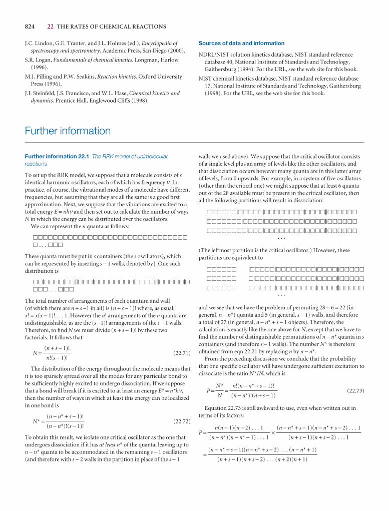
824 22 THE RATES OF CHEMICAL REACTIONS
J.C. Lindon, G.E. Tranter, and J.L. Holmes (ed.), Encyclopedia ofspectroscopy and spectrometry. Academic Press, San Diego (2000).
S.R. Logan, Fundamentals of chemical kinetics. Longman, Harlow(1996).
M.J. Pilling and P.W. Seakins, Reaction kinetics. Oxford UniversityPress (1996).
J.I. Steinfeld, J.S. Francisco, and W.L. Hase, Chemical kinetics anddynamics. Prentice Hall, Englewood Cliffs (1998).
Sources of data and information
NDRL/NIST solution kinetics database, NIST standard referencedatabase 40, National Institute of Standards and Technology,Gaithersburg (1994). For the URL, see the web site for this book.
NIST chemical kinetics database, NIST standard reference database17, National Institute of Standards and Technology, Gaithersburg(1998). For the URL, see the web site for this book.
Further information
Further information 22.1 The RRK model of unimolecularreactions
To set up the RRK model, we suppose that a molecule consists of sidentical harmonic oscillators, each of which has frequency ν. Inpractice, of course, the vibrational modes of a molecule have differentfrequencies, but assuming that they are all the same is a good firstapproximation. Next, we suppose that the vibrations are excited to atotal energy E = nhν and then set out to calculate the number of waysN in which the energy can be distributed over the oscillators.
We can represent the n quanta as follows:
�������������������������������
� . . . ���
These quanta must be put in s containers (the s oscillators), whichcan be represented by inserting s − 1 walls, denoted by |. One suchdistribution is
��|����|��||���|��������|����|||�����|���� . . . �|��
The total number of arrangements of each quantum and wall (of which there are n + s −1 in all) is (n + s − 1)! where, as usual, x! = x(x − 1)! . . . 1. However the n! arrangements of the n quanta areindistinguishable, as are the (s −1)! arrangements of the s − 1 walls.Therefore, to find N we must divide (n + s − 1)! by these twofactorials. It follows that
N = (22.71)
The distribution of the energy throughout the molecule means thatit is too sparsely spread over all the modes for any particular bond tobe sufficiently highly excited to undergo dissociation. If we supposethat a bond will break if it is excited to at least an energy E* = n*hν,then the number of ways in which at least this energy can be localizedin one bond is
N* = (22.72)
To obtain this result, we isolate one critical oscillator as the one thatundergoes dissociation if it has at least n* of the quanta, leaving up ton − n* quanta to be accommodated in the remaining s − 1 oscillators(and therefore with s − 2 walls in the partition in place of the s − 1
(n − n* + s − 1)!
(n − n*)!(s − 1)!
(n + s − 1)!
n!(s − 1)!
walls we used above). We suppose that the critical oscillator consistsof a single level plus an array of levels like the other oscillators, andthat dissociation occurs however many quanta are in this latter arrayof levels, from 0 upwards. For example, in a system of five oscillators(other than the critical one) we might suppose that at least 6 quantaout of the 28 available must be present in the critical oscillator, thenall the following partitions will result in dissociation:
������|�����|��������|����||������
�������|����|��������|����||������
��������|���|��������|����||������
· · ·
(The leftmost partition is the critical oscillator.) However, thesepartitions are equivalent to
������ |�����|��������|����||�����
������ �|����|��������|����||�����
������ ��|���|��������|����||�����
· · ·
and we see that we have the problem of permuting 28 − 6 = 22 (ingeneral, n − n*) quanta and 5 (in general, s − 1) walls, and therefore a total of 27 (in general, n − n* + s − 1 objects). Therefore, thecalculation is exactly like the one above for N, except that we have tofind the number of distinguishable permutations of n − n* quanta in scontainers (and therefore s − 1 walls). The number N* is thereforeobtained from eqn 22.71 by replacing n by n − n*.
From the preceding discussion we conclude that the probabilitythat one specific oscillator will have undergone sufficient excitation todissociate is the ratio N*/N, which is
P = = (22.73)
Equation 22.73 is still awkward to use, even when written out interms of its factors:
P = ×
=(n − n* + s − 1)(n − n* + s − 2) . . . (n − n* + 1)
(n + s − 1)(n + s − 2) . . . (n + 2)(n + 1)
(n − n* + s − 1)(n − n* + s − 2) . . . 1
(n + s − 1)(n + s − 2) . . . 1
n(n − 1)(n − 2) . . . 1
(n − n*)(n − n* − 1) . . . 1
n!(n − n* + s − 1)!
(n − n*)!(n + s − 1)
N*
N
EXERCISES 825
However, because s − 1 is small (in the sense s − 1 << n − n*), we canapproximate this expression by
P ≈ =s−1
Because the energy of the excited molecule is E = nhν and the criticalenergy is E* = n*hν, this expression may be written
DEFn − n*
n
ABC(n − n*)(n − n*) . . . (n − n*)s −1 factors
(n)(n) . . . (n)s −1 factors
P = 1 −s−1
as in eqn 22.68a. The dispersal of the energy of the collision reducesthe rate constant below its simple ‘Lindemann’ form, and to obtainthe observed rate constant we should multiply the latter by theprobability that the energy will in fact be localized in the bond ofinterest, which gives eqn 22.68b.
DEFE*
E
ABC
Discussion questions
22.1 Consult literature sources and list the observed timescales during whichthe following processes occur: radiative decay of excited electronic states,molecular rotational motion, molecular vibrational motion, proton transferreactions, the initial event of vision, energy transfer in photosynthesis, theinitial electron transfer events in photosynthesis, the helix-to-coil transition inpolypeptides, and collisions in liquids.
22.2 Write a brief report on a recent research article in which at least one ofthe following techniques was used to study the kinetics of a chemical reaction:stopped-flow techniques, flash photolysis, chemical quench-flow methods,freeze quench methods, temperature-jump methods, or pressure-jumpmethods. Your report should be similar in content and size to one of theImpact sections found throughout this text.
22.3 Describe the main features, including advantages and disadvantages, ofthe following experimental methods for determining the rate law of a reaction:the isolation method, the method of initial rates, and fitting data to integratedrate law expressions.
22.4 Distinguish between reaction order and molecularity.
22.5 Assess the validity of the following statement: the rate-determining stepis the slowest step in a reaction mechanism.
22.6 Distinguish between a pre-equilibrium approximation and a steady-stateapproximation.
22.7 Distinguish between kinetic and thermodynamic control of a reaction.
22.8 Define the terms in and limit the generality of the expression ln k = ln A − Ea/RT.
22.9 Distinguish between a primary and a secondary kinetic isotope effect.Discuss how kinetic isotope effects in general can provide insight into themechanism of a reaction.
22.10 Discuss the limitations of the generality of the expression k =kakb[A]/(kb + k′a[A]) for the effective rate constant of a unimolecular reactionA → P with the following mechanism: A + A 5 A* + A (ka, k′a), A* → P (kb).Suggest an experimental procedure that may either support or refute themechanism.
Exercises
22.1a The rate of the reaction A + 2 B → 3 C + D was reported as 1.0 mol dm−3 s−1. State the rates of formation and consumption of the participants.
22.1b The rate of the reaction A + 3 B → C + 2 D was reported as 1.0 mol dm−3 s−1. State the rates of formation and consumption of the participants.
22.2a The rate of formation of C in the reaction 2 A + B → 2 C + 3 D is 1.0 mol dm−3 s−1. State the reaction rate, and the rates of formation orconsumption of A, B, and D.
22.2b The rate of consumption of B in the reaction A + 3 B → C + 2 D is 1.0 mol dm−3 s−1. State the reaction rate, and the rates of formation orconsumption of A, C, and D.
22.3a The rate law for the reaction in Exercise 22.1a was found to be v =k[A][B]. What are the units of k? Express the rate law in terms of the rates offormation and consumption of (a) A, (b) C.
22.3b The rate law for the reaction in Exercise 22.1b was found to be v = k[A][B]2. What are the units of k? Express the rate law in terms of the ratesof formation and consumption of (a) A, (b) C.
22.4a The rate law for the reaction in Exercise 22.2a was reported as d[C]/dt = k[A][B][C]. Express the rate law in terms of the reaction rate; whatare the units for k in each case?
22.4b The rate law for the reaction in Exercise 22.2b was reported as d[C]/dt= k[A][B][C]−1. Express the rate law in terms of the reaction rate; what are theunits for k in each case?
22.5a At 518°C, the rate of decomposition of a sample of gaseousacetaldehyde, initially at a pressure of 363 Torr, was 1.07 Torr s−1 when 5.0 percent had reacted and 0.76 Torr s−1 when 20.0 per cent had reacted. Determinethe order of the reaction.
22.5b At 400 K, the rate of decomposition of a gaseous compound initially at a pressure of 12.6 kPa, was 9.71 Pa s−1 when 10.0 per cent had reacted and 7.67 Pa s−1 when 20.0 per cent had reacted. Determine the order of thereaction.
22.6a At 518°C, the half-life for the decomposition of a sample of gaseousacetaldehyde (ethanal) initially at 363 Torr was 410 s. When the pressure was169 Torr, the half-life was 880 s. Determine the order of the reaction.
22.6b At 400 K, the half-life for the decomposition of a sample of a gaseouscompound initially at 55.5 kPa was 340 s. When the pressure was 28.9 kPa, thehalf-life was 178 s. Determine the order of the reaction.
22.7a The rate constant for the first-order decomposition of N2O5 in thereaction 2 N2O5(g) → 4 NO2(g) + O2(g) is k = 3.38 × 10⁻⁵ s−1 at 25°C. What isthe half-life of N2O5? What will be the pressure, initially 500 Torr, at (a) 10 s,(b) 10 min after initiation of the reaction?
22.7b The rate constant for the first-order decomposition of a compound Ain the reaction 2 A → P is k = 2.78 × 10⁻⁷ s−1 at 25°C. What is the half-life of A?What will be the pressure, initially 32.1 kPa, at (a) 10 s, (b) 10 min afterinitiation of the reaction?
826 22 THE RATES OF CHEMICAL REACTIONS
22.8a A second-order reaction of the type A + B → P was carried out in asolution that was initially 0.050 mol dm−3 in A and 0.080 mol dm−3 in B. After1.0 h the concentration of A had fallen to 0.020 mol dm−3. (a) Calculate therate constant. (b) What is the half-life of the reactants?
22.8b A second-order reaction of the type A + 2 B → P was carried out in asolution that was initially 0.075 mol dm−3 in A and 0.030 mol dm−3 in B. After1.0 h the concentration of A had fallen to 0.045 mol dm−3. (a) Calculate therate constant. (b) What is the half-life of the reactants?
22.9a If the rate laws are expressed with (a) concentrations in moles perdecimetre cubed, (b) pressures in kilopascals, what are the units of the second-order and third-order rate constants?
22.9b If the rate laws are expressed with (a) concentrations in molecules permetre cubed, (b) pressures in newtons per metre squared, what are the unitsof the second-order and third-order rate constants?
22.10a The second-order rate constant for the reaction
CH3COOC2H5(aq) + OH−(aq) → CH3CO2−(aq) + CH3CH2OH(aq)
is 0.11 dm3 mol−1 s−1. What is the concentration of ester after (a) 10 s, (b) 10 min when ethyl acetate is added to sodium hydroxide so that the initial concentrations are [NaOH] = 0.050 mol dm−3 and [CH3COOC2H5] =0.100 mol dm−3?
22.10b The second-order rate constant for the reaction A + 2 B → C + D is0.21 dm3 mol−1 s−1. What is the concentration of C after (a) 10 s, (b) 10 minwhen the reactants are mixed with initial concentrations of [A] = 0.025 moldm−3 and [B] = 0.150 mol dm−3?
22.11a A reaction 2 A → P has a second-order rate law with k = 3.50 × 10⁻⁴
dm3 mol−1 s−1. Calculate the time required for the concentration of A tochange from 0.260 mol dm−3 to 0.011 mol dm−3.
22.11b A reaction 2 A → P has a third-order rate law with k = 3.50 × 10⁻⁴ dm6
mol−2 s−1. Calculate the time required for the concentration of A to changefrom 0.077 mol dm−3 to 0.021 mol dm−3.
22.12a Show that t1/2 ∝ 1/[A]n−1 for a reaction that is nth-order in A.
22.12b Deduce an expression for the time it takes for the concentration of asubstance to fall to one-third its initial value in an nth-order reaction.
22.13a The pKa of NH4+ is 9.25 at 25°C. The rate constant at 25°C for the
reaction of NH4+ and OH− to form aqueous NH3 is 4.0 × 10¹⁰ dm3 mol−1 s−1.
Calculate the rate constant for proton transfer to NH3. What relaxation timewould be observed if a temperature jump were applied to a solution of 0.15 mol dm−3 NH3(aq) at 25°C?
22.13b The equilibrium A 5 B + C at 25°C is subjected to a temperaturejump that slightly increases the concentrations of B and C. The measuredrelaxation time is 3.0 µs. The equilibrium constant for the system is 2.0 × 10⁻¹⁶
at 25°C, and the equilibrium concentrations of B and C at 25°C are both 2.0 × 10⁻⁴ mol dm−3. Calculate the rate constants for steps (1) and (2).
22.14a The rate constant for the decomposition of a certain substance is 2.80 × 10⁻³ dm3 mol−1 s−1 at 30°C and 1.38 × 10⁻² dm3 mol−1 s−1 at 50°C.Evaluate the Arrhenius parameters of the reaction.
22.14b The rate constant for the decomposition of a certain substance is 1.70 × 10⁻² dm3 mol−1 s−1 at 24°C and 2.01 × 10⁻² dm3 mol−1 s−1 at 37°C.Evaluate the Arrhenius parameters of the reaction.
22.15a The base-catalysed bromination of nitromethane-d3 in water at roomtemperature (298 K) proceeds 4.3 times more slowly than the bromination ofthe undeuterated material. Account for this difference. Use kf(C-H) = 450 N m−1.
22.15b Predict the order of magnitude of the isotope effect on the relativerates of displacement of (a) 1H and 3H, (b) 16O and 18O. Will raising thetemperature enhance the difference? Take kf (C-H) = 450 N m−1,kf (C-O) = 1750 N m−1.
22.16a The effective rate constant for a gaseous reaction that has aLindemann–Hinshelwood mechanism is 2.50 × 10⁻⁴ s−1 at 1.30 kPa and 2.10 × 10⁻⁵ s−1 at 12 Pa. Calculate the rate constant for the activation step inthe mechanism.
22.16b The effective rate constant for a gaseous reaction that has aLindemann–Hinshelwood mechanism is 1.7 × 10⁻³ s−1 at 1.09 kPa and 2.2 × 10⁻⁴ s−1 at 25 Pa. Calculate the rate constant for the activation step in the mechanism.
Problems*
Numerical problems
22.1 The data below apply to the formation of urea from ammonium cyanate,NH4CNO → NH2CONH2. Initially 22.9 g of ammonium cyanate wasdissolved in in enough water to prepare 1.00 dm3 of solution. Determine theorder of the reaction, the rate constant, and the mass of ammonium cyanateleft after 300 min.
t/min 0 20.0 50.0 65.0 150
m(urea)/g 0 7.0 12.1 13.8 17.7
22.2 The data below apply to the reaction, (CH3)3CBr + H2O → (CH3)3COH+ HBr. Determine the order of the reaction, the rate constant, and the molarconcentration of (CH3)3CBr after 43.8 h.
t /h 0 3.15 6.20 10.00 18.30 30.80
[(CH3)3CBr]/(10−2 mol dm−3) 10.39 8.96 7.76 6.39 3.53 2.07
22.3 The thermal decomposition of an organic nitrile produced the followingdata:
t /(103 s) 0 2.00 4.00 6.00 8.00 10.00 12.00 ∞
[nitrile]/(mol dm− 3) 1.10 0.86 0.67 0.52 0.41 0.32 0.25 0
Determine the order of the reaction and the rate constant.
22.4 The following data have been obtained for the decomposition ofN2O5(g) at 67°C according to the reaction 2 N2O5(g) → 4 NO2(g) + O2(g).Determine the order of the reaction, the rate constant, and the half-life. It isnot necessary to obtain the result graphically, you may do a calculation usingestimates of the rates of change of concentration.
t /min 0 1 2 3 4 5
[N2O5]/(mol dm− 3) 1.000 0.705 0.497 0.349 0.246 0.173
22.5 A first-order decomposition reaction is observed to have the followingrate constants at the indicated temperatures. Estimate the activation energy.
k /(10−3 s−1) 2.46 45.1 576
θ / °C 0 20.0 40.0
* Problems denoted with the symbol ‡ were supplied by Charles Trapp, Carmen Giunta, and Marshall Cady.
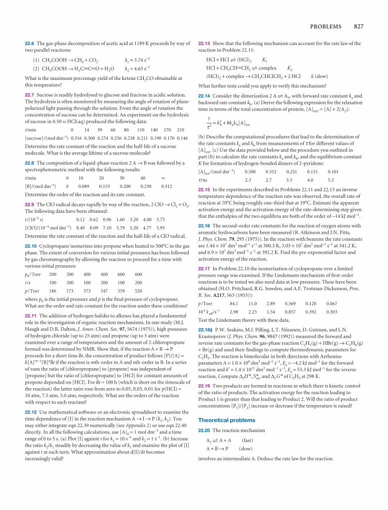
PROBLEMS 827
22.6 The gas-phase decomposition of acetic acid at 1189 K proceeds by way oftwo parallel reactions:
(1) CH3COOH → CH4 + CO2 k1 = 3.74 s−1
(2) CH3COOH → H2C=C=O + H2O k2 = 4.65 s−1
What is the maximum percentage yield of the ketene CH2CO obtainable atthis temperature?
22.7 Sucrose is readily hydrolysed to glucose and fructose in acidic solution.The hydrolysis is often monitored by measuring the angle of rotation of plane-polarized light passing through the solution. From the angle of rotation theconcentration of sucrose can be determined. An experiment on the hydrolysisof sucrose in 0.50 M HCl(aq) produced the following data:
t/min 0 14 39 60 80 110 140 170 210
[sucrose]/(mol dm−3) 0.316 0.300 0.274 0.256 0.238 0.211 0.190 0.170 0.146
Determine the rate constant of the reaction and the half-life of a sucrosemolecule. What is the average liftime of a sucrose molecule?
22.8 The composition of a liquid-phase reaction 2 A → B was followed by aspectrophotometric method with the following results:
t/min 0 10 20 30 40 ∞
[B]/(mol dm−3) 0 0.089 0.153 0.200 0.230 0.312
Determine the order of the reaction and its rate constant.
22.9 The ClO radical decays rapidly by way of the reaction, 2 ClO → Cl2 + O2.The following data have been obtained:
t /(10−3 s) 0.12 0.62 0.96 1.60 3.20 4.00 5.75
[ClO]/(10− 6 mol dm−3) 8.49 8.09 7.10 5.79 5.20 4.77 3.95
Determine the rate constant of the reaction and the half-life of a ClO radical.
22.10 Cyclopropane isomerizes into propene when heated to 500°C in the gasphase. The extent of conversion for various initial pressures has been followedby gas chromatography by allowing the reaction to proceed for a time withvarious initial pressures:
p0 /Torr 200 200 400 400 600 600
t /s 100 200 100 200 100 200
p /Torr 186 173 373 347 559 520
where p0 is the initial pressure and p is the final pressure of cyclopropane.What are the order and rate constant for the reaction under these conditions?
22.11 The addition of hydrogen halides to alkenes has played a fundamentalrole in the investigation of organic reaction mechanisms. In one study (M.J.Haugh and D.R. Dalton, J. Amer. Chem. Soc. 97, 5674 (1975)), high pressuresof hydrogen chloride (up to 25 atm) and propene (up to 5 atm) wereexamined over a range of temperatures and the amount of 2-chloropropaneformed was determined by NMR. Show that, if the reaction A + B → Pproceeds for a short time δt, the concentration of product follows [P]/[A] =k[A]m−1[B]nδt if the reaction is mth-order in A and nth-order in B. In a seriesof runs the ratio of [chloropropane] to [propene] was independent of[propene] but the ratio of [chloropropane] to [HCl] for constant amounts ofpropene depended on [HCl]. For δt ≈ 100 h (which is short on the timescale ofthe reaction) the latter ratio rose from zero to 0.05, 0.03, 0.01 for p(HCl) =10 atm, 7.5 atm, 5.0 atm, respectively. What are the orders of the reaction with respect to each reactant?
22.12 Use mathematical software or an electronic spreadsheet to examine thetime dependence of [I] in the reaction mechanism A → I → P (k1, k2). Youmay either integrate eqn 22.39 numerically (see Appendix 2) or use eqn 22.40directly. In all the following calculations, use [A]0 = 1 mol dm−3 and a timerange of 0 to 5 s. (a) Plot [I] against t for k1 = 10 s−1 and k2 = 1 s−1. (b) Increasethe ratio k2/k1 steadily by decreasing the value of k1 and examine the plot of [I]against t at each turn. What approximation about d[I]/dt becomesincreasingly valid?
22.13 Show that the following mechanism can account for the rate law of thereaction in Problem 22.11:
HCl + HCl 5 (HCl)2 K1
HCl + CH3CH=CH2 5 complex K2
(HCl)2 + complex → CH3CHClCH3 + 2 HCl k (slow)
What further tests could you apply to verify this mechanism?
22.14 Consider the dimerization 2 A 5 A2, with forward rate constant ka andbackward rate constant kb. (a) Derive the following expression for the relaxationtime in terms of the total concentration of protein, [A]tot, = [A] + 2[A2]:
= k2b + 8kak b[A]tot
(b) Describe the computational procedures that lead to the determination ofthe rate constants ka and kb from measurements of τ for different values of[A]tot. (c) Use the data provided below and the procedure you outlined in part (b) to calculate the rate constants ka and kb, and the equilibrium constantK for formation of hydrogen-bonded dimers of 2-pyridone:
[A]tot /(mol dm− 3) 0.500 0.352 0.251 0.151 0.101
τ /ns 2.3 2.7 3.3 4.0 5.3
22.15 In the experiments described in Problems 22.11 and 22.13 an inversetemperature dependence of the reaction rate was observed, the overall rate ofreaction at 70°C being roughly one-third that at 19°C. Estimate the apparentactivation energy and the activation energy of the rate-determining step giventhat the enthalpies of the two equilibria are both of the order of −14 kJ mol−1.
22.16 The second-order rate constants for the reaction of oxygen atoms witharomatic hydrocarbons have been measured (R. Atkinson and J.N. Pitts, J. Phys. Chem. 79, 295 (1975)). In the reaction with benzene the rate constantsare 1.44 × 10⁷ dm3 mol−1 s−1 at 300.3 K, 3.03 × 10⁷ dm3 mol−1 s−1 at 341.2 K,and 6.9 × 10⁷ dm3 mol−1 s−1 at 392.2 K. Find the pre-exponential factor andactivation energy of the reaction.
22.17 In Problem 22.10 the isomerization of cyclopropane over a limitedpressure range was examined. If the Lindemann mechanism of first-orderreactions is to be tested we also need data at low pressures. These have beenobtained (H.O. Pritchard, R.G. Sowden, and A.F. Trotman-Dickenson, Proc.R. Soc. A217, 563 (1953)):
p /Torr 84.1 11.0 2.89 0.569 0.120 0.067
10 4 k eff /s−1 2.98 2.23 1.54 0.857 0.392 0.303
Test the Lindemann theory with these data.
22.18‡ P.W. Seakins, M.J. Pilling, L.T. Niiranen, D. Gutman, and L.N.Krasnoperov (J. Phys. Chem. 96, 9847 (1992)) measured the forward andreverse rate constants for the gas-phase reaction C2H5(g) + HBr(g) → C2H6(g)+ Br(g) and used their findings to compute thermodynamic parameters forC2H5. The reaction is bimolecular in both directions with Arrheniusparameters A = 1.0 × 10⁹ dm3 mol−1 s−1, Ea = −4.2 kJ mol−1 for the forwardreaction and k′ = 1.4 × 10¹¹ dm3 mol−1 s−1, Ea = 53.3 kJ mol−1 for the reversereaction. Compute ∆fH
7, S 7m, and ∆f G 7 of C2H5 at 298 K.
22.19 Two products are formed in reactions in which there is kinetic controlof the ratio of products. The activation energy for the reaction leading toProduct 1 is greater than that leading to Product 2. Will the ratio of productconcentrations [P1]/[P2] increase or decrease if the temperature is raised?
Theoretical problems
22.20 The reaction mechanism
A2 5 A + A (fast)
A + B → P (slow)
involves an intermediate A. Deduce the rate law for the reaction.
1
τ2
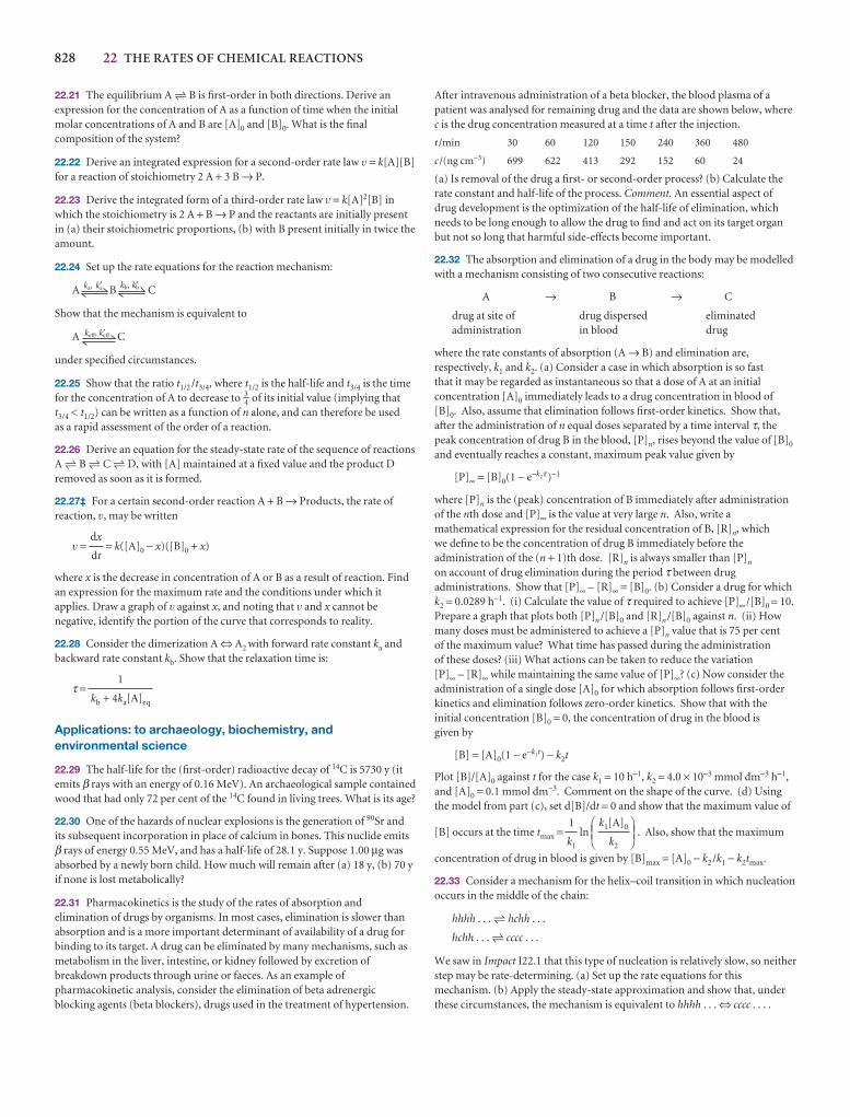
After intravenous administration of a beta blocker, the blood plasma of apatient was analysed for remaining drug and the data are shown below, wherec is the drug concentration measured at a time t after the injection.
t /min 30 60 120 150 240 360 480
c /(ng cm−3) 699 622 413 292 152 60 24
(a) Is removal of the drug a first- or second-order process? (b) Calculate therate constant and half-life of the process. Comment. An essential aspect ofdrug development is the optimization of the half-life of elimination, whichneeds to be long enough to allow the drug to find and act on its target organbut not so long that harmful side-effects become important.
22.32 The absorption and elimination of a drug in the body may be modelledwith a mechanism consisting of two consecutive reactions:
A → B → C
drug at site of drug dispersed eliminatedadministration in blood drug
where the rate constants of absorption (A → B) and elimination are,respectively, k1 and k2. (a) Consider a case in which absorption is so fast that it may be regarded as instantaneous so that a dose of A at an initialconcentration [A]0 immediately leads to a drug concentration in blood of[B]0. Also, assume that elimination follows first-order kinetics. Show that,after the administration of n equal doses separated by a time interval τ, thepeak concentration of drug B in the blood, [P]n, rises beyond the value of [B]0
and eventually reaches a constant, maximum peak value given by
[P]∞ = [B]0(1 − e−k2τ)−1
where [P]n is the (peak) concentration of B immediately after administrationof the nth dose and [P]∞ is the value at very large n. Also, write amathematical expression for the residual concentration of B, [R]n, which we define to be the concentration of drug B immediately before theadministration of the (n + 1)th dose. [R]n is always smaller than [P]n
on account of drug elimination during the period τ between drugadministrations. Show that [P]∞ – [R]∞ = [B]0. (b) Consider a drug for whichk2 = 0.0289 h−1. (i) Calculate the value of τ required to achieve [P]∞ /[B]0 = 10.Prepare a graph that plots both [P]n /[B]0 and [R]n /[B]0 against n. (ii) Howmany doses must be administered to achieve a [P]n value that is 75 per cent of the maximum value? What time has passed during the administration of these doses? (iii) What actions can be taken to reduce the variation [P]∞ – [R]∞ while maintaining the same value of [P]∞? (c) Now consider theadministration of a single dose [A]0 for which absorption follows first-orderkinetics and elimination follows zero-order kinetics. Show that with theinitial concentration [B]0 = 0, the concentration of drug in the blood is given by
[B] = [A]0(1 − e−k1t) − k2t
Plot [B]/[A]0 against t for the case k1 = 10 h−1, k2 = 4.0 × 10⁻³ mmol dm−3 h−1,and [A]0 = 0.1 mmol dm−3. Comment on the shape of the curve. (d) Usingthe model from part (c), set d[B]/dt = 0 and show that the maximum value of
[B] occurs at the time tmax = ln . Also, show that the maximum
concentration of drug in blood is given by [B]max = [A]0 − k2 /k1 − k2tmax.
22.33 Consider a mechanism for the helix–coil transition in which nucleationoccurs in the middle of the chain:
hhhh . . . 5 hchh . . .
hchh . . . 5 cccc . . .
We saw in Impact I22.1 that this type of nucleation is relatively slow, so neitherstep may be rate-determining. (a) Set up the rate equations for thismechanism. (b) Apply the steady-state approximation and show that, underthese circumstances, the mechanism is equivalent to hhhh . . . ⇔ cccc . . . .
DEFk1[A]0
k2
ABC1
k1
828 22 THE RATES OF CHEMICAL REACTIONS
22.21 The equilibrium A 5 B is first-order in both directions. Derive anexpression for the concentration of A as a function of time when the initialmolar concentrations of A and B are [A]0 and [B]0. What is the finalcomposition of the system?
22.22 Derive an integrated expression for a second-order rate law v = k[A][B]for a reaction of stoichiometry 2 A + 3 B → P.
22.23 Derive the integrated form of a third-order rate law v = k[A]2[B] inwhich the stoichiometry is 2 A + B → P and the reactants are initially presentin (a) their stoichiometric proportions, (b) with B present initially in twice theamount.
22.24 Set up the rate equations for the reaction mechanism:
A B C
Show that the mechanism is equivalent to
A C
under specified circumstances.
22.25 Show that the ratio t1/2 /t3/4, where t1/2 is the half-life and t3/4 is the timefor the concentration of A to decrease to 3–
4 of its initial value (implying that t3/4 < t1/2) can be written as a function of n alone, and can therefore be used as a rapid assessment of the order of a reaction.
22.26 Derive an equation for the steady-state rate of the sequence of reactionsA 5 B 5 C 5 D, with [A] maintained at a fixed value and the product Dremoved as soon as it is formed.
22.27‡ For a certain second-order reaction A + B → Products, the rate ofreaction, v, may be written
v = = k([A]0 − x)([B]0 + x)
where x is the decrease in concentration of A or B as a result of reaction. Findan expression for the maximum rate and the conditions under which itapplies. Draw a graph of v against x, and noting that v and x cannot benegative, identify the portion of the curve that corresponds to reality.
22.28 Consider the dimerization A ⇔ A2 with forward rate constant ka andbackward rate constant kb. Show that the relaxation time is:
τ =
Applications: to archaeology, biochemistry, andenvironmental science
22.29 The half-life for the (first-order) radioactive decay of 14C is 5730 y (itemits β rays with an energy of 0.16 MeV). An archaeological sample containedwood that had only 72 per cent of the 14C found in living trees. What is its age?
22.30 One of the hazards of nuclear explosions is the generation of 90Sr andits subsequent incorporation in place of calcium in bones. This nuclide emitsβ rays of energy 0.55 MeV, and has a half-life of 28.1 y. Suppose 1.00 µg wasabsorbed by a newly born child. How much will remain after (a) 18 y, (b) 70 yif none is lost metabolically?
22.31 Pharmacokinetics is the study of the rates of absorption andelimination of drugs by organisms. In most cases, elimination is slower thanabsorption and is a more important determinant of availability of a drug forbinding to its target. A drug can be eliminated by many mechanisms, such asmetabolism in the liver, intestine, or kidney followed by excretion ofbreakdown products through urine or faeces. As an example ofpharmacokinetic analysis, consider the elimination of beta adrenergicblocking agents (beta blockers), drugs used in the treatment of hypertension.
1
kb + 4ka[A]eq
dx
dt
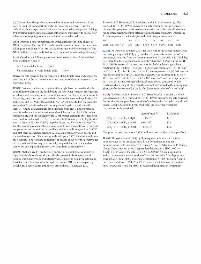
PROBLEMS 829
(c) Use your knowledge of experimental techniques and your results fromparts (a) and (b) to support or refute the following statement: It is verydifficult to obtain experimental evidence for intermediates in protein foldingby performing simple rate measurements and one must resort to special flow,relaxation, or trapping techniques to detect intermediates directly.
22.34 Propose a set of experiments in which analysis of the line-shapes ofNMR transitions (Section 15.7) can be used to monitor fast events in proteinfolding and unfolding. What are the disadvantages and disadvantages of thisNMR method over methods that use electronic and vibrational spectroscopy?
22.35 Consider the following mechanism for renaturation of a double helixfrom its strands A and B:
A + B 5 unstable helix (fast)
Unstable helix → stable double helix (slow)
Derive the rate equation for the formation of the double helix and express therate constant of the renaturation reaction in terms of the rate constants of theindividual steps.
22.36‡ Prebiotic reactions are reactions that might have occurred under theconditions prevalent on the Earth before the first living creatures emerged andwhich can lead to analogues of molecules necessary for life as we now know it.To qualify, a reaction must proceed with favourable rates and equilibria. M.P.Robertson and S.I. Miller (Science 268, 702(1995)) have studied the prebioticsynthesis of 5-substituted uracils, among them 5-hydroxymethyluracil(HMU). Amino acid analogues can be formed from HMU under prebioticconditions by reaction with various nucleophiles, such as H2S, HCN, indole,imidazole, etc. For the synthesis of HMU (the uracil analogue of serine) fromuracil and formaldehyde (HCHO), the rate of addition is given by log {k/(dm3
mol−1 s−1)} = 11.75 −5488/(T/K) (at pH = 7), and log K = −1.36 + 1794/(T/K).For this reaction, calculate the rates and equilibrium constants over a range oftemperatures corresponding to possible prebiotic conditions, such as 0–50°C,and plot them against temperature. Also, calculate the activation energy andthe standard reaction Gibbs energy and enthalpy at 25°C. Prebiotic conditionsare not likely to be standard conditions. Speculate about how the actual valuesof the reaction Gibbs energy and enthalpy might differ from the standardvalues. Do you expect that the reaction would still be favourable?
22.37‡ Methane is a by-product of a number of natural processes (such asdigestion of cellulose in ruminant animals, anaerobic decomposition oforganic waste matter) and industrial processes (such as food production andfossil fuel use). Reaction with the hydroxyl radical OH is the main path bywhich CH4 is removed from the lower atmosphere. T. Gierczak, R.K.
Talukdar, S.C. Herndon, G.L. Vaghjiani, and A.R. Ravishankara (J. Phys.Chem. A 101, 3125 (1997)) measured the rate constants for the elementarybimolecular gas-phase reaction of methane with the hydroxyl radical over arange of temperatures of importance to atmospheric chemistry. Deduce theArrhenius parameters A and Ea from the following measurements:
T/K 295 223 218 213 206 200 195
k /(10 6 dm3 mol−1 s−1) 3.55 0.494 0.452 0.379 0.295 0.241 0.217
22.38‡ As we saw in Problem 22.37, reaction with the hydroxyl radical OH isthe main path by which CH4, a by-product of many natural and industrialprocesses, is removed from the lower atmosphere. T. Gierczak, R.K. Talukdar,S.C. Herndon, G.L. Vaghjiani, and A.R. Ravishankara (J. Phys. Chem. A 101,3125 (1997)) measured the rate constants for the bimolecular gas-phasereaction CH4(g) + OH(g) → CH3(g) + H2O(g) and found A = 1.13 × 10⁹ dm3
mol−1 s−1 and Ea = 14.1 kJ mol−1 for the Arrhenius parameters. (a) Estimate therate of consumption of CH4. Take the average OH concentration to be 1.5 ×10⁻²¹ mol dm−3, that of CH4 to be 4.0 × 10⁻⁸ mol dm−3, and the temperature tobe −10°C. (b) Estimate the global annual mass of CH4 consumed by thisreaction (which is slightly less than the amount introduced to the atmosphere)given an effective volume for the Earth’s lower atmosphere of 4 × 10²¹ dm3.
22.39‡ T. Gierczak, R.K. Talukdar, S.C. Herndon, G.L. Vaghjiani, and A.R.Ravishankara ( J. Phys. Chem. A 101, 3125 (1997)) measured the rate constantsfor the bimolecular gas-phase reaction of methane with the hydroxyl radical inseveral isotopic variations. From their data, the following Arrheniusparameters can be obtained:
A /(dm3 mol−1 s−1) Ea /(kJ mol−1)
CH4 + OH → CH3 + H2O 1.13 × 10⁹ 14.1
CD4 + OH → CD3 + DOH 6.0 × 10⁸ 17.5
CH4 + OD → CH3 + DOH 1.01 × 10⁹ 13.6
Compute the rate constants at 298 K, and interpret the kinetic isotope effects.
22.40‡ The oxidation of HSO3− by O2 in aqueous solution is a reaction
of importance to the processes of acid rain formation and flue gasdesulfurization. R.E. Connick, Y.-X. Zhang, S. Lee, R. Adamic, and P. Chieng(Inorg. Chem. 34, 4543 (1995)) report that the reaction 2 HSO3
− + O2 →2 SO4
2− + 2 H+ follows the rate law v = k[HSO3−]2[H+]2. Given a pH of 5.6
and an oxygen molar concentration of 2.4 × 10⁻⁴ mol dm−3 (both presumedconstant), an initial HSO3
− molar concentration of 5 × 10⁻⁵ mol dm−3, and arate constant of 3.6 × 10⁶ dm9 mol−3 s−1, what is the initial rate of reaction?How long would it take for HSO3
− to reach half its initial concentration?
The kinetics ofcomplex reactions
This chapter extends the material introduced in Chapter 22 by showing how to deal withcomplex reaction mechanisms. First, we consider chain reactions and see that either com-plicated or simple rate laws can be obtained, depending on the conditions. Under certaincircumstances, a chain reaction can become explosive, and we see some of the reasonsfor this behaviour. An important application of these more complicated techniques is to thekinetics of polymerization reactions. There are two major classes of polymerization processand the average molar mass of the product varies with time in distinctive ways. Second, wedescribe homogeneous catalysis and apply the associated concepts to enzyme-catalysedreactions. Finally, we describe the principles of photochemistry and apply them to problemsin environmental science, biochemistry, and medicine.
Many reactions take place by mechanisms that involve several elementary steps. Sometake place at a useful rate only after absorption of light or if a catalyst is present. In thischapter we see how to develop the ideas introduced in Chapter 22 to deal with thesespecial kinds of reactions.
Chain reactions
Many gas-phase reactions and liquid-phase polymerization reactions are chain re-actions. In a chain reaction, a reaction intermediate produced in one step generates an intermediate in a subsequent step, then that intermediate generates another inter-mediate, and so on. The intermediates in a chain reaction are called chain carriers. Ina radical chain reaction the chain carriers are radicals (species with unpaired electrons).Ions may also act as chain carriers. In nuclear fission the chain carriers are neutrons.
23.1 The rate laws of chain reactions
A chain reaction can have a simple rate law. As a first example, consider the pyrolysis,or thermal decomposition in the absence of air, of acetaldehyde (ethanal, CH3CHO),which is found to be three-halves order in CH3CHO:
CH3CHO(g) → CH4(g) + CO(g) v = k[CH3CHO]3/2 (23.1)
Some ethane is also detected. The Rice–Herzfeld mechanism for this reaction is asfollows (the dot signifies an unpaired electron and marks a radical):
Initiation: CH3CHO → ·CH3 + ·CHO v = ki[CH3CHO]Propagation: CH3CHO + ·CH3 → CH3CO· + CH4 v = kp[CH3CHO][·CH3]Propagation: CH3CO· → ·CH3 + CO v = k′p[CH3CO·]Termination: ·CH3 + ·CH3 → CH3CH3 v = kt[·CH3]2
Chain reactions
23.1 The rate laws of chainreactions
23.2 Explosions
Polymerization kinetics
23.3 Stepwise polymerization
23.4 Chain polymerization
Homogeneous catalysis
23.5 Features of homogeneouscatalysis
23.6 Enzymes
Photochemistry
23.7 Kinetics of photophysical andphotochemical processes
I23.1 Impact on environmentalscience: The chemistry ofstratospheric ozone
I23.2 Impact on biochemistry: Harvesting of light duringplant photosynthesis
23.8 Complex photochemicalprocesses
I23.3 Impact on medicine:Photodynamic therapy
Checklist of key ideas
Further reading
Further information 23.1: The Förstertheory of resonance energy transfer
Discussion questions
Exercises
Problems
23
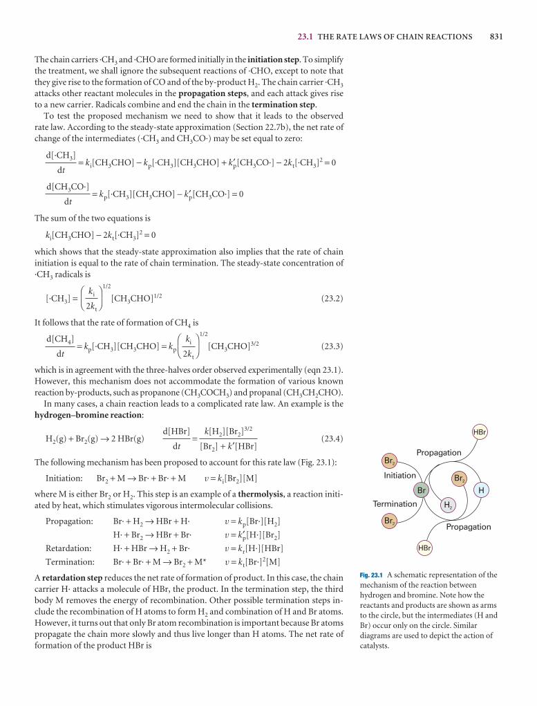
23.1 THE RATE LAWS OF CHAIN REACTIONS 831
The chain carriers ·CH3 and ·CHO are formed initially in the initiation step. To simplifythe treatment, we shall ignore the subsequent reactions of ·CHO, except to note thatthey give rise to the formation of CO and of the by-product H2. The chain carrier ·CH3
attacks other reactant molecules in the propagation steps, and each attack gives riseto a new carrier. Radicals combine and end the chain in the termination step.
To test the proposed mechanism we need to show that it leads to the observed rate law. According to the steady-state approximation (Section 22.7b), the net rate ofchange of the intermediates (·CH3 and CH3CO·) may be set equal to zero:
= ki[CH3CHO] − kp[·CH3][CH3CHO] + k′p[CH3CO·] − 2kt[·CH3]2 = 0
= kp[·CH3][CH3CHO] − k′p[CH3CO·] = 0
The sum of the two equations is
ki[CH3CHO] − 2kt[·CH3]2 = 0
which shows that the steady-state approximation also implies that the rate of chaininitiation is equal to the rate of chain termination. The steady-state concentration of·CH3 radicals is
[·CH3] =1/2
[CH3CHO]1/2 (23.2)
It follows that the rate of formation of CH4 is
= kp[·CH3][CH3CHO] = kp
1/2
[CH3CHO]3/2 (23.3)
which is in agreement with the three-halves order observed experimentally (eqn 23.1).However, this mechanism does not accommodate the formation of various known reaction by-products, such as propanone (CH3COCH3) and propanal (CH3CH2CHO).
In many cases, a chain reaction leads to a complicated rate law. An example is thehydrogen–bromine reaction:
H2(g) + Br2(g) → 2 HBr(g) = (23.4)
The following mechanism has been proposed to account for this rate law (Fig. 23.1):
Initiation: Br2 + M → Br· + Br· + M v = ki[Br2][M]
where M is either Br2 or H2. This step is an example of a thermolysis, a reaction initi-ated by heat, which stimulates vigorous intermolecular collisions.
Propagation: Br· + H2 → HBr + H· v = kp[Br·][H2]
H· + Br2 → HBr + Br· v = k′p[H·][Br2]
Retardation: H· + HBr → H2 + Br· v = kr[H·][HBr]
Termination: Br· + Br· + M → Br2 + M* v = kt[Br·]2[M]
A retardation step reduces the net rate of formation of product. In this case, the chaincarrier H· attacks a molecule of HBr, the product. In the termination step, the thirdbody M removes the energy of recombination. Other possible termination steps in-clude the recombination of H atoms to form H2 and combination of H and Br atoms.However, it turns out that only Br atom recombination is important because Br atomspropagate the chain more slowly and thus live longer than H atoms. The net rate offormation of the product HBr is
k[H2][Br2]3/2
[Br2] + k′[HBr]
d[HBr]
dt
DF
ki
2kt
AC
d[CH4]
dt
DF
ki
2kt
AC
d[CH3CO·]
dt
d[·CH3]
dt
Initiation
Propagation
Propagation
Termination
HBr
Br2
Br2
H2
Br2
Br H
HBr
Fig. 23.1 A schematic representation of themechanism of the reaction betweenhydrogen and bromine. Note how thereactants and products are shown as armsto the circle, but the intermediates (H andBr) occur only on the circle. Similardiagrams are used to depict the action ofcatalysts.
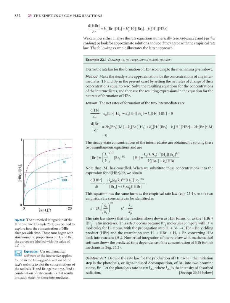
832 23 THE KINETICS OF COMPLEX REACTIONS
1
10
100[HB
r]/2
[H] 20
k t[H ]2 0
1
00
2012–
/21
Fig. 23.2 The numerical integration of theHBr rate law, Example 23.1, can be used toexplore how the concentration of HBrchanges with time. These runs began withstoichiometric proportions of H2 and Br2;the curves are labelled with the value of 2k′ − 1.
Exploration Use mathematicalsoftware or the interactive applets
found in the Living graphs section of thetext’s web site to plot the concentrations ofthe radicals H· and Br· against time. Find acombination of rate constants that resultsin steady states for these intermediates.
= kp[Br·][H2] + k′p[H·][Br2] − kr[H·][HBr]
We can now either analyse the rate equations numerically (see Appendix 2 and Furtherreading) or look for approximate solutions and see if they agree with the empirical ratelaw. The following example illustrates the latter approach.
Example 23.1 Deriving the rate equation of a chain reaction
Derive the rate law for the formation of HBr according to the mechanism given above.
Method Make the steady-state approximation for the concentrations of any inter-mediates (H· and Br· in the present case) by setting the net rates of change of theirconcentrations equal to zero. Solve the resulting equations for the concentrationsof the intermediates, and then use the resulting expressions in the equation for thenet rate of formation of HBr.
Answer The net rates of formation of the two intermediates are
= kp[Br·][H2] − k ′p[H·][Br2] − kr[H·][HBr] = 0
= 2ki[Br2][M] − kp[Br·][H2] + k ′p[H·][Br2] + kr[H·][HBr] − 2kt[Br·]2[M]
= 0
The steady-state concentrations of the intermediates are obtained by solving thesetwo simultaneous equations and are
[Br·] =1/2
[Br2]1/2 [H·] =
Note that [M] has cancelled. When we substitute these concentrations into the expression for d[HBr]/dt, we obtain
=
This equation has the same form as the empirical rate law (eqn 23.4), so the twoempirical rate constants can be identified as
k = 2kp
1/2
k′ =
The rate law shows that the reaction slows down as HBr forms, or as the [HBr]/[Br2] ratio increases. This effect occurs because Br2 molecules compete with HBrmolecules for H· atoms, with the propagation step H· + Br2 → HBr + Br· yieldingproduct (HBr) and the retardation step H· + HBr → H2 + Br· converting HBr back into reactant (H2). Numerical integration of the rate law with mathematicalsoftware shows the predicted time dependence of the concentration of HBr for thismechanism (Fig. 23.2).
Self-test 23.1 Deduce the rate law for the production of HBr when the initiationstep is the photolysis, or light-induced decomposition, of Br2 into two bromineatoms, Br·. Let the photolysis rate be v = Iabs, where Iabs is the intensity of absorbedradiation. [See eqn 23.39 below]
kr
k ′p
DF
ki
kt
AC
2kp(ki /kt)1/2[H2][Br2]3/2
[Br2] + (kr /k ′p)[HBr]
d[HBr]
dt
kp(ki/kt)1/2[H2][Br2]1/2
k ′p[Br2] + kr[HBr]
DF
ki
kt
AC
d[Br·]
dt
d[H·]
dt
d[HBr]
dt
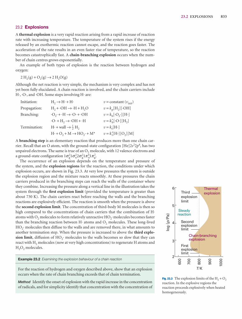
23.2 EXPLOSIONS 833
600
700
800
900
1000
Secondexplosionlimit
Firstexplosionlimit
Chain-branchingexplosion
6
5
4
3
2
log
(/P
a)p
T/K
Steadyreaction
Thirdexplosionlimit
Thermalexplosion
Fig. 23.3 The explosion limits of the H2 + O2
reaction. In the explosive regions thereaction proceeds explosively when heatedhomogeneously.
23.2 Explosions
A thermal explosion is a very rapid reaction arising from a rapid increase of reactionrate with increasing temperature. The temperature of the system rises if the energy released by an exothermic reaction cannot escape, and the reaction goes faster. Theacceleration of the rate results in an even faster rise of temperature, so the reaction becomes catastrophically fast. A chain-branching explosion occurs when the num-ber of chain centres grows exponentially.
An example of both types of explosion is the reaction between hydrogen and oxygen:
2 H2(g) + O2(g) → 2 H2O(g)
Although the net reaction is very simple, the mechanism is very complex and has notyet been fully elucidated. A chain reaction is involved, and the chain carriers includeH·, ·O·, and ·OH. Some steps involving H· are:
Initiation: H2 → H· + H· v = constant (vinit)
Propagation: H2 + ·OH → ·H + H2O v = kp[H2][·OH]
Branching: ·O2· + ·H → ·O· + ·OH v = kb[·O2·][H·]
·O· + H2 → ·OH + ·H v = k ′b[·O·][H2]
Termination: H· + wall → 1–2 H2 v = kt[H·]
H· + O2 + M → HO2· + M* v = k ′t[H·][O2][M]
A branching step is an elementary reaction that produces more than one chain car-rier. Recall that an O atom, with the ground-state configuration [He]2s22p4, has twounpaired electrons. The same is true of an O2 molecule, with 12 valence electrons anda ground-state configuration 1σ g
21σu22σ g
21π u41π g
2.The occurrence of an explosion depends on the temperature and pressure of
the system, and the explosion regions for the reaction, the conditions under which explosion occurs, are shown in Fig. 23.3. At very low pressures the system is outsidethe explosion region and the mixture reacts smoothly. At these pressures the chaincarriers produced in the branching steps can reach the walls of the container wherethey combine. Increasing the pressure along a vertical line in the illustration takes thesystem through the first explosion limit (provided the temperature is greater thanabout 730 K). The chain carriers react before reaching the walls and the branching reactions are explosively efficient. The reaction is smooth when the pressure is abovethe second explosion limit. The concentration of third-body M molecules is then sohigh compared to the concentrations of chain carriers that the combination of H·atoms with O2 molecules to form relatively unreactive HO2· molecules becomes fasterthan the branching reaction between H· atoms and O2 molecules. These long-livedHO2· molecules then diffuse to the walls and are removed there, in what amounts toanother termination step. When the pressure is increased to above the third explo-sion limit, diffusion of HO2· molecules to the walls becomes so slow that they canreact with H2 molecules (now at very high concentrations) to regenerate H atoms andH2O2 molecules.
Example 23.2 Examining the explosion behaviour of a chain reaction
For the reaction of hydrogen and oxygen described above, show that an explosionoccurs when the rate of chain branching exceeds that of chain termination.
Method Identify the onset of explosion with the rapid increase in the concentrationof radicals, and for simplicity identify that concentration with the concentration of
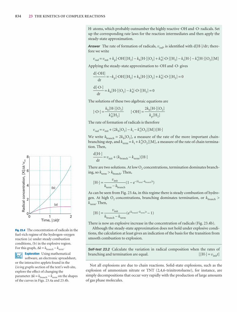
834 23 THE KINETICS OF COMPLEX REACTIONS
0
2
4
6
8
Rad
ical
con
cent
ratio
n, [X
]Dk/
v ini
t
0 21Time, | |Dk t
(a)
(b)
Fig. 23.4 The concentration of radicals in thefuel-rich regime of the hydrogen–oxygenreaction (a) under steady combustionconditions, (b) in the explosive region. For this graph, ∆k = kbranch − kterm.
Exploration Using mathematicalsoftware, an electronic spreadsheet,
or the interactive applets found in theLiving graphs section of the text’s web site,explore the effect of changing theparameter ∆k = kbranch − kterm on the shapesof the curves in Figs. 23.4a and 23.4b.
H· atoms, which probably outnumber the highly reactive ·OH and ·O· radicals. Setup the corresponding rate laws for the reaction intermediates and then apply thesteady-state approximation.
Answer The rate of formation of radicals, vrad, is identified with d[H·]/dt ; there-fore we write
vrad = vinit + kp[·OH][H2] − kb[H·][O2] + kb′[·O·][H2] − kt[H·] − k ′t[H·][O2][M]
Applying the steady-state approximation to ·OH and ·O· gives
= −kp[·OH][H2] + kb[H·][O2] + k b′[·O·][H2] = 0
= kb[H·][O2] − k b′[·O·][H2] = 0
The solutions of these two algebraic equations are
[·O·] = [·OH] =
The rate of formation of radicals is therefore
vrad = vinit + (2kb[O2] − kt − k ′t[O2][M])[H·]
We write kbranch = 2kb[O2], a measure of the rate of the more important chain-branching step, and kterm = kt + k ′t[O2][M], a measure of the rate of chain termina-tion. Then,
= vinit + (kbranch − kterm)[H·]
There are two solutions. At low O2 concentrations, termination dominates branch-ing, so kterm > kbranch. Then,
[H·] = (1 − e−(kterm−kbranch)t)
As can be seen from Fig. 23.4a, in this regime there is steady combustion of hydro-gen. At high O2 concentrations, branching dominates termination, or kbranch >kterm. Then,
[H·] = (e(kbranch−k term)t − 1)
There is now an explosive increase in the concentration of radicals (Fig. 23.4b).Although the steady-state approximation does not hold under explosive condi-
tions, the calculation at least gives an indication of the basis for the transition fromsmooth combustion to explosion.
Self-test 23.2 Calculate the variation in radical composition when the rates ofbranching and termination are equal. [[H·] = vinitt]
Not all explosions are due to chain reactions. Solid-state explosions, such as the explosion of ammonium nitrate or TNT (2,4,6-trinitrotoluene), for instance, are simply decompositions that occur very rapidly with the production of large amountsof gas phase molecules.
vinit
kbranch − kterm
vinit
kterm − kbranch
d[H·]
dt
2kb[H·][O2]
kp[H2]
kb[H·][O2]
k b′[H2]
d[·O·]
dt
d[·OH]
dt
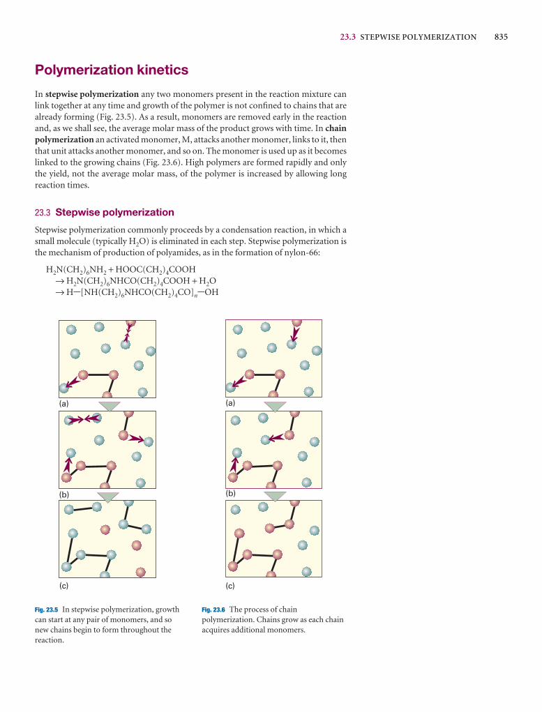
23.3 STEPWISE POLYMERIZATION 835
Polymerization kinetics
In stepwise polymerization any two monomers present in the reaction mixture canlink together at any time and growth of the polymer is not confined to chains that arealready forming (Fig. 23.5). As a result, monomers are removed early in the reactionand, as we shall see, the average molar mass of the product grows with time. In chainpolymerization an activated monomer, M, attacks another monomer, links to it, thenthat unit attacks another monomer, and so on. The monomer is used up as it becomeslinked to the growing chains (Fig. 23.6). High polymers are formed rapidly and onlythe yield, not the average molar mass, of the polymer is increased by allowing longreaction times.
23.3 Stepwise polymerization
Stepwise polymerization commonly proceeds by a condensation reaction, in which asmall molecule (typically H2O) is eliminated in each step. Stepwise polymerization isthe mechanism of production of polyamides, as in the formation of nylon-66:
H2N(CH2)6NH2 + HOOC(CH2)4COOH→ H2N(CH2)6NHCO(CH2)4COOH + H2O→ H-[NH(CH2)6NHCO(CH2)4CO]n-OH
(a)
(b)(c)
(c)
(a)
(b)
(c)
Fig. 23.5 In stepwise polymerization, growthcan start at any pair of monomers, and sonew chains begin to form throughout thereaction.
Fig. 23.6 The process of chainpolymerization. Chains grow as each chainacquires additional monomers.
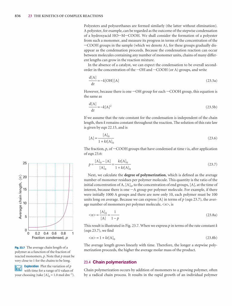
836 23 THE KINETICS OF COMPLEX REACTIONS
Polyesters and polyurethanes are formed similarly (the latter without elimination). A polyester, for example, can be regarded as the outcome of the stepwise condensationof a hydroxyacid HO-M-COOH. We shall consider the formation of a polyesterfrom such a monomer, and measure its progress in terms of the concentration of the-COOH groups in the sample (which we denote A), for these groups gradually dis-appear as the condensation proceeds. Because the condensation reaction can occurbetween molecules containing any number of monomer units, chains of many differ-ent lengths can grow in the reaction mixture.
In the absence of a catalyst, we can expect the condensation to be overall second-order in the concentration of the -OH and -COOH (or A) groups, and write
= −k[OH][A] (23.5a)
However, because there is one -OH group for each -COOH group, this equation isthe same as
= −k[A]2 (23.5b)
If we assume that the rate constant for the condensation is independent of the chainlength, then k remains constant throughout the reaction. The solution of this rate lawis given by eqn 22.15, and is
[A] = (23.6)
The fraction, p, of -COOH groups that have condensed at time t is, after applicationof eqn 23.6:
p = = (23.7)
Next, we calculate the degree of polymerization, which is defined as the averagenumber of monomer residues per polymer molecule. This quantity is the ratio of theinitial concentration of A, [A]0, to the concentration of end groups, [A], at the time ofinterest, because there is one -A group per polymer molecule. For example, if therewere initially 1000 A groups and there are now only 10, each polymer must be 100units long on average. Because we can express [A] in terms of p (eqn 23.7), the aver-age number of monomers per polymer molecule, <n>, is
<n> = = (23.8a)
This result is illustrated in Fig. 23.7. When we express p in terms of the rate constant k(eqn 23.7), we find
<n> = 1 + kt[A]0 (23.8b)
The average length grows linearly with time. Therefore, the longer a stepwise poly-merization proceeds, the higher the average molar mass of the product.
23.4 Chain polymerization
Chain polymerization occurs by addition of monomers to a growing polymer, oftenby a radical chain process. It results in the rapid growth of an individual polymer
1
1 − p
[A]0
[A]
kt[A]0
1 + kt[A]0
[A]0 − [A]
[A]0
[A]0
1 + kt[A]0
d[A]
dt
d[A]
dt
0 0.2 0.4 0.6 0.8 1Fraction condensed, p
0
5
10
15
20
25
Ave
rag
e ch
ain
len
gth
,n
Fig. 23.7 The average chain length of apolymer as a function of the fraction ofreacted monomers, p. Note that p must bevery close to 1 for the chains to be long.
Exploration Plot the variation of pwith time for a range of k values of
your choosing (take [A]0 = 1.0 mol dm−3).
23.4 CHAIN POLYMERIZATION 837
chain for each activated monomer. Examples include the addition polymerizations ofethene, methyl methacrylate, and styrene, as in
-CH2CHX· + CH2=CHX → -CH2CHXCH2CHX·
and subsequent reactions. The central feature of the kinetic analysis (which is sum-marized in the Justification below) is that the rate of polymerization is proportional tothe square root of the initiator concentration:
v = k[I]1/2[M] (23.9)
Justification 23.1 The rate of chain polymerization
There are three basic types of reaction step in a chain polymerization process:
(a) Initiation:
I → R· + R· vi = ki[I]
M + R· → ·M1 (fast)
where I is the initiator, R· the radical I forms, and ·M1 is a monomer radical. Wehave shown a reaction in which a radical is produced, but in some polymeriza-tions the initiation step leads to the formation of an ionic chain carrier. The rate-determining step is the formation of the radicals R· by homolysis of the initiator, sothe rate of initiation is equal to the vi given above.
(b) Propagation:
M + ·M1 → ·M2
M + ·M2 → ·M3
�M + ·Mn−1 → ·Mn vp = kp[M][·M]
If we assume that the rate of propagation is independent of chain size for sufficientlylarge chains, then we can use only the equation given above to describe the propa-gation process. Consequently, for sufficiently large chains, the rate of propagation isequal to the overall rate of polymerization.
Because this chain of reactions propagates quickly, the rate at which the total con-centration of radicals grows is equal to the rate of the rate-determining initiationstep. It follows that
production
= 2fki[I] (23.10)
where f is the fraction of radicals R· that successfully initiate a chain.
(c) Termination:
·Mn + ·Mm → Mn+m (mutual termination)
·Mn + ·Mm → Mn + Mm (disproportionation)
M + ·Mn → ·M + Mn (chain transfer)
In mutual termination two growing radical chains combine. In termination by disproportionation a hydrogen atom transfers from one chain to another, corres-ponding to the oxidation of the donor and the reduction of the acceptor. In chaintransfer, a new chain initiates at the expense of the one currently growing.
Here we suppose that only mutual termination occurs. If we assume that the rateof termination is independent of the length of the chain, the rate law for termination is
vt = kt[·M]2
DEFd[·M]
dt
ABC
838 23 THE KINETICS OF COMPLEX REACTIONS
and the rate of change of radical concentration by this process is
depletion
= −2kt[·M]2
The steady-state approximation gives:
= 2fki[I] − 2kt[·M]2 = 0
The steady-state concentration of radical chains is therefore
[·M] =1/2
[I]1/2 (23.11)
Because the rate of propagation of the chains is the negative of the rate at which themonomer is consumed, we can write vP = −d[M]/dt and
vP = kP[·M][M] = kp
1/2
[I]1/2[M] (23.12)
This rate is also the rate of polymerization, which has the form of eqn 23.9.
The kinetic chain length, ν, is the ratio of the number of monomer units con-sumed per activated centre produced in the initiation step:
ν = (23.13)
The kinetic chain length can be expressed in terms of the rate expressions inJustification 23.1. To do so, we recognize that monomers are consumed at the rate thatchains propagate. Then,
ν =
By making the steady-state approximation, we set the rate of production of radicalsequal to the termination rate. Therefore, we can write the expression for the kineticchain length as
ν = =
When we substitute the steady-state expression, eqn 23.11, for the radical concentra-tion, we obtain
ν = k[M][I]−1/2 k = 1–2 kp( fkikt)−1/2 (23.14)
Consider a polymer produced by a chain mechanism with mutual termination. Inthis case, the average number of monomers in a polymer molecule, <n>, produced by the reaction is the sum of the numbers in the two combining polymer chains. Theaverage number of units in each chain is ν. Therefore,
<n> = 2ν = 2k[M][I]−1/2 (23.15)
with k given in eqn 23.14. We see that, the slower the initiation of the chain (thesmaller the initiator concentration and the smaller the initiation rate constant), thegreater the kinetic chain length, and therefore the higher the average molar mass ofthe polymer. Some of the consequences of molar mass for polymers were explored inChapter 19: now we have seen how we can exercise kinetic control over them.
kp[M]
2kt[·M]
kp[·M][M]
2kt[M·]2
rate of propagation of chains
rate of production of radicals
number of monomer units consumed
number of activated centres produced
DEFfki
kt
ABC
DEFfki
kt
ABC
d[·M]
dt
DEFd[·M]
dt
ABC
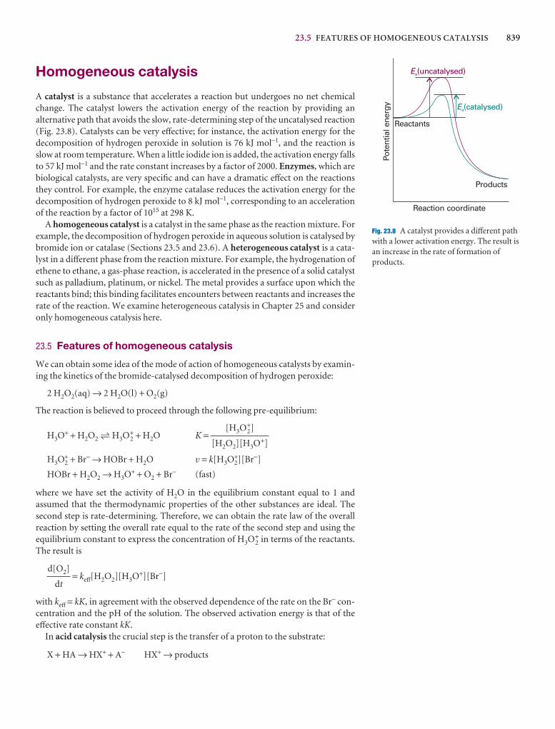
23.5 FEATURES OF HOMOGENEOUS CATALYSIS 839
Homogeneous catalysis
A catalyst is a substance that accelerates a reaction but undergoes no net chemicalchange. The catalyst lowers the activation energy of the reaction by providing an alternative path that avoids the slow, rate-determining step of the uncatalysed reaction(Fig. 23.8). Catalysts can be very effective; for instance, the activation energy for thedecomposition of hydrogen peroxide in solution is 76 kJ mol−1, and the reaction isslow at room temperature. When a little iodide ion is added, the activation energy fallsto 57 kJ mol−1 and the rate constant increases by a factor of 2000. Enzymes, which arebiological catalysts, are very specific and can have a dramatic effect on the reactionsthey control. For example, the enzyme catalase reduces the activation energy for thedecomposition of hydrogen peroxide to 8 kJ mol−1, corresponding to an accelerationof the reaction by a factor of 1015 at 298 K.
A homogeneous catalyst is a catalyst in the same phase as the reaction mixture. Forexample, the decomposition of hydrogen peroxide in aqueous solution is catalysed bybromide ion or catalase (Sections 23.5 and 23.6). A heterogeneous catalyst is a cata-lyst in a different phase from the reaction mixture. For example, the hydrogenation ofethene to ethane, a gas-phase reaction, is accelerated in the presence of a solid catalystsuch as palladium, platinum, or nickel. The metal provides a surface upon which thereactants bind; this binding facilitates encounters between reactants and increases therate of the reaction. We examine heterogeneous catalysis in Chapter 25 and consideronly homogeneous catalysis here.
23.5 Features of homogeneous catalysis
We can obtain some idea of the mode of action of homogeneous catalysts by examin-ing the kinetics of the bromide-catalysed decomposition of hydrogen peroxide:
2 H2O2(aq) → 2 H2O(l) + O2(g)
The reaction is believed to proceed through the following pre-equilibrium:
H3O+ + H2O2 5 H3O2+ + H2O K =
H3O2+ + Br− → HOBr + H2O v = k[H3O2
+][Br−]
HOBr + H2O2 → H3O+ + O2 + Br− (fast)
where we have set the activity of H2O in the equilibrium constant equal to 1 and assumed that the thermodynamic properties of the other substances are ideal. Thesecond step is rate-determining. Therefore, we can obtain the rate law of the overallreaction by setting the overall rate equal to the rate of the second step and using theequilibrium constant to express the concentration of H3O2
+ in terms of the reactants.The result is
= keff[H2O2][H3O+][Br−]
with keff = kK, in agreement with the observed dependence of the rate on the Br− con-centration and the pH of the solution. The observed activation energy is that of the effective rate constant kK.
In acid catalysis the crucial step is the transfer of a proton to the substrate:
X + HA → HX+ + A− HX+ → products
d[O2]
dt
[H3O2+]
[H2O2][H3O+]
Ea(uncatalysed)
Reactants
Products
Pote
ntia
l ene
rgy
Reaction coordinate
Ea(catalysed)
Fig. 23.8 A catalyst provides a different pathwith a lower activation energy. The result isan increase in the rate of formation ofproducts.
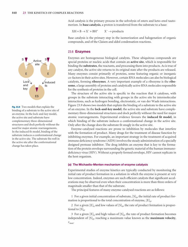
840 23 THE KINETICS OF COMPLEX REACTIONS
Acid catalysis is the primary process in the solvolysis of esters and keto–enol tauto-merism. In base catalysis, a proton is transferred from the substrate to a base:
XH + B → X− + BH+ X− → products
Base catalysis is the primary step in the isomerization and halogenation of organiccompounds, and of the Claisen and aldol condensation reactions.
23.6 Enzymes
Enzymes are homogeneous biological catalysts. These ubiquitous compounds arespecial proteins or nucleic acids that contain an active site, which is responsible forbinding the substrates, the reactants, and processing them into products. As is true ofany catalyst, the active site returns to its original state after the products are released.Many enzymes consist primarily of proteins, some featuring organic or inorganic co-factors in their active sites. However, certain RNA molecules can also be biologicalcatalysts, forming ribozymes. A very important example of a ribozyme is the ribo-some, a large assembly of proteins and catalytically active RNA molecules responsiblefor the synthesis of proteins in the cell.
The structure of the active site is specific to the reaction that it catalyses, withgroups in the substrate interacting with groups in the active site by intermolecular interactions, such as hydrogen bonding, electrostatic, or van der Waals interactions.Figure 23.9 shows two models that explain the binding of a substrate to the active siteof an enzyme. In the lock-and-key model, the active site and substrate have comple-mentary three-dimensional structures and dock perfectly without the need for majoratomic rearrangements. Experimental evidence favours the induced fit model, inwhich binding of the substrate induces a conformational change in the active site.Only after the change does the substrate fit snugly in the active site.
Enzyme-catalysed reactions are prone to inhibition by molecules that interfere with the formation of product. Many drugs for the treatment of disease function byinhibiting enzymes. For example, an important strategy in the treatment of acquiredimmune deficiency syndrome (AIDS) involves the steady administration of a speciallydesigned protease inhibitor. The drug inhibits an enzyme that is key to the forma-tion of the protein envelope surrounding the genetic material of the human immuno-deficiency virus (HIV). Without a properly formed envelope, HIV cannot replicate inthe host organism.
(a) The Michaelis–Menten mechanism of enzyme catalysis
Experimental studies of enzyme kinetics are typically conducted by monitoring theinitial rate of product formation in a solution in which the enzyme is present at verylow concentration. Indeed, enzymes are such efficient catalysts that significant accel-erations may be observed even when their concentration is more than three orders ofmagnitude smaller than that of the substrate.
The principal features of many enzyme-catalysed reactions are as follows:
1 For a given initial concentration of substrate, [S]0, the initial rate of product for-mation is proportional to the total concentration of enzyme, [E]0.
2 For a given [E]0 and low values of [S]0, the rate of product formation is propor-tional to [S]0.
3 For a given [E]0 and high values of [S]0, the rate of product formation becomesindependent of [S]0, reaching a maximum value known as the maximum velocity,vmax.
S
E
ES
Inducedfit
Lockandkey
Activesite
E
S
Fig. 23.9 Two models that explain thebinding of a substrate to the active site ofan enzyme. In the lock-and-key model, the active site and substrate havecomplementary three-dimensionalstructures and dock perfectly without theneed for major atomic rearrangements. In the induced fit model, binding of thesubstrate induces a conformational changein the active site. The substrate fits well inthe active site after the conformationalchange has taken place.
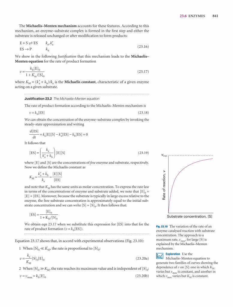
23.6 ENZYMES 841
The Michaelis–Menten mechanism accounts for these features. According to thismechanism, an enzyme–substrate complex is formed in the first step and either thesubstrate is released unchanged or after modification to form products:
E + S 5 ES ka, k′a(23.16)
ES → P kb
We show in the following Justification that this mechanism leads to the Michaelis–Menten equation for the rate of product formation
v = (23.17)
where KM = (k ′a + kb)/ka is the Michaelis constant, characteristic of a given enzymeacting on a given substrate.
Justification 23.2 The Michaelis–Menten equation
The rate of product formation according to the Michaelis–Menten mechanism is
v = kb[ES] (23.18)
We can obtain the concentration of the enzyme–substrate complex by invoking thesteady-state approximation and writing
= ka[E][S] − k ′a[ES] − kb[ES] = 0
It follows that
[ES] = [E][S] (23.19)
where [E] and [S] are the concentrations of free enzyme and substrate, respectively.Now we define the Michaelis constant as
KM = =
and note that KM has the same units as molar concentration. To express the rate lawin terms of the concentrations of enzyme and substrate added, we note that [E]0 =[E] + [ES]. Moreover, because the substrate is typically in large excess relative to theenzyme, the free substrate concentration is approximately equal to the initial sub-strate concentration and we can write [S] ≈ [S]0. It then follows that:
[ES] =
We obtain eqn 23.17 when we substitute this expression for [ES] into that for therate of product formation (v = kb[ES]).
Equation 23.17 shows that, in accord with experimental observations (Fig. 23.10):
1 When [S]0 << KM, the rate is proportional to [S]0:
v = [S]0[E]0 (23.20a)
2 When [S]0 >> KM, the rate reaches its maximum value and is independent of [S]0:
v = vmax = kb[E]0 (23.20b)
ka
KM
[E]0
1 + KM/[S]0
[E][S]
[ES]
k ′a + kb
ka
DEFka
k ′a + kb
ABC
d[ES]
dt
kb[E]0
1 + Km /[S]0
Rat
e of
rea
ctio
n,v
vmax
Substrate concentration, [S]
Fig. 23.10 The variation of the rate of anenzyme-catalysed reaction with substrateconcentration. The approach to amaximum rate, vmax, for large [S] isexplained by the Michaelis–Mentenmechanism.
Exploration Use theMichaelis–Menten equation to
generate two families of curves showing thedependence of v on [S]: one in which KM
varies but vmax is constant, and another inwhich vmax varies but KM is constant.
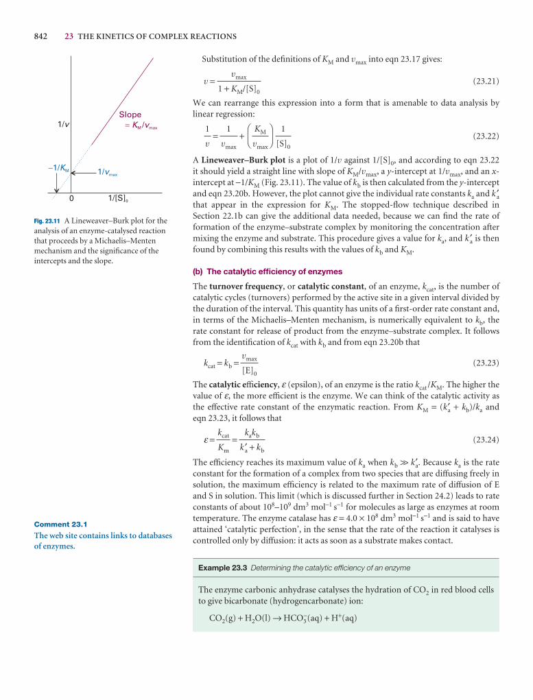
842 23 THE KINETICS OF COMPLEX REACTIONS
1/[S]0
1/v
0
Slope/� K vM max
1/vmax�1/KM
Fig. 23.11 A Lineweaver–Burk plot for theanalysis of an enzyme-catalysed reactionthat proceeds by a Michaelis–Mentenmechanism and the significance of theintercepts and the slope.
Comment 23.1
The web site contains links to databasesof enzymes.
Substitution of the definitions of KM and vmax into eqn 23.17 gives:
v = (23.21)
We can rearrange this expression into a form that is amenable to data analysis by linear regression:
= + (23.22)
A Lineweaver–Burk plot is a plot of 1/v against 1/[S]0, and according to eqn 23.22 it should yield a straight line with slope of KM/vmax, a y-intercept at 1/vmax, and an x-intercept at −1/KM (Fig. 23.11). The value of kb is then calculated from the y-interceptand eqn 23.20b. However, the plot cannot give the individual rate constants ka and k ′athat appear in the expression for KM. The stopped-flow technique described inSection 22.1b can give the additional data needed, because we can find the rate of formation of the enzyme–substrate complex by monitoring the concentration aftermixing the enzyme and substrate. This procedure gives a value for ka, and k ′a is thenfound by combining this results with the values of kb and KM.
(b) The catalytic efficiency of enzymes
The turnover frequency, or catalytic constant, of an enzyme, kcat, is the number ofcatalytic cycles (turnovers) performed by the active site in a given interval divided bythe duration of the interval. This quantity has units of a first-order rate constant and,in terms of the Michaelis–Menten mechanism, is numerically equivalent to kb, therate constant for release of product from the enzyme–substrate complex. It followsfrom the identification of kcat with kb and from eqn 23.20b that
kcat = kb = (23.23)
The catalytic efficiency, ε (epsilon), of an enzyme is the ratio kcat /KM. The higher thevalue of ε, the more efficient is the enzyme. We can think of the catalytic activity as the effective rate constant of the enzymatic reaction. From KM = (k′a + kb)/ka andeqn 23.23, it follows that
ε = = (23.24)
The efficiency reaches its maximum value of ka when kb >> k′a. Because ka is the rateconstant for the formation of a complex from two species that are diffusing freely insolution, the maximum efficiency is related to the maximum rate of diffusion of E and S in solution. This limit (which is discussed further in Section 24.2) leads to rateconstants of about 108–109 dm3 mol−1 s−1 for molecules as large as enzymes at roomtemperature. The enzyme catalase has ε = 4.0 × 10⁸ dm3 mol−1 s−1 and is said to haveattained ‘catalytic perfection’, in the sense that the rate of the reaction it catalyses iscontrolled only by diffusion: it acts as soon as a substrate makes contact.
Example 23.3 Determining the catalytic efficiency of an enzyme
The enzyme carbonic anhydrase catalyses the hydration of CO2 in red blood cellsto give bicarbonate (hydrogencarbonate) ion:
CO2(g) + H2O(l) → HCO3−(aq) + H+(aq)
kakb
k ′a + kb
kcat
Km
vmax
[E]0
1
[S]0
DF
KM
vmax
AC
1
vmax
1
v
vmax
1 + KM/[S]0
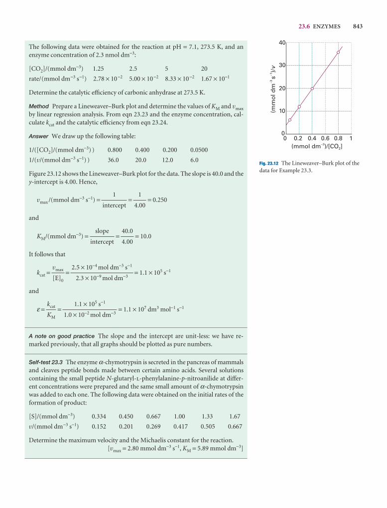
23.6 ENZYMES 843
0 0.2 0.4 0.6 0.8 1(mmol dm )/[CO ]�3
2
(mm
ol d
ms
)/�
�3
1v
10
20
30
40
0
Fig. 23.12 The Lineweaver–Burk plot of thedata for Example 23.3.
The following data were obtained for the reaction at pH = 7.1, 273.5 K, and an enzyme concentration of 2.3 nmol dm−3:
[CO2]/(mmol dm−3) 1.25 2.5 5 20
rate/(mmol dm−3 s−1) 2.78 × 10⁻² 5.00 × 10⁻² 8.33 × 10⁻² 1.67 × 10⁻¹
Determine the catalytic efficiency of carbonic anhydrase at 273.5 K.
Method Prepare a Lineweaver–Burk plot and determine the values of KM and vmax
by linear regression analysis. From eqn 23.23 and the enzyme concentration, cal-culate kcat and the catalytic efficiency from eqn 23.24.
Answer We draw up the following table:
1/([CO2]/(mmol dm−3) ) 0.800 0.400 0.200 0.0500
1/(v/(mmol dm−3 s−1) ) 36.0 20.0 12.0 6.0
Figure 23.12 shows the Lineweaver–Burk plot for the data. The slope is 40.0 and they-intercept is 4.00. Hence,
vmax /(mmol dm−3 s−1) = = = 0.250
and
KM/(mmol dm−3) = = = 10.0
It follows that
kcat = = = 1.1 × 10⁵ s−1
and
ε = = = 1.1 × 10⁷ dm3 mol−1 s−1
A note on good practice The slope and the intercept are unit-less: we have re-marked previously, that all graphs should be plotted as pure numbers.
Self-test 23.3 The enzyme α-chymotrypsin is secreted in the pancreas of mammalsand cleaves peptide bonds made between certain amino acids. Several solutionscontaining the small peptide N-glutaryl-l-phenylalanine-p-nitroanilide at differ-ent concentrations were prepared and the same small amount of α-chymotrypsinwas added to each one. The following data were obtained on the initial rates of theformation of product:
[S]/(mmol dm−3) 0.334 0.450 0.667 1.00 1.33 1.67
v/(mmol dm−3 s−1) 0.152 0.201 0.269 0.417 0.505 0.667
Determine the maximum velocity and the Michaelis constant for the reaction.[vmax = 2.80 mmol dm−3 s−1, KM = 5.89 mmol dm−3]
1.1 × 10⁵ s−1
1.0 × 10⁻² mol dm−3
kcat
KM
2.5 × 10⁻⁴ mol dm−3 s−1
2.3 × 10⁻⁹ mol dm−3
vmax
[E]0
40.0
4.00
slope
intercept
1
4.00
1
intercept
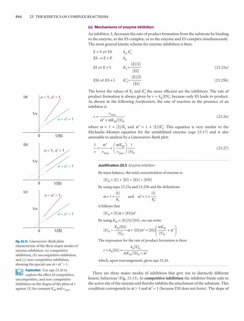
844 23 THE KINETICS OF COMPLEX REACTIONS
(c) Mechanisms of enzyme inhibition
An inhibitor, I, decreases the rate of product formation from the substrate by bindingto the enzyme, to the ES complex, or to the enzyme and ES complex simultaneously.The most general kinetic scheme for enzyme inhibition is then:
E + S 5 ES ka, k ′aES → E + P kb
EI 5 E + I KI = (23.25a)
ESI 5 ES + I K S′ = (23.25b)
The lower the values of KI and K ′I the more efficient are the inhibitors. The rate ofproduct formation is always given by v = kb[ES], because only ES leads to product. As shown in the following Justification, the rate of reaction in the presence of an inhibitor is
v = (23.26)
where α = 1 + [I]/KI and α′ = 1 + [I]/K ′I. This equation is very similar to theMichaelis–Menten equation for the uninhibited enzyme (eqn 23.17) and is alsoamenable to analysis by a Lineweaver–Burk plot:
= + (23.27)
Justification 23.3 Enzyme inhibition
By mass balance, the total concentration of enzyme is:
[E]0 = [E] + [EI] + [ES] + [ESI]
By using eqns 23.25a and 23.25b and the definitions
α = 1 + and α′ = 1 +
it follows that
[E]0 = [E]α + [ES]α′
By using KM = [E][S]/[ES], we can write
[E]0 = α + [ES]α′ = [ES] + α′
The expression for the rate of product formation is then:
v = kb[ES] =
which, upon rearrangement, gives eqn 23.26.
There are three major modes of inhibition that give rise to distinctly differentkinetic behaviour (Fig. 23.13). In competitive inhibition the inhibitor binds only tothe active site of the enzyme and thereby inhibits the attachment of the substrate. Thiscondition corresponds to α > 1 and α′ = 1 (because ESI does not form). The slope of
kb[E]0
αKM /[S]0 + α′
DEFαKM
[S]0
ABCKM[ES]
[S]0
[I]
K′I
[I]
KI
1
[S]0
DF
αKM
vmax
AC
α′vmax
1
v
vmax
α′ + αKM/[S]0
[E][I]
[EI]
[E][I]
[EI]
1/[S]
1/v
0
1/[S]
1/v
0
1/[S]
1/v
0
a a’ 1= =
a a1, ’ 1> =
a a’ 1= =
a a’ 1= =
a a1, ’ 1= >
a a’ 1= >
(a)
(b)
(c)
a a
a a
a
a
a
a
a
a
a
a
Fig. 23.13 Lineweaver–Burk plotscharacteristic of the three major modes ofenzyme inhibition: (a) competitiveinhibition, (b) uncompetitive inhibition,and (c) non-competitive inhibition,showing the special case α = α′ > 1.
Exploration Use eqn 23.26 to explore the effect of competitive,
uncompetitive, and non-competitiveinhibition on the shapes of the plots of vagainst [S] for constant KM and vmax.
23.7 KINETICS OF PHOTOPHYSICAL AND PHOTOCHEMICAL PROCESSES 845
the Lineweaver–Burk plot increases by a factor of α relative to the slope for data on theuninhibited enzyme (α = α′ = 1). The y-intercept does not change as a result of com-petitive inhibition (Fig. 23.13a). In uncompetitive inhibition the inhibitor binds to a site of the enzyme that is removed from the active site, but only if the substrate is already present. The inhibition occurs because ESI reduces the concentration of ES,the active type of complex. In this case α = 1 (because EI does not form) and α′ > 1.The y-intercept of the Lineweaver–Burk plot increases by a factor of α′ relative to the y-intercept for data on the uninhibited enzyme but the slope does not change (Fig. 23.13b). In non-competitive inhibition (also called mixed inhibition) the inhibitor binds to a site other than the active site, and its presence reduces the abilityof the substrate to bind to the active site. Inhibition occurs at both the E and ES sites.This condition corresponds to α > 1 and α′ > 1. Both the slope and y-intercept of theLineweaver–Burk plot increase upon addition of the inhibitor. Figure 23.13c showsthe special case of KI = K ′I and α = α′, which results in intersection of the lines at thex-axis.
In all cases, the efficiency of the inhibitor may be obtained by determining KM andvmax from a control experiment with uninhibited enzyme and then repeating the experiment with a known concentration of inhibitor. From the slope and y-interceptof the Lineweaver–Burk plot for the inhibited enzyme (eqn 23.27), the mode of inhibition, the values of α or α′, and the values of KI or K ′I may be obtained.
Photochemistry
Many reactions can be initiated by the absorption of electromagnetic radiation by one of the mechanisms described in Chapter 14. The most important of all are thephotochemical processes that capture the radiant energy of the Sun. Some of these reactions lead to the heating of the atmosphere during the daytime by absorption ofultraviolet radiation (Impact I23.1). Others include the absorption of visible radiationduring photosynthesis (Impact I7.2 and I23.2). Without photochemical processes, the Earth would be simply a warm, sterile, rock. Table 23.1 summarizes commonphotochemical reactions.
23.7 Kinetics of photophysical and photochemical processes
Photochemical processes are initiated by the absorption of radiation by at least onecomponent of a reaction mixture. In a primary process, products are formed directlyfrom the excited state of a reactant. Examples include fluorescence (Section 14.3) andthe cis–trans photoisomerization of retinal (Table 23.1, see also Impact I14.1). Prod-ucts of a secondary process originate from intermediates that are formed directly fromthe excited state of a reactant. Examples include photosynthesis and photochemicalchain reactions (Section 23.8).
Competing with the formation of photochemical products is a host of primaryphotophysical processes that can deactivate the excited state (Table 23.2). Therefore,it is important to consider the timescales of excited state formation and decay beforedescribing the mechanisms of photochemical reactions.
(a) Timescales of photophysical processes
Electronic transitions caused by absorption of ultraviolet and visible radiation occurwithin 10−16–10−15 s. We expect, then, that the upper limit for the rate constant ofa first-order photochemical reaction is about 1016 s−1. Fluorescence is slower than
Comment 23.2
The web site contains links to databaseson photochemical reactions.
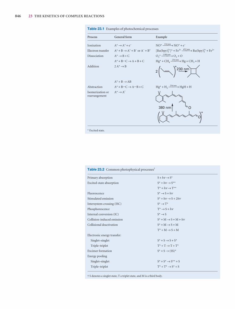
846 23 THE KINETICS OF COMPLEX REACTIONS
Table 23.1 Examples of photochemical processes
Process General form Example
Ionization A* → A+ + e− NO* –134––nm––→ NO+ + e−
Electron transfer A* + B → A+ + B− or A− + B+ [Ru(bpy)32+]* + Fe3+ –452––nm––→ Ru(bpy)3
3+ + Fe2+
Dissociation A* → B + C O3* –1180–––nm––→ O2 + O
A* + B-C → A + B + C Hg* + CH4 –254––nm––→ Hg + CH3 + H
Addition 2 A* → B
A* + B → AB
Abstraction A* + B-C → A-B + C Hg* + H2 –254––nm––→ HgH + H
Isomerization or A* → A′rearrangement
* Excited state.
Table 23.2 Common photophysical processes†
Primary absorption S + hν → S*
Excited-state absorption S* + hν → S**
T* + hν → T**
Fluorescence S* → S + hνStimulated emission S* + hν → S + 2hνIntersystem crossing (ISC) S* → T*
Phosphorescence T* → S + hνInternal conversion (IC) S* → S
Collision-induced emission S* + M → S + M + hνCollisional deactivation S* + M → S + M
T* + M → S + M
Electronic energy transfer:
Singlet–singlet S* + S → S + S*
Triple–triplet T* + T → T + T*
Excimer formation S* + S → (SS)*
Energy pooling
Singlet–singlet S* + S* → S** + S
Triple–triplet T* + T* → S* + S
† S denotes a singlet state, T a triplet state, and M is a third body.
23.7 KINETICS OF PHOTOPHYSICAL AND PHOTOCHEMICAL PROCESSES 847
absorption, with typical lifetimes of 10−12–10−6 s. Therefore, the excited singlet statecan initiate very fast photochemical reactions in the femtosecond (10−15 s) to pico-second (10−12 s) timescale. Examples of such ultrafast reactions are the initial events of vision (Impact I14.1) and of photosynthesis. Typical intersystem crossing (ISC) andphosphorescence times for large organic molecules are 10−12–10−4 s and 10−6 –10−1 s,respectively. As a consequence, excited triplet states are photochemically important.Indeed, because phosphorescence decay is several orders of magnitude slower thanmost typical reactions, species in excited triplet states can undergo a very large num-ber of collisions with other reactants before deactivation. The interplay between reac-tion rates and excited state lifetimes is a very important factor in the determination ofthe kinetic feasibility of a photochemical process.
Illustration 23.1 Exploring the photochemical roles of excited singlet and triplet states
To estimate whether the excited singlet or triplet state of the reactant is a suitableproduct precursor, we compare the emission lifetimes with the relaxation time, τ,of the reactant due to the chemical reaction. As an illustration, consider a uni-molecular photochemical reaction with rate constant k = 1.7 × 10⁴ s−1 and relaxa-tion time τ = 1/(1.7 × 104 s−1) = 59 µs that involves a reactant with an observedfluorescence lifetime of 1.0 ns and an observed phosphorescence lifetime of 1.0 ms.The excited singlet state is too short-lived and is not expected to be a major sourceof product in this reaction. On the other hand, the excited triplet state is a goodcandidate for a precursor.
(b) The primary quantum yield
We shall see that the rates of deactivation of the excited state by radiative, non-radiative,and chemical processes determine the yield of product in a photochemical reaction.The primary quantum yield, φ, is defined as the number of photophysical or photo-chemical events that lead to primary products divided by the number of photons absorbed by the molecule in the same interval. It follows that the primary quantumyield is also the rate of radiation-induced primary events divided by the rate of pho-ton absorption. Because the rate of photon absorption is equal to the intensity of lightabsorbed by the molecule (Section 13.2), we write
φ = = = [23.28]
A molecule in an excited state must either decay to the ground state or form a photo-chemical product. Therefore, the total number of molecules deactivated by radiativeprocesses, non-radiative processes, and photochemical reactions must be equal to thenumber of excited species produced by absorption of light. We conclude that the sumof primary quantum yields φi for all photophysical and photochemical events i mustbe equal to 1, regardless of the number of reactions involving the excited state. It fol-lows that
∑i
φi = ∑i
= 1 (23.29)
It follows that for an excited singlet state that decays to the ground state only via thephotophysical processes described in Section 23.7(a), we write
φ f + φIC + φISC + φp = 1
vi
Iabs
v
Iabs
rate of process
intensity of light absorbed
number of events
number of photons absorbed
848 23 THE KINETICS OF COMPLEX REACTIONS
where φf, φIC, φISC, and φp are the quantum yields of fluorescence, internal conversion,intersystem crossing, and phosphorescence, respectively. The quantum yield of pho-ton emission by fluorescence and phosphorescence is φemission = φf + φp, which is less than 1. If the excited singlet state also participates in a primary photochemical reaction with quantum yield φR, we write
φf + φIC + φISC + φp + φR = 1
We can now strengthen the link between reaction rates and primary quantum yield already established by eqns 23.28 and 23.29. By taking the constant Iabs out of the sum-mation in eqn 23.29 and rearranging, we obtain Iabs = ∑i vi. Substituting this resultinto eqn 23.29 gives the general result
φi = (23.30)
Therefore, the primary quantum yield may be determined directly from the experi-mental rates of all photophysical and photochemical processes that deactivate the excited state.
(c) Mechanism of decay of excited singlet states
Consider the formation and decay of an excited singlet state in the absense of a chem-ical reaction:
Absorption: S + hνi → S* vabs = Iabs
Fluorescence: S* → S + hνf vf = kf[S*]
Internal conversion: S* → S vIC = kIC[S*]
Intersystem crossing: S* → T* vISC = kISC[S*]
in which S is an absorbing species, S* an excited singlet state, T* an excited tripletstate, and hνi and hνf are the energies of the incident and fluorescent photons, respec-tively. From the methods developed in Chapter 22 and the rates of the steps that formand destroy the excited singlet state S*, we write the rate of formation and decay of S* as:
Rate of formation of [S*] = Iabs
Rate of decay of [S*] = −kf[S*] − kISC[S*] − kIC[S*] = −(kf + kISC + kIC)[S*]
It follows that the excited state decays by a first-order process so, when the light isturned off, the concentration of S* varies with time t as:
[S*]t = [S*]0e−t/τ0 (23.31)
where the observed fluorescence lifetime, τ0, is defined as:
τ0 = (23.32)
We show in the following Justification that the quantum yield of fluorescence is
φf = (23.33)kf
kf + kISC + kIC
1
kf + kISC + kIC
vi
∑i
vi
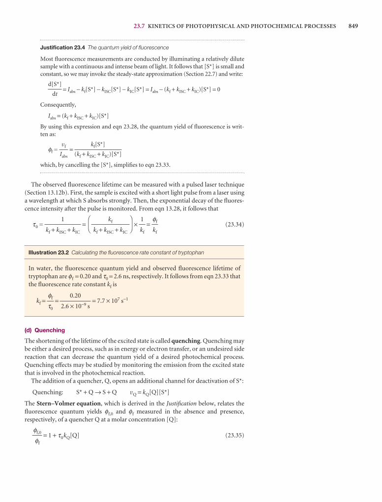
23.7 KINETICS OF PHOTOPHYSICAL AND PHOTOCHEMICAL PROCESSES 849
Justification 23.4 The quantum yield of fluorescence
Most fluorescence measurements are conducted by illuminating a relatively dilutesample with a continuous and intense beam of light. It follows that [S*] is small andconstant, so we may invoke the steady-state approximation (Section 22.7) and write:
= Iabs − kf[S*] − kISC[S*] − kIC[S*] = Iabs − (kf + kISC + kIC)[S*] = 0
Consequently,
Iabs = (kf + kISC + kIC)[S*]
By using this expression and eqn 23.28, the quantum yield of fluorescence is writ-ten as:
φf = =
which, by cancelling the [S*], simplifies to eqn 23.33.
The observed fluorescence lifetime can be measured with a pulsed laser technique(Section 13.12b). First, the sample is excited with a short light pulse from a laser usinga wavelength at which S absorbs strongly. Then, the exponential decay of the fluores-cence intensity after the pulse is monitored. From eqn 13.28, it follows that
τ0 = = × = (23.34)
Illustration 23.2 Calculating the fluorescence rate constant of tryptophan
In water, the fluorescence quantum yield and observed fluorescence lifetime oftryptophan are φf = 0.20 and τ0 = 2.6 ns, respectively. It follows from eqn 23.33 thatthe fluorescence rate constant kf is
kf = = = 7.7 × 10⁷ s−1
(d) Quenching
The shortening of the lifetime of the excited state is called quenching. Quenching maybe either a desired process, such as in energy or electron transfer, or an undesired sidereaction that can decrease the quantum yield of a desired photochemical process.Quenching effects may be studied by monitoring the emission from the excited statethat is involved in the photochemical reaction.
The addition of a quencher, Q, opens an additional channel for deactivation of S*:
Quenching: S* + Q → S + Q vQ = kQ[Q][S*]
The Stern–Volmer equation, which is derived in the Justification below, relates thefluorescence quantum yields φf,0 and φf measured in the absence and presence, respectively, of a quencher Q at a molar concentration [Q]:
= 1 + τ0kQ[Q] (23.35)φf,0
φf
0.20
2.6 × 10⁻⁹ s
φf
τ0
φf
kf
1
kf
DF
kf
kf + kISC + kIC
AC
1
kf + kISC + kIC
kf[S*]
(kf + kISC + kIC)[S*]
vf
Iabs
d[S*]
dt
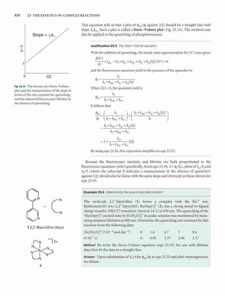
850 23 THE KINETICS OF COMPLEX REACTIONS
f f/
[Q]
Slope = 0kQt
0
1
t
ff
Fig. 23.14 The format of a Stern–Volmerplot and the interpretation of the slope interms of the rate constant for quenchingand the observed fluorescence lifetime inthe absence of quenching.
This equation tells us that a plot of φf,0 /φf against [Q] should be a straight line withslope τ0kQ. Such a plot is called a Stern–Volmer plot (Fig. 23.14). The method mayalso be applied to the quenching of phosphorescence.
Justification 23.5 The Stern–Volmer equation
With the addition of quenching, the steady-state approximation for [S*] now gives:
= Iabs − (kf + kIC + kISC + kIC + kQ[Q])[S*] = 0
and the fluorescence quantum yield in the presence of the quencher is:
φf =
When [Q] = 0, the quantum yield is
φf,0 =
It follows that
= ×
=
= 1 + [Q]
By using eqn 23.34, this expression simplifies to eqn 23.35.
Because the fluorescence intensity and lifetime are both proportional to thefluorescence quantum yield (specifically, from eqn 23.34, τ = φf /kf), plots of If,0 /If andτ0 /τ (where the subscript 0 indicates a measurement in the absence of quencher)against [Q] should also be linear with the same slope and intercept as those shown foreqn 23.35.
Example 23.4 Determining the quenching rate constant
The molecule 2,2′-bipyridine (1) forms a complex with the Ru2+ ion.Ruthenium(II) tris-(2,2′-bipyridyl), Ru(bipy)3
2+ (2), has a strong metal-to-ligandcharge transfer (MLCT) transition (Section 14.2) at 450 nm. The quenching of the*Ru(bipy)3
2+ excited state by Fe(H2O)63+ in acidic solution was monitored by meas-
uring emission lifetimes at 600 nm. Determine the quenching rate constant for thisreaction from the following data:
[Fe(H2O)63+]/(10− 4 mol dm−3) 0 1.6 4.7 7 9.4
t/(10−7 s) 6 4.05 3.37 2.96 2.17
Method Re-write the Stern–Volmer equation (eqn 23.35) for use with lifetimedata then fit the data to a straight-line.
Answer Upon substitution of τ0/τ for φ0,f /φf in eqn 23.35 and after rearrangement,we obtain:
kQ
kf + kISC + kIC
kf + kISC + kIC + kQ[Q]
kf + kISC + kIC
DEFkf + kISC + kIC + kQ[Q]
kf
ABCDEF
kf
kf + kISC + kIC
ABCφf,0
φf
kf
kf + kISC + kIC
kf
kf + kISC + kIC + kQ[Q]
d[S*]
dt
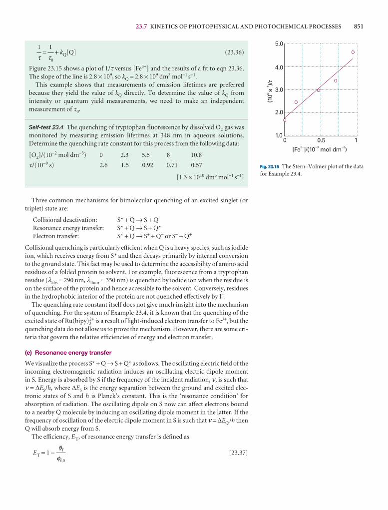
23.7 KINETICS OF PHOTOPHYSICAL AND PHOTOCHEMICAL PROCESSES 851
0 0.5 1
[Fe ]/(10 mol dm )3 3 3� � �
1.0
2.0
3.0
4.0
5.0
(10
s)/
61
��
Fig. 23.15 The Stern–Volmer plot of the datafor Example 23.4.
= + kQ[Q] (23.36)
Figure 23.15 shows a plot of 1/τ versus [Fe3+] and the results of a fit to eqn 23.36.The slope of the line is 2.8 × 10⁹, so kQ = 2.8 × 10⁹ dm3 mol−1 s−1.
This example shows that measurements of emission lifetimes are preferred because they yield the value of kQ directly. To determine the value of kQ fromintensity or quantum yield measurements, we need to make an independent measurement of τ0.
Self-test 23.4 The quenching of tryptophan fluorescence by dissolved O2 gas wasmonitored by measuring emission lifetimes at 348 nm in aqueous solutions.Determine the quenching rate constant for this process from the following data:
[O2]/(10−2 mol dm−3) 0 2.3 5.5 8 10.8
τ/(10−9 s) 2.6 1.5 0.92 0.71 0.57
[1.3 × 10¹⁰ dm3 mol−1 s−1]
Three common mechanisms for bimolecular quenching of an excited singlet (ortriplet) state are:
Collisional deactivation: S* + Q → S + QResonance energy transfer: S* + Q → S + Q*Electron transfer: S* + Q → S+ + Q− or S− + Q+
Collisional quenching is particularly efficient when Q is a heavy species, such as iodideion, which receives energy from S* and then decays primarily by internal conversionto the ground state. This fact may be used to determine the accessibility of amino acidresidues of a folded protein to solvent. For example, fluorescence from a tryptophanresidue (λabs ≈ 290 nm, λfluor ≈ 350 nm) is quenched by iodide ion when the residue ison the surface of the protein and hence accessible to the solvent. Conversely, residuesin the hydrophobic interior of the protein are not quenched effectively by I−.
The quenching rate constant itself does not give much insight into the mechanismof quenching. For the system of Example 23.4, it is known that the quenching of theexcited state of Ru(bipy)3
2+ is a result of light-induced electron transfer to Fe3+, but thequenching data do not allow us to prove the mechanism. However, there are some cri-teria that govern the relative efficiencies of energy and electron transfer.
(e) Resonance energy transfer
We visualize the process S* + Q → S + Q* as follows. The oscillating electric field of theincoming electromagnetic radiation induces an oscillating electric dipole moment in S. Energy is absorbed by S if the frequency of the incident radiation, ν, is such thatν = ∆ES/h, where ∆ES is the energy separation between the ground and excited elec-tronic states of S and h is Planck’s constant. This is the ‘resonance condition’ for absorption of radiation. The oscillating dipole on S now can affect electrons bound to a nearby Q molecule by inducing an oscillating dipole moment in the latter. If thefrequency of oscillation of the electric dipole moment in S is such that ν = ∆EQ /h thenQ will absorb energy from S.
The efficiency, E T, of resonance energy transfer is defined as
E T = 1 − [23.37]φf
φf,0
1
τ0
1
τ
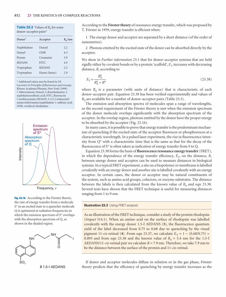
852 23 THE KINETICS OF COMPLEX REACTIONS
Table 23.3 Values of R0 for somedonor–acceptor pairs*
Donor† Acceptor R0 /nm
Naphthalene Dansyl 2.2
Dansyl ODR 4.3
Pyrene Coumarin 3.9
IEDANS FITC 4.9
Tryptophan IEDANS 2.2
Tryptophan Haem (heme) 2.9
* Additional values may be found in J.R.Lacowicz in Principles of fluorescence spectroscopy,Kluwer Academic/Plenum, New York (1999).† Abbreviations: Dansyl, 5-dimethylamino-1-naphthalenesulfonic acid; FITC, fluorescein 5-isothiocyanate; IEDANS, 5-((((2-iodoacetyl)amino)ethyl)amino)naphthalene-1-sulfonic acid;ODR, octadecyl-rhodamine.
Inte
nsity
Frequency, �
Absorptionspectrumof Q
Emissionspectrumof S*
�
Fig. 23.16 According to the Förster theory,the rate of energy transfer from a moleculeS* in an excited state to a quencher moleculeQ is optimized at radiation frequencies inwhich the emission spectrum of S* overlapswith the absorption spectrum of Q, asshown in the shaded region.
According to the Förster theory of resonance energy transfer, which was proposed byT. Förster in 1959, energy transfer is efficient when:
1 The energy donor and acceptor are separated by a short distance (of the order ofnanometres).
2 Photons emitted by the excited state of the donor can be absorbed directly by theacceptor.
We show in Further information 23.1 that for donor–acceptor systems that are heldrigidly either by covalent bonds or by a protein ‘scaffold’, E T increases with decreasingdistance, R, according to
ET = (23.38)
where R0 is a parameter (with units of distance) that is characteristic of eachdonor–acceptor pair. Equation 23.38 has been verified experimentally and values ofR0 are available for a number of donor–acceptor pairs (Table 23.3).
The emission and absorption spectra of molecules span a range of wavelengths, so the second requirement of the Förster theory is met when the emission spectrum of the donor molecule overlaps significantly with the absorption spectrum of the acceptor. In the overlap region, photons emitted by the donor have the proper energyto be absorbed by the acceptor (Fig. 23.16).
In many cases, it is possible to prove that energy transfer is the predominant mechan-ism of quenching if the excited state of the acceptor fluoresces or phosphoresces at acharacteristic wavelength. In a pulsed laser experiment, the rise in fluorescence inten-sity from Q* with a characteristic time that is the same as that for the decay of thefluorescence of S* is often taken as indication of energy transfer from S to Q.
Equation 23.38 forms the basis of fluorescence resonance energy transfer (FRET),in which the dependence of the energy transfer efficiency, ET, on the distance, R,between energy donor and acceptor can be used to measure distances in biologicalsystems. In a typical FRET experiment, a site on a biopolymer or membrane is labelledcovalently with an energy donor and another site is labelled covalently with an energyacceptor. In certain cases, the donor or acceptor may be natural constituents of the system, such as amino acid groups, cofactors, or enzyme substrates. The distance between the labels is then calculated from the known value of R0 and eqn 23.38.Several tests have shown that the FRET technique is useful for measuring distancesranging from 1 to 9 nm.
Illustration 23.3 Using FRET analysis
As an illustration of the FRET technique, consider a study of the protein rhodopsin(Impact I14.1). When an amino acid on the surface of rhodopsin was labelled covalently with the energy donor 1.5-I AEDANS (3), the fluorescence quantumyield of the label decreased from 0.75 to 0.68 due to quenching by the visual pigment 11-cis-retinal (4). From eqn 23.37, we calculate E T = 1 − (0.68/0.75) =0.093 and from eqn 23.38 and the known value of R0 = 5.4 nm for the 1.5-IAEDANS/11-cis-retinal pair we calculate R = 7.9 nm. Therefore, we take 7.9 nm tobe the distance between the surface of the protein and 11-cis-retinal.
If donor and acceptor molecules diffuse in solution or in the gas phase, Förster theory predicts that the efficiency of quenching by energy transfer increases as the
R60
R60 + R6
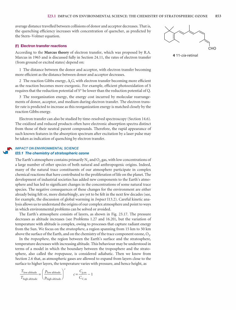
I23.1 IMPACT ON ENVIRONMENTAL SCIENCE: THE CHEMISTRY OF STRATOSPHERIC OZONE 853
average distance travelled between collisions of donor and acceptor decreases. That is,the quenching efficiency increases with concentration of quencher, as predicted bythe Stern–Volmer equation.
(f ) Electron transfer reactions
According to the Marcus theory of electron transfer, which was proposed by R.A.Marcus in 1965 and is discussed fully in Section 24.11, the rates of electron transfer(from ground or excited states) depend on:
1 The distance between the donor and acceptor, with electron transfer becomingmore efficient as the distance between donor and acceptor decreases.
2 The reaction Gibbs energy, ∆rG, with electron transfer becoming more efficientas the reaction becomes more exergonic. For example, efficient photooxidation of Srequires that the reduction potential of S* be lower than the reduction potential of Q.
3 The reorganization energy, the energy cost incurred by molecular rearrange-ments of donor, acceptor, and medium during electron transfer. The electron trans-fer rate is predicted to increase as this reorganization energy is matched closely by thereaction Gibbs energy.
Electron transfer can also be studied by time-resolved spectroscopy (Section 14.6).The oxidized and reduced products often have electronic absorption spectra distinctfrom those of their neutral parent compounds. Therefore, the rapid appearance ofsuch known features in the absorption spectrum after excitation by a laser pulse maybe taken as indication of quenching by electron transfer.
IMPACT ON ENVIRONMENTAL SCIENCE
I23.1 The chemistry of stratospheric ozone
The Earth’s atmosphere contains primarily N2 and O2 gas, with low concentrations ofa large number of other species of both natural and anthropogenic origins. Indeed,many of the natural trace constituents of our atmosphere participate in complexchemical reactions that have contributed to the proliferation of life on the planet. Thedevelopment of industrial societies has added new components to the Earth’s atmo-sphere and has led to significant changes in the concentrations of some natural tracespecies. The negative consequences of these changes for the environment are either already being felt or, more disturbingly, are yet to be felt in the next few decades (see,for example, the discussion of global warming in Impact I13.2). Careful kinetic ana-lysis allows us to understand the origins of our complex atmosphere and point to waysin which environmental problems can be solved or avoided.
The Earth’s atmosphere consists of layers, as shown in Fig. 23.17. The pressure decreases as altitude increases (see Problems 1.27 and 16.20), but the variation oftemperature with altitude is complex, owing to processes that capture radiant energyfrom the Sun. We focus on the stratosphere, a region spanning from 15 km to 50 kmabove the surface of the Earth, and on the chemistry of the trace component ozone, O3.
In the troposphere, the region between the Earth’s surface and the stratosphere,temperature decreases with increasing altitude. This behaviour may be understood interms of a model in which the boundary between the troposphere and the strato-sphere, also called the tropopause, is considered adiabatic. Then we know fromSection 2.6 that, as atmospheric gases are allowed to expand from layers close to thesurface to higher layers, the temperature varies with pressure, and hence height, as
= c
c = − 1Cp,m
CV, m
DF
plow altitude
phigh altitude
AC
Tlow altitude
Thigh altitude
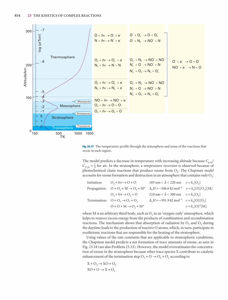
854 23 THE KINETICS OF COMPLEX REACTIONS
The model predicts a decrease in temperature with increasing altitude because Cp,m/CV,m ≈ 7–5 for air. In the stratosphere, a temperature inversion is observed because ofphotochemical chain reactions that produce ozone from O2. The Chapman model accounts for ozone formation and destruction in an atmosphere that contains only O2:
Initiation: O2 + hν → O + O 185 nm < λ < 220 nm v = k1[O2]
Propagation: O + O2 + M → O3 + M* ∆rH = −106.6 kJ mol−1 v = k2[O][O2][M]
O3 + hν → O2 + O 210 nm < λ < 300 nm v = k3[O3]
Termination: O + O3 → O2 + O2 ∆rH = −391.9 kJ mol−1 v = k4[O][O3]
O + O + M → O2 + M* v = k5[O]2[M]
where M is an arbitrary third body, such as O2 in an ‘oxygen-only’ atmosphere, whichhelps to remove excess energy from the products of combination and recombinationreactions. The mechanism shows that absorption of radiation by O2 and O3 duringthe daytime leads to the production of reactive O atoms, which, in turn, participate inexothermic reactions that are responsible for the heating of the stratosphere.
Using values of the rate constants that are applicable to stratospheric conditions,the Chapman model predicts a net formation of trace amounts of ozone, as seen inFig. 23.18 (see also Problem 23.33). However, the model overestimates the concentra-tion of ozone in the stratosphere because other trace species X contribute to catalyticenhancement of the termination step O3 + O → O2 + O2 according to
X + O3 → XO + O2
XO + O → X + O2
150 500 1000 1500T/K
0
100
200
300
Alt
itu
de/
km
Thermosphere
Mesosphere
Stratosphere
Troposphere
-7
-6
-5-4-3
-2-1012
log
(/T
orr
)p
O O e+ ® +h + -n
N N N2 + ® +hn
O O O3 2+ ® +hn
N O NO N2
+ ++ ® +
N O N O2 2 2 2
+ ++ ® +
O O e2 2+ ® +h + -n
O O O O+ ++ ® +2 2
O N NO N+ ++ ® +2
O N NO NO2 2+ +
+ ® +
O O e2 2+ ® +h + -n
N N e2 2+ ® +h + -n
N N e+ ® +h + -n
NO NO e+ ® +h + -n
O O O2 + ® +hn
O N NO NO2 2+ +
+ ® +
N O NO N2
+ ++ ® +
N O N O2 2 2 2
+ ++ ® +
O e O O++ ® +
-
NO e N O++ ® +
-
Tropopause
Stratopause
Mesopause
n
n
n
n
n
n
n
n
n
Fig. 23.17 The temperature profile through the atmosphere and some of the reactions thatoccur in each region.

23.1 IMPACT ON ENVIROMENTAL SCIENCE: THE CHEMISTRY OF STRATOSPHERIC OZONE 855
The catalyst X can be H, OH, NO, or Cl. Chlorine atoms are produced by photolysisof CH3Cl which, in turn, is a by-product of reactions between Cl− and decaying vegetation in oceans. Nitric oxide, NO, is produced in the stratosphere from reac-tion between excited oxygen atoms and N2O, which is formed mainly by microbial denitrification processes in soil. The hydroxyl radical is a product, along with themethyl radical, of the reaction between excited oxygen atoms and methane gas, whichis a by-product of a number of natural processes (such as digestion of cellulose in ruminant animals, anaerobic decomposition of organic waste matter) and industrialprocesses (such as food production and fossil fuel use). In spite of the presence ofthese catalysts, a natural stratosphere is still capable to maintain a low concentrationof ozone.
The chemistry outlined above shows that the photochemical reactions of theChapman model account for absorption of a significant portion of solar ultravioletradiation in the stratosphere. Hence, the surface of the Earth is bathed by lower energyradiation, which does not damage biological tissue (see Impact I23.3). However, some pollutants can lower the concentration of stratospheric ozone. For example,chlorofluorocarbons (CFCs) have been used as propellants and refrigerants overmany years. As CFC molecules diffuse slowly into the middle stratosphere, they arefinally photolysed by ultraviolet radiation. For CF2Cl2, also known as CFC-12, the reaction is:
CF2Cl2 + hν → CF2Cl + Cl
We already know that the resulting Cl atoms can participate in the decomposition ofozone according to the catalytic cycle shown in Fig. 23.19. A number of experimentalobservations have linked this chemistry of CFCs to a dangerously rapid decline in theconcentration of stratospheric ozone over the last three decades.
Ozone depletion has increased the amount of ultraviolet radiation at the Earth’ssurface, particularly radiation in the ‘UVB range’, 290–320 nm. The physiologicalconsequences of prolonged exposure to UVB radiation include DNA damage, princip-ally by photodimerization of adjacent thymine bases to yield either a cyclobutane
0
1
2
0 20 40t/ms
[O],[
O]/(
10m
olec
ules
cm
)3
83
�
O3
O
0 100 200 300t/min
5
10
0[O]/(
10m
olec
ules
cm
)9
3�
t/min
0[O]/(
10m
olec
ules
cm
)3
133
�
2
4
0 100 200 300(a) (b) (c)
Fig. 23.18 Net formation of ozone via the Chapman model in a stratospheric model containingonly O2, O, andO3. The rate constants are consistent with reasonable stratospheric conditions.(a) Early reaction period after irradiation begins at t = 0. (b) Late reaction period, showingthat the concentration of O atoms begins to level off after about 4 hours of continuousirradiation. (c) Late reaction period, showing that the ozone concentration also begins to leveloff similarly. For details of the calculation, see Problem 23.33 and M.P. Cady and C.A. Trapp,A Mathcad primer for physical chemistry. Oxford University Press (1999).
Cl ClO
O3 O2
O2 O
Fig. 23.19 A catalytic cycle showing thepropagation of ozone decomposition bychlorine atoms.
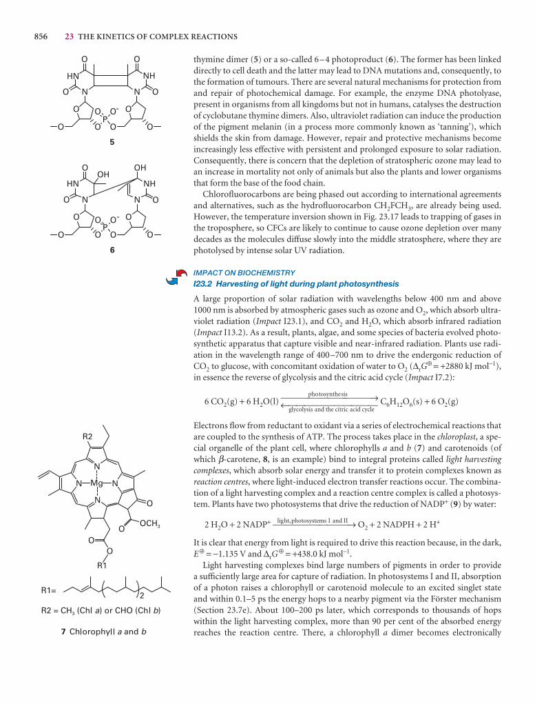
856 23 THE KINETICS OF COMPLEX REACTIONS
thymine dimer (5) or a so-called 6–4 photoproduct (6). The former has been linkeddirectly to cell death and the latter may lead to DNA mutations and, consequently, tothe formation of tumours. There are several natural mechanisms for protection fromand repair of photochemical damage. For example, the enzyme DNA photolyase, present in organisms from all kingdoms but not in humans, catalyses the destructionof cyclobutane thymine dimers. Also, ultraviolet radiation can induce the productionof the pigment melanin (in a process more commonly known as ‘tanning’), whichshields the skin from damage. However, repair and protective mechanisms becomeincreasingly less effective with persistent and prolonged exposure to solar radiation.Consequently, there is concern that the depletion of stratospheric ozone may lead toan increase in mortality not only of animals but also the plants and lower organismsthat form the base of the food chain.
Chlorofluorocarbons are being phased out according to international agreementsand alternatives, such as the hydrofluorocarbon CH2FCH3, are already being used.However, the temperature inversion shown in Fig. 23.17 leads to trapping of gases inthe troposphere, so CFCs are likely to continue to cause ozone depletion over manydecades as the molecules diffuse slowly into the middle stratosphere, where they arephotolysed by intense solar UV radiation.
IMPACT ON BIOCHEMISTRY
I23.2 Harvesting of light during plant photosynthesis
A large proportion of solar radiation with wavelengths below 400 nm and above 1000 nm is absorbed by atmospheric gases such as ozone and O2, which absorb ultra-violet radiation (Impact I23.1), and CO2 and H2O, which absorb infrared radiation(Impact I13.2). As a result, plants, algae, and some species of bacteria evolved photo-synthetic apparatus that capture visible and near-infrared radiation. Plants use radi-ation in the wavelength range of 400–700 nm to drive the endergonic reduction ofCO2 to glucose, with concomitant oxidation of water to O2 (∆rG
⊕ = +2880 kJ mol−1),in essence the reverse of glycolysis and the citric acid cycle (Impact I7.2):
6 CO2(g) + 6 H2O(l) ––––––pho–––to–syn–––the––sis––––––→ C6H12O6(s) + 6 O2(g)←gly—
col—
ysis—
a–
nd—
the—
cit—
ric—
ac–
id—
cy–cle—
Electrons flow from reductant to oxidant via a series of electrochemical reactions thatare coupled to the synthesis of ATP. The process takes place in the chloroplast, a spe-cial organelle of the plant cell, where chlorophylls a and b (7) and carotenoids (ofwhich β-carotene, 8, is an example) bind to integral proteins called light harvestingcomplexes, which absorb solar energy and transfer it to protein complexes known asreaction centres, where light-induced electron transfer reactions occur. The combina-tion of a light harvesting complex and a reaction centre complex is called a photosys-tem. Plants have two photosystems that drive the reduction of NADP+ (9) by water:
2 H2O + 2 NADP+ –lig––ht,–p–h–o–to–sys––te–m– s–I– a–n–d–II–→ O2 + 2 NADPH + 2 H+
It is clear that energy from light is required to drive this reaction because, in the dark,E⊕ = −1.135 V and ∆rG
⊕ = +438.0 kJ mol−1.Light harvesting complexes bind large numbers of pigments in order to provide
a sufficiently large area for capture of radiation. In photosystems I and II, absorptionof a photon raises a chlorophyll or carotenoid molecule to an excited singlet state and within 0.1–5 ps the energy hops to a nearby pigment via the Förster mechanism(Section 23.7e). About 100–200 ps later, which corresponds to thousands of hopswithin the light harvesting complex, more than 90 per cent of the absorbed energyreaches the reaction centre. There, a chlorophyll a dimer becomes electronically
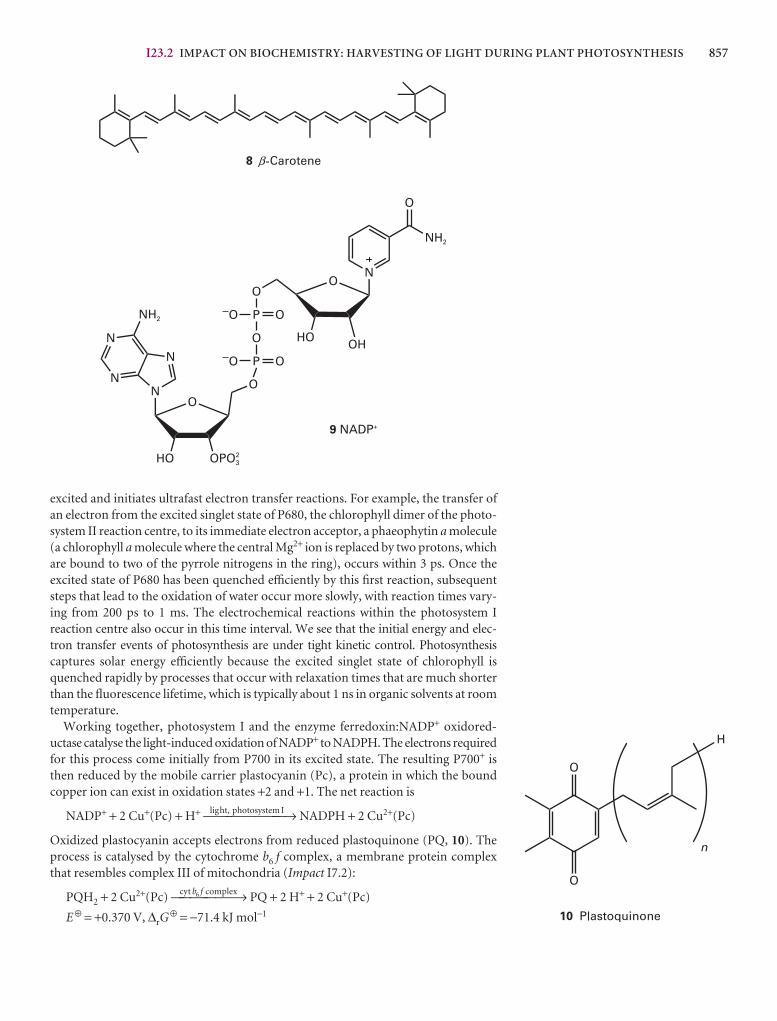
I23.2 IMPACT ON BIOCHEMISTRY: HARVESTING OF LIGHT DURING PLANT PHOTOSYNTHESIS 857
excited and initiates ultrafast electron transfer reactions. For example, the transfer ofan electron from the excited singlet state of P680, the chlorophyll dimer of the photo-system II reaction centre, to its immediate electron acceptor, a phaeophytin a molecule(a chlorophyll a molecule where the central Mg2+ ion is replaced by two protons, whichare bound to two of the pyrrole nitrogens in the ring), occurs within 3 ps. Once the excited state of P680 has been quenched efficiently by this first reaction, subsequentsteps that lead to the oxidation of water occur more slowly, with reaction times vary-ing from 200 ps to 1 ms. The electrochemical reactions within the photosystem I reaction centre also occur in this time interval. We see that the initial energy and elec-tron transfer events of photosynthesis are under tight kinetic control. Photosynthesiscaptures solar energy efficiently because the excited singlet state of chlorophyll isquenched rapidly by processes that occur with relaxation times that are much shorterthan the fluorescence lifetime, which is typically about 1 ns in organic solvents at roomtemperature.
Working together, photosystem I and the enzyme ferredoxin:NADP+ oxidored-uctase catalyse the light-induced oxidation of NADP+ to NADPH. The electrons requiredfor this process come initially from P700 in its excited state. The resulting P700+ isthen reduced by the mobile carrier plastocyanin (Pc), a protein in which the boundcopper ion can exist in oxidation states +2 and +1. The net reaction is
NADP+ + 2 Cu+(Pc) + H+ –lig––ht,––p–h–o–to–sys––te–m––I–→ NADPH + 2 Cu2+(Pc)
Oxidized plastocyanin accepts electrons from reduced plastoquinone (PQ, 10). Theprocess is catalysed by the cytochrome b6 f complex, a membrane protein complexthat resembles complex III of mitochondria (Impact I7.2):
PQH2 + 2 Cu2+(Pc) – c–yt––b–6 f––c–o–m–p–lex–→ PQ + 2 H+ + 2 Cu+(Pc)
E⊕ = +0.370 V, ∆rG⊕ = −71.4 kJ mol−1
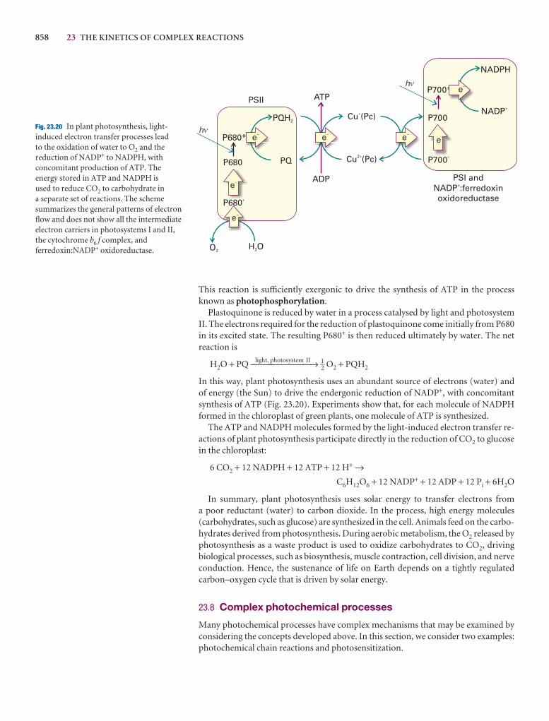
858 23 THE KINETICS OF COMPLEX REACTIONS
This reaction is sufficiently exergonic to drive the synthesis of ATP in the processknown as photophosphorylation.
Plastoquinone is reduced by water in a process catalysed by light and photosystemII. The electrons required for the reduction of plastoquinone come initially from P680in its excited state. The resulting P680+ is then reduced ultimately by water. The netreaction is
H2O + PQ –lig––ht,––p–h–o–to–sys––te–m––II–→ 1–2 O2 + PQH2
In this way, plant photosynthesis uses an abundant source of electrons (water) and of energy (the Sun) to drive the endergonic reduction of NADP+, with concomitantsynthesis of ATP (Fig. 23.20). Experiments show that, for each molecule of NADPHformed in the chloroplast of green plants, one molecule of ATP is synthesized.
The ATP and NADPH molecules formed by the light-induced electron transfer re-actions of plant photosynthesis participate directly in the reduction of CO2 to glucosein the chloroplast:
6 CO2 + 12 NADPH + 12 ATP + 12 H+ →C6H12O6 + 12 NADP+ + 12 ADP + 12 Pi + 6H2O
In summary, plant photosynthesis uses solar energy to transfer electrons from a poor reductant (water) to carbon dioxide. In the process, high energy molecules (carbohydrates, such as glucose) are synthesized in the cell. Animals feed on the carbo-hydrates derived from photosynthesis. During aerobic metabolism, the O2 released byphotosynthesis as a waste product is used to oxidize carbohydrates to CO2, driving biological processes, such as biosynthesis, muscle contraction, cell division, and nerveconduction. Hence, the sustenance of life on Earth depends on a tightly regulated carbon–oxygen cycle that is driven by solar energy.
23.8 Complex photochemical processes
Many photochemical processes have complex mechanisms that may be examined byconsidering the concepts developed above. In this section, we consider two examples:photochemical chain reactions and photosensitization.
Cu (Pc)2�
O2
P680*
P680
h
PSII
H O2
ADP
P680�
PQH2
e�
PQ
e�
Cu (Pc)�
e� e�
ATPP700*
P700
h
PSI andNADP :ferredoxinoxidoreductase
+
P700�
NADPH
e�
NADP�
e�
e�
�
�
Fig. 23.20 In plant photosynthesis, light-induced electron transfer processes lead to the oxidation of water to O2 and thereduction of NADP+ to NADPH, withconcomitant production of ATP. Theenergy stored in ATP and NADPH is used to reduce CO2 to carbohydrate in a separate set of reactions. The schemesummarizes the general patterns of electronflow and does not show all the intermediateelectron carriers in photosystems I and II,the cytochrome b6 f complex, andferredoxin:NADP+ oxidoreductase.
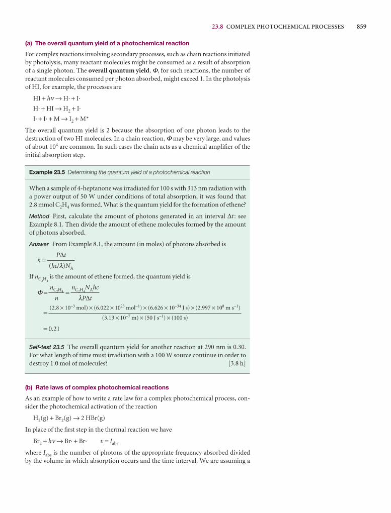
23.8 COMPLEX PHOTOCHEMICAL PROCESSES 859
(a) The overall quantum yield of a photochemical reaction
For complex reactions involving secondary processes, such as chain reactions initiatedby photolysis, many reactant molecules might be consumed as a result of absorptionof a single photon. The overall quantum yield, Φ, for such reactions, the number ofreactant molecules consumed per photon absorbed, might exceed 1. In the photolysisof HI, for example, the processes are
HI + hν → H· + I·
H· + HI → H2 + I·
I· + I· + M → I2 + M*
The overall quantum yield is 2 because the absorption of one photon leads to the destruction of two HI molecules. In a chain reaction, Φ may be very large, and valuesof about 104 are common. In such cases the chain acts as a chemical amplifier of theinitial absorption step.
Example 23.5 Determining the quantum yield of a photochemical reaction
When a sample of 4-heptanone was irradiated for 100 s with 313 nm radiation witha power output of 50 W under conditions of total absorption, it was found that 2.8 mmol C2H4 was formed. What is the quantum yield for the formation of ethene?
Method First, calculate the amount of photons generated in an interval ∆t : seeExample 8.1. Then divide the amount of ethene molecules formed by the amountof photons absorbed.
Answer From Example 8.1, the amount (in moles) of photons absorbed is
n =
If nC2H4is the amount of ethene formed, the quantum yield is
Φ = =
=
= 0.21
Self-test 23.5 The overall quantum yield for another reaction at 290 nm is 0.30.For what length of time must irradiation with a 100 W source continue in order todestroy 1.0 mol of molecules? [3.8 h]
(b) Rate laws of complex photochemical reactions
As an example of how to write a rate law for a complex photochemical process, con-sider the photochemical activation of the reaction
H2(g) + Br2(g) → 2 HBr(g)
In place of the first step in the thermal reaction we have
Br2 + hν → Br· + Br· v = Iabs
where Iabs is the number of photons of the appropriate frequency absorbed divided by the volume in which absorption occurs and the time interval. We are assuming a
(2.8 × 10⁻³ mol) × (6.022 × 10²³ mol−1) × (6.626 × 10−34 J s) × (2.997 × 10⁸ m s−1)
(3.13 × 10⁻⁷ m) × (50 J s−1) × (100 s)
nC2H4NAhc
λP∆t
nC2H4
n
P∆t
(hc/λ)NA
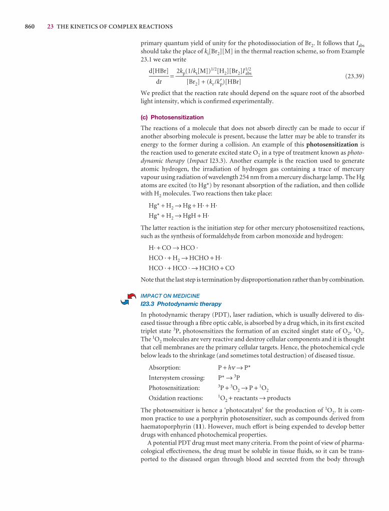
860 23 THE KINETICS OF COMPLEX REACTIONS
primary quantum yield of unity for the photodissociation of Br2. It follows that Iabs
should take the place of ki[Br2][M] in the thermal reaction scheme, so from Example23.1 we can write
= (23.39)
We predict that the reaction rate should depend on the square root of the absorbedlight intensity, which is confirmed experimentally.
(c) Photosensitization
The reactions of a molecule that does not absorb directly can be made to occur ifanother absorbing molecule is present, because the latter may be able to transfer itsenergy to the former during a collision. An example of this photosensitization isthe reaction used to generate excited state O2 in a type of treatment known as photo-dynamic therapy (Impact I23.3). Another example is the reaction used to generateatomic hydrogen, the irradiation of hydrogen gas containing a trace of mercuryvapour using radiation of wavelength 254 nm from a mercury discharge lamp. The Hgatoms are excited (to Hg*) by resonant absorption of the radiation, and then collidewith H2 molecules. Two reactions then take place:
Hg* + H2 → Hg + H· + H·
Hg* + H2 → HgH + H·
The latter reaction is the initiation step for other mercury photosensitized reactions,such as the synthesis of formaldehyde from carbon monoxide and hydrogen:
H· + CO → HCO ·
HCO · + H2 → HCHO + H·
HCO · + HCO · → HCHO + CO
Note that the last step is termination by disproportionation rather than by combination.
IMPACT ON MEDICINE
I23.3 Photodynamic therapy
In photodynamic therapy (PDT), laser radiation, which is usually delivered to dis-eased tissue through a fibre optic cable, is absorbed by a drug which, in its first excitedtriplet state 3P, photosensitizes the formation of an excited singlet state of O2, 1O2.The 1O2 molecules are very reactive and destroy cellular components and it is thoughtthat cell membranes are the primary cellular targets. Hence, the photochemical cyclebelow leads to the shrinkage (and sometimes total destruction) of diseased tissue.
Absorption: P + hν → P*
Intersystem crossing: P* → 3P
Photosensitization: 3P + 3O2 → P + 1O2
Oxidation reactions: 1O2 + reactants → products
The photosensitizer is hence a ‘photocatalyst’ for the production of 1O2. It is com-mon practice to use a porphyrin photosensitizer, such as compounds derived fromhaematoporphyrin (11). However, much effort is being expended to develop betterdrugs with enhanced photochemical properties.
A potential PDT drug must meet many criteria. From the point of view of pharma-cological effectiveness, the drug must be soluble in tissue fluids, so it can be trans-ported to the diseased organ through blood and secreted from the body through
2kp(1/kt[M])1/2[H2][Br2]I abs1/2
[Br2] + (kr /k′p)[HBr]
d[HBr]
dt
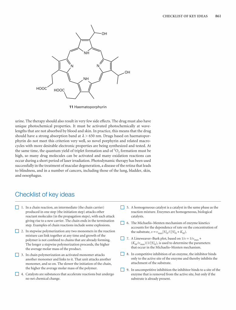
CHECKLIST OF KEY IDEAS 861
urine. The therapy should also result in very few side effects. The drug must also haveunique photochemical properties. It must be activated photochemically at wave-lengths that are not absorbed by blood and skin. In practice, this means that the drugshould have a strong absorption band at λ > 650 nm. Drugs based on haematopor-phyrin do not meet this criterion very well, so novel porphyrin and related macro-cycles with more desirable electronic properties are being synthesized and tested. Atthe same time, the quantum yield of triplet formation and of 1O2 formation must behigh, so many drug molecules can be activated and many oxidation reactions canoccur during a short period of laser irradiation. Photodynamic therapy has been usedsuccessfully in the treatment of macular degeneration, a disease of the retina that leadsto blindness, and in a number of cancers, including those of the lung, bladder, skin,and oesophagus.
Checklist of key ideas
1. In a chain reaction, an intermediate (the chain carrier)produced in one step (the initiation step) attacks otherreactant molecules (in the propagation steps), with each attackgiving rise to a new carrier. The chain ends in the terminationstep. Examples of chain reactions include some explosions.
2. In stepwise polymerization any two monomers in the reactionmixture can link together at any time and growth of thepolymer is not confined to chains that are already forming.The longer a stepwise polymerization proceeds, the higher the average molar mass of the product.
3. In chain polymerization an activated monomer attacksanother monomer and links to it. That unit attacks anothermonomer, and so on. The slower the initiation of the chain,the higher the average molar mass of the polymer.
4. Catalysts are substances that accelerate reactions but undergono net chemical change.
5. A homogeneous catalyst is a catalyst in the same phase as thereaction mixture. Enzymes are homogeneous, biologicalcatalysts.
6. The Michaelis–Menten mechanism of enzyme kineticsaccounts for the dependence of rate on the concentration ofthe substrate, v = vmax[S]0 /([S]0 + KM).
7. A Lineweaver–Burk plot, based on 1/v = 1/vmax +(KM /vmax)(1/[S]0), is used to determine the parameters that occur in the Michaelis–Menten mechanism.
8. In competitive inhibition of an enzyme, the inhibitor bindsonly to the active site of the enzyme and thereby inhibits theattachment of the substrate.
9. In uncompetitive inhibition the inhibitor binds to a site of theenzyme that is removed from the active site, but only if thesubstrate is already present.

862 23 THE KINETICS OF COMPLEX REACTIONS
Further reading
Articles and texts
J. Andraos, How mathematics figures in chemistry: some examples. J. Chem. Educ. 76, 258 (1999).
C.E. Carraher, Jr., Seymour/Carraher’s polymer chemistry, MarcelDekker (2000).
A. Fersht, Structure and mechanism in protein science: a guide toenzyme catalysis and protein folding. W.H. Freeman, New York(1999).
A.M. Kuznetsov and J. Ulstrup, Electron transfer in chemistry andbiology: an introduction to the theory. Wiley, New York (1998).
J.I. Steinfeld, J.S. Francisco, and W.L. Hase, Chemical kinetics anddynamics. Prentice Hall, Englewood Cliffs (1998).
N.J. Turro, Modern molecular photochemistry. University ScienceBooks, Sausalito (1991).
K.E. van Holde, W.C. Johnson and P.H. Ho, Principles of physicalbiochemistry. Prentice Hall, Upper Saddle River (1998).
D. Voet and J.G. Voet, Biochemistry. Wiley, New York (2004).
Sources of data and information
D.R. Lide (ed.), CRC handbook of chemistry and physics, Section 5.CRC Press, Boca Raton (2000).
S.L. Murov, I. Carmichael, and G.L. Hug, Handbook ofphotochemistry. Marcel Dekker, New York (1993).
NDRL/NIST solution kinetics database, NIST standard referencedatabase 40, National Institute of Standards and Technology,Gaithersburg (1994). The URL is available on the web site for thisbook.
NIST chemical kinetics database, NIST standard reference database17, National Institute of Standards and Technology, Gaithersburg(1998). The URL is available on the web site for this book.
Further information
Further information 23.1 The Förster theory of resonance energy transfer
From the qualitative description given in Section 23.7e, we concludethat resonance energy transfer arises from the interaction betweentwo oscillating dipoles with moments µS and µQ. From Section 18.4,the energy of the dipole–dipole interaction, Vdipole–dipole, is
Vdipole–dipole ∝
where R is the distance between the dipoles. We saw in Section 9.10that the rate of a transition from a state i to a state f at a radiationfrequency ν is proportional to the square modulus of the matrixelement of the perturbation between the two states:
wf←i ∝ |H fi(1) |2
µSµQ
R3
For energy transfer, the wavefunctions of the initial and final statesmay be denoted as ψS*ψQ and ψSψQ*, respectively, and H (1) may bewritten from Vdipole–dipole. It follows that the rate of energy transfer,wT, at a fixed distance R is given (using notation introduced inFurther information 9.1) by
wT ∝ ψSψQ* µSµQ ψS*ψQ
2
= ψS µS ψS*
2
ψQ* µQ ψQ
2
We have used the fact that the terms related to S are functions ofcoordinates that are independent of those for the functions related to Q. In the last expression, the integrals are squares of transitiondipole moments at the radiation frequency ν, the first
1
R6
1
R6
10. In non-competitive inhibition, the inhibitor binds to a siteother than the active site, and its presence reduces the abilityof the substrate to bind to the active site.
11. The primary quantum yield of a photochemical reaction is thenumber of reactant molecules producing specified primaryproducts for each photon absorbed; the overall quantum yieldis the number of reactant molecules that react for each photonabsorbed.
12. The observed fluorescence lifetime is related to the quantum yield, φf , and rate constant, kf, of fluorescence byτ0 = φf /kf.
13. A Stern–Volmer plot is used to analyse the kinetics offluorescence quenching in solution. It is based on theStern–Volmer equation, φf,0 /φf = 1 + τ0kQ[Q].
14. Collisional deactivation, electron transfer, and resonanceenergy transfer are common fluorescence quenchingprocesses. The rate constants of electron and resonance energy transfer decrease with increasing separation betweendonor and acceptor molecules.
15. In photosensitization, the reaction of a molecule that does notabsorb radiation directly is made to occur by energy transferduring a collision with a molecule that does absorb radiation.
EXERCISES 863
Discussion questions
23.1 Identify any initiation, propagation, retardation, inhibition, andtermination steps in the following chain mechanisms:
(a) (1) AH → A· + H·
(2) A· → B· + C
(3) AH + B· → A· + D
(4) A· + B· → P
(b) (1) A2 → A· + A·
(2) A· → B· + C
(3) A· + P → B·
(4) A· + B· → P
23.2 Bearing in mind distinctions between the mechanisms of stepwise andchain polymerization, describe ways in which it is possible to control themolar mass of a polymer by manipulating the kinetic parameters ofpolymerization.
23.3 Discuss the features, advantages, and limitations of theMichaelis–Menten mechanism of enzyme action.
23.4 Distinguish between competitive, non-competitive, and uncompetitiveinhibition of enzymes. Discuss how these modes of inhibition may be detectedexperimentally.
23.5 Distinguish between the primary quantum yield and overall quantumyield of a chemical reaction. Describe an experimental procedure for thedetermination of the quantum yield.
23.6 Discuss experimental procedures that make it possible to differentiatebetween quenching by energy transfer, collisions, or electron transfer.
23.7 Summarize the main features of the Förster theory of resonance energytransfer. Then, discuss FRET in terms of Förster theory.
ET = w0 = (kf + k IC + k ISC)[S*] (23.40)
where w0 is the rate of deactivation of S* in the absence of thequencher. The efficiency, ET, may be expressed in terms of theexperimental fluorescence quantum yields ϕf,0 and ϕf of the donor inthe absence and presence of the acceptor, respectively. To proceed,we use eqn 23.30 to write:
φf,0 = and φf =
where vf is the rate of fluorescence. Subsituting these results into eqn23.40 gives, after a little algebra, eqn 23.37.
Alternatively, we can express w0 in terms of the parameter R0, thecharacteristic distance at which wT = w0 for a specified pair of S and Q(Table 23.3). By using wT ∝ R−6 and w0 ∝ R0
−6, we can rearrange theexpression for ET into eqn 23.38.
vf
w0 + wT
vf
w0
wT
wT + w0
corresponding to emission of S* to S and the second to absorption of Q to Q*.
We interpret the expression for wT as follows. The rate of energytransfer is proportional to R− 6, so it decreases sharply with increasingseparation between the energy donor and acceptor. Furthermore, theenergy transfer rate is optimized when both emission of radiation byS* and absorption of radiation by Q are efficient at the frequency ν.Because the absorption and emission spectra of large molecules incondensed phases are broad, it follows that the energy transfer rate isoptimal at radiation frequencies in which the emission spectrum ofthe donor and the absorption spectrum of the acceptor overlapsignificantly.
In practice, it is more convenient to measure the efficiency ofenergy transfer and not the rate itself. In much the same way that wedefined the quantum yield as a ratio of rates, we can also define theefficiency of energy transfer, E T, as the ratio
Exercises
In the following exercises and problems, it is recommended that rateconstants are labelled with the number of the step in the proposed reactionmechanism, and any reverse steps are labelled similarly but with a prime.
23.1a Derive the rate law for the decomposition of ozone in the reaction 2 O3(g) → 3 O2(g) on the basis of the following proposed mechanism:
(1) O3 5 O2 + O k1, k ′1(2) O + O3 → O2 + O2 k2
23.1b On the basis of the following proposed mechanism, account for theexperimental fact that the rate law for the decomposition 2 N2O5(g) →4 NO2(g) + O2(g) is v = k[N2O5].
(1) N2O5 5 NO2 + NO3 k1, k ′1(2) NO2 + NO3 → NO2 + O2 + NO k2
(3) NO + N2O5 → NO2 + NO2 + NO2 k3
23.2a A slightly different mechanism for the decomposition of N2O5 fromthat in Exercise 23.1b has also been proposed. It differs only in the last step,which is replaced by
(3) NO + NO3 → NO2 + NO2 k3
Show that this mechanism leads to the same overall rate law.
23.2b Consider the following mechanism for the thermal decomposition of R2:
(1) R2 → R + R
(2) R + R2 → PB + R′(3) R′ → PA + R
(4) R + R → PA + PB
where R2, PA, PB are stable hydrocarbons and R and R′ are radicals. Find thedependence of the rate of decomposition of R2 on the concentration of R2.
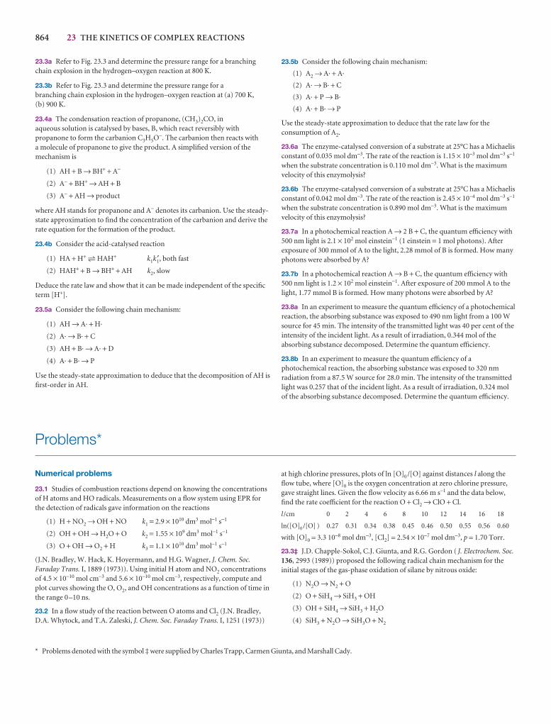
864 23 THE KINETICS OF COMPLEX REACTIONS
Problems*
Numerical problems
23.1 Studies of combustion reactions depend on knowing the concentrationsof H atoms and HO radicals. Measurements on a flow system using EPR forthe detection of radicals gave information on the reactions
(1) H + NO2 → OH + NO k1 = 2.9 × 10¹⁰ dm3 mol−1 s−1
(2) OH + OH → H2O + O k2 = 1.55 × 10⁹ dm3 mol−1 s−1
(3) O + OH → O2 + H k3 = 1.1 × 10¹⁰ dm3 mol−1 s−1
(J.N. Bradley, W. Hack, K. Hoyermann, and H.G. Wagner, J. Chem. Soc.Faraday Trans. I, 1889 (1973)). Using initial H atom and NO2 concentrationsof 4.5 × 10⁻¹⁰ mol cm−3 and 5.6 × 10⁻¹⁰ mol cm−3, respectively, compute andplot curves showing the O, O2, and OH concentrations as a function of time inthe range 0–10 ns.
23.2 In a flow study of the reaction between O atoms and Cl2 (J.N. Bradley,D.A. Whytock, and T.A. Zaleski, J. Chem. Soc. Faraday Trans. I, 1251 (1973))
at high chlorine pressures, plots of ln [O]0 /[O] against distances l along theflow tube, where [O]0 is the oxygen concentration at zero chlorine pressure,gave straight lines. Given the flow velocity as 6.66 m s−1 and the data below,find the rate coefficient for the reaction O + Cl2 → ClO + Cl.
l /cm 0 2 4 6 8 10 12 14 16 18
ln([O]0 /[O] ) 0.27 0.31 0.34 0.38 0.45 0.46 0.50 0.55 0.56 0.60
with [O]0 = 3.3 10−8 mol dm−3, [Cl2] = 2.54 × 10⁻⁷ mol dm−3, p = 1.70 Torr.
23.3‡ J.D. Chapple-Sokol, C.J. Giunta, and R.G. Gordon ( J. Electrochem. Soc.136, 2993 (1989)) proposed the following radical chain mechanism for theinitial stages of the gas-phase oxidation of silane by nitrous oxide:
(1) N2O → N2 + O
(2) O + SiH4 → SiH3 + OH
(3) OH + SiH4 → SiH3 + H2O
(4) SiH3 + N2O → SiH3O + N2
* Problems denoted with the symbol ‡ were supplied by Charles Trapp, Carmen Giunta, and Marshall Cady.
23.5b Consider the following chain mechanism:
(1) A2 → A· + A·
(2) A· → B· + C
(3) A· + P → B·
(4) A· + B· → P
Use the steady-state approximation to deduce that the rate law for theconsumption of A2.
23.6a The enzyme-catalysed conversion of a substrate at 25°C has a Michaelisconstant of 0.035 mol dm−3. The rate of the reaction is 1.15 × 10⁻³ mol dm−3 s−1
when the substrate concentration is 0.110 mol dm−3. What is the maximumvelocity of this enzymolysis?
23.6b The enzyme-catalysed conversion of a substrate at 25°C has a Michaelisconstant of 0.042 mol dm−3. The rate of the reaction is 2.45 × 10⁻⁴ mol dm−3 s−1
when the substrate concentration is 0.890 mol dm−3. What is the maximumvelocity of this enzymolysis?
23.7a In a photochemical reaction A → 2 B + C, the quantum efficiency with500 nm light is 2.1 × 10² mol einstein−1 (1 einstein = 1 mol photons). Afterexposure of 300 mmol of A to the light, 2.28 mmol of B is formed. How manyphotons were absorbed by A?
23.7b In a photochemical reaction A → B + C, the quantum efficiency with500 nm light is 1.2 × 10² mol einstein−1. After exposure of 200 mmol A to thelight, 1.77 mmol B is formed. How many photons were absorbed by A?
23.8a In an experiment to measure the quantum efficiency of a photochemicalreaction, the absorbing substance was exposed to 490 nm light from a 100 Wsource for 45 min. The intensity of the transmitted light was 40 per cent of theintensity of the incident light. As a result of irradiation, 0.344 mol of theabsorbing substance decomposed. Determine the quantum efficiency.
23.8b In an experiment to measure the quantum efficiency of aphotochemical reaction, the absorbing substance was exposed to 320 nmradiation from a 87.5 W source for 28.0 min. The intensity of the transmittedlight was 0.257 that of the incident light. As a result of irradiation, 0.324 molof the absorbing substance decomposed. Determine the quantum efficiency.
23.3a Refer to Fig. 23.3 and determine the pressure range for a branchingchain explosion in the hydrogen–oxygen reaction at 800 K.
23.3b Refer to Fig. 23.3 and determine the pressure range for a branching chain explosion in the hydrogen–oxygen reaction at (a) 700 K, (b) 900 K.
23.4a The condensation reaction of propanone, (CH3)2CO, inaqueous solution is catalysed by bases, B, which react reversibly withpropanone to form the carbanion C3H5O−. The carbanion then reacts with a molecule of propanone to give the product. A simplified version of themechanism is
(1) AH + B → BH+ + A−
(2) A− + BH+ → AH + B
(3) A− + AH → product
where AH stands for propanone and A− denotes its carbanion. Use the steady-state approximation to find the concentration of the carbanion and derive therate equation for the formation of the product.
23.4b Consider the acid-catalysed reaction
(1) HA + H+ 5 HAH+ k1k ′1, both fast
(2) HAH+ + B → BH+ + AH k2, slow
Deduce the rate law and show that it can be made independent of the specificterm [H+].
23.5a Consider the following chain mechanism:
(1) AH → A· + H·
(2) A· → B· + C
(3) AH + B· → A· + D
(4) A· + B· → P
Use the steady-state approximation to deduce that the decomposition of AH isfirst-order in AH.
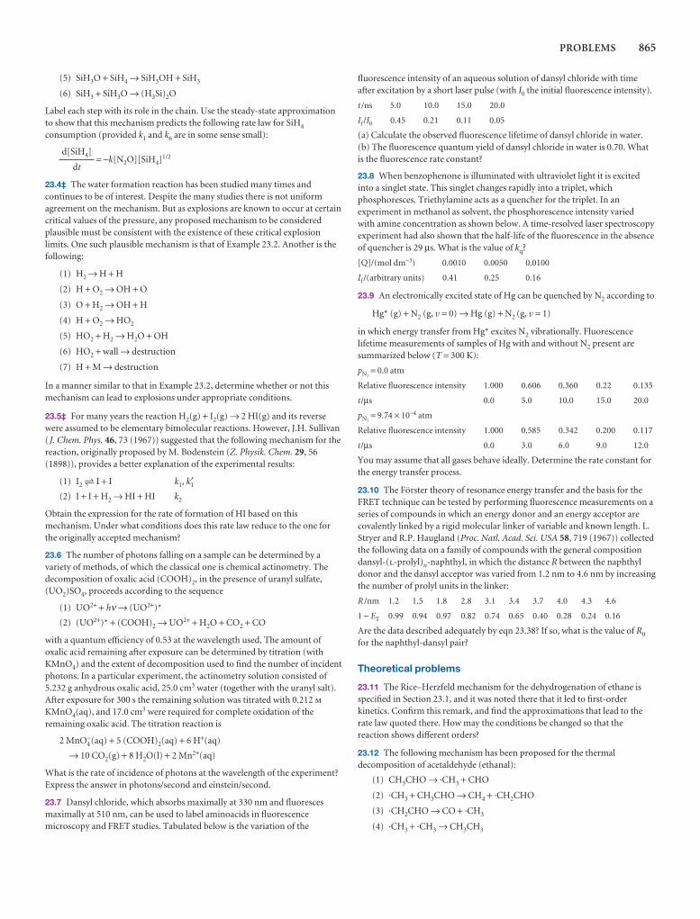
PROBLEMS 865
fluorescence intensity of an aqueous solution of dansyl chloride with timeafter excitation by a short laser pulse (with I0 the initial fluorescence intensity).
t /ns 5.0 10.0 15.0 20.0
If /I0 0.45 0.21 0.11 0.05
(a) Calculate the observed fluorescence lifetime of dansyl chloride in water.(b) The fluorescence quantum yield of dansyl chloride in water is 0.70. Whatis the fluorescence rate constant?
23.8 When benzophenone is illuminated with ultraviolet light it is excitedinto a singlet state. This singlet changes rapidly into a triplet, whichphosphoresces. Triethylamine acts as a quencher for the triplet. In anexperiment in methanol as solvent, the phosphorescence intensity varied with amine concentration as shown below. A time-resolved laser spectroscopyexperiment had also shown that the half-life of the fluorescence in the absenceof quencher is 29 µs. What is the value of kq?
[Q]/(mol dm−3) 0.0010 0.0050 0.0100
If /(arbitrary units) 0.41 0.25 0.16
23.9 An electronically excited state of Hg can be quenched by N2 according to
Hg* (g) + N2 (g, v = 0) → Hg (g) + N2 (g, v = 1)
in which energy transfer from Hg* excites N2 vibrationally. Fluorescencelifetime measurements of samples of Hg with and without N2 present aresummarized below (T = 300 K):
pN2= 0.0 atm
Relative fluorescence intensity 1.000 0.606 0.360 0.22 0.135
t/µs 0.0 5.0 10.0 15.0 20.0
pN2= 9.74 × 10⁻⁴ atm
Relative fluorescence intensity 1.000 0.585 0.342 0.200 0.117
t/µs 0.0 3.0 6.0 9.0 12.0
You may assume that all gases behave ideally. Determine the rate constant forthe energy transfer process.
23.10 The Förster theory of resonance energy transfer and the basis for theFRET technique can be tested by performing fluorescence measurements on aseries of compounds in which an energy donor and an energy acceptor arecovalently linked by a rigid molecular linker of variable and known length. L.Stryer and R.P. Haugland (Proc. Natl. Acad. Sci. USA 58, 719 (1967)) collectedthe following data on a family of compounds with the general compositiondansyl-(l-prolyl)n-naphthyl, in which the distance R between the naphthyldonor and the dansyl acceptor was varied from 1.2 nm to 4.6 nm by increasingthe number of prolyl units in the linker:
R /nm 1.2 1.5 1.8 2.8 3.1 3.4 3.7 4.0 4.3 4.6
1 − ET 0.99 0.94 0.97 0.82 0.74 0.65 0.40 0.28 0.24 0.16
Are the data described adequately by eqn 23.38? If so, what is the value of R0
for the naphthyl-dansyl pair?
Theoretical problems
23.11 The Rice–Herzfeld mechanism for the dehydrogenation of ethane isspecified in Section 23.1, and it was noted there that it led to first-orderkinetics. Confirm this remark, and find the approximations that lead to therate law quoted there. How may the conditions be changed so that thereaction shows different orders?
23.12 The following mechanism has been proposed for the thermaldecomposition of acetaldehyde (ethanal):
(1) CH3CHO → ·CH3 + CHO
(2) ·CH3 + CH3CHO → CH4 + ·CH2CHO
(3) ·CH2CHO → CO + ·CH3
(4) ·CH3 + ·CH3 → CH3CH3
(5) SiH3O + SiH4 → SiH3OH + SiH3
(6) SiH3 + SiH3O → (H3Si)2O
Label each step with its role in the chain. Use the steady-state approximationto show that this mechanism predicts the following rate law for SiH4
consumption (provided k1 and k6 are in some sense small):
= −k[N2O][SiH4]1/2
23.4‡ The water formation reaction has been studied many times andcontinues to be of interest. Despite the many studies there is not uniformagreement on the mechanism. But as explosions are known to occur at certaincritical values of the pressure, any proposed mechanism to be consideredplausible must be consistent with the existence of these critical explosionlimits. One such plausible mechanism is that of Example 23.2. Another is thefollowing:
(1) H2 → H + H
(2) H + O2 → OH + O
(3) O + H2 → OH + H
(4) H + O2 → HO2
(5) HO2 + H2 → H2O + OH
(6) HO2 + wall → destruction
(7) H + M → destruction
In a manner similar to that in Example 23.2, determine whether or not thismechanism can lead to explosions under appropriate conditions.
23.5‡ For many years the reaction H2(g) + I2(g) → 2 HI(g) and its reversewere assumed to be elementary bimolecular reactions. However, J.H. Sullivan( J. Chem. Phys. 46, 73 (1967)) suggested that the following mechanism for thereaction, originally proposed by M. Bodenstein (Z. Physik. Chem. 29, 56(1898)), provides a better explanation of the experimental results:
(1) I2 5 I + I k1, k′1(2) I + I + H2 → HI + HI k2
Obtain the expression for the rate of formation of HI based on thismechanism. Under what conditions does this rate law reduce to the one forthe originally accepted mechanism?
23.6 The number of photons falling on a sample can be determined by avariety of methods, of which the classical one is chemical actinometry. Thedecomposition of oxalic acid (COOH)2, in the presence of uranyl sulfate,(UO2)SO4, proceeds according to the sequence
(1) UO2+ + hν → (UO2+)*
(2) (UO2+)* + (COOH)2 → UO2+ + H2O + CO2 + CO
with a quantum efficiency of 0.53 at the wavelength used. The amount ofoxalic acid remaining after exposure can be determined by titration (withKMnO4) and the extent of decomposition used to find the number of incidentphotons. In a particular experiment, the actinometry solution consisted of5.232 g anhydrous oxalic acid, 25.0 cm3 water (together with the uranyl salt).After exposure for 300 s the remaining solution was titrated with 0.212 mKMnO4(aq), and 17.0 cm3 were required for complete oxidation of theremaining oxalic acid. The titration reaction is
2 MnO4−(aq) + 5 (COOH)2(aq) + 6 H+(aq)
→ 10 CO2(g) + 8 H2O(l) + 2 Mn2+(aq)
What is the rate of incidence of photons at the wavelength of the experiment?Express the answer in photons/second and einstein/second.
23.7 Dansyl chloride, which absorbs maximally at 330 nm and fluorescesmaximally at 510 nm, can be used to label aminoacids in fluorescencemicroscopy and FRET studies. Tabulated below is the variation of the
d[SiH4]
dt
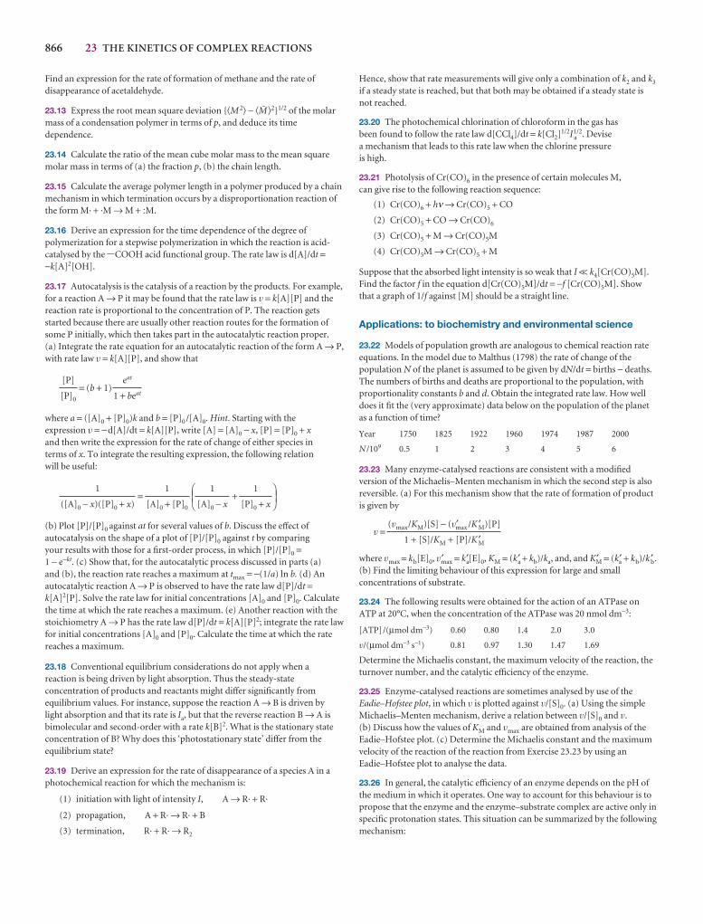
Hence, show that rate measurements will give only a combination of k2 and k3
if a steady state is reached, but that both may be obtained if a steady state isnot reached.
23.20 The photochemical chlorination of chloroform in the gas hasbeen found to follow the rate law d[CCl4]/dt = k[Cl2]1/2I a
1/2. Devise a mechanism that leads to this rate law when the chlorine pressure is high.
23.21 Photolysis of Cr(CO)6 in the presence of certain molecules M, can give rise to the following reaction sequence:
(1) Cr(CO)6 + hν → Cr(CO)5 + CO
(2) Cr(CO)5 + CO → Cr(CO)6
(3) Cr(CO)5 + M → Cr(CO)5M
(4) Cr(CO)5M → Cr(CO)5 + M
Suppose that the absorbed light intensity is so weak that I << k4[Cr(CO)5M].Find the factor f in the equation d[Cr(CO)5M]/dt = −f [Cr(CO)5M]. Showthat a graph of 1/f against [M] should be a straight line.
Applications: to biochemistry and environmental science
23.22 Models of population growth are analogous to chemical reaction rateequations. In the model due to Malthus (1798) the rate of change of thepopulation N of the planet is assumed to be given by dN/dt = births − deaths.The numbers of births and deaths are proportional to the population, withproportionality constants b and d. Obtain the integrated rate law. How welldoes it fit the (very approximate) data below on the population of the planetas a function of time?
Year 1750 1825 1922 1960 1974 1987 2000
N /109 0.5 1 2 3 4 5 6
23.23 Many enzyme-catalysed reactions are consistent with a modifiedversion of the Michaelis–Menten mechanism in which the second step is alsoreversible. (a) For this mechanism show that the rate of formation of productis given by
v =
where vmax = kb[E]0, v′max = ka′[E]0, KM = (ka′ + kb)/ka, and, and K′M = (k′a + kb)/kb′ .(b) Find the limiting behaviour of this expression for large and smallconcentrations of substrate.
23.24 The following results were obtained for the action of an ATPase onATP at 20°C, when the concentration of the ATPase was 20 nmol dm−3:
[ATP]/(µmol dm−3) 0.60 0.80 1.4 2.0 3.0
v/(µmol dm−3 s−1) 0.81 0.97 1.30 1.47 1.69
Determine the Michaelis constant, the maximum velocity of the reaction, theturnover number, and the catalytic efficiency of the enzyme.
23.25 Enzyme-catalysed reactions are sometimes analysed by use of theEadie–Hofstee plot, in which v is plotted against v/[S]0. (a) Using the simpleMichaelis–Menten mechanism, derive a relation between v/[S]0 and v.(b) Discuss how the values of KM and vmax are obtained from analysis of theEadie–Hofstee plot. (c) Determine the Michaelis constant and the maximumvelocity of the reaction of the reaction from Exercise 23.23 by using anEadie–Hofstee plot to analyse the data.
23.26 In general, the catalytic efficiency of an enzyme depends on the pH ofthe medium in which it operates. One way to account for this behaviour is topropose that the enzyme and the enzyme–substrate complex are active only inspecific protonation states. This situation can be summarized by the followingmechanism:
(vmax/KM)[S] − (v′max /K ′M)[P]
1 + [S]/KM + [P]/K ′M
866 23 THE KINETICS OF COMPLEX REACTIONS
Find an expression for the rate of formation of methane and the rate ofdisappearance of acetaldehyde.
23.13 Express the root mean square deviation {�M 2� − �J�2}1/2 of the molarmass of a condensation polymer in terms of p, and deduce its timedependence.
23.14 Calculate the ratio of the mean cube molar mass to the mean squaremolar mass in terms of (a) the fraction p, (b) the chain length.
23.15 Calculate the average polymer length in a polymer produced by a chainmechanism in which termination occurs by a disproportionation reaction ofthe form M· + ·M → M + :M.
23.16 Derive an expression for the time dependence of the degree ofpolymerization for a stepwise polymerization in which the reaction is acid-catalysed by the -COOH acid functional group. The rate law is d[A]/dt =−k[A]2[OH].
23.17 Autocatalysis is the catalysis of a reaction by the products. For example,for a reaction A → P it may be found that the rate law is v = k[A][P] and thereaction rate is proportional to the concentration of P. The reaction getsstarted because there are usually other reaction routes for the formation ofsome P initially, which then takes part in the autocatalytic reaction proper. (a) Integrate the rate equation for an autocatalytic reaction of the form A → P,with rate law v = k[A][P], and show that
= (b + 1)
where a = ([A]0 + [P]0)k and b = [P]0 /[A]0. Hint. Starting with the expression v = −d[A]/dt = k[A][P], write [A] = [A]0 − x, [P] = [P]0 + xand then write the expression for the rate of change of either species in terms of x. To integrate the resulting expression, the following relation will be useful:
= +
(b) Plot [P]/[P]0 against at for several values of b. Discuss the effect ofautocatalysis on the shape of a plot of [P]/[P]0 against t by comparing your results with those for a first-order process, in which [P]/[P]0 =1 − e−kt. (c) Show that, for the autocatalytic process discussed in parts (a) and (b), the reaction rate reaches a maximum at tmax = −(1/a) ln b. (d) Anautocatalytic reaction A → P is observed to have the rate law d[P]/dt =k[A]2[P]. Solve the rate law for initial concentrations [A]0 and [P]0. Calculatethe time at which the rate reaches a maximum. (e) Another reaction with thestoichiometry A → P has the rate law d[P]/dt = k[A][P]2; integrate the rate lawfor initial concentrations [A]0 and [P]0. Calculate the time at which the ratereaches a maximum.
23.18 Conventional equilibrium considerations do not apply when a reaction is being driven by light absorption. Thus the steady-stateconcentration of products and reactants might differ significantly fromequilibrium values. For instance, suppose the reaction A → B is driven by light absorption and that its rate is Ia, but that the reverse reaction B → A isbimolecular and second-order with a rate k[B]2. What is the stationary stateconcentration of B? Why does this ‘photostationary state’ differ from theequilibrium state?
23.19 Derive an expression for the rate of disappearance of a species A in aphotochemical reaction for which the mechanism is:
(1) initiation with light of intensity I, A → R· + R·
(2) propagation, A + R· → R· + B
(3) termination, R· + R· → R2
DEF1
[P]0 + x
1
[A]0 − x
ABC1
[A]0 + [P]0
1
([A]0 − x)([P]0 + x)
eat
1 + beat
[P]
[P]0
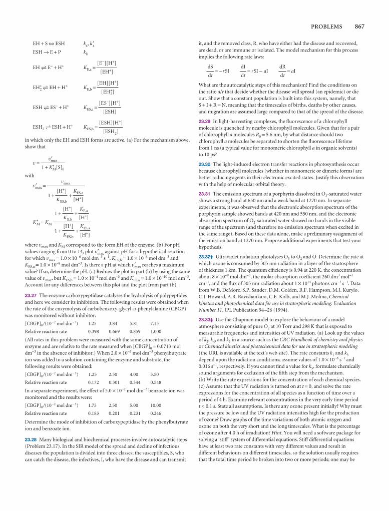
PROBLEMS 867
EH + S ⇔ ESH ka, k a′ESH → E + P kb
EH 5 E− + H+ KE,a =
EH2+ 5 EH + H+ KE,b =
ESH 5 ES− + H+ KES,a =
ESH2 5 ESH + H+ KES,b =
in which only the EH and ESH forms are active. (a) For the mechanism above,show that
v =
with
v′max =
1 + +
1 + +K ′M = KM
1 + +
where vmax and KM correspond to the form EH of the enzyme. (b) For pHvalues ranging from 0 to 14, plot v′max against pH for a hypothetical reactionfor which vmax = 1.0 × 10⁻⁶ mol dm−3 s−1, KES,b = 1.0 × 10⁻⁶ mol dm−3 andKES,a = 1.0 × 10⁻⁸ mol dm−3. Is there a pH at which v′max reaches a maximumvalue? If so, determine the pH. (c) Redraw the plot in part (b) by using the samevalue of vmax, but KES,b = 1.0 × 10⁻⁴ mol dm−3 and KES,a = 1.0 × 10⁻¹⁰ mol dm−3.Account for any differences between this plot and the plot from part (b).
23.27 The enzyme carboxypeptidase catalyses the hydrolysis of polypeptidesand here we consider its inhibition. The following results were obtained whenthe rate of the enzymolysis of carbobenzoxy-glycyl-D-phenylalanine (CBGP)was monitored without inhibitor:
[CBGP]0 /(10−2 mol dm−3) 1.25 3.84 5.81 7.13
Relative reaction rate 0.398 0.669 0.859 1.000
(All rates in this problem were measured with the same concentration ofenzyme and are relative to the rate measured when [CBGP]0 = 0.0713 moldm−3 in the absence of inhibitor.) When 2.0 × 10⁻³ mol dm−3 phenylbutyrateion was added to a solution containing the enzyme and substrate, thefollowing results were obtained:
[CBGP]0 /(10−2 mol dm− 3) 1.25 2.50 4.00 5.50
Relative reaction rate 0.172 0.301 0.344 0.548
In a separate experiment, the effect of 5.0 × 10⁻² mol dm−3 benzoate ion wasmonitored and the results were:
[CBGP]0 /(10−2 mol dm− 3) 1.75 2.50 5.00 10.00
Relative reaction rate 0.183 0.201 0.231 0.246
Determine the mode of inhibition of carboxypeptidase by the phenylbutyrateion and benzoate ion.
23.28 Many biological and biochemical processes involve autocatalytic steps(Problem 23.17). In the SIR model of the spread and decline of infectiousdiseases the population is divided into three classes; the susceptibles, S, whocan catch the disease, the infectives, I, who have the disease and can transmit
KES,a
[H+]
[H+]
KES,b
KE,a
[H+]
[H+]
KE,b
KES,a
[H+]
[H+]
KES,b
vmax
v′max
1 + K′M[S]0
[ESH][H+]
[ESH2]
[ES−][H+]
[ESH]
[EH][H+]
[EH2+]
[E−][H+]
[EH+]
it, and the removed class, R, who have either had the disease and recovered,are dead, or are immune or isolated. The model mechanism for this processimplies the following rate laws:
= −rSI = rSI − aI = aI
What are the autocatalytic steps of this mechanism? Find the conditions onthe ratio a/r that decide whether the disease will spread (an epidemic) or dieout. Show that a constant population is built into this system, namely, that S + I + R = N, meaning that the timescales of births, deaths by other causes,and migration are assumed large compared to that of the spread of the disease.
23.29 In light-harvesting complexes, the fluorescence of a chlorophyllmolecule is quenched by nearby chlorophyll molecules. Given that for a pairof chlorophyll a molecules R0 = 5.6 nm, by what distance should twochlorophyll a molecules be separated to shorten the fluorescence lifetime from 1 ns (a typical value for monomeric chlorophyll a in organic solvents) to 10 ps?
23.30 The light-induced electron transfer reactions in photosynthesis occurbecause chlorophyll molecules (whether in monomeric or dimeric forms) arebetter reducing agents in their electronic excited states. Justify this observationwith the help of molecular orbital theory.
23.31 The emission spectrum of a porphyrin dissolved in O2-saturated watershows a strong band at 650 nm and a weak band at 1270 nm. In separateexperiments, it was observed that the electronic absorption spectrum of theporphyrin sample showed bands at 420 nm and 550 nm, and the electronicabsorption spectrum of O2-saturated water showed no bands in the visiblerange of the spectrum (and therefore no emission spectrum when excited inthe same range). Based on these data alone, make a preliminary assignment ofthe emission band at 1270 nm. Propose additional experiments that test yourhypothesis.
23.32‡ Ultraviolet radiation photolyses O3 to O2 and O. Determine the rate atwhich ozone is consumed by 305 nm radiation in a layer of the stratosphere of thickness 1 km. The quantum efficiency is 0.94 at 220 K, the concentrationabout 8 × 10⁻⁹ mol dm−3, the molar absorption coefficient 260 dm3 mol−1
cm−1, and the flux of 305 nm radiation about 1 × 10¹⁴ photons cm−2 s−1. Datafrom W.B. DeMore, S.P. Sander, D.M. Golden, R.F. Hampson, M.J. Kurylo,C.J. Howard, A.R. Ravishankara, C.E. Kolb, and M.J. Molina, Chemicalkinetics and photochemical data for use in stratospheric modeling: EvaluationNumber 11, JPL Publication 94–26 (1994).
23.33‡ Use the Chapman model to explore the behaviour of a modelatmosphere consisting of pure O2 at 10 Torr and 298 K that is exposed tomeasurable frequencies and intensities of UV radiation. (a) Look up the valuesof k2, k4, and k5 in a source such as the CRC Handbook of chemistry and physicsor Chemical kinetics and photochemical data for use in stratospheric modeling(the URL is available at the text’s web site). The rate constants k1 and k3
depend upon the radiation conditions; assume values of 1.0 × 10⁻⁸ s−1 and0.016 s−1, respectively. If you cannot find a value for k5, formulate chemicallysound arguments for exclusion of the fifth step from the mechanism. (b) Write the rate expressions for the concentration of each chemical species.(c) Assume that the UV radiation is turned on at t = 0, and solve the rateexpressions for the concentration of all species as a function of time over aperiod of 4 h. Examine relevant concentrations in the very early time period t < 0.1 s. State all assumptions. Is there any ozone present initially? Why mustthe pressure be low and the UV radiation intensities high for the productionof ozone? Draw graphs of the time variations of both atomic oxygen andozone on both the very short and the long timescales. What is the percentageof ozone after 4.0 h of irradiation? Hint. You will need a software package forsolving a ‘stiff ’ system of differential equations. Stiff differential equationshave at least two rate constants with very different values and result indifferent behaviours on different timescales, so the solution usually requiresthat the total time period be broken into two or more periods; one may be
dR
dt
dI
dt
dS
dt

868 23 THE KINETICS OF COMPLEX REACTIONS
very short and another very long. For help with using mathematical softwareto solve systems of differential equations, see M.P. Cady and C.A. Trapp, A Mathcad primer for physical chemistry. Oxford University Press (1999).
23.34‡ Chlorine atoms react rapidly with ozone in the gas-phase bimolecularreaction Cl + O3 → ClO + O2 with k = (1.7 × 10¹⁰ dm3 mol−1 s−1)e−260/(T/K)
(W.B. DeMore, S.P. Sander, D.M. Golden, R.F. Hampson, M.J. Kurylo, C.J.Howard, A.R. Ravishankara, C.E. Kolb, and M.J. Molina, Chemical kineticsand photochemical data for use in stratospheric modeling: EvaluationNumber 11, JPL Publication 94–26 (1994)). Estimate the rate of this reactionat (a) 20 km, where [Cl] = 5 × 10⁻¹⁷ mol dm−3, [O3] = 8 × 10⁻⁹ mol dm−3, andT = 220 K; (b) 45 km, where [Cl] = 3 × 10⁻¹⁵ mol dm−3, [O3] = 8 × 10⁻¹¹ moldm−3, and T = 270 K.
23.35‡ Because of its importance in atmospheric chemistry, the thermaldecomposition of nitric oxide, 2 NO(g) → N2(g) + O2(g), has been amongstthe most thoroughly studied of gas-phase reactions. The commonly acceptedmechanism has been that of H. Wise and M.F. Freech (J. Chem. Phys. 22, 1724(1952)):
(1) NO + NO → N2O + O k1
(2) O + NO → O2 + N k2
(3) N + NO → N2 + O k3
(4) O + O + M → O2 + M k4
(5) O2 + M → O + O + M k ′4
(a) Label the steps of this mechanism as initiation, propagation, etc. (b) Writedown the full expression for the rate of disappearance of NO. What does thisexpression for the rate become on the basis of the assumptions that v2 = v3
when [N] reaches its steady state concentration, that the rate of thepropagation step is more rapid than the rate of the initiation step, and thatoxygen atoms are in equilibrium with oxygen molecules? (c) Find anexpression for the effective activation energy, Ea,eff , for the overall reaction interms of the activation energies of the individual steps of the reaction. (d)Estimate Ea,eff from the bond energies of the species involved. (e) It has beenpointed out by R.J. Wu and C.T. Yeh (Int. J. Chem. Kinet. 28, 89 (1996)) thatthe reported experimental values of Ea,eff obtained by different authors havevaried from 253 to 357 kJ mol−1. They suggest that the assumption of oxygenatoms and oxygen molecules being in equilibrium is unwarranted and that thesteady-state approximation needs to be applied to the entire mechanism.Obtain the overall rate law based on the steady-state approximation and findthe forms that it assumes for low NO conversion (low O2 concentration).(f) When the reaction conversion becomes significant, Wu and Yeh suggestthat two additional elementary steps,
(6) O2 + M → O + O + M k6
(7) NO + O2 → O + NO2 k7
start to compete with step (1) as the initiation step. Obtain the rate laws basedon these alternative mechanisms and again estimate the apparent activationenergies. Is the range of these different theoretically estimated values for Ea,eff
consistent with the range of values obtained experimentally?
Molecular reactiondynamics
The simplest quantitative account of reaction rates is in terms of collision theory, which canbe used only for the discussion of reactions between simple species in the gas phase.Reactions in solution are classified into two types: diffusion-controlled and activation-controlled. The former can be expressed quantitatively in terms of the diffusion equation. Intransition state theory, it is assumed that the reactant molecules form a complex that canbe discussed in terms of the population of its energy levels. Transition state theory inspiresa thermodynamic approach to reaction rates, in which the rate constant is expressed interms of thermodynamic parameters. This approach is useful for parametrizing the rates of reactions in solution. The highest level of sophistication is in terms of potential energy surfaces and the motion of molecules through these surfaces. As we shall see, such an approach gives an intimate picture of the events that occur when reactions occur and isopen to experimental study. We also use transition state theory to examine the transfer of electrons in homogeneous systems and see that the rate of the process depends on the distance between electron donor and acceptor, the standard Gibbs energy of reaction,and the energy associated with molecular rearrangements that accompany the transfer of charge.
Now we are at the heart of chemistry. Here we examine the details of what happens tomolecules at the climax of reactions. Extensive changes of structure are taking placeand energies the size of dissociation energies are being redistributed among bonds:old bonds are being ripped apart and new bonds are being formed.
As may be imagined, the calculation of the rates of such processes from first prin-ciples is very difficult. Nevertheless, like so many intricate problems, the broad featurescan be established quite simply. Only when we enquire more deeply do the complica-tions emerge. In this chapter we look at several approaches to the calculation of a rateconstant for elementary bimolecular processes, ranging from electron transfer tochemical reactions involving bond breakage and formation. Although a great deal ofinformation can be obtained from gas-phase reactions, many reactions of interesttake place in solution, and we shall also see to what extent their rates can be predicted.
Reactive encounters
In this section we consider two elementary approaches to the calculation of reactionrates, one relating to gas-phase reactions and the other to reactions in solution. Bothapproaches are based on the view that reactant molecules must meet, and that reac-tion takes place only if the molecules have a certain minimum energy. In the collisiontheory of bimolecular gas-phase reactions, which we mentioned briefly in Section 22.5,
24Reactive encounters
24.1 Collision theory
24.2 Diffusion-controlledreactions
24.3 The material balanceequation
Transition state theory
24.4 The Eyring equation
24.5 Thermodynamic aspects
The dynamics of molecularcollisions
24.6 Reactive collisions
24.7 Potential energy surfaces
24.8 Some results fromexperiments and calculations
24.9 The investigation of reactiondynamics with ultrafast lasertechniques
Electron transfer inhomogeneous systems
24.10 The rates of electron transferprocesses
24.11 Theory of electron transferprocesses
24.12 Experimental results
I24.1 Impact on biochemistry:Electron transfer in andbetween proteins
Checklist of key ideas
Further reading
Further information 24.1: The Gibbsenergy of activation of electrontransfer and the Marcus cross-relation
Discussion questions
Exercises
Problems
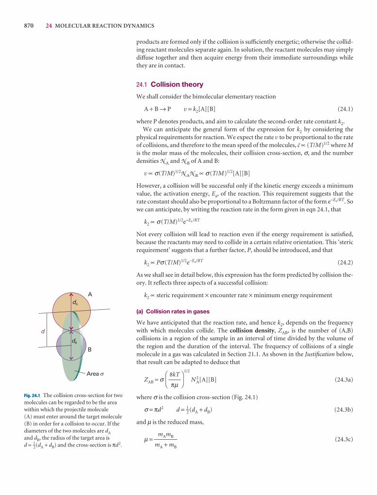
870 24 MOLECULAR REACTION DYNAMICS
products are formed only if the collision is sufficiently energetic; otherwise the collid-ing reactant molecules separate again. In solution, the reactant molecules may simplydiffuse together and then acquire energy from their immediate surroundings whilethey are in contact.
24.1 Collision theory
We shall consider the bimolecular elementary reaction
A + B → P v = k2[A][B] (24.1)
where P denotes products, and aim to calculate the second-order rate constant k2.We can anticipate the general form of the expression for k2 by considering the
physical requirements for reaction. We expect the rate v to be proportional to the rate of collisions, and therefore to the mean speed of the molecules, K ∝ (T/M)1/2 where Mis the molar mass of the molecules, their collision cross-section, σ, and the numberdensities N A and N B of A and B:
v ∝ σ(T/M)1/2N AN B ∝ σ(T/M)1/2[A][B]
However, a collision will be successful only if the kinetic energy exceeds a minimumvalue, the activation energy, Ea, of the reaction. This requirement suggests that therate constant should also be proportional to a Boltzmann factor of the form e−Ea/RT. Sowe can anticipate, by writing the reaction rate in the form given in eqn 24.1, that
k2 ∝ σ(T/M)1/2e−Ea /RT
Not every collision will lead to reaction even if the energy requirement is satisfied, because the reactants may need to collide in a certain relative orientation. This ‘stericrequirement’ suggests that a further factor, P, should be introduced, and that
k2 ∝ Pσ(T/M)1/2e−Ea/RT (24.2)
As we shall see in detail below, this expression has the form predicted by collision the-ory. It reflects three aspects of a successful collision:
k2 ∝ steric requirement × encounter rate × minimum energy requirement
(a) Collision rates in gases
We have anticipated that the reaction rate, and hence k2, depends on the frequencywith which molecules collide. The collision density, ZAB, is the number of (A,B) collisions in a region of the sample in an interval of time divided by the volume of the region and the duration of the interval. The frequency of collisions of a singlemolecule in a gas was calculated in Section 21.1. As shown in the Justification below,that result can be adapted to deduce that
ZAB = σ1/2
N 2A[A][B] (24.3a)
where σ is the collision cross-section (Fig. 24.1)
σ = πd2 d = 1–2 (dA + dB) (24.3b)
and µ is the reduced mass,
µ = (24.3c)mAmB
mA + mB
DF
8kT
πµ
AC
Area
A
B
dA
dB
d
s
Fig. 24.1 The collision cross-section for twomolecules can be regarded to be the areawithin which the projectile molecule (A) must enter around the target molecule (B) in order for a collision to occur. If thediameters of the two molecules are dA
and dB, the radius of the target area is d = 1–2(dA + dB) and the cross-section is πd2.
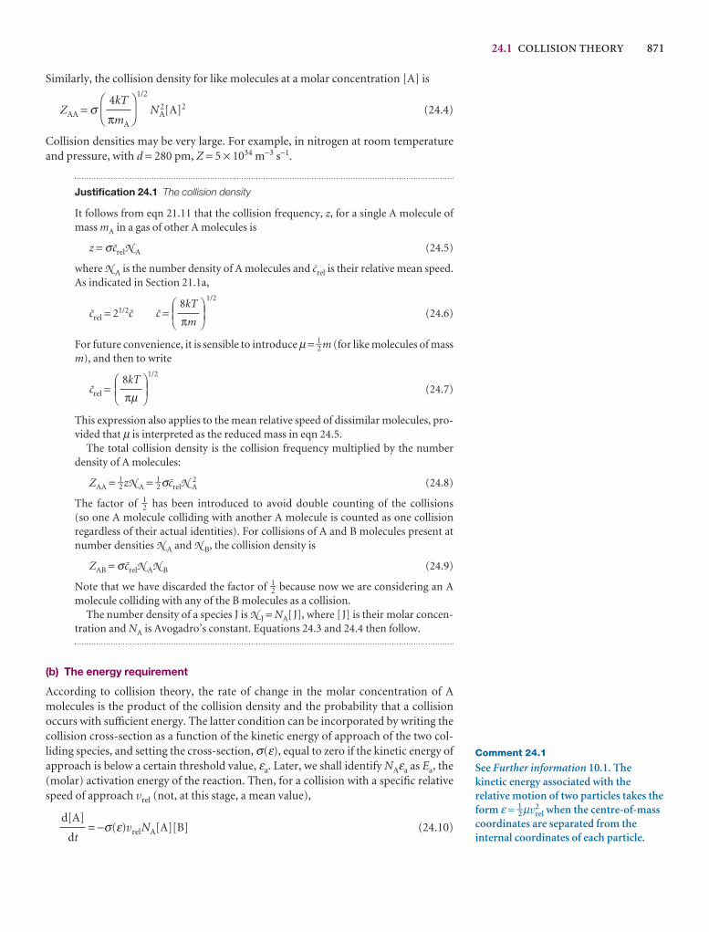
24.1 COLLISION THEORY 871
Similarly, the collision density for like molecules at a molar concentration [A] is
ZAA = σ1/2
N 2A[A]2 (24.4)
Collision densities may be very large. For example, in nitrogen at room temperatureand pressure, with d = 280 pm, Z = 5 × 1034 m−3 s−1.
Justification 24.1 The collision density
It follows from eqn 21.11 that the collision frequency, z, for a single A molecule ofmass mA in a gas of other A molecules is
z = σKrelN A (24.5)
where N A is the number density of A molecules and Krel is their relative mean speed.As indicated in Section 21.1a,
Krel = 21/2K K = 1/2
(24.6)
For future convenience, it is sensible to introduce µ = 1–2 m (for like molecules of massm), and then to write
Krel =1/2
(24.7)
This expression also applies to the mean relative speed of dissimilar molecules, pro-vided that µ is interpreted as the reduced mass in eqn 24.5.
The total collision density is the collision frequency multiplied by the numberdensity of A molecules:
ZAA = 1–2 zN A = 1–2 σKrelN A2 (24.8)
The factor of 1–2 has been introduced to avoid double counting of the collisions (so one A molecule colliding with another A molecule is counted as one collision regardless of their actual identities). For collisions of A and B molecules present atnumber densities N A and N B, the collision density is
ZAB = σKrelN AN B (24.9)
Note that we have discarded the factor of 1–2 because now we are considering an Amolecule colliding with any of the B molecules as a collision.
The number density of a species J is N J = NA[J], where [J] is their molar concen-tration and NA is Avogadro’s constant. Equations 24.3 and 24.4 then follow.
(b) The energy requirement
According to collision theory, the rate of change in the molar concentration of Amolecules is the product of the collision density and the probability that a collision occurs with sufficient energy. The latter condition can be incorporated by writing thecollision cross-section as a function of the kinetic energy of approach of the two col-liding species, and setting the cross-section, σ(ε), equal to zero if the kinetic energy ofapproach is below a certain threshold value, εa. Later, we shall identify NAεa as Ea, the(molar) activation energy of the reaction. Then, for a collision with a specific relativespeed of approach vrel (not, at this stage, a mean value),
= −σ(ε)vrelNA[A][B] (24.10)d[A]
dt
DEF8kT
πµABC
DEF8kT
πm
ABC
DF
4kT
πmA
AC
Comment 24.1
See Further information 10.1. Thekinetic energy associated with therelative motion of two particles takes theform ε = 1–2 µv2
rel when the centre-of-masscoordinates are separated from theinternal coordinates of each particle.
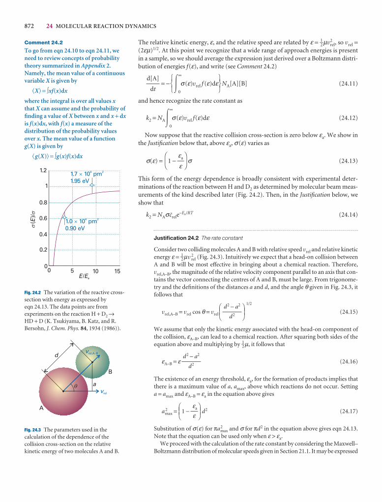
872 24 MOLECULAR REACTION DYNAMICS
The relative kinetic energy, ε, and the relative speed are related by ε = 1–2 µv2rel, so vrel =
(2εµ)1/2. At this point we recognize that a wide range of approach energies is presentin a sample, so we should average the expression just derived over a Boltzmann distri-bution of energies f(ε), and write (see Comment 24.2)
= − �∞
0
σ(ε)vrel f (ε)dε NA[A][B] (24.11)
and hence recognize the rate constant as
k2 = NA�∞
0
σ(ε)vrel f(ε)dε (24.12)
Now suppose that the reactive collision cross-section is zero below εa. We show inthe Justification below that, above εa, σ(ε) varies as
σ(ε) = 1 − σ (24.13)
This form of the energy dependence is broadly consistent with experimental deter-minations of the reaction between H and D2 as determined by molecular beam meas-urements of the kind described later (Fig. 24.2). Then, in the Justification below, weshow that
k2 = NAσKrele−Ea/RT (24.14)
Justification 24.2 The rate constant
Consider two colliding molecules A and B with relative speed vrel and relative kineticenergy ε = 1–2 µv 2
rel (Fig. 24.3). Intuitively we expect that a head-on collision betweenA and B will be most effective in bringing about a chemical reaction. Therefore,vrel,A–B, the magnitude of the relative velocity component parallel to an axis that con-tains the vector connecting the centres of A and B, must be large. From trigonome-try and the definitions of the distances a and d, and the angle θ given in Fig. 24.3, itfollows that
vrel,A–B = vrel cos θ = vrel
1/2
(24.15)
We assume that only the kinetic energy associated with the head-on component ofthe collision, εA–B, can lead to a chemical reaction. After squaring both sides of theequation above and multiplying by 1–2 µ, it follows that
εA–B = ε (24.16)
The existence of an energy threshold, εa, for the formation of products implies thatthere is a maximum value of a, amax, above which reactions do not occur. Setting a = amax and εA–B = εa in the equation above gives
a 2max = 1 − d2 (24.17)
Substitution of σ(ε) for πa2max and σ for πd2 in the equation above gives eqn 24.13.
Note that the equation can be used only when ε > εa.We proceed with the calculation of the rate constant by considering the Maxwell–
Boltzmann distribution of molecular speeds given in Section 21.1. It may be expressed
DEFεa
εABC
d2 − a2
d2
DEFd2 − a2
d2
ABC
DF
εa
ε
AC
567
123
d[A]
dt
Comment 24.2
To go from eqn 24.10 to eqn 24.11, weneed to review concepts of probabilitytheory summarized in Appendix 2.Namely, the mean value of a continuousvariable X is given by
�X� = ∫xf(x)dx
where the integral is over all values xthat X can assume and the probability offinding a value of X between x and x + dxis f(x)dx, with f(x) a measure of thedistribution of the probability valuesover x. The mean value of a functiong(X) is given by
�g(X)� = ∫g(x)f(x)dx
s(
)/E
0 5 10 15E E/ a
0
0.2
0.4
0.6
0.8
1
1.2
1.0 10 pm0.90 eV
´4 2
1.7 10 pm1.95 eV
´4 2
ss
d
a
B
vrel,A B�
vrel
�
A
Fig. 24.3 The parameters used in thecalculation of the dependence of thecollision cross-section on the relativekinetic energy of two molecules A and B.
Fig. 24.2 The variation of the reactive cross-section with energy as expressed by eqn 24.13. The data points are fromexperiments on the reaction H + D2 →HD + D (K. Tsukiyama, B. Katz, and R.Bersohn, J. Chem. Phys. 84, 1934 (1986)).
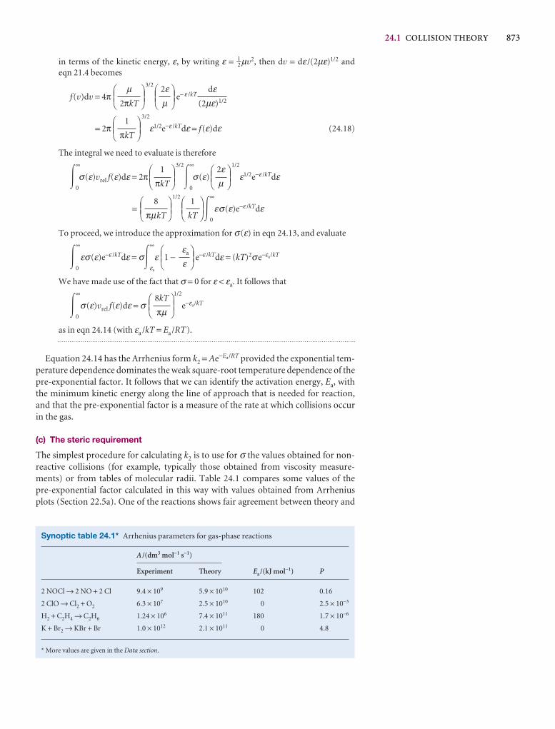
24.1 COLLISION THEORY 873
in terms of the kinetic energy, ε, by writing ε = 1–2 µv2, then dv = dε /(2µε)1/2 andeqn 21.4 becomes
f(v)dv = 4π3/2
e− ε /kT
= 2π3/2
ε1/2e−ε /kTdε = f(ε)dε (24.18)
The integral we need to evaluate is therefore
�∞
0
σ(ε)vrel f(ε)dε = 2π3/2
�∞
0
σ(ε)
1/2
ε1/2e−ε /kTdε
=1/2
�∞
0
εσ(ε)e−ε /kTdε
To proceed, we introduce the approximation for σ(ε) in eqn 24.13, and evaluate
�∞
0
εσ(ε)e−ε /kTdε = σ�∞
εa
ε 1 − e−ε /kTdε = (kT)2σe−εa/kT
We have made use of the fact that σ = 0 for ε < εa. It follows that
�∞
0
σ(ε)vrel f(ε)dε = σ1/2
e−εa/kT
as in eqn 24.14 (with εa /kT = Ea /RT).
Equation 24.14 has the Arrhenius form k2 = Ae−Ea/RT provided the exponential tem-perature dependence dominates the weak square-root temperature dependence of thepre-exponential factor. It follows that we can identify the activation energy, Ea, withthe minimum kinetic energy along the line of approach that is needed for reaction,and that the pre-exponential factor is a measure of the rate at which collisions occurin the gas.
(c) The steric requirement
The simplest procedure for calculating k2 is to use for σ the values obtained for non-reactive collisions (for example, typically those obtained from viscosity measure-ments) or from tables of molecular radii. Table 24.1 compares some values of thepre-exponential factor calculated in this way with values obtained from Arrheniusplots (Section 22.5a). One of the reactions shows fair agreement between theory and
DEF8kT
πµABC
DEFεa
εABC
DEF1
kT
ABCDEF
8
πµkT
ABC
DEF2εµ
ABCDEF
1
πkT
ABC
DEF1
πkT
ABC
dε(2µε)1/2
DEF2εµ
ABCDEF
µ2πkT
ABC
Synoptic table 24.1* Arrhenius parameters for gas-phase reactions
A /(dm3 mol−1 s−1)
Experiment Theory Ea/(kJ mol−1) P
2 NOCl → 2 NO + 2 Cl 9.4 × 10⁹ 5.9 × 10¹⁰ 102 0.16
2 ClO → Cl2 + O2 6.3 × 10⁷ 2.5 × 10¹⁰ 0 2.5 × 10⁻³
H2 + C2H4 → C2H6 1.24 × 10⁶ 7.4 × 10¹¹ 180 1.7 × 10⁻⁶
K + Br2 → KBr + Br 1.0 × 10¹² 2.1 × 10¹¹ 0 4.8
* More values are given in the Data section.
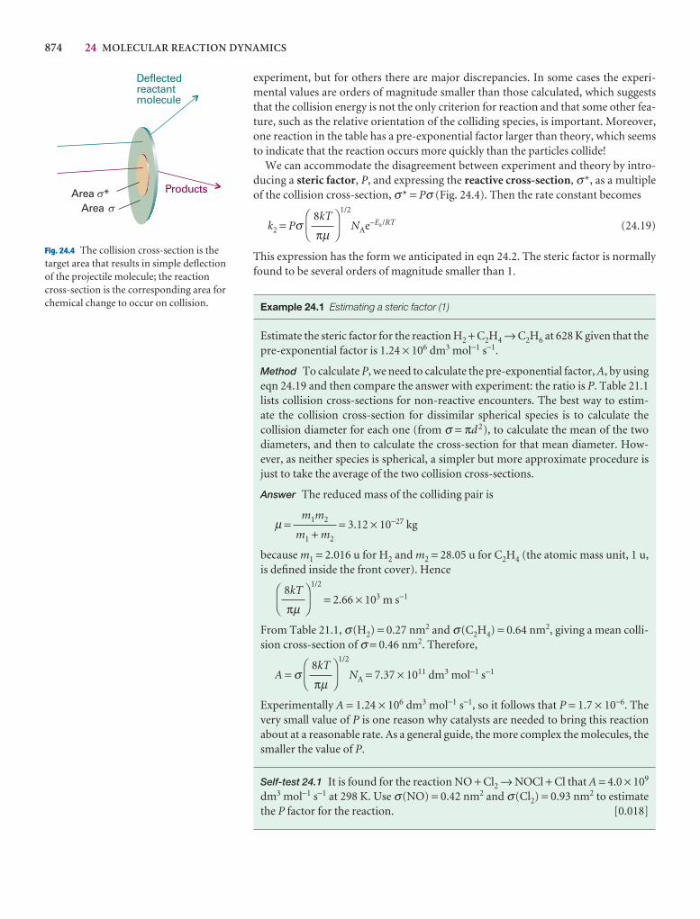
874 24 MOLECULAR REACTION DYNAMICS
Area *$
Area
Products
Deflectedreactantmolecule
$
$
Fig. 24.4 The collision cross-section is thetarget area that results in simple deflectionof the projectile molecule; the reactioncross-section is the corresponding area forchemical change to occur on collision.
experiment, but for others there are major discrepancies. In some cases the experi-mental values are orders of magnitude smaller than those calculated, which suggeststhat the collision energy is not the only criterion for reaction and that some other fea-ture, such as the relative orientation of the colliding species, is important. Moreover,one reaction in the table has a pre-exponential factor larger than theory, which seemsto indicate that the reaction occurs more quickly than the particles collide!
We can accommodate the disagreement between experiment and theory by intro-ducing a steric factor, P, and expressing the reactive cross-section, σ*, as a multipleof the collision cross-section, σ* = Pσ (Fig. 24.4). Then the rate constant becomes
k2 = Pσ1/2
NAe−Ea/RT (24.19)
This expression has the form we anticipated in eqn 24.2. The steric factor is normallyfound to be several orders of magnitude smaller than 1.
Example 24.1 Estimating a steric factor (1)
Estimate the steric factor for the reaction H2 + C2H4 → C2H6 at 628 K given that thepre-exponential factor is 1.24 × 10⁶ dm3 mol−1 s−1.
Method To calculate P, we need to calculate the pre-exponential factor, A, by usingeqn 24.19 and then compare the answer with experiment: the ratio is P. Table 21.1lists collision cross-sections for non-reactive encounters. The best way to estim-ate the collision cross-section for dissimilar spherical species is to calculate the collision diameter for each one (from σ = πd 2), to calculate the mean of the two diameters, and then to calculate the cross-section for that mean diameter. How-ever, as neither species is spherical, a simpler but more approximate procedure isjust to take the average of the two collision cross-sections.
Answer The reduced mass of the colliding pair is
µ = = 3.12 × 10⁻²⁷ kg
because m1 = 2.016 u for H2 and m2 = 28.05 u for C2H4 (the atomic mass unit, 1 u,is defined inside the front cover). Hence
1/2
= 2.66 × 10³ m s−1
From Table 21.1, σ(H2) = 0.27 nm2 and σ(C2H4) = 0.64 nm2, giving a mean colli-sion cross-section of σ = 0.46 nm2. Therefore,
A = σ1/2
NA = 7.37 × 10¹¹ dm3 mol−1 s−1
Experimentally A = 1.24 × 10⁶ dm3 mol−1 s−1, so it follows that P = 1.7 × 10⁻⁶. Thevery small value of P is one reason why catalysts are needed to bring this reactionabout at a reasonable rate. As a general guide, the more complex the molecules, thesmaller the value of P.
Self-test 24.1 It is found for the reaction NO + Cl2 → NOCl + Cl that A = 4.0 × 10⁹
dm3 mol−1 s−1 at 298 K. Use σ(NO) = 0.42 nm2 and σ(Cl2) = 0.93 nm2 to estimatethe P factor for the reaction. [0.018]
DF
8kT
πµ
AC
DF
8kT
πµ
AC
m1m2
m1 + m2
DF
8kT
πµ
AC
24.1 COLLISION THEORY 875
An example of a reaction for which it is possible to estimate the steric factor is K +Br2 → KBr + Br, with the experimental value P = 4.8. In this reaction, the distance ofapproach at which reaction occurs appears to be considerably larger than the distanceneeded for deflection of the path of the approaching molecules in a non-reactive collision. It has been proposed that the reaction proceeds by a harpoon mechanism.This brilliant name is based on a model of the reaction that pictures the K atom as approaching a Br2 molecule, and when the two are close enough an electron (the harpoon) flips across from K to Br2. In place of two neutral particles there are now two ions, so there is a Coulombic attraction between them: this attraction is the lineon the harpoon. Under its influence the ions move together (the line is wound in), thereaction takes place, and KBr + Br emerge. The harpoon extends the cross-section forthe reactive encounter, and the reaction rate is greatly underestimated by taking forthe collision cross-section the value for simple mechanical contact between K + Br2.
Example 24.2 Estimating a steric factor (2)
Estimate the value of P for the harpoon mechanism by calculating the distance atwhich it becomes energetically favourable for the electron to leap from K to Br2.
Method We should begin by identifying all the contributions to the energy of interaction between the colliding species. There are three contributions to the energy of the process K + Br2 → K+ + Br2
−. The first is the ionization energy, I, of K.The second is the electron affinity, Eea, of Br2. The third is the Coulombic inter-action energy between the ions when they have been formed: when their separationis R, this energy is −e2/4πε0R. The electron flips across when the sum of these threecontributions changes from positive to negative (that is, when the sum is zero).
Answer The net change in energy when the transfer occurs at a separation R is
E = I − Eea −
The ionization energy I is larger than Eea, so E becomes negative only when R hasdecreased to less than some critical value R* given by
= I − Eea
When the particles are at this separation, the harpoon shoots across from K to Br2,so we can identify the reactive cross-section as σ* = πR*2. This value of σ* impliesthat the steric factor is
P = = =2
where d = R(K) + R(Br2). With I = 420 kJ mol−1 (corresponding to 7.0 × 10⁻¹⁹ J),Eea ≈ 250 kJ mol−1 (corresponding to 4.2 × 10⁻¹⁹ J), and d = 400 pm, we find P = 4.2,in good agreement with the experimental value (4.8).
Self-test 24.2 Estimate the value of P for the harpoon reaction between Na and Cl2for which d ≈ 350 pm; take Eea ≈ 230 kJ mol−1. [2.2]
Example 24.2 illustrates two points about steric factors. First, the concept of a stericfactor is not wholly useless because in some cases its numerical value can be estimated.
567
e2
4πε0d(I − Eea)
123
R*2
d2
σ*
σ
e2
4πε0R*
e2
4πε0R
876 24 MOLECULAR REACTION DYNAMICS
Second (and more pessimistically) most reactions are much more complex than K +Br2, and we cannot expect to obtain P so easily. What we need is a more powerful the-ory that lets us calculate, and not merely guess, its value. We go some way to setting upthat theory in Section 24.4.
24.2 Diffusion-controlled reactions
Encounters between reactants in solution occur in a very different manner from encounters in gases. Reactant molecules have to jostle their way through the solvent,so their encounter frequency is considerably less than in a gas. However, because amolecule also migrates only slowly away from a location, two reactant molecules thatencounter each other stay near each other for much longer than in a gas. This linger-ing of one molecule near another on account of the hindering presence of solventmolecules is called the cage effect. Such an encounter pair may accumulate enoughenergy to react even though it does not have enough energy to do so when it firstforms. The activation energy of a reaction is a much more complicated quantity in solu-tion than in a gas because the encounter pair is surrounded by solvent and we need toconsider the energy of the entire local assembly of reactant and solvent molecules.
(a) Classes of reaction
The complicated overall process can be divided into simpler parts by setting up a sim-ple kinetic scheme. We suppose that the rate of formation of an encounter pair AB isfirst-order in each of the reactants A and B:
A + B → AB v = kd[A][B] (24.20a)
As we shall see, kd (where the d signifies diffusion) is determined by the diffusionalcharacteristics of A and B. The encounter pair can break up without reaction or it cango on to form products P. If we suppose that both processes are pseudofirst-order reactions (with the solvent perhaps playing a role), then we can write
AB → A + B v = kd′[AB] (24.20b)
and
AB → P v = ka[AB] (24.20c)
The concentration of AB can now be found from the equation for the net rate ofchange of concentration of AB:
= kd[A][B] − kd′[AB] − ka[AB] ≈ 0 (24.21)
where we have applied the steady-state approximation. This expression solves to
[AB] = (24.22)
The rate of formation of products is therefore
≈ ka[AB] = k2[A][B] k2 = (24.23)
Two limits can now be distinguished. If the rate of separation of the unreacted encounter pair is much slower than the rate at which it forms products, then k ′d << ka
and the effective rate constant is
kakd
ka + k ′d
d[P]
dt
kd[A][B]
ka + k ′d
d[AB]
dt
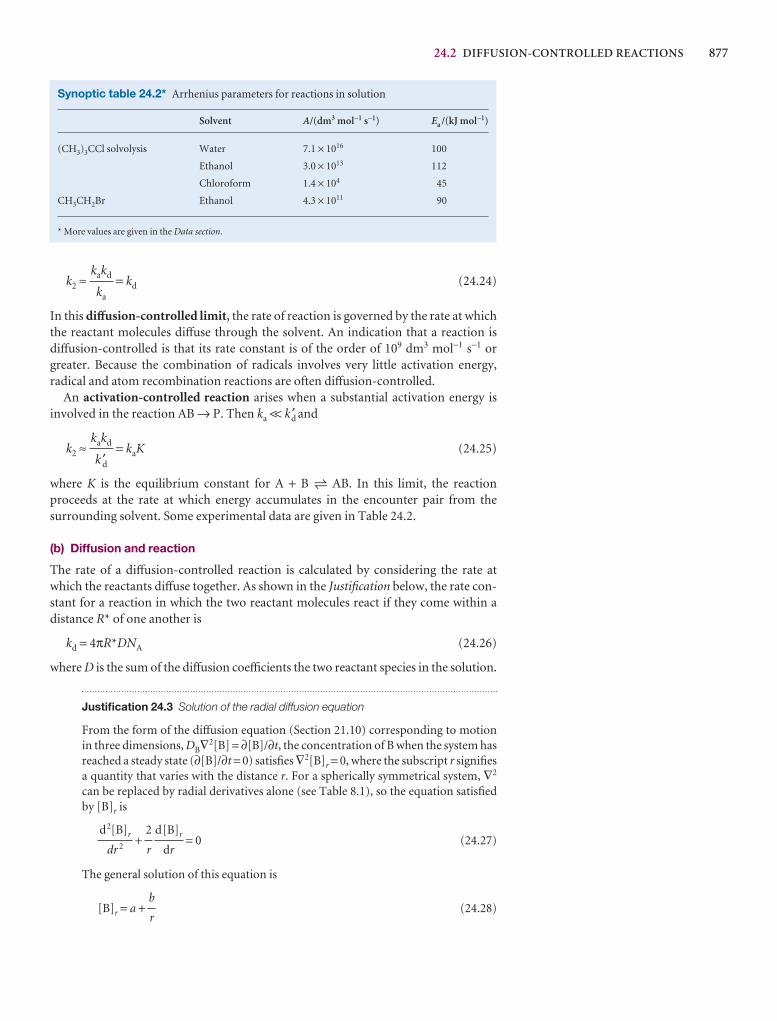
24.2 DIFFUSION-CONTROLLED REACTIONS 877
k2 ≈ = kd (24.24)
In this diffusion-controlled limit, the rate of reaction is governed by the rate at whichthe reactant molecules diffuse through the solvent. An indication that a reaction isdiffusion-controlled is that its rate constant is of the order of 109 dm3 mol−1 s−1 orgreater. Because the combination of radicals involves very little activation energy, radical and atom recombination reactions are often diffusion-controlled.
An activation-controlled reaction arises when a substantial activation energy is involved in the reaction AB → P. Then ka << kd′ and
k2 ≈ = kaK (24.25)
where K is the equilibrium constant for A + B 5 AB. In this limit, the reaction proceeds at the rate at which energy accumulates in the encounter pair from the surrounding solvent. Some experimental data are given in Table 24.2.
(b) Diffusion and reaction
The rate of a diffusion-controlled reaction is calculated by considering the rate atwhich the reactants diffuse together. As shown in the Justification below, the rate con-stant for a reaction in which the two reactant molecules react if they come within adistance R* of one another is
kd = 4πR*DNA (24.26)
where D is the sum of the diffusion coefficients the two reactant species in the solution.
Justification 24.3 Solution of the radial diffusion equation
From the form of the diffusion equation (Section 21.10) corresponding to motionin three dimensions, DB∇2[B] = ∂[B]/∂t, the concentration of B when the system hasreached a steady state (∂[B]/∂t = 0) satisfies ∇2[B]r = 0, where the subscript r signifiesa quantity that varies with the distance r. For a spherically symmetrical system, ∇2
can be replaced by radial derivatives alone (see Table 8.1), so the equation satisfiedby [B]r is
+ = 0 (24.27)
The general solution of this equation is
[B]r = a + (24.28)b
r
d[B]r
dr
2
r
d2[B]r
dr 2
kakd
k ′d
kakd
ka
Synoptic table 24.2* Arrhenius parameters for reactions in solution
Solvent A/(dm3 mol−1 s−1) Ea /(kJ mol−1)
(CH3)3CCl solvolysis Water 7.1 × 10¹⁶ 100
Ethanol 3.0 × 10¹³ 112
Chloroform 1.4 × 10⁴ 45
CH3CH2Br Ethanol 4.3 × 10¹¹ 90
* More values are given in the Data section.
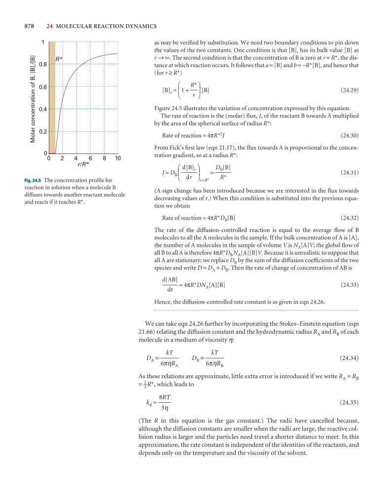
878 24 MOLECULAR REACTION DYNAMICS
as may be verified by substitution. We need two boundary conditions to pin downthe values of the two constants. One condition is that [B]r has its bulk value [B] as r → ∞. The second condition is that the concentration of B is zero at r = R*, the dis-tance at which reaction occurs. It follows that a = [B] and b = −R*[B], and hence that(for r ≥ R*)
[B]r = 1 + [B] (24.29)
Figure 24.5 illustrates the variation of concentration expressed by this equation.The rate of reaction is the (molar) flux, J, of the reactant B towards A multiplied
by the area of the spherical surface of radius R*:
Rate of reaction = 4πR*2J (24.30)
From Fick’s first law (eqn 21.17), the flux towards A is proportional to the concen-tration gradient, so at a radius R*:
J = DBr =R*
= (24.31)
(A sign change has been introduced because we are interested in the flux towardsdecreasing values of r.) When this condition is substituted into the previous equa-tion we obtain
Rate of reaction = 4πR*DB[B] (24.32)
The rate of the diffusion-controlled reaction is equal to the average flow of Bmolecules to all the A molecules in the sample. If the bulk concentration of A is [A],the number of A molecules in the sample of volume V is NA[A]V; the global flow ofall B to all A is therefore 4πR*DB NA[A][B]V. Because it is unrealistic to suppose thatall A are stationary; we replace DB by the sum of the diffusion coefficients of the twospecies and write D = DA + DB. Then the rate of change of concentration of AB is
= 4πR*DNA[A][B] (24.33)
Hence, the diffusion-controlled rate constant is as given in eqn 24.26.
We can take eqn 24.26 further by incorporating the Stokes–Einstein equation (eqn21.66) relating the diffusion constant and the hydrodynamic radius RA and RB of eachmolecule in a medium of viscosity η:
DA = DB = (24.34)
As these relations are approximate, little extra error is introduced if we write RA = RB
= 1–2 R*, which leads to
kd = (24.35)
(The R in this equation is the gas constant.) The radii have cancelled because, although the diffusion constants are smaller when the radii are large, the reactive col-lision radius is larger and the particles need travel a shorter distance to meet. In thisapproximation, the rate constant is independent of the identities of the reactants, anddepends only on the temperature and the viscosity of the solvent.
8RT
3η
kT
6πηRB
kT
6πηRA
d[AB]
dt
DB[B]
R*
DEFd[B]r
dr
ABC
DEFR*
r
ABC
0
0.2
0.4
0.6
0.8
1
Mol
ar c
once
ntra
tion
of
B, [
B] /
[B]
r
0 2 4 6 8 10r R/ *
R*
Fig. 24.5 The concentration profile forreaction in solution when a molecule Bdiffuses towards another reactant moleculeand reacts if it reaches R*.
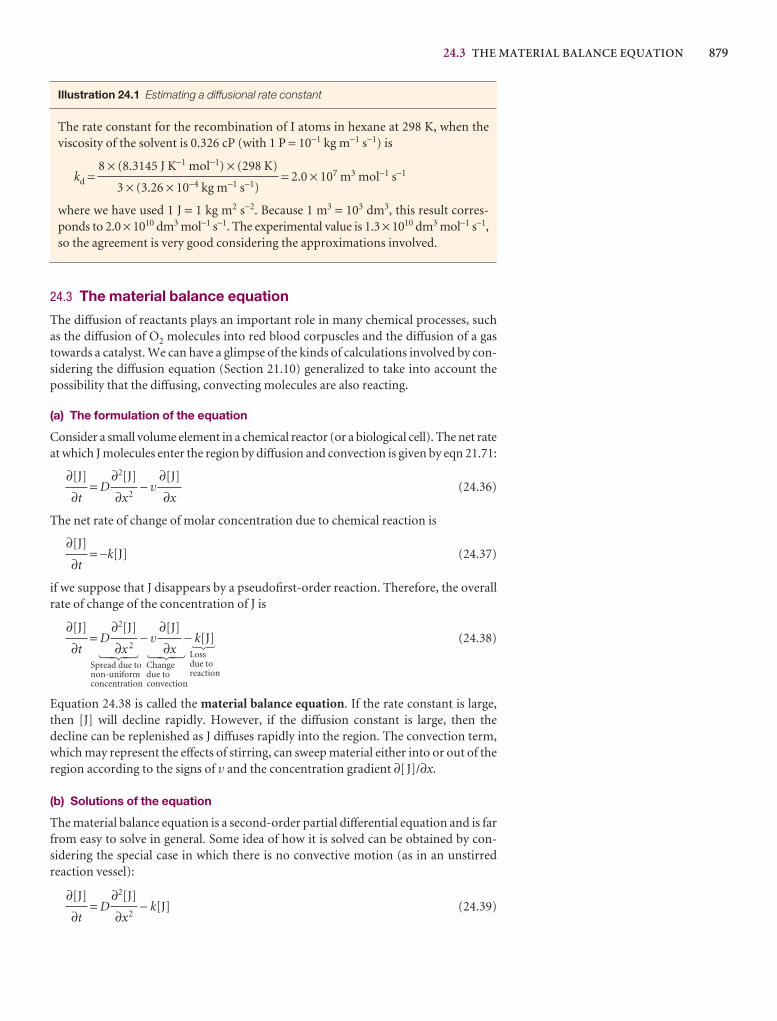
24.3 THE MATERIAL BALANCE EQUATION 879
Illustration 24.1 Estimating a diffusional rate constant
The rate constant for the recombination of I atoms in hexane at 298 K, when theviscosity of the solvent is 0.326 cP (with 1 P = 10−1 kg m−1 s−1) is
kd = = 2.0 × 10⁷ m3 mol−1 s−1
where we have used 1 J = 1 kg m2 s−2. Because 1 m3 = 103 dm3, this result corres-ponds to 2.0 × 10¹⁰ dm3 mol−1 s−1. The experimental value is 1.3 × 10¹⁰ dm3 mol−1 s−1,so the agreement is very good considering the approximations involved.
24.3 The material balance equation
The diffusion of reactants plays an important role in many chemical processes, suchas the diffusion of O2 molecules into red blood corpuscles and the diffusion of a gastowards a catalyst. We can have a glimpse of the kinds of calculations involved by con-sidering the diffusion equation (Section 21.10) generalized to take into account thepossibility that the diffusing, convecting molecules are also reacting.
(a) The formulation of the equation
Consider a small volume element in a chemical reactor (or a biological cell). The net rateat which J molecules enter the region by diffusion and convection is given by eqn 21.71:
= D − v (24.36)
The net rate of change of molar concentration due to chemical reaction is
= −k[J] (24.37)
if we suppose that J disappears by a pseudofirst-order reaction. Therefore, the overallrate of change of the concentration of J is
= D − v − k[J] (24.38)
Spread due to ChangeLoss
non-uniform due todue to
concentration convectionreaction
Equation 24.38 is called the material balance equation. If the rate constant is large,then [J] will decline rapidly. However, if the diffusion constant is large, then the decline can be replenished as J diffuses rapidly into the region. The convection term,which may represent the effects of stirring, can sweep material either into or out of theregion according to the signs of v and the concentration gradient ∂[J]/∂x.
(b) Solutions of the equation
The material balance equation is a second-order partial differential equation and is farfrom easy to solve in general. Some idea of how it is solved can be obtained by con-sidering the special case in which there is no convective motion (as in an unstirred reaction vessel):
= D − k[J] (24.39)∂2[J]
∂x2
∂[J]
∂t
! @1 2 31 2 3
∂[J]
∂x
∂2[J]
∂x 2
∂[J]
∂t
∂[J]
∂t
∂[J]
∂x
∂2[J]
∂x2
∂[J]
∂t
8 × (8.3145 J K−1 mol−1) × (298 K)
3 × (3.26 × 10−4 kg m−1 s−1)
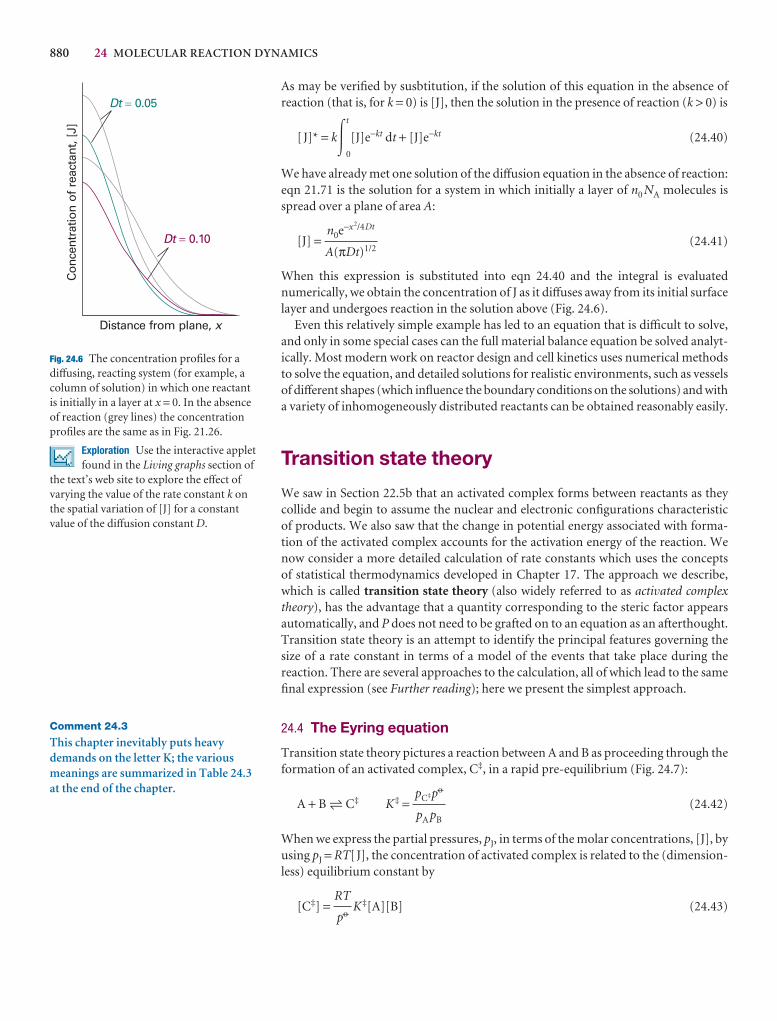
880 24 MOLECULAR REACTION DYNAMICS
As may be verified by susbtitution, if the solution of this equation in the absence of reaction (that is, for k = 0) is [J], then the solution in the presence of reaction (k > 0) is
[J]* = k�t
0
[J]e−kt dt + [J]e−kt (24.40)
We have already met one solution of the diffusion equation in the absence of reaction:eqn 21.71 is the solution for a system in which initially a layer of n0 NA molecules isspread over a plane of area A:
[J] = (24.41)
When this expression is substituted into eqn 24.40 and the integral is evaluated numerically, we obtain the concentration of J as it diffuses away from its initial surfacelayer and undergoes reaction in the solution above (Fig. 24.6).
Even this relatively simple example has led to an equation that is difficult to solve,and only in some special cases can the full material balance equation be solved analyt-ically. Most modern work on reactor design and cell kinetics uses numerical methodsto solve the equation, and detailed solutions for realistic environments, such as vesselsof different shapes (which influence the boundary conditions on the solutions) and witha variety of inhomogeneously distributed reactants can be obtained reasonably easily.
Transition state theory
We saw in Section 22.5b that an activated complex forms between reactants as theycollide and begin to assume the nuclear and electronic configurations characteristic of products. We also saw that the change in potential energy associated with forma-tion of the activated complex accounts for the activation energy of the reaction. Wenow consider a more detailed calculation of rate constants which uses the concepts of statistical thermodynamics developed in Chapter 17. The approach we describe,which is called transition state theory (also widely referred to as activated complextheory), has the advantage that a quantity corresponding to the steric factor appearsautomatically, and P does not need to be grafted on to an equation as an afterthought.Transition state theory is an attempt to identify the principal features governing thesize of a rate constant in terms of a model of the events that take place during the reaction. There are several approaches to the calculation, all of which lead to the samefinal expression (see Further reading); here we present the simplest approach.
24.4 The Eyring equation
Transition state theory pictures a reaction between A and B as proceeding through theformation of an activated complex, C‡, in a rapid pre-equilibrium (Fig. 24.7):
A + B 5 C‡ K‡ = (24.42)
When we express the partial pressures, pJ, in terms of the molar concentrations, [J], byusing pJ = RT[J], the concentration of activated complex is related to the (dimension-less) equilibrium constant by
[C‡] = K‡[A][B] (24.43)RT
p7
pC‡p7
pA pB
n0e−x2/4Dt
A(πDt)1/2
Dt � 0.05
Dt � 0.10
Distance from plane, x
Con
cent
ratio
n o
f re
acta
nt, [
J]
Fig. 24.6 The concentration profiles for adiffusing, reacting system (for example, acolumn of solution) in which one reactantis initially in a layer at x = 0. In the absenceof reaction (grey lines) the concentrationprofiles are the same as in Fig. 21.26.
Exploration Use the interactive appletfound in the Living graphs section of
the text’s web site to explore the effect ofvarying the value of the rate constant k onthe spatial variation of [J] for a constantvalue of the diffusion constant D.
Comment 24.3
This chapter inevitably puts heavydemands on the letter K; the variousmeanings are summarized in Table 24.3at the end of the chapter.
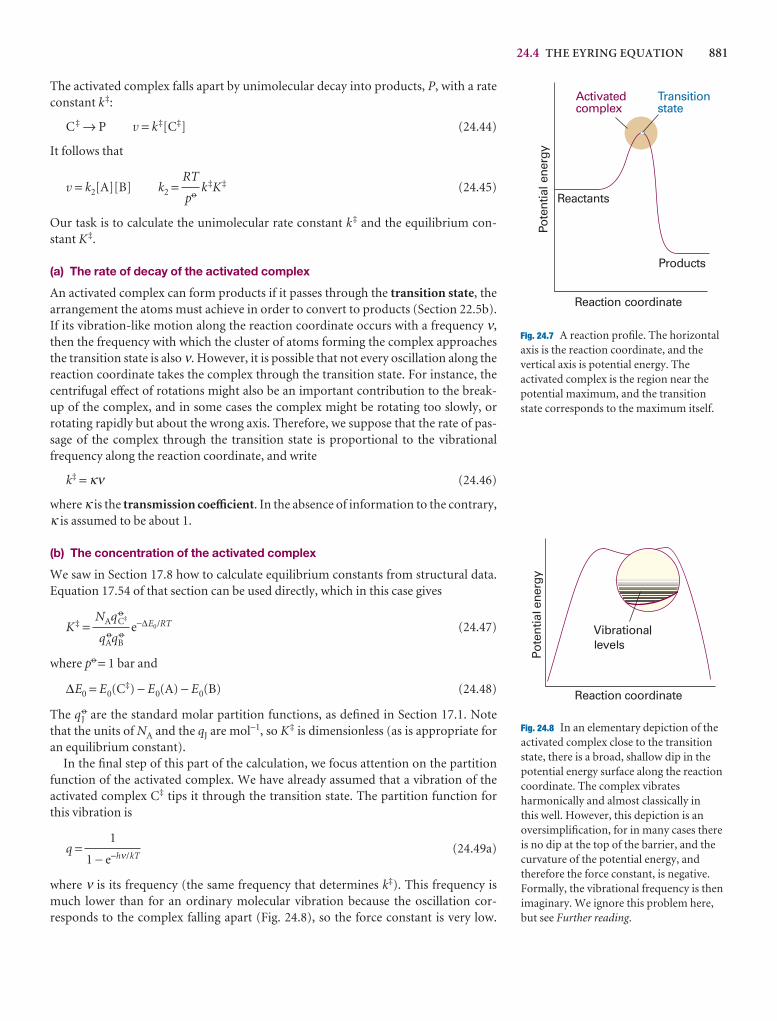
24.4 THE EYRING EQUATION 881
The activated complex falls apart by unimolecular decay into products, P, with a rateconstant k‡:
C‡ → P v = k‡[C‡] (24.44)
It follows that
v = k2[A][B] k2 = k‡K‡ (24.45)
Our task is to calculate the unimolecular rate constant k‡ and the equilibrium con-stant K‡.
(a) The rate of decay of the activated complex
An activated complex can form products if it passes through the transition state, thearrangement the atoms must achieve in order to convert to products (Section 22.5b).If its vibration-like motion along the reaction coordinate occurs with a frequency ν,then the frequency with which the cluster of atoms forming the complex approachesthe transition state is also ν. However, it is possible that not every oscillation along thereaction coordinate takes the complex through the transition state. For instance, thecentrifugal effect of rotations might also be an important contribution to the break-up of the complex, and in some cases the complex might be rotating too slowly, or rotating rapidly but about the wrong axis. Therefore, we suppose that the rate of pas-sage of the complex through the transition state is proportional to the vibrational frequency along the reaction coordinate, and write
k‡ = κν (24.46)
where κ is the transmission coefficient. In the absence of information to the contrary,κ is assumed to be about 1.
(b) The concentration of the activated complex
We saw in Section 17.8 how to calculate equilibrium constants from structural data.Equation 17.54 of that section can be used directly, which in this case gives
K‡ = e−∆E0/RT (24.47)
where p7 = 1 bar and
∆E0 = E0(C‡) − E0(A) − E0(B) (24.48)
The qJ7 are the standard molar partition functions, as defined in Section 17.1. Note
that the units of NA and the qJ are mol−1, so K‡ is dimensionless (as is appropriate foran equilibrium constant).
In the final step of this part of the calculation, we focus attention on the partitionfunction of the activated complex. We have already assumed that a vibration of the activated complex C‡ tips it through the transition state. The partition function forthis vibration is
q = (24.49a)
where ν is its frequency (the same frequency that determines k‡). This frequency ismuch lower than for an ordinary molecular vibration because the oscillation cor-responds to the complex falling apart (Fig. 24.8), so the force constant is very low.
1
1 − e−hν/kT
NAq 7C‡
q 7Aq 7
B
RT
p7
Activatedcomplex
Transitionstate
Reactants
Products
Reaction coordinate
Pote
ntia
l ene
rgy
Fig. 24.7 A reaction profile. The horizontalaxis is the reaction coordinate, and thevertical axis is potential energy. Theactivated complex is the region near thepotential maximum, and the transitionstate corresponds to the maximum itself.
Fig. 24.8 In an elementary depiction of theactivated complex close to the transitionstate, there is a broad, shallow dip in thepotential energy surface along the reactioncoordinate. The complex vibratesharmonically and almost classically in this well. However, this depiction is anoversimplification, for in many cases thereis no dip at the top of the barrier, and thecurvature of the potential energy, andtherefore the force constant, is negative.Formally, the vibrational frequency is thenimaginary. We ignore this problem here,but see Further reading.
882 24 MOLECULAR REACTION DYNAMICS
Therefore, provided that hν/kT << 1, the exponential may be expanded and the parti-tion function reduces to
q = ≈ (24.49b)
1 − 1 − + · · ·
We can therefore write
qC‡ ≈ ’C‡ (24.50)
where ’ denotes the partition function for all the other modes of the complex. Theconstant K‡ is therefore
K‡ = I‡ I‡ = e−∆E0/RT (24.51)
with I‡ a kind of equilibrium constant, but with one vibrational mode of C‡ discarded.
(c) The rate constant
We can now combine all the parts of the calculation into
k2 = k‡ K‡ = κν I‡ (24.52)
At this stage the unknown frequencies ν cancel and, after writing I ‡c = (RT/p7)I‡, we
obtain the Eyring equation:
k2 =κ I ‡c (24.53)
The factor I ‡c is given by eqn 24.51 and the definition I ‡
c = (RT/p7)I‡ in terms of thepartition functions of A, B, and C‡, so in principle we now have an explicit expressionfor calculating the second-order rate constant for a bimolecular reaction in terms ofthe molecular parameters for the reactants and the activated complex and the quan-tity κ.
The partition functions for the reactants can normally be calculated quite readily,using either spectroscopic information about their energy levels or the approximateexpressions set out in Table 17.3. The difficulty with the Eyring equation, however,lies in the calculation of the partition function of the activated complex: C‡ is difficultto investigate spectroscopically (but see Section 24.9), and in general we need to makeassumptions about its size, shape, and structure. We shall illustrate what is involved inone simple but significant case.
(d) The collision of structureless particles
Consider the case of two structureless particles A and B colliding to give an activatedcomplex that resembles a diatomic molecule. Because the reactants J = A, B are struc-tureless ‘atoms’, the only contributions to their partition functions are the transla-tional terms:
q 7J = ΛJ = V 7
m = (24.54)
The activated complex is a diatomic cluster of mass mC = mA + mB and moment of inertia I. It has one vibrational mode, but that mode corresponds to motion along the
RT
p7
h
(2πmJkT)1/2
V 7m
Λ3J
kT
h
RT
p7
kT
hνRT
p7
NA’ 7C‡
q 7Aq 7
B
kT
hν
kT
hν
DEFhνkT
ABC
kT
hν
1
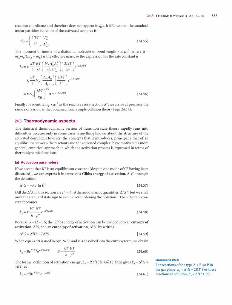
24.5 THERMODYNAMIC ASPECTS 883
reaction coordinate and therefore does not appear in ’C‡. It follows that the standardmolar partition function of the activated complex is
q 7C‡ = (24.55)
The moment of inertia of a diatomic molecule of bond length r is µr 2, where µ =mAmB/(mA + mB) is the effective mass, so the expression for the rate constant is
k2 = κ e−∆E0/RT
= κ NA e−∆E0/RT
= κNA
1/2
πr 2e−∆E0/RT (24.56)
Finally, by identifying κ πr2 as the reactive cross-section σ*, we arrive at precisely thesame expression as that obtained from simple collision theory (eqn 24.14).
24.5 Thermodynamic aspects
The statistical thermodynamic version of transition state theory rapidly runs intodifficulties because only in some cases is anything known about the structure of theactivated complex. However, the concepts that it introduces, principally that of anequilibrium between the reactants and the activated complex, have motivated a moregeneral, empirical approach in which the activation process is expressed in terms ofthermodynamic functions.
(a) Activation parameters
If we accept that I‡ is an equilibrium constant (despite one mode of C‡ having beendiscarded), we can express it in terms of a Gibbs energy of activation, ∆‡G, throughthe definition
∆‡G = −RT ln I‡ [24.57]
(All the ∆‡X in this section are standard thermodynamic quantities, ∆‡X 7, but we shallomit the standard state sign to avoid overburdening the notation). Then the rate con-stant becomes
k2 = κ e−∆‡G /RT (24.58)
Because G = H − TS, the Gibbs energy of activation can be divided into an entropy ofactivation, ∆‡S, and an enthalpy of activation, ∆‡H, by writing
∆‡G = ∆‡H − T∆‡S [24.59]
When eqn 24.59 is used in eqn 24.58 and κ is absorbed into the entropy term, we obtain
k2 = Be∆‡S/Re−∆‡H/RT B = (24.60)
The formal definition of activation energy, Ea = RT 2(∂ ln k/∂T), then gives Ea = ∆‡H +2RT, so
k2 = e2Be∆‡S/Re−Ea/RT (24.61)
RT
p7
kT
h
RT
p7
kT
h
DF
8kT
πµ
AC
DF
2IkT
$2
AC
DF
ΛAΛB
ΛC‡
AC
kT
h
DF
2IkT
$2
AC
DF
NAΛ3AΛ3
B
Λ3C‡V 7
m
AC
RT
p7
kT
h
V 7m
Λ3C‡
DF
2IkT
$2
AC
Comment 24.4
For reactions of the type A + B 5 P inthe gas phase, Ea = ∆‡H + 2RT. For thesereactions in solution, Ea = ∆‡H + RT.
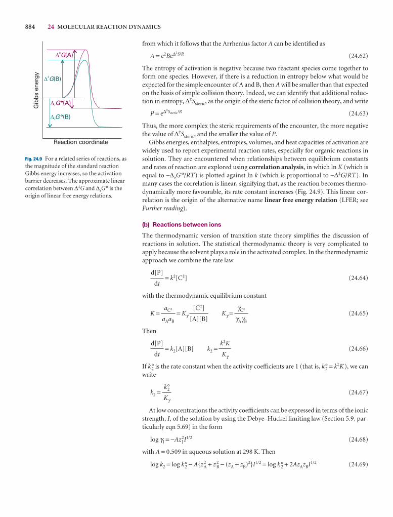
884 24 MOLECULAR REACTION DYNAMICS
from which it follows that the Arrhenius factor A can be identified as
A = e2Be∆‡S/R (24.62)
The entropy of activation is negative because two reactant species come together toform one species. However, if there is a reduction in entropy below what would be expected for the simple encounter of A and B, then A will be smaller than that expectedon the basis of simple collision theory. Indeed, we can identify that additional reduc-tion in entropy, ∆‡Ssteric, as the origin of the steric factor of collision theory, and write
P = e∆‡Ssteric/R (24.63)
Thus, the more complex the steric requirements of the encounter, the more negativethe value of ∆‡Ssteric, and the smaller the value of P.
Gibbs energies, enthalpies, entropies, volumes, and heat capacities of activation arewidely used to report experimental reaction rates, especially for organic reactions insolution. They are encountered when relationships between equilibrium constantsand rates of reaction are explored using correlation analysis, in which ln K (which isequal to −∆rG
7/RT) is plotted against ln k (which is proportional to −∆‡G/RT). Inmany cases the correlation is linear, signifying that, as the reaction becomes thermo-dynamically more favourable, its rate constant increases (Fig. 24.9). This linear cor-relation is the origin of the alternative name linear free energy relation (LFER; seeFurther reading).
(b) Reactions between ions
The thermodynamic version of transition state theory simplifies the discussion of reactions in solution. The statistical thermodynamic theory is very complicated toapply because the solvent plays a role in the activated complex. In the thermodynamicapproach we combine the rate law
= k‡[C‡] (24.64)
with the thermodynamic equilibrium constant
K = = Kγ Kγ = (24.65)
Then
= k2[A][B] k2 = (24.66)
If k°2 is the rate constant when the activity coefficients are 1 (that is, k°2 = k‡K), we canwrite
k2 = (24.67)
At low concentrations the activity coefficients can be expressed in terms of the ionicstrength, I, of the solution by using the Debye–Hückel limiting law (Section 5.9, par-ticularly eqn 5.69) in the form
log γJ = −Az J2I1/2 (24.68)
with A = 0.509 in aqueous solution at 298 K. Then
log k2 = log k°2 − A{z 2A + z 2
B − (zA + zB)2}I1/2 = log k°2 + 2AzAzBI1/2 (24.69)
k°2
Kγ
k‡K
Kγ
d[P]
dt
γC‡
γAγB
[C‡]
[A][B]
aC‡
aAaB
d[P]
dt
Reaction coordinate
Gib
bs e
nerg
y
‡G(B)
‡G(A)
rG °(B)
rG°(A)
Fig. 24.9 For a related series of reactions, asthe magnitude of the standard reactionGibbs energy increases, so the activationbarrier decreases. The approximate linearcorrelation between ∆‡G and ∆rG
7 is theorigin of linear free energy relations.
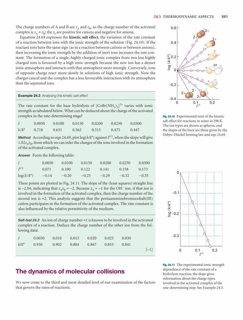
24.5 THERMODYNAMIC ASPECTS 885
�0.4
�0.2
0.2
0.4
0.6
log
(/
°)k
k
0 0.1 0.2I 1/2
2�2�
2�
2�
2�
�
�
��
�
�
�2�
0�or
Fig. 24.10 Experimental tests of the kinetic salt effect for reactions in water at 298 K.The ion types are shown as spheres, and the slopes of the lines are those given by theDebye–Hückel limiting law and eqn 24.69.
0 0.1 0.2
0
�0.1
�0.2
�0.3
log
(/
°)k
k
I 1/2
Fig. 24.11 The experimental ionic strengthdependence of the rate constant of ahydrolysis reaction: the slope givesinformation about the charge typesinvolved in the activated complex of therate-determining step. See Example 24.3.
The charge numbers of A and B are zA and zB, so the charge number of the activatedcomplex is zA + zB; the zJ are positive for cations and negative for anions.
Equation 24.69 expresses the kinetic salt effect, the variation of the rate constant of a reaction between ions with the ionic strength of the solution (Fig. 24.10). If the reactant ions have the same sign (as in a reaction between cations or between anions),then increasing the ionic strength by the addition of inert ions increases the rate con-stant. The formation of a single, highly charged ionic complex from two less highlycharged ions is favoured by a high ionic strength because the new ion has a denserionic atmosphere and interacts with that atmosphere more strongly. Conversely, ionsof opposite charge react more slowly in solutions of high ionic strength. Now thecharges cancel and the complex has a less favourable interaction with its atmospherethan the separated ions.
Example 24.3 Analysing the kinetic salt effect
The rate constant for the base hydrolysis of [CoBr(NH3)5]2+ varies with ionicstrength as tabulated below. What can be deduced about the charge of the activatedcomplex in the rate-determining stage?
I 0.0050 0.0100 0.0150 0.0200 0.0250 0.0300
k /k° 0.718 0.631 0.562 0.515 0.475 0.447
Method According to eqn 24.69, plot log(k/k°) against I1/2, when the slope will give1.02zAzB, from which we can infer the charges of the ions involved in the formationof the activated complex.
Answer Form the following table:
I 0.0050 0.0100 0.0150 0.0200 0.0250 0.0300
I1/2 0.071 0.100 0.122 0.141 0.158 0.173
log(k /k°) −0.14 −0.20 −0.25 −0.29 −0.32 −0.35
These points are plotted in Fig. 24.11. The slope of the (least squares) straight lineis −2.04, indicating that zAzB = −2. Because zA = −1 for the OH− ion, if that ion is involved in the formation of the activated complex, then the charge number of thesecond ion is +2. This analysis suggests that the pentaamminebromocobalt(III)cation participates in the formation of the activated complex. The rate constant isalso influenced by the relative permittivity of the medium.
Self-test 24.3 An ion of charge number +1 is known to be involved in the activatedcomplex of a reaction. Deduce the charge number of the other ion from the fol-lowing data:
I 0.0050 0.010 0.015 0.020 0.025 0.030
k/k° 0.930 0.902 0.884 0.867 0.853 0.841[−1]
The dynamics of molecular collisions
We now come to the third and most detailed level of our examination of the factorsthat govern the rates of reactions.
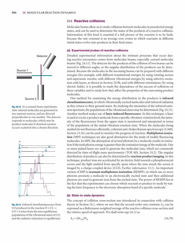
886 24 MOLECULAR REACTION DYNAMICS
24.6 Reactive collisions
Molecular beams allow us to study collisions between molecules in preselected energystates, and can be used to determine the states of the products of a reactive collision.Information of this kind is essential if a full picture of the reaction is to be built, because the rate constant is an average over events in which reactants in differentinitial states evolve into products in their final states.
(a) Experimental probes of reactive collisions
Detailed experimental information about the intimate processes that occur dur-ing reactive encounters comes from molecular beams, especially crossed molecularbeams (Fig. 24.12). The detector for the products of the collision of two beams can bemoved to different angles, so the angular distribution of the products can be deter-mined. Because the molecules in the incoming beams can be prepared with differentenergies (for example, with different translational energies by using rotating sectorsand supersonic nozzles, with different vibrational energies by using selective excita-tion with lasers, as shown in Section 24.9b, and with different orientations (by usingelectric fields), it is possible to study the dependence of the success of collisions onthese variables and to study how they affect the properties of the outcoming productmolecules.
One method for examining the energy distribution in the products is infraredchemiluminescence, in which vibrationally excited molecules emit infrared radiationas they return to their ground states. By studying the intensities of the infrared emis-sion spectrum, the populations of the vibrational states may be determined (Fig. 24.13).Another method makes use of laser-induced fluorescence. In this technique, a laseris used to excite a product molecule from a specific vibration-rotation level; the inten-sity of the fluorescence from the upper state is monitored and interpreted in terms of the population of the initial vibration-rotation state. When the molecules beingstudied do not fluoresce efficiently, coherent anti-Stokes Raman spectroscopy (CARS,Section 13.16) can be used to monitor the progress of reaction. Multiphoton ioniza-tion (MPI) techniques are also good alternatives for the study of weakly fluorescingmolecules. In MPI, the absorption of several photons by a molecule results in ioniza-tion if the total photon energy is greater than the ionization energy of the molecule. Oneor more pulsed lasers are used to generate the molecular ions, which are commonlydetected by time-of-flight mass spectrometry (TOF-MS, Section 19.2). The angulardistribution of products can also be determined by reaction product imaging. In thistechnique, product ions are accelerated by an electric field towards a phosphorescentscreen and the light emitted from specific spots where the ions struck the screen is imaged by a charge-coupled device (CCD, Further information 13.1). An importantvariant of MPI is resonant multiphoton ionization (REMPI), in which one or morephotons promote a molecule to an electronically excited state and then additionalphotons are used to generate ions from the excited state. The power of REMPI lies inthe fact that the experimenter can choose which reactant or product to study by tun-ing the laser frequency to the electronic absorption band of a specific molecule.
(b) State-to-state dynamics
The concept of collision cross-section was introduced in connection with collisiontheory in Section 24.1, where we saw that the second-order rate constant, k2, can beexpressed as a Boltzmann-weighted average of the reactive collision cross-section andthe relative speed of approach. We shall write eqn 24.12 as
k2 = �σvrel�NA (24.70)
Source 1
Source 2
Detector
Fig. 24.12 In a crossed-beam experiment,state-selected molecules are generated intwo separate sources, and are directedperpendicular to one another. The detectorresponds to molecules (which may beproduct molecules if chemical reactionoccurs) scattered into a chosen direction.
0
1
2
3
4
567
v
Fig. 24.13 Infrared chemiluminescence fromCO produced in the reaction O + CS →CO + S arises from the non-equilibriumpopulations of the vibrational states of COand the radiative relaxation to equilibrium.
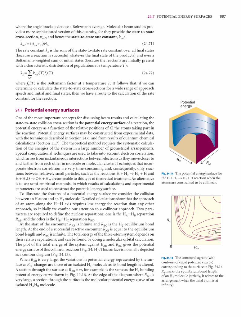
24.7 POTENTIAL ENERGY SURFACES 887
where the angle brackets denote a Boltzmann average. Molecular beam studies pro-vide a more sophisticated version of this quantity, for they provide the state-to-statecross-section, σnn′, and hence the state-to-state rate constant, knn′:
knn′ = �σnn′vrel�NA (24.71)
The rate constant k2 is the sum of the state-to-state rate constant over all final states(because a reaction is successful whatever the final state of the products) and over aBoltzmann-weighted sum of initial states (because the reactants are initially presentwith a characteristic distribution of populations at a temperature T):
k2 = ∑n,n′
knn′(T)fn(T) (24.72)
where fn(T) is the Boltzmann factor at a temperature T. It follows that, if we can determine or calculate the state-to-state cross-sections for a wide range of approachspeeds and initial and final states, then we have a route to the calculation of the rateconstant for the reaction.
24.7 Potential energy surfaces
One of the most important concepts for discussing beam results and calculating thestate-to-state collision cross-section is the potential energy surface of a reaction, thepotential energy as a function of the relative positions of all the atoms taking part inthe reaction. Potential energy surfaces may be constructed from experimental data,with the techniques described in Section 24.6, and from results of quantum chemicalcalculations (Section 11.7). The theoretical method requires the systematic calcula-tion of the energies of the system in a large number of geometrical arrangements.Special computational techniques are used to take into account electron correlation,which arises from instantaneous interactions between electrons as they move closer toand farther from each other in molecule or molecular cluster. Techniques that incor-porate electron correlation are very time-consuming and, consequently, only reac-tions between relatively small particles, such as the reactions H + H2 → H2 + H and H + H2O → OH + H2, are amenable to this type of theoretical treatment. An alternativeis to use semi-empirical methods, in which results of calculations and experimentalparameters are used to construct the potential energy surface.
To illustrate the features of a potential energy surface we consider the collision between an H atom and an H2 molecule. Detailed calculations show that the approachof an atom along the H-H axis requires less energy for reaction than any other approach, so initially we confine our attention to a collinear approach. Two para-meters are required to define the nuclear separations: one is the HA-HB separationRAB, and the other is the HB-HC separation RBC.
At the start of the encounter RAB is infinite and RBC is the H2 equilibrium bondlength. At the end of a successful reactive encounter RAB is equal to the equilibriumbond length and RBC is infinite. The total energy of the three-atom system depends ontheir relative separations, and can be found by doing a molecular orbital calculation.The plot of the total energy of the system against RAB and RBC gives the potential energy surface of this collinear reaction (Fig. 24.14). This surface is normally depictedas a contour diagram (Fig. 24.15).
When RAB is very large, the variations in potential energy represented by the sur-face as RBC changes are those of an isolated H2 molecule as its bond length is altered.A section through the surface at RAB = ∞, for example, is the same as the H2 bondingpotential energy curve drawn in Fig. 11.16. At the edge of the diagram where RBC isvery large, a section through the surface is the molecular potential energy curve of anisolated HAHB molecule.
Potentialenergy
RBCRAB
Re
Re
RBC
RAB0
Fig. 24.14 The potential energy surface forthe H + H2 → H2 + H reaction when theatoms are constrained to be collinear.
Fig. 24.15 The contour diagram (withcontours of equal potential energy)corresponding to the surface in Fig. 24.14.Re marks the equilibrium bond length of an H2 molecule (strictly, it relates to thearrangement when the third atom is atinfinity).
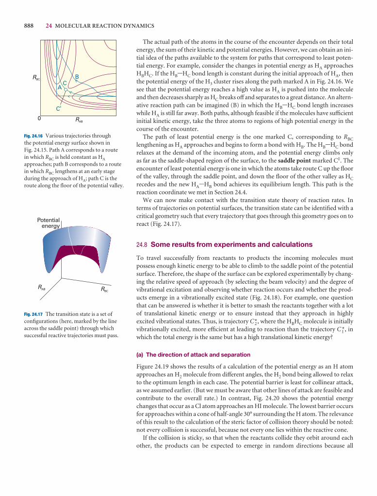
888 24 MOLECULAR REACTION DYNAMICS
The actual path of the atoms in the course of the encounter depends on their totalenergy, the sum of their kinetic and potential energies. However, we can obtain an ini-tial idea of the paths available to the system for paths that correspond to least poten-tial energy. For example, consider the changes in potential energy as HA approachesHBHC. If the HB-HC bond length is constant during the initial approach of HA, thenthe potential energy of the H3 cluster rises along the path marked A in Fig. 24.16. Wesee that the potential energy reaches a high value as HA is pushed into the moleculeand then decreases sharply as HC breaks off and separates to a great distance. An altern-ative reaction path can be imagined (B) in which the HB-HC bond length increaseswhile HA is still far away. Both paths, although feasible if the molecules have sufficientinitial kinetic energy, take the three atoms to regions of high potential energy in thecourse of the encounter.
The path of least potential energy is the one marked C, corresponding to RBC
lengthening as HA approaches and begins to form a bond with HB. The HB-HC bondrelaxes at the demand of the incoming atom, and the potential energy climbs only as far as the saddle-shaped region of the surface, to the saddle point marked C‡. Theencounter of least potential energy is one in which the atoms take route C up the floorof the valley, through the saddle point, and down the floor of the other valley as HC
recedes and the new HA-HB bond achieves its equilibrium length. This path is the reaction coordinate we met in Section 24.4.
We can now make contact with the transition state theory of reaction rates. Interms of trajectories on potential surfaces, the transition state can be identified with acritical geometry such that every trajectory that goes through this geometry goes on toreact (Fig. 24.17).
24.8 Some results from experiments and calculations
To travel successfully from reactants to products the incoming molecules must possess enough kinetic energy to be able to climb to the saddle point of the potentialsurface. Therefore, the shape of the surface can be explored experimentally by chang-ing the relative speed of approach (by selecting the beam velocity) and the degree of vibrational excitation and observing whether reaction occurs and whether the prod-ucts emerge in a vibrationally excited state (Fig. 24.18). For example, one questionthat can be answered is whether it is better to smash the reactants together with a lotof translational kinetic energy or to ensure instead that they approach in highly excited vibrational states. Thus, is trajectory C 2*, where the HBHC molecule is initiallyvibrationally excited, more efficient at leading to reaction than the trajectory C 1*, inwhich the total energy is the same but has a high translational kinetic energy?
(a) The direction of attack and separation
Figure 24.19 shows the results of a calculation of the potential energy as an H atomapproaches an H2 molecule from different angles, the H2 bond being allowed to relaxto the optimum length in each case. The potential barrier is least for collinear attack,as we assumed earlier. (But we must be aware that other lines of attack are feasible andcontribute to the overall rate.) In contrast, Fig. 24.20 shows the potential energychanges that occur as a Cl atom approaches an HI molecule. The lowest barrier occursfor approaches within a cone of half-angle 30° surrounding the H atom. The relevanceof this result to the calculation of the steric factor of collision theory should be noted:not every collision is successful, because not every one lies within the reactive cone.
If the collision is sticky, so that when the reactants collide they orbit around eachother, the products can be expected to emerge in random directions because all
RBC
RAB0
B
AC
C‡
Fig. 24.16 Various trajectories through the potential energy surface shown in Fig. 24.15. Path A corresponds to a route in which RBC is held constant as HA
approaches; path B corresponds to a routein which RBC lengthens at an early stageduring the approach of HA; path C is theroute along the floor of the potential valley.
Potentialenergy
RAB RBC
Fig. 24.17 The transition state is a set ofconfigurations (here, marked by the lineacross the saddle point) through whichsuccessful reactive trajectories must pass.
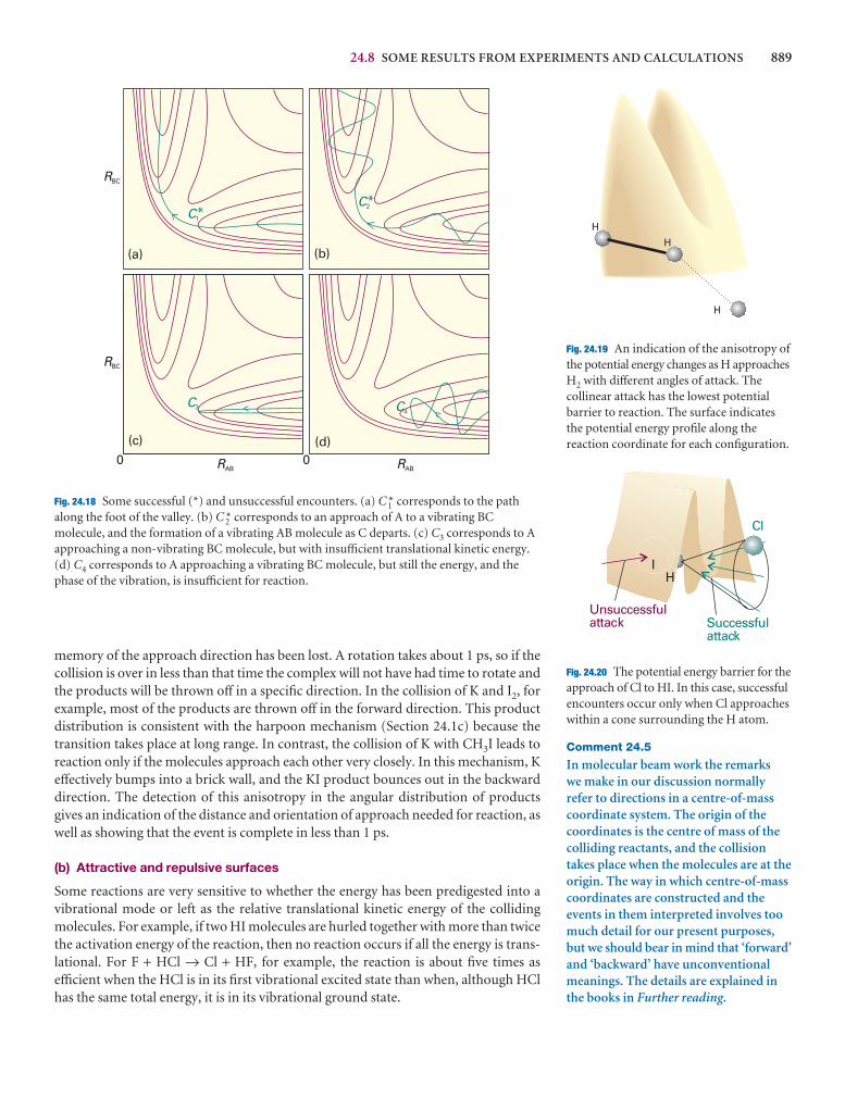
24.8 SOME RESULTS FROM EXPERIMENTS AND CALCULATIONS 889
memory of the approach direction has been lost. A rotation takes about 1 ps, so if thecollision is over in less than that time the complex will not have had time to rotate andthe products will be thrown off in a specific direction. In the collision of K and I2, forexample, most of the products are thrown off in the forward direction. This productdistribution is consistent with the harpoon mechanism (Section 24.1c) because thetransition takes place at long range. In contrast, the collision of K with CH3I leads toreaction only if the molecules approach each other very closely. In this mechanism, Keffectively bumps into a brick wall, and the KI product bounces out in the backwarddirection. The detection of this anisotropy in the angular distribution of productsgives an indication of the distance and orientation of approach needed for reaction, aswell as showing that the event is complete in less than 1 ps.
(b) Attractive and repulsive surfaces
Some reactions are very sensitive to whether the energy has been predigested into a vibrational mode or left as the relative translational kinetic energy of the collidingmolecules. For example, if two HI molecules are hurled together with more than twicethe activation energy of the reaction, then no reaction occurs if all the energy is trans-lational. For F + HCl → Cl + HF, for example, the reaction is about five times asefficient when the HCl is in its first vibrational excited state than when, although HClhas the same total energy, it is in its vibrational ground state.
RBC
RBC
RAB RAB0 0
C1*
(a) (b)
C2*
C3 C4
(c) (d)
Fig. 24.18 Some successful (*) and unsuccessful encounters. (a) C 1* corresponds to the pathalong the foot of the valley. (b) C 2* corresponds to an approach of A to a vibrating BCmolecule, and the formation of a vibrating AB molecule as C departs. (c) C3 corresponds to Aapproaching a non-vibrating BC molecule, but with insufficient translational kinetic energy.(d) C4 corresponds to A approaching a vibrating BC molecule, but still the energy, and thephase of the vibration, is insufficient for reaction.
H
H
H
H
Unsuccessfulattack Successful
attack
IH
Cl
Fig. 24.20 The potential energy barrier for theapproach of Cl to HI. In this case, successfulencounters occur only when Cl approacheswithin a cone surrounding the H atom.
Fig. 24.19 An indication of the anisotropy ofthe potential energy changes as H approachesH2 with different angles of attack. Thecollinear attack has the lowest potentialbarrier to reaction. The surface indicatesthe potential energy profile along thereaction coordinate for each configuration.
Comment 24.5
In molecular beam work the remarks we make in our discussion normallyrefer to directions in a centre-of-masscoordinate system. The origin of thecoordinates is the centre of mass of thecolliding reactants, and the collisiontakes place when the molecules are at theorigin. The way in which centre-of-masscoordinates are constructed and theevents in them interpreted involves toomuch detail for our present purposes,but we should bear in mind that ‘forward’and ‘backward’ have unconventionalmeanings. The details are explained inthe books in Further reading.
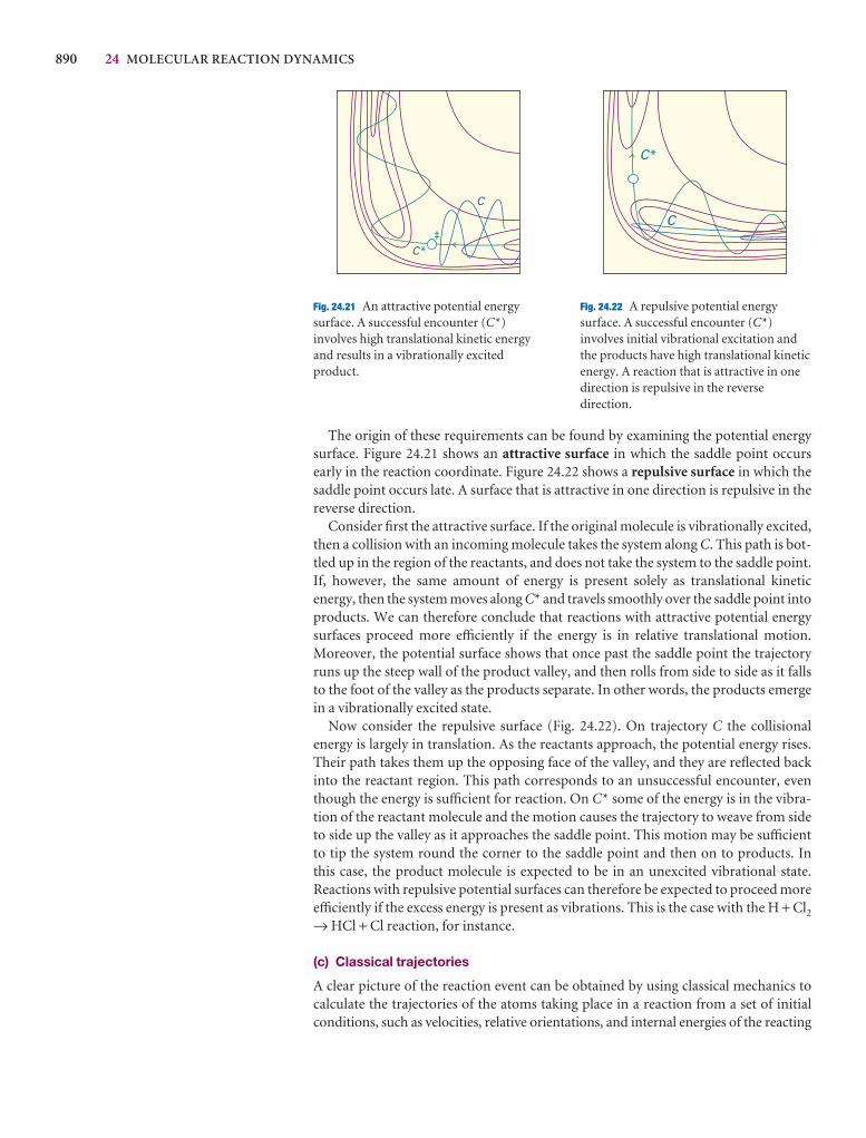
890 24 MOLECULAR REACTION DYNAMICS
The origin of these requirements can be found by examining the potential energysurface. Figure 24.21 shows an attractive surface in which the saddle point occursearly in the reaction coordinate. Figure 24.22 shows a repulsive surface in which thesaddle point occurs late. A surface that is attractive in one direction is repulsive in thereverse direction.
Consider first the attractive surface. If the original molecule is vibrationally excited,then a collision with an incoming molecule takes the system along C. This path is bot-tled up in the region of the reactants, and does not take the system to the saddle point.If, however, the same amount of energy is present solely as translational kinetic energy, then the system moves along C* and travels smoothly over the saddle point intoproducts. We can therefore conclude that reactions with attractive potential energysurfaces proceed more efficiently if the energy is in relative translational motion.Moreover, the potential surface shows that once past the saddle point the trajectoryruns up the steep wall of the product valley, and then rolls from side to side as it fallsto the foot of the valley as the products separate. In other words, the products emergein a vibrationally excited state.
Now consider the repulsive surface (Fig. 24.22). On trajectory C the collisional energy is largely in translation. As the reactants approach, the potential energy rises.Their path takes them up the opposing face of the valley, and they are reflected backinto the reactant region. This path corresponds to an unsuccessful encounter, eventhough the energy is sufficient for reaction. On C* some of the energy is in the vibra-tion of the reactant molecule and the motion causes the trajectory to weave from sideto side up the valley as it approaches the saddle point. This motion may be sufficientto tip the system round the corner to the saddle point and then on to products. In this case, the product molecule is expected to be in an unexcited vibrational state.Reactions with repulsive potential surfaces can therefore be expected to proceed moreefficiently if the excess energy is present as vibrations. This is the case with the H + Cl2→ HCl + Cl reaction, for instance.
(c) Classical trajectories
A clear picture of the reaction event can be obtained by using classical mechanics tocalculate the trajectories of the atoms taking place in a reaction from a set of initialconditions, such as velocities, relative orientations, and internal energies of the reacting
C*‡
C
C*
C
Fig. 24.21 An attractive potential energysurface. A successful encounter (C*)involves high translational kinetic energyand results in a vibrationally excitedproduct.
Fig. 24.22 A repulsive potential energysurface. A successful encounter (C*)involves initial vibrational excitation andthe products have high translational kineticenergy. A reaction that is attractive in onedirection is repulsive in the reversedirection.
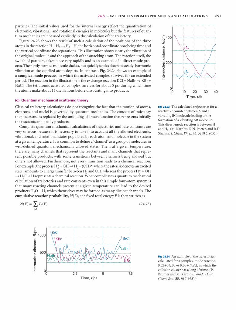
24.8 SOME RESULTS FROM EXPERIMENTS AND CALCULATIONS 891
particles. The initial values used for the internal energy reflect the quantization ofelectronic, vibrational, and rotational energies in molecules but the features of quan-tum mechanics are not used explicitly in the calculation of the trajectory.
Figure 24.23 shows the result of such a calculation of the positions of the threeatoms in the reaction H + H2 → H2 + H, the horizontal coordinate now being time andthe vertical coordinate the separations. This illustration shows clearly the vibration ofthe original molecule and the approach of the attacking atom. The reaction itself, theswitch of partners, takes place very rapidly and is an example of a direct mode pro-cess. The newly formed molecule shakes, but quickly settles down to steady, harmonicvibration as the expelled atom departs. In contrast, Fig. 24.24 shows an example of a complex mode process, in which the activated complex survives for an extended period. The reaction in the illustration is the exchange reaction KCl + NaBr → KBr +NaCl. The tetratomic activated complex survives for about 5 ps, during which timethe atoms make about 15 oscillations before dissociating into products.
(d) Quantum mechanical scattering theory
Classical trajectory calculations do not recognize the fact that the motion of atoms,electrons, and nuclei is governed by quantum mechanics. The concept of trajectorythen fades and is replaced by the unfolding of a wavefunction that represents initiallythe reactants and finally products.
Complete quantum mechanical calculations of trajectories and rate constants arevery onerous because it is necessary to take into account all the allowed electronic, vibrational, and rotational states populated by each atom and molecule in the system at a given temperature. It is common to define a ‘channel’ as a group of molecules inwell-defined quantum mechanically allowed states. Then, at a given temperature,there are many channels that represent the reactants and many channels that repre-sent possible products, with some transitions between channels being allowed butothers not allowed. Furthermore, not every transition leads to a chemical reaction.For example, the process H2* + OH → H2 + (OH)*, where the asterisk denotes an excitedstate, amounts to energy transfer between H2 and OH, whereas the process H2* + OH→ H2O + H represents a chemical reaction. What complicates a quantum mechanicalcalculation of trajectories and rate constants even in this simple four-atom system isthat many reacting channels present at a given temperature can lead to the desiredproducts H2O + H, which themselves may be formed as many distinct channels. Thecumulative reaction probability, N(E), at a fixed total energy E is then written as
N(E) = ∑i, j
Pij(E) (24.73)
0
200
400
Inte
rnuc
lear
dis
tanc
e,/p
mR
0 10 20 30 40Time, /fst
RAB
RBC
Fig. 24.23 The calculated trajectories for areactive encounter between A and avibrating BC molecule leading to theformation of a vibrating AB molecule. This direct-mode reaction is between Hand H2. (M. Karplus, R.N. Porter, and R.D.Sharma, J. Chem. Phys., 43, 3258 (1965).)
Time, /pst0 2.5 5 7.5
500
1000
Inte
rnuc
lear
dis
tanc
e,/p
mR
0
BrCl
NaBr
KBr
KBr
NaBr
BrCl
Fig. 24.24 An example of the trajectoriescalculated for a complex-mode reaction,KCl + NaBr → KBr + NaCl, in which thecollision cluster has a long lifetime. (P.Brumer and M. Karplus, Faraday Disc.Chem. Soc., 55, 80 (1973).)
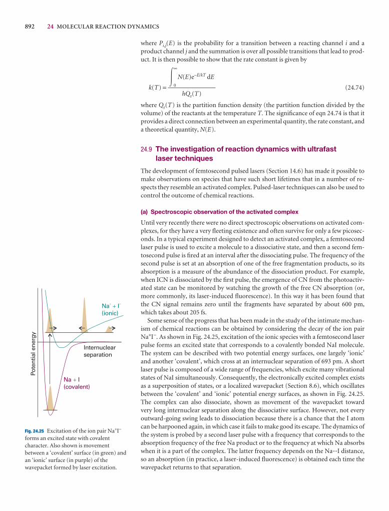
892 24 MOLECULAR REACTION DYNAMICS
where Pi,j(E) is the probability for a transition between a reacting channel i and aproduct channel j and the summation is over all possible transitions that lead to prod-uct. It is then possible to show that the rate constant is given by
k(T) = (24.74)
where Qr(T) is the partition function density (the partition function divided by thevolume) of the reactants at the temperature T. The significance of eqn 24.74 is that itprovides a direct connection between an experimental quantity, the rate constant, anda theoretical quantity, N(E).
24.9 The investigation of reaction dynamics with ultrafast laser techniques
The development of femtosecond pulsed lasers (Section 14.6) has made it possible tomake observations on species that have such short lifetimes that in a number of re-spects they resemble an activated complex. Pulsed-laser techniques can also be used tocontrol the outcome of chemical reactions.
(a) Spectroscopic observation of the activated complex
Until very recently there were no direct spectroscopic observations on activated com-plexes, for they have a very fleeting existence and often survive for only a few picosec-onds. In a typical experiment designed to detect an activated complex, a femtosecondlaser pulse is used to excite a molecule to a dissociative state, and then a second fem-tosecond pulse is fired at an interval after the dissociating pulse. The frequency of thesecond pulse is set at an absorption of one of the free fragmentation products, so itsabsorption is a measure of the abundance of the dissociation product. For example,when ICN is dissociated by the first pulse, the emergence of CN from the photoactiv-ated state can be monitored by watching the growth of the free CN absorption (or,more commonly, its laser-induced fluorescence). In this way it has been found thatthe CN signal remains zero until the fragments have separated by about 600 pm,which takes about 205 fs.
Some sense of the progress that has been made in the study of the intimate mechan-ism of chemical reactions can be obtained by considering the decay of the ion pairNa+I−. As shown in Fig. 24.25, excitation of the ionic species with a femtosecond laserpulse forms an excited state that corresponds to a covalently bonded NaI molecule.The system can be described with two potential energy surfaces, one largely ‘ionic’and another ‘covalent’, which cross at an internuclear separation of 693 pm. A short laser pulse is composed of a wide range of frequencies, which excite many vibrational states of NaI simultaneously. Consequently, the electronically excited complex existsas a superposition of states, or a localized wavepacket (Section 8.6), which oscillates between the ‘covalent’ and ‘ionic’ potential energy surfaces, as shown in Fig. 24.25.The complex can also dissociate, shown as movement of the wavepacket toward very long internuclear separation along the dissociative surface. However, not every outward-going swing leads to dissociation because there is a chance that the I atomcan be harpooned again, in which case it fails to make good its escape. The dynamics of the system is probed by a second laser pulse with a frequency that corresponds to theabsorption frequency of the free Na product or to the frequency at which Na absorbswhen it is a part of the complex. The latter frequency depends on the Na···I distance,so an absorption (in practice, a laser-induced fluorescence) is obtained each time thewavepacket returns to that separation.
�∞
0
N(E)e−E/kT dE
hQr(T)
Na I(covalent)
�
Na I(ionic)
��
�
Internuclearseparation
Pote
ntia
l ene
rgy
Fig. 24.25 Excitation of the ion pair Na+I−
forms an excited state with covalentcharacter. Also shown is movementbetween a ‘covalent’ surface (in green) andan ‘ionic’ surface (in purple) of thewavepacket formed by laser excitation.
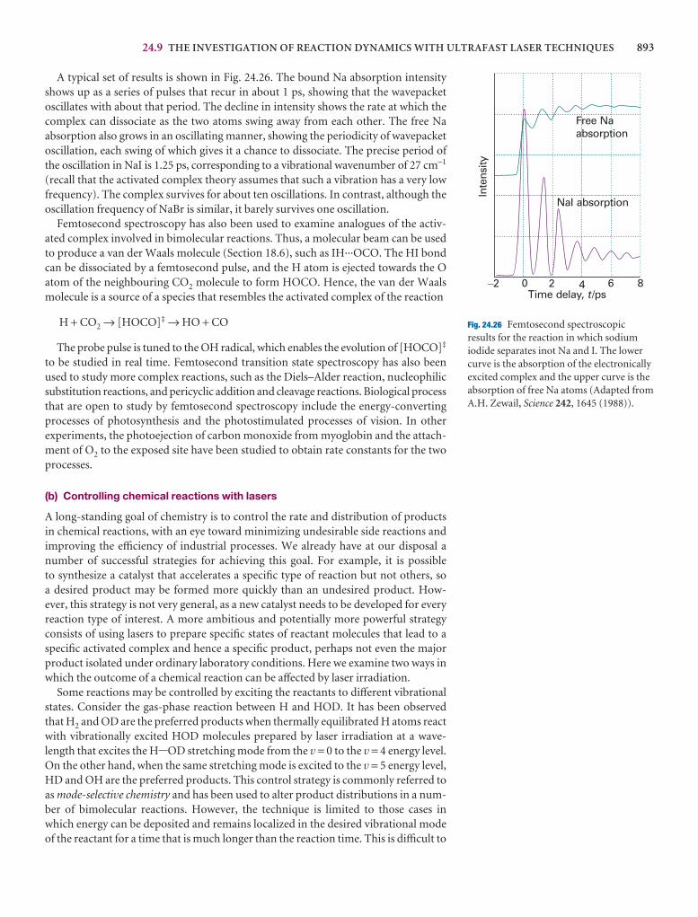
24.9 THE INVESTIGATION OF REACTION DYNAMICS WITH ULTRAFAST LASER TECHNIQUES 893
A typical set of results is shown in Fig. 24.26. The bound Na absorption intensityshows up as a series of pulses that recur in about 1 ps, showing that the wavepacket oscillates with about that period. The decline in intensity shows the rate at which thecomplex can dissociate as the two atoms swing away from each other. The free Na absorption also grows in an oscillating manner, showing the periodicity of wavepacketoscillation, each swing of which gives it a chance to dissociate. The precise period ofthe oscillation in NaI is 1.25 ps, corresponding to a vibrational wavenumber of 27 cm−1
(recall that the activated complex theory assumes that such a vibration has a very lowfrequency). The complex survives for about ten oscillations. In contrast, although theoscillation frequency of NaBr is similar, it barely survives one oscillation.
Femtosecond spectroscopy has also been used to examine analogues of the activ-ated complex involved in bimolecular reactions. Thus, a molecular beam can be usedto produce a van der Waals molecule (Section 18.6), such as IH···OCO. The HI bondcan be dissociated by a femtosecond pulse, and the H atom is ejected towards the Oatom of the neighbouring CO2 molecule to form HOCO. Hence, the van der Waalsmolecule is a source of a species that resembles the activated complex of the reaction
H + CO2 → [HOCO]‡ → HO + CO
The probe pulse is tuned to the OH radical, which enables the evolution of [HOCO]‡
to be studied in real time. Femtosecond transition state spectroscopy has also beenused to study more complex reactions, such as the Diels–Alder reaction, nucleophilicsubstitution reactions, and pericyclic addition and cleavage reactions. Biological processthat are open to study by femtosecond spectroscopy include the energy-convertingprocesses of photosynthesis and the photostimulated processes of vision. In other experiments, the photoejection of carbon monoxide from myoglobin and the attach-ment of O2 to the exposed site have been studied to obtain rate constants for the twoprocesses.
(b) Controlling chemical reactions with lasers
A long-standing goal of chemistry is to control the rate and distribution of productsin chemical reactions, with an eye toward minimizing undesirable side reactions andimproving the efficiency of industrial processes. We already have at our disposal anumber of successful strategies for achieving this goal. For example, it is possible to synthesize a catalyst that accelerates a specific type of reaction but not others, so a desired product may be formed more quickly than an undesired product. How-ever, this strategy is not very general, as a new catalyst needs to be developed for everyreaction type of interest. A more ambitious and potentially more powerful strategy consists of using lasers to prepare specific states of reactant molecules that lead to aspecific activated complex and hence a specific product, perhaps not even the majorproduct isolated under ordinary laboratory conditions. Here we examine two ways inwhich the outcome of a chemical reaction can be affected by laser irradiation.
Some reactions may be controlled by exciting the reactants to different vibrationalstates. Consider the gas-phase reaction between H and HOD. It has been observedthat H2 and OD are the preferred products when thermally equilibrated H atoms reactwith vibrationally excited HOD molecules prepared by laser irradiation at a wave-length that excites the H-OD stretching mode from the v = 0 to the v = 4 energy level.On the other hand, when the same stretching mode is excited to the v = 5 energy level,HD and OH are the preferred products. This control strategy is commonly referred toas mode-selective chemistry and has been used to alter product distributions in a num-ber of bimolecular reactions. However, the technique is limited to those cases inwhich energy can be deposited and remains localized in the desired vibrational modeof the reactant for a time that is much longer than the reaction time. This is difficult to
�2 0 2 4 6 8Time delay, /pst
Inte
nsity
Free Naabsorption
NaI absorption
Fig. 24.26 Femtosecond spectroscopicresults for the reaction in which sodiumiodide separates inot Na and I. The lowercurve is the absorption of the electronicallyexcited complex and the upper curve is theabsorption of free Na atoms (Adapted fromA.H. Zewail, Science 242, 1645 (1988)).
894 24 MOLECULAR REACTION DYNAMICS
achieve in large molecules, in which intramolecular vibrational relaxation redistri-butes energy among the many vibrational modes within a few picoseconds.
A strategy that seeks to avoid the problem of vibrational relaxation uses ultrafastlasers and is related closely to the techniques used for the spectroscopic detection oftransition states. Consider the reaction I2 + Xe → XeI* + I, which occurs via a harpoonmechanism with a transition state denoted as [Xe+···I−···I]. The reaction can be initi-ated by exciting I2 to an electronic state at least 52 460 cm−1 above the ground state andthen followed by measuring the time dependence of the chemiluminescence of XeI*.To exert control over the yield of the product, a pair of femtosecond pulses can beused to induce the reaction. The first pulse excites the I2 molecule to a low energy andunreactive electronic state. We already know that excitation by a femtosecond pulsegenerates a wavepacket that can be treated as a particle travelling across the potential energy surface. In this case, the wavepacket does not have enough energy toreact, but excitation by another laser pulse with the proper wavelength can providethe necessary additional energy. It follows that activated complexes with differentgeometries can be prepared by varying the time delay between the two pulses, as thepartially localized wave packet will be at different locations along the potential energysurface as it evolves after being formed by the first pulse. Because the reaction occursvia the harpoon mechanism, the product yield is expected to be optimal if the secondpulse is applied when the wave packet is at a point where the Xe···I2 distance is justright for electron transfer from Xe to I2 to occur (see Example 24.2). This type of control of the I2 + Xe reaction has been demonstrated.
So far, the control techniques we have discussed have only been applied to reactionsbetween relatively small molecules, with simple and well-understood potential energysurfaces. Extension of these techniques to the controlled synthesis of materials in routine laboratory work will require much more sophisticated knowledge of howlaser pulses may be combined to stimulate a specific molecular response in a complexsystem.
Electron transfer in homogeneous systems
We end the chapter by applying the concepts of transition state theory and quantumtheory to the study of a deceptively simple process, electron transfer betweenmolecules in homogeneous systems. We begin by examining the features of a theorythat describes the factors governing the rates of electron transfer. Then, we discuss thetheory in the light of experimental results on a variety of systems, including proteincomplexes. We shall see that relatively simple expressions may be used to predict therates of electron transfer with reasonable accuracy.
24.10 The rates of electron transfer processes
Consider electron transfer from a donor species D to an acceptor species A in solution.The net reaction is
D + A → D+ + A− v = kobs[D][A] K = (24.75)
In the first step of the mechanism, D and A must diffuse through the solution and collide to form a complex DA, in which the donor and acceptor are separated by a distance comparable to r, the distance between the edges of each species. We assumethat D, A, and DA are in equilibrium:
[D+][A−]
[D][A]
24.10 THE RATES OF ELECTRON TRANSFER PROCESSES 895
D + A 5 DA KDA = = (24.76a)
where ka and k a′ are, respectively, the rate constants for the association and dissoci-ation of the DA complex. Next, electron transfer occurs within the DA complex toyield D+A−:
DA → D+A− vet = ket[DA] (24.76b)
where ket is the first-order rate constant for the forward electron transfer step. TheD+A− complex has two possible fates. First, reverse electron transfer with a rate con-stant kr can regenerate DA:
D+A− → DA vr = kr[D+A−] (24.76c)
Second, D+A− can break apart and the ions diffuse through the solution:
D+A− → D+ + A− vd = kd[D+A−] (24.76d)
We show in the following Justification that
= + 1 + (24.77)
Justification 24.4 The rate constant for electron transfer in solution
To find an expression for the second-order rate constant kobs for electron transferbetween D and A in solution, we begin by equating the rate of the net reaction (eqn24.75) to the rate of formation of separated ions, the reaction products (eqn 24.76d):
v = kobs[D][A] = kd[D+A−]
Now we apply the steady-state approximation to the intermediate D+A−:
= ket[DA] − kr[D+A−] − kd[D+A−] = 0
It follows that
[D+A−] = [DA]
However, DA is also an intermediate so we apply the steady-state approximationagain
= ka[D][A] − k ′a[DA] − ket[DA] + kr[D+A−] = 0
Substitution of the initial expression for the steady-state concentration of D+A− intothis expression for [DA] gives, after some algebra, a new expression for [D+A−]:
[D+A−] = [D][A]
When we multiply this expression by kd, we see that the resulting equation has theform of the rate of electron transfer, v = kobs[D][A], with kobs given by
kobs =
To obtain eqn 24.77, we divide the numerator and denominator on the right-handside of this expression by kdket and solve for the reciprocal of kobs.
kdkaket
k′akr + k′akd + kdket
kaket
k′akr + k′akd + kdket
d[DA]
dt
ket
kr + kd
d[D+A−]
dt
DF
kr
kd
AC
k ′akaket
1
ka
1
kobs
[DA]
[D][A]
ka
k ′a
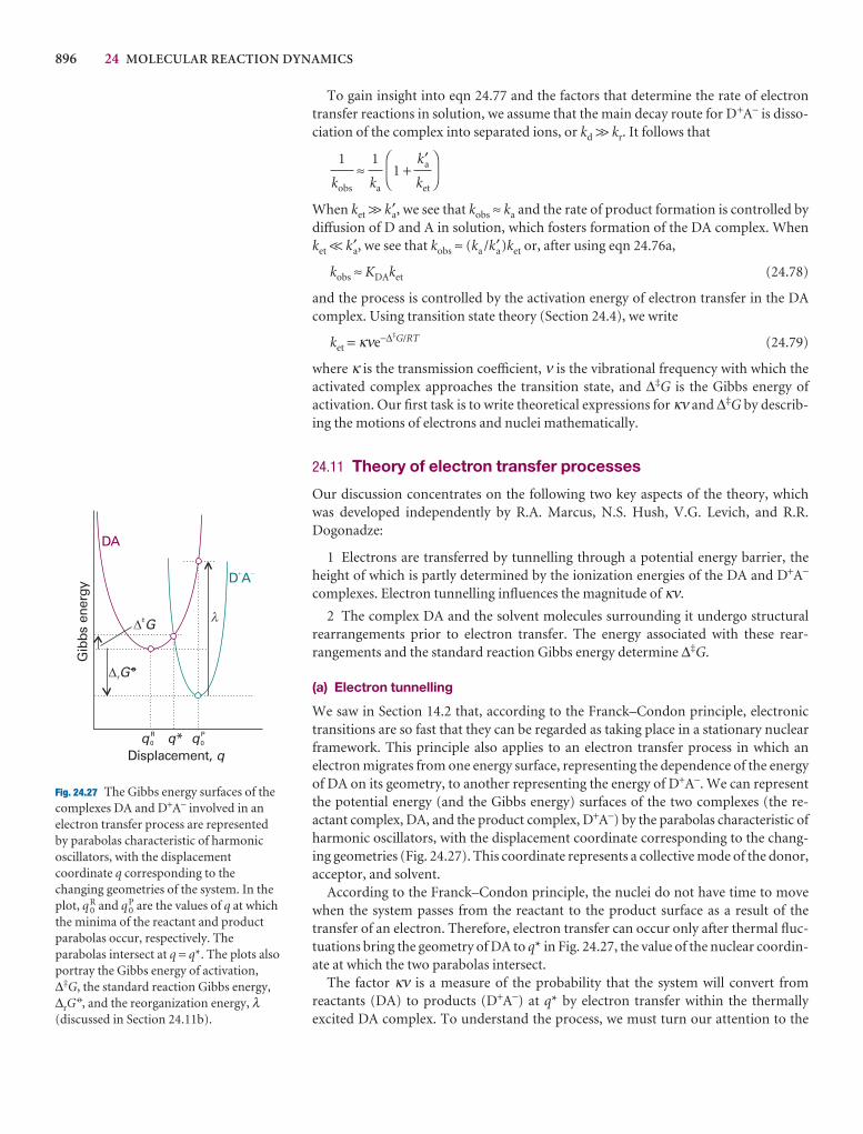
896 24 MOLECULAR REACTION DYNAMICS
To gain insight into eqn 24.77 and the factors that determine the rate of electrontransfer reactions in solution, we assume that the main decay route for D+A− is disso-ciation of the complex into separated ions, or kd >> kr. It follows that
≈ 1 +
When ket >> k′a, we see that kobs ≈ ka and the rate of product formation is controlled bydiffusion of D and A in solution, which fosters formation of the DA complex. Whenket << k′a, we see that kobs ≈ (ka /k′a)ket or, after using eqn 24.76a,
kobs ≈ KDAket (24.78)
and the process is controlled by the activation energy of electron transfer in the DAcomplex. Using transition state theory (Section 24.4), we write
ket = κνe−∆‡G/RT (24.79)
where κ is the transmission coefficient, ν is the vibrational frequency with which theactivated complex approaches the transition state, and ∆‡G is the Gibbs energy of activation. Our first task is to write theoretical expressions for κν and ∆‡G by describ-ing the motions of electrons and nuclei mathematically.
24.11 Theory of electron transfer processes
Our discussion concentrates on the following two key aspects of the theory, which was developed independently by R.A. Marcus, N.S. Hush, V.G. Levich, and R.R.Dogonadze:
1 Electrons are transferred by tunnelling through a potential energy barrier, theheight of which is partly determined by the ionization energies of the DA and D+A−
complexes. Electron tunnelling influences the magnitude of κν.
2 The complex DA and the solvent molecules surrounding it undergo structuralrearrangements prior to electron transfer. The energy associated with these rear-rangements and the standard reaction Gibbs energy determine ∆‡G.
(a) Electron tunnelling
We saw in Section 14.2 that, according to the Franck–Condon principle, electronictransitions are so fast that they can be regarded as taking place in a stationary nuclearframework. This principle also applies to an electron transfer process in which anelectron migrates from one energy surface, representing the dependence of the energyof DA on its geometry, to another representing the energy of D+A−. We can representthe potential energy (and the Gibbs energy) surfaces of the two complexes (the re-actant complex, DA, and the product complex, D+A−) by the parabolas characteristic ofharmonic oscillators, with the displacement coordinate corresponding to the chang-ing geometries (Fig. 24.27). This coordinate represents a collective mode of the donor,acceptor, and solvent.
According to the Franck–Condon principle, the nuclei do not have time to movewhen the system passes from the reactant to the product surface as a result of thetransfer of an electron. Therefore, electron transfer can occur only after thermal fluc-tuations bring the geometry of DA to q* in Fig. 24.27, the value of the nuclear coordin-ate at which the two parabolas intersect.
The factor κν is a measure of the probability that the system will convert fromreactants (DA) to products (D+A−) at q* by electron transfer within the thermally excited DA complex. To understand the process, we must turn our attention to the
DF
k′aket
AC
1
ka
1
kobs
Gib
bs e
nerg
y
DA
D A� �
rG°
�
q0R q* q0
P
Displacement, q
‡G
Fig. 24.27 The Gibbs energy surfaces of thecomplexes DA and D+A− involved in anelectron transfer process are represented by parabolas characteristic of harmonicoscillators, with the displacementcoordinate q corresponding to thechanging geometries of the system. In theplot, q 0
R and q 0P are the values of q at which
the minima of the reactant and productparabolas occur, respectively. Theparabolas intersect at q = q*. The plots alsoportray the Gibbs energy of activation,∆‡G, the standard reaction Gibbs energy,∆rG
7, and the reorganization energy, λ(discussed in Section 24.11b).
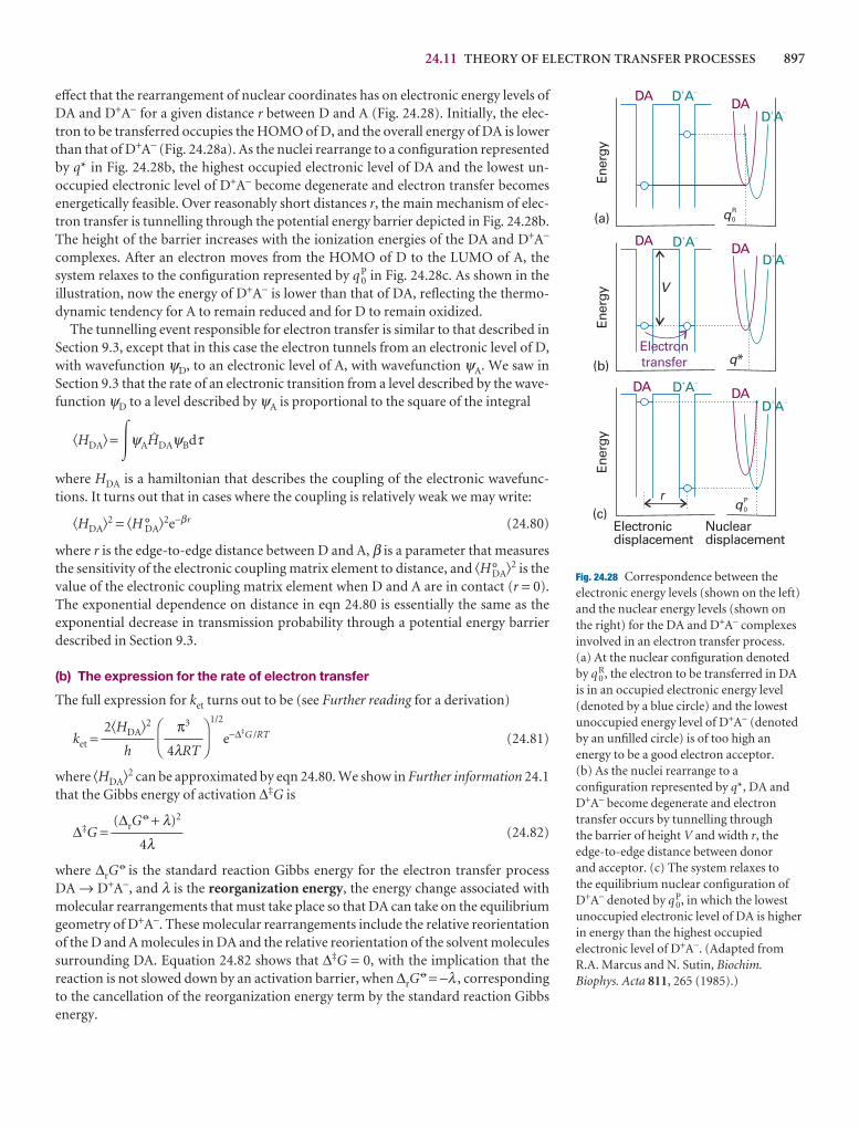
24.11 THEORY OF ELECTRON TRANSFER PROCESSES 897
effect that the rearrangement of nuclear coordinates has on electronic energy levels ofDA and D+A− for a given distance r between D and A (Fig. 24.28). Initially, the elec-tron to be transferred occupies the HOMO of D, and the overall energy of DA is lowerthan that of D+A− (Fig. 24.28a). As the nuclei rearrange to a configuration representedby q* in Fig. 24.28b, the highest occupied electronic level of DA and the lowest un-occupied electronic level of D+A− become degenerate and electron transfer becomes energetically feasible. Over reasonably short distances r, the main mechanism of elec-tron transfer is tunnelling through the potential energy barrier depicted in Fig. 24.28b.The height of the barrier increases with the ionization energies of the DA and D+A−
complexes. After an electron moves from the HOMO of D to the LUMO of A, the system relaxes to the configuration represented by q 0
P in Fig. 24.28c. As shown in theillustration, now the energy of D+A− is lower than that of DA, reflecting the thermo-dynamic tendency for A to remain reduced and for D to remain oxidized.
The tunnelling event responsible for electron transfer is similar to that described inSection 9.3, except that in this case the electron tunnels from an electronic level of D,with wavefunction ψD, to an electronic level of A, with wavefunction ψA. We saw inSection 9.3 that the rate of an electronic transition from a level described by the wave-function ψD to a level described by ψA is proportional to the square of the integral
�HDA� = �ψA@DAψBdτ
where HDA is a hamiltonian that describes the coupling of the electronic wavefunc-tions. It turns out that in cases where the coupling is relatively weak we may write:
�HDA�2 = �H °DA�2e−βr (24.80)
where r is the edge-to-edge distance between D and A, β is a parameter that measuresthe sensitivity of the electronic coupling matrix element to distance, and �H°DA�2 is thevalue of the electronic coupling matrix element when D and A are in contact (r = 0).The exponential dependence on distance in eqn 24.80 is essentially the same as the exponential decrease in transmission probability through a potential energy barrierdescribed in Section 9.3.
(b) The expression for the rate of electron transfer
The full expression for ket turns out to be (see Further reading for a derivation)
ket =1/2
e−∆‡G /RT (24.81)
where �HDA�2 can be approximated by eqn 24.80. We show in Further information 24.1that the Gibbs energy of activation ∆‡G is
∆‡G = (24.82)
where ∆rG7 is the standard reaction Gibbs energy for the electron transfer process
DA → D+A−, and λ is the reorganization energy, the energy change associated withmolecular rearrangements that must take place so that DA can take on the equilibriumgeometry of D+A−. These molecular rearrangements include the relative reorientationof the D and A molecules in DA and the relative reorientation of the solvent moleculessurrounding DA. Equation 24.82 shows that ∆‡G = 0, with the implication that the reaction is not slowed down by an activation barrier, when ∆rG
7 = −λ , correspondingto the cancellation of the reorganization energy term by the standard reaction Gibbsenergy.
(∆rG7 + λ)2
4λ
DF
π3
4λRT
AC
2�HDA�2
h
DAD A� �
q0R
*q
Nucleardisplacement
q0P
Ener
gy
DA
Ener
gy
Electrontransfer
DA
Ener
gy
Electronicdisplacement
(a)
(b)
(c)r
DA
DA
DA
V
D A� �
D A� �
D A� �
D A� �
D A� �
Fig. 24.28 Correspondence between theelectronic energy levels (shown on the left)and the nuclear energy levels (shown on the right) for the DA and D+A− complexesinvolved in an electron transfer process. (a) At the nuclear configuration denoted by q 0
R, the electron to be transferred in DAis in an occupied electronic energy level(denoted by a blue circle) and the lowestunoccupied energy level of D+A− (denotedby an unfilled circle) is of too high anenergy to be a good electron acceptor. (b) As the nuclei rearrange to aconfiguration represented by q*, DA andD+A− become degenerate and electrontransfer occurs by tunnelling through the barrier of height V and width r, theedge-to-edge distance between donor and acceptor. (c) The system relaxes to the equilibrium nuclear configuration of D+A− denoted by q 0
P, in which the lowestunoccupied electronic level of DA is higherin energy than the highest occupiedelectronic level of D+A−. (Adapted fromR.A. Marcus and N. Sutin, Biochim.Biophys. Acta 811, 265 (1985).)
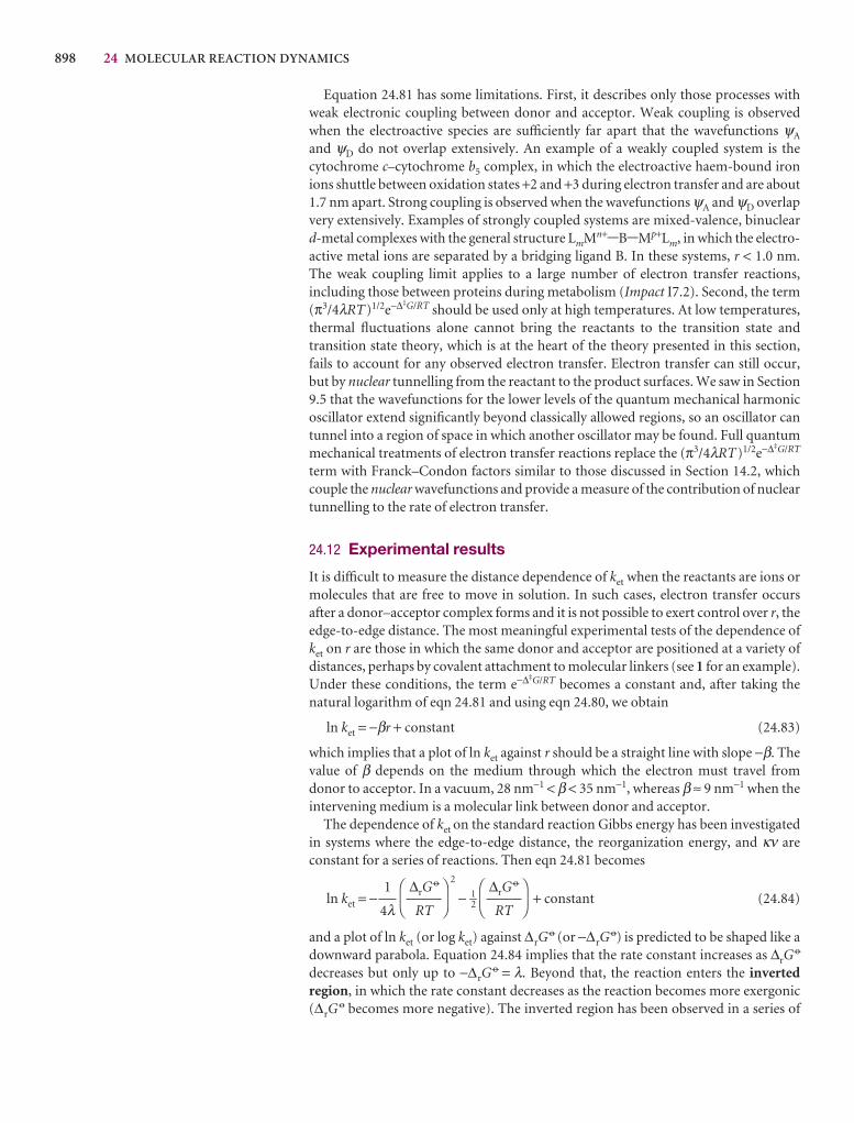
898 24 MOLECULAR REACTION DYNAMICS
Equation 24.81 has some limitations. First, it describes only those processes withweak electronic coupling between donor and acceptor. Weak coupling is observedwhen the electroactive species are sufficiently far apart that the wavefunctions ψA
and ψD do not overlap extensively. An example of a weakly coupled system is the cytochrome c–cytochrome b5 complex, in which the electroactive haem-bound ironions shuttle between oxidation states +2 and +3 during electron transfer and are about1.7 nm apart. Strong coupling is observed when the wavefunctions ψA and ψD overlapvery extensively. Examples of strongly coupled systems are mixed-valence, binucleard-metal complexes with the general structure LmMn+-B-Mp+Lm, in which the electro-active metal ions are separated by a bridging ligand B. In these systems, r < 1.0 nm. The weak coupling limit applies to a large number of electron transfer reactions, including those between proteins during metabolism (Impact I7.2). Second, the term(π3/4λRT)1/2e−∆‡G/RT should be used only at high temperatures. At low temperatures,thermal fluctuations alone cannot bring the reactants to the transition state and transition state theory, which is at the heart of the theory presented in this section,fails to account for any observed electron transfer. Electron transfer can still occur,but by nuclear tunnelling from the reactant to the product surfaces. We saw in Section9.5 that the wavefunctions for the lower levels of the quantum mechanical harmonicoscillator extend significantly beyond classically allowed regions, so an oscillator cantunnel into a region of space in which another oscillator may be found. Full quantummechanical treatments of electron transfer reactions replace the (π3/4λRT)1/2e−∆‡G/RT
term with Franck–Condon factors similar to those discussed in Section 14.2, whichcouple the nuclear wavefunctions and provide a measure of the contribution of nucleartunnelling to the rate of electron transfer.
24.12 Experimental results
It is difficult to measure the distance dependence of ket when the reactants are ions ormolecules that are free to move in solution. In such cases, electron transfer occursafter a donor–acceptor complex forms and it is not possible to exert control over r, theedge-to-edge distance. The most meaningful experimental tests of the dependence ofket on r are those in which the same donor and acceptor are positioned at a variety ofdistances, perhaps by covalent attachment to molecular linkers (see 1 for an example).Under these conditions, the term e−∆‡G/RT becomes a constant and, after taking thenatural logarithm of eqn 24.81 and using eqn 24.80, we obtain
ln ket = −βr + constant (24.83)
which implies that a plot of ln ket against r should be a straight line with slope −β. Thevalue of β depends on the medium through which the electron must travel fromdonor to acceptor. In a vacuum, 28 nm−1 < β < 35 nm−1, whereas β ≈ 9 nm−1 when theintervening medium is a molecular link between donor and acceptor.
The dependence of ket on the standard reaction Gibbs energy has been investigatedin systems where the edge-to-edge distance, the reorganization energy, and κν areconstant for a series of reactions. Then eqn 24.81 becomes
ln ket = −2
− 1–2 + constant (24.84)
and a plot of ln ket (or log ket) against ∆rG7 (or −∆rG
7) is predicted to be shaped like adownward parabola. Equation 24.84 implies that the rate constant increases as ∆rG
7
decreases but only up to −∆rG7 = λ. Beyond that, the reaction enters the inverted
region, in which the rate constant decreases as the reaction becomes more exergonic(∆rG
7 becomes more negative). The inverted region has been observed in a series of
DF
∆rG7
RT
AC
DF
∆rG7
RT
AC
1
4λ
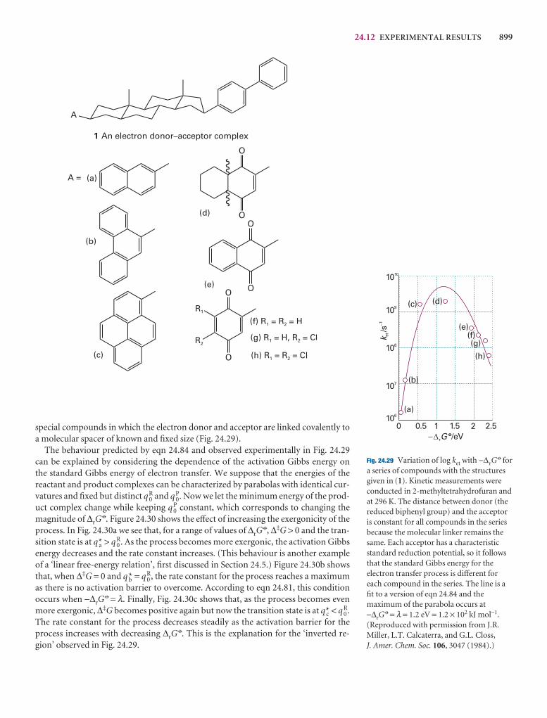
24.12 EXPERIMENTAL RESULTS 899
special compounds in which the electron donor and acceptor are linked covalently toa molecular spacer of known and fixed size (Fig. 24.29).
The behaviour predicted by eqn 24.84 and observed experimentally in Fig. 24.29can be explained by considering the dependence of the activation Gibbs energy on the standard Gibbs energy of electron transfer. We suppose that the energies of the reactant and product complexes can be characterized by parabolas with identical cur-vatures and fixed but distinct q 0
R and q 0P. Now we let the minimum energy of the prod-
uct complex change while keeping q 0P constant, which corresponds to changing the
magnitude of ∆rG7. Figure 24.30 shows the effect of increasing the exergonicity of the
process. In Fig. 24.30a we see that, for a range of values of ∆rG7, ∆‡G > 0 and the tran-
sition state is at q a* > q 0R. As the process becomes more exergonic, the activation Gibbs
energy decreases and the rate constant increases. (This behaviour is another exampleof a ‘linear free-energy relation’, first discussed in Section 24.5.) Figure 24.30b showsthat, when ∆‡G = 0 and q b* = q 0
R, the rate constant for the process reaches a maximumas there is no activation barrier to overcome. According to eqn 24.81, this conditionoccurs when −∆rG
7 = λ. Finally, Fig. 24.30c shows that, as the process becomes evenmore exergonic, ∆‡G becomes positive again but now the transition state is at q c* < q 0
R.The rate constant for the process decreases steadily as the activation barrier for theprocess increases with decreasing ∆rG
7. This is the explanation for the ‘inverted re-gion’ observed in Fig. 24.29.
(a)
(b)
(c) (d)
(e)(f)(g)
(h)
0 0.5 1 1.5 2
1010
108
109
107
106
k et/s
�1
�rG °/eV2.5
Fig. 24.29 Variation of log ket with −∆rG7 for
a series of compounds with the structuresgiven in (1). Kinetic measurements wereconducted in 2-methyltetrahydrofuran andat 296 K. The distance between donor (thereduced biphenyl group) and the acceptoris constant for all compounds in the seriesbecause the molecular linker remains thesame. Each acceptor has a characteristicstandard reduction potential, so it followsthat the standard Gibbs energy for theelectron transfer process is different foreach compound in the series. The line is afit to a version of eqn 24.84 and themaximum of the parabola occurs at −∆rG
7 = λ = 1.2 eV = 1.2 × 10² kJ mol−1.(Reproduced with permission from J.R.Miller, L.T. Calcaterra, and G.L. Closs, J. Amer. Chem. Soc. 106, 3047 (1984).)
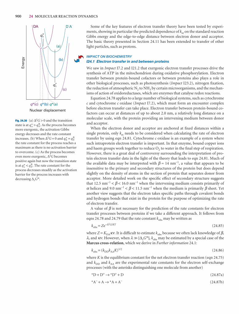
900 24 MOLECULAR REACTION DYNAMICS
Some of the key features of electron transfer theory have been tested by experi-ments, showing in particular the predicted dependence of ket on the standard reactionGibbs energy and the edge-to-edge distance between electron donor and acceptor.The basic theory presented in Section 24.11 has been extended to transfer of otherlight particles, such as protons.
IMPACT ON BIOCHEMISTRY
I24.1 Electron transfer in and between proteins
We saw in Impact I7.2 and I21.2 that exergonic electron transfer processes drive thesynthesis of ATP in the mitochondrion during oxidative phosphorylation. Electrontransfer between protein-bound cofactors or between proteins also plays a role inother biological processes, such as photosynthesis (Impact I23.2), nitrogen fixation,the reduction of atmospheric N2 to NH3 by certain microorganisms, and the mechan-isms of action of oxidoreductases, which are enzymes that catalyse redox reactions.
Equation 24.78 applies to a large number of biological systems, such as cytochromec and cytochrome c oxidase (Impact I7.2), which must form an encounter complex before electron transfer can take place. Electron transfer between protein-bound co-factors can occur at distances of up to about 2.0 nm, a relatively long distance on amolecular scale, with the protein providing an intervening medium between donorand acceptor.
When the electron donor and acceptor are anchored at fixed distances within a single protein, only ket needs to be considered when calculating the rate of electrontransfer by using eqn 24.81. Cytochrome c oxidase is an example of a system wheresuch intraprotein electron transfer is important. In that enzyme, bound copper ionsand haem groups work together to reduce O2 to water in the final step of respiration.However, there is a great deal of controversy surrounding the interpretation of pro-tein electron transfer data in the light of the theory that leads to eqn 24.81. Much ofthe available data may be interpreted with β ≈ 14 nm−1, a value that appears to be insensitive to the primary and secondary structures of the protein but does dependslightly on the density of atoms in the section of protein that separates donor from acceptor. More detailed work on the specific effect of secondary structure suggeststhat 12.5 nm−1 < β < 16.0 nm−1 when the intervening medium consists primarily of α helices and 9.0 nm−1 < β < 11.5 nm−1 when the medium is primarily β sheet. Yet another view suggests that the electron takes specific paths through covalent bondsand hydrogen bonds that exist in the protein for the purpose of optimizing the rate of electron transfer.
A value of β is not necessary for the prediction of the rate constants for electrontransfer processes between proteins if we take a different approach. It follows fromeqns 24.78 and 24.79 that the rate constant kobs may be written as
kobs = Ze−∆‡G/RT (24.85)
where Z = KDAκν. It is difficult to estimate kobs because we often lack knowledge of β,λ, and κν. However, when λ >> |∆rG
7 |, kobs may be estimated by a special case of theMarcus cross-relation, which we derive in Further information 24.1:
kobs = (kDDkAAK)1/2 (24.86)
where K is the equilibrium constant for the net electron transfer reaction (eqn 24.75)and kDD and kAA are the experimental rate constants for the electron self-exchangeprocesses (with the asterisks distinguishing one molecule from another)
*D + D+ → *D+ + D (24.87a)
*A− + A → *A + A− (24.87b)
Ener
gy
(c)
DA D A� �
(b)
(a)
q*(a)
Nuclear displacement
q*(b)q*(c)
q0P
q0R
Fig. 24.30 (a) ∆‡G > 0 and the transitionstate is at q a* > q 0
R. As the process becomesmore exergonic, the activation Gibbsenergy decreases and the rate constantincreases. (b) When ∆‡G = 0 and q b* = q 0
R
the rate constant for the process reaches amaximum as there is no activation barrierto overcome. (c) As the process becomeseven more exergonic, ∆‡G becomespositive again but now the transition stateis at q c* < q 0
R. The rate constant for theprocess decreases steadily as the activationbarrier for the process increases withdecreasing ∆rG
7.
I24.1 IMPACT ON BIOCHEMISTRY: ELECTRON TRANSFER IN AND BETWEEN PROTEINS 901
The rate constants estimated by eqn 24.86 agree fairly well with experimental rateconstants for electron transfer between proteins, as we see in the following Example.
Example 24.4 Using the Marcus cross-relation
The following kinetic and thermodynamic data were obtained for cytochrome cand cytochrome c551, two proteins in which haem-bound iron ions shuttle betweenthe oxidation states Fe(II) and Fe(III):
kii/(dm3 mol−1 s−1) E 7/V
cytochrome c 1.5 × 10 2 0.260
cytochrome c551 4.6 × 10⁷ 0.286
Estimate the rate constant kobs for the process
cytochrome c551(red) + cytochrome c(ox) → cytochrome c551(ox)+ cytochrome c(red)
Then, compare the estimated value with the observed value of 6.7 × 10⁴ dm3
mol−1 s−1.
Method We use the standard potentials and eqns 7.30 (ln K = νFE 7/RT) and 7.37 (E 7 = E R
7 − E L7) to calculate the equilibrium constant K. Then, we use eqn 24.86, the
calculated value of K, and the self-exchange rate constants kii to calculate the rateconstant kobs.
Answer The two reduction half-reactions are
Right: cytochrome c(ox) + e− → cytochrome c(red) E R7 = +0.260 V
Left: cytochrome c551(ox) + e− → cytochrome c 551(red) E L7 = +0.286 V
The difference is
E 7 = (0.260 V) − (0.286 V) = −0.026 V
It then follows from eqn 7.30 with ν = 1 and RT/F = 25.69 mV that
ln K = − = −
Therefore, K = 0.36. From eqn 24.76 and the self-exchange rate constants, we calculate
kobs = {(1.5 × 10² dm3 mol−1 s−1) × (4.6 × 107 dm3 mol−1 s−1) × 0.36}1/2
= 5.0 × 10⁴ dm3 mol−1 s−1
The calculated and observed values differ by only 25 per cent, indicating that theMarcus relation can lead to reasonable estimates of rate constants for electrontransfer.
Self-test 24.4 Estimate kobs for the reduction by cytochrome c of plastocyanin, aprotein containing a copper ion that shuttles between the +2 and +1 oxidationstates and for which kAA = 6.6 × 10² dm3 mol−1 s−1 and E 7 = 0.350 V.
[1.8 × 10³ dm3 mol−1 s−1]
2.6
2.569
0.026V
25.69 × 10⁻³ V

902 24 MOLECULAR REACTION DYNAMICS
Checklist of key ideas
1. In collision theory, it is supposed that the rate is proportionalto the collision frequency, a steric factor, and the fraction ofcollisions that occur with at least the kinetic energy Ea alongtheir lines of centres.
2. A reaction in solution may be diffusion-controlled if its rate iscontrolled by the rate at which reactant molecules encountereach other in solution. The rate of an activation-controlledreaction is controlled by the rate of accumulating sufficientenergy.
3. In transition state theory, it is supposed that an activatedcomplex is in equilibrium with the reactants, and that the rateat which that complex forms products depends on the rate atwhich it passes through a transition state. The result is theEyring equation, k2 = κ(kT/h)I ‡
c.
4. The rate constant may be parametrized in terms of the Gibbs energy, entropy, and enthalpy of activation, k2 = (kT/h)e∆*S/Re−∆*H/RT.
5. The kinetic salt effect is the effect of an added inert salt on therate of a reaction between ions, log k2 = log k°2 + 2AzAzBI1/2.
6. Techniques for the study of reactive collisions include infraredchemiluminescence, laser-induced fluorescence, multiphotonionization (MPI), reaction product imaging, and resonantmultiphoton ionization (REMPI).
7. A potential energy surface maps the potential energy as afunction of the relative positions of all the atoms taking part ina reaction. In an attractive surface, the saddle point (thehighest point) occurs early on the reaction coordinate. In arepulsive surface, the saddle point occurs late on the reactioncoordinate.
8. Ultrafast laser techniques can be used to probe directly theactivated complex and to control the outcome of somechemical reactions.
9. The rate constant of electron transfer in a donor–acceptorcomplex depends on the distance between electron donor and acceptor, the standard reaction Gibbs energy, and thereorganization energy, λ: ket ∝ e−βre−∆‡G/RT (constant T), with∆‡G = (∆rG
7 + λ)2/4λ.
10. The Marcus cross-relation predicts the rate constant forelectron transfer in solution from the reaction’s equilibriumconstant K and the self-exchange rate constants kii: kobs =(kDDkAAK)1/2.
Table 24.3 Summary of uses of k
Symbol Significance
k Boltzmann’s constant
k2 Second-order rate constant
k2° Rate constant at zero ionic strength
ka, kb, . . . Rate constants for individual steps
k ′a, k ′b, . . . Rate constants for individual reverse steps
k‡ Rate constant for unimolecular decay of activated complex
K Equilibrium constant (dimensionless)
Kγ Ratio of activity coefficients
K‡ Proportionality constant in transition state theory
κ Transmission coefficient
I Equilibrium constant with one mode discarded
kf Force constant
FURTHER INFORMATION 903
Further reading
Articles and texts
A.J. Alexander and R.N. Zare, Anatomy of elementary chemicalreactions. J. Chem. Educ. 75, 1105 (1998).
G.D. Billing and K.V. Mikkelsen, Advanced molecular dynamics andchemical kinetics. Wiley, New York (1997).
D.C. Clary, Quantum theory of chemical reaction dynamics. Science279, 1879 (1998).
F.F. Crim, Vibrational state control of bimolecular reactions:discovering and directing the chemistry. Acc. Chem. Res. 32, 877(1999).
D.M. Hirst, Potential energy surfaces. Taylor and Francis, London(1985).
A.M. Kuznetsov and J. Ulstrup, Electron transfer in chemistry andbiology: an introduction to the theory. Wiley, New York (1998).
R.D. Levine and R.B. Bernstein, Molecular reaction dynamics andchemical reactivity. Clarendon Press, Oxford (1987).
J.I. Steinfeld, J.S. Francisco and W.L. Hase, Chemical kinetics anddynamics. Prentice Hall, Upper Saddle River (1999).
A.H. Zewail, Femtochemistry: atomic-scale dynamics of the chemicalbond using ultrafast lasers. Angew. Chem. Int. Ed. 39, 2586 (2000).
Further information
Further information 24.1 The Gibbs energy of activation ofelectron transfer and the Marcus cross-relation
The simplest way to derive an expression for the Gibbs energy ofactivation of electron transfer processes is to construct a model inwhich the surfaces for DA (the ‘reactant complex’, denoted R) andfor D+A− (the ‘product complex’, denoted P) are described byclassical harmonic oscillators with identical reduced masses µ andangular frequencies ω, but displaced minima, as shown in Fig. 24.27.The molar Gibbs energies Gm,R(q) and Gm,P(q) of the reactant andproduct complexes, respectively, may be written as
Gm,R(q) = 1–2 NAµω2(q − q 0R)2 + Gm,R(q 0
R) (24.88a)
Gm,P(q) = 1–2 NAµω2(q − q 0P)2 + Gm,P(q 0
P) (24.88b)
where q 0R and q 0
P are the values of q at which the minima of thereactant and product parabolas occur, respectively. The standardreaction Gibbs energy for the electron transfer process DA → D+A− is∆rG
7 = Gm,P(q 0P) − Gm,R(q 0
R), the difference in standard molar Gibbsenergy between the minima of the parabolas. In Fig. 24.27, ∆rG
7 < 0.We also note that q*, the value of q corresponding to the transition
state of the complex, may be written in terms of the parameter α, thefractional change in q:
q* = q 0R + α(q 0
P − q 0R) (24.89)
We see from Fig. 24.27 that ∆‡G = Gm,R(q*) − Gm,R(q 0R). It then
follows from eqns 24.88a, 24.88b, and 24.89 that
∆‡G = 1–2NAµω2(q* − q 0R)2 = 1–2NAµω2{α(q 0
P − q 0R)}2 (24.90)
We now define the reorganization energy, λ, as
λ = 1–2NAµω2(q 0P − q 0
R)2 (24.91)
which can be interpreted as Gm,R(q 0P) − Gm,R(q 0
R) and, consequently,as the (Gibbs) energy required to deform the equilibriumconfiguration of DA to the equilibrium configuration of D+A− (asshown in Fig. 24.27). It follows from eqns 24.90 and 24.91 that
∆‡G = α2λ (24.92)
Because Gm,R(q*) = Gm,P(q*), it follows from eqns 24.88b, 24.91, and24.92 that
α2λ = 1–2NAµω2{(α − 1)(q 0P − q 0
R)}2 + ∆rG7
= (α − 1)λ + ∆rG7 (24.93)
which implies that
α = 1–2 + 1 (24.94)
By combining eqns 24.92 and 24.94, we obtain eqn 24.82. We canobtain an identical relation if we allow the harmonic oscillators tohave different angular frequencies and hence different curvatures (see Further reading).
Equation 24.82 can be used to derive the form of the Marcus cross-relation (eqn 24.86) used in Impact I24.1. We begin by using eqn 24.85 to write the rate constants for the self-exchangereactions as
kDD = ZDDe−∆‡GDD/RT kAA = ZAAe−∆‡GAA/RT
For the net reaction (also called the ‘cross-reaction’) and the self-exchange reactions, the Gibbs energy of activation may be writtenfrom eqn 24.82 as
∆‡G = + +
When λ >> |∆rG7 |, we obtain
∆‡G = +
This expression can be used without further elaboration to denote theGibbs energy of activation of the net reaction. For the self-exchangereactions, we set ∆rG
7DD = ∆rG
7AA = 0 and write
∆‡GDD = ∆‡GAA =λAA
4
λDD
4
λ4
∆rG7
2
λ4
∆rG7
2
∆rG72
4λ
DEF∆rG
7
λABC
904 24 MOLECULAR REACTION DYNAMICS
It follows that
kDD = ZDDe−λDD/4RT kAA = ZAAe−λAA/4RT
To make further progress, we assume that the reorganization energyof the net reaction is the arithmetic mean of the reorganizationenergies of the self-exchange reactions:
λDA =
It follows that the Gibbs energy of activation of the net reaction is
∆‡G = + +
Therefore, the rate constant for the net reaction is
kobs = Ze−∆rG7/2RTe−λDD/8RTe−λAA/8RT
λAA
8
λDD
8
∆rG7
2
λDD + λAA
2
We can use eqn 7.17 (ln K = −∆rG7/RT) to write
K = e−∆rG7/RT
Then, by combining this expression with the expressions for kDD andkAA, and using the relations ex+y = exey and ex/2 = (ex )1/2, we obtain themost general case of the Marcus cross-relation:
kobs = (kDDkAAK)1/2f
where
f =
In practice, the factor f is usually set to 1 and we obtain eqn 24.86.
Z
(ZAAZDD)1/2
Discussion questions
24.1 Describe the essential features of the harpoon mechanism.
24.2 Distinguish between a diffusion-controlled reaction and an activation-controlled reaction.
24.3 Describe the formulation of the Eyring equation.
24.4 Discuss the physical origin of the kinetic salt effect.
24.5 Describe how the following techniques are used in the study of chemicaldynamics: infrared chemiluminescence, laser-induced fluorescence,multiphoton ionization, resonant multiphoton ionization, reaction productimaging, and femtosecond spectroscopy.
24.6 Justify the following statements: (a) Reactions with attractive potentialenergy surfaces proceed more efficiently if the energy is in relativetranslational motion. (b) Reactions with repulsive potential surfaces proceedmore efficiently if the excess energy is present as vibrations.
24.7 A method for directing the outcome of a chemical reaction consists ofusing molecular beams to control the relative orientations of reactants duringa collision. Consider the reaction Rb + CH3I → RbI + CH3. How should CH3Imolecules and Rb atoms be oriented to maximize the production of RbI?
24.8 Discuss how the following factors determine the rate of electron transferin homogeneous systems: the distance between electron donor and acceptor,and the reorganization energy of redox active species and the surroundingmedium.
Exercises
24.1a Calculate the collision frequency, z, and the collision density, Z, inammonia, R = 190 pm, at 25°C and 100 kPa. What is the percentage increasewhen the temperature is raised by 10 K at constant volume?
24.1b Calculate the collision frequency, z, and the collision density, Z, incarbon monoxide, R = 180 pm at 25°C and 100 kPa. What is the percentageincrease when the temperature is raised by 10 K at constant volume?
24.2a Collision theory demands knowing the fraction of molecular collisionshaving at least the kinetic energy Ea along the line of flight. What is thisfraction when (a) Ea = 10 kJ mol−1, (b) Ea = 100 kJ mol−1 at (i) 300 K and (ii) 1000 K?
24.2b Collision theory demands knowing the fraction of molecular collisionshaving at least the kinetic energy Ea along the line of flight. What is thisfraction when (a) Ea = 15 kJ mol−1, (b) Ea = 150 kJ mol−1 at (i) 300 K and (ii) 800 K?
24.3a Calculate the percentage increase in the fractions in Exercise 24.2awhen the temperature is raised by 10 K.
24.3b Calculate the percentage increase in the fractions in Exercise 24.2bwhen the temperature is raised by 10 K.
24.4a Use the collision theory of gas-phase reactions to calculate thetheoretical value of the second-order rate constant for the reaction H2(g) +I2(g) → 2 HI(g) at 650 K, assuming that it is elementary bimolecular. Thecollision cross-section is 0.36 nm2, the reduced mass is 3.32 × 10⁻²⁷ kg, and the activation energy is 171 kJ mol−1.
24.4b Use the collision theory of gas-phase reactions to calculate thetheoretical value of the second-order rate constant for the reaction D2(g) +Br2(g) → 2 DBr(g) at 450 K, assuming that it is elementary bimolecular. Takethe collision cross-section as 0.30 nm2, the reduced mass as 3.930 u, and theactivation energy as 200 kJ mol−1.
24.5a A typical diffusion coefficient for small molecules in aqueous solutionat 25°C is 5 × 10⁻⁹ m2 s−1. If the critical reaction distance is 0.4 nm, what valueis expected for the second-order rate constant for a diffusion-controlledreaction?
24.5b Suppose that the typical diffusion coefficient for a reactant in aqueoussolution at 25°C is 4.2 × 10⁻⁹ m2 s−1. If the critical reaction distance is 0.50 nm,what value is expected for the second-order rate constant for the diffusion-controlled reaction?

PROBLEMS 905
24.6a Calculate the magnitude of the diffusion-controlled rate constant at 298 K for a species in (a) water, (b) pentane. The viscosities are 1.00 × 10⁻³ kg m−1 s−1, and 2.2 × 10⁻⁴ kg m−1 s−1, respectively.
24.6b Calculate the magnitude of the diffusion-controlled rate constant at298 K for a species in (a) decylbenzene, (b) concentrated sulfuric acid. Theviscosities are 3.36 cP and 27 cP, respectively.
24.7a Calculate the magnitude of the diffusion-controlled rate constant at298 K for the recombination of two atoms in water, for which η = 0.89 cP.Assuming the concentration of the reacting species is 1.0 mmol dm−3 initially,how long does it take for the concentration of the atoms to fall to half thatvalue? Assume the reaction is elementary.
24.7b Calculate the magnitude of the diffusion-controlled rate constant at298 K for the recombination of two atoms in benzene, for which η = 0.601 cP.Assuming the concentration of the reacting species is 1.8 mmol dm−3 initially,how long does it take for the concentration of the atoms to fall to half thatvalue? Assume the reaction is elementary.
24.8a For the gaseous reaction A + B → P, the reactive cross-section obtainedfrom the experimental value of the pre-exponential factor is 9.2 × 10⁻²² m2.The collision cross-sections of A and B estimated from the transport propertiesare 0.95 and 0.65 nm2, respectively. Calculate the P-factor for the reaction.
24.8b For the gaseous reaction A + B → P, the reactive cross-section obtainedfrom the experimental value of the pre-exponential factor is 8.7 × 10⁻²² m2.The collision cross-sections of A and B estimated from the transportproperties are 0.88 and 0.40 nm2, respectively. Calculate the P factor for thereaction.
24.9a Two neutral species, A and B, with diameters 588 pm and 1650 pm,respectively, undergo the diffusion-controlled reaction A + B → P in a solventof viscosity 2.37 × 10⁻³ kg m−1 s−1 at 40°C. Calculate the initial rate d[P]/dt ifthe initial concentrations of A and B are 0.150 mol dm−3 and 0.330 mol dm−3,respectively.
24.9b Two neutral species, A and B, with diameters 442 pm and 885 pm,respectively, undergo the diffusion-controlled reaction A + B → P in a solventof viscosity 1.27 cP at 20°C. Calculate the initial rate d[P]/dt if the initialconcentrations of A and B are 0.200 mol dm−3 and 0.150 mol dm−3,respectively.
24.10a The reaction of propylxanthate ion in acetic acid buffer solutions hasthe mechanism A− + H+ → P. Near 30°C the rate constant is given by theempirical expression k2 = (2.05 × 10¹³)e−(8681 K)/T dm3 mol−1 s−1. Evaluate theenergy and entropy of activation at 30°C.
24.10b The reaction A− + H+ → P has a rate constant given by the empiricalexpression k2 = (8.72 × 10¹²)e−(6134 K)/T dm3 mol−1 s−1. Evaluate the energy andentropy of activation at 25°C.
24.11a When the reaction in Exercise 24.10a occurs in a dioxane/watermixture that is 30 per cent dioxane by mass, the rate constant fits k2 = (7.78 ×10¹⁴)e−(9134 K)/T dm3 mol−1 s−1 near 30°C. Calculate ∆‡G for the reaction at 30°C.
24.11b A rate constant is found to fit the expression k2 = (6.45 × 10¹³)e−(5375 K)/T dm3 mol−1 s−1 near 25°C. Calculate ∆‡G for the reaction at 25°C.
24.12a The gas-phase association reaction between F2 and IF5 is first-order ineach of the reactants. The energy of activation for the reaction is 58.6 kJ mol−1.At 65°C the rate constant is 7.84 × 10⁻³ kPa−1 s−1. Calculate the entropy ofactivation at 65°C.
24.12b A gas-phase recombination reaction is first-order in each of thereactants. The energy of activation for the reaction is 49.6 kJ mol−1. At 55°Cthe rate constant is 0.23 m3 s−1. Calculate the entropy of activation at 55°C.
24.13a Calculate the entropy of activation for a collision between twostructureless particles at 300 K, taking M = 50 g mol−1 and σ = 0.40 nm2.
24.13b Calculate the entropy of activation for a collision between twostructureless particles at 500 K, taking M = 78 g mol−1 and σ = 0.62 nm2.
24.14a The pre-exponential factor for the gas-phase decomposition of ozone at low pressures is 4.6 × 10¹² dm3 mol−1 s−1 and its activation energy is 10.0 kJ mol−1. What are (a) the entropy of activation, (b) the enthalpy ofactivation, (c) the Gibbs energy of activation at 298 K?
24.14b The pre-exponential factor for a gas-phase decomposition of ozone at low pressures is 2.3 × 10¹³ dm3 mol−1 s−1 and its activation energy is 30.0 kJ mol−1. What are (a) the entropy of activation, (b) the enthalpy of activation, (c) the Gibbs energy of activation at 298 K?
24.15a The rate constant of the reaction H2O2(aq) + I−(aq) + H+(aq) →H2O(l) + HIO(aq) is sensitive to the ionic strength of the aqueous solution inwhich the reaction occurs. At 25°C, k = 12.2 dm6 mol−2 min−1 at an ionicstrength of 0.0525. Use the Debye–Hückel limiting law to estimate the rateconstant at zero ionic strength.
24.15b At 25°C, k = 1.55 dm6 mol−2 min−1 at an ionic strength of 0.0241 for areaction in which the rate-determining step involves the encounter of twosingly charged cations. Use the Debye–Hückel limiting law to estimate the rateconstant at zero ionic strength.
24.16a For a pair of electron donor and acceptor, HAB = 0.03 cm−1, ∆rG7 =
−0.182 eV and ket = 30.5 s−1 at 298 K. Estimate the value of the reorganizationenergy.
24.16b For a pair of electron donor and acceptor, ket = 2.02 × 10⁵ s−1 for ∆rG7
= −0.665 eV. The standard reaction Gibbs energy changes to ∆rG7 = −0.975 eV
when a substituent is added to the electron acceptor and the rate constant forelectron transfer changes to ket = 3.33 × 10⁶ s−1. The experiments wereconducted at 298 K. Assuming that the distance between donor and acceptoris the same in both experiments, estimate the values of HAB and λ.
24.17a For a pair of electron donor and acceptor, ket = 2.02 × 10⁵ s−1 whenr = 1.11 nm and ket = 4.51 × 10⁵ s−1 when r = 1.23 nm. Assuming that ∆rG
7
and λ are the same in both experiments, estimate the value of β.
24.17b Refer to Exercise 24.17a. Estimate the value of ket when r = 1.48 nm.
Problems*
Numerical problems
24.1 In the dimerization of methyl radicals at 25°C, the experimental pre-exponential factor is 2.4 × 10¹⁰ dm3 mol−1 s−1. What are (a) the reactive cross-section, (b) the P factor for the reaction if the C-H bond length is 154 pm?
24.2 Nitrogen dioxide reacts bimolecularly in the gas phase to give 2 NO +O2. The temperature dependence of the second-order rate constant for therate law d[P]/dt = k[NO2]2 is given below. What are the P factor and thereactive cross-section for the reaction?
* Problems denoted with the symbol ‡ were supplied by Charles Trapp, Carmen Giunta, and Marshall Cady.
24.9‡ For the thermal decomposition of F2O by the reaction 2 F2O(g) →2 F2(g) + O2(g), J. Czarnowski and H.J. Schuhmacher (Chem. Phys. Lett. 17,235 (1972)) have suggested the following mechanism:
(1) F2O + F2O → F + OF + F2O k1
(2) F + F2O → F2 + OF k2
(3) OF + OF → O2 + F + F k3
(4) F + F + F2O → F2 + F2O k4
(a) Using the steady-state approximation, show that this mechanism isconsistent with the experimental rate law −d[F2O]/dt = k[F2O]2 + k′[F2O]3/2.(b) The experimentally determined Arrhenius parameters in the range501–583 K are A = 7.8 × 10¹³ dm3 mol−1 s−1, Ea/R = 1.935 × 10⁴ K for k and andA = 2.3 × 10¹⁰ dm3 mol−1 s−1, Ea /R = 1.691 × 10⁴ K for k′. At 540 K, ∆fH
7(F2O)= +24.41 kJ mol−1, D(F-F) = 160.6 kJ mol−1, and D(O-O) = 498.2 kJ mol−1.Estimate the bond dissociation energies of the first and second F-O bondsand the Arrhenius activation energy of reaction 2.
24.10‡ For the gas-phase reaction A + A → A2, the experimental rateconstant, k2, has been fitted to the Arrhenius equation with the pre-exponential factor A = 4.07 × 10⁵ dm3 mol−1 s−1 at 300 K and an activationenergy of 65.43 kJ mol−1. Calculate ∆‡S, ∆‡H, ∆‡U, and ∆‡G for the reaction.
24.11‡ One of the most historically significant studies of chemical reactionrates was that by M. Bodenstein (Z. physik. Chem. 29, 295 (1899)) of the gas-phase reaction 2 HI(g) → H2(g) + I2(g) and its reverse, with rate constantsk and k′, respectively. The measured rate constants as a function oftemperature are
T /K 647 666 683 700 716 781
k /(22.4 dm3 mol− 1 min−1) 0.230 0.588 1.37 3.10 6.70 105.9
k′/(22.4 dm3 mol−1 min−1) 0.0140 0.0379 0.0659 0.172 0.375 3.58
Demonstrate that these data are consistent with the collision theory ofbimolecular gas-phase reactions.
24.12 Use the approximate form of the Marcus relation (eqn 24.86 with f = 1)to estimate the rate constant for the reaction Ru(bpy)3
3+ + Fe(H2O)62+ →
Ru(bpy)32+ + Fe(H2O)6
3+, where bpy stands for 4,4′-bipyridine. The followingdata are useful:
Ru(bpy)33+ + e− → Ru(bpy)3
2+ E 7 = 1.26 V
Fe(H2O)63+ + e− → Fe(H2O)6
2+ E 7 = 0.77 V
*Ru(bpy)33+ + Ru(bpy) 3
2+ → *Ru(bpy)32+ + Ru(bpy)3
3+
kRu = 4.0 × 10⁸ dm3 mol−1 s−1
*Fe(H2O)63+ + Fe(H2O) 6
2+ → *Fe(H2O)62+ + Fe(H2O)6
3+
kFe = 4.2 dm3 mol−1 s−1
Theoretical problems
24.13 Confirm that eqn 24.40 is a solution of eqn 24.39, where [J]t is asolution of the same equation but with k = 0 and for the same initialconditions.
24.14 Evaluate [J]* numerically using mathematical software for integrationin eqn 24.40, and explore the effect of increasing reaction rate constant on thespatial distribution of J.
24.15 Estimate the orders of magnitude of the partition functions involved ina rate expression. State the order of magnitude of q T
m /NA, qR, qV, qE for typicalmolecules. Check that in the collision of two structureless molecules the orderof magnitude of the pre-exponential factor is of the same order as thatpredicted by collision theory. Go on to estimate the P factor for a reaction inwhich A + B → P, and A and B are nonlinear triatomic molecules.
24.16 Use the Debye–Hückel limiting law to show that changes in ionicstrength can affect the rate of reaction catalysed by H+ from the deprotonation
906 24 MOLECULAR REACTION DYNAMICS
T /K 600 700 800 1000
k /(cm3 mol−1 s−1) 4.6 × 10² 9.7 × 10³ 1.3 × 10⁵ 3.1 × 10⁶
Take σ = 0.60 nm2.
24.3 The diameter of the methyl radical is about 308 pm. What is themaximum rate constant in the expression d[C2H6]/dt = k[CH3]2 for second-order recombination of radicals at room temperature? 10 per cent of a 1.0-dm3 sample of ethane at 298 K and 100 kPa is dissociated into methyl radicals.What is the minimum time for 90 per cent recombination?
24.4 The rates of thermolysis of a variety of cis- and trans-azoalkanes havebeen measured over a range of temperatures in order to settle a controversyconcerning the mechanism of the reaction. In ethanol an unstable cis-azoalkane decomposed at a rate that was followed by observing the N2
evolution, and this led to the rate constants listed below (P.S. Engel and D.J.Bishop, J. Amer. Chem. Soc. 97, 6754 (1975)). Calculate the enthalpy, entropy,energy, and Gibbs energy of activation at –20°C.
θ /°C −24.82 −20.73 −17.02 −13.00 −8.95
10 4 × k /s−1 1.22 2.31 4.39 8.50 14.3
24.5 In an experimental study of a bimolecular reaction in aqueous solution,the second-order rate constant was measured at 25°C and at a variety of ionicstrengths and the results are tabulated below. It is known that a singly chargedion is involved in the rate-determining step. What is the charge on the otherion involved?
I 0.0025 0.0037 0.0045 0.0065 0.0085
k /(dm3 mol−1 s−1) 1.05 1.12 1.16 1.18 1.26
24.6 The rate constant of the reaction I−(aq) + H2O2(aq) → H2O(l) + IO−(aq)varies slowly with ionic strength, even though the Debye–Hückel limiting lawpredicts no effect. Use the following data from 25°C to find the dependence oflog kr on the ionic strength:
I/(mol kg−1) 0.0207 0.0525 0.0925 0.1575
kr /(dm3 mol−1 min−1) 0.663 0.670 0.679 0.694
Evaluate the limiting value of kr at zero ionic strength. What does the resultsuggest for the dependence of log γ on ionic strength for a neutral molecule inan electrolyte solution?
24.7 The total cross-sections for reactions between alkali metal atoms andhalogen molecules are given in the table below (R.D. Levine and R.B.Bernstein, Molecular reaction dynamics, Clarendon Press, Oxford, 72 (1974)).Assess the data in terms of the harpoon mechanism.
σ*/nm2 Cl2 Br2 I2
Na 1.24 1.16 0.97
K 1.54 1.51 1.27
Rb 1.90 1.97 1.67
Cs 1.96 2.04 1.95
Electron affinities are approximately 1.3 eV (Cl2), 1.2 eV (Br2), and 1.7 eV (I2), and ionization energies are 5.1 eV (Na), 4.3 eV (K), 4.2 eV (Rb), and 3.9 eV (Cs).
24.8‡ M. Cyfert, B. Latko, and M. Wawrzeczyk (Int. J. Chem. Kinet. 28, 103(1996)) examined the oxidation of tris(1,10-phenanthroline)iron(II) byperiodate in aqueous solution, a reaction that shows autocatalytic behaviour.To assess the kinetic salt effect, they measured rate constants at a variety ofconcentrations of Na2SO4 far in excess of reactant concentrations andreported the following data:
[Na2SO4]/(mol kg −1) 0.2 0.15 0.1 0.05 0.25 0.0125 0.005
k/(dm3/2 mol−1/2 s−1) 0.462 0.430 0.390 0.321 0.283 0.252 0.224
What can be inferred about the charge of the activated complex of the rate-determining step?
PROBLEMS 907
of a weak acid. Consider the mechanism: H+(aq) + B(aq) → P, where H+
comes from the deprotonation of the weak acid, HA. The weak acid has a fixedconcentration. First show that log [H+], derived from the ionization of HA,depends on the activity coefficients of ions and thus depends on the ionicstrength. Then find the relationship between log(rate) and log [H+] to showthat the rate also depends on the ionic strength.
24.17 The Eyring equation can also be applied to physical processes. As anexample, consider the rate of diffusion of an atom stuck to the surface of asolid. Suppose that in order to move from one site to another it has to reachthe top of the barrier where it can vibrate classically in the vertical directionand in one horizontal direction, but vibration along the other horizontaldirection takes it into the neighbouring site. Find an expression for the rate ofdiffusion, and evaluate it for W atoms on a tungsten surface (Ea = 60 kJ mol−1).Suppose that the vibration frequencies at the transition state are (a) the sameas, (b) one-half the value for the adsorbed atom. What is the value of thediffusion coefficient D at 500 K? (Take the site separation as 316 pm and ν = 1 × 10¹¹ Hz.)
24.18 Suppose now that the adsorbed, migrating species treated in Problem24.17 is a spherical molecule, and that it can rotate classically as well as vibrateat the top of the barrier, but that at the adsorption site itself it can only vibrate.What effect does this have on the diffusion constant? Take the molecule to bemethane, for which B = 5.24 cm−1.
24.19 Show that the intensities of a molecular beam before and after passingthrough a chamber of length l containing inert scattering atoms are related byI = I0e−N σl, where σ is the collision cross-section and N the number density ofscattering atoms.
24.20 In a molecular beam experiment to measure collision cross-sections itwas found that the intensity of a CsCl beam was reduced to 60 per cent of itsintensity on passage through CH2F2 at 10 µTorr, but that when the target wasAr at the same pressure the intensity was reduced only by 10 per cent. Whatare the relative cross-sections of the two types of collision? Why is one muchlarger than the other?
24.21‡ Show that bimolecular reactions between nonlinear molecules aremuch slower than between atoms even when the activation energies of bothreactions are equal. Use transition state theory and make the followingassumptions. (1) All vibrational partition functions are close to unity; (2) all rotational partition functions are approximately 1 × 101.5, which is areasonable order of magnitude number; (3) the translational partitionfunction for each species is 1 × 1026.
24.22 This exercise gives some familiarity with the difficulties involved inpredicting the structure of activated complexes. It also demonstrates theimportance of femtosecond spectroscopy to our understanding of chemicaldynamics because direct experimental observation of the activated complexremoves much of the ambiguity of theoretical predictions. Consider the attackof H on D2, which is one step in the H2 + D2 reaction. (a) Suppose that the Happroaches D2 from the side and forms a complex in the form of an isoscelestriangle. Take the H-D distance as 30 per cent greater than in H2 (74 pm) andthe D-D distance as 20 per cent greater than in H2. Let the critical coordinatebe the antisymmetric stretching vibration in which one H-D bond stretchesas the other shortens. Let all the vibrations be at about 1000 cm−1. Estimate k2
for this reaction at 400 K using the experimental activation energy of about 35 kJ mol−1. (b) Now change the model of the activated complex in part (a)and make it linear. Use the same estimated molecular bond lengths andvibrational frequencies to calculate k2 for this choice of model. (c) Clearly,there is much scope for modifying the parameters of the models of theactivated complex. Use mathematical software or write and run a programthat allows you to vary the structure of the complex and the parameters in a plausible way, and look for a model (or more than one model) that gives a value of k close to the experimental value, 4 × 10⁵ dm3 mol−1 s−1.
Applications: to environmental science and biochemistry
24.23‡ R. Atkinson (J. Phys. Chem. Ref. Data 26, 215 (1997)) has reviewed alarge set of rate constants relevant to the atmospheric chemistry of volatileorganic compounds. The recommended rate constant for the bimolecularassociation of O2 with an alkyl radical R at 298 K is 4.7 × 10⁹ dm3 mol−1 s−1 forR = C2H5 and 8.4 × 10⁹ dm3 mol−1 s−1 for R = cyclohexyl. Assuming no energybarrier, compute the steric factor, P, for each reaction. (Hint. Obtain collisiondiameters from collision cross-sections of similar molecules in the Datasection.)
24.24‡ The compound α-tocopherol, a form of vitamin E, is a powerfulantioxidant that may help to maintain the integrity of biological membranes.R.H. Bisby and A.W. Parker (J. Amer. Chem. Soc. 117, 5664 (1995)) studiedthe reaction of photochemically excited duroquinone with the antioxidant inethanol. Once the duroquinone was photochemically excited, a bimolecularreaction took place at a rate described as diffusion-limited. (a) Estimate therate constant for a diffusion-limited reaction in ethanol. (b) The reported rateconstant was 2.77 × 10⁹ dm3 mol−1 s−1; estimate the critical reaction distance ifthe sum of diffusion constants is 1 × 10⁻⁹ m2 s−1.
24.25 The study of conditions that optimize the association of proteins insolution guides the design of protocols for formation of large crystals that are amenable to analysis by the X-ray diffraction techniques discussed inChapter 20. It is important to characterize protein dimerization because theprocess is considered to be the rate-determining step in the growth of crystalsof many proteins. Consider the variation with ionic strength of the rateconstant of dimerization in aqueous solution of a cationic protein P:
I 0.0100 0.0150 0.0200 0.0250 0.0300 0.0350
k/k° 8.10 13.30 20.50 27.80 38.10 52.00
What can be deduced about the charge of P?
24.26 A useful strategy for the study of electron transfer in proteins consistsof attaching an electroactive species to the protein’s surface and thenmeasuring ket between the attached species and an electroactive proteincofactor. J.W. Winkler and H.B. Gray (Chem. Rev. 92, 369 (1992)) summarizedata for cytochrome c (Impact I7.2) modified by replacement of the haem ironby a zinc ion, resulting in a zinc-porphyrin (ZnP) moiety in the interior of theprotein, and by attachment of a ruthenium ion complex to a surface histidineaminoacid. The edge-to-edge distance between the electroactive species wasthus fixed at 1.23 nm. A variety of ruthenium ion complexes with differentstandard reduction potentials were used. For each ruthenium-modifiedprotein, either the Ru2+ → ZnP+ or the ZnP* → Ru3+, in which the electrondonor is an electronic excited state of the zinc-porphyrin formed by laserexcitation, was monitored. This arrangement leads to different standardreaction Gibbs energies because the redox couples ZnP+/ZnP and ZnP+/ZnP*have different standard potentials, with the electronically excited porphyrinbeing a more powerful reductant. Use the following data to estimate thereorganization energy for this system:
−∆ rG7/eV 0.665 0.705 0.745 0.975 1.015 1.055
ket /(10 6 s−1) 0.657 1.52 1.12 8.99 5.76 10.1
24.27 The photosynthetic reaction centre of the purple photosyntheticbacterium Rhodopseudomonas viridis contains a number of bound cofactorsthat participate in electron transfer reactions. The following table shows datacompiled by Moser et al. (Nature 355, 796 (1992)) on the rate constants forelectron transfer between different cofactors and their edge-to-edge distances:
Reaction BChl− → BPh BPh− → BChl2+ BPh− → QA cyt c559 → BChl2
+
r /nm 0.48 0.95 0.96 1.23
k et /s−1 1.58 × 10¹² 3.98 × 10⁹ 1.00 × 10⁹ 1.58 × 10⁸
Reaction QA− → QB QA
− → BChl2+
r/nm 1.35 2.24
ket /s−1 3.98 × 10⁷ 63.1

908 24 MOLECULAR REACTION DYNAMICS
(BChl, bacteriochlorophyll; BChl2, bacteriochlorophyll dimer, functionallydistinct from BChl; BPh, bacteriophaeophytin; QA and QB, quinone moleculesbound to two distinct sites; cyt c559, a cytochrome bound to the reaction centrecomplex). Are these data in agreement with the behaviour predicted by eqn24.83? If so, evaluate the value of β.
24.28 The rate constant for electron transfer between a cytochrome c and thebacteriochlorophyll dimer of the reaction centre of the purple bacteriumRhodobacter sphaeroides (Problem 24.27) decreases with decreasingtemperature in the range 300 K to 130 K. Below 130 K, the rate constantbecomes independent of temperature. Account for these results.
24.29 Azurin is a protein containing a copper ion that shuttles between the +2and +1 oxidation states, and cytochrome c is a protein in which a haem-boundiron ion shuttles between the +3 and +2 oxidation states. The rate constant forelectron transfer from reduced azurin to oxidized cytochrome c is 1.6 × 10³
dm3 mol−1 s−1. Estimate the electron self-exchange rate constant for azurinfrom the following data:
k ii /(dm3 mol−1 s−1) E 7/V
cytochrome c 1.5 × 10² 0.260
azurin ? 0.304

Processes at solidsurfaces
In this chapter we see how solids grow at their surfaces and how the details of the structureand composition of solid surfaces can be determined experimentally. A major part of thematerial concerns the extent to which a surface is covered and the variation of the extent ofcoverage with the pressure and temperature. This material is used to discuss how surfacesaffect the rate and course of chemical change by acting as the site of catalysis. Reactionsat surfaces include the processes that lie at the heart of electrochemistry. Therefore, we revisit in this chapter some of the topics treated in Chapter 7, but focus on the dynamics of electrode processes rather than the equilibrium properties treated there. Finally, we ana-lyse the kinetics of reactions that are responsible for power production in fuel cells and forcorrosion.
Processes at solid surfaces govern the viability of industry both constructively, as incatalysis, and destructively, as in corrosion. Chemical reactions at solid surfaces maydiffer sharply from reactions in the bulk, for reaction pathways of much lower activa-tion energy may be provided, and hence result in catalysis. The concept of a solid sur-face has been extended in recent years with the availability of microporous materialsas catalysts.
An important kinetic problem examined in this chapter is the rate at which oxid-izable or reducible species—in short, electroactive species—can donate or acceptelectrons on the surfaces of electrodes. In Chapter 24 we explored the dynamics of electron transfer in homogeneous systems. In heterogeneous systems, the rates of processes that occur at the interface between the phases, such as an electrode immersed in an ionic solution, are very important. A measure of this rate is the cur-rent density, j, the charge flux through a region (the electric current divided by thearea of the region). We shall discuss the properties that control the current densityand its consequences.
We shall see that acronyms are widely used in surface studies; for convenience, a list of the acronyms used in this chapter is given in Table 25.7 at the end of the chapter.
The growth and structure of solid surfaces
In this section we see how surfaces are extended and crystals grow. The attachment ofparticles to a surface is called adsorption. The substance that adsorbs is the adsorbateand the underlying material that we are concerned with in this section is the adsorb-ent or substrate. The reverse of adsorption is desorption.
25The growth and structure ofsolid surfaces
25.1 Surface growth
25.2 Surface composition
The extent of adsorption
25.3 Physisorption andchemisorption
25.4 Adsorption isotherms
25.5 The rates of surface processes
I25.1 Impact on biochemistry:Biosensor analysis
Heterogeneous catalysis
25.6 Mechanisms ofheterogeneous catalysis
25.7 Catalytic activity at surfaces
I25.2 Impact on technology:Examples of catalysis in thechemical industry
Processes at electrodes
25.8 The electrode–solutioninterface
25.9 The rate of charge transfer
25.10 Voltammetry
25.11 Electrolysis
25.12 Working galvanic cells
I25.3 Impact on technology: Fuel cells
25.13 Corrosion
I25.4 Impact on technology:Protecting materials againstcorrosion
Checklist of key ideas
Further reading
Further information 25.1: The relationbetween electrode potential and theGalvani potential
Discussion questions
Exercises
Problems
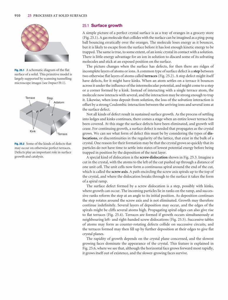
910 25 PROCESSES AT SOLID SURFACES
25.1 Surface growth
A simple picture of a perfect crystal surface is as a tray of oranges in a grocery store(Fig. 25.1). A gas molecule that collides with the surface can be imagined as a ping-pongball bouncing erratically over the oranges. The molecule loses energy as it bounces,but it is likely to escape from the surface before it has lost enough kinetic energy to betrapped. The same is true, to some extent, of an ionic crystal in contact with a solution.There is little energy advantage for an ion in solution to discard some of its solvatingmolecules and stick at an exposed position on the surface.
The picture changes when the surface has defects, for then there are ridges of incomplete layers of atoms or ions. A common type of surface defect is a step betweentwo otherwise flat layers of atoms called terraces (Fig. 25.2). A step defect might itselfhave defects, for it might have kinks. When an atom settles on a terrace it bouncesacross it under the influence of the intermolecular potential, and might come to a stepor a corner formed by a kink. Instead of interacting with a single terrace atom, themolecule now interacts with several, and the interaction may be strong enough to trapit. Likewise, when ions deposit from solution, the loss of the solvation interaction isoffset by a strong Coulombic interaction between the arriving ions and several ions atthe surface defect.
Not all kinds of defect result in sustained surface growth. As the process of settlinginto ledges and kinks continues, there comes a stage when an entire lower terrace hasbeen covered. At this stage the surface defects have been eliminated, and growth willcease. For continuing growth, a surface defect is needed that propagates as the crystalgrows. We can see what form of defect this must be by considering the types of dis-locations, or discontinuities in the regularity of the lattice, that exist in the bulk of acrystal. One reason for their formation may be that the crystal grows so quickly that itsparticles do not have time to settle into states of lowest potential energy before beingtrapped in position by the deposition of the next layer.
A special kind of dislocation is the screw dislocation shown in Fig. 25.3. Imagine acut in the crystal, with the atoms to the left of the cut pushed up through a distance ofone unit cell. The unit cells now form a continuous spiral around the end of the cut,which is called the screw axis. A path encircling the screw axis spirals up to the top ofthe crystal, and where the dislocation breaks through to the surface it takes the formof a spiral ramp.
The surface defect formed by a screw dislocation is a step, possibly with kinks,where growth can occur. The incoming particles lie in ranks on the ramp, and succes-sive ranks reform the step at an angle to its initial position. As deposition continuesthe step rotates around the screw axis and is not eliminated. Growth may thereforecontinue indefinitely. Several layers of deposition may occur, and the edges of the spirals might be cliffs several atoms high. Propagating spiral edges can also give rise to flat terraces (Fig. 25.4). Terraces are formed if growth occurs simultaneously atneighbouring left- and right-handed screw dislocations (Fig. 25.5). Successive tablesof atoms may form as counter-rotating defects collide on successive circuits, and the terraces formed may then fill up by further deposition at their edges to give flatcrystal planes.
The rapidity of growth depends on the crystal plane concerned, and the slowestgrowing faces dominate the appearance of the crystal. This feature is explained in Fig. 25.6, where we see that, although the horizontal face grows forward most rapidly,it grows itself out of existence, and the slower-growing faces survive.
Fig. 25.1 A schematic diagram of the flatsurface of a solid. This primitive model islargely supported by scanning tunnellingmicroscope images (see Impact I9.1).
Fig. 25.2 Some of the kinds of defects thatmay occur on otherwise perfect terraces.Defects play an important role in surfacegrowth and catalysis.
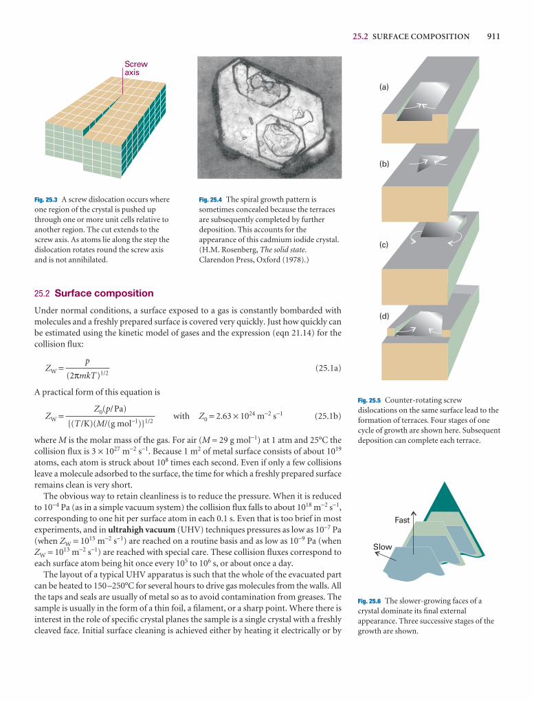
25.2 SURFACE COMPOSITION 911
25.2 Surface composition
Under normal conditions, a surface exposed to a gas is constantly bombarded withmolecules and a freshly prepared surface is covered very quickly. Just how quickly canbe estimated using the kinetic model of gases and the expression (eqn 21.14) for thecollision flux:
ZW = (25.1a)
A practical form of this equation is
ZW = with Z0 = 2.63 × 1024 m−2 s−1 (25.1b)
where M is the molar mass of the gas. For air (M ≈ 29 g mol−1) at 1 atm and 25°C thecollision flux is 3 × 1027 m−2 s−1. Because 1 m2 of metal surface consists of about 1019
atoms, each atom is struck about 108 times each second. Even if only a few collisionsleave a molecule adsorbed to the surface, the time for which a freshly prepared surfaceremains clean is very short.
The obvious way to retain cleanliness is to reduce the pressure. When it is reducedto 10−4 Pa (as in a simple vacuum system) the collision flux falls to about 1018 m−2 s−1,corresponding to one hit per surface atom in each 0.1 s. Even that is too brief in mostexperiments, and in ultrahigh vacuum (UHV) techniques pressures as low as 10−7 Pa(when ZW = 1015 m−2 s−1) are reached on a routine basis and as low as 10−9 Pa (whenZW = 1013 m−2 s−1) are reached with special care. These collision fluxes correspond toeach surface atom being hit once every 105 to 106 s, or about once a day.
The layout of a typical UHV apparatus is such that the whole of the evacuated partcan be heated to 150–250°C for several hours to drive gas molecules from the walls. Allthe taps and seals are usually of metal so as to avoid contamination from greases. Thesample is usually in the form of a thin foil, a filament, or a sharp point. Where there isinterest in the role of specific crystal planes the sample is a single crystal with a freshlycleaved face. Initial surface cleaning is achieved either by heating it electrically or by
Z0(p/Pa)
{(T /K)(M/(g mol−1)}1/2
p
(2πmkT)1/2
Fig. 25.3 A screw dislocation occurs whereone region of the crystal is pushed upthrough one or more unit cells relative toanother region. The cut extends to thescrew axis. As atoms lie along the step thedislocation rotates round the screw axisand is not annihilated.
Fig. 25.4 The spiral growth pattern issometimes concealed because the terracesare subsequently completed by furtherdeposition. This accounts for theappearance of this cadmium iodide crystal.(H.M. Rosenberg, The solid state.Clarendon Press, Oxford (1978).)
Fig. 25.5 Counter-rotating screwdislocations on the same surface lead to theformation of terraces. Four stages of onecycle of growth are shown here. Subsequentdeposition can complete each terrace.
Fig. 25.6 The slower-growing faces of acrystal dominate its final externalappearance. Three successive stages of thegrowth are shown.
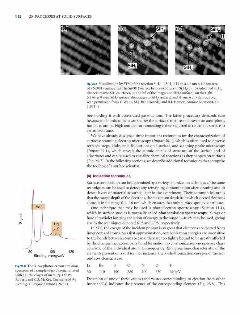
912 25 PROCESSES AT SOLID SURFACES
bombarding it with accelerated gaseous ions. The latter procedure demands care because ion bombardment can shatter the surface structure and leave it an amorphousjumble of atoms. High temperature annealing is then required to return the surface toan ordered state.
We have already discussed three important techniques for the characterization ofsurfaces: scanning electron microscopy (Impact I8.1), which is often used to observeterraces, steps, kinks, and dislocations on a surface, and scanning probe microscopy(Impact I9.1), which reveals the atomic details of structure of the surface and of adsorbates and can be used to visualize chemical reactions as they happen on surfaces(Fig. 25.7). In the following sections, we describe additional techniques that comprisethe toolbox of a surface scientist.
(a) Ionization techniques
Surface composition can be determined by a variety of ionization techniques. The sametechniques can be used to detect any remaining contamination after cleaning and todetect layers of material adsorbed later in the experiment. Their common feature isthat the escape depth of the electrons, the maximum depth from which ejected electronscome, is in the range 0.1–1.0 nm, which ensures that only surface species contribute.
One technique that may be used is photoelectron spectroscopy (Section 11.4),which in surface studies is normally called photoemission spectroscopy. X-rays orhard ultraviolet ionizing radiation of energy in the range 5–40 eV may be used, givingrise to the techniques denoted XPS and UPS, respectively.
In XPS, the energy of the incident photon is so great that electrons are ejected frominner cores of atoms. As a first approximation, core ionization energies are insensitiveto the bonds between atoms because they are too tightly bound to be greatly affectedby the changes that accompany bond formation, so core ionization energies are char-acteristic of the individual atom. Consequently, XPS gives lines characteristic of theelements present on a surface. For instance, the K-shell ionization energies of the sec-ond row elements are
Li Be B C N O F
50 110 190 280 400 530 690 eV
Detection of one of these values (and values corresponding to ejection from otherinner shells) indicates the presence of the corresponding element (Fig. 25.8). This
Fig. 25.7 Visualization by STM of the reaction SiH3 → SiH2 + H on a 4.7 nm × 4.7 nm area of a Si(001) surface. (a) The Si(001) surface before exposure to Si2H6(g). (b) Adsorbed Si2H6
dissociates into SiH2(surface), on the left of the image, and SiH3(surface), on the right. (c) After 8 min, SiH3(surface) dissociates to SiH2(surface) and H(surface). (Reproduced with permission from Y. Wang, M.J. Bronikowski, and R.J. Hamers, Surface Science 64, 311(1994).)
Fig. 25.8 The X-ray photoelectron emissionspectrum of a sample of gold contaminatedwith a surface layer of mercury. (M.W.Roberts and C.S. McKee, Chemistry of themetal–gas interface, Oxford (1978).)
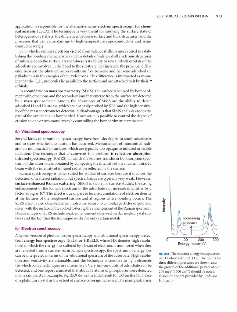
25.2 SURFACE COMPOSITION 913
application is responsible for the alternative name electron spectroscopy for chem-ical analysis (ESCA). The technique is very useful for studying the surface state of heterogeneous catalysts, the differences between surface and bulk structures, and theprocesses that can cause damage to high-temperature superconductors and semi-conductor wafers.
UPS, which examines electrons ejected from valence shells, is more suited to estab-lishing the bonding characteristics and the details of valence shell electronic structuresof substances on the surface. Its usefulness is its ability to reveal which orbitals of theadsorbate are involved in the bond to the substrate. For instance, the principal differ-ence between the photoemission results on free benzene and benzene adsorbed onpalladium is in the energies of the π electrons. This difference is interpreted as mean-ing that the C6H6 molecules lie parallel to the surface and are attached to it by their πorbitals.
In secondary-ion mass spectrometry (SIMS), the surface is ionized by bombard-ment with other ions and the secondary ions that emerge from the surface are detectedby a mass spectrometer. Among the advantages of SIMS are the ability to detect adsorbed H and He atoms, which are not easily probed by XPS, and the high sensitiv-ity of the mass spectrometer detector. A disadvantage is that SIMS analysis erodes thepart of the sample that is bombarded. However, it is possible to control the degree oferosion to one or two monolayers by controlling the bombardment parameters.
(b) Vibrational spectroscopy
Several kinds of vibrational spectroscopy have been developed to study adsorbatesand to show whether dissociation has occurred. Measurement of transmitted radi-ation is not practical in surfaces, which are typically too opaque to infrared or visibleradiation. One technique that circumvents this problem is reflection–absorptioninfrared spectroscopy (RAIRS), in which the Fourier-transform IR absorption spec-trum of the adsorbate is obtained by comparing the intensity of the incident infraredbeam with the intensity of infrared radiation reflected by the surface.
Raman spectroscopy is better suited for studies of surfaces because it involves thedetection of scattered radiation, but spectral bands are typically very weak. However,surface-enhanced Raman scattering (SERS) is viable for surface studies: the strongenhancement of the Raman spectrum of the adsorbate can increase intensities by afactor as big as 106. The effect is due in part to local accumulations of electron densityat the features of the roughened surface and at regions where bonding occurs. TheSERS effect is also observed when molecules adsorb to colloidal particles of gold andsilver, with the surface of the colloid fostering the enhancement of the Raman spectrum.Disadvantages of SERS include weak enhancement observed on flat single crystal sur-faces and the fact that the technique works for only certain metals.
(c) Electron spectroscopy
A hybrid version of photoemission spectroscopy and vibrational spectroscopy is elec-tron energy loss spectroscopy (EELS, or HREELS, where HR denotes high resolu-tion) in which the energy loss suffered by a beam of electrons is monitored when theyare reflected from a surface. As in Raman spectroscopy, the spectrum of energy losscan be interpreted in terms of the vibrational spectrum of the adsorbate. High resolu-tion and sensitivity are attainable, and the technique is sensitive to light elements (to which X-ray techniques are insensitive). Very tiny amounts of adsorbate can bedetected, and one report estimated that about 48 atoms of phosphorus were detectedin one sample. As an example, Fig. 25.9 shows the EELS result for CO on the (111) faceof a platinum crystal as the extent of surface coverage increases. The main peak arises
Fig. 25.9 The electron energy loss spectrumof CO adsorbed on Pt(111). The results forthree different pressures are shown, and the growth of the additional peak at about200 meV (1600 cm−1) should be noted.(Based on spectra provided by Professor H. Ibach.)
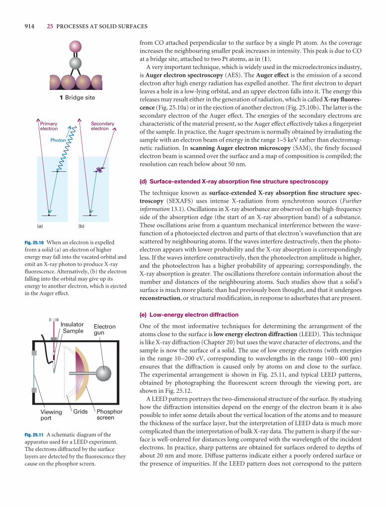
914 25 PROCESSES AT SOLID SURFACES
from CO attached perpendicular to the surface by a single Pt atom. As the coverage increases the neighbouring smaller peak increases in intensity. This peak is due to COat a bridge site, attached to two Pt atoms, as in (1).
A very important technique, which is widely used in the microelectronics industry,is Auger electron spectroscopy (AES). The Auger effect is the emission of a secondelectron after high energy radiation has expelled another. The first electron to departleaves a hole in a low-lying orbital, and an upper electron falls into it. The energy thisreleases may result either in the generation of radiation, which is called X-ray fluores-cence (Fig. 25.10a) or in the ejection of another electron (Fig. 25.10b). The latter is thesecondary electron of the Auger effect. The energies of the secondary electrons arecharacteristic of the material present, so the Auger effect effectively takes a fingerprintof the sample. In practice, the Auger spectrum is normally obtained by irradiating thesample with an electron beam of energy in the range 1–5 keV rather than electromag-netic radiation. In scanning Auger electron microscopy (SAM), the finely focusedelectron beam is scanned over the surface and a map of composition is compiled; theresolution can reach below about 50 nm.
(d) Surface-extended X-ray absorption fine structure spectroscopy
The technique known as surface-extended X-ray absorption fine structure spec-troscopy (SEXAFS) uses intense X-radiation from synchrotron sources (Furtherinformation 13.1). Oscillations in X-ray absorbance are observed on the high-frequencyside of the absorption edge (the start of an X-ray absorption band) of a substance.These oscillations arise from a quantum mechanical interference between the wave-function of a photoejected electron and parts of that electron’s wavefunction that arescattered by neighbouring atoms. If the waves interfere destructively, then the photo-electron appears with lower probability and the X-ray absorption is correspondinglyless. If the waves interfere constructively, then the photoelectron amplitude is higher,and the photoelectron has a higher probability of appearing; correspondingly, the X-ray absorption is greater. The oscillations therefore contain information about thenumber and distances of the neighbouring atoms. Such studies show that a solid’ssurface is much more plastic than had previously been thought, and that it undergoesreconstruction, or structural modification, in response to adsorbates that are present.
(e) Low-energy electron diffraction
One of the most informative techniques for determining the arrangement of theatoms close to the surface is low energy electron diffraction (LEED). This techniqueis like X-ray diffraction (Chapter 20) but uses the wave character of electrons, and thesample is now the surface of a solid. The use of low energy electrons (with energies in the range 10–200 eV, corresponding to wavelengths in the range 100–400 pm) ensures that the diffraction is caused only by atoms on and close to the surface. The experimental arrangement is shown in Fig. 25.11, and typical LEED patterns, obtained by photographing the fluorescent screen through the viewing port, areshown in Fig. 25.12.
A LEED pattern portrays the two-dimensional structure of the surface. By studyinghow the diffraction intensities depend on the energy of the electron beam it is alsopossible to infer some details about the vertical location of the atoms and to measurethe thickness of the surface layer, but the interpretation of LEED data is much morecomplicated than the interpretation of bulk X-ray data. The pattern is sharp if the sur-face is well-ordered for distances long compared with the wavelength of the incidentelectrons. In practice, sharp patterns are obtained for surfaces ordered to depths ofabout 20 nm and more. Diffuse patterns indicate either a poorly ordered surface orthe presence of impurities. If the LEED pattern does not correspond to the pattern
Fig. 25.11 A schematic diagram of theapparatus used for a LEED experiment.The electrons diffracted by the surfacelayers are detected by the fluorescence theycause on the phosphor screen.
Fig. 25.10 When an electron is expelled from a solid (a) an electron of higherenergy may fall into the vacated orbital andemit an X-ray photon to produce X-rayfluorescence. Alternatively, (b) the electronfalling into the orbital may give up itsenergy to another electron, which is ejectedin the Auger effect.
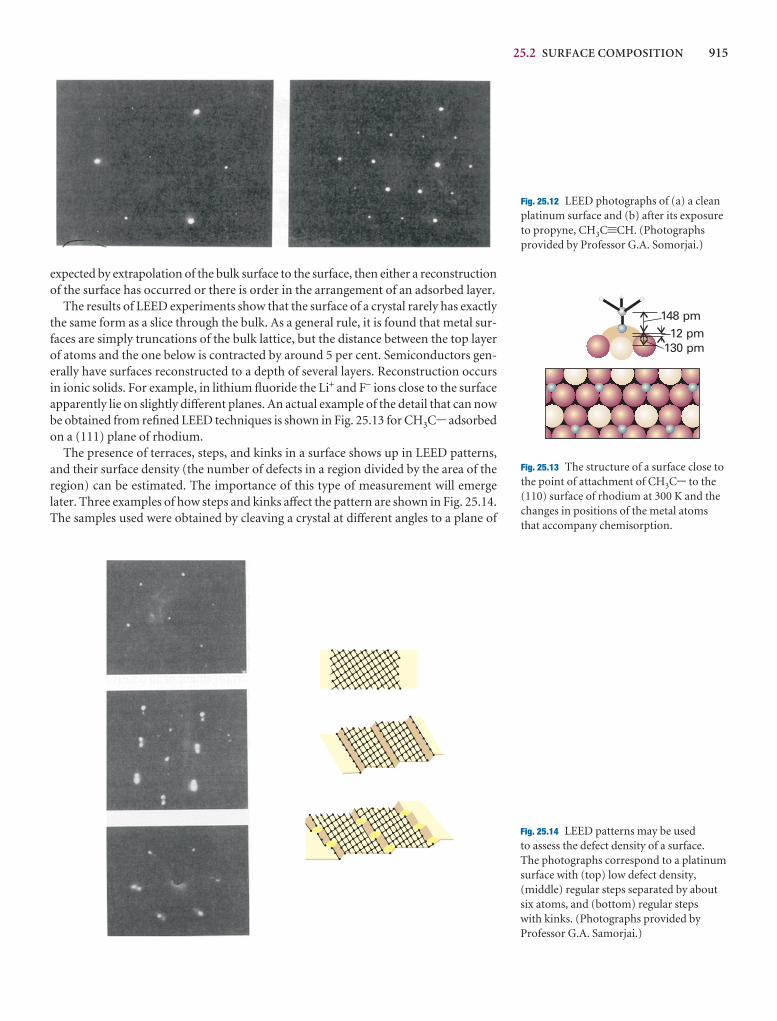
25.2 SURFACE COMPOSITION 915
Fig. 25.12 LEED photographs of (a) a cleanplatinum surface and (b) after its exposureto propyne, CH3C.CH. (Photographsprovided by Professor G.A. Somorjai.)
Fig. 25.13 The structure of a surface close tothe point of attachment of CH3C- to the(110) surface of rhodium at 300 K and thechanges in positions of the metal atomsthat accompany chemisorption.
Fig. 25.14 LEED patterns may be used to assess the defect density of a surface. The photographs correspond to a platinumsurface with (top) low defect density,(middle) regular steps separated by aboutsix atoms, and (bottom) regular steps with kinks. (Photographs provided byProfessor G.A. Samorjai.)
expected by extrapolation of the bulk surface to the surface, then either a reconstructionof the surface has occurred or there is order in the arrangement of an adsorbed layer.
The results of LEED experiments show that the surface of a crystal rarely has exactlythe same form as a slice through the bulk. As a general rule, it is found that metal sur-faces are simply truncations of the bulk lattice, but the distance between the top layerof atoms and the one below is contracted by around 5 per cent. Semiconductors gen-erally have surfaces reconstructed to a depth of several layers. Reconstruction occursin ionic solids. For example, in lithium fluoride the Li+ and F− ions close to the surfaceapparently lie on slightly different planes. An actual example of the detail that can nowbe obtained from refined LEED techniques is shown in Fig. 25.13 for CH3C- adsorbedon a (111) plane of rhodium.
The presence of terraces, steps, and kinks in a surface shows up in LEED patterns,and their surface density (the number of defects in a region divided by the area of theregion) can be estimated. The importance of this type of measurement will emergelater. Three examples of how steps and kinks affect the pattern are shown in Fig. 25.14.The samples used were obtained by cleaving a crystal at different angles to a plane of
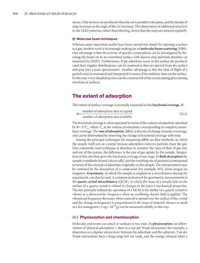
916 25 PROCESSES AT SOLID SURFACES
atoms. Only terraces are produced when the cut is parallel to the plane, and the density ofsteps increases as the angle of the cut increases. The observation of additional structurein the LEED patterns, rather than blurring, shows that the steps are arrayed regularly.
(f) Molecular beam techniques
Whereas many important studies have been carried out simply by exposing a surfaceto a gas, modern work is increasingly making use of molecular beam scattering (MBS).One advantage is that the activity of specific crystal planes can be investigated by dir-ecting the beam on to an orientated surface with known step and kink densities (asmeasured by LEED). Furthermore, if the adsorbate reacts at the surface the products(and their angular distributions) can be analysed as they are ejected from the surfaceand pass into a mass spectrometer. Another advantage is that the time of flight of aparticle may be measured and interpreted in terms of its residence time on the surface.In this way a very detailed picture can be constructed of the events taking place duringreactions at surfaces.
The extent of adsorption
The extent of surface coverage is normally expressed as the fractional coverage, θ :
θ = [25.2]
The fractional coverage is often expressed in terms of the volume of adsorbate adsorbedby θ = V/V∞, where V∞ is the volume of adsorbate corresponding to complete mono-layer coverage. The rate of adsorption, dθ/dt, is the rate of change of surface coverage,and can be determined by observing the change of fractional coverage with time.
Among the principal techniques for measuring dθ/dt are flow methods, in whichthe sample itself acts as a pump because adsorption removes particles from the gas.One commonly used technique is therefore to monitor the rates of flow of gas intoand out of the system: the difference is the rate of gas uptake by the sample. Integra-tion of this rate then gives the fractional coverage at any stage. In flash desorption thesample is suddenly heated (electrically) and the resulting rise of pressure is interpretedin terms of the amount of adsorbate originally on the sample. The interpretation maybe confused by the desorption of a compound (for example, WO3 from oxygen ontungsten). Gravimetry, in which the sample is weighed on a microbalance during theexperiment, can also be used. A common instrument for gravimetric measurements isthe quartz crystal microbalance (QCM), in which the mass of a sample laid on thesurface of a quartz crystal is related to changes in the latter’s mechanical properties.The key principle behind the operation of a QCM is the ability of a quartz crystal to vibrate at a characteristic frequency when an oscillating electric field is applied. Thevibrational frequency decreases when material is spread over the surface of the crystaland the change in frequency is proportional to the mass of material. Masses as smallas a few nanograms (1 ng = 10−9 g) can be measured reliably in this way.
25.3 Physisorption and chemisorption
Molecules and atoms can attach to surfaces in two ways. In physisorption (an abbre-viation of ‘physical adsorption’), there is a van der Waals interaction (for example, adispersion or a dipolar interaction) between the adsorbate and the substrate. Van derWaals interactions have a long range but are weak, and the energy released when a
number of adsorption sites occupied
number of adsorption sites available

25.4 ADSORPTION ISOTHERMS 917
particle is physisorbed is of the same order of magnitude as the enthalpy of condensa-tion. Such small energies can be absorbed as vibrations of the lattice and dissipated as thermal motion, and a molecule bouncing across the surface will gradually lose its energy and finally adsorb to it in the process called accommodation. The enthalpy ofphysisorption can be measured by monitoring the rise in temperature of a sample ofknown heat capacity, and typical values are in the region of 20 kJ mol−1 (Table 25.1).This small enthalpy change is insufficient to lead to bond breaking, so a physisorbedmolecule retains its identity, although it might be distorted by the presence of the surface.
In chemisorption (an abbreviation of ‘chemical adsorption’), the molecules (oratoms) stick to the surface by forming a chemical (usually covalent) bond, and tend tofind sites that maximize their coordination number with the substrate. The enthalpyof chemisorption is very much greater than that for physisorption, and typical valuesare in the region of 200 kJ mol−1 (Table 25.2). The distance between the surfaceand the closest adsorbate atom is also typically shorter for chemisorption than for physisorption. A chemisorbed molecule may be torn apart at the demand of the unsatisfied valencies of the surface atoms, and the existence of molecular fragmentson the surface as a result of chemisorption is one reason why solid surfaces catalyse reactions.
Except in special cases, chemisorption must be exothermic. A spontaneous processrequires ∆G < 0. Because the translational freedom of the adsorbate is reduced whenit is adsorbed, ∆S is negative. Therefore, in order for ∆G = ∆H − T∆S to be negative,∆H must be negative (that is, the process is exothermic). Exceptions may occur if theadsorbate dissociates and has high translational mobility on the surface. For example,H2 adsorbs endothermically on glass because there is a large increase of translationalentropy accompanying the dissociation of the molecules into atoms that move quitefreely over the surface. In its case, the entropy change in the process H2(g) → 2 H(glass)is sufficiently positive to overcome the small positive enthalpy change.
The enthalpy of adsorption depends on the extent of surface coverage, mainly because the adsorbate particles interact. If the particles repel each other (as for CO onpalladium) the adsorption becomes less exothermic (the enthalpy of adsorption lessnegative) as coverage increases. Moreover, LEED studies show that such species settleon the surface in a disordered way until packing requirements demand order. If theadsorbate particles attract one another (as for O2 on tungsten), then they tend to clus-ter together in islands, and growth occurs at the borders. These adsorbates also showorder–disorder transitions when they are heated enough for thermal motion to over-come the particle–particle interactions, but not so much that they are desorbed.
25.4 Adsorption isotherms
The free gas and the adsorbed gas are in dynamic equilibrium, and the fractional cov-erage of the surface depends on the pressure of the overlying gas. The variation of θwith pressure at a chosen temperature is called the adsorption isotherm.
(a) The Langmuir isotherm
The simplest physically plausible isotherm is based on three assumptions:
1 Adsorption cannot proceed beyond monolayer coverage.
2 All sites are equivalent and the surface is uniform (that is, the surface is perfectlyflat on a microscopic scale).
3 The ability of a molecule to adsorb at a given site is independent of the occupationof neighbouring sites (that is, there are no interactions between adsorbed molecules).
Synoptic table 25.1* Maximumobserved enthalpies of physisorption
Adsorbate Dad H 7/(kJ mol−1)
CH4 −21
H2 −84
H2O −59
N2 −21
* More values are given in the Data section.
Synoptic table 25.2* Enthalpies ofchemisorption, ∆adH 7/(kJ mol−1)
Adsorbate Adsorbent (substrate)
Cr Fe Ni
CH4 −427 −285 −243
CO −192
H2 −188 −134
NH3 −188 −155
* More values are given in the Data section.
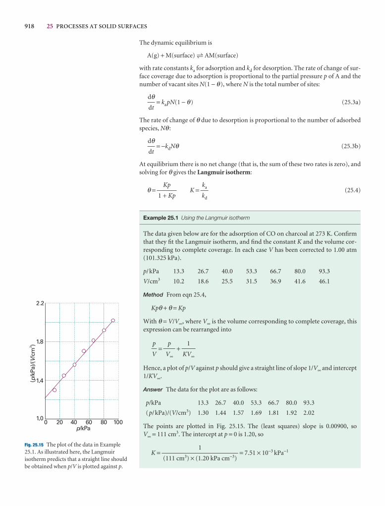
918 25 PROCESSES AT SOLID SURFACES
Fig. 25.15 The plot of the data in Example25.1. As illustrated here, the Langmuirisotherm predicts that a straight line shouldbe obtained when p/V is plotted against p.
The dynamic equilibrium is
A(g) + M(surface) 5 AM(surface)
with rate constants ka for adsorption and kd for desorption. The rate of change of sur-face coverage due to adsorption is proportional to the partial pressure p of A and thenumber of vacant sites N(1 − θ), where N is the total number of sites:
= kapN(1 − θ) (25.3a)
The rate of change of θ due to desorption is proportional to the number of adsorbedspecies, Nθ :
= −kdNθ (25.3b)
At equilibrium there is no net change (that is, the sum of these two rates is zero), andsolving for θ gives the Langmuir isotherm:
θ = K = (25.4)
Example 25.1 Using the Langmuir isotherm
The data given below are for the adsorption of CO on charcoal at 273 K. Confirmthat they fit the Langmuir isotherm, and find the constant K and the volume cor-responding to complete coverage. In each case V has been corrected to 1.00 atm(101.325 kPa).
p/kPa 13.3 26.7 40.0 53.3 66.7 80.0 93.3
V/cm3 10.2 18.6 25.5 31.5 36.9 41.6 46.1
Method From eqn 25.4,
Kpθ + θ = Kp
With θ = V/V∞, where V∞ is the volume corresponding to complete coverage, thisexpression can be rearranged into
= +
Hence, a plot of p/V against p should give a straight line of slope 1/V∞ and intercept1/KV∞.
Answer The data for the plot are as follows:
p/kPa 13.3 26.7 40.0 53.3 66.7 80.0 93.3
(p/kPa)/(V/cm3) 1.30 1.44 1.57 1.69 1.81 1.92 2.02
The points are plotted in Fig. 25.15. The (least squares) slope is 0.00900, so V∞ = 111 cm3. The intercept at p = 0 is 1.20, so
K = = 7.51 × 10⁻³ kPa−11
(111 cm3) × (1.20 kPa cm−3)
1
KV∞
p
V∞
p
V
ka
kd
Kp
1 + Kp
dθdt
dθdt
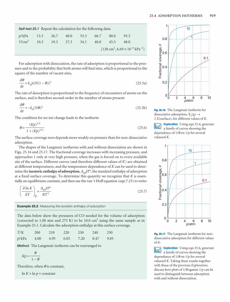
25.4 ADSORPTION ISOTHERMS 919
Fig. 25.17 The Langmuir isotherm for non-dissociative adsorption for different valuesof K.
Exploration Using eqn 25.6, generatea family of curves showing the
dependence of 1/θ on 1/p for severalvaluesof K. Taking these results togetherwith those of the previous Exploration,discuss how plots of 1/θ against 1/p can beused to distinguish between adsorptionwith and without dissociation.
Fig. 25.16 The Langmuir isotherm fordissociative adsorption, X2(g) →2 X(surface), for different values of K.
Exploration Using eqn 25.4, generatea family of curves showing the
dependence of 1/θ on 1/p for severalvaluesof K.
Self-test 25.1 Repeat the calculation for the following data:
p/kPa 13.3 26.7 40.0 53.3 66.7 80.0 93.3
V/cm3 10.3 19.3 27.3 34.1 40.0 45.5 48.0
[128 cm3, 6.69 × 10⁻³ kPa−1]
For adsorption with dissociation, the rate of adsorption is proportional to the pres-sure and to the probability that both atoms will find sites, which is proportional to thesquare of the number of vacant sites,
= ka p{N(1 − θ)}2 (25.5a)
The rate of desorption is proportional to the frequency of encounters of atoms on thesurface, and is therefore second-order in the number of atoms present:
= −kd(Nθ)2 (25.5b)
The condition for no net change leads to the isotherm
θ = (25.6)
The surface coverage now depends more weakly on pressure than for non-dissociativeadsorption.
The shapes of the Langmuir isotherms with and without dissociation are shown inFigs. 25.16 and 25.17. The fractional coverage increases with increasing pressure, andapproaches 1 only at very high pressure, when the gas is forced on to every availablesite of the surface. Different curves (and therefore different values of K) are obtainedat different temperatures, and the temperature dependence of K can be used to deter-mine the isosteric enthalpy of adsorption, ∆adH7, the standard enthalpy of adsorptionat a fixed surface coverage. To determine this quantity we recognize that K is essen-tially an equilibrium constant, and then use the van ’t Hoff equation (eqn 7.23) to write:
θ
= (25.7)
Example 25.2 Measuring the isosteric enthalpy of adsorption
The data below show the pressures of CO needed for the volume of adsorption(corrected to 1.00 atm and 273 K) to be 10.0 cm3 using the same sample as inExample 25.1. Calculate the adsorption enthalpy at this surface coverage.
T/K 200 210 220 230 240 250
p/kPa 4.00 4.95 6.03 7.20 8.47 9.85
Method The Langmuir isotherm can be rearranged to
Kp =
Therefore, when θ is constant,
ln K + ln p = constant
θ1 − θ
∆adH 7
RT 2
DF
∂ ln K
∂T
AC
(Kp)1/2
1 + (Kp)1/2
dθdt
dθdt
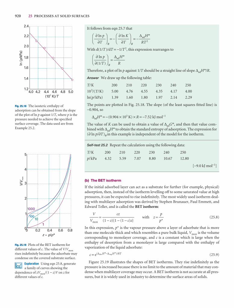
920 25 PROCESSES AT SOLID SURFACES
Fig. 25.18 The isosteric enthalpy ofadsorption can be obtained from the slopeof the plot of ln p against 1/T, where p is thepressure needed to achieve the specifiedsurface coverage. The data used are from Example 25.2.
Fig. 25.19 Plots of the BET isotherm fordifferent values of c. The value of V/Vmon
rises indefinitely because the adsorbate maycondense on the covered substrate surface.
Exploration Using eqn 25.8, generatea family of curves showing the
dependence of zVmon/(1 − z)V on z fordifferent values of c.
It follows from eqn 25.7 that
θ
= −θ
= −
With d(1/T)/dT = −1/T 2, this expression rearranges to
θ
=
Therefore, a plot of ln p against 1/T should be a straight line of slope ∆adH 7/R.
Answer We draw up the following table:
T/K 200 210 220 230 240 250
103/(T/K) 5.00 4.76 4.55 4.35 4.17 4.00
ln(p/kPa) 1.39 1.60 1.80 1.97 2.14 2.29
The points are plotted in Fig. 25.18. The slope (of the least squares fitted line) is −0.904, so
∆adH 7 = −(0.904 × 10³ K) × R = −7.52 kJ mol−1
The value of K can be used to obtain a value of ∆adG 7, and then that value com-bined with ∆adH 7 to obtain the standard entropy of adsorption. The expression for(∂ ln p/∂T)θ in this example is independent of the model for the isotherm.
Self-test 25.2 Repeat the calculation using the following data:
T/K 200 210 220 230 240 250
p/kPa 4.32 5.59 7.07 8.80 10.67 12.80
[−9.0 kJ mol−1]
(b) The BET isotherm
If the initial adsorbed layer can act as a substrate for further (for example, physical)adsorption, then, instead of the isotherm levelling off to some saturated value at highpressures, it can be expected to rise indefinitely. The most widely used isotherm deal-ing with multilayer adsorption was derived by Stephen Brunauer, Paul Emmett, andEdward Teller, and is called the BET isotherm:
= with z = (25.8)
In this expression, p* is the vapour pressure above a layer of adsorbate that is morethan one molecule thick and which resembles a pure bulk liquid, Vmon is the volumecorresponding to monolayer coverage, and c is a constant which is large when the enthalpy of desorption from a monolayer is large compared with the enthalpy of vaporization of the liquid adsorbate:
c = e(∆desH7−∆vapH 7)/RT (25.9)
Figure 25.19 illustrates the shapes of BET isotherms. They rise indefinitely as thepressure is increased because there is no limit to the amount of material that may con-dense when multilayer coverage may occur. A BET isotherm is not accurate at all pres-sures, but it is widely used in industry to determine the surface areas of solids.
p
p*
cz
(1 − z){1 − (1 − c)z}
V
Vmon
∆adH 7
R
DF
∂ ln p
∂(1/T)
AC
∆adH 7
RT 2
DF
∂ ln K
∂T
AC
DF
∂ ln p
∂T
AC
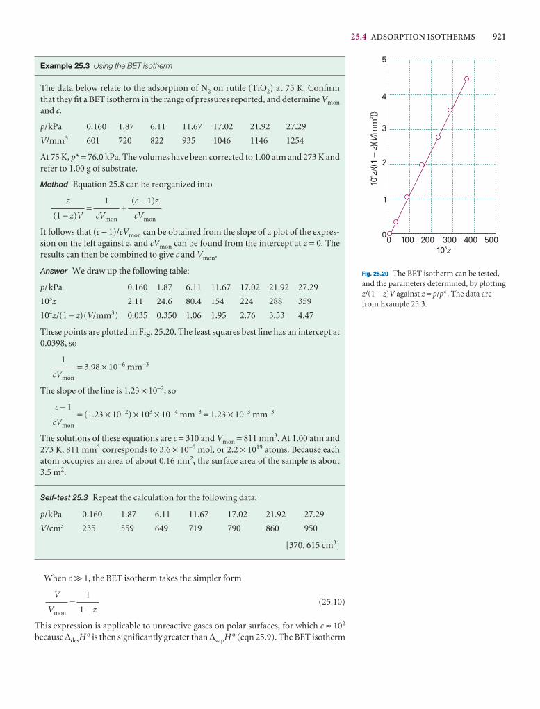
25.4 ADSORPTION ISOTHERMS 921
Fig. 25.20 The BET isotherm can be tested,and the parameters determined, by plotting z/(1 − z)V against z = p/p*. The data are from Example 25.3.
Example 25.3 Using the BET isotherm
The data below relate to the adsorption of N2 on rutile (TiO2) at 75 K. Confirm that they fit a BET isotherm in the range of pressures reported, and determine Vmon
and c.
p/kPa 0.160 1.87 6.11 11.67 17.02 21.92 27.29
V/mm3 601 720 822 935 1046 1146 1254
At 75 K, p* = 76.0 kPa. The volumes have been corrected to 1.00 atm and 273 K andrefer to 1.00 g of substrate.
Method Equation 25.8 can be reorganized into
= +
It follows that (c − 1)/cVmon can be obtained from the slope of a plot of the expres-sion on the left against z, and cVmon can be found from the intercept at z = 0. Theresults can then be combined to give c and Vmon.
Answer We draw up the following table:
p/kPa 0.160 1.87 6.11 11.67 17.02 21.92 27.29
103z 2.11 24.6 80.4 154 224 288 359
104z/(1 − z)(V/mm3) 0.035 0.350 1.06 1.95 2.76 3.53 4.47
These points are plotted in Fig. 25.20. The least squares best line has an intercept at0.0398, so
= 3.98 × 10⁻⁶ mm−3
The slope of the line is 1.23 × 10⁻², so
= (1.23 × 10−2) × 103 × 10−4 mm−3 = 1.23 × 10⁻³ mm−3
The solutions of these equations are c = 310 and Vmon = 811 mm3. At 1.00 atm and273 K, 811 mm3 corresponds to 3.6 × 10⁻⁵ mol, or 2.2 × 10¹⁹ atoms. Because eachatom occupies an area of about 0.16 nm2, the surface area of the sample is about 3.5 m2.
Self-test 25.3 Repeat the calculation for the following data:
p/kPa 0.160 1.87 6.11 11.67 17.02 21.92 27.29
V/cm3 235 559 649 719 790 860 950
[370, 615 cm3]
When c >> 1, the BET isotherm takes the simpler form
= (25.10)
This expression is applicable to unreactive gases on polar surfaces, for which c ≈ 102
because ∆desH7 is then significantly greater than ∆vapH 7 (eqn 25.9). The BET isotherm
1
1 − z
V
Vmon
c − 1
cVmon
1
cVmon
(c − 1)z
cVmon
1
cVmon
z
(1 − z)V
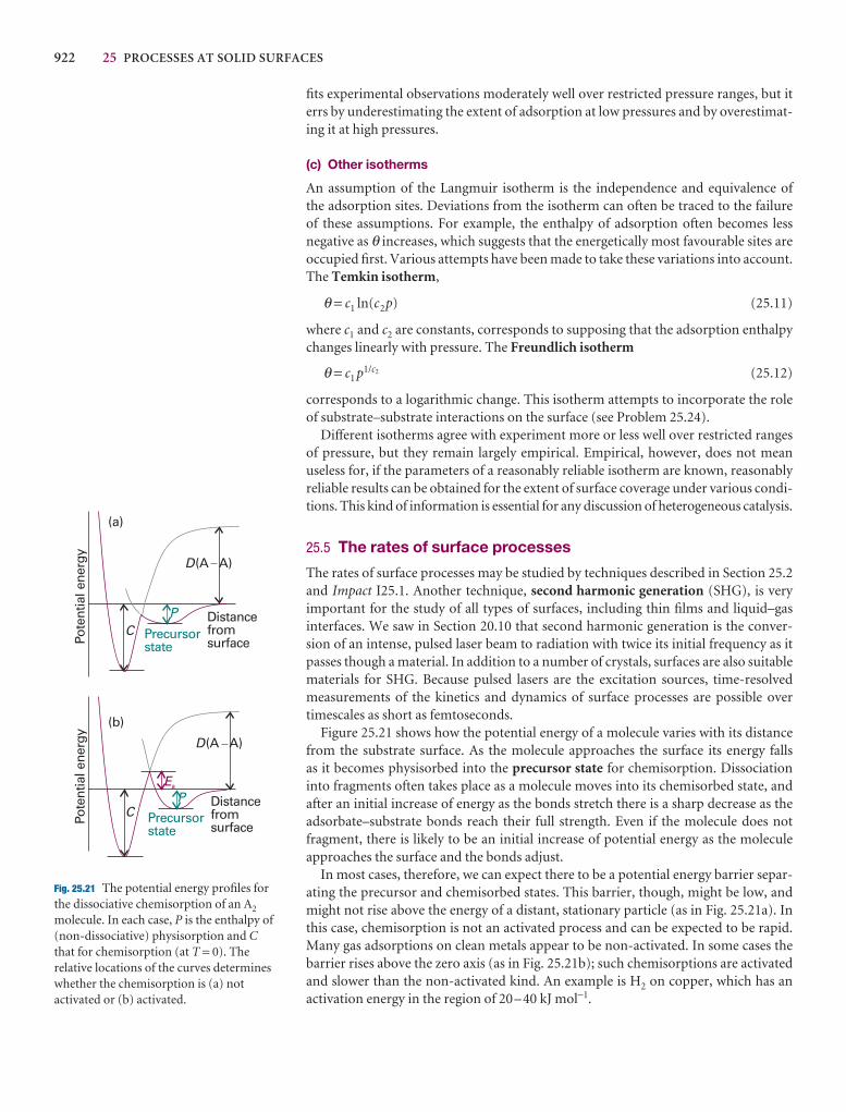
922 25 PROCESSES AT SOLID SURFACES
fits experimental observations moderately well over restricted pressure ranges, but iterrs by underestimating the extent of adsorption at low pressures and by overestimat-ing it at high pressures.
(c) Other isotherms
An assumption of the Langmuir isotherm is the independence and equivalence of the adsorption sites. Deviations from the isotherm can often be traced to the failure of these assumptions. For example, the enthalpy of adsorption often becomes lessnegative as θ increases, which suggests that the energetically most favourable sites are occupied first. Various attempts have been made to take these variations into account.The Temkin isotherm,
θ = c1 ln(c2p) (25.11)
where c1 and c2 are constants, corresponds to supposing that the adsorption enthalpychanges linearly with pressure. The Freundlich isotherm
θ = c1 p1/c2 (25.12)
corresponds to a logarithmic change. This isotherm attempts to incorporate the roleof substrate–substrate interactions on the surface (see Problem 25.24).
Different isotherms agree with experiment more or less well over restricted rangesof pressure, but they remain largely empirical. Empirical, however, does not meanuseless for, if the parameters of a reasonably reliable isotherm are known, reasonablyreliable results can be obtained for the extent of surface coverage under various condi-tions. This kind of information is essential for any discussion of heterogeneous catalysis.
25.5 The rates of surface processes
The rates of surface processes may be studied by techniques described in Section 25.2and Impact I25.1. Another technique, second harmonic generation (SHG), is veryimportant for the study of all types of surfaces, including thin films and liquid–gas interfaces. We saw in Section 20.10 that second harmonic generation is the conver-sion of an intense, pulsed laser beam to radiation with twice its initial frequency as it passes though a material. In addition to a number of crystals, surfaces are also suitablematerials for SHG. Because pulsed lasers are the excitation sources, time-resolvedmeasurements of the kinetics and dynamics of surface processes are possible overtimescales as short as femtoseconds.
Figure 25.21 shows how the potential energy of a molecule varies with its distancefrom the substrate surface. As the molecule approaches the surface its energy falls as it becomes physisorbed into the precursor state for chemisorption. Dissociationinto fragments often takes place as a molecule moves into its chemisorbed state, andafter an initial increase of energy as the bonds stretch there is a sharp decrease as theadsorbate–substrate bonds reach their full strength. Even if the molecule does notfragment, there is likely to be an initial increase of potential energy as the molecule approaches the surface and the bonds adjust.
In most cases, therefore, we can expect there to be a potential energy barrier separ-ating the precursor and chemisorbed states. This barrier, though, might be low, andmight not rise above the energy of a distant, stationary particle (as in Fig. 25.21a). Inthis case, chemisorption is not an activated process and can be expected to be rapid.Many gas adsorptions on clean metals appear to be non-activated. In some cases thebarrier rises above the zero axis (as in Fig. 25.21b); such chemisorptions are activatedand slower than the non-activated kind. An example is H2 on copper, which has an activation energy in the region of 20–40 kJ mol−1.
Fig. 25.21 The potential energy profiles forthe dissociative chemisorption of an A2
molecule. In each case, P is the enthalpy of(non-dissociative) physisorption and Cthat for chemisorption (at T = 0). Therelative locations of the curves determineswhether the chemisorption is (a) notactivated or (b) activated.
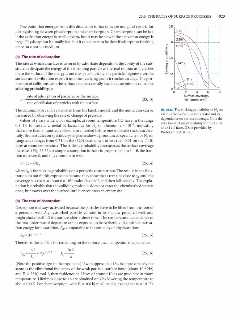
25.5 THE RATES OF SURFACE PROCESSES 923
One point that emerges from this discussion is that rates are not good criteria fordistinguishing between physisorption and chemisorption. Chemisorption can be fastif the activation energy is small or zero, but it may be slow if the activation energy islarge. Physisorption is usually fast, but it can appear to be slow if adsorption is takingplace on a porous medium.
(a) The rate of adsorption
The rate at which a surface is covered by adsorbate depends on the ability of the sub-strate to dissipate the energy of the incoming particle as thermal motion as it crasheson to the surface. If the energy is not dissipated quickly, the particle migrates over thesurface until a vibration expels it into the overlying gas or it reaches an edge. The pro-portion of collisions with the surface that successfully lead to adsorption is called thesticking probability, s:
s = [25.13]
The denominator can be calculated from the kinetic model, and the numerator can bemeasured by observing the rate of change of pressure.
Values of s vary widely. For example, at room temperature CO has s in the range0.1–1.0 for several d-metal surfaces, but for N2 on rhenium s < 10−2, indicating that more than a hundred collisions are needed before one molecule sticks success-fully. Beam studies on specific crystal planes show a pronounced specificity: for N2 ontungsten, s ranges from 0.74 on the (320) faces down to less than 0.01 on the (110)faces at room temperature. The sticking probability decreases as the surface coverageincreases (Fig. 25.22). A simple assumption is that s is proportional to 1 − θ, the frac-tion uncovered, and it is common to write
s = (1 − θ)s0 (25.14)
where s0 is the sticking probability on a perfectly clean surface. The results in the illus-tration do not fit this expression because they show that s remains close to s0 until thecoverage has risen to about 6 × 10¹³ molecules cm−2, and then falls steeply. The expla-nation is probably that the colliding molecule does not enter the chemisorbed state atonce, but moves over the surface until it encounters an empty site.
(b) The rate of desorption
Desorption is always activated because the particles have to be lifted from the foot ofa potential well. A physisorbed particle vibrates in its shallow potential well, andmight shake itself off the surface after a short time. The temperature dependence ofthe first-order rate of departure can be expected to be Arrhenius-like, with an activa-tion energy for desorption, Ed, comparable to the enthalpy of physisorption:
kd = Ae−Ed/RT (25.15)
Therefore, the half-life for remaining on the surface has a temperature dependence
t1/2 = = τ0eEd/RT τ0 = (25.16)
(Note the positive sign in the exponent.) If we suppose that 1/τ0 is approximately thesame as the vibrational frequency of the weak particle–surface bond (about 1012 Hz)and Ed ≈ 25 kJ mol−1, then residence half-lives of around 10 ns are predicted at roomtemperature. Lifetimes close to 1 s are obtained only by lowering the temperature toabout 100 K. For chemisorption, with Ed = 100 kJ mol−1 and guessing that τ0 = 10−14 s
ln 2
A
ln 2
kd
rate of adsorption of particles by the surface
rate of collision of particles with the surface
Fig. 25.22 The sticking probability of N2 onvarious faces of a tungsten crystal and itsdependence on surface coverage. Note thevery low sticking probability for the (110)and (111) faces. (Data provided byProfessor D.A. King.)
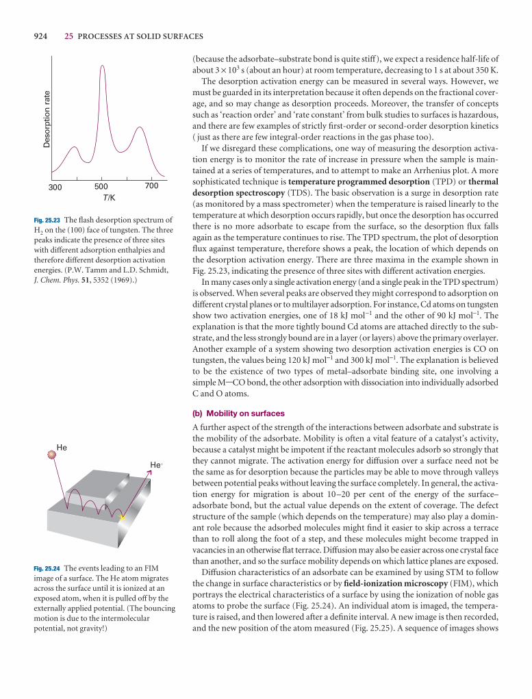
924 25 PROCESSES AT SOLID SURFACES
(because the adsorbate–substrate bond is quite stiff), we expect a residence half-life ofabout 3 × 10³ s (about an hour) at room temperature, decreasing to 1 s at about 350 K.
The desorption activation energy can be measured in several ways. However, wemust be guarded in its interpretation because it often depends on the fractional cover-age, and so may change as desorption proceeds. Moreover, the transfer of conceptssuch as ‘reaction order’ and ‘rate constant’ from bulk studies to surfaces is hazardous,and there are few examples of strictly first-order or second-order desorption kinetics( just as there are few integral-order reactions in the gas phase too).
If we disregard these complications, one way of measuring the desorption activa-tion energy is to monitor the rate of increase in pressure when the sample is main-tained at a series of temperatures, and to attempt to make an Arrhenius plot. A moresophisticated technique is temperature programmed desorption (TPD) or thermaldesorption spectroscopy (TDS). The basic observation is a surge in desorption rate(as monitored by a mass spectrometer) when the temperature is raised linearly to thetemperature at which desorption occurs rapidly, but once the desorption has occurredthere is no more adsorbate to escape from the surface, so the desorption flux fallsagain as the temperature continues to rise. The TPD spectrum, the plot of desorptionflux against temperature, therefore shows a peak, the location of which depends onthe desorption activation energy. There are three maxima in the example shown inFig. 25.23, indicating the presence of three sites with different activation energies.
In many cases only a single activation energy (and a single peak in the TPD spectrum)is observed. When several peaks are observed they might correspond to adsorption ondifferent crystal planes or to multilayer adsorption. For instance, Cd atoms on tungstenshow two activation energies, one of 18 kJ mol−1 and the other of 90 kJ mol−1. The explanation is that the more tightly bound Cd atoms are attached directly to the sub-strate, and the less strongly bound are in a layer (or layers) above the primary overlayer.Another example of a system showing two desorption activation energies is CO ontungsten, the values being 120 kJ mol−1 and 300 kJ mol−1. The explanation is believedto be the existence of two types of metal–adsorbate binding site, one involving a simple M-CO bond, the other adsorption with dissociation into individually adsorbedC and O atoms.
(b) Mobility on surfaces
A further aspect of the strength of the interactions between adsorbate and substrate isthe mobility of the adsorbate. Mobility is often a vital feature of a catalyst’s activity,because a catalyst might be impotent if the reactant molecules adsorb so strongly thatthey cannot migrate. The activation energy for diffusion over a surface need not be the same as for desorption because the particles may be able to move through valleys between potential peaks without leaving the surface completely. In general, the activa-tion energy for migration is about 10–20 per cent of the energy of the surface–adsorbate bond, but the actual value depends on the extent of coverage. The defectstructure of the sample (which depends on the temperature) may also play a domin-ant role because the adsorbed molecules might find it easier to skip across a terracethan to roll along the foot of a step, and these molecules might become trapped in vacancies in an otherwise flat terrace. Diffusion may also be easier across one crystal facethan another, and so the surface mobility depends on which lattice planes are exposed.
Diffusion characteristics of an adsorbate can be examined by using STM to followthe change in surface characteristics or by field-ionization microscopy (FIM), whichportrays the electrical characteristics of a surface by using the ionization of noble gasatoms to probe the surface (Fig. 25.24). An individual atom is imaged, the tempera-ture is raised, and then lowered after a definite interval. A new image is then recorded,and the new position of the atom measured (Fig. 25.25). A sequence of images shows
Fig. 25.23 The flash desorption spectrum ofH2 on the (100) face of tungsten. The threepeaks indicate the presence of three siteswith different adsorption enthalpies andtherefore different desorption activationenergies. (P.W. Tamm and L.D. Schmidt, J. Chem. Phys. 51, 5352 (1969).)
Fig. 25.24 The events leading to an FIMimage of a surface. The He atom migratesacross the surface until it is ionized at anexposed atom, when it is pulled off by theexternally applied potential. (The bouncingmotion is due to the intermolecularpotential, not gravity!)
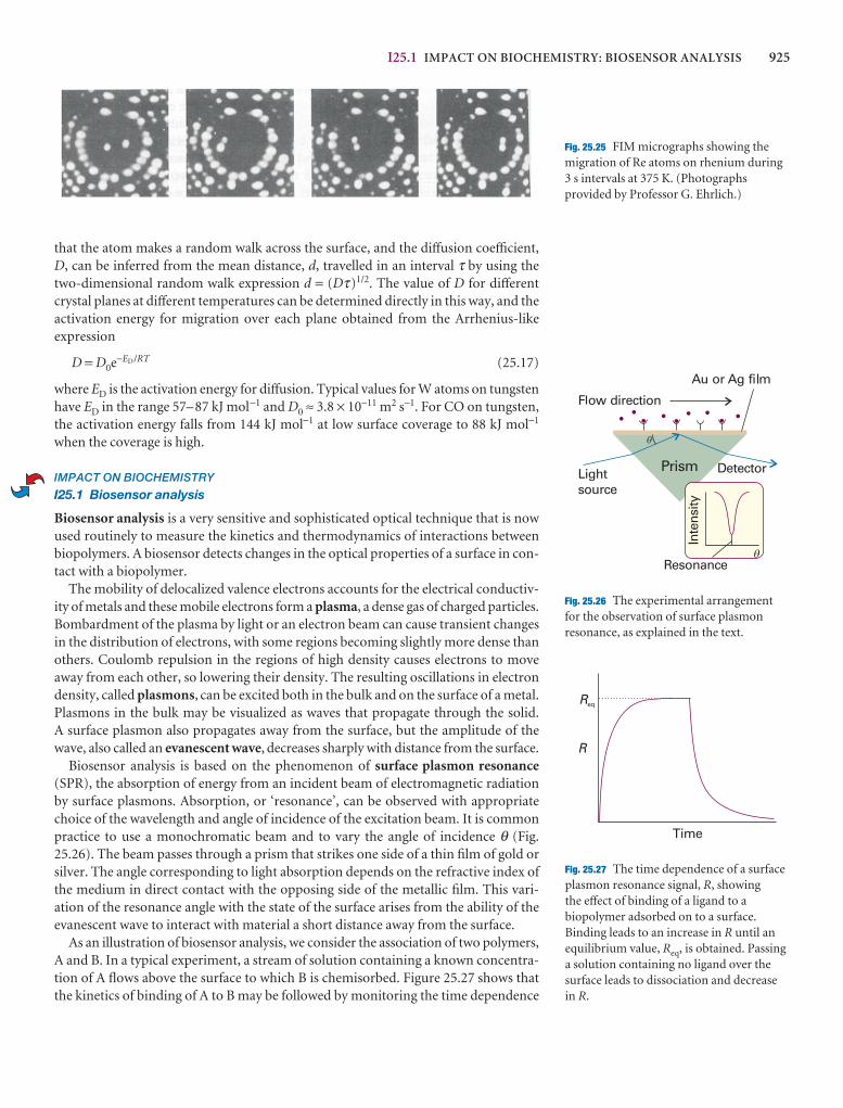
I25.1 IMPACT ON BIOCHEMISTRY: BIOSENSOR ANALYSIS 925
that the atom makes a random walk across the surface, and the diffusion coefficient,D, can be inferred from the mean distance, d, travelled in an interval τ by using thetwo-dimensional random walk expression d = (Dτ)1/2. The value of D for differentcrystal planes at different temperatures can be determined directly in this way, and theactivation energy for migration over each plane obtained from the Arrhenius-like expression
D = D0e−ED/RT (25.17)
where ED is the activation energy for diffusion. Typical values for W atoms on tungstenhave ED in the range 57–87 kJ mol−1 and D0 ≈ 3.8 × 10⁻¹¹ m2 s−1. For CO on tungsten,the activation energy falls from 144 kJ mol−1 at low surface coverage to 88 kJ mol−1
when the coverage is high.
IMPACT ON BIOCHEMISTRY
I25.1 Biosensor analysis
Biosensor analysis is a very sensitive and sophisticated optical technique that is nowused routinely to measure the kinetics and thermodynamics of interactions betweenbiopolymers. A biosensor detects changes in the optical properties of a surface in con-tact with a biopolymer.
The mobility of delocalized valence electrons accounts for the electrical conductiv-ity of metals and these mobile electrons form a plasma, a dense gas of charged particles.Bombardment of the plasma by light or an electron beam can cause transient changesin the distribution of electrons, with some regions becoming slightly more dense thanothers. Coulomb repulsion in the regions of high density causes electrons to moveaway from each other, so lowering their density. The resulting oscillations in electrondensity, called plasmons, can be excited both in the bulk and on the surface of a metal.Plasmons in the bulk may be visualized as waves that propagate through the solid. A surface plasmon also propagates away from the surface, but the amplitude of thewave, also called an evanescent wave, decreases sharply with distance from the surface.
Biosensor analysis is based on the phenomenon of surface plasmon resonance(SPR), the absorption of energy from an incident beam of electromagnetic radiationby surface plasmons. Absorption, or ‘resonance’, can be observed with appropriatechoice of the wavelength and angle of incidence of the excitation beam. It is commonpractice to use a monochromatic beam and to vary the angle of incidence θ (Fig.25.26). The beam passes through a prism that strikes one side of a thin film of gold orsilver. The angle corresponding to light absorption depends on the refractive index ofthe medium in direct contact with the opposing side of the metallic film. This vari-ation of the resonance angle with the state of the surface arises from the ability of theevanescent wave to interact with material a short distance away from the surface.
As an illustration of biosensor analysis, we consider the association of two polymers,A and B. In a typical experiment, a stream of solution containing a known concentra-tion of A flows above the surface to which B is chemisorbed. Figure 25.27 shows thatthe kinetics of binding of A to B may be followed by monitoring the time dependence
Fig. 25.25 FIM micrographs showing themigration of Re atoms on rhenium during3 s intervals at 375 K. (Photographsprovided by Professor G. Ehrlich.)
Fig. 25.26 The experimental arrangementfor the observation of surface plasmonresonance, as explained in the text.
Fig. 25.27 The time dependence of a surfaceplasmon resonance signal, R, showing the effect of binding of a ligand to abiopolymer adsorbed on to a surface.Binding leads to an increase in R until anequilibrium value, Req, is obtained. Passinga solution containing no ligand over thesurface leads to dissociation and decreasein R.
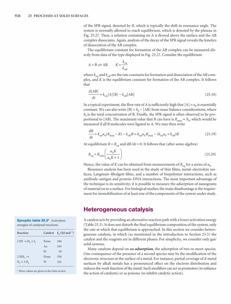
926 25 PROCESSES AT SOLID SURFACES
of the SPR signal, denoted by R, which is typically the shift in resonance angle. Thesystem is normally allowed to reach equilibrium, which is denoted by the plateau inFig. 25.27. Then, a solution containing no A is flowed above the surface and the ABcomplex dissociates. Again, analysis of the decay of the SPR signal reveals the kineticsof dissociation of the AB complex.
The equilibrium constant for formation of the AB complex can be measured dir-ectly from data of the type displayed in Fig. 25.27. Consider the equilibrium
A + B 5 AB K =
where kon and koff are the rate constants for formation and dissociation of the AB com-plex, and K is the equilibrium constant for formation of the AB complex. It followsthat
= kon[A][B] − koff[AB] (25.18)
In a typical experiment, the flow rate of A is sufficiently high that [A] = a0 is essentiallyconstant. We can also write [B] = b0 − [AB] from mass-balance considerations, whereb0 is the total concentration of B. Finally, the SPR signal is often observed to be pro-portional to [AB]. The maximum value that R can have is Rmax ∝ b0, which would bemeasured if all B molecules were ligated to A. We may then write
= kona0(Rmax − R) − koff R = kona0 Rmax − (kona0 + koff)R (25.19)
At equilibrium R = Req and dR /dt = 0. It follows that (after some algebra)
Req = Rmax (25.20)
Hence, the value of K can be obtained from measurements of Req for a series of a0.Biosensor analysis has been used in the study of thin films, metal–electrolyte sur-
faces, Langmuir–Blodgett films, and a number of biopolymer interactions, such as antibody–antigen and protein–DNA interactions. The most important advantage ofthe technique is its sensitivity; it is possible to measure the adsorption of nanogramsof material on to a surface. For biological studies, the main disadvantage is the require-ment for immobilization of at least one of the components of the system under study.
Heterogeneous catalysis
A catalyst acts by providing an alternative reaction path with a lower activation energy(Table 25.3). It does not disturb the final equilibrium composition of the system, onlythe rate at which that equilibrium is approached. In this section we consider hetero-geneous catalysis, in which (as mentioned in the introduction to Section 23.5) the catalyst and the reagents are in different phases. For simplicity, we consider only gas/solid systems.
Many catalysts depend on co-adsorption, the adsorption of two or more species.One consequence of the presence of a second species may be the modification of theelectronic structure at the surface of a metal. For instance, partial coverage of d-metalsurfaces by alkali metals has a pronounced effect on the electron distribution and reduces the work function of the metal. Such modifiers can act as promoters (to enhancethe action of catalysts) or as poisons (to inhibit catalytic action).
DF
a0K
a0K + 1
AC
dR
dt
d[AB]
dt
kon
koff
Synoptic table 25.3* Activationenergies of catalysed reactions
Reaction Catalyst Ea /(kJ mol−1)
2 HI → H2 + I2 None 184
Au 105
Pt 59
2 NH3 → None 350
N2 + 3 H2 W 162
* More values are given in the Data section.
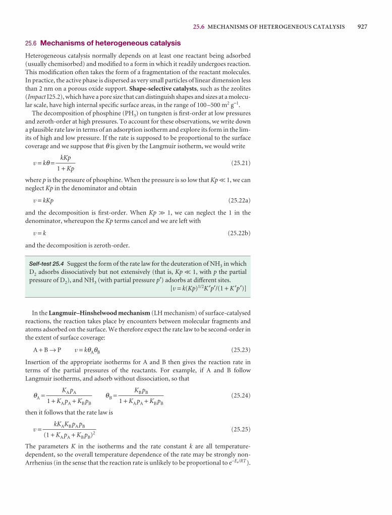
25.6 MECHANISMS OF HETEROGENEOUS CATALYSIS 927
25.6 Mechanisms of heterogeneous catalysis
Heterogeneous catalysis normally depends on at least one reactant being adsorbed(usually chemisorbed) and modified to a form in which it readily undergoes reaction.This modification often takes the form of a fragmentation of the reactant molecules.In practice, the active phase is dispersed as very small particles of linear dimension lessthan 2 nm on a porous oxide support. Shape-selective catalysts, such as the zeolites(Impact I25.2), which have a pore size that can distinguish shapes and sizes at a molecu-lar scale, have high internal specific surface areas, in the range of 100–500 m2 g−1.
The decomposition of phosphine (PH3) on tungsten is first-order at low pressuresand zeroth-order at high pressures. To account for these observations, we write downa plausible rate law in terms of an adsorption isotherm and explore its form in the lim-its of high and low pressure. If the rate is supposed to be proportional to the surfacecoverage and we suppose that θ is given by the Langmuir isotherm, we would write
v = kθ = (25.21)
where p is the pressure of phosphine. When the pressure is so low that Kp << 1, we canneglect Kp in the denominator and obtain
v = kKp (25.22a)
and the decomposition is first-order. When Kp >> 1, we can neglect the 1 in the denominator, whereupon the Kp terms cancel and we are left with
v = k (25.22b)
and the decomposition is zeroth-order.
Self-test 25.4 Suggest the form of the rate law for the deuteration of NH3 in whichD2 adsorbs dissociatively but not extensively (that is, Kp << 1, with p the partialpressure of D2), and NH3 (with partial pressure p′) adsorbs at different sites.
[v = k(Kp)1/2K ′p′/(1 + K ′p′)]
In the Langmuir–Hinshelwood mechanism (LH mechanism) of surface-catalysedreactions, the reaction takes place by encounters between molecular fragments andatoms adsorbed on the surface. We therefore expect the rate law to be second-order inthe extent of surface coverage:
A + B → P v = kθAθB (25.23)
Insertion of the appropriate isotherms for A and B then gives the reaction rate interms of the partial pressures of the reactants. For example, if A and B followLangmuir isotherms, and adsorb without dissociation, so that
θA = θB = (25.24)
then it follows that the rate law is
v = (25.25)
The parameters K in the isotherms and the rate constant k are all temperature-dependent, so the overall temperature dependence of the rate may be strongly non-Arrhenius (in the sense that the reaction rate is unlikely to be proportional to e−Ea/RT ).
kKAKB pA pB
(1 + KA pA + KB pB)2
KB pB
1 + KA pA + KB pB
KA pA
1 + KA pA + KB pB
kKp
1 + Kp
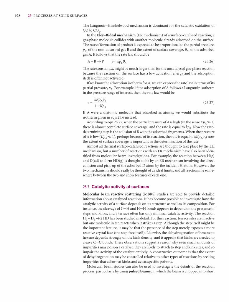
928 25 PROCESSES AT SOLID SURFACES
The Langmuir–Hinshelwood mechanism is dominant for the catalytic oxidation ofCO to CO2.
In the Eley–Rideal mechanism (ER mechanism) of a surface-catalysed reaction, agas-phase molecule collides with another molecule already adsorbed on the surface.The rate of formation of product is expected to be proportional to the partial pressure,pB, of the non-adsorbed gas B and the extent of surface coverage, θA, of the adsorbedgas A. It follows that the rate law should be
A + B → P v = kpBθA (25.26)
The rate constant, k, might be much larger than for the uncatalysed gas-phase reactionbecause the reaction on the surface has a low activation energy and the adsorption itself is often not activated.
If we know the adsorption isotherm for A, we can express the rate law in terms of itspartial pressure, pA. For example, if the adsorption of A follows a Langmuir isothermin the pressure range of interest, then the rate law would be
v = (25.27)
If A were a diatomic molecule that adsorbed as atoms, we would substitute theisotherm given in eqn 25.6 instead.
According to eqn 25.27, when the partial pressure of A is high (in the sense KpA >> 1)there is almost complete surface coverage, and the rate is equal to kpB. Now the rate-determining step is the collision of B with the adsorbed fragments. When the pressureof A is low (KpA << 1), perhaps because of its reaction, the rate is equal to kKpA pB; nowthe extent of surface coverage is important in the determination of the rate.
Almost all thermal surface-catalysed reactions are thought to take place by the LHmechanism, but a number of reactions with an ER mechanism have also been iden-tified from molecular beam investigations. For example, the reaction between H(g)and D(ad) to form HD(g) is thought to be by an ER mechanism involving the directcollision and pick-up of the adsorbed D atom by the incident H atom. However, thetwo mechanisms should really be thought of as ideal limits, and all reactions lie some-where between the two and show features of each one.
25.7 Catalytic activity at surfaces
Molecular beam reactive scattering (MBRS) studies are able to provide detailed information about catalysed reactions. It has become possible to investigate how thecatalytic activity of a surface depends on its structure as well as its composition. Forinstance, the cleavage of C-H and H-H bonds appears to depend on the presence ofsteps and kinks, and a terrace often has only minimal catalytic activity. The reactionH2 + D2 → 2 HD has been studied in detail. For this reaction, terrace sites are inactivebut one molecule in ten reacts when it strikes a step. Although the step itself might bethe important feature, it may be that the presence of the step merely exposes a morereactive crystal face (the step face itself). Likewise, the dehydrogenation of hexane tohexene depends strongly on the kink density, and it appears that kinks are needed tocleave C-C bonds. These observations suggest a reason why even small amounts ofimpurities may poison a catalyst: they are likely to attach to step and kink sites, and soimpair the activity of the catalyst entirely. A constructive outcome is that the extent of dehydrogenation may be controlled relative to other types of reactions by seekingimpurities that adsorb at kinks and act as specific poisons.
Molecular beam studies can also be used to investigate the details of the reactionprocess, particularly by using pulsed beams, in which the beam is chopped into short
kKpA pB
1 + KpA
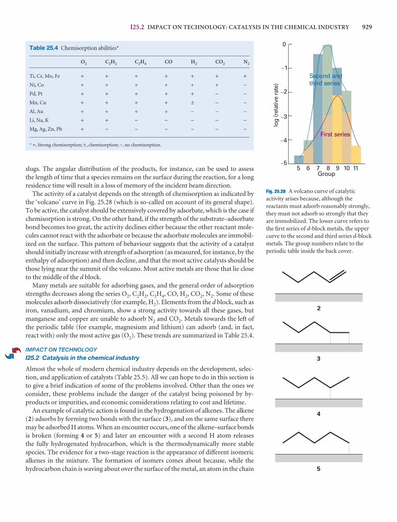
I25.2 IMPACT ON TECHNOLOGY: CATALYSIS IN THE CHEMICAL INDUSTRY 929
slugs. The angular distribution of the products, for instance, can be used to assess the length of time that a species remains on the surface during the reaction, for a longresidence time will result in a loss of memory of the incident beam direction.
The activity of a catalyst depends on the strength of chemisorption as indicated bythe ‘volcano’ curve in Fig. 25.28 (which is so-called on account of its general shape).To be active, the catalyst should be extensively covered by adsorbate, which is the case ifchemisorption is strong. On the other hand, if the strength of the substrate–adsorbatebond becomes too great, the activity declines either because the other reactant mole-cules cannot react with the adsorbate or because the adsorbate molecules are immobil-ized on the surface. This pattern of behaviour suggests that the activity of a catalystshould initially increase with strength of adsorption (as measured, for instance, by theenthalpy of adsorption) and then decline, and that the most active catalysts should bethose lying near the summit of the volcano. Most active metals are those that lie closeto the middle of the d block.
Many metals are suitable for adsorbing gases, and the general order of adsorptionstrengths decreases along the series O2, C2H2, C2H4, CO, H2, CO2, N2. Some of thesemolecules adsorb dissociatively (for example, H2). Elements from the d block, such asiron, vanadium, and chromium, show a strong activity towards all these gases, butmanganese and copper are unable to adsorb N2 and CO2. Metals towards the left ofthe periodic table (for example, magnesium and lithium) can adsorb (and, in fact,react with) only the most active gas (O2). These trends are summarized in Table 25.4.
IMPACT ON TECHNOLOGY
I25.2 Catalysis in the chemical industry
Almost the whole of modern chemical industry depends on the development, selec-tion, and application of catalysts (Table 25.5). All we can hope to do in this section isto give a brief indication of some of the problems involved. Other than the ones weconsider, these problems include the danger of the catalyst being poisoned by by-products or impurities, and economic considerations relating to cost and lifetime.
An example of catalytic action is found in the hydrogenation of alkenes. The alkene(2) adsorbs by forming two bonds with the surface (3), and on the same surface theremay be adsorbed H atoms. When an encounter occurs, one of the alkene–surface bondsis broken (forming 4 or 5) and later an encounter with a second H atom releases the fully hydrogenated hydrocarbon, which is the thermodynamically more stablespecies. The evidence for a two-stage reaction is the appearance of different isomericalkenes in the mixture. The formation of isomers comes about because, while thehydrocarbon chain is waving about over the surface of the metal, an atom in the chain
Fig. 25.28 A volcano curve of catalyticactivity arises because, although thereactants must adsorb reasonably strongly,they must not adsorb so strongly that theyare immobilized. The lower curve refers tothe first series of d-block metals, the uppercurve to the second and third series d-blockmetals. The group numbers relate to theperiodic table inside the back cover.
Table 25.4 Chemisorption abilities*
O2 C2H2 C2H4 CO H2 CO2 N2
Ti, Cr, Mo, Fe + + + + + + +Ni, Co + + + + + + −Pd, Pt + + + + + − −Mn, Cu + + + + ± − −Al, Au + + + + − − −Li, Na, K + + − − − − −Mg, Ag, Zn, Pb + − − − − − −
* +, Strong chemisorption; ±, chemisorption; −, no chemisorption.
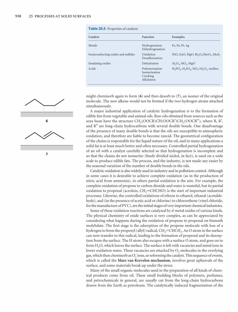
930 25 PROCESSES AT SOLID SURFACES
might chemisorb again to form (6) and then desorb to (7), an isomer of the originalmolecule. The new alkene would not be formed if the two hydrogen atoms attachedsimultaneously.
A major industrial application of catalytic hydrogenation is to the formation of edible fats from vegetable and animal oils. Raw oils obtained from sources such as thesoya bean have the structure CH2(OOCR)CH(OOCR′)CH2(OOCR″), where R, R′,and R″ are long-chain hydrocarbons with several double bonds. One disadvantage of the presence of many double bonds is that the oils are susceptible to atmosphericoxidation, and therefore are liable to become rancid. The geometrical configurationof the chains is responsible for the liquid nature of the oil, and in many applications asolid fat is at least much better and often necessary. Controlled partial hydrogenationof an oil with a catalyst carefully selected so that hydrogenation is incomplete and so that the chains do not isomerize (finely divided nickel, in fact), is used on a widescale to produce edible fats. The process, and the industry, is not made any easier bythe seasonal variation of the number of double bonds in the oils.
Catalytic oxidation is also widely used in industry and in pollution control. Althoughin some cases it is desirable to achieve complete oxidation (as in the production of nitric acid from ammonia), in others partial oxidation is the aim. For example, thecomplete oxidation of propene to carbon dioxide and water is wasteful, but its partialoxidation to propenal (acrolein, CH2=CHCHO) is the start of important industrialprocesses. Likewise, the controlled oxidations of ethene to ethanol, ethanal (acetalde-hyde), and (in the presence of acetic acid or chlorine) to chloroethene (vinyl chloride,for the manufacture of PVC), are the initial stages of very important chemical industries.
Some of these oxidation reactions are catalysed by d-metal oxides of various kinds.The physical chemistry of oxide surfaces is very complex, as can be appreciated byconsidering what happens during the oxidation of propene to propenal on bismuthmolybdate. The first stage is the adsorption of the propene molecule with loss of a hydrogen to form the propenyl (allyl) radical, CH2=CHCH2. An O atom in the surfacecan now transfer to this radical, leading to the formation of propenal and its desorp-tion from the surface. The H atom also escapes with a surface O atom, and goes on toform H2O, which leaves the surface. The surface is left with vacancies and metal ions inlower oxidation states. These vacancies are attacked by O2 molecules in the overlyinggas, which then chemisorb as O2
− ions, so reforming the catalyst. This sequence of events,which is called the Mars van Krevelen mechanism, involves great upheavals of thesurface, and some materials break up under the stress.
Many of the small organic molecules used in the preparation of all kinds of chem-ical products come from oil. These small building blocks of polymers, perfumes, and petrochemicals in general, are usually cut from the long-chain hydrocarbonsdrawn from the Earth as petroleum. The catalytically induced fragmentation of the
Table 25.5 Properties of catalysts
Catalyst Function Examples
Metals Hydrogenation Fe, Ni, Pt, AgDehydrogenation
Semiconducting oxides and sulfides Oxidation NiO, ZnO, MgO, Bi2O3/MoO3, MoS2Desulfurization
Insulating oxides Dehydration Al2O3, SiO2, MgO
Acids Polymerization H3PO4, H2SO4, SiO3 /Al2O3, zeolitesIsomerizationCrackingAlkylation
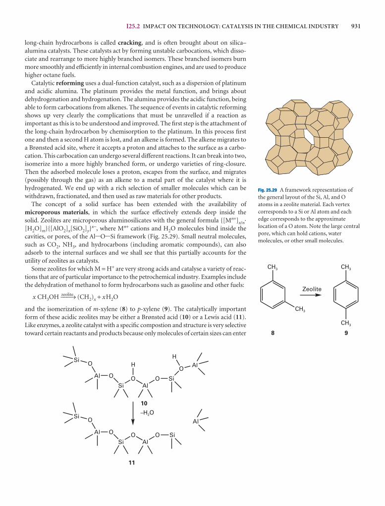
I25.2 IMPACT ON TECHNOLOGY: CATALYSIS IN THE CHEMICAL INDUSTRY 931
long-chain hydrocarbons is called cracking, and is often brought about on silica–alumina catalysts. These catalysts act by forming unstable carbocations, which disso-ciate and rearrange to more highly branched isomers. These branched isomers burnmore smoothly and efficiently in internal combustion engines, and are used to producehigher octane fuels.
Catalytic reforming uses a dual-function catalyst, such as a dispersion of platinumand acidic alumina. The platinum provides the metal function, and brings about dehydrogenation and hydrogenation. The alumina provides the acidic function, beingable to form carbocations from alkenes. The sequence of events in catalytic reformingshows up very clearly the complications that must be unravelled if a reaction as important as this is to be understood and improved. The first step is the attachment ofthe long-chain hydrocarbon by chemisorption to the platinum. In this process firstone and then a second H atom is lost, and an alkene is formed. The alkene migrates toa Brønsted acid site, where it accepts a proton and attaches to the surface as a carbo-cation. This carbocation can undergo several different reactions. It can break into two,isomerize into a more highly branched form, or undergo varieties of ring-closure.Then the adsorbed molecule loses a proton, escapes from the surface, and migrates(possibly through the gas) as an alkene to a metal part of the catalyst where it is hydrogenated. We end up with a rich selection of smaller molecules which can bewithdrawn, fractionated, and then used as raw materials for other products.
The concept of a solid surface has been extended with the availability of microporous materials, in which the surface effectively extends deep inside the solid. Zeolites are microporous aluminosilicates with the general formula {[Mn+]x/n·[H2O]m}{[AlO2]x[SiO2]y}
x−, where Mn+ cations and H2O molecules bind inside thecavities, or pores, of the Al-O-Si framework (Fig. 25.29). Small neutral molecules,such as CO2, NH3, and hydrocarbons (including aromatic compounds), can also adsorb to the internal surfaces and we shall see that this partially accounts for the utility of zeolites as catalysts.
Some zeolites for which M = H+ are very strong acids and catalyse a variety of reac-tions that are of particular importance to the petrochemical industry. Examples includethe dehydration of methanol to form hydrocarbons such as gasoline and other fuels:
x CH3OH zeolite−−−→ (CH2)x + xH2O
and the isomerization of m-xylene (8) to p-xylene (9). The catalytically importantform of these acidic zeolites may be either a Brønsted acid (10) or a Lewis acid (11).Like enzymes, a zeolite catalyst with a specific compostion and structure is very selectivetoward certain reactants and products because only molecules of certain sizes can enter
Fig. 25.29 A framework representation ofthe general layout of the Si, Al, and Oatoms in a zeolite material. Each vertexcorresponds to a Si or Al atom and eachedge corresponds to the approximatelocation of a O atom. Note the large centralpore, which can hold cations, watermolecules, or other small molecules.
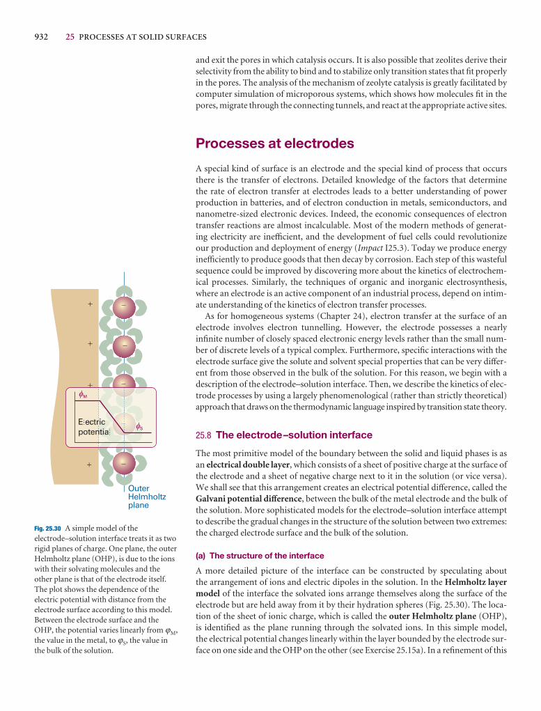
932 25 PROCESSES AT SOLID SURFACES
and exit the pores in which catalysis occurs. It is also possible that zeolites derive theirselectivity from the ability to bind and to stabilize only transition states that fit properlyin the pores. The analysis of the mechanism of zeolyte catalysis is greatly facilitated bycomputer simulation of microporous systems, which shows how molecules fit in thepores, migrate through the connecting tunnels, and react at the appropriate active sites.
Processes at electrodes
A special kind of surface is an electrode and the special kind of process that occursthere is the transfer of electrons. Detailed knowledge of the factors that determine the rate of electron transfer at electrodes leads to a better understanding of power production in batteries, and of electron conduction in metals, semiconductors, andnanometre-sized electronic devices. Indeed, the economic consequences of electrontransfer reactions are almost incalculable. Most of the modern methods of generat-ing electricity are inefficient, and the development of fuel cells could revolutionize our production and deployment of energy (Impact I25.3). Today we produce energyinefficiently to produce goods that then decay by corrosion. Each step of this wastefulsequence could be improved by discovering more about the kinetics of electrochem-ical processes. Similarly, the techniques of organic and inorganic electrosynthesis,where an electrode is an active component of an industrial process, depend on intim-ate understanding of the kinetics of electron transfer processes.
As for homogeneous systems (Chapter 24), electron transfer at the surface of anelectrode involves electron tunnelling. However, the electrode possesses a nearlyinfinite number of closely spaced electronic energy levels rather than the small num-ber of discrete levels of a typical complex. Furthermore, specific interactions with theelectrode surface give the solute and solvent special properties that can be very differ-ent from those observed in the bulk of the solution. For this reason, we begin with adescription of the electrode–solution interface. Then, we describe the kinetics of elec-trode processes by using a largely phenomenological (rather than strictly theoretical)approach that draws on the thermodynamic language inspired by transition state theory.
25.8 The electrode–solution interface
The most primitive model of the boundary between the solid and liquid phases is asan electrical double layer, which consists of a sheet of positive charge at the surface ofthe electrode and a sheet of negative charge next to it in the solution (or vice versa).We shall see that this arrangement creates an electrical potential difference, called theGalvani potential difference, between the bulk of the metal electrode and the bulk ofthe solution. More sophisticated models for the electrode–solution interface attemptto describe the gradual changes in the structure of the solution between two extremes:the charged electrode surface and the bulk of the solution.
(a) The structure of the interface
A more detailed picture of the interface can be constructed by speculating about the arrangement of ions and electric dipoles in the solution. In the Helmholtz layermodel of the interface the solvated ions arrange themselves along the surface of theelectrode but are held away from it by their hydration spheres (Fig. 25.30). The loca-tion of the sheet of ionic charge, which is called the outer Helmholtz plane (OHP),is identified as the plane running through the solvated ions. In this simple model, the electrical potential changes linearly within the layer bounded by the electrode sur-face on one side and the OHP on the other (see Exercise 25.15a). In a refinement of this
Fig. 25.30 A simple model of theelectrode–solution interface treats it as tworigid planes of charge. One plane, the outerHelmholtz plane (OHP), is due to the ionswith their solvating molecules and theother plane is that of the electrode itself.The plot shows the dependence of theelectric potential with distance from theelectrode surface according to this model.Between the electrode surface and theOHP, the potential varies linearly from ϕM,the value in the metal, to ϕS, the value inthe bulk of the solution.
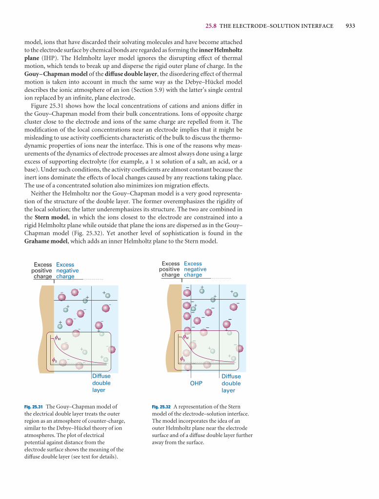
25.8 THE ELECTRODE–SOLUTION INTERFACE 933
model, ions that have discarded their solvating molecules and have become attachedto the electrode surface by chemical bonds are regarded as forming the inner Helmholtzplane (IHP). The Helmholtz layer model ignores the disrupting effect of thermal motion, which tends to break up and disperse the rigid outer plane of charge. In theGouy–Chapman model of the diffuse double layer, the disordering effect of thermalmotion is taken into account in much the same way as the Debye–Hückel model describes the ionic atmosphere of an ion (Section 5.9) with the latter’s single centralion replaced by an infinite, plane electrode.
Figure 25.31 shows how the local concentrations of cations and anions differ in the Gouy–Chapman model from their bulk concentrations. Ions of opposite chargecluster close to the electrode and ions of the same charge are repelled from it. Themodification of the local concentrations near an electrode implies that it might bemisleading to use activity coefficients characteristic of the bulk to discuss the thermo-dynamic properties of ions near the interface. This is one of the reasons why meas-urements of the dynamics of electrode processes are almost always done using a largeexcess of supporting electrolyte (for example, a 1 m solution of a salt, an acid, or abase). Under such conditions, the activity coefficients are almost constant because theinert ions dominate the effects of local changes caused by any reactions taking place.The use of a concentrated solution also minimizes ion migration effects.
Neither the Helmholtz nor the Gouy–Chapman model is a very good representa-tion of the structure of the double layer. The former overemphasizes the rigidity of the local solution; the latter underemphasizes its structure. The two are combined inthe Stern model, in which the ions closest to the electrode are constrained into a rigid Helmholtz plane while outside that plane the ions are dispersed as in the Gouy–Chapman model (Fig. 25.32). Yet another level of sophistication is found in theGrahame model, which adds an inner Helmholtz plane to the Stern model.
Fig. 25.31 The Gouy–Chapman model ofthe electrical double layer treats the outerregion as an atmosphere of counter-charge,similar to the Debye–Hückel theory of ionatmospheres. The plot of electricalpotential against distance from theelectrode surface shows the meaning of thediffuse double layer (see text for details).
Fig. 25.32 A representation of the Sternmodel of the electrode–solution interface.The model incorporates the idea of anouter Helmholtz plane near the electrodesurface and of a diffuse double layer furtheraway from the surface.
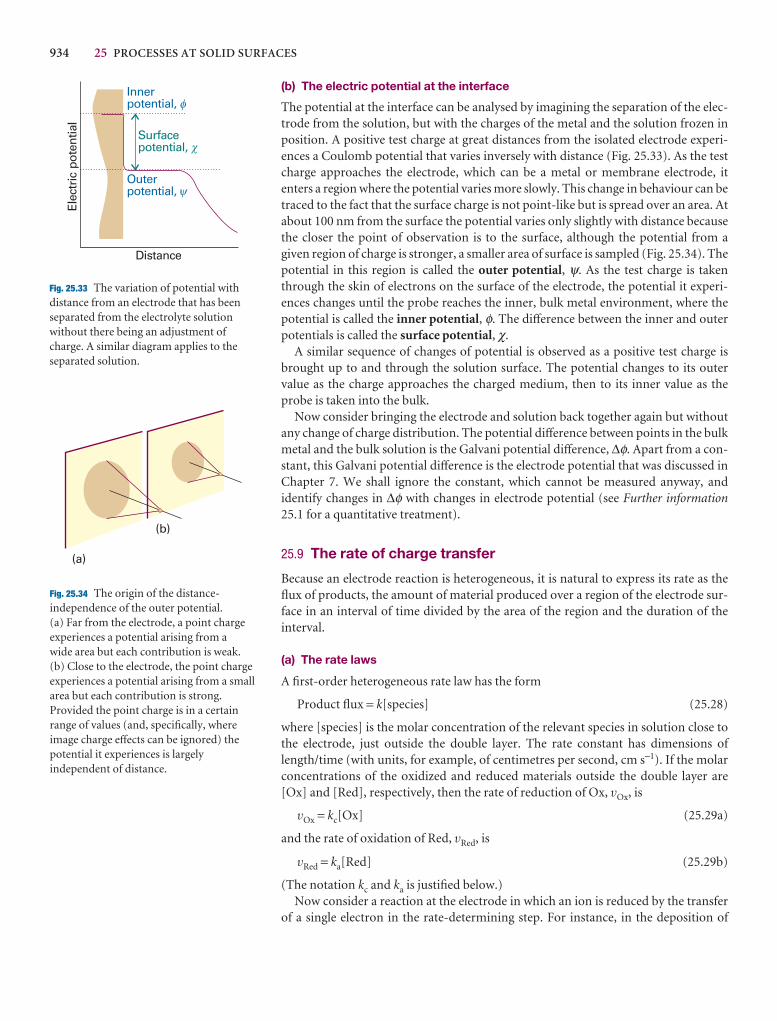
934 25 PROCESSES AT SOLID SURFACES
(b) The electric potential at the interface
The potential at the interface can be analysed by imagining the separation of the elec-trode from the solution, but with the charges of the metal and the solution frozen inposition. A positive test charge at great distances from the isolated electrode experi-ences a Coulomb potential that varies inversely with distance (Fig. 25.33). As the testcharge approaches the electrode, which can be a metal or membrane electrode, it enters a region where the potential varies more slowly. This change in behaviour can betraced to the fact that the surface charge is not point-like but is spread over an area. Atabout 100 nm from the surface the potential varies only slightly with distance becausethe closer the point of observation is to the surface, although the potential from agiven region of charge is stronger, a smaller area of surface is sampled (Fig. 25.34). Thepotential in this region is called the outer potential, ψ. As the test charge is takenthrough the skin of electrons on the surface of the electrode, the potential it experi-ences changes until the probe reaches the inner, bulk metal environment, where thepotential is called the inner potential, φ. The difference between the inner and outerpotentials is called the surface potential, χ.
A similar sequence of changes of potential is observed as a positive test charge isbrought up to and through the solution surface. The potential changes to its outervalue as the charge approaches the charged medium, then to its inner value as theprobe is taken into the bulk.
Now consider bringing the electrode and solution back together again but withoutany change of charge distribution. The potential difference between points in the bulkmetal and the bulk solution is the Galvani potential difference, ∆φ. Apart from a con-stant, this Galvani potential difference is the electrode potential that was discussed inChapter 7. We shall ignore the constant, which cannot be measured anyway, andidentify changes in ∆φ with changes in electrode potential (see Further information25.1 for a quantitative treatment).
25.9 The rate of charge transfer
Because an electrode reaction is heterogeneous, it is natural to express its rate as theflux of products, the amount of material produced over a region of the electrode sur-face in an interval of time divided by the area of the region and the duration of theinterval.
(a) The rate laws
A first-order heterogeneous rate law has the form
Product flux = k[species] (25.28)
where [species] is the molar concentration of the relevant species in solution close tothe electrode, just outside the double layer. The rate constant has dimensions oflength/time (with units, for example, of centimetres per second, cm s−1). If the molarconcentrations of the oxidized and reduced materials outside the double layer are[Ox] and [Red], respectively, then the rate of reduction of Ox, vOx, is
vOx = kc[Ox] (25.29a)
and the rate of oxidation of Red, vRed, is
vRed = ka[Red] (25.29b)
(The notation kc and ka is justified below.)Now consider a reaction at the electrode in which an ion is reduced by the transfer
of a single electron in the rate-determining step. For instance, in the deposition of
Fig. 25.33 The variation of potential withdistance from an electrode that has beenseparated from the electrolyte solutionwithout there being an adjustment ofcharge. A similar diagram applies to theseparated solution.
Fig. 25.34 The origin of the distance-independence of the outer potential. (a) Far from the electrode, a point chargeexperiences a potential arising from a wide area but each contribution is weak.(b) Close to the electrode, the point chargeexperiences a potential arising from a smallarea but each contribution is strong.Provided the point charge is in a certainrange of values (and, specifically, whereimage charge effects can be ignored) thepotential it experiences is largelyindependent of distance.
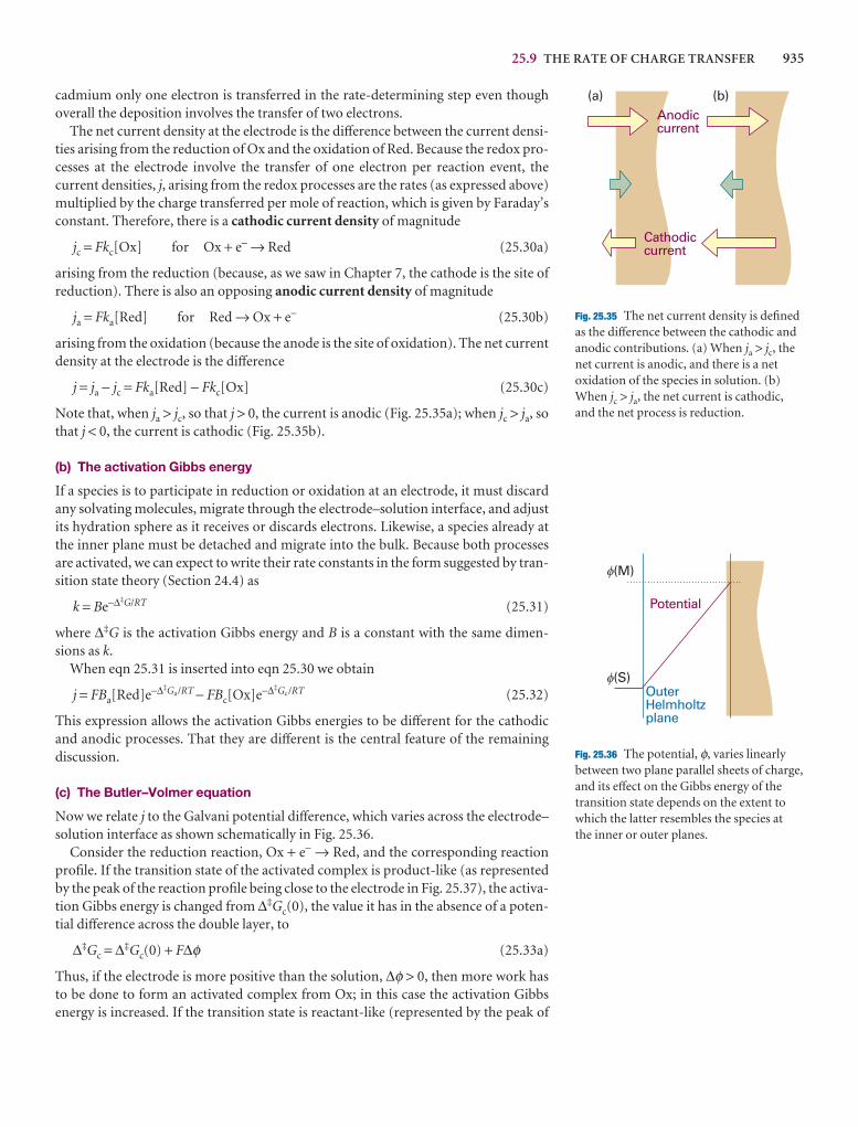
25.9 THE RATE OF CHARGE TRANSFER 935
cadmium only one electron is transferred in the rate-determining step even thoughoverall the deposition involves the transfer of two electrons.
The net current density at the electrode is the difference between the current densi-ties arising from the reduction of Ox and the oxidation of Red. Because the redox pro-cesses at the electrode involve the transfer of one electron per reaction event, thecurrent densities, j, arising from the redox processes are the rates (as expressed above)multiplied by the charge transferred per mole of reaction, which is given by Faraday’sconstant. Therefore, there is a cathodic current density of magnitude
jc = Fkc[Ox] for Ox + e− → Red (25.30a)
arising from the reduction (because, as we saw in Chapter 7, the cathode is the site ofreduction). There is also an opposing anodic current density of magnitude
ja = Fka[Red] for Red → Ox + e− (25.30b)
arising from the oxidation (because the anode is the site of oxidation). The net currentdensity at the electrode is the difference
j = ja − jc = Fka[Red] − Fkc[Ox] (25.30c)
Note that, when ja > jc, so that j > 0, the current is anodic (Fig. 25.35a); when jc > ja, sothat j < 0, the current is cathodic (Fig. 25.35b).
(b) The activation Gibbs energy
If a species is to participate in reduction or oxidation at an electrode, it must discardany solvating molecules, migrate through the electrode–solution interface, and adjustits hydration sphere as it receives or discards electrons. Likewise, a species already atthe inner plane must be detached and migrate into the bulk. Because both processesare activated, we can expect to write their rate constants in the form suggested by tran-sition state theory (Section 24.4) as
k = Be−∆‡G/RT (25.31)
where ∆‡G is the activation Gibbs energy and B is a constant with the same dimen-sions as k.
When eqn 25.31 is inserted into eqn 25.30 we obtain
j = FBa[Red]e−∆‡Ga/RT − FBc[Ox]e−∆‡Gc/RT (25.32)
This expression allows the activation Gibbs energies to be different for the cathodicand anodic processes. That they are different is the central feature of the remainingdiscussion.
(c) The Butler–Volmer equation
Now we relate j to the Galvani potential difference, which varies across the electrode–solution interface as shown schematically in Fig. 25.36.
Consider the reduction reaction, Ox + e− → Red, and the corresponding reactionprofile. If the transition state of the activated complex is product-like (as representedby the peak of the reaction profile being close to the electrode in Fig. 25.37), the activa-tion Gibbs energy is changed from ∆‡Gc(0), the value it has in the absence of a poten-tial difference across the double layer, to
∆‡Gc = ∆‡Gc(0) + F∆φ (25.33a)
Thus, if the electrode is more positive than the solution, ∆φ > 0, then more work hasto be done to form an activated complex from Ox; in this case the activation Gibbs energy is increased. If the transition state is reactant-like (represented by the peak of
Fig. 25.35 The net current density is definedas the difference between the cathodic andanodic contributions. (a) When ja > jc, thenet current is anodic, and there is a netoxidation of the species in solution. (b)When jc > ja, the net current is cathodic,and the net process is reduction.
Fig. 25.36 The potential, φ, varies linearlybetween two plane parallel sheets of charge,and its effect on the Gibbs energy of thetransition state depends on the extent towhich the latter resembles the species at the inner or outer planes.
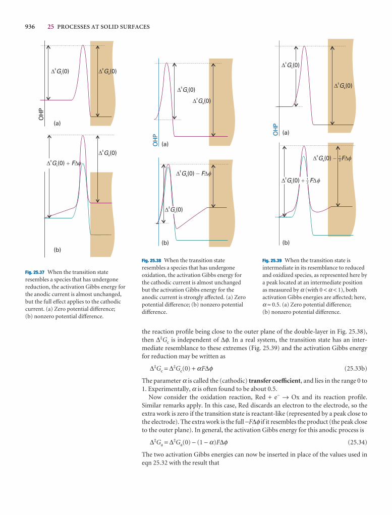
936 25 PROCESSES AT SOLID SURFACES
the reaction profile being close to the outer plane of the double-layer in Fig. 25.38),then ∆‡Gc is independent of ∆φ. In a real system, the transition state has an inter-mediate resemblance to these extremes (Fig. 25.39) and the activation Gibbs energyfor reduction may be written as
∆‡Gc = ∆‡Gc(0) + αF∆φ (25.33b)
The parameter α is called the (cathodic) transfer coefficient, and lies in the range 0 to1. Experimentally, α is often found to be about 0.5.
Now consider the oxidation reaction, Red + e− → Ox and its reaction profile.Similar remarks apply. In this case, Red discards an electron to the electrode, so theextra work is zero if the transition state is reactant-like (represented by a peak close tothe electrode). The extra work is the full −F∆φ if it resembles the product (the peak closeto the outer plane). In general, the activation Gibbs energy for this anodic process is
∆‡Ga = ∆‡Ga(0) − (1 − α)F∆φ (25.34)
The two activation Gibbs energies can now be inserted in place of the values used ineqn 25.32 with the result that
Fig. 25.37 When the transition stateresembles a species that has undergonereduction, the activation Gibbs energy forthe anodic current is almost unchanged,but the full effect applies to the cathodiccurrent. (a) Zero potential difference;(b) nonzero potential difference.
Fig. 25.38 When the transition stateresembles a species that has undergoneoxidation, the activation Gibbs energy forthe cathodic current is almost unchangedbut the activation Gibbs energy for theanodic current is strongly affected. (a) Zeropotential difference; (b) nonzero potentialdifference.
Fig. 25.39 When the transition state isintermediate in its resemblance to reducedand oxidized species, as represented here bya peak located at an intermediate positionas measured by α (with 0 < α < 1), bothactivation Gibbs energies are affected; here,α ≈ 0.5. (a) Zero potential difference;(b) nonzero potential difference.
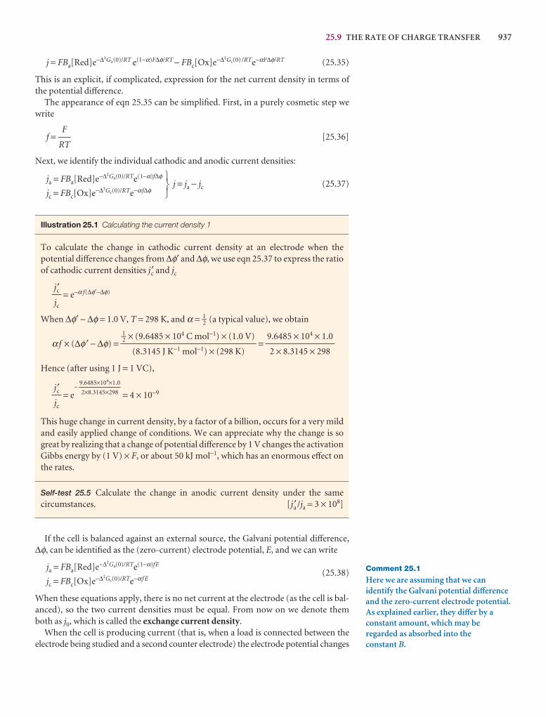
25.9 THE RATE OF CHARGE TRANSFER 937
Comment 25.1
Here we are assuming that we canidentify the Galvani potential differenceand the zero-current electrode potential.As explained earlier, they differ by aconstant amount, which may beregarded as absorbed into the constant B.
j = FBa[Red]e−∆‡Ga(0)/RT e(1−α)F∆φ/RT − FBc[Ox]e−∆‡Gc(0) /RTe−αF∆φ/RT (25.35)
This is an explicit, if complicated, expression for the net current density in terms ofthe potential difference.
The appearance of eqn 25.35 can be simplified. First, in a purely cosmetic step wewrite
f = [25.36]
Next, we identify the individual cathodic and anodic current densities:
ja = FBa[Red]e−∆‡Ga(0)/RTe(1−α)f∆φ
jc = FBc[Ox]e−∆‡Gc(0)/RTe−αf∆φj = ja − jc (25.37)
Illustration 25.1 Calculating the current density 1
To calculate the change in cathodic current density at an electrode when the potential difference changes from ∆φ′ and ∆φ, we use eqn 25.37 to express the ratioof cathodic current densities jc′ and jc
= e−α f(∆φ′−∆φ)
When ∆φ′ − ∆φ = 1.0 V, T = 298 K, and α = 1–2 (a typical value), we obtain
α f × (∆φ′ − ∆φ) = =
Hence (after using 1 J = 1 VC),
= e−
= 4 × 10⁻⁹
This huge change in current density, by a factor of a billion, occurs for a very mildand easily applied change of conditions. We can appreciate why the change is sogreat by realizing that a change of potential difference by 1 V changes the activationGibbs energy by (1 V) × F, or about 50 kJ mol−1, which has an enormous effect onthe rates.
Self-test 25.5 Calculate the change in anodic current density under the same circumstances. [j ′a /ja = 3 × 10⁸]
If the cell is balanced against an external source, the Galvani potential difference,∆φ, can be identified as the (zero-current) electrode potential, E, and we can write
ja = FBa[Red]e−∆‡Ga(0)/RTe(1−α)fE
jc = FBc[Ox]e−∆‡Gc(0)/RTe−αf E(25.38)
When these equations apply, there is no net current at the electrode (as the cell is bal-anced), so the two current densities must be equal. From now on we denote themboth as j0, which is called the exchange current density.
When the cell is producing current (that is, when a load is connected between theelectrode being studied and a second counter electrode) the electrode potential changes
9.6485×104×1.0
2×8.3145×298j ′cjc
9.6485 × 104 × 1.0
2 × 8.3145 × 298
1–2 × (9.6485 × 104 C mol−1) × (1.0 V)
(8.3145 J K−1 mol−1) × (298 K)
j ′cjc
567
F
RT
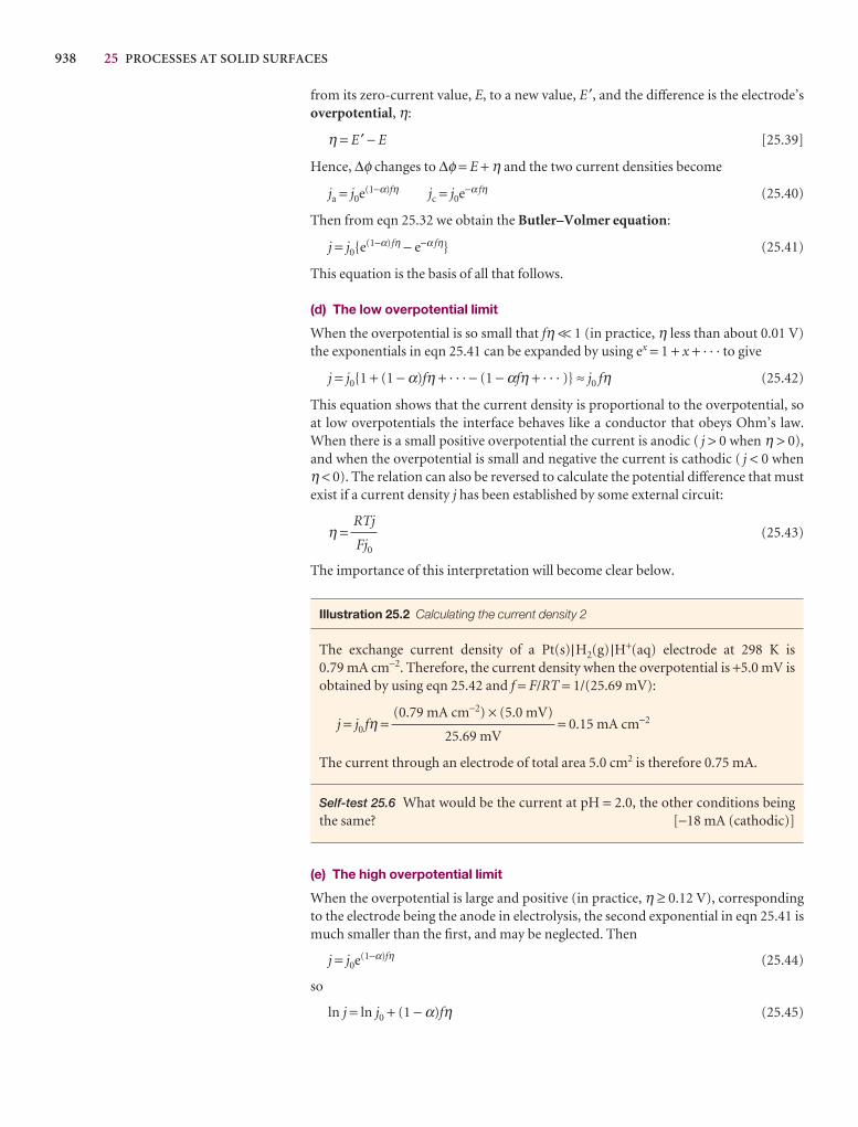
938 25 PROCESSES AT SOLID SURFACES
from its zero-current value, E, to a new value, E ′, and the difference is the electrode’soverpotential, η:
η = E ′ − E [25.39]
Hence, ∆φ changes to ∆φ = E + η and the two current densities become
ja = j0e(1−α)fη jc = j0e−α fη (25.40)
Then from eqn 25.32 we obtain the Butler–Volmer equation:
j = j0{e(1−α)fη − e−α fη} (25.41)
This equation is the basis of all that follows.
(d) The low overpotential limit
When the overpotential is so small that fη << 1 (in practice, η less than about 0.01 V)the exponentials in eqn 25.41 can be expanded by using ex = 1 + x + · · · to give
j = j0{1 + (1 − α)fη + · · · − (1 − αfη + · · · )} ≈ j0 fη (25.42)
This equation shows that the current density is proportional to the overpotential, soat low overpotentials the interface behaves like a conductor that obeys Ohm’s law.When there is a small positive overpotential the current is anodic ( j > 0 when η > 0),and when the overpotential is small and negative the current is cathodic ( j < 0 when η < 0). The relation can also be reversed to calculate the potential difference that mustexist if a current density j has been established by some external circuit:
η = (25.43)
The importance of this interpretation will become clear below.
Illustration 25.2 Calculating the current density 2
The exchange current density of a Pt(s)|H2(g) |H+(aq) electrode at 298 K is 0.79 mA cm−2. Therefore, the current density when the overpotential is +5.0 mV isobtained by using eqn 25.42 and f = F/RT = 1/(25.69 mV):
j = j0 fη = = 0.15 mA cm−2
The current through an electrode of total area 5.0 cm2 is therefore 0.75 mA.
Self-test 25.6 What would be the current at pH = 2.0, the other conditions beingthe same? [−18 mA (cathodic)]
(e) The high overpotential limit
When the overpotential is large and positive (in practice, η ≥ 0.12 V), correspondingto the electrode being the anode in electrolysis, the second exponential in eqn 25.41 ismuch smaller than the first, and may be neglected. Then
j = j0e(1−α)fη (25.44)
so
ln j = ln j0 + (1 − α)fη (25.45)
(0.79 mA cm−2) × (5.0 mV)
25.69 mV
RTj
Fj0
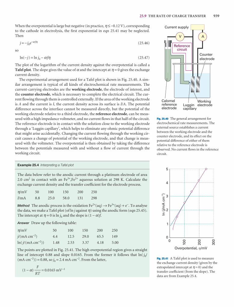
25.9 THE RATE OF CHARGE TRANSFER 939
Fig. 25.40 The general arrangement forelectrochemical rate measurements. Theexternal source establishes a currentbetween the working electrode and thecounter electrode, and its effect on thepotential difference of either of themrelative to the reference electrode isobserved. No current flows in the referencecircuit.
Fig. 25.41 A Tafel plot is used to measurethe exchange current density (given by theextrapolated intercept at η = 0) and thetransfer coefficient (from the slope). Thedata are from Example 25.4.
When the overpotential is large but negative (in practice, η ≤ −0.12 V), correspondingto the cathode in electrolysis, the first exponential in eqn 25.41 may be neglected.Then
j = − j0e−α fη (25.46)
so
ln(− j) = ln j0 − α fη (25.47)
The plot of the logarithm of the current density against the overpotential is called aTafel plot. The slope gives the value of α and the intercept at η = 0 gives the exchangecurrent density.
The experimental arrangement used for a Tafel plot is shown in Fig. 25.40. A sim-ilar arrangement is typical of all kinds of electrochemical rate measurements. The current-carrying electrodes are the working electrode, the electrode of interest, andthe counter electrode, which is necessary to complete the electrical circuit. The cur-rent flowing through them is controlled externally. If the area of the working electrode is A and the current is I, the current density across its surface is I/A. The potentialdifference across the interface cannot be measured directly, but the potential of theworking electrode relative to a third electrode, the reference electrode, can be meas-ured with a high impedance voltmeter, and no current flows in that half of the circuit.The reference electrode is in contact with the solution close to the working electrodethrough a ‘Luggin capillary’, which helps to eliminate any ohmic potential differencethat might arise accidentally. Changing the current flowing through the working cir-cuit causes a change of potential of the working electrode, and that change is meas-ured with the voltmeter. The overpotential is then obtained by taking the differencebetween the potentials measured with and without a flow of current through theworking circuit.
Example 25.4 Interpreting a Tafel plot
The data below refer to the anodic current through a platinum electrode of area 2.0 cm2 in contact with an Fe3+,Fe2+ aqueous solution at 298 K. Calculate the exchange current density and the transfer coefficient for the electrode process.
η/mV 50 100 150 200 250
I/mA 8.8 25.0 58.0 131 298
Method The anodic process is the oxidation Fe2+(aq) → Fe3+(aq) + e−. To analysethe data, we make a Tafel plot (of ln j against η) using the anodic form (eqn 25.45).The intercept at η = 0 is ln j0 and the slope is (1 − α)f.
Answer Draw up the following table:
η/mV 50 100 150 200 250
j/(mA cm−2) 4.4 12.5 29.0 65.5 149
ln( j/(mA cm−2)) 1.48 2.53 3.37 4.18 5.00
The points are plotted in Fig. 25.41. The high overpotential region gives a straightline of intercept 0.88 and slope 0.0165. From the former it follows that ln( j0/(mA cm−2)) = 0.88, so j0 = 2.4 mA cm−2. From the latter,
(1 − α) = 0.0165 mV−1F
RT
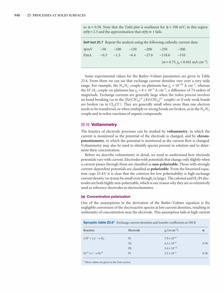
940 25 PROCESSES AT SOLID SURFACES
Synoptic table 25.6* Exchange current densities and transfer coefficients at 298 K
Reaction Electrode j0 /(A cm−2) a
2 H+ + 2 e− → H2 Pt 7.9 × 10⁻⁴
Ni 6.3 × 10⁻⁶ 0.58
Pb 5.0 × 10⁻¹²
Fe3+ + e− → Fe2+ Pt 2.5 × 10⁻³ 0.58
* More values are given in the Data section.
so α = 0.58. Note that the Tafel plot is nonlinear for η < 100 mV; in this region α fη = 2.3 and the approximation that α fη >> 1 fails.
Self-test 25.7 Repeat the analysis using the following cathodic current data:
η/mV −50 −100 −150 −200 −250 −300
I/mA −0.3 −1.5 −6.4 −27.6 −118.6 −510
[α = 0.75, j0 = 0.041 mA cm−2]
Some experimental values for the Butler–Volmer parameters are given in Table25.6. From them we can see that exchange current densities vary over a very widerange. For example, the N2,N3
− couple on platinum has j0 = 10−76 A cm−2, whereas the H+,H2 couple on platinum has j0 = 8 × 10⁻⁴ A cm−2, a difference of 73 orders ofmagnitude. Exchange currents are generally large when the redox process involves no bond breaking (as in the [Fe(CN)6]3−,[Fe(CN)6]4− couple) or if only weak bondsare broken (as in Cl2,Cl−). They are generally small when more than one electronneeds to be transferred, or when multiple or strong bonds are broken, as in the N2,N3
−
couple and in redox reactions of organic compounds.
25.10 Voltammetry
The kinetics of electrode processes can be studied by voltammetry, in which the current is monitored as the potential of the electrode is changed, and by chrono-potentiometry, in which the potential is monitored as the current flow is changed.Voltammetry may also be used to identify species present in solution and to deter-mine their concentration.
Before we describe voltammetry in detail, we need to understand how electrode potentials vary with current. Electrodes with potentials that change only slightly whena current passes through them are classified as non-polarizable. Those with stronglycurrent-dependent potentials are classified as polarizable. From the linearized equa-tion (eqn 25.43) it is clear that the criterion for low polarizability is high exchange current density (so η may be small even though j is large). The calomel and H2/Pt elec-trodes are both highly non-polarizable, which is one reason why they are so extensivelyused as reference electrodes in electrochemistry.
(a) Concentration polarization
One of the assumptions in the derivation of the Butler–Volmer equation is the negligible conversion of the electroactive species at low current densities, resulting inuniformity of concentration near the electrode. This assumption fails at high current
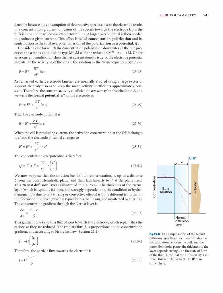
25.10 VOLTAMMETRY 941
densities because the consumption of electroactive species close to the electrode resultsin a concentration gradient; diffusion of the species towards the electrode from thebulk is slow and may become rate-determining. A larger overpotential is then neededto produce a given current. This effect is called concentration polarization and itscontribution to the total overpotential is called the polarization overpotential, ηc.
Consider a case for which the concentration polarization dominates all the rate pro-cesses and a redox couple of the type Mz+,M with the reduction Mz+ + z e− → M. Underzero-current conditions, when the net current density is zero, the electrode potentialis related to the activity, a, of the ions in the solution by the Nernst equation (eqn 7.29):
E = E 7 + ln a (25.48)
As remarked earlier, electrode kinetics are normally studied using a large excess ofsupport electrolyte so as to keep the mean activity coefficients approximately con-stant. Therefore, the constant activity coefficient in a = γc may be absorbed into E, andwe write the formal potential, E°, of the electrode as
E° = E 7 + ln γ [25.49]
Then the electrode potential is
E = E° + ln c (25.50)
When the cell is producing current, the active ion concentration at the OHP changesto c′ and the electrode potential changes to
E′ = E° + ln c ′ (25.51)
The concentration overpotential is therefore
ηc = E′ + E = ln (25.52)
We now suppose that the solution has its bulk concentration, c, up to a distance δ from the outer Helmholtz plane, and then falls linearly to c ′ at the plane itself. This Nernst diffusion layer is illustrated in Fig. 25.42. The thickness of the Nernst layer (which is typically 0.1 mm, and strongly dependent on the condition of hydro-dynamic flow due to any stirring or convective effects) is quite different from that ofthe electric double layer (which is typically less than 1 nm, and unaffected by stirring).The concentration gradient through the Nernst layer is
= (25.53)
This gradient gives rise to a flux of ions towards the electrode, which replenishes thecations as they are reduced. The (molar) flux, J, is proportional to the concentrationgradient, and according to Fick’s first law (Section 21.4)
J = −D (25.54)
Therefore, the particle flux towards the electrode is
J = D (25.55)c − c ′
δ
DF
∂c
∂x
AC
c ′ − cδ
dc
dx
DF
c ′c
AC
RT
zF
RT
zF
RT
zF
RT
zF
RT
zF
Fig. 25.42 In a simple model of the Nernstdiffusion layer there is a linear variation inconcentration between the bulk and theouter Helmholtz plane; the thickness of thelayer depends strongly on the state of flowof the fluid. Note that the diffusion layer ismuch thicker relative to the OHP thanshown here.
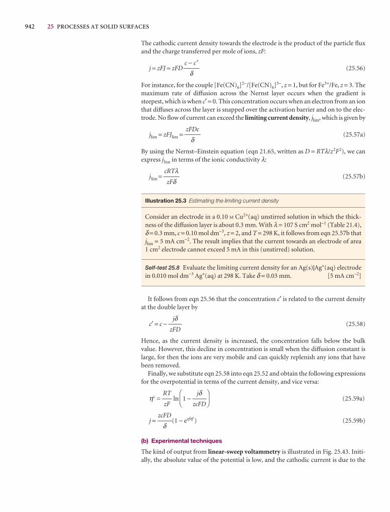
942 25 PROCESSES AT SOLID SURFACES
The cathodic current density towards the electrode is the product of the particle fluxand the charge transferred per mole of ions, zF:
j = zFJ = zFD (25.56)
For instance, for the couple [Fe(CN)6]2−/[Fe(CN)6]3−, z = 1, but for Fe3+/Fe, z = 3. Themaximum rate of diffusion across the Nernst layer occurs when the gradient is steepest, which is when c′ = 0. This concentration occurs when an electron from an ionthat diffuses across the layer is snapped over the activation barrier and on to the elec-trode. No flow of current can exceed the limiting current density, jlim, which is given by
jlim = zFJlim = (25.57a)
By using the Nernst–Einstein equation (eqn 21.65, written as D = RTλ/z2F2), we canexpress jlim in terms of the ionic conductivity λ:
jlim = (25.57b)
Illustration 25.3 Estimating the limiting current density
Consider an electrode in a 0.10 M Cu2+(aq) unstirred solution in which the thick-ness of the diffusion layer is about 0.3 mm. With λ = 107 S cm2 mol−1 (Table 21.4),δ = 0.3 mm, c = 0.10 mol dm−3, z = 2, and T = 298 K, it follows from eqn 25.57b thatjlim = 5 mA cm−2. The result implies that the current towards an electrode of area 1 cm2 electrode cannot exceed 5 mA in this (unstirred) solution.
Self-test 25.8 Evaluate the limiting current density for an Ag(s)|Ag+(aq) electrodein 0.010 mol dm−3 Ag+(aq) at 298 K. Take δ = 0.03 mm. [5 mA cm−2]
It follows from eqn 25.56 that the concentration c′ is related to the current densityat the double layer by
c′ = c − (25.58)
Hence, as the current density is increased, the concentration falls below the bulkvalue. However, this decline in concentration is small when the diffusion constant islarge, for then the ions are very mobile and can quickly replenish any ions that havebeen removed.
Finally, we substitute eqn 25.58 into eqn 25.52 and obtain the following expressionsfor the overpotential in terms of the current density, and vice versa:
ηc = ln 1 − (25.59a)
j = (1 − ezfηc) (25.59b)
(b) Experimental techniques
The kind of output from linear-sweep voltammetry is illustrated in Fig. 25.43. Initi-ally, the absolute value of the potential is low, and the cathodic current is due to the
zcFD
δ
DF
jδzcFD
AC
RT
zF
jδzFD
cRTλzFδ
zFDc
δ
c − c ′δ
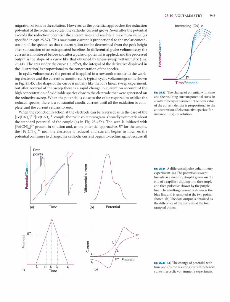
25.10 VOLTAMMETRY 943
migration of ions in the solution. However, as the potential approaches the reductionpotential of the reducible solute, the cathodic current grows. Soon after the potentialexceeds the reduction potential the current rises and reaches a maximum value (asspecified in eqn 25.57). This maximum current is proportional to the molar concen-tration of the species, so that concentration can be determined from the peak heightafter subtraction of an extrapolated baseline. In differential pulse voltammetry thecurrent is monitored before and after a pulse of potential is applied, and the processedoutput is the slope of a curve like that obtained by linear-sweep voltammetry (Fig.25.44). The area under the curve (in effect, the integral of the derivative displayed inthe illustration) is proportional to the concentration of the species.
In cyclic voltammetry the potential is applied in a sawtooth manner to the work-ing electrode and the current is monitored. A typical cyclic voltammogram is shownin Fig. 25.45. The shape of the curve is initially like that of a linear sweep experiment,but after reversal of the sweep there is a rapid change in current on account of the high concentration of oxidizable species close to the electrode that were generated onthe reductive sweep. When the potential is close to the value required to oxidize thereduced species, there is a substantial anodic current until all the oxidation is com-plete, and the current returns to zero.
When the reduction reaction at the electrode can be reversed, as in the case of the[Fe(CN)6]
3−/[Fe(CN)6]4− couple, the cyclic voltammogram is broadly symmetric about
the standard potential of the couple (as in Fig. 25.45b). The scan is initiated with[Fe(CN)6]3− present in solution and, as the potential approaches E 7 for the couple,the [Fe(CN)6]3− near the electrode is reduced and current begins to flow. As the potential continues to change, the cathodic current begins to decline again because all
Fig. 25.43 The change of potential with timeand the resulting current/potential curve ina voltammetry experiment. The peak valueof the current density is proportional to theconcentration of electroactive species (forinstance, [Ox]) in solution.
Fig. 25.45 (a) The change of potential withtime and (b) the resulting current/potentialcurve in a cyclic voltammetry experiment.
Fig. 25.44 A differential pulse voltammetryexperiment. (a) The potential is sweptlinearly as a mercury droplet grows on theend of a capillary dipping into the sampleand then pulsed as shown by the purpleline. The resulting current is shown as theblue line and is sampled at the two pointsshown. (b) The data output is obtained asthe difference of the currents at the twosampled points.
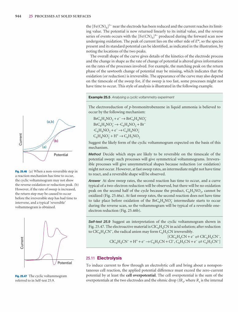
944 25 PROCESSES AT SOLID SURFACES
Fig. 25.46 (a) When a non-reversible step ina reaction mechanism has time to occur,the cyclic voltammogram may not showthe reverse oxidation or reduction peak. (b)However, if the rate of sweep is increased,the return step may be caused to occurbefore the irreversible step has had time tointervene, and a typical ‘reversible’voltammogram is obtained.
Fig. 25.47 The cyclic voltammogramreferred to in Self-test 25.9.
the [Fe(CN)6]3− near the electrode has been reduced and the current reaches its limit-ing value. The potential is now returned linearly to its initial value, and the reverse series of events occurs with the [Fe(CN)6]4− produced during the forward scan nowundergoing oxidation. The peak of current lies on the other side of E 7, so the speciespresent and its standard potential can be identified, as indicated in the illustration, bynoting the locations of the two peaks.
The overall shape of the curve gives details of the kinetics of the electrode processand the change in shape as the rate of change of potential is altered gives informationon the rates of the processes involved. For example, the matching peak on the returnphase of the sawtooth change of potential may be missing, which indicates that the oxidation (or reduction) is irreversible. The appearance of the curve may also dependon the timescale of the sweep for, if the sweep is too fast, some processes might nothave time to occur. This style of analysis is illustrated in the following example.
Example 25.5 Analysing a cyclic voltammetry experiment
The electroreduction of p-bromonitrobenzene in liquid ammonia is believed tooccur by the following mechanism:
BrC6H4NO2 + e− → BrC6H4NO2−
BrC6H4NO2− → ·C6H4NO2 + Br−
·C6H4NO2 + e− → C6H4NO2−
C6H4NO2− + H+ → C6H5NO2
Suggest the likely form of the cyclic voltammogram expected on the basis of thismechanism.
Method Decide which steps are likely to be reversible on the timescale of the potential sweep: such processes will give symmetrical voltammograms. Irrevers-ible processes will give unsymmetrical shapes because reduction (or oxidation)might not occur. However, at fast sweep rates, an intermediate might not have timeto react, and a reversible shape will be observed.
Answer At slow sweep rates, the second reaction has time to occur, and a curvetypical of a two-electron reduction will be observed, but there will be no oxidationpeak on the second half of the cycle because the product, C6H5NO2, cannot be oxidized (Fig. 25.46a). At fast sweep rates, the second reaction does not have timeto take place before oxidation of the BrC6H4NO2
− intermediate starts to occur during the reverse scan, so the voltammogram will be typical of a reversible one-electron reduction (Fig. 25.46b).
Self-test 25.9 Suggest an interpretation of the cyclic voltammogram shown in Fig. 25.47. The electroactive material is ClC6H4CN in acid solution; after reductionto ClC6H4CN−, the radical anion may form C6H5CN irreversibly.
[ClC6H4CN + e− 5 ClC6H4CN−,ClC6H4CN− + H+ + e− → C6H5CN + Cl−, C6H5CN + e− 5 C6H5CN−]
25.11 Electrolysis
To induce current to flow through an electrolytic cell and bring about a nonspon-taneous cell reaction, the applied potential difference must exceed the zero-currentpotential by at least the cell overpotential. The cell overpotential is the sum of theoverpotentials at the two electrodes and the ohmic drop (IRs, where Rs is the internal
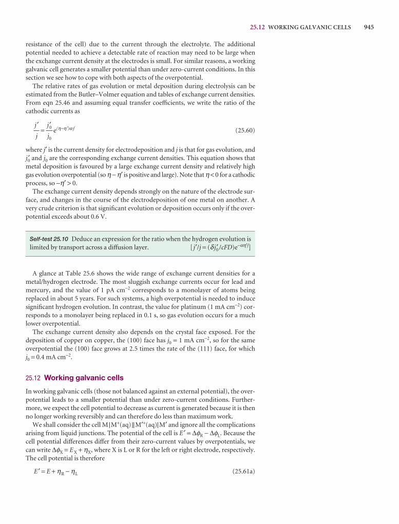
25.12 WORKING GALVANIC CELLS 945
resistance of the cell) due to the current through the electrolyte. The additional potential needed to achieve a detectable rate of reaction may need to be large when the exchange current density at the electrodes is small. For similar reasons, a working galvanic cell generates a smaller potential than under zero-current conditions. In thissection we see how to cope with both aspects of the overpotential.
The relative rates of gas evolution or metal deposition during electrolysis can be estimated from the Butler–Volmer equation and tables of exchange current densities.From eqn 25.46 and assuming equal transfer coefficients, we write the ratio of the cathodic currents as
= e(η−η′)α f (25.60)
where j′ is the current density for electrodeposition and j is that for gas evolution, andj ′0 and j0 are the corresponding exchange current densities. This equation shows thatmetal deposition is favoured by a large exchange current density and relatively highgas evolution overpotential (so η − η′ is positive and large). Note that η < 0 for a cathodicprocess, so −η′ > 0.
The exchange current density depends strongly on the nature of the electrode sur-face, and changes in the course of the electrodeposition of one metal on another. Avery crude criterion is that significant evolution or deposition occurs only if the over-potential exceeds about 0.6 V.
Self-test 25.10 Deduce an expression for the ratio when the hydrogen evolution islimited by transport across a diffusion layer. [ j′/j = (δ j ′0 /cFD)e−αη′f]
A glance at Table 25.6 shows the wide range of exchange current densities for ametal/hydrogen electrode. The most sluggish exchange currents occur for lead andmercury, and the value of 1 pA cm−2 corresponds to a monolayer of atoms being replaced in about 5 years. For such systems, a high overpotential is needed to inducesignificant hydrogen evolution. In contrast, the value for platinum (1 mA cm−2) cor-responds to a monolayer being replaced in 0.1 s, so gas evolution occurs for a muchlower overpotential.
The exchange current density also depends on the crystal face exposed. For the deposition of copper on copper, the (100) face has j0 = 1 mA cm−2, so for the sameoverpotential the (100) face grows at 2.5 times the rate of the (111) face, for which j0 = 0.4 mA cm−2.
25.12 Working galvanic cells
In working galvanic cells (those not balanced against an external potential), the over-potential leads to a smaller potential than under zero-current conditions. Further-more, we expect the cell potential to decrease as current is generated because it is thenno longer working reversibly and can therefore do less than maximum work.
We shall consider the cell M |M+(aq) ||M′+(aq)|M′ and ignore all the complicationsarising from liquid junctions. The potential of the cell is E ′ = ∆φR − ∆φL. Because thecell potential differences differ from their zero-current values by overpotentials, wecan write ∆φX = E X + ηX, where X is L or R for the left or right electrode, respectively.The cell potential is therefore
E ′ = E + ηR − ηL (25.61a)
j ′0j0
j ′j
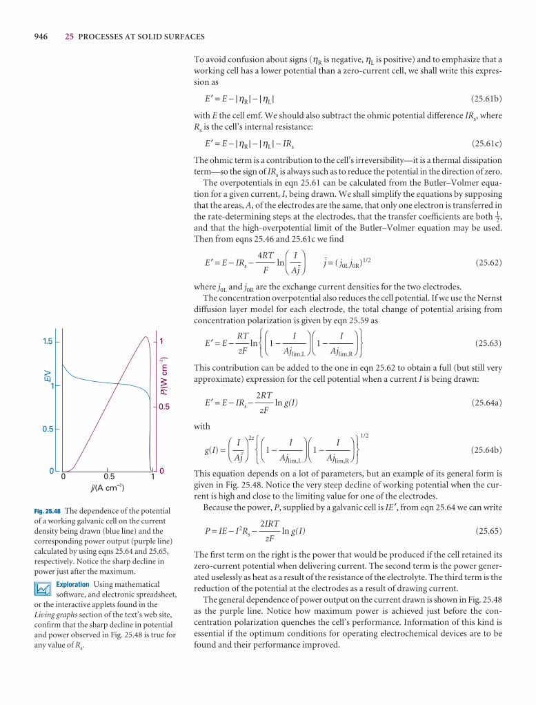
946 25 PROCESSES AT SOLID SURFACES
To avoid confusion about signs (ηR is negative, ηL is positive) and to emphasize that aworking cell has a lower potential than a zero-current cell, we shall write this expres-sion as
E ′ = E − |ηR | − |ηL | (25.61b)
with E the cell emf. We should also subtract the ohmic potential difference IRs, whereRs is the cell’s internal resistance:
E ′ = E − |ηR | − |ηL | − IRs (25.61c)
The ohmic term is a contribution to the cell’s irreversibility—it is a thermal dissipationterm—so the sign of IRs is always such as to reduce the potential in the direction of zero.
The overpotentials in eqn 25.61 can be calculated from the Butler–Volmer equa-tion for a given current, I, being drawn. We shall simplify the equations by supposingthat the areas, A, of the electrodes are the same, that only one electron is transferred inthe rate-determining steps at the electrodes, that the transfer coefficients are both 1–2,and that the high-overpotential limit of the Butler–Volmer equation may be used.Then from eqns 25.46 and 25.61c we find
E ′ = E − IRs − ln H = ( j0L j0R)1/2 (25.62)
where j0L and j0R are the exchange current densities for the two electrodes.The concentration overpotential also reduces the cell potential. If we use the Nernst
diffusion layer model for each electrode, the total change of potential arising fromconcentration polarization is given by eqn 25.59 as
E ′ = E − ln 1 − 1 − (25.63)
This contribution can be added to the one in eqn 25.62 to obtain a full (but still veryapproximate) expression for the cell potential when a current I is being drawn:
E ′ = E − IRs − ln g(I) (25.64a)
with
g(I) =2z
1 − 1 −
1/2
(25.64b)
This equation depends on a lot of parameters, but an example of its general form isgiven in Fig. 25.48. Notice the very steep decline of working potential when the cur-rent is high and close to the limiting value for one of the electrodes.
Because the power, P, supplied by a galvanic cell is IE ′, from eqn 25.64 we can write
P = IE − I2Rs − ln g(I) (25.65)
The first term on the right is the power that would be produced if the cell retained itszero-current potential when delivering current. The second term is the power gener-ated uselessly as heat as a result of the resistance of the electrolyte. The third term is thereduction of the potential at the electrodes as a result of drawing current.
The general dependence of power output on the current drawn is shown in Fig. 25.48as the purple line. Notice how maximum power is achieved just before the con-centration polarization quenches the cell’s performance. Information of this kind is essential if the optimum conditions for operating electrochemical devices are to befound and their performance improved.
2IRT
zF
567
DF
I
Ajlim,R
AC
DF
I
Ajlim,L
AC
123
DF
I
AH
AC
2RT
zF
567
DF
I
Ajlim,R
AC
DF
I
Ajlim,L
AC
123
RT
zF
DF
I
AH
AC
4RT
F
Fig. 25.48 The dependence of the potentialof a working galvanic cell on the currentdensity being drawn (blue line) and thecorresponding power output (purple line)calculated by using eqns 25.64 and 25.65,respectively. Notice the sharp decline inpower just after the maximum.
Exploration Using mathematicalsoftware, and electronic spreadsheet,
or the interactive applets found in theLiving graphs section of the text’s web site,confirm that the sharp decline in potentialand power observed in Fig. 25.48 is true forany value of Rs.
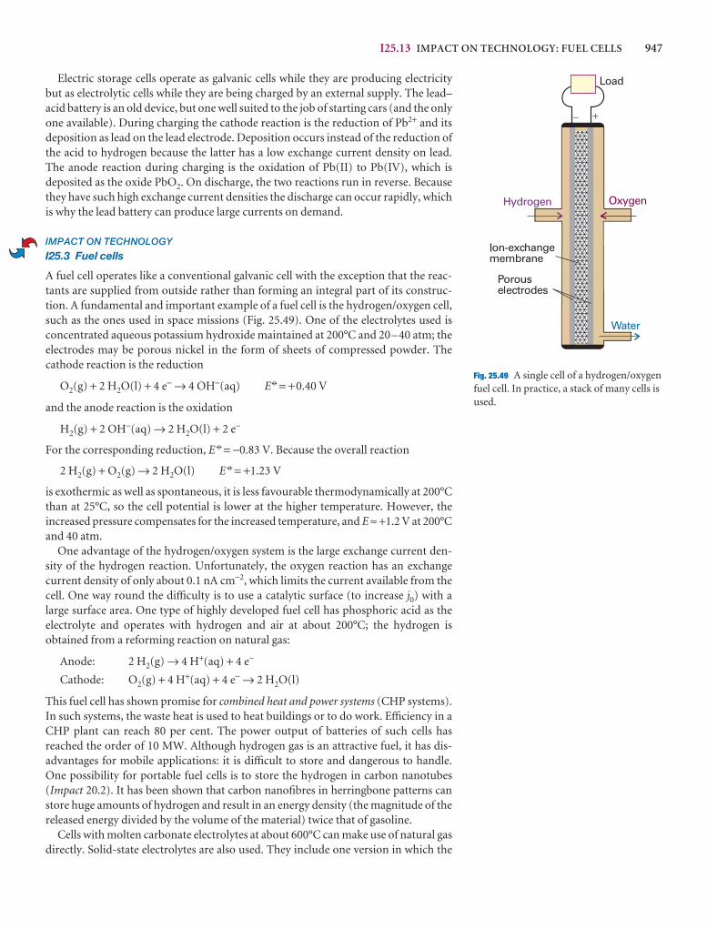
I25.13 IMPACT ON TECHNOLOGY: FUEL CELLS 947
Electric storage cells operate as galvanic cells while they are producing electricitybut as electrolytic cells while they are being charged by an external supply. The lead–acid battery is an old device, but one well suited to the job of starting cars (and the onlyone available). During charging the cathode reaction is the reduction of Pb2+ and itsdeposition as lead on the lead electrode. Deposition occurs instead of the reduction ofthe acid to hydrogen because the latter has a low exchange current density on lead.The anode reaction during charging is the oxidation of Pb(II) to Pb(IV), which is deposited as the oxide PbO2. On discharge, the two reactions run in reverse. Becausethey have such high exchange current densities the discharge can occur rapidly, whichis why the lead battery can produce large currents on demand.
IMPACT ON TECHNOLOGY
I25.3 Fuel cells
A fuel cell operates like a conventional galvanic cell with the exception that the reac-tants are supplied from outside rather than forming an integral part of its construc-tion. A fundamental and important example of a fuel cell is the hydrogen/oxygen cell,such as the ones used in space missions (Fig. 25.49). One of the electrolytes used isconcentrated aqueous potassium hydroxide maintained at 200°C and 20–40 atm; theelectrodes may be porous nickel in the form of sheets of compressed powder. Thecathode reaction is the reduction
O2(g) + 2 H2O(l) + 4 e− → 4 OH−(aq) E 7 = +0.40 V
and the anode reaction is the oxidation
H2(g) + 2 OH−(aq) → 2 H2O(l) + 2 e−
For the corresponding reduction, E 7 = −0.83 V. Because the overall reaction
2 H2(g) + O2(g) → 2 H2O(l) E 7 = +1.23 V
is exothermic as well as spontaneous, it is less favourable thermodynamically at 200°Cthan at 25°C, so the cell potential is lower at the higher temperature. However, the increased pressure compensates for the increased temperature, and E ≈ +1.2 V at 200°Cand 40 atm.
One advantage of the hydrogen/oxygen system is the large exchange current den-sity of the hydrogen reaction. Unfortunately, the oxygen reaction has an exchangecurrent density of only about 0.1 nA cm−2, which limits the current available from thecell. One way round the difficulty is to use a catalytic surface (to increase j0) with alarge surface area. One type of highly developed fuel cell has phosphoric acid as theelectrolyte and operates with hydrogen and air at about 200°C; the hydrogen is obtained from a reforming reaction on natural gas:
Anode: 2 H2(g) → 4 H+(aq) + 4 e−
Cathode: O2(g) + 4 H+(aq) + 4 e− → 2 H2O(l)
This fuel cell has shown promise for combined heat and power systems (CHP systems).In such systems, the waste heat is used to heat buildings or to do work. Efficiency in aCHP plant can reach 80 per cent. The power output of batteries of such cells hasreached the order of 10 MW. Although hydrogen gas is an attractive fuel, it has dis-advantages for mobile applications: it is difficult to store and dangerous to handle.One possibility for portable fuel cells is to store the hydrogen in carbon nanotubes(Impact 20.2). It has been shown that carbon nanofibres in herringbone patterns canstore huge amounts of hydrogen and result in an energy density (the magnitude of thereleased energy divided by the volume of the material) twice that of gasoline.
Cells with molten carbonate electrolytes at about 600°C can make use of natural gasdirectly. Solid-state electrolytes are also used. They include one version in which the
Fig. 25.49 A single cell of a hydrogen/oxygenfuel cell. In practice, a stack of many cells isused.
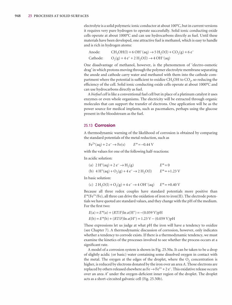
948 25 PROCESSES AT SOLID SURFACES
electrolyte is a solid polymeric ionic conductor at about 100°C, but in current versionsit requires very pure hydrogen to operate successfully. Solid ionic conducting oxidecells operate at about 1000°C and can use hydrocarbons directly as fuel. Until thesematerials have been developed, one attractive fuel is methanol, which is easy to handleand is rich in hydrogen atoms:
Anode: CH3OH(l) + 6 OH−(aq) → 5 H2O(l) + CO2(g) + 6 e−
Cathode: O2(g) + 4 e− + 2 H2O(l) → 4 OH−(aq)
One disadvantage of methanol, however, is the phenomenon of ‘electro-osmoticdrag’ in which protons moving through the polymer electrolyte membrane separatingthe anode and cathode carry water and methanol with them into the cathode com-partment where the potential is sufficient to oxidize CH3OH to CO2, so reducing theefficiency of the cell. Solid ionic conducting oxide cells operate at about 1000°C andcan use hydrocarbons directly as fuel.
A biofuel cell is like a conventional fuel cell but in place of a platinum catalyst it usesenzymes or even whole organisms. The electricity will be extracted through organicmolecules that can support the transfer of electrons. One application will be as thepower source for medical implants, such as pacemakers, perhaps using the glucosepresent in the bloodstream as the fuel.
25.13 Corrosion
A thermodynamic warning of the likelihood of corrosion is obtained by comparingthe standard potentials of the metal reduction, such as
Fe2+(aq) + 2 e− → Fe(s) E 7 = −0.44 V
with the values for one of the following half-reactions:
In acidic solution:
(a) 2 H+(aq) + 2 e− → H2(g) E 7 = 0
(b) 4 H+(aq) + O2(g) + 4 e− → 2 H2O(l) E 7 = +1.23 V
In basic solution:
(c) 2 H2O(l) + O2(g) + 4 e− → 4 OH−(aq) E 7 = +0.40 V
Because all three redox couples have standard potentials more positive thanE 7(Fe2+/Fe), all three can drive the oxidation of iron to iron(II). The electrode poten-tials we have quoted are standard values, and they change with the pH of the medium.For the first two:
E(a) = E 7(a) + (RT/F)ln a(H+) = −(0.059 V)pH
E(b) = E 7(b) + (RT/F)ln a(H+) = 1.23 V − (0.059 V)pH
These expressions let us judge at what pH the iron will have a tendency to oxidize (see Chapter 7). A thermodynamic discussion of corrosion, however, only indicateswhether a tendency to corrode exists. If there is a thermodynamic tendency, we mustexamine the kinetics of the processes involved to see whether the process occurs at asignificant rate.
A model of a corrosion system is shown in Fig. 25.50a. It can be taken to be a dropof slightly acidic (or basic) water containing some dissolved oxygen in contact withthe metal. The oxygen at the edges of the droplet, where the O2 concentration ishigher, is reduced by electrons donated by the iron over an area A. Those electrons arereplaced by others released elsewhere as Fe → Fe2+ + 2 e−. This oxidative release occursover an area A′ under the oxygen-deficient inner region of the droplet. The dropletacts as a short-circuited galvanic cell (Fig. 25.50b).
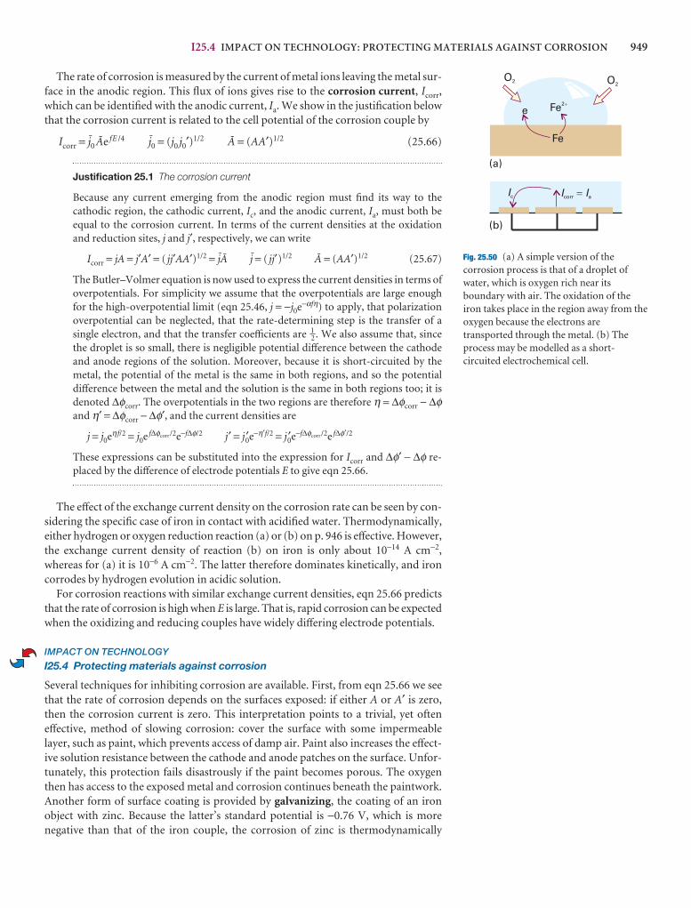
I25.4 IMPACT ON TECHNOLOGY: PROTECTING MATERIALS AGAINST CORROSION 949
The rate of corrosion is measured by the current of metal ions leaving the metal sur-face in the anodic region. This flux of ions gives rise to the corrosion current, Icorr,which can be identified with the anodic current, Ia. We show in the justification belowthat the corrosion current is related to the cell potential of the corrosion couple by
Icorr = H0 Ae fE /4 H0 = (j0 j0′)1/2 A = (AA′)1/2 (25.66)
Justification 25.1 The corrosion current
Because any current emerging from the anodic region must find its way to the cathodic region, the cathodic current, Ic, and the anodic current, Ia, must both beequal to the corrosion current. In terms of the current densities at the oxidation and reduction sites, j and j′, respectively, we can write
Icorr = jA = j′A′ = ( jj′AA′)1/2 = HA H = ( jj′)1/2 A = (AA′)1/2 (25.67)
The Butler–Volmer equation is now used to express the current densities in terms ofoverpotentials. For simplicity we assume that the overpotentials are large enoughfor the high-overpotential limit (eqn 25.46, j = −j0e−αfη) to apply, that polarizationoverpotential can be neglected, that the rate-determining step is the transfer of a single electron, and that the transfer coefficients are 1–2. We also assume that, sincethe droplet is so small, there is negligible potential difference between the cathodeand anode regions of the solution. Moreover, because it is short-circuited by themetal, the potential of the metal is the same in both regions, and so the potentialdifference between the metal and the solution is the same in both regions too; it isdenoted ∆φcorr. The overpotentials in the two regions are therefore η = ∆φcorr − ∆φand η′ = ∆φcorr − ∆φ′, and the current densities are
j = j0eηf/2 = j0e f∆φcorr/2e−f∆φ/2 j′ = j ′0e−η′f/2 = j ′0e−f∆φcorr/2e f∆φ′/2
These expressions can be substituted into the expression for Icorr and ∆φ′ − ∆φ re-placed by the difference of electrode potentials E to give eqn 25.66.
The effect of the exchange current density on the corrosion rate can be seen by con-sidering the specific case of iron in contact with acidified water. Thermodynamically,either hydrogen or oxygen reduction reaction (a) or (b) on p. 946 is effective. However,the exchange current density of reaction (b) on iron is only about 10−14 A cm−2,whereas for (a) it is 10−6 A cm−2. The latter therefore dominates kinetically, and ironcorrodes by hydrogen evolution in acidic solution.
For corrosion reactions with similar exchange current densities, eqn 25.66 predictsthat the rate of corrosion is high when E is large. That is, rapid corrosion can be expectedwhen the oxidizing and reducing couples have widely differing electrode potentials.
IMPACT ON TECHNOLOGY
I25.4 Protecting materials against corrosion
Several techniques for inhibiting corrosion are available. First, from eqn 25.66 we seethat the rate of corrosion depends on the surfaces exposed: if either A or A′ is zero,then the corrosion current is zero. This interpretation points to a trivial, yet ofteneffective, method of slowing corrosion: cover the surface with some impermeablelayer, such as paint, which prevents access of damp air. Paint also increases the effect-ive solution resistance between the cathode and anode patches on the surface. Unfor-tunately, this protection fails disastrously if the paint becomes porous. The oxygenthen has access to the exposed metal and corrosion continues beneath the paintwork.Another form of surface coating is provided by galvanizing, the coating of an iron object with zinc. Because the latter’s standard potential is −0.76 V, which is more negative than that of the iron couple, the corrosion of zinc is thermodynamically
Fig. 25.50 (a) A simple version of thecorrosion process is that of a droplet ofwater, which is oxygen rich near itsboundary with air. The oxidation of theiron takes place in the region away from theoxygen because the electrons aretransported through the metal. (b) Theprocess may be modelled as a short-circuited electrochemical cell.
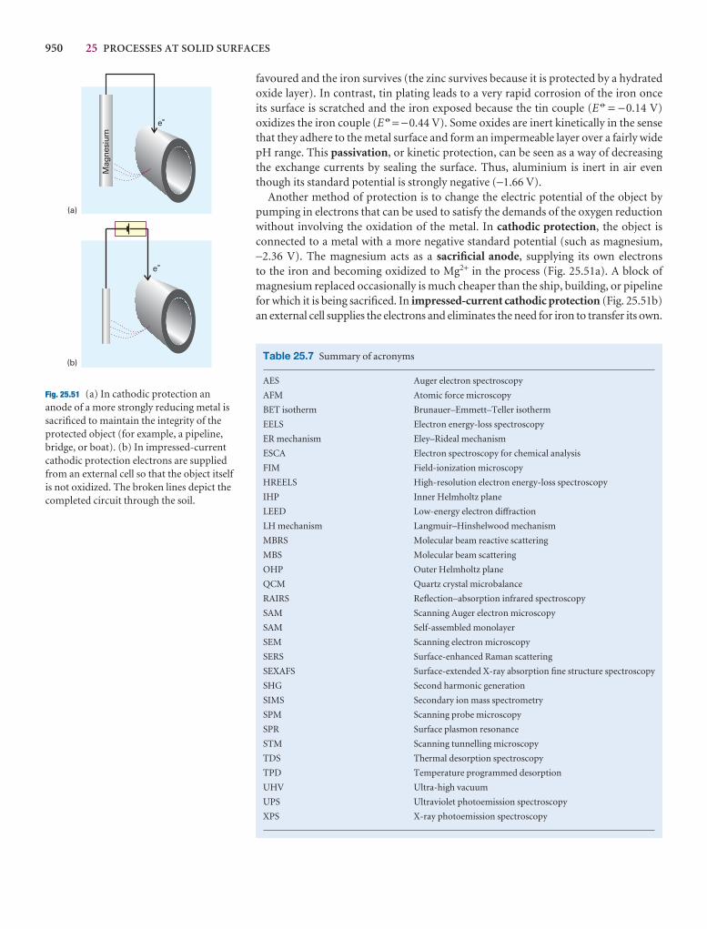
950 25 PROCESSES AT SOLID SURFACES
favoured and the iron survives (the zinc survives because it is protected by a hydratedoxide layer). In contrast, tin plating leads to a very rapid corrosion of the iron once its surface is scratched and the iron exposed because the tin couple (E 7 = −0.14 V) oxidizes the iron couple (E 7 = −0.44 V). Some oxides are inert kinetically in the sensethat they adhere to the metal surface and form an impermeable layer over a fairly widepH range. This passivation, or kinetic protection, can be seen as a way of decreasingthe exchange currents by sealing the surface. Thus, aluminium is inert in air eventhough its standard potential is strongly negative (−1.66 V).
Another method of protection is to change the electric potential of the object bypumping in electrons that can be used to satisfy the demands of the oxygen reductionwithout involving the oxidation of the metal. In cathodic protection, the object isconnected to a metal with a more negative standard potential (such as magnesium, −2.36 V). The magnesium acts as a sacrificial anode, supplying its own electrons to the iron and becoming oxidized to Mg2+ in the process (Fig. 25.51a). A block ofmagnesium replaced occasionally is much cheaper than the ship, building, or pipelinefor which it is being sacrificed. In impressed-current cathodic protection (Fig. 25.51b)an external cell supplies the electrons and eliminates the need for iron to transfer its own.
Fig. 25.51 (a) In cathodic protection ananode of a more strongly reducing metal issacrificed to maintain the integrity of theprotected object (for example, a pipeline,bridge, or boat). (b) In impressed-currentcathodic protection electrons are suppliedfrom an external cell so that the object itselfis not oxidized. The broken lines depict thecompleted circuit through the soil.
Table 25.7 Summary of acronyms
AES Auger electron spectroscopy
AFM Atomic force microscopy
BET isotherm Brunauer–Emmett–Teller isotherm
EELS Electron energy-loss spectroscopy
ER mechanism Eley–Rideal mechanism
ESCA Electron spectroscopy for chemical analysis
FIM Field-ionization microscopy
HREELS High-resolution electron energy-loss spectroscopy
IHP Inner Helmholtz plane
LEED Low-energy electron diffraction
LH mechanism Langmuir–Hinshelwood mechanism
MBRS Molecular beam reactive scattering
MBS Molecular beam scattering
OHP Outer Helmholtz plane
QCM Quartz crystal microbalance
RAIRS Reflection–absorption infrared spectroscopy
SAM Scanning Auger electron microscopy
SAM Self-assembled monolayer
SEM Scanning electron microscopy
SERS Surface-enhanced Raman scattering
SEXAFS Surface-extended X-ray absorption fine structure spectroscopy
SHG Second harmonic generation
SIMS Secondary ion mass spectrometry
SPM Scanning probe microscopy
SPR Surface plasmon resonance
STM Scanning tunnelling microscopy
TDS Thermal desorption spectroscopy
TPD Temperature programmed desorption
UHV Ultra-high vacuum
UPS Ultraviolet photoemission spectroscopy
XPS X-ray photoemission spectroscopy

FURTHER READING 951
Further reading
Articles and texts
A.W. Adamson and A. Gast, Physical chemistry of surfaces. Wiley, NewYork (1997).
A.J. Bard and L.R. Faulkner, Electrochemical methods: fundamentalsand applications. Wiley, New York (2000).
J.O’M. Bockris, R.E. White, and B.E. Conway (ed.), Modern aspects ofelectrochemistry. Vol. 33. Plenum, New York (1999).
G. Ertl, H. Knözinger, and J. Weitkamp, Handbook of heterogeneouscatalysis. VCH, Weinheim (1997).
M.G. Fontanna and R.W. Staehle (ed.), Advances in corrosion scienceand technology. Plenum, New York (1980).
C.H. Hamann, W. Vielstich, and A. Hammett, Electrochemistry.Wiley–VCH, New York (1998).
J.C. Lindon, G.E. Tranter, and J.L. Holmes (ed.), Encyclopedia ofspectroscopy and spectrometry. Academic Press, San Diego (2000).
N. Mizuno and M. Misono, Heterogeneous catalysis. Chem. Rev. 98,199 (1998).
G.A. Somorjai, Modern surface science and surface technologies: an introduction. Chem. Rev. 96, 1223 (1996).
Checklist of key ideas
1. Adsorption is the attachment of molecules to a surface; thesubstance that adsorbs is the adsorbate and the underlyingmaterial is the adsorbent or substrate. The reverse ofadsorption is desorption.
2. The collision flux, Z W, of gas molecules bombarding a solidsurface is related to the gas pressure by Z W = p/(2πmkT)1/2.
3. Techniques for studying surface composition and structureinclude scanning electron microscopy (SEM), scanning probemicroscopy (STM), photoemission spectroscopy, sescondary-ion mass spectrometry, surface-enhanced Raman scattering(SERS), Auger electron spectroscopy (AES), low energyelectron diffraction (LEED), and molecular beam scattering(MBS).
4. The fractional coverage, θ, is the ratio of the number ofoccupied sites to the number of available sites.
5. Techniques for studying the rates of surface processes include flash desorption, biosensor analysis, second harmonicgeneration (SHG), gravimetry by using a quartz crystalmicrobalance (QCM), and molecular beam reactive scattering (MRS).
6. Physisorption is adsorption by a van der Waals interaction;chemisorption is adsorption by formation of a chemical(usually covalent) bond.
7. The Langmuir isotherm is a relation between the fractionalcoverage and the partial pressure of the adsorbate: θ = Kp/(1 + Kp).
8. The isosteric enthalpy of adsorption is determined from a plotof ln K against 1/T.
9. The BET isotherm is an isotherm applicable when multilayeradsorption is possible: V/Vmon = cz/(1 − z){1 − (1 − c)z},with z = p/p*.
10. The sticking probability, s, is the proportion of collisions withthe surface that successfully lead to adsorption.
11. Desorption is an activated process with half-life t1/2 = τ0eEd/RT;the desorption activation energy is measured by temperature-
programmed desorption (TPD) or thermal desorptionspectroscopy (TDS).
12. In the Langmuir–Hinshelwood mechanism (LH mechanism)of surface-catalysed reactions, the reaction takes place byencounters between molecular fragments and atoms adsorbedon the surface.
13. In the Eley–Rideal mechanism (ER mechanism) of a surface-catalysed reaction, a gas-phase molecule collides with anothermolecule already adsorbed on the surface.
14. An electrical double layer consists of a sheet of positive chargeat the surface of the electrode and a sheet of negative chargenext to it in the solution (or vice versa).
15. The Galvani potential difference is the potential differencebetween the bulk of the metal electrode and the bulk of thesolution.
16. Models of the double layer include the Helmholtz layer modeland the Gouy–Chapman model.
17. The current density, j, at an electrode is expressed by theButler–Volmer equation, j = j0{e(1−α)fη − e−αfη}, where η is theoverpotential, η = E′ − E, α is the transfer coefficient, and j0 isthe exchange-current density.
18. A Tafel plot is a plot of the logarithm of the current densityagainst the overpotential: the slope gives the value of α andthe intercept at η = 0 gives the exchange-current density.
19. Voltammetry is the study of the current through an electrodeas a function of the applied potential difference. Experimentaltechniques include linear-sweep voltammetry, differentialpulse voltammetry, and cyclic voltammetry.
20. To induce current to flow through an electrolytic cell andbring about a nonspontaneous cell reaction, the appliedpotential difference must exceed the cell emf by at least the celloverpotential.
21. The corrosion current is a current proportional to the rate atwhich metal ions leave a metal surface in the anodic regionduring corrosion.
952 25 PROCESSES AT SOLID SURFACES
Discussion questions
25.1 (a) Distinguish between a step and a terrace. (b) Describe how steps andterraces can be formed by dislocations.
25.2 (a) Describe the advantages and limitations of each of the spectroscopictechniques designated by the acronyms AES, EELS, HREELS, RAIRS, SERS, SEXAFS, SHG, UPS, and XPS. (b) Describe the advantages and
limitations of each of the microscopy, diffraction, and scattering techniquesdesignated by the acronyms AFM, FIM, LEED, MBRS, MBS, SAM, SEM, and STM.
25.3 Distinguish between the following adsorption isotherms: Langmuir,BET, Temkin, and Freundlich.
C.D.S. Tuck, Modern battery construction. Ellis Horwood, New York(1991).
J. Vickerman, Surface analysis: techniques and applications. Wiley,New York (1997).
Sources of data and information
C.M.A. Brett and A.M.O. Brett, Electrode potentials. OxfordChemistry Primers, Oxford University Press (1998).
D. Linden (ed.), Handbook of batteries and cells. McGraw-Hill, New York (1984).
Further information
Further information 25.1 The relation between electrode potentialand the Galvani potential
To demonstrate the relation between ∆φ and E, consider the cellPt |H2(g)|H+(g)| |M+(aq)|M(s) and the half-reactions
M+(aq) + e− → M(s) H+(aq) + e− → 1–2 H2(g)
The Gibbs energies of these two half-reactions can be expressed interms of the chemical potentials, µ, of all the species. However, wemust take into account the fact that the species are present in phaseswith different electric potentials. Thus, a cation in a region of positivepotential has a higher chemical potential (is chemically more active in a thermodynamic sense) than in a region of zero potential.
The contribution of an electric potential to the chemical potentialis calculated by noting that the electrical work of adding a charge ze toa region where the potential is φ is zeφ, and therefore that the workper mole is zFφ, where F is Faraday’s constant. Because at constanttemperature and pressure the maximum electrical work can beidentified with the change in Gibbs energy (Section 7.7), thedifference in chemical potential of an ion with and without theelectrical potential present is zFφ. The chemical potential of an ion inthe presence of an electric potential is called its electrochemicalpotential, G. It follows that
G = µ + zFφ [25.68]
where µ is the chemical potential of the species when the electricalpotential is zero. When z = 0 (a neutral species), the electrochemicalpotential is equal to the chemical potential.
To express the Gibbs energy for the half-reactions in terms of theelectrochemical potentials of the species we note that the cations M+
are in the solution where the inner potential is φS and the electronsare in the electrode where it is φM. It follows that
∆ rGR = G(M) − {G(M+) + G(e−)}
= µ(M) − {µ(M+) + FφS + µ(e−) − FφM}
= µ(M) − µ(M+) − µ(e−) + F∆φR
where ∆φR = φM − φS is the Galvani potential difference at the right-hand electrode. Likewise, in the hydrogen half-reaction, the electronsare in the platinum electrode at a potential φPt and the H+ ions are inthe solution where the potential is φS:
∆rGL = 1–2 G(H2) − {G(H+) + G(e−)}
= 1–2 µ(H2) − µ(H+) − µ(e−) + F∆φL
where ∆φL = φPt − φS is the Galvani potential difference at the left-hand electrode.
The overall reaction Gibbs energy is
∆rGR − ∆rGL = µ(M) + µ(H+) − µ(M+) − 1–2 µ(H2) + F(∆φR − ∆φL)
= ∆rG + F(∆φR − ∆φL)
where ∆rG is the Gibbs energy of the cell reaction. When the cell isbalanced against an external source of potential the entire system is atequilibrium. The overall reaction Gibbs energy is then zero (becauseits tendency to change is balanced against the external source ofpotential and overall there is stalemate), and the last equationbecomes
0 = ∆rG + F(∆φR − ∆φL)
which rearranges to
∆rG = −F(∆φR − ∆φL) (25.69)
If we compare this with the result established in Section 7.7 that ∆rG = −FE and E = ER − EL, we can conclude that (ignoring the effectsof any metal–platinum and liquid junction potentials that may bepresent in an actual cell)
ER − EL = ∆φR − ∆φL (25.70)
This is the result we wanted to show, for it implies that the Galvanipotential difference at each electrode can differ from the electrodepotential by a constant at most; that constant cancels when thedifference is taken.

EXERCISES 953
25.4 Consider the analysis of surface plasmon resonance data (as in biosensoranalysis) and discuss how a plot of a0 /Req against a0 may be used to evaluateRmax and K.
25.5 Describe the essential features of the Langmuir–Hinshelwood,Eley–Rideal, and Mars van Krevelen mechanisms for surface-catalysedreactions.
25.6 Account for the dependence of catalytic activity of a surface on thestrength of chemisorption, as shown in Fig. 25.28.
25.7 Discuss the unique physical and chemical properties of zeolites thatmake them useful heterogeneous catalysts.
25.8 (a) Discuss the main structural features of the electrical double layer. (b)Distinguish between the electrical double layer and the Nernst diffusion layer.
25.9 Define the terms in and limit the generality of the following expressions:(a) j = j0 fη, (b) j = j0e(1−α)fη, and (c) j = −j0e−α fη.
25.10 Discuss the technique of cyclic voltammetry and account for thecharacteristic shape of a cyclic voltammogram, such as those shown in Figs.25.45 and 25.46.
25.11 Discuss the principles of operation of a fuel cell.
25.12 Discuss the chemical origins of corrosion and useful strategies forpreventing it.
Exercises
25.1a Calculate the frequency of molecular collisions per square centimetreof surface in a vessel containing (a) hydrogen, (b) propane at 25°C when thepressure is (i) 100 Pa, (ii) 0.10 µTorr.
25.1b Calculate the frequency of molecular collisions per square centimetreof surface in a vessel containing (a) nitrogen, (b) methane at 25°C when thepressure is (i) 10.0 Pa, (ii) 0.150 µTorr.
25.2a What pressure of argon gas is required to produce a collision rate of 4.5 × 10²⁰ s−1 at 425 K on a circular surface of diameter 1.5 mm?
25.2b What pressure of nitrogen gas is required to produce a collision rate of5.00 × 1019 s−1 at 525 K on a circular surface of diameter 2.0 mm?
25.3a Calculate the average rate at which He atoms strike a Cu atom in asurface formed by exposing a (100) plane in metallic copper to helium gas at80 K and a pressure of 35 Pa. Crystals of copper are face-centred cubic with acell edge of 361 pm.
25.3b Calculate the average rate at which He atoms strike an iron atom in asurface formed by exposing a (100) plane in metallic iron to helium gas at 100 K and a pressure of 24 Pa. Crystals of iron are body-centred cubic with a cell edge of 145 pm.
25.4a A monolayer of N2 molecules (effective area 0.165 nm2) is adsorbed onthe surface of 1.00 g of an Fe/Al2O3 catalyst at 77 K, the boiling point of liquidnitrogen. Upon warming, the nitrogen occupies 2.86 cm3 at 0°C and 760 Torr.What is the surface area of the catalyst?
25.4b A monolayer of CO molecules (effective area 0.165 nm2) is adsorbed onthe surface of 1.00 g of an Fe/Al2O3 catalyst at 77 K, the boiling point of liquidnitrogen. Upon warming, the carbon monoxide occupies 4.25 cm3 at 0°C and1.00 bar. What is the surface area of the catalyst?
25.5a The volume of oxygen gas at 0°C and 101 kPa adsorbed on the surfaceof 1.00 g of a sample of silica at 0°C was 0.284 cm3 at 142.4 Torr and 1.430 cm3
at 760 Torr. What is the value of Vmon?
25.5b The volume of gas at 20°C and 1.00 bar adsorbed on the surface of 1.50 g of a sample of silica at 0°C was 1.60 cm3 at 52.4 kPa and 2.73 cm3 at104 kPa. What is the value of Vmon?
25.6a The enthalpy of adsorption of CO on a surface is found to be −120 kJmol−1. Estimate the mean lifetime of a CO molecule on the surface at 400 K.
25.6b The enthalpy of adsorption of ammonia on a nickel surface is found tobe −155 kJ mol−1. Estimate the mean lifetime of an NH3 molecule on thesurface at 500 K.
25.7a The average time for which an oxygen atom remains adsorbed to atungsten surface is 0.36 s at 2548 K and 3.49 s at 2362 K. Find the activation
energy for desorption. What is the pre-exponential factor for these tightlychemisorbed atoms?
25.7b The chemisorption of hydrogen on manganese is activated, but onlyweakly so. Careful measurements have shown that it proceeds 35 per centfaster at 1000 K than at 600 K. What is the activation energy for chemisorption?
25.8a The adsorption of a gas is described by the Langmuir isotherm with K = 0.85 kPa−1 at 25°C. Calculate the pressure at which the fractional surfacecoverage is (a) 0.15, (b) 0.95.
25.8b The adsorption of a gas is described by the Langmuir isotherm with K = 0.777 kPa−1 at 25°C. Calculate the pressure at which the fractional surfacecoverage is (a) 0.20, (b) 0.75.
25.9a A certain solid sample adsorbs 0.44 mg of CO when the pressure of thegas is 26.0 kPa and the temperature is 300 K. The mass of gas adsorbed whenthe pressure is 3.0 kPa and the temperature is 300 K is 0.19 mg. The Langmuirisotherm is known to describe the adsorption. Find the fractional coverage ofthe surface at the two pressures.
25.9b A certain solid sample adsorbs 0.63 mg of CO when the pressure of thegas is 36.0 kPa and the temperature is 300 K. The mass of gas adsorbed whenthe pressure is 4.0 kPa and the temperature is 300 K is 0.21 mg. The Langmuirisotherm is known to describe the adsorption. Find the fractional coverage ofthe surface at the two pressures.
25.10a For how long on average would an H atom remain on a surface at 298 K if its desorption activation energy were (a) 15 kJ mol−1, (b) 150 kJ mol−1?Take τ0 = 0.10 ps. For how long on average would the same atoms remain at1000 K?
25.10b For how long on average would an atom remain on a surface at 400 Kif its desorption activation energy were (a) 20 kJ mol−1, (b) 200 kJ mol−1? Takeτ0 = 0.12 ps. For how long on average would the same atoms remain at 800 K?
25.11a A solid in contact with a gas at 12 kPa and 25°C adsorbs 2.5 mg of thegas and obeys the Langmuir isotherm. The enthalpy change when 1.00 mmolof the adsorbed gas is desorbed is +10.2 J. What is the equilibrium pressure forthe adsorption of 2.5 mg of gas at 40°C?
25.11b A solid in contact with a gas at 8.86 kPa and 25°C adsorbs 4.67 mg of the gas and obeys the Langmuir isotherm. The enthalpy change when 1.00 mmol of the adsorbed gas is desorbed is +12.2 J. What is the equilibriumpressure for the adsorption of the same mass of gas at 45°C?
25.12a Hydrogen iodide is very strongly adsorbed on gold but only slightlyadsorbed on platinum. Assume the adsorption follows the Langmuir isothermand predict the order of the HI decomposition reaction on each of the twometal surfaces.

954 25 PROCESSES AT SOLID SURFACES
25.12b Suppose it is known that ozone adsorbs on a particular surface inaccord with a Langmuir isotherm. How could you use the pressuredependence of the fractional coverage to distinguish between adsorption (a) without dissociation, (b) with dissociation into O + O2, (c) withdissociation into O + O + O?
25.13a Nitrogen gas adsorbed on charcoal to the extent of 0.921 cm3 g−1 at490 kPa and 190 K, but at 250 K the same amount of adsorption was achievedonly when the pressure was increased to 3.2 MPa. What is the enthalpy ofadsorption of nitrogen on charcoal?
25.13b Nitrogen gas adsorbed on a surface to the extent of 1.242 cm3 g−1 at350 kPa and 180 K, but at 240 K the same amount of adsorption was achievedonly when the pressure was increased to 1.02 MPa. What is the enthalpy ofadsorption of nitrogen on the surface?
25.14a In an experiment on the adsorption of oxygen on tungsten it wasfound that the same volume of oxygen was desorbed in 27 min at 1856 K and2.0 min at 1978 K. What is the activation energy of desorption? How longwould it take for the same amount to desorb at (a) 298 K, (b) 3000 K?
25.14b In an experiment on the adsorption of ethene on iron it was foundthat the same volume of the gas was desorbed in 1856 s at 873 K and 8.44 s at1012 K. What is the activation energy of desorption? How long would it takefor the same amount of ethene to desorb at (a) 298 K, (b) 1500 K?
25.15a The Helmholtz model of the electric double layer is equivalent to aparallel plate capacitor. Hence the potential difference across the double layeris given by ∆ϕ = σd /ε, where d is the distance between the plates and σ is thesurface charge density. Assuming that this model holds for concentrated saltsolutions calculate the magnitude of the electric field at the surface of silica in5.0 M NaCl(aq) if the surface charge density is 0.10 C m−2.
25.15b Refer to the preceding exercise. Calculate the magnitude of the electricfield at the surface of silica in 4.5 M NaCl(aq) if the surface charge density is0.12 C m−2.
25.16a The transfer coefficient of a certain electrode in contact with M3+ andM4+ in aqueous solution at 25°C is 0.39. The current density is found to be55.0 mA cm−2 when the overvoltage is 125 mV. What is the overvoltagerequired for a current density of 75 mA cm−2?
25.16b The transfer coefficient of a certain electrode in contact with M2+ andM3+ in aqueous solution at 25°C is 0.42. The current density is found to be17.0 mA cm−2 when the overvoltage is 105 mV. What is the overvoltagerequired for a current density of 72 mA cm−2?
25.17a Determine the exchange current density from the information givenin Exercise 25.16a.
25.17b Determine the exchange current density from the information givenin Exercise 25.16b.
25.18a To a first approximation, significant evolution or deposition occurs inelectrolysis only if the overpotential exceeds about 0.6 V. To illustrate thiscriterion determine the effect that increasing the overpotential from 0.40 V to0.60 V has on the current density in the electrolysis of 1.0 M NaOH(aq), whichis 1.0 mA cm−2 at 0.4 V and 25°C. Take α = 0.5.
25.18b Determine the effect that increasing the overpotential from 0.50 V to0.60 V has on the current density in the electrolysis of 1.0 M NaOH(aq), whichis 1.22 mA cm−2 at 0.50 V and 25°C. Take α = 0.50.
25.19a Use the data in Table 25.6 for the exchange current density andtransfer coefficient for the reaction 2 H+ + 2 e− → H2 on nickel at 25°C todetermine what current density would be needed to obtain an overpotential of0.20 V as calculated from (a) the Butler–Volmer equation, and (b) the Tafelequation. Is the validity of the Tafel approximation affected at higheroverpotentials (of 0.4 V and more)?
25.19b Use the data in Table 25.6 for the exchange current density andtransfer coefficient for the reaction Fe3+ + e−→ Fe2+ on platinum at 25°C todetermine what current density would be needed to obtain an overpotential of0.30 V as calculated from (a) the Butler–Volmer equation, and (b) the Tafelequation. Is the validity of the Tafel approximation affected at higheroverpotentials (of 0.4 V and more)?
25.20a Estimate the limiting current density at an electrode in which theconcentration of Ag+ ions is 2.5 mmol dm−3 at 25°C. The thickness of theNernst diffusion layer is 0.40 mm. The ionic conductivity of Ag+ at infinitedilution and 25°C is 6.19 mS m2 mol−1.
25.20b Estimate the limiting current density at an electrode in which theconcentration of Mg2+ ions is 1.5 mmol dm−3 at 25°C. The thickness of theNernst diffusion layer is 0.32 mm. The ionic conductivity of Mg2+ at infinitedilution and 25°C is 10.60 mS m2 mol−1.
25.21a A 0.10 M CdSO4(aq) solution is electrolysed between a cadmiumcathode and a platinum anode with a current density of 1.00 mA cm−2. Thehydrogen overpotential is 0.60 V. What will be the concentration of Cd2+ ionswhen evolution of H2 just begins at the cathode? Assume all activitycoefficients are unity.
25.21b A 0.10 M FeSO4(aq) solution is electrolysed between a magnesiumcathode and a platinum anode with a current density of 1.50 mA cm−2. Thehydrogen overpotential is 0.60 V. What will be the concentration of Fe2+ ionswhen evolution of H2 just begins at the cathode? Assume all activitycoefficients are unity.
25.22a A typical exchange current density, that for H+ discharge at platinum,is 0.79 mA cm−2 at 25°C. What is the current density at an electrode when itsoverpotential is (a) 10 mV, (b) 100 mV, (c) −5.0 V? Take α = 0.5.
25.22b The exchange current density for a Pt|Fe3+,Fe2+ electrode is 2.5 mAcm−2. The standard potential of the electrode is +0.77 V. Calculate the currentflowing through an electrode of surface area 1.0 cm2 as a function of thepotential of the electrode. Take unit activity for both ions.
25.23a Suppose that the electrode potential is set at 1.00 V. The exchangecurrent density is 6.0 × 10⁻⁴ A cm−2 and α = 0.50. Calculate the current densityfor the ratio of activities a(Fe3+)/a(Fe2+) in the range 0.1 to 10.0 and at 25°C.
25.23b Suppose that the electrode potential is set at 0.50 V. Calculate thecurrent density for the ratio of activities a(Cr3+)/a(Cr2+) in the range 0.1 to10.0 and at 25°C.
25.24a What overpotential is needed to sustain a current of 20 mA at aPt |Fe3+,Fe2+ electrode in which both ions are at a mean activity a = 0.10?The surface area of the electrode is 1.0 cm2.
25.24b What overpotential is needed to sustain a current of 15 mA at aPt |Ce4+,Ce3+ electrode in which both ions are at a mean activity a = 0.010?
25.25a How many electrons or protons are transported through the doublelayer in each second when the Pt,H2 |H+, Pt |Fe3+,Fe2+, and Pb,H2 |H+
electrodes are at equilibrium at 25°C? Take the area as 1.0 cm2 in each case.Estimate the number of times each second a single atom on the surface takespart in a electron transfer event, assuming an electrode atom occupies about(280 pm)2 of the surface.
25.25b How many electrons or protons are transported through the doublelayer in each second when the Cu,H2 |H+ and Pt |Ce4+,Ce3+ electrodes are atequilibrium at 25°C? Take the area as 1.0 cm2 in each case. Estimate thenumber of times each second a single atom on the surface takes part in aelectron transfer event, assuming an electrode atom occupies about (260 pm)2
of the surface.
25.26a What is the effective resistance at 25°C of an electrode interface whenthe overpotential is small? Evaluate it for 1.0 cm2 (a) Pt,H2 |H+, (b) Hg,H2 |H+
electrodes.
PROBLEMS 955
25.26b Evaluate the effective resistance at 25°C of an electrode interface for1.0 cm2 (a) Pb,H2 |H+, (b) Pt|Fe2+,Fe3+ electrodes.
25.27a State what happens when a platinum electrode in an aqueous solutioncontaining both Cu2+ and Zn2+ ions at unit activity is made the cathode of anelectrolysis cell.
25.27b State what happens when a platinum electrode in an aqueous solutioncontaining both Fe2+ and Ni2+ ions at unit activity is made the cathode of anelectrolysis cell.
25.28a What are the conditions that allow a metal to be deposited fromaqueous acidic solution before hydrogen evolution occurs significantly at 293 K? Why may silver be deposited from aqueous silver nitrate?
25.28b The overpotential for hydrogen evolution on cadmium is about 1 V atcurrent densities of 1 mA cm−2. Why may cadmium be deposited fromaqueous cadmium sulfate?
25.29a The exchange current density for H+ discharge at zinc is about 50 pAcm−2. Can zinc be deposited from a unit activity aqueous solution of a zincsalt?
25.29b The standard potential of the Zn2+ |Zn electrode is −0.76 V at 25°C.The exchange current density for H+ discharge at platinum is 0.79 mA cm−2.Can zinc be plated on to platinum at that temperature? (Take unit activities.)
25.30a Can magnesium be deposited on a zinc electrode from a unit activityacid solution at 25°C?
25.30b Can iron be deposited on a copper electrode from a unit activity acidsolution at 25°C?
25.31a Calculate the maximum (zero-current) potential difference of anickel–cadmium cell, and the maximum possible power output when 100 mAis drawn at 25°C.
25.31b Calculate the maximum (zero-current) potential difference of alead–acid cell, and the maximum possible power output when 100 mA isdrawn at 25°C.
25.32a The corrosion current density jcorr at an iron anode is 1.0 A m−2. Whatis the corrosion rate in millimetres per year? Assume uniform corrosion.
25.32b The corrosion current density jcorr at a zinc anode is 2.0 A m−2. Whatis the corrosion rate in millimetres per year? Assume uniform corrosion.
Problems*
Numerical problems
25.1 The movement of atoms and ions on a surface depends on their abilityto leave one position and stick to another, and therefore on the energy changesthat occur. As an illustration, consider a two-dimensional square lattice ofunivalent positive and negative ions separated by 200 pm, and consider acation on the upper terrace of this array. Calculate, by direct summation, itsCoulombic interaction when it is in an empty lattice point directly above ananion. Now consider a high step in the same lattice, and let the cation moveinto the corner formed by the step and the terrace. Calculate the Coulombicenergy for this position, and decide on the likely settling point for the cation.
25.2 In a study of the catalytic properties of a titanium surface it wasnecessary to maintain the surface free from contamination. Calculate thecollision frequency per square centimetre of surface made by O2 molecules at(a) 100 kPa, (b) 1.00 Pa and 300 K. Estimate the number of collisions madewith a single surface atom in each second. The conclusions underline theimportance of working at very low pressures (much lower than 1 Pa, in fact)in order to study the properties of uncontaminated surfaces. Take the nearest-neighbour distance as 291 pm.
25.3 Nickel is face-centred cubic with a unit cell of side 352 pm. What is thenumber of atoms per square centimetre exposed on a surface formed by (a) (100), (b) (110), (c) (111) planes? Calculate the frequency of molecularcollisions per surface atom in a vessel containing (a) hydrogen, (b) propane at25°C when the pressure is (i) 100 Pa, (ii) 0.10 µTorr.
25.4 The data below are for the chemisorption of hydrogen on copperpowder at 25°C. Confirm that they fit the Langmuir isotherm at lowcoverages. Then find the value of K for the adsorption equilibrium and theadsorption volume corresponding to complete coverage.
p/Pa 25 129 253 540 1000 1593
V/cm3 0.042 0.163 0.221 0.321 0.411 0.471
25.5 The data for the adsorption of ammonia on barium fluoride are reported below. Confirm that they fit a BET isotherm and find values of c and Vmon.
(a) θ = 0°C, p* = 429.6 kPa:
p/kPa 14.0 37.6 65.6 79.2 82.7 100.7 106.4
V/cm3 11.1 13.5 14.9 16.0 15.5 17.3 16.5
(b) θ = 18.6°C, p* = 819.7 kPa:
p/kPa 5.3 8.4 14.4 29.2 62.1 74.0 80.1 102.0
V/cm3 9.2 9.8 10.3 11.3 12.9 13.1 13.4 14.1
25.6 The following data have been obtained for the adsorption of H2 on thesurface of 1.00 g of copper at 0°C. The volume of H2 below is the volume thatthe gas would occupy at STP (0°C and 1 atm).
p/atm 0.050 0.100 0.150 0.200 0.250
V/cm3 1.22 1.33 1.31 1.36 1.40
Determine the volume of H2 necessary to form a monolayer and estimate the surface area of the copper sample. The density of liquid hydrogen is 0.708 g cm−3.
25.7 The adsorption of solutes on solids from liquids often follows aFreundlich isotherm. Check the applicability of this isotherm to the followingdata for the adsorption of acetic acid on charcoal at 25°C and find the valuesof the parameters c1 and c2.
[acid]/(mol dm−3) 0.05 0.10 0.50 1.0 1.5
wa /g 0.04 0.06 0.12 0.16 0.19
wa is the mass adsorbed per unit mass of charcoal.
25.8 In some catalytic reactions the products may adsorb more strongly thanthe reacting gas. This is the case, for instance, in the catalytic decomposition ofammonia on platinum at 1000°C. As a first step in examining the kinetics of
* Problems denoted with the symbol ‡ were supplied by Charles Trapp, Carmen Giunta, and Marshall Cady.
25.14 The standard potentials of lead and tin are −126 mV and −136 mVrespectively at 25°C, and the overvoltage for their deposition are close to zero.What should their relative activities be in order to ensure simultaneousdeposition from a mixture?
25.15 The limiting current density for the reaction I3− + 2 e− → 3 I− at a
platinum electrode is 28.9 µA cm−2 when the concentration of KI is 6.6 ×10⁻⁴ mol dm−3 and the temperature 25°C. The diffusion coefficient of I3
− is1.14 × 10−9 m2 s−3. What is the thickness of the diffusion layer?
25.16 Estimating the power output and potential of a cell under operating conditions is very difficult, but eqn 25.65 summarizes, in anapproximate way, some of the parameters involved. As a first step inmanipulating this expression, identify all the quantities that depend on theionic concentrations. Express E in terms of the concentration andconductivities of the ions present in the cell. Estimate the parameters forZn(s) |ZnSO4(aq)||CuSO4(aq)|Cu(s). Take electrodes of area 5 cm2 separatedby 5 cm. Ignore both potential differences and resistance of the liquidjunction. Take the concentration as 1 mol dm−3, the temperature 25°C, andneglect activity coefficients. Plot E as a function of the current drawn. On thesame graph, plot the power output of the cell. What current corresponds tomaximum power?
25.17 Consider a cell in which the current is activation-controlled. Show thatthe current for maximum power can be estimated by plotting log(I/I0) and c1 − c2I against I (where I0 = A2j0 j ′0 and c1 and c2 are constants), and looking forthe point of intersection of the curves. Carry through this analysis for the cellin Problem 25.16 ignoring all concentration overpotentials.
25.18‡ The rate of deposition of iron, v, on the surface of an iron electrodefrom an aqueous solution of Fe2+ has been studied as a function of potential,E, relative to the standard hydrogen electrode, by J. Kanya (J. Electroanal.Chem. 84, 83 (1977)). The values in the table below are based on the dataobtained with an electrode of surface area 9.1 cm2 in contact with a solution ofconcentration 1.70 µmol dm−3 in Fe2+. (a) Assuming unit activity coefficients,calculate the zero current potential of the Fe2+/Fe cathode and theoverpotential at each value of the working potential. (b) Calculate thecathodic current density, jc, from the rate of deposition of Fe2+ for each valueof E. (c) Examine the extent to which the data fit the Tafel equation andcalculate the exchange current density.
v/(pmol s−1) 1.47 2.18 3.11 7.26
−E /mV 702 727 752 812
25.19‡ The thickness of the diffuse double layer according to theGouy–Chapman model is given by eqn 19.46. Use this equation to calculateand plot the thickness as a function of concentration and electrolyte type at25°C. For examples, choose aqueous solutions of NaCl and Na2SO4 ranging inconcentration from 0.1 to 100 mmol dm−3.
25.20‡ V.V. Losev and A.P. Pchel’nikov (Soviet Electrochem. 6, 34 (1970))obtained the following current–voltage data for an indium anode relative to astandard hydrogen electrode at 293 K:
−E /V 0.388 0.365 0.350 0.335
j/(A m−2) 0 0.590 1.438 3.507
Use these data to calculate the transfer coefficient and the exchange currentdensity. What is the cathodic current density when the potential is 0.365 V?
25.21‡ The redox reactions of quinones have been the subject of many studiesover the years and they continue to be of interest to electrochemists. In a studyof methone (1,1-dimethyl-3,5-cyclohexanedione) by E. Kariv, J. Hermolin,and E. Gileadi (Electrochim. Acta 16, 1437 (1971)), the followingcurrent–voltage data were obtained for the reduction of the quinone inanhydrous butanol on a mercury electrode:
−E /V 1.50 1.58 1.63 1.72 1.87 1.98 ≥2.10
j /(A m−2 ) 10 30 50 100 200 250 290
956 25 PROCESSES AT SOLID SURFACES
this type of process, show that the rate of ammonia decomposition shouldfollow
= −kc
in the limit of very strong adsorption of hydrogen. Start by showing that,when a gas J adsorbs very strongly, and its pressure is pJ, the fraction ofuncovered sites is approximately 1/KpJ. Solve the rate equation for thecatalytic decomposition of NH3 on platinum and show that a plot of F(t) =(1/t) ln(p/p0) against G(t) = (p − p0)/t, where p is the pressure of ammonia,should give a straight line from which kc can be determined. Check the ratelaw on the basis of the data below, and find kc for the reaction.
t /s 0 30 60 100 160 200 250
p /kPa 13.3 11.7 11.2 10.7 10.3 9.9 9.6
25.9‡ A. Akgerman and M. Zardkoohi (J. Chem. Eng. Data 41, 185 (1996))examined the adsorption of phenol from aqueous solution on to fly ash at 20°C. They fitted their observations to a Freundlich isotherm of the form cads = Kc1/n
sol, where cads is the concentration of adsorbed phenol and csol isthe concentration of aqueous phenol. Among the data reported are thefollowing:
c sol /(mg g−1) 8.26 15.65 25.43 31.74 40.00
c ads /(mg g−1) 4.4 19.2 35.2 52.0 67.2
Determine the constants K and n. What further information would benecessary in order to express the data in terms of fractional coverage, θ?
25.10‡ C. Huang and W.P. Cheng (J. Colloid Interface Sci. 188, 270 (1997))examined the adsorption of the hexacyanoferrate(III) ion, [Fe(CN)6]3−, on γ-Al2O3 from aqueous solution. They modelled the adsorption with a modifiedLangmuir isotherm, obtaining the following values of K at pH = 6.5:
T/K 283 298 308 318
10−11K 2.642 2.078 1.286 1.085
Determine the isosteric enthalpy of adsorption, ∆adsH7, at this pH. The
researchers also reported ∆adsS7 = +146 J mol−1 K−1 under these conditions.
Determine ∆adsG7.
25.11‡ M.-G. Olivier and R. Jadot (J. Chem. Eng. Data 42, 230 (1997))studied the adsorption of butane on silica gel. They report the followingamounts of absorption (in moles per kilogram of silica gel) at 303 K:
p /kPa 31.00 38.22 53.03 76.38 101.97
n/(mol kg−1) 1.00 1.17 1.54 2.04 2.49
p /kPa 130.47 165.06 182.41 205.75 219.91
n /(mol kg−1) 2.90 3.22 3.30 3.35 3.36
Fit these data to a Langmuir isotherm, and determine the value of n thatcorresponds to complete coverage and the constant K.
25.12‡ The following data were obtained for the extent of adsorption, s, ofacetone on charcoal from an aqueous solution of molar concentration, c,at 18°C.
c /(mmol dm−3) 15.0 23.0 42.0 84.0 165 390 800
s/(mmol acetone/g charcoal) 0.60 0.75 1.05 1.50 2.15 3.50 5.10
Which isotherm fits this data best, Langmuir, Freundlich, or Temkin?
25.13 In an experiment on the Pt |H2 |H+ electrode in dilute H2SO4 thefollowing current densities were observed at 25°C. Evaluate α and j0 for theelectrode.
η /mV 50 100 150 200 250
j/(mA cm−2) 2.66 8.91 29.9 100 335
How would the current density at this electrode depend on the overpotentialof the same set of magnitudes but of opposite sign?
pNH3
pH2
dpNH3
dt

PROBLEMS 957
(a) How well do these data fit the empirical Tafel equation? (b) The authorspostulate that the reduction product is the dimer HMMH formed by thefollowing mechanism (where the quinone is denoted M):
(1) M(sol) 5 M(ads)
(2) M(ads) + H+ + e− → MH(ads)
(3) MH(ads) + MH(ads) 5 HMMH
The affixes sol and ads refer to species in solution and on the surface of theelectrode, respectively. Does this mechanism help to explain thecurrent–voltage data?
25.22‡ An early study of the hydrogen overpotential is that of H. Bowden andT. Rideal (Proc. Roy. Soc. A120, 59 (1928)), who measured the overpotentialfor H2 evolution with a mercury electrode in dilute aqueous solutions ofH2SO4 at 25°C. Determine the exchange current density and transfercoefficient, α, from their data:
j /(mA m−2 ) 2.9 6.3 28 100 250 630 1650 3300
η/V 0.60 0.65 0.73 0.79 0.84 0.89 0.93 0.96
Explain any deviations from the result expected from the Tafel equation.
Theoretical problems
25.23 Although the attractive van der Waals interaction between individualmolecules varies as R−6, the interaction of a molecule with a nearby solid (a homogeneous collection of molecules) varies as R−3, where R is its verticaldistance above the surface. Confirm this assertion. Calculate the interactionenergy between an Ar atom and the surface of solid argon on the basis of aLennard-Jones (6,12)-potential. Estimate the equilibrium distance of an atomabove the surface.
25.24 Use the Gibbs adsorption isotherm (another name for eqn 19.50), toshow that the volume adsorbed per unit area of solid, Va /σ, is related to thepressure of the gas by Va = −(σ /RT)(dµ/d ln p), where µ is the chemicalpotential of the adsorbed gas.
25.25 If the dependence of the chemical potential of the gas on the extent ofsurface coverage is known, the Gibbs adsorption isotherm, eqn 19.50, can beintegrated to give a relation between Va and p, as in a normal adsorptionisotherm. For instance, suppose that the change in the chemical potential of agas when it adsorbs is of the form dµ = −c2(RT/σ)dVa, where c2 is a constant ofproportionality: show that the Gibbs isotherm leads to the Freundlichisotherm in this case.
25.26 Finally we come full circle and return to the Langmuir isotherm. Findthe form of dµ that, when inserted in the Gibbs adsorption isotherm, leads tothe Langmuir isotherm.
25.27 Show that, for the association part of the surface plasmon resonanceexperiment in Fig. 25.27, R(t) = Req(1 − e−kobst) and write an expression for kobs.Then, derive an expression for R(t) that applies to the dissociation part of thesurface plasmon resonance experiment in Fig. 25.27.
25.28 If α = 1–2 , an electrode interface is unable to rectify alternating current
because the current density curve is symmetrical about η = 0. When α ≠ 1–2 , the
magnitude of the current density depends on the sign of the overpotential,and so some degree of ‘faradaic rectification’ may be obtained. Suppose thatthe overpotential varies as η = η0 cos ωt. Derive an expression for the meanflow of current (averaged over a cycle) for general α, and confirm that themean current is zero when α = 1–
2 . In each case work in the limit of small η0
but to second order in η0F/RT. Calculate the mean direct current at 25°C for a1.0 cm2 hydrogen–platinum electrode with α = 0.38 when the overpotentialvaries between ±10 mV at 50 Hz.
25.29 Now suppose that the overpotential is in the high overpotential regionat all times even though it is oscillating. What waveform will the current across
the interface show if it varies linearly and periodically (as a sawtoothwaveform) between η− and η+ around η0? Take α = 1–
2.
25.30 Derive an expression for the current density at an electrode where therate process is diffusion-controlled and ηc is known. Sketch the form of j /jL asa function of ηc. What changes occur if anion currents are involved?
Applications: to chemical engineering and environmentalscience
25.31 The designers of a new industrial plant wanted to use a catalyst code-named CR-1 in a step involving the fluorination of butadiene. As a first step inthe investigation they determined the form of the adsorption isotherm. Thevolume of butadiene adsorbed per gram of CR-1 at 15°C varied with pressureas given below. Is the Langmuir isotherm suitable at this pressure?
p /kPa 13.3 26.7 40.0 53.3 66.7 80.0
V/cm 3 17.9 33.0 47.0 60.8 75.3 91.3
Investigate whether the BET isotherm gives a better description of the adsorptionof butadiene on CR-1. At 15°C, p*( butadiene) = 200 kPa. Find Vmon and c.
25.32‡ In a study relevant to automobile catalytic converters, C.E. Wartnaby,A. Stuck, Y.Y. Yeo, and D.A. King (J. Phys. Chem. 100, 12483 (1996))measured the enthalpy of adsorption of CO, NO, and O2 on initially cleanplatinum 110 surfaces. They report ∆adsH
7 for NO to be −160 kJ mol−1. Howmuch more strongly adsorbed is NO at 500°C than at 400°C?
25.33‡ The removal or recovery of volatile organic compounds (VOCs) fromexhaust gas streams is an important process in environmental engineering.Activated carbon has long been used as an adsorbent in this process, but thepresence of moisture in the stream reduces its effectiveness. M.-S. Chou andJ.-H. Chiou ( J. Envir. Engrg. ASCE, 123, 437(1997)) have studied the effect ofmoisture content on the adsorption capacities of granular activated carbon(GAC) for normal hexane and cyclohexane in air streams. From their data fordry streams containing cyclohexane, shown in the table below, they concludethat GAC obeys a Langmuir type model in which qVOC,RH=0 = abcVOC /(1 +bcVOC), where q = mVOC /mGAC, RH denotes relative humidity, a the maximumadsorption capacity, b is an affinity parameter, and c is the abundance in partsper million (ppm). The following table gives values of qVOC,RH=0 forcyclohexane:
c /ppm 33.6°C 41.5°C 57.4°C 76.4°C 99°C
200 0.080 0.069 0.052 0.042 0.027
500 0.093 0.083 0.072 0.056 0.042
1000 0.101 0.088 0.076 0.063 0.045
2000 0.105 0.092 0.083 0.068 0.052
3000 0.112 0.102 0.087 0.072 0.058
(a) By linear regression of 1/qVOC, RH=0 against 1/cVOC, test the goodness of fitand determine values of a and b. (b) The parameters a and b can be related to∆adsH, the enthalpy of adsorption, and ∆bH, the difference in activation energyfor adsorption and desorption of the VOC molecules, through Arrhenius typeequations of the form a = kaexp(−∆adsH/RT) and b = kbexp(−∆bH/RT). Testthe goodness of fit of the data to these equations and obtain values for ka, kb,∆adsH, and ∆bH. (c) What interpretation might you give to ka and kb?
25.34‡ M.-S. Chou and J.-H. Chiou (J. Envir. Engrg., ASCE, 123, 437(1997))have studied the effect of moisture content on the adsorption capacities ofgranular activated carbon (GAC, Norit PK 1–3) for the volatile organiccompounds (VOCs) normal hexane and cyclohexane in air streams. Thefollowing table shows the adsorption capacities (qwater = mwater /mGAC) of GACfor pure water from moist air streams as a function of relative humidity (RH)in the absence of VOCs at 41.5°C.
RH 0.00 0.26 0.49 0.57 0.80 1.00
qwater 0.00 0.026 0.072 0.091 0.161 0.229

958 25 PROCESSES AT SOLID SURFACES
The authors conclude that the data at this and other temperatures obey aFreundlich type isotherm, qwater = k(RH)1/n. (a) Test this hypothesis for theirdata at 41.5°C and determine the constants k and n. (b) Why might VOCsobey the Langmuir model, but water the Freundlich model? (c) When bothwater vapour and cyclohexane were present in the stream the values given inthe table below were determined for the ratio rVOC = qVOC/qVOC, RH=0 at 41.5°C.
RH 0.00 0.10 0.25 0.40 0.53 0.76 0.81
rVOC 1.00 0.98 0.91 0.84 0.79 0.67 0.61
The authors propose that these data fit the equation rVOC = 1 − qwater. Testtheir proposal and determine values for k and n and compare to thoseobtained in part (b) for pure water. Suggest reasons for any differences.
25.35‡ The release of petroleum products by leaky underground storagetanks is a serious threat to clean ground water. BTEX compounds (benzene,toluene, ethylbenzene, and xylenes) are of primary concern due to their abilityto cause health problems at low concentrations. D.S. Kershaw, B.C. Kulik, andS. Pamukcu (J. Geotech. & Geoenvir. Engrg. 123, 324(1997)) have studied theability of ground tyre rubber to sorb (adsorb and absorb) benzene and o-xylene. Though sorption involves more than surface interactions, sorptiondata are usually found to fit one of the adsorption isotherms. In this study, theauthors have tested how well their data fit the linear (q = Kceq), Freundlich (q = KFc1/n
eq ), and Langmuir (q = KLMceq /(1 + KLceq) type isotherms, where q isthe mass of solvent sorbed per gram of ground rubber (in milligrams per gram),the Ks and M are empirical constants, and ceq the equilibrium concentrationof contaminant in solution (in milligrams per litre). (a) Determine the unitsof the empirical constants. (b) Determine which of the isotherms best fits thedata in the table below for the sorption of benzene on ground rubber.
c eq /(mg dm−3) 97.10 36.10 10.40 6.51 6.21 2.48
q/(mg g−1) 7.13 4.60 1.80 1.10 0.55 0.31
(c) Compare the sorption efficiency of ground rubber to that of granulatedactivated charcoal, which for benzene has been shown to obey the Freundlichisotherm in the form q = 1.0c1.6
eq with coefficient of determination R2 = 0.94.
25.36 Calculate the thermodynamic limit to the zero-current potential of fuel cells operating on (a) hydrogen and oxygen, (b) methane and air, and (c) propane and air. Use the Gibbs energy information in the Data section,and take the species to be in their standard states at 25°C.
25.37 For each group below, determine which metal has a thermodynamictendency to corrode in moist air at pH = 7. Take as a criterion of corrosion ametal ion concentration of at least 10−6 mol dm−3.
(a) Fe, Cu, Pb, Al, Ag, Cr, Co
(b) Ni, Cd, Mg, Ti, Mn
25.38 Estimate the magnitude of the corrosion current for a patch of zinc ofarea 0.25 cm2 in contact with a similar area of iron in an aqueous environmentat 25°C. Take the exchange current densities as 1 µA cm−2 and the local ionconcentrations as 1 µmol dm−3.
25.39 The corrosion potential of iron immersed in a de-aerated acidicsolution of pH = 3 is −0.720 V as measured at 25°C relative to the standardcalomel electrode with potential 0.2802 V. A Tafel plot of cathodic currentdensity against overpotential yields a slope of 18 V−1 and the hydrogen ionexchange current density j0 = 0.10 µA cm−2. Calculate the corrosion rate inmilligrams of iron per square centimetre per day (mg cm−2 d−1).

Appendix 1Quantities, units, and notationalconventionsThe result of a measurement is a physical quantity (such as mass or density) that is reported as a numerical multiple of an agreed unit:
physical quantity = numerical value × unit
For example, the mass of an object may be reported as m = 2.5 kg and its density as d = 1.010 kg dm−3 where the units are, respectively, 1 kilogram (1 kg) and 1 kilogramper decimetre cubed (1 kg dm−3). Units are treated like algebraic quantities, and maybe multiplied, divided, and cancelled. Thus, the expression (physical quantity)/unit is simply the numerical value of the measurement in the specified units, and hence is a dimensionless quantity. For instance, the mass reported above could be denotedm/kg = 2.5 and the density as d/(kg dm−3) = 1.01.
Physical quantities are denoted by italic or (sloping) Greek letters (as in m for massand Π for osmotic pressure). Units are denoted by Roman letters (as in m for metre).
Names of quantities
A substance is a distinct, pure form of matter. The amount of substance, n (morecolloquially ‘number of moles’ or ‘chemical amount’), in a sample is reported in terms of the mole (mol): 1 mol is the amount of substance that contains as many objects(atoms, molecules, ions, or other specified entities) as there are atoms in exactly 12 gof carbon-12. This number is found experimentally to be approximately 6.02 × 10²³
(see the endpapers for more precise values). If a sample contains N entities, the amountof substance it contains is n = N/NA, where NA is the Avogadro constant: NA = 6.02 ×10²³ mol−1. Note that NA is a quantity with units, not a pure number.
An extensive property is a property that depends on the amount of substance in thesample. Two examples are mass and volume. An intensive property is a property thatis independent of the amount of substance in the sample. Examples are temperature,mass density (mass divided by volume), and pressure.
A molar property, Xm, is the value of an extensive property, X, of the sample dividedby the amount of substance present in the sample: Xm = X /n. A molar property is intensive. An example is the molar volume, Vm, the volume of a sample divided by theamount of substance in the sample (the volume per mole). The one exception to thenotation Xm is the molar mass, which is denoted M. The molar mass of an element is the mass per mole of its atoms. The molar mass of a molecular compound is the
A1Names of quantities
Units
Notational conventions
Further reading
960 Appendix 1 QUANTITIES, UNITS, AND NOTATIONAL CONVENTIONS
mass per mole of molecules, and the molar mass of an ionic compound is the mass permole of formula units. A formula unit of an ionic compound is an assembly of ionscorresponding to the chemical formula of the compound; so the formula unit NaClconsists of one Na+ ion and one Cl− ion. The names atomic weight and molecular weightare still widely used in place of molar mass (often with the units omitted), but we shallnot use them in this text.
The molar concentration (‘molarity’) of a solute in a solution is the amount ofsubstance of the solute divided by the volume of the solution. Molar concentrationis usually expressed in moles per decimetre cubed (mol dm−3 or mol L−1; 1 dm3
is identical to 1 L). A solution in which the molar concentration of the solute is 1 mol dm−3 is prepared by dissolving 1 mol of the solute in sufficient solvent to prepare 1 dm3 of solution. Such a solution is widely called a ‘1 molar’ solution and denoted 1 m. The term molality refers to the amount of substance of solute divided bythe mass of solvent used to prepare the solution. Its units are typically moles of soluteper kilogram of solvent (mol kg−1).
Units
In the International System of units (SI, from the French Système Internationald’Unités), the units are formed from seven base units listed in Table A1.1. All otherphysical quantities may be expressed as combinations of these physical quantities andreported in terms of derived units. Thus, volume is (length)3 and may be reported asa multiple of 1 metre cubed (1 m3), and density, which is mass/volume, may be reported as a multiple of 1 kilogram per metre cubed (1 kg m−3).
A number of derived units have special names and symbols. The names of units derived from names of people are lower case (as in torr, joule, pascal, and kelvin), buttheir symbols are upper case (as in Torr, J, Pa, and K). Among the most important forour purposes are those listed in Table A1.2. In all cases (both for base and derivedquantities), the units may be modified by a prefix that denotes a factor of a power of10. In a perfect world, Greek prefixes of units are upright (as in µm) and sloping forphysical properties (as in µ for chemical potential), but available typefaces are not always so obliging. Among the most common prefixes are those listed in Table A1.3.Examples of the use of these prefixes are
1 nm = 10−9 m 1 ps = 10−12 s 1 µmol = 10−6 mol
Table A1.1 The SI base units
Physical quantity Symbol for quantity Base unit
Length l metre, m
Mass M kilogram, kg
Time t second, s
Electric current I ampere, A
Thermodynamic temperature T kelvin, K
Amount of substance n mole, mol
Luminous intensity I candela, cd
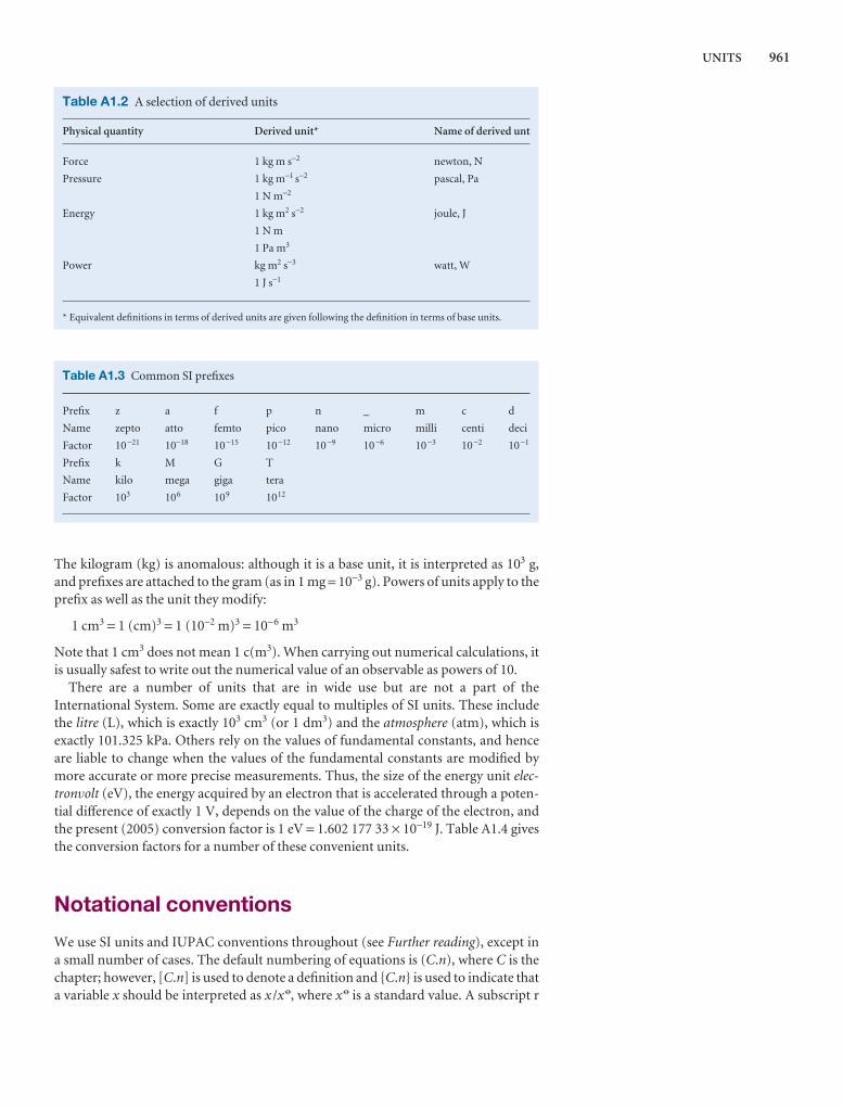
UNITS 961
The kilogram (kg) is anomalous: although it is a base unit, it is interpreted as 103 g,and prefixes are attached to the gram (as in 1 mg = 10−3 g). Powers of units apply to theprefix as well as the unit they modify:
1 cm3 = 1 (cm)3 = 1 (10−2 m)3 = 10−6 m3
Note that 1 cm3 does not mean 1 c(m3). When carrying out numerical calculations, itis usually safest to write out the numerical value of an observable as powers of 10.
There are a number of units that are in wide use but are not a part of theInternational System. Some are exactly equal to multiples of SI units. These includethe litre (L), which is exactly 103 cm3 (or 1 dm3) and the atmosphere (atm), which isexactly 101.325 kPa. Others rely on the values of fundamental constants, and henceare liable to change when the values of the fundamental constants are modified bymore accurate or more precise measurements. Thus, the size of the energy unit elec-tronvolt (eV), the energy acquired by an electron that is accelerated through a poten-tial difference of exactly 1 V, depends on the value of the charge of the electron, andthe present (2005) conversion factor is 1 eV = 1.602 177 33 × 10−19 J. Table A1.4 givesthe conversion factors for a number of these convenient units.
Notational conventions
We use SI units and IUPAC conventions throughout (see Further reading), except ina small number of cases. The default numbering of equations is (C.n), where C is thechapter; however, [C.n] is used to denote a definition and {C.n} is used to indicate thata variable x should be interpreted as x /x 7, where x 7 is a standard value. A subscript r
Table A1.3 Common SI prefixes
Prefix z a f p n _ m c d
Name zepto atto femto pico nano micro milli centi deci
Factor 10−21 10−18 10−15 10−12 10−9 10−6 10−3 10−2 10−1
Prefix k M G T
Name kilo mega giga tera
Factor 103 106 109 1012
Table A1.2 A selection of derived units
Physical quantity Derived unit* Name of derived unt
Force 1 kg m s−2 newton, N
Pressure 1 kg m−1 s−2 pascal, Pa
1 N m−2
Energy 1 kg m2 s−2 joule, J
1 N m
1 Pa m3
Power kg m2 s−3 watt, W
1 J s−1
* Equivalent definitions in terms of derived units are given following the definition in terms of base units.
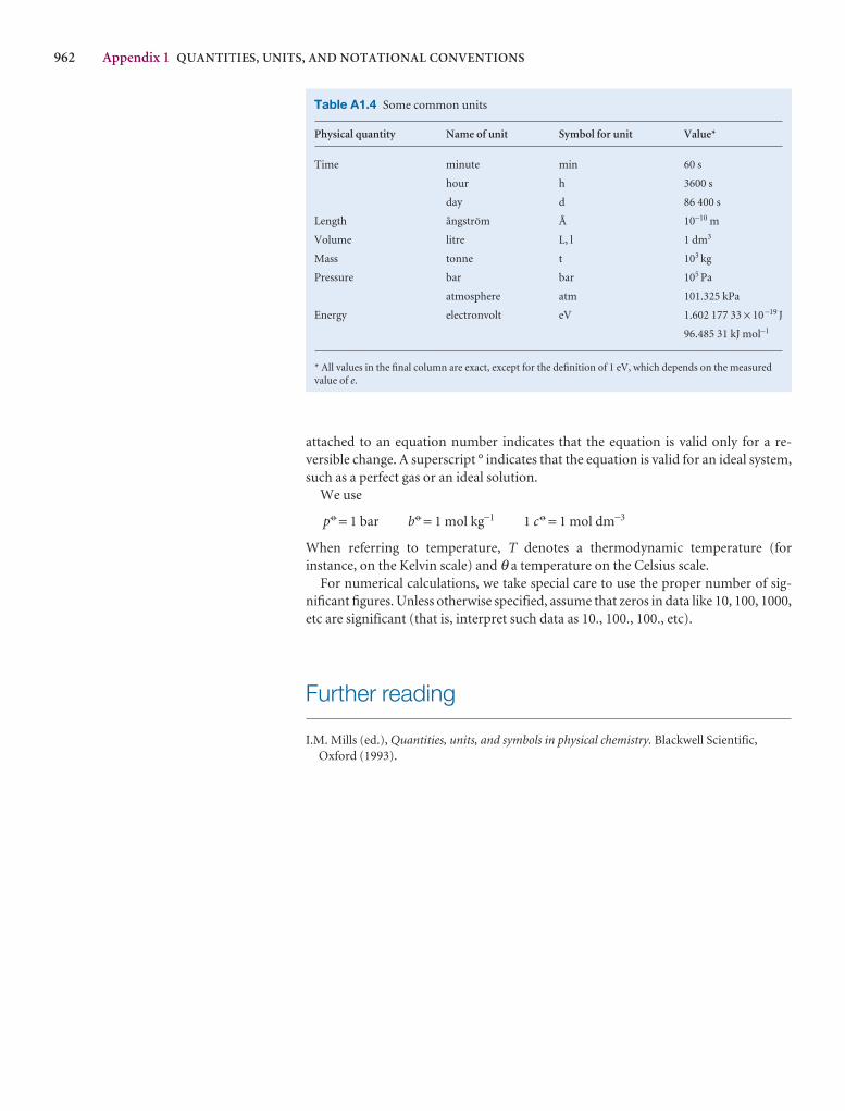
962 Appendix 1 QUANTITIES, UNITS, AND NOTATIONAL CONVENTIONS
attached to an equation number indicates that the equation is valid only for a re-versible change. A superscript ° indicates that the equation is valid for an ideal system,such as a perfect gas or an ideal solution.
We use
p7 = 1 bar b7 = 1 mol kg−1 1 c 7 = 1 mol dm−3
When referring to temperature, T denotes a thermodynamic temperature (for instance, on the Kelvin scale) and θ a temperature on the Celsius scale.
For numerical calculations, we take special care to use the proper number of sig-nificant figures. Unless otherwise specified, assume that zeros in data like 10, 100, 1000,etc are significant (that is, interpret such data as 10., 100., 100., etc).
Further reading
I.M. Mills (ed.), Quantities, units, and symbols in physical chemistry. Blackwell Scientific,Oxford (1993).
Table A1.4 Some common units
Physical quantity Name of unit Symbol for unit Value*
Time minute min 60 s
hour h 3600 s
day d 86 400 s
Length ångström Å 10−10 m
Volume litre L, l 1 dm3
Mass tonne t 103 kg
Pressure bar bar 105 Pa
atmosphere atm 101.325 kPa
Energy electronvolt eV 1.602 177 33 × 10−19 J
96.485 31 kJ mol−1
* All values in the final column are exact, except for the definition of 1 eV, which depends on the measuredvalue of e.

Appendix 2MathematicaltechniquesBasic procedures
A2.1 Logarithms and exponentials
The natural logarithm of a number x is denoted ln x, and is defined as the power towhich e = 2.718 . . . must be raised for the result to be equal to x. It follows from thedefinition of logarithms that
ln x + ln y + · · · = ln xy · · · (A2.1)
ln x − ln y = ln(x/y) (A2.2)
a ln x = ln xa (A2.3)
We also encounter the common logarithm of a number, log x, the logarithm com-piled with 10 in place of e. Common logarithms follow the same rules of addition andsubtraction as natural logarithms. Common and natural logarithms are related by
ln x = ln 10 log x ≈ 2.303 log x (A2.4)
The exponential function, ex, plays a very special role in the mathematics of chem-istry. The following properties are important:
exeyez . . . . = ex+y+z+ · · · (A2.5)
ex/ey = ex−y (A2.6)
(ex)a = eax (A2.7)
A2.2 Complex numbers and complex functions
Complex numbers have the form
z = x + iy (A2.8)
where i = (−1)1/2. The real numbers x and y are, respectively, the real and imaginaryparts of z, denoted Re(z) and Im(z). We write the complex conjugate of z, denoted z*,by replacing i by −i:
z* = x − iy (A2.9)
The absolute value or modulus of the complex number z is denoted |z | and is given by:
|z | = (z*z)1/2 = (x2 + y2)1/2 (A2.10)
The following rules apply for arithmetic operations involving complex numbers:
1 Addition. If z = x + iy and z′ = x′ + iy′, then
z ± z′ = (x ± x′) + i(y ± y′) (A2.11)
A2Basic procedures
A2.1 Logarithms and exponentials
A2.2 Complex numbers andcomplex functions
A2.3 Vectors
Calculus
A2.4 Differentiation andintegration
A2.5 Power series and Taylorexpansions
A2.6 Partial derivatives
A2.7 Functionals and functionalderivatives
A2.8 Undetermined multipliers
A2.9 Differential equations
Statistics and probability
A2.10 Random selections
A2.11 Some results of probabilitytheory
Matrix algebra
A2.12 Matrix addition andmultiplication
A2.13 Simultaneous equations
A2.14 Eigenvalue equations
Further reading
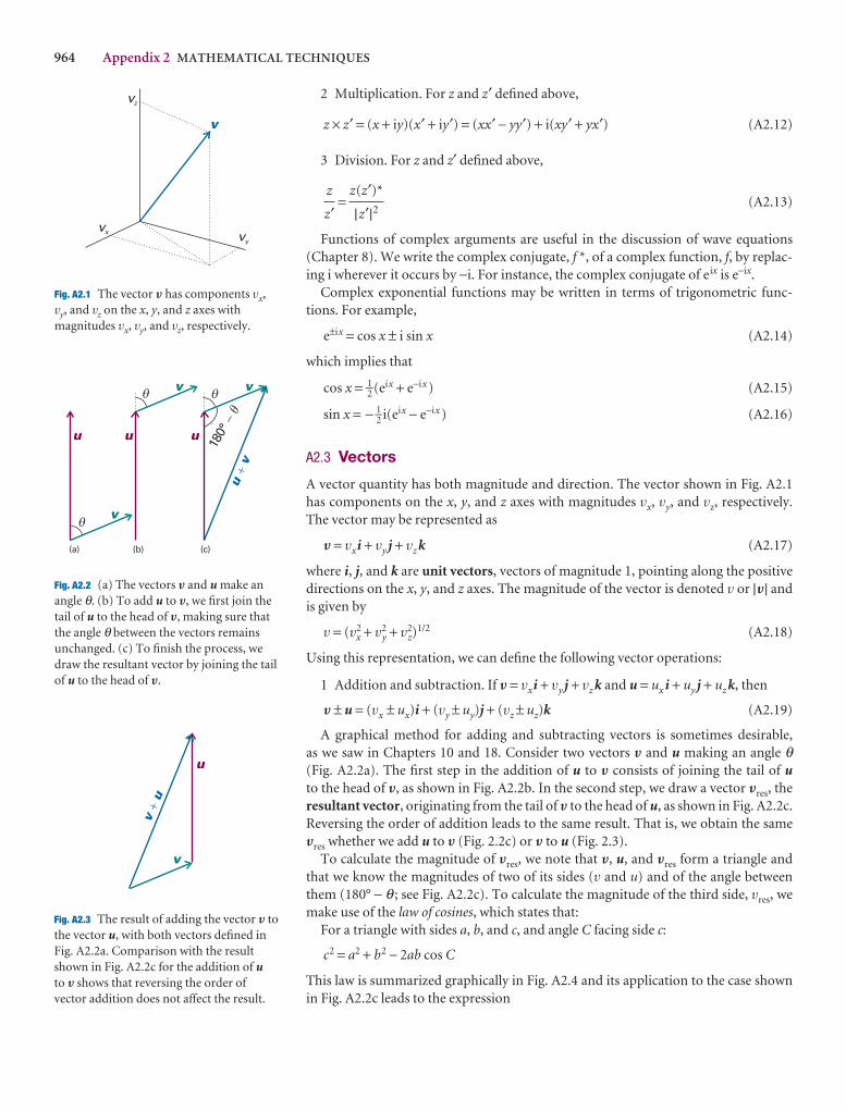
964 Appendix 2 MATHEMATICAL TECHNIQUES
2 Multiplication. For z and z′ defined above,
z × z′ = (x + iy)(x′ + iy′) = (xx′ − yy′) + i(xy′ + yx′) (A2.12)
3 Division. For z and z′ defined above,
= (A2.13)
Functions of complex arguments are useful in the discussion of wave equations(Chapter 8). We write the complex conjugate, f *, of a complex function, f, by replac-ing i wherever it occurs by −i. For instance, the complex conjugate of eix is e−ix.
Complex exponential functions may be written in terms of trigonometric func-tions. For example,
e±ix = cos x ± i sin x (A2.14)
which implies that
cos x = 1–2 (eix + e−ix ) (A2.15)
sin x = − 1–2 i(eix − e−ix ) (A2.16)
A2.3 Vectors
A vector quantity has both magnitude and direction. The vector shown in Fig. A2.1has components on the x, y, and z axes with magnitudes vx, vy, and vz, respectively.The vector may be represented as
V = vxi + vy j + vz k (A2.17)
where i, j, and k are unit vectors, vectors of magnitude 1, pointing along the positivedirections on the x, y, and z axes. The magnitude of the vector is denoted v or |V| andis given by
v = (v2x + v2
y + v2z)
1/2 (A2.18)
Using this representation, we can define the following vector operations:
1 Addition and subtraction. If V = vxi + vy j + vz k and u = ux i + uy j + uz k, then
V ± u = (vx ± ux)i + (vy ± uy)j + (vz ± uz)k (A2.19)
A graphical method for adding and subtracting vectors is sometimes desirable, as we saw in Chapters 10 and 18. Consider two vectors V and u making an angle θ(Fig. A2.2a). The first step in the addition of u to V consists of joining the tail of uto the head of V, as shown in Fig. A2.2b. In the second step, we draw a vector Vres, the resultant vector, originating from the tail of V to the head of u, as shown in Fig. A2.2c.Reversing the order of addition leads to the same result. That is, we obtain the sameVres whether we add u to V (Fig. 2.2c) or V to u (Fig. 2.3).
To calculate the magnitude of Vres, we note that V, u, and Vres form a triangle andthat we know the magnitudes of two of its sides (v and u) and of the angle betweenthem (180° − θ ; see Fig. A2.2c). To calculate the magnitude of the third side, vres, wemake use of the law of cosines, which states that:
For a triangle with sides a, b, and c, and angle C facing side c:
c2 = a2 + b2 − 2ab cos C
This law is summarized graphically in Fig. A2.4 and its application to the case shownin Fig. A2.2c leads to the expression
z(z′)*
|z′|2z
z′vx vy
vz
v
Fig. A2.1 The vector V has components vx,vy, and vz on the x, y, and z axes withmagnitudes vx, vy, and vz, respectively.
(a) (b) (c)
u
v
��
180°
�
�
v v
u u
uv
��
Fig. A2.2 (a) The vectors V and u make anangle θ. (b) To add u to V, we first join thetail of u to the head of V, making sure thatthe angle θ between the vectors remainsunchanged. (c) To finish the process, wedraw the resultant vector by joining the tailof u to the head of V.
vu
�
u
v
Fig. A2.3 The result of adding the vector V tothe vector u, with both vectors defined inFig. A2.2a. Comparison with the resultshown in Fig. A2.2c for the addition of uto V shows that reversing the order ofvector addition does not affect the result.
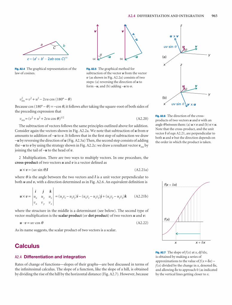
A2.4 DIFFERENTIATION AND INTEGRATION 965
v2res = v2 + u2 − 2vu cos (180° − θ)
Because cos (180° − θ) = −cos θ, it follows after taking the square-root of both sides ofthe preceding expression that
vres = (v2 + u2 + 2vu cos θ)1/2 (A2.20)
The subtraction of vectors follows the same principles outlined above for addition.Consider again the vectors shown in Fig. A2.2a. We note that subtraction of u from Vamounts to addition of −u to V. It follows that in the first step of subtraction we draw−u by reversing the direction of u (Fig. A2.5a) Then, the second step consists of addingthe −u to V by using the strategy shown in Fig. A2.2c: we draw a resultant vector Vres byjoining the tail of −u to the head of V.
2 Multiplication. There are two ways to multiply vectors. In one procedure, thecross-product of two vectors u and V is a vector defined as
u × V = (uv sin θ)l (A2.21a)
where θ is the angle between the two vectors and l is a unit vector perpendicular toboth u and V, with a direction determined as in Fig. A2.6. An equivalent definition is
u × V = = (uyvz − uzvy)i − (uxvz − uzvx)j + (uxvy − uyvx)k (A2.21b)
where the structure in the middle is a determinant (see below). The second type ofvector multiplication is the scalar product (or dot product) of two vectors u and V:
u · V = uv cos θ (A2.22)
As its name suggests, the scalar product of two vectors is a scalar.
Calculus
A2.4 Differentiation and integration
Rates of change of functions—slopes of their graphs—are best discussed in terms ofthe infinitesimal calculus. The slope of a function, like the slope of a hill, is obtainedby dividing the rise of the hill by the horizontal distance (Fig. A2.7). However, because
i j ku u ux y z
x y zv v v
a bC
c a b ab C( 2 cos )� � �2 2 1/2
Fig. A2.4 The graphical representation of thelaw of cosines.
(a) (b)
v
��u
v
�u
vu
�
Fig. A2.5 The graphical method forsubtraction of the vector u from the vectorV (as shown in Fig. A2.2a) consists of twosteps: (a) reversing the direction of u toform −u, and (b) adding −u to V.
u
x
y
z
v
u vx
�
x
y
z
(a)
(b)
uv sin
u v�
uv sin v ux
�
�
Fig. A2.6 The direction of the cross-products of two vectors u and V with anangle θ between them: (a) u × V and (b) V × u.Note that the cross-product, and the unitvector l of eqn A2.21, are perpendicular toboth u and V but the direction depends onthe order in which the product is taken.
f x x( )� �
f x( )
x x x� �
Fig. A2.7 The slope of f(x) at x, df /dx,is obtained by making a series ofapproximations to the value of f(x + δx) −f(x) divided by the change in x, denoted δx,and allowing δx to approach 0 (as indicatedby the vertical lines getting closer to x.
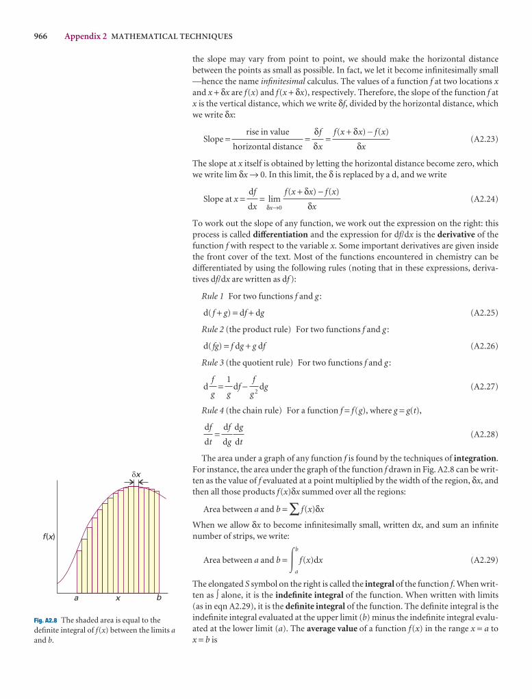
966 Appendix 2 MATHEMATICAL TECHNIQUES
the slope may vary from point to point, we should make the horizontal distance between the points as small as possible. In fact, we let it become infinitesimally small—hence the name infinitesimal calculus. The values of a function f at two locations xand x + δx are f(x) and f(x + δx), respectively. Therefore, the slope of the function f atx is the vertical distance, which we write δf, divided by the horizontal distance, whichwe write δx:
Slope = = = (A2.23)
The slope at x itself is obtained by letting the horizontal distance become zero, whichwe write lim δx → 0. In this limit, the δ is replaced by a d, and we write
Slope at x = = limδx→0
(A2.24)
To work out the slope of any function, we work out the expression on the right: thisprocess is called differentiation and the expression for df/dx is the derivative of thefunction f with respect to the variable x. Some important derivatives are given insidethe front cover of the text. Most of the functions encountered in chemistry can bedifferentiated by using the following rules (noting that in these expressions, deriva-tives df/dx are written as df ):
Rule 1 For two functions f and g :
d( f + g) = df + dg (A2.25)
Rule 2 (the product rule) For two functions f and g :
d( fg) = f dg + g df (A2.26)
Rule 3 (the quotient rule) For two functions f and g :
d = df − dg (A2.27)
Rule 4 (the chain rule) For a function f = f(g), where g = g(t),
= (A2.28)
The area under a graph of any function f is found by the techniques of integration.For instance, the area under the graph of the function f drawn in Fig. A2.8 can be writ-ten as the value of f evaluated at a point multiplied by the width of the region, δx, andthen all those products f(x)δx summed over all the regions:
Area between a and b = ∑ f(x)δx
When we allow δx to become infinitesimally small, written dx, and sum an infinitenumber of strips, we write:
Area between a and b = �b
a
f(x)dx (A2.29)
The elongated S symbol on the right is called the integral of the function f. When writ-ten as ∫ alone, it is the indefinite integral of the function. When written with limits (as in eqn A2.29), it is the definite integral of the function. The definite integral is the indefinite integral evaluated at the upper limit (b) minus the indefinite integral evalu-ated at the lower limit (a). The average value of a function f(x) in the range x = a tox = b is
dg
dt
df
dg
df
dt
f
g 2
1
g
f
g
f(x + δx) − f(x)
δx
df
dx
f(x + δx) − f(x)
δx
δf
δx
rise in value
horizontal distance
f x( )
xa b
�x
Fig. A2.8 The shaded area is equal to thedefinite integral of f(x) between the limits aand b.
A2.5 POWER SERIES AND TAYLOR EXPANSIONS 967
Average value of f (x) from a to b = �b
a
f(x)dx (A2.30)
The mean value theorem states that a continuous function has its mean value at leastonce in the range.
Integration is the inverse of differentiation. That is, if we integrate a function andthen differentiate the result, we get back the original function. Some important integralsare given on the front back cover of the text. Many other standard forms are found intables (see Further reading) and it is also possible to calculate definite and indefiniteintegrals with mathematical software. Two integration techniques are useful:
Technique 1 (integration by parts) For two functions f and g :
�f dx = fg − �g dx (A2.31)
Technique 2 (method of partial fractions) To solve an integral of the form
� dx, where a and b are constants, we write
= −
and integrate the expression on the right. It follows that
� = � − �= ln − ln + constant (A2.32)
A2.5 Power series and Taylor expansions
A power series has the form
c0 + c1(x − a) + c2(x − a)2 + · · · + cn(x − a)n + · · · =∞
∑n= 0
cn(x − a)n (A2.33)
where cn and a are constants. It is often useful to express a function f(x) in the vicinityof x = a as a special power series called the Taylor series, or Taylor expansion, whichhas the form:
f(x) = f(a) + (x − a) +a
(x − a)2 + · · · +a
(x − a)n
=∞
∑n= 0 a
(x − a)n (A2.34)
where n! denotes a factorial, given by
n! = n(n − 1)(n − 2) . . . 1 (A2.35)
By definition 0! = 1. The following Taylor expansions are often useful:
= 1 − x + x 2 + · · ·
ex = 1 + x + 1–2 x2 + · · ·
ln x = (x − 1) − 1–2 (x − 1)2 + 1–3 (x − 1)3 − 1–4 (x − 1)4 + · · ·
ln(1 + x) = x − 1–2 x2 + 1–3 x3 − · · ·
If x << 1, then (1 + x)−1 ≈ 1 − x, ex ≈ 1 + x, and ln(1 + x) ≈ x.
1
1 + x
DF
dnf
dxn
AC
1
n!
DF
dnf
dx n
AC
1
n!
DF
d2f
dx2
AC
1
2!
DF
df
dx
AC
DF
1
b − x
1
a − x
AC
1
b − a
JKLdx
b − x
dx
a − x
GHI1
b − a
dx
(a − x)(b − x)
DF
1
b − x
1
a − x
AC
1
b − a
1
(a − x)(b − x)
1
(a − x)(b − x)
df
dx
dg
dx
1
b − a
968 Appendix 2 MATHEMATICAL TECHNIQUES
A2.6 Partial derivatives
A partial derivative of a function of more than one variable, such as f(x,y), is the slopeof the function with respect to one of the variables, all the other variables being heldconstant (see Fig. 2.21). Although a partial derivative shows how a function changeswhen one variable changes, it may be used to determine how the function changeswhen more than one variable changes by an infinitesimal amount. Thus, if f is a func-tion of x and y, then when x and y change by dx and dy, respectively, f changes by
df =y
dx +x
dy (A2.36)
where the symbol ∂ is used (instead of d) to denote a partial derivative. The quantitydf is also called the differential of f. For example, if f = ax3y + by2, then
y
= 3ax2yx
= ax3 + 2by
Then, when x and y undergo infinitesimal changes, f changes by
df = 3ax2ydx + (ax3 + 2by)dy
Partial derivatives may be taken in any order:
= (A2.37)
For the function f given above, it is easy to verify that
y x
= 3ax2
x y
= 3ax2
In the following, z is a variable on which x and y depend (for example, x, y, and zmight correspond to p, V, and T).
Relation 1 When x is changed at constant z:
z
=y
+x z
(A2.38)
Relation 2
z
= (A2.39)
Relation 3
z
= −y x
(A2.40)
By combining this relation and Relation 2 we obtain the Euler chain relation:
z y x
= −1 (A2.41)
Relation 4 This relation establishes whether or not df is an exact differential.
df = g(x,y)dx + h(x,y)dy is exact ifx
=y
(A2.42)
If df is exact, its integral between specified limits is independent of the path.
DF
∂h
∂x
AC
DF
∂g
∂y
AC
DF
∂z
∂y
AC
DF
∂x
∂z
AC
DF
∂y
∂x
AC
DF
∂z
∂y
AC
DF
∂x
∂z
AC
DF
∂x
∂y
AC
1
(∂x/∂y)z
DF
∂y
∂x
AC
DF
∂y
∂x
AC
DF
∂f
∂y
AC
DF
∂f
∂x
AC
DF
∂f
∂x
AC
DEF
DF
∂f
∂y
AC
∂∂x
ABC
DEF
DF
∂f
∂x
AC
∂∂y
ABC
∂2f
∂y∂x
∂2f
∂x∂y
DF
∂f
∂y
AC
DF
∂f
∂x
AC
DF
∂f
∂y
AC
DF
∂f
∂x
AC
A2.8 UNDETERMINED MULTIPLIERS 969
A2.7 Functionals and functional derivatives
Just as a function f can be regarded as a set of mathematical procedures that associatesa number f(x) to a specified value of a variable x, so a functional G gives a prescriptionfor associating a number G[ f ] to a function f(x) over a specified range of the variablex. That is, the functional is a function of a function. Functionals are important inquantum chemistry. We saw in Chapter 11 that the energy of a molecule is a func-tional of the electron density, which in turn is a function of the position.
To make the following discussion more concrete, consider the functional
G[ f ] = �1
0
f(x)2 dx (A2.43)
If we let f(x) = x, then G[ f ] = 1–3 over the range 0 ≤ x ≤ 1. However, if f(x) = sin πx, thenG[ f ] = 1–2 over the range 0 ≤ x ≤ 1.
Just as the derivative of a function f(x) tells us how the function changes with smallchanges δx in the variable x, so a functional derivative tells us about the variation δGof a functional G[ f ] with small changes δf in the function f(x). By analogy with eqnA2.24, we can write the following definition of the functional derivative as
= limδf→0
(A2.44)
However, this equation does not give us a simple method for calculating the func-tional derivative. It can be shown that an alternative definition of δG/δf is (see Furtherreading):
G[ f + δf ] − G[ f ] = �b
a
δf (x) dx (A2.45)
where the integral is evaluated in the range over which x varies.To see how eqn A2.45 is used to calculate a functional derivative, consider the func-
tional given by eqn A2.43. We begin by writing
G[ f + δf ] = �1
0
{ f(x) + δf(x)}2dx = �1
0
{ f(x)2 + 2f(x)δf(x) + δf(x)2}dx
= �1
0
{ f(x)2 + 2f(x)δf(x)}dx = G[ f ] + �1
0
2f(x)δf(x)dx
where we have ignored the minute contribution from δf 2 to arrive at the penultimateexpression and then used eqn A2.43 to write the final expression. It follows that
G[ f + δf ] − G[ f ] = �1
0
2f(x)δf(x)dx
By comparing this expression with eqn A2.45, we see that the functional derivative is
= 2f(x)
A2.8 Undetermined multipliers
Suppose we need to find the maximum (or minimum) value of some function f thatdepends on several variables x1, x2, . . . , xn. When the variables undergo a smallchange from xi to xi + δxi the function changes from f to f + δf, where
δG
δf
DF
δG
δf
AC
G[ f + δf ] − G[ f ]
δf
δG
δf
970 Appendix 2 MATHEMATICAL TECHNIQUES
δf =n
∑i
δxi (A2.46)
At a minimum or maximum, δf = 0, so then
n
∑i
δxi = 0 (A2.47)
If the xi were all independent, all the δxi would be arbitrary, and this equation couldbe solved by setting each (∂f/∂xi) = 0 individually. When the xi are not all independent,the δxi are not all independent, and the simple solution is no longer valid. We proceedas follows.
Let the constraint connecting the variables be an equation of the form g = 0. For ex-ample, in Chapter 16, one constraint was n0 + n1 + · · · = N, which can be written
g = 0, with g = (n0 + n1 + · · ·) − N
The constraint g = 0 is always valid, so g remains unchanged when the xi are varied:
δg = ∑i
δxi = 0 (A2.48)
Because δg is zero, we can multiply it by a parameter, λ, and add it to eqn A2.47:
n
∑i
+ λ δxi = 0 (A2.49)
This equation can be solved for one of the δx, δxn for instance, in terms of all the otherδxi. All those other δxi (i = 1, 2, . . . n − 1) are independent, because there is only oneconstraint on the system. But here is the trick: λ is arbitrary; therefore we can chooseit so that the coefficient of δxn in eqn A2.49 is zero. That is, we choose λ so that
+ λ = 0 (A2.50)
Then eqn A2.49 becomes
n−1
∑i
+ λ δxi = 0 (A2.51)
Now the n − 1 variations δxi are independent, so the solution of this equation is
+ λ = 0 i = 1, 2, . . . , n − 1 (A2.52)
However, eqn A2.50 has exactly the same form as this equation, so the maximum orminimum of f can be found by solving
+ λ = 0 i = 1, 2, . . . , n (A2.53)
The use of this approach was illustrated in the text for two constraints and thereforetwo undetermined multipliers λ1 and λ2 (α and −β).
The multipliers λ cannot always remain undetermined. One approach is to solveeqn A2.50 instead of incorporating it into the minimization scheme. In Chapter 16 weused the alternative procedure of keeping λ undetermined until a property was calcu-lated for which the value was already known. Thus, we found that β = 1/kT by calcu-lating the internal energy of a perfect gas.
DF
∂g
∂xi
AC
DF
∂f
∂xi
AC
DF
∂g
∂xi
AC
DF
∂f
∂xi
AC
567
DF
∂g
∂xi
AC
DF
∂f
∂xi
AC
123
DF
∂g
∂xn
AC
DF
∂f
∂xn
AC
567
DF
∂g
∂xi
AC
DF
∂f
∂xi
AC
123
DF
∂g
∂xi
AC
DF
∂f
∂xi
AC
DF
∂f
∂xi
AC
A2.9 DIFFERENTIAL EQUATIONS 971
A2.9 Differential equations
(a) Ordinary differential equations
An ordinary differential equation is a relation between derivatives of a function ofone variable and the function itself, as in
a + b + cy = 0 (A2.54)
The coefficients a, b, etc. may be functions of x. The order of the equation is the orderof the highest derivative that occurs in it, so eqn A2.54 is a second-order equation.Only rarely in science is a differential equation of order higher than 2 encountered. A solution of a differential equation is an expression for y as a function of x. The process of solving a differential equation is commonly termed ‘integration’, and in simple cases simple integration can be employed to find y(x). A general solution of adifferential equation is the most general solution of the equation and is expressed interms of a number of constants. When the constants are chosen to accord with certainspecified initial conditions (if one variable is the time) or certain boundary condi-tions (to fulfil certain spatial restrictions on the solutions), we obtain the particularsolution of the equation. A first–order differential equation requires the specificationof one boundary (or initial) condition; a second–order differential equation requiresthe specification of two such conditions, and so on.
First-order differential equations may often be solved by direct integration. For example, the equation
= axy
with a constant may be rearranged into
= axdx
and then integrated to
ln y = 1–2 ax 2 + A
where A is a constant. If we know that y = y0 when x = 0 (for instance), then it followsthat A = ln y0, and hence the particular solution of the equation is
ln y = 1–2 ax2 + ln y0
This expression rearranges to
y = y0eax2/2
First-order equations of a more complex form can often be solved by the appropriatesubstitution. For example, it is sensible to try the substitution y = sx, and to change thevariables from x and y to x and s. An alternative useful transformation is to write x =u + a and y = v + b, and then to select a and b to simplify the form of the resulting expression.
Solutions to complicated differential equations may also be found by referring totables (see Further reading). For example, first-order equations of the form
+ yf(x) = g(x) (A2.55)dy
dx
dy
y
dy
dx
dy
dx
d2y
dx2
972 Appendix 2 MATHEMATICAL TECHNIQUES
appear in the study of chemical kinetics. The solution is given by
ye ∫f(x)dx = �e ∫f(x)dxg(x)dx + constant (A2.56)
Mathematical software is now capable of finding analytical solutions of a wide varietyof differential equations.
Second-order differential equations are in general much more difficult to solvethan first-order equations. One powerful approach commonly used to lay siege to second-order differential equations is to express the solution as a power series:
y =∞
∑n= 0
cnxn (A2.57)
and then to use the differential equation to find a relation between the coefficients.This approach results, for instance, in the Hermite polynomials that form part of thesolution of the Schrödinger equation for the harmonic oscillator (Section 9.4). All thesecond-order differential equations that occur in this text are tabulated in compila-tions of solutions or can be solved with mathematical software, and the specializedtechniques that are needed to establish the form of the solutions may be found inmathematical texts.
(b) Numerical integration of differential equations
Many of the differential equations that describe physical phenomena are so com-plicated that their solutions cannot be cast as functions. In such cases, we resort to numerical methods, in which approximations are made in order to integrate thedifferential equation. Software packages are now readily available that can be used tosolve almost any equation numerically. The general form of such programs to solvedf /dx = g(x), for instance, replaces the infinitesimal quantity df = g(x)dx by the smallquantity ∆f = g(x)∆x, so that
f (x + ∆x) ≈ f(x) + g(x)∆x
and then proceeds numerically to step along the x-axis, generating f (x) as it goes. Theactual algorithms adopted are much more sophisticated than this primitive scheme,but stem from it. Among the simple numerical methods, the fourth-order Runge–Kutta method is one of the most accurate.
The Further reading section lists monographs that discuss the derivation of thefourth-order Runge–Kutta method. Here we illustrate the procedure with a first-orderdifferential equation of the form:
= f(x,y) (A2.58)
One example of this differential equation in chemical kinetics is eqn 22.36, which describes the time dependence of the concentration of an intermediate I in the reac-tion sequence A → I → P.
To obtain an approximate value of the integral of eqn A2.58, we proceed by rewrit-ing it in terms of finite differences instead of differentials:
= f(x,y)
where ∆y may also be written as y(x + ∆x) − y(x). The fourth-order Runge–Kuttamethod is based on the following approximation:
y(x + ∆x) = y(x) + 1–6(k1 + 2k2 + 2k3 + k4) (A2.59)
∆y
∆x
dy
dx
A2.10 RANDOM SELECTIONS 973
where
k1 = f(x,y)∆x (A2.60a)
k2 = f(x + 1–2 ∆x, y + 1–2 k1)∆x (A2.60b)
k3 = f(x + 1–2 ∆x, y + 1–2 k2)∆x (A2.60c)
k4 = f(x + ∆x, y + k3)∆x (A2.60d)
Therefore, if we know the functional form of f(x,y) and y(0), we can use eqnsA2.60(a–d) to calculate values of y for a range of x values. The process can be automated easily with an electronic spreadsheet or with mathematical software. The accuracy of the calculation increases with decreasing values of the increment ∆x.
(c) Partial differential equations
A partial differential equation is a differential in more than one variable. An example is
= a (A2.61)
with y a function of the two variables x and t. In certain cases, partial differential equa-tions may be separated into ordinary differential equations. Thus, the Schrödingerequation for a particle in a two-dimensional square well (Section 9.2) may be separ-ated by writing the wavefunction, ψ(x,y), as the product X(x)Y(y), which results inthe separation of the second-order partial differential equation into two second-orderdifferential equations in the variables x and y. A good guide to the likely success ofsuch a separation of variables procedure is the symmetry of the system.
Statistics and probability
Throughout the text, but especially in Chapters 16, 17, 19, and 21, we use several ele-mentary results from two branches of mathematics: probability theory, which dealswith quantities and events that are distributed randomly, and statistics, which pro-vides tools for the analysis of large collections of data. Here we introduce some of thefundamental ideas from these two fields.
A2.10 Random selections
Combinatorial functions allow us to express the number of ways in which a system ofparticles may be configured; they are especially useful in statistical thermodynamics(Chapters 16 and 17). Consider a simple coin-toss problem. If n coins are tossed, thenumber N(n,i) of outcomes that have i heads and (n − i) tails, regardless of the orderof the results, is given by the coefficients of the binomial expansion of (1 + x)n:
(1 + x)n = 1 +n
∑i= 1
N(n,i)xi, N(n,i) = (A2.62)
The numbers N(n,i), which are sometimes denoted , are also called binomialcoefficients.
Suppose that, unlike the coin-toss problem, there are more than two possible resultsfor each event. For example, there are six possible results for the roll of a die. For n rollsof the die, the number of ways, W, that correspond to n1 occurrences of the number 1,n2 occurrences of the number 2, and so on, is given by
DF
n
i
AC
n!
(n − i)!i!
∂2y
∂x2
∂2y
∂t2
974 Appendix 2 MATHEMATICAL TECHNIQUES
W = , n =6
∑i= 1
ni
This is an example of a multinomial coefficient, which has the form
W = , n =m
∑i= 1
ni (A2.63)
where W is the number of ways of achieving an outcome, n is the number of events,and m is the number of possible results. In Chapter 16 we use the multinomial co-efficient to determine the number of ways to configure a system of identical particlesgiven a specific distribution of particles into discrete energy levels.
In chemistry it is common to deal with a very large number of particles and out-comes and it is useful to express factorials in different ways. We can simplify factorialsof large numbers by using Stirling’s approximation:
n! ≈ (2π)1/2nn+ 1–2e−n (A2.64)
The approximation is in error by less than 1 per cent when n is greater than about 10.For very large values of n, it is possible to use another form of the approximation:
ln n! ≈ n ln n − n (A2.65)
A2.11 Some results of probability theory
Here we develop two general results of probability theory: the mean value of a variableand the mean value of a function. The calculation of mean values is useful in the description of random coils (Chapter 19) and molecular diffusion (Chapter 21).
The mean value (also called the expectation value) �X� of a variable X is calculatedby first multiplying each discrete value xi that X can have by the probability pi that xi
occurs and then summing these products over all possible N values of X:
�X� =N
∑i= 1
xi pi
When N is very large and the xi values are so closely spaced that X can be regarded as varying continuously, it is useful to express the probability that X can have a valuebetween x and x + dx as
Probability of finding a value of X between x and x + dx = f(x)dx
where the function f(x) is the probability density, a measure of the distribution of theprobability values over x, and dx is an infinitesimally small interval of x values. It fol-lows that the probability that X has a value between x = a and x = b is the integral of theexpression above evaluated between a and b:
Probability of finding a value of X between a and b = �b
a
f(x)dx
The mean value of the continuously varying X is given by
�X� = �+∞
−∞
xf(x)dx (A2.66)
This expression is similar to that written for the case of discrete values of X, withf (x)dx as the probability term and integration over the closely spaced x values replac-ing summation over widely spaced xi.
n!
n1!n2! . . . nm!
n!
n1!n2!n3!n4!n5!n6!
A2.12 MATRIX ADDITION AND MULTIPLICATION 975
The mean value of a function g(X) can be calculated with a formula similar to thatfor �X�:
�g(X)� = �+∞
−∞
g(x)f(x)dx (A2.67)
Matrix algebra
A matrix is an array of numbers. Matrices may be combined together by addition ormultiplication according to generalizations of the rules for ordinary numbers. Mostnumerical matrix manipulations are now carried out with mathematical software.
Consider a square matrix M of n2 numbers arranged in n columns and n rows.These n2 numbers are the elements of the matrix, and may be specified by stating therow, r, and column, c, at which they occur. Each element is therefore denoted Mrc. Forexample, in the matrix
M =
the elements are M11 = 1, M12 = 2, M21 = 3, and M22 = 4. This is an example of a 2 × 2matrix. The determinant, |M |, of this matrix is
|M | = = 1 × 4 − 2 × 3 = −2
A diagonal matrix is a matrix in which the only nonzero elements lie on the major diagonal (the diagonal from M11 to Mnn). Thus, the matrix
D =
is diagonal. The condition may be written
Mrc = mrδrc (A2.68)
where δrc is the Kronecker delta, which is equal to 1 for r = c and to 0 for r ≠ c. In theabove example, m1 = 1, m2 = 2, and m3 = 1. The unit matrix, 1 (and occasionally I), isa special case of a diagonal matrix in which all nonzero elements are 1.
The transpose of a matrix M is denoted MT and is defined by
M Tmn = Mnm (A2.69)
Thus, for the matrix M we have been using,
M T =
Matrices are very useful in chemistry. They simplify some mathematical tasks, such assolving systems of simultaneous equations, the treatment of molecular symmetry(Chapter 12), and quantum mechanical calculations (Chapter 11).
A2.12 Matrix addition and multiplication
Two matrices M and N may be added to give the sum S = M + N, according to the rule
Src = Mrc + Nrc (A2.70)
1 32 4
⎛⎝⎜
⎞⎠⎟
1 0 00 2 00 0 1
⎛
⎝⎜⎜
⎞
⎠⎟⎟
1 23 4
1 23 4
⎛⎝⎜
⎞⎠⎟
976 Appendix 2 MATHEMATICAL TECHNIQUES
(that is, corresponding elements are added). Thus, with M given above and
N =
the sum is
S =
Two matrices may also be multiplied to give the product P = MN according to the rule
Prc = ∑n
MrnNnc (A2.71)
For example, with the matrices given above,
P =
It should be noticed that in general MN ≠ NM, and matrix multiplication is in generalnon-commutative.
The inverse of a matrix M is denoted M−1, and is defined so that
MM −1 = M −1M = 1 (A2.72)
The inverse of a matrix can be constructed by using mathematical software, but insimple cases the following procedure can be carried through without much effort:
1 Form the determinant of the matrix. For example, for our matrix M, |M | = −2.
2 Form the transpose of the matrix. For example, M T = .
3 Form * ′, where * ′rc is the cofactor of the element Mrc, that is, it is the determin-ant formed from M with the row r and column c struck out. For example,
* ′ =
4 Construct the inverse as M −1 = * ′/ |M |. For example,
M −1 = 1––−2
A2.13 Simultaneous equations
A set of n simultaneous equations
a11x1 + a12x2 + · · · + a1nxn = b1
a21x1 + a22x2 + · · · + a2nxn = b2
� (A2.73)
an1x1 + an2x2 + · · · + annxn = bn
can be written in matrix notation if we introduce the column vectors x and b:
x = b =
bb
bn
1
2
M
⎛
⎝
⎜⎜⎜⎜
⎞
⎠
⎟⎟⎟⎟
xx
xn
1
2
M
⎛
⎝
⎜⎜⎜⎜
⎞
⎠
⎟⎟⎟⎟
4 23 1
2 132
12
−−
⎛⎝⎜
⎞⎠⎟
= −−
⎛⎝⎜
⎞⎠⎟
4 23 1
−−
⎛⎝⎜
⎞⎠⎟
1 32 4
⎛⎝⎜
⎞⎠⎟
1 23 4
5 67 8
1 5 2 7 1 6 2 83 5 4 7 3 6 4 8
19 2243 50
⎛⎝⎜
⎞⎠⎟
⎛⎝⎜
⎞⎠⎟
= × + × × + ×× + × × + ×
⎛⎝⎜
⎞⎠⎟
= ⎛⎝⎜
⎞⎠⎟
1 23 4
5 67 8
6 810 12
⎛⎝⎜
⎞⎠⎟
+ ⎛⎝⎜
⎞⎠⎟
= ⎛⎝⎜
⎞⎠⎟
5 67 8
⎛⎝⎜
⎞⎠⎟
A2.14 EIGENVALUE EQUATIONS 977
Then, with the a matrix of coefficients arc, the n equations may be written as
ax = b (A2.74)
The formal solution is obtained by multiplying both sides of this matrix equation bya−1, for then
x = a−1b (A2.75)
A2.14 Eigenvalue equations
An eigenvalue equation is a special case of eqn A2.74 in which
ax = λx (A2.76)
where λ is a constant, the eigenvalue, and x is the eigenvector. In general, there are neigenvalues λ(i), and they satisfy the n simultaneous equations
(a − λ1)x = 0 (A2.77)
There are n corresponding eigenvectors x(i). Equation A2.77 has a solution only if thedeterminant of the coefficients is zero. However, this determinant is just |a − λ1 |, sothe n eigenvalues may be found from the solution of the secular equation:
|a − λ1 | = 0 (A2.78)
The n eigenvalues the secular equation yields may be used to find the n eigenvectors.These eigenvectors (which are n × 1 matrices), may be used to form an n × n matrix X.Thus, because
x(1) = x(2) = etc.
we may form the matrix
X = (x(1), x(2), . . . , x(n)) =
so that Xrc = xr(c). If further we write Λrc = λrδrc, so that L is a diagonal matrix with the
elements λ1, λ2, . . . , λn along the diagonal, then all the eigenvalue equations ax(i) =lix
(i) may be confined into the single equation
aX = XL (A2.79)
because this expression is equal to
∑n
arn Xnc = ∑n
XrnΛnc
or
∑n
arnxn(c) = ∑
n
xr(n)λnδnc = λc xr
(c)
as required. Therefore, if we form X−1 from X, we construct a similarity transformation
L = X −1aX (A2.80)
x x x
x x x
x x x
n
n
n n nn
11
12
1
21
22
2
1 2
( ) ( ) ( )
( ) ( ) ( )
( ) ( ) ( )
L
L
M M M
L
⎛
⎝
⎜⎜⎜⎜
⎞
⎠
⎟⎟⎟⎟
x
x
xn
12
22
2
( )
( )
( )M
⎛
⎝
⎜⎜⎜⎜
⎞
⎠
⎟⎟⎟⎟
x
x
xn
11
21
1
( )
( )
( )M
⎛
⎝
⎜⎜⎜⎜
⎞
⎠
⎟⎟⎟⎟

978 Appendix 2 MATHEMATICAL TECHNIQUES
that makes a diagonal (because L is diagonal). It follows that if the matrix X thatcauses X−1aX to be diagonal is known, then the problem is solved: the diagonal matrixso produced has the eigenvalues as its only nonzero elements, and the matrix X usedto bring about the transformation has the corresponding eigenvectors as its columns.The solutions of eigenvalue equations are best found by using mathematical software.
Further reading
P.W. Atkins, J.C. de Paula, and V.A. Walters, Explorations in physicalchemistry. W.H. Freeman and Company, New York (2005).
J.R. Barrante, Applied mathematics for physical chemistry. PrenticeHall, Upper Saddle River (2004).
M.P. Cady and C.A. Trapp, A Mathcad primer for physical chemistry.W.H. Freeman and Company, New York (2000).
R.G. Mortimer, Mathematics for physical chemistry. Academic Press,San Diego (2005).
D.A. McQuarrie, Mathematical methods for scientists and engineers.University Science Books, Sausalito (2003).
D. Zwillinger (ed.), CRC standard mathematical tables and formulae.CRC Press, Boca Raton (1996).
Appendix 3Essential concepts of physicsEnergy
The central concept of all explanations in physical chemistry, as in so many otherbranches of physical science, is that of energy, the capacity to do work. We make useof the apparently universal law of nature that energy is conserved, that is, energy canneither be created nor destroyed. Although energy can be transferred from one loca-tion to another, the total energy is constant.
A3.1 Kinetic and potential energy
The kinetic energy, EK, of a body is the energy the body possesses as a result of its motion. For a body of mass m travelling at a speed v,
EK = 1–2mv2 (A3.1)
The potential energy, EP or V, of a body is the energy it possesses as a result of its posi-tion. The zero of potential energy is arbitrary. For example, the gravitational potentialenergy of a body is often set to zero at the surface of the Earth; the electrical potentialenergy of two charged particles is set to zero when their separation is infinite. No uni-versal expression for the potential energy can be given because it depends on the typeof interaction the body experiences. One example that gives rise to a simple expressionis the potential energy of a body of mass m in the gravitational field close to the surfaceof the Earth (a gravitational field acts on the mass of a body). If the body is at a heighth above the surface of the Earth, then its potential energy is mgh, where g is a constantcalled the acceleration of free fall, g = 9.81 m s−2, and V = 0 at h = 0 (the arbitrary zeromentioned previously).
The total energy is the sum of the kinetic and potential energies of a particle:
E = EK + EP (A3.2)
A3.2 Energy units
The SI unit of energy is the joule (J), which is defined as
1 J = 1 kg m2 s−2 (A3.3)
Calories (cal) and kilocalories (kcal) are still encountered in the chemical literature: bydefinition, 1 cal = 4.184 J. An energy of 1 cal is enough to raise the temperature of 1 gof water by 1°C.
The rate of change of energy is called the power, P, expressed as joules per second,or watt, W:
1 W = 1 J s−1 (A3.4)
A3Energy
A3.1 Kinetic and potential energy
A3.2 Energy units
Classical mechanics
A3.3 The trajectory in terms of theenergy
A3.4 Newton’s second law
A3.5 Rotational motion
A3.6 The harmonic oscillator
Waves
A3.7 The electromagnetic field
A3.8 Features of electromagneticradiation
A3.9 Refraction
A3.10 Optical activity
Electrostatics
A3.11 The Coulomb interaction
A2.12 The Coulomb potential
A2.13 The strength of the electricfield
A2.14 Electric current and power
Further reading
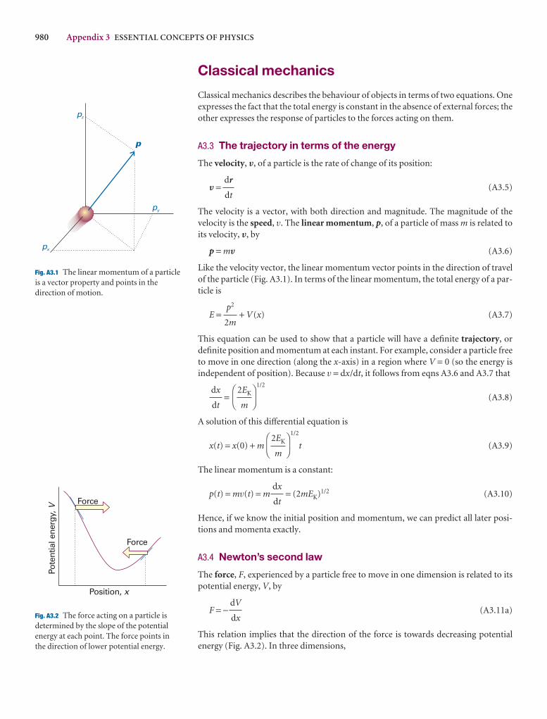
980 Appendix 3 ESSENTIAL CONCEPTS OF PHYSICS
Classical mechanics
Classical mechanics describes the behaviour of objects in terms of two equations. Oneexpresses the fact that the total energy is constant in the absence of external forces; theother expresses the response of particles to the forces acting on them.
A3.3 The trajectory in terms of the energy
The velocity, V, of a particle is the rate of change of its position:
V = (A3.5)
The velocity is a vector, with both direction and magnitude. The magnitude of the velocity is the speed, v. The linear momentum, p, of a particle of mass m is related toits velocity, V, by
p = mV (A3.6)
Like the velocity vector, the linear momentum vector points in the direction of travelof the particle (Fig. A3.1). In terms of the linear momentum, the total energy of a par-ticle is
E = + V(x) (A3.7)
This equation can be used to show that a particle will have a definite trajectory, ordefinite position and momentum at each instant. For example, consider a particle freeto move in one direction (along the x-axis) in a region where V = 0 (so the energy isindependent of position). Because v = dx/dt, it follows from eqns A3.6 and A3.7 that
=1/2
(A3.8)
A solution of this differential equation is
x(t) = x(0) + m
1/2
t (A3.9)
The linear momentum is a constant:
p(t) = mv(t) = m = (2mEK)1/2 (A3.10)
Hence, if we know the initial position and momentum, we can predict all later posi-tions and momenta exactly.
A3.4 Newton’s second law
The force, F, experienced by a particle free to move in one dimension is related to itspotential energy, V, by
F = − (A3.11a)
This relation implies that the direction of the force is towards decreasing potential energy (Fig. A3.2). In three dimensions,
dV
dx
dx
dt
DF
2EK
m
AC
DF
2EK
m
AC
dx
dt
p2
2m
dr
dt
p
pz
px
py
Fig. A3.1 The linear momentum of a particleis a vector property and points in thedirection of motion.
Pote
ntia
l ene
rgy,
V
Position, x
Force
Force
Fig. A3.2 The force acting on a particle isdetermined by the slope of the potentialenergy at each point. The force points inthe direction of lower potential energy.
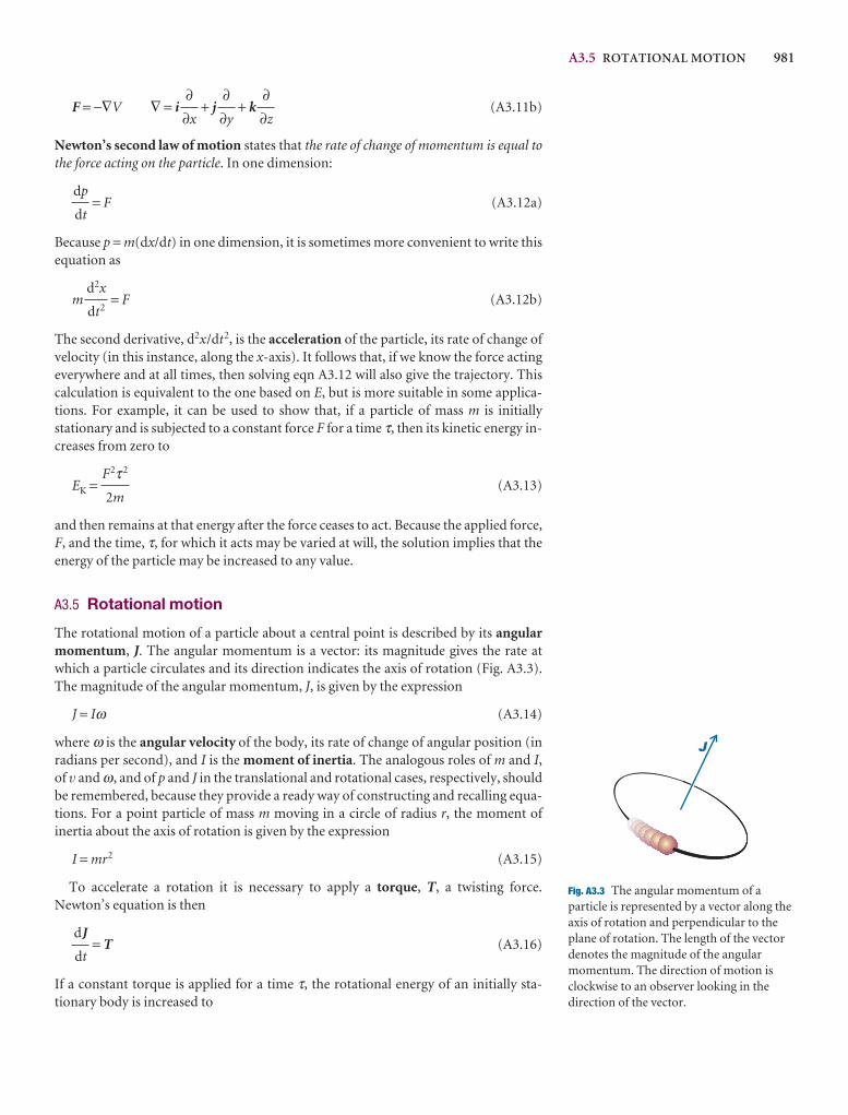
A3.5 ROTATIONAL MOTION 981
F = −∇V ∇ = i + j + k (A3.11b)
Newton’s second law of motion states that the rate of change of momentum is equal tothe force acting on the particle. In one dimension:
= F (A3.12a)
Because p = m(dx/dt) in one dimension, it is sometimes more convenient to write thisequation as
m = F (A3.12b)
The second derivative, d2x/dt2, is the acceleration of the particle, its rate of change ofvelocity (in this instance, along the x-axis). It follows that, if we know the force actingeverywhere and at all times, then solving eqn A3.12 will also give the trajectory. Thiscalculation is equivalent to the one based on E, but is more suitable in some applica-tions. For example, it can be used to show that, if a particle of mass m is initially stationary and is subjected to a constant force F for a time τ, then its kinetic energy in-creases from zero to
EK = (A3.13)
and then remains at that energy after the force ceases to act. Because the applied force,F, and the time, τ, for which it acts may be varied at will, the solution implies that theenergy of the particle may be increased to any value.
A3.5 Rotational motion
The rotational motion of a particle about a central point is described by its angularmomentum, J. The angular momentum is a vector: its magnitude gives the rate atwhich a particle circulates and its direction indicates the axis of rotation (Fig. A3.3).The magnitude of the angular momentum, J, is given by the expression
J = Iω (A3.14)
where ω is the angular velocity of the body, its rate of change of angular position (inradians per second), and I is the moment of inertia. The analogous roles of m and I,of v and ω, and of p and J in the translational and rotational cases, respectively, shouldbe remembered, because they provide a ready way of constructing and recalling equa-tions. For a point particle of mass m moving in a circle of radius r, the moment of inertia about the axis of rotation is given by the expression
I = mr2 (A3.15)
To accelerate a rotation it is necessary to apply a torque, T, a twisting force.Newton’s equation is then
= T (A3.16)
If a constant torque is applied for a time τ, the rotational energy of an initially sta-tionary body is increased to
dJ
dt
F2τ2
2m
d2x
dt2
dp
dt
∂∂z
∂∂y
∂∂x
J
Fig. A3.3 The angular momentum of aparticle is represented by a vector along theaxis of rotation and perpendicular to theplane of rotation. The length of the vectordenotes the magnitude of the angularmomentum. The direction of motion isclockwise to an observer looking in thedirection of the vector.
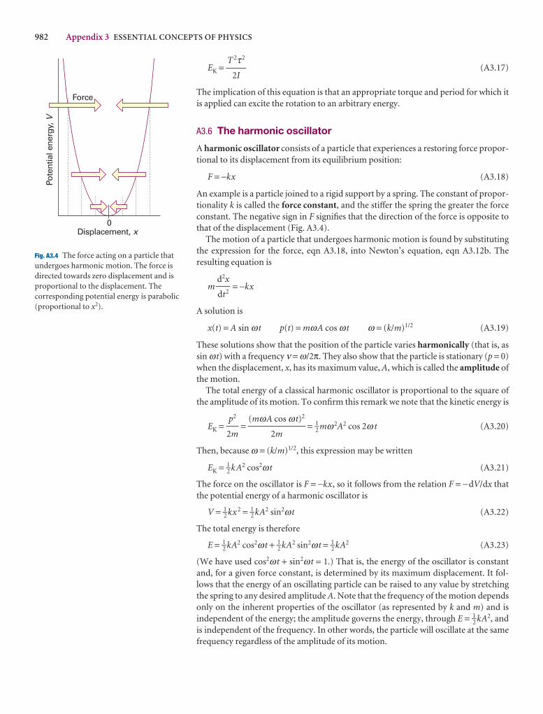
982 Appendix 3 ESSENTIAL CONCEPTS OF PHYSICS
EK = (A3.17)
The implication of this equation is that an appropriate torque and period for which itis applied can excite the rotation to an arbitrary energy.
A3.6 The harmonic oscillator
A harmonic oscillator consists of a particle that experiences a restoring force propor-tional to its displacement from its equilibrium position:
F = −kx (A3.18)
An example is a particle joined to a rigid support by a spring. The constant of propor-tionality k is called the force constant, and the stiffer the spring the greater the forceconstant. The negative sign in F signifies that the direction of the force is opposite tothat of the displacement (Fig. A3.4).
The motion of a particle that undergoes harmonic motion is found by substitutingthe expression for the force, eqn A3.18, into Newton’s equation, eqn A3.12b. The resulting equation is
m = −kx
A solution is
x(t) = A sin ω t p(t) = mωA cos ω t ω = (k/m)1/2 (A3.19)
These solutions show that the position of the particle varies harmonically (that is, assin ω t) with a frequency ν = ω/2π. They also show that the particle is stationary (p = 0)when the displacement, x, has its maximum value, A, which is called the amplitude ofthe motion.
The total energy of a classical harmonic oscillator is proportional to the square ofthe amplitude of its motion. To confirm this remark we note that the kinetic energy is
EK = = = 1–2 mω2A2 cos 2ω t (A3.20)
Then, because ω = (k/m)1/2, this expression may be written
EK = 1–2 kA2 cos2ω t (A3.21)
The force on the oscillator is F = −kx, so it follows from the relation F = −dV/dx thatthe potential energy of a harmonic oscillator is
V = 1–2 kx 2 = 1–2 kA2 sin2ω t (A3.22)
The total energy is therefore
E = 1–2 kA2 cos2ω t + 1–2 kA2 sin2ω t = 1–2 kA2 (A3.23)
(We have used cos2ω t + sin2ω t = 1.) That is, the energy of the oscillator is constantand, for a given force constant, is determined by its maximum displacement. It fol-lows that the energy of an oscillating particle can be raised to any value by stretchingthe spring to any desired amplitude A. Note that the frequency of the motion dependsonly on the inherent properties of the oscillator (as represented by k and m) and is independent of the energy; the amplitude governs the energy, through E = 1–2 kA2, andis independent of the frequency. In other words, the particle will oscillate at the samefrequency regardless of the amplitude of its motion.
(mωA cos ω t)2
2m
p2
2m
d2x
dt2
T 2τ2
2I
Displacement, x0
Pote
ntia
l ene
rgy,
V
Force
Fig. A3.4 The force acting on a particle thatundergoes harmonic motion. The force isdirected towards zero displacement and isproportional to the displacement. Thecorresponding potential energy is parabolic(proportional to x2).
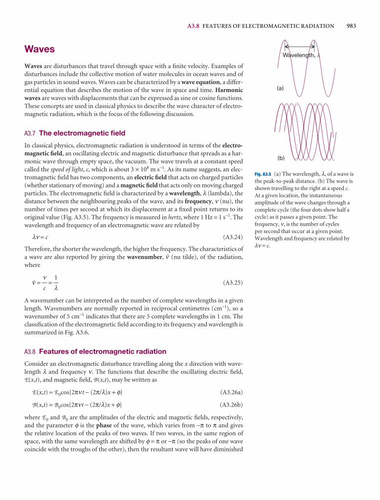
A3.8 FEATURES OF ELECTROMAGNETIC RADIATION 983
Waves
Waves are disturbances that travel through space with a finite velocity. Examples ofdisturbances include the collective motion of water molecules in ocean waves and ofgas particles in sound waves. Waves can be characterized by a wave equation, a differ-ential equation that describes the motion of the wave in space and time. Harmonicwaves are waves with displacements that can be expressed as sine or cosine functions.These concepts are used in classical physics to describe the wave character of electro-magnetic radiation, which is the focus of the following discussion.
A3.7 The electromagnetic field
In classical physics, electromagnetic radiation is understood in terms of the electro-magnetic field, an oscillating electric and magnetic disturbance that spreads as a har-monic wave through empty space, the vacuum. The wave travels at a constant speedcalled the speed of light, c, which is about 3 × 10⁸ m s−1. As its name suggests, an elec-tromagnetic field has two components, an electric field that acts on charged particles(whether stationary of moving) and a magnetic field that acts only on moving chargedparticles. The electromagnetic field is characterized by a wavelength, λ (lambda), thedistance between the neighbouring peaks of the wave, and its frequency, ν (nu), thenumber of times per second at which its displacement at a fixed point returns to itsoriginal value (Fig. A3.5). The frequency is measured in hertz, where 1 Hz = 1 s−1. Thewavelength and frequency of an electromagnetic wave are related by
λν = c (A3.24)
Therefore, the shorter the wavelength, the higher the frequency. The characteristics ofa wave are also reported by giving the wavenumber, # (nu tilde), of the radiation,where
# = = (A3.25)
A wavenumber can be interpreted as the number of complete wavelengths in a givenlength. Wavenumbers are normally reported in reciprocal centimetres (cm−1), so awavenumber of 5 cm−1 indicates that there are 5 complete wavelengths in 1 cm. Theclassification of the electromagnetic field according to its frequency and wavelength issummarized in Fig. A3.6.
A3.8 Features of electromagnetic radiation
Consider an electromagnetic disturbance travelling along the x direction with wave-length λ and frequency ν. The functions that describe the oscillating electric field,E(x,t), and magnetic field, B(x,t), may be written as
E(x,t) = E0cos{2πν t − (2π/λ)x + φ} (A3.26a)
B(x,t) = B0cos{2πνt − (2π/λ)x + φ} (A3.26b)
where E0 and B0 are the amplitudes of the electric and magnetic fields, respectively,and the parameter φ is the phase of the wave, which varies from −π to π and gives the relative location of the peaks of two waves. If two waves, in the same region ofspace, with the same wavelength are shifted by φ = π or −π (so the peaks of one wavecoincide with the troughs of the other), then the resultant wave will have diminished
1
λνc
Wavelength,
(a)
(b)
�
Fig. A3.5 (a) The wavelength, λ, of a wave isthe peak-to-peak distance. (b) The wave isshown travelling to the right at a speed c.At a given location, the instantaneousamplitude of the wave changes through acomplete cycle (the four dots show half acycle) as it passes a given point. Thefrequency, ν, is the number of cycles per second that occur at a given point.Wavelength and frequency are related byλν = c.
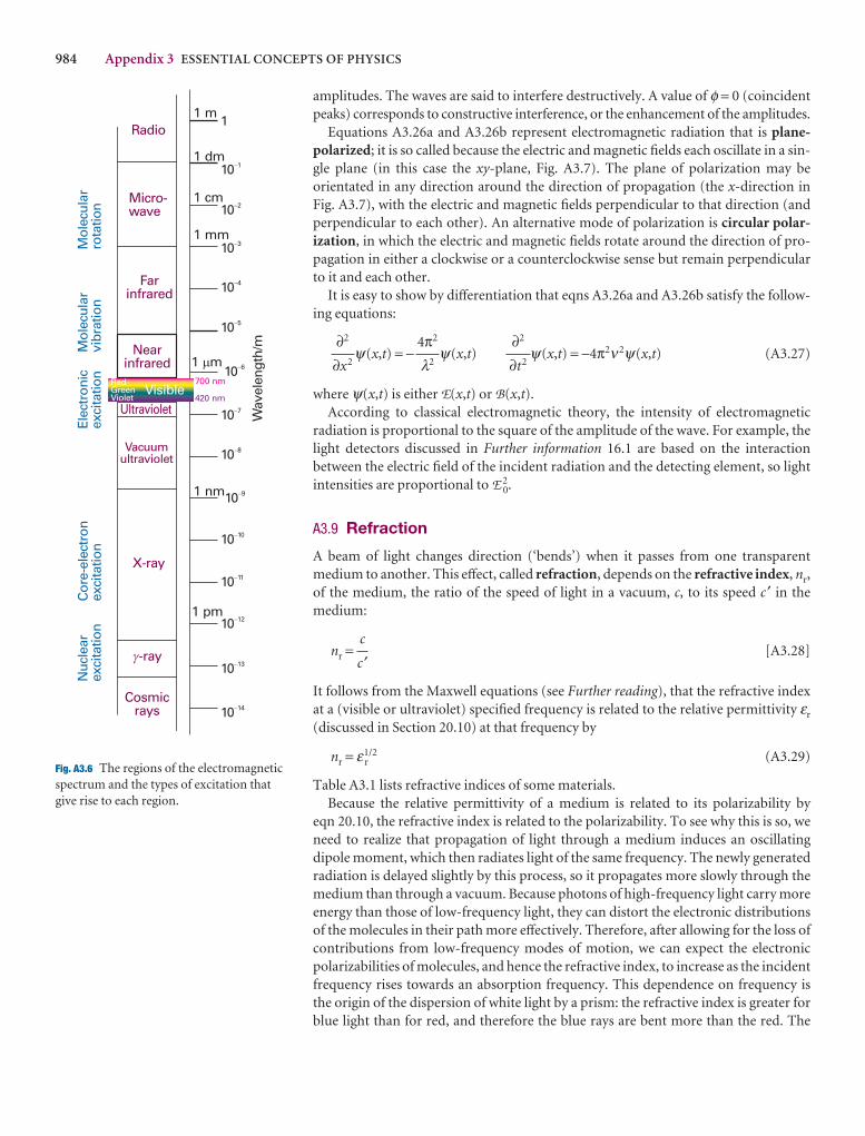
984 Appendix 3 ESSENTIAL CONCEPTS OF PHYSICS
amplitudes. The waves are said to interfere destructively. A value of φ = 0 (coincidentpeaks) corresponds to constructive interference, or the enhancement of the amplitudes.
Equations A3.26a and A3.26b represent electromagnetic radiation that is plane-polarized; it is so called because the electric and magnetic fields each oscillate in a sin-gle plane (in this case the xy-plane, Fig. A3.7). The plane of polarization may beorientated in any direction around the direction of propagation (the x-direction inFig. A3.7), with the electric and magnetic fields perpendicular to that direction (andperpendicular to each other). An alternative mode of polarization is circular polar-ization, in which the electric and magnetic fields rotate around the direction of pro-pagation in either a clockwise or a counterclockwise sense but remain perpendicularto it and each other.
It is easy to show by differentiation that eqns A3.26a and A3.26b satisfy the follow-ing equations:
ψ(x,t) = − ψ(x,t) ψ(x,t) = −4π2ν2ψ(x,t) (A3.27)
where ψ(x,t) is either E(x,t) or B(x,t).According to classical electromagnetic theory, the intensity of electromagnetic
radiation is proportional to the square of the amplitude of the wave. For example, thelight detectors discussed in Further information 16.1 are based on the interaction between the electric field of the incident radiation and the detecting element, so lightintensities are proportional to E 2
0.
A3.9 Refraction
A beam of light changes direction (‘bends’) when it passes from one transparentmedium to another. This effect, called refraction, depends on the refractive index, nr,of the medium, the ratio of the speed of light in a vacuum, c, to its speed c ′ in themedium:
nr = [A3.28]
It follows from the Maxwell equations (see Further reading), that the refractive indexat a (visible or ultraviolet) specified frequency is related to the relative permittivity εr
(discussed in Section 20.10) at that frequency by
nr = ε r1/2 (A3.29)
Table A3.1 lists refractive indices of some materials.Because the relative permittivity of a medium is related to its polarizability by
eqn 20.10, the refractive index is related to the polarizability. To see why this is so, weneed to realize that propagation of light through a medium induces an oscillatingdipole moment, which then radiates light of the same frequency. The newly generatedradiation is delayed slightly by this process, so it propagates more slowly through themedium than through a vacuum. Because photons of high-frequency light carry moreenergy than those of low-frequency light, they can distort the electronic distributionsof the molecules in their path more effectively. Therefore, after allowing for the loss ofcontributions from low-frequency modes of motion, we can expect the electronic polarizabilities of molecules, and hence the refractive index, to increase as the incidentfrequency rises towards an absorption frequency. This dependence on frequency isthe origin of the dispersion of white light by a prism: the refractive index is greater forblue light than for red, and therefore the blue rays are bent more than the red. The
c
c ′
∂2
∂t2
4π2
λ2
∂2
∂x2
10�14
10�13
10�12
10�11
10�10
10�9
10�8
10�7
10�6
10�5
10�4
10�3
10�2
10�1
1
1 pm
1 nm
1 m
1 mm
1 cm
1 dm
1 mRadio
Micro-wave
Farinfrared
Nearinfrared
Ultraviolet
Vacuumultraviolet
X-ray
�-ray
Cosmicrays
Wav
elen
gth/
m
Mol
ecul
arro
tatio
nM
olec
ular
vibr
atio
nEl
ectr
onic
exci
tatio
nC
ore-
elec
tron
exci
tatio
nN
ucle
arex
cita
tion
VisibleRed
VioletGreen
700 nm
420 nm
�
Fig. A3.6 The regions of the electromagneticspectrum and the types of excitation thatgive rise to each region.
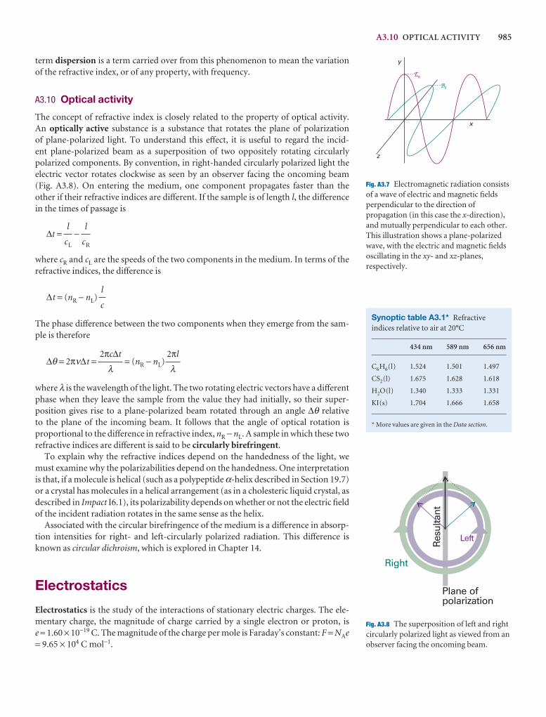
A3.10 OPTICAL ACTIVITY 985
term dispersion is a term carried over from this phenomenon to mean the variationof the refractive index, or of any property, with frequency.
A3.10 Optical activity
The concept of refractive index is closely related to the property of optical activity. An optically active substance is a substance that rotates the plane of polarization of plane-polarized light. To understand this effect, it is useful to regard the incid-ent plane-polarized beam as a superposition of two oppositely rotating circularly polarized components. By convention, in right-handed circularly polarized light theelectric vector rotates clockwise as seen by an observer facing the oncoming beam(Fig. A3.8). On entering the medium, one component propagates faster than theother if their refractive indices are different. If the sample is of length l, the differencein the times of passage is
∆t = −
where cR and cL are the speeds of the two components in the medium. In terms of therefractive indices, the difference is
∆t = (nR − nL)
The phase difference between the two components when they emerge from the sam-ple is therefore
∆θ = 2πν∆t = = (nR − nL)
where λ is the wavelength of the light. The two rotating electric vectors have a differentphase when they leave the sample from the value they had initially, so their super-position gives rise to a plane-polarized beam rotated through an angle ∆θ relativeto the plane of the incoming beam. It follows that the angle of optical rotation is proportional to the difference in refractive index, nR − nL. A sample in which these tworefractive indices are different is said to be circularly birefringent.
To explain why the refractive indices depend on the handedness of the light, wemust examine why the polarizabilities depend on the handedness. One interpretationis that, if a molecule is helical (such as a polypeptide α-helix described in Section 19.7)or a crystal has molecules in a helical arrangement (as in a cholesteric liquid crystal, asdescribed in Impact I6.1), its polarizability depends on whether or not the electric fieldof the incident radiation rotates in the same sense as the helix.
Associated with the circular birefringence of the medium is a difference in absorp-tion intensities for right- and left-circularly polarized radiation. This difference isknown as circular dichroism, which is explored in Chapter 14.
Electrostatics
Electrostatics is the study of the interactions of stationary electric charges. The ele-mentary charge, the magnitude of charge carried by a single electron or proton, is e ≈ 1.60 × 10⁻¹⁹ C. The magnitude of the charge per mole is Faraday’s constant: F = NAe= 9.65 × 10⁴ C mol−1.
2πl
λ2πc∆t
λ
l
c
l
cR
l
cL
Plane ofpolarization
Right
Left
Res
ulta
nt
Fig. A3.8 The superposition of left and rightcircularly polarized light as viewed from anobserver facing the oncoming beam.
Synoptic table A3.1* Refractiveindices relative to air at 20°C
434 nm 589 nm 656 nm
C6H6(l) 1.524 1.501 1.497
CS2(l) 1.675 1.628 1.618
H2O(l) 1.340 1.333 1.331
KI(s) 1.704 1.666 1.658
* More values are given in the Data section.
y
x
z
E0
B0
Fig. A3.7 Electromagnetic radiation consistsof a wave of electric and magnetic fieldsperpendicular to the direction ofpropagation (in this case the x-direction),and mutually perpendicular to each other.This illustration shows a plane-polarizedwave, with the electric and magnetic fieldsoscillating in the xy- and xz-planes,respectively.
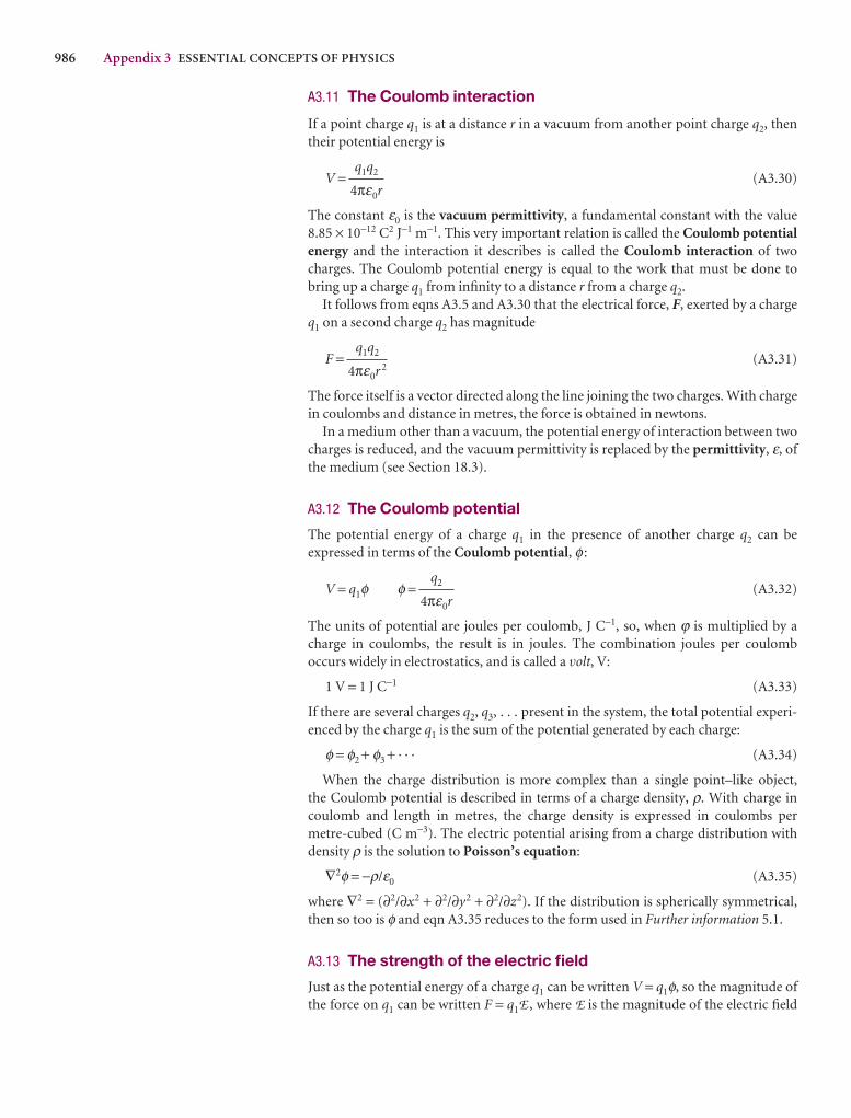
986 Appendix 3 ESSENTIAL CONCEPTS OF PHYSICS
A3.11 The Coulomb interaction
If a point charge q1 is at a distance r in a vacuum from another point charge q2, thentheir potential energy is
V = (A3.30)
The constant ε0 is the vacuum permittivity, a fundamental constant with the value8.85 × 10−12 C2 J−1 m−1. This very important relation is called the Coulomb potentialenergy and the interaction it describes is called the Coulomb interaction of twocharges. The Coulomb potential energy is equal to the work that must be done tobring up a charge q1 from infinity to a distance r from a charge q2.
It follows from eqns A3.5 and A3.30 that the electrical force, F, exerted by a chargeq1 on a second charge q2 has magnitude
F = (A3.31)
The force itself is a vector directed along the line joining the two charges. With chargein coulombs and distance in metres, the force is obtained in newtons.
In a medium other than a vacuum, the potential energy of interaction between twocharges is reduced, and the vacuum permittivity is replaced by the permittivity, ε, ofthe medium (see Section 18.3).
A3.12 The Coulomb potential
The potential energy of a charge q1 in the presence of another charge q2 can be expressed in terms of the Coulomb potential, φ :
V = q1φ φ = (A3.32)
The units of potential are joules per coulomb, J C−1, so, when ϕ is multiplied by acharge in coulombs, the result is in joules. The combination joules per coulomb occurs widely in electrostatics, and is called a volt, V:
1 V = 1 J C−1 (A3.33)
If there are several charges q2, q3, . . . present in the system, the total potential experi-enced by the charge q1 is the sum of the potential generated by each charge:
φ = φ2 + φ3 + · · · (A3.34)
When the charge distribution is more complex than a single point–like object, the Coulomb potential is described in terms of a charge density, ρ. With charge incoulomb and length in metres, the charge density is expressed in coulombs per metre-cubed (C m−3). The electric potential arising from a charge distribution withdensity ρ is the solution to Poisson’s equation:
∇2φ = −ρ/ε0 (A3.35)
where ∇2 = (∂2/∂x2 + ∂2/∂y2 + ∂2/∂z2). If the distribution is spherically symmetrical,then so too is φ and eqn A3.35 reduces to the form used in Further information 5.1.
A3.13 The strength of the electric field
Just as the potential energy of a charge q1 can be written V = q1φ, so the magnitude ofthe force on q1 can be written F = q1E , where E is the magnitude of the electric field
q2
4πε0r
q1q2
4πε0r 2
q1q2
4πε0r
FURTHER READING 987
strength arising from q2 or from some more general charge distribution. The electricfield strength (which, like the force, is actually a vector quantity) is the negative gradi-ent of the electric potential:
/ = −∇φ (A3.36)
A3.14 Electric current and power
The motion of charge gives rise to an electric current, I. Electric current is measuredin ampere, A, where
1 A = 1 C s−1 (A3.37)
If the current flows from a region of potential φi to φf, through a potential difference∆φ = φf − φi, the rate of doing work is the current (the rate of transfer of charge) multiplied by the potential difference, I∆φ. The rate of doing electrical work is theelectrical power, P, so
P = I∆φ (A3.38)
With current in amperes and the potential difference in volts, the power works out inwatts. The total energy, E, supplied in an interval ∆t is the power (the rate of energysupply) multiplied by the duration of the interval:
E = P∆t = I∆φ∆t (A3.39)
The energy is obtained in joules with the current in amperes, the potential differencein volts, and the time in seconds.
Further reading
R.P. Feynman, R.B. Leighton, and M. Sands, The Feynman lectures onphysics. Vols 1–3. Addison–Wesley, Reading (1966).
G.A.D. Ritchie and D.S. Sivia, Foundations of physics for chemists.Oxford Chemistry Primers, Oxford University Press (2000).
W.S. Warren, The physical basis of chemistry. Academic Press, San Diego (2000).
R. Wolfson and J.M. Pasachoff, Physics for scientists and engineers.Benjamin Cummings, San Francisco (1999).

Contents
The following is a directory of all tables in the text; those included in this Data section are marked with an asterisk. Theremainder will be found on the pages indicated.
Physical properties of selected materials*Masses and natural abundances of selected nuclides*
1.1 Pressure units (4)1.2 The gas constant in various units (9)1.3 The composition of dry air at sea level (11)1.4 Second virial coefficients*1.5 Critical constants of gases*1.6 van der Waals coefficients*1.7 Selected equations of state (19)
2.1 Varieties of work (34)2.2 Temperature variation of molar heat capacities*2.3 Standard enthalpies of fusion and vaporization at the
transition temperature*2.4 Enthalpies of transition [notation] (51)2.5 Thermodynamic data for organic compounds*2.6 Thermochemical properties of some fuels (53)2.7 Thermodynamic data for inorganic compounds*2.7a Standard enthalpies of hydration at infinite dilution*2.7b Standard ion hydration enthalpies*2.8 Expansion coefficients and isothermal
compressibilities*2.9 Inversion temperatures, normal freezing and boiling
points, and Joule–Thomson coefficients*
3.1 Standard entropies (and temperatures) of phasetransitions*
3.2 Standard entropies of vaporization of liquids*3.3 Standard Third-Law entropies [see Tables 2.5
and 2.7]*3.4 Standard Gibbs energies of formation [see Tables 2.5
and 2.7]*3.5 The Maxwell relations (104)3.6 The fugacity of nitrogen*
5.1 Henry’s law constants for gases*5.2 Freezing point and boiling point constants*5.3 Standard states [summary of definitions] (158)5.4 Ionic strength and molality (164)5.5 Mean activity coefficients in water*5.6 Relative permitivities (dielectric constants)*
Data section
7.1 Varieties of electrode (216)7.2 Standard potentials*7.3 The electrochemical series of metals (*)7.4 Acidity constants for aqueous solutions*
8.1 The Schrödinger equation (255)8.2 Constraints of the uncertainty principle (271)
9.1 The Hermite polynomials (293)9.2 The error function*9.3 The spherical harmonics (302)9.4 Properties of angular momentum (309)
10.1 Hydrogenic radial wavefunctions (324)10.2 Effective nuclear charge*10.3 Ionization energies*10.4 Electron affinities*
11.1 Some hybridization schemes (368)11.2 Bond lengths*11.3 Bond dissociation enthalpies*11.4 Pauling and Mulliken electronegativities*11.5 Ab initio calculations and spectroscopic data (398)
12.1 The notation for point groups (408)12.2 The C2v character table (415)12.3 The C3v character table (416)
13.1 Moments of inertia [formulae] (440)13.2 Properties of diatomic molecules*13.3 Typical vibrational wavenumbers*
14.1 Colour, frequency, and energy of light*14.2 Ground and excited states of O2 (483)14.3 Absorption characteristics of some groups and
molecules*14.4 Characteristics of laser radiation and their chemical
applications (500)
15.1 Nuclear spin and nuclear structure (515)15.2 Nuclear spin properties*15.3 Hyperfine coupling constants for atoms*
17.1 Rotational and vibrational temperatures [see alsoTable 13.2] (594)

DATA SECTION 989
17.2 Symmetry numbers [see also Table 13.2] (596)17.3 Contributions to the molecular partition function
[formulae] (615)17.4 Thermodynamic functions in terms of the partition
function [formulae] (616)17.5 Contributions to mean energies and heat capacities
[formulae] (616)
18.1 Dipole moments, polarizabilities, and polarizabilityvolumes*
18.2 Partial charges in polypeptides (622)18.3 Multipole interaction energies (630)18.4 Lennard-Jones (12,6)-potential parameters*18.5 Surface tensions of liquids*
19.1 Radius of gyration*19.2 Diffusion coefficients in water*19.3 Frictional coefficients and molecular geometry*19.4 Intrinsic viscosity*
20.1 The seven crystal systems (699)20.2 The crystal structures of some elements (716)20.3 Ionic radii*20.4 Madelung constants (719)20.5 Lattice enthalpies*20.6 Magnetic susceptibilities*
21.1 Collision cross-sections*21.2 Transport properties of gases*21.3 Transport properties of perfect gases [summary of
formulae] (758)21.4 Viscosities of liquids*21.5 Limiting ionic conductivities in water*21.6 Ionic mobilities in water*
21.7 Debye–Hückel–Onsager coefficients for (1,1)-electrolytes*
21.8 Diffusion coefficients*
22.1 Kinetic data for first-order reactions*22.2 Kinetic data for second-order reactions*22.3 Integrated rate laws (803)22.4 Arrhenius parameters*
23.1 Photochemical processes (846)23.2 Common photophysical processes (846)23.3 Values of R0 for donor–acceptor pairs (852)
24.1 Arrhenius parameters for gas-phase reactions*24.2 Arrhenius parameters for reactions in solution [see
Table 22.4]*24.3 Summary of uses of k [notation] (902)
25.1 Maximum observed enthalpies of physisorption*25.2 Enthalpies of chemisorption*25.3 Activation energies of catalysed reactions*25.4 Properties of catalysts (929)25.5 Chemisorption abilities (930)25.6 Exchange current densities and transfer coefficients*25.7 Summary of acronyms (950)
A1.1 The SI base units (960)A1.2 A selection of derived units (961)A1.3 Common SI prefixes (961)A1.4 Some common units (962)
A3.1 Refractive indices relative to air*
Character tables
The following tables reproduce and expand the data given in the short tables in the text, and follow their numbering. Standardstates refer to a pressure of p7 = 1 bar. The general references are as follows:
AIP: D.E. Gray (ed.), American Institute of Physics handbook. McGraw Hill, New York (1972).
AS: M. Abramowitz and I.A. Stegun (ed.), Handbook of mathematical functions. Dover, New York (1963).
E: J. Emsley, The elements. Oxford University Press (1991).
HCP: D.R. Lide (ed.), Handbook of chemistry and physics. CRC Press, Boca Raton (2000).
JL: A.M. James and M.P. Lord, Macmillan’s chemical and physical data. Macmillan, London (1992).
KL: G.W.C. Kaye and T.H. Laby (ed.), Tables of physical and chemical constants. Longman, London (1973).
LR: G.N. Lewis and M. Randall, resived by K.S. Pitzer and L. Brewer, Thermodynamics. McGraw-Hill, New York (1961).
NBS: NBS tables of chemical thermodynamic properties, published as J. Phys. and Chem. Reference Data, 11, Supplement 2 (1982).
RS: R.A. Robinson and R.H. Stokes, Electrolyte solutions. Butterworth, London (1959).
TDOC: J.B. Pedley, J.D. Naylor, and S.P. Kirby, Thermochemical data of organic compounds. Chapman & Hall, London (1986).
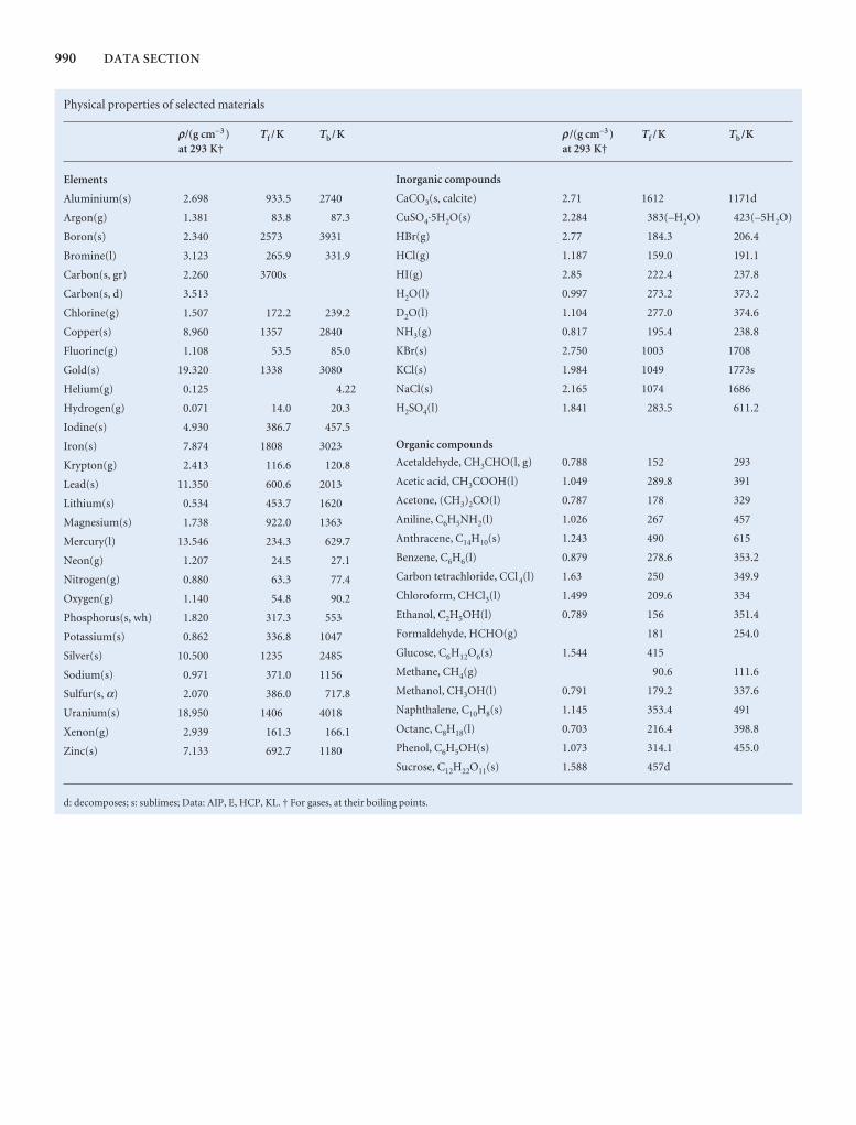
990 DATA SECTION
Physical properties of selected materials
r/(g cm−3 ) Tf /K Tb /K r/(g cm−3 ) Tf /K Tb /Kat 293 K† at 293 K†
Elements
Aluminium(s) 2.698 933.5 2740
Argon(g) 1.381 83.8 87.3
Boron(s) 2.340 2573 3931
Bromine(l) 3.123 265.9 331.9
Carbon(s, gr) 2.260 3700s
Carbon(s, d) 3.513
Chlorine(g) 1.507 172.2 239.2
Copper(s) 8.960 1357 2840
Fluorine(g) 1.108 53.5 85.0
Gold(s) 19.320 1338 3080
Helium(g) 0.125 4.22
Hydrogen(g) 0.071 14.0 20.3
Iodine(s) 4.930 386.7 457.5
Iron(s) 7.874 1808 3023
Krypton(g) 2.413 116.6 120.8
Lead(s) 11.350 600.6 2013
Lithium(s) 0.534 453.7 1620
Magnesium(s) 1.738 922.0 1363
Mercury(l) 13.546 234.3 629.7
Neon(g) 1.207 24.5 27.1
Nitrogen(g) 0.880 63.3 77.4
Oxygen(g) 1.140 54.8 90.2
Phosphorus(s, wh) 1.820 317.3 553
Potassium(s) 0.862 336.8 1047
Silver(s) 10.500 1235 2485
Sodium(s) 0.971 371.0 1156
Sulfur(s, α) 2.070 386.0 717.8
Uranium(s) 18.950 1406 4018
Xenon(g) 2.939 161.3 166.1
Zinc(s) 7.133 692.7 1180
d: decomposes; s: sublimes; Data: AIP, E, HCP, KL. † For gases, at their boiling points.
Inorganic compounds
CaCO3(s, calcite) 2.71 1612 1171d
CuSO4·5H2O(s) 2.284 383(–H2O) 423(–5H2O)
HBr(g) 2.77 184.3 206.4
HCl(g) 1.187 159.0 191.1
HI(g) 2.85 222.4 237.8
H2O(l) 0.997 273.2 373.2
D2O(l) 1.104 277.0 374.6
NH3(g) 0.817 195.4 238.8
KBr(s) 2.750 1003 1708
KCl(s) 1.984 1049 1773s
NaCl(s) 2.165 1074 1686
H2SO4(l) 1.841 283.5 611.2
Organic compounds
Acetaldehyde, CH3CHO(l, g) 0.788 152 293
Acetic acid, CH3COOH(l) 1.049 289.8 391
Acetone, (CH3)2CO(l) 0.787 178 329
Aniline, C6H5NH2(l) 1.026 267 457
Anthracene, C14H10(s) 1.243 490 615
Benzene, C6H6(l) 0.879 278.6 353.2
Carbon tetrachloride, CCl 4(l) 1.63 250 349.9
Chloroform, CHCl3(l) 1.499 209.6 334
Ethanol, C2H5OH(l) 0.789 156 351.4
Formaldehyde, HCHO(g) 181 254.0
Glucose, C6H12O6(s) 1.544 415
Methane, CH4(g) 90.6 111.6
Methanol, CH3OH(l) 0.791 179.2 337.6
Naphthalene, C10H8(s) 1.145 353.4 491
Octane, C8H18(l) 0.703 216.4 398.8
Phenol, C6H5OH(s) 1.073 314.1 455.0
Sucrose, C12H22O11(s) 1.588 457d
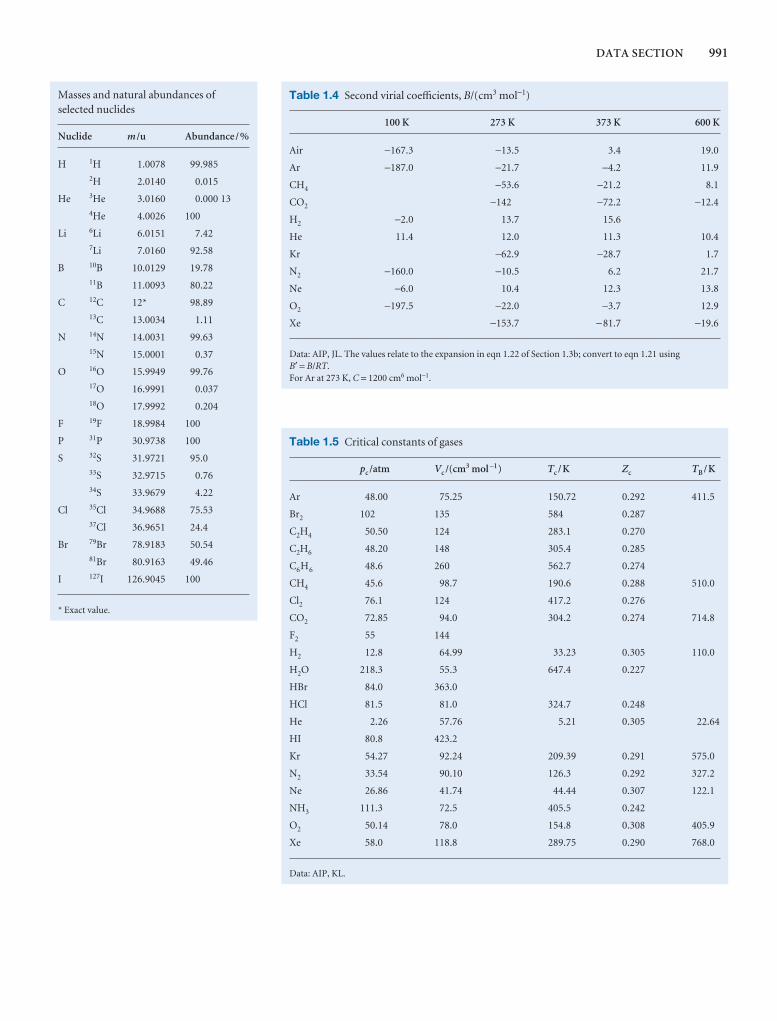
DATA SECTION 991
Table 1.5 Critical constants of gases
pc /atm Vc /(cm3 mol −1) Tc /K Zc TB /K
Ar 48.00 75.25 150.72 0.292 411.5
Br2 102 135 584 0.287
C2H4 50.50 124 283.1 0.270
C2H6 48.20 148 305.4 0.285
C6H6 48.6 260 562.7 0.274
CH4 45.6 98.7 190.6 0.288 510.0
Cl2 76.1 124 417.2 0.276
CO2 72.85 94.0 304.2 0.274 714.8
F2 55 144
H2 12.8 64.99 33.23 0.305 110.0
H2O 218.3 55.3 647.4 0.227
HBr 84.0 363.0
HCl 81.5 81.0 324.7 0.248
He 2.26 57.76 5.21 0.305 22.64
HI 80.8 423.2
Kr 54.27 92.24 209.39 0.291 575.0
N2 33.54 90.10 126.3 0.292 327.2
Ne 26.86 41.74 44.44 0.307 122.1
NH3 111.3 72.5 405.5 0.242
O2 50.14 78.0 154.8 0.308 405.9
Xe 58.0 118.8 289.75 0.290 768.0
Data: AIP, KL.
Masses and natural abundances ofselected nuclides
Nuclide m /u Abundance/%
H 1H 1.0078 99.9852H 2.0140 0.015
He 3He 3.0160 0.000 134He 4.0026 100
Li 6Li 6.0151 7.427Li 7.0160 92.58
B 10B 10.0129 19.7811B 11.0093 80.22
C 12C 12* 98.8913C 13.0034 1.11
N 14N 14.0031 99.6315N 15.0001 0.37
O 16O 15.9949 99.7617O 16.9991 0.03718O 17.9992 0.204
F 19F 18.9984 100
P 31P 30.9738 100
S 32S 31.9721 95.033S 32.9715 0.7634S 33.9679 4.22
Cl 35Cl 34.9688 75.5337Cl 36.9651 24.4
Br 79Br 78.9183 50.5481Br 80.9163 49.46
I 127I 126.9045 100
* Exact value.
Table 1.4 Second virial coefficients, B/(cm3 mol−1)
100 K 273 K 373 K 600 K
Air −167.3 −13.5 3.4 19.0
Ar −187.0 −21.7 −4.2 11.9
CH4 −53.6 −21.2 8.1
CO2 −142 −72.2 −12.4
H2 −2.0 13.7 15.6
He 11.4 12.0 11.3 10.4
Kr −62.9 −28.7 1.7
N2 −160.0 −10.5 6.2 21.7
Ne −6.0 10.4 12.3 13.8
O2 −197.5 −22.0 −3.7 12.9
Xe −153.7 −81.7 −19.6
Data: AIP, JL. The values relate to the expansion in eqn 1.22 of Section 1.3b; convert to eqn 1.21 using B′ = B/RT.For Ar at 273 K, C = 1200 cm6 mol−1.
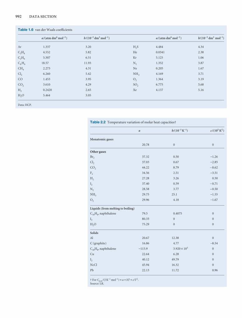
992 DATA SECTION
Table 1.6 van der Waals coefficients
a /(atm dm6 mol−2 ) b /(10−2 dm3 mol−1) a /(atm dm6 mol−2 ) b/(10−2 dm3 mol−1)
Ar 1.337 3.20 H2S 4.484 4.34
C2H4 4.552 5.82 He 0.0341 2.38
C2H6 5.507 6.51 Kr 5.125 1.06
C6 H6 18.57 11.93 N2 1.352 3.87
CH4 2.273 4.31 Ne 0.205 1.67
Cl2 6.260 5.42 NH3 4.169 3.71
CO 1.453 3.95 O2 1.364 3.19
CO2 3.610 4.29 SO2 6.775 5.68
H2 0.2420 2.65 Xe 4.137 5.16
H2O 5.464 3.05
Data: HCP.
Table 2.2 Temperature variation of molar heat capacities†
a b/(10−3 K−1) c /(105 K2 )
Monatomic gases
20.78 0 0
Other gases
Br2 37.32 0.50 −1.26
Cl2 37.03 0.67 −2.85
CO2 44.22 8.79 −8.62
F2 34.56 2.51 −3.51
H2 27.28 3.26 0.50
I2 37.40 0.59 −0.71
N2 28.58 3.77 −0.50
NH3 29.75 25.1 −1.55
O2 29.96 4.18 −1.67
Liquids (from melting to boiling)
C10H8, naphthalene 79.5 0.4075 0
I2 80.33 0 0
H2O 75.29 0 0
Solids
Al 20.67 12.38 0
C (graphite) 16.86 4.77 −8.54
C10H8, naphthalene −115.9 3.920 × 10³ 0
Cu 22.64 6.28 0
I2 40.12 49.79 0
NcCl 45.94 16.32 0
Pb 22.13 11.72 0.96
† For Cp,m /(J K−1 mol−1) = a + bT + c/T 2.Source: LR.
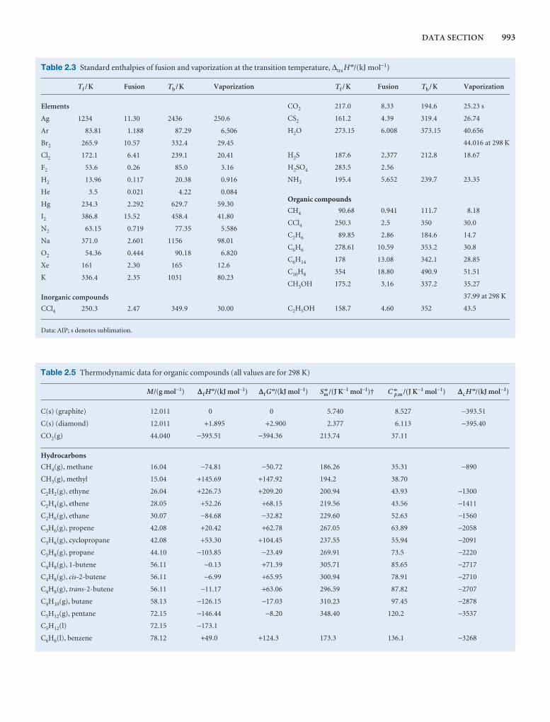
DATA SECTION 993
Table 2.5 Thermodynamic data for organic compounds (all values are for 298 K)
M/(g mol−1) D f H 7/(kJ mol−1) Df G 7/(kJ mol−1) Sm7 /(J K−1 mol−1)† C 7
p,m /(J K−1 mol−1) Dc H 7/(kJ mol−1)
C(s) (graphite) 12.011 0 0 5.740 8.527 −393.51
C(s) (diamond) 12.011 +1.895 +2.900 2.377 6.113 −395.40
CO2(g) 44.040 −393.51 −394.36 213.74 37.11
Hydrocarbons
CH4(g), methane 16.04 −74.81 −50.72 186.26 35.31 −890
CH3(g), methyl 15.04 +145.69 +147.92 194.2 38.70
C2H2(g), ethyne 26.04 +226.73 +209.20 200.94 43.93 −1300
C2H4(g), ethene 28.05 +52.26 +68.15 219.56 43.56 −1411
C2H6(g), ethane 30.07 −84.68 −32.82 229.60 52.63 −1560
C3H6(g), propene 42.08 +20.42 +62.78 267.05 63.89 −2058
C3H6(g), cyclopropane 42.08 +53.30 +104.45 237.55 55.94 −2091
C3H8(g), propane 44.10 −103.85 −23.49 269.91 73.5 −2220
C4H8(g), 1-butene 56.11 −0.13 +71.39 305.71 85.65 −2717
C4H8(g), cis-2-butene 56.11 −6.99 +65.95 300.94 78.91 −2710
C4H8(g), trans-2-butene 56.11 −11.17 +63.06 296.59 87.82 −2707
C4H10(g), butane 58.13 −126.15 −17.03 310.23 97.45 −2878
C5H12(g), pentane 72.15 −146.44 −8.20 348.40 120.2 −3537
C5H12(l) 72.15 −173.1
C6H6(l), benzene 78.12 +49.0 +124.3 173.3 136.1 −3268
Table 2.3 Standard enthalpies of fusion and vaporization at the transition temperature, ∆trs H 7/(kJ mol−1)
Tf /K Fusion Tb /K Vaporization Tf /K Fusion Tb /K Vaporization
Elements
Ag 1234 11.30 2436 250.6
Ar 83.81 1.188 87.29 6.506
Br2 265.9 10.57 332.4 29.45
Cl2 172.1 6.41 239.1 20.41
F2 53.6 0.26 85.0 3.16
H2 13.96 0.117 20.38 0.916
He 3.5 0.021 4.22 0.084
Hg 234.3 2.292 629.7 59.30
I2 386.8 15.52 458.4 41.80
N2 63.15 0.719 77.35 5.586
Na 371.0 2.601 1156 98.01
O2 54.36 0.444 90.18 6.820
Xe 161 2.30 165 12.6
K 336.4 2.35 1031 80.23
Inorganic compounds
CCl4 250.3 2.47 349.9 30.00
Data: AIP; s denotes sublimation.
CO2 217.0 8.33 194.6 25.23 s
CS2 161.2 4.39 319.4 26.74
H2O 273.15 6.008 373.15 40.656
44.016 at 298 K
H2S 187.6 2.377 212.8 18.67
H2SO4 283.5 2.56
NH3 195.4 5.652 239.7 23.35
Organic compounds
CH4 90.68 0.941 111.7 8.18
CCl4 250.3 2.5 350 30.0
C2H6 89.85 2.86 184.6 14.7
C6H6 278.61 10.59 353.2 30.8
C6H14 178 13.08 342.1 28.85
C10H8 354 18.80 490.9 51.51
CH3OH 175.2 3.16 337.2 35.27
37.99 at 298 K
C2H5OH 158.7 4.60 352 43.5
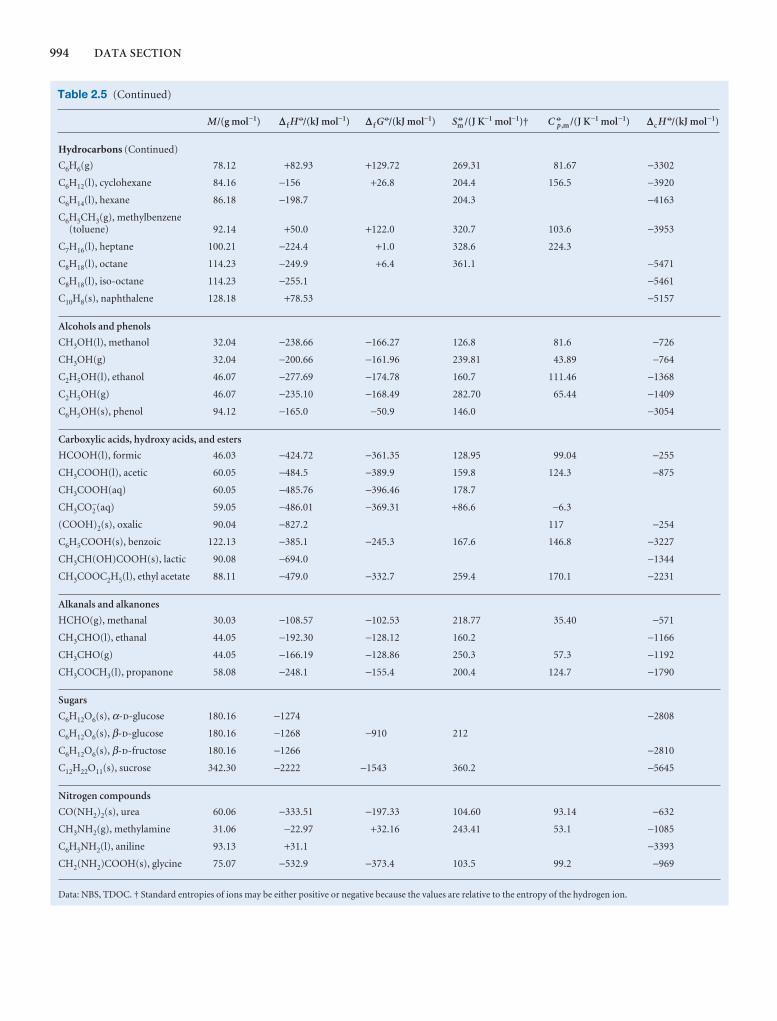
994 DATA SECTION
Hydrocarbons (Continued)
C6H6(g) 78.12 +82.93 +129.72 269.31 81.67 −3302
C6H12(l), cyclohexane 84.16 −156 +26.8 204.4 156.5 −3920
C6H14(l), hexane 86.18 −198.7 204.3 −4163
C6H5CH3(g), methylbenzene (toluene) 92.14 +50.0 +122.0 320.7 103.6 −3953
C7H16(l), heptane 100.21 −224.4 +1.0 328.6 224.3
C8H18(l), octane 114.23 −249.9 +6.4 361.1 −5471
C8H18(l), iso-octane 114.23 −255.1 −5461
C10H8(s), naphthalene 128.18 +78.53 −5157
Alcohols and phenols
CH3OH(l), methanol 32.04 −238.66 −166.27 126.8 81.6 −726
CH3OH(g) 32.04 −200.66 −161.96 239.81 43.89 −764
C2H5OH(l), ethanol 46.07 −277.69 −174.78 160.7 111.46 −1368
C2H5OH(g) 46.07 −235.10 −168.49 282.70 65.44 −1409
C6H5OH(s), phenol 94.12 −165.0 −50.9 146.0 −3054
Carboxylic acids, hydroxy acids, and esters
HCOOH(l), formic 46.03 −424.72 −361.35 128.95 99.04 −255
CH3COOH(l), acetic 60.05 −484.5 −389.9 159.8 124.3 −875
CH3COOH(aq) 60.05 −485.76 −396.46 178.7
CH3CO2−(aq) 59.05 −486.01 −369.31 +86.6 −6.3
(COOH)2(s), oxalic 90.04 −827.2 117 −254
C6H5COOH(s), benzoic 122.13 −385.1 −245.3 167.6 146.8 −3227
CH3CH(OH)COOH(s), lactic 90.08 −694.0 −1344
CH3COOC2H5(l), ethyl acetate 88.11 −479.0 −332.7 259.4 170.1 −2231
Alkanals and alkanones
HCHO(g), methanal 30.03 −108.57 −102.53 218.77 35.40 −571
CH3CHO(l), ethanal 44.05 −192.30 −128.12 160.2 −1166
CH3CHO(g) 44.05 −166.19 −128.86 250.3 57.3 −1192
CH3COCH3(l), propanone 58.08 −248.1 −155.4 200.4 124.7 −1790
Sugars
C6H12O6(s), α-d-glucose 180.16 −1274 −2808
C6H12O6(s), β-d-glucose 180.16 −1268 −910 212
C6H12O6(s), β-d-fructose 180.16 −1266 −2810
C12H22O11(s), sucrose 342.30 −2222 −1543 360.2 −5645
Nitrogen compounds
CO(NH2)2(s), urea 60.06 −333.51 −197.33 104.60 93.14 −632
CH3NH2(g), methylamine 31.06 −22.97 +32.16 243.41 53.1 −1085
C6H5NH2(l), aniline 93.13 +31.1 −3393
CH2(NH2)COOH(s), glycine 75.07 −532.9 −373.4 103.5 99.2 −969
Data: NBS, TDOC. † Standard entropies of ions may be either positive or negative because the values are relative to the entropy of the hydrogen ion.
Table 2.5 (Continued)
M/(g mol−1) D f H 7/(kJ mol−1) D f G 7/(kJ mol−1) Sm7 /(J K−1 mol−1)† C 7
p,m /(J K−1 mol−1) Dc H 7/(kJ mol−1)
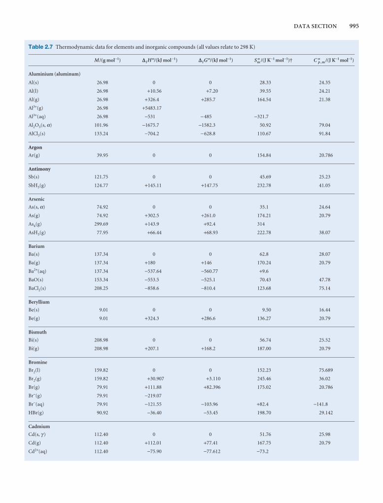
DATA SECTION 995
Table 2.7 Thermodynamic data for elements and inorganic compounds (all values relate to 298 K)
M /(g mol−1) D f H 7/(kJ mol −1) D f G 7/(kJ mol−1) Sm7 /(J K−1 mol−1)† C 7
p , m /(J K−1 mol−1)
Aluminium (aluminum)
Al(s) 26.98 0 0 28.33 24.35
Al(l) 26.98 +10.56 +7.20 39.55 24.21
Al(g) 26.98 +326.4 +285.7 164.54 21.38
Al3+(g) 26.98 +5483.17
Al3+(aq) 26.98 −531 −485 −321.7
Al2O3(s, α) 101.96 −1675.7 −1582.3 50.92 79.04
AlCl3(s) 133.24 −704.2 −628.8 110.67 91.84
Argon
Ar(g) 39.95 0 0 154.84 20.786
Antimony
Sb(s) 121.75 0 0 45.69 25.23
SbH3(g) 124.77 +145.11 +147.75 232.78 41.05
Arsenic
As(s, α) 74.92 0 0 35.1 24.64
As(g) 74.92 +302.5 +261.0 174.21 20.79
As4(g) 299.69 +143.9 +92.4 314
AsH3(g) 77.95 +66.44 +68.93 222.78 38.07
Barium
Ba(s) 137.34 0 0 62.8 28.07
Ba(g) 137.34 +180 +146 170.24 20.79
Ba2+(aq) 137.34 −537.64 −560.77 +9.6
BaO(s) 153.34 −553.5 −525.1 70.43 47.78
BaCl2(s) 208.25 −858.6 −810.4 123.68 75.14
Beryllium
Be(s) 9.01 0 0 9.50 16.44
Be(g) 9.01 +324.3 +286.6 136.27 20.79
Bismuth
Bi(s) 208.98 0 0 56.74 25.52
Bi(g) 208.98 +207.1 +168.2 187.00 20.79
Bromine
Br2(l) 159.82 0 0 152.23 75.689
Br2(g) 159.82 +30.907 +3.110 245.46 36.02
Br(g) 79.91 +111.88 +82.396 175.02 20.786
Br−(g) 79.91 −219.07
Br−(aq) 79.91 −121.55 −103.96 +82.4 −141.8
HBr(g) 90.92 −36.40 −53.45 198.70 29.142
Cadmium
Cd(s, γ ) 112.40 0 0 51.76 25.98
Cd(g) 112.40 +112.01 +77.41 167.75 20.79
Cd2+(aq) 112.40 −75.90 −77.612 −73.2
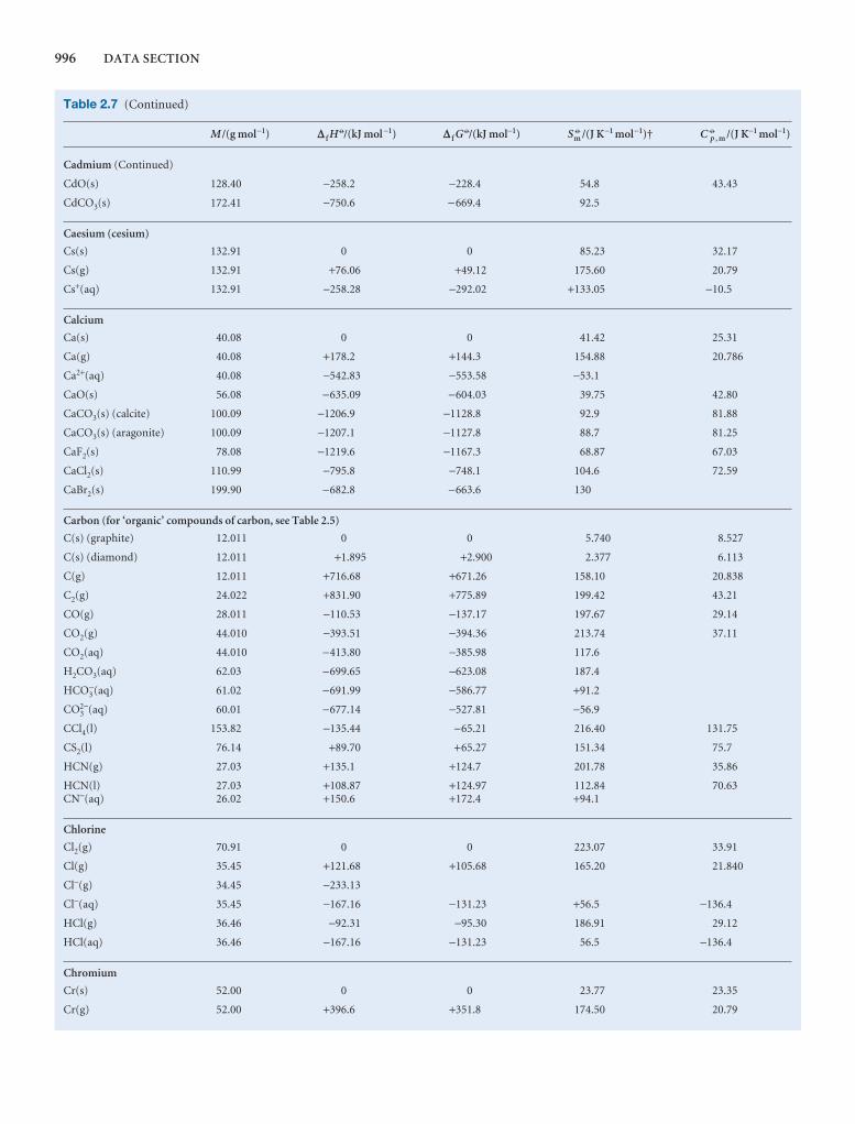
996 DATA SECTION
Table 2.7 (Continued)
M /(g mol−1) D f H 7/(kJ mol −1) D f G 7/(kJ mol−1) Sm7 /(J K−1 mol−1)† C 7
p , m /(J K−1 mol−1)
Cadmium (Continued)
CdO(s) 128.40 −258.2 −228.4 54.8 43.43
CdCO3(s) 172.41 −750.6 −669.4 92.5
Caesium (cesium)
Cs(s) 132.91 0 0 85.23 32.17
Cs(g) 132.91 +76.06 +49.12 175.60 20.79
Cs+(aq) 132.91 −258.28 −292.02 +133.05 −10.5
Calcium
Ca(s) 40.08 0 0 41.42 25.31
Ca(g) 40.08 +178.2 +144.3 154.88 20.786
Ca2+(aq) 40.08 −542.83 −553.58 −53.1
CaO(s) 56.08 −635.09 −604.03 39.75 42.80
CaCO3(s) (calcite) 100.09 −1206.9 −1128.8 92.9 81.88
CaCO3(s) (aragonite) 100.09 −1207.1 −1127.8 88.7 81.25
CaF2(s) 78.08 −1219.6 −1167.3 68.87 67.03
CaCl2(s) 110.99 −795.8 −748.1 104.6 72.59
CaBr2(s) 199.90 −682.8 −663.6 130
Carbon (for ‘organic’ compounds of carbon, see Table 2.5)
C(s) (graphite) 12.011 0 0 5.740 8.527
C(s) (diamond) 12.011 +1.895 +2.900 2.377 6.113
C(g) 12.011 +716.68 +671.26 158.10 20.838
C2(g) 24.022 +831.90 +775.89 199.42 43.21
CO(g) 28.011 −110.53 −137.17 197.67 29.14
CO2(g) 44.010 −393.51 −394.36 213.74 37.11
CO2(aq) 44.010 −413.80 −385.98 117.6
H2CO3(aq) 62.03 −699.65 −623.08 187.4
HCO3−(aq) 61.02 −691.99 −586.77 +91.2
CO32−(aq) 60.01 −677.14 −527.81 −56.9
CCl4(l) 153.82 −135.44 −65.21 216.40 131.75
CS2(l) 76.14 +89.70 +65.27 151.34 75.7
HCN(g) 27.03 +135.1 +124.7 201.78 35.86
HCN(l) 27.03 +108.87 +124.97 112.84 70.63CN−(aq) 26.02 +150.6 +172.4 +94.1
Chlorine
Cl2(g) 70.91 0 0 223.07 33.91
Cl(g) 35.45 +121.68 +105.68 165.20 21.840
Cl−(g) 34.45 −233.13
Cl−(aq) 35.45 −167.16 −131.23 +56.5 −136.4
HCl(g) 36.46 −92.31 −95.30 186.91 29.12
HCl(aq) 36.46 −167.16 −131.23 56.5 −136.4
Chromium
Cr(s) 52.00 0 0 23.77 23.35
Cr(g) 52.00 +396.6 +351.8 174.50 20.79
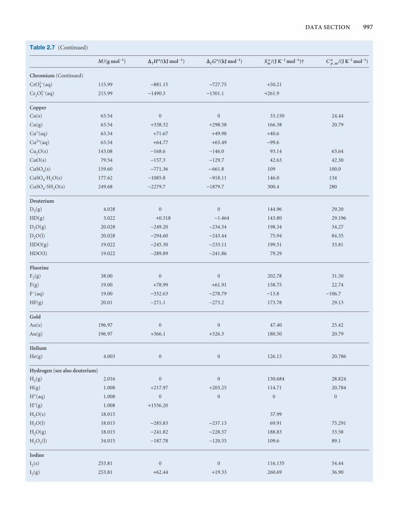
DATA SECTION 997
Table 2.7 (Continued)
M /(g mol−1) D f H 7/(kJ mol −1) D f G 7/(kJ mol−1) Sm7 /(J K−1 mol−1)† C 7
p , m /(J K−1 mol−1)
Chromium (Continued)
CrO42−(aq) 115.99 −881.15 −727.75 +50.21
Cr2O72−(aq) 215.99 −1490.3 −1301.1 +261.9
Copper
Cu(s) 63.54 0 0 33.150 24.44
Cu(g) 63.54 +338.32 +298.58 166.38 20.79
Cu+(aq) 63.54 +71.67 +49.98 +40.6
Cu2+(aq) 63.54 +64.77 +65.49 −99.6
Cu2O(s) 143.08 −168.6 −146.0 93.14 63.64
CuO(s) 79.54 −157.3 −129.7 42.63 42.30
CuSO4(s) 159.60 −771.36 −661.8 109 100.0
CuSO4·H2O(s) 177.62 −1085.8 −918.11 146.0 134
CuSO4·5H2O(s) 249.68 −2279.7 −1879.7 300.4 280
Deuterium
D2(g) 4.028 0 0 144.96 29.20
HD(g) 3.022 +0.318 −1.464 143.80 29.196
D2O(g) 20.028 −249.20 −234.54 198.34 34.27
D2O(l) 20.028 −294.60 −243.44 75.94 84.35
HDO(g) 19.022 −245.30 −233.11 199.51 33.81
HDO(l) 19.022 −289.89 −241.86 79.29
Fluorine
F2(g) 38.00 0 0 202.78 31.30
F(g) 19.00 +78.99 +61.91 158.75 22.74
F−(aq) 19.00 −332.63 −278.79 −13.8 −106.7
HF(g) 20.01 −271.1 −273.2 173.78 29.13
Gold
Au(s) 196.97 0 0 47.40 25.42
Au(g) 196.97 +366.1 +326.3 180.50 20.79
Helium
He(g) 4.003 0 0 126.15 20.786
Hydrogen (see also deuterium)
H2(g) 2.016 0 0 130.684 28.824
H(g) 1.008 +217.97 +203.25 114.71 20.784
H+(aq) 1.008 0 0 0 0
H+(g) 1.008 +1536.20
H2O(s) 18.015 37.99
H2O(l) 18.015 −285.83 −237.13 69.91 75.291
H2O(g) 18.015 −241.82 −228.57 188.83 33.58
H2O2(l) 34.015 −187.78 −120.35 109.6 89.1
Iodine
I2(s) 253.81 0 0 116.135 54.44
I2(g) 253.81 +62.44 +19.33 260.69 36.90

998 DATA SECTION
Table 2.7 (Continued)
M /(g mol−1) D f H 7/(kJ mol −1) D f G 7/(kJ mol−1) Sm7 /(J K−1 mol−1)† C 7
p , m /(J K−1 mol−1)
Iodine (Continued)
I(g) 126.90 +106.84 +70.25 180.79 20.786
I−(aq) 126.90 −55.19 −51.57 +111.3 −142.3
HI(g) 127.91 +26.48 +1.70 206.59 29.158
Iron
Fe(s) 55.85 0 0 27.28 25.10
Fe(g) 55.85 +416.3 +370.7 180.49 25.68
Fe2+(aq) 55.85 −89.1 −78.90 −137.7
Fe3+(aq) 55.85 −48.5 −4.7 −315.9
Fe3O4(s) (magnetite) 231.54 −1118.4 −1015.4 146.4 143.43
Fe2O3(s) (haematite) 159.69 −824.2 −742.2 87.40 103.85
FeS(s, α) 87.91 −100.0 −100.4 60.29 50.54
FeS2(s) 119.98 −178.2 −166.9 52.93 62.17
Krypton
Kr(g) 83.80 0 0 164.08 20.786
Lead
Pb(s) 207.19 0 0 64.81 26.44
Pb(g) 207.19 +195.0 +161.9 175.37 20.79
Pb2+(aq) 207.19 −1.7 −24.43 +10.5
PbO(s, yellow) 223.19 −217.32 −187.89 68.70 45.77
PbO(s, red) 223.19 −218.99 −188.93 66.5 45.81
PbO2(s) 239.19 −277.4 −217.33 68.6 64.64
Lithium
Li(s) 6.94 0 0 29.12 24.77
Li(g) 6.94 +159.37 +126.66 138.77 20.79
Li+(aq) 6.94 −278.49 −293.31 +13.4 68.6
Magnesium
Mg(s) 24.31 0 0 32.68 24.89
Mg(g) 24.31 +147.70 +113.10 148.65 20.786
Mg2+(aq) 24.31 −466.85 −454.8 −138.1
MgO(s) 40.31 −601.70 −569.43 26.94 37.15
MgCO3(s) 84.32 −1095.8 −1012.1 65.7 75.52
MgCl2(s) 95.22 −641.32 −591.79 89.62 71.38
Mercury
Hg(l) 200.59 0 0 76.02 27.983
Hg(g) 200.59 +61.32 +31.82 174.96 20.786
Hg2+(aq) 200.59 +171.1 +164.40 −32.2
Hg22+(aq) 401.18 +172.4 +153.52 +84.5
HgO(s) 216.59 −90.83 −58.54 70.29 44.06
Hg2Cl2(s) 472.09 −265.22 −210.75 192.5 102
HgCl2(s) 271.50 −224.3 −178.6 146.0
HgS(s, black) 232.65 −53.6 −47.7 88.3

DATA SECTION 999
Table 2.7 (Continued)
M /(g mol−1) D f H 7/(kJ mol −1) D f G 7/(kJ mol−1) Sm7 /(J K−1 mol−1)† C 7
p , m /(J K−1 mol−1)
Neon
Ne(g) 20.18 0 0 146.33 20.786
Nitrogen
N2(g) 28.013 0 0 191.61 29.125
N(g) 14.007 +472.70 +455.56 153.30 20.786
NO(g) 30.01 +90.25 +86.55 210.76 29.844
N2O(g) 44.01 +82.05 +104.20 219.85 38.45
NO2(g) 46.01 +33.18 +51.31 240.06 37.20
N2O4(g) 92.1 +9.16 +97.89 304.29 77.28
N2O5(s) 108.01 −43.1 +113.9 178.2 143.1
N2O5(g) 108.01 +11.3 +115.1 355.7 84.5
HNO3(l) 63.01 −174.10 −80.71 155.60 109.87
HNO3(aq) 63.01 −207.36 −111.25 146.4 −86.6
NO3−(aq) 62.01 −205.0 −108.74 +146.4 −86.6
NH3(g) 17.03 −46.11 −16.45 192.45 35.06
NH3(aq) 17.03 −80.29 −26.50 111.3
NH4+(aq) 18.04 −132.51 −79.31 +113.4 79.9
NH2OH(s) 33.03 −114.2
HN3(l) 43.03 +264.0 +327.3 140.6 43.68
HN3(g) 43.03 +294.1 +328.1 238.97 98.87
N2H4(l) 32.05 +50.63 +149.43 121.21 139.3
NH4NO3(s) 80.04 −365.56 −183.87 151.08 84.1
NH4Cl(s) 53.49 −314.43 −202.87 94.6
Oxygen
O2(g) 31.999 0 0 205.138 29.355
O(g) 15.999 +249.17 +231.73 161.06 21.912
O3(g) 47.998 +142.7 +163.2 238.93 39.20
OH−(aq) 17.007 −229.99 −157.24 −10.75 −148.5
Phosphorus
P(s, wh) 30.97 0 0 41.09 23.840
P(g) 30.97 +314.64 +278.25 163.19 20.786
P2(g) 61.95 +144.3 +103.7 218.13 32.05
P4(g) 123.90 +58.91 +24.44 279.98 67.15
PH3(g) 34.00 +5.4 +13.4 210.23 37.11
PCl3(g) 137.33 −287.0 −267.8 311.78 71.84
PCl3(l) 137.33 −319.7 −272.3 217.1
PCl5(g) 208.24 −374.9 −305.0 364.6 112.8
PCl5(s) 208.24 −443.5
H3PO3(s) 82.00 −964.4
H3PO3(aq) 82.00 −964.8
H3PO4(s) 94.97 −1279.0 −1119.1 110.50 106.06
H3PO4(l) 94.97 −1266.9
H3PO4(aq) 94.97 −1277.4 −1018.7 −222

1000 DATA SECTION
Table 2.7 (Continued)
M /(g mol−1) D f H 7/(kJ mol −1) D f G 7/(kJ mol−1) Sm7 /(J K−1 mol−1)† C 7
p , m /(J K−1 mol−1)
Phosphorus (Continued)
PO43−(aq) 94.97 −1277.4 −1018.7 −221.8
P4O10(s) 283.89 −2984.0 −2697.0 228.86 211.71
P4O6(s) 219.89 −1640.1
Potassium
K(s) 39.10 0 0 64.18 29.58
K(g) 39.10 +89.24 +60.59 160.336 20.786
K+(g) 39.10 +514.26
K+(aq) 39.10 −252.38 −283.27 +102.5 21.8
KOH(s) 56.11 −424.76 −379.08 78.9 64.9
KF(s) 58.10 −576.27 −537.75 66.57 49.04
KCl(s) 74.56 −436.75 −409.14 82.59 51.30
KBr(s) 119.01 −393.80 −380.66 95.90 52.30
Kl(s) 166.01 −327.90 −324.89 106.32 52.93
Silicon
Si(s) 28.09 0 0 18.83 20.00
Si(g) 28.09 +455.6 +411.3 167.97 22.25
SiO2(s, α) 60.09 −910.94 −856.64 41.84 44.43
Silver
Ag(s) 107.87 0 0 42.55 25.351
Ag(g) 107.87 +284.55 +245.65 173.00 20.79
Ag+(aq) 107.87 +105.58 +77.11 +72.68 21.8
AgBr(s) 187.78 −100.37 −96.90 107.1 52.38
AgCl(s) 143.32 −127.07 −109.79 96.2 50.79
Ag2O(s) 231.74 −31.05 −11.20 121.3 65.86
AgNO3(s) 169.88 −129.39 −33.41 140.92 93.05
Sodium
Na(s) 22.99 0 0 51.21 28.24
Na(g) 22.99 +107.32 +76.76 153.71 20.79
Na+(aq) 22.99 −240.12 −261.91 59.0 46.4
NaOH(s) 40.00 −425.61 −379.49 64.46 59.54
NaCl(s) 58.44 −411.15 −384.14 72.13 50.50
NaBr(s) 102.90 −361.06 −348.98 86.82 51.38
NaI(s) 149.89 −287.78 −286.06 98.53 52.09
Sulfur
S(s, α) (rhombic) 32.06 0 0 31.80 22.64
S(s, β) (monoclinic) 32.06 +0.33 +0.1 32.6 23.6
S(g) 32.06 +278.81 +238.25 167.82 23.673
S2(g) 64.13 +128.37 +79.30 228.18 32.47
S2−(aq) 32.06 +33.1 +85.8 −14.6
SO2(g) 64.06 −296.83 −300.19 248.22 39.87
SO3(g) 80.06 −395.72 −371.06 256.76 50.67
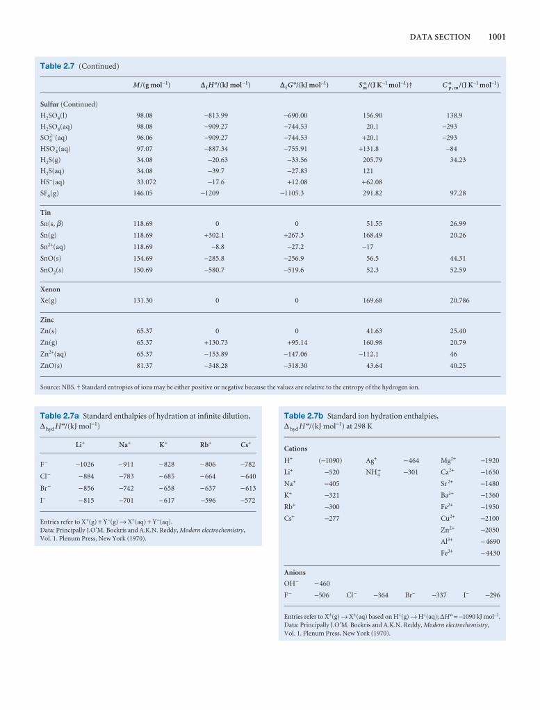
DATA SECTION 1001
Table 2.7a Standard enthalpies of hydration at infinite dilution,∆hyd H 7/(kJ mol−1)
Li+ Na+ K+ Rb+ Cs+
F− −1026 −911 −828 −806 −782
Cl− −884 −783 −685 −664 −640
Br− −856 −742 −658 −637 −613
I− −815 −701 −617 −596 −572
Entries refer to X+(g) + Y−(g) → X+(aq) + Y−(aq).Data: Principally J.O’M. Bockris and A.K.N. Reddy, Modern electrochemistry,Vol. 1. Plenum Press, New York (1970).
Table 2.7b Standard ion hydration enthalpies, ∆hyd H 7/(kJ mol−1) at 298 K
Cations
H+ (−1090) Ag+ −464 Mg2+ −1920
Li+ −520 NH4+ −301 Ca2+ −1650
Na+ −405 Sr 2+ −1480
K+ −321 Ba2+ −1360
Rb+ −300 Fe2+ −1950
Cs+ −277 Cu2+ −2100
Zn2+ −2050
Al3+ −4690
Fe3+ −4430
Anions
OH− −460
F− −506 Cl− −364 Br− −337 I− −296
Entries refer to X±(g) → X±(aq) based on H+(g) → H+(aq); ∆H7 = −1090 kJ mol−1.Data: Principally J.O’M. Bockris and A.K.N. Reddy, Modern electrochemistry,Vol. 1. Plenum Press, New York (1970).
Table 2.7 (Continued)
M /(g mol−1) D f H 7/(kJ mol −1) D f G 7/(kJ mol−1) Sm7 /(J K−1 mol−1)† C 7
p , m /(J K−1 mol−1)
Sulfur (Continued)
H2SO4(l) 98.08 −813.99 −690.00 156.90 138.9
H2SO4(aq) 98.08 −909.27 −744.53 20.1 −293
SO42−(aq) 96.06 −909.27 −744.53 +20.1 −293
HSO4−(aq) 97.07 −887.34 −755.91 +131.8 −84
H2S(g) 34.08 −20.63 −33.56 205.79 34.23
H2S(aq) 34.08 −39.7 −27.83 121
HS−(aq) 33.072 −17.6 +12.08 +62.08
SF6(g) 146.05 −1209 −1105.3 291.82 97.28
Tin
Sn(s, β) 118.69 0 0 51.55 26.99
Sn(g) 118.69 +302.1 +267.3 168.49 20.26
Sn2+(aq) 118.69 −8.8 −27.2 −17
SnO(s) 134.69 −285.8 −256.9 56.5 44.31
SnO2(s) 150.69 −580.7 −519.6 52.3 52.59
Xenon
Xe(g) 131.30 0 0 169.68 20.786
Zinc
Zn(s) 65.37 0 0 41.63 25.40
Zn(g) 65.37 +130.73 +95.14 160.98 20.79
Zn2+(aq) 65.37 −153.89 −147.06 −112.1 46
ZnO(s) 81.37 −348.28 −318.30 43.64 40.25
Source: NBS. † Standard entropies of ions may be either positive or negative because the values are relative to the entropy of the hydrogen ion.
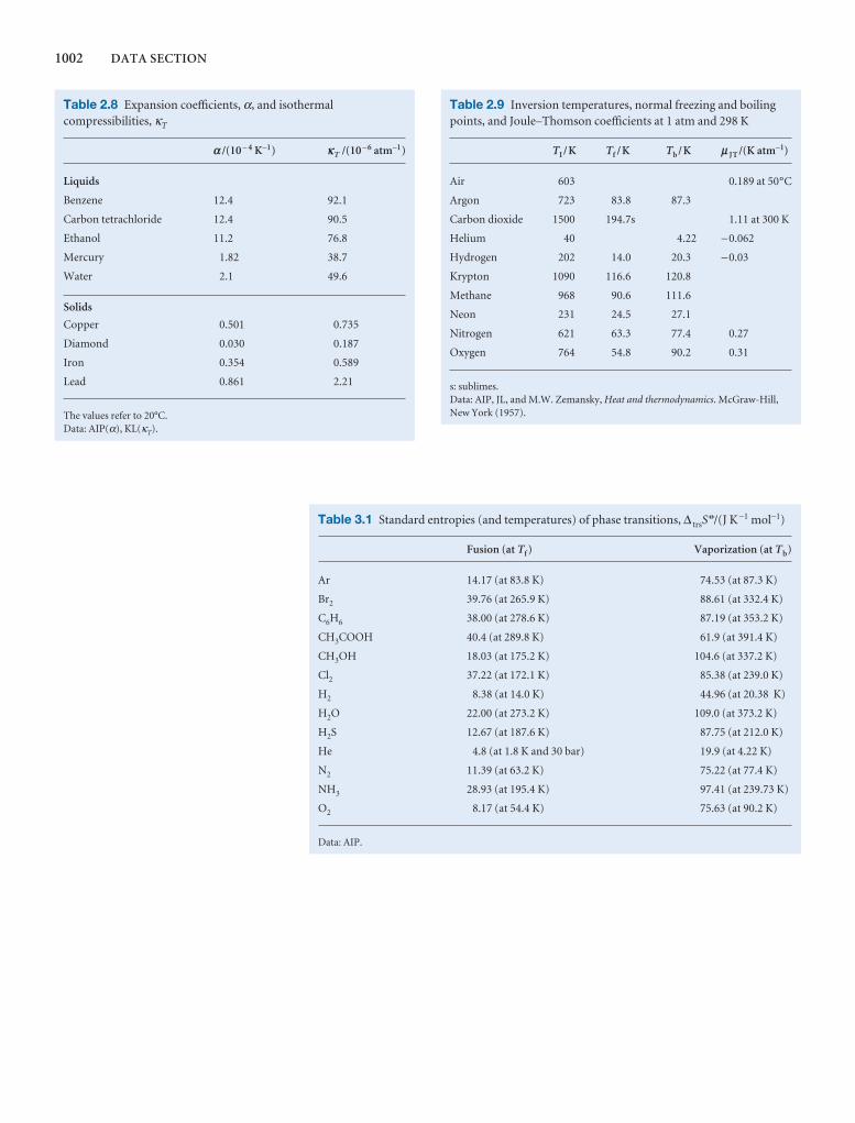
1002 DATA SECTION
Table 3.1 Standard entropies (and temperatures) of phase transitions, ∆ trsS7/(J K−1 mol−1)
Fusion (at Tf ) Vaporization (at Tb)
Ar 14.17 (at 83.8 K) 74.53 (at 87.3 K)
Br2 39.76 (at 265.9 K) 88.61 (at 332.4 K)
C6H6 38.00 (at 278.6 K) 87.19 (at 353.2 K)
CH3COOH 40.4 (at 289.8 K) 61.9 (at 391.4 K)
CH3OH 18.03 (at 175.2 K) 104.6 (at 337.2 K)
Cl2 37.22 (at 172.1 K) 85.38 (at 239.0 K)
H2 8.38 (at 14.0 K) 44.96 (at 20.38 K)
H2O 22.00 (at 273.2 K) 109.0 (at 373.2 K)
H2S 12.67 (at 187.6 K) 87.75 (at 212.0 K)
He 4.8 (at 1.8 K and 30 bar) 19.9 (at 4.22 K)
N2 11.39 (at 63.2 K) 75.22 (at 77.4 K)
NH3 28.93 (at 195.4 K) 97.41 (at 239.73 K)
O2 8.17 (at 54.4 K) 75.63 (at 90.2 K)
Data: AIP.
Table 2.8 Expansion coefficients, α, and isothermalcompressibilities, κT
a /(10 − 4 K−1) kT /(10 −6 atm−1)
Liquids
Benzene 12.4 92.1
Carbon tetrachloride 12.4 90.5
Ethanol 11.2 76.8
Mercury 1.82 38.7
Water 2.1 49.6
Solids
Copper 0.501 0.735
Diamond 0.030 0.187
Iron 0.354 0.589
Lead 0.861 2.21
The values refer to 20°C.Data: AIP(α), KL(κT).
Table 2.9 Inversion temperatures, normal freezing and boilingpoints, and Joule–Thomson coefficients at 1 atm and 298 K
TI /K Tf /K Tb /K m JT /(K atm−1)
Air 603 0.189 at 50°C
Argon 723 83.8 87.3
Carbon dioxide 1500 194.7s 1.11 at 300 K
Helium 40 4.22 −0.062
Hydrogen 202 14.0 20.3 −0.03
Krypton 1090 116.6 120.8
Methane 968 90.6 111.6
Neon 231 24.5 27.1
Nitrogen 621 63.3 77.4 0.27
Oxygen 764 54.8 90.2 0.31
s: sublimes.Data: AIP, JL, and M.W. Zemansky, Heat and thermodynamics. McGraw-Hill,New York (1957).
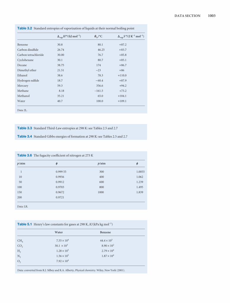
DATA SECTION 1003
Table 3.6 The fugacity coefficient of nitrogen at 273 K
p /atm f p/atm f
1 0.999 55 300 1.0055
10 0.9956 400 1.062
50 0.9912 600 1.239
100 0.9703 800 1.495
150 0.9672 1000 1.839
200 0.9721
Data: LR.
Table 5.1 Henry’s law constants for gases at 298 K, K/(kPa kg mol−1)
Water Benzene
CH4 7.55 × 10⁴ 44.4 × 10³
CO2 30.1 × 10³ 8.90 × 10²
H2 1.28 × 10⁵ 2.79 × 10⁴
N2 1.56 × 10⁵ 1.87 × 10⁴
O2 7.92 × 10⁴
Data: converted from R.J. Silbey and R.A. Alberty, Physical chemistry. Wiley, New York (2001).
Table 3.2 Standard entropies of vaporization of liquids at their normal boiling point
D vap H 7/(kJ mol−1) qb /°C D vap S 7/(J K−1 mol−1)
Benzene 30.8 80.1 +87.2
Carbon disulfide 26.74 46.25 +83.7
Carbon tetrachloride 30.00 76.7 +85.8
Cyclohexane 30.1 80.7 +85.1
Decane 38.75 174 +86.7
Dimethyl ether 21.51 −23 +86
Ethanol 38.6 78.3 +110.0
Hydrogen sulfide 18.7 −60.4 +87.9
Mercury 59.3 356.6 +94.2
Methane 8.18 −161.5 +73.2
Methanol 35.21 65.0 +104.1
Water 40.7 100.0 +109.1
Data: JL.
Table 3.3 Standard Third-Law entropies at 298 K: see Tables 2.5 and 2.7
Table 3.4 Standard Gibbs energies of formation at 298 K: see Tables 2.5 and 2.7
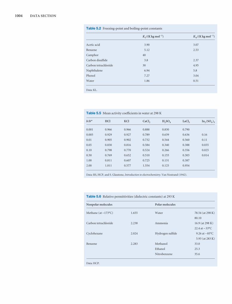
1004 DATA SECTION
Table 5.6 Relative permittivities (dielectric constants) at 293 K
Nonpolar molecules Polar molecules
Methane (at −173°C) 1.655 Water 78.54 (at 298 K)
80.10
Carbon tetrachloride 2.238 Ammonia 16.9 (at 298 K)
22.4 at −33°C
Cyclohexane 2.024 Hydrogen sulfide 9.26 at −85°C
5.93 (at 283 K)
Benzene 2.283 Methanol 33.0
Ethanol 25.3
Nitrobenzene 35.6
Data: HCP.
Table 5.5 Mean activity coefficients in water at 298 K
b /b 7 HCl KCl CaCl2 H2SO4 LaCl3 In2 (SO4 )3
0.001 0.966 0.966 0.888 0.830 0.790
0.005 0.929 0.927 0.789 0.639 0.636 0.16
0.01 0.905 0.902 0.732 0.544 0.560 0.11
0.05 0.830 0.816 0.584 0.340 0.388 0.035
0.10 0.798 0.770 0.524 0.266 0.356 0.025
0.50 0.769 0.652 0.510 0.155 0.303 0.014
1.00 0.811 0.607 0.725 0.131 0.387
2.00 1.011 0.577 1.554 0.125 0.954
Data: RS, HCP, and S. Glasstone, Introduction to electrochemistry. Van Nostrand (1942).
Table 5.2 Freezing-point and boiling-point constants
K f /(K kg mol −1) K b /(K kg mol −1)
Acetic acid 3.90 3.07
Benzene 5.12 2.53
Camphor 40
Carbon disulfide 3.8 2.37
Carbon tetrachloride 30 4.95
Naphthalene 6.94 5.8
Phenol 7.27 3.04
Water 1.86 0.51
Data: KL.

DATA SECTION 1005
Table 7.2 Standard potentials at 298 K. (a) In electrochemical order
Reduction half-reaction E 7/V Reduction half-reaction E 7/V
Strongly oxidizing Cu2+ + e− → Cu+ +0.16
H4XeO6 + 2H+ + 2e− → XeO3 + 3H2O +3.0 Sn4+ + 2e− → Sn2+ +0.15
F2 + 2e− → 2F− +2.87 AgBr + e− → Ag + Br− +0.07
O3 + 2H+ + 2e− → O2 + H2O +2.07 Ti4+ + e− → Ti3+ 0.00
S2O82− + 2e− → 2SO4
2− +2.05 2H+ + 2e− → H2 0, by definition
Ag 2+ + e− → Ag+ +1.98 Fe3+ + 3e− → Fe −0.04
Co3+ + e− → Co2+ +1.81 O2 + H2O + 2e− → HO2− + OH− −0.08
H2O2 + 2H+ + 2e− → 2H2O +1.78 Pb2+ + 2e− → Pb −0.13
Au+ + e− → Au +1.69 In+ + e− → In −0.14
Pb4+ + 2e− → Pb2+ +1.67 Sn2+ + 2e− → Sn −0.14
2HClO + 2H+ + 2e− → Cl2 + 2H2O +1.63 AgI + e− → Ag + I− −0.15
Ce4+ + e− → Ce3+ +1.61 Ni2+ + 2e− → Ni −0.23
2HBrO + 2H+ + 2e− → Br2 + 2H2O +1.60 Co2+ + 2e− → Co −0.28
MnO4− + 8H+ + 5e− → Mn2+ + 4H2O +1.51 In3+ + 3e− → In − 0.34
Mn3+ + e− → Mn2+ +1.51 Tl+ + e− → Tl − 0.34
Au3+ + 3e− → Au +1.40 PbSO4 + 2e− → Pb + SO42− − 0.36
Cl2 + 2e− → 2Cl− +1.36 Ti3+ + e− → Ti2+ −0.37
Cr2O72− + 14H+ + 6e− → 2Cr3+ + 7H2O +1.33 Cd2+ + 2e− → Cd −0.40
O3 + H2O + 2e− → O2 + 2OH− +1.24 In2+ + e− → In+ − 0.40
O2 + 4H+ + 4e− → 2H2O +1.23 Cr3+ + e− → Cr2+ −0.41
ClO4− + 2H+ + 2e− → ClO3
− + H2O +1.23 Fe2+ + 2e− → Fe − 0.44
MnO2 + 4H+ + 2e− → Mn2+ + 2H2O +1.23 In3+ + 2e− → In+ −0.44
Br2 + 2e− → 2Br− +1.09 S + 2e− → S2− −0.48
Pu4+ + e− → Pu3+ +0.97 In3+ + e− → In2+ −0.49
NO3− + 4H+ + 3e− → NO + 2H2O +0.96 U4+ + e− → U3+ −0.61
2Hg2+ + 2e− → Hg 22+ +0.92 Cr3+ + 3e− → Cr −0.74
ClO− + H2O + 2e− → Cl− + 2OH− +0.89 Zn2+ + 2e− → Zn −0.76
Hg2+ + 2e− → Hg +0.86 Cd(OH)2 + 2e− → Cd + 2OH− −0.81
NO3− + 2H+ + e− → NO2 + H2O +0.80 2H2O + 2e− → H2 + 2OH− −0.83
Ag+ + e− → Ag +0.80 Cr2+ + 2e− → Cr −0.91
Hg22+ + 2e− → 2Hg +0.79 Mn2+ + 2e− → Mn −1.18
Fe3+ + e− → Fe2+ +0.77 V2+ + 2e− → V −1.19
BrO− + H2O + 2e− → Br− + 2OH− +0.76 Ti2+ + 2e− → Ti −1.63
Hg2SO4 + 2e− → 2Hg + SO42− +0.62 Al3+ + 3e− → Al −1.66
MnO42− + 2H2O + 2e− → MnO2 + 4OH− +0.60 U3+ + 3e− → U −1.79
MnO4− + e− → MnO4
2− +0.56 Sc3+ + 3e− → Sc −2.09
I2 + 2e− → 2I− +0.54 Mg2+ + 2e− → Mg −2.36
CU+ + e− → Cu +0.52 Ce3+ + 3e− → Ce −2.48
I3− + 2e− → 3I− +0.53 La3+ + 3e− → La −2.52
NiOOH + H2O + e− → Ni(OH)2 + OH− +0.49 Na+ + e− → Na −2.71
Ag2CrO4 + 2e− → 2Ag + CrO42− +0.45 Ca2+ + 2e− → Ca −2.87
O2 + 2H2O + 4e− → 4OH− +0.40 Sr2+ + 2e− → Sr −2.89
ClO4− + H2O + 2e− → ClO3
− + 2OH− +0.36 Ba2+ + 2e− → Ba −2.91
[Fe(CN)6]3− + e− → [Fe(CN)6]4− +0.36 Ra2+ + 2e− → Ra −2.92
Cu2+ + 2e− → Cu +0.34 Cs+ + e− → Cs −2.92
Hg2Cl2 + 2e− → 2Hg + 2Cl− +0.27 Rb+ + e− → Rb −2.93
AgCl + e− → Ag + Cl− +0.22 K+ + e− → K −2.93
Bi3+ + 3e− → Bi +0.20 Li+ + e− → Li −3.05
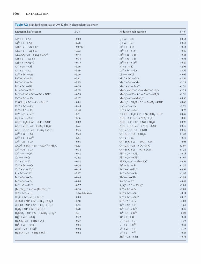
1006 DATA SECTION
Table 7.2 Standard potentials at 298 K. (b) In electrochemical order
Reduction half-reaction E 7/V Reduction half-reaction E 7/V
Ag+ + e− → Ag +0.80 I2 + 2e− → 2I− +0.54
Ag2+ + e− → Ag+ +1.98 I−3 + 2e− → 3I− +0.53
AgBr + e− → Ag + Br− +0.0713 In+ + e− → In −0.14
AgCl + e− → Ag + Cl− +0.22 In2+ + e− → In+ −0.40
Ag2CrO4 + 2e− → 2Ag + CrO42− +0.45 In3+ + 2e− → In+ −0.44
AgF + e− → Ag + F− +0.78 In3+ + 3e− → In −0.34
AgI + e− → Ag + I− −0.15 In3+ + e− → In2+ −0.49
Al3+ + 3e− → Al −1.66 K+ + e− → K −2.93
Au+ + e− → Au +1.69 La3+ + 3e− → La −2.52
Au3+ + 3e− → Au +1.40 Li+ + e− → Li −3.05
Ba2+ + 2e− → Ba +2.91 Mg2+ + 2e− → Mg −2.36
Be2+ + 2e− → Be −1.85 Mn2+ + 2e− → Mn −1.18
Bi3+ + 3e− → Bi +0.20 Mn3+ + e− → Mn2+ +1.51
Br2 + 2e− → 2Br− +1.09 MnO2 + 4H+ + 2e− → Mn2+ + 2H2O +1.23
BrO− + H2O + 2e− → Br− + 2OH− +0.76 MnO4− + 8H+ + 5e− → Mn2+ + 4H2O +1.51
Ca2+ + 2e− → Ca −2.87 MnO4− + e− → MnO4
2− +0.56
Cd(OH)2 + 2e− → Cd + 2OH− −0.81 MnO42 − + 2H2O + 2e− → MnO2 + 4OH− +0.60
Cd2+ + 2e− → Cd −0.40 Na+ + e− → Na −2.71
Ce3+ + 3e− → Ce −2.48 Ni2+ + 2e− → Ni −0.23
Ce4+ + e− → Ce3+ +1.61 NiOOH + H2O + e− → Ni(OH)2 + OH− +0.49
Cl2 + 2e− → 2Cl− +1.36 NO3− + 2H+ + e− → NO2 + H2O −0.80
ClO− + H2O + 2e− → Cl− + 2OH− +0.89 NO3− + 4H+ + 3e− → NO + 2H2O +0.96
ClO4− + 2H+ + 2e− → ClO3
− + H2O +1.23 NO3− + H2O + 2e− → NO2
− + 2OH− +0.10
ClO4− + H2O + 2e− → ClO3
− + 2OH− +0.36 O2 + 2H2O + 4e− → 4OH− +0.40
Co2+ + 2e− → Co −0.28 O2 + 4H+ + 4e− → 2H2O +1.23
Co3+ + e− → Co2+ +1.81 O2 + e− → O2− −0.56
Cr2+ + 2e− → Cr −0.91 O2 + H2O + 2e− → HO2− + OH− −0.08
Cr2O72 − + 14H+ + 6e− → 2Cr3 + + 7H2O +1.33 O3 + 2H+ + 2e− → O2 + H2O +2.07
Cr3+ + 3e− → Cr −0.74 O3 + H2O + 2e− → O2 + 2OH− +1.24
Cr3+ + e− → Cr2+ −0.41 Pb2+ + 2e− → Pb −0.13
Cs+ + e− → Cs −2.92 Pb4+ + 2e− → Pb2+ +1.67
Cu+ + e− → Cu +0.52 PbSO4 + 2e− → Pb + SO42− −0.36
Cu2+ + 2e− → Cu +0.34 Pt2+ + 2e− → Pt +1.20
Cu2+ + e− → Cu+ +0.16 Pu4+ + e− → Pu3+ +0.97
F2 + 2e− → 2F− +2.87 Ra2+ + 2e− → Ra −2.92
Fe2+ + 2e− → Fe −0.44 Rb+ + e− → Rb −2.93
Fe3+ + 3e− → Fe −0.04 S + 2e− → S2− −0.48
Fe3+ + e− → Fe2+ +0.77 S2O82− + 2e− → 2SO4
2− +2.05
[Fe(CN)6]3− + e− → [Fe(CN)6]4− +0.36 Sc3+ + 3e− → Sc −2.09
2H+ + 2e− → H2 0, by definition Sn2+ + 2e− → Sn −0.14
2H2O + 2e− → H2 + 2OH− −0.83 Sn4+ + 2e− → Sn2+ +0.15
2HBrO + 2H+ + 2e− → Br2 + 2H2O +1.60 Sr2+ + 2e− → Sr −2.89
2HClO + 2H+ + 2e− → Cl2 + 2H2O +1.63 Ti2+ + 2e− → Ti −1.63
H2O2 + 2H+ + 2e− → 2H2O +1.78 Ti3+ + e− → Ti2+ −0.37
H4XeO6 + 2H+ + 2e− → XeO3 + 3H2O +3.0 Ti4+ + e− → Ti3+ 0.00
Hg22+ + 2e− → 2Hg +0.79 Tl+ + e− → Tl −0.34
Hg2Cl2 + 2e− → 2Hg + 2Cl− +0.27 U3+ + 3e− → U −1.79
Hg2+ + 2e− → Hg +0.86 U4+ + e− → U3+ −0.61
2Hg2+ + 2e− → Hg22+ +0.92 V2+ + 2e− → V −1.19
Hg2SO4 + 2e− → 2Hg + SO42− +0.62 V3+ + e− → V2+ −0.26
Zn2+ + 2e− → Zn −0.76

DATA SECTION 1007
Table 7.4 Acidity constants for aqueous solutions at 298 K. (a) In order of acid strength
Acid HA A− Ka pKa
Hydriodic HI I− 1011 −11
Hydrobromic HBr Br− 109 −9
Hydrochloric HCl Cl− 107 −7
Sulfuric H2SO4 HSO4− 102 −2
Perchloric* HClO4 ClO4− 4.0 × 101 −1.6
Hydronium ion H3O+ H2O 1 0.0
Oxalic (COOH)2 HOOCCO2− 5.6 × 10⁻² 1.25
Sulfurous H2SO3 HSO3− 1.4 × 10⁻² 1.85
Hydrogensulfate ion HSO4− SO4
2− 1.0 × 10⁻² 1.99
Phosphoric H3PO4 H2PO4− 6.9 × 10⁻³ 2.16
Glycinium ion +NH3CH2COOH NH2CH2COOH 4.5 × 10⁻³ 2.35
Hydrofluoric HF F− 6.3 × 10⁻⁴ 3.20
Formic HCOOH HCO2− 1.8 × 10⁻⁴ 3.75
Hydrogenoxalate ion HOOCCO2− C2O4
2− 1.5 × 10⁻⁵ 3.81
Lactic CH3CH(OH)COOH CH3CH(OH)CO2− 1.4 × 10⁻⁴ 3.86
Acetic (ethanoic) CH3COOH CH3CO2− 1.4 × 10⁻⁵ 4.76
Butanoic CH3CH2CH2COOH CH3CH2CH2CO2− 1.5 × 10⁻⁵ 4.83
Propanoic CH3CH2COOH CH3CH2CO2− 1.4 × 10⁻⁵ 4.87
Anilinium ion C6H5NH3+ C6H5NH2 1.3 × 10⁻⁵ 4.87
Pyridinium ion C5H5NH+ C6H5N 5.9 × 10⁻⁶ 5.23
Carbonic H2CO3 HCO3− 4.5 × 10⁻⁷ 6.35
Hydrosulfuric H2S HS− 8.9 × 10⁻⁸ 7.05
Dihydrogenphosphate ion H2PO4− HPO4
2− 6.2 × 10⁻⁸ 7.21
Hypochlorous HClO ClO− 4.0 × 10⁻⁸ 7.40
Hydrazinium ion NH2NH3+ NH2NH2 8 × 10⁻⁹ 8.1
Hypobromous HBrO BrO− 2.8 × 10⁻⁹ 8.55
Hydrocyanic HCN CN− 6.2 × 10⁻¹⁰ 9.21
Ammonium ion NH 4+ NH3 5.6 × 10⁻¹⁰ 9.25
Boric* B(OH)3 B(OH)4− 5.4 × 10⁻¹⁰ 9.27
Trimethylammonium ion (CH3)3NH+ (CH3)3N 1.6 × 10⁻¹⁰ 9.80
Phenol C6H5OH C6H5O− 1.0 × 10⁻¹⁰ 9.99
Hydrogencarbonate ion HCO3− CO3
2− 4.8 × 10⁻¹¹ 10.33
Hypoiodous HIO IO− 3 × 10⁻¹¹ 10.5
Ethylammonium ion CH3CH2NH 3+ CH3CH2NH2 2.2 × 10⁻¹¹ 10.65
Methylammonium ion CH3NH3+ CH3NH2 2.2 × 10⁻¹¹ 10.66
Dimethylammonium ion (CH3)2NH2+ (CH3)2NH 1.9 × 10⁻¹¹ 10.73
Triethylammonium ion (CH3CH2)3NH+ (CH3CH2)3N 1.8 × 10⁻¹¹ 10.75
Diethylammonium ion (CH3CH2)2NH2+ (CH3CH2)2NH 1.4 × 10⁻¹¹ 10.84
Hydrogenarsenate ion HAsO42− AsO4
3− 5.1 × 10⁻¹² 11.29
Hydrogenphosphate ion HPO42− PO4
3− 4.8 × 10⁻¹³ 12.32
Hydrogensulfide ion HS− S2− 1.0 × 10⁻¹⁹ 19.00
* At 293 K.

1008 DATA SECTION
Table 7.4 Acidity constants for aqueous solutions at 298 K. (b) In alphabetical order
Acid HA A− Ka pKa
Acetic (ethanoic) CH3COOH CH3CO 2− 1.4 × 10⁻⁵ 4.76
Ammonium ion NH4+ NH3 5.6 × 10⁻¹⁰ 9.25
Anilinium ion C6H5NH3+ C6H5NH2 1.3 × 10⁻⁵ 4.87
Boric* B(OH)3 B(OH) 4− 5.4 × 10⁻¹⁰ 9.27
Butanoic CH3CH2CH2COOH CH3CH2CH2CO2− 1.5 × 10⁻⁵ 4.83
Carbonic H2CO3 HCO3− 4.5 × 10⁻⁷ 6.35
Diethylammonium ion (CH3CH2)2NH2+ (CH3CH2)2NH 1.4 × 10⁻¹¹ 10.84
Dihydrogenphosphate ion H2PO4− HPO4
2− 6.2 × 10⁻⁸ 7.21
Dimethylammonium ion (CH3)2NH2+ (CH3)2NH 1.9 × 10⁻¹¹ 10.73
Ethylammonium ion CH3CH2NH3+ CH3CH2NH2 2.2 × 10⁻¹¹ 10.65
Formic HCOOH HCO2− 1.8 × 10⁻⁴ 3.75
Glycinium ion +NH3CH2COOH NH2CH2COOH 4.5 × 10⁻³ 2.35
Hydrazinium ion NH2NH3+ NH2NH2 8 × 10⁻⁹ 8.1
Hydriodic HI I− 1011 −11
Hydrobromic HBr Br− 109 −9
Hydrochloric HCl Cl− 107 −7
Hydrocyanic HCN CN− 6.2 × 10⁻¹⁰ 9.21
Hydrofluoric HF F− 6.3 × 10⁻⁴ 3.20
Hydrogenarsenate ion HAsO42− AsO4
3− 5.1 × 10⁻¹² 11.29
Hydrogencarbonate ion HCO3− CO3
2− 4.8 × 10⁻¹¹ 10.33
Hydrogenoxalate ion HOOCCO2− C2O4
2− 1.5 × 10⁻⁵ 3.81
Hydrogenphosphate ion HPO42− PO4
3− 4.8 × 10⁻¹³ 12.32
Hydrogensulfate ion HSO4− SO4
2− 1.0 × 10⁻² 1.99
Hydrogensulfide ion HS− S2− 1.0 × 10⁻¹⁹ 19.00
Hydronium ion H3O+ H2O 1 0.0
Hydrosulfuric H2S HS− 8.9 × 10⁻⁸ 7.05
Hypobromous HBrO BrO− 2.8 × 10⁻⁹ 8.55
Hypochlorous HClO ClO− 4.0 × 10⁻⁸ 7.40
Hypoiodous HIO IO− 3 × 10⁻¹¹ 10.5
Lactic CH3CH(OH)COOH CH3CH(OH)CO2− 1.4 × 10⁻⁴ 3.86
Methylammonium ion CH3NH3+ CH3NH2 2.2 × 10⁻¹¹ 10.66
Oxalic (COOH)2 HOOCCO2− 5.6 × 10⁻² 1.25
Perchloric* HClO4 ClO4− 4.0 × 101 −1.6
Phenol C6H5OH C6H5O− 1.0 × 10⁻¹⁰ 9.99
Phosphoric H3PO4 H2PO4− 6.9 × 10⁻³ 2.16
Propanoic CH3CH2COOH CH3CH2CO2− 1.4 × 10⁻⁵ 4.87
Pyridinim ion C5H5NH+ C6H5N 5.9 × 10⁻⁶ 5.23
Sulfuric H2SO4 HSO4− 102 −2
Sulfurous H2SO3 HSO3− 1.4 × 10⁻² 1.85
Triethylammonium ion (CH3CH2)3NH+ (CH3CH2)3N 1.8 × 10⁻¹¹ 10.75
Trimethylammonium ion (CH3)3NH+ (CH3)3N 1.6 × 10⁻¹⁰ 9.80
* At 293 K.
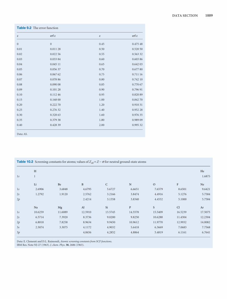
DATA SECTION 1009
Table 9.2 The error function
z erf z z erf z
0 0 0.45 0.475 48
0.01 0.011 28 0.50 0.520 50
0.02 0.022 56 0.55 0.563 32
0.03 0.033 84 0.60 0.603 86
0.04 0.045 11 0.65 0.642 03
0.05 0.056 37 0.70 0.677 80
0.06 0.067 62 0.75 0.711 16
0.07 0.078 86 0.80 0.742 10
0.08 0.090 08 0.85 0.770 67
0.09 0.101 28 0.90 0.796 91
0.10 0.112 46 0.95 0.820 89
0.15 0.168 00 1.00 0.842 70
0.20 0.222 70 1.20 0.910 31
0.25 0.276 32 1.40 0.952 28
0.30 0.328 63 1.60 0.976 35
0.35 0.379 38 1.80 0.989 09
0.40 0.428 39 2.00 0.995 32
Data: AS.
Table 10.2 Screening constants for atoms; values of Zeff = Z − σ for neutral ground-state atoms
H He
1s 1 1.6875
Li Be B C N O F Ne
1s 2.6906 3.6848 4.6795 5.6727 6.6651 7.6579 8.6501 9.6421
2s 1.2792 1.9120 2.5762 3.2166 3.8474 4.4916 5.1276 5.7584
2p 2.4214 3.1358 3.8340 4.4532 5.1000 5.7584
Na Mg Al Si P S Cl Ar
1s 10.6259 11.6089 12.5910 13.5745 14.5578 15.5409 16.5239 17.5075
2s 6.5714 7.3920 8.3736 9.0200 9.8250 10.6288 11.4304 12.2304
2p 6.8018 7.8258 8.9634 9.9450 10.9612 11.9770 12.9932 14.0082
3s 2.5074 3.3075 4.1172 4.9032 5.6418 6.3669 7.0683 7.7568
3p 4.0656 4.2852 4.8864 5.4819 6.1161 6.7641
Data: E. Clementi and D.L. Raimondi, Atomic screening constants from SCF functions.IBM Res. Note NJ-27 (1963). J. chem. Phys. 38, 2686 (1963).

1010 DATA SECTION
Table 10.4 Electron affinities, Eea/(kJ mol−1)
H He
72.8 −21
Li Be B C N O F Ne
59.8 ≤0 23 122.5 −7 141 322 −29
−844
Na Mg Al Si P S Cl Ar
52.9 ≤0 44 133.6 71.7 200.4 348.7 −35
−532
K Ca Ga Ge As Se Br Kr
48.3 2.37 36 116 77 195.0 324.5 −39
Rb Sr In Sn Sb Te I Xe
46.9 5.03 34 121 101 190.2 295.3 −41
Cs Ba Tl Pb Bi Po At Rn
45.5 13.95 30 35.2 101 186 270 −41
Data: E.
Table 10.3 Ionization energies, I /(kJ mol−1)
H He
1312.0 2372.3
5250.4
Li Be B C N O F Ne
513.3 899.4 800.6 1086.2 1402.3 1313.9 1681 2080.6
7298.0 1757.1 2427 2352 2856.1 3388.2 3374 3952.2
Na Mg Al Si P S Cl Ar
495.8 737.7 577.4 786.5 1011.7 999.6 1251.1 1520.4
4562.4 1450.7 1816.6 1577.1 1903.2 2251 2297 2665.2
2744.6 2912
K Ca Ga Ge As Se Br Kr
418.8 589.7 578.8 762.1 947.0 940.9 1139.9 1350.7
3051.4 1145 1979 1537 1798 2044 2104 2350
2963 2735
Rb Sr In Sn Sb Te I Xe
403.0 549.5 558.3 708.6 833.7 869.2 1008.4 1170.4
2632 1064.2 1820.6 1411.8 1794 1795 1845.9 2046
2704 2943.0 2443
Cs Ba Tl Pb Bi Po At Rn
375.5 502.8 589.3 715.5 703.2 812 930 1037
2420 965.1 1971.0 1450.4 1610
2878 3081.5 2466
Data: E.
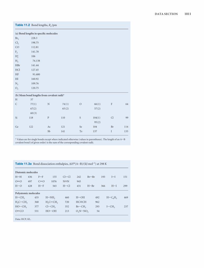
DATA SECTION 1011
Table 11.2 Bond lengths, Re /pm
(a) Bond lengths in specific molecules
Br2 228.3
Cl2 198.75
CO 112.81
F2 141.78
H2+ 106
H2 74.138
HBr 141.44
HCl 127.45
HF 91.680
HI 160.92
N2 109.76
O2 120.75
(b) Mean bond lengths from covalent radii*
H 37
C 77(1) N 74(1) O 66(1) F 64
67(2) 65(2) 57(2)
60(3)
Si 118 P 110 S 104(1) Cl 99
95(2)
Ge 122 As 121 Se 104 Br 114
Sb 141 Te 137 I 133
* Values are for single bonds except where indicated otherwise (values in parentheses). The length of an A-Bcovalent bond (of given order) is the sum of the corresponding covalent radii.
Table 11.3a Bond dissociation enthalpies, ∆H 7(A-B)/(kJ mol−1) at 298 K
Diatomic molecules
H-H 436 F-F 155 Cl-Cl 242 Br-Br 193 I-I 151
O=O 497 C=O 1076 N.N 945
H-O 428 H-F 565 H-Cl 431 H-Br 366 H-I 299
Polyatomic molecules
H-CH3 435 H-NH2 460 H-OH 492 H-C6H5 469
H3C-CH3 368 H2C=CH2 720 HC.CH 962
HO-CH3 377 Cl-CH3 352 Br-CH3 293 I-CH3 237
O=CO 531 HO-OH 213 O2N-NO2 54
Data: HCP, KL.
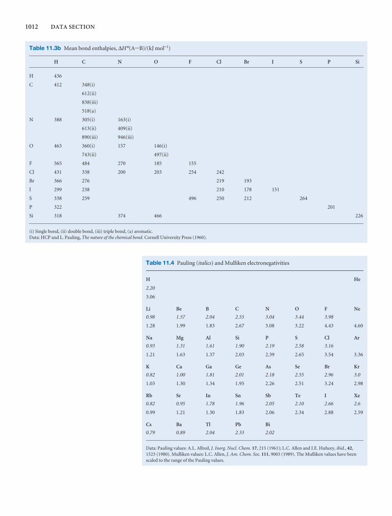
1012 DATA SECTION
Table 11.4 Pauling (italics) and Mulliken electronegativities
H He
2.20
3.06
Li Be B C N O F Ne
0.98 1.57 2.04 2.55 3.04 3.44 3.98
1.28 1.99 1.83 2.67 3.08 3.22 4.43 4.60
Na Mg Al Si P S Cl Ar
0.93 1.31 1.61 1.90 2.19 2.58 3.16
1.21 1.63 1.37 2.03 2.39 2.65 3.54 3.36
K Ca Ga Ge As Se Br Kr
0.82 1.00 1.81 2.01 2.18 2.55 2.96 3.0
1.03 1.30 1.34 1.95 2.26 2.51 3.24 2.98
Rb Sr In Sn Sb Te I Xe
0.82 0.95 1.78 1.96 2.05 2.10 2.66 2.6
0.99 1.21 1.30 1.83 2.06 2.34 2.88 2.59
Cs Ba Tl Pb Bi
0.79 0.89 2.04 2.33 2.02
Data: Pauling values: A.L. Allred, J. Inorg. Nucl. Chem. 17, 215 (1961); L.C. Allen and J.E. Huheey, ibid., 42,1523 (1980). Mulliken values: L.C. Allen, J. Am. Chem. Soc. 111, 9003 (1989). The Mulliken values have beenscaled to the range of the Pauling values.
Table 11.3b Mean bond enthalpies, ∆H 7(A-B)/(kJ mol−1)
H C N O F Cl Br I S P Si
H 436
C 412 348(i)
612(ii)
838(iii)
518(a)
N 388 305(i) 163(i)
613(ii) 409(ii)
890(iii) 946(iii)
O 463 360(i) 157 146(i)
743(ii) 497(ii)
F 565 484 270 185 155
Cl 431 338 200 203 254 242
Br 366 276 219 193
I 299 238 210 178 151
S 338 259 496 250 212 264
P 322 201
Si 318 374 466 226
(i) Single bond, (ii) double bond, (iii) triple bond, (a) aromatic.Data: HCP and L. Pauling, The nature of the chemical bond. Cornell University Press (1960).
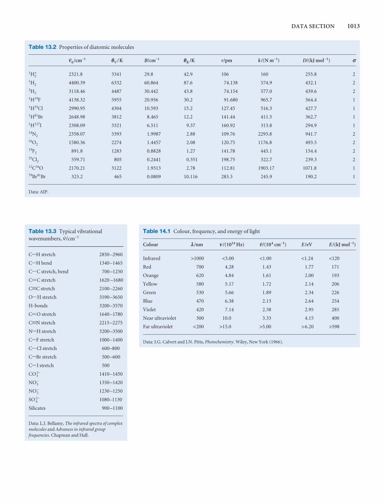
DATA SECTION 1013
Table 13.2 Properties of diatomic molecules
§0 /cm−1 qV /K B/cm−1 qR /K r/pm k /(N m−1) D/(kJ mol −1) s
1H2+ 2321.8 3341 29.8 42.9 106 160 255.8 2
1H2 4400.39 6332 60.864 87.6 74.138 574.9 432.1 22H2 3118.46 4487 30.442 43.8 74.154 577.0 439.6 21H19F 4138.32 5955 20.956 30.2 91.680 965.7 564.4 11H35Cl 2990.95 4304 10.593 15.2 127.45 516.3 427.7 11H81Br 2648.98 3812 8.465 12.2 141.44 411.5 362.7 11H127I 2308.09 3321 6.511 9.37 160.92 313.8 294.9 114N2 2358.07 3393 1.9987 2.88 109.76 2293.8 941.7 216O2 1580.36 2274 1.4457 2.08 120.75 1176.8 493.5 219F2 891.8 1283 0.8828 1.27 141.78 445.1 154.4 235Cl2 559.71 805 0.2441 0.351 198.75 322.7 239.3 212C16O 2170.21 3122 1.9313 2.78 112.81 1903.17 1071.8 179Br81Br 323.2 465 0.0809 10.116 283.3 245.9 190.2 1
Data: AIP.
Table 13.3 Typical vibrationalwavenumbers, #/cm−1
C-H stretch 2850–2960
C-H bend 1340–1465
C-C stretch, bend 700–1250
C=C stretch 1620 –1680
C.C stretch 2100–2260
O-H stretch 3590–3650
H-bonds 3200–3570
C=O stretch 1640–1780
C.N stretch 2215–2275
N-H stretch 3200–3500
C-F stretch 1000–1400
C-Cl stretch 600–800
C-Br stretch 500–600
C-I stretch 500
CO32− 1410–1450
NO3− 1350–1420
NO2− 1230–1250
SO 42− 1080–1130
Silicates 900–1100
Data: L.J. Bellamy, The infrared spectra of complexmolecules and Advances in infrared groupfrequencies. Chapman and Hall.
Table 14.1 Colour, frequency, and energy of light
Colour l/nm n /(1014 Hz) §/(104 cm−1) E /eV E /(kJ mol−1)
Infrared >1000 <3.00 <1.00 <1.24 <120
Red 700 4.28 1.43 1.77 171
Orange 620 4.84 1.61 2.00 193
Yellow 580 5.17 1.72 2.14 206
Green 530 5.66 1.89 2.34 226
Blue 470 6.38 2.13 2.64 254
Violet 420 7.14 2.38 2.95 285
Near ultraviolet 300 10.0 3.33 4.15 400
Far ultraviolet <200 >15.0 >5.00 >6.20 >598
Data: J.G. Calvert and J.N. Pitts, Photochemistry. Wiley, New York (1966).
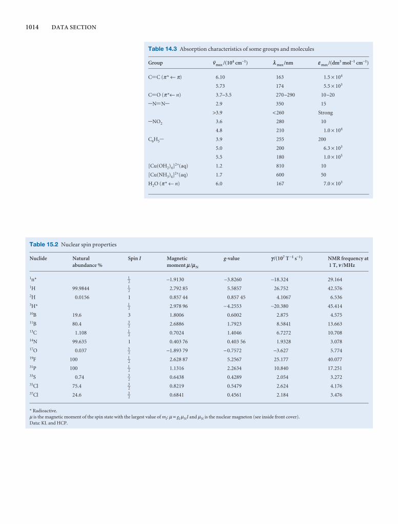
1014 DATA SECTION
Table 15.2 Nuclear spin properties
Nuclide Natural Spin I Magnetic g-value g /(107 T −1 s−1) NMR frequency atabundance % moment m /mN 1 T, n /MHz
1n* 1–2 −1.9130 −3.8260 −18.324 29.164
1H 99.9844 1–2 2.792 85 5.5857 26.752 42.576
2H 0.0156 1 0.857 44 0.857 45 4.1067 6.5363H* 1–
2 2.978 96 −4.2553 −20.380 45.41410B 19.6 3 1.8006 0.6002 2.875 4.57511B 80.4 3–
2 2.6886 1.7923 8.5841 13.66313C 1.108 1–
2 0.7024 1.4046 6.7272 10.70814N 99.635 1 0.403 76 0.403 56 1.9328 3.07817O 0.037 5–
2 −1.893 79 −0.7572 −3.627 5.77419F 100 1–
2 2.628 87 5.2567 25.177 40.07731P 100 1–
2 1.1316 2.2634 10.840 17.25133S 0.74 3–
2 0.6438 0.4289 2.054 3.27235Cl 75.4 3–
2 0.8219 0.5479 2.624 4.17637Cl 24.6 3–
2 0.6841 0.4561 2.184 3.476
* Radioactive.µ is the magnetic moment of the spin state with the largest value of mI: µ = gI µNI and µN is the nuclear magneton (see inside front cover).Data: KL and HCP.
Table 14.3 Absorption characteristics of some groups and molecules
Group §max /(104 cm−1) lmax /nm emax /(dm3 mol−1 cm−1)
C=C (π* ← π) 6.10 163 1.5 × 10⁴
5.73 174 5.5 × 10³
C=O (π*← n) 3.7–3.5 270–290 10–20
-N=N- 2.9 350 15
>3.9 <260 Strong
-NO2 3.6 280 10
4.8 210 1.0 × 10⁴
C6H5- 3.9 255 200
5.0 200 6.3 × 10³
5.5 180 1.0 × 10⁵
[Cu(OH2)6]2+(aq) 1.2 810 10
[Cu(NH3)4]2+(aq) 1.7 600 50
H2O (π* ← n) 6.0 167 7.0 × 10³
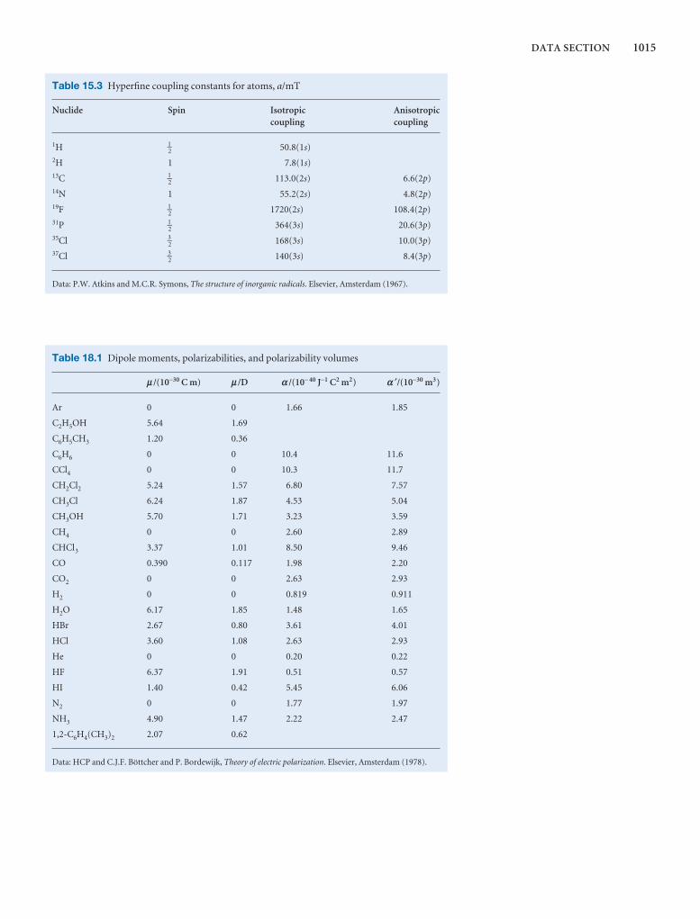
DATA SECTION 1015
Table 15.3 Hyperfine coupling constants for atoms, a/mT
Nuclide Spin Isotropic Anisotropic coupling coupling
1H 1–2 50.8(1s)
2H 1 7.8(1s)13C 1–
2 113.0(2s) 6.6(2p)14N 1 55.2(2s) 4.8(2p)19F 1–
2 1720(2s) 108.4(2p)31P 1–
2 364(3s) 20.6(3p)35Cl 3–
2 168(3s) 10.0(3p)37Cl 3–
2 140(3s) 8.4(3p)
Data: P.W. Atkins and M.C.R. Symons, The structure of inorganic radicals. Elsevier, Amsterdam (1967).
Table 18.1 Dipole moments, polarizabilities, and polarizability volumes
m /(10−30 C m) m /D a /(10− 40 J−1 C2 m2) a ′/(10−30 m3)
Ar 0 0 1.66 1.85
C2H5OH 5.64 1.69
C6H5CH3 1.20 0.36
C6H6 0 0 10.4 11.6
CCl4 0 0 10.3 11.7
CH2Cl2 5.24 1.57 6.80 7.57
CH3Cl 6.24 1.87 4.53 5.04
CH3OH 5.70 1.71 3.23 3.59
CH4 0 0 2.60 2.89
CHCl3 3.37 1.01 8.50 9.46
CO 0.390 0.117 1.98 2.20
CO2 0 0 2.63 2.93
H2 0 0 0.819 0.911
H2O 6.17 1.85 1.48 1.65
HBr 2.67 0.80 3.61 4.01
HCl 3.60 1.08 2.63 2.93
He 0 0 0.20 0.22
HF 6.37 1.91 0.51 0.57
HI 1.40 0.42 5.45 6.06
N2 0 0 1.77 1.97
NH3 4.90 1.47 2.22 2.47
1,2-C6H4(CH3)2 2.07 0.62
Data: HCP and C.J.F. Böttcher and P. Bordewijk, Theory of electric polarization. Elsevier, Amsterdam (1978).
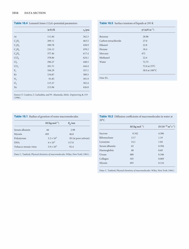
1016 DATA SECTION
Table 18.4 Lennard-Jones (12,6)-potential parameters
(e/k)/K r0/pm
Ar 111.84 362.3
C2H2 209.11 463.5
C2H4 200.78 458.9
C2H6 216.12 478.2
C6H6 377.46 617.4
CCl4 378.86 624.1
Cl2 296.27 448.5
CO2 201.71 444.4
F2 104.29 357.1
Kr 154.87 389.5
N2 91.85 391.9
O2 113.27 365.4
Xe 213.96 426.0
Source: F. Cuadros, I. Cachadiña, and W. Ahamuda, Molec. Engineering, 6, 319(1996).
Table 18.5 Surface tensions of liquids at 293 K
g /(mN m−1)
Benzene 28.88
Carbon tetrachloride 27.0
Ethanol 22.8
Hexane 18.4
Mercury 472
Methanol 22.6
Water 72.75
72.0 at 25°C
58.0 at 100°C
Data: KL.
Table 19.2 Diffusion coefficients of macromolecules in water at20°C
M/(kg mol−1) D/(10−10 m2 s−1)
Sucrose 0.342 4.586
Ribonuclease 13.7 1.19
Lysozyme 14.1 1.04
Serum albumin 65 0.594
Haemoglobin 68 0.69
Urease 480 0.346
Collagen 345 0.069
Myosin 493 0.116
Data: C. Tanford, Physical chemistry of macromolecules. Wiley, New York (1961).
Table 19.1 Radius of gyration of some macromolecules
M/(kg mol−1) Rg /nm
Serum albumin 66 2.98
Myosin 493 46.8
Polystyrene 3.2 × 10³ 50 (in poor solvent)
DNA 4 × 10³ 117.0
Tobacco mosaic virus 3.9 × 10⁴ 92.4
Data: C. Tanford, Physical chemistry of macromolecules. Wiley, New York (1961).
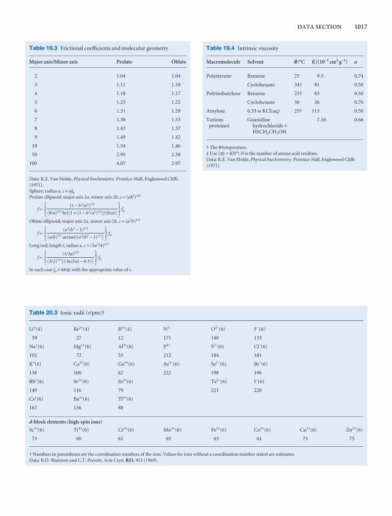
DATA SECTION 1017
Table 19.4 Intrinsic viscosity
Macromolecule Solvent q /°C K /(10−3 cm3 g−1) a
Polystyrene Benzene 25 9.5 0.74
Cyclohexane 34† 81 0.50
Polyisobutylene Benzene 23† 83 0.50
Cyclohexane 30 26 0.70
Amylose 0.33 m KCl(aq) 25† 113 0.50
Various Guanidine 7.16 0.66proteins‡ hydrochloride +
HSCH2CH2OH
† The θ temperature.‡ Use [η] = KN a; N is the number of amino acid residues.Data: K.E. Van Holde, Physical biochemistry. Prentice-Hall, Englewood Cliffs(1971).
Table 20.3 Ionic radii (r/pm)†
Li+(4) Be2+(4) B3+(4) N3− O2−(6) F−(6)
59 27 12 171 140 133
Na+(6) Mg2+(6) Al3+(6) P3− S2−(6) Cl−(6)
102 72 53 212 184 181
K+(6) Ca2+(6) Ga3+(6) As3−(6) Se2−(6) Br−(6)
138 100 62 222 198 196
Rb+(6) Sr2+(6) In3+(6) Te2−(6) I−(6)
149 116 79 221 220
Cs+(6) Ba2+(6) Tl3+(6)
167 136 88
d-block elements (high-spin ions)
Sc3+(6) Ti4+(6) Cr3+(6) Mn3+(6) Fe2+(6) Co3+(6) Cu2+(6) Zn2+(6)
73 60 61 65 63 61 73 75
† Numbers in parentheses are the coordination numbers of the ions. Values for ions without a coordination number stated are estimates.Data: R.D. Shannon and C.T. Prewitt, Acta Cryst. B25, 925 (1969).
Table 19.3 Frictional coefficients and molecular geometry
Major axis/Minor axis Prolate Oblate
2 1.04 1.04
3 1.11 1.10
4 1.18 1.17
5 1.25 1.22
6 1.31 1.28
7 1.38 1.33
8 1.43 1.37
9 1.49 1.42
10 1.54 1.46
50 2.95 2.38
100 4.07 2.97
Data: K.E. Van Holde, Physical biochemistry. Prentice-Hall, Englewood Cliffs(1971).Sphere; radius a, c = af0
Prolate ellipsoid; major axis 2a, minor axis 2b, c = (ab2)1/3
f = f0
Oblate ellipsoid; major axis 2a, minor axis 2b, c = (a2b)1/3
f = f0
Long rod; length l, radius a, c = (3a2/4)1/3
f = f0
In each case f0 = 6πηc with the appropriate value of c.
567(1/2a)2/3
(3/2)1/3{2 ln(l/a) − 0.11}
123
567(a2/b2 − 1)1/2
(a/b)2/3 arctan[(a2/b2 − 1)1/2]
123
567(1 − b2/a2)1/2
(b/a)2/3 ln{[1 + (1 − b2/a2)1/2]/(b/a)}
123
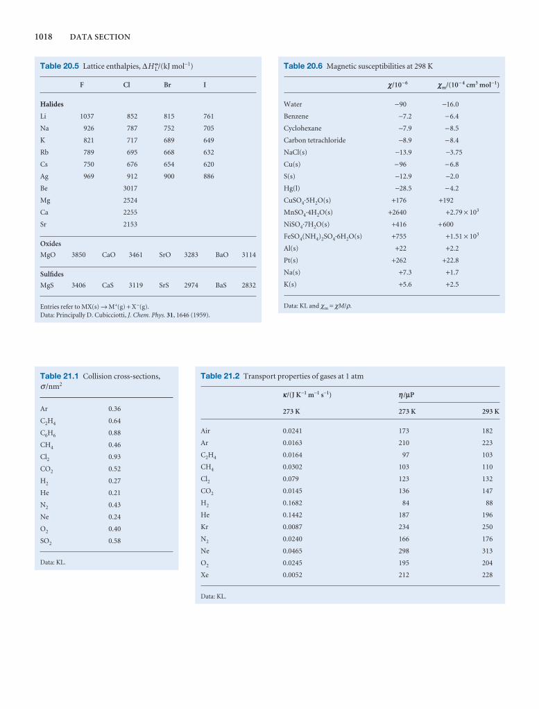
1018 DATA SECTION
Table 20.5 Lattice enthalpies, ∆H L7/(kJ mol−1)
F Cl Br I
Halides
Li 1037 852 815 761
Na 926 787 752 705
K 821 717 689 649
Rb 789 695 668 632
Cs 750 676 654 620
Ag 969 912 900 886
Be 3017
Mg 2524
Ca 2255
Sr 2153
Oxides
MgO 3850 CaO 3461 SrO 3283 BaO 3114
Sulfides
MgS 3406 CaS 3119 SrS 2974 BaS 2832
Entries refer to MX(s) → M+(g) + X−(g).Data: Principally D. Cubicciotti, J. Chem. Phys. 31, 1646 (1959).
Table 20.6 Magnetic susceptibilities at 298 K
c/10−6 cm/(10− 4 cm3 mol−1)
Water −90 −16.0
Benzene −7.2 −6.4
Cyclohexane −7.9 −8.5
Carbon tetrachloride −8.9 −8.4
NaCl(s) −13.9 −3.75
Cu(s) −96 −6.8
S(s) −12.9 −2.0
Hg(l) −28.5 −4.2
CuSO4·5H2O(s) +176 +192
MnSO4·4H2O(s) +2640 +2.79 × 10³
NiSO4·7H2O(s) +416 +600
FeSO4(NH4)2SO4·6H2O(s) +755 +1.51 × 10³
Al(s) +22 +2.2
Pt(s) +262 +22.8
Na(s) +7.3 +1.7
K(s) +5.6 +2.5
Data: KL and χm = χM/ρ.
Table 21.1 Collision cross-sections,σ /nm2
Ar 0.36
C2H4 0.64
C6H6 0.88
CH4 0.46
Cl2 0.93
CO2 0.52
H2 0.27
He 0.21
N2 0.43
Ne 0.24
O2 0.40
SO2 0.58
Data: KL.
Table 21.2 Transport properties of gases at 1 atm
k/(J K−1 m−1 s−1) h/mP
273 K 273 K 293 K
Air 0.0241 173 182
Ar 0.0163 210 223
C2H4 0.0164 97 103
CH4 0.0302 103 110
Cl2 0.079 123 132
CO2 0.0145 136 147
H2 0.1682 84 88
He 0.1442 187 196
Kr 0.0087 234 250
N2 0.0240 166 176
Ne 0.0465 298 313
O2 0.0245 195 204
Xe 0.0052 212 228
Data: KL.
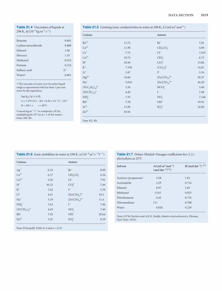
DATA SECTION 1019
Table 21.6 Ionic mobilities in water at 298 K, u/(10−8 m2 s−1 V−1)
Cations Anions
Ag+ 6.24 Br− 8.09
Ca2+ 6.17 CH3CO2− 4.24
Cu2+ 5.56 Cl− 7.91
H+ 36.23 CO32− 7.46
K+ 7.62 F− 5.70
Li+ 4.01 [Fe(CN)6]3− 10.5
Na+ 5.19 [Fe(CN)6]4 − 11.4
NH4+ 7.63 I− 7.96
[N(CH3)4]+ 4.65 NO3− 7.40
Rb+ 7.92 OH− 20.64
Zn2+ 5.47 SO42 − 8.29
Data: Principally Table 21.4 and u = λ /zF.
Table 21.7 Debye–Hückel–Onsager coefficients for (1,1)-electrolytes at 25°C
Solvent A/(mS m2 mol−1/ B/(mol dm−3)−1/2
(mol dm−3)1/2)
Acetone (propanone) 3.28 1.63
Acetonitrile 2.29 0.716
Ethanol 8.97 1.83
Methanol 15.61 0.923
Nitrobenzene 4.42 0.776
Nitromethane 111 0.708
Water 6.020 0.229
Data: J.O’M. Bockris and A.K.N. Reddy, Modern electrochemistry. Plenum,New York (1970).
Table 21.5 Limiting ionic conductivities in water at 298 K, λ /(mS m2 mol−1)
Cations Anions
Ba2+ 12.72 Br− 7.81
Ca2+ 11.90 CH3CO2− 4.09
Cs+ 7.72 Cl− 7.635
Cu2+ 10.72 ClO4− 6.73
H+ 34.96 CO32− 13.86
K+ 7.350 (CO2)22− 14.82
Li+ 3.87 F− 5.54
Mg2+ 10.60 [Fe(CN)6]3− 30.27
Na+ 5.010 [Fe(CN)6]4 − 44.20
[N(C2H5)4]+ 3.26 HCO2− 5.46
[N(CH3)4]+ 4.49 I− 7.68
NH4+ 7.35 NO3
− 7.146
Rb+ 7.78 OH− 19.91
Sr2+ 11.89 SO42− 16.00
Zn2+ 10.56
Data: KL, RS.
Table 21.4 Viscosities of liquids at 298 K, η/(10−3 kg m−1 s−1)
Benzene 0.601
Carbon tetrachloride 0.880
Ethanol 1.06
Mercury 1.55
Methanol 0.553
Pentane 0.224
Sulfuric acid 27
Water† 0.891
† The viscosity of water over its entire liquidrange is represented with less than 1 per centerror by the expression
log(η20 /η) = A /B,
A = 1.370 23(t − 20) + 8.36 × 10− 4(t − 20)2
B = 109 + t t = θ/°C
Convert kg m−1 s−1 to centipoise (cP) bymultiplying by 103 (so η ≈ 1 cP for water).Data: AIP, KL.
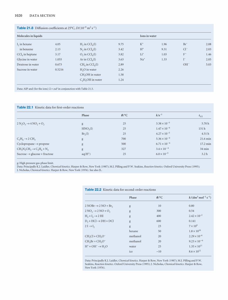
1020 DATA SECTION
Table 21.8 Diffusion coefficients at 25°C, D/(10−9 m2 s−1)
Molecules in liquids Ions in water
I2 in hexane 4.05 H2 in CCl4(l) 9.75 K+ 1.96 Br− 2.08
in benzene 2.13 N2 in CCl4(l) 3.42 H+ 9.31 Cl− 2.03
CCl4 in heptane 3.17 O2 in CCl4(l) 3.82 Li+ 1.03 F− 1.46
Glycine in water 1.055 Ar in CCl4(l) 3.63 Na+ 1.33 I− 2.05
Dextrose in water 0.673 CH4 in CCl4(l) 2.89 OH− 5.03
Sucrose in water 0.5216 H2O in water 2.26
CH3OH in water 1.58
C2H5OH in water 1.24
Data: AIP and (for the ions) λ = zuF in conjunction with Table 21.5.
Table 22.1 Kinetic data for first-order reactions
Phase q /°C k /s−1 t1/2
2 N2O5 → 4 NO2 + O2 g 25 3.38 × 10⁻⁵ 5.70 h
HNO3(l) 25 1.47 × 10⁻⁶ 131 h
Br2(l) 25 4.27 × 10⁻⁵ 4.51 h
C2H6 → 2 CH3 g 700 5.36 × 10⁻⁴ 21.6 min
Cyclopropane → propene g 500 6.71 × 10− 4 17.2 min
CH3N2CH3 → C2H6 + N2 g 327 3.4 × 10− 4 34 min
Sucrose → glucose + fructose aq(H+) 25 6.0 × 10⁻⁵ 3.2 h
g: High pressure gas-phase limit.Data: Principally K.J. Laidler, Chemical kinetics. Harper & Row, New York (1987); M.J. Pilling and P.W. Seakins, Reaction kinetics. Oxford University Press (1995); J. Nicholas, Chemical kinetics. Harper & Row, New York (1976). See also JL.
Table 22.2 Kinetic data for second-order reactions
Phase q /°C k /(dm3 mol−1 s−1)
2 NOBr → 2 NO + Br2 g 10 0.80
2 NO2 → 2 NO + O2 g 300 0.54
H2 + I2 → 2 HI g 400 2.42 × 10⁻²
D2 + HCl → DH + DCl g 600 0.141
2 I → I2 g 23 7 × 10⁹
hexane 50 1.8 × 10¹⁰
CH3Cl + CH3O− methanol 20 2.29 × 10⁻⁶
CH3Br + CH3O− methanol 20 9.23 × 10− 6
H+ + OH− → H2O water 25 1.35 × 10¹¹
ice −10 8.6 × 10¹²
Data: Principally K.J. Laidler, Chemical kinetics. Harper & Row, New York (1987); M.J. Pilling and P.W.Seakins, Reaction kinetics. Oxford University Press (1995); J. Nicholas, Chemical kinetics. Harper & Row, New York (1976).
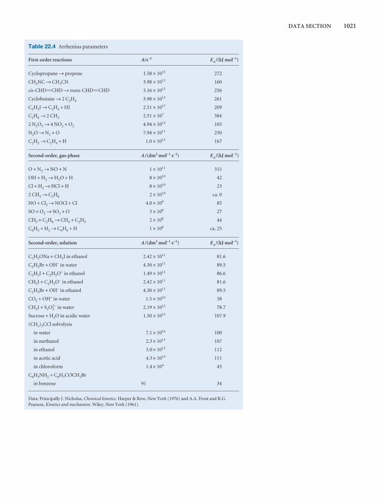
DATA SECTION 1021
Table 22.4 Arrhenius parameters
First-order reactions A/s−1 E a /(kJ mol−1)
Cyclopropane → propene 1.58 × 10¹⁵ 272
CH3NC → CH3CN 3.98 × 10¹³ 160
cis-CHD=CHD → trans-CHD=CHD 3.16 × 10¹² 256
Cyclobutane → 2 C2H4 3.98 × 10¹³ 261
C2H5I → C2H4 + HI 2.51 × 10¹⁷ 209
C2H6 → 2 CH3 2.51 × 10⁷ 384
2 N2O5 → 4 NO2 + O2 4.94 × 10¹³ 103
N2O → N2 + O 7.94 × 10¹¹ 250
C2H5 → C2H4 + H 1.0 × 10¹³ 167
Second-order, gas-phase A /(dm3 mol−1 s−1) E a /(kJ mol−1)
O + N2 → NO + N 1 × 10¹¹ 315
OH + H2 → H2O + H 8 × 10¹⁰ 42
Cl + H2 → HCl + H 8 × 10¹⁰ 23
2 CH3 → C2H6 2 × 10¹⁰ ca. 0
NO + Cl2 → NOCl + Cl 4.0 × 10⁹ 85
SO + O2 → SO2 + O 3 × 10⁸ 27
CH3 + C2H6 → CH4 + C2H5 2 × 10⁸ 44
C6H5 + H2 → C6H6 + H 1 × 10⁸ ca. 25
Second-order, solution A /(dm3 mol−1 s−1) E a /(kJ mol−1)
C2H5ONa + CH3I in ethanol 2.42 × 10¹¹ 81.6
C2H5Br + OH− in water 4.30 × 10¹¹ 89.5
C2H5I + C2H5O− in ethanol 1.49 × 10¹¹ 86.6
CH3I + C2H5O− in ethanol 2.42 × 10¹¹ 81.6
C2H5Br + OH− in ethanol 4.30 × 10¹¹ 89.5
CO2 + OH− in water 1.5 × 10¹⁰ 38
CH3I + S2O32− in water 2.19 × 10¹² 78.7
Sucrose + H2O in acidic water 1.50 × 10¹⁵ 107.9
(CH3)3CCl solvolysis
in water 7.1 × 10¹⁶ 100
in methanol 2.3 × 10¹³ 107
in ethanol 3.0 × 10¹³ 112
in acetic acid 4.3 × 10¹³ 111
in chloroform 1.4 × 10⁴ 45
C6H5NH2 + C6H5COCH2Br
in benzene 91 34
Data: Principally J. Nicholas, Chemical kinetics. Harper & Row, New York (1976) and A.A. Frost and R.G.Pearson, Kinetics and mechanism. Wiley, New York (1961).
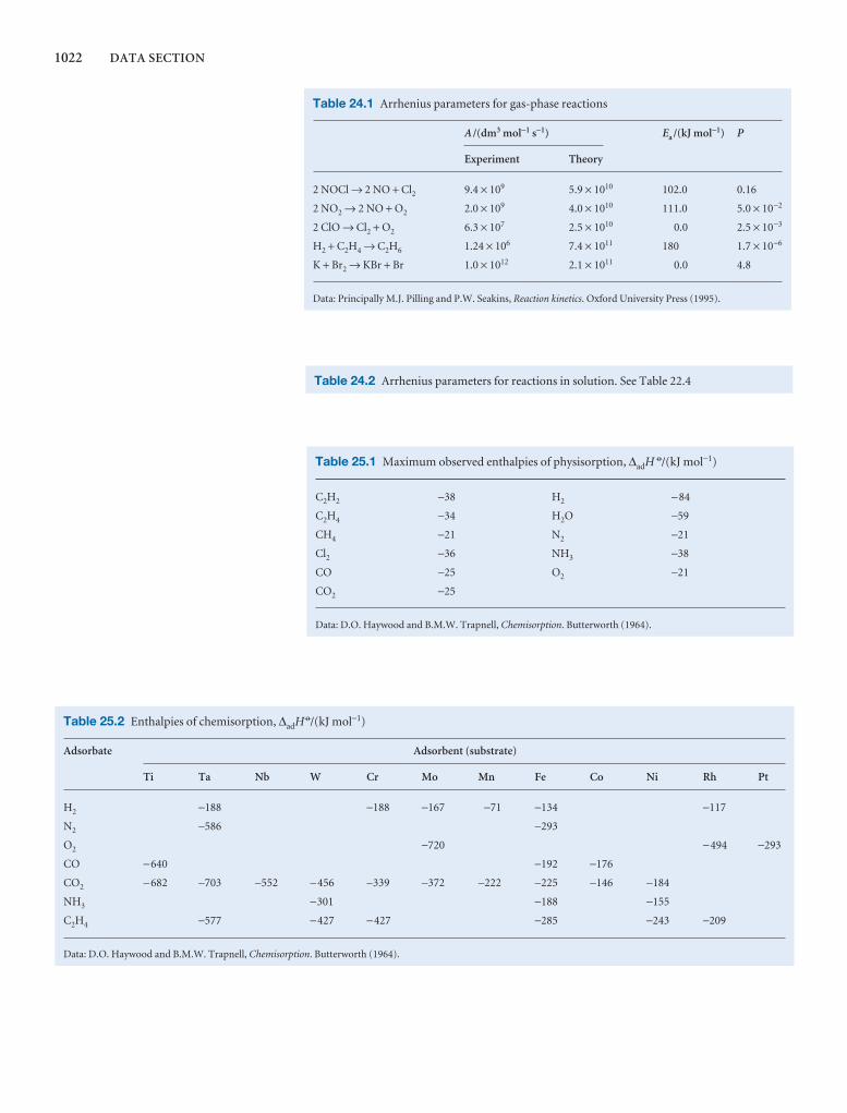
1022 DATA SECTION
Table 24.1 Arrhenius parameters for gas-phase reactions
A /(dm3 mol−1 s−1) Ea /(kJ mol−1) P
Experiment Theory
2 NOCl → 2 NO + Cl2 9.4 × 10⁹ 5.9 × 10¹⁰ 102.0 0.16
2 NO2 → 2 NO + O2 2.0 × 10⁹ 4.0 × 10¹⁰ 111.0 5.0 × 10⁻²
2 ClO → Cl2 + O2 6.3 × 10⁷ 2.5 × 10¹⁰ 0.0 2.5 × 10⁻³
H2 + C2H4 → C2H6 1.24 × 10⁶ 7.4 × 10¹¹ 180 1.7 × 10⁻⁶
K + Br2 → KBr + Br 1.0 × 10¹² 2.1 × 10¹¹ 0.0 4.8
Data: Principally M.J. Pilling and P.W. Seakins, Reaction kinetics. Oxford University Press (1995).
Table 24.2 Arrhenius parameters for reactions in solution. See Table 22.4
Table 25.1 Maximum observed enthalpies of physisorption, ∆adH 7/(kJ mol−1)
C2H2 −38 H2 −84
C2H4 −34 H2O −59
CH4 −21 N2 −21
Cl2 −36 NH3 −38
CO −25 O2 −21
CO2 −25
Data: D.O. Haywood and B.M.W. Trapnell, Chemisorption. Butterworth (1964).
Table 25.2 Enthalpies of chemisorption, ∆adH 7/(kJ mol−1)
Adsorbate Adsorbent (substrate)
Ti Ta Nb W Cr Mo Mn Fe Co Ni Rh Pt
H2 −188 −188 −167 −71 −134 −117
N2 −586 −293
O2 −720 −494 −293
CO −640 −192 −176
CO2 −682 −703 −552 −456 −339 −372 −222 −225 −146 −184
NH3 −301 −188 −155
C2H4 −577 −427 −427 −285 −243 −209
Data: D.O. Haywood and B.M.W. Trapnell, Chemisorption. Butterworth (1964).
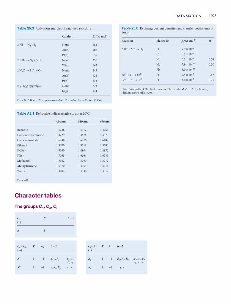
DATA SECTION 1023
Table 25.3 Activation energies of catalysed reactions
Catalyst Ea /(kJ mol−1)
2 HI → H2 + I2 None 184
Au(s) 105
Pt(s) 59
2 NH3 → N2 + 3 H2 None 350
W(s) 162
2 N2O → 2 N2 + O2 None 245
Au(s) 121
Pt(s) 134
(C2H5)2O pyrolysis None 224
I2(g) 144
Data: G.C. Bond, Heterogeneous catalysis. Clarendon Press, Oxford (1986).
Table 25.6 Exchange current densities and transfer coefficients at298 K
Reaction Electrode j0 /(A cm−2) a
2 H+ + 2 e− → H2 Pt 7.9 × 10⁻⁴
Cu 1 × 10⁻⁶
Ni 6.3 × 10⁻⁶ 0.58
Hg 7.9 × 10⁻¹³ 0.50
Pb 5.0 × 10⁻¹²
Fe3+ + e− → Fe2+ Pt 2.5 × 10⁻³ 0.58
Ce4+ + e− → Ce3+ Pt 4.0 × 10⁻⁵ 0.75
Data: Principally J.O’M. Bockris and A.K.N. Reddy, Modern electrochemistry.Plenum, New York (1970).
Table A3.1 Refractive indices relative to air at 20°C
434 nm 589 nm 656 nm
Benzene 1.5236 1.5012 1.4965
Carbon tetrachloride 1.4729 1.4676 1.4579
Carbon disulfide 1.6748 1.6276 1.6182
Ethanol 1.3700 1.3618 1.3605
KCl(s) 1.5050 1.4904 1.4973
Kl(s) 1.7035 1.6664 1.6581
Methanol 1.3362 1.3290 1.3277
Methylbenzene 1.5170 1.4955 1.4911
Water 1.3404 1.3330 1.3312
Data: AIP.
C1 E h = 1(1)
A 1
Cs = Ch E σh h = 2(m)
A′ 1 1 x, y, Rz x2, y2,z2, xy
A″ 1 −1 z, Rx, Ry yz, xz
Ci = S2 E i h = 2(⁄)
Ag 1 1 Rx, Ry, Rz x2, y2, z2,xy, xz, yz
Au 1 −1 x, y, z
Character tables
The groups C1, Cs, Ci

1024 DATA SECTION
C4v, 4mm E C2 2C4 2σv 2σd h = 8
A1 1 1 1 1 1 z, z2, x2 + y2
A2 1 1 1 −1 1 Rz
B1 1 1 −1 1 −1 x2 − y2
B2 1 1 −1 −1 1 xy
E 2 −2 0 0 0 (x, y), (xz, yz) (Rx, Ry)
C5v E 2C5 2C52 5σv h = 10, a = 72°
A1 1 1 1 1 z, z2, x2 + y2
A2 1 1 1 −1 Rz
E1 2 2 cos α 2 cos 2α 0 (x, y), (xz, yz) (Rx, Ry)
E2 2 2 cos 2α 2 cos α 0 (xy, x2 − y2)
C6v, 6mm E C2 2C3 2C6 3σd 3σv h = 12
A1 1 1 1 1 1 1 z, z2, x2 + y2
A2 1 1 1 1 −1 1 Rz
B1 1 −1 1 −1 −1 1
B2 1 −1 1 −1 1 −1
E1 2 −2 −1 1 0 0 (x, y), (xz, yz) (Rx, Ry)
E2 2 2 −1 −1 0 0 (xy, x2 − y2)
C2v, 2mm E C2 σv σ′v h = 4
A1 1 1 1 1 z, z2, x2, y2
A2 1 1 −1 −1 xy Rz
B1 1 −1 1 −1 x, xz Ry
B2 1 −1 −1 1 y, yz Rx
C3v, 3m E 2C3 3σv h = 6
A1 1 1 1 z, z2, x2 + y2
A2 1 1 −1 Rz
E 2 −1 0 (x, y), (xy, x2 − y2) (xz, yz) (Rx , Ry)
The groups Cnv
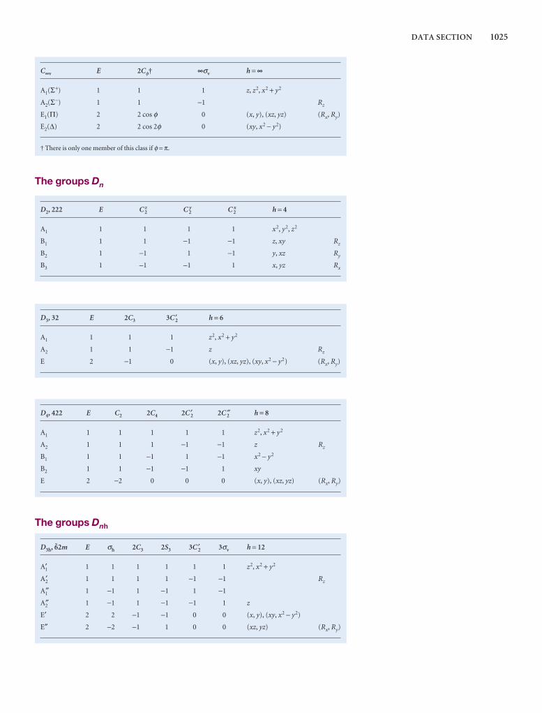
DATA SECTION 1025
C•v E 2Cφ† •σv h = •
A1(Σ+) 1 1 1 z, z2, x2 + y2
A2(Σ−) 1 1 −1 Rz
E1(Π) 2 2 cos φ 0 (x, y), (xz, yz) (Rx, Ry)
E2(∆) 2 2 cos 2φ 0 (xy, x2 − y2)
† There is only one member of this class if φ = π.
D4, 422 E C2 2C4 2C ′2 2C 2″ h = 8
A1 1 1 1 1 1 z2, x2 + y2
A2 1 1 1 −1 −1 z Rz
B1 1 1 −1 1 −1 x2 − y2
B2 1 1 −1 −1 1 xy
E 2 −2 0 0 0 (x, y), (xz, yz) (Rx, Ry)
D3, 32 E 2C3 3C ′2 h = 6
A1 1 1 1 z2, x2 + y2
A2 1 1 −1 z Rz
E 2 −1 0 (x, y), (xz, yz), (xy, x2 − y2) (Rx, Ry)
D2, 222 E C2z C 2
y C 2x h = 4
A1 1 1 1 1 x2, y2, z2
B1 1 1 −1 −1 z, xy Rz
B2 1 −1 1 −1 y, xz Ry
B3 1 −1 −1 1 x, yz Rx
The groups Dn
The groups Dnh
D3h, %2m E σh 2C3 2S3 3C ′2 3σv h = 12
A′1 1 1 1 1 1 1 z2, x2 + y2
A′2 1 1 1 1 −1 −1 Rz
A1″ 1 −1 1 −1 1 −1
A2″ 1 −1 1 −1 −1 1 z
E′ 2 2 −1 −1 0 0 (x, y), (xy, x2 − y2)
E″ 2 −2 −1 1 0 0 (xz, yz) (Rx, Ry)
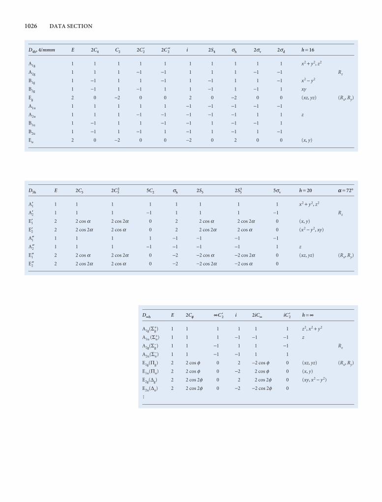
1026 DATA SECTION
D•h E 2Cf •C ′2 i 2iC• iC ′2 h = •
A1g(Σg+) 1 1 1 1 1 1 z2, x2 + y2
A1u (Σu+) 1 1 1 −1 −1 −1 z
A2g(Σg−) 1 1 −1 1 1 −1 Rz
A2u(Σu−) 1 1 −1 −1 1 1
E1g(Πg) 2 2 cos φ 0 2 −2 cos φ 0 (xz, yz) (Rx, Ry)
E1u(Πu) 2 2 cos φ 0 −2 2 cos φ 0 (x, y)
E2g(∆g) 2 2 cos 2φ 0 2 2 cos 2φ 0 (xy, x2 − y2)
E2u(∆u) 2 2 cos 2φ 0 −2 −2 cos 2φ 0
�
D5h E 2C5 2C52 5C2 σh 2S5 2S5
3 5σv h = 20 a = 72°
A′1 1 1 1 1 1 1 1 1 x2 + y2, z2
A′2 1 1 1 −1 1 1 1 −1 Rz
E′1 2 2 cos α 2 cos 2α 0 2 2 cos α 2 cos 2α 0 (x, y)
E′2 2 2 cos 2α 2 cos α 0 2 2 cos 2α 2 cos α 0 (x2 − y2, xy)
A″1 1 1 1 1 −1 −1 −1 −1
A″2 1 1 1 −1 −1 −1 −1 1 z
E″1 2 2 cos α 2 cos 2α 0 −2 −2 cos α −2 cos 2α 0 (xz, yz) (Rx, Ry)
E″2 2 2 cos 2α 2 cos α 0 −2 −2 cos 2α −2 cos α 0
D4h, 4/mmm E 2C4 C2 2C ′2 2C 2″ i 2S4 σh 2σv 2σd h = 16
A1g 1 1 1 1 1 1 1 1 1 1 x2 + y2, z2
A2g 1 1 1 −1 −1 1 1 1 −1 −1 Rz
B1g 1 −1 1 1 −1 1 −1 1 1 −1 x2 − y2
B2g 1 −1 1 −1 1 1 −1 1 −1 1 xy
Eg 2 0 −2 0 0 2 0 −2 0 0 (xz, yz) (Rx, Ry)
A1u 1 1 1 1 1 −1 −1 −1 −1 −1
A2u 1 1 1 −1 −1 −1 −1 −1 1 1 z
B1u 1 −1 1 1 −1 −1 1 −1 −1 1
B2u 1 −1 1 −1 1 −1 1 −1 1 −1
Eu 2 0 −2 0 0 −2 0 2 0 0 (x, y)

DATA SECTION 1027
I E 12C5 12C52 20C3 15C2 h = 60
A 1 1 1 1 1 z2 + y2 + z2
T1 3 1–2(1 + ) 1–
2(1 − ) 0 −1 (x, y, z)
T2 3 1–2(1 − ) 1–
2(1 + ) 0 −1 (Rx, Ry, Rz)
G 4 −1 −1 1 0
G 5 0 0 −1 1 (2z2 − x2 − y2, x2 − y2, xy, yz, zx)
Further information: P.W. Atkins, M.S. Child, and C.S.G. Phillips, Tables for group theory. Oxford UniversityPress (1970).
55
55
Oh (m3m) E 8C3 6C2 6C2 3C2 (= C 42) i 6S4 8S6 3σh 6σd h = 48
A1g 1 1 1 1 1 1 1 1 1 1 x2 + y2 + z2
A2g 1 1 −1 −1 1 1 −1 1 1 −1
Eg 2 −1 0 0 2 2 0 −1 2 0 (2z2 − x2 − y2, x2 − y2)
T1g 3 0 −1 1 −1 3 1 0 −1 −1 (Rx, Ry, Rz)
T2g 3 0 1 −1 −1 3 −1 0 −1 1 (xy, yz, xy)
A1u 1 1 1 1 1 −1 −1 −1 −1 −1
A2u 1 1 −1 −1 1 −1 1 −1 −1 1
Eu 2 −1 0 0 2 −2 0 1 −2 0
T1u 3 0 −1 1 −1 −3 −1 0 1 1 (x, y, z)
T2u 3 0 1 −1 −1 −3 1 0 1 −1
Td, ∞3m E 8C3 3C2 6σd 6S4 h = 24
A1 1 1 1 1 1 x2 + y2 + z2
A2 1 1 1 −1 −1
E 2 −1 2 0 0 (3z2 − r2, x2 − y2)
T1 3 0 −1 −1 1 (Rx, Ry, Rz)
T2 3 0 −1 1 −1 (x, y, z), (xy, xz, yz)
The cubic groups
The icosahedral group

Chapter 1
1.1 (a) 10.5 bar, (b) 10.4 bar.
1.2 (a) 1.07 bar; (b) 803 Torr.
1.3 120 kPa.
1.4 2.67 × 10³ kg.
1.5 1.5 × 10³ Pa.
1.6 115 kPa.
1.7 R = 0.082 061 5 dm3 atm K−1 mol−1, M = 31.9987 g mol−1.
1.8 P4.
1.9 2.61 kg.
1.10 (a) 3.14 dm3; (b) 28.2 kPa.
1.11 16.14 g mol−1.
1.12 −270°C.
1.13 (a) (i) 1.0 atm, (ii) 270 atm.
(b) (i) 0.99 atm, (ii) 190 atm.
11.4 a = 1.34 × 10⁻¹ kg m5 s−2 mol−2, b = 4.36 × 10⁻⁵ m3 mol−1.
1.15 (a) 1.12, repulsive; (b) 2.7 dm3 mol−1.
1.16 (a) 0.124 dm3 mol−1; (b) 0.112 dm3 mol−1.
1.17 (a) 8.7 cm3; (b) −0.15 dm3 mol−1.
1.18 (a) xN = 0.63, xH = 0.37;
(b) pN = 2.5 atm, pH = 1.5 atm;
(c) 4.0 atm.
1.19 b = 0.0493 dm3 mol−1, r = 1.94 × 10⁻¹⁰ m, a = 3.16 dm6 atm mol−2.
1.20 (a) 1259 K; (b) 0.129 nm.
1.21 (a) p = 2.6 atm, T = 881 K;
(b) p = 2.2 atm, T = 718 K;
(c) p = 1.4 atm, T = 356 K.
1.22 b = 1.3 × 10⁻⁴ m3 mol−1, Z = 0.67.
Chapter 2
2.1 59 J.
2.2 −91 J.
2.3 (a) ∆U = ∆H = 0, q = −w = 1.62 × 10³ J;
(b) ∆U = ∆H = 0, q = −w = 1.38 × 10³ J;
(c) ∆U = ∆H = 0, q = w = 0.
2.4 p2 = 143 kPa, w = 0, q = 3.28 × 10³ J, ∆U = 3.28 × 10³ J.
2.5 (a) −19 J; (b) −52.8 J.
2.6 ∆H = q = −70.6 kJ, w = 5.60 × 10³ J, ∆U = −65.0 kJ.
2.7 −188 J.
2.8 (a) ∆H = q = 14.9 × 10³ J, w = −831 J, ∆U = 14.1 kJ.
(b) ∆H = 14.9 kJ, w = 0, ∆U = q = 14.1 kJ.
2.9 200 K.
2.10 −325 J.
2.11 8.5 Torr.
2.12 Cp,m = 53 J K−1 mol−1, CV,m = 45 J K−1 mol−1.
2.13 ∆H = q = 2.0 × 10³ J mol−1, ∆U = 1.6 × 10³ J mol−1.
2.14 q = 0, w = −3.5 × 10³ J = ∆U, ∆T = −24 K, ∆H = −4.5 × 10³ J.
2.15 Vf = 0.0205 m3, Tf = 279 K, w = −6.7 × 10² J.
2.16 q = ∆H = 24.0 kJ, w = −1.6 kJ, ∆U = 22.4 kJ.
2.17 −3053.6 kJ mol−1.
Solutions to b) exercises
2.18 −1152 kJ mol−1.
2.19 C = 68.3 J K−1, ∆T = +64.1 K.
2.20 +84.40 kJ mol−1.
2.21 +1.90 kJ mol−1.
2.22 (a) ∆r H 7 = −589.56 kJ mol−1, ∆rU7 = −582.13 kJ mol−1.
(b) ∆fH7(HI) = 26.48 kJ mol−1, ∆f H
7(H2O) = −241.82 kJ mol−1.
2.23 −760.3 kJ mol−1.
2.24 +52.5 kJ mol−1.
2.25 −566.93 kJ mol−1.
2.26 (a) ∆rH7(298 K) = −175 kJ mol−1, ∆rU
7(298 K) = −173 kJ mol−1;
(b) ∆r H 7(348 K) = −176 mol−1.
2.27 −65.49 kJ mol−1.
2.28 −1587 kJ mol−1.
2.29 0.48 K atm−1.
2.30 ∆Um = +129 J mol−1, q = +7.7465 kJ mol−1, w = −7.62 kJ mol−1.
2.31 1.27 × 10⁻³ K−1.
2.32 3.6 × 10² atm.
2.33 −41.2 J atm−1 mol−1, q (supplied) = 27.2 × 10³ J.
Chapter 33.1 (a) 1.8 × 10² J K−1; (b) 1.5 × 10² J K−1.
3.2 152.65 J K−1 mol−1.
3.3 −7.3 J K−1.
3.4 ∆S = q = 0, w = ∆U = +2.75 kJ, ∆H = +3.58 kJ.
3.5 ∆Htot = 0, ∆Stot = 24 J K−1.
3.6 (a) 0; (b) −230 J; (c) −230 J; (d) −5.3 K; (e) 3.2 J K−1.
3.7 (a) 104.6 J K−1; (b) −104.6 J K−1.
3.8 (a) −21.0 J K−1 mol−1; (b) +512.0 J K−1 mol−1.
3.9 (a) −212.40 kJ mol−1; (b) −5798 kJ mol−1.
3.10 (a) −212.55 kJ mol−1; (b) −5798 kJ mol−1.
3.11 −86.2 kJ mol−1.
3.12 −197 kJ mol−1.
3.13 (a) ∆S(gas) = +3.0 J K−1, ∆S(surroundings) = −3.0 J K−1, ∆S(total) = 0;
(b) ∆S(gas) = +3.0 J K−1, ∆S(surroundings) = 0; ∆S(total) = +3.0 J K−1;
(c) ∆S(gas) = 0, ∆S(surroundings) = 0, ∆S(total) = 0.
3.14 2108.11 kJ mol−1.
3.15 (a) 0.500; (b) 0.50 kJ; (c) 0.5 kJ.
3.16 −2.0 J.
3.17 −42.8 J K−1.
3.18 3.0 kJ.
3.19 2.71 kJ mol−1.
3.20 −0.93 kJ mol−1.
3.21 200 J.
3.22 +2.88 kJ mol−1.
Chapter 44.1 296 K = 23°C.
4.2 ∆fusS = +5.5 J K−1 mol−1, ∆fusH = +2.4 kJ mol−1.
4.3 25.25 kJ mol−1.
4.4 (a) 31.11 kJ mol−1; (b) 276.9 K.
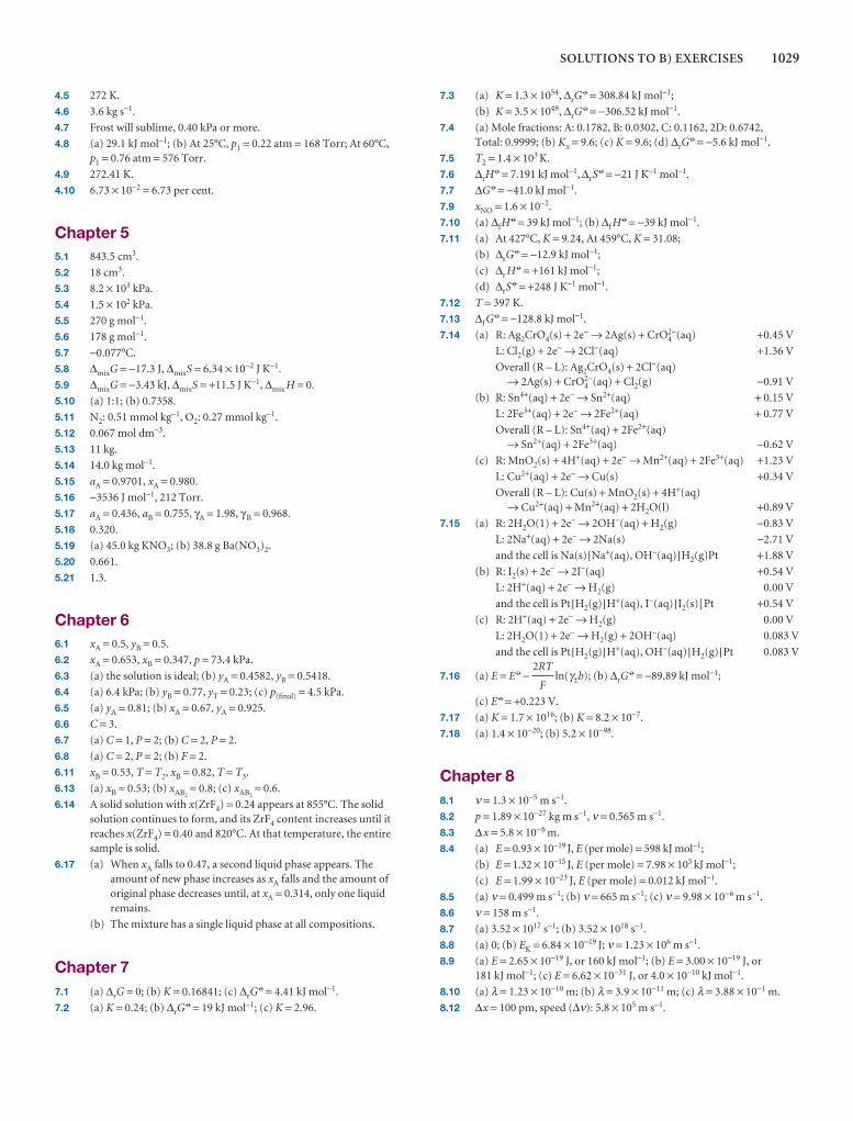
SOLUTIONS TO B) EXERCISES 1029
4.5 272 K.
4.6 3.6 kg s−1.
4.7 Frost will sublime, 0.40 kPa or more.
4.8 (a) 29.1 kJ mol−1; (b) At 25°C, p1 = 0.22 atm = 168 Torr; At 60°C, p1 = 0.76 atm = 576 Torr.
4.9 272.41 K.
4.10 6.73 × 10−2 = 6.73 per cent.
Chapter 55.1 843.5 cm3.
5.2 18 cm3.
5.3 8.2 × 10³ kPa.
5.4 1.5 × 10² kPa.
5.5 270 g mol−1.
5.6 178 g mol−1.
5.7 −0.077°C.
5.8 ∆mixG = −17.3 J, ∆mixS = 6.34 × 10⁻² J K−1.
5.9 ∆mixG = −3.43 kJ, ∆mixS = +11.5 J K−1, ∆mix H = 0.
5.10 (a) 1:1; (b) 0.7358.
5.11 N2: 0.51 mmol kg−1, O2: 0.27 mmol kg−1.
5.12 0.067 mol dm−3.
5.13 11 kg.
5.14 14.0 kg mol−1.
5.15 aA = 0.9701, xA = 0.980.
5.16 −3536 J mol−1, 212 Torr.
5.17 aA = 0.436, aB = 0.755, γA = 1.98, γB = 0.968.
5.18 0.320.
5.19 (a) 45.0 kg KNO3; (b) 38.8 g Ba(NO3)2.
5.20 0.661.
5.21 1.3.
Chapter 66.1 xA = 0.5, yB = 0.5.
6.2 xA = 0.653, xB = 0.347, p = 73.4 kPa.
6.3 (a) the solution is ideal; (b) yA = 0.4582, yB = 0.5418.
6.4 (a) 6.4 kPa; (b) yB = 0.77, yT = 0.23; (c) p(final) = 4.5 kPa.
6.5 (a) yA = 0.81; (b) xA = 0.67, yA = 0.925.
6.6 C = 3.
6.7 (a) C = 1, P = 2; (b) C = 2, P = 2.
6.8 (a) C = 2, P = 2; (b) F = 2.
6.11 xB = 0.53, T = T2, xB = 0.82, T = T3.
6.13 (a) xB ≈ 0.53; (b) xAB2≈ 0.8; (c) xAB2
≈ 0.6.
6.14 A solid solution with x(ZrF4) = 0.24 appears at 855°C. The solidsolution continues to form, and its ZrF4 content increases until itreaches x(ZrF4) = 0.40 and 820°C. At that temperature, the entiresample is solid.
6.17 (a) When xA falls to 0.47, a second liquid phase appears. Theamount of new phase increases as xA falls and the amount of original phase decreases until, at xA = 0.314, only one liquid remains.
(b) The mixture has a single liquid phase at all compositions.
Chapter 77.1 (a) ∆rG = 0; (b) K = 0.16841; (c) ∆rG
7 = 4.41 kJ mol−1.
7.2 (a) K = 0.24; (b) ∆rG7 = 19 kJ mol−1; (c) K = 2.96.
7.3 (a) K = 1.3 × 1054, ∆rG7 = 308.84 kJ mol−1;
(b) K = 3.5 × 1049, ∆rG7 = −306.52 kJ mol−1.
7.4 (a) Mole fractions: A: 0.1782, B: 0.0302, C: 0.1162, 2D: 0.6742, Total: 0.9999; (b) Kx = 9.6; (c) K = 9.6; (d) ∆rG
7 = −5.6 kJ mol−1.
7.5 T2 = 1.4 × 10³ K.
7.6 ∆rH7 = 7.191 kJ mol−1, ∆rS
7 = −21 J K−1 mol−1.
7.7 ∆G 7 = −41.0 kJ mol−1.
7.9 xNO = 1.6 × 10⁻².
7.10 (a) ∆fH7 = 39 kJ mol−1; (b) ∆f H
7 = −39 kJ mol−1.
7.11 (a) At 427°C, K = 9.24, At 459°C, K = 31.08;
(b) ∆rG7 = −12.9 kJ mol−1;
(c) ∆r H 7 = +161 kJ mol−1;
(d) ∆rS7 = +248 J K−1 mol−1.
7.12 T = 397 K.
7.13 ∆f G7 = −128.8 kJ mol−1.
7.14 (a) R: Ag2CrO4(s) + 2e− → 2Ag(s) + CrO42−(aq) +0.45 V
L: Cl2(g) + 2e− → 2Cl−(aq) +1.36 V
Overall (R – L): Ag2CrO4(s) + 2Cl−(aq)→ 2Ag(s) + CrO4
2−(aq) + Cl2(g) −0.91 V
(b) R: Sn4+(aq) + 2e− → Sn2+(aq) + 0.15 V
L: 2Fe3+(aq) + 2e− → 2Fe2+(aq) + 0.77 V
Overall (R – L): Sn4+(aq) + 2Fe2+(aq)→ Sn2+(aq) + 2Fe3+(aq) −0.62 V
(c) R: MnO2(s) + 4H+(aq) + 2e− → Mn2+(aq) + 2Fe3+(aq) +1.23 V
L: Cu2+(aq) + 2e− → Cu(s) +0.34 V
Overall (R – L): Cu(s) + MnO2(s) + 4H+(aq)→ Cu2+(aq) + Mn2+(aq) + 2H2O(l) +0.89 V
7.15 (a) R: 2H2O(1) + 2e− → 2OH−(aq) + H2(g) −0.83 V
L: 2Na+(aq) + 2e− → 2Na(s) −2.71 V
and the cell is Na(s) |Na+(aq), OH−(aq) |H2(g)Pt +1.88 V
(b) R: I2(s) + 2e− → 2I−(aq) +0.54 V
L: 2H+(aq) + 2e− → H2(g) 0.00 V
and the cell is Pt |H2(g) |H+(aq), I−(aq) |I2(s) |Pt +0.54 V
(c) R: 2H+(aq) + 2e− → H2(g) 0.00 V
L: 2H2O(1) + 2e− → H2(g) + 2OH−(aq) 0.083 V
and the cell is Pt |H2(g) |H+(aq), OH−(aq) |H2(g) |Pt 0.083 V
7.16 (a) E = E 7 − ln(γ±b); (b) ∆rG7 = −89.89 kJ mol−1;
(c) E 7 = +0.223 V.
7.17 (a) K = 1.7 × 10¹⁶; (b) K = 8.2 × 10⁻⁷.
7.18 (a) 1.4 × 10⁻²⁰; (b) 5.2 × 10−98.
Chapter 88.1 ν = 1.3 × 10⁻⁵ m s−1.
8.2 p = 1.89 × 10⁻²⁷ kg m s−1, ν = 0.565 m s−1.
8.3 ∆x = 5.8 × 10⁻⁶ m.
8.4 (a) E = 0.93 × 10⁻¹⁹ J, E (per mole) = 598 kJ mol−1;
(b) E = 1.32 × 10⁻¹⁵ J, E (per mole) = 7.98 × 10⁵ kJ mol−1;
(c) E = 1.99 × 10⁻²³ J, E (per mole) = 0.012 kJ mol−1.
8.5 (a) ν = 0.499 m s−1; (b) ν = 665 m s−1; (c) ν = 9.98 × 10⁻⁶ m s−1.
8.6 ν = 158 m s−1.
8.7 (a) 3.52 × 10¹⁷ s−1; (b) 3.52 × 10¹⁸ s−1.
8.8 (a) 0; (b) EK = 6.84 × 10⁻¹⁹ J; ν = 1.23 × 10⁶ m s−1.
8.9 (a) E = 2.65 × 10⁻¹⁹ J, or 160 kJ mol−1; (b) E = 3.00 × 10⁻¹⁹ J, or 181 kJ mol−1; (c) E = 6.62 × 10⁻³¹ J, or 4.0 × 10⁻¹⁰ kJ mol−1.
8.10 (a) λ = 1.23 × 10⁻¹⁰ m; (b) λ = 3.9 × 10⁻¹¹ m; (c) λ = 3.88 × 10⁻¹ m.
8.12 ∆x = 100 pm, speed (∆ν): 5.8 × 10⁵ m s−1.
2RT
F
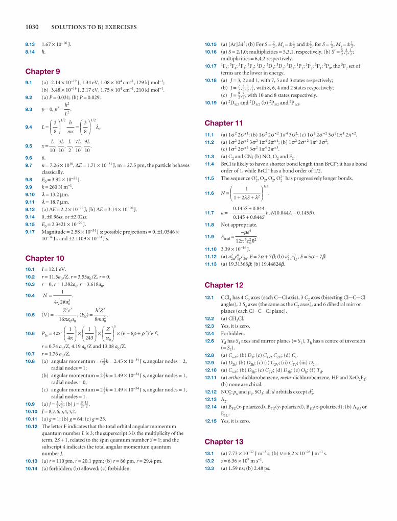
1030 SOLUTIONS TO B) EXERCISES
8.13 1.67 × 10⁻¹⁶ J.
8.14 $.
Chapter 99.1 (a) 2.14 × 10⁻¹⁹ J, 1.34 eV, 1.08 × 104 cm−1, 129 kJ mol−1;
(b) 3.48 × 10⁻¹⁹ J, 2.17 eV, 1.75 × 104 cm−1, 210 kJ mol−1.
9.2 (a) P = 0.031; (b) P = 0.029.
9.3 p = 0, p2 = .
9.4 L =1/2
=1/2
λc.
9.5 x = , , , , .
9.6 6.
9.7 n = 7.26 × 10¹⁰, ∆E = 1.71 × 10⁻³¹ J, m = 27.5 pm, the particle behavesclassically.
9.8 E0 = 3.92 × 10⁻²¹ J.
9.9 k = 260 N m−1.
9.10 λ = 13.2 µm.
9.11 λ = 18.7 µm.
9.12 (a) ∆E = 2.2 × 10⁻²⁹ J; (b) ∆E = 3.14 × 10⁻²⁰ J.
9.14 0, ±0.96α, or ±2.02α.
9.15 E0 = 2.3421 × 10⁻²⁰ J.
9.17 Magnitude = 2.58 × 10⁻³⁴ J s; possible projections = 0, ±1.0546 ×10⁻³⁴ J s and ±2.1109 × 10⁻³⁴ J s.
Chapter 1010.1 I = 12.1 eV.
10.2 r = 11.5a0 /Z, r = 3.53a0 /Z, r = 0.
10.3 r = 0, r = 1.382a0, r = 3.618a0.
10.4 .
10.5 �V� = − , �EK� = .
10.6 P3s = 4πr2 × ×3
× (6 − 6ρ + ρ2)2e−ρ,
r = 0.74 a0 /Z, 4.19 a0 /Z and 13.08 a0 /Z.
10.7 r = 1.76 a0 /Z.
10.8 (a) angular momentum = 6 1–2 h = 2.45 × 10⁻³⁴ J s, angular nodes = 2,
radial nodes = 1;
(b) angular momentum = 2 1–2 h = 1.49 × 10⁻³⁴ J s, angular nodes = 1,
radial nodes = 0;
(c) angular momentum = 2 1–2 h = 1.49 × 10⁻³⁴ J s, angular nodes = 1,
radial nodes = 1.
10.9 (a) j = 1–2 , 3–
2 ; (b) j = 9–2 ,11––
2 .
10.10 J = 8,7,6,5,4,3,2.
10.11 (a) g = 1; (b) g = 64; (c) g = 25.
10.12 The letter F indicates that the total orbital angular momentumquantum number L is 3; the superscript 3 is the multiplicity of theterm, 2S + 1, related to the spin quantum number S = 1; and thesubscript 4 indicates the total angular momentum quantum number J.
10.13 (a) r = 110 pm, r = 20.1 ppm; (b) r = 86 pm, r = 29.4 pm.
10.14 (a) forbidden; (b) allowed; (c) forbidden.
DEFZ
α0
ABCDEF
1
243
ABCDEF
1
4π
ABC
$2Z2
8ma02
Z2e2
16πε0a0
Na
=1
4 2 03π
9L
10
7L
10
L
2
3L
10
L
10
DEF3
8
ABCh
mc
DEF3
8
ABC
h2
L2
10.15 (a) [Ar]3d 3; (b) For S = 3–2 , Ms = ± 1–
2 and ± 3–2 , for S = 1–
2 , Ms = ± 1–2 .
10.16 (a) S = 2,1,0; multiplicities = 5,3,1, respectively. (b) S′ = 5–2 , 3–
2 , 1–2 ;
multiplicities = 6,4,2 respectively.
10.17 1F3; 3F4; 3F3; 3F2; 1D2; 3D3; 3D2; 3D1; 1P1; 3P2; 3P1; 3P0, the 3F2 set ofterms are the lower in energy.
10.18 (a) J = 3, 2 and 1, with 7, 5 and 3 states respectively;
(b) J = 7–2 , 5–
2 , 3–2 , 1–
2 , with 8, 6, 4 and 2 states respectively;
(c) J = 9–2 , 7–
2 , with 10 and 8 states respectively.
10.19 (a) 2D5/2 and 2D3/2 (b) 2P3/2 and 2P1/2.
Chapter 1111.1 (a) 1σ2 2σ*1; (b) 1σ2 2σ*2 1π4 3σ2; (c) 1σ2 2σ*2 3σ21π4 2π*2.
11.2 (a) 1σ2 2σ*2 3σ2 1π4 2π*4; (b) 1σ2 2σ*2 1π4 3σ2;(c) 1σ2 2σ*2 3σ2 1π4 2π*3.
11.3 (a) C2 and CN; (b) NO, O2 and F2.
11.4 BrCl is likely to have a shorter bond length than BrCl−; it has a bondorder of 1, while BrCl− has a bond order of 1/2.
11.5 The sequence O+2, O2, O−
2, O22− has progressively longer bonds.
11.6 N =1/2
.
11.7 a = − b, N(0.844A − 0.145B).
11.8 Not appropriate.
11.9 Etrial = .
11.10 3.39 × 10⁻¹⁶ J.
11.12 (a) a22ue4
1g e12u, E = 7α + 7β; (b) a2
2ue31g , E = 5α + 7β.
11.13 (a) 19.31368β; (b) 19.44824β.
Chapter 12
12.1 CCl4 has 4 C3 axes (each C-Cl axis), 3 C2 axes (bisecting Cl-C-Clangles), 3 S4 axes (the same as the C2 axes), and 6 dihedral mirrorplanes (each Cl-C-Cl plane).
12.2 (a) CH3Cl.
12.3 Yes, it is zero.
12.4 Forbidden.
12.6 Td has S4 axes and mirror planes (= S1), Th has a centre of inversion(= S2).
12.8 (a) C∞V; (b) D3; (c) C4V, C2V; (d) Cs.
12.9 (a) D2h; (b) D2h; (c) (i) C2V; (ii) C2V; (iii) D2h.
12.10 (a) C∞V; (b) D5h; (c) C2V; (d) D3h; (e) Oh; (f) Td.
12.11 (a) ortho-dichlorobenzene, meta-dichlorobenzene, HF and XeO2F2;(b) none are chiral.
12.12 NO3−: px and py, SO3: all d orbitals except d z
2.
12.13 A2.
12.14 (a) B3U(x-polarized), B2U(y-polarized), B1U(z-polarized); (b) A1U orE1U.
12.15 Yes, it is zero.
Chapter 1313.1 (a) 7.73 × 10⁻³² J m−3 s; (b) ν = 6.2 × 10⁻²⁸ J m−3 s.
13.2 s = 6.36 × 10⁷ m s−1.
13.3 (a) 1.59 ns; (b) 2.48 ps.
−µe4
12π3ε20 $2
0.145S + 0.844
0.145 + 0.844S
DEF1
1 + 2λS + λ2
ABC
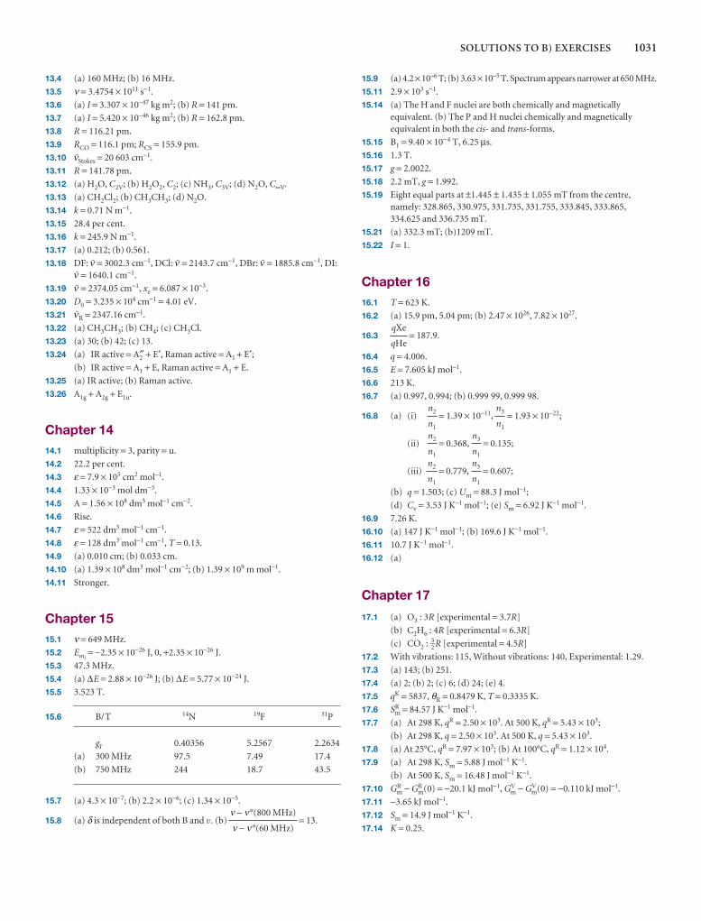
SOLUTIONS TO B) EXERCISES 1031
13.4 (a) 160 MHz; (b) 16 MHz.
13.5 ν = 3.4754 × 10¹¹ s−1.
13.6 (a) I = 3.307 × 10−47 kg m2; (b) R = 141 pm.
13.7 (a) I = 5.420 × 10−46 kg m2; (b) R = 162.8 pm.
13.8 R = 116.21 pm.
13.9 RCO = 116.1 pm; RCS = 155.9 pm.
13.10 ÄStokes = 20 603 cm−1.
13.11 R = 141.78 pm.
13.12 (a) H2O, C2V; (b) H2O2, C2; (c) NH3, C3V; (d) N2O, C∞V.
13.13 (a) CH2Cl2; (b) CH3CH3; (d) N2O.
13.14 k = 0.71 N m−1.
13.15 28.4 per cent.
13.16 k = 245.9 N m−1.
13.17 (a) 0.212; (b) 0.561.
13.18 DF: # = 3002.3 cm−1, DCl: # = 2143.7 cm−1, DBr: # = 1885.8 cm−1, DI:# = 1640.1 cm−1.
13.19 # = 2374.05 cm−1, xe = 6.087 × 10⁻³.
13.20 D0 = 3.235 × 104 cm−1 = 4.01 eV.
13.21 #R = 2347.16 cm−1.
13.22 (a) CH3CH3; (b) CH4; (c) CH3Cl.
13.23 (a) 30; (b) 42; (c) 13.
13.24 (a) IR active = A2″ + E′, Raman active = A1 + E′;(b) IR active = A1 + E, Raman active = A1 + E.
13.25 (a) IR active; (b) Raman active.
13.26 A1g + A2g + E1u.
Chapter 1414.1 multiplicity = 3, parity = u.
14.2 22.2 per cent.
14.3 ε = 7.9 × 105 cm2 mol−1.
14.4 1.33 × 10⁻³ mol dm−3.
14.5 A = 1.56 × 10⁸ dm3 mol−1 cm−2.
14.6 Rise.
14.7 ε = 522 dm3 mol−1 cm−1.
14.8 ε = 128 dm3 mol−1 cm−1, T = 0.13.
14.9 (a) 0.010 cm; (b) 0.033 cm.
14.10 (a) 1.39 × 10⁸ dm3 mol−1 cm−2; (b) 1.39 × 10⁹ m mol−1.
14.11 Stronger.
Chapter 1515.1 ν = 649 MHz.
15.2 EmI= −2.35 × 10⁻²⁶ J, 0, +2.35 × 10⁻²⁶ J.
15.3 47.3 MHz.
15.4 (a) ∆E = 2.88 × 10⁻²⁶ J; (b) ∆E = 5.77 × 10⁻²⁴ J.
15.5 3.523 T.
15.6 B/T 14N 19F 31P
gI 0.40356 5.2567 2.2634
(a) 300 MHz 97.5 7.49 17.4
(b) 750 MHz 244 18.7 43.5
15.7 (a) 4.3 × 10⁻⁷; (b) 2.2 × 10⁻⁶; (c) 1.34 × 10⁻⁵.
15.8 (a) δ is independent of both B and v. (b) = 13.ν − ν°(800 MHz)
ν − ν°(60 MHz)
15.9 (a) 4.2 × 10⁻⁶ T; (b) 3.63 × 10⁻⁵ T. Spectrum appears narrower at 650 MHz.
15.11 2.9 × 10³ s−1.
15.14 (a) The H and F nuclei are both chemically and magneticallyequivalent. (b) The P and H nuclei chemically and magneticallyequivalent in both the cis- and trans-forms.
15.15 B1 = 9.40 × 10⁻⁴ T, 6.25 µs.
15.16 1.3 T.
15.17 g = 2.0022.
15.18 2.2 mT, g = 1.992.
15.19 Eight equal parts at ±1.445 ± 1.435 ± 1.055 mT from the centre,namely: 328.865, 330.975, 331.735, 331.755, 333.845, 333.865,334.625 and 336.735 mT.
15.21 (a) 332.3 mT; (b)1209 mT.
15.22 I = 1.
Chapter 1616.1 T = 623 K.
16.2 (a) 15.9 pm, 5.04 pm; (b) 2.47 × 1026, 7.82 × 1027.
16.3 = 187.9.
16.4 q = 4.006.
16.5 E = 7.605 kJ mol−1.
16.6 213 K.
16.7 (a) 0.997, 0.994; (b) 0.999 99, 0.999 98.
16.8 (a) (i) = 1.39 × 10⁻¹¹, = 1.93 × 10⁻²²;
(ii) = 0.368, = 0.135;
(iii) = 0.779, = 0.607;
(b) q = 1.503; (c) Um = 88.3 J mol−1;
(d) Cv = 3.53 J K−1 mol−1; (e) Sm = 6.92 J K−1 mol−1.
16.9 7.26 K.
16.10 (a) 147 J K−1 mol−1; (b) 169.6 J K−1 mol−1.
16.11 10.7 J K−1 mol−1.
16.12 (a)
Chapter 17
17.1 (a) O3 : 3R [experimental = 3.7R]
(b) C2H6 : 4R [experimental = 6.3R]
(c) CO2 : 5–2 R [experimental = 4.5R]
17.2 With vibrations: 115, Without vibrations: 140, Experimental: 1.29.
17.3 (a) 143; (b) 251.
17.4 (a) 2; (b) 2; (c) 6; (d) 24; (e) 4.
17.5 qK = 5837, θR = 0.8479 K, T = 0.3335 K.
17.6 SRm = 84.57 J K−1 mol−1.
17.7 (a) At 298 K, qR = 2.50 × 10³. At 500 K, qR = 5.43 × 10³;
(b) At 298 K, q = 2.50 × 10³. At 500 K, q = 5.43 × 10³.
17.8 (a) At 25°C, qR = 7.97 × 10³; (b) At 100°C, qR = 1.12 × 10⁴.
17.9 (a) At 298 K, Sm = 5.88 J mol−1 K−1.
(b) At 500 K, Sm = 16.48 J mol−1 K−1.
17.10 GRm − GR
m(0) = −20.1 kJ mol−1, GVm − GV
m(0) = −0.110 kJ mol−1.
17.11 −3.65 kJ mol−1.
17.12 Sm = 14.9 J mol−1 K−1.
17.14 K ≈ 0.25.
n3
n1
n2
n1
n3
n1
n2
n1
n3
n1
n2
n1
qXe
qHe
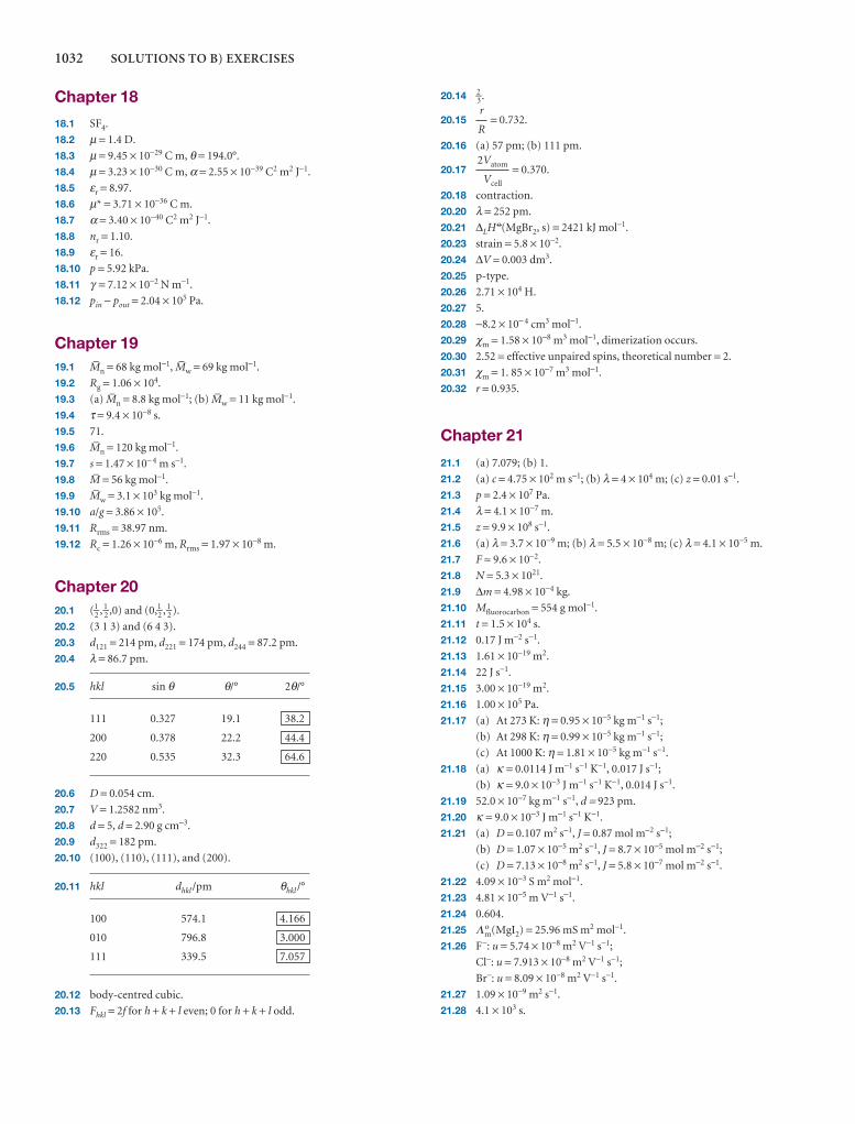
1032 SOLUTIONS TO B) EXERCISES
Chapter 18
18.1 SF4.
18.2 µ = 1.4 D.
18.3 µ = 9.45 × 10⁻²⁹ C m, θ = 194.0°.
18.4 µ = 3.23 × 10⁻³⁰ C m, α = 2.55 × 10−39 C2 m2 J−1.
18.5 εr = 8.97.
18.6 µ* = 3.71 × 10−36 C m.
18.7 α = 3.40 × 10−40 C2 m2 J−1.
18.8 nr = 1.10.
18.9 εr = 16.
18.10 p = 5.92 kPa.
18.11 γ = 7.12 × 10⁻² N m−1.
18.12 pin − pout = 2.04 × 10⁵ Pa.
Chapter 1919.1 •n = 68 kg mol−1, •w = 69 kg mol−1.
19.2 Rg = 1.06 × 10⁴.
19.3 (a) •n = 8.8 kg mol−1; (b) •w = 11 kg mol−1.
19.4 τ = 9.4 × 10⁻⁸ s.
19.5 71.
19.6 •n = 120 kg mol−1.
19.7 s = 1.47 × 10− 4 m s−1.
19.8 • = 56 kg mol−1.
19.9 •w = 3.1 × 10³ kg mol−1.
19.10 a/g = 3.86 × 10⁵.
19.11 Rrms = 38.97 nm.
19.12 Rc = 1.26 × 10⁻⁶ m, Rrms = 1.97 × 10⁻⁸ m.
Chapter 2020.1 (1–
2 , 1–2 ,0) and (0,1–2 , 1–
2 ).
20.2 (3 1 3) and (6 4 3).
20.3 d121 = 214 pm, d221 = 174 pm, d244 = 87.2 pm.
20.4 λ = 86.7 pm.
20.5 hkl sin θ θ/° 2θ/°
111 0.327 19.1 38.2
200 0.378 22.2 44.4
220 0.535 32.3 64.6
20.6 D = 0.054 cm.
20.7 V = 1.2582 nm3.
20.8 d = 5, d = 2.90 g cm−3.
20.9 d322 = 182 pm.
20.10 (100), (110), (111), and (200).
20.11 hkl dhkl /pm θhkl /°
100 574.1 4.166
010 796.8 3.000
111 339.5 7.057
20.12 body-centred cubic.
20.13 Fhkl = 2f for h + k + l even; 0 for h + k + l odd.
20.14 2–3.
20.15 = 0.732.
20.16 (a) 57 pm; (b) 111 pm.
20.17 = 0.370.
20.18 contraction.
20.20 λ = 252 pm.
20.21 ∆LH 7(MgBr2, s) = 2421 kJ mol−1.
20.23 strain = 5.8 × 10⁻².
20.24 ∆V = 0.003 dm3.
20.25 p-type.
20.26 2.71 × 10⁴ H.
20.27 5.
20.28 −8.2 × 10− 4 cm3 mol−1.
20.29 χm = 1.58 × 10⁻⁸ m3 mol−1, dimerization occurs.
20.30 2.52 = effective unpaired spins, theoretical number = 2.
20.31 χm = 1. 85 × 10−7 m3 mol−1.
20.32 r = 0.935.
Chapter 21
21.1 (a) 7.079; (b) 1.
21.2 (a) c = 4.75 × 10² m s−1; (b) λ = 4 × 10⁴ m; (c) z = 0.01 s−1.
21.3 p = 2.4 × 10⁷ Pa.
21.4 λ = 4.1 × 10⁻⁷ m.
21.5 z = 9.9 × 10⁸ s−1.
21.6 (a) λ = 3.7 × 10⁻⁹ m; (b) λ = 5.5 × 10⁻⁸ m; (c) λ = 4.1 × 10⁻⁵ m.
21.7 F ≈ 9.6 × 10⁻².
21.8 N = 5.3 × 10²¹.
21.9 ∆m = 4.98 × 10⁻⁴ kg.
21.10 Mfluorocarbon = 554 g mol−1.
21.11 t = 1.5 × 10⁴ s.
21.12 0.17 J m−2 s−1.
21.13 1.61 × 10⁻¹⁹ m2.
21.14 22 J s−1.
21.15 3.00 × 10⁻¹⁹ m2.
21.16 1.00 × 10⁵ Pa.
21.17 (a) At 273 K: η = 0.95 × 10⁻⁵ kg m−1 s−1;
(b) At 298 K: η = 0.99 × 10⁻⁵ kg m−1 s−1;
(c) At 1000 K: η = 1.81 × 10⁻⁵ kg m−1 s−1.
21.18 (a) κ = 0.0114 J m−1 s−1 K−1, 0.017 J s−1;
(b) κ = 9.0 × 10⁻³ J m−1 s−1 K−1, 0.014 J s−1.
21.19 52.0 × 10⁻⁷ kg m−1 s−1, d = 923 pm.
21.20 κ = 9.0 × 10⁻³ J m−1 s−1 K−1.
21.21 (a) D = 0.107 m2 s−1, J = 0.87 mol m−2 s−1;
(b) D = 1.07 × 10⁻⁵ m2 s−1, J = 8.7 × 10⁻⁵ mol m−2 s−1;
(c) D = 7.13 × 10⁻⁸ m2 s−1, J = 5.8 × 10⁻⁷ mol m−2 s−1.
21.22 4.09 × 10⁻³ S m2 mol−1.
21.23 4.81 × 10⁻⁵ m V−1 s−1.
21.24 0.604.
21.25 Λom(MgI2) = 25.96 mS m2 mol−1.
21.26 F−: u = 5.74 × 10⁻⁸ m2 V−1 s−1;
Cl−: u = 7.913 × 10⁻⁸ m2 V−1 s−1;
Br−: u = 8.09 × 10⁻⁸ m2 V−1 s−1.
21.27 1.09 × 10⁻⁹ m2 s−1.
21.28 4.1 × 10³ s.
2Vatom
Vcell
r
R
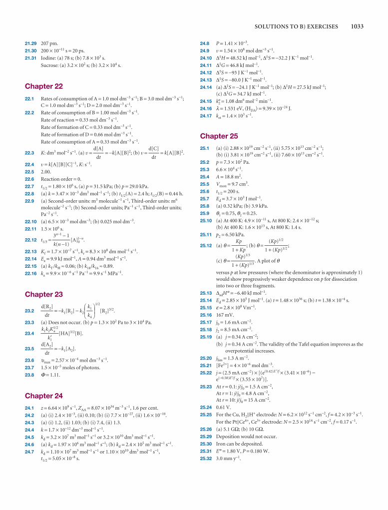
SOLUTIONS TO B) EXERCISES 1033
21.29 207 pm.
21.30 200 × 10−11 s = 20 ps.
21.31 Iodine: (a) 78 s; (b) 7.8 × 10³ s.
Sucrose: (a) 3.2 × 10² s; (b) 3.2 × 10⁴ s.
Chapter 22
22.1 Rates of consumption of A = 1.0 mol dm−3 s−1; B = 3.0 mol dm−3 s−1;C = 1.0 mol dm−3 s−1; D = 2.0 mol dm−3 s−1.
22.2 Rate of consumption of B = 1.00 mol dm−3 s−1.
Rate of reaction = 0.33 mol dm−3 s−1.
Rate of formation of C = 0.33 mol dm−3 s−1.
Rate of formation of D = 0.66 mol dm−3 s−1.
Rate of consumption of A = 0.33 mol dm−3 s−1.
22.3 K: dm3 mol−2 s−1. (a) v = = −k[A][B]2; (b) v = = k[A][B]2.
22.4 v = k[A][B][C]−1, K: s−1.
22.5 2.00.
22.6 Reaction order = 0.
22.7 t1/2 = 1.80 × 10⁶ s, (a) p = 31.5 kPa; (b) p = 29.0 kPa.
22.8 (a) k = 3.47 × 10⁻³ dm3 mol−1 s−1; (b) t1/2(A) = 2.4 h; t1/2(B) = 0.44 h.
22.9 (a) Second-order units: m3 molecule−1 s−1, Third-order units: m6
molecule−2 s−1; (b) Second-order units; Pa−1 s−1, Third-order units;Pa−2 s−1.
22.10 (a) 6.5 × 10⁻³ mol dm−3; (b) 0.025 mol dm−3.
22.11 1.5 × 10⁶ s.
22.12 t1/3 = [A]01−n.
22.13 Kf = 1.7 × 10⁻⁷ s−1, kr = 8.3 × 10⁸ dm mol−1 s−1.
22.14 Ea = 9.9 kJ mol−1, A = 0.94 dm3 mol−1 s−1.
22.15 (a) kT /kH ≈ 0.06; (b) k18/k16 ≈ 0.89.
22.16 ka = 9.9 × 10− 6 s−1 Pa−1 = 9.9 s−1 MPa−1.
Chapter 23
23.2 = −k1[R2] − k2
1/2
[R2]3/2.
23.3 (a) Does not occur. (b) p = 1.3 × 10² Pa to 3 × 10⁴ Pa.
23.4 [HA]3/2[B].
23.5 = −k1[A2].
23.6 υmax = 2.57 × 10⁻⁴ mol dm−3 s−1.
23.7 1.5 × 10⁻⁵ moles of photons.
23.8 Φ = 1.11.
Chapter 24
24.1 z = 6.64 × 10⁹ s−1, ZAA = 8.07 × 1034 m−3 s−1, 1.6 per cent.
24.2 (a) (i) 2.4 × 10⁻³, (ii) 0.10; (b) (i) 7.7 × 10⁻²⁷, (ii) 1.6 × 10⁻¹⁰.
24.3 (a) (i) 1.2, (ii) 1.03; (b) (i) 7.4, (ii) 1.3.
24.4 k = 1.7 × 10⁻¹² dm−3 mol−1 s−1.
24.5 kd = 3.2 × 10⁷ m3 mol−1 s−1 or 3.2 × 10¹⁰ dm3 mol−1 s−1.
24.6 (a) kd = 1.97 × 10⁶ m3 mol−1 s−1; (b) kd = 2.4 × 10⁵ m3 mol−1 s−1.
24.7 kd = 1.10 × 10⁷ m3 mol−1 s−1 or 1.10 × 10¹⁰ dm3 mol−1 s−1,t1/2 = 5.05 × 10⁻⁸ s.
d[A2]
dt
k1k2Ka1/2
k′1
DEFk1
k4
ABCd[R2]
dt
3n−1 − 1
k(n −1)
d[C]
dt
d[A]
dt
24.8 P = 1.41 × 10⁻³.
24.9 v = 1.54 × 10⁸ mol dm−3 s−1.
24.10 ∆‡H = 48.52 kJ mol−1, ∆‡S = −32.2 J K−1 mol−1.
24.11 ∆‡G = 46.8 kJ mol−1.
24.12 ∆‡S = −93 J K−1 mol−1.
24.13 ∆‡S = −80.0 J K−1 mol−1.
24.14 (a) ∆‡S = −24.1 J K−1 mol−1; (b) ∆‡H = 27.5 kJ mol−1;(c) ∆‡G = 34.7 kJ mol−1.
24.15 k°2 = 1.08 dm6 mol−2 min−1.
24.16 λ = 1.531 eV, �HDA� = 9.39 × 10⁻²⁴ J.
24.17 ket = 1.4 × 10³ s−1.
Chapter 25
25.1 (a) (i) 2.88 × 1019 cm−2 s−1, (ii) 5.75 × 1013 cm−2 s−1;(b) (i) 3.81 × 1019 cm−2 s−1, (ii) 7.60 × 1013 cm−2 s−1.
25.2 p = 7.3 × 10² Pa.
25.3 6.6 × 10⁴ s−1.
25.4 A = 18.8 m2.
25.5 Vmon = 9.7 cm3.
25.6 t1/2 = 200 s.
25.7 Ed = 3.7 × 10³ J mol−1.
25.8 (a) 0.32 kPa; (b) 3.9 kPa.
25.9 θ1 = 0.75, θ2 = 0.25.
25.10 (a) At 400 K: 4.9 × 10⁻¹¹ s, At 800 K: 2.4 × 10⁻¹² s;(b) At 400 K: 1.6 × 10¹³ s, At 800 K: 1.4 s.
25.11 p2 = 6.50 kPa.
25.12 (a) θ = ; (b) θ = ;
(c) θ = . A plot of θ
versus p at low pressures (where the denominator is approximately 1)would show progressively weaker dependence on p for dissociationinto two or three fragments.
25.13 ∆adH 7 = −6.40 kJ mol−1.
25.14 Ed = 2.85 × 10⁵ J mol−1. (a) t = 1.48 × 1036 s; (b) t = 1.38 × 10⁻⁴ s.
25.15 ε = 2.8 × 10⁸ Vm−1.
25.16 167 mV.
25.17 j0 = 1.6 mA cm−2.
25.18 j2 = 8.5 mA cm−2.
25.19 (a) j = 0.34 A cm−2;
(b) j = 0.34 A cm−2. The validity of the Tafel equation improves as the overpotential increases.
25.20 jlim = 1.3 A m−2.
25.21 [Fe2+] = 4 × 10⁻⁶ mol dm−3.
25.22 j = (2.5 mA cm−2) × [(e(0.42)E ′/f × (3.41 × 10⁻⁶) −e(−0.58)E′/f × (3.55 × 10⁷)].
25.23 At r = 0.1: j/j0 = 1.5 A cm−2,At r = 1: j/j0 = 4.8 A cm−2,At r = 10: j/j0 = 15 A cm−2.
25.24 0.61 V.
25.25 For the Cu, H2 |H+ electrode: N = 6.2 × 10¹² s−1 cm−2, f = 4.2 × 10⁻³ s−1.
For the Pt |Ce4+, Ce3+ electrode: N = 2.5 × 10¹⁴ s−1 cm−2, f = 0.17 s−1.
25.26 (a) 5.1 GΩ; (b) 10 GΩ.
25.29 Deposition would not occur.
25.30 Iron can be deposited.
25.31 E 7 = 1.80 V, P = 0.180 W.
25.32 3.0 mm y−1.
(Kp)1/3
1 + (Kp)1/3
(Kp)1/2
1 + (Kp)1/2
Kp
1 + Kp
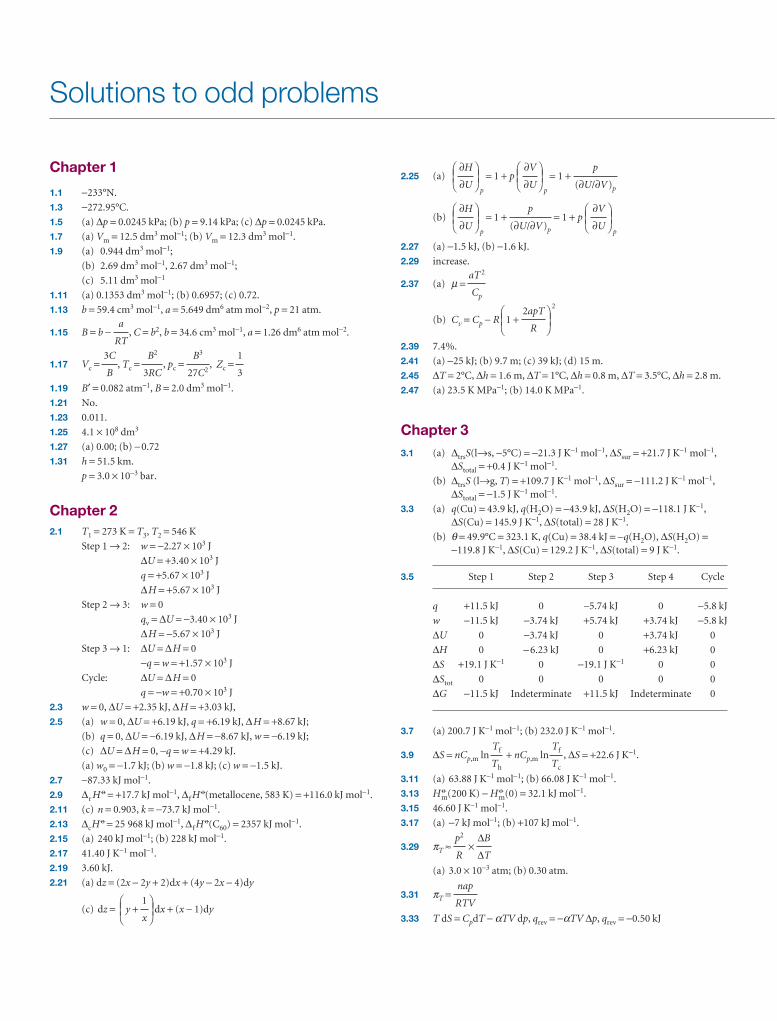
Chapter 1
1.1 −233°N.
1.3 −272.95°C.
1.5 (a) ∆p = 0.0245 kPa; (b) p = 9.14 kPa; (c) ∆p = 0.0245 kPa.
1.7 (a) Vm = 12.5 dm3 mol−1; (b) Vm = 12.3 dm3 mol−1.
1.9 (a) 0.944 dm3 mol−1;
(b) 2.69 dm3 mol−1, 2.67 dm3 mol−1;
(c) 5.11 dm3 mol−1
1.11 (a) 0.1353 dm3 mol−1; (b) 0.6957; (c) 0.72.
1.13 b = 59.4 cm3 mol−1, a = 5.649 dm6 atm mol−2, p = 21 atm.
1.15 B = b − , C = b2, b = 34.6 cm3 mol−1, a = 1.26 dm6 atm mol−2.
1.17 Vc = , Tc = , pc = , Zc =
1.19 B′ = 0.082 atm−1, B = 2.0 dm3 mol−1.
1.21 No.
1.23 0.011.
1.25 4.1 × 10⁸ dm3
1.27 (a) 0.00; (b) −0.72
1.31 h = 51.5 km.
p = 3.0 × 10⁻³ bar.
Chapter 22.1 T1 = 273 K = T3, T2 = 546 K
Step 1 → 2: w = −2.27 × 10³ J
∆U = +3.40 × 10³ J
q = +5.67 × 10³ J
∆H = +5.67 × 10³ J
Step 2 → 3: w = 0
qv = ∆U = −3.40 × 10³ J
∆H = −5.67 × 10³ J
Step 3 → 1: ∆U = ∆H = 0
−q = w = +1.57 × 10³ J
Cycle: ∆U = ∆H = 0
q = −w = +0.70 × 10³ J
2.3 w = 0, ∆U = +2.35 kJ, ∆H = +3.03 kJ,
2.5 (a) w = 0, ∆U = +6.19 kJ, q = +6.19 kJ, ∆H = +8.67 kJ;
(b) q = 0, ∆U = −6.19 kJ, ∆H = −8.67 kJ, w = −6.19 kJ;
(c) ∆U = ∆H = 0, −q = w = +4.29 kJ.
(a) w0 = −1.7 kJ; (b) w = −1.8 kJ; (c) w = −1.5 kJ.
2.7 −87.33 kJ mol−1.
2.9 ∆r H 7 = +17.7 kJ mol−1, ∆f H7(metallocene, 583 K) = +116.0 kJ mol−1.
2.11 (c) n = 0.903, k = −73.7 kJ mol−1.
2.13 ∆cH 7 = 25 968 kJ mol−1, ∆f H7(C60) = 2357 kJ mol−1.
2.15 (a) 240 kJ mol−1; (b) 228 kJ mol−1.
2.17 41.40 J K−1 mol−1.
2.19 3.60 kJ.
2.21 (a) dz = (2x − 2y + 2)dx + (4y − 2x − 4)dy
(c) dz = y + dx + (x − 1)dyDEF
1
x
ABC
1
3
B3
27C2
B2
3RC
3C
B
a
RT
Solutions to odd problems
2.25 (a)p
= 1 + pp
= 1 +
(b)p
= 1 + = 1 + pp
2.27 (a) −1.5 kJ, (b) −1.6 kJ.
2.29 increase.
2.37 (a) µ =
(b) Cv = Cp − R 1 + 2
2.39 7.4%.
2.41 (a) −25 kJ; (b) 9.7 m; (c) 39 kJ; (d) 15 m.
2.45 ∆T = 2°C, ∆h = 1.6 m, ∆T = 1°C, ∆h = 0.8 m, ∆T = 3.5°C, ∆h = 2.8 m.
2.47 (a) 23.5 K MPa−1; (b) 14.0 K MPa−1.
Chapter 33.1 (a) ∆trsS(l→s, −5°C) = −21.3 J K−1 mol−1, ∆Ssur = +21.7 J K−1 mol−1,
∆Stotal = +0.4 J K−1 mol−1.
(b) ∆trsS (l→g, T) = +109.7 J K−1 mol−1, ∆Ssur = −111.2 J K−1 mol−1,∆Stotal = −1.5 J K−1 mol−1.
3.3 (a) q(Cu) = 43.9 kJ, q(H2O) = −43.9 kJ, ∆S(H2O) = −118.1 J K−1,∆S(Cu) = 145.9 J K−1, ∆S(total) = 28 J K−1.
(b) θ = 49.9°C = 323.1 K, q(Cu) = 38.4 kJ = −q(H2O), ∆S(H2O) =−119.8 J K−1, ∆S(Cu) = 129.2 J K−1, ∆S(total) = 9 J K−1.
3.5 Step 1 Step 2 Step 3 Step 4 Cycle
q +11.5 kJ 0 –5.74 kJ 0 −5.8 kJ
w −11.5 kJ −3.74 kJ +5.74 kJ +3.74 kJ −5.8 kJ
∆U 0 −3.74 kJ 0 +3.74 kJ 0
∆H 0 −6.23 kJ 0 +6.23 kJ 0
∆S +19.1 J K−1 0 −19.1 J K−1 0 0
∆Stot 0 0 0 0 0
∆G −11.5 kJ Indeterminate +11.5 kJ Indeterminate 0
3.7 (a) 200.7 J K−1 mol−1; (b) 232.0 J K−1 mol−1.
3.9 ∆S = nCp,m ln + nCp,m ln , ∆S = +22.6 J K−1.
3.11 (a) 63.88 J K−1 mol−1; (b) 66.08 J K−1 mol−1.
3.13 H 7m(200 K) − H 7
m(0) = 32.1 kJ mol−1.
3.15 46.60 J K−1 mol−1.
3.17 (a) −7 kJ mol−1; (b) +107 kJ mol−1.
3.29 πT ≈ ×
(a) 3.0 × 10⁻³ atm; (b) 0.30 atm.
3.31 πT =
3.33 T dS = CpdT − αTV dp, qrev = −αTV ∆p, qrev = −0.50 kJ
nap
RTV
∆B
∆T
p2
R
Tf
Tc
Tf
Th
DEF2apT
R
ABC
aT 2
Cp
DEF∂V
∂U
ABCp
(∂U/∂V)p
DEF∂H
∂U
ABC
p
(∂U/∂V)p
DEF∂V
∂U
ABCDEF
∂H
∂U
ABC
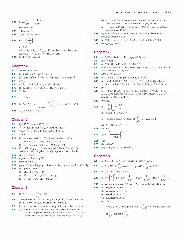
SOLUTIONS TO ODD PROBLEMS 1035
3.35 lnφ = + + . . .
f = 0.9991 atm
3.37 −21 kJ mol−1.
3.39 13 per cent increase.
3.43 ε = 1 − 1/c
ε = 0.47
∆S1 = ∆S3 = ∆Ssur,1 = ∆Ssur,2 = 0 [adiabatic reversible steps]
∆S2 = ∆Ssur,4 = +33 J K−1 = −∆Ssur,2 = −∆S4
3.45 (a) 1.00 kJ; (b) 8.4 kJ.
Chapter 44.1 196.0 K, 11.1 Torr.
4.3 (a) 5.56 kPa K−1 ; (b) 2.5 per cent.
4.5 (a) −1.63 cm3 mol−1 ; (b) +30.1 dm3 mol−1, +0.6 kJ mol−1.
4.7 22°C.
4.9 (a) Tb = 227.5°C; (b) ∆vapH = +53 kJ mol−1;
4.11 (b) 171.18 K; (c) T = 383.6 K; (d) 33.0 kJ mol−1.
4.15 9.8 Torr.
4.17 − × Cp,m.
4.21 (a) ∆Ur(Tr,Vr) = −�∞
Trconstant
dVr; (c) 0.85 to 0.90.
4.23 ∆ vapH = 1.60 × 10⁴ bar.
Chapter 55.1 kA = 15.58 kPa, kB = 47.03 kPa.
5.3 Vsalt = −1.4 cm3 mol−1, VH20 = 18.04 cm3 mol−1.
5.5 VE = 57.9 cm3, VW = 45.8 cm3, ∆V = +0.96 cm3.
5.7 4 ions.
5.11 (a) propionic acid: V1 = Vm,1 + a0x22 + a1(3x1 − x2)x 2
2,
oxane: V2 = Vm,2 + a0x21 + a1(x1 − 3x2)x2
1,
(b) V1 = 75.63 cm3 mol−1, V2 = 99.06 cm3 mol−1.
5.13 KH = 371 bar, γCO2= 1.01 (at 10p/bar), 0.99(at 20p/bar), 1.00(at
30p/bar), 0.99 (at 40p/bar), 0.98(at 60p/bar), 0.94 (at 80p/bar).
5.15 ∆mixG = −4.6 kJ.
5.17 µA = µA* + RT lnxA + gRTx2B
5.19 80.36 cm3 mol−1.
5.25 pN2at 4.0 atm = 56 µg, pN2
at 1.0 atm = 14 µg, increase = 1.7 × 10² µg N2.
5.29 (a) g cm K−1 mol−1,
(b) M = 1.1 × 10⁵ g mol−1,
(d) B′ = 21.4 cm3 g−1, C′ = 211 cm6 g−2,
(e) B′ = 28.0 cm3 g−1, C′ = 196 cm6 g−2.
Chapter 6
6.1 (b) 391.0 K; (c) = 0.532.
6.3 Temperature (γO2): 0.877 (78 K), 1.079 (80 K), 1.039 (82 K), 0.995
(84 K), 0.993 (86 K), 0.990 (88 K), 0.987 (90.2 K).
6.7 MgCu2: 16 per cent mg by mass, Mg2Cu: 43 per cent mg by mass.
6.9 (a) Eutectic: 40.2 at per cent Si at 1268°C; 69.4 at per cent Si at1030°C. Congruent melting compounds: Ca2Si = 1314°C; CaSi =1324°C. Incongruent melting compounds: CaSi2 = 1040°C;
nliq
nvap
2pr(Tr,Vr)
TrVr
1
T
DEFVB
VA
ABC
(C − B2)p2
2R2T 2
Bp
RT
(b) At 1000°C, the phases at equilibrium will be Ca(s) and liquid (13 at per cent Si). Relative amounts, nCa /nliq = 2.86;
(c) (i) nSi/nliq = 0.53 at slightly above 1030°C, (ii) nSi/nCaSi2= 0.665
slightly below 1030°C.
6.13 (i) Below a denaturant concentration of 0.1 only the native andunfolded forms are stable.
6.19 (a) 2150°C (b) y(MgO) = 0.18, x(MgO) = 0.35, (c) c = 2640°C.
6.21 (b) nliq/nvap = 10.85.
Chapter 77.1 (a) ∆rG
7 = +4.48 kJ mol−1; (b) pIBr = 0.101 atm.
7.3 ∆fH7 = 8.48 R.
7.5 ∆rG7 (T)/(kJ mol−1) = 78 − 0.161 × (T/K).
7.7 First experiment, K = 0.740, second experiment, K = 5.71, enthalpy ofdimerization = −103 kJ mol−1.
7.9 ∆H 7 = +158 kJ mol−1.
7.11 (a) At 298 K: 1.2 × 10⁸; (b) At 700 K: 2.7 × 10³.
7.13 (a) CuSO4: 4.0 × 10⁻³; ZnSO4: 1.2 × 10⁻²; (b) γ± (CuSO4) = 0.74,γ± (ZnSO4) = 0.60; (c) Q = 5.9; (d) E 7 = +1.102 V; (e) E = +1.079 V.
7.15 pH = 2.0.
7.17 E 7 = +0.268 43 V, γ± = 0.9659 (1.6077 mmol kg−1), 0.9509 (3.0769mmol kg−1), 0.9367 (5.0403 mmol kg−1), 0.9232 (7.6938 mmol kg−1),0.9094 (10.9474 mmol kg−1),
7.19 γ = 0.533.
7.21 (a)T ,n
= − ;
(b) 2.80 × 10⁻³ mV atm−1;
(c) the linear fit and constancy of are very good;
(d) 3.2 × 10⁻⁷ atm−1.
7.23 −1.15 V.
7.25 ξ = 1 − 1/2
7.31 Yes.
7.33 (b) +0.206 V.
7.35 (iv) HNO3·3H2O is most stable.
Chapter 88.1 (a) ∆E = 1.6 × 1033 J m−3; (b) ∆E = 2.5 × 10⁻⁴ J m−3.
8.3 (a) θ E = 2231 K, = 0.031; (b) θ E = 343 K, = 0.897.
8.5 (a) 9.0 × 10⁻⁶; (b) 1.2 × 10⁻⁶.
8.13 (a) N =1/2
; (b) N = ; (c) N = ; (d) N = .
8.15 (a) Yes, eigenvalue = ik; (b) No; (c) Yes, eigenvalue = 0; (d) No; (e) No.
8.17 (a) Yes, eigenvalue = −k2;
(b) Yes, eigenvalue = −k2;
(c) Yes, eigenvalue = 0;
(d) Yes, eigenvalue = 0;
(e) No.
Hence, (a,b,c,d) are eigenfunctions of ; (b,d) are eigenfunctions
of , but not of .d
dx
d2
dx 2
d2
dx 2
1
(32πa5)1/2
1
(πa3)1/2
1
c(2L)1/2
DEF2
L
ABC
CV
3R
CV
3R
DEF1
1 + ap/p7
ABC
DEF∂E
∂p
ABC
∆rV
νF
DEF∂E
∂p
ABC
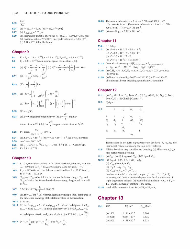
1036 SOLUTIONS TO ODD PROBLEMS
8.19 .
8.21 (a) r = 6a0, r2 = 42a02; (b) r = 5a0, r 2 = 30a0
2.
8.27 (a) λrelativistic = 5.35 pm.
8.29 (a) Methane is unstable above 825 K; (b) λmax (1000 K) = 2880 nm;(c) Excitance ratio = 7.7 × 10⁻⁴; Energy density ratio = 8.8 × 10⁻³;(d) 2.31 × 10⁻⁷, it hardly shines.
Chapter 99.1 E2 − E1 = 1.24 × 10−39 J, n = 2.2 × 10⁹ J, En − En−1 = 1.8 × 10⁻³⁰ J.
9.3 E1 = 1.30 × 10⁻²² J, minimum angular momentum = ±η.
9.5 (a) E1(1) = + sin ; (b) E 1
(1) = + sin = 0.1984ε.
9.11 (a) P = ; (b) �x� = .
9.13 �T� = v + $ω.
9.15 (a) δx = L −1/2
, δp = ;
(b) δx = v +1/2
, δp = v + $ωm
1/2
.
9.19 �T� = −1–2�V�.
9.23 (a) E = 0, angular momentum = 0; (b) E = , angular
momentum = 61/2$; (c) E = , angular momentum = .
9.25 θ = arccos , 54°44′.
9.31 (a) ∆E = 3.3 × 10⁻¹⁹ J; (b) v = 4.95 × 10⁻¹⁴ J s−1; (c) lower, increases.
9.33 ω = 2.68 × 10⁻¹⁴ J s−1.
9.35 (a) lz = 5.275 × 10⁻³⁴ J s, E±5 = 1.39 × 10⁻²⁴ J; (b) v = 9.2 × 10⁸ Hz.
9.37 F = 5.8 × 10⁻¹¹ N.
Chapter 1010.1 n2 → 6, transitions occur at 12 372 nm, 7503 nm, 5908 nm, 5129 nm,
. . . , 3908 nm (at n2 = 15), converging to 3282 nm as n2 → ∞.
10.3 RLi2+ = 987 663 cm−1, the Balmer transitions lie at # = 137 175 cm−1,85 187 cm−1, 122.5 eV.
10.5 2P1/2 and 2P3/2, of which the former has the lower energy, 2P3/2 and2P5/2 of which the former has the lower energy, the ground state willbe 2P3/2.
10.7 3.3429 × 10⁻²⁴ kg, = 1.000 272.
10.9 (a) ∆# = 0.9 cm−1, (b) Normal Zeeman splitting is small compared tothe difference in energy of the states involved in the transition.
10.11 ±106 pm.
10.13 (b) For 3s, ρnode = 3 + √3 and ρnode = 3 − √3, no nodal plane; for 3px,
ρnode = 0 and ρnode = 4, yz nodal plane (φ = 90°); for 3dxy, ρnode = 0,
xz nodal plane (φ = 0) and yz nodal plane (φ = 90°); (c) (r)3s = .
10.17 �r−1�1s = ; (b) �r−1�2s = ; (c) �r−1�2p = .Z
4a0
Z
4a0
Z
a0
27a0
2
ID
IH
ml
{l(l + 1)}1/2
2 3$6$2
I
3$2
I
JKL
DEF1
2
ABCGHI
JKL
$
ωm
DEF1
2
ABCGHI
nh
2L
DEF1
2π2n2
1
12
ABC
DEF1
2
ABC1
2
N 2
4κ2
N 2
2κ
DEFπ10
ABCεπ
ε10
DEFπa
L
ABCεπ
εa
L
$2k2
2m
10.25 The wavenumbers for n = 3 → n = 2: 4He = 60 957.4 cm−1,3He = 60 954.7 cm−1. The wavenumbers for n = 2 → n = 1: 4He =329 170 cm−1, 3He = 329 155 cm−1.
10.27 (a) receeding; s = 3.381 × 10⁵ ms−1.
Chapter 1111.3 R = 2.1a0.
11.7 (a) P = 8.6 × 10⁻⁷ / P = 2.0 × 10− 6;
(b) P = 8.6 × 10⁻⁷ / P = 2.0 × 10− 6;(c) P = 3.7 × 10⁻⁷ / P = 0;
(d) P = 4.9 × 10⁻⁷/ P = 5.5 × 10⁻⁷.
11.13 Delocalization energy = 2{Ewith resonance − Ewithout resonance}
= {(αO − αN)2 + 12β2}1/2 − {(αO − αN)2 + 4β2}1/2
11.15 (a) C2H4: −3.813, C4H6: −4.623, C6H8: −5.538, C8H10: −5.873;(b) 8.913 eV.
11.29 (a) linear relationship; (b) E 7 = −0.122 V; (c) E 7 = −0.174 V,ubiquinone a better oxidizing agent than plastiquinone.
Chapter 1212.1 (a) D3d; (b) chair: D3d, boat: C2V; (c) D2h; (d) D3; (d) D4d; (i) Polar:
Boat C6H12; (ii) Chiral: [Co(en)3]3+.
12.3 C2σh = i.
12.7 1 σx σy σz
1 1 σx σy σz
σx σx 1 iσx −iσy
σy σy − 1 iσx
iσz
σz σz iσy − 1
iσz
The matrices do not form a group since the products iσz, iσy, iσx andtheir negatives are not among the four given matrices.
12.9 All five d orbitals may contribute to bonding. (b) All except A2(dxy)may participate in bonding.
12.11 (a) D2h ; (b) (i) Staggered: C2h; (ii) Eclipsed: C2V.
12.13 (a) C2V, f → 2A1 + A2 + 2B1 + 2B2;
(b) C3V, f → + A2 + 3E;
(c) Td, f → A1 + T1 + T2;
(d) Oh, f → A2U + T1U + T2U.
Lanthanide ion (a) tetrahedral complex: f → A1 + T1 + T2 in Td
symmetry, and there is one nondegenerate orbital and two sets oftriply degenerate orbitals. (b) octahedral complex: f → A2U + T1U +T2U, and the pattern of splitting is the same.
12.15 irreducible representations: 4A1 + 2B1 + 3B2 + A2
Chapter 13
13.1 T/K E/J m−3 Eclass/J m−3
(a) 1500 2.136 × 10⁻⁶ 2.206
(b) 2500 9.884 × 10⁻⁴ 3.676
(c) 5800 3.151 × 10⁻¹ 8.528
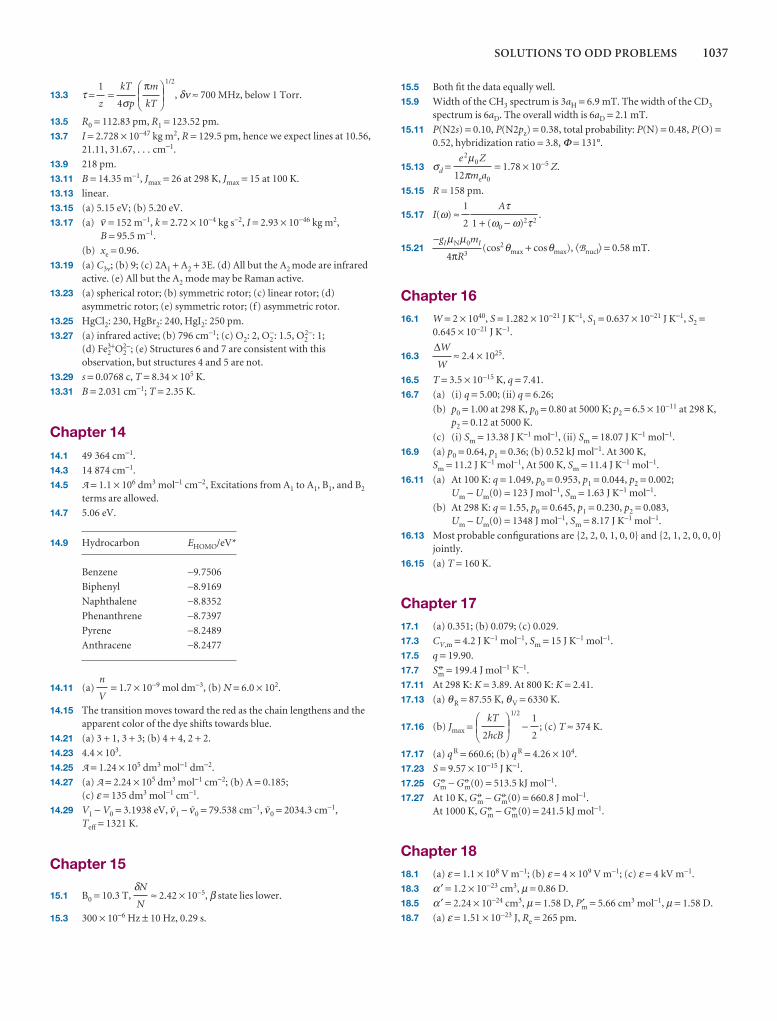
SOLUTIONS TO ODD PROBLEMS 1037
13.3 τ = =1/2
, δν ≈ 700 MHz, below 1 Torr.
13.5 R0 = 112.83 pm, R1 = 123.52 pm.
13.7 I = 2.728 × 10−47 kg m2, R = 129.5 pm, hence we expect lines at 10.56,21.11, 31.67, . . . cm−1.
13.9 218 pm.
13.11 B = 14.35 m−1, Jmax = 26 at 298 K, Jmax = 15 at 100 K.
13.13 linear.
13.15 (a) 5.15 eV; (b) 5.20 eV.
13.17 (a) # = 152 m−1, k = 2.72 × 10⁻⁴ kg s−2, I = 2.93 × 10−46 kg m2,B = 95.5 m−1.
(b) xe = 0.96.
13.19 (a) C3v; (b) 9; (c) 2A1 + A2 + 3E. (d) All but the A2 mode are infraredactive. (e) All but the A2 mode may be Raman active.
13.23 (a) spherical rotor; (b) symmetric rotor; (c) linear rotor; (d)asymmetric rotor; (e) symmetric rotor; (f) asymmetric rotor.
13.25 HgCl2: 230, HgBr2: 240, HgI2: 250 pm.
13.27 (a) infrared active; (b) 796 cm−1; (c) O2: 2, O2−: 1.5, O2
2−: 1; (d) Fe2
3+O22−; (e) Structures 6 and 7 are consistent with this
observation, but structures 4 and 5 are not.
13.29 s = 0.0768 c, T = 8.34 × 10⁵ K.
13.31 B = 2.031 cm−1; T = 2.35 K.
Chapter 14
14.1 49 364 cm−1.
14.3 14 874 cm−1.
14.5 A = 1.1 × 10⁶ dm3 mol−1 cm−2, Excitations from A1 to A1, B1, and B2
terms are allowed.
14.7 5.06 eV.
14.9 Hydrocarbon EHOMO/eV*
Benzene −9.7506
Biphenyl −8.9169
Naphthalene −8.8352
Phenanthrene −8.7397
Pyrene −8.2489
Anthracene −8.2477
14.11 (a) = 1.7 × 10⁻⁹ mol dm−3, (b) N = 6.0 × 10².
14.15 The transition moves toward the red as the chain lengthens and theapparent color of the dye shifts towards blue.
14.21 (a) 3 + 1, 3 + 3; (b) 4 + 4, 2 + 2.
14.23 4.4 × 10³.
14.25 A = 1.24 × 10⁵ dm3 mol−1 dm−2.
14.27 (a) A = 2.24 × 10⁵ dm3 mol−1 cm−2; (b) A = 0.185;(c) ε = 135 dm3 mol−1 cm−1.
14.29 V1 − V0 = 3.1938 eV, #1 − #0 = 79.538 cm−1, #0 = 2034.3 cm−1,Teff = 1321 K.
Chapter 15
15.1 B0 = 10.3 T, ≈ 2.42 × 10⁻⁵, β state lies lower.
15.3 300 × 10−6 Hz ± 10 Hz, 0.29 s.
δN
N
n
V
DEFπm
kT
ABCkT
4σp
1
z
15.5 Both fit the data equally well.
15.9 Width of the CH3 spectrum is 3aH = 6.9 mT. The width of the CD3
spectrum is 6aD. The overall width is 6aD = 2.1 mT.
15.11 P(N2s) = 0.10, P(N2pz) = 0.38, total probability: P(N) = 0.48, P(O) =0.52, hybridization ratio = 3.8, Φ = 131°.
15.13 σd = = 1.78 × 10⁻⁵ Z.
15.15 R = 158 pm.
15.17 I(ω) ≈ .
15.21 (cos2θmax + cosθmax), �Bnucl� = 0.58 mT.
Chapter 1616.1 W = 2 × 1040, S = 1.282 × 10⁻²¹ J K−1, S1 = 0.637 × 10⁻²¹ J K−1, S2 =
0.645 × 10⁻²¹ J K−1.
16.3 ≈ 2.4 × 1025.
16.5 T = 3.5 × 10⁻¹⁵ K, q = 7.41.
16.7 (a) (i) q = 5.00; (ii) q = 6.26;
(b) p0 = 1.00 at 298 K, p0 = 0.80 at 5000 K; p2 = 6.5 × 10⁻¹¹ at 298 K, p2 = 0.12 at 5000 K.
(c) (i) Sm = 13.38 J K−1 mol−1, (ii) Sm = 18.07 J K−1 mol−1.
16.9 (a) p0 = 0.64, p1 = 0.36; (b) 0.52 kJ mol−1. At 300 K, Sm = 11.2 J K−1 mol−1, At 500 K, Sm = 11.4 J K−1 mol−1.
16.11 (a) At 100 K: q = 1.049, p0 = 0.953, p1 = 0.044, p2 = 0.002;Um − Um(0) = 123 J mol−1, Sm = 1.63 J K−1 mol−1.
(b) At 298 K: q = 1.55, p0 = 0.645, p1 = 0.230, p2 = 0.083,Um − Um(0) = 1348 J mol−1, Sm = 8.17 J K−1 mol−1.
16.13 Most probable configurations are {2, 2, 0, 1, 0, 0} and {2, 1, 2, 0, 0, 0}jointly.
16.15 (a) T = 160 K.
Chapter 1717.1 (a) 0.351; (b) 0.079; (c) 0.029.
17.3 CV,m = 4.2 J K−1 mol−1, Sm = 15 J K−1 mol−1.
17.5 q = 19.90.
17.7 S 7m = 199.4 J mol−1 K−1.
17.11 At 298 K: K = 3.89. At 800 K: K = 2.41.
17.13 (a) θR = 87.55 K, θV = 6330 K.
17.16 (b) Jmax =1/2
− ; (c) T ≈ 374 K.
17.17 (a) q R = 660.6; (b) q R = 4.26 × 10⁴.
17.23 S = 9.57 × 10⁻¹⁵ J K−1.
17.25 G 7m − G 7
m(0) = 513.5 kJ mol−1.
17.27 At 10 K, G 7m − G 7
m(0) = 660.8 J mol−1.At 1000 K, G 7
m − G 7m(0) = 241.5 kJ mol−1.
Chapter 1818.1 (a) ε = 1.1 × 10⁸ V m−1; (b) ε = 4 × 10⁹ V m−1; (c) ε = 4 kV m−1.
18.3 α′ = 1.2 × 10⁻²³ cm3, µ = 0.86 D.
18.5 α′ = 2.24 × 10⁻²⁴ cm3, µ = 1.58 D, P′m = 5.66 cm3 mol−1, µ = 1.58 D.
18.7 (a) ε = 1.51 × 10⁻²³ J, Re = 265 pm.
1
2
DEFkT
2hcB
ABC
∆W
W
−gIµNµ0mI
4πR3
Aτ1 + (ω0 − ω)2τ2
1
2
e 2µ0 Z
12πmea0
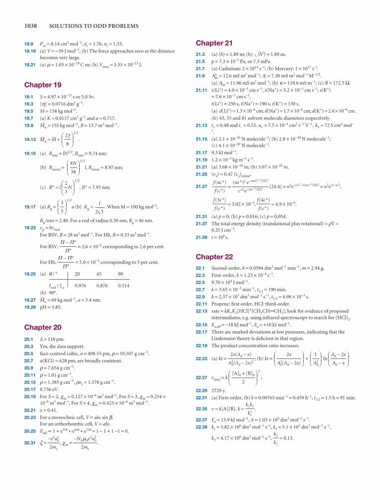
1038 SOLUTIONS TO ODD PROBLEMS
18.9 Pm = 8.14 cm3 mol−1, εr = 1.76, nr = 1.33.
18.19 (a) V = −39 J mol−1, (b) The force approaches zero as the distancebecomes very large.
18.21 (a) µ = 1.03 × 10⁻²⁹ C m; (b) Vmax = 3.55 × 10⁻²³ J.
Chapter 19
19.1 S = 4.97 × 10⁻¹³ s or 5.0 Sv.
19.3 [η] = 0.0716 dm3 g−1.
19.5 M = 158 kg mol−1.
19.7 (a) K = 0.0117 cm3 g−1 and a = 0.717.
19.9 •n = 155 kg mol−1, B = 13.7 m3 mol−1.
19.13 •n ≈ • +1/2
.
19.15 (a) Rrms = lN1/2, Rrms = 9.74 nm;
(b) Rmean =1/2
l, Rmean = 8.97 nm;
(c) R* = l N
1/2
, R* = 7.95 nm;
19.17 (a) Rg =1/2
a (b) . When M = 100 kg mol−1,
Rg /nm = 2.40. For a rod of radius 0.50 nm, Rg = 46 nm.
19.23 vp = 8vmol
For BSV, B = 28 m3 mol−1. For Hb, B = 0.33 m3 mol−1.
For BSV, = 2.6 × 10⁻² corresponding to 2.6 per cent.
For Hb, = 5.0 × 10⁻² corresponding to 5 per cent.
19.25 (a) θ / ° 20 45 90
Irod / Icc 0.976 0.876 0.514
(b) 90°.
19.27 •n = 69 kg mol−1, a = 3.4 nm.
19.29 pH = 3.85.
Chapter 20
20.1 λ = 118 pm.
20.3 Yes, the data support.
20.5 face-centred cubic, a = 408.55 pm, ρ = 10.507 g cm−3.
20.7 a(KCl) = 628 pm, are broadly conistent.
20.9 ρ = 7.654 g cm−3.
20.11 ρ = 1.01 g cm−3.
20.15 ρ = 1.385 g cm−3, ρos = 1.578 g cm−3.
20.17 0.736 eV.
20.19 For S = 2, χm = 0.127 × 10⁻⁶ m3 mol−1, For S = 3, χm = 0.254 ×10⁻⁶ m3 mol−1, For S = 4, χm = 0.423 × 10⁻⁶ m3 mol−1.
20.21 x = 0.41.
20.23 For a monoclinic cell, V = abc sin β.For an orthorhombic cell, V = abc.
20.25 Fhkl ∝ 1 + e5iπ + e6iπ + e7iπ = 1 − 1 + 1 −1 = 0.
20.31 ξ = , χm = .−NAµ0e2a2
0
2me
−e2a20
2me
Π − Π°
Π°
Π − Π°
Π°
Rl
g =2 3
DEF3
5
ABC
DEF2
3
ABC
DEF8N
3π
ABC
DEF2γπ
ABC
Chapter 2121.3 (a) �h� = 1.89 m; (b) = 1.89 m.
21.5 p = 7.3 × 10⁻³ Pa, or 7.3 mPa.
21.7 (a) Cadmium: 2 × 10¹⁴ s−1; (b) Mercury: 1 × 10¹⁷ s−1.
21.9 Λ°m = 12.6 mS m2 mol−1; K = 7.30 mS m2 mol−1 M−1/2.
(a) Λm = 11.96 mS m2 mol−1; (b) κ = 119.6 mS m−1; (c) R = 172.5 Ω.
21.11 s(Li+) = 4.0 × 10⁻³ cm s−1, s(Na+) = 5.2 × 10⁻³ cm s−1; s(K+)= 7.6 × 10⁻³ cm s−1.
t(Li+) = 250 s, t(Na+) = 190 s, t(K+) = 130 s.
(a) d(Li+) = 1.3 × 10⁻⁶ cm; d(Na+) = 1.7 × 10⁻⁶ cm; d(K+) = 2.4 × 10⁻⁶ cm.
(b) 43, 55 and 81 solvent molecule diameters respectively.
21.13 t+ = 0.48 and t− = 0.52. u+ = 7.5 × 10⁻⁴ cm2 s−1 V−1. λ+ = 72 S cm2 mol−1.
21.15 (a) 2.1 × 10⁻²⁰ N molecule−1; (b) 2.8 × 10⁻²⁰ N molecule−1;(c) 4.1 × 10⁻²⁰ N molecule−1.
21.17 9.3 kJ mol−1.
21.19 1.2 × 10⁻³ kg m−1 s−1.
21.21 (a) 3.68 × 10⁻¹⁰ m; (b) 3.07 × 10⁻¹⁰ m.
21.25 �vx� = 0.47 �vx�initial.
21.27 = [24.4] = n2e−(n2−1)mc*2/2kT = n2e(1−n2),
= 3.02 × 10⁻³, = 4.9 × 10⁻⁶.
21.31 (a) p = 0; (b) p = 0.016; (c) p = 0.054.
21.37 The total energy density (translational plus rotational) = ρT =0.25 J cm−3.
21.39 t = 108 s.
Chapter 2222.1 Second-order, k = 0.0594 dm3 mol−1 min−1, m = 2.94 g.
22.3 First-order, k = 1.23 × 10⁻⁴ s−1.
22.5 9.70 × 10⁴ J mol−1.
22.7 k = 3.65 × 10⁻³ min−1, t1/2 = 190 min.
22.9 k = 2.37 × 10⁷ dm3 mol−1 s−1, t1/2 = 4.98 × 10⁻³ s.
22.11 Propene: first order, HCl: third-order.
22.13 rate = kK1K2[HCl]3[CH3CH=CH2]; look for evidence of proposedintermediates, e.g. using infrared spectroscopy to search for (HCl)2.
22.15 Ea,eff = −18 kJ mol−1, Ea = +10 kJ mol−1.
22.17 There are marked deviations at low pressures, indicating that theLindemann theory is deficient in that region.
22.19 The product concentration ratio increases.
22.23 (a) kt = ; (b) kt = + ln
22.27 vmax = k
2
;
22.29 2720 y.
22.31 (a) First-order, (b) k = 0.00765 min−1 = 0.459 h−1, t1/2 = 1.5 h = 91 min.
22.35 v = k[A][B], k = .
22.37 Ea = 13.9 kJ mol−1, A = 1.03 × 10⁹ dm3 mol−1 s−1.
22.39 k1 = 3.82 × 10⁶ dm3 mol−1 s−1, k2 = 5.1 × 10⁵ dm3 mol−1 s−1,
k3 = 4.17 × 10⁶ dm3 mol−1 s−1, = 0.13.k2
k1
k1k2
k′1
DEF[A]0 + [B]0
2
ABC
DEFA0 − 2x
A0 − x
ABCDEF
1
A02
ABCDEF
2x
A02(A0 − 2x)
ABC2x(A0 − x)
A02(A0 − 2x)2
f(4c*)
f(c*)
f(3c*)
f(c*)
(nc*)2 e−mn2c*2/2kT
c*2e−mc*2/2kT
f(nc*)
f(c*)
� �h2
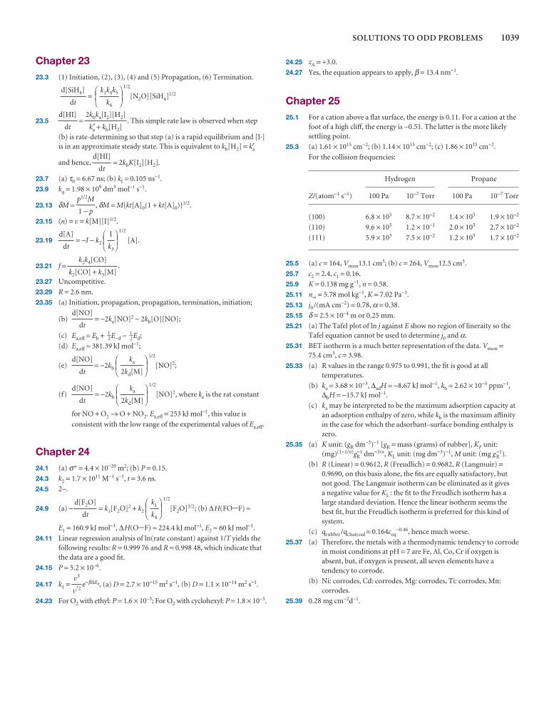
SOLUTIONS TO ODD PROBLEMS 1039
Chapter 2323.3 (1) Initiation, (2), (3), (4) and (5) Propagation, (6) Termination.
=1/2
[N2O][SiH4]1/2
23.5 = . This simple rate law is observed when step
(b) is rate-determining so that step (a) is a rapid equilibrium and [I·]is in an approximate steady state. This is equivalent to kb[H2] = ka′
and hence, = 2kbK[I2][H2].
23.7 (a) τ0 = 6.67 ns; (b) kf = 0.105 ns−1.
23.9 kq = 1.98 × 10⁹ dm3 mol−1 s−1.
23.13 δM = , δM = M{kt[A]0(1 + kt[A]0)}1/2.
23.15 �n� = v = k[M][I]1/2.
23.19 = −I − k2
1/2
[A].
23.21 f = .
23.27 Uncompetitive.
23.29 R = 2.6 nm.
23.35 (a) Initiation, propagation, propagation, termination, initiation;
(b) = −2ka[NO]2 − 2kb[O][NO];
(c) Ea,eff = Eb + 1–2E−d − 1–
2Ed;
(d) Ea,eff ≈ 381.39 kJ mol−1;
(e) = −2kb
1/2
[NO]2;
(f) = −2kb
1/2
[NO]2, where ke is the rat constant
for NO + O2 → O + NO2. Ea,eff = 253 kJ mol−1, this value is
consistent with the low range of the experimental values of Ea,eff.
Chapter 2424.1 (a) σ* = 4.4 × 10⁻²⁰ m2; (b) P = 0.15.
24.3 k2 = 1.7 × 10¹¹ M−1 s−1, t = 3.6 ns.
24.5 2−.
24.9 (a) − = k1[F2O]2 + k2
1/2
[F2O]3/2; (b) ∆H(FO-F) ≈
E1 = 160.9 kJ mol−1, ∆H(O-F) ≈ 224.4 kJ mol−1, E2 ≈ 60 kJ mol−1.
24.11 Linear regression analysis of ln(rate constant) against 1/T yields thefollowing results: R = 0.999 76 and R = 0.998 48, which indicate thatthe data are a good fit.
24.15 P = 5.2 × 10⁻⁶.
24.17 k1 = e−β∆E0, (a) D = 2.7 × 10⁻¹⁵ m2 s−1, (b) D = 1.1 × 10⁻¹⁴ m2 s−1.
24.23 For O2 with ethyl: P = 1.6 × 10⁻³; For O2 with cyclohexyl: P = 1.8 × 10⁻³.
v3
v‡2
DEFk1
k4
ABCd[F2O]
dt
DEFka
2kd[M]
ABCd[NO]
dt
DEFka
2kd[M]
ABCd[NO]
dt
d[NO]
dt
k2k4[CO]
k2[CO] + k3[M]
DEFI
k3
ABCd[A]
dt
p1/2M
1 − p
d[HI]
dt
2kbka[I2][H2]
k′a + kb[H2]
d[HI]
dt
DEFk1k4k5
k6
ABCd[SiH4]
dt
24.25 zA = +3.0.
24.27 Yes, the equation appears to apply, β = 13.4 nm−1.
Chapter 2525.1 For a cation above a flat surface, the energy is 0.11. For a cation at the
foot of a high cliff, the energy is −0.51. The latter is the more likelysettling point.
25.3 (a) 1.61 × 1015 cm−2; (b) 1.14 × 1015 cm−2; (c) 1.86 × 1015 cm−2.
For the collision frequencies:
Hydrogen Propane
Z/(atom−1 s−1) 100 Pa 10−7 Torr 100 Pa 10−7 Torr
(100) 6.8 × 10⁵ 8.7 × 10⁻² 1.4 × 10⁵ 1.9 × 10⁻²
(110) 9.6 × 10⁵ 1.2 × 10⁻¹ 2.0 × 10⁵ 2.7 × 10⁻²
(111) 5.9 × 10⁵ 7.5 × 10⁻² 1.2 × 10⁵ 1.7 × 10⁻²
25.5 (a) c = 164, Vmon13.1 cm3; (b) c = 264, Vmon12.5 cm3.
25.7 c2 = 2.4, c1 = 0.16.
25.9 K = 0.138 mg g−1, n = 0.58.
25.11 n∞ = 5.78 mol kg−1, K = 7.02 Pa−1.
25.13 j0 /(mA cm−2) = 0.78, α = 0.38.
25.15 δ = 2.5 × 10⁻⁴ m or 0.25 mm.
25.21 (a) The Tafel plot of ln j against E show no region of lineraity so theTafel equation cannot be used to determine j0 and α.
25.31 BET isotherm is a much better representation of the data. Vmon =75.4 cm3, c = 3.98.
25.33 (a) R values in the range 0.975 to 0.991, the fit is good at alltemperatures.
(b) ka = 3.68 × 10⁻³, ∆adH = −8.67 kJ mol−1, kb = 2.62 × 10⁻⁵ ppm−1,∆bH = −15.7 kJ mol−1.
(c) ka may be interpreted to be the maximum adsorption capacity atan adsorption enthalpy of zero, while kb is the maximum affinityin the case for which the adsorbant–surface bonding enthalpy iszero.
25.35 (a) K unit: (gR dm−3)−1 [gR = mass (grams) of rubber], KF unit:(mg)(1−1/n)gR
−1 dm−3/n, KL unit: (mg dm−3)−1, M unit: (mg gR−1).
(b) R (Linear) = 0.9612, R (Freudlich) = 0.9682, R (Langmuir) =0.9690, on this basis alone, the fits are equally satisfactory, butnot good. The Langmuir isotherm can be eliminated as it gives a negative value for KL : the fit to the Freudlich isotherm has alarge standard deviation. Hence the linear isotherm seems thebest fit, but the Freudlich isotherm is preferred for this kind ofsystem.
(c) qrubber /qcharcoal = 0.164ceq−0.46, hence much worse.
25.37 (a) Therefore, the metals with a thermodynamic tendency to corrodein moist conditions at pH = 7 are Fe, Al, Co, Cr if oxygen isabsent, but, if oxygen is present, all seven elements have atendency to corrode.
(b) Ni: corrodes, Cd: corrodes, Mg: corrodes, Ti: corrodes, Mn:corrodes.
25.39 0.28 mg cm−2d−1.

(T) denotes a table in the DataSection.
A
A2 spectrum 531ab initio method 394absolute value 963absorbance 432absorption spectroscopy 431abundant-spin species 541acceleration 981acceleration of free fall 979acceptable wavefunction 272accommodation 917acetaldehyde pyrolysis 830achiral molecule 412acid 763acid catalysis 839acidity constant 763, (T) 1007acronyms 950activated complex 809, 881activated complex theory 880activation, enthalpy of 51activation energy 807, (T) 1023
composite reaction 822negative 822
activation Gibbs energy (electrode)935
activation-controlled reaction 877active site 840active transport 770activity 158, 204
ion 163activity coefficient 159
determination 228additional work 34, 99adiabat 48adiabatic bomb calorimeter 38adiabatic boundary 6adiabatic demagnetization 568adiabatic expansion 47, 48, 69adiabatic flame calorimeter 42adiabatic nuclear demagnetization
568adiabatic process, entropy change
80ADP 224, 225adsorbate 909adsorbent 909adsorption 909adsorption isotherm 917adsorption rate 923aerobic metabolism 225aerosol 682AES 914AFM 289, 637air, composition 11
Airy radius 466all-trans-retinal 490allowed transition 335, 435alloy 175
microstructure 191alpha-helix 677alveoli 147amount of substance 959amplitude 982anaerobic metabolism 225angstrom 961angular momentum 297, 981
commutator 307magnitude 305operator 307orbital 326quantization 298summary of properties 309total 349, 352z-component 306
angular velocity 981anharmonic 455anharmonicity constant 455anode 217anodic current density 935anti-parallel beta-sheet 678anti-Stokes radiation 431anti-bonding orbital 371anticyclone 12antiferromagnetic phase 736antioxidant 386antisymmetric stretch 461antisymmetric wavefunction 338apomyoglobin 819aragonite 43area 966argon viscosity 760argon-ion laser 507aromatic stability 392array detector 470Arrhenius equation 807Arrhenius parameters 807, 873, (T)
1021ascorbic acid 386asymmetric rotor 442asymmetry potential 230asymptotic solution 323atmosphere 11, 462
temperature 463temperature profile 854
atmosphere (unit) 4, 961atmosphere composition 853atmospheric ozone 855atom 320
configuration 337many-electron 336selection rule 335term symbol 352
atomic force microscopy 289, 637atomic level 349atomic orbital 326atomic weight 959atomization, enthalpy of 51ATP 224, 858attractive surface 890Aufbau principle, see building-up
principle 340Auger electron spectroscopy 914autocatalysis 803autoprotolysis rate 806avalanche photodiode 473average molar mass 653average value 528, 966Avogadro’s principle 7AX energy levels 524AX2 spectrum 526AX3 spectrum 526Axilrod–Teller formula 636axis of improper rotation 406axis of symmetry 405azeotrope 184azimuth 301
B
Balmer series 320band formation 724band gap 725band head 487band spectra 457band width 725bar 4, 961barometer 4barometric formula 12barrier penetration 286barrier transmission 287base 763base catalysis 840base pairs 680base-stacking 681base unit 960basis set 380Bayard–Alpert pressure gauge 5Beer–Lambert law 432bends, the 147benzene, MO description 391Berthelot equation of state 19BET isotherm 920beta-barrel 679beta-pleated sheet 678beta-sheet 678bilayer 686bimolecular reaction 810binomial coefficient 973binomial expansion 571, 973biochemical cascade 491
biofuel cell 948biological standard state 161, 209biosensor analysis 925bipolaron 674Birge–Sponer plot 456bivariant 176black body 245black-body radiation 245block-diagonal matrix 414Blodgett, K. 687blue sky 658body-centred unit cell 699Bohr frequency condition 249Bohr magneton 514Bohr model 360Bohr radius 324boiling 118boiling point (T) 990boiling point constant 151, (T) 1004boiling temperature 118Boltzmann distribution 81, 208, 563,
582chemical equilibrium 212
Boltzmann formula 81, 575, 583Boltzmann, L. 81bond 362bond dissociation energy 377bond dissociation enthalpy 377, (T)
1011bond enthalpy 55bond length (T) 1011
determination 448bond order 376bond order correlations 377bond torsion 676bonding orbital 370Born equation 102, 110Born interpretation 256, 272Born, M. 102, 256Born–Mayer equation 719Born–Haber cycle 719Born–Oppenheimer approximation
363, 473boson 309, 338bouncing ball 77bound state, hydrogen atom 326boundary 5boundary condition 278, 971
cyclic 298boundary surface 329, 369Boyle temperature 16Boyle’s law 7bra 313bracket notation 313Brackett series 321Bragg, W. and L. 704Bragg’s law 704branch 458, 487
Index

INDEX 1041
branching step 833brass 131Bravais lattice 699breathing 147Bremsstrahlung 702Brønsted acid 763Brønsted base 763Brunauer, S. 920bubble 642buckminsterfullerene 410building-up principle 340bulk modulus 722bumping 645butadiene, MO description 389
C
caesium-chloride structure 717cage effect 876calamitic liquid crystal 189calcite 43calorie 31, 979calorimeter 38calorimeter constant 38calorimetry 38camphor 628candela 960canonical distribution 578canonical ensemble 577canonical partition function 578capacitance manometer 5capillary action 643capillary electrophoresis 664capillary technique 778carbon dioxide
isotherm 15phase diagram 120supercritical 119vibrations 461
carbon dioxide laser 507carbon monoxide, residual entropy
610carbon nanotube 728carbonyl group 489Carnot cycle 82carotene 281, 398, 857CARS 465casein 682catalyst 839catalyst properties 930catalytic constant 842catalytic efficiency 842catalytic hydrogenation 930catalytic oxidation 930cathode 217cathodic current density 935cathodic protection 950cavity 642CCD 473ccp 716CD spectra 491cell, electrochemical 216cell emf 219
cell notation 218cell overpotential 944cell potential 219cell reaction 218Celsius scale 6centre of symmetry 406centrifugal distortion 446centrifugal distortion constant 446centrifugal effect 323ceramic 736cesium, see caesium 717CFC 855chain carrier 830chain polymerization 835, 836chain reaction 830chain relation 68, 968chain rule 966chain transfer 837chain-branching explosion 833channel former 770Chapman model 855character 413character table 413, (T) 1023characteristic rotational temperature
594characteristic vibrational
temperature 597charge-coupled device 473charge transfer rate 934charge-transfer transition 489Charles’s law 7chemical equilibrium 208
Boltzmann distribution 208, 212chemical exchange 532, 533chemical kinetics 791chemical potential 122
chemical equilibrium 201general definition 138significance 139standard 141variation with pressure 123variation with temperature 123
chemical potential (band theory) 726
chemical potential gradient 772chemical quench flow method 794chemical shift 519
electronegativity 522typical 520
chemiluminescence 886chemiosmotic theory 227chemisorption 917chemisorption ability 929chiral molecule 412, 491chlorofluorocarbon 855chlorophyll 856, 857chloroplast 254, 856cholesteric phase 189cholesterol 687chorine atom ozone decomposition
855CHP system 947chromatic aberration 490
chromatography 119chromophore 487, (T) 1014chromosphere 346chronopotentiometry 940circular dichroism 491circular polarization 491circularly birefringent 985circularly polarized 984circumstellar space 480cis-retinal 490, 853citric acid cycle 225, 856Clapeyron equation 126class 415, 416classical mechanics 243clathrate 635Clausius inequality 86, 95Clausius–Clapeyron equation 128Clausius–Mossotti equation 627Clebsch–Gordan series 352close-packed 715closed shell 339closed system 28cloud colour 658cloud formation 645CMC 685CNDO 394co-adsorption 926coagulation 684COBE 438coefficient of performance 85coefficient of thermal conductivity
758coefficient of viscosity 758, 759, 785cofactor (matrix) 976coherence length 497coherent anti-Stokes Raman
spectroscopy 465coherent radiation 497colatitude 301cold denaturation 819collapse pressure 688colligative property 150collision 9, 753
elastic 748reactive 886
collision cross-section 753, 870, (T)1018
collision density 870collision diameter 753collision flux 755collision frequency 753, 755collision theory 809, 870collision-induced emission 846collisional deactivation 438, 846collisional lifetime 438colloid 682colloid stability 683colour 481, (T) 1013column vector 976combination difference 458combination principle 321combinatorial function 973combined gas law 10
combined heat and power system947
combustion, enthalpy of 51common logarithm 963commutator 271
angular momentum 307commute 271competitive inhibition 844complementary observable 271complete neglect of differential
overlap 394complete set 267complete shell 339complex conjugate 256, 963complex mode process 891complex number 256, 963component 175compound semiconductor 726compressibility 722compression factor 14, 111Compton wavelength 316computational chemistry 393concentration cell 218concentration polarization 941concentration profile 878condensation 17, 645conductance 761conducting polymer 674conductivity 762
thermal 758configuration
atom 337macromolecule 667statistical 561
configuration integral 604confocal microscopy 504conformation 667conformational conversion 532conformational energy 675conformational entropy 671congruent melting 192conjugated polyene 401consecutive reactions 811consolute temperature 186constant
acidity 763anharmonicity 455boiling point 151calorimeter 38centrifugal distortion 446critical 16dielectric 110equilibrium 203Faraday’s 985force 452, 982freezing point 153gas 8Lamé 743Madelung 719Michaelis 841normalization 255Planck’s 246rotational 443

1042 INDEX
Rydberg 320, 327scalar coupling 524second radiation 275spin–orbit coupling 350time 801
constituent 175constrained chain 672constructive interference 370contact angle 644continuum generation 503contour diagram (reaction) 887contour length 670convection 12, 777convective flux 777cooling 86cooling curve 178, 191Cooper pair 737cooperative transition 572coordination 717coordination number 716core hamiltonian 393Corey–Pauling rules 675corona 346correlation analysis 884correlation diagram 355correlation spectroscopy 543corresponding states 21corrosion 948corrosion current 949Cosmic Background Explorer 438cosmic ray 244, 984COSY 543Coulomb integral 380Coulomb interaction 986Coulomb operator 393Coulomb potential 110, 986
shielded 167Coulomb potential energy 986counter electrode 939covalent bond 362covalent network solid 720cracking 931cream 682critical compression factor 21critical constant 16, 17critical field 737critical isotherm 15critical micelle concentration 685critical molar volume 17critical point 17critical pressure 17, 118critical solution temperature 186critical temperature 17, 118cross-peaks 546cross-product 965cross-relation 900, 903cross-section 753, 870
state-to-state 887crossed-beam technique 648crossed molecular beams 886cryogenics 568crystal diode 473crystal structure 697, 715
crystal system 698crystallinity 673crystallographic point group 408crystallography 711cubic close packed 716cubic F 716cubic group 410cubic unit cell 698cumulative reaction probability 891Curie law 734Curie temperature 736current 987current density 909curvature 264curved surface 643CW spectrometer 520cyclic boundary condition 301cyclic voltammetry 943cyclone 12cytochrome 228cytosol 771
D
d block 342D lines 351d orbital 334d orbital hybridization 367d–d transition 484, 487d-metal complex 488Dalton’s law 13, 179Daniell cell 218dark current 473Davisson, C. 252Davisson–Germer experiment 252Davydov splitting 730de Broglie relation 252, 278de Broglie wavelength 570de Broglie, L. 252Debye equation 627Debye extrapolation 91Debye formula 248Debye length 168Debye T 3 law 91Debye temperature 248Debye, P. 248, 703Debye–Hückel limiting law 164Debye–Hückel theory 164, 167, 222Debye–Hückel–Onsager coefficient
(T) 1019Debye–Hückel–Onsager theory 769decomposition vapour pressure 206defect surface 910definite integral 966degeneracy 416
rotational 445degenerate 286degenerate orbital 334degradation 668degree of conversion 572degree of deprotonation 763degree of dissociation 207, 211degree of freedom 176
degree of ionization 763degree of polymerization 835delocalization energy 390delta scale 519denaturation 198, 668, 681, 819density (T) 990density functional theory 397density of states 245, 744depolarization 464depression of freezing point 151derivative 966derived unit 960derived units 961Derjaguin, B. 683deshielded nucleus 519desorption 909desorption rate 923destructive interference 372detection period 543detector 471, 473determinant 382, 975deuterium lamp 470DFT 395diagonal peaks 546dialysis 155, 712diamagnetic 377, 734diamagnetic contribution 521diamond structure 720diamond-anvil cell 178diathermic boundary 5diatomic molecule (T) 1013diatomic molecule spectra 482dielectric 619dielectric constant 110, (T) 1004Dieterici equation of state 19differential 968differential equation 811, 971differential overlap 394differential pulse voltammetry 943differential scanning calorimeter 46differential scattering cross-section
640differentiation 966diffraction 702diffraction grating 471diffraction limit 466diffraction order 471diffraction pattern 702diffractometer 703diffuse double layer 933diffusion 747, 757, 772, 776
reaction 877, 879relation to curvature 777relation to mobility 774
diffusion coefficient 758, 759, 784,(T) 1016
viscosity 775diffusion equation 877diffusion-controlled limit 877dihelium 373dilute-spin species 541diode laser 732dioxygen, electronic states 483
dipole 620dipole moment 620, (T) 1015
induced 624measurement 446
dipole–charge interaction 629dipole–dipole interaction 631, 646dipole–dipole interaction (EPR) 553dipole–induced dipole interaction
633Dirac bracket notation 313direct method 710direct mode process 891direct product decomposition 420discotic liquid crystal 189dismutation 385disorder 81disperse phase 682dispersing element 432, 471dispersion 81, 175, 985dispersion interaction 633, 677disproportionation 837dissociation 495
degree of 207, 211dissociation energy 363
determination 456dissociation equilibrium 612dissociation limit 495distillation 182
partially miscible liquids 187distinguishable molecules 580distortion polarization 626distribution of speeds 749disulfide bond 681DNA 652, 680
analysis 664damage 855intercalation 638structure from X-rays 711
Dogonadze, R.R. 896donor–acceptor pair 852dopant 726doping 191Doppler broadening 436Doppler effect 361, 436dot product 350, 514, 965drift speed 661, 765, 774droplet 642drug design 638dry air 11DSC 42duality 253Dulong and Petit law 247Dulong, P.-L. 247dust grain 438DVLO theory 684dye laser 508dynamic light scattering 660dynode 473
E
Eadie–Hofstee plot 867Earth surface temperature 463

INDEX 1043
eddy 11edible fat 930EELS 913effect 769
cage 876centrifugal 323Doppler 361, 436electrophoretic 769Joule–Thomson 64kinetic isotope 816kinetic salt 885Meissner 737photoelectric 250relaxation 769salting-in 173salting-out 173Stark 446
effective mass 453effective nuclear charge 339, (T)
1009effective potential energy 323effective transverse relaxation time
538efficiency 83, 585effusion 747Ehrenfest classification 129Ehrenfest equations 134eigenfunction 262eigenvalue 262eigenvalue equation 261, 977eigenvector 977Einstein, A. 247Einstein coefficient 434Einstein formula 602Einstein formula (heat capacity) 247Einstein relation 774Einstein temperature 247Einstein–Smoluchowski equation 782elastic collision 9elastic deformation 720elastic limit 723elastomer 673electric conduction 747electric dipole 620electric field 244, 631, 983electric field strength 987electric potential 110electrical conductivity, temperature
dependence 726electrical double layer 683, 932electrical heating 38electrical power 38, 987electro-osmotic drag 948electroactive species 909electrochemical cell 216electrochemical correlations 397electrochemical potential 952electrochemical series 224electrode 216
counter 939reference 939varieties 216working 939
electrode compartment 216electrode concentration cell 218electrode potential 941, 952electrode process 932electrode, varieties of 216electrode–surface interface 932electrodialysis 683electrokinetic potential 683electrolysis 944electrolyte 216, 762electrolyte concentration cell 218electrolytic cell 216electromagnetic field 243, 983electromagnetic radiation 491electromagnetic spectrum 244, 984electromotive force 219electron, magnetic moment 514electron affinity 344
periodicity 344electron affinity (T) 1010electron density 396, 708electron diffraction 252, 714electron energy loss spectroscopy
913electron gain
electrical 51enthalpy of 51
electron in magnetic field 514electron interaction integrals 371electron microscopy 253electron pair 337electron pair formation 364electron paramagnetic resonance
516, 549electron scattering factor 742electron spectroscopy for chemical
analysis 913electron spin resonance 516, 549electron transfer
between proteins 900reaction 853, 894
electron-gain enthalpy 343electronegativity 379, (T) 1012electronic partition function 597electronic polarizability 626electronic structure 320electronvolt 961electrophoresis 663electrophoretic effect 769electrostatic potential surface 396electrostatics 985elementary reaction 809elevation of boiling point 150Eley–Rideal mechanism 928Ellingham diagram 215elpot surface 396emf 219
temperature variation 231emission spectroscopy 431Emmett, P. 920emulsification 683emulsion 682end separation (polymer) 669
endergonic 202endothermic process 29energy 29, 979
conformational 675electron in magnetic field 514harmonic oscillator 291multipole interaction 630nucleus in magnetic field 515particle in a box 280quantization 246, 260rotational 443zero-point 281
energy density 755energy dispersal 77energy flux 757energy pooling 846ensemble 577enthalpy 40
electron gain 343ionization 343partition function 590reaction 212variation with temperature 46
enthalpy and entropy, relationbetween 44
enthalpy density 53enthalpy of activation 51, 883enthalpy of atomization 51enthalpy of chemisorption 917, (T)
1022enthalpy of combustion 51, 52enthalpy of electron gain 51, 343enthalpy of formation 51enthalpy of fusion 50, (T) 993enthalpy of hydration 51enthalpy of ionization 51, 343enthalpy of mixing 51, 143enthalpy of physisorption 917, (T)
1022enthalpy of reaction 51enthalpy of solution 51enthalpy of sublimation 51enthalpy of transition 50
notation 51enthalpy of vaporization 49, 50, (T)
993entropy
Boltzmann formula 575conformational 671excess 149from Q 579harmonic oscillator 576internal energy 589measurement 91partial molar 94partition function 589reaction 93residual 93, 609statistical 575statistical definition 80thermodynamic definition 78Third-Law 93, 575two-level system 576
units 79variation with temperature 89
entropy changeadiabatic process 80heating 89perfect gas expansion 79phase transition 87surroundings 79
entropy determination 91entropy of activation 883entropy of mixing 143entropy of transition (T) 1002entropy of vaporization 88, (T) 1003enzyme 839, 840epifluorescence 504EPR 516, 549EPR spectrometer 549equation
Arrhenius 807Born 102, 110Born–Mayer 719Clapeyron 126Clausius–Clapeyron 128Clausius–Mossotti 627Debye 627differential 971diffusion 776eigenvalue 261, 977Einstein–Smoluchowski 782Eyring 882fundamental 139generalized diffusion 777Gibbs–Duhem 140Gibbs–Helmholtz 105Hartree–Fock 393Karplus 528Margules 162Mark–Kuhn–Houwink–Sakurada
666material balance 879McConnell 552Michaelis–Menten 841Nernst 221Nernst–Einstein 775partial differential 973Poisson’s 168, 986Roothaan 393Sackur–Tetrode 580secular 380, 977Stern–Volmer 849Stokes–Einstein 775, 878Thomson 127transcendental 186van der Waals 17van ’t Hoff 156, 212, 919virial 16Wierl 742
equation of state 3partition function 604thermodynamic 104
equilibrium 35approach to 804Boltzmann distribution 208, 212

1044 INDEX
chemical 201effect of compression 211effect of temperature 211mechanical 4response to pressure 210sedimentation 662thermal 6thermodynamic criterion 122
equilibrium bond length 363equilibrium constant 203
contributions to 613electrochemical prediction 228molecular interpretation 208partition function 611relation between 208relation to rate constant 804standard cell emf 221standard Gibbs energy of reaction
206thermodynamic 205
equilibrium table 207equipartition theorem 31, 247, 600equivalent nuclei 526, 530ER mechanism 928error function 297error function (T) 1009ESCA 913escape depth 912ESR 516, 549essential symmetry 699ethanal pyrolysis 830ethanol 396ethene, MO description 387Euler chain relation 68, 968eutectic 191eutectic halt 192evanescent wave 925evolution period 543exact differential 58, 968
criterion for 103excess entropy 149excess function 149exchange–correlation energy 395exchange–correlation potential 395exchange current density 937, (T)
1023exchange operator 393exchange process 532excimer formation 846exciplex laser 507excited state absorption 846excited state decay 848exciton 304, 729exciton band 730excluded volume 18exclusion principle 337exclusion rule 464exercise 53exergonic 202exocytosis 687exothermic process 29exp-6 potential 637expansion coefficient 62, (T) 1002
expansion work 33expectation value 267, 974explosion 833exponential decay 799exponential function 963extended Debye–Hückel law 165extensive property 31, 959extent of reaction 201, 794extinction coefficient 432extra work, see additional work 34extrinsic semiconductor 726eye 490Eyring equation 882
F
f block 342face-centred cubic 716face-centred unit cell 699factorial 967far infrared 244far-field confocal microscopy 504fat 53fcc 716FEMO 401femtochemistry 892femtosecond spectroscopy 893Fermi calculation 790Fermi contact interaction 528Fermi level 725fermion 309, 338Fermi–Dirac distribution 726ferrocene 411ferromagnetism 736fibre 673Fick’s first law of diffusion 757,
773Fick’s second law of diffusion 776FID 535, 554field 244
electric 244, 983electromagnetic 243, 983magnetic 244, 983
field-ionization microscopy 924FIM 924fine structure
atomic 351fine structure (NMR) 524finite barrier 288first ionization energy 342First Law of thermodynamics 32first-order correction 310first-order differential equation
811first-order phase transition 129first-order reaction 796, 798first-order spectra 532flash desorption 916flash photolysis 793flocculation 684flow method 793fluctuations 578fluid mosaic model 687
fluorescence 492, 846laser-induced 886solvent effect 493
fluorescence lifetime 848fluorescence microscopy 494fluorescence quantum yield 848fluorescence resonance energy
transfer 852flux 757
toward electrode 941Fock operator 393Fock, V. 344food, energy reserves 52forbidden transition 335, 435force 637, 980
between charges 986generalized 34thermodynamic 772
force constant 290, 452force field 462formal potential 941formaldehyde synthesis 860formation 204
enthalpy of 51formula unit 959Förster theory 852, 863Förster, T. 852four-centred integral 395four-circle diffractometer 704four-helix bundle 678Fourier transform 554Fourier transform technique 432,
471Fourier-transform NMR 533fractional coverage 916fractional distillation 183fracture 723framework representation 931Franck–Condon factor 486Franck–Condon principle 484, 493Franklin, R. 711free energy, see Gibbs energy 98free expansion 34free particle 277free-electron molecular orbital
theory 401free-induction decay 535freely jointed chain 75, 668freeze quench method 794freezing point constant 153, (T) 1004freezing temperature 120Frenkel exciton 729frequency 244, 983frequency-domain signal 536frequency doubling 732FRET 852Freundlich isotherm 922frictional coefficient 660, (T) 1017Friedrich, W. 702frontier orbital 388FT-NMR 533fuel, thermochemical properties 53fuel cell 947
fuel-rich regime 834fugacity 111fugacity coefficient 111full rotation group 411functional 395, 969functional derivative 395, 969functional MRI 541fundamental equation 103, 139fundamental transition 455fusion, enthalpy of 50
G
g subscript 372g-value 514, 550Galileo 4Galvani potential 952Galvani potential difference 932,
934galvanic cell 216
working 945galvanizing 949gamma-ray region 244, 984gas 3
kinetic model 9gas constant 8gas laser 506gas laws 7gas mixture 12gas solubility 147gas solvation 124gas-sensing electrode 230gauss 514Gaussian function 292Gaussian-type orbital 395gel 682gel electrophoresis 664general solution 971generalized diffusion equation 777generalized displacement 34generalized force 34genomics 664gerade symmetry 372Gerlach, W. 307Germer. 248GFP 494Gibbs energy 96
formation 100maximum non-expansion work
99mixing 142mixing (partial miscibility) 186partial molar 138partition function 591perfect gas 107properties 105reaction 100, 201solvation 110standard reaction 202, 220surface 688variation with pressure 106variation with temperature 105
Gibbs energy of activation 883

INDEX 1045
Gibbs energy of activation (electrontransfer) 903
Gibbs energy of formation 204Gibbs energy of mixing, ideal
solution 148Gibbs energy of reaction 100Gibbs isotherm 689Gibbs, J.W. 176Gibbs–Duhem equation 140Gibbs–Helmholtz equation 105glancing angle 704glass electrode 229glass transition temperature 674global warming 462globar 470glucose oxidation 226glycolysis 225Gouy balance 734Gouy–Chapman model 933Grahame model 933Graham’s law of effusion 756grand canonical ensemble 577graphical representation 396graphite structure 720gravimetry 916green fluorescent protein 494greenhouse effect 462gross selection rule 436Grotrian diagram 336Grotthuss mechanism 766group theory 404GTO 395Gunn oscillator 550
H
haematoporphyrin 861hair 681half-life 800, (T) 1020
summary 803half-reaction 216hamiltonian
core 393Hückel method 388hydrogen molecule-ion 368
hamiltonian matrix 389hamiltonian operator 261hard sphere packing 716hard-sphere potential 637harmonic motion 290harmonic oscillator 291
energy 291entropy 576penetration 296wavefunction 291
harmonic oscillator (classical) 982harmonic wave 983Harned cell 222harpoon mechanism 875Hartree, D.R. 344Hartree–Fock equations 393Hartree–Fock self-consistent field
344
hcp 715, 716heat 29heat and work equivalence of 32heat at constant pressure 41heat capacity 39, 247, (T) 992
constant pressure 45constant volume 38, 39contributions summary 616, 620molar 45partition function 601phase transition 130relation between 63, 69relation between (perfect gas) 47rotational transitions 602specific 39variation with temperature 46vibrational contribution 602
heat capacity ratio 48heat engine 76
efficiency 83Heisenberg uncertainty principle
269, 272Heisenberg, W. 269helium 337
Grotrian diagram 348helium-neon laser 506helix scattering 711helix–coil transition 571, 818Helmholtz energy 96
molecular interpretation 97partition function 590
Helmholtz layer model 932Henry, W. 145Henry’s law 145Henry’s law constant (T) 1003Hermann–Mauguin system 406Hermite polynomial 292hermitian operator 264, 283hermiticity 313Hertz 244Hess’s law 53heterogeneous catalysis 927
rate law 927heterogeneous catalyst 839heterogeneous reaction rate 795heteronuclear diatomic molecule,
MO description 368, 379heteronuclear spin system 532hexagonal unit cell 699hexagonally close-packed 715HF-SCF 344high-energy phosphate bond 225high-performance liquid
chromatography 119high-temperature superconductor
736highest occupied molecular orbital
388Hinshelwood, C.N. 820HOMO 388homogeneity index 654homogeneous catalyst 839homogenized milk 682
homonuclear diatomic moleculeMO description 368molecular orbital diagram 375VB description 363
homonuclear spin system 532Hooke’s law 673HPLC 119HREELS 913HTSC 736Hückel approximations 387Hückel method 387Hückel, E. 387Hull, A. 703Humphreys series 359Hund’s maximum multiplicity rule
341Hush, N.S. 896hybrid orbital 366hybridization 366hybridization schemes 368hydration, enthalpy of 51hydrodynamic flow 647hydrodynamic radius 766hydrofluorocarbon 856hydrogen atom
bound state 326energies 324wavefunction 324
hydrogen bond 634, 677hydrogen–bromine reaction 831,
860hydrogen electrode 222hydrogen fluoride, MO description
379, 384hydrogen ion
conduction by 766enthalpy of formation 55Gibbs energy of formation 100standard entropy 94
hydrogen moleculeMO description 373 VB description 364
hydrogen molecule ion 368hydrogen–oxygen reaction 833hydrogen peroxide decomposition
839hydrogen storage 947hydrogen/oxygen fuel cell 947hydrogenation 929hydrogenic atom 320hydrogenic orbital, mean radius
330hydronium ion 766hydrophilic 682hydrophobic 635, 682hydrophobic interaction 636hydrophobicity constant 635hydrostatic pressure 5hydrostatic stress 721hyperbola 7hyperfine coupling constant 551, (T)
1015hyperfine structure 551
hyperpolarizability 732hypertonic 155
I
IC 495, 846ice 121
phase diagram 121residual entropy 93, 610structure 121, 721
icosahedral group 410ideal gas, see perfect gas 8ideal solution 144
Gibbs energy of mixing 148ideal–dilute solution 146identity operation 405IHP 933immiscible liquids 184impact parameter 640impressed-current cathodic
protection 950improper rotation 406incident beam flux 648incongruent melting 193indefinite integral 966independent migration of ions 763independent molecules 579indicator diagram 35indicator solution 768indistinguishable molecules 580induced dipole moment 624induced fit model 840induced magnetic moment 736induced-dipole–induced-dipole
interaction 633induction period 812inelastic neutron scattering 761inexact differential 58infectious disease kinetics 867infinite temperature 567, 584infrared 244infrared active 454infrared activity 467infrared chemiluminescence 886infrared inactive 454infrared region 984inhibition 844inhomogeneous broadening 538initial condition 971initiation step 831inner Helmholtz plane 933inner potential 934insulator 723integral 966integral protein 687integrated absorption coefficient 433integrated rate law 798
summary 803integrated signal 521integration 966integration by parts 967intensive property 959interference 251, 370

1046 INDEX
interferogram 472interferometer 471intermolecular interaction 14internal conversion 495internal energy 30
fluid 609from Q 578general changes in 59heat at constant volume 37molecular contributions 31partition function 573properties 103statistical 573
internal pressure 60International System (point groups)
406International System (units) 960interstellar cloud 439intersystem crossing 494intrinsic semiconductor 726intrinsic viscosity 665, (T) 1017inverse matrix 976inversion operation 406inversion recovery technique 538inversion symmetry 372inversion temperature 66, (T) 1002inverted region 899iodine, metallic 178ion
activity 163Gibbs energy of formation 101standard entropy 94
ion channel 770ion mobility 765, 774ion pump 770ion-selective electrode 229ionic atmosphere 164, 683, 769ionic bond 362ionic mobility (T) 1019ionic radius (T) 1017ionic solid 717ionic strength 164ionization, enthalpy of 51, 343ionization energy 327, 342, (T) 1010
periodicity 343spectroscopic measurement 325
ion–ion interaction (conductivity)769
irreducible representation 415irrep 415ISC 494, 846isenthalpic process 64isobar 10, 12isobaric calorimeter 41isochore 10isodensity surface 396isoelectric focusing 665isoelectric point 665isolated system 29isolation method 797isopleth 181isosteric enthalpy of adsorption 919isotherm 7, 10, 15
isothermal compressibility 62, (T)1002
isothermal expansion 79isothermal Joule–Thomson
coefficient 65isothermal reversible expansion 36isotope abundance (T) 991isotope separation 501isotopomer 501
J
Jablonski diagram 495Jeans, J. 245jj-coupling 355joule 31, 961, 979Joule experiment 60Joule, J.P. 31, 60Joule–Thomson coefficient 63, (T)
1002Joule–Thomson effect 64
K
K-radiation 703Karplus equation 528Kassel form 821Kassel, L.S. 821Keesom interaction 632kelvin 6Kelvin equation 645Kelvin scale 6Kelvin statement 76keratin 681Kerr lens 733Kerr medium 733ket 313kinetic chain length 838kinetic control 815kinetic energy 9, 979kinetic energy density 755kinetic energy operator 264kinetic isotope effect 816kinetic model 747kinetic model of gas 9kinetic pressure 609kinetic theory, transport properties
758Kirchhoff ’s law 56klystron 550KMT, see kinetic model 747Knipping, P. 702Knudsen method 756Kohlrausch’s law 762Kohn–Sham equations 395Koopmans’ theorem 378Krafft temperature 685Kronecker delta 311, 975krypton-ion laser 507
L
Lagrange method 582, 970Laguerre polynomial 324
Lamb formula 521lambda line 121, 122lambda-transition 130Lamé constants 743lamellar micelle 685laminar flow 758lamp 470Landau, L. 683Langevin function 624Langmuir isotherm 918Langmuir, I. 687Langmuir–Blodgett film 687Langmuir–Hinshelwood mechanism
927Laplace equation 643laplacian 168, 255, 301Laporte selection rule 483Larmor frequency 515, 534laser 732laser action 496laser radiation characteristics 500laser-induced fluorescence 886lattice energy 718lattice enthalpy (T) 1018lattice point 698law
Beer–Lambert 432Boyle’s 7Charles’s 7combined gas 10cosines 370Curie 734Dalton’s 13, 179Debye T3 91Debye–Hückel limiting 164Dulong and Petit 247extended Debye-Hückel 165Fick’s first 757, 773Fick’s second 776First 32gas 7Graham’s 756Henry’s 145Hess’s 53Hooke’s 673, 723Kirchhoff ’s 56Kohlrausch’s 762limiting 7motion 981Newton’s second 981Ostwald’s dilution 764Raoult’s 144, 179Rayleigh–Jeans 245Second 76Stefan–Boltzmann 275Stokes’ 775Third 93Wien’s 275Zeroth 6
law of cosines 370, 964LCAO-MO 369, 374, 386
symmetry considerations 424LCAO-MO (solids) 724
Le Chatelier, H. 210Le Chatelier’s principle 210LED 732LEED 914legendrian 255, 301Lennard-Jones parameters (T) 1016Lennard-Jones potential 637level
atomic 349energies 350
lever rule 181levitation 737Lewis, G.N. 362LFER 884, 899LH mechanism 927lifetime 437
rotational state 462lifetime broadening 438ligand-field splitting parameter 488ligand-to-metal transition 489light 242, 481light (T) 1013light-emitting diode 732light harvesting 856light harvesting complex 856light-induced photoisomerization
713light scattering 657, 691limiting current density 942limiting ionic conductivity (T) 1019limiting law 7, 164limiting molar conductivity 762limiting transport number 768Linde refrigerator 66Lindemann, F. (Lord Cherwell) 820Lindemann–Hinshelwood
mechanism 820line alternation 451line broadening (NMR) 532line intensity 517line shape 436linear combination 267
degenerate orbital 334linear combination of atomic
orbitals 369, 374, 386linear free energy relation 884, 899linear momentum, wavefunction
261linear rotor 442, 445linear-sweep voltammetry 942Lineweaver–Burk plot 842lipid bilayer 779lipid raft model 687liposome 685liquid, molecular motion 761liquid crystal 191, 685
phase diagram 192liquid crystal display 189liquid junction potential 218liquid structure 606liquid viscosity 761liquid–liquid phase diagram 185liquid–solid phase diagram 189

INDEX 1047
liquid–vapour boundary 127lithium atom 337litre 961LMCT 489local contribution to shielding 521local density approximation 396local minima 677lock-and-key model 840logarithm 963London formula 635London interaction 633long-range order 606longitudinal relaxation time 536low energy electron diffraction 914low overpotential limit 938low temperature 85lower critical solution temperature
186lowest occupied molecular orbital
388Luggin capillary 939LUMO 388lung 147Lyman series 320lyophilic 682lyophobic 682lyotropic liquid crystal 189lyotropic mesomorph 685
M
macromolecule 652macular pigment 490Madelung constant 719magic-angle spinning 549magnetic field 244, 983magnetic flux density 734magnetic induction 514magnetic levitation 737magnetic moment 514, 735magnetic quantum number 302magnetic resonance imaging 540magnetic susceptibility 522, (T) 1018magnetically equivalent nuclei 530magnetizability 734magnetization 733magnetization vector 534magnetogyric ratio 514MALDI 655MALDI-TOF 655manometer 5, 24many-electron atom 320, 336Marcus cross-relation 903Marcus inverted region 899Marcus theory 853, 896Marcus, R.A. 821, 896Margules equation 162Mark–Kuhn–Houwink–Sakurada
equation 666Mars van Kreelen mechanism 930MAS 549mass spectrometry 655material balance equation 879
matrix addition 975matrix algebra 975matrix diagonalization 389matrix element 310, 313, 975matrix-assisted laser desorption/
ionization 655matter flux 757matter, nature of 309maximum multiplicity 341maximum velocity 840maximum work 96Maxwell construction 20Maxwell distribution 750Maxwell relation 104Mayer f-function 605MBE 728MBRS 928MBS 916McConnell equation 552mean activity coefficient 163, (T)
1004mean bond enthalpy 55, (T) 1012mean cubic molar mass 653mean displacement 294mean distance diffused 781mean energies summary 616mean energy 599mean free path 754mean molar mass 653mean radius, hydrogenic orbital 330mean rotational energy 600mean speed 751, 752mean square displacement 294mean square molar mass 653mean translational energy 600mean value 528, 974mean value theorem 967mean vibrational energy 600measurement, interpretation 267mechanical equilibrium 4mechanical property 721mechanism of reaction 791Meissner effect 737melting, response to pressure 123melting point (T) 990melting temperature 119melting temperature (polymer) 674membrane
formation 685transport across 779
mercury photosensitization 860meridional scattering 711meso-tartaric acid 407mesopause 854mesophase 189mesosphere 854metal extraction 215metal-to-ligand transition 489metallic conductor 723metallic lustre 730metastable excited state 496metastable phase 118methane, VB description 365
method of initial rates 797method of undetermined multipliers
582mho 762micelle 685Michaelis constant 841Michaelis–Menten equation 841Michaelis–Menten mechanism 841Michelson interferometer 432, 471microcanonical ensemble 577microporous material 931microstructure 191microwave background radiation
438microwave region 244, 984Mie potential 637milk 682Miller indices 700mirror plane 406Mitchell, P. 228mitochondrion 225mixed inhibition 845mixing
enthalpy of 51role in equilibrium 203
MLCT 489mmHg 4MO 368MO theory 362mobility 765mobility on surface 924mode locking 499mode-selective chemistry 893model
Bohr 360Chapman 855Gouy–Chapman 933Grahame 933Helmholtz 932kinetic 9, 747RRK 821, 824RRKM 821Zimm–Bragg 572zipper 572
moduli 721modulus 963molality 140, 960molar absorption coefficient 432molar concentration 140, 960molar conductivity 762
diffusion coefficient 775molar heat capacity 45molar magnetic susceptibility 734molar mass 653molar mss 959molar partition function 591molar polarization 627molar property 959molar volume 959molarity 140, 960mole 959mole fraction 13molecular beam 640, 647
molecular beam epitaxy 728molecular beam scattering 916molecular beams 886molecular cloud 439molecular collision 753molecular dynamics 607, 677molecular flow 647molecular interaction 14molecular interpretation
equilibrium constant 208heat and work 29
molecular mechanics 677molecular modelling 56molecular orbital 368molecular orbital energy level
diagram 373molecular orbital theory 362, 368molecular partition function 564,
591molecular potential energy curve 363
hydrogen molecule-ion 371molecular recognition 638molecular scattering 641molecular solid 720molecular spectroscopy 430molecular speed, distribution of 750molecular vibration 452
symmetry 467molecular weight, see molar mass
653, 959molecularity 810molten globule 198moment of inertia 297, 441, 981momentum flux 758momentum operator 263momentum representation 276monochromatic source 470monochromator 471monoclinic unit cell 698, 699monodisperse 653monolayer 687monomer 652monopole 630Monte Carlo method 607Morse potential energy 455most probable radius 332most probable speed 752mouse cell 466moving boundary method 768MPI 886MRI 540Mulliken electronegativity 380, (T)
1012multi-walled nanotube 720multinomial coefficient 562, 974multiphoton ionization 886multiphoton process 500multiple quantum transition 547multiplicity 353, 482multipole 630multipole interaction energy 630mutual termination 837MWNT 720

1048 INDEX
N
n-fold rotation 405n-pole 630n-type semiconductivity 727NADH 225NADP 857, 858nanocrystal 304nanodevice 690, 728nanofabrication 690nanoscience 288nanotechnology 288, 289nanotube 720, 728nanowire 728narcosis 147natural linewidth 438natural logarithm 963Nd-YAG laser 731near infrared region 984near-field optical microscopy 504nearly free-electron approximation
724negative phototactic response 713negative temperature 584neighbouring group contribution
521, 522nematic phase 189neodymium laser 731neon atom 341Nernst diffusion layer 941Nernst equation 221Nernst filament 470Nernst heat theorem 92Nernst–Einstein equation 775network solid 720neutron diffraction 713neutron magnetic scattering 714neutron scattering 761newton 961Newtonian flow 758Newton’s second law of motion 981nicotine 186nitric oxide 386
electronic partition function 598magnetism 744
nitrogenfugacity (T) 1003VB description 364
nitrogen fixation 385nitrogen laser 507nitrogen narcosis 147NMR 517
line intensity 517spectrometer 517
nodal plane 333node 261NOE 542NOESY 548non-Arrhenius behaviour 817non-competitive inhibition 845non-polarizable electrode 940nonexpansion work 34nonlinear phenomena 732
nonradiative decay 492normal boiling point 118normal freezing point 120normal melting point 120normal mode 461
group theory 467infrared activity 467
normal transition temperature 87normal Zeeman effect 360normalization 258, 278, 279normalization constant 257notation
orbital 421notational conventions 962NSOM 504nuclear g-factor 516nuclear magnetic resonance 517nuclear magneton 516nuclear Overhauser effect 542nuclear spin 515, (T) 1014
nuclear constitution 515properties 516
nuclear spin quantum number 515nuclear statistics 451nucleation 645nucleation step 572nucleic acid 679nuclide abundance (T) 991nuclide mass (T) 991number-average molar mass 653numerical integration 972nylon-66 673, 835
O
O branch 459oblate 444observable 262, 272
complementary 271octahedral complex 488octane 53octupole 631off-diagonal peaks 546OHP 932oil hydrogenation 930one-component system 177one-dimensional crystal 718one-dimensional random walk 781open system 28operator 261, 272
angular momentum 307Coulomb 393exchange 393hermitian 264, 283kinetic energy 264momentum 263position 263potential energy 263
optical activity 985optical density 432optical Kerr effect 733optical trapping 568optically active 412
orbitalanti-bonding 371atomic 326bonding 370Gaussian type 395
orbital angular momentum 326total 352
orbital angular momentumquantum number 302
orbital approximation 336orbital energy variation 376orbital notation 421order of group 416order of reaction 796order–disorder transition 131ordinary differential equation 971ore reduction 215orientation polarization 626Orion nebula 439ortho-hydrogen 452orthogonal function 265, 282orthogonality 265, 282orthonormal 283orthorhombic unit cell 699oscillator strength 511osmometry 156osmosis 156osmotic pressure 156osmotic virial coefficient 157Ostwald viscometer 666Ostwald’s dilution law 764Otto cycle 116outer Helmholtz plane 932outer potential 934overall order 796overall partition function 599Overbeek, J.T.G. 683Overhauser effect spectroscopy 548overlap, symmetry relation 421overlap density 370overlap integral 371, 375overpotential 938overtone 456oxidant 216oxidation 216oxidative phosphorylation 225, 227oxygen
electronic states 483molecular properties 483
ozone 853
P
p band 725P branch 458p orbital 332
real form 333p-type semiconductivity 726P680 857P700 858packing fraction 716PAGE 664para-hydrogen 452
parabolic potential 291, 452parallel band 461parallel beta-sheet 678parallel spins 347paramagnetic 377, 734paramagnetic contribution 521paramagnetism 376parcel (of air) 12parity 372, 482parity selection rule 483partial charge 379partial derivative 39, 968partial differential equation 973partial fraction 967, 803partial molar entropy 94partial molar Gibbs energy 138partial molar quantity 136partial molar volume 137partial pressure 12partial vapour pressure 124partially miscible 149partially miscible liquids 185
distillation 187particle in a box 278
partition function 568quantum number 280
particle in a sphere 304particle on a ring 297particle on a sphere 301particular solution 971partition function
canonical 578contributions to 615electronic 597enthalpy 590entropy 575, 589equally spaced levels 563equation of state 604equilibrium constant 611factorization 569Gibbs energy 591heat capacity 601Helmholtz energy 590internal energy 573, 589molar 591molecular 564, 591overall 599particle in a box 568pressure 590rate constant 882rotational 592second virial coefficient 605standard molar 611thermodynamic functions from
616thermodynamic information 578translational 568, 592two-level system 564vibrational 596
partition ratio 779pascal 4, 961Pascal’s triangle 526Paschen series 320

INDEX 1049
passive transport 770patch clamp technique 771patch electrode 771path function 57Patterson synthesis 709Pauli exclusion principle 337Pauli principle 338, 451Pauling electronegativity 379, (T)
1012PDT 861PEMD pulse sequence 543penetration 286, 296, 340peptide link 571, 667, 675peptizing agent 682perfect elastomer 673perfect gas 8
enthalpy of mixing 143entropy change 79, 87entropy of mixing 143equilibria 202Gibbs energy 107Gibbs energy of mixing 142internal energy 574isothermal expansion 87molar volume 11statistical entropy 580transport properties 757, 784
perfect-gas temperature scale 6periodicity 341peripheral protein 687permanent waving 681permittivity 110, 627, 984, 986perpendicular band 461persistence length 75perturbation theory 310, 313
polarizability 625time-dependent 311time-independent 310
Petit, A.-T. 247phaeophytin 857phase 117, 174phase (wave) 983phase boundary 118, 126phase diagram 118
carbon dioxide 120helium 121ice 121liquid crystal 190liquid–liquid 185liquid–solid 189sodium and potassium 192water 120, 177
phase problem 709phase rule 176phase separation 185phase transition 117, 129
entropy of 87phase-sensitive detection 550phosphatidyl choline 686phosphine decomposition 927phospholipid 199, 686phosphorescence 492, 494, 846photocatalyst 861
photocathode 473photochemical processes 845photochemistry 845photodeflection 502photodiode 473photodissociation 502photodynamic therapy 860photoelectric effect 250photoelectron 378photoelectron spectroscopy 378, 912photoemission spectroscopy 912photoionization 501photoisomerization 502photomultiplier tube 473photon 250photophosphorylation 858photosensitization 860photosphere 346photosynthesis 856photosystem I and II 856phototactic response 713photovoltaic cell detector 473physical quantity 959physical state 3physisorption 916pi bond 365pi orbital 374pi-bond formation energy 390pi-electron bonding energy 390pi pulse 538pi-stacking interaction 638pi*-n transition 489pi*-pi transition 489pi/2 pulse 534Planck distribution 246Planck, M. 246Planck’s constant 246plane polarized 491, 984plane separation 701plasma 755, 925plasmid 289plasmon 925plastic 674plastic deformation 721plastoquinone 858PMT 473Pockels cell 498point dipole 629point group 405point group notation 408Poiseuille’s formula 760Poisson’s equation 168, 986Poisson’s ratio 722polar bond 379polar coordinates 258, 301polar molecule 411, 621polarizability 449, 624, (T) 1015
frequency dependence 626polarizability volume 624, (T) 1015polarizable electrode 940polarization 623polarization (radiation) 491polarization mechanism 528, 553
polarization overpotential 941polarized light 491polaron 674polyacetylene 674polyacrylamide gel electrophoresis
664polyatomic molecule
MO description 386VB description 365vibration 460
polychromatic source 470polychromator 471polydisperse 653polydispersity index 654polyelectrolyte 680polyelectronic atom 320polyene 281polymer 652polymerization kinetics 835polymorph 121polynucleotide 679polypeptide 667, 677
helix–coil transition 818polypeptide conformation transition
571polypeptide melting 134polytype 715population 81, 561population inversion 496porphine 319, 429position operator 263positronium 359postulates 272potassium–bromine reaction 875potential difference 987potential energy 9, 979potential energy operator 263potential energy profile 809potential energy surface 887powder diffraction pattern 707powder diffractometer 703power 979
working cell 946power output (laser) 498power series 967pre-equilibrium 815pre-exponential factor 807pre-exponential factor (T) 1021prebiotic reactions 829precession 514, 534precision-specified transition 501precursor state 922predissociation 495prefixes for units 960, 961preparation period 543pressure 4
adiabatic process 48and altitude 12critical 17hydrostatic 5internal 60, 104kinetic 609kinetic model 748
partition function 590variation with reaction 792
pressure gauge 5pressure jump 805pressure units 4primary absorption 846primary kinetic isotope effect 816primary process 845primary quantum yield 847primary structure 667primitive unit cell 697, 699principal axis 405, 444principal quantum number 326principle
Avogadro’s 7building-up 340equal a priori probabilities 561equipartition 247exclusion 337Franck–Condon 484, 896Le Chatelier’s 210Pauli 338, 451Ritz combination 321uncertainty 269, 271variation 380
principle of corresponding states 21principle of equal a priori
probabilities 561probability amplitude 256probability density 256, 260, 974probability theory 973product rule 966projection reconstruction 540prolate 444promotion 365propagation step 572, 831protein crystallization 712protein folding problem 675proteomics 664proton decoupling 541proton pump 772pseudo first-order reaction 797psi 4pulse technique 533pulsed beam 928pulsed-field electrophoresis 664pumping 496pure shear 721pyroelectric detector 473p–n junction 727
Q
Q branch 458, 459Q-switching 498QCM 916QSAR 638QSSA 812quadrupole 631quantitative structure–activity
relationships 638quantity calculus 7quantization

1050 INDEX
angular momentum 298energy 246, 260space 307
quantum defect 347quantum dot 306quantum mechanics 242quantum number
angular momentum 302magnetic 302nuclear spin 515orbital angular momentum 302particle in a box 280principal 326spin 308spin magnetic 308total angular momentum 352total orbital angular momentum
352total spin 352
quantum oscillation 641quantum yield 859quartz crystal microbalance 916quartz–tungsten–halogen lamp 470quasi-steady-state approximation
812quaternary structure 668quenching 849quenching method 794quinoline 407quotient rule 966
R
R branch 458radial distribution function
atom 331liquid 606
radial wave equation 322radial wavefunction 323radiation, black-body 245radiation source 470radiative decay 492radical chain reaction 830radio region 244, 984radius
hydrodynamic 766most probable 332Stokes 766
radius of gyration 658, 671, (T) 1016radius of shear 683radius ratio 717rainbow angle 641RAIRS 913Ramachandran plot 676Raman activity 468Raman imaging 473Raman spectra
polyatomic molecule 464rotational 449vibrational 459
Raman spectroscopy 431, 500Ramsperger, H.C. 821random coil 668
random walk 781Raoult, F. 144Raoult’s law 144, 179rate
charge transfer 934surface process 922
rate constant (T) 1020diffusion controlled 878electron transfer 895Kassel form 821partition function 882state-to-state 887
rate law 795heterogeneous catalysis 927
rate of adsorption 916rate of formation 794rate of reaction 794rate-determining step 814Rayleigh radiation 431Rayleigh ratio 657, 691Rayleigh scattering 657Rayleigh, Lord 245Rayleigh–Jeans law 245RDS 814reaction centre 856reaction coordinate 809reaction enthalpy 51
from enthalpy of formation 55measurement 212temperature dependence 56
reaction entropy 93reaction Gibbs energy 100, 201, 220reaction mechanism 791reaction order 796reaction product imaging 886reaction profile 809reaction quotient 202reaction rate 794
collision theory 809, 870temperature dependence 807
reactive collision 886reactive cross-section 871, 874read gradient 540real gas 8, 14real-time analysis 793reciprocal identity 70recursion relation 292redox couple 216redox reaction 216reduced mass 322, 752reduced representation 414reduced variable 21reducing agent 216reductant 216reference electrode 939reference state 54refinement 710reflected wave 287reflection 406reflection (X-ray) 704reflection-absorption infrared
spectroscopy 913reflection symmetry 483
reforming 931refraction 984refractive index 732, 984, (T) 1023refrigeration 85regular solution 162, 186relation between Q and q 579relative mean speed 752relative motion 357relative permittivity 110, 627relativistic effect 276relaxation effect 769relaxation method 805relaxation time 536, 539REMPI 886reorganization energy 897representation 414representative matrix 413repulsion 637repulsive surface 890residual entropy 93, 609resolution (microscopy) 466resolution (spectroscopy) 473resonance 513resonance condition 516resonance energy transfer 851, 863resonance integral 380resonance Raman spectroscopy 465resonant mode (laser) 497resonant multiphoton ionization 886respiratory chain 226restoring force elastomer 673resultant vector 964retardation step 831retinal 490, 853retinol 491reversible change 35reversible expansion 36rheology 721rheometer 666rhodamine 6G 508rhodopsin 490ribosome 840ribozyme 840Rice, O.K. 821Rice–Herzfeld mechanism 830ridge (atmospheric) 12rigid rotor 442Rise–Ramsperger–Kassel model 821Ritz combination principles 321RNA 680, 840rock-salt structure 717rods and cones 490Röntgen, W. 702root mean square deviation 270root mean square distance 781root mean square separation 670root mean square speed 9, 749rotating frame 534rotating rheometer 666rotational constant 443rotational energy level 443rotational line intensity 448rotational motion 297
rotational Raman spectra 449rotational spectrum 448rotational structure 487rotational temperature 594rotational term 443rotational transitions 446rotor 442RRK model 821, 824RRKM model 821rubber 694ruby glass 682rule
exclusion 464gross selection 436Hund’s 341lever 181phase 176Schultze–Hardy 684selection 335, 356, 423specific selection 436Trouton’s 88Walden’s 776
Runge–Kutta method 972Russell–Saunders coupling 354ruthenocene 411Rydberg atom 360Rydberg constant 320, 327Rydberg molecule 401Rydberg state 347Rydberg, J. 320
S
s band 725S branch 459s orbital 328Sackur–Tetrode equation 580sacrificial anode 950saddle point 888SALC 422salt bridge 216salting-in effect 173salting-out effect 173SAM 690, 914SATP 11saturable absorber 498Sayre probability relation 710scalar coupling constant 524scalar product 350, 514, 965scanning Auger electron microscopy
914scanning electron microscopy 254scanning probe microscopy 289scanning tunnelling microscopy 289Scatchard equation 156scattering factor 706scattering theory 891SCF 119, 344, 393Scherrer, P. 703Schoenflies system 406Schrödinger equation
one dimensional 254particle on a sphere 301

INDEX 1051
three-dimensional 255time-dependent 255time-independent 254vibrating molecule 453
Schultze–Hardy rule 684Schumann–Runge band 510screening constant (T) 1009screw axis 910screw dislocation 910scuba diving 147SDS-PAGE 665second explosion limit 833second harmonic generation 922second ionization energy 342Second Law of thermodynamics 76second radiation constant 275second virial coefficient (T) 991
partition function 605second-order correction 310second-order phase transition 130second-order reaction 801secondary kinetic isotope effect 816secondary process 845secondary-ion mass spectrometry
913secular 380secular determinant 382secular equation 380sedimentation 660sedimentation constant 661sedimentation equilibrium 662selection rule 473
atom 335diatomic molecules 483infrared 474Laporte 483many-electron atom 356microwave transition 474molecular vibration 454normal mode 467parity 483rotational 447rotational Raman 449symmetry considerations 423vibrational Raman 459, 476vibrations 473
selectivity coefficient 230selectivity filter 771self-assembled monolayer 670self-assembly 681self-consistent field 344, 393SEM 254semi-empirical method 394semiconductor 723, 726semipermeable membrane 154separation of motion 357separation of variables 284, 358, 973
atom 322sequencing 668SERS 913SEXAFS 914SFC 119shape-selective catalyst 927
SHE 222shear 721shear modulus 722shell 328SHG 922shielded Coulomb potential 167shielded nuclear charge 339shielding 339
electronegativity 522local contribution 521
shielding constantatom 339
NMR 518short-range order 606SI 960side-centred unit cell 699siemens 762sigma bond 364sigma electron 370sigma orbital 369, 373sign convention 33signal enhancement (NOE) 543similarity transformation 977simple distillation 183SIMS 913simultaneous equations 976single-molecule spectroscopy 504single-valued function 259single-walled nanotube 720, 728singlet state 347singlet–singlet energy transfer 846SIR model 867Slater determinant 339, 392slice selection 540slip plane 723smectic phase 189smoke 682sodium D lines 351solar radiation 463solder 191solid-state NMR 548solid–liquid boundary 126solid–vapour boundary 129soliton 674solubility 153solute activity 159solution, enthalpy of 51solvation, Gibbs energy of 110solvent-accessible surface 396solvent contribution 521, 524sp hybrid 367sp2 hybrid 367sp3 hybrid 366space group 405space lattice 697space quantization 307spatial coherence 497specific enthalpy 52specific heat capacity 39specific selection rule 436specific volume (polymer) 674spectral regions 244spectrometer 431, 470, 517, 549
spectrophotometry 792spectroscopic transition 249spectroscopy 248, 431spectrum 249speed 980
distribution 749drift 765, 774mean 751, 752most probable 752relative mean 752root mean square 749
speed of light 243sphalerite 717spherical harmonic 302spherical polar coordinates 168, 258,
301spherical rotor 442spin 308
total 352spin correlation 341spin density 552spin echo 539spin label 554, 686spin magnetic quantum number
308spin packet 539spin paired 337spin probe 554spin quantum number 308spin relaxation 536spin-1/2 nucleus 517spin–lattice relaxation time 536spin–orbit coupling 348spin–orbit coupling constant 350spin–spin coupling 528spin–spin relaxation time 538spiral growth 911spiral ramp 910SPM 289spontaneity, criteria for 95spontaneous 76spontaneous cooling 86spontaneous emission 434SPR 925square square well 283SQUID 735stability parameter 571standard ambient temperature and
pressure 11standard boiling point 118standard chemical potential 141standard emf 220
determination 222standard enthalpy change 49standard enthalpy of formation 54standard enthalpy of fusion 50standard enthalpy of transition 50standard enthalpy of vaporization
49, 50standard entropy 93standard freezing point 120standard Gibbs energy of formation
204
standard Gibbs energy of reaction100
standard hydrogen electrode 222standard model (stellar structure)
790standard molar partition function
611standard potential 222, (T) 1005
combining 222equilibrium constant 228
standard pressure 4standard reaction enthalpy 51standard reaction entropy 93standard reaction Gibbs energy 202,
220standard state 49
biological 161, 209standard state summary 158standard temperature and pressure
11star 346Stark effect 446, 621Stark modulation 446state function 31, 57
entropy 82state-to-state cross-section 887state-to-state dynamics 886state-to-state reaction dynamics 501statistical entropy 81, 575
perfect gas 580statistical thermodynamics 560statistics 973steady-state approximation 812, 831steam distillation 184Stefan–Boltzmann law 275stellar interior 755stellar structure 346, 755, 790step 910stepwise polymerization 835steric factor 874steric requirement 873Stern model 933Stern, O. 307Stern–Gerlach experiment 307Stern–Volmer equation 849Stern–Volmer plot 850steroid binding 639sticking probability 923stimulated absorption 434stimulated emission 434, 846stimulated Raman spectroscopy 501Stirling’s approximation 563, 974STM 289stoichiometric coefficient 203stoichiometric number 203Stokes formula 765Stokes radiation 431Stokes radius 766Stokes’ law 775Stokes–Einstein equation 775, 878Stokes–Einstein relation 660stopped-flow technique 793STP 11

1052 INDEX
strain 721stratosphere 853stress 721strong electrolyte 762strongly coupled spectra 532structure factor (X-ray) 706structure factor (light scattering) 657structure refinement 710sublimation
enthalpy of 51sublimation vapour pressure 118subshell 328subshell energies 340substance 959substrate 840, 909sulfur dioxide spectrum 484Sun 754supercoiled DNA 680superconducting magnet 517superconducting quantum
interference device 735superconductor 723, 736supercooled 645supercritical carbon dioxide 119supercritical fluid 17, 118supercritical fluid chromatography
119supercritical water 119superfluid 121superheated 645superoxide ion 385superposition 267, 364superradiant 507supersaturated 645supersonic beam 647supersonic nozzle 648supertwist 189surface composition 688, 911surface defect 910surface excess 688surface film balance 687surface Gibbs energy 688surface growth 910surface plasmon resonance 925surface potential 934surface pressure 687surface reconstruction 915surface tension 642, 689, (T) 1016surface-enhanced Raman scattering
913surface-extended X-ray absorption
fine structure spectroscopy914
surfactant accumulation 689surroundings 28
entropy change 79susceptibility 522sweating 53SWNT 720, 728symmetric rotor 442, 444symmetric stretch 461symmetry and degeneracy 286symmetry axis 405
symmetry element 404symmetry number 595symmetry operation 404symmetry species 415, 416symmetry-adapted linear
combination 422synchrotron radiation 470, 713synchrotron storage ring 470system 28
one-component 177systematic absences 707Système International 4
T
T1-weighted image 540T2-weighted image 541T 3 law 91Tafel plot 939Taylor expansion 967Taylor series 967TDS 924Teller, E. 920TEM 253Temkin isotherm 922temperature 5
characteristic rotational 594characteristic vibrational 597consolute 186critical solution 186Curie 736Debye 248Einstein 248infinite 567, 584Krafft 685Néel 736negative 584
temperature conversion 7temperature jump 805temperature scale, thermodynamic
86temperature-independent
paramagnetism 736temperature–composition diagram
182temporal coherence 497tensile strength 723term, atomic 321term symbol
atom 352diatomic molecules 482
termination step 831terrace 910tertiary structure 668tesla 514tetragonal unit cell 699tetrahedral group 410theorem
equipartition 31, 600Koopmans’ 378Nernst heat 92virial 296
theoretical plate 183
theoryactivated complex 880Debye–Hückel 164, 167, 222Debye–Hückel–Onsager 769Förster 852Marcus 896transition state 880
thermal analysis 178, 191thermal conduction 747thermal conductivity 758, 759, 785thermal de Broglie wavelength 570thermal desorption spectroscopy 924thermal equilibrium 6thermal explosion 833thermal motion 29thermal neutrons 714thermal wavelength 570thermochemical equation 51thermochemistry 49thermodynamic data:
inorganic (T) 995organic (T) 993
thermodynamic equation of state104
thermodynamic equilibriumconstant 205
thermodynamic force 772thermodynamic function,
electrochemicaldetermination 230
thermodynamic limit 577thermodynamic temperature scale 6,
86thermodynamics 28
First Law 32Second Law 76Third Law 93Zeroth Law 6
thermogram 43thermolysis 831thermometer 6thermosphere 854theta-solution 659theta-temperature 659third explosion limit 833Third Law of thermodynamics 93Third-Law entropy 93, 575Thomson equation 127three-level laser 496tie line 181tight-binding approximation 724time constant 801time-dependent perturbation theory
311, 315time-dependent Schrödinger
equation 255time-domain signal 536time-independent perturbation
theory 310, 313time-independent Schrödinger
equation 254time-of-flight spectrometer 655time-resolved spectroscopy 503
time-resolved X-ray diffraction 713TIP 736titanium ion spectrum 488TMS 519TOF 655tonne 961torque 981torr 4Torricelli 4total angular momentum 349total angular momentum quantum
number 352total energy 979total orbital angular momentum
quantum number 352total rate of absorption 434total spin quantum number 352TPD 924trajectory 980trajectory on surface 888trans-retinal 490transcendental equation 186transfer coefficient 937, (T) 1023transfer RNA 680transition 335
charge-transfer 489cooperative 572enthalpy of 50helix–coil 571, 818polypeptide conformation 571spectroscopic 249
transition dipole interaction 729transition dipole moment 312, 335,
435, 473, 484symmetry considerations 424
transition metal 342transition rate 312transition state 809, 881, 888transition state theory 880transition temperature 87, 117translational motion 277transmission coefficient 881transmission electron microscopy
253transmission probability 287transmittance 432transmitted wave 287transport number 768transport properties 747, (T) 1018
kinetic theory 758perfect gas 757, 784
transpose matrix 975transverse relaxation time 537trial wavefunction 380triclinic unit cell 699tridiagonal determinant 724trigonal unit cell 699trihydrogen molecule ion 429triple point 86, 120triplet state 494
vector diagram 347triplet–triplet energy transfer 846tRNA 680

INDEX 1053
tropopause 12, 853troposphere 11, 853trough (atmospheric) 12Trouton’s rule 88tunnelling 286, 296, 817, 896turnover frequency 842two-dimensional box 283two-dimensional electrophoresis 665two-dimensional NMR 543two-level system 564, 573Type I and II superconductor 737
U
u subscript 372ubiquitin (thermogram) 43UHV 911ultracentrifugation 660ultracentrifuge 661ultrafast techniques 892ultrahigh vacuum technique 911ultrapurity 192ultraviolet 244ultraviolet catastrophe 246ultraviolet photoelectron
spectroscopy 378, 913ultraviolet radiation 855ultraviolet region 984uncertainty principle 269uncompetitive inhibition 845undetermined multiplier 970undetermined multipliers 582ungerade symmetry 372uniaxial stress 721unimolecular reaction 810, 820unique rate of reaction 794unit 959unit cell 698unit cell volume 743unit matrix 975unit vector 964upper critical solution temperature
186UPS 378, 912, 913uranium isotope separation 502urea 53US standard atmosphere 12UVB 855
V
vacuum permittivity 986vacuum ultraviolet 244valence band 726valence bond theory 362, 363van der Waals coefficients 18, (T)
992
van der Waals equation 17, 19fugacity coefficient 112internal pressure 105
van der Waals interaction 629van der Waals isotherms 20van der Waals loops 20van der Waals molecule 641van der Waals, J.D. 17van ’t Hoff equation (equilibrium)
212van ’t Hoff equation (osmosis) 156vanishing integral 419, 423vaporization
enthalpy of 49, 50entropy of 88
vapour composition 179vapour diffusion method 712vapour pressure 17, 118
curved surface 645decomposition 206effect of applied pressure 124partial 124variation with composition 179
vapour pressure lowering 150variance 176variation principle 380VB theory 362vector 964vector addition 964vector algebra 964vector diagram
parallel spins 347spin paired 337triplet state 347
vector model 308vector multiplication 965vector product 965vector representation 300velocity 980velocity selector 647, 753vertical transition 484Verwey, E. 683vibration 452vibrational microscopy 466vibrational modes 460vibrational motion 290vibrational partition function 596vibrational progression 485vibrational Raman spectra 459vibrational term 453vibrational wavenumber (T) 1013vibration–rotation spectra 457vibronic laser 731vibronic transition 484virial 609virial coefficient 16virial equation of state 16, 19
virial theorem 296viscosity 665, 747, 758, 759, 761, 785,
(T) 1019diffusion coefficient 775
viscosity-average molar mass 653visible region 984vision 490vitamin C 386volcano curve 929voltammetry 940volume magnetic susceptibility 734von Laue, M. 702
W
Walden’s rule 776Wannier exciton 729water
conduction in 766entropy of vaporization 89phase diagram 120, 177radial distribution function 606residual entropy 610supercritical 119superfluid phase 122triple point 86, 120VB description 365vibrations 461viscosity 761
Watson, J. 711watt 961, 979wave 983wave equation 983wave packet 269wavefunction 253, 272
acceptability 259acceptable 272antisymmetric 338constraints 259harmonic oscillator 291hydrogen 324interpretation 256linear momentum 261particle in a box 280particle on a rectangular surface
285radial 323separation 322trial 380
wavelength 244wavenumber 244, 983wavepacket 892wave–particle duality 253weak acid 763weak electrolyte 763, 764weather 11weather map 12
weight (configuration) 562weight-average molar mass 652wet 644white paper 658wide-field epifluorescence method
504Wierl equation 742Wilkins, M. 711wind 11, 12work 29
additional 34, 99against constant pressure 35electrical 34expansion 33gas production 36general expression 33maximum 96maximum non-expansion 99nonexpansion 34surface expansion 34varieties of 34
work function 301wrinkle, Nature’s abhorrence of 777
X
X-ray 702X-ray crystallography 711X-ray diffraction 702X-ray fluorescence 914X-ray photoelectron spectroscopy
912X-ray region 244, 984xanthophyll 490xenon discharge lamp 470XPS 912
Y
yield point 723Young’s modulus 722
Z
Z-average molar mass 653Zeeman effect 360zeolite 931zero-order reaction 796zero-point energy 281, 291Zeroth Law of thermodynamics 6zeta potential 683Zimm–Bragg model 572zinc blende 717zipper model 572zone levelling 191zone refining 190


![[solution] atkins physical chemistry 9th edition instructors solutions manual](https://img.pdfslide.net/doc/110x75/6348140ade40dd034d0905c7/solution-atkins-physical-chemistry-9th-edition-instructors-solutions-manual.jpg)