Embed Size (px)
Citation preview
Master of Science in Energy and Nuclear Engineering
Politecnico di Torino - Department of Energy (DENERG)
Academic Year 2018-2019
Master of Science in Power and Nuclear Engineering
Atomistic study of radiation damage in
advanced SiC grades
Academic Supervisor
Prof. ZUCCHETTI Massimo a
Company Supervisor
BONNY Giovanni, PhD b
Student
Firma del candidato
Buongiorno Ludovica (s240378)
July 2019
a
Politecnico di Torino b
Universiteit Ghent, SCK•CEN

I
Acknowledgements
This work is the final step of my study career, which allowed me to be part of an exciting
Erasmus+ Degree Program between Politecnico di Torino and SCK•CEN under the
supervision of the University of Liège, which gave me the possibility to achieve the
ambitious title of Nuclear Engineer recognized by ENEN society and all Europe. All the
hurdles and the difficult moments I faced in these years would have been so hard without
the help of some people that I want to acknowledge.
I want to thank my promoter in Politecnico di Torino, Massimo Zucchetti, for the
encouragement and trust he gave me in these years as his student. It was an honour to
have you as a professor and promoter for both the Bachelor and Master thesis.
I would like to thank my mentor and supervisor Giovanni Bonny, who followed me from
the beginning of this master thesis project until the end.
He gave me strength and trust even if I didn’t have the proper basis in computational
molecular dynamics, and he offered me academic material and guidance in any moment
I really needed it which allowed me to complete all the tasks I was supposed to fulfill. I
hope that this thesis can be a proper beginning for bigger projects related to ATF
technologies for PWRs.
Second, all my acknowledgements go to my boyfriend and life partner Alexandro Fulco,
who was and is probably the only one who really believes in me and my skills, who gave
me a proper place to live, taking care of me when I didn’t have enough resources to
continue my projects. He stayed and stays near me in positive and negative situations,
supporting me every single moment of the day, following me in my life projects and
ambitions. We created a beautiful family together in these two years and I hope one day
I can do as much as he did for me. I love you, my dear.
Last but not least, I thank my family, not always supportive in my decisions, but always
present when I needed help. To my real friends, Ashkhen, Verino, Andrea and all the
others, I want to say thank you for not having abandoned me even if I am far away from
you, who often call me, text me and listen to me when I need support. I hope you can
enjoy this proclamation day.
I want to dedicate a little space to my uncle who died in may this year. Dear Zio Beppe,
I know you would have been happy to see me graduating. Life decided to take you away
from us, but, even if I was not physically near you, I always acknowledged your love
for me and my sister, and this thesis is partially dedicated to you.

II
To Alexandro, my dear
To my Uncle Beppe

III
IV
Abstract
Nowdays, SiC/PyC fibers are taken into account for accident tolerant fuel cladding,
coatings and even structural components. Presently, many international efforts are
focused in the Horizon 2020 IL TROVATORE® project to investigate the radiation
tolerance of these classes of materials. In the present thesis, we use atomistic methods
to explore the damage production and accumulation in the SiC/PyC composite.
Classical molecular statics will be applied to characterize the interaction of point defects
near radiation defects and defects inherent to the material. Classical molecular dynamics
will be applied to study the effect of the SiC/PyC interface on the primary damage
production in SiC. SiC damage results have been collected and compared with those
obtained using BCA (Binary Collision approximation) methods, in order to find an
analytical correlation which can predict the clustering process in SiC without using MD
methods for larger range of PKA energies, reducing the total computational costs. The
result of this study will be used to parameterize a higher scale object kinetic Monte Carlo
method for direct comparison between the model and the experimentally observed
microstructure under irradiation.
Keywords: Molecular dynamics; SiC; SiC fibers; Molecular statics; Multiscale
modelling; OKMC; NRT formulas;
Negli ultimi anni, fibre al carburo di silicio sono state prese in considerazione come
copertura per migliorare la resistenza dei fuel claddings in caso di incidente, mantelli
e perfino materiali strutturali per reattori ad acqua e a fusione. In questo momento,
grazie ad un fitto network di partecipanti al progetto Horizon 2020 IL TROVATORE®
in tutto il mondo, si sta ampliando la ricerca basata sullo studio sugli effetti e i danni
su materiali innovativi come SiC/PyC (interfaccia di carburo di silicio e graphite)
soggetti a irradiazione. In questa tesi, utilizziamo metodi atomistici per determinare la
V
produzione di difetti e il loro accumulo in compositi SiC/PyC. Metodi di statica
molecolare tradizionale (MS) sono utilizzati per caratterizzare l’interazione dei difetti
puntuali in prossimità di difetti prodotti dall’irradiazione del materiale e altri difetti
inerenti alle caratteristiche di base del materiale. Metodi di dinamica molecolare,
invece, sono utilizzati per studiare l’effetto che l’interfaccia SiC/PyC ha sulla
produzione di difetti nel carburo di silicio puro. I risultati relativi alla formazione dei
difetti puntuali in SiC sono stati raccolti, analizzati e messi a confronti con gli altri
ricavati dall’utilizzo di metodi tradizionali quali TRIM, SRIM e formule analitiche
(NRT) in modo da determinare una correlazione matematica che predica la formazione
di clusters nel cuore del carburo di silicio riducendo notevolmente il tempo di
simulazione. Infine i risultati di questo studio saranno utilizzati come input per
determinare l’evoluzione di questi difetti a lungo termine utilizzando programmi base
Montecarlo (OKMC) per determinare affinità e differenze con eventuali futuri
esperimenti.
VI
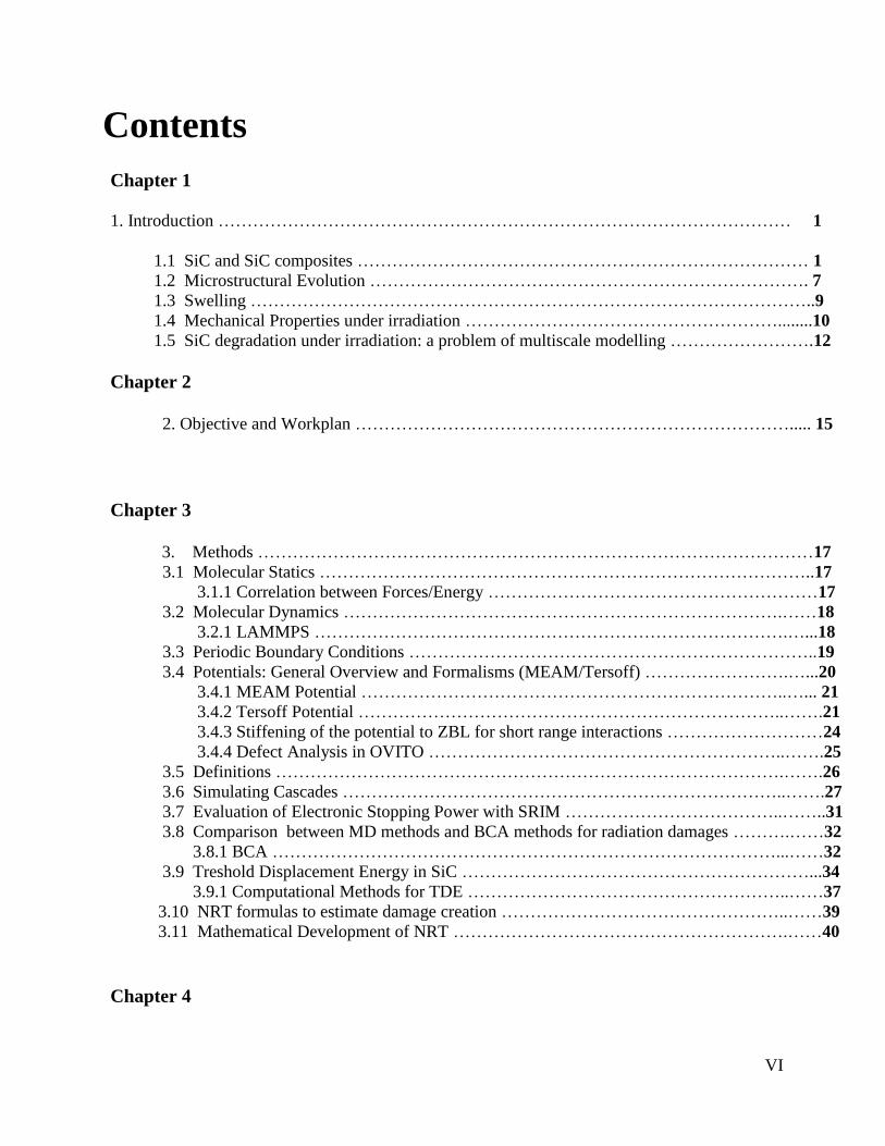
Contents Chapter 1
1. Introduction ……………………………………………………………………………………… 1
1.1 SiC and SiC composites …………………………………………………………………… 1
1.2 Microstructural Evolution …………………………………………………………………. 7
1.3 Swelling ……………………………………………………………………………………..9
1.4 Mechanical Properties under irradiation ………………………………………………........10
1.5 SiC degradation under irradiation: a problem of multiscale modelling …………………….12
Chapter 2
2. Objective and Workplan …………………………………………………………………..... 15
Chapter 3
3. Methods ……………………………………………………………………………………17
3.1 Molecular Statics …………………………………………………………………………..17
3.1.1 Correlation between Forces/Energy …………………………………………………17
3.2 Molecular Dynamics ………………………………………………………………….……18
3.2.1 LAMMPS ……………………………………………………………………….…...18
3.3 Periodic Boundary Conditions ……………………………………………………………..19
3.4 Potentials: General Overview and Formalisms (MEAM/Tersoff) …………………….…...20
3.4.1 MEAM Potential ………………………………………………………………..…... 21
3.4.2 Tersoff Potential ………………………………………………………………..…….21
3.4.3 Stiffening of the potential to ZBL for short range interactions ………………………24
3.4.4 Defect Analysis in OVITO ……………………………………………………..…….25
3.5 Definitions …………………………………………………………………………….…….26
3.6 Simulating Cascades …………………………………………………………………..…….27
3.7 Evaluation of Electronic Stopping Power with SRIM ………………………………..……..31
3.8 Comparison between MD methods and BCA methods for radiation damages ……….……32
3.8.1 BCA ……………………………………………………………………………...……32
3.9 Treshold Displacement Energy in SiC ……………………………………………………...34
3.9.1 Computational Methods for TDE ………………………………………………..……37
3.10 NRT formulas to estimate damage creation …………………………………………..……39
3.11 Mathematical Development of NRT ………………………………………………….……40
Chapter 4
VII
4. Atomic Structure of SiC and Graphite ………………………………………………..…….44
4.1 SiC atomic structure …………………………………………………………………..……44
4.2 Graphite atomic structure …………………………………………………………….……46
4.3 Point defects …………………………………………………………………………..……47
4.3.1 SiC: vacancies ………………………………………………………………….…...47
4.3.2 Graphite: vacancies …………………………………………………………….…...48
4.3.3 SiC: interstitials ………………………………………………………………...…...48
4.3.4 Graphite: interstitials …………………………………………………………..……50
Chapter 5
5. Results and Discussion ……………………………………………………………………53
5.1 Potential selection …………………………………………………………………..…… 53
5.1.1 SiC potentials ……………………………………………………………………53
5.1.2 Graphite potentials ………………………………………………………………56
5.1.3 Conclusions ………………………………………………………………..…….58
5.2 Stopping Power in SiC ……………………………………………………………………59
5.3 Cascade in SiC …………………………………………………………………………… 62
5.4 Binary Collision Approximation …………………………………………………….……69
5.6 Interfaces SiC/graphite ……………………………………………………………………78
5.6.1 Interface Energy …………………………………………………………….…...78
5.6.2 Binding Energy of point defects to interfaces ……………………………...……82
Chapter 6
6. Summary and Conclusions …………………………………………………………...……92
VIII
List of figures
1.1
1.1.2
1.1.3
1.1.4
1.2.1
1.2.2
1.3.1
1.4.1
1.4.2
3.3.1
3.5.1
3.5.2
3.9.1
3.9.2
3.9.3
3.10.1
Chapter 1
Stacking sequence of SiC bilayers of the most common polytypes of SiC (from left to right): 3C,
2H, 4H and 6H ……………………………………………………………….…………………... . 2
Phase diagram of the C/Si system ……………………………………………………….……….. . 3
TRISO Fuel compact and coating fuel …………………………………………………..………… 5
Prototype SiC/SiC control rods with articulating joints …………………………………………… 6
Microstructural features observed in SiC as function of temperature and damage (dpa).. ………….8
Dependence of defect radius (a) and defect density (b) on irradiation temperature in Si‐ion and
neutron irradiated 3C‐SiC……………………………………………………….…………………..9
Irradiation‐induced swelling of β-SiC for a wide temperature range …………………...………….10
Flexural behavior of non-irradiated and irradiated CVI SiC/SiC composites. The stress-strain curves
are shifted to aid visibility ………………………………………………...…………………….…11
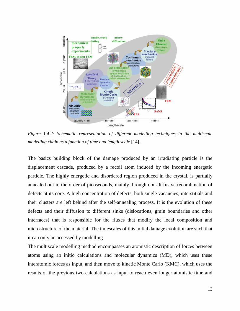
Schematic representation of different modelling techniques in the multiscale modelling chain as a
function of time and length scale……………………………………………..…………………....13
Chapter 3
The square periodic boundary conditions commonly used for equilibrium molecular dynamics
simulations as 2D representation. The central cell (bold) is the primary cell and the cells surrounding
it are its periodic images. Particles 1’ and 3’ are periodic images of particles 1 and 3,
respectively………………………………………………...………………………………………20
Representation of the simulation domain: from the reference state represented in Ovito to the
cascade event simulation ……………………………………………………….....………………28
Schemes of the collision events…………………………..………………………………………..29
A Si PKA along the [111] direction. Carbon atoms are drawn in black, and silicon toms in yellow.
The silicon PKA is drawn in orange and the vacancy is represented by an open circle. A kinetic
energy E is given to a Si atom, which is subsequently displaced. If E<Ed, the PKA returns to its
original location. If E>Ed, there is formation of a silicon vacancy VSi and a silicon tetrahedral
interstitial surrounded by four carbon atoms SiTC………….……………………………………..35
Representation of the main crystallographic directions in 3C-SiC [100] direction. Carbon atoms are
drawn in black, and silicon atoms in yellow…………………………..………………………….36
Potential energy of the system 3C-SiC in function of time for different kinetic energies of the PKA
atoms………………………………………………………………………...……………………38
Distance of closest approach representation ……………………………………………..………42
Chapter 4
IX
4.1.1
4.1.2
4.2.1
4.3.1
4.3.2
4.3.3
4.3.4
4.3.5
4.3.6
4.3.7
4.3.8
5.2.1
5.2.2
5.2.3
5.3.1
Schematic of a 3C-SiC unit cell. This structure is known as the `zinc-blende' structure. The red
spheres are the carbon atoms, the larger ones the silicon. In blue, orange and green it is possible to
distinguish the first, second and third neighbor distance in the cubic cell.
…………………………………………………………………………………………………….44
Schematic representation of the stacking order of 3C-SiC (cubic stacking). 3C-SiC is one of the
extremes of the SiC polytypes, and is the only cubic polytype. Miller indices are given to show the
orientation, the large and small spheres in each bi-layer denote a silicon and carbon atom,
respectively ……………………………………………………………………………………….46
An orthogonal unit cell (white solid lines) viewed from the top for graphite. The carbons (circles) in
the A (B) planes are shown in dark (light) gray circles ……………………….………………….46
Si vacancy 3D representation …………………………………………………………………….47
β-vacancy in graphite (coplanar class) and cross-layer Vαβ vacancy (cross-layer class) 2D
representation ………………………………………………………………………..………..…..48
Configurations of Si interstitials in SiC (in yellow Si and in grey C atoms). Interstitials Si atoms are
represented as orange spheres …………………………………………………………………….49
Configurations of C interstitials in SiC (in yellow Si and in grey C atoms). Interstitials C atoms are
represented as green spheres ……………………………………………….……………………..59
Interstitial atoms in graphite: the spiro interstitial and Y-lid transition state. The prismatic types of
interstitials have been seen to be, in literature, the most unstable forms, changing shape, directions
and bonding after relaxation ……………………………………………………………………...50
Grafted interstitial defect in graphite ……………………………………………………………..51.
β-split interstitial defect in graphite ……………………………………………………...……….51
Canted interstitial defect in graphite …………………………………………………….………52
Chapter 5
Electronic and nuclear stopping power for Si-PKA atom in function of PKA kinetic energy. On
right-hand picture it is represented the evolution of the electronic and nuclear stopping power for
1keV < Ek <100 keV. ……………………………………………………………………………59
Electronic and nuclear stopping power for C-PKA atom in function of PKA kinetic energy. On right-
hand picture it is represented the evolution of the electronic and nuclear stopping power for 1keV
< Ek <100 keV. …………………………………………………………………………………..60
A) Velocity of the Si-PKA atom in Ang/ps in function of the kinetic energy. As it is possible to see
from the picture the tendency of the curve can be approximated with a linear regression as
y=0.0069·x.
B) Velocity of the C-PKA atom in Ang/ps in function of the kinetic energy. As it is possible to see
from the picture the tendency of the curve can be approximated with a linear regression as
y=0.0038·x. ………………………………………………………………………………………61
The final defect states of at 5keV (a), at 10 keV (b) and a 50 keV (c) and 100 keV (d) cascade in SiC
from which can be clearly seen the transition from a single pocket of atomic displacements to
multiple subcascades. ………………………………………….…………………………………62
X
5.3.2
5.3.3
5.3.4
5.3.5
5.3.6
5.5.1
5.5.2
5.5.3
5.5.4
5.5.5
5.5.6
5.5.7
5.6.1
Plot of the total number of vacancies or interstitials (C defects plus Si defects) for 10 keV ans
100keV Si-PKA through the simulated time. ………………………………………………….64
Plots of the number of Si and C defects averaged over the 10 non-wrap-around runs and different
energy Si-PKA values (5keV, 100 keV). ……………………………………………………….65
Plot of the number of C and Si vacancies created by 10 keV Si-PKA in function of time simulated
in this work from Devanathan and Samolyuk . The two plots differs from the one of this work
because the temperature was controlled during the simulation by coupling the atoms along the four
cell boundaries to a reservoir of heat at 300 K while the simulation of this work has been kept at 0
K. ……………………………………….…………………………………………………….....66
A) The graph represents a statistics of vacancy cluster count versus the cluster size. The five group
of columns represent the values found for 1keV, 5keV, 10keV, 50keV and 100 keV. B) The graph
represents a statistics of interstitial clusters count versus the cluster size. The five group of columns
represent the values found for 1keV, 5keV, 10keV, 50keV and 100
keV.………………………………………………………………………………………………… ………………………………………………...67
Interstitial and vacancy clusters linear approximation in function of the cluster size. In the picture is
possible to see that bot interstitial and vacancy clusters follow a linear approximation on logarithmic
scale.……………………………………………………………………………………. ……………………………………………………………68
Comparison of NRT formulas with different values of TDE ( TDESi=46 eV TDEC=36 eV calculated
with Erhart-Albe potential in blue, TDESi=15 eV TDEC=28 eV using the values suggested in TRIM
in red, TDESi= 38 eV TDEC=19 Ev suggested on DFT calculations in yellow)
…………………………………………………………………………………………………………..…………………………………………….…69
Comparison of SiC defects calculated with values of TDE for the Kirchin-Pease formula (1974)
(TDESi=46 eV TDEC=36 eV calculated with Erhart-Albe potential in blue, TDESi=15 eV TDEC=28
eV using the values suggested in TRIM in red TDESi= 38 eV TDEC=19 Ev suggested on DEFT
calculations in yellow) ………………………………………………………………………………………………………………….…71
Defect production efficiency as a function of PKA damage energy. ………………………..…72
Comparison of TRIM computational results calculated with different values of TDE (TDESi=46 eV
TDEC=36 eV calculated with Erhart-Albe potential in blue dots, TDESi=15 eV TDEC=28 eV using
the values suggested in TRIM in red dots TDESi= 38 eV TDEC=19 Ev suggested on DEFT
calculations in yellow dots) …………………………………..…………………………………………………………………….….73
Defect production efficiency as a function of PKA damage energy in TRIM. ………….……..74
Evaluation of SiC defects calculated using the Kirchin-Pease formula, using the closest approach
approximation. Comparison of TRIM computational results, Kirchin-Pease, NRT (1975) formula
with molecular dynamics results TDE values from Erhart-Albe potential (TDESi=46 eV TDEC=36 )
………………………………………………………………………………………………………………………………………………………….…75
A) The results in the graph represent the C/Si ratio for vacancies using TRIM compared with those
reported for MD calculations. It is possible to see that C/Si ratio calculated for MD results is in good
agreement with that calculated for TRIM in which it was used the TDE values calculated with
Erhart-Albe potential. ……………………………………………………..………………………………………………………….……76
B) C/Si ratio for interstitials defect and vacancies defects reported for SiC. It is possible to see a
constant tendency for both C/Si ratio defined for vacancies and
interstitials……………………………………………………………..…………………………………………………….…………………..79
Color map representing the [001] SiC/graphite interface system potential energy. The scope of the
image is furnishing a visual representation of those configuration which have lower potential energy
and so which are more stable. In red the most stable configuration. For our calculation we chose
XI
5.6.2
5.6.3
5.6.4
5.6.5
5.6.6
5.6.7
5.6.8
5.6.9
5.6.10
5.6.11
5.6.12
those interface which coordinates are x=23 and y=10.
……………………………………………………………………………………………………………………………….…………………….………80
Color map representing the [111] SiC/graphite interface system potential energy. The scope of the
image is furnishing a visual representation of those configuration which have lower potential energy
and so which are more stable. In red the most stable configuration. For our calculation we chose
those interface which coordinates are x=50 and y=37.
…………………………………………………………………………………………………………………………………………………………..….83
[001/001] SiC/graphite interface front overview and [111/001] SiC/graphite interface front view
most stable configuration. ………………………………………………………………………………………………………………...84
The figure represents the binding energy between Si vacancy created in the system alternating first
Si layer (in blue) and C layer (in red) on the interface. ………………….……………………...84
The figure represents the binding energy between C vacancy created in the system alternating first
Si layer (in blue) and C layer (in red) on the interface. ……………………………………………………………….…85
Non relaxed [111/100] SiC/graphite interface: a) original structure with Si layer, b) rebuilt structure
with Si layer, c) original structure with C layer, d) rebuilt structure with C
layer……………………………………………………………………………………………………………………………………..……………..86
The figure represents the binding energy between Si vacancy created in the original system
alternating first Si layer (in blue) and C layer (in red) on the interface………….…………………….. 87
The figure represents the binding energy between Si vacancy created in the manually rebuilt system
alternating first Si layer (in blue) and C layer (in red) on the interface…..……………………………….….88
The figure represents the binding energy between C vacancy created in the original system
alternating first Si layer (in blue) and C layer (in red) on the interface…………..……………….…… 89
The figure represents the binding energy between C vacancy created in the manually rebuilt system
alternating first Si layer (in blue) and C layer (in red) on the interface………………………....90
The figure represents the binding energy between C<100> dumbbell created in the system alternating
first Si layer (in blue) and C layer (in red) on the interface………………….. ……………………….….90
The figure represents the binding energy between tetrahedral interstitial SiTC created in the system
alternating first Si layer (in blue) and C layer (in red) on the interface……...…………………………..91
XII
List of tables
1.1
3.6.1
3.9.1
5.1.1
5.1.2
5.1.3
5.1.4
5.6.1
5.6.2
Material properties of SiC compared with cubic diamond……………………………………….4
Velocity of Si-PKA atoms along the <1 3 5> direction………………………………………….30
Treshold diplacement energy values for this work compared with DFT analysis and experiment from
[43], [44], [45] …………………………………………………………………………………...36
results of lattice parameter (a) and cohesive energy (Ec) obtained using different potential formalism
……………………………………………………………………………………………………54
Results of points defect formation energies obtained using different potential formalism……...55
Results of lattice parameter (a) and cohesive energy (Ec) obtained using different potential
formalism………………………………………………………………………………………....57
Results of points defect formation energies obtained using different potential formalism………58
Potential energy of the most stable configurations of [100/100] and [111/100] SiC/graphite interface
……………………………………………………………………………………………………………………………………………………………….81
Interface Energy calculation of the most stable configurations of [100/100] and [111/100] SiC/graphite
interface ……………………………………………………………………………………………………………………………………………….81

XIII
XIV
Nomenclature ASME American Society of Mechanical Engineers
ASTM American Society for Testing and Material
BOP Bond Order Potential
C Carbon
CM Center of Mass
CSi Carbon antisite
DPA Displacements per atom
DFT Density Functional Theory
ES Electronic Stopping (Power)
FP Frenkel Pair
HTGR High Temperature Gas Reactor
keV 103 elettronvolt
LOCA Loss of Coolant Accident
MC Monte Carlo method
MEAM Modified Embebbed Atom Method
MD Molecular dynamics
MS Molecular statics
NRT Norgett-Robinson-Torrens
OKMC Object Kinetic Monte Carlo
PKA Primary Knock-on Atom
PWR Pressurized Water Reactor
Si Silicon
SiC Silicon Carbide
SiC/PyC Silicon Carbide / Pyrolytic Graphite interface
SiC Si antisite
SIA Self-Interstitial Atoms
SRIM Stopping and Range of Ions in Matter
XV
T89 Original Tersoff Potential (1989)
T90 Modified Tersoff Potential (1990)
T94 Modified Tersoff Potential (1994)
TDE Treshold Displacement Energy
TEM Transmission Electron Microscope
TRIM Transport od Atoms in Matter
TRISO Tristructural-isotropic
V Vacancy
VHTR Very High Temperature Reactor
ZBL Ziegler-Biersack-Littmark

XVI
1
Chapter 1
1. Introduction
This introduction exposes the context of this work, pointing out the importance of this
research thesis on industrial applications related to the use of SiC fibers, mainly in nuclear
industry.
After the description of the main mechanical and thermic properties of SiC and SiC/PyC
fibers, an outline of the thesis is given in order to introduce the overall topic to the reader.
1.1. SiC and SiC Composites Silicon carbide, also called moissanite is found in only minute quantities in certain types
of meteorite and in corundum deposits. Because of its rare occurrence in nature, all the
silicon carbide sold in the world is synthetic. Natural moissanite was first found in 1893 as
a small component of the Canyon Diablo meteorite in Arizona by Dr. F.H Moissan, after
whom the material was named in 1905.
Silicon Carbide has been recognized as an ideal material for applications that require
superior hardness, high thermal conductivity, low thermal expansion, chemical and
oxidation resistance.
In the solid state, the stoichiometric composition of silicon and carbon termed silicon
carbide (SiC) is the only chemical stable compound in the C/Si system.
More than 250 different types of structures, so-called polytypes of SiC exist [1]. The
differences between all these compounds consist mainly in the stacking sequence of
identical, close-packed SiC bilayers.
2
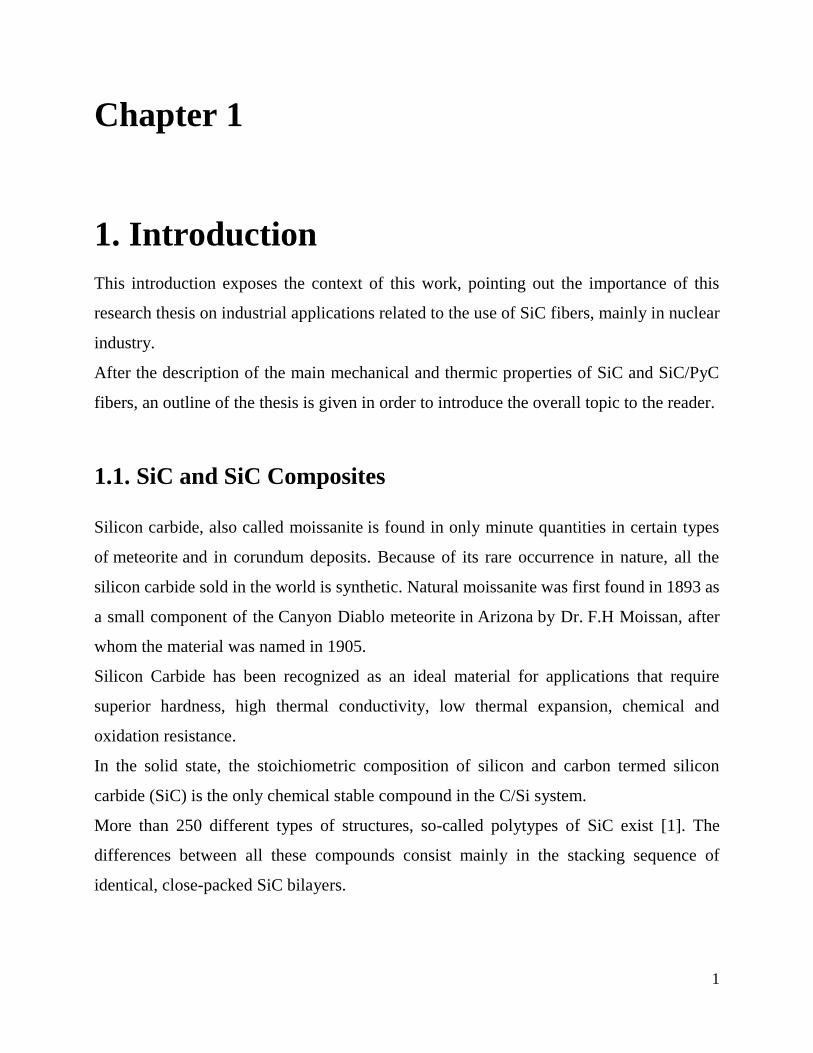
The Figure 1.1 shows the stacking sequence of the most common and technologically most
important SiC polytypes, which are the cubic (3C) and hexagonal (2H, 4H and 6H)
polytypes.
Figure 1.1: Stacking sequence of SiC bilayers of the most common polytypes of SiC (from left to
right): 3C, 2H, 4H and 6H [2].
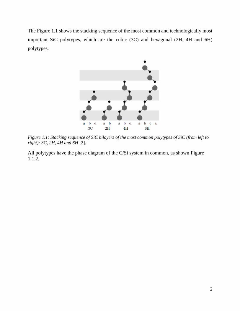
All polytypes have the phase diagram of the C/Si system in common, as shown Figure
1.1.2.
3
Figure 1.1.2: Phase diagram of the C/Si system [3]
Because of its high mechanical stability, heat resistance, radiation hardness and low neutron
capture cross section, it is proposed for operation in harsh and radiation-hard environments,
which make it a suitable candidate cladding (coating) material for nuclear fusion. A
European project dedicated to the use of advanced carbides as coatings for accident tolerent
fuels is the IL TROVATORE project, to which the present thesis contributes.
The low neutron capture cross section and radiation hardness favors its use in nuclear
detector applications. In fact, the high breakdown field coupled with the high thermal
conductivity allow SiC transistors to handle much higher power densities and frequencies
in stable operation at high temperatures.
Moreover, in addition to high-temperature operations, the wide band gap also allows the
use of SiC in optoelectronic devices: the SiC photodiodes serve as excellent sensors
applicable in the monitoring and control of turbine engine combustion.
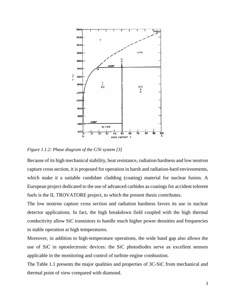
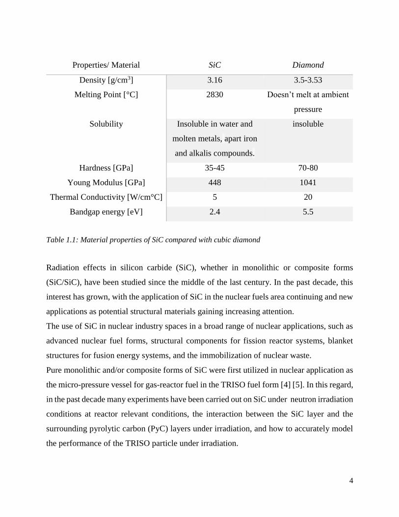
The Table 1.1 presents the major qualities and properties of 3C-SiC from mechanical and
thermal point of view compared with diamond.
4
Properties/ Material SiC Diamond
Density [g/cm3] 3.16 3.5-3.53
Melting Point [°C] 2830 Doesn’t melt at ambient
pressure
Solubility Insoluble in water and
molten metals, apart iron
and alkalis compounds.
insoluble
Hardness [GPa] 35-45 70-80
Young Modulus [GPa] 448 1041
Thermal Conductivity [W/cm°C] 5 20
Bandgap energy [eV] 2.4 5.5
Table 1.1: Material properties of SiC compared with cubic diamond
Radiation effects in silicon carbide (SiC), whether in monolithic or composite forms
(SiC/SiC), have been studied since the middle of the last century. In the past decade, this
interest has grown, with the application of SiC in the nuclear fuels area continuing and new
applications as potential structural materials gaining increasing attention.
The use of SiC in nuclear industry spaces in a broad range of nuclear applications, such as
advanced nuclear fuel forms, structural components for fission reactor systems, blanket
structures for fusion energy systems, and the immobilization of nuclear waste.
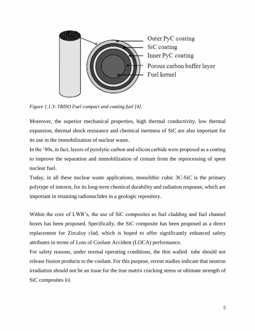
Pure monolithic and/or composite forms of SiC were first utilized in nuclear application as
the micro-pressure vessel for gas-reactor fuel in the TRISO fuel form [4] [5]. In this regard,
in the past decade many experiments have been carried out on SiC under neutron irradiation
conditions at reactor relevant conditions, the interaction between the SiC layer and the
surrounding pyrolytic carbon (PyC) layers under irradiation, and how to accurately model
the performance of the TRISO particle under irradiation.
5
Figure 1.1.3: TRISO Fuel compact and coating fuel [4].
Moreover, the superior mechanical properties, high thermal conductivity, low thermal
expansion, thermal shock resistance and chemical inertness of SiC are also important for
its use in the immobilization of nuclear waste.
In the ‘80s, in fact, layers of pyrolytic carbon and silicon carbide were proposed as a coating
to improve the separation and immobilization of cesium from the reprocessing of spent
nuclear fuel.
Today, in all these nuclear waste applications, monolithic cubic 3C-SiC is the primary
polytype of interest, for its long-term chemical durability and radiation response, which are
important in retaining radionuclides in a geologic repository.
Within the core of LWR’s, the use of SiC composites as fuel cladding and fuel channel
boxes has been proposed. Specifically, the SiC composite has been proposed as a direct
replacement for Zircaloy clad, which is hoped to offer significantly enhanced safety
attributes in terms of Loss of Coolant Accident (LOCA) performance.
For safety reasons, under normal operating conditions, the thin walled tube should not
release fission products to the coolant. For this purpose, recent studies indicate that neutron
irradiation should not be an issue for the true matrix cracking stress or ultimate strength of
SiC composites [6].
6
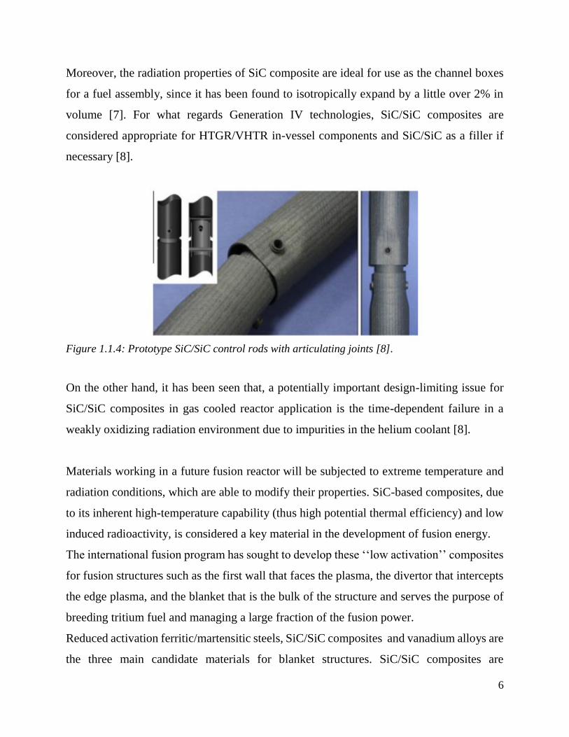
Moreover, the radiation properties of SiC composite are ideal for use as the channel boxes
for a fuel assembly, since it has been found to isotropically expand by a little over 2% in
volume [7]. For what regards Generation IV technologies, SiC/SiC composites are
considered appropriate for HTGR/VHTR in-vessel components and SiC/SiC as a filler if
necessary [8].
Figure 1.1.4: Prototype SiC/SiC control rods with articulating joints [8].
On the other hand, it has been seen that, a potentially important design-limiting issue for
SiC/SiC composites in gas cooled reactor application is the time-dependent failure in a
weakly oxidizing radiation environment due to impurities in the helium coolant [8].
Materials working in a future fusion reactor will be subjected to extreme temperature and
radiation conditions, which are able to modify their properties. SiC-based composites, due
to its inherent high-temperature capability (thus high potential thermal efficiency) and low
induced radioactivity, is considered a key material in the development of fusion energy.
The international fusion program has sought to develop these ‘‘low activation’’ composites
for fusion structures such as the first wall that faces the plasma, the divertor that intercepts
the edge plasma, and the blanket that is the bulk of the structure and serves the purpose of
breeding tritium fuel and managing a large fraction of the fusion power.
Reduced activation ferritic/martensitic steels, SiC/SiC composites and vanadium alloys are
the three main candidate materials for blanket structures. SiC/SiC composites are
7
considered an advanced structural material because of their attractive safety features when
used in a helium-cooled ceramic breeding (HCCB) blanket or self-cooled lead-lithium
(SCLL) blanket.
In particular, the most significant achievement in this process was the development of
exceptionally radiation-resistant SiC/SiC composites, which proved to not deteriorate the
mechanical properties irradiated up to a high neutron fluence. This is especially true for
SiC/SiC fibers enriched in oxides (e.g 30% ZrSiO4, Tyranno-SA and Hi-Nicalon type-S),
which show better high temperature and cracking resistance [8].
In general, the first wall undergoes the harshest irradiation damage in fusion devices.
Moreover, because the radiation effect on lattice thermal conduction is inevitable, the
radiation-induced decrease in thermal conductivity is a critical design-limitation for a
ceramic first wall.
In conclusion, the future use of this material is mostly dependent on the creation of nuclear-
specific ASTM standards and the creation of ASME design code development specifically
dedicated to the application of these materials in all type of nuclear reactors.
1.2. Microstructural Evolution
Many authors in literature identified guidelines for ion irradiation to screen SiC/SiC for use
in LWRs for ATF applications. For this specific use of SiC and/or SiC fibres in the nuclear
sector, the assessment of the SiC/SiC composites is constrained to a narrow window of
conditions: E =400‐500 GPa, flexural strength = 300–450 MPa, flexural strain = 1–1.25%,
and irradiation swelling = 1–2% in the 300–600°C range. In addition, the material has to
demonstrate radiation stability up to a fast fluence of 20x1021 n/cm2, or about 20 dpa.
8
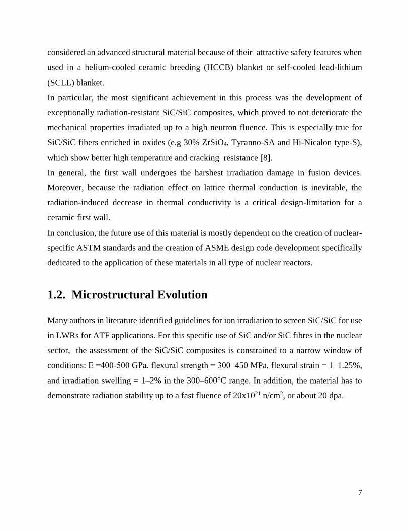
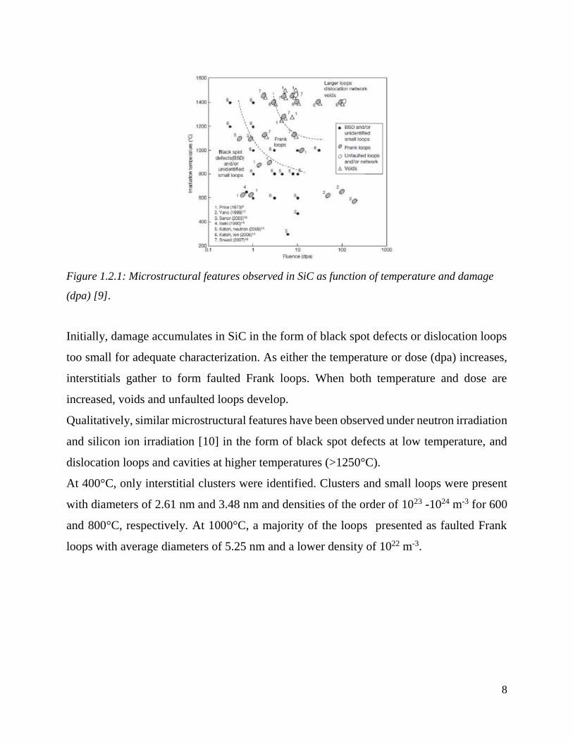
Figure 1.2.1: Microstructural features observed in SiC as function of temperature and damage
(dpa) [9].
Initially, damage accumulates in SiC in the form of black spot defects or dislocation loops
too small for adequate characterization. As either the temperature or dose (dpa) increases,
interstitials gather to form faulted Frank loops. When both temperature and dose are
increased, voids and unfaulted loops develop.
Qualitatively, similar microstructural features have been observed under neutron irradiation
and silicon ion irradiation [10] in the form of black spot defects at low temperature, and
dislocation loops and cavities at higher temperatures (>1250°C).
At 400°C, only interstitial clusters were identified. Clusters and small loops were present
with diameters of 2.61 nm and 3.48 nm and densities of the order of 1023 -1024 m-3 for 600
and 800°C, respectively. At 1000°C, a majority of the loops presented as faulted Frank
loops with average diameters of 5.25 nm and a lower density of 1022 m-3.
9
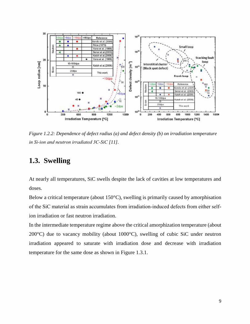
Figure 1.2.2: Dependence of defect radius (a) and defect density (b) on irradiation temperature
in Si‐ion and neutron irradiated 3C‐SiC [11].
1.3. Swelling
At nearly all temperatures, SiC swells despite the lack of cavities at low temperatures and
doses.
Below a critical temperature (about 150°C), swelling is primarily caused by amorphisation
of the SiC material as strain accumulates from irradiation‐induced defects from either self-
ion irradiation or fast neutron irradiation.
In the intermediate temperature regime above the critical amorphization temperature (about
200°C) due to vacancy mobility (about 1000°C), swelling of cubic SiC under neutron
irradiation appeared to saturate with irradiation dose and decrease with irradiation
temperature for the same dose as shown in Figure 1.3.1.
10
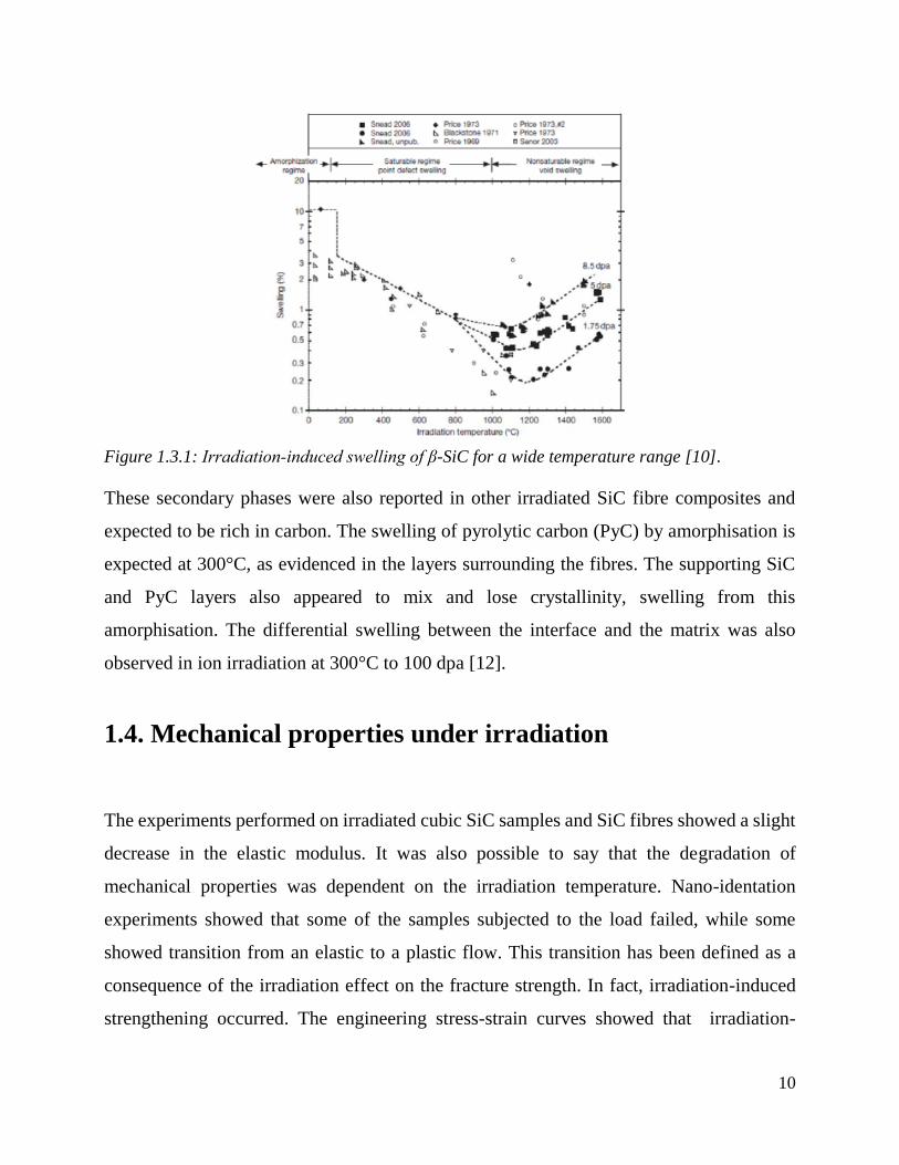
Figure 1.3.1: Irradiation‐induced swelling of β-SiC for a wide temperature range [10].
These secondary phases were also reported in other irradiated SiC fibre composites and
expected to be rich in carbon. The swelling of pyrolytic carbon (PyC) by amorphisation is
expected at 300°C, as evidenced in the layers surrounding the fibres. The supporting SiC
and PyC layers also appeared to mix and lose crystallinity, swelling from this
amorphisation. The differential swelling between the interface and the matrix was also
observed in ion irradiation at 300°C to 100 dpa [12].
1.4. Mechanical properties under irradiation
The experiments performed on irradiated cubic SiC samples and SiC fibres showed a slight
decrease in the elastic modulus. It was also possible to say that the degradation of
mechanical properties was dependent on the irradiation temperature. Nano-identation
experiments showed that some of the samples subjected to the load failed, while some
showed transition from an elastic to a plastic flow. This transition has been defined as a
consequence of the irradiation effect on the fracture strength. In fact, irradiation-induced
strengthening occurred. The engineering stress-strain curves showed that irradiation-
11
induced strengthening seemed to be significant between 300 and 800 °C. As explained in
the previous section, the observed microstructures of ion-irradiated SiC showed the
appearance of small clusters when the temperature reaches 400°C. These defects, are
expected to affect the mechanical properties and induce various radiation effects.
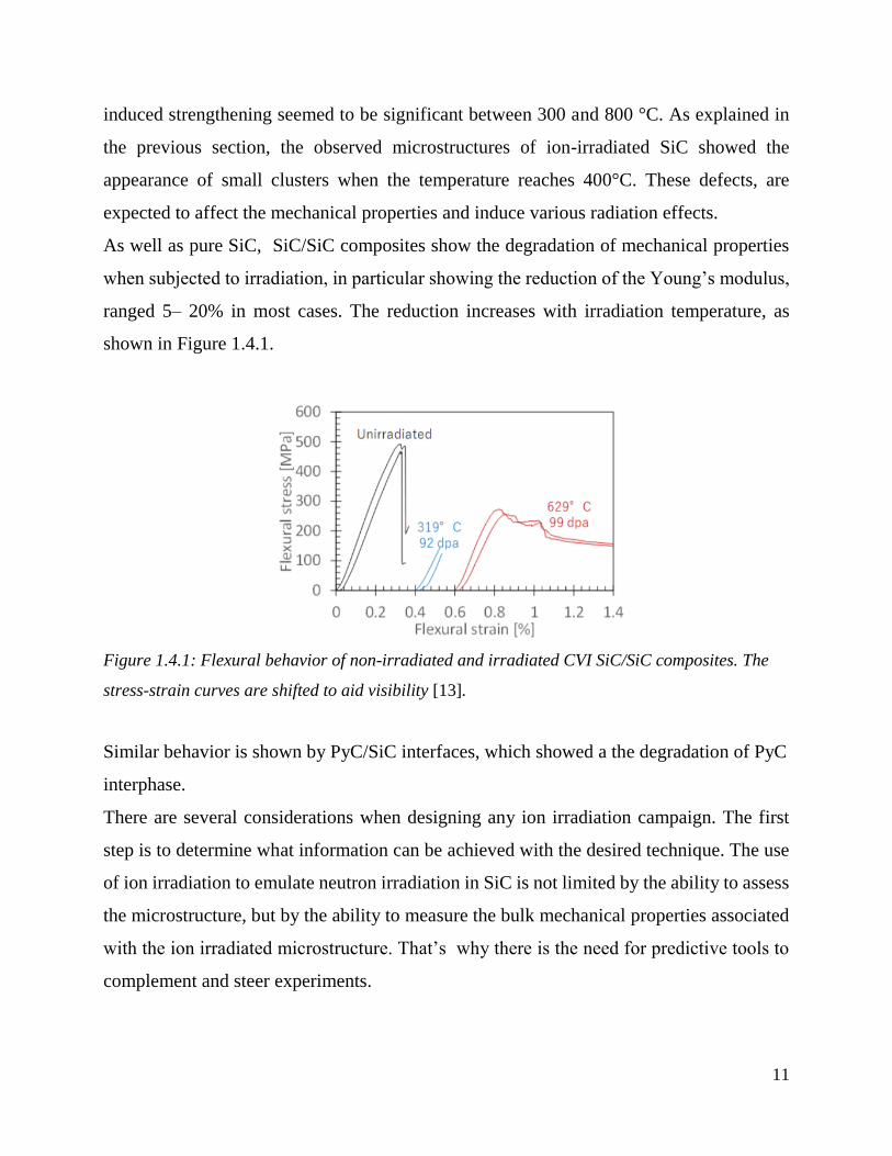
As well as pure SiC, SiC/SiC composites show the degradation of mechanical properties
when subjected to irradiation, in particular showing the reduction of the Young’s modulus,
ranged 5– 20% in most cases. The reduction increases with irradiation temperature, as
shown in Figure 1.4.1.
Figure 1.4.1: Flexural behavior of non-irradiated and irradiated CVI SiC/SiC composites. The
stress-strain curves are shifted to aid visibility [13].
Similar behavior is shown by PyC/SiC interfaces, which showed a the degradation of PyC
interphase.
There are several considerations when designing any ion irradiation campaign. The first
step is to determine what information can be achieved with the desired technique. The use
of ion irradiation to emulate neutron irradiation in SiC is not limited by the ability to assess
the microstructure, but by the ability to measure the bulk mechanical properties associated
with the ion irradiated microstructure. That’s why there is the need for predictive tools to
complement and steer experiments.
12
1.5. SiC degradation under irradiation: a problem of multi-
scale modelling
As these materials are degraded by their exposure to high temperatures, irradiation and a
corrosive environment, it is necessary to address the issue of long term degradation of
materials under service exposure in advanced plants.
Thus, irradiation damage becomes a multi-scale problem: A higher confidence in life-time
assessments of these materials requires an understanding of the related physical phenomena
on a range of scales from the atomic level of single defect energetics all the way up to
macroscopic components.
Recently, there has been a surge to study materials using multiscale modelling, by
performing studies using a wide range of techniques. This has come about with the
recognition that the macroscopic failure of a component is associated with events that start
at the atomic level. The multiscale modelling, in fact, intends to follow the development of
phenomena that originate at the atomic level using appropriate modelling schemes, all the
way to the macroscopic level. This procedure enables physical insight into the material’s
behavior, which might otherwise be lost if only experimental correlations are used.
Experiments are then needed to test or validate critical aspects of the modelling.
13
Figure 1.4.2: Schematic representation of different modelling techniques in the multiscale
modelling chain as a function of time and length scale [14].
The basics building block of the damage produced by an irradiating particle is the
displacement cascade, produced by a recoil atom induced by the incoming energetic
particle. The highly energetic and disordered region produced in the crystal, is partially
annealed out in the order of picoseconds, mainly through non-diffusive recombination of
defects at its core. A high concentration of defects, both single vacancies, interstitials and
their clusters are left behind after the self-annealing process. It is the evolution of these
defects and their diffusion to different sinks (dislocations, grain boundaries and other
interfaces) that is responsible for the fluxes that modify the local composition and
microstructure of the material. The timescales of this initial damage evolution are such that
it can only be accessed by modelling.
The multiscale modelling method encompasses an atomistic description of forces between
atoms using ab initio calculations and molecular dynamics (MD), which uses these
interatomic forces as input, and then move to kinetic Monte Carlo (KMC), which uses the
results of the previous two calculations as input to reach even longer atomistic time and
14
length scales. Modelling of the mechanical properties of the material is achieved by
implementing dislocation dynamics (DD) simulations and the proper macroscopic scale
then uses finite element (FE) methods and continuum models.
Thus, the interchange between computational models and experiment is critical in
developing accurate predictive models. Improvements of micro- and nanostructural
investigation methods (quantitative electron microscopy and microanalysis), high
resolution transmission microscopy, atomic force microscopy, X-ray technologies, together
with specimen preparation (like FIB) are allowing a direct coupling of the local mechanical
properties with the local microstructure.
To contribute to this topic, the present thesis focusses on primary damage production and
defect interface interactions. Large-scale molecular dynamics (MD) simulations have been
applied to study defect production for lattice atom recoil energies in the range 1-100 keV,
caused by primary knock-on atoms (PKAs) in 3C-SiC. Finally size and composition
distribution of in-cascade clusters provide a critical input for long-term defect evolution
models. Molecular static simulations have been employed to estimate the binding erergy
between different point defects and SiC/graphite interface. Also these results provide input
for long-term defect evolution models.
15
Chapter 2
2. Objectives and work plan
The objectives of the present thesis are twofold:
I. perform an in-depth MD study to characterize primary damage in SiC;
II. initiate a study to characterize the binding energy between point defects and the
SiC/graphite interface.
Both objectives will provide direct input to coarse grain models such as object kinetic
Monte Carlo and rate theory models.
To reach these objectives, the following work plan is followed:
Potential selection
Amongst different potentials available in the literature we computed the energetic stability
of point defects (vacancy/interstitial/anti-sites) in both 3C-SiC and graphite. The results
were compared with available DFT data and the potential providing best agreement with
DFT was retained for further studies.
Stiffening of the selected potential
Once the most appropriate equilibrium potential is selected, it needs to be stiffened to
correctly reproduce the electronic and nuclear stopping power. For the nuclear stopping
power the potential was smoothly merged to the ZBL screened Coulomb potential such that
the equilibrium properties were not modified. For the electronic stopping, a viscous friction
term was introduced in the MD integration algorithm such that the electronic stopping
power predicted by SRIM is reproduced.
Cascade simulations using MD
16
Using the stiffened potential and the appropriate viscosity term, cascades were simulated
for PKA energies in the range 1-100keV along high index directions at zero Kelvin. Each
condition was simulated 10 times to achieve statistics.
Analysis of the MD results
Defect analyses are performed on the MD results to characterize the cascades in terms of
produced Frenkel pairs, anti-sites and vacancy/interstitial clusters. Regressions as a
function of PKA energy were derived.
Cascade simulations using BCA
The BCA method and NRT formula were applied and their defect production compared to
the MD results. The aim is to reliably estimate the total defect production based on
BCA/NRT methods, while their clustering probability is obtained from the regressions
based on the MD results.
Initiation of defect/interface interactions
Molecular static calculations were performed to estimate the binding energy between
point-defects and different SiC/graphite interface configurations.
17
Chapter 3
3. Methods
3.1 Molecular statics
Atomistic simulations describe materials at the level of atoms. In the case of Molecular
Statics (MS), the relaxed configuration of atoms is found using a conjugate gradient or
some similar (constrained) minimization of the total energy. This provides information
about crystal lattice structure in different phases and under different conditions.
3.1.1 Correlation Force/Energy
For any potential U(r) ,force exerted on atom i due to atom j is given by the following
equation
f U rij d i (3.1)
Then we have total force exerted on a particular atom
F f rij ij
r rij c
( )
(3.2)
Finally, the potential energy of atom i directly given by the potential
E U ri
u
ij
r rij c
d i (3.3)
18
The equilibrium state of the lattice corresponds to the global minimum of its potential
energy. Generally, at each step the unbalanced resultant forces acting on each atom are
found. Then each atom is moved into the direction of the unbalanced force vector by the
amount functionally dependent on the magnitude of this force.
3.2 Molecular Dynamics
MD simulates the time evolution of a system of classical particles by repeatedly solving
Newton's second law of motion for each individual particle; on an atomistic scale, it
simulates the trajectories of individual particles rather than bulk properties of the material.
Assuming that at some time ti, the positions r(ti), velocities v(ti), and masses m of the
particles are known, the MD algorithm will proceed as follows:
1. Using a provided potential V (r0, r1, r2… ), the net force F = -∇V on each particle is
computed at time step ti.
2. Using Newton's second law F = ma, the acceleration of each particle is computed at
time step ti.
3. Using the acceleration a(ti), the position r(ti), and the velocity v(ti) the position and
velocity of the particles at the next time step, r(ti+1) and v(ti+1), are computed.
4. Steps 1-3 are repeated for time step ti+1
3.2.1 LAMMPS
19
LAMMPS (Large-scale Atomic/Molecular Massively Parallel Simulator, see
http://lammps.sandia.gov), an MD program developed by Sandia National Laboratories, was
used in this project to simulate the effect of PKA energy on defect production on irradiated
SiC and SiC/graphite interface. LAMMPS utilizes parallel computing to simulate
collections of atoms and/or molecules using standard molecular dynamics code [15]. At the
end of the simulation, LAMMPS outputs a text or dump file containing the coordinates
and energies of all particles in the manually built simulation box, as well as any other
parameters that the user requests. In this project, for each atom in the simulation, LAMMPS
outputs the atom ID, the location, the potential energy. These outputs were then used in
OVITO, along with some of OVITO's [16] analysis methods, to analyze the defects in each
simulation.
3.3 Periodic Boundary Conditions
For a system to remain homogeneous in space one applies periodic boundary conditions.
When using PBC, particles are enclosed in a box, in such a way we can image that it is
replicated to infinity by rigid translation in all the three cartesian directions, completely
filling the space. In other words, the cells adjacent to the central simulation cell are periodic
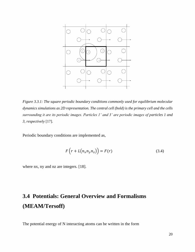
images of it. In Figure 3.3.1 particles that move out through one face of the cell are replaced
by their images coming in through the opposite face. For example, particle 1 moves out of
the right-hand face of the central simulation cell and is replaced by particle 1’ coming in
from the left image box. The interactions between particles are calculated such that an atom
interacts with its closest image.
20
Figure 3.3.1: The square periodic boundary conditions commonly used for equilibrium molecular
dynamics simulations as 2D representation. The central cell (bold) is the primary cell and the cells
surrounding it are its periodic images. Particles 1’ and 3’ are periodic images of particles 1 and
3, respectively [17].
Periodic boundary conditions are implemented as,
𝐹 (𝑟 + 𝐿(𝑛𝑥𝑛𝑦𝑛𝑧)) = 𝐹(𝑟) (3.4)
where nx, ny and nz are integers. [18].
3.4 Potentials: General Overview and Formalisms
(MEAM/Tersoff)
The potential energy of N interacting atoms can be written in the form
21
𝑈(𝑟) = ∑ 𝑈1(𝑟𝑖)𝑖 + ∑ ∑ 𝑈2(𝑟𝑖, 𝑟𝑗)𝑗>𝑖𝑖 + ∑ ∑ ∑ 𝑈3(𝑟𝑖,𝑟𝑗 , 𝑟𝑘)𝑘>𝑗>𝑖𝑗>𝑖𝑖 … (3.5)
where U is the total potential energy. U1 is a single particle potential describing external
forces. Examples of single particle potentials are the gravitational force or an electric field.
U2 is a two body pair potential which only depends on the distance rij between the two
atoms i and j. If not only pair potentials are considered, three body potentials U3 or many
body potentials Un can be included. Usually these higher order terms are avoided since they
are not easy to model and it is rather time consuming to evaluate potentials and forces
originating from these many body terms.
In our work we used three-body potentials in form of MEAM and Tersoff type potentials.
3.4.1 MEAM Potential
The MEAM was created by Baskes, by modifying the EAM so that the directionality of
bonding is considered, and was applied to provide interatomic potentials of various fcc,
bcc, diamond, and gaseous elements [19].
The general MEAM formalism can be expressed as following:
𝑈 = 𝐹𝑖(��𝑖) +1
2 ∑ 𝛷𝑖𝑗(𝑅𝑖𝑗)𝑗≠𝑖 (3.6)
Fi is the embedding function, ��𝑖 is the background electron density at site i, and 𝛷𝑖𝑗(𝑅𝑖𝑗) is
the pair interaction between atoms i and j separated by a distance Rij. Within EAM the
background density has a central symmetry, while in MEAM, it depends on the angle
formed between two nearest neighbor atoms from atom i.
3.4.2 Tersoff Potential
Tersoff proposed an empirical interatomic potential for covalent systems [20][21]. The
Tersoff potential explicitly incorporates the dependence of bond order on local
22
environments, permitting an improved description of covalent materials. Due to the
covalent character, Tersoff restricted the interaction to nearest neighbor atoms accompanied
by an increase in computational efficiency for the evaluation of forces and energy based on
the short-range potential. Tersoff applied the potential to silicon [20], carbon and also to
multicomponent systems like silicon carbide [21].
Tersoff incorporated the concept of bond order in a three-body potential formalism. The
interatomic potential is taken to have the form
𝐸 = ∑ 𝐸𝑖 =𝑖1
2 ∑ 𝑉𝑖𝑗𝑖≠𝑗≠ (3.7)
𝑉𝑖𝑗 = 𝑓𝑐(𝑟𝑖𝑗)[𝑉𝑅(𝑟𝑖𝑗) + 𝑏𝑖𝑗𝑉𝐴(𝑟𝑖𝑗)] (3.8)
E is the total energy of the system, constituted either by the sum over the site energies Ei or
by the bond energies Vij . The indices i and j correspond to the atoms of the system with rij
being the distance from atom i to atom j. The functions VR and VA represent a repulsive and
an attractive pair potential. The repulsive part is due to the orthogonalization energy of
overlapped atomic wave functions.
In case of the Erhart-Albe potential, the repulsive and attractive terms change slightly form
the original formalism in the following way:
(3.9)
(3.10)
23
where D0 and r0 are the dimer energy and bond length. The parameter b can be determined
from the ground-state oscillation frequency of the dimer, while S is adjusted to the slope of
the Pauling plot. The cutoff function is defined as,
The parameters R and D specify the position and the width of the cutoff region. The
bond-order is given by
and the angular function
(3.14)
The three-body interactions are determined by the parameters 2μ, γ, c, d, and h, which leads
in total to up to nine adjustable parameters, all of them depending on the type of atoms i
and j.
The parameter optimization proceeds as follows: First, the pair parameters are adjusted to
the dimer properties D0, r0, β and the slope of the Pauling plot(S). Thereafter, the three-
body parameters are fitted to the cohesive energies and bond lengths of several high-
symmetry structures as well as to the elastic constants of the ground structures. The
(3.11)
(3.12)
(3.13)
24
transferability of the potential is enforced by including a variety of differently coordinated
structures in the fitting database [22].
3.4.3 Stiffening of the potential to ZBL for short range interaction
In case of high energy events, such as simulations of collision cascades due to high energy
ion irradiation, the repulsive potential can be modified to give a more accurate behavior at
interatomic distances much shorter than in typical near-equilibrium simulations. Another
repulsive function, VR0(r), in addition to the original VR (r), is often included as
the total potential energy of a system of atoms is given by
(3.18)
Where ff represents the short-range function through the use of the Fermi function
(3.19)
The use of this function allows for a smooth connection between the equilibrium potential
and the short range ZBL potential.
(3.15)
(3.16)
(3.17)
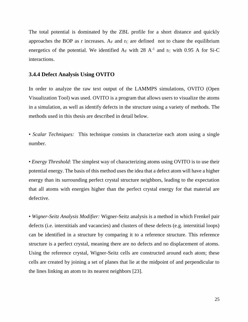
25
The total potential is dominated by the ZBL profile for a short distance and quickly
approaches the BOP as r increases. AF and rC are defined not to chane the equilibrium
energetics of the potential. We identified AF with 28 A-1 and rC with 0.95 A for Si-C
interactions.
3.4.4 Defect Analysis Using OVITO
In order to analyze the raw text output of the LAMMPS simulations, OVITO (Open
Visualization Tool) was used. OVITO is a program that allows users to visualize the atoms
in a simulation, as well as identify defects in the structure using a variety of methods. The
methods used in this thesis are described in detail below.
• Scalar Techniques: This technique consists in characterize each atom using a single
number.
• Energy Threshold: The simplest way of characterizing atoms using OVITO is to use their
potential energy. The basis of this method uses the idea that a defect atom will have a higher
energy than its surrounding perfect crystal structure neighbors, leading to the expectation
that all atoms with energies higher than the perfect crystal energy for that material are
defective.
• Wigner-Seitz Analysis Modifier: Wigner-Seitz analysis is a method in which Frenkel pair
defects (i.e. interstitials and vacancies) and clusters of these defects (e.g. interstitial loops)
can be identified in a structure by comparing it to a reference structure. This reference
structure is a perfect crystal, meaning there are no defects and no displacement of atoms.
Using the reference crystal, Wigner-Seitz cells are constructed around each atom; these
cells are created by joining a set of planes that lie at the midpoint of and perpendicular to
the lines linking an atom to its nearest neighbors [23].
26
3.5 Definitions
Characteristic energy values
One of the main objectives of this work is to study the evolution of point defects and clusters
in irradiated SiC and SiC/graphite interface. In order to do that, it is first necessary to define
some characteristic energy values that give information about the stability of the material
crystallographic configuration or will tell us if a particular transformation is
thermodynamically favored. It is therefore crucial to have a precise definition for each of
these energies.
- Cohesive energy: it is the difference between the energy of a solid and the energy of the
isolated atoms. In practice, it can be calculated using the following equation:
𝐸𝑐𝑜ℎ =𝐸𝑡𝑜𝑡,𝑠𝑦𝑠𝑡𝑒𝑚
𝑁− 𝐸𝑖 (3.20)
In our case Ei= 0 and N is total number of atoms in the system.
- Binding energy: when more than one lattice defect exists, they may repel or tend to cluster;
if they cluster, it is because the total energy decreases when they join: the corresponding
energy gain is called binding energy. It is calculated using atomistic simulation techniques
as the difference between the energy the crystal when the defects are far (configuration A)
and the same crystal when the defects are closer from each other (configuration B):
𝐸𝑏𝑖𝑛𝑑𝑖𝑛𝑔 = 𝐸𝐴 − 𝐸𝐵 (3.21)
- Formation Energy: the defect formation energy is how much cohesive energy is needed
to form a point defect in a perfect lattice.
The formation energies Ef were obtained from the total energies of the supercells with a
defect
27
𝐸𝑓 = 𝐸𝑑 − 𝐸 − ∑ 𝑁𝑖𝜇𝑖𝑖 (3.22)
Ed is the total energy of the defected supercell and E the total energy of perfect graphite and
perfect cubic silicon boxes, which we calculated for supercells of the same size as used in
the runs with the defects. Ni represented the total number of species in the supercell and μ
in this formula is the pure cohesive energy of Si bulk and graphite bulk.
Following the method described by Erhart and Albe [22]. The formation energy reduces
then to
In the case of graphite the formula reduces to
𝐸𝑓 = 𝐸𝑑 − 𝐸 − 𝑁𝑐𝜇𝐶
Where Nc is the total number of atoms after the insertion of vacancy (Nperfect -1) or
interstitials (Nperfect +1).
3.6 Simulating cascades
Our simulations used the variable time step procedure, based on the phases of cascade
formation. We performed 10 different cascades for each energy simply changing the seed
number which changes slightly the track and the velocity along one coordinate of the
direction. Each cascade was reached about 20 ps.
(3.23)
(3.24)
28
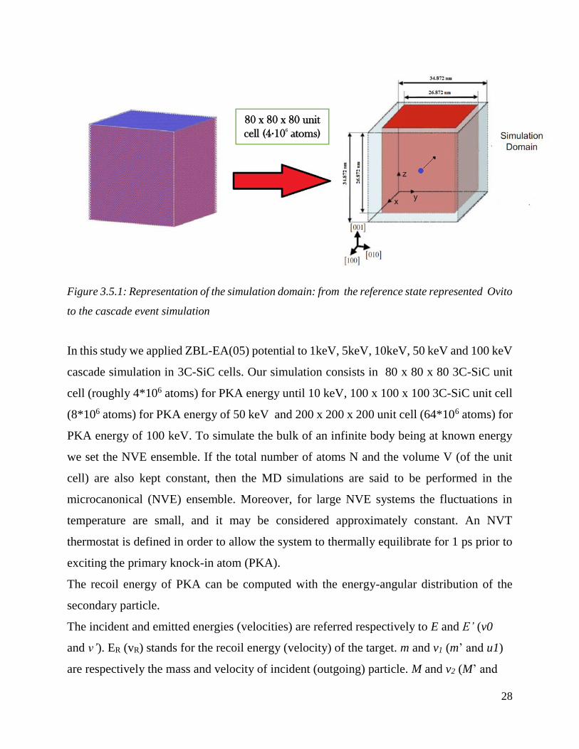
Figure 3.5.1: Representation of the simulation domain: from the reference state represented Ovito
to the cascade event simulation
In this study we applied ZBL-EA(05) potential to 1keV, 5keV, 10keV, 50 keV and 100 keV
cascade simulation in 3C-SiC cells. Our simulation consists in 80 x 80 x 80 3C-SiC unit
cell (roughly 4*106 atoms) for PKA energy until 10 keV, 100 x 100 x 100 3C-SiC unit cell
(8*106 atoms) for PKA energy of 50 keV and 200 x 200 x 200 unit cell (64*106 atoms) for
PKA energy of 100 keV. To simulate the bulk of an infinite body being at known energy
we set the NVE ensemble. If the total number of atoms N and the volume V (of the unit
cell) are also kept constant, then the MD simulations are said to be performed in the
microcanonical (NVE) ensemble. Moreover, for large NVE systems the fluctuations in
temperature are small, and it may be considered approximately constant. An NVT
thermostat is defined in order to allow the system to thermally equilibrate for 1 ps prior to
exciting the primary knock-in atom (PKA).
The recoil energy of PKA can be computed with the energy-angular distribution of the
secondary particle.
The incident and emitted energies (velocities) are referred respectively to E and E’ (v0
and v’). ER (vR) stands for the recoil energy (velocity) of the target. m and v1 (m’ and u1)
are respectively the mass and velocity of incident (outgoing) particle. M and v2 (M’ and
80 x 80 x 80 unit
cell (4·106
atoms)
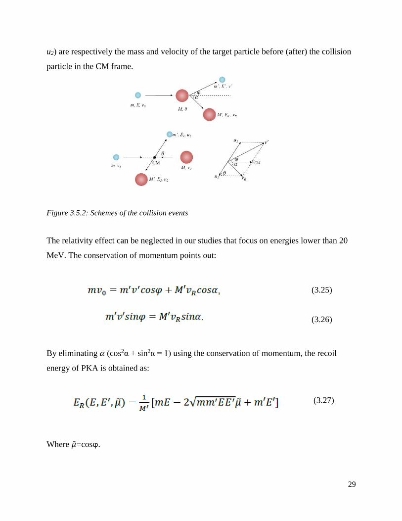
29
u2) are respectively the mass and velocity of the target particle before (after) the collision
particle in the CM frame.
Figure 3.5.2: Schemes of the collision events
The relativity effect can be neglected in our studies that focus on energies lower than 20
MeV. The conservation of momentum points out:
By eliminating 𝛼 (cos2α + sin2α = 1) using the conservation of momentum, the recoil
energy of PKA is obtained as:
Where 𝜇=cosϕ.
(3.25)
(3.26)
(3.27)
30
Performing very fast calculation, considering a range of neutron interaction between
0.025 eV and 2 MeV, and imposing that the neutrons loses entirely its energy after the
collision (which is improbable in reality) and the angle of scattering is 0°, we obtain that
the recoil energy of the Si atom approaches 100 keV.
That’s why we decided to take into account 5 sets of energies: 1keV, 5 keV, 10 keV, 50
keV and 100 keV.
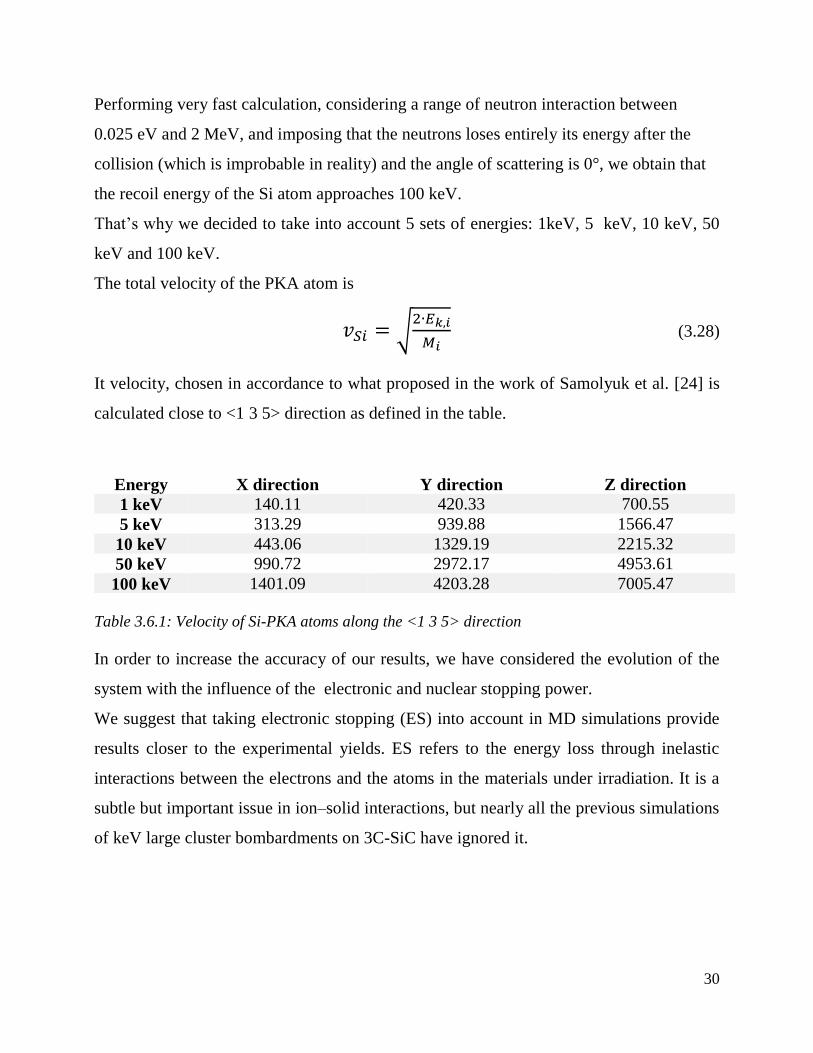
The total velocity of the PKA atom is
𝑣𝑆𝑖 = √2∙𝐸𝑘,𝑖
𝑀𝑖 (3.28)
It velocity, chosen in accordance to what proposed in the work of Samolyuk et al. [24] is
calculated close to <1 3 5> direction as defined in the table.
Table 3.6.1: Velocity of Si-PKA atoms along the <1 3 5> direction
In order to increase the accuracy of our results, we have considered the evolution of the
system with the influence of the electronic and nuclear stopping power.
We suggest that taking electronic stopping (ES) into account in MD simulations provide
results closer to the experimental yields. ES refers to the energy loss through inelastic
interactions between the electrons and the atoms in the materials under irradiation. It is a
subtle but important issue in ion–solid interactions, but nearly all the previous simulations
of keV large cluster bombardments on 3C-SiC have ignored it.
Energy X direction Y direction Z direction
1 keV 140.11 420.33 700.55
5 keV 313.29 939.88 1566.47
10 keV 443.06 1329.19 2215.32
50 keV 990.72 2972.17 4953.61
100 keV 1401.09 4203.28 7005.47
31
3.7 Evaluation of the electronic stopping with SRIM
Linear stopping power (stopping force) is defined as S = -dE/dx, where E is the ion energy
and x is the path length. We often use the mass stopping power S/ρ, where ρ is the mass
density of the material.
Electronic stopping (collisions between ion and target electrons) leads primarily to
excitation and ionization of target atoms, and to energy loss of ion.
Nuclear stopping (elastic “billiard ball” collisions between ion and target atom) leads
to change of direction, and to energy loss of ion. (No nuclear forces are involved!)
The total stopping power is the sum of nuclear and electronic stopping power:
𝑆𝑡𝑜𝑡 = 𝑆𝑒𝑙 + 𝑆𝑛 (3.29)
In order to incorporate the electronic stopping power in MD simulation, we have to
calculate the friction term which modifies the velocity of the incoming particle in the
system.
Knowing from the Newton law the dumping force is given by:
𝑚 ∙𝑑2𝑟
𝑑𝑡2= �� = 𝐹𝑛𝑢𝑐
+ 𝐹𝑒𝑙 = 𝛾 ∙𝑑𝑟
𝑑𝑡 (3.30)
The larger the coefficient (γ), the faster the kinetic energy is reduced. The nuclear stopping
power is already accounted for by the ZBL screened Coulomb potential.
32
3.8 Comparison between MD methods and BCA methods for
radiation damages
3.8.1 BCA
One of the widely accepted techniques utilized for studying ion irradiation induced damage
on surfaces, which is important at higher energies, is the Binary Collision Approximation
(BCA). In BCA the assumption is made that collisions between atoms can be approximated
as elastic binary collisions. In this technique, a single collision between the incident ion and
a substrate atom is evaluated by solving the classical scattering integral between two
colliding particles (the interatomic potential is usually a screened Coulomb potential).
The solution of the integral results in both the scattering angle of the incident ion and its
energy loss, which is transferred to the substrate.
BCA methods use a maximum impact parameter set by the density of the medium and a
constant mean free path between collisions. The scattering angle is determined by a specific
formula, tested against published integral tables and represents the scattering from the ZBL
“universal” potential seen previously in the chapter dedicated to the short range fitting of
the BOP used in MD simulations.
The advantages of BCA is its speed, which is 4-5 orders of magnitude faster than MD [25].
Therefore BCA is based on some assumptions and limitations. This approximation emerges
when incident ions have low energies, or in very dense substrate materials, or when
chemical effects play a role in materials.
A static Monte-Carlo program which is known as transport of ions in matter is (TRIM).
The program assumes an amorphous substrate structure at zero temperature and infinite
side size and treats the bombardment of incident ions on different substrate structures [26].
Stopping and Range of Ions in Matter (SRIM) code [see: http://www.srim.org/] is another
program which can calculate interaction of ions with matter. The core of SRIM is TRIM.
33
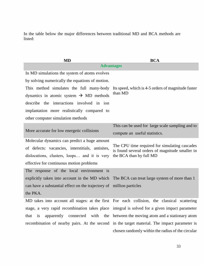
In the table below the major differences between traditional MD and BCA methods are
listed:
MD
BCA
Advantages
In MD simulations the system of atoms evolves
by solving numerically the equations of motion.
This method simulates the full many-body
dynamics in atomic system MD methods
describe the interactions involved in ion
implantation more realistically compared to
other computer simulation methods
Its speed, which is 4-5 orders of magnitude faster
than MD
More accurate for low energetic collisions
This can be used for large scale sampling and to
compute an useful statistics.
Molecular dynamics can predict a huge amount
of defects: vacancies, interstitials, antisites,
dislocations, clusters, loops… and it is very
effective for continuous motion problems
The CPU time required for simulating cascades
is found several orders of magnitude smaller in
the BCA than by full MD
The response of the local environment is
explicitly taken into account in the MD which
can have a substantial effect on the trajectory of
the PKA.
The BCA can treat large system of more than 1
million particles
MD takes into account all stages: at the first
stage, a very rapid recombination takes place
that is apparently connected with the
recombination of nearby pairs. At the second
For each collision, the classical scattering
integral is solved for a given impact parameter
between the moving atom and a stationary atom
in the target material. The impact parameter is
chosen randomly within the radius of the circular
34
stage, relaxation occurs much more slowly under
the conditions of diffusion controlled reaction.
area of interaction cross-section and is calculated
based only on composition and atomic density of
the target material
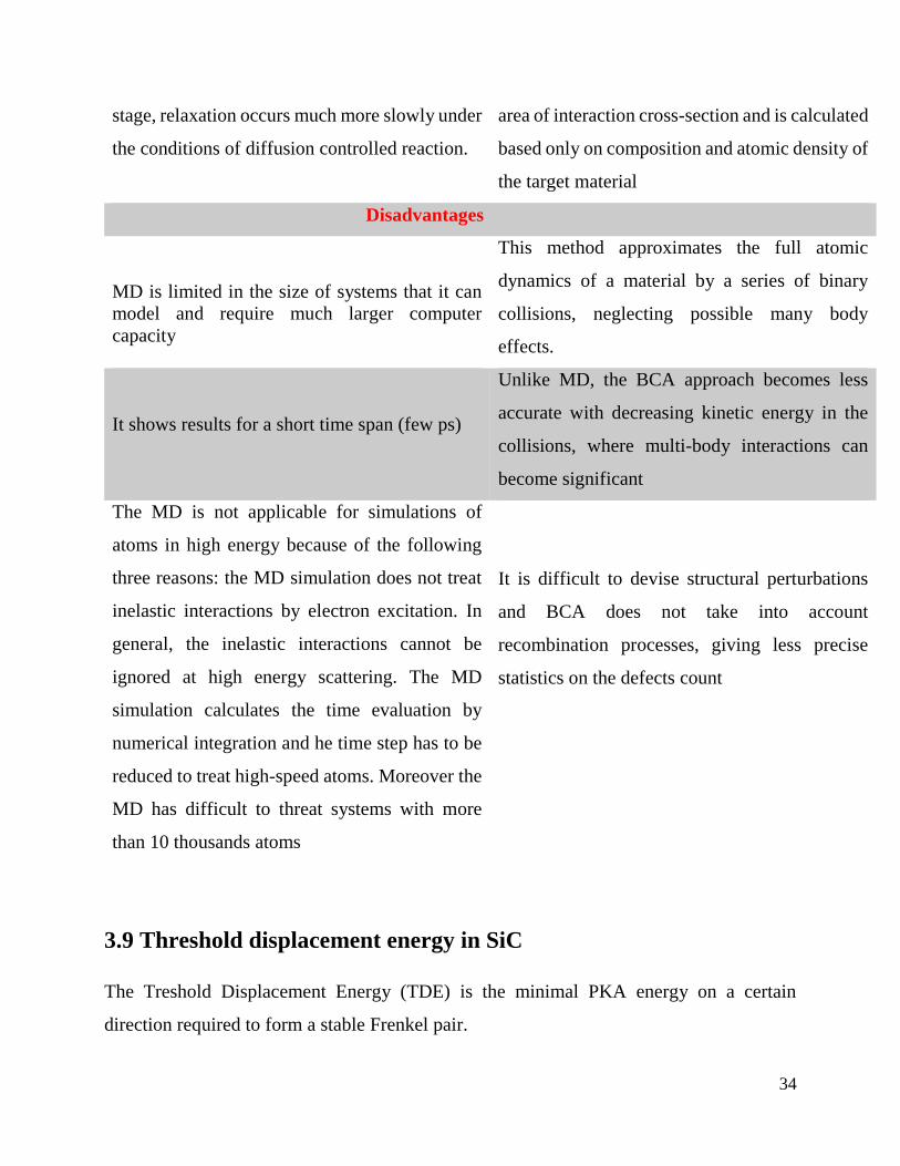
Disadvantages
MD is limited in the size of systems that it can
model and require much larger computer
capacity
This method approximates the full atomic
dynamics of a material by a series of binary
collisions, neglecting possible many body
effects.
It shows results for a short time span (few ps)
Unlike MD, the BCA approach becomes less
accurate with decreasing kinetic energy in the
collisions, where multi-body interactions can
become significant
The MD is not applicable for simulations of
atoms in high energy because of the following
three reasons: the MD simulation does not treat
inelastic interactions by electron excitation. In
general, the inelastic interactions cannot be
ignored at high energy scattering. The MD
simulation calculates the time evaluation by
numerical integration and he time step has to be
reduced to treat high-speed atoms. Moreover the
MD has difficult to threat systems with more
than 10 thousands atoms
It is difficult to devise structural perturbations
and BCA does not take into account
recombination processes, giving less precise
statistics on the defects count
3.9 Threshold displacement energy in SiC
The Treshold Displacement Energy (TDE) is the minimal PKA energy on a certain
direction required to form a stable Frenkel pair.
35
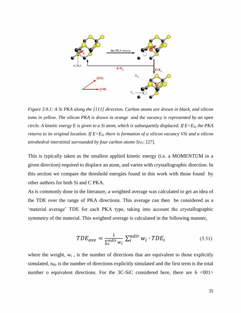
Figure 3.9.1: A Si PKA along the [111] direction. Carbon atoms are drawn in black, and silicon
toms in yellow. The silicon PKA is drawn in orange and the vacancy is represented by an open
circle. A kinetic energy E is given to a Si atom, which is subsequently displaced. If E<Ed, the PKA
returns to its original location. If E>Ed, there is formation of a silicon vacancy VSi and a silicon
tetrahedral interstitial surrounded by four carbon atoms SiTC. [27].
This is typically taken as the smallest applied kinetic energy (i.e. a MOMENTUM in a
given direction) required to displace an atom, and varies with crystallographic direction. In
this section we compare the threshold energies found in this work with those found by
other authors for both Si and C PKA.
As is commonly done in the literature, a weighted average was calculated to get an idea of
the TDE over the range of PKA directions. This average can then be considered as a
‘material average’ TDE for each PKA type, taking into account the crystallographic
symmetry of the material. This weighted average is calculated in the following manner,
𝑇𝐷𝐸𝑎𝑣𝑒 =1
∑ 𝑤𝑖𝑛𝑑𝑖𝑟𝑖
∑ 𝑤𝑖𝑛𝑑𝑖𝑟𝑖 ∙ 𝑇𝐷𝐸𝑖 (3.31)
where the weight, wi , is the number of directions that are equivalent to those explicitly
simulated, ndir is the number of directions explicitly simulated and the first term is the total
number o equivalent directions. For the 3C-SiC considered here, there are 6 <001>
36
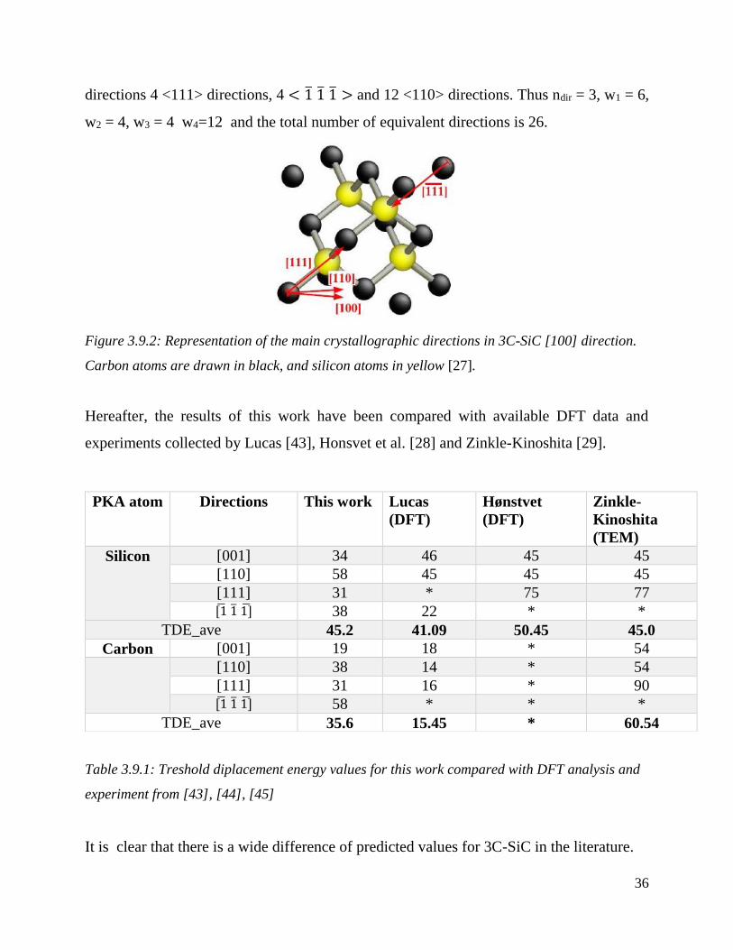
directions 4 <111> directions, 4 < 1 1 1 > and 12 <110> directions. Thus ndir = 3, w1 = 6,
w2 = 4, w3 = 4 w4=12 and the total number of equivalent directions is 26.
Figure 3.9.2: Representation of the main crystallographic directions in 3C-SiC [100] direction.
Carbon atoms are drawn in black, and silicon atoms in yellow [27].
Hereafter, the results of this work have been compared with available DFT data and
experiments collected by Lucas [43], Honsvet et al. [28] and Zinkle-Kinoshita [29].
Table 3.9.1: Treshold diplacement energy values for this work compared with DFT analysis and
experiment from [43], [44], [45]
It is clear that there is a wide difference of predicted values for 3C-SiC in the literature.
PKA atom Directions This work Lucas
(DFT)
Hønstvet
(DFT)
Zinkle-
Kinoshita
(TEM)
Silicon [001] 34 46 45 45
[110] 58 45 45 45
[111] 31 * 75 77 [1 1 1] 38 22 * *
TDE_ave 45.2 41.09 50.45 45.0
Carbon [001] 19 18 * 54 [110] 38 14 * 54
[111] 31 16 * 90 [1 1 1] 58 * * *
TDE_ave 35.6 15.45 * 60.54
37
There have been several measurements of the Ed, with different techniques, but a large
dispersion of values is obtained. In lack of precise data, Devianathan and Gao-Weber
proposed as average values for the C and Si sublattices 20 eV and 35 eV, respectively
(Atomic scale simulation of defect production in irradiated 3C-SiC). However, subsequent
molecular dynamics studies did not clearly confirm these values. Average values were
found from 17 to 40 eV for C sublattice and from 42 to 57 eV for Si sublattice, with extreme
values very different.
The work of Lucas has shown that, in silicon carbide, the error due to the cell size problem
is small compared to the discrepancy found between different calculation methods. This is
an important point, because choosing for different box size does not interfere with the
validity of this assumption.
3.9.1: Computational Method for TDE
For this work we took the threshold energy value from <100>, <110> ,<111>, and <
1 1 1 > directions using Erhart-Albe potential. In this section we describe the
computational method.
The threshold displacement energy is determined by examining the response of a perfect
crystal, when an initial kinetic energy is given to an atom located in the center of the
simulation cell.
Consequently this atom, which is usually called the primary knock-on atom (PKA), recoils
in the direction of the initial impulsion. The relaxation of the system is monitored and the
amount of initial energy transferred to the atom is gradually increased (5 eV increment)
until a stable Frenkel pair is formed, performing 10 runs for each threshold energy in order
to increase the precision of our statistic.
In order to identify a stable Frenkel pair, we performed the Wigner-Seitz analysis over each
of the 10 runs for each kinetic energy ( 1 eV increment).
38
Different results are expected for the Si sublattice as Si is heavier than C.
Indeed, higher energies are needed to create a stable Frenkel pair, which can be obtained
with a secondary knock-on C atom in some cases. In our work, for Si [100] we found that
the Frenkel pair forms at 34 eV, in good agreement with other MD simulations performed
with Tersoff potential and in the same range of DFT. The Si [110] case is certainly the most
complicated one due to the high kinetic energy transferred to the PKA. For example,
Pearson [30] reported that Si PKA can form a defect for Ed = 146 eV.
However, in our work, defects formed at 31 eV, a low result compared to DFT data, but it
is still in the same range of values for MD simulations data.
Along the Si <111> direction, we observed the creation of defects at Ed equal respectively
to 36 and 38 eV.
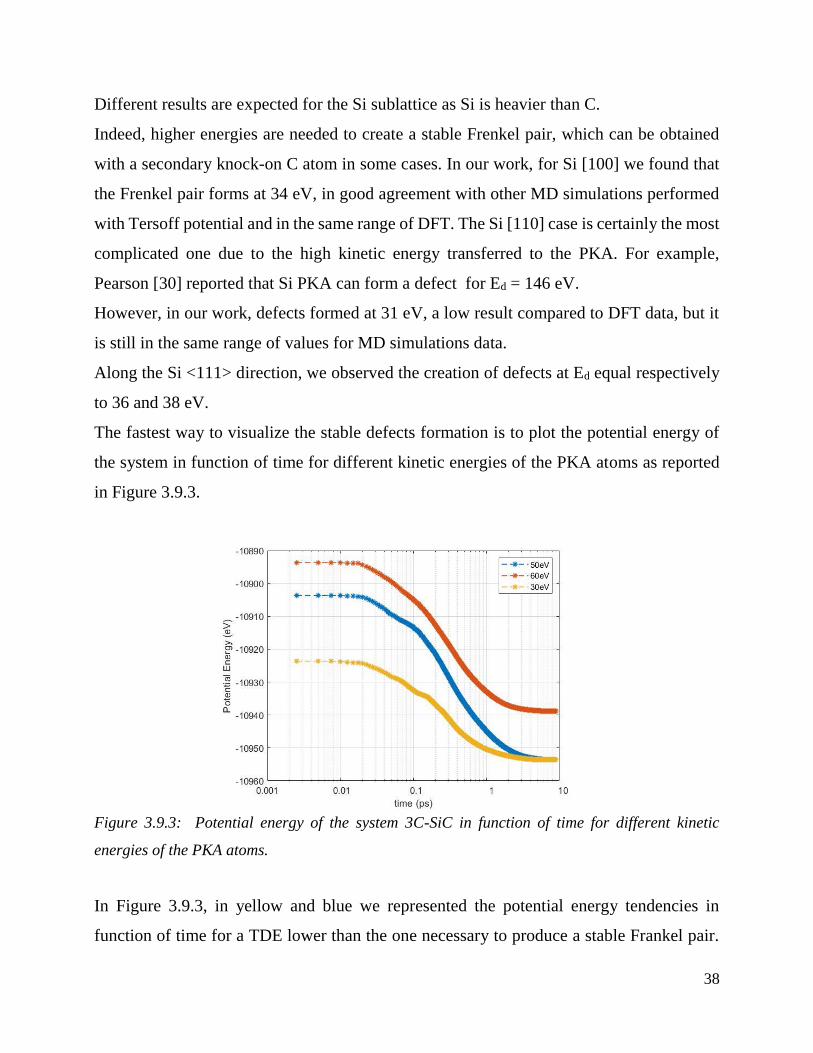
The fastest way to visualize the stable defects formation is to plot the potential energy of
the system in function of time for different kinetic energies of the PKA atoms as reported
in Figure 3.9.3.
Figure 3.9.3: Potential energy of the system 3C-SiC in function of time for different kinetic
energies of the PKA atoms.
In Figure 3.9.3, in yellow and blue we represented the potential energy tendencies in
function of time for a TDE lower than the one necessary to produce a stable Frankel pair.
39
In fact the system ends at the same energy level. On the other hand, in red, it is represented
the potential energy trend for TDE > Ed requested for a stable Frenkel pairs. On the third
phase the system stabilized to higher value of energy because of the presence of defects
which will not be annihilated. This method is easy and efficient, since it is not necessary to
check for multiple value of energies opening every time Ovito analysis. In fact it was
necessary to plot only the final value of the potential energy to visualize immediately the
difference in energy between a intact system and the one with stable Frenkel pairs.
When the Si-PKA atom along <111> direction has a kinetic energy of 30 and 50 eV the
vacancies and interstitials recombine and the system comes back to its original form. On
the other end for E ≥ Ed (60 eV) the system relaxed to an higher value of potential energy.
3.10 NRT formulas to estimate damage creation
A simple procedure, the NRT formulation, is proposed for calculating the number of atomic
displacements produced in a damage cascade by a primary knock-on atom of known energy.
The formulae have been chosen to give results in close accord with recent computer
simulations of radiation damage phenomena.
If we assume that the number of displacements produced by a PKA, ndisp, is proportional to
the fraction of the PKA energy that is deposited in elastic collisions, Td, we can write
For very low recoil energies E this number is given by
𝑛𝑑𝑖𝑠𝑝𝑙,𝑁𝑅𝑇 = 1 𝐸𝑇𝐷𝐸 < 𝑇𝑑 < 2𝐸𝑇𝐷𝐸
and for higher energies
𝑛𝑑𝑖𝑠𝑝𝑙,𝑁𝑅𝑇 = 0.8𝑇𝑑
2𝐸𝑇𝐷𝐸 𝑇𝑑 > 𝐸𝑇𝐷𝐸
40
𝑇𝑑 is expressed in keV and is the total energy available for displacing atoms, excluding
energy losses due to electronic excitation
𝐸𝑇𝐷𝐸 is the threshold displacement energy [31]:
The coefficient 0.8 can be seen as a kind of damage efficiency, originally deduced from
binary collision approximation calculations [NRT], while ETDE is the threshold
displacement energy calculated for Si and C displacements.
In particular, it is possible to observe a certain number of displaced atoms only if Td >
2ETDE; otherwise, if ETDE < Td < 2 ETDE, only one atom is displaced from its original lattice
site and there are no stable displacements at all when the damage energy of the incident
neutron is lower than the threshold displacement energy.
The errors seen from NRT formula are related to the fact that it does not account for
anything other than the total number of atomic displacements and it provides no information
on in-cascade formation of point defects and clusters. Moreover, it has also been shown
that at non-zero temperatures many of the created defects recombine, so that the net
surviving defect fraction is even lower. This means that the dpa is mainly a conventional
quantity to visualize the consequences of irradiation at 0K and to measure damage that
allows comparison between different irradiation-induced changes of material properties and
irradiation experiments with different particles (neutrons, ions, electrons, etc.).
3.11 Mathematical Development of NRT formula
In Norgett-Robinson-Torrens general formulation, Td is expressed as following [32]
𝑇𝑑 =𝐸𝑟𝑒𝑐𝑜𝑖𝑙
1+𝑘𝑑𝑔(𝜖𝑑) (3.32)
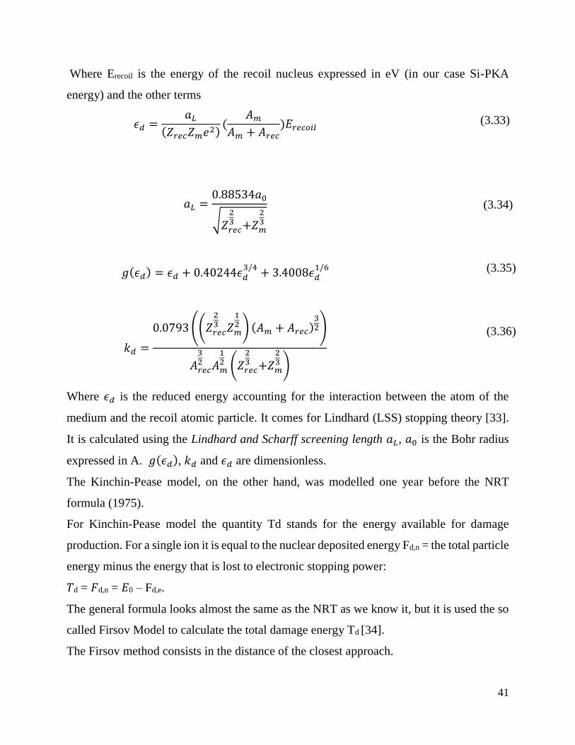
41
Where Erecoil is the energy of the recoil nucleus expressed in eV (in our case Si-PKA
energy) and the other terms
𝜖𝑑 =𝑎𝐿
(𝑍𝑟𝑒𝑐𝑍𝑚𝑒2)(
𝐴𝑚
𝐴𝑚 + 𝐴𝑟𝑒𝑐
)𝐸𝑟𝑒𝑐𝑜𝑖𝑙
𝑎𝐿 =0.88534𝑎0
√𝑍𝑟𝑒𝑐
23 +𝑍𝑚
23
𝑔(𝜖𝑑) = 𝜖𝑑 + 0.40244𝜖𝑑3/4
+ 3.4008𝜖𝑑1/6
𝑘𝑑 =
0.0793 ((𝑍𝑟𝑒𝑐
23 𝑍𝑚
12 ) (𝐴𝑚 + 𝐴𝑟𝑒𝑐)
32)
𝐴𝑟𝑒𝑐
32 𝐴𝑚
12 (𝑍𝑟𝑒𝑐
23 +𝑍𝑚
23 )
Where 𝜖𝑑 is the reduced energy accounting for the interaction between the atom of the
medium and the recoil atomic particle. It comes for Lindhard (LSS) stopping theory [33].
It is calculated using the Lindhard and Scharff screening length 𝑎𝐿, 𝑎0 is the Bohr radius
expressed in A. 𝑔(𝜖𝑑), 𝑘𝑑 and 𝜖𝑑 are dimensionless.
The Kinchin-Pease model, on the other hand, was modelled one year before the NRT
formula (1975).
For Kinchin-Pease model the quantity Td stands for the energy available for damage
production. For a single ion it is equal to the nuclear deposited energy Fd,n = the total particle
energy minus the energy that is lost to electronic stopping power:
𝑇d = 𝐹d,n = 𝐸0 – Fd,e.
The general formula looks almost the same as the NRT as we know it, but it is used the so
called Firsov Model to calculate the total damage energy Td [34].
The Firsov method consists in the distance of the closest approach.
(3.33)
(3.34)
(3.35)
(3.36)
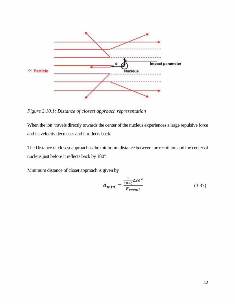
42
Figure 3.10.1: Distance of closest approach representation
When the ion travels directly towards the center of the nucleus experiences a large repulsive force
and its velocity decreases and it reflects back.
The Distance of closest approach is the minimum distance between the recoil ion and the center of
nucleus just before it reflects back by 180o.
Minimum distance of closet approach is given by
𝑑𝑚𝑖𝑛 =
1
4𝜋𝜀02𝑍𝑒2
𝐸𝑟𝑒𝑐𝑜𝑖𝑙 (3.37)
43
In order to calculate the total damage energy it is necessary to calculate the total energy
after the impact:
𝐴 =0.05941(𝑍𝑚𝑍𝑟𝑒𝑐𝑜𝑖𝑙)
53𝐸𝑟𝑒𝑐𝑜𝑖𝑙
𝐴𝑚
𝐵 = 0.3042(𝑍𝑚𝑍𝑟𝑒𝑐𝑜𝑖𝑙)13
𝑄 = 𝑒𝑛𝑒𝑟𝑔𝑦 𝑙𝑜𝑠𝑠 = 𝐴/(1 + 𝐵 ∙ 𝑑𝑚𝑖𝑛)5
𝑇𝑑 = 𝐸𝑟𝑒𝑐𝑜𝑖𝑙 − 𝑄
As it is possible to see from the formalism, the model proposed the year before the NRT
formula results more straight forward and simple to compute, giving similar results to
computational methods as BCA methods (SRIM).
(3.38)
(3.39)
(3.40)
(3.41)
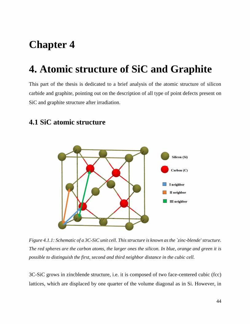
44
Chapter 4
4. Atomic structure of SiC and Graphite
This part of the thesis is dedicated to a brief analysis of the atomic structure of silicon
carbide and graphite, pointing out on the description of all type of point defects present on
SiC and graphite structure after irradiation.
4.1 SiC atomic structure
Figure 4.1.1: Schematic of a 3C-SiC unit cell. This structure is known as the zinc-blende' structure.
The red spheres are the carbon atoms, the larger ones the silicon. In blue, orange and green it is
possible to distinguish the first, second and third neighbor distance in the cubic cell.
3C-SiC grows in zincblende structure, i.e. it is composed of two face-centered cubic (fcc)
lattices, which are displaced by one quarter of the volume diagonal as in Si. However, in
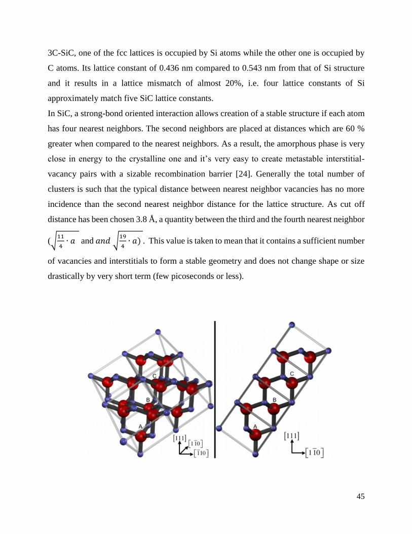
45
3C-SiC, one of the fcc lattices is occupied by Si atoms while the other one is occupied by
C atoms. Its lattice constant of 0.436 nm compared to 0.543 nm from that of Si structure
and it results in a lattice mismatch of almost 20%, i.e. four lattice constants of Si
approximately match five SiC lattice constants.
In SiC, a strong-bond oriented interaction allows creation of a stable structure if each atom
has four nearest neighbors. The second neighbors are placed at distances which are 60 %
greater when compared to the nearest neighbors. As a result, the amorphous phase is very
close in energy to the crystalline one and it’s very easy to create metastable interstitial-
vacancy pairs with a sizable recombination barrier [24]. Generally the total number of
clusters is such that the typical distance between nearest neighbor vacancies has no more
incidence than the second nearest neighbor distance for the lattice structure. As cut off
distance has been chosen 3.8 Å, a quantity between the third and the fourth nearest neighbor
(√11
4∙ 𝑎 and 𝑎𝑛𝑑 √
19
4∙ 𝑎) . This value is taken to mean that it contains a sufficient number
of vacancies and interstitials to form a stable geometry and does not change shape or size
drastically by very short term (few picoseconds or less).
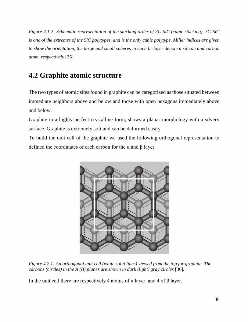
46
Figure 4.1.2: Schematic representation of the stacking order of 3C-SiC (cubic stacking). 3C-SiC
is one of the extremes of the SiC polytypes, and is the only cubic polytype. Miller indices are given
to show the orientation, the large and small spheres in each bi-layer denote a silicon and carbon
atom, respectively [35].
4.2 Graphite atomic structure
The two types of atomic sites found in graphite can be categorized as those situated between
immediate neighbors above and below and those with open hexagons immediately above
and below.
Graphite in a highly perfect crystalline form, shows a planar morphology with a silvery
surface. Graphite is extremely soft and can be deformed easily.
To build the unit cell of the graphite we used the following orthogonal representation to
defined the coordinates of each carbon for the α and β layer.
Figure 4.2.1: An orthogonal unit cell (white solid lines) viewed from the top for graphite. The
carbons (circles) in the A (B) planes are shown in dark (light) gray circles [36].
In the unit cell there are respectively 4 atoms of α layer and 4 of β layer.
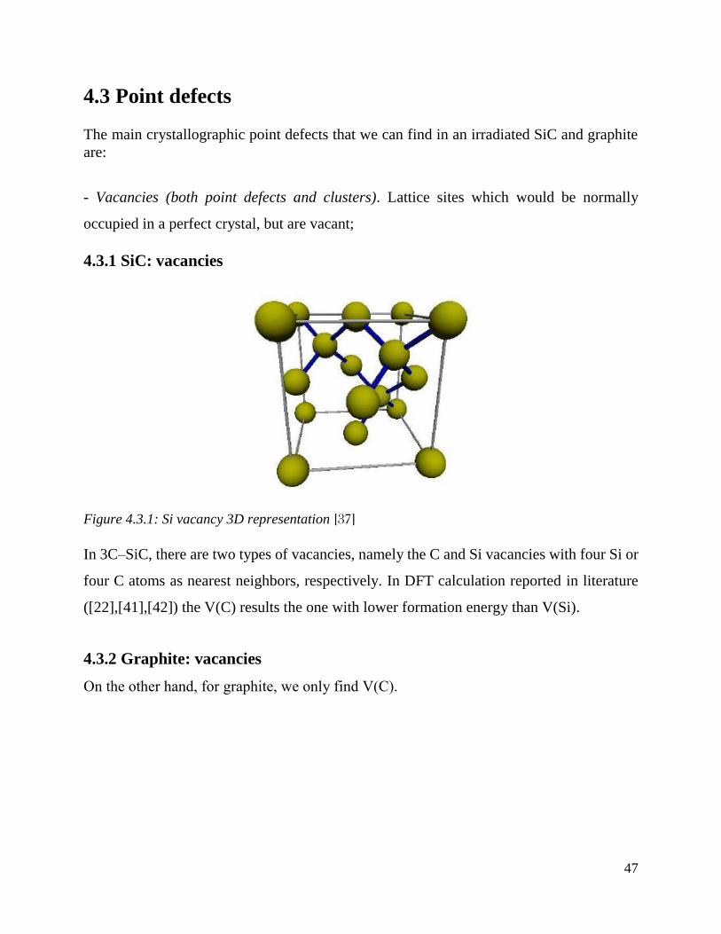
47
4.3 Point defects
The main crystallographic point defects that we can find in an irradiated SiC and graphite
are:
- Vacancies (both point defects and clusters). Lattice sites which would be normally
occupied in a perfect crystal, but are vacant;
4.3.1 SiC: vacancies
Figure 4.3.1: Si vacancy 3D representation [37]
In 3C–SiC, there are two types of vacancies, namely the C and Si vacancies with four Si or
four C atoms as nearest neighbors, respectively. In DFT calculation reported in literature
([22],[41],[42]) the V(C) results the one with lower formation energy than V(Si).
4.3.2 Graphite: vacancies
On the other hand, for graphite, we only find V(C).
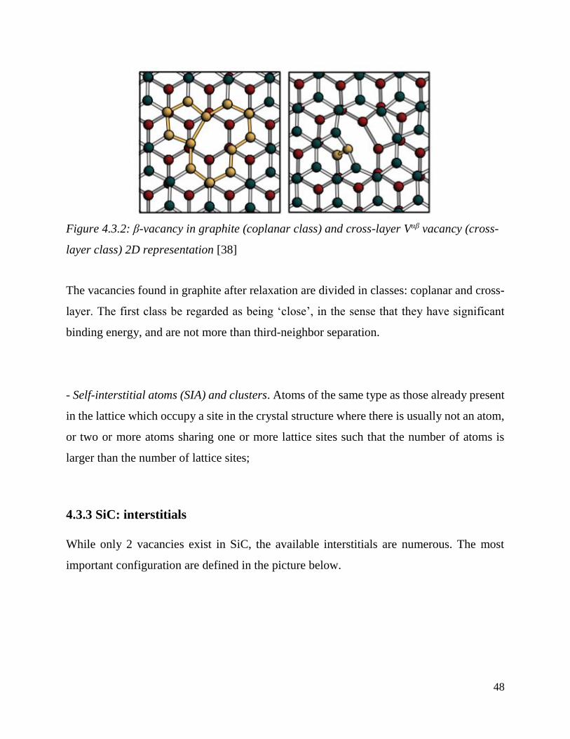
48
Figure 4.3.2: β-vacancy in graphite (coplanar class) and cross-layer Vαβ vacancy (cross-
layer class) 2D representation [38]
The vacancies found in graphite after relaxation are divided in classes: coplanar and cross-
layer. The first class be regarded as being ‘close’, in the sense that they have significant
binding energy, and are not more than third-neighbor separation.
- Self-interstitial atoms (SIA) and clusters. Atoms of the same type as those already present
in the lattice which occupy a site in the crystal structure where there is usually not an atom,
or two or more atoms sharing one or more lattice sites such that the number of atoms is
larger than the number of lattice sites;
4.3.3 SiC: interstitials
While only 2 vacancies exist in SiC, the available interstitials are numerous. The most
important configuration are defined in the picture below.
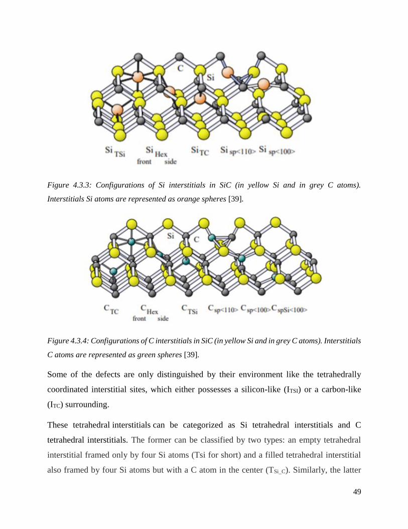
49
Figure 4.3.3: Configurations of Si interstitials in SiC (in yellow Si and in grey C atoms).
Interstitials Si atoms are represented as orange spheres [39].
Figure 4.3.4: Configurations of C interstitials in SiC (in yellow Si and in grey C atoms). Interstitials
C atoms are represented as green spheres [39].
Some of the defects are only distinguished by their environment like the tetrahedrally
coordinated interstitial sites, which either possesses a silicon-like (ITSI) or a carbon-like
(ITC) surrounding.
These tetrahedral interstitials can be categorized as Si tetrahedral interstitials and C
tetrahedral interstitials. The former can be classified by two types: an empty tetrahedral
interstitial framed only by four Si atoms (Tsi for short) and a filled tetrahedral interstitial
also framed by four Si atoms but with a C atom in the center (TSi_C). Similarly, the latter
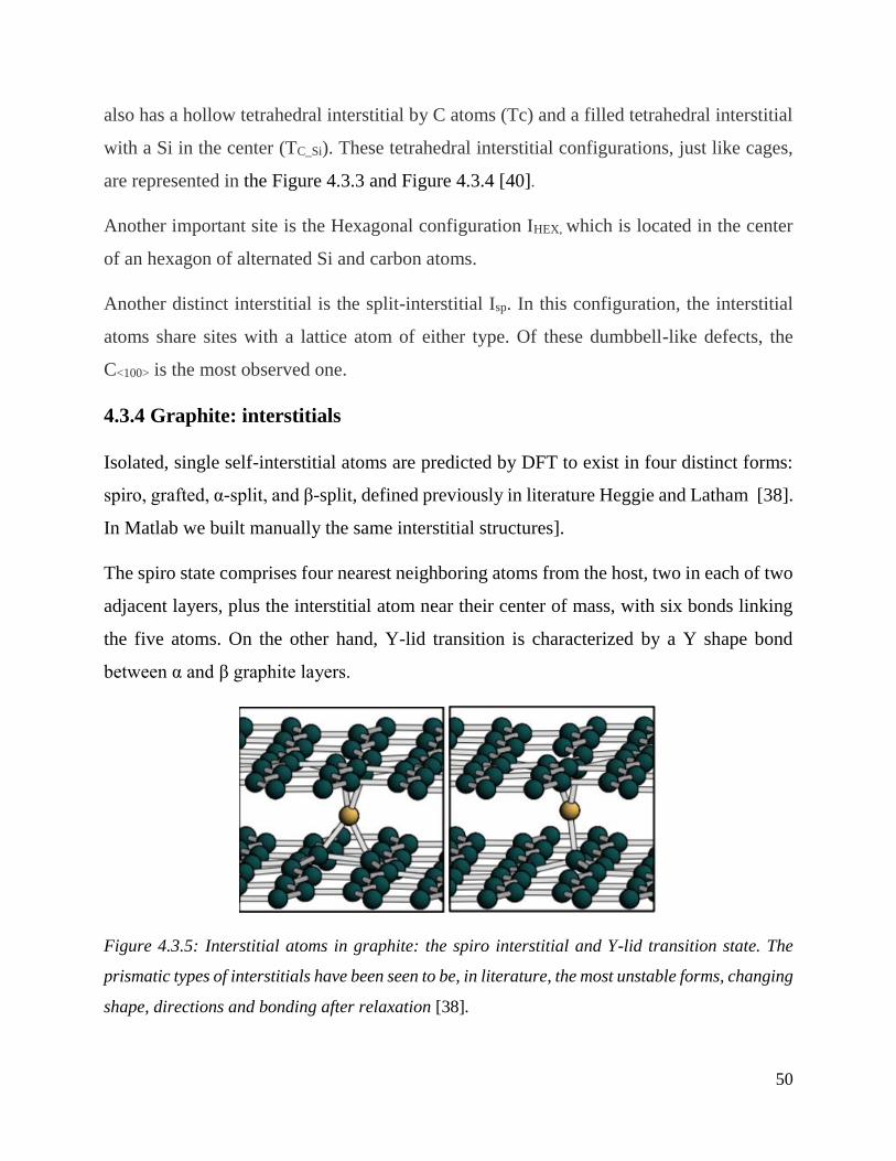
50
also has a hollow tetrahedral interstitial by C atoms (Tc) and a filled tetrahedral interstitial
with a Si in the center (TC_Si). These tetrahedral interstitial configurations, just like cages,
are represented in the Figure 4.3.3 and Figure 4.3.4 [40].
Another important site is the Hexagonal configuration IHEX, which is located in the center
of an hexagon of alternated Si and carbon atoms.
Another distinct interstitial is the split-interstitial Isp. In this configuration, the interstitial
atoms share sites with a lattice atom of either type. Of these dumbbell-like defects, the
C<100> is the most observed one.
4.3.4 Graphite: interstitials
Isolated, single self-interstitial atoms are predicted by DFT to exist in four distinct forms:
spiro, grafted, α-split, and β-split, defined previously in literature Heggie and Latham [38].
In Matlab we built manually the same interstitial structures].
The spiro state comprises four nearest neighboring atoms from the host, two in each of two
adjacent layers, plus the interstitial atom near their center of mass, with six bonds linking
the five atoms. On the other hand, Y-lid transition is characterized by a Y shape bond
between α and β graphite layers.
Figure 4.3.5: Interstitial atoms in graphite: the spiro interstitial and Y-lid transition state. The
prismatic types of interstitials have been seen to be, in literature, the most unstable forms, changing
shape, directions and bonding after relaxation [38].
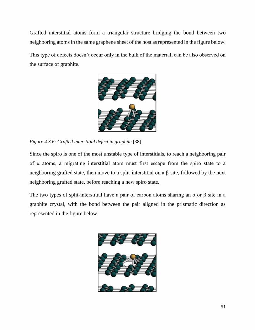
51
Grafted interstitial atoms form a triangular structure bridging the bond between two
neighboring atoms in the same graphene sheet of the host as represented in the figure below.
This type of defects doesn’t occur only in the bulk of the material, can be also observed on
the surface of graphite.
Figure 4.3.6: Grafted interstitial defect in graphite [38]
Since the spiro is one of the most unstable type of interstitials, to reach a neighboring pair
of α atoms, a migrating interstitial atom must first escape from the spiro state to a
neighboring grafted state, then move to a split-interstitial on a β-site, followed by the next
neighboring grafted state, before reaching a new spiro state.
The two types of split-interstitial have a pair of carbon atoms sharing an α or β site in a
graphite crystal, with the bond between the pair aligned in the prismatic direction as
represented in the figure below.
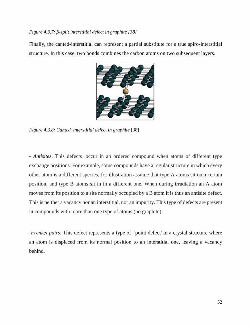
52
Figure 4.3.7: β-split interstitial defect in graphite [38]
Finally, the canted-interstitial can represent a partial substitute for a true spiro-interstitial
structure. In this case, two bonds combines the carbon atoms on two subsequent layers.
Figure 4.3.8: Canted interstitial defect in graphite [38]
- Antisites. This defects occur in an ordered compound when atoms of different type
exchange positions. For example, some compounds have a regular structure in which every
other atom is a different species; for illustration assume that type A atoms sit on a certain
position, and type B atoms sit in in a different one. When during irradiation an A atom
moves from its position to a site normally occupied by a B atom it is thus an antisite defect.
This is neither a vacancy nor an interstitial, nor an impurity. This type of defects are present
in compounds with more than one type of atoms (no graphite).
-Frenkel pairs. This defect represents a type of 'point defect' in a crystal structure where
an atom is displaced from its normal position to an interstitial one, leaving a vacancy
behind.
53
Chapter 5
5. Results and Discussion
This part of the thesis is devoted to an analysis of the results obatained through
computational methods in MD and BCA.
The results obatained have been analyzed and manipulated in Matlab in order to have a
visual analysis of the data.
5.1 Potential Selection
5.1.1 SiC potentials
A total of 10 potentials have been used to compare the lattice parameter and the cohesive
energy of a SiC supercell.
Tersoff potentials can be applied on silicon, carbon and also to multicomponent systems
like silicon carbide.
The Gao-Weber potential has been taken into account as an empirical many-body
interatomic potential. It is developed by fitting to various equilibrium properties and stable
defect configurations in bulk SiC, using a lattice relaxation fitting approach. In the end, it
has been excluded because it cannot correctly reproduce the C-C interaction in graphite.
From literature, in fact, the Gao–Weber potential provides a satisfactory description of SiC
properties, but it has been excluded for its incompatibility with C-C bonds in pure graphite.
A compilation of data in Table 5.1.1 includes results obtained with our SiC potential and
with three different versions of the Tersoff potential [T89, T90, T94, Erhart-Albe] for SiC
and by Gao and Weber’s. Obviously, the SiC parametrization of EH05 bond-order potential
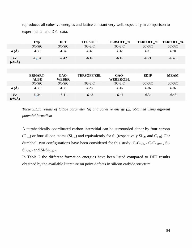
54
reproduces all cohesive energies and lattice constant very well, especially in comparison to
experimental and DFT data.
Table 5.1.1: results of lattice parameter (a) and cohesive energy (Ec) obtained using different
potential formalism
A tetrahedrically coordinated carbon interstitial can be surrounded either by four carbon
(CTC) or four silicon atoms (SiTC) and equivalently for Si (respectively SiTSi and CTSi). For
dumbbell two configurations have been considered for this study: C-C<100>, C-C<110> , Si-
Si<100> and Si-Si<110>.
In Table 2 the different formation energies have been listed compared to DFT results
obtained by the available literature on point defects in silicon carbide structure.
Exp. DFT TERSOFF TERSOFF_89 TERSOFF_90 TERSOFF_94
3C-SiC 3C-SiC 3C-SiC 3C-SiC 3C-SiC 3C-SiC
a (Å) 4.36 4.34 4.32 4.32 4.31 4.28
Ec
(eV/Å)
-6,.34 -7.42 -6.16 -6.16 -6.21 -6.43
ERHART-
ALBE
GAO-
WEBER
TERSOFF/ZBL GAO-
WEBER/ZBL
EDIP MEAM
3C-SiC 3C-SiC 3C-SiC 3C-SiC 3C-SiC 3C-SiC
a (Å) 4.36 4.36 4.28 4.36 4.36 4.36
Ec
(eV/Å)
6,.34 -6.41 -6.43 -6.41 -6.34 -6.43
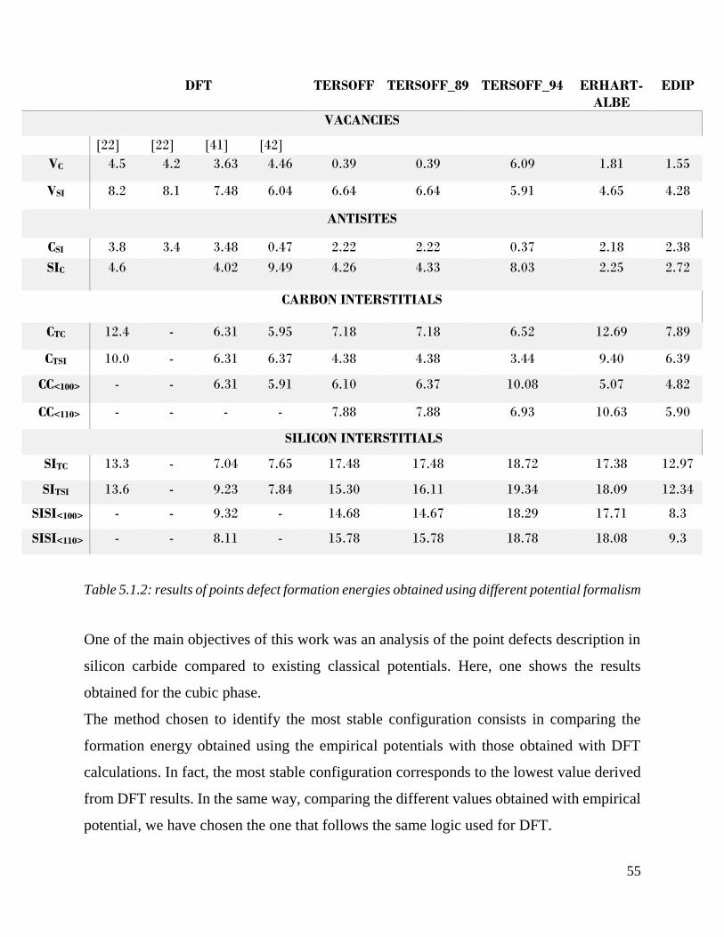
55
Table 5.1.2: results of points defect formation energies obtained using different potential formalism
One of the main objectives of this work was an analysis of the point defects description in
silicon carbide compared to existing classical potentials. Here, one shows the results
obtained for the cubic phase.
The method chosen to identify the most stable configuration consists in comparing the
formation energy obtained using the empirical potentials with those obtained with DFT
calculations. In fact, the most stable configuration corresponds to the lowest value derived
from DFT results. In the same way, comparing the different values obtained with empirical
potential, we have chosen the one that follows the same logic used for DFT.
DFT TERSOFF TERSOFF_89 TERSOFF_94 ERHART-
ALBE
EDIP
VACANCIES
[22] [22] [41] [42]
VC 4.5 4.2 3.63 4.46 0.39 0.39 6.09 1.81 1.55
VSI 8.2 8.1 7.48 6.04 6.64 6.64 5.91 4.65 4.28
ANTISITES
CSI 3.8 3.4 3.48 0.47 2.22 2.22 0.37 2.18 2.38
SIC 4.6 4.02 9.49 4.26 4.33 8.03 2.25 2.72
CARBON INTERSTITIALS
CTC 12.4 - 6.31 5.95 7.18 7.18 6.52 12.69 7.89
CTSI 10.0 - 6.31 6.37 4.38 4.38 3.44 9.40 6.39
CC<100> - - 6.31 5.91 6.10 6.37 10.08 5.07 4.82
CC<110> - - - - 7.88 7.88 6.93 10.63 5.90
SILICON INTERSTITIALS
SITC 13.3 - 7.04 7.65 17.48 17.48 18.72 17.38 12.97
SITSI 13.6 - 9.23 7.84 15.30 16.11 19.34 18.09 12.34
SISI<100> - - 9.32 - 14.68 14.67 18.29 17.71 8.3
SISI<110> - - 8.11 - 15.78 15.78 18.78 18.08 9.3
56
Considering first the vacancies, the formation energies for carbon vacancies computed with
all potentials apart the new version of Tersoff (T94) are smaller than those found for silicon
vacancies as defined by the DFT results.
The most stable configurations is found in literature to be CC<100> dumbbell interstitial. The
tetrahedral interstitials, on the other hand, are found to be significantly higher in energy.
All Tersoff potentials, apart EA05, yield formation energies of dumbbell interstitials higher
than for other types of interstitials showing that CTSi tetrahedral configurations are the most
stable defects, contradicting the results found in DFT. So, only EA05 and EDIP are in
accordance with the predictions of DFT analysis provided in the table. The properties of
silicon interstitials are very difficult to reproduce with empirical potentials. DFT
calculations showed that the most stable configuration is the SiTC tetrahedral interstitial.
From this last results, it is possible to exclude EDIP potential, since it predicts that SiSi<100>
dumbbell is the most stable configuration, incompatible with the results obtained in DFT.
Therefore, our final choice fell on EA05 potential.
5.1.2 Graphite potentials
For the first part of this work one is interested in choosing the suited potential for atomic
scale simulations of processes which involve transitions between widely different atomic
configurations. In the course of the this first set of data it has been derived parameters for
both Si-C interactions for both silicon and carbon and revisited the parameters set for C-C
bonds too.
For graphite 6 potentials have been chosen.
The database for fitting procedure includes experimental data such as cohesive energy and
lattice parameter of Si, C and SiC which ensure that the potential and DFT calculations
will accurately reproduce the structural and elastic properties of the materials.
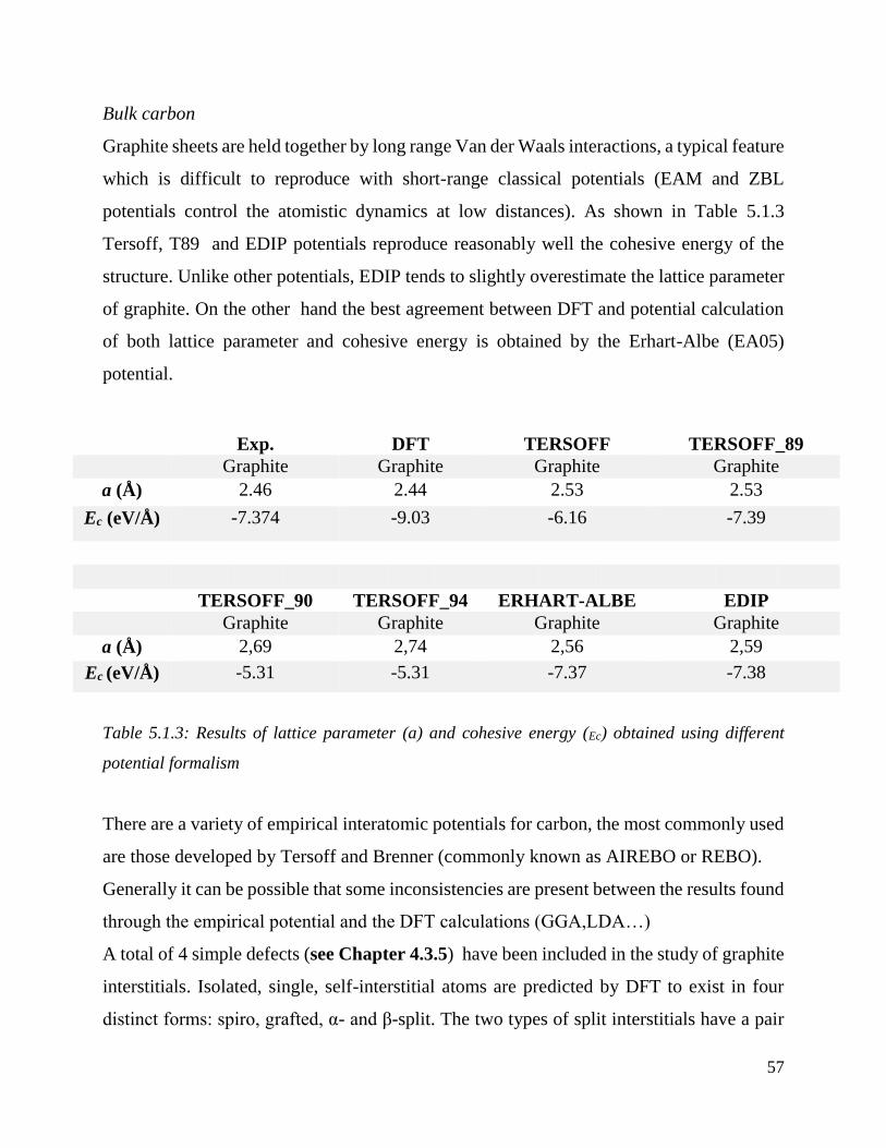
57
Bulk carbon
Graphite sheets are held together by long range Van der Waals interactions, a typical feature
which is difficult to reproduce with short-range classical potentials (EAM and ZBL
potentials control the atomistic dynamics at low distances). As shown in Table 5.1.3
Tersoff, T89 and EDIP potentials reproduce reasonably well the cohesive energy of the
structure. Unlike other potentials, EDIP tends to slightly overestimate the lattice parameter
of graphite. On the other hand the best agreement between DFT and potential calculation
of both lattice parameter and cohesive energy is obtained by the Erhart-Albe (EA05)
potential.
Table 5.1.3: Results of lattice parameter (a) and cohesive energy (Ec) obtained using different
potential formalism
There are a variety of empirical interatomic potentials for carbon, the most commonly used
are those developed by Tersoff and Brenner (commonly known as AIREBO or REBO).
Generally it can be possible that some inconsistencies are present between the results found
through the empirical potential and the DFT calculations (GGA,LDA…)
A total of 4 simple defects (see Chapter 4.3.5) have been included in the study of graphite
interstitials. Isolated, single, self-interstitial atoms are predicted by DFT to exist in four
distinct forms: spiro, grafted, α- and β-split. The two types of split interstitials have a pair
Exp. DFT TERSOFF TERSOFF_89
Graphite Graphite Graphite Graphite
a (Å) 2.46 2.44 2.53 2.53
Ec (eV/Å) -7.374 -9.03 -6.16 -7.39
TERSOFF_90 TERSOFF_94 ERHART-ALBE EDIP
Graphite Graphite Graphite Graphite
a (Å) 2,69 2,74 2,56 2,59
Ec (eV/Å) -5.31 -5.31 -7.37 -7.38
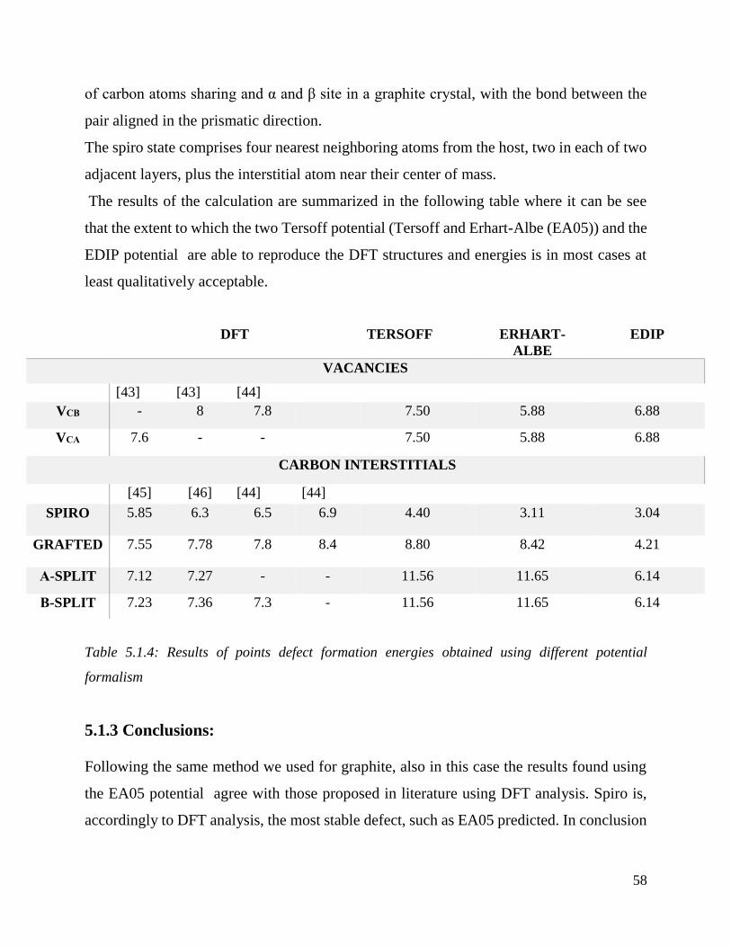
58
of carbon atoms sharing and α and β site in a graphite crystal, with the bond between the
pair aligned in the prismatic direction.
The spiro state comprises four nearest neighboring atoms from the host, two in each of two
adjacent layers, plus the interstitial atom near their center of mass.
The results of the calculation are summarized in the following table where it can be see
that the extent to which the two Tersoff potential (Tersoff and Erhart-Albe (EA05)) and the
EDIP potential are able to reproduce the DFT structures and energies is in most cases at
least qualitatively acceptable.
Table 5.1.4: Results of points defect formation energies obtained using different potential
formalism
5.1.3 Conclusions:
Following the same method we used for graphite, also in this case the results found using
the EA05 potential agree with those proposed in literature using DFT analysis. Spiro is,
accordingly to DFT analysis, the most stable defect, such as EA05 predicted. In conclusion
DFT TERSOFF ERHART-
ALBE
EDIP
VACANCIES
[43] [43] [44]
VCΒ - 8 7.8 7.50 5.88 6.88
VCΑ 7.6 - - 7.50 5.88 6.88
CARBON INTERSTITIALS
[45] [46] [44] [44]
SPIRO 5.85 6.3 6.5 6.9 4.40 3.11 3.04
GRAFTED 7.55 7.78 7.8 8.4 8.80 8.42 4.21
Α-SPLIT 7.12 7.27 - - 11.56 11.65 6.14
Β-SPLIT 7.23 7.36 7.3 - 11.56 11.65 6.14
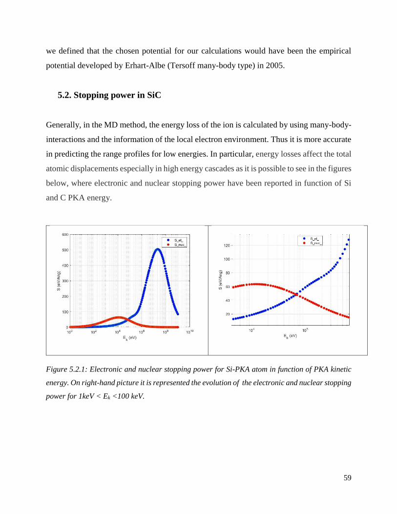
59
we defined that the chosen potential for our calculations would have been the empirical
potential developed by Erhart-Albe (Tersoff many-body type) in 2005.
5.2. Stopping power in SiC
Generally, in the MD method, the energy loss of the ion is calculated by using many-body-
interactions and the information of the local electron environment. Thus it is more accurate
in predicting the range profiles for low energies. In particular, energy losses affect the total
atomic displacements especially in high energy cascades as it is possible to see in the figures
below, where electronic and nuclear stopping power have been reported in function of Si
and C PKA energy.
Figure 5.2.1: Electronic and nuclear stopping power for Si-PKA atom in function of PKA kinetic
energy. On right-hand picture it is represented the evolution of the electronic and nuclear stopping
power for 1keV < Ek <100 keV.
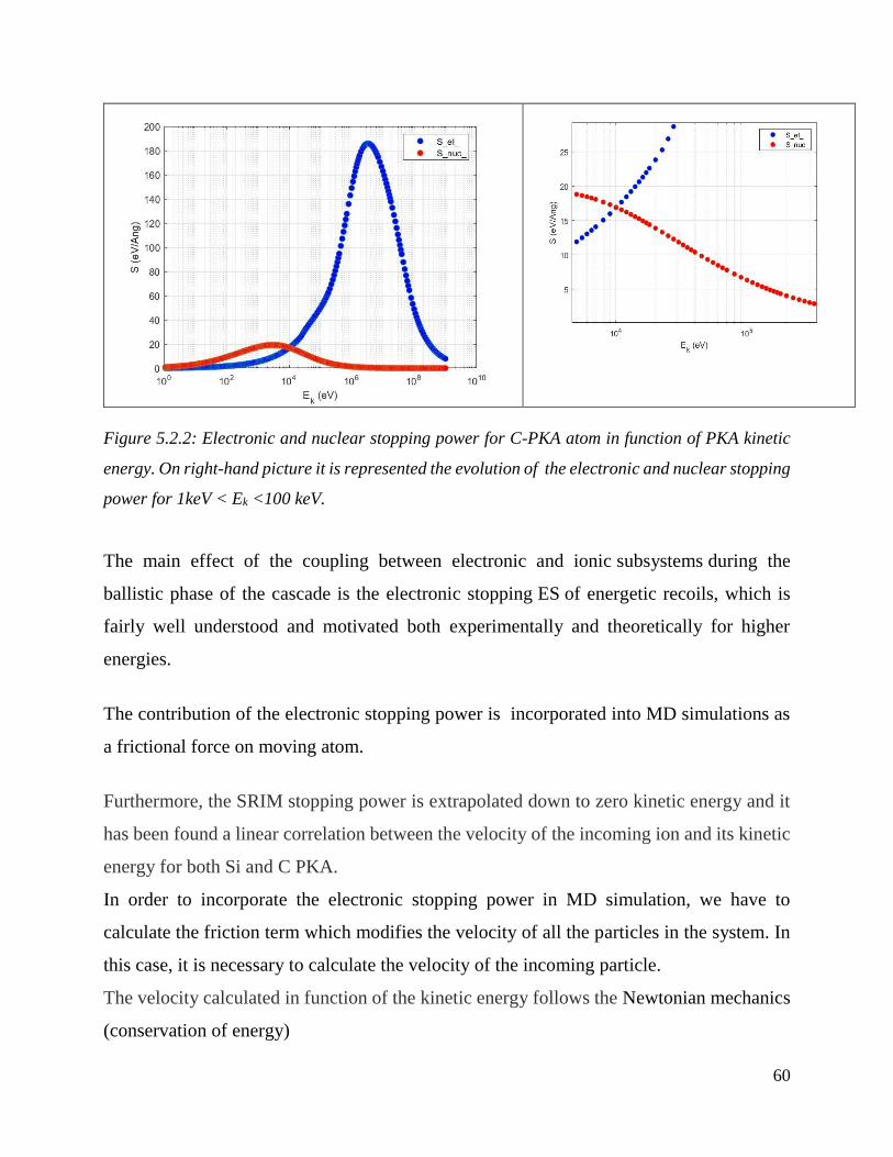
60
Figure 5.2.2: Electronic and nuclear stopping power for C-PKA atom in function of PKA kinetic
energy. On right-hand picture it is represented the evolution of the electronic and nuclear stopping
power for 1keV < Ek <100 keV.
The main effect of the coupling between electronic and ionic subsystems during the
ballistic phase of the cascade is the electronic stopping ES of energetic recoils, which is
fairly well understood and motivated both experimentally and theoretically for higher
energies.
The contribution of the electronic stopping power is incorporated into MD simulations as
a frictional force on moving atom.
Furthermore, the SRIM stopping power is extrapolated down to zero kinetic energy and it
has been found a linear correlation between the velocity of the incoming ion and its kinetic
energy for both Si and C PKA.
In order to incorporate the electronic stopping power in MD simulation, we have to
calculate the friction term which modifies the velocity of all the particles in the system. In
this case, it is necessary to calculate the velocity of the incoming particle.
The velocity calculated in function of the kinetic energy follows the Newtonian mechanics
(conservation of energy)
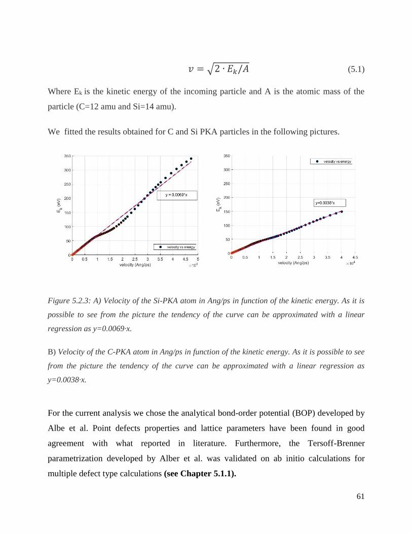
61
𝑣 = √2 ∙ 𝐸𝑘/𝐴 (5.1)
Where Ek is the kinetic energy of the incoming particle and A is the atomic mass of the
particle (C=12 amu and Si=14 amu).
We fitted the results obtained for C and Si PKA particles in the following pictures.
Figure 5.2.3: A) Velocity of the Si-PKA atom in Ang/ps in function of the kinetic energy. As it is
possible to see from the picture the tendency of the curve can be approximated with a linear
regression as y=0.0069·x.
B) Velocity of the C-PKA atom in Ang/ps in function of the kinetic energy. As it is possible to see
from the picture the tendency of the curve can be approximated with a linear regression as
y=0.0038·x.
For the current analysis we chose the analytical bond-order potential (BOP) developed by
Albe et al. Point defects properties and lattice parameters have been found in good
agreement with what reported in literature. Furthermore, the Tersoff-Brenner
parametrization developed by Alber et al. was validated on ab initio calculations for
multiple defect type calculations (see Chapter 5.1.1).
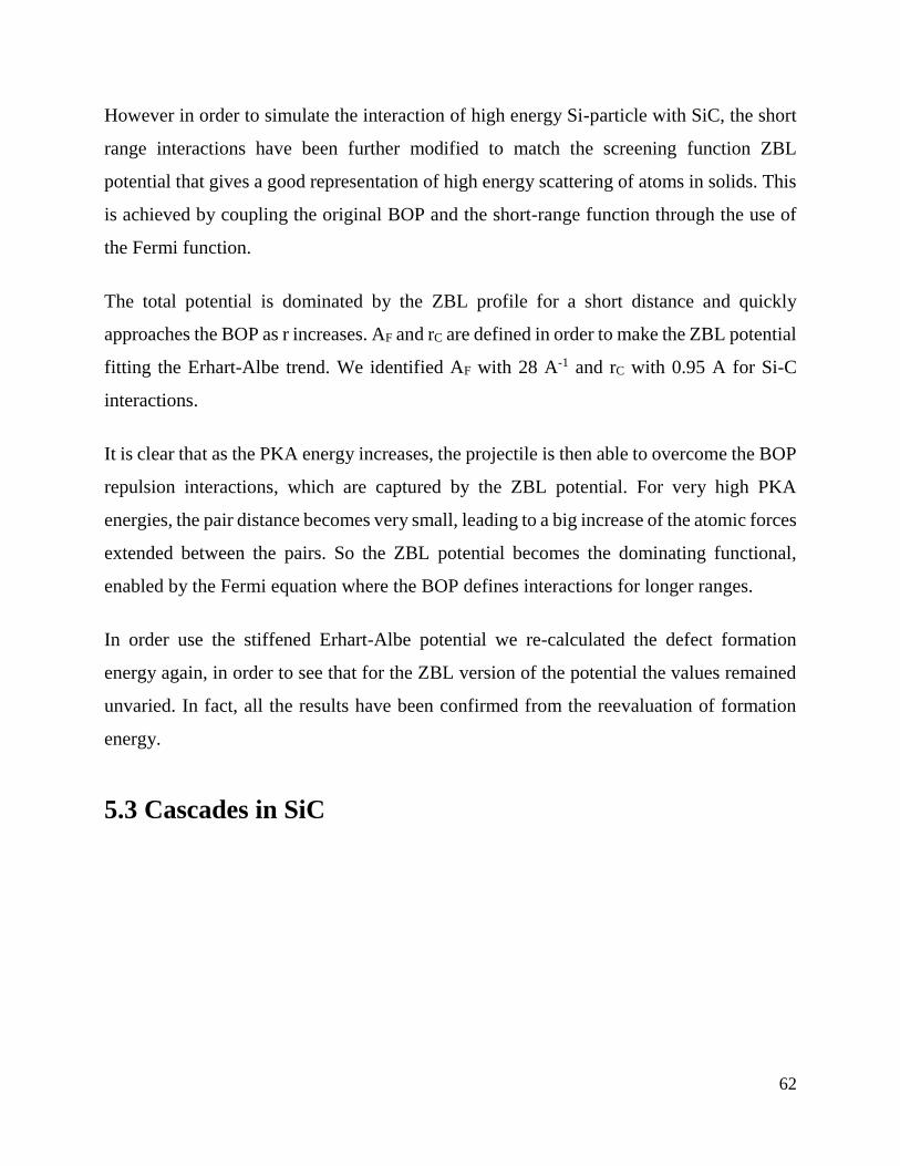
62
However in order to simulate the interaction of high energy Si-particle with SiC, the short
range interactions have been further modified to match the screening function ZBL
potential that gives a good representation of high energy scattering of atoms in solids. This
is achieved by coupling the original BOP and the short-range function through the use of
the Fermi function.
The total potential is dominated by the ZBL profile for a short distance and quickly
approaches the BOP as r increases. AF and rC are defined in order to make the ZBL potential
fitting the Erhart-Albe trend. We identified AF with 28 A-1 and rC with 0.95 A for Si-C
interactions.
It is clear that as the PKA energy increases, the projectile is then able to overcome the BOP
repulsion interactions, which are captured by the ZBL potential. For very high PKA
energies, the pair distance becomes very small, leading to a big increase of the atomic forces
extended between the pairs. So the ZBL potential becomes the dominating functional,
enabled by the Fermi equation where the BOP defines interactions for longer ranges.
In order use the stiffened Erhart-Albe potential we re-calculated the defect formation
energy again, in order to see that for the ZBL version of the potential the values remained
unvaried. In fact, all the results have been confirmed from the reevaluation of formation
energy.
5.3 Cascades in SiC
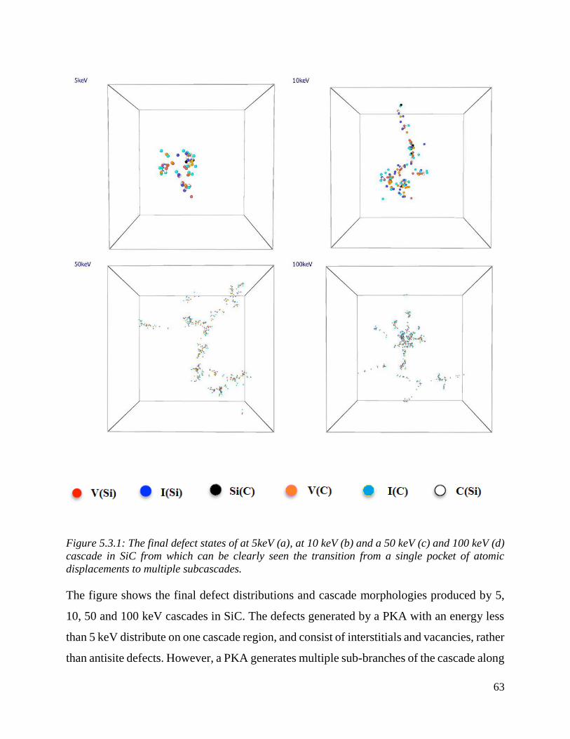
63
Figure 5.3.1: The final defect states of at 5keV (a), at 10 keV (b) and a 50 keV (c) and 100 keV (d)
cascade in SiC from which can be clearly seen the transition from a single pocket of atomic
displacements to multiple subcascades.
The figure shows the final defect distributions and cascade morphologies produced by 5,
10, 50 and 100 keV cascades in SiC. The defects generated by a PKA with an energy less
than 5 keV distribute on one cascade region, and consist of interstitials and vacancies, rather
than antisite defects. However, a PKA generates multiple sub-branches of the cascade along
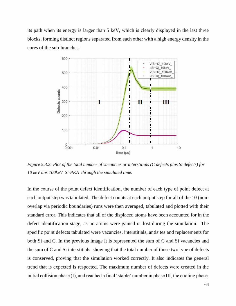
64
its path when its energy is larger than 5 keV, which is clearly displayed in the last three
blocks, forming distinct regions separated from each other with a high energy density in the
cores of the sub-branches.
Figure 5.3.2: Plot of the total number of vacancies or interstitials (C defects plus Si defects) for
10 keV ans 100keV Si-PKA through the simulated time.
In the course of the point defect identification, the number of each type of point defect at
each output step was tabulated. The defect counts at each output step for all of the 10 (non-
overlap via periodic boundaries) runs were then averaged, tabulated and plotted with their
standard error. This indicates that all of the displaced atoms have been accounted for in the
defect identification stage, as no atoms were gained or lost during the simulation. The
specific point defects tabulated were vacancies, interstitials, antisites and replacements for
both Si and C. In the previous image it is represented the sum of C and Si vacancies and
the sum of C and Si interstitials showing that the total number of those two type of defects
is conserved, proving that the simulation worked correctly. It also indicates the general
trend that is expected is respected. The maximum number of defects were created in the
initial collision phase (I), and reached a final ‘stable’ number in phase III, the cooling phase.
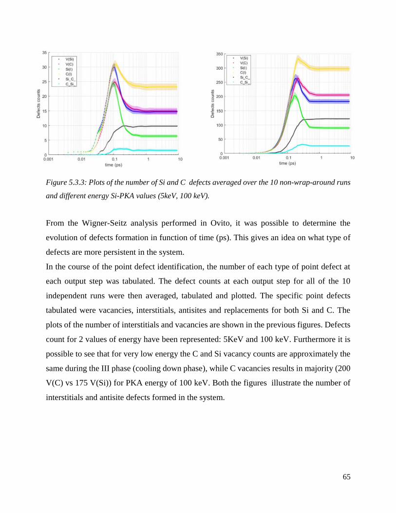
65
Figure 5.3.3: Plots of the number of Si and C defects averaged over the 10 non-wrap-around runs
and different energy Si-PKA values (5keV, 100 keV).
From the Wigner-Seitz analysis performed in Ovito, it was possible to determine the
evolution of defects formation in function of time (ps). This gives an idea on what type of
defects are more persistent in the system.
In the course of the point defect identification, the number of each type of point defect at
each output step was tabulated. The defect counts at each output step for all of the 10
independent runs were then averaged, tabulated and plotted. The specific point defects
tabulated were vacancies, interstitials, antisites and replacements for both Si and C. The
plots of the number of interstitials and vacancies are shown in the previous figures. Defects
count for 2 values of energy have been represented: 5KeV and 100 keV. Furthermore it is
possible to see that for very low energy the C and Si vacancy counts are approximately the
same during the III phase (cooling down phase), while C vacancies results in majority (200
V(C) vs 175 V(Si)) for PKA energy of 100 keV. Both the figures illustrate the number of
interstitials and antisite defects formed in the system.
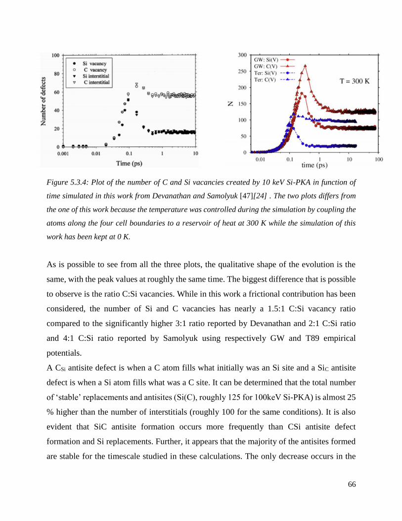
66
Figure 5.3.4: Plot of the number of C and Si vacancies created by 10 keV Si-PKA in function of
time simulated in this work from Devanathan and Samolyuk [47][24] . The two plots differs from
the one of this work because the temperature was controlled during the simulation by coupling the
atoms along the four cell boundaries to a reservoir of heat at 300 K while the simulation of this
work has been kept at 0 K.
As is possible to see from all the three plots, the qualitative shape of the evolution is the
same, with the peak values at roughly the same time. The biggest difference that is possible
to observe is the ratio C:Si vacancies. While in this work a frictional contribution has been
considered, the number of Si and C vacancies has nearly a 1.5:1 C:Si vacancy ratio
compared to the significantly higher 3:1 ratio reported by Devanathan and 2:1 C:Si ratio
and 4:1 C:Si ratio reported by Samolyuk using respectively GW and T89 empirical
potentials.
A CSi antisite defect is when a C atom fills what initially was an Si site and a SiC antisite
defect is when a Si atom fills what was a C site. It can be determined that the total number
of ‘stable’ replacements and antisites (Si(C), roughly 125 for 100keV Si-PKA) is almost 25
% higher than the number of interstitials (roughly 100 for the same conditions). It is also
evident that SiC antisite formation occurs more frequently than CSi antisite defect
formation and Si replacements. Further, it appears that the majority of the antisites formed
are stable for the timescale studied in these calculations. The only decrease occurs in the
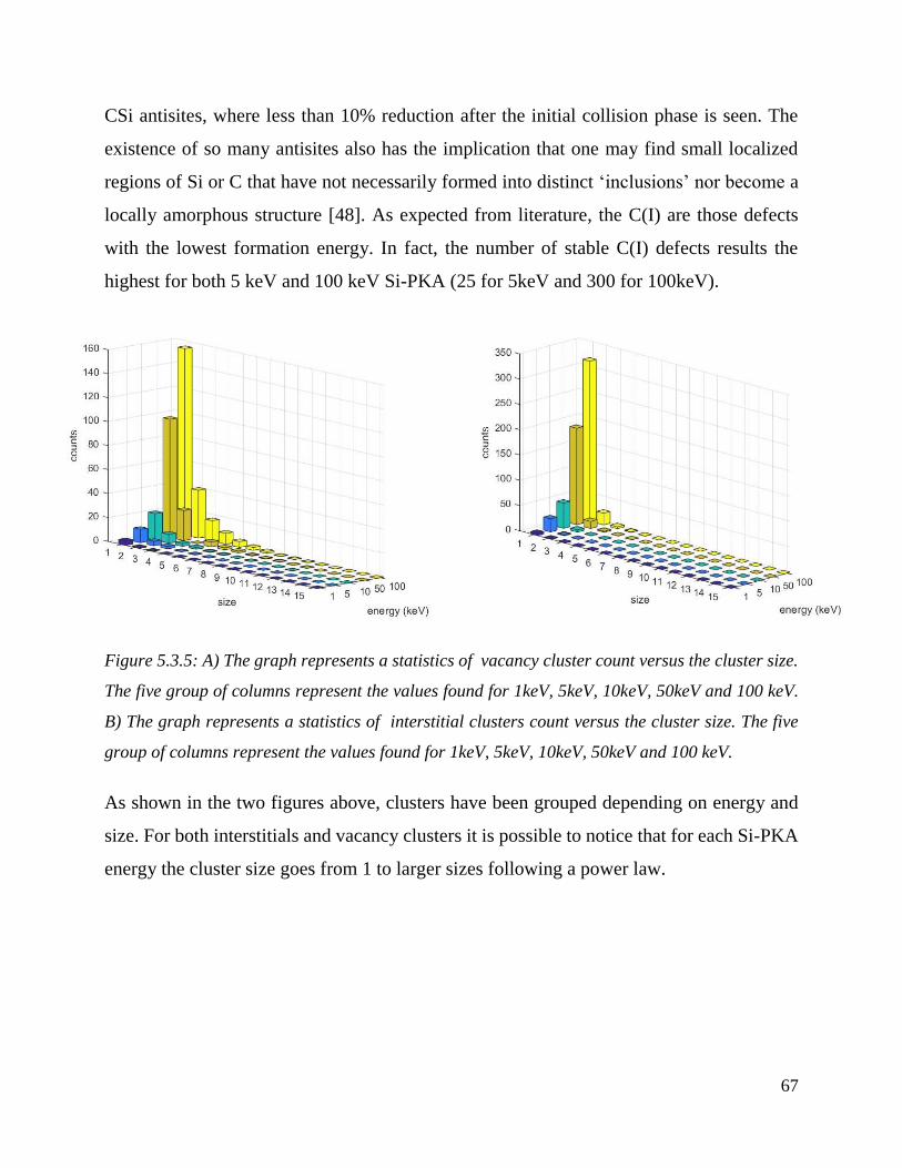
67
CSi antisites, where less than 10% reduction after the initial collision phase is seen. The
existence of so many antisites also has the implication that one may find small localized
regions of Si or C that have not necessarily formed into distinct ‘inclusions’ nor become a
locally amorphous structure [48]. As expected from literature, the C(I) are those defects
with the lowest formation energy. In fact, the number of stable C(I) defects results the
highest for both 5 keV and 100 keV Si-PKA (25 for 5keV and 300 for 100keV).
Figure 5.3.5: A) The graph represents a statistics of vacancy cluster count versus the cluster size.
The five group of columns represent the values found for 1keV, 5keV, 10keV, 50keV and 100 keV.
B) The graph represents a statistics of interstitial clusters count versus the cluster size. The five
group of columns represent the values found for 1keV, 5keV, 10keV, 50keV and 100 keV.
As shown in the two figures above, clusters have been grouped depending on energy and
size. For both interstitials and vacancy clusters it is possible to notice that for each Si-PKA
energy the cluster size goes from 1 to larger sizes following a power law.
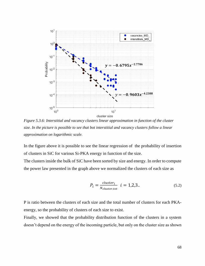
68
Figure 5.3.6: Interstitial and vacancy clusters linear approximation in function of the cluster
size. In the picture is possible to see that bot interstitial and vacancy clusters follow a linear
approximation on logarithmic scale.
In the figure above it is possible to see the linear regression of the probability of insertion
of clusters in SiC for various Si-PKA energy in function of the size.
The clusters inside the bulk of SiC have been sorted by size and energy. In order to compute
the power law presented in the graph above we normalized the clusters of each size as
𝑃𝑖 =𝑐𝑙𝑢𝑠𝑡𝑒𝑟𝑖
𝑁𝑐𝑙𝑢𝑠𝑡𝑒𝑟,𝑡𝑜𝑡 𝑖 = 1,2,3.. (5.2)
P is ratio between the clusters of each size and the total number of clusters for each PKA-
energy, so the probability of clusters of each size to exist.
Finally, we showed that the probability distribution function of the clusters in a system
doesn’t depend on the energy of the incoming particle, but only on the cluster size as shown
𝒚 = −𝟎. 𝟔𝟕𝟗𝟓𝒙−𝟐.𝟕𝟕𝟖𝟔
𝑦 = −𝟎. 𝟗𝟔𝟎𝟑𝒙−𝟒.𝟐𝟑𝟖𝟖
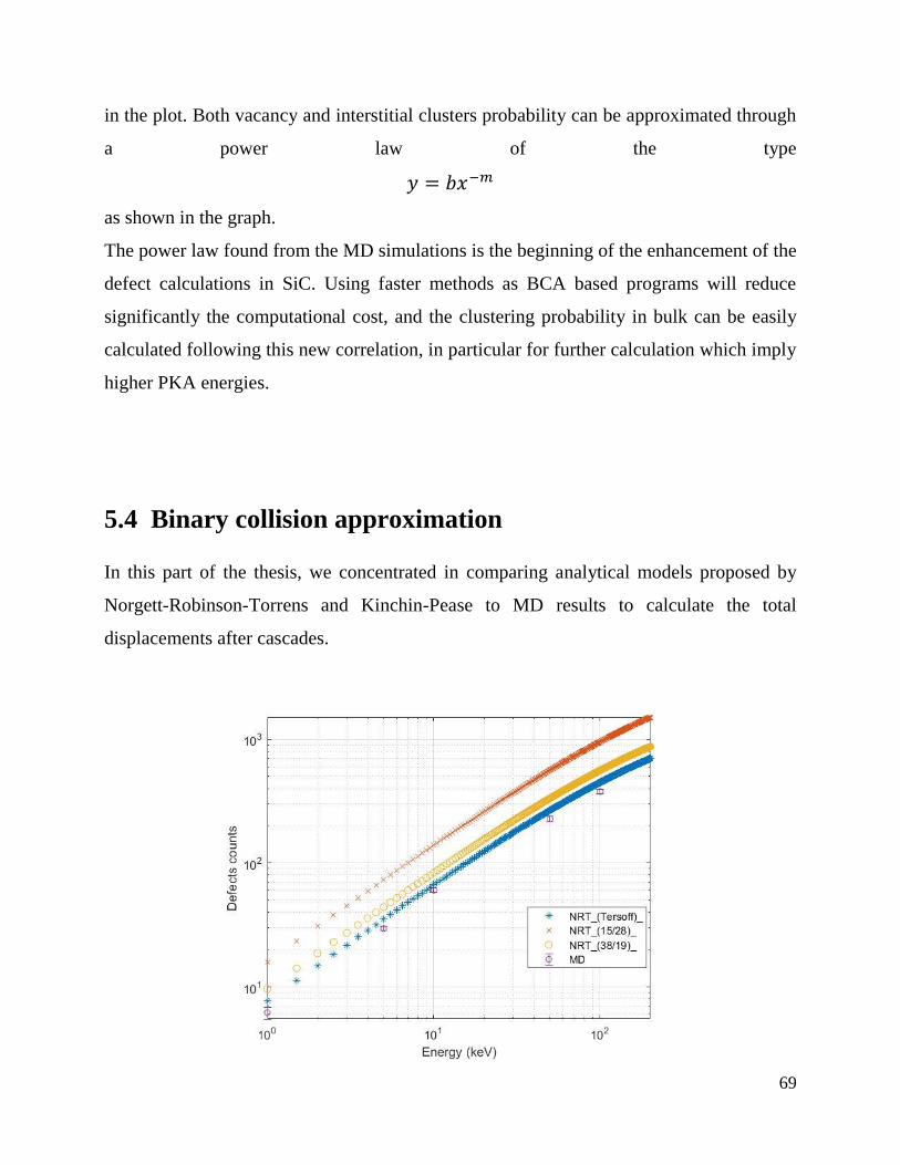
69
in the plot. Both vacancy and interstitial clusters probability can be approximated through
a power law of the type
𝑦 = 𝑏𝑥−𝑚
as shown in the graph.
The power law found from the MD simulations is the beginning of the enhancement of the
defect calculations in SiC. Using faster methods as BCA based programs will reduce
significantly the computational cost, and the clustering probability in bulk can be easily
calculated following this new correlation, in particular for further calculation which imply
higher PKA energies.
5.4 Binary collision approximation In this part of the thesis, we concentrated in comparing analytical models proposed by
Norgett-Robinson-Torrens and Kinchin-Pease to MD results to calculate the total
displacements after cascades.
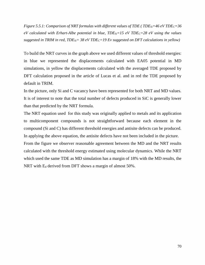
70
Figure 5.5.1: Comparison of NRT formulas with different values of TDE ( TDESi=46 eV TDEC=36
eV calculated with Erhart-Albe potential in blue, TDESi=15 eV TDEC=28 eV using the values
suggested in TRIM in red, TDESi= 38 eV TDEC=19 Ev suggested on DFT calculations in yellow)
To build the NRT curves in the graph above we used different values of threshold energies:
in blue we represented the displacements calculated with EA05 potential in MD
simulations, in yellow the displacements calculated with the averaged TDE proposed by
DFT calculation proposed in the article of Lucas et al. and in red the TDE proposed by
default in TRIM.
In the picture, only Si and C vacancy have been represented for both NRT and MD values.
It is of interest to note that the total number of defects produced in SiC is generally lower
than that predicted by the NRT formula.
The NRT equation used for this study was originally applied to metals and its application
to multicomponent compounds is not straightforward because each element in the
compound (Si and C) has different threshold energies and antisite defects can be produced.
In applying the above equation, the antisite defects have not been included in the picture.
From the figure we observer reasonable agreement between the MD and the NRT results
calculated with the threshold energy estimated using molecular dynamics. While the NRT
which used the same TDE as MD simulation has a margin of 18% with the MD results, the
NRT with Ed derived from DFT shows a margin of almost 50%.
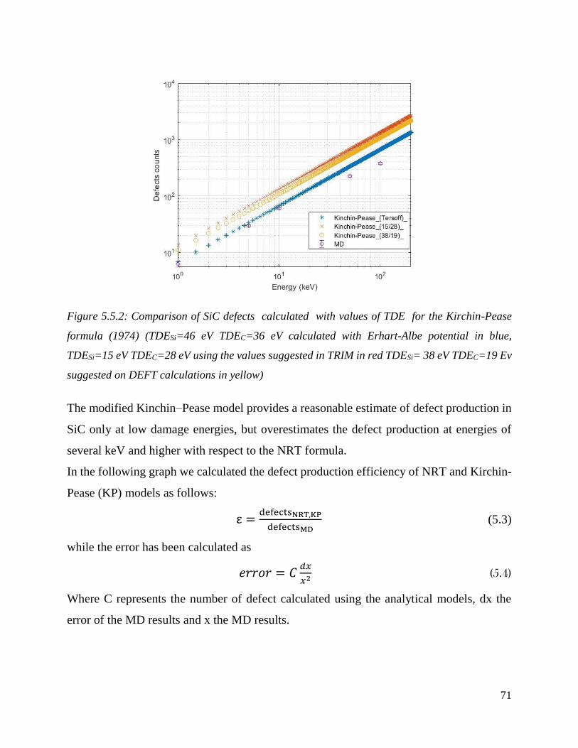
71
Figure 5.5.2: Comparison of SiC defects calculated with values of TDE for the Kirchin-Pease
formula (1974) (TDESi=46 eV TDEC=36 eV calculated with Erhart-Albe potential in blue,
TDESi=15 eV TDEC=28 eV using the values suggested in TRIM in red TDESi= 38 eV TDEC=19 Ev
suggested on DEFT calculations in yellow)
The modified Kinchin–Pease model provides a reasonable estimate of defect production in
SiC only at low damage energies, but overestimates the defect production at energies of
several keV and higher with respect to the NRT formula.
In the following graph we calculated the defect production efficiency of NRT and Kirchin-
Pease (KP) models as follows:
ε =defectsNRT,KP
defectsMD (5.3)
while the error has been calculated as
𝑒𝑟𝑟𝑜𝑟 = 𝐶𝑑𝑥
𝑥2 (5.4)
Where C represents the number of defect calculated using the analytical models, dx the
error of the MD results and x the MD results.
72
Figure 5.5.3: Defect production efficiency as a function of PKA damage energy.
Although the defect production efficiency in SiC decreases almost continuously with
increasing PKA energy, similar to behavior in metals, the relative damage efficiency is
much higher in SiC compared to metals [49]. Only for 10keV it is possible to see an increase
in the efficiency for both NRT and KP method, which can be justified as a lack of statistics
(only 10 independent simulations for MD). In this study it is possible to see that the use of
Ed respectively equal to 36 eV for C and 46 eV for Si which were used to calculate Ndisp ,
gives a resulting defect production efficiency exceeded 0.8 for almost all PKA energies.
In this part of the study, computer simulations based on the binary collision approximation
(BCA) and molecular dynamics (MD) methods are employed to determine the dependence
of displaced atom production on the damage energy of the primary knock-on atom (PKA).
The damage energy is the kinetic energy of the PKA that is dissipated by nuclear collision
processes (nuclear stopping), with the remainder of the PKA energy being dissipated by
ionization and electronic excitation processes (electronic stopping) (see previous part).
What we expect, combining the friction force calculated in TRIM with MD is that the BCA
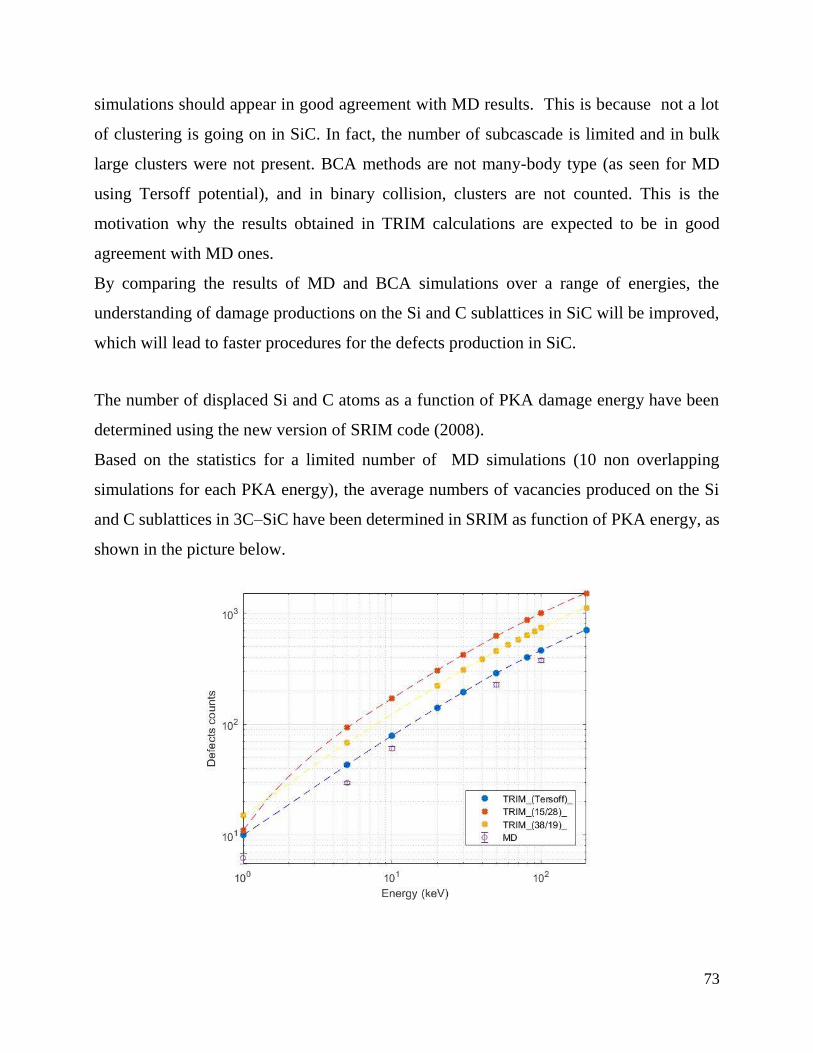
73
simulations should appear in good agreement with MD results. This is because not a lot
of clustering is going on in SiC. In fact, the number of subcascade is limited and in bulk
large clusters were not present. BCA methods are not many-body type (as seen for MD
using Tersoff potential), and in binary collision, clusters are not counted. This is the
motivation why the results obtained in TRIM calculations are expected to be in good
agreement with MD ones.
By comparing the results of MD and BCA simulations over a range of energies, the
understanding of damage productions on the Si and C sublattices in SiC will be improved,
which will lead to faster procedures for the defects production in SiC.
The number of displaced Si and C atoms as a function of PKA damage energy have been
determined using the new version of SRIM code (2008).
Based on the statistics for a limited number of MD simulations (10 non overlapping
simulations for each PKA energy), the average numbers of vacancies produced on the Si
and C sublattices in 3C–SiC have been determined in SRIM as function of PKA energy, as
shown in the picture below.
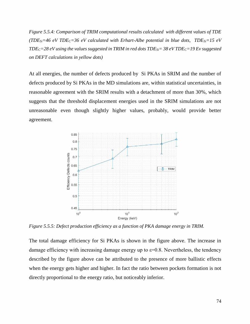
74
Figure 5.5.4: Comparison of TRIM computational results calculated with different values of TDE
(TDESi=46 eV TDEC=36 eV calculated with Erhart-Albe potential in blue dots, TDESi=15 eV
TDEC=28 eV using the values suggested in TRIM in red dots TDESi= 38 eV TDEC=19 Ev suggested
on DEFT calculations in yellow dots)
At all energies, the number of defects produced by Si PKAs in SRIM and the number of
defects produced by Si PKAs in the MD simulations are, within statistical uncertainties, in
reasonable agreement with the SRIM results with a detachment of more than 30%, which
suggests that the threshold displacement energies used in the SRIM simulations are not
unreasonable even though slightly higher values, probably, would provide better
agreement.
Figure 5.5.5: Defect production efficiency as a function of PKA damage energy in TRIM.
The total damage efficiency for Si PKAs is shown in the figure above. The increase in
damage efficiency with increasing damage energy up to ε=0.8. Nevertheless, the tendency
described by the figure above can be attributed to the presence of more ballistic effects
when the energy gets higher and higher. In fact the ratio between pockets formation is not
directly proportional to the energy ratio, but noticeably inferior.
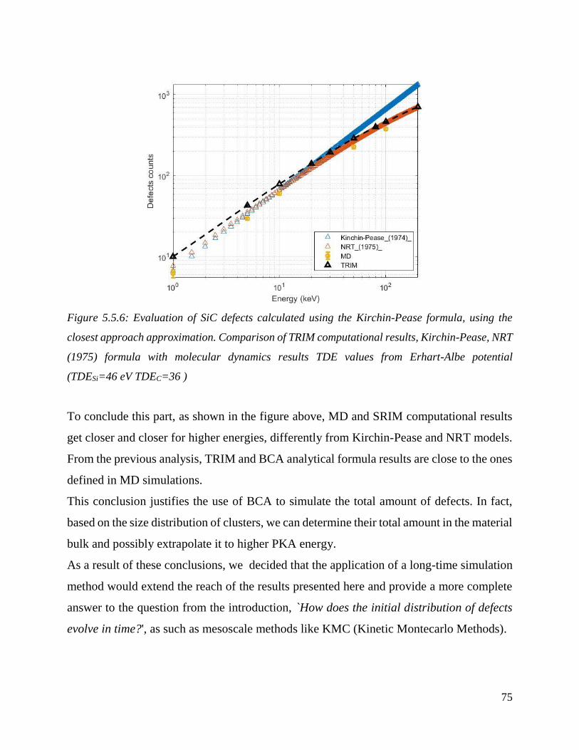
75
Figure 5.5.6: Evaluation of SiC defects calculated using the Kirchin-Pease formula, using the
closest approach approximation. Comparison of TRIM computational results, Kirchin-Pease, NRT
(1975) formula with molecular dynamics results TDE values from Erhart-Albe potential
(TDESi=46 eV TDEC=36 )
To conclude this part, as shown in the figure above, MD and SRIM computational results
get closer and closer for higher energies, differently from Kirchin-Pease and NRT models.
From the previous analysis, TRIM and BCA analytical formula results are close to the ones
defined in MD simulations.
This conclusion justifies the use of BCA to simulate the total amount of defects. In fact,
based on the size distribution of clusters, we can determine their total amount in the material
bulk and possibly extrapolate it to higher PKA energy.
As a result of these conclusions, we decided that the application of a long-time simulation
method would extend the reach of the results presented here and provide a more complete
answer to the question from the introduction, `How does the initial distribution of defects
evolve in time?', as such as mesoscale methods like KMC (Kinetic Montecarlo Methods).
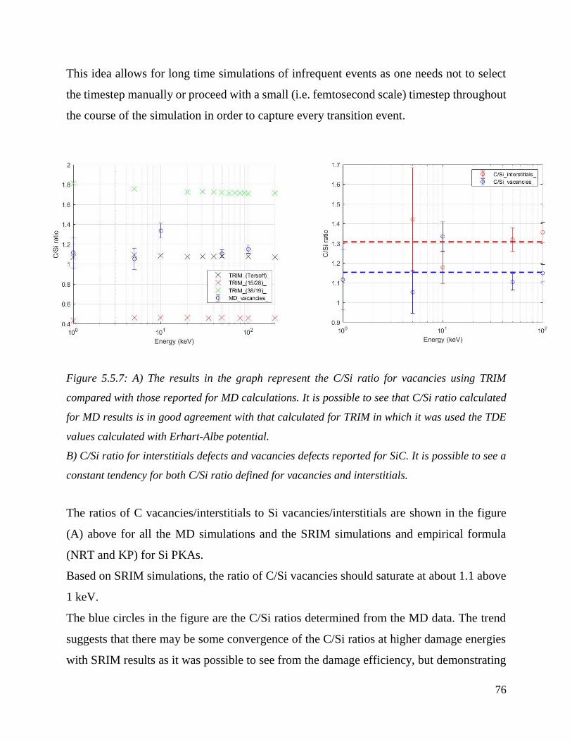
76
This idea allows for long time simulations of infrequent events as one needs not to select
the timestep manually or proceed with a small (i.e. femtosecond scale) timestep throughout
the course of the simulation in order to capture every transition event.
Figure 5.5.7: A) The results in the graph represent the C/Si ratio for vacancies using TRIM
compared with those reported for MD calculations. It is possible to see that C/Si ratio calculated
for MD results is in good agreement with that calculated for TRIM in which it was used the TDE
values calculated with Erhart-Albe potential.
B) C/Si ratio for interstitials defects and vacancies defects reported for SiC. It is possible to see a
constant tendency for both C/Si ratio defined for vacancies and interstitials.
The ratios of C vacancies/interstitials to Si vacancies/interstitials are shown in the figure
(A) above for all the MD simulations and the SRIM simulations and empirical formula
(NRT and KP) for Si PKAs.
Based on SRIM simulations, the ratio of C/Si vacancies should saturate at about 1.1 above
1 keV.
The blue circles in the figure are the C/Si ratios determined from the MD data. The trend
suggests that there may be some convergence of the C/Si ratios at higher damage energies
with SRIM results as it was possible to see from the damage efficiency, but demonstrating
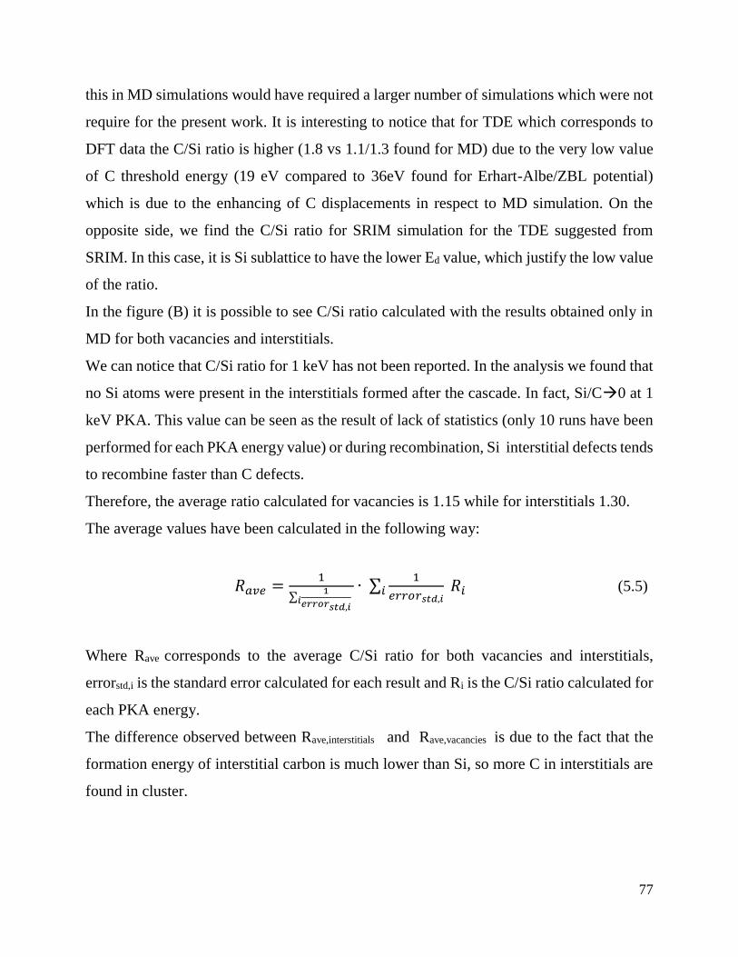
77
this in MD simulations would have required a larger number of simulations which were not
require for the present work. It is interesting to notice that for TDE which corresponds to
DFT data the C/Si ratio is higher (1.8 vs 1.1/1.3 found for MD) due to the very low value
of C threshold energy (19 eV compared to 36eV found for Erhart-Albe/ZBL potential)
which is due to the enhancing of C displacements in respect to MD simulation. On the
opposite side, we find the C/Si ratio for SRIM simulation for the TDE suggested from
SRIM. In this case, it is Si sublattice to have the lower Ed value, which justify the low value
of the ratio.
In the figure (B) it is possible to see C/Si ratio calculated with the results obtained only in
MD for both vacancies and interstitials.
We can notice that C/Si ratio for 1 keV has not been reported. In the analysis we found that
no Si atoms were present in the interstitials formed after the cascade. In fact, Si/C0 at 1
keV PKA. This value can be seen as the result of lack of statistics (only 10 runs have been
performed for each PKA energy value) or during recombination, Si interstitial defects tends
to recombine faster than C defects.
Therefore, the average ratio calculated for vacancies is 1.15 while for interstitials 1.30.
The average values have been calculated in the following way:
𝑅𝑎𝑣𝑒 =1
∑1
𝑒𝑟𝑟𝑜𝑟𝑠𝑡𝑑,𝑖 𝑖
∙ ∑1
𝑒𝑟𝑟𝑜𝑟𝑠𝑡𝑑,𝑖 𝑅𝑖 𝑖 (5.5)
Where Rave corresponds to the average C/Si ratio for both vacancies and interstitials,
errorstd,i is the standard error calculated for each result and Ri is the C/Si ratio calculated for
each PKA energy.
The difference observed between Rave,interstitials and Rave,vacancies is due to the fact that the
formation energy of interstitial carbon is much lower than Si, so more C in interstitials are
found in cluster.
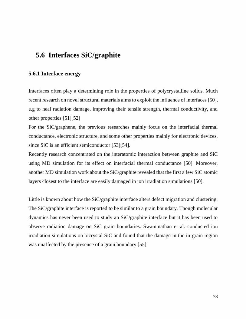
78
5.6 Interfaces SiC/graphite
5.6.1 Interface energy
Interfaces often play a determining role in the properties of polycrystalline solids. Much
recent research on novel structural materials aims to exploit the influence of interfaces [50],
e.g to heal radiation damage, improving their tensile strength, thermal conductivity, and
other properties [51][52]
For the SiC/graphene, the previous researches mainly focus on the interfacial thermal
conductance, electronic structure, and some other properties mainly for electronic devices,
since SiC is an efficient semiconductor [53][54].
Recently research concentrated on the interatomic interaction between graphite and SiC
using MD simulation for its effect on interfacial thermal conductance [50]. Moreover,
another MD simulation work about the SiC/graphite revealed that the first a few SiC atomic
layers closest to the interface are easily damaged in ion irradiation simulations [50].
Little is known about how the SiC/graphite interface alters defect migration and clustering.
The SiC/graphite interface is reported to be similar to a grain boundary. Though molecular
dynamics has never been used to study an SiC/graphite interface but it has been used to
observe radiation damage on SiC grain boundaries. Swaminathan et al. conducted ion
irradiation simulations on bicrystal SiC and found that the damage in the in-grain region
was unaffected by the presence of a grain boundary [55].
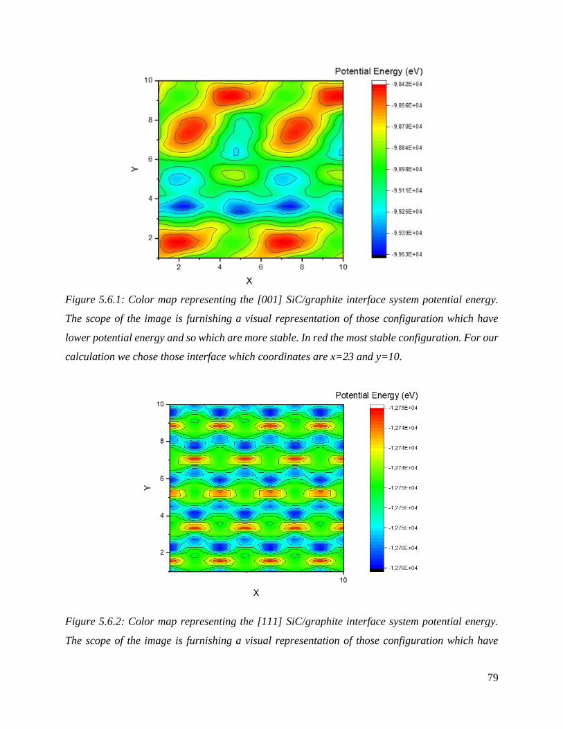
79
Figure 5.6.1: Color map representing the [001] SiC/graphite interface system potential energy.
The scope of the image is furnishing a visual representation of those configuration which have
lower potential energy and so which are more stable. In red the most stable configuration. For our
calculation we chose those interface which coordinates are x=23 and y=10.
Figure 5.6.2: Color map representing the [111] SiC/graphite interface system potential energy.
The scope of the image is furnishing a visual representation of those configuration which have
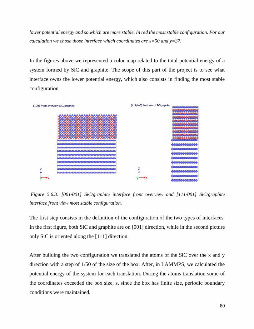
80
lower potential energy and so which are more stable. In red the most stable configuration. For our
calculation we chose those interface which coordinates are x=50 and y=37.
In the figures above we represented a color map related to the total potential energy of a
system formed by SiC and graphite. The scope of this part of the project is to see what
interface owns the lower potential energy, which also consists in finding the most stable
configuration.
Figure 5.6.3: [001/001] SiC/graphite interface front overview and [111/001] SiC/graphite
interface front view most stable configuration.
The first step consists in the definition of the configuration of the two types of interfaces.
In the first figure, both SiC and graphite are on [001] direction, while in the second picture
only SiC is oriented along the [111] direction.
After building the two configuration we translated the atoms of the SiC over the x and y
direction with a step of 1/50 of the size of the box. After, in LAMMPS, we calculated the
potential energy of the system for each translation. During the atoms translation some of
the coordinates exceeded the box size, s, since the box has finite size, periodic boundary
conditions were maintained.
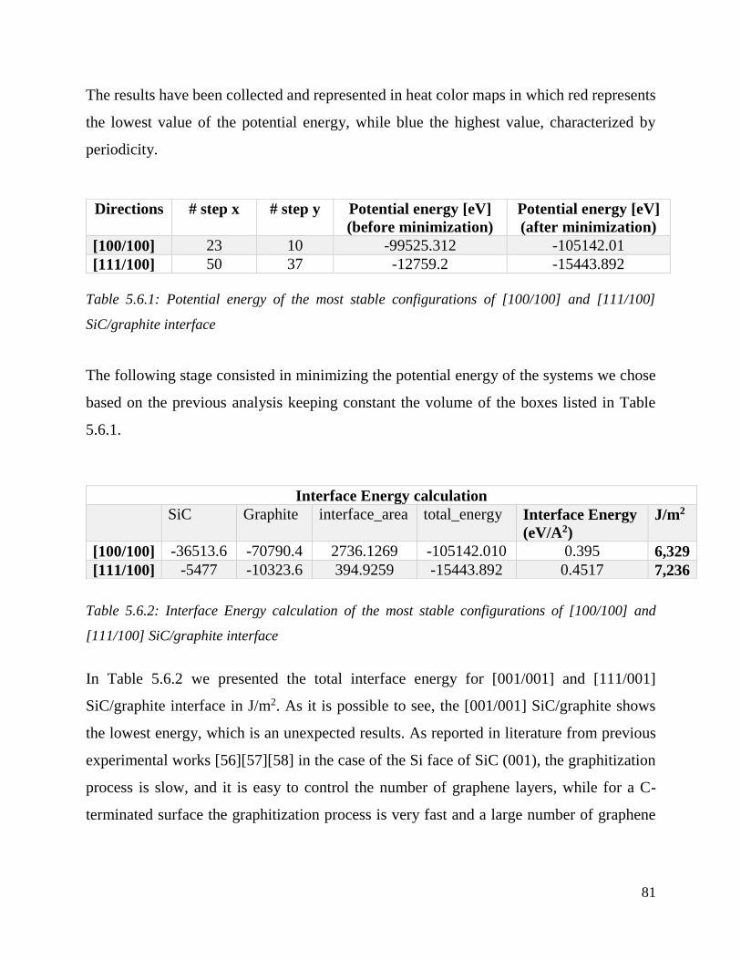
81
The results have been collected and represented in heat color maps in which red represents
the lowest value of the potential energy, while blue the highest value, characterized by
periodicity.
Table 5.6.1: Potential energy of the most stable configurations of [100/100] and [111/100]
SiC/graphite interface
The following stage consisted in minimizing the potential energy of the systems we chose
based on the previous analysis keeping constant the volume of the boxes listed in Table
5.6.1.
Table 5.6.2: Interface Energy calculation of the most stable configurations of [100/100] and
[111/100] SiC/graphite interface
In Table 5.6.2 we presented the total interface energy for [001/001] and [111/001]
SiC/graphite interface in J/m2. As it is possible to see, the [001/001] SiC/graphite shows
the lowest energy, which is an unexpected results. As reported in literature from previous
experimental works [56][57][58] in the case of the Si face of SiC (001), the graphitization
process is slow, and it is easy to control the number of graphene layers, while for a C-
terminated surface the graphitization process is very fast and a large number of graphene
Directions # step x # step y Potential energy [eV]
(before minimization)
Potential energy [eV]
(after minimization)
[100/100] 23 10 -99525.312 -105142.01
[111/100] 50 37 -12759.2 -15443.892
Interface Energy calculation
SiC Graphite interface_area total_energy Interface Energy
(eV/A2)
J/m2
[100/100] -36513.6 -70790.4 2736.1269 -105142.010 0.395 6,329
[111/100] -5477 -10323.6 394.9259 -15443.892 0.4517 7,236

82
layers are formed. Nevertheless, the most suitable surface remains 3C SiC (111). Because
of this, we expected to find interface energy lower for SiC(111) oriented.
This results can be explained because of the periodicity of the boundary conditions that
gives as a result only an average value of the energy of the interface, since the atom layer
of SiC in contact with the graphite changes depending on the position of the interface.
Because of this, it has been proposed to use the semi-infinite crystal method. However, this
is a complex non-standard method that is outside the scope of the present thesis.
5.6.2 Binding Energy of point defects to interfaces
In this part of the thesis we are interested in finding the binding energy between the defects
created in proximity of the interface in function of the distance.
To assess trapping of point defects at SiC-graphite interfaces, the binding energy energies
of vacancies and interstitials at these interfaces were computed in function of the distance
from the first carbon layer of the graphite. On the interface structure C and Si layers were
alternated and free surface has been created over SiC and graphite boxes; after, vacancies
were created by deleting an atom, and interstitials by inserting an atom at a desired location.
Defect structures were relaxed at constant volume through conjugate gradient energy
minimization to relax configurations with closely spaced atoms that may arise due to
interstitial/vacancy insertion.
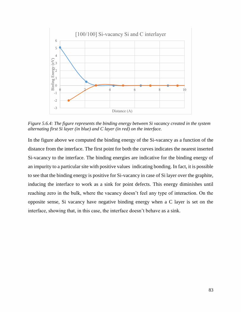
83
Figure 5.6.4: The figure represents the binding energy between Si vacancy created in the system
alternating first Si layer (in blue) and C layer (in red) on the interface.
In the figure above we computed the binding energy of the Si-vacancy as a function of the
distance from the interface. The first point for both the curves indicates the nearest inserted
Si-vacancy to the interface. The binding energies are indicative for the binding energy of
an impurity to a particular site with positive values indicating bonding. In fact, it is possible
to see that the binding energy is positive for Si-vacancy in case of Si layer over the graphite,
inducing the interface to work as a sink for point defects. This energy diminishes until
reaching zero in the bulk, where the vacancy doesn’t feel any type of interaction. On the
opposite sense, Si vacancy have negative binding energy when a C layer is set on the
interface, showing that, in this case, the interface doesn’t behave as a sink.
-3
-2
-1
0
1
2
3
4
5
6
0 2 4 6 8 10Bin
fing E
ner
gy (
eV)
Distance (A)
[100/100] Si-vacancy Si and C interlayer
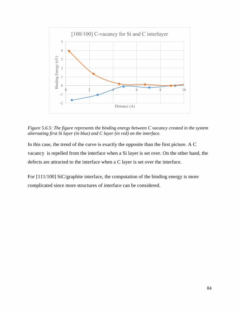
84
Figure 5.6.5: The figure represents the binding energy between C vacancy created in the system
alternating first Si layer (in blue) and C layer (in red) on the interface.
In this case, the trend of the curve is exactly the opposite than the first picture. A C
vacancy is repelled from the interface when a Si layer is set over. On the other hand, the
defects are attracted to the interface when a C layer is set over the interface.
For [111/100] SiC/graphite interface, the computation of the binding energy is more
complicated since more structures of interface can be considered.
-2
-1
0
1
2
3
4
5
0 2 4 6 8 10
Bin
din
g E
ner
gy (
eV)
Distance (A)
[100/100] C-vacancy for Si and C interlayer
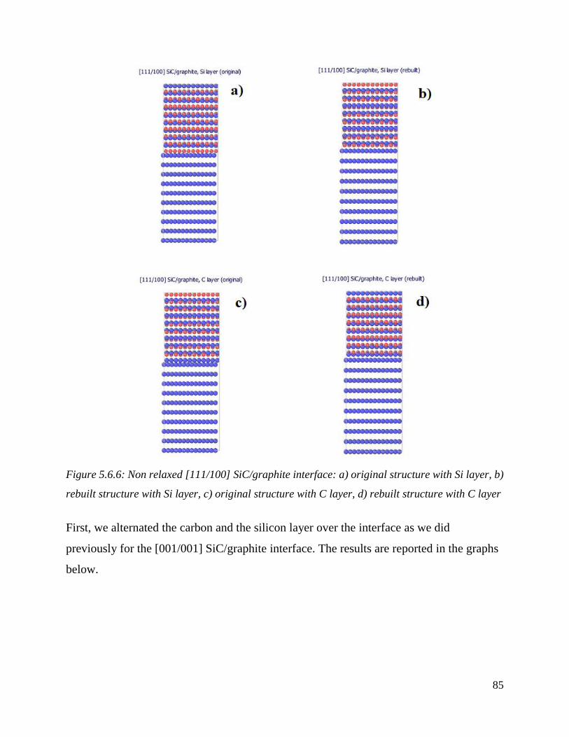
85
Figure 5.6.6: Non relaxed [111/100] SiC/graphite interface: a) original structure with Si layer, b)
rebuilt structure with Si layer, c) original structure with C layer, d) rebuilt structure with C layer
First, we alternated the carbon and the silicon layer over the interface as we did
previously for the [001/001] SiC/graphite interface. The results are reported in the graphs
below.
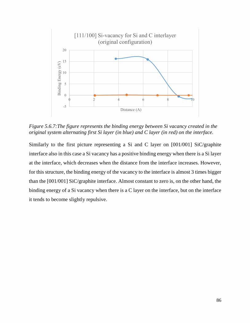
86
Figure 5.6.7:The figure represents the binding energy between Si vacancy created in the
original system alternating first Si layer (in blue) and C layer (in red) on the interface.
Similarly to the first picture representing a Si and C layer on [001/001] SiC/graphite
interface also in this case a Si vacancy has a positive binding energy when there is a Si layer
at the interface, which decreases when the distance from the interface increases. However,
for this structure, the binding energy of the vacancy to the interface is almost 3 times bigger
than the [001/001] SiC/graphite interface. Almost constant to zero is, on the other hand, the
binding energy of a Si vacancy when there is a C layer on the interface, but on the interface
it tends to become slightly repulsive.
-5
0
5
10
15
20
0 2 4 6 8 10
Bin
din
g E
ner
gy (
eV)
Distance (A)
[111/100] Si-vacancy for Si and C interlayer
(original configuration)
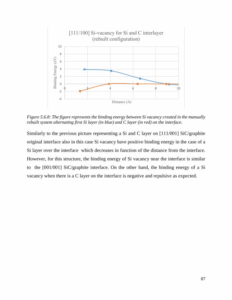
87
Figure 5.6.8: The figure represents the binding energy between Si vacancy created in the manually
rebuilt system alternating first Si layer (in blue) and C layer (in red) on the interface.
Similarly to the previous picture representing a Si and C layer on [111/001] SiC/graphite
original interface also in this case Si vacancy have positive binding energy in the case of a
Si layer over the interface which decreases in function of the distance from the interface.
However, for this structure, the binding energy of Si vacancy near the interface is similar
to the [001/001] SiC/graphite interface. On the other hand, the binding energy of a Si
vacancy when there is a C layer on the interface is negative and repulsive as expected.
-4
-2
0
2
4
6
8
10
0 2 4 6 8 10Bin
din
g E
ner
gy (
eV)
Distance (A)
[111/100] Si-vacancy for Si and C interlayer
(rebuilt configuration)
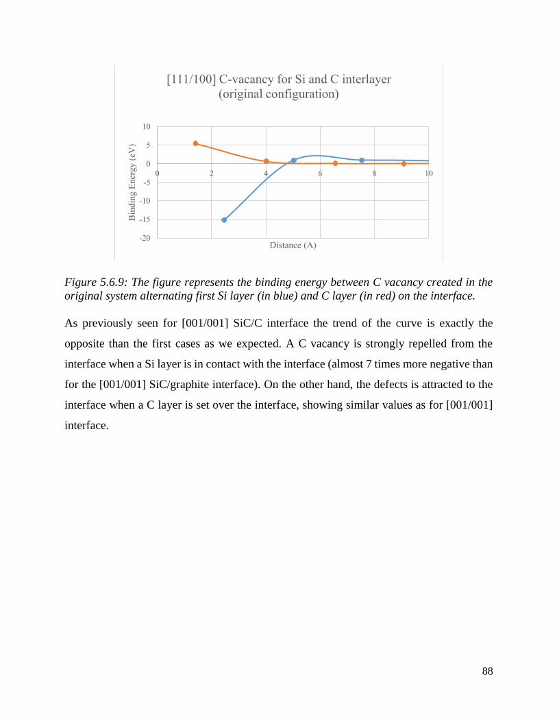
88
Figure 5.6.9: The figure represents the binding energy between C vacancy created in the
original system alternating first Si layer (in blue) and C layer (in red) on the interface.
As previously seen for [001/001] SiC/C interface the trend of the curve is exactly the
opposite than the first cases as we expected. A C vacancy is strongly repelled from the
interface when a Si layer is in contact with the interface (almost 7 times more negative than
for the [001/001] SiC/graphite interface). On the other hand, the defects is attracted to the
interface when a C layer is set over the interface, showing similar values as for [001/001]
interface.
-20
-15
-10
-5
0
5
10
0 2 4 6 8 10
Bin
din
g E
ner
gy (
eV)
Distance (A)
[111/100] C-vacancy for Si and C interlayer
(original configuration)
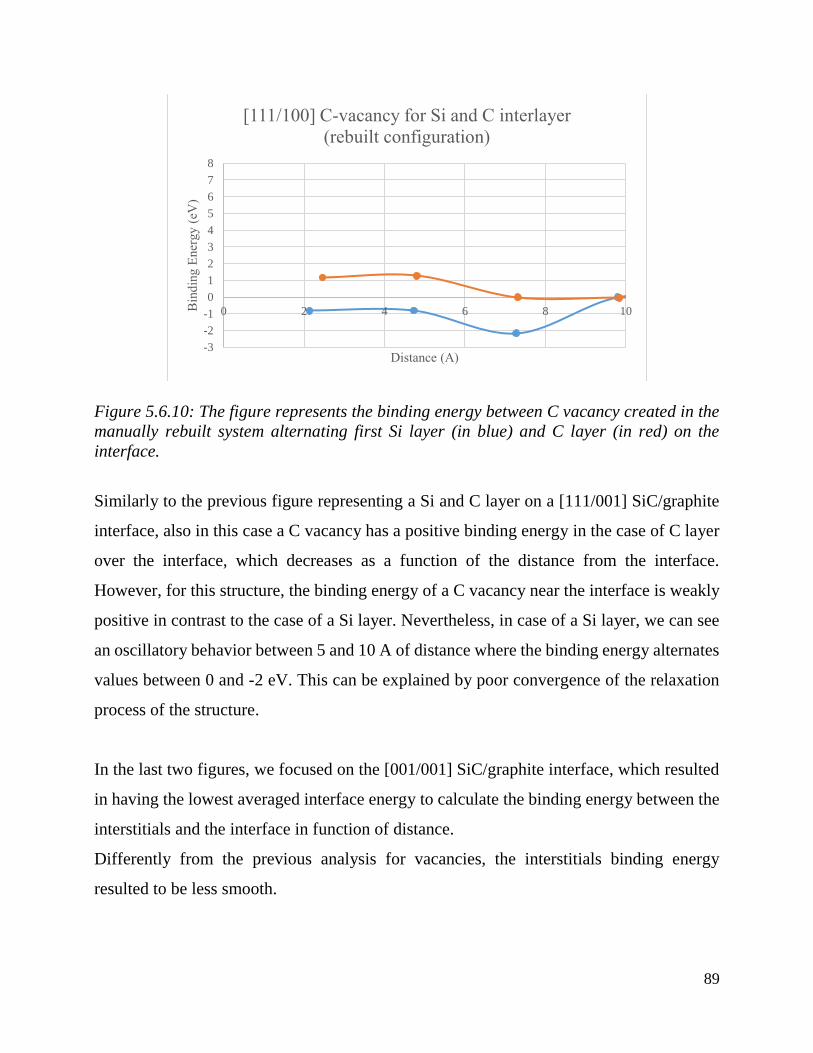
89
Figure 5.6.10: The figure represents the binding energy between C vacancy created in the
manually rebuilt system alternating first Si layer (in blue) and C layer (in red) on the
interface.
Similarly to the previous figure representing a Si and C layer on a [111/001] SiC/graphite
interface, also in this case a C vacancy has a positive binding energy in the case of C layer
over the interface, which decreases as a function of the distance from the interface.
However, for this structure, the binding energy of a C vacancy near the interface is weakly
positive in contrast to the case of a Si layer. Nevertheless, in case of a Si layer, we can see
an oscillatory behavior between 5 and 10 A of distance where the binding energy alternates
values between 0 and -2 eV. This can be explained by poor convergence of the relaxation
process of the structure.
In the last two figures, we focused on the [001/001] SiC/graphite interface, which resulted
in having the lowest averaged interface energy to calculate the binding energy between the
interstitials and the interface in function of distance.
Differently from the previous analysis for vacancies, the interstitials binding energy
resulted to be less smooth.
-3
-2
-1
0
1
2
3
4
5
6
7
8
0 2 4 6 8 10Bin
din
g E
ner
gy (
eV)
Distance (A)
[111/100] C-vacancy for Si and C interlayer
(rebuilt configuration)
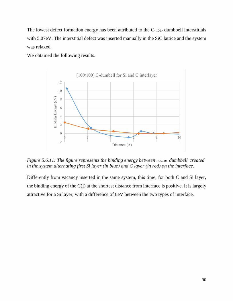
90
The lowest defect formation energy has been attributed to the C<100> dumbbell interstitials
with 5.07eV. The interstitial defect was inserted manually in the SiC lattice and the system
was relaxed.
We obtained the following results.
Figure 5.6.11: The figure represents the binding energy between C<100> dumbbell created
in the system alternating first Si layer (in blue) and C layer (in red) on the interface.
Differently from vacancy inserted in the same system, this time, for both C and Si layer,
the binding energy of the C(I) at the shortest distance from interface is positive. It is largely
attractive for a Si layer, with a difference of 8eV between the two types of interface.
-2
0
2
4
6
8
10
12
0 2 4 6 8 10
Bin
din
g E
ner
gy (
eV)
Distance (A)
[100/100] C-dumbell for Si and C interlayer
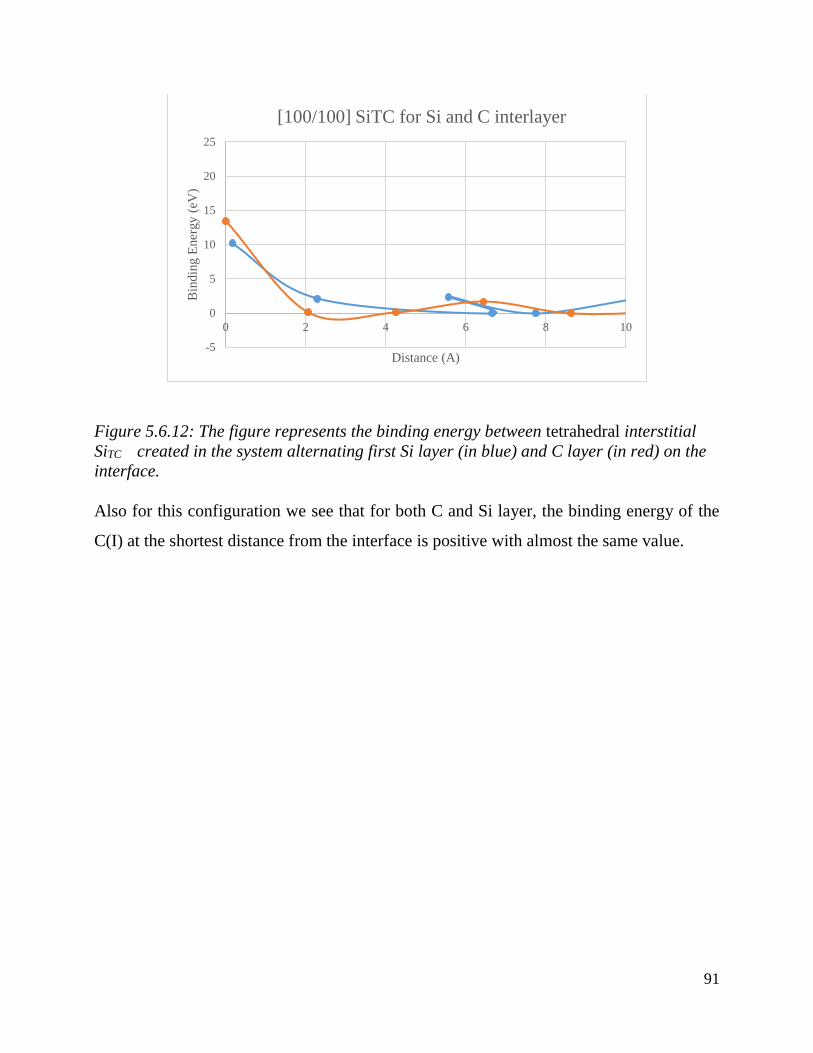
91
Figure 5.6.12: The figure represents the binding energy between tetrahedral interstitial
SiTC created in the system alternating first Si layer (in blue) and C layer (in red) on the
interface.
Also for this configuration we see that for both C and Si layer, the binding energy of the
C(I) at the shortest distance from the interface is positive with almost the same value.
-5
0
5
10
15
20
25
0 2 4 6 8 10
Bin
din
g E
ner
gy (
eV)
Distance (A)
[100/100] SiTC for Si and C interlayer
92
Chapter 6
6. Summary and Conclusions
In recent years, computational models have claimed an important role in understanding the
mechanisms at work leading to the degradation of materials under irradiation. The
phenomenon of radiation in materials is inherently a multi-scale problem: a flux of
subatomic particles (neutrons) interacts with lattice atoms leading to the failure of
macroscopic components. Given the different length- and time scales involved, multi-scale
modelling techniques are used to simulate the damage mechanisms active at the different
scales of the radiation process.
In this thesis we aim to contribute by providing input data to meso-scale models by means
of atomistic simulations.
Chapter 1 of this dissertation provided a review of the literature regarding the utilization of
3C-SiC and SiC fibers (e.g SiC/SiC, SiC/PyC, Tyranno…) nuclear power applications and
industry.
For atomistic simulations, a PKA kinetic energy between 1 and 100 keV were chosen for
its relevance to both fusion and fission applications as well as being within the energy range
where classical molecular dynamics simulations of atomic collisions are valid.
In Chapter 2 there is a brief description of the workplan of the thesis.
Chapter 3 is dedicated to the results obtained using different empirical potentials in
molecular statics to find the formation energy of each point defects for both SiC and
graphite. The most stable configurations is found in literature to be CC<100> dumbbell
interstitial for carbon, while SiTC is the most stable configuration reported in literature for
93
Si in 3C-SiC. For graphite, on the other hand, the spiro structure wss found to be the most
stable defect from DFT results. In conclusion, we found that only Erhart-Albe empirical
potential was in accordance with the predicted results obtained in DFT.
Moreover, Chapter 3 focuses on how the nuclear and electronic stopping power contributes
in molecular dynamics to receive more accurate results; through the use of SRIM in this
section, we found a linear fitting curve which combine the velocity with the predicted
kinetic energy of the incoming particle.
The last part of Chapter 3 is also dedicated to calculate the TDE necessary to implement
the cascade on TRIM and finding the correct results while using the empirical formulas. In
general, the TDEs calculated with the potential used here have been compared with
experimental and DFT results obtained from other authors. The TDE variations found in
this work were attributed to subtle differences in the definition of different stiffening. It
was concluded that the potential performed sufficiently well to justify its use.
The final section of the third chapter is completely dedicated to empirical formulas
proposed in literature to generate the total number of displacements in studied materials.
This results have been compared with those found using TRIM simulations and MD
dynamics, seeing that, for TRIM there is an increase on Defect production efficiency as a
function of PKA damage due to the fact that in there is the presence of more ballistic effects
when the energy gets higher and higher and, since TRIM cannot predict clustering and/or
recombination effects, it means that defects don’t have a very high probability to form large
clusters at high PKA-energy. We could conclude from this study that TRIM and similar
BCA programs can be a substitute to MD for the generation of point defects in SiC.
Chapter 4 is dedicated to the description of the atomic structure of both SiC and graphite.
We dedicated the final part of Chapter 4 to the characteristics of the point defects which
can form after the radiation damage in the bulk of the two compunds.
94
Chapter 5 is related to the verification procedure. It consists in the reproduction of the 1 to
100 keV Si PKA cascade simulations in a perfect silicon carbide crystal with no thermal
effects on the damage state. The results showed good qualitative agreement with the
published results, verifying the simulation and post-processing procedure. This part is the
key part of our work, since it has been possible, through the defect analysis performed in
Ovito, to extract the statistical clustering (vacancy and interstitial) distribution in SiC bulk
for given PKA energy, which is completely new in terms of available literature on the
argument.
The main outcome of these results is that, using the mathematical formula derived from the
distribution, it will be possible to find the total number of clusters in SiC bulk without the
auxiliary of MD simulations, extremely time consuming compared to BCA methods.
This information will be used to generate the clusters distribution studied in the long-time
calculations in future works. Probably, further simulations and statistical analysis is
required to improve the quality of the spatial distributions, though those calculated here
provided a good initial approximation.
We found that the C/Si ratio necessary as an input for KMC programs to detect the
evolution of the defects for larger arc of time.
We found for vacancies C/Si ratios that TRIM and MD gives approximately same results
and the fact that for interstitials C/Si is ratio is higher in value in respect to vacancies is due
to the fact that formation energy of interstitial carbon is much lower than Si, so more C in
interstitials are found in cluster.
The final part is dedicated to SiC/graphite interface. Interfaces play a big role in industrial
sector, in particular when subjected to irradiation. Not many studies have been performed
of SiC/graphite interface, but in the last years these are intensifying also because of its use
in TRISO technologies.
Interface energy calculations have been performed for two differently oriented SiC/graphite
interfaces: in the first one SiC is [100] oriented while in the second case SiC is [111]
oriented. It has been found, in contradiction with literature, that SiC[100]/graphite interface
95
has a lower interfacial energy of SiC[111]/graphite interface. This has been explained as
the total interface energy in our work correspond to an averaging of the energies found for
C and Si layers that can be alternated on the surface. Moreover, it has been found essential
performing the same calculation for semi-infinite crystal which was not possible to compute
in LAMMPS.
Defects (vacancies and most stable interstitials) have been injected in the system and we
calculated the total binding energy between the defect and the interface in function of the
distance, alternating C and Si layers over the interface and eliminating the results which
corresponds to free surface.
It has been found that the binding energy is included between -5 eV (repulsive binding
energy, the defect is not absorbed in the sink) and +15 eV (attractive binding energy, the
defect tends to migrate on the sink), values which have been expected from the available
literature.
In conclusion, the main contributions of this work are:
Quantitative characterization of the statistical distribution of vacancy and interstitial
clusters after simulated cascade formation in 3C-SiC.
Utilization BCA methods for detection of 3C-SiC damage simulated in cascade
formation in bulk
Input for KMC calculations: C/Si ratios found for both interstitials and vacancies
Initial study of SiC/graphite interface from the molecular statics point of view
Based on the experience gained during this work the following are recommended as
avenues of future research that directly build on the work in this dissertation:
On SiC and graphite materials:

96
Stability of point defects and point defect clusters over timescales much greater than
10 ps.
Damage cascade simulation in graphite bulk performance.
On SiC/graphite interfaces:
Multiple and different position and direction should be taken into consideration.
The use of semi-infinite crystal boundary condition.
Cascade simulations using MD on interfaces should be performed using the same
potential.
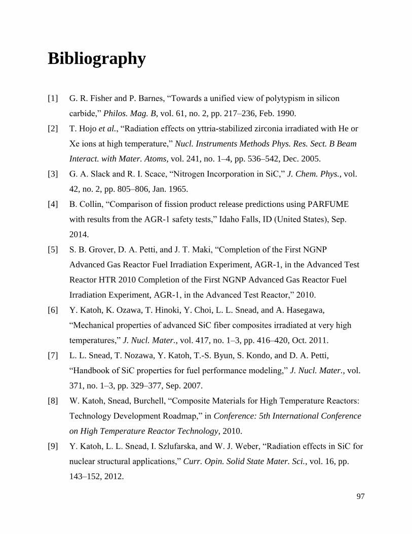
97
Bibliography
[1] G. R. Fisher and P. Barnes, “Towards a unified view of polytypism in silicon
carbide,” Philos. Mag. B, vol. 61, no. 2, pp. 217–236, Feb. 1990.
[2] T. Hojo et al., “Radiation effects on yttria-stabilized zirconia irradiated with He or
Xe ions at high temperature,” Nucl. Instruments Methods Phys. Res. Sect. B Beam
Interact. with Mater. Atoms, vol. 241, no. 1–4, pp. 536–542, Dec. 2005.
[3] G. A. Slack and R. I. Scace, “Nitrogen Incorporation in SiC,” J. Chem. Phys., vol.
42, no. 2, pp. 805–806, Jan. 1965.
[4] B. Collin, “Comparison of fission product release predictions using PARFUME
with results from the AGR-1 safety tests,” Idaho Falls, ID (United States), Sep.
2014.
[5] S. B. Grover, D. A. Petti, and J. T. Maki, “Completion of the First NGNP
Advanced Gas Reactor Fuel Irradiation Experiment, AGR-1, in the Advanced Test
Reactor HTR 2010 Completion of the First NGNP Advanced Gas Reactor Fuel
Irradiation Experiment, AGR-1, in the Advanced Test Reactor,” 2010.
[6] Y. Katoh, K. Ozawa, T. Hinoki, Y. Choi, L. L. Snead, and A. Hasegawa,
“Mechanical properties of advanced SiC fiber composites irradiated at very high
temperatures,” J. Nucl. Mater., vol. 417, no. 1–3, pp. 416–420, Oct. 2011.
[7] L. L. Snead, T. Nozawa, Y. Katoh, T.-S. Byun, S. Kondo, and D. A. Petti,
“Handbook of SiC properties for fuel performance modeling,” J. Nucl. Mater., vol.
371, no. 1–3, pp. 329–377, Sep. 2007.
[8] W. Katoh, Snead, Burchell, “Composite Materials for High Temperature Reactors:
Technology Development Roadmap,” in Conference: 5th International Conference
on High Temperature Reactor Technology, 2010.
[9] Y. Katoh, L. L. Snead, I. Szlufarska, and W. J. Weber, “Radiation effects in SiC for
nuclear structural applications,” Curr. Opin. Solid State Mater. Sci., vol. 16, pp.
143–152, 2012.
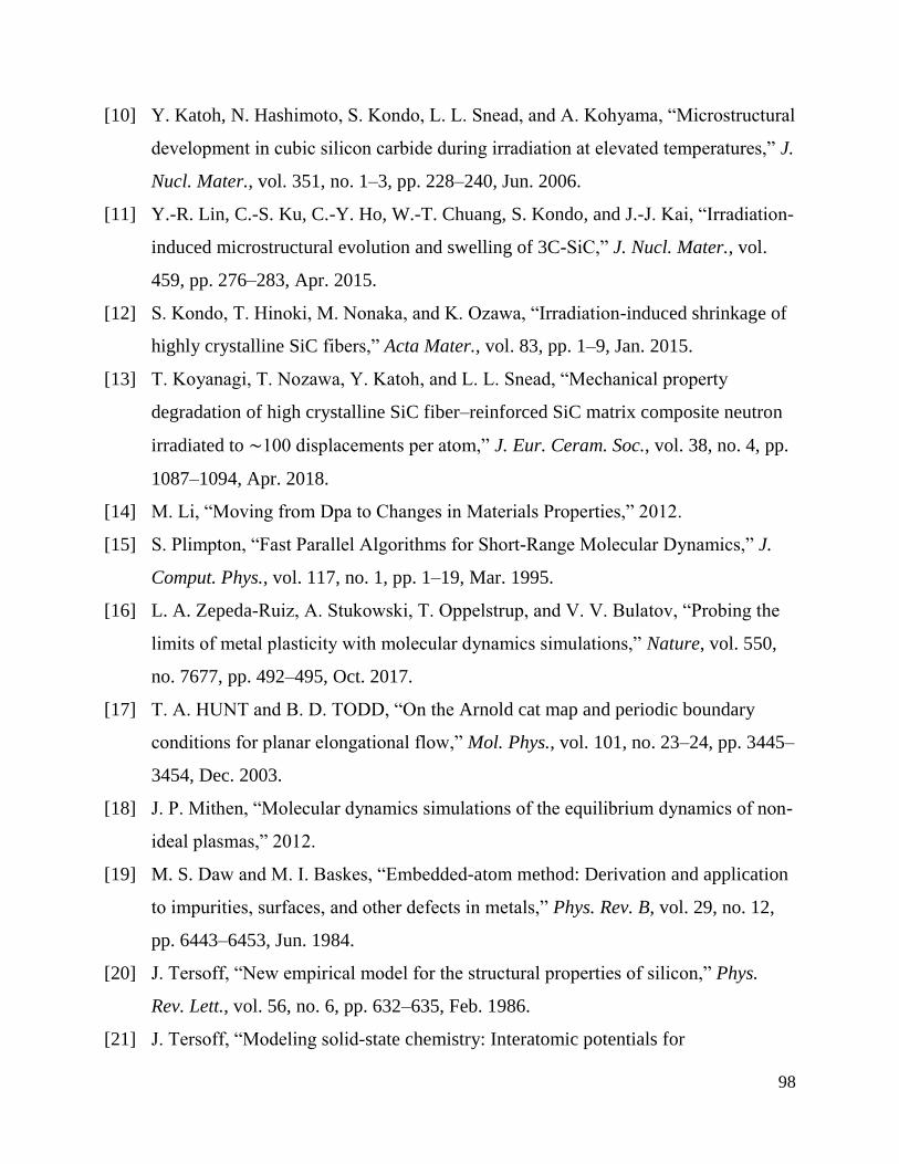
98
[10] Y. Katoh, N. Hashimoto, S. Kondo, L. L. Snead, and A. Kohyama, “Microstructural
development in cubic silicon carbide during irradiation at elevated temperatures,” J.
Nucl. Mater., vol. 351, no. 1–3, pp. 228–240, Jun. 2006.
[11] Y.-R. Lin, C.-S. Ku, C.-Y. Ho, W.-T. Chuang, S. Kondo, and J.-J. Kai, “Irradiation-
induced microstructural evolution and swelling of 3C-SiC,” J. Nucl. Mater., vol.
459, pp. 276–283, Apr. 2015.
[12] S. Kondo, T. Hinoki, M. Nonaka, and K. Ozawa, “Irradiation-induced shrinkage of
highly crystalline SiC fibers,” Acta Mater., vol. 83, pp. 1–9, Jan. 2015.
[13] T. Koyanagi, T. Nozawa, Y. Katoh, and L. L. Snead, “Mechanical property
degradation of high crystalline SiC fiber–reinforced SiC matrix composite neutron
irradiated to ∼100 displacements per atom,” J. Eur. Ceram. Soc., vol. 38, no. 4, pp.
1087–1094, Apr. 2018.
[14] M. Li, “Moving from Dpa to Changes in Materials Properties,” 2012.
[15] S. Plimpton, “Fast Parallel Algorithms for Short-Range Molecular Dynamics,” J.
Comput. Phys., vol. 117, no. 1, pp. 1–19, Mar. 1995.
[16] L. A. Zepeda-Ruiz, A. Stukowski, T. Oppelstrup, and V. V. Bulatov, “Probing the
limits of metal plasticity with molecular dynamics simulations,” Nature, vol. 550,
no. 7677, pp. 492–495, Oct. 2017.
[17] T. A. HUNT and B. D. TODD, “On the Arnold cat map and periodic boundary
conditions for planar elongational flow,” Mol. Phys., vol. 101, no. 23–24, pp. 3445–
3454, Dec. 2003.
[18] J. P. Mithen, “Molecular dynamics simulations of the equilibrium dynamics of non-
ideal plasmas,” 2012.
[19] M. S. Daw and M. I. Baskes, “Embedded-atom method: Derivation and application
to impurities, surfaces, and other defects in metals,” Phys. Rev. B, vol. 29, no. 12,
pp. 6443–6453, Jun. 1984.
[20] J. Tersoff, “New empirical model for the structural properties of silicon,” Phys.
Rev. Lett., vol. 56, no. 6, pp. 632–635, Feb. 1986.
[21] J. Tersoff, “Modeling solid-state chemistry: Interatomic potentials for
99
multicomponent systems,” Phys. Rev. B, vol. 39, no. 8, pp. 5566–5568, Mar. 1989.
[22] P. Erhart and K. Albe, “Analytical potential for atomistic simulations of silicon,
carbon, and silicon carbide,” Phys. Rev. B, vol. 71, no. 3, p. 035211, Jan. 2005.
[23] P. F. Zou, R. F. W. Bader, and IUCr, “A topological definition of a Wigner–Seitz
cell and the atomic scattering factor,” Acta Crystallogr. Sect. A Found. Crystallogr.,
vol. 50, no. 6, pp. 714–725, Nov. 1994.
[24] G. D. Samolyuk, Y. N. Osetsky, and R. E. Stoller, “Molecular dynamics modeling
of atomic displacement cascades in 3C–SiC: Comparison of interatomic potentials,”
J. Nucl. Mater., vol. 465, pp. 83–88, Oct. 2015.
[25] K. Vörtler, “Computer simulation of multi-elemental fusion reactor materials.”
2011.
[26] R. Behrisch and W. Eckstein, Sputtering by particle bombardment : experiments
and computer calculations from threshold to MeV energies. Springer, 2007.
[27] G. Lucas and L. Pizzagalli, “Ab initio molecular dynamics calculations of threshold
displacement energies in silicon carbide,” Sep. 2007.
[28] I. A. Hønstvet, R. E. Smallman, and P. M. Marquis, “A determination of the atomic
displacement energy in cubic silicon carbide,” Philos. Mag. A, vol. 41, no. 2, pp.
201–207, Feb. 1980.
[29] S. J. Zinkle and C. Kinoshita, “Defect production in ceramics,” J. Nucl. Mater., vol.
251, pp. 200–217, Nov. 1997.
[30] H. Huang, N. M. Ghoniem, J. K. Wong, and M. Baskes, “Molecular dynamics
determination of defect energetics in beta -SiC using three representative empirical
potentials,” Model. Simul. Mater. Sci. Eng., vol. 3, no. 5, pp. 615–627, Sep. 1995.
[31] M. I. Norgett, M. T. Robinson, and I. M. Torrens, “A PROPOSED METHOD OF
CALCULATING DISPLACEMENT DOSE RATES.”
[32] M. T. Robinson, “Basic physics of radiation damage production,” J. Nucl. Mater.,
vol. 216, pp. 1–28, Oct. 1994.
[33] J. Lindhard, “This Week’s Citation Classic,” 1963.
[34] J. R. Beeler, Radiation effects, computer experiments. North-Holland Pub. Co.,
100
1983.
[35] D. E. Farrell, Vacancy clustering phenomena in silicon carbide reactor
components : a multiple time-scale atomistic problem. .
[36] S. Fujita, J. R. Mcnabb Iii, H.-C. Ho, and A. Suzuki, “Lattice Stability and
Reflection Symmetry,” J. Mod. Phys., vol. 6, pp. 691–697, 2015.
[37] Frank Zirkelbach, “Atomistic simulation study on silicon carbide precipitation in
silicon,” Universit¨at Augsburg, 2012.
[38] C. D. Latham, A. J. McKenna, T. P. Trevethan, M. I. Heggie, M. J. Rayson, and P.
R. Briddon, “On the validity of empirical potentials for simulating radiation damage
in graphite: a benchmark,” J. Phys. Condens. Matter, vol. 27, no. 31, p. 316301,
Aug. 2015.
[39] M. Bockstedte, A. Mattausch, and O. Pankratov, “Ab initio study of the annealing
of vacancies and interstitials in cubic SiC: Vacancy-interstitial recombination and
aggregation of carbon interstitials,” Phys. Rev. B, vol. 69, no. 23, p. 235202, Jun.
2004.
[40] X. K. Lu, T. Y. Xin, Q. Zhang, Y. J. Feng, X. L. Ren, and Y. X. Wang, “Decentral
distribution of helium in β-SiC: Studied by density functional theory,” Nucl. Mater.
Energy, vol. 13, pp. 35–41, Dec. 2017.
[41] G. Lucas and L. Pizzagalli, “Structure and stability of irradiation-induced Frenkel
pairs in 3C-SiC using first principles calculations,” Nucl. Instruments Methods
Phys. Res. Sect. B Beam Interact. with Mater. Atoms, vol. 255, no. 1, pp. 124–129,
Feb. 2007.
[42] E. J. Bylaska, K. Tsemekhman, and F. Gao, “New development of self-interaction
corrected DFT for extended systems applied to the calculation of native defects in
3C–SiC,” Phys. Scr., vol. T124, no. T124, pp. 86–90, May 2006.
[43] A. A. El-Barbary, R. H. Telling, C. P. Ewels, M. I. Heggie, and P. R. Briddon,
“Structure and energetics of the vacancy in graphite,” Phys. Rev. B, vol. 68, no. 14,
p. 144107, Oct. 2003.
[44] L. Li, S. Reich, and J. Robertson, “Defect energies of graphite: Density-functional
101
calculations.”
[45] J. P. Perdew and Y. Wang, “Accurate and simple analytic representation of the
electron-gas correlation energy,” Phys. Rev. B, vol. 45, no. 23, pp. 13244–13249,
Jun. 1992.
[46] J. P. Perdew, K. Burke, and M. Ernzerhof, “Generalized Gradient Approximation
Made Simple,” Phys. Rev. Lett., vol. 77, no. 18, pp. 3865–3868, Oct. 1996.
[47] R. Devanathan, T. Diaz de la Rubia, and W. J. Weber, “Displacement threshold
energies in β-SiC,” J. Nucl. Mater., vol. 253, no. 1–3, pp. 47–52, Mar. 1998.
[48] R. Rurali, E. Hernández, P. Godignon, J. Rebollo, and P. Ordejón, “First-principles
studies of the diffusion of B impurities and vacancies in SiC,” Phys. Rev. B, vol. 69,
no. 12, p. 125203, Mar. 2004.
[49] F. Gao, R. Devanathan, and W. J. Weber, “Si Displacement Cascades Revealed by
Atomic-Scale Simulations in 3C-SiC,” Fusion Technol., vol. 39, no. 2P2, pp. 574–
578, Mar. 2001.
[50] A. Misra and L. Thilly, “Structural metals at extremes,” MRS Bull., vol. 35, no. 12,
pp. 965–977, 2010.
[51] S. Stankovich et al., “Graphene-based composite materials,” Nature, vol. 442, no.
7100, pp. 282–286, Jul. 2006.
[52] T. Kuilla, S. Bhadra, D. Yao, N. H. Kim, S. Bose, and J. H. Lee, “Recent advances
in graphene based polymer composites,” Prog. Polym. Sci., vol. 35, no. 11, pp.
1350–1375, Nov. 2010.
[53] M. Li, J. Zhang, X. Hu, and Y. Yue, “Thermal transport across graphene/SiC
interface: effects of atomic bond and crystallinity of substrate,” Appl. Phys. A, vol.
119, no. 2, pp. 415–424, May 2015.
[54] M. Inoue, H. Kageshima, Y. Kangawa, and K. Kakimoto, “First-principles
calculation of 0 th -layer graphene-like growth of C on SiC(0001),” Phys. Rev.
B, vol. 86, no. 8, p. 085417, Aug. 2012.
[55] N. Swaminathan, M. Wojdyr, D. D. Morgan, and I. Szlufarska, “Radiation
interaction with tilt grain boundaries in β-SiC,” J. Appl. Phys., vol. 111, no. 5, p.
102
054918, Mar. 2012.
[56] O. J. Guy and K.-A. D. Walker, “Graphene Functionalization for Biosensor
Applications,” Silicon Carbide Biotechnol., pp. 85–141, Jan. 2016.
[57] B. Gupta, E. Placidi, C. Hogan, N. Mishra, F. Iacopi, and N. Motta, “The transition
from 3C SiC(111) to graphene captured by Ultra High Vacuum Scanning Tunneling
Microscopy,” Carbon N. Y., vol. 91, pp. 378–385, Sep. 2015.
[58] N. Mishra, J. Boeckl, N. Motta, and F. Iacopi, “Graphene growth on silicon carbide:
A review,” Phys. status solidi, vol. 213, no. 9, pp. 2277–2289, Sep. 2016.


