arX

iv:c

ond-

mat

/011

2492

v1 [

cond

-mat

.mtr

l-sc

i] 3

0 D

ec 2

001

Atomistic Study of Structural Correlations at

a Liquid-Solid Interface

Adham Hashibon a,∗ Joan Adler a Michael W. Finnis b

Wayne D. Kaplan c

aDepartment of Physics, Technion, Haifa 32000, Israel

bAtomistic Simulation Group, School of Mathematics and Physics,

The Queen’s University of Belfast, Belfast BT7 1NNcDepartment of Materials Engineering, Technion, Haifa 32000, Israel

Abstract

Structural correlations at a liquid-solid interface were explored with molecular dy-namics simulations of a model aluminium system using the Ercolessi-Adams po-tential and up to 4320 atoms. Substrate atoms were pinned to their equilibriumcrystalline positions while liquid atoms were free to move. The density profile at theinterface was investigated for different substrate crystallographic orientations andtemperatures. An exponential decay of the density profile was observed, ρ(z) ∼ e−κz,leading to the definition of κ as a quantitative measure of the ordering at the liquidsolid interface. A direct correlation between the amount of ordering in the liquidphase and the underlying substrate orientation was found.

Key words: solid-liquid interfaces, computer simulation, aluminium, layeringPACS: 68.45.-v, 68.35.-p, 02.70.Ns, 68.45.Gd

1 Introduction

Metal-ceramic interfaces play a prominent role in a variety of technologicalapplications and processes that range from electronic devices, protective coat-ings, high-temperature structural components, and liquid phase joining pro-cesses. The functionality of these systems depends crucially on their macro-scopic properties such as fracture strength, yield, and electrical conductivity.

∗ phadham@technion.ac.il, Tel:+972-4-8292043, Fax: +972-4-8221514

Preprint submitted to Elsevier Science 1 February 2008

These properties are strongly correlated with microscopic details of the metal-ceramic interface such as wetting, chemistry, diffusion, and structure. Corre-lating macroscopic properties to the structure and chemistry of interfaces isone of the most intriguing topics in materials science. Experimental studiesof the atomistic structure of a solid-liquid internal interface are technicallydifficult to conduct [1,2]. Therefore, atomistic simulations of metal ceramicinterfaces can serve as an important tool to understand and predict the effectof the interface region on the material properties. Ab-initio electronic structurecalculations provide detailed information of the chemical bonding across theinterface, but are very expensive in terms of computer power and time. Conse-quently, they are limited to modeling small systems, which are not of sufficientsize to contain large structural defects. Moreover, a dynamical simulation ofa liquid-solid interface is beyond both system size and CPU limitations forab-initio calculations.

Atomistic simulations, such as Molecular Dynamics (MD) or Monte Carlopermit the controlled study of these systems at the atomistic level for a largenumber of atoms and for large structures. However the main limitation to suchsimulations is the lack of appropriate interatomic potential schemes whichcan model both metallic and ionic bonding across the interface. Nevertheless,simplified models can be used to obtain qualitative basic insights into theproblem. In this study we introduce a model system in which the ceramic isassumed to be composed of atoms pinned to their equilibrium lattice positions,while the metal atoms are free to evolve under the influence of their interatomicpotential.

The atoms of a liquid metal which are adjacent to a rigid crystalline substrateare in an environment which is strongly affected by the symmetry of theunderlying substrate. Theoretical studies [3], which are mainly computational,have shown that ordering occurs in the first layers of the liquid adjacent tothe crystal surface. The same result emerges from experimental studies ofsolid-liquid interfaces [1,3]. A particularly interesting study with respect tothe current project was conducted by Huisman et al.[1], who investigated theinterface structure of liquid gallium in contact with a diamond (111) surface.They observed pronounced layering of the liquid metal density profile whichdecays exponentially with increasing distance from the diamond. Moreover,the interlayer spacing was equal to the repeat distance of (100) planes ofupright gallium dimers in solid α-Ga. Thus it appears that the liquid near thesurface assumes a solid-like structure similar to the α-phase.

Consequently, at a solid-liquid interface, there should be a transition from asolid-like phase in the liquid near the interface to a liquid like phase furtheraway from the interface. The extent over which such a transition occurs shouldbe directly related to the structure of the underlying surface. In the currentresearch, simulations have been conducted to study the density profile and

2

structure of the liquid-metal/hard-wall interface as a function of temperatureand substrate structure. In particular we show that the decay of the densityprofile is quantitatively and qualitatively related to the underlying structureof the substrate.

2 System and Simulation Method

The initial configuration for the simulations was a crystalline face-centered-cubic (fcc) aluminium lattice. A liquid-solid interface was formed by pinningthe atoms in the first few layers to their ideal lattice positions, and allowing therest of the atoms to move freely under the effect of the interatomic potential.The lattice parameter of the fcc aluminium crystal was a = 4.1A, which isclose to the value obtained for aluminium at the melting point (T = 940K)with the potential model used here [4] (see below for more details of thepotential). Three orientations for the terminating substrate plane were used:(100), (110), and (111). An example of a simulation cell with a (110) interface isshown in Fig. 1. The light gray atoms were fixed to their equilibrium positionsthroughout the simulation. The number of particles in each sample, as well asthe geometry, are described in Table 1.

In the plane of the interface (the xy plane) periodic boundary conditionswere applied. In the direction perpendicular to the interface (the z direction),the boundary conditions are expected to simulate the bulk media on eitherside of the interface. On the rigid (substrate) side where atoms are fixed tocrystalline positions, it is sufficient to require that the extent of the region inthe z direction to be larger than the cutoff of the interaction potential. In thisway liquid atoms near the interface do not “see” the bottom of the rigid layer,hence it acts like a semi infinite bulk system. On the liquid (metal) side thesituation is more difficult. If periodic boundary conditions are applied, the firstrigid layer (see Fig. 1) and the last liquid layer will interact forming a secondinterface in the system. These two interfaces can then interact with each other,unless the dimension in the z direction is very large so that the interactionis negligible. In addition, due to the confinement of the simulation cell, thesystem will not be able to respond to volume changes caused by stress at theinterface. One way to overcome this difficulty is to use a model in which thesample is enclosed by two moving rigid walls as proposed by Lutsko et al. [5].Here, to allow for volume deformations, the z dimension is considered as adynamic variable and a formulation is introduced to allow a flexible length ofthe sample normal to the interface in response to stresses in the simulationcell.

In this study a liquid layer is deposited above the solid layer, and then avacuum region is inserted with periodic boundary conditions in all directions.

3

In this way we have one free liquid interface and one internal solid-liquidinterface. Provided that the height of the liquid layer is large enough in the zdirection, there will be no interaction between the free liquid surface and theinternal rigid-liquid interface. In addition the system will be free to respondto stresses at the interface since there is nothing to limit the liquid fromexpanding in the z direction.

Since periodic boundary conditions were also applied in the z direction, thereare two requirements on the extent of the vacuum region. Firstly, it shouldbe larger than the cutoff distance of the interatomic potential, otherwise theupper most liquid layer will interact with the bottom of the rigid layer. Sec-ondly, if liquid atoms evaporate from the free surface and enter into the vac-uum region, there is a chance that these vapor atoms would reach the end ofthe vacuum and interact with the bottom region via the periodic boundarycondition. However, as discussed below, there are practically no vapor atomsduring the simulation time. Hence it is sufficient to have a large enough vac-uum based on the cutoff distance only. In practice we chose a vacuum regionof 15 times the extent of the cutoff distance. The system was simulated us-ing an MD technique, which consists of the numerical integration of Newton’sequation of motion for the various atoms [6]. The velocity-Verlet integrationalgorithm [6,7] was used in the simulations. For the interatomic potential, anembedded atom potential developed by Ercolessi and Adams (EA) [8] wasused. This potential was constructed by the so called force matching method,whereby the potential was fitted to a very large amount of data obtained fromboth experiment and first principle calculations, with emphasis given to matchthe interatomic forces obtained from the potential to those obtained from firstprinciples. The potential has been tested in detail for aluminium[4,9], and wasfound to be consistent with experimental results. As an example, the calcu-lated melting point for aluminium is T=939±5K in excellent agreement withthe experimental value of T=933.6K.

One advantage for using a more realistic metallic potential (instead of a simplerpair potential such as a Leonard-Jones (LJ) 6-12 potential), is that it gives therealistic low vapor pressure characteristic of liquid metals. Simulations thatwere performed with a LJ potential resulted in evaporation of a large portionof the liquid. In the case of liquid aluminium, the low vapor pressure results inas little as 10−8 vapor atoms in a simulation box of cubic side equal to ∼ 40A,therefore, in effect no vapor atoms are observed during the simulations.

As a validation of our implementation of the EA potential we calculated thecalorie curve for a bulk liquid system i.e. the internal energy as a functionof temperature E(T ), the pressure, and the translational order parameter asfunctions of temperature. In all cases we observed a discontinuous jump at atemperature of T = 930±15K, which is consistent with the calculated meltingtemperature of Ercolessi and Adams[8]. Of course this is not the best way to

4

measure the melting point, but it suffices as a preliminary check of our correctimplementation of the EA potential in our code scheme.

As stated above, the size of the substrate (the rigid layers) is determinedby the cutoff of the interaction potential. The range of effective interactionsin an EAM type of potential is actually twice the cutoff radius of the gluepart, which for the EA potential is Rcutoff = 5.558A. For example, with alattice constant of a = 4.1A, and a (220) inter-planar distance (or d-spacing)of d220 = a/

√8, at least eight (220) atomic planes should be introduced into

the rigid region 1 . For the [111] direction, with an inter-planar distance ofd111 = a/

√3, five planes are required. In this case, the “liquid” atoms do not

interact with the bottom of the rigid sample, which is effectively a semi-infinitebulk. A simple way of modifying the substrate liquid interaction is to reducethe number of substrate planes from this value, and we have included suchresults here.

The atoms in the fixed region were excluded from the equations of motion,although the forces they exert on the adjacent layers were included. In thisway these fixed layers can be thought of as being a part of a different materialwith a much higher melting temperature, such as a ceramic.

The temperature of the simulations was controlled by a simple ad-hoc rescalingof the velocities of the particles, so that the required average kinetic tempera-ture was reached [7]. Two schemes of temperature control were used; rescalingof all particle velocities, and rescaling only of the velocities of atoms adjacentto the fixed region, i.e. of the two layers next to the fixed one. The time stepof the MD integration in normalized units was t = 0.02, where the normalizedunit is τ = 4.25 × 10−14 in real seconds.

2.1 Computing the Density Profile

The density profile ρ(z) is defined as the average density of particles in a sliceof width ∆z parallel to the hard wall surface and centered around x. Thesimulation cell is divided into equal layers or bins parallel to the interface.

1 Normally the d-spacing of a family of planes with Miller indices (hkl) is given by:dhkl = alatt/

√h2 + k2 + l2. For example in the case of (110) planes: d110 = alatt/

√2.

However, this is not the smallest distance between two consecutive planes havingthe same in-plane structure as the (110) plane. The family of planes that includesall planes with a (110) structure is in fact the (220) family. Hence in calculatingthe d-spacing for the (110) surface, we used d220. Similarly for the (100) family, weused d200.

5

The expression for the density profile is

ρ(z) =〈Nz〉

LxLy∆z(1)

where Lx and Ly are the x and y dimensions of the cell, respectively, and zis perpendicular to the interface, ∆z is the bin width, and Nz is the numberof particles between z − ∆z/2 and z + ∆z/2 at time t. The angled bracketsindicate a time average.

In order to reduce the statistical error of the sampling, a proper choice of binwidth must be made. Very small bin widths results in too few particles at eachtime step, hence a large scatter of the data. Very large bins will not show theactual dependence of the density profile over distance. Two basic width scaleshave been used: a coarse scale, in which the width of the bins was set equalto the bulk crystal d-spacing for a particular orientation, and a fine scale forwhich each coarse scale bin was divided into 10 or 25 sections.

2.2 Equilibration and Computation of Averages

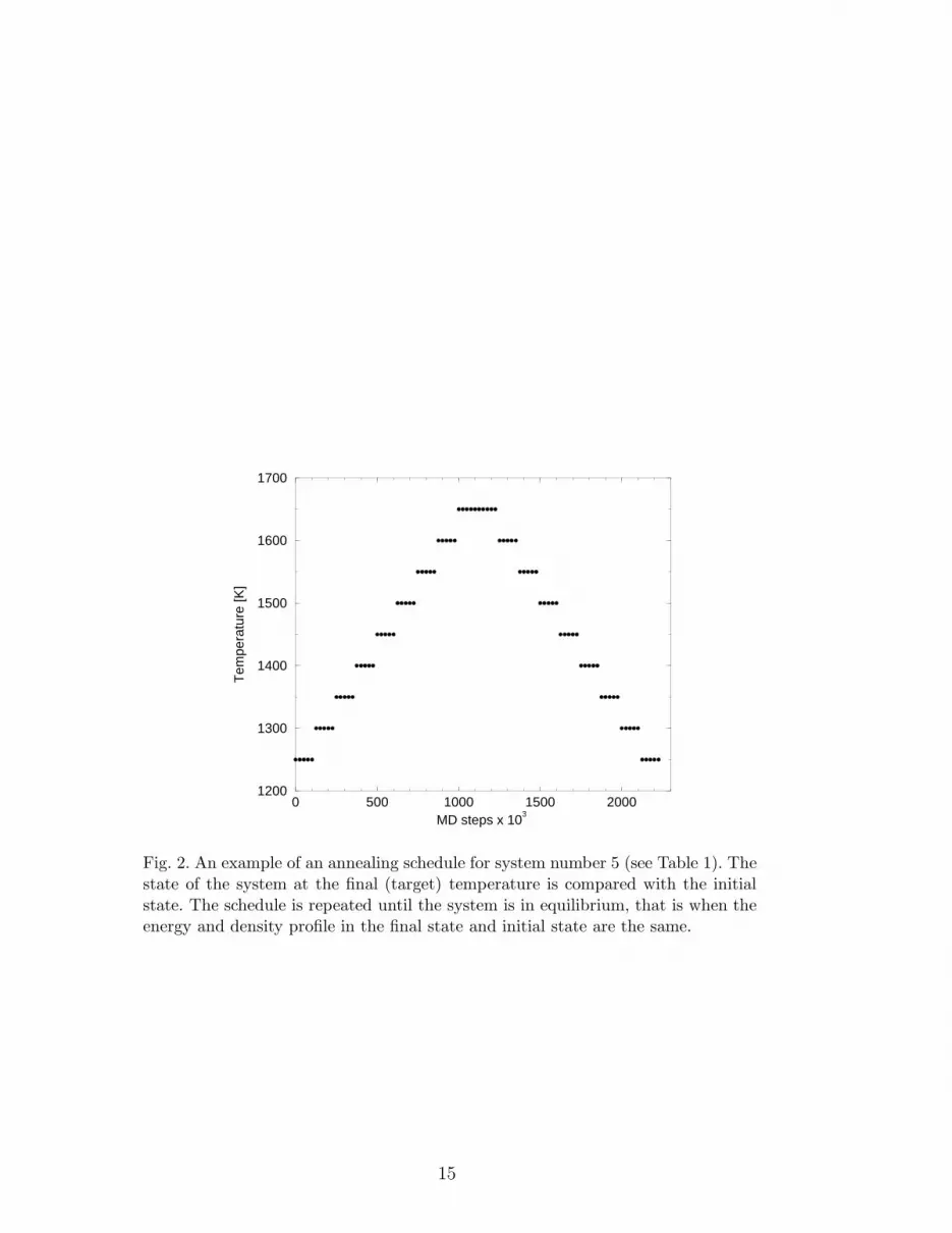
For each system described in Table 1 a series of simulations was conducted attemperatures ranging from T = 800K up to T = 2000K in steps of 50K. Toobtain an equilibrated sample at a particular temperature, an ideal configura-tion is annealed by heating the system in steps of 50K to a higher temperaturethan required, and then cooling down in steps of 50K to the target tempera-ture. Fig. 2 shows one such annealing schedule for system No. 1 (see Table 1).After annealing, the system is further equilibrated at the target temperaturefor at least 50, 000 MD steps for the smaller systems and 100, 000 steps forthe larger systems, before sampling begins.

Measurements of the density profile are obtained by accumulating ρ(z) viaequation (1) over 20,000 to 50,000 MD steps, then averaging over these toproduce a single measurement. In equilibrium, these measurements of ρ(z)do not change substantially in time, and are independent of the annealingschedule.

3 Results and Discussion

The density profiles ρ(z) of the liquid part of the samples are shown at twotemperatures in Figs. 3, 4, and 5 for the (111), (110), and (100) interfaces,respectively. The inserts in the figures are enlargements of the profiles of the

6

first few layers, with the abscissa given as the average number of particles perbin 〈Nz〉 [see equation (1)], rather than as the density. These density profilesshow large oscillations corresponding to the layering of the liquid near thehard wall. The oscillations dampen gradually within the interfacial region,until the uniform density of the liquid phase is reached, which is the same inall systems: ρl = 0.0051 ± 0.0005 atoms/A3. As expected, the density profileat a higher temperature decays faster as a function of the distance from theinterface than the density profile at a low temperature.

In order to facilitate a direct comparison between the density profiles, the den-sity is normalized by the magnitude of the first peak as shown in Fig. 6, wherethe density profiles for these systems are plotted at T = 1000K. It is easy tosee from Fig. 6 that ordering at the (111) and (100) interfaces extends furtherinto the liquid than at the (110) interface. However, the number of densitypeaks is very similar in all directions, while the distance between consecutivepeaks varies substantially with interface direction. This distance, or interlayerspacing can be identified with the d-spacing of the quasi solid region withinthe liquid. The calculation of the d-spacing is made with an algorithm thatsearches for maxima in the density profile, and then calculates the difference inthe locations of each consecutive maxima, giving the d-spacing. The d-spacingis plotted in Fig. 7 at T = 1000K. The data in Fig. 7 includes the analysisof the d-spacing even well inside the liquid region, where the ”maxima” arein random locations and are due to noise in the data. This explains the largescatter of data at a distance from the interface, and can serve as an indicationof the point at which the ordering terminates. For example, it is observed thatthe ordering of the (111) interface extends up to almost 25A, before becomingtoo noisy. It is also clear that the interlayer spacing in the quasi-liquid is thesame as that in the rigid substrate, at least in the first few layers. However,the (100) layers show a very large expansion of the d-spacing in the directionof that of the (111) system. Similar behavior was previously observed [10–12],and arises from the fact that perturbations within the liquid are more energet-ically favored if their periodicity is 2π/Q0, where Q0 is the wave vector at thefirst peak of the structure factor S(Q). For an fcc liquid metal this distance isvery close to d111 [12]. The d-spacing starts to deviate from the bulk value faraway from the substrate, as can be seen for the (111) case, where d alternatesbetween two values very close to d111 before becoming completely random. Forthe (110) case a shift in the interlayer spacing is not observed. This may beattributed to the large difference between d110 and d111.

In order to analyze the decay of the density profile as a function of temperatureand substrate orientation, the envelope of the density profile was extracted andplotted against distance from the surface, as shown in Fig. 8 (a). The profile isthen fitted assuming an exponential decay: ρ(z) ∼ exp (−κz), where κ = 1/ξ,and ξ is the correlation length at the interface. The parameter κ can then beused to quantitatively describe the amount of disorder at the interface. The

7

exact function that has been used in the fitting has an extra constant term, b,to account for the background liquid density, and a normalization factor, a:

ρ(z) = ae−κz + b (2)

This form of decay of the density profile is typically obtained from a meanfield treatment of binary fluid interfaces [12,13]. A good check of the validityof this assumption is that log(ρ(z) − b) is linear in z. A few typical examplesare shown in Fig. 8 (b). The large scatter for points far from the solid-liquidinterface, i.e. well within the normal liquid phase, is due to the sensitivity ofthe logarithm to small arguments, since the difference between ρ(z) and b forpoints inside the liquid is very small.

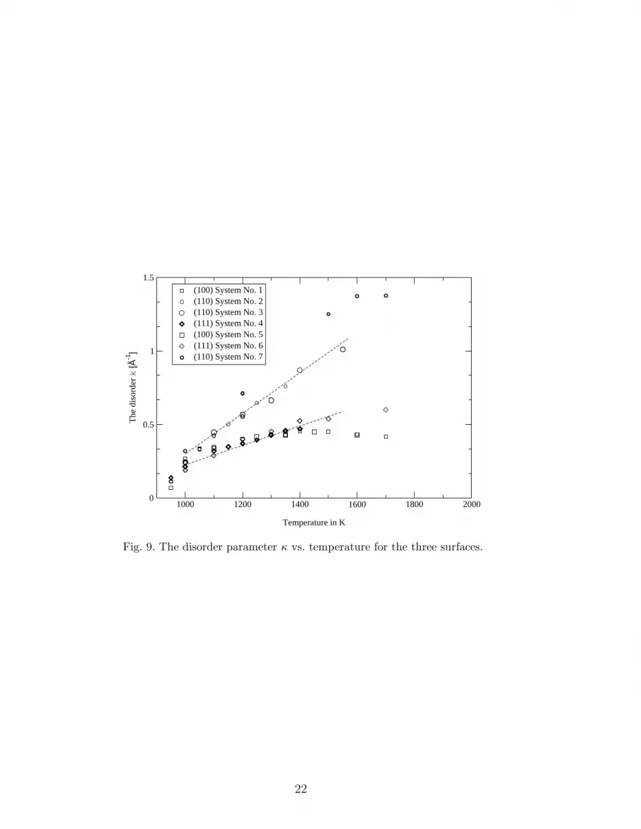
The results of the density profile analysis for the three interfaces, namely(111), (110) and (100) are shown in Fig. 9. Here the disorder parameter κ isplotted against temperature for the three orientations (111), (110) and (100),for various systems as indicated in the figure. It is clear that the finite sizeeffects are very small, as can be seen from the compatible κ values for systemsNo. 1 and 5 (see Table 1) and systems No. 2 and 3. Moreover, we note that thewidth of the underlying rigid substrate does not alter the qualitative behaviorof κ, as seen from the results for systems No. 6 and 7. However, there isa tendency for κ to be larger for a thick substrate, as evident mainly fromthe results for system 7. This can be attributed to the “gluing” nature ofthe potential, namely that the energy of an atom is lower when it has moreneighbors. Hence when there are more substrate layers the energy of the overallsystem is lowered, and the net force exerted on the liquid is lower than witha thinner substrate which leads to less ordering in the liquid phase.

The amount of disorder, κ, is consistently smaller for the (111) and (100)surfaces than for the (110) system, as shown in Fig. 9. In other words, theordering at the (111) and (100) interfaces is larger, and extends further intothe liquid, than the ordering at the (110) interface.

The close-packed surfaces (100) and (111) in an ideal system have a lowerenergy than the (110) surface, and therefore are more stable against thermaleffects. The formation energies of an ideal surface, as calculated with the EApotential [9], and with LDA [14] are shown in table 2. The formation energiesof an ideal (111) and (100) surfaces are similar, with the difference betweenthem being only ∼ 0.1 eV/atom with the EA potential. The formation energyof the (110) surface is 0.26 eV/atom higher than that of the (100) surface.The similarity of the formation energies of the ideal (111) and (100) systemsis compatible with the behavior of κ in Fig. 9, where κ for the (111) and(100) systems are almost indistinguishable. This suggest that the the energybalance between the different surfaces is not altered by the presence of a liquidphase, although this is not immediately obvious, and explicit calculations have

8

to be made for the different energies of a solid/liquid interface. However, thebehavior of κ strongly suggests that the energy balance is not drasticallychanged.

Fig. 9 also shows that the rate of increase of disorder is larger in the [110]direction than for the closed packed surfaces (100) and (111). Again this isconsistent with the lower formation energy of ordered (111) and (100) surfaces.Another striking difference is that as temperature increases the amount of dis-order in the closed packed directions seems to saturate while that for the (110)surface seems to increase approximately linearly with temperature. There iseven a slight decrease in κ i.e. an increase of ordering, at high temperatures.Note that data for high temperatures (T > 1400K) should be analyzed withcaution since at these temperatures there are one or two peaks at most andthe fitting procedure is no longer accurate.

To summarize, the results indicate that the interaction between the orderedsolid and the liquid induced layering oscillations within the liquid with a pe-riodicity of the interlayer spacing d. If this periodicity is also commensuratewith the natural periodicity of the liquid, as given by 2π/Q0 (see above), thenthese oscillations are enhanced, and survive a further distance into the liquid.This is the case for the (111) interface. In the case where the d-spacing isvery close to 2π/Q0, such as for the (100) interface, then after some distance(about three layers in Fig. 7) when the effect of the hard-wall has faded, thed-spacing switches to a value close to 2π/Q0. When the d-spacing is far from2π/Q0, then the oscillations fade away after a short distance.

This suggests that κ depends strongly on the d-spacing of the underlying sub-strate. In fact a reasonable order of magnitude estimate for κn as a function oforientation n, can be obtained by assuming that to first order, the orientationdependence is related only to the d-spacing by:

κ ∼ 1

d(3)

With the value used for the lattice parameter we obtain:

κ111 = 0.433A−1

, κ110 = 0.689A−1

, and κ100 = 0.488A−1. (4)

Inspection of Fig. 9 shows that this occurs for an intermediate temperatureof approximately 1200K. Again we obtain similar κ values for the (111) and(100) surfaces, even when neglecting the jump in d100 which would make κeven more comparable.

The assumption that the layering periodicity within the liquid follows thatof the underlying substrate allows us to explain the different rates at which

9

disorder increases with temperature for the different orientations, as shown inFig. 9. If the d-spacing in the liquid region adjacent to the substrate is large,as the case for the closed-packed surfaces (111) and (100), then the overlapbetween the density peaks is very small, as can be seen from Fig. 6. For opensurfaces such as (110) the d-spacing is smaller and the overlap is larger. A smalloverlap leads to a small number of atoms in between the peaks, as is clearlyobserved from the deep valleys in Fig. 6, while a large overlap leads to a higherdensity of atoms in between the peaks. In a metallic system, the energy of anatom is lower when it is in a dense environment, and as a result atoms tendto reside in a dense layer rather than in a less dense valley. Breaking the orderof the layers essentially means that more atoms leave the ordered layers andreside between the layers. Therefore, in orientations with a large d-spacing,where valleys are almost void of atoms, the barrier to such interlayer diffusionis large. So for close-packed surfaces (111) and (100), where order prevailsup to higher temperatures, the peaks remain well separated, and hence astemperature increases, there is almost no increase in κ. For the (110) interface,the larger overlap between the peaks allows for easy interlayer diffusion, andhence κ increases readily.

We presume that the link between the d-spacing of the liquid and the substrateis not causal, but is due to the imposition of a parallel structure on the liquidby the substrate surface. If the liquid atoms under the first peak in the liquiddensity are strongly correlated with the surface atomic structure, then the factthat our substrate was chosen to have nearly the same atomic density as theliquid ensures that the distance to the second liquid peak is the same as theinterplanar spacing in the substrate. It might be interesting to demonstratethis by varying the d spacing of the substrate without changing the densitywithin the lattice planes parallel to the surface. We would not expect this tolead to significant changes in the liquid peak separations. Other extensions ofthis study would be to introduce a substrate with a different lattice structureto that of the frozen liquid, eg. bcc in the case of liquid aluminium. Finally,the effect of varying the lattice parameter of the substrate, such that it is nolonger commensurate with the frozen liquid in its normal crystal structure,may induce some interesting effects for further study.

4 Summary and Conclusions

Atomistic simulations on a model liquid-solid interface have been performed,and the density profile of the liquid phase as a function of temperature andsubstrate orientation has been studied. The substrate was composed of alu-minium atoms pinned to an fcc lattice structure, while the liquid metal wascomposed of normal liquid aluminum. Substantial ordering was found in theliquid near the interface. The density profiles showed large oscillations cor-

10

responding to the layering of the liquid near the interface. The oscillationsdampen gradually within the interfacial region according to ρ(z) ∼ e−κz, untilthe density of the liquid phase is reached. The ordering was found to ex-tend further into the liquid region at close-packed interfaces such as (111) and(100). Moreover, the periodicity of the liquid layering was found to be stronglycorrelated to the inter-planar spacing of the rigid substrate, which in turn isrelated to the planar structure of the underlying substrate.

The decay parameter κ was defined as a disorder parameter which gives theextent at which the layering extends into the liquid. It was found that κ is con-sistently larger for the (110) interface, than for the (111) and (100) interfaces.Moreover, as temperature increases, κ for the open-surface (110) increases ap-proximately linearly with temperature, while for the (111) and (100) interfacesit saturates. The interlayer spacing in the liquid also determined the amountof overlap between the density peaks. The smaller the d-spacing, the largerthe overlap between the ordered liquid layers, which leads to an enhancedinterlayer diffusion resulting in a faster increase of disorder.

Acknowledgements: We are grateful to D.G. Brandon for critical review ofthe manuscript and valuable suggestions. The work of A.H. was supported byboth the Milton and Edwards Fellowship, and the Israel Science Ministry. Wealso acknowledge S.G. Lipson for helpful comments. These calculations weremade on the computers of the Computational Physics Group at the Technion,the Technion Computer Center, and S. Brandon’s Linux cluster. Support ofthe Israel Science Ministry under grant 1560199, the German-Israel ScienceFoundation under grant 653-181.14/1999, and the US-Israel Binational ScienceFoundation (BSF Grant 1998102) is acknowledged.

References

[1] W. J. Huisman, J. F. Peters, M. J. Zwanenburg, S. A. de Vries, T. E. Derry,D. Aberanathy, and J. F. Van der Veen, Nature, 1997, 390, 379.

[2] Reichert H, Klein O, Dosch H, Denk M, Honklmaki V, Lippmann T, ReiterG., Nature, 2000, 408, 839.

[3] J.M. Howe, Phil. Mag. A, 74, 761 (1996), and references therein.

[4] F. Ercolessi, and J. B. Adams, Euro. Phys. Lett., 1004, 26, 583.

[5] J.F. Lutsko, D. Wolf, S.R. Phillpot, and S. Yip, Phys. Rev. B., 1989, 40, 2841.

[6] D. Frenkel, and B. Smit, “Understanding Molecular Simulation, from

Algorithms to Applications”, Academic Press 1996.

11

[7] M.P. Allen, and D.J. Tildesley, Computer Simulation of Liquids, OxfordUniversity Press, 1987.

[8] F. Ercolessi, E. Tosatti, and M. Parrinello, Phys. Rev. Lett., 1986, 57, 719,and F. Ercolessi, M. Parrinello, and E. Tosatti, Phil. Mag. A, 1988, 58, 213.

[9] U. Hansen, P. Vogl, and V. Fiorentini, Phys. Rev. B., 1999, 60, 5055.

[10] R.L. Davidchack and B.B. Laird, J. Chem. Phys., 1998. 108 9457.

[11] J.Q. Broughton and G.H. Gilmer, J. Chem. Phys., 1986. 84, 5749.

[12] O. Tomagnini, F. Ercolessi, S. Iarlori, F.D. Di Tolla, and E. Tosatti, Phys.

Rev. Lett., 1996, 76, 1118.

[13] P. Tarazona and L. Vicente, Mol. Phys., 1985, 56, 557.

[14] R. Stumpf and M. Scheffler, Phys. Rev. B., 1996, 53, 4958.

12

Figure 1: An example of a cell for the simulation of a system with a free (110) surface.The total number of atoms is 1944, out of which 432 atoms are ’solid’ (lightgray) and the rest are “liquid” (dark gray) aluminium atoms.

Figure 2: An example of an annealing schedule for system number 5 (see Table 1).The state of the system at the final (target) temperature is compared withthe initial state. The schedule is repeated until the system is in equilibrium,that is when the energy and density profile in the final state and initial stateare the same.

Figure 3: The density profile ρ(z) as a function of distance from the hard wall z,is shown for a (111) system at two temperatures: T1 = 1000K, and T2 =1200K. The insert is a plot of the average number of atoms per bin 〈Nx〉for the region near to the rigid wall. Data is from a simulation on systemnumber 4 described in Table 1.

Figure 4: The density profile ρ(z) as a function of distance from the hard wall z,is shown for a (110) system at two temperatures: T1 = 1000K, and T2 =1200K. The insert is a plot of the average number of atoms per bin 〈Nx〉for the region near to the rigid wall. Data is from a simulation on systemnumber 2 described in Table 1.

Figure 5: The density profile ρ(z) as a function of distance from the hard wall z,is shown for a (100) system at two temperatures: T1 = 1000K, and T2 =1200K. The insert is a plot of the average number of atoms per bin 〈Nx〉for the region near to the rigid wall. Data is from a simulation on systemnumber 1 described in Table 1.

Figure 6: Normalized fine scale density profile for (a): (111), (b):(110), and (c) (100)interfaces at the same temperature (1000K).

Figure 7: Layer separation across the samples at T=1000K, the dark symbols arewithin the rigid substrate, and the open symbols are within the liquid.

Figure 8: The envelope of the density profile obtained for a (110) sample at T =1000K. System numbers are defined in Table 1.

Figure 9: The disorder parameter κ vs. temperature for the three surfaces.

13

Table 1Simulation cell geometry.

System No. Interface plane No. of planes in each direction No. of rigid planes Number of atoms

1 (100) 22[100] × 14[010] × 14[001] 3 2156

2 (110) 12[111] × 30[110] × 36[211] 6 2160

3 (110) 18[111] × 30[110] × 48[211] 6 4320

4 (111) 18[111] × 18[110] × 36[211] 3 1944

5 (100) 40[100] × 14[010] × 14[001] 3 3920

6 (111) 32[111] × 18[110] × 36[211] 14 3456

7 (110) 12[111] × 34[110] × 36[211] 10 2448

Table 2Ideal surface formation energies for aluminium as calculated with the Ercolessi-Adams potential [9] and with LDA [14].

System EA [eV/A2] [eV/atom] LDA [eV/A2] [eV/atom]]

(111) 0.054 0.38 0.07 0.48

(100) 0.059 0.48 0.071 0.56

(110) 0.065 0.74 0.08 0.89

[110]

[111]

z

x

y

Fig. 1. An example of a cell for the simulation of a system with a free (110) surface.The total number of atoms is 1944, out of which 432 atoms are ’solid’ (light gray)and the rest are “liquid” (dark gray) aluminium atoms.

14

0 500 1000 1500 2000MD steps x 10

3

1200

1300

1400

1500

1600

1700

Tem

pera

ture

[K]

Fig. 2. An example of an annealing schedule for system number 5 (see Table 1). Thestate of the system at the final (target) temperature is compared with the initialstate. The schedule is repeated until the system is in equilibrium, that is when theenergy and density profile in the final state and initial state are the same.

15

5 15 25 35 45Position along the [111] direction x, in [Å]

0

0.05

0.1

0.15

0.2

0.25

0.3

Den

sity

ρ(x

) [a

tom

s/Å

3 ] x10

−1

5 10 15 20 25x

0

20

40

60<

Nx>

1000K1200K

Fig. 3. The density profile ρ(z) as a function of distance from the hard wall z, isshown for a (111) system at two temperatures: T1 = 1000K, and T2 = 1200K. Theinsert is a plot of the average number of atoms per bin 〈Nx〉 for the region near tothe rigid wall. Data is from a simulation on system number 4 described in Table 1

16

5 25 45Position along the (110) direction x, in [Å]

0

0.05

0.1

0.15

0.2

dens

ity ρ

(x)

[ato

ms/

Å3 ] x

10−

1

7 9 11 13 15 17 19x

0

10

20<

Nx>

1000K1200K

Fig. 4. The density profile ρ(z) as a function of distance from the hard wall z, isshown for a (110) system at two temperatures: T1 = 1000K, and T2 = 1200K. Theinsert is a plot of the average number of atoms per bin 〈Nx〉 for the region near tothe rigid wall. Data is from a simulation on system number 2 described in Table 1.

17

0 10 20 30 40 50Position along the [100] direction x, in [Å]

0

0.05

0.1

0.15

0.2

0.25

Den

sity

ρ(x

) [a

tom

s/Å

3 ] x 1

0−1

0 10x

0

10

20

30

40

50<

Nx>

1000K1200K

Fig. 5. The density profile ρ(z) as a function of distance from the hard wall z, isshown for a (100) system at two temperatures: T1 = 1000K, and T2 = 1200K. Theinsert is a plot of the average number of atoms per bin 〈Nx〉 for the region near tothe rigid wall. Data is from a simulation on system number 1 described in Table 1.

18

−2 0 2 4 6 8 10 12 14 16 18Position normal to interface [Å]

0

0.3

0.6

0.9

−2 0 2 4 6 8 10 12 14 16 180

0.3

0.6

0.9

Nor

mal

ized

den

sity

pro

file

−2 0 2 4 6 8 10 12 14 16 180

0.2

0.4

0.6

0.8

1

(a) (100)

(b) (110)

(c) (111)

Fig. 6. Normalized fine scale density profile for (a): (111), (b):(110), and (c) (100)interfaces at the same temperature (1000K).

19

0 10 20 30 40 50

peak position [Å]

0

0.5

1

1.5

2

2.5

3

d-sp

acin

g [Å

]

(111)(100)(110)

Fig. 7. Layer separation across the samples at T=1000K, the dark symbols arewithin the rigid substrate, and the open symbols are within the liquid.

20

(a)

0 10 20 30Distance normal to interface, x in [Å]

0

10

20

30

40

ρ(x)

1250K (111) − system 4density peaksA fit of ρ(x)=ae

(−κx)+b

(b)

0 10 20 30 40 50Distance normal to interface, x in [Å]

−5

0

5

log(

ρ(x)

−b)

1250K (111) − system 41100K (100) − system 51100K (110) − system 2

Fig. 8. The envelope of the density profile obtained for a (110) sample at T = 1000K.System numbers are defined in Table 1.

21

1000 1200 1400 1600 1800 2000

Temperature in K

0

0.5

1

1.5

The

dis

orde

r k

[Å-1

]

(100) System No. 1(110) System No. 2(110) System No. 3(111) System No. 4(100) System No. 5(111) System No. 6(110) System No. 7

Fig. 9. The disorder parameter κ vs. temperature for the three surfaces.

22