Embed Size (px)
Citation preview
Sometimes when this place gets kind of empty,
Sound of their breath fades with the light. I think about the loveless fascination,
Under the milky way tonight.
Lower the curtain down in memphis,
Lower the curtain down all right.
I got no time for private consultation, Under the milky way tonight.
Wish I knew what you were looking for.
Might have known what you would find.
And it’s something quite peculiar, Something thats shimmering and white.
It leads you here despite your destination,
Under the milky way tonight
(chorus)
ath, empty, loveless, fascination, pr
sad, calm : D / D2 / 3 / 1
waiting, day, flashing, eyes, starin
calm, positive : C / C3 / 4 / 3
never, respect, dark, anger, regrets, fear, cle
angry, intense : A / A1 / 2 / 1
anic, life, wonder, blessed, hang, dj
nervous, sad : C / C1 / 3 / 1
P.W.M. (Pieter) Kanters
Master Thesis
June 2009
HAIT Master Thesis series nr. 09-001
Thesis submitted in partial fulfilment of the
requirements for the degree of Master of Arts
Tilburg centre for Creative Computing (TiCC) Faculty of Humanities Department of Communication and Information Sciences Tilburg University Tilburg, The Netherlands
Thesis committee: Dr. M.M. (Menno) van Zaanen TiCC Research Group, Tilburg University Prof. dr. H.J. (Jaap) van den Herik TiCC Research Group, Tilburg University Prof. dr. E.O. (Eric) Postma TiCC Research Group, Tilburg University Drs. M.G.J. (Marieke) van Erp
Faculty of Humanities, Tilburg University
Automatic Mood Classification
for Music
I
Automatic Mood Classification for Music
P.W.M. Kanters
HAIT Master Thesis series nr. 09-001
Tilburg centre for Creative Computing (TiCC)
Thesis submitted in partial fulfilment
of the requirements for the degree of
Master of Arts in Communication and Information Sciences,
Master Track Human Aspects of Information Technology,
at the Faculty of Humanities
of Tilburg University
Thesis committee:
Dr. M.M. van Zaanen Prof. dr. H.J. van den Herik
Prof. dr. E.O. Postma Drs. M.G.J. van Erp
Tilburg University Tilburg centre for Creative Computing (TiCC)
Faculty of Humanities Department of Communication and Information Sciences
Tilburg, The Netherlands June 2009
I
Preface
This Master’s Thesis concludes my studies in Human Aspects of Information Technology (HAIT) at
Tilburg University. It describes the development, implementation, and analysis of an automatic
mood classifier for music.
I would like to thank those who have contributed to and supported the contents of the thesis.
Special thanks goes to my supervisor Menno van Zaanen for his dedication and support during the
entire process of getting started up to the final results. Moreover, I would like to express my
appreciation to Fredrik Mjelle for providing the user-tagged instances exported out of the MOODY
database, which was used as the dataset for the experiments.
Furthermore, I would like to thank Toine Bogers for pointing me out useful website links regarding
music mood classification and sending me papers with citations and references. I would also like to
thank Michael Voong for sending me his papers on music mood classification research, Jaap van den
Herik for his support and structuring of my writing and thinking. I would like to recognise Eric Postma
and Marieke van Erp for their time assessing the thesis as members of the examination committee.
Finally, I would like to express my gratitude to my family for their enduring support.
Pieter Kanters
Tilburg, June 2009
II
Abstract
This research presents the outcomes of research into using the lingual part of music for building an
automatic mood classification system. Using a database consisting of extracted lyrics and user-
tagged mood attachments, we built a classifier based on machine learning techniques. By testing the
classification system on various mood frameworks (or dimensions) we examined to what extent it is
possible to attach mood tags automatically to songs based on lyrics only. Furthermore, we examined
to what extent the linguistic part of music revealed adequate information for assigning a mood
category and which aspects of mood can be classified best.
Our results show that the use of term frequencies and tf*idf values provide a valuable source of
information for automatic mood classifications for music, based on lyrics solely. The experiments in
this thesis show that the information extracted from the linguistic aspect of music provides sufficient
information to the system for an automatic classification of mood for music tracks. Furthermore, our
results show that mood prediction on the arousal/energy aspect of mood are the best ones to arrive
at a good classification, although predictions on other aspects of mood such as valence/tension and
combinations of aspects lead to almost equal accuracy values for the performances of the
classification system.
III
Table of contents
Preface ............................................................................................................................................... I
Abstract ............................................................................................................................................ II
Table of contents.............................................................................................................................. III
1. Introduction .................................................................................................................................. 1
1.1 Analog music: a look in the past ............................................................................................... 1
1.1.1 The beginnings of music .................................................................................................... 1
1.1.2 Changes in the use of language and music ......................................................................... 1
1.1.3 Changes in storage ............................................................................................................ 2
1.2 Digital music: a brief overview ................................................................................................. 2
1.2.1 Invention of the compact disk ........................................................................................... 2
1.2.2 The MPEG-1 Layer 3 format .............................................................................................. 3
1.2.3 Digitalisation through the world wide web ........................................................................ 3
1.2.4 Improved music distribution ............................................................................................. 3
1.2.5 Current music development .............................................................................................. 4
2. Motivation ..................................................................................................................................... 5
2.1 Organisation of music collections ............................................................................................. 5
2.1.1 Assigning properties to music tracks.................................................................................. 5
2.1.2 Music collections: access and retrieval .............................................................................. 6
2.1.3 Recommendation and tagging of music ............................................................................. 7
2.2 Problem statement and research questions ............................................................................. 7
2.2.1 Problem statement ........................................................................................................... 7
2.2.2 Research question 1 .......................................................................................................... 9
2.2.3 Research question 2 .......................................................................................................... 9
2.2.4 A preferred deliverable ..................................................................................................... 9
2.3 Research methodology ............................................................................................................ 9
2.4 Thesis outline......................................................................................................................... 10
3. Scientific background ................................................................................................................... 10
3.1 Human moods and emotions ................................................................................................. 11
3.2 Language and mood ............................................................................................................... 12
3.3 Language and music (lyrics).................................................................................................... 13
3.4 Mood tagging for music tracks ............................................................................................... 14
3.4.1 Different events, one mood ............................................................................................ 14
IV
3.4.2 Social tagging .................................................................................................................. 15
3.5 Creating playlists .................................................................................................................... 15
3.5.1 Mood-based music playlists ............................................................................................ 16
3.5.2 Reasons for creating playlists .......................................................................................... 16
3.5.3 Automatic playlist generation ......................................................................................... 17
3.6 Star rating and music recommendation ................................................................................. 18
3.7 Music, mood and colour ........................................................................................................ 18
3.7.1 Adding images to music................................................................................................... 19
3.7.2 MOODY’s mood tagging framework .................................................................................. 19
4. Research design ........................................................................................................................... 21
4.1 Machine learning ................................................................................................................... 21
4.1.1 Concept learning ............................................................................................................. 21
4.1.2 The inductive learning hypothesis ................................................................................... 22
4.1.3 TIMBL: Tilburg Memory Based Learner ............................................................................ 22
4.1.4 k-Nearest Neighbours ..................................................................................................... 22
4.1.5 k-Fold cross-validation .................................................................................................... 23
4.2 Theoretical design of a classification tool based on machine learning .................................... 23
5. Implementation ........................................................................................................................... 25
5.1 Data collection ....................................................................................................................... 25
5.1.1 Data extraction ............................................................................................................... 25
5.1.2 Exporting and cleaning up the data ................................................................................. 26
5.2 Feature construction .............................................................................................................. 27
5.2.1 Generating features ........................................................................................................ 28
5.2.2 Term frequency and inversed document frequency......................................................... 28
5.2.3 The use of tf*idf weights ................................................................................................. 30
5.2.4 Normalisation and feature overview ............................................................................... 31
6. Experiments and tests ................................................................................................................. 32
6.1 Experimental setup ................................................................................................................ 32
6.1.1 TIMBL settings ................................................................................................................. 32
6.1.2 Used features .................................................................................................................. 33
6.2. Experiments and test results ................................................................................................. 33
6.2.1 Baseline .......................................................................................................................... 33
6.2.2 Test results using basic features ...................................................................................... 34
6.2.3 Test results using advanced features without basic features ........................................... 34
7. Evaluation and discussion ............................................................................................................ 35
V
7.1 Evaluation .............................................................................................................................. 36
7.2 Answer to RQ1 ....................................................................................................................... 36
7.3 Answer to RQ2 ....................................................................................................................... 38
8. Conclusion ................................................................................................................................... 39
8.1 Research questions ................................................................................................................ 39
8.2 Problem statement ................................................................................................................ 40
8.3 Final conclusion ..................................................................................................................... 41
8.4 Future research ..................................................................................................................... 42
References ...................................................................................................................................... 44
1
1. Introduction
This section covers a brief introduction to the field of music. A historical overview is given to obtain
some insight into the transition from analog to digital recording, i.e. the early beginnings of music
and the changes through the decades towards the music business nowadays. Section 1.1 describes
the ancient beginnings of music, which is continued by fitting a theoretical description of the
transitions to digital music in section 1.2. At the end of this chapter, the current developments in
digital music are discussed.
1.1 Analog music: a look in the past
We will first take a brief look at events in the history of music. We discuss the beginnings of music in
section 1.1.1, changes in use of language and music are discussed in section 1.1.2, and section 1.1.3
describes the changes in storage of music up to the twentieth century.
1.1.1 The beginnings of music
As long as human beings have been communicating with each other, music has existed. Kunej & Turk
(2000) state that “there is no doubt that the beginnings of music extend back into the Paleolithic,
many tens of thousands of years into the past.”
In the beginning music was not more than vocal sounds made to communicate with each other
(Kunej & Turk, 2000). The usage of musical instruments such as the flute together with primal
screams and other vocal sounds were the first means people used to communicate. Later these
squeeks, screams, and shouts changed to vocal pronounciations: the beginnings of human language.
As language developed, so did music: words, evolved out of the ancient screams, were wrapped in a
melodious way.
Music can be a tool for people to communicate with each other, consisting of messages wrapped in
a melodious and rhythmic manner. Like talking or writing it contains information which can be sent
to the addressee, in case of music to the listener. The communicative use of music, for example to
inform or entertain, changed over time.
1.1.2 Changes in the use of language and music
During the middle ages music was used to send messages over a longer distance, for instance, by
troubadours remembering and reproducing stories on long journeys. The so-called troubadour song
held a message, and by using rhyme and melody it was easy to remember.
2
It is common knowledge that language as a communication tool has changed over time, for example
by changes in dialects or by adding and fading out words in the vocabulary. For music, the same
holds true. At first, each musical appearance was unique, unrecorded, and used purely for
communicative senses. Later on it changed to mass reproduction and entertainment. So, in
retrospect we conclude that language changed and therefore the music.
1.1.3 Changes in storage
Since the 19th century the way music was stored has changed considerably. Before the 19th century
there was no actual music storage at all: the music played and sung could not be recorded and
storage could only take place in the mind. In order to let more people hear it, it had to be physically
played over and again.
With the invention of the phonograph in the 1860s, people could record music and replay it at a
later time and a different location. In the 20th century the gramophone, and the invention of the
cassette tape thereafter, made music more accessible to the mass. A stimulus to this development
was the improved recording quality and the more portable players. The changes in storage had many
ramifications. The cassette initiated an era in which people could record music themselves, which
was not possible with the phonograph and the gramophone.
1.2 Digital music: a brief overview
In the twentieth century the way music was stored changed from the analogue mode to the digital
music recording. After the invention of the compact disk, digital music storage became widespread
and music distribution changed.
1.2.1 Invention of the compact disk
In 1980, the Dutch electronics company Philips started manufacturing the compact disk. It was
invented and further developed by the Philips NatLab in Eindhoven, the Netherlands. It was one of
the first approaches to digital music recording. Whereas systems prior to 1980 recorded in analogue
mode, the compact disk stored the music digitally. In the analogue mode, the peaks and valleys
grooved in the record are converted by electronical impulses to reproduce the analogue music
waves. In the digital recording mode, the music is converted into binary code (Philips Research,
2008).
With digital recording many copies can be made while keeping the same sound quality of the original
source recording. In contrast to the compact disk, copies on magnetic tapes or vinyl recordings
suffer from a considerable loss of sound quality. The compact disk has blurred the boundary
between the concepts of ‘original’ and copy for music recording, as every copy of a recording on a
compact disk has an equal sound quality and the original source can not be distinguished from the
3
copies. Moreover, the compact disk has additional advantages, namely (1) records on tape can be
damaged or erased more easily by magnets, and (2) vinyl recordings can be warped or scratched
which impacts sound quality.
The launch of the compact disk led to a spectacular leap in pre-recorded music sales. There was a
relative short period of transition from analog to digital music. In 1996 nearly three-quarters of
Dutch households owned a CD player and an average of 65 CDs each, while ten years earlier the
percentage was just 5% (Hansman, Mulder & Verhoeff, 1999).
1.2.2 The MPEG-1 Layer 3 format
In addition to the digital compact disk format, in 1992 a new digital music format was introduced:
the MPEG-1 Layer 3 (now called: MP3) format. It was based on digital storage, and used a new
compression technique. The technique was perfectly suitable for storage on personal computer
harddrives. Recording on sources with interchangeable media such as compact disks now became
less popular. In contrast to songs on pre-recorded compact disks which cannot be removed or
changed, MP3 files can be erased from the computer’s harddisk and new recordings can be made
immediately. Properties of MP3 files, for instance, the filename or the enclosed ID3-tag, can also be
modified (see section 2.1.1).
1.2.3 Digitalisation through the world wide web
In the 1990s multimedia became more common. All multimedia resources became digitised with the
rise of the World Wide Web only a few years later. The World Wide Web is a layer on the Internet,
first developed in 1989. The Internet started as ARPANET in the 1960s, a network of military devices
and computers communicating with each other. Later this network expanded and resulted in what
we now call the Internet. It links personal computers together, enabling communication of files.
Afterwards the World Wide Web, the graphical shell, was developed, and multimedia was linked
together.
For instance, on the World Wide Web music tracks were shared, which made the MP3 format
popular due to the compressed size of the files. MP3 became widespread by 1996 and quickly took
hold among active music fans (Haring, 2000).
1.2.4 Improved music distribution
A legal experiment occured in the form of NAPSTER’S peer-to-peer sharing network, where users
could find and download songs for free. The files were not stored on the server, instead NAPSTER
linked computers and enabed download and share of music files from one computer (peer) to
another through a user-friendly interface. Moreover, this decentralized way boosted the music
4
sharing and enabled sharing files in other formats, such as video and later on electronic books
(Haring, 2000).
Shortly thereafter, digital music was distributed by online music services such as ITUNES1 and
Beatport2, where the music listener pays for a non-tangible product: the digital download. Mc Hugh
(2003) stated that “the maturing distributed file sharing technology implemented by Napster has
first enabled the dissemination of musical content in digital form, permitting customers to retrieve
stored music files from around the world.”
1.2.5 Current music development
The use of music and distribution of it is still developing. Celma & Lamere (2007) state that we have
seen an incredible transformation in the music world by the transition from albums and compact
disks to individual MP3s and mixes. Together with online music services we see collections of several
million songs on the Internet. The experiences of Pirate Bay3, a website used by millions to exchange
movies and music, are an example of the current technological developments and the legal reactions
on this development by the intellectual property right holders. Four men behind this Swedish file-
sharing website have been found guilty of collaborating to violate copyright law in a landmark court
verdict in Stockholm (Curry & Mackay, 2009).
On the one hand music has had a pushed approach for centuries: one had to listen to the music
being served. For instance, at marches, meetings and events the audience had no control over what
music was being played and listeners requesting tracks at radio stations had only marginal influences
on the playlists.
On the other hand nowadays you can listen to music that you want to hear and react on that kind of
music through the Internet: the pull-method. The one-way approach mentioned above, where
listeners had hardly any influence on music playlists, changed to some kind of control by the listener
throughout the last decades. Inventions such as the gramophone, cassette, compact disk, and
portable music players made the user select the tracks being played. The modern digital world with
internet, digital music, and collective sharing created a platform where everybody can export
playlists, radio streams, and music preferences.
In a growing world of online music stores, digital sounds, collaborative listening, and musical
interactions, it is important to have an efficient organisation of the music itself. In terms of search
and retrieval methods it is essential to have an organised library with music that can be classified in
different ways, such as tempo, genre, age, or mood. Due to the fact that the World Wide Web is
growing fast, increasingly more data becomes available daily. This development requires an efficient
organisation in order to let users find the information they are looking for. At the same time the
enlarging databases provide us with more information we can use to organise our own files.
1 http://www.apple.com/itunes
2 http://www.beatport.com
3 http://piratebay.org
5
2. Motivation
Many aspects of the music itself (such as lyrics, genre, key or era) are shared on the Internet. They
are available to other users. The following three issues have advantages for music information
retrieval: (1) the added value of correctly assigning properties to music, (2) ordening the properties
and (3) sharing the content on the web. Section 2.1 describes the properties and organisation of
music collections. Thereafter the aim of this thesis is stated in section 2.2 with a problem statement,
two research questions and a thesis outline.
2.1 Organisation of music collections
This section treats the assignment of correct properties for music tracks, access and retrieval of
music collections and recommendation systems. Subsection 2.1.1 describes the assignment of
properties to music tracks. The access and retrieval of files in music collections is discussed in
subsection 2.1.2. In subsection 2.1.3 music recommendation systems, Web 2.0 involvement and
tagging of music is described.
2.1.1 Assigning properties to music tracks
Digital music can hold information such as artist, track name, year, and album in the source, in the
form of ID3-tags. These tags are metadata in the MP3-file, telling the audio software on the
computer the characteristics of the file (for instance, title, artist, length, format, audio codec, and
genre).
When ID3 was introduced in 1996 for use with the MP3 format, it could only store a limited number
of bytes with selected information per field (artist, year, publisher, etc.) as metadata, and it was not
compatible with international tokens. It soon was called ID3v1. After the implementation of ID3v2, a
new version storing information in a variable number of dimensions, the metadata was stored in the
beginning of the audio file. It featured additions, such as a comment field and fields for website links
and cover art. The ID3v2-tag lyrics can also store lyrics. They can be used to let the audio program
inform the listeners on the lyrics of the music track to which the user is listening.
ID3-tags can be imported into the computer and then assigned to the relevant music tracks. The
properties are read automatically from the metadata on the compact disk without human
intervention. Moreover, automatically downloading properties for music tracks from online libraries
can be handled by audio software.
If no tags are given, properties can be found or searched for on the Internet by the user. For
instance, this may happen in online music databases such as Discogs4, Allmusic
5 or Last.fm.
So, at times, the tags will be found automatically provided that they are enclosed in the source.
4 http://www.discogs.com
5 http://www.allmusic.com
6
Otherwise, the user can obtain the information by searching through the Internet manually. In many
other cases the information can be found in an automatic manner via tailor made applications.
2.1.2 Music collections: access and retrieval
Playlists and music collections have to be organised in the best possible way in order to find the
relevant information effectively. Preferably, the search process is based on a wide variety of
properties. By correctly assigning properties to the music, the categorisation, access and ordening of
the files can be done in a more natural, straightforward way. For instance, books in physical libraries
have been arranged on keywords (comparable with tags), genre or era. Organising digital music files
will be done at the same way, i.e. natural and effective for people.
However, the final arrangement in a physical library, based on keyword, is static. When someone
wants to see an overview of books written by the same author and afterwards the range of books
written in a particular genre or era, the person has to re-organise the collection dynamically.
Compared to the organisation of information in a library, digital files can be easily re-arranged to
other classes or categories; for instance, files sorted on genre criteria can be re-arranged according
to another category, based on artist or year. The indexes can be built in case they are needed. This
can be done by selecting different criteria such as filenames, key metadata or tags. Therefore the
indexes are changeable for other points of view, or as Andric & Haus (2006) state: “The music
collections of today are more flexible. Namely, their contents can be listened to in any order or
combination –one just has to make a playlist of desired music pieces.”
”Today’s music listener faces a myriad of obstacles when trying to find suitable music for a specific
context” (Meyers, 2007). As the multimedia content is growing, and digital music libraries are
expanding at an exponential rate, it is important to secure effective information access and retrieval.
Meyers (2007) also states that “the need for innovative and novel music classification and retrieval
tools is becoming more and more apparent”.
Finding an efficient, straightforward and hierarchical organisation with access to an increasing
amount of data and files (in this case music tracks) is a challenging problem. When browsing or
searching through the huge database of songs of an individual music listener, new tools are essential
to meet the user’s requirements on the file management level.
By using new classification and retrieval tools, music listeners will see relevant output by these tools
that meet their requests. For instance, a proper playlist may be built or the organisation of the music
collection based on genre or key is presented in time for an interesting audience. Music listeners
require new ways to access their music collection, such as alternative classification taxonomies and
playlist generation tools (Meyers, 2007).
7
2.1.3 Recommendation and tagging of music
A relatively new field of exploring music is defined by online recommendation systems, such as
Last.fm6 and Pandora
7. They let the user discover new music based on similar characteristics to the
music currently owned by the user. These systems provide recommendations for music listeners,
helping them to discover new music (cf. Celma & Lamere, 2007).
Pandora provides music recommendations based on human analysis of musical content, with
features such as vocal harmonies and rhythm syncopation. Recommendations on Last.fm are based
on social tagging of music (see section 3.4.2). This is considered as a valuable resource for music
information retrieval and music classification (Meyers, 2007). Online music recommendations are
briefly discussed in section 3.6.
Moreover, online recommendation and social tagging are characteristics of Web 2.0, a term which
describes the increase of interactivity on the World Wide Web. Web 2.0 is seen as a new stage
where users interact with each other through collaboration on web content (Oreilly, 2007). Search
engine optimisation, social tagging and interactive web applications are examples of this concept.
Because of new possibilities and techniques in the digital era, communication takes place in new
fields, especially in the Web 2.0 environment. People will offer, find, and interact with online music
content. They communicate in a new way by reacting on the online content, for instance, via tagging
or comments, or by offering information of personal music tastes. Social tagging (see section 3.4),
and active sharing of multimedia content, put the communicative meaning of music to a new level.
2.2 Problem statement and research questions
In this section we describe the aim of the thesis, viz. automatic assignments of mood-based tags of
songs in a database. To reach this aim we deal with a formalized problem statement in subsection
2.2.1. Two research questions (RQ1 and RQ2) are introduced thereafter in subsections 2.2.2 and
2.2.3 respectively. Finally, a deliverable is described in subsection 2.2.4.
2.2.1 Problem statement
Music can be classified in many different ways: genre, timbre, tempo, artist, trackname, year,
loudness, and so on. Much research has been done in the context of music classification techniques
(Liu, Lu & Zhang, 2003; Meyers, 2007; Yang, 2007). Classification on several musical aspects gives
efficient organisation outcomes on those characteristics. The classifications can help to organise the
music tracks in the way that is preferred by the user. One particular type of classification, the one we
are going to look at here, is mood classification, also referred to as music emotion classification
(Yang et al., 2007).
6 http://www.last.fm
7 http://www.pandora.com
8
Main Goal
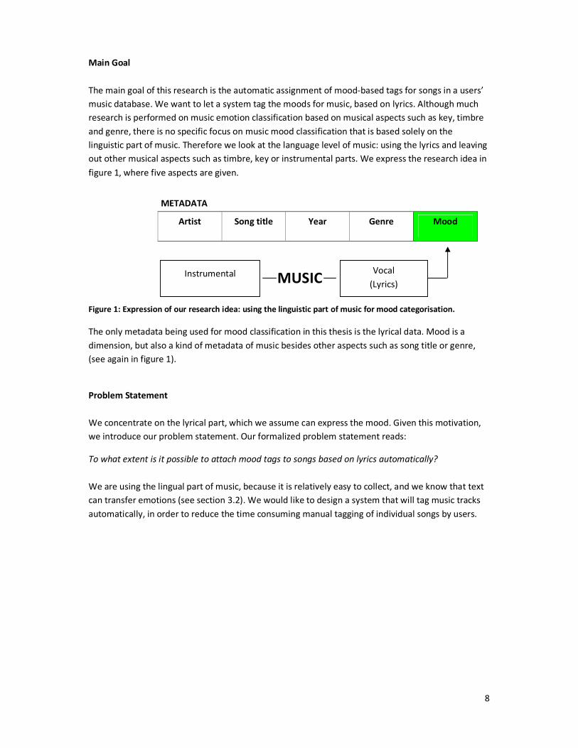
The main goal of this research is the automatic assignment of mood-based tags for songs in a users’
music database. We want to let a system tag the moods for music, based on lyrics. Although much
research is performed on music emotion classification based on musical aspects such as key, timbre
and genre, there is no specific focus on music mood classification that is based solely on the
linguistic part of music. Therefore we look at the language level of music: using the lyrics and leaving
out other musical aspects such as timbre, key or instrumental parts. We express the research idea in
figure 1, where five aspects are given.
Artist Song title Year Genre Mood
MUSIC
Figure 1: Expression of our research idea: using the linguistic part of music for mood categorisation.
The only metadata being used for mood classification in this thesis is the lyrical data. Mood is a
dimension, but also a kind of metadata of music besides other aspects such as song title or genre,
(see again in figure 1).
Problem Statement
We concentrate on the lyrical part, which we assume can express the mood. Given this motivation,
we introduce our problem statement. Our formalized problem statement reads:
To what extent is it possible to attach mood tags to songs based on lyrics automatically?
We are using the lingual part of music, because it is relatively easy to collect, and we know that text
can transfer emotions (see section 3.2). We would like to design a system that will tag music tracks
automatically, in order to reduce the time consuming manual tagging of individual songs by users.
METADATA
Instrumental Vocal
(Lyrics)

9
2.2.2 Research question 1
From the above reasoning and our main goal, a first research question is stated as follows:
RQ1: In how far can the linguistic part of music reveal sufficient information for categorising music
into moods?
In this thesis we only take hold of the lyrical part of music. Our aim is to see whether the lyrical part
of music can provide sufficient information to tag music tracks. Although the other kinds of musical
information can also help with expressing or revealing a certain mood or state of emotion, this type
of information is not taken into consideration in this thesis but it can be done so in future work (see
section 8.2).
2.2.3 Research question 2
Moods can be categorised in several ways. In this thesis we are using four different mood
categorisations: the Arousal, Moody, Valence and Thayer divisions (see section 3.7.2). Given this
differentation, we state a second research question.
RQ2: What aspects of mood can be classified best based on lyrics alone and with what granularity?
The answer to this question can lead to the mood categorisation that gives the best classification
values, based on the properties of mood which determine the partitioning.
2.2.4 A preferred deliverable
The final stage in this research is the development of a music mood assignment system which
automatically assigns a mood to a song after analysing the lyrics. With this process the user does not
have to tag the whole music database on the computer manually, as it will be generated
automatically for all songs. Furthermore, creating playlists based on moods can be done
automatically and shared on the Internet for collaborative listening.
2.3 Research methodology
In order to design a system that tags music based on moods automatically, we study the field of
machine learning. By using (1) machine learning techniques with features extracted out of a dataset
and (2) suitable evaluation techniques, the goal of this thesis can be approached. The research
questions and the problem statement will guide our research.
To achieve the aim of this thesis and find answers to the research questions, a theoretical
background in the research area of music emotion classification has to be agreed upon.
10
Possibly, there are many perspectives. After performing a literature survey in respectively chapters 3
and 4, we will choose our research approach and start collecting data in order to set up the
experiments. With the experimental data consisting of plain text, analysis of the lyrics can be done in
an easy and effective manner. Several scripts and programs have to be built up in chapter 5.
In order to extract information from the collected lyrics, two stages of viz. (1) cleaning up the text
and (2) extracting features have to be performed. An overview of the several steps of machine
learning and classification techniques, will help to set up the experiments in chapter 5.
Test- and training rounds using a system based on machine learning techniques in chapter 6 should
give results with answers on the research questions in chapter 7. A final conclusion can take place
afterwards in chapter 8.
The research methodology is stated as follows:
• Reviewing the literature → chapters 3 and 4
• Implementation and deriving the experiments → chapter 5
• Performing the experiments → chapter 6
• Analysing the results → chapter 7
• Evaluating and answering research question 1 and research question 2 → chapter 7
• Evaluating and answering the problem statement / thesis conclusion → chapter 8
2.4 Thesis outline
In this chapter, it was made clear why new classification techniques for music are subject to
research. The idea of automatically classifying music tracks based on moods by exploring the
linguistic part, was formalized by a problem statement and two research questions. These questions
form the basic outline of the research reported in this thesis.
The outline of this thesis is as follows. An introduction describing the beginnings of music and the
transition from analogue to digital recording are the subject of chapter 1. Chapter 2 deals with the
motivation and implementation of a problem statement and two research questions. In chapter 3
the scientific background is discussed. It forms a step to the implementation of the research design
background. Chapter 4 deals with (1) the description of classification techniques, (2) the use of
frameworks and (3) the approach of fulfilling the aim of this thesis. In chapter 5, the approach used
to process the data is described. Access and preprocessing on the data are discussed, and the actual
classification tests are prepared. The actual experiments and tests with their results are the subject
of chapter 6. Chapter 7 continues with an evaluation of the results in the experimental environment.
The conclusions and discussion topics are presented in chapter 8.
11
3. Scientific background
As this thesis builds on mood categorisation of music, first the distinction between moods and
emotions is discussed in section 3.1. In sections 3.2 the following step, the overlap of human
language and moods, is described. Then section 3.3 describes the overlap of human language and
music (lyrics). Section 3.4 focusses on mood tagging for music tracks, and section 3.5 gives a
summary on creating playlists based on characteristics such as mood tags. Star rating, one approach
to music categorisation is discussed in section 3.6. Furthermore, the field of music recommendation
is cited. Finally, section 3.7 reviews the addition of images and colours to music tracks and the
description of a mood-tag application called MOODY.
3.1 Human moods and emotions
Human beings are continuously being exposed to emotions and moods. A mood is a kind of internal
subjective state in a person’s mind, which can hold for hours or days. The American psychologist
Robert E. Thayer (1982) has done research on moods and the behaviour of humans regarding to
moods.
According to results in his research, mood is a relatively long lasting, affective or emotional state. In
contrast to an emotion, its duration takes place over a longer period of time and individual events or
stimuli do not have a direct effect in changing a mood. Where emotions, such as fear or surprise, can
change over a short period of time, mostly by a particular cause or event, moods tend to last longer.
Siemer (2005) states that moods, in contrary to emotions, are not being directed at a specific object.
“When one has the emotion of sadness, one is normally sad about a specific state of affairs, such as
an irrevocable personal loss. In contrast, if one is in a sad mood, one is not sad about anything
specific, but sad “about nothing (in particular)”.”
In addition, Robbins & Judge (2008) state that emotions are intense feelings that are directed at
someone or something, whereas moods are feelings that tend to be less intense than emotions and
lack a contextual stimulus. Both emotions and moods are elements of affect: a broad range of
emotions that people experience.
To distinguish the use of moods instead of emotions in this thesis, we assume that an emotion is a
part of the mood. Several emotions can occur in a mood, which is the global feeling. In this thesis we
look at music tracks. Music tracks have an overlaying feeling in the form of a mood, with several
emotions which can change during the musical periods (see section 3.4).
12
Thayer’s arousal-valence emotion plane
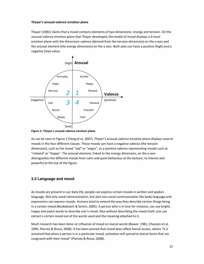
Thayer (1982) claims that a mood contains elements of two dimensions: energy and tension. On the
arousal-valence emotion plane that Thayer developed, the model of mood displays a 4-level
emotion plane with the dimension valence (derived from the tension dimension) on the x-axis and
the arousal element (the energy dimension) on the y-axis. Both axes can have a positive (high) and a
negative (low) value.
Figure 2. Thayer’s arousal-valence emotion plane.
As can be seen in Figure 2 (Yang et al, 2007), Thayer’s arousal-valence emotion plane displays several
moods in the four different classes. These moods can have a negative valence (the tension
dimension), such as the mood “sad” or “angry”, or a positive valence representing moods such as
“relaxed” or “happy”. The arousal element, linked to the energy dimension, on the y-axis
distinguishes the different moods from calm and quiet behaviour at the bottom, to intense and
powerful at the top of the figure.
3.2 Language and mood
As moods are present in our daily life, people can express certain moods in written and spoken
language. Not only vocal communication, but also non-vocal communication like body language and
expressions can express moods. Humans tend to extend the way they describe certain things being
in a certain mood (Beukeboom & Semin, 2005). A person who is in love for instance, can use bright,
happy and joyful words to describe one’s mood. Also without describing the mood itself, one can
extract a certain mood out of the words used and the meaning attached to it.
Much research has been done on influence of mood on lexical words (Bower, 1981; Chastain et al,
1995; Piercey & Rioux, 2008). It has been proved that mood does affect lexical access, where “it is
assumed that when a person is in a particular mood, activation will spread to lexical items that are
congruent with their mood” (Piercey & Rioux, 2008).
Excited
Happy
Pleased
Sad
Bored
Sleepy
Annoying
Angry
Nervous
Relaxed
Peaceful
Calm
1 2
3 4
Valence
Arousal
(low)
(high)
(positive) (negative)
13
A mood is based on exclusively subjectively experienced mental events. The definition of moods
makes reference to the (presumed) underlying dispositional basis of these mental events (Siemer,
2005). Humans are aware of experiencing a mood, and it can have effect on the language used in
conversations and global communication. Therefore the mental state of the speaker can be
expressed through speech and language.
Because language can hold emotionally or affectively loaded words through expression by humans,
mood categorisation based on the words and attitude of the sender or speaker can be done
(Chastain et al, 1995). Conversations, utterances, and attitudes (i.e. reactions on stimuli) produced
by a person can be analysed by another person and then classified even though the adressee is not
necessarily experiencing the same mood. The language used, with additional body language and
expressions, can reveal the mood a person experiences.
Meyers (2007) states that the most common of the categorical approaches to emotion modelling is
that of Paul Ekman’s basic emotions, which encompasses the emotions of happiness, sadness, anger,
fear, surprise and disgust (Ekman 1992). In addition to this categorisation, Thayer’s dimensional
approach (see section 3.1) can help classify the language used and extract the mood the speaker is
experiencing and intending to reveal.
3.3 Language and music (lyrics)
Analogously to the written and spoken communication in daily life, music lyrics can express mood
states of the writer. The text contains words and phrases that express moods and emotions. Similar
to the way people tend to show characteristics of a certain mood in their communication towards
another, so do music tracks. Both instrumental tracks and songs with lyrics can express feelings or
emotion.
A musician can have the intention to give a music track a certain feel, with emphasis on a certain
mood. Think of a heavy metal artist who wants his track to be listened to as a sad, intense track, or a
pop band recording a new track which has to be happy and calm. In order to reach this, the
songwriter can put words in the lyrics of the track which tend to characterise that type of mood.
By implementing content in the lyrics such as emotionally loaded sentences and words such “death”,
“dark”, or “miserable” the track can have a sad, intense load. Words like “fun”, “joy”, and “party”
can characterise the text, and furthermore the song, as a happy track in a calm manner.
Emphasizing mood in lyrics
Compared to written natural language, lyrics can also contain lexical items which emphasize a
certain mood, items that are activated by the sender (the artist or songwriter) who has the intention
of transferring a mood. We assume that the lyrics are the indicators of certain moods, which can be
exposed without the musical tracks and musical characteristics, such as tempo, key, and timbre.
14
In addition, we assume that lyrics alone can express moods, and the instrumental parts emphasize
the feelings exposed in the text. Although we mention the instrumental part of music here, we will
focus on the linguistic aspects of music.
Although the emphasis in spoken language (the voice, loudness and pitch in the song) may also be
important to extract and discover emotional loads, the contents of the words or phrases can have a
emotional level without being spoken. For instance, words such as “happy” or “dead” do not have to
be pronounced to have an emotional load.
Where emotionally loaded words and phrases can be used in spoken natural language to emphasize
a certain feel or emotion, the same can be done in written language. Emotions and moods can be
expressed in texts and from that point it can be used in music by implementing emotionally loaded
words and phrases in lyrics.
So the plain lyrics, the text in the song itself, is used for mood categorisation in this thesis. We want
to test whether the use of lyrics (or text) provides sufficient information for assigning moods to
music tracks in general, and whether the textual aspects in lyrics can be seen as representatives for
spoken and written natural language regarding the expression of moods.
3.4 Mood tagging for music tracks
As in daily life moments in time can be categorised by mood. Music tracks have a time spanning
appearance which can be seen as a moment or period, where a mood (or field of mood) is felt.
Koopman & Davis (2001) state that the musical period is a continuous time with a same mood which
is assumed to be there for the whole track, and music presents a continuous process itself. “People
do not merely perceive a succession of patterns in music; we experience musical parts as being
connected parts packed into a dynamic whole.”
A musical track has a stated play time, the track has one mood which characterises the whole track.
Therefore we assume that a song has exactly one mood. This forms the base for the description in
subsection 3.4.1, where the assumption of one mood for a song is explained. The concept of social
tagging is discussed in subsection 3.4.2.
3.4.1 Different events, one mood
People can have different emotions at a time but are experiencing a certain mood. For instance,
when someone is in a sad mood, someone can be angry for a moment or feeling happy when
reacting on a particular event, i.e. receiving a present. Although the emotions are present for a short
period of time, the overall mood remains the same. This is also noticeable in music: a song is based
on parts with a mood which can be attached to the whole track in general. Although an artist can
sing about a person who felt happy in the past in a sad song (i.e. the chorus), the overal mood of the
song remains sad. Therefore a music track has several emotions which are being linked together into
a whole track, which tends to have one certain mood.
15
Because these moods are related to the way a song is played, together with the affective parts in the
lyrical content and present in a stated period (i.e. the individual track or the whole playlist on the
album with the same classified mood), people can specify a mood the same way they tend to feel a
mood period in daily life (Liu et al., 2003). Therefore mood tagging for music tracks can be a
powerful tool to mirror daily emotions in music preferences. Mood tagging and tagging in general is
a relatively new way of expressing one’s feelings or thoughts.
3.4.2 Social tagging
According to Tonkin (2008), “social tagging, which is also known as collaborative tagging, social
classification, and social indexing, allows ordinary users to assign keywords, or tags, to items.”
Tagging is the process of assigning keywords to (mostly digital) items such as photos, folders,
documents, video or music. It is a form of indexing, in which the user attaches keywords which are
typically freely chosen instead of used from a controlled vocabulary.
Social tagging is the collaboratively describing and classifying of items, which results in an item
taxonomy called ‘folksonomy’, a portmanteau of folk and taxonomy (Vander Wal, 2005). The count
of tags for an item can differ from one (global) tag, for instance, “nature” for a photo of a forest, to
tens of keywords, for example on a graduation photo with all names of the persons, date, time,
place and so on. As there is no controlled vocabulary, any term may be used and any number of
terms may be used on a particular item.
Social tagging taxonomies are subdivided into broad folksonomies and narrow folksonomies. Where
many people tag the same objects with their own tags in a broad folksonomy (i.e. music tagging on
Last.fm), a narrow folksonomy consists of many people tagging their own objects with their own
tags, such as Flickr8 for online photos or YouTube
9 for videos.
Tags attached to items can be made visible for everyone on the web. Tagging digital items such as
music tracks (i.e. genre, year, artist, album) helps ordening files, and lets other users take over
information and interests.
3.5 Creating playlists
Because we identify with music, it can affect us in a powerful way (Koopman & Davies, 2001). We
tend to be attracted to listen to music compilations that match our current mood, or to listen to
music that has the preferred emotional level and/or the opposite (desired) mood of the one we are
in at the time of listening. One way of listening to music with regard to emotional levels is the
generation of mood-based playlists, which is described in subsection 3.5.1. Reasons for creating
music playlists is discussed in subsection 3.5.2, and 3.5.3 deals with automatic playlist generation.
8 http://www.flickr.com
9 http://www.youtube.com
16
3.5.1 Mood-based music playlists
Although mood classifications can differ from person to person, music tracks will almost have the
same emotional meaning or load in a certain mood field. As stated in subsection 3.4.3, people can
specify a mood the same way they tend to feel a mood period in daily life (Liu et al, 2003). People
tend to organise music tracks in particular classifications, of which one can be personal mood favors.
The organisation of music tracks based on moods is one example of playlist creation.
The final result of creating mood playlists will end up in a list of tracks that have been tagged the
same mood. These playlists can add value to the current mood of the user or can change the mood
in the most bright insight. For instance, when someone is feeling sad, listening to a music playlist
with excited/happy mood classified tracks can help changing the persons’ mood over time.
Even without proper mood tags for music as introduced here, people are creating playlists based on
moods. Studies by Voong & Beale (2007) show that “many choose to create playlists grouped by
mood, for example, by naming a playlist “relaxing”.”
3.5.2 Reasons for creating playlists
People share their playlists in order to exchange favours and interests in certain types of music.
Exchange of music among the people was always an important social interaction, but with the large
collections of MP3 music it became much more intensive than ever (Andric & Haus, 2006). Not only
the sharing of music interests makes creating playlists popular, also the individual music needs in
certain contexts affects the decision to create personal playlists.
Andric & Haus (2006) state that “many social contexts, like for example, working place, or driving a
car, do not allow for wasting too much time on choosing music. On the other side, the relaxing role
of music, and the intensified need for leisure and idleness in the relaxing moments, lower the will for
making intellectual effort for selection of appropriate musical contents.”
Pauws & Eggen (2002) state that “current music players allow playing a personally created temporal
sequence of songs in one go, once the playlist or program has been created”. After a playlist has
been created, someone can play the sequence of songs again for personal purposes, or for sharing
with other people.
However, choice and assembling of adequate playlists is time consuming. Some parts of music
collections are often acquired without detailed examination of their contents, and the sheer size of
the music collections overwhelmingly exceeds a person’s ability to recall which compositions comply
best with the current mood (Pauws & Eggen, 2002).
In order to simplify the creation of playlists, it is important to have correctly tagged instances in the
music library. With correct metadata in the ID3-tags, finding similar songs and music parts and
putting them in a playlist can get easier. The selecting procedure for individual music needs, ending
up in a playlist, is much easier when the user can find the music files easily, with detailed
information held with the contents (Andric & Haus, 2006).
17
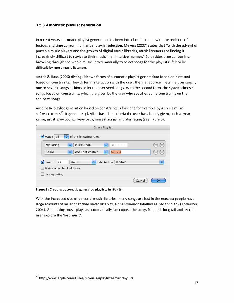
3.5.3 Automatic playlist generation
In recent years automatic playlist generation has been introduced to cope with the problem of
tedious and time consuming manual playlist selection. Meyers (2007) states that “with the advent of
portable music players and the growth of digital music libraries, music listeners are finding it
increasingly difficult to navigate their music in an intuitive manner.” So besides time consuming,
browsing through the whole music library manually to select songs for the playlist is felt to be
difficult by most music listeners.
Andric & Haus (2006) distinguish two forms of automatic playlist generation: based on hints and
based on constraints. They differ in interaction with the user: the first approach lets the user specify
one or several songs as hints or let the user seed songs. With the second form, the system chooses
songs based on constraints, which are given by the user who specifies some constraints on the
choice of songs.
Automatic playlist generation based on constraints is for done for example by Apple’s music
software ITUNES10
. It generates playlists based on criteria the user has already given, such as year,
genre, artist, play counts, keywords, newest songs, and star rating (see figure 3).
Figure 3: Creating automatic generated playlists in ITUNES.
With the increased size of personal music libraries, many songs are lost in the masses: people have
large amounts of music that they never listen to, a phenomenon labelled as The Long Tail (Anderson,
2004). Generating music playlists automatically can expose the songs from this long tail and let the
user explore the ‘lost music’.
10
http://www.apple.com/itunes/tutorials/#playlists-smartplaylists
18
3.6 Star rating and music recommendation
In addition to formal metadata in digital music tracks, such as key, era, or genre, music tracks can
also be classified in terms of rating, which can be seen as personal metadata. The user can rate an
individual track or compilation, mostly in terms of stars count ranging from one star (disliked by the
user, not listened to regularly) to 5 stars where the user likes the track and will play it regularly.
This rating system gives insight into the considerations of an individual music recommendation, as
the user has told the system the kind of tracks he/she liked or disliked.
Exploring music goes beyond the known tracks on the users’ computer or in a cd library. Given the
rating and the correct tags which can categorise the music track such as genre, era, and artist,
recommender systems such as Last.fm and Pandora can recommend unknown music similar to the
known music the person likes, based on several characteristics.
These systems try to provide the user with a more enjoyable listening experience. As Celma &
Lamere (2007) state, "music recommender systems serve as the middle-man in the music
marketplace, helping a music listener to find their next 5-star song among millions of 0-star songs."
But star rating does not seem to be a particular useful feature, as nearly 60% of 56 participants
indicated in a user research (Beale & Voong, 2006). The star rating system is regarded as inadequate,
and Beale & Voong (2006) therefore conclude that “users would like a way of managing their music
by mood”.
3.7 Music, mood and colour
In the recent years, much research has been performed in the field of colour representation for
music tracks and moods (Barbiere, Vidal & Zellner, 2007; Beale & Voong, 2006; Voong & Beale, 2007;
Geleijnse et al, 2008). Besides music, colours are related to emotions in a consistant manner, where
one can assign a colour to an emotion or mood in general, out of a range of colours.
Supported by psychological theories, Voong & Beale (2007) state that colour is often associated with
moods and emotions and that it provides a natural and straightforward way of expressing something
about a song. By extending the graphics user interface of Apple’s music software ITUNES with colour
selection per song, Voong & Beale (2007) found evidence in their studies that mood categorisation
by associating moods with colour, helps users to create playlists with more ease. They state that
“users reason about colour associations with a high degree of accuracy, showing that the tagging
system aids recall of music.”
In this section the use of colour for distinctions in music and mood is discussed. Subsection 3.7.1
deals with the addition of images to music. Section 3.7.2 captures the use of color in Moody’s mood
tagging framework.
19
3.7.1 Adding images to music
So mood categorisation for music, based on colours, proves to be an efficient tool for categorisation
and playlist generation. Furthermore, research by Geleijnse et al. (2008) focusses on enriching music
by adding lyrics, automatically separating the music track in segments, and assigning colour and
images to the track. Lyrics are assigned to the segments or so-called stanza’s (for instance, verse-
chorus-verse-chorus-bridge-outro). By extracting and selecting keywords in these added lyrics, their
system can browse through Google Images11
or Flickr12
to find images and colour schemes which
enrich the music being played. The images shown are based on a vast percentage of a particular
colour pattern.
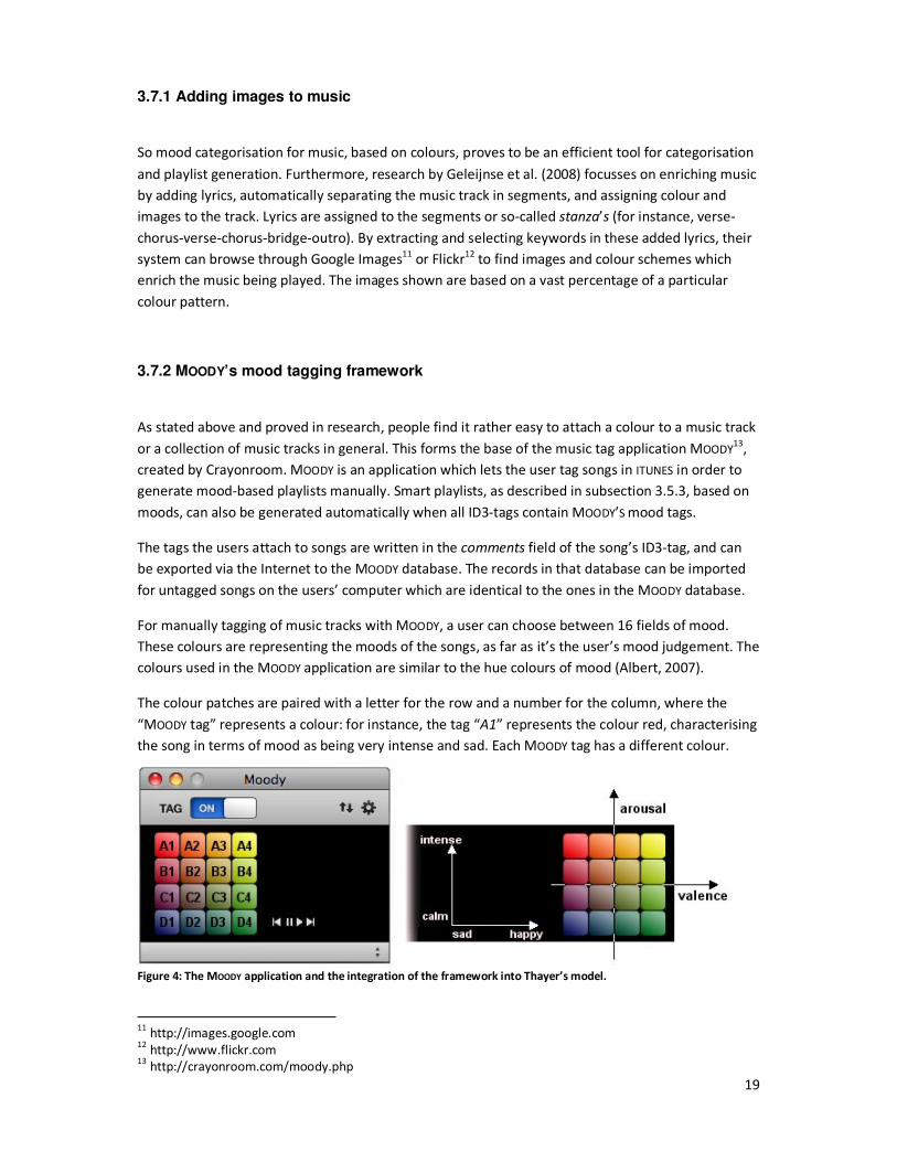
3.7.2 MOODY’s mood tagging framework
As stated above and proved in research, people find it rather easy to attach a colour to a music track
or a collection of music tracks in general. This forms the base of the music tag application MOODY13
,
created by Crayonroom. MOODY is an application which lets the user tag songs in ITUNES in order to
generate mood-based playlists manually. Smart playlists, as described in subsection 3.5.3, based on
moods, can also be generated automatically when all ID3-tags contain MOODY’S mood tags.
The tags the users attach to songs are written in the comments field of the song’s ID3-tag, and can
be exported via the Internet to the MOODY database. The records in that database can be imported
for untagged songs on the users’ computer which are identical to the ones in the MOODY database.
For manually tagging of music tracks with MOODY, a user can choose between 16 fields of mood.
These colours are representing the moods of the songs, as far as it’s the user’s mood judgement. The
colours used in the MOODY application are similar to the hue colours of mood (Albert, 2007).
The colour patches are paired with a letter for the row and a number for the column, where the
“MOODY tag” represents a colour: for instance, the tag “A1” represents the colour red, characterising
the song in terms of mood as being very intense and sad. Each MOODY tag has a different colour.
Figure 4: The MOODY application and the integration of the framework into Thayer’s model.
11
http://images.google.com 12
http://www.flickr.com 13
http://crayonroom.com/moody.php
20
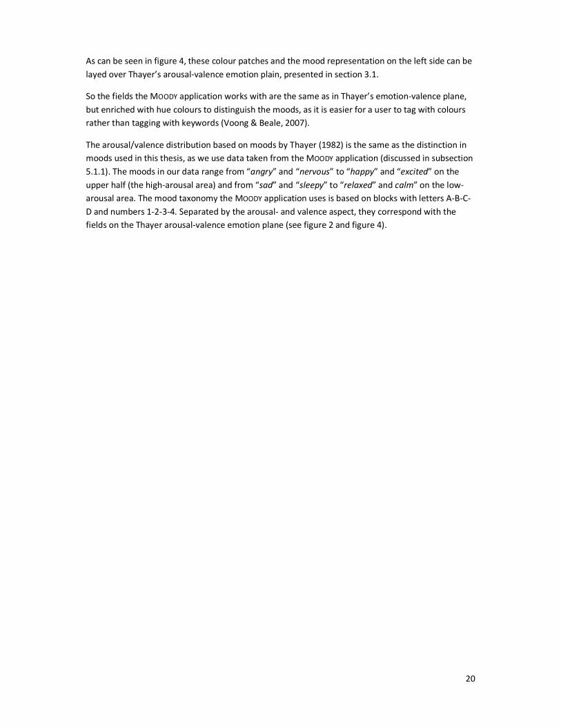
As can be seen in figure 4, these colour patches and the mood representation on the left side can be
layed over Thayer’s arousal-valence emotion plain, presented in section 3.1.
So the fields the MOODY application works with are the same as in Thayer’s emotion-valence plane,
but enriched with hue colours to distinguish the moods, as it is easier for a user to tag with colours
rather than tagging with keywords (Voong & Beale, 2007).
The arousal/valence distribution based on moods by Thayer (1982) is the same as the distinction in
moods used in this thesis, as we use data taken from the MOODY application (discussed in subsection
5.1.1). The moods in our data range from “angry” and “nervous” to “happy” and “excited” on the
upper half (the high-arousal area) and from “sad” and “sleepy” to “relaxed” and calm” on the low-
arousal area. The mood taxonomy the MOODY application uses is based on blocks with letters A-B-C-
D and numbers 1-2-3-4. Separated by the arousal- and valence aspect, they correspond with the
fields on the Thayer arousal-valence emotion plane (see figure 2 and figure 4).
21
4. Research design
This chapter describes the way that the concepts of mood, frameworks, and tagging of music as
classification tools are implemented in a research design. Section 4.1 describes the implementation
of machine learning techniques for categorisation and classifications. Section 4.2 covers a global
overview of the theoretical design of a classification tool, based on machine learning techniques. In
section 4.3 a common evaluation technique called k-fold cross-validation is discussed.
4.1 Machine learning
The aim of this thesis is the automatic assignment of mood tags for music, based on lyrics. The word
automatic in this context means that the users do not have to classify themselves: the system will
classify based on machine learning techniques.
Machine learning is the covering term for using developed techniques and algorithms to let a
computer learn a specific job. With the use of algorithms a machine can learn, and work without the
need of specific human control within a certain task. Information is extracted automatically on
statistical and computational basis.
The term ‘learning’ in machine learning holds the gaining of new information from the current task,
which is stored to improve the results in upcoming events where the same task is executed. The
system stores information of the seen (test-) instances and applies the collected information for
upcoming new items. When a new instance is encountered, in order to assign a target value for this
new instance the system examines its relationship to the previously stored examples (Mitchell,
1997).
Different learning techniques apply to machine learning. Subsection 4.1.1 deals with concept
learning. The inductive learning hypothesis is briefly discussed in subsection 4.1.2. Thereafter, in
subsection 4.1.3 a machine learning system called TIMBL is introduced.The concept of k-Nearest
Neighbours is covered in subsection 4.1.4. Finally, subsection 4.1.5 deals with the k-fold cross-
validation evaluation technique.
4.1.1 Concept learning
Within machine learning a common used technique is concept learning, which holds the basis of
learning through comparing new concepts with ones seen earlier. “Concept learning can be
formulated as a problem of searching through a predefined space of potential hypotheses for the
hypothesis that fits best the training examples” (Mitchell 1997). This learning method, also called
instance-based learning, is used in nearest neighbour methods regarding machine learning (see
section 4.1.4).
22
4.1.2 The inductive learning hypothesis
The inductive learning hypothesis as described by Mitchell (1997) assumes that any hypothesis
found to approximate the target function well over a sufficiently large set of training examples will
also approximate the target function well over other unobserved examples. So a system can predict
a mood class (which is the target function in this thesis) by comparing the new instance (an
unobserved example) against the observed training examples.
4.1.3 TIMBL: Tilburg Memory Based Learner
In this thesis the TIMBL program is used for classifications. TIMBL, which stands for Tilburg Memory
Based Learner, is a machine learning software package which implements a family of Memory-Based
Learning techniques for discrete data. It stores a representation of the training set explicitly in the
memory, thus the term Memory Based in the name. New classifications are made by extrapolating
from the most similar stored cases.
In other words, at classification time there is the extrapolation of a class from the most similar items
in the memory to the new test item (Daelemans et al, 2007). This technique for classification has
similarities with the core k-Nearest Neighbour (k-NN) classifications, on which most machine
learning applications are based.
4.1.4 k-Nearest Neighbours
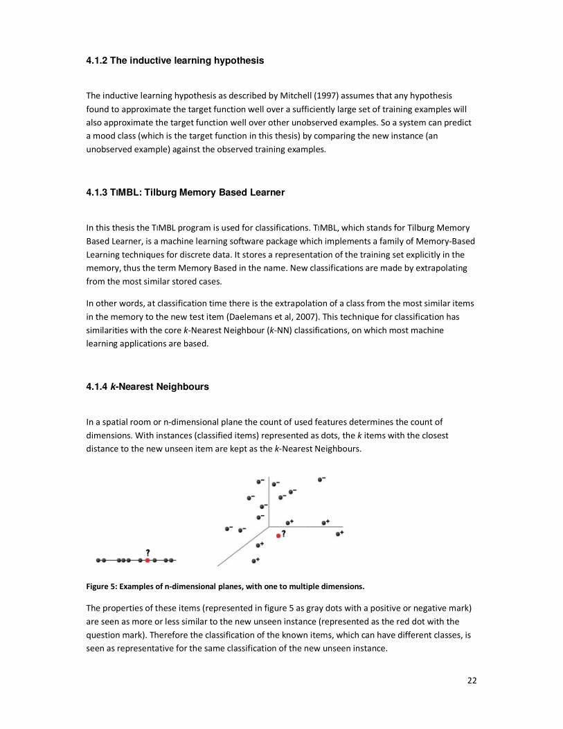
In a spatial room or n-dimensional plane the count of used features determines the count of
dimensions. With instances (classified items) represented as dots, the k items with the closest
distance to the new unseen item are kept as the k-Nearest Neighbours.
Figure 5: Examples of n-dimensional planes, with one to multiple dimensions.
The properties of these items (represented in figure 5 as gray dots with a positive or negative mark)
are seen as more or less similar to the new unseen instance (represented as the red dot with the
question mark). Therefore the classification of the known items, which can have different classes, is
seen as representative for the same classification of the new unseen instance.
23
In this thesis the spatial room consists of the number of used features (see subsection 5.2.4) with k
lyrics represented as grey dots. Each lyric in the n-dimensional plane has a mood class, determined
by the feature values. Each time a new lyric is implemented, represented as the red dot, its
properties are compared to the feature values in the spatial room. The k lyrics closest to the new
lyric are seen as representatives, and their mood classes are used for the classification of the new
lyric. For instance, if the new lyric has almost similar feature values as the lyrics with mood class C in
the Arousal division in its neighbourhood, classification can occasionally lead to attachment of mood
class C for the new lyric.
Distances from the new unseen item to all stored known dots (which are stored in memory in the
training phase) are computed and the k closest samples are selected. So a new instance or dot is
classified by a majority vote of its neighbours in the feature space, with the new item being assigned
to the class most common amongst its k-Nearest Neighbours.
Voting only takes place during the actual classification phase, where the test sample (the unknown
instance) is represented as a vector in the feature space. During the training phase the known items
and respective feature vectors are only stored.
4.1.5 k-Fold cross-validation
One technique to show the system’s performance on predicting classifications for unknown data is
cross-validation. Cross-validation is the statistical practice of dividing data into partitions or subsets,
such that the analysis is initially performed on a single subset which is seen as the test dataset. The
other subsets in the form of training data are retained for subsequent use in confirming and
validating the initial analysis. Afterwards the statistical outcomes show the overall performance of
the system for computing and analysing data it has not seen before; the new data.
The data is subdivided in folds for training- and test stages (see section 5.2). All folds minus one (k-1)
are set as training samples, where the fold being left out is used as test data. In other words: each
fold (k) can be used as test set, where the other (k-1) sets are put together to form a training set.
With each computation leaving one fold out and combining the other folds, k settings with other
training data sets and testing data sets are computed.
After the computation, the average accuracy across all k-trials is computed. With this technique, the
so-called k-fold cross-validation, each of the k subdivided data sets is used in a test set exactly once,
and gets to be in a training set k-1 times.
4.2 Theoretical design of a classification tool based on machine learning
Now that the concept of machine learning is described, a global overview of a classification tool is
presented in this section. In this overview the concept of machine learning is visualised to expose
the different stages of processing. The distinction between the training- and testing phase is visible.
The data used in training mode is extracted out of the database, as the same is done for testing
purposes.
24
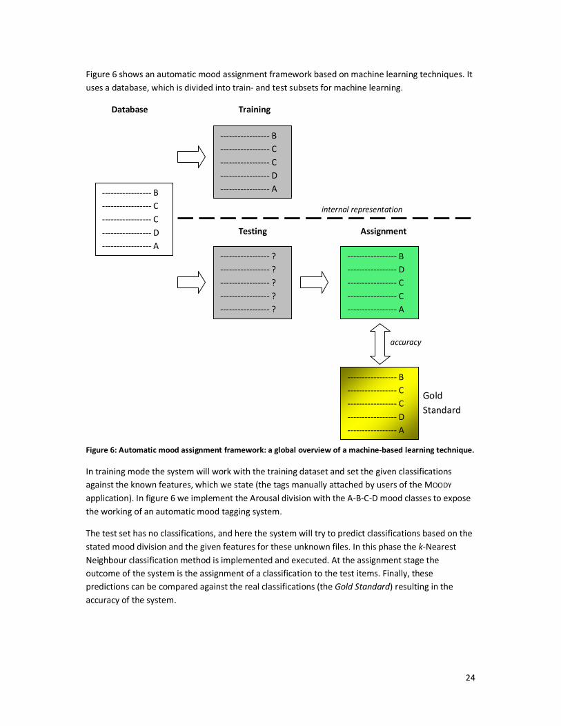
Figure 6 shows an automatic mood assignment framework based on machine learning techniques. It
uses a database, which is divided into train- and test subsets for machine learning.
Database Training
internal representation
Testing Assignment
Assignment
accuracy
Gold
Standard
Figure 6: Automatic mood assignment framework: a global overview of a machine-based learning technique.
In training mode the system will work with the training dataset and set the given classifications
against the known features, which we state (the tags manually attached by users of the MOODY
application). In figure 6 we implement the Arousal division with the A-B-C-D mood classes to expose
the working of an automatic mood tagging system.
The test set has no classifications, and here the system will try to predict classifications based on the
stated mood division and the given features for these unknown files. In this phase the k-Nearest
Neighbour classification method is implemented and executed. At the assignment stage the
outcome of the system is the assignment of a classification to the test items. Finally, these
predictions can be compared against the real classifications (the Gold Standard) resulting in the
accuracy of the system.
----------------- B
----------------- C
----------------- C
----------------- D
----------------- A
----------------- ?
----------------- ?
----------------- ?
----------------- ?
----------------- ?
----------------- B
----------------- C
----------------- C
----------------- D
----------------- A ----------------- B
----------------- D
----------------- C
----------------- C
----------------- A
----------------- B
----------------- C
----------------- C
----------------- D
----------------- A
25
5. Implementation
This chapter deals with the implementation of the research design. Section 5.1 covers the collection
of the data used for the experiments. The extraction, export and cleanup of data is described.
Section 5.2 continues with the feature construction, with the generation of features and explanation
of the tf*idf technique.
5.1 Data collection
Until recently, music listeners could read the lyrics of the songs they were listening to by checking,
for example, the paper inlay in the compact disk. As more music is bought digitally via the Internet
nowadays, printed lyrics on compact disk inlays are getting rare. A new way of enclosing lyrics is the
storage of text in the digital MP3-file itself, by implementing an ID3-tag (as stated in subsection
2.1.1).
However, lyrics written in ID3-tags in the MP3-files are not yet generally accepted by either players
or providers of digital music at the moment, although this may change in the near future. Therefore
other ways to get the lyrics of the songs are being used by music listeners.
One way of obtaining the lyrics is searching through the Internet. Collected lyrics and other
information about the albums, artists, and songs can be found on the web. Websites with huge
collections of lyrics on the Internet have expanded the last couple of years. At these gateways one
can find lyrics i.e. by artist, album or genre.
The advantages of a lyrics database on the Internet consist of (1) hierarchical storage and access for
the user, (2) linking to similar artists/songs/albums, (3) straightforward management and (4) lots of
capacity due to the small data size of plain text.
This section covers the collecting of data for the experiments. The use of MOODY data and the
extraction of lyrics from online sources is discussed in subsection 5.1.1. The next step, exporting and
cleaning up the collected data, is described in subsection 5.1.2.
5.1.1 Data extraction
As this thesis focusses on lyrics and experimenting with the lingual content of music, i.e. on word
levels and other textual characteristics, the lyrics have to be found first. The music tracks of which
the lyrics are taken from are generated out of the MOODY database. MOODY provides access to the
tag data. The records on the MOODY server are used for this research and picked out at random. The
extracted data with user-tagged moods consists of 10,000 lines with records, containing the name of
the artist, the name of the song, and the corresponding user-tagged mood.
Each record consists of an artist name and the name of the song, which are useful for the lyrics
extraction phase. The lyrics extraction phase works as follows: first a separate record in the mood-
tags database is read, which provides the artist and the title of the song of which the lyrics have to
26
be found. These two parameters are put in a dynamic link of eight different online lyrics databases
which are used as the lyrics sources.
The script automatically extracts the lyrics from the Internet when found in the database of one of
the sources. The choice of using eight different online lyrics databases was made after having several
rounds of finding lyrics through the script. Each time the sources were expanded with new sources in
order to find more lyrics from the records in the MOODY database used in this thesis. After using
eight online lyrics databases, 5,631 lyrics were found.
For each source, addresses are downloaded and searched through for valid content until the lyrics
are found. As the records in the MOODY database consists of instrumental music as well as songs in
foreign languages, no lyrics are found for these records in our implemented lyrics sources.
We encountered a problem with whitespaces in the database records. Sometimes whitespaces in,
for instance, the artists name did not match with the way the artist name is spelled on the lyrics
sources. For instance, a record was not found in the lyrics sources, because the artist name in the
data record was spelled “arcticmonkeys” instead of “arctic monkeys”. Due to several other spelling
variations in the data for artist names, such as “acdc”, “ac-dc” or “ac dc” for the artist AC/DC, we had
to change the lyrics extraction script.
We implemented conversions in the script to improve the results, such as changing whitespaces to
underscores, and deleting quotation marks. It did not improve for some instances in the database
records and it would take too much time to change all individual records that were not found.
Because the HTML-pages of the lyrics databases consist of a large amount of HTML markup, images
and unfamiliar code, the source code of the lyrics page has to be cleaned. This is done by searching
down the HTML-tree until the real lyrics text section is found. These lyrics, enclosed in a pre-
specified HTML-tag, are exported.
5.1.2 Exporting and cleaning up the data
The lyrics are exported as plain text. The reason for choosing plain text instead of XML, HTML or
other formats was the readability and the ease of manipulation of the plain text for further
operations. The plain text only shows the textual volume where no markup is needed. For further
operations in the feature construction stage there was no need for textual attributes such as fonts,
boldface, colour and other markup, therefore the plain text was the best suitable format to work
with.
The lyrics are cleaned up by translating HTML-entities, removing unwanted text which is not part of
the lyric (for instance, informational terms for website users such as “chorus” and occurances of “For
more lyrics go to ...”) and removing unimportant whitespaces and empty lines.
By cleaning up the lyrics, we encounter some problems. First of all informational metadata is
deleted, which tells us for instance, where a chorus starts, a bridge ends and how many times a
sentence sung by the artist has to be repeated. Any occurance of i.e. “4x”, “bridge” or “repeat until
fade out” in a chorus is thrown away, although these parts of a lyric are of importance for re-playing
the music track.
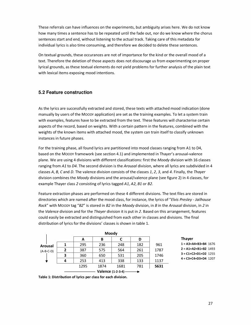
27
Arousal
(A-B-C-D)
Thayer
1 = A3+A4+B3+B4 1676
2 = A1+A2+B1+B2 1493
3 = C1+C2+D1+D2 1255
4 = C3+C4+D3+D4 1207
Moody
These referrals can have influences on the experiments, but ambiguity arises here. We do not know
how many times a sentence has to be repeated until the fade out, nor do we know where the chorus
sentences start and end, without listening to the actual track. Taking care of this metadata for
individual lyrics is also time consuming, and therefore we decided to delete these sentences.
On textual grounds, these occurances are not of importance for the kind or the overall mood of a
text. Therefore the deletion of those aspects does not discourage us from experimenting on proper
lyrical grounds, as these textual elements do not yield problems for further analysis of the plain text
with lexical items exposing mood intentions.
5.2 Feature construction
As the lyrics are successfully extracted and stored, these texts with attached mood indication (done
manually by users of the MOODY application) are set as the training examples. To let a system train
with examples, features have to be extracted from the text. These features will characterise certain
aspects of the record, based on weights. With a certain pattern in the features, combined with the
weights of the known items with attached mood, the system can train itself to classify unknown
instances in future phases.
For the training phase, all found lyrics are partitioned into mood classes ranging from A1 to D4,
based on the MOODY framework (see section 4.1) and implemented in Thayer’s arousal-valence
plane. We are using 4 divisions with different classifications: first the Moody division with 16 classes
ranging from A1 to D4. The second division is the Arousal division, where all lyrics are subdivided in 4
classes A, B, C and D. The valence division consists of the classes 1, 2, 3, and 4. Finally, the Thayer
division combines the Moody divisions and the arousal/valence plane (see figure 2) in 4 classes, for
example Thayer class 2 consisting of lyrics tagged A1, A2, B1 or B2.
Feature extraction phases are performed on these 4 different divisions. The text files are stored in
directories which are named after the mood class, for instance, the lyrics of “Elvis Presley - Jailhouse
Rock” with MOODY tag “B2” is stored in B2 in the Moody division, in B in the Arousal division, in 2 in
the Valence division and for the Thayer division it is put in 2. Based on this arrangement, features
could easily be extracted and distinguished from each other in classes and divisions. The final
distribution of lyrics for the divisions’ classes is shown in table 1.
Valence (1-2-3-4)
Table 1: Distribution of lyrics per class for each division.
A B C D
1 295 236 248 182 961
2 387 575 564 261 1787
3 360 650 531 205 1746
4 253 413 338 133 1137
1295 1874 1681 781 5631
28
With the lyrics partitioned in division classes, information can be extracted from the collected data.
This section describes the generation of features from the lyrics. Subsection 5.2.1 deals with the
generation of features such as character count, word count and line count. The term frequency and
tf*idf technique is described in subsection 5.2.2. In subsection 5.2.3 an explanation of the different
use of tf*idf techniques for feature construction is discussed. Finally, subsection 5.2.4 covers a
normalisation implementation and a feature overview.
5.2.1 Generating features
For testing- and training phases, several features are generated. The first feature is line count, were
the count of lines in each lyric in each training subdivision is computed and implemented in a list; the
list of feature “lc” in the training subset. The second feature is word count (wc), with a list of total
words per lyric. The third feature is the character count, with the count of all characters in a single
lyric being put in the feature list “cc”.
It might be possible that one of these features (or a combination of the features) describes some
important characteristics per class for weighting. The values can tell something about the lyrics and
the subsequent class if the values of the features per class differ from each other on a big scale. One
or more features can be identifiers for categorising certain classes, but also for the experiment of
showing certain characteristics on these features (word count, line count and character count) itself.
Word counts and line counts can be of importance as identifiers for certain kinds of music, so we
have assumptions in that field. It could be that lyrics of music tracks in a calm manner can contain
fewer words than nervous or excited tracks.
This is extrapolated as we can use fewer words in daily life to express a calm, peaceful mood in our
messages compared to messages regarding excitement or joy. Think of a conversation with someone
who is sleepy and tired, compared to a conversation where you ask someone who feels excited to
tell you how that person experienced the day. The last conversation will probably end up with more
words.
Another assumption can be that music tracks labelled “angry” can have less sentences (line counts)
than pleased, happy tracks. Although these thoughts are just assumptions which are not grounded,
we can use the features to see if in this context these assumptions can be true. Therefore we are
going to take a look at this point.
5.2.2 Term frequency and inversed document frequency
The fourth feature holds the tf*idf values. The standalone term frequency values are used as a fifth
feature. The use of tf*idf values is a powerful technique to emphasize the importance of a term in a
document, compared to all documents in the database (Ramos 2003).
29
The term frequency (tf) in a document measures the number of occurances of that term in a
document.
This formula measures the importance of term ti in document dj, with ni,j occurances of the term in
document dj, divided by the sum of the number of occurences of all terms in the document dj.
The inverse document frequency (idf) measures the importance of the term in the whole collection
of items.
In this formula the number of all documents D is divided by the number of documents where the
term (ti) appears, and taking the logarithm of that quotient (Crestani et al, 2001).
After computing these weights, they are multiplied to get the tf*idf value:
This tf*idf weight shows the relevance of the document for the term compared to the other
documents: the higher the tf*idf value for term ti in that particular document, the higher the
document will be sorted in a resulting list of documents in the database based on relevance. The
higher the position of the document in the vector, the more relevant the document is for the given
term ti.
If term ti appears in all documents, or in most of the documents in a large database, the tf*idf weight
has a low value. The term ti is less important, as it does not judge for listing documents on its own:
the term ti does not distinguish the importance of documents compared to others, as term ti
appears in all documents.
These terms with their tf*idf weights are important for the upcoming phases: the terms with a high
tf*idf weight are seen as important identifiers for a class. When an unknown lyric is analyzed, the
lyrics are searched through and afterwards all terms are looked up in the tf*idf frequency lists per
class, where tf*idf scores of the terms for each class are held.
The tf*idf value in each class is stored in a new list with the term and the corresponding tf*idf values
for all classes as attributes. After analysing all terms in an unseen lyrics, the more counts of a term
combined with a high tf*idf value in a particular class, can help judging the unknown lyric as a whole
as a potential candidate for classifying in that particular class. Together with the other features, the
overall tf*idf result as a feature for can participate in attaching the mood value of a particular class
to a new, unseen lyric.
30
5.2.3 The use of tf*idf weights
The tf*idf technique is used differently in this thesis than it is normally used. In general, tf*idf is used
for ranking documents based on terms: the documents with the highest tf*idf value for (a) certain
term(s) are ranked on top. On information retrieval grounds, the documents on top are of more
importance for a user (who is sending a query with term ti), than the documents which have lower
tf*idf weights of that term.
In this thesis we are not looking at the word level (with terms for judgements) but at the document
level. Although one or more terms can also judge for assigning mood to a lyric, the collective weights
for all terms in a document/lyric are used as a feature for classifying. Each lyric is seen as a collection
of terms which have individual tf*idf weights, but there is no overall ranking on the collection of
documents afterwards.
So terms with a tf*idf value are not seen as stand-alone identifiers for ranking documents or
showing the importance of documents regarding the high tf*idf value of the term up front in this
thesis. As mood tags are attached to the found lyrics, the terms are seen as identifiers for the mood
classes the lyrics are in. In other words, the overall terms in the lyrics judge for classification. All
terms in new unseen lyrics are compared to the terms with tf*idf values for each class in the lyrics
database and the total weights of tf*idf values can judge for a certain class.
In this thesis we are dealing with moods, which are seen as the documents. As the features are
divided per class in the training database, the tf*idf values for term ti will characterise the attached
mood of that document, the lyric. For instance, the term ti has a high tf*idf value in class X compared
to the other classes. Therefore when the term ti occurs in an unseen lyric, it will have a weight which
can occasionally lead to the assignment of mood Y based on the tf*idf values, combined with
weightings on other features.
For the tf*idf feature, the lyrics in the subdivided mood classes are analysed through a tf*idf value
generator. This process ends up in a list of tf*idf values, ranging from high values on top to low
values, with the tf*idf value followed by the term.
We expose the problem of upcoming tf*idf features having the value “0” regularly. This takes place
when several words in a lyric also occur in most of the other lyrics. While we are dealing with a
relative small number of classes in this thesis, it is likely that several terms in lyrics appear in all
classes, where the lyrics per class represent the documents.
As stated above, for calculating the idf-value of the tf*idf algorithm the log of the sum of all
documents D, divided by the number of documents where the term (ti) appears in, is taken. If term ti
appears in all documents, the count of all documents is equal to the count of documents with term
ti. When taking the logarithm of 1 (all documents: ‘D’ divided by the same value ‘D(ti)’ of documents
where term ti appears) the outcome is 0. So in this case term ti appears in all classes, and therefore
the tf*idf value of term ti calculated on the database equals 0.
In order to cope with this problem, we implement the Laplace smoothing method, also known as
“add-one smoothing”, in the tf*idf calculator script. Before calculating the idf value, +1 is added to
the number of documents D.
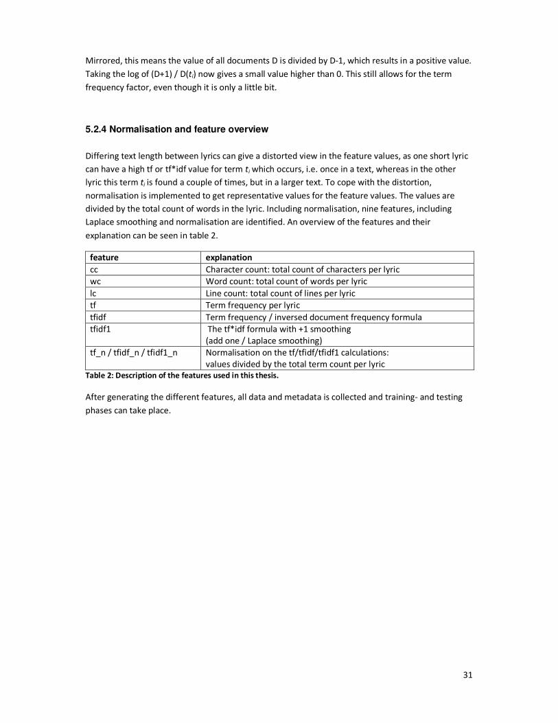
31
Mirrored, this means the value of all documents D is divided by D-1, which results in a positive value.
Taking the log of (D+1) / D(ti) now gives a small value higher than 0. This still allows for the term
frequency factor, even though it is only a little bit.
5.2.4 Normalisation and feature overview
Differing text length between lyrics can give a distorted view in the feature values, as one short lyric
can have a high tf or tf*idf value for term ti which occurs, i.e. once in a text, whereas in the other
lyric this term ti is found a couple of times, but in a larger text. To cope with the distortion,
normalisation is implemented to get representative values for the feature values. The values are
divided by the total count of words in the lyric. Including normalisation, nine features, including
Laplace smoothing and normalisation are identified. An overview of the features and their
explanation can be seen in table 2.
feature explanation
cc Character count: total count of characters per lyric
wc Word count: total count of words per lyric
lc Line count: total count of lines per lyric
tf Term frequency per lyric
tfidf Term frequency / inversed document frequency formula
tfidf1 The tf*idf formula with +1 smoothing
(add one / Laplace smoothing)
tf_n / tfidf_n / tfidf1_n Normalisation on the tf/tfidf/tfidf1 calculations:
values divided by the total term count per lyric
Table 2: Description of the features used in this thesis.
After generating the different features, all data and metadata is collected and training- and testing
phases can take place.
32
6. Experiments and tests
This chapter uses the implementation of machine learning (ML) as described in chapter 4 and 5 to
test the performance of assigning moods to music tracks based on lyrics solely. In section 6.1 the
experimental setup is explained, with the used features and TIMBL settings. Explanation of running
the training- and testing phases is discussed in section 6.2. Section 6.3 covers the test results. The
conclusions on the test results in section 6.4 form the chapter conclusions, which feeds the
upcoming chapter 7 with the evaluation.
6.1 Experimental setup
With all features generated and set, all preparations for the machine learning phases, are done. By
stating the features to be used, and applying the TIMBL settings, the machine learning system can
perform training- and test phases.
The TiMBL machine learning software executes 3 phases automatically. In the first phase it reads the
datafiles, where features and classes are stated and gain ratio’s are computed. So the records in the
feature directories are read and algorithms are applied to catch regularities between several records
in a class.
Phase two holds the learning from the datafiles, where the classifications are set, and based on
these classifications the features are analysed. These classifications are not set in the third phase
(testing), where the analysis of the new instances is matched with the feature values and the
corresponding classifications which are being used in the training phase. Finally, in the third phase,
the trained classifier is applied to the test set.
6.1.1 TIMBL settings
An experiment with testing and training phases included is started by executing TIMBL with two files:
the training data and the testing data. In both the training and testing phases, the IB1 algorithm is
used.
For the experiments TIMBL is used with the default settings. Similarity between instances in the test-
and training data is computed as weighted overlap. TIMBL sets the default feature weighting as Gain
Ratio.
As stated in section 4.1.5, 10-fold cross-validation is set for evaluation on the system’s performance
on predicting classifications.
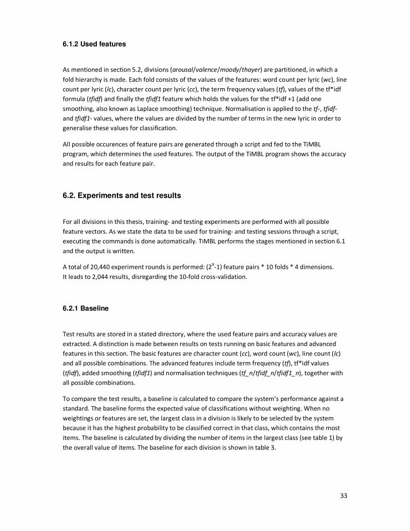
33
6.1.2 Used features
As mentioned in section 5.2, divisions (arousal/valence/moody/thayer) are partitioned, in which a
fold hierarchy is made. Each fold consists of the values of the features: word count per lyric (wc), line
count per lyric (lc), character count per lyric (cc), the term frequency values (tf), values of the tf*idf
formula (tfidf) and finally the tfidf1 feature which holds the values for the tf*idf +1 (add one
smoothing, also known as Laplace smoothing) technique. Normalisation is applied to the tf-, tfidf-
and tfidf1- values, where the values are divided by the number of terms in the new lyric in order to
generalise these values for classification.
All possible occurences of feature pairs are generated through a script and fed to the TiMBL
program, which determines the used features. The output of the TiMBL program shows the accuracy
and results for each feature pair.
6.2. Experiments and test results
For all divisions in this thesis, training- and testing experiments are performed with all possible
feature vectors. As we state the data to be used for training- and testing sessions through a script,
executing the commands is done automatically. TIMBL performs the stages mentioned in section 6.1
and the output is written.
A total of 20,440 experiment rounds is performed: (29-1) feature pairs * 10 folds * 4 dimensions.
It leads to 2,044 results, disregarding the 10-fold cross-validation.
6.2.1 Baseline
Test results are stored in a stated directory, where the used feature pairs and accuracy values are
extracted. A distinction is made between results on tests running on basic features and advanced
features in this section. The basic features are character count (cc), word count (wc), line count (lc)
and all possible combinations. The advanced features include term frequency (tf), tf*idf values
(tfidf), added smoothing (tfidf1) and normalisation techniques (tf_n/tfidf_n/tfidf1_n), together with
all possible combinations.
To compare the test results, a baseline is calculated to compare the system’s performance against a
standard. The baseline forms the expected value of classifications without weighting. When no
weightings or features are set, the largest class in a division is likely to be selected by the system
because it has the highest probability to be classified correct in that class, which contains the most
items. The baseline is calculated by dividing the number of items in the largest class (see table 1) by
the overall value of items. The baseline for each division is shown in table 3.
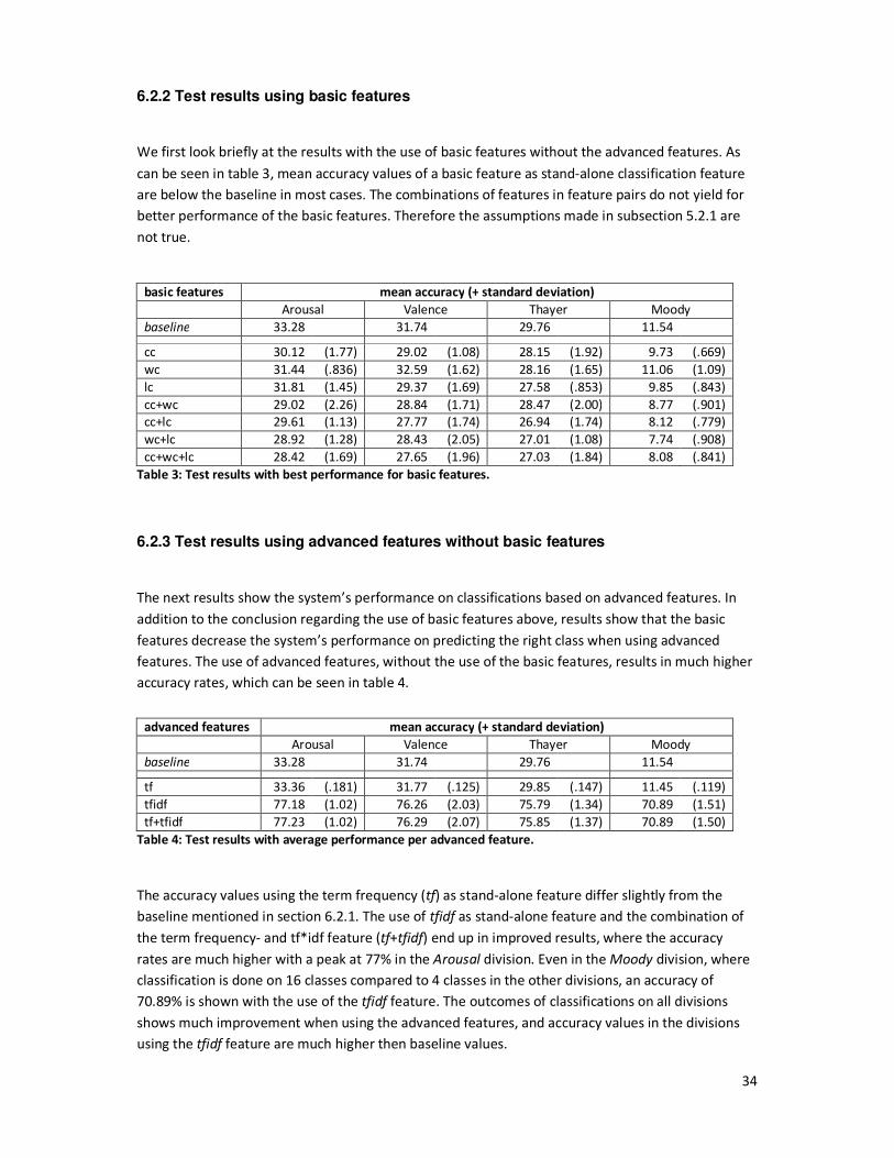
34
6.2.2 Test results using basic features
We first look briefly at the results with the use of basic features without the advanced features. As
can be seen in table 3, mean accuracy values of a basic feature as stand-alone classification feature
are below the baseline in most cases. The combinations of features in feature pairs do not yield for
better performance of the basic features. Therefore the assumptions made in subsection 5.2.1 are
not true.
Table 3: Test results with best performance for basic features.
6.2.3 Test results using advanced features without basic features
The next results show the system’s performance on classifications based on advanced features. In
addition to the conclusion regarding the use of basic features above, results show that the basic
features decrease the system’s performance on predicting the right class when using advanced
features. The use of advanced features, without the use of the basic features, results in much higher
accuracy rates, which can be seen in table 4.
Table 4: Test results with average performance per advanced feature.
The accuracy values using the term frequency (tf) as stand-alone feature differ slightly from the
baseline mentioned in section 6.2.1. The use of tfidf as stand-alone feature and the combination of
the term frequency- and tf*idf feature (tf+tfidf) end up in improved results, where the accuracy
rates are much higher with a peak at 77% in the Arousal division. Even in the Moody division, where
classification is done on 16 classes compared to 4 classes in the other divisions, an accuracy of
70.89% is shown with the use of the tfidf feature. The outcomes of classifications on all divisions
shows much improvement when using the advanced features, and accuracy values in the divisions
using the tfidf feature are much higher then baseline values.
basic features mean accuracy (+ standard deviation)
Arousal Valence Thayer Moody
baseline 33.28 31.74 29.76 11.54
cc 30.12 (1.77) 29.02 (1.08) 28.15 (1.92) 9.73 (.669)
wc 31.44 (.836) 32.59 (1.62) 28.16 (1.65) 11.06 (1.09)
lc 31.81 (1.45) 29.37 (1.69) 27.58 (.853) 9.85 (.843)
cc+wc 29.02 (2.26) 28.84 (1.71) 28.47 (2.00) 8.77 (.901)
cc+lc 29.61 (1.13) 27.77 (1.74) 26.94 (1.74) 8.12 (.779)
wc+lc 28.92 (1.28) 28.43 (2.05) 27.01 (1.08) 7.74 (.908)
cc+wc+lc 28.42 (1.69) 27.65 (1.96) 27.03 (1.84) 8.08 (.841)
advanced features mean accuracy (+ standard deviation)
Arousal Valence Thayer Moody
baseline 33.28 31.74 29.76 11.54
tf 33.36 (.181) 31.77 (.125) 29.85 (.147) 11.45 (.119)
tfidf 77.18 (1.02) 76.26 (2.03) 75.79 (1.34) 70.89 (1.51)
tf+tfidf 77.23 (1.02) 76.29 (2.07) 75.85 (1.37) 70.89 (1.50)
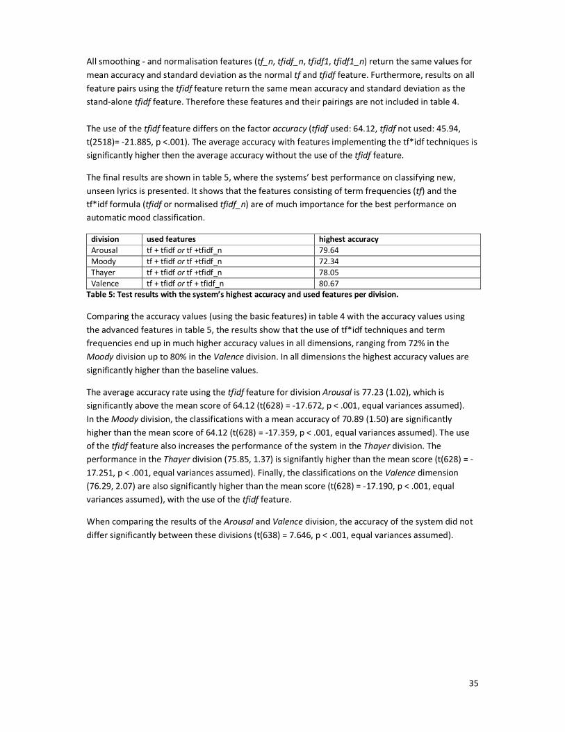
35
All smoothing - and normalisation features (tf_n, tfidf_n, tfidf1, tfidf1_n) return the same values for
mean accuracy and standard deviation as the normal tf and tfidf feature. Furthermore, results on all
feature pairs using the tfidf feature return the same mean accuracy and standard deviation as the
stand-alone tfidf feature. Therefore these features and their pairings are not included in table 4.
The use of the tfidf feature differs on the factor accuracy (tfidf used: 64.12, tfidf not used: 45.94,
t(2518)= -21.885, p <.001). The average accuracy with features implementing the tf*idf techniques is
significantly higher then the average accuracy without the use of the tfidf feature.
The final results are shown in table 5, where the systems’ best performance on classifying new,
unseen lyrics is presented. It shows that the features consisting of term frequencies (tf) and the
tf*idf formula (tfidf or normalised tfidf_n) are of much importance for the best performance on
automatic mood classification.
division used features highest accuracy
Arousal tf + tfidf or tf +tfidf_n 79.64
Moody tf + tfidf or tf +tfidf_n 72.34
Thayer tf + tfidf or tf +tfidf_n 78.05
Valence tf + tfidf or tf + tfidf_n 80.67
Table 5: Test results with the system’s highest accuracy and used features per division.
Comparing the accuracy values (using the basic features) in table 4 with the accuracy values using
the advanced features in table 5, the results show that the use of tf*idf techniques and term
frequencies end up in much higher accuracy values in all dimensions, ranging from 72% in the
Moody division up to 80% in the Valence division. In all dimensions the highest accuracy values are
significantly higher than the baseline values.
The average accuracy rate using the tfidf feature for division Arousal is 77.23 (1.02), which is
significantly above the mean score of 64.12 (t(628) = -17.672, p < .001, equal variances assumed).
In the Moody division, the classifications with a mean accuracy of 70.89 (1.50) are significantly
higher than the mean score of 64.12 (t(628) = -17.359, p < .001, equal variances assumed). The use
of the tfidf feature also increases the performance of the system in the Thayer division. The
performance in the Thayer division (75.85, 1.37) is signifantly higher than the mean score (t(628) = -
17.251, p < .001, equal variances assumed). Finally, the classifications on the Valence dimension
(76.29, 2.07) are also significantly higher than the mean score (t(628) = -17.190, p < .001, equal
variances assumed), with the use of the tfidf feature.
When comparing the results of the Arousal and Valence division, the accuracy of the system did not
differ significantly between these divisions (t(638) = 7.646, p < .001, equal variances assumed).
36
7. Evaluation and discussion
In this chapter, evaluation takes place. The test results in chapter 6 are subject to evaluation, where
the scientific background of chapters 3 and 4 is implemented. Section 7.1 covers the evaluation of
the test results. In section 7.2 the theories and scientific background are compared to the outcomes
to conclude the first research question, as the same is done for the second research question in
section 7.3.
7.1 Evaluation
The test results in section 6.2 show significant differences between uses of feature pairs. Out of
2,044 results, the tests using the tfidf feature or the tf+tfidf combination perform the best in all
divisions. Classifications using the Arousal framework with the use of features based on tf*idf
techniques and term frequencies end up in the most satisfying performance.
7.2 Answer to RQ1
In section 2.2.2 we introduced the first research question, on which we describe the answer in this
section. The first research question was stated:
RQ1: In how far can the linguistic part of music reveal sufficient information for categorising music
into moods?
We may conclude that basic features such as word count and line count do not reveal sufficient
information for judgements on mood categorisation. The results show that the use of basic features
such as character count, word count and line count do not yield for higher accuracy rates. The
information extracted out of lyrics which consist of text characteristics such as character counts,
word counts, line counts or the combination of these features is insufficient and decreases the
overall performance when using advanced features.
As the highest scores are achieved without using one of the cc/wc/lc features, we may conclude that
these factors do not extract sufficient information out of the lyrics for the system to perform better.
This outcome reveals that there is not much difference in the text length between lyrics in different
classes; there is no clear difference in values between classes in this thesis.
However, the use of mainly tf*idf values on lyrics does indeed reveal sufficient information for
assigning mood categorisations. Test results prove that the system’s performance increases
dramatically when implementing the tf*idf formula on lyrics, where at best a mean of 76% of the
classifications is correct. The use of the tf+tfidf feature pair ends up in the best performance,
although it slightly differs from the results using the stand-alone tfidf feature.
The outcomes of the experiments confirm our assumption that words can reveal and describe
moods. The tf*idf calculation, which set higher values to words that characterise a class (and the
37
subsequent mood), is proven a powerful feature in this thesis. As it calculates on word level, and
applies higher scores to words characterising a certain mood or class compared to others, the final
calculation and weighting for a new lyric results in adequate classifications. Regarding the higher
accuracy values when using the tfidf feature, we may conclude that both the term frequency (tf) and
tf*idf techniques provide the system with important information for automatically classifying moods
for music tracks.
When comparing the results on the systems’ lowest and highest performance rates, we see that
there is no significant difference between the mood divisions. The use of the advanced features
show high accuracy rates up to 80% with a mean accuracy of 77% in the Arousal division, whereas in
the other divisions mean accuracy values also reach 71% (Moody division, consisting of 16 classes) to
76% (Valence division). Based on the similarities between these divisions, we may conclude that the
lingual part of music reveals equal information on the valence/tension level for mood classification
as on the arousal/energy level.
The statement Beukeboom & Semin (2005) made, indicating that mood affects word choice and that
lexical items can express moods, is supported by the results in this thesis. The high accuracy of the
system using tf- and tfidf features shows that there are distinct words in the lyrics (with high tf*idf
scores) which judge for certain moods. These terms or words in lyrics can be compared to triggering
lexical items in one’s mind for expressing mood. The music artist or songwriter can have the
intention to express a mood in the music track, and the mood affects the word choice in the lyric.
These mood-affected words are revealed by the tf*idf formula which calculates high values for
words which are representative for certain mood classes.
Furthermore, it supports the research by Liu et al. (2003), namely the statement that “people can
specify a mood the same way they tend to feel a mood period in daily life, because moods are
related to the way a song is played, together with the affective parts in the lyrical content and
present in a stated period.” The emphasis on the lyrical content in their statement has a
precipitation in this thesis, where we may conclude that moods, reflected in written text, is felt the
same way in music as in daily life. The lyrical content of a music track can expose this mood, as
written or spoken text does. People tend to tag a mood to a music track with ease, as they can
characterise a mood in written or spoken language. These mood tagged instances form the basis for
the data used in this thesis.
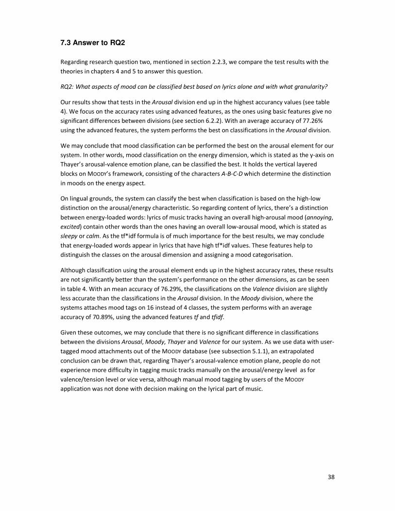
38
7.3 Answer to RQ2
Regarding research question two, mentioned in section 2.2.3, we compare the test results with the
theories in chapters 4 and 5 to answer this question.
RQ2: What aspects of mood can be classified best based on lyrics alone and with what granularity?
Our results show that tests in the Arousal division end up in the highest accurancy values (see table
4). We focus on the accuracy rates using advanced features, as the ones using basic features give no
significant differences between divisions (see section 6.2.2). With an average accuracy of 77.26%
using the advanced features, the system performs the best on classifications in the Arousal division.
We may conclude that mood classification can be performed the best on the arousal element for our
system. In other words, mood classification on the energy dimension, which is stated as the y-axis on
Thayer’s arousal-valence emotion plane, can be classified the best. It holds the vertical layered
blocks on MOODY’s framework, consisting of the characters A-B-C-D which determine the distinction
in moods on the energy aspect.
On lingual grounds, the system can classify the best when classification is based on the high-low
distinction on the arousal/energy characteristic. So regarding content of lyrics, there’s a distinction
between energy-loaded words: lyrics of music tracks having an overall high-arousal mood (annoying,
excited) contain other words than the ones having an overall low-arousal mood, which is stated as
sleepy or calm. As the tf*idf formula is of much importance for the best results, we may conclude
that energy-loaded words appear in lyrics that have high tf*idf values. These features help to
distinguish the classes on the arousal dimension and assigning a mood categorisation.
Although classification using the arousal element ends up in the highest accuracy rates, these results
are not significantly better than the system’s performance on the other dimensions, as can be seen
in table 4. With an mean accuracy of 76.29%, the classifications on the Valence division are slightly
less accurate than the classifications in the Arousal division. In the Moody division, where the
systems attaches mood tags on 16 instead of 4 classes, the system performs with an average
accuracy of 70.89%, using the advanced features tf and tfidf.
Given these outcomes, we may conclude that there is no significant difference in classifications
between the divisions Arousal, Moody, Thayer and Valence for our system. As we use data with user-
tagged mood attachments out of the MOODY database (see subsection 5.1.1), an extrapolated
conclusion can be drawn that, regarding Thayer’s arousal-valence emotion plane, people do not
experience more difficulty in tagging music tracks manually on the arousal/energy level as for
valence/tension level or vice versa, although manual mood tagging by users of the MOODY
application was not done with decision making on the lyrical part of music.
39
8. Conclusion
In this chapter the final conclusions are stated. It goes back to the second chapter, where a problem
statement for this thesis was stated, which in turn was divided into two research questions. In this
chapter these questions are answered, starting in section 8.1 with the answers on the research
questions. Section 8.2 describes the answer on the problem statement, and in section 8.3 a final
conclusion is drawn. Finally, section 8.4 covers the suggestions for future research and limitations in
this thesis.
8.1 Research questions
The answers on RQ1 and RQ2 in sections 7.2 and 7.3 respectively show that the lingual part of music
in the form of lyrics reveal sufficient information to end up with classifications with an average
accuracy of 75% (using advanced features) in automatic mood classifications performed by our
system. We have to take into consideration that with an accuracy of 80% at best, the system still
attaches a wrong mood tag to 1 out of 5 music tracks (see the description on future work in section
8.4). But seen from the point of the lyrical metadata of music solely exposing mood, it proves that
much information for classifying the mood of a music track is stored in the lingual data.
As the classifications are performed using the information extracted out of music lyrics, our test
results show the use of tf*idf techniques and term frequencies as powerful tools for extracting
important information for classification tasks by the system. Lyrical content in the form of words can
describe moods as in spoken or written language. They are highlighted as the terms with high tf*idf
values are important characteristics for a mood class, which in turn is of importance for classification
using k-Nearest Neighbour methods.
Regarding differences in accuracy of classifications by the system between the used mood divisions
Arousal/Moody/Thayer/Valence in this thesis, our test results show that automatic classification on
the arousal aspect (arousal/energy) can be performed the best by our system. The terms extracted
out of the lyrical data in this thesis exposed more information on the arousal aspect, which results in
the best performance in the Arousal dimension.
The linguistic information of music does expose sufficient differences between classes in all mood
divisions for classification, regarding the slight differences in accuracy values between the divisions.
Where tf*idf techniques and term frequencies are seen as powerful tools in the divisions , and being
used as features held responsible for significant better performance of the system, these extracted
features do yield for satisfying classification performances in the Arousal/Moody/Thayer/Valence
divisions.
40
8.2 Problem statement
By analysing the test results and implementing the conclusions on the research questions in section
8.1, we can answer our problem statement. The problem statement mentioned in section 2.2.1
reads:
To what extent is it possible to attach mood tags to songs based on lyrics automatically?
The test results prove that the lingual metadata of music in the form of lyrics provides the system
sufficient information to classify with a system performance of 80% at best. Both term freqencies
and tf*idf values contribute to the highest accuracy rates.
Extracting information out of the lingual metadata of music tracks for basic features, such as
character counts, word counts, and line counts, does not provide the automatic mood classification
system sufficient information to perform with satisfying classification outcomes.
The use of tf*idf values and term frequencies, extracted out of the lingual metadata, contributes to
significantly better performances of the system in the classification stages. With use of these
advanced features the automatic attachment of mood tags based on lyrics can be done in a
sufficient manner with better results in prospect when extending and feeding more extracted
musical metadata to the system.
Regarding the aspects of mood that are classified the best, we may conclude that automatic
attachment of mood tags to songs based on lyrics can be done the best on the arousal/energy
aspect, where the distinction between high arousal (annoying, excited) and low arousal (sleepy,
calm) is made. Classifications on the Moody division with 16 independent classes showed satisfying
results which are significantly higher with implementation of the tf*idf techniques. Finally,
automatic mood classification on both the Thayer and Valence division, show performances that are
slightly less accurate then the best performances in the Arousal division (with the arousal/energy
dimension ranging from low arousal, for example, sleepy or calm, to high arousal, such as
excitement and angriness). Comparing accuracy rates of all divisions, results show that sufficient
information on the arousal aspect or valence aspect (or combinations of these in the Thayer division)
is found in the lingual data.
It can be concluded that the lingual part of music, with the emphasis on using tf*idf techniques,
reveals a large amount of information for automatic mood categorisation on music, but it lacks
additional information for the system in the classifying process for ending up with a high accuracy
regarding the systems’ performance and significant outcomes. More information besides the
analysed features used in this thesis is needed in order to gain better outcomes and improved
classifications. Automatic mood classifications based on the linguistic aspects of music solely does
not yield for satisfying results yet.
41
8.3 Final conclusion
The research presented in this thesis is an attempt to design, implement and evaluate a mood-based
classification system for music based on lyrics. The main goal is the automatic assignment of mood-
based tags for songs in a users’ music database, based on lyrics. By automatically assigning mood
tags to the music properties, users can experience their music without the hassle of assigning mood
properties to all songs in a music collection manually. It can let users simplify the creation of playlists
based on moods, and let them listen to music tracks in a new way and rediscover songs in The Long
Tail in a large music collection.
The results show that the tfidf feature improved the results significantly in this thesis. It shows the
importance of the tf*idf formula for (music) information retrieval fields, as it is a powerful tool to
emphasise the importance of keywords and lexical items regarding the ordening and classification of
instances in classes or hierarchies. This conclusion goes along with the statement by Ramos (2003).
The use of basic features such as word counts do not yield satisfying results, as the system’s
accuracy performs below the baseline.
Although the system’s performance on predicting and assigning mood to music tracks based on lyrics
solely is not suitable (yet) for adequate output, results show that assigning of mood can be done in
an automatic manner without human intervention. It will decrease the effort of creating mood
playlists and can let the listener experience music tracks in a new way. In order to improve the
results, other musical characteristics in the field of music emotion recognition have to be
implemented besides the linguistic part, such as tempo, key or genre. With this added information,
the system’s performance on automatic mood classification for music is likely to be more
progressive.
Taking the description above in consideration, a final conclusion on this research can be drawn. The
system in this thesis, tagging music tracks automatically based on textual grounds, showed
encouraging results with an accuracy of more than 80% using the tfidf- and tf-features. The
outcomes prove that the lingual part of music reveals much information on mood-exposing grounds.
We have to take note that a mean accuracy of 77% on automatic attachment of mood tags based on
lyrics does not offer a bright insight, as we can not compare that value to human performances. If
tagging is performed by humans, standard deviations between users is present. The mood tags
assigned by users of the MOODY application, which were set as the Gold Standard, are influenced by
these standard deviations between humans.
Continuing on this statement, one of the weaknesses in this classification system lies in the use of
only lingual elements of music. With the use of other music characteristics such as key, genre or
tempo, the system’s performance can be enriched and can result in more accurate classifications.
As tools for extracting features out of music tracks (such as tempo and key) are getting more
accurate, and research continues on improving these extraction techniques, accuracy on
classification systems using these features will also improve.
42
8.4 Future research
A number of limitations apply to this research and can be held for future work. First, the
implementation in this thesis was only performed with a database consisting of the gross of lyrics
with English as the main language. Future work is to extend the work by enlarging the lyrics
database with multiple languages. Here we can ask questions about what differences are noticable
regarding tf- and tf*idf values and overall results between languages. Furthermore we could extend
the lyrics sources in order to find and extract more lyrics, and building up a larger database for the
experiments.
Second, we made choices regarding the selection of classes and divisions. The Arousal-, Valence- and
Thayer-division where conducted out of the Moody division/framework, where other classes could
have been used. Choosing other divisions or more specific arrangements by fields of mood could
give new insights.
In this thesis the system works on perfect classifications. Especially in the Moody division, where the
distances between the 16 classes is relatively vague and no specified borders are set, the mood
classification can be tolerable in cases where the system marks the classification as wrong (i.e.
where the system assigned the tag “B1” to a music track instead of “B2”). We did not focus on this
aspect, as it is difficult to compare the individual classifications with the original mood attachments,
which can have a mutually short distance in the classes. Moreover, detailed information on standard
deviation values of the users of the MOODY application can be analysed or implemented to get
insight in the way humans attach mood tags to music tracks.
As mentioned in section 2.2.2, besides lyrics, other kinds of musical information can help expressing
or revealing a certain mood or state of emotion. Although these musical aspects are out of scope for
this thesis, it can give new insights and results when implementing those analysed characteristics in
our system.
One particular aspect of language we did not cope with is ambiguity, which is also present in lyrics of
music tracks. Take for example the Leningrad Cowboys’ track “Happy Being Miserable”, which has an
underlying meaning, like other songs having lyrical content with a broader meaning. This can not be
exposed by the use of term frequency and tf*idf formulas, nor do automatic text analysis programs
provide sufficient outcomes, as language ambiguity is a problem which can only be discovered the
best by humans.
At this point we can not forsee whether it is possible to reach 100% similarity in the future between
automatic mood classifications and manually tagged mood classifications by humans.
Emotions and language are not to be understood by systems the same way it is felt by humans.
The possibilities of extracting more important information out of the lyrical text and ending up with
higher system performances on automatic mood classifications based on the lingual part of music
can be held for future work.
43
In this thesis we had to cope with lots of mood-tagged songs lacking lyrical content: instrumental
music in the database. As we rely on categorisation by analysing the lingual part of music solely, we
had to leave these instances behind. The appearance of instrumental music in this thesis with moods
tagged by users of the MOODY application, slightly confirms that music tracks contain mood
characteristics, even if there is no lingual part in the music track. It supports the conclusions made in
other research fields of music emotion classification that other aspects such as key, genre,
instruments and timbre express moods in music.
The research mentioned in section 2.2.1 has shown that music emotion classification based on
tempo, key and timbre gave significant results. Enriching the used features in this thesis with
acoustic or nonlinguistic data, extracted out of audio files by other music classification tools, would
be a definite improvement on the accuracy in our music mood classification system.
In contrary, this thesis shows that the use of the linguistic part of music, analysed through tf*idf
formulas and other techniques, can be an effective addition to the music emotion classification
techniques already available.
44
References Albert A. (2007). Color hue and mood: The effect of variation of red hues on positive and negative mood states, Journal of
the Behavioral Sciences, Vol. 1, Fall 2007.
Anderson C., Carnagey L., and Eubanks J. (2003). Exposure to Violent Media: The Effects of Songs With Violent Lyrics on
Aggressive Thoughts and Feelings, Journal of Personality and Social Psychology, Vol. 84, Iss. 5; p. 960-971.
Andric A., Haus G. (2006). Automatic Playlist Generation Based On Tracking User’s Listening Habits, Journal of Multimedia
Tools and Applications, Springer Netherlands: Jun 2006, Vol. 29, Iss. 2; p. 127-151.
Barbiere M., Vidal A., and Zellner D. (2007). The Colour of Music: Correspondence Through Emotion, Empirical Studies of
the Arts, Vol. 25, Iss. 2; p. 193-208.
Beale R., Voong M. (2006). Managing Online Music: Attitudes, Playlists, Mood and Colour. Proceedings of HCI 2006:
Engage, ACM 2006, London, p. 113-117.
Beukeboom C. J., Semin G. R. (2005). How mood turns on language. Journal of experimental social psychology, 2006, Vol.
42, Iss. 5; p. 553-566.
Celma O. (2006). Music Recommendation: a multi-faceted approach, Doctoral Pre-Thesis Work, Universitat Pompeu Fabra,
Barcelona, 139 pages.
Celma O., Lamere, P. (2007). Tutorial On Music Recommendation, Eight International Conference on Music Information
Retrieval: ISMIR 2007, Vienna, Austria.
Chastain G., Seibert, P., Ferraro, F. (1995). Mood and Lexical Access of Positive, Negative, and Neutral Words, The Journal
of General Psychology, Vol. 122, Iss. 2; p. 137-157.
Crestani F., Lalmas M., Van Rijsbergen, C.J. (2001). Logic and Uncertainty in Information Retrieval, Lectures on Information
Retrieval, p. 179-206.
Cunningham S., Bainbridge D. and Falconer A. (2006). “More of an Art than a Science”: Supporting the Creation of Playlists
and Mixes, proceedings of the Seventh International Conference on Music Information Retrieval. ISMIR 2006, Victoria,
Canada.
Curry N., Mackay M. (2009). Four found guilty in landmark Pirate Bay case. Online news article, CNN.com Technology,
Cable News Network. Retrieved 20 April 2009, from http://www.cnn.com/2009/TECH/04/17/sweden.piracy.jail/
Daelemans W., Zavrel J., Van der Sloot K. and Van den Bosch A. (2007). TiMBL: Tilburg Memory Based Learner, version 6.1,
Reference Guide. ILK Technological report 07-xx, available from
http://ilk.uvt.nl/downloads/pub/papers/Timbl_6.1_Manual.pdf
Ekman P. (1992). An argument for basic emotions. Cognition & Emotion: Vol 6; p. 169-200.
Feng Y., Zhuang Y. and Pan Y. (2003). Popular Music retrieval by detecting mood, Proceedings of the 26th annual
international ACM SIGIR conference on Research and development in information retrieval, Toronto, Canada, p. 375-376.
Geleijnse G., Sekulovski D., Korst J., Pauws S., Kater B., Vignoli, F. (2008). Enriching music with synchronized lyrics, images
and coloured lights. Proceedings of the 1st international conference on Ambient media and systems, 2008, Quebec,
Canada.
Hansman H., Mulder C., Verhoeff, R. (1999). The Adoption of the Compact Disk Player: An Event History Analysis for the
Netherlands, Journal of Cultural Economics. Akron: Aug 1999. Vol. 23, Iss. 3; p. 221-232.
Haring B. (2000). Beyond the Charts: Mp3 and the Digital Music Revolution, JM Northern Media LLC, 174.
Matravers, D. (2003). The Experience of emotion in music, Journal of Aesthetics and Art Criticism, p. 353-363.
Mc Hugh J. (2003). Why Wi-Fi is a good business?, Wired: Sept 2003; p. 25–26.
45
Meyers O. C. (2007). A Mood-Based Music Classification and Exploration System, McGill University (2004) at the
Massachusetts Institute of Technology, June 2007.
Mitchell T. (1997). Machine Learning, McGraw-Hill, USA, ISBN 0-07-042807-7.
Kim Y. E., Schmidt E. and Emelle L. (2008). Moodswings: A Collaborative Game for Music Mood Label Collection,
proceedings of the Ninth International Conference on Music Information Retrieval: ISMIR 2008, Philadelphia, Pennsylvania,
pp. 231-236.
Koopman C., Davies, S. (2001). Musical meaning in a broader perspective, Journal of Aesthetics and Art Criticism, Vol 59,
Iss. 3; p. 261-273.
Kunej P., Turk I. (2000). New Perspectives on the beginnings of Music: Archaeological and Museological Analysis of a
Middle Paleolithic Bone "Flute". The Origins of Music, Cambridge, MIT Press; p. 235-268.
Laurier C., Herrera P. (2008). Mood Cloud: A Real-Time Music Mood Visualization Tool. CMMR, Computer Music Modeling
and Retrieval, p.163-167.
Lewis L., Dember W., Scheff B. and Radenhausen R. (1995). Can experimentally induced mood affect optimism and
pessimism scores?, Current Psychology, Vol 14, Iss. 1; p. 29-41.
Liu D., Lu L. and Zhang H. (2003). Automatic Mood Detection from Acoustic Music Data. Fourth International Conference on
Music Information Retrieval: ISMIR 2003, Baltimore, Maryland, USA, Johns Hopkins University; p. 13-17.
Oreilly, T. (2007). What is Web 2.0: Design Patterns and Business Models for the Next Generation of Software,
Communications and Strategies, Iss. 1, p. 17. First Quarter 2007. Available at SSRN: http://ssrn.com/abstract=1008839
Pauws S. (2000). Music and Choice: Adaptive Systems and Multimodal Interaction. Doctoral Thesis, Eindhoven University of
Technology, the Netherlands.
Pauws S., Eggen B. (2002). PATS: Realization and user evaluation of an automatic playlist generator. Proceedings of the 3rd
International Conference on Music Information Retrieval: ISMIR 2002, Paris, France.
Philips Research (2008). Research Dossier: Optical Recording. Online article, Philips Research Department, the Netherlands.
Retreived 12 August 2008, from http://www.research.philips.com/newscenter/dossier/optrec/index.html
Piercey C. D., Rioux N. (2008). Inconsistent Mood Congruent Effects in Lexical Decision Experiments. Journal of Articles in
Support of the Null Hypothesis, Vol 5, Iss. 2, p. 19-26.
Ramos J. (2003). Using TF-IDF to Determine Word Relevance in Document Queries, First International Conference on
Machine Learning, 2003, Rutgers University. Available from
http://www.cs.rutgers.edu/~mlittman/courses/ml03/iCML03/papers/ramos.pdf
Robbins S. P., Judge T. A. (2008). Organizational Behaviour, 13th Edition, Prentice Hall, p. 285.
Siemer M. (2005). Moods as multiple-object directed and as objectless affective states: An examination of the dispositional
theory of moods. Cognition & Emotion: January 2008. Vol 22, Iss. 1; p. 815-845.
Thayer R. E. (1982). The Biopsychology of Mood and Arousal, Oxford University Press, USA.
Tonkin E., Corrado E., Moulaison H., Kipp M., Resmini A., Pfeiffer H. and Zhang Q. (2008). Collaborative and Social Tagging
Networks. Ariadne: Jan 2008. Vol. 54. Retreived 4 September 2008, from http://www.ariadne.ac.uk/issue54/tonkin-et-al/
Vander Wal T. (2005). Explaining and Showing Broad and Narrow Folksonomies. Retrieved 6 October 2008, from
http://www.vanderwal.net/random/entrysel.php?blog=1635
Voong M., Beale R. (2007). Music Organisation Using Colour Synaesthesia. CHI ’07: Extended Abstracts; p. 1869-1874.
Yang Y., Liu C. and Chen, H. (2007). Music Emotion Classification: A Fuzzy Approach. Proceedings of the 14th annual ACM
international conference on Multimedia, Santa Barbara, CA, USA; p. 81-84.


![[Mood, mood fluctuations and depression: role of the circadian rhythms]](https://img.pdfslide.net/doc/110x75/6347136162473b71ec01100b/mood-mood-fluctuations-and-depression-role-of-the-circadian-rhythms.jpg)