Embed Size (px)
Citation preview

1
This is the final accepted (prepublication) version of the following article to be published in Psychological Assessment: http://www.apa.org/pubs/journals/pas/index.aspx
This material is copyrighted by the American Psychological Association: http://www.apa.org/about/contact/copyright/seek-permission.aspx.
In compliance with regulations of the American Psychological Association, we note that: This article may not exactly replicate the final version published in the APA journal. It is not the copy of record.
Marsh, H. W., Lüdtke, O., Muthén, B., Asparouhov, T., Morin, A. J. S., Trautwein, U. & Nagengast, B. (in press). A new look at the big-five factor structure through exploratory structural equation modeling. Psychological Assessment, xx, xxx-xxx.
A New Look at the Big-Five Factor Structure through Exploratory Structural Equation Modeling
Herbert W. Marsh, Oxford University, UK
Oliver Lüdtke, Max Planck Institute for Human Development, Berlin Bengt Muthén, University of California, Los Angeles
Tihomir Asparouhov, Muthén & Muthén Inc., Los Angeles Alexandre J.S. Morin, Department of Psychology, University of Sherbrooke
Ulrich Trautwein, Max Planck Institute for Human Development, Berlin Benjamin Nagengast, Oxford University, UK
11 August 2009
5 November, 2009 20 December, 2009
Accepted 8 January 2010
Author note Herbert W. Marsh, Oxford University, UK; Oliver Lüdtke, Max Planck Institute for Human Development, Center for Educational Research; Ulrich Trautwein, Max Planck Institute for Human Development, Center for Educational Research; Tihomir Asparouhov, Muthén & Muthén; Bengt Muthén, University of California, Los Angeles; Alexandre J.S. Morin, Department of Psychology, University of Sherbrooke, Québec, Canada; Benjamin Nagengast, University of Oxford, UK. This research was supported in part by a grant to the first author from the UK Economic and Social Research Council. Two of the coauthors (Tihomir Asparouhov and Bengt Muthén) are associated with Muthén & Muthén Inc., which distributes Mplus used to do the analyses in this investigation. Requests for further information about this investigation should be sent to Professor Herbert W. Marsh, Department of Educational Studies, University of Oxford, 15 Norham Gardens, Oxford OX2 6PY UK; E-mail: [email protected].
New Look Big-Five Factor Structure
2
Abstract
NEO instruments are widely used to assess big-five personality factors, but confirmatory factor
analyses (CFA) conducted at the item-level do not support their a priori structure, due in part, to
the overly restrictive CFA assumptions. We demonstrate that exploratory structural equation
modeling (ESEM), an integration of CFA and EFA, overcomes these problems with responses (n=
3390) to the 60-item NEO-FFI: (a) ESEM fits the data better and results in substantially more
differentiated (less correlated) factors than CFA; (b) tests of gender invariance with the 13-model
ESEM taxonomy of full measurement invariance of factor loadings, factor variance-covariances,
item uniquenesses, correlated uniquenesses, item intercepts, differential item functioning, and
latent means show that women score higher on all NEO big-five factors; (c) longitudinal analyses
support measurement invariance over time and the maturity principle (decreases in Neuroticism,
increases in Agreeableness, Openness and Conscientiousness). Based on ESEM, we addressed
substantively important questions with broad applicability to personality research that could not be
appropriately addressed with either traditional EFA or CFA approaches.

New Look Big-Five Factor Structure
3
Arguably, the most important advance in personality psychology in the past half-century has
been the emerging consensus that individual differences in adults’ personality characteristics can
be organized in terms of five broad trait domains: Extraversion, Agreeableness, Conscientiousness,
Neuroticism, and Openness. These big-five factors now serve as a common language in the field,
facilitating communication and collaboration. Although there are several big-five instruments
(e.g., Benet-Martínez & John, 1998, Caprara & Perugini, 1994; Goldberg, 1990; Gosling,
Rentfrow & Swann, 2003; John & Srivastava, 1999; Paunonen, 2003; Paunonen & Ashton, 2001,
Saucier, 1998), the family of NEO instruments—including 60-item NEO-FFI (Costa & McCrae,
1992; McCrae & Costa, 2004) considered here—appear to be most widely used instruments and to
have received the most attention over recent years (Boyle, 2008).
Factor analysis has been at the heart of these exciting breakthroughs. Exploratory factor
analyses (EFAs) have consistently identified the big-five factors and an impressive body of
empirical research supports their stability and predictive validity (see McCrae & Costa, 1997).
However, confirmatory factor analyses (CFAs) have failed to provide clear support for the five
factor model based on standard measures such as the NEO instruments. For example, in a
particularly relevant study comparing EFA and CFA factor structures based on NEO-PI responses,
Vassend and Skrondal (1997) reported highly discrepant findings leading them to conclude: “(i)
that the original NEO-PI model as well as later EFA-based revisions are false or at least
unsatisfactory, and (ii) that at present we do not know how the NEO-PI scales should be modelled
with the aim of obtaining a common, acceptable NEO-PI version.”(p. 157). Problematic results
based on CFAs have led some researchers to question the appropriateness of CFA for big-five
research (see Borkenau & Ostendorf, 1990; Church & Burke, 1994; McCrae, Zonderman, Costa,
Bond & Paunonen, 1996; Parker, Bagby & Summerfeldt, 1993; Vassend & Skrondal, 1997).
However, many of the methodological and statistical advances in quantitative psychology in the

New Look Big-Five Factor Structure
4
last two decades are associated with latent-variable approaches such as CFA and structural
equation models (SEMs). Hence, failure to embrace these new and evolving methodologies
(throwing the baby out with the bathwater) would have dire consequences—particularly for a field
of research so fundamentally based on factor analysis. Indeed, assumptions of factorial and
measurement invariance (in relation to multiple groups, time, covariates, and outcomes) that
underpin nearly all big-five studies cannot be appropriately evaluated with traditional approaches
to EFA and thus have been largely ignored in big-five EFA research. Here we outline a new
approach to factor analysis – an integration of EFA and CFA – that has the potential to resolve this
dilemma and has wide applicability to all disciplines of psychology that are based on the
measurement of latent constructs. Thus, our study is a substantive-methodological synergy (Marsh
& Hau, 2007), demonstrating the importance of applying new and evolving methodological
approaches to substantively important issues.
Methodological Focus: Exploratory Structural Equation Modeling (ESEM)
EFA versus CFA.
Many measurement instruments used in psychological assessment apparently have well-defined
EFA structures, but are not supported by CFAs (Marsh, Muthén, Asparouhev, Ludtke, Robitzsch,
Morin & Trautwein, 2009). This concern led McCrae et al (1996, p.568) to conclude: In actual
analyses of personality data from Borkenau and Ostendorf (1990) to Holden and Fekken (1994),
structures that are known to be reliable showed poor fits when evaluated by CFA techniques. We
believe this points to serious problems with CFA itself when used to examine personality structure
(also see Costa & McCrae, 1992; 1995; McCrae & Costa, 1997). Church and Burke (1994)
similarly concluded on the basis of their empirical research that: Poor fits of a priori models
highlighted not only the limited specificity of personality structure theory, but also the limitations
of confirmatory factor analysis for testing personality structure models (p. 93). They argued that

New Look Big-Five Factor Structure
5
the independent clusters model (ICM) used in CFA studies that requires each indicator to load on
only one factor is too restrictive for personality research, as indicators are likely to have secondary
loadings unless researchers resort to using a small number of near synonyms to infer each factor.
Consistent with these concerns, Marsh et al. (2009) claimed that many ad hoc strategies used to
compensate for the inappropriateness of CFA in psychological research more generally are
dubious, counterproductive, misleading, or simply wrong. Of particular relevance to the present
investigation, the inappropriate imposition of zero factor loadings usually leads to distorted factors
with positively biased factor correlations that might lead to biased estimates in SEMs
incorporating other constructs (also see Marsh, et al., 2009). In a similar vein, Marsh (2007;
Marsh, Hau & Grayson, 2005) concluded that many psychological instruments used in applied
research do not even meet minimum criteria of acceptable fit according to current standards.
Apparently, many applied researchers persist with inappropriate ICM-CFA models because
they believe that EFA approaches are out-dated and that methodological advances associated with
CFAs are not applicable to EFAs. Here we demonstrate how it is possible to apply EFA rigorously
in a way that allows researchers to define more appropriately the underlying factor structure, and
still apply the advanced statistical methods typically associated with CFAs and SEMs. This is
accomplished with the ESEM procedure recently implemented in the Mplus statistical package
(version 5.2, Muthén & Muthén, 2008). Within the ESEM framework, the applied personality
researcher has access to typical SEM parameter estimates, standard errors, goodness-of-fit
statistics, and statistical advances normally associated with CFA and SEMs (see Asparouhov &
Muthén, 2009; Marsh et al., 2009). Here we apply ESEM to NEO-FFI responses.
Tests of Factorial and Measurement Invariance.
Particularly for research based on the NEO-FFI instrument used to measure the big-five
personality factors, we know of no CFAs carried out at the item level that provides acceptable

New Look Big-Five Factor Structure
6
support for the a priori big-five factor structure. This is remarkable, given the wide-spread
acceptance of the big-five factor structure and the NEO-FFI. Hence, it is not surprising that
research into the big-five factor structure on responses to individual items continues to be based
almost entirely on EFA (for exceptions, see Benet-Martinez & John, 1998; Dolan, Oort, Stoel &
Wichterts, 2009; Gunnarsson & Ostensson, 2008; Gustavsson, Eriksson, Hilding, 2008; also see
Reise, Smith & Furr, 2001). We suggest that this failure to apply CFA models in big-five research
is due in large part to the inappropriateness of the typical ICM-CFA structure. Although
identification of the appropriate factor structure is very important in its own right, there are many
other important advantages to the use of CFA that cannot be easily incorporated into EFA and thus
have been largely ignored in big-five personality research. Thus, for example, studies that use big-
five scale scores (or factor scores based on EFAs) are not corrected for measurement error.
Although it is possible to correct for a very simple form of measurement error (i.e., the typical
correction for attenuation based on reliability estimates), in many applications the error structure is
more complex (e.g., longitudinal studies as considered here) so that the typical correction for
attenuation is not sufficient.
A particularly important application of CFA techniques is to test the assumptions about the
invariance of the big-five factor structure over multiple groups or over time (Gustavsson et al.,
2008; Nye, Roberts, Saucier & Zhou, 2008; Riese, et al., 2001). Unless the underlying factors are
measuring the same construct in the in the same way and the measurements themselves are
operating in the same way (across groups or over time), mean differences and other comparisons
are likely to be invalid. Although some aspects of factor similarity can be addressed in part with
EFA approaches (e.g., the similarity of the factor loadings), most cannot. In particular, an
important assumption in the comparison of big-five factors over different groups (e.g., men and
women) or over time is the invariance of item intercepts. More specifically, it is important to

New Look Big-Five Factor Structure
7
ascertain that mean differences based on latent constructs (big-five factors) are reflected in each of
the individual items used to infer the latent constructs. For example, if the apparent level of gender
differences on Extraversion varies substantially from item to item for different items used to infer
this construct, then the gender differences based on the corresponding latent construct are
idiosyncratic to the particular items used to infer Extraversion. Similarly, if responses to individual
Extraversion items differ systematically with age (for different respondents) or over time (for the
same respondents), then findings based on comparisons of scale scores might be invalid. In each
case, these results would suggest that conclusions about differences in Extraversion do not
generalize over even the set of items used in the instrument – let alone the population of items that
could have been used. Hence, conclusions about differences in Extraversion might be idiosyncratic
to the particular set of items and not be generalizable. From this perspective, it is important to
evaluate the invariance of different aspects of the factor structure at the level of the individual
item. Although issues of non-invariance of item intercepts (hereafter referred to as differential item
functioning) are well known in evaluating the appropriateness of standardized achievement tests,
these issues have been largely ignored in big-five research (but see Jackson, Bogg, Walton, Wood,
Harms, Lodi-Smith & Roberts, 2009; Nye, Roberts, Saucier & Zhou, 2008; Reise, et al., 2001).
Substantive Focus on Big-Five Personality Factors and the NEO-FFI
Gender Differences in Personality Traits.
There is a long history of the search for gender differences in personality research (e.g.,
Feingold, 1994; Hall, 1984; Maccoby & Jacklin, 1974). Noting that Feingold (1994) had organized
his review in part on the basis of the five broad factors and 30 facets of the NEO personality
inventory, Costa, Terracciano and McCrae (2001) greatly expanded the research based on the 30
facets measured by the NEO-PI-R for responses from 26 countries (N=23,031). Interestingly, they
found that gender differences within the set of six facets comprising each of the big-five factors

New Look Big-Five Factor Structure
8
were not entirely consistent. Women had consistently higher scores across six facets representing
Neuroticism and Agreeableness, whilst gender differences were consistently small for
Conscientiousness. However, gender differences were less consistent for Extraversion and
Openness; for each of these big-five factors at least two (of 6) facets favored women and at least
two favored men. Hence, the size and even the direction of gender differences would differ
depending on which facet (or mix of facets) was considered. Thus, even at the facet level there is
apparently differential item (facet) functioning for some of the big-five factors that compromises
conclusions based on big-five measures that are aggregated across facets. Logically, this implies
that there is also likely to be differential item functioning at the level of individual items in relation
to gender differences for NEO-FFI responses considered here.
Although there is considerable study-to-study variation in observed gender differences that may
be a function of age, nationality, and the particular instrument considered, there is clear support for
the conclusions that women tend to score higher than men in relation to Neuroticism and
Agreeableness. Although less consistent, there is also evidence that women score higher on
Conscientiousness and Extraversion, but no clear support for evidence of gender differences in
Openness. There is no evidence that men score higher than women on any of the big-five factors
as measured and labeled on the NEO-FFI (although women’s higher scores on Neuroticism are
sometimes summarized as lower scores on emotional stability). Particularly relevant to the current
study (based on late-adolescent responses by Germans), Schmitt, Realo, Voracek and Allik (2008)
reported that for their German sample (N=790), women scored higher than men did on all big-five
factors: Neuroticism (effect size = d=.48), Extraversion (d=.12), Agreeableness (d=.09),
Conscientiousness (d=.23), and Openness (d=.11). Similarly, Donnellan and Lucas (2008) also
found that for the late-adolescent sample (aged 16-19) most relevant to the present investigation,

New Look Big-Five Factor Structure
9
German women consistently scored higher than German men: Neuroticism (d=.47), Extraversion
(d=.24), Agreeableness (d=.31), Conscientiousness (d=.34), and Openness (d=.36).
Longitudinal Invariance: Stability and Change in Personality Traits.
The literature on personality development distinguishes several types of personality change and
continuity (Caspi & Shiner, 2006; Lüdtke, Trautwein & Husemann, 2009). Here we distinguish
between correlational (rank-order stability), mean-level stability, and structural stability over time.
For correlational (rank-order) stability, cross-sectional and longitudinal research (Roberts &
DelVecchio, 2000; see also Fraley & Roberts, 2005; Klimstra, Hale, Raaijmakers, Branje &
Meeus, 2009; Lüdtke et al., 2009) shows that correlational stability increases with age, particularly
for the middle-to-late adolescent period that is the focus of the present investigation.
Studies of mean-level change with respect to lifespan changes in Big-five traits show that most
people become more dominant, agreeable, conscientious, and emotionally stable. Caspi, Roberts,
and Shiner (2005) coined the term maturity principle to describe these findings of increasing
psychological maturity from adolescence to middle age. In their meta-analysis of longitudinal
studies, Roberts, Walton, and Viechtbauer (2006) also found substantial increases in Openness.
For the 18- to 22-year age group most relevant to the present investigation, Robins, Fraley,
Roberts & Trzesniewski (2001) found Agreeableness (d = .44), Conscientiousness (d = .27), and
Openness (d = .22) to increase over a 4-year period and Neuroticism (d = –.49) to decrease. No
statistically significant change was found for Extraversion. In summary, although results from
these studies are not entirely consistent, there is general support for the maturity principle of
increases in all big-five factors (or decreases in Neuroticism instead of increases in Emotional
Stability) except, perhaps, for Extraversion.
Structural stability assesses the extent to which the same factors are being assessed in different
groups or over time. At least some level of structural invariance is a prerequisite for assessing

New Look Big-Five Factor Structure
10
either mean differences between groups or stability over time. If the nature of the factors changes
so that factors are qualitatively different, then interpretations of stability over time are
questionable. It is most appropriate to evaluate factorial and measurement invariance based on
responses to individual items. However, personality researchers have been remarkably
unsuccessful in obtaining acceptable levels of goodness of fit for the a priori big-five factor CFA
structure when based on responses to individual items in studies of the NEO-FFI instrument
considered here. Indeed, this might be considered as the major limitation in big-five personality
research, particularly in relation to testing assumptions underpinning the valid assessment of
stability over time as well as the valid comparison of latent means across groups. For this reason
some studies have sought to formally test full measurement invariance based on mean responses
averaged across different items; facet scores (e.g., Gignac, 2009; McCrae et al., 1996; Saucier,
1998; Small, Hertzog, Hultsch & Dixon, 2003), parcel scores (Allemand, Zimprich & Hendriks,
2008; Allemand, Zimprich & Hertzog, 2007; Lüdtke et al., 2009; Marsh, Trautwein, Lüdtke,
Köller & Baumert, 2006), or scale scores (e.g., Mroczek & Spiro, 2003). Although potentially
useful, there are important limitations to these analyses when conducted without prior verification
of measurement invariance at the item level–an assumption underlying tests of mean differences
(over time or across groups) and differential item functioning that could compromise the validity
of interpretations based analyses of aggregated scores (see later discussion for further elaboration).
In the present investigation, we address these concerns, introducing a new ESEM approach that
integrates the logic of EFA approach typically used in big-five personality research and the CFA
approach widely argued to be inappropriate to big-five research.
The Present Investigation: A Substantive Methodological Synergy.
Our study is a substantive-methodological synergy, demonstrating the power and flexibility of
ESEM methods that integrate CFA and EFA (based on the Mplus statistical package, Muthén &

New Look Big-Five Factor Structure
11
Muthén, 2008) to address substantively important issues about the big-five factor structure based
on responses to the 60-item NEO-FFI instrument. We begin by comparing CFA and ESEM
approaches, testing the assumption that ESEM models fit better than corresponding CFA models.
For both CFA and ESEM models we include both freely estimated uniquenesses (reflecting a
combination of measurement error specific variances) and a priori correlated uniquenesses (CUs;
covariances between the specific variance components associated with two different items from
the same big-five facet). Big-five theory posits that the big-five factors should be reasonably
orthogonal, but constraining all (non-target) cross-loadings to be zero in the ICM-CFA model is
posited to systematically inflate and bias estimates of the factor correlations. Hence support for the
prediction that big-five factors are reasonably orthogonal is hypothesizsd to be stronger in ESEM
models than in the CFA models.
We then extend ESEM to test a 13-model taxonomy of measurement invariance, testing
invariance of factor loadings, factor variances-covariances, item uniquenesses, CUs, item
intercepts, and latent means–with a specific focus on gender differences in the latent means of the
big-five factors. Of particular interest are tests of the invariance of item intercepts that are an
implicit assumption in the comparison of latent (or manifest) group means, but largely ignored in
previous big-five research (but see Jackson et al., 2009; Nye, et al., 2008; Reise, et al., 2001).
Based on previous research we expect systematic differences, mostly reflecting higher means for
women (particularly for the late-adolescent German sample considered here). Consistent with
previous research we also predict that there is differential item functioning in NEO-FFI responses
(non-invariance of item intercepts) that would compromise the interpretation of latent mean
comparisons, but explore alternatives to circumvent this problem.
Finally, we apply ESEM to test-retest data, testing a set of models of measurement invariance
over time with the inclusion of CUs relating responses to the same item on multiple occasions.
New Look Big-Five Factor Structure
12
Although these (within-group) tests of longitudinal invariance largely parallel those based on
(between-group) tests over gender, the substantive implications are quite different. Indeed, given
that participants are in their final year of high school at Time 1 and several years after graduation
at Time 2, it is reasonable that there might be systematic changes in big-five latent means. Based
on the maturity principle, we expect decreases in Neuroticism and increases in Agreeableness,
Openness and Conscientiousness.
Previous research has suggested a problem with the evaluation of stability over time for NEO-
FFI responses that is especially relevant to the present investigation. NEO-FFI responses
consistently have high levels of short-term test-retest stability (.86 -.90; McCrae & Costa, 2004;
Robins et al, 2001), and internal consistency (.68-.86; Costa & McCrae, 1992). However, this
research suggests problems associated with a complex error structure in that test-retest correlations
are larger than internal consistency measures of reliability. In particular, test-retest correlations
would be greater than 1.0 if corrected for (internal consistency) unreliability. This suggests that
observed test-retest correlations are more positively biased by correlated uniquenesses associated
with specific variances of the same items administered on different occasions than negatively
biased by the failure to control for measurement error in the factors. Traditional EFA approaches
are unable to appropriately distinguish between measurement error on each occasion, correlated
uniquenesses over time, and true stability of latent traits over time, but these issues can been
addressed by ESEM as demonstrated in the present investigation.
Methods
Participants
The data come from a large, ongoing German study (Transformation of the Secondary School
System and Academic Careers; TOSCA; see Köller, Watermann, Trautwein, & Lüdtke, 2004; also
see Lüdtke et al., 2009; Marsh et al., 2006). A random sample of 149 upper secondary schools in a

New Look Big-Five Factor Structure
13
single German state was selected to be representative of the traditional and vocational gymnasium
school types attended by the college-bound student population. At Time 1 (T1), the students (n=
3390, 45% men, 55% women) were in their final year of upper secondary schooling (M age =
19.51, SD = 0.77). Two trained research assistants administered materials in each school and
students participated voluntarily, without any financial incentive. At T1, all students were asked to
provide written consent to be contacted again later for a second wave of data collection. At Time 2
(T2), two years after graduation from high school, participants completed an extensive
questionnaire taking about two hours in exchange for a financial reward of 10 Euro.
For evaluation of longitudinal stability, our analyses are restricted to the responses by the 1570
(39% men, 61% women) students who completed the NEO-FFI at both T1 and T2. To test for
attrition effects, we compared continuers, who participated at both time points, to drop outs, who
only participated in the first wave. Continuers had slightly lower grade point averages (M=2.5 vs.
2.3) and were more likely to be female. Selectivity effects exceeding d =.10 were found for two of
the big-five scale scores; continuers had higher Conscientiousness and Agreeableness scores.
Although drop-outs and continuers differed statistically significantly in some domains, the
magnitude of these differences was small and indicative of only small selectivity effects. As part
of the analysis, we also compare factor structures based on all students at T1 as well as those who
completed instruments at both T1 and T2.
Measures: Big-Five dimensions.
The 60-item NEO-FFI (Costa & McCrae, 1992) provides a short measure of the big-five
personality factors (Costa & McCrae, 1989). For each factor, McCrae and Costa (1989) selected
12 items from the 180 items of the longer NEO-PI (and the full 240-item NEO-PI-R), based
primarily on correlations between each NEO-PI item and factor scores (McCrae & Costa, 1989).
We measured the Big-five factors using the German version (Borkenau & Ostendorf, 1993) of the

New Look Big-Five Factor Structure
14
NEO-FFI whose responses have high reliability, validity, and comparability with responses to the
original English-language version (e.g., Borkenau & Ostendorf, 1993). In our study, items were
rated on a 4-point scale from 1 = strongly disagree to 4 = strongly agree. Psychometric analyses of
the 4-point response format show that this format has some advantages over a 5-point scale
(Lüdtke, Trautwein, Nagy, & Köller, 2004). Coefficient alpha reliabilities at the two points of
measurement were .78 and .80 (Extraversion), .72 and .73 (Agreeableness), .83 and .84
(Conscientiousness), .83 and .87 (Neuroticism), and .73 and .74 (Openness to Experience). Hence,
consistent with previous research (e.g., Church & Burke, 1994; McCrae et al., 1996), there are
small increases in reliability with increased age during this late-adolescent period.
Statistical Analyses.
Analyses were conducted with Mplus (version 5.2, Muthén & Muthén, 2008). Preliminary
analyses consisted of a traditionnel CFA based on the Mplus robust maximum likelihood estimator
(MRL) with standard errors and tests of fit that are robust in relation to non-normality and non-
independence of observations (Muthén & Muthén, 2008). The main focus is on the application of
ESEM to responses to the 60-item NEO big-five personality instrument. The ESEM approach
differs from the typical CFA approach in that all factor loadings are estimated, subject to
constraints so that the model can be identified (for further details of the ESEM approach and
identification issues, see Supplemental Appendix 1; also see Asparouhov & Muthén, 2009). Here
we used an oblique geomin rotation (the default in the Mplus) with an epsilon value of .5 and the
MLR estimation. A critical advantage of the ESEM approach is the ability to test full measurement
invariance for an EFA solution in relation to multiple groups or occasions.
Factorial and Measurement invariance. Marsh et al. (2009) proposed a 13-model
taxonomy of invariance tests that integrated factor analysis (e.g., Jöreskog & Sörbom, 1988;
Marsh, 1994; 2007) and measurement invariance (e.g., Meredith, 1964; 1993; Meredith & Teresi,
New Look Big-Five Factor Structure
15
2006) traditions to testing invariance over multiple groups or occasions. Following the
measurement invariance tradition, we use terminology proposed by Meredith (1964, 1993) that has
achieved broad acceptance. Although tests of invariance are frequently based on covariance
matrices emerging from the factor analysis tradition, tests of full measurement invariance begin
with raw data (or mean augmented covariance matrices) and should be done at the item level to
evaluate item functioning
In the Meredith (1964, 1993) tradition, the sequence of invariance testing generally begins
with a model with no invariance of any parameters estimates (i.e., all parameters are freely
estimated) such that only similarity of the overall pattern of parameters is evaluated (configural
invariance). Technically, this model might not be an invariance model in that it does not require
any estimated parameters to be the same. However, it does provide a test of the ability of the a
priori model to fit the data in each group (or occasion) without invariance constraints and a
baseline for comparing other models that do impose equality constraints on the parameter
estimates across groups or over time. Configural invariance models are followed by tests of Weak
measurement invariance that are satisfied if factor loadings are invariant over groups or occasions,
although Byrne, Shavelson and Muthén (1889) also argued for the usefulness of a less demanding
test of partial invariance in which some parameter estimates are not constrained to be invariant.
Strong measurement invariance is satisfied if the indicator means (i.e. the intercepts of responses
to individual items) and factor loadings are invariant over groups. If factor loadings and item
intercepts are invariant over groups, then changes in the latent factor means can reasonably be
interpreted as changes in the latent constructs. Strict measurement invariance is satisfied if factor
loadings, item intercepts, and item uniquenesses are all invariant across groups or over time. Strict
measurement invariance is required in order to compare big-five scale (manifest) scale scores (or

New Look Big-Five Factor Structure
16
factor scores) over time or across different groups. As comparisons based on latent constructs are
corrected for measurement error, they only require strong measurement invariance.
The taxonomy of 13 partially nested models (Marsh, et al., 2009) expand this measurement
invariance tradition; models vary from the least restrictive model of configural invariance with no
invariance constraints to a model of complete invariance that posits strict invariance as well as the
invariance of the latent means and of the factor variance-covariance matrix (Table 1; for a more
extended discussion of these issues, see also Marsh, et al., 2009). All models except the configural
invariance model (Model 1) assume the invariance of factor loadings, but it is possible to test – for
example – the invariance of indicator uniquenesses with or without the invariance of item
intercepts. However, models with freely estimated indicator intercepts and freely estimated latent
means are not identified. So in models with freely estimated intercepts, the latent means are fixed
to be zero. Then, when the intercepts are constrained to equality across groups (or occasions), the
latent means are constrained to be zero in one group (or occasion) and freely estimated in the
second group (or occasion). In this manner, the latent means in the second group (or occasion) and
their statistical significance reflect the differences between the two groups (or occasions).
Here we demonstrate the application of tests of measurement invariance over gender and across
time based on our taxonomy of invariance tests (Table 1). Such tests have typically used
SEM/CFA. Related multiple group methods have been proposed for EFA (e.g., Cliff, 1966;
Meredith, 1964), but they mainly focus on the similarity of factor patterns rather than formal tests
of invariance (but also see Dolan et al., 2009). However, the ESEM model can be extended to
multiple groups or longitudinal analyses such that the ESEM solution is estimated separately for
each group or occasion and parameters can be constrained to be invariant across groups or over
time (Marsh, et al., 2009; also see Supplemental Appendix 1).

New Look Big-Five Factor Structure
17
Correlated Uniquenesses (CUs). In general, the use of ex-post facto CUs should be avoided
(e.g., Marsh, 2007), but there are some circumstances in which a priori CUs should be included.
When the same items are used on multiple occasions, there are likely to be correlations between
the unique components of the same item administered on the different occasions that cannot be
explained in terms of correlations between the factors. Indeed, Marsh and Hau (1996; Marsh,
2007), Jöreskog (1979), and others argue that the failure to include these CUs is likely to
systematically bias parameter estimates such that test-retest correlations among matching latent
factors are systematically inflated, which can then systematically bias other parameter estimates
(especially in SEMs). In the extreme, test-retest correlations might be so substantially inflated that
the failure to include appropriate CUs can result in improper solutions such as a non-positive
definite factor variance-covariance matrix or estimated test-retest correlations that are greater than
1.0 (e.g., Marsh, Martin & Debus, 2001; Marsh, Martin & Hau, 2006). Previous research showed
that short-term test-retest correlations for NEO-FFI factors are systematically larger than internal
consistency estimates of reliability so that disattenuated test-retest correlations would be greater
than 1.0 (see earlier discussion). This suggests that there are likely to be substantial CUs test-retest
data considered here. For this reason, Marsh and Hau argued that CUs relating responses to the
same items on different occasions should always be included in the a priori model, but it is easy to
evaluate the extent to which the exclusion of these a priori CUs affects the fit of the model and the
nature of parameter estimates (particularly test-retest stability coefficients) by constraining them to
be zero. Importantly it is difficult to either test or correct complex structures of measurement error
with EFAs and scale scores typically used in big-five research.
As described in more detail by McCrae and Costa (2004), in the NEO-PI-R (with 240 items)
each of the big-five factors was represented by six facets and each facet was represented by
multiple items. However, in the construction of the (short) NEO-FFI, items were selected to best

New Look Big-Five Factor Structure
18
represent each of the big-five factors without reference to the facets. More specifically, each big-
five factor was represented by a factor score (based on an EFA with varimax rotation) and items
were selected that were most highly correlated with this factor score. Hence, some facets are over-
represented (relative to the design of the full NEO-PI-R) whilst other facets are represented by a
single item or not represented at all. We posited that items that came from the same facet of a
specific big-five factor would have higher correlations than items that came from different facets
of the same big-five factor – beyond correlations that could be explained in terms of the common
big-five factor that they represented. Here we modeled these potentially inflated correlations due
to facets as CUs relating each pair of items from the same facet. Based on the mapping NEO-FFI
items onto the NEO-PI-R facets (Paul Costa, personal communication, 2009; also see
Supplemental Appendix 2), this resulted in an a priori set of 57 CUs inherent to the design of the
NEO-FFI. Although we argue that this set of a priori CUs should be included in all factor analyses
of NEO-FFI responses, we systematically evaluate models with and without these CUs as well as
the invariance of these CUs over multiple (gender) groups and over time.
Goodness of fit. CFA/SEM research typically focuses on the ability of a priori models to fit the
data as summarized by sample size independent indexes of fit (e.g., Marsh, 2007; Marsh, Balla &
Hau, 1996; Marsh, Balla, & McDonald, 1988; Marsh et al., 2005). Here we consider the Root
Mean Square Error of Approximation (RMSEA), the Tucker-Lewis Index (TLI), and the
Comparative Fit Index (CFI), as operationalized in Mplus in association with the MLR estimator
(Muthén & Muthén, 2008). We also considered the robust χ2 test statistic and evaluation of
parameter estimates. For the TLI and CFI values greater than .90 and .95 typically reflect
acceptable and excellent fit to the data. For the RMSEA values of less than .05 and .08 reflect a
close fit and a reasonable fit to the data, respectively (Marsh, Hau, & Wen, 2004). However, we
emphasize that these cut-off values only constitute rough guidelines; there is considerable

New Look Big-Five Factor Structure
19
evidence that realistically large factor structures (e.g., instruments with at least 50 items and at
least 5 factors) are typically unable to satisfy even the minimally acceptable standards of fit
(Marsh, 2007; Marsh et al., 2005; also see Marsh, Hau, Balla & Grayson, 1998). However,
because there are very few applications of ESEM – and none that fully evaluate the
appropriateness of the traditional CFA indexes of fit – it is unclear as to how relevant these CFA
indexes and proposed cut-off values are for ESEM studies (Marsh, et al., 2009).
In CFA studies it is typically more useful to compare the relative fit of a taxonomy of of
nested (or partially nested) models designed a priori to evaluate particular aspects of interest than
single models (Marsh, 2007; Marsh, et al., 2009). Any two models are nested so long as the set of
parameters estimated in the more restrictive model is a subset of the parameters estimated in the
less restrictive model. This comparison can be based on a chi-square difference test, but this test
suffers the same problems as the chi-square test used to test goodness of fit that led to the
development of fit indexes (see Marsh et al., 1998). For this reason, researchers have posited a
variety of ad hoc guidelines to evaluate when differences in fit are sufficiently large to reject a
more parsimonious model (i.e., the more highly constrained model with fewer estimated
parameters) in favor of a more complex model. It has been suggested that support for the more
parsimonious model requires a change in CFI of less than .01 (Chen, 2007; Cheung & Rensvold,
2002) or a change in RMSEA of less than .015 (Chen, 2007). Marsh (2007) noted that some
indexes (e.g., TLI and RMSEA) incorporate a penalty for parsimony so that the more
parsimonious model can fit the data better than a less parsimonious model (i.e., the gain in
parsimony is greater than the loss in fit). Hence, a more conservative guideline is that the more
parsimonious model is supported if TLI or RMSEA is as good as or better than that for the more
complex model. Nevertheless all these proposals should be considered as rough guidelines or rules
of thumb.

New Look Big-Five Factor Structure
20
Especially in relation to the taxonomy of invariance tests, support for the invariance of a
set of parameters should be based in part on the similarly of parameters in models that do not
impose invariance constraints as well as the goodness of fit for models that do. Here, we focus on
both the similarity of the patterns of parameters and the levels of the parameter estimates. For
example, here we evaluate the similarity of factor loadings based on various CFA and ESEM
models–whether the same item has a relatively high or low factor loading across different groups
(or occasions)–with a profile similarity index (PSI). To compute the PSI we simply construct a
column that contains all the factor loadings for one group and a second column of corresponding
factor loadings for the second group, and then correlate the values from the two columns. Hence
the PSI is merely the correlation between the two sets of factor loadings. To evaluate levels of the
parameter estimates, we compare descriptive statistics for the set of coefficients in each group.
Ultimately, however, an evaluation of goodness of fit must be based upon a subjective integration
of many sources of information, including fit indexes, a detailed evaluation of parameter estimates
in relation to a priori hypotheses, previous research, and common sense.
RESULTS
Big-Five Factor Structure: ESEM versus CFA
The starting point for the present investigation is to test our a prior hypothesis that the
ESEM model provides a better fit to NEO-FFI responses than a traditional ICM CFA model.
Indeed, as emphasized by Marsh et al. (2009), the ESEM analysis is predicated on the assumption
that ESEM performs noticeably better than the ICM-CFA model in terms of goodness of fit (Table
2) and the construct validity of the interpretation of the factor structure.
The ICM-CFA solution does not provide an acceptable fit to the data (TLI = .672; CFI =
.685; see TGCFA1A in Table 2), consistent with previous research. The next model (TGCFA1B)
incorporates a priori CUs (based on the facet structure of the NEO-PI-R; see earlier discussion and

New Look Big-Five Factor Structure
21
Supplemental Appendix 2); results are still inadequate, albeit improved (TLI = .731; CFI = .750).
The corresponding ESEM solutions fit the data much better. Although the fit of total group with
no a priori CUs is still not acceptable (TGESEM1A: TLI = .821; CFI = .851; Table 2), the
inclusion of CUs results in a marginally acceptable fit to the data (TGESEM2A: TLI = .893; CFI =
.914; RMSEA = .028).
It is also instructive to compare parameter estimates based on the ICM-CFA and ESEM
solutions (Supplemental Appendix 3). In both types of models, the factor loadings tend to be
modest, with few factor loadings greater than .7 and some factor loadings less than .30. Although
CFA factor loadings (Mdn = .47) are slightly higher than for the ESEM model (Mdn = .46), the
differences are typically very small and the pattern of factor loadings is very similar for the CFA
and ESEM solutions. To quantify this subjective evaluation we computed a PSI in which the
vector of 60 CFA factor loadings was related to the corresponding vector of 60 EFA target
loadings. The PSI (r = .87) demonstrated that ESEM and CFA factor loadings were highly related.
Consistent with McCrae and Costa (2004), the 14 items that they noted as potentially weak also
had lower factor loadings than the remaining 56 items for both ICM-CFA (M = .38 vs. .49) and
ESEM (M = .32 vs. .48) solutions. Although a few of these 14 items performed well here, we note
that these same items also did well in the original McCrae and Costa study. Importantly, almost all
60 items load more positively on the ESEM factor each was designed to measure and less
positively on all other factors.
A detailed evaluation of the factor correlations among the big-five factors demonstrates a
critical advantage of the ESEM approach over the ICM-CFA approach. Although patterns of
correlations are very similar, the CFA factor correlations (-.502 to +.400; Mdn absolute value =
.197) tend to be systematically larger than the ESEM factor correlations (-.205 to +.140; Mdn
absolute value = .064). Thus, for example, the negative correlation between Neuroticism and

New Look Big-Five Factor Structure
22
Extraversion is -.502 based on the CFA solution but only -.205 for the ESEM solution. Similarly,
the correlation between Extraversion and Conscientiousness is +.400 for the CFA results, but only
+.104 for the ESEM results. In this respect, the ESEM solution is more consistent with a priori
predictions that the big-five personality factors are reasonably orthogonal.
Clearly the ESEM solution is superior to the CFA solution, both in terms of fit and
distinctiveness of the factors that is consistent with big-five theory. The comparison of results
from these two models provides the initial and most important test for the appropriateness of the
ESEM model – at least relative to the CFA model. It is also important to emphasize that the
goodness of fit for the ESEM model is apparently far better than what has ever been achieved in
previous research with the NEO-FFI based on factor analyses conducted at the item level.
Invariance over Gender
How stable is the NEO-FFI factor structure over gender? Are there systematic gender
differences in latent means and are the underlying assumptions met that are needed to justify
interpretations of these results? To address these questions, we applied our taxonomy of 13 ESEM
models (Table 1). The basic strategy is to apply the set of 13 models designed to test different
levels of factorial and measurement invariance, ranging from the least demanding model that
imposes no invariance constraints (configural invariance) to the most demanding model that posits
complete gender invariance in relation to the big-five factor structure, latent means, and item
intercepts. However, application of this taxonomy of models is complicated by two features that
are partially idiosyncratic to this application; the a priori CUs and tests of partial invariance of
item intercepts (Byrne et al., 1989). The results already presented based on the total sample
indicate that a priori CUs are necessary to achieve even a minimally acceptable fit to the data.
However, it is also important to determine the extent to which these a priori CUs are invariant over
gender and how these influence the behavior of the various models.
New Look Big-Five Factor Structure
23
For all 13 models we begin by evaluating the 57 a priori CUs. Hence, we first test models
with no CUs (e.g., MG1 in Table 2 corresponds to the first model in the invariance taxonomy in
Table 1). We then test two additional variations in which the a priori CUs are allowed to vary for
men and women (submodels labelled “A” in Table 3 as in MG1A) and a corresponding submodel
in which the CUs are constrained to be invariant over responses by men and women (submodels
labelled “B” in Table 3 as in MG1B). Hence, within this set of three submodels there is a
systematic nesting to evaluate the a priori CUs and their invariance over gender in relation to each
of the 13 invariance models described in Table 1.
For the models that posit gender differences in latent means for the big-five factors, we
also test several models to evaluate partial invariance. Submodels labelled “C” posit partial
invariance (i.e., item intercepts identified in preliminary analyses are freely estimated and not
constrained to be invariant over gender – see subsequent discussion), but with no CUs. In
submodels labelled “D” the set of 57 a priori CUs is added, and in submodels labelled “E” these a
priori CUs are constrained to be equal over gender. Hence, within this set of five submodels there
is a systematic nesting that allows evaluation of the CUs and their invariance over gender, partial
invariance, and combinations of these constraints.
Model MG1 (Table 3) with no invariance constraints does not provide an acceptable fit to
the data (TLI=.823, CFI=.852). Indeed, these fit statistics are approximately the same as those
based on the total group ESEM model (TGESEM in Table 2) with twice the degrees of freedom
(2960 vs. 1480) and twice the number of estimated parameters (820 vs. 410). However, consistent
with earlier results, the inclusion of the set of a priori CUs substantially improves the fit to a
marginally acceptable level (TLI=.891, CFI=.912; MG1A in Table 3). Importantly, constraining
these a priori CUs to be invariant over gender (MG1C in Table 2) resulted in almost no change in
fit. For fit indexes that control for parsimony, the fit is essentially unchanged or slightly better for

New Look Big-Five Factor Structure
24
MG1C than MG1B (891 to .892 for TLI; .028 to .028 for RMSEA). For the CFI that is monotonic
with parsimony, the change (.908 to .907) is clearly less than the .01 value typically used to
support invariance constraints. These results are substantively important, demonstrating that the
sizes of the 57 a priori CUs are reasonably invariant over gender. For each of the 13 models used
to test the factorial invariance of the full mean structure (Table 1), the inclusion of this set of a
priori CUs substantially improves the goodness of fit to a similar degree. Furthermore, for each of
these tests comparing freely estimated CUs and constraining CUs to be invariant over gender,
there is support for the invariance of the CUs. The consistency of this pattern of results over the
wide variety of different models is impressive and provides clear support for the inclusion of these
a priori CUs based on the design of the NEO-FFI. However, in order facilitate communication of
the results, we will focus primarily on models in which CUs are included and constrained to be
invariant over gender (e.g., Model MG1b for Model 1).
Descriptive Similarity of Solutions for Men and Women. Before formally testing the
invariance of different parameters over gender, it is useful to evaluate the similarity of solutions
when these parameters are freely estimated for men and women (see Supplemental Appendix 4).
Of particular importance are the factor loadings. First we evaluate how similar the pattern of factor
loadings is for men and women based on a PSI (i.e., the relation between the 300 factor loadings
based on responses by men to those based on responses by women). The extremely high PSI (r =
.97) indicates that the pattern of factor loadings is very similar. Furthermore, the actual values of
the factor loadings are very similar across the two groups. Non-target loadings are consistently
small for both groups (Males, -.33 to +.32; Mdn = -.01; Females: -.38 to +.32; Mdn = -.01), whilst
target loadings were consistently higher (Males, .05 to +.74; Mdn = .46; Females: .10 to +.73; Mdn
= .46). Although there are apparently a few weak items, even these items are typically weak across
both groups. The pattern of factor correlations for the two groups is also very similar (PSI = .93),
New Look Big-Five Factor Structure
25
whilst the absolute values of the correlations are consistently small (Males, .01 to .20; Mdn = .06;
Females: .00 to .25; Mdn = .06). Item uniquenesses are also similar for the two groups (PSI = .91)
as are the values for the two groups (Males, .43 to .99; Mdn = .72; Females: .47 to .99; Mdn = .73).
The invariance of item intercepts is especially important for subsequent tests of
measurement invariance. The pattern of item intercepts is similar for the two groups (PSI = .94),
but intercepts are somewhat higher for females (2.49 to 6.32; Mdn = 3.46) than males (3.52 to
5.95; Mdn = 3.42). A nominal test of the significance of this difference was statistically significant
(M for males = 3.52, M for women = 3.83, paired t-test = 7.15, df = 59, p < .001; similar tests of
significance or each of the other sets of parameters were non-significant). These differences in
intercepts are consistent higher mean ratings by women, but more appropriate tests of this
observation require more formal tests of mean structure invariance pursued in the next section.
In summary, descriptive summaries of parameter estimates in Supplemental Appendix 4
suggest that the factor solutions – with the possible exception of item intercepts – are very similar
for the two groups. We now pursue formal tests of this invariance in relation to the taxonomy of
invariance models presented in Table 1.
Tests of Invariance over gender. Weak factorial/measurement invariance tests whether the
factor loadings are the same for men and women. Model MG2B (along with MG2 and MG2A)
tests the invariance of factor loadings over gender. The critical comparison between the more
parsimonious MG2B (with factor loadings invariant) and less parsimonious MG1B (with no factor
loading invariance) supports the invariance of factor loadings over gender. Fit indexes that control
for model parsimony are as good or better for the more parsimonious MG2B (TLI=.896 vs. .892;
RMSEA=.027 vs. .028), whilst the difference in CFI (.907 vs. .911) is less than the value of .01
typically used to reject the more parsimonious model.

New Look Big-Five Factor Structure
26
Strong measurement invariance requires that item intercepts – as well as factor loadings –
are invariant over groups. The critical comparison is thus between Models MGI2B and MGI5B
and tests whether differences in the 60 intercepts can be explained in terms of 5 latent means (i.e.,
a complete absence of differential functioning). The change in df=55 represents the 60 new
constraints on item intercepts less the 5 latent factor means that are now freely estimated.
However, the fit of MG5B (TLI= .878, CFI=.888) is not acceptable and is worse than the fit that of
the corresponding and MG2B (TLI= .896, CFI=.907). Hence, gender differences at the level of
item means cannot be explained in terms of the factor means and there is differential item
functioning between gender groups.
Because there is strong evidence that item intercepts are not completely invariant and
invariance of item intercepts is so central to the evaluation of latent mean differences, we pursued
alternative tests of partial invariance of item intercepts (models MG5C- MG5E in Table 2). Based
on (ex post facto) modification indexes in which we freed parameters one at a time, we identified
23 (of 60) item intercepts that contributed most to the misfit associated with the complete
invariance of item intercepts (see Supplemental Appendix 2). The results support partial
invariance of item intercepts. For example, fit indexes that control for parsimony are nearly the
same for MG5E compared to MG2B (.895 vs. .896 for TLI, .027 vs. .027 for RMSEA), whilst the
difference in CFIs (.905 vs. .907) is less than the .01 value that would lead to the rejection of
constraints imposed in MG5E. However, the interpretation of these results is cautioned by ex post-
facto modifications (see subsequent discussion about partial invariance).
Strict measurement invariance requires that item uniquenesses, item intercepts, and factors
loadings are all invariant over the groups. Here, the critical comparison is between models MGI5
and MGI7; the change in df=60 represents the 60 new constraints for item uniquenesses. Although
model MG7B does not provide an adequate goodness of fit to the data, the addition of the ex post

New Look Big-Five Factor Structure
27
facto partial-invariance strategy for the intercepts substantially improves the fit. However, the fit
of MG7E (TLI= .888, CFI=.897) is only marginally acceptable and is apparently worse than the fit
of that of the corresponding model MG5E (TLI= .895, CFI= .905). However, comparison of all the
various pairs of models that test this invariance of the uniquenesses (MG3B vs. MG2B; MG6B vs.
MG4B; MG7B vs. MG5B; MG7E vs MG5E; MG9B vs. MG8B; MG 9E vs MG 8E; MG11B vs.
MG10B; MG13B vs. MG12B; MG13E vs MG12E) consistently result in a change in CFIs that is
slightly less than the .01 value typically used to support the more parsimonious model with
uniquenesses invariant. Although it would be possible to pursue a strategy of partial invariance of
uniquenesses, we did not do so as the evaluation of latent mean differences that is our main focus
does not depend on the invariance of uniquenesses.
Factor variance-covariance invariance is typically not a focus of measurement invariance,
but is frequently an important focus of studies of the invariance of covariance structures–
particularly studies of the discriminant validity of multidimensional constructs that might
subsequently be extended to include relations with other constructs. Although the comparison of
correlations among big-five factors across groups is common, these are typically based on
manifest scores that do not control for measurement error and make implicit invariance
assumptions that are rarely tested. Here, the most basic comparison is between Models MGI2
(factor loadings invariant) and MGI4 (factor loadings and factor variance-covariances invariant).
The change in df=15 represents the 10 factor covariances and 5 factor variances. The results
provide reasonable support for the additional invariance constraints, both in terms of the values for
the fit indexes and their comparison with MG2. For example, fit indexes that control for
parsimony are nearly the same for MG4B compared to MG2B (.895 vs. .896 for TLI, .028 vs. .027
for RMSEA), whilst the difference in CFIs (.905 vs. .907) is less than the .01 cut-off value that
would lead to the rejection of constraints imposed in MG4B.

New Look Big-Five Factor Structure
28
Tests of the invariance of the latent factor variance-covariance matrix, as is the case with
other comparisons, could be based on any pair of the six models in Table 3 that differ only in
relation to the factor variance-covariance matrix being free or not. Although each of these pairs of
models differ by df=15 corresponding to the parameters in the variance-covariance matrix, they
are not equivalent; support for the invariance of the variance-covariance matrix could be found in
some of those comparisons, but not in others. Although we suggest that the comparison between
models MGI4 and MGI2 is the most basic comparison, valuable information can also be obtained
from the other comparisons as well. Especially if there are systematic, substantively important
differences in the interpretations based on these different comparisons, further scrutiny would be
warranted in that true differences in the factor variance-covariance matrix might be “absorbed”
into differences in other parameters that are not constrained to be invariant. Fortunately, this
complication is not evident in the present investigation as support for the invariance of factor
variance-covariance matrix is consistent across each of these alternative comparisons.
Finally, we are now in a position to address the issue of the invariance of the factor means
across the two groups. The final four models (MG10-MG13 in Table 3) in the taxonomy all
constrain mean differences between males and females to be zero – in combination with the
invariance of other parameters. Again, there are several models that could be used to test gender
mean invariance: (a) MGI5 (FL, Inter; strong measurement invariance) versus MGI10 (FL, Inter,
FMn); (b) MGI7 (FL, Inter, Uniq; strict measurement invariance) versus MGI11 (FL, Inter, Uniq,
FMn); (c) MGI8 (FL, Inter, FVCV) versus MGI12 (FL, Inter, FVCV, FMn); (d) MGI9 (FL,
FVCV, Uniq, Inter) versus MGI13 (FL, FVCV, Uniq, Inter, FMn). However, our earlier inspection
of item intercepts suggests that there are systematic gender differences in latent means. Hence it is
not surprising that Models 10-13 are also rejected. These results imply that latent means
representing the big-five factors differ systematically for men and women. Consistent with a priori

New Look Big-Five Factor Structure
29
predictions, latent means are systematically higher for women on all big-five latent means,
although the largest differences are for Neuroticism and Conscientiousness
An alternative, pragmatic approach to the comparison of the means for the different models
is to evaluate the extent to which the pattern of latent mean gender differences vary as a function
of the models considered. Hence, in Table 4 we summarize gender differences based on each of
the 24 models that provide estimates of gender differences. The set of 276 PSIs among all possible
pairs of the 24 profiles varied from .852 to .999 (M r = .957). Hence, the pattern of gender
differences was very similar across the different models. This suggests, at least in this application,
that gender differences are reasonably robust in relation to violations of underlying assumptions of
gender invariance in the various models.
Invariance over Time.
With some adaptation, it is possible to apply the same set of 13 models to test the
invariance of the big-five factor structure over time using the ESEM approach with test-retest data.
As with the tests of invariance over gender, we hypothesized that the same set of 57 a priori CUs
(based on the design of the NEO instrument) are required. As there are parallel CUs for T1 and T2
responses, we can also test the invariance of these CUs over time. However, we also posit a second
a priori set of 60 CUs to account for the residual associations between matching items at T1 and
T2 (see earlier discussion). Here we distinguish within-wave CUs (WWCUs) and cross-wave CUs
(CWCUs). The WWCUs consist of 57 WWCUs that are specific to the design of the NEO-FFI
already considered in previous analyses. In the longitudinal models considered here, we also posit
that the same set of WWCUs affect responses at T1 and T2, and test their invariance over time.
CWCUs are the set of 60 CWCUs relating uniquenesses associated with matching items at T1 and
T2. In these longitudinal models, we evaluate the effect of their inclusion on goodness of fit and

New Look Big-Five Factor Structure
30
on other parameter estimates in the model – particularly latent test-retest correlations of the same
construct over time.
Longitudinal Factor Structure of NEO-FFI Responses. Configural invariance refers to
tests of whether the a priori model fits the data when no invariance constraints are imposed (LIM1
in Table 4). In LIM1 no CUs are posited (neither WWCUs nor CWCUs) and the fit of LIM1 is
poor (TLI = .712, CFI = .737). In model LIM1A the inclusion of the 60 CWCUs improves the fit
substantially (TLI = .886, CFI = .874), but is still not acceptable. In LIM1B the two sets of 57
WWCUs (but not CWCUs) are added to model LIM1 and then constrained to be invariant over
time in LIM1C. Based on goodness of fit, there is a modest increase in goodness of fit associated
with the addition of WWCUs, and little or no decrement in fit associated with holding them
invariant over the two waves of data. However, both of these models are technically improper in
that the factor variance/covariance matrix is not positive definite (suggesting that some one or
combination of the latent variables is a linear combination of some other variable or some different
combination of variables). Clearly this dictates caution in the interpretation of the results or,
perhaps, that this model should simply be rejected as mis-specified. Although these problems
support our contention that CWCUs should be included, we return to this issue shortly.
In Model LIM1D, all the a priori CUs are included (the two sets of WWCUs and the one
set of CWCUs). Then, in LIM1E, the two sets of WWCUs are constrained to be invariant over
time. Unlike the previous two longitudinal models, solutions based on these models are fully
proper, represent a substantial improvement in goodness of fit over previous models, and are at
least marginally acceptable in terms of goodness of fit (TLIs and CFIs > .90). Furthermore, model
LIM1E provides good support for the invariance of the WWCUs over time (T1 & T2).
It is also instructive to compare the parameter estimates based on Time 1 and Time 2
ESEM solutions (Supplemental Appendix 4). The sizes of the factor loadings tend to be modest,

New Look Big-Five Factor Structure
31
with few factor loadings greater than .7 and some target factor loadings less than .30. However, the
pattern of loadings is very similar across the two waves (PSI = .98). Although T2 target loadings
(.10 to .72; Mdn = .50) are slightly higher than for the T1 target loadings (.05 to .72; Mdn = .48),
the differences are small. For both waves of data the average non-target loading is close to zero,
but quite variable (T1: -.43 to .27, Mdn =.00; T2: -.41 to .26, Mdn =.00). Also, the pattern of
correlations among the 10 T1 factor correlations is very similar to the matching T2 factor
correlations (PSI = .954). In each case the absolute value of correlations is modest (T1: Mdn r =
.096; T2: Mdn r = .088). Finally, the pattern of intercepts is also very similar (PSI = .966),
although T1 intercepts are consistently somewhat lower than those at T2 (T1: Mdn = 3.56 M=
3.75; T2: Mdn = 3.61 M= 3.83). Particularly results for T1 responses are very similar to those
considered earlier (Table 2), but this is hardly surprising as the T1 responses considered here are a
subset of the data considered earlier. What is important, however, is the factor solution for T1 is
highly similar to that based on T2 responses by the same students. Below we pursue more formal
tests of these observations for ESEM models of longitudinal invariance. Based on our initial
analyses, we consider primarily submodel E that includes CWCUs and invariant WWCUs.
Invariance of NEO-FFI factor structure over time. Weak factorial/measurement
invariance tests the invariance of factor loadings over time. Because model LIM2E (with factor
loadings invariant over time) is so much more parsimonious than LIM1E (factor loadings free), it
is not surprising that the CFI is marginally better for LIM1E (.912) than LIM2E (.907). However,
this difference is less than the .01 difference typically taken as support for the less parsimonious
model. Furthermore, indexes that take into account parsimony (TLI and RMSEA) are nearly
identical for the two models. Consistent with this observation, factor loadings for T1 and T2 when
invariance constraints were not imposed were very similar (see earlier discussion).

New Look Big-Five Factor Structure
32
Strong measurement invariance requires that item intercepts – as well as factor loadings –
are invariant over time and the critical comparison is between models LIM2E (factor loadings
invariance) and LIM5E (factor loadings and item intercepts invariant). The CFI for LIM5E (.899)
is marginally lower than those for LIM2E (ΔCFI=.008) and particularly LIM1E (ΔCFI=.013), and
these differences approach or exceed the nominal .01 cut-off. This difference is also evident in
differences in TLIs that control for parsimony (.893 vs. .901 and .902). These results indicate that
there is only modest support for invariance of item intercepts and suggest that there might be
differential item functioning over time. Furthermore, this pattern of results is replicated in the
comparison of other models that differ only in terms of intercept invariance (e.g., LIM8E vs.
LIM4E, LIM9E vs. LIM6E). Because the invariance of item intercepts is so central to the
evaluation of latent mean differences, we pursued alternative tests of partial invariance of item
intercepts. Based on (ex post facto) modification indexes, we identified 11 (of 60) item intercepts
that contributed most to the misfit associated with the complete invariance of item intercepts.
Based on submodel LIM5Ep (the ‘p’ indicating partial invariance; CFI=.904, TLI=.898) we
conclude that there is at least reasonable support for the partial invariance of item intercepts.
Although the improved fit of this submodel (LIM5Ep) over the corresponding submodel of full
intercept invariance (LIM5E) is not large, for now we focus on models of partial intercept
invariance (based on freeing these 11 item intercepts), rather than complete intercept invariance
(but return to this issue in subsequent discussion).
Strict measurement invariance requires item uniquenesses, as well as item intercepts and
factors loadings, to be invariant over time. The critical submodel LIM7Ep tests the invariance of
factor loadings and item uniquenesses and partial invariance of item intercepts (CFI= .899,
TLI=.894). Consistent with interpretations of previous models, comparison of this submodel
LIM7Ep with model LIM5Ep suggests modest support for the invariance of item uniquenesses

New Look Big-Five Factor Structure
33
(ΔCFI=.005, ΔTLI=.004). Additional comparisons of models differing only by the inclusion of
invariant items’ uniquenesses support this conclusion. Although it would be possible to pursue
tests of partial invariance of uniquenesses, we did not do so as the evaluation of latent mean
differences does not depend on the invariance of uniquenesses.
Tests of the invariance of the latent factor variance-covariance matrix, as is the case with
other comparisons, could be based on any pair models in Table 4 that differ only in relation to the
factor variance-covariance matrix being free or not. The most basic comparison (LIM4E vs.
LIM2E) suggests good support for the invariance of the factor variance-covariance matrix
(ΔCFI=.000, ΔTLI=.000). Other pairs of models in Table 5 that differ only in relation to the factor
variance-covariance matrix being free or not also show good support for the invariance of the
factor variance-covariance matrix over time.
Finally, we are now in a position to address the issue of the invariance of the latent factor
means over time. Submodels LIM10Ep-LIM13Ep each test the invariance of latent mean
differences in combination with the invariance of other parameter estimates. Because there are
only five latent mean differences, the additional parsimony associated with these models is not
substantial in comparison with the corresponding models that do not constrain latent mean
differences to be invariant. In each case, the fit of models positing no latent mean differences is at
least marginally poorer than the corresponding models in which latent mean differences are freely
estimated: differences in CFI (.005 to .006), TLI (.006 to .007) based on comparisons of
submodels LIM10E and LIM5E, LIM11E and LIM7E, LIM12E and LIM8E, and LIM13E and
LIM9E. However, support for systematic differences in latent means is only marginal.
As evaluation of latent means is a central, a priori feature of these models, we present mean
differences for each of the 28 models that result in mean differences (Table 6) rather than rely
exclusively on indexes of fit – especially given that the results based on the fit indexes does not

New Look Big-Five Factor Structure
34
seem conclusive. There is a remarkably similar pattern to the mean differences. The set of 378
PSIs between all possible pairs of profiles vary from .993 to over .999 (M PSI = .998). There are,
however, small but systematic differences in the size of means based on complete and partial
invariance constraints. In each case the absolute value of mean differences based on complete
invariance models are slightly larger than that based on partial invariance. Thus, for example, the
standardized mean values for Neuroticism decline about .23 over time for models of complete
invariance, but only about .20 for models with partial invariance. For Agreeableness, there is an
increase of about .30 for models of complete invariance but increases of only about .26 for models
of partial invariance. There are smaller increases in Openness and Conscientiousness that are also
slightly larger for models with complete invariance. Only for measures of Extraversion are the
standardized mean differences consistently close to zero (statistically non-significant).
The changes in these latent mean differences over time – especially the decrease in
Neuroticism and the increases in Agreeableness, Openness and Conscientiousness– is consistent
with the maturity principle (Caspi et al., 2005) discussed earlier. Indeed, given the relatively short
interval between the two measures, it might be surprising that the differences are as large as they
are. However, it is also important to note that these results are based on responses by the same
students in their final year of high school and again several years latter, a period during which
changes in maturity might be expected to be significant.
DISCUSSION, IMPLICATIONS AND DIRECTIONS FOR FURTHER RESEARCH
Summary and Implications
The a priori big-five factors are clearly identified by both ESEM and ICM-CFA. The
pattern and even the sizes of factor loadings are similar for the two approaches. However, the
ESEM solution fits the data much better than the ICM-CFA solution and resulted in substantially
less correlated factors (Mdn absolute r = .06 vs. .20) that are consistent with big-five theory.

New Look Big-Five Factor Structure
35
Subsequent ESEM analyses support measurement invariance over gender and over time,
analyses that could not have been done appropriately with traditional EFA approaches (or ICM-
CFA models that were not able to fit the data). The gender invariance analysis showed that women
scored higher on all five NEO-FFI factors whilst the analysis of test-retest data was supportive of
the maturity principle (Caspi et al., 2005). Although consistent with previous research based on
manifest variables, this is apparently the first research to even pursue these issues in relation to
latent big-five factors and appropriate tests of full measurement and structural invariance in
relation to a detailed taxonomy of invariance models (e.g., Table 1). This is critical in that
measurement invariance assumptions are prerequisite to making valid mean comparisons–
particularly the assumption of strong measurement invariance with full or at least partial
invariance of item intercepts. Whilst we focused on mean differences across gender and over time,
strong measurement invariance requirements are equally relevant to all big-five studies of mean
differences for other groups or relations with other constructs. More generally, we recommend that
subsequent CFA studies should routinely consider ESEM solutions as a viable alternative, even
when the fit of CFA solutions is apparently acceptable.
Strengths, Limitation, and Directions for Further Research.
The size of factor correlations. Big-five factors are posited by to be relatively
uncorrelated. This was a key issue in the McCrae et al. (1996; also see Parker et al., 1993)
criticism of CFA as they suggested that forcing an ICM-CFA structure would lead to inflated
correlations among the big-five factors. Our results support this contention. In an ICM-CFA
solution, the relation between a specific item and a non-target factor that would be accounted by a
cross-loading can only be represented through the factor correlation between the two factors. If
there are at least moderate cross-loadings in the true population model and these are constrained to
be zero as in the ICM-CFA model, estimated factor correlations are likely to be inflated and the

New Look Big-Five Factor Structure
36
differences can be substantial (e.g., .34 vs. .72, Marsh et al., 2009). This issue is also relevant to
research based on simple scale scores and EFA factor scores. Correlations based on (a) ICM-CFA
latent factors are likely to be inflated as shown here; (b) EFA factor scores are likely to be
attenuated (because they do not correct for unreliability); and (c) manifest scale scores are likely to
be both inflated and attenuated (although it would be difficult to determine the relative sizes of
these counter-balancing biases). In all ICM-CFA applications, factor correlations will be at least
somewhat inflated unless all non-target loadings are close to zero. This results in multicollinearity
and undermines discriminant validity in relation to predicting other outcomes and providing
distinct profiles of personality.
Complex measurement error structures. Big-five research has largely ignored fundamental
issues related to complex structures of measurement error. Although big-five researchers routinely
report coefficient alpha estimates of reliability, the “state of the art” has moved well beyond these
historically acceptable measures. Coefficient alpha estimates of reliability provide an index of one
aspect of measurement error, but largely ignore other aspects of unreliability and does not correct
parameter estimates for unreliability (also see Sijtsma, 2009). Particularly in path models with
many different constructs, the failure to control for measurement error can have unanticipated
results (see discussion of the “phantom” effect by Marsh et al., in press).
For test-retest correlations, there are at least two crucial components of measurement error
that are typically off-setting at least to an extent. Measurement error for constructs at each time
considered separately attenuates the sizes of correlations. However, responses to the same items on
two occasions are typically more positively correlated than can be explained in terms of
correlations between the factors that they represent, and inflates the correlations. Indeed, typical
short-term test-retest correlations in big-five studies (86 -.90; McCrae & Costa, 2004) corrected
for typical internal consistency reliability estimates (.68-.86; Costa & McCrae, 1992) would result

New Look Big-Five Factor Structure
37
in test-retest correlations greater than 1.0. In the present investigation, estimated test-retest
correlations were based on a longer time interval, but still approached 1.0 and resulted in improper
solutions. Problems such as these led Marsh and Hau (1996) to recommend that CUs should
always be incorporated into evaluations of test-retest correlations. Here we demonstrated how this
can be done in ESEM models.
In the present investigation, we also evaluated an additional source of measurement error
that is idiosyncratic to the design of the NEO-FFI. More specifically, we posited that items from
the same facet of the long form of the NEO would be more highly correlated than items designed
to measure the same factor but from different facets. There was strong support for this additional
source of measurement error; inclusion of WWCUs contributed substantially to goodness of fit,
and they were reasonably invariant over responses by men and women and over time for responses
by the same individuals. Although these WWCUs were idiosyncratic to the design of the NEO-
FFI, there are many other method effects that also distort findings if not controlled. Indeed, the
logic underlying these WWCUs is similar to that based on the CWCUs that are routinely
incorporated into longitudinal models.
Taxonomy of measurement invariance models. In psychological assessment research, there
has been an unfortunate schism between factor analysts who focus on the invariance of factor
structures over groups or over time, and measurement invariance researchers who focus on
differential item functioning and assumptions underlying the appropriate comparison of latent or
manifest mean test scores. The taxonomy of invariance models proposed here (also see Marsh, et
al., 2009) brings together these two approaches. The actual models would be equally appropriate
for either ESEM or CFA approaches, although not for traditional approaches to EFA. Although the
taxonomy incorporates a richer selection of models, it is not meant to be exhaustive. Indeed, here
we expanded the basic taxonomy to include diverse variations of the models to incorporate a priori

New Look Big-Five Factor Structure
38
CUs and ex-post facto partial invariance. Furthermore, researchers might choose to focus on some
models rather than others in a specific application.
Our taxonomy is more comprehensive than traditional approaches to measurement
invariance, allowing us to integrate concerns typically not considered in studies of measurement
invariance. Tests of measurement invariance typically follow a particular sequence of tests in
which the fulfilment of invariance at each step is dependent upon fulfilment of invariance on the
previous step. However, there is no reason why an applied researcher, for example, should not
evaluate the invariance of item uniquenesses even if there is not support for the invariance of item
intercepts. Indeed, this is routine practice in tests from the factor analysis perspective that typically
do not even consider item-intercept invariance. Furthermore, tests of measurement invariance
typically do not consider the invariance of variance-covariance matrices, so that it is unclear where
they would fit into a measurement invariance sequence. In addition, tests of measurement
invariance base critical decisions (e.g., invariance of item intercepts) on the comparison of one
pair of models. In contrast, our approach provides tests of the invariance of the same set of
parameter estimate based on many different pairs of models. Although this feature of our
taxonomy appears to be potentially valuable, more research is needed to evaluate this difference.
Finally, it is important to emphasize that we use terms such as configural invariance, weak
invariance, strong invariance, and strict invariance in precisely the same way as these terms are
traditionally used in tests of measurement invariance and use the same models as used in tests of
measurement invariance.
In summary, we suggest that there are two main contributions to this taxonomy. First, it
provides a concrete set of models that incorporates all or most of the specific models considered
by both factor analysts and measurement invariance researchers, and identifies an apparent
limitation in much personality research. Second, the application of this taxonomy demonstrates the

New Look Big-Five Factor Structure
39
flexibility of the ESEM approach, integrating many of the best features of traditional CFA and
EFA approaches.
Goodness of fit. Quantitative psychologists are constantly seeking universal “golden rules”—
guidelines that allow them to make objective interpretations of their data rather than being forced
to defend subjective interpretations (Marsh et al., 2004). Marsh et al. likened this to pursuit of the
mythical Golden Fleece, the fountain of youth, and absolute truth and beauty—appealing, but
unlikely to ever be realized. Over time a plethora of different indexes have been proposed; most
were substantially related but had somewhat different properties (e.g., Marsh et al., 1988).
However, there is even less consensus today than in the past as to what constitutes an acceptable
fit; some still treat the indexes and recommended cut-offs as golden rules, others argue that fit
indexes should be discarded altogether, a few argue that we should dispense with multiple
indicators altogether and rely solely on chi-square goodness-of-fit indexes, and many (like us)
argue that they should treated as rough guidelines to be interpreted cautiously in combination with
other features of the data [see the special issue of Personality and Individual Differences, volume
42, 2007 in which different authors advocate each of these positions]. These problems are not
resolved by comparing the fit of alternative models as applied researchers are still left with the task
of deciding whether differences in model fit are sufficiently large to be substantively meaningful.
Nevertheless, there are important advantages in using an a priori taxonomy of models that
facilitates communication and allows the researchers to pinpoint sources of misfit.
Given the lack of consensus about the appropriate use of fit indexes, it is not surprising that
there is also ambiguity in their application in ESEM and to the new issues that ESEM raises. For
example, because the number of factor loadings alone in ESEM applications is the product of the
number of items times the number of factors, the total number of parameter estimates in ESEM
applications can be massively more than in the typical CFA application. This feature might make

New Look Big-Five Factor Structure
40
problematic any index that does not control for model parsimony (due to capitalization on chance)
and call into question the appropriateness of controls for parsimony in those indexes that do. In the
present investigation (with 60 items and five factors) interpretations based on CFI and TLI in
relation to existing standards were reasonably interpretable, whilst almost all the models
considered here were “excellent” in relation to an RMSEA cut-off of .05. Although changes in
RMSEA values for nested models behaved more reasonably, even here there was not good
differentiation between models where the fit was apparently relatively good and relatively poor.
In summary, the introduction of ESEM provides no panacea to evaluating goodness of fit.
Clearly there is need for more research – particularly in relation to applied practice where ESEM is
likely to be most beneficial. However, given the current thinking about goodness of fit in CFA
applications, unambiguous cut-off values of acceptable fit – or even differences in fit for nested
models – seem unlikely. In the meantime, we suggest that applied researchers use an eclectic
approach based on a subjective integration of a variety of different indexes, detailed evaluations of
the actual parameter estimates in relation to theory, a priori predictions, common sense, and a
comparison of viable alternative models specifically designed to evaluate goodness of fit in
relation to key issues. This is consistent with the approach we used here (and incorporates an
emphasis on the careful consideration of parameter estimates that constitutes best practice in
personality research based on EFAs). In particular, we recommend that cut-off values for
goodness-of-fit indexes should be interpreted cautiously and not used mindlessly.
Other alternative approaches based on item aggregates. Other researchers have used a variety
of different strategies that allowed them to apply CFA approaches to NEO responses (or other big-
five measures). However, most of these big-five studies were not based on analyses at the item
level, instead using one of a variety of aggregate scores based on the mean response to different
items; for example, facet scores (e.g., McCrae et al., 1996; Saucier, 1998; Small et al., 2003),

New Look Big-Five Factor Structure
41
parcel scores (e.g., Allemand et al., 2008; Allemand et al, 2007; Lüdtke et al., 2009; Marsh et al.,
2006), or scale scores (e.g., Mroczek,& Spiro, 2003). Although potentially appropriate and useful
for some specific purposes, there are important limitations to the use of aggregate scores. Thus, for
example, the use of item aggregates instead of individual items would not allow researchers to
evaluate (at the level of the individual item) differential item functioning, items with low target
factor loadings, or items with substantial non-target cross-loadings (or modification indexes that
are indicative of cross-loadings). Analyses of item aggregates also mask potential method effects
that are idiosyncratic to specific items.
Particularly when there are substantial cross-loadings at the individual item level, analyses
based on item-aggregates that mask these effects are likely to result in inflated factor correlations
in much the same way as the ICM-CFA models resulted in inflated factor correlations compared to
those with the ESEM approach. Also, results based on analyses of item-aggregates would not
provide unambiguous information on how existing instruments should be improved by identifying
potentially weak items. Furthermore, it is well known (see Marsh, 2007) that the use of item
parcels typically results in systematically inflated factor loadings, lower indicator uniquenesses,
and inflated goodness-of-fit indexes relative to corresponding analyses at the individual item level.
Thus, results about the quality of the factor solution based on item aggregates are not comparable
to those based on individual items. Of particular relevance to the present investigation, tests of
measurement invariance based on our taxonomy of invariance models would unlikely to be valid
unless they are based on responses to individual items.
Although a detailed discussion of the rationale for using item-aggregates is beyond the scope of
present investigation (see Little, Cunningham, Shahar & Widaman, 2002; Marsh, 2007), most of
these rationales are based at least implicitly on the assumption that the a priori model tested at the
item level provides a good fit to the data. However, it is difficult to support this argument unless
New Look Big-Five Factor Structure
42
analyses are actually done at the item level. Nevertheless, the controversial literature on the
appropriate use of item-aggregates does suggest some special cases in which the use of item-
aggregates might be justified (e.g., when the sample size is small or the number of items is large).
Our position is not that analyses based on item-aggregates are inherently bad, but merely that
results should be interpreted appropriately and with due caution. We suspect that some analyses
based on item aggregates were conducted because of problems associated with application of the
ICM-CFA approach at the item level so that the ESEM approach demonstrated here provides a
viable alternative. Hence, we recommend that applied researchers who chose to do CFA analyses
at the item-aggregate level should evaluate the appropriateness of the ESEM approach for analyses
at the individual item level, and compare results based on the two approaches.
Partial invariance based on ex post facto modification indexes. In the earlier discussion we
indicated that this was an area of concern, a limitation in the present investigation, and a direction
for further research. In the present investigation, support for the full invariance of item intercepts
in relation to time was marginal and was clearly lacking in relation to gender. We, as is likely to be
the case in many applied studies, had a choice. We could have adopted a purist perspective and
simply not pursued any further analyses. Instead we took a pragmatic perspective and sought
support for partial invariance. Although clearly ex post facto, there are several justifications for
our decision. First, the sample size was sufficiently large that capitalization on chance was not a
major concern. Second, there were 12 items for each big-five factor so that at least 5 or 6 items per
factor had invariant intercepts in our tests of gender invariance (and even more for tests of
invariance over time). This is very different from many applications based on only a few items per
factor such that there may be only one or two items with invariant intercepts after introducing
partial invariance. Third, these ex post facto modifications were reasonably invariant over gender
and over time, supporting their generaliazability and stability. Finally, the patterns of gender

New Look Big-Five Factor Structure
43
differences and latent mean differences over time were similar for the fully and partially invariant
solutions. A stronger approach might be to posit a priori those item intercepts for which invariance
is likely to fail or, perhaps, to evaluate the ex post facto reasonableness of item intercepts that were
not invariant (e.g., Roberts et al., 2006). However, we had no a priori basis for knowing which
item intercepts would fail and suspect that this is likely to be the case for most applied studies.
Also, we have always been a bit suspect of the reasonableness of ex post facto explanations (if
they are so reasonable, then why was the explanation not an a priori hypothesis). Furthermore,
such ex post facto scrutiny is likely to be more valuable at the stage of instrument construction
when applied researchers are selecting the best items from a large pool of items than when
evaluating one of the most widely used instruments in personality research. Nevertheless, we
readily concede that this issue is a limitation in our study and one that needs further research and
consideration in the context of ESEM and measurement invariance more generally.
CONCLUSIONS
Why have big-five researchers not taken more advantage of the tremendous advances in
statistical methodology that appear to be highly relevant to important substantive concerns like
those considered here? Many of these advances are based substantially on CFA and related
statistical techniques. We argued here that the traditional ICM-CFA model is not appropriate for
the NEO-FFI and suspect that this would also be the case for many personality measures. Indeed,
this is commonly expressed by big-five researchers (e.g., McCrae et al. 1996) and consistent with
the failure of big-five CFAs based on item-level responses for NEO instruments to achieve
acceptable levels of fit (but see Benet-Martinez & John, 1998). However, personality researchers
proclaiming the inappropriateness of CFA are also forced to forgo the many methodological
advances that are associated with CFA, an ironic situation in a discipline that has made such
extensive use of factor analysis. We suspect that the failure to incorporate these important

New Look Big-Five Factor Structure
44
advances can be overcome – at least to some extent – through application of the ESEM approach
as demonstrated here.
Importantly, the analytical strategies demonstrated here could also be applied in traditional
ICM-CFA studies. In this respect we present the ESEM model as a viable alternative to the ICM-
CFA model, but do not argue that the ESEM approach should replace the corresponding CFA
approach. Indeed, when the more parsimonious ICM-CFA model fits the data as well as the ESEM
model, the ICM-CFA should be used. However, when the ICM CFA model is unable to fit the data
whilst the ESEM model is able to do so, we suggest that advanced statistical strategies such as
those demonstrated here are more appropriately conducted with ESEM models than with ICM-
CFA models. From this perspective, our results provide clear evidence that an ESEM approach is
more appropriate than a traditional ICM-CFA approach for big-five responses to the NEO-FFI.
Although ESEM is not a panacea and may not be appropriate in some applications, it provides the
applied personality research considerable flexibility to address issues such as those raised here
when the traditional ICM-CFA approach is not appropriate. Because ESEM is a new statistical
tool, “best practice” will have to evolve with experience. Nevertheless, results of the present
investigation (also see Marsh, et al., 2009) provide considerable promise for the application of
ESEM for big-five studies, and for psychological assessment research more generally.
New Look Big-Five Factor Structure
45
References
Allemand, M., Zimprich, D., & Hendriks, A. A. J. (2008). Age differences in five personality
domains across the life span. Developmental Psychology, 44, 758-770.
Allemand, M., Zimprich, D., & Hertzog, C. (2007). Cross-sectional age differences and
longitudinal age changes of personality in middle adulthood and old age. Journal of
Personality, 75, 323–358.
Asendorpf, J. B., & Wilpers, S. (1998). Personality effects on social relationships. Journal of
Personality and Social Psychology, 74, 1531-1544.
Asparouhov, T. & Muthén, B. (2009). Exploratory structural equation modeling. Structural
Equation Modeling. [http://www.statmodel.com/download/EFACFA810.pdf]
Benet-Martinez, V., & John, O. P. (1998). Los Cinco Grandes across cultures and ethnic groups:
Multitrait-multimethod analyses of the Big Five in Spanish and English. Journal of
Personality and Social Psychology, 75, 729-750.
Borkenau, P., & Ostendorf, F. (1990). Comparing exploratory and confirmatory factor analysis:
A study on the 5-factor model of personality. Personality and Individual Differences, 11(5),
515-524.
Borkenau, P., & Ostendorf, F. (1993). NEO-Fünf-Faktoren Inventar nach Costa und McCrae.
[NEO Five Factor Inventory after Costa and McCrae]. Göttingen: Hogrefe.
Boyle, G. J. (2008). Critique of the five-factor model of personality. In Boyle, G. J., Matthews,
G., & Saklofske, D. H. (Eds), The SAGE handbook of personality theory and assessment, Vol
1: Personality theories and models. (pp. 295-312). Thousand Oaks, CA: Sage.
Browne, M. W. (2001). An overview of analytic rotation in exploratory factor analysis.
Multivariate Behavioral Research, 36, 111-150.

New Look Big-Five Factor Structure
46
Byrne, B. M., Shavelson, R. J., & Muthén, B. (1989). Testing for the equivalence of factor
covariance and mean structures: The issue of partial measurement invariance. Psychological
Bulletin, 105, 456-466.
Caprara, G. V., & Perugini, M. (1994). Personality described by adjectives: The generalizability
of the Big Five to the Italian lexical context. European Journal of Personality, 8, 357-369.
Caspi, A., Roberts, B. W., & Shiner, R. L. (2005). Personality development: Stability and change.
Annual Review of Psychology, 56, 453-484.
Caspi, A., & Shiner, R. L. (2006). Personality development. In N. Eisenberg, W. Damon, & R.
M. Lerner (Eds.), Handbook of child psychology: Vol. 3. Social, emotional, and personality
development (6th ed., pp. 300-365). Hoboken, NJ: Wiley.
Chen, F. F. (2007). Sensitivity of goodness of fit indexes to lack of measurement invariance.
Structural Equation Modeling, 14, 464-504.
Cheung, G. W., & Rensvold, R. B. (2001). The effects of model parsimony and sampling error on
the fit of structural equation models. Organizational Research Methods, 4, 236-264 .
Church, A. T., & Burke, P. J. (1994). Exploratory and Confirmatory Tests of the Big 5 and
Tellegens 3-Dimensional and 4-Dimensional Models. Journal of Personality and Social
Psychology, 66(1), 93-114.
Cliff, N. (1966). Orthogonal rotation to congruence. Psychometrika, 31, 33-42.
Costa, P. T. Jr., & McCrae, R. R. (1989). The NEO-PI/NEO-FFI manual supplement. Odessa,
FL: Psychological Assessment Resources.
Costa, P. T., & McCrae, R. R. (1992). Revised NEO Personality Inventory (NEO PI-R) and NEO
Five Factor Inventory (NEO-FFI): Professional manual. Odessa, FL: Psychological
Assessment Resources.

New Look Big-Five Factor Structure
47
Costa, P. T., Jr., & McCrae, R. R. (1995). Domains and facets: Hierarchical personality
assessment using the Revised NEO Personality Inventory. Journal of Personality Assessment,
64, 21-50.
Costa, P.T., Jr., Terracciano, A., & McCrae, R. R. (2001). Gender differences in personality traits
across cultures: Robust and surprising findings. Journal of Personality and Social Psychology,
81, 322-331.
Digman, J. M. (1990). Personality structure: Emergence of the five-factor model. Annual Review
of Psychology, 41, 417–440.
Dolan, C.V., Oort, F.J., Stoel, R.D., & Wichterts, J.M. (2009). Testing measurement invariance
in the target rotated multigroup exploratory factor model. Structural Equation Modeling, 16,
295-314.
Donnellan, M. B., & Lucas, R. E. (2008). Age differences in the big five across the life span:
Evidence from two national samples. Psychology and Aging, 23, 558-566.
Feingold, A. (1994). Gender differences in personality: A metaanalysis. Psychological Bulletin,
116, 429-456.
Fraley, R., & Roberts, B. W. (2005). Patterns of continuity: A dynamic model for
conceptualizing the stability of individual differences in psychological constructs across the
life course. Psychological Review, 112, 60-74.
Gignac, G. E. (2009). Partial confirmatory factor analysis: Described and illustrated on the NEO–
PI–R. Journal of Personality Assessment, 91, 40–47.
Goldberg, L. R. (1990). An alternative ``description of personality": The Big Five factor
structure. Journal of Personality and Social Psychology, 59, 1216-1229.
Goldberg, L. R. (1993). The structure of phenotypic personality traits. American Psychologist,
48, 26-34.

New Look Big-Five Factor Structure
48
Gosling, S. D., Rentfrow, P. J., & Swann Jr., W. B. (2003). A very brief measure of the Big-Five
personality domains. Journal of Research in Personality, 37, 504-528
Gustavsson, J. P., Eriksson, A. K., Hilding, A., Gunnarsson, M., & Ostensson, C. G. (2008).
Measurement invariance of personality traits from a five-factor model perspective: Multi-
group confirmatory factor analyses of the HP5 inventory. Scandinavian Journal of
Psychology, 49(5), 459-467.
Hall, J. A. (1984). Nonverbal sex differences: Communication accuracy and expressive style.
Baltimore: Johns Hopkins University Press.
Hayashi, K., & Marcoulides, G. A. (2006). Examining identification issues in factor analysis.
Structural Equation Modeling, 13, 631–645.
Holden, R. R., & Fekken, G. C. (1994). The NEO Five-Factor Inventory in a Canadian context:
psychometric properties for a sample of university women. Personality and Individual
Differences, 17, 441–444.
Jackson, J. J., Bogg, T., Walton, K., Wood, D., Harms, P. D., Lodi-Smith, J. L., & Roberts, B. W.
(2009). Not all conscientiousness scales change alike: A multi-method, multi-sample study of
age differences in the facets of conscientiousness. Journal of Personality and Social
Psychology, 96, 446-459.
Jennrich, R. I. (2006). Rotation to Simple Loadings Using Component Loss Functions: The
Oblique Case. Psychometrika, 71, 173-191.
Jennrich, R.I., & Sampson, P. F. (1966). Rotation to simple loadings. Psychometrika, 31, 313-
323.
John, O. P., & Srivastava, S. (1999). The Big Five trait taxonomy: History, measurement, and
theoretical perspectives. In L. A. Pervin & O. P. John (Eds.), Handbook of personality theory
and research (Vol. 2, pp. 102–138). New York: Guilford.

New Look Big-Five Factor Structure
49
Jöreskog, K. G. (1979). Statistical estimation of structural models in longitudinal investigations.
In J. R. Nesselroade & B. Baltes (Eds.), Longitudinal research in the study of behavior and
development (pp. 303-351). New York: Academic Press.
Jöreskog, K. G., & Sörbom, D. (1988). LISREL 7 - A guide to the program and applications (2nd
ed.). Chicago, Illinois: SPSS.
Klimstra, T. A., Hale III, W. W., Raaijmakers, Q. A. W., Branje, S. J. T., & Meeus, W. H. J.
(2009). Maturation of personality in adolescence. Journal of Personality and Social
Psychology, 96, 898-912.
Köller, O., Watermann, R., Trautwein, U., & Lüdtke, O. (2004). Wege zur Hochschulreife in
Baden-Württemberg. TOSCA—Eine Untersuchung an allgemein bildenden und beruflichen
Gymnasien [Educational pathways to college in Baden-Württemberg. TOSCA—A study of
traditional and vocational Gymnasium schools].
Little, T. D., Cunningham, W. A., Shahar, G., & Widaman, K. F. (2002). To parcel or not to
parcel: Exploring the question, weighing the merits. Structural Equation Modeling, 9, 151–
173.
Lüdtke, Trautwein & Husemann (2009). Goal and personality trait development in a transitional
period: Assessing change and stability in personality development. Personality and Social
Psychology Bulletin, 35, 428-441
Lüdtke, O., Trautwein, U., Nagy, G., & Köller, O. (2004). Eine Validierungsstudie zum NEO-
FFI in einer Stichprobe junger Erwachsener: Effekte des Itemformats, faktorielle Validität und
Zusammenhänge mit Schulleistungsindikatoren [A validation of the NEO-FFI in a sample of
young adults: Effects of the response format, factorial validity, and relations with indicators of
academic achievement]. Diagnostica, 50, 134-144.

New Look Big-Five Factor Structure
50
Maccoby, E. E., & Jacklin, C. N. (1974). The psychology of sex differences. Stanford, CA:
Stanford University Press.
Marsh, H. W. (1994). Confirmatory factor analysis models of factorial invariance: A multifaceted
approach. Structural Equation Modeling, 1, 5-34.
Marsh, H. W. (2007). Application of confirmatory factor analysis and structural equation
modeling in sport/exercise psychology. In G. Tenenbaum & R. C. Eklund (Eds.), Handbook of
on sport psychology (3rd ed., pp. 774 - 798). New York: Wiley.
Marsh, H. W., Balla, J. R., & Hau, K. T. (1996). An evaluation of incremental fit indices: A
clarification of mathematical and empirical processes. In G. A. Marcoulides & R. E.
Schumacker (Eds.), Advanced structural equation modeling techniques (pp. 315-353).
Hillsdale, NJ: Erlbaum.
Marsh, H. W., Balla, J. R., & McDonald, R. P. (1988). Goodness-of-fit indexes in confirmatory
factor analysis: The effect of sample size. Psychological Bulletin, 103, 391-410.
Marsh, H. W., & Grayson, D. (1994). Longitudinal stability of latent means and individual
differences: A unified approach. Structural Equation Modeling, 1, 317-359.
Marsh, H. W., & Hau, K-T. (1996). Assessing goodness of fit: Is parsimony always desirable?
Journal of Experimental Education, 64, 364-390.
Marsh, H. W., & Hau, K-T. (2007). Applications of latent-variable models in educational
psychology: The need for methodological-substantive synergies. Contemporary Educational
Psychology, 32, 151-171.
Marsh, H. W., Hau, K-T., Balla, J. R., & Grayson, D. (1998) Is more ever too much? The number
of indicators per factor in confirmatory factor analysis. Multivariate Behavioral Research, 33,
181-220.
Marsh, H. W., Hau, K-T., & Grayson, D. (2005). Goodness of Fit Evaluation in Structural

New Look Big-Five Factor Structure
51
Equation Modeling. In A. Maydeu-Olivares & J. McCardle (Eds.), Psychometrics. A
Festschrift to Roderick P. McDonald. Hillsdale, NJ: Erlbaum.
Marsh, H. W., Hau, K.T., & Wen, Z., (2004). In search of golden rules: Comment on hypothesis
testing approaches to setting cutoff values for fit indexes and dangers in overgeneralising Hu
& Bentler’s (1999) findings. Structural Equation Modeling, 11, 320-341.
Marsh, H. W., Martin, A., & Debus, R. (2001). Individual differences in verbal and math self-
perceptions: One factor, two factors, or does it depend on the construct? In R. Riding & S.
Rayner (Eds.). Self perception. International Perspectives on Individual Differences, (pp. 149-
170). Westport, CT: Ablex.
Marsh, H. W., Martin, A. J., & Hau, K-T. (2006). A Multiple Method Perspective on Self-
concept Research in Educational Psychology: A Construct Validity Approach. In M. Eid & E.
Diener (Eds.), Handbook of Multimethod Measurement in Psychology (pp. 441-456). APA:
Washington DC.
Marsh, H. W., Muthén, B., Asparouhov. T., Lüdtke, O., Robitzsch, A., Morin, A.J.S., &
Trautwein, U. (2009). Exploratory structural equation modeling, integrating CFA and EFA:
Application to students’ evaluations of university teaching. Structural Equation Modeling, 16,
439-476 .
Marsh; H. W., Seaton, M., Kuyper, H., Dumas; F., Huguet, P., Regner, I., Buunk, A. P., Monteil,
J. M, Blanton, H., Gibbons, F. X. (in press). Phantom behavioral assimilation effects:
Systematic biases in social comparison choice studies. Journal of Personality.
Marsh, H. W., Tracey, D. K., Craven, R. G. (2006). Multidimensional self-concept structure for
preadolescents with mild intellectual disabilities: A hybrid multigroup-mimic approach to
factorial invariance and latent mean differences. Educational and Psychological
Measurement, 66, 795-818.

New Look Big-Five Factor Structure
52
Marsh, H. W., Trautwein, U., Lüdtke, O., Köller, O. & Baumert, J. (2006) Integration of
multidimensional self-concept and core personality constructs: Construct validation and
relations to well-being and achievement. Journal of Personality, 74, 403-455.
McCrae, R. R., & Costa, P. T. Jr. (1989). Rotation to maximize the construct validity of factors in
the NEO Personality Inventory. Multivariate Behavioral Research, 24, 107–124.
McCrae, R. R., Zonderman, A. B., Costa, P. T., Jr., Bond, M. H., & Paunonen, S. (1996).
Evaluating the replicability of factors in the revised NEO Personality Inventory: Confirmatory
factor analysis versus procrustes rotation. Journal of Personality and Social Psychology, 70,
552–566.
McCrae, R. R., & Costa, P. T. Jr. (1997). Personality trait structure as a human universal.
American Psychologist, 52, 509–516.
McCrae, R. R., & Costa, P. T. Jr. (2001). Gender differences in personality traits across cultures:
Robust and surprising findings. Journal Of Personality And Social Psychology, 81, 322-331.
McCrae, R. R., & Costa, P. T. Jr. (2004). A contemplated revision of the NEO Five-Factor
Inventory .Personality and Individual Differences, 36, 587–596
Meredith, W. (1964). Rotation to achieve factorial invariance. Psychometrika, 29, 187-206.
Meredith, W. (1993). Measurement invariance, factor analysis and factorial invariance,
Psychometrika, 58, 525-543.
Meredith, W., & Teresi, J. (2006). An essay on measurement and factorial invariance. Medical
Care, 44 (Suppl 3), S69-S77.
Mroczek, D. K., & Spiro, A., III. (2003). Modeling intraindividual change in personality traits:
Findings from the normative aging study. Journal of Gerontology: Psychological Sciences,
58B, 153–165.
Muthén, L. K., & Muthén, B. (2008). Mplus user’s guide. Los Angeles CA: Muthén & Muthén.

New Look Big-Five Factor Structure
53
Nye, C., Roberts, B. W. Saucier, G., & Zhou, X. (2008). Testing the measurement equivalence
of personality adjective items across cultures. Journal of Research in Personality, 42, 1524-
1536
Parker, J. D. A., Bagby, R. M., & Summerfeldt, L. J. (1993). Confirmatory Factor-Analysis of the
Revised Neo-Personality Inventory. Personality and Individual Differences, 15(4), 463-466.
Paunonen, S. V. (2003). Big Five factors of personality and replicated predictions of behavior.
Journal of Personality and Social Psychology, 84, 411-422.
Paunonen, S. V., & Ashton, M. C. (2001). Big Five factors and facets and the prediction of
behavior. Journal of Personality and Social Psychology, 81, 524-539.
Reise, S. P., Smith, L. R., & Furr, M. (2001). Invariance on the NEO PI-R Neuroticism Scale.
Multivariate Behavioral Research, 36, 83 – 110.
Robert, C., Lee, W. C., & Chan, K.-Y. (2006). An empirical analysis of measurement
equivalence with the INCOL measure of individualism and collectivism: Implications for
valid cross-cultural inference. Personnel Psychology, 59, 65-99.
Roberts, B. W., & DelVecchio, W. F. (2000). The rank–order consistency of personality traits
from childhood to old age: A quantitative review of longitudinal studies. Psychological
Bulletin, 126, 5-25.
Roberts, B. W., Walton, K. E., & Viechtbauer, W. (2006). Patterns of mean-level change in
personality traits across the life course: A metaanalysis of longitudinal studies. Psychological
Bulletin, 132, 1-25.
Robins, R. W., Fraley, R. C., Roberts, B. W., & Trzesniewski, K. H. (2001). A longitudinal study
of personality change in young adulthood. Journal of Personality, 69, 617-640.
Saucier, G. (1998). Replicable item-cluster subcomponents in the NEO Five-Factor Inventory.
Journal of Personality Assessment, 70, 263–276.
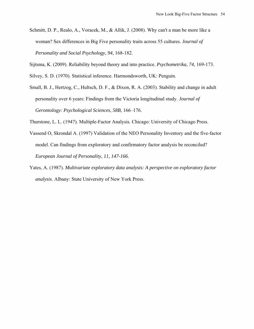
New Look Big-Five Factor Structure
54
Schmitt, D. P., Realo, A., Voracek, M., & Allik, J. (2008). Why can't a man be more like a
woman? Sex differences in Big Five personality traits across 55 cultures. Journal of
Personality and Social Psychology, 94, 168-182.
Sijtsma, K. (2009). Reliability beyond theory and into practice. Psychometrika, 74, 169-173.
Silvey, S. D. (1970). Statistical inference. Harmondsworth, UK: Penguin.
Small, B. J., Hertzog, C., Hultsch, D. F., & Dixon, R. A. (2003). Stability and change in adult
personality over 6 years: Findings from the Victoria longitudinal study. Journal of
Gerontology: Psychological Sciences, 58B, 166–176.
Thurstone, L. L. (1947). Multiple-Factor Analysis. Chicago: University of Chicago Press.
Vassend O, Skrondal A. (1997) Validation of the NEO Personality Inventory and the five-factor
model. Can findings from exploratory and confirmatory factor analysis be reconciled?
European Journal of Personality, 11, 147-166.
Yates, A. (1987). Multivariate exploratory data analysis: A perspective on exploratory factor
analysis. Albany: State University of New York Press.
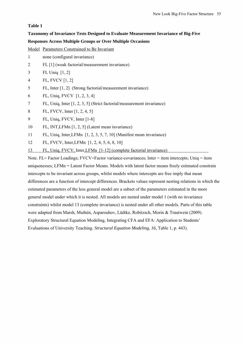
New Look Big-Five Factor Structure
55
Table 1
Taxonomy of Invariance Tests Designed to Evaluate Measurement Invariance of Big-Five
Responses Across Multiple Groups or Over Multiple Occasions
Model Parameters Constrained to Be Invariant
1 none (configural invariance)
2 FL [1] (weak factorial/measurement invariance)
3 FL Uniq [1, 2]
4 FL, FVCV [1, 2]
5 FL, Inter [1, 2] (Strong factorial/measurement invariance)
6 FL, Uniq, FVCV [1, 2, 3, 4]
7 FL, Uniq, Inter [1, 2, 3, 5] (Strict factorial/measurement invariance)
8 FL, FVCV, Inter [1, 2, 4, 5]
9 FL, Uniq, FVCV, Inter [1-8]
10 FL, INT,LFMn [1, 2, 5] (Latent mean invariance)
11 FL, Uniq, Inter,LFMn [1, 2, 3, 5, 7, 10] (Manifest mean invariance)
12 FL, FVCV, Inter,LFMn [1, 2, 4, 5, 6, 8, 10]
13 FL, Uniq, FVCV, Inter,LFMn [1-12] (complete factorial invariance)
Note. FL= Factor Loadings; FVCV=Factor variance-covariances; Inter = item intercepts; Uniq = item
uniquenesses; LFMn = Latent Factor Means. Models with latent factor means freely estimated constrain
intercepts to be invariant across groups, whilst models where intercepts are free imply that mean
differences are a function of intercept differences. Brackets values represent nesting relations in which the
estimated parameters of the less general model are a subset of the parameters estimated in the more
general model under which it is nested. All models are nested under model 1 (with no invariance
constraints) whilst model 13 (complete invariance) is nested under all other models. Parts of this table
were adapted from Marsh, Muthén, Asparouhov, Lüdtke, Robitzsch, Morin & Trautwein (2009).
Exploratory Structural Equation Modeling, Integrating CFA and EFA: Application to Students’
Evaluations of University Teaching. Structural Equation Modeling, 16, Table 1, p. 443).

New Look Big-Five Factor Structure
56
Table 2
Summary of Goodness-of-Fit Statistics for Total Group Models (T1 data) CHI/df CFI TLI FParm RMSEA Description
Total Group
Total Group CFA 15487.981/1700 .685 .672 190 .049 TGCFA1A: no CUs; no gender
12566.894/1643 .750 .731 247 .044 TGCFA1B: CUs; no gender
Total Group ESEM 8013.035/1480 .851 .821 410 .036 TGESEM1A: no CUs; no gender
5201.229/1423 .914 .893 467 .028 TGESEM1B: CUs; no gender
____________________________________________________________________________________
Note. CHI/df= chi-square/degrees of freedom ratio; CFI= Comparative fit index; TLI=Tucker-Lewis Index;
NFParm=Number of Free Parameters; RMSEA= Root Mean Square Error of Approximation. CUs = a priori
correlated uniquenesses based on the facet design of the instrument.

New Look Big-Five Factor Structure
57
Table 3 Summary of Goodness-of-Fit Statistics for All Gender Invariance Models (T1 data)
CHI/df CFI TLI FParm RMSEA Description
Model MG1: (configural invariance) 9373/2960 .852 .823 820 .036 MG1: no invariance (configural invariance) 6654/2846 .912 .891 934 .028 MG1A: MG1A with CUs (not invariant over sex) 6743/2903 .911 .892 877 .028 MG1B: MG1A with CUs IN (invariant over sex)
Model MG2(FL, weak factorial/measurement invariance) 9831/3235 .848 .833 545 .035 MG2: In = FL (weak factorial/measurement invariance) 7124/3121 .908 .895 659 .028 MG2a: MG2 with CUs 7218/3178 .907 .896 602 .027 MG2B: MG2A with CUs IN
Model MG3 (FL & Uniq) 10264/3295 .839 .827 485 .035 MG3: IN = FL, Uniq 7513/3181 .900 .889 599 .028 MG3A: MG3 with CUs 7644/3238 .898 .889 542 .028 MG3B: MG3A with CUs IN
Model MG4 (FL & FVCV) 9908/3250 .846 .833 530 .035 MG4: IN = FL, FVCV 7204/3136 .906 .894 643 .028 MG4A: MG4 with CUs 7296/3193 .905 .895 587 .028 MG4b: MG4A with CUs IN
Model MG5 (FL & Inter; Strong factorial/measurement invariance) 10937.377/3290 .824 .810 490 .037 MG5: IN = FL, Inter 7982/3176 .889 .876 604 .030 MG5A: MG5 with CUs . 8079/3233 .888 .878 547 .033 MG5b: MG5A with CUs IN 9951/3267 .846 .833 513 .035 MG5C: MG5 with part-In, No CUs. 7223/3153 .906 .895 627 .028 MG5D: MG5C with CUs . 7316/3210 .905 .895 570 .027 MG5E: MG5D with CUs IN
Model MG6 (FL, FVCV, Uniq) 103461/3310 .838 .826 470 .035 MG6: IN = FL, FVCV, Uniq, 7602/3196 .898 .887 584 .029 MG6A: MG6 with CUs 7731/3253 .897 .888 527 .028 MG6B: MG6A with CUs IN
Model MG7 (FL, Uniq, Inter; Strict factorial/measurement invariance) 11377/3350 .815 .804 430 .038 MG7: IN = FL, Uniq, Inter 8376/3236 .881 .870 544 .031 MG7A: MG7 with CUs 8505/3293 .880 .871 487 .031 MG7B: MG7A with CUs IN 10383/3327 .837 .827 453 .035 MG7C: MG7 with Inter (P-IN), No CUs 7611/3213 .899 .888 567 .028 MG7D: MG7C with CUs 7744/3270 .897 .888 510 .028 MG7E: MG7D with CUs IN
Model MG8 (FL, FVCV, Inter) 11012/3305 .822 .809 475 .037 MG8: IN = FL, FVCV, Inter 8060/3191 .888 .875 589 .030 MG8a: MG8 with CUs 8156/3248 .887 .877 532 .030 MG8b: MG8A with CUs IN 10029/3282 .844 .832 498 .035 MG8C: MG8 with Inter (P-IN), No CUs 7303/3168 .905 .893 612 .028 MG8d: MG8C with CUs 7397/3225 .904 .894 555 .028 MG8E: MG8D with CUs IN
Table 3(continued on next page)

New Look Big-Five Factor Structure
58
Table 3(continued)
CHI/df CFI TLI FParm RMSEA Description
Model MG9 (FL, Uniq, FVCV, Inter) 11458/3365 .813 .803 415 .038 MG9: IN = FL, FVCV, Uniq, Inter 8464/3251 .880 .869 529 .031 MG9A: MG9 with CUs 8591/3308 .878 .870 472 .031 MG9B: MG9A with CUs IN 10467/3342 .836 .826 438 .035 MG9C: MG9 with Inter (P-IN), No CUs 7700/3228 .897 .887 552 .029 MG9D: MG9C with CUs . 7829/3285 .895 .887 495 .029 MG9E: MG9D with CUs IN
Model MG10 (FL, Inter, FMns; Latent mean invariance 11550/3295 .809 .795 485 .039 MG10: IN = FL, Inter, FMGn 8625/3181 .874 .860 599 .032 MG10A: MG10 with CUs 8720/3238 .873 .862 542 .032 MG10b: MG10A with CUs IN 10466/3272 .834 .820 508 .036 MG10C: MG10 with Inter (P-IN), No CUs 7749/3158 .894 .881 622 .029 MG10D: MG10C with CUs 7842/3215 .893 .882 565 .029 MG10E: MG10D with CUs IN
Model MG11 (FL, Uniq, Inter, FMns; Manifest mean invariance) 11990/3355 .801 .790 425 .039 MG11: IN = FL, Uniq, Inter, FMGn 9020/3241 .867 .854 539 .032 MG11A: MG10 with CUs 9149/3298 .865 .855 482 .032 MG11B: MG10A with CUs IN 10902/3332 .825 .814 448 .037 MG11C: MG10 with Inter (P-IN), No CUs 8141/3218 .886 .875 562 .030 MG11D: MG10C with CUs 8272/3275 .885 .875 505 .030 MG11E: MG10D with CUs IN
Model MG12 (FL, FVCV, Inter, FMns) 11638/3310 .808 .794 470 .039 MG12: IN = FL, FVCV, Inter, FMGn 8717/3196 .873 .859 584 .032 MG12a: MG12 with CUs 8812/3253 .872 .860 527 .032 MG12B: MG12A with CUs IN 10552/3287 .832 .819 493 .036 MG12C: MG12 with Inter (P-IN), No CUs 7838/3173 .892 .888 607 .029 MG12D: MG12C with CUs 7931/3230 .892 .881 550 .029 MG12E: MG12D with CUs IN
Model MG13 (FL, Uniq, FVCV, Inter, FMns; complete factorial invariance) 12084/3370 .799 .789 410 .039 MG13: IN=FL, Inter, Uniq, fvcv, FMGn 9121/3256 .865 .853 524 .033 MG13A: MG13 with CUs 9249/3313 .863 .854 467 .033 MG13A: MG13A with CUs IN 10994/3347 .824 .813 433 .037 MG13C: MG13 Inter (P-IN), No CUs 8240/3233 .884 .873 547 .030 MG13D: MG13C with CUs 8368/3290 .883 .873 490 .030 MG13E: MG13D with CUs IN
Note. CHI/df= chi-square/degrees of freedom ratio; CFI= Comparative fit index; TLI=Tucker-Lewis Index; NFParm=Number of Free Parameters; RMSEA= Root Mean Square Error of Approximation. For multiple group invariance models, the “IN” means the sets of parameters constrained to be invariant across the multiple groups (P-IN means partial invariance): FL= Factor Loadings; FVCV=Factor variance-covariances; Inter = item intercepts; Uniq = item uniquenesses; FMn = Factor Means.
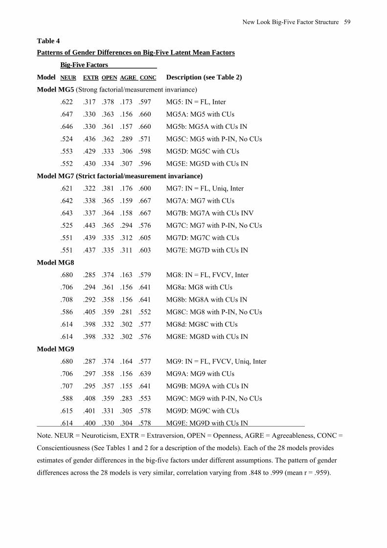
New Look Big-Five Factor Structure
59
Table 4 Patterns of Gender Differences on Big-Five Latent Mean Factors
Big-Five Factors
Model NEUR EXTR OPEN AGRE CONC Description (see Table 2)
Model MG5 (Strong factorial/measurement invariance)
.622 .317 .378 .173 .597 MG5: IN = FL, Inter
.647 .330 .363 .156 .660 MG5A: MG5 with CUs
.646 .330 .361 .157 .660 MG5b: MG5A with CUs IN
.524 .436 .362 .289 .571 MG5C: MG5 with P-IN, No CUs
.553 .429 .333 .306 .598 MG5D: MG5C with CUs
.552 .430 .334 .307 .596 MG5E: MG5D with CUs IN
Model MG7 (Strict factorial/measurement invariance)
.621 .322 .381 .176 .600 MG7: IN = FL, Uniq, Inter
.642 .338 .365 .159 .667 MG7A: MG7 with CUs
.643 .337 .364 .158 .667 MG7B: MG7A with CUs INV
.525 .443 .365 .294 .576 MG7C: MG7 with P-IN, No CUs
.551 .439 .335 .312 .605 MG7D: MG7C with CUs
.551 .437 .335 .311 .603 MG7E: MG7D with CUs IN
Model MG8
.680 .285 .374 .163 .579 MG8: IN = FL, FVCV, Inter
.706 .294 .361 .156 .641 MG8a: MG8 with CUs
.708 .292 .358 .156 .641 MG8b: MG8A with CUs IN
.586 .405 .359 .281 .552 MG8C: MG8 with P-IN, No CUs
.614 .398 .332 .302 .577 MG8d: MG8C with CUs
.614 .398 .332 .302 .576 MG8E: MG8D with CUs IN
Model MG9
.680 .287 .374 .164 .577 MG9: IN = FL, FVCV, Uniq, Inter
.706 .297 .358 .156 .639 MG9A: MG9 with CUs
.707 .295 .357 .155 .641 MG9B: MG9A with CUs IN
.588 .408 .359 .283 .553 MG9C: MG9 with P-IN, No CUs
.615 .401 .331 .305 .578 MG9D: MG9C with CUs
.614 .400 .330 .304 .578 MG9E: MG9D with CUs IN
Note. NEUR = Neuroticism, EXTR = Extraversion, OPEN = Openness, AGRE = Agreeableness, CONC =
Conscientiousness (See Tables 1 and 2 for a description of the models). Each of the 28 models provides
estimates of gender differences in the big-five factors under different assumptions. The pattern of gender
differences across the 28 models is very similar, correlation varying from .848 to .999 (mean r = .959).

New Look Big-Five Factor Structure
60
Table 5
Summary of Goodness-of-Fit Statistics for All Longitudinal Invariance Models (T1/T2 data) CHI/df CFI TLI FParm RMSEA Description
Model LIMM1: (configural invariance) 22586.204/6535 .737 .712 845 .040 LIM1: no invariance (configurual invariance)
13439.12/6475 .886 .874 905 .026 LIM1A: LIM1 with 60 CWCCUs
19608.380/6421 .784 .760 959 .036 LIM1B: LIM1 with 57 WWCCUs (free)**
19688.836/6478 .783 .761 902 .036 LIM1C: LIM1 with 57 WWCCUs (IN)**
11699.942/6361 .912 .902 1019 .023 LIM1D: LIM1 with 60 CWCCUs & 57 WWCCUs (free)
11774.709/6418 .912 .902 962 .023 LIM1E: LIM1 with 60 CWCCUs & 57 WWCCUs (IN)
Model LIM2(FL, weak factorial/measurement invariance) 23310.487/6810 .729 .716 570 .039 LIM2: In = FL (weak factorial/measurement invariance)
14031.355/6750 .881 .874 630 .026 LIM2A: LIM2 with 60 CWCCUs
20276.775/6696 .777 .763 684 .036 LIM2B: LIM2 with 57 WWCCUs (free)**
20373.406/6753 .777 .764 627 .036 LIM2C: LIM2 with 57W WCCUs (IN)**
12268.578/6636 .908 .901 744 .023 LIM2D: LIM2 with 60 CWCCUs & 57 WWCCUs (free)
12362.858/6693 .907 .901 687 .023 LIM2E: LIM2 with 60 CWCCUs & 57 WWCCUs (IN)
Model LIM3 (FL & Uniq) 23618.054/6870 .725 .715 510 .039 LIM3: In = FL, Uniq
14340.892/6810 .877 .871 570 .027 LIM3A: LIM3 with 60 CWCCUs
20543.564/6756 .774 .761 624 .036 LIM3B: LIM3 with 57 WWCCUs (free)**
20706.696/6713 .772 .761 567 .036 LIM3C: LIM3 with 57 WWCCUs(IN)**
12543.203/6696 .904 .898 684 .024 LIM3D: LIM3 with 60 CWCUs & 57 WWCU (free)
12694.848/6753 .903 .897 627 .024 LIM3E: LIM3 with 60CWCUs & 57WWCU (IN)
Model LIM4 (FL & FVCV) 23350.852/6825 .729 .717 555 .039 LIM4: IN = FL, FVCV
14068.6115/6765 .880 .874 615 .026 LIM4A: LIM4 with 60 CWCCUs
20309.085/6711 .777 .763 684 .036 LIM4B: LIM4 with 57 WWCCUs (free)**
20406.865/6768 .776 .764 612 .036 LIM4C: LIM4 with 57 WWCCUs (IN)**
12298.072/6651 .907 .901 729 .023 LIM4D: LIM4 with 60 CWCCUs & 57 WWCCUs (Free)
12393.301/6708 .907 .901 672 .023 LIM4E: LIM4 with 60 CWCCUs & 57 WWCCUs (IN)
Model LIM5 (FL & Inter; Strong factorial/measurement invariance) 12795.596/6691 .900 .893 689 .024 LIM5D: IN = FL, Inter, with 60 CWCUs & 57 WWCCUs (free)
12887.877/6748 .899 .893 632 .024 LIM5E: LIM5D with 60 CWCCUs 57 & WWCCUs (IN)
12524.171/6680 .904 .898 700 .024 LIM5Dp: LIM5D with Inter (P-IN), 60 CWCCUs & 57 WWCCUs (free)
12618.552/6737 .904 .898 643 .024 LIM5Ep: LIM5D with Inter (P-IN), 60 CWCCUs & 57 WWCCUs (IN)
Model LIM6 (FL, FVCV, Uniq) 12578.414/6711 .904 .898 669 .024 LIM6D: IN = FL, FVCV, Uniq, with 60 CWCCUs & 57 WWCCUs (Free)
12729.497/6768 .901 .897 612 .024 LIM6E: LIM6D with 60 CWCCUs & 57 WWCCUs (IN)
Table 5 (continued on next page)

New Look Big-Five Factor Structure
61
CHI/df CFI TLI NFParm RMSEA Description
Model LIM7 (FL, Uniq, Inter; Strict factorial/measurement invariance) 13070.134/6751 .896 .890 629 .024 LIM7D: IN = FL, Uniq, Inter, with 60 CWCUs & 57 WWCCUs (Free) 13222.070/6808 .895 .890 572 .024 LIM7E: LIM7D with 60CWCUs & 57 WWCCUs(IN) 12798.663/6740 .901 .895 640 .024 LIM7Dp: LIM7D with Inter (P-IN), 60CWCUs & 57 WWCCUs (Free) 12950.495/6797 .899 .894 583 .024 LIM7Ep: LIM7D with Inter (P-IN), 60CWCUs & 57 WWCCUs (IN)
Model LIM8 (FL, FVCV, Inter) 12826/6706 .900 .893 674 .024 LIM8D: IN = FL, FVCV, Inter with 60 CWCUs & 57 WWCCUs (FR) 12919/6763 .899 .893 617 .024 LIM8E: LIM8D with 60 CWCUs & 57 WWCCUs (IN) 12554/6695 .904 .898 685 .024 LIM8Dp: LIM8D with Inter (P-IN), 60CWCUs & 57 WWCCUs (FR) 12649/6752 .903 .898 628 .024 LIM8Ep: LIM8D with Inter (P-IN), 60CWCUs & 57 WWCCUs (IN)
Model LIM9 (FL, Uniq, FVCV, Inter) 13106/6766 .896 .890 614 .024 LIM9D: IN = FL, FVCV, Uniq, Inter with 60 CWCUs & 57 WWCCUs (FR) 13257/6823 .894 .890 557 .025 LIM9E: LIM9D with 60 CWCUs & 57 WWCCUs (IN) 12834/6755 .900 .895 625 .024 LIM9Dp: LIM9D with Inter (P-IN), 60CWCUs & 57 WWCCUs (FR) 12985/6812 .899 .894 568 .024 LIM9Ep: LIM9D with Inter (P-IN), 60CWCUs & 57 WWCCUs (IN)
Model LIM10 (FL, Inter, FMns) (Latent mean invariance) 13166/6696 .894 .887 684 .025 LIM10D: IN = FL, Inter, FMn, with 60 CWCUs & 57 WWCCUs (FR) 13258/6753 .893 .887 627 .025 LIM10E: LIM10D with 60 CWCUs & 57 WWCCUs (IN) 12765/6685 .900 .894 695 .024 LIM10Dp: LIM10D with Inter (P-IN), 60CWCUs & 57 WWCCUs (FR) 12859/6742 .900 .894 638 .024 LIM10EP: LIM10D with Inter (P-IN), 60CWCUs & 57 WWCCUs (IN)
Model LIM11 (FL, Uniq, Inter, FMn; Manifest mean invariance) 13440/6756 .890 .884 624 .025 LIM11D: IN = FL, Uniq, Inter, FMn, with 60 CWCUs & 57 WWCCUs (FR) 13593/6813 .889 .883 567 .025 LIM11E: LIM11D with 60 CWCUs & 57 WWCCUs (IN) 13039/6745 .897 .891 635 .024 LIM11Dp: LIM11D with Inter (P-IN), 60CWCUs & 57 WWCCUs (FR) 13191/6802 .895 .890 578 .024 LIM11Ep: LIM11D with Inter (P-IN), 60CWCUs & 57 WWCCUs (IN)
Model LIM12 (FL, FVCV, Inter, FMn) 13196/6711 .894 .887 669 .025 LIM12D: IN = FL, FVCV, Inter, FMn, with 60 CWCUs & 57 WWCCUs (FR) 13289/6768 .893 .887 612 .025 LIM12E: LIM12D with 60 CWCUs & 57 WWCCUs (IN) 12794/6700 .900 .894 680 .024 LIM12Dp: LIM12D with Inter (P-IN), 60CWCUs & 57 WWCCUs (FR) 12889/6757 .899 .894 623 .025 LIM12Ep: LIM12D with Inter (P-IN), 60CWCUs & 57 WWCCUs (IN)
Model LIM13 (FL, Uniq, FVCV, Inter, FMn; complete factorial invariance) 13476/6771 .890 .884 609 .025 LIM13D:IN=FL, Uniq, FVCV, Inter, FMn, 60 CWCUs & 57 WWCCUs (FR) 13628/6828 .889 .883 552 .025 LIM13E: LIM13D with 60 CWCUs & 57 WWCCUs (IN) 130746817 .896 .891 620 .024 LIM13Dp: LIM13D with Inter (P-IN), 60CWCUs & 57 WWCCUs (FR) 132266817 .895 .890 563 .024 LIM13Ep: LIM13D with Inter (P-IN), 60CWCUs & 57 WWCCUs (IN)
Note. CHI/df= chi-square/degrees of freedom ratio; CFI= Comparative fit index; TLI=Tucker-Lewis Index; NFParm=Number of Free Parameters; RMSEA= Root Mean Square Error of Approximation. For multiple group invariance models, the “IN=” means the sets of parameters constrained to be invariant across the multiple groups (P-IN means partial invariance): FL= Factor Loadings; FVCV=Factor variance-covariances; Inter = item intercepts; Uniq = item uniquenesses; FMn = Factor Means. ** Models results in improper solutions and should be interpreted cautiously (or ignored)

New Look Big-Five Factor Structure
62
Table 6
Test-retest Correlations between Matching Big-Five Factors at Time1 & 2 Model 1 LIM1 LIM1A LIM1B* LIM1C* LIM1D LIM1E
T2NEUR WITH T1NEUR .777 .749 .793 .794 .760 .760
T2EXTR WITH T1EXTR .888 .812 .917 .917 .841 .842
T2OPEN WITH T1OPEN .915 .849 .953 .953 .873 .874
T2AGRE WITH T1AGRE .812 .767 .831 .830 .784 .783
T2CONC WITH T1CONC .899 .810 .931 .932 .833 .835
Model 2 LIM2 LIM2A LIM2B* LIM2C* LIM2D LIM2E
T2NEUR WITH T1NEUR .780 .750 .794 .795 .759 .760
T2EXTR WITH T1EXTR .892 .813 .920 .920 .843 .843
T2OPEN WITH T1OPEN .921 .850 .957 .957 .880 .879
T2AGRE WITH T1AGRE .811 .767 .830 .830 .781 .780
T2CONC WITH T1CONC .901 .811 .933 .934 .831 .832
Model 3 LIM3 LIM3A LIM3B* LIM3C* LIM3D LIM3E
T2NEUR WITH T1NEUR .780 .748 .794 .795 .756 .757
T2EXTR WITH T1EXTR .892 .818 .920 .920 .842 .843
T2OPEN WITH T1OPEN .922 .850 .959 .958 .878 .879
T2AGRE WITH T1AGRE .810 .764 .829 .828 .880 .881
T2CONC WITH T1CONC .900 .814 .932 .933 .831 .832
Model 4 LIM4 LIM4A LIM4B* LIM4C* LIM4D LIM4E
T2NEUR WITH T1NEUR .775 .744 .791 .791 .756 .756
T2EXTR WITH T1EXTR .891 .817 .920 .920 .842 .842
T2OPEN WITH T1OPEN .921 .850 .957 .958 .878 .878
T2AGRE WITH T1AGRE .810 .764 .829 .829 .780 .783
T2CONC WITH T1CONC .901 .814 .933 .935 .831 .831
Note. T1= Time 1; T2= Time 2; NEUR = Neuroticism, EXTR = Extraversion, OPEN = Openness, AGRE =
Agreeableness, CONC = Conscientiousness. For a description of the models tested (e.g., LIM1, LIM1A,
LIM1B, LIM1C, LIM1D and LIM1E) and their fit to the data, see Table 6.
* These Models results in improper solutions and should be interpreted cautiously (or ignored)

New Look Big-Five Factor Structure
63
Table 7
Patterns of Mean Differences over Time for Big-Five Factors
Description (see Table 2) NEUR EXTR OPEN AGRE CONC
Model LIM5 (FL & Inter; Strong factorial/measurement invariance)
LIM5D: IN = FL, Inter, with 60 CWCUs & 57 WWCCUs (free)) -.228 .015 .176 .332 .227
LIM5E: LIM5D with 60 CWCCUs 57 & WWCCUs (IN) -.226 .016 .175 .331 .226
LIM5Dp: LIM5D with Inter (P-IN), 60 CWCCUs & 57 WWCCUs (free) -.202 .032 .127 .260 .194
LIM5Ep: LIM5D with Inter (P-IN), 60 CWCCUs & 57WWCCUs (IN) -.200 .033 .127 .259 .193
Model LIM7 (FL, Uniq, Inter; Strict factorial/measurement invariance)
LIM7D: IN = FL, Uniq, Inter, with 60 CWCUs & 57 WWCCUs (Free) -.227 .015 .178 .336 .226
LIM7E: LIM7D with 60CWCUs & 57 WWCCUs (IN) -.227 .015 .178 .334 .226
LIM7Dp: LIM7D with Inter (P-IN), 60CWCUs & 57 WWCCUs (Free) -.203 .032 .129 .262 .193
LIM7Ep: LIM7D with Inter (P-IN), 60CWCUs & 57 WWCCUs (IN) -.201 .032 .128 .261 .193
Model LIM8 (FL, FVCV, Inter)
LIM8D: IN = FL, FVCV, Inter with 60 CWCUs & 57 WWCCUs (Free) -.235 .014 .171 .336 .227
LIM8E: LIM8D with 60 CWCUs & 57 WWCCUs (IN) -.235 .014 .171 .336 .227
LIM8Dp: LIM8D with Inter (P-IN), 60CWCUs & 57 WWCCUs (Free) -.209 .032 .123 .255 .195
LIM8Ep: LIM8D with Inter (P-IN), 60CWCUs & 57 WWCCUs (IN) -.208 .032 .123 .255 .195
Model LIM9 (FL, Uniq, FVCV, Inter)
LIM9D: IN = FL, FVCV, Uniq, Inter, 60 CWCUs & 57 WWCCUs (Free) -.234 .014 .171 .337 .226
LIM9E: LIM9D with 60 CWCUs & 57 WWCCUs (IN) -.235 .014 .171 .326 .227
LIM9Dp: LIM9D with Inter (P-IN), 60CWCUs & 57 WWCCUs (Free) -.220 .031 .123 .255 .194
LIM9Ep LIM9D with Inter (P-IN), 60CWCUs & 57 WWCCUs (IN) -.209 .031 .123 .255 .194
Note. NEUR = Neuroticism, EXTR = Extraversion, OPEN = Openness, AGRE = Agreeableness, CONC =
Conscientiousness. See Tables 1 and 2 for a description of the models. Each of the 16 models provides
estimates of latent mean differences over time for the big-five factors under different assumptions. The pattern
of differences across the 28 models is very similar, correlations varying from .993 to .999 (mean r = .9975).

New Look Big-Five Factor Structure
64
Supplemental Material to be placed on the Psychological Assessment (APA) Website
Supplemental Appendix 1: The Exploratory Structural Equation Modelling (ESEM)
Approach
In the ESEM model (Asparouhov & Muthén, 2009; Marsh, Muthén, et al., 2009), there are p
dependent variables Y = (Y1, ..., Yp) and q independent variables X = (X1, ...,Xq) and m latent
variables η = (η1, ..., ηm) under the standard assumptions that the ε and ζ are normally distributed
residuals with mean 0 and variance covariance matrix θ and ψ respectively. Λ is a factor loading
matrix, whilst B and Γ are matrices of regression coefficients relating latent variables to each
other.
(2) +Γ+Β+=+Κ+Λ+=
ξηαηεην
X(1) XY
Although all parameters can be identified with the maximum likelihood estimation method
(ML), the model is generally not identified unless additional constraints are imposed. As in CFA
analyses, the two typical approaches are to identify the metric of the latent variable by either
fixing the variance of the latent variable to be 1.0 or by fixing one of the factor loadings for each
factor typically to be 1.0.
The ESEM approach differs from the typical CFA approach in that all factor loadings are
estimated, subject to constraints so that the model can be identified. In particular, when more than
one factor is posited (m > 1.0), further constrains are required to achieve an identified solution. To
resolve this problem, consider any m x m square matrix (m = number of factors), a square matrix
that we refer to as H. In this (mxm) square matrix H one can replace the η vector by H η in the
ESEM model (1-2) which will also alter the parameters in the model as well; Λ to Λ H−1, the α
vector H α, the Γ matrix to H Γ, the B matrix to HBH−1 and the Ψ matrix to HΨHT. Since H has
m2 elements, the ESEM model has a total of m2 indeterminacies that must be resolved. Two
variations of this model are considered; one where factors are orthogonal so that the factor
variance-covariance matrix (Ψ) is an identity matrix, and an oblique model where Ψ is an

New Look Big-Five Factor Structure
65
unrestricted correlation matrix (i.e., all correlations and residual correlations between the latent
variables are estimated as free parameters). This model can also be extended to include a
structured variance-covariance matrix (Ψ).
For an orthogonal matrix H (i.e., a square mxm matrix H such that HHT = I), one can
replace the η vector by H η and obtain an equivalent model in which the parameters are changed.
EFA can resolve this non-identification problem by minimizing f(Λ*) = f(Λ H−1), where f is a
function called the rotation criteria or simplicity function (Asparouhov & Muthén, 2009; Jennrich
& Sampson, 1966), typically such that among all equivalent Λ parameters the simplest solution is
obtained. There are a total of m(m−1)/2 constraints in addition to m(m + 1)/2 constraints that are
directly imposed on the Ψ matrix for a total of m2 constraints needed to identify the model. The
identification for the oblique model is developed similarly such that a total of m2 constraints
needed to identify the model are imposed. Although the requirement for m2 constraints is only a
necessary condition and in some cases it may be insufficient, in most cases the model is identified
if and only if the Fisher information matrix is not singular (Silvey, 1970). This method can be
used in the ESEM framework as well (Asparouhov & Muthén, 2009; also see Hayashi &
Marcoulides, 2006).
The estimation of the ESEM model consists of several steps (Asparouhov & Muthén,
2009). Initially a SEM model is estimated using the ML estimator. The factor variance covariance
matrix is specified as an identity matrix (ψ = I), giving m(m + 1)/2 restrictions. The EFA loading
matrix (Λ), has all entries above the main diagonal (i.e., for the first m rows and column in the
upper right hand corner of factor loading matrix, Λ), fixed to 0, providing remaining m(m − 1)/2
identifying restrictions. This initial, unrotated model provides starting values that can be
subsequently rotated into an EFA model with m factors. The asymptotic distribution of all
parameter estimates in this starting value model is also obtained. Then the ESEM variance
covariance matrix is computed (based only on Λ ΛT + θ and ignoring the remaining part of the
model).

New Look Big-Five Factor Structure
66
The correlation matrix is also computed and, using the delta method (Asparouhov &
Muthén, 2009), the asymptotic distribution of the correlation matrix and the standardization
factors are obtained. In addition, again using the delta method, the joint asymptotic distribution of
the correlation matrix, standardization factors and all remaining parameters in the model are
computed and used to obtain the standardized rotated solution based on the correlation matrix and
its asymptotic distribution (Asparouhov & Muthén, 2009). This method is also extended to
provide the asymptotic covariance of the standardized rotated solution, standardized unrotated
solution, standardization factors, and all other parameters in the model. This asymptotic
covariance is then used to compute the asymptotic distribution of the optimal rotation matrix H
and all unrotated parameters which is then used to compute the rotated solution for the model and
its asymptotic variance covariance.
In Mplus multiple random starting values are used in the estimation process to protect against
non-convergence and local minimums in the rotation algorithms. Although a wide variety of
orthogonal and oblique rotation procedures are available, leading authorities on this topic (e.g.,
Asparouhov & Muthén, 2009; Browne, 2001; Jennrich, 2006) have recommended Geomin
rotation, but made it clear that the researchers should explore alternative solutions with different
rotation strategies. In the context of the present investigation, geomin ration had a desirable
theoretical and statistical rationales in that it was developed specifically to better represent simple
structure as conceived by Thurstone (1947) which is very different to how it has sometimes been
interpreted and clearly inconsistent with the ICM-CFA model. Geomin rotations also incorporate
a complexity parameter consistent with Thrustone’s original proposal. As operationalized in
Mplus, this complexity parameter (ε) takes on small positive value that increases with the number
of factors (Browne, 2001; Asparouhov & Muthén, 2009). In the present investigation we found
that increasing the ε altered the balance between the sizes of cross-loadings and factor
correlations. As we were especially concerned with the sizes of factor correlations, we set the
epsilon at a rather high value (.5) that resulted in somewhat lower factor correlations and

New Look Big-Five Factor Structure
67
somewhat higher cross-loadings. Nevertheless, consistent with recommendations, we explored a
number of different rotations in preliminary analyses. There did not seem to be substantial
differences results based on the various rotations, consistent with suggestions by Asparouhov &
Muthén (2009) who concluded that “In most ESEM applications the choice of the rotation
criterion will have little or no effect on the rotated parameter estimates” (p. 428). Although we
had a clear basis for using the geomin rotation, we are not suggesting that this will always – or
even generally – be the best rotation in other studies. Quite the contrary, following
recommendations based on Asparouhov and Muthén (2009), Browne (2001) and others – as well
as our own personal experience, we suggest that applied researchers should evaluate the
theoretical and mathematical rationales for difference rotations, experiment with a number of
different rotations and complexity parameters, and chose the one that is most appropriate for their
specific application. We also note that this is clearly an area where more research – using both
simulation and read data – is needed.
With ESEM models it is possible to constrain the loadings to be equal across two or more
sets of EFA blocks in which the different blocks represent multiple discrete groups or multiple
occasions for the same group. This is accomplished by first estimating an unrotated solution with
all loadings constrained to be equal across the groups or over time. If the starting solutions in the
rotation algorithm are the same, and no loading standardizing is used, the optimal rotation matrix
will be the same as well as the subsequent rotated solutions. Thus obtaining a model with
invariant rotated Λ* amounts to simply estimating a model with invariant unrotated Λ, a standard
task in maximum likelihood estimation.
For an oblique rotation it is also possible to test the invariance of the factor variance-
covariance matrix (Ψ) matrix across the groups. To obtain non-invariant Ψs an unrotated solution
with Ψ = I is specified in the first group and an unrestricted Ψ is specified in all other groups.
Note that this unrestricted specification means that Ψ is not a correlation matrix as factor
variances are freely estimated. It is not possible in the ESEM framework to estimate a model

New Look Big-Five Factor Structure
68
where in the subsequent groups the Ψ matrix is an unrestricted correlation matrix, because even if
the factor variances are constrained to be 1 in the unrotated solution, they will not be 1 in the
rotated solution. However, it is possible to estimate an unrestricted Ψ in all but the first group and
after the rotation the rotated Ψ can be constrained to be invariant or varying across groups.
Similarly, when the rotated and unrotated loadings are invariant across groups, it is possible to test
the invariance of the factor intercept and the structural regression coefficients. These coefficients
can also be invariant or varying across groups simply by estimating the invariant or group-varying
unrotated model. However, in this framework only full invariance can be tested in relation to
parameters in Ψ and Λ in that it is not possible to have measurement invariance for one EFA
factor but not for the other EFA factors. Similar restrictions apply to the factor variance
covariance, intercepts and regression coefficients, although it is possible to have partial invariance
in the ε matrix of residuals. (It is however, possible to have different blocks of ESEM factors such
that invariance constraints are imposed in one block, but not the other). Furthermore, if the ESEM
model contains both EFA factors and CFA factors, then all of the typical strategies for the SEM
factors can be pursued with the CFA factors.

New Look Big-Five Factor Structure—Supplemental Materials 1
1
Supplemental Material to be placed on the Psychological Assessment (APA) Website
Supplemental Appendix 2
A Priori Correlated Uniquenesses Based on the Design of the NEO
Q24R & Q29R;
Q04 & Q34; Q04 & Q49; Q04 & Q14R; Q04 & Q39R; Q34 & Q49; Q34 & Q14R; Q34 & Q39R; Q49 &
Q14R; Q49 & Q39R; Q14R & Q39R;
Q19 & Q09R; Q19 & Q54R; Q19 & Q44R; Q09R & Q54R; Q09R & Q44R; Q54R & Q44R;
Q05 & Q15R; Q05 & Q55R; Q15R & Q55R;
Q20 & Q40; Q20 & Q45R; Q40 & Q45R;
Q25 & Q35; Q25 & Q60; Q35 & Q60;
Q10 & Q50; Q10 & Q30R; Q50 & Q30R;
Q02 & Q27R;
Q32 & Q47; Q32 & Q52; Q47 & Q52;
Q07 & Q37; Q07 & Q12R; Q07 & Q42R; Q37 & Q12R; Q37 & Q42R; Q12R & Q42R;
Q21 & Q01R; Q21 & Q31R; Q01R & Q31R;
Q26 & Q16R; Q26 & Q46R; Q16R & Q46R;
Q06 & Q56;
Q11 & Q41; Q11 & Q51; Q41 & Q51;
Q13 & Q43; Q13 & Q23R; Q43 & Q23R;
Q28 & Q08R;
Q53 & Q58; Q53 & Q48R; Q58 & Q48R;
Q18R & Q38R;
Note. The 60-item NEO Five-Factor Inventory (NEO-FFI) was developed to provide a concise measure of
the five basic personality factors (Costa & McCrae, 1989). For each scale, 12 items were selected from the
pool of 180 NEO Personality Inventory (NEO-PI) items, chiefly on the basis of their correlations with
validimax factor scores.The 180 items were designed to measure 20 subdomains, 4 subdomains for each of
the big-five factors. For present purposes, consistent with this design feature of the NEO-FFI, we posited a
priori correlated uniquenesses for items from the same subdomain. Thus, items from the same subdomain
were posited to be more highly correlated than items designed from different subdomains representing the
same big-five factor. In subsequent tests of partial invariance over time, the following 11 items had non-
invariant itercepts: Q36, Q41, Q18r,Q38r, Q15r,Q20, Q50,Q04, Q13, Q01R, Q31R. In subsequent tests of
partial invariance over gender, the following 23 items had non-invariant itercepts: Q11, Q43, Q48R, Q58,
Q04, Q09R, Q34, Q49, Q13, Q31R, Q37, Q23R, Q53, Q60, Q19, Q52, Q54r, Q59R, Q45r, Q50, Q57r,
Q29r, Q20

New Look Big-Five Factor Structure—Supplemental Materials 2
2
Supplemental Appendix 3 ESEM Solution: Five-Factor CFA and ESEM Solutions Based on Responses to 60 NEO items CFA (TGCFAM1B in Table 2) ESEM (TGESEM1B in Table 2) Factor Loadings
F1 Neuroticism
Q01Ra .086 .000 .000 .000 .000 .081 -.025 -.030 .010 -.003
Q06* .539 .000 .000 .000 .000 .505 -.149 -.089 -.045 .162 Q11 .534 .000 .000 .000 .000 .559 .008 .036 -.010 .081 Q16R .427 .000 .000 .000 .000 .316 -.228 .107 .013 -.085 Q21 .625 .000 .000 .000 .000 .625 -.069 .040 .061 -.095 Q26 .703 .000 .000 .000 .000 .635 -.125 .020 -.054 -.035 Q31R .456 .000 .000 .000 .000 .438 -.050 .099 .005 .103 Q36 .457 .000 .000 .000 .000 .469 -.011 .011 .027 -.153 Q41 .621 .000 .000 .000 .000 .564 -.079 -.025 -.191 .017 Q46R .573 .000 .000 .000 .000 .477 -.200 .159 -.011 -.036 Q51 .661 .000 .000 .000 .000 .620 -.055 -.004 -.090 -.026 Q56 .437 .000 .000 .000 .000 .438 -.015 .021 -.025 .037 F2 Extraversion
Q02 .000 .597 .000 .000 .000 .051 .683 -.038 -.071 .047 Q07 .000 .378 .000 .000 .000 .098 .391 .001 -.005 .170 Q12R* .000 .362 .000 .000 .000 -.200 .230 -.019 -.003 .146 Q17 .000 .618 .000 .000 .000 .003 .625 .185 .022 .100 Q22 .000 .361 .000 .000 .000 .037 .538 .023 -.028 -.360 Q27R* .000 .356 .000 .000 .000 -.057 .289 -.089 -.163 .327 Q32 .000 .439 .000 .000 .000 -.189 .382 .106 .099 -.138 Q37 .000 .650 .000 .000 .000 -.182 .534 -.075 .042 .164 Q42R* .000 .576 .000 .000 .000 -.321 .379 -.051 .033 .176 Q47 .000 .129 .000 .000 .000 .177 .344 .021 -.014 -.280 Q52 .000 .565 .000 .000 .000 -.111 .510 .031 .196 -.048 Q57R .000 .404 .000 .000 .000 -.157 .302 -.082 .056 .053 F3 Openness
Q03R* .000 .000 .269 .000 .000 .093 -.079 .267 -.220 .038 Q08R* .000 .000 .740 .000 .000 -.072 -.029 .719 -.077 -.030 Q13 .000 .000 .478 .000 .000 .160 .052 .482 -.033 .081 Q18R .000 .000 .316 .000 .000 -.238 -.157 .342 -.017 -.011 Q23R .000 .000 .565 .000 .000 .072 .063 .559 .000 .070 Q28* .000 .000 .283 .000 .000 -.044 .207 .262 .016 -.049 Q33R .000 .000 .365 .000 .000 .051 .131 .371 .042 .181 Q38R* .000 .000 .053 .000 .000 -.092 -.117 .074 -.092 -.114 Q43 .000 .000 .604 .000 .000 .104 .028 .609 .006 .038 Q48R .000 .000 .468 .000 .000 -.094 -.076 .479 -.037 .021 Q53 .000 .000 .377 .000 .000 -.160 .073 .433 .247 -.137 Q58 .000 .000 .421 .000 .000 -.139 -.070 .455 -.029 -.199 F4 Agreeableness
Q05 .000 .000 .000 .573 .000 .078 -.025 -.076 .588 .092 Q10 .000 .000 .000 .590 .000 -.112 -.016 -.062 .521 .018 Q15R* .000 .000 .000 .340 .000 -.175 -.131 -.031 .328 -.046 Q20 .000 .000 .000 .576 .000 .112 .079 .041 .601 .128 Q25 .000 .000 .000 .498 .000 -.120 .133 -.050 .498 -.177 Q30R .000 .000 .000 .591 .000 -.160 -.060 -.028 .509 .099 Q35 .000 .000 .000 .607 .000 -.007 .128 .057 .628 -.069 Q40 .000 .000 .000 .465 .000 .017 .090 .033 .458 .047 Q45R .000 .000 .000 .514 .000 -.095 -.047 -.093 .453 .109 Q50 .000 .000 .000 .746 .000 .038 .020 -.041 .738 .059 Q55R .000 .000 .000 .531 .000 -.206 -.037 -.093 .462 .098 Q60 .000 .000 .000 .345 .000 .005 -.032 .124 .469 -.334
Appendix 2 (continued on next page)
New Look Big-Five Factor Structure—Supplemental Materials 3
3
Appendix 3 (continued) ESEM Solution: Five-Factor CFA and ESEM Solutions Based on Responses to 60 NEO items CFA (TGCFAM1B in Table 2) CFA (TGESEM1B in Table 2) Factor Loadings
F5 Conscientiousness
Q04 .000 .000 .000 .000 .442 .078 .194 .081 .207 .272 Q09R* .000 .000 .000 .000 .336 -.337 -.062 .057 .129 .265 Q14R .000 .000 .000 .000 .527 -.084 -.076 -.057 .041 .524 Q19* .000 .000 .000 .000 .382 .157 .255 .081 .019 .326 Q24R* .000 .000 .000 .000 .494 -.125 .098 .002 .066 .463 Q29R* .000 .000 .000 .000 .275 -.213 .010 .069 -.065 .318 Q34* .000 .000 .000 .000 .304 -.130 .316 .004 .074 .098 Q39R .000 .000 .000 .000 .625 .010 .137 .019 -.038 .556 Q44R .000 .000 .000 .000 .333 .029 .056 .012 -.115 .387 Q49 .000 .000 .000 .000 .481 .177 .118 .190 .218 .349 Q54R .000 .000 .000 .000 .258 .074 -.158 .002 .068 .308 Q59R .000 .000 .000 .000 .528 .070 -.055 .000 .080 .602 Factor Correlations F1 1.0 1.0 F2 -.502 1.0 -.205 1.0 F3 .054 .081 1.0 .063 .049 1.0 F4 -.305 .253 -.092 1.0 -.166 .120 -.016 1.0 F5 -.149 .400 .062 .245 -.038 .140 -.014 .065 1.0
Note. The CFA and ESEM models each specified five factors (see Table 2 for goodness-of-fit statistics). All parameter estimates are completely standardized. N = 3390 sets of ratings for the 60 NEO-FFI items. Both models also included a set of 60 a priori correlated uniquenesses, relating items from the same subfactor (based on the design of the 360-item version of the instrument). * Items suggested to be weak by McCrae and Costa (2004): 6, 12, 27, 42, 3, 8, 28, 38, 9, 19, 24, 29, 34, and 15). Note that some of the supposedly weak items from the original NEO-FFI actually performed well but were recommended for revision because of potential reading level difficulties for younger students. In particular, item Q06 had the third highest factor loading of the 12 Neuroticism items in the original NEO-FFI and performed considerably better than its replacement item in the NEO-FFI-R in the McCrae and Cost (2004) study, and performed well here as well. a We also note that Q01 had a surprisingly low factor loading for time 1 responses considered here whilst it performed adequately for time 2 responses considered in the longitudinal analyses by the same students (see Appendix 4). As this was the first item in the instrument, we suspect that the problem was idiosyncratic to some aspect of the administration of materials at time 1 and not inherent to the item itself. For completeness sake we retained the item and note that its exclusion had little effect on results presented here in part because it did not load substantially on any of the big-five factors.

New Look Big-Five Factor Structure—Supplemental Materials 4
4
Supplemental Appendix 4
Big-five Factors Based on Responses to 60-item NEO For Males and Females Factor Loadings __ Item Intercepts
Males Females Male Female
NEUR EXTR OPEN AGRE CONC NEUR EXTR OPEN AGRE CONC
Neurotiism
Q01R .047 -.008 -.066 -.004 -.009 .110 -.033 -.013 -.002 .021 2.955 3.378
Q06 .498 -.138 -.077 .153 -.061 .493 -.175 -.128 .143 -.042 2.878 3.120
Q11 .508 -.034 -.019 .036 .006 .530 -.011 .025 .031 -.054 2.604 2.923
Q16R .257 -.224 .128 -.064 .003 .370 -.210 .070 -.104 .032 2.801 2.989
Q21 .593 -.100 .001 -.102 .065 .613 -.051 .044 -.117 .061 2.910 3.091
Q26 .608 -.134 .041 -.034 -.036 .654 -.110 -.018 -.047 -.059 2.335 2.490
Q31R .311 -.067 .079 .060 -.020 .460 -.082 .054 .054 -.014 2.776 3.426
Q36 .463 .006 .002 -.183 .059 .464 -.026 .017 -.118 .012 3.593 3.691
Q41 .565 -.058 -.044 .002 -.202 .543 -.103 -.038 -.003 -.189 2.780 2.895
Q46R .411 -.239 .132 -.031 -.021 .490 -.177 .148 -.087 -.006 2.827 3.248
Q51 .594 -.031 -.019 .012 -.095 .615 -.074 -.021 -.081 -.094 2.735 2.814
Q56 .477 -.002 .011 .048 -.026 .382 -.043 .008 .007 -.027 2.951 3.313
Extraversion
Q02 .006 .643 -.026 -.001 -.096 .037 .699 -.082 .044 -.064 3.862 4.172
Q07 .135 .324 -.037 .155 .029 .014 .416 -.005 .138 -.055 4.488 5.080
Q12R -.198 .190 -.009 .118 .039 -.236 .228 -.037 .142 -.065 3.288 3.756
Q17 -.007 .606 .224 .052 .015 -.016 .626 .120 .136 .012 4.893 5.966
Q22 .043 .563 -.017 -.328 -.039 .003 .524 .055 -.382 -.008 2.999 3.039
Q27R -.075 .278 -.057 .317 -.163 -.056 .273 -.143 .299 -.187 3.343 3.417
Q32 -.116 .371 .080 -.123 .160 -.231 .387 .147 -.108 .057 3.420 3.390
Q37 -.116 .567 -.082 .203 .062 -.201 .507 -.062 .178 .013 4.707 5.028
Q42R -.271 .409 -.080 .173 .056 -.349 .342 -.025 .205 -.010 3.550 3.728
Q47 .173 .320 .006 -.280 .017 .152 .359 .036 -.275 -.028 3.007 3.166
Q52 -.101 .537 .010 -.050 .167 -.108 .487 .053 .001 .217 4.131 4.482
Q57R -.146 .333 -.049 .088 .057 -.129 .291 -.099 .059 .057 3.449 3.420
Openness
Q03R .104 -.092 .250 .062 -.226 .089 -.067 .271 .013 -.219 3.098 3.329
Q08R -.103 -.077 .739 -.023 -.066 -.015 .023 .684 -.026 -.082 2.463 2.910
Q13 .156 .054 .481 .068 -.041 .095 .005 .473 .038 -.064 2.458 2.985
Q18R -.228 -.141 .316 .014 .010 -.221 -.162 .369 -.011 -.051 3.333 3.395
Q23R .025 .051 .508 .024 -.051 .046 .033 .584 .060 .010 2.179 2.970
Q28 -.031 .258 .296 -.079 -.005 -.031 .167 .237 .015 .036 3.009 3.056
Q33R .033 .162 .345 .158 .035 .020 .068 .366 .179 .008 4.292 5.117
Q38R -.084 -.113 .070 -.148 -.113 -.085 -.114 .095 -.077 -.058 3.244 3.383
Q43 .082 .004 .625 .009 -.018 .041 -.005 .591 -.004 -.003 2.301 2.954
Q48R -.036 -.045 .528 .089 -.055 -.041 -.055 .470 .041 .002 3.398 3.365
Q53 -.096 .120 .448 -.064 .260 -.131 .070 .461 -.097 .256 4.490 4.630
Q58 -.065 -.012 .568 -.126 .039 -.056 -.053 .462 -.121 -.042 3.419 2.944
Appendix 3 (continued on next page)

New Look Big-Five Factor Structure—Supplemental Materials 5
5
Appendix 4 (continued) Factor Loadings __ Item Intercepts
Males Females Male Female
NEUR EXTR OPEN AGRE CONC NEUR EXTR OPEN AGRE CONC
Agreeableness
Q04 .163 .221 .080 .339 .224 .091 .195 .086 .307 .194 4.992 5.248
Q09R -.286 -.047 .084 .313 .149 -.284 -.046 .058 .307 .115 4.939 4.518
Q14R -.122 -.121 -.085 .510 .014 -.012 -.030 -.046 .541 .036 3.707 4.231
Q19 .179 .187 .140 .327 .006 .171 .307 .008 .341 .037 4.587 5.109
Q24R -.129 .066 -.015 .440 .056 -.145 .091 -.020 .448 .033 3.690 4.092
Q29R -.217 -.008 .055 .278 -.058 -.243 -.012 .053 .302 -.109 2.829 3.144
Q34 -.139 .302 -.028 .168 .073 -.059 .362 .047 .108 .075 5.945 6.324
Q39R .022 .150 -.026 .577 -.099 -.002 .108 .019 .530 -.031 3.722 4.302
Q44R .041 .015 -.020 .376 -.135 .019 .069 .010 .369 -.125 3.571 3.773
Q49 .241 .127 .196 .419 .220 .193 .129 .171 .356 .216 4.535 5.134
Q54R .076 -.152 -.025 .319 .076 .122 -.146 .023 .335 .050 2.821 3.043
Q59R .031 -.138 -.018 .595 .054 .038 -.035 -.060 .535 .056 3.376 4.482
Conscientiousness
Q05 .068 -.013 -.088 .081 .590 .027 -.066 -.096 .081 .568 3.260 3.768
Q10 -.133 -.008 -.095 .026 .470 -.158 -.048 -.045 -.014 .548 3.486 3.690
Q15R -.171 -.066 -.007 -.032 .336 -.147 -.171 -.027 -.001 .325 3.533 3.502
Q20 .115 .069 .036 .169 .604 .104 .081 .032 .116 .595 4.687 5.464
Q25 -.059 .116 -.064 -.194 .553 -.214 .119 -.033 -.157 .455 3.499 3.682
Q30R -.178 -.070 -.022 .058 .504 -.187 -.077 -.045 .112 .493 2.945 3.070
Q35 -.056 .121 .029 -.041 .618 -.016 .126 .064 -.090 .623 3.929 4.340
Q40 -.070 .070 .038 .015 .461 .071 .095 .016 .083 .446 5.118 6.040
Q45R -.209 -.052 -.120 .085 .441 -.071 -.071 -.098 .091 .427 3.427 3.787
Q50 .001 .035 -.050 .103 .734 .071 .018 -.032 .063 .727 3.989 4.347
Q55R -.209 .020 -.126 .078 .447 -.213 -.098 -.060 .138 .448 4.272 4.572
AQ60 .013 .067 .119 -.268 .514 .063 -.052 .170 -.273 .457 3.599 3.112
Factor Correlations
Male Female _
NEUR 1.00 1.00
EXTR -.194 1.00 -.252 1.00
OPEN .059 .048 1.00 .027 .036 1.00
CONC -.200 .168 -.040 1.00 -.121 .173 -.060 1.00
AGRE -.061 .084 -.005 .064 1.00 -.155 .057 .001.067 1.00
Note. Factor analysis (ESEM) was conducted on responses to the 60 NEO items by men and women. The
big-five factors are well defined in that nearly all the target loadings that define each of the factors (shaded
in gray) are substantial and larger than the non-target loading.

New Look Big-Five Factor Structure—Supplemental Materials 6
6
Supplemental Appendix 5 ESEM Test-Retest Factor Solution: Big-five Factors Based on Responses to 60-item NEO Collected at Time 1 and Time 2 (Model LIM1D; see Table 5) Factor Loadings Item Intercepts T1/T2 Time 1 Time 2 Time 1 Time 2 Corr NEUR EXTR OPEN AGRE CONC NEUR EXTR OPEN AGRE CONC Uniq Neuroticism Q01R .120 -.022 -.033 .000 -.015 .548 -.024 -.026 .054 .043 3.165 2.815 .037 Q06 .509 -.092 -.092 -.041 .213 .535 -.078 -.110 -.043 .121 2.994 2.859 .184 Q11 .618 .079 .012 .023 .069 .624 .054 .001 .030 -.004 2.741 2.641 .323 Q16R .366 -.178 .107 .028 -.102 .504 -.138 .095 .013 -.024 2.958 2.872 .097 Q21 .697 -.005 .006 .083 -.050 .679 -.031 -.012 .049 -.112 3.040 2.809 .231 Q26 .674 -.060 .000 -.046 .009 .651 -.073 .022 -.046 -.026 2.421 2.180 .290 Q31R .504 .000 .072 .019 .050 .647 .011 .058 .013 .066 3.135 2.875 .185 Q36 .487 -.013 -.005 .046 -.117 .492 .018 .002 .062 -.184 3.689 3.088 .293 Q41 .609 -.016 -.080 -.182 .030 .640 -.030 -.039 -.166 .066 2.815 2.578 .171 Q46R .544 -.126 .165 -.002 -.043 .599 -.174 .090 .016 -.007 3.031 2.813 .141 Q51 .664 -.023 -.049 -.077 .003 .687 -.011 -.043 -.109 .045 2.782 2.531 .157 Q56 .452 -.008 -.019 .003 .005 .429 .051 -.035 -.081 .017 3.177 2.842 .346 Extraversion Q02 -.001 .684 -.037 -.045 -.002 .016 .705 -.060 -.059 -.005 4.030 3.885 .299 Q07 .055 .402 -.031 -.077 .113 -.044 .422 -.039 -.074 .132 4.844 4.967 .351 Q12R -.261 .214 -.027 -.039 .118 -.218 .328 -.012 -.039 .113 3.589 3.750 .110 Q17 -.025 .614 .212 .023 .033 -.010 .630 .120 -.004 .111 5.417 5.228 .218 Q22 .031 .558 .036 -.001 -.385 .019 .571 .028 -.005 -.345 2.989 3.026 .412 Q27R -.086 .340 -.102 -.142 .211 .002 .387 -.097 -.121 .236 3.442 3.415 .354 Q32 -.240 .389 .133 .079 -.150 -.173 .382 .114 .132 -.148 3.472 3.679 .347 Q37 -.278 .497 -.073 -.030 .119 -.316 .504 -.021 .008 .143 5.082 4.988 .248 Q42R -.407 .349 -.040 -.024 .093 -.433 .352 -.008 .035 .127 3.690 3.703 .291 Q47 .182 .375 .033 .017 -.273 .199 .339 .023 .057 -.266 3.184 3.114 .369 Q52 -.143 .496 .044 .183 -.084 -.136 .502 .026 .185 -.069 4.335 4.344 .274 Q57R -.186 .374 -.082 .023 -.052 -.147 .428 -.053 .007 -.080 3.527 3.454 .339 Openness Q03R .126 -.067 .245 -.213 .002 .129 -.057 .264 -.229 .039 3.288 3.179 .293 Q08R -.040 -.039 .689 -.056 -.030 -.055 -.024 .704 -.072 -.026 2.750 3.034 .269 Q13 .170 .027 .529 -.064 .112 .121 .011 .556 -.023 .076 2.737 3.157 .373 Q18R -.209 -.169 .395 -.029 -.023 -.146 -.100 .352 -.005 -.077 3.479 3.456 .328 Q23R .096 .029 .602 .009 .079 .140 .034 .637 .021 .065 2.557 2.740 .319 Q28 -.045 .162 .234 .002 -.014 -.007 .124 .221 -.006 .001 3.061 3.065 .616 Q33R .041 .102 .407 .055 .156 .084 .104 .382 .044 .130 4.806 4.857 .273 Q38R -.056 -.135 .049 -.066 -.107 -.113 -.128 .102 -.088 -.088 3.287 3.414 .447 Q43 .120 .023 .649 .005 .049 .173 .037 .620 .010 .024 2.663 2.885 .267 Q48R -.077 -.053 .481 -.061 .020 -.109 -.149 .554 -.065 .017 3.425 3.531 .211 Q53 -.195 .027 .458 .214 -.172 -.137 .062 .368 .275 -.123 4.693 5.356 .369 Q58 -.138 -.129 .477 -.039 -.178 -.068 -.118 .520 -.027 -.174 3.089 3.201 .352 Appendix 3 (continued on next page)

New Look Big-Five Factor Structure—Supplemental Materials 7
7
Appendix 5 (continued) Factor Loadings Item Intercepts T1/T2 Time 1 Time 2 Time 1 Time 2 Corr NEUR EXTR OPEN AGRE CONC NEUR EXTR OPEN AGRE CONC Uniq Agreeableness Q04 .017 .154 .081 .199 .262 .026 .138 .073 .171 .349 5.348 5.795 .272 Q09R -.357 -.121 .060 .100 .303 -.338 -.089 .039 .133 .244 4.742 5.007 .300 Q14R -.150 -.106 -.024 .030 .554 -.140 -.062 -.017 .008 .599 4.070 4.240 .269 Q19 .131 .264 .060 .014 .299 .069 .191 .047 -.053 .408 4.998 4.857 .279 Q24R -.172 .095 .057 .082 .437 -.173 .143 .062 .049 .421 3.919 3.816 .215 Q29R -.221 .027 .059 -.052 .274 -.196 .028 .109 -.046 .235 3.046 3.115 .404 Q34 -.157 .260 .026 .086 .140 -.188 .217 .087 .089 .177 6.391 6.452 .329 Q39R -.059 .145 .006 -.049 .587 -.040 .119 .014 -.033 .609 4.035 4.257 .279 Q44R -.004 .087 .029 -.103 .345 .026 .069 .025 -.135 .351 3.856 3.698 .236 Q49 .113 .064 .229 .221 .394 .125 .024 .256 .162 .476 5.037 5.292 .185 Q54R .038 -.159 .023 .060 .302 .044 -.128 .002 .068 .310 3.117 3.189 .476 Q59R .042 -.028 -.016 .094 .600 .021 -.052 -.032 .086 .609 3.957 3.986 .443 Conscientiousness Q05 .085 -.031 -.090 .608 .080 .046 -.042 -.063 .577 .099 3.651 4.188 .370 Q10 -.135 -.018 -.030 .517 .036 -.124 -.057 -.032 .546 .066 3.731 4.304 .146 Q15R -.179 -.119 -.042 .345 -.072 -.128 -.080 -.025 .503 -.047 3.646 4.110 .206 Q20 .064 .014 .028 .605 .104 .078 .017 .034 .551 .152 5.331 6.325 .185 Q25 -.182 .114 -.082 .496 -.175 -.161 .164 -.018 .479 -.147 3.687 3.771 .265 Q30R -.187 -.071 .001 .509 .071 -.125 .006 -.041 .522 .070 3.068 3.093 .284 Q35 -.014 .107 .059 .643 -.105 .041 .131 .044 .651 -.134 4.228 4.404 .254 Q40 .016 .068 .017 .465 .022 -.060 .066 .021 .442 .081 5.795 6.536 .135 Q45R -.133 -.050 -.073 .460 .031 -.111 -.030 -.049 .440 .101 3.758 3.943 .260 Q50 .043 .022 -.021 .724 .017 .055 .040 -.042 .723 .015 4.368 4.952 .135 Q55R -.259 -.052 -.087 .459 .083 -.268 -.084 -.053 .489 .107 4.526 4.773 .243 AQ60 .030 -.056 .113 .479 -.300 .114 -.035 .075 .532 -.227 3.246 3.536 .465 Factor Correlations Time 1 Time 2 _ NEUR 1.000 EXTR -.241 1.000 OPEN .071 .061 1.000 CONC -.185 .075 .002 1.000 AGRE -.023 .185 -.042 .074 1.000 Time 2 NEUR .760 -.171 .096 -.140 -.008 1.000 EXTR -.216 .841 .018 .052 .170 -.267 1.000 OPEN -.003 .055 .873 -.036 -.015 .021 .109 1.000 CONC -.140 .071 -.058 .784 .100 -.200 .129 .002 1.000 AGRE .056 .120 -.041 .027 .833 -.002 .142 .023 .067 1.000
Note. Factor analysis (ESEM) was conducted on responses to the 60 NEO items administered at time 1 (T1) and time 2. The big-five factors are well defined in that nearly all the target loadings that define each of the factors (underlined, bolded, and shaded in gray) are substantial and larger than the non-target loading. Correlations between matching Time 1 and Time 2 factors (factor correlations underlined, bolded and shaded in gray) are substantial. Item intercepts are factor means of the items. Correlated uniquenesses relating uniquenesses relating responses to the same item administered on two different times are moderate to large.


![1. Isi Header [edit salimi].4.4 - http:/jurnal.fkip.uns.ac.id](https://img.pdfslide.net/doc/110x75/63123ebcc72bc2f2dd039b46/1-isi-header-edit-salimi44-httpjurnalfkipunsacid.jpg)