Embed Size (px)
Citation preview

Automatic spline smoothing of non-stationary kinematic signals using bilayered partitioning
and blending with correlation analysis
Suchul Shin†, Byounghyun Yoo‡*, Soonhung Han§ †Samsung Techwin, ‡Korea Institute of Science and Technology, §KAIST
Abstract—Measurement errors of kinematic signals introduced by motion capture systems are
unacceptably amplified when differentiating the signal to derive acceleration. Existing fully automatic methods for solving this problem have a weakness on non-stationary signals involving impacts, while semi-automatic methods each require that users carefully determine the values of configurable parameters. We propose an automatic method that estimates acceleration from non-stationary kinematic signals using bilayered partitioning and blending (BPB) with correlation analysis. The method has a configurable parameter, the partition length, and the recommended value of the partition length that is empirically derived can be used without prior knowledge of kinematic signals. Having applied this algorithm to synthetic sinusoidal data, benchmarking data in the biomechanics community, and our own measurement data, we compared the results with those of existing automatic methods. The evaluation confirms that the proposed method estimates acceleration more accurately from non-stationary signals than existing fully automatic methods and is more robust than existing semi-automatic methods.
Keywords—acceleration estimation, kinematic signal, non-stationary data, correlation analysis, spline smoothing, bilayered partitioning and blending
1. Introduction
Biomechanical motion analysis is usually performed using kinematic signals measured by motion capture systems because these can measure the position and orientation of multi-joint movements simultaneously [1, 2]. However, systematic measurement errors of the motion capture systems appearing in the form of noise in the recorded displacement signals are unacceptably amplified when differentiating displacements to obtain velocity and acceleration. Although noise removal algorithms have been widely adopted to address this issue, mis-specified parameter values for these algorithms lead to inaccurate acceleration estimation. Thus, attempts have been made to automate the process of estimating acceleration from displacement signals.
The first attempts at fully-automatic acceleration estimation utilized the characteristic of white noise. Woltring [3] proposed generalized cross-validation spline smoothing (GCVSPL), which used generalized cross-validation [4] for choosing a smoothing parameter. D'Amico and Ferrigno [5] proposed the linear-phase autoregressive model-based derivative assessment algorithm (LAMBDA), which identified an optimal cut-off frequency by modeling the original
* Corresponding author E-mail address: [email protected]
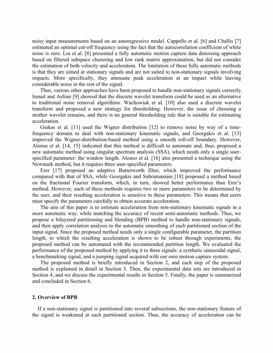
noisy input measurements based on an autoregressive model. Cappello et al. [6] and Challis [7] estimated an optimal cut-off frequency using the fact that the autocorrelation coefficient of white noise is zero. Liu et al. [8] presented a fully automatic motion capture data denoising approach based on filtered subspace clustering and low rank matrix approximation, but did not consider the estimation of both velocity and acceleration. The limitation of these fully automatic methods is that they are aimed at stationary signals and are not suited to non-stationary signals involving impacts. More specifically, they attenuate peak acceleration at an impact while leaving considerable noise in the rest of the signal.
Thus, various other approaches have been proposed to handle non-stationary signals correctly. Ismail and Asfour [9] showed that the discrete wavelet transform could be used as an alternative to traditional noise removal algorithms. Wachowiak et al. [10] also used a discrete wavelet transform and proposed a new strategy for thresholding. However, the issue of choosing a mother wavelet remains, and there is no general thresholding rule that is suitable for estimating acceleration.
Giakas et al. [11] used the Wigner distribution [12] to remove noise by way of a time-frequency domain to deal with non-stationary kinematic signals, and Georgakis et al. [13] improved the Wigner-distribution-based method using a smooth roll-off boundary. However, Alonso et al. [14, 15] indicated that this method is difficult to automate and, thus, proposed a new automatic method using singular spectrum analysis (SSA), which needs only a single user-specified parameter: the window length. Alonso et al. [16] also presented a technique using the Newmark method, but it requires three user-specified parameters.
Erer [17] proposed an adaptive Butterworth filter, which improved the performance compared with that of SSA, while Georgakis and Subramaniam [18] proposed a method based on the fractional Fourier transform, which, in turn, showed better performance than Erer’s method. However, each of these methods requires two or more parameters to be determined by the user, and their resulting acceleration is sensitive to these parameters. This means that users must specify the parameters carefully to obtain accurate acceleration.
The aim of this paper is to estimate acceleration from non-stationary kinematic signals in a more automatic way, while matching the accuracy of recent semi-automatic methods. Thus, we propose a bilayered partitioning and blending (BPB) method to handle non-stationary signals, and then apply correlation analysis to the automatic smoothing of each partitioned section of the input signal. Since the proposed method needs only a single configurable parameter, the partition length, to which the resulting acceleration is shown to be robust through experiments, the proposed method can be automated with the recommended partition length. We evaluated the performance of the proposed method by applying it to three signals: a synthetic sinusoidal signal, a benchmarking signal, and a jumping signal acquired with our own motion capture system.
The proposed method is briefly introduced in Section 2, and each step of the proposed method is explained in detail in Section 3. Then, the experimental data sets are introduced in Section 4, and we discuss the experimental results in Section 5. Finally, the paper is summarized and concluded in Section 6.
2. Overview of BPB
If a non-stationary signal is partitioned into several subsections, the non-stationary feature of the signal is weakened at each partitioned section. Thus, the accuracy of acceleration can be

improved by individually estimating acceleration for each section. However, discontinuities occur at the boundaries of the sections because of the edge effects [19] of the smoothing methods. Therefore, we propose the BPB method as depicted in Fig. 1, which makes a clone signal (a copied layer in Fig. 1(b)) and uniformly divides the two layers so that each section of the original layer overlaps with half of the adjacent section of the copied layer (Fig. 1(c)), separately estimates the acceleration for each section (Fig. 1(d)), and, finally, blends each overlapped acceleration pair of the half sections (Fig. 1(e)). The final blending step is for the weighted average of the double estimates of the same section of a signal in order to ensure that the weight at the end of each section is zero to overcome the edge effects. In the next section, we explain each step in greater detail: the partition length in Section 3.1, the automatic estimation of acceleration in Section 3.2, and the blending in Section 3.3.
3. Methods
3.1. Partition length
The partition length is the only configurable parameter of our method. The estimated acceleration is more accurate with a smaller partition length because this is better for dealing with non-stationary signals. However, the length of data points, at which the edge effect occurs, is invariant, and the estimated acceleration of each partitioned section is more influenced by the edge effect as the partition length decreases. From the work of Woltring [3], it is known that the shortest signal length in number of data points, from which acceleration can be automatically estimated, is generally about 40. Empirically, we found that the minimum partition length is about 30, and we recommend 50 for general cases in the proposed method by our experiments including the results explained in Section 5 with Fig. 8(d), Fig 9(d), Fig. 11(d), and Fig. 12(d).
3.2. Automatic estimation of acceleration
In this section, the method that automatically estimates acceleration for each individual partition is presented. The correlation analysis in Section 3.2.2 is performed to derive a correlation equation used in the proposed method; the derived correlation is used in the iterative estimation process in Section 3.2.3, which is performed separately for each given input signal.
3.2.1. Spline smoothing
Existing fully automatic methods for estimating acceleration from displacement measurements are based on statistical signal noise information on the white noise. Thus, they do not work correctly for partitioned sections because each section lacks sufficient data points to obtain statistical information on the white noise. Therefore, we propose a new automation method that uses the correlation between the input data and their optimal smoothing parameters.
For the new automatic method, we selected spline smoothing [20, 21] as the noise removal algorithm because, owing to its single smoothing parameter, it is easy to analyze the correlation, and its edge effect is weaker than that of low-pass filters and the least squares regression method. We used fifth order (quintic) spline smoothing because it is known to be optimal in estimating acceleration from displacement measurements [3].
The quintic spline smoothing is defined [20] as

min! !
𝜆∆𝑡! 𝑠 ! 𝑡!𝑑𝑡
!!
!!+ 𝑦! − 𝑠 𝑡! !
!
!!!
, (1)
where 𝑦! is the input displacement of the 𝑖th data point, 𝑡!, is the time at the 𝑖th data point, 𝑛 is the number of data points, ∆𝑡 is the time interval between the data points, 𝑠 𝑡 is the smoothed displacement function in polynomial form, 𝑠 ! 𝑡 is the third derivative of 𝑠 𝑡 , and 𝜆 is the smoothing parameter. The left term is a penalty on the roughness of the smoothed displacement function, while the right term is the error between the smoothed displacement and input displacement. The smoothing parameter, 𝜆 , controls the tradeoff between the left term “roughness” and the right term “error.” In other words, it controls the smoothness of 𝑠 𝑡 . The acceleration is obtained by analytically differentiating the spline polynomials 𝑠 𝑡 and is denoted as 𝑠 ! 𝑡 . Therefore, 𝜆 should be optimally determined for accurate estimation of the true acceleration for given input signal.
3.2.2. Correlation analysis for automatic spline smoothing
We expect that the optimal smoothing parameter is related to the ratio of the error to the roughness of the true signal. The error, 𝐸, and roughness, 𝑅!, of the true signal are defined as
E = 𝑦! − 𝑓 𝑡! !!
!!!
, 𝑅! = ∆𝑡! 𝑓 ! 𝑡!𝑑𝑡 ,
!!
!! (2)
where 𝑓 𝑡 is the displacement function of the true signal, which is actually unknown. We examined how the optimal smoothing parameter is related to the ratio 𝐸 𝑅! through
correlation analysis. For this, we created a sample motion data set with 10,000 motion signals. The displacement of each motion signal was generated by low-pass filtering a random white noise signal with a certain cut-off frequency. The acceleration of this signal was obtained by numerical second order differentiation. The number of data points, sampling rate, and cut-off frequency were randomly selected within the ranges 20 to 200, 10 to 1000 Hz, and 0.01 to 25 % of the selected sampling rate, respectively.
The final displacement signals were obtained by adding white noise to the randomly generated signals. The standard deviation of the white noise was randomly selected within the range in which log 𝐸 𝑅! has a value between - 5 and 10, because the correlation analysis is performed in a logarithmic scale owing to the broad distribution of the optimal smoothing parameters.
The optimal smoothing parameter for each noisy signal was calculated using the bisection method, which minimizes the root mean squared error (RMSE) of the estimated acceleration. If the root mean square of the magnitude of the estimated acceleration is less than half that of the true acceleration, we exclude these data because the noise is too large and, thus, the estimated acceleration and optimal smoothing parameter are meaningless.
Then, we performed regression analysis on the collected sample motion data. Regression analysis is a statistical technique to estimate a correlation by fitting a correlation model to a sample data set. The results of the regression analysis are depicted in Fig. 2. The blue points that indicate the generated sample data are marked according to their 𝐸 𝑅! and 𝜆. The black line that is fitted to the sample data set represents the relation between log 𝐸 𝑅! and log 𝜆 . The coefficient of the determinant for the regression analysis was 0.931, which means that it can explain 93.1% of the correlation, and we obtained the correlation

𝜆opt ≈ 𝑒!!.!"#𝐸𝑅!
!.!"#
. (3)
3.2.3. Iterative estimation of optimal smoothing parameters using the correlation
The analyzed correlation cannot be used directly, because 𝐸 and 𝑅! are unknown in practical smoothing of kinematic signals. However, the optimal smoothing parameter can be estimated by finding the value that satisfies the correlation model.
Initially, the displacement data smoothed with an optimal smoothing parameter are regarded as the true displacement data; that is, 𝑠!opt 𝑡 ≅ 𝑓 𝑡 . Then, the optimal smoothing parameter is approximated using the following equations
𝐸! = 𝑦! − 𝑠! 𝑡! !!!!! , (4)
𝑅!,! = ∆𝑡! 𝑠! ! 𝑡!𝑑𝑡!!
!!, (5)
𝜆opt = 𝑒!!.!"#!!opt!!,!opt
!.!"#
, (6)
where 𝐸! and 𝑅!,! are the error and roughness of the displacement data smoothed with the smoothing parameter 𝜆.
𝜆opt can be obtained by finding the solution that minimizes
𝑃 𝜆 = 𝑒!!.!"#𝐸!𝑅!,!
!.!"#
− 𝜆 . (7)
By the definition of 𝐸! , 𝑅!,! , and spline smoothing, if 𝜆 = 0, 𝐸! 𝑅!,! = 0; if 𝜆! < 𝜆! ,
𝐸!! 𝑅!,!! < 𝐸!! 𝑅!,!! ; and if 𝜆 → ∞ , lim!→!! !! !!,!
!"→ 0 . Therefore, 𝑃 0 = 0 , and the
derivative satisfies 𝑃! 0 > 0. Hence, we deduce 𝑃 𝜆 > 0 when 𝜆 < 𝜆opt and 𝑃 𝜆 < 0 when 𝜆 > 𝜆opt.
Then, we can find the solution of 𝑃 𝜆 using the following iterative process:
𝜆! = 𝑒!!.!"#𝐸!!𝑅!,!!
!.!"#
,
(8)
𝜆! = 𝑒!!.!"#𝐸!!𝑅!,!!
!.!"#
,
⋮
𝜆!!! = 𝑒!!.!"#𝐸!!𝑅!,!!
!.!"#
.
This iterative process of Eq. (8) is depicted in Fig. 3. If the initial smoothing parameter, 𝜆!, is not zero, the resulting smoothing parameter converges to the optimal parameter, as shown in Fig. 3. If 𝜆! < 𝜆opt , then 𝐸!! < 𝐸!opt and 𝑅!,!! > 𝑅!,!opt by their definitions by (4) and (5), respectively. If we apply these two equations to (6) and (8), we derive 𝜆!!! < 𝜆!"#. In addition, 𝑃 𝜆! > 0 because 𝜆! < 𝜆opt, then 𝜆!!! > 𝜆! by (7). Hence, 𝜆! < 𝜆!!! < 𝜆!"# when 𝜆! < 𝜆opt. In the same way, 𝜆! > 𝜆!!! > 𝜆!"# when 𝜆! > 𝜆opt . Therefore, 𝜆! converges to 𝜆opt by the iterative process in (8). That is,

𝜆opt = lim!→!
𝜆! . (9) We define the estimated error ratio as
𝐸𝐸𝑅! =
1𝑛 𝑠! ! 𝑡! − 𝑠!! ! 𝑡!
!!!!!
1𝑛 𝑠!! ! 𝑡!
!!!!!
(10)
and terminate the iterative process when
𝐸𝐸𝑅! − 𝐸𝐸𝑅!!!
𝐸𝐸𝑅!≤ 0.01 . (11)
3.3. Blending
Let 𝑎! 𝑡 and 𝑎! 𝑡 be the acceleration of the original and cloned signals, respectively, which are estimated by using the proposed method in Section 3.2. Furthermore, let 𝐵 𝑥 be a blending (weighting) function, whose value gradually varies from zero to one over the interval [0,1]. Then, we can derive the blended acceleration, 𝛼 𝑡 , over the time interval 𝑡! , 𝑡!!! of the kth overlapped half sections, in a way similar to the edge blending method for a multi-projection system [22], defined as
𝛼 𝑡 = 𝐵𝑡 − 𝑡!
𝑡!!! − 𝑡!𝑎!! ! mod ! 𝑡 + 1− 𝐵
𝑡 − 𝑡!𝑡!!! − 𝑡!
𝑎!! ! mod ! 𝑡 , (12)
where 𝑘 mod 2 denotes the remainder when dividing 𝑘 by 2. As 𝐵 𝑥 , we use Eq. (1) of [22], but any function that satisfies the condition as mentioned above can be used; empirically, the type of blending function itself does not make much difference for the acceleration estimates if the function satisfies the condition. Then, the blended acceleration is 𝑎!! ! mod ! at 𝑡!, weighted average of the double estimates 𝑎!! ! mod ! and 𝑎!! ! mod ! at 𝑡! < 𝑡 < 𝑡!!!, and 𝑎!! ! mod ! at 𝑡!!!. At the two ends of the half section, one of 𝑎! and 𝑎! fades away because estimated acceleration is inaccurate due to edge effects.
4. Evaluation data
4.1. Sinusoidal data (stationary)
We used synthetic sinusoidal data to evaluate the proposed method on stationary signals. The oscillating frequency, amplitude, sampling rate, and duration were selected as 1 Hz, 1 m, 100 Hz, and 3 s, respectively. White noise with a standard deviation of 0.01 m was added to the signal. The numerically calculated acceleration and true acceleration are shown in Fig. 4(a) and (b), respectively. The amount of added noise is adequate for evaluating the performance of acceleration estimation because the signal-to-noise ratio of the numerically calculated acceleration is -24.6 dB, which means that the amplitude of the error is about seventeen times as large as the amplitude of the true acceleration, as shown in Fig. 4(a) and (b).

4.2. Dowling’s data (non-stationary)
Dowling’s data [23] have been used as benchmarking data to evaluate the accuracy of the acceleration estimated from non-stationary displacement measurements in most of the related work [11, 14-18]. The motion of these data involves a horizontally rotating pendulum that impacts with a non-rigid barrier [11]. The data consist of the angular displacement and acceleration, recorded simultaneously at 512 Hz, with 600 data points for each. The numerically calculated acceleration and measured acceleration are shown in Fig. 4(c) and (d), respectively.
4.3. Measurement data (non-stationary)
Since Dowling’s data do not actually comprise biomechanical movement, we conducted an additional experiment to evaluate the use of the proposed method for biomechanical motion analysis. We measured the acceleration and displacement of jumping motion in place at 100 Hz using the InvenSense MPU-9150 as the accelerometer and the NDI Optotrak Certus as the motion capture system. To validate the accuracy of the two measurement systems, we measured the acceleration and displacement of jumping motion 1 m from the motion capture device because this is close enough to ensure that the measured displacement does not have much noise. We compared the numerically calculated acceleration and measured acceleration as shown in Fig. 5. Since the two acceleration values are almost the same, we can regard the measured acceleration as the ground truth.
Finally, we measured another jumping motion 7 m from the motion capture system; the numerically calculated acceleration and measured acceleration are shown in Fig. 4(e) and (f), respectively.
5. Results
5.1. Sinusoidal data
The results of the sinusoidal data are shown in Fig. 6. We compared the acceleration estimated using the proposed method (Fig. 6(a)) with that estimated using GCVSPL (Fig. 6(b)) [3], LAMBDA (Fig. 6(c)) [5], the auto-correlation method (Fig. 6(d)) [6], sequential SSA (Fig. 6(e)) [15], and the adaptive Butterworth filtering method (Fig. 6(f)) [17]. The parameters of each of the semi-automatic methods were manually selected to minimize RMSE; we used a partition length of 50 for the proposed method, a window length of 40 for sequential SSA, and two cut-off frequencies of 1.3 and 1.4 Hz for the adaptive Butterworth method. We excluded 30 data points at each end of the signal when calculating RMSE for each method in order to separate accuracy from edge effects. In terms of the RMSE, the proposed method performs better than the auto-correlation method, but worse than the others. The auto-correlation method and the adaptive Butterworth filtering method generate edge effects, as shown in Fig. 6(d) and (f). The best method for this stationary data is sequential SSA.

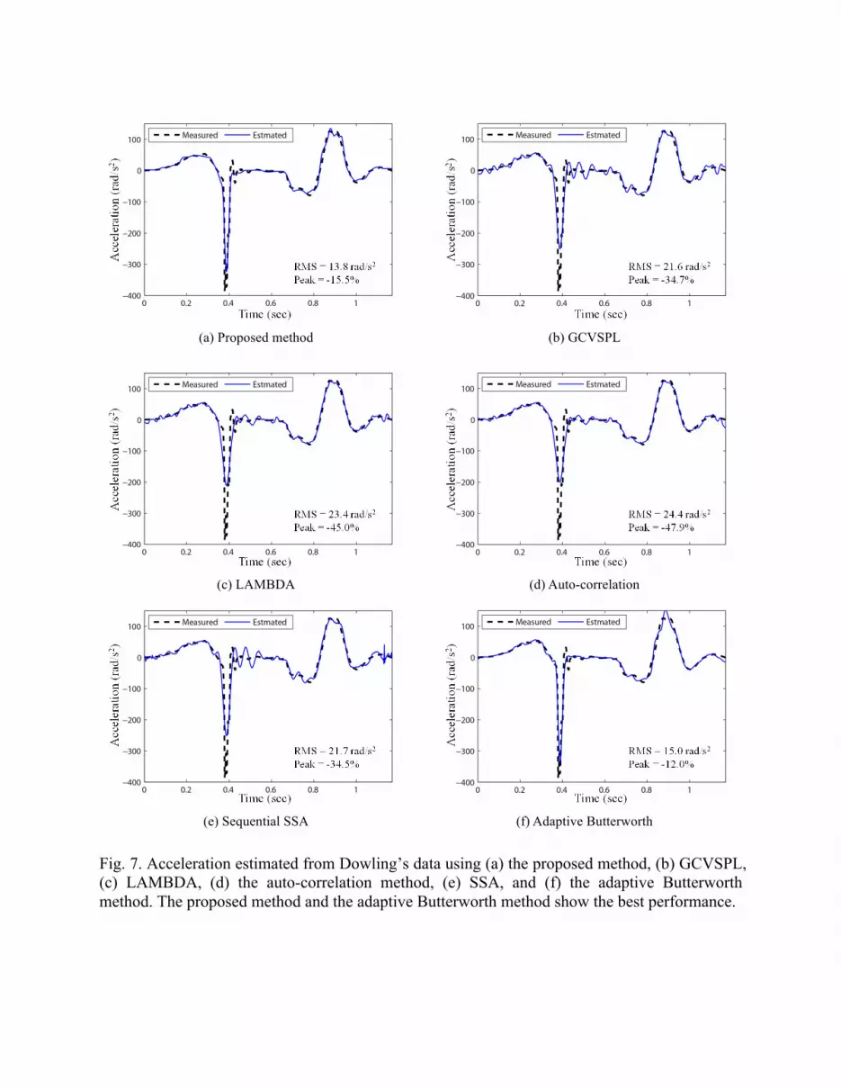
5.2. Dowling’s data
The results of Dowling’s data are shown in Fig. 7. In this experiment, like that in [18], we used another metric, peak error, to evaluate the performance on non-stationary signals. Peak error is defined as
peak error =𝑎! − 𝑎!
𝑎! , (13)
where 𝑎 is the estimated acceleration, 𝑎 is the true acceleration, and 𝐼 is the index of the data point that is closest to the peak acceleration during an impact. We used 50 as the partition length for the proposed method, and the same parameters for SSA and the adaptive Butterworth method as specified in [14] and [17], respectively.
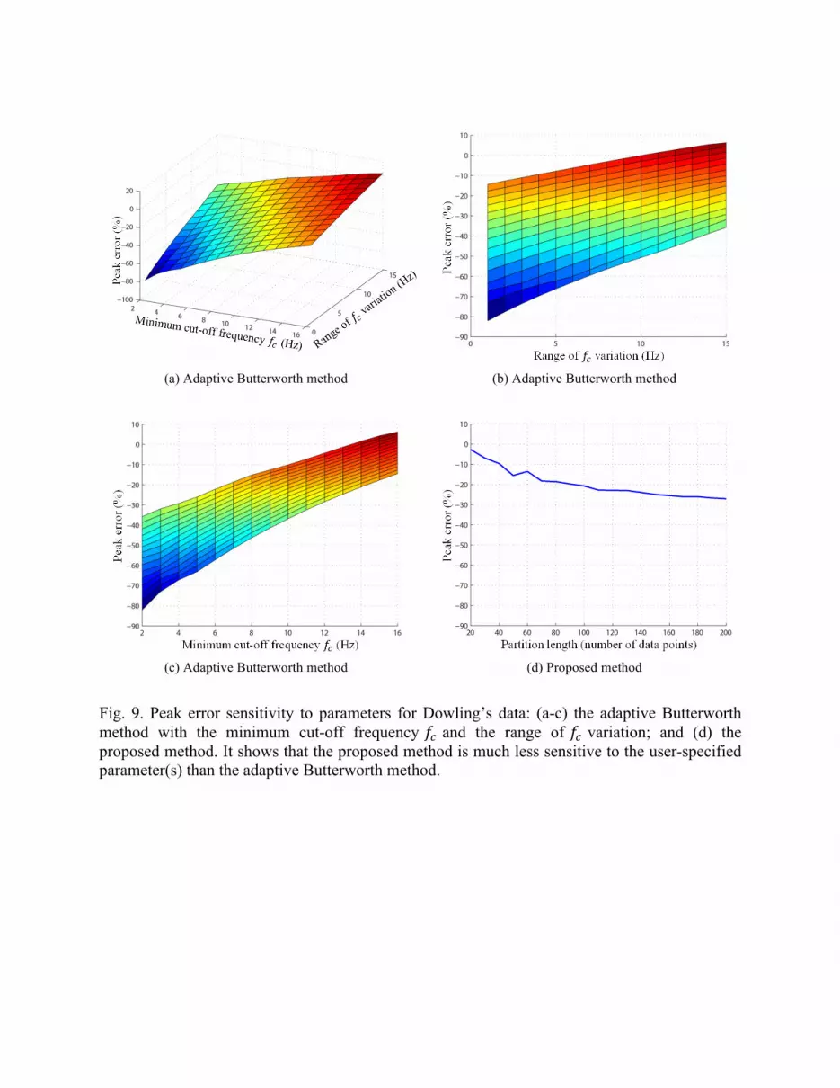
In this experiment, the proposed method yields the smallest RMSE of all the other methods, and the smallest peak error, except for that by the adaptive Butterworth filtering method. The difference in the peak error values by the proposed method and the adaptive Butterworth filtering method is only 3.5 %. Moreover, the adaptive Butterworth filtering method is sensitive to the two user-specified parameters, as shown in Fig. 8(a-c) and Fig. 9(a-c). The RMSE of the estimated acceleration varies from 15 rad/s2 to 44 rad/s2 according to the selection of the minimum cut-off frequency and the range of variation of the cut-off frequency as shown in Fig. 8(a-c). In addition, the peak error varies from -82% to -6% as shown in Fig. 9(a-c). This means that there is a risk of obtaining inaccurate acceleration through errors in the manually specified parameters.
On the contrary, the RMSE of the acceleration estimated by the proposed method varies from 14 rad/s2 to 43 rad/s2 according to its partition length as shown in Fig. 8(d). However, the recommended partition length is 50, and the minimum partition length is generally 40 according to the work of Woltring [3], as explained in Section 3.1. Then, the RMSE varies from 14 rad/s2 to 22 rad/s2 when the partition length is greater than 40. In addition, the peak error varies from -27% to -10% when the partition length is greater than 40, as shown in Fig. 9(d). This means that the proposed method is less sensitive to changes in the user-specified parameter (the partition length) than the adaptive Butterworth method is.
The RMSE of the acceleration of Dowling’s data estimated by the method of Georgakis and Subramaniam [18] is 13.7 rad/s2, which is just 0.1 rad/s2 smaller than that of the proposed method, while the peak error is - 2.9 %, which is superior to that of the proposed method. However, the method of Georgakis and Subramaniam requires a cut-off frequency and a threshold value for the rate of change of the residual energy, which must be carefully specified by the user and thereby vulnerable to error.
5.3. Measurement data
The results of the jumping motion data are shown in Fig. 10. We used 50 as the partition length for the proposed method, 6 as the window length for SSA, and 7 Hz and 8 Hz as the low and high cut-off frequencies, respectively, for the adaptive Butterworth method, all of which minimize the RMSE.
In this experiment, the proposed method yields the best results in terms of both RMSE and peak error, both of which are remarkably smaller than those by the other methods. For these data, the adaptive Butterworth method does not have the advantage on peak error compared with the other methods, unlike for Dowling’s data. The sensitivity of the adaptive Butterworth method is

worse than the Dowling’s data as shown in Fig. 11(a-c) and Fig. 12(a-c). The RMSE of the acceleration estimated by the adaptive Butterworth method varies from 2 m/s2 to 7 m/s2 according to the selection of the minimum cut-off frequency and the range of variation of the cut-off frequency as shown in Fig. 11(a-c). However, the RMSE of the acceleration estimated by the proposed method varies from 1.4 m/s2 to 2 m/s2 as the partition length changes from 20 to 200 as shown in Fig. 11(d). Moreover, the peak error of the adaptive Butterworth method varies from at least -60% to 33%, as shown in Fig. 12(a-c), but the peak error of the proposed method varies -29% to -13%, as shown in Fig. 12(d). Thus, the proposed method is much less sensitive to the user-specified parameter(s) than the adaptive Butterworth method. The robustness of the proposed method facilitates automatic determination of parameter values.
6. Conclusion
We proposed an automatic method for estimating acceleration from non-stationary kinematic displacement signals. More specifically, we proposed the BPB method to deal with non-stationary signals, and proposed a correlation-based method to automatically estimate optimal smoothing parameters for short-length partitioned sections. The only parameter that can be specified by the user is the partition length.
Through three experiments, we found that the proposed method yields better RMSE and peak error for non-stationary signals than existing methods such as GCVSPL, LAMBDA, the auto-correlation method, and SSA, and similar or better RMSE and peak error than the adaptive Butterworth method. The advantage of the proposed method over the adaptive Butterworth method is that it is more robust to the user-specified parameter(s). Therefore, the proposed method can more easily be automated while maintaining accuracy of acceleration that is estimated from "non-stationary" signals. As a result, we recommended a value for the partition length that can be used for general cases without prior knowledge of signals, and we verified it through the three experiments.

References
[1] Chiari, L., Croce, U. D., Leardini, A., and Cappozzo, A., 2005, "Human movement analysis using stereophotogrammetry: Part 2: Instrumental errors," Gait & Posture, 21(2), pp. 197-211.
[2] Xiao, J., Feng, Y., X. Yang, M. Ji, Zhang, J. J., and Zhuang, Y., 2014, "Sparse motion bases selection for human motion denoising," Signal Processing, DOI: 10.1016/j.sigpro.2014.08.017.
[3] Woltring, H. J., 1985, "On optimal smoothing and derivative estimation from noisy displacement data in biomechanics," Human Movement Science, 4(3), pp. 229-245.
[4] Golub, G. H., Heath, M., and Wahba, G., 1979, "Generalized Cross-Validation as a Method for Choosing a Good Ridge Parameter," Technometrics, 21(2), pp. 215-223.
[5] D'Amico, M., and Ferrigno, G., 1990, "Technique for the evaluation of derivatives from noisy biomechanical displacement data using a model-based bandwidth-selection procedure," Med. Biol. Eng. Comput., 28(5), pp. 407-415.
[6] Cappello, A., La Palombara, P. F., and Leardini, A., 1996, "Optimization and smoothing techniques in movement analysis," International Journal of Bio-Medical Computing, 41(3), pp. 137-151.
[7] Challis, J., 1999, "A procedure for the automatic determination of filter cutoff frequency for the processing of biomechanical data," Journal of Applied Biomechanics, 15, pp. 303-317.
[8] Liu, X., Cheung, Y., Peng, S., Cui, Z., Zhong, B., and Du, J., 2014, "Automatic motion capture data denoising via filtered subspace clustering and low rank matrix approximation," Signal Processing, 105, pp. 350-362.
[9] Ismail, A. R., and Asfour, S. S., 1999, "Discrete wavelet transform: a tool in smoothing kinematic data," Journal of Biomechanics, 32(3), pp. 317-321.
[10] Wachowiak, M. P., Rash, G. S., Quesada, P. M., and Desoky, A. H., 2000, "Wavelet-based noise removal for biomechanical signals: a comparative study," IEEE Transactions on Biomedical Engineering, 47(3), pp. 360-368.
[11] Giakas, G., Stergioulas, L. K., and Vourdas, A., 2000, "Time-frequency analysis and filtering of kinematic signals with impacts using the Wigner function: accurate estimation of the second derivative," Journal of Biomechanics, 33(5), pp. 567-574.
[12] Wigner, E., 1932, "On the Quantum Correction For Thermodynamic Equilibrium," Physical Review, 40(5), pp. 749-759.
[13] Georgakis, A., Stergioulas, L. K., and Giakas, G., 2002, "Wigner filtering with smooth roll-off boundary for differentiation of noisy non-stationary signals," Signal Processing, 82, pp. 1411-1415.
[14] Alonso, F. J., Del Castillo, J., and Pintado, P., 2005, "Application of singular spectrum analysis to the smoothing of raw kinematic signals," Journal of Biomechanics, 38(5), pp. 1085-1092.

[15] Alonso, F. J., Del Castillo, J., and Pintado, P., 2004, "An Automatic Filtering Procedure for Processing Biomechanical Kinematic Signals," Biological and Medical Data Analysis, J. Barreiro, F. Martín-Sánchez, V. Maojo, and F. Sanz, eds., Springer Berlin Heidelberg, pp. 281-291.
[16] Alonso, F. J., Cuadrado, J., Lugrís, U., and Pintado, P., 2010, "A compact smoothing-differentiation and projection approach for the kinematic data consistency of biomechanical systems," Multibody System Dynamics, 24, pp. 67-80.
[17] Erer, K. S., 2007, "Adaptive usage of the Butterworth digital filter," Journal of Biomechanics, 40(13), pp. 2934-2943.
[18] Georgakis, A., and Subramaniam, S. R., 2009, "Estimation of the Second Derivative of Kinematic Impact Signals Using Fractional Fourier Domain Filtering," Biomedical Engineering, IEEE Transactions on, 56(4), pp. 996-1004.
[19] Vint, P. F., and Hinrichs, R. N., 1996, "Endpoint error in smoothing and differentiating raw kinematic data: An evaluation of four popular methods," Journal of Biomechanics, 29(12), pp. 1637-1642.
[20] Reinsch, C., 1967, "Smoothing by spline functions," Numer. Math., 10(3), pp. 177-183.
[21] Reinsch, C., 1971, "Smoothing by spline functions. II," Numer. Math., 16(5), pp. 451-454.
[22] Tseng, C. W., Hsu, S. P., and Chang, Y. C., 2013, "Constructing a projector matrix for the quadratic curved screen," in IEEE Conference on Industrial Electronics and Applications (ICIEA), pp. 1129-1134.
[23] Dowling, J., 1985, "A modelling strategy for the smoothing of biomechanical data," Biomechanics, B. Johnsson, ed., Human Kinetics, Champaign, IL, pp. 1163-1167.

Fig. 1. Overview of the bilayered partitioning and blending method: (a) input displacement data; (b) cloning the input data; (c) bilayered partitioning; (d) acceleration estimation of each section; (e) blending the estimated acceleration values of overlapped sections; and (f) blended acceleration.

Fig. 2. Results of regression analysis of the correlation between the input motion data and their optimal parameters; the coefficient of the determinant is 0.931, which means that it can explain 93.1% of the correlation.

Fig. 3. Iterative estimation of the optimal smoothing parameter; 𝜆! is the initial smoothing parameter less than 𝜆opt , and 𝜆′! is the initial smoothing parameter greater than 𝜆opt . Both converge to 𝜆opt through the proposed iteration process.

(a) calculated acceleration of stationary motion (b) measured acceleration of stationary motion
(c) calculated acceleration of Dowling’s data (d) measured acceleration of Dowling’s data
(e) calculated acceleration of jumping motion (f) measured acceleration of jumping motion
Fig. 4. Experimental data to evaluate the proposed method: (a) numerically calculated acceleration from displacement measurements of the stationary motion; (b) directly measured acceleration of the stationary motion; (c) numerically calculated acceleration of Dowling’s data; (d) measured acceleration of Dowling’s data; (e) numerically calculated acceleration of the jumping motion; and (f) measured acceleration of the jumping motion.
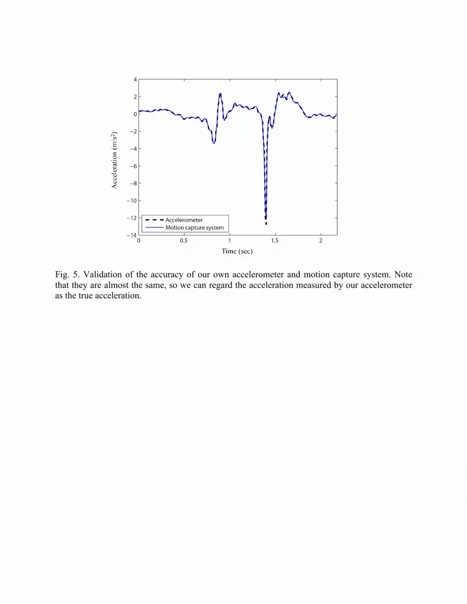
Fig. 5. Validation of the accuracy of our own accelerometer and motion capture system. Note that they are almost the same, so we can regard the acceleration measured by our accelerometer as the true acceleration.

(a) Proposed method (b) GCVSPL
(c) LAMBDA (d) Auto-correlation
(e) Sequential SSA (f) Adaptive Butterworth
Fig. 6. Acceleration estimated from the stationary motion data using (a) the proposed method, (b) GCVSPL, (c) LAMBDA, (d) the auto-correlation method, (e) sequential SSA, and (f) the adaptive Butterworth method. The sequential SSA shows the best performance for stationary signal.
(a) Proposed method (b) GCVSPL
(c) LAMBDA (d) Auto-correlation
(e) Sequential SSA (f) Adaptive Butterworth
Fig. 7. Acceleration estimated from Dowling’s data using (a) the proposed method, (b) GCVSPL, (c) LAMBDA, (d) the auto-correlation method, (e) SSA, and (f) the adaptive Butterworth method. The proposed method and the adaptive Butterworth method show the best performance.

(a) Adaptive Butterworth method (b) Adaptive Butterworth method
(c) Adaptive Butterworth method (d) Proposed method
Fig. 8. RMSE sensitivity to parameters for Dowling’s data: (a-c) the adaptive Butterworth method with the minimum cut-off frequency 𝑓! and the range of 𝑓! variation; and (d) the proposed method. It shows that the proposed method is less sensitive to the user-specified parameter(s) than the adaptive Butterworth method.
(a) Adaptive Butterworth method (b) Adaptive Butterworth method
(c) Adaptive Butterworth method (d) Proposed method
Fig. 9. Peak error sensitivity to parameters for Dowling’s data: (a-c) the adaptive Butterworth method with the minimum cut-off frequency 𝑓! and the range of 𝑓! variation; and (d) the proposed method. It shows that the proposed method is much less sensitive to the user-specified parameter(s) than the adaptive Butterworth method.

(a) Proposed method (b) GCVSPL
(c) LAMBDA (d) Auto-correlation
(e) Sequential SSA (f) Adaptive Butterworth
Fig. 10. Acceleration estimated from the jumping motion data using (a) the proposed method, (b) GCVSPL, (c) LAMBDA, (d) the auto-correlation method, (e) sequential SSA, and (f) the adaptive Butterworth method. The proposed method shows the best performance in terms of the RMSE and the peak error.

(a) Adaptive Butterworth method (b) Adaptive Butterworth method
(c) Adaptive Butterworth method (d) Proposed method
Fig. 11. RMSE sensitivity to parameters for the jumping data: (a-c) the adaptive Butterworth method with the minimum cut-off frequency 𝑓! and the range of 𝑓! variation; and (d) the proposed method. It shows that the proposed method is much less sensitive to the user-specified parameter(s) than the adaptive Butterworth method.
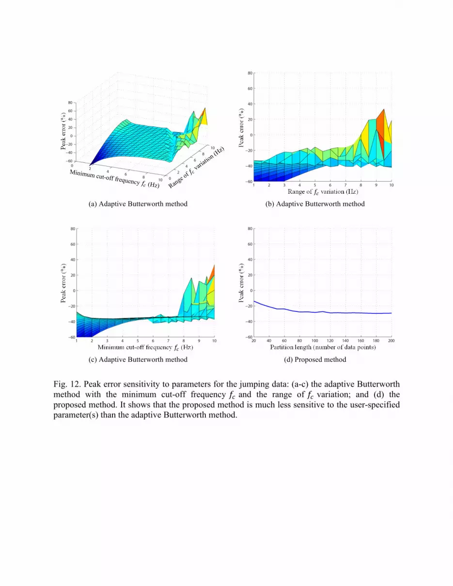
(a) Adaptive Butterworth method (b) Adaptive Butterworth method
(c) Adaptive Butterworth method (d) Proposed method
Fig. 12. Peak error sensitivity to parameters for the jumping data: (a-c) the adaptive Butterworth method with the minimum cut-off frequency 𝑓! and the range of 𝑓! variation; and (d) the proposed method. It shows that the proposed method is much less sensitive to the user-specified parameter(s) than the adaptive Butterworth method.


