HAL Id: hal-01485736https://hal.archives-ouvertes.fr/hal-01485736

Submitted on 9 Mar 2017

HAL is a multi-disciplinary open accessarchive for the deposit and dissemination of sci-entific research documents, whether they are pub-lished or not. The documents may come fromteaching and research institutions in France orabroad, or from public or private research centers.

L’archive ouverte pluridisciplinaire HAL, estdestinée au dépôt et à la diffusion de documentsscientifiques de niveau recherche, publiés ou non,émanant des établissements d’enseignement et derecherche français ou étrangers, des laboratoirespublics ou privés.

Autonomous car driving by a humanoid robotAntonio Paolillo, Pierre Gergondet, Andrea Cherubini, Marilena Vendittelli,

Abderrahmane Kheddar

To cite this version:Antonio Paolillo, Pierre Gergondet, Andrea Cherubini, Marilena Vendittelli, Abderrahmane Kheddar.Autonomous car driving by a humanoid robot. Journal of Field Robotics, Wiley, 2018, 35 (2), pp.169-186. �10.1002/rob.21731�. �hal-01485736�

Autonomous car driving by a humanoid robot

Antonio PaolilloCNRS-UM LIRMM

161 Rue Ada, 34090 Montpellier, FranceCNRS-AIST JRL UMI3218/RL

1-1-1 Umezono, 305-8560 Tsukuba, Japan.paolillo@lirmm.fr

Pierre GergondetCNRS-AIST JRL UMI3218/RL

1-1-1 Umezono, 305-8560 Tsukuba, Japan.pierre.gergondet@aist.go.jp

Andrea CherubiniCNRS-UM LIRMM

161 Rue Ada, 34090 Montpellier, Francecherubini@lirmm.fr

Marilena VendittelliDIAG, Sapienza Universita di Romavia Ariosto 25, 00185 Roma, Italyvendittelli@diag.uniroma.it

Abderrahmane KheddarCNRS-AIST JRL UMI3218/RL

1-1-1 Umezono, 305-8560 Tsukuba, Japan.CNRS-UM LIRMM

161 Rue Ada, 34090 Montpellier, France.kheddar@lirmm.fr

Abstract

Enabling a humanoid robot to drive a car, requires the development of a set ofbasic primitive actions. These include: walking to the vehicle, manually con-trolling its commands (e.g., ignition, gas pedal and steering), and moving withthe whole-body, to ingress/egress the car. In this paper, we present a sensor-based reactive framework for realizing the central part of the complete task,consisting in driving the car along unknown roads. The proposed frameworkprovides three driving strategies by which a human supervisor can teleoperatethe car, ask for assistive driving, or give the robot full control of the car. Avisual servoing scheme uses features of the road image to provide the referenceangle for the steering wheel to drive the car at the center of the road. Simulta-neously, a Kalman filter merges optical flow and accelerometer measurements,to estimate the car linear velocity and correspondingly compute the gas pedalcommand for driving at a desired speed. The steering wheel and gas pedalreference are sent to the robot control to achieve the driving task with the hu-manoid. We present results from a driving experience with a real car and thehumanoid robot HRP-2Kai. Part of the framework has been used to performthe driving task at the DARPA Robotics Challenge.

1 Introduction

The potential of humanoid robots in the context of disaster has been exhibited recentlyat the DARPA Robotics Challenge (DRC), where robots performed complex locomotionand manipulation tasks (DARPA Robotics Challenge, 2015). The DRC has shown thathumanoids should be capable of operating machinery, originally designed for humans. TheDRC utility car driving task is a good illustration of the complexity of such tasks.

Worldwide, to have the right to drive a vehicle, one needs to be delivered a license, requiringmonths of practice, followed by an examination test. To make a robot drive in similarconditions, the perception and control algorithms should reproduce the human driving skills.

If the vehicle can neither be customized nor automated, it is more convenient to think of arobot in terms of anthropomorphic design. A driving robot must have motion capabilities foroperations such as: reaching the vehicle, entering it, sitting in a stable posture, controlling itscommands (e.g., ignition, steering wheel, pedals), and finally egressing it. All these skills canbe seen as action templates, to be tailored to each vehicle and robot, and, more importantly,to be properly combined and sequenced to achieve driving tasks.

Noticeable research is currently made, to automate the driving operation of unmannedvehicles, with the ultimate goal of reproducing the tasks usually performed by humandrivers (Nunes et al., 2009; Zhang et al., 2008; Hentschel and Wagner, 2010), by relyingon visual sensors (Newman et al., 2009; Broggi et al., 2010; Cherubini et al., 2014). Thesuccess of the DARPA Urban Challenges (Buehler et al., 2008; Thrun et al., 2006), and theimpressive demonstrations made by Google (Google, 2015), have heightened expectationsthat autonomous cars will very soon be able to operate in urban environments. Consideringthis, why bother making a robot drive a car, if the car can make its way without a robot?Although both approaches are not exclusive, this is certainly a legitimate question.

One possible answer springs from the complexity of autonomous cars, which host a distributedrobot, with various sensors and actuators controlling the different tasks. With a centralizedrobot, such embedded devices can be removed from the car. The reader may also wonderwhen should a centralized robot be preferred to a distributed one, i.e., a fully automated car?

We answer this question through concrete application examples. In the DRC (Pratt andManzo, 2013), one of the eight tasks that robot must overtake is driving a utility vehicle. Thereason is that in disaster situations, the intervention robot must operate vehicles – usuallydriven by humans – to transport tools, debris, etc. Once the vehicle reaches the interventionarea, the robot should execute other tasks, (e.g., turning a valve, operating a drill). Withouta humanoid, these tasks can be hardly achieved by a unique system. Moreover, the robotshould operate cranks or other tools attached to the vehicle (Hasunuma et al., 2003; Yokoiet al., 2006). A second demand comes from the car manufacturing industry (Hirata et al.,2015). In fact, current crash-tests dummies are passive and non-actuated. Instead, in crashsituations, real humans perform protective motions and stiffen their body, all behaviors thatare programmable on humanoid robots. Therefore, robotic crash-test dummies would be

2

more realistic in reproducing typical human behaviors.

These applications, along with the DRC itself, and with the related algorithmic questions,motivate the interest for developing a robot driver. However, this requires the solution ofan unprecedented “humanoid-in-the-loop” control problem. In our work, we successfullyaddress this, and demonstrate the capability of a humanoid robot to drive a real car. Thiswork is based on preliminary results carried out with the HRP-4 robot, driving a simu-lated car (Paolillo et al., 2014). Here, we add new features to that framework, and presentexperiments with humanoid HRP-2Kai driving a real car outdoor on an unknown road.

The proposed framework presents the following main features:

• car steering control, to keep the car at a defined center of the road;

• car velocity control, to drive the car at a desired speed;

• admittance control, to ensure safe manipulation of the steering wheel;

• three different driving strategies, allowing intervention or supervision of a humanoperator, in a smooth shared autonomy manner.

The modularity of the approach allows to easily enable or disable each of the modules thatcompose the framework. Furthermore, to achieve the driving task, we propose to use onlystandard sensors for a common full-size humanoid robot, i.e., a monocular camera mountedon the head of the robot, the Inertial Measurement Unit (IMU) in the chest, and the forcesensors at the wrists. Finally, the approach being purely reactive, it does not need anya priori knowledge of the environment. As a result, the framework allows - under certainassumptions - to make the robot drive along a previously unknown road.

The paper organization reflects the schematic description of the approach given in the nextSect. 2, at the end of which we also provide a short description of the paper sections.

2 Problem formulation and proposed approach

The objective of this work is to enable a humanoid robot to autonomously drive a car at thecenter of an unknown road, at a desired velocity. More specifically, we focus on the drivingtask and, therefore, consider the robot sitting in the car, already in a correct driving posture.

Most of the existing approaches have achieved this goal by relying on teleoperation (DRC-Teams, 2015; Kim et al., 2015; McGill et al., 2015). Atkeson and colleagues (Atkeson et al.,2015) propose an hybrid solution, with teleoperated steering and autonomous speed control.The velocity of the car, estimated with stereo cameras, is fed back to a PI controller, whileLIDAR, IMU and visual odometry data support the operator during the steering procedures.In (Kumagai et al., 2015), the gas pedal is teleoperated and a local planner, using robot

3

kinematics for vehicle path estimation, and point cloud data for obstacle detection, enablesautonomous steering. An impedance system is used to ensure safe manipulation of thesteering wheel.

Other researchers have proposed fully autonomous solutions. For instance, in (Jeong et al.,2015), autonomous robot driving is achieved by following the proper trajectory among obsta-cles, detected with laser measurements. LIDAR scans are used in (Rasmussen et al., 2014)to plan a path for the car, while the velocity is estimated with a visual odometry module.The operation of the steering wheel and gas pedal is realized with simple controllers.

We propose a reactive approach for autonomous driving that relies solely on standard hu-manoids sensor equipment, thus making it independent from the vehicle sensorial capabili-ties, and does not require expensive data elaboration for building local representations of theenvironment and planning safe paths. In particular, we use data from the robot on-boardcamera and IMU, to close the autonomous driver feedback loop. The force measured on therobot wrists is exploited to operate the car steering wheel.

In designing the proposed solution, some simplifying assumptions have been introduced, tocapture the conceptual structure of the problem, without losing generality:

1. The car brake and clutch pedals are not considered, and the driving speed is assumedto be positive and independently controlled through the gas pedal. Hence, the steeringwheel and the gas pedals are the only vehicle controls used by the robot for driving.

2. The robot is already in its driving posture on the seat, with one hand on the steeringwheel, the foot on the pedal, and the camera pointing the road, with focal axisaligned with the car sagittal plane. The hand grasping configuration is unchangedduring operation.

3. The road is assumed to be locally flat, horizontal, straight, and delimited by parallelborders1. Although global convergence can be proved only for straight roads, turnswith admissible curvature bounds are also feasible, as shown in the Experimentalsection. Instead, crossings, traffic lights, and pedestrians are not negotiated, androad signs are not interpreted.

Given these assumptions, we propose the control architecture in Fig. 1. The robot sits in thecar, with its camera pointing to the road. The acquired images and IMU data are used bytwo branches of the framework running in parallel: car steering and velocity control. Theseare described hereby.

The car steering algorithm guarantees that the car is maintained at the center of the road.To this end, the IMU is used to get the camera orientation with respect to the road, whilean image processing algorithm detects the road borders (road detection). These borders

1The assumption on parallel road borders can be relaxed, as proved in (Paolillo et al., 2016). We maintainthe assumption here to keep the description of the controller simpler, as will be shown in Sect. 5.1.

4

perception

car control

robot control

road

detection

car velocity

estimation

steering

control

car velocity

control

wheel

operation

pedal

operation

force

sensing

IMU

camera images

task-based quadratic

programming control

visual

features

estimated

velocity

desired velocity

steering wheel

reference

hand

reference

gas pedal

reference

foot

referencearm jointscommand

ankle joint

command

Figure 1: Conceptual block diagram of the driving framework.

are used to compute the visual features feeding the steering control block. Finally, thecomputed steering wheel reference angle is transformed by the wheel operation block into adesired trajectory for the robot hand that is operating the steering wheel. This trajectorycan be adjusted by an admittance system, depending on the force exchanged between therobot hand and the steering wheel.

The car velocity control branch aims at making the car progress at a desired speed, throughthe gas pedal operation by the robot foot. A Kalman Filter (KF) fuses visual and inertialdata to estimate the velocity of the vehicle (car velocity estimation) sent as feedback to thecar velocity control, which provides the gas pedal reference angle for obtaining the desiredvelocity. The pedal operation block transforms this signal into a reference for the robot foot.

Finally, the reference trajectories for the hand and the foot respectively operating the steeringwheel and the pedal, are converted into robot postural tasks, by the task-based quadraticprogramming controller.

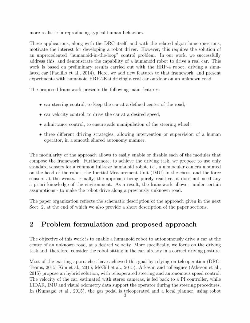
The driving framework, as described above, allows a humanoid robot to autonomously drivea car along an unknown road, at a desired velocity. We further extend the versatility ofour framework by implementing three different “driving modes”, in order to ease humansupervision and eventual intervention if needed:

• Autonomous. Car steering and velocity control are both enabled, as indicated above,and the robot autonomously drives the car without any human aid.

5

Table 1: Driving modes. For each mode, the steering and the car velocity control are properlyenabled or disabled.

Driving mode Steering Car velocitycontrol control

Autonomous enabled enabledAssisted enabled? disabledTeleoperated disabled disabled? Road detection is assisted by the human.

• Assisted. A human takes care of the road detection, the car velocity estimation,and the control, by teleoperating the robot ankle, and manually selecting the visualfeatures (road borders). These are then used by the steering controller to computethe robot arm command.

• Teleoperated. Both the robot hand and foot are teleoperated for steering the wheeland the gas pedal operation, respectively. The reference signals are sent to the task-based quadratic programming control through a keyboard or joystick. The humanuses the robot camera images as visual feedback for driving.

For each of the driving modes, the car steering and velocity controllers are enabled or dis-abled, as described in Table 1. The human user/supervisor can intervene at any momentduring the execution of the driving task, to select one of the three driving modes. Theselection, as well as the switching between modes, is done by pushing proper joystick (orkeyboard) buttons.

The framework has a modular structure, as presented in Fig. 1. In the following Sections,we detail the primitive functionalities required by the autonomous mode, since the assistedand teleoperation modes use a subset of such functionalities.

The rest of paper is organized as follows. Section 3 describes the model used for the car-robot system. Then, the main components of the proposed framework are detailed. Sect. 4presents the perception part, i.e., the algorithms used to detect the road and to estimate thecar velocity. Section 5 deals with car control, i.e., how the feedback signals are transformedinto references for the steering wheel and for the gas pedal, while Sect. 6 focuses on hu-manoid control, i.e., on the computation of the commands for the robot hand and foot. Theexperiments carried out with HRP-2Kai are presented in Sect. 7. Finally, Sect. 8 concludesthe paper and outlines future research perspectives.

3 Modelling

The design of the steering controller is based on the car kinematic model. This is a reasonablechoice since, for nonholonomic systems, it is possible to cancel the dynamic parameters via

6

Fw yw

zw

Fc

yc

zc

Fb

xb

zb

zwc

ywc

γ

opticalaxis

(a)

Fw

WFp

path

leftroad border

right

road borderx

xw

c

θφ

v

ω

(b)

Figure 2: Side (a) and top view (b) of a humanoid robot driving a car with relevant variables.

feedback, and to solve the control problem at the velocity level, provided that the velocityissued by the controller is differentiable (De Luca and Oriolo, 1995). To recover the dynamicsystem control input, it is however necessary to know the exact dynamic model, which is ingeneral not available. Although some approximations are therefore necessary, these do notaffect the controller in the considered scenario (low accelerations, flat and horizontal road).On-line car dynamic parameter identification could be envisaged, and seamlessly integratedin our framework, whenever the above assumptions are not valid. Note, however, that theproposed kinematic controller would remain valid, since it captures the theoretic challengeof driving in the presence of nonholonomic constraints.

To derive the car control model, consider the reference frame Fw placed on the car rear axlemidpoint W , with the y-axis pointing forward, the z-axis upward and the x-axis completingthe right handed frame (see Fig. 2a). The path to be followed is defined as the set of pointsthat maximize the distance from both the left and right road borders. On this path, weconsider a tangent Frenet Frame Fp, with origin on the normal projection of W on the path.Then, the car configuration with respect to the path is defined by x, the Cartesian abscissaof W in Fp, and by θ, the car orientation with respect to the path tangent (see Fig. 2b).Describing the car motion through the model of a unicycle, with an upper curvature boundcM ∈ R+, x and θ evolve according to:

x = v sin θ

θ = ω

∣∣∣ωv

∣∣∣ < cM , (1)

where v and ω represent respectively the linear and angular velocity of the unicycle. Thefront wheel orientation φ can be approximately related to v and ω through:

φ = arctan

(ωl

v

), (2)

with l the constant distance between the rear and front wheel axes2.2Bounds on the front wheels orientation characterizing common service cars induce the maximum curva-

7

Fs

xs

ys

zs

Fh

xh

yh

zh

αβ

r

Figure 3: The steering wheel, with rotation angle α, hand and steering frames, Fh and Fs.The parameters r, the radius of the wheel, and β, characterizing the grasp configuration, arealso shown here.

Note that a complete car-like model could have been used, for control design purposes,by considering the front wheels orientation derivative as the control input. The unicyclestabilizing controller adopted in this paper can in fact be easily extended to include thedynamics of the front wheels orientation, for example through backstepping techniques.However, in this case, a feedback from wheel orientation would have been required by thecontroller, but is, generally, not available. A far more practical solution is to neglect thefront wheels orientation dynamics, usually faster than that of the car, and consider a staticrelationship between the front wheels orientation and the car angular velocity. This will onlyrequire a rough guess on the value of the parameter l, since the developed controller showssome robustness with respect to model parameters uncertainties as will be shown in Sect. 5.

The steering wheel is shown in Fig. 3, where we indicate, respectively with Fh and Fs, thehand and steering wheel reference frames. The origin of Fs is placed at the center of thewheel, and α is the rotation around its z-axis, that points upward. Thus, positive values ofα make the car turn left (i.e., lead to negative ω).

Neglecting the dynamics of the steering mechanism (Mohellebi et al., 2009), assuming thefront wheels orientation φ to be proportional to the steering wheel angle α, controlled by thedriver hands, and finally assuming small angles ωl/v in (2), leads to:

α = kαω

v, (3)

with kα a negative3 scalar, characteristic of the car, accounting also for l.

The gas pedal is modeled by its inclination angle ζ, that yields a given car acceleration a =dv/dt. According to experimental observations, at low velocities, the relationship betweenthe pedal inclination and the car acceleration is linear:

ζ = kζa. (4)

The pedal is actuated by the motion of the robot foot, that is pushing it (see Fig. 4a).

ture constraint in (1).3Because of the chosen angular conventions.

8

ζ

qa

(a)

∆ζ

∆qa

C1

C2C3

lp

la

(b)

Figure 4: (a) The robot foot operates the gas pedal by regulating the joint angle at the ankleqa, to set a pedal angle ζ, and yield car acceleration a. (b) Geometric relationship betweenthe ankle and the gas pedal angles.

Assuming small values of ∆qa and ∆ζ, the point of contact between the foot and the pedalcan be considered fixed on both the foot and the pedal, i.e., the length of the segment C2C3

in Fig. 4b can be considered close to zero4. Hence, the relationship between ∆qa and ∆ζ iseasily found to be

∆ζ =lalp

∆qa, (5)

where la (lp) is the distance of the ankle (pedal) rotation axis from the contact point of thefoot with the pedal.

The robot body reference frame Fb is placed on the robot chest, with x-axis pointing forward,and z-axis upward. Both the accelerations measured by the IMU, and the humanoid tasks,are expressed in this frame. We also indicate with Fc the robot camera frame (see Fig. 2).Its origin is in the optical center of the camera, with z-axis coincident with the focal axis.The y-axis points downwards, and the x-axis completes the right-handed frame. Fc is tiltedby an angle γ (taken positive downwards) with respect to the frame Fw, whereas the vectorpwc = (xwc , y

wc , z

wc )T indicates the position vector of the camera frame expressed in the car

reference frame.

Now, the driving task can be formulated. It consists in leading the car on the path, andaligning it with the path tangent:

(x, θ)→ (0, 0) , (6)

while driving at a desired velocity:v → v∗. (7)

Task (6) is achieved by the steering control that uses the kinematic model (1), and is realizedby the robot hand according to the steering angle α. Concurrently, (7) is achieved by the car

4For the sake of clarity, in Fig. 4b the length of the segment C2C3 is much bigger than zero. However,this length, along with angles ∆qa and ∆ζ, is almost null.

9

M

V

image plane

xi

yi

xv xm

left roadborder

right roadborder

Figure 5: The images of the road borders define the middle and vanishing point, respectivelyM and V . Their abscissa values are denoted with xm and xv.

velocity control realized by the robot foot that sets a proper angle ζ for the gas pedal. Thecomputation of α and ζ rely on the perception module, that is detailed in the next Section.

4 Perception

The block diagram of Fig. 1 shows our perception-action approach. At a higher level, theperception block, whose details are described in this Section, provides the feedback signalsfor the car and robot control.

4.1 Road detection

This Section describes the procedure used to derive the road visual features, required tocontrol the steering wheel. These visual features are: (i) the vanishing point (V ), i.e., theintersection of the two borders, and (ii) the middle point (M), i.e., the midpoint of thesegment connecting the intersections of the borders with the image horizontal axis. Bothare shown in Fig. 5.

Hence, road detection consists of extracting the road borders from the robot camera images.After this operation, deriving the vanishing and middle point is trivial. Since the focusof this work is not to advance the state-of-the-art on road/lane detection, but rather topropose a control architecture for humanoid car driving, we develop a simple image processingalgorithm for road border extraction. More complex algorithms can be used to improve thedetection and tracking of the road (Liu et al., 2008; Lim et al., 2009; Meuter et al., 2009;Nieto et al., 2012), or even to detect road markings (Vacek et al., 2007). However, ourmethod has the advantage of being based solely on vision, avoiding the complexity inducedby integration of other sensors (Dahlkamp et al., 2006; Ma et al., 2000). Note that moreadvanced software is owned by car industries, and therefore hard to find in open-code sourceor binary.

Part of the road borders extraction procedure follows standard techniques used in the field10

(a) On-board camera image with the red detectedroad borders. The vanishing and middle pointare shown respectively in cyan and green.

(b) First color detection.

(c) Second color detection.

(d) Mask obtained after dilation and erosion.

(e) Convex hull after Gaussian filtering. (f) Canny edge detection.

(g) Hough transform. (h) Merged segments.

Figure 6: Main steps of the road detection algorithm. Although the acquired robot image (a)is shown in gray-scale here, the proposed road detection algorithm processes color images.

of computer vision (Laganiere, 2011) and is based on the OpenCV library (Bradski, 2000)that provides ready-to-use methods for our vision-based algorithm. More in detail, the stepsused for the detection of the road borders on the currently acquired image are describedbelow, with reference to Fig. 6.

• From the image, a Region Of Interest (ROI), shown with white borders in Fig. 6a,is manually selected at the initialization, and kept constant during the driving ex-periment. Then, at each cycle of the image processing, we compute the average andstandard deviation of hue and saturation channels of the HSV (Hue, Saturation andValue) color space on two central rectangular areas in the ROI. These values areconsidered for the thresholding operations described in the next step.

• Two binary images (Fig. 6b and 6c) are obtained by discerning the pixels in the ROI,whose hue and saturation value are in the ranges (average ± standard deviation)defined in the previous step. This operation allows to detect the road, while beingadaptive to color variation. The HSV value channel is not considered, in order to be

11

robust to luminosity changes.

• To remove “salt and pepper noise”, the dilation and erosion operators are applied tothe binary images. Then, the two images are merged by using the OR logic operatorto obtain a mask of the road (Fig. 6d).

• The convex hull is computed with areas greater than a given threshold on the maskfound in the previous step; then, a Gaussian filter is applied for smoothing. Theresult is shown in Fig. 6e.

• The Canny edge detector (Fig. 6f), followed by Hough transform (Fig. 6g) are applied,to detect the line segments on the image.

• Similar segments are merged5, as depicted in Fig. 6h.

This procedure gives two lines corresponding to the image projection of the road borders.However, in real working conditions, it may happen that one or both the borders are notdetectable because of noise on the image, or failures in the detection process. For thisreason, we added a recovery strategy, as well as a tracking procedure, to the pipeline. Therecovery strategy consists in substituting the borders, that are not detected, with artificialones, defined offline as oblique lines that, according to the geometry of the road and to theconfiguration of the camera, most likely correspond to the road borders. This allows thecomputation of the vanishing and middle point even when one (or both) real road bordersare not correctly detected. On the other hand, the tracking procedure gives continuity androbustness to the detection process, by taking into account the borders detected on theprevious image. It consists of a simple KF, with state composed of the slope and interceptof the two borders6. In the prediction step, the KF models the position of lines on theimage plane as constant (a reasonable design choice, under Assumption 3, of locally flatand straight road), whereas the measurement step uses the road borders as detected in thecurrent image.

From the obtained road borders (shown in red in Fig.6a), the vanishing and middle pointare derived, with simple geometrical computations. Their values are then smoothed witha low-pass frequency filter, and finally fed to the steering control, that will be described inSect. 5.1.

4.2 Car velocity estimation

To keep the proposed framework independent from the car characteristics, we propose toestimate the car speed v, by using only the robot sensors, and avoiding information comingfrom the car equipment, such as GPS, or speedometer. To this end, we use the robot camera,

5For details on this step, refer to (Paolillo et al., 2016).6Although 3 parameters are sufficient if the borders are parallel, a 4-dimensional state vector will cover

all cases, while guaranteeing robustness to image processing noise.

12

Fc

xc

yc

zc

optical axis

image plane

xi

yif (xg, yg, zg)

(xp, yp)

(a)

Fc

yc

zc

yp

zw

c

image plane

(xg, yg , zg)

γ

ǫ

(b)

Figure 7: Schematic representation of the robot camera looking at the road. (a) Any visiblecartesian point (xg, yg, zg) on the ground has a projection on the camera image plane, whosecoordinates expressed in pixels are (xp, yp). (b) The measurement of this point on the imageplane, together with the camera configuration parameters, can be used to estimate the depthzg of the point.

to measure the optical flow, i.e. the apparent motion of selected visual features, due to therelative motion between camera and scene.

The literature in the field of autonomous car control provides numerous methods for esti-mating the car speed by means of optical flow (Giachetti et al., 1998; Barbosa et al., 2007).To improve the velocity estimate, the optical flow can be fused with inertial measurements,as done in the case of aerial robots, in (Grabe et al., 2012). Inspired by that approach, wedesign a KF, fusing the acceleration measured by the robot IMU and the velocity measuredwith optical flow.

Considering the linear velocity and acceleration along the forward car axis yw as state ξ =(v a)T of the KF, we use a simple discrete-time stochastic model to describe the car motion:

ξk+1 =

(1 ∆T0 1

)ξk + nk, (8)

with ∆T the sampling time, and nk the zero-mean white gaussian noise. The correspondingoutput of the KF is modeled as:

ηk = ξk +mk, (9)

where mk indicates the zero-mean white gaussian noise associated to the measurement pro-cess. The state estimate is corrected, thanks to the computation of the residual, i.e., thedifference between measured and predicted outputs. The measurement is based on both theoptical flow (vOF ), and the output of the IMU accelerometers (aIMU). Then, the estimationof the car velocity v will correspond to the first element of state vector ξ. The process toobtain vOF and aIMU is detailed below.

13

4.2.1 Measure of the car speed with optical flow

To measure the car velocity vOF in the KF, we use optical flow. Optical flow can be usedto reconstruct the motion of the camera, and from that, assuming that the transformationfrom the robot camera frame to the car frame is known, it is straightforward to derive thevehicle velocity.

More in detail, the 6D velocity vector vc of the frame Fc can be related to the velocity ofthe point tracked in the image xp through the following relation:

xp = Lvc, (10)

where the interaction matrix L is expressed as follows (Chaumette and Hutchinson, 2006):

L =

(−Sx

zg0 xp

zg

xpypSy

−(Sx +x2pSx

) ypSx

Sy

0 −Sy

zg

ypzg

Sy +y2pSy

−xpypSy

−xpSy

Sx

). (11)

Here, (xp, yp) are the image coordinates (in pixels) of the point on the ground, expressed as(xg, yg, zg) in the camera frame (see Fig. 7). Furthermore, it is Sx,y = fαx,y, where f is thecamera focal length and αx/αy the pixel aspect ratio. In the computation of L, we considerthat the image principal point coincides with the image center. As shown in Fig. 7b, thepoint depth zg can be reconstructed through the image point ordinate yp and the cameraconfiguration (tilt angle γ and height zwc ):

zg =zwc cos ε

sin(γ + ε), ε = arctan

(ypSy

). (12)

Actually, the camera velocity vc is computed by taking into account n tracked points, i.e.,in (10), we consider respectively L = (L1 · · ·Ln)T and ˆxp = (xp,1 · · · xp,n)T , instead of Land xp. Then, vc is obtained by solving a least-squares problem7:

vc = arg minχ||Lχ− ˆxp||2. (13)

The reconstruction of ˆxp in (13) is based on the computation of the optical flow. However,during the navigation of the car, the vibration of the engine, poor textured views and otherun-modeled effects add noise to the measurement process (Giachetti et al., 1998). Further-more, other factors, such as variable light conditions, shadows, and repetitive textures, canjeopardize feature tracking. Therefore, raw optical flow, as provided by off-the-shelf algo-rithms –e.g., from the OpenCV library (Bradski, 2000), gives noisy data that are insufficientfor accurate velocity estimation; so filtering and outlier rejection techniques must be added.

7To solve the least-square problem, n ≥ 3 points are necessary. In our implementation, we used theopenCV solve function, and in order to filter the noise due to few contributions, we set n ≥ 25. If n < 25,we set vc = 0.

14

Since the roads are generally poor in features, we use a dense optical flow algorithm, thatdiffers from sparse algorithms, in that it computes the apparent motion of all the pixels of theimage plane. Then, we filter the dense optical flow, first according to geometric rationales,and then with an outlier rejection method (Barbosa et al., 2007). The whole procedure isdescribed below, step-by-step:

• Take two consecutive images from the robot on-board camera.

• Consider only the pixels in a ROI that includes the area of the image plane corre-sponding to the road. This ROI is kept constant along all the experiment and, thus,identical for the two consecutive frames.

• Covert the frames to gray scale, apply a Gaussian filter, and equalize with respectto the histogram. This operation reduces the measurement noise, and robustifies themethod with respect to light changes.

• Compute the dense optical flow, using the Farneback algorithm (Farneback, 2003)implemented in OpenCV.

• Since the car is supposed to move forward, in the dense optical flow vector, consideronly those elements pointing downwards on the image plane, and discard those nothaving a significant centrifugal motion from the principal point. Furthermore, con-sider only contributions with length between an upper and a lower threshold, andwhose origin is on an image edge (detected applying Canny operator).

• Reject the outliers, i.e., the contributions (xp,i, yp,i), i ∈ {1, . . . , n}, such that xp,i /∈[¯xp ± σx] and yp,i /∈ [¯yp ± σy], where ¯xp (¯yp ) and σx (σy) are the average and standarddeviation of the optical flow horizontal (vertical) contributions. This operation ismade separately for the contributions of the right and left side of the image, wherethe module and the direction of the optical flow vectors can be quite different (e.g.,on turns).

The final output of this procedure, ˆxp, is fed to (13), to obtain vc, that is then low-passfiltered. To transform the velocity vc in frame Fc, obtained from (13), into velocity vw inthe car frame Fw, we apply:

vw = W wc vc, (14)

with W wc the twist transformation matrix

W wc =

(Rwc SwcR

wc

03×3 Rwc

), (15)

Rwc the rotation matrix from car to camera frame, and Swc the skew symmetric matrix

associated to the position pwc of the origin of Fc in Fw.

Finally, the speed of the car is set as the y-component of vw: vOF = vw,y. This will constitutethe first component of the KF measurement vector.

15

4.2.2 Measure of the car acceleration with robot accelerometers

The IMU mounted on-board the humanoid robot is used to measure acceleration, in order toimprove the car velocity estimation through the KF. In particular, given the raw accelerom-eter data, we first compensate the gravity component, with a calibration executed at thebeginning of each experiment8. This gives ab, the 3D robot acceleration, expressed in therobot frame Fb. Then, we transform ab in the car frame Fw, to obtain:

aw = Rwb ab, (16)

where Rwb is the rotation matrix relative to the robot body - vehicle transformation. Fi-

nally, aIMU is obtained by selecting the y-component of aw. This will constitute the secondcomponent of the KF measurement vector.

5 Car control

The objective of car control is (i) to drive the rear wheel axis center W along the curvilinearpath that is equally distant from the left and right road borders (see Fig. 2b), while aligningthe car with the tangent to this path, and (ii) to track desired vehicle velocity v∗. Basi-cally, car control consists in achieving tasks (6) and (7), with the steering and car velocitycontrollers described in the following subsections.

5.1 Steering control

Given the visual features extracted from the images of the robot on-board camera, the vision-based steering controller generates the car angular velocity input ω to regulate both x andθ to zero. This reference input is eventually translated in motion commands for the robothands.

The controller is based on the algorithm introduced by (Toibero et al., 2009) for unicyclecorridor following, and recently extended to the navigation of humanoids in environmentswith corridors connected through curves and T-junctions (Paolillo et al., 2016). In view ofAssumption 3 in Sect. 2, the same algorithm can be applied here. For the sake of complete-ness, in the following, we briefly recall the derivation of the features model (that can befound, for example, also in (Vassallo et al., 2000)) and the control law originally presentedby (Toibero et al., 2009). In doing so, we illustrate the adaptations needed to deal with thespecificity of our problem.

The projection matrix transforming the homogeneous coordinates of a point, expressed inFp, to its homogeneous coordinates in the image, is:

P = K T cw T

wp , (17)

8The assumption on horizontal road in Sect. 3 avoids the need for repeating this calibration.

16

where K is the camera calibration matrix (Ma et al., 2003), T cw the transformation from

the car frame Fw to Fc, and T wp from the path frame Fp to Fw.

As intuitive from Fig. 2, the projection matrix depends on both the car coordinates, and thecamera intrinsic and extrinsic parameters. Here, we assume that the camera principal pointcoincides with the image center, and we neglect image distortion. Furthermore, P has beencomputed neglecting the z-coordinates of the features, since they do not affect the controltask. Under these assumptions, using P , the abscissas of the vanishing and middle point,respectively denoted by xv and xm, can be expressed as (Toibero et al., 2009; Vassallo et al.,2000):

xv = k1 tan θ

xm = k2x

cθ+ k3 tan θ + k4,

(18)

where

k1 = −Sx/cγk2 = −Sxsγ/zwck3 = −Sxcγ − Sxsγywc /zwck4 = −Sxsγxwc /zwc .

We denote cos(∗) and sin(∗) with c∗ and s∗, respectively. Note that with respect to the visualfeatures model in (Toibero et al., 2009; Vassallo et al., 2000), the expression of the middlepoint changes, due to the introduction of the lateral and longitudinal displacement, xwc andywc respectively, of the camera frame with respect to the car frame. As a consequence, toregulate the car position to the road center, we must define a new visual feature xm = xm−k4.Then, the navigation task (6) is equivalent to the following visual task:

(xm, xv)→ (0, 0) . (19)

In fact, according to (18), asymptotic convergence of xv and xm to zero implies convergenceof x and θ to zero, achieving the desired path following task.

Feedback stabilization of the dynamics of xm, is given by the following angular velocitycontroller (Toibero et al., 2009):

ω =k1

k1k3 + xmxv

(−k2k1vxv − kpxm

), (20)

with kp a positive scalar gain. This controller guarantees asymptotic convergence of bothxm and xv to zero, under the conditions that v > 0, and that k2 and k3 have the same sign,which is always true if (i) γ ∈ (0, π/2) and (ii) ywc > −zwc / tan γ, two conditions alwaysverified with the proposed setup.

Note that this controller has been obtained considering the assumption of parallel roadborders. Nevertheless, this assumption can be easily relaxed since we showed in (Paolillo

17

et al., 2016) that the presence of non-parallel borders does not jeopardize the controller’slocal convergence.

To realize the desired ω in (20), the steering wheel must be turned according to (3):

α =kαk1

k1k3 + xmxv

(−k2k1xv − kp

xmv

), (21)

where xm and xv are obtained by the image processing algorithm of Sect. 4.1, while the valueof v is estimated through the velocity estimation module presented in Sect. 4.2.

5.2 Car velocity control

In view of the assumption of low acceleration, and by virtue of the linear relationship betweenthe car acceleration and the pedal angle (eq. (4)), to track a desired car linear velocity v∗

we designed a PID feedback controller to compute the gas pedal command:

ζ = kv,p ev + kv,i

∫ev + kv,d

d

dtev. (22)

Here, ev = (v∗ − v) is the difference between the desired and current value of the velocity,as computed by the car velocity estimation block, while kv,p, kv,i and kv,d are the positiveproportional, integral and derivative gains, respectively. In the design of the velocity controllaw, we decided to insert an integral action to compensate for constant disturbances (like,e.g., the effect of a small road slope) at steady state. The derivative term helped achievinga damped control action. The desired velocity v∗ is set constant here.

6 Robot control

This section presents the lower level of our controller, which enables the humanoid robot toturn the driving wheel by α, and push the pedal by ζ.

6.1 Wheel operation

The reference steering angle α is converted to the reference pose of the hand grasping thewheel, through the rigid transformation

T b∗h = T b

s (α)T sh (r, β) .

Here, T b∗h and T b

s are the transformation matrices expressing respectively the poses of framesFh and Fs in Fig. 3 with respect to Fb in Fig. 2a. Constant matrix T s

h expresses the poseof Fh with respect to Fs, and depends on the steering wheel radius r, and on the angle βparameterizing the hand position on the wheel.

18

For a safe interaction between the robot hand and the steering wheel, it is obvious tothink of an admittance or impedance controller, rather than solely a force or position con-troller (Hogan, 1985). We choose to use the following admittance scheme:

f − f ∗ = M∆x+B∆x+K∆x, (23)

where f and f ∗ are respectively the sensed and desired generalized interaction forces in Fh;M , B and K ∈ R6×6 are respectively the mass, damping and stiffness diagonal matrices. Asa consequence of the force f applied on Fh, and on the base of the values of the admittancematrices, (23) generates variations of pose ∆x, velocity ∆x and acceleration ∆x of Fh withrespect to Fs. Thus, the solution of (23) leads to the vector ∆x that can be used to computethe transformation matrix ∆T , and to build up the new desired pose for the robot hands:

T bh = T b∗

h ·∆T . (24)

In cases where the admittance controller is not necessary, we simply set ∆T = I.

6.2 Pedal operation

Since there exists a linear relationship between the variation of the robot ankle and thevariation of the gas pedal angle, to operate the gas pedal it is sufficient to move the anklejoint angle qa. From (22), we compute the command for the robot ankle’s angle as:

qa =ζ

ζmax

(qa,max − qa,min) + qa,min. (25)

Here, qa,max is the robot ankle configuration, at which the foot pushes the gas pedal, pro-ducing a significant car acceleration. Instead, at qa = qa,min, the foot is in contact with thepedal, but not yet pushing it. These values depend both on the car type, and on the posi-tion of the foot with respect to the gas pedal. A calibration procedure is run before startingdriving, to identify the proper values of qa,min and qa,max. Finally, ζmax is set to avoid largeaccelerations, while saturating the control action.

6.3 Humanoid task-based control

As shown above, wheel and pedal operation are realized respectively in the operational space(by defining a desired hand pose T b

h) and in the articular space (via the desired ankle jointangle qa). Both can be realized using our task-based quadratic programming (QP) controller,assessed in complex tasks such as ladder climbing (Vaillant et al., 2016). The joint anglesand desired hand pose are formulated as errors that appear among the sum of weighted least-squares terms in the QP cost function. Other intrinsic robot constraints are formulated aslinear expressions of the QP variables, and appear in the constraints. The QP controlleris solved at each control step. The QP variable vector x = (qT ,λT )T , gathers the jointacceleration q, and the linearized friction cones’ base weights λ, such that the contact forcesf are equal to Kfλ (with Kf the discretized friction cone matrix). The desired acceleration

19

q is integrated twice to feed the low level built-in PD control of HRP-2Kai. The driving taskwith the QP controller writes as follows:

minimizex

N∑i=1

wi‖Ei(q, q, q)‖2 + wλ‖λ‖2

subject to

1) dynamic constraints

2) sustained contact positions

3) joint limits

4) non-desired collision avoidance constraints

5) self-collision avoidance constraints,

(26)

where wi and wλ are task weights or gains, and Ei(q, q, q) is the error in the task space.Details on the QP constraints (since they are common to most tasks) can be found in (Vaillantet al., 2016).

Here, we explicit the tasks used specifically during the driving (i.e. after the driving postureis reached). We use four (N = 4) set-point objective tasks; each task (i) is defined by itsassociated task-error εi so that Ei = Kpiεi +Kvi εi + εi.

The driving wheel of the car has been modeled as another ‘robot’ having one joint (rotation).We then merged the model of the driving wheel to that of the humanoid and linked them,through a position and orientation constraint, so that the desired driving wheel steeringangle α, as computed by (24), induces a motion on the robot (right arm) gripper. The tasklinking the humanoid robot to the driving wheel ‘robot’ is set as part of the QP constraints,along with all sustained contacts (e.g. buttock on the car seat, thighs, left foot).

The steering angle α (i.e. the posture of the driving wheel robot) is a set-point task (E1).The robot whole-body posture including the right ankle joint control (pedal) is also a set-point task (E2), which realizes the angle qa provided by (25). Additional tasks were set tokeep the gaze direction constant (E3), and to fix the left arm, to avoid collisions with thecar cockpit during the driving operation (E4).

7 Experimental results

We tested our driving framework with the full-size humanoid robot HRP-2Kai built byKawada Industries. For the experiments, we used the Polaris Ranger XP900, the sameutility vehicle employed at the DRC. HRP-2Kai has 32 degrees of freedom, is 1.71 m tall andweighs 65 kg. It is equipped with an Asus Xtion Pro 3D sensor, mounted on its head andused in this work as a monocular camera. The Xtion camera provides images at 30 Hz witha resolution of 640×480 pixels. From camera calibration, it results Sx ' Sy = 535 pixels. Inthe presented experiments, xwc = −0.4 m, ywc = 1 m and zwc = 1.5 m were manually measured.However, it would be possible to estimate the robot camera position, with respect to the

20

car frame, by localization of the humanoid (Oriolo et al., 2015), or by using the geometricinformation of the car (that can be known, e.g., in the form of a CAD model, as shownin Fig. 2). HRP-2Kai is also equipped with an IMU (of rate 500 Hz) located in the chest.Accelerometer data have been merged with the optical flow to estimate the car linear velocity,as explained in Sect. 4.2. Furthermore, a built-in filter processes the IMU data to providean accurate measurement of the robot chest orientation. This is kinematically propagatedup to the Xtion sensor to get γ, the tilt angle of the camera with respect to the ground.

The task-based control is realized through the QP framework (see Sect. 6.3) which allows toeasily set different tasks that can be achieved concurently by the robot. The following tablegives the weights of the 4 set-point tasks described in Sect. 6.3. Note that Kvi = 2×

√Kpi .

Table 2: QP weights and set-point gains.

E1 E2 E3 E4

w 100 5 1000 1000Kp 5 1 (ankle = 100) 10 10

As for the gains in Section 5, we set kv,p = 10−8, kv,d = 3 ·10−9 and kv,i = 2 ·10−9 to track thecar desired velocity v∗, whereas in the steering wheel controller we choose the gain kp = 3,and we set the parameter kα = −5. While the controller gains have been chosen as a tradeoffbetween reactivity and control effort, the parameter kα was roughly estimated. Given theconsidered scenario, an exact knowledge of this parameter is generally not possible, sinceit depends on the car characteristics. It is however possible to show that, at the kinematiclevel, this kind of parameter uncertainty will induce a non-persistent perturbation on thenominal closed loop dynamics.

Proving the boundedness of the perturbation term induced by parameter uncertainties wouldallow to conclude about the local asymptotic stability of the perturbed system. In general,this would imply a bound on the parameter uncertainty, to be satisfied to preserve localstability. While this analysis is beyond the scope of this paper, we note also that in prac-tice it is not possible to limit the parameter uncertainty, that depends on the car and theenvironment characteristics. Therefore, we rely on the experimental verification of the vision-based controller robustness, delegating to the autonomous-assisted-teleoperated frameworkthe task of taking the autonomous mode controller within its region of local asymptoticstability. In other words, when the system is too far from the equilibrium condition, andconvergence of the vision-based controller could be compromised, due to model uncertaintiesand unexpected perturbations, the user can always resort to the other driving modes.

In the KF used for the car velocity estimation, the process and the measurement noisecovariances matrices are set to diag(1e−4, 1e−4) and diag(1e2, 1e2), respectively. Since theforward axis of the robot frame is aligned with the forward axis of the vehicle frame, to getaIMU we didn’t apply the transformation (16), but we simply collected the acceleration alongthe forward axis of the robot frame, as given by the accelerometers. The sampling time ofthe KF was set to ∆T = 0.002 s (being 500 Hz the frequency of the IMU measurements, the

21

(a) Human-like grasp.

0 50 100 150 200 250 300−20

0

20

time [s]

f x [N]

0 50 100 150 200 250 300−0.02

0

0.02

∆ x

[m]

(b) Admittance along x-axis

0 50 100 150 200 250 300−20

0

20

time [s]

f y [N]

0 50 100 150 200 250 300−0.02

0

0.02

∆ y

[m]

(c) Admittance along y-axis

0 50 100 150 200 250 300−20

0

20

time [s]

f z [N]

0 50 100 150 200 250 300−0.02

0

0.02

∆ z

[m]

(d) Admittance along z-axis

Figure 8: Left: setup of an experiment that requires admittance control on the steering hand.Right: output of the admittance controller in the hand frame during the same experiment.

filter runs at the same rate).

The cut-off frequencies of the low-pass filters applied to the visual features and the carvelocity estimate were set to 8 and 2.5 Hz, respectively.

At the beginning of each campaign of experiments, we arrange the robot in the correctdriving posture in the car as shown in Fig. 9a. This posture (except for the driving legand arm) is assumed constant during driving: all control parameters are kept constant. Atinitialization, we also correct eventual bad orientations of the camera with respect to theground plane, by applying a rotation to the acquired image, and by regulating the pitch andyaw angles of the robot neck, so as to align the focal axis with the forward axis of the carreference frame. The right foot is positioned on the gas pedal, and the calibration proceduredescribed in Sect. 6.2 is used to obtain qa,max and qa,min.

To ease full and stable grasping of the steering wheel, we designed a handle, fixed to the wheel(visible in Fig. 9a), allowing the alignment of the wrist axis with that of the steer. Withreference to Fig. 3, this corresponds to configuring the hand grasp with r = 0 and, to complywith the shape of the steering wheel, β = 0.57 rad. Due to the robot kinematic constraints,such as joint limits and auto-collisions avoidance, imposed by our driving configuration, therange of the steering angle α is restricted from approximately -2 rad to 3 rad. These limitscause bounds on the maximum curvature realizable by the car. Nevertheless, all of the

22

(a) Driving posture (b) Top view of the experimental area

Figure 9: The posture taken by HRP-2Kai during the experiments (a) and the experimentalarea at the AIST campus (b).

followed paths were compatible with this constraint. For more challenging maneuvers, graspreconfiguration should be integrated in the framework.

With this grasping setup, we achieved a good alignment between the robot hand and thesteering wheel. Hence, during driving, the robot did not violate the geometrical constraintsimposed by the steering wheel mechanism. In this case, the use of the admittance controlfor safe manipulation is not necessary. However, we showed in (Paolillo et al., 2014), thatthe admittance control can be easily plugged in our framework, whenever needed. In fact, inthat work, an HRP-4, from Kawada Industries, turns the steering wheel with a more ‘human-like’ grasp (r = 0.2 m and β = 1.05 rad, see Fig. 8a). Due to the characteristics of boththe grasp and the HRP-4 hand, admittance control is necessary. For sake of completeness,we report, in Fig. 8b-8d, plots of the admittance behavior relative to that experiment. Inparticular, to have good tracking of the steering angle α, while complying with the steeringwheel geometric constraint, we designed a fast (stiff) behavior along the z-axis of the handframe, Fh, and a slow (compliant) along the x and y-axes. To this end, we set the admittanceparameters: mx = my = 2000 kg, mz = 10 kg, bx = by = 1600 kg/s, bz = 240 kg/s, andkx = ky = 20 kg/s2, kz = 1000 kg/s2. Furthermore, we set the desired forces f ∗

x = f ∗z = 0 N,

while along the y-axis of the hand frame f ∗y = 5 N, to improve the grasping stability. Note

that the evolution of the displacements along the x and y-axes (plots in Fig. 8b-8c), are theresults of a dynamic behavior that filters the high frequency of the input forces, while alongthe z-axis the response of the system is more reactive.

In the rest of this section, we present the HRP-2Kai outdoor driving experiments. In par-ticular, we present the results of the experiments performed at the authorized portion ofthe AIST campus in Tsukuba, Japan. A top view of this experimental field is shown inFig. 9b. The areas highlighted in red and yellow correspond to the paths driven using

23

Figure 10: First experiment: autonomous car driving.

the autonomous and teleoperated mode, respectively, as further described below. Further-more, we present an experiment performed at the DRC final, showing the effectiveness ofthe assisted driving mode. For a quantitative evaluation of the approach, we present theplots of the variables of interest. The same experiments are shown in the video availableat https://youtu.be/SYHI2JmJ-lk, that also allows a qualitative evaluation of the onlineimage processing. Quantitatively, we successfully carried out 14 experiments over of 15 repe-titions, executed at different times, between 10:30 a.m. and 4 p.m., proving image processingrobustness in different light conditions.

7.1 First experiment: autonomous car driving

In the first experiment, we tested the autonomous mode, i.e., the effectiveness of our frame-work to make a humanoid robot drive a car autonomously. For this experiment, we choosev∗ = 1.2 m/s, while the foot calibration procedure gave qa,max = −0.44 rad and qa,min =−0.5 rad.

Figure 10 shows eight snapshots taken from the video of the experiment. The car starts withan initial lateral offset, that is corrected after a few meters. The snapshots (as well as thevideo) of the experiment show that the car correctly travels at the center of a curved path,for about 100 m. Furthermore, one can observe that the differences in the light conditions

24

0 20 40 60 80 100

−2

0

2

a IMU

[m/s

2 ]

time [s]

Acceleration of the car from IMU

10 20 30 40 50 60 70 80 90 1000

0.5

1

1.5

2

v OF [m

/s]

time [s]

Speed of the car from optical flow

10 20 30 40 50 60 70 80 90 1000

0.5

1

1.5

2

v [m

/s]

time [s]

Speed of the car from Kalman filter

Figure 11: First experiment: autonomous car driving. Acceleration aIMU measured with therobot IMU (top), linear velocity vOF measured with the optical flow (center), and car speedv estimated by the KF (bottom).

(due to the tree shadows) and in the color of the road, do not jeopardize the correct detectionof the borders and, consequently, the driving performance.

Figure 11 shows the plots related to the estimation of the car speed, as described in Sect. 4.2.On the top, we plot aIMU, the acceleration along the forward axis of the car, as reconstructedfrom the robot accelerometers. The center plot shows the car speed measured with theoptical flow-based method (vOF), whereas the bottom plot gives the trace of the car speedv obtained by fusing aIMU and vOF. Note that the KF reduces the noise of the vOF signal, avery important feature for keeping the derivative action in the velocity control law (22).

As well known, reconstruction from vision (e.g., the “structure from motion” problem) suffersfrom a scale problem, in the translation vector estimate (Ma et al., 2003). This issue, dueto the loss of information in mapping 2D to 3D data, is also present in optical flow velocityestimation methods. Here, this can lead to a scaled estimate of the car velocity. For thisreason, we decided to include another sensor information in the estimation process: theacceleration provided by the IMU. Note, however, that in the current state of the work, thevelocity estimate accuracy has been only evaluated qualitatively. In fact, that high accuracyis only important in the transient phases (initial error recovery and curve negotiation).Instead, it can be easily shown that the perturbation induced by velocity estimate inaccuracy

25

time [s]

x m [p

ixel

]Middle point

10 20 30 40 50 60 70 80 90 100−320

0

320k

4

Vanishing point

time [s]

x v [pix

el]

10 20 30 40 50 60 70 80 90 100−320

0

320

time [s]

α [r

ad]

Steering angle

10 20 30 40 50 60 70 80 90 100−3.14

0

3.14commandencoder

(a)

Car speed

time [s]

v [m

/s]

10 20 30 40 50 60 70 80 90 1000

1.2

measured velocitydesired velocity

Robot ankle angle

time [s]

q a [rad

]

10 20 30 40 50 60 70 80 90 100

−0.5

−0.44 commandencoder

(b)

Figure 12: First experiment: autonomous car driving. (a) Middle point abscissa xm (top),vanishing point abscissa xv (center), and steering angle α (bottom). (b) Car speed v (top),already shown in fig 10, and ankle joint angle qa (bottom).

on the features dynamics vanishes at the regulation point corresponding to the desired drivingtask, and that by limiting the uncertainty on the velocity value, it is possible to preserve localstability. In fact, the driving performance showed that the estimation was accurate enough,for the considered scenario. In different conditions, finer tuning of the velocity estimatormay be necessary.

Plots related to the steering wheel control are shown in Fig. 12a. The steering control isactivated about 8 s after the start of the experiment and, after a transient time of a fewseconds, it leads the car to the road center. Thus, the middle and vanishing points (thetop and center plots, respectively) correctly converge to the desired values, i.e., xm goes tok4 = 30 pixels (since γ = 0.2145 rad –see expression of k4 in Sect. 5.1), and xv to 0. Thebottom plot shows the trend of the desired steering command α, as computed from the visualfeatures, and from the estimated car speed according to (21). The same signal, reconstructedfrom the encoders (black dashed line) shows that the steering command is smoothed by thetask-based quadratic programming control, avoiding undesirable fast signal variations.

Fig. 12b presents the plots of the estimated vs desired car speed (top) and the ankle anglecommand sent to the robot to operate the gas pedal and drive the car at the desired velocity(bottom).

Also in this case, after the initial transient, the car speed converges to the nominal desiredvalues (no ground truth was available). The oscillations observable at steady state are due tothe fact that the resolution of the ankle joint is coarser than that of the gas pedal. Note, infact, that even if the robot ankle moves in a small range, the car speed changes significantly.The noise on the ankle command, as well as the initial peak, are due to the derivative termof the gas pedal control (22). However, the signal is smoothed by the task-based quadraticprogramming control (see the dashed black line, i.e., the signal reconstructed by encoder

26

Figure 13: Second experiment: switching between teleoperated and autonomous modes.

readings), preventing jerky motion of the robot foot.

In the same campaign of experiments, we performed ten autonomous car driving experiments.In nine of them (including the one presented just above), the robot successfully drove thecar for the entire path. One of the experiments failed due to a critical failure of the imageprocessing. It was not possible to perform experiments on other tracks (with different roadshapes and environmental conditions), because our application was rejected after complexadministrative paperwork required to access other roads in the campus.

7.2 Second experiment: switching between teleoperated and autonomousmodes

In some cases, the conditions ensuring the correct behaviour of the autonomous mode arerisky. Thus, it is important to allow a user to supervise the driving operation, and controlthe car if required. As described in Sect. 2, our framework allows a human user to interveneat any time, during the driving operation, to select a particular driving strategy. Thesecond experiment shows the switching between the autonomous and teleoperated modes.In particular, in some phases of the experiment, the human takes control of the robot, byselecting the teleoperated mode. In these phases, proper commands are sent to the robot,to drive the car along two very sharp curves, connecting two straight roads traveled in

27

time [s]

x m [p

ixel

]Middle point

0 20 40 60 80 100 120 140 160−320

0

320k

4

Vanishing point

time [s]

x v [pix

el]

0 20 40 60 80 100 120 140 160−320

0

320

time [s]

α [r

ad]

Steering angle

0 20 40 60 80 100 120 140 160−3.14

0

3.14commandencoder

(a)

Car speed

time [s]

v [m

/s]

0 20 40 60 80 100 120 140 1600

1.5

measured velocitydesired velocity

Robot ankle angle

time [s]

q a [rad

]

0 20 40 60 80 100 120 140 160

−0.5

−0.43 commandencoder

(b)

Figure 14: Second experiment: switching between teleoperated and autonomous modes. (a)Middle point abscissa xm (top), vanishing point abscissa xv (center), and steering angle α(bottom). (b) Car speed v (top) and ankle joint angle qa (bottom).

autonomous mode. Snapshots of this second experiment are shown in Fig. 13.

For this experiment we set v∗ = 1.5 m/s, while after the initial calibration of the gas pedal,qa,min = −0.5 rad and qa,max = −0.43 rad. Note that the difference in the admissible anklerange with respect to the previous experiment is due to a slightly different position of therobot foot on the gas pedal.

Figure 14a shows the signals of interest for the steering control. In particular, one canobserve that when the control is enabled (shadowed areas of the plots) there is the samecorrect behavior of the system seen in the first experiment. When the user asks for theteleoperated mode (non-shadowed areas of the plots), the visual features are not considered,and the steering command is sent to the robot via keyboard or joystick by the user. Between75 and 100 s, the user controlled the robot (in teleoperated mode) to make it steer on the rightas much as possible. Because of the kinematic limits and of the grasping configuration, therobot saturated the steering angle at about -2 rad even if the user asked a wider steering. Thisis evident on the plot of the steering angle command of Fig. 14a (bottom): note the differencebetween the command (blue continuous curve), and the steering angle reconstructed fromthe encoders (black dashed curve).

Similarly, Fig. 14b shows the gas pedal control behavior when switching between the twomodes. When the gas pedal control is enabled, the desired car speed is properly tracked byoperating the robot ankle joint (shadowed areas of the top plot in Fig. 14b). On the otherhand, when the control is disabled (non-shadowed areas of the plots), the ankle command(blue curve in Fig. 14b, bottom), as computed by (25), is not considered, and the robotankle is teleoperated with the keyboard/joystick interface, as noticeable from the encoderplot (black dashed curve).

28

Figure 15: Third experiment: assisted driving mode at the DRC finals. Snapshots takenfrom the DRC official video.

At the switching between the two modes, the control keeps sending commands to the robotwithout any interruption, and the smoothness of the signals allows to have continuous robotoperation. In summary, the robot could perform the entire experiment (along a path of130 m ca., for more than 160 s) without the need to stop the car. This was achieved thanksto two main design choices. Firstly, from a perception viewpoint, monocular camera andIMU data are light to be processed, allowing a fast and reactive behavior. Secondly, thecontrol framework at all the stages (from the higher level visual control to the low levelkinematic control) guarantees smooth signals, even at the switching moments.

The same experiment presented just above was performed five other times, during the sameday. Four experiments resulted successful, while two failed do to human errors during tele-operation.

7.3 Third experiment: assisted driving at the DRC finals

The third experiment shows the effectiveness of the assisted driving mode. This strategywas used to make the robot drive at the DRC finals, where the first of the eight tasksconsisted in driving a utility vehicle along a straight path, with two sets of obstacles. Wesuccessfully completed the task, by using the assisted mode. Snapshots taken from the DRC

29

finals official video (DARPAtv, 2015) are shown in Fig. 15. The human user teleoperatedHRP-2Kai remotely, by using the video stream from the robot camera as the only feedbackfrom the challenge field. In the received images, the user selected, via mouse, the properartificial road borders (red lines in the figure), to steer the car along the path. Note that theseartificial road borders, manually set by the user, may not correspond to the real borders ofthe road. In fact, they just represent geometrical references - more intuitive for humans - toeasily define the vanishing and middle points and steer the car by using (21). Concurrently,the robot ankle was teleoperated to achieve a desired car velocity. In other words, withreference to the block diagram of Fig. 1, the user provides the visual features to the steeringcontrol, and the gas pedal reference to the pedal operation block. Basically, s/he takes theplace of the road detection and car velocity estimation/control blocks. The assisted modecould be seen as a sort of shared control between the robot and the a human supervisor, andallows the human to interfere with the robot operation if required. As stated in the previoussection, at any time, during the execution of the driving experience, the user can instantlyand smoothly switch to one of the other two driving modes. At the DRC, we used a wideangle camera, although the effectiveness of the assisted mode was also verified with a Xtioncamera.

8 Conclusions

In this paper, we have proposed a reactive control architecture for car driving by a humanoidrobot on unkown roads. The proposed approach consists in extracting road visual features,to determine a reference steering angle to keep the car at the center of a road. The gaspedal, operated by the robot foot, is controlled by estimating the car speed using visual andinertial data. Three different driving modes (autonomous, assisted, and teleoperated) extendthe versatility of our framework. The experimental results carried out with the humanoidrobot HRP-2Kai have shown the effectiveness of the proposed approach. The assisted modewas successfully used to complete the driving task at the DRC finals.

The driving task has addressed, as an explicative case-study of humanoids controlling human-tailored devices. In fact, besides the achievement of the driving experience, we believethat humanoids are the most sensible platforms for helping humans with everyday task,and the proposed work shows that complex real-world tasks can be actually performed inautonomous, assisted and teleoperated way. Obviously, the complexity of the task comesalso with the complexity of the framework design, on both perception and control point-of-views. This led us to make some working assumptions that, in some cases, limited the rangeof application of our methods.

Further investigations shall deal with the task complexity, to advance the state-of-art ofalgorithms, and make humanoids capable of helping humans with dirty, dangerous and de-manding jobs. Future work will be done, in order to make the autonomous mode workefficiently in the presence of sharp curves. To this end, and to overcome the problem of lim-ited steering motions, we plan to include, in the framework, the planning of variable graspingconfigurations, to achieve more complex manoeuvres. We are also planning to go to driving

30

on uneven terrains, where the robot has also to sustain its attitude, w.r.t. sharp changes ofthe car orientation. Furthermore, the introduction of obstacle avoidance algorithms, basedon optical flow, will improve the driving safety. Finally, we plan to add brake control and toperform the entire driving task, including car ingress and egress.

Acknowledgments

This work is supported by the EU FP7 strep project KOROIBOT www.koroibot.eu, andby the Japan Society for Promotion of Science (JSPS) Grant-in-Aid for Scientific Research(B) 25280096. This work was also in part supported by the CNRS PICS Project ViNCI.The authors deeply thank Dr. Eiichi Yoshida for taking in charge the administrative proce-dures in terms of AIST clearance and transportation logistics, without which the experimentscould not be conducted; Dr Fumio Kanehiro for lending the car and promoting this research;Herve Audren and Arnaud Tanguy for their kind support during the experiments.

References

Atkeson, C. G., Babu, B. P. W., Banerjee, N., Berenson, D., Bove, C. P., Cui, X. DeDonato,M., Du, R., Feng, S., Franklin, P., Gennert, M., Graff, J. P., He, P., Jaeger, A., Kim,J., Knoedler, K., Li, L., Liu, C., Long, X., Padir, T., Polido, F., Tighe, G. G., andXinjilefu, X. (2015). NO FALLS, NO RESETS: Reliable humanoid behavior in theDARPA Robotics Challenge. In 2015 15th IEEE-RAS Int. Conf. on Humanoid Robots,pages 623–630.

Barbosa, R., Silva, J., Junior, M. M., and Gallis, R. (2007). Velocity estimation of a mobilemapping vehicle using filtered monocular optical flow. In International Symposium onMobile Mapping Technology, volume 5.

Bradski, G. (2000). The OpenCV library. Dr. Dobb’s Journal of Software Tools, 25(11):120–126.

Broggi, A., Bombini, L., Cattani, S., Cerri, P., and Fedriga, R. I. (2010). Sensing require-ments for a 13,000 km intercontinental autonomous drive. In 2010 IEEE IntelligentVehicles Symposium (IV), pages 500–505.

Buehler, M., Lagnemma, K., and Singh, S. E. (2008). Special issue on the 2007 DARPAUrban Challenge, part I-III. Journal of Field Robotics, 25(8-10):423–860.

Chaumette, F. and Hutchinson, S. (2006). Visual servo control, Part I: Basic approaches.IEEE Robot. Automat. Mag., 13(4):82–90.

Cherubini, A., Spindler, F., and Chaumette, F. (2014). Autonomous visual navigationand laser-based moving obstacle avoidance. IEEE Trans. on Intelligent TransportationSystems, 31(1–2):2101–2110.

31

Dahlkamp, H., Kaehler, A., Stavens, D., Thrun, S., and Bradski, G. R. (2006). Self-supervised monocular road detection in desert terrain. In Robotics: Science and Systems.

DARPA Robotics Challenge (2015). DRC Finals. http://www.theroboticschallenge.org/.

DARPAtv (2015). Team AIST-NEDO driving on the second day of the DRC finals. Retrievedfrom https://youtu.be/s6ZdC ZJXK8.

De Luca, A. and Oriolo, G. (1995). Kinematics and Dynamics of Multi-Body Systems, CISMCourses and Lectures, volume 360, chapter Modelling and control of nonholonomic me-chanical systems, pages 277–3429. Springer Verlag, Wien.

DRC-Teams (2015). What happened at the DARPA Robotics Challenge?www.cs.cmu.edu/ cga/drc/events.

Farneback, G. (2003). Image Analysis: 13th Scandinavian Conference, SCIA 2003 Halmstad,Sweden, volume 2749 of Lecture Notes in Computer Science, chapter Two-Frame MotionEstimation Based on Polynomial Expansion, pages 363–370. Springer Berlin Heidelberg.

Giachetti, A., Campani, M., and Torre, V. (1998). The use of optical flow for road navigation.IEEE Trans. on Robotics and Automation, 14(1):34–48.

Google (2015). Google self-driving car project. https://www.google.com/selfdrivingcar.

Grabe, V., Bulthoff, H., and Giordano, P. (2012). On-board velocity estimation and closed-loop control of a quadrotor UAV based on optical flow. In IEEE Int. Conf. on Roboticsand Automation, pages 491–497.

Hasunuma, H., Nakashima, K., Kobayashi, M., Mifune, F., Yanagihara, Y., Ueno, T., Ohya,K., and Yokoi, K. (2003). A tele-operated humanoid robot drives a backhoe. In IEEEInt. Conf. on Robotics and Automation, pages 2998–3004.

Hentschel, M. and Wagner, B. (2010). Autonomous robot navigation based on open streetmap geodata. In 13th Int. IEEE Conf. on Intelligent Transportation Systems, pages1645–1650.

Hirata, N., Mizutani, N., Matsui, H., Yano, K., and Takahashi, T. (2015). Fuel consumptionin a driving test cycle by robotic driver considering system dynamics. In 2015 IEEEInt. Conf. on Robotics and Automation, pages 3374–3379.

Hogan, N. (1985). Impedance control - An approach to manipulation. I - Theory. II -Implementation. III - Applications. Journal of Dynamic Systems and MeasurementControl B, 107:1–24.

Jeong, H., Oh, J., Kim, M., Joo, K., Kweon, I. S., and Oh, J.-H. (2015). Control strategiesfor a humanoid robot to drive and then egress a utility vehicle for remote approach. In2015 15th IEEE-RAS Int. Conf. on Humanoid Robots, pages 811–816.

32

Kim, S., Kim, M., Lee, J., Hwang, S., Chae, J., Park, B., Cho, H., Sim, J., Jung, J., Lee,H., Shin, S., Kim, M., Kwak, N., Lee, Y., Lee, S., Lee, M., Yi, S., Chang, K.-S. K., andPark, J. (2015). Approach of team SNU to the DARPA Robotics Challenge finals. In2015 15th IEEE-RAS Int. Conf. on Humanoid Robots, pages 777–784.

Kumagai, I., Terasawa, R., Noda, S., Ueda, R., Nozawa, S., Kakiuchi, Y., Okada, K., andInaba, M. (2015). Achievement of recognition guided teleoperation driving system forhumanoid robots with vehicle path estimation. In 2015 15th IEEE-RAS Int. Conf. onHumanoid Robots, pages 670–675.

Laganiere, R. (2011). OpenCV 2 Computer Vision Application Programming Cookbook: Over50 recipes to master this library of programming functions for real-time computer vision.Packt Publishing Ltd.

Lim, K. H., Seng, K. P., Ngo, A. C. L., and Ang, L.-M. (2009). Real-time implementation ofvision-based lane detection and tracking. In Int. Conf. on Intelligent Human-MachineSystems and Cybernetics, 2009, volume 2, pages 364–367.

Liu, W., Zhang, H., Duan, B., Yuan, H., and Zhao, H. (2008). Vision-based real-time lanemarking detection and tracking. In 11th Int. IEEE Conf. on Intelligent TransportationSystems, 2008, pages 49–54.

Ma, B., Lakshmanan, S., and Hero, A. O. (2000). Simultaneous detection of lane andpavement boundaries using model-based multisensor fusion. IEEE Transactions onIntelligent Transportation Systems, 1(3):135–147.

Ma, Y., Soatto, S., Kosecka, J., and Sastry, S. S. (2003). An Invitation to 3-D Vision: FromImages to Geometric Models. SpringerVerlag.

McGill, S., Yi, S.-J., and Lee, D. D. (2015). Team THOR’s adaptive autonomy for disasterresponse humanoids. In 2015 15th IEEE-RAS Int. Conf. on Humanoid Robots, pages453–460.

Meuter, M., Muller-Schneiders, S., Mika, A., Hold, S., Nunny, C., and Kummert, A. (2009).A novel approach to lane detection and tracking. In 12th Int. IEEE Conf. on IntelligentTransportation Systems, 2009, pages 1–6.

Mohellebi, H., Kheddar, A., and Espie, S. (2009). Adaptive haptic feedback steering wheelfor driving simulators. IEEE Transactions on Vehicular Technology, 58(4):1654–1666.

Newman, P., Sibley, G., Smith, M., Cummins, M., Harrison, A., Mei, C., Posner, I., Shade,R., Schroeter, D., Murphy, L., Churchill, W., Cole, D., and Reid, I. (2009). Navigating,recognizing and describing urban spaces with vision and lasers. Int. J. of RoboticsResearch, 28(11-12):1406–1433.

Nieto, M., Cortes, A., Otaegui, O., Arrospide, J., and Salgado, L. (2012). Real-time lanetracking using Rao-Blackwellized particle filter. Journal of Real-Time Image Processing,pages 1–13.

33

Nunes, U., Laugier, C., and Trivedi, M. M. (2009). Guest editorial introducing perception,planning, and navigation for intelligent vehicles. IEEE Trans. on Intelligent Transporta-tion Systems, 10(3):375–379.

Oriolo, G., Paolillo, A., Rosa, L., and Vendittelli, M. (2015). Humanoid odometric localiza-tion integrating kinematic, inertial and visual information. Autonomous Robots, pages1–13. DOI:10.1007/s10514-015-9498-0.

Paolillo, A., Cherubini, A., Keith, F., Kheddar, A., and Vendittelli, M. (2014). Towardautonomous car driving by a humanoid robot: A sensor-based framework. In 2014 14thIEEE-RAS Int. Conf. on Humanoid Robots, pages 451–456.

Paolillo, A., Faragasso, A., Oriolo, G., and Vendittelli, M. (2016). Vision-based maze navi-gation for humanoid robots. Autonomous Robots, pages 1–17. DOI:10.1007/s10514-015-9533-1.

Pratt, G. and Manzo, J. (2013). The DARPA Robotics Challenges. IEEE Robotics Automa-tion Magazine, 20(2):10–12.

Rasmussen, C., Sohn, K., Wang, Q., and Oh, P. (2014). Perception and control strategiesfor driving utility vehicles with a humanoid robot. In 2014 IEEE/RSJ Int. Conf. onIntelligent Robots and Systems, pages 973–980.

Thrun, S., Montemerlo, M., Dahlkamp, H., Stavens, D., Aron, A., Diebel, J., Fong, P., Gale,J., Halpenny, M., Hoffmann, G., Lau, K., Oakley, C., Palatucci, M., Pratt, V., Stang,P., Strohband, S., Dupont, C., Jendrossek, L.-E., Koelen, C., Markey, C., Rummel,C., van Niekerk, J., Jensen, E., Alessandrini, P., Bradski, G., Davies, B., Ettinger, S.,Kaehler, A., Nefian, A., and Mahoney, P. (2006). Stanley: The robot that won theDARPA Grand Challenge. Journal of Field Robotics, 23(9):661–692.

Toibero, J., Soria, C., Roberti, F., Carelli, R., and Fiorini, P. (2009). Switching visualservoing approach for stable corridor navigation. In IEEE Int. Conf. on AdvancedRobotics, pages 1–6.

Vacek, S., Schimmel, C., and Dillmann, R. (2007). Road-marking analysis for autonomousvehicle guidance. In 3rd European Conference on Mobile Robots.

Vaillant, J., Kheddar, A., Audren, H., Keith, F., Brossette, S., Escande, A., Bouyarmane,K., Kaneko, K., Morisawa, M., Gergondet, P., Yoshida, E., Kajita, S., and Kanehiro, F.(2016). Multi-contact vertical ladder climbing with an HRP-2 humanoid. AutonomousRobots, pages 1–20.

Vassallo, R. F., Schneebeli, H. J., and Santos-Victor, J. (2000). Visual servoing and appear-ance for navigation. Robotics and Autonomous Systems, 31(1–2):87–97.

Yokoi, K., Nakashima, K., Kobayashi, M., Mihune, H., Hasunuma, H., Yanagihara, Y., Ueno,T., Gokyuu, T., and Endou, K. (2006). A tele-operated humanoid operator. Int. J. ofRobotics Research, 5-6:593–602.

34

Zhang, Y., Lin, W., and Chin, Y.-K. (2008). Driving skill characterization: A feasibilitystudy. In IEEE Int. Conf. on Robotics and Automation, 2008, pages 2571–2576.

35