TrafficView: traffic data dissemination using car-to-car communication

TrafficView: Traffic Data Dissemination using Car-to-CarCommunication∗

Tamer Nadeema, Sasan Dashtinezhada, Chunyuan Liaoa Liviu Iftode b

{nadeem,sasan,liaomay}@cs.umd.edu [email protected] of Computer Science, University of Maryland, College Park, MD, USA

bDepartment of Computer Science Rutgers University, Brunswick, NJ, USA

Vehicles are part of people’s life in modern society, into which more and more high-tech devices are integrated, and a common platform for inter-vehicle communication isnecessary to realize an intelligent transportation system supporting safe driving, dynamicroute scheduling, emergency message dissemination, and traffic condition monitoring.TrafficView, which is a part of the e-Road project, defines a framework to disseminate andgather information about the vehicles on the road. With such a system, vehicle’s driver willbe provided with road traffic information that helps driving in situations as foggy weather,or finding an optimal route in a trip several miles long. This paper describes the design andimplementation of TrafficView and the different mechanisms used in the system.

I. Introduction

Vehicles are part of people’s life in modern society, intowhich more and more high-tech devices are integrated.Most of the current research focuses on the functionalitiesof individual vehicles, and less attention has been paid tothe cooperation among vehicles and road facilities, whichforms the transportation system. Moreover, a commonplatform for inter-vehicle communication is necessaryto realize an intelligent transportation system supportingsafe driving, dynamic route scheduling, emergencymessage dissemination, traffic condition monitoring, etc.

Thee-Roadproject is an attempt to achieve the afore-mentioned goals by providing a scalable infrastructurefor inter-vehicle communication. Specifically, the e-Road project is aimed at building a system consistsof: 1) Real-time message dissemination platformtobe used in sending messages about traffic conditionmonitoring, road condition, accident report, road-sidee-advertisements, etc., 2)Information query platformthat enables vehicles to query for information aboutspecific objects or places such as road condition atExit 11, and 3)Reliable information exchange protocolto the connection-oriented applications such as musicdownloading, back-seat passenger games, or connectionto the Internet.

In this paper, we presentTrafficView, which is a partof the e-Road project. TrafficView defines a frameworkto disseminate and gather information about the vehicles

∗This paper is an extended version of the paper ”TrafficView: AScalable Traffic Monitoring System” that appeared in ”2004 IEEEInternational Conference on Mobile Data Management (MDM’04)”.This work is supported in part by National Science Foundation underANI-0121416.

Messages, Alerts, Ads, etc.

N

S

E W

Title

Accident 10 miles ahead on first lane

Gas station 3 miles ahead on right

1

TrafficView + _

1

Toolbar: Zoomin, Zoomout, Road

status, Directions, etc.

Slide bar for areas infront or

behind you

Your car

Other cars

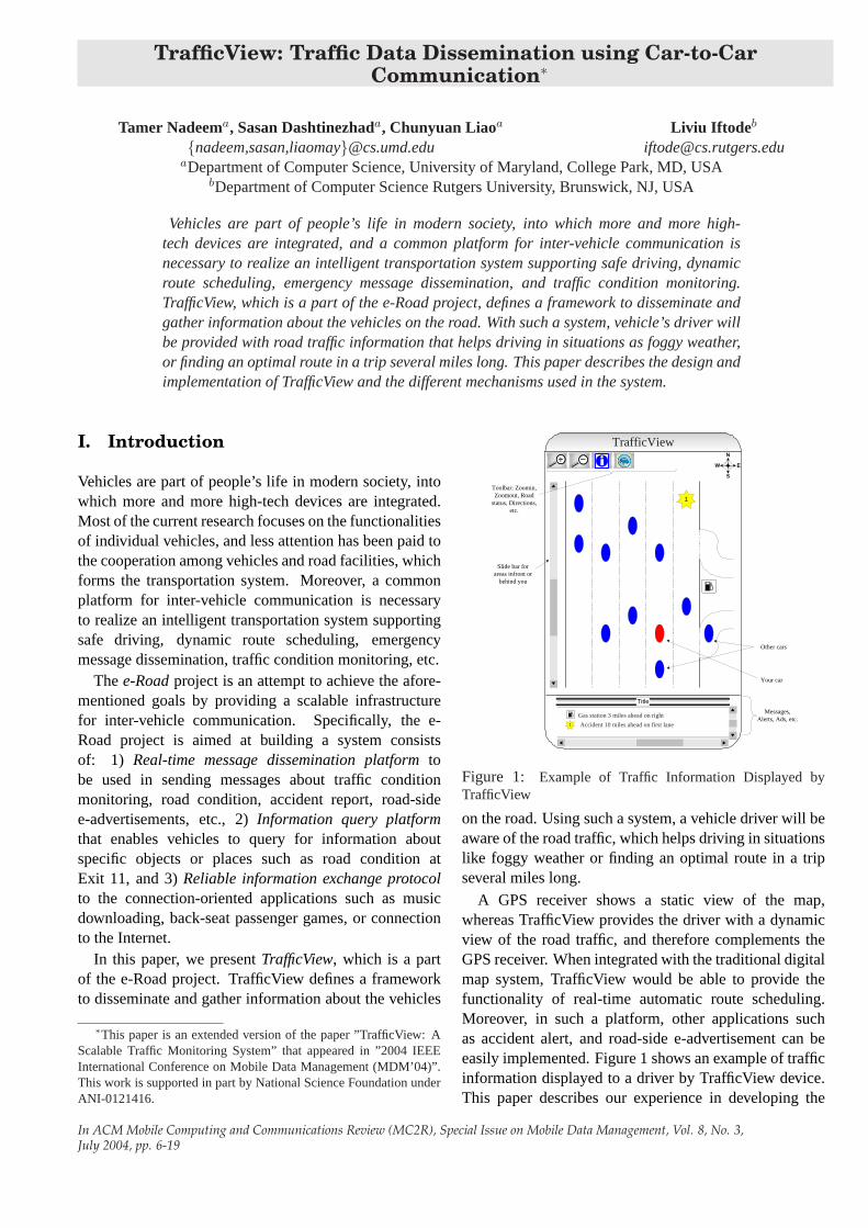
Figure 1: Example of Traffic Information Displayed byTrafficView

on the road. Using such a system, a vehicle driver will beaware of the road traffic, which helps driving in situationslike foggy weather or finding an optimal route in a tripseveral miles long.

A GPS receiver shows a static view of the map,whereas TrafficView provides the driver with a dynamicview of the road traffic, and therefore complements theGPS receiver. When integrated with the traditional digitalmap system, TrafficView would be able to provide thefunctionality of real-time automatic route scheduling.Moreover, in such a platform, other applications suchas accident alert, and road-side e-advertisement can beeasily implemented. Figure 1 shows an example of trafficinformation displayed to a driver by TrafficView device.This paper describes our experience in developing the

In ACM Mobile Computing and Communications Review (MC2R), Special Issue on Mobile Data Management, Vol. 8, No. 3,July 2004, pp. 6-19

TrafficView system. Throughout our experimentation,we performed a detailed study of different informationdissemination techniques under various road density andvehicle mobility conditions.

The rest of the paper is organized as follows: The nextsection summarize the related work, and the descriptionof the problem is given in Section III. In Section IVand Section V we describe the design of TrafficViewand the mechanisms used in the system. The Systemperformance is studied in Section VI. Finally we presentour conclusions and future work in Section VII.

II. Related Work

The research in Inter-Vehicle-Communication hasemerged in the past couple of years; mainly becauseit is a good experimental platform for Mobile Ad HocNetworks (MANETs), and has a great market potential[8]. In addition to the similarities to MANETs suchas short radio transmission range, low bandwidth,omnidirectional broadcast (at most times) and lowstorage capacity, inter-vehicle communication has itsunique characteristics and challenges as well:

• Rapid changes in link topology. Because of therelative movement of the vehicles, the connectivitybetween vehicles is always changing. For example,if vehicles’ speed is 60mph (25m/s), and the wirelesstransmission range is 250m, the connectivity betweentwo vehicles could last for at most500/25 = 20sec.

• Frequently disconnected network.In low vehicledensity case, gaps between vehicles might be severalmiles, far beyond the transmission range of wirelessnetworks. In turn, the disconnection time could beminutes. Such situation is common due to the fastmovement of vehicles and high dynamic traffics.

• Data compression/aggregation.Wireless networkshave a limited available bandwidth. In order to builda scalable system, data compression/aggregationmechanisms are required to save the bandwidth.

• Prediction of vehicle’s positions.Vehicles run alongpre-built roads, which remain unchanged over years.Therefore, given the average speed, current position,and road trajectory of a specific vehicle, the futureposition of that vehicle can be predicted.

• Energy is not an issue.Nodes, in sensor networks,are battery-powered and it is not easy to replace thebattery after deployment. Hence, many efforts havebeen made to conserve energy in sensor networks.On the other hand, in a vehicle network, the vehicleitself can be used as a source of electric power, andtherefore, energy is not a big issue.

Several major automobile manufactures and universi-ties have begun to investigate in this field; GM researchcenter in CMU [7], BMW Research Labs [16] andFord Research Labs [11], Rice University [17][13], andHarvard University [4] are a few to name. CarNet [12]project focuses on how the radio nodes in the vehiclesget IP connectivity with the help of Grid [9]. In [14],a wireless traffic light system is presented. At theintersection, a static control unit periodically broadcaststhe current light status, location of intersection, and areference point, using which the vehicles approachingthe intersection can check their relative position andmake a decision accordingly. They also designedcollision warning system [11] in which peer-to-peerbeacon message exchange is used.

An architecture of the vehicular communication is de-scribed in [5]. It integrates inter-vehicle communication(IVC) with Vehicle-Roadside Communication (VRC),where both moving vehicles and base stations can bepeers in the system. The peers are organized into PeerSpaces for message exchange, in which flooding is themain method of delivery. Authors in [13] examine thefeasibility of short range communication between fastmoving vehicles using Bluetooth, and a mobile test-bedRUSH has been established in [17], composed of the fixedbase station and mobile nodes on shuttle buses.

Two delivery modes known as pessimistic and opti-mistic forwarding are compared in disconnected vehiclenetworks in [4]. The experiment shows that the averagedelay in optimistic delivery is better. The authors of [3]propose a ”wait-and-resend” scheme where a mobilenode can cache the message for a while before newneighbors enter its transmission range, and [10] proposesan algorithm to dynamically modify the trajectories of theintermediate nodes to approach next available nodes, forrelaying the message to the destination.

III. Problem Description

Given a set of moving vehicles on the road, the goal isto exchange information about the position and speedof those vehicles among them to enable each individualvehicle to view and assess traffic and road conditions infront of it. As the vehicles move along the road, theymight enter the transmission range of some vehicles, andexit that of others. Figure 2 (a) shows an example of aroad with four lanes, on which four vehicles are moving.Two main mechanisms could be used to achieve thisgoal: floodinganddiffusion. In the flooding mechanism,each individual vehicle periodically broadcasts (pushes)information about itself. Whenever a vehicle receives abroadcast message, it stores it andimmediatelyforwardsit by rebroadcast the message. Obviously, this method is


1

2

3

4

1

2

3

4

1

2

3

4

{3} : x 3 , y 3 {2} : x 2 , y 2 {1} : x 1 , y 1

{4} : x 4 , y 4 {3} : x 3 , y 3

{2,1} : x 21 , y 21

{1} : x 1 , y 1

{2} : x 2 , y 2 {1} : x 1 , y 1

{3} : x 3 , y 3 {2} : x 2 , y 2 {1} : x 1 , y 1

{1} : x 1 , y 1

{2} : x 2 , y 2 {1} : x 1 , y 1

{4} : x 4 , y 4 {3} : x 3 , y 3

{4} : x 4 , y 4

{3} : x 3 , y 3

{2} : x 2 , y 2

{1} : x 1 , y 1

After Broadcast

Period

After Broadcast

Period

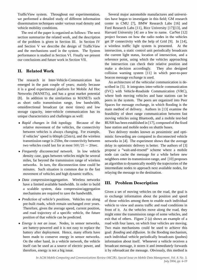
Initially, each car knows about itself only. Assume that each car

can hold 3 records at most.

After first broadcast period, each car knows about other cars one hop away

(e.g. car 4 knows about car 3 only since it is in the car 3 transmission range)

After second broadcast period, each car knows about cars two hops away. Car 4

knows about other 3 cars, but since it can accomodate 3 records only, it aggregated the

most closed 2 cars (i.e. car 1 and car 2) in one record.

Figure 2:The problem this paper addresses (a) and the diffusion mechanism (b and c)

not scalable, due to messages flooding over the network,especially in high density roads.

In the other mechanism –the diffusion mechanism–each vehicle broadcasts information about itself and theother vehicles it knows about. Whenever a vehiclereceives broadcast information, it updates its storedinformation and defers forwarding the information tothe next broadcast period, at which time it broadcastsits updated information. The diffusion mechanism isscalable, since the number of broadcast messages islimited and no flooding is used. We use the diffusionmechanism in TrafficView.

As an illustration of the diffusion mechanism, assumefor Figure 2(a), vehicles 2 and 3 are in the transmissionrange of vehicle 1. Likewise, vehicles 3 and 4 are in therange of vehicles 2 and 3, respectively. At the beginning,each vehicle knows only its own position and speed.After the first broadcast period (part (b) of the figure),vehicles 2 and 3 hear vehicle 1’s broadcast about itself,and store such information. The same happens for vehicle4 hearing vehicle 3’s broadcast message. After the nextbroadcast period (part (c)), vehicle 4 hears the messagebroadcast by vehicle 3 which includes information aboutall of 1, 2, and 3, and updates its local information.

TrafficView does not suffer from memory limitationdue to the small size of the stored records. As will beshown in Section IV, the average size for data records ison the order of 50 bytes. Assuming a very high density,five-lane road in which the distance between consecutivevehicles is 5 meters, about 5K bytes will be neededto store the information about all the vehicles in 100meters, and about 1M bytes to store information of all thevehicles in 20Km. Most of the current portable devicescome with more memory than these values.

On the other hand, assuming a transmission range of250m for the wireless network card, there will be 50vehicles competing for the same wireless medium in asingle lane, and about 250 vehicles in a five-lane roadassuming the lanes are close to each other. Hence,the total amount of data that needs to be broadcastby these vehicles every broadcast period is 250MB,which is beyond the capabilities of the current wirelesstechnology. To cope with the bandwidth limitation, eachvehicle is allowed to broadcast a small packet –a fewkilobytes in size– every broadcast period to allow othersurrounding vehicles to share the medium. Therefore,compression/aggregation mechanisms are needed toreduce the size of information to fit into the broadcastpacket (node 4 in Figure 2(c)).

For simplicity, we assume throughout this paper thatthe road is straight. In the general case, the direction ofthe movement of a vehicle can be included in the recordsent out about that vehicle, and then used to estimate itsposition on the road trajectory. Moreover, without lossof generality, we assume that the road is along they axis,and all the vehicles are moving in the positive direction ofthe road. In a real situation, a road might be bidirectional,where vehicles move in two opposite directions. In thiscase, a vehicle will need to examine the movement vectorin a record received about another vehicle, and ignore itif that vehicle is moving in the opposite direction. Thiscan also be applied in the case of an intersection wherea vehicle might hear about different vehicles moving indifferent directions.

IV. System Design

In this section we present the design of the implementedprototype of TrafficView system. Hereafter we use the


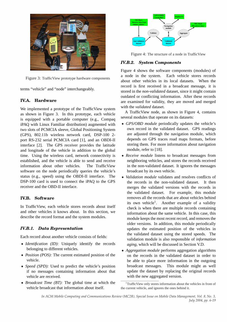
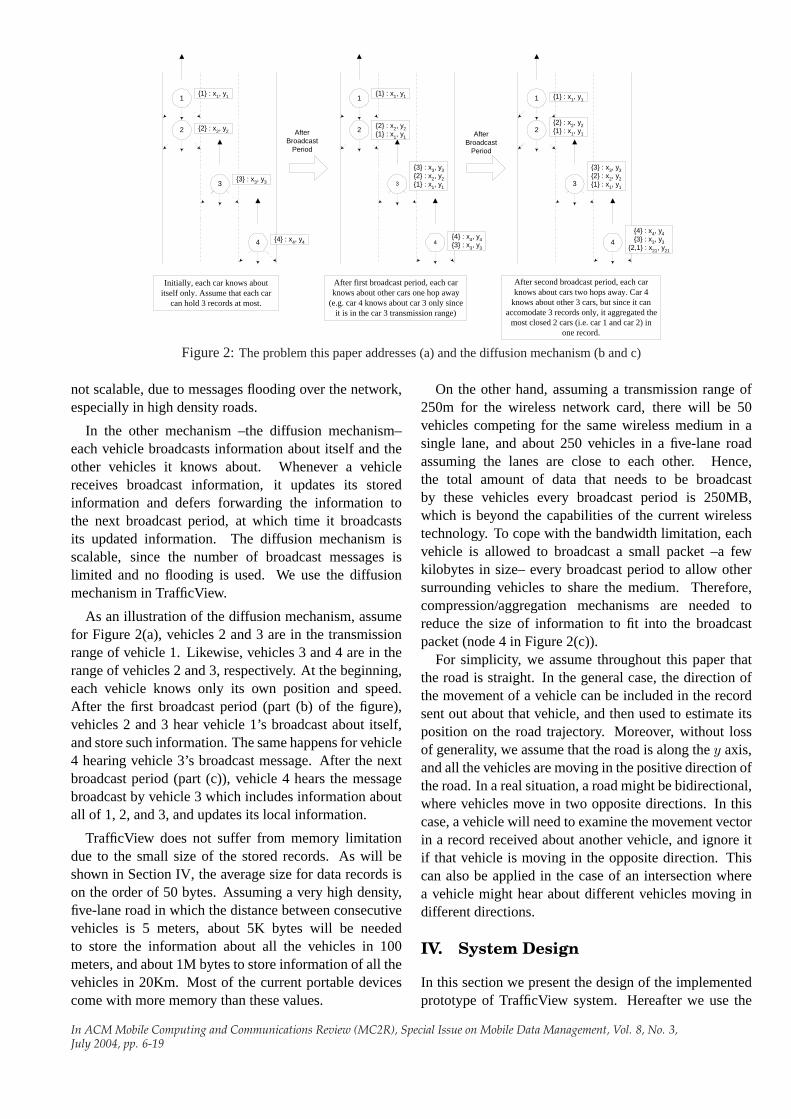
Figure 3:TrafficView prototype hardware components

terms “vehicle” and “node” interchangeably.

IV.A. Hardware

We implemented a prototype of the TrafficView systemas shown in Figure 3. In this prototype, each vehicleis equipped with a portable computer (e.g., CompaqiPAQ with Linux Familiar distribution) augmented withtwo slots of PCMCIA sleeve, Global Positioning System(GPS), 802.11b wireless network card, DSP-100 2-port RS-232 serial PCMCIA card [1], and an OBDI-IIinterface [2]. The GPS receiver provides the latitudeand longitude of the vehicle in addition to the globaltime. Using the wireless card, network connectivity isestablished, and the vehicle is able to send and receiveinformation about other vehicles. The TrafficViewsoftware on the node periodically queries the vehicle’sstatus (e.g., speed) using the OBDI-II interface. TheDSP-100 card is used to connect the iPAQ to the GPSreceiver and the OBD-II interface.

IV.B. Software

In TrafficView, each vehicle stores records about itselfand other vehicles it knows about. In this section, wedescribe the record format and the system modules.

IV.B.1. Data Representation

Each record about another vehicle consists of fields:

• Identification (ID): Uniquely identify the recordsbelonging to different vehicles.

• Position (POS):The current estimated position of thevehicle.

• Speed (SPD):Used to predict the vehicle’s positionif no messages containing information about thatvehicle are received.

• Broadcast Time (BT):The global time at which thevehicle broadcast that information about itself.

NIC/Recv "Receive data from

remote vehicle"

Non-validated dataset

Display/UI

NIC/Send "Broadcast data"

GPS/OBDII "Local data"

Validated dataset

Validate Aggregate

Navigation module

Figure 4:The structure of a node in TrafficView

IV.B.2. System Components

Figure 4 shows the software components (modules) ofa node in the system. Each vehicle stores recordsabout other vehicles in its local datasets. When therecord is first received in a broadcast message, it isstored in thenon-validateddataset, since it might containoutdated or conflicting information. After these recordsare examined for validity, they are moved and mergedwith thevalidateddataset.

A TrafficView node, as shown in Figure 4, containsseveral modules that operate on its datasets:

• GPS/OBD moduleperiodically updates the vehicle’sown record in the validated dataset. GPS readingsare adjusted through the navigation module, whichdepends on GPS traces road maps formats, beforestoring them. For more information about navigationmodule, refer to [18].

• Receive modulelistens to broadcast messages fromneighboring vehicles, and stores the records receivedin the non-validated dataset. It ignores the messagesbroadcast by its own vehicle.

• Validation modulevalidates and resolves conflicts ofthe records in the non-validated dataset. It thenmerges the validated versions with the records inthe validated dataset. For example, this moduleremoves all the records that are about vehicles behindits own vehicle1. Another example of a validitycheck is when there are multiple records containinginformation about the same vehicle. In this case, thismodule keeps the most recent record, and removes theolder versions. In addition, this module periodicallyupdates the estimated position of the vehicles inthe validated dataset using the stored speeds. Thevalidation module is also responsible ofinformationaging, which will be discussed in Section V.D.

• Aggregation moduleperforms aggregation algorithmson the records in the validated dataset in order tobe able to place more information in the outgoingbroadcast messages. This module might as wellupdate the dataset by replacing the original recordswith the new aggregated version.

1TrafficView only stores information about the vehicles in front ofthe current vehicle, and ignores the ones behind it.


• Send modulewrites the contents of the records inthe validated dataset in a broadcast message andbroadcasts it on the wireless channel using thewireless card.

• Display/UI moduleis responsible of displaying thevalidated records periodically on the display. It is alsoresponsible for the user interaction (e.g., graphicallyand/or audibly).

V. Data Aggregation Mechanisms

A MAC layer protocol (e.g., IEEE 802.11b protocol)limits the size of the payload that is sent on the networkchannel to a maximum size (which is 2312 bytes for802.11b). In TrafficView, the number of records ina node’s validated dataset can be large, making itimpossible to fit all of them in one broadcast message. Inorder to deliver as much information about other vehiclesas possible, data compression/aggregation techniquesshould be applied to the validated records. Datacompression and aggregation are two different concepts.Data compression is actually ”binary compression” inthe sense that it does not base the decisions made onthe semantics of the data. Moreover, data compressiontechniques require a lot of computation resources whichis not suitable for most portable devices. In this paper wefocus on data aggregation mechanisms only.

Data aggregation is based on the date semantics. Forexample, the records from two vehicles can be replacedby a single record with little error if the vehicles are veryclose to each other, and they are moving with relativelythe same speed. The way data aggregation contributes tothe TrafficView system is by delivering as many recordsas possible in one broadcast message. This way, morenew records can be delivered in certain period of timeand the overall system performance is improved.

V.A. Data Aggregation Basics

A single aggregated record will represent informationabout a set of vehicles. In this paper we adopt onesimple format for the aggregated records2: In anaggregated record, the ID field is extended to a list ofvehicles’ IDs while the other fields –position, speed,and broadcast time– remain as single values for all thevehicles stored in the record. Formally, if the records(ID1,POS1,SPD1,BT 1) . . . (IDn,POSn,SPDn,BTn)are being aggregated, anddi is the estimated distancebetween the current vehicle and the vehicle withIDi, theaggregated record will be

({ID1, . . . , IDn},POSa,SPDa,BT a) where

2We are developing other aggregation formats for the TrafficViewsystem.

0

5

10

15

20

25

30

35

40

45

1000 2000 3000 4000

Ave

rage

Rec

ord

Late

ncy

(sec

)

Distance Between Sender and Receiver (m)

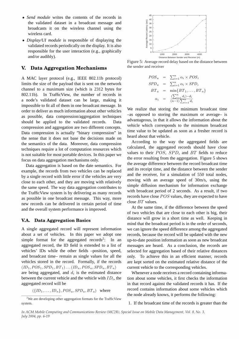
Figure 5:Average record delay based on the distance betweenthe sender and receiver

POSa =∑n

i=1 αi × POS i

SPDa =∑n

i=1 αi × SPD i

BT a = min{BT 1, . . . ,BTn}αi =

(∑n

i=1di)−di

(n−1)∑n

i=1di

We realize that storing the minimum broadcast time–as opposed to storing the maximum or average– isadvantageous, in that it allows the information about thevehicle which corresponds to the minimum broadcasttime value to be updated as soon as a fresher record isheard about that vehicle.

According to the way the aggregated fields arecalculated, the aggregated records should have closevalues to theirPOS, SPD, and BT fields to reducethe error resulting from the aggregation. Figure 5 showsthe average difference between the record broadcast timeand its receipt time, and the distance between the senderand the receiver, for a simulation of 550 total nodes,moving with an average speed of 30m/s, using thesimple diffusion mechanism for information exchangewith broadcast period of 2 seconds. As a result, if tworecords have closePOS values, they are expected to havecloseBT values.

At the same time, if the difference between the speedof two vehicles that are close to each other is big, theirdistance will grow in a short time as well. Keeping inmind that the broadcast period is in the order of seconds,we can ignore the speed difference among the aggregatedrecords, because the record will be updated with the newup-to-date position information as soon as new broadcastmessages are heard. As a conclusion, the records areselected for aggregation based of their relative distancesonly. To achieve this in an efficient manner, recordsare kept sorted on the estimated relative distance of thecurrent vehicle to the corresponding vehicles.

Whenever a node receives a record containing informa-tion about some vehicles, it first checks the informationin that record against the validated records it has. If therecord contains information about some vehicles whichthe node already knows, it performs the following:

1. If the broadcast time of the records is greater than the


ID relative distance speed broadcast time

1 40 30 9.802 65 25 9.753 120 35 9.004 140 20 8.805 250 30 6.906 280 15 6.757 600 30 4.25

Table 1: Sample records used to illustrate differentaggregation algorithms

broadcast time of the stored record, it means the newrecord is fresher, and therefore the node removes thecorresponding vehicle ID from its stored record,

2. Otherwise, the new record contains older information,and hence the node removes the correspondingvehicle ID from the received record.

In TrafficView, vehicles apply the aggregation proce-dure on the records in the validated dataset each broadcastperiod to prepare the broadcast packet. Our preliminaryexperiments showed that the effect of each vehicleeither replacing its current validated records with theaggregated version, or maintaining the original recordsin its validated dataset, on the quality of the informationgained by other vehicles on the road, is almost identical;the only difference being the imposed overhead in thenext broadcast period. We therefore decided to replacethe validated dataset records with the new aggregatedversion during each broadcast period in order to reducethe overall aggregation overhead.

In the following subsections, we describe differentalgorithms to select records for aggregations. Table 1 listsa set of records that will be used for the illustration.

V.B. Ratio-based Algorithm

The algorithm divides the road in front of the vehicle toa number of regions (ri). For each region, an aggregationratio (ai) is assigned. The aggregation ratio is definedas the inverse of the number of individual records thatwould be aggregated in a single record. Each regionis assigned a portion (pi where 0 < pi ≤ 1) of theremaining free space in the broadcast message. Theaggregation ratios and region portion values are assignedaccording to the importance of the regions and howaccurate the broadcast information about the vehicles inthat region is needed to be. For example, assigningdecreasing values to the aggregation ratios and equalvalues to portion parameters will result in broadcastingless accurate information about regions that are fartheraway from the current vehicle, since for those regions,each individual record will represent large number ofaggregated vehicles (records).

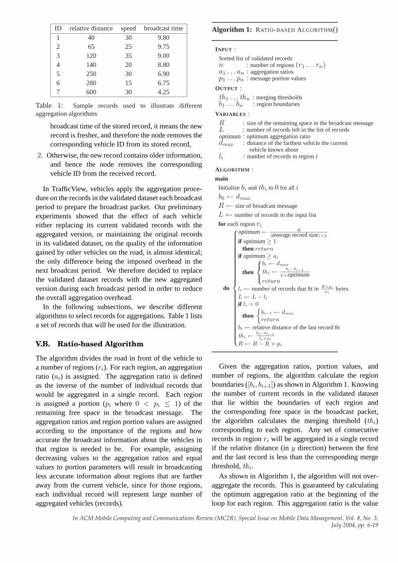
Algorithm 1: RATIO-BASED ALGORITHM()

I NPUT :Sorted list of validated recordsn : number of regions(r1 . . . rn)a1 . . . an : aggregation ratiosp1 . . . pn : message portion values

OUTPUT :th1 . . . thn : merging thresholdsb1 . . . bn : region boundaries

VARIABLES :R : size of the remaining space in the broadcast messageL : number of records left in the list of recordsoptimum : optimum aggregation ratiodmax : distance of the farthest vehicle the current

vehicle knows aboutli : number of records in regioni

ALGORITHM :main

Initialize bi andthi to 0 for all ib0 ← dmax

R ← size of broadcast message

L ← number of records in the input list

for each regionri

do

optimum← R

(average record size)×L

if optimum≥ 1then return

if optimum≥ ai

then

bi ← dmax

thi ← bi−bi−1

L×optimumreturn

li ← number of records that fit inR×piai

bytesL ← L− liif li = 0

then

{bi−1 ← dmax

return

bi ← relative distance of the last record fitthi ← bi−bi−1

li×ai

R ← R−R× pi

Given the aggregation ratios, portion values, andnumber of regions, the algorithm calculate the regionboundaries ([bi, bi+1[) as shown in Algorithm 1. Knowingthe number of current records in the validated datasetthat lie within the boundaries of each region andthe corresponding free space in the broadcast packet,the algorithm calculates the merging threshold (thi)corresponding to each region. Any set of consecutiverecords in regionri will be aggregated in a single recordif the relative distance (iny direction) between the firstand the last record is less than the corresponding mergethreshold,thi.

As shown in Algorithm 1, the algorithm will not over-aggregate the records. This is guaranteed by calculatingthe optimum aggregation ratio at the beginning of theloop for each region. This aggregation ratio is the value


ID(s) relative distance speed broadcast time

1, 2, 3 67.56 29.39 9.004, 5, 6 215.22 21.68 6.75

7 600 30 4.25

Table 2:Records sent out by the Ratio-based algorithm

needed to fit the rest of the records in the message freespace. If this ratio is greater than or equal to one,the algorithm terminates since no aggregation is needed.Otherwise, the optimum value and the aggregation ratioof the current region are compared and the maximumamong these two is used.

After the algorithm aggregates the records, it startswriting the record contents to the broadcast message untilno free space is left. There is no guarantee to write all therecord contents in the message. The tradeoff between thenumber of records written and the accuracy of the recordsis governed by the used parameter values.

As an example, assume a vehicle withID = 0, usingthis algorithm, divides the road into two regions, and thecorresponding parameter area1 = 0.5 with p1 = 0.5 anda2 = 0.25 with p2 = 0.5. If the algorithm is applied tothe records of Table 1, it will calculate the parameters:b1 = 120, th1 = 80, b2 = 600, andth2 = 261.8. Notethat th2 is calculated using the optimal aggregation ratio0.46 instead of the input value,0.25.

After calculating the parameters, in the first region,the algorithm first combines records 1 and 2, and thencombines the result with record 3. Likewise, the records4, 5, and 6 are combined in the second region. Therecords sent out by the algorithm are shown in Table 2.Record 7 is sent not aggregated.

V.C. Cost-based Aggregation

In the Ratio-based algorithm, records that satisfy themerging threshold, (thi), criterion are “blindly” com-bined without considering the cost of the aggregation.In contrast, the Cost-based algorithm assigns a cost foraggregating each pair of records, and whenever it needsto aggregate two records, the two that correspond tothe minimum cost are chosen. Assume two recordsstoring aggregated information abouts1 ands2 numberof vehicles, with a relative distance ofd1 and d2,respectively. The cost of aggregating the two records iscalculated as follow:

cost =|d1 − da| × s1 + |d2 − da| × s2

da

whereda is the relative distance of the aggregated groupof records (vehicles). This formula is calculated such thatit: 1) assigns a high cost for the vehicles that are relativelyclose to the current vehicle (1/da), 2) tries to minimizethe error introduced during the merging (|di − da|), and

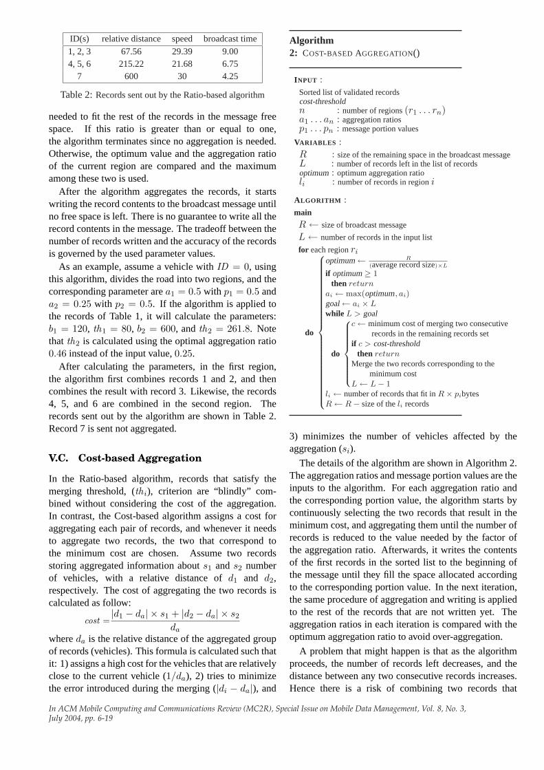
Algorithm2: COST-BASED AGGREGATION()

I NPUT :Sorted list of validated recordscost-thresholdn : number of regions(r1 . . . rn)a1 . . . an : aggregation ratiosp1 . . . pn : message portion values

VARIABLES :R : size of the remaining space in the broadcast messageL : number of records left in the list of recordsoptimum : optimum aggregation ratioli : number of records in regioni

ALGORITHM :main

R ← size of broadcast message

L ← number of records in the input list

for each regionri

do

optimum← R

(average record size)×L

if optimum≥ 1then return

ai ← max(optimum, ai)goal← ai × Lwhile L > goal

do

c ← minimum cost of merging two consecutiverecords in the remaining records set

if c > cost-thresholdthen return

Merge the two records corresponding to theminimum cost

L ← L− 1li ← number of records that fit inR× pibytesR ← R− size of theli records

3) minimizes the number of vehicles affected by theaggregation (si).

The details of the algorithm are shown in Algorithm 2.The aggregation ratios and message portion values are theinputs to the algorithm. For each aggregation ratio andthe corresponding portion value, the algorithm starts bycontinuously selecting the two records that result in theminimum cost, and aggregating them until the number ofrecords is reduced to the value needed by the factor ofthe aggregation ratio. Afterwards, it writes the contentsof the first records in the sorted list to the beginning ofthe message until they fill the space allocated accordingto the corresponding portion value. In the next iteration,the same procedure of aggregation and writing is appliedto the rest of the records that are not written yet. Theaggregation ratios in each iteration is compared with theoptimum aggregation ratio to avoid over-aggregation.

A problem that might happen is that as the algorithmproceeds, the number of records left decreases, and thedistance between any two consecutive records increases.Hence there is a risk of combining two records that


ID(s) relative distance speed broadcast time

1, 2 49.52 28.09 9.753, 4 129.23 28.07 8.805, 6 264.15 22.92 6.75

Table 3:Records sent out by the Cost-based algorithm

correspond to vehicles that are too far away from eachother. To avoid this problem, the algorithm terminatesas soon as the calculated cost is greater than a thresholdparameter (cost-threshold.)

For example, assume vehicle withID = 0 intends touse this algorithm for the records listed in Table 1, wherea1 = a2 = 0.5, p1 = p2 = 0.5, andcost-threshold= 0.9.During the first iteration (a1), it first aggregates records5 and 6 (cost = 0.11), then 3 and 4 (cost = 0.15), andfinally 1 and 2 (cost = 0.50). In the second phase (a2),the minimum cost is 1.22, which is greater than the costthreshold, therefore the algorithm terminates. Table 3lists the records that are sent out by vehicle0 and thecorresponding fields. In this case, vehicle0 cannot fitrecord 7 in its message.

V.D. Information Aging

The records stored in both the validated and non-validateddatasets, must be examined to verify that they reflectthe current state of the road and eliminate any outdated(old) information. For example, vehicles included in thevalidated dataset might have exited the road. Moreover,new received records (non-validated) might containinaccurate information due to frequent changes in thespeed of the corresponding vehicles and/or aggregationmechanisms applied to the data within relaying nodes.

There are two main problems here: how shouldthe value of the information in a broadcast messagebe assessed, and how can a balance between knowinginaccurate information about a vehicle, and having noknowledge about it, be achieved. In general, if the costof knowing inaccurate information about vehiclej that isat a relative distance ofd is a functionc1(j, d), and thecost of having no information aboutj is another functionc2(j, d), the information should be accepted and storedif c1(j, d) < c2(j, d), otherwise it should be dropped.Unfortunately, it is not clear how to assign values to thesetwo functions.

To solve this problem, TrafficView exploits two agingmechanisms. The first mechanism associates a timerwith each record added to the validated dataset. Thistimer is reset each time the record is updated by abroadcast message. If the timer is expired, the record isdropped. The second mechanism, which we call Receive-aging, deals with newly received records via broadcastmessages. Whenever a new record is received, the

0

1000

2000

3000

4000

5000

6000

7000

8000

0 1000 2000 3000 4000 5000 6000 7000 8000

Ave

rage

est

imat

ion

erro

r (m

)

Distance between sender and receiver (m)

Usigng receive-agingWithout receive-aging

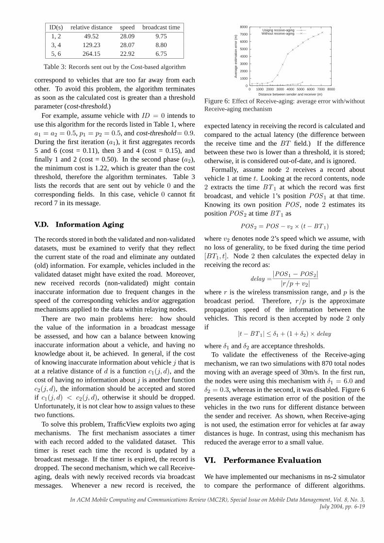
Figure 6:Effect of Receive-aging: average error with/withoutReceive-aging mechanism

expected latency in receiving the record is calculated andcompared to the actual latency (the difference betweenthe receive time and theBT field.) If the differencebetween these two is lower than a threshold, it is stored;otherwise, it is considered out-of-date, and is ignored.

Formally, assume node2 receives a record aboutvehicle1 at timet. Looking at the record contents, node2 extracts the timeBT 1 at which the record was firstbroadcast, and vehicle1’s position POS 1 at that time.Knowing its own positionPOS , node 2 estimates itspositionPOS 2 at timeBT 1 as

POS2 = POS − v2 × (t− BT 1)

wherev2 denotes node2’s speed which we assume, withno loss of generality, to be fixed during the time period[BT1, t]. Node2 then calculates the expected delay inreceiving the record as:

delay =|POS1 − POS 2||r/p + v2|

wherer is the wireless transmission range, andp is thebroadcast period. Therefore,r/p is the approximatepropagation speed of the information between thevehicles. This record is then accepted by node2 onlyif

|t− BT 1| ≤ δ1 + (1 + δ2)× delay

whereδ1 andδ2 are acceptance thresholds.To validate the effectiveness of the Receive-aging

mechanism, we ran two simulations with 870 total nodesmoving with an average speed of 30m/s. In the first run,the nodes were using this mechanism withδ1 = 6.0 andδ2 = 0.3, whereas in the second, it was disabled. Figure 6presents average estimation error of the position of thevehicles in the two runs for different distance betweenthe sender and receiver. As shown, when Receive-agingis not used, the estimation error for vehicles at far awaydistances is huge. In contrast, using this mechanism hasreduced the average error to a small value.

VI. Performance Evaluation

We have implemented our mechanisms in ns-2 simulatorto compare the performance of different algorithms.


In this section, we present the experiments, and thecorresponding results. In addition, we evaluated theprototype using real GPS traces obtained on a highway.

VI.A. Scenario Generator

Modelling road traffic is a research topic about whicha lot of work has been done. For example CORSIM[6] is a microscopic traffic simulator developed by TheFederal Highway Administration. Unfortunately, noneof the traffic modeler tools are freely available to public.We have therefore developed our own scenario generatortool based on “setdest”—a generator tool for random-waypoint mobility model, developed at Carnegie Mellon.

The scenario generator accepts as parameters simula-tion time, road length, nodes average speed, number oflanes on the road, and the average gap length betweenvehicles. It uses a simplified traffic model as follows:

• Entries and Exits:The entries and exits are evenlydistributed along the road each 1000 meters. Vehiclesmay enter the road at each entry except the last oneand leave at any subsequent exit. Vehicles enter theroad at the front-end entry with a probability of 0.7,and at side entries with a probability of 0.3.

• Speed Changes:To model the changes to the node’sspeed, the road between the entry point and exitpoint of a node is divided into regions of 50meters, and a constant speed of max speed× (0.75 +rand(−2, 2) × 0.125) is used for each region, whererand(a, b) returns a uniformly distributed randominteger betweena andb.

• Changing Lanes:Vehicles can change their lanes withno dependence on other vehicles. The probabilityof staying on the same lane is 0.6 whereas theprobability of changing to the right or left lane is 0.2.

• Vehicle Density: The density of vehicles is animportant factor because it determines the numberof neighboring nodes in the transmission range of avehicle, which has a great impact on the transmissiondelay and available bandwidth of the network. Thescenario generator initially puts

road-length×number of lanesaverage gap

activenodes, evenly distributed, on the road. Oncea vehicle leaves the road at one of the exits, it isdeactivated, and a new node is added (activated) tothe road randomly. As soon as a node is deactivated,it will no longer affect our metric calculationsintroduced in the next section.

Figure 7 shows the histogram of the average speedand number of lane changes per minute for a scenariogenerate with average speed = 30m, and average gap =

14

16

18

20

22

24

26

28

15 20 25 30 35 40 45

Per

cent

age

of c

ars

Average speed

05

1015202530354045

-1 0 1 2 3 4 5 6

Per

cent

age

of c

ars

Avg # of lane change/minute

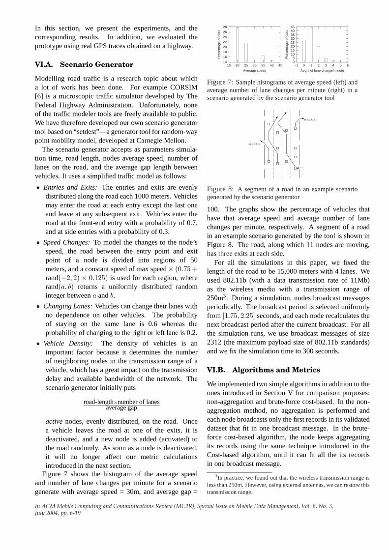
Figure 7:Sample histograms of average speed (left) andaverage number of lane changes per minute (right) in ascenario generated by the scenario generator tool

exits

exits

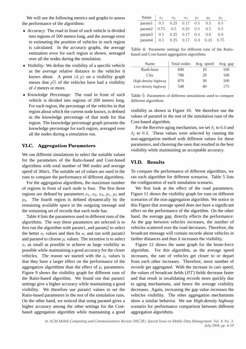
Figure 8: A segment of a road in an example scenariogenerated by the scenario generator

100. The graphs show the percentage of vehicles thathave that average speed and average number of lanechanges per minute, respectively. A segment of a roadin an example scenario generated by the tool is shown inFigure 8. The road, along which 11 nodes are moving,has three exits at each side.

For all the simulations in this paper, we fixed thelength of the road to be 15,000 meters with 4 lanes. Weused 802.11b (with a data transmission rate of 11Mb)as the wireless media with a transmission range of250m3. During a simulation, nodes broadcast messagesperiodically. The broadcast period is selected uniformlyfrom [1.75, 2.25] seconds, and each node recalculates thenext broadcast period after the current broadcast. For allthe simulation runs, we use broadcast messages of size2312 (the maximum payload size of 802.11b standards)and we fix the simulation time to 300 seconds.

VI.B. Algorithms and Metrics

We implemented two simple algorithms in addition to theones introduced in Section V for comparison purposes:non-aggregation and brute-force cost-based. In the non-aggregation method, no aggregation is performed andeach node broadcasts only the first records in its validateddataset that fit in one broadcast message. In the brute-force cost-based algorithm, the node keeps aggregatingits records using the same technique introduced in theCost-based algorithm, until it can fit all the its recordsin one broadcast message.

3In practice, we found out that the wireless transmission range isless than 250m. However, using external antennas, we can restore thistransmission range.


We will use the following metrics and graphs to assessthe performance of the algorithms:

• Accuracy: The road in front of each vehicle is dividedinto regions of 500 meters long, and the average errorin estimating the position of vehicles in each regionis calculated. In the accuracy graphs, the averageestimation error for each region is shown, averagedover all the nodes during the simulation.

• Visibility: We define the visibility of a specific vehicleas theaverage relative distance to the vehicles itknows about. A point(d, p) on a visibility graphmeans thatp% of the vehicles have had a visibilityof d meters or more.

• Knowledge Percentage: The road in front of eachvehicle is divided into regions of 200 meters long.For each region, the percentage of the vehicles in thatregion about which the current node knows, is definedas the knowledge percentage of that node for thatregion. The knowledge percentage graph presents theknowledge percentage for each region, averaged overall the nodes during a simulation run.

VI.C. Aggregation Parameters

We ran different simulations to select the suitable valuesfor the parameters of the Ratio-based and Cost-basedalgorithms with total number of 960 nodes and averagespeed of 30m/s. The suitable set of values are used in theruns to compare the performance of different algorithms.

For the aggregation algorithms, the maximum numberof regions in front of each node is four. The first threeregions are defined by parametersa1, a2, a3, p1, p2 andp3. The fourth region is defined dynamically by theremaining available space in the outgoing message andthe remaining set of records that each node has.

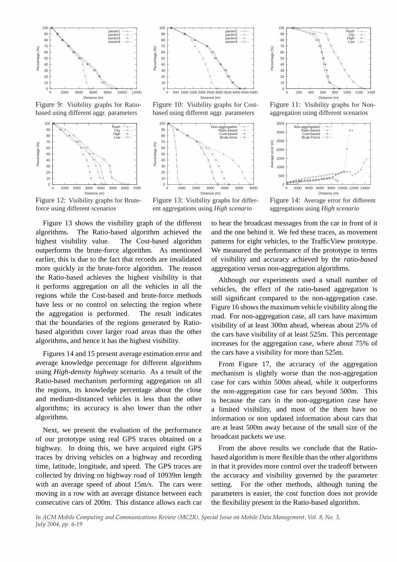
Table 4 lists the parameters used in different runs of thealgorithms. The way these parameters are selected is tofirst run the algorithm with param1, and param2 to selectthe betterai values and then fixai and run with param3and param4 to choosepi values. The incentive is to selectai as small as possible to achieve as large visibility aspossible while maintaining a good accuracy for the closervehicles. The reason we started with theai values isthat they have a larger effect on the performance of theaggregation algorithms than the effect ofpi parameters.Figure 9 shows the visibility graph for different runs ofthe Ratio-based algorithm. We found out that param1settings give a higher accuracy while maintaining a goodvisibility. We therefore use param1 values to set theRatio-based parameters in the rest of the simulation runs.On the other hand, we noticed that using param4 gives ahigher accuracy among the other settings for the Cost-based aggregation algorithm while maintaining a good

Name a1 a2 a3 p1 p2 p3

param1 0.5 0.25 0.17 0.5 0.5 0.5param2 0.75 0.5 0.25 0.5 0.5 0.5param3 0.5 0.25 0.17 0.4 0.6 0.8param4 0.5 0.25 0.17 0.3 0.43 0.75

Table 4: Parameter settings for different runs of the Ratio-based and Cost-based aggregation algorithms

Name Total nodes Avg. speed Avg. gap

Rush-hour 690 10 100City 780 20 100

High-density highway 870 30 100Low-density highway 548 40 175

Table 5:Parameters of different simulations used to comparedifferent algorithms

visibility as shown in Figure 10. We therefore use thevalues of param4 in the rest of the simulation runs of theCost-based algorithm.

For the Receive-aging mechanism, we setδ1 to 6.0 andδ2 to 0.3. These values were selected by running thenon-aggregation method with different values for theseparameters, and choosing the ones that resulted in the bestvisibility while maintaining an acceptable accuracy.

VI.D. Results

To compare the performance of different algorithms, weran each algorithm for different scenarios. Table 5 liststhe configuration of each simulation scenario.

We first look at the effect of the road parameters.Figure 11 shows the visibility graph for runs on differentscenarios of the non-aggregation algorithm. We notice inthis Figure that average speed does not have a significanteffect on the performance of the algorithm. On the otherhand, the average gap, directly effects the performance:As the gap between vehicles increases, the number ofvehicles scattered over the road decreases. Therefore, thebroadcast message will contain records about vehicles infarther distances and thus it increases the visibility.

Figure 12 shows the same graph for the brute-forcealgorithm. For this algorithm, as the average speedincreases, the rate of vehicles get closer to or departfrom each other increases. Therefore, more number ofrecords get aggregated. With the increase in cars speed,the values of broadcast fields (BT ) fields decrease fasterand that result in invalidating records more quickly dueto aging mechanisms, and hence the average visibilitydecreases. Again, increasing the gap value increases thevehicles visibility. The other aggregation mechanismsshow a similar behavior. We useHigh-density highwayscenario for performance comparison between differentaggregation algorithms.


0

10

20

30

40

50

60

70

80

90

100

0 2000 4000 6000 8000 10000 12000

Per

cent

age

(%)

Distance (m)

param1param2param3param4

Figure 9: Visibility graphs for Ratio-based using different aggr. parameters

0

10

20

30

40

50

60

70

80

90

100

0 500 1000 1500 2000 2500 3000 3500 4000 4500 5000

Per

cent

age

(%)

Distance (m)

param1param2param3param4

Figure 10: Visibility graphs for Cost-based using different aggr. parameters

0

10

20

30

40

50

60

70

80

90

100

0 200 400 600 800 1000 1200 1400

Per

cent

age

(%)

Distance (m)

RushCity

HighLow

Figure 11: Visibility graphs for Non-aggregation using different scenarios

0

10

20

30

40

50

60

70

80

90

100

0 1000 2000 3000 4000 5000 6000 7000

Per

cent

age

(%)

Distance (m)

RushCity

HighLow

Figure 12:Visibility graphs for Brute-force using different scenarios

0

10

20

30

40

50

60

70

80

90

100

0 1000 2000 3000 4000 5000 6000

Per

cent

age

(%)

Distance (m)

Non-aggregationRatio-basedCost-basedBrute-force

Figure 13:Visibility graphs for differ-ent aggregations usingHigh scenario

0

500

1000

1500

2000

2500

3000

3500

0 2000 4000 6000 8000 10000 12000 14000

Ave

rage

err

or (

m)

Distance (m)

Non-aggregationRatio-basedCost-basedBrute Force

Figure 14:Average error for differentaggregations usingHigh scenario

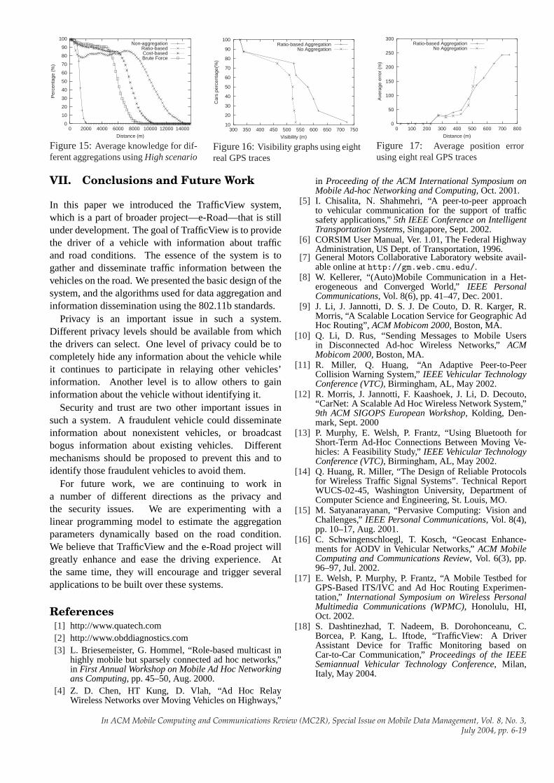
Figure 13 shows the visibility graph of the differentalgorithms. The Ratio-based algorithm achieved thehighest visibility value. The Cost-based algorithmoutperforms the brute-force algorithm. As mentionedearlier, this is due to the fact that records are invalidatedmore quickly in the brute-force algorithm. The reasonthe Ratio-based achieves the highest visibility is thatit performs aggregation on all the vehicles in all theregions while the Cost-based and brute-force methodshave less or no control on selecting the region wherethe aggregation is performed. The result indicatesthat the boundaries of the regions generated by Ratio-based algorithm cover larger road areas than the otheralgorithms, and hence it has the highest visibility.

Figures 14 and 15 present average estimation error andaverage knowledge percentage for different algorithmsusingHigh-density highwayscenario. As a result of theRatio-based mechanism performing aggregation on allthe regions, its knowledge percentage about the closeand medium-distanced vehicles is less than the otheralgorithms; its accuracy is also lower than the otheralgorithms.

Next, we present the evaluation of the performanceof our prototype using real GPS traces obtained on ahighway. In doing this, we have acquired eight GPStraces by driving vehicles on a highway and recordingtime, latitude, longitude, and speed. The GPS traces arecollected by driving on highway road of 10939m lengthwith an average speed of about 15m/s. The cars weremoving in a row with an average distance between eachconsecutive cars of 200m. This distance allows each car

to hear the broadcast messages from the car in front of itand the one behind it. We fed these traces, as movementpatterns for eight vehicles, to the TrafficView prototype.We measured the performance of the prototype in termsof visibility and accuracy achieved by theratio-basedaggregation versus non-aggregation algorithms.

Although our experiments used a small number ofvehicles, the effect of the ratio-based aggregation isstill significant compared to the non-aggregation case.Figure 16 shows the maximum vehicle visibility along theroad. For non-aggregation case, all cars have maximumvisibility of at least 300m ahead, whereas about 25% ofthe cars have visibility of at least 525m. This percentageincreases for the aggregation case, where about 75% ofthe cars have a visibility for more than 525m.

From Figure 17, the accuracy of the aggregationmechanism is slightly worse than the non-aggregationcase for cars within 500m ahead, while it outperformsthe non-aggregation case for cars beyond 500m. Thisis because the cars in the non-aggregation case havea limited visibility, and most of the them have noinformation or non updated information about cars thatare at least 500m away because of the small size of thebroadcast packets we use.

From the above results we conclude that the Ratio-based algorithm is more flexible than the other algorithmsin that it provides more control over the tradeoff betweenthe accuracy and visibility governed by the parametersetting. For the other methods, although tuning theparameters is easier, the cost function does not providethe flexibility present in the Ratio-based algorithm.


0

10

20

30

40

50

60

70

80

90

100

0 2000 4000 6000 8000 10000 12000 14000

Per

cent

age

(%)

Distance (m)

Non-aggregationRatio-basedCost-basedBrute Force

Figure 15:Average knowledge for dif-ferent aggregations usingHigh scenario

10

20

30

40

50

60

70

80

90

100

300 350 400 450 500 550 600 650 700 750

Car

s pe

rcen

tage

(%)

Visibility (m)

Ratio-based AggregationNo Aggregation

Figure 16:Visibility graphs using eightreal GPS traces

0

50

100

150

200

250

300

0 100 200 300 400 500 600 700 800

Ave

rage

err

or (

m)

Distance (m)

Ratio-based AggregationNo Aggregation

Figure 17: Average position errorusing eight real GPS traces

VII. Conclusions and Future Work

In this paper we introduced the TrafficView system,which is a part of broader project—e-Road—that is stillunder development. The goal of TrafficView is to providethe driver of a vehicle with information about trafficand road conditions. The essence of the system is togather and disseminate traffic information between thevehicles on the road. We presented the basic design of thesystem, and the algorithms used for data aggregation andinformation dissemination using the 802.11b standards.

Privacy is an important issue in such a system.Different privacy levels should be available from whichthe drivers can select. One level of privacy could be tocompletely hide any information about the vehicle whileit continues to participate in relaying other vehicles’information. Another level is to allow others to gaininformation about the vehicle without identifying it.

Security and trust are two other important issues insuch a system. A fraudulent vehicle could disseminateinformation about nonexistent vehicles, or broadcastbogus information about existing vehicles. Differentmechanisms should be proposed to prevent this and toidentify those fraudulent vehicles to avoid them.

For future work, we are continuing to work ina number of different directions as the privacy andthe security issues. We are experimenting with alinear programming model to estimate the aggregationparameters dynamically based on the road condition.We believe that TrafficView and the e-Road project willgreatly enhance and ease the driving experience. Atthe same time, they will encourage and trigger severalapplications to be built over these systems.

References[1] http://www.quatech.com[2] http://www.obddiagnostics.com[3] L. Briesemeister, G. Hommel, “Role-based multicast in

highly mobile but sparsely connected ad hoc networks,”in First Annual Workshop on Mobile Ad Hoc Networkingans Computing, pp. 45–50, Aug. 2000.

[4] Z. D. Chen, HT Kung, D. Vlah, “Ad Hoc RelayWireless Networks over Moving Vehicles on Highways,”

in Proceeding of the ACM International Symposium onMobile Ad-hoc Networking and Computing, Oct. 2001.

[5] I. Chisalita, N. Shahmehri, “A peer-to-peer approachto vehicular communication for the support of trafficsafety applications,”5th IEEE Conference on IntelligentTransportation Systems, Singapore, Sept. 2002.

[6] CORSIM User Manual, Ver. 1.01, The Federal HighwayAdministration, US Dept. of Transportation, 1996.

[7] General Motors Collaborative Laboratory website avail-able online athttp://gm.web.cmu.edu/.

[8] W. Kellerer, “(Auto)Mobile Communication in a Het-erogeneous and Converged World,”IEEE PersonalCommunications, Vol. 8(6), pp. 41–47, Dec. 2001.

[9] J. Li, J. Jannotti, D. S. J. De Couto, D. R. Karger, R.Morris, “A Scalable Location Service for Geographic AdHoc Routing”,ACM Mobicom 2000, Boston, MA.

[10] Q. Li, D. Rus, “Sending Messages to Mobile Usersin Disconnected Ad-hoc Wireless Networks,”ACMMobicom 2000, Boston, MA.

[11] R. Miller, Q. Huang, “An Adaptive Peer-to-PeerCollision Warning System,”IEEE Vehicular TechnologyConference (VTC), Birmingham, AL, May 2002.

[12] R. Morris, J. Jannotti, F. Kaashoek, J. Li, D. Decouto,“CarNet: A Scalable Ad Hoc Wireless Network System,”9th ACM SIGOPS European Workshop, Kolding, Den-mark, Sept. 2000

[13] P. Murphy, E. Welsh, P. Frantz, “Using Bluetooth forShort-Term Ad-Hoc Connections Between Moving Ve-hicles: A Feasibility Study,”IEEE Vehicular TechnologyConference (VTC), Birmingham, AL, May 2002.

[14] Q. Huang, R. Miller, “The Design of Reliable Protocolsfor Wireless Traffic Signal Systems”. Technical ReportWUCS-02-45, Washington University, Department ofComputer Science and Engineering, St. Louis, MO.

[15] M. Satyanarayanan, “Pervasive Computing: Vision andChallenges,”IEEE Personal Communications, Vol. 8(4),pp. 10–17, Aug. 2001.

[16] C. Schwingenschloegl, T. Kosch, “Geocast Enhance-ments for AODV in Vehicular Networks,”ACM MobileComputing and Communications Review, Vol. 6(3), pp.96–97, Jul. 2002.

[17] E. Welsh, P. Murphy, P. Frantz, “A Mobile Testbed forGPS-Based ITS/IVC and Ad Hoc Routing Experimen-tation,” International Symposium on Wireless PersonalMultimedia Communications (WPMC), Honolulu, HI,Oct. 2002.

[18] S. Dashtinezhad, T. Nadeem, B. Dorohonceanu, C.Borcea, P. Kang, L. Iftode, “TrafficView: A DriverAssistant Device for Traffic Monitoring based onCar-to-Car Communication,”Proceedings of the IEEESemiannual Vehicular Technology Conference, Milan,Italy, May 2004.


Documents

TrafficView: traffic data dissemination using car-to-car communication