Benchmark cases for outdoor sound propagation models

Benchmark cases for outdoor sound propagation models K. Attenborough and S. Taherzadeh The Open Universit)', Milton Keynes MK7 6AA, England, United Kingdom

H. E. Bass, X. Di, a) and R. Raspet The University of Mississippi, University, Mississippi 38677

G. R. Becker and A. Gfidesen Atlas Elektronik Grab!I, D-2800 Bremen 44, Germany

A. Chrestman

USAE Waterways Experiment Station, Vicksburg, Mississippi 39180-6199

G. A. Daigle and A. UEsp6rance b) National Research Council of Canada, Ottawa, Ontario K1A OR6, Canada

Y. Gabillet

Centre Scientifique et Techt, ique du B•timent, 38400 Saint-Martin-d'H•res, France

K. E. Gilbert

Pennsylvania State University, State College, Pennsylvania 16804

Y. L. Li and M. J. White

U.S. Army Construction Engineering Research Laboratory, Champaign, Illinois 61826-9005

P. Naz

French-German Institute of Research of Saint Louis, 68301 Sabtt Louis, France

J. M. Noble

U.S. Army Research Lab, White Sands Missile Range, New Mexico 88002-550l

H. A. J. M. van Hoof

Physics and Electronics Lab/TNO, 2509 J.G. The Hague, The Netherlands

(Received 15 June 1993; revised 12 May 1994; accepted 22 August 1994)

The computational tools available for prediction of sound propagation through the atmosphere have increased dramatically during the past decade. The numerical techniques include analytical solutions for selected index of refraction profiles, ray trace techniques which inclade interaction with a complex impedance boundary, a Gaussian beam ray trace algorithm, and more sophisticated approximate solutions to the full wave equation; the fast field program (FFP) and the parabolic equation (PE) solutions. This large array of computational approaches raises questions concerning under what conditions the various approaches are reliable and concerns about possible errors in specific implementations. This paper presents comparisons of predictions from the several models assuming a complex impedance ground and four atmospheric conditkms. For the cases studied, it was found that the FFP and PE algorithms agree to within numerical accuracy over the full range of conditions and agree with the analytical solutions where available. Comparisons to ray solutions define regimes where ray approaches can be used. There is no attempt to compare calculated transmission losses to measurements.

PACS numbers: 43.28.Fp, 43.20.Bi

INTRODUCTION

Propagation of sound outdoors involves a number of physical phenomena including geometric spreading, molecu- lar absorption, reflection from a complex impedance boundary, refraction, diffraction, and scattering. • Accurate predictions of sound transmission loss (TL) from a source to a receiver must somehow account for all of these phenomena

a•Also with National Research Council of Canada, Ottawa, Ontario K1A 0R6, Canada.

b)Also with Universit6 de Sherbrooke, Sherbrooke, Quebec JIK 2RI, Canada.

simultaneously. Although this goal is beyond current capa- bilities, a great deal of progress has been made in the past decade. Specifically, numerical techniques originally developed for applications in underwater acoustics have been modified for atmospheric predictions and new analytical results provide solutions for •nore realistic conditions. Some progress has been made toward including turbulence and terrain in the propagation models, but research on these aspects is still in progress.

Ray tracing has been a standard approach extensively used to predict outdoor sound levels in the presence of speed of sound gradients even though the mathematical conditions

173 d. Acoust. Soc. Am. 97 (1), January 1995 0001-4966/95/97(1)/173/19/$6.00 173

for ray solutions are seldom met outdoors. Recent analytical solutions include a refractive atmosphere and a complex impedance boundary 2'3 but are only applicable to cases where the speed of sound varies with altitude in a specific func- tional form. Numerical solutions to the wave equation include the diffraction effects which limit the applicability of ray solutions and can be applied to arbitrary speed of sound profiles. 4'5 For this reason, the development of numerical algorithms to predict transmission loss through the atmosphere is being pursued by a number of groups throughout the world.

Research groups in many countries have developed propagation models to predict transmission loss. The models can be generally classified as analytic (such as normal mode models), ray trace, a variation of the fast field program (FFP), or a form of the parabolic equation (PE). Though many of the groups involved share results at international meetings, the codes were generally developed independently. Members of NATO Panel 3 Research Study Group 11 (RSG- 11) began an effort in 1990 to compare predictions of the various models and different implementations of the same model. The goals of this effort were to identify any differences and sources of those differences and to provide a set of results which future researchers can use to check new models

and codes.

Thus the objective of this paper to look for consensus between models or, more accurately, significant differences, to investigate regimes of validity and to examine artifacts. We have chosen not to evaluate accuracy in any systematic way nor computational requirements since these change rapidly.

Assessing the quality of numerical computation schemes is an issue that has recently received considerable attention in underwater acoustics. 6 At technical meetings it became common to find numerical results presented in profusion that differed for the same problem. Researchers in underwater acoustics therefore explored the utility of benchmark solutions as standards against which numerical codes could be tested. The success of their efforts inspired the members of RSG-11 to also develop benchmarks.

We define a "benchmark" throughout this paper as a well-defined environment given in terms of a set of numerical parameters. This set of parameters represents the input data for model runs.

Comparison of different codes and models requires se- lection of suitable atmospheric conditions, ground surface, frequencies, and ranges. These were limited, in many cases, by the current state of development of the different approaches. Since most models do not include turbulence, quiet atmospheres were assumed. Similar reasons led the group to consider only flat terrain. Even with these limitations, however, much of the physics is included.

The absence of turbulence or real terrain in the calcula-

tions severely limits comparison to experimental data. In fact, no such comparisons are made here. There are limited comparisons of data to individual models in many of the references cited. In those cases, however, differences are often attributed to atmospheric inhomogeneities. That may well be the reason, but it involves an assumption not necessary to

meet the goals of this study. If predictions based upon the same set of assumptions do not agree, the reason for the difference should provide guidance as to the applicability of the models.

In the case of the underwater acoustic benchmarks re-

suits of individual contributions were published in The Jour- nal of the Acoustical Society of America following the format presented in Ref. 6. In the present case members of RSG-11 concluded that much of the material used in the atmospheric benchmarks could be found in existing archival papers and that it would be more expedient to publish the results as a single summary paper.

The next section explains in more detail the propagation conditions assumed for the benchmark calculations. The con-

ditions selected represent cases where there is no refraction, downward refraction, upward refraction (including shadow zones), and ducted propagation. The exact profiles are not realistic but these conditions should provide good tests of predictive abilities of the different approaches. Further, the exact profiles were chosen because there are analytical solutions for the first three cases. Section II describes the differ-

ent models. In some cases, differences in implementations are also described. Although the issue of CPU time is discussed, a comprehensive comparison is beyond the scope of this paper and is not considered in detail here. In the fourth section, results are given and interpreted for selected cases. A complete set of results is given only for the FFP/PE calculations (these two approaches are usually in agreement to within about 0.5 dB) since it is these two methods that appear most accurate and versatile.

I. DEFINITION OF BENCHMARK CASES

The aim of the benchmark cases outlined in this section

is to create a set of well-defined test cases for which com-

puter codes for airborne sound propagation, of any origin, may be compared with respect to computational effort and numerical accuracy. It is intended to check numerical perfor- mance of computer codes by comparing their outputs with test cases for which analytical solutions exist. Researchers of other laboratories are invited to use the standard test cases

and to compare their results with examples discussed in Sec. III.

A. General considerations

Benchmark cases for numerical tests of propagation codes should be defined in such a way as to cover the range between "simple" cases for which analytical solutions might be available and relevant cases with boundary conditions close to real world situations. Due to the large variations in propagation conditions of the real world, cases must be idealized; e.g. simplified in such a way as to allow for complete analytical solutions or at least piecewise analytical solutions. This is also motivated by the need to study typical numerical limitations such as

(1) discretizing sound profiles, (2) truncation of numerical approximations, (3) capping of profiles at a certain height. Aside from the "simple" case or cases which can serve

as the basis for computing a numerical reference it is very

174 J. Acoust. Soc. Am., Vol. 97, No. 1, January 1995 Attenborough et aL: Benchmark cases for sound propagation models 174

difficult to define other cases which are both realistic and few

in number and still possibly rewarding to overcome the problems of complexity due to all possible variations of parameters. Another problem area is the types of outputs one needs to compare the outputs of various codes; e.g., whether one cares for the details in the interference nulls or just for the average level. Again a compromise has to be found in order to keep the number of graphs as low as possible without neglecting essential features of the codes. A description of the benchmark cases is given below.

B. Common parameters for benchmark cases

1. Basic parameters

All comparisons rely on a model geometry of two in- nite half-spaces, the airspace and the groundspace. Unless otherwise noted the interface between both spaces is re-

garded as a smooth infinite plane. There is an acoustic point source at source height hs above the interface and a receiving microphone at a horizontal range R and receiver height hr. The source emits a constant tone of frequency f.

The following. quantities were chosen for calculations:

h•=5 m (source height),

hr = 1 m (receiver height),

R=20(I m; .tO 000 m

(horizontal range to receiver),

f=10;100;1000 Hz (frequency).

The transmission loss (TL) was considered to be the most useful quantity to be used for comparison purposes. The following definition is used:

(total acoustic pressure at a field point) TL=- 20 log (acoustic pressure of direct sound field at I m from source' (1)

2. Plot parameters

For ease of quantitative comparison the graphical outputs of the various propagation codes are standardized by using the following three types of output graphs:

1. TL versus horizontal range. 2. TL versus frequency at R=200 m and R= 10 000

m.

3. Contour plot: Height versus range with TL contours at 6-dB increments, maximum height being 1000 m.

various authors on a site at Wezep, The Netherlands 7 reveal- ing a homogeneous and isotropic layer of porous sand, 2-m deep, above a nonporous sabstrate. The resulting values are given in Table I. For those codes that require input only of surface impedance, a four parameter model 8 has beet] used. The specific characteristic impedance of the ground, and hence the specific surface impedance where the ground is acoustically homogeneous, may be calculated from

C. Characterization of the ground

Ground impedance plays a major role in airborne sound propagation near the surface. Typically outdoor ground surfaces are uneven and their character will vary with range but here it is assumed

(a) that the ground is transversely uniform and its properties do not vary with range,

(b) that all interfaces are fiat and horizontal. The properties of the ground surface that have the most

influence on outdoor propagation below 1000 Hz are its flow resistivity and any near surface layering. Typically the ground surface may be treated as an impedance boundary. At higher frequencies the tortuosity and porosity will be important. Moreover in predicting the response of a buried geo- phone to acoustic sources above the surface the elasticity of the ground is important as well as its porosity and flow resistivity (see, for example, Ref. 23). The seismic profile of the ground is required as input to the SAFARI code, 21 originally developed for use in underwater acoustics. It has been found necessary to specify sufficient parameters to allow in- puts to any of the codes that are compared in this paper even though the resulting complication may not be needed simply for predicting sound in the atmosphere. A series of careful and comprehensive measurements have been carried out by

Zc = toPt,( to)/( kt, poco), (2)

where

TABLE I. Parameters used to characterize the ground and air at surface.

Parameters Value

Flow resistivity (o'} 366 000 Pa s m -2 Porosity (fl) 0.27 Pore shape factor (s•,) 0.25 Grain shape factor (n'} 0.5 (N.B. tortuosity q2 = Fl- "') (tonuosity = 1.925) N• (Prandfl number) 0.724 y (ratio of specific heals) 1.4 Po (air density at 20 øC} 1.205 kg m -3 c o (speed of sound at 20 øC) 343.23 m s • Upper p velocily 270 m s -• Upper s velocity 190 m s -1 Lower p velocity 500 m s • Lower s velocity 330 m s- • Solid bulk modulus 4.6X 10 n Pa

Upper layer thickness 2 m Bulk density 1700 kg m • p,s damping 0.02 dB per wavelength

175 d. Acoust. Soc. Am., Vol. 97, No. 1, January 1995 Attenborough et al.: Benchmark cases for sound propagation models 175

and

h= (1/2sp)[ 8poq2 to/•ff ] 1/2. Using the values in Table I, the real and imaginary parts of impedance given by Eq. (2) are (38,79,38.41), (12.81,11.62), and (5.96,2.46) at 10, 100, and 1000 Hz, respectively.

D. Speed of sound profiles

1. General

All test cases assume the following general boundary conditions:

i. Atmospheric density and pressure are assumed constant.

ii. The density P0 of the air at ground level is 1.205 kg/m 3 at T= 20 øC and p = 1 arm.

iii. The attenuation coefficient, a for atmospheric absorption is taken at a relative humidity (RH) of 70% and at a temperature T= 20 øC. The frequency dependence of a is as defined by ANSI S1.267

iv. Under the conditions as above the sound velocity co at the surface will be c0=343.23•--343 m/s.

2. Test cases

Illustrations of the test cases are depicted in Fig. 1. Case 1 is the above mentioned "simple" case to study

numerical effects of propagation codes. The profile simply consists of an isovelocity (homogeneous) medium with a constant sound speed c o . For numerical reasons, the predictions for this case are sensitive to the numerical truncation of

the medium to at a finite height. Case 2 is a strong positive sound speed gradient as oc-

curs under "downwind" conditions. The real world condi-

tions were idealized to a linear profile with a constant gradient of 0.1 s -]. No assumptions are made with respect to an upper boundary of the linear increase of sound speed. This case is intended to stimulate investigations on the effects of profile height on the sound field at a given range.

Case 3 depicts another idealized real world situation: Sound propagation under "upwind" conditions. For ease of systematic investigations only the sign of the gradient was changed from case 2. All other aspects discussed for case 2 apply to case 3 as well.

Case 4, as can be seen in Fig. 1, is a composite profile. This ducting type of sound profile is a rather typical obser- vation in many real situations. To keep all cases systematic, case 4 includes only elements of earlier discussions. The profile starts at the surface with a positive gradient up to a height of 100 m. The gradient is constant at a rate of 0.1 s -•. At a height of 100 m an inversion occurs yielding a constant negative gradient of -0.1 s •. The negative gradient contin- ues to 300 m height. At this point the sound speed assumes a constant value to infinite height.

Case I: ;}

Case 2:

CGso 3:

Case

c O C

300m -

lOOm

O. I/s

c o c

O.I/s

c o c

-O.I/s

+ O.I/s

C 0 •C

FIG. 1. Speed of sound profile for the four teal cases.

3. Contour plots

Plots of height versus range with TL contours at 6-dB increments, maximum height being 1000 m, were also produced for the four cases.

II. DESCRIPTION OF THE MODELS

In this section the different models and the different

implementations of the same model used in the benchmarks are briefly summarized. A complete and detailed description of each model can be found in the references cited in the text

below. The analytical solutions for cases 1, 2, and 3 are first

176 d. Acoust. Soc. Am., VoL 97, No. 1, January 1995 Attenborough et al.: Benchmark cases for sound propagation models 176

described, No analytical solution for case 4 is discussed. Ray tracing is extensively used in atmospheric sound propagation. Therefore, next, three ray tracing based models are described. Third, the numerical models are discussed. These include four implementations of the FFP and two implementations of the PE.

A. Analytical wave solutions

We start with the classical wave equation for the acoustic pressure: ]ø

c2(z-• 9' p(r,z,t)=-47r&(x,y,z-zs,t), (3) where ,• represents a delta-function source of unit strength, c(z) is the speed of sound, and zs is the height coordinate of the source.

Assuming simple harmonic time dependence exp(-io•t), Eq. (3) becomes the Helmholtz equation

(V2 + k2)p(r,z) = -4 w&(r,Z- Zs), (4)

where the wave number k= •o/c(z). In cylindrical coordinates (r,O,z) and for cylindrical

symmetry so that there is no variation with O, the Helmholtz equation becomes

oz +k p=- (5) where the source has been assumed to be at r = 0.

Equation (5) can be solved with a zero-order Hankel transformre:

p(r,z) = - •(Kr)P(K,z)K dK, (6)

where He • is the Hankel function of the first kind and of order 0 and P(K,z) satisfies

d2p(K,z) + [k2(z)-K2]p(K,z) = - 8(z- zfi. (7) dz 2

In Eq. (7), K represents the horizontal component of the wave number. The function P(K,2) must satisfy an impedance boundary condition at the ground, must be continuous at the source, have a discontinuous derivative with height at the source and must satisfy a radiation boundary condition at large height.

Analytical solutions for P(K,z) can be found when the sound-speed variation with height is approximated by

c(0)

c(z)= x/1-'•-•-•az •c(0)(1 +az) (8) in the case of downward refraction and

c(0)

c(z) = •l-•-•az •- c(O)( 1 - az) (9) in the case o• upward refraction. In the above a is defined by

\aZ]o

and c(0)=c o is the sound speed at the ground surface. As noted, these profiles approximate linear variations near the ground.

If ka(z) is linear, P(K,z) can be expressed in terms of Airy functions. Airy functions are desirable since they have no branch cuts in the complex plane, which simplifies the analysis and the search for poles. To obtain the acoustic pressure p(r,z), the expression for P(K,z) in terms of Airy functions is substituted into Eq. (6), the residue of the integrand is calculated at each pole of the integral, and the results summed to form the total solution. Note that the effect of the

ground impedance on these. solutions, as well as the effect of the ground impedance on the normal modes is discussed in detail in Refs. 2 sad 3.

1. Normal mode.; solutions for downward refraction

(case 2)

The normal mode sol.:tion 3 is the residue series for the

acoustic pressure corresponding to downward refraction (cse 2):

irr H&(k,,r)Ai(r•+z•/l)Ai(r•+z/l) p(r,z)= T ]y• r.[Ai(•.) 1•- [Ai' (•.)] • '

0o)

where r,, = (k•;- k•)l are the zeros of Ai'(r•)+¾Ai(rn)=O, ko=:Odc(O ) and k n is the wave number of the nth mode. The abbreviations are

2 113 ¾= (ikolpc)/Z, l= (r•/2k 0) ,

where Z is the acoustic impedance and r c is the radius of curvature of the ray paths (which are arc of circles in the case of a linear profile). The downward refracting case does not converge rapidly since the poles mostly lie close to the real axis. The number of modes necessary to accurately evaluate the downward refraction integral may be approximated by

where f is the frequency. If the gradient expressed in Eq. (8) is truncated at a given height, the series will not contain modes which are reflected from the gradient above this height. In most cases, the nth mode height, h•, may be approximated by h, • ( 3 •'n 2/•/2 ) l. At long ranges, the largest conlributions to the integral Eq. (6) result from poles of P(K,z) which arise from the ground reflected term. Hence the solution is accurate at sufficient range for the direct wave to be negligible with respect to the sum of the residues of the integral.

2. Residue series: for upward refraction (case 3)

The residue series for the acoustic pressure for upward refraction (case 3) is m

177 J. Acoust. Sec. Am., Vol. 97. No. 1, January 1995 Attenborough et aL: Benchmark cases i'or sound propagation models 177

•ei*r/6

p(r,z) = l -- Z H}(knr)Ai[bn- (Zs/1)e2irr/3lAi[bn- (z/l)e 2i•r/3] [Ai' (b.)] 2- b.[Ai(bn)] 2 (11)

where bn = 2 2 2 (kn-ko)l exp(2i•-/3) are the zeros of Ai'(b.)+ ye 2i*'•3 Ai(b.)=0. The other quantities are the same. The upward refracting case converges rapidly since the absorption increases very rapidly for higher-order poles.

3. Homogeneous medium (case 1)

In the absence of refraction (case 1), the basic problem is described in Fig. 2. The sound emitted by a monopole source S travels to a receiver along a direct ray path and a ray path reflected from the ground with a grazing angle •p. The ray paths are straight. In this case the solution to Eq. (3) for the acoustic pressure at the receiver can be written in the following form n

p(r) = [A(Ri)/Ri]exp(ikRi)

+ Q[A (R2)/Re]exp(ikR2), (12)

where R• and R 2 are the path lengths of the direct and reflected paths respectively, and t.he amp!Rude A(R) accounts for atmospheric absorption. The quantity Q is a reflection coefficient which has been modified for spherical waves re- flecting from a complex plane boundary. A good approximation for Q is

Q = Re(½) + B[ 1 - Re(tp) ]F(w), (13)

where Re(•b) is the plane-wave reflection coefficient and the boundary loss function F(w) is defined in terms of the numerical distance w and complimentary error function:

F(w) = 1 + i(rr) t/2we- • erfc( - iw). (14)

In Eqs. (13) and (14), B• 1 is a correction term close to unity which can be set to unity at near grazing incidence. Expressions for Rt,(•p), B, and w in the general case of a ground of extended reaction can be found in Ref. 11.

For most purposes it is sufficient to assume locally re- acting ground and to set B = 1. In this case

sin ½- 1/Z

R(½) = sin •p+ I/Z (15) and

W 2---- «ikR2(sin •p+ l/Z) 2, (16)

where Z is the normalized acoustic impedance of the ground. We note that both Rp and }v are functions of the grazing

angle tp and that Re--, - 1 when tp•0. Further, for high frequencies Q =R e .

B. Ray tracing and hybrid solutions

1. Inhomogeneous atmosphere

The effects of curved ray paths on the total sound field can be described from general principles even for complex sound speed profiles. Figure 3 illustrates curved direct and reflected ray paths for weak refraction in the case of downward and upward refraction, respectively. The total path lengths R• and R 2 are modified thus changing the path length difference between direct and reflected paths. More impor- tantly, the effective grazing angle •p for the reflected ray is different. In the case of downward refraction, the grazing angle for the reflected ray is greater than in the absence of refraction. This has the consequence that the reflection coefficient R(q/) deviates further from -1, the destructive interference between direct and reflected waves becomes less

complete and their geometrical interference is shifted to higher frequencies. In the case of upward refraction, the grazing angle for the reflected ray is smaller than in the absence of refraction. The reflection coefficient tends more to-

ward -1, the destructive interference is enhanced and the geometrical interference is shifted to lower frequencies.

In the cases of extreme downward refraction or at longer ranges, there are usually many ground reflected paths. There is no general ray tracing solution for this case. In the case of upward refraction at long ranges, the receiver can be beyond the shadow boundary and according to ray theory there is no sound. In this situation, wave theory, or wave extensions of ray theory must be used.

The following describes three models based on ray theory. The first model is restricted to a single bounce but assumes an arbitrary sound speed profile. This model was designed to predict sound propagation from aircraft and does

R• (o)

FIG. 2. Schematic showing geometrical definitions for direct and reflected ray paths in the absence of refraction {case 1}.

HG. 3. Curved ray paths in the presence of a (a) downward refracting atmosphere (case 2) and (b) upward refracting atmosphere (case 3).

178 J. Acoust. Soc. Am., Vol. 97, No. 1, January 1995 Attenborough et eL: Benchmark cases for sound propagation models 178

not account for multiple reflections from the ground. The second model assumes a linear sound speed profile but can account for the effects of multiple bounces. The third model is an extension of ray theory to account for wave effects.

2. The single bounce arbitrary profile model

In the cases of mild downward or upward refraction, the model ASOPRAT m uses a raytrace program to obtain the total path lengths, R• and R2, and the grazing angle. Also, propagation constant and attenuation coefficients are computed from the raytrace program information about the paths R] and R 2 . These calculated total path lengths and modified grazing angle are then used in Eqs. (15) and (16) and the resulting numerical distance and reflection coefficient are used to calculate the total field using Eq. (12).

When there is strong downward refraction or at long ranges where there are multiple reflected ray paths, ASO- PRAT only accounts for one reflected path. The shortest ground-reflected path for R 2 is chosen since it is usually strongest in amplitude. The reflected paths that strike the ground more than once are disallowed under the assumption that ground reflections produce a loss in amplitude and co- herenee and paths with fewer reflections usually have larger amplitudes.

In ASOPRAT, the atmosphere is divided into horizontal layers which have different values of sound speed. The sound speed and wind speed are assumed to vary linearly with height between interfaces. This assumption permits solution of the acoustic ray equation in closed form but can sometimes lead to false caustics caused by sound speed slope discontinuities. An image atmosphere has also been inserted so reflected eigenrays can be treated as direct eigenrays.

For horizontally stratified media, the ray paths are given by Snell's law,

cos O(z) cos 0, -- = --, (17)

Cz Cs

where c, is the sound speed at the source and s C is a constant. The initial angle measured from horizontal is 0s with upward-sloping rays having positive launch angles. If the sound speed gradient is constant (g= dc/dz), the ray paths are arcs of circles with radius of curvature rc= 1/•g.

3. The multiple bounce linear profile model

This heuristic model •3 assumes that many realistic sound speed profiles can be approximated by a linear sound speed profile. The assumption of a linearly varying sound speed profile permits solutions of the acoustic ray equations in closed form. In the case of weak refraction there is the direct

ray path and one reflected ray path (Fig. 3) and one can calculate the effective geometrical parameters of these two rays. In Eq. (12), the geometrical interference resulting from the path length difference between direct and reflected rays is represented by k(R2-R O. However, because the sound speed varies with the height, the wave number k is not constant over all the rays. To consider such phenomena, the model uses the difference in the travel times between the

rays instead of the difference in path lengths. Applying Eq. (12), the mean square sound pressure becomes

A(Rt} 2 A(R2)2IQI 2 2A(R•)A(R2)IQI p2(r)= •-1 --+ R• I- R,R2

X cos[2*r/l r2- r]) + Arg(Q)], (18)

where r• and r 2 are the effective travel times for R 1 and R 2 computed using eqnations fi)und in Ref. 13.

In the presence of a strong positive sound speed gradient, and/or for larger propagation distances, additional rays that go through n reflection,'; on the ground appear between the source and the receive]'. These additional rays can be determined using the following 4th order equation

n(n+ 1)x 4-- (2n+ l )Rx3 +[br2 +(2n 2- l )bs2 + R2]x 2

- (2n- 1 )b•Rx+ n(n- 1)b• 4= 0, (19)

where bi2=(zi/a)(2+azi) fi)r i=s or r and R is the horizontal distance between source and receiver. In Eq. (19), n is the number of rettections and the unknown x is the horizontal

distance between the source and the first reflection on the

ground. This equation must be solved successively from n=0,1,2,3 .... {the number of reflections on the ground), until there is no real solution for x, i.e., as long as 0<x<R. In presence of a positive gradient, there is at least one direct ray (for n=0) and one reflected ray (for n= 1). When the receiver moves closer to the ground and further from the source, or when the gradient increases, the complex conju- gate of the roots may become real, which means that additional reflected rays have to be considered. For n = 2, two additional reflected rays may appear, and for n>2, four additional reflected rays may appear for each n.

Defining N as the total number of rays reaching the receiver (including the direct ray), the total sound pressure at the receiver can be calculated by summing up the contributions of all the N rays involved. This is done in the model using the following expression.

N 2 • N • p2(r)=/• A•IQ•I- +2• A•IQ,IA)QjI •-• R iR j '- i=2 j-I

(20)

where i= 1 denotes the dire:t ray, and therefore Q] = 1. A i represents the standard attenuation of a single ray due to atmospheric absorption, computed using the refracted length of the path, R i. •'i is the travel time of the ray, Qi is the equivalent reflection coefficient on the ground of this ray calculated with

Qi=Q( ½i) "', (21)

where •Pi is the angle of reflection on the ground, and n i is the number of reflections.

The case of a weak sound speed gradient is therefore defined by putting N= 2; in this case there is only one direct and one reflected ray, and Eq. (20) reduces to Eq. (18).

179 d. Acoust. Soc. Am., Vol. 97, No. 1, January 1995 Attenborough e! aL: Benchmar< cases fcr sound propagation models 179

4. Gaussian beam approach

The basic concept of the theory is to launch a fan of beams from the source and to trace the propagation of these beams through the medium. The wave equation is solved in the immediate vicinity of each ray and the acoustic pressure at a receiver is obtained by summing the contribution of each of the individual beams. The solution is everywhere uniform thus removing the singularities at caustics found in the tra- ditional ray tracing methods. The procedure is not sensitive to the exact details of the medium since, contrary to ray methods, the Gaussian beam provides a local averaging. It is not necessary to find the rays that exactly intercept the receiver, thus reducing computation time.

The first step of the Gaussian beam method is to solve the classical ray equations to obtain the central ray of the beam:

dr

• :Ve+[k/lk]].c (22) dk

- Iklgrad c-• k i grad Ve, (23) dt

where V e is the vector wind speed, k is the wave number, c is the speed of sound, r is the position vector along the ray, and d/dt is the derivative with respect to time. These equations can be solved by standard numerical techniques or analyti- cally in the case of a linear profile.

The second step of the Gaussian beam method is to solve the wave equation locally in ray-centered coordinates using the parabolic approximation. The ray-centered coordinate system is an orthogonal curvilinear system that follows a particular ray. In a two-dimensional medium, the ray centered coordinates can be specified by the unit vector t tangent to the ray in the (x,z) plane and the unit vector n normal to the ray. In the case of a point source, the solution of the local parabolic equation (see Sec. II D) is TM

, [ c(0)q(0) =[ c(s) Xexp{-iw[r(s)+ « M(s)n2]}, (24)

where s is the distance along the central ray from the source and n represents the length in a direction perpendicular to the ray at s, c(s) is the sound speed, r(s) is the travel time along the central ray, and the function M(s) is given by

M(s)=p(s)/q(s), (25) where

and

p(s)=ep](s)+p2(s),

q(s)=eq•(s)+q2(s),

(26)

(27)

e= e•+ie2, e2•>0. (28)

The complex number e is the Gaussian beam parameter and {Pi, qi, i= 1,2} are the two real, independent solutions of the following ray tracing system

and

dpi ds

- [Cnn/C2($)]qi($) (29)

dqi ds C(S)pi(s)' (30)

where Cnn = c•2c(s)/c•n 2 denotes the second normal derivative of the sound speed c(s). The condition that e2•>0 in Eq. (28) guarantees that the energy is localized in the vicinity of the central ray. Equations (29) and (30) are solved step by step along each ray by standard numerical techniques in the same way as the ray equations. The choice of the Gaussian beam parameter e and the initial condition at s = 0 in the case of atmospheric sound propagation are discussed in Ref. 15.

The third step of the Gaussian beam method is a super- position of all Gaussian beams passing in the neighborhood of the receiver. We designate a as the launch angle of a ray with respect to an arbitrary axis passing through the source. The total field at a point located at the receiver is

p(r,w) = f qb(a,w)u(s,n,•o)da, (31) where qo(a,w) is the weight function determined by expand- ing the wave field at the source and matching the high frequency asymptotic behavior of the integral in Eq. (31) to the exact solution for the source in a homogeneous medium.

C. FFP models

1. Introduction

The fast field program (FFP) technique was developed for the prediction of underwater sound propagation ]6-•8 and has been adapted to propagation in the atmosphere by several authors. Four such adaptations are called CERL-FFP, 4'•9 CFFP, 2ø SAFARI, 21 and FFLAG. 23

Full details of there adaptations will not be given here. Descriptions will be limited to outlines of basic formulations and differences. Further information on standard FFP meth-

ods may be found in two tutorial articles. 24'25 Fast field pro- grams permit the prediction of sound-pressure level in a horizontally stratified atmosphere at an arbitrary point on or above a fiat continuous ground, with range-independent properties, from a point source somewhere in the same half space. They allow specification of effective sound speed as arbitrary functions of height above the ground.

The basis of the FFP method is to work numerically from exact integral representations of the sound field within each layer in terms of coefficients that may be determined from boundary conditions. The method gets its name from the discrete Fourier transform used to evaluate these inte-

grals.

2. Basic formulation

By taking the Hankel transform of Eq. (5) it is possible to remove the r dependence. Writing the zero order Hankel transform of p and its inverse as

180 J. Acoust. Soc. Am., Vol. 97, No. 1, January 1995 Attenborough eta/.: Benchmark cases for sound propagation models 180

p(r,z) = P(K,z)Jo(Kr)K dK

and

P(K,z) = f:p(r,z)Jo(Kr)r dr (3•)

it is possible to obtain

d2p

• + [kZ(z) - KZ]P = - 2 8(z- Zs), (33)

where K is the horizontal wave number.

Equation (33), known as the height (or depth)-dependent transformed wave equation, reduces the problem to one that is one dimensional and forms the starting point of the FFP or Green's function method. The solution (P(K,z)) to Eq. (33) is the sum of a particular solution (ib(K,z)) and any linear combination of the two independent solutions [P-(K,z) and P+(K,z)] to the corresponding homogeneous equation (where the right-hand side is zero). Hence

P(K,z) = ib(K,z) + A - ( K)P- (K,z) + A + (K)P + (K,z), (34)

where A-(K) and A +(K) are arbitrary coefficients to be determined from the boundary conditions. The most conve- nient choice for the particular solution is the field produced by the source or sources in the absence of boundaries. When the unknown coefficients have been found, the total field at angular frequency •o is found at any range r by carrying out the inverse Hankel transform according to Eq. (32).

The various FFP methods differ initially according to whether the sound speed gradient within each layer is assumed to be zero (as in the CERL-FFP and FFLAGS) or constant (as in CFFP and SAFARI). The form assumed for the transformed pressure potential within homogeneous layers, •b(K,z),

d•(K,z) =A -e-"'Z+A : e ø"• (35)

and within constant gradient layers in which c(z)= [1/o(az+b)lUZ,

•b(K,z) =A + Ai(•) +A - Bi(•), (36)

where Ai and Bi are Airy functions of the first and second kind, respectively, and • is a transformed height variable.

CERL-FFP and CFFP treat the ground surface as an impedance boundary, while SAFARI allows the ground to be layered and elastic and FFLAGS permits ground layering, elasticity and porosity. Consequently SAFARI introduces two potentials in the form of Eq. (36) in each elastic ground layer and FFLAGS introduces three potentials in the form of Eq. (35) in each porous and elastic ground layer. Boundary conditions are solved to determine the unknown coefficients.

CERL-FFP and CFFP use a transmission line method 24 to do

this whereas FFLAGS and SAFARI use a global matrix method. 2]

After application of the appropriate number of boundary conditions to determine the unknown coefficients it remains

to evaluate the Hankel transform integrals of the form of Eq.

(32). Typically the Bessel function is replaced by the sum of two Hankel functions and the outgoing wave Henkel function is replaced by its asymptotic form.

This results in integrals of the form

G(r,z) = e i•rln g(K,z)e-i&r f• dK. JO

(37)

The indefinite integrals are then replaced by finite sums using discrete Fourier transkJrms. If the maximum value of wave number in the sum is Kma x and N discrete values of K are introduced, then the wave number intervals are given by AK=Km•/(N-1 ) and correspond to range intervals Ar = 2 w/NAK, so for example,

p(r,, ,z) = 2(1 - i) ,]"•AK • P(Kn) •e 2"rim/N, n =0

(38)

where K•=nAK and r•=mAr (or re+mAr, where r o is the desired staring range). Various numerical di•cuities follow from the truncation of the integral to a finite sum and •om the behavior of the integrand. For a detailed discussion of these see Refs. 21 and 22.

Different methods of dealing with these difficulties are used in CERL-FFP and in S•ARI or FF•GS. In the F•

implementations employed in CERL-•P, S•I, and FF•GS, the relationship AKAr=2•/N must hold. •is does not allow the user to speci• the desired range •ints independently of the step sizes used for the horizontal wave number K (i.e., the frequency range). CFFP uses the following range inte•als

Ar = 2n •/ Km•:, , (39)

where n is any real number and evaluates the sums in •. (38) by means of the chi•--z tr•sfo•. 2ø •is allows free- dom both to select the desired ranges and to decrease the AK adaptively for accurate evaluation of the integral transfo• without changing the output range values.

3. Execution times (CPU times)

It is beyond the scope and purpose of this paper to provide a detailed discussion of computational effort since each code has been run under different conditions on different

machines. Nonetheless the fi311owing qualitative remarks can be made. The CPU time is directly proportional to the number of integration points and therefore the CPU time is al- most proportional to the range. Increasing the frequency requires that the integration limit be increased and therefore one has to increase the number of integration points to obtain a given range. Thus in an indirect way the frequency also influences the CPU time. The CPU time also depends on the number of air layers (and ground layers for FFLAGS) used in the FFP. Increasing the number of layers requires more CPU time for evaluation of the height-dependent Green's function. Typically the codes takes minutes to mn on a fast workstation.

181 J. Acoust. Soc. Am., VoL 97, No. 1, January 1995 Attenbomugh et aL: Benchma•'k cases for sound propagation models 181

D. PE models

1. Introduction

The parabolic equation (PE) method has been a very useful technique for solving a variety of wave propagation problems. It has been used in optics and electromagnetic studies, 26 seismic prediction problems, 27 underwater acoustics, 28 and more recently in atmospheric sound propagation. s'29-3• The technique employs an assumption that wave motion for a particular problem is always directed away from the source or that there is very little backscatter- ing. The advantage in making this assumption is that it reduces a boundary value problem to an initial boundary value problem that results in a differential equation that is often much easier to solve.

Several PE methods have been developed for outdoor sound propagation, with many similarities between them. Departures from the usual atmospheric model include sound propagation over ground whose impedance varies with range, 32 sound propagation over a large ridge, 33 propagation through large-scale turbulence 34 and through randomly inhomogeneous media. 35 In this paper, we compare results from two PE-type models for the four benchmark cases.

2. Basic formulation

Here we present some important steps in the derivation of the PE. Precise details of the derivation may be found in the many references cited above. The boundary condition at the ground surface (assuming flat ground) is the local reaction condition:

'•P+ikl•pl =0, (40) az /

where fi is the complex surface admittance, which has been normalized by the characteristic impedance (pc) of the air just above the surface; i.e., fi= 1/Z where Z is the specific acoustic impedance of the ground divided by pc. Proceeding with Eq. (5), the change of variables U=pr 1/2 and the far- field assumption (/r>>l) lead to the well-known Helmholtz wave equation for the field U in two dimensions (r,z):

82U 82U 2 8r 2 + • + k U = 0. (41)

Let 0 denote the operator in the last two terms of Eq. (41); that is

82

(• = • + k 2. (42) Assuming k to be independent of range, Eq. (41) can be written

8 O ~

•rr + i X/-• •rr-i U=0. (43) The factors represents propagation of incoming and outgoing waves respectively, if we use a time dependence exp(- Rot). Considering only the outgoing wave Eq. (43) reduces to

OV _i•f•U ' (44)

Most implementations of the PE can be traced back to Eq. (44). The approach for advancing the field in range is the point of departure for the two PE methods we describe. The software implementation of the two approaches are called the FINITE-PE 5'3ø and FAST-PEri respectivelyß

The FINITE-PE method numerically integrates the differential equation using a Crank-Nicolson approach. The operator • is cast in the form of a rational Pad• expansion 27 for small argument 0. That is, we write q-• as ko',/1 +•, where O=(O/ko •- 1), and

qi-; 0 -- (45) 1+ ¬0

The wave number k 0 is chosen as some constant, mean value of k(z).

The FAST-PE uses a Green's function approach and a split operation that factors propagation effects into an operator for a homogeneous medium and another operator for propagation through the inhomogeneous perturbation. The operator • is evaluated using a spectral decomposition, leading naturally to a Green's function implementation which, besides being relatively easy to compute, directly in- corporates boundary conditions such as finite ground impedance. Defining O0 = 0 - Bk2, where Bk 2 = k2(z) - k0 2 and using an expansion for x/O0 gives

•k2 (46) This results in the so-called split step approximation.

3. Notes on implementation

The FINITE-PE uses a spacing between points of 1/k o on its computational grid in height and the same spacing for range step intervals. A very small spacing was chosen near the ground to correctly match the boundary conditions. A Gaussian-shaped amplitude function was used to model the source and its image in the ground, as a starting field for the modelß The amplitude of the image Gaussian was modified to satisfy the reflection coefficient at the ground. The wave number was made to be complex-valued to accommodate loss in the mediaß An absorbing layer approximately 30 wavelengths thick was used to attenuate reflections from the upper boundary, and correctly simulate radiation boundary conditions at infinityß The vertical grid height was fixed to either 500 or 1000 m, to ensure that no unwanted signals would arrive at the receiver, following the 45-deg beamwidth of the wide-angle PE.

In the FAST-PE, all of the range-stepping is accom- plished via an FFT algorithm applied to the vertical field at each step. The computational grid must be of equal spacing in height to satisfy constraints placed on the computation by the FFT Since the boundary condition is modeled explicitly in the algorithm (there are explicit terms for the field reflected from the ground), the grid size is not limited to a minimum spacing that might be needed to model the large variation of the field close to the boundary. Thus, the range step size may be considerably larger than the FINITE-PE


(however, to accurately track rapid deterministic spatial variations in the medium, the FAST-PE generally must use reduced range and height steps, as must the FINITE-PE). An absorbing layer of 30 wavelengths and fixed grid height was also used in the FAST-PE.

4. Execution time (CPU time)

On one computer we used, the finite-PE computational time rose according to the square of frequency and the square of the range of the most distant receiver. This was, of course, to be expected from the equal height and range spacing and the placement of the top boundary. The short-range, low- frequency cases usually ran faster with the finite-PE than with the CERL-FFP model we tested. On the other hand,

there was generally not enough computational time available to complete the long-range high-frequency cases, using the finite-PE.

On another computer the FAST-PE and FINITE-PE were exercised on the test cases and the run times were logged. 3t For a constant sound speed (case 1) the FAST-PE calculation was 400, 90, and 80 times faster than the FINITE-PE at 1000, 100, and 10 Hz, respectively. The speed advantage was essentially the same for upward refraction (case 3): 450, 120, and 80 times faster, respectively, at 1000, 100, and 10 Hz. For downward refraction (case 2) and ducted propagation (case 4) the speed advantage was somewhat less. For case 2, at 1000, 100, and 10 Hz the FAST-PE speed advantage was 163, 40, and 86, respectively. For ducted propagation (case 4) and the same three frequencies the speed advantage was, respectively, 70, 44, and 81.

IV. RESULTS

From a practical point of view, downward refraction (case 2) represent propagation conditions for which large detection ranges are possible. Further, agreement between the various models and experimental data is generally good for downward refraction. On the other hand, although upward refraction (case 3) is as commonly occurring, detection ranges are shorter and the agreement of the models with experimental data is not good (for example, see the data in Ref. 30). There is no analytical solution for ducted propagation (case 4) and an isovelocity (homogeneous) medium (case 1) is rarely achieved. For these reasons, we only provide here a complete discussion of all the models for case 2. This is followed by a detailed discussion of all four cases for the FFP and PE.

A. Case 2; 200 m, 100 Hz

Case 2 for a horizontal propagation distance of 200 m and a frequency of 100 Hz has been selected for a detailed comparison of results. All the methods are applicable to this problem and all the wave solution equations perform best for lower frequencies. This case corresponds to propagation at a relatively short distance under downward refraction conditions. In the real world, this situation is expected to be relatively insensitive to atmospheric turbulence. Equation (19) predicts that there should only be one ground reflected ray.

0

.• -50

•-• -70

20 40 60 ;lO I 120 I 160 180 200

Range (m)

FIG. 4. Transmission loss versus range for case 2, 200 m, 100 Hz, obtained from all the models except SAFARI FFP.

1. Normal mode solution

The discrete normal mode solution [Sec. II A 1, Eq. (10)] for a sound :speed gradient represented by Eq. (8) for the impedance of 'Eq. (2) is displayed in Fig. 4 for 100 Hz and ranges up to 200 m. Note that Eq. (8) represents a linear profile for az small, but becomes infinite at z= 1/2a and that the solution does not contain the direct wave. For this reason

the discrete normal mode solution will not be accurate near

the source. At long ranges, the direct wave decays spheri- cally while the modes decay cylindrically so that the direct wave is negligible.

2. Ray tracing solutions

The same curve as Fig. 4 is also obtained from the single bounce ray tracing model (Sec. IIB 2). The single bounce model is a hybrid that uses ray tracing to obtain the total path length of direct and reflected ray and the grazing angle. In general the ray tracing is not restricted to any particular form of atmospheric profile. The resulting grazing angle, when used in Eqs. (12)--(16), modifies the phase of the reflected ray and in turn modifies the transmission loss. The impedance was calculated using Eq. (2).

The same curve as in Fig. 4 is also obtained using the multiple bounce model [Sec. IIB 3, Eq. (20)]. The multiple bounce model is also a hybrid model that assumes at the onset a linear sourid speed profile and therefore derives the modified path lengths and grazing angle from analytical equations. For case 2, both hybrid models yield the same results since only one reflection occurs IN = 2 in Eq. (20)].

The Gaussian beam solution [Sec. IIB4, Eq. (31)] yields a curve that is indistinguishable from the one in Fig. 4. This is expected since, in the case of a single reflection, there are no singularities where conventional ray tracing would fail.

3. CERL FFP

The curve in Fig. 4 is also obtained from the CERL FFP solution [Sec. II C 2, Eq. (35) with the ground surface as an impedance plane]. In using the CERL FFP. only the number and distribution of sound speed layers, the extra loss and the number of integration points were varied. Default values for other parameters (](max, layer cutoff tolerance, and number of points per FFT) were used. Sufficient layering to represent

183 d. Acoust. Soc. Am., Vol. 97, No. 1, January 1995 Attenborough et aL: Benchmark cases for sound propagation models 183

0

• -30

,- -40 .o

• -70 -80

2 4 60 8 100 120 140 160 180 200

Range (m)

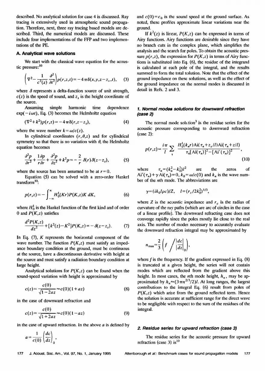
FIG. 5. Transmission loss versus range for case 2, 200 m, 100 Hz, obtained from SAFARI FFP.

the sound speed profile and sufficient number of sampling points to represent the integrand were provided. The number of layers and number of sampling points were continually adjusted where possible to achieve convergence of the TL within 0.5 dB. The run time for convergent solutions was minimized and, given convergence, the extra loss was minimized. Finally, the layer thickness was 2.5 m, with a 100 m isospeed cap.

4. CFFP

The CFFP solution [Sec. II C 2, Eq. (36) with the ground surface as an impedance plane] was implemented using 12 layers and a cap of 12 m. The artificial attenuation used to move poles off the integration path was 1 x 10 -8 Np/m. For this case, 64 k points were required. The resulting curve is indistinguishable from the one in Fig. 4.

5. FFLAG FFP

For this implementation [Sec. II C 2, Eq. (35) for a po- roelastic ground surface] the atmosphere is modeled by a 12 layer system each about 1 m thick. The air density is calculated by assuming that p= r•/c 2 and the constant of propor- tionality r] is calculated by substituting the surface values of P0 and c o .

The complete parameter set given in Table I is used to model the ground as a thick porous elastic layer over a porous elastic half-space. However, for this parameter set, the predictions are expected to be indistinguishable from those over a rigid porous half-space and the resulting curve is indistinguishable from the one in Fig. 4.

Rmax=MAr (m), where f=frequency, Cmin=minimum phase velocity, M = number of range intervals and Rmax= maximum useable range.

As the range increases to 200 m, SAFARI predicts less transmission loss than the normal mode or ray tracing solutions because SAFARI assumes a nonporous elastic soil. In fact for ranges less than 200 m, the transmission loss is close to geometric spreading and the inversion does not affect the loss until larger distances at this frequency.

7. The FINITE PE

The result of the FINITE PE calculation [Sec. IID 1, Eq. (45) with the ground surface as an impedance plane] is indistinguishable from the curve in Fig. 4. The range and height step sizes were both 0.547 m (usually equal to ¬ wavelength), the upper edge of the field array was equal to 400 m, and the total number of grid points needed in each field array was 730.

8. FAST-PE

The numerical implementation of the FAST-PE {Sec. III D 2, Eq. (46) with the ground surface impedance plane] on a computer requires the computation of a forward and inverse Fourier transform. For efficiency, a fast Fourier transform (FFT) is used. A numerical Fourier transform requires finite limits on the integration. The lower end of the transform is truncated at the ground while the upper limit is truncated at a height which is defined as zto p. The calculated results are also indistinguishable from the curve in Fig. 4 but took less time to compute than the FINITE PE employing a Crank Nicolson method. A complete discussion of the speed advantage of FAST PE is found in Ref. 31 where run times were logged for the FAST-PE and FINITE-PE on the same computer.

9. Summary

In summary, at this short range, all the models (except SAFARI) agree to within the thickness of the line when the same set of parameters are used as input data. The curve obtained from SAFARI, predicts less transmission loss than the other models because of the assumption of an elastic soil with no porosity. Finally, although FFLAG also assumes an elastic soil, the addition assumption of porosity leads FFLAG to agree with models that assume the ground surface as an impedance plane.

6. SAFARI FFP

This implementation [Sec. II C 2, Eq. (36) for an elastic surface, i.e., porosity is not included] characterizes the ground by compressional and shear wave velocities and compressional and shear wave attenuation from the relevant parameters listed in Table I. The result is the curve in Fig. 5. In the calculation the wave number spectrum is limited to a 4096 samples FFT length. The wave number resolution Ak and spatial resolution Ar are linked by minimum phase velocity: e.g., Ak=2•f/CminM (m-l), Ar=cmin/f (m) and

B. Case 2; 10 000 m, 100 Hz

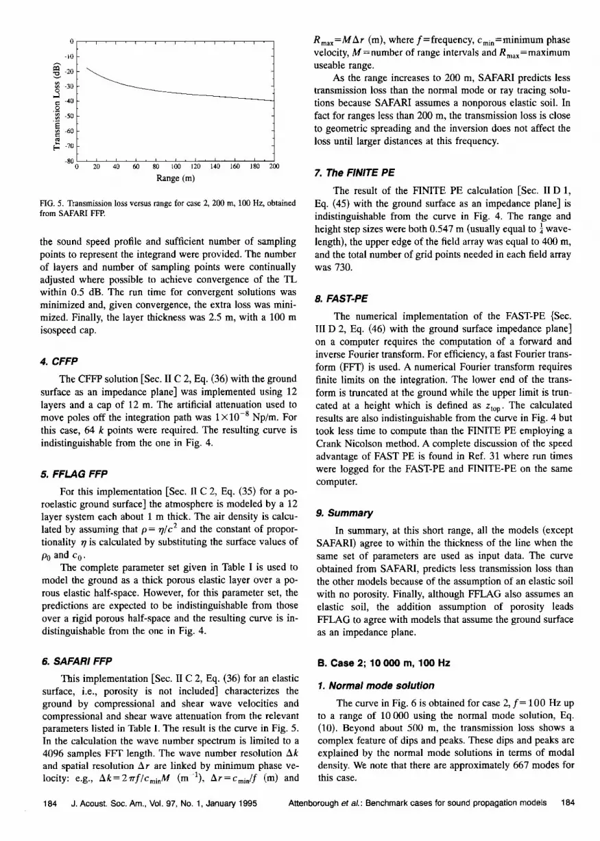
1. Normal mode solution

The curve in Fig. 6 is obtained for case 2, f= 100 Hz up to a range of 10 000 using the normal mode solution, Eq. (10). Beyond about 500 m, the transmission loss shows a complex feature of dips and peaks. These dips and peaks are explained by the normal mode solutions in terms of modal density. We note that there are approximately 667 modes for this case.


0

• •_0 • -30

• -40

.• -50 • -60

•_• -70

0.0 1.0k 2.0k 3,0k 4,0k $,0k 6,0k 7,0k 8,0k 9.0k 10Ok

Range (m)

FIG. 6. Transmission loss versus range for case 2, 10 km, 100 Hz, obtained from the normal mode solution.

0

• -30 o

,- -40 ._• .• -50 • -60

•. 70 -80

0.0 1.Ok :;.Ok 3.Ok 4.Ok 5.Ok 60k 7.Ok 8.Ok 9.Ok IO.Ok

Range (m)

FIG. 8. Transmission loss versus range for case 2, 10 kin, 100 Hz, obtained from the single bounce ray model.

2. Ray tracing solutions

At longer ranges, Eq. (19) predicts additional rays that go through multiple reflections on the ground. The curve in Fig. 7 is obtained using the multiple bounce ray model, Eq. (20). The discontinuity that appears at about 500 m corresponds to the sudden appearance of additional rays and is an artifact of the model. However the dip corresponds to physical reality and is explained by a ray model by interference between the various rays. As the range increases, more rays appear in the summation Eq. (20). The additional rays produce the interferences in the curve and contribute to reducing the transmission loss (increasing relative levels). At a range of about 10 km, Eq. (19) predicts up to 100 rays reflected from the ground.

The curve in Fig. 8 is the result of the single bounce ray model described in Sec. IIB 2. Since the calculation is re-

stricted to a single bounce, the dips corresponding to the additional rays are absent and at ranges beyond about 1500 m, the transmission loss is greater than the loss predicted when the additional rays are accounted for.

The curve in Fig. 9 was obtained from the Gaussian beam solution, Eq. (31). We note that the beam summation smooths the sharp discontinuity around 500 m that is produced by the multiple bound ray model.

It is interesting to note that on the whole the average TL predicted from the Gaussian beam solution agrees with the TL obtained from the multiple bounce ray model. Not sur-

prisingly, though, the detailed fine structure in the dip and peaks differs due to the nature of the approximations inher- ent in the ray tracing solutions. The same comments apply to the comparison with the normal mode solution. We note, however, that in a real atmosphere, turbulence would smooth out most of the fine structure predicted by this test case.

3. FFP solutions

The curve calculated from three FFPs that assume a porous ground is shc,wn in Fig. 10. The agreement between the three calculations is within the accuracy of implementation (typically 0.5 dB). The features, predicted as ray interferences according to. ray theory and modal density according to the residue series, are reproduced by the numerical solution of the full wave equation.

The curve obtained fi'om the FFLAG FFP is indistin-

guishable to witlain numerical implementation from the curves obtained ttom the CERL FFP and the CFFP. The

FFLAG FFP allows for a ].ayered porous and elastic ground using the full range of parameters in Table I. On the other hand the CERL FFP and the CFFP models the ground as a porous half-space. The agreement suggests that a complex impedance plane is a good approximation to the layered ground described in Table I for the benchmark cases. As expected, although not shown here, SAFARI yields a different result from the other FFPs.

0

-30

-•o

-70

-80 0.0 1.0k 2.0k 3.0k 4.0k 5.0k 6.0k 7.0k 8.0k 9.0k 10.Ok

Range (m)

-30

-40

-60

-70 -80

0.0 l.Ok 2.,3k 3.Ok 4.Ok 5.Ok 6.Ok 7.Ok 8.Ok 9.Ok 10.Ok

Range (m)

FIG. 7. Transmission loss versus range for case 2, 10 km, 100 Hz, obtained from the multiple bounce ray model.

FIG. 9. Transmission loss versus range for case 2, 10 km, 100 Hz, obtained from the Gaussian beam model.

185 J. Acoust. Soc. Am., Vol. 97, No. 1, January 1995 Attenborough et al.: Benchmark cases for sound propagation models 185

o.o l.ok 2.0k 3.o• 4.ok 5.ok 6.ok ?.ok s.ok 90k 10.0k

Range (m)

FIG. 10. Transmission loss versus range for case 2, 10 km, 100 Hz, obtained from the CERL FFP, CFFP, FFLAG FFP, and the FAST PE.

4. PE solutions

As noted earlier, computational time is excessive for this long range case using the FINITE PE. The FAST-PE, however, runs in just a few minutes. Details of the fine structure depend upon the height at which the calculation is truncated but the general form is the same as that in Fig. 10.

C. All cases for the FFP and PE

In this section the numerical techniques are used to calculate the transmission loss for the full range of atmospheric conditions described by cases 1 to 4. In the preceding section, results showed that three of the FFP solutions and the

0

-20

-30

-40

-50

-70

0

0 ,

-10

-20 -30

-50

-70

0

-10

-20

-30

-4o

-50

-60

-70

-80

IOHz

20 40 60 80 100 120 140 160 180 200

•oo Hz

20 40 60 80 100 120 140 160 180 200

Iooo Hz

20 40 60 80 100 120 140 160 180 200

Case 1

0.0 1.0k 2.0k 3.0k 4.0k 5.0k 6.0k 7.0k 8.Ok 9.0k 10.Ok

-60

-70

-%.0 1.0k 2.Ok 3.Ok 4.Ok 5.Ok 6.0k 7.0k 8.0k 9.0k 10.Ok

tOO0 HZ

0.0 l.Ok 2.Ok 3.0k 4.0/( 5.0k 6.Ok 7.Ok 8.Ok 9.0k 10.0k

Range (m)

FIG. 11. Transmission loss for case I for the FFP and PE. The curves obtained from the two models are indistinguishable.

186 J. Acoust. See. Am., Vol. 97, No. 1, January 1995 Attenborough et al.: Benchmark cases for sound propagation models 186

two PE methods agree with the analytical solution Eq. (10) for case 2, to within the accuracy of implementation (The results from the SAFARI FFP differed because of the as-

sumption of an elastic ground surface). Although not shown here, the FFP and the PE also agree with the analytical solution Eq. (11) for case 3 and the analytical solution Eq. (12) for case 1. Therefore detailed comparison here are restricted to the FFP (except SAFARI) and the PE. In the FFP input parameters were adjusted to obtain an accurate prediction over the entire range of interest for each case, while mini- mizing run time. The PE used accurately propagates the phases for angles under 45 ø from horizontal. Consequently, very high angles modes in case 2 at 10 Hz, 10 km have phase errors in the PE solution. We note that case 1 is the most

difficult to implement with the FFP's. Case 2 is most difficult for the PE due to the large number of trapped modes. The

larger number of modes make the sampling in wave number space less sensitive for the FFP's, since the total solution is the sum of many contributions. Sampling errors of a few modes will not alter the total solution significantly. The FINITE-PE is generally prohibitively slow at longer range or high frequencies, t]•ough it needs much less parameter "tun- ing" than the FFP to obtairt convergence.

1. Case I

Case 1 is a model for sound propagation near the ground in a homogeneous atmosphere and the results are shown in Fig. 11. In case 1• spherical spreading dominates the solution, with a 6-dB enhancement of the field at low frequen-

-10 • -20

-40

-50

-60

-70

-80

I0 HZ

20 40 60 80 100 120 140 160 180 200

Case 2

I0 HZ

0.0 l.Ok 2.Ok 3.Ok 4.Ok 5.Ok 6,Ok 7.Ok 8.Ok 9.Ok lO.Ok

0

-10

-20

-30

-40

-50

-6O

-70

-80 0

I00 HZ

20 40 60 80 1(30 120 140 160 180 200

I00 HZ

0.0 1.0k ';'.Ok 3.0k 4.0k 5.0k 6.0k ?,Ok 8.0k 9.0k 10.0k

-10 -20

-30

-40

-50

-6O

-70

-80 0 20 40 60 80

I000 HZ

-60 ,• -70

100 120 140 160 180 200 0.0 1.0k 2.0k 3.0k 4.0k 5.0k 6.0k 7.0k

Range (m)

I000 HZ

8.0k 9.0k IO0k

FIG. 12. Transmission loss for case 2 for the FFP and PE. The curves obtained from the two models are indistinguishable.

187 J. Acoust. Soc. Am., Vol. 97, No. 1, January 1995 AEonborough et al.: Benchmark cases for sound propagation models 187

-20

-30

-40

I0 HZ

-50

-60

-70

-80 20 40 60 80 100 120 140 160 180 200

0 [ [ i [ [ i [

-10

-20

-30

-40

-50

-60

-70

-80 o

1oo Hz

20 40 60 80 100 120 140 160 180 200

0

-10

-20

-30

-40

-50

-60

-70

-80 0

I000 HZ

Case 3

-10

-20

0.0 1.0k 2.0k 3.0k 4.0k 5.0k 6.0k 7.0k 8.0k 9.0k 10.0k

0.0 1.0k 2,0k 3.0k 4.0k

I00 HZ

5.0k 6.0k 7.0k 8.0k 9.0k 10.0k

I000 HZ

20 40 60 80 100 120 140 160 180 200 0,0 1,0k 2.0k 3,0k 4,0k $.0k 6.0k 7.0k 8.0k 9.0k 10,0k

Range (m)

FIG, 13. Transmission loss for case 3 for the FFP and PE. The curves obtained from the two models are indistinguishable.

cies. There is negligible attenuation of the wave at 10 Hz from atmospheric absorption in the atmosphere. There is also negligible ground attenuation from the finite-impedance ground surface at 10 Hz. At 100 Hz, the atmospheric attenuation is 0.18 dB/lun. A ground shadow appears at around 850 m and the signal decays at 46 dB per decade of distance (spherical spreading amounts to 20 dB per decade of distance). At 1 kHz, the atmospheric attenuation is 5.4 dB/km. Beyond 200 m a ground shadow occurs and the field decays at 56 dB per decade of distance, including spherical spreading, thus greatly exceeding the decay rate from atmospheric absorption. Although case 1 is the most difficult for the FFP's, when properly implemented, curves obtained from the FFP's and the PE's are indistinguishable. The analytical so-

lution for this case is Eq. (12) and this solution agrees with all the numerical results.

2. Case 2

Case 2 models sound propagation near the ground in a downward refracting situation and was considered in detail in the previous section for all the models. The curves obtained in the case of the FFP and the PE are indistinguishable and a complete set of curves are shown in Fig. 12.

3. Case 3

Case 3 models sound propagation near the ground in an upward refracting environment. At short range (under 200 m)


o

-20

-30

-4o

-60

-80 o

io Hz

20 40 60 80 100 120 140 160 1•0 200

Case 4

0.0 l.Ok 2.Ok 3.Ok 4.Ok 5.Ok 6.Qk 7.Ok 8,Ok 9.Ok 10:Ok

o

-1o

-20

-30

-4o

-50

-60

-70

-80 o

I00 Hz

20 40 60 80 100 120 140 160 180 200

IOQ H!

).0 1.0k 2.0k 3.0k 4.0k 5.0k 6.Ok 7.Ok 8.0k 9.0k 10.Ok

o

-1o

-20

-30

-4o

-50

-70

-80 ' o

iooo Hz

20 40 60 80 100 120 140 160 180 200

-60

-70

0.0 1.0k 2.0k 3.01( 4.0k 5.0k 6.0k 7.0k 8.0k 9.0k 10.0k

Range (m)

FIG. 14. Transmission loss for case 4 for the FFP and PE. The curves obtained from tl',e two moclels are indistinguishable.

the predicted curves show very little variation from case 1 except for an increase in TL for 1000 Hz beyond about 130 m. At longer ranges, all curves rapidly decay in the shadow zone formcd by the sound speed profile. The results of the PE are indistinguishable from the FFP. A complete set of curves are shown in Fig. 13.

The analytical solution for this case within the shadow zone is the residue series given by Eq. (11) and calculations using this expression, while not shown, agree with the results in Fig. 13. We note, however, that despite agreement between the calculations, the large attenuation predicted at the longer range is not supported by experimental data (for example, see the results shown in Ref. 30).

4. Case 4

Case 4 model'; sound propagation near the ground in a profile that traps eaergy near the ground, and refracts sound waves away from the ground at altitudes above 100 m. Above 300 m, the profile is constant. At short range (under 200 m) there is no difference between predictions for this situation and case 2 (downward refraction).

At longer ranges, higher angle modes of propagation interact with the upward refracting portion of the sound speed profile and "leak" energy out of the waveguide formed at the ground. At 100 Hz the curve shows less energy in the signal beyond 1.5 km than in case 2. At 1000 Hz, essentially all of the energy is trapped in the waveguide, and

189 d. Acoust. Soc. Am., Vol. 97, No. 1, January 1995 Attenborough et el.: Benchmark cases for sound propagation models 189

100o

E 900 800

700

soo 500

400

300

200

100

TL Level - Benchmark case 2 - f=10 Hz

I I

I 2 3 4 5 6 7 8

Range (km) 9

'1

TL (DB)

ABOVE -36.0

-42.0 - -36.0

-48.0 - -42.0

.64.0 - -48.0

-60.0 - -54.0

-66.0 - -60.0

-72.0 - -66.0

-78.0 - -72.0

-84.0 - -78.0

BELOW -84.0

FIG. 15. Contour plot for case 2, 10 Hz.

there is no difference in the results from case 2. The com-

plete set of curves are shown in Fig. 14. There is no analytical solution for this case.

O. Contour plot

For illustrative purposes a contour plot of transmission loss is shown in Fig. 15 for case 2, R= 10 km, f= 10 Hz which can be compared directly with the ray diagram in Fig. 16.

V. SUMMARY

Benchmarks were calculated using analytical models, ray tracing models, the FFP solution and the PE solution. The analytical models included two residue series for cases 2 and 3, respectively, and the result of a steepest descent integration for case 1. The ray tracing included a model restricted to a single bounce, a multiple bounce model and a Gaussian beam summation. Four different implementations of the FFP were considered. In one FFP (SAFARI), the ground is assumed to be a nonporous elastic layered interface. Two FFP's (CERL-FFP, CFFP) considers the ground to be a rigid semi-infinite porous surface while the fourth FFP (FFLAGS) assumed a porous elastic layer above a nonporous elastic substrate. The PEs considered included a Crank-

Nicolson version (FINITE PE) and a fast Green's function method (FAST PE).

For all cases, results show that the FFP and the PE agree with the analytical solution, where an analytical solution is available, to within the accuracy of implementation. Any differences between the various implementations of the FFP and the PE can readily be attributed to different assumptions in the models. For example SAFARI predicts less transmis-

sion loss than the other versions because it assumes a non-

porous ground. The results from the ray tracing models depend on how

many physical mechanisms are included and to what level of detail they are considered. For example a ray model that assumes a single bounce at all distances predicts larger transmission loss at long ranges for a downward refracting atmosphere than the other models. In the absence of upward refraction, for the cases considered, the ray trace algorithms give reasonable agreement with the more accurate techniques (FFP and PE).

None of the models considered here include the effects

of turbulence, rough ground, or terrain features. These effects are all present to some degree in experimental data. For this reason, the results of the calculations presented here may not compare well to experimental data especially in refractive

I000 -

900 -

800 -

•'• 700-

•-• 600-

• 500- '• 400- • 300-

200 -

100 -

0

Ray Trace - Propa3D/ISL - Benchmark case 2

I 3 3 4 5 6

Range (kin) 8 9 10

FIG. 16. Ray diagram for case 2.


shadow zones. The benchmark calculations presented here should be used to test theory and algorithms in the absence of these complications which are always present in the real world. Then the user can proceed to include other effects with a confidence that refraction, diffraction, and ground reflection have been properly accounted for.

ACKNOWLEDGMENTS

The authors are rigorously listed in alphabetical order with authors from the same institution grouped together. The editing of the manuscript and preparation of the figures was coordinated by the National Research Council of Canada. NATO DRG Panel 3 is acknowledged for sponsoring and providing the frame work for this investigation. Atlas Elek- tronik GmbH acknowledges MoD-Bonn FRG, R0 T II[/4, Mr. H. Wolff. Work at the National Research Council was

supported in part by DND/DREV. Work at the Open Univer- sity, England, was supported in part by the U.S. Army (WES) through its European Research Office.

•J. E. Piemy, T. F. W. Embleton, and L. C. Sutherland, "Review of noise propagation in the atmosphere," J. Acoust. Sec. Am. 61, 1403-1418 (1977).

2R. Rasper, G. E. Baird, and W. Wu, "The relationship between upward refraction above a complex impedance plane and the spherical wave evaluation for a homogeneous atmosphere," J. Acoust. Sec. Am. 89, 107- 114 (1991).

3R. Raspet, G. Baird, and W. Wu, "Normal mode solutioo for low frequency sound propagation in a downward refracting atmosphere above a complex impedance plane," J. Acoust. Soc. Am. 91, 1341-1352 (1992).

48. W. Lee, N. Boog, W. E Richards, and R. Raspet, "Impedance formulation of the fast field program for acoustic wave propagation in the at- rodsphere," J. Acoust. Soc. Am. 79, 628-634 {1986).

SK. E. Gilbert and M. 1. White, "Application of the parabolic equation to sound propagation in a refracting atmosphere," J. Acoust. Sec. Am. 85, 630-637 (1989).

6L. B. Felsen, "Benchmarks: An option for quality assessment," J. Acoust. Soc. Am. 87, 1497-1498 (1990).

?H. A. J. M. van Hoof and K. W. F. M. Doorman, "Coupling of airborne sound in a sandy soil," Laboratory for Electronic Developments TNO (1983). The Wezep soil is also measurement No. 12 in M. J. M. Martens, L. A.M. vander Heijden, H. H. J. Walthous' and W. J. J. M. van Rems, "Classification of soils based on acoustic impedance air flow resistivity and other physical soil parameters," J. Acoust. Soc. Am. 78, 970-980 (1985).

SThe expressions for k} and Pt, Cid) are found in K. Attenborough, "Acous- tical impedance models for outdoor ground surfaces," J. Sound Vib. 99, 501-544 {1985), however, X is written here as a function of the pore shape factor ratio s•, defined by Eq. (21) in K. Attenborough, "On the acoustic slow wave in air-filled granular materials," J. Acoust. Sec. Am. 81, 93- I02 (I987). A good appreciation of the role of the flow resistivity, tortuosity, and porosity of ground surface can be found in K. Attenborough, "Ground parameter information for propagation modeling," J. Acoust. Sec. Am. 92, 418-427 (1992) and H. M. Hess, K. Atlenborough, and N. W. Heap, "Ground characterization by short-range propagation measure- meats," J. Acoust. Sec. Am. 87, 1975-1986 (1990}.

'•ANSI SI.26-1978, "Method for the calculation of the absorption of sound by the atmosphere" {Acoustical Society of America, New York, 1978}.

mA. Berry and G. A. Daigle, "Controlled experiments on the diffraction of sound by a curved surface," J. Acoust. Sec. Am. 83, 2047-2058 (1988).

n K. Attenborough, S. I. Hayek, and J. M. Lawther, "Propagation of sound above a porous half-space," J. Acoust. Sec. Am. 68, 1493-1501 (1980). Typographical corrections can be found in the Appendix in K. B. Rasmus- sen, "Sound propagation over grass covered ground," 1. Sound Vib. 78, 247-255 (1981).

•:Anon., "Advanced Sound Propagation in the Atmosphere," University of Mississippi (1991). AShPRAT includes the CERL I:FP as a default in shadow zones. Only the ray trace part is described here.

13A. L'Esphrance, P. Herzog, G. A. Daigle, and J. Nicolas, "Heuristic model

for outdoor sound propagation based on an extension of the geometrical ray theory in the case of a linear sound speed profile," Appl. Acoust. 37, 111-139 (1992).

taV. Cerveny, M. M. Popov, and 1. Psencik, "Computation of wave fields in inhomogeneous media-Gaussian beam approach," Geophys. J. R. Astron. Soc. 70, 109-128 (1982).

tSy. Gabtiler, H. Schroeder, G. A. Daigle, and A. L'Esphrance, "Application of the Gaussian beam approach to sound propagation in the atmosphere: Theory and experiments," J. Acoust. Soc. Am. 93, 3105-3116 (1993).

•6F. R. DiNapoli, "A fast field program for multilayered media," Naval Underwater Systems Center, Tech. Rep. 4103 (1971).

•7H_ W. Kutschale, "The integral solution of the sound field in a multilayered liquid-.,•did half-space with numerical computations for low- frequency propagation in the Arctic Ocean," Tech. Rep. No. I (CU-I-70, ONR Contract N00014-67-A-0108-0016), Lamont-Doherty Geological Observatory, Columbra University, Palisades, New York (1970).

•SH. W. Kutschale, "Rapid computation by wave theory of the propagation loss in the Arctic Ocean," Tech. Rep. No. 8, Lamont-Doherty Geological Observatory, Columbra University, Palisades, New York (1981}.

•OR. Rasper, S. W. Lee, E. Kuester. D.C. Chang, W. F. Richards, R. Gilberl, and N. [long, "Fast-field prograra for a layered medium bounded by complex impedance surfaces," J. Ac3ust. Soc. •Mm. 77, 345 352 119851.

•Y. L. Li, S..I. Franke, and C. H. Liu, "Numerical implementation of an adaptive fasl-field program for snund propagation in layered media using the chirp z transform," J. Acoust. Sec. Am. 89, 2068-2075 (1991).

• A. Gtidesen, "Application of the SAFARI model to sound propagation in the atmosphere," J. Acoust. Soc. Am. 87, 1968-1974 (1990). For a detailed discussion of the use of SAFARI in underwater acoustics, see H.

Schmidt, "SAFARI User's Gtide," SACLANTCEN Report SR-114, NATO (1988) and C. H. Harrison, "Ocean Propagation Models," Appl. Acoust. •7, 163-201 (1989).

•2T. L. Richards and K. Attenborough, "Accurate FFT-based Hankel trans- forms for prediction of outdoor sound propagation," J. Sound Vib. 109. 157-167 (1980).

2•S. Thorns, S. Taherzadeh, and K Anenborough, "Sound propagation in a refracting fluid above a layered tluid-saturated porous elastic material," J. Acoust. Soc. Am. 93, 173-181 •1993).

•48. J. Franke and G. W. Swenson, Jr., "A brief tutorial on the Fast Field Program applied to Sound Propagation in the Air," Appl. Acoust. 27(3), 203-216 (1980).

•M. West, R. A. Sack, and F. Walkden, "The fast field program. A .second tutorial: Application to long range sound propagation in the atmosphere," Appl. Acoust. 33, 199-228 (1991).

•hG. D. Deckcry, "M•xlcling electromagnetic wave propagation in the tro- posphere using the parabolic equation," IEEE Trans. Antennas Propag. 36(I0), 1464-1470 (October, 1988).

•? J. K Claerbout, Fundamentals o[ Geophysical Data Processing (McGraw- Hill, New York, 1976), p. 206.

Z•E D. Tappert, "The parabolic approximation melbod," in Wave Propaga- tion and Underwater Acoustics, edited by J. B_ Keller and J. S_ Papadakis (Springer-Verlag, New York, 19;'7).

•M. K. Myers and G. L. McAninch, "Parabolic approximation for sound propagation in the atmosphere," AIAA J. 16, 836-842 (August 1978).

SUM. J. White and K. E. Gilbert, ' Application of the parabolic equation to the outdoor propagation of sound," Appl. Acoust. 2713), 227-238 (1989}.

3• K. E. Gilbert and X. Di, "A Fast Green's function method for one-way sound propagation in the atmosphere," J. Acoust. Soc. Am. 93, 714-720 (1992}. The software package that implements The Green's Function PE {GF-PE) is referred tc as "FAST-PE" in this article.

32j. C. Craddeck and IV. J. White, "Propagation of acoustic waves past an impedance di•ontinutty: a paratolic equation approach," J. Acuust. Sec. Am. 91, 3184-3191 (1992).

a'•J. S. Robertson, M. J. Jacobson, W. L. Siegmann, and D. P. Santandrea, "Acoustical effects of a large ridge on low-frequency sound propagation in stationary and moving atmospheres," RPI Math. Rep. No. 181, Dept. of Mathematical Sciencei, Rensselear Polytechnic Institute, Troy, NY 12180- 3590 (November 1989).

•J. M. Noble, 1t. E. Bass' and R. Rasper, "Effects of large-scale wind driven turbulence on sound prol:,agation," .I. Acuust. Soc. Am. 87, S149 (1990).

35 K. E. Gilbert, R. Ras[et, and X. Di, "Calculation of turbulence etfects in an upward refracting atmosphere," 1. Acoust. Soc. Am. 87, 2428-2437 (1990).


Documents

Benchmark cases for outdoor sound propagation models