Embed Size (px)
Citation preview

NIST Special Publication 1194
Benefits and Costs of Energy Standard
Adoption for New Residential
Buildings: National Summary
Joshua Kneifel
Eric O’Rear
This publication is available free of charge from:
http://dx.doi.org/10.6028/NIST.SP.1194


NIST Special Publication 1194
Benefits and Costs of Energy Standard Adoption for New
Residential Buildings: National Summary
Joshua Kneifel
Eric O’Rear
Applied Economics Office
Engineering Laboratory
This publication is available free of charge from:
http://dx.doi.org/10.6028/NIST.SP.1194
June 2015
U.S. Department of Commerce Penny Pritzker, Secretary
National Institute of Standards and Technology Willie May, Under Secretary of Commerce for Standards and Technology and Director

Certain commercial entities, equipment, or materials may be identified in this
document in order to describe an experimental procedure or concept adequately.
Such identification is not intended to imply recommendation or endorsement by the
National Institute of Standards and Technology, nor is it intended to imply that the
entities, materials, or equipment are necessarily the best available for the purpose.
National Institute of Standards and Technology Special Publication 1194
Natl. Inst. Stand. Technol. Spec. Publ. 1194, 80 pages (June 2014)
http://dx.doi.org/10.6028/NIST.SP.1194
CODEN: NSPUE2

Abstract
Energy efficiency requirements in energy codes for residential buildings vary across
states, and many states have not yet adopted the latest energy efficiency code edition. As
of July 2014, states had adopted energy codes ranging across editions of the International
Energy Conservation Code (IECC) (2003, 2006, 2009, and 2012). Some states do not
have a code requirement for energy efficiency, leaving it up to the locality or jurisdiction
to set its own requirements. This study considers the impacts that the adoption of newer,
more stringent energy codes for residential buildings would have on building energy use,
operational energy costs, building life-cycle costs, and “cradle-to-grave” life-cycle
carbon emissions.
The results of this report are based on analysis of the Building Industry Reporting and
Design for Sustainability (BIRDS) new residential database, which includes 9120 whole
building energy simulations covering 10 building types in 228 cities across all U.S. states
for study periods ranging from 1 year to 40 years. The performance of buildings designed
to meet current state energy codes is compared to their performance when meeting new
editions of IECC design requirements to determine whether more stringent energy code
editions are cost-effective in reducing energy consumption and life-cycle carbon
emissions. The estimated savings for each of the building types are aggregated using city-
level new residential building construction data to calculate the magnitude of the
incremental savings that a state may realize if it were to adopt a more energy efficient
code edition as its state energy code. These state-level estimates are further aggregated to
the national level to estimate the potential total impact from nationwide adoption of more
stringent energy codes.
Keywords
Building economics; economic analysis; life-cycle costing; life-cycle assessment; energy
efficiency; residential buildings

vi

vii
Preface
This study was conducted by the Applied Economics Office in the Engineering
Laboratory (EL) at the National Institute of Standards and Technology (NIST). The study
is designed to assess the energy use, life-cycle cost, and life-cycle carbon emissions
impacts from the adoption of new state energy codes based on more stringent building
energy code editions. The intended audience is researchers and policy makers in the
residential building sector, and others interested in residential building energy efficiency.
Disclaimers
The policy of the National Institute of Standards and Technology is to use metric units in
all of its published materials. Because this report is intended for the U.S. construction
industry that uses U.S. customary units, it is more practical and less confusing to include
U.S. customary units as well as metric units. Measurement values in this report are
therefore stated in metric units first, followed by the corresponding values in U.S.
customary units within parentheses.

viii

ix
Acknowledgements
The authors wish to thank all those who contributed ideas and suggestions for this report.
They include Dr. David Butry and Dr. Robert Chapman of EL’s Applied Economics
Office, Dr. William Healy of EL’s Energy and Environment Division, and Dr. Nicos S.
Martys of EL’s Materials and Structural Systems Division. A special thanks to Brian
Presser, Samuel Sharpe, and Priya Lavappa for developing the BIRDS new residential
database.
Author Information
Joshua D. Kneifel
Economist
National Institute of Standards and Technology
Engineering Laboratory
100 Bureau Drive, Mailstop 8603
Gaithersburg, MD 20899-8603
Tel.: 301-975-6857
Email: [email protected]
Eric G. O’Rear
Economist
National Institute of Standards and Technology
Engineering Laboratory
100 Bureau Drive, Mailstop 8603
Gaithersburg, MD 20899-8603
Tel.: 301-975-4570
Email: [email protected]

x

xi
Table of Contents Abstract .............................................................................................................................. v Preface .............................................................................................................................. vii Acknowledgements .......................................................................................................... ix Author Information ......................................................................................................... ix List of Figures ................................................................................................................. xiii List of Tables ................................................................................................................... xv List of Acronyms ........................................................................................................... xvii Executive Summary ........................................................................................................ xx 1 Introduction ............................................................................................................... 1
1.1 Background .......................................................................................................... 1
1.2 Literature Review ................................................................................................. 2
1.3 Purpose ................................................................................................................. 4
1.4 Approach .............................................................................................................. 5
2 Study Design .............................................................................................................. 7 2.1 Building Types ..................................................................................................... 7
2.2 Building Designs .................................................................................................. 8
2.3 Study Period Lengths ......................................................................................... 12
3 Cost Data.................................................................................................................. 13 3.1 First Costs ........................................................................................................... 13
3.2 Future Costs........................................................................................................ 15
4 Building Stock Data ................................................................................................ 21 4.1 Databases ............................................................................................................ 21
4.2 Weighting Factors .............................................................................................. 22
5 Analysis Approach .................................................................................................. 27 5.1 Energy Use ......................................................................................................... 27
5.2 Life-Cycle Costing ............................................................................................. 27
5.3 Environmental Impact Assessment .................................................................... 28
5.4 Analysis Metrics ................................................................................................. 29
6 Nationwide Impacts of Adopting 2012 IECC Design .......................................... 33 6.1 Percentage Reductions ....................................................................................... 33
6.1.1 Results by Building Type.......................................................................... 33
6.1.2 Results by Climate Zone ........................................................................... 38
6.1.3 Results by State Energy Code ................................................................... 42
6.2 Total Changes ..................................................................................................... 46
6.2.1 Total Savings by State .............................................................................. 46
6.2.2 Regional and National Impacts ................................................................. 49
6.3 Savings per Unit of Floor Area .......................................................................... 49
6.3.1 State-Level Savings .................................................................................. 49
6.3.1.1 Energy Use and Energy Cost Savings per Unit of Floor Area .. 49
6.3.1.2 Energy Cost Savings per Unit of Energy Savings ..................... 50
6.3.1.3 Savings in Life-Cycle Carbon Emissions per Unit of Energy
Savings ................................................................................................... 52
6.3.1.4 Life-Cycle Cost Savings per Unit of Floor Area ....................... 53

xii
6.3.2 Regional and National Savings per Unit of Floor Area ............................ 54
7 Discussion................................................................................................................. 59 7.1 Key Findings ...................................................................................................... 59
7.1.1 Percentage Changes .................................................................................. 59
7.1.2 Total Changes ........................................................................................... 60
7.1.3 Change per Unit of Floor Area ................................................................. 61
7.2 Limitations and Future Research........................................................................ 61
References ........................................................................................................................ 65 A Building Type, New Construction, and Emissions Rates .................................... 69 B Percentage Changes by State for the Nationwide Adoption of the 2012 IECC 73 C Total Changes from the Nationwide Adoption of the 2012 IECC ...................... 75 D Savings per Unit of Floor Area from the Nationwide Adoption of the 2012
IECC..................................................................................................................... 77

xiii
List of Figures
Figure 2-1 State Residential Energy Codes ...................................................................... 10 Figure 2-2 Locations and Climate Zones .......................................................................... 11
Figure 3-1 Baseline Construction Costs ........................................................................... 13 Figure 3-2 Baseline Maintenance, Repair, and Replacement Costs by Year ................... 17 Figure 4-1 Cities and Associated (Colored) County Clusters ........................................... 22 Figure 4-2 Data Processing for Weighting Development ................................................. 23 Figure 6-1 Average Percentage Reduction in Energy Use, Energy Costs, Life-Cycle
Emissions, and LCC for 1- and 2-Story Homes (10-Year Study Period) ......................... 42 Figure 6-2 Baseline IECC Codes for all U.S. States......................................................... 43
Figure 6-3 Average Percentage Savings by State in (a) Energy Use and (b) Energy Costs
Savings (10-Year Study Period) ....................................................................................... 44 Figure 6-4 Average Percentage Savings in Emissions for all U.S. States (10-Year Study
Period) ............................................................................................................................... 45 Figure 6-5 Average Percentage Savings in Life-Cycle Costs for all U.S. States (10-Year
Study Period) .................................................................................................................... 45 Figure 6-6 Total Average New Residential Floor Area Constructed Annually in Each
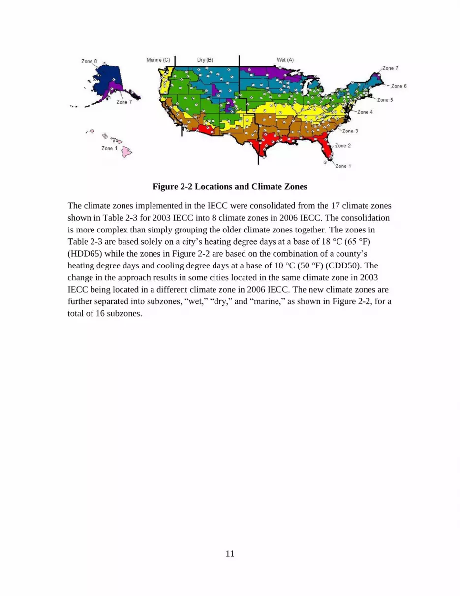
State................................................................................................................................... 47 Figure 6-7 Total Savings in Energy Use, Energy Costs, Life-Cycle Carbon Emissions,
and Life-Cycle Costs (10-Year Study Period) .................................................................. 48
Figure 6-8 Energy Savings per Unit of Floor Area by State (10-Year Study Period) ...... 50
Figure 6-9 Energy Cost Savings per Megawatt-Hour Reduced and Weighted Average
Energy Price by State (10-Year Study Period) ................................................................. 51 Figure 6-10 (a) Building America U.S. Climate Regions and (b) the Average Natural Gas
Offset by State (10-Year Study Period) ............................................................................ 52 Figure 6-11 Emissions Savings per MWh Reduced and the Weighted Average Offset of
Natural Gas by State (10-Year)......................................................................................... 53 Figure 6-12 Life-Cycle Cost Savings per Unit of Floor Area by State (10-Year) ............ 54 Figure A-1 Conditioned Floor Area of New 1-Story Single-Family Housing ................. 69
Figure A-2 Conditioned Floor Area of New 2-Story Single-Family Housing ................. 70

xiv

xv
List of Tables
Table 2-1 Building Prototype Characteristics ..................................................................... 8 Table 2-2 Energy Code by State ......................................................................................... 9
Table 2-3 2003 IECC Climate Zones................................................................................ 12 Table 3-1 Energy Efficiency Component Requirements for Alternative Building Designs
........................................................................................................................................... 15 Table 3-2 2009 SPV Discount Factors for Future Non-Fuel Costs, 3 % Real Discount
Rate ................................................................................................................................... 16
Table 4-1 Percentages of One- and Multi-Story Homes by Census Region..................... 24 Table 4-2 Building Types, Bin Ranges, and Percentage of Each Building Design .......... 24
Table 4-3 Percentage of Each Building Type for One- and Multi-Story Homes (New
England Division) ............................................................................................................. 25 Table 4-4 Percentage of Each Building Type by Census Division ................................... 26 Table 5-1 Greenhouse Gas Global Warming Potentials ................................................... 29 Table 6-1 Nationwide Average Percentage Reduction in Energy Use from Adoption of
the 2012 IECC Design by Building Type ......................................................................... 34 Table 6-2 Nationwide Average Percentage Reduction in Energy Costs from Adoption of
the 2012 IECC Design by Building Type and Study Period Length ................................ 35 Table 6-3 Nationwide Average Percentage Reduction in Life-Cycle Carbon Emissions
from Adoption of the 2012 IECC Design by Building Type ............................................ 36
Table 6-4 National Average Percentage Reduction in Life-Cycle Costs from Adoption of
the 2012 IECC Design by Building Type and Study Period Length ................................ 37 Table 6-5 Nationwide Average Percentage Reduction in the Four Performance Metrics
from Adoption of the 2012 IECC Design by Building Type (10-Year) ........................... 37
Table 6-6 Average Percentage Reduction in Energy Use from Adoption of the 2012
IECC by Climate Zone and Baseline Code for 1- and 2-Story Homes ............................ 39
Table 6-7 Average Percentage Reduction in Energy Costs from Adoption of the 2012
IECC by Climate Zone and Baseline Code for 1- and 2-Story Homes (10-Year Study
Period) ............................................................................................................................... 40
Table 6-8 Average Percentage Reduction in Emissions from Adoption of the 2012 IECC
by Climate Zone and Baseline Code for 1- and 2-Story Homes....................................... 40
Table 6-9 Average Percentage Reduction in Life-Cycle Costs from Adoption of the 2012
IECC by Climate Zone and Baseline Code for 1- and 2-Story Homes (10-Year Study
Period) ............................................................................................................................... 41 Table 6-10 Total Savings by Census Region from Adoption of the 2012 IECC (10-Year
Study Period) .................................................................................................................... 49 Table 6-11 Energy Use Reductions per Unit of Newly Constructed Floor Area from
Adoption of the 2012 IECC by Census Region (10-Year Study Period) ......................... 54 Table 6-12 Energy Cost Reduction per kWh of Energy Savings from Adoption of the
2012 IECC by Census Region (10-Year) .......................................................................... 55
Table 6-13 Reduced Carbon Emissions per GWH of Energy Savings from Adoption of
the 2012 IECC by Census Region (10-Year Study Period) .............................................. 56 Table 6-14 Life-Cycle Cost Savings per Unit of Newly Constructed Floor Area from
Adoption of the 2012 IECC by Census Region (10-Year Study Period) ......................... 57 Table A-1 CO2, CH4, and N2O Emissions Rates Electricity Generation by State ............ 71

xvi
Table B-1 Total Changes in Fuel Use and the Proportional Changes in Natural Gas Use
Relative to 2012 IECC ...................................................................................................... 73 Table B-2 Summary of Average Savings in Energy Use, Energy Costs, Carbon
Emissions, and Life-Cycle Costs for all U.S. States (10-Year) ........................................ 74
Table C-1 Total Reductions by State from Adoption of the 2012 IECC (10-Year) ......... 75 Table D-1 Savings in Energy Use per Unit of Floor Area from Adoption of the 2012
IECC (10-Year) ................................................................................................................. 77 Table D-2 Reduction in Energy Costs per MWh of Reduced Energy Use from Adoption
of the 2012 IECC (10-Year) ............................................................................................. 78
Table D-3 Reduction in Total Carbon Emissions per Unit of Floor Area from Adoption of
the 2012 IECC (10-Year) .................................................................................................. 79
Table D-4 Savings in Life-Cycle Costs per Unit of Floor Area from Adoption of the 2012
IECC (10-Year) ................................................................................................................. 80

xvii
List of Acronyms
Acronym Definition
AEO Applied Economics Office
AFUE Annual Fuel Utilization Efficiency
AIRR Adjusted Internal Rate of Return
ASHRAE American Society of Heating, Refrigerating, and Air-Conditioning Engineers
BIRDS Building Industry Reporting and Design for Sustainability
CBECS Commercial Building Energy Consumption Survey
CH4 Methane
CO2 Carbon Dioxide
CO2e Carbon Dioxide Equivalent
DOE Department of Energy
EEFG EnergyPlus Example File Generator
eGRID Emissions and Generation Resource Integrated Database
EIA Energy Information Administration
EL Engineering Laboratory
EPA Environmental Protection Agency
FEMP Federal Energy Management Program
FERC Federal Energy Regulatory Commission
HVAC Heating, Ventilating, and Air-Conditioning
I-P Inch-Punds (Customary Units)
IECC International Energy Code Council
ISO International Organization for Standardization
LCA Life-Cycle Assessment
LCC Life-Cycle Cost
LEC Low Energy Case
MBH thousand Btu per hour
MRR Maintenance, Repair, and Replacement
N2O Nitrous Oxide
NAHB National Association of Home Builders
NERC North American Electric Reliability Corporation
NIST National Institute of Standards and Technology
PNNL Pacific Northwest National Laboratory
ROI Return on Investment
S-I System International (Metric Units)
SEER Seasonal Energy Efficiency Ratio
SHGC Solar Heat Gain Coefficient

xviii

xix
Acronym Definition
SPV Single Present Value
UPV* Uniform Present Value Modified for Fuel Price Escalation

xx
Executive Summary
Energy efficiency requirements in energy codes for residential buildings vary across
states, and many states have not yet adopted the latest energy efficiency code edition. As
of July 2014, states had adopted energy codes ranging across editions of the International
Energy Conservation Code (IECC) (2003, 2006, 2009, and 2012). Some states do not
have a code requirement for energy efficiency, leaving it up to the locality or jurisdiction
to set its own requirements. This study considers the impacts that the adoption of newer,
more stringent energy codes for residential buildings would have on building energy use,
operational energy costs, building life-cycle costs, and “cradle-to-grave” life-cycle
carbon emissions.
The results of this report are based on analysis of the Building Industry Reporting and
Design for Sustainability (BIRDS) new residential database, which includes 9120 whole
building energy simulations covering 10 building types in 228 cities across all U.S. states
for study periods ranging from 1 year to 40 years. The performance of buildings designed
to meet current state energy codes is compared to their performance when meeting new
editions of IECC design requirements to determine whether more stringent energy code
editions are cost-effective in reducing energy consumption and life-cycle carbon
emissions.
Assuming a 10-year study period, nationwide adoption of 2012 IECC would lead to
significant average percentage reductions in energy consumption (19.2 %), energy costs
(15.2 %), life-cycle carbon emissions (11.2 %), and life-cycle costs (1.7 %). The
percentage reductions in energy costs are smaller than the percentage reductions in
energy consumption because the majority of the reductions are from natural gas, which is
cheaper than electricity. The percentage reductions in life-cycle carbon emissions are
much lower than the reductions in energy consumption because of two factors. First, the
emissions rate is lower for natural gas than for electricity. Since most of the reductions in
energy consumption are from natural gas, the emissions reductions are lower. Second,
life-cycle carbon emissions include emissions from both the energy consumption of the
building and the embodied emissions from the materials used in construction of the
building. In order to reduce energy consumption, additional materials must be installed in
the building, leading to higher embodied emissions that offset some of the energy-related
carbon emissions reductions.
The estimated savings vary by building prototype, baseline code edition of IECC, and
climate zone of a building's location. One-story houses realize smaller savings than
2-story houses with approximately the same conditioned floor area. Two factors could be
driving these differences. First, 2-story houses have more volume per unit of floor area,
which causes energy use to meet the heating and cooling loads to account for a greater
fraction of total energy use. Second, the two-story houses have less window glazing per

xxi
unit of wall area, which could lead to greater savings from changes in requirements for
wall insulation. Similar results and interpretations occur for energy costs, life-cycle
carbon emissions, and life-cycle costs. On average, locations with older editions of IECC
as their baseline code realize slightly greater reductions in energy use, energy costs, and
life-cycle carbon emissions. Life-cycle cost savings are greatest for locations with 2003
IECC as the baseline code, on average, followed by 2009 IECC. Although locations with
older baseline codes realize greater reductions, on average, this trend does not hold at the
climate zone level. In fact, locations with a baseline code of 2003 IECC lead to the
greatest reductions in energy use, energy costs, and carbon emissions for only two of
eight climate zones. This result may be driven by the change in climate zone definitions
from 2003 IECC to 2006 IECC and the resulting changes in building requirements for
locations in those climate zones across IECC editions. On average, the percentage
reductions in energy use, energy costs, and life-cycle carbon emissions increase as the
climate zone gets colder, with a small drop as the climate shifts from primarily cooling to
primarily heating loads. Life-cycle cost reductions do not follow the same trend, with
Zone 1 realizing greater life-cycle cost reductions than Zone 2, and Zone 6 realizing
lower reductions than Zone 5. This deviation may be a result of the differences in the
additional investment costs, on average, of meeting the 2012 IECC across climate zones.
These same results hold at the state level, with states in colder climates realizing greater
reductions in energy use, energy costs, and life-cycle carbon emissions. However, there is
some variation in percentage reductions for energy costs and carbon emissions driven by
variation in energy prices and electricity-related emissions rates, respectively.
The estimated savings for each of the building types are aggregated using city-level new
residential building construction data to calculate the magnitude of the incremental
savings that a state may realize if it were to adopt a more energy efficient code edition as
its state energy code. The amount of new floor area constructed in a state is the key driver
to the magnitude of the estimated reductions in energy use, energy costs, and life-cycle
carbon emissions, with Texas and North Carolina realizing the greatest reductions while
Alaska and Vermont realize the smallest reductions in energy use, energy costs, life-cycle
carbon emissions, and life-cycle costs. These state-level estimates are aggregated to the
national level to estimate the potential total impact from nationwide adoption of more
stringent energy codes. The impacts aggregated at the national level total 2.4 TWh of
energy consumption, $993 million in energy costs, 9.3 million metric tons CO2e of life-
cycle emissions, and $601 million for one year’s worth of construction for a 10-year
study period.
After controlling for the amount of newly constructed floor area, the results are similar to
the percentage change results. Energy savings per unit of floor area is driven primarily by
climate zone. For example, states such as Alaska have the least amount of new
construction, but achieve some of the most extensive reductions in energy use per m2

xxii
(ft2). States with greater reductions in total energy use generally realize greater energy
cost savings. Other factors such as energy prices and the fuel mix of the total reductions
in energy use in a state also impact the magnitude of energy cost savings. Higher energy
prices, greater proportions of energy use accounted for by electricity, and smaller shifts in
consumption from natural gas to electricity lead to greater reductions in energy costs per
unit of floor area. Similarly, higher emissions rates for electricity, greater proportions of
energy use accounted for by electricity, and smaller shifts in consumption from natural
gas to electricity lead to greater reductions in life-cycle carbon emissions per unit of floor
area. Similar to energy use, life-cycle cost savings per unit of floor area are greater for
states in colder climate zones.
The analysis in this study is limited in scope and would be strengthened by including
sensitivity analysis, expanding the BIRDS database and metrics, and allowing public
access to all the results. Environmental assessment could be expanded beyond life-cycle
carbon emissions to cover all environmental impact categories. Additional energy
efficiency measures, fuel types, discount rates, building constructions (e.g., wall types),
and building types (e.g., low-rise apartment building) would also expand the scope of the
database. Uncertainty analysis on these factors as well as other factors, such as local
energy pricing schedules, jurisdictional code adoptions and enforcement, occupancy and
behavior patterns, and financing options, should be considered in future analysis.
Energy, environmental, and economic performance are but three attributes of building
performance. The BIRDS model assumes that its building prototypes all meet minimum
technical performance requirements. However, there may be significant differences in
technical performance not evaluated in BIRDS, such as indoor environmental quality
performance, which may affect energy, environmental, and economic considerations.
The extensive BIRDS new residential database can be used to answer many more
questions than posed in this report, and will be made available to the public through
BIRDS v2.0 that allows others access to the database for their own research on building
energy efficiency and sustainability. These improvements are underway, with
comprehensive sustainability assessment and more detailed reporting and release of the
BIRDS v2.0 software scheduled for September 2015.

xxiii
1
1 Introduction
1.1 Background
Building stakeholders need practical metrics, data, and tools to support decisions related
to sustainable building designs, technologies, standards, and codes. The Engineering
Laboratory (EL) of the National Institute of Standards and Technology (NIST) has
addressed this high priority national need by extending its metrics and tools for
sustainable building products, known as Building for Environmental and Economic
Sustainability (BEES), to entire buildings. These entire or “whole” building sustainability
metrics have been developed based on innovative extensions to life-cycle assessment
(LCA) and life-cycle costing (LCC) approaches involving whole building energy
simulations. The measurement system evaluates the sustainability of both the materials
and the energy used by a building over time. It assesses the “carbon footprint” of
buildings as well as 11 other environmental performance metrics, and integrates
economic performance metrics to yield science-based measures of the business case for
investment choices in high-performance green buildings.
The approach developed for BEES has now been applied at the whole building level to
address building sustainability measurement in a holistic, integrated manner that
considers complex interactions among building materials, energy technologies, and
systems across dimensions of performance, scale, and time. Building Industry Reporting
and Design for Sustainability (BIRDS) applies the new sustainability measurement
system to an extensive whole building performance database NIST has compiled for this
purpose. The energy, environmental, and cost data in BIRDS measure building operating
energy use through detailed energy simulations, building materials use through
innovative life-cycle material inventories, and building costs over time. BIRDS v1.0
includes energy, environmental, and cost measurements for 12 540 new commercial and
non-low-rise residential buildings, covering 11 building prototypes in 228 cities across all
U.S. states for 9 study period lengths. See Lippiatt et al. (2013) for additional details.
Similarly, the new residential building database incorporated into BIRDS v2.0 includes
energy, environmental, and cost measurements for 9120 new residential buildings,
covering 10 single family dwellings (5 1-story and 5 2-story of varying conditioned floor
area) in 228 cities across all U.S. states for study period length ranging from 1 year to 40
years. The sustainability performance of buildings designed to meet current state energy
codes can be compared to their performance when meeting three alternative building
energy code editions to determine the impact of energy efficiency on sustainability
performance. The impact of the building location and the investor’s time horizon on
sustainability performance can also be measured.

2
1.2 Literature Review
The U.S. Department of Energy (DOE), through DOE-funded national laboratories, is on
the forefront of whole building energy simulation development, including reference
building prototypes for both new and existing commercial and residential buildings.
To meet statutory requirements, DOE tasks the Pacific Northwest National Laboratory
(PNNL) with estimating the energy use and energy cost savings associated with the
standard/code building requirements relative to a baseline edition for each new edition of
ASHRAE 90.1 for commercial buildings and IECC for residential buildings. PNNL has
also begun to incorporate some LCC estimates into their analysis.
Adopting newer editions of ASHRAE 90.1 for new commercial buildings leads to
reductions in energy consumption and energy costs. PNNL (2009a) estimates the impacts
for each state of adopting ASHRAE 90.1-2007 as the commercial building energy code
relative to the state’s current energy code, which vary across states. The annual energy
use savings and energy cost savings are estimated for three Department of Energy (DOE)
benchmark buildings -- a medium-sized office building, a non-refrigerated warehouse,
and a mid-rise apartment building--for 97 cities located across the United States.
Halverson et al. (2011a) estimates that, on average, adoption of ASHRAE 90.1-2007
reduces site energy by 4.6 % relative to ASHRAE 90.1-2004. Halverson et al. (2011b)
estimates an 18.5 % reduction in site energy use, on average, from the adoption of
ASHRAE 90.1-2010 relative to ASHRAE 90.1-2007 while Halverson et al. (2014)
estimates a 7.6 % reduction from building to meet ASHRAE 90.1-2013 relative to
ASHRAE 90.1-2010.
Adopting newer editions of IECC for new residential buildings lead to reductions in
energy consumption and energy costs. PNNL (2009b) estimates the impact of adoption of
2009 IECC for residential buildings for each state relative to its current energy code,
including a summary of the changes in energy efficiency construction requirements and
the estimated energy use and energy cost savings. Lucas et al. (2012) estimates the
energy and life-cycle cost savings for adoption of newer editions of the IECC across
climates zones for a single-family dwelling and apartment building across different
foundation types. Relative to 2006 IECC, the adoption of 2009 IECC and 2012 IECC
lead to average reductions in energy costs of 11 % and 32 %, respectively. Additionally,
all climate zones realize reductions in life-cycle costs with the coldest climate zones
realizing the greatest life-cycle cost savings and Zone 1 (maritime climate) realizing
greater life-cycle cost savings than zones characterized as having hot-humid, hot-dry,
mixed-dry, or mixed-humid climate conditions (Zone 2 through Zone 4). Mendon et al.
(2013) estimates the LCC effectiveness of 2009 IECC and 2012 IECC relative to 2006
IECC for 109 U.S. cities. Mendon et al. (2014) is the most recent PNNL analysis, looking

3
at the impacts of 2015 IECC, which are found to lead to a minimal reduction (1.1 % on
average) in energy use relative to 2012 IECC.
The National Association of Home Builders (NAHB) Research Center has completed
similar analyses as those presented by PNNL. NAHB (2012a) develops a methodology to
calculate energy performance in residential buildings, including simulation modeling
assumptions for a “standard reference house” based on national average characteristics.
NAHB (2012b) and NAHB (2012c) estimate the cost-effectiveness of constructing to
meet 2009 IECC and 2012 IECC relative to 2006 IECC, respectively. Constructing to
meet 2009 IECC reduces site energy consumption by 10.7 % with an average payback
period of 5.6 years. Constructing to meet 2012 IECC reduces site energy consumption by
three times that of 2009 IECC (33.9 %), but has a higher average payback period of 10.4
years because the initial additional costs are much higher for building to meet 2012 IECC
versus 2009 IECC.
NIST has expanded on the DOE and PNNL research by increasing the number of
locations considered in analysis, including life-cycle costing and life-cycle assessment
results, and considering a range of study periods. Kneifel (2010) creates a framework to
simultaneously analyze the impacts of improving energy efficiency on energy use, energy
costs, life-cycle costs, and carbon emissions through an integrated design context for new
commercial buildings. The paper compares the savings of constructing 11 prototype
commercial buildings to meet the building envelope requirements of ASHRAE 90.1-2007
and a “Low Energy Case,” relative to ASHRAE 90.1-2004, for 16 cities in different
climate zones across the contiguous United States. The paper finds minimal
improvements in energy efficiency from building to meet ASHRAE 90.1-2007 relative to
ASHRAE 90.1-2004 while significant savings is found by building to meet the “Low
Energy Case.” The “Low Energy Case” is often cost-effective on a first cost basis and is
always cost-effective over the longer study period lengths.
Kneifel (2011a) expands on the framework and analysis in Kneifel (2010) by analyzing
the impact of adopting the building envelope requirements of ASHRAE 90.1-2007 and a
“Low Energy Case” relative to ASHRAE 90.1-2004 in terms of energy use, energy costs,
energy-related carbon emissions, and life-cycle costs for 228 cities across the U.S. with at
least one city in each state. Analysis includes 4 study period lengths (1, 10, 25, and 40
years). The paper finds that, on average, the more energy efficient building designs are
cost-effective. However, there is significant variation across states in terms of energy use
savings and life-cycle cost-effectiveness driven by both climate and construction costs.
There is also significant variation across cities within a state, even cities located within
the same climate zone. These variations are a result of differences in local material and
labor costs as well as energy costs.

4
Kneifel (2013a) analyzes 12 540 whole-building energy simulations in the Building
Industry Reporting and Design for Sustainability (BIRDS) database covering 11 building
types in 228 cities across all U.S. states for 9 study period lengths (1, 5, 10, 15, 20, 25,
30, 35, and 40 years). Current state energy code performance is compared to the
performance of alternative ASHRAE 90.1 Standard editions to determine whether more
stringent energy standard editions are cost-effective in reducing energy consumption and
energy-related carbon emissions. This analysis includes a “Low Energy Case” (LEC)
building design based on ASHRAE 189.1-2009, which increases energy efficiency beyond
the ASHRAE 90.1-2007 design. Results are analyzed in detail for the ASHRAE 90.1-2007
and LEC designs. Results are aggregated at the state level for seven states (Alaska,
Colorado, Florida, Maryland, Oregon, Tennessee, Wisconsin) to estimate the magnitude
of total energy use savings, energy cost savings, life-cycle cost savings and energy-
related carbon emissions reductions that could be attained by adoption of a more stringent
state energy code for commercial buildings.
Kneifel (2013b), Kneifel (2013c), Kneifel (2013d), and Kneifel (2013e) implement the
analysis approach developed in Kneifel (2013a) for an individual state and analyze each
state in the Northeast, Midwest, South, and West Census Regions, respectively. The
results for each state, both on a percentage and aggregate basis, are compared across the
Census Region to determine the driving factors for variation across states in the relative
impacts of adopting more stringent state energy codes. The results are aggregated to the
Census Region level to estimate the total region-wide impacts.
Kneifel (2013f) analyzes the results developed in Kneifel (2013a, 2013b, 2013c, 2013d,
2013e) from the BIRDS new commercial database, and summarizes the results into the
key nationwide trends and important interpretations for energy efficiency in new
commercial buildings.
1.3 Purpose
The purpose of this study is to use the same methodology as used for the BIRDS new
commercial buildings database reports and analyze the results from the BIRDS new
residential database, and summarize the results into the key nationwide trends and
important interpretations for energy efficiency in new residential buildings. The
performance of buildings designed to meet current state energy codes is compared to
their performance when meeting newer editions of IECC for residential building
requirements to determine whether more stringent energy standard editions are
cost-effective in reducing energy consumption and environmental impacts. The estimated
savings for each of the building types are aggregated using new residential building
construction data to calculate the magnitude of the incremental savings that the nation
may realize if its states were to adopt more energy efficient state residential energy codes.

5
1.4 Approach
This study uses the Building Industry Reporting and Design for Sustainability (BIRDS)
new residential database to analyze the benefits and costs of increasing building energy
efficiency across the United States. BIRDS is a compilation of whole building energy
simulations, building construction cost data, maintenance, repair, and replacement rates
and costs, and energy-related carbon emissions data for 10 building prototypes in 228
cities across all U.S. states. The analysis compares energy performance of buildings
designed to each state’s current energy code for residential buildings to the performance
of more energy efficient building designs to determine the energy use savings, energy
cost savings, environmental impact reductions, and the associated life-cycle costs
resulting from adopting stricter state energy codes.
Results are analyzed both in percentage and total value terms. The percentage savings
results allow for direct comparisons across energy standard editions, building types, study
period lengths, climate zones, and cities both within each state and across the nation.
Results are aggregated to the state and national levels to estimate the magnitude of total
energy use savings, energy cost savings, and carbon emissions reductions that could be
attained by adoption of more stringent energy codes, and the associated total life-cycle
costs.
Results are summarized using both tables and figures. In cases where the material being
discussed is of secondary importance, the associated table or figure is placed in the
Appendices. The order in which tables and figures appear in the Appendices corresponds
to the order in which they are cited in the text.

6

7
2 Study Design
The operating energy component of the BIRDS new residential database was built
following the framework developed in Kneifel (2010) and further expanded in Kneifel
(2013a) and Kneifel (2013b). The BIRDS new residential database includes the results of
9120 whole building energy simulations covering 4 energy efficiency designs for 10
single-family dwellings, 228 cities across the United States, and 40 study period lengths.
2.1 Building Types
The building characteristics in Table 2-1 describe the 10 building types included in the
BIRDS new residential database, which include 5 1-story and 5 2-story single-family
detached homes of varying conditioned floor area to represent the distribution of new
home construction in the United States.
The prototype buildings range in size from 111.9 m2 (1205 ft2) to 420.2 m2 (4523 ft2).
The house dimension ratios are the same at approximately 2.56:1 and 1.60:1 for the
1-story and 2-story prototypes, respectively. These alternative building sizes are based on
the U.S. Census’ Survey of Construction (SOC) database (U.S. Census Bureau 2013).
Figure A-1 and Figure A-2 in Appendix A show the percentile breakdown of the size of
new single-family detached houses for 1-story and 2-story houses, respectively, both in
frequency (left y-axis) and cumulative distribution (right y-axis).1 The building sizes
selected for the residential prototype sizes attempt to represent the 10th, 30th, 50th, 70th,
and 90th percentiles for each distribution.
All building prototypes are assumed to have wood-framing, 3 bedrooms, 2.4 m (8 ft) high
ceilings, a roof slope of 4:12 with 0.3 m (1 ft) overhangs on the north and south sides of
the building, and no garage. The fraction of wall area covered by fenestration ranges from
15 % to 24 %.
1 Homes with less than 700 ft2 are assumed to have 700 ft2.

8
Table 2-1 Building Prototype Characteristics
Floors Conditioned Floor Area
m2 (ft2)
Dimensions
m (ft) Fenestration
1 111.9 (1205) 6.61 x 16.89
(21.67x55.42) 15 %
1 148.6 (1600) 7.62 x 19.51
(25.0x64.0) 17 %
1 176.6 (1901) 8.31 x 21.26
(27.25x69.75) 18 %
1 215.8 (2323) 9.17 x 23.53
(30.1x77.21) 20 %
1 292.8 (3152) 10.67 x 27.43
(35.0x90.0) 24 %
2 148.8 (1602) 6.8x10.9
(22.37x35.8) 13 %
2 204.9 (2205) 8.00 x 12.80
(26.25x42.0) 15 %
2 251.2 (2704) 8.86 x 14.17
(29.07x46.5) 17 %
2 311.0 (3348) 9.85 x 15.78
(32.33x51.78) 19 %
2 420.2 (4523) 11.49 x 18.29
(37.7x60.0) 22 %
2.2 Building Designs
Current state energy codes are based on different editions of the International Energy
Conservation Code (IECC), which have requirements that vary based on a building’s
characteristics and the climate zone of the location. For the BIRDS new residential
database, the IECC-equivalent design is used to meet current state energy codes and to
define the alternative building designs. Table 2-2 shows that residential building energy
codes as of November 2014 vary by state. It is important to consider that local
jurisdictions have adopted energy standard editions that are more stringent than the state
energy codes.2
2 Local and jurisdictional requirements can be obtained from the Database of State Incentives for
Renewables and Efficiency (DSIRE) (NC Clean Energy Technology Center 2015).

9
Table 2-2 Energy Code by State as of November 2014
Location Energy Code Location Energy Code Location Energy Code
AK None LA 2006 OH 2009
AL 2009 MA 2012 OK 2006
AR 2003 MD 2012 OR 2009
AZ None ME None PA 2009
CA 2012 MI 2009 RI 2012
CO 2003 MN 2006 SC 2009
CT 2009 MO None SD None
DE 2012 MS None TN 2006
FL 2009 MT 2009 TX 2009
GA 2009 NC 2009 UT 2009
HI 2006 ND 2009 VA 2012
IA 2012 NE 2009 VT 2009
ID 2009 NH 2009 WA 2012
IL 2012 NJ 2009 WI 2006
IN 2009 NM 2009 WV 2009
KS None NV 2009 WY None
KY 2009 NY 2009
Note: Some city ordinances require energy codes that exceed state energy codes.
Note: State codes as of December 1, 2011.
State energy codes vary from no state code to 2003 IECC to 2012 IECC with some
regional trends shown in Figure 2-1. The states in the central U.S. tend to wait longer to
adopt newer IECC editions. However, there are many cases in which energy codes of
neighboring states vary drastically. For example, Missouri has no state energy code while
of the 8 surrounding states, 1 has no state energy code, 1 has adopted 2003 IECC, 2 have
adopted 2006 IECC, 2 have adopted 2009 IECC, and 2 have adopted 2012 IECC.

10
Figure 2-1 State Residential Energy Codes3
The prototype buildings are designed to meet the requirements for each of the editions of
IECC (2003, 2006, 2009, and 2012) in the 228 cities, which are shown in Figure 2-2
along with current climate zones used in defining IECC building requirements. These
cities are selected for three reasons. First, the cities are spread out to represent the entire
United States, and represent as many climate zones in each state as possible. Second, the
locations cover all the major population centers in the country. Third, multiple locations
for a climate zone within a state are included to allow building costs to vary for each
building design.
3 Figure was obtained from the Department of Energy (DOE) (2014) in November 2014.
11
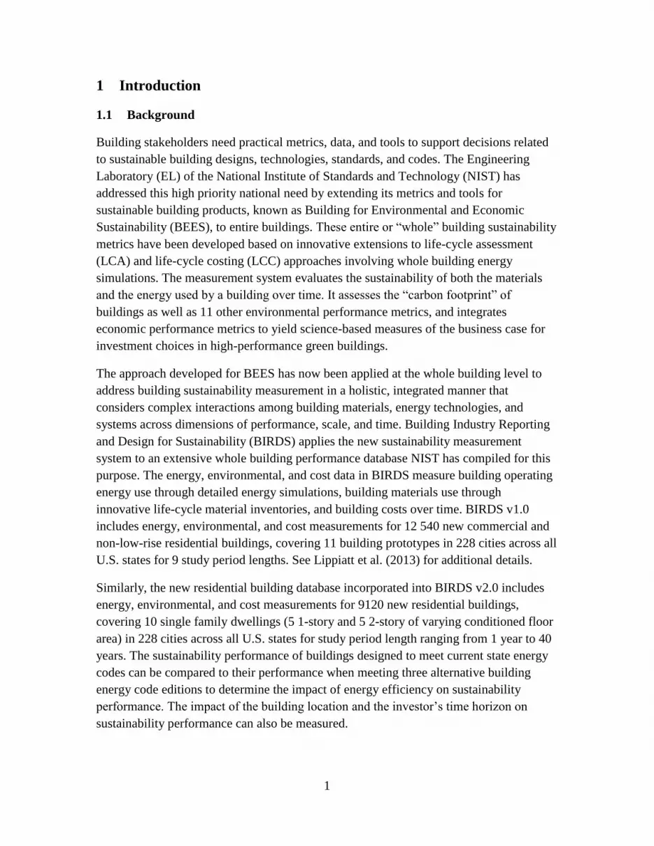
Figure 2-2 Locations and Climate Zones
The climate zones implemented in the IECC were consolidated from the 17 climate zones
shown in Table 2-3 for 2003 IECC into 8 climate zones in 2006 IECC. The consolidation
is more complex than simply grouping the older climate zones together. The zones in
Table 2-3 are based solely on a city’s heating degree days at a base of 18 °C (65 °F)
(HDD65) while the zones in Figure 2-2 are based on the combination of a county’s
heating degree days and cooling degree days at a base of 10 °C (50 °F) (CDD50). The
change in the approach results in some cities located in the same climate zone in 2003
IECC being located in a different climate zone in 2006 IECC. The new climate zones are
further separated into subzones, “wet,” “dry,” and “marine,” as shown in Figure 2-2, for a
total of 16 subzones.

12
Table 2-3 2003 IECC Climate Zones
Climate Zone
Zone HDD65
1 0 to 499
2 500 to 999
3 1000 to 1499
4 1500 to 1999
5 2000 to 2499
6 2500 to 2999
7 3000 to 3499
8 3500 to 3999
9 4000 to 4499
10 4500 to 4999
11 5000 to 5499
12 5500 to 5999
13 6000 to 6499
14 6500 to 6999
15 7000 to 8499
16 8500 to 8999
17 9000 to 12 999
HDD65 = Annual Heating Degree Days base 18 °C (65 °F)4
2.3 Study Period Lengths
Forty study period lengths are chosen to represent the wide cross section of potential
investment time horizons. A 1-year study period is representative of a developer that
intends to sell a property soon after it is constructed. A 5-year to 15-year study period
best represents a building owner’s time horizon because few owners are concerned about
costs realized beyond a decade into the future. The 20-year to 40-year study periods
better represent institutions, such as colleges, government agencies, or long-term
homeowners, because these entities will own buildings for 20 or more years. BIRDS sets
the maximum study period at 40 years for consistency with requirements for federal
building life-cycle cost analysis defined in the Energy Independence and Security Act of
2007. Beyond 40 years, technological obsolescence becomes an issue, data become too
uncertain, and the farther in the future, the less important the costs.
4 A Heating Degree Day of “HDD” is the number of degrees the average temperature is below some
specified baseline each day. Generally, the assumed baseline temperature is an indoor temperature of 18
°C (65 °F)

13
3 Cost Data
Building construction costs are obtained from two sources: RSMeans (2011) and
Faithful + Gould (2012). The baseline costs of each prototypical building is estimated
based on the average cost per unit of floor area for “average” construction quality in
RSMeans (2011) for 1-story and 2-story single-family dwellings, which is a function of
total floor area. Costs are grouped into two categories: first costs that include initial
building construction costs and future costs that include operational costs, maintenance,
repair, and replacement costs, and building residual value. Both of these cost categories
are described below.
3.1 First Costs
Figure 3-1 shows that the average cost per unit of floor area decreases as the total floor
area increases for both 1- and 2-story single-family dwellings. A power curve is fit to the
available data points (base index of the cost per unit of floor area for the 1-story,
148.6 m2 (1000 ft2) house).5
Figure 3-1 Baseline Construction Costs6
Incremental cost data from Faithful + Gould (2012) for each required energy efficiency
measure are added to the baseline costs used to estimate the total first costs of a building
that is compliant with each of the four energy efficiency design alternatives: 2003 IECC,
2006 IECC, 2009 IECC, and 2012 IECC. Six components -- roof insulation, wall
insulation, foundation insulation, air sealant, windows, and lighting -- are changed to
make the prototypical designs compliant with 2003, 2006, 2009, and 2012 IECC. A
5 Indexed to protect proprietary RSMeans data. 6 1 m2 = 10.764 ft2
50
60
70
80
90
100
110
120
130
140
500 1500 2500 3500 4500
Cost
In
dex
Floor Area (ft2)
1-Story
2-Story

14
summary of the requirement ranges (varying climate zone) for each building design are
shown in Table 3-1.
The cost data for windows is based on the cost per unit of area for “average casement
window across sizes” in the F+G database (Faithful+Gould 2012). The lowest cost
window that meets the maximum window characteristics (U-factor and solar heat gain
coefficient (SHGC)) required by the building design is selected.
There are three different insulation values required for the BIRDS new residential
prototypes: wall, ceiling, and foundation. The foundation insulation requirements include
two values, the R-value of the insulation and the depth of the insulation. Based on these
two values, a cost per linear unit is estimated and multiplied by the total perimeter of the
prototype. The cost of ceiling insulation is estimated based on the cost per unit of area for
a given R-value multiplied by the area of the top story ceiling. The wall insulation
requirements are met using wall cavity insulation or a combination of wall cavity
insulation and rigid exterior insulation. Costs per unit of floor area for installed insulation
are treated as additive, and are multiplied by the net exterior wall area (gross wall area
minus window area) to estimate the total installed cost of the insulation.
Infiltration rates allowed are maximum requirements based on blower door test. The
fraction of hard-wired lighting that is high efficiency is adjusted to meet each edition’s
requirements.
The capacity of the HVAC equipment varies based on the thermal load for a given
building prototype, with all equipment meeting minimum federal requirements (SEER 13
for AC unit and 80 % Annual Fuel Utilization Efficiency (AFUE) for gas furnace).
Installed costs for AC units (2.0, 2.5, 3.0, 4.0, or 5.0 ton) and furnaces (40 MBH to 50
MBH, 60 MBH to 64 MBH, 78 MBH to 80 MBH, and 96 MBH to 100 MBH) are
selected based on the closest match to the “autosized” system in the E+ simulation.7
7 MBH is thousands of BTUs per hour.

15
Table 3-1 Energy Efficiency Component Requirements for Alternative Building
Designs
Design
Comp. Parameter Units 2003 IECC 2006 IECC 2009 IECC 2012 IECC
Ceiling
Insulation R-Value
m2∙K/W
(ft2∙°F∙h/Btu) 2.3 to 8.6
(13.0 to 49.0)
5.3 to 8.6
(30.0 to 49.0)
5.3 to 8.6
(30.0 to 49.0)
5.3 to 8.6
(30.0 to 49.0)
Wall
Insulation R-Value
m2∙K/W
(ft2∙°F∙h/Btu) 1.9 to 3.7
(11.0 to 21.0)
2.3 to 3.7
(13.0 to 21.0)
2.3 to 3.7
(13.0 to 21.0)
2.3 to 3.5+0.9/3.7+1.8
(13.0 to 20+5/13+10)
Foundation
Insulation R-value
m2∙K/W
(ft2∙°F∙h/Btu) 0.0 to 3.2
(0 to 18.0)
0 to 1.7
(0 to 10.0)
0 to 1.7
(0 to 10.0)
0 to 1.7
(0 to 10.0)
Depth m (ft) 0 to 1.2
(0 to 4.0)
0 to 1.2
(0 to 4.0)
0 to 1.2
(0 to 4.0)
0 to 1.2
(0 to 4.0)
Infiltration Air Changes
Per Hour ACH50 NR 7.0 7.0 3.0 to 5.0
Windows U-Factor W/(m2∙K)
(Btu/(h∙ft2∙°F) 1.99 to NR
(0.35 to NR)
1.99 to 6.81
(0.35 to 1.2)
1.99 to 6.81
(0.35 to 1.2)
1.82 to NR
(0.32 to NR)
SHGC Fraction NR 0.30 to NR† 0.30 to NR† 0.25 to NR
Lighting
Fraction
High
Efficiency
Fraction NR NR 50 % 75 %
NR = No Requirement for one or more climate zones. By definition, the value of SHGC cannot exceed 1.0.
3.2 Future Costs
Future costs of a building include maintenance, repair, and replacement (MRR) costs as
well as operational energy-related costs from electricity and natural gas consumption.
Each of these is discussed below.
Building MRR costs are discounted to equivalent present values using the Single Present
Value (SPV) factors for future non-fuel costs reported in Rushing, Kneifel, and Lippiatt
(2011). These factors are calculated using the DOE Federal Energy Management
Program (FEMP) 2011 real discount rate for federal energy conservation projects (3 %).
Table 3-2 reports the SPV factors used to develop the BIRDS new residential database.
The MRR costs for each year (CMRR,i) are multiplied by the SPV for that year and then
summed and indexed to determine the total present value MRR costs (CMRR).

16
Table 3-2 2009 SPV Discount Factors for Future Non-Fuel Costs, 3 % Real Discount
Rate
Yrs SPV Factor Yrs SPV Factor Yrs SPV Factor Yrs SPV Factor 1 0.971 11 0.722 21 0.538 31 0.400 2 0.943 12 0.701 22 0.522 32 0.388 3 0.915 13 0.681 23 0.507 33 0.377 4 0.888 14 0.661 24 0.492 34 0.366 5 0.863 15 0.642 25 0.478 35 0.355 6 0.837 16 0.623 26 0.464 36 0.345 7 0.813 17 0.605 27 0.450 37 0.335 8 0.789 18 0.587 28 0.437 38 0.325 9 0.766 19 0.570 29 0.424 39 0.316 10 0.744 20 0.554 30 0.412 40 0.307
The electricity and natural gas use predicted by the building’s energy simulation is used
as the annual energy use of the building for each year of the selected study period.
Electricity and natural gas prices are assumed to change over time according to U.S.
Energy Information Administration forecasts from 2011 to 2041. These forecasts are
embodied in the FEMP Modified Uniform Present Value Discount Factors for energy
price estimates (UPV*) reported in Rushing, Kneifel, and Lippiatt (Rushing, Kneifel et
al. 2011).8 Multiplying the annual electricity costs and natural gas costs by the associated
UPV* value for the study period of interest estimates the present value total electricity
costs (CElect) and natural gas costs (CGas). The discount factors vary by Census region, end
use, and fuel type.
Total present value future costs (CFuture) is the sum of present value location-indexed
MRR costs and present value energy costs, as shown in the following equation:
𝐶𝐹𝑢𝑡𝑢𝑟𝑒 = 𝐶𝑀𝑅𝑅 + 𝐶𝐸𝑙𝑒𝑐𝑡 + 𝐶𝐺𝑎𝑠
Residential building component and building lifetimes are based on three data sources:
NAHB (2007) for building components excluding lighting, U.S. EPA (2012) for light
bulbs, and U.S. Census (2011) for building lifetime. A residential building’s service
lifetime is assumed constant across climate zones at 100 years because, when well
maintained, a building can remain in use for up to or beyond 100 years. This assumption
is supported by the data in Table C-010AH of the 2011 AHS (Annual Housing Survey),
which shows that about half of all owner-occupied housing units are 40 years of age or
older and 6 % are 96 years of age or older (U.S. Census Bureau 2011). Additionally,
NAHB (2007) estimates the lifetime of a number of house components (e.g., foundations,
chimneys) to be greater than 100 years, which implies that the house structure lasts over
100 years. Insulation and air sealants are assumed to have a lifespan greater than 40 years
8 Since the U.S. Energy Information Administration forecasts end at year 30, the escalation rates for years
31-40 are assumed to be the same as for year 30.

17
and have no maintenance or repair requirements. Windows have an assumed lifespan of
20 years with costs that vary depending on the required window specifications. Windows
are assumed to have no maintenance costs or repair costs. The heating and air
conditioning units have assumed lifespans of 15 years while the water heater is assumed
to have a lifespan of 10 years. Incandescent and compact fluorescent light (CFL) bulbs
are assumed to have lifespans of 1 year and 7 years, respectively (U.S. EPA 2012).
MRR cost data are collected from two sources: U.S. Census Bureau (2011) and
Faithful + Gould (2011). The total maintenance and repair costs per square foot of
conditioned floor area represent the baseline (non-energy related) MRR costs per unit of
floor area, which occur for a building type regardless of the energy efficiency measures
incorporated into the design. These data are collected from Table C-12-OO and Table C-
15-OO in U.S. Census Bureau (2011), which reports median floor area and average
maintenance and repair costs per unit of floor area for “Total Owner-Occupied Units”
Housing Units and “New Construction the Past 4 Years” Housing Units, respectively.
These two data points are used to interpolate and extrapolate for all years considered (1
through 40) as shown in Figure 3-2. These costs are assumed to include all maintenance
and repair costs associated with a single-family dwelling.
Figure 3-2 Baseline Maintenance, Repair, and Replacement Costs by Year
Faithful and Gould (2011) is the source of replacement costs for the individual
components for which costs change across alternative building designs, which in this
$0.00
$0.02
$0.04
$0.06
$0.08
$0.10
$0.12
$0.14
$0.16
$0.18
$0.20
$0.22
$0.24
$0.00
$0.20
$0.40
$0.60
$0.80
$1.00
$1.20
$1.40
$1.60
$1.80
$2.00
$2.20
$2.40
$2.60
1 3 5 7 9 11 13 15 17 19 21 23 25 27 29 31 33 35 37 39
Base
lin
e M
&R
Cost
s [$
/ft2
]
Base
lin
e M
&R
Cost
s [$
/m2]
Year

18
analysis are the HVAC system, lighting, and windows. The replacement cost of windows
is assumed to be equal to the initial installation costs of the same window. The cost of
replacing CFL light bulbs is greater than the cost of replacing incandescent light bulbs.
However, CFLs last 7 times longer than incandescents, which may lead to the total
replacement costs of light bulbs over the study period to be lower for the more efficient
CFLs. The HVAC system capacity size varies based on the thermal performance of the
building design, which results in varying replacement costs because smaller capacity
systems are relatively cheaper.
Future MRR costs are discounted to equivalent present values using the Single Present
Value (SPV) factors for future non-fuel costs reported in Rushing, Kneifel, and Lippiatt
(2011), which are calculated using the U.S. Department of Energy's 2011 real discount
rate for energy conservation projects (3 %).
Annual energy costs are estimated by multiplying annual electricity and natural gas use
predicted by the building’s energy simulation by the average state retail residential
electricity and natural gas prices, respectively. Average state residential electricity and
natural gas prices for 2011 are collected from the Energy Information Administration
(EIA) Electric Power Annual State Data Tables (U.S. Energy Information Administration
(EIA) 2013a) and Natural Gas Navigator (U.S. Energy Information Administration (EIA)
2013b), respectively.
A building's residual value is its value remaining at the end of the study period. In life-
cycle costing it is treated as a negative cost item. In BIRDS, it is estimated in four parts,
for the building (excluding HVAC, windows, and lighting), HVAC system, windows, and
lighting, based on the approach defined in Fuller and Petersen (1996). The building's
residual value is calculated as the building's location-indexed first cost multiplied by one
minus the ratio of the study period to the service life of the building, discounted from the
end of the study period. For example, if a building has first costs (excluding HVAC,
windows, and lighting) of $500 000, a 10 year service life, and the study period length is
100 years, the residual value of the building in year 10 (excluding HVAC, window, and
lighting) is $500 000 ∗ (1 −10
100) = $450 000.
Because they may be replaced during the study period, residual values for the HVAC
system, windows, and lighting are computed separately. The remaining “life” of the
HVAC equipment is determined by taking its service life minus the number of years
since its last installation (as of the end of the study period), whether it occurred during
building construction or replacement. The ratio of remaining life to service life is
multiplied by the location-indexed installed cost of the system and discounted from the
end of the study period. For example, assume an HVAC system’s installed costs are
$12 000 with a service life of 15 years, and a 20-year study period length. After one
replacement, the system is 5 years old at the end of the study period, leaving 10 years

19
remaining in its service life. The residual value in year 20 is $12 000 ∗ (1 −10
15) =
$4000. The residual value for the light bulbs and windows is computed in a similar
manner.
The total residual value of the building and its HVAC, windows, and lighting, multiplied
by the SPV factor for the number of years in the study period, estimates the present value
residual value (CResidual).

20

21
4 Building Stock Data
Aggregating the savings for newly constructed residential buildings to the state and
national levels requires new construction data for each building type within each state.
The BIRDS new residential database incorporates 10 prototype buildings (5 1-story, 5 2-
story) of varying floor areas. Certain areas of the country have particular housing
characteristics. For example, there is a large prevalence of single-story dwellings in states
like Florida while the northeast region of the U.S. is characterized by a significantly
greater share of multi-level homes. These differences may have an impact on the level of
energy savings resulting from adoption of more efficient state energy codes.
Additionally, each city in a state should not be weighted equally when estimating savings
because the amount of new floor area constructed across cities in a state can vary
significantly. In order to develop more accurate state-level estimates, the amount of
newly constructed floor area in a state should be dissected and associated with the most
representative city in a state. Weighting factors are developed to associate the amount of
new floor area for each building prototype for each of the 228 cities in the BIRDS new
residential database. This chapter will describe the databases and weighting factors
developed to allow for aggregate savings estimates.
4.1 Databases
Two data sources are required to use the BIRDS new residential database results to
develop aggregated savings at the state level, one to determine by much how much to
weight each building prototype within a city and another to determine by how much to
weight each city within a state.
The United States Census Bureau provides annual microdata based on newly constructed
homes. All data is based on a national sample survey of new construction called the
Survey of Construction (SOC) (U.S. Census Bureau 2013). Survey responses shed light
on close to 60 different characteristics of newly constructed homes in the U.S. The
weights used for this analysis are extracted from the 2013 SOC survey by determining the
proportion of detached 1-story and 2-story homes relative to all single-family home data
points in the sample. We then associate these weights to the 10 prototype homes
represented in the BIRDS residential database, with the total new floor area. The building
prototype weights are developed at the Census division level.
A newly accessed database from McGraw-Hill Dodge Construction (MHDC) includes
newly constructed floor area by year from 1970 to 2012 by county across the entire United
States. Kneifel and Butry (2014a) developed an approach to associate the MHDC data for
each county in a state to one of the 228 cities included in the BIRDS databases based on
distance from the centroid (geometric center of a 2-dimensional region) of the county
within the same climate zone as shown in Figure 4-1. The purpose of developing these

22
county “clusters” is to associate the new floor area constructed in a county to the most
representative city in BIRDS, both in terms of climate and building construction costs.
Figure 4-1 Cities and Associated (Colored) County Clusters
The weights developed from the MHDC data for 2012 are used to associate the county
“cluster” new floor area to the 10 building prototype results for the city in BIRDS mapped
to that particular cluster. The weighting factors are described in detail below.
4.2 Weighting Factors
The weighting factors are developed using the combination of the SOC data and MHDC
data. Significant data processing is required to create the building prototype-city weights.
Figure 4-2 shows how the SOC and MHDC databases are manipulated to develop the
desired information. The MHDC data for new residential construction in 2012 is mapped
to the county clusters based on the 228 cities in the BIRDS databases, leading to total
new residential floor area for each county cluster. The 2013 SOC data is used to allocate
the total new floor area from the 2012 MHDC data to the results for each of the building
prototypes.

23
Figure 4-2 Data Processing for Weighting Development
Since this study considers single-family detached dwellings, only detached units are
included in the weighting allocation development. Note that 88% of all new floor area are
from detached unit construction with the remaining 12% of floor area in attached units.
The 2013 SOC new floor area data for detached units is used to estimate the fraction of
new floor area for a city that should be associated with each of the 10 building
prototypes. The prototypes vary in two ways, by number of stories and conditioned floor
area (CFA). However, the data that is publically available is at the Census division for
floor area by number of stories and national level for floor area by CFA.
The fraction of floor area by number of stories is filtered by Census Division and grouped
into two categories: 1-story and 2-story or greater detached housing units. For this study,
three-story unit floor area is included in the 2-story unit floor area values because 3-story
units are rare, accounting for no more than 4 % of units for any Census division. Table
4-1 shows the resulting percentages of single- and multi-story units across the nine
Census divisions, which highlight that new construction in the North Census Region and
the Pacific Census Division is primarily units with 2-stories or greater while the new
construction in the South Census Region, Midwest Census Region, and Mountain Census
Division are about a 50/50 split between 1-story and 2-story or greater units. These trends
may be driven by geographic and land availability factors. These fractions will be used to
allocate the amount of new floor area to 1-story and 2-story building prototypes for a
county cluster based on the Census division in which it is located.
2013 SOC
2012 MHDC
Construction
Floor Area
by County
Floor Area by
County Cluster
Kneifel & Butry
(2014) County
Clusters
Detached
Census Division
By Division-
Stories-CFA
(%)
1-Story
Attached
2-Story
+
1-Story 2-Story + 1-Story
by CFA
2-Story +
by CFA
Floor Area by Building
Type by County Cluster

24
Table 4-1 Percentages of One- and Multi-Story Homes by Census Region
Regions
North South Midwest Pacific
Stories
New
England
Middle
Atlantic
South
Atlantic
East
South
Central
West
South
Central
East
North
Central
West
North
Central
Mountain Pacific
1 14 % 23 % 40 % 49 % 55 % 51 % 52 % 49 % 31 %
2+ 86 % 77 % 60 % 51 % 45 % 49 % 48 % 51 % 69 %
The relative percentage of floor area for each building prototype (5 1-story and 5 2-story
houses) is based on the national distribution of new floor area by CFA for a unit. The new
floor area for detached units in the SOC data ranges from 84 m2 (900 ft2) to 743 m2 (8000
ft2) or greater. The new floor area is filtered into 10 bins based on number of stories and
CFA, with each bin associated to a prototype. The percentage of total new floor area that
is allocated to each bin by number of stories is shown in Table 4-2.
Table 4-2 Building Types, Bin Ranges, and Percentage of Each Building Design
1-Story 2-Story
Building Type
m2 (ft2)
Bin Range - m2(ft2) Percentage Building Type
m2 (ft2)
Bin Range - m2(ft2) Percentage
111.9 (1205) ≤ 130.1 (1400) 13.7 % 148.8 (1602) ≤ 176.5 (1900) 10.9 %
148.6 (1600) 130.2-167.2 (1401–1800) 22.2 % 204.9 (2205) 176.6-232.3 (1901-2500) 22.1 %
176.6 (1901) 167.3-204.4 (1801-2200) 22.5 % 251.2 (2704) 232.4-288.0 (2501-3100) 24.0 %
215.8 (2323) 204.5-241.5 (2201-2600) 15.3 % 311.0 (3348) 288.1-334.5 (3101-3600) 17.1 %
292.8 (3152) ≥ 241.6 (2601) 26.3 % 420.2 (4523) ≥ 334.5 (3600+) 25.9 %
The Census division-level new floor area weights by number of stories combined with
the national-level new floor area weights by building prototype to develop the final
weights given to each building type in a county cluster (i.e., city) in a given division.
Table 4-3 illustrates the process for calculating this final series of weights using the New
England census division as an example.

25
Table 4-3 Percentage of Each Building Type for One- and Multi-Story Homes (New
England Division)
Census Division – New England
1-Story (14%) Percentage Final Weights
111.9 (1205) 14 % 14% · 14% = 2 %
148.6 (1600) 22 % 14% · 22% = 3 %
176.6 (1901) 22 % 14% · 22% = 4 %
215.8 (2323) 15 % 14% · 15% = 2 %
292.8 (3152) 26 % 14% · 26% = 4 %
Multi-Story (86%) Percentage Final Weights
148.8 (1602) 11 % 86% · 11% = 9 %
204.9 (2205) 22 % 86% · 22% = 19 %
251.2 (2704) 24 % 86% · 24% = 21 %
311.0 (3348) 17 % 86% · 17% = 15 %
420.2 (4523) 26 % 86% · 26% = 22 %
Similar calculations are done to calculate the relative percentage of each building type
across all census divisions, which are listed in Table 4-4. The BIRDS database includes
the 10 residential prototype buildings in all fifty states. Implementing the division-level
weights to the results for each building type is likely to result in varying levels of
reductions in energy use, energy costs, life-cycle costs, and life-cycle carbon emissions
from adoption of new editions of IECC.

26
Table 4-4 Percentage of Each Building Type by Census Division
North South Midwest Pacific
New
England
Middle
Atlantic
South
Atlantic
East
South
Central
West
South
Central
East
North
Central
West
North
Central
Mountain Pacific
One-Story
111.9 (1205) 2 % 3 % 5 % 7 % 8 % 7 % 7 % 7 % 4 %
148.6 (1600) 3 % 5 % 9 % 11 % 12 % 11 % 12 % 11 % 7 %
176.6 (1901) 3 % 5 % 9 % 11 % 12 % 11 % 12 % 11 % 7 %
215.8 (2323) 2 % 4 % 6 % 8 % 8 % 8 % 8 % 7 % 5 %
292.8 (3152) 4 % 6 % 10 % 13 % 14 % 13 % 14 % 13 % 8 %
Multi-Story
148.8 (1602) 9 % 8 % 7 % 6 % 5 % 5 % 5 % 6 % 8 %
204.9 (2205) 19 % 17 % 13 % 11 % 10 % 11 % 10 % 11 % 15 %
251.2 (2704) 21 % 19 % 14 % 12 % 11 % 12 % 11 % 12 % 17 %
311.0 (3348) 15 % 13 % 10 % 9 % 8 % 8 % 8 % 9 % 12 %
420.2 (4523) 22 % 20 % 16 % 13 % 12 % 13 % 12 % 13 % 18 %

27
5 Analysis Approach
The analysis in this report compares benefits and costs of the current state energy codes
to more stringent alternatives. The relative changes in energy use, energy costs,
environmental impacts, and life-cycle costs use the current energy code for a state as the
baseline and uses each IECC edition that is newer than the edition required by the current
state energy code as an alternative design. The results are considered on both a
percentage change and an aggregate change basis.
5.1 Energy Use
The analysis uses each state’s current energy code as the baseline energy efficiency
design. For any state without a state energy code, 2003 IECC is assumed to be the
baseline because it represents minimum energy-related industry practices. The baseline
for each state is compared to the higher energy efficiency building designs to determine
the relative annual energy savings resulting from adopting the alternative code edition as
the state’s energy code. For example, if a state’s energy code has adopted 2006 IECC as
its energy code requirements, this baseline energy use is compared to the energy use of
all newer energy code editions, 2009 IECC and 2012 IECC.
It is assumed that the building maintains its energy efficiency performance throughout the
study period, resulting in energy consumption remaining constant over the entire study
period. This assumption is reasonable given the maintenance, repair, and replacement
costs included in the analysis to ensure the building and its equipment perform as
expected.
5.2 Life-Cycle Costing
Life-cycle costing (LCC) takes into account all relevant costs throughout the chosen
study period, including construction costs, maintenance, repair, and replacement costs,
energy costs, and residual values. A cost’s present value (PV) is calculated by
discounting its nominal value into today’s dollars based on the year the cost occurs and
the assumed discount rate. LCC of buildings typically compares the costs for a baseline
building design to the costs for alternative, more energy-efficient building designs to
determine if future operational savings justify higher initial investments.9 For this study,
the design based on any IECC edition that is newer than the code edition required by the
current state energy code is compared to the baseline state energy code compliant design
to determine the changes in life-cycle costs.
9 All life-cycle cost calculations are based on ASTM Standards of Building Economics (2012) and Fuller
and Petersen (1996).

28
Two metrics are used to analyze changes in life-cycle costs: net LCC savings and net
LCC savings as a percentage of base case LCC. Net LCC savings is the difference
between the base case and alternative design's LCCs.
5.3 Environmental Impact Assessment
The BIRDS database expands on Kneifel (2011a) by conducting a life-cycle assessment
(LCA) of greenhouse gas emissions for a building across its life-cycle, following
guidance in the International Organization for Standardization (ISO) 14040 series of
standards for LCA. The analysis quantifies the greenhouse gas emissions from
construction of the building, maintenance, repair, and replacement of building
components, and operational energy consumption on a cradle-to-grave basis, including
emissions from raw materials acquisition, materials processing, generation, transmission,
distribution, use, and end-of-life.
The assessment of cradle-to-grave carbon emissions considers a number of greenhouse
gases. Carbon dioxide (CO2), methane (CH4), and nitrous oxide (N2O) are the most
prevalent. Both the embodied emissions in the building and its components as well as two
types of energy consumption, electricity and natural gas, are included in the assessment.
While carbon emissions from natural gas use can be assessed on a national average basis,
those from electricity use are highly dependent upon the fuel mixes of regional electricity
grids. For this reason, electricity emissions are assessed at the state-level using North
American Electric Reliability Corporation (NERC) sub-region level data.10 The life-cycle
data sets for natural gas production and combustion as well as for all fuel sources in the
electricity grid come from the U.S. Life-Cycle Inventory (LCI) database (National
Renewable Energy Laboratory (NREL) 2012). The state-level average emissions rates per
GWh (MBtu) of electricity generated, as shown in Table A-1 of the Appendix, are obtained
from the 2007 Emissions and Generation Resource Integrated Database (Environmental
Protection Agency (EPA) 2007), which is a collection of data from the EIA, the Federal
Energy Regulatory Commission (FERC), and the Environmental Protection Agency
(EPA). 11
The embodied and operating energy-related greenhouse gas emissions are converted into
a common unit of measure called carbon dioxide equivalents (CO2e) using equivalency
factors reported in Table 5-1, which represent the global warming potential (GWP) of 1
unit of greenhouse gas relative to that of the same amount of carbon dioxide. For
example, 1 unit of methane has 25 times the GWP as the same amount of carbon dioxide,
and nitrous oxide has 298 times the GWP as carbon dioxide. The aggregated CO2e is
10 For states located in more than one NERC sub-region, a weighted average of emissions rates for the
multiple sub-regions is implemented. Source: North American Electric Reliability Corporation (NERC)
(2011). 11 Emissions rates are held constant over all study periods.

29
calculated by taking the amount of each flow multiplied by its CO2e factor, and summing
the resulting CO2 equivalencies. The results are analyzed in metric tons of CO2e
emissions, and will be referred to as “carbon emissions” for the remainder of the report.
Table 5-1 Greenhouse Gas Global Warming Potentials
Environmental Flow GWP (CO2e)
Carbon Dioxide (CO2) 1
Methane (CH4) 25
Nitrous Oxide (N2O) 298
Ethane, 1,1-difluoro-, HFC-152a 124
Ethane, 1,1,1-trichloro-, HCFC-140 146
Ethane, 1,1,1,2-tetrafluoro-, HFC-134a 1430
Ethane, 1,1,2-trichloro-1,2,2-trifluoro-, CFC-113 6130
Ethane, 1,2-dichloro-1,1,2,2-tetrafluoro-, CFC-114 10 000
Ethane, hexafluoro-, HFC-116 12 200
Methane, bromo-, Halon 1001 5
Methane, bromochlorodifluoro-, Halon 1211 1890
Methane, bromotrifluoro-, Halon 1301 7140
Methane, chlorodifluoro-, HCFC-22 1810
Methane, dichloro-, HCC-30 9
Methane, dichlorodifluoro-, CFC-12 10 900
Methane, monochloro-, R-40 13
Methane, tetrachloro-, CFC-10 1400
Methane, tetrafluoro-, CFC-14 7390
Methane, trichlorofluoro-, CFC-11 4750
Methane, trifluoro-, HFC-23 14 800
5.4 Analysis Metrics
Three metrics are used to analyze the results: simple percentage changes, aggregate
changes, and changes per unit of floor area. The average percentage savings energy use,
energy cost, carbon emissions, and LCCs are calculated by taking the average of the
percentage savings weighted by new floor area for each single-family detached location-
building type combination in the state or nation.
The estimated change in total energy use, energy costs, energy-related carbon emissions,
and life-cycle costs for each of the building types is combined with new residential
building construction data to calculate the magnitude of the available total savings a state
may realize if it were to adopt a more energy efficient standard as its state energy code
using the following equation.

30
(1) 𝐼𝑗𝑘 =
∑ 𝐶𝐹𝐴𝑗𝑖∗𝑅𝑗𝑖𝑘10
𝑖=1
∑ 𝐹𝑗𝑖10𝑖=1
Where 𝐼𝑗𝑘 = total change in performance metric k12 for state j
CFAji = average annual newly constructed floor area for building type i for state j
Rji = average change per unit of floor area for building type i for state j
Fji = fraction of average annual new floor area represented by building type i for
state j
For each building type i, the average change per unit of floor area for all cities in a state
(Ri) is multiplied by the average annual floor area of new construction for 2003 to 2007
for building type i in that state (CFAi) to estimate the total savings for that building type
for that state. The impacts are summed across all ten building prototypes. These impacts
are then divided by the amount of average annual new residential floor area represented
by the ten building prototypes (F), which scale the results to the statewide impacts of all
new residential construction (Ij). Using this approach to estimate the total impacts for a
state requires the assumption that the savings realized by the BIRDS building prototypes
are representative of new residential building construction as a whole.
The national-level impacts (IT) are estimated using Equation 2, where the impacts for
state j estimated using Equation 1 (Ij) are summed across all fifty states.
(2) 𝐼𝑇𝑘 = ∑ (𝐼𝑗
𝑘)50𝑗=1
Where 𝐼𝑇𝑘 = nationwide total impacts on k
𝐼𝑗𝑘 = total impacts on k in state j
The third metric, change per unit of floor area, allows for comparisons across states to
determine which states realize the greatest impacts per unit of construction. Equation 3
shows this calculation, where the total statewide impacts estimated in Equation 1 (Ij) are
divided by the total average annual new floor area for all building types in a state
(TCFAj), providing a means for a cost performance comparison across states.
(3) 𝐴𝑉𝐺𝐼𝑗𝑘 =
𝐼𝑗
𝑇𝐶𝐹𝐴𝑗
Where 𝐴𝑉𝐺𝐼𝑗𝑘 = average impact on k per unit of new floor area in state j
𝐼𝑗𝑘 = total impacts on k in state j
TCFAj = total average annual new floor area for all building types in state j
12 A change in the performance metric k refers to the change energy use, energy costs, life-cycle costs, or
life-cycle carbon emissions.

31
It is necessary to assume a particular study period length to generate results. Although the
annual energy use savings and energy-related carbon emissions reductions, both in
percentage and total value terms, are assumed to be the same across study period lengths,
the energy costs and life-cycle costs vary with the study period length because costs vary
year-over-year. A 10-year study period is used for the majority of this analysis because it
is the most realistic investor time frame of the 9 study period length options.

32

33
6 Nationwide Impacts of Adopting 2012 IECC Design
This section analyzes the benefits and costs of nationwide adoption of the 2012 IECC for
residential buildings relative to currently adopted state energy codes. Benefits are
examined across several dimensions (study period, location, and code edition) in order to
better understand the full scope of the impacts associated with more energy efficient new
single-family dwellings. Changes in annual energy use, energy costs, life-cycle costs, and
life-cycle carbon emissions stemming from the adoption of stricter energy codes are
expressed in terms of percentage reduction, total reduction, and change per unit of floor
area.
6.1 Percentage Reductions
Average reductions or percentage change impacts from adopting the 2012 IECC design
are estimated for energy use, energy costs, life-cycle carbon emissions, and life-cycle
costs. Impacts are evaluated across four dimensions: study period length, building type,
climate zone, and state energy code.
6.1.1 Results by Building Type
Incorporating 2012 IECC requirements in new residential construction will impact energy
consumption, energy costs, life-cycle carbon emissions, and life-cycle costs. The
magnitude of these impacts is likely to vary as study period length increases. 1-, 5-, 10-,
20-, and 40-year study period lengths are considered to gain a better understanding of
these variations.
Table 6-1 shows the national average percentage reduction in annual energy usage across
all U.S. states from nationwide adoption of the 2012 IECC relative to currently adopted
state energy codes. Because the BIRDS database assumes that energy efficiency is
maintained constant over time, reductions will be consistent across all study period
lengths. Percent reductions vary across building types and range from 17.0 % to 21.9 %,
with a weighted national average reduction of 19.2 %. Results in Table 6-1 suggest that
the larger the building, the greater the average percentage reduction in energy
consumption. Two factors that impact the relative percentage changes are the fraction of
energy use associated with meeting heating and cooling loads and the basic geometry of
the building, including the glazing (i.e., windows) fraction of wall area. All prototypes
assume the same occupancy and equipment operation. As the building increases in size,
meeting heating and cooling loads becomes a greater portion of total energy demand.
Given a specific amount of total floor area, the heating and cooling loads will be reduced
as the exterior surface area of the building decreases. Additionally, less window area (as a
percentage of wall area) will lead to greater impacts from greater insulation requirements
because the requirement will impact a greater portion of the wall area. As a result, a 2-

34
story building will have lower heating and cooling loads than a 1-story building with the
same amount of floor area.
Table 6-1 Nationwide Average Percentage Reduction in Energy Use from Adoption
of the 2012 IECC Design by Building Type
Number of
Stories
Building
Type m2 (ft2)
Percentage
Change
1
1
111.9 (1205) 17.0 %
1 148.6 (1600) 18.1 %
1 176.6 (1901) 19.1 %
1 215.8 (2323) 18.8 %
1 292.8 (3152) 19.8 %
2 148.8 (1602) 18.0 % 2 204.9 (2205) 19.6 %
2 251.2 (2704) 19.4 %
2 311.0 (3348) 20.5 %
2 420.2 (4523) 21.9 %
Average 19.2 %
The national average percent changes in energy-related expenditures across each building
type and study length are displayed in Table 6-2. There is minimal variation in energy
cost savings over time. Percent changes range between 11.8 % and 18.9 % depending on
building type and time period. More sizeable reductions (regardless of study period) are
witnessed with larger homes (all 2-story and larger single-story homes). Average percent
changes across all 10 building types range between 15.1 % for a 1-year study period, and
15.7 % for a 40-year study period. These marginal changes (percentage terms) in average
energy cost reductions are due to the assumed escalation of energy prices in the future
(Rushing, Kneifel et al. 2011). Percent changes in energy costs are smaller than the
reductions in energy use because majority of the reductions occur for the cheaper of the
two primary fuel sources, natural gas.

35
Table 6-2 Nationwide Average Percentage Reduction in Energy Costs from
Adoption of the 2012 IECC Design by Building Type and Study Period Length
Stories Building Type
m2 (ft2)
112 (1205)
Study Period Length
1 5 10 20 40
1 111.9 (1205) 11.8 % 11.8 % 11.9 % 12.1 % 12.4 %
1 148.6 (1600) 13.6 % 13.6 % 13.6 % 13.9 % 14.2 %
1 176.6 (1901) 14.4 % 14.3 % 14.4 % 14.7 % 15.1 %
1 215.8 (2323) 15.6 % 15.5 % 15.6 % 15.8 % 16.2 %
1 292.8 (3152) 16.9 % 16.9 % 17.0 % 17.2 % 17.5 %
2 148.8 (1602) 13.3 % 13.3 % 13.4 % 13.6 % 14.0 %
2 204.9 (2205) 15.2 % 15.1 % 15.2 % 15.4 % 15.8 %
2 251.2 (2704) 15.5% 15.4 % 15.5 % 15.8 % 16.1 %
2 311.0 (3348) 16.7 % 16.7 % 16.8 % 17.0 % 17.4 %
2 420.2 (4523) 18.2 % 18.1 % 18.2 % 18.5 % 18.9 %
Average 15.1 % 15.1 % 15.2 % 15.4 % 15.7 %
Constructing a residential building to meet 2012 IECC requirements results in fewer total
life-cycle carbon emissions than meeting requirements set by current state energy codes
based on an older edition of IECC. Table 6-3 shows the nationwide average percent
changes in GWP (emissions) for each building type. We stated previously that the
national average percentage change in energy use is constant across all study periods,
which means that average energy-related carbon emissions are constant. Additionally, the
building construction-related emissions are equally associated with years across the study
period. National average percent changes range between 8.1 % and 14.5 % depending on
the building type, with a nationwide average percentage change of 11.2 %. Emissions
reductions for each building are directly related to its energy use, with 2-story houses
achieving greater reductions in both energy use and emissions than single-story houses of
similar size and the largest 2-story prototype attaining the largest average reduction of
any building type (14.5 %). These results indicate the importance of considering both
energy-related and embodied carbon emissions.

36
Table 6-3 Nationwide Average Percentage Reduction in Life-Cycle Carbon
Emissions from Adoption of the 2012 IECC Design by Building Type
Stories Building
Type m2 (ft2)
Percentage
Change
1
11
111.9 (1205) 8.1 % 1 148.6 (1600) 9.5 % 1 176.6 (1901) 9.7 % 1 215.8 (2323) 10.1 % 1 292.8 (3152) 11.3 %
2 148.8 (1602) 11.2 % 2 204.9 (2205) 11.9 % 2 251.2 (2704) 12.6 % 2 311.0 (3348) 13.0 % 2 420.2 (4523) 14.5 %
Average 11.2 %
The average percentage changes in LCC for every building type and study period length
are shown in Table 6-4. As expected, there are substantial increases in LCC for a study
period of 1 year given the higher initial investment costs required for building a more
energy-efficient building. The average percentage change in life-cycle costs decreases as
the study period length increases from a 42.0 % increase for a 1-year study period to a
2.9 % decrease for a 40-year study period. All but 1 building type realizes LCC savings
(negative % change) after five years. On the other hand, all 10 buildings realize average
LCC savings for study periods of 10 years or more.
The life-cycle cost increase is large in percentage terms for a 1-year study period because
the additional increase in first costs is divided by a relatively small value. For example,
assume two building designs: Building A (baseline) has first costs of $150 000 and
annual energy costs of $2000; Building B has first costs of $200 000 and annual energy
costs of $1400. Annual energy costs are reduced by $600 (30 %) for an additional first
cost of $50 000. The life-cycle costs for each building are as follows assuming a 3 %
discount rate and 65 year building lifetime:
𝐿𝐶𝐶𝐴 = 150 000 + (2000 ∗1
(1.03)1) − (150 000 ∗
64
65∗
1
(1.03)1) = $8609
𝐿𝐶𝐶𝐵 = 200 000 + (1400 ∗1
(1.03)1) − (200 000 ∗
64
65∗
1
(1.03)1) = $10 213
In this example, the percentage change in life-cycle costs (19 %) is the difference
between the life-cycle costs ($1603) divided by the life-cycle costs for the baseline
building design ($8609). The change in life-cycle costs is small in magnitude, but large in
percentage terms.

37
Table 6-4 National Average Percentage Reduction in Life-Cycle Costs from
Adoption of the 2012 IECC Design by Building Type and Study Period Length
Stories Building
Type m2 (ft2)
112 (1205)
Study Period Length
1 5 10 20 40
1 111.9 (1205) -17.6 % -0.1 % 1.1 % 1.8 % 2.4 %
1 148.6 (1600) -16.3 % 0.5 % 1.5 % 2.2 % 2.7 %
1 176.6 (1901) -15.9 % 0.8 % 1.7 % 2.4 % 2.9 %
1 215.8 (2323) -20.9 % 0.8 % 1.8 % 2.5 % 3.0 %
1 292.8 (3152) -27.7 % 1.0 % 2.0 % 2.7 % 3.2 %
2 148.8 (1602) -16.5 % 0.5 % 1.4 % 2.1 % 2.6 %
2 204.9 (2205) -18.3 % 1.1 % 1.8 % 2.4 % 2.9 %
2 251.2 (2704) -24.2 % 1.2 % 1.9 % 2.5 % 3.0 %
2 311.0 (3348) -30.1 % 1.3 % 2.1 % 2.7 % 3.2 %
2 420.2 (4523) -232.7 % 1.5 % 2.3 % 2.9 % 3.4 %
Average -42.0 % 0.9 % 1.7 % 2.4 % 2.9 %
A snapshot of the average reductions in energy use, energy costs, life-cycle carbon
emissions, and LCCs, stemming from nationwide adoption of the 2012 IECC building
codes is shown in Table 6-5. Assuming a 10-year study period, findings suggest that
relative to all other single-story homes, the largest single-story home (293 m2 [3152 ft2])
achieves the greatest reductions in the above four metrics, while the smallest (112 m2
[1205 ft2]) achieves the least. A similar trend is discovered for 2-story homes, where the
420 m2 (4523 ft2) home outperformed all 1- and 2-story homes.
Table 6-5 Nationwide Average Percentage Reduction in the Four Performance
Metrics from Adoption of the 2012 IECC Design by Building Type (10-Year)
Number of
Stories Building
Type m2 (ft2)
Percentage Change
Energy Use Energy Costs GWP LCC
1 111.9 (1205) 17.0 % 11.9 % 8.1 % 1.1 %
1 148.6 (1600) 18.1 % 13.6 % 9.5 % 1.5 %
1 176.6 (1901) 19.1 % 14.4 % 9.7 % 1.7 %
1 215.8 (2323) 18.8 % 15.6 % 10.1 % 1.8 %
1 292.8 (3152) 19.8 % 17.0 % 11.3 % 2.0 %
2 148.8 (1602) 18.0 % 13.4 % 11.2 % 1.4 %
2 204.9 (2205) 19.6 % 15.2 % 11.9 % 1.8 %
2 251.2 (2704) 19.4 % 15.5 % 12.6 % 1.9 %
2 311.0 (3348) 20.5 % 16.8 % 13.0 % 2.1 %
2 420.2 (4523) 21.9 % 18.2 % 14.5 % 2.3 %
Average 19.2 % 15.2 % 11.2 % 1.7 %

38
6.1.2 Results by Climate Zone
Considering results by climate zone helps shed some light on the relationship between
climate zone and the benefits of nationally adopting 2012 IECC. It was discovered in the
previous section that weighting based on newly constructed floor area had only minimal
impacts on our results. For the sake of simplicity, changes in energy use, energy costs,
emissions, and LCC will be calculated without our series of weights. The assumed study
period length is 10 years.
The BIRDS new residential database considers both 1- and 2-story family dwellings.
Table 6-6 shows the average percentage change in energy use by climate zone and
baseline code (see Figure 2-1) from adoption of the 2012 IECC for both a 1- and 2-story
home. Similar trends can be seen in the average energy use reductions across climate
zones for both 1- and 2-story homes – the changes in average energy consumption tends
to grow larger as the climate zone grows colder. Only in Zone 4 and Zone 5 are
exceptions, which realize slightly smaller reductions in energy use than the previous
zone, which may be a result of changes in requirements across IECC editions, as
displayed in Table 3-1. Average reductions in energy use are greater for 2-story homes in
all climate zones.
Table 6-6 reveals an unexpected inconsistency between baseline code and energy
savings. Although locations with older baseline codes realize greater reductions, on
average (final column), this trend does not hold at the climate zone level. In fact,
locations with a baseline code of 2003 IECC lead to the greatest reductions for two
climate zones for both 1-story and 2-story houses. Locations with a baseline code of 2006
IECC realize the greatest reductions for four climate zones for 1-story houses and four
climate zones for 2-story houses. This result may be driven by the change in climate zone
definitions and the resulting changes in building requirements for locations in those
climate zones.

39
Table 6-6 Average Percentage Reduction in Energy Use from Adoption of the 2012
IECC by Climate Zone and Baseline Code for 1- and 2-Story Homes
(a) Average (1-Story)
Climate Zone
Baseline
Code
1 2 3 4 5 6 7 8 All
2003 17. 2 % 21.6 % 23.1 % 21.5 % 22.5 % 22.8 % 25.0 % 22.0 %
2006 6.9 % 11. 4 % 23.2 % 22.9 % 25.0 % 24.7 % 19.0 %
2009 5.1 % 10. 2 % 20.4 % 23.2 % 22.6 % 23.0 % 23.8 % 18.3 %
Avg 6.0 % 12.9 % 21.7 % 23.1 % 22.0 % 23.5 % 23.8 % 25.0 % 19.8 %
(b) Average (2-Story)
Climate Zone
Baseline
Code
1 2 3 4 5 6 7 8 All
2003 16.1 % 24.3 % 25.2 % 23.9 % 26.5 % 26.6 % 28.3 % 24.4 %
2006 9.3 % 11.9 % 26.0 % 25.6 % 28.7 % 28.3 % 21.6 %
2009 6.6 % 10.4 % 23.1 % 25.7 % 24.5 % 27.0 % 27.3 % 20.6 %
Avg 7.9 % 12.8 % 24.5 % 25.5 % 24.2 % 27.4 % 27.4 % 28.3 % 22.3 %
The BIRDS database assumes that each home consumes two fuel types – natural gas for
space and water heating and electricity for all other household demands (e.g., cooling,
plug loads, etc.). Pricing and emissions profiles differ for electricity and natural gas.
Despite regional variations in energy prices, electricity is often more expensive and
associated with more emissions than natural gas. Because of this, changes in energy
demands and fuel source mixes in response to 2012 IECC can have a significant impact
on energy costs. The first of these can be seen in Table 6-7, which shows the average
reductions in energy costs by climate zone and baseline code. Energy cost savings
increase from Zone 1 to Zone 3 with the increase in energy use savings, which are
primarily from reductions in electricity to meet cooling loads. Average energy cost
savings then decrease in magnitude from Zone 3 to Zone 5 as energy use shifts to a more
heating dominated climate. The final column unveils a similar trend to that found in
Table 6-6 – average reductions are greater for older baseline codes.

40
Table 6-7 Average Percentage Reduction in Energy Costs from Adoption of the 2012
IECC by Climate Zone and Baseline Code for 1- and 2-Story Homes (10-Year Study
Period)
(a) Average (1-Story)
Climate Zone
Baseline
Code
1 2 3 4 5 6 7 8 All
2003 17.1 % 17.9 % 17.8 % 16.2 % 17.7 % 17.0 % 19.8 % 17.6 %
2006 7.5 % 10.6 % 19.4 % 17.4 % 18.4 % 19.3 % 15.4 %
2009 5.4 % 8.7 % 16.3 % 17.7 % 16.8 % 17.6 % 18.0 % 14.3 %
Average 6.4 % 12.1 % 17.9 % 17.6 % 16.5 % 17.9 % 18.1 % 19.8 % 15.8 %
(b) Average (2-Story)
Climate Zone
Baseline
Code
1 2 3 4 5 6 7 8 All
2003 16.1 % 20.4 % 18.9 % 17.5 % 20.5 % 19.8 % 22.6 % 19.4 %
2006 10.1 % 11.6 % 21.9 % 19.2 % 21.2 % 22.0 % 17.7 %
2009 6.9 % 9.1 % 18.4 % 19.3 % 17.8 % 20.6 % 20.6 % 16.1 %
Average 8.5 % 12.2 % 20.2 % 19.2 % 17.7 % 20.8 % 20.8 % 22.6 % 17.7 %
Table 6-8 shows that average reductions in CO2 emissions range from 3.9 % to 17.3 %
for 1-story houses, and 5.5 % to 20.2 % for 2-story houses. Similar to energy costs,
1- and 2-story homes in Zone 1 and Zone 8 realize the smallest and largest average
reductions, respectively, while Zone 4 and Zone 5 deviate slightly from the trend of
increasing reductions with colder climates. Emissions (the energy-related portion) are
correlated with energy costs because the same fuel that is more expensive also has a
higher emissions rate per unit of energy (electricity).
Table 6-8 Average Percentage Reduction in Emissions from Adoption of the 2012
IECC by Climate Zone and Baseline Code for 1- and 2-Story Homes
(a) Average (1-Story)
Climate Zone
Baseline
Code
1 2 3 4 5 6 7 8 All
2003 10.9 % 12.4 % 12.4 % 11.8 % 12.1 % 13.3 % 17.3 % 12.9 %
2006 4.6 % 7.1 % 14.0 % 9.7 % 15.4 % 14.4 % 10.9 %
2009 3.2 % 7.5 % 10.5 % 11.0 % 13.1 % 14.4 % 13.6 % 10.5 %
Average 3.9 % 8.5 % 12.3 % 11.0 % 12.4 % 14.0 % 13.8 % 17.3 % 11.6 %
(b) Average (2-Story)
Climate Zone
Baseline
Code
1 2 3 4 5 6 7 8 All
2003 11.4 % 15.1 % 14.2 % 13.5 % 14.6 % 15.9 % 20.2 % 15.0 %
2006 6.6 % 8.6 % 16.8 % 11.5 % 18.5 % 17.1 % 13.2 %
2009 4.4 % 8.7 % 12.8 % 12.9 % 14.9 % 17.6 % 16.2 % 12.5 %
Average 5.5 % 9.6 % 14.9 % 12.8 % 14.2 % 16.9 % 16.4 % 20.2 % 13.8 %

41
The average reductions in LCC for 1- and 2-story single-family dwellings are reported in
Table 6-9. Results suggest that it is cost-effective to adopt the 2012 IECC edition across
all 8 climate zones (assuming a 10-year study period). Average LCC reductions range
from 0.6 % (Zone 2) to 4.4 % (Zone 8) for a single-story home. For 2-story homes they
range between 1.1 % (Zone 2) to 4.6 % (Zone 8). Average LCC reductions are
noticeably larger for 2-story homes. Previous findings imply that the smallest cutbacks in
energy use, energy costs, and emissions occur in Zone 1. However, the percentage
reductions in LCC for Zone 1 and Zone 5 are greater than those for Zone 2 and Zone 3
for one-story buildings and Zone 2 through Zone 4 for 2-story buildings. This deviation
may be a result of the differences in the additional investment costs, on average, of
meeting the 2012 IECC across climate zones. For example, a house in Zone 2 may be
required to make more building envelope improvements than in Zone 1 to meet 2012
IECC. The higher investment costs are not offset by enough energy cost savings in Zone
2 to lead to equivalent percentage reductions in LCCs relative to Zone 1. Zone 5 through
Zone 8 generate more sizeable LCC reductions and further reinforces that states located
in colder climates collectively benefit more by adopting the 2012 IECC edition than
states in warmer climate zones.
Table 6-9 Average Percentage Reduction in Life-Cycle Costs from Adoption of the
2012 IECC by Climate Zone and Baseline Code for 1- and 2-Story Homes (10-Year
Study Period)
(a) Average (1-Story)
Climate Zone
Baseline
Code
1 2 3 4 5 6 7 8 All
2003 1.4 % 1.2 % 2.2 % 2.6 % 2.7 % 3.1 % 4.4 % 2.5 %
2006 1.6 % -0.4 % 0.9 % 0.6 % 2.1 % 2.2 % 1.2 %
2009 1.1 % 0.9 % 1.5 % 2.2 % 3.2 % 3.2 % 3.4 % 2.2 %
Average 1.4 % 0.6 % 1.2 % 1.6 % 2.9 % 2.7 % 2.9 % 4.4 % 2.2 %
(b) Average (2-Story)
Climate Zone
Baseline
Code
1 2 3 4 5 6 7 8 All
2003 1.9 % 1.6 % 2.7 % 2.8 % 2.7 % 3.1 % 4.6 % 2.8 %
2006 2.7 % 0.2 % 1.5 % 1 % 2.5 % 2.5 % 1.7 %
2009 1.4 % 1.2 % 1.9 % 2.4 % 3.4 % 3.4 % 3.5 % 2.4 %
Average 2.0 % 1.1 % 1.6 % 2.0 % 3.1 % 2.9 % 3.0 % 4.6 % 2.6 %
Analysis on a location’s climate zone helps clarify the relationship between a state’s
geographic location and potential savings gained by adopting 2012 IECC. Figure 6-1
summarizes the above tables by showing the total average reductions in energy use,

42
energy costs, life-cycle emissions, and LCC for 1- and 2-story homes in each climate
zone. Again, 2-story homes realize greater average percentage reductions than 1-story
homes in each of the four metrics. The relationship between climate zone and average
reductions is revealed, showing that average percentage savings increase as the climate
zone grows colder. This holds true except in the mixed climate zones (Zone 4 and
Zone 5), where there is a slight dip in the average percentage reductions after Zone 3 in
three of the four performance metrics.
Figure 6-1 Average Percentage Reduction in Energy Use, Energy Costs, Life-Cycle
Emissions, and LCC for 1- and 2-Story Homes (10-Year Study Period)
6.1.3 Results by State Energy Code
There is an implicit assumption that newer editions of IECC would lead to lower energy
consumption. States with older editions of the IECC standards are expected to produce
more significant reductions in energy use, energy costs, life-cycle carbon emissions, and
life-cycle costs when adopting newer codes. This section analyzes the state-level impacts
of 2012 IECC adoption relative to a state’s baseline code. States that have already
adopted 2012 IECC as of July 2014 are excluded from the analysis. Figure 6-2 shows the
assumed baseline IECC edition for each of the fifty states used for this analysis. As of
2014, states such as Alaska and Mississippi have yet to adopt IECC standards statewide,
adopting the code only at the local government level or not at all. For this analysis, we

43
assume that states like Alaska and Mississippi have adopted the oldest version of the
IECC captured in BIRDS, the 2003 IECC.
Figure 6-2 Baseline IECC Codes for all U.S. States as of July 2014
Assuming a 10-year study period length, the average percent changes in energy use and
energy costs are shown in Figure 6-3. States shaded in grey currently build according to
2012 IECC, so there are no additional savings to be recouped in this study. Cross hatching
is used to indicate all states with no code or a code based on 2003 IECC. A total of ten
states achieve average reductions of 25 % or more.
Cross-referencing Figure 6-2 (using cross hatching) with Figure 6-3 reveals that there is
no direct correlation between code edition and average statewide reductions in energy
use. For example, the state of Arizona currently constructs new single-family dwellings
based on 2003 IECC codes and achieves an average reduction of 17.5 %. On the other
hand, New Mexico builds according to 2009 IECC and realizes an average reduction of
23.2 %. Both the state-level and previously discussed climate zone-level results reveal
that differences are minimal between code edition requirements across 2003 IECC, 2006
IECC, and 2009 IECC. Figure 6-3 reveals the states that realize greater reductions in
energy use also realize greater energy cost savings. However, despite a high correlation
between energy use and energy costs, there are no states generating energy cost
reductions proportional to their reductions in energy use. For example, New Jersey,
Wisconsin, and Vermont achieve cost reductions of 19 %, 20 % and 21 %, respectively,
despite realizing reductions in energy use by more than 26 % each. The reason for this
result is that the reductions in energy demands are primarily driven by reductions in
heating load, which is met using natural gas. Since natural gas is the cheaper of the two
fuel sources, average percentage reductions in energy costs will be smaller than the
changes in energy use. Table B-1 in the appendix further supports this result, showing the
total reductions in electricity and natural gas consumption, and the proportional changes
in natural gas consumption relative to electricity following the adoption of the 2012
IECC. Every state realizes considerably higher reductions in natural gas demands than

44
electricity demands. The large price differential between the two fuels results in less than
proportional reductions in energy costs.
Figure 6-3 Average Percentage Savings by State in (a) Energy Use and (b) Energy
Costs Savings (10-Year Study Period)
Percentage reductions in life-cycle emissions shown in Figure 6-4 are highly correlated
with reductions in energy use, with states in colder climates realizing greater carbon
emission savings. However, the percentage changes in emissions are noticeably smaller
than the reductions in energy use. Similar to energy costs, the changing proportions of
natural gas in response to the adoption of 2012 IECC is partly responsible for this result.
Natural gas emits fewer carbon emissions than electricity, which means that emission
reductions associated with operating energy consumption will be smaller than the
percentage changes in energy use. Another factor is associated with the embodied energy
in the building. 2012 IECC requires additional installed building materials to meet the
incorporated energy-efficiency measures. These additional materials increase the overall
level of embodied emissions, and as a result, the reduction in carbon emissions associated
with less energy consumption will be partially offset by increases in product-related
flows – leading to even smaller changes in carbon emissions. States such as Vermont and
Wisconsin that were leaders in energy consumption savings continue to be leaders in
emissions reductions, but at lower percentage savings relative to energy reductions.
(b)
(a)

45
Figure 6-4 Average Percentage Savings in Emissions for all U.S. States (10-Year
Study Period)
Figure 6-5 displays the average percentage changes in life-cycle costs for each state
assuming a 10-year investor time horizon from nationwide adoption of 2012 IECC.
Adoption of 2012 IECC appears to be cost-effective for every state. Louisiana is the only
state where life-cycle savings are negative (-0.06%). Many states with considerable
energy cost savings realize greater percentage reductions in overall life-cycle costs.
Maine, New Hampshire, and Vermont – for example – are three states that significantly
lower their energy use and energy costs relative to all other states, and are the only three
states to lower their LCC by more than 4.0 %. North Dakota and South Dakota are states
that fall below the 4.0 % range despite being leaders in energy cost savings. It is likely
that the additional construction costs to meet 2012 IECC offset some of the energy cost
savings in these states.
Figure 6-5 Average Percentage Savings in Life-Cycle Costs for all U.S. States (10-
Year Study Period)
Table B-2 in Appendix B shows the average reductions in energy use, energy costs,
emissions, and LCC for a 10-year study period for all U.S. states that have not yet
adopted 2012 IECC. The general consensus from the results is that there is no apparent
correlation between baseline code edition and the magnitude of average percentage

46
reductions in any of the four metrics. For example, Maine achieves almost a 26 %
reduction in energy use by switching from 2003 IECC to 2012 IECC. On the other hand,
the state of Vermont realizes a very similar level of energy savings even though the state
has 2009 IECC as their baseline code. Similar inconsistencies surface with state average
reductions in energy costs, life-cycle carbon emissions, and LCC.
As of July 2014, only 10 states build single-family dwellings according to 2012 IECC.
The findings in this section suggest that transitioning to 2012 IECC building codes by the
rest of the country will produce cost-effective reductions in energy use and life-cycle
carbon emissions for study periods of 10 years or longer. However, there is no definitive
relationship between current baseline code edition for a state and potential savings from
adopting 2012 IECC. States that have currently adopted older editions of IECC will not
necessarily realize the largest average savings in energy use, costs, or emissions, after
switching to 2012 IECC.
6.2 Total Changes
The above section highlights the average percentage changes in energy use, energy costs,
life-cycle carbon emissions, and life-cycle costs. It did not consider the magnitude of the
impacts in terms of both total and per unit of floor area. This section uses the total
amount of newly constructed floor area for each of the 10 prototype buildings in each
state to estimate the magnitude of the total impacts from nationwide adoption of 2012
IECC for residential buildings.
6.2.1 Total Savings by State
Controlling for all newly constructed floor area within a state allows us to determine the
magnitude of the total impacts from adopting the 2012 IECC nationwide, as well as
which states could benefit the most. Absolute changes in the four metrics are calculated
using the formulas described in section 5.4.
Figure 6-6 shows the total average amount of new floor area constructed annually (1000
m2) for single-family detached homes in each state. Again, states shaded in gray
currently have adopted 2012 IECC statewide. The greatest reductions in energy use,
energy costs, and life-cycle carbon emissions, are expected to occur in those states with
the greatest amount of newly constructed residential floor area (Arizona, Georgia,
Florida, North Carolina, and Texas).

47
Figure 6-6 Total Average New Residential Floor Area Constructed Annually in
Each State
Table C-1 in Appendix C provides a summary of the total savings in energy use, energy
costs, LCC, and life-cycle carbon emissions for a single year’s worth of construction
given the nationwide adoption of the 2012 IECC assuming a 10-year study period. These
results are also summarized in Figure 6-7, which shows the total changes in the four
metrics across the U.S. Figure 6-7(a) shows that some states realizing significant percent
changes in energy use (Texas, North Carolina, and Tennessee) also realize larger changes
in total energy consumption. The primary driver behind these reductions is the amount of
total new floor area constructed annually. Texas and North Carolina realize the most
extensive changes in energy use with reductions of 260 GWh and 189 GWh, respectively.
Hawaii, Alaska, and Vermont are three states with the least amount of new floor area and
only realize 2 GWh, 5 GWh, and 7 GWh in savings, respectively.
Similarly, states with more new residential construction realize greater total changes in
energy costs, life-cycle carbon emissions, and LCC. Figure 6-7(b) – (d) show that Texas
and North Carolina realize the greatest savings in energy costs, emissions, and LCC.
Alaska, Vermont, and New Mexico realize the smallest savings in all three. These
findings continue to highlight the significance of energy cost savings in calculating the
LCC savings earned by adopting 2012 IECC.
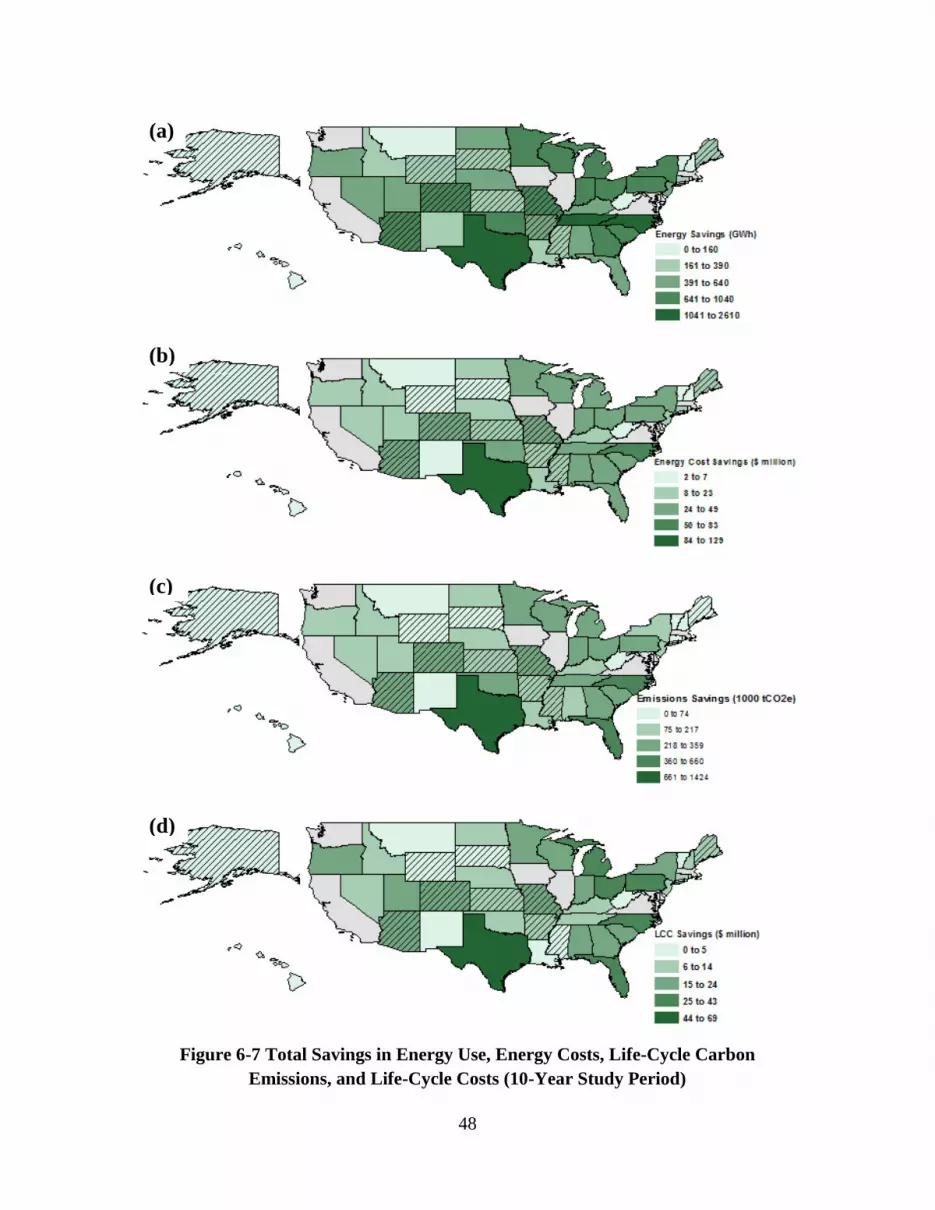
48
Figure 6-7 Total Savings in Energy Use, Energy Costs, Life-Cycle Carbon
Emissions, and Life-Cycle Costs (10-Year Study Period)
(d)
(a)
(b)
(c)

49
6.2.2 Regional and National Impacts
The regional impacts of adopting the 2012 IECC across the nation on energy use, energy
costs, LCC, and life-cycle carbon emissions are calculated by summing total changes
across all states within each of the four Census Regions. Table 6-10 displays the total
changes in the metrics for the four regions under the assumption of a 10-year study
period. The South Census Region achieves the greatest reductions in energy use, energy
costs, carbon emissions, and LCC. The Northeast region realizes the least. Once again it
is shown that total savings are primarily driven by the amount of newly constructed floor
area. National adoption of the 2012 IECC leads to reductions of 2.4 TWh in energy use,
$1.0 billion in energy costs, 9.3 million metric tons in emissions, and $0.6 billion in LCC
over a 10-year study period.
Table 6-10 Total Savings by Census Region from Adoption of the 2012 IECC
(10-Year Study Period)
Census
Region
Average New CFA
1000 m2 (1000 ft2)
Energy Use
(GWh)
Energy Costs
($million)
Emissions
(1000 tCO2e)
LCC
($million)
Northeast 5959 (64 146) 2793 112 820 106
Midwest 12 601 (135 631) 6627 204 2125 172
South 49 268 (529 922) 10 812 513 4837 344
West 12 603 (135 657) 4044 164 1528 114
National 80 394 (865 357) 24 277 993 9311 601
6.3 Savings per Unit of Floor Area
The total savings estimated in Section 6-2 was driven by the amount of newly constructed
floor, making it difficult to analyze the other factors that may be driving variation in the
results. This section normalizes the results by estimating the reductions per unit of floor
area in order to analyze these other factors.
6.3.1 State-Level Savings
The weighted average reductions in energy use are estimated at the city-level and then
aggregated to a state-level weighted average using the county clustering approach defined
in Section 4.2.
6.3.1.1 Energy Use and Energy Cost Savings per Unit of Floor Area
Aggregate energy savings and energy savings per unit of newly constructed floor area for
each state are shown in Table D-1, and are organized by savings per unit of new floor

50
area in descending order. Once controlling for the amount of newly constructed building
stock, the results are similar to the percentage change results. States such as Alaska have
the least amount of new construction but achieve some of the most extensive reductions
in energy use per m2 (ft2). Energy savings per unit of floor area is driven primarily by
climate zone, as shown in Figure 6-8. States located in milder climate zones (Zone 1
through Zone 4) realize smaller reductions in energy use per m2 (ft2) than states located in
colder climates (Zone 5 through Zone 8).
Figure 6-8 Energy Savings per Unit of Floor Area by State (10-Year Study Period)
6.3.1.2 Energy Cost Savings per Unit of Energy Savings
Results from Section 6-2 showed that states with greater reductions in total energy use
generally realize greater energy cost savings. Other factors such as energy prices and the
fuel mix of the total reductions in energy use in a state also impact the magnitude of
energy cost savings. Table D-2 sheds some light on the impacts of energy prices and
changes in annual energy consumption on energy cost savings per MWh of energy
savings. Listed are the state average electricity and natural gas rates, rate differentials,
weighted average energy prices (weighted by the baseline proportions of natural gas and
electricity consumed in the state), changes in electricity and natural gas use following
nationwide adoption of 2012 IECC, and the resulting energy cost savings per MWh
reduced. States with higher average weighted energy prices produce larger energy cost
savings per MWh saved. All states – with the exception of Florida and Hawaii – satisfy
the majority of their energy needs using natural gas. Large discrepancies in fuel mix
proportions, which drive down weighted average energy prices in most states, reveals that
energy cost savings are particularly sensitive to changes in natural gas prices.
The relationship between weighted average energy prices and energy cost savings per
MWh saved is shown in Figure 6-9. States located in the southern part of the U.S., along
the east coast, and Hawaii have both the highest weighted average energy prices and
energy cost savings per MWh reduced. Hawaii faces the highest weighted average energy
price ($0.32) relative to all other states. Electricity rates in the state are at least two times

51
higher than rates in other states, while natural gas rates are at least three times higher.
Their uniquely high prices coupled with their heavy dependence on costly electricity
results in an exceptionally high weighted average energy price. States in all remaining
parts of the U.S. face much lower average energy prices and realize at most moderate
cost savings by adopting the 2012 IECC.
Figure 6-9 Energy Cost Savings per Megawatt-Hour Reduced and Weighted
Average Energy Price by State (10-Year Study Period)
Figure 6-9 suggests that there is some correlation between weighted average energy
prices and energy cost savings per MWh saved. From Table D-2, states realizing greater
energy cost savings per MWh reduced generally achieve larger cutbacks in electricity use
relative to other states. Electricity is more costly per kWh than natural gas on average,
which means that states can recoup greater cost savings per MWh reduced the more they
lower their electricity use. The inexpensiveness of natural gas requires that substantial
reductions in its use occur in order for there to be significant levels of energy cost savings
per unit of energy savings.
Another factor that impacts the energy cost savings is the shift in the fuel mix from
natural gas to electricity consumption. The adoption of 2012 IECC leads to reductions in
both natural gas and electricity consumption. However, the magnitude of natural gas
reductions in most states is greater than that of electricity, increasing the proportion of
consumption accounted for by electricity (referred to as an “offset” throughout the
remainder of this document). States with a large enough price difference coupled with
minor offsets in natural gas can still realize considerable energy cost savings. Large
savings may also arise in states with smaller energy price differentials and larger natural
gas offsets. The smallest energy cost savings per MWh saved are likely to occur in states
with larger energy price differentials and a smaller fraction of natural gas being offset by
changes in electricity use.
Figure 6-10 shows the Building America Climate Regions for the Contiguous U.S.
(Figure 6-10a) and the average offset (Figure 6-10b), which is the average shift in the
WEP
$0.04 - $0.06
$0.07 - $0.10
$0.11 - $0.32
$/MWh
0 to 29
30 to 39
40 to 44
45 to 54
55 to 306

52
proportion of consumption from natural gas to electricity in each state from the adoption
of 2012 IECC. The smallest offset occurs for Hawaii followed by Alaska, Florida, and
Louisiana, which are all states in the hottest (Hawaii, Florida, and Louisiana) and coldest
(Alaska) climate zones in the country. These extreme climates have either little, or no,
heating or cooling loads and will not shift demands regardless of the efficiency of the
building design. The greatest offsets occur in states that are at least partially in the mixed
climate zones (ASHRAE Climate Zone 3A (northern portion), Zone 4A, and Zone 4B),
which can realize significant shifts from heating to cooling in the transition seasons
(spring and fall).
Figure 6-10 (a) Building America U.S. Climate Regions and (b) the Average Natural
Gas Offset by State (10-Year Study Period)13
6.3.1.3 Savings in Life-Cycle Carbon Emissions per Unit of Energy Savings
It was determined from Figure 6-7 that there is strong correlation between total energy
savings and savings in life-cycle carbon emissions. States with the largest reductions in
13 Source: Building America Climate Region Map (U.S. Department of Energy (DOE) 2015)
(a)
(b)

53
energy use generally produce the largest reductions in emissions. Other factors such as
statewide changes in the fuel mix of the energy use savings and changes in the
cradle-to-grave construction-related emissions associated with 2012 IECC building
efficiency requirement, potentially impact the carbon emissions savings. Table D-3 in the
Appendix shows total life-cycle emissions savings, emissions savings per unit of floor
area, emission savings per MWh of energy saved, the average proportion of energy
consumption represented by natural gas under the baseline energy code, and the weighted
average fraction of natural gas offset by changes in electricity consumption in each state.
States with a greater proportion of electricity-based energy consumption realize greater
reductions per unit of energy reduction, with 8 of the 11 states with the greatest
reductions per MWh of energy use savings having natural gas account for less than 60 %
of total average energy consumption under their baseline state energy code (bolded in
Table D-3). It is also evident that there is a relationship between natural gas offsets and
carbon emissions savings per MWh reduced, with 4 of the 5 states that have offsets of
less than 4 % (bolded in Table D-3) in those same top 11. For example, the offset for
Florida is only 0.9% and it realizes almost 0.88 tCO2e savings per MWh reduced.
Missouri, however, offsets roughly 6% of its natural gas for the more carbon intensive
electricity and realizes only 0.34 tCO2e savings per MWh saved after the adoption of the
2012 IECC. This finding is further supported by Figure 6-11, which shows both the
average emissions savings per unit of energy saved and the weighted average natural gas
offsets in each state. States with higher natural gas offsets generally realize smaller life-
cycle carbon emissions savings per MWh saved.
Figure 6-11 Emissions Savings per MWh Reduced and the Weighted Average Offset
of Natural Gas by State (10-Year)
6.3.1.4 Life-Cycle Cost Savings per Unit of Floor Area
Changes in LCC per unit of newly constructed floor area are shown in Table D-4. Similar
to energy use, climate is a key driver to LCC reductions per unit of floor area. Maine,
Vermont, and New York, for example, realize the greatest savings per unit of floor area

54
and are located in colder climate zones (Zone 5, Zone 6, or Zone 7). Figure 6-12 shows
that LCC savings per m2 grow larger as the climate zone grows colder. Similar to energy
costs, Hawaii is the outlier, realizing significant LCC savings per unit of floor area
because of its uniquely high energy prices. There is no correlation between LCC savings
and state baseline codes.
Figure 6-12 Life-Cycle Cost Savings per Unit of Floor Area by State (10-Year)
6.3.2 Regional and National Savings per Unit of Floor Area
Table 6-11 shows both the total energy savings and the energy savings per unit of floor
area in each of the U.S. Census Regions for a 10-year study period. Total energy use is
correlated with the total amount of newly constructed building floor area. Regions with
the largest amounts of new CFA realize the largest reductions in annual energy use. This,
however, is not the case when comparing average savings per m2 (ft2) with the total
amount of newly constructed floor area. States located in the Midwest Census Region
realize the largest reductions in energy use per unit of floor area, while the South Census
Region realizes the least. Nationwide energy savings is approximately 30 kWh/m2
(3 kWh/ft2).
Table 6-11 Energy Use Reductions per Unit of Newly Constructed Floor Area from
Adoption of the 2012 IECC by Census Region (10-Year Study Period)
Census
Region
Total New CFA
1000 m2 (1000 ft2)
Energy Use
(GWh)
kWh/m2 kWh/ft2
Northeast 5959 (64 146) 2793 469 44
Midwest 12 601 (135 631) 6627 526 49
South 49 268 (529 922) 10 812 220 20
West 12 603 (135 657) 4044 321 30
Total 80 394 (865 357) 2428 302 28

55
The energy cost savings per kWh of energy savings, electricity rates, natural gas rates,
weighted average energy prices, and the percentage offset of natural gas are displayed in
Table 6-12. The Northeast Census Region has both the highest average percentage of
offset natural gas and average electricity price – realizing the third greatest reduction in
energy cost per unit of energy saved behind the South and West Census Regions.
Conversely, the Midwest region has both the second lowest percentage of offset natural
gas and electricity prices, and realizes the lowest level of energy cost savings per unit of
energy saved with an average reduction of $0.03 per kWh.
Table 6-12 Energy Cost Reduction per kWh of Energy Savings from Adoption of
the 2012 IECC by Census Region (10-Year)
Census
Region
Offset*
(%)
Electricity Rate*
($/kWh)
Natural Gas Rate*
($/kWh)
Weighted
Energy Price*
($/kWh)
Energy Cost
Reduction
($/kWh)
Northeast 5.4 0.16 0.05 0.07 0.04
Midwest 4.9 0.11 0.03 0.05 0.03
South 5.1 0.10 0.04 0.07 0.05
West 4.6 0.11 0.04 0.05 0.04
Total 5.0 0.11 0.04 0.06 0.04
*Weighted by energy use savings for a state
Table 6-13 shows total life-cycle carbon emissions savings, the weighted average fraction
of natural gas offset by changes in electricity use, and the emissions savings per GWh
saved across the four Census Regions. Regions with higher natural gas offsets are likely
to realize smaller reductions in life-cycle emissions per unit of energy savings. The
Northeast Census Region on average has the highest percentage of offset natural gas and
achieves the lowest reduction in life-cycle emissions per GWh saved. Meanwhile, the
West Census Region realizes the second highest average reduction in emissions per unit
of energy savings as a result of having the lowest percentage of offset natural gas. There
does exist ambiguity in the relationship between emission reductions per GWh saved and
natural gas offsets. For example, the South Census Region exhibits the highest level of
life-cycle emissions reduced per GWh of energy reduced despite having the second
highest percentage offset of natural gas. This ambiguity is due to the South’s warm
climate zones, which leads to greater electricity use to meet cooling loads and less natural
gas use to meet heating loads.

56
Table 6-13 Reduced Carbon Emissions per GWH of Energy Savings from Adoption
of the 2012 IECC by Census Region (10-Year Study Period)
Census
Region
Emissions
Reduction
(1000 tCO2e)
Offset*
(%)
Weighted Avg.
Electricity Emissions
Rate (tCO2e/MWh)
CO2e Reduction
(t/GWh)
Northeast 820 5.4 620 29
Midwest 2125 4.9 905 32
South 4837 5.1 796 44
West 1528 4.6 687 37
Total 8738 5.0 788 38
Average LCC savings (total and per unit of floor area) and fuel prices (electricity, natural
gas, and weighted average) in the four Census Regions are shown in Table 6-14. There
appears to be a direct relationship between the LCC savings and the level of energy
savings per unit of floor area and regional electricity rates. Regions with greater energy
use savings per unit of floor area and higher electricity rates tend to realize greater LCC
savings per unit of floor area. The Northeast Region achieves the greatest reduction in
LCC per unit of floor area, and has both the second largest reduction in energy use per
unit of floor area and the highest average electricity price. Alternatively, the South
Census Region achieves the smallest reduction in LCC. Its electricity rates are the lowest
of all the regions and its energy savings per unit of floor area are the smallest. Those
regions falling in the middle (Midwest and West) have the first and third largest
reductions in energy use per unit of floor area, and an average electricity rate $0.11/ kWh.
The national average LCC savings per unit of floor area is approximately $7.47/m2
($0.69/ft2). Other factors, such as local construction costs, will also have an impact on
these regional LCC savings estimates.

57
Table 6-14 Life-Cycle Cost Savings per Unit of Newly Constructed Floor Area from
Adoption of the 2012 IECC by Census Region (10-Year Study Period)
Census
Region
Energy Use
Savings
(kWh/m2)
Electricity Rate
($/kWh)*
Natural Gas
Rate
($/kWh)*
Weighted
Energy Price
($/kWh)*
LCC
Savings
($million)
LCC
Savings
($/m2)
LCC
Savings
($/ft2)
Northeast 469 0.16 0.05 0.07 91 15.30 1.42
Midwest 526 0.11 0.03 0.05 155 12.26 1.14
South 220 0.10 0.04 0.07 241 4.90 0.45
West 321 0.11 0.04 0.05 114 9.03 0.84
Total 302 0.11 0.04 0.06 601 7.47 0.69
*Weighted by energy use savings for a state

58

59
7 Discussion
This study analyzes the impacts of adopting the latest, more stringent state energy codes
based on the BIRDS new residential database for 10 prototypical building types (wood-
framed single-family detached buildings) in 228 U.S. locations. Results are summarized
at the state, regional, and national levels. This section will discuss key findings,
limitations of the research, and recommended directions for future research.
7.1 Key Findings
The key findings from this study are analyzed for each sustainability performance metric
in terms of percentage change, total change, and change per unit of floor area.
7.1.1 Percentage Changes
Assuming a 10-year study period, nationwide adoption of 2012 IECC would lead to
significant average percentage reductions in energy consumption (19.2 %), energy costs
(15.2 %), life-cycle carbon emissions (11.2 %), and life-cycle costs (1.7 %). The
percentage reductions in energy costs are smaller than the percentage reductions in
energy consumption because the majority of the reductions are from natural gas, which is
cheaper than electricity. The percentage reductions in life-cycle carbon emissions are
much lower than the reductions in energy consumption because of two factors. First, the
emissions rate is lower for natural gas than for electricity. Since most of the reductions in
energy consumption are from natural gas, the emissions reductions are lower. Second,
life-cycle carbon emissions include emissions from both the energy consumption of the
building and the embodied emissions from the materials used in construction of the
building. In order to reduce energy consumption, additional materials must be installed in
the building, leading to higher embodied emissions that offset some of the energy-related
carbon emissions reductions.
The estimated savings vary by building prototype, with 1-story houses realizing smaller
savings than 2-story houses with approximately the same conditioned floor area. Two
factors could be driving these differences. First, 2-story houses have more volume per
unit of floor area, which causes energy use to meet the heating and cooling loads to
account for a greater fraction of total energy use. Second, the two-story houses have less
window glazing per unit of wall area, which could lead to greater savings from changes
in requirements for wall insulation. Similar results and interpretations occur for energy
costs, life-cycle carbon emissions, and life-cycle costs.
The baseline code edition of IECC and climate zone of a location will impact the
estimated savings from the adoption of 2012 IECC. On average, locations with older
editions of IECC as their baseline code realize slightly greater reductions in energy use,
energy costs, and life-cycle carbon emissions. Life-cycle cost savings are greatest for

60
locations with 2003 IECC the baseline code, on average, followed by 2009 IECC.
Although locations with older baseline codes realize greater reductions, on average, this
trend does not hold at the climate zone level. In fact, locations with a baseline code of
2003 IECC lead to the greatest reductions in energy use, energy costs, and carbon
emissions for only two of eight climate zones. This result may be driven by the change in
climate zone definitions and the resulting changes in building requirements for locations
in those climate zones. On average, the percentage reductions in energy use, energy costs,
and life-cycle carbon emissions increase as the climate zone gets colder, with a small
drop as the climate shifts from primarily cooling to primarily heating loads. Life-cycle
cost reductions do not follow the same trend, with Zone 1 realizing greater life-cycle cost
reductions than Zone 2, and Zone 6 realizing lower reductions than Zone 5. This
deviation may be a result of the differences in the additional investment costs, on
average, of meeting the 2012 IECC across climate zones. These same results hold at the
state level, with states in colder climates realizing greater reductions in energy use,
energy costs, and life-cycle carbon emissions. However, there is some variation in
percentage reductions for energy costs and carbon emissions driven by variation in
energy prices and electricity-related emissions rates, respectively.
7.1.2 Total Changes
Total changes are estimated by using the weighted average change per unit of new floor
area and multiplying by the total new floor area for 2012 associated with the city’s
“county cluster.” These cluster-level estimates are aggregated at the state, census region,
and national level to determine the magnitude of the impact from nationwide adoption of
2012 IECC. The amount of new floor area constructed in a state is the key driver to the
magnitude of the estimated reductions in energy use, energy costs, and life-cycle carbon
emissions, with Texas and North Carolina realizing the greatest reductions while Alaska
and Vermont realize the smallest reductions in energy use, energy costs, life-cycle carbon
emissions, and life-cycle costs.
Similarly, census regions with more constructed new floor area realize greater reductions.
The South Census Region realizes savings of 1.1 TWh of energy consumption, $513
million in energy costs, 4.8 million tCO2e of life-cycle emissions, and $344 million for
one year’s worth of construction for a 10-year study period. The smallest reductions are
realized in the Northeast Census Region at 279 GWh of energy consumption, $112
million in energy costs, 820 000 tCO2e of life-cycle emissions, and $106 million for one
year’s worth of construction for a 10-year study period. The impacts aggregated at the
national level total 2.4 TWh of energy consumption, $993 million in energy costs,
9.3 million tCO2e of life-cycle emissions, and $601 million for one year’s worth of
construction for a 10-year study period.

61
7.1.3 Change per Unit of Floor Area
After controlling for the amount of newly constructed floor area, the results are similar to
the percentage change results. Energy savings per unit of floor area are driven primarily
by climate zone. For example, states such as Alaska have the least amount of new
construction, but achieve some of the most extensive reductions in energy use per m2
(ft2). States with greater reductions in total energy use generally realize greater energy
cost savings. Other factors such as energy prices and the fuel mix of the total reductions
in energy use in a state also impact the magnitude of energy cost savings. Higher energy
prices, greater proportions of energy use accounted for by electricity, and smaller shifts in
consumption from natural gas to electricity lead to greater reductions in energy costs per
unit of floor area. Similarly, higher emissions rates for electricity, greater proportions of
energy use accounted for by electricity, and smaller shifts in consumption from natural
gas to electricity lead to greater reductions in life-cycle carbon emissions per unit of floor
area. Similar to energy use, life-cycle cost savings per unit of floor area are greater for
states in colder climate zones.
Savings in energy use per unit of floor area are greater in the colder regions, with the
Midwest realizing the greatest savings followed by the Northeast. The savings in energy
costs per unit of floor area are greatest for the South Census Region while the savings are
smallest for the Midwest. The South has the highest weighted average energy price and a
high average offset while the Midwest has the lowest weighted average energy price and
a lower offset. The South also realizes the greatest life-cycle carbon emissions savings
per unit of floor area because of the region’s high proportion of electricity consumption.
The Northeast realizes the greatest life-cycle cost savings per unit of floor area while the
South has the smallest life-cycle cost savings.
7.2 Limitations and Future Research
The analysis in this study is limited in scope and would be strengthened by including
sensitivity analysis, expanding the BIRDS database and metrics, and allowing public
access to all the results.
Uncertainty analysis is needed for at least three elements of the analysis. First, consider
the assumed discount rate. Although 3 % is a reasonable discount rate, in real terms, for
federal government investment decisions, it may be too low of a value for an expected
real return on an alternative investment in the private sector (Rushing et al. 2011).
Sensitivity analysis on the assumed discount rate is needed to determine the robustness of
the cost results. Second, the current analysis assumes that building cooling loads are met
by equipment running on electricity while space and water heating loads are met by
equipment running on natural gas, which is not the typical fuel mix for some areas of the
nation. The database should be expanded to include alternative heating fuel source

62
options, such as electricity in the South, because the results could be significantly
impacted.
Additional data are needed to refine and expand the BIRDS database. The 10 prototypical
single-family dwellings analyzed in this study may not be representative of the entire
building stock because of the assumed simplicity of the building geometry. For this
reason, the results should be considered as general magnitudes for making reasonable
comparisons instead of precise quantitative analysis. Future research should include
additional prototypes in the database. The state average energy cost rates do not control
for local variation in energy tariffs. By using utility-level energy cost data as discussed in
Kneifel and Butry (2014b), the accuracy of the estimates in BIRDS could be improved.
BIRDS currently assumes an adoption and enforcement (i.e., commissioning) rate of
100 %. Cort and Butner (2012) finds that local adoption of building energy codes varies
across states. States with state energy codes have an average adoption rate of 88 % (49 %
to 100 %) while states without a state energy code have an average adoption rate of 52 %
(3 % to 97 %). The granularity within each state should be considered to determine how
it may impact the current estimates.
Taylor, Fernandez, and Lucas (2012) defines methodology to evaluate the
cost-effectiveness of states adopting newer editions of IECC for residential buildings.
The main difference between their methodologies and that used in this study is the home
purchase financing approach (mortgage versus 100 % cash).
Alternative assumptions should be considered for a number of factors, including
foundation type and heating equipment fuel type. An additional building type should be
added to the database to account for low-rise multifamily housing units (i.e., low-rise
apartment building).
The analysis in this study ignores the impacts that variations in occupancy and behavior
patterns, in terms of plug and process load use, thermostat setpoints, and number of
occupants, and HVAC equipment efficiency have on the reductions in energy use. Homes
with greater plug and process loads will realize smaller percentage changes in energy use
because the energy efficiency measures considered in this study focus on the IECC
requirements (building envelope and lighting) holding constant the efficiency of other
equipment (HVAC equipment and appliances) used in the building and the number of
occupants living in the building. Future research should consider the impact that
improved equipment efficiency and occupant activity may have on the overall energy
savings realized by energy efficiency improvements to buildings.
Analysis based on the energy performance is susceptible to the limitations of current
whole building energy simulation models. As the underlying simulation software

63
improves in accuracy and uncertainty, the sustainability analysis related to the modeling
will improve as well.
Energy, environmental, and economic performance are but three attributes of building
performance. The BIRDS model assumes that its building prototypes all meet minimum
technical performance requirements. However, there may be significant differences in
technical performance not evaluated in BIRDS, such as indoor environmental quality
performance, which may affect energy, environmental, and economic considerations.
Finally, a more comprehensive analysis of the environmental performance could be
completed. This study applies environmental life cycle assessment methods to estimate
the reductions in life-cycle carbon emissions. The BIRDS database could be expanded to
the full range of 11 life-cycle environmental impacts covering human health effects,
ecological health effects, and resource depletion.

64

65
References
ASTM International (2012). ASTM Standards on Building Economics: 7th Edition. West
Conshohocken, PA, ASTM International.
Cort, K. and R. Butner (2012). An Analysis of Statewide Adoption Rates of Building
Energy Code by Local Jurisdictions. Pacific Northwest National Laboratory (PNNL).
Richland, WA.
Energy Independence and Security Act (EISA) of 2007, Pub. L. No. 110-140, 2007
Environmental Protection Agency (EPA) (2007). "2007 Emissions and Generation
Integrated Database (eGRID2007)." from http://www.epa.gov/cleanenergy/energy-
resources/egrid/index.html.
Faithful+Gould (2011). Residential Energy Efficiency Measures: Location Factors,
National Renewable Energy Laboratory.
Faithful+Gould (2012). Residential Energy Efficiency Measures: Prototype Estimate and
Cost Data Revision 6.0, National Renewable Energy Laboratory.
Fuller, S. and S. Petersen (1996). "Life-Cycle Costing Manual for the Federal Energy
Management program, 1995 Edition." NIST handbook 135.
Halverson, M., et al. (2011a). ANSI/ASHRAE/IESNA Standard 90.1-2007 Final
Determination Quantitative Analysis. Pacific Northwest National Laboratory. Richland,
WA.
Halverson, M., et al. (2011b). ANSI/ASHRAE/IESNA Standard 90.1-2010 Final
Determination Quantitative Analysis. Pacific Northwest National Laboratory. Richland,
WA.
Halverson, M., et al. (2014). ANSI/ASHRAE/IES Standard 90.1-2013 Preliminary
Determination: Quantitative Analysis. Pacific Northwest National Laboratory. Richland,
WA.
Kneifel, J. (2010). "Life-Cycle Carbon and Cost Analysis of Energy Efficiency Measures
in New Commercial Buildings." Energy and Buildings 42(3): 333-340.

66
Kneifel, J. (2011a). "Beyond the code: Energy, carbon, and cost savings using
conventional technologies." Energy and Buildings 43(4): 951-959.
Kneifel, J. (2013a). "Benefits and Costs of Energy Standard Adoption in New
Commercial Buildings." NIST Special Publication 1147.
Kneifel, J. (2013b). "Benefits and Costs of Energy Standard Adoption in New
Commercial Buildings: Northeast Census Region." NIST Special Publication 1148-1.
Kneifel, J. (2013c). "Benefits and Costs of Energy Standard Adoption in New
Commercial Buildings: Midwest Census Region." NIST Special Publication 1148-2.
Kneifel, J. (2013d). "Benefits and Costs of Energy Standard Adoption in New
Commercial Buildings: South Census Region." NIST Special Publication 1148-3.
Kneifel, J. (2013e). "Benefits and Costs of Energy Standard Adoption in New
Commercial Buildings: West Census Region." NIST Special Publication 1148-4.
Kneifel, J. (2013f). "Benefits and Costs of Energy Standard Adoption in New
Commercial Buildings: National Summary." NIST Special Publication 1161.
Kneifel, J. and D. Butry (2014a). "Impact of More Precise Construction Data on
Estimated Savings from Energy Standard Adoption for Commercial Buildings." NIST
Special Publication 1178.
Lippiatt, B., et al. (2013). Building Industry Reporting and Design for Sustainability
(BIRDS) Technical Manual and User Guide, NIST TN 1814. National Institute of
Standards and Technology. Gaithersburg, MD.
Lucas, R., et al. (2012). National Energy and Cost Savings for New Single-and
Multifamily Homes: A Comparison of the 2006, 2009, and 2012 Editions of the IECC.
Pacific Northwest National Laboratory (PNNL). Richland, WA.
Mendon, V., et al. (2013). Cost-Effectiveness Analysis of the 2009 and 2012 IECC
Residential Provisions: Technical Support Document. Pacific Northwest National
Laboratory (PNNL). Richland, Washington.

67
Mendon, V., et al. (2014). 2015 IECC Determination of Energy Savings: Preliminary
Technical Analysis. Pacific Northwest National Laboratory (PNNL). Richland, WA.
National Association of Home Builders (NAHB) Research Center (2012a). Methodology
for Calculating Energy Use in Residential Buildings. Upper Marlboro, MD, National
Association of Homebuilders.
National Association of Home Builders (NAHB) Research Center (2012b). 2009 IECC
Cost Effectiveness Analysis. Upper Marlboro, MD, National Association of Home
Builders.
National Association of Home Builders (NAHB) Research Center (2012c). 2012 IECC
Cost Effectiveness Analysis. Upper Marlboro, MD, National Association of Home
Builders.
National Renewable Energy Laboratory (NREL) (2012). "U.S. Life-Cycle Inventory
Database (LCI)." from http://www.nrel.gov/lci/.
NC Clean Energy Technology Center (2015). Database of State Incentives for
Renewables and Efficiency (DSIRE): Rules, Regulations, and Policies for Energy
Efficiency Database. 2010.
North American Electric Reliability Corporation (NERC) (2011). "Regional Entities."
Retrieved December 2011, from
http://www.nerc.com/AboutNERC/keyplayers/Pages/Regional-Entities.aspx.
Pacific Northwest National Laboratory (PNNL) (2009a). Impacts of Standard ASHRAE
90.1-2007 for Commercial Buildings at State Level. U.S. Department of Energy Building
Energy Codes Program. Richland, WA.
Pacific Northwest National Laboratory (PNNL) (2009b). Impacts of the 2009 IECC for
Residential Buildings at State Level. U.S. Department of Energy Building Energy Codes
Program. Richland, WA.
RSMeans (2011). "CostWorks Databases." from http://www.meanscostworks.com/.
Rushing, A., et al. (2011). Energy Price Indices and Discount Factors for Life-Cycle Cost
Analysis - 2011. Gaithersburg, MD, National Institute of Standards and Technology.

68
Taylor, T., et al. (2012). Methodology for Evaluating Cost-Effectiveness of Residential
Energy Code Changes. Pacific Northwest National Laboratory (PNNL). Richland, WA.
U.S. Census Bureau (2011). "American Housing Survey (AHS) for the United States,
Series H-150, Complete Set of Tables and Standard Errors." from
http://www.census.gov/programs-surveys/ahs/.
U.S. Census Bureau (2013). "Survey of Construction, Annual 2013 Characteristics of
New Housing." from http://www.census.gov/construction/chars/.
U.S. Department of Energy (DOE) (2014). "Building Energy Codes Program, Status of
State Energy Code Adoption." 2014, from http://www.energycodes.gov/adoption/states.
U.S. Department of Energy (DOE) (2015). "Building America Climate Region Map."
Retrieved April 4, 2015, from http://energy.gov/eere/buildings/building-america-climate-
specific-guidance.
U.S. Energy Information Administration (EIA) (2013a). "Electric Power Annual State
Data Tables." 2013, from http://www.eia.doe.gov/fuelelectric.html.
U.S. Energy Information Administration (EIA) (2013b). "Natural Gas Navigator." 2013,
from http://www.eia.doe.gov/oil_gas/natural_gas/info_glance/natural_gas.html.

69
A Building Type, New Construction, and Emissions Rates
Figure A-1 Conditioned Floor Area of New 1-Story Single-Family Housing
0%
10%
20%
30%
40%
50%
60%
70%
80%
90%
100%
0
5000
10000
15000
20000
25000
30000
35000
40000
45000
50000
Hou
sin
g U
nit
s
Conditioned Floor Area - m2 (ft2)
Frequency
Cumulative %

70
Figure A-2 Conditioned Floor Area of New 2-Story Single-Family Housing
0%
10%
20%
30%
40%
50%
60%
70%
80%
90%
100%
0
5000
10000
15000
20000
25000
30000
35000
40000
45000
50000
55000
60000
Hou
sin
g U
nit
s
Conditioned Floor Area - m2 (ft2)
Frequency
Cumulative %

71
Table A-1 CO2, CH4, and N2O Emissions Rates Electricity Generation by State
State
CO2 CH4 N2O CO2 CH4 N2O
(t/GWh) (t/GWh) (t/GWh) State (t/GWh) (t/GWh) (t/GWh)
AK 603.4 57.9 1.9 MT 542.8 30.1 0.4
AL 804.2 42.7 0.5 NC 616.6 30.5 0.2
AR 695.9 58.6 1.7 ND 851.1 40.4 0.2
AZ 746.9 53.2 1.2 NE 851.1 40.4 0.2
CA 450.0 45.8 1.5 NH 550.4 47.0 1.4
CO 938.8 54.0 0.8 NJ 618.7 33.4 0.4
CT 550.4 47.0 1.4 NM 778.5 55.3 1.3
DE 618.7 33.4 0.4 NV 465.6 27.6 0.4
FL 767.5 57.2 1.5 NY 480.7 32.3 0.8
GA 804.2 42.7 0.5 OH 835.7 38.9 0.2
HI 807.1 28.0 0.1 OK 904.8 63.9 1.4
IA 851.1 40.4 0.2 OR 465.6 27.6 0.4
ID 465.6 27.6 0.4 PA 672.9 34.7 0.4
IL 948.3 44.4 0.2 RI 550.4 47.0 1.4
IN 835.7 38.9 0.2 SC 616.6 30.5 0.2
KS 926.0 44.8 0.3 SD 851.1 40.4 0.2
KY 781.9 36.9 0.2 TN 781.9 36.9 0.2
LA 719.2 59.2 1.6 TX 790.9 65.8 1.8
MA 550.4 47.0 1.4 UT 465.6 27.6 0.4
MD 618.7 33.4 0.4 VA 689.6 33.3 0.2
ME 550.4 47.0 1.4 VT 550.4 47.0 1.4
MI 861.4 46.8 0.6 WA 465.6 27.6 0.4
MN 851.1 40.4 0.2 WI 860.7 44.1 0.4
MO 939.4 44.6 0.2 WV 835.7 38.9 0.2
MS 709.8 48.3 1.0 WY 623.7 36.4 0.5

72

73
B Percentage Changes by State for the Nationwide Adoption of the
2012 IECC
Table B-1 Total Changes in Fuel Use and the Proportional Changes in Natural Gas
Use Relative to 2012 IECC
State Total Change in
Electricity Use (kWh)
Total Change in Natural
Gas Use (kWh)
Proportional Change in
Natural Gas Use Relative
to 2012 (%)
Baseline Code - 2003
AK 518,722 11,831,124 -2.7%
AR 330,639 1,269,709 -4.7%
AZ 921,722 2,449,190 -3.2%
CO 434,222 5,158,645 -4.6%
KS 356,833 3,769,208 -5.9%
ME 151,444 2,725,539 -4.0%
MO 352,250 3,373,408 -6.0%
MS 321,417 920,328 -4.9%
SD 256,861 3,889,825 -4.5%
WY 373,750 5,252,095 -4.3%
Baseline Code - 2006
HI 289,250 167 1.5%
LA 581,167 892,549 -2.1%
MN 419,833 7,687,868 -4.0%
OK 346,083 1,646,174 -5.0%
TN 551,861 3,424,105 -6.5%
WI 424,472 6,652,033 -4.6%
Baseline Code - 2009
AL 404,083 1,772,320 -5.4%
CT 96,194 1,938,468 -5.5%
FL 661,222 459,970 -0.9%
GA 645,139 2,640,729 -5.4%
ID 153,694 2,568,780 -4.9%
IN 253,778 4,004,026 -5.6%
KY 204,889 2,679,536 -6.6%
MI 500,139 11,002,912 -4.6%
MT 531,083 10,693,172 -4.6%
NC 520,694 3,689,814 -6.8%
ND 190,500 4,477,969 -4.3%
NE 324,500 5,575,752 -5.2%
NH 56,222 1,103,394 -4.7%
NJ 139,278 2,040,696 -6.7%
NM 261,694 1,912,633 -6.2%
NV 435,306 4,635,394 -4.7%
NY 387,278 8,112,725 -5.2%
OH 310,750 6,284,263 -5.2%
OR 402,167 7,453,577 -5.2%
PA 418,278 7,850,294 -5.3%
SC 333,917 1,463,581 -5.8%
TX 2,047,444 6,191,258 -4.4%
UT 104,528 1,495,999 -5.1%
VT 55,944 1,223,484 -4.8%
WV 178,333 2,522,417 -5.9%

74
Table B-2 Summary of Average Savings in Energy Use, Energy Costs, Carbon
Emissions, and Life-Cycle Costs for all U.S. States (10-Year)
State Code Percentage Change
Energy Use Energy Costs Emissions LCC
AK 2003 -37.2% -17.1% -14.3% -2.5%
AL 2003 -13.2% -16.7% -11.3% -2.0%
AR 2003 -23.6% -20.3% -14.0% -1.7%
AZ 2003 -17.4% -17.0% -11.7% -1.8%
CO 2003 -23.0% -16.5% -13.5% -2.3%
CT 2003 -24.4% -16.8% -15.3% -3.6%
FL 2003 -10.8% -8.2% -7.5% -0.8%
GA 2003 -21.1% -16.7% -11.2% -1.8%
HI 2003 -3.4% -9.3% -6.1% -2.4%
ID 2003 -54.9% -17.3% -12.5% -2.4%
IN 2006 -24.3% -17.4% -13.3% -2.7%
KS 2006 -24.6% -17.8% -13.5% -2.4%
KY 2006 -17.6% -18.9% -11.1% -1.9%
LA 2006 -12.8% -12.8% -9.3% -0.1%
ME 2006 -26.0% -20.6% -14.9% -4.2%
MI 2006 -18.7% -17.1% -14.5% -3.5%
MN 2009 -26.3% -19.9% -16.6% -1.9%
MO 2009 -24.0% -18.8% -13.4% -2.3%
MS 2009 -22.3% -18.2% -14.1% -1.0%
MT 2009 -10.6% -18.7% -16.1% -2.5%
NC 2009 -20.7% -17.8% -10.8% -1.9%
ND 2009 -26.1% -20.3% -16.9% -3.1%
NE 2009 -24.2% -17.8% -15.2% -3.1%
NH 2009 -25.4% -19.3% -16.6% -4.1%
NJ 2009 -27.5% -19.2% -13.4% -2.4%
NM 2009 -54.3% -16.3% -11.2% -1.1%
NV 2009 -21.5% -17.3% -12.7% -1.3%
NY 2009 -26.2% -18.6% -15.1% -3.9%
OH 2009 -23.1% -16.6% -13.3% -3.2%
OK 2009 -52.8% -22.0% -16.6% -1.8%
OR 2009 -19.8% -20.2% -15.5% -3.7%
PA 2009 -24.2% -18.0% -13.8% -3.0%
SC 2009 -33.2% -16.7% -11.5% -1.7%
SD 2009 -25.8% -20.0% -14.3% -3.0%
TN 2009 -20.7% -18.7% -11.4% -0.9%
TX 2009 -14.8% -12.0% -9.8% -1.2%
UT 2009 -26.0% -15.6% -13.5% -2.3%
VT 2009 -26.5% -21.1% -17.1% -5.2%
WI 2009 -26.6% -19.5% -16.8% -2.5%
WV 2009 -33.5% -18.5% -11.6% -2.2%
WY 2009 -21.5% -19.6% -13.7% -2.5%

75
C Total Changes from the Nationwide Adoption of the 2012 IECC
Table C-1 Total Reductions by State from Adoption of the 2012 IECC (10-Year)
State Code Average Annual New Floor Area
1000 m2 (1000 ft2)
Energy Use
(million kWh)
Energy Costs
($million)
Emissions
(1000 tCO2e)
LCC
($million)
TX 2009 15 189 2607 129 1424.4 69.3
FL 2009 8264 620 48.8 545.4 26.3
NC 2009 6346 1893 83 659.6 42.9
GA 2009 3419 880 45.7 358.9 24.3
AZ 2003 3345 642 46.3 355.3 23.8
TN 2006 2962 1042 39.3 328.9 9.2
SC 2009 2895 749 35.8 276.4 16.8
LA 2006 2280 351 18 191.7 -0.1
CO 2003 2267 917 26.6 332.8 21.3
AL 2009 2260 578 31 217.0 17.6
PA 2009 2036 838 32.8 264.6 28.3
OH 2009 1845 840 27.3 274.1 26.6
MO 2003 1820 749 28.6 252.5 18.3
IN 2009 1800 850 24.8 272.2 20.9
OK 2006 1719 757 29.7 325.2 11.1
MI 2009 1647 900 28.6 285.0 26.7
UT 2009 1647 576 16.1 193.3 15
MN 2006 1504 1017 27.9 320.4 14.5
NV 2009 1457 398 19.1 157.7 8.6
NY 2009 1428 741 27.5 202.3 23.5
WI 2006 1345 836 26.9 278.1 16
AR 2003 1256 437 18.3 173.2 7.8
MS 2003 1187 323 14.2 172.4 4.2
NJ 2009 1181 560 23.1 155.4 14.4
OR 2009 1180 539 21 170.0 20.2
KY 2009 1152 455 15.7 127.4 8.7
ID 2009 1010 387 10.9 138.2 9.8
NE 2009 810 405 11.3 128.8 10.7
ND 2009 706 476 11.6 132.2 9.2
KS 2003 698 298 10 108.0 6.6
NM 2009 645 203 7 56.4 2.7
ME 2003 451 240 10.5 64.3 8.5
CT 2009 435 190 8.2 61.2 8
SD 2003 425 256 7 73.7 5
HI 2006 358 230 7.2 19.4 5.1
WY 2003 343 170 4.9 46.9 3.2
NH 2009 306 155 6.8 50.4 5.7
WV 2009 302 119 4.2 36.8 2.9
MT 2009 275 138 3.9 44.5 2.9
VT 2009 123 69 3.3 22.0 2.8
AK 2003 76 50 1.6 13.8 1.1

76
77
D Savings per Unit of Floor Area from the Nationwide Adoption of the
2012 IECC
Table D-1 Savings in Energy Use per Unit of Floor Area from Adoption of the 2012
IECC (10-Year)
State Climte Zone(s) Average Annual New Floor Area
1000 m2 (1000 ft2)
Energy Savings
(GWh)
kWh/m2 kWh/ft2
MN 6,7 1504 (16 191) 1017 675.9 62.8
ND 6,7 706 (7599) 476 674.3 62.6
AK 7,8 76 (822) 50 649.1 60.3
WI 6 1345 (14 479) 836 621.8 57.8
SD 6 443 (4766) 256 603.2 56.0
VT 6 123 (1322) 69 560.7 52.1
MI 5,6,7 1647 (17 731) 900 546.1 50.7
ME 6,7 452 (4862) 240 532.7 49.5
NY 5,6 1428 (15 374) 741 518.9 48.2
NH 6 306 (3291) 155 508.5 47.2
MT 6 275 (2960) 138 503.1 46.7
NE 5 810 (8715) 405 500.8 46.5
WY 6 343 (3696) 170 496.6 46.1
NJ 4 1181 (12 707) 560 474.1 44.0
IN 4,5 1800 (19 380) 850 472.1 43.9
OR 4,5 1180 (12 706) 539 456.6 42.4
OH 5 1845 (19 858) 840 455.3 42.3
OK 3 1719 (18 506) 757 440.5 40.9
CT 5 435 (4683) 190 435.8 40.5
KS 4,5 698 (7513) 298 426.4 39.6
PA 4,5,6 2036 (21 911) 838 411.8 38.3
MO 4 1820 (19 588) 749 411.5 38.2
CO 5,6 2267 (24 396) 917 404.8 37.6
KY 4 1152 (12 405) 455 395.2 36.7
WV 4,5 302 (3249) 119 394.5 36.7
ID 5,6 1010 (10 872) 387 383.0 35.6
TN 3,4 2962 (31 879) 1042 351.9 32.7
UT 5 1647 (17 728) 576 349.6 32.5
AR 3 1256 (13 515) 437 348.1 32.3
NM 3,4 645 (6942) 203 314.3 29.2
NC 3,4 6346 (68 311) 1893 298.3 27.7
NV 3 1457 (15 678) 398 273.2 25.4
MS 3 1187 (12 775) 323 272.4 25.3
SC 3 2895 (31 159) 749 258.6 24.0
GA 2,3 3419 (36 807) 880 257.4 23.9
AL 2,3 2260 (24 324) 578 255.9 23.8
AZ 4,5 3345 (36 001) 642 192.0 17.8
TX 2,3,4 15 189 (163 491) 2607 171.6 15.9
LA 2,3 2280 (24 545) 351 153.9 14.3
FL 1,2 8264 (88 955) 620 75.1 7.0
HI 1 358 (3855) 23 65.4 6.1

78
Table D-2 Reduction in Energy Costs per MWh of Reduced Energy Use from
Adoption of the 2012 IECC (10-Year)
State Electricity
Rate
($/kWh)
Natural Gas
Rate ($/kWh)
Price
Differential
($/kWh)
Weighted
Energy Price
($/kWh)
Change in
Electricity Use
Change in
Natural
Gas Use
Energy Cost
Reduction
($/MWh)
HI $0.35 $0.19 $0.16 $0.32 289,250 167 $305
FL $0.12 $0.06 $0.05 $0.10 661,222 459,970 $79
AZ $0.11 $0.05 $0.06 $0.08 921,722 2,449,190 $72
AL $0.11 $0.05 $0.06 $0.08 404,083 1,772,320 $54
GA $0.11 $0.05 $0.06 $0.07 645,139 2,640,729 $52
LA $0.09 $0.04 $0.05 $0.06 581,167 892,549 $51
VT $0.16 $0.06 $0.11 $0.07 55,944 1,223,484 $48
TX $0.11 $0.04 $0.08 $0.07 2,047,444 6,191,258 $49
SC $0.11 $0.04 $0.07 $0.07 333,917 1,463,581 $48
NV $0.12 $0.04 $0.08 $0.06 435,306 4,635,394 $48
NH $0.17 $0.05 $0.12 $0.07 56,222 1,103,394 $44
NC $0.10 $0.04 $0.06 $0.06 520,694 3,689,814 $44
ME $0.15 $0.05 $0.11 $0.07 151,444 2,725,539 $44
CT $0.18 $0.05 $0.13 $0.07 96,194 1,938,468 $43
NY $0.18 $0.05 $0.14 $0.07 387,278 8,112,725 $37
MS $0.10 $0.03 $0.07 $0.06 321,417 920,328 $44
NJ $0.16 $0.04 $0.12 $0.07 139,278 2,040,696 $41
AR $0.09 $0.04 $0.05 $0.06 330,639 1,269,709 $42
PA $0.13 $0.04 $0.09 $0.06 418,278 7,850,294 $39
OK $0.09 $0.04 $0.06 $0.05 346,083 1,646,174 $39
OR $0.10 $0.04 $0.05 $0.06 402,167 7,453,577 $39
MO $0.10 $0.04 $0.06 $0.06 352,250 3,373,408 $38
TN $0.10 $0.03 $0.07 $0.06 551,861 3,424,105 $38
WV $0.09 $0.04 $0.06 $0.05 178,333 2,522,417 $35
KY $0.09 $0.04 $0.06 $0.05 204,889 2,679,536 $35
NM $0.11 $0.03 $0.08 $0.06 261,694 1,912,633 $35
KS $0.11 $0.03 $0.07 $0.05 356,833 3,769,208 $34
OH $0.11 $0.04 $0.08 $0.05 310,750 6,284,263 $32
MI $0.13 $0.04 $0.10 $0.05 500,139 11,002,912 $32
WI $0.13 $0.03 $0.10 $0.05 424,472 6,652,033 $32
AK $0.18 $0.03 $0.15 $0.05 518,722 11,831,124 $32
IN $0.10 $0.03 $0.07 $0.05 253,778 4,004,026 $29
CO $0.11 $0.03 $0.09 $0.05 434,222 5,158,645 $29
WY $0.09 $0.03 $0.06 $0.04 373,750 5,252,095 $28
MT $0.10 $0.03 $0.07 $0.04 531,083 10,693,172 $28
NE $0.09 $0.03 $0.06 $0.04 324,500 5,575,752 $28
ID $0.08 $0.03 $0.05 $0.04 153,694 2,568,780 $28
UT $0.09 $0.03 $0.06 $0.04 104,528 1,495,999 $28
MN $0.11 $0.03 $0.08 $0.04 419,833 7,687,868 $27
SD $0.09 $0.03 $0.06 $0.04 256,861 3,889,825 $27
ND $0.09 $0.03 $0.06 $0.04 190,500 4,477,969 $24

79
Table D-3 Reduction in Total Carbon Emissions per Unit of Floor Area from
Adoption of the 2012 IECC (10-Year)
State 1000 tCO2e kg CO2e/m2 kg CO2e/ft2 tCO2e/MWh Baseline Prop.
Nat. Gas
Offset (%)
FL 542.9 6.1 65.7 0.88 30.80% -0.90%
HI 9.3 2.4 26 0.83 16.40% 1.50%
TX 1420 8.7 93.5 0.55 53.90% -4.40%
AZ 320.5 8.9 95.8 0.55 59.10% -3.20%
LA 125.5 5.1 55 0.55 48.70% -2.10%
MS 149.4 11.7 125.9 0.53 57.10% -4.90%
OK 275.4 14.9 160.2 0.43 68.40% -5.00%
GA 357.9 9.7 104.7 0.41 58.50% -5.40%
NV 157.2 10 108 0.4 74.60% -4.70%
AR 144.5 10.7 115.1 0.4 64.30% -4.70%
AL 216.3 8.9 95.7 0.38 59.20% -5.40%
SC 275.5 8.8 95.2 0.37 59.90% -5.80%
ID 137.9 12.7 136.5 0.36 77.00% -4.90%
CO 274.1 11.2 120.9 0.36 76.90% -4.60%
KS 87.3 11.6 125.1 0.36 74.00% -5.90%
NC 657.8 9.6 103.6 0.35 64.80% -6.80%
UT 192.8 10.9 117.1 0.34 74.70% -5.10%
MO 198.4 10.1 109 0.34 71.80% -6.00%
OH 273.5 13.8 148.3 0.33 79.00% -5.20%
WI 237.9 16.4 176.9 0.33 81.40% -4.60%
CT 61 13 140.3 0.32 77.60% -5.50%
IN 271.7 14 150.9 0.32 76.70% -5.60%
MI 284.5 16 172.7 0.32 81.80% -4.60%
MT 44.4 15 161.5 0.32 81.60% -4.60%
NE 128.6 14.8 158.8 0.32 78.90% -5.20%
NH 50.3 15.3 164.6 0.32 80.50% -4.70%
PA 264 12 129.7 0.32 78.00% -5.30%
VT 22 16.6 179.2 0.32 81.60% -4.80%
OR 169.6 13.4 143.7 0.32 76.90% -5.20%
MN 275.5 17 183.1 0.32 84.00% -4.00%
TN 243 7.6 82.1 0.32 66.00% -6.50%
WV 36.8 11.3 121.8 0.31 74.40% -5.90%
SD 58.9 12.9 138.5 0.29 81.10% -4.50%
KY 127.1 10.2 110.3 0.28 73.30% -6.60%
ND 132 17.4 187 0.28 83.90% -4.30%
NJ 155 12.2 131.3 0.28 75.20% -6.70%
NM 56.3 8.1 87.2 0.28 67.30% -6.20%
AK 11.4 13.8 148.7 0.28 88.20% -2.70%
NY 202 13.1 141.4 0.27 80.30% -5.20%
ME 52.8 10.9 117 0.27 83.40% -4.00%
WY 37.2 10.1 108.4 0.27 80.00% -4.30%

80
Table D-4 Savings in Life-Cycle Costs per Unit of Floor Area from Adoption of the
2012 IECC (10-Year)
State Climate
Zone(s)
Average Annual New Floor Area
1000 m2 (1000 ft2)
LCC ($ million) $/m2 $/ft2
VT 6 123 (1322) 2.8 23.0 2.1
ME 6,7 452 (4862) 8.5 18.8 1.7
CT 5 435 (4683) 8.0 18.5 1.7
NH 6 306 (3291) 5.7 18.5 1.7
OR 4,5 1180 (12 706) 20.2 17.1 1.6
NY 5,6 1428 (15 374) 23.5 16.5 1.5
MI 5,6,7 1647 (17 731) 26.7 16.2 1.5
AK 7,8 76 (822) 1.1 14.8 1.4
HI 1 358 (3855) 5.1 14.4 1.3
OH 5 1845 (19 858) 26.6 14.4 1.3
PA 4,5,6 2036 (21 911) 28.3 13.9 1.3
NE 5 810 (8715) 10.7 13.2 1.2
ND 6,7 706 (7599) 9.2 13.0 1.2
NJ 4 1181 (12 707) 14.4 12.2 1.1
WI 6 1345 (14 479) 16.0 11.9 1.1
SD 6 443 (4766) 5.0 11.7 1.1
IN 4,5 1800 (19 380) 20.9 11.6 1.1
MT 6 275 (2960) 2.9 10.5 1.0
MO 4 1820 (19 588) 18.3 10.1 0.9
ID 5,6 1010 (10 872) 9.8 9.7 0.9
MN 6,7 1504 (16 191) 14.5 9.7 0.9
WV 4,5 302 (3249) 2.9 9.7 0.9
KS 4,5 698 (7513) 6.6 9.5 0.9
CO 5,6 2267 (24 396) 21.3 9.4 0.9
WY 6 343 (3696) 3.2 9.4 0.9
UT 5 1647 (17 728) 15.0 9.1 0.8
AL 2,3 2260 (24 324) 17.6 7.8 0.7
KY 4 1152 (12 405) 8.7 7.6 0.7
AZ 4,5 3345 (36 001) 23.8 7.1 0.7
GA 2,3 3419 (36 807) 24.3 7.1 0.7
NC 3,4 6346 (68 311) 42.9 6.8 0.6
OK 3 1719 (18 506) 11.1 6.5 0.6
AR 3 1256 (13 515) 7.8 6.2 0.6
NV 3 1457 (15 678) 8.6 5.9 0.5
SC 3 2895 (31 159) 16.8 5.8 0.5
TX 2,3,4 15 189 (163 491) 69.3 4.6 0.4
NM 3,4 645 (6942) 2.7 4.3 0.4
MS 3 1187 (12 775) 4.2 3.6 0.3
FL 1,2 8264 (88 955) 26.3 3.2 0.3
TN 3,4 2962 (31 879) 9.2 3.1 0.3
LA 2,3 2280 (24 545) -0.1 0.0 0.0


