Embed Size (px)
Citation preview

UC BerkeleyEnvelope Systems
TitlePredicting natural ventilation in residential buildings in the context of urban environments
Permalinkhttps://escholarship.org/uc/item/3hg066qm
AuthorSharag-Eldin, A.
Publication Date1998-11-30
eScholarship.org Powered by the California Digital LibraryUniversity of California
PREDICTING NATURAL VENTILATION IN RESIDENTIAL BUILDINGS IN THE CONTEXT OF URBAN ENVIRONMENTS
by
Adil M. K. Sharag-Eldin
B.Sc. (University of Khartoum) 1983S.M.Arch.S. (Massachusetts Institute of Technology) 1988
A dissertation submitted in partial satisfaction of the
requirements for the degree of
Doctor of Philosophyin
Architecture
in the
GRADUATE DIVISION
of the
UNIVERSITY OF CALIFORNIA, BERKELEY
Committee in Charge:
Professor Edward E. Arens, ChairProfessor Charles C. Benton
Professor Robert Reed
Fall 1998

Acknowledgments
I would like to express my gratitude first to Professor Edward Arens, my thesis supervisor
for his guidance, friendship, and support throughout the research and writing of this dis-
sertation. His patience and attention to details have helped me to remain on the path during
the long and arduous course of my studies. Without him, there would be no dissertation.
My appreciation extends to the members of my dissertation committee, professors Charles
Benton and Robert Reed. Their contribution was instrumental in shaping the dissertation
the way it is represented here.
I wish also to thank professors Gail Brager and Nezar Al Sayyad for their participation in
the Qualifying exam committee. With the members of the dissertation committee, their
comments and discussions have enriched and broadened the scope of the research.
I wish to acknowledge Fred Bauman and Charlie Hezinga for their friendship and help in
the various stages of the project.
This project has been funded by two grants from the University of California Energy Insti-
tute. Without these grants, conducting this project would have been very difficult if not
impossible.
Adiyana, my wife, supporter, and friend. Because of her believe in me, I could finish the
dissertation despite the hurdles. Without her Love and sacrifices, nothing would have been
possible.

1
Abstract
Predicting Natural Ventilation in Residential Buildings in the
Context of Urban Environments
ByAdil M. K. Sharag-Eldin
Doctor of Philosophy in Architecture
University of California, Berkeley
Professor Edward E. Arens, Chair
The objective of this dissertation was to develop, through systematic research and experi-
mentation, a mathematical model for predicting exterior surface pressures and indoor air
velocities for small-scale buildings in urban settings. The resulting model is a step-by-step
series of functions that produce these results while accounting for various possible geo-
metric relationships between the building and the urban surroundings.
This study was conducted in two phases. The first phase developed an empirical Pressure
Prediction Model (PPM) for shielded surfaces using a sequence of wind tunnel tests. The
model produces a non-dimensional Pressure Modification Coefficient ( ) using a set of
geometric variables that describe urban surroundings in terms of obstruction blocks and
the gaps between them. A number of empirical corrections account for horizontal dis-
placement of obstructions and for wind direction effects. is then used to calculate the
average pressure coefficient on shielded surfaces. The wind tunnel tests show that the
shielding effect of an obstruction block is significant within a
±
70˚ arc around the wind
direction, and that it is possible to predict the shielding effect of multiple obstruction
Cpm
Cpm

2
blocks within this arc by averaging the shielding effects of individual obstruction blocks
and summing the effects of all the gaps.
The second phase concentrated on the development of an Indoor Velocity Prediction
Model (IVM). The IVM uses the PPM-predicted surface pressures on shielded walls as
input to a model developed by Ernest (1991) to determine the Indoor Velocity Coefficients
(IVC). The IVM model also adopts a procedure developed by Arens
et al
(1986) to convert
remote weather station data into site-specific wind speeds. Arens’ procedure corrects for
the differences in height between the weather station and the site, the differences in terrain
roughness characteristics between the two locations, and wind acceleration due to site
topography.
The PPM was verified against Wiren’s (1984) tests of an instrumented model in different
arrays of similarly configured obstruction blocks, and against an instrumented model in a
more complex layout. The predicted and the measured pressure values showed a reason-
ably good fit in both cases. The successes and limitation of the model are discussed.
The IVM predictions of interior airflow were not validated here. Ernest has validated his
model in both unobstructed and simply-obstructed conditions, and the PPM is not
expected to change the nature of the interior flows predicted by Ernest’s model.

TOC
Table of Contents....2....4.....4
...9
.10.11.13..181821..27
.30
.301
.31
Acknowledgments iiiTable of Contents ivList of Figures xList of Tables xviiList of Symbols xviii
Chapter 1: Introduction1.1 Prelude.....................................................................1.2 General Objectives...................................................1.3 Scope ......................................................................
Chapter 2: Notes on Natural Ventilation in the Context of the Built Environment
2.1 Introduction ..............................................................2.2 Climatic Determinants in Architecture and Urban
Form .........................................................................2.3 Climate and The Built Form.....................................2.4 Wind and the Built Form ..........................................2.5 Examples ................................................................
2.5.1 Examples form Warm-humid Climates............2.5.2 Examples form Hot-dry Climates.....................
2.6 Conclusion...............................................................
Chapter 3: Ventilation Research: Background3.1 Introduction ..............................................................3.2 Ventilation.................................................................
3.2.1 Airflow Cooling Effects ...................................33.2.2 Ventilation Requirements................................3.2.3 Mechanisms Affecting Natural Ventilation Air-
iv

323232.343536.37.38.38.4041.41.4142.422
..42.434444..45
.48
..48
..49
..515
6
60644
6455
6666677
..70
Table of Contents
flow ..................................................................3.2.3.1 Thermal Forces..................................3.2.3.2 Wind Forces.......................................
3.3 Natural Ventilation Research ....................................3.3.1 Mean Wind Speed Coefficient Method............3.3.2 Discharge Coefficient Method .........................
3.4 Shielding Effects.......................................................3.5 Methods for Predicting Wind Pressures ...................
3.5.1 Empirical Pressure Models..............................3.5.2 Computational Models ...................................
3.5.2.1 Advantages ........................................3.5.2.2 Disadvantages...................................
3.5.3 Field Measurements at Full Scale....................3.5.3.1 Advantages ........................................3.5.3.2 Disadvantages...................................
3.6 Summary of Variables affecting Airflow ...................43.6.1 Layout Patterns...............................................3.6.2 Compactness of Layout ...................................3.6.3 Boundary Layer and Terrain Effects ................3.6.4 Effects of Vegetative Windbreaks....................
3.7 Conclusion...............................................................
Chapter 4: Development of an Empirical Model for the Predic-tion of Surface Pressures in Shielded Environments
4.1 Introduction ..............................................................4.2 The Proposed Model...............................................4.3 Approach..................................................................4.4 Background..............................................................4.5 Multiple Rows of Obstruction Blocks ......................5
4.5.1 Tsutsumi et al’s Experiments ...........................54.5.2 Verifying the Effect of Multiple Obstruction
Rows ................................................................4.6 Definition of Variables...............................................
4.6.1 Wind Direction Angle ......................................64.6.2 Obstruction Block Description .........................
4.6.2.1 Horizontal Angle ...............................64.6.2.2 Vertical Angle ...................................64.6.2.3 Model Spacing ..................................4.6.2.4 Obstruction Spacing ..........................4.6.2.5 Displacement Angle ..........................
4.7 Angular Description of Obstruction Blocks ..............64.8 Summary and Conclusions ......................................
v

7071.74.745
75.76 8.81.82..84
5
88889
0901
935968.999900
203040608
09091113
314
Table of Contents
4.9 Developing the Mathematical Model ........................4.10 Pressure Shielding Modification Coefficient...........4.11 The Unobstructed Model ........................................
4.11.1 Swami and Chandra’s Model ........................4.11.2 The Modified Unobstructed Model ................7
4.11.2.1 Setup of Experiment ........................4.11.2.2 Results ............................................4.11.2.3 Relating to Wind Direction and Side
Aspect Ratio .....................................74.12 The Orthogonal Configurations..............................
4.12.1 Tested Configurations ...................................4.12.2 General Discussion.......................................
4.12.2.1 Effect of Spacing on Pressure Coefficients ......................................8
4.12.2.2 Changing the Horizontal Angle of Obstruction .......................................8
4.12.2.2.1 Results .................................. 4.12.2.2.2 Discussion..............................
4.12.2.3 Changing the Vertical Angle of Obstruction...................................9
4.12.2.3.1 Results ................................... 4.12.2.3.2 Analysis ................................. 9
4.12.3 Deriving the Model.........................................4.12.3.1 Analysis of Variables: .....................94.12.3.2 The Functions ..................................
4.12.4 Limitation of the Orthogonal Model ..............94.13 The Displacement Correction.................................
4.13.1 Varying Displacement Angle .........................4.13.1.1 Setup of Experiments ....................14.13.1.2 The Choice of the Displacement
Angle ..............................................104.13.1.3 Results ...........................................14.13.1.4 Discussion......................................1
4.13.2 Deriving the Correction Function.................14.13.3 Effect of Roof Shapes...................................14.13.4 Additional Corrections .................................1
4.14 Effect of Changing the Wind Direction.................14.14.1 Wind Direction Scenarios.............................14.14.2 The Equivalent Obstruction Block ...............1
4.14.2.1 Premise of Wind Direction Analysis..........................................11
4.14.2.2 Redefining the Angles ...................14.14.3 Scenario I: Wind Direction Change with
vi

141516
0202013
25252633353535
13743
1444549
51515252536
56585960
2
2
36367168
Table of Contents
respect to both Model and Obstruction..........14.14.3.1 Experiment setup ...........................14.14.3.2 Discussion of the Results...............14.14.3.3 Redefining the Angles of
Obstruction .....................................124.14.3.4 Corrected Displacement Angle......14.14.3.5 Corrected Displacement Angle......14.14.3.6 Corrected Vertical Angle...............124.14.3.7 Predicting Accelerated Effects ......12
4.14.4 Scenario II: Wind Direction Change with respect to Model only.....................................1
4.14.4.1 Experiment Setup ..........................14.14.4.2 Discussion of the Results...............14.14.4.3 Scenario II Functions.....................1
4.15 Multiple Obstructions............................................14.15.1 The Premise of the Experiments...................14.15.2 Experiment Setup ........................................14.15.3 The Results ...................................................4.15.4 Discussion of the Results..............................14.15.5 The Gap Rule................................................4.15.6 Deriving the Function...................................1
4.16 Complex Instrumented Models .............................14.17 Verification of the Model .......................................1
4.17.1 Wiren’s Experiments ....................................14.17.2 Wiren’s Single obstruction Experiments......1
4.17.2.1 Description ....................................14.17.2.2 Results and Discussion ..................1
4.17.3 Wiren’s Multiple Obstructions .....................154.17.3.1 Description ....................................14.17.3.2 Discussion of Results ....................1
4.17.4 The Realistic Model .....................................14.17.4.1 Description ....................................14.17.4.2 Difference from Other Physical
Models............................................164.17.4.2.1 Non-parallel Obstruction
Blocks .................................. 164.17.4.2.2 Complex Obstruction
Model................................... 1634.17.4.2.3 Partially Hidden Obstruction
Blocks .................................. 164.17.4.3 Results ...........................................14.17.4.4 Discussion......................................1
4.18 Conclusions ...........................................................
vii

72
737475
76
801
23
444
4 6 -8
093946
197.197198
9800
203034406
Table of Contents
Chapter 5: Implementations of the Prediction Model5.1 Introduction .............................................................15.2 Application of Pressure Modification Coefficient
Method.....................................................................15.3 Inputting Model Description Variables....................1
5.3.1 Conventions....................................................15.3.2 Graphically Determining Angles of
Obstruction Blocks.........................................15.3.3 Calculating the Angles to Obstruction
Blocks ............................................................15.3.3.1 Wind Direction ................................18
5.3.3.1.1 Weather Station Wind Direction ............................. 181
5.3.3.1.2 Model Wind Direction .......... 185.3.3.1.3 Relative Wind Direction........ 18
5.3.3.2 The Mathematical Definition of the Angles.......................................18
5.3.3.2.1 Model Wind Direction........... 185.3.3.2.2 Relative Wind Direction........ 18
5.3.3.3 The Equivalent Obstruction Block (EOB) .............................................18
5.3.3.4 Calculating the Angles of Descriptionof Real Obstruction Blocks ............18
5.3.3.5 Calculating the Angles of Descriptionof Equivalent Obstruction Block (General Form).......................................18
5.3.3.6 Defining the 140˚ Shielding Effective-ness Zone (SEZ) .............................19
5.3.3.7 Defining a Gap ................................15.3.4 Complex Obstruction Blocks .........................1
5.4 Predicting Indoor Air Velocity.................................195.5 Weather Data ...........................................................5.6 Pressure Data ..........................................................5.7 Wind Speeds at Site .................................................
5.7.1 Terrain Roughness and Height above the Ground ...........................................................1
5.7.2 Hills and Escarpments ....................................25.7.3 Application of SITECLIMATE Factors.........20
5.8 Predicting Indoor Ventilation Coefficients ..............25.8.1 Advantages of IVC Model..............................25.8.2 Limitations of the IVC Model ........................20
5.9 The IVM Calculation Algorithm .............................205.10 Example of IVM use .............................................2
viii

206
0911
21314415
Table of Contents
5.11 Conclusion.............................................................
Chapter 6: Conclusions and Recommendations6.1 Summary of Findings ..............................................26.2 Impact of Study .......................................................26.3 The Model as a Design Tool ....................................6.4 Unique Features of the IVM Model ........................26.5 Limitation of the IVM Model..................................216.6 Future Work .............................................................2
Chapter 7: Bibliography
Appendix A 250Appendix B 260Appendix C 266Appendix D 292Appendix E 311Appendix F 320Appendix G 340Appendix H 363
ix

...9
10
11
12
. 14
.15
16
.17
.17
a, .19
20
0
..22
.23
LOF
List of Figures
Figure 2-1 Cool Towers in Hyderabad, Source: Melaragno (Ref. 161) ..................................................................
Figure 2-2 Determinants of built form. ........................................
Figure 2-3 Climatic effects on building form. Examples for Hot-dry climate (left), and for Warm-humid region (right). Source: Konya (Ref. 260). .............................
Figure 2-4 Window Configuration in Hot-arid Climates, Source: Norberg-Schulz (Ref. 273). ..........................
Figure 2-5 Sketch of housing layout at Kahun, Source: (Ref. 30)
Figure 2-6 Settlement in hot dry climate, Source: Koenigsbergeret al (Ref. 259). .........................................................
Figure 2-7 Alley ways, Omdurman, Sudan. Dimensions of the alley guarantee shading throughout most of the day hours. Source: Norberg-Schulz (Ref. 273). ........
Figure 2-8 Row Housing in Southeast Asia. Source: (Ref. 34). ..
Figure 2-9 Naturally ventilated traditional building, Source: (Ref. 289) ....................................................
Figure 2-10 House (converted rice granary), Sigumpar, IndonesiSource: (Ref. 267) ....................................................
Figure 2-11 Example of porous wall construction in Java, Source: Author’s collection. ......................................
Figure 2-12 University of Indonesia Campus, Source: Author’s Collection. ..................................................2
Figure 2-13 Tower head designs, Source: (Ref. 283). ................
Figure 2-14 Multi-opening wind catcher in Kerman Bazaar, Iran. Source: (Ref. 238). ...........................................
x

, 23
4
25
26
26
32
3
.. 43
44
52
54
54
55
6
57
58
59
61
61
62
63
4
List of Figures
Figure 2-15 Example of a single-opening wind catchers in Al-KufaIraq, Source: (Ref. 246) ...............................................
Figure 2-16 Single-opening tower head is located at position where effect of surrounding buildings is minimal. ...... 2
Figure 2-17 Examples of Hassan Fathy’s reintroduction of traditional architectural design features. .....................
Figure 2-18 Modern Design Solutions, University of Qatar, Source: (Ref. 287). ........................................................
Figure 2-19 Bird’s eye-view of the University of Qatar. Source: Ibid. ................................................................
Figure 3-1 Schematic illustration of ventilation requirements, adapted from van Straaten (Ref. 200) .........................
Figure 3-2 Forces Affecting Natural Airflow ................................. 3
Figure 3-3 Tested Patterns in Shielded Studies ............................
Figure 3-4 Gradient height depends on the roughness of the terrain. .........................................................................
Figure 4-1 Comparison between examples from Hussain et al, Wiren, and Ernest shielding experiment results ..........
Figure 4-2 An example of Wiren’s test configuration (the one-row Grid-iron pattern) ..........................................
Figure 4-3 An example of Lee et al experiment (the Normal Pattern) ....................................................
Figure 4-4 Ernest’s shielded model configuration .........................
Figure 4-5 Multiple discrete obstruction windward blocks. .......... 5
Figure 4-6 Tsutsumi et al experimental setup (Ref. 212). ..............
Figure 4-7 The result of increasing the number of obstruction blocks. Source: Tsutsumi et al (Ref. 212). ..................
Figure 4-8 The three airflow regimes between two identical blocks, Source: Lee et al (Ref. 149) ............................
Figure 4-9 Setup of an initial experiment to study the effect of windward multiple rows on surface pressures. ...........
Figure 4-10 Surface pressure measurement results for obstruction width=20 cm .............................................
Figure 4-11 Surface pressure measurement results for obstruction width=61 cm .............................................
Figure 4-12 Flow regimes around lows of long obstruction blocks.
Figure 4-13 Definition of Wind Direction angle ............................ 6
xi

. 65
67
68
68
. 69
1
7
77
78
80
82
84
84
85
85
n 86
87
88
9
List of Figures
Figure 4-14 Location of representative point on instrumented Surface ........................................................................
Figure 4-15 Basic variables: Horizontal Angle (ah) ........................ 65
Figure 4-16 Basic variables: Vertical Angle (av). ............................ 66
Figure 4-17 Basic variables: Spacing (Sm)...................................... 66
Figure 4-18 Basic variables: Displacement Angles.........................
Figure 4-19 Comparison of Ernest’s and Wiren’s experiments .....
Figure 4-20 Ernest’s and Wiren’s tested configurations .................
Figure 4-21 Obstruction angles coincident with measured surface pressure coefficients........................................
Figure 4-22 The Shielding Effect of an Obstruction Block. .......... 7
Figure 4-23 Definition of the Side Aspect Ratio (As) .................... 75
Figure 4-24 Effect of Side Aspect Ratio () on average pressure coefficients relative to wind direction ......................... 7
Figure 4-25 Effect of Side Aspect Ratio on mean normalized pressure coefficients relative to wind direction ...........
Figure 4-26 Self-shielding when wind direction ≥120˚ ................. 78
Figure 4-27 Pressure Coefficient of windward surface is relative to the Side Aspect Ratio of the model .........................
Figure 4-28 Effect of changing wind direction on surface pressure coefficients. A comparison between the existing and proposed models. ....................................
Figure 4-29 Orthogonal configurations. .........................................
Figure 4-30 Tested obstruction widths (Orthogonal configurations)
Figure 4-31 Tested Obstruction Heights (Orthogonal Configurations) ............................................................
Figure 4-32 Pressure coefficient on windward side (ww) ..............
Figure 4-33 Pressure modification coefficients on windward side (ww). ....................................................................
Figure 4-34 The only test condition when values of two obstructioblocks were identical with reference to Spacing. ........
Figure 4-35 The long wake generated behind an infinitely long obstruction block. ................................................
Figure 4-36 The relatively short wake generated behind a small obstruction block. ........................................................
Figure 4-37 Effect of varying the horizontal angle of obstruction . 8
xii

. 90
1
92
93
95
96
97
8
00
00
01
02
03
03
04
05
107
107
09
10
111
2
13
List of Figures
Figure 4-38 The shielding effectiveness zone. ..............................
Figure 4-39 The effect of varying vertical angle of obstruction .... 9
Figure 4-40 The wake length is proportional to obstruction height.
Figure 4-41 For the same obstruction vertical angles, remained largely unaffected by the obstruction height. ..............
Figure 4-42 Measured pressure modification coefficients for orthogonal configurations. ...........................................
Figure 4-43 Basic variables in orthogonal function .......................
Figure 4-44 Predicted vs. measured values of surface pressure coefficients-Equation (4-12). .......................................
Figure 4-45 Model contour graphically represents the mathematical function in Equation (D-1). .................. 9
Figure 4-46 Varying the displacement angle. ............................... 1
Figure 4-47 Shielding Effect of displacement of obstruction block. ......................................................................... 1
Figure 4-48 Displacement configuration variables. ..................... 1
Figure 4-49 Displacement angle () growth relative to obstruction block. ...................................................... 1
Figure 4-50 Alternative definition of . .......................................... 1
Figure 4-51 Effect of displacement angle on the pressure coefficients. ............................................................... 1
Figure 4-52 Effect of displacement angle on the pressure modification coefficients. .......................................... 1
Figure 4-53 Displacement correction of values as predicted by the Orthogonal Model. ......................................... 1
Figure 4-54 Predicted vs. measured values. ................................
Figure 4-55 Correcting value based on displacement angle. .....
Figure 4-56 Gable roof angular description. ................................ 1
Figure 4-57 The relationship between the (SEZ) and the horizontal angle. ........................................................ 1
Figure 4-58 Spacing correction as a result of wind direction changes. .....................................................................
Figure 4-59 The possible instrumented model-obstruction block relationship with respect to wind direction. .............. 11
Figure 4-60 Scenario III represents a combination of Scenarios I and II. ...................................................................... 1
xiii

14
15
16
7
18
18
19
20
21
22
25
26
28
28
29
30
30
31
31
List of Figures
Figure 4-61 The equivalent obstruction retains the same horizontal angle. ........................................................ 1
Figure 4-62 Experiment setup for scenario I. ............................... 1
Figure 4-63 Pressure coefficients variation with wind direction. . 1
Figure 4-64 Most of the variation in the value of Cpm occurs between 0°-60° and 140•-180•. ................................. 11
Figure 4-65 Pressure coefficients variation with wind direction (unobstructed side). ................................................... 1
Figure 4-66 Except for few exceptions, the unobstructed side is not affected by the shielding block on the opposite side. ............................................................. 1
Figure 4-67 Leeward blocks increase the pressure at the obstruction-facing surface. ........................................ 1
Figure 4-68 Modified angles of obstruction. ................................ 1
Figure 4-69 Wind flows behind rotated obstruction block raising surface pressure coefficients. ......................... 1
Figure 4-70 The vertical angle appears to diminish with increase in wind direction relative to normal and displacement angle. ................................................... 1
Figure 4-71 Pressurization of leeward surface depends on the relative position of the adjacent block and wind direction. .................................................................... 1
Figure 4-72 Experiment setup for scenario II .............................. 1
Figure 4-73 The Pressure coefficients lines in Scenario II consist of two parts. ................................................... 1
Figure 4-74 Effect of changing the wind direction on for a 25 cm wide obstruction block. ....................................... 1
Figure 4-75 Effect of changing the wind direction on for a 25 cm wide obstruction block. ............................... 1
Figure 4-76 Effect of changing the wind direction on for a 61 cm wide obstruction block. ............................... 1
Figure 4-77 Effect of changing the wind direction on for a 61 cm wide obstruction block. ............................. 1
Figure 4-78 Effect of changing the wind direction on for a 86 cm wide obstruction block. ............................... 1
Figure 4-79 Effect of changing the wind direction on for a 86 cm wide obstruction block. ............................... 1
xiv

32
32
36
137
40
41
45
50
50
51
52
53
56
7
57
58
61
61
62
64
List of Figures
Figure 4-80 Effect of changing the vertical Spacing of a 200 cm wide obstruction block. ................................ 1
Figure 4-81 Effect of changing the wind direction on for a 200 cm wide obstruction block. ............................. 1
Figure 4-82 Setup of experiment. The drawing shows the studied variables. ....................................................... 1
Figure 4-83 The tested three shift positions. ................................
Figure 4-84 Effect of changing spacing (So) and gap width (g). .. 138
Figure 4-85 Effect of changing gap width (g) and spacing (So). 139
Figure 4-86 Effect of changing displacement (d) and gap width (g). ................................................................... 1
Figure 4-87 Effect of changing gap width (g) and displacement (d). ....................................................... 1
Figure 4-88 The Gaps are the spaces between the obstruction blocks and lie within the SEZ. .................................. 1
Figure 4-90 Self-shielding should be treated as an obstruction block. ......................................................................... 1
Figure 4-91 Self-shielding of the instrumented model. ............... 1
Figure 4-92 Surface pressures on L-shaped building, Sources: Ernest (Ref. 74). ......................................... 1
Figure 4-93 Wiren’s single obstruction experiments. ................... 1
Figure 4-94 Comparison between the prediction model and Wiren’s results. .......................................................... 1
Figure 4-95 The average pressure coefficients at the gable wall is lower when unobstructed than when shielded. ...... 1
Figure 4-96 Wiren multiple blocks grid-iron configuration. ........ 15
Figure 4-97 Wiren’s grid-iron layout and spacing. ...................... 1
Figure 4-98 Comparison between the prediction model and Wiren’s results. .......................................................... 1
Figure 4-99 Plan of the complex layout model. ........................... 1
Figure 4-100 Instrumented model used in the complex layout experiments. ................................................... 1
Figure 4-101 View from the southwest corner of the tested model and the surrounding blocks. ...................................... 1
Figure 4-102 Comparison between predicted and measured values of on the North side of the model. ................ 1
xv

65
66
67
3
75
76
178
78
79
80
81
82
82
3
85
87
89
90
2
93
194
96
96
01
List of Figures
Figure 4-103 Comparison between predicted and measured values of on the South side of the model ................. 1
Figure 4-104 Comparison between predicted and measured values of on the East side of the model. ................... 1
Figure 4-105 Comparison between predicted and measured values of on the West side of the model. .................. 1
Figure 5-1 The Different phases of the Indoor Velocity Model (IVM). ....................................................................... 17
Figure 5-2 Using the polar coordinates as basis for describing obstruction blocks. .................................................... 1
Figure 5-3 Polar coordinates for an obstruction block with one corner not visible from surface in question. .............. 1
Figure 5-4 The base layer of the protractor ..................................
Figure 5-5 Wind directions relative to model surfaces. ................ 1
Figure 5-6 The wind direction layer and cursor. .......................... 1
Figure 5-7 An example of protractor use. .................................... 1
Figure 5-8 For the same wind direction, each surface experiences a different view of the wind. .................. 1
Figure 5-9 Weather station wind direction. .................................. 1
Figure 5-10 Wind direction as used in the prediction model. ...... 1
Figure 5-11 Wind direction as used in the determination of the relative location of the obstruction blocks. ............... 18
Figure 5-12 Equivalent obstruction widths. ................................. 1
Figure 5-13 Calculating the obstruction angles based on the polar coordinates when wind direction=0˚. .............. 1
Figure 5-14 Polar coordinates of the EOB. .................................. 1
Figure 5-15 The determination of the values of the SEZ relative to polar coordinates ................................................... 1
Figure 5-16 Defining the 140˚ limit of the obstruction block. ..... 19
Figure 5-17 Self-shielding reduces the horizontal angle of view and consequently reduces the shielding effect of the obstruction block. ................................................ 1
Figure 5-18 The Gap should be treated as a solid object. ............
Figure 5-19 Complex obstruction blocks. .................................... 1
Figure 5-20 Partially. hidden obstruction blocks ......................... 1
Figure 5-21 Aerodynamic acceleration over a low hill without separation (Source: Arens et al (Ref. 10) .................. 2
xvi

xvii
Table
2-1 Summary of Climatic Impact on Building Form in Selected Hot Climates.......................................... 13
Table
4-1 Angular Description of the Obstruction in tested Configurations ..................................................... 69
Table
4-2 Tested Configurations for the Unobstructed Model (13 Wind Directions)................................ 76
Table
4-3 Tested Orthogonal Configurations with Variable Spacings () ........................................................... 82
Table
4-4 Displacement Experiments Setup ....................... 101
Table
4-5 Scenario II Functions .......................................... 133
Table
4-6 Tested Variables in the Multiple Obstruction Block Configuration .......................................... 136
Table
4-7 Wiren’s Single Obstruction Configurations ...... 152
Table
4-8 Wiren’s Multiple Obstruction Configurations.... 157
Table
5-1 Maximum Fractional Speed-up Ratios for Different Hill Shapes ......................................... 202
List of Tables
LOT

LOS
List of Symbols
Nomenclature
= Open inlet area, mm2 or m2
= Open outlet area, mm2 or m2
= Interior area of wall, mm2 or m2
= Face Aspect Ratio, ND
= Side Aspect ratio, Equation (4-7), NDa
= Discharge Coefficient, ND
= Mean Surface pressure coefficient,
Equation (4-1), ND
=
= Surface pressure coefficient at point
= Mean surface pressure coefficient at
wind direction , ND
= Pressure Coefficient on a shielded sur-
face, Equation (4-2), ND
= Pressure Coefficient on an unshielded
surface, Equation (4-2), ND
= Pressure Shielding Modification Coeffi-
cient Equation (4-3), ND
= Pressure Shielding Modification Coeffi-
cient, Equation (4-8), ND
AiAoAwAfAs
CdCp
CpavCpi
i
CpΘΘ
Cp shielded( )
Cp unshielded( )
Cpm
Cpm ortho( )
xviii

,
List of Symbols
= Corrected to account of wind dis-
placement angle effect, Equation (4-
9), ND
= Corrected to account for wind
direction effect, Equation (4-9), ND
= Normalized Pressure Coefficients, Equa-
tion (4-2), ND
= Coefficient of spatial variation, ND
= Average velocity coefficient, Equation
(5-29), ND
= Zero plane displacement height, Equa-
tion (A-1), mm
= Model depth, mm
= Gap or spacing between adjacent blocks
Equation (4-21), m or mm
= Model height, m or mm
= Obstruction height, m or mm
k = von Karman’s constant, Equation (A-1),
ND
= Normalized surface pressure, Equation
(4-7), ND
= Mean dynamic pressure at surface, Pa
= Mean pressure at model surface, Pa
= Interior partition type, Equation (5-29),
ND
= Mean static reference pressure, Pa
= Radial coordinate of calculated corner
point of an equivalent obstruction block,
Equation (5-9), Sob
= Radial coordinate of point n, expressed
in obstruction heights ( ), Section
5.3.1, So
Cpmαd corr( )Cpm
αd
CpmΘ corr( )Cpm
ΘCp Norm( )
CsvCv
d
dmg
htmhto
NCp
PdynPmPn
Psrcalc
rnhto
xix

-
t
-
List of Symbols
= Radial coordinate of the point connect-
ing the mid points of both the surface
and the equivalent adjacent block, Equa-
tion (5-10), So
= Roughness wind speed modification fac
tor, Equation (5-21), ND
= Spacing or distance between an adjacen
block and the surface for which the pres
sure is predicted, m or mm
= Spacing expressed in model heights
( ), ND
= Spacing expressed in obstruction heights
( ), ND
= Slope wind acceleration factor, Equation
(5-24), ND
= Maximum fractional speed-up ratio at
ground level, Equation (5-27), m/s
= friction velocity, Equation (A-1), m/s
= Mean wind velocity at eave height,
Equation (3-3) m/s
= Mean wind velocity at gradient height,
m/sec
= Indoor velocity, m/sec
= Outdoor velocity, m/sec
= Velocity at reference height, m/sec
= Velocity at weather station, m/sec
= Mean wind velocity at height , Equa-
tion (A-1), m/s
= Model width, mm
= Obstruction width, m or mm
= Height above ground level, Equation (A-
1), m
= Height at point i, m
rw2----
ROGRAT
S
Smhtm
Sohto
SLPFAC
Smax
U fVe
Vg
ViVoVrVwVz z
WmWoz
Zi
xx

List of Symbols
a. ND = Non Dimensional.
b. = Obstruction spacing.
Greek Letters
= Gradient Height, m
= Roughness length, Equation (A-1), m
Zgz0
S0
= Velocity profile exponent, Table B-1, ND
= Horizontal angle of obstruction descrip-
tion, Section 4.6.2.1, degree
= Vertical angle of obstruction description,
Section 4.6.2.2, degree
= Displacement angle of obstruction block
relative to the surface under consider-
ation, Section 4.6.2.5, degree
= Absolute value of difference
= Wind direction, degree
= Wind direction as presented in weather
data (0˚-360˚), Section 5.3.3.1.1, degree
= Wind direction used in the prediction
model, Section 5.3.3.1.2, degree
= Wind direction relative to the surface for
which the pressure is predicted, Section
5.3.3.1.3, degree
= Angular polar coordinate of point n, Sec-
tion 5.3.1, degree
= Multiplication notation
= Density of air, kg/m3
= Summation notation
= Wall porosity (window area/wall area),
Equation (5-29), ND
ααh
αv
αd
∆ΘΘws
Θm
Θrel
λn
ΠρΣϕ
xxi

1
Chapter 1

1
Introductions a
der-
nts
for
i-
atic
are
al
nd
al
r
di-
m-
of
ng
1.1 Prelude Wind is one of the most noticeable of the invisible element
person may encounter. Throughout history, a general un
standing of the effects of wind on shaping human settleme
has evolved. This understanding has been intuitive, a product
of a long trial-and-error process. Since the requirements
human habitability vary for different climates, different arch
tecture and urban plans have evolved in the different clim
regions of the world. These traditional vernacular designs
usually able to provide their occupants with effective therm
comfort, often in spite of constraints in available materials a
energy for space conditioning. In many climates, therm
comfort is provided by allowing fresh air to flow into interio
spaces (natural ventilation).
Since the introduction of electricity and mechanical air-con
tioning, building designers could create islands of indoor co
fort isolated from their climates. The result is that the art
designing for comfort via natural ventilation is disappeari
among the building design community.
2

Chapter 1
ble.
of
s on
eers
ace
e of
as
e
g
roofs
d
truc-
pli-
B.
nd
ri-
tly,
w-
t-
As a result of the technical advances in aerodynamics, scien-
tific understanding of natural ventilation has become possi
Engineers have used wind tunnels to study the strength
structures against wind forces by measuring wind pressure
building surface.
Since the second half of the nineteenth century, the engin
have established a link between indoor airflow and surf
pressures on buildings. In fact, the earliest recorded us
wind tunnels for studying pressures on model buildings w
by W. C. Kernot in Australia and Irminger in Denmark in th
1890’s (Ref. 30). Kernot studied building models includin
the effect of parapet walls and surface pressures on gable
of various angles of inclination. In Denmark, Irminger worke
on flat plates, airfoil sections, and simple building models1.
Researchers have used methods developed for studying s
tural wind problems in natural ventilation studies. These ap
cations began in the 1940’s and 50’ with the work of J.
Dick et al on the studies of infiltration in houses (Ref. 69), a
Smith, White, and Caudill in the Texas Engineering Expe
ments (Refs. 187, 221, & 47) on natural ventilation. Curren
building aerodynamic studies are concerned with the follo
ing aspects of design:
• To provide thermal comfort through allowing cooler ou
side air to remove solar and internal heat gains.
1-1 From class notes, Prof. Arens, E. 1993.
3
Chapter 1
ion
li-
id
eg-
tic
pre-
in
dict-
hed
ist-
ted
f
lop-
s on
he-
ion
to
d to
art
ct of
ns.
the
• To reduce energy consumption by using natural ventilat
to cool the structure at night (often applied to hot-dry c
mates).
• To cool building occupants by air movement (warm hum
climates).
• To understand the effects of surrounding buildings and v
etation on airflow through buildings openings.
1.2 General Objectives
The objective of this study is to develop, through systema
research and experimentation, a numerical model for the
diction of natural ventilation in small-scale buildings with
urban settings. There are already generic models for pre
ing natural ventilation, but these models depend on publis
surface pressure data to predict interior airflow. Most of ex
ing published data have been collected either for isola
buildings or for buildings in highly prescribed layouts o
obstruction blocks. This study concentrates on the deve
ment of a mathematical model to predict surface pressure
shielded buildings that is independent of layout. This mat
matical model is based on a flexible system of obstruct
block description that is intended to allow the model
accommodate many urban patterns. The is also develope
be easy to use by designers.
1.3 Scope The dissertation is divided into three parts. The first p
(Chapter 2) uses vernacular examples to illustrate the effe
natural ventilation in shaping architectural and urban desig
The second part (Chapters 3 and 4) deals with developing
4
Chapter 1
el
d to
ide
lies
g
tic
an
on-
rm-
tural
he
rage
tical
res.
first
sured
nd a
k
ent
ich
ect of
unc-
cor-
ion
scientifically-based ventilation prediction tools. Wind tunn
testing and mathematical correlation techniques were use
provide functions that can be generalized to apply in a w
variety of urban situations. The third part (Chapter 5) app
the functions to predict natural ventilation for a buildin
located in the heart of complex urban surroundings.
Chapter 2 includes examples of how to incorporate clima
requirements in the design of individual building and urb
planning. These examples illustrate the adaptation of envir
ment responsive design features in both hot-arid and wa
humid climates.
Chapter 3 includes a discussion of the requirements for na
ventilation and the mechanisms affecting indoor airflow. T
chapter also provides a comprehensive background cove
of natural ventilation research and prediction techniques.
Chapter 4 encompasses the development of the mathema
functions needed for predicting building surface pressu
The experiments were conducted in four phases. The
phase was to establish a basic relationship between mea
pressures on the wall surfaces of a target model building a
geometric description of the individual building bloc
obstructing it. The second phase dealt with the displacem
of the obstruction block relative to each surface on wh
pressure was measured. Phase two concluded that the eff
this displacement could be treated as a correction to the f
tions provided in phase one. The third phase was an added
rection based upon the effect of changing the wind direct
5

Chapter 1
se
he
con-
ing
lex
the-
del
na-
vel-
the
ur-
The
ion
pe-
of a
re-
re
in
nd
gh-
of
the
tors
relative to the model and its obstruction. The fourth pha
involves the effect of multiple obstruction blocks and t
spaces between them on the target building. Chapter 4
cludes with the verification of the mathematical model us
data obtained from previous experiments and from comp
urban patterns tested in the wind tunnel facility.
Chapter 5 discusses the application of the developed ma
matical model referred to as the Pressure Prediction Mo
(PPM). The first part of the chapter deals with the determi
tion of the inputs to the model. These inputs include the de
opment of mathematical and geometric functions for
description of obstruction blocks relative to the target s
faces. Other inputs include weather and pressure data.
application of the mathematical model includes an illustrat
of a method for transforming weather station data to site s
cific conditions. The chapter also describes the integration
mathematical model developed by Ernest (Ref. 74) for the p
diction of indoor velocity coefficients using surface pressu
data provided by the mathematical model developed
Chapter 4.
Appendix A describes the wind tunnel, the instrumented a
obstruction models and the various instruments used throu
out the research.
Appendix B describes a detailed calculation of the effect
using different boundary layers from the one used in
experiments. The resulting boundary layer conversion fac
are tabulated.
6

Chapter 1
s on
iffer-
the
res-
in
own
on
truc-
on
od-
d to
per-
ion
Appendix C is a documentation of pressure measurement
unobstructed models of various sizes and shapes under d
ent wind directions. These unobstructed pressures are
basis for the mathematical functions provided in the PPM.
Appendix D documents test results of shielded surface p
sures used in the derivation of the mathematical function
phase one of Chapter 4.
Data used for deriving the displacement corrections are sh
in Appendix E .
Appendix F shows the result of changing wind direction
surface pressures for the various tested surfaces and obs
tion geometries.
Appendix G illustrates the results of the multiple obstructi
study.
Appendix H , demonstrates the use of the mathematical m
els, its input, and the different phases of calculations use
produce the indoor velocity values. These calculations are
formed on the complex model pattern used for the verificat
of the mathematical model in Chapter 4.
7

8
Chapter 2

9
2
Notes on Natural Ventilation in the Context of the Built Environment
2.1 Introduction
Natural ventilation has always affected the environment
within which human settlements have evolved. Among the
many physical factors involved in creating buildings, climate
plays a major role in shaping the built environment. Natural
ventilation has manifested itself in dramatic architectural
design solutions (Figure 2-1). However, building layout also
affects the movement of wind around and within buildings.
This chapter describes the reciprocal relationship between cli-
mate and the built form.
Figure 2-1 Cool Towers in Hyderabad, Source: Melaragno (Ref. 161)

Chapter 2
10
2.2 Climatic Determinants in Architecture and Urban Form
The unique combination of various forces that determine the
built form creates an urban context unique to the place and
time in which the building is situated (Ref. 279). At the indi-
vidual building level, climate has an essential role in defining
the most suitable architectural form.
Determinants of architectural form can be divided into physi-
cal and non-physical components. While the emphasis in this
study, is on the role of climate as a force shaping architectural
form, the author recognizes the complex interaction between
the built form and its many determinants. This understanding
is illustrated in the following conceptual model:
Figure 2-2 Determinants of built form.
Non-physical forces include defense, religion, and socio-eco-
nomic factors. Although more difficult to circumscribe than
the physical influences, non-physical determinants offer
broader range of explanations to match the diversity in the
architectural form. In contrast, the physical factors are easy to
define and their effects are easy to detect. Climate, site, tech-
nology, and other material resources are among those physical
forces that determine the built form.
The proposed model shows two-way links between the built
form and its determinant forces (Figure 2-2). This two-way
Physical Forces Non-physical Forces
The Built Form

Chapter 2
11
relationship suggests that the built form affects its determi-
nants as well as it is affected by them. With the multiplicity of
determinants, the role of each form-generating force is limited
to modifying the built form instead of deciding it.
This chapter will concentrate on the role of climate in modify-
ing the built form in both individual and urban scales. Exam-
ples of buildings in two climatic regions will be used to
demonstrate the range of built form adaptation to climate.
2.3 Climate and The Built Form
Shelter
is one of the basic purposes of the house. By defini-
tion, it protects against climatic elements and provides com-
fortable, safe, and defensible domain. Depending on the
climatic conditions, the built environment has taken various
forms to provide the basic requirements of shelter (Ref. 260).
Figure 2-3 Climatic effects on building form. Examples for Hot-dry climate (left), and for Warm-humid region (right). Source: Konya (Ref. 260).
Figure 2-3 shows schematics of two primary patterns of build-
ing form adaptation to hot-arid and warm-humid climates. In
a b
Chapter 2
12
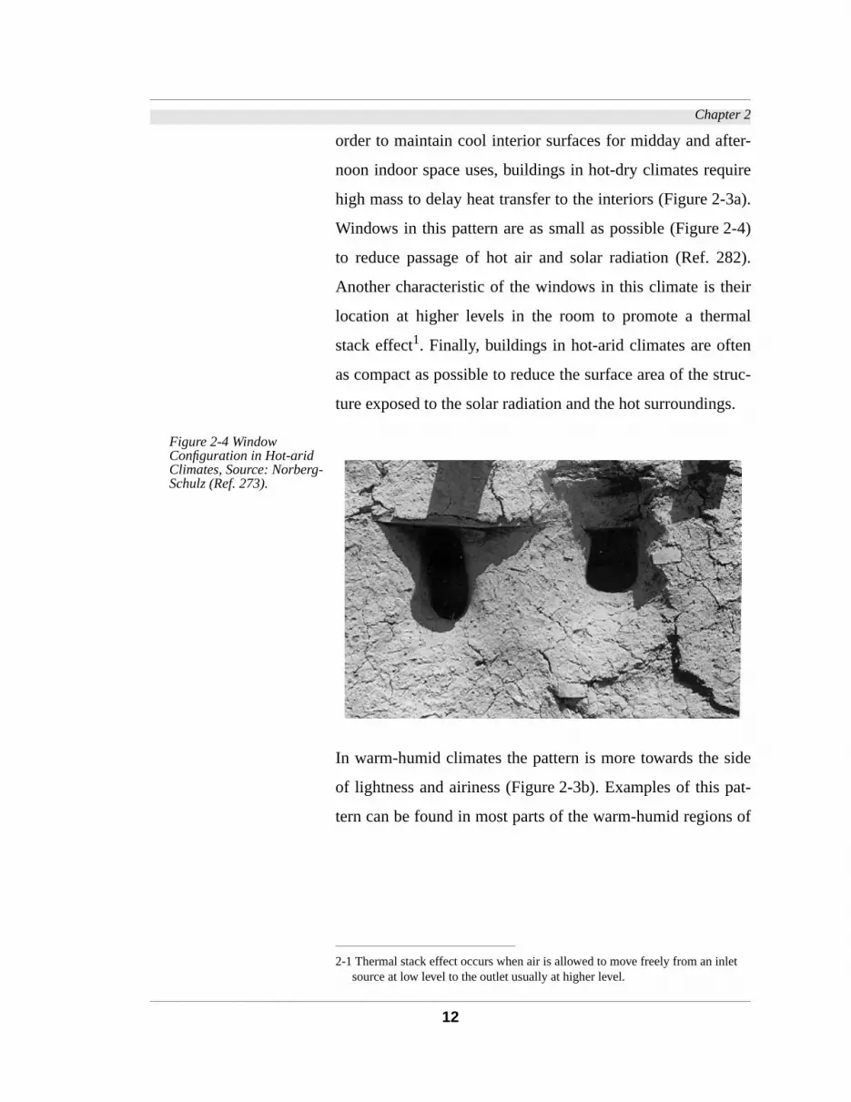
order to maintain cool interior surfaces for midday and after-
noon indoor space uses, buildings in hot-dry climates require
high mass to delay heat transfer to the interiors (Figure 2-3a).
Windows in this pattern are as small as possible (Figure 2-4)
to reduce passage of hot air and solar radiation (Ref. 282).
Another characteristic of the windows in this climate is their
location at higher levels in the room to promote a thermal
stack effect
1
. Finally, buildings in hot-arid climates are often
as compact as possible to reduce the surface area of the struc-
ture exposed to the solar radiation and the hot surroundings.
2-1 Thermal stack effect occurs when air is allowed to move freely from an inlet source at low level to the outlet usually at higher level.
Figure 2-4 Window Configuration in Hot-arid Climates, Source: Norberg-Schulz (Ref. 273).
In warm-humid climates the pattern is more towards the side
of lightness and airiness (Figure 2-3b). Examples of this pat-
tern can be found in most parts of the warm-humid regions of

Chapter 2
13
the world except in a few cases where cultural and social rea-
sons override environmental requirements
2
.
TABLE 2-1 shows a summary of the impact of the hot-dry and
warm-humid climates on the built form. These climatic
responses carry design decisions that influence the architec-
tural style most suited for each climate.
2-2 Examples of anticlimatic designs were observed by the author in Java, Indone-sia where thermal stack effect is used instead of direct ventilation through win-dows because of the fear of air penetrating human body and disturbing its balance.
2.4 Wind and the Built Form
Although the field of building aerodynamics is relatively new,
designing for wind is as ancient as buildings themselves. Since
the beginning of human settlements, traditional plans have
maintained formal structures that responded to climate. The
TABLE 2-1
Summary of Climatic Impact on Building Form in Selected Hot Climates
Building Element
Climate
Hot Dry Warm Humid
Geometry As compact as possibleElongated perpendicular to wind direction
Walls Massive Light
WindowsAperture should be as small as possible
As open as possible to allow for maximum air velocity for occupants’ comfort
ShadingImportant to shade at all times Shading is important
Surface to Volume Ratio As small as possible not as important
Relation to groundClose or even under-ground
Elevated from the ground if possible

Chapter 2
14
archeological digs of the ancient city of Kahun in Egypt 2000
B.C. showed urban zoning based on separating the city into
favorable and unfavorable wind sites. Public buildings and
officials’ housing were located in zones that enjoy the flow of
pleasant northerly winds, while the less affluent groups were
housed at the west side of town where they were exposed to
the hot westerly wind. In addition, the houses on the west side
shielded the more affluent area from the unfavorable wind.
Other examples include the Feng Shui principles in ancient
China which encouraged the integration of elements of wind
and light in building designs. Greek writings also show that
the integration of wind in the design of settlements was a con-
scious decision shared by both the designers and settlers (Ref.
216).
Figure 2-5 Sketch of housing layout at Kahun, Source: (Ref. 30).
Tests of traditional settlements in Dubai (Ref. 251) show that
the orientation, the high and massive walls, the narrow alleys,
and the compactness of the open spaces were successful at
ameliorating its harsh climate. These elements are typical

Chapter 2
15
urban morphological characteristics of settlements in hot arid
climates (Figures 2-6 and 2-7).
Figure 2-6 Settlement in hot dry climate, Source: Koenigsberger et al (Ref. 259).

Chapter 2
16
Figure 2-7 Alley ways, Omdurman, Sudan. Dimensions of the alley guarantee shading throughout most of the day hours. Source: Norberg-Schulz (Ref. 273).
In contrast, warm-humid planning strategies involved promot-
ing natural ventilation of individual buildings and increasing
wind speeds in outdoor spaces (Figure 2-8).

Chapter 2
17
Figure 2-8 Row Housing in Southeast Asia. Source: (Ref. 34).
Figure 2-9 Naturally ventilated traditional building, Source: (Ref. 289)
RRRReeeeaaaallll YYYY
KKKKiiiittttcccchhhheeeennnn
SSSSttttoooorrrraaaaggggeeeeBBBBeeeeddddrrrroooooooommmm
BBBBeeeeddddrrrroooooooommmm
CCCCoooouuuurrrrttttyyyyaaaarrrrdddd
SSSShhhhooooppppOOOOffffffffiiiicccceeee
SSSSttttrrrreeeeeeeetttt
WWWWaaaarrrrmmmm AAAAiiiirrrrWWWWaaaarrrrmmmm AAAAiiiirrrr
FFFFrrrreeeesssshhhhCCCCoooooooollll BBBBrrrreeee
WWWWaaaarrrrmmmm AAAAiiiirrrr
VVVVeeeennnnttttiiiillllaaaaCCCCoooooooollllBBBBrrrreeeeeeeezzzzeeee
WWWWaaaarrrrmmmm AAAAiiiirrrr

Chapter 2
18
2.5 Examples
This section includes examples demonstrating the influence of
wind on traditional Indonesian and Middle Eastern architec-
ture. These examples illustrate the adaptation of architectural
elements such as roofs and cool towers to meet the demands of
warm-humid and hot-dry climates respectively.
2.5.1 Examples form Warm-humid Climates
The climate of the Indonesian Archipelago is predominantly
warm-humid with a brief hot-dry season. The similarity of
architectural forms
3
are due to the uniformity of climatic con-
ditions. To provide thermal comfort for building occupants in
this climate, traditional buildings have large openings on their
exterior walls (Ref. 260 and 240) to maximize indoor airflow
4
.
Figures 2-9 to 2-11 show examples of design solutions to pro-
vide interior spaces with high airflow rates through large win-
dows, louvered walls and roof openings.
2-3 Based on author’s observation.
2-4 Table TABLE 2-1.

Chapter 2
19
Figure 2-10 House (converted rice granary), Sigumpar, Indonesia, Source: (Ref. 267)
In addition to direct ventilation schemes, examples of thermal
stratification-promoting designs can be found in east Java.
Removal of the buildup of warm air to provide thermal com-
fort of occupants is achieved by venting stratified interior air
through roofs and high ceilings (Figure 2-9).To maximize air-
flow through roof openings, many exterior walls in Javanese
houses are porous to permit the displacement of indoor hot air
with cooler outdoor air (Figure 2-11).
Chapter 2
20
Figure 2-11 Example of porous wall construction in Java, Source: Author’s collection.
Figure 2-12 University of Indonesia Campus, Source: Author’s Collection.
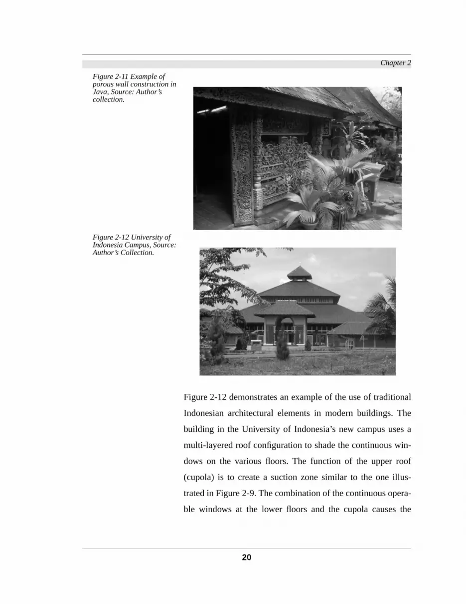
Figure 2-12 demonstrates an example of the use of traditional
Indonesian architectural elements in modern buildings. The
building in the University of Indonesia’s new campus uses a
multi-layered roof configuration to shade the continuous win-
dows on the various floors. The function of the upper roof
(cupola) is to create a suction zone similar to the one illus-
trated in Figure 2-9. The combination of the continuous opera-
ble windows at the lower floors and the cupola causes the

Chapter 2
21
wind to flow upwards, replacing hot interior air with cooler
outside air.
2.5.2 Examples form Hot-dry Climates
In many locations in the Middle East, North Africa, and the
Northwestern corner of the Indian subcontinent, a traditional
ventilation and cooling system has developed. This system is
known as wind towers or wind catchers (
Malqafs
) in Egypt
(Ref. 246),
Badgirs
in Iran the Gulf area (Ref. 238, 6, and
223), and recently referred to as cool towers or ventilation
towers (Ref. 282 and 264). These are all vented towers or ver-
tical projections in the roof intended to catch or remove air
from the interior spaces (Ref. 237).
Ventilation towers -in most cases- act as wind scoops captur-
ing air at roof level and diverting it to indoor spaces. The tem-
perature of inlet air is sometimes cooled by passing it through
underground enclosures. In dry climates, the air is cooled and
humidity raised by passing the airflow over water-filled jars or
though wetted pads.
The design of the inlet portion of ventilation towers (tower
head) depends on the prevailing wind direction. A single-
opening tower suits cases where the prevailing wind comes
from a single direction, while a multi-opening tower head best
suits cases where the wind comes from different compass
directions (Figure 2-13).

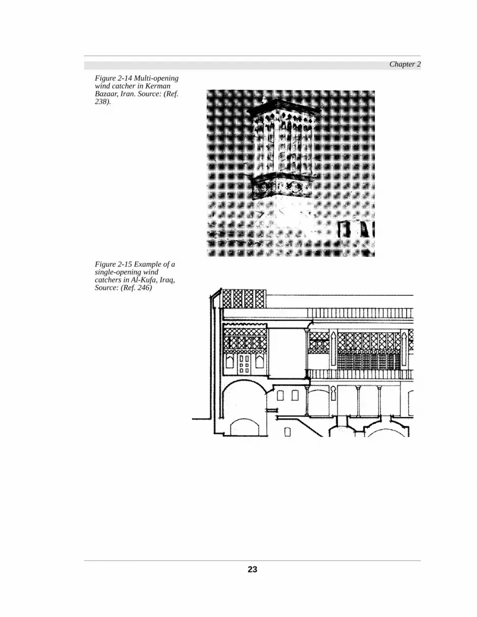
Chapter 2
22
Figure 2-13 Tower head designs, Source: (Ref. 283).
The tower head configuration affects interior and exterior
building design. Because it requires maximum exposure to
different wind directions, a ventilation tower with a multi-
opening head usually becomes a dominant architectural fea-
ture (Figure 2-14). This exterior dominance is often reflected
in the interior plan. The multi-opening tower is usually con-
nected to a large interior space where the cool air is delivered.
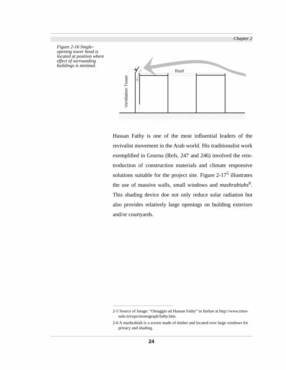
In contrast, single-opening towers are usually less prominent
in both the exterior and interior plan. This configuration is a
product of restricting tower head to a single wind direction. To
maximize exposure to prevailing wind direction, the ventila-
tion tower is often located at the perimeter facing the roof of
the building instead of the exterior (Figure 2-15). This loca-
tion allows the wind tower to face the airflow unaffected by
surrounding buildings (Figure 2-16).
Single-opening Tower Head Multi-opening Tower Head
Chapter 2
23
Figure 2-14 Multi-opening wind catcher in Kerman Bazaar, Iran. Source: (Ref. 238).
Figure 2-15 Example of a single-opening wind catchers in Al-Kufa, Iraq, Source: (Ref. 246)
Chapter 2
24
Figure 2-16 Single-opening tower head is located at position where effect of surrounding buildings is minimal.
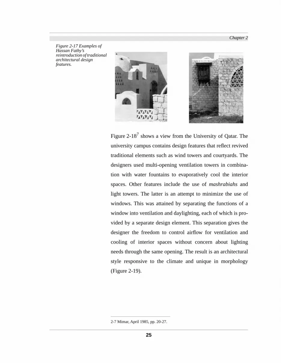
Hassan Fathy is one of the most influential leaders of the
revivalist movement in the Arab world. His traditionalist work
exemplified in Gourna (Refs. 247 and 246) involved the rein-
troduction of construction materials and climate responsive
solutions suitable for the project site. Figure 2-17
5
illustrates
the use of massive walls, small windows and
mashrabiahs
6
.
This shading device doe not only reduce solar radiation but
also provides relatively large openings on building exteriors
and/or courtyards.
2-5 Source of Image: “Omaggio ad Hassan Fathy” in
Italian
at http://www.trien-nale.it/expo/monograph/fathy.htm.
2-6 A mashrabiah is a screen made of timber and located over large windows for privacy and shading.
Roof
Ven
tilat
ion
Tow
er
Chapter 2
25
Figure 2-17 Examples of Hassan Fathy’s reintroduction of traditional architectural design features.
Figure 2-18
7
shows a view from the University of Qatar. The
university campus contains design features that reflect revived
traditional elements such as wind towers and courtyards. The
designers used multi-opening ventilation towers in combina-
tion with water fountains to evaporatively cool the interior
spaces. Other features include the use of
mashrabiahs
and
light towers. The latter is an attempt to minimize the use of
windows. This was attained by separating the functions of a
window into ventilation and daylighting, each of which is pro-
vided by a separate design element. This separation gives the
designer the freedom to control airflow for ventilation and
cooling of interior spaces without concern about lighting
needs through the same opening. The result is an architectural
style responsive to the climate and unique in morphology
(Figure 2-19).
2-7 Mimar, April 1985, pp. 20-27.

Chapter 2
26
Figure 2-18 Modern Design Solutions, University of Qatar, Source: (Ref. 287).
Figure 2-19 Bird’s eye-view of the University of Qatar. Source: Ibid.

Chapter 2
27
In all the examples, wind plays an important role in shaping
the form of individual buildings as well as the architectural
style of the region. The examples also demonstrate the effect
of the wind in shaping the urban morphology. To incorporate
wind in the design of individual buildings or urban layouts,
knowledge of wind behavior around buildings is paramount.
Tools and/or algorithms -if available- should be used to predict
wind flow patterns in urban areas.
2.6 Conclusion
Traditional buildings provide rich examples to architects and
urban planners of how to promote natural ventilation. This
chapter gave a few selected examples characterizing ventila-
tion design in the opposite poles of humid and arid climates.
Most the examples discussed in this chapter demonstrate the
effect of wind on the built form except the example of the city
of Kahun in ancient Egypt (Figure 2-5). The builders of the
city used the general layout to direct favorable breezes
towards and diverted unfavorable winds from certain sections
of Kahun. This exemplifies the use of urban layout to manipu-
late wind movement around buildings.
Although the effect of wind in determining street sizes and
building spacing is generally understood, other factors affect-
ing zonal layout and street pattern often prevail. Designing for
natural ventilation in such conditions requires an understand-
ing of the effect of building layouts on wind movement. To
provide a comprehensive understanding of wind movement
around buildings, wind design should account for the individ-

Chapter 2
28
ual buildings as well as the urban layout. Inversely, relative
sizes and shapes of buildings and the spacing between build-
ings can also be manipulated to produce the desired wind flow
patterns. This study will attempt to provide a set of tools to
allow the designers to determine indoor airflow of buildings in
urban settings.

29
Chapter 3

3
Ventilation Research: Backgroundion
ent
ir
uses
ol-
pre-
al
ious
tly
on
w
ap-
in
uch
ace,
3.1 Introduction This Chapter deals with the description of natural ventilat
and the progression in knowledge leading to the developm
of a mathematical model for the prediction of indoor a
speeds. The chapter begins with a brief description of the
of ventilation, its requirements, and flow mechanisms. F
lows, is a section that discusses the potential impacts of a
diction model on energy, building standards, and therm
comfort.
The subsequent sections of the chapter describe prev
research studies that dealt with ventilation prediction direc
or indirectly. The indirect methods use wind pressures
building surfaces to compute infiltration and interior airflo
through windows located on those surfaces. Finally, the ch
ter dedicates a section to the variables affecting airflow
urban areas.
3.2 Ventilation Natural ventilation is defined as desirable air exchange (s
as through open windows) capable of cooling either the sp
30

Chapter 3
te-
ide
nd-
em-
ion
re is
ght.
dur-
is
the
air-
ver
g
ec-
. 95
efit
as
and
the structure, or the occupants’ bodies. Ventilation cools in
rior spaces by displacing the hot inside air with cooler outs
air. This displacement can be obtained naturally through wi
induced pressure or thermal stack effect.
3.2.1 Airflow Cooling Effects
The amount of heat removed is a function of the ambient t
perature, outdoor temperature and airflow rate. Ventilat
may be used to cool buildings when the outdoor temperatu
less than that of the indoor air. This occurs most often at ni
By removing the sensible heat stored in the building mass
ing nighttime ventilating, interior mean radiant temperature
lowered throughout the early part of the next day. When
outdoor temperature is higher than the indoor temperature,
flow may be cooled evaporatively or through passing air o
shaded spaces.
In humid climates, ventilation is most effective in coolin
building occupants directly. This takes place through conv
tion and evaporation off the skin.
3.2.2 Ventilation Requirements
The requirements of ventilation can be categorized (Refs
and 200) under thermal comfort and health (Figure 3-1). By
satisfying both requirements, residential buildings can ben
from the potential energy saving of natural ventilation use
an alternative to compressor-based cooling during warm
transitional seasons [Givoni (Ref. 102), Byrne et al (Ref. 45),
Arens et al (Refs. 11 and 13)].
31

Chapter 3
ce
sur-
adi-
rior
nd
oor
nt is
her
son
ent
well
tial
es-
ll
all
Figure 3-1 Schematic illustration of ventilation requirements, adapted from van Straaten (Ref. 200)
3.2.3 Mechanisms Affecting Natural Ventilation Airflow
Wind-induced airflow is a result of a pressure differen
between the outside and inside a structure, or between the
faces within which fenestration is located. This pressure gr
ent may be caused either by the difference in interior-exte
temperature (thermal forces) or by external wind flow (wi
forces).
3.2.3.1 Thermal Forces When two openings are at different heights and the ind
temperature is higher than the outside, a pressure gradie
generated causing the inside air to move out of the hig
openings and the outside air into the lower openings [Wat
and Labs (Ref. 219)]. The airflow in this regime is depend
on the temperature difference between inlet and outlet as
as the aperture difference in height (Figure 3-2).
3.2.3.2 Wind Forces The difference in dynamic wind pressure creates a poten
for the air to flow from a point to another point where the pr
sure is lower [Givoni (Ref. 102)]. When wind strikes a wa
perpendicular to its direction of flow, the surface of the w
Removal of bodyand other odorsRemoval of
internally gener-ated pollutants
Provision of suffi-cient oxygen forrespiration
Dilution of respi-ratory pathogens
THERMAL COMFORTHEALTH
VENTILATION BENEFITS
Cooling and/orheating of struc-ture
Air movement forbody cooling
Removal ofexcess heatin occupiedspaces
32

Chapter 3
pres-
than
ibu-
w-
edge
ists
the
s the
g
the
s is
rtia
74.
t of
ts
er-
the
two
experiences pressure higher than that of the atmospheric
sure. The leeward surface experiences pressures lower
that of the atmosphere with less variation in pressure distr
tion than the windward side (Figure 3-2). The side walls ho
ever, experience negative pressures around the windward
and positive pressures at the leeward end.
Cross ventilation occurs when a pressure difference ex
between two exterior openings, whether they are located in
same or different surfaces. This pressure difference cause
indoor air to flow from inlet/s to outlet/s located in buildin
walls at lower surface pressure. In addition, even when
measured pressure difference between the two aperture
equal to zero, some airflow can still occur as a result of ine
from wind entering the window [Ernest and Evans (Refs.
and 78)], or from differences in pressure along the heigh
each window (Ref. 102).
Natural airflow inside buildings is a combination of the effec
of both thermal and wind forces. However, the airflow gen
ated from combing the two forces does not exceed 40% of
windflow generated by the greater force even when the
forces are in the same direction (Ref. 102).
Figure 3-2 Forces Affecting Natural Airflow
Wind Forces Thermal Forces
+ +-
-
33

Chapter 3
d
an-
that
sur-
data
use
ngs
that
ter-
rge
the
that
ing
gs
gs,
d-
kes
pes
es.
3.3 Natural Ventilation Research
Recent studies have quantified and developed models for:
• Indoor ventilation velocities for occupant cooling [Chan
et al, Ernest et al, Bauman et al (Refs. 50, 74-76, 35)].
• Air changes for space cooling [Vickery et al (Ref. 215)].
• Heat transfer coefficients for high air change rates to qu
tify structural cooling under natural ventilation [Pedersenet
al, Spitler (Refs. 172 and 194).
• Infiltration [ASHRAE (Ref. 19)].
The common denominator for these wind effect models is
the designer needs to know wind pressures on building
faces to implement these models.
At present, the designer cannot use weather station wind
to obtain pressure distributions on building surfaces beca
most of the available building pressure data apply to buildi
in open terrain conditions. There are, however, models
take into account generalized effects such as the upwind
rain roughness in the surrounding 5 km, the effect of la
hills, and the height of the building being modeled above
ground surface (Ref. 19).
Although these are useful models, they describe effects
have little impact on building pressures in most actual build
sites. The most important factor influencing wind on buildin
is the large-scale obstruction blocks, i.e., other buildin
trees, etc. in the immediate vicinity of the building being mo
eled. These obstruction blocks cast various forms of wa
downwind. The combined effect of these surroundings sha
wind pressures on other buildings situated within their wak
34

Chapter 3
ses.
lti-
e
ed
ties.
the
ac-
ngs
heir
rob-
the
ur-
ing
or
la-
od
air
tun-
o an
ce
nd
It is not easy to describe these wakes for modeling purpo
For one thing, the number of potential configurations of mu
ple upwind obstructions is virtually infinite, and to rationaliz
them into a set of useful dimensions requires some inform
decisions about the importance of wake-shaping proper
For another, the building being modeled interacts with
wake from its surroundings, so it is not enough just to char
terize the wake-generating properties of the surroundi
alone.
Finally, researchers of this subject have not conducted t
experiments in a consistent way, but have bounded the p
lems they worked on in whatever way was convenient for
study at hand. Their studies of wind pressure in built-up s
roundings can not be generalized for application in a build
energy simulation program such as DOE-2, CALRES
BLAST (Ref. 132).
From the literature review, two categories of empirical venti
tion prediction models could be identified;
3.3.1 Mean Wind Speed Coefficient Method
The first category is the Mean Wind Speed Coefficient Meth
where velocity coefficients are used to predict indoor
speeds. This method relies on data obtained through wind
nel studies of indoor air velocities and presented as ratios t
outdoor reference velocity [Equation (3-1)]. The referen
velocity ( ) is usually taken at 10 m height above grou
(Ref. 25).
Vo
35

Chapter 3
7),
ar-
nd
for
for
ed
een
ut-
en
1 (3-1)
Where
Models in this category are by Aynsley (Refs. 30 and 2
Givoni (Ref. 102), and Chandra (Ref. 54). Despite the app
ent simplicity of the speed coefficient method, obtaining wi
tunnel results may be too difficult and costly, especially
small designs.
3-1 Source: Aynsley 1977 (Ref. 30).
3.3.2 Discharge Coefficient Method
The second category uses the discharge coefficient ( )
the prediction of the natural ventilation. The mean wind spe
entering a space is a function of the difference betw
the windward and leeward pressure Coefficients ( ), o
door air velocity ( ), and the discharge coefficient ( ):
(3-2)
Where
Cv
Vi
Vo------=
Vi indoor air speed (m/s)=
Vo wind speed at site (m/s)=
Cv velocity Coefficient (ND)=
Cd
Vw
Cp∆
Vo Cd
Vw Cd CpV02∆[ ]
1 2⁄⋅=
Vw mean wind speed through an opening (m/s)=
Cd discharge coefficient (ND)=
Cp∆ mean pressure difference coefficient betwe=
windward and leeward surfaces (ND)
V0 wind speed at site (m/s)=
36

Chapter 3
rent
d as
es-
res-
e
ic-
2),
ild-
pre-
E
fil-
gy
cal
e
Wind flow creates pressure differences between the diffe
sides of a building. Surface pressures are usually presente
non-dimensional coefficients relating wind pressures to pr
sures measured at eave height. The numerical value of p
sure coefficients is determined using the following formula:
(3-3)
Where
=mean surface pressure coefficient for each point in th
facade (ND)
=mean pressure at each point on the facade (Pa)
=mean static reference pressure (Pa)
=density of air (kg/m3)
=mean reference velocity at eave height (m/s)
Examples of the discharge coefficient indoor velocity pred
tion methods are found in Ernest (Ref. 76), Chand (Ref. 5
Allard et al (Ref. 5), and Murakami (Ref. 167).
3.4 Shielding Effects
There are a few ways to account for upwind shielding in bu
ing energy simulation, but most of these methods do not
dict surface pressures. For infiltration calculations, ASHRA
Handbook Chapter 23 describes the approach of the LBL in
tration model, which is implemented in most building ener
simulation programs. It uses coefficients based on five lo
shielding classes2 which, when multiplied by the square of th
3-2 Tables 6 and 8, ASHRAE Fundamentals Handbook, 1989, pp. 23.17-18.
Cpi
Pm Ps–( )
0.5 ρ Ve2⋅ ⋅( )
-------------------------------=
Cpi
Pm
Ps
ρ
Ve
37

Chapter 3
ese
pe-
gs
le,
the
d to
in-
tle
nat-
im-
on
ned
ted
the
var-
rom
tud-
d
ious
ind
gs
her
wind speed, give an estimate of outdoor wind velocity. Th
shielding coefficients do not consider the effects of any s
cific obstructions in the vicinity of the building (Ref. 79).
For natural ventilation through large area window openin
the situation is equally inadequate. CALRES, for examp
uses a single factor to predict the local wind speed from
weather tape values. The local wind speed is then converte
air changes using a simple model for airflow through w
dows. In energy code simulations using CALRES, lit
energy effect can be observed from implementing various
ural ventilation strategies. The credit given to designers is l
ited to the potential benefits of introducing natural ventilati
on reducing mechanical system requirements of the desig
space.
3.5 Methods for Predicting Wind Pressures
Most of the existing wind pressure data have been collec
for structural engineering purposes where the interest is in
maximum or minimum pressure values the wind exerts on
ious building shapes. Such data are therefore obtained f
wind tunnel tests on models of unshielded buildings.
3.5.1 Empirical Pressure Models
Swami and Chandra (Ref. 203) summarized many such s
ies for their applicability to natural ventilation design, an
produced functions describing the wind pressures on var
unshielded building shapes through the full range of w
approach angles. However, the vast majority of real buildin
is shielded from the wind by vegetation, topography, or ot
38

Chapter 3
ind
ocks
nd,
y of
rows
ion-
ces
the
ind
ns
of
g
es
nce
ried
ct-
es
wed
as
ind
0˚
res-
the
buildings. Such shielding, considerably changes the w
pressures on building surfaces.
Few researchers have studied the effects of obstruction bl
on building surface pressures. Lee and Soliman, Cha
Wiren, and Balazs have studied the pressures on arra
cubes, and Ernest and Bauman have studied pressures on
of buildings. These studies have resulted in coherent relat
ships defining building surface pressures (Cp), or often the dif-
ference between building windward and leeward surfa
( ), as a function of array spacing and arrangement of
arrays. According to those studies two or three rows of upw
obstructions were sufficient to define the upwind obstructio
(Refs. 13 and 149), similar to the underlining assumption
the program SITECLIMATE (Ref. 10).
The study of Lee et al (Ref. 149) analyzed the shieldin
effects of windward buildings on wind pressure differenc
( ) across the modeled building. In this study, the dista
between the model and the windward obstruction was va
until the effect of the windward block was no longer dete
able. The experiment showed that three wake flow regim
were formed between the two blocks. The same study sho
that for wind direction between 0˚-60˚ from normal, there w
little effect on the pressure difference from changing the w
direction. However, when the wind direction exceeded 6
from the normal to the surface of the tested model, the p
sure difference of the shielded building approached that of
equivalent unobstructed (isolated) model.
Cp∆
Cp∆
39

Chapter 3
d to
g
Ref.
p a
tion
The
m-
ild-
sys-
al
the
e
d-
ri-
a-
of
uta-
es-
ped
nt of
have
fol-
Recently, mathematical relationships have been develope
account for the effect of surrounding buildings on buildin
surface pressures. Among those, Swami and Chandra (
203) used Wiren’s set of experiments (Ref. 226) to develo
function that predicts the pressure shielding of any obstruc
block based on its position relative to the tested surface.
problem with Swami and Chandra’s approach is that it is li
ited to the specific layouts tested in Wiren’s study. Knoll et al
(Ref. 140), on the other hand, related the surrounding bu
ings to the tested surfaces through a Cartesian coordinate
tem. The result is a more flexible model where individu
adjacent blocks are considered despite the layout in which
building is set. Knoll’s approach is however limited by th
inability of the algorithm to take into account complex buil
ing shapes and the effects of gaps between the buildings.
3.5.2 Computational Models
Computational Fluid Dynamic Modeling (CFD) is a nume
cal solution of fluid flow problems using mathematical equ
tions based on fundamental laws of conservation
momentum, energy, and mass (Refs. 131 and 222). Comp
tional techniques for predicting wind velocities, surface pr
sures and fluid temperature distributions were first develo
for nuclear and aerospace industries. With the advanceme
computational speeds and capacities, these methods
found their way into building-oriented applications.
CFD models in buildings may be used to determine the
lowing (Ref. 131):
40

Chapter 3
era-
typ-
d
nce
es
in
nts.
37
ed
. In
d to
FD
dic-
nly
g;
ns
ctual
aller
• Thermal comfort parameters such as air speed and temp
ture.
• Effectiveness of ventilation systems.
• Efficiency of energy distribution in spaces.
3.5.2.1 Advantages In general, current models are capable of simulating most
ical indoor airflows. However, a limited set of outdoor win
environments may be simulated with reasonable resembla
to results obtained from wind tunnel comparisons [Gadilheet
al (Ref. 90)]. These models offer the following advantag
over other ventilation prediction tools;
• CFD models do not require physical modeling such as
wind tunnels.
• They are usually less expensive than full-scale experime
• They proved to be useful in parametric studies (Refs. 1
and 195).
3.5.2.2 Disadvantages Computation Fluid Dynamic models require specializ
expertise to run, monitor, and analyze generated results
addition, substantial computing power and time are neede
run them. With the advancement in computers, however, C
models may represent attractive alternatives to other pre
tion tools in the future. Currently, these algorithms are mai
used in research instead of design because of the followin
• The difficulty to input and establish boundary conditio
which have major effects on the simulation.
• The difficulty to validate results of the simulation.
3.5.3 Field Measurements at Full Scale
Full scale measurement studies use full-scale models or a
structures to test parameters that cannot be modeled at sm
41

Chapter 3
or
ced
o be
ings
g.,
),
ore
el
h-
ow
ild-
ed.
f the
y of
uts,
he
tag-
ribed
nd
scale (Ref. 187). Indoor airflows can be measured directly
through the detection of the decay of a tracer gas introdu
into the space in question. Pressure sensors can als
attached to building surfaces both inside and outside build
(Ref. 112).
3.5.3.1 Advantages • High confidence in results.
• Used for the verification of other prediction methods; e.
wind tunnel and CFD methods [Ashley (Ref. 15
Katayama et al (Ref. 133)].
3.5.3.2 Disadvantages • For design purposes, field measurements are usually m
costly to do than simulation (mathematical or wind tunn
modeling).
• Limited parameters for generalized studies.
• Often difficult to maintain steady state conditions throug
out tests (Ref. 217).
3.6 Summary of Variables affecting Airflow
Despite the large number of variables that can affect airfl
around buildings (and consequently the airflow inside bu
ings), four general categories of variables can be identifi
These are the pattern of urban layout, the compactness o
layout, terrain effect on the boundary layer, and the porosit
obstructions such as trees.
3.6.1 Layout Patterns Because of the enormous number of possible urban layo
only few regular layouts have been tested (Figure 3-3). T
predominant layouts are; normal patterns (Grid-iron) and s
gered patterns. Examples of these configurations are desc
in Soliman (Ref. 191), Wise (Ref. 228), Wiren (Ref. 225), a
42

Chapter 3
es
m
the
sur-
elves
out,
ince
een
tion
acing
Chand et al (Ref. 50). Their studies prove that wind pressur
of shielded building surfaces are drastically different fro
those of unshielded buildings.
Figure 3-3 Tested Patterns in Shielded Studies
3.6.2 Compactness of Layout
Compactness of the layout is a general term that includes
distances between the obstruction blocks and the tested
faces as well as the spaces between the blocks thems
(Refs. 149 and 192). In general, the more compact the lay
the lower the local wind speeds and surface pressures. S
the compactness of layout is a function of the spacing betw
blocks, it can be concluded that there is an inverse rela
between wind speeds and surface pressures and the sp
between blocks.
Normal Pattern
Staggered Pattern
Instrumented Block whosesurface pressures are tested
43

Chapter 3
der
rent
to
n at
are
and
by
e a
ces
and
trees
he
Figure 3-4 Gradient height depends on the roughness of the terrain.
3.6.3 Boundary Layer and Terrain Effects
The terrain affects the degree of exposure of the site un
investigation. Different terrain roughnesses generate diffe
boundary layers and exponential functions can be used
determine wind speeds at any height from a known locatio
reference height. These characteristic boundary layers
shown in Figure 3-4.
Effects of terrain on boundary layers are well documented
can be estimated using any of the methods suggested
ESDU (Refs. 72 & 73), Murakami et al (Ref. 168), Arens et al
(Ref. 10), or Aynsley (Ref. 24)].
Local topography such as hills and valleys also can hav
strong influence on the boundary layer. Such non-flat surfa
redirect the airflow, changing its strength, steadiness
direction (Refs. 12, 96, &127).
3.6.4 Effects of Vegetative Windbreaks
Some studies have been conducted to assess the effect of
on the wind environment, particularly of shelterbelts for t
275 m
365 m
460 m
Wind Velocity
Hei
ght
abov
e G
roun
d
OpenCountry
Suburban
City
44

Chapter 3
are
man
om
ef.
the
this
ert
bs
hat
ngs
s.
lex
hed
el-
ased
tion
tions
s in
er-
ld-
ary
that
air
reduction of ground wind speeds over crops. Shelterbelts
also applicable in areas where pedestrians and other hu
activities might be adversely affected by high wind levels.
Wind speeds downwind of shelterbelts are reduced (fr
15%–68%) depending on their density or permeability (R
161). The higher the density of the vegetation, the shorter
distance to where the wind regains most of its energy (
occurs 8–17 times the height of the wind screen). Rob
White’s investigation (Ref. 221) of the effect of trees, shru
and hedges on the natural ventilation of buildings found t
the type of vegetation, and its distance from the openi
greatly influences the airflow inside the sheltered structure
The analysis of the effect of vegetation on airflow is a comp
issue (Ref. 96). However, some studies have establis
empirical coefficients through which the wake behind a sh
terbelt can be predicted (Ref. 10). These estimates are b
on the freestream wind speeds, profile, density of vegeta
and the distance behind the shelterbelt. Seasonal correc
may be applied to account for leaf loss of deciduous tree
winter.
3.7 Conclusion The wind is an integral ingredient in the determination of th
mal comfort for the occupants of a naturally ventilated bui
ing. Early consideration of thermal comfort may be necess
if acceptable climate responsive solutions are desired.
Recently, mathematical models have been developed
apply building surface pressure data to predict indoor
45

Chapter 3
ed
ilable
ild-
s of
sted
are
heir
the
not
on-
velocities, and flow patterns in simple single and partition
spaces. However, very few surfaces pressure data are ava
for situations where the building is surrounded by other bu
ings that affect the wind on its surfaces. The few database
measured pressures are limited by the specificity of the te
layout configurations.
Computational fluid dynamics methods, on the other hand,
in most cases inaccessible to the designers by virtue of t
complex input and the computation time they require.
The few available pressure prediction models that consider
shielding effects of surroundings are simple and do
address the complex variations in urban form that might c
front the modeler.
46

47
Chapter 4

4
Development of an Empirical Model for the Prediction of Surface Pressures in Shielded Environmentsws
ind
m-
e,
ted
on
m
The
ks,
tical
thin
iri-
an-
the
s
4.1 Introduction Pressure differences on building surfaces drive the airflo
through openings in those surfaces. The distribution of w
pressure on building walls and windows varies with the geo
etry of the building, wind direction, the adjacent roof shap
and the surrounding building blocks. The wakes genera
behind windward obstruction blocks cause the pressures
surfaces falling within these wakes to vary significantly fro
surface pressures in similar unshielded circumstances.
shielding effect is a factor of the number of obstruction bloc
their size, and position relative to the surface.
This chapter describes the development of a mathema
model to predict the pressures on wall surfaces located wi
wakes of windward buildings. The model is based on emp
cal results of wind tunnel tests, developed in a stepwise m
ner to retain simplicity in the final mathematical model.
4.2 The Proposed Model
The general objective of the intended model is to predict
effect of the surrounding buildings on the indoor airflow
48

Chapter 4
as
ior
M)
nd-
he
ural
of
sily
sur-
ble
rgy
s of
es,
the
uld
of
d to
sures
of
sin-
ion
through building fenestration. To do this, new work w
required for predicting wind pressures on building exter
vertical surfaces behind or adjacent to obstruction blocks.
To be useful in design, the pressure prediction model (PP
should use simple techniques for characterizing the surrou
ing buildings. The method should not require from t
designer any knowledge of the fundamentals of architect
aerodynamics. The input should be limited to a description
the surrounding buildings in terms that can either be ea
taken off site plans or measured using conventional site
veying methods.
The model should be in the form of an algorithm compati
with existing wind databases so it can be used with ene
analysis programs. The model should allow direct estimate
the effect of wind shielding on building surface pressur
given the configuration of surrounding obstructions, and
terrain roughness. The outcome of such an algorithm sho
be hourly pressure values in a format matching that
recorded hourly wind speed and direction data.
Finally, as a by-product of the physical experiments neede
produce this model, an extensive database of surface pres
could be accumulated.
4.3 Approach The first step in developing the algorithm for the prediction
surface pressures was to investigate the validity of using a
gle obstruction block to represent multiple rows of obstruct
blocks.
49

Chapter 4
y-to-
d on
to
y-
re
was
tion-
ous
ind-
n
ace
een
ind
th,
und-
he
no
by
ur-
icu-
The second was to establish a simple-to-obtain and eas
use set of model variables. These variables were base
angular description of individual obstruction blocks relative
the surface on which air pressure was to be determined.
Third, in developing a non-dimensional coefficient for stud
ing the shielding effects, a function for predicting pressu
coefficients of the unobstructed instrumented surfaces
needed. This was done by adapting a mathematical rela
ship developed by Lee et al (Ref. 149).
Fourth, these simple relationships were studied for vari
arrangements of the instrumented model and a single w
ward obstruction block. Both the width of the obstructio
block and the distance from the instrumented model surf
were varied. In these tests, the center-to-center line betw
the model and obstruction block was parallel to the w
direction1. Variables such as the obstruction height and dep
the size and shape of the instrumented model, and the bo
ary layer characteristics were kept constant.
The fifth step involved varying the displacement of t
obstruction block so that the center-to-center line was
longer parallel to the wind direction. This was achieved
sliding the obstruction block parallel to the instrumented s
face and simultaneously maintaining both blocks perpend
lar to the wind direction.
4-1 This setup is referred to as the orthogonal Configuration (Section 4.12).
50

Chapter 4
ed
r the
he
del
A-
ple
was
al
cks.
ri-
tru-
ects
oth
rpo-
el.
ata
-
lex
ing
res
Sixth, the effect of changing the wind direction was analyz
under two scenarios. These scenarios based on whethe
obstruction is parallel to the instrumented model or not. T
two scenarios involved rotating both the instrumented mo
and obstruction block on the wind tunnel turntable (Figure
1) to simulate wind direction change.
The seventh step was the study of the effect of multi
obstructions blocks on the instrumented surface. This
accomplished by comparing the shielding effect of individu
blocks to the measured pressure values of the multiple blo
These tests involved rotating two obstruction blocks of va
able gap widths, spacing, and displacement from the ins
mented surface.
Eighth, the mathematical model needed to include the eff
of roof shapes and more complex building plan forms. B
had been analyzed in previous research and could be inco
rated into the algorithm.
The ninth step was to verify the resulting mathematical mod
This verification used results from two sources. The first d
were obtained from a study conducted at the National Swedish
Institute for Building Research (Refs. 225 and 226). The sec
ond source of data was a wind tunnel study of a comp
urban setting, conducted by the author.
4.4 Background A number of research studies have analyzed the shield
effects of surrounding buildings on wall surface pressu
[Lee et al (Ref. 149), Hussain et al (Ref. 124), Ernest (Ref.
51

Chapter 4
nt,
or-
s of
ted
the
ld-
ruc-
he
rom
the
and
rface
ure stru-
74), and Wiren (Ref. 225)]. To take urban layouts into accou
they tested standardized configurations; e.g. grid-iron (n
mal), staggered, and free layouts (Figure 3-3). The result
the different studies vary because of the difference in tes
model configurations. The variation can be attributed to
many variables involved in describing the surrounding bui
ing configurations, e.g. spacing between model and obst
tions, relative position of obstruction to model, and t
number of windward blocks (Figures 4-3, 4-2, and 4-4).
Figure 4-1 Comparison between examples from Hussain et al, Wiren, and Ernest shielding experiment results
Figure 4-1 shows a comparison of the results obtained f
urban layout effect studies conducted by Hussain et al (Ref.
124), Wiren (Ref. 225), and Ernest (Ref. 74). The data in
graph are represented in pressure coefficient differences2 as a
function of the distance between the instrumented models
4-2 The pressure coefficient is a non-dimensional ratio between the average supressure and wind pressure at a specific reference height (Eq.3-3). Pressure coefficient difference in these studies refers to the absolute value of the presscoefficient difference between the windward and leeward surfaces of the inmented models.
BBBBBBBB
BBBB
B
B
J
J
J
H
H
H
H
H
HH
H H
-0.60
-0.40
-0.20
0.00
0.20
0.40
0.60
0.80
1.00
1.20
0 1 2 3 4 5 6 7 8 9 10
Pre
ssu
re D
iffe
ren
ce C
oef
fici
ents
(C
p)
Spacing (S/H)
B Hussain et al 1980
J Wiren 1984
H Ernest 1991
52

Chapter 4
r-
rib-
r of
ree
nt
rly
i-
lted
ver
sts,
ock
f a
da-
tion
ed by
he
ect
over,
ks
the
ing
not
of
re at
the obstruction blocks3. Ernest’s results are noticeably diffe
ent from the other two studies. This difference can be att
uted to differences in the test models and in the numbe
obstruction blocks. Wiren’s results4 were obtained by testing a
gable-roofed model amid a normal layout (Figure 4-2) of th
rows of identical obstruction blocks. Hussain’s experime
tested a cubic model with a flat roof in the middle of simila
configured array of obstruction blocks (Figure 4-3). The sim
larity in configuration between these two experiments resu
in an almost identical distribution of surface pressures o
spacing5 despite the differences in roof shapes. Ernest’s te
on the other hand, used a single flat-roofed obstruction bl
extending the width of the wind tunnel (200 cm) upwind o
flat-roofed model. The long obstruction block causes a fun
mentally different shielding effect.
This result demonstrates the problems of applying predic
models based on specific layouts such as the one suggest
Lee et al (Ref. 149). However, all studies showed that t
outer or peripheral obstruction blocks and rows did not aff
the pressure values on the measured surfaces. More
increasing the number of rows of obstruction bloc
(upstream) showed little effect on surface pressures after
third row (Refs. 34, 225, and 212). This means that add
more blocks beyond the closest rows of obstructions does
4-3 The distance was expressed as spacing, or the ratio between the distancebetween the instrumented model and the obstruction blocks and the heightthe obstruction block/s.
4-4 Wiren’s experiments are described in details in Section 4.17.1.
4-5 Data are corrected for boundary layer characteristics and reference pressueave height.
53

Chapter 4
gs
significantly change the shielding effect of the surroundin
(Figure 4-7).
Figure 4-2 An example of Wiren’s test configuration (the one-row Grid-iron pattern)
Figure 4-3 An example of Lee et al experiment (the Normal Pattern)
Spacing
54

Chapter 4
to
ari-
truc-
ed
uch
al
the
the
ruc-
tru-
rent
act
cks
the
tion
Figure 4-4 Ernest’s shielded model configuration
In summary, most of the available prediction models apply
specific urban layout configurations. These models use v
ables such as the spacing and the number of upwind obs
tion rows to predict surface pressure in a shield
environment. However, they do not address other factors s
as; the effect of changing the position of the individu
obstruction blocks relative to the instrumented surface,
effect of multiple blocks of different size and shapes, and
size and position of the gaps between these blocks.
4.5 Multiple Rows of Obstruction Blocks
As described above, beyond three rows of windward obst
tion blocks there was no effect on the pressure on the ins
mented surface. This might be attributed to the appa
impermeability of the windward obstructions despite the f
that the blockage was formed by several discrete blo
(Figure 4-5). The question would then be, should only
obstruction blocks visible to the surfaces under considera
55

Chapter 4
ct-
dded
ed
ing
tive
be included in the definition of obstruction blocks in predi
ing the shielding effects?
Figure 4-5 Multiple discrete obstruction windward blocks.
4.5.1 Tsutsumi et al ’s Experiments
In a series of experiments conducted by Tsutsumi et al (Ref.
212), surface pressures were measured for a block embe
within arrays of identical blocks in normal grid and stagger
layouts (Figure 4-6). The number of rows and the spac
between the block were varied to evaluate their respec
effects on measured surface pressures.
Plan View
View of Windward Obstruction
Wind Direction
56

Chapter 4
ore
ect
tice-
two
by
rd
the
Figure 4-6 Tsutsumi et al experimental setup (Ref. 212).
The results shown in Figure 4-7 indicate that adding m
rows beyond the first or second does not significantly aff
the surface pressures. However, Figure 4-7a shows a no
able jump in the measured pressures between one and
rows of upwind obstruction blocks. This might be caused
the conditions of this experiment. There are no windwa
roughness elements for simulating a boundary layer on
windward section of the wind tunnel (Figure 4-6).
4.3 m
1.5 m
1.5
m
Staggered Layout Normal Grid Layout
No
obst
ruct
ion
1 R
ow U
pwin
d
2 R
ows
Upw
ind
3 R
ows
Upw
ind
Sc
re
en
Wind
Instrumented modelvariable location
57

Chapter 4
of
ere
wind
ry
ows
op-
ind
Figure 4-7 The result of increasing the number of obstruction blocks. Source: Tsutsumi et al (Ref. 212).
The resulting high wind speed incident on the first row
windward obstructions causes a large wake within which th
are low surface pressures on the second row (one row up
of the model in Figure 4-7a). A fully developed bounda
layer appears to be generated only beyond three upwind r
of obstruction blocks. This can be attributed to the devel
ment of a flow regime where the distance between the upw
0
0.1
0.2
0.3
0.4
0.5
0.6
0 1 2 3 4 5 6 7 8 9
Pre
ssur
e C
oeffi
cien
t (C
p)Number of Rows Upwind
Normal Grid
Staggered Grid
NoObstructions
(a) Width-to-height ratio =4
0
0.1
0.2
0.3
0.4
0.5
0.6
0 1 2 3 4 5 6 7 8 9
Pre
ssur
e C
oeffi
cien
t (C
p)
Number of Rows Upwind
Normal Grid
Staggered Grid
NoObstructions
(b) Width-to-height ratio =1.3
58

Chapter 4
ents
g
d-
ea-
odel
ntly
he
the
d is
ari-
the
elements allows stable vortices to form between the elem
(Figure 4-8c). This flow pattern is similar to the skimmin
regime described by Lee et al (Ref. 149) and shown in
Figure 4-8. With multiple rows of obstruction blocks, a boun
ary layer develops where stable pressure coefficients are m
sured on the instrumented model surfaces.
Figure 4-8 The three airflow regimes between two identical blocks, Source: Lee et al (Ref. 149)
Figure 4-7a shows that wind pressures measured on the m
surface in the staggered layout experiments were consiste
lower than in the normal grid layout. By staggering t
obstruction blocks, the wind was less able to flow through
gaps than in the case of normal grid layout where the win
channeled through the gaps.
Figure 4-7b, on the other hand, does not show significant v
ations in the measured values of surface pressures on
a. Isolated Roughness Flow Regime
b. Wake Interference Flow Regime
c. Wake Skimming Flow Regime
59

Chapter 4
ow
4-
ted
e
ron
eeds
of
on-
4-9
e the
o,
l
e
i’s
vel-
instrumented model after the first row (normal) or second r
(staggered). Unlike the smaller obstruction blocks (Figure
7a), the tested configuration blocks in Figure 4-7b genera
skimming airflow regimes very early in the wind tunnel. Th
staggered grid needed two rows to stabilize while the grid-i
layout needed one. This is because the staggered layout n
two rows upwind to have one obstruction directly upwind.
4.5.2 Verifying the Effect of Multiple Obstruction Rows
In order to determine the possibility of substituting an array
discrete obstruction blocks with a single block, the author c
ducted a number of preliminary wind tunnel tests. Figure
shows the variables tested in these experiments. These ar
obstruction widths (20 and 61 cm), number of rows (one, tw
and three), the spacing (Sm) between the instrumented mode
and the first windward row6 (2, 3, 4, and 6 Spacings), and th
spacing between the first and second rows7 (2, 3, and 4). To
avoid the anomalous first two rows described in Tsutsum
experiments, the setup of experiments included a fully de
oped boundary layer upwind of the instrumented model.
4-6 Spacing#1 (Figure 4-9).
4-7 Spacing#2.
60

Chapter 4
Figure 4-9 Setup of an initial experiment to study the effect of windward multiple rows on surface pressures.
Figure 4-10 Surface pressure measurement results for obstruction width=20 cm
Instrumented model First Row Second Row
Spacing#1 Spacing#2
ObstructionBlocks
Wind
Side View
Plan View
Ob
stru
ctio
nw
idth
20
an
d 6
1 c
m
20
cm
10 cm
10
cm
2, 3, and 4
Ob
stru
ctio
nw
idth
20
an
d 6
1 c
m
10 cm 10 cm
B
B BJ
J JH
H H
F F F
-1
-0.8
-0.6
-0.4
-0.2
0
0.2
0.4
0.6
0.8
1
2 3 4
Pre
ssur
e C
oeffi
cien
t (C
p)
Spacing#1 between first row and surface
B single obstruction row
Jtwo rows ofobstructions,Spacing#2=2
Htwo rows ofobstructions,Spacing#2=3
F unobstructed
61

Chapter 4
ruc-
tru-
0.5
tion
ted
pac-
t of
pac-
of
was
he
tion
tion
sult,
gle
Figure 4-11 Surface pressure measurement results for obstruction width=61 cm
Figure 4-10 shows that upon adding a second row of obst
tion blocks (20 cm in width), surface pressures on the ins
mented model increased by a maximum of 20% (from 0.4-
Cp) above those measured when using a single obstruc
row. The maximum difference in pressure between obstruc
and unobstructed models occurred when Spacing#1 and S
ing#2 were equal to 2. At all tested spacing#1, the effec
increasing the spacing between the obstruction rows (s
ing#2) was negligible.
When the obstruction block width was 61 cm, the effect
adding a second obstruction row at spacing#1 equals to 2,
very apparent (Figure 4-11). This effect diminishes with t
increase of the spacing#1. This can be attributed to forma
of airflow regimes similar to those described in Lee et al (Ref.
149). Figure 4-12a shows that when spacing of obstruc
rows was small, the two rows acted as a single row. As a re
the wake behind the two rows is smaller than that of a sin
B
B
B
J
J
J
H
HH
F
F
F
-1
-0.8
-0.6
-0.4
-0.2
0
0.2
0.4
0.6
0.8
1
2 4 6
Pre
ssur
e C
oeffi
cien
t (C
p)
Spacing#1 between first row and surface
B single obstruction row
Jtwo rows ofobstructions,Spacing#2=2
Htwo rows ofobstructions,Spacing#2=3
Ftwo rows ofobstructions,Spacing#2=4
unobstructed
62

Chapter 4
ere
with
rated
row
ere
elop
iso-
gree
be
uc-
ern.
le
tical
ws
ted
re-
ay
block (Ref. 79). Figure 4-12c represents a flow regime wh
the wake generated behind the first row does not interfere
the one behind the second row. As a result, the wake gene
behind the second row is similar to one behind a single
(Figure 4-12d). Figure 4-12b represents a flow regime wh
the space between the two rows is not small enough to dev
a stable vortex and at the same time not large enough for
lated roughness flow regime to take place. These results a
with the conclusions of Gowda et al (Ref. 108).
Figure 4-12 Flow regimes around lows of long obstruction blocks.
In conclusion, additional rows of obstruction blocks can
ignored in any proposed mathematical model if the obstr
tion blocks have the same widths as the model of conc
This is especially true for any obstruction block not visib
from the instrumented surface. The proposed mathema
model however, should account for the effect of multiple ro
of obstruction blocks when wake interference and isola
roughness flow regimes are encountered.
An additional conclusion that can be interpreted from the p
vious study is that a single windward obstruction block m
a. SkimmingFlow Regime
b. Wake InterferenceFlow Regime
c. Isolated RougnessFlow Regime
d. Single Obstruction
Wake Length
63

Chapter 4
uc-
rier
n
the
def-
s to
gle
d a
ea-
.
tric
the
-18
be used to predict the effect of an array of windward obstr
tion blocks when the array forms an impermeable bar
windward of the building (Section 4.5). This conclusio
agrees with the supposition set by Ernest (Ref. 75).
4.6 Definition of Variables
The following sections describe the general definition of
variables and terminology used throughout the study. The
inition of some of these variables is refined in later section
account for complexities in the mathematical model.
4.6.1 Wind Direction Angle ( )
The wind direction angle is defined in this study as the an
(in degrees) between a line denoting the wind direction an
line perpendicular to the surface of interest. The angle is m
sured clockwise and ranges between 0˚-360˚ (Figure 4-13)
Figure 4-13 Definition of Wind Direction angle
4.6.2 Obstruction Block Description
Individual obstruction blocks are described using geome
angles from a point established at the bottom center of
obstruction-facing surface (Figure 4-14). Figures 4-15 to 4
represent the four geometric variables used in this model.
Θ
Wind Direction Angle (Θ)360˚
64

Chapter 4
ing
sing
of
en
sur-
hat
e of
Figure 4-14 Location of representative point on instrumented Surface
4.6.2.1 Horizontal Angle
( )
The horizontal angle ( ) is defined as the angle originat
from the center of the instrumented surface and encompas
the visible limits of the obstruction block from the center
the instrumented model (Figure 4-15).
Figure 4-15 Basic variables: Horizontal Angle (αh)
4.6.2.2 Vertical Angle ( ) The definition of the vertical angle ( ) is that angle betwe
a line connecting the bottom center of the instrumented
face to the center of the obstruction block and a line t
encompasses the highest visible edge on the vertical plan
the obstruction block (Figure 4-16).
Elevation
Pressure Measurement Locations
Representitive Point Location
Instrumented Model Surface
αh
αh
2
31
αh1αh2
αh3
InstrumentedSurface
αv αv
65

Chapter 4
rom
the
del
nce
the
en
mal
as a
Figure 4-16 Basic variables: Vertical Angle (αv).
4.6.2.3 Model Spacing (S m) Model spacing is defined as the perpendicular distance f
the center of the instrumented surface to the center of
obstruction block divided by the height of instrumented mo
(Figure 4-17).
Figure 4-17 Basic variables: Spacing (Sm).
4.6.2.4 Obstruction Spac-ing (S o)
The obstruction spacing represents the same dista
described in Section 4.6.2.3 divided by the height of
obstruction block instead of the instrumented model. Wh
the line connecting the two centers coincides with the nor
wind direction, the obstruction spacing can be expressed
function of the vertical angle as follows:
αv
αv
1
2
3
S1
S2S3
InstrumentedModel
ObstructionBlocks
66

Chapter 4
the
the
f pre-
si-
cific
effi-
by
nts
ind
ent
plot-
of
oth
4.6.2.5 Displacement
Angle ( )
The displacement angle (Figure 4-18) is defined as
angle between the wind direction and the line bisecting
horizontal angle ( ) of an obstruction.
Figure 4-18 Basic variables: Displacement Angles
The choice of the these angles was based on a number o
liminary experiments. The criterion for choice was the sen
tivity of measured surface pressures to changes in the spe
geometric variable.
4.7 Angular Description of Obstruction Blocks
Figure 4-19 shows a comparison between the pressure co
cient results obtained from shielded model experiments
Ernest and Wiren (Refs. 74 & 225). These experime
involved locating models with instrumented surfaces beh
windward obstruction blocks. The shown pressure coeffici
values were measured at the windward shielded surfaces
ted against obstruction spacing. By comparing the effects
the single obstruction on pressure coefficient values in b
experiments the following can be observed:
So αv( ) 1–tan=
αd
αd
αh
Win
d D
irect
ion
1
2
αh1/2
αd1
αd2
αh2/2
Cp
67

Chapter 4
he
and
val-
in
rms
tru-
tion
At equal to about 0.0 (points A and B in Figure 4-19), t
corresponding values of spacing on the x-axis were 2.3
7.4 in Wiren’s and Ernest respectively. Both these spacing
ues corresponded to geometric relationships illustrated
Figure 4-20. This relationship can also be described in te
of obstruction angles from a representative point on the ins
mented surface (Figure 4-14). The measured obstruc
angles both configurations are described in TABLE 4-1 .
Figure 4-19 Comparison of Ernest’s and Wiren’s experiments
Figure 4-20 Ernest’s and Wiren’s tested configurations
Cp
B
BB
B
J
J J
H
H
H
H
HH
HH H
-1.4
-1.2
-1
-0.8
-0.6
-0.4
-0.2
0
0.2
0.4
1 2 3 4 5 6 7 8 9 10
Pre
ssur
e C
oeffi
cien
t @ w
indw
ard
surf
aces
(C
p)
Spacing (S/H)
B Wiren's Single
J Wiren's Multiple
H Ernest's Long
A B
Wiren's Experiment Ernest's Experiment
68

Chapter 4
hor
d an
the
ntil
The
tted
he
ere
ip
scrip-
In addition to Ernest’s and Wiren’s experiments, the aut
tested surface pressures on an instrumented model behin
89 cm wide obstruction block. The spacing between
obstruction block and the instrumented model was varied u
the measured pressure coefficient was equal to zero.
angles of view at that location were measured and plo
against Ernest’s and Wiren’s experiments (Figure 4-21). T
three points can be connected with straight line wh
. This simple relation may indicate a relationsh
between surface pressures and the proposed angles of de
tion of the windward obstruction blocks.
Figure 4-21 Obstruction angles coincident with measured surface pressure coefficients ( )=0
TABLE 4-1 Angular Description of the Obstruction in tested Configurations
Experiments Horizontal Angle of View Vertical Angle of View
Ernest 110˚ 40˚
Wiren 7˚ 23˚
Cp
Cp 0=
Cp
0 30 60 90 120 150 180
15
30
45
60
75
90
Cp=0
Horizontal Angle (°)
Ver
tical
Ang
le (
°
)
Wiren
Ernest
89 cm obstruction block
69

Chapter 4
the
he
re-
los-
ge
be
the
he-
lded
tion
del
odel
ure is
ruc-
4-
al
ock.
4.8 Summary and Conclusions
The following are four points that can be concluded from
analysis thus far:
• In most cases only visible obstruction blocks affect t
pressure values on surfaces of concern.
• In most cases, multi-row obstruction blocks can be rep
sented by a single block located at the location of the c
est obstruction block.
• If an array of obstructions form an impermeable blocka
in the windward direction, a single obstruction block can
used to represent the array.
• A number of geometric angles may be used to predict
effect of obstruction blocks on the surfaces of concern.
4.9 Developing the Mathematical Model
The following sections describe the development of a mat
matical model to predict mean surface pressures on shie
surfaces.
Based on the premise that a smaller or a distant obstruc
block produces less shielding effect on an instrumented mo
than a close or a large one (Ref. 10), the mathematical m
was structured in such way that the average surface press
determined by averaging the shielding effects of the obst
tion blocks visible from the instrumented model (Figure
22). The prediction of the shielding effect of individu
obstructions is based on the solid angle describing each bl
70

Chapter 4
ree
.11).
the
s of
ent
ur-
r.
ace
Figure 4-22 The Shielding Effect of an Obstruction Block.
The proposed mathematical functions were built upon th
components:
• Surface pressures on the unobstructed block (Section 4
• Surface pressures on the shielded bock (Section 4.12).
• The development of a non-dimensional factor that uses
ratio two above pressures (Section 4.10).
4.10 Pressure Shielding Modification Coefficient
Swami and Chandra (Ref. 203) showed that the proportion
a building surface affect the values of wind pressure incid
on that surface. To eliminate the effects of differences in s
face dimensions, Swami et al used a non-dimensional facto
This factor is calculated by normalizing the average surf
Win
d D
irect
ion
TestedModel
Obstruction blocks
Shielding Effect ofIndividual Obstruction Blocks
Cpm
71

Chapter 4
on
ith-
d in
dels
int
of
the
nel
. The
face
e is
the
pres-
out
be
pressure coefficients ( ) to those at wind directi8.
In their model, the mean Pressure Coefficient ( ) is an ar
metic average of individual pressure coefficients measure
an even array on the surface of the instrumented mo
[Equation (4-1)]. The local Pressure Coefficient for each po
on the surface ( ) is defined as a non-dimensional ratio
the surface dynamic wind pressure averaged over time to
free-stream dynamic pressure at the model eave height9. For
this work, the dynamic pressure of the free-stream wind tun
at eave height was obtained in a separate wind tunnel test
pressure coefficient for each point at the instrumented sur
was calculated according to Equation (3-3).
The Pressure Coefficient averaged for the whole facad
determined using the following function:
(4-1)
In order to describe the shielding of surrounding buildings,
measured pressure coefficient had to be referenced to the
sure coefficient on the same instrumented model with
upstream obstructions. For any wind angle Θ, the mean pres-
sure coefficients of shielded instrumented surfaces could
4-8 In Swami and Chandra’s (Ref. 203), Normalized Pressure Coefficient was
defined as .
4-9 Eave height is 3.0 m or 10 cm model at scale (Section A.3 in Appendix A).
Cp
Θ( ) 0°=
CpΘ
Cpat Θ 0°=-------------------------
Cp
Cpi
Cp
Cpi
i 1=
n
∑n
-------------------=
72

Chapter 4
ded
nts
d
ing
rm.
e to
res
nal
an
ob-
he
e-
es
divided by the mean pressure coefficient on the unshiel
model resulting in normalized mean pressure coefficie
( in Equation 4-2).
(4-2)
Examining wind direction effects on showe
that zero pressure coefficients can be found. To avoid divid
by zero, Equation (4-2) was modified to an exponential fo
This form has the added advantage of being more sensitiv
variation in small values of the unshielded surface pressu
than is the normalized form. The result is a non-dimensio
coefficient that characterizes the degree of shielding of
obstructed building surface compared to an identical un
structed surface in similar boundary layer conditions. T
Pressure Modification Coefficient ( ) is defined math
matically as follows:
(4-3)
Where
Cp Norm( )
Cp Norm( )
Cp ShieldedΘ( )
Cp UnshieldedΘ( )----------------------------------------=
Cp UnshieldedΘ( )
Cpm
Cpme
Cp ShieldedΘ( )
eCp UnshieldedΘ( )
------------------------------------=
eCp ShieldedΘ( ) Cp UnshieldedΘ( )–[ ]
=
Cpm Pressure Modification Coefficient=
Cp ShieldedΘ( ) Pressure Coefficient on shielded surfac=
at wind direction ΘCp UnshieldedΘ( ) Pressure Coefficient on unshielded=
surfaces at wind direction Θ
73
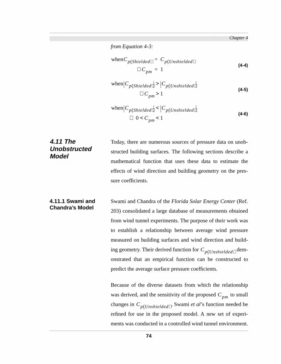
Chapter 4
nob-
e a
the
s-
ained
as
sure
ild-
-
to
ship
all
eri-
ent.
from Equation 4-3:
(4-4)
(4-5)
(4-6)
4.11 The Unobstructed Model
Today, there are numerous sources of pressure data on u
structed building surfaces. The following sections describ
mathematical function that uses these data to estimate
effects of wind direction and building geometry on the pre
sure coefficients.
4.11.1 Swami and Chandra’s Model
Swami and Chandra of the Florida Solar Energy Center (Ref.
203) consolidated a large database of measurements obt
from wind tunnel experiments. The purpose of their work w
to establish a relationship between average wind pres
measured on building surfaces and wind direction and bu
ing geometry. Their derived function for dem
onstrated that an empirical function can be constructed
predict the average surface pressure coefficients.
Because of the diverse datasets from which the relation
was derived, and the sensitivity of the proposed to sm
changes in , Swami et al’s function needed be
refined for use in the proposed model. A new set of exp
ments was conducted in a controlled wind tunnel environm
whenCp Shielded( ) Cp Unshielded( )=
C∴ pm 1=
whenCp Shielded( ) Cp Unshielded( )>
Cpm∴ 1>
whenCp Shielded( ) Cp Unshielded( )<
∴ 0 C< pm 1<
Cp Unshielded( )
Cpm
Cp Unshielded( )
74

Chapter 4
nd
is
g-
ect
ded
ind
el
atio
of
The following section describes this set of experiments a
addresses the derivation of a new ( ). Th
modification of Swami and Chandra’s model involved chan
ing their equation coefficients.
4.11.2 The Modified Unobstructed Model
The experiments devised to predict the wind direction eff
on model surface wind pressure involved testing unshiel
instrumented models of different geometries.
4.11.2.1 Setup of Experi-ment
Nine model configurations were tested relative to 13 w
directions (0˚-180˚ in 15˚ intervals). The difference in mod
configuration was expressed in terms of the Side Aspect R
( ) or ratio between the length ( ) to the width ( )
the model (Figure 4-23).
Figure 4-23 Definition of the Side Aspect Ratio (As)
The following table shows the tested configurations:
Cp UnshieldedΘ( )
As Lm Wm
Side Ratio (As) = Wm
/dm
Wm
dm
Win
d D
irect
ion
75

Chapter 4
ion
be
be
fig-
nd
t
be
Face
s
as
ur-
ed
re-
a. The total number of tests in this experiment was 117.
4.11.2.2 Results Figure 4-24 shows the effects of changing the wind direct
on the mean Surface Pressure Coefficients ( ). It should
noted that the values at wind direction ( ) may
divided into two groups. The first group corresponds to con
urations with Side Aspect Ratios , while the seco
applies when . All the values of in the firs
group had the same value (Figure 4-24). This should
expected since all tested configurations had the same
Aspect Ratio ( ) or windward surface dimension
( ) cm. The Face Aspect Ratio is defined
the ratio between the width and height of the wind-facing s
face. The second group of configurations ( ) show
variation at caused by the difference in their cor
sponding .
TABLE 4-2 Tested Configurations for the Unobstructed Model (13 Wind Directions) a
Unobstructed Block Configurations
Dimensions
Side Ratios (As)
1:1
(1.0)
2:3
(0.67)
1:2
(0.50)
2:5
(0.40)
1:3
(0.33)
Dimensions _____
Side Ratios (As) _____
3:2
(1.50)
2:1
(2.0)
5:2
(2.50)
3:1
(3.0)
25 25× 25 37.5× 25 50× 25 62.5× 25 75×
37.5 25× 50 25× 62.5 25× 75 25×
Cp
Cp Θ 0°
=
As 1.0≤
As 1.0> CpΘ 0=
Af
25 long 10 high×
As 1.0>
CpΘ 0=
Af
76

Chapter 4
ssed
er
n
-
is
ge
Figure 4-24 Effect of Side Aspect Ratio ( ) on average pressure coefficients relative to wind direction
Figure 4-25 Effect of Side Aspect Ratio on mean normalized pressure coefficients relative to wind direction
Figure 4-24 represents the same data in Figure 4-25 expre
as values. The latter Figure shows consistently low
values of when than when betwee
. However, at , the configura
tions with maintained higher values. Th
behavior at can be explained by the lar
As
BB
B
B
B
B
B B
BB
B
BB
JJ
J
J
J
J
JJ
JJ
J
JJ
HH
H
H
H
H
H
H
HH
H
HH
FF
F
F
F
F
F
F
F
FF
FF
M MM
M
M
M
M
M
M
M M
MM
-1
-0.8
-0.6
-0.4
-0.2
0
0.2
0.4
0.6
0.8
0 15 30 45 60 75 90 105120 135150 165180
Mea
sure
d av
erag
e C
p
Wind Direction (°)
B As=0.33
J As=0.40
H As=0.50
F As=0.67
As=1.00
As=1.50
As=2.00
As=2.50
M As=3.00
Effect of Changing Model Aspect Ratio (As)
on Measured Pressure Coefficients
BB
B
B
B
B
B B
BB
B
BB
JJ
J
J
J
J
JJ
J
JJ
JJ
HH
H
H
H
H
H
H
HH
H
HH
FF
F
F
F
F
F
F
F
FF
FF
M M
M
M
M
M
M
M
M
M M
MM
-1.5
-1
-0.5
0
0.5
1
0 15 30 45 60 75 90 105 120135 150165 180
Nor
mal
ized
Cp
(Cp/
Cp@
0)
Wind Direction (°)
B As=0.33
J As=0.40
H As=0.50
F As=0.67
As=1.00
As=1.50
As=2.00
As=2.50
M As=3.00
Effect of Changing Model Aspect Ratio (As)
on Normalized Pressure Coefficients
NCp
NCp As 1.0≤ As 1.0>
0° Θ 90
°≤= 120° Θ 180
°≤ ≤
As 1.0≤ NCp
120° Θ 180
°≤ ≤
77

Chapter 4
ce
ide
at
-
be
4-
eci-
.
self-shielding where . This in effect tends to redu
the values of measured below those with smaller S
Aspect Ratios (Figure 4-26). On the other hand,
, the relatively large wind-facing surface in con
figurations where causes the values of to
higher than those with smaller Side Aspect Ratios (Figure
27).
Figure 4-26 Self-shielding when wind direction ≥120˚
Figure 4-27 Pressure Coefficient of windward surface is relative to the Side Aspect Ratio of the model
4.11.2.3 Relating to Wind Direction and Side Aspect Ratio
In order to neutralize the Face Aspect Ratio10 ( ) effect and
in agreement with Swami and Chandra (Ref. 203), the d
4-10 The Face Aspect Ratio is the ratio between the model length to its height
As 1.0>
NCp
0° Θ 90
°≤=
As 1.0> NCp
Wind Direction
(-) (-)
Instrumented Surface
Wind Direction
(+)(+)
Instrumented Surface
NCp Af
78

Chapter 4
effi-
on
sed.
ind
to
sion
ing
and
sion was made to normalize the values of the pressure co
cients to the value of at or ( ).
In the interest of modifying Swami and Chandra’s functi
instead of proposing a new one, the same variables were u
These variables are the Side Aspect Ratio ( ) and the w
direction. As a result, new coefficients were introduced
achieve the desired degree of refinement. A linear regres
routine was used to determine the equation coefficients giv
the highest fit between the measured data and Swami
Chandra’s function (Ref. 203):
(4-7)
where;
The new coefficient of Equation 4-7 are:
Cp Θ 0°= NCp
As
NCp C0 C1Θ2----
sin⋅ C2 Θ( )sin⋅[ ] 2+ + +
ln=
C3 2 Θ G××( )sin[ ] 3⋅ C4Θ2----
cos⋅+ +
C5 G2 Θ
2----
sin2
⋅ ⋅ C6Θ2----
cos2
⋅+
NCp Normalized Cp=
Θ Wind direction in degrees=
G As( )ln=
As Side Aspect Ratio=
79

Chapter 4
an-
ion
ion.
se-
ugh-
ure-
Figure 4-28 Effect of changing wind direction on surface pressure coefficients. A comparison between the existing and proposed models.
Figure 4-28 shows a comparison between Swami and Ch
dra’s mathematical relationship and the modified vers
developed in this section applied to the same configurat
The adoption of the modified version of the equation in con
quent analyses provides consistency in the data used thro
out the development of the shielded-surfaces-press
prediction model.
C0 2.295=
C1 1.768–=
C2 0.935–=
C3 0.147=
C4 0.483=
C5 0.034–=
C6 0.006–=
II
I
I
I
I
I
I I
I
II
I
XX
X
X
X
X
X
XX
X
XX
X
-1.4
-1.2
-1
-0.8
-0.6
-0.4
-0.2
0
0.2
0.4
0.6
0.8
1
0 15 30 45 60 75 90 105 120 135 150 165 180
Nor
mal
ized
Pre
ssur
e C
oeffi
cien
ts (N
Cp)
Wind Direction (°)
I Swami et al (avg.)
X Measured in wind tunnel (avg.)
Proposed Modification
Swami's Data Spread
Comparison between Swami et al, Proposed Modification,
and Measured Values of N Cp
80

Chapter 4
la-
si-
the
y.
)
face
ntal
to
ks
on-
on-
by
l in
tion
in
ing
ad
the
er-
i-
lock
the
u-
4.12 The Orthogonal Configurations
The number of different positions of an obstruction block re
tive to the surface of concern can be infinite. With such po
tional changes, all four geometric variables describing
location of the obstruction block (Section 4.6.2) will var
However, changing one variable such as the spacing (
between the obstruction block and the instrumented sur
involves changing derivative variables such as the horizo
( ) and vertical ( ) angles.
At this stage of investigation, the research was restricted
configurations in which the model and obstruction bloc
were always perpendicular to the wind direction. These c
figurations are referred to in the study as the Orthogonal C
figurations and the mathematical relationship produced
these tests is described as the orthogonal model.
This section includes a description of the orthogonal mode
terms of the tested configurations, variables, and deriva
of a mathematical function. The orthogonal configurations
this research were defined as those which fulfill the follow
geometric criteria (Figure 4-29):
• Only one obstruction block was tested. The initial tests h
shown that a single windward block causes most of
shielding for the surface of interest (Section 4.5).
• Both model and obstruction block were placed with cent
lines aligned with the wind direction (Figure 4-29). Inc
dences when the instrumented model and obstruction b
were not symmetrical were discussed as a part of
expansion of the model to include non-orthogonal config
rations. Thus;
So
αh αv
81

Chapter 4
.
ion
nal
are
in
• The wind direction was always 0°. Effect of changing wind
direction will be discussed in later stages of the research
• Finally, both the instrumented surface and the obstruct
surface facing it remained parallel to each other. Additio
configurations where the two blocks were not parallel
handled in later experiments.Figure 4-29 Orthogonal configurations.
4.12.1 Tested Configurations
The following table (TABLE 4-3) lists the tested variables
the orthogonal configurations.
CL
Win
d di
rect
ion
Θ=0
°
Instrumented Model(dimensions remained
constant)
Single Obstruction Block
Obstruction block width
Obstruction blockheight
Spa
cing
Instrumented Surface #2
Instrumented Surface #1
TABLE 4-3 Tested Orthogonal Configurations with
Variable Spacings ( ) a
Obstruction Model Height
(cm)
Obstruction Block Width (cm)
200 150 89 61 25
7 - - - - Xb
10 Xc Xc Xb Xd Xb
Sm
82

Chapter 4
of
th
ith
ths
ck
ns
.0,
tion
of
red.
ura-
the
ight,
d in
a. Refer to definition in Section 4.6.2.3.
b. Spacings =1-10.
c. Spacings =2-10.
d. Spacings = 2, 3, 4, and 6.
A total of 61 tests were performed resulting in 122 values
the mean Pressure Modification Coefficient ( ) for bo
windward and leeward surfaces of instrumented model.
To understand the effect of obstruction width, five blocks w
the same height 3.0 m (10 cm model scale) and varying wid
were tested (TABLE 4-3). The effect of obstruction blo
height was analyzed using four obstruction configuratio
with a single width 7.5 m (25 cm) and four heights 2.1, 3
5.1, and 7.5 m (7, 10, 17, and 25 cm respectively). In addi
to width and height of the obstruction blocks, the effect
spacing from the instrumented model was also conside
Figures 4-30 and 4-31 show the tested obstruction config
tions and the instrumented model. In order to comply with
angular description concept discussed in Section 4.7, he
width, and spacing of the obstruction width were expresse
angular format ( and ).
17 - - - - Xb
25 - - - - Xc
TABLE 4-3 Tested Orthogonal Configurations with
Variable Spacings ( ) a (Continued)
Obstruction Model Height
(cm)
Obstruction Block Width (cm)
200 150 89 61 25
Sm
Cpm
αh αv
83
Chapter 4
ure-
re-
ach
Figure 4-30 Tested obstruction widths (Orthogonal configurations)
Figure 4-31 Tested Obstruction Heights (Orthogonal Configurations)
4.12.2 General Discussion
Appendix D contains the results of the 122 surface meas
ments using the orthogonal configurations. The collected
and values in Appendix D, Figures 4-32 and 4-33 rep
sent the arithmetic mean of 27 measurement points on e
surface (Equation 4-1).
200 cm
150 cm
89 cm
25 cm
25 cm
25
cmInstrumented Model
Obstruction Blocks
10
cm
10
cm
10
cm
10
cm
25 c
m
17 c
m
10 c
m
7 cm
10 c
m
Cp
Cpm
84

Chapter 4
the
ed
-
ock
4.12.2.1 Effect of Spacing on Pressure Coefficients
Figures 4-32 and 4-33 illustrate the relationship between
surface pressures and model spacing (Sm)11. The highest pres-
sure modification coefficient values ( ) were obtain
behind the smallest obstruction block ( ) while the low
est values were measured when the widest bl
( ) was tested.
4-11 Definition in Section 4.6.2.3, page 66
Figure 4-32 Pressure coefficient on windward side (ww)
Figure 4-33 Pressure modification coefficients on windward side (ww).
Cpm
25 7×
Cpm
200 10×
B
B
B
B
BB
BB B
J
J
J
JJ
J J J J
H H
H
H
H
HH
H
H H
F
F
F
F
M M M M M M M M M M
-1.4
-1.2
-1
-0.8
-0.6
-0.4
-0.2
0
0.2
0.4
0.6
1 2 3 4 5 6 7 8 9 10
Pre
ssur
e C
oeffi
cien
t (C
p)
Model Spacings (S/Hm)
B 200X10 (ww)
J 150X10 (ww)
H 89X10 (ww)
F 61X10 (ww)
25X10 (ww)
25X7 (ww)
25X17 (ww)
25X25 (ww)
M Unobstructed
Key:
Configuration wXs
Where:
w=obstruction width
s=spacing
B
B
B
B
BB
BB
B
J
J
J
JJ
J J J J
H H
H
H
H
HH
H
H H
F
F
F
F
0
0.1
0.2
0.3
0.4
0.5
0.6
0.7
0.8
0.9
1
1 2 3 4 5 6 7 8 9 10Pre
ssur
e S
hiel
ding
Mod
ifica
tion
Coe
ffici
ent (
Cpm
)
Model Spacings (S/Hm)
B 200X10 (ww)
J 150X10 (ww)
H 89X10 (ww)
F 61X10 (ww)
25X10 (ww)
25X7 (ww)
25X17 (ww)
25X25 (ww)
85
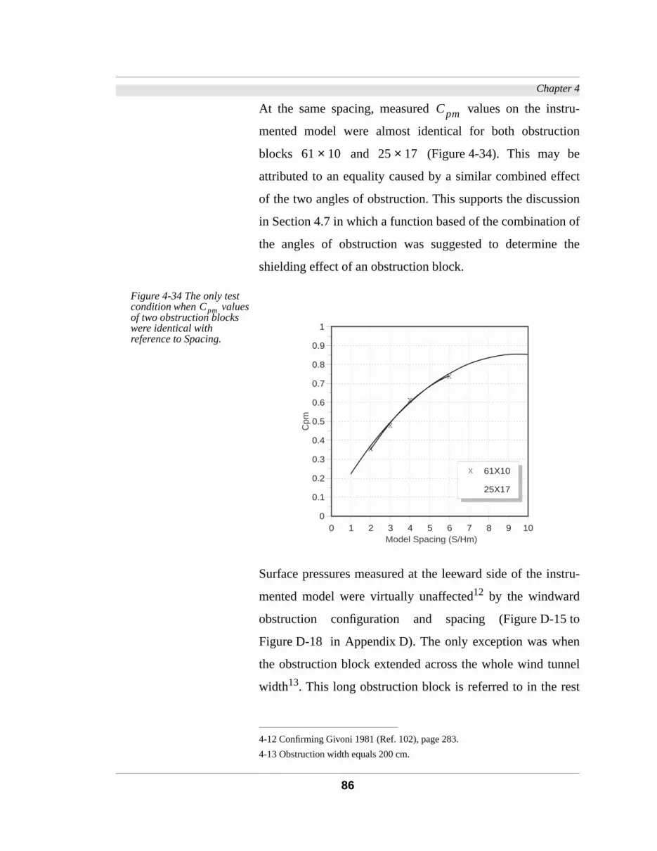
Chapter 4
tru-
ion
e
fect
ion
of
the
stru-
to
en
nel
st
At the same spacing, measured values on the ins
mented model were almost identical for both obstruct
blocks and (Figure 4-34). This may b
attributed to an equality caused by a similar combined ef
of the two angles of obstruction. This supports the discuss
in Section 4.7 in which a function based of the combination
the angles of obstruction was suggested to determine
shielding effect of an obstruction block.
Figure 4-34 The only test condition when values of two obstruction blocks were identical with reference to Spacing.
Surface pressures measured at the leeward side of the in
mented model were virtually unaffected12 by the windward
obstruction configuration and spacing (Figure D-15
Figure D-18 in Appendix D). The only exception was wh
the obstruction block extended across the whole wind tun
width13. This long obstruction block is referred to in the re
4-12 Confirming Givoni 1981 (Ref. 102), page 283.
4-13 Obstruction width equals 200 cm.
Cpm
61 10× 25 17×
Cpm
X
X
X
X
0
0.1
0.2
0.3
0.4
0.5
0.6
0.7
0.8
0.9
1
0 1 2 3 4 5 6 7 8 9 10
Cpm
Model Spacing (S/Hm)
X 61X10
25X17
86

Chapter 4
the
the
the
es
on
-
ith
g
ich
not
ard
of the study as the infinitely long obstruction block. It could
represent a row-housing type of development where
deflected wind does not have a chance to reattach from
sides. The only reattachment of the wind possible was over
top of the obstruction block (Figure 4-35). The valu
(Figure D-15 ) measured behind the obstructi
block at the closest Spacing (Sm=2) from the instrumented sur
face showed about a 20% reduction when compared w
spacings ≥ 5. This was caused by the extraordinarily lon
wake generated behind the block. Other smaller blocks (wh
might represent more realistic adjacent buildings) did
show any effect on the values measured in the leew
surface of the instrumented model.
Figure 4-35 The long wake generated behind an infinitely long obstruction block.
Cp
200 10×
Cp
Instrumented ModelObstruction Block
Wake
87
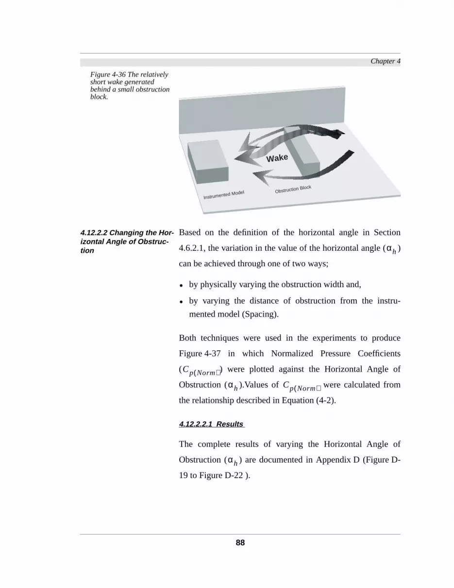
Chapter 4
ion
)
u-
uce
ts
f
m
of
D-
Figure 4-36 The relatively short wake generated behind a small obstruction block.
4.12.2.2 Changing the Hor-izontal Angle of Obstruc-tion
Based on the definition of the horizontal angle in Sect
4.6.2.1, the variation in the value of the horizontal angle (
can be achieved through one of two ways;
• by physically varying the obstruction width and,
• by varying the distance of obstruction from the instr
mented model (Spacing).
Both techniques were used in the experiments to prod
Figure 4-37 in which Normalized Pressure Coefficien
( ) were plotted against the Horizontal Angle o
Obstruction ( ).Values of were calculated fro
the relationship described in Equation (4-2).
4.12.2.2.1 Results
The complete results of varying the Horizontal Angle
Obstruction ( ) are documented in Appendix D (Figure
19 to Figure D-22 ).
Instrumented Model Obstruction Block
Wake
αh
Cp Norm( )
αh Cp Norm( )
αh
88

Chapter 4
ri-
en
-
alue
k
the
ee
in
ct
g
e
he
the
Figure 4-37 Effect of varying the horizontal angle of obstruction
4.12.2.2.2 Discussion
Plotting the Pressure Coefficients against the Ho
zontal Angle of Obstruction ( ) shows the following:
• The data points where the Horizontal Angle lies betwe
15˚ and 140˚ ( ) show that val
ues tend to decrease with the increase of . As the v
of decreases, approaches unity14.
• When , neither the size of obstruction bloc
nor its distance from the instrumented surface affects
pressure coefficients. This range of coincides with L
et al’s Isolated Roughness Flow Regime (Ref. 149).
• In most of the obtained values, at , an increase
obstruction width or reduction of spacing does not affe
the value. When exceeds 140˚, the resultin
airflow behind the obstruction block is similar to that of th
skimming flow regime discussed in Lee et al (Figure 4-8).
This skimming flow phenomenon can occur in spite of t
4-14 The only exception is when testing the infinitely long obstruction block at smallest spacings (2).
B
B
B
B
BB
BBB
J
J
J
JJ
JJJJ
HH
H
H
H
HH
H
HH
F
F
F
F
-2-1.8-1.6-1.4-1.2
-1-0.8-0.6-0.4-0.2
00.20.40.60.8
1
0 15 30 45 60 75 90 105 120 135 150 165 180
Nor
mal
ized
Pre
ssur
e C
oeffi
cien
t [C
p(N
orm
)]
Horizontal Angle (°)
B 200X10
J 150X10
H 89X10
F 61X10
25X10
25X7
25X17
25X25
Effect of Horizontal Angle (αh) on Normalized
Pressure Coefficients [Cp(Norm)] on Obstruction Facing Surface
Obstruction widths =200, 150, 89, 61 and 25 cm
Obstruction height=10, 7, 17, and 25 cm
Cp Norm( )
αh
15° αh 140°< < Cp Norm( )αh
αh Cp Norm( )
0° αh≤ 15°<
αh
αh 140°>
Cp Norm( ) αh
89

Chapter 4
ffi-
r
-
one
It
s of
the
ck.
role
of
D
spacing. The 140˚ arc within which most pressure coe
cients values are affected will be referred to as the Shield-
ing Effectiveness Zone (SEZ) of the surface unde
consideration (Figure 4-38).
• At , the measured values repre
sent the Wake Interference Regime (Figure 4-8). This z
contained the highest density of points (Figure 4-37).
should also be noted that the largest variation in value
occur in this zone.Figure 4-38 The shielding effectiveness zone.
4.12.2.3 Changing the Ver-tical Angle of Obstruction
The variation of the vertical angle of obstruction αv, as defined
in Section 4.6.2.2, can be obtained through the variation of
inter-model spacing and the height of the obstruction blo
The experiments included the two approaches to study the
of the vertical angle in shielding effect of obstruction block.
4.12.2.3.1 Results
The effect of varying the vertical angle on the value
is plotted in Figure 4-39 as well as Appendix
(Figure D-23 to Figure D-26 ).
15° Θ 140°< < Cp Norm( )
Cp Norm( )
Shielding Effectiveness Zone (SEZ)
Obstruction Block
InstrumentedModel
140˚
Instrumented Surface
Cp Norm( )
90

Chapter 4
face
nts
tion
es at
ck
ide is
it is
the
Figure 4-39 The effect of varying vertical angle of obstruction
4.12.2.3.2 Anal ysis
Arthur Bowen of the Conseil National de Researches in Can-
ada (Ref. 42) conducted experiments that determined sur
pressures for four model-building heights. His measureme
of surface pressures clearly demonstrated an inverse rela
between the height of the model and the surface pressur
the leeward side. As the height of instrumented blo
increases, the surface pressure measured at its leeward s
reduced and consequently the length of the wake behind
increased15. The longer the wake behind a block, the larger
magnitude and extend of its shielding effect (Figure 4-40).
4-15 This is also evident from Evans experiments (Ref. 79).
B
B
B
B
BBBBB
J
J
J
JJ
JJJJ
HH
H
H
H
HHH
HH
F
F
F
F
-2-1.8-1.6-1.4-1.2
-1-0.8-0.6-0.4-0.2
00.20.40.60.8
1
0 15 30 45 60
Nor
mal
ized
Pre
ssur
e C
oeffi
cien
t [C
p(N
orm
)]
Vertical Angle (°)
B 200X10
J 150X10
H 89X10
F 61X10
25X10
25X7
25X17
25X25
Effect of Horizontal Angle (αv) on Normalized
Pressure Coefficients [Cp(Norm)] on Obstruction Facing Surface
Obstruction widths =200, 150, 89, 61, and 25 cm
Obstruction height=10, 7, 17, and 25 cm
25 cm wide obstruction blocks
10 cm high obstruction blocks
91

Chapter 4
na-
be
res-
nd-
he
the
ted
ed
idth
ion
at
ng
to
Figure 4-40 The wake length is proportional to obstruction height.
My tests (Figure 4-39) supported Bowen’s conclusion. In a
lyzing the measured values, the following could
observed:
• There is an inverse relationship between the surface p
sure coefficients and the vertical angle describing the wi
ward obstruction block.
• At , which is equivalent to Lee et al ‘s (Ref.
149) Isolated Roughness Flow Regime at 2.6 model spac-
ing (Sm), no noticeable shift could be observed in t
obtained data. This shows that neither the spacing nor
vertical angle alone can fully describe the wake genera
behind an obstruction block. The spread of Normaliz
pressure data demonstrates the significance of the w
and the horizontal obstruction angle of the obstruct
block.
• There were not enough data points of
, which corresponded roughly to the 1.2 spaci
Skimming Flow Regime at Lee et al ‘s experiments, to
observe any shift in the measured surface pressures.
• Similarly, the range which corresponded
the Wake Interference Flow Regime, showed not significant
difference from the rest of the measured vertical angles.
Wake1
Wake2
Hei
ght 1
Hei
ght 2
Cp Norm( )
0° α< v 25°<
Cp Norm( )αv 45°>
25° αv 45°> >
92

Chapter 4
tion
lly
at
af-
1.
del
e
f
e in
edic-
ec-
r to
It should also be noted that regardless of the obstruc
height, the 25 cm wide obstruction block maintained virtua
the same values with the same This means th
for the same vertical angle, value remains un
fected by a small change in the horizontal angle Figure 4-4
Figure 4-41 For the same obstruction vertical angles,
remained largely unaffected by the obstruction height.
4.12.3 Deriving the Model
As seen in Figure 4-1, expressing in terms of the mo
spacing (Sm) did not explain the differences between th
results of the three experiments16. The angular description o
the obstruction blocks from the vantage point of the surfac
question, on the other hand, has provided the proposed pr
tion model with a more comprehensive set of variables (S
tion 4.7). In addition, the identification of the “lines of sight”
to the obstruction block enhances the ability of the designe
input the actual description of the surrounding blocks.
4-16 Wiren’s, Lee et al and Ernest.
Cp Norm( ) αv
Cp Norm( )
Cpm
αv
Cp
93

Chapter 4
ribe
u-
and
ec-
in
ca-
ed
I proposed a formula using the two angles required to desc
the outline of the obstruction block in an orthogonal config
ration17. The generic form was as follows:
(4-8)
In the cases when the centerlines of the obstruction block
the instrumented surface do not coincide with the wind dir
tion i.e. the obstruction asymmetrically shields the surface
question, I suggest the following correction function (generic
form):
(4-9)
Where (Equations 4-8 and 4-9)
Figure 4-42 shows a contour graph of the Pressure Modifi
tion Coefficients ( ) of the tested configurations plott
against both angles of description (αh, αv). It can be noted that
the values formed two shapes around the line where;
4-17 Refer to the discussion in Section 4.12 on page 81.
Cpm ortho( ) Ci f αh αv( , ),=
Cpmαd corr( ) f Cpm ortho( ) αd,( )=
Cpmαd corr( ) Displacement-corrected Modification=
Coefficient
Cpm Pressure Modification Coefficient=
Ci Formula Constants=
i 0 1 … N, , ,=
αh Horizontal Angle=
αv Vertical Angle=
αd Displacement Angle=
Cpm
Cpm
94

Chapter 4
line
his
less
the
tion
ise
pack-
(4-10)
The lines connecting the values above the bisection
were all convex while those below the line were concave. T
means that above the bisection line, values of were
sensitive to αv with the increase of αh. On the other hand,
below the line, with the increase of αh, became very sen-
sitive to the increase in the value of αv. Thus, the bisection line
describes the zone where the value of is neutral to
acceleration of both angles of view. Consequently, a func
was developed based on the relationship between αh and αv
shown in Equation (4-10).
Figure 4-42 Measured pressure modification coefficients for orthogonal configurations.
4.12.3.1 Analysis of Vari-ables:
The function coefficients were determined using a stepw
nonlinear regression routine18 in which the parameters in
Figure 4-43 were used.
4-18 Software used in the statistical analysis of the data is SPSS 6.0 Graduateage for the Macintosh platform.
αv
αh
2------=
Cpm
Cpm
Cpm
Cpm
0.2
0.3
0.4
0.5
0.5
0.60.70.8
0.9
X
XX
XXXXXX
X
XX
XXXXXX
X
X
XX
XXXXXX
X
X
XX
XXXXXX
X
X
X
XX
XXXXX
X
XX
XXXXXXX
X
X
XX
XXXXX
X
XX
X
0
10
20
30
40
50
60
70
0 15 30 45 60 75 90 105 120 135 150 165
Ver
tical
Ang
le (
°)
Horizontal Angle (°)
Effect of Obstruction Angles on Pressure Modification Coefficient
(Cpm) on the Obstruction-facing Surface
95

Chapter 4
sult-
an
)
Figure 4-43 Basic variables in orthogonal function
4.12.3.2 The Functions The stepwise regression analysis was conducted twice re
ing in two Functions. The first function would suffice as
easy-to-use, simple, and less accurate (adjusted
function for hand and quick calculations [Equation (4-11)].
(4-11)
where
11
1
1
11111
2
22
22
2222
33
3
3
3
333
33
4
4
4
4
5
5
5
5
55
5555
0
0.1
0.2
0.3
0.4
0.5
0.6
0.7
0.8
0.9
1
0
0.1
0.2
0.3
0.4
0.5
0.6
0.7
Pre
ssure
Modifi
catio
n C
oeffic
ein
t (C
pm
)
11
1
1
11111
2
22
22
2222
3 3
3
3
3
333
33
4
4
4
4
5
5
5
5
55
5555
00.1
0.2
0.3
0.4
0.5
0.6
0.7
0.8
0.9 1
11
1
1
11111
2
22
22
2222
3 3
3
3
3
333
33
4
4
4
4
5
5
5
5
55
5555
-0.6
-0.5
-0.4
-0.3
-0.2
-0.1 0
1 200X10
2 150X10
3 89X10
4 61X10
5 25X10
25X7
25X17
25X25
αh
2------
sin αvsin⋅ αh
2------
αvsin
cos αv
αh
2------
sincosln
R2
0.967=
Cpm ortho( ) C0
αh
2------
sin αv( )sin⋅ ⋅ +=
C1
αh
2------
αv( )sin
cos⋅ +
C2 αv( )cos
αh
2------
sinln⋅
C0 0.8548C1
–0.7677
C2 0.6261–
===
96

Chapter 4
ith
ter
in
ing
be
d
ular
the
The second function resulted in a lengthy expression w
high-fitting regression value (adjusted )19. The
more complex relationship would be suitable for compu
applications and is documented in equation (D-1)
Appendix D.
4-19 Figure 4-44
Figure 4-44 Predicted vs. measured values of surface pressure coefficients-Equation (4-12).
The more complex of the two equations was used in plott
the contour diagram shown Figure 4-45. This diagram can
used to graphically predict knowing both an
. Based on the parameters of the experiments, the ang
variables of Equations (4-11) and (D-1) were bounded by
following limits:
R2
0.995=
[
[
[
[
[
[
[[[
[
[
[
[
[
[[[[
[
[
[
[
[
[[[
[[
[
[
[
[[[[[[[
[
[
[
[[[[ [[[
[
[
[
[[[[[[[
[
[
[
[[
[[[[
[
[
[
[
-1.4
-1.2
-1
-0.8
-0.6
-0.4
-0.2
0
0.2
0.4
0.6
-1.4 -1.2 -1 -0.8 -0.6 -0.4 -0.2 0 0.2 0.4 0.6
Pre
dict
ed P
ress
ure
Coe
ffici
ents
(C
p)
Measured Pressure Coefficients (Cp)
Correlation Fit
Cpm ortho( ) αh
αv
97

Chapter 4
be
dels
m).
less
lar
on-
effi-
m
(4-12)
Figure 4-45 Model contour graphically represents the mathematical function in Equation (D-1).
4.12.4 Limitation of the Orthogonal Model
The limitations of the mathematical orthogonal model can
summarized in the following:
• The model is based on tests conducted on cubical mo
that represent single-floor buildings.
• Tested obstruction blocks had the same depth (10 c
Deeper obstruction blocks have shorter wakes and
shielding effect than shallower blocks with similar angu
description (Ref. 79). However, some initial tests were c
ducted with a deeper block (25 cm) and the pressure co
cients on the instrumented surface varied only slightly fro
those of the 10 cm deep block.
0° αh 140°≤ ≤
0° αv 60°≤ ≤
Predicting Pressure Modification Coefficient (Cpm) based on
both Horizontal and Vertical Angles of Obstruction
Horizontal Angle of Obstruction -αh (°)
Ver
tical
Ang
leof
Obs
truc
tion
-αv (
°)
-0.4
-0.2
0
00.2
0.2
0.4
0.4
0.6
0.6
0.8
0
5
10
15
20
25
30
35
40
45
50
55
60
65
70
0 20 40 60 80 100 120 140
Limits of the function
98

Chapter 4
r-
k is
nts
ry
ce-
he
gu-
to
the
s
ot
the
uc-
tion
tion
ce
ent
ion
he
gle
der
he
• The orthogonal model -by definition- cannot predict su
face pressures on occasions when the obstruction bloc
not symmetrical around the line connecting the mid poi
of the block and the instrumented model. The prima
example of this asymmetry would be a horizontal displa
ment of the obstruction block from the center line of t
instrumented model.
• Since the derived orthogonal model was based on confi
rations where wind direction was always perpendicular
both the obstruction block and the instrumented model,
effect of the wind direction on the values of wa
unaccounted for.
• The effect of multiple obstruction blocks on was n
considered in the orthogonal model.
4.13 The Displacement Correction
Displacement as defined in Section 4.6.2.5, occurs when
instrumented surface does not fall directly behind the obstr
tion block thus causing misalignment between the obstruc
block and the model (Figure 4-18).
4.13.1 Varying Displacement Angle
Increasing the displacement angle ( ) shifts the obstruc
block laterally relative to the instrumented model surfa
(Figure 4-46). The premise under which the displacem
effect was studied is as follows;
With the increase in angle, the Pressure Modificat
Coefficient increases until it reaches unity or t
unshielded condition (Figure 4-46). As the displacement an
increases, the portion of the instrumented surface falling un
the obstruction block wake is reduced (Figure 4-47). T
Cpm
Cpm
αd
αd
Cpm
99

Chapter 4
rom
ce
ter-
ion
ri-
the
ts of
the
result is an average value between those obtained f
an unshielded surface and a symmetrically shielded surfa20
in similar terrain conditions.
4-20 Orthogonal configuration.
Figure 4-46 Varying the displacement angle.
Figure 4-47 Shielding Effect of displacement of obstruction block.
4.13.1.1 Setup of Experi-ments
A total number of 63 experiments were conducted to de
mine the effect of varying the displacement of the obstruct
block. TABLE 4-4 lists the tested configurations. Three va
ables were tested (Figure 4-48): the obstruction width,
spacing, and the horizontal shift of obstruction block. The lat-
ter is defined here as the distance between the mid poin
the obstruction block and the instrumented surface. In
Cpm
1 2 3
αd1 αd2 αd3
Win
d di
rect
ion
OrthogonalConfiguration
Displaced ObstructionConfigurations
100

Chapter 4
be
analysis however, the horizontal displacement willexpressed in angular terms ( )21. The dimensions of the
instrumented model in all experiments remained constant.
4-21 The displacement angle is defined in Section 4.6.2.5.
a. Figure 4-48 illustrates the definitions of the experiment’s three variables.
Figure 4-48 Displacement configuration variables.
αd
TABLE 4-4 Displacement Experiments Setup a
Obstruction Width (cm) 25 61 86
Spacing (Sm) 2 3 4 6 2 3 4 6 2
Shift (cm)Shift.(cm)
Shift. (cm)
0.0 X X X X 0.0 X X X X 0.0 X
6.25 X X X X 7.63 X X X X 21.5 X
12.5 X X X X 15.25 X X X X 43.0 X
18.75 X X X X 22.88 X X X X - -
25.0 X X X X 30.5 X X X X - -
31.25 X X X X 38.13 X X X X - -
37.5 X X X X 45.75 X X X X - -
- - - - - 53.63 X X X X - -
Obstruction Width
Spa
cing
HorizontalShift
Mid Points
InstrumentedModel
25 cm
25 c
m
101

Chapter 4
ntial
as a
on
fts
ck
ion
4-
ym-
an
u-
the
nts
to
tion
of
al
4.13.1.2 The Choice of the Displacement Angle
Before starting the discussion of the tests results, it is esse
to explain the reason for defining the displacement angle
bisecting of an obstruction’s horizontal angle of view (Secti
4.6.2.5). This definition is more sensitive to horizontal shi
than to an asymmetrical elongation of the obstruction blo
(Figure 4-49). The shielding effect of a displaced obstruct
block is lower than that of a fully obstructing block (Figure
49a). On the other hand, the shielding effect of a long as
metric obstruction block is not much different than that of
obstruction block in orthogonal relationship with the instr
mented surface (Figure 4-49b). The suggested definition of
displacement angle is responsive to both requireme
mentioned above.
Figure 4-49 Displacement angle ( ) growth relative to obstruction block.
Preliminary tests verified the sensitivity of as compared
the equivalent angle using the actual center of the obstruc
block. That alternative definition exaggerates the effect
obstruction elongation (Figure 4-50), relative to its actu
shielding effect.
αd
αd Displaced Obstruction Block Elongated Obstruction Block
a b
αd1 αd2
αd
102

Chapter 4
d in
4-
Figure 4-50 Alternative definition of .
4.13.1.3 Results The results of Displacement experiments are documente
detail in Appendix E and summarized in Figures 4-51 and
52.
Figure 4-51 Effect of displacement angle ( ) on the pressure coefficients.
αd Dispalced Obstruction Block Elongated Obstruction Block
a b
αd1 αd2
αd
B
B
B
B B B B
J J
J J
J J J
H H H HH
H H
F
F
F
F
F
F F F
-0.6
-0.4
-0.2
0
0.2
0.4
0.6
0.8
0 15 30 45 60
Pre
ssur
e C
oeffi
cien
t (C
p)
Displacement Angle (°)
B 2-25
J 4-25
H 6-25
F 2-61
3-61
4-61
6-61
2-86
Key:
Configuration s-w
Where:
s=spacing (TABLE 4-4 )
w=obstruction width
103

Chapter 4
the
ship
val-
les
e
the
be
an
s a
the
tion
he
w-
ed
Figure 4-52 Effect of displacement angle on the pressure modification coefficients.
4.13.1.4 Discussion The results shown in Figures 4-51 and 4-52 support
premise suggested in Section 4.13.1 about the relation
between surface pressures and displacement angles. The
ues of approached 1.0 with displacement ang
. In addition, measured values wer
influenced by the size of the obstruction block as well as
spacing from the instrumented surface.
Since both the size of the obstruction and its spacing can
expressed using the angles of obstruction description,
orthogonal value of can be predicted. Figure 4-53 i
contour graph demonstrating the error/correction when
orthogonal prediction was used for a displaced obstruc
block. It should be noted that at values of , t
orthogonal model did not greatly overestimate . Ho
ever, with the increased , values quickly approach
unity.
αd
B
B
B
B B B B
J J
J J
J JJ
H HH
HH
H H
FF
F
F
F
F F F
0.2
0.3
0.4
0.5
0.6
0.7
0.8
0.9
1
0 15 30 45 60
Pre
ssur
e S
hiel
ding
Mod
ifica
tion
Coe
ffici
ent (
Cpm
)
Displacement Angle (°)
B 2-25
J 4-25
H 6-25
F 2-61
3-61
4-61
6-61
2-86
Cpm
αd 40° 50°–> Cpm
Cpm
0° αd 15°< <
Cpm
αd Cpm
104

Chapter 4
o-
aly-
the
hen
the
ded
ese
the
E-
on
cts
Figure 4-53 Displacement correction of values as predicted by the Orthogonal Model.
Appendix E contains graphs illustrating the pr
files on both the obstructed and unobstructed surfaces. An
sis of these results demonstrates that the wake behind
obstruction block maintains its rectangular shape even w
the instrumented model is located within it. As a result,
pressure profile on the obstruction-facing surface was divi
-in most of the tested configurations- into two sections. Th
two parts were directly related to the wake created by
obstruction block wake. This was demonstrated in Figure
2 to Figure E-8 where value on the unshielded22
portion of the surface equaled unity. The shielded portion,
the other hand, was affected by the windward shielding effe
similar to the orthogonal configurations.
4-22 Presented in Appendix E with a shaded area.
Cpm
0.4
0.60.8
0.8
X XX
XX
XX
X X X X XX
XX X X X X X X
X XX
X
X
X
X
X
X XX
X
XX
XX
X X XX
XX
XX
X X X XX
XX
XX
X
0
0.1
0.2
0.3
0.4
0.5
0.6
0.7
0.8
0.9
1
0 15 30 45 60
Pre
dict
ed C
pm (
orth
o)
Displacement Angle (°)
Measured Cpm
Cp Norm( )
Cp Norm( )
105

Chapter 4
eded
the
ent
e
ion
4.13.2 Deriving the Correction Function
Based on the above discussion, only two variables are ne
to correct for the displacement effects. These variables are
orthogonal estimation of the Pressure Modification Coeffici
( ) and the displacement angle. Accordingly, th
following function was developed using a stepwise regress
routine, resulting in a correlation fit with an adjusted R2=0.94
(Figure 4-54):
(4-13)
Where
and;
It should be noted that if;
therefore;
and if;
therefore;
Cpm ortho( )
Cpmαd corr( )Cpm ortho( ) C1 2 αd⋅( )
C2 2 αd⋅( )sin[ ] 2⋅ C3 1 e2 αd⋅( )sin[ ]
Cpm ortho( )
–
⋅+ +
sin⋅+=
C1 0.5046C2 0.2216C2 0.4718
===
0° αd 90°<≤
Cpm 1.0=
Cpm corr_d( ) Cpm=
1.0=
αd 0°=
Cpm corr_d( ) Cpm=
106

Chapter 4
(4-
ted
ed -
e
Figure 4-54 Predicted vs. measured values.
Figure 4-55 shows a graphical representation of equation
13) where the displacement corrected was plot
against the displacement angle ( ). This graph can be us
within the limits of its variables- to manually determine th
displacement correction.
Figure 4-55 Correcting value based on
displacement angle.
Cpm
X
X
X
XXXX
XX
X X
X XX
X XXXX
XX
XX
X
X
X
XXX
X
X
X
X
XXXX
X
X
X
X
XX
XX
X
X
XX
XXX
0.3
0.4
0.5
0.6
0.7
0.8
0.9
1
0.3 0.4 0.5 0.6 0.7 0.8 0.9 1
Pre
dict
ed C
pmMeasured Cpm
Cpm
αd
Cpm
0.5
0.6
0.7
0.8
0.9
0
0.1
0.2
0.3
0.4
0.5
0.6
0.7
0.8
0.9
1
0 10 20 30 40 50 60 70
Pre
dict
ed O
rtho
gona
l Cpm
Displacement Angle (°)
Measured Zone
107

Chapter 4
ted
sed
at
he
ri-
he
her
ke
d in
e
ce,
age
e
of
ve
ea-
del,
tion
ke
the
on
tly
4.13.3 Effect of Roof Shapes
Even though in all of the experiments both the instrumen
model and the obstruction block had flat roofs, the propo
prediction model suggests the following;
• In case of an obstruction block with a gable roof (non-fl
roof), the vertical angle ( ) is to be measured from t
highest visible point (ridge line). The corresponding ho
zontal angle ( ) is then taken off at the location of t
ridge line on the plan (Figure 4-56). As a result, the hig
the roof pitch, the higher the and the longer its wa
(Evans 1974, Ref. 79). This proposition has been teste
Section 4.17.1 with reasonable success.
• Ernest’s experiments23 1991 (Ref. 74) showed that on th
windward side of an instrumented unobstructed surfa
roof shape and slope have minimal effect on the aver
surface pressures. Similarly, Kindangen et al’s (Ref. 137)
CFD24 calculations showed insignificant variation in th
average velocity coefficient in most of the studied ro
geometries25.
• Both Evans and Ernest26 agreed that extended eaves ha
very limited effect on surface pressure coefficients m
sured at the surface under the eave. In the prediction mo
the eave is neglected in describing both the obstruc
block and the building under investigation.
In conclusion, the proposed prediction model will not ta
into account the effect of roof shape aside from extending
viewable plane to the ridge or to the highest viewable line
the obstruction block. The horizontal angle may be sligh
4-23 pp. 58-61.
4-24 Computational fluid dynamics.
4-25 The only significant variation was found at wind direction Θ=0˚
4-26 pp. 77-78.
αv
αh
αv
108

Chapter 4
tion
ruc-
del
nd
n
ec-
t at
ion
ill
reduced in this definition because it extends the obstruc
plane to the ridge line instead of the closest surface of obst
tion block.
Figure 4-56 Gable roof angular description.
4.13.4 Additional Corrections
Three additional corrections to the pressure prediction mo
were studied:
• The effect of changing the wind direction on the value a
distribution of the pressure coefficients (Section 4.14).
• The shielding effects of multiple windward obstructio
blocks (Section 4.15).
• The effect of the geometry of the instrumented model (S
tion 4.16).
4.14 Effect of Changing the Wind Direction
In all the previous experiments wind direction was constan
Θ=0˚. Based on the definitions of the angles of obstruct
(Section 4.6), a change in the wind direction from 0˚ w
affect the angles of view in the following ways:
αv
αh
Section
Plan
Eave LineRidge Line
109

Chapter 4
i-
rc
i-
f
zon-
ed
the
).
• Wind direction is not included in the definition of the Hor
zontal Angle27 ( ). However, since there exists a 140˚ a
(SEZ) within which the shielding effect is most prom
nent28, the following should be considered. If the limits o
the SEZ arc extend over the arc encompassing the hori
tal angle ( ), the horizontal angle will only be measur
within the SEZ (Figure 4-57).
• The vertical angle is reduced as a consequence of
reduction in width of the obstruction block (Figure 4-58
The effect was found to be insignificant.
4-27 Section 4.6.2.1, page 65.
4-28 Refer to Section 4.12.2.2, page 88.
Figure 4-57 The relationship between the (SEZ) and the horizontal angle.
αh
αh
140˚ SEZαh
140˚ SEZ
αh
Win
d D
irect
ion
a b
110

Chapter 4
la-
n,
ral-
ith
ock
ock
nd
, a
the
Figure 4-58 Spacing correction as a result of wind direction changes.
4.14.1 Wind Direction Scenarios
Because wind direction experiments involve the rotation re
tive to the wind direction, of the model and/or the obstructio
three scenarios could be envisaged (Figure 4-59);
In the first scenario, the obstruction block is positioned pa
lel to the instrumented model and the wind changes w
respect to both instrumented model and obstruction bl
(Figure 4-62). In the second scenario, the obstruction bl
remains perpendicular to the wind direction while the wi
changes only with respect to the model. In this scenario
non-orthogonal (non-parallel) relation exists between
instrumented model and the adjacent surface.
Win
d D
irect
ion
S1S2
111

Chapter 4
s a
del.
rel-
tion
bi-
ns
Figure 4-59 The possible instrumented model-obstruction block relationship with respect to wind direction.
Similar to the second scenario, the third scenario involve
non-orthogonal relationship between obstruction and mo
However, in this case, the wind direction remains constant
ative to the instrumented model rather than the obstruc
block. As can be seen in Figure 4-60, scenario III is a com
nation of scenarios I and II. The prediction model correctio
can therefore be based on tests of the two scenarios.
Win
d D
irect
ion
Scenario I
Scenario II
Scenario III
Orthogonal Configurations Wind Direction Scenarios
ObstructionBlock
InstrumentedModel
Ort
hogo
nal R
elat
ions
hip
Non
-ort
hogo
nal R
elat
ions
hip
112

Chapter 4
or-
be
The
ons
An
pre-
ne
tion
er-
uiva-
the
ular
Figure 4-60 Scenario III represents a combination of Scenarios I and II.
4.14.2 The Equivalent Obstruction Block
The two-steps of the orthogonal model (Section 4.12) c
rected for horizontal displacement (Section 4.13) might
called the Displacement Pressure Prediction model.
orthogonal model was developed from tests of obstructi
that were always perpendicular to the wind direction.
imaginary equivalent obstruction plane could be used to re
sent the rotated obstruction block (Figure 4-61). This pla
has the same horizontal angle( ) of the actual obstruc
block and differs only in the fact that it always remains p
pendicular to the wind direction.
4.14.2.1 Premise of Wind Direction Analysis
The premise of my research at this stage was that the eq
lent orthogonal plane can mathematically substitute for
actual obstruction block when the latter was not perpendic
Win
d D
irect
ion
Wind
Dire
ction
Win
d D
irect
ion
Wind
Dire
ction
Scenario II Scenario III
Orthogonal Configurations Scenario I
αh
113
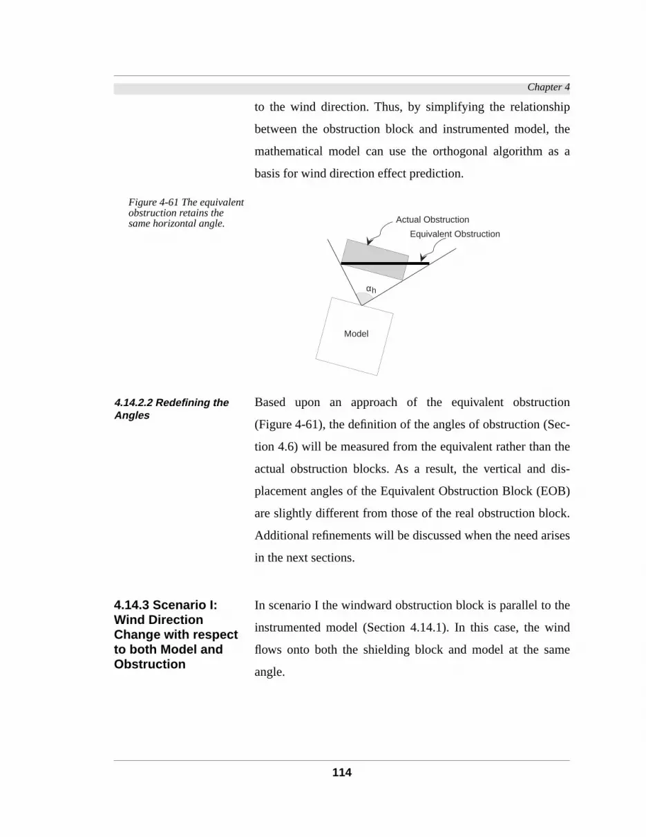
Chapter 4
ip
the
s a
tion
ec-
the
is-
B)
k.
ises
he
ind
me
to the wind direction. Thus, by simplifying the relationsh
between the obstruction block and instrumented model,
mathematical model can use the orthogonal algorithm a
basis for wind direction effect prediction.
Figure 4-61 The equivalent obstruction retains the same horizontal angle.
4.14.2.2 Redefining the Angles
Based upon an approach of the equivalent obstruc
(Figure 4-61), the definition of the angles of obstruction (S
tion 4.6) will be measured from the equivalent rather than
actual obstruction blocks. As a result, the vertical and d
placement angles of the Equivalent Obstruction Block (EO
are slightly different from those of the real obstruction bloc
Additional refinements will be discussed when the need ar
in the next sections.
4.14.3 Scenario I: Wind Direction Change with respect to both Model and Obstruction
In scenario I the windward obstruction block is parallel to t
instrumented model (Section 4.14.1). In this case, the w
flows onto both the shielding block and model at the sa
angle.
Equivalent Obstruction
Actual Obstruction
Model
αh
114

Chapter 4
as
ble
4-
.
tion
aces
the
nder
l of
4.14.3.1 Experiment setup In the boundary layer wind tunnel, wind direction change w
achieved through the rotation of the models on the turnta
(Figure A-1). The following variables were tested (Figure
62):
• Three actual obstruction widths (25, 61, and 86 cm)
• Four spacings ( ) between the model and the obstruc
block (2, 3, 4, and 6).
• Seven wind directions (Θ = 0°-180° in 15° intervals.)
Surface Pressure Coefficients were measured on two surf
on opposite sides of the model. One surface always faced
obstruction block while the opposite side never ‘saw’ the
block (Figure 4-62).
The total number of tested configurations was 12, tested u
seven (7) wind directions, and for two (2) surfaces (a tota
168 surfaces were measured).
Figure 4-62 Experiment setup for scenario I.
Wo
Sm
Θ
w=25, 61, and 86 cm
Obstructed Side
Unobstructed Side
Sm = 2, 3,4, and 6
115
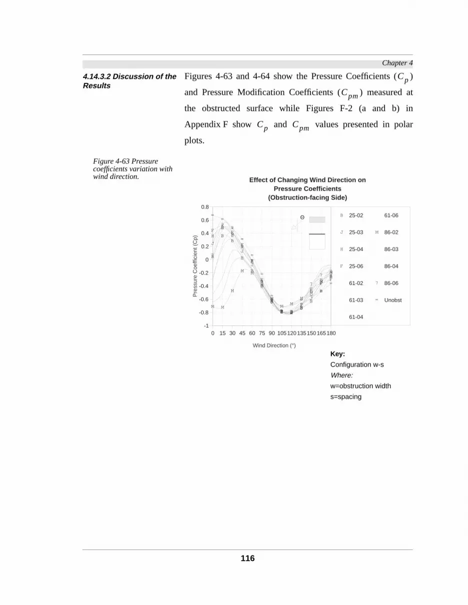
Chapter 4
)
at
in
lar
4.14.3.2 Discussion of the Results
Figures 4-63 and 4-64 show the Pressure Coefficients (
and Pressure Modification Coefficients ( ) measured
the obstructed surface while Figures F-2 (a and b)
Appendix F show and values presented in po
plots.
Figure 4-63 Pressure coefficients variation with wind direction.
Cp
Cpm
Cp Cpm
B
BB
B
B
B
B
B BB
B
B
B
J
J
J
J
J
J
J
J JJ
J
J
J
H
HH
H
H
H
H
H HH
H
HH
FF
F
F
F
F
F
F F
F
FF
F
M M
M
M M
M
M
M MM
M
M
M
7
77
7
7
7
7
7 7
7
7
77
==
=
=
=
=
=
==
==
=
=
-1
-0.8
-0.6
-0.4
-0.2
0
0.2
0.4
0.6
0.8
0 15 30 45 60 75 90 105120 135150 165180
Pre
ssur
e C
oeffi
cien
t (C
p)
Wind Direction (°)
B 25-02
J 25-03
H 25-04
F 25-06
61-02
61-03
61-04
61-06
M 86-02
86-03
86-04
7 86-06
= Unobst
Effect of Changing Wind Direction onPressure Coefficients
(Obstruction-facing Side)
Θ
Key:
Configuration w-s
Where:
w=obstruction width
s=spacing
116

Chapter 4
ns.
0˚,
ra-
ca-
the
la-
the
ues
ra-
n
zon-
of
the
7).
Figure 4-64 Most of the variation in the value of Cpm occurs between 0°-60° and 140•-180•.
In all figures, the graphs are divided into three sectio
Figure 4-63 shows that between wind directions 0˚ to 6
values rapidly increased to peak in all tested configu
tions between 15˚-45˚. The variation of the Pressure Modifi
tion Coefficients in this sector of wind direction was due to
shielding effect of the obstruction block and its location re
tive to the instrumented surface. Obstruction blocks with
largest obstruction angles maintained the lowest val
while smaller blocks produced the highest values of .
Limited variation could be observed in the tested configu
tions for wind directions 60˚-140˚. The lack of variation ca
be attributed to the decrease in the values of both the hori
tal and vertical angles for the EOB with the rotation
the wind beyond the 60˚ mark. This was true regardless of
size and distance of the block from the model (Figure 4-5
B
BB
BB
BB
B B
BB
B
B
J
J JJ J J
JJ
J
JJ
J J
H
HH H H H H
H H
H
H
HH
F
FF F F F F
F F
F
F FF
M M
M
M
MM
M
M
M
M M
M M
7
77
7 7 77
77
7
77
7
0
0.2
0.4
0.6
0.8
1
1.2
1.4
1.6
0 15 30 45 60 75 90 105 120135150 165180
Pre
ssur
e M
odifi
catio
n C
oeffi
cien
t (C
pm)
Wind Direction (°)
B 25-02
J 25-03
H 25-04
F 25-06
61-02
61-03
61-04
61-06
M 86-02
86-03
86-04
7 86-06
Effect of Changing Wind Direction onPressure Modification Coefficients
(Obstruction-facing Side)
Θ
Cpm
Cpm
Cpm
αh αv
117

Chapter 4
for
F-
The same was true for the unobstructed side or the side
which both and are equal to zero (Figures 4-66 and
2 c and d).
Figure 4-65 Pressure coefficients variation with wind direction (unobstructed side).
Figure 4-66 Except for few exceptions, the unobstructed side is not affected by the shielding block on the opposite side.
αh αv
B B
B
B
B
B
B
B B
BB
B
B
J JJ
J
J
J
J
J J
JJ
J
J
HH
H
H
H
H
H
H H
H
HH
H
FF
F
F
F
F
F
F F
F
FF
F
M M M
M
M
M
M
M M
MM
M
M
7 77
7
7
7
7
7 7
77
7
7
==
=
=
=
=
=
==
==
=
=
-1
-0.8
-0.6
-0.4
-0.2
0
0.2
0.4
0.6
0.8
0 15 30 45 60 75 90 105120 135150165 180
Pre
ssur
e (C
p)
Wind Direction (°)
B 25-02
J 25-03
H 25-04
F 25-06
61-02
61-03
61-04
61-06
M 86-02
86-03
86-04
7 86-06
= Unobst
Effect of Changing Wind Direction onPressure Coefficients(Unobstructed Side)
Θ
BB B B B B B B
B B B B BJ J
J J J JJ J
J JJ J J
H HH H H H H H H H
H H HF F
F F FF F F F
FF F
F
MM
M M M MM M
MM
M
MM
7 77 7 7
7 7 7 77
7 77
0
0.2
0.4
0.6
0.8
1
1.2
1.4
0 15 30 45 60 75 90 105 120135 150165 180
Pre
ssur
e S
hiel
ding
Mod
ifica
tion
Coe
ffici
ent (
Cpm
)
Wind Direction (°)
B 25-02
J 25-03
H 25-04
F 25-06
61-02
61-03
61-04
61-06
M 86-02
86-03
86-04
7 86-06
Effect of Changing Wind Direction onPressure Modification Coefficients
(Unobstructed Side)
Θ
118

Chapter 4
a-
eded
nd
trib-
truc-
rea
ur-
he
han
ure
all
d
sts
us
When wind direction was , most of the me
sured surface pressures for the obstructed surface exce
those of an unshielded block i.e (Figure 4-64 a
F-2 b). The reason for such an increase in can be at
uted to the increase in pressure caused by the leeward obs
tion that obstructs the flow and directs it to the enclosed a
between the two blocks (Figure 4-67). The resulting press
ization is related to the width of the leeward block, with t
longest blocks causing higher pressure coefficients t
smaller ones (Figure 4-64).
Figure 4-67 Leeward blocks increase the pressure at the obstruction-facing surface.
The width of obstruction blocks does not affect the Press
Modification Coefficients on the unobstructed side in
wind directions except normal (Figure 4-66). At this win
direction, the wake of the long obstruction block (86 cm) ca
a long wake within which even the leeward side falls, th
reducing its pressure.
140° Θ 180
°≤ ≤
Cpm 1.0>
Cpm
Θ = 180°
Cpm
119

Chapter 4
uc-
of
in
but
def-
2, the
lent
).
he
the
unt
c-
ing
in
4.14.3.3 Redefining the Angles of Obstruction
As mentioned in Section 4.14.2.2, when rotating the obstr
tion block relative to the wind direction, some of the angles
description had to be modified. This modification was done
such a way that did not overrule the previous definitions
rather encompassed the orthogonal model in the modified
inition.
4.14.3.4 Corrected Dis-
placement Angle
Based on the research premise discussed in Section 4.14.
horizontal angle remains the same after using an equiva
obstruction block within the SEZ’s 140˚ arc (Figure 4-68
However, on increasing the wind direction, more of t
obstruction block falls outside the SEZ and consequently
value of gets smaller than .
Figure 4-68 Modified angles of obstruction.
4.14.3.5 Corrected Dis-
placement Angle
On the other hand, the definition of the displacement angle
on the equivalent obstruction block does not take into acco
the rotation of the obstruction block relative to the wind dire
tion. This rotation causes the wind to flow behind the shield
block and to flow parallel to the model. This in turn, results
αh corr( )
αh corr( ) αh
20.0°αh
αh/2
αd(measured)
αh/2
Win
d D
irect
ion
αd corr( )
αd
120
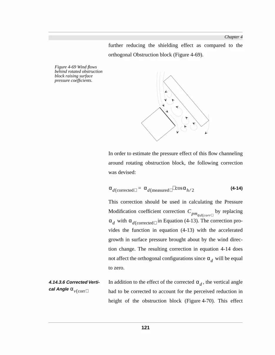
Chapter 4
the
ling
n
ure
g
-
ted
ec-
oes
ual
gle
n in
ct
further reducing the shielding effect as compared to
orthogonal Obstruction block (Figure 4-69).
Figure 4-69 Wind flows behind rotated obstruction block raising surface pressure coefficients.
In order to estimate the pressure effect of this flow channe
around rotating obstruction block, the following correctio
was devised:
(4-14)
This correction should be used in calculating the Press
Modification coefficient correction by replacin
with in Equation (4-13). The correction pro
vides the function in equation (4-13) with the accelera
growth in surface pressure brought about by the wind dir
tion change. The resulting correction in equation 4-14 d
not affect the orthogonal configurations since will be eq
to zero.
4.14.3.6 Corrected Verti-
cal Angle
In addition to the effect of the corrected , the vertical an
had to be corrected to account for the perceived reductio
height of the obstruction block (Figure 4-70). This effe
αd corrected( ) αd measured( ) αh 2⁄cos⋅=
Cpmαd corr( )
αd αd corrected( )
αd
αv corr( )
αd
121

Chapter 4
the
ted
ion
the
ect-
nt of
l in
or
causes the vertical angle to appear to diminish with
increase in wind direction as viewed from the instrumen
surface.
Figure 4-70 The vertical angle appears to diminish with increase in wind direction relative to normal and displacement angle.
Because of the diminishing effect of the rotating obstruct
block, the Vertical Angle has to be corrected to reflect
perspective effect. This correction was determined by corr
ing the measured based on the degree of displaceme
the obstruction block (Figure 4-70). The correction of the
uses expressed as follows:
(4-15)
This correction should be used in the orthogonal mode
Equations 4-13 and (D-1), substituting either the calculated
Height of obstruction #2 appearssmaller than obstruction block #1
1
2
Win
d D
ire
ctio
n
αd1 αd2
αd1<αd2
αv
αv
αv
αv corr( ) αv αd corr( )cos⋅=
122

Chapter 4
r-
el,
.
the
ing
as
rst
s
in
s
-
s
the
tion
tal
the
measured values of by . The wind direction co
rected version of the orthogonal model is as follows29:
(4-16)
It should be noted that if in the orthogonal mod
therefore , and consequently
Figure 4-64 is a plot of measured values of on
shielded surface for all (12) tested configurations. Correct
both and as shown in Equations 4-14 and 4-15 w
found to suffice with an adjusted equal to 0.96 for the fi
two parts of the curve i.e. ( ). At wind direction
, the obstruction block can not be seen with
the SEZ ( ). As a result, values alway
equals to 1.0.
4-29 Use the same equation coefficients of Equation (4-13).
4.14.3.7 Predicting Accel-erated Effects
At Θ ( ), the wind-direction-corrected Pres
sure Shielding Modification Coefficient curve ( ) i
above unity. This pressurization is caused by redirecting
wind to the obstruction-facing surface between the obstruc
block and the model and is proportional to the horizon
angle . As the obstruction block gets larger or closer,
αv αv corr( )
CpmΘ Corr( )C0
αh corr( )2
------------------ sin αv corr( )( )sin⋅ ⋅ +=
C1
αh corr( )2
------------------
αv corr( )( )sin
cos⋅ +
C2 αv corr( )( )cos
αh corr( )2
------------------ sin
ln⋅
αdcos 0=
αd corr( )cos 1= αv corr( ) αv=
Cpm
αd αv
R2
0° Θ 140
°<≤
90° Θ 140°<≤
αh 0°= CpmΘ corr( )
140° Θ 180°≤<
Cpmαd corr( )
αh
123
Chapter 4
he
-up
of
7.
sur-
en
ed
ere
ore
EZ,
catchment area of airflow is increased (Figure 4-67). T
expression that was derived to predict the pressure build
accounting of changes in wind direction is as follows:
When
(4-17)
Where
Because of the way the simulation model is structured30, the
calculated value of at will
always equal 1.0, therefore equation 4-17 will be:
(4-18)
The resulting total fit of the data has an adjusted value
0.96 and is represented in Appendix F in Figures F-2 to F-
It should be noted that the pressurization of the leeward
face facing a downwind obstruction block occurs only wh
the obstruction block falls directly behind the instrument
surface. If the block is displaced relative to the surface, th
will be no pressurization at the surface and theref
(Figure 4-71).
4-30 The model assumes that if the obstruction does not fall within the 140˚ Sthe obstruction block has no shielding effect on the instrumented model.
140° Θ 180
°<≤
CpmΘ corr( )Cpmα corr( )
C+1
αh 2⁄cos⋅
C2 Θcos⋅ C3 αh 2⁄cos( ) Θcos⋅+ +
=
C1 0.6364C2
–1.0530
C3
–0.2610–
===
Cpmαd corr( )140
° Θ< 180°≤
CpmΘ corr( )1.0 C+ 1 αh 2⁄cos⋅ C2 Θcos⋅+ +=
C3 αh 2⁄cos( ) Θcos⋅
R2
CpmΘ corr( )Cpmαd corr( )
=
124

Chapter 4
pes
lel
ical
not
nt
ke
ace
cir-
rallel
ra-
tru-
ion
di-
an
Figure 4-71 Pressurization of leeward surface depends on the relative position of the adjacent block and wind direction.
4.14.4 Scenario II: Wind Direction Change with respect to Model only
This set of experiments was designed to account for the ty
of urban layout in which the building of interest is not paral
to the surrounding buildings. Even though the mathemat
model thus far can substitute an obstruction block that is
perpendicular to the wind direction with an equivale
obstruction31, the dynamic relationship between the wa
behind the obstruction block and the instrumented surf
makes it necessary to consider special corrections in these
cumstances.
4-31 Section 4.14.2.
4.14.4.1 Experiment Setup The second scenario was envisaged to contain a non-pa
model-to-obstruction relationship. However, in this configu
tion, the wind changes its direction with respect to the ins
mented model only in 15˚ increments while the obstruct
block remains perpendicular to all wind directions. An ad
tional obstruction block (200 cm) was tested to simulate
infinitely long obstruction of which no edges could be ‘seen’
Win
d D
irect
ion
Q =
180
°
a b
Instrumented Surfaces
125

Chapter 4
e
es
d.
ve
tru-
cm
f 1
ind
in
2 or
a
ec-
sure
within the 140˚ viewing Shielding Effectiveness Zon
(SEZ)32. The following is a description of the tested variabl
in this set of experiments:
• Four obstruction widths (25, 61, 86, and 200) were teste
• For all obstruction widths except the 200 cm block, fi
spacings between the obstruction block and the ins
mented model (2, 3, 4, 6, and 8) were tested. The 200
block was tested under 9 spacings (2-10 in intervals o
Spacings).
• Due to the asymmetry of this setup (Figure 4-72), 13 w
directions were tested for each configuration (0˚-180˚
15˚ intervals).
The resulting total number of tested configurations was 31
(624 surfaces).
4-32 The cross section width of the wind tunnel is approximately 210 cm, thus200 cm wide obstruction entirely blocks the flow of air around its sides.
Figure 4-72 Experiment setup for scenario II
4.14.4.2 Discussion of the Results
Graphs demonstrating the effect of changing the wind dir
tion on the surface pressure coefficients ( ) and Pres
Θ
w=25, 61, 86 , and 200 cm
Obstructed Side
Unobstructed Side
S=2–10*
*3, 5, 7, 9 Additional spacing (S) for obstruction width = 200 cm only
Cp
126

Chapter 4
in
ting
ame
4-
two
4-
ves
no
ne.
t of
an
n-
of
m-
4-
ch
tin-
ow
in-
e
ne
Modification Coefficients ( ) are documented
Appendix F (Figure F-10).
Similar to scenario I (Section 4.14.3), all curves represen
the Surface Pressure Coefficients ( ) demonstrate the s
behavior in terms of being composed of two parts (Figure
73). However, the following is observed:
• Unlike Scenario I, the separation points between the
parts do not always fall at 140˚ wind direction (Figure
73). Instead, it varies with the horizontal angle of view
(Figures 4-74 to 4-81). The point separating the two cur
coincides with the point where the obstruction block can
longer be seen within the Shielding Effectiveness zo
This is true for values of horizontal angle .
• Branching out from the above observation, the right par
the curve ( ) is affected by the spacing rather th
by angles of view since -according to the definitio
equals to zero.
• at the left part of the curve however, is a function
the shielding effect as well as of the wind direction.
• The infinitely long obstruction (200 cm) demonstrates si
ilar two-part behavior at spacings 6-10 (Figures 4-80 and
81). However, at small spacings (2-5), the curve is mu
flatter and the two sections of the graphs were hardly dis
guishable. This can be explained by the lack of airfl
from the sides. This in turn, prevents the wake from dim
ishing by forcing the air to flow only over the top of th
obstruction model. The result is a much larger wake zo
behind the infinitely long obstruction.
Cpm
Cp
αh
0° α≤ h 10°≤
αh 10°=
αh
Cpm
127

Chapter 4
Figure 4-73 The Pressure coefficients lines in Scenario II consist of two parts.
Figure 4-74 Effect of changing the wind direction on for a 25 cm wide obstruction block.
0 15 30 45 60 75 90 105120135150165180-1.5
-1
-0.5
0
0.5
1
Pre
ssur
e C
oeffi
cien
t (C
p)
Wind Direction (°)
25 cm width
Unobstructed
64 62 57 51 34 15 0 0 0 0 0 0 064 62 57 51 34 15 0 0 0 0 0 0 0Horizontal Angle (°)Horizontal Angle (°)
0 15 30 45 60 75 90 105120135150165180-1.5
-1
-0.5
0
0.5
1
Pre
ssur
e C
oeffi
cien
t (C
p)
Wind Direction (°)
200 cm width
Unobstructed
90 90 89 88 73 57 41 25 10 0 0 0 090 90 89 88 73 57 41 25 10 0 0 0 0Horizontal Angle (°)Horizontal Angle (°)
a b
Cp
BB
BB B
B
B
B
B
BB
B B
JJ
JJ J
J
J
JJ
J
JJ J
HH
HH
H
H
H
HH
H
HH H
FF
F
F
F
F
F
F
F
F
FF F
-1.2
-1
-0.8
-0.6
-0.4
-0.2
0
0.2
0.4
0.6
0.8
0 15 30 45 60 75 90 105120135 150165 180
Sur
face
Pre
ssur
e C
oeffi
cien
t (C
p)
Wind Direction (°)
B 25-2
J 25-3
H 25-4
F 25-6
25-8
Unobstructed
Measured Surface Pressure Coefficients
Obstruction Width = 25 cm
128

Chapter 4
ck,
ure
d
ob-
s
age
e.
Figure 4-75 Effect of changing the wind direction on for a 25 cm wide obstruction block.
Because of the small width of the 25 cm obstruction blo
variation in the spacing affects the values of the Press
Coefficients ( ) only between 0˚-60˚. Beyond this win
direction range, measured almost coincides with the un
structed block. However, Figure 4-75 shows that the
graph demonstrates a need for correction at wind direction≥
105˚. The 105˚ wind direction corresponds to the aver
wind direction after which the obstruction is no longer visibl
Cpm
B BB
B
B
B
B
B
B
B B B
B
J JJ
J
J
J
J
J
J
J
J J
J
H HH
H
H
H
H
H
H
H
H H
H
F F F F
F F
F
F
FF
F F
F
0
0.2
0.4
0.6
0.8
1
1.2
1.4
0 15 30 45 60 75 90 105 120135 150165 180
Pre
ssur
e S
hiel
ding
Mod
ifica
tion
Coe
ffici
ent (
Cpm
)
Wind Direction (°)
B 25-2
J 25-3
H 25-4
F 25-6
25-8
Measured Surface Pressure Shielding Modification Coefficients
Obstruction Width = 25 cm
Cp
Cp
Cpm
129

Chapter 4
Figure 4-76 Effect of changing the wind direction on for a 61 cm wide obstruction block.
Figure 4-77 Effect of changing the wind direction on for a 61 cm wide obstruction block.
Cp
B BB
BB
BB B
B
B
B
BB
JJ J
JJ J
J
J
J J
J J J
HH
H H H H H
H
H
H
HH H
FF
FF F
F
F
F F
F
F F F
-1.2
-1
-0.8
-0.6
-0.4
-0.2
0
0.2
0.4
0.6
0.8
0 15 30 45 60 75 90 105120135150165180
Sur
face
Pre
ssur
e C
oeffi
cien
t (C
p)
Wind Direction (°)
B 61-2
J 61-3
H 61-4
F 61-6
61-8
Unobstructed
Measured Surface Pressure Coefficients
Obstruction Width = 61 cm
Cpm
B BB
B
B
B
B
B
B
B
BB
B
J JJ
J
J
J
J
J
J
J
J JJ
H HH
H
H
H
HH
HH
H H
H
F FF
F
F
FF
F F
F
FF
F
0
0.2
0.4
0.6
0.8
1
1.2
1.4
1.6
1.8
2
0 15 30 45 60 75 90 105120135150165180
Pre
ssur
e S
hiel
ding
Mod
ifica
tion
Coe
ffici
ent (
Cpm
)
Wind Direction (°)
B 61-2
J 61-3
H 61-4
F 61-6
61-8
Measured Surface Pressure Shielding Modification Coefficients
Obstruction Width = 61 cm
130

Chapter 4
ce
el in
nal
ion
y the
red
cm
Figure 4-78 Effect of changing the wind direction on for a 86 cm wide obstruction block.
Figure 4-79 Effect of changing the wind direction on for a 86 cm wide obstruction block.
With longer obstruction widths (61 and 86 cm), the differen
between the unobstructed value and the shielded mod
the 0˚-90˚ range can be largely explained by the orthogo
model (Figures 4-76 and 4-78). However, a slight correct
was needed to account for the depressurization caused b
obstruction block (Figures 4-77 and 4-79). When compa
with the unobstructed block, and to a lesser extent, the 25
Cp
B B BB
BB
BB B B B B B
J JJ J
J J
J JJ
J J J JH H HH H H
HH
HH H H H
FF F F F
FF
F
FF
F F F
-1.2
-1
-0.8
-0.6
-0.4
-0.2
0
0.2
0.4
0.6
0.8
0 15 30 45 60 75 90 105120135150165180
Sur
face
Pre
ssur
e C
oeffi
cien
t (C
p)
Wind Direction (°)
B 86-2
J 86-3
H 86-4
F 86-6
86-8
Unobstructed
Measured Surface Pressure Coefficients
Obstruction Width = 86 cm
Cpm
B BB
B
B
B
B
BB
B
BB
B
J JJ
J
J
J
J
J J
JJ
J
J
H HH
H
H
H
H
H
H
H HH
H
F FF
F
F
F
F
F
F
F FF
F
0
0.2
0.4
0.6
0.8
1
1.2
1.4
1.6
1.8
2
0 15 30 45 60 75 90 105120135150165 180
Pre
ssur
e S
hiel
ding
Mod
ifica
tion
Coe
ffici
ent (
Cpm
)
Wind Direction (°)
B 86-2
J 86-3
H 86-4
F 86-6
86-8
Measured Surface Pressure Shielding Modification Coefficients
Obstruction Width = 86 cm
Cp
131

Chapter 4
the
.
re
ths
wide block, it is evident that the correction is dependent on
wind direction ( ) and the visibility of the obstruction block
Figure 4-80 Effect of changing the vertical Spacing of a 200 cm wide obstruction block.
Figure 4-81 Effect of changing the wind direction on for a 200 cm wide obstruction block.
The infinitely long obstruction blocks (200 cm wide) a
found to behave in a similar fashion to the smaller wid
Θ
BB
BB
B B BB
BB B B B
JJ J
J J J JJ J J
J J J
H H H H H H H H H H H H H
F F F F F FF F F F F F F
M M MM
M
M
M
MM
MM M M
-1.4
-1.2
-1
-0.8
-0.6
-0.4
-0.2
0
0.2
0.4
0.6
0.8
0 15 30 45 60 75 90 105120 135150165180
Sur
face
Pre
ssur
e C
oeffi
cien
t (C
p)
Wind Direction (°)
B 200-2
J 200-3
H 200-4
F 200-5
200-6
200-7
200-8
200-9
M 200-10
Unobstructed
Measured Surface Pressure Coefficients
Obstruction Width = 200 cm
Cp
B BB B
B
B
B
B
B
B BB
B
J JJ
J
J
J
J
J
J
J J
J
J
H HH
H
H
H
H
HH
HH
H
H
F FF
F
F
F
F
FF
FF
F
F
M MM
M
M
M
MM
M
M MM
M
0
0.2
0.4
0.6
0.8
1
1.2
1.4
0 15 30 45 60 75 90 105120135150 165180
Pre
ssur
e S
hiel
ding
Mod
ifica
tion
Coe
ffici
ent (
Cpm
)
Wind Direction (°)
B 200-2
J 200-3
H 200-4
F 200-5
200-6
200-7
200-8
200-9
M 200-10
Measured Surface Pressure Shielding Modification Coefficients
Obstruction Width = 200 cm
132

Chapter 4
arge
ived
ck
s of
en
and
II
tion
except that the curves were much flatter because of the l
wake bubble formed behind the obstruction block.
Based on the above discussion, two formulæ were der
based on the horizontal visibility of the obstruction blo
( ). The purpose of these functions is to correct the value
predicted Pressure Modification Coefficients wh
the geometric relationship between the obstruction block
the instrumented model resembles those of Scenario 33.
These relationships were organized in the following order:
4-33 Non-orthogonal relationship between the instrumented model and obstrucblock.
4.14.4.3 Scenario II Func-tions
When;
Therefore;
αh
Cpmαd corr( )
TABLE 4-5 Scenario II Functions
Obstruction Visibility Formula
Equation 4-19
Equation 4-20
αh 10°>
αh 10°≤
αh 10°>
133
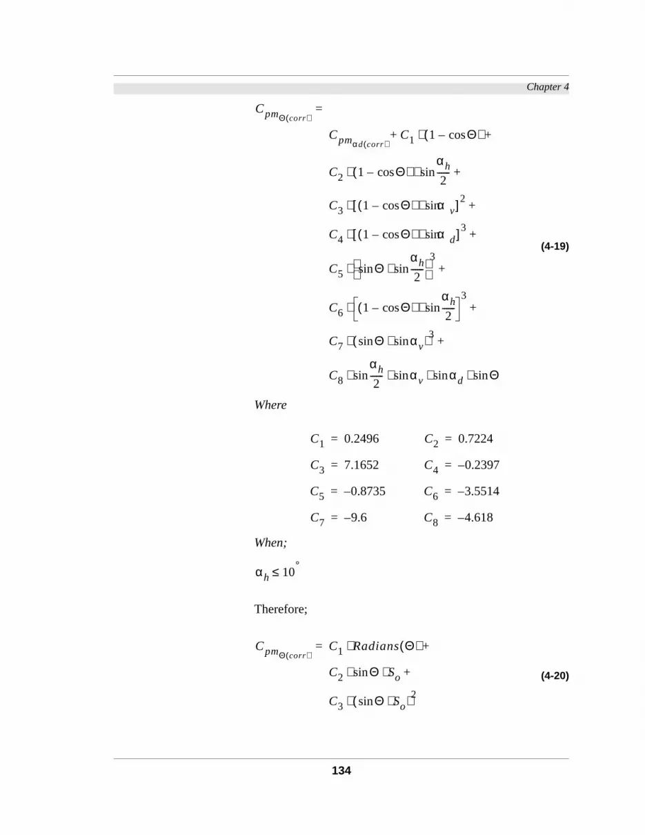
Chapter 4
(4-19)
Where
When;
Therefore;
(4-20)
CpmΘ corr( )=
Cpmαd corr( )C1 1 Θcos–( ) +⋅+
C2 1 Θcos–( )αh
2------sin⋅ ⋅ +
C3 1 Θcos–( ) αvsin⋅[ ] 2⋅ +
C4 1 Θcos–( ) αdsin⋅[ ] 3⋅ +
C5 Θsinαh
2------sin⋅
3
⋅ +
C6 1 Θcos–( )αh
2------sin⋅
3⋅ +
C7 Θsin αvsin⋅( )3⋅ +
C8
αh
2------sin αvsin αdsin Θsin⋅ ⋅ ⋅ ⋅
C1 0.2496= C2 0.7224=
C3 7.1652= C4 0.2397–=
C5 0.8735–= C6 3.5514–=
C7 9.6–= C8 4.618–=
αh 10°≤
CpmΘ corr( )C1 RadiansΘ( )⋅ +=
C2 Θsin So⋅ ⋅ +
C3 Θsin So⋅( )2⋅
134

Chapter 4
an
e
on
Coef-
sin-
to
be
ual
the
ks,
re
he
ted
ble
Where
The result of these corrections is a data correlation fit of
adjusted for the left part of the curve while th
right side function has an adjusted . A comparis
between the measured and predicted values of Pressure
ficients are presented in Appendix F, Figures F-9 to F-12.
4.15 Multiple Obstructions
So far all the experiments and functions were based on a
gle obstruction block. In this set of tests the objective was
identify the shielding effects of multiple obstruction blocks.
4.15.1 The Premise of the Experiments
The shielding effect of a group of obstruction blocks could
estimated based on averaging the shielding of the individ
component blocks of the group and the gaps between
obstruction blocks.
4.15.2 Experiment Setup
In order to test the effect of the multiple obstruction bloc
two identical and horizontally aligned obstruction blocks we
located parallel to the instrumented model (Figure 4-82). T
relationship between these two blocks and the instrumen
was varied to analyze the effect of the variables listed in Ta
4-6.
C1 0.3179=
C2 0.113=
C3 0.0064–=
R2
0.92=
R2
0.98=
135

Chapter 4
fol-
Figure 4-82 Setup of experiment. The drawing shows the studied variables.
The shielding effect was analyzed based upon varying the
lowing parameters:
TABLE 4-6 Tested Variables in the Multiple Obstruction Block Configuration
Description of the Variables Variation (#)
• The gap between the obstructions blocks(g).
12.5, 25, and 37.5 cm (4).
• Spacing between the obstruction blocksand the instrumented model (So). 2, 3, and 4 (3).
• Horizontal shift (d). This was performedfor one spacing only (2).
Three shift configura-tions were tested. See Figure 4-83.
• Wind Directions (Θ). 0˚-90˚ in 15˚ intervals (7).
g
So
Horizontal Shift (d)
Win
d D
ire
ctio
n
Θ = 0˚-90˚
g = Gap
So = Obstruction Spacing
136

Chapter 4
d in
sus
nts
w a
is
ssure
n
ures.
the
f the
clu-
t
red
ap
, in
ck.
to
sur-
Figure 4-83 The tested three shift positions.
The resulting total number of conducted tests was 105.
4.15.3 The Results Figures 4-84 to 4-87 show the various test results presente
comparative form to show the effect of each variable ver
wind direction on the average surface pressure coefficie
( ). Each figure contains three smaller figures that sho
third variable. In each of the small figures, a fourth variable
represented by three curves. Data representing the Pre
Modification Coefficient ( ) are similarly presented i
Appendix G (Figure G-3 ).
In general, the larger the gap, the higher the surface press
When the gap is wide enough, the airflow between
obstruction blocks causes the values to equal those o
unobstructed surface. This observation agrees with the con
sion of Chand et al (Ref. 50). However, the gap width is no
the operative factor in increasing the value of the measu
. In analyzing the data, it was found that with large g
widths, the obstruction blocks tend to be further apart. This
turn, reduces the shielding effect of each obstruction blo
The value of for the multiple obstruction was similar
that of the block at a closer distance to the instrumented
Shift 1 Shift 2 Shift 3
Cp
Cpm
Cp
Cp
Cp
137

Chapter 4
that
the
tive
ich
face regardless of the gap width (Figure G-4 ). This means
the effect of the gap is a function of its separation between
obstruction blocks. Therefore, the location of the gap rela
to the instrumented surface should be the variable by wh
the gap effect is determined.
138

Chapter 4
Figure 4-84 Effect of changing spacing (So) and gap width (g).
2, 3, and 4 Spacings
1/2 Obstruction Width
θ=0°-90°
G
GG
G G
G
G
CC C C
C
C
C-0.8
-0.6
-0.4
-0.2
0
0.2
0.4
0.6
0 15 30 45 60 75 90
Cp
WD (°)
G 2-H-1
C 3-H-1
4-H-1
1 Obstruction Width
2, 3, and 4 Spacingsθ=0°-90°
GG
G GG
G
G
C
C
C CC
C
C
-0.8
-0.6
-0.4
-0.2
0
0.2
0.4
0.6
0 15 30 45 60 75 90
Cp
WD (°)
G 2-O-1
C 3-O-1
4-O-1
1 1/2 Obstruction Width
2, 3, and 4 Spacingsθ=0°-90°
GG
G
GG
G
G
C
C
CC
C
C
C
-0.8
-0.6
-0.4
-0.2
0
0.2
0.4
0.6
0 15 30 45 60 75 90
Cp
WD (°)
G 2-X-1
C 3-X-1
4-X-1
139

Chapter 4
Figure 4-85 Effect of changing gap width (g) and spacing (So).
1/2, 1, 1 1/2 Obstruction Width
2 Spacingsθ=0°-90°
G
GG
G G
G
G
CC
C CC
C
C
-0.8
-0.6
-0.4
-0.2
0
0.2
0.4
0.6
0 15 30 45 60 75 90
Cp
WD (°)
G 2-H-1
C 2-O-1
2-X-1
1/2, 1, 1 1/2 Obstruction Width
3 Spacingsθ=0°-90°
GG G G
G
G
G
C
C
C CC
C
C
-0.8
-0.6
-0.4
-0.2
0
0.2
0.4
0.6
0 15 30 45 60 75 90
Cp
WD (°)
G 3-H-1
C 3-O-1
3-X-1
1/2, 1, 1 1/2 Obstruction Width
4 Spacingsθ=0°-90°
G GG
G
G
G
G
CC C C
C
C
C
-0.8
-0.6
-0.4
-0.2
0
0.2
0.4
0.6
0 15 30 45 60 75 90
Cp
WD (°)
G 4-H-1
C 4-O-1
4-X-1
140

Chapter 4
Figure 4-86 Effect of changing displacement (d) and gap width (g).
1/2 Obstruction Width
2 Spacingsθ=0°-90°
1, 2, and 3 Displacements
G
GG
G G
G
G
C
CC
C C
C
C
-0.8
-0.6
-0.4
-0.2
0
0.2
0.4
0.6
0 15 30 45 60 75 90
Cp
WD (°)
G 2-H-1
C 2-H-2
2-H-3
1 Obstruction Width
2 Spacingsθ=0°-90°
1, 2, and 3 Displacements
GG
G GG
G
G
C
CC C
C
C
C
-0.8
-0.6
-0.4
-0.2
0
0.2
0.4
0.6
0 15 30 45 60 75 90
Cp
WD (°)
G 2-O-1
C 2-O-2
2-O-3
1 1/2 Obstruction Width
2 Spacingsθ=0°-90°
1, 2, and 3 Displacements
GG
G
GG
G
G
C
CC C
C
C
C
-0.8
-0.6
-0.4
-0.2
0
0.2
0.4
0.6
0 15 30 45 60 75 90
Cp
WD (°)
G 2-X-1
C 2-X-2
2-X-3
141

Chapter 4
of
ted
pro-
Figure 4-87 Effect of changing gap width (g) and displacement (d).
Figures G-2.1.-G-2.15 in Appendix G represent the profiles
the Pressure Modification Coefficients values distribu
alongside the obstructed and unobstructed surfaces. The
1/2, 1, 1 1/2 Obstruction Width
2 Spacingsθ=0°-90°
G
GG
G G
G
G
CC
C CC
C
C
-0.8
-0.6
-0.4
-0.2
0
0.2
0.4
0.6
0 15 30 45 60 75 90
Cp
WD (°)
G 2-H-1
C 2-O-1
2-X-1
1/2, 1, 1 1/2 Obstruction Width
2 Spacings θ=0°-90°
displacement=2G
GG
G G
G
G
C
CC C
C
C
C
-0.8
-0.6
-0.4
-0.2
0
0.2
0.4
0.6
0 15 30 45 60 75 90
Cp
WD (°)
G 2-H-2
C 2-O-2
2-X-2
1/2, 1, 1 1/2 Obstruction Width
2 Spacings θ=0°-90°
displacement=3G
G G
G
G
G
G
C
C C
C
C
C
C
-0.8
-0.6
-0.4
-0.2
0
0.2
0.4
0.6
0 15 30 45 60 75 90
Cp
WD (°)
G 2-H-3
C 2-O-3
2-X-3
Cpm
142

Chapter 4
05
ng
two
pre-
tes
m
ses
ck
see
the
ing
d
vid-
the
is
ined
ge
at
ted
tion
the
the
to
.
files are plotted for each wind direction for each of the 1
tested configurations.
4.15.4 Discussion of the Results
The averaging of the obstruction blocks within the Shieldi
Effectiveness Zone (SEZ) could be achieved by one of
methods;
The first method establishes an average shielding block re
senting all existing blocks within the SEZ, and then calcula
the Pressure Modification Coefficients . The proble
with this approach is that the prediction model already u
equivalent obstruction blocks in estimating individual blo
shielding effects with respect to changes in wind direction (
section 4.14.2). The multiple steps needed to determine
equivalent obstruction block geometry and the result
shielding will have very little to do with the actual layout an
geometry of the obstruction blocks.
The second method calculates the value for each indi
ual block, and then averages the coefficients rather than
dimensions of the obstruction block. The problem with th
approach is that the averaging is not linear, i.e. the obta
values do not correspond well to the arithmetic avera
of individual values of . However, the author found th
the geometric average of the values might be correc
using the relative location of the gaps between the obstruc
blocks. This means that a block that is located in front of
instrumented model, relative to the wind direction, has
largest effect. In addition, the more perpendicular the gap
the instrumented surface, the higher the corresponding
Cpm
Cpm
Cpm
Cpm
Cpm
Cpm
143

Chapter 4
ruc-
for
en-
he
ace
ld-
id-
the
pre-
ll
ge
-4
ction
gap
ge
alt
that
sing
tion
These gaps tend to offset the shielding effect of the obst
tion blocks by increasing the surface pressures. Correcting
these factors results in a prediction model that is not only s
sitive to the relative location of each obstruction block to t
surface but also to the gaps in between.
4.15.5 The Gap Rule The gap in the mathematical model is defined as the sp
between and around the obstruction blocks within the Shie
ing Effectiveness Zone (140° windward arc). If the gap exists
between two objects, but part of it lies outside the 140° arc,
then only the part of the gap that lies within the SEZ is cons
ered (Figure 4-88).
Figure G-4 in Appendix G shows a comparison between
measured behind the two obstruction blocks and the
dicted value of each of the individual blocks. In a
cases, the combined shielding did not equal the avera34
shielding of the individual blocks. The analysis of Figure G
showed that it was necessary to add an element in the fun
that represents the gap between the blocks. To take the
into account in the determination of the weighted avera
Pressure Modification Coefficient, the gap should be de
with as an object of zero height (Figure 4-88). This means
the displacement angle of the gap should be measured u
the same definition that is used for measuring obstruc
blocks.
4-34 Arithmetic or geometric.
Cpm
Cpm
144

Chapter 4
ion
fect.
the
ion-
ion
as
hip
the
is-
take
en
as
Figure 4-88 The Gaps are the spaces between the obstruction blocks and lie within the SEZ.
Since the gap is a void, the gap rule is a location funct
rather than a function that denotes the magnitude of an ef
This means that only the location of the gap relative to
instrumented surface is accounted for in the derived relat
ship.
4.15.6 Deriving the Function
The fitting function was derived using a nonlinear regress
routine to determine the power to which each variable w
raised (Equation 4-21). The general form of the relations
is:
(4-21)
The First part of the right side of the equation deals with
averaging of the effects of the individual shielding blocks (d
cussed in section 4.15.3). The second part, was added to
into account the effect of the location of the gaps betwe
obstruction blocks (section 4.15.5). The resulting formula w
as follows;
αdg 2
αhg 2
Gap 2Gap 1
Gap 3SEZ
CpmmultipleCpmi
( )k1( ) n⁄ αd gapi( )cos( )k2
n---------------------------------------∑+∏=
145

Chapter 4
(4-22)
Where;
and;
CpmmultipleCpm1
Cpm2⋅ …( )
k1 +=
C1
αdgap1
cos αdgap2
cos …+ +
n------------------------------------------------------------------
k2
+
C2
αdgap1
cos αdgap2
cos …+ +
m------------------------------------------------------------------
2 k⋅ 2
CpmmultiplePressure Modification Coefficient of=
multiple objects
CpmiPredicted corrected individual Pressure=
Modification Coefficient
CpmΘ corr( )=
αdgapn
Displacement angle of Gap=
n Number of adjacent blocks seen by the surface=
m Numbe of visible gaps within SEZ=
i 1 2,=
C1 0.481=
C2 0.5874–=
k1 1.0907=
k2 1.8738=
146

Chapter 4
Figure 4-89 Comparison between measured and predicted values of a. (Figure G-5 shows the comparison
between the measured and predicted values of ) .
Cp
Cpm
I IIH, O, X
S=2
I
I II I
I
I
XX
X X X
X
X-0.6
-0.4
-0.2
0
0.2
0.4
0.6
0.8
0 15 30 45 60 75 90
Cp
WD (°)
2-H-1
II
I I I
I
I
XX
XX X
X
X
-0.8
-0.6
-0.4
-0.2
0
0.2
0.4
0.6
0.8
0 15 30 45 60 75 90
Cp
WD (°)
2-0-1
II
I
II
I
I
X XX
XX
X
X
-0.8
-0.6
-0.4
-0.2
0
0.2
0.4
0.6
0.8
0 15 30 45 60 75 90
Cp
WD (°)
2-X-1
H, O, X
S=2I II
I
I
II I
I
I
XX
XX
X
X
X
-0.8
-0.6
-0.4
-0.2
0
0.2
0.4
0.6
0.8
0 15 30 45 60 75 90
Cp
WD (°)
2-H-2
I
II I
I
I
I
XX
X XX
X
X
-0.8
-0.6
-0.4
-0.2
0
0.2
0.4
0.6
0.8
0 15 30 45 60 75 90
Cp
WD (°)
2-O-2
I
II I
I
I
I
XX
X XX
X
X
-0.8
-0.6
-0.4
-0.2
0
0.2
0.4
0.6
0.8
0 15 30 45 60 75 90
Cp
WD (°)
2-X-2
I IIH, O, X
S=2
I
I I
I
I
I
I
X
XX
X
X
X
X-0.8
-0.6
-0.4
-0.2
0
0.2
0.4
0.6
0.8
0 15 30 45 60 75 90
Cp
WD (°)
2-H-3
I
I I
I
I
I
I
X
X XX
X
X
X-0.8
-0.6
-0.4
-0.2
0
0.2
0.4
0.6
0.8
0 15 30 45 60 75 90
Cp
WD (°)
2-O-3
I
I I
I
I
I
I
X
X XX
X
X
X-0.8
-0.6
-0.4
-0.2
0
0.2
0.4
0.6
0.8
0 15 30 45 60 75 90
Cp
WD (°)
2-X-3
H, O, X
S=3
I II
II I I
I
I
I
XX
XX X
X
X
-0.8
-0.6
-0.4
-0.2
0
0.2
0.4
0.6
0.8
0 15 30 45 60 75 90
Cp
WD (°)
3-H-1
I
II I
I
I
I
XX
X X X
X
X
-0.8
-0.6
-0.4
-0.2
0
0.2
0.4
0.6
0.8
0 15 30 45 60 75 90
Cp
WD (°)
3-O-1
I
I
II
I
I
I
XX
X XX
X
X
-0.8
-0.6
-0.4
-0.2
0
0.2
0.4
0.6
0.8
0 15 30 45 60 75 90
Cp
WD (°)
3-X-1
147

Chapter 4
ion
e.
d
be
es-
n the
ed
ul-
a-
and
ion
a. For the description of the variables in the left margin of the graphs, refer to TABLE 4-6 .
It should be noted that there are many visible obstruct
blocks whose shielding is small or negligible, i.
, the resulting will be exaggerate
when applying Equation (4-22). Such blocks should not
included in the equation. Similarly, on analyzing surface pr
sures above those obtained from unshielded surfaces whe
wind direction exceeds 140˚, the value of calculat
was higher than 1.0. As a result, the blocks that f
fill the following condition are not to be included in the Equ
tion (4-22):
(4-23)
Figure 4-89 shows the comparison between the predicted
the measured values of the multiple obstruction funct
Legend:
Figure 4-89 Comparison between measured and predicted values of a. (Figure G-5 shows the comparison
between the measured and predicted values of ) (Continued).
Cp
Cpm
H, O, X
S=4
I II
I II
I
I
I
I
X X X XX
X
X
-0.8
-0.6
-0.4
-0.2
0
0.2
0.4
0.6
0.8
0 15 30 45 60 75 90
Cp
WD (°)
4-H-1
II I I
I
I
I
X XX X
X
X
X
-0.8
-0.6
-0.4
-0.2
0
0.2
0.4
0.6
0.8
0 15 30 45 60 75 90
Cp
WD (°)
4-O-1
4-X-1
II
I II
I
I
X XX X
X
X
X
-0.8
-0.6
-0.4
-0.2
0
0.2
0.4
0.6
0.8
0 15 30 45 60 75 90
Cp
WD (°)
I measured
X Predicted
CpmΘ corr( )1.0≈ Cpmmultiple
Cpmmultiple
0.99 CpmΘ corr( )1.06< <
148

Chapter 4
an
lex
in
est
ing
ered
an
e
her
ble
the
del
ean
ult,
for
n
k
. In general, the prediction fits the measured data with
adjusted correlation coefficient .
4.16 Complex Instrumented Models
This part deals with the estimation of values for comp
building forms. These include L, U, Z-shaped building
which wall surfaces may be shielded from the wind by the r
of the building. In these cases, only the obstruction build
blocks that are seen from the surface of interest are consid
(Figure 4-90). This case is similar to situations where
obstruction block is not fully visible from the mid point of th
surface of a simple rectangular model (Figure 4-91). In eit
case, only the obstruction blocks located within the visi
portion of the shielding effectiveness zone are included in
model.
The major difference between the simple and complex mo
forms, however, is that each has a different value of m
unobstructed Pressure Coefficient ( ). As a res
the denominator in equation (4-3) for the L-shaped model,
example, will reflect the effect of the self-shielding o
values35 (Figure 4-92).
4-35 For a full description of the sources of pressure data of unobstructed blocrefer to Section 5.6, page 197.
Cpm
R2
0.95=
Cpm
CpUnshielded
CpUnshielded
149

Chapter 4
ures
an
ist.
the
in
Figure 4-90 Self-shielding should be treated as an obstruction block.
Figure 4-91 Self-shielding of the instrumented model.
The consequence of this suggestion is that surface press
coefficients ( ) of a rectangular model will be different th
those for an L-shaped model when identical conditions ex
This occurs despite the fact that there is no difference in
value of predicted Pressure Modification Coefficient ( )
either configuration.
Θ˚
Equivalent Obstruction I
Equivalent Obstruction II
Surface
(Not included in model)
20˚
Wind Direction Θ
20˚
Cp
Cpm
150

Chapter 4
)
to
ady-
ond,
on
po-
ion
dis-
le-
ns.
ild-
und-
and
are
Figure 4-92 Surface pressures on L-shaped building, Sources: Ernest (Ref. 74).
4.17 Verification of the Model
In this section the Pressure Modification Coefficient (
model was subjected to verification in two stages. First,
compare the predicted pressure coefficients values to alre
obtained values from previous research projects and; sec
to verify the mathematical model with pressure modificati
coefficients obtained by testing a realistic model of a hy
thetical urban area. This model is described fully in Sect
4.17.4 and used in the example discussed in Appendix H .
4.17.1 Wiren’s Experiments
Wiren’s earlier experiments at the National Swedish Institute
for Building Research (Ref. 227) were used to verify the
model. These experiments investigated the wind pressure
tribution of a model of a typical Swedish house with doub
pitched (gable) roof under various shielding configuratio
The studied variables were the number of surrounding bu
ing rows (1, 2, and 3), and the spacing between the surro
ing buildings as well as between the surroundings blocks
the model (1, 1.5, 2, and 3 spacings). These experiments
illustrated in Figures 4-93 and 4-96.
0˚ -90˚90˚
Cp 0.0
0.7
-0.3
Wind Direction
Unobs
tru
cted m
odel
L-shaped Unobstructe
d model
Cpm
Cpm
151

Chapter 4
the
ef-
ob-
sic
ion
ble
no
ions
ffi-
ion
ients
4.17.2 Wiren’s Single obstruction Experiments
The most basic configuration in Wiren’s experiments was
single windward obstruction (Figure 4-93). His pressure co
ficients for the four surfaces were then compared to an un
structed model (A00). This setup was used to verify the ba
orthogonal mathematical prediction model.
The variables in this set of experiments began with variat
of the spacings of the windward block from the model (Ta
4-7). Both model and obstruction block were centered, thus
displacement was considered. Second, seven wind direct
0˚-90˚, in 15˚ intervals were tested obtaining pressure coe
cients for the four model surfaces.
4.17.2.1 Description The mathematical model for a single obstruction (sect
4.14.2) was used to estimate the average pressure coeffic
on both facade and gable end walls.
Figure 4-93 Wiren’s single obstruction experiments.
Wind Direction
Facade
Gable
TABLE 4-7 Wiren’s Single Obstruction Configurations
Configuration A10 A20 A30 A40
a/l 1 1.5 2 3
152

Chapter 4
the
the
er-
end
res
ner
the
rse
report
4.17.2.2 Results and Dis-cussion
The following section discusses the results of predicting
surface pressures on four model surfaces and explains
results for each of the configurations.
Figure 4-94 Comparison between the prediction model and Wiren’s results.
Figure 4-94 shows four graphs of the model predicting av
age Pressure Coefficients on the facade and gable
walls for both windward and leeward directions and compa
the results with the measured data36. This comparison shows a
good agreement on the windward facade wall (top left cor
of Figure 4-94).
However, the measured values for the leeward side of
facade wall (top right corner of Figure 4-94) show an inve
4-36 The measured data was extracted from a scanned copy of a graph in the (Ref. 227) using dataThief© 2.0b by Kees Huyser and Jan Van der Laan.
-1
-0.8
-0.6
-0.4
-0.2
0
0.2
0.4
0.6
0.8
1
0 15 30 45 60 75 90
Cp
av.
Wd (°)
Θ
-1
-0.8
-0.6
-0.4
-0.2
0
0.2
0.4
0.6
0.8
1
0 15 30 45 60 75 90
Cpa
v.
Wd (°)
Θ
-1
-0.8
-0.6
-0.4
-0.2
0
0.2
0.4
0.6
0.8
1
0 15 30 45 60 75 90
Cp
av.
Wd (°)
Θ
-1
-0.8
-0.6
-0.4
-0.2
0
0.2
0.4
0.6
0.8
1
0 15 30 45 60 75 90
Cpa
v.
Wd (°)
A00
A10 (meas)
A10 (calc)
A20 (meas)
A20 (calc)
A30 (meas)
A30 (calc)
A40 (meas)
A40 (calc)
Θ
Windward Side Leeward Side Facade
Gable
walls
Walls
Cpav
153

Chapter 4
ck
esult
the,
tion
n.
oin-
he-
ions
nts
ind
red
be
se
s in
the
he
on
and
ate
’s
ke
n
ures
s rel-
ild-
effect between the spacing of the obstruction building blo
and the average surface pressures between 0˚-15˚. This r
could not be predicted by the pressure shielding model as
unobstructed side (leeward side) did not see the obstruc
block at any of the relative positions at any wind directio
Thus, no effect was predicted and the resulting values c
cided with those of the unobstructed model. In fact, this p
nomenon was not encountered while testing the configurat
in The Effect of Changing Wind Direction (Section 4.14.3)
where very little variation occurred in the pressure coefficie
on the unobstructed side between 0˚-15˚. When the w
directions is greater than 30˚, the prediction fits the measu
results well. The disagreement (between 0˚ and 15˚) can
explained by the following; at wind directions normal or clo
to normal to the surface under consideration, the wake size
Wiren’s experiments were larger than those generated by
this experiment’s simple cubical model used for deriving t
mathematical relationships. Evans’ experiments (Ref. 79)
the size and extend of the wake behind various block sizes
configurations showed that double-pitched roofs tend to cre
longer wakes (maximum 35% longer wake37) than those gen-
erated behind blocks with flat roofs. As a result, Wiren
instrumented model at this wind direction was within the wa
of upwind block, preventing it from fully developing its ow
wake, and consequently increasing the surface press
above those of the unobstructed model.
4-37 The study that was conducted on various building geometries, roof shapeshowed that the wake length of a 1:2 roof slope increased the by about 35%ative to the flat roof, however this increase was inversely correlated with buing lengths
154

Chapter 4
t-
ded
re-
cted
lls
d is
iga-
the
ade
l-
gu-
ide,
ides
the
At wind directions , the instrumented model falls ou
side the generated wake, thus remaining virtually unshiel
by the obstruction block. The result in this range is well p
dicted by the model and both the measured and predi
values coincide with the unobstructed block.
In the other two walls (gable walls), the prediction model fa
short by overestimating the shielding effects when the win
parallel or near parallel (0˚-15˚) to the surface under invest
tion38. The probable reason for this discrepancy is that
model assumes no shielding is taking effect since the fac
cannot ‘see’ the obstruction block. As a result, predicted va
ues of equal those obtained from the unshielded confi
ration (Figure 4-94). Similar to the case on the leeward s
the wake generated by the windward block engulfs the s
parallel to the wind direction. Consequently, the value of
is increased by the elimination of the separation zone at
windward corner of the block (Figure 4-95).
4-38 At wind direction 0˚, the gable wall is actually at 90˚ relative to the wind direction. In Chapter 5, this issue will be thoroughly discussed.
Θ 30°≥
Cpav
Cpav
Cpav
155
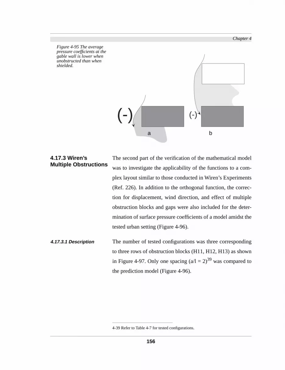
Chapter 4
del
m-
nts
c-
le
ter-
the
ding
wn
Figure 4-95 The average pressure coefficients at the gable wall is lower when unobstructed than when shielded.
4.17.3 Wiren’s Multiple Obstructions
The second part of the verification of the mathematical mo
was to investigate the applicability of the functions to a co
plex layout similar to those conducted in Wiren’s Experime
(Ref. 226). In addition to the orthogonal function, the corre
tion for displacement, wind direction, and effect of multip
obstruction blocks and gaps were also included for the de
mination of surface pressure coefficients of a model amidst
tested urban setting (Figure 4-96).
4.17.3.1 Description The number of tested configurations was three correspon
to three rows of obstruction blocks (H11, H12, H13) as sho
in Figure 4-97. Only one spacing (a/l = 2)39 was compared to
the prediction model (Figure 4-96).
4-39 Refer to Table 4-7 for tested configurations.
(-) (-)
a b
156

Chapter 4
Figure 4-96 Wiren multiple blocks grid-iron configuration.
Figure 4-97 Wiren’s grid-iron layout and spacing.
a/l=b/l
TABLE 4-8 Wiren’s Multiple Obstruction Configurations
Configuration H11 H12 H13
a/l=b/l 1 1.5 2
157

Chapter 4
lues
the
the
ur-
rve
all
ra-
ent
1)
ion
Figure 4-98 Comparison between the prediction model and Wiren’s results.
4.17.3.2 Discussion of Results
Figure 4-98 shows a comparison between the measured va
of when 48 adjacent obstruction blocks surround
instrumented model. The following can be observed from
comparison:
• The predicted values of at the windward facade s
face (top left corner Figure 4-98) fit the measured cu
except at the 0˚-15˚ wind directions. This is true for
tested configurations except for the single row configu
tion (H11). The reason for the discrepancy is the inher
problem of the multiple effect function (equation 4-2
where the averaging of a large number of obstruct
-1
-0.8
-0.6
-0.4
-0.2
0
0.2
0.4
0.6
0.8
1
0 15 30 45 60 75 90
Cpav.
Wd (°)
Θ
Windward Side Leeward Side
-1
-0.8
-0.6
-0.4
-0.2
0
0.2
0.4
0.6
0.8
1
0 15 30 45 60 75 90
Cpa
v.
Wd (°)
Θ
-1
-0.8
-0.6
-0.4
-0.2
0
0.2
0.4
0.6
0.8
1
0 15 30 45 60 75 90
Cpav.
Wd (°)
Θ
-1
-0.8
-0.6
-0.4
-0.2
0
0.2
0.4
0.6
0.8
1
0 15 30 45 60 75 90
Cpa
v.
Wd (°)
A00
H11 (meas)
H11 (calc)
H12 (meas)
H12 (calc)
H13 (meas)
H13 (calc)
Θ
Facade
GableWalls
Walls
Cpav
Cpav
158

Chapter 4
,
er-
or-
t of
ion
ur-
om
ior
he
ove
eld-
the
for
out
sev-
all
del
m-
tions
B-
blocks with high modification coefficients ( )
tend to favor the high values and produce slightly exagg
ated values of .
• The predicted values for leeward side (top right c
ner Figure 4-98) show a good fit from 0˚-30˚ as a resul
the correction for pressurization effect analyzed in Sect
4.14.3. However, at wind directions ≥ 45˚, the model does
not account for any shielding by obstruction blocks the s
face does not see.
• The predicted values of the at the gable walls (bott
two graphs of Figure 4-98) demonstrates similar behav
to those calculated for the single obstruction, with t
exception of the leeward gable side at wind direction ab
60˚, where the pressurization correction reduces the shi
ing effect40.
4-40 Increased the value of the Pressure Modification Coefficients.
4.17.4 The Realistic Model
The intention of this section is to demonstrate the ability of
mathematical (PMC) model to predict surface pressures
buildings located at complex urban layouts. The tested lay
did not represent an actual site, but attempted to include
eral geometric and spatial complexities that might not
occur in one site. The result was a simple rectangular mo
with its four wall surfaces facing different quadrants of a co
plex hypothetical urban layout (Figure 4-99).
The surface pressures were measured in boundary condi
similar to those of a small town or a suburban setting (Table
1).
Cpm 1.0≈
Cpav
Cpav
Cpav
159

Chapter 4
rent
ere
ition
to
, the
the
nd
sty-
is-
the
del
set
hts
ted
4.17.4.1 Description The instrumented model was constructed out of transpa
2mm thick plexiglass measuring mm
(Figure 4-100). Two adjacent surfaces of the model w
rigged with 24 pressure taps connected to the data acquis
system described in Section A.2 in Appendix A. In order
measure the surface pressures on the other two sides
model was rotated 180˚. Finally, to take into account
change of wind direction, the whole layout setup (model a
surroundings) was rotated from 0˚-360˚ at 10˚ intervals.
The surrounding obstructions were made of extruded poly
rene blocks of different heights and located at different d
tances from the instrumented model. In addition, two of
obstruction blocks were not parallel to the instrumented mo
and positioned on the northwestern quadrant of the site. A
of obstructions made up of three blocks of different heig
and positions relative to the instrumented model was loca
on the east side of the site.
200 100 98××
160
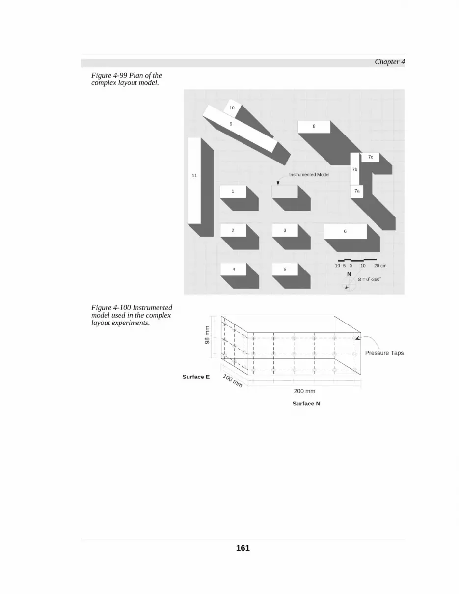
Chapter 4
Figure 4-99 Plan of the complex layout model.
Figure 4-100 Instrumented model used in the complex layout experiments.
NΘ = 0˚-360˚
0510 10 20 cm
Instrumented Model
1
2 3
4 5
6
7a
7b
7c
89
10
11
Pressure Taps
Surface N
Surface E
200 mm
100 mm
98 m
m
161

Chapter 4
re-
e-
the
our
etric
t of
Figure 4-101 View from the southwest corner of the tested model and the surrounding blocks.
4.17.4.2 Difference from Other Physical Models
The difference between this configuration and most of the p
vious studies lies in the level of complexity in both the geom
try of the obstruction blocks and the relationship between
instrumented and the surrounding blocks. The major f
areas of difference are as follows:
4.17.4.2.1 Non-parallel Obstruction Bloc ks
Two blocks (9 and 10) were chosen to represent this geom
configuration. The two blocks were located to the northwes
the model site (Figure 4-99).
162

Chapter 4
bic
f the
ape,
be
le
tion
i.e.
-
m-
ory
ind
e
val-
s
4.17.4.2.2 Comple x Obstruction Model
An obstruction block that was made up of three simple cu
blocks (7a, b, and c) was located at the northeastern side o
model facing the east side. These three blocks varied in sh
height, and relation to the surfaces from which they could
seen.
4.17.4.2.3 Partiall y Hid den Obstruction Bloc ks
The model contained two categories of partially visib
obstruction blocks. The first category was when an obstruc
block could be seen over a relatively shorter block
. An example of this was posi
tioned behind the non-parallel obstruction block and the co
plex obstruction block (10 and 7c). The second categ
occurred when a long obstruction block was located beh
shorter one and parts of it were still visibl
( ). Such conditions were included
in the model on the western side of the site (11).
4.17.4.3 Results Following the steps explained in Chapter 5, the predicted
ues were compared to the measured Pressure Coefficient
in Figures 4-102 to 4-105.
αvback block αv front block>
αv back block αv front block>
Cp
163

Chapter 4
Figure 4-102 Comparison between predicted and measured values of on the North side of the model.
Cp
-2 -1.5 -1 -0.5 0 0.5 1
0° 15°30°
45°
60°
75°
90°
105°
120°
135°
150°165°180°195°
210°
225°
240°
255°
270°
285°
300°
315°
330°345°
X X
X XXXXXX
X
XX
XXXX
XXXXX
XX
XX
XX
X
X
XXXX X X X X
Cp_unobst
X Cp_meas
Cp_pred
Cp
164

Chapter 4
Figure 4-103 Comparison between predicted and measured values of on the South side of the model
Cp
-2 -1.5 -1 -0.5 0 0.5 1
0° 15°30°
45°
60°
75°
90°
105°
120°
135°
150°165°180°195°
210°
225°
240°
255°
270°
285°
300°
315°
330°345°
X XX X
XXXXXXXX
XX
XX
XXX
XXX
XX
XX
X
XXX X X XX
XX X
Cp_unobst
X Cp_meas
Cp_pred
Cp
165

Chapter 4
Figure 4-104 Comparison between predicted and measured values of on the East side of the model.
Cp
-2 -1.5 -1 -0.5 0 0.5 1
0° 15°30°
45°
60°
75°
90°
105°
120°
135°
150°165°180°195°
210°
225°
240°
255°
270°
285°
300°
315°
330°345°
X X X X X XX
X
X
X
X
X
X
X
XX
XXXXXX
XX
XXXXXXXX X X
X XX
Cp_unobst
X Cp_meas
Cp_pred
Cp
166

Chapter 4
data.
pre-
ea-
e of
Figure 4-105 Comparison between predicted and measured values of on the West side of the model.
4.17.4.4 Discussion In general, the predicted values are close to the measured
However, there are some exceptions where the pressure
diction model fell short:
Figure 4-102 shows a comparison between the predicted, m
sured and unobstructed values of on the north surfac
Cp
-2 -1.5 -1 -0.5 0 0.5 1
0° 15°30°
45°
60°
75°
90°
105°
120°
135°
150°165°180°195°
210°
225°
240°
255°
270°
285°
300°
315°
330°345°
XXX X X
XXXXXXX
XXX
XXXXXXXX
X
X
X
X
X
X
X
X
XX
X X XX
Cp_unobst
X Cp_meas
Cp_pred
Cp
Cp
167

Chapter 4
5˚,
nts.
ted
the
c-
els
tical
rved
tion
rom
tion
The
ual
to
nc-
an
ay
way
be
ock
ion
ee-
cing
the instrumented model. In wind directions between 330˚-1
the prediction model overestimates the pressure coefficie
The high value of could be attributed to the gap loca
upwind which in the mathematical model tends to increase
value of . However, the orientation of obstru
tion block (9) in relation to the instrumented model chann
the flow and shifts the wake towards the north surface.
Figure 4-102 shows that between 70˚-125˚ the mathema
model underestimates values. The same can be obse
in Figure 4-104 (110˚-150˚). In both cases, the pressuriza
is caused by airflow through gaps that could not be seen f
the surface under investigation.
4.18 Conclusions A mathematical model has been developed for the predic
of surface pressure coefficients in a shielded environment.
model uses three angles of description for the individ
obstruction blocks relative to surface for which pressure is
be estimated. A number of corrections were added to the fu
tion to account for building geometric relationships other th
orthogonal symmetrical configurations.
Wind direction affects airflow around buildings in such a w
that the generated wakes are shifted either towards or a
from the surface in question. These effects are found to
influenced by the relationship between the obstruction bl
and the model, wind direction, and whether the obstruct
block could be visible to the surface under consideration. L
ward blocks affect the surface pressures of the surfaces fa
Cp
Cpm multiple( )
Cp
168

Chapter 4
ver-
the
al
locks
tion
on
ost
tal
od fit
e of
nd
in
l of a
ing
nd
was
the
ure
ot be
lly
g in
ined
them by increasing the pressures as a result of airflow di
sion into the wake of the instrumented model.
The effect of multiple obstructions is estimated based on
geometric averaging of the shielding effect of the individu
blocks. Passageways or gaps between the obstruction b
increase the surface pressures as a function of their loca
relative to the instrumented surface.
An arc of 140˚ around the axis formed by the wind directi
striking the surface is found to be the limit beyond which m
obstruction blocks do not affect the surface pressures.
The verification of the model using Wiren’s experimen
results shows that the proposed procedure produces a go
to data obtained from some of his experiments. This despit
Wiren’s use of gable-roof models for both instrumented a
surrounding blocks instead of the flat-roof models used
deriving the mathematical model.
When the mathematical model was tested against a mode
hypothetical urban setting that contained complex build
configurations, multiple gaps and building relationships, a
various block heights, a reasonable fit was produced. This
true except for wind directions where the gaps between
surrounding blocks channeled the air causing press
increases even on surfaces from which these gaps could n
seen. Another effect, a shifting of wake could not be fu
described or predicted by the mathematical model, resultin
predicted surface pressure values higher than those obta
from the tests.
169

Chapter 4
ore
uts,
t of
face
was
ings
In many ways the gap effects in the verification are m
extreme than would normally be encountered in urban layo
where there are more obstructions beyond the gaps.
In general, the proposed model was found to predict mos
the possible relationships between the instrumented sur
and the obstruction blocks. This meant that the model
flexible enough to predict surface pressures in urban sett
unrestricted by a pre-tested layout.
170

171
Chapter 5

5
Implementations of the Prediction Modelthe
tion
r 4.
in
, a
ion
the
on
he
ind
l as
re
ing
ta
oor
5.1 Introduction This Chapter deals with developing the tools for predicting
surface pressures of shielded buildings. This determina
follows the mathematical relationships discussed in Chapte
The tools include methods for describing obstruction blocks
the form needed by the mathematical model. In addition
method for predicting local wind speeds from weather stat
data is described.
The second part of the chapter deals with the integration of
Pressure Prediction Model (PPM) with the Indoor Ventilati
Coefficient (IVC) Model developed by Ernest (Ref. 74). T
IVC model uses pressure coefficient values and local w
speeds to predict indoor air velocities, turbulence, as wel
other descriptives of indoor airflow.
Figure 5-1 shows how the PPM, IVC, and SITECLIMATE a
combined in this chapter to produce a method for predict
indoor air velocities of shielded buildings using wind da
obtained at remote stations. This model is called the Ind
Velocity Model (IVM).
172

Chapter 5
ion
e.
er-
ion
sure
-
Figure 5-1 The Different phases of the Indoor Velocity Model (IVM).
5.2 Application of Pressure Modification Coefficient Method
Natural ventilation is predicted by the Pressure Modificat
Coefficient Method (PMC) through the following steps:
• Obtain Surface pressure data for an unobstructed surfac
• Calculate the pressures for wind directions other than p
pendicular to the surface.
• Determine the angles describing the individual obstruct
blocks visible to the surface under consideration.
• For the surface under consideration, calculate the pres
modification coefficients of the visible individual obstruc
tion blocks.
UnobstructedSurface Pressures
Pressure PredictionModel (PPM)
Indoor VelocityCoefficient (IVC) Model
ComplexShapes
RectangularShapes
Pressure ModificationCoefficient (PMC)
Site-Specific WindData (SITECLIMATE)
In
do
or
V
el
oc
it
y
Mo
de
l
(I
VM
)
173

Chapter 5
tion
ec-
aces
l-
vari-
ed
atic
ck
ang-
d or
ela-
seri-
el.
sal
ses
cks
d by
n
the
s of
ion
uc-
r on
re
• Calculate surface pressures using the pressure modifica
coefficients and the pressure coefficients of the wind-dir
tion-coincident unobstructed surfaces.
• Use the calculated pressure values at the different surf
to predict indoor air velocities using the IVC model deve
oped by Ernest (briefly discussed in Section 5.8).
5.3 Inputting Model Description Variables
The research thus far has concentrated on the geometric
ables from which the mathematical functions were deriv
(i.e. , , , and ). These angles represent a st
description of the relationship between the obstruction blo
and the surface for which the pressure is calculated. On ch
ing the wind direction, these angles have to be re-measure
recalculated to account for the newly created geometric r
tionships between the blocks and the model. This process
ously complicates implementation of the mathematical mod
To simplify the input to the mathematical model, a univer
system of obstruction description was developed that u
polar coordinates to describe the individual obstruction blo
and the gaps in between them. A similar system was use
Taylor et al (Ref. 208) to describe windward obstructio
blocks. The advantages of using polar coordinates over
using cartesian angles of description were as follows:
• The polar coordinates are measured once. The change
the geometric relationships caused by the wind direct
changes are calculated from the same coordinates.
• The polar coordinates of the visible corners of the obstr
tion blocks are easier to measure, whether from plans o
site specially when large number of wind directions a
involved.
αh αv αd αdg
174

Chapter 5
of
olar
e
the
er
an
the
is
ails,
5.3.1 Conventions In order to use a single function for calculating the angles
description, a standard convention for measuring the p
coordinates was established (Figure 5-2).
Figure 5-2 Using the polar coordinates as basis for describing obstruction blocks.
In the proposed polar coordinate system, the radial distanc(r)
is measured in terms of the obstruction spacings1 ( ) from
the center of the surface to the outermost visible corner of
obstruction block. If a corner of is obscured by anoth
obstruction block, the furthest visible point of the surface c
be used instead (Figure 5-3). The polar angular coordinate(λ)
is measured from a line perpendicular to the surface of
model (polar axis). As a convention, any angle left of the ax
is negative while on the right is positive (Figure 5-2).
5-1 Distance of obstruction block expressed in terms of its height, for more detrefer to the definition in Section 4.6.2.4, page 66.
+- Surface
λ2b
λ1b Pt.1b
Pt.2b−λ2a
−λ1a
Pol
ar A
xis
-Θ +Θa
bPt.1a
Pt.2a
r1ar2a
r1b r2b
So
175

Chapter 5
rdi-
ro-
the
he-
to
sur-
tion
ce
oor-
face
yer
is
eft,
.3.3
ri-
Figure 5-3 Polar coordinates for an obstruction block with one corner not visible from surface in question.
5.3.2 Graphically Determining Angles of Obstruction Blocks
A special protractor was devised to measure the polar coo
nates of the visible corners of obstructing buildings. This p
tractor can either be used directly for measuring
coordinates, as will be shown in this section, or for the mat
matical derivation of the obstruction angles (equations 5-7
5-20).
The protractor consists of two layers and a cursor for mea
ing both the angular and radial coordinates of the obstruc
block and the wind direction acting on the building surfa
under considerations (Figure 5-6).
The first layer (Figure 5-4) is used to measure the polar c
dinates of obstruction blocks and gaps, seen from the sur
for which the pressure coefficient to be determined. This la
is composed of two concentric circles. The inner circle
marked 0˚-180˚ on the right side and 0˚-(-180˚) on the l
corresponding to the convention established in Section 5
and illustrated in Figure 5-2. At the center of the circle, a ho
Surface
λ2
Pt.2
−λ1 Pol
ar A
xis
Pt.1
176
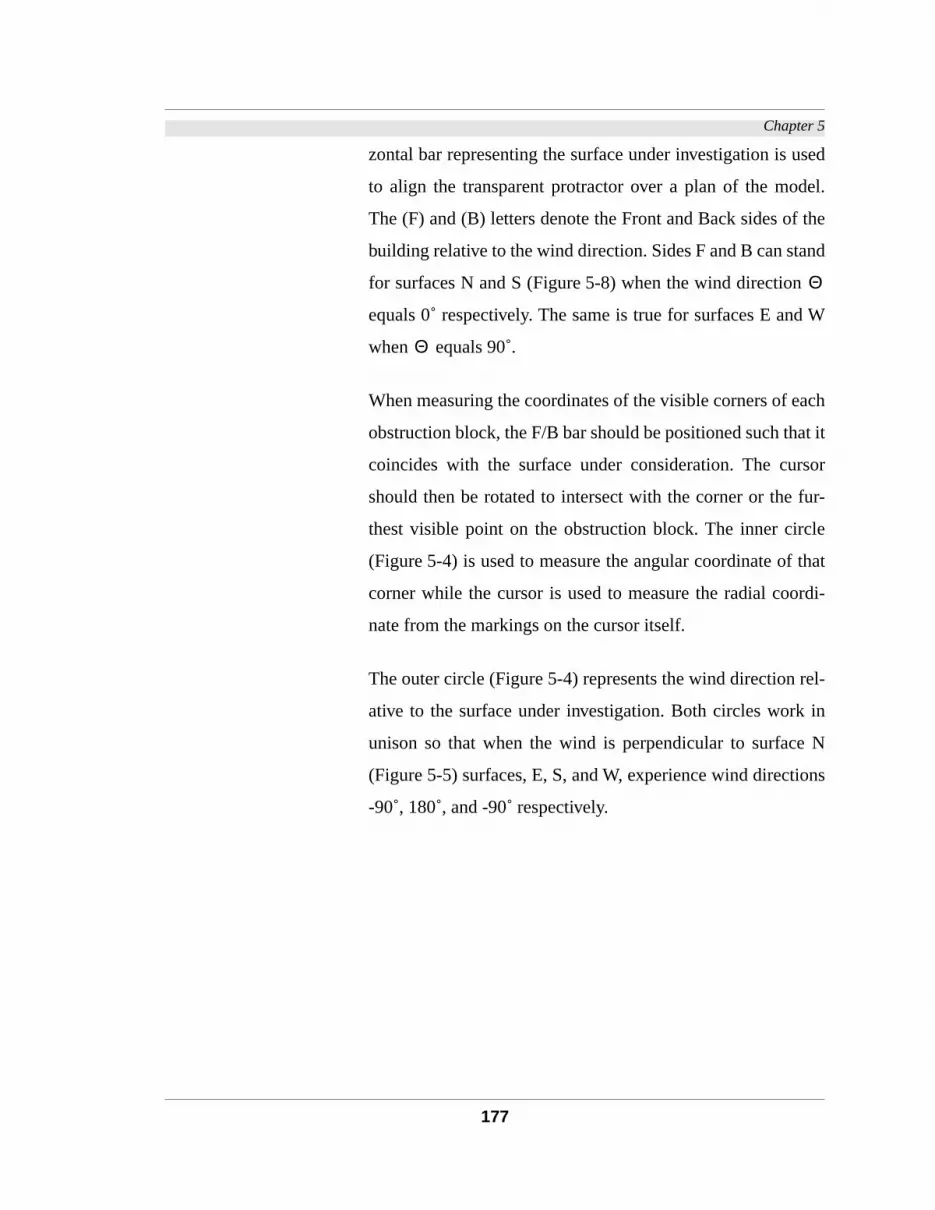
Chapter 5
sed
del.
the
nd
d W
ach
at it
sor
fur-
le
that
rdi-
rel-
in
N
ons
zontal bar representing the surface under investigation is u
to align the transparent protractor over a plan of the mo
The (F) and (B) letters denote the Front and Back sides of
building relative to the wind direction. Sides F and B can sta
for surfaces N and S (Figure 5-8) when the wind direction
equals 0˚ respectively. The same is true for surfaces E an
when equals 90˚.
When measuring the coordinates of the visible corners of e
obstruction block, the F/B bar should be positioned such th
coincides with the surface under consideration. The cur
should then be rotated to intersect with the corner or the
thest visible point on the obstruction block. The inner circ
(Figure 5-4) is used to measure the angular coordinate of
corner while the cursor is used to measure the radial coo
nate from the markings on the cursor itself.
The outer circle (Figure 5-4) represents the wind direction
ative to the surface under investigation. Both circles work
unison so that when the wind is perpendicular to surface
(Figure 5-5) surfaces, E, S, and W, experience wind directi
-90˚, 180˚, and -90˚ respectively.
Θ
Θ
177

Chapter 5
the
ical
on
Figure 5-4 The base layer of the protractor
Figure 5-5 Wind directions relative to model surfaces.
The second layer (Figure 5-6) is used in determining
Shielding Effectiveness Zone component of the mathemat
model. This layer contains a line indicating the wind directi
F
B
0360 10
20
30
40
50
60
70
80
90
350340
330
320
310
300
290
280
270
180 170160
150
140
130
120
110
100
190200
210
220
230
240
250
260
0 15
30
45
60
75
90
105
120
135
150
165±180
-15
-30
-45
-60
-75
-90
-105
-120
-135
-150
-165
Blocks and Gaps
Wind Direction
F
B
0˚
-90˚
±180˚
90˚
Win
d D
irect
ion
N
E
S
W
178

Chapter 5
40
one
der
ation
tor
ea-
e of
to
tion
es.
the
the
ple,
er,
in the middle of a transparent sector covering an arc of 1°
representing the shielding effectiveness zone (SEZ). This z
of the protractor is used to determine what the surface ‘sees’ at
a certain wind direction. Obstruction blocks that show un
the transparent SEZ are the ones to be used in the estim
of the shielding effect. Any block lying in the shaded sec
Pressure Prediction Model (PPM).
Figure 5-6 The wind direction layer and cursor.
The cursor (Figure 5-6 left) is the pointing, marking, and m
suring scale of the protractor from the center of the surfac
the building. It is designed for two purposes. The first is
mark the polar angles of the visible edges of an obstruc
block. The second, is to measure the distance to these edg
Figure 5-7 shows an example of using the protractor. First,
user aligns the first layer on top of the model plan so that
F/B bar coincides with the surface of interest. In the exam
two obstruction blocks appear in view of surface N. Howev
win
d di
rect
ion
0
10
20
30
40
50
0
10
20
30
40
50
179

Chapter 5
ec-
i-
n
ing
ge
ical
n for
ine
-
when the second layer is positioned to match the wind dir
tion (Θ˚), the left block is no longer visible. The polar coord
nates (r1,-λ1) and (r2,λ2) of the remaining block are then take
off using the inner circle of the first layer and the cursor.
Figure 5-7 An example of protractor use.
5.3.3 Calculating the Angles to Obstruction Blocks
Repeating such measurements for all wind directions us
the protractor (Section 5.3.2) would be difficult for any lar
number of obstructions. Instead, a number of mathemat
equations can be used to calculate the angles of descriptio
the polar coordinates (rn,λn) of all the visible corners of
obstruction blocks. The equations are expanded to determ
the visibility of obstruction blocks within the Shielding Effec
tiveness Zone.
WD (Θ
˚)-λ1
r1Surface N
+-λ2
r2
180
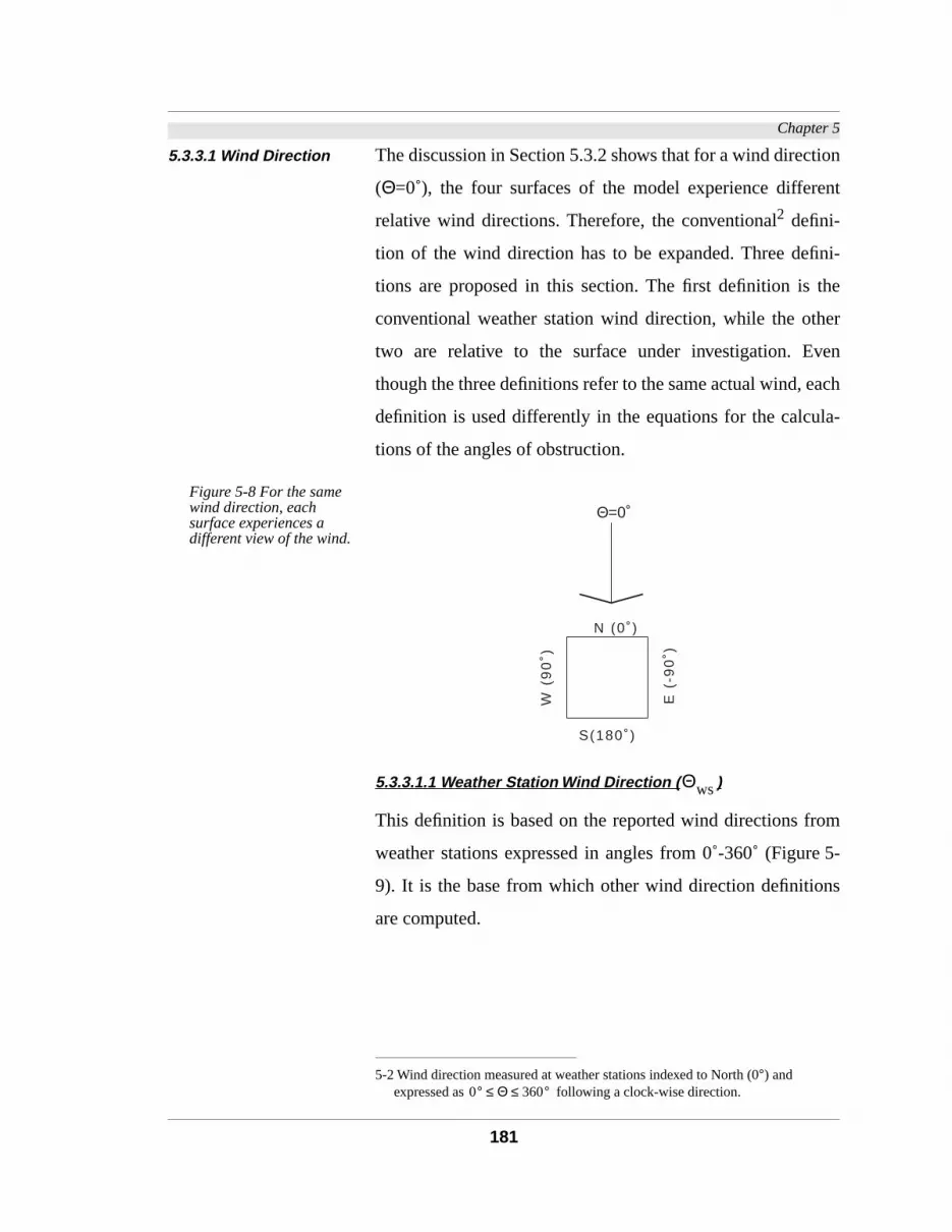
Chapter 5
tion
ent
ni-
the
er
en
ach
la-
om
e 5-
ns
5.3.3.1 Wind Direction The discussion in Section 5.3.2 shows that for a wind direc
(Θ=0˚), the four surfaces of the model experience differ
relative wind directions. Therefore, the conventional2 defini-
tion of the wind direction has to be expanded. Three defi
tions are proposed in this section. The first definition is
conventional weather station wind direction, while the oth
two are relative to the surface under investigation. Ev
though the three definitions refer to the same actual wind, e
definition is used differently in the equations for the calcu
tions of the angles of obstruction.
5-2 Wind direction measured at weather stations indexed to North (0°) and expressed as following a clock-wise direction.
Figure 5-8 For the same wind direction, each surface experiences a different view of the wind.
5.3.3.1.1 Weather Station Wind Direction ( )
This definition is based on the reported wind directions fr
weather stations expressed in angles from 0˚-360˚ (Figur
9). It is the base from which other wind direction definitio
are computed.
0° Θ 360°≤ ≤
Θ=0˚
N (0˚)
E (
-90
˚)
W (
90
˚)
S (180˚)
Θws
181

Chapter 5
di-
s
e
he
the
t of
Figure 5-9 Weather station wind direction.
5.3.3.1.2 Model Wind Direction ( )
This definition is used in the calculation of all Pressure Mo
fication Coefficients3. The range of this angle is defined a
(Figure 5-10). Hence, for surface N, th
wind direction 340˚ is handled in the prediction model t
same as 20˚. The only difference is the relative position of
surrounding obstruction blocks seen from the vantage poin
that surface.
5-3 Used in all the surface pressure calculations in Chapter 4.
Figure 5-10 Wind direction as used in the prediction model.
Θws=0˚-360˚
Θmod
0° Θmod 180°≤ ≤
Θmod=0˚-180˚
N
182

Chapter 5
the
of
on
sig-
At
e
he
ur
The
at
5.3.3.1.3 Relative Wind Direction ( )
The relative wind direction is used in the determination of
position of the obstruction blocks relative to the surface
interest. The relative wind direction range is 0˚-±180˚
(Figure 5-11).
Figure 5-11 Wind direction as used in the determination of the relative location of the obstruction blocks.
Figure 5-11 shows that for surface N, the wind direction
the right side of the line perpendicular to the surface is de
nated a positive sign while the left of the line is negative.
wind direction , Figure 5-8 shows that the relativ
wind direction depends on the relative position of t
surface to the wind direction. The sign of at the fo
sides correspond to the previously discussed convention.
following is the values of for all the surfaces
:
(5-1)
Θrel
Θrel=0˚-±180˚
N
+-
Θws 0°=
Θrel
Θrel
Θrel
Θws 0°=
Surface NΘrel Θws 0°=@, 0°=
Surface SΘrel Θws 0°=@, 180°=
Surface EΘrel Θws 0°=@, 90°–=
Surface WΘrel Θws 0°=@, 90°=
183
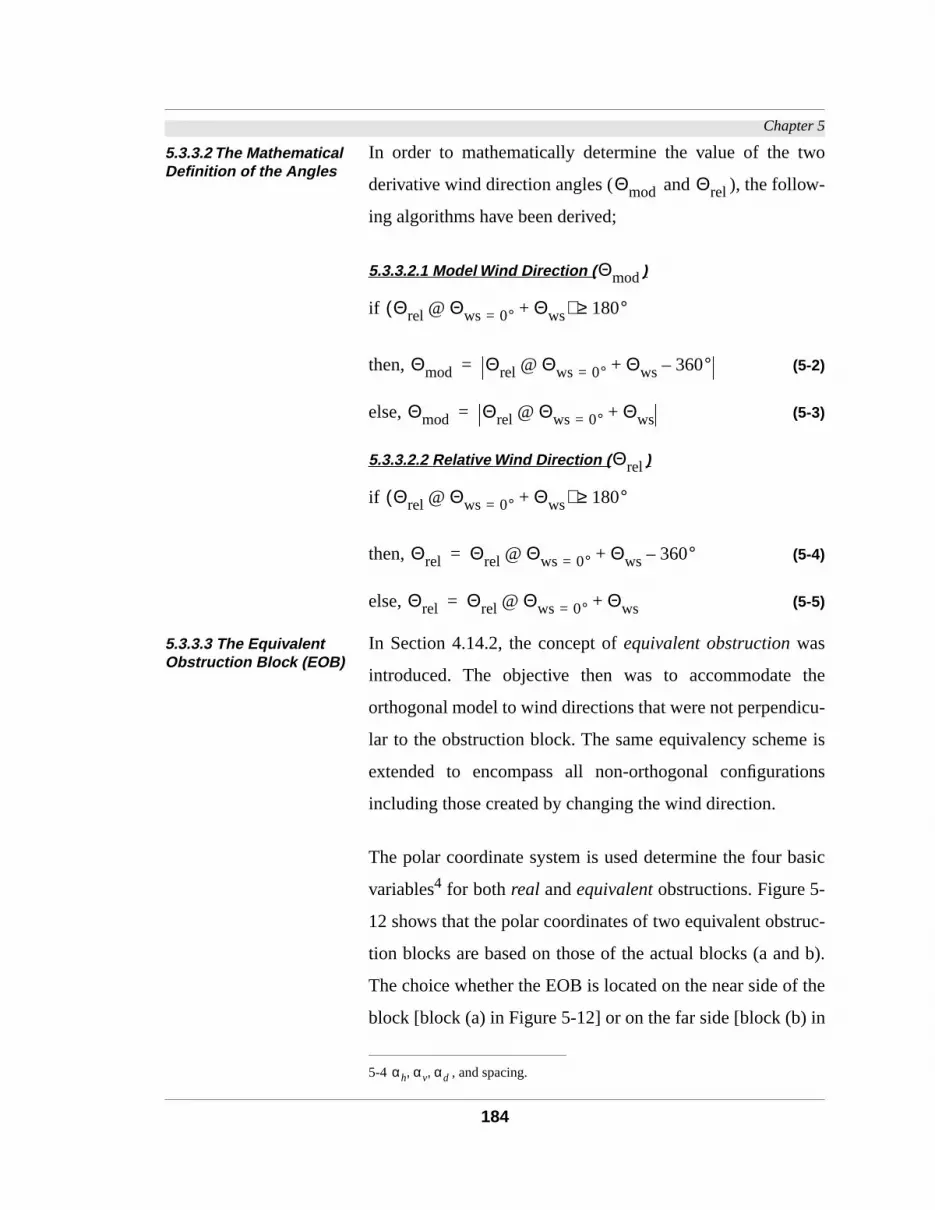
Chapter 5
wo
-
the
cu-
e is
ons
asic
ruc-
d b).
f the
in
5.3.3.2 The Mathematical Definition of the Angles
In order to mathematically determine the value of the t
derivative wind direction angles ( and ), the follow
ing algorithms have been derived;
5.3.3.2.1 Model Wind Direction ( )
if
then, (5-2)
else, (5-3)
5.3.3.2.2 Relative Wind Direction ( )
if
then, (5-4)
else, (5-5)
5.3.3.3 The Equivalent Obstruction Block (EOB)
In Section 4.14.2, the concept of equivalent obstruction was
introduced. The objective then was to accommodate
orthogonal model to wind directions that were not perpendi
lar to the obstruction block. The same equivalency schem
extended to encompass all non-orthogonal configurati
including those created by changing the wind direction.
The polar coordinate system is used determine the four b
variables4 for both real and equivalent obstructions. Figure 5-
12 shows that the polar coordinates of two equivalent obst
tion blocks are based on those of the actual blocks (a an
The choice whether the EOB is located on the near side o
block [block (a) in Figure 5-12] or on the far side [block (b)
5-4 , and spacing.
Θmod Θrel
Θmod
Θrel Θws 0°=@ Θws+( ) 180°≥
Θmod Θrel Θws 0°=@ Θws 360°–+=
Θmod Θrel Θws 0°=@ Θws+=
Θrel
Θrel Θws 0°=@ Θws+( ) 180°≥
Θrel Θrel Θws 0°=@ Θws 360°–+=
Θrel Θrel Θws 0°=@ Θws+=
αh αv αd, ,
184

Chapter 5
om
ig-
f
nt 1
rge
a-
er
are
is
r
ck
he
sti-
ent
the
Figure 5-12] depends on the selection of the first point fr
which the equivalent would be calculated (Pt1 a&b).
It is therefore, essential to define which point is to be des
nated as Point 1 (Pt.1), since the mathematical description o
the equivalent depends on it. Figure 5-12 shows that poi
was chosen in such a way that the obstruction block with la
windward depth (block b in Figure 5-12) will have an equiv
lent block of a spacing larger than the one with a shallow
depth (block a). Since the vertical and displacement angles
measured from the EOB, the shielding effect of block (a)
larger than that of block (b)5. This selection of points orde
takes into account the relatively shorter wake length of blo
(b) in accordance with the results of Evans (Ref. 79). T
slightly wider equivalent width does not lead to the over e
mation of the shielding effect since the large displacem
angle will guarantee the insignificance of this extension to
obstruction width.
5-5 Refer to Section 4.14.2.2, page 114.
Figure 5-12 Equivalent obstruction widths.
a
b
Pt1a
Pt2a
Pt2b
Pt1b
185

Chapter 5
ys
12).
m
geo-
the
ine
or-
ds
ruc-
tru-
to
e is
onal
-13
ost
used
In general, the rule of thumb is that the Point 1 is alwa
located at the edge of the longer visible surface (Figure 5-
The following is a description of a mathematical algorith
that checks the selection of the points. The purpose of the
metric relation presented in Equation (5-6) is to eliminate
need for the user of the mathematical model to predeterm
the order of each visible corners of each block.
After randomly choosing the polar coordinates of the two c
ners of the obstruction building (rx,λx and ry,λy), the following
function will determine whether the order is correct or nee
to be changed;
if (5-6)
Therefore, choose point with higher absolute value of λ to be Point 1.
Else, choose point with lower absolute value of λ to be point 1.
5.3.3.4 Calculating the Angles of Description of Real Obstruction Blocks
This section is limited to the special case when both obst
tion and equivalent obstruction block are parallel to the ins
mented surface6. It occurs when the obstruction is parallel
the surface and the wind direction is 0˚. This special cas
used as a base for general equations involving non-orthog
configurations and wind directions other than 0˚. Figure 5
illustrates the input of polar coordinates of the two outer m
5-6 This means that the geometric function described in this section can not bein the derivation of the four variables in either Scenario II or Scenario III or when .
r x λxsin⋅ r y λysin⋅–
r y λycos⋅ r x λxcos⋅–------------------------------------------------------ 1≤
Θ o°≠
186

Chapter 5
tion
-
visible corners of the block (pt.1 and pt.2) as well as the
derived variables used to calculate the angles of obstruc
, , and .
Figure 5-13 Calculating the obstruction angles based on the polar coordinates when wind direction=0˚.
When the wind direction (for orthogonal configura
tions), the angles of description for the real obstruction block
are calculated as follows:
(5-7)
(5-8)
(5-9)
(5-10)
(5-11)
αh αv αd
Pt.1(r1,λ1)
Pt.2(r2,λ2)
r 1
r 2
r w/2
λ1
λ2
Obstht
αd
αh
Modelht
Θ 0°=
αh λ1 λ2–=
Spacing So( ) λ1cos r1⋅=
rcalc
So
λ2cos--------------=
rw 2⁄λ1sin r1⋅ λ2sin rcalc⋅+
2-----------------------------------------------------------
2
So2
+=
αv
htorw 2⁄-----------
atan=
187

Chapter 5
ck
ons
g
er-
o-
lent
he
olar
.
lent
he
the
r
(5-12)
Where
However, it should be noted that when the obstruction blo
falls outside the SEZ, should be equals to 1.0 (Equati
4-11 and 4-13). In order to obtain , the followin
values of the angles should be used:
(5-13)
5.3.3.5 Calculating the Angles of Description of Equivalent Obstruction Block (General Form)
For the likely occasions when the wind direction is not p
pendicular to the obstruction block, a group of modified ge
metric functions are needed to describe the equiva
obstruction block. To avoid complicating the data input, t
new derived coordinates are based on the measured p
coordinates of the visible corners (Equations 5-14 to 5-17)
In order to calculate the polar coordinates of the equiva
obstruction plane, the polar coordinates of point Pt.calc have to
be determined (Figure 5-14). This involves calculating t
radial distance of the intercept to the equivalent plane and
line of vision ( ).
αd
λ1 λ2+
2---------------------=
λn Polar angular coordinate of visible obstruction corne=
SoDistance of obstruction block from surface
hto------------------------------------------------------------------------------------------------------=
rn Radial distance coordinate in Spacings So( )=
hto Obstruction height=
Cpm
Cpm 1.0=
αh 0°=
αv 0°=
and αd 90°=
rcalc
188

Chapter 5
xi-of
.
Figure 5-14 Polar coordinates of the EOB.
(use Equation 5-7).
(5-14)
(5-15)
∴ polar coordinates are -Figure 5-14
(5-16)
use equation 5-117.
5-7 It should be noted that the above calculation of the value of is an appromation since the value of the equivalent obstruction is large than that the original. Thus, the result will always be smaller than the actual value of
r 1
r w/2
r calc
Equivalent Obstruc-tion Plane
Win
d D
irect
ion
Θ
Pt.calc(rcalc,λ2)
Pt.1(r1,λ1)Pt.2(r2,λ2)
λ1
λ2
αh/2
αd
Spa
cing
s (S
)
Pt.2(r2,λ2)
Polar A
xis
Bottom Plane
αh
SpacingSo( ) Θrel λ–1
cos r1⋅=
rcalc
Θrel λ–1
cos r1⋅
Θrel λ–2
cos--------------------------------------------=
rcalc λ2,( )
rw 2⁄
Θrel λ–1
sin r1⋅ Θrel λ–2
sin rcalc⋅+
2--------------------------------------------------------------------------------------------------
2
So2
+=
αv
αvrw 2⁄
αv
189

Chapter 5
he
n
ose
tion
ed
ea-
n-
on
(5-17)
5.3.3.6 Defining the 140˚ Shielding Effectiveness Zone (SEZ)
The 140˚ limit of the shielding effectiveness zone of t
obstruction block8 is measured relative to the wind directio
(Figure 5-16a). The limits of this zone always supersede th
of the outer most visible angles that define the obstruc
block (Figure 5-16b). However, since the 140˚ limit is bas
on the wind direction, while the polar coordinates are m
sured from the polar axis (Figure 5-15), the following relatio
ships is developed to reconcile the two:
(5-18)
and
(5-19)
5-8 The 140˚ Shielding Effectiveness Zone is discussed in Section 4.12.2.2.2 page 89 and illustrated in Figure 5-16a.
Figure 5-15 The determination of the values of the SEZ relative to polar coordinates
αd
λ1 λ2+
2--------------------- Θrel–=
λ70 70° Θws Θrel 0=–( )–=
λ 70– 70–( )° Θws Θrel 0=–( )–=
-70˚
λ70λ−70
(WD)Θrel = Θws-Θrel=0
WD
Pol
ar A
xis
70˚
190

Chapter 5
the
e
)
are
ec-
d 5-
Consequently, the horizontal angle can be defined as
visible portion of the obstruction block that lies within th
140˚ zone of shielding effectiveness (Figure 5-16a to 5-16c9.
As a result of this definition, Equation (5-20) represents
the polar coordinates of the point where the shielding eff
tiveness arc intercepts the equivalent obstruction block:
if , or ;
∴ (5-20)
5-9 The model self-shielding is also treated in the same way (Figures 5-16b an16c).
αh
λn 70°≥ λm 70–( )°≤
Ptcalcrcalc 70°±( ) Θws Θrel 0=–( )–( ),[ ]
191

Chapter 5
e of
the
the
Figure 5-16 Defining the 140˚ limit of the obstruction block.
Figures 5-16c demonstrates an instance when the surfac
the model under consideration obstructs the full view of
shielding block. In such cases, the self-obstruction of
20˚
Ptcalc(2)(rcalc,λ=20)
Wind Direction Θ
20˚
Wind Direction Θ
20˚
20˚
Win
d D
irect
ion
Θ
20˚
Equivalent Obstruction Plane
Shielding Effectiveness Zone (SEZ)
a
b
c
192

Chapter 5
the
sur-
uc-
ble
the
ng
cor-
or-
e
gap
model surface should be taken into account in determining
horizontal angle of view. This should take place when mea
ing the polar coordinates of the visible corners of the obstr
tion block.
The self-shielding of the model surface reduces the viewa
area of the obstruction block and consequently reduces
horizontal angle of obstruction. Similar to the 140˚ shieldi
effectiveness zone, this reduction supersedes the visible
ners of the obstruction block.
In the example shown in Figure 5-17, Pt.1 is determined by the
self-shielding of the model surface. As a result, the polar co
dinate of point Pt.1 is (r1,λ1).
Figure 5-17 Self-shielding reduces the horizontal angle of view and consequently reduces the shielding effect of the obstruction block.
5.3.3.7 Defining a Gap The angle that describes a gap10 can be calculated using th
polar coordinates of the points encompassing the
5-10 The gap is defined in Section 4.15.5, page 144.
20˚20˚
Pt.1(r1,λ1)
Pt.2(r2,λ2)
Polar Axis
−λ1 -λ2
Win
d D
irect
ion
Θ
193

Chapter 5
qua-
an
nti-
.3.3
m-
er
ec-
fect
di-
d-
the
n
(Figure 5-18). These coordinates are then plugged into e
tion 5-17 to determine the displacement angle of
equivalent gap whose horizontal angle of obstruction is ide
cal to that of the original gap.
Figure 5-18 The Gap should be treated as a solid object.
5.3.4 Complex Obstruction Blocks
The obstruction angles discussed in sections 5.3.2 and 5
are for simple obstruction block configurations. More co
plex obstruction configurations can include:
• Multiple obstruction blocks surrounding the surface und
consideration. This level of complexity is addressed in S
tion 4.15 where the weighted average of the shielding ef
of individual blocks and gaps was determined11. That
approach allows the angle determination functions of in
vidual blocks to be used in describing complex surroun
ings. An example of this concept is demonstrated in
verification of the model using Wiren’s multiple grid-iro
setup (Section 4.17.3).
5-11 See Equation 4-22.
αdg
Win
d D
irect
ion
Gap
Equivalent Gap
Pt.1(r1,λ1)
Pt.2(r2,λ2)
Pt.calc(rcalc,λ2)
194

Chapter 5
o-
s.
m-
ild-
e
ed
on
r
he
an
n-
he
er
isi-
the
is
tal
-
an
be
• Complex individual obstruction blocks such as the juxtap
sition of building blocks with different heights and form
The determination of the shielding effect of the these co
plex forms can be obtained by breaking the complex bu
ing block into simpler components (Figure 5-19). Th
shielding effect of the whole complex is then determin
using the multiple obstruction formula derived in Secti
4.15.
• Hidden buildings are encountered either horizontally o
vertically12. Figure 5-20 demonstrates the concept of t
partially hidden adjacent block where only a part of
obstruction block is visible from the surface. The horizo
tally hidden block (left model in Figure 5-20) causes t
longer block to be divided into two blocks. The high
block on the other hand, is measured as if it were fully v
ble despite the fact that the lower part is hidden behind
shorter and closer block (top side of the model).
• When a non-uniform layout of surrounding buildings
being considered, the method for determining the to
shielding effect is not different from that of a uniform lay
out. The reason for this is that the non-uniform layout c
be broken into individual blocks each of which can
related to the surface of concern.
5-12 Explained in Section 4.17.4.2.3.
195

Chapter 5
oor
sed
fi-
ific
Figure 5-19 Complex obstruction blocks.
Figure 5-20 Partially. hidden obstruction blocks
5.4 Predicting Indoor Air Velocity
The following sections describe a model to predict the ind
velocity using the pressure prediction model (PPM) discus
in Chapter 4, a model for predicting indoor velocity coef
cients (IVC) developed by Ernest (Ref. 74), and a site-spec
196

Chapter 5
el-
e
be
in
ef.
di-
der-
the
hip
.
r the
ol-
are
me
ion
that
d to
evel-
sur-
us
weather data conversion procedure (SITECLIMATE) dev
oped by Arens et al (Ref. 10). The combination of the thre
models constitutes the prediction algorithm that will
referred to as the Indoor Velocity Model (IVM).
5.5 Weather Data Wind data come from a variety of sources. In applying them
the proposed model, one should consider the following (R
10):
• Location of the station.
• Terrain and geographic features affecting climatic con
tions at the location of the station.
• Height at which wind measurements were taken.
• Distance from site under consideration and a general un
standing of the nature of the terrain between the site and
weather station.
• Location and setting of the sensors and the relations
with the buildings or structures in their immediate vicinity
5.6 Pressure Data Building surface pressure data have long been available fo
structural design community (Ref. 7). Data exclusively c
lected for infiltration and ventilation studies have been r
until recently. Most data are for unshielded buildings. So
included the effects of surroundings in arrays of obstruct
blocks (Section 4.4). The problem with these studies is
their geometries are quite specific making their results har
generalize. Despite these limitations, researchers have d
oped a large body of pressure data that describe specific
face pressure for simple building blocks under numero
197

Chapter 5
the
ting
the
ca-
tions
a as
ur-
ata
nifi-
ci-
eous.
nd
s at
and
first
e
es-
he-
dif-
for
ro-
e
conditions (Ref. 27). The proposed algorithm modifies
available pressure data for use in the IVM model by correc
for the terrain effects, the location of data sources, and
effects of immediate surrounding buildings.
5.7 Wind Speeds at Site
Available weather data are most likely to be measured at lo
tions remote from the sites of concern such as weather sta
located at airport and atop of high-rise buildings. These dat
are of little use in the design of buildings located amid s
rounding terrains different from those where the weather d
were collected. Since the conditions at the sites may sig
cantly differ from those at the weather station, design de
sions based on the data collected at the latter can be erron
This section uses a method developed by Arens et al (Ref. 10)
in 1985 to create site-specific weather data.
The SITECLIMAE routine corrects the weather station wi
data to account for the factors affecting wind characteristic
the site. The factors include the terrain roughness, hills
escarpments, and wakes behind upwind obstructions. The
two factors will be incorporated directly in the IVM while th
wake effect of obstruction blocks is accounted for by the pr
sure prediction part of the model (PPM) developed in this t
sis.
5.7.1 Terrain Roughness and Height above the Ground
In order to account for the roughness of the terrain and the
ference in height between the weather station and the site
which the wind speed is determined, the logarithmic wind p
file equation (A-1) in Appendix A is used. If the distanc
198

Chapter 5
than
ind
nce
0 m,
pro-
ata
is
e
ess
d in
ta-
s the 10).
between the weather station and the site of concern is less
500 m, the routine assumes that no significant change in w
characteristic takes place. However, when the dista
between the weather station and building site exceeds 50
the procedure assumes a fully developed boundary layer
file downstream of the site. To modify the weather station d
to account for the site roughness, the following equation
used to calculate the roughness factor13 (ROGRAT).
(5-21)
Where
According to Bietry et al (Ref. 36), all roughness factors ar
defined in terms of a particular reference height and roughn
length. The reference height is 10 meters above the groun
open terrain ( ) to match typical airport weather s
tion conditions. With these values and using the notation:
(5-22)
Equation (5-21) can be written as:
5-13 The roughness factor is defined as a non-dimensional ratio that describemodification level of wind speed downstream of a surface roughness (Ref.
ROGRATuf
uf 1--------
zz0-----
ln
z1z10--------
ln-------------------⋅=
uf friction velocity characteristic of the site=
uf 1 friction velocity characteristic of the weather sation=
z0 site roughness length (see Appendix A.1.2)=
z10 weather station roughness length=
z0 0.07=
puf
uf 1--------
=
199

Chapter 5
er-
AT)
in
ness
rs,
een
x H
on
on
e
ated
(5-23)
When multiplied by the measured wind velocity at the ref
ence weather data location, the roughness factor (ROGR
predicts the velocity at height downwind of a change
roughness from open terrain having a characteristic rough
length of . Note that when is not equal to 10 mete
Equation (5-23) also accounts for changes in height betw
the measurement and site locations. Table H-7 in Appendi
lists typical values of and the ratio to apply in Equai
(5-23).
5.7.2 Hills and Escarpments
The SITECLIMATE routine also accounts for the accelerati
effect of wind flowing up moderately-sloped hills. Th
changes in velocity at any height above a hill can be estim
using a slope factor (SLPFAC) that is defined as;
(5-24)
Where (refer to Figure 5-21);
ROGRAT 0.2pz
z10--------
ln⋅=
z
z0 z
z0 p
SLPFAC (x,∆z) U x ∆z,( )U0 ∆z( )---------------------=
x upwind distance from the top of the slope=
z∆ vertical height above the local terrain=
U x z∆,( ) mean wind speed at any point=
U0 z∆( ) undisturbed upstream wind profile=
200

Chapter 5
d
d
nd
n
al
ion
he
Figure 5-21 Aerodynamic acceleration over a low hill without separation (Source: Arens et al (Ref. 10)
Since the velocity perturbation is defined as:
(5-25)
Which, in its normalized form, is defined as fractional speed-
up ratio:, or;
(5-26)
This algorithm is applicable to moderately-slope
( ), approaching wind ( ), and constricte
to windward side of the hill, and wind directions within ±45˚
of normal.
In order to calculate the SLPFAC, the fractional speed-up is
estimated to be -25% of which occurs at the grou
level at the top of the hill (TABLE 5-1). A linear interpolatio
is then used to determine the fractional speed-up ratio at the
ground level at the building site ( ). An exponenti
reduction factor (RF) is calculated to account for the reduct
with height of from its maximum value at the surface. T
slope factor in Equation (5-26) can be rewritten as:
U0(∆z) U0(∆z)
U(x,∆z)
∆z
x
Wind
L
h
h/2
Z
U∆ U x z∆,( ) U0 z∆( )–=
S x z∆,( )∆ U x z∆,( )U0 z∆( )---------------------=
SLPFAC 1.0–=
h L⁄ 0.5< U0 3 m/s>
Smax∆
Smax∆ site,
S∆
201

Chapter 5
et
dow
;
(5-27)
Where14:
and;
5-14 Taylor and Lee (Ref. 207).
a. Arens et al (Ref. 10).
5.7.3 Application of SITECLIMATE Factors
By applying the following equation, the designer would g
reference wind speed values that approximate those at win
level at the site of concern:
(5-28)
SLPFAC 1.0 RF( ) Smax∆ site,×+=
RF eφ z L⁄∆–
=
Smax∆ site, maximum fractional speed-up ratio at=
ground level at building site
φ 4.0 for the three-dimensional hills, and=
3.0 for the two-dimensional hills=
2.5 for two-dimensional escarpment=
TABLE 5-1 Maximum Fractional Speed-up Ratios
( ) for Different Hill Shapes a
Hill Description
Two-dimensional ridge.
Two-dimensional escarpment.
Combination two-dimensional ridge and escarpment.
Three-dimensional axisymmetric hill.
Combination two-dimensional ridge and three-dimen-sional axisymmetric hill.
Smax∆
Smax
2.0 h L⁄( )
0.8 h L⁄( )
1.4 h L⁄( )
1.6 h L⁄( )
1.8 h L⁄( )
Vo Vw ROGRAT SLPFAC××=
202

Chapter 5
hat
ial
s.
eral
n,
ra-
ns.
ity
nical
ri-
tly
city
e-
-
irec-
where
5.8 Predicting Indoor Ventilation Coefficients
Ernest (Ref. 74) developed a set of empirical functions t
predict the interior velocity coefficients, coefficient of spat
variation, and turbulence coefficients of interior wind flow
The mathematical relationships take into account sev
building configurations such as relation to wind directio
pressure on external surfaces, number, location and size15 of
openings as well as inlet-outlet relationship. Other configu
tions included wing walls, roof shapes, and interior partitio
This model is referred to in this study as the Indoor Veloc
Coefficients (IVC) prediction model.
5-15 Wall porosity of floor area.
5.8.1 Advantages of IVC Model
• Ease of use as it is designed to be used by non-tech
users.
• The model requires only few input environmental va
ables16 in addition to the ones that can be taken off direc
from architectural drawings.
• The broad spectrum of predicted outputs, such as velo
coefficients, turbulence levels, velocity distribution is us
ful for analyzing indoor thermal comfort analysis pro
grams.
5-16 These variables include pressure data, boundary layer conditions, wind dtions.
Vo reference site velocity m/s=
Vw weather station velocity m/s=
0.06 ϕ 0.25≤ ≤( )
203

Chapter 5
-
oth
me
el
ite
rom
ws
r to
sin-
le-
ou-
E
es
ures
ifi-
for
he
• The ventilation coefficients (IVC) and shielding modifica
tion (PPM) prediction models are compatible because b
studies were conducted in the same facility, using the sa
instrumentations, boundary layer, and pressure model.
5.8.2 Limitations of the IVC Model
• The pressure difference coefficients in the IVC mod
were derived from models with openings on the oppos
sides of the instrumented model at the same height f
ground surface. Thus, the functions do not apply to airflo
through windows located at wall surfaces perpendicula
each other.
• The model does not account for multiple openings on a
gle surface.
5.9 The IVM Calculation Algorithm
The following is a summary of the steps required in the imp
mentation of the model:
• STEP1: Determine the reference site velocity using the r
tine described in Section 5.7. Using the SITECLIMAT
routine, correct for the effects of boundary layer differenc
and terrain.
• STEP 2: Determine the unobstructed surface press
from available pressure data. This study’s Pressure Mod
cation Coefficients (PMC) model can be used to correct
the shielding effects of visible obstruction blocks on t
surface pressures.
Cp∆
204

Chapter 5
ent
-
nt-
me
ent,
ity
i-
ind
sub-
tial
ty
cal-
peed
hird
pace
ms
• STEP 3: Determine the average indoor velocity coeffici
( ) using Ernest’s IVC model (Ref. 74). This step is com
puted in four stages using four different functions accou
ing for wind direction ( ), window size ( ), interior
partitions ( ), and window accessories17 ( ).
(5-29)
Where
• STEP 4: Determine indoor turbulence levels. The outco
of this step is to produce an average turbulence coeffici
a dimensionless indicator of the indoor turbulence intens
levels in the space under investigation.
• STEP 5: Determine indoor velocity distribution. This distr
bution describes the percentage floor area in which w
exceeds a specified speed. It is determined in three
steps: First, the determination of the coefficient of spa
distribution ( ). Second, calculated the veloci
exceeded for a certain percentage of the space. Third,
culate the percentage of the space in which a certain s
is exceeded. It is important to note that the second and t
substeps are interchangeable, i.e. if the percentage of s
is given, the velocity can be estimated, and vice versa.
5-17 Window accessories in this context are referred to window type and in terof presence and porosity of screens.
Cv
f 1 f 2f 3 f 4
Cv f 1 Cp Θ,( ) f 2 ϕ( ) f 3 pn Θ,( ) f 4⋅ ⋅ ⋅=
Cv average indoor velocity coefficient=
Cp pressure coefficient=
Θ wind direction=
ϕ building porosity=
pn interior partition type=
Csv
205

Chapter 5
ict
lar
ec-
in
tion
the
o
he
n
est
the
the
st
the
uc-
sure
of
r to
ind
40˚
tion
-
5.10 Example of IVM use
Appendix H demonstrates the use of the IVM to pred
indoor air velocities in the single-space flat-roofed rectangu
building located in a complex urban setting described in S
tion 4.17.4. The tested building has two large openings
opposite sides (north and south) and shielded by obstruc
blocks on all sides. The example shows how the IVM uses
three prediction models (SITECLIMATE, PPM, and IVC) t
calculate the indoor air velocity for all wind directions.
The wind rose in Figure H-22 shows the sensitivity of t
mathematical model (IVM) to the surrounding obstructio
blocks and their relative positions to the openings. The low
indoor air speeds correspond to a wind direction facing
windowless sides of the instrumented model. However,
wind direction facing the window did not produce the highe
predicted indoor velocities. Instead, these coincided with
wind directions flowing through the gaps between the obstr
tion blocks.
5.11 Conclusion This chapter is devoted to the implementation of the Pres
Prediction Model (PPM) developed in Chapter 4. A set
functions has been developed in the first part of the chapte
calculate the obstruction angles for visible blocks at any w
direction. These functions were formulated so that the 1
shielding effectiveness zone, self-shielding, and obstruc
visibility in relation to wind direction, are all taken into con
sideration.
206
Chapter 5
iple
di-
le
the
, the
her
of a
truc-
n of
el
ed
the
ts at
in at
ina-
ity
The study sets the rules governing the treatment of mult
and complex obstruction blocks by breaking them into in
vidual units of simple rectangular geometries. Partially visib
objects are also handled by rules set in the chapter. If
obstruction block is seen above a closer and shorter one
model deals with it as a completely visible block. On the ot
hand, parts of a model that can be seen behind the sides
shorter and closer model are considered as separate obs
tion blocks.
The second part of the chapter deals with the combinatio
the PPM with an indoor velocity coefficient prediction mod
developed by David Ernest (Ref. 74). A third routine is add
to convert weather station data to outdoor air velocities at
site. This routine is developed by Arens et al (Ref. 10) to
determine the wind speeds at the site from measuremen
the weather station considering the differences in the terra
the two locations and the topography at the site. The comb
tion of the three models is referred to as the Indoor Veloc
Model (IVM) and its use is demonstrated in Appendix H .
207

208
Chapter 6

6
Conclusions and Recommendationstack-
ific
tic
the
ay
hi-
ith
in
ir-
tion
re-
ould
lt-
truc-
of
6.1 Summary of Findings
Thermal comfort issues in designed spaces should not be
led as fixes to environmental problems rising form the spec
design solution. Instead, early consideration of clima
impact on space and form should be an integral part of
design process.
Airflow is among the climatic elements that a designer m
manipulate to achieve thermal comfort for occupants of arc
tectural spaces. This study aims at providing designers w
the ability to predict indoor air velocity of buildings located
an urban setting.
In developing a tool for predicting building pressure and a
flows, the traditional measure of spacing between obstruc
blocks and the test building was not the only variable to p
dict pressure coefficients. For the same spacing, one w
find substantially different wind pressure coefficients, resu
ing from factors such as size, shape, and number of obs
tion blocks and their relative position to the wall surface
concern.
209

Chapter 6
ible
the
ese
the
to
ion
n air
this
res-
pre-
ne.
the
lent
del
r to
to
f the
be
a
the
aps
ard
ual
On the other hand, the proposed angular description of vis
surrounding buildings was found to successfully describe
shielding effect of the tested building. The reason is that th
angles include in their definition the spatial description of
obstruction blocks and their locations and heights relative
the tested surfaces. The obstruction and gap visibility criter
was true in most tested situations, except in instances whe
is channeled to surfaces that cannot see the gaps. When
happens, the result is always underestimating the wind p
sures.
The study showed that a three dimensional block can be re
sented (geometrically) by a two dimensional equivalent pla
This plane has the same horizontal angle of obstruction of
3-D object it replaces. The advantage of using an equiva
plane is that, for wind directions other than 0˚, the mo
assumes that the obstruction block is always perpendicula
the wind direction. The resulting 2-D obstruction is easier
describe mathematically and does not sacrifice accuracy o
model.
The shielding effect of multiple obstruction blocks can
computed or estimated by averaging1 the shielding effect of
individual blocks. However, averaging alone produces
weighted value that does not take into account the effect of
gaps between the surrounding buildings. The effect of g
can be added to the average shielding effect of windw
6-1 Using geometric averaging of Pressure Modification Coefficients of individobstruction blocks. (See Section 4.15.6).
210

Chapter 6
of
est.
ce
ct is
the
e of
ms
tion
sure
to
tu-
o-
in
nd-
be
si-
ext
be
the
pre-
rds
r-
be
obstruction blocks. Thus providing a complete description
the obstruction field of view as seen by the surface of inter
Analysis shows that neither the gap width nor its distan
from the surface influences the gap effect. Instead, the effe
directly correlated to the position of the gap relative to
building surface.
Since the product of this mathematical model is an estimat
surface pressures, any of the ventilation prediction algorith
that use these values can be used to predict the ventila
rates within a space. Accurately predicted surface pres
coefficients will allow these existing ventilation models
respond well to the urban setting in which the building is si
ated.
6.2 Impact of Study
The proposed Indoor Velocity Model (IVM) is aimed at pr
viding the designer with a tool to predict natural ventilation
indoor environments based on the knowledge of the surrou
ing buildings. With this knowledge, the designer would
able to incorporate natural ventilation into the design of re
dential and other comparable low-rise buildings in the cont
of a built-up area. The benefits of this incorporation can
categorized in the following;
The IVM developed in this study can be used to help
designers to predict energy uses of a space. The pressure
diction component of the model provides a key step towa
predicting energy uses resulting from infiltration-driven the
mal loads. Indoor velocity estimation derived from can Cp
211

Chapter 6
ol-
e
to
sible
e,
. By
ner
in
r-
The
efit
rgy
on.
ar-
be
er
ing
r-
ow
la-
t to
ion
d.
used to predict thermal comfort and nighttime structural co
ing.
If indoor thermal comfort in ventilated buildings could b
accurately predicted, one would expect energy efficiency
benefit from such knowledge. The designer has an acces
tool for studying the effect of changing window location, siz
building orientation on the overall energy usage of a space
considering the surrounding buildings and gaps, the desig
can obtain more realistic predictions of natural ventilation
urban settings.
Infiltration-driven thermal loads depend in part on the diffe
ence between the exterior and interior surface pressures.
infiltration algorithms in energy analysis programs can ben
from the input of this model. Through such programs, ene
standards may better account for ventilation and infiltrati
Thus, by rewarding the designer for her/his application of v
ious ventilation strategies, reliance on air-conditioning may
reduced.
With the IVM, operable windows for ventilation can be bett
incorporated in the architectural design. Since surround
buildings affect airflow in or around the building wall su
faces, this model could play a role in the selection of wind
location and sizing.
The ability to accurately and reliably predict natural venti
tion, can help reduce air-conditioning use as a supplemen
the overall cooling system. As a result of the partial reduct
in cooling loads, smaller air-conditioning units would be use
212

Chapter 6
ng
ally
s a
r to
rly
tion
h-
the
ing
the
of a
sed
ed a
in
res
-
that
-
In addition, by accounting for the effects of the surroundi
buildings, the resulting surface pressures which are usu
lower than those of published data (for isolated buildings)
may further reduce the air-conditioning component sizes a
result of the lower expected infiltration rates.
6.3 The Model as a Design Tool
The model can be used as a tool that allows the designe
evaluate different ventilation-promoting design solutions ea
in the design process. The variation may include the loca
of windows, spacing and location of walls relative to neig
boring buildings.
The example demonstrated in Appendix H shows how
model can also be used to predict natural ventilation know
the surrounding buildings, and some design elements of
building. This usage represents a post-design evaluation
proposed or even an existing structure.
Window sizing is another way the proposed model can be u
as design tool. Arens and Watanabe (Ref. 13) have publish
method for designing naturally ventilated buildings using b
climate data in which the window sizing procedure requi
surface pressures2. A component of IVM model (Pressure Pre
diction Model) can produce site-specific pressure values
replace the tabulated data3 and surrounding building correc
tion factors4 suggested by the authors.
6-2 Steps 8 and 9 in the window sizing procedure (Ref. 13).
6-3 Tables A-1 and A-2 (ibid).
6-4 Table A-3 (ibid).
213

Chapter 6
ro-
oth
aps
n
ay-
be
ion
n.
for
ion
n of
les
ol-
o-
a-
ure
lly
ar
on
6.4 Unique Features of the IVM Model
The following is a summary of the of advantages of the p
posed mathematical model and prediction method;
• The prediction model takes into account the effect of b
the spacing between the obstruction buildings and the g
between individual blocks.
• It links between the effect of the individual obstructio
building and the effect of multiple obstructions.
• It can be used to predict indoor airflows in most urban l
outs.
• The pressure prediction component of the model can
used as source of input data for many ventilation predict
methods that use pressure coefficients in their calculatio
• The IVM model may be used as source of input data
various energy estimation and thermal comfort predict
algorithms.
6.5 Limitation of the IVM Model
As in any model based on empirical studies, the applicatio
the suggested coefficients is limited by the range of variab
included in the determination of those coefficients. The f
lowing is an itemization of the limitations of the proposed pr
cedure:
• Only simple single-space models were used in the deriv
tion of the functions.
• Average coefficients do not help in identifying the press
distribution across the surface which may vary drastica
in the same surface.
• The model allows velocity prediction only for rectangul
buildings with sharp edges, since the model is based
wake shapes of rectangular blocks.
214

Chapter 6
is-
ces,
an-
t the
or
ng
be
ign
ion
the
the
ed
t act
e of
• No vegetation or permeable obstruction were studied.
• The model overestimates the shielding effect of the d
placed wake configurations.
• The model does not predict pressures on the roof surfa
or the effect of roof pitch on the surface pressures.
• The model does not predict the effect of any gaps that c
not be seen from the surface. These gaps can affec
pressure if the gap redirects the wind.
• No model spacing ( ) was tested.
6.6 Future Work the follwing is a list of items and topics for future work:
• The development of a simplified manual method f
quickly and roughly estimating the impact of surroundi
buildings on specific building wall. This method should
developed to help the designer during the early des
stages.
• Expand the model to include high-rise buildings.
• Include roof form, pitch, and eaves in the model.
• Develop functions to predict surface pressure distribut
on shielded building surfaces.
• Expand the model to predict pressure at any point of
surface and where windows are located rather than
mean for the whole surface.
• Correct for, and take into account the effect of displac
wakes.
• Consider gaps that can not be seen from the surface bu
as channels for the wind to reach the site and the surfac
concern.
• Test model spacings .
Sm 1<
Sm 1<
215

Chapter 6
er-
• Include functions to determine the shielding effects of pmeable object such as trees, wind screens or fences.
216
7
Bibliography-
n
he
eannt
is.he
-
n
7.1 Ventilation: 1. Air Infiltration and Ventilation Centre (AIVC). 1987. Natural Ventilation of School Buildings, Research Report,Second Consortium of Local Authorities, Air Infiltratioand Ventilation Centre, Great Britain.
2. Akbari, H., Y.J. Huang, and H. Taha. Date Unknown, TWind-shielding and Shading Effects of Trees on Resi-dential Heating and Cooling Requirements, TechnicalReport: LBL-24131.
3. Akins, R. E., J.A. Peterka, and J.E. Cermak. 1977. “MForce and Moment Coefficients for Building TurbuleBoundary Layers.” Journal of Industrial Aerodynam-ics,Vol.2, pp. 195-209.
4. Allard, F., E. Dascalaki, K. Limam, and M. SantamourSeptember 1996. “Natural Ventilation Studies within tEC PASCOOL Joule II Project.” Air Infiltration Review,The World Wide Web Edition,Vol.17, no. 4,.
5. Allard, F., and M. Herrlin. 1989. “Wind-induced Ventilation.” ASHRAE Transactions,Vol.95, no. 2,
6. Alp, Ahmet Vefik. 1991. “Vernacular Climate Control iDesert Architecture.” Energy and Buildings,Vol.16, pp.809-815.
7. American Society of Civil Engineers. 1987. Wind TunnelModel Studies of Buildings and Structures, New York,
217

Bibliography
ls
85.-
4.y
ind
for-
e.”
la-
d
-
American Society of Civil Engineers, ASCE Manuaand Reports on Engineering Practice No. 67.
8. Anton, Howard, Calculus with Analytic Geometry. JohnWiley and Sons, New York, 1980.
9. Arens, Edward A. 1976. Aerodynamic Effects of terrain,Vegetation, and Wind Screens, [Transcript].
10. Arens, E. A., E. Lee, F. Bauman, and Flynn L. 19“SITECLIMATE: a Program to Create Hourly Site-specific Weather Data.” Proceedings of the ASHRAE/DOE/BETCC Conference on Thermal Performance of theExterior Envelopes of Buildings III, Clearwater Beach,FL, pp. 91-108.
11. Arens, E. A., A. G. Blyholder and G. E. Schiller. 198“Predicting Thermal Comfort of People in NaturallVentilated Buildings.” ASHRAE Transactions, Vol. 90,Part 1B:.
12. Arens. E.A, and J. Peterka. 1986 1. “Controlling the WClimate around Buildings”, in Civil Engineering Prac-tice, Vol. 1, No. 1, Boston, MA.
13. Arens, E. A. and N. Watanabe. 1986 2. “A Method Designing Naturally Cooled Buildings using Bin Climate Data.” ASHRAE Transactions, Vol. 92, Part 2B:.
14. Arens, Edward A., and Phillip B. Williams. 1977. “Theffect of Wind on Energy Consumption in BuildingsEnergy and Buildings,Vol.1, pp. 77-84.
15. Ashley, Sophia, and Max Sherman. 1984. “The Calcution of Natural Ventilation and Comfort.” ASHRAETransactions,Vol.90, no. 1B, pp. 253-271.
16. ASHRAE. 1989 1. ASHRAE Standard 62-1989, Atlanta,GA, American Society of Heating, Refrigerating anAir-conditioning Engineers.
17. ______. 1989 2. ASHRAE Standard AHRAE/IES 90.1–198, Atlanta, GA, American Society of Heating, Refrigerating and Air-conditioning Engineers.
218

Bibliography
-
r-
.”
n-
AE
i-
g
n-d
s-.”
in
i-
ary.”
.”
18. ______. 1989 3. “Chapter 14: Air Flow Around Buildings.” ASHRAE Handbook of Fundamentals, Atlanta:American Society of Heating, Refrigerating and Aiconditioning Engineers, Inc.
19. ______. 1989 4. “Chapter 23: Infiltration and VentilationASHRAE Handbook of Fundamentals, Atlanta: Ameri-can Society of Heating, Refrigerating and Air-conditioing Engineers Inc.
20. ______. 1989 5. “Chapter 24: Weather Data.” ASHRHandbook of Fundamentals, Atlanta: American Societyof Heating, Refrigerating and Air-conditioning Engneers Inc.
21. ______. 1981 1. Standard 55-81 - Thermal environmentconditions for human occupancy. Atlanta: AmericanSociety of Heating, Refrigerating and Air-conditioninEngineers, Inc.
22. ______. 1981 2. Cooling and Heating Calculation Maual, Atlanta, GA: American Society of Heating anRefrigerating and Air-conditioning Engineers, Inc.
23. Awbi, H. B. 1991. Ventilation of Buildings. London: E &FN Spon.
24. Aynsley, Richard M. 1989. “The Estimation of Wind Presures at Ventilation Inlets and Outlets of BuildingsASHRAE Transactions, Vol. 95, Part 2:.
25. ______. 1982. “Natural Ventilation Model Studies.” Proceedings of the International Workshop on WindTunnel Modeling Criteria and Techniques for CivilEngineering Applications, ed. A. Reinhold Timothy.Gaithersburg, Maryland, USA, April. Cambridge Unversity Press, pp. 465-485.
26. ________. 1985. “Modeling Parameters for BoundLayer Wind Tunnel Studies of Natural VentilationASHRAE Transactions,Vol.91, no. 2A,
27. ________,1982. “Natural Ventilation Model StudiesProceedings of the International Workshop on Wind
219
Bibliography
ings
n.-
of
i--
Aal.
owfer-
un-
tu-
n-r-
onin
Tunnel Modeling Criteria and techniques for Civil Engi-neering Applications, Timothy A. Reinhold. Cambridge,New York: Cambridge University Press, pp 465-485.
28. ________. 1988. “A Resistance Approach to EstimatNatural Airflow through Buildings with Large Openingdue to Wind.” ASHRAE Transactions,Vol.94, part 2,
29. Aynsley, Richard M., and Marcus Spruill. Date Unknow“Thermal Comfort Models for Outdoor Thermal Comfort in Warm Humid Climates and the Probabilities Low Wind Speeds.” [Transcript]
30. Aynsley, R. M., Melbourne W., Vickery B. 1977. Archtectural Aerodynamics. London: Applied Science Publishers.
31. Baechlin, Wolfgang. 1987. “Pressure inside Buildings –Dominant Parameter for Calculating Effective NaturVentilation.” Indoor Air ‘87, Proceedings of the 4thInternational Conference on Indoor Air Quality and Cli-mate, Vol. 3, pp. 337-341.
32. Baker, P. H., R.D. Heap, and S. Sharples. 1986. “Airflthough Perforated Screens at Small Pressure Difence.” Building Services Engineering Research & Tech-nology, Vol. 7, no. 2, pp. 96-97.
33. Balazs, K. 1989. “A Wind Pressure Database from Hgary for Ventilation and Infiltration Calculations.” AirInfiltration Review, Vol. 10, No. 4:.
34. Bauman, F., D. Ernest and E. Arens. 1988. ASEAN Naral Ventilation Study: Wind Pressure Distributions onLong Building Rows in Urban Surroundings. FinalReport, CEDR-03-88. Berkeley, CA: Center of Enviromental Design Research, University of California Bekeley.
35. ______. 1988. “The Effects of Surrounding Buildings Wind Pressure Distributions and Natural Ventilation Long Building Rows.” ASHRAE Transactions, Vol. 94,Part 2:pp. 1670-1695.
220

Bibliography
ro-the-
d.”
ril
nti--of
il
wal.
R-
dsna-
.
36. Bietry, J., C. Sacre, and E. Simu. 1978. “Mean Wind Pfiles and Change of Terrain Roughness”. Journal of Structural Division, ASCE 104, No ST10, pp. 15851593.
37. Blomsterberg, A. 1992. “Improved Ventilation Combinewith Energy Efficiency in Naturally Ventilated HousesVentilation for Energy Efficiency and Optimum IndoorAir Quality, 13th. AIVC Conference, Nice, France, pp.166-174.
38. Bloomfield, D. P., K. J. Lomas, and J.C. Martin. Ap1992. Assessing Programs which Predict the ThermalPerformance of Buildings. BRE Information Paper.
39. Borges, A. R. Janeiro, and J.A. Gil Saraiva. 1983. “Velation Rates of Two Communication Low Rise Buildings as Affected by Terrain Roughness.” Journal Wind Engineering and Industrial Aerodynamics,Vol.15,pp. 39-46.
40. Bowen, Arthur J. 1976. A Wind Tunnel Investigationusing Simple Building Models to Obtain Mean SurfaceWind Pressure Coefficients for Air Infi ltration Esti-mates, Report LTR-LA-209, National Research CouncCanada.
41. ______. 1983. “Design Guidelines on Lateral Airflothrough and around Buildings.” Second InternationPLEA Conference, Oxford, Pergamon Publishers, pp517-533.
42. ______. December 1976. A Wind Tunnel Investigationusing Simple Building Models to Obtain Mean SurfaceWind Pressure Coefficients for Air Infi ltration Esti-mates, National Research Council Canada, Report LTLA-209.
43. ______. 1981. ““Historical Responses to Cooling Neein Shelter and Settlement, Proceedings of the Intertional Passive and Hybrid Cooling Conference, Ameri-can Section of the International Solar Energy Society
221

Bibliography
er--
ley.s-
G.tu-
s
982.
w.”
5.
9.
of
a-g
M.
44. Busch, John F. 1992. “A Tale of Two Populations: Thmal Comfort in Air-conditioned and Naturally Ventilated Offices in Thailand.” Energy and Building,Vol.18,pp. 235-249.
45. Byrne, S. J., Y. J. Huang, R. L. Ritschard and D. M. Fo1986. “The Impact of Wind Induced Ventilation on Reidential Cooling Load and Human Comfort.” ASHRAETransactions, Vol. 92, Part 2:pp. 793-803.
46. California Energy Commission. 1988. Energy Conserva-tion Manual for New Residential Buildings. Sacra-mento, CA.
47. Caudill, William W, Sharman E. Crites, and Elmer Smith. 1951. Some General Considerations in the Naral Ventilation of Buildings. Research Report, TexaEngineering Experiment Station, College Station, TX.
48. Cermak, J. E., M. Poreh, J. A. Peterka and S. Ayad. 1Wind Tunnel Investigation of Natural Ventilation Amer-ican Society of Civil Engineers Convention and ExhibitPreprint. New Orleans: LA., Preprint 82-519.
49. Chand, I. and Krishak N.L.V. 1969. “Effect of WindoSize, Location, and Orientation on Indoor Air MotionJournal of the Institute of Engineers (India), CI Vol.49:pp. 375-378.
50. Chand, I., N. L. V. Krishak and V. K. Sharma. 197“Studies of Air Motion in Shielded Buildings.” TheIndian Engineer Vol. 19, pp. 23-29.
51. Chand, Ishwar, V.K. Sharma, and N.L.V. Krishak. 198“Ventilation Survey of Typical Airy Buildings – A FewCase Studies in Hot Dry and Hot Humid Zones India.” Building and Energy, Vol.24, no. 3, pp. 229-238.
52. Chand, Ishwar. Date Unknown. “Wind Induced Ventiltion in Shielded Buildings.” Report, Central BuildinResearch Institute, Roorkee, India.
53. Chandra, Subrato, Philip W. Fairey, and Michael Houston. 1986. Cooling with Ventilation, Golden Colo-
222

Bibliography
RI/
er,ral,
e
ki--
2.ea
hete
t.a
st-g-al
rado: Solar Energy Research Institute, Report no. SESP-273-2966.
54. Chandra, Subarto, and Philip W. Fairey. 1982. PassiveCooling by Natural Ventilation, Florida Solar EnergyCenter.
55. Chandra, Subarto, and Philip W. Fairly. 1981. PassiveCooling by Natural Ventilation: a Literature Review,Draft Final Report Task 1, Florida Solar Energy CentReport number FSEC-CR-81-27 (TT), Caper CanevFlorida.
56. Chien, Ning et. al. 1951. Wind-tunnel Studies of PressurDistribution on Elementary Building Forms, Iowa Insti-tute of Hydraulic Research, State University of Iowa.
57. Choinière, Y., H. Tanaka, J.A. Munroe, and A. SuchorsTremblay. 1991. “Prediction of Wind-Induced Ventilation for Livestock Housing.” 8th. Annual ICWE (Draft).
58. Choinière, Y., J.A. Munroe, and A.S. -Tremblay. 199“NATVENT Software Predictions versus Full-scalEstimates of Wind Induced Natural Ventilation in Swine Barn.” Agricultural Institute of Canada AnnualConference.
59. Chow, W. K., and W.Y. Fung. 1994. “Investigation of tSubject Response to Elevated Air Velocities: ClimaChamber Experiments in Hong Kong.” Energy andBuilding,Vol.20, pp. 187-192.
60. Clifford, M. J., P.J. Everitt, R. Clarke, and S.B. Riffa1997. “Using Computational Fluid Dynamics as Design Tool for Naturally Ventilated Buildings.” Build-ing and Environment,Vol.32, no. 4, pp. 305-312.
61. Cook, Jeffrey. 1989. Passive Cooling, Cambridge, Massa-chusetts: The MIT Press.
62. Cook, N. 1982. “Simulation Techniques for Short Tesection Wind Tunnels: Roughness, Barrier, and Mixindevice Methods.” Proceedings of the Internation
223

Bibliography
tor-
ton
i-
vy.
u-
nti-nd
tu-
rc-
Workshop on Wind Tunnel Modeling Criteria and Tech-niques for Civil Engineering Applications, pp. 126-136.
63. ______. 1977. “Determination of the Model Scale Facin Wind-tunnel Simulations of the Adiabatic Atmospheric Boundary Layer.” Journal of Industrial Aerody-namics,Vol.2, pp. 311-321.
64. Cooper, Alison. March 1993. “Using CFD TechniquesEvaluate Wind Pressure Distribution for Air InfiltratioAnalysis.” Air Infiltration Review,Vol.14, no. 2.
65. Cowan, H. 1980. Solar Energy Applications in the Designof Buildings, Applied Science Publishers Ltd. London.
66. Degelman, L. O. 1986. Bin and Degree Hour WeatherData for Simplified Energy Calculations. Atlanta: Amer-ican Society for Heating Refrigerating, and Air-condtioning Engineers, Inc.
67. Department of the Air Force, the Army, and the Na1978. Engineering Weather Data. Publication AFM 88-29, Washington D.C.
68. Dick J.B. October 1951. “Ventilation Research in Occpied Houses.” Vol.19, pp. 306-326.
69. ______. June 1950. “The Fundamentals of Natural Velation of Houses.” Journal of the Institute of Heating aVentilating Engineers,Vol.18, pp. 123-134.
70. ______. December 1949. “Experimental Studies in Naral Ventilation of Houses.” Vol.17, pp. 429-466.
71. Dubin, Fred S and Chalmers G. Long Jr. 1978. EnegyConservation Standards for Building Design, Constrution, and Operation. McGraw-Hill Co. New York.
72. Engineering Sciences Data Units,1983. Strong Winds inthe Atmospheric Boundary Layer, London: ESDU Inter-national Ltd.Item No. 83045.
73. Engineering Sciences Data Units,1984. Longitudinal Tur-bulence Intensities over Terrain with Roughness
224

Bibliography
u-
f
re-
es-”on
a-d-
ith
ent
-
ila-on
g.t.”
Changes for Flat or Hilly Sites, London: ESDU Interna-tional Ltd.Item No. 84030.
74. Ernest, D. R. 1991. Predicting Wind-Induced Indoor AirMotion, Occupant Comfort, and Cooling Loads in Natrally Ventilated Buildings. Doctoral Dissertation. Berke-ley: Department of Architecture, University oCalifornia, Berkeley.
75. Ernest, D. R., F. Bauman and E. Arens. 1991. “The Pdiction of Indoor Air Motion for Occupant Cooling inNaturally Ventilated Buildings.” ASHRAE Transactions,Vol. 97, Part 1.
76. ______. 1991 2. “The Prediction of External Wind Prsure on Wind-induced Air Motion inside Buildings.Proceedings of the 8th. International Conference Wind Engineering, July 8. London, Ontario.
77. Etheridge, D. W., and J.A. Nolan. 1979. “Ventilation Mesurements at Model Scale in a Turbulent Flow.” Builing and Environment,Vol.14, pp. 53-64.
78. Evans, Benjamin H. 1979. “Energy Conservation wNatural Airflow through Windows.” ASHRAE Transac-tions,Vol.85 Part 2, pp. 641-650.
79. ______. 1975. Natural Airfl ow around Buildings.Research report No. 50, Texas Engineering ExperimStation, College Station, TX.
80. Fanger, P.O. 1992. “Efficient Ventilation for Human Comfort.” International Symposium on Room Air Convec-tion and Ventilation Effectiveness, University of TokyoJapan.
81. Fanger, P.O. 1990. “New Principles for a Future Venttion Standards.” The Fifth International Conference Indoor Air Quality and Climate, July 29-August 3, Tor-onto, Canada, pp. 353-363.
82. Fanger, P. O., A.K. Melikov, H. Hanzawa, and J. Rin1988. “Air Turbulence and Sensation of DroughEnergy and Buildings,Vol.12, pp. 21-39.
225

Bibliography
dueofof
Dis-t-.”
91.nnb-
ourd
of
r-
ept.
a--,
as.le
83. Fanger, P.O., and C.J.K. Pedersen,1977. “Discomfortto Air Velocities in Space.” Proceedings of Meeting Commission B1, B2, E1 of the International Institute Refrigeration, Vol. 4, pp 289-296.
84. Farrel, Cesar and M. Sitheeq. 1993, “Wind Pressure tribution on Sheltered Buildings: An Analysis of Exising Data for Application to Infiltration Loss EstimatesConference Proceedings: The 7th. U.S. National Con-ference on Wind Engineering. Vol.1, June 27-30,UCLA, pp. 223-232.
85. Fernandez, A., S. de Schiller, and J.M. Evans. 19“Wind in Urban Spaces: Development and Applicatioof an Evaluation Method.” Architecture and UrbaSpace, Sept.1991 Seville, Spain, Kluwer Academic Pulishers, pp. 35-40.
86. Fleury, B., and C.Nicolas. 1992. “Occupant's Behaviwith Respect to Window Opening: A Technical anSociological Study.” Ventilation for Energy Efficiencyand Optimum Indoor Air Quality, 13th. AIVC Confer-ence, Sept.92, Nice, France, pp. 198-206.
87. Fountain, Mark. December 1993. Laboratory Studiesthe Effect of Air Movement on Thermal Comfort: Acomparison and Discussion of Methods. Draft Report,Center for Environmental Design, University of Califonia, Berkeley.
88. Fontaine, J. R., F. Biolley, R. Rapp, and J.C. Sérieys.S1991. “Ventilation Flow Analysis - Flow Visualizationand LDA Measurements in Water Scale Models, Validtion of Numerical Results.” Air Movement and Ventilation Control within Buildings, 12th AIVC ConferenceOttawa, Canada, pp. 47-75.
89. Fürbringer, Jean-Marie, and Hacobus Van Der Ma1995. “Suitable Algorithms for Calculating Air RenewaRate by Pulsating Air Flow Through a Single LargOpening.” Building and Envrionemnt,Vol.30, no. 4, pp.493-503.
226
Bibliography
ri-n-e.”
90.
et
e
tion
et
ld-th.
so-
ity
ng
d
90. Gadilhe, A., L. Janvier, and G. Barnaud. 1993. “Numecal and Experimental Modeling of the Three-dimesional Turbulent Wind Flow through an Urban SquarJournal of Wind Engineering and Industrial Aerody-namics,Vol.46 & 47, pp. 755-763.
91. Gadilhe, Agnès, and Camille Solliece. December 19Coefficients de Pression: Faisabilité d' un déterminationnumérique, CSTB Paris, France Centre Scientifique Technique du Batiment 315.
92. Gandemer, Jacques, and Guy Barnaud. 1989. VentilationNaturelle en Climat Tropical Humide: Prise end Comptdu Vent dans l'Habitat. CIB, pp. 227-236.
93. Gandemer, Jacques, and Alain Guyot. 1981. La ProtecContre le Ven: Aérodynamique des Brise-vent et Con-seils Partiques. Paris, France: Centre Scientifque Technique du Batiment (CSTB),
94. Gandemer, J. 1975. “Wind Environment around Buiings: Aerodynamic Concepts.” Proceedings of the 4International Conference on Wind Effects on Buildings,pp 423-432.
95. Gaze, A. I.,1986. Natural Ventilation of Buildings – AReview, with an Annotated Bibliography, ResearchReport 11/86: Timber Research and Development Asciation.
96. Geiger, Rudolf,1975. The Climate near the Ground, 5th.ed. Cambridge, Massachusetts: Harvard UniversPress.
97. Givoni, Baruch. 1998. Climate Considerations in Buildiand Urban Design. New York: Van Nostrand Reinhold.
98. Givoni, Baruch. 1994. Passive and Low Energy Coolingof Buildings. New York: Van Nostrand Reinhold.
99. Givoni, Baruch. 1992. “Comfort, Climate Analysis anBuilding Design Guidelines.” Building and Environ-ment,Vol.18, pp. 11-23.
227

Bibliography
ry
ive
of”
cts
te
.
ecthe in
non
ibu-
100. ______. 1991. “Urban Design for Humid and Hot DRegions.” Architecture and Urban Space, Seville, Spain,Kluwer Academic Publishers, pp. 19-31.
101. ______. 1984. “Options and Applications of PassCooling.” Energy and Buildings,Vol.7, pp. 297-300.
102. ______. 1981. Man, Climate, and Architecture. NewYork: Van Nostrand Reinhold.
103. ______. June 1965. “Laboratory Study of the EffectWindow Size and Location on Indoor Air Motion.Architectural Science Review, pp. 42-45.
104. ______. 1964. “Physiological and Architectural Aspeof Ventilation in a Hot Climate.” Natural Ventilation ofRooms,Vol.4, pp. 31-34.
105. Glaumann, Mauritz. Date Unknown. Wind Environmentin Housing Areas in Sweden. The National SwedishInstitute for Building Research.
106. Glaumann, Mauritz, and Ulla Westerberg. DaUnknown. Climatic Planning-Wind. The NationalSwedish Institute for Building Research.
107. ______.Date Unknown. Estimation of Local Windiness.The National Swedish Institute for Building Research
108. Gowda, B.H. Lakshmana and M. Sitheeq. 1990. “Effof Interference on the Pressure Distribution on tGround Plane around two Low-rise Prismatic BodiesTandem Arrangement.” Applied Scientific Research,Vol. 47, pp. 129-149.
109. Grimsrud, D. T. 1990. “Future Directions for VentilatioStandards.” The Fifth International Conference Indoor Air Quality and Climate, July 29-August 1990,Toronto, Canada, pp. 365-369.
110. Grosso Mario. 10 September 1989. “Pressure Distrtion.” COMIS Fundamentals, TG VII Draft.
228

Bibliography
nd
l
toi-
ents-
7.i-
s
oflly
ed
111. ______. 1992. “Wind Pressure Distribution arouBuildings: A Parametrical Model.” Energy and Build-ings, Vol. 18, pp. 101-131.
112. Gustén, Jan,1989. Wind Pressures on Low-rise Build-ings: An Air Infi ltration Analysis Based on Full-scaleMeasurements, Gothenburg: Division of StructuraDesign, Chalmers University of Technology
113. Hanafi, Zulkifi. 1994. “Housing Design in relation Environmental Comfort – A Comparison of the Tradtional Malay House and Modern Housing.”
114. Hanby, V. I. 1978. “The use of Models to RepresTrees on Wind Tunnel Experiments.” Journal of Indutrial Aerodynamics,Vol.3, pp. 379-386.
115. Handa, Kamal. 1979. Wind Induced Natural Ventilation,Swedish Council for Building Research, Report D10.
116. Hanzawa, H., A.K. Melikov, and P.O. Fanger. 198“Airflow Characteristics in the Occupied Zone of Ventlated Spaces.” ASHRAE Transactions,Vol.93, no. 1, pp.524-538.
117. Holford, Lord. 1971. Problems for the Architect andTown Planner caused by Air in Motion. PhilosophyTransactions Royal Society, Vol.269, pp. 335-341.
118. Holleman, Theo R. 1951. Air Flow through Conven-tional Window Openings, Research report No. 33, TexaEngineering Experiment Station, College Station, TX.
119. Holmes, M. J., and F. Cousins. 1992. “Optimizationthe Thermal and Ventilation Performance of NaturaVentilated Building Facades.” Ventilation for EnergyEfficiency and Optimum Indoor Air Quality, 13th. AIVCConference, Sept. 1992, Nice, France.
120. Holmes, J. D. 1983. Wind loads on low Rise Buildings: aReview, Commonwealth Scientific and IndustrialResearch Organization. Melbourne, Australia: Printby BUIDREASEARCH.
229

Bibliography
tiveull-ur
res
dyups
sen,ch.al
nel
ind
an-or
g
for
e
121. ______. 1980. “Discussion: In response to: ComparaMeasurements of Wind Pressure on a Model of the Fscale Experimental House at Aylesbury, England.” Jo-nal of Industrial Aerodynamics, Vol.6, pp. 181-182.
122. Holmes, J. D. and R. J. Best. 1979. A Wind Tunnel Studyof Wind Pressures on Grouped Tropical Houses, JamesCook University. Wind Engineering Report 5/79.
123. Hosker, R.P. Jr. 1985. “Flow around Isolated Structuand Building Clusters: A Review.” ASHRAE Transac-tions,Vol.91, no. 2.
124. Hussain, M. and B. E. Lee. 1980. “A Wind Tunnel Stuof the Mean pressure Forces acting on a Large Groof Low-rise Buildings.” Journal of Wind Engineeringand Industrial Aerodynamics, Vol. 6:pp. 207-225.
125. Iversen, D. James, Wen-Ping Wang, Keld R. RasmusHarald E. Mikkelsen, Jan F. Hasiuk, and Rod N. Lea1990. “The Effect of a Roughness Element on LocStation Transport.” Journal of Wind Engineering andIndustrial Aerodynamics,Vol.36, pp. 845-854.
126. Iversen, James D., and Wen-Ping Wang. “Wind TunModeling of Time-Dependent Drift Topography.”
127. Jackson, P. and J.R.C. Hunt. 1975. “Turbulent WFlow over a Low Hill.” in Quarterly Journal of the RoyalMeteorological Society, Vol. No. 101, pp. 929–955.
128. Janssen, John. 1984. “The ASHRAE Ventilation Stdard 62-1981.” 3rd. International Conference on IndoAir Quality and Climate, Vol.5, August 20-24 1984,Stockholm, Sweden, Swedish Council for BuildinResearch, pp. 199-206.
129. Jensen, Martin. November 1958. “The Model-Law the Phenomena in Natural Wind.” Ingeniøren,Vol.2, no.4, pp. 121-128.
130. Jensen, M. and N. Franck. 1965. Model-scale Tests inTurbulent Wind, Part II: Phenomena Dependent of th
230

Bibliography
nal
B.l
aletila-ce
a,2.nl
l
ing
o-
.
97.n
ng
Velocity Pressure. Wind Loads on Buildings, DanishTechnical Press, Copenhagen.
131. Jones, P. J., and G.E. Whittle. 1992. “ComputatioFluid Dynamics for Building Air Flow Prediction–Cur-rent Status and Capabilities.” Building and Environ-ment,Vol.27, no. 3, pp. 321-338.
132. Kammerud, R., E. Ceballos, B. Curtis, W. Place andAnderson. 1984. “Ventilation Cooling of ResidentiaBuildings.” ASHRAE Transactions, Vol. 90, Part 1B:pp.226-252.
133. Katayama, T., J. Tsutsumi, and A. Ishii,1991. “Full-scMeasurements and Wind Tunnel Tests on Cross-vention.” Proceedings of the 8th. International Conferenon Wind Engineering,
134. Kato, Shinsuke, Shuzo Murakami, Akashi MochidShin-ichi Akabayashi, and Yoshihide Tominaga. 199“Velocity–Pressure Field of Cross Ventilation with OpeWindows Analyzed by Wind Tunnel and NumericaSimulation.” Journal of Wind Engineering and IndustriaAerodynamics, no. 2575-2586.
135. Kenworthy, A. T. 1985. “Wind as an Influential Factorthe Orientation of the Orthogonal Street Grid.” Buildinand Environment, Vol.20, no. 1, pp. 33-38.
136. Kimura, Ken-ichi. 1992. “Effect of Ventilative Coolingon Indoor Thermal Environment.” International Sympsium on Room Air Convection and Ventilation Effec-tiveness, July 1992, University of Tokyo, Tokyo, Japan
137. Kindangen, J., G. Krauss, and P. Depecker. 19“Effects of Roof Shapes on Wind-Induced Air MotioInside Buildings.” Building and Environment,Vol.32,no. 1, pp. 1-11.
138. Kishore, V. V. N. 1988. “Assessment of Natural CooliPotential for Buildings in Different Climatic Condi-tions.” ASHRAE Transactions, Vol.23, no. 3, pp. 215-223.
231
Bibliography
96.
al
nd
97.
ntssi-
0.
e
d
ru--
139. Knoll, B., J.C. Phaff, and W.F. de Gids. June 19“Pressure Coefficient Simulation Program.” Air Infiltra-tion Review, Vol.17, no. 3.
140. Knoll, B., and W. Kornaat. 1991. “Controlled NaturVentilation.” Air Movement and Ventilation Controlwithin Buildings, 12th AIVC Conference, Sept. 1991,Ottawa, Canada, pp. 193-217.
141. Koenigsberger, OH., T.G. Ingersoll, A. Mathews, aS.V. Szoklay. 1973. Manual of Tropical Housing andBuilding, London, Longman.
142. Krauss, G., J. I. Kindangen, and P. Depecker. 19“Using Artificial Neural Networks to Predict InteriorVelocity Coefficients.” Building and Environ-ment,Vol.32, no. 4, pp. 295-303.
143. Krüger, Ulf. “Laboratory Tests and Field Measuremeof a Air Velocities and Temperature Gradients in Redential Buildings.” pp. 325-339.
144. Kukreja, C. P. 1978. Tropical Architecture. TATAMcGraw-Hill Publishing Company Ltd, New Delhi.
145. Kwok, K. C. S., and H.A. Bridgman. September 198“Wind Tunnel Model Study of Environmental WindConditions around Building.” Architectural SciencReview, Vol.23, pp. 57-63.
146. Lawson, T. V. 1980 1. Wind Effects on Buildings, Vol.1.London: Applied Science Publishers Ltd.
147. ______. 1980 2. Wind Effects on Buildings, Vol.2. Lon-don: Applied Science Publishers Ltd.
148. Lebrun, J., and V. Goedseels. 1989. Air Flow Patterns inVentilated Spaces, Technical Report, The National Funfor Scientific Research in Belgium, Liege, Belgium.
149. Lee, B. E., M. Hussain and B. F. Soliman. 1980, Febary. “Predicting Natural Ventilation Forces Upon Lowrise Buildings.” ASHRAE Journal, pp. 35-39.
232

Bibliography
o-.”
90.-
rt
ir
v-il.
tedof
nte-s
ndof
M.enp-
77.
150. Lee, B. E. 1977. “The Susceptibility of Tests on Twdimensional Bluff Bodies to Incident Flow VariationsJournal of Industrial Aerodynamics,Vol.2, pp. 133-148.
151. Linden, P. F., G.F. Lane-Serff, and D.A. Smeed. 19“Emptying Filling Boxes: the Fluid Mechanics of Natural Ventilation.” Journal of Fluid Mechanics,Reprint,Vol.212, pp. 309-335.
152. Lord, D. 1986. “Air Quality in Western Culture: A ShoHistory.” IQ'86: Managing Indoor Air for Health andEnergy Conservation, April 20-23, 1986 Atlanta, GAAmerican Society of heating, Refrigerating, and AConditioning Engineers, pp. 106-118.
153. Mair, W. A., and D.J. Maul. 1971. “Aerodynamic Behaiour of Bodies in the Wakes of Other Bodies.” PhTrans. Roy. Soc., Vol.269, pp. 425-437.
154. Mathews, E. H. 1987. “Prediction of the Wind-generaPressure Distribution around Buildings.” Journal Wind Engineering and Industrial Aerodynamics, Vol.25,pp. 219-228.
155. Mathews, E. H., and P. G. Rousseau. 1994. “A New Igrated Design Tool for Naturally Ventilated BuildingPart 1: Ventilation Model.” Building and Environment,Vol.29, no. 4, pp. 461-471.
156. Mathews, E. M., Y. Etzion, E. Erell, P.G. Richards, aP.G. Rousseau. October 1992. “Simplified Analysis Naturally Ventilated Desert Buildings.” Building andEnvironment, Vol.27, no. 4, pp. 423-432.
157. Mattingly, George E., David T. Harrje, and Gordon Heisler. 1979. “The Effectiveness of an EvergreWindbreak for Reducing Residential Energy Consumtion.” ASHRAE Transactions, Vol.85, no. 2.
158. Mattingly, George E., and Eugene F. Peters. 19“Wind and Trees: Air Infiltration Effects on Energy inHousing.” Journal of Industrial Aerodynamics,Vol.2, pp.1-19.
233
Bibliography
tivee,.”
ndg
i-.,
al
al
iesrer
ntl.”
a-
.
nd-.”
159. Mayer, Erhard. “New Measurements of the ConvecHeat Transfer Coefficient: Influences of TurbulencMean Air Velocity and Geometry of the Human Bodypp. 263-276.
160. McNall, P. E. 1983. “The Impact of Building Codes aRegulations on Indoor Air Quality.” An EngineerinFoundation Conference on Management of Atmo-spheres in Tightly Enclosed Spaces, Oct. 17-21, 1983,Santa Barbara, California Atlanta, GA American Socety of Heating, Refrigerating and Air Conditioning, Incpp. 57-61.
161. Melaragno, M. G. 1982. Wind in Architectural and Envi-ronmental Design. New York: Van Nostrand ReinholdCo.
162. Melbourne, W. H. 1987. “Criteria for EnvironmentWind Conditions.” Journal of Industrial Aerodynamics,Vol.3, pp. 241-249.
163. Milbank, Neal. February 1978. “Principles of NaturVentilation.” BRE Digest, pp. 1-7.
164. Milica, Jovanovic Popovic. 1991. “Residential Densitand Application of Passive Solar Systems.” Architectuand Urban Space, Sept. 1991 Seville, Spain KluweAcademic Publishers, pp. 263-267.
165. Moser, Alfred. March 1993. “Annex 26: Energy EfficieVentilation of Large Enclosures - Large is BeautifuAir Infi ltration, Vol.14, no. 2.
166. ______. “Scaling for Air Flow Patterns in Room Ventiltion.” Air Movement and Ventilation Control withinBuildings, 12th. AIVC Conference, Ottawa, Canada, pp77-89.
167. Murakami, S., S. Kato, S. Akabayashi, K. Mizutani aY. -D Kim. 1991. “Wind Tunnel Test on Velocity-Pressure Field of Cross-Ventilation with Open WindowsASHRAE Transactions, Vol. 97, Part 1.
234

Bibliography
ic-
ts
es
m
i-
dy at
nnene
e inhe
indi-nd-
tec-ric
168. Murakami, Shuzo, and Hiromi Komine. 1983. “Predtion Method for Surface Wind Velocity Distribution byMeans of Regression Analysis of Topographic Effecon Local Wind Speeds.” Journal of Wind Engineeringand Industrial Aerodynamics, Vol.15, pp. 217-230.
169. Nielsen, Peter V.,1989. “Airflow Simulation Techniqu-Progress and Trends.” Progress and Trends in Air Infi l-tration and Ventilation Research, 10th. AIVC Confer-ence, pp 165-184.
170. ________,October 1988. “Simplified Models for RooAir Distribution.” Air Flow Pattern within Buildings,Institute for Building Technology and Structural Engneering. International Energy Agency ed. Denmark.
171. Ohba, M., and S. Murakami N. Kobayashi. 1988. “Stuon the Assessment of Environmental Wind ConditionsGround Level in a Built-up Area.” Journal of WindEngineering and Industrial Aerodynamics, Vol.28, pp.129-138.
172. Pederson, C. O., J. D. Spitler, C. E. Fisher, P. F. Meand J. Cantillo. “Standard Hourly Energy CalculatioMethods for Predicting Performance of VentilativCooling.” Final Report, ASHRAE 529-RP. University ofIllinois at Urbana Champaign.
173. Peterka, J. A. and J. E. Cermak. 1975. “TurbulencBuilding Wakes.” Pp. 447-463 in the Proceedings of t4th. International Conference on Wind Effects on Build-ings and Structures, London: Cambridge UniversityPress.
174. Poreh, M., J. E. Cermak and J. A. Peterka. 1982. “WTunnel Research of Flow fields within Naturally Ventlated Rooms of Simple Geometry”, Fluid Dynamics aDiffusion Laboratory. Report CER82-83MP-JECJAP17. Fort Collins, CO.: Colorado State University.
175. Raine, J. K., and D.C. Stevenson. 1977. “Wind Protion by Model Fences in a Simulated AtmospheBoundary Layer.” Journal of Industrial Aerodynamics,Vol.2, pp. 159-180.
235

Bibliography
ed
wsngm
93. to
te-s
gia,
93.s-
ingal
i-
Airin
ndl
176. Rao, Jiwu, and Fariborz Haghighat. “Wind InducFluctuating Airflow in Buildings.” Air Movement andVentilation Control within Buildings, 12th AIVC Con-ference, Ottawa, Canada, pp. 111-121.
177. Richalet, V., and F. Neirac. 1992. “Influence of WindoOpenings on Building Thermal Characterization usiIdentification Techniques.” International Symposiuon Air Convention and Ventilation Effectiveness, July1992, University of Tokyo, Japan, pp. 612-617.
178. Ring, J. W., Richard de Dear, and Arsen Melikof. 19“Human Thermal Sensation: Frequency ResponseSinusoidal Stimuli at the Surface of the Skin.” Energyand Buildings,Vol.20, pp. 159-165.
179. Rousseau, P. G., and E.H. Mathews. 1994. “A New Ingrated Design Tool for Naturally Ventilated BuildingPart 2: Integration and Application.” Building and Envi-ronment, Vol.29, no. 4, pp. 473-484.
180. Schiller, Gail. 1991. Architecture 243: Natural Coolinand Ventilation, a class reader. University of CalifornBerkeley, Vol. 2.
181. Selvam, R. Panneer, and Phani B. Konduru. 19“Computational and Experimental Roof Corner Presures on the texas Tech Building.” Journal of WindEngineering and Industrial Aerodynamics, Vol.46 & 47,pp. 449-454.
182. Shao, L., S. Sharples, and I.C. Ward. 1992. “BuildPressure Coefficients: Application of three-dimensionCFD Methods to Prediction.” Building Service Engneering Research Technology, Vol.13, no. 2, pp. 107-111.
183. Sharag-Eldin, Adil and T. Xu. 1998. “Fan Generated Frequencies and Potential Effects on Comfort”, (progress).
184. Sherman M.H., and D.T. Grimsrud. 1982. “Wind aInfiltration Interaction for Small Buildings.” TechnicaReport LBL-13949: Annual Meeting of American Soci-
236

Bibliography
re-
n-
ls
ge
ve-ol-
mein
e
ety of Civil Engineers, 23-29 October 1982, NewOrleans, LA.
185. Simu, E., R. Scanlan. 1978. Wind Effects on Structures:An Introduction to Wind Engineering. New York: JohnWiley and Sons.
186. Smith, M. G., R.R. Walker, and M.D.A.E.S. Petera. Pdiction of Natural Ventilation Air Flow in a Non-urbanOffice. Building Research Establishment, [Report trascript], Watford, UK, pp. 463-478.
187. Smith, Elmer G. 1951. The Feasibility of using Modefor Predetermining Natural Ventilation. ResearchReport, Texas Engineering Experiment Station, ColleStation, TX.
188. Sobin, H. 1981. “Window Design for Passive VentilatiCooling: An Experimental Model-Scale Study”, Proceedings of the 1981 International Passive/Hybrid Coing Conference, pp. 191-195.
189. Sobin, H. 1983. Analysis of Wind Tunnel Data on Natu-rally Ventilated Models. Tuscon: Harris Sobin Assoc.
190. Soliman, Baher F.,December 1973. Effect of BuildingGrouping on Wind Induced Natural Ventilation, ReportNo. BS 14.
191. Soliman, B. F. 1976. Effect of Building Group Geometryon Wind Pressure and Properties of Flow. Report No.B.S. 29.
192. Soliman, Baher F., and Brian E. Lee. 1974. “SoAspects of Density and Form relevant to Air Flow Urban Areas.” Build Inrternational,Vol.7, pp. 451-473.
193. Souster, C. G., and B.E. Lee. July 1975. The Measure-ment of Airfl ow Patterns Upstream of Some SimplBuilding Shapes, BS 26.
194. Spitler, Jeffry David. 1990. An Experimental Investiga-tion of Air Flow and Convective Heat Transfer in Enclo-
237

Bibliography
.
al–
ro.-
ulys.”
n-ur
an
5-
ofy.
nd
d of
71.-
sures having Large Ventilative Flow Rates. DoctoralDissertation. Urbana-Champaign: University of Illinois
195. Stathopoulos, T., and Y.S. Zhou. April 1995. “NumericEvaluation of Wind Pressures on Flat Roofs with the kεModel.” Building and Environment,Vol.30, no. 2, pp.267-276.
196. Stathopoulos, T., Dominic Chiovitti, and Luisa Doda1994. “Wind Shielding Effects of Trees on Low Buildings.” Building and Environment, Vol.29, no. 2, pp. 141-150.
197. Stathopoulos, Theodore, and Horia D. Luchian. J1989. “Transient Wind-induced Internal PressureJournal of Engineering Mechanics, Vol.115, no. 7, pp.1501-1515.
198. Stathopoulos, T., and R. Storms. 1986. “Wind Enviromental Conditions in Passage Between Buildings.” Jo-nal of Wind Engineering and Industrial Aerodynamics,Vol.24, pp. 19-31.
199. Steemers, K. A. 1991. “Low Energy Design in an UrbContext.” Architecture and Urban Space, Sept. 1991,Seville, Spain, Kluwer Academic Publishers, pp. 27280.
200. Straaten (van), J. F.,1967. Thermal PerformanceBuildings, Amsterdam: Elsevier Publishing Companpp 228-283.
201. Suchorski-Tremblay, A., Y. Choinière, J.A. Munroe, aA.S. Tremblay. 1992. “NATVENT: A Natural Ventila-tion Software Package for Livestock Buildings anGreenhouses.”paper no. 92-203, Agricultural InstituteCanada Annual Conference, July 1992, Brandon, Mani-toba.
202. Sundaram, T. R., G. A. Ludwig, and G. T. Skinner,19“Modeling of the Turbulence Structure of the Atmospheric Surface Layer.” Paper 71-136, 9th. AtmosphericSciences Meeting, New York: AIAA.
238

Bibliography
forof
rch
:
rd
er-n
forale
.
forby
orn-
ndI..”
er
203. Swami, M. V. and S. Chandra. 1988. “Correlation Pressure Distribution on Buildings and Calculation Natural-ventilation air Flow.” ASHRAE Transactions,Vol. 94, Part 1:pp. 243-266.
204. Swami, Muthusamy V., and Subrato Chandra, Ma1987. Procedures for Calculating Natural VentilationAirfl ow Rates in Buildings, Cape Canaveral, FloridaFlorida Solar Energy Center.
205. Tacken, M. 1989. “A Comfortable Wind Climate foOutdoor Relaxation in Urban Areas.” Building anEnvironment, Vol.24, pp. 321-324.
206. Takakura, S., Y. Syama, and M. Aoyama. 1993. “Numical Simulation of Flow field around Buildings in aUrban Area.” Journal of Wind Engineering and Indus-trial Aerodynamics, Vol.46, pp. 765-771.
207. Taylor, P. and R.J. Lee. 1984. “Simple Guidelines Estimating Wind Speed Variations due to Small scTopographical Features”, Climatological Bulletin of theCanadian Meteorological and Oceanographic Bulletin
208. Taylor, P. and J. Salmon, November 1993. “A Model the Correction of Surface Wind Data for Sheltering Upwind Obstacles”, Journal of Applied Meteorology,American Meteorological Society: pp. 1683-1694.
209. Teichman, K. Y., and J.E. Wood. “Ventilation and IndoAir Quality: Regulations, Codes, and Voluntary Consesus Standards.” in the Proceedings of the ASHRAEConference: IAQ 87, May 18-20, 1987, Arlington, Vir-ginia, pp. 3-13.
210. Telbany, M. M. M., M.R. Mokhtarzadeh-Dehghan, aA.J. Reynolds. 1985. “Single-sided Ventilation–Part The Flow between a Cavity and External Air StreamBuilding and Environment, Vol.20, no. 1, pp. 15-24.
211. ______. 1985. “Single-sided Ventilation–Part II. FurthConsiderations.” Building and Environment, Vol.20, no.1, pp. 25-32.
239

Bibliography
inded
uoofal
.
n
alti--
-
nts
94.al
tic-
ed
09-
212. Tsutsumi, J., T. Katayama, and M. Nishida. 1991. “WTunnel Tests of Wind Pressure on Regularly AlignBuildings.” International Conference of Wind Engineer-ing, July 1991, University of Western Ontario.
213. Tsutsumi, Jun-ichiro, Tadahisa Katayama, TetsHayashi, and Ping He. 1992. “Numerical Simulation Cross-ventilation in a Single Unit House.” InternationSymposium on Air Convention and Ventilation Effec-tiveness, July 1992, University of Tokyo, Japan, pp632-637.
214. Tucker, W. Gene. “ASHRAE Standard 62: Ventilatiofor Acceptable Indoor Air Quality.” pp. 211-219.
215. Vickery, B. J. and C. Karakatsanis. 1987. “ExternWind Pressure Distributions and Induced Internal Venlation Flow in Low-rise Industrial and Domestic Structures.” ASHRAE Transactions, Vol. 93, Part 2:pp. 2198-2213.
216. Vitruvius,1960. The Ten Books of Architecture. Trans-lated by Morris Hicky Morgan. New York: Dover Publications, Inc.
217. Walker, Iain S. September 1992. “Pressure Coefficieon Sheltered Buildings.” Air Infiltration Review,Vol.13,no. 4.
218. Walker, Iain S., and David J. Wilson. December 19“Practical Methods for Improving Estimates of NaturVentilation Rates.” Air Infiltration Review.
219. Watson, Donald, and Kenneth Labs. 1983. ClimaDesign. Energy-efficient Buildings: Principles and Practices. New York: McGraw-Hill Book Co.,
220. Warren, P. R., and L.M. Parkins. 1984. “Single-sidVentilation through Open Windows.” Windows in Build-ing Design and Maintenance, Proceedings AppendixPart 2; 13-15, June 1984, Goteberg, Sweden, pp. 2228.
240
Bibliography
i-
gol
si-l
7.
er
,
h
n,
n-).”
221. White, Robert F. 1954. Effects of Landscape Develop-ment on the Natural Ventilation of Buildings and theirAdjacent Areas. Research Report No. 45, Texas Engneering Experiment Station, College Station, TX.
222. Whittle, Geoff. December 1996. “Flow Simulation usinComputational Fluid Dynamics -a Cost Effective Tofor Flow Simulation.” Air Infiltration Review,Vol.18, no.1, pp. 5-7.
223. Wilson, A. Grant. 1990. “A Canadian Standard for Redential Ventilation Systems.” The Fifth InternationaConference on Indoor Air Quality and Climate, July 29-August 3, 1990, Toronto, Canada Ottawa, pp. 371-37
224. Wilson, D. J., and I.S. Walker. 1991. “Wind SheltEffects on Air Infiltration for Row of Houses.” AirMovement and Ventilation Control within Buildings,12th AIVC Conference, Sept. 1991, Ottawa, Canadapp. 335-345.
225. Wirén, B. G. 1985. Effects of Surrounding Buildings onWind Pressure Distributions and Ventilation Losses forSingle-family Houses; Part 1: 1 1/2 Storey DetachedHouses. Report No. M85:19. The National swedisInstitute for Building Research.
226. ______. 1987. Effects of Surrounding Buildings onWind Pressure Distributions and Ventilation Losses forSingle-family Houses; Part 2: 2 Storey Terrace Houses.The National swedish Institute for Building Research.
227. ______. 1984. Wind Pressure Distribution and Ventila-tion Losses for a Single-family House as Influenced bySurrounding Buildings - a Wind Tunnel Study. WindPressure Workshop, Sweden: Air Infiltration Centre.
228. Wise, A. F. E. 1971. Effects due to Groups of Buildings.Philosophic transactions of the Royal Society, Londono. 269, pp. 469-485.
229. Wood, C. J. 1983. “Building Orientation and Enviromental Wind-comfort (an Epitaph to the Green Giant
241

Bibliography
M.n
aki-fn-a-
aryan”
io.gg-
-
ng
n-of
sion of
Journal of Wind Engineering and Industrial Aerody-namics, Vol.12, pp. 237-244.
230. Yamamoto, T., D.S. Ensor, L.E.Sparks, M.Inokushi, Koganei, and M. Lee. “Ventilation Model: Comparisoof PC and Work Station.” pp. 326-333.
231. Yamanaka, Toshio, Masaya Narasaki, and MasaHiguchi. October 1992. “Design Method of Windforced Ventilation including Effect of Turbulence oWind on Ventilation: Part 3–The Air Flow Rate and Vetilation Efficiency in the Case of one-opening Ventiltion.” (Japanese with English Abstract), Transactions ofthe Heating, Refrigerating, Air-conditioning and Sani-tary Engineers of Japan, no. 50, pp. 1-13
232. Zhang, J. S., G.J. Wu, and L.L Christianson. Febru1992. “Full-scale Experimental Results on the MeTurbulent Behaviour of Room Ventilation Flows.ASHREA Transactions, Vol.98, no. 2.
233. Zhu, Dan, Srinivasa Reddy Mallidi, and Paul Faz1995. “Approach for Urban Driving Rain Index by usinClimatological Data Recorded at Suburban Meteoroloical Station.” Building and Environment, Vol.30, no. 2,pp. 229-236.
7.2 Climate and Culture
234. Al-Khuli, Muhammad Badr al-Din. 1978. Al-Mu'aththirat al-munakhiyah wa-al-'imarah al-'Arabiyah, Daral-Ma'arif, Al-Qahirah.
235. Allen, Edward, J. A. Moore, D. E. Mahone. 1981. Begin-ning Exercises In Energy-conscious Design: A ResourceBook In Building Climatology, Association of Colle-giate, Schools of Architecture, Series title: Teachipassive design in architecture, Washington, DC.
236. Alvarez Servando (ed.). 1991. International PLEA Coference Architecture and urban space: proceedings the Ninth International PLEA Conference, Seville,Spain, September 24-27, 1991, sponsors, Commisof the European Communities, Published on behalf
242

Bibliography
-
d
ng,
alr-
-
2,
Cul-
rs,
iad
ot
the International PLEA Organisation by Kluwer Academic Publishers, Boston.
237. Bahadori, Mehdi N. 1979. “Natural Cooling in Hot AriRegions.” Pp. 195-225 in Solar Energy Application inBuilding, ed. Sayigh. New York: Academic Press.
238. Beazley, Elisabeth and M. Harverson. 1982. Living WithThe Desert: Working Buildings Of The Iranian Plateau,Aris & Phillips, Warminster, Wilts, England.
239. Bourdier, J.P, and N. AlSayyad (eds.) 1989. DwelliSettlements and Tradition: Cross-cultural Perspectives,International Association for the Study of TraditionEnvironments, Berkeley, CA, University Press of Ameica, Lanham.
240. Campbell, Robin McKellar. 1965. Designing for Comfort in Tropical Climate, Melbourne University Depart-ment of Architecture, Tropical building studies, v. no. 2. Melbourne, Australia.
241. Carter, George Francis. 1964. Man and the Land, a tural Geography, Holt, Rinehart and Winston, NewYork.
242. Coles, Anne and Peter Jackson. 1975. A Wind TowerHouse in Dubai, Art and Archaeology Research PapeSeries title: AARP (Series), London.
243. Crouch, Dora P., A. Petruccioli, I. Boolaky. 1989. Physi-cal Determinants of Settlement Form, Center for Envi-ronmental Design Research, University of Californat Berkeley, Series title: Traditional dwellings ansettlements working paper series;
244. Eliade, Mircea. 1959. The Sacred and the Profane: theNature of Religion, R. Trask (trans), New York.
245. Evans, Martin. 1980. Housing, Climate, and Comfort, J.Wiley, New York.
246. Fathi, H. 1986. Natural Energy and Vernacular Architec-ture: Principles and Examples with Reference to H
243

Bibliography
b-
Aed
by
o
in a
l18,
nal
ss:
Arid Climates, Shearer, W. and A. Sultan (eds.), Pulished by the University of Chicago Press, Chicago.
247. Fathi, Hassan. 1969. Gourna: A Tale of Two Villages, bythe Ministry of Culture, Cairo
248. Fernandes, E. et. al. 1989. Energy And buildings ForTemperate Climates: A Mediterranean RegionalApproach: proceedings of the Sixth International PLEConference, 27-31 July 1988, Porto, Portugal, Publishon behalf of the International PLEA, Organisation Pergamon Press, New York.
249. De Figueroa C.A. 1980. Architecture for the Tropics: ABibliographical Synthesis (from the Beginning to 1972),Editorial Universitaria, University de Puerto Rico, RiPiedras, Puerto Rico.
250. Fry, Maxwell and Jane Drew. 1982. Tropical Architec-ture in the Dry and Humid Zones, 2d ed., R.E. KriegerPub. Co., Malabar, Fla.
251. Gabriel, P. and D. Garda. 1988. “Climatic Response Traditional Settlement: Bastakia of Dubai”, in Tradi-tional Dwellings and Settlements in a Comparative Per-spective, International Symposium- University ofCalifornia, Berkeley, Bourdier, J.P., and N.
252. Gabriel, Paul et. al. 1989. Form, Energy and Climate,Center for Environmental Design Research, Universityof California at Berkeley, Series title: Traditionadwellings and settlements working paper series, vol. Berkeley, CA.
253. Gideon S. Golany, (ed.). 1983. Design For Arid Regions,Van Nostrand Reinhold, New York.
254. Golany, G. (ed.). 1982. Desert Planning: InternatioIssues, The Architectural Press, London.
255. Hough, Michael. 1984. City form and natural procetowards a new urban vernacular, Van Nostrand Rein-hold, New York.
244

Bibliography
ur
he
80.
-
s
ity
fg.
li-
es,
u
256. Jackson, W. A. Douglas. 1985. The Shaping of OWorld: A Human and Cultural Geography, Wiley, NewYork.
257. Jordan, Terry G., and Lester Rowntree. 1986. THuman Mosaic: A Thematic Introduction to CulturalGeography, 4th ed., Harper & Row, New York.
258. Kenneth N. Clark and Patricia Paylore, (eds.). 19Desert Housing: Balancing Experience and Technologyfor Dwelling in Hot Arid Zones, sponsored by the Uni-versity of Arizona Arid Lands Natural Resources Committee, University of Arizona, Office of Arid LandsStudies, Tucson, Ariz.
259. Koenigsberger, et. al. 1973. Manual Tropical Housingand Building: Part 1, Climatic Design, Longman, Lon-don.
260. Konya, Allan. 1980. Design Primer for Hot Climate,The Architectural Press Ltd. London.
261. Lynch, Kevin. 1984. Good City Form, The MIT Press,Cambridge, MA
262. Lynch, Kevin. 1985 (17th. ed.). The Image of the C,The MIT Press, Cambridge, MA.
263. Manzoor, Shokrollah. 1989. Tradition and Development:an Approach to Vernacular Architectural Patterns inIran, Chalmers University of Technology, School oArchitecture, Division for Housing Design, Gothenbur
264. Markus, T. A., and E. N. Morris. 1980. Buildings, Cmate, and Energy, Pitman Pub., Marshfield, Mass.
265. McIntyre, D. A. 1980. Indoor Climate, Applied SciencePublishers, Series title: Architectural science seriLondon.
266. Meffert, Erich F. 1980. Hygrothermal Comfort in LamTown: A Building-climatological Investigation into aHigh-density Settlement in the Warm-humid Climate ofthe Kenyan Coast, University of Nairobi, Dept. of
245

Bibliography
ies
he
he
rta,
7.
rs,
ta
le:l-
.
nds
rin-
Architecture, Environmental Science Section, Sertitle: Environmental science; paper no. 6, Nairobi.
267. Ministry of Public Works, and Electric Power and tBuilding Research Institute. DATE UNKNOWN. Tradi-tional Buildings of Indonesia: volume 1, Batak Toba,Bandung, Indonesia.
268. Ministry of Public Works, and Electric Power and tBuilding Research Institute. DATE UNKNOWN. Tradi-tional Buildings of Indonesia: volume 2, Batak Karo,Bandung, Indonesia.
269. Ministry of Information. 1990. Jakarta: Overview,Pemerintah Daerah Khusus Ibukota Jakarta, JakaIndonesia.
270. Mousalli, M. S., F. A. Shaker and O. A. Mandily. 197An Introduction to Urban Patterns in Saudi Arabia: TheCentral Region, Art and Archaeology Research PapeSeries title: AARPs, London.
271. National Buildings Organisation. 1961. Climatic DaFor Design Of Buildings (Jaipur Region), NationalBuildings Organization. The Organization, Series titNational Buildings Organisation (India) Technical buletin No. 17, New Delhi.
272. Nilsson, Sten Ake. 1968. European Architecture in India,1750-1850, [1st American ed.], Taplinger Pub. CoNew York.
273. Norberg-Shultz, C. 1980. Genius Loci: towards a Phe-nomenology of Architecture, Rizzoli International Pub-lications, Inc., New York.
274. Olgyay, Aladar, and V. Olgyay. 1957. Solar Control aShading Devices, Princeton University Press, Serietitle: Princeton paperbacks, Princeton.
275. Olgyay, V. 1963. Design With Climate: BioclimaticApproach to Architectural Regionalism. Some chaptersbased on cooperative research with Aladar Olgyay. Pceton, N.J., Princeton University Press.
246
Bibliography
gra-
a,
ll,
intof,i,
ute
d
an
9,si.
276. Powell, Robert, and Ken Yeang. 1989. Rethinking TheEnvironmental Filter, Landmark Books, Singapore.
277. Prasad, Dharmendra. 1986. Social and Cultural Geophy of Hyderabad City: A Historical Perspective, Inter-India Publications, New Delhi, India.
278. Prijotomo, J. 1984. Ideas and Forms of Javanese Archi-tecture, Gadjah Mada University Press, YokyacartIndonesia.
279. Rapoport, Amos. 1969. House Form and Culture, Foun-dations of Cultural Geography Series, Prentice-HaInc., Englewood Cliffs, NJ.
280. Saini, B. S. and G.C. Borrack. 1960. Control of Wind-blown Sand and Dust by Building Design and TownPlanning in the Arid Zone, University of Melbourne,Department of Architecture, Melbourne.
281. Sehgal, J. L. 1964. Control of Sunlight PenetrationBuildings at Stations between Latitude 17030' N 20030' N, National Buildings Organisation, Ministry oWorks & Housing & Regional Housing Centre, ECAFESeries title: Technical information series, New DelhIndia.
282. Sharag-Eldin, Adil. 1988 The Architectural Implicationsof Passive Solar Energy in Hot Arid Climates, Master ofScience in Architectural Studies, Massachusetts Institof Technology, Cambridge, MA.
283. ______. 1994. “The Direction Sensitivity of WinCatchers” from the Proceedings of the 19th. PassiveCooling Conference, ASES, San Jose, CA.
284. Singh, R. L. (ed.). 1973. IGU Symposium on UrbGeography in Developing Countries, proceedings ofI.G.U. Symposium no. 15, Varanasi, November 22-21968, National Geographical Society of India, Varana
285. Taha, Haider Ghani Hasoon. 1984. Energy and ClimaticPerformance versus Design and Form: A Comparative
247

Bibliography
.
vel-fort-
n
ter
-
Analysis of Urban Patterns in Hot-arid Climates. DIS-SERTATION, University of California, Los Angles, CA
286. Tappuni, R. and A. Rassam. 1981. “Analysis and Deopment of Two Vernacular Passive Cooling Systems Use in the Design of Modern Buildings”. in Solar Heaing, Cooling, and Desalination, Veziroglu, T. (ed.),Alternative Energy Sources IV, Vol. 2, Ann Arbor, MI.
287. Taylor, Brian Brace, 1985. “University, Qatar”. iMimar: Architecture in Development. Concept MediaPte Ltd. Singapore, pp. 20-27.
288. Williams, J.F., S. Brunn, and J. Datden. 1983. “Chap1; World Urban Development” in Cities of the World:World Urban Regional Development, Brunn and Will-iams (eds.), Harper and Row, Publishers, New York.
289. Yeang, K. 1987. Tropical Urban Regionalism: Buildingin a Southeast Asian City, Concept Media Pte Ltd. Singapore.
248

249
Appendix A

Appenices
Appendix ABoundary Layer, tested Model, and Instrumentation
of
and
was
e.
-
As
ies
ion
ces
ow
ted
n
are
sure
ted
is
tion
f
A.1 General Setup of the Experiments
This Appendix includes a description of the general setup
the experiments, the boundary layer, instrumentation,
the measurement procedures.
A.1.1 The Boundary Layer Wind Tunnel
The systematic parametric study discussed in the text
conducted in a Boundary Layer Wind Tunnel (BLWT)1 in
which only small number of variables were tested at a tim
The BLWT is of an open circuit design with interior dimen
sions of 1.5 m high, 2.1 m wide, and 19.5 m in length.
shown in Figure A-1, the flow processing section occup
the first 12.8 m of the wind tunnel. This processing sect
contains a combination of turbulence-generating devi
and roughness blocks that cover the floor to simulate fl
characteristics of the wind approaching the instrumen
model2. Immediately downwind of the processing sectio
there is a 3.5 m testing section in which the scale models
placed on a 2.0 m diameter rotating turntable. The pres
and velocity data processing instrumentation are loca
under the turntable. A PC-based data acquisition system
located at an adjacent room and is used for data collec
and analysis of obtained data.
A-1. The facility is located in the Building Science Laboratory, Department oArchitecture at the University of California, Berkeley.
A-2. For a break down of the processing section, refer to TABLE A-1 .
250

Appendix A
f
fol-
Figure A-1 Boundary layer wind tunnel.
Figure A-2 Model and boundary layer growth acceleration roughness blocks -inside view of the BLWT.
A.1.2 Boundary Layer The variation of wind velocity with height in the lower level o
the atmospheric boundary layer can be represented by the
lowing relationship (Ref 202):
(A-1)
Where
1.0 2.0 m 3.5 m 3.0 m 4.5 m 0.6 1.8 mFanTurn table Wood Blocks
on SideWood Blocks
on EndBricks on Side Bellmouth
1.24
m
0.9 m
Reference Pitot Tube
Model 1.5
mTurbulence GridSpires and Trip Fence
Filter and Flow Straightner
Vz
Uf
k-------
z d–( )z0
----------------ln⋅=
251

Appendix A
.079
in
el
eds
ber
o
f a
ef
le-
for a
For this study, the roughness length was maintained at 0
m (full scale), corresponding to a relatively smooth terra
typical of a village or outskirts of small towns. The mod
roughness was purposefully kept low to increase wind spe
near the ground, thus maintaining a high Reynold num
while still simulating realistic flow conditions. Methods t
artificially accelerate the development of a boundary layer o
sufficient depth in a short wind tunnel were used [Cook (R
62)]. The following wind tunnel devices and roughness e
ments were used to produce the desired boundary layer
model of 1:30 scale (Figure 1):
Vz mean velocity at height z (m/s)=
U f friction velocity (m/s)=
k von Karmans constant=
0.4=
z height above ground level (m)=
d zero plane displacement height (m)=
z0 roughness length (m)=
TABLE A-1 Boundary Layer Description
Description
Distance from Trip
Fence (m)
Length of
Section (m)
Element Geometry
(mm)
Density
(%)
1
a filter and a square mesh turbulence grid at entrance to wind tunnel -0.6 _____ _____ _____
2
four spires 0.9 m high spaced 0.42 m c/c with a 0.34 m high sawtooth (0.2 m high teeth) and a trip fence 0.6 m downwind of grid 0.0 _____ _____ _____
3 Bricks placed on side 0.6 4.5
100 high 210 wide 60 deep 16.5
252

Appendix A
bu-
nel
he
are
res-
fit
ent
efs.
seen
the
With a reference mean velocity of 9.4 m/s, velocity and tur
lence intensity profiles were measured in the wind tun
immediately upwind of the model location to document t
approaching wind conditions. These measured profiles
presented in Figure A-3. The solid line represents the reg
sion fit (R2 = 0.984) of the measured to predicted data. The
produced a full-scale roughness length (z0) of 0.079 m for a
displacement height (d) of 0.0 m, in reasonable agreem
with the expected range of values described by ESDU (R
72 and 73). The measured turbulence intensities are also
to correspond well to ESDU values for the lower region of
atmospheric boundary layer (Ref 73).
4wood blocks placed on end 5.1 3.0
88 high 88 wide 38 deep 5.5
5wood blocks placed on side 8.1 3.5
38 high 88 wide 88 deep 12.8
TABLE A-1 Boundary Layer Description (Continued)
Description
Distance from Trip
Fence (m)
Length of
Section (m)
Element Geometry
(mm)
Density
(%)
253

Appendix A
ers
5
tes
tem
on-
e of
was
ry
ted
Figure A-3 Mean velocity and turbulence intensity profiles.
A.2 Measurement Instrumentation
Two Validyne Model DP103 differential pressure transduc
(TRANS#1 & 2) were connected to Validyne Model CD1
sine wave carrier demodulator (SIG COND), which genera
the analog signals to be read by the data acquisition sys
(Figure A-4). The voltage read by the computer was then c
verted into a pressure reading based on the calibration curv
the transducer. Each pressure tap on the model surface
connected by 0.60 m long 1.6 mm vinyl tubing to a rota
valve that allowed each tap to be sequentially connec
[[[[ [[
[ [[[
[[[ [[ [
[[
[[
[[[[
[[
[[[
[
[
[
[
[
[
[
[
X XXX XXXXXX
XXXX XX XXX
XX
XX
XXX
XXX
X
X
X
X
X
X
X
X
X
0
2
4
6
8
10
12
14
16
18
20
0.35 0.4 0.45 0.5 0.55 0.6 0.65 0.7
0.15 0.2 0.25 0.3 0.35
z-d
Fu
ll S
cale
Hei
gh
t (m
)
Velocity Ratio (V(z)/Vref)
Turbulence Intensity
Wind Tunnel Boundary Layer ProfilesZ0 = 0.08 m
d = 0.0 m
Velocity Profile
Data Fit
Turbulence Intensity
Profile
ESDU Curve
254

Appendix A
es-
port
er
y a
en
odel
L2
r-
nel
his
mi-
n-
through a 4-meter long 1.6 mm O.D. tubing to a single pr
sure transducer. The rotary valve consists of three 24-
Scanivalve Corp. Model W0602/1P-24T fluid switch waf
(FSW) allowing up to 72 ports to be sequentially scanned b
single transducer. Computer-controlled switching betwe
each pressure port was made possible by Scanivalve M
WS5-24 solenoid stepper drive (DRIVE) and a Model CTR
solenoid controller (CTLR). The Dwyer Model 166-12 refe
ence Pitot tube was mounted at 0.25 m below the wind tun
ceiling and 0.90 m upwind the front end of the turntable. T
location, away from the building models, was chosen to eli
nate potential flow interference with the building model co
figurations.
Figure A-4 Pressure measurement setup.
CTLR DRIVE
SIG COND
SIG COND
TR
AN
S#2
TR
AN
S#1
FSW
OU
T
1
24
PitotTube
WIND
MODEL
255
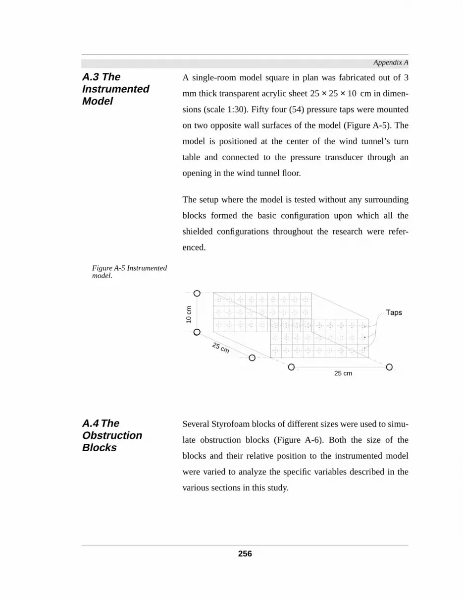
Appendix A
f 3
n-
ted
he
rn
h an
ing
he
fer-
mu-
he
del
the
A.3 The Instrumented Model
A single-room model square in plan was fabricated out o
mm thick transparent acrylic sheet cm in dime
sions (scale 1:30). Fifty four (54) pressure taps were moun
on two opposite wall surfaces of the model (Figure A-5). T
model is positioned at the center of the wind tunnel’s tu
table and connected to the pressure transducer throug
opening in the wind tunnel floor.
The setup where the model is tested without any surround
blocks formed the basic configuration upon which all t
shielded configurations throughout the research were re
enced.
Figure A-5 Instrumented model.
A.4 The Obstruction Blocks
Several Styrofoam blocks of different sizes were used to si
late obstruction blocks (Figure A-6). Both the size of t
blocks and their relative position to the instrumented mo
were varied to analyze the specific variables described in
various sections in this study.
25 25 10××
25 cm
10 c
m
25 cm
256

Appendix A
nter
le
he
stem
led
aver-
ure at
for-
nor-
and
d.
ver-
ppo-
sure
Figure A-6 Upwind obstruction and instrumented model configurations.
A.5 Measurement The instrumented model (Section A.3) was located the ce
of the turn table (Figure A-3) while a single or multip
obstruction blocks were positioned at specified locations. T
pressure was then measured using the data acquisition sy
described in Section A.2.
Each measured location point (tap–Figure A-5) was samp
at 15 scans per second for 30 seconds. The mathematical
age of the 450 scans was then used to represent the press
that point. From previous analyses of the wind tunnel per
mance, the data collected for the same point tend to be
mally distributed, thus the average represents an unbiased
robust measure for the central tendency of the data obtaine
Twenty seven (27) surface wind pressure readings were a
aged to determine the mean pressure on each of the two o
site surfaces of the instrumented model. The average pres
Obstruction
Model
Wind Direction
257

Appendix A
the
d in
s of
mine
-
was then used in equations (3-3) and (4-1) to determine
pressure coefficient values3.
In all tests, an unobstructed instrumented model was teste
the beginning of the experiments. The pressure coefficient
the obstructed and unobstructed were then used to deter
the Pressure Modification Coefficient ( )4.
A-3. Defined in Section 4.10.
A-4. Refer to Section 4.10 for the definition of the Pressure Modification Coeffi
cient ( ).
Cpm
Cpm
258

259
Appendix B

Appenices
Appendix BBoundary Layer Conversion
ere
tion
er
tion
er-
for
the
ifi-
B.1 Derivation of the Conversion Factor
Because all the tests needed to determine values w
conducted under a single boundary layer condition (Sec
A.1.2), a correction factor would be applied when oth
boundary layer characteristics are encountered. This sec
explains the algebraic derivation of the boundary layer conv
sion factors. These factors should be used to correct
boundary layer conditions not used in the derivation of
mathematical model for the prediction of the Pressure Mod
cation Coefficient.
Since;
(B-1)
and from equation 4-3 in text of report;
(B-2)
(B-3)
and;
(B-4)
Cpm
Cp
Pm Ps–( )
0.5 ρ Ve2⋅ ⋅( )
-------------------------------=
Cpm eCp Shielded( ) Cp Unshielded( )–[ ]
=
Cpmie
PmiPs–( )
0.5 ρ vei
2⋅ ⋅--------------------------
PuniPs–( )
0.5 ρ vuni
2⋅ ⋅-----------------------------–
=
Cpm1
Cpm2
------------- eCp ob1( ) Cp unob1( )–( )
eCp ob2( ) Cp unob2( )–( )
----------------------------------------------=
260

Appendix B
-8
in
From equations A-3 and A-4
(B-5)
Since;
(B-6)
and;
(B-7)
Therefore;
(B-8)
Therefore by substituting value of from equation A
in A-5;
(B-9)
From the exponential function that describes the decreasemean wind speeds due to terrain roughness (Ref 18):
(B-10)
Cpm1
Cpm2
------------- e
2 Pm1Ps–( )⋅
ρ ve1
2⋅----------------------------------
2 Pm2Ps–( )⋅
ρ ve2
2⋅----------------------------------–
=
Pdynamic PmiPs–=
P 0.5 ρ v2⋅ ⋅=
PmiPs– 0.5 ρ v
2⋅ ⋅=
PmiPs–
Cpm1
Cpm2
------------- e
2 0.5 ρ v12⋅ ⋅( )⋅
ρ ve1
2⋅-------------------------------------
2 0.5 ρ v22⋅ ⋅( )⋅
ρ ve2
2⋅-------------------------------------–
=
e
v12
ve1
2-------
v22
ve2
2-------–
=
Vz Vg
Zi
Zg------
α
⋅=
261

Appendix B
Where
Substituting from A-10 into A-9, therefore;
(B-11)
(B-12)
or;
(B-13)
Vz Mean wind speed at heightZi Z0+( )=
Vg Mean wind speed at gradient height =
Zi Height at point i=
Zg Gradient height=
α Velocity profile exponent=
Vi
Cpm1
Cpm2
------------- e
Vg1
Z1
Zg1
-------- α1
⋅
2
Vg1
Ze1
Zg1
--------
α1
⋅
2------------------------------------------
Vg2
Z2
Zg2
-------- α2
⋅
2
Vg2
Ze2
Zg2
--------
α2
⋅
2------------------------------------------–
=
Cpm1
Cpm2
------------- e
Z1
Zg1
--------
Ze1
Zg1
-------- --------------
2 α1⋅ Z2
Zg2
--------
Ze2
Zg2
-------- --------------
2 α2⋅
–
=
Cpm1
Cpm2
------------- e
Z1
Ze1
-------- 2α1
e
Z2
Ze2
-------- 2α2
--------------------------=
262

Appendix B
r 5
-1- er
us
FIGURE A-1. Boundary Layer ConversionPressure Shielding Modification Coefficient
Assuming a to be equal to half the height of the model o
cm (1.67 m) and eave height to be 10 cm (3.33 m) -Figure Aand since all the tests are conducted under a boundary laywith a full-scale roughness height ( ) value of 0.08 and a
velocity profile exponent of about 0.2, therefore;
or; (B-14)
(B-15)
B.2 Boundary Layer Conversion
The following table shows the conversion factors for vario
boundary layer conditions.
Cpm
275 m
365 m
460 m
Hei
ght
abov
e G
roun
d
OpenCountry
Suburban
City
Zi
Z0
Cpm1
Cpm2
------------- e
Z1
Ze1
-------- 2α1
e
1.67 0.08–3.33 0.08–---------------------------
2 0.2×----------------------------------------------=
Cpm1
Cpm2
-------------e
Z1
Ze1
-------- 2α1
e0.75
-------------------------- e
Z1
Ze1
-------- 2α1
2.12--------------------------==
263
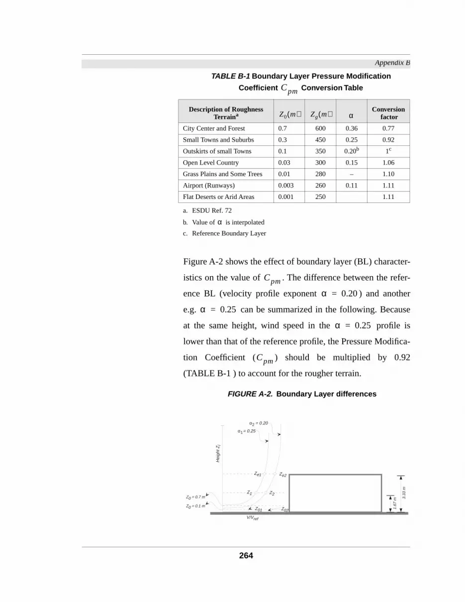
Appendix B
er-
fer-
er
se
is
ca-
2
a. ESDU Ref. 72
b. Value of is interpolated
c. Reference Boundary Layer
Figure A-2 shows the effect of boundary layer (BL) charact
istics on the value of . The difference between the re
ence BL (velocity profile exponent ) and anoth
e.g. can be summarized in the following. Becau
at the same height, wind speed in the profile
lower than that of the reference profile, the Pressure Modifi
tion Coefficient ( ) should be multiplied by 0.9
(TABLE B-1 ) to account for the rougher terrain.
FIGURE A-2. Boundary Layer differences
TABLE B-1 Boundary Layer Pressure Modification
Coefficient Conversion Table
Description of Roughness Terrain a
Conversion factor
City Center and Forest 0.7 600 0.36 0.77
Small Towns and Suburbs 0.3 450 0.25 0.92
Outskirts of small Towns 0.1 350 0.20b 1c
Open Level Country 0.03 300 0.15 1.06
Grass Plains and Some Trees 0.01 280 – 1.10
Airport (Runways) 0.003 260 0.11 1.11
Flat Deserts or Arid Areas 0.001 250 1.11
Cpm
Z0 m( ) Zg m( ) α
α
Cpm
α 0.20=
α 0.25=
α 0.25=
Cpm
3.33
m
1.67
m
V/Vref
Hei
ght Z
i
Z0 = 0.7 m
Z0 = 0.1 m
α1 = 0.25
α2 = 0.20
Ze2Ze1
Z1 Z2
Z01 Z02
264

265
Appendix C
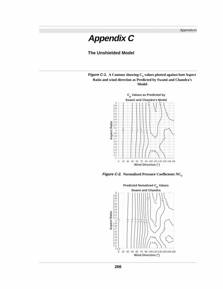
Appendices
Appendix CThe Unshielded Model
Figure C-1. A Contour showing Cp values plotted against bott Aspect Ratio and wind direction as Predicted by Swami and Chandra’s
Model
Figure C-2. Normalized Pressure Coefficients NCp
-0.8
-0.6
-0.6
-0.6
-0.4
-0.4
-0.4-0.20.
0
0.2
0.4
0.6
11.11.21.31.41.51.61.71.81.9
22.12.22.32.42.52.62.72.82.9
3
0 15 30 45 60 75 90 105 120 135 150 165 180
Asp
ect
Rat
io
Wind Direction (°)
Cp Values as Predicted by
Swami and Chandra's Model
-1.2
-1.0
-1.0
-0.8
-0.8
-0.8 -0.6
-0.6
-0.6
-0.4
-0.4-0.20.
00.
20.
4
0.6
0.8
1.0
1.0
11.11.21.31.41.51.61.71.81.9
22.12.22.32.42.52.62.72.82.9
3
0 15 30 45 60 75 90 105120135150165180
Asp
ect
Rat
io
Wind Direction (°)
Predicted Nomalized Cp Values
Swami and Chandra
266

Appendix C
Figure C-3. Contour plot showing the measured surface pressure coefficients Cp
Figure C-4. Measured NCp values plotted against Aspect Ratio (As)
and wind direction ( )
Measured Cp Values
-0.8
-0.6
-0.6
-0.4
-0.4
-0.2
0.00.2
0.4
0.6
0.2
0.4
0.6
0.8
1
1.2
1.4
1.6
1.8
2
2.2
2.4
2.6
2.8
3
0 15 30 45 60 75 90 105120135150165180S
ide
Rat
io
Wind Direction (°)
Θ
-1.2-1.2 -1-1
-0.8
-0.8
-0.6
-0.6
-0.4
-0.200.2
0.4
0.6
0.8
1
1
0.2
0.4
0.6
0.8
1
1.2
1.4
1.6
1.8
2
2.2
2.4
2.6
2.8
3
0 15 30 45 60 75 90 105120135150165180
Sid
e R
atio
Wind Direction (°)
Measured Nomalized Cp Values
267

Appendix C
Figure C-5 Surface PressuresAs=1.00, Wind Direction=noted in front of surface
0°
-1.00
-0.90
-0.80
-0.70
-0.60
-0.50
-0.40
-0.30
-1.10
250
200
150
100
50
0
0 10 20 30 40 50 60 70 80 9010
0
0.60.7
0.7
0.7
0.80.8
1009080706050403020100
0 50 100 150 200 250
90°90°
180°
-0.36
-0.36
-0.34
-0.38
-0.380102030405060708090100
250 200 150 100 50 0
-1
-0.9
-0.8
-0.7
-0.6
-0.5
-0.4
-0.3
-1.1
250
200
150
100
50
0
100
90 80 70 60 50 40 30 20 10 0
268

Appendix C
Figure C-6 Surface PressuresAs=1.00, Wind Direction=noted in front of surface
0.5
0.5
0.6
0.60.7
0.8
1009080706050403020100
0 50 100 150 200 250
15°
-0.52-0.5-0.48-0.46-0.44 -0.42 -0.4-0.38
-0.36
0102030405060708090100
250 200 150 100 50 0
-1
-0.9
-0.8
-0.7
-0.6
-0.5
250
200
150
100
50
0
100
90 80 70 60 50 40 30 20 10 0
-0.5-0.4-0.3-0.2
-0.1
250
200
150
100
50
0
0 10 20 30 40 50 60 70 80 9010
0
105°75°
165°
269

Appendix C
Figure C-7 Surface PressuresAs=1.00, Wind Direction=noted in front of surface
30°
0.3
0.4
0.50.6
0.7
1009080706050403020100
0 50 100 150 200 250
-1
-0.9
-0.8
-0.7
-0.7-0.6
0
50
100
150
200
250
100
90 80 70 60 50 40 30 20 10 0
-0.58-0.56-0.54 -0.52
-0.5-0.48 -0.46-0.44
0102030405060708090100
250 200 150 100 50 0
0
0
0.1
0.2
250
200
150
100
50
0
0 10 20 30 40 50 60 70 80 9010
0
120°60°
150°
270

Appendix C
Figure C-8 Surface PressuresAs=1.00, Wind Direction=noted in front of surface
0.1
0.1
0.2
0.2
0.30.4
0.5
1009080706050403020100
0 50 100 150 200 250
45°
0.10.1
0.2
0.2
0.30.4
0.5
250
200
150
100
50
0
0 10 20 30 40 50 60 70 80 9010
0
-0.8-0.7
-0.6
-0.6
0102030405060708090100
250 200 150 100 50 0
-0.8
-0.7
-0.6-0.6
0
50
100
150
200
250
100
90 80 70 60 50 40 30 20 10 0
135°45°
135°
271

Appendix C
Figure C-9 Surface PressuresAs=2 and 0.5, Wind Direction=noted in front of surface
0.4
0.5
0.5
0.5 0.6
0.60.7
100908070605040302010
0
0 50 100 150 200 250 300 350 400 450 500
0°
-0.45-0.45-0.4
-0.4-0.5
0102030405060708090100
0 50 100 150 200 250 300 350 400 450 500
-1.1
-1
-0.9
-0.8
-0.7
-0.6
-0.5
-0.4
250
200
150
100
50
0
100
90 80 70 60 50 40 30 20 10 0
-1.1
-1
-0.9
-0.8
-0.7
-0.6
-0.5
-0.4
250
200
150
100
50
0
0 10 20 30 40 50 60 70 80 90 100
90°90°
180°
272

Appendix C
Figure C-10 Surface PressuresAs=2 and 0.5, Wind Direction=noted in front of surface
0.3
0.4
0.40.5
0.5
0.5
0.6
0.6
0.70.8
100908070605040302010
00 50 100 150 200 250 300 350 400 450 500
15°
-0.55-0.5-0.5-0.45
-0.4
0102030405060708090100
0 50 100 150 200 250 300 350 400 450 500
-1
-0.9
-0.8
-0.7
-0.6
250
200
150
100
50
0
100
90 80 70 60 50 40 30 20 10 0
-0.8-0.7-0.6-0.5-0.4
-0.3
-0.2
250
200
150
100
50
0
0 10 20 30 40 50 60 70 80 90 100
105°
165°
75°
273

Appendix C
Figure C-11 Surface PressuresAs=2 and 0.5, Wind Direction=noted in front of surface
0.2
0.3
0.30.40.5
0.60.7
100908070605040302010
00 50 100 150 200 250 300 350 400 450 500
30°
-0.8-0.8 -0.7-0.7-0.6-0.5-0.5
-0.9
0102030405060708090100
0 50 100 150 200 250 300 350 400 450 500
-0.65
-0.65
250
200
150
100
50
0
100
90 80 70 60 50 40 30 20 10 0
-0.3-0.2
-0.2
-0.1
-0.1
0
250
200
150
100
50
0
0 10 20 30 40 50 60 70 80 90 100
120°
150°
60°
274

Appendix C
Figure C-12 Surface PressuresAs=2 and 0.5, Wind Direction=noted in front of surface
0.1
0.20.30.4
0.50.6 0.5
1009080706050403020100
0 50 100 150 200 250 300 350 400 450 500
45°
-1.1
-1-1 -0.9-0.9
-0.8
-0.8-0.8-0.7
-0.7
-0.6-0.6
-0.6
-0.5
-0.5
-0.4
-0.4
-1.2
0102030405060708090100
0 50 100 150 200 250 300 350 400 450 500
-0.65
-0.6
-0.55
-0.5
250
200
150
100
50
0
100
90 80 70 60 50 40 30 20 10 0
0
0.1
0.2
0.3
0.4
250
200
150
100
50
0
0 10 20 30 40 50 60 70 80 90 100
135°
135°
45°
275

Appendix C
Figure C-13 Surface PressuresAs=2 and 0.5, Wind Direction=noted in front of surface
-0.050
0.05 0.05
0.1
0.1
0.15
0.15 0.20.25
0.3
100908070605040302010
0
0 50 100 150 200 250 300 350 400 450 500
60°
-1.1-1-1 -0.9-0.9
-0.8
-0.8-0.8
-0.7
-0.7-0.6-0.6
-0.6
-0.5-0.5
-0.4
-0.4-0.3
0102030405060708090100
0 50 100 150 200 250 300 350 400 450 500
-0.55
-0.5
-0.45
250
200
150
100
50
0
100
90 80 70 60 50 40 30 20 10 0
0.20.250.3
0.35
0.35
0.40.45
0.50.55
0.6
0.650.70.750.8
250
200
150
100
50
0
0 10 20 30 40 50 60 70 80 90 100
150°
120°
30°
276

Appendix C
Figure C-14 Surface PressuresAs=2 and 0.5, Wind Direction=noted in front of surface
75°
-0.4-0.3-0.2 -0.1-0.1
0
1009080706050403020100
0 50 100 150 200 250 300 350 400 450 500
-0.8-0.8 -0.7-0.7-0.6-0.5
-0.5-0.9
0102030405060708090100
0 50 100 150 200 250 300 350 400 450 500
-0.45
-0.4
-0.35
250
200
150
100
50
0
100
90 80 70 60 50 40 30 20 10 0
0.5
0.6
0.6
0.7
0.7
0.8
250
200
150
100
50
0
0 10 20 30 40 50 60 70 80 90 100
165°
105°
15°
277

Appendix C
Figure C-15 Surface PressuresAs=2 and 0.5, Wind Direction=noted in front of surface
90°
-0.5
-0.4
-0.4 -0.3-0.3 -0.3 -0.2-0.2
1009080706050403020100
0 50 100 150 200 250 300 350 400 450 500
-0.5
-0.4
-0.4 -0.3-0.3 -0.3 -0.2-0.2
0102030405060708090100
0 50 100 150 200 250 300 350 400 450 500
0.5
0.6
0.6
0.7
0.7
0.8
250
200
150
100
50
0
0 10 20 30 40 50 60 70 80 90 100
-0.34
-0.32
-0.32
-0.32
250
200
150
100
50
0
100
90 80 70 60 50 40 30 20 10 0
180°
90°
0°
278

Appendix C
Figure C-16 Surface PressuresAs=3 and 0.33, Wind Direction=noted in front of surface
Figure C-17 Surface PressuresAs=3 and 0.33, Wind Direction=noted in front of surface
0.4
0.40.40.40.50.50.5
0.60.6
0.6
100806040200
0 100 200 300 400 500 600 7000°
-0.6-0.55-0.55 -0.55-0.55 -0.5-0.5 -0.5-0.45
-0.45
020406080100
0 100 200 300 400 500 600 700
-1.2-1.1
-1-0.9-0.8-0.7
-0.6
-0.5
250
200
150
100
50
0
100
80 60 40 20 0
-1.2-1.1-1
-0.9-0.8-0.7
-0.6
-0.5
250
200
150
100
50
0
0 20 40 60 80 100
90°
180°
90°
0.3
0.3
0.40.4
0.4
0.5 0.50.6
0.70.8 0.3
100806040200
0 100 200 300 400 500 600 700
-0.75
-0.75-0.7
-0.7 -0.65-0.65 -0.6 -0.55-0.55
-0.5-0.5
-0.5
-0.45-0.4
020406080100
0 100 200 300 400 500 600 700
-1.2-1.1
-1-0.9-0.8-0.7
-0.6
-0.5
250
200
150
100
50
0
100
80 60 40 20 0
15°
-0.9-0.8-0.7-0.6-0.5
-0.4
-0.3
-0.3
250
200
150
100
50
0
0 20 40 60 80 100
105°
165
75°
279

Appendix C
Figure C-18 Surface PressuresAs=3 and 0.33, Wind Direction=noted in front of surface
Figure C-19 Surface PressuresAs=3 and 0.33, Wind Direction=noted in front of surface
30°
0.4
0.40.40.40.50.50.5
0.60.6
0.6
100806040200
0 100 200 300 400 500 600 700
-0.6-0.5-0.5 -0.5-0.5 -0.5-0.5 -0.5-0.4-0.4
020406080100
0 100 200 300 400 500 600 700
-0.65
-0.6
-0.6
250
200
150
100
50
0
100
80 60 40 20 0
-0.3
-0.3
-0.2
-0.2
-0.1
-0.1
0
250
200
150
100
50
0
0 20 40 60 80 100
120°
150°
60°
0.2
0.4
0.40.6 0.2
100806040200
0 100 200 300 400 500 600 700
45°
-1.4-1.2
-1
-1-1
-0.8
-0.8-0.6
-0.6 -0.4
-0.4
020406080100
0 100 200 300 400 500 600 700
-0.6
-0.55
-0.5
250
200
150
100
50
0
100
80 60 40 20 0
-0.10
0.1
0.2
0.30.3
250
200
150
100
50
0
0 20 40 60 80 100
135°
135°
45°
280

Appendix C
Figure C-20 Surface PressuresAs=3 and 0.33, Wind Direction=noted in front of surface
Figure C-21 Surface PressuresAs=3 and 0.33, Wind Direction=noted in front of surface
00.1
0.20.2
0.3 0.30.1
100806040200
0 100 200 300 400 500 600 700
60°
-1.2-1.1
-1
-1-0.9
-0.9-0.8
-0.8
-0.7
-0.7
-0.6
-0.6-0.5
-0.5 -0.4-0.3
-0.3
020406080100
0 100 200 300 400 500 600 700
-0.5
-0.45
250
200
150
100
50
0
100
80 60 40 20 0
0.20.3
0.40.5
0.60.7
250
200
150
100
50
0
0 20 40 60 80 100
150°
120°
30°
75°
-0.4-0.3-0.2 -0.1-0.1 0
0
00
100806040200
0 100 200 300 400 500 600 700
-0.9-0.8
-0.8-0.7-0.7 -0.6-0.6 -0.5-0.4 -0.3-0.3 -0.2
-0.2-0.2
020406080100
0 100 200 300 400 500 600 700
-0.4
-0.35
250
200
150
100
50
0
100
80 60 40 20 0
0.5
0.6 0.7
0.8
250
200
150
100
50
0
0 20 40 60 80 100
165°
105°
15°
281
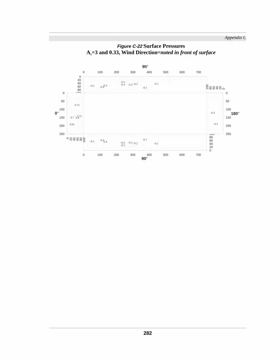
Appendix C
Figure C-22 Surface PressuresAs=3 and 0.33, Wind Direction=noted in front of surface
90°
-0.5-0.5 -0.4-0.4
-0.4 -0.3 -0.2-0.1
-0.1
10080604020
0
0 100 200 300 400 500 600 700
-0.5-0.5 -0.4
-0.4-0.4 -0.3 -0.2
-0.1
-0.1
020406080100
0 100 200 300 400 500 600 700
-0.3
-0.3
250
200
150
100
50
0
100
80 60 40 20 0
0.65
0.7
0.75
0.750.8
250
200
150
100
50
0
0 20 40 60 80 100
180°
90°
0°
282

Appendix C
Figure C-23 Surface PressuresAs=1.5 and 0.67, Wind Direction=noted in front of surface
Figure C-24 Surface PressuresAs=1.5 and 0.67, Wind Direction=noted in front of surface
0.5
0.5
0.6
0.6
0.6
0.70.8
100806040200
0 50 100 150 200 250 300 350
0°
-0.35-0.35-0.35
020406080100
0 50 100 150 200 250 300 350
-1.1-1
-0.9-0.8
-0.7
-0.6
-0.5
-0.4
250
200
150
100
50
0
10080 60 40 20 0
-1.1-1
-0.9-0.8
-0.7
-0.6
-0.5
-0.4
250
200
150
100
50
0
0 20 40 60 80100
90°90°
180°
15°
0.4
0.5
0.6
0.60.70.8
100806040200
0 50 100 150 200 250 300 350
-0.45-0.45 -0.4-0.4-0.4
-0.4
020406080100
0 50 100 150 200 250 300 350
-1
-0.9
-0.8
-0.7
-0.6
250
200
150
100
50
0
10080 60 40 20 0
-1.1-1
-0.9-0.8
-0.7
-0.6
-0.5
-0.4
250
200
150
100
50
0
0 20 40 60 80100
105°
165°
75°
283

Appendix C
Figure C-25 Surface PressuresAs=1.5 and 0.67, Wind Direction=noted in front of surface
Figure C-26 Surface PressuresAs=1.5 and 0.67, Wind Direction=noted in front of surface
0.20.3
0.4
0.50.6
0.70.8
100806040200
0 50 100 150 200 250 300 350
30°
-0.55
-0.55-0.5
020406080100
0 50 100 150 200 250 300 350
-0.8
-0.7
250
200
150
100
50
0
10080 60 40 20 0
-0.1
0
0
0.10.2
250
200
150
100
50
0
0 20 40 60 80100
120°
150°
60°
0.1
0.2
0.2
0.3
0.40.5
0.6
10080604020
0
0 50 100 150 200 250 300 350
45°
-0.8 -0.75 -0.75-0.75
-0.7-0.7
-0.7-0.7
-0.65-0.65
-0.6-0.6-0.8
-0.85
020406080100
0 50 100 150 200 250 300 350
-0.55
-0.55
-0.5
250
200
150
100
50
0
10080 60 40 20 0
0
0.1
0.2
0.3
0.4
250
200
150
100
50
0
0 20 40 60 80100
135°
135°
284

Appendix C
Figure C-27 Surface PressuresAs=1.5 and 0.67, Wind Direction=noted in front of surface
Figure C-28 Surface PressuresAs=1.5 and 0.67, Wind Direction=noted in front of surface
0
0.10.2
0.3
10080604020
0
0 50 100 150 200 250 300 350
60°
-0.85-0.8-0.75
-0.75 -0.75-0.7
-0.7-0.7
-0.65-0.65
-0.6-0.6
-0.55
-0.8-0.85
-0.8-0.85
020406080100
0 50 100 150 200 250 300 350
-0.55
-0.55
-0.5
-0.45
250
200
150
100
50
0
10080 60 40 20 0
0.3
0.4
0.50.6
0.7
250
200
150
100
50
0
0 20 40 60 80100
150°
120°
30°
-0.5-0.4-0.3-0.2 -0.1-0.1
0
10080604020
0
0 50 100 150 200 250 300 350
75°
-0.7
-0.65
-0.6
-0.6-0.6
-0.55
-0.55
-0.5
-0.5
-0.45-0.45
020406080100
0 50 100 150 200 250 300 350
-0.45
-0.4
-0.35
250
200
150
100
50
0
10080 60 40 20 0
0.5
0.6
0.7
0.8
250
200
150
100
50
0
0 20 40 60 80100
165°15°
105°
285

Appendix C
Figure C-29 Surface PressuresAs=1.5 and 0.67, Wind Direction=noted in front of surface
-0.6 -0.5 -0.4 -0.3
10080604020
0
0 50 100 150 200 250 300 350
90°
-0.6 -0.5 -0.4 -0.3
020406080100
0 50 100 150 200 250 300 350
-0.35
250
200
150
100
50
0
10080 60 40 20 0
0.6
0.65
0.65
0.65
0.70.750.8
0.85
250
200
150
100
50
0
0 20 40 60 80100
90°
0° 180°
286

Appendix C
Figure C-30 Surface PressuresAs=2.5 and 0.4, Wind Direction=noted in front of surface
Figure C-31 surface PressuresAs=2.5 and 0.4, Wind Direction=noted in front of surface
0°
0.40.4
0.5
0.50.50.5
0.60.6
0.6 0.7
10080604020
0
0 100 200 300 400 500 600
-0.5-0.5
-0.5-0.45-0.45
-0.4
020406080100
0 100 200 300 400 500 600
-1.2-1.1
-1-0.9-0.8
-0.7
-0.6
-0.5
250
200
150
100
50
0
10080 60 40 20 0
-1.2-1.1
-1-0.9-0.8
-0.7
-0.6
-0.5
250
200
150
100
50
0
0 20 40 60 80100
90°90°
180°
287

Appendix C
Figure C-32 surface PressuresAs=2.5 and 0.4, Wind Direction=noted in front of surface
Figure C-33 surface PressuresAs=2.5 and 0.4, Wind Direction=noted in front of surface
15°
0.4
0.40.5
0.5
0.60.7 0.6
100806040200
0 100 200 300 400 500 600
-0.6-0.6-0.55
-0.5-0.45
-0.45
-0.4
-0.4
020406080100
0 100 200 300 400 500 600
-1
-0.9
-0.8
-0.7
250
200
150
100
50
0
10080 60 40 20 0
-0.8-0.7-0.6-0.5
-0.4
-0.3
-0.3
250
200
150
100
50
0
0 20 40 60 80100
105°
165°
75°
30°
0.2
0.30.40.50.6
0.70.8
10080604020
0
0 100 200 300 400 500 600
-1.05-1.05
-1-0.95-0.9-0.85-0.8-0.75 -0.7 -0.65 -0.6 -0.55-0.5 -0.45 -0.4-1.1
020406080100
0 100 200 300 400 500 600
-0.65
250
200
150
100
50
0
10080 60 40 20 0
-0.3
-0.2
-0.2
-0.1
-0.1
0
250
200
150
100
50
0
0 20 40 60 80100
120°
150°
60°
288

Appendix C
Figure C-34 surface PressuresAs=2.5 and 0.4, Wind Direction=noted in front of surface
Figure C-35 surface PressuresAs=2.5 and 0.4, Wind Direction=noted in front of surface
45°
0.1
0.20.3
0.40.50.6
10080604020
0
0 100 200 300 400 500 600
-1.4-1.3-1.2-1.1 -1 -0.9 -0.8 -0.7 -0.6 -0.5
-0.4-0.4
020406080100
0 100 200 300 400 500 600
-0.6
-0.55
-0.5
250
200
150
100
50
0
10080 60 40 20 0
-0.1
0
0.1
0.2
0.3
0.4
0.5
250
200
150
100
50
0
0 20 40 60 80100
45° 135°
135°
60°
00.10.2
0.3
10080604020
0
0 100 200 300 400 500 600
-1.1-1 -0.9 -0.8 -0.7 -0.6 -0.5 -0.4
-0.3
-0.3
020406080100
0 100 200 300 400 500 600
-0.55
-0.5
-0.45
250
200
150
100
50
0
10080 60 40 20 0
0.3
0.4
0.5
0.6
0.7
0.8
250
200
150
100
50
0
0 20 40 60 80100
150°
120°
289

Appendix C
Figure C-36 surface PressuresAs=2.5 and 0.4, Wind Direction=noted in front of surface
Figure C-37 surface PressuresAs=2.5 and 0.4, Wind Direction=noted in front of surface
75°
-0.4-0.3-0.2 -0.1-0.10
10080604020
0
0 100 200 300 400 500 600
-0.9 -0.8 -0.7 -0.6 -0.5 -0.4 -0.3-0.2
020406080100
0 100 200 300 400 500 600
-0.4
-0.35
250
200
150
100
50
0
10080 60 40 20 0
0.50.5
0.6
0.7
250
200
150
100
50
0
0 20 40 60 80100
165°
105°
15°
90°
-0.9-0.8-0.7-0.6-0.5-0.4 -0.3 -0.2
10080604020
0
0 100 200 300 400 500 600
-0.9-0.8-0.7-0.6-0.5-0.4 -0.3 -0.2
020406080100
0 100 200 300 400 500 600
-0.3
-0.3
-0.3
250
200
150
100
50
0
10080 60 40 20 0
0.7
0.7
0.7
0.8
250
200
150
100
50
0
0 20 40 60 80100
90°
0° 180°
290

291
Appendix D

Appendices
Appendix DOrthogonal Configurations
ns
effi-
)
n the
ted
D.1 Experiments Results
The following are the results of the orthogonal configuratio
experiments (refer to Section 4.9, page 70).
D.1.1 Spacing Figures D-1 to D-18 represent the measured Pressure Co
cients ( ) and Pressure Modification Coefficients (
expressed as a function of the obstruction spacing betwee
instruemented model and the obstrcution block1. The graphs
in figures D-15 to D-18 represent a summary of the collec
data and are used for comparison purposes.
D-1. Expressed in obstruction heights.
Cp Cpm
292

Appendix D
Figure D-1 Measured pressure coefficients on windward2 and leeward3 surfaces ( ) obstruction block
Figure D-2 Measured pressure coefficients on windward and leeward surfaces ( ) obstruction block
D-2.Obstruction-facing surface
D-3.Unobstructed surface
200 10×
B
B
B
B
BB
BB B
JJ
JJ
J J J J J
H
HH
HH
H HH H
-1.4
-1.2
-1
-0.8
-0.6
-0.4
-0.2
0
0.2
0.4
0.6
0.8
1
1.2
1 2 3 4 5 6 7 8 9 10
Pre
ssur
e C
oeffi
cien
t (C
p)
Spacing (S/H)
B Cpw
J Cpl
H Cp
150 10×
B
B
B
BB
B B B B
J J J J J J J J J
H
H
H
HH
H H H H
-1.4
-1.2
-1
-0.8
-0.6
-0.4
-0.2
0
0.2
0.4
0.6
0.8
1
1.2
1 2 3 4 5 6 7 8 9 10
Pre
ssur
e C
oeffi
cien
t (C
p)
Spacing (S/H)
B Cpw
J Cpl
H Cp
293

Appendix D
Figure D-3 Measured cressure Coefficients on windward and leeward surfaces ( ) obstruction block
Figure D-4 Measured pressure coefficients on windward and leeward surfaces ( ) obstruction block
89 10×
B B
B
B
BB
BB
B B
J J J J J JJ J J J
H H
HH
H
HH
HH H
-1.4
-1.2
-1
-0.8
-0.6
-0.4
-0.2
0
0.2
0.4
0.6
0.8
1
1.2
1 2 3 4 5 6 7 8 9 10
Pre
ssur
e C
oeffi
cien
t (C
p)
Spacing (S/H)
B Cpw
J Cpl
H Cp
25 10×
B
B
BB
B BB B B
B
J J J J JJ J J J
J
H
H
H
HH H H H H H
-1.4
-1.2
-1
-0.8
-0.6
-0.4
-0.2
0
0.2
0.4
0.6
0.8
1
1.2
1 2 3 4 5 6 7 8 9 10
Pre
ssur
e C
oeffi
cien
t (C
p)
Spacing (S/H)
B Cpw
J Cpl
H Cp
294

Appendix D
Figure D-5 Measured pressure coefficients on windward and leeward surfaces ( ) obstruction block
Figure D-6 Measured pressure coefficients on windward and leeward surfaces ( ) obstruction block
25 17×
B
B
B
BB
BB
B B B
JJ
J J J J J J J J
H
H
H
H
HH
H H H H
-1.4
-1.2
-1
-0.8
-0.6
-0.4
-0.2
0
0.2
0.4
0.6
0.8
1
1.2
1 2 3 4 5 6 7 8 9 10
Pre
ssur
e C
oeffi
cien
t (C
p)
Spacing (S/H)
B Cpw
J Cpl
H Cp
25 7×
B
BB B
B B B B B B
J J J J J J J J J J
H
HH
H H H H H H H
-1.4
-1.2
-1
-0.8
-0.6
-0.4
-0.2
0
0.2
0.4
0.6
0.8
1
1.2
1 2 3 4 5 6 7 8 9 10
Pre
ssur
e C
oeffi
cien
t (C
p)
Spacing (S/H)
B Cpw
J Cpl
H Cp
295

Appendix D
Figure D-7 Measured pressure coefficients on windward and leeward surfaces ( ) obstruction block
Figure D-8 Measured pressure modification coefficients on windward and leewardsurfaces ( ) obstruction block
25 25×
B
B
B
BB
BB B B
J J J J J J J J J
H
H
H
H
HH
H H H
-1.4
-1.2
-1
-0.8
-0.6
-0.4
-0.2
0
0.2
0.4
0.6
0.8
1
1.2
1 2 3 4 5 6 7 8 9 10
Pre
ssur
e C
oeffi
cien
t (C
p)
Spacing (S/H)
B Cpw
J Cpl
H Cp
200 10×
BB
B
B
BB
BB
B
JJ
JJ
J J J J J
0
0.2
0.4
0.6
0.8
1
1.2
1 2 3 4 5 6 7 8 9 10
Pre
ssur
e M
odifi
catio
n C
oeffi
cien
t (C
pm)
Spacing (S/H)
B Cpmw
J Cpml
296

Appendix D
Figure D-9 Measured pressure modification coefficients on windward and leewardsurfaces ( ) obstruction block
Figure D-10 Measured pressure modification coefficients on windward and leewardsurfaces ( ) obstruction block
150 10×
B
BB
BB
B B B B
JJ
JJ
JJ
J J J
0
0.2
0.4
0.6
0.8
1
1.2
1 2 3 4 5 6 7 8 9 10
Pre
ssur
e M
odifi
catio
n C
oeffi
cien
t (C
pm)
Spacing (S/H)
B Cpmw
J Cpml
89 10×
B B
B
B
B
BB
B
B B
J JJ J
JJ
J JJ
J
0
0.2
0.4
0.6
0.8
1
1.2
1 2 3 4 5 6 7 8 9 10
Pre
ssur
e M
odifi
catio
n C
oeffi
cien
t (C
pm)
Spacing (S/H)
B Cpmw
J Cpml
297

Appendix D
Figure D-11 Measured pressure modification coefficients on windward and leewardsurfaces ( ) obstruction block
Figure D-12 Measured pressure modification coefficients on windward and leewardsurfaces ( ) obstruction block
25 10×
B
B
B
B
BB
B B BB
J J JJ
J
JJ
J JJ
0
0.2
0.4
0.6
0.8
1
1.2
1 2 3 4 5 6 7 8 9 10
Pre
ssur
e M
odifi
catio
n C
oeffi
cien
t (C
pm)
Spacing (S/H)
B Cpmw
J Cpml
25 17×
B
B
B
B
BB
BB B
B
J
JJ
JJ J J
JJ J
0
0.2
0.4
0.6
0.8
1
1.2
1 2 3 4 5 6 7 8 9 10
Pre
ssur
e M
odifi
catio
n C
oeffi
cien
t (C
pm)
Spacing (S/H)
B Cpmw
J Cpml
298

Appendix D
Figure D-13 Measured pressure modification coefficients on windward and leewardsurfaces ( ) obstruction block
Figure D-14 Measured pressure modification coefficients on windward and leewardsurfaces ( ) obstruction block
25 7×
B
B
BB
B BB B B B
J J J JJ
J J J JJ
0
0.2
0.4
0.6
0.8
1
1.2
1 2 3 4 5 6 7 8 9 10
Pre
ssur
e M
odifi
catio
n C
oeffi
cien
t (C
pm)
Spacing (S/H)
B Cpmw
J Cpml
25 25×
B
B
B
B
B
BB B
B
JJ J J
J J J JJ
0
0.2
0.4
0.6
0.8
1
1.2
1 2 3 4 5 6 7 8 9 10
Pre
ssur
e M
odifi
catio
n C
oeffi
cien
t (C
pm)
Spacing (S/H)
B Cpmw
J Cpml
299

Appendix D
Figure D-15 Effect of spacing on pressure coefficients ( ) on windward (ww) andleeward (lw) sides
Figure D-16 Effect of spacing on pressure coefficients ( ) on windward (ww) andleeward (lw) sides
Cp
1 1 1 1 1 1 1 1 1 1
2
2
2
2
22
22 2
3
3
3
33
3 3 3 3
4 4
4
4
44
44
4 4
5
5
5
5
6
6
66
6 66 6 6
6
M M M M M M M M M M
-2
-1.8
-1.6
-1.4
-1.2
-1
-0.8
-0.6
-0.4
-0.2
0
0.2
0.4
0.6
1 2 3 4 5 6 7 8 9 10
Pre
ssur
e C
oeffi
cien
t (C
p)
Spacing (S/H)
1 Unobstructed
2 200X10 (ww)
3 150X10 (ww)
4 89X10 (ww)
5 61X10 (ww)
6 25X10 (ww)
200X10 (lw)
150X10 (lw)
M 89X10 (lw)
25X10 (lw)
Obstruction widths =200, 150, 89, 61, and 25 cm
Obstruction height=10 cm
Cp
1 1 1 1 1 1 1 1 1 1
2
22 2
2 2 2 2 2 2
3
3
33
3 33 3 3 3
4
4
4
44
44
4 4 4
5
5
55
55 5 5 5
M M M M M M M M M
-2-1.8-1.6
-1.4-1.2
-1
-0.8-0.6-0.4
-0.20
0.2
0.40.6
1 2 3 4 5 6 7 8 9 10
Pre
ssur
e C
oeffi
cien
t (C
p)
Spacing (S/H)
1 Unobstructed
2 25X7 (ww)
3 25X10 (ww)
4 25X17 (ww)
5 25X25 (ww)
25X7 (lw)
25X10 (lw)
25X17 (lw)
M 25X25 (lw)
Obstruction widths =25 cm
Obstruction height=7, 10, 17, and 25 cm
300

Appendix D
Figure D-17 Effect of spacing on pressure modification coefficients ( ) on windward (ww) and leeward (lw) sides
Figure D-18 Effect of spacing on pressure modification coefficients ( ) on windward (ww) and leeward (lw) sides
Cpm
11
11
11
11 1
22
2
22
2 2 2 2
3 3
33
33
33
3 3
4
4
4
4
5
5
5
5
55
5 5 55
M M MM
M
MM
M MM
0
0.2
0.4
0.6
0.8
1
1.2
1 2 3 4 5 6 7 8 9 10
Pre
ssur
e M
odifi
catio
n C
oeffi
cien
t (C
pm)
Spacing (S/H)
1 200X10 (ww)
2 150X10 (ww)
3 89X10 (ww)
4 61X10 (ww)
5 25X10 (ww)
200X10 (lw)
150X10 (lw)
89X10 (lw)
M 25X10 (lw)
Obstruction widths =200, 150, 89, 61, and 25 cm
Obstruction height=10 cm
Cpm
1
1
11
1 11 1 1 1
2
2
2
2
22
2 2 22
3
3
3
33
33
3 33
4
4
4
4
4
44 4
4
0
0.2
0.4
0.6
0.8
1
1.2
1 2 3 4 5 6 7 8 9 10
Pre
ssur
e M
odifi
catio
n C
oeffi
cien
t (C
pm)
Spacing (S/H)
1 25X7 (ww)
2 25X10 (ww)
3 25X17 (ww)
4 25X25 (ww)
25X7 (lw)
25X10 (lw)
25X17 (lw)
25X25 (lw)
Obstruction widths =25 cm
Obstruction height=7, 10, 17, and 25 cm
301

Appendix D
effi-
)
D.1.2 Horizontal Angle
Figures D-19 to D-22 represent the measured Pressure Co
cients ( ) and Pressure Modification Coefficients (
expressed as a function of the horizontal angle4 ( ).
D-4. For the definition of the obstruction angles, refer to Section 4.6, page 64
Figure D-19 Effect of horizontal angle ( ) on pressure coefficients ( ) on the obstruction facing side
Cp Cpm
αh
αh Cp
1111111111
2
2
2
2
22
222
3
3
3
33
3333
44
4
4
444
444
5
5
5
5
6
6
66
66666
6
-2-1.8-1.6-1.4-1.2
-1-0.8-0.6-0.4-0.2
00.20.40.6
0 15 30 45 60 75 90 105 120 135 150 165 180
Pre
ssur
e C
oeffi
cien
t (C
p)
Horizontal Angle (°)
1 Unobstructed
2 200X10
3 150X10
4 89X10
5 61X10
6 25X10
Obstruction widths =200, 150, 89, 61, and 25 cm
Obstruction height=10 cm
302

Appendix D
Figure D-20 Effect of horizontal angle ( ) on pressure coefficients ( ) on the obstruction facing side
Figure D-21 Effect of horizontal angle ( ) on pressure modification coefficients ( ) on the obstruction facing side
αh Cp
1111111111
2
222
222222
3
3
33
33333
3
4
4
4
44
44444
5
5
55
555
55
-2-1.8-1.6-1.4-1.2
-1-0.8-0.6-0.4-0.2
00.20.40.6
0 15 30 45 60 75 90 105 120 135 150 165 180
Pre
ssur
e C
oeffi
cien
t (C
p)
Horizontal Angle (°)
1 Unobstructed
2 25X7
3 25X10
4 25X17
5 25X25
Obstruction widths =25 cm
Obstruction height=7, 10, 17, and 25 cm
αhCpm
11
1
1
11
11
1
2
22
22
2222
33
3
3
3
33
3
33
4
4
4
4
5
5
5
5
55
5555
0
0.1
0.2
0.3
0.4
0.5
0.6
0.7
0.8
0.9
1
0 15 30 45 60 75 90 105 120 135 150 165 180
Pre
ssur
e M
odifi
catio
n C
oeffi
cien
t (C
pm)
Horizontal Angle (°)
1 200X10
2 150X10
3 89X10
4 61X10
5 25X10
Obstruction widths =200, 150, 89, 61, and 25 cm
Obstruction height=10 cm
303

Appendix D
effi-
)
Figure D-22 Effect of horizontal angle ( ) on pressure modification coefficients ( ) on the obstruction facing side
D.1.3 Vertical Angle Figures D-23 to D-26 represent the measured Pressure Co
cients ( ) and Pressure Modification Coefficients (
expressed as a function of the Vertical Angle ( ).
αhCpm
1
1
11
11111
1
2
2
2
2
22
2222
3
3
3
3
33
333
3
4
4
4
4
4
444
4
0
0.1
0.2
0.3
0.4
0.5
0.6
0.7
0.8
0.9
1
0 15 30 45 60 75 90 105 120 135 150 165 180
Pre
ssur
e M
odifi
catio
n C
oeffi
cien
t (C
pm)
Horizontal Angle (°)
1 25X7
2 25X10
3 25X17
4 25X25
Obstruction widths =25 cm
Obstruction height=7, 10, 17, and 25 cm
Cp Cpm
αv
304

Appendix D
Figure D-23 Effect of vertical angle ( ) on pressure coefficients ( ) on the obstruction facing side
Figure D-24 Effect of vertical Angle ( ) on pressure coefficients ( ) on the obstruction facing side
αv Cp
Obstruction widths =200, 150, 89, 61, and 25 cm
Obstruction height=10 cm
1111111111
2
2
2
2
22
222
3
3
3
33
3333
44
4
4
444
444
5
5
5
5
6
6
66
66666
6
-2-1.8-1.6-1.4-1.2
-1-0.8-0.6-0.4-0.2
00.20.40.6
0 5 10 15 20 25 30 35 40 45
Pre
ssur
e C
oeffi
cien
t (C
p)
Vertical Angle (°)
1 Unobstructed
2 200X10
3 150X10
4 89X10
5 61X10
6 25X10
αv Cp
Obstruction widths =25 cm
Obstruction height=7, 10, 17, and 25 cm
1111111111
2
222
222222
3
3
33
33333
3
4
4
4
44
44444
5
5
55
555
55
-2-1.8-1.6-1.4-1.2
-1-0.8-0.6-0.4-0.2
00.20.40.6
0 5 10 15 20 25 30 35 40 45
Pre
ssur
e C
oeffi
cien
t (C
p)
Vertical Angle (°)
1 Unobstructed
2 25X7
3 25X10
4 25X17
5 25X25
305

Appendix D
Figure D-25 Effect of vertical angle ( ) on pressure modification coefficients ( ) on the obstruction facing side
Figure D-26 Effect of vertical angle ( ) on pressure modification coefficients ( ) on the obstruction facing side
αvCpm
Obstruction widths =200, 150, 89, 61 and 25 cm
Obstruction height=10 cm
11
1
1
11
111
2
22
22
2222
33
3
3
3
33
3
33
4
4
4
4
5
5
5
5
55
5555
0
0.1
0.2
0.3
0.4
0.5
0.6
0.7
0.8
0.9
1
0 5 10 15 20 25 30 35 40 45
Pre
ssur
e C
oeffi
cien
t (C
pm)
Vertical Angle (°)
1 200X10
2 150X10
3 89X10
4 61X10
5 25X10
αvCpm
Obstruction widths =25 cm
Obstruction height=7, 10, 17, and 25 cm
1
1
11
11111
1
2
2
2
2
22
2222
3
3
3
3
33
333
3
4
4
4
4
4
444
4
0
0.1
0.2
0.3
0.4
0.5
0.6
0.7
0.8
0.9
1
0 5 10 15 20 25 30 35 40 45
Pre
ssur
e C
oeffi
cien
t (C
pm)
Vertical Angle (°)
1 25X7
2 25X10
3 25X17
4 25X25
306

Appendix D
the
for
cu-
he
ng
in
he
al-
D.2 Complex Function
Section 4.12.3 in Chapter 4 describes the derivation of
orthogonal model. Two functions were developed: the first
ease of use5, and the second for accuracy. For increased ac
racy6, the following function i.e. Equation D-1 represents t
long version of the Orthogonal function used in determini
the Pressure Modification Coefficient values shown
Figure 4-457. This function is also intended to be used in t
algorithm described in Chapter 5 and Appendix H .
D-5.Equation 4-11, page 96.
D-6.Increase the sensitivity of the function to predict minute variations in vues relative to the simple function described above.
D-7. page 98.
Cpm
Cpm
307

Appendix D
(D-1)
where
Cpm(ortho) C0
αh
2------
sin αv( )sin C1
αh
2------
cosαv( )sin
C2
αh
2------
cosαv( )sin 2
C3 αv( )cos
αh
2------
sin
C4 αv( )cos
αh
2------
sin2
C5
αh
2------
cosαv( )sin
αv( )cos
αh
2------
sin
C6
αh
2------
cosαv( )sin 2
αv( )cos
αh
2------
sin2
C7 αv( )cos
αh
2------
sin3
C8
αh
2------
cosαv( )sin 3
⋅
C9 αv( )cos
αh
2------
sinln⋅ C10
αh
2------
cos
αh
2------
sin αv( )sin⋅
⋅
C11 αv( )cos[ ]
αh
2------
sin αv( )sin⋅⋅
C12
αh
2------
cos
αh
2------
sin αv( )sin⋅
αv( )cos[ ]
αh
2------
sin αv( )sin⋅⋅ ⋅
+
+ +
+
+
⋅+
⋅ ⋅+
⋅ ⋅+⋅+
⋅+⋅+
⋅+⋅ ⋅=
C1 10.4352–= C7 16.7205–=
C2 72.0518–= C8 60.1141=
C3 12.5624–= C9 11.7711=
C4 41.4130–= C10 4.4688–=
308

Appendix D
C5 107.5238–= C11 54.1139=
C6 72.5058= C12 85.4555=
C13 32.6831–=
309

310
Appendix E

Appendices
Appendix EDisplacement Effects
ent
this
tal
ted;
tal
sted
is
al-
This appendix was created to document the displacem
effects of the obstruction model on the pressure coefficient
profile across the shielded model surface. The objective of
set of experiments was to locate the effects of horizon
obstruction model displacement. Three variables were tes
1) obstruction width, 2) displacement, and 3) the horizon
spacing. The specifics of the tested configurations were li
in Table 4-4. A full discussion of the displacement effect
presented in Section 4.13.1, page 99.
Figure E-1. Displacement Shielding.
All data in the following figures were based on the Norm
ized Pressure Coefficients (see definition below).
Cp
Obstruction Block
Spa
cing
s Shift
311

Appendix E
(E-1)Cp Norm( ) Normalized Pressure Coefficient=
Cp Shielded( ) Cp Unshielded( )⁄=
Figure E-2 Displacement profiles for obstruction width=25 cm and spacing =20 cm (shaded area = shielded area).
-1.5
-1.0
-0.5
0.0
0.5
1.0
1.5
Cp(
Nor
m)
-1.5
-1.0
-0.5
0.0
0.5
1.0
1.5
Cp(
Nor
m)
-1.5
-1.0
-0.5
0.0
0.5
1.0
1.5
Cp(
Nor
m)
-1.5
-1.0
-0.5
0.0
0.5
1.0
1.5
Cp(
Nor
m)
-1.5
-1.0
-0.5
0.0
0.5
1.0
1.5
Cp(
Nor
m)
-1.5
-1.0
-0.5
0.0
0.5
1.0
1.5
Cp(
Nor
m)
-1.5
-1.0
-0.5
0.0
0.5
1.0
1.5
Cp(
Nor
m)
312

Appendix E
Figure E-3 Displacement profile for obstruction width=25 cm and spacing =40 cm.
-1.5
-1.0
-0.5
0.0
0.5
1.0
1.5
Cp(
Nor
m)
-1.5
-1.0
-0.5
0.0
0.5
1.0
1.5
Cp(
Nor
m)
-1.5
-1.0
-0.5
0.0
0.5
1.0
1.5
Cp(
Nor
m)
-1.5
-1.0
-0.5
0.0
0.5
1.0
1.5
Cp(
Nor
m)
-1.5
-1.0
-0.5
0.0
0.5
1.0
1.5C
p(N
orm
)
-1.5
-1.0
-0.5
0.0
0.5
1.0
1.5
Cp(
Nor
m)
-1.5
-1.0
-0.5
0.0
0.5
1.0
1.5
Cp(
Nor
m)
313

Appendix E
Figure E-4 Displacement profile for obstruction width=25 cm and spacing =60 cm.
-1.5
-1.0
-0.5
0.0
0.5
1.0
1.5
Cp(
Nor
m)
-1.5
-1.0
-0.5
0.0
0.5
1.0
1.5
Cp(
Nor
m)
-1.5
-1.0
-0.5
0.0
0.5
1.0
1.5
Cp(
Nor
m)
-1.5
-1.0
-0.5
0.0
0.5
1.0
1.5
Cp(
Nor
m)
-1.5
-1.0
-0.5
0.0
0.5
1.0
1.5C
p(N
orm
)
-1.5
-1.0
-0.5
0.0
0.5
1.0
1.5
Cp(
Nor
m)
-1.5
-1.0
-0.5
0.0
0.5
1.0
1.5
Cp(
Nor
m)
314

Appendix E
Figure E-5 Displacement profile for obstruction width=61 cm and spacing =20 cm.
-1.5
-1.0
-0.5
0.0
0.5
1.0
1.5
Cp(
Nor
m)
-1.5
-1.0
-0.5
0.0
0.5
1.0
1.5
Cp(
Nor
m)
-1.5
-1.0
-0.5
0.0
0.5
1.0
1.5
Cp(
Nor
m)
-1.5
-1.0
-0.5
0.0
0.5
1.0
1.5
Cp(
Nor
m)
-1.5
-1.0
-0.5
0.0
0.5
1.0
1.5C
p(N
orm
)
-1.5
-1.0
-0.5
0.0
0.5
1.0
1.5
Cp(
Nor
m)
-1.5
-1.0
-0.5
0.0
0.5
1.0
1.5
Cp(
Nor
m)
-1.5
-1.0
-0.5
0.0
0.5
1.0
1.5
Cp(
Nor
m)
315

Appendix E
Figure E-6 Displacement profile for obstruction width=61 cm and spacing =30 cm.
-1.5
-1.0
-0.5
0.0
0.5
1.0
1.5
Cp(
Nor
m)
-1.5
-1.0
-0.5
0.0
0.5
1.0
1.5
Cp(
Nor
m)
-1.5
-1.0
-0.5
0.0
0.5
1.0
1.5
Cp(
Nor
m)
-1.5
-1.0
-0.5
0.0
0.5
1.0
1.5
Cp(
Nor
m)
-1.5
-1.0
-0.5
0.0
0.5
1.0
1.5C
p(N
orm
)
-1.5
-1.0
-0.5
0.0
0.5
1.0
1.5
Cp(
Nor
m)
-1.5
-1.0
-0.5
0.0
0.5
1.0
1.5
Cp(
Nor
m)
-1.5
-1.0
-0.5
0.0
0.5
1.0
1.5
Cp(
Nor
m)
316

Appendix E
Figure E-7 Displacement profile for obstruction width=61 cm and spacing =40 cm.
-1.5
-1.0
-0.5
0.0
0.5
1.0
1.5
Cp(
Nor
m)
-1.5
-1.0
-0.5
0.0
0.5
1.0
1.5
Cp(
Nor
m)
-1.5
-1.0
-0.5
0.0
0.5
1.0
1.5
Cp(
Nor
m)
-1.5
-1.0
-0.5
0.0
0.5
1.0
1.5
Cp(
Nor
m)
-1.5
-1.0
-0.5
0.0
0.5
1.0
1.5C
p(N
orm
)
-1.5
-1.0
-0.5
0.0
0.5
1.0
1.5
Cp(
Nor
m)
-1.5
-1.0
-0.5
0.0
0.5
1.0
1.5
Cp(
Nor
m)
-1.5
-1.0
-0.5
0.0
0.5
1.0
1.5
Cp(
Nor
m)
317

Appendix E
Figure E-8 Displacement profile for obstruction width=61 cm and spacing =60 cm.
-1.5
-1.0
-0.5
0.0
0.5
1.0
1.5
Cp(
Nor
m)
-1.5
-1.0
-0.5
0.0
0.5
1.0
1.5
Cp(
Nor
m)
-1.5
-1.0
-0.5
0.0
0.5
1.0
1.5
Cp(
Nor
m)
-1.5
-1.0
-0.5
0.0
0.5
1.0
1.5
Cp(
Nor
m)
-1.5
-1.0
-0.5
0.0
0.5
1.0
1.5C
p(N
orm
)
-1.5
-1.0
-0.5
0.0
0.5
1.0
1.5
Cp(
Nor
m)
-1.5
-1.0
-0.5
0.0
0.5
1.0
1.5
Cp(
Nor
m)
318

319
Appendix F
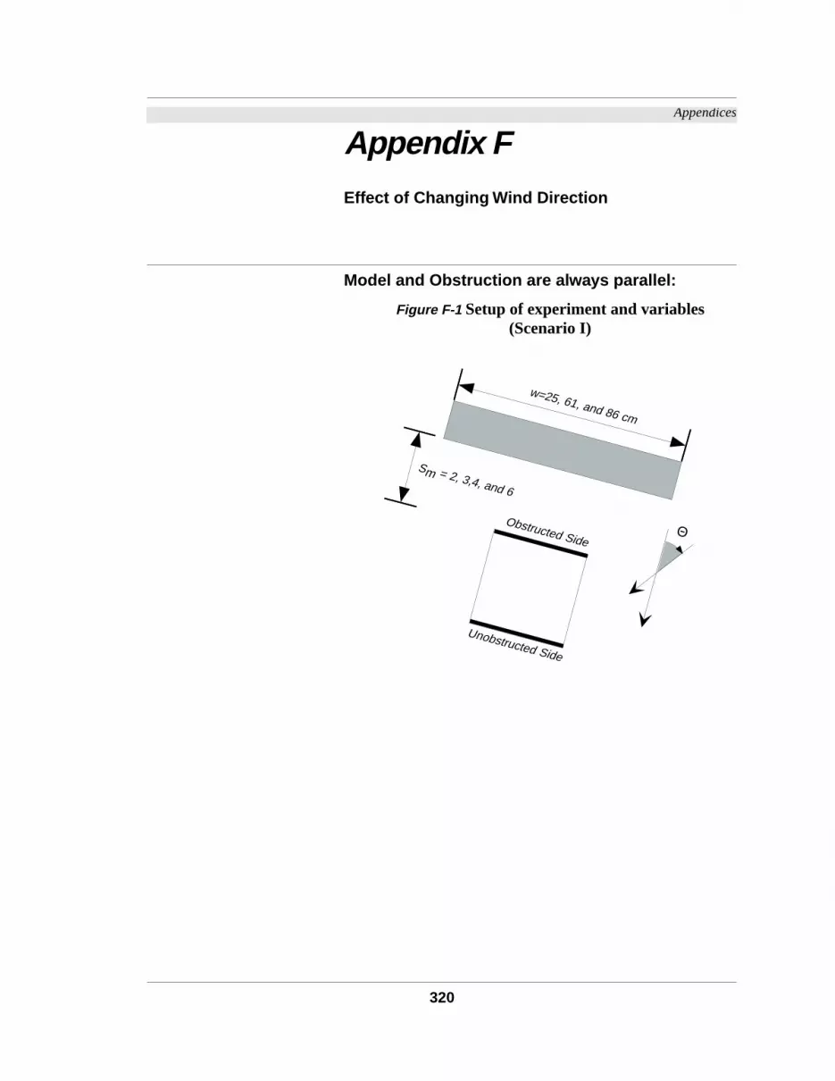
Appendices
Appendix FEffect of Changing Wind Direction
Model and Obstruction are always parallel:
Figure F-1 Setup of experiment and variables (Scenario I)
Θ
w=25, 61, and 86 cm
Obstructed Side
Unobstructed Side
Sm = 2, 3,4, and 6
320

Appendix F
Figure F-2 Effect of changing wind direction-measured data
a.Effect of changing the wind direction on pres-sure coefficients (Cp)
(Obstruction-facing side)
b.Effect of changing the wind direction on pres-sure modification coeffi-cients (Cp.m)
(Obstruction-facing side)
-1.0 -0.5 0.0 0.5 1.0
0°15°
30°
45°
60°
75°
90°
105°
120°
135°
150°
165°180°
195°
210°
225°
240°
255°
270°
285°
300°
315°
330°
345°
B
B
B
B
B
B
BBBB
B
B
B
B
B
BBB
B
B
B
B
B
B
B
J
J
J
J
J
J
JJJJ
J
J
J
J
J
JJJ
J
J
J
J
J
J
J
HH
H
H
H
H
HHHH
H
HH
H
H
HHH
H
H
H
H
H
HHF F
F
F
F
F
FFF
F
F
FF
F
F
F
FFF
F
F
F
F
F F
M M
M
M
M
M
MMM
M
M
M
M
M
M
M
MM
M
M
M
M
M
M M
7
7
7
7
7
7
777
7
7
77
7
7
7
77
7
7
7
7
7
7
7
B 25-02
J 25-03
H 25-04
F 25-06
61-02
61-03
61-04
61-06
M 86-02
86-03
86-04
7 86-06
Unobstructed
0.0 0.5 1.0 1.5
0°15°
30°
45°
60°
75°
90°
105°
120°
135°
150°
165°180°
195°
210°
225°
240°
255°
270°
285°
300°
315°
330°
345°
B
BB
B
B
B
B
B
B
B
B
B
B
B
B
B
B
B
B
B
B
B
BB
B
J
JJ
J
J
J
J
J
J
J
J
JJ
J
J
J
J
J
J
J
J
J
JJ
JH
HH
H
H
H
H
H
H
H
H
HHH
H
H
H
H
H
H
H
H
HH
HF
FF
F
F
F
F
F
F
F
F
FFF
F
F
F
F
F
F
F
F
FF
F
M MM
MM
M
M
M
M
M
M
MM
M
M
M
M
M
M
M
MM
MM M
7
7 7
7
7
7
7
7
7
7
7
777
7
7
7
7
7
7
7
7
7 7
7
B 25-02
J 25-03
H 25-04
F 25-06
61-02
61-03
61-04
61-06
M 86-02
86-03
86-04
7 86-06
321

Appendix F
c.Effect of changing the wind direction on pres-sure coefficients (Cp)
(Unobstructed side)
d.Effect of changing the wind direction on pres-sure modification coeffi-cients (Cp.m)
(Unobstructed side)
Figure F-2 Effect of changing wind direction-measured data (Continued)
-1.0 -0.5 0.0 0.5 1.0
0°15°
30°
45°
60°
75°
90°
105°
120°
135°
150°
165°180°
195°
210°
225°
240°
255°
270°
285°
300°
315°
330°
345°
BB
B
B
B
B
BBB
BB
B
B
B
BB
BBB
B
B
B
B
BBJ
J
J
J
J
J
JJJ
J
J
J
J
J
J
J
JJJ
J
J
J
J
JJH
H
H
H
H
H
HHH
H
H
H
H
H
H
H
HHH
H
H
H
H
HHF
F
F
F
F
F
FFF
F
F
FF
F
F
F
FFF
F
F
F
F
FF
M M
M
M
M
M
MMM
MM
M
M
M
MM
MM
M
M
M
M
M
M M
77
7
7
7
7
777
7
7
7
7
7
7
7
777
7
7
7
7
77
B 25-02
J 25-03
H 25-04
F 25-06
61-02
61-03
61-04
61-06
M 86-02
86-03
86-04
7 86-06
Unobstructed
0.0 0.5 1.0 1.5
0°15°
30°
45°
60°
75°
90°
105°
120°
135°
150°
165°180°
195°
210°
225°
240°
255°
270°
285°
300°
315°
330°
345°
B BB
B
B
B
B
B
B
B
B
BB
B
B
B
B
B
B
B
B
B
BB BJ J
J
J
J
J
J
J
J
J
J
JJJ
J
J
J
J
J
J
J
J
JJ JH H
H
H
H
H
H
H
H
H
H
HHH
H
H
H
H
H
H
H
H
HH HF F
F
F
F
F
F
F
F
F
F
FFF
F
F
F
F
F
F
F
F
FF F
MM M
M
M
M
M
M
M
MM
M
M
M
MM
M
M
M
M
M
M
M MM
7 77
7
7
7
7
7
7
7
7
7
7
7
7
7
7
7
7
7
7
7
77 7
B 25-02
J 25-03
H 25-04
F 25-06
61-02
61-03
61-04
61-06
M 86-02
86-03
86-04
7 86-06
322

Appendix F
Figure F-3 Comparison between measured and predicted values of on the obstructed side. (obstruction width=25 cm)
Spacing=20 cm Spacing=30 cm
Spacing=40 cm Spacing=40 cm
Legend
Cp
[
[ [[
[[
[[ [ [ [
[[
-1-0.8-0.6-0.4-0.2
00.20.40.60.8
10
15 30 45 60 75 90 105
120
135
150
165
180
Cp
Mea
sure
d
Wind Direction (°)
25-2 Obstructed
[[
[[
[
[
[[ [ [
[[
[
-1-0.8-0.6-0.4-0.2
00.20.40.60.8
1
015 30 45 60 75 90 10
512
013
515
016
518
0Pre
ssur
e C
oeffi
cien
t (C
p)
Wind Direction (°)
25-3 Obstructed
[[ [
[[
[
[[ [ [
[[ [
-1-0.8-0.6-0.4-0.2
00.20.40.60.8
1
0 15 30 45 60 75 90 105
120
135
150
165
180P
ress
ure
Coe
ffici
ent (
Cp)
Wind Direction (°)
25-4 Obstructed
[ [ [[
[
[
[[ [
[[ [ [
-1-0.8-0.6-0.4-0.2
00.20.40.60.8
1
015 30 45 60 75 90 10
512
013
515
016
518
0Pre
ssur
e C
oeffi
cien
t (C
p)
Wind Direction (°)
25-6 Obstructed
[ Cp Measured
Cp Predicted
323

Appendix F
Figure F-4 Comparison between measured and predicted values of on the obstructed side. (obstruction width=61 cm)
Spacing=20 cm Spacing=30 cm
Spacing=40 cm Spacing=60 cm
Legend
Cp
[[
[ [[
[[
[ [[ [
[[
-1-0.8-0.6-0.4-0.2
00.20.40.60.8
10 15 30 45 60 75 90 105
120
135
150
165
180P
ress
ure
Coe
ffici
ent (
Cp)
Wind Direction (°)
61-2 Obstructed
[
[[
[[
[
[[ [ [
[[
[
-1-0.8-0.6-0.4-0.2
00.20.40.60.8
1
015 30 45 60 75 90 10
512
013
515
016
518
0Pre
ssur
e C
oeffi
cien
t (C
p)
Wind Direction (°)
61-3 Obstructed
[
[ [[
[
[
[[ [ [
[
[ [
-1-0.8-0.6-0.4-0.2
00.20.40.60.8
1
0 15 30 45 60 75 90 105
120
135
150
165
180P
ress
ure
Coe
ffici
ent (
Cp)
Wind Direction (°)
61-4 Obstructed
[
[[
[[
[
[[ [
[
[[ [
-1-0.8-0.6-0.4-0.2
00.20.40.60.8
1
0 15 30 45 60 75 90 105
120
135
150
165
180P
ress
ure
Coe
ffici
ent (
Cp)
Wind Direction (°)
61-6 Obstructed
[ Cp Measured
Cp Predicted
324

Appendix F
Figure F-5 Comparison between measured and predicted values of on the obstructed side. (obstruction width=86 cm)
Spacing=20 cm Spacing=30 cm
Spacing=40 cm Spacing=60 cm
Legend
Cp
[ [[
[ [[
[[ [ [ [
[[
-1-0.8-0.6-0.4-0.2
00.20.40.60.8
10
15 30 45 60 75 90 105
120
135
150
165
180P
ress
ure
Coe
ffici
ent (
Cp)
Wind Direction (°)
86-2 Obstructed
[[ [
[[
[[
[ [ [[
[[
-1-0.8-0.6-0.4-0.2
00.20.40.60.8
1
0 15 30 45 60 75 90 105
120
135
150
165
180P
ress
ure
Coe
ffici
ent (
Cp)
Wind Direction (°)
86-3 Obstructed
[
[[
[[
[[
[ [ [[
[ [
-1-0.8-0.6-0.4-0.2
00.20.40.60.8
1
015 30 45 60 75 90 10
512
013
515
016
518
0Pre
ssur
e C
oeffi
cien
t (C
p)
Wind Direction (°)
86-4 Obstructed
[
[ [
[[
[
[[ [
[
[[ [
-1-0.8-0.6-0.4-0.2
00.20.40.60.8
1
0 15 30 45 60 75 90 105
120
135
150
165
180P
ress
ure
Coe
ffici
ent (
Cp)
Wind Direction (°)
86-6 Obstructed
[ Cp Measured
Cp Predicted
325

Appendix F
Figure F-6 Comparison between measured and predicted values of on the unobstructed side. (obstruction width=25 cm)
Spacing=20 cm Spacing=30 cm
Spacing=40 cm Spacing=60 cm
Legend
Cp
[ [[
[[
[
[[ [
[ [ [[
-1-0.8-0.6-0.4-0.2
00.20.40.60.8
10 15 30 45 60 75 90 105
120
135
150
165
180
Cp
Mea
sure
d
Wind Direction (°)
25-2 unobstructed
[ [ [[
[
[
[[ [
[ [ [[
-1-0.8-0.6-0.4-0.2
00.20.40.60.8
1
0 15 30 45 60 75 90 105
120
135
150
165
180P
ress
ure
Coe
ffici
ent (
Cp)
Wind Direction (°)
25-3 unobstructed
[ [ [[
[
[
[[ [
[ [ [ [
-1-0.8-0.6-0.4-0.2
00.20.40.60.8
1
0 15 30 45 60 75 90 105
120
135
150
165
180P
ress
ure
Coe
ffici
ent (
Cp)
Wind Direction (°)
25-4 unobstructed
[ [ [[
[
[
[[ [
[[ [ [
-1-0.8-0.6-0.4-0.2
00.20.40.60.8
1
0 15 30 45 60 75 90 105
120
135
150
165
1 80P
ress
ure
Coe
ffici
ent (
Cp)
Wind Direction (°)
25-6 unobstructed
[ Cp Measured
Cp Predicted
326

Appendix F
Figure F-7 Comparison between measured and predicted values of on the unobstructed side. (obstruction width=61 cm)
Spacing=20 cm Spacing=30 cm
Spacing=40 cm Spacing=60 cm
Legend
Cp
[ [[
[[
[
[[ [
[ [[
[
-1-0.8-0.6-0.4-0.2
00.20.40.60.8
10 15 30 45 60 75 90 105
120
135
150
165
180P
ress
ure
Coe
ffici
ent (
Cp)
Wind Direction (°)
61-2 unobstructed
[ [ [[
[
[
[[ [
[ [ [[
-1-0.8-0.6-0.4-0.2
00.20.40.60.8
1
0 15 30 45 60 75 90 105
120
135
150
165
180P
ress
ure
Coe
ffici
ent (
Cp)
Wind Direction (°)
61-3 unobstructed
[ [ [[
[
[
[[ [
[ [ [[
-1-0.8-0.6-0.4-0.2
00.20.40.60.8
1
0 15 30 45 60 75 90 105
120
135
150
165
180P
ress
ure
Coe
ffici
ent (
Cp)
Wind Direction (°)
61-4 unobstructed
[ [[
[[
[
[[ [
[[ [
[
-1-0.8-0.6-0.4-0.2
00.20.40.60.8
1
0 15 30 45 60 75 90 105
120
135
150
165
180P
ress
ure
Coe
ffici
ent (
Cp)
Wind Direction (°)
61-6 unobstructed
[ Cp Measured
Cp Predicted
327

Appendix F
Figure F-8 Comparison between measured and predicted values of on the unobstructed side. (obstruction width=86 cm)
Spacing=20 cm Spacing=30 cm
Spacing=40 cm Spacing=80
Legend:
Cp
[ [ [[
[
[
[[ [
[ [[
[
-1-0.8-0.6-0.4-0.2
00.20.40.60.8
10
15 30 45 60 75 90 105
120
135
150
165
180P
ress
ure
Coe
ffici
ent (
Cp)
Wind Direction (°)
86-2 unobstructed
[ [ [[
[
[
[[ [
[ [ [[
-1-0.8-0.6-0.4-0.2
00.20.40.60.8
1
0 15 30 45 60 75 90 105
120
135
150
165
180P
ress
ure
Coe
ffici
ent (
Cp)
Wind Direction (°)
86-3 unobstructed
[ [ [[
[
[
[[ [
[ [ [[
-1-0.8-0.6-0.4-0.2
00.20.40.60.8
1
015 30 45 60 75 90 10
512
013
515
016
518
0Pre
ssur
e C
oeffi
cien
t (C
p)
Wind Direction (°)
86-4 unobstructed
[ [ [[
[
[
[[ [
[ [ [[
-1-0.8-0.6-0.4-0.2
00.20.40.60.8
1
0 15 30 45 60 75 90 105
120
135
150
165
180P
ress
ure
Coe
ffici
ent (
Cp)
Wind Direction (°)
86-6 unobstructed
[ Cp Measured
Cp Predicted
328

Appendix F
Obstruction is always perpendicular to wind direction:
Figure F-9 Setup of experiment for scenario II
Θ
w=25, 61, 86 , and 200 cm
Obstructed Side
Unobstructed Side
S=2–10*
*3, 5, 7, 9 Additional spacing (S) for obstruction width = 200 cm only
329

Appendix F
Figure F-10 Effect of changing wind direction-measured data
a.Effect of changing the wind direction on surface pressure coefficients (Cp)
Obstruction Width=25 cm
b.Effect of changing the wind Direction on surface pressure coefficients (Cp.m)
Obstruction Width=25 cm
-1 -0.5 0 0.5 1
0° 15°30°
45°
60°
75°
90°
105°
120°
135°
150°165°180°195°
210°
225°
240°
255°
270°
285°
300°
315°
330°345°
BB
B
B
B
B
BBB
BB
BBBB
B
BBB
B
B
B
B
BB
JJ
J
J
J
J
JJJ
J
JJJJ
J
J
JJJ
J
J
J
J
JJH
H
H
H
H
H
HHH
H
HHHH
H
H
HHH
H
H
H
H
HHF
F
F
F
F
F
FFF
F
FFFF
F
F
FFF
F
F
F
F
FF
B 25-2
J 25-3
H 25-4
F 25-6
25-8
Unobstructed
0 0.5 1 1.5 2
0° 15°
30°
45°
60°
75°
90°
105°
120°
135°
150°
165°180°195°
210°
225°
240°
255°
270°
285°
300°
315°
330°
345°
B B BB B
B
B
B
B
BB
BBBB
B
B
B
B
B
B BB B B
J J JJ
J
J
J
J
J
J
JJJJ
J
J
J
J
J
J
JJ
J J JH H H
HH
H
H
H
H
H
HH
HH
H
H
H
H
H
H
HH
H H HF F
FF
F
F
F
F
F
F
FF
FF
F
F
F
F
F
F
FF
FF F B 25-2
J 25-3
H 25-4
F 25-6
25-8
Unobstructed
330
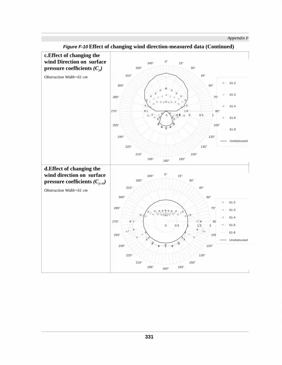
Appendix F
c.Effect of changing the wind Direction on surface pressure coefficients (Cp)
Obstruction Width=61 cm
d.Effect of changing the wind direction on surface pressure coefficients (Cp.m)
Obstruction Width=61 cm
Figure F-10 Effect of changing wind direction-measured data (Continued)
-1 -0.5 0 0.5 1
0° 15°
30°
45°
60°
75°
90°
105°
120°
135°
150°
165°180°195°
210°
225°
240°
255°
270°
285°
300°
315°
330°
345°
B B B BBB
B
BBB
B
BB
B
B
BBB
B
BBB B B B
JJ J
JJ
J
J
JJJ
JJJJ
J
JJJ
J
J
JJ
J JJ
HH
HH
H
H
H
HH
H
HHHH
H
H
HH
H
H
H
HH
HHF
FF
F
F
F
F
FF
F
FFFF
F
F
FF
F
F
F
FF
FF
B 61-2
J 61-3
H 61-4
F 61-6
61-8
Unobstructed
0 0.5 1 1.5 2
0° 15°
30°
45°
60°
75°
90°
105°
120°
135°
150°
165°180°195°
210°
225°
240°
255°
270°
285°
300°
315°
330°
345°
BB B B BB
B
B
BB
B
BBB
B
BB
B
B
BB B B BB
J J J J JJ
J
JJ
J
JJJJ
J
JJ
J
J
JJ J J J J
H H H H HH
H
HH
H
HHHH
H
H
HH
H
HH H H H HF F F F F
F
F
FF
F
FFFF
F
F
FF
F
FF F F F F
B 61-2
J 61-3
H 61-4
F 61-6
61-8
Unobstructed
331

Appendix F
e.Effect of changing the wind direction on surface pressure coefficients (Cp)
Obstruction Width=86 cm
f.Effect of changing the wind direction on surface pressure coefficients (Cp.m)
Obstruction Width=86 cm
Figure F-10 Effect of changing wind direction-measured data (Continued)
-1 -0.5 0 0.5 1
0° 15°
30°
45°
60°
75°
90°
105°
120°
135°
150°
165°180°195°
210°
225°
240°
255°
270°
285°
300°
315°
330°
345°
BBB B BB
B
B
BB
BBBB
BB
B
B
BBB B BBB
J J J JJJ
J
J
JJ
JJJJ
JJ
J
J
J
JJ
J J J J
H H HH
H
H
H
HH
HH
HHHH
HH
H
H
H
HH
H H H
FF
F
F
F
F
F
FF
FF
FFFF
F
FF
F
F
F
F
FF
FB 86-2
J 86-3
H 86-4
F 86-6
86-8
Unobstructed
0 0.5 1 1.5 2
0° 15°
30°
45°
60°
75°
90°
105°
120°
135°
150°
165°180°195°
210°
225°
240°
255°
270°
285°
300°
315°
330°
345°
BBB B BB
B
B
B
BBBBB
BB
B
B
B
BB B BBBJ
J J J JJ
J
J
JJJ
JJJJJ
J
J
J
JJ J J JJ
H H H H HH
H
H
HH
HHHHHH
H
H
H
HH H H H H
F F F FF
F
F
F
F
FF
FFFF
F
F
F
F
F
FF F F F
B 86-2
J 86-3
H 86-4
F 86-6
86-8
Unobstructed
332

Appendix F
g.Effect of changing the wind direction on surface pressure coefficients (Cp)
Obstruction Width=200 cm
h.Effect of changing the wind direction on surface pressure coefficients (Cp.m)
Obstruction Width=200 cm
Figure F-10 Effect of changing wind direction-measured data (Continued)
-1 -0.5 0 0.5 1
0° 15°
30°
45°
60°
75°
90°
105°
120°
135°
150°
165°180°195°
210°
225°
240°
255°
270°
285°
300°
315°
330°
345°
BBBBBBBBB
BBBBBBBBB
BBBBBB
B
JJJJJJJJJJJJJJJ
JJJJJJJJJJ
H H HHHHHHHHHHHHH
HHHHHHHH H H
F FFFFFFFFF
FFFFFFFFFFFFF
F F
MM
M
M
M
M
MM
M
MMMMMM
M
MM
M
M
M
M
MM
M
B 200-2
J 200-3
H 200-4
F 200-5
200-6
200-7
200-8
200-9
M 200-10
Unobstructed
0 0.5 1 1.5 2
0° 15°
30°
45°
60°
75°
90°
105°
120°
135°
150°
165°180°195°
210°
225°
240°
255°
270°
285°
300°
315°
330°
345°
BBBB B BB
B
BBBBBBBB
B
B
BB B BBBBJ
JJJ J JJ
J
JJJJJJJJ
J
J
JJ J JJJJ
HHH H HH
H
H
HHHHHHHH
H
H
H
HH H HHH
F F F F FF
F
F
FFFFFFFF
F
F
F
FF F F F F
M M M MM
M
M
M
M
MMMMMM
M
M
M
M
M
MM M M M
B 200-2
J 200-3
H 200-4
F 200-5
200-6
200-7
200-8
200-9
M 200-10
Unobstructed
333

Appendix F
Figure F-11 Comparison between measured and predicted values of . (obstruction width=25 cm)
Spacing=20 cm Spacing=30 cm
Spacing=40 cm Spacing=60 cm
Spacing=80 cm
Legend:
Cp
25-2
[ [ [ [ [ [[
[
[[ [ [ [
-1.4-1.2
-1-0.8-0.6-0.4-0.2
00.20.40.60.8
10
15 30 45 60 75 90 105
120
135
150
165
180P
ress
ure
Coe
ffici
ent (
Cp)
Wind Direction (°)
25-3
[ [ [ [ [[
[
[[
[[
[ [
-1.4-1.2
-1-0.8-0.6-0.4-0.2
00.20.40.60.8
1
015 30 45 60 75 90 10
512
013
515
016
518
0Pre
ssur
e C
oeffi
cien
t (C
p)
Wind Direction (°)
25-4
[ [ [ [ [[
[
[
[[
[ [[
-1.4-1.2
-1-0.8-0.6-0.4-0.2
00.20.40.60.8
1
015 30 45 60 75 90 10
512
013
515
016
518
0Pre
ssur
e C
oeffi
cien
t (C
p)
Wind Direction (°)
25-6
[ [ [[
[[
[
[
[ [[ [
[
-1.4-1.2
-1-0.8-0.6-0.4-0.2
00.20.40.60.8
1
015 30 45 60 75 90 10
512
013
515
016
518
0Pre
ssur
e C
oeffi
cien
t (C
p)
Wind Direction (°)
25-8
[ [[
[[
[
[
[
[ [[ [ [
-1.4-1.2
-1-0.8-0.6-0.4-0.2
00.20.40.60.8
1
015 30 45 60 75 90 10
512
013
515
016
518
0Pre
ssur
e C
oeffi
cien
t (C
p)
Wind Direction (°)
[ Cp Measured
Cp Predicted
334

Appendix F
Figure F-12 Comparison between measured and predicted values of . (obstruction width=61 cm)
Spacing=20 cm Spacing=30 cm
Spacing=40 cm Spacing=60 cm
Spacing=80 cm
Legend:
Cp
61-2
[ [ [ [ [ [ [ [[ [
[[ [
-1.4-1.2
-1-0.8-0.6-0.4-0.2
00.20.40.60.8
10
15 30 45 60 75 90 105
120
135
150
165
180P
ress
ure
Coe
ffici
ent (
Cp)
Wind Direction (°)
61-3
[ [ [ [ [ [ [[
[ [
[ [ [
-1.4-1.2
-1-0.8-0.6-0.4-0.2
00.20.40.60.8
1
015 30 45 60 75 90 10
512
013
515
016
518
0Pre
ssur
e C
oeffi
cien
t (C
p)
Wind Direction (°)
61-4
[ [ [ [ [ [ [[
[
[[ [ [
-1.4-1.2
-1-0.8-0.6-0.4-0.2
00.20.40.60.8
1
015 30 45 60 75 90 10
512
013
515
016
518
0Pre
ssur
e C
oeffi
cien
t (C
p)
Wind Direction (°)
61-6
[ [ [ [ [[
[
[[
[[ [ [
-1.4-1.2
-1-0.8-0.6-0.4-0.2
00.20.40.60.8
1
015 30 45 60 75 90 10
512
013
515
016
518
0Pre
ssur
e C
oeffi
cien
t (C
p)
Wind Direction (°)
61-8
[ [ [ [ [[
[
[
[ [[ [ [
-1.4-1.2
-1-0.8-0.6-0.4-0.2
00.20.40.60.8
1
015 30 45 60 75 90 10
512
013
515
016
518
0Pre
ssur
e C
oeffi
cien
t (C
p)
Wind Direction (°)
[ Cp Measured
Cp Predicted
335

Appendix F
Figure F-13 Comparison between measured and predicted values of . (obstruction width=86 cm)
Spacing=20 cm Spacing=30 cm
Spacing=40 cm Spacing=60 cm
Spacing=80 cm
Legend:
Cp
86-2
[ [ [ [ [ [[ [ [ [ [ [ [
-1.4-1.2
-1-0.8-0.6-0.4-0.2
00.20.40.60.8
10
15 30 45 60 75 90 105
120
135
150
165
180P
ress
ure
Coe
ffici
ent (
Cp)
Wind Direction (°)
86-3
[ [ [ [ [ [[ [ [ [ [ [ [
-1.4-1.2
-1-0.8-0.6-0.4-0.2
00.20.40.60.8
1
015 30 45 60 75 90 10
512
013
515
016
518
0Pre
ssur
e C
oeffi
cien
t (C
p)
Wind Direction (°)
86-4
[ [ [ [ [ [ [ [ [ [ [ [ [
-1.4-1.2
-1-0.8-0.6-0.4-0.2
00.20.40.60.8
1
015 30 45 60 75 90 10
512
013
515
016
518
0Pre
ssur
e C
oeffi
cien
t (C
p)
Wind Direction (°)
86-6
[ [ [ [ [ [ [[
[[ [ [ [
-1.4-1.2
-1-0.8-0.6-0.4-0.2
00.20.40.60.8
1
015 30 45 60 75 90 10
512
013
515
016
518
0Pre
ssur
e C
oeffi
cien
t (C
p)
Wind Direction (°)
86-8
[ [ [ [ [ [[
[[
[ [ [ [
-1.4-1.2
-1-0.8-0.6-0.4-0.2
00.20.40.60.8
1
015 30 45 60 75 90 10
512
013
515
016
518
0Pre
ssur
e C
oeffi
cien
t (C
p)
Wind Direction (°)
[ Cp Measured
Cp Predicted
336
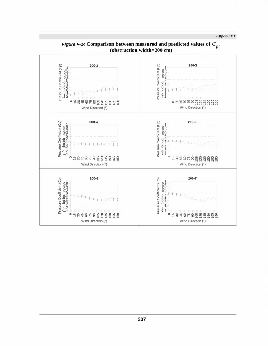
Appendix F
Figure F-14 Comparison between measured and predicted values of . (obstruction width=200 cm)
Cp
200-2
[ [ [ [ [ [ [ [ [ [ [ [ [
-1.4-1.2
-1-0.8-0.6-0.4-0.2
00.20.40.60.8
10
15 30 45 60 75 90 105
120
135
150
165
1 80P
ress
ure
Coe
ffici
ent (
Cp)
Wind Direction (°)
200-3
[ [ [ [ [ [ [ [ [ [ [ [ [
-1.4-1.2
-1-0.8-0.6-0.4-0.2
00.20.40.60.8
1
015 30 45 60 75 90 10
512
013
515
016
518
0Pre
ssur
e C
oeffi
cien
t (C
p)
Wind Direction (°)
200-4
[ [ [ [ [ [ [ [ [ [ [ [ [
-1.4-1.2
-1-0.8-0.6-0.4-0.2
00.20.40.60.8
1
015 30 45 60 75 90 10
512
013
515
016
518
0Pre
ssur
e C
oeffi
cien
t (C
p)
Wind Direction (°)
200-5
[ [ [ [ [ [ [ [ [ [ [ [ [
-1.4-1.2
-1-0.8-0.6-0.4-0.2
00.20.40.60.8
1
015 30 45 60 75 90 10
512
013
515
016
518
0Pre
ssur
e C
oeffi
cien
t (C
p)
Wind Direction (°)
200-6
[ [ [ [ [ [ [ [ [ [ [ [ [
-1.4-1.2
-1-0.8-0.6-0.4-0.2
00.20.40.60.8
1
015 30 45 60 75 90 10
512
013
515
016
518
0Pre
ssur
e C
oeffi
cien
t (C
p)
Wind Direction (°)
200-7
[ [ [ [ [ [ [[ [ [ [ [ [
-1.4-1.2
-1-0.8-0.6-0.4-0.2
00.20.40.60.8
1
015 30 45 60 75 90 10
512
013
515
016
518
0Pre
ssur
e C
oeffi
cien
t (C
p)
Wind Direction (°)
337

Appendix F
Legend:
Figure F-14 Comparison between measured and predicted values of . (obstruction width=200 cm) (Continued)
Cp
200-8
[ [ [ [ [ [[ [ [ [ [ [ [
-1.4-1.2
-1-0.8-0.6-0.4-0.2
00.20.40.60.8
10
15 30 45 60 75 90 105
120
135
150
165
180P
ress
ure
Coe
ffici
ent (
Cp)
Wind Direction (°)
200-9
[ [ [ [ [ [[
[ [[ [ [ [
-1.4-1.2
-1-0.8-0.6-0.4-0.2
00.20.40.60.8
1
015 30 45 60 75 90 10
512
013
515
016
518
0Pre
ssur
e C
oeffi
cien
t (C
p)
Wind Direction (°)
200-10
[ [ [ [ [ [[
[ [[ [ [ [
-1.4-1.2
-1-0.8-0.6-0.4-0.2
00.20.40.60.8
1
015 30 45 60 75 90 10
512
013
515
016
518
0Pre
ssur
e C
oeffi
cien
t (C
p)
Wind Direction (°)
[ Cp Measured
Cp Predicted
338

339
Appendix G

Appendices
Appendix GMultiple Obstruction Blocks
si-
del.
eri-
.
n
This appendix shows the effect of two obstruction blocks po
tioned on the windward side of the of the instrumented mo
Figure G-1 illustrates the variables studied in this set of exp
ments and these are:
1. The spacing between the obstruction blocks (gap).
2. The spacing between the obstruction blocks and the model
3. Wind direction.
4. Horizontal shift or changing the position of the two obstructio
blocks relative to the instrumented surface.
Figure G-1 The studied variables
g
So
Horizontal Shift (d)
Win
d D
ire
ctio
n
Θ = 0˚-90˚
g = Gap
So = Obstruction Spacing
340

Appendix G
Figure G-2.1 Pressure modification coefficients profiles as shielded by two
obstruction blocks 2 spacings and 12.5 cm between blocks
Cpm
Θ
WD
S=2
s=12.5 cm
1.51.5
1
0.5
0
-0.5
-1
0 250
-1
-0.5
0
0.5
1
1.5
0 250
Cpm
Θ=0°
1.51.5
1
0.5
0
-0.5
-1
0 250
-1
-0.5
0
0.5
1
1.5
0 250
Cpm
Θ=15°
1.51.5
1
0.5
0
-0.5
-1
0 250
-1
-0.5
0
0.5
1
1.5
0 250
Cpm
Θ=30°
1.51.5
1
0.5
0
-0.5
-1
0 250
-1
-0.5
0
0.5
1
1.5
0 250C
pm
Θ=45°
1.51.5
1
0.5
0
-0.5
-1
0 250
-1
-0.5
0
0.5
1
1.5
0 250
Cpm
Θ=60°
1.51.5
1
0.5
0
-0.5
-1
0 250
-1
-0.5
0
0.5
1
1.5
0 250
Cpm
Θ=75°
1.51.5
1
0.5
0
-0.5
-1
0 250
-1
-0.5
0
0.5
1
1.5
0 250
Cpm
Θ=90°
341

Appendix G
Figure G-2.2 Pressure modification coefficients profiles as shielded by two
obstruction blocks 2 spacings and 25 cm between blocks
Cpm
Θ
WD S=2
s=25cm
1.51.5
1
0.5
0
-0.5
-1
0 250
-1
-0.5
0
0.5
1
1.5
0 250
Cpm
Θ=0°
1.51.5
1
0.5
0
-0.5
-1
0 250
-1
-0.5
0
0.5
1
1.5
0 250
Cpm
Θ=15°
1.51.5
1
0.5
0
-0.5
-1
0 250
-1
-0.5
0
0.5
1
1.5
0 250
Cpm
Θ=30°
1.51.5
1
0.5
0
-0.5
-1
0 250
-1
-0.5
0
0.5
1
1.5
0 250C
pm
Θ=45°
1.51.5
1
0.5
0
-0.5
-1
0 250
-1
-0.5
0
0.5
1
1.5
0 250
Cpm
Θ=60°
1.51.5
1
0.5
0
-0.5
-1
0 250
-1
-0.5
0
0.5
1
1.5
0 250
Cpm
Θ=75°
1.51.5
1
0.5
0
-0.5
-1
0 250
-1
-0.5
0
0.5
1
1.5
0 250
Cpm
Θ=90
342

Appendix G
Figure G-2.3 Pressure modification coefficients profiles as shielded by two
obstruction blocks 2 spacings and 37.5 cm between blocks
Cpm
Θ
WD
s=37.5 cm
S=2
1.51.5
1
0.5
0
-0.5
-1
0 250
-1
-0.5
0
0.5
1
1.5
0 250
Cpm
Θ=0°
1.51.5
1
0.5
0
-0.5
-1
0 250
-1
-0.5
0
0.5
1
1.5
0 250
Cpm
Θ=15°
1.51.5
1
0.5
0
-0.5
-1
0 250
-1
-0.5
0
0.5
1
1.5
0 250
Cpm
Θ=30°
1.51.5
1
0.5
0
-0.5
-1
0 250
-1
-0.5
0
0.5
1
1.5
0 250
Cpm
Θ=45°
1.51.5
1
0.5
0
-0.5
-1
0 250
-1
-0.5
0
0.5
1
1.5
0 250
Cpm
Θ=60°
1.51.5
1
0.5
0
-0.5
-1
0 250
-1
-0.5
0
0.5
1
1.5
0 250
Cpm
Θ=75°
1.51.5
1
0.5
0
-0.5
-1
0 250
-1
-0.5
0
0.5
1
1.5
0 250
Cpm
Θ=90°
343

Appendix G
d
Figure G-2.4 Pressure modification coefficients profiles as shielded by two
obstruction blocks 2 spacings and 12.5 cm between blocks and horizontally displace
Cpm
Θ
WD
s=12.5 cm
S=2
d=12.5 cm
1.51.5
1
0.5
0
-0.5
-1
0 250
-1
-0.5
0
0.5
1
1.5
0 250
Cpm
Θ=0°
1.51.5
1
0.5
0
-0.5
-1
0 250
-1
-0.5
0
0.5
1
1.5
0 250
Cpm
Θ=15°
1.51.5
1
0.5
0
-0.5
-1
0 250
-1
-0.5
0
0.5
1
1.5
0 250
Cpm
Θ=30°
1.51.5
1
0.5
0
-0.5
-1
0 250
-1
-0.5
0
0.5
1
1.5
0 250
Cpm
Θ=45°
1.51.5
1
0.5
0
-0.5
-1
0 250
-1
-0.5
0
0.5
1
1.5
0 250
Cpm
Θ=60°
1.51.5
1
0.5
0
-0.5
-1
0 250
-1
-0.5
0
0.5
1
1.5
0 250
Cpm
Θ=75°
1.51.5
1
0.5
0
-0.5
-1
0 250
-1
-0.5
0
0.5
1
1.5
0 250
NC
p
Θ=90°
344

Appendix G
Figure G-2.5 Pressure modification coefficients profiles as shielded by two
obstruction blocks 2 spacings and 25 cm between blocks and horizontally displaced
Cpm
Θ
WDS=2
s=25 cm
d=12.5 cm
1.51.5
1
0.5
0
-0.5
-1
0 250
-1
-0.5
0
0.5
1
1.5
0 250
Cpm
Θ=0°
1.51.5
1
0.5
0
-0.5
-1
0 250
-1
-0.5
0
0.5
1
1.5
0 250
Cpm
Θ=15°
1.51.5
1
0.5
0
-0.5
-1
0 250
-1
-0.5
0
0.5
1
1.5
0 250
Cpm
Θ=30°
1.51.5
1
0.5
0
-0.5
-1
0 250
-1
-0.5
0
0.5
1
1.5
0 250
Cpm
Θ=45°
1.51.5
1
0.5
0
-0.5
-1
0 250
-1
-0.5
0
0.5
1
1.5
0 250
Cpm
Θ=60°
1.51.5
1
0.5
0
-0.5
-1
0 250
-1
-0.5
0
0.5
1
1.5
0 250
Cpm
Θ=75°
1.51.5
1
0.5
0
-0.5
-1
0 250
-1
-0.5
0
0.5
1
1.5
0 250
Cpm
Θ=90°
345

Appendix G
d
Figure G-2.6 Pressure modification coefficients profiles as shielded by two
obstruction blocks 2 spacings and 37.5 cm between blocks and horizontally displace
Cpm
Θ
WDS=2
s=37.5 cm
d=12.5 cm
1.51.5
1
0.5
0
-0.5
-1
0 250
-1
-0.5
0
0.5
1
1.5
0 250
Cpm
Θ=0°
1.51.5
1
0.5
0
-0.5
-1
0 250
-1
-0.5
0
0.5
1
1.5
0 250
Cpm
Θ=15°
1.51.5
1
0.5
0
-0.5
-1
0 250
-1
-0.5
0
0.5
1
1.5
0 250
Cpm
Θ=30°
1.51.5
1
0.5
0
-0.5
-1
0 250
-1
-0.5
0
0.5
1
1.5
0 250
Cpm
Θ=45°
1.51.5
1
0.5
0
-0.5
-1
0 250
-1
-0.5
0
0.5
1
1.5
0 250
Cpm
Θ=60°
1.51.5
1
0.5
0
-0.5
-1
0 250
-1
-0.5
0
0.5
1
1.5
0 250
Cpm
Θ=75°
1.51.5
1
0.5
0
-0.5
-1
0 250
-1
-0.5
0
0.5
1
1.5
0 250
Cpm
Θ=90°
346

Appendix G
d
Figure G-2.7 Pressure modification coefficients profiles as shielded by two
obstruction blocks 2 spacings and 12.5 cm between blocks and horizontally displace
Cpm
Θ
WDS=2
s=12.5 cm
d=25 cm
1.51.5
1
0.5
0
-0.5
-1
0 250
-1
-0.5
0
0.5
1
1.5
0 250
Cpm
Θ=0°
1.51.5
1
0.5
0
-0.5
-1
0 250
-1
-0.5
0
0.5
1
1.5
0 250
Cpm
Θ=15°
1.51.5
1
0.5
0
-0.5
-1
0 250
-1
-0.5
0
0.5
1
1.5
0 250
Cpm
Θ=30°
1.51.5
1
0.5
0
-0.5
-1
0 250
-1
-0.5
0
0.5
1
1.5
0 250
Cpm
Θ=45°
1.51.5
1
0.5
0
-0.5
-1
0 250
-1
-0.5
0
0.5
1
1.5
0 250
Cpm
Θ=60°
1.51.5
1
0.5
0
-0.5
-1
0 250
-1
-0.5
0
0.5
1
1.5
0 250
Cpm
Θ=75°
1.51.5
1
0.5
0
-0.5
-1
0 250
-1
-0.5
0
0.5
1
1.5
0 250
Cpm
Θ=90°
347

Appendix G
Figure G-2.8 Pressure modification coefficients profiles as shielded by two
obstruction blocks 2 spacings and 25 cm between blocks and horizontally displaced
Cpm
Θ
WDS=2
s=25 cm
d=25 cm
1.51.5
1
0.5
0
-0.5
-1
0 250
-1
-0.5
0
0.5
1
1.5
0 250
Cpm
Θ=0°
1.51.5
1
0.5
0
-0.5
-1
0 250
-1
-0.5
0
0.5
1
1.5
0 250
Cpm
Θ=15°
1.51.5
1
0.5
0
-0.5
-1
0 250
-1
-0.5
0
0.5
1
1.5
0 250
Cpm
Θ=30°
1.51.5
1
0.5
0
-0.5
-1
0 250
-1
-0.5
0
0.5
1
1.5
0 250
Cpm
Θ=45°
1.51.5
1
0.5
0
-0.5
-1
0 250
-1
-0.5
0
0.5
1
1.5
0 250
NC
p
Θ=60°
1.51.5
1
0.5
0
-0.5
-1
0 250
-1
-0.5
0
0.5
1
1.5
0 250
NC
p
Θ=75°
1.51.5
1
0.5
0
-0.5
-1
0 250
-1
-0.5
0
0.5
1
1.5
0 250
Cpm
Θ=90°
348

Appendix G
d
Figure G-2.9 Pressure modification coefficients profiles as shielded by two
obstruction blocks 2 spacings and 37.5 cm between blocks and horizontally displace
Cpm
Θ
WDS=2
s=37.5 cm
d=25 cm
1.51.5
1
0.5
0
-0.5
-1
0 250
-1
-0.5
0
0.5
1
1.5
0 250
Cpm
Θ=0°
1.51.5
1
0.5
0
-0.5
-1
0 250
-1
-0.5
0
0.5
1
1.5
0 250
Cpm
Θ=15°
1.51.5
1
0.5
0
-0.5
-1
0 250
-1
-0.5
0
0.5
1
1.5
0 250
Cpm
Θ=30°
1.51.5
1
0.5
0
-0.5
-1
0 250
-1
-0.5
0
0.5
1
1.5
0 250
Cpm
Θ=45°
1.51.5
1
0.5
0
-0.5
-1
0 250
-1
-0.5
0
0.5
1
1.5
0 250
Cpm
Θ=60°
1.51.5
1
0.5
0
-0.5
-1
0 250
-1
-0.5
0
0.5
1
1.5
0 250
Cpm
Θ=75°
1.51.5
1
0.5
0
-0.5
-1
0 250
-1
-0.5
0
0.5
1
1.5
0 250
Cpm
Θ=90°
349

Appendix G
d
Figure G-2.10 Pressure modification coefficients profiles as shielded by two
obstruction blocks 3 spacings and 12.5 cm between blocks and horizontally centere
Cpm
Θ
WD
s=12.5 cm
S=3
1.51.5
1
0.5
0
-0.5
-1
0 250
-1
-0.5
0
0.5
1
1.5
0 250
Cpm
Θ=0°
1.51.5
1
0.5
0
-0.5
-1
0 250
-1
-0.5
0
0.5
1
1.5
0 250
Cpm
Θ=15°
1.51.5
1
0.5
0
-0.5
-1
0 250
-1
-0.5
0
0.5
1
1.5
0 250
Cpm
Θ=30°
1.51.5
1
0.5
0
-0.5
-1
0 250
-1
-0.5
0
0.5
1
1.5
0 250
Cpm
Θ=45°
1.51.5
1
0.5
0
-0.5
-1
0 250
-1
-0.5
0
0.5
1
1.5
0 250
Cpm
Θ=60°
1.51.5
1
0.5
0
-0.5
-1
0 250
-1
-0.5
0
0.5
1
1.5
0 250
Cpm
Θ=75°
1.51.5
1
0.5
0
-0.5
-1
0 250
-1
-0.5
0
0.5
1
1.5
0 250
Cpm
Θ=90°
350

Appendix G
Figure G-2.11 Pressure modification coefficients profiles as shielded by two
obstruction blocks 3 spacings and 25 cm between blocks and horizontally centered
Cpm
Θ
WD
s=25 cm
S=3
1.51.5
1
0.5
0
-0.5
-1
0 250
-1
-0.5
0
0.5
1
1.5
0 250
Cpm
Θ=00°
1.51.5
1
0.5
0
-0.5
-1
0 250
-1
-0.5
0
0.5
1
1.5
0 250
Cpm
Θ=15°
1.51.5
1
0.5
0
-0.5
-1
0 250
-1
-0.5
0
0.5
1
1.5
0 250
Cpm
Θ=30°
1.51.5
1
0.5
0
-0.5
-1
0 250
-1
-0.5
0
0.5
1
1.5
0 250
Cpm
Θ=45°
1.51.5
1
0.5
0
-0.5
-1
0 250
-1
-0.5
0
0.5
1
1.5
0 250
Cpm
Θ=60°
1.51.5
1
0.5
0
-0.5
-1
0 250
-1
-0.5
0
0.5
1
1.5
0 250
Cpm
Θ=75°
1.51.5
1
0.5
0
-0.5
-1
0 250
-1
-0.5
0
0.5
1
1.5
0 250
Cpm
Θ=90°
351

Appendix G
d
Figure G-2.12 Pressure modification coefficients profiles as shielded by two
obstruction blocks 3 spacings and 37.5 cm between blocks and horizontally centere
Cpm
Θ
WD
s=37.5 cm
S=3
1.51.5
1
0.5
0
-0.5
-1
0 250
-1
-0.5
0
0.5
1
1.5
0 250
Cpm
Θ=0°
1.51.5
1
0.5
0
-0.5
-1
0 250
-1
-0.5
0
0.5
1
1.5
0 250
Cpm
Θ=15°
1.51.5
1
0.5
0
-0.5
-1
0 250
-1
-0.5
0
0.5
1
1.5
0 250
Cpm
Θ=30°
1.51.5
1
0.5
0
-0.5
-1
0 250
-1
-0.5
0
0.5
1
1.5
0 250
Cpm
Θ=45°
1.51.5
1
0.5
0
-0.5
-1
0 250
-1
-0.5
0
0.5
1
1.5
0 250
Cpm
Θ=60°
1.51.5
1
0.5
0
-0.5
-1
0 250
-1
-0.5
0
0.5
1
1.5
0 250
Cpm
Θ=75°
1.51.5
1
0.5
0
-0.5
-1
0 250
-1
-0.5
0
0.5
1
1.5
0 250
Cpm
Θ=90°
352

Appendix G
d
Figure G-2.13 Pressure modification coefficients profiles as shielded by two
obstruction blocks 4 spacings and 12.5 cm between blocks and horizontally centere
Cpm
Θ
WD
s=12.5 cm
S=4
1.51.5
1
0.5
0
-0.5
-1
0 250
-1
-0.5
0
0.5
1
1.5
0 250
Cpm
Θ=0°
1.51.5
1
0.5
0
-0.5
-1
0 250
-1
-0.5
0
0.5
1
1.5
0 250
Cpm
Θ=15°
1.51.5
1
0.5
0
-0.5
-1
0 250
-1
-0.5
0
0.5
1
1.5
0 250
Cpm
Θ=30°
1.51.5
1
0.5
0
-0.5
-1
0 250
-1
-0.5
0
0.5
1
1.5
0 250
Cpm
Θ=45°
1.51.5
1
0.5
0
-0.5
-1
0 250
-1
-0.5
0
0.5
1
1.5
0 250
Cpm
Θ=60°
1.51.5
1
0.5
0
-0.5
-1
0 250
-1
-0.5
0
0.5
1
1.5
0 250
Cpm
Θ=75°
1.51.5
1
0.5
0
-0.5
-1
0 250
-1
-0.5
0
0.5
1
1.5
0 250
Cpm
Θ=90°
353

Appendix G
Figure G-2.14 Pressure modification coefficients profiles as shielded by two
obstruction blocks 4 spacings and 25 cm between blocks and horizontally centered
Cpm
Θ
WD
S=4
s=25 cm
1.51.5
1
0.5
0
-0.5
-1
0 250
-1
-0.5
0
0.5
1
1.5
0 250
Cpm
Θ=0°
1.51.5
1
0.5
0
-0.5
-1
0 250
-1
-0.5
0
0.5
1
1.5
0 250
Cpm
Θ=15°
1.51.5
1
0.5
0
-0.5
-1
0 250
-1
-0.5
0
0.5
1
1.5
0 250
Cpm
Θ=30°
1.51.5
1
0.5
0
-0.5
-1
0 250
-1
-0.5
0
0.5
1
1.5
0 250
Cpm
Θ=45°
1.51.5
1
0.5
0
-0.5
-1
0 250
-1
-0.5
0
0.5
1
1.5
0 250
Cpm
Θ=60°
1.51.5
1
0.5
0
-0.5
-1
0 250
-1
-0.5
0
0.5
1
1.5
0 250
Cpm
Θ=75°
1.51.5
1
0.5
0
-0.5
-1
0 250
-1
-0.5
0
0.5
1
1.5
0 250
Cpm
Θ=90°
354

Appendix G
d
Figure G-2.15 Pressure modification coefficients profiles as shielded by two
obstruction blocks 4 spacings and 37.5 cm between blocks and horizontally centere
Cpm
Θ
WD
s=37.5 cm
S=4
1.51.5
1
0.5
0
-0.5
-1
0 250
-1
-0.5
0
0.5
1
1.5
0 250
Cpm
Θ=0°
1.51.5
1
0.5
0
-0.5
-1
0 250
-1
-0.5
0
0.5
1
1.5
0 250
Cpm
Θ=15°
1.51.5
1
0.5
0
-0.5
-1
0 250
-1
-0.5
0
0.5
1
1.5
0 250
Cpm
Θ=30°
1.51.5
1
0.5
0
-0.5
-1
0 250
-1
-0.5
0
0.5
1
1.5
0 250
Cpm
Θ=45°
1.51.5
1
0.5
0
-0.5
-1
0 250
-1
-0.5
0
0.5
1
1.5
0 250
Cpm
Θ=60°
1.51.5
1
0.5
0
-0.5
-1
0 250
-1
-0.5
0
0.5
1
1.5
0 250
Cpm
Θ=75°
1.51.5
1
0.5
0
-0.5
-1
0 250
-1
-0.5
0
0.5
1
1.5
0 250
Cpm
Θ=90°
355

Appendix G
Figure G-3 Effect of two shielding blocks on obstructed surface of model
GG
G
G
G GG
C CC
CC C
C
0
0.2
0.4
0.6
0.8
1
1.2
0 15 30 45 60 75 90
Cpm
WD (°)
G 2-H-1
C 3-H-1
4-H-1
GG
GG
G GG
CC C
CC C
C
0
0.2
0.4
0.6
0.8
1
1.2
0 15 30 45 60 75 90
Cpm
WD (°)
G 2-O-1
C 3-O-1
4-O-1
G G
G G
GG
G
CC
CC
C C C
0
0.2
0.4
0.6
0.8
1
1.2
0 15 30 45 60 75 90
Cpm
WD (°)
G 2-X-1
C 3-X-1
4-X-1
2, 3, and 4 Spacings
1/2 Obstruction Width
θ=0°-90°
1 Obstruction Width
2, 3, and 4 Spacingsθ=0°-90°
1 1/2 Obstruction Width
2, 3, and 4 Spacingsθ=0°-90°
GG
G
G
G GG
CC
CC
C CC
0
0.2
0.4
0.6
0.8
1
1.2
0 15 30 45 60 75 90
Cpm
WD (°)
G 2-H-1
C 2-O-1
2-X-1
G GG
GG G
G
CC C
CC C
C
0
0.2
0.4
0.6
0.8
1
1.2
0 15 30 45 60 75 90
Cpm
WD (°)
G 3-H-1
C 3-O-1
3-X-1
GG
GG G G G
C CC
C C C C
0
0.2
0.4
0.6
0.8
1
1.2
0 15 30 45 60 75 90
Cpm
WD (°)
G 4-H-1
C 4-O-1
4-X-1
1/2, 1, 1 1/2 Obstruction Width
2 Spacingsθ=0°-90°
1/2, 1, 1 1/2 Obstruction Width
3 Spacingsθ=0°-90°
1/2, 1, 1 1/2 Obstruction Width
4 Spacingsθ=0°-90°
356

Appendix G
Figure G-3 Effect of two shielding blocks on obstructed surface of model (Continued)
GG
G
G
G GG
CC
C C
C CC
0
0.2
0.4
0.6
0.8
1
1.2
0 15 30 45 60 75 90
Cpm
WD (°)
G 2-H-1
C 2-H-2
2-H-3
GG
GG
G GG
C
C
C
CC C
C
0
0.2
0.4
0.6
0.8
1
1.2
0 15 30 45 60 75 90
Cpm
WD (°)
G 2-O-1
C 2-O-2
2-O-3
G G
G G
GG
G
C
C
CC
C CC
0
0.2
0.4
0.6
0.8
1
1.2
0 15 30 45 60 75 90
Cpm
WD (°)
G 2-X-1
C 2-X-2
2-X-3
1/2 Obstruction Width
2 Spacingsθ=0°-90°
1, 2, and 3 Displacements
1 Obstruction Width
2 Spacingsθ=0°-90°
1, 2, and 3 Displacements1 1/2 Obstruction Width
2 Spacingsθ=0°-90°
1, 2, and 3 Displacements
GG
G
G
G GG
CC
CC
C CC
0
0.2
0.4
0.6
0.8
1
1.2
0 15 30 45 60 75 90
Cpm
WD (°)
G 2-H-1
C 2-O-1
2-X-1
GG
G G
G GG
C
C
C
CC C
C
0
0.2
0.4
0.6
0.8
1
1.2
0 15 30 45 60 75 90
Cpm
WD (°)
G 2-H-2
C 2-O-2
2-X-2
G
GG G G G
G
C
CC
C C CC
0
0.2
0.4
0.6
0.8
1
1.2
0 15 30 45 60 75 90
Cpm
WD (°)
G 2-H-3
C 2-O-3
2-X-3
1/2, 1, 1 1/2 Obstruction Width
2 Spacingsθ=0°-90°
1/2, 1, 1 1/2 Obstruction Width
2 Spacings θ=0°-90°
displacement=2
1/2, 1, 1 1/2 Obstruction Width
2 Spacings θ=0°-90°
displacement=3
357

Appendix G
Figure G-4 . Comparison between the predicted value of for the individual
shielding blocks and the measured values.
Cpm
I IIH, O, X
S=2
GG
GG
GG GC C C C
C C C
0
0.2
0.4
0.6
0.8
1
1.2
0 15 30 45 60 75 90
Cpm
WD (°)
G Block1
C Block2
measured
2-H-1
GG
GG
GG GC C C C C C C
0
0.2
0.4
0.6
0.8
1
1.2
0 15 30 45 60 75 90C
pmWD (°)
G Block1
C Block2
measured
G GG
GG
GGC C C
C C C C
0
0.2
0.4
0.6
0.8
1
1.2
0 15 30 45 60 75 90
Cpm
WD (°)
G Block1
C Block2
measured
H, O, X
S=2I II
G
GG
GG
G GC C C C C C C
0
0.2
0.4
0.6
0.8
1
1.2
0 15 30 45 60 75 90
Cpm
WD (°)
G Block1
C Block2
measured
G
GG
GG
G GC C C C C C C
0
0.2
0.4
0.6
0.8
1
1.2
0 15 30 45 60 75 90
Cpm
WD (°)
G Block1
C Block2
measured
G
GG
GG
G GC C C C C C C
0
0.2
0.4
0.6
0.8
1
1.2
0 15 30 45 60 75 90C
pm
WD (°)
G Block1
C Block2
measured
I IIH, O, X
S=2
GG
GG G G GC C
C C C C C
0
0.2
0.4
0.6
0.8
1
1.2
0 15 30 45 60 75 90
Cpm
WD (°)
G Block1
C Block2
measured
GG
GG G G GC C C C C C C
0
0.2
0.4
0.6
0.8
1
1.2
0 15 30 45 60 75 90
Cpm
WD (°)
G Block1
C Block2
measured
GG
GG G G GC
C C C C C C
0
0.2
0.4
0.6
0.8
1
1.2
0 15 30 45 60 75 90
Cpm
WD (°)
G Block1
C Block2
measured
358

Appendix G
Figure G-4 . Comparison between the predicted value of for the individual
shielding blocks and the measured values. (Continued)
Cpm
H, O, X
S=3
I II
GG
GG
G G GCC C C
C C C
0
0.2
0.4
0.6
0.8
1
1.2
0 15 30 45 60 75 90
Cpm
WD (°)
G Block1
C Block2
measured
3-H-1
GG
G GG
G GC C C CC C C
0
0.2
0.4
0.6
0.8
1
1.2
0 15 30 45 60 75 90
Cpm
WD (°)
G Block1
C Block2
measured
GG
G GG
G GC C CC C C C
0
0.2
0.4
0.6
0.8
1
1.2
0 15 30 45 60 75 90
Cpm
WD (°)
G Block1
C Block2
measured
H, O, X
S=4
I II
GG G
GG G G
CC C C C C C
0
0.2
0.4
0.6
0.8
1
1.2
0 15 30 45 60 75 90
Cpm
WD (°)
G Block1
C Block2
measured
4-H-1
GG
GG
G G GC C C CC C C
0
0.2
0.4
0.6
0.8
1
1.2
0 15 30 45 60 75 90
Cpm
WD (°)
G Block1
C Block2
measured
GG
G GG G GC C C C C C C
0
0.2
0.4
0.6
0.8
1
1.2
0 15 30 45 60 75 90
Cpm
WD (°)
G Block1
C Block2
measured
359

Appendix G
Figure G-5 Comparison between measured and predicted values of Cpm
I IIH, O, X
S=2
GG
G
G
G GG
X X XX
XX X
0
0.2
0.4
0.6
0.8
1
1.2
0 15 30 45 60 75 90
Cpm
WD (°)
G measured
X Predicted
2-H-1
GG
GG
G GG
X X X X
XX X
0
0.2
0.4
0.6
0.8
1
1.2
0 15 30 45 60 75 90
Cpm
WD (°)
G measured
X Predicted
2-O-1
G G
G G
GG
G
X X X XX
XX
0
0.2
0.4
0.6
0.8
1
1.2
0 15 30 45 60 75 90
Cpm
WD (°)
G measured
X Predicted
2-X-1
H, O, X
S=2I II
GG
G G
G GG
X X X
X
X X X
0
0.2
0.4
0.6
0.8
1
1.2
0 15 30 45 60 75 90
Cpm
WD (°)
G measured
X Predicted
2-H-2
G
G
G
GG G
G
X X X
XX X X
0
0.2
0.4
0.6
0.8
1
1.2
0 15 30 45 60 75 90
Cpm
WD (°)
G measured
X Predicted
2-O-2
G
G
GG
G GG
[ [ [
[[ [ [
0
0.2
0.4
0.6
0.8
1
1.2
0 15 30 45 60 75 90
Cpm
WD (°)
G measured
[ Predicted
2-X-2
I IIH, O, X
S=2 G
GG G G G
G
X
X
X X X X X
0
0.2
0.4
0.6
0.8
1
1.2
0 15 30 45 60 75 90
Cpm
WD (°)
G measured
X Predicted
2-H-3
G
GG
G G GG
X
X
X X X X X
0
0.2
0.4
0.6
0.8
1
1.2
0 15 30 45 60 75 90
Cpm
WD (°)
G measured
X Predicted
2-O-3
G
GG G G
GG
X
XX X X X X
0
0.2
0.4
0.6
0.8
1
1.2
0 15 30 45 60 75 90
Cpm
WD (°)
G measured
X Predicted
2-X-3
360

Appendix G
)
Figure G-5 Comparison between measured and predicted values of (ContinuedCpmH, O, X
S=3
I II
G GG
GG G
G
X X X
X
X XX
0
0.2
0.4
0.6
0.8
1
1.2
0 15 30 45 60 75 90
Cpm
WD (°)
G measured
X Predicted
3-H-1
GG G
GG G
G
X X XX
X XX
0
0.2
0.4
0.6
0.8
1
1.2
0 15 30 45 60 75 90
Cpm
WD (°)
G measured
X Predicted
3-O-1
GG
GG
G G G
X X XX
XX X
0
0.2
0.4
0.6
0.8
1
1.2
0 15 30 45 60 75 90
Cpm
WD (°)
G measured
X Predicted
3-X-1
H, O, X
S=4
I II
GG
GG G G G
X XX
XX X
X
0
0.2
0.4
0.6
0.8
1
1.2
0 15 30 45 60 75 90
Cpm
WD (°)
G measured
X Predicted
4-H-1
G GG
G G G G
X X X
X
X XX
0
0.2
0.4
0.6
0.8
1
1.2
0 15 30 45 60 75 90
Cpm
WD (°)
G measured
X Predicted
4-O-1
GG G
GG G G
X X X
XX X X
0
0.2
0.4
0.6
0.8
1
1.2
0 15 30 45 60 75 90
Cpm
WD (°)
G measured
X Predicted
4-X-1
361

362
Appendix H

Appendices
Appendix HModel Application and Algorithm
H.1 Algorithm
Figure H-1 Diagram showing the procedural flow of the model for predicting velocity coefficients Cv
Choose a Single SurfaceChoose a Single Surface
Choose another Wind DirectionChoose another Wind Direction
Establish Terrain
INPUT
Establish Terrain
INPUT
Calculate Multiple Obstruction with Gaps
Section 3.7.4.4
Calculate Multiple Obstruction with Gaps
Section 4.15.6
Choose Wind Direction
INPUT/File
Choose Wind Direction
INPUT/File
Identify Surround Buildings in 140 ° arcIdentify Surround. Buildings in 140 ° arc
Section 5.3.3
Identify Gaps with arcIdentify Gaps within arc
Calculate
Calculate Orthogonal C p
Section 3.5
Calculate Orthogonal C p
Section 4.12.3
Calculate Displacement Correction -if any
Section 3.5.4
Calculate Displacement Correction -if any
Section 4.13.1
If Wind Direction ≠ 0then Choose
If Wind Direction ≠ 0then Choose
Scenario (I)
sec. 3.7.2 sec. 3.7.3
Scenario (II) Scenario (I)
sec. 4.14.3 sec. 4.14.4
Scenario (II)
Calculate Wind Direction Correction
Section 3.7
Calculate Wind Direction Correction
section 4.14
Choose another Obstruction BlockChoose another Obstruction Block
Calculate Gap Effects
Section 4.16.5
Choose a Single Obstruction Block within arc
Convert C pm to Cp
Section H.2.12
Correct for Boundary Layer
Section B.2
Choose another Wind DirectionChoose another Surface
Save Cp Value
Calculate avg. Indoor Velocity Flow
Section H.3
Begin
End
Calculate Site Velocity
Section H.3.6
363

Appendix H
ion
e-
s the
lex
fied
the
vel
d in
ef.
, an
ict
if-
dic-
the
ach
or-
ured
own
H.2 Sample Calculations
This part contains a sample calculation of the Indoor Ventilat
prediction Model (IVM) with a detailed description of the proc
dure used. The site and model configuration were the same a
ones used for the verification of the model using the comp
urban layout1.
H-1. For a more detailed description of the tested model and configuration of the obstruction blocks refer to Section 4.17.4 in page 159.
H.2.1 Inputting Terrain Types
The terrain types around the building of concern was identi
and input using Table B-1. The terrain information is used in
IVM in two ways:
• Conversion from weather station data to site’s street le
velocities. Examples of these conversion methods are foun
Arens 1985 (Ref. 10), Aynsley 1989. (Ref. 24), ASHRAE (R
16), Swami and Chandra 1987 (Ref. 203). For this example
adapted version of SITECLIMATE method was used to pred
the wind speeds at the site (Section 5.7).
• Correcting value using Table B-1 to account for the d
ference in terrain type from the one used in deriving the pre
tion model.
H.2.2 Inputting the Obstruction Coordinates
As discussed in Chapter 5, the input for the model is based on
polar coordinates of the outermost visible corners/edges of e
visible obstruction block. Figure H-2 demonstrates how the co
dinates of the corners/edges were taken off. A list of the meas
polar coordinates of all adjacent blocks for each surface is sh
in Table H-1.
Cpm
364

Appendix H
Figure H-2 Description of surrounding blocks.
1
2 3
4 5
6
7b
7a
7c
89
10
11
11a
11b
North
EastSouth
West
Θ = 0˚-360˚
Table H-1 Polar coordinates of the corners of the surrounding obstruction blocks relative to the four
surfaces .
Surface BlockaBlock Height Point r (S)b c (°°°°)
Nor
th
7B 7 1 8.1 63.8
2 7.2 90
7C 17 1 3.8d 67.3
2 4.4 76.2
8 25 1 2.1 41.2
2 2.0 11.4
9 10 1 3.4 -8.9
2 8.3 -50.1
10 24.7 1 2.9 -28
2 3.0 -40.3
11 10 1 7.5 -60.4
2 6.5 -90
λ
365

Appendix H
a. Refer to Figure H-2.
b. The radial coordinate is measured in terms of obstruction Spacing (So).
Sou
th
2 10 1 5.4 68.1
2 4.2 45.2
3 10 1 2.3 26.6
2 2.3 -26.6
4 10 1 7.1 44.9
2 6.6 27
6 10 1 6.7 -72.4
2 4.4 -43.9
11 10 1 6.8 72.8
2 6.5 90
Eas
t
6 10 1 5.9 25.1
2 4.2 61.2
7A 25 1 1.6 7.0
2 1.6 -7.0
7B 7 1 7.2 -36.4
2 5.8 -7
7C 17 1 4.0 -20
2 3.4 -31.2
8 25 1 2.1 -60.9
2 1.8 -90
Wes
t
1 10 1 2.1 13.9
2 2.1 -13.9
2 10 1 4.7 -32.1
2 4.0 -11.3
4 10 1 6.3 -60.7
2 6.8 -73.1
9 10 1 8.0 47.3
2 3.0 90
10 24.7 1 2.9 58.1
2 2.9 71
11ae 10 1 6.9 37.3
2 5.7 14.1
11b 10 1 5.7 -14.1
2 6.0 -24.4
Table H-1 Polar coordinates of the corners of the surrounding obstruction blocks relative to the four
surfaces (Continued).
Surface BlockaBlock Height Point r (S)b c (°°°°)λ
366

Appendix H
ates
he
sec-
as
the
ting
ngu-
ears
e of
irec-
s of
and
the
) to
of
360
nd
at
.
c. Angular coordinate of visible edge of obstruction block.
d. Refer to Section H.2.3
e. Note that for the west surface, obstruction block has been divided into two sections: 11a and 11b (Figure H-2)
H.2.3 Running a Point Order Check
Following the rules stated in Section 5.3.3.3, the point coordin
in bold font in Table H-1 have been flagged for order errors. T
three points were then reversed in the calculation in the next
tion. However, the corner coordinates of block 9 were kept
ordered in Table H-1. This exception was used to account for
shifted wake effect discussed in Section 4.17.4.4. By selec
point 1 to be the one with the smallest absolute value of the a
lar polar coordinates, the equivalent obstruction plane app
closer to the north surface, thus decreasing the predicted valu
.
H.2.4 Determining the Relative Wind Direction
Based on the discussion in Section 5.3.3.1, the relative wind d
tions for the four facades were determined. At 0˚, the value
were 0˚, -90˚, 180˚, and +90˚ for the North, East, South,
West facades respectively2. For wind directions , Equa-
tions (5-4) and (5-5) were used.
H-2. Refer to Equation (5-1).
H.2.5 Calculating the Angles of Obstruction
Using the geometric relationships discussed in Chapter 5,
angles of obstructions were calculated [Equations (5-7), (5-14
(5-20)]. Figures H-3 to H-6 show the result of the calculations
the three angles of obstruction for the four surfaces for the
wind directions. As a visual hint, it should be noted that wi
direction at roughly coincides with the wind direction
which the shielding effect of that obstruction block is maximum
Cpm
ΘrelΘrel
Θrel 0°>
max αh
367

Appendix H
Figure H-3 Angles of obstruction for the North facade.
0 15 30 45 60 75 90
0° 15°30°
45°
60°
75°
90°
105°
120°
135°
150°165°180°195°
210°
225°
240°
255°
270°
285°
300°
315°
330°345°
North: 7b
0 15 30 45 60 75 90
0° 15°30°
45°
60°
75°
90°
105°
120°
135°
150°165°180°195°
210°
225°
240°
255°
270°
285°
300°
315°
330°345°
North: 7c
0 15 30 45 60 75 90
0° 15°30°
45°
60°
75°
90°
105°
120°
135°
150°165°180°195°
210°
225°
240°
255°
270°
285°
300°
315°
330°345°
North: 8
0 15 30 45 60 75 90
0° 15°30°
45°
60°
75°
90°
105°
120°
135°
150°165°180°195°
210°
225°
240°
255°
270°
285°
300°
315°
330°345°
North: 9
0 15 30 45 60 75 90
0° 15°30°
45°
60°
75°
90°
105°
120°
135°
150°165°180°195°
210°
225°
240°
255°
270°
285°
300°
315°
330°345°
North: 10
0 15 30 45 60 75 90
0° 15°30°
45°
60°
75°
90°
105°
120°
135°
150°165°180°195°
210°
225°
240°
255°
270°
285°
300°
315°
330°345°
North: 11
alpha_h alpha_v alpha_d
368

Appendix H
Figure H-4 Angles of obstruction for the South facade.
0 15 30 45 60 75 90
0° 15°30°
45°
60°
75°
90°
105°
120°
135°
150°165°180°195°
210°
225°
240°
255°
270°
285°
300°
315°
330°345°
South: 2
0 15 30 45 60 75 90
0° 15°30°
45°
60°
75°
90°
105°
120°
135°
150°165°180°195°
210°
225°
240°
255°
270°
285°
300°
315°
330°345°
South: 3
0 15 30 45 60 75 90
0° 15°30°
45°
60°
75°
90°
105°
120°
135°
150°165°180°195°
210°
225°
240°
255°
270°
285°
300°
315°
330°345°
South: 4
0 15 30 45 60 75 90
0° 15°30°
45°
60°
75°
90°
105°
120°
135°
150°165°180°195°
210°
225°
240°
255°
270°
285°
300°
315°
330°345°
South: 6
0 15 30 45 60 75 90
0° 15°30°
45°
60°
75°
90°
105°
120°
135°
150°165°180°195°
210°
225°
240°
255°
270°
285°
300°
315°
330°345°
South: 11
alpha_h alpha_v alpha_d
369

Appendix H
Figure H-5 Angles of obstruction for the East facade.
0 15 30 45 60 75 90
0° 15°30°
45°
60°
75°
90°
105°
120°
135°
150°165°180°195°
210°
225°
240°
255°
270°
285°
300°
315°
330°345°
East: 6
0 15 30 45 60 75 90
0° 15°30°
45°
60°
75°
90°
105°
120°
135°
150°165°180°195°
210°
225°
240°
255°
270°
285°
300°
315°
330°345°
East: 7a
0 15 30 45 60 75 90
0° 15°30°
45°
60°
75°
90°
105°
120°
135°
150°165°180°195°
210°
225°
240°
255°
270°
285°
300°
315°
330°345°
East: 7b
0 15 30 45 60 75 90
0° 15°30°
45°
60°
75°
90°
105°
120°
135°
150°165°180°195°
210°
225°
240°
255°
270°
285°
300°
315°
330°345°
East: 7c
0 15 30 45 60 75 90
0° 15°30°
45°
60°
75°
90°
105°
120°
135°
150°165°180°195°
210°
225°
240°
255°
270°
285°
300°
315°
330°345°
East: 8
alpha_h alpha_v alpha_d
370

Appendix H
Figure H-6 c Angles of obstruction for the West facade.
0 15 30 45 60 75 90
0° 15°30°
45°
60°
75°
90°
105°
120°
135°
150°165°180°195°
210°
225°
240°
255°
270°
285°
300°
315°
330°345°
West: 1
0 15 30 45 60 75 90
0° 15°30°
45°
60°
75°
90°
105°
120°
135°
150°165°180°195°
210°
225°
240°
255°
270°
285°
300°
315°
330°345°
West: 2
0 15 30 45 60 75 90
0° 15°30°
45°
60°
75°
90°
105°
120°
135°
150°165°180°195°
210°
225°
240°
255°
270°
285°
300°
315°
330°345°
West: 4
0 15 30 45 60 75 90
0° 15°30°
45°
60°
75°
90°
105°
120°
135°
150°165°180°195°
210°
225°
240°
255°
270°
285°
300°
315°
330°345°
West: 9
0 15 30 45 60 75 90
0° 15°30°
45°
60°
75°
90°
105°
120°
135°
150°165°180°195°
210°
225°
240°
255°
270°
285°
300°
315°
330°345°
West: 10
0 15 30 45 60 75 90
0° 15°30°
45°
60°
75°
90°
105°
120°
135°
150°165°180°195°
210°
225°
240°
255°
270°
285°
300°
315°
330°345°
West: 11a
371

Appendix H
are
on
ter-
H.2.6 Inputting the Gap Description
As defined in Section 5.3.3.7, the gaps’ polar coordinates
taken off from the plan (Figure H-7). Similar to the obstructi
blocks, only gaps visible from the surface are considered in de
mining the overall shielding effect.
Figure H-7 Determination of the Gaps coordinates
0 15 30 45 60 75 90
0° 15°30°
45°
60°
75°
90°
105°
120°
135°
150°165°180°195°
210°
225°
240°
255°
270°
285°
300°
315°
330°345°
West: 11b
alpha_h alpha_v alpha_d
Θ = 0˚-360˚
g1
g2
g3
g4
g5
g6
g7
South
EastWest
North
372

Appendix H
eck
Gap
hat
a. Refer to Figure H-7.
H.2.7 Running a Point Order Check for the Gaps
Similar to the procedure discussed in H.2.3, a point order ch
was run to determine the correct order of the gap coordinates.
coordinates in Bold letters in Table H-2 show the points t
needed re-ordering.
Table H-2 Coordinates of visible Gaps.
Surfacea GapBlock Height Point r (S) (°°°°)
Nor
th
g1 10 1 8.4 -50.1
10 2 7.5 -60.4
g6 7 1 8.0 63.8
25 2 2.1 41.2
7g 25 1 1.7 14.1
10 2 3.4 -8.9
Sou
th
g2 10 1 5.4 68.1
10 2 6.8 72.9
g4 10 1 2.3 -26.6
10 2 4.4 -43.7
g5 10 1 6.7 -72.6
25 2 2.0 -90
Eas
t
g4 10 1 4.2 61.3
10 2 2.5 90
g5 25 1 1.7 7
10 2 5.9 25.1
g6 7 1 7.2 -36.4
25 2 2.1 -60.9
Wes
t
g1 10 1 6.9 37.3
10 2 8.0 47.3
g2 10 1 6.0 -24.4
10 2 4.7 -32.1
g3 10 1 6.8 -73.1
10 2 5.5 -90
λ
373

Appendix H
ment
cor-
lcu-
ces
H.2.8 Determine the Angular Description of the Gaps
The lone parameter needed to define the gap is the displace
angle ( ) and was calculated using Equation (5-17) and
rected in Equations (5-18) to (5-20). Table H-2 shows the ca
lated displacement angles of all visible gaps for the four surfa
of the model.
αdg
374

Appendix H
Figure H-8 Calculated Displacement Angle of visible Gaps.
0 15 30 45 60 75 90
0° 15°30°
45°
60°
75°
90°
105°
120°
135°
150°165°180°195°
210°
225°
240°
255°
270°
285°
300°
315°
330°345°
g1
g6
g7
North Side
0 15 30 45 60 75 90
0° 15°30°
45°
60°
75°
90°
105°
120°
135°
150°165°180°195°
210°
225°
240°
255°
270°
285°
300°
315°
330°345°
g2
g4
g5
South Side
375

Appendix H
al
fol-
ter 4
le
the
-1)
H.2.9 Calculate for Individual Blocks
The determination of the shielding effect of the individu
obstruction blocks on the four model surfaces described in the
lowing sections adheres to the algorithm presented in Chap
and illustrated in Figure H-1.
H.2.9.1 Orthogonal Model This calculation is performed on all obstruction blocks visib
from the surface for which was determined. Based on
angles of obstruction determined in STEP H.2.5, formula (D
0 15 30 45 60 75 90
0° 15°30°
45°
60°
75°
90°
105°
120°
135°
150°165°180°195°
210°
225°
240°
255°
270°
285°
300°
315°
330°345°
g4
g5
g6
East Side
0 15 30 45 60 75 90
0° 15°30°
45°
60°
75°
90°
105°
120°
135°
150°165°180°195°
210°
225°
240°
255°
270°
285°
300°
315°
330°345°
g1
g2
g3
West Side
Cpm
Cpm
376

Appendix H
es
s
he
etric
ual
w
s
cor-
.
(4-
res-
do
rip-
io II
ver,
s 9
ese
on
was used to calculate the value of for all surfac
based on the individual shielding of all visible blocks3.
H-3. A simpler version of the relationship was described in Equation (4-11), Section4.12.3.2.
H.2.9.2 Correction for Dis-placement
Similarly, the correction for displacement ( ) wa
implemented using formula (4-13) for all obstruction blocks. T
resulting values were then categorized based on the geom
relation between the considered surface and the individ
obstruction block.
H.2.9.3 Correction for Wind Direction (Scenario I)
The effect of changing the wind direction for blocks that follo
scenario I configuration4 was performed for all obstruction block
except for blocks 9 and 10 (Figure H-2). This means that no
rection was needed except that was applied when
When this latter condition was met, the correction in Equation
17) was applied. However, only blocks 1, 3 and 7a cause the p
surization effect described in Equation (4-17). The other blocks
not cause this pressurization and thus
(Figure 4-71)
H-4. Section 4.14.3 on page 114.
H.2.9.4 Correction for Wind Direction (Scenario II)
Even though obstruction blocks 9 and 10 fit Scenario III desc
tion, the discussion in Section 4.14.1 explained that Scenar
correction was to be used. The applied correction for
was described in Equation (4-19) in Section 4.14.4.3. Howe
when the pressurization is non-effectual since block
and 10 are shifted relative to the considered surface. In th
cases, the value of and pressurizati
is expected (Figure 4-71).
Cpm ortho( )
Cpmαd corr( )
αh 140°>
CpmΘ corr( )Cpmαd corr( )
=
αh 10°>
αh 10°<
CpmΘ corr( )Cpmαd corr( )
=
377

Appendix H
ere
nd-
d-
n
cal-
(4-
ing
e
on
H.2.9.5 Correction for Boundary Layer
The boundary conditions under which the model is tested w
described in Section 4.17.4. The correction factor for that bou
ary layer is 0.92 (TABLE B-1 ). Each value of calculated indivi
ual was multiplied by the boundary layer correctio
factor.
H.2.10 Calculating for the Multiple
Obstruction
Based on the input from Section H.2.9 and Section H.2.8, the
culated values of and were used in Equation
22) to determine the average shielding effect of surround
obstruction blocks ( ). Figures H-9 to H-12 show th
result of calculating the shielding effect of multiple obstructi
blocks on each surface.
Figure H-9 Predicted pressure modification coefficients on the North surface
CpmΘ corr( )
Cpm CpmΘ corr( )αdg
Cpmmultiple
0 0.5 1 1.5 2
0° 15°30°
45°
60°
75°
90°
105°
120°
135°
150°165°180°195°
210°
225°
240°
255°
270°
285°
300°
315°
330°345°
XXXX X X
XXXXXXXXX
XX
XXXX
XXX
XX
X
XXX X X XXX
XX
Cpm
378
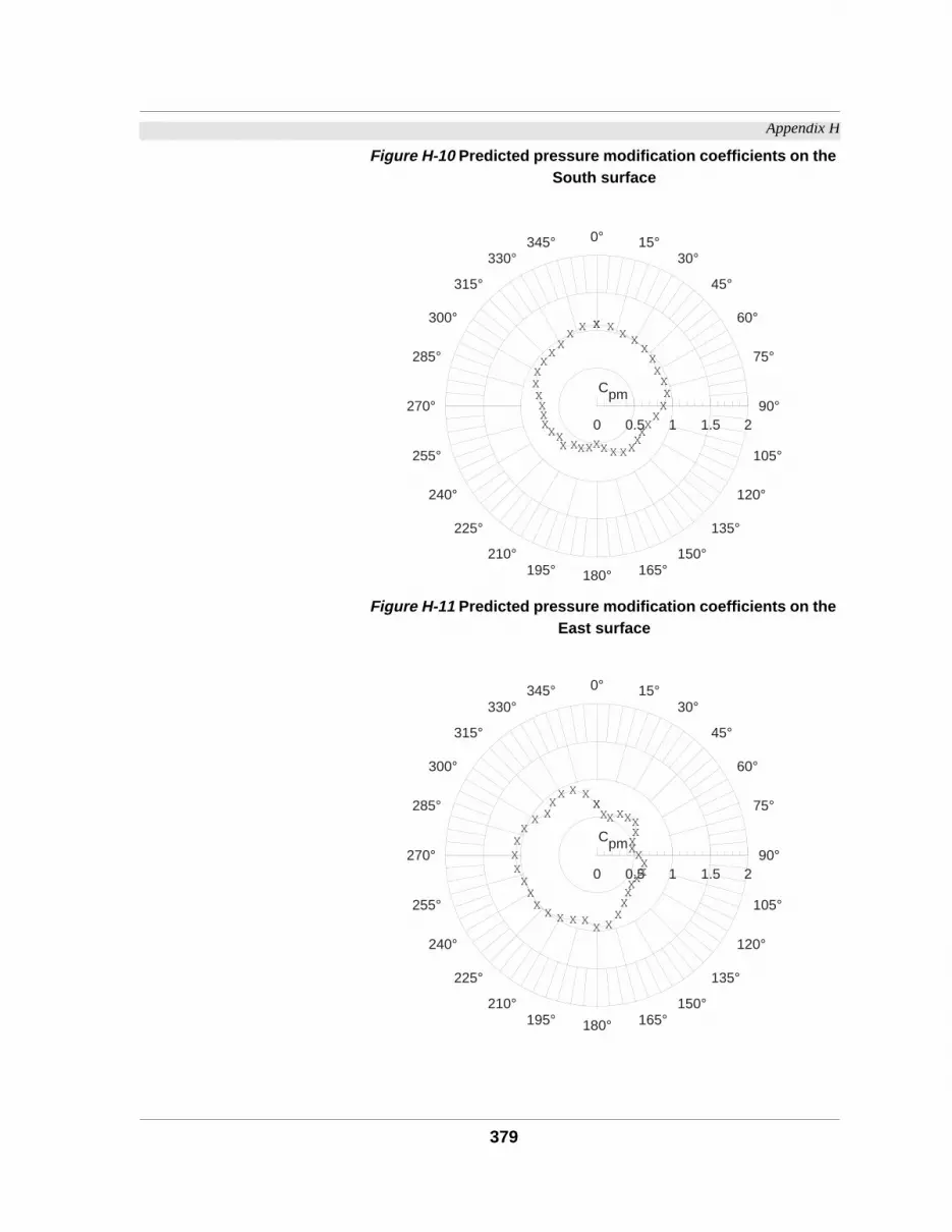
Appendix H
Figure H-10 Predicted pressure modification coefficients on the South surface
Figure H-11 Predicted pressure modification coefficients on the East surface
0 0.5 1 1.5 2
0° 15°30°
45°
60°
75°
90°
105°
120°
135°
150°165°180°195°
210°
225°
240°
255°
270°
285°
300°
315°
330°345°
X XX X
XXXXXXX
XXXXXXX
XXXXXXX
XXXXXXXXXXX X
Cpm
0 0.5 1 1.5 2
0° 15°30°
45°
60°
75°
90°
105°
120°
135°
150°165°180°195°
210°
225°
240°
255°
270°
285°
300°
315°
330°345°
XXX XXX
XXXXXXXX
XXX
XXXXXX
XXXXXXXX X
XX X X
X
Cpm
379

Appendix H
sure
hat
w.
on-
oeffi-
ddi-
ented
Figure H-12 Predicted pressure Modification coefficients on the West surface
H.2.11 Determination of Unobstructed Values
This section deals with the conversion of the calculated Pres
Modification Coefficients to Pressure Coefficient values t
can be used in existing models for predicting indoor airflo
Based on Equation (4-3), the calculated values of were c
verted to using the following relationship;
(H-1)
H.2.11.1 at Wind
Direction
Some of the sources for the unshielded surface pressure c
cients on building surfaces are described in Section 5.6. In a
tion to these sources, the data from this research are docum
in Appendix C, and can also be used.
0 0.5 1 1.5 2
0° 15°30°
45°
60°
75°
90°
105°
120°
135°
150°165°180°195°
210°
225°
240°
255°
270°
285°
300°
315°
330°345°
X
XX
X
X
X XXXXXXX
XXXX
XXXXX
XXXXXXXXXXXXX
X
X
Cpm
Cp Cpm
Cpm
Cp Shielded( )
Cp Shielded( ) Cpm eCp Unshielded( )⋅ln=
Cp
Θ 0°=
380

Appendix H
d
s)
lues
the
ami
this
y be
the
of
of
hip
uld
Fig-
atio
on-
For this experiment, the values of for all win
directions for the two surfaces (N or long and E or short side5
were measured in the wind tunnel. Figure H-13 shows the va
of the pressure coefficient of the unobstructed model used in
determination of values as in Figures G- 14 to G-17.
H-5. Refer to Figure 4-100, pp. page 161.
H.2.11.2 Calculate at
Wind Direction
When the wind direction is larger than 0˚, models such as Sw
and Chandra (Ref. 203) or the modified function developed in
research (Section 4.11.2) and illustrated in Equation (4-7) ma
used. Figures 4-24 and 4-28 can also be used to provide
designer with the row data needed to establish the value
. The latter will be used in the determination
the Pressure Modification Coefficient using the relations
described in Section 4.10 and shown in Equation (H-1). It sho
be noted that the slight difference between the two curves in
ure H-13 is due to the difference in their respective aspect r
( ). In Equation (4-7), the aspect ratio of the surface under c
sideration is accounted for in the prediction of the .
Cp Unshielded( )
Cpm
Cp
Θ 0°>
Cp Unshielded( )
Cpm
As
Cpm@Θ
381

Appendix H
and
del
to
Figure H-13 Pressure modification coefficients of the unobstructed instrumented model
H.2.12 Determination of the Shielded Pressure Coefficients
Based on the values of calculated in Section H.2.10
Equation (H-1), the Pressure Coefficients of the shielded m
( ) were calculated and presented in Figures G- 14
G-17.
-2 -1.5 -1 -0.5 0 0.5 1
0°
30°
60°
90°
120°
150°
180°
210°
240°
270°
300°
330° [ [[
[
[
[
[
[
[[
[[[[[[
[[[[
[[[[[[
[[
[
[
[
[
[
[[
[ [X X XX
X
X
X
X
XXXXXXX
XXXXXX
XXXXXXX
X
X
X
X
X
XX X X
[ Long Side
X Short Side
Cp
Cp Shielded( )
Cpm
Cp Shielded( )
382

Appendix H
Figure H-14 Predicted pressure coefficients on the North surface
Figure H-15 Predicted pressure coefficients on the South surface
-2 -1.5 -1 -0.5 0 0.5 1
0° 15°30°
45°
60°
75°
90°
105°
120°
135°
150°165°180°195°
210°
225°
240°
255°
270°
285°
300°
315°
330°345°
XX
XX X
X
X
XXXXXXXXX
XXXX
XXX
XXX
XXX
XXXXXX
XX
Cp
-2 -1.5 -1 -0.5 0 0.5 1
0° 15°30°
45°
60°
75°
90°
105°
120°
135°
150°165°180°195°
210°
225°
240°
255°
270°
285°
300°
315°
330°345°
X XXXXXXXXXXX
X
X
XX
XXXXXX
X
XX
XXXXXXXXXXX X
Cp
383

Appendix H
an-
Figure H-16 Predicted pressure coefficients on the East surface
Figure H-17 Predicted pressure coefficients on the West surface
H.2.13 Building Characteristics
The building in our case is a single storey with a flat roof, rect
gular plan, and single space with no interior partitions.
-2 -1.5 -1 -0.5 0 0.5 1
0° 15°30°
45°
60°
75°
90°
105°
120°
135°
150°165°180°195°
210°
225°
240°
255°
270°
285°
300°
315°
330°345°
XXX
X X XX
X
X
X
X
XX
XXXX
XX
XXXXXX
XXXXXXXX X X XX
Cp
-2 -1.5 -1 -0.5 0 0.5 1
0° 15°30°
45°
60°
75°
90°
105°
120°
135°
150°165°180°195°
210°
225°
240°
255°
270°
285°
300°
315°
330°345°
X X XX
X
X XXXXX
XX
XXXXXXXXXX
X
X
X
X
X
X
X
XX
X X X X X
Cp
384

Appendix H
are
area
the
ec-
si-
nt
ibu-
As shown in Figure H-18, the windows in the experiment
located on the long sides opposite to each other6. The windows in
both walls have the same dimensions, location, and surface
(Figure 18).
Figure H-18 The Windows Configurations
H-6. Surfaces N and S.
H.3 Determining Indoor Velocity
The transformation of the predicted pressure data involves
implementation of Ernest mathematical model discussed in S
tion 5.8. The determination of the indoor air velocity of the phy
cal model follows a step-by-step calculation of the differe
variables described in Equation (5-29).
H.3.1 Effect of Pressure Distribution and Wind Direction (f1)
The function that is used to determine effect if pressure distr
tion and wind direction7 is as follows8:
(H-2)
Where
H-7. Refer to Equation (5-29).
H-8. Ernest 1991, ((Ref. 74)), Equation A.3-2 pp. 249.
Ai= 44.3 sq. cm
Ao= 44.3 sq. cm
Long side
Short Side
f 1 Cp Θ,( ) C1 ∆Cp⋅ C2 Cpw Θcos⋅ ⋅+ +(=
C3 Cpl Θwscos⋅ ⋅ C4 Θwscos⋅ C5+ + )0.5
385

Appendix H
,
e
here
s
tion
nd
is
The empirical coefficients are:
Since Ernest’s Model limits wind direction to
wind direction had to be broken into thre
quadrants 90˚ each. In both the first and fourth quadrants w
and respectively, surface N wa
the windward surface while S was the leeward side in Equa
(H-2). In the second and third quadrants ( a
), surface N becomes the leeward while S
the windward surface in Equation (H-2).
Table H-3 Result of calculating f1 (First Quadrant)
0 0 0.4143 -0.3014 0.71566 0.40591
10 10 0.21888 -0.3295 0.54836 0.35594
20 20 -0.0814 -0.4554 0.37401 0.30032
30 30 -0.1382 -0.5658 0.42766 0.32428
40 40 -0.0129 -0.6684 0.65546 0.39732
50 50 0.07248 -0.7343 0.80675 0.4357
60 60 -0.0867 -0.772 0.68537 0.39935
70 70 -0.3001 -0.6927 0.39264 0.30233
80 80 -0.4921 -0.5874 0.09526 0.16049
90 90 -0.6498 -0.5063 0.14352 0.18583
Θ Wind direction 0° Θ 90°≤ ≤( )=
Cpw Pressure coefficient at windward side=
Cpl Pressure coefficient at leeward side=
Cp∆ Cpw Cpl–=
C1 0.0203=
C2 0.0296=
C3 0.0651–=
C4 0.0178–=
C5 0.0054=
0° Θ 90°≤ ≤
90° Θws< 360°≤
0° Θ 90°≤ ≤ 270° Θ 360°≤ ≤
90° Θws 180°≤ ≤
180° Θws 270°≤ ≤
Θws Θ Cpw Cpl Cp∆ f Cp Θ,( )
386

Appendix H
Table H-4 Result of calculating f1 (Second Quadrant)
Table H-5 Result of calculating f1 (Third Quadrant)
Table H-6 Result of calculating f1 (Fourth Quadrant)
180 0 0.13062 -0.3014 0.43198 0.31429
170 10 0.21498 -0.3295 0.54446 0.35466
160 20 0.29556 -0.4554 0.75101 0.42096
150 30 0.29906 -0.6343 0.9334 0.47212
140 40 0.19773 -0.8326 1.03031 0.49691
130 50 0.02241 -0.8431 0.86548 0.45316
120 60 -0.1761 -0.8336 0.65751 0.39307
110 70 -0.3299 -0.7748 0.44486 0.32176
100 80 -0.4269 -0.7113 0.28438 0.25668
90 90 -0.5063 -0.6498 0.14352 0.18583
Θws Θ Cpw Cpl Cp∆ f Cp Θ,( )
180 0 0.13062 -0.3014 0.43198 0.31429
190 10 0.20101 -0.3295 0.53049 0.35006
200 20 0.21157 -0.4554 0.66702 0.39727
210 30 0.12107 -0.6343 0.7554 0.42685
220 40 0.14458 -0.8015 0.94605 0.47651
230 50 -0.0831 -0.7929 0.70978 0.41188
240 60 -0.1891 -0.775 0.58585 0.37129
250 70 -0.3303 -0.5829 0.25267 0.24544
260 80 -0.5458 -0.287 0.25886 0.23515
270 90 -0.7129 -0.1583 0.55466 0.3435
360 0 0.4143 -0.3014 0.71566 0.40591
350 10 0.29602 -0.3295 0.62551 0.38026
340 20 0.05105 -0.4554 0.5065 0.34753
330 30 -0.1376 -0.6343 0.49673 0.35079
320 40 -0.137 -0.7405 0.60357 0.38486
310 50 -0.1001 -0.7958 0.69574 0.40815
300 60 -0.0425 -0.7999 0.75742 0.41912
290 70 -0.0948 -0.7981 0.7033 0.39861
280 80 -0.2226 -0.788 0.56539 0.35334
270 90 -0.1583 -0.7129 0.55466 0.3435
Θws Θ Cpw Cpl Cp∆ f Cp Θ,( )
Θws Θ Cpw Cpl Cp∆ f Cp Θ,( )
387

Appendix H
was
nity
ab-
sed
e
Since it is assumed in this example that the reference velocity
measured at eave height, the ratio of should equal u
and no correction for the value of f1 was needed.
H.3.2 Effect of Window Size (f 2)
In Section H.2.13, the porosity ( ) of the two walls were est
lished (Figure 18). The effect of window size is determined ba
on the following function9:
(H-3)
Where;
The resulting value of is;
The derived value of porosity is within the limits i.
.
The function accounting for building porosity is10:
(H-4)
Where;
H-9. Ernest, D. Op. Cit, Equation A.3-3 on pp. 250.
H-10. Ibid. Equation A.3-4 on pp. 250.
Ve Vr⁄
ϕ
ϕ2 Ai Ao⋅ ⋅
Aw 2 Ai2⋅ 2 Ao
2⋅+( )0.5
⋅--------------------------------------------------------------=
ϕ Building porosity=
Ai Open inlet area=
Ao Open outlet area=
Aw Interior of wall containing opening=
ϕ 2 44.3 44.3××
192 2 44.32× 2 44.3
2×+( )0.5
⋅[ ]---------------------------------------------------------------------------------=
0.23=
ϕ
0.06 ϕ 0.25≤ ≤
f 2 ϕ( ) C1 ϕ⋅ C2+=
388

Appendix H
and
The resulting f2 for the model is 1.22.
H.3.3 Effect of Interior Partitions (f 3)
Since no partitions were inside the model, the value of f3 is 1.0.
H.3.4 Effect of Window Accessories (f4)
Since no insect screen or awning is specified f4 will be 1.0.
H.3.5 Calculating Velocity Coefficient (Cv)
Based on Equation (5-29), the values of were calculated
shown in Figure H-19.
Figure H-19 Calculated velocity coefficient (Cv)
C1 3.48=
C2 0.42=
Cv
0 0.2 0.4 0.6 0.8
0° 15°30°
45°
60°
75°
90°
105°
120°
135°
150°165°180°195°
210°
225°
240°
255°
270°
285°
300°
315°
330°345°
XXX X X X
X
X
XXXXX
X
X
XXXX
XXXXXX
X
X
XX
XXX
X
XXX X X
XX
Cv
389

Appendix H
the
lcu-
the
In
irec-
or-
nal
a
ed-
, the
n.
data
del
o-
Other indoor airflow characteristics can be predicted based on
velocity coefficient values. Based on Ernest’s model, the ca
lated velocity coefficient values can be used to determine
indoor turbulence11 and indoor velocity distribution12 of the
building for which indoor airflow was to be studied13.
H-11. Turbulence Coefficient (Ct).
H-12. Coefficient of Spatial Variation (Csv).
H-13. Ernest op. cit. pp. 254-261.
H.3.6 Determining the Wind Speed at Site
Wind data can be in hourly, tri-hourly, daily, monthly formats.
all cases the wind speeds are associated with cardinal wind d
tion. The indoor velocity prediction routine can use all these f
mats resulting in indoor airflow predictions related to seaso
variation as well as diurnal in the case of hourly data.
Based on a hypothetical wind rose14 and an adapted site wind
velocity prediction routine from SITECLIMATE (Section 5.7),
year-round wind speed and corresponding probability of exce
ance was determined (Figure H-21). For ventilation purposes
1% and 5% exceedance lines were reasonable levels for desig
Section 5.7 discusses the correction of weather station wind
to the specific site conditions for use by the Indoor Velocity Mo
(IVM). The two correction factors applied to the data from hyp
thetical wind rose mentioned above, are calculated below;
H-14.Reference: ASHRAE Handbook of Fundamentals 1989, pp. 14.8.
390

Appendix H
an
a-
t to
).
.
s at
the
H.3.6.1 Effect of Terrain and Height
Arens et al (Ref. 10) state that if the reference is located in
open terrain15 –typical airport weather station conditions–, equ
tion (5-21)16 can be rewritten as:
(H-5)
Where
The boundary conditions of the tested model were equivalen
those of a small town or a suburban development (
From Table H-7, the value of p in equation (H-6) is equal to 1.15
Since the eave height was taken to be 2.5 m, therefore;
Table H-7 Mean Wind Profile Parameters17
In the example, the assumption is that the boundary condition
the eight cardinal wind direction to be the same. Therefore,
H-15. or and .
H-16. page 199.
H-17. Source: Bietry et al (Ref. 36).
0.005 0.83
0.07 1.00
0.3 1.15
1.00 1.33
2.50 1.46
z10 10 m= z0 0.07=
ROGRAT 0.2pz
z10--------
ln⋅=
puf
uf 1--------
=
z height of eave (m)=
z10 0.3 m=
ROGRAT∴ 0.2 1.152.50.3-------
ln××=
0.49=
z0p
U f
U f 1---------
=
391

Appendix H
for
nce
C is
ver-
con-
value of ROGRAT=0.49 should be multiplied by the wind data
all wind directions (Figure H-20).
Figure H-20 Application of SITECLIMATE: eight cardinal wind directions to correspond with different boundary layers and
topography around the site
H.3.6.2 Effect of Topogra-phy
The effect of topography was not included in this example si
the urban layout was assumed to be flat. Therefore, SLPFA
taken to be 1.0.
Figure H-21 shows the result of weather station wind data con
sion to site wind speeds at a point located in the middle of the
sidered model18.
H-18. The location of the point is take without the model in place.
N
NE
E
SE
S
SW
W
NW23˚
68˚
113˚
158˚203˚
248˚
293˚
338˚
392

Appendix H
ted
imal
nd
ing
side
Figure H-21 Wind Speeds and probability of exceedance at the Building Site.
H.3.7 Determining Indoor Wind Velocity
Figure H-22 demonstrates the result of calculating the predic
interior velocity of the space19.
(H-6)
Where
The polar diagram shows that indoor wind speeds were at min
levels when wind direction is parallel to the windows (90˚ a
270˚). However, at wind direction equals to 270˚, the surround
buildings were lower in height that those facing the eastern
H-19. Based on Equation (3-1).
0 1 2 3 4 5
0° 15°30°
45°
60°
75°
90°
105°
120°
135°
150°165°180°195°
210°
225°
240°
255°
270°
285°
300°
315°
330°345°
m/sec
5%1%
0.1%
Wind velocityprobability ofExceedance
Vi Cv Vo×=
Vi Indoor air speed m/s=
Vo Wind speed at site m/s=
393

Appendix H
fer-
ind
hest
ngs.
tries
s,
(90˚). The mathematical model was able to predict these dif
ence resulting in lower indoor wind speeds at corresponding w
angles.
The wind directions at which the space experienced the hig
indoor air speeds coincided with the gaps between the buildi
This proves that the model can handle complex urban geome
where multiple surrounding buildings of various sizes, form
interacting with each other.
Figure H-22 Predicted interior wind velocities.
0 1 2 3
0° 15°30°
45°
60°
75°
90°
105°
120°
135°
150°165°180°195°
210°
225°
240°
255°
270°
285°
300°
315°
330°345°
m/sec
5%1%
0.1%
Interior wind velocityprobability ofExceedance
394


