1

We thank the Editor for the time spent reviewing our manuscript. The Editor decided that the manuscript should

be accepted if the reviewer comments are implemented in the revised manuscript. We copy here our reply to the

two reviewers, followed by a marked-up version of the revised manuscript.

Reviewer #1: 5

We thank the anonymous referee #1 for the remarkably extensive and constructive review of our manuscript. We

revised the manuscript by accommodating the referee's suggestions as much as possible. In the following, we

provide our responses (written in red, added text to the manuscript italic) to the referee's comments (written in

black).

10

As currently written, it is difficult to discern the scientific questions the manuscript is attempting to address.

While the authors describe in some detail “what” was done in the analyses, it was not clear “why” a particular

analysis was conducted in the study. The manuscript indicated that land management for carbon mitigation could

potentially have effects on a variety of ecosystem service indicators, but it was difficult to place the results into

context to understand the main “take-home” messages that the authors intended to convey with the manuscript. 15

As ecosystem service indicators can be interpreted as proxies for several ecosystem services (as indicated by the

authors, see Section 2.4) and models can be applied to address a variety of scientific issues, it is not clear what

the simulated effects on ecosystem service indicators are supposed to mean without understanding the underlying

scientific questions being . There appears to be several scientific issues that the manuscript seems to be

attempting to address along with some potentially interesting and useful information that is worthy of publication 20

if these scientific issues could be clarified. Below, some ideas are suggested to help clarify the scientific issues

and improve presentation of the results and discussion.

We agree that the scientific questions and take-home messages could have been emphasised better in the

manuscript and thus adopted the reviewer’s suggestions to revise the manuscript accordingly. 25

1) Overall, the motivation for the study in the manuscript appears to be that land management for enhancing

carbon sequestration and/or reducing carbon loss (i.e. land-based mitigation) could have “unintended” effects on

other ecosystem services provided by land ecosystems including biophysical processes that influence the Earth’s

energy balance in addition to land carbon fluxes, the ability to provide food and fiber, the ability to moderate 30

water availability, and the ability to improve air and water quality. Land-based mitigation may enhance some of

these ecosystem services, but degrade other ecosystem services. Thus, the basic scientific question that the

manuscript appears to be trying to address is “What is the impact of land management for carbon mitigation on

other ecosystem services?”

35

The manuscript also recognizes that two general carbon mitigation approaches have been suggested in the past: 1)

avoided deforestation in combination with afforestation and reforestation (ADAFF); and bioenergy production

and consumption with carbon capture and storage (BECCS). In addition, the manuscript recognizes that instead

of one approach or the other, some combination of these two mitigation approaches will most likely be

implemented in the future. Thus, two secondary scientific questions that the manuscript appears to be trying to 40

2

address are “Do the effects of land-based mitigation on other ecosystem services differ based on the mitigation

approach?” and “If so, do the effects of one mitigation approach on other ecosystem services have a more

dominant effect than the other mitigation approach?”

The impacts of land-based carbon mitigation on ecosystem services and the differences between the mitigation 5

options are indeed the primary research questions of our study. Carbon removal itself is one of the analysed

ecosystem service indicators but is to some degree already predetermined by the mitigation scenarios in which

carbon removal was the exclusive objective determining LU patterns. We formulated the proposed questions

(slightly modified) at the end of the introduction section. In particular, we rephrase the proposed third scientific

question: 10

“The main research questions we address in this study are:

1. What are the impacts of land management for carbon uptake on other ecosystem service indicators?

2. Do the effects of land-based climate change mitigation on ecosystem service indicators differ based on

the mitigation approach (BECCS, ADAFF, or a combination of both)? 15

3. If so, can a mitigation approach be identified in which trade-offs between other ecosystem service

indicators are less pronounced than in the other approaches?”

The manuscript also uses output from two land-use models (IMAGE/LPJmL and MAgPIE/LPJmL) to prescribe 20

projections of land use for the study, but it is not clear why the authors are using two land-use scenarios in

general or the results from these two models in particular. It may be that the authors simply wanted to examine

how uncertainty of land-use projections to a single climate change scenario might influence the effects of land-

based mitigation on ecosystem services to somewhat quantify the “noise” associated with evaluating effects. Or,

the authors might have been attempting to address the scientific question “How do differences in the 25

implementation of a particular mitigation approach influence the effect of land-based mitigation on other

ecosystem services. Besides influencing different parts of the world (see Figure 2), the two land-use models also

appeared to differ in the basic implementation of the land-based mitigation approaches (see Figure 1, Table A2).

For the ADAFF mitigation approach, the IMAGE/LPJmL land-use projection appeared to gain natural areas

mostly from the abandonment of pastures whereas the MAgPIE/LPJml projection appeared to gain natural areas 30

mostly from the abandonment of croplands. Also, for the BECCS/ADAFF option, it was interesting that the

IMAGE/LPJmL land-use projetion has more cropland than the baseline whereas the MAgPIE/LPJmL projection

has less cropland than the baseline. For the BECCS mitigation option, all of the additional cropland appeared to

be derivced from the conversion of natural areas to agriculture in the IMAGE/LPJmL land-use projection

whereas less additional cropland appeared to be derived from the conversion of natural areas to agriculture in the 35

MAgPIE/LPJmL projection, but more cropland appeared to be derived from more intensive use of pastures. With

the exception of noting that more natural area came from cropland in the MAgPIE/LPJmL ADAFF land-use

projection, the authors did not really note these systematic biases in their analysis.

We indeed used land-use projections from the two land-use models to capture the uncertainty arising from 40

different model assumptions related to the implementation of land-based mitigation for a given CDR target,

thereby affecting land demand and spatial distribution of mitigation activities. As shown in Figure 2 and Table

A2, land-cover patterns by the end of the century are very different for the two land-use models, which to us

seems an important aspect to our study. We clarify this in the introduction:

45

3

“By using LU patters from two different LU models we explore some of the uncertainty in indicators of ES

arising from different model assumptions concerning the land demand of land-based mitigation.”

The reviewer points out some interesting differences in converted land-covers which are apparent from the

figures and tables but not mentioned in the text. We agree it would be useful to highlight these patterns in the text 5

and added the following text to section 2.1:

“Avoided deforestation and afforestation in the ADAFF scenarios is chiefly located in the tropics (Fig. 2b) and

afforestation typically takes place on pastures or degraded forests in IMAGE but on croplands in MAgPIE (Table

S2). Bioenergy production area in BECCS is increased mainly at the expense of natural vegetation in IMAGE but 10

taken also from existing agricultural land in MAgPIE. Total cropland area increases in the scenario combining

both strategies (BECCS-ADAFF) compared to BASE for IMAGE but decreases for MAgPIE BECCS-ADAFF

(Fig. 1)”

The manuscript uses the dynamic global vegetation model (DGVM) LPJ-GUESS to estimate land carbon 15

sequestration/loss and the ecosystem service indicators. However, the land-use models also used a DGVM, i.e.

LPJmL in their simulations. It is not clear from the manuscript what potential benefits were derived from using

LPJ-GUESS instead of the LPJmL results for the analysis. Perhaps, some of the output for the ecosystem service

indicators were just not available from the IMAGE/LPJmL and MAgPIE/LPJmL simulations to conduct the

analyses. Or, perhaps there were improvements in the representation of ecosystem processes in LPJ-GUESS than 20

in LPJmL, which might provide other scientific questions that the authors think the manuscript might be

addressing, but if so, it is not clear what these scientific questions are.

The main purpose of LPJmL being coupled to the LUMs is to provide C stocks from which LUC decisions can be

derived. Consequently, most variables were indeed not reported, or in many cases even simulated (e.g. N 25

leaching, BVOC emissions), by both land-use models. The use of LPJ-GUESS allowed us to address a wider

range of ES indicators in a consistent modelling framework. We clarified this in section 2.4:

“With the exception of C storage and crop production these variables were not available from the LUMs.”

30

Additionally, LPJ-GUESS represents some ecosystem processes in more detail compared to LPJmL. As

mentioned now in section 2.1 and 4.7, LPJ-GUESS simulates forest re-growth explicitly by the representation of

different age classes. LPJ-GUESS also has a coupled C-N cycle, which is not represented in LPJmL.

It is not clear why the authors have quantified carbon sequestration for the various simulations in the manuscript. 35

Did they expect carbon sequestration rates to vary with mitigation approaches or implementation of those

approaches in the two land-use change projections? Did they expect the effects on other ecosystem service

indicators to depend on the magnitude of carbon sequestration rates? Or, did they want to indicate a level of the

potential tradeoffs between carbon sequestration and other ecosystem services if the land management led to

degradation of the other ecosystem service? 40

We consider carbon sequestration as one of the analysed ecosystem service indicators. Our study shows that

simulated carbon uptake in LPJ-GUESS is different compared to the LUMs. This was expected: while LPJ-

GUESS shares some history with LPJmL the model is in many respects very different, for instance in its coupled

C-N cycles and its fundamentally different representation of canopy establishment, growth and mortality. The 45

large uncertainty in carbon removal potential in land-based mitigation efforts should be considered to assess the

4

associated climate benefits and co-benefits/trade-offs with other ecosystem services (see former section 4.2, now

section 4.7).

Besides examining overall effects at the global scale, the manuscript looks at how these land-based mitigation

effects ecosystem service indicators over time (Figure A1 and A4) and space (Figure 4, A2, and A3). Thus, 5

another scientific question the manuscript appears to address is “Do these land-based mitigation effects on other

ecosystem services vary across the globe or change over time.

By clarifying the scientific questions being addressed in the Introduction and/or Methods sections will help the

reader to understand the logic behind the analysis. 10

We added this question to the introduction:

“4. What are the spatial and temporal patterns of the impacts of land-based mitigation on ecosystem service

indicators?” 15

2) The manuscript appears to evaluate qualitative effects of land-based mitigation on other ecosystem services by

using directional changes in ecosystem service indicators. In Table 2, the authors nicely indicate how the

ecosystem service indicators relate to the various ecosystem services. However, Table 2 is not currently

referenced until the Discussion section. As the information in Table 2 does not appear to depend on any study 20

results, it would be better to move Table 2 to section 2.4 (and rename to be Table1) to link how mitigation-

induced changes in ecosystem services (i.e. the scientific questions) are being evaluated with the ecosystem

service indicators. As several ecosystem service indicators appear to be related to a single ecosystem service and

other ecosystem service indicators appear to be related to more than one ecosystem service, the Results and

Discussion sections could be reorganized to be consistent with the information presented in Table 2. Some of this 25

organization already exists in the Discussion section of the manuscript with Section 4.3 describing the effects on

water availability and potential implications on flood protection, Section 4.4 describing the effects on food

production, and Section 4.5 describing the effects on water and air quality. Section 4.1 also appears to be

describing carbon mitigation effects on other ecosystem services affecting climate change mitigation although the

section title is described a little differently. Because Section 4.2 appears to be focused on comparing land-based 30

carbon mitigation results of this study to other studies, it might be better to have this section occur (perhaps a new

Section 4.1) before discussing the effects of land-based carbon mitigation on other ecosystem services in the later

subsections. However, because the focus of the paper seems to be on the effects of land-based mitigation on other

ecosystem services rather than land-based carbon mitigation per se, the text in this section tends to distract the

reader from those messages so that it might be better to have this text in a section at the end of the Discussion, 35

perhaps under a title of something like “Role of model assumptions on the uncertainty of land-based carbon

mitigation and its relative importance to other ecosystem services”.

The reviewer rightly points out that Table 2 should be moved to section 2.4 to introduce the relationship between

ecosystem service indicators and ecosystem services already at an earlier stage. We restructured the discussion 40

according to the logic of Table 2. We agree that the carbon removal section 4.2. might distract a bit too much

from the main message of the manuscript and it is a good suggestion to move the (revised) sub-section to the end

of the discussion.

By moving Table 2 to Section 2.4, the current general organization of the Results section would be okay, but it 45

would be desirable that between the Results and Discussion sections, the reader would understand the “take-

5

home” messages. One “take-home” message may be that land-based carbon mitigation, regardless of mitigation

approach:

- Reduces crop production

5

- Potentially improves water and air quality by reducing nitrogen loss

A second “take-home” message may be that the effects of carbon mitigation on some ecosystem services depend

on the mitigation approach and sometimes depends on the particular implementation of the BECCS mitigation

approach: 10

- ADAFF tends to enhance climate change mitigation by enhancing evapotranspiration;

BECCS effects depend on land-use projection with IMAGE/LPJmL tends to reduce climate change mitigation by

slightly reducing evapotranspiration and MAgPIE/LPJmL tends to enhance climate change mitigation by slightly

enhancing evapotranspiration; 15

ADAFF effects on climate change mitigation by evapotranspiration changes appear to dominate in the

ADAFF/BECCS mitigation option.

- ADAFF tends to reduce climate change mitigation by slightly reducing albedo; BECCS tends to enhance

climate change mitigation by slightly increasing albedo; ADAFF effects on climate change mitigation by albedo 20

changes appear to dominate in the ADAFF/BECCS mitigation option

- ADAFF tends to reduce water availability by slightly reducing runoff; BECCS effects depend on climate

change mitigation with IMAGE/LPJmL tending to enhance water availability by slightly increasing runoff and

MAgPIE/LPJmL tending to reduce water availability by slightly decreasing runoff; ADAFF effects on water 25

availability by runoff changes appear to dominate in the ADAFF/BECCS mitigation option

- ADAFF tends to increase flood protection by slightly reducing peak runoff; BECCS effects depend on climate

change mitigation with IMAGE/LPJmL tending to decrease flood protection by slightly increasing peak runoff

and MAgPIE/LPJmL does not seem to have an effect on flood protection; ADAFF effects on flood protection by 30

peak runoff changes appear to dominate in the ADAFF/BECCS mitigation option

- ADAFF degrades air quality by increasing BVOCs; BECCS enhances air quality by decreasing BVOCs;

ADAFF degrades air quality by increasing BVOCs; ADAFF effects on air quality by BVOC changes appear to

dominate in the ADAFF/BECCS mitigation option 35

A third “take-home” message might be that the implementation of a mitigation approach (or “option”) influences

the temporal and spatial variability of land-based carbon mitigation and its effects on other ecosystem services.

The reviewer nicely summarised the key findings of our study. A summary of the main results is indeed 40

necessary and was not put clearly in the first version of the manuscript. We revised the conclusion section 5

accordingly:

“Terrestrial ecosystems provide us with many valuable services like climate and air quality regulation, water and

food provision, or flood protection. While substantial changes in ecosystem functions are likely to occur within 45

the 21st century even in the absence of land-based climate change mitigation, additional impacts are to be

6

expected from land management for negative emissions. In all mitigation simulations, what might generally be

perceived as beneficial effects on some ecosystem functions and their services ((e.g. decreased N loss improving

water/air quality), were counteracted by negative effects on others (e.g. reduced crop production), including

substantial temporal and regional variations. Environmental side-effects in our ADAFF simulations were usually

larger than in BECC, presumably reflecting the larger area affected by land-cover transitions in ADAFF. 5

Without a valuation exercise it is not possible to state whether one option would be “better” than the other. All

mitigation options reduced crop production (in the absence of assumptions about large technology-related yield

increases) but potentially improve air and water quality via reduced N loss. Impacts on climate via biophysical

effects and on water availability and flood risks via changes in runoff were found to be relatively small in terms

of percentage changes when averaged over large areas, but this does not exclude the possibility of significant 10

impacts e.g. on the scale of large catchments.”

Additionally, we aimed to emphasize the implications of our main results when revising the discussion section.

3) The additional amount of carbon uptake related to the simulated land-based mitigation efforts estimated by the 15

study in the manuscript are 40 to 60% less than the 130 Gt C presumed by the studies that developed the

IMAGE/LPJmL and MAgPIE/LPJmL land-use projections. This discrepancy where the same land-use

projections have such large differences in simulated carbon sequestration rates suggests that there are some major

differences in model assumptions between this study and the studies used to develop the land-use projections.

The manuscript seems to attempt to address this discrepancy in the Abstract, the Methods section, the Results 20

section and the Discussion section which distracts the reader from what otherwise appears to be the main focus of

the manuscript, the effect of carbon mitigation activities on other ecosystem services, and confounds the “take-

home” messages to be derived from the analysis in the manuscript. While the discrepancy in carbon sequestration

rates should be addressed by the manuscript, the importance of the discrepancy needs to be related to the

objectives of the manuscript. 25

One possibility might be to indicate that if there are trade-offs between land-based carbon mitigation and their

effects on other ecosystem services, then decisions would depend on the magnitude of carbon mitigation that

might be achieved to determine the worthiness of the mitigation activity. There may be, however, large

uncertainties in the amount of carbon sequestration that may be estimated for a particular land-use projection 30

based on assumptions used by various models and give the above example. Then describe some of the potential

differences in assumptions that might affect carbon sequestration estimates, such as part of the text in current

Section 4.2. As indicated in comment 2), this text may be organized into a section placed at the end of the

Discussion with perhaps the title “Role of model assumptions on the uncertainty of land-based carbon mitigation

and its relative importance to other ecosystem services”. While it is still worthwhile to indicate the assumed 35

carbon sequestration used by the studies used to develop the land-use projections because it affected the

distribution of the projected land use, mention of the 130 Gt C in the Abstract is more confusing than helpful and

should be deleted. In addition, comparisons of the results of this study to the carbon results of studies used to

generate the land-use projections (including the comparisons of crop production) should be deleted from the

Results section and restricted to the Discussion section where the results of this study are compared to other 40

studies to provide perspective.

We agree that focusing on carbon uptake, while being one of the ecosystem service indicators analysed in this

study, distracts from the main message. The differences in carbon uptake will be the subject of an upcoming

manuscript, but we - as the reviewer - think that some information should be already provided in the present 45

manuscript. We removed the 130 GtC target and the crop production numbers reported by the land-use models

7

from the abstract and the results. Additionally, we adapted the reviewer’s suggestions about restructuring section

4.2 and placing it at the end of the discussion section:

“4.7 Role of model assumptions on carbon uptake via land-based mitigation and implications for other ecosystem

services 5

Our simulations show that trade-offs between C uptake and other ES are to be expected. Consequently, the

question whether land-based mitigation projects should be realized depends not only on the effects on ES, but

also on the magnitude of C uptake that will be achieved. However, our study suggests that potential C uptake is

highly model-dependent: C uptake in the three land-based mitigation options in LPJ-GUESS…” 10

4) In the Methods section, the authors describe how bioenergy crops, carbon capture and storage, and

afforestation are simulated in IMAGE/LPJmL and MAgPIE/LPJmL, but not LPJ-GUESS. Yet, the carbon

dynamics in the analysis of the manuscript is being simulated by LPJ-GUESS using land-use change projections

developed with IMAGE/LPJmL and MAgPIE/LPJmL. Thus, it would seem to make more relevant to describe 15

how LPJ-GUESS estimates carbon dynamics for bioenergy crops, the influence of N fertilizer application on

bioenergy crop production, carbon capture and storage, and afforestation rather than the land-use models in the

Methods section and perhaps move the description of how these models estimate carbon dynamics of bioenergy

crops, the influence of N fertilizer application on bioenergy crop production, carbon capture and storage, and

afforestation are simulated by land-use models to the Appendix in support of how the land-use projections were 20

developed.

We think that describing the assumptions made in the land-use models is important to understand the resulting

land-use patterns in the mitigation scenarios and should thus be part of the main text. How LPJ-GUESS

represents carbon dynamics and human management is described extensively in the cited literature and some 25

model features particularly relevant for this study are mentioned in the discussion (e.g. forest regrowth in former

section 4.2, now section 4.7) or the Supplement (e.g. residue removal in Supplement A, CCS in Supplement B).

However, we expanded the LPJ-GUESS description in section 2.1:

“Vertical forest structure is accounted for by the use of different age classes for woody PFTs…Croplands are 30

represented by prescribed fractions of five crop functional types (CFTs, see Table S1) which are moderately

tilled, fertilized, and harvested (Olin et al., 2015a), and are prescribed to be either irrigated or rain-fed

(Lindeskog et al., 2013). Specific bioenergy crops are currently not represented.”

5) The second sentence of the Abstract is a bit awkward and confusing. “However, land-based mitigation’s 35

prospect of success depends on potential side-effects on important ecosystem services.” It is not clear what the

authors are trying to say here.

We rephrased the sentence:

40

“However, the acceptance and feasibility of land-based mitigation projects depends on potential side-effects on

other important ecosystem functions and their services.”

6) The first paragraph of the Discussion seems more appropriate to be in the Methods section (Section 2.4) It is

also not clear what the last sentence of this paragraph in the Discussion is attempting to say: “The changes in our 45

mitigation simulations will occur in addition to the changes originating from climate change, increased

8

atmospheric CO2, and non-mitigation related LU/management changes over the century, thereby intensifying or

dampening the supply of ES to human societies.” Perhaps the message is something like “Ecosystem services

will be influenced by changes in climate, atmospheric chemistry and land use even in the absence of land

management for carbon mitigation. To separate these non-mitigation effects from those effects associated with a

mitigation approach, we compare changes in ecosystem service indicators in the baseline simulations over the 5

21st century to the changes that occur when a mitigation approach is implemented. Land-based mitigation may

potentially enhance or degrade another ecosystem service to human societies.”

We moved the paragraph to section 2.4. The reviewer is right about the meaning of the last sentence of the

paragraph and we adopted the suggested revision to the sentence to make the statement clearer. 10

7) In section 4.1, it would probably be worthwhile to note that using an Earth System Model of Intermediate

Complexity, Hallgren et al. (2013) found that the unintended biogeophysical cooling effects of biofuels

production more than compensated for the warming effects associated with enhanced release of greenhouse gases

from the biofuels production at the global scale. This study also found that biofuel production had small impacts 15

on global surface temperatures, but had larger impacts on regional surface temperatures, such as the Amazon

Basin and part of the Congo Basin.

We included the following sentence in section 4.1:

20

“A modelling study by Hallgren et al. (2013) found that while albedo effects and C emissions from deforestation

for biofuel production might balance on the global scale, biophysical effects can be large locally.”

8) In section 4.1, it seems strange that the authors would discuss changes in BVOCs as part of the climate

regulation via biogeochemical effects, but not changes in carbon storage, which would seem to be more 25

substantial. In addition, wouldn’t changes in BVOCs and their effects on warming/cooling be included in the

calculations of the effects of overall changes in the carbon budget on warming?

The magnitude of C losses from BVOCs is relatively small. We added the following sentence to the paragraph:

30

“BVOC emissions also impact climate directly by reducing terrestrial C stocks but the magnitude is small

(<0.5%) compared to total GPP.”

Ideally, one could estimate the total climate effect of all analysed ES indicators but as indicated in the text this is

particularly difficult for BVOCs. Additionally, we were only able to analyse effects on some of the many ES 35

indicators that ecosystems provide. A calculation of the overall climate effect of land-based mitigation is thus

beyond the scope of our study.

9) In Section 4.2, there are a couple of additional issues that might be influencing the discrepancies between LPJ-

GUESS and the target value (i.e. 130 Gt C) used in the land-use models that seem to be missing from this 40

Discussion. First, is the 130 Gt C actually CO2-C or CO2 equivalent C? If the latter, then some of the 130 Gt C

could be greenhouse gases other than CO2 so that the discrepancy between LPJ-GUESS and the land-use models

may not be as bad as indicated in the text. Second, was there a dynamic linkage between LPJmL and IMAGE or

MAgPIE so that information on changes in land productivity and land management were passed iteratively

between the two models such as in Reilly et al. (2012)? Or was information just passed between the two models 45

non-iteratively, such as in Melillo et al. (2009)? The first approach would allow feedbacks to potentially

9

influence carbon sequestration whereas the second approach would not allow such feedbacks. By prescribing

land use, the carbon dynamics of LPJ-GUESS would not be influenced by potential feedbacks that might have

occurred if the land-use models and LPJmL passed information iteratively to estimate different carbon

sequestration rates.

5

The 130 GtC are CO2-C, not CO2-equivalent. We clarified this in the introduction:

“Each of these target a CDR of 130 GtC (only CO2-carbon, omitting other greenhouse gases) by the end of the

century, which is approximately equivalent to the cumulative deforestation CO2 emissions from the late 19th

century to today, or around 60 ppm (Le Quere et al., 2015).“ 10

Information was passed non-iteratively between the land-use models and LPJmL. We clarify this in section 2.2:

“The LU scenarios were created using harmonized assumptions about climate change, atmospheric composition,

and socio-economic development and thus did not include C cycle feedbacks.” 15

10) In the first sentence of Section 4.3, not clear what “replacing grassland, respectively shrublands, with large

variability” means. Did the authors mean “replacing grasslands and shrublands, respectively, with large

variability”. This strange wording associated with “respectively” occurs in several places in the manuscript.

20

This is indeed what we meant. We changed the wording accordingly in such cases.

11) In the fourth sentence of the third paragraph of Section 4.3, the sentence is awkward and difficult to

understand. It might improve if the phrase “They found no longer a statistically significant correlation” became

“They did not find a statistically significant correlation”. 25

We changed the sentence accordingly.

12) In Section 4.4, the authors should relate the study results to Reilly et al. (2012) who found higher prices for

agricultural products due to mitigation costs of land, energy, and other greenhouse gas controls in their ADAFF-30

like (i.e. the No Biofuels scenario in Reilly et al. 2012) and ADAFF/BECCS-like (i.e. Energy + Land scenario in

Reilly et al. 2012), but did not find higher prices for agricultural products in the BECCS-like (i.e. the Energy-

Only scenario in Reilly et al. 2012) scenario because the higher mitigation costs were offset by benefits of

avoided environmental damage to other ecosystem services.

35

We added the following sentence to section 4.4:

“Similar results have been reported by Reilly et al. (2012) who found that afforestation substantially increases

prices for agricultural products, while the cultivation of biofuels has little impacts on agricultural prices due to

benefits of avoided environmental damage offsetting higher mitigation costs.” 40

References

Hallgren, W., C. A. Schlosser, E. Monier, D. Kicklighter, A. Sokolov, and J. Melillo (2013)

Climate impacts of a large-scale biofuels expansion. Geophysical Research Letters 40, 1624-1630 doi:

10.1002/grl.50352. 45

Melillo, J. M., J. M. Reilly, D. W. Kicklighter, A. C. Gurgel, T. W. Cronin, S. Paltsev, B.

10

S. Felzer, X. Wang, A. P. Sokolov and C. A. Schlosser (2009) Indirect emissions from biofuels: how important?

Science 326, 1397-1399, doi: 10.1126/science.1180251.

Reilly, J., J. Melillo, Y. Cai, D. Kicklighter, A. Gurgel, S. Paltsev, T. Cronin, A. Sokolov and A. Schlosser (2012)

Using land to mitigate climate change: hitting the target, recognizing the tradeoffs. Environmental Science and

Technology 46(11), 5672-5679, doi: 10.1021/es2034729. 5

Reviewer #2:

We thank the anonymous referee #2 for the helpful comments which helped to improve our manuscript further. 10

We revised the manuscript by accommodating the referee's suggestions as much as possible. In the following, we

provide our responses (written in red, added text to the manuscript italic) to the referee's comments (written in

black).

15

The manuscript quantifies potential carbon mitigation using land cover and land use change scenarios related to a

BECCS, an afforestation, and combined scenario using the LPJ-GUESS dynamic global vegetation model. In

addition to quantifying carbon mitigation, they also quantify changes in a variety of ecosystem services that LPJ-

GUESS variables can roughly be related to, including albedo, N losses, biodiversity, run off, etc. Given the

importance of carbon management in mitigating climate change, this manuscript is very useful to have in the 20

literature to provide a context for evaluating trade-offs.

We are happy the reviewer acknowledges the significance of our study.

My main comments are: 25

1. The work is all modeling based and so the performance of the model under present day conditions and the

uncertainties moving into the future are quite important but are neglected. It would be helpful to investigate these

uncertainties more formally, or to add a section in the Discussion on ’Uncertainties’, what the authors consider to

be of highest importance and what should be done to reduce the uncertainties. 30

We agree with the reviewer that uncertainties should be investigated. LPJ-GUESS has been confronted against a

wide range of local to global scale observations, and model performance has been reported extensively in many

of the previously published studies. We therefore added a brief re-cap on these to the paper but refer the reader

mainly to these other papers. We also provide two additional figures: 35

“4.1 Modelling uncertainties under present-day and future climate

The ES indicators analysed in this study are subject to uncertainties arising from knowledge gaps, simplified

modelling assumptions, and the need to use parameterisations suited for global simulations. LPJ-GUESS has

been extensively evaluated against present-day C fluxes and stocks, both for natural and agricultural systems, at 40

11

site scale and against global estimates (e.g. Fleischer et al., 2015;Piao et al., 2013;Pugh et al., 2015;Smith et al.,

2014). The use of forcing climate data from only one climate models can be a major source of uncertainty as

shown by the large variability in future terrestrial C stocks introduced by different climate change realisations

even for the same emissions pathway (Ahlstrom et al., 2012). As we use here the low emission scenario RCP2.6

we expect this effect to be relatively small. The albedo calculation in this study was not used previously but 5

patterns simulated by LPJ-GUESS under present-day conditions (Fig. S5) broadly agree with Fig. 3 in Boisier et

al. (2013). Evapotranspiration and runoff in LPJ were evaluated by Gerten et al. (2004). Global total runoff

calculated in this study for the 1961-1990 period is 26% higher than their results. Simulation biases against

global estimates and observations from large river basins in the Gerten study were mainly attributed to

uncertainties in climate input data and to human activities such as LUC (which is now accounted for) and human 10

water withdrawal. Spatial runoff patterns as simulated by the current LPJ-GUESS version (Fig. S6.) seem to

reveal some improvements compared to the biases reported in Gerten et al. (2004) in mid and high latitudes, but

the model still overestimates runoff in parts of the tropics. With respect to crop production, simulated crop yields

in LPJ-GUESS are constrained by N and water limitation, but not by local management decisions, crop

varieties/breeds, diseases and weeds (Lindeskog et al., 2013;Olin et al., 2015b). While we accounted for these 15

additional restrictions by scaling simulated present-day yields to observations, adopting the original LPJ-GUESS

yield variations into the future might create substantial biases in simulated changes in crop production. Global

N-leaching rates are highly uncertain but the annual rate simulated with LPJ-GUESS (if all N losses are

assumed to be via leaching) is within the range of published studies (Olin et al., 2015a). For BVOCs, global data

sets for evaluation are not available (Arneth et al., 2007;Schurgers et al., 2009). Spatial emission patterns are in 20

good agreement to other simulations (Hantson et al., 2017).

While LPJ-GUESS has thus been evaluated as comprehensively as possible a further next step for multi-process

evaluation would be adopting a formalised benchmarking system that allows also to score model performance

(Kelley et al., 2013). Likewise, large uncertainties reside in the actual LUMs, which differ to a large degree in

their estimates of main land cover classes for the present day (Alexander et al., 2017;Prestele et al., 2016), and 25

for which evaluation against observations has been identified as a challenge (van Vliet et al., 2016).”

2. I agree with the second reviewer that it is somewhat confusing to have the IMAGE and MAGPIE models run

with LPJml, and then for this publication to use LPJ-GUESS. I understand that the IAM models needed a

terrestrial biosphere model to generate the land-use change scenarios, but its not clear whether you want to 30

compare with the LPJml results, or whether to simply use the land cover/land use change scenarios as driver data

for LPJ-GUESS.

Most of the analysed ecosystem service indicators were not simulated/reported by the LUMs so we used LPJ-

GUESS to analyse impacts on a wide range of ecosystem services within a consistent modelling framework. In 35

cases where the output was also available from the LUMs we made a comparison to the LPJ-GUESS results. We

made this clearer by including the following statement in section 2.4:

“With the exception of C removal and crop production these variables were not available from both LUMs.”

40

We also made it clearer that our results are LPJ-GUESS output by using the terms LPJGIMAGE and LPJGMAgPIE

instead of IMAGE/MAgPIE when referring to results from LPJ-GUESS simulations driven by IMAGE and MAgPIE land-

use patterns.

12

3. The implementation of land cover and land use change in LPJ-GUESS is a bit vague. Please specify

i) if gross or net land cover change transitions are used, ii) if wood harvest is considered, and iii) whether product

pools are included.

While it is now technically possible to simulate gross transitions in LPJ-GUESS (Bayer et al., 2017), the LUMs 5

in this study used only net transitions. Wood harvest was not reported by the LUMs. We made this clear in the

scenario description section 2.2:

“LUC was provided by the LUMs as net land cover transitions. Wood harvest was not accounted for in the data

provided by the LUMs.”

LPJ-GUESS represents a product pool. We added the following sentence to the LPJ-GUESS description section 10

2.1:

“When forests are cleared for agriculture, 20% of the woody biomass enters a product pool (turnover time of 25

years), with the rest being oxidized (74%) or transferred to the litter (6%).”

References 15

Bayer, A. D., Lindeskog, M., Pugh, T. A. M., Anthoni, P. M., Fuchs, R., and Arneth, A.: Uncertainties in the land-use flux resulting from land-use change reconstructions and gross land transitions, Earth Syst Dynam, 8, 91-111, doi:10.5194/esd-8-91-2017, 2017.

20

25

13

Global consequences of afforestation and bioenergy cultivation on

ecosystem service indicators

Andreas Krause1, Anita D. Bayer

1, Thomas A. M. Pugh

1,2, Anita D. Bayer

1, Jonathan C. Doelman

3,

Florian Humpenöder4, Peter Anthoni

1, Stefan Olin

5, Benjamin L. Bodirsky

4, Alexander Popp

4, Elke 5

Stehfest3, Almut Arneth

1

1Karlsruhe Institute of Technology, Institute of Meteorology and Climate Research – Atmospheric Environmental Research

(IMK-IFU), Kreuzeckbahnstr. 19, Garmisch-Partenkirchen, 82467, Germany

2School of Geography, Earth & Environmental Science and Birmingham Institute of Forest Research, University of 10

Birmingham, Birmingham, B15 2TT, United Kingdom

3PBL, Netherlands Environmental Assessment Agency, 2500 GH The Hague, Postbus 30314, Netherlands

4Potsdam Institute for Climate Impact Research (PIK), Telegrafenberg, PO Box 60 12 03, Potsdam, 14412, Germany

5Department of Physical Geography and Ecosystem Science, Lund University, Lund, 22362, Sweden

Correspondence to: Andreas Krause (andreas.krause@kit.edu) 15

Abstract. Land management for carbon storage is discussed as being indispensable for climate change mitigation because of

its large potential to remove carbon dioxide from the atmosphere, and to avoid further emissions from deforestation.

However, the acceptance and feasibility of land-based mitigation’s prospect of success projects depends on potential side-

effects on other important ecosystem functions and their services. Here, we use projections of future land use and land cover

for different land-based mitigation options from two land-use models (IMAGE and MAgPIE) and evaluate their effects with 20

a global dynamic vegetation model (LPJ-GUESS). In the land-use models, a cumulative carbon removal target of 130 GtC

by the end of the 21st century was set to be achieved either via growth of bioenergy crops combined with carbon capture and

storage, via avoided deforestation and afforestation, or via a combination of both . We compare these scenarios to a reference

scenario without land-based mitigation and analyse the LPJ-GUESS simulations with the aim to assess synergies and trade-

offs across a range of ecosystem service indicators: carbon sequestrationstorage, surface albedo, evapotranspiration, water 25

runoff, crop production, nitrogen loss, and emissions of biogenic volatile organic compounds.

In our mitigation simulations cumulative carbon removal storage by year 2099 ranged between 55 and 89 GtC, and thus

lower than the removal simulated by the land-use models. Other ecosystem service indicators were influenced

heterogeneously both positively and negatively, with large variability across regions and land -use scenarios. Avoided 30

deforestation and afforestation led to an increase in evapotranspiration and enhanced emissions of biogenic volatile organic

compounds, and to a decrease in albedo, runoff, and nitrogen loss. Also crop production decreased could decrease in the

afforestation scenarios as a result of reduced crop area, especially for MAgPIE land-use patterns, if assumed increases in

Formatiert: Schriftart: (Standard)Times New Roman

14

crop yields cannot be realized. Bioenergy-based climate change mitigation was projected to affect less area globally than in

the forest expansion scenarios, and resulted in less pronounced changes in most ecosystem service indicators than forest-

based mitigation, but included a possible decrease in nitrogen loss, crop production, nitrogen loss and biogenic volatile

organic compounds emissions.

1 Introduction 5

If the trend in global carbon dioxide (CO2) emissions observed over the last two decades continues, the atmospheric CO2

concentration is expected to exceed 900 ppm at the end of the 21st century resulting in a surface temperature increase of

several degrees (Friedlingstein et al., 2014; Le Quere et al., 2015; Peters et al., 2013). However, during the COP21 climate

conference in Paris 2015, participating parties agreed to limit global warming to 2 °C or less relative to the preindustrial era,

and by today, 146 164 countries have ratified the agreement (http://unfccc.int/paris_agreement/items/9485.php, accessed 10

1217 May September 2017). The <2 °C warming goal requires greenhouse gas (GHG) concentrations to approximately

follow or stay below the representative concentration pathway 2.6 (RCP2.6, van Vuuren et al., 2011), which will require

serious reductions in CO2 (and other GHG) emissions across all sectors. Present projections indicate that without substantial

net negative CO2 emissions later during this century the Paris goal will not be achievable (Fuss et al., 2014; Rogelj et al.,

2015), and that some negative emissions need to be realized in 10-20 years already (Anderson and Peters, 2016). 15

The total carbon dioxide removal (CDR) necessary to achieve the 2° C target has been estimated to be at least 25-100 GtC by

the end of this century but could be as high as 800 GtC (Gasser et al., 2015)is typically around 100-230 GtC (Rogelj et al.,

2015; Smith et al., 2016), depending on the actual future CO2 emission pathway and including the need to avoid carbon (C)

emissions from further land clearance. Two main strategies of land-based climate change mitigation are commonly discussed 20

for CDR: growth of bioenergy crops in combination with carbon capture and storage (BECCS), and avoided deforestation in

combination with afforestation and reforestation (ADAFF) (Humpenöder et al., 2014; van Vuuren et al., 2013; Williamson,

2016). BECCS involves the planting of bioenergy crops or trees, which are burned in power stations or converted to biofuels,

and the released CO2 being captured for long-term underground storage in geological reservoirs. ADAFF utilizes the natural

C uptake of forest ecosystems in biomass and soil by maintaining and expanding global forest area. 25

The total land demand for and spatial patterns of these mitigation strategies is are highly uncertain due to strong

dependencies on underlying assumptions about future environmental and socio-economic changes (Boysen et al., 2017; Popp

et al., 2017; Slade et al., 2014). BECCS and ADAFF will likely increase pressure on food-producing agricultural areas and,

in the case of BECCS, natural ecosystems. Moreover, similar to other mitigation technologies, the practicability feasibility 30

and effectivity effectiveness of BECCS and ADAFF are debated (Keller et al., 2014; Williamson, 2016). For instance, in

boreal and many temperate regions tree cover reduces surface albedo, thereby causing local warming (Alkama and Cescatti,

15

2016). Additionally, reduced CO2 emissions through forest protection and expansion might be counteracted by cropland

expansion in non-forest areas (Popp et al., 2014). BECCS will createincludes substantial economic costs in its CCS

component (Smith et al., 2016) and is currently far from being deployable at the commercial scale (Peters et al., 2017;

Reiner, 2016). It will also require sufficient safe geologic C storage capacities (Scott et al., 2015). Additionally, the

efficiency of BECCS might diminish when C emissions from deforestation (Wiltshire and Davies-Barnard, 2015) or nitrous 5

oxide (N2O) emissions from bioenergy crops (Crutzen et al., 2008) are considered (with the latter often being accounted for

in BECCS scenarios, e.g. Humpenöder et al., 2014).

But even if land-based measures were to be successful with respect to their primary goal of permanently and substantially

reducing atmospheric CO2 levels to mitigate climate change, impacts on ecosystems and societies are likely to be complex 10

(Bennett et al., 2009; Creutzig et al., 2015; Foley et al., 2005; Smith and Torn, 2013; Smith et al., 2013; Viglizzo et al.,

2012) and include effects far away from the original land-use (LU) location (DeFries et al., 2004; Rodriguez et al., 2006).

The multiplicity of environmental implications caused by large-scale CO2 removal have so far been largely neglected

(Williamson, 2016). The relevance of negative emission technologies, combined with our limited knowledge of their

feasibility and risks, encourages the exploration of potential synergies and trade-offs between terrestrial ecosystem services 15

(ES, defined as benefits that people obtain from ecosystems; MEA, 2005) that are affected in land-based mitigation projects.

Such work will facilitate decision-making as to whether the realization of such projects is desirable for society.

In this study, we utilize projections of future LU from one Integrated Assessment Model (IAM, IMAGE) and one LU model

(MAgPIE), that are created based on three large-scale land-based mitigation scenariosoptions (BECCS, ADAFF, and a 20

combination of both). Each of these target a CDR of 130 GtC (only CO2-carbon, omitting other greenhouse gases) by the end

of the century, which is approximately equivalent to the cumulative deforestation CO2 emissions from the late 19th

century to

today, or around 60 ppm (Le Quere et al., 2015). We use these spatially explicit LU patterns as input for simulations with the

LPJ-GUESS dynamic vegetation model to analyse effects on a variety of ecosystem functions that serve as indicators for

important ecosystem services. By using LU patters from two different LU models we explore some of the uncertainty in 25

indicators of ES arising from different model assumptions concerning the land demand of land-based mitigation. The main

research questions we address in this study are:

4. What are the impacts of land management for carbon uptake on other ecosystem service indicators?

5. Do the effects of land-based climate change mitigation on ecosystem service indicators differ based on the

mitigation approach (BECCS, ADAFF, or a combination of both)? 30

6. If so, can a mitigation approach be identified in which trade-offs between other ecosystem service indicators are

less pronounced than in the other approaches?

7. What are the spatial and temporal patterns of the impacts of land-based mitigation on ecosystem service indicators?

Formatiert: Listenabsatz, NummerierteListe + Ebene: 1 +Nummerierungsformatvorlage: 1, 2, 3,… + Beginnen bei: 1 + Ausrichtung:Links + Ausgerichtet an: 0,63 cm +Einzug bei: 1,27 cm

Formatiert: Schriftart: (Standard)+Textkörper (Times New Roman)

16

This is to our knowledge the first time that global LU scenarios from LU models (which are coupled to a vegetation model,

in both cases LPJmL) are being used as input to a process-based ecosystem model to assess changes in ecosystem function

and effects on multiple ES indicators.

2 Methods 5

2.1 LPJ-GUESS

The processed-based dynamic global vegetation model (DGVM) LPJ-GUESS simulates vegetation dynamics in response to

climate, land-use change (LUC), atmospheric CO2 and nitrogen (N) input (Olin et al., 2015a; Smith et al., 2014). The model

distinguishes between natural, pasture and cropland land-cover types (Lindeskog et al., 2013), all of which include C-N

dynamics (Olin et al., 2015a; Smith et al., 2014). Vegetation dynamics in natural land cover are characterized by the 10

establishment, competition and mortality of twelve plant functional types (PFTs, ten groups of tree species, C3 and C4

grasses) in a number of replicate patches (10 in this study for primary vegetation, 2 for abandoned agricultural areas).

Vertical forest structure is accounted for by the use of different age classes for woody PFTs. When forests are cleared for

agriculture, 20% of the woody biomass enters a product pool (turnover time of 25 years), with the rest being oxidized (74%)

or transferred to the litter (6%). Pastures are populated by C3 or C4 grasses which are annually harvested (50% of above-15

ground biomass) (Lindeskog et al., 2013). Croplands are represented by prescribed fractions of five crop functional types

(CFTs, see Table A1S1) which are fertilized, irrigated, moderately tilled, fertilized, and harvested (Olin et al., 2015a), and

are prescribed to be either irrigated or rain-fed (Lindeskog et al., 2013). Specific bioenergy crops are currently not

represented. While LPJ-GUESS does not assume yield increases due to technological progress (in contrast to the

LUMsIMAGE and MAgPIE), climate change adaption is simulated by using a dynamic potential heat unit (PHU) calculation 20

(Lindeskog et al., 2013). The PHU sum needed for the full development of a crop determines its harvesting time. For

irrigated crops, water supply is assumed to be available as required to fulfil the plant’s water demand. Unmanaged cover

grass (C3 or C4 type depending on climate) is allowed to grow in croplands between growing seasons.

2.2 The IMAGE and MAgPIE models and the provided land-use scenarios

IMAGE is an IAM model frameworks that includes several sub-models representing the energy system, agricultural 25

economy, LU, natural vegetation and the climate system (Stehfest et al., 2014). Socio-economic parameters are usually

calculated for 26 world regions, and most environmental parameters are modelled on a 0.5° x 0.5° grid at annua l time steps.

LU dynamics are driven by demand for and supply of crops, animal products and bioenergy. Bioenergy demand to achieve a

specific CDR target is determined by the energy system sub-model which uses land availability from the LU sub-model

following a set of sustainability criteria (Hoogwijk et al., 2003). For this study, bioenergy crops are included as fast growing 30

17

C4 grasses (Doelman et al., submitted) as these produce higher yields than woody plants in many locations. The level of

agricultural intensification required to free up land for afforestation to achieve a specific CDR target is estimated using a

stepwise approach of increasing yields and livestock efficiencies. This implies that reduced crop and pasture areas go with

higher yields and livestock efficiencies, thereby allowing the same food production as in the baseline. Afforestation is

assumed to occur first in grid-cells with high potential for forest growth. IMAGE also represents degraded areas (calibrated 5

so that, together with areas cleared for agriculture, FAO deforestation statistics are met) which can be reforested as part of

the afforestation activities (Doelman et al., submitted). Natural vegetation regrowth trajectories and also crop yields, C and

water dynamics are modelled dynamically by the DGVM internally coupled DGVM LPJmL (Bondeau et al., 2007; Stehfest

et al., 2014).

10

MAgPIE is a global multi-regional partial equilibrium model of the agricultural sector (Lotze-Campen et al., 2008; Popp et

al., 2014). The model aims to minimize the global costs for agricultural production throughout the 21st century at a 5-year

time step (recursive dynamic optimization) and is driven by demand for agricultural commodities and associated costs in ten

world regions. The cost minimization is subject to various spatially explicit biophysical factors such as land and water

availability as well as crop yields (provided by LPJmL). Major options to fulfil increasing demand are intensification (yield-15

increasing technologies), expansion (LU changeC) and international trade. Demand for CDR enters the model at the global

scale, while the spatial distribution of bioenergy production or afforestation is derived endogenously in the model (involvin g

economic and biophysical factors). Bioenergy demand is fulfilled chiefly through the growth and harvest of grassy energy

crops; woody bioenergy in this study is grown only on less than 1% of the area used for bioenergy. Actual bioenergy yields

are derived from potential LPJmL yields (using information about observed LU intensity and agricultural area for 20

initialization) but can exceed LPJmL yields over time due to technological progress (Humpenöder et al., 2014). Afforestation

is assumed to occur as managed re-growth of natural vegetation according to parameterized parameterised s-shaped growth

curves towards a maximum potential natural vegetation C density as provided by LPJmL, with soil C increasing linearly

towards its potential maximum within 20 years (Humpenöder et al., 2014). For simplicity, we refer to both IMAGE and

MAgPIE as LU models (LUMs) in the following. 25

As input to our study we used the baseline projections (without land-based mitigation) from IMAGE and MAgPIE, and three

land-based mitigation scenarios, each calculated by both LUMs, which were all based on the assumption of a cumulative

CDR target of 130 GtC by the year 2100. In the “BECCS” scenario this was is achieved via bioenergy plant cultivation and

subsequent CCS, the “ADAFF” scenario involved involves maintaining and expanding of global forest area, and in 30

“BECCS-ADAFF” the CDR demand was is fulfilled in equal parts via both options. While the CDR target in ADAFF was is

achieved via terrestrial C uptake (CDR = ∆ vegetation C + ∆ soil C + ∆ product pool), in BECCS it was is fulfilled solely via

CSS CCS (CDR = cumulative CCS) and thus did not account for changes in vegetation and soil C. The baseline scenario

(“BASE”) involved involves no land-based mitigation but land-use change (LUC) took takes place in response to, e.g.among

18

others increasing food demand, dependent on population and GDP growth, and technological changes. LUC was provided

by the LUMs as net land cover transitions. Wood harvest was not accounted for in the data provided by the LUMs. All of

these scenarios were developed with RCP2.6 climate produced by the IPSL-CM5A-LR general circulation model (GCM),

bias corrected to the 1960-1999 historical period (Hempel et al., 2013). The LU scenarios were created using harmonized

assumptions about climate change, atmospheric composition, and socio-economic development and thus did not include C 5

cycle feedbacks. As it seems currently unlikely that the RCP2.6 pathway can be achieved without any land-based mitigation

(Fuss et al., 2014), the BASE scenario should rather be regarded as a diagnostic scenario to isolate the LU effects induced by

the mitigation scenarios from other factors. CO2 fertilization effects on plant growth were simulated in the LUMs’ crop

growth and vegetation models. Both LUMs harmonized their cropland and pasture LU patterns to the spatially explicit

HYDE 3.1 dataset (Klein Goldewijk et al., 2011) in the year 1995 (MAgPIE) or 2005 (IMAGE), with small differences 10

deviations in the area of different the land cover classes occurring due to different land masks and calibration routines. The

simulation period was 1970-2100 in IMAGE and 1995-2100 in MAgPIE. Socio-economic developments as input to the

LUMs were based on the Shared Socio-economic Pathway 2 (SSP2, “Middle of the Road”) (O'Neill et al., 2014; Popp et al.,

2017). We only used spatially explicit LU and land management (irrigation and synthetic and plus organic N fertilizer)

patterns from the LUMs as input to the LPJ-GUESS simulations, ; other variables also available from the LUMs (e.g. C 15

stocks or crop production) were calculated with LPJ-GUESS. Details about the conversion of IMAGE and MAgPIE

MAgPIE-LU data to LPJ-GUESS input data can be found in the Appendix Supplement A.

Even though MAgPIE and IMAGE derive crop yields and C densities from the same DGVM (LPJmL; Bondeau et al., 2007),

the land demand to meet the same CDR target is larger in IMAGE than in MAgPIE. This reflects different model 20

approaches: While in IMAGE bioenergy cultivation can only be established in unproductive regions not needed for food

production, in MAgPIE there is a competition for land between food production and land-based mitigation. Concerning

afforestation, managed regrowth (according to prescribed growth curves) is assumed in MAgPIE while in IMAGE natural

succession regrowth dynamically calculated within LPJmL is implemented. Consequently, bioenergy production in MAgPIE

is located in regions with mostly higher yields compared to IMAGE, and forest regrowth occurs at a faster rate, resulting in 25

less LUC and mitigation actions starting later in all the MAgPIE scenarios (Fig. 1, Table A2S2). In the BASE scenario, the

area under natural vegetation decreases throughout the future for both IMAGE and MAgPIE (Fig. 1, Table A2S2), but more

so for IMAGE due to the representation of degraded forests (which are treated as pasturesgrassland in IMAGE, see appendix

Supplement A). Substantial regional differences between both LUMs exist by the end of the century in the BASE scenario

(Fig. 2a). Avoided deforestation and afforestation in the ADAFF scenarios is concentrated chiefly located in the tropics (Fig. 30

2b) and afforestation typically takes place on pastures or degraded forests in IMAGE but on croplands in MAgPIE (Table

S2). The area under natural vegetation decreases for the BECCS scenarios, including substantial regional differences (Fig.

2c), but increases for BECCS-ADAFF (Fig. 1)Bioenergy production area in BECCS is increased mainly at the expense of

natural vegetation in IMAGE but taken also from existing agricultural land in MAgPIE. Total cropland area increases in the

19

scenario combining both strategies (BECCS-ADAFF) compared to BASE for IMAGE but decreases for MAgPIE BECCS-

ADAFF (Fig. 1). IMAGE uses a slightly larger grid-list than MAgPIE and accounts for the water fraction of a grid-cell; but

as the impacts on land-based mitigation in LPJ-GUESS turned out to be small (<2 GtC over the simulation period) we only

included grid-cells in our simulations for which LU data was provided by both LUMs (assuming 100% land cover) to

facilitate comparison of the results. 5

2.3 Simulations setup

The IMAGE and MAgPIE models and the provided land-use scenarios

The LPJ-GUESS simulations were forced by daily atmospheric climate variables (surface temperature, precipitation, short-

wave radiation) extracted from bias-corrected simulated IPSL-CM5A-LR RCP2.6 climate (1950-2099) from the first phase

of ISI-MIP project (Warszawski et al., 2014). For the historical period we randomly chose years from the period 1950-1959 10

to generate climate data for the years 1901-1949. A repeating climate cycle from the 1901-1930 period was used for the

model’s spin-up. The global average surface temperature increase in IPSL-CM5A-LR is 1.3 °C (1.6 °C on land) by the end

of the century (2070-2099) compared to present-day (1980-2009) for RCP2.6. This value is in the middle of an ensemble of

a wider range of GCM models used in ISI-MIP (Warszawski et al., 2014). Historical (1901-2005) and future (RCP2.6,

20052006-2099) atmospheric CO2 mixing ratios were taken from Meinshausen et al. (2011). The year 1901 value (296 15

ppmv) was used for the spin-up. Future atmospheric CO2 mixing ratio peaks at 443 ppmv in year 2052 and drops to ~424

ppmv by the end of the century (Meinshausen et al., 2011). Gridded N deposition rates were available as decadal monthly

averages for the historical and future (RCP2.6) period (Lamarque et al., 2010; Lamarque et al., 2011). N deposition for year

1901 was used for the spin-up. Spatially explicit LU patterns and N fertilization were adopted from IMAGE and MAgPIE

(see also Appendix Supplement A). We used the year 1901 land cover map for the spin-up, thereby omitting LUC occurring 20

before the 20th

century as we assumed legacy effects from pre-1900 1901 LUC on the future C cycle to be small.

2.4 Analysed ecosystem service indicators

We analysed the implications of future LU patterns for the following ES indicators: C storage (as an indicator for global

climate change mitigation), surface albedo and evapotranspiration (indicators for regional climate effects in response to lan d-

cover change), annual runoff (indicator for water availability), peak monthly runoff (indicator for flood protection), crop 25

production (excluding cotton, forage crops, and pasture harvest; indicator for food production), N loss (in LPJ -GUESS

currently not differentiated into dissolved N vs. N lost to the atmosphere; indicator for water or air quality, or GHG losses),

and emissions of the most common biogenic volatile organic compounds (BVOCs) - isoprene and monoterpenes (indicator

for air quality). With the exception of C storage and crop production these variables were not available from the LUMs.

Most of these variables are direct outputs from LPJ-GUESS simulations. Calculations for ES indicators not taken directly 30

20

from model outputs (C storage via CCS, crop production scaled to EarthStat, albedo) or differednt from the standard model

setup (BVOCs) are provided in the AppendixSupplement B-E.

Our The analysed ES indicators can serve as proxies for several ES linked to human well-being. In some cases, ES indicators

could be interpreted as proxies for several ES. Table 1 gives a qualitative overview how these ES indicators and 5

corresponding ES are interlinked. We do not aim to value and rank individual ES indicators and thus do not assess here how

relative changes could be differently prioritized in decision-making for land management. While this is certainly too simple

of a generalization for fully assessing the implications of such scenarios, ranking or prioritizing individual ES indicators is a

substantial challenge, which is beyond the scope of this study. A given relative change can be more crucial for some

indicators than for others and their importance can also vary across regions and parties concerned. ES will be influenced by 10

changes in climate, atmospheric chemistry, and LU even in the absence of land management for C mitigation. To separate

these non-mitigation effects from those effects associated with a mitigation approach, we compared changes in ES indicators

in the BASE simulations over the 21st century to the changes that occur when a mitigation approach is implemented. Land-

based mitigation may thus potentially enhance or degrade ES to human societies. In some cases, ES indicators could be

interpreted as proxies for several ES. Most of these variables are direct outputs from LPJ-GUESS simulations. Calculations 15

for ES indicators not taken directly from model outputs (C storage via CCS, crop production scaled to EarthStat, albedo) or

differed from the standard model setup (BVOCs) are provided in the Appendix B-E.

3 Results

In the following, the expressions “LPJGIMAGEIMAGE” and “LPJGMAgPIEMAgPIE” refer to results from LPJ-GUESS

simulations driven by LU patterns from the IMAGE and MAgPIE LUMs, plus climate, CO2, and N deposition from RCP2.6. 20

In the discussion section aAt some points we refer to output directly taken from the IMAGE and MAgPIE scenarios, in

which case this is explicitly stated (“in the original results/directly from the LUMs /the LUMs report”).

3.1 Carbon storage

Total global C pools simulated with LPJ-GUESS are generally lower for LPJGIMAGEIMAGE than for LPJGMAgPIEMAgPIE

LU patterns for all scenarios (Table 12, Fig. A1aS1a). This difference is mainly a result of the representation of degraded 25

forests as grasslands in IMAGE IMAGE-LU patterns (see Table A2S2), while MAgPIE does not include degraded forests.

Moreover, some temperate croplands that are specified in the MAgPIE MAgPIE-LU patterns to grow fodder are represented

in LPJ-GUESS by rain-fed or irrigated, harvested grass. This crop type increases soil C relative to cereal cropss because the

larger below-ground/above-ground biomass ratio results in less C being removed during harvest and thus more C input to the

soil. C sequestration is calculated by LPJ-GUESS for both BASE simulations within the 21st century, resulting in total C 30

21

pools of 1995 (LPJGIMAGEIMAGE) and 2047 (LPJGMAgPIEMAgPIE) GtC by 2090-2099 (Table 12). The combined effects of

LU, changing climate, N deposition, and atmospheric CO2 levels thus enhance total C pools by ~1.7% and 3.2% (33 and 64

Gt) between the beginning and the end of the century (Fig. 3a).

As expected from the overall scenario objective, total, vegetation, and soil C pools are higher in the ADAFF simulations than 5

relative to the respective in BASE at the end of the century (Table 12, Fig. A1aS1a-c). The additional C uptake for ADAFF

is larger for LPJGIMAGEIMAGE (3.6% or 72 GtC in year 2090-2099, 76 GtC in year 2099) than for LPJGMAgPIEMAgPIE

(2.4% or 49 GtC in year 2090-2099, 55 GtC in year 2099, Fig. 3b). This reflects the larger afforestation area and earlier

afforestation activities in IMAGE (Fig. 1, Fig. 2b). The largest changes in total C are found in tropical regions, especially in

Africa (+15% and +9%, Fig. 4b), respectively and/or tropical forests (+13% and +8%, Fig. A2bS2b), mostly due to 10

increases in vegetation C. Still, the total C uptake of 76 GtC in IMAGE ADAFF compared with the BASE simulation (55

GtC in the MAgPIE case) is well below the CDR target of 130 GtC that underlies the LU scenarios, which is presumably

mainly a result of less soil C uptake in LPJ-GUESS.

The BECCS scenario focusing on bioenergy crops and CCS as a climate change mitigation strategy removes slightly less C 15

from the atmosphere than ADAFF (both compared to BASE 2090-2099) for LPJGIMAGEIMAGE LU patterns but removes

more C for LPJGMAgPIEMAgPIE (Table 12, Fig. 3c). Interestingly, LPJGIMAGEIMAGE ADAFF accumulates more C than

LPJGIMAGEIMAGE BECCS within the first half of the century, while BECCS is then catching catches up during the second

half of the century (Fig. A1aS1a); this acceleration of the BECCS sink is related to a steady increase in bio-energy area

throughout the century. The additional total C storage achieved by the period 2090-2099 (compared to BASE 2090-2099) is 20

66 GtC (74 GtC in year 2099) for LPJGIMAGEIMAGE and 61 GtC (69 GtC in year 2099) for LPJGMAgPIEMAgPIE. Within

these totals, cumulative C storage via CCS (harvested C from bioenergy crops) is 100 GtC and 74 GtC by the end of the

century (Table 12), but total C uptake is less than cumulative CCS as LPJ-GUESS simulates a loss of vegetation and soil C

from expanded agricultural land. C storage in the combined bioenergy/avoided deforestation and afforestation case (BECCS -

ADAFF) most of the timemostly lies between the BECCS and the ADAFF case but for LPJGIMAGEIMAGE exceeds both 25

ADAFF and BECCS by the end of the century (Table 12, Fig. 3d, Fig. A1aS1a, Fig. A3S3).

3.2 Albedo

Globally averaged January albedo under present-day conditions is significantly higher (~0.25) than July albedo (~0.18) due

to the extensive northern-hemisphere snow cover in January. Both values decrease throughout the 21st century in the BASE

simulations, but more so for January (-4.1% and -3.7% for LPJGIMAGEIMAGE, respectively and LPJGMAgPIEMAgPIE, 30

respectively) than for July (-1.7% and -1.8%) as a result of northward vegetation shifts and reductions in snow cover (Table

22

12, Fig. 3a, Fig. A1dS1d-e). Regionally, Ffor both months and both LUMs, greatest reductions occur in high latitudes (Fig.

4a).

An increase in forested area as in the ADAFF scenario results in further albedo reductions that are - at least for July albedo -

comparable in magnitude to the changes in BASE throughout the century (Table 12, Fig. 3b). Only small increases compared 5

to BASE occur in the BECCS simulations (Fig. 3c) as the land demand for bioenergy crop cultivation is relatively small.

BECCS-ADAFF results in a decrease in January and July albedo for both LUMs.

3.3 Evapotranspiration

Global evapotranspiration in the BASE simulations decreases much more for LPJGIMAGEIMAGE (-1.2%) than for

LPJGMAgPIEMAgPIE (0.1%; Table 12, Fig 3a, Fig. A1fS1f) due to different deforestation rates. There is large spatial 10

variability with evapotranspiration decreasing in some regions but increasing in others (Fig. 4a), mainly driven by shifting

rainfall patterns (not shown).

As expected from the generally high evapotranspiration rates of forests, end-of-century evapotranspiration in ADAFF is

2.1% and 1.3% higher than in BASE for LPJGIMAGEIMAGE and LPJGMAgPIEMAgPIE, respectively (Fig. 3b), with the largest 15

increase occurring in Africa (Fig. 4b). BECCS results in a change of -0.4% and +0.2% for LPJGIMAGEIMAGE, respectively

and LPJGMAgPIEMAgPIE, respectively, and BECCS-ADAFF in an increase of 1.3% and 0.8% compared to BASE.

3.4 Runoff

In the BASE simulations, global annual runoff increases by 4.9% and 4.1% until by the end of the century for LPJGIMAGE

IMAGE, respectively and LPJGMAgPIEMAgPIE, respectively, with a slightly larger increase of 5.2% and 5.0% in peak 20

monthly runoff (Table 12, Fig. 3a). This increase is mainly driven by precipitation changes, but forest loss and increased

water use efficiency simulated under elevated CO2 levels also play a role. Similar to evapotranspiration, spatial patterns are

heterogeneous, with generally larger changes in annual runoff than in peak monthly runoff in high latitudes and reverse

patterns in parts of the (sub)tropics (Fig. 4a, Fig. A2aS2a).

25

Changes in runoff in the mitigation simulations are opposite to evapotranspiration changes (Fig. 3b-d, Fig. 4b-c), and the

effects of land-based mitigation on annual runoff are often larger than on peak monthly runoff. ADAFF reduces annual

runoff by 2.2% and 1.1% (LPJGIMAGEIMAGE and LPJGMAgPIEMAgPIE) and peak monthly runoff by 1.3% and 0.7%, while

BECCS increases annual runoff by 0.3% and 0.2% and peak monthly runoff by 0.2% and 0.0%.

23

3.5 Crop Production

Globally, total crop production simulated by LPJ-GUESS averages ~29 and 27 Ecal yr-1

over the years 2000-2009 and

increases by 24% and 64% to 36 and 45 Ecal yr-1

by the end of the century for the LPJGIMAGEIMAGE, respectively and

LPJGMAgPIEMAgPIE, BASE simulations, respectively (Table 12, Fig. A1iS1i), while it increases by 78% and 96% in the

original LUM results (for comparison, the increase is 78% and 96% in the original IMAGE and MAgPIE results, 5

respectively). The large differences in crop production increase between LPJGIMAGEIMAGE and LPJGMAgPIEMAgPIE can be

explained by variations in management and crop types (e.g. whether the LUMs assume C3 or C4 crops to be grown in

certain regions), and the area and location of managed land, which differs considerably by the end of the century, especially

in Africa (Fig. 2a). Sensitivity simulations in which N fertilizer rates, cropland area, atmospheric CO2 mixing ratio, or the

dynamic PHU calculation (i.e. adaption to climate change via selecting suitable crop varieties, see Sect. 2.1) were fixed at 10

year 2009 levels indicate that around 62% and 39% (LPJGIMAGEIMAGE and LPJGMAgPIEMAgPIE, respectively) of the crop

production increase in the BASE simulations can be attributed to increases in N fertilizer rates, 22% and 74% to cropland

expansion, 26% and 10% to increased atmospheric CO2 levels, and 9% and 4% to dynamic PHU calculation (Fig. A4aS4a).

The numbers do not add up to 100% due to non-linear effects, interdependencies between variables (crop area/fertilization)

and additional influences we did not analyse (e.g. climate, N deposition, crop types and irrigation) we did not analyse. 15

Crop production calculated with LPJ-GUESS is reduced in all mitigation simulations compared to BASE, by contrast to a set

requirement in the LUMs to retain annual production at similar levels to BASE: In the LUMs this is achieved through further

technology increases (for example through improved management, inputs, pest control, better crop varieties) compared to

BASE. The decline simulated in LPJ-GUESS, which is larger for LPJGMAgPIEMAgPIE than for LPJGIMAGEIMAGE, 20

especially for ADAFF (LPJGIMAGE(IMAGE -3% for the 2090-2099 period compared to 2090-2099 BASE;

LPJGMAgPIEMagPIE -35%), occurs because in LPJ-GUESS we captures only yield increases achieved through higher N

input, and thuswhich only covers a part of the additional technological yield increase assumed by the LUMs for the

mitigation scenarios (and which thus therefore allows for shrinking production area, see Table A2S2).

3.6 Nitrogen loss 25

Global N loss in the BASE simulations increases strongly over the 21st century by 82% for LPJGIMAGEIMAGE and 62% for

LPJGMAgPIEMAgPIE (Fig. 3a). Most of the increase is caused by fertilization but increasing N deposition contributes as well

(+19% over the century) contributes as well. N loss is higher for LPJGMAgPIEMAgPIE than for LPJGIMAGEIMAGE at the

beginning and end of the 21st century, but higher for LPJGIMAGEIMAGE around mid-century (Table 12, Fig. A1jS1j). As

total fertilizer application is higher for LPJGMAgPIE MAgPIE throughout the entire century these differences can be explained 30

by spatial heterogeneity (e.g. in India where fertilization has a large impact on N loss, fertilizer rates are generally high er for

24

LPJGIMAGEIMAGE than for LPJGMAgPIEMAgPIE). Increases in N losses correspond roughly to increases in N application,

and to crop production increases in the original LUMs, . This indicating indicates that crops in LPJ-GUESS approach N

saturation, and cannot use the additional N for higher yields, and thus that N application rates, while consistent with LUM

yield levels, are too high for LPJ-GUESS yields. Sensitivity simulations indicate that most of the N loss increase between

2000-2009 and 2090-2099 is induced by increased fertilizer application/cropland expansions, while increasing atmospheric 5

CO2 and dynamic PHU calculation reduce N loss (Fig. A4bS4b).

N loss in ADAFF decreases by 6.7% for LPJGIMAGEIMAGE and 13.2% for LPJGMAgPIEMAgPIE compared to BASE 2090-

2099 (Fig. 3b), but with large variability across regions (Fig. 4b). The decrease can be attributed to lower global fertilize r

amounts in ADAFF than in BASE for both LUMs, as forests are not fertilized. In the BECCS simulations the decrease is 10

larger for LPJGIMAGEIMAGE (-10.3%) than for LPJGMAgPIEMAgPIE (-7.6%), including substantial regional variations,

especially in South America (Fig. 4c). The fertilization of bioenergy crops (for which low fertilizer rates are assumed in th e

LUMs) adds N to the system, however, crop N uptake and subsequent removal during harvest are also enhanced, resulting in

a net N removal in LPJ-GUESS (and thus less N available to leave the system via leaching or in gaseous form). N loss

reductions in BECCS-ADAFF lie between ADAFF and BECCS for LPJGMAgPIEMAgPIE (-9.2%) but are smallest amongst 15

all mitigation simulations for LPJGIMAGEIMAGE (-5.5%).

3.7 BVOCs

Changes in BVOC emissions are dominated by isoprene emissions, which are, by weight, an order of magnitude higher than

those of monoterpenes (Table 12, Fig. A1kS1k-l). In the BASE simulations, total BVOC emissions from 2000-2009 to 2090-

2099 decrease by 11% for LPJGIMAGEIMAGE LU but only by 2% for LPJGMAgPIE MAgPIE LU (Fig. 3a). Spatially, BVOC 20

emissions generally increase in high latitudes but decrease in the tropics (Fig. 4a), corresponding to northwards forest shifts

and deforestation/forest degradation concentrated in low latitudes (not shown). The tropics dominate the overall response

due to much higher typical emission rates.

As expected from the generally high emission potential of woody vegetation (compared with herbaceous), BVOC emissions 25

increase in the ADAFF simulations (24% and 16% for LPJGIMAGEIMAGE, respectively and LPJGMAgPIEMAgPIE,

respectively). Following the spatial change in forest cover, the increase mainly occurs in the tropics (Fig. 4b). In the BECCS

simulations, BVOC emissions decrease by 8% for LPJGIMAGEIMAGE and by 2% for LPJGMAgPIEMAgPIE (Fig. 3c) due to

the low emissions of grassy bioenergy crops (corn in LPJ-GUESS). BECCS-ADAFF results in 11% and 7% higher

emissions for LPJGIMAGEIMAGE, respectively and LPJGMAgPIEMAgPIE, respectively (Fig. 3d). 30

25

4 Discussion

Our analysed ES indicators can serve as proxies for several ES linked to human well-being. Table 2 gives a qualitative

overview how these ES indicators and corresponding ES are interlinked. We do not aim to value and rank individual ES

indicators and thus do not assess here how relative changes could be differently prioritized in decision-making for land

management. While this is certainly a too simple generalization for fully assessing the implications of such scenarios, 5

ranking or prioritizing individual ES indicators is a substantial challenge, which is beyond the scope of this study. A given

relative change can be more crucial for some indicators than for others and their importance can also vary across regions.

The changes in our mitigation simulations will occur in addition to the changes originating from climate change, increased

atmospheric CO2, and non-mitigation related LU/management changes over this century, thereby intensifying or dampening

the supply of ES to human societies. 10

4.1 Modelling uncertainties under present-day and future climate

The ES indicators analysed in this study are subject to uncertainties arising from knowledge gaps, simplified modelling

assumptions, and the need to use parameterisations suited for global simulations. LPJ-GUESS has been extensively

evaluated against present-day C fluxes and stocks, both for natural and agricultural systems, at site scale and against global

estimates (e.g. Fleischer et al., 2015; Piao et al., 2013; Pugh et al., 2015; Smith et al., 2014). The use of forcing climate data 15

from only one climate models can be a major source of uncertainty as shown by the large variability in future terrestrial C

stocks introduced by different climate change realisations even for the same emissions pathway (Ahlstrom et al., 2012). As

we use here the low emission scenario RCP2.6 we expect this effect to be relatively small. The albedo calculation in this

study was not used previously but patterns simulated by LPJ-GUESS under present-day conditions (Fig. S5) broadly agree

with Fig. 3 in Boisier et al. (2013). Evapotranspiration and runoff in LPJ were evaluated by Gerten et al. (2004). Global total 20

runoff calculated in this study for the 1961-1990 period is 26% higher than their results. Simulation biases against global

estimates and observations from large river basins in the Gerten study were mainly attributed to uncertainties in climate input

data and to human activities such as LUC (which is now accounted for) and human water withdrawal . Spatial runoff patterns

as simulated by the current LPJ-GUESS version (Fig. S6.) seem to reveal some improvements compared to the biases

reported in Gerten et al. (2004) in mid and high latitudes, but the model still overestimates runoff in parts of the tropics. With 25

respect to crop production, simulated crop yields in LPJ-GUESS are constrained by N and water limitation, but not by local

management decisions, crop varieties/breeds, diseases and weeds (Lindeskog et al., 2013; Olin et al., 2015b), and future

improvement in plant breeding are ignored. While we accounted for the additional restrictions by scaling simulated present-

day yields to observations, applying the unscaled LPJ-GUESS yield changes into the future might create substantial

underestimation of future yields and crop production, as the only yield-augmenting factor for a given crop type in LPJ-30

GUESS is increased N input. Global N-leaching rates are highly uncertain but the annual rate simulated with LPJ-GUESS (if

all N losses are assumed to be via leaching) is within the range of published studies (Olin et al., 2015a). Future modelled N

leaching may also be affected by ignoring improvements in plant breeds, as current representation of crops may not be able

Formatiert: Schriftart: Fett

26

to absorb the N input computed in the LUMs for improved varieties and management. For BVOCs, global data sets for

evaluation are not available (Arneth et al., 2007; Schurgers et al., 2009). Spatial emission patterns are in good agreement to

other simulations (Hantson et al., 2017).

While LPJ-GUESS has thus been evaluated as comprehensively as possible a further next step for multi-process evaluation 5

would be adopting a formalised benchmarking system that allows also to score model performance (Kelley et al., 2013).

Likewise, large uncertainties reside in the actual LUMs, which differ to a large degree in their estimates of main land cover

classes for the present day (Alexander et al., 2017; Prestele et al., 2016), and for which evaluation against observations has

been identified as a challenge (van Vliet et al., 2016).

10

4.1 2 Climate regulation via biogeochemical and biophysical effects

In our LPJ-GUESSOur LPJGIMAGE simulations, the IMAGE mitigation scenarios are slightly more effective than the

LPJGMAgPIEMAgPIE scenarios simulations in terms of simulated C uptake, but all simulations diverge from the CDR target

initially implemented in the LUMs (see Sect. 4.27). Land-based mitigation might also impact the emissions of other GHG

(e.g. N2O, see Table 21), but future fertilizer application rates and emissions from bioenergy crops are highly uncertain 15

(Davidson and Kanter, 2014). While N2O contributes to global warming, the net effect of reactive N might be a cooling

when accounting for short-lived pollutants and interactions with the C cycle (Erisman et al., 2011). In our LPJ-GUESS

simulations, reductions in N losses suggest a decrease in gaseous N emissions for both ADAFF and BECCS, however, no

quantifications are possible as LPJ-GUESS does not yet differentiate between different forms of N losses.

20

Climate effects of well-mixed GHG are global, whereas biophysical effects are primarily felt on the local scale (Alkama and

Cescatti, 2016). Surface albedo in regions with seasonal snow cover is expected to decrease significantly for afforestation

scenarios (Bala et al., 2007; Bathiany et al., 2010; Betts, 2000; Davies-Barnard et al., 2014), thereby opposing the

biogeochemical cooling effect. Effects of enhanced forest cover are less pronounced in lower latitudes (Li et al., 2015) and

for BECCS scenarios (Smith et al., 2016). A modelling study by Hallgren et al. (2013) found that while albedo effects and C 25

emissions from deforestation for biofuel production might balance on the global scale, biophysical effects can be large

locally. In our BECCS simulations, albedo changes are relatively small. Limited impacts of BECCS on albedo also emerge

in our simulations. However, we find noticeable albedo reductions in ADAFF despite the fact that for both LUMs

afforestation was concentrated in snow-free regions where satellites rarely observe albedo differences between forests and

open land exceeding 0.05 (Li et al., 2015). 30

Formatiert: Schriftartfarbe:Automatisch

27

High evapotranspiration rates, as often observed in forests, cool the local surface. In tropica l regions, this cooling effect

exceeds the warming effect from lower albedo (Alkama and Cescatti, 2016; Li et al., 2015). Current anthropogenic land-

cover changes have been estimated to reduce terrestrial evapotranspiration by ~5% (Sterling et al., 2013). In our simulations,

impacts of land-based mitigation on global evapotranspiration range from -0.4% (LPJGIMAGEIMAGE BECCS) to +2.1%

(LPJGIMAGEIMAGE ADAFF). On the regional scale this can translate to absolute changes of more than 100 mm yr-1

in some 5

tropical areas (e.g. central Africa). While these changes seem relatively small compared to the mean differences between

forests and non-forests reported by Li et al. (2015) (141 mm yr-1

20°N-50°N, 238 mm yr-1

20°S-50°S, 428 mm yr-1

20°S-

20°N), our results still suggest that Reducing Emissions from Deforestation and Forest Degradation (REDD) activities would

not only help mitigating global climate change via avoided C losses but could provide additional local cooling, serving as a

“payback” for tropical countries. The simulated evaporative water loss due to ADAFF at the end of the century (~1200 km3 10

yr-1

for LPJGIMAGEIMAGE, 750 km

3 yr

-1 for LPJGMAgPIEMAgPIE for a C sequestration rate of ~0.8 and 1.4 GtC yr

-1,

respectively) is higher than estimated by Smith et al. (2016) (370 km3

yr-1

for a C sequestration rate of ~1.1 GtC yr-1

).

Furthermore, Smith et al. (2016) assumed that dedicated rain-fed bioenergy crops consume more water than the replaced

vegetation (with additional water required for CCS), while in our simulations bioenergy crops had little impact on

evapotranspiration as they were represented as corn. LU driven changes in evapotranspiration rates can also modify the 15

amount of atmospheric water vapour and cloud cover, with consequences for direct radiative forcing, planetary albedo and

precipitation (e.g. Sampaio et al., 2007, see also Table 1), however, such interactions cannot be captured by our model setup.

BVOCs influence climate via their influence on tropospheric ozone, methane and secondary organic aerosol formation

(Arneth et al., 2010; Scott et al., 2014), which depend strongly on local conditions such as levels of nitrogen oxides (NOX) or 20

background aerosol (Carslaw et al., 2010; Rosenkranz et al., 2015). BVOC emissions also impact climate directly by

reducing terrestrial C stocks but the magnitude is small (<0.5%) compared to total GPP. While enhanced leaf level BVOC

emissions are driven by warmer temperatures, uncertainties arise from additional CO2 effects (which suppress leaf

emissions). On the canopy scale, isoprene emissions generally decrease for deforestation scenarios (Hantson et al., 2017) but

increase for woody biofuel plantations, which tend to use high-emitting tree species (Rosenkranz et al., 2015). In our 25

simulations, we find increases in BVOC emissions for ADAFF but not so for BECCS as bioenergy crops are were grown as

low-emitting corn. The high spatial and temporal variability of the BVOC emissions, complications of atmospheric transport

and gaps in our knowledge of the reactions involved make it difficult to judge if an increase in BVOC emissions results in a

warming or cooling. The global effect (assuming present-day air pollution in 1850 and excluding aerosol-cloud interactions)

of historic (1850s-2000s) reductions in BVOC emissions (20-25%) due to deforestation has been estimated to be a cooling of 30

-0.11 ± 0.17 W m-2

(Unger, 2014). Accordingly, the substantial increase in BVOC emissions in our ADAFF simulations

(16% and 24%) might induce a similar warming of similar magnitude.

28

4.2 Carbon uptake in LPJ-GUESS

C uptake in the three land-based mitigation options in LPJ-GUESS is lower than the target value used in the LUMs. When

the underlying reasons for model-model discrepancies are explored, a number of reasons can be identified such as bioenergy

yields, forest regrowth, legacy effects from past LUC and recovery of soil carbon in response to reforestation. Additionally,

in the BECCS scenarios, the CDR target was implemented as a CCS target which does not account for additional LUC 5

emissions, partly explaining the lower CDR values.

For forest regrowth, the current model configuration of LPJ-GUESS simulates natural forest succession, including the

representation of different age classes. Krause et al. (2016) showed that the recovery of C in ecosystems following different

agricultural LU histories broadly agreed with site-based measurements. LPJ-GUESS also has N (and soil water availability) 10

as an explicit constraint on forest growth and has been successfully tested against a broad range of observations (Fleischer et

al., 2015; Smith et al., 2014). While these studies indicate an overall realistic rate of forest growth the model output has not

yet been systematically assessed against fast-growing monoculture plantations that are used in some

reforestation/afforestation projects. Forest (re)growth is simulated very differently in LPJ-GUESS (representing different age

classes and their competition), IMAGE-LPJmL (one individual per PFT) and MAgPIE-LPJmL (managed regrowth, see Sect. 15

2.2). LPJmL also does not yet consider N constraints on vegetation regrowth. C losses from deforestation and maximum C

sequestration following reforestation depend on potential C densities which are likely different in LPJmL and LPJ -GUESS.

In the LUMs, the model’s algorithm knows C pools and can thus decide to reforest the most suitable areas while in LPJ-

GUESS other regions might have more reforestation potential. Additionally, in MAgPIE, climate change impacts on natural

vegetation C stocks have not been accounted for in the CDR target. In IMAGE, reforestation preferentially occurs in 20

degraded forests which are assumed to be completely deforested. While we follow this approach in LPJ-GUESS to ensure

consistency, C accumulation potential in these areas is likely overestimated as some tree cover is likely to ex ist in degraded

forests. Finally, soil C sequestration rates are likely different between LPJ-GUESS and LPJmL, especially for MAgPIE-

LPJmL where the assumption of soil C recovering within 20 years is likely overoptimistic (see Krause et al., 2016).

25

For BECCS, LPJ-GUESS simulates CCS rates of ~2.2 and 1.8 GtC yr-1

(IMAGE and MAgPIE) by the end of the 21st

century, compared to ~2.8 GtC yr-1

reported from the LUMs directly. The number from the LUMs is close to the mean

removal rate of 3.3 GtC yr-1

reported in Smith et al. (2016) for scenarios of similar production area (380-700 vs.

493/363 Mha in our IMAGE/MAgPIE BECCS scenario) and slightly larger CO2 mixing ratios (430-480 ppmv vs.

424 ppmv). Discrepancies between the models arise mainly from differences in assumptions about bioenergy crop yields. In 30

our LPJ-GUESS simulations we grew bioenergy crops as a crop functional type with parameters taken to represent

maize/corn. By the end of the century, bioenergy yields simulated by LPJ-GUESS are higher for MAgPIE BECCS LU

patterns (on average 13.8 t dry mass ha-1

yr-1

, 10% of total above-ground biomass remaining onsite) than for IMAGE

Feldfunktion geändert

Feldfunktion geändert

Feldfunktion geändert

Feldfunktion geändert

29

BECCS LU patterns (12.2 t dry mass ha-1

yr-1

) due to different fertilizer rates and production locations. Bioenergy crop

yields in LPJ-GUESS might be influenced by inconsistencies between the models about fertilization of bioenergy crops:

While the LUMs generally assume high N application, fertilizer rates are reduced in areas used for bioenergy production

because bioenergy crops are less N demanding. Consequently, the fertilizer rates from the LUMs might be insufficient to

fulfil the N demand of bioenergy crops in LPJ-GUESS where corn yields respond strongly to fertilization (Blanke et al., 5

2017). In contrast, bioenergy crops in the LUMs are represented by dedicated lignocellulosic energy grasses. Reported yields

of dedicated bioenergy crops under present-day conditions show large variability (miscanthus x giganteus: 5-44 t dry mass

ha-1

yr-1

; switchgrass: 1-35 t ha-1

yr-1

; woody species: 0-51 t ha-1

yr-1

), depending on location, plot size and management

(Searle and Malins, 2014). By the end of the century, the LUMs report average bioenergy yields of ~15.0 t ha-1

yr-1

(IMAGE) and ~20.3 t ha-1

yr-1

(MAgPIE), but how bioenergy yields will evolve in reality when averaged across regions 10

(including more marginal land) is highly uncertain (Creutzig, 2016; Searle and Malins, 2014; Slade et al., 2014).

Legacy effects from historic LU might also impact future C uptake as the soil C balance continues to respond to LUC

decades or even centuries after (Krause et al., 2016; Pugh et al., 2015). We assessed the contribution of legacy effects by

comparing a LPJ-GUESS simulation in which LU (but not climate and CO2) was held constant from year 1970 for IMAGE 15

and 1995 for MAgPIE (consistent with the scenario starting years in each model) with a run with fixed LU from year 1901

on. The differences then seen over the 21st century between these two simulations would arise chiefly from legacy fluxes of

20th

century LUC. These were found to be ~17-18 GtC (not shown), accounting for part of the difference in uptake between

LPJ-GUESS and the LUMs. In the LUMs, harmonisation to history has been done with respect to land cover, but not with

respect to changes in vegetation and soil C pools (prior to 1970/1995). 20

Our results show that assumptions about forest growth and C densities, bioenergy crop yields, and time scales of soil

processes can critically influence the C removal potential of land-based mitigation. Large uncertainties about forest regrowth

trajectories in different DGVMs (Pongratz et al., in preparation) and BECCS potential to remove C from the atmosphere

(Creutzig et al., 2015; Kemper, 2015) have been reported before, including the importance of second-generation bioenergy 25

crops (Kato and Yamagata, 2014) and LU-driven C losses in vegetation and soils (Wiltshire and Davies-Barnard, 2015). This

is clearly an important subject for future research. Additional analyses about the difference in C removal between the LUMs

and LPJ-GUESS, including results from additional DGVMs, are on-going and will be published in a separate manuscript

(Krause et al., in preparation).

4.3 Water availability 30

Forests generally reduce local river flow compared to grass- and croplands. Based on 26 catchment data sets including 504

observations worldwide, Farley et al. (2005) reported an average decrease of 44% and 31% in annual stream flow caused by

Feldfunktion geändert

Feldfunktion geändert

Feldfunktion geändert

30

woody plantations replacing grasslands and shrublands, respectively shrublands, with large variability across different

plantation ages. Simulations by Sterling et al. (2013) suggest that historic land-cover changes were responsible for a 7%

increase in total runoff. The reduction in global annual runoff due to ADAFF (1200/600 km3 yr

-1 compared to BASE 2090-

2099) corresponds to around 16-32% of human runoff withdrawal (Oki and Kanae, 2006), which could be seen as a potential

risk to freshwater supply. Regional changes range from -5.2% to +0.4% across all scenarios, but in many cases impacts on 5

irrigation (the largest consumer of freshwater) potential in fact might be small: Modelling work suggests that renewable

water supply will exceed the irrigation demand in most regions by the end of the century for RCP8.5 (Elliott et al., 2014).

However, Elliott et al. also found that regions with the largest potential for yield increases from increased irrigation are also

the regions most likely to suffer from water limitations. Patterns will be different in an RCP2.6 world as CO2 fertilization

significantly reduced global irrigation demand (8-15% on presently irrigated area) in the Elliott et al. crop models and 10

climate impacts are expected to be less severe in RCP2.6.

In uncoupled simulations, such as done here, atmospheric feedbacks related to higher evapotranspiration cannot be captured.

At regional/continental scale, there is evidence that afforestation might actually increase runoff as the larger

evapotranspiration rates enhance precipitation (Ellison et al., 2012). However, based on regional climate modelling, Jackson 15

et al. (2005) concluded that atmospheric feedbacks would unlikely not likely offset water losses in temperate regions where

the additional atmospheric moisture cannot be lifted high enough to form clouds.

Changing runoff affects water supply but can also contribute to changes in flood risks. Bradshaw et al. (2007), using a multi-

model approach and data from 56 developing countries, calculated a 4-28% increase in flood frequency and a 4-8% increase 20

in flood duration for a hypothetical reduction of 10% natural forest cover, while e.g. van Dijk et al. (2009) questioned forest

potential to reduce large-scale flooding and argued that the frequency of reported floods can be mainly explained by

population density. Ferreira and Ghimire (2012) extended the original Bradshaw sample to all countries (129) that reported

at least one large flood between 1990 and 2009 and included socioeconomic factors in their analyses. They found did not

find no longer a statistically significant correlation between forest cover and reported floods. In our simulations, peak 25

monthly runoff is generally reduced for ADAFF, however, given maximum regional changes of -3.6% (Africa,

LPJGIMAGEIMAGE ADAFF) and presuming that floods are largely controlled by other factors than forest cover, we expect

large-scale LU effects on flooding to be limited.

4.4 Food production

Increasing food production in a sustainable way to feed a growing population is a major challenge of the modern world 30

(Tilman et al., 2002). Population and income growth (in SSP2 population peaks in 2070 at 9.4 billion people, and per capita

GDP continuous continues to increase until 2100 (Dellink et al., 2017; Samir and Lutz, 2017)) will are projected to be

31

accompanied by an increased need of total calories and shifts in diets (Popp et al., 2017). For SSP2, economic modelling

suggests that global food crop demand will increase by 50-97% between 2005 and 2050 (Valin et al., 2014). In the present

study, the corresponding increase reported directly from the LUMs is 38% for IMAGE and 52% for MAgPIE in 2050 (78%

and 96% in year 2100), equivalent to a 21% and 7% increase in per-capita food crop supply. In our LPJ-GUESS BASE

simulations we find crop production increases of ~22/45% (LPJGIMAGEIMAGE/LPJGMAgPIEMAgPIE) by 2050 and ~24/64% 5

by the end of the century (corresponding to a per-capita increase for MAgPIE but a decrease for IMAGE). However, the

production increase is significantly reduced in the mitigation simulations, especially for LPJGMAgPIEMAgPIE ADAFF due to

production shifts and the abandonment of croplands for reforestation. Similar results have been reported by Reilly et al.

(2012) who found that afforestation substantially increases prices for agricultural products, while the cultivation of biofuels

has little impacts on agricultural prices due to benefits of avoided environmental damage offsetting higher mitigation costs. 10

Crop yields in LPJ-GUESS are a function of environmental conditions, fertilizers, irrigation, and adaption to climate change

by selecting suitable varieties. In our BASE simulations, the combined effect is an average yield increase of ~17% and ~41%

(LPJGIMAGEIMAGE and LPJGMAgPIEMAgPIE) between 2000-2009 and 2090-2099. In the LUMs the mitigation scenarios are

characterized by additional yield increases compared to BASE, triggered by increased land prices. This intensification is to

some extent reflected in the fertilizer rates (derived from yields) provided by the LUMs, however, other management 15

improvements and investments in research and development leading to higher-yielding varieties also impact future yield

increases. Additional assumptions about yield increases driven by technological progress can thus not be captured by LPJ -

GUESS. The simulated decline in productivity in response to shrinking cropland area in the mitigation scenarios suggests

that, when adapting N fertilization, irrigation and cropland area and location from the LUMs, additional yield increases of u p

to 6.6% and 35% (LPJGIMAGEIMAGE and LPJGMAgPIEMAgPIE) would be required between the 2000s and the 2090s to 20

produce the same amount of food crops as in the BASE scenario, equivalent to ~0.07% and 0.33% per year.

4.5 Water and air quality

Managed agricultural systems directly impact freshwater quality. Historically, approximately 20% of reactive N moved into

aquatic ecosystems (Galloway et al., 2004), causing drinking water pollution and eutrophication. The global N-leaching rate

is highly uncertain but the rate simulated with LPJ-GUESS (if all N losses are assumed to be via leaching) is within the 25

range of published studies (Olin et al., 2015a). As N loss in LPJ-GUESS is largely driven by fertilization (Blanke et al.,

2017), the much higher future fertilization rates compared to present-day (+78% for LPJGIMAGEIMAGE; +95% for

LPJGMAgPIEMAgPIE) lead to an increase in N loss of ~82% and 62% in BASE. Such a massive large increase would have

severe impacts on water ways and coastal zones, where current levels of N pollution are already having substantial effects

(Camargo and Alonso, 2006). However, as discussed above, the N application rates are derived from crop yields in the 30

LUMs, and can only be partially utilized by LPJ-GUESS due to its lower yield levels. Increasing crop yields by increased N

inputs leads to a strong decline in nutrient use efficiency and declining returns on yields (Cassman et al., 2002; Mueller et

32

al., 2017). In contrast to the BASE simulations, the mitigation simulations result in somewhat lower N losses because less

fertilizer is applied (ADAFF) or because bioenergy harvest removes more N than added via bioenergy crop fertilization

(BECCS). Simulated N losses in LPJ-GUESS are affected by different assumptions about N fertilizers and inconsistencies

between the models: Fertilizer rates in the LUMs were calculated to support the estimated crop yields (and hence the ensuing

N demand). The resulting grid-cell averages available to LPJ-GUESS did not take into account differences in N application 5

across crop types in a grid-cell (Mueller et al., 2012). Additionally, IMAGE and MAgPIE simulate further increases in crop

productivity and N use efficiency and therefore nutrient recovery in harvested biomass, which may only be partly captured

by LPJ-GUESS (see Sect. 4.4).

Although we do not explicitly simulate emissions of N gases, increased N losses suggest an excess of soil N, which increases 10

the likelihood of gaseous reactive N emissions such as NOX and ammonia (NH3) pollution, contributing to particulate matter

formation, visibility degradation and atmospheric N deposition (Behera et al., 2013). The chemical form and level of these

emissions will strongly depend on soil water status (Liu et al., 2007). Improvements in air quality, e.g. via reductions in

tropospheric ozone (O3), are not only relevant for human health but can also enhance plant productivity and crop yields

(Wilkinson et al., 2012). The response of O3 to BVOC emissions changes depends on the local NOX:BVOC ratio (Sillman, 15

1999). An increase in BVOC emissions slightly suppresses O3 concentration in remote regions of low NOX background but

promotes it in polluted regions of high NOX background (Pyle et al., 2011). Ganzeveld et al. (2010) used a chemistry-climate

model to study the effects of LUC in the SRES A2 scenario (tropical deforestation) on atmospheric chemistry. By year 2050,

they found increases in boundary layer ozone mixing ratios of up to 9 ppb (20%). Changes in the concentrati on of the

hydroxyl radical resulting from deforestation (the primary atmospheric oxidant, and main determinant of atmospheric 20

methane lifetime) are much less clear due to uncertainties in isoprene oxidation chemistry (Fuchs et al., 2013; Hansen et al.,

2017; Lelieveld et al., 2008), but O3 concentrations were not sensitive to this uncertainty (Pugh et al., 2010). ADAFF

describes a reverse scenario, with forest expansion being largely concentrated in the tropics. The sign of changes in the

ADAFF simulations is reverse to changes in Ganzeveld et al.: By mid-century, global N loss in ADAFF decreases by ~8%

and 4% and isoprene emissions increase by ~14% and 4% compared to BASE. Consequently, we would expect tropospheric 25

O3 burden in ADAFF to decrease in the tropics but to increase in large parts of the mid-latitudes. However, changes in

overall air quality will likely be dominated by anthropogenic emissions rather than LUC (Martin et al., 2015). BVOC

emissions might also increase in bioenergy scenarios (Rosenkranz et al., 2015), however,but this does not happen in our

study as the LUMs assumed grasses to be the predominant bioenergy crop.

4.6 Potential impacts on biodiversity 30

Global-scale approaches that link changes in LU, climate, and other drivers to effects on biodiversity are scarce, and

burdened with high uncertainty, though some approaches exist (Alkemade et al., 2009; Visconti et al., 2011) and

33

biodiversity, whether it is being perceived as a requisite for the provision of ES or an ES per se, with its own intrinsic value

(Liang et al., 2016; Mace et al., 2012), has not been considered in our analysis.

Nevertheless, it is evident that biodiversity can be in critical conflict with demands for land resources such as food or timber

(Behrman et al., 2015; Murphy and Romanuk, 2014). LUC has been the most critical driver of recent species loss (Jantz et 5

al., 2015; Newbold et al., 2014). This has led to substantial concerns that land requirements for bioenergy crops would be

competing with conservation areas directly or by leakage. Santangeli et al. (2016) found around half of today’s global

bioenergy production potential to be located either in already protected areas or in land that has highest priority for

protection, indicating a high risk for biodiversity in absence of strong regulatory conservation efforts.

10

In principle, avoided deforestation and reforestation/afforestation should maintain and enhance habitat and species richness,

since forests are amongst the most diverse ecosystems (Liang et al., 2016). Forestation could also support the restoration of

degraded ecosystems. However, success of large-scale reforestation/afforestation programs under a C-uptake as well as a

biodiversity perspective will depend critically on the types of forests promoted and so far show mixed results (Cunningham

et al., 2015; Hua et al., 2016). Likewise, even under a globally implemented forest conservation scheme there may be 15

cropland expansion into non-forested regions that could well be C-rich (implying reduced overall C -mitigation) but also

diverse such as savannas or natural grasslands.

4.27 Role of model assumptions on carbon uptake via land-based mitigation and implications for other ecosystem

services Carbon uptake in LPJ-GUESS

Our simulations show that trade-offs between C uptake and other ES are to be expected. Consequently, the question whether 20

land-based mitigation projects should be realized depends not only on the effects on ES, but also on the magnitude of C

uptake that will be achieved. However, our study suggests that potential C uptake is highly model-dependent: C uptake in the

three land-based mitigation options in LPJ-GUESS is lower than the target value used in the LUMs. When the underlying

reasons for model-model discrepancies are explored, a number of reasons can be identified such as bioenergy yields, forest

regrowth, legacy effects from past LUC and recovery of soil carbon in response to reforestation. Additionally, in the BECCS 25

scenarios, the CDR target was implemented as a CCS target which does not account for additional LUC emissions, partly

explaining the lower CDR values.

For forest regrowth, the current model configuration of LPJ-GUESS simulates natural forest succession, including the

representation of different age classes. Krause et al. (2016) showed that the recovery of C in ecosystems following different 30

agricultural LU histories broadly agreed with site-based measurements. LPJ-GUESS also has N (and soil water availability)

as an explicit constraint on forest growth and has been successfully tested against a broad range of observations (Fleischer et

Feldfunktion geändert

Feldfunktion geändert

34

al., 2015; Smith et al., 2014).. While tThese studies indicate an overall realistic rate of forest growth under natural

succession. However, much of the afforestation may occur with management facilitating fast built -up of C stocks (as

assumed in MAgPIE), but LPJ-GUESS does not implement the model output has not yet been systematically assessed

against fast-growing monoculture plantations and has thus not been evaluated against this type of regrowth. that are used in

some reforestation/afforestation projects. Forest (re)growth is simulated very differently in LPJ-GUESS (representing where 5

different age classes and their competition are simulated), IMAGE-LPJmL (where in this study the dynamically coupled

LPJmL DGVM simulates natural regrowth in one individual per PFT) and MAgPIE-LPJmL (where managed regrowth is

prescribed towards potential C densities from LPJmL, see Sect. 2.2). LPJmL also does not yet consider N constraints on

vegetation regrowth. C losses from deforestation and maximum C sequestrationuptake following reforestation depend on

potential C densities which are likely different in LPJmL and LPJ-GUESS. In the LUMs, the model’s algorithm 10

knowsadopts C pools from LPJmL and can thus decide to reforest the most suitable areas while in LPJ-GUESS other regions

might have more reforestation potential. Additionally, in MAgPIE, climate change impacts on natural vegetation C stocks

have not been accounted for in the CDR target. In IMAGE, reforestation preferentially occurs in degraded forests which are

assumed to be completely deforested. While we follow this approach in LPJ-GUESS to ensure consistency, C accumulation

potential in these areas is likely overestimated as some tree cover is likely to exist in degraded forests . Finally, soil C 15

sequestration rates are likely different between LPJ-GUESS and LPJmL, especially for MAgPIE-LPJmL where the

assumption of soil C recovering within 20 years is likely overoptimistic (see Krause et al., 2016).

For BECCS, LPJ-GUESS simulates CCS rates of ~2.2 and 1.8 GtC yr-1

(LPJGIMAGEIMAGE and LPJGMAgPIEMAgPIE) by the

end of the 21st century, compared to ~2.8 GtC yr

-1 reported from the LUMs directly. The number from the LUMs is close to 20

the mean removal rate of 3.3 GtC yr-1

reported in Smith et al. (2016) for scenarios of similar production area (380-700 vs.

493/363 Mha in our IMAGE/MAgPIE BECCS scenario, respectively) and slightly larger CO2 mixing ratiosconcentrations

(430-480 ppmv vs. 424 ppmv). Discrepancies between the models arise mainly from differences in assumptions about

bioenergy crop yields. In our LPJ-GUESS simulations we grew bioenergy crops as corn (i.e. a crop functional type with

parameters taken to representfrom maize/corn). By the end of the century, simulated bioenergy yields simulated by LPJ-25

GUESS are higher for LPJGMAgPIEMAgPIE BECCS LU patterns (on average 13.8 t dry mass ha-1

yr-1

, 10% of total above-

ground biomass remaining onsite) than for LPJGIMAGEIMAGE BECCS LU patterns (12.2 t dry mass ha-1

yr-1

) due to

different fertilizer rates and production locations. Bioenergy crop yields in LPJ-GUESS might be influenced by

inconsistencies between the models about fertilization of bioenergy crops: While the LUMs generally assume high N

application, fertilizer rates are reduced in areas used for bioenergy production because bioenergy crops are less N 30

demanding. Consequently, the fertilizer rates from the LUMs might be insufficient to fulfil the N demand of the corn-based

bioenergy crops in LPJ-GUESS, which where corn yields responds strongly to fertilization (Blanke et al., 2017). In contrast,

bioenergy crops in the LUMs are represented by dedicated lignocellulosic energy grasses. Reported yields of dedicated

bioenergy crops under present-day conditions show large variability (miscanthus x giganteus: 5-44 t dry mass ha-1

yr-1

;

Feldfunktion geändert

Feldfunktion geändert

35

switchgrass: 1-35 t ha-1

yr-1

; woody species: 0-51 t ha-1

yr-1

), depending on location, plot size and management (Searle and

Malins, 2014). By the end of the century, the LUMs report average bioenergy yields of ~15.0 t ha-1

yr-1

(IMAGE) and ~20.3

t ha-1

yr-1

(MAgPIE), but how bioenergy yields will evolve in reality when averaged across regions (including more margi nal

land) is highly uncertain (Creutzig, 2016; Searle and Malins, 2014; Slade et al., 2014).

5

Legacy effects from historic LU might also impact future C uptake as the soil C balance continues to respond to LUC

decades or even centuries after (Krause et al., 2016; Pugh et al., 2015). We assessed the contribution of legacy effects by

comparing an LPJ-GUESS simulation in which LU (but not climate and CO2) was held constant from year 1970 for IMAGE

and 19955 for MAgPIE (consistent with the scenario starting years in each model) with a run with fixed LU from year 1901

on. The differences then seen over the 21st century between these two simulations would arise chiefly from legacy fluxes of 10

20th

century LUC. These were found to be ~17-18 GtC (not shown), accounting for part of the difference in uptake between

LPJ-GUESS and the LUMs. In the LUMs, harmonisation to history has been done with respect to land cover, but this was

not possible with respect to changes in vegetation and soil C pools (prior to 1970/19955).

Our results show that assumptions about forest growth and C densities, bioenergy crop yields, and time scales of soil 15

processes can critically influence the C removal potential of land-based mitigation. Large uncertainties about forest regrowth

trajectories in different DGVMs (Pongratz et al., in preparation) and BECCS potential to remove C from the atmosphere

(Creutzig et al., 2015; Kemper, 2015) have been reported before, including the importance of second-generation bioenergy

crops (Kato and Yamagata, 2014) and LU-driven C losses in vegetation and soils (Wiltshire and Davies-Barnard, 2015). This

is clearly an important subject for future research. Additional analyses about the difference in C removal between the LUMs 20

and LPJ-GUESS, including results from additional DGVMs, are on-going and will be published in a separate manuscript

(Krause et al., in preparation).

4.7 5 Conclusions

Terrestrial ecosystems provide us with many valuable services like climate and air quality regulation, water and food 25

provision, or flood protection. While substantial changes in ecosystem functions are likely to occur within the 21st century

even in the absence of land-based climate change mitigation, Land-basedadditional impacts are to be expected from land

management for negative emissions mitigation in LPJ-GUESS substantially affected simulated ecosystem functions. In all

mitigation simulations, what might generally be perceived as beneficial effects on some ecosystem functions and their

services (e.g. decreased N loss improving water/air quality), were counteracted by negative effects on others (e.g. reduced 30

crop production), including substantial temporal and regional variations. Environmental side-effects in our ADAFF

simulations were usually larger than in BECCS, presumably reflecting the larger area affected by land-cover transitions in

Feldfunktion geändert

Feldfunktion geändert

Feldfunktion geändert

Formatiert: Hochgestellt

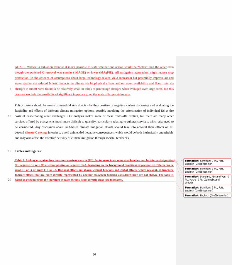
36

ADAFF. Without a valuation exercise it is not possible to state whether one option would be “better” than the other even

though the achieved C removal was similar (IMAGE) or lower (MAgPIE). All mitigation approaches might reduce crop

production (in the absence of assumptions about large technology-related yield increases) but potentially improve air and

water quality via reduced N loss. Impacts on climate via biophysical effects and on water availability and flood risks via

changes in runoff were found to be relatively small in terms of percentage changes when averaged over large areas, but this 5

does not exclude the possibility of significant impacts e.g. on the scale of large catchments.

Policy makers should be aware of manifold side effects - be they positive or negative - when discussing and evaluating the

feasibility and effects of different climate mitigation options, possibly involving the prioritization of individual ES at th e

costs of exacerbating other challenges. Our analysis makes some of these trade-offs explicit, but there are many other 10

services offered by ecosystems much more difficult to quantify, particularly relating to cultural services, which also need to

be considered. Any discussion about land-based climate mitigation efforts should take into account their effects on ES

beyond climate C storage in order to avoid unintended negative consequences, which would be both intrinsically undesirable

and may also affect the effective delivery of climate mitigation through societal feedbacks.

Tables and Figures 15

Table 1: Linking ecosystem functions to ecosystem services (ES). An increase in an ecosystem function can be interpreted positive

(+), negative (-), zero (0) or either positive or negative (+/-), depending on the background conditions or perspective. Effects can be

small (+ or -) or large (++ or --). Regional effects are shown without brackets and global effects, where relevant, in brackets.

Indirect effects that are more directly represented by another ecosystem function considered here are not shown. The table is

based on evidence from the literature in cases the link is not directly clear (see footnotes). 20

Formatiert: Schriftart: 9 Pt., Fett,Englisch (Großbritannien)

Formatiert: Standard, Abstand Vor: 0Pt., Nach: 0 Pt., Zeilenabstand: einfach

Formatiert: Schriftart: 9 Pt., Fett,Englisch (Großbritannien)

Formatiert: Schriftart: 9 Pt., Fett,Englisch (Großbritannien)

Formatiert: Englisch (Großbritannien)

37

Ecosystem function ES –

climate

change

mitigation

ES – water

availability

ES – flood

protection

ES – water

quality

ES – air

quality

ES – food

production

C storage ↑ ++ (++)

Surface albedo ↑ ++ (+)a

Evapotranspiration ↑ ++ (+/-)b

Annual runoff ↑ ++ - 0/+c

Peak monthly runoff ↑ 0/+d -- 0/-

e 0/-

f

Crop production ↑ ++ (++)

N loss ↑ +/- (+/-)g --

g7 - (-)

g

BVOC emissions ↑ +/- (+/-)h 0/-- (0/-)

i

a The global effects of LU-driven albedo changes seem to be small (e.g. de Noblet-Ducoudre et al., 2012).

b Local surface cooling as heat is needed to evaporate water. On larger scales, the effect could be either a warming due to

increases in atmospheric water vapor (Boucher et al., 2004) or a cooling due to increased planetary albedo resulting from

more cloudiness (Bala et al., 2007; Ban-Weiss et al., 2011). 5

c High flows imply more volume for dilution, prevent algae growth and maintain oxygen levels (Whitehead et al., 2009).

d Effect of peak monthly runoff on water availability is dependent on seasonal rainfall distribution and regional water storage

capacity. Annual runoff is the clearer indicator.

e Soil erosion and associated re-mobilization of metals is enhanced during flood events (Whitehead et al., 2009).

f Due to flood damage in croplands (Posthumus et al., 2009). 10

g LPJ-GUESS at present calculates total N loss and does not differentiate between leaching and gaseous loss. As thus we

indicate several effects that would arise from N emitted as N2O (a greenhouse gas), emitted as NOX or NH3 (affecting air

quality and aerosol formation), or as dissolved N. The net effect of N loss on climate has been estimated to be a small

cooling (Erisman et al., 2011) but uncertainties are large.

h The net impact of BVOC emissions is very uncertain. On the global scale, increased BVOC emissions might result in a 15

warming (Unger, 2014).

i BVOCs often increase ozone and aerosol formation, primarily locally (Rosenkranz et al., 2015), with principally opposite

warming and cooling effects (Unger, 2014).

Table 12: Global net-total values ± standard deviations (over 10 years) of all analysed ecosystem functions as simulated by LPJ-20

GUESS for all scenarios and different time-periods and for LPJGIMAGEIMAGE LU patterns (blue) and LPJGMAgPIEMAgPIE LU

Formatiert: Standard, Abstand Vor: 0Pt., Nach: 0 Pt., Zeilenabstand: einfach

Feldfunktion geändert

Feldfunktion geändert

Feldfunktion geändert

Feldfunktion geändert

Feldfunktion geändert

Feldfunktion geändert

Formatiert: Englisch (USA)

Formatiert: Standard, Abstand Vor: 0Pt., Nach: 0 Pt., Zeilenabstand: einfach

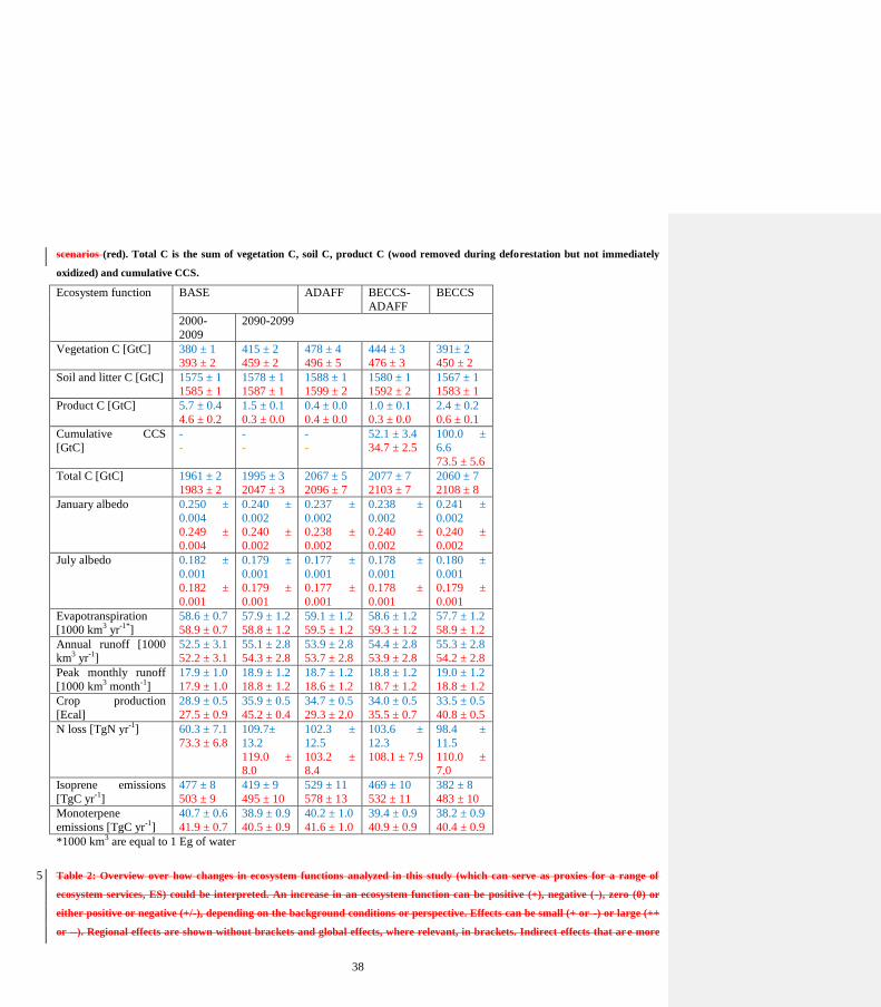
38

scenarios (red). Total C is the sum of vegetation C, soil C, product C (wood removed during deforestation but not immediately

oxidized) and cumulative CCS.

Ecosystem function BASE

ADAFF BECCS-

ADAFF

BECCS

2000-

2009

2090-2099

Vegetation C [GtC] 380 ± 1

393 ± 2

415 ± 2

459 ± 2

478 ± 4

496 ± 5

444 ± 3

476 ± 3

391± 2

450 ± 2

Soil and litter C [GtC] 1575 ± 1

1585 ± 1

1578 ± 1

1587 ± 1

1588 ± 1

1599 ± 2

1580 ± 1

1592 ± 2

1567 ± 1

1583 ± 1

Product C [GtC] 5.7 ± 0.4

4.6 ± 0.2

1.5 ± 0.1

0.3 ± 0.0

0.4 ± 0.0

0.4 ± 0.0

1.0 ± 0.1

0.3 ± 0.0

2.4 ± 0.2

0.6 ± 0.1

Cumulative CCS

[GtC]

-

-

-

-

-

-

52.1 ± 3.4

34.7 ± 2.5

100.0 ±

6.6

73.5 ± 5.6

Total C [GtC] 1961 ± 2

1983 ± 2

1995 ± 3

2047 ± 3

2067 ± 5

2096 ± 7

2077 ± 7

2103 ± 7

2060 ± 7

2108 ± 8

January albedo 0.250 ±

0.004

0.249 ±

0.004

0.240 ±

0.002

0.240 ±

0.002

0.237 ±

0.002

0.238 ±

0.002

0.238 ±

0.002

0.240 ±

0.002

0.241 ±

0.002

0.240 ±

0.002

July albedo 0.182 ±

0.001

0.182 ±

0.001

0.179 ±

0.001

0.179 ±

0.001

0.177 ±

0.001

0.177 ±

0.001

0.178 ±

0.001

0.178 ±

0.001

0.180 ±

0.001

0.179 ±

0.001

Evapotranspiration

[1000 km3 yr

-1*]

58.6 ± 0.7

58.9 ± 0.7

57.9 ± 1.2

58.8 ± 1.2

59.1 ± 1.2

59.5 ± 1.2

58.6 ± 1.2

59.3 ± 1.2

57.7 ± 1.2

58.9 ± 1.2

Annual runoff [1000

km3 yr

-1]

52.5 ± 3.1

52.2 ± 3.1

55.1 ± 2.8

54.3 ± 2.8

53.9 ± 2.8

53.7 ± 2.8

54.4 ± 2.8

53.9 ± 2.8

55.3 ± 2.8

54.2 ± 2.8

Peak monthly runoff

[1000 km3 month

-1]

17.9 ± 1.0

17.9 ± 1.0

18.9 ± 1.2

18.8 ± 1.2

18.7 ± 1.2

18.6 ± 1.2

18.8 ± 1.2

18.7 ± 1.2

19.0 ± 1.2

18.8 ± 1.2

Crop production

[Ecal]

28.9 ± 0.5

27.5 ± 0.9

35.9 ± 0.5

45.2 ± 0.4

34.7 ± 0.5

29.3 ± 2.0

34.0 ± 0.5

35.5 ± 0.7

33.5 ± 0.5

40.8 ± 0.5

N loss [TgN yr-1

] 60.3 ± 7.1

73.3 ± 6.8

109.7±

13.2

119.0 ±

8.0

102.3 ±

12.5

103.2 ±

8.4

103.6 ±

12.3

108.1 ± 7.9

98.4 ±

11.5

110.0 ±

7.0

Isoprene emissions

[TgC yr-1

]

477 ± 8

503 ± 9

419 ± 9

495 ± 10

529 ± 11

578 ± 13

469 ± 10

532 ± 11

382 ± 8

483 ± 10

Monoterpene

emissions [TgC yr-1

]

40.7 ± 0.6

41.9 ± 0.7

38.9 ± 0.9

40.5 ± 0.9

40.2 ± 1.0

41.6 ± 1.0

39.4 ± 0.9

40.9 ± 0.9

38.2 ± 0.9

40.4 ± 0.9

*1000 km3 are equal to 1 Eg of water

Table 2: Overview over how changes in ecosystem functions analyzed in this study (which can serve as proxies for a range of 5

ecosystem services, ES) could be interpreted. An increase in an ecosystem function can be positive (+), negative (-), zero (0) or

either positive or negative (+/-), depending on the background conditions or perspective. Effects can be small (+ or -) or large (++

or --). Regional effects are shown without brackets and global effects, where relevant, in brackets. Indirect effects that ar e more

39

directly represented by another ecosystem function considered here are not shown. The table is based on evidence from the

literature in cases the link is not directly clear (see footnotes).

Ecosystem function ES –

climate

change

mitigation

ES – water

availability

ES – flood

protection

ES – water

quality

ES – air

quality

ES – food

production

C storage ↑ ++ (++)

Surface albedo ↑ ++ (+)a

Evapotranspiration ↑ ++ (+/-)b

Annual runoff ↑ ++ - 0/+c

Peak monthly runoff ↑ 0/+d -- 0/-

e 0/-

f

Crop production ↑ ++ (++)

N loss ↑ +/- (+/-)g --

7 - (-)

g

BVOC emissions ↑ +/- (+/-)h 0/-- (0/-)

i

a The global effects of LU-driven albedo changes seem to be small (e.g. de Noblet-Ducoudre et al., 2012).

b Local surface cooling as heat is needed to evaporate water. On larger scales, the effect could be either a warming due to 5

increases in atmospheric water vapor (Boucher et al., 2004) or a cooling due to increased planetary albedo resulting from

more cloudiness (Bala et al., 2007; Ban-Weiss et al., 2011).

c High flows imply more volume for dilution, prevent algae growth and maintain oxygen levels (Whitehead et al., 2009).

d Effect of peak monthly runoff on water availability is dependent on seasonal rainfall distribution and regional water storage

capacity. Annual runoff is the clearer indicator. 10

e Soil erosion and associated re-mobilization of metals is enhanced during flood events (Whitehead et al., 2009).

f Due to flood damage in croplands (Posthumus et al., 2009).

g LPJ-GUESS at present calculates total N loss and does not differentiate between leaching and gaseous loss. As thus we

indicate several effects that would arise from N emitted as N2O (a greenhouse gas), emitted as NOX or NH3 (affecting air

quality and aerosol formation), or as dissolved N. The net effect of N loss on climate has been estimated to be a small 15

cooling (Erisman et al., 2011) but uncertainties are large.

h The net impact of BVOC emissions is very uncertain. On the global scale, increased BVOC emissions might result in a

warming (Unger, 2014).

i BVOCs often increase ozone and aerosol formation, primarily locally (Rosenkranz et al., 2015), with principally opposite

warming and cooling effects (Unger, 2014). 20

Feldfunktion geändert

Feldfunktion geändert

Feldfunktion geändert

Feldfunktion geändert

Feldfunktion geändert

Feldfunktion geändert

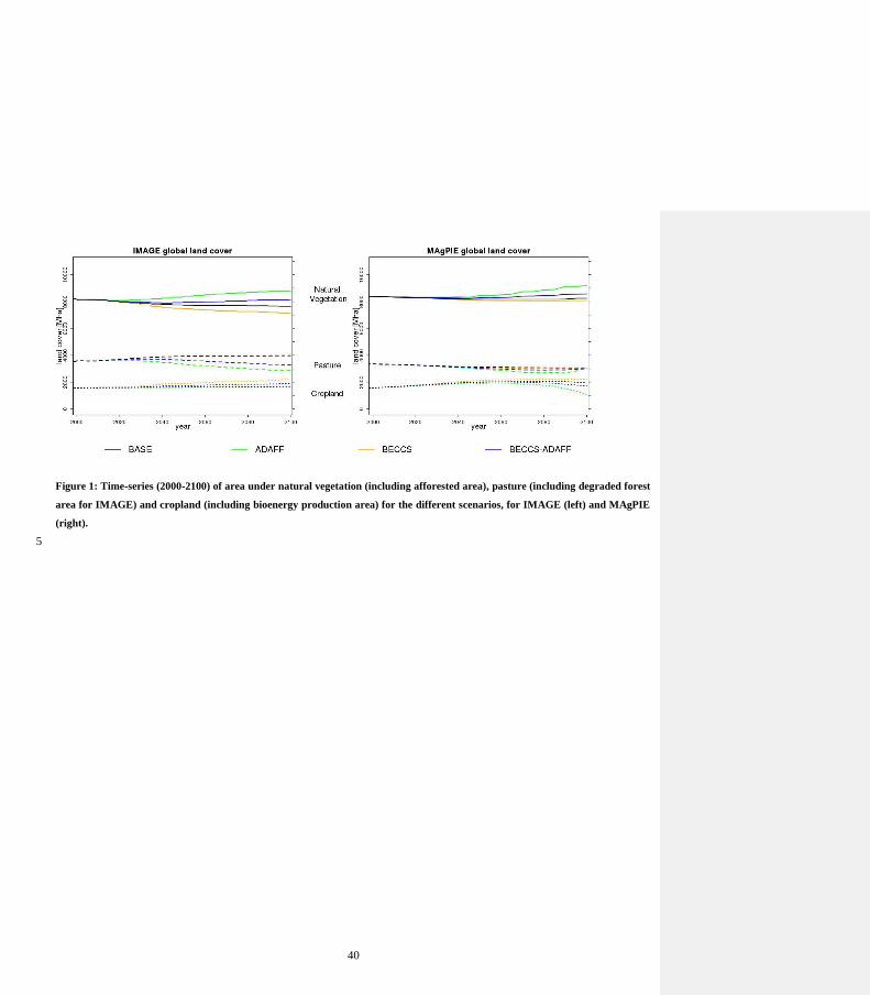
40

Figure 1: Time-series (2000-2100) of area under natural vegetation (including afforested area), pasture (including degraded forest

area for IMAGE) and cropland (including bioenergy production area) for the different scenarios, for IMAGE (left) and MAgPIE

(right).

5

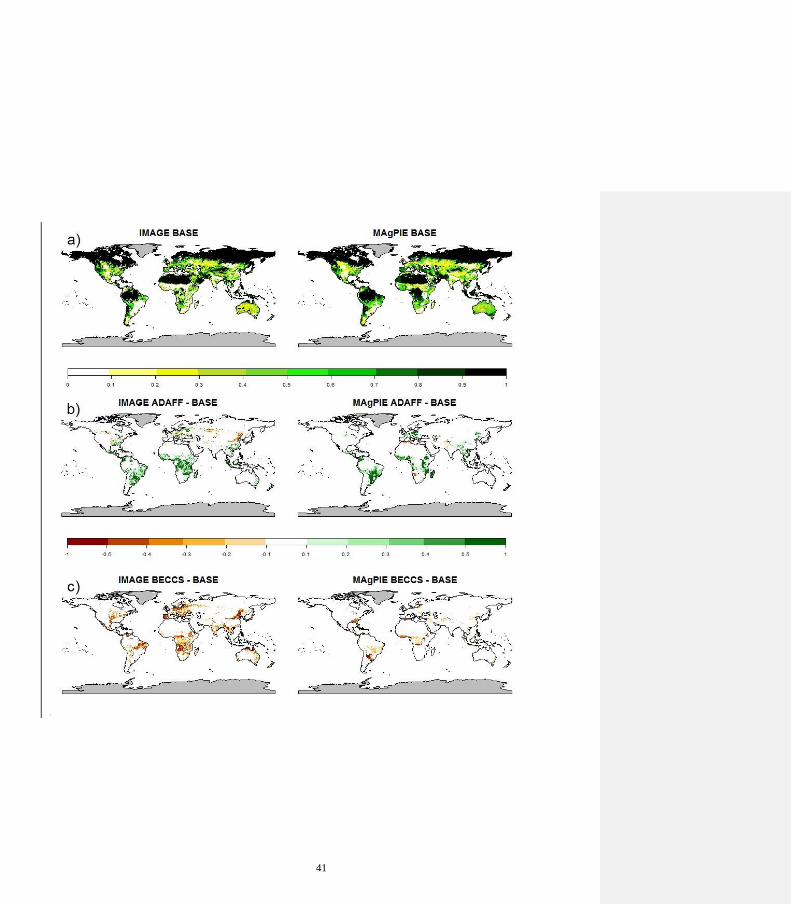
41

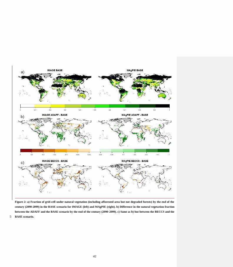
42

Figure 2: a) Fraction of grid-cell under natural vegetation (including afforested area but not degraded forests) by the end of the

century (2090-2099) in the BASE scenario for IMAGE (left) and MAgPIE (right). b) Difference in the natural vegeta tion fraction

between the ADAFF and the BASE scenario by the end of the century (2090-2099). c) Same as b) but between the BECCS and the

BASE scenario. 5

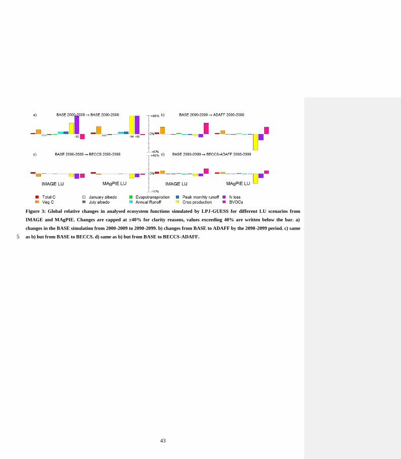
43

Figure 3: Global relative changes in analysed ecosystem functions simulated by LPJ-GUESS for different LU scenarios from

IMAGE and MAgPIE. Changes are capped at ±40% for clarity reasons, values exceeding 40% are written below the bar. a)

changes in the BASE simulation from 2000-2009 to 2090-2099. b) changes from BASE to ADAFF by the 2090-2099 period. c) same

as b) but from BASE to BECCS. d) same as b) but from BASE to BECCS-ADAFF. 5

44

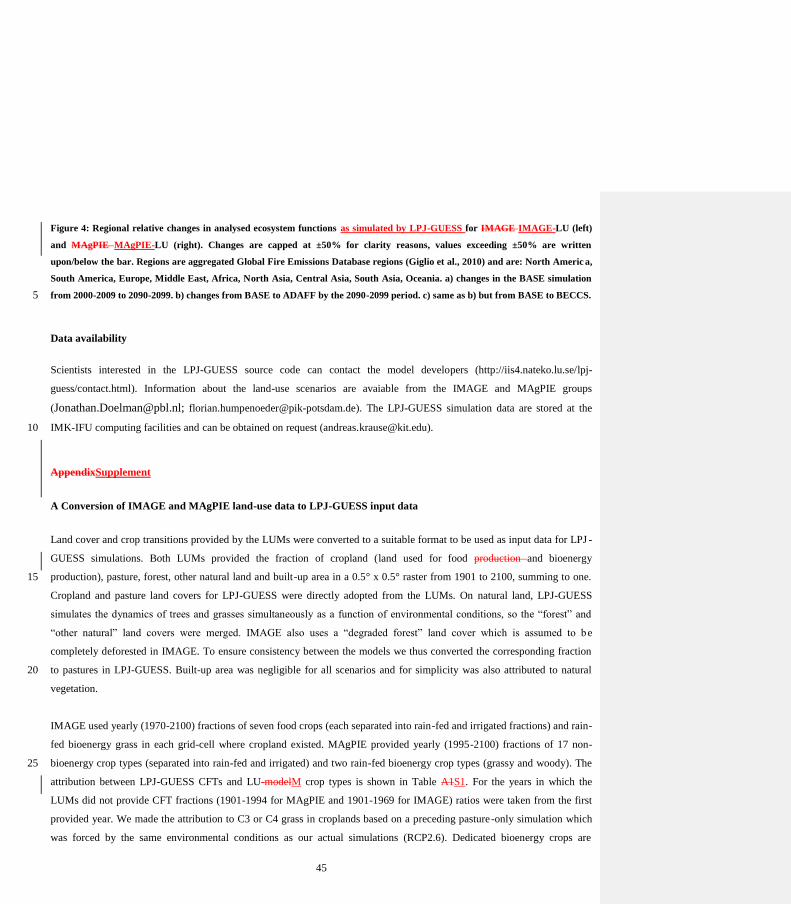
45

Figure 4: Regional relative changes in analysed ecosystem functions as simulated by LPJ-GUESS for IMAGE IMAGE-LU (left)

and MAgPIE MAgPIE-LU (right). Changes are capped at ±50% for clarity reasons, values exceeding ±50% are written

upon/below the bar. Regions are aggregated Global Fire Emissions Database regions (Giglio et al., 2010) and are: North Americ a,

South America, Europe, Middle East, Africa, North Asia, Central Asia, South Asia, Oceania. a) changes in the BASE simulation

from 2000-2009 to 2090-2099. b) changes from BASE to ADAFF by the 2090-2099 period. c) same as b) but from BASE to BECCS. 5

Data availability

Scientists interested in the LPJ-GUESS source code can contact the model developers (http://iis4.nateko.lu.se/lpj-

guess/contact.html). Information about the land-use scenarios are avaiable from the IMAGE and MAgPIE groups

(Jonathan.Doelman@pbl.nl; florian.humpenoeder@pik-potsdam.de). The LPJ-GUESS simulation data are stored at the

IMK-IFU computing facilities and can be obtained on request (andreas.krause@kit.edu). 10

AppendixSupplement

A Conversion of IMAGE and MAgPIE land-use data to LPJ-GUESS input data

Land cover and crop transitions provided by the LUMs were converted to a suitable format to be used as input data for LPJ -

GUESS simulations. Both LUMs provided the fraction of cropland (land used for food production and bioenergy

production), pasture, forest, other natural land and built-up area in a 0.5° x 0.5° raster from 1901 to 2100, summing to one. 15

Cropland and pasture land covers for LPJ-GUESS were directly adopted from the LUMs. On natural land, LPJ-GUESS

simulates the dynamics of trees and grasses simultaneously as a function of environmental conditions, so the “forest” and

“other natural” land covers were merged. IMAGE also uses a “degraded forest” land cover which is assumed to be

completely deforested in IMAGE. To ensure consistency between the models we thus converted the corresponding fraction

to pastures in LPJ-GUESS. Built-up area was negligible for all scenarios and for simplicity was also attributed to natural 20

vegetation.

IMAGE used yearly (1970-2100) fractions of seven food crops (each separated into rain-fed and irrigated fractions) and rain-

fed bioenergy grass in each grid-cell where cropland existed. MAgPIE provided yearly (1995-2100) fractions of 17 non-

bioenergy crop types (separated into rain-fed and irrigated) and two rain-fed bioenergy crop types (grassy and woody). The 25

attribution between LPJ-GUESS CFTs and LU-modelM crop types is shown in Table A1S1. For the years in which the

LUMs did not provide CFT fractions (1901-1994 for MAgPIE and 1901-1969 for IMAGE) ratios were taken from the first

provided year. We made the attribution to C3 or C4 grass in croplands based on a preceding pasture-only simulation which

was forced by the same environmental conditions as our actual simulations (RCP2.6). Dedicated bioenergy crops are

46

currently not implemented in LPJ-GUESS and were represented by corn. Removed residues of bioenergy crops (90%) were

included in the CCS calculation (see appendix Supplement B), while removed residues of food crops (75%) were emitted to

the atmosphere. Residues left on-site (10% and 25%, respectively) went to the litter.

Average annual N fertilizer rates per cropland area (synthetic and organic fertilizer, derived from yields) were provided by 5

IMAGE (1970-2100) and MAgPIE (1995-2100) and had to be extended to year 1901. Historic N fertilizer rates (synthetic

fertilizer on C3+C4 annual and perennial crops) were available from the recently released LUH2 data set (Hurtt et al, in

preparation, http://luh.umd.edu/index.shtml). However, as LUH2 only considers synthetic fertilizer, the correlation between

LUH2 and the LUMs in the first provided year was poor in terms of spatial patterns and total amount of applied N, making a

simple merging inapplicable. We thus decided to use IMAGE and MAgPIE N fertilizer rates and spatial patterns for the 10

available time periods and computed a historic hindcast, starting with the initial spatial patterns and rates in IMAGE and

MAgPIE multiplied by the relative year-to-year per-country change in the LUH2 data set in the period prior to 1970 and

1995, respectively. This resulted in a smooth historical to future N fertilizer dataset reflecting the LUMs spatial patterns in

terms of absolute values with historic variations based on LUH2 relative changes and late historic to future variations

adopted unmodified from the LUMs. Fertilizer rates differed significantly between IMAGE and MAgPIE, with MAgPIE 15

exceeding IMAGE fertilizer rates in most locations. As no fertilization occurred before 1916 in LUH2 (before the Haber-

Bosch process was found), we applied a minimum fertilizer rate of 6 kg N ha-1

yr-1

(in addition to atmospheric deposition) to

all areas under crops throughout the entire simulation period to limit continued soil N depletion. As the LUMs only provided

per-cropland fertilizer rates, we applied the same amount of fertilizer for all CFTs in a grid-cell, and distributed the annual

amount over the year as a function of crop phenological state (Olin et al., 2015b). 20

B Carbon storage via CCS

Bioenergy yields included removed harvestable organs and crop residues (90% of total above-ground biomass). We

estimated the total amount of C sequestered via CCS in the bioenergy simulations by assuming an 80% capture rate upon

oxidization, which is the same value as in the LUMs (Klein et al., 2014). The total C was then the sum of terrestrial C

(vegetation, soil and litter, C stored in wood products) and C stored via CCS. 25

C Albedo calculation

We calculated January and July surface albedo mainly based on mean winter (snow-free and snow-covered) and summer

albedo values for different land cover types derived from MODIS satellite observations by Boisier et al. (2013). For the

Southern Hemisphere we switched snow-free winter and summer albedo values. The LPJ-GUESS PFTs fractional plant

cover determines the fraction of the grid-cell occupied by the land cover groups (crops, grasses, evergreen trees, deciduous 30

trees, bare soil). For tropical evergreen trees we assumed an albedo of 0.140 year-round based on Boisier et al. (2013). For

47

woody bioenergy we assumed the same albedo as deciduous forests. The albedo of the non-vegetated fraction of the grid-cell

under snow-free conditions was taken from Houldcroft et al. (2009) (average of white and black sky albedo), assuming a

value of 0.15 at locations where no measurements were available. We estimated the grid-cell’s monthly fraction under snow

cover fsnow as

𝑓snow =𝑧sn

0.01 + 𝑧sn

where zsn is the average monthly snow depth (m) (Wang and Zeng, 2010, equation 17) which can be output from LPJ-5

GUESS. The albedo of the snow-covered fraction was calculated based on the values from Boisier et al. (2013) for snow-

covered vegetation and bare soil and the grid-cell albedo was then the area-weighted average of snow-covered and snow-free

albedos.

D Crop yield scaling

To account for spatial variations in crop management other than irrigation and fertilization, which are not accounted for in 10

LPJ-GUESS, we scaled our food crop yields to the actual yields from the EarthStat data set (Monfreda et al., 2008), thereby

only taking the absolute year-to-year changes from LPJ-GUESS. For this, we re-scaled yields of our four food CFTs

(temperate wheat, temperate other summer crops, rice, corn) around the year 2000 (1997-2003) to match actual yields based

on area-weighted yields of major food crops in the EarthStat data set (aggregated to 0.5° x 0.5° resolution; see Table A1 S1

for which crop types were aggregated to which CFT). We then used these actual yields over the full crop yield time series, 15

with year-to-year variations calculated based on the yield changes in LPJ-GUESS (area-weighted between rain-fed and

irrigated yields). If crops were present in the LUMs but no adequate crop types were available in the EarthStat data set for a

grid-cell we took the yields unmodified from LPJ-GUESS. We first converted dry matter yields per m2 as given by LPJ-

GUESS/EarthStat to fresh matter yields and finally to kcal. Fodder and cotton were not used for the crop production

calculation. Total crop production was then the sum of temperate wheat, temperate other summer crops, rice and non-20

bioenergy corn production. Yields of bioenergy crops (grown as corn) were used unmodified to estimate CCS (see appendix

Supplement B) due to limited observational data of bioenergy crop yields.

E BVOC emission factors of bioenergy crops

Crop BVOC emission scaling factors were taken from natural C3 or C4 grass, apart from woody bioenergy crops, which we

grew as corn but used isoprene emission scaling factors of 45 μg(C) g−1

(leaf foliar mass) h−1

(Ashworth et al., 2012). These 25

values are much higher than the values for normal grasses (8 μg g−1

h−1

for C4 grasses and 16 μg g−1

h−1

for C3 grasses) and

account for the fact that isoprene emissions from typical woody bioenergy species like oil palm or willow are very high.

48

Table A1S1: Crop functional types (CFTs) used in this study, how the LU models’ crop types were aggregated to these CFTs, and

EarthStat major crops used to calculate circa year 2000 actual yields of these CFTs.

LPJ-GUESS CFT

(photosynthetic

pathway)

IMAGE and MAgPIE crop types aggregated to

this CFT

EarthStat major crop types used to

calculate circa year 2000 actual

yields of LPJ-GUESS crops

temperate wheat

(C3), representing

C3 crops with winter

or spring sowing

depending on

historical climate

temperate cereals, rapeseed rye, barley, wheat, rapeseed

temperate other

summer crops (C3)

representing C3

crops with spring

sowing only

potatoes, cassava, pulses, soybean, groundnuts,

sunflower, palm oil, sugar beet, cotton, roots and

tubers, oil crops, others

potato, cassava, groundnut,

soybean, sunflower, oilpalm

rice (C3) (paddy) rice rice

corn (C4) maize, tropical cereals, sugarcane, bioenergy

crops

maize, millet, sorghum, sugarcane;

bioenergy yields were not modified

due to limited observational data

crop grass (C3 or C4) fodder unmodified as not used for crop

production calculation

Table A2S2: Global area [Mha] under natural vegetation, pasture (parenthesesbrackets: degraded forests) and cropland

(brackets: bioenergy) for the different scenarios for the 2000-2009 and 2090-2099 periods. 5

Scenario (year) IMAGE MAgPIE

Natural Pasture Cropland Natural Pasture Cropland

BASE(2000-2009) 8155 3584(313) 1569 8367 3332 1609

BASE(2090-2099) 7664 3974(551) 1671 8225 3073 2010

ADAFF (2090-2099) 8783 2879(14) 1645 9139 2832 1338

BECCS (2090-2099) 7162 3981(551) 2165(493) 8074 3015 2219(363)

BECCS-ADAFF (2090-2099) 8119 3307(14) 1882(254) 8561 2964 1783(158)

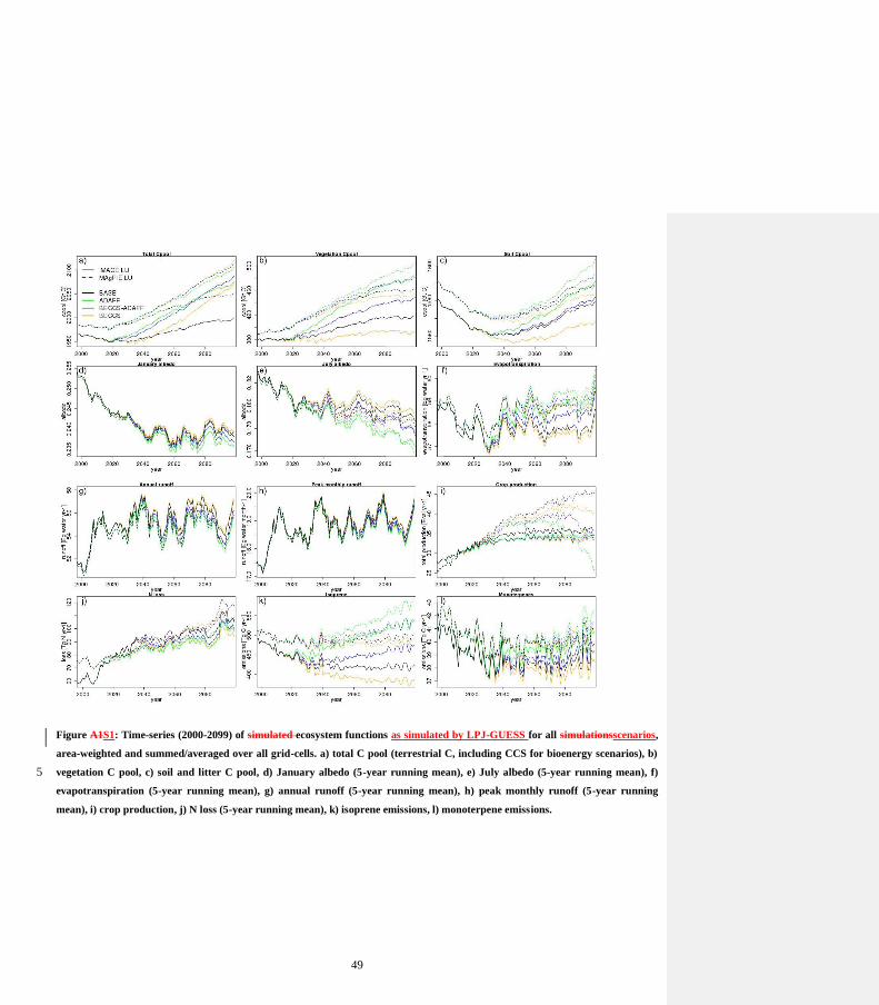
49

Figure A1S1: Time-series (2000-2099) of simulated ecosystem functions as simulated by LPJ-GUESS for all simulationsscenarios,

area-weighted and summed/averaged over all grid-cells. a) total C pool (terrestrial C, including CCS for bioenergy scenarios), b)

vegetation C pool, c) soil and litter C pool, d) January albedo (5-year running mean), e) July albedo (5-year running mean), f) 5

evapotranspiration (5-year running mean), g) annual runoff (5-year running mean), h) peak monthly runoff (5-year running

mean), i) crop production, j) N loss (5-year running mean), k) isoprene emissions, l) monoterpene emissions.

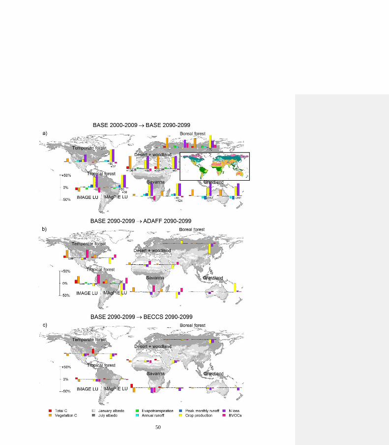
50

51

Figure A2S2: Same as Fig. 4 but changes shown for different biomes rather than Global Fire Emissions DatabaseGFED regions.

Biomes are aggregated from the biomes used in Smith et al. (2014): tundra+desert+woodland+shrubland; dry+moist savanna; dry

and tall grassland; tropical forest; temperate forest; boreal+temperate/boreal mixed forest. The LAI map used for the biome

classification was taken from the LPJGMAgPIEMAgPIE BASE simulation and the 2000-2009 period. The coloured snapshot in a)

shows the same biomes as the grey-coloured biomes in the larger maps to facilitate differantiation. 5

Figure A3S3: Regional relative changes in analyzed analysed ecosystem functions as simulated by LPJ-GUESS for IMAGE

IMAGE-LU (left) and MAgPIE MAgPIE-LU (right) from BASE to BECCS-ADAFF by the 2090-2099 period. Changes are capped

at ±50% for clarity reasons, values exceeding ±50% are written upon/below the bar. The decrease in crop production might occur

if increases in crop yields cannot be realized. Regions are aggregated Global Fire Emissions Database regions (Giglio et al., 2010). 10

52

Figure A4S4: Impacts of fixing N fertilizers, crop area, dynamic PHU calculation (i.e. adaption to climate change via selecting

suitable varieties) and atmospheric CO2 concentration at year 2009 levels on LPJ-GUESS crop production (a) and N loss (b), for 5

the BASE simulations.

53

Figure S5: Mean surface albedo in January (top) and July (bottom) in LPJGIMAGE BASE (2000-2011). The scale is the same as in

Boisier et al. (2013).

5

Figure S6: Total annual runoff in LPJGIMAGE BASE (1961-1990). The scale is the same as in Gerten et al. (2004).

54

Competing interests

The authors declare that they have no conflict of interest.

Acknowledgements

This work was funded by the Helmholtz Association through the International Research Group CLUCIE and by the 5

European Commission's 7th Framework Programme, under Grant Agreement number 603542 (LUC4C). AK, AB and AA

acknowledge also support by the European Commission's 7th Framework Programme, under Grant Agreement number

308393 (OPERAs). This work was supported, in part, by the German Federal Ministry of Education and Research (BMBF),

through the Helmholtz Association and its research program ATMO. It also represents paper number 22 of the Birmingham

Institute of Forest Research. 10

References

Ahlstrom, A., Schurgers, G., Arneth, A., and Smith, B.: Robustness and uncertainty in terrestrial ecosystem carbon response to CMIP5

climate change projections, Environ Res Lett, 7, doi:10.1088/1748-9326/7/4/044008, 2012.

Alexander, P., Prestele, R., Verburg, P. H., Arneth, A., Baranzelli, C., Silva, F. B. E., Brown, C., Butler, A., Calvin, K., Dendoncker, N.,

Doelman, J. C., Dunford, R., Engstrom, K., Eitelberg, D., Fujimori, S., Harrison, P. A., Hasegawa, T., Havlik, P., Holzhauer, S., 15 Humpenoder, F., Jacobs-Crisioni, C., Jain, A. K., Krisztin, T., Kyle, P., Lavalle, C., Lenton, T., Liu, J. Y., Meiyappan, P., Popp, A.,

Powell, T., Sands, R. D., Schaldach, R., Stehfest, E., Steinbuks, J., Tabeau, A., van Meijl, H., Wise, M. A., and Rounsevell, M. D. A .:

Assessing uncertainties in land cover projections, Global Change Biol, 23, 767-781, doi:10.1111/gcb.13447, 2017.

Alkama, R., and Cescatti, A.: Biophysical climate impacts of recent changes in global forest cover, Science, 351, 600-604,

doi:10.1126/science.aac8083, 2016. 20 Alkemade, R., van Oorschot, M., Miles, L., Nellemann, C., Bakkenes, M., and ten Brink, B.: GLOBIO3: A framework to investigate

options for reducing global terrestrial biodiversity loss, Ecosystems, 12, 374–390, doi:10.1007/s10021-009-9229-5, 2009.

Anderson, K., and Peters, G.: The trouble with negative emissions, Science, 354, 182-183, doi:10.1126/science.aah4567, 2016.

Arneth, A., Niinemets, U., Pressley, S., Back, J., Hari, P., Karl, T., Noe, S., Prentice, I. C., Serca, D., Hickler, T., Wolf , A., and Smith, B.:

Process-based estimates of terrestrial ecosystem isoprene emissions: incorporating the effects of a direct CO2-isoprene interaction, Atmos 25 Chem Phys, 7, 31-53, doi:10.5194/acp-7-31-2007, 2007.

Arneth, A., Harrison, S. P., Zaehle, S., Tsigaridis, K., Menon, S., Bartlein, P. J., Feichter, J., Korhola, A., Kulmala, M., O'Donnell, D.,

Schurgers, G., Sorvari, S., and Vesala, T.: Terrestrial biogeochemical feedbacks in the climate system, Nat Geosci, 3, 525-532,

doi:10.1038/ngeo905, 2010.

Ashworth, K., Folberth, G., Hewitt, C. N., and Wild, O.: Impacts of near-future cultivation of biofuel feedstocks on atmospheric 30 composition and local air quality, Atmos Chem Phys, 12, 919-939, doi:10.5194/acp-12-919-2012, 2012.

Bala, G., Caldeira, K., Wickett, M., Phillips, T. J., Lobell, D. B., Delire, C., and Mirin, A.: Combined climate and carbon -cycle effects of

large-scale deforestation, P Natl Acad Sci USA, 104, 6550-6555, doi:10.1073/pnas.0608998104, 2007.

Ban-Weiss, G. A., Bala, G., Cao, L., Pongratz, J., and Caldeira, K.: Climate forcing and response to idealized changes in surface latent and

sensible heat, Environ Res Lett, 6, doi:10.1088/1748-9326/6/3/034032, 2011. 35 Bathiany, S., Claussen, M., Brovkin, V., Raddatz, T., and Gayler, V.: Combined biogeophysical and biogeochemical effects of l arge-scale

forest cover changes in the MPI earth system model, Biogeosciences, 7, 1383-1399, doi:10.5194/bg-7-1383-2010, 2010.

Bayer, A. D., Lindeskog, M., Pugh, T. A. M., Anthoni, P. M., Fuchs, R., and Arneth, A.: Uncertainties in the land -use flux resulting from

land-use change reconstructions and gross land transitions, Earth Syst Dynam, 8, 91-111, doi:10.5194/esd-8-91-2017, 2017.

55

Behera, S. N., Sharma, M., Aneja, V. P., and Balasubramanian, R.: Ammonia in the atmosphere: a review on emission sources,

atmospheric chemistry and deposition on terrestrial bodies, Environ Sci Pollut R, 20, 8092-8131, doi:10.1007/s11356-013-2051-9, 2013.

Behrman, K. D., Juenger, T. E., Kiniry, J. R., and Keitt, T. H.: Spatial land use trade-offs for maintenance of biodiversity, biofuel, and

agriculture, Landscape Ecol, 30, 1987-1999, doi:10.1007/s10980-015-0225-1, 2015.

Bennett, E. M., Peterson, G. D., and Gordon, L. J.: Understanding relationships among multiple ecosystem services, Ecol Lett, 12, 1394-5 1404, doi:10.1111/j.1461-0248.2009.01387.x, 2009.

Betts, R. A.: Offset of the potential carbon sink from boreal forestation by decreases in surface albedo, Nature, 408, 187-190,

doi:10.1038/35041545, 2000.

Blanke, J. H., Olin, S., Stürck, J., Sahlin, U., Lindeskog, M., Helming, J., and Lehsten, V.: Assessing the impact of changes in land-use

intensity and climate on simulated trade-offs between crop yield and nitrogen leaching, Agriculture, Ecosystems and Environment, 239, 10 385-398, doi:10.1016/j.agee.2017.01.038, 2017.

Boisier, J. P., de Noblet-Ducoudre, N., and Ciais, P.: Inferring past land use-induced changes in surface albedo from satellite observations:

a useful tool to evaluate model simulations, Biogeosciences, 10, 1501-1516, doi:10.5194/bg-10-1501-2013, 2013.

Bondeau, A., Smith, P. C., Zaehle, S., Schaphoff, S., Lucht, W., Cramer, W., Gerten, D., Lotze -Campen, H., Muller, C., Reichstein, M.,

and Smith, B.: Modelling the role of agriculture for the 20th century global terrestrial carbon balance, Global Change Biol, 13, 679-706, 15 doi:10.1111/j.1365-2486.2006.01305.x, 2007.

Boucher, O., Myhre, G., and Myhre, A.: Direct human influence of irrigation on atmospheric water vapour and climate, Clim Dynam, 22,

597-603, doi:10.1007/s00382-004-0402-4, 2004.

Boysen, L. R., Lucht, W., and Gerten, D.: Trade-offs for food production, nature conservation and climate limit the terrestrial carbon

dioxide removal potential, Global Change Biol, doi:10.1111/gcb.13745, 2017. 20 Bradshaw, C. J. A., Sodhi, N. S., Peh, K. S. H., and Brook, B. W.: Global evidence that deforestation amplifies flood risk and severity in

the developing world, Global Change Biol, 13, 2379-2395, doi:10.1111/j.1365-2486.2007.01446.x, 2007.

Camargo, J. A., and Alonso, A.: Ecological and toxicological effects of inorganic nitrogen pollution in aquatic ecosystems: A global

assessment, Environ Int, 32, 831-849, doi:10.1016/j.envint.2006.05.002, 2006.

Carslaw, K. S., Boucher, O., Spracklen, D. V., Mann, G. W., Rae, J. G. L., Woodward, S., and Kulmala, M.: A review of natural aerosol 25 interactions and feedbacks within the Earth system, Atmos Chem Phys, 10, 1701-1737, doi:10.5194/acp-10-1701-2010, 2010.

Cassman, K. G., Dobermann, A., and Walters, D. T.: Agroecosystems, nitrogen-use efficiency, and nitrogen management, Ambio, 31,

132-140, doi:10.1639/0044-7447(2002)031[0132:Anuean]2.0.Co;2, 2002.

Creutzig, F., Ravindranath, N. H., Berndes, G., Bolwig, S., Bright, R., Cherubini, F., Chum, H., Corbera, E., Delucchi, M., Faaij, A.,

Fargione, J., Haberl, H., Heath, G., Lucon, O., Plevin, R., Popp, A., Robledo-Abad, C., Rose, S., Smith, P., Stromman, A., Suh, S., and 30 Masera, O.: Bioenergy and climate change mitigation: an assessment, Gcb Bioenergy, 7, 916-944, doi:10.1111/gcbb.12205, 2015.

Creutzig, F.: Economic and ecological views on climate change mitigation with bioenergy and negative emissions, Gcb Bioenergy, 8, 4-

10, doi:10.1111/gcbb.12235, 2016.

Crutzen, P. J., Mosier, A. R., Smith, K. A., and Winiwarter, W.: N2O release from agro-biofuel production negates global warming

reduction by replacing fossil fuels, Atmos Chem Phys, 8, 389-395, doi:10.5194/acp-8-389-2008, 2008. 35 Cunningham, S. C., Mac Nally, R., Baker, P. J., Cavagnaro, T. R., Beringer, J., Thomson, J. R., and Thompson, R. M.: Balancing the

environmental benefits of reforestation in agricultural regions, Perspect Plant Ecol, 17, 301-317, doi:10.1016/j.ppees.2015.06.001, 2015.

Davidson, E. A., and Kanter, D.: Inventories and scenarios of nitrous oxide emissions, Environ Res Lett, 9, doi:10.1088/1748 -

9326/9/10/105012, 2014.

Davies-Barnard, T., Valdes, P. J., Singarayer, J. S., Pacifico, F. M., and Jones, C. D.: Full effects of land use change in the representative 40 concentration pathways, Environ Res Lett, 9, doi:10.1088/1748-9326/9/11/114014, 2014.

de Noblet-Ducoudre, N., Boisier, J. P., Pitman, A., Bonan, G. B., Brovkin, V., Cruz, F., Delire, C., Gayler, V., van den Hurk, B. J. J. M.,

Lawrence, P. J., van der Molen, M. K., Muller, C., Reick, C. H., Strengers, B. J., and Voldoire, A.: Determining Robust Impac ts of Land-

Use-Induced Land Cover Changes on Surface Climate over North America and Eurasia: Results from the First Set of LUCID Experiments,

J Climate, 25, 3261-3281, doi:10.1175/Jcli-D-11-00338.1, 2012. 45 DeFries, R. S., Foley, J. A., and Asner, G. P.: Land-use choices: balancing human needs and ecosystem function, Front Ecol Environ, 2,

249-257, doi:10.1890/1540-9295(2004)002[0249:Lcbhna]2.0.Co;2, 2004.

Dellink, R., Chateau, J., Lanzi, E., and Magne, B.: Long-term economic growth projections in the Shared Socioeconomic Pathways,

Global Environ Chang, 42, 200-214, doi:10.1016/j.gloenvcha.2015.06.004, 2017.

Elliott, J., Deryng, D., Mueller, C., Frieler, K., Konzmann, M., Gerten, D., Glotter, M., Florke, M., Wada, Y., Best, N., Eisner, S., Fekete, 50 B. M., Folberth, C., Foster, I., Gosling, S. N., Haddeland, I., Khabarov, N., Ludwig, F., Masaki, Y., Olin, S., Rosenzweig, C., Ruane, A.

C., Satoh, Y., Schmid, E., Stacke, T., Tang, Q. H., and Wisser, D.: Constraints and potentials of future irrigation water availability on

agricultural production under climate change, P Natl Acad Sci USA, 111, 3239-3244, doi:10.1073/pnas.1222474110, 2014.

Ellison, D., Futter, M. N., and Bishop, K.: On the forest cover-water yield debate: from demand- to supply-side thinking, Global Change

Biol, 18, 806-820, doi:10.1111/j.1365-2486.2011.02589.x, 2012. 55

56

Erisman, J. W., Galloway, J., Seitzinger, S., Bleeker, A., and Butterbach-Bahl, K.: Reactive nitrogen in the environment and its effect on

climate change, Curr Opin Env Sust, 3, 281-290, doi:10.1016/j.cosust.2011.08.012, 2011.

Farley, K. A., Jobbagy, E. G., and Jackson, R. B.: Effects of afforestation on water yield: a global synthesis with implications for policy,

Global Change Biol, 11, 1565-1576, doi:10.1111/j.1365-2486.2005.01011.x, 2005.

Ferreira, S., and Ghimire, R.: Forest cover, socioeconomics, and reported flood frequency in developing countries, Water Resour Res, 48, 5 doi:10.1029/2011wr011701, 2012.

Fleischer, K., Warlind, D., van der Molen, M. K., Rebel, K. T., Arneth, A., Erisman, J. W., Wassen, M. J., Smith, B., Gough, C. M.,

Margolis, H. A., Cescatti, A., Montagnani, L., Arain, A., and Dolman, A. J.: Low historical nitrogen deposition effect on carbon

sequestration in the boreal zone, J Geophys Res-Biogeo, 120, 2542-2561, doi:10.1002/2015JG002988, 2015.

Foley, J. A., DeFries, R., Asner, G. P., Barford, C., Bonan, G., Carpenter, S. R., Chapin, F. S., Coe, M. T., Daily, G. C., Gibbs, H. K., 10 Helkowski, J. H., Holloway, T., Howard, E. A., Kucharik, C. J., Monfreda, C., Patz, J. A., Prentice, I. C., Ramankutty, N., a nd Snyder, P.

K.: Global consequences of land use, Science, 309, 570-574, doi:10.1126/science.1111772, 2005.

Friedlingstein, P., Meinshausen, M., Arora, V. K., Jones, C. D., Anav, A., Liddicoat, S. K., and Knutti, R.: Uncertainties in CMIP5

Climate Projections due to Carbon Cycle Feedbacks, J Climate, 27, 511-526, doi:10.1175/Jcli-D-12-00579.1, 2014.

Fuchs, H., Hofzumahaus, A., Rohrer, F., Bohn, B., Brauers, T., Dorn, H. P., Haseler, R., Holland, F., Kaminski, M., Li, X., Lu, K., Nehr, 15 S., Tillmann, R., Wegener, R., and Wahner, A.: Experimental evidence for efficient hydroxyl radical regeneration in isoprene oxidation,

Nat Geosci, 6, 1023-1026, doi:10.1038/NGEO1964, 2013.

Fuss, S., Canadell, J. G., Peters, G. P., Tavoni, M., Andrew, R. M., Ciais, P., Jackson, R. B., Jones, C. D., Kraxner, F., Nakicenovic, N., Le

Quere, C., Raupach, M. R., Sharifi, A., Smith, P., and Yamagata, Y.: COMMENTARY: Betting on negative emissions, Nat Clim Change,

4, 850-853, doi:10.1038/nclimate2392, 2014. 20 Galloway, J. N., Dentener, F. J., Capone, D. G., Boyer, E. W., Howarth, R. W., Seitzinger, S. P., Asner, G. P., Cleveland, C. C., Green, P.

A., Holland, E. A., Karl, D. M., Michaels, A. F., Porter, J. H., Townsend, A. R., and Vorosmarty, C. J.: Nitrogen cycles: pas t, present, and

future, Biogeochemistry, 70, 153-226, doi:10.1007/s10533-004-0370-0, 2004.

Ganzeveld, L., Bouwman, L., Stehfest, E., van Vuuren, D. P., Eickhout, B., and Lelieveld, J.: Impact of future land use and land cover

changes on atmospheric chemistry-climate interactions, J Geophys Res-Atmos, 115, doi:10.1029/2010jd014041, 2010. 25 Gasser, T., Guivarch, C., Tachiiri, K., Jones, C. D., and Ciais, P.: Negative emissions physically needed to keep global warming below 2

degrees C, Nat Commun, 6, doi:10.1038/Ncomms8958, 2015.

Gerten, D., Schaphoff, S., Haberlandt, U., Lucht, W., and Sitch, S.: Terrestrial vegetation and water balance - hydrological evaluation of a

dynamic global vegetation model, J Hydrol, 286, 249-270, doi:10.1016/j.jhydrol.2003.09.029, 2004.

Giglio, L., Randerson, J. T., van der Werf, G. R., Kasibhatla, P. S., Collatz, G. J., Morton, D. C., and DeFries, R. S.: Assessing variability 30 and long-term trends in burned area by merging multiple satellite fire products, Biogeosciences, 7, 1171-1186, doi:10.5194/bg-7-1171-

2010, 2010.

Hallgren, W., Schlosser, C. A., Monier, E., Kicklighter, D., Sokolov, A., and Melillo, J.: Climate impacts of a large-scale biofuels

expansion, Geophys Res Lett, 40, 1624-1630, doi:10.1002/grl.50352, 2013.

Hansen, R. F., Lewis, T. R., Graham, L., Whalley, S. K., Seakins, P. W., Heard, D. E., and Blitz, M. A.: OH production from the 35 photolysis of isoprene-derived peroxy radicals: cross-sections, quantum yields and atmospheric implications, Phys. Chem. Chem. Phys,

19, 2332-2345, doi:10.1039/c6cp06718b, 2017.

Hantson, S., Knorr, W., Schurgers, G., Pugh, T. A. M., and Arneth, A.: Global isoprene and monoterpene emissions under changing

climate, vegetation, CO2 and land use, Atmos Environ, 155, 35-45, doi:10.1016/j.atmosenv.2017.02.010, 2017.

Hempel, S., Frieler, K., Warszawski, L., Schewe, J., and Piontek, F.: A trend-preserving bias correction - the ISI-MIP approach, Earth Syst 40 Dynam, 4, 219-236, doi:10.5194/esd-4-219-2013, 2013.

Hoogwijk, M., Faaija, A., van den Broek, R., Berndes, G., Gielen, D., and Turkenburg, W.: Exploration of the ranges of the global

potential of biomass for energy, Biomass Bioenerg, 25, 119-133, doi:10.1016/S0961-9534(02)00191-5, 2003.

Houldcroft, C. J., Grey, W. M. F., Barnsley, M., Taylor, C. M., Los, S. O., and North, P. R. J.: New Vegetation Albedo Parame ters and

Global Fields of Soil Background Albedo Derived from MODIS for Use in a Climate Model, J Hydrometeorol, 10, 183-198, 45 doi:10.1175/2008JHM1021.1, 2009.

Hua, F. Y., Wang, X. Y., Zheng, X. L., Fisher, B., Wang, L., Zhu, J. G., Tang, Y., Yu, D. W., and Wilcove, D. S.: Opportunities for

biodiversity gains under the world's largest reforestation programme, Nat Commun, 7, doi:10.1038/Ncomms12717, 2016.

Humpenöder, F., Popp, A., Dietrich, J. P., Klein, D., Lotze-Campen, H., Bonsch, M., Bodirsky, B. L., Weindl, I., Stevanovic, M., and

Muller, C.: Investigating afforestation and bioenergy CCS as climate change mitigation strategies, Environ Res Lett, 9, doi:10.1088/1748 -50 9326/9/6/064029, 2014.

Jackson, R. B., Jobbagy, E. G., Avissar, R., Roy, S. B., Barrett, D. J., Cook, C. W., Farley, K. A., le Mait re, D. C., McCarl, B. A., and

Murray, B. C.: Trading water for carbon with biological sequestration, Science, 310, 1944-1947, doi:10.1126/science.1119282, 2005.

Jantz, S. M., Barker, B., Brooks, T. M., Chini, L. P., Huang, Q. Y., Moore, R. M., Noel, J., and Hurtt, G. C.: Future habitat loss and

extinctions driven by land-use change in biodiversity hotspots under four scenarios of climate-change mitigation, Conserv Biol, 29, 1122-55 1131, doi:10.1111/cobi.12549, 2015.

57

Kato, E., and Yamagata, Y.: BECCS capability of dedicated bioenergy crops under a future land-use scenario targeting net negative carbon

emissions, Earths Future, 2, 421-439, doi:10.1002/2014EF000249, 2014.

Keller, D. P., Feng, E. Y., and Oschlies, A.: Potential climate engineering effectiveness and side effects during a high carbon dioxide-

emission scenario, Nat Commun, 5, doi:10.1038/ncomms4304, 2014.

Kelley, D. I., Prentice, I. C., Harrison, S. P., Wang, H., Simard, M., Fisher, J. B., and Willis, K. O.: A comprehensive benchmarking 5 system for evaluating global vegetation models, Biogeosciences, 10, 3313-3340, doi:10.5194/bg-10-3313-2013, 2013.

Kemper, J.: Biomass and carbon dioxide capture and storage: A review, Int J Greenh Gas Con, 40, 401-430,

doi:10.1016/j.ijggc.2015.06.012, 2015.

Klein, D., Luderer, G., Kriegler, E., Strefler, J., Bauer, N., Leimbach, M., Popp, A., Dietrich, J. P., Humpenoder, F., Lotze -Campen, H.,

and Edenhofer, O.: The value of bioenergy in low stabilization scenarios: an assessment using REMIND-MAgPIE, Climatic Change, 123, 10 705-718, doi:10.1007/s10584-013-0940-z, 2014.

Klein Goldewijk, K., Beusen, A., van Drecht, G., and de Vos, M.: The HYDE 3.1 spatially explicit database of human-induced global

land-use change over the past 12,000 years, Global Ecol Biogeogr, 20, 73-86, doi:10.1111/j.1466-8238.2010.00587.x, 2011.

Krause, A., Pugh, T. A. M., Bayer, A. D., Lindeskog, M., and Arneth, A.: Impacts of land-use history on the recovery of ecosystems after

agricultural abandonment, Earth Syst Dynam, 7, 745-766, doi:10.5194/esd-7-745-2016, 2016. 15 Lamarque, J. F., Bond, T. C., Eyring, V., Granier, C., Heil, A., Klimont, Z., Lee, D., Liousse, C., Mieville, A., Owen, B., S chultz, M. G.,

Shindell, D., Smith, S. J., Stehfest, E., Van Aardenne, J., Cooper, O. R., Kainuma, M., Mahowald, N., McConnell, J. R., Naik, V., Riahi,

K., and van Vuuren, D. P.: Historical (1850-2000) gridded anthropogenic and biomass burning emissions of reactive gases and aerosols:

methodology and application, Atmos Chem Phys, 10, 7017-7039, doi:10.5194/acp-10-7017-2010, 2010.

Lamarque, J. F., Kyle, G. P., Meinshausen, M., Riahi, K., Smith, S. J., van Vuuren, D. P., Conley, A. J., and Vitt, F.: Globa l and regional 20 evolution of short-lived radiatively-active gases and aerosols in the Representative Concentration Pathways, Climatic Change, 109, 191-

212, doi:10.1007/s10584-011-0155-0, 2011.

Le Quere, C., Moriarty, R., Andrew, R. M., Canadell, J. G., Sitch, S., Korsbakken, J. I., Friedlingstein, P., Peters, G. P., Andres, R. J.,

Boden, T. A., Houghton, R. A., House, J. I., Keeling, R. F., Tans, P., Arneth, A., Bakker, D. C. E., Barbero, L., Bopp, L., Chang, J.,

Chevallier, F., Chini, L. P., Ciais, P., Fader, M., Feely, R. A., Gkritzalis, T., Harris, I., Hauck, J., Ilyina, T., Jain, A. K., Kato, E., Kitidis, 25 V., Klein Goldewijk, K., Koven, C., Landschutzer, P., Lauvset, S. K., Lefevre, N., Lenton, A., Lima, I. D., Metzl, N., Millero, F., Munro,

D. R., Murata, A., Nabel, J. E. M. S., Nakaoka, S., Nojiri, Y., O'Brien, K., Olsen, A., Ono, T., Perez, F. F., Pfeil, B., Pie rrot, D., Poulter,

B., Rehder, G., Rodenbeck, C., Saito, S., Schuster, U., Schwinger, J., Seferian, R., Steinhoff, T., Stocker, B. D., Sutton, A . J., Takahashi,

T., Tilbrook, B., van der Laan-Luijkx, I. T., van der Werf, G. R., van Heuven, S., Vandemark, D., Viovy, N., Wiltshire, A., Zaehle, S., and

Zeng, N.: Global Carbon Budget 2015, Earth Syst Sci Data, 7, 349-396, doi:10.5194/essd-7-349-2015, 2015. 30 Lelieveld, J., Butler, T. M., Crowley, J. N., Dillon, T. J., Fischer, H., Ganzeveld, L., Harder, H., Lawrence, M. G. , Martinez, M.,

Taraborrelli, D., and Williams, J.: Atmospheric oxidation capacity sustained by a tropical forest, Nature, 452, 737 -740,

doi:10.1038/nature06870, 2008.

Li, Y., Zhao, M. S., Motesharrei, S., Mu, Q. Z., Kalnay, E., and Li, S. C.: Local cooling and warming effects of forests based on satellite

observations, Nat Commun, 6, doi:10.1038/Ncomms7603, 2015. 35 Liang, J. J., Crowther, T. W., Picard, N., Wiser, S., Zhou, M., Alberti, G., Schulze, E. D., McGuire, A. D., Bozzato, F., Pre tzsch, H., de-

Miguel, S., Paquette, A., Herault, B., Scherer-Lorenzen, M., Barrett, C. B., Glick, H. B., Hengeveld, G. M., Nabuurs, G. J., Pfautsch, S.,

Viana, H., Vibrans, A. C., Ammer, C., Schall, P., Verbyla, D., Tchebakova, N., Fischer, M., Watson, J. V., Chen, H. Y. H., Lei, X. D.,

Schelhaas, M. J., Lu, H. C., Gianelle, D., Parfenova, E. I., Salas, C., Lee, E., Lee, B., Kim, H. S., Bruelheide, H., Coomes, D. A., Piotto,

D., Sunderland, T., Schmid, B., Gourlet-Fleury, S., Sonke, B., Tavani, R., Zhu, J., Brandl, S., Vayreda, J., Kitahara, F., Searle, E. B., 40 Neldner, V. J., Ngugi, M. R., Baraloto, C., Frizzera, L., Balazy, R., Oleksyn, J., Zawila-Niedzwiecki, T., Bouriaud, O., Bussotti, F., Finer,

L., Jaroszewicz, B., Jucker, T., Valladares, F., Jagodzinski, A. M., Peri, P. L., Gonmadje, C., Marthy, W., O'Brien, T., Martin, E. H.,

Marshall, A. R., Rovero, F., Bitariho, R., Niklaus, P. A., Alvarez-Loayza, P., Chamuya, N., Valencia, R., Mortier, F., Wortel, V., Engone-

Obiang, N. L., Ferreira, L. V., Odeke, D. E., Vasquez, R. M., Lewis, S. L., and Reich, P. B.: Positive biodiversity-productivity relationship

predominant in global forests, Science, 354, 196, doi:10.1126/science.aaf8957, 2016. 45 Lindeskog, M., Arneth, A., Bondeau, A., Waha, K., Seaquist, J., Olin, S., and Smith, B.: Implications of accounting for land use in

simulations of ecosystem carbon cycling in Africa, Earth Syst Dynam, 4, 385-407, doi:10.5194/esd-4-385-2013, 2013.

Liu, G. D., Li, Y. C., and Alva, A. K.: Moisture quotients for ammonia volatilization from four soi ls in potato production regions, Water

Air Soil Poll, 183, 115-127, doi:10.1007/s11270-007-9361-9, 2007.

Lotze-Campen, H., Muller, C., Bondeau, A., Rost, S., Popp, A., and Lucht, W.: Global food demand, productivity growth, and the scar city 50 of land and water resources: a spatially explicit mathematical programming approach, Agr Econ-Blackwell, 39, 325-338,

doi:10.1111/j.1574-0862.2008.00336.x, 2008.

Mace, G. M., Norris, K., and Fitter, A. H.: Biodiversity and ecosystem services: a multilayered relationship, Trends Ecol Evol, 27, 19-26,

doi:10.1016/j.tree.2011.08.006, 2012.

58

Martin, M. V., Heald, C. L., Lamarque, J. F., Tilmes, S., Emmons, L. K., and Schichtel, B. A.: How emissions, climate, and land use

change will impact mid-century air quality over the United States: a focus on effects at national parks, Atmos Chem Phys, 15, 2805-2823,

doi:10.5194/acp-15-2805-2015, 2015.

Meinshausen, M., Smith, S. J., Calvin, K., Daniel, J. S., Kainuma, M. L. T., Lamarque, J. F., Matsumoto, K., Montzka, S. A., Raper, S. C.

B., Riahi, K., Thomson, A., Velders, G. J. M., and van Vuuren, D. P. P.: The RCP greenhouse gas concentrations and their exten sions 5 from 1765 to 2300, Climatic Change, 109, 213-241, doi:10.1007/s10584-011-0156-z, 2011.

Millennium Ecosystem Assessment: Ecosystems and Human Well-being: Synthesis, Washington, DC, 155, 2005.

Monfreda, C., Ramankutty, N., and Foley, J. A.: Farming the planet: 2. Geographic distribution of crop areas, yields, physiol ogical types,

and net primary production in the year 2000, Global Biogeochem Cy, 22, doi:10.1029/2007gb002947, 2008.

Mueller, N. D., Gerber, J. S., Johnston, M., Ray, D. K., Ramankutty, N., and Foley, J. A.: Closing yield gaps through nutrien t and water 10 management, Nature, 490, 254-257, doi:10.1038/nature11420, 2012.

Mueller, N. D., Lassaletta, L., Runck, B. C., Billen, G., Garnier, J., and Gerber, J. S.: Declining spatial efficiency of global cropland

nitrogen allocation, Global Biogeochem Cy, 31, 245-257, doi:10.1002/2016GB005515, 2017.

Murphy, G. E. P., and Romanuk, T. N.: A meta-analysis of declines in local species richness from human disturbances, Ecol Evol, 4, 91-

103, doi:10.1002/ece3.909, 2014. 15 Newbold, T., Hudson, L. N., Phillips, H. R. P., Hill, S. L. L., Contu, S., Lysenko, I., Blandon, A., Butchart, S. H. M., Booth, H. L., Day, J.,

De Palma, A., Harrison, M. L. K., Kirkpatrick, L., Pynegar, E., Robinson, A., Simpson, J., Mace, G. M., Scharlemann, J. P. W., and

Purvis, A.: A global model of the response of tropical and sub-tropical forest biodiversity to anthropogenic pressures, P Roy Soc B-Biol

Sci, 281, doi:10.1098/Rspb.2014.1371, 2014.

O'Neill, B. C., Kriegler, E., Riahi, K., Ebi, K. L., Hallegatte, S., Carter, T. R., Mathur, R., and van Vuuren, D. P.: A new scenario 20 framework for climate change research: the concept of shared socioeconomic pathways, Climatic Change, 122, 387-400,

doi:10.1007/s10584-013-0905-2, 2014.

Oki, T., and Kanae, S.: Global hydrological cycles and world water resources, Science, 313, 1068-1072, doi:10.1126/science.1128845,

2006.

Olin, S., Lindeskog, M., Pugh, T. A. M., Schurgers, G., Warlind, D., Mishurov, M., Zaehle, S., Stocker, B. D., Smith, B., and Arneth, A.: 25 Soil carbon management in large-scale Earth system modelling: implications for crop yields and nitrogen leaching, Earth Syst Dynam, 6,

745-768, doi:10.5194/esd-6-745-2015, 2015a.

Olin, S., Schurgers, G., Lindeskog, M., Warlind, D., Smith, B., Bodin, P., Holmer, J., and Arneth, A.: Modelling the response of yields and

tissue C : N to changes in atmospheric CO2 and N management in the main wheat regions of western Europe, Biogeosciences, 12, 2489-

2515, doi:10.5194/bg-12-2489-2015, 2015b. 30 Peters, G. P., Andrew, R. M., Boden, T., Canadell, J. G., Ciais, P., Le Quere, C., Marland, G., Raupach, M. R., and Wilson, C .:

COMMENTARY: The challenge to keep global warming below 2 degrees C, Nat Clim Change, 3, 4-6, doi:10.1038/nclimate1783, 2013.

Peters, G. P., Andrew, R. M., Canadell, J. G., Fuss, S., Jackson, R. B., Korsbakken, J. I., Le Quere, C., and Nakicenovic, N. : Key

indicators to track current progress and future ambition of the Paris Agreement, Nat Clim Change, 7, 118-123, doi:10.1038/Nclimate3202,

2017. 35 Piao, S. L., Sitch, S., Ciais, P., Friedlingstein, P., Peylin, P., Wang, X. H., Ahlstrom, A., Anav, A., Canadell, J. G., Cong , N., Huntingford,

C., Jung, M., Levis, S., Levy, P. E., Li, J. S., Lin, X., Lomas, M. R., Lu, M., Luo, Y. Q., Ma, Y. C., Myneni, R. B., Poulter , B., Sun, Z. Z.,

Wang, T., Viovy, N., Zaehle, S., and Zeng, N.: Evaluation of terrestrial carbon cycle models for their response to climate variability and to

CO2 trends, Global Change Biol, 19, 2117-2132, doi:10.1111/gcb.12187, 2013.

Popp, A., Humpenoder, F., Weindl, I., Bodirsky, B. L., Bonsch, M., Lotze-Campen, H., Muller, C., Biewald, A., Rolinski, S., Stevanovic, 40 M., and Dietrich, J. P.: Land-use protection for climate change mitigation, Nat Clim Change, 4, 1095-1098, doi:10.1038/Nclimate2444,

2014.

Popp, A., Calvin, K., Fujimori, S., Havlik, P., Humpenoder, F., Stehfest, E., Bodirsky, B. L., Dietrich, J. P., Doelmann, J. C., Gusti, M.,

Hasegawa, T., Kyle, P., Obersteiner, M., Tabeau, A., Takahashi, K., Valin, H., Waldhoff, S., Weindl, I., Wise, M., Kriegler, E., Lotze-

Campen, H., Fricko, O., Riahi, K., and van Vuuren, D. P.: Land-use futures in the shared socio-economic pathways, Global Environ 45 Chang, 42, 331-345, doi:10.1016/j.gloenvcha.2016.10.002, 2017.

Posthumus, H., Morris, J., Hess, T. M., Neville, D., Phillips, E., and Baylis, A.: Impacts of the summer 2007 floods on agriculture in

England, J Flood Risk Manag, 2, 182-189, doi:10.1111/j.1753-318X.2009.01031.x, 2009.

Prestele, R., Alexander, P., Rounsevell, M. D. A., Arneth, A., Calvin, K., Doelman, J., Eitelberg, D. A., Engstrom, K., Fujimori, S.,

Hasegawa, T., Havlik, P., Humpenoder, F., Jain, A. K., Krisztin, T., Kyle, P., Meiyappan, P., Popp, A., Sands, R. D., Schaldach, R., 50 Schungel, J., Stehfest, E., Tabeau, A., Van Meijl, H., Van Vliet, J., and Verburg, P. H.: Hotspots of uncertainty in land -use and land-cover

change projections: a global-scale model comparison, Global Change Biol, 22, 3967-3983, doi:10.1111/gcb.13337, 2016.

Pugh, T. A. M., MacKenzie, A. R., Hewitt, C. N., Langford, B., Edwards, P. M., Furneaux, K. L., Heard, D. E., Hopkins, J. R., Jones, C.

E., Karunaharan, A., Lee, J., Mills, G., Misztal, P., Moller, S., Monks, P. S., and Whalley, L. K.: Simulating atmospheric composition over

a South-East Asian tropical rainforest: performance of a chemistry box model, Atmos Chem Phys, 10, 279-298, doi:10.5194/acp-10-279-55 2010, 2010.

59

Pugh, T. A. M., Arneth, A., Olin, S., Ahlström, A., Bayer, A. D., Klein Goldewijk, K., Lindeskog, M., and Schurgers, G.: Simulated

carbon emissions from land use change are substantially enhanced by accounting for agricultural management, Environ Res Lett, 10,

doi:10.1088/1748-9326/10/12/124008, 2015.

Pyle, J. A., Warwick, N. J., Harris, N. R. P., Abas, M. R., Archibald, A. T., Ashfold, M. J., Ashworth, K., Barkley, M. P., C arver, G. D.,

Chance, K., Dorsey, J. R., Fowler, D., Gonzi, S., Gostlow, B., Hewitt, C. N., Kurosu, T. P., Lee, J. D., Langford, S. B., Mills, G., Moller, 5 S., MacKenzie, A. R., Manning, A. J., Misztal, P., Nadzir, M. S. M., Nemitz, E., Newton, H. M., O'Brien, L. M., Ong, S., Oram, D.,

Palmer, P. I., Peng, L. K., Phang, S. M., Pike, R., Pugh, T. A. M., Rahman, N. A., Robinson, A. D., Sentian, J., Abu Samah, A., Skiba, U.,

Ung, H. E., Yong, S. E., and Young, P. J.: The impact of local surface changes in Borneo on atmospheric composition at wider spatial

scales: coastal processes, land-use change and air quality, Philos T R Soc B, 366, 3210-3224, doi:10.1098/rstb.2011.0060, 2011.

Reilly, J., Melillo, J., Cai, Y. X., Kicklighter, D., Gurgel, A., Paltsev, S., Cronin, T., Sokolov, A., and Schlosser, A.: Us ing Land To 10 Mitigate Climate Change: Hitting the Target, Recognizing the Trade-offs, Environ Sci Technol, 46, 5672-5679, doi:10.1021/es2034729,

2012.

Reiner, D. M.: Learning through a portfolio of carbon capture and storage demonstration projects, Nat Energy, 1,

doi:10.1038/Nenergy.2015.11, 2016.

Rodriguez, J. P., Beard, T. D., Bennett, E. M., Cumming, G. S., Cork, S. J., Agard, J., Dobson, A. P., and Peterson, G. D.: Trade-offs 15 across space, time, and ecosystem services, Ecol Soc, 11, 2006.

Rogelj, J., Luderer, G., Pietzcker, R. C., Kriegler, E., Schaeffer, M., Krey, V., and Riahi, K.: Energy system transformations for limiting

end-of-century warming to below 1.5 degrees C, Nat Clim Change, 5, 519–527, doi:10.1038/nclimate2572, 2015.

Rosenkranz, M., Pugh, T. A. M., Schnitzler, J. P., and Arneth, A.: Effect of land-use change and management on biogenic volatile organic

compound emissions - selecting climate-smart cultivars, Plant Cell Environ, 38, 1896-1912, doi:10.1111/pce.12453, 2015. 20 Samir, K. C., and Lutz, W.: The human core of the shared socioeconomic pathways: Population scenarios by age, sex and level of

education for all countries to 2100, Global Environ Chang, 42, 181-192, doi:10.1016/j.gloenvcha.2014.06.004, 2017.

Sampaio, G., Nobre, C., Costa, M. H., Satyamurty, P., Soares, B. S., and Cardoso, M.: Regional climate change over eastern Amazonia

caused by pasture and soybean cropland expansion, Geophys Res Lett, 34, doi:10.1029/2007gl030612, 2007.

Santangeli, A., Toivonen, T., Pouzols, F. M., Pogson, M., Hastings, A., Smith, P., and Moilanen, A.: Global change synergie s and trade-25 offs between renewable energy and biodiversity, Gcb Bioenergy, 8, 941-951, doi:10.1111/gcbb.12299, 2016.

Schurgers, G., Arneth, A., Holzinger, R., and Goldstein, A. H.: Process-based modelling of biogenic monoterpene emissions combining

production and release from storage, Atmos Chem Phys, 9, 3409-3423, doi:10.5194/acp-9-3409-2009, 2009.

Scott, C. E., Rap, A., Spracklen, D. V., Forster, P. M., Carslaw, K. S., Mann, G. W., Pringle, K. J., Kivekas, N., Kulmala, M ., Lihavainen,

H., and Tunved, P.: The direct and indirect radiative effects of biogenic secondary organic aerosol, Atmos Chem Phys, 14, 447-470, 30 doi:10.5194/acp-14-447-2014, 2014.

Scott, V., Haszeldine, R. S., Tett, S. F. B., and Oschlies, A.: Fossil fuels in a trillion tonne world, Nat Cl im Change, 5, 419-423,

doi:10.1038/Nclimate2578, 2015.

Searle, S. Y., and Malins, C. J.: Will energy crop yields meet expectations?, Biomass Bioenerg, 65, 3-12,

doi:10.1016/j.biombioe.2014.01.001, 2014. 35 Sillman, S.: The relation between ozone, NOx and hydrocarbons in urban and polluted rural environments, Atmos Environ, 33, 1821-1845,

doi:10.1016/S1352-2310(98)00345-8, 1999.

Slade, R., Bauen, A., and Gross, R.: Global bioenergy resources, Nat Clim Change, 4, 99-105, doi:10.1038/Nclimate2097, 2014.

Smith, B., Warlind, D., Arneth, A., Hickler, T., Leadley, P., Siltberg, J., and Zaehle, S.: Implications of incorporating N cycling and N

limitations on primary production in an individual-based dynamic vegetation model, Biogeosciences, 11, 2027-2054, doi:10.5194/bg-11-40 2027-2014, 2014.

Smith, L. J., and Torn, M. S.: Ecological limits to terrestrial biological carbon dioxide removal, Climatic Change, 118, 89 -103,

doi:10.1007/s10584-012-0682-3, 2013.

Smith, P., Ashmore, M. R., Black, H. I. J., Burgess, P. J., Evans, C. D., Quine, T. A., Thomson, A. M., Hicks, K., and Orr, H. G.: The role

of ecosystems and their management in regulating climate, and soil, water and air quality, J Appl Ecol, 50, 812 -829, doi:10.1111/1365-45 2664.12016, 2013.

Smith, P., Davis, S. J., Creutzig, F., Fuss, S., Minx, J., Gabrielle, B., Kato, E., Jackson, R. B., Cowie, A., Kriegler, E., van Vuuren, D. P.,

Rogelj, J., Ciais, P., Milne, J., Canadell, J. G., McCollum, D., Peters, G., Andrew, R., Krey, V., Shrestha, G., Friedlingste in, P., Gasser, T.,

Grubler, A., Heidug, W. K., Jonas, M., Jones, C. D., Kraxner, F., Littleton, E., Lowe, J., Moreira, J. R., Nakicenovic, N., O bersteiner, M.,

Patwardhan, A., Rogner, M., Rubin, E., Sharifi, A., Torvanger, A., Yamagata, Y., Edmonds, J., and Cho, Y.: Bioph ysical and economic 50 limits to negative CO2 emissions, Nat Clim Change, 6, 42-50, doi:10.1038/Nclimate2870, 2016.

Stehfest, E., van Vuuren, D., Kram, T., Bouwman, L., Alkemade, R., Bakkenes, M., Biemans, H., Bouwman, A., den Elzen, M., Jan se, J.,

Lucas, P., van Minnen, J., Müller, C., and Prins, A.: Integrated Assessment of Global Environmental Change with IMAGE 3.0 : Model

description and policy applications, The Hague: PBL Netherlands Environmental Assessment Agency, 2014.

Sterling, S. M., Ducharne, A., and Polcher, J.: The impact of global land-cover change on the terrestrial water cycle, Nat Clim Change, 3, 55 385-390, doi:10.1038/Nclimate1690, 2013.

60

Tilman, D., Cassman, K. G., Matson, P. A., Naylor, R., and Polasky, S.: Agricultural sustainability and intensive production practices,

Nature, 418, 671-677, doi:10.1038/nature01014, 2002.

Unger, N.: Human land-use-driven reduction of forest volatiles cools global climate, Nat Clim Change, 4, 907-910,

doi:10.1038/nclimate2347, 2014.

Valin, H., Sands, R. D., van der Mensbrugghe, D., Nelson, G. C., Ahammad, H., Blanc, E., Bodirsky, B., Fujimori, S., Hasegawa, T., 5 Havlik, P., Heyhoe, E., Kyle, P., Mason-D'Croz, D., Paltsev, S., Rolinski, S., Tabeau, A., van Meijl, H., von Lampe, M., and

Willenbockel, D.: The future of food demand: understanding differences in global economic models, Agr Econ-Blackwell, 45, 51-67,

doi:10.1111/agec.12089, 2014.

van Dijk, A. I. J. M., van Noordwijk, M., CaldeR, I. R., Bruijnzeel, S. L. A., Schellekens, J., and Chappell, N. A.: Forest -flood relation still

tenuous - comment on 'Global evidence that deforestation amplifies flood risk and severity in the developing world' by Bradshaw et al., 10 Global Change Biol, 15, 110-115, doi:10.1111/j.1365-2486.2008.01708.x, 2009.

van Vliet, J., Bregt, A. K., Brown, D. G., van Delden, H., Heckbert, S., and Verburg, P. H.: A review of current calibration and validation

practices in land-change modeling, Environ Modell Softw, 82, 174-182, doi:10.1016/j.envsoft.2016.04.017, 2016.

van Vuuren, D. P., Edmonds, J., Kainuma, M., Riahi, K., Thomson, A., Hibbard, K., Hurtt, G. C., Kram, T., Krey, V., Lamarque, J. F.,

Masui, T., Meinshausen, M., Nakicenovic, N., Smith, S. J., and Rose, S. K.: The representative concentration pathways: an overview, 15 Climatic Change, 109, 5-31, doi:10.1007/s10584-011-0148-z, 2011.

van Vuuren, D. P., Deetman, S., van Vliet, J., van den Berg, M., van Ruijven, B. J., and Koelbl, B.: The role of negative CO2 emissions

for reaching 2 degrees C-insights from integrated assessment modelling, Climatic Change, 118, 15-27, doi:10.1007/s10584-012-0680-5,

2013.

Viglizzo, E. F., Paruelo, J. M., Laterra, P., and Jobbagy, E. G.: Ecosystem service evaluation to support land-use policy, Agr Ecosyst 20 Environ, 154, 78-84, doi:10.1016/j.agee.2011.07.007, 2012.

Visconti, P., Pressey, R. L., Giorgini, D., Maiorano, L., Bakkenes, M., Boitani, L., Alkemade, R., Falcucci, A., Chiozza, F., and Rondinini,

C.: Future hotspots of terrestrial mammal loss, Philosophical Transactions of the Royal Society B: Biological Sciences, 366, 2693–2702,

doi:10.1098/rstb.2011.0105.0, 2011.

Wang, Z., and Zeng, X. B.: Evaluation of Snow Albedo in Land Models for Weather and Climate Studies, J Appl Meteorol Clim, 49 , 363-25 380, doi:10.1175/2009JAMC2134.1, 2010.

Warszawski, L., Frieler, K., Huber, V., Piontek, F., Serdeczny, O., and Schewe, J.: The Inter-Sectoral Impact Model Intercomparison

Project (ISI-MIP): Project framework, P Natl Acad Sci USA, 111, 3228-3232, doi:10.1073/pnas.1312330110, 2014.

Whitehead, P. G., Wilby, R. L., Battarbee, R. W., Kernan, M., and Wade, A. J.: A review of the potential impacts of climate change on

surface water quality, Hydrolog Sci J, 54, 101-123, doi:10.1623/hysj.54.1.101, 2009. 30 Wilkinson, S., Mills, G., Illidge, R., and Davies, W. J.: How is ozone pollution reducing our food supply?, J Exp Bot, 63, 527-536,

doi:10.1093/jxb/err317, 2012.

Williamson, P.: Scrutinize CO2 removal methods, Nature, 530, 153-155, doi:10.1038/530153a, 2016.

Wiltshire, A., and Davies-Barnard, T.: Planetary limits to BECCS negative emissions, AVOID2 WPD.2a Report 1, 2015.

35