Climate-induced interannual variability of marine ... - Biogeosciences

Biogeosciences, 5, 597–614, 2008www.biogeosciences.net/5/597/2008/© Author(s) 2008. This work is distributed underthe Creative Commons Attribution 3.0 License.

Biogeosciences

Climate-induced interannual variability of marine primary andexport production in three global coupled climate carbon cyclemodels

B. Schneider1,*, L. Bopp1, M. Gehlen1, J. Segschneider2, T. L. Fr olicher3, P. Cadule1, P. Friedlingstein1, S. C. Doney4,M. J. Behrenfeld5, and F. Joos3,6

1Laboratoire du Climat et de l’Environnement (LSCE), L’Orme des Merisiers Bat. 712, F-91191 Gif sur Yvette, France2Max-Planck-Institut fur Meteorologie, Bundesstrasse 55, D-20146 Hamburg, Germany3Climate and Environmental Physics, Physics Institute, University of Bern, Sidlerstrasse 5, CH-3012 Bern, Switzerland4Dept. of Marine Chemistry and Geochemistry, Woods Hole Oceanographic Institution, Woods Hole, MA 02543-1543, USA5Department of Botany and Plant Pathology, Cordley Hall 2082, Oregon State University, Corvallis, OR 97331-2902, USA6Oeschger Centre for Climate Change Research, University of Bern, Bern, Switzerland* now at: Institute of Geosciences, University of Kiel, Ludewig-Meyn-Str. 10, D-24098 Kiel, Germany

Received: 7 June 2007 – Published in Biogeosciences Discuss.: 22 June 2007Revised: 7 April 2008 – Accepted: 7 April 2008 – Published: 23 April 2008

Abstract. Fully coupled climate carbon cycle models aresophisticated tools that are used to predict future climatechange and its impact on the land and ocean carbon cy-cles. These models should be able to adequately representnatural variability, requiring model validation by observa-tions. The present study focuses on the ocean carbon cy-cle component, in particular the spatial and temporal vari-ability in net primary productivity (PP) and export produc-tion (EP) of particulate organic carbon (POC). Results fromthree coupled climate carbon cycle models (IPSL, MPIM,NCAR) are compared with observation-based estimates de-rived from satellite measurements of ocean colour and resultsfrom inverse modelling (data assimilation). Satellite obser-vations of ocean colour have shown that temporal variabilityof PP on the global scale is largely dominated by the perma-nently stratified, low-latitude ocean (Behrenfeld et al., 2006)with stronger stratification (higher sea surface temperature;SST) being associated with negative PP anomalies. Resultsfrom all three coupled models confirm the role of the low-latitude, permanently stratified ocean for anomalies in glob-ally integrated PP, but only one model (IPSL) also reproducesthe inverse relationship between stratification (SST) and PP.An adequate representation of iron and macronutrient co-limitation of phytoplankton growth in the tropical ocean has

Correspondence to:B. Schneider([email protected])

shown to be the crucial mechanism determining the capabil-ity of the models to reproduce observed interactions betweenclimate and PP.

1 Introduction

Marine net primary productivity (PP) is a key process inthe global carbon cycle, controlling the uptake of dissolvedinorganic carbon (DIC) in the sunlit surface waters of theocean and its transformation into organic carbon (OC). Sub-sequent gravitational sinking of detrital particulate organiccarbon (POC) through the water column results in the ex-port of POC (EP) from the surface into the ocean’s interior,where it becomes partly or entirely remineralised and eventu-ally transported back to the surface as DIC and nutrients. Theexport of organic matter leads to a depletion in DIC and nu-trients in the surface and an enrichment in the deep. Withoutthis biological cycle, surface water pCO2 and consequentlyatmospheric CO2 would be higher than observed (Volk andHoffert, 1985). However, neither absolute values for globalannual PP and EP nor their spatial and temporal variabilityare well known from direct observations. Changes in oceancirculation and nutrient cycling from climate change will im-pact PP and EP differently, requiring a better understandingof the controlling mechanisms.

Published by Copernicus Publications on behalf of the European Geosciences Union.

http://creativecommons.org/licenses/by/3.0/

598 B. Schneider et al.: Marine productivity in coupled climate models

Satellite measurements of ocean colour have been used toderive surface water chlorophyll concentrations (Chl), phyto-plankton carbon biomass (Cphyto), and PP (Behrenfeld et al.,2006, 1997; Carr et al., 2006). These methods have the ad-vantage in that they provide large spatial and temporal cover-age of vast ocean areas. Reference measurements from ship-based observations, however, are still sparse. Complex algo-rithms lead stepwise from ocean colour measurements to Chlconcentrations and Cphyto, and then from Chl, Cphyto, light,mixed layer depth, and temperature to PP, and sometimeseven further to EP estimates. These steps include a numberof assumptions concerning, for example, vertical and tem-poral resolution of the parameters to be determined, whichincreases the uncertainty for the results obtained after eachstep. For example, Carr et al. (2006) examined results from24 different methods to determine PP from ocean colour andseven general circulation models (GCMs), finding a factorof two difference between global bulk estimates for PP, thatrange from 35 to 78 Gt C yr−1. A similar spread is foundfor both types of methods, satellite colour algorithms (35 to68 Gt C yr−1) and GCMs (37 to 78 Gt C yr−1). Nevertheless,patterns of spatial and temporal variability of PP are similarbetween different approaches, giving a first indication of thespatio-temporal variability of PP.

Export fluxes of organic carbon (OC) are even harder toconstrain than PP. They are difficult to be measured directlyand in some approaches have to be referred to a certain depthlevel, which is defined differently across studies (Dunne etal., 2005; Oschlies and Kahler, 2004; Laws et al., 2000;Schlitzer, 2000), complicating comparison. Observation-based estimates suggest that global POC export production isin the range of 11 to 22 Gt C yr−1 (Laws et al, 2000; Schlitzeret al., 2000; Eppley and Peterson, 1979).

Ocean circulation and mixing is an important governingfactor for biological productivity and organic matter export.It controls the transport of nutrients into the euphotic zoneand thus nutrient availability for marine biological produc-tion. Najjar et al. (2007) found that the global carbon ex-port (POC and DOC) varied from 9 to 28 Gt C yr−1 in 13different ocean circulation models using the same biogeo-chemical model (OCMIP-2). Those models who are ableto realistically reproduce radiocarbon and CFC distributions(Matsumoto et al., 2004) yield POC export in a range of 6-13 Gt C yr−1. The importance of realistic physics has alsobeen highlighted by Doney et al. (2004) using the same 13ocean models. The export of organic matter is, however, animportant quantity to constrain as it describes the amount ofOC that is transported from the surface ocean to depth, caus-ing a vertical gradient of dissolved inorganic carbon (DIC)in the water column (Volk and Hoffert, 1985). Potentialchanges in export may alter the exchange and partitioningof carbon between oceanic and atmospheric reservoirs.

A quantitative understanding of the processes that controlPP and EP and their implementation in coupled climate bio-geochemical models is essential to project the effect of future

climate change on marine productivity, carbon export fluxes(Bopp et al., 2005; Maier-Reimer et al., 1996) and their pos-sible feedbacks on the climate system (Friedlingstein et al.,2006; Plattner et al., 2001; Joos et al.,1999). Unfortunately,productivity and export are not well constrained by direct ob-servations, making it difficult to validate corresponding re-sults from climate models. Productivity estimates from cou-pled models and satellite observations are largely indepen-dent in construction, and cross-comparison of the two ap-proaches provides a promising way to assess their overallskill and identify the main underlying mechanisms that con-trol PP and EP variability. To do so, this study investigatesresults from three fully coupled climate carbon cycle mod-els (IPSL, MPIM, NCAR) that include interactions betweenthe atmosphere, ocean circulation and sea-ice, marine bio-geochemical cycles and the terrestrial biosphere. As all threemodels differ in their major components (atmosphere, ocean,terrestrial, and marine biospheres), the aim of this study isto give a description of the present day PP and EP as simu-lated by coupled models. We use coupled models, becauseit would not be sufficient to investigate the primary and ex-port production in a (far cheaper) set of forced ocean-onlymodel experiments, since climate in the fully coupled mod-els (e.g. ocean currents and resulting nutrient distributions,cloud cover, and resulting insolation) will most likely differfrom any reanalysed state.

2 Methodology

Modelled circulation fields are compared with observationsof temperature (T ), salinity (S), mixed layer depth (MLD)and water mass transports of the Atlantic Meridional Over-turning Circulation (AMOC). To assess the models’ capabil-ity to reproduce El Nino Southern Oscillation (ENSO) vari-ability, maximum entropy power spectra of sea surface tem-peratures (SST) from the equatorial Pacific are computed.The representation of marine biogeochemical cycles is as-sessed by comparing modelled with observed PO3−

4 concen-trations, which in the current study are fully prognostic incontrast to the former model simulations of the OCMIP-2study, where PO3−

4 was restored (Najjar et al., 2007). Theevaluation of PP covers global annual mean fields, globalintegrals, seasonal cycle and interannual variability. Wecompare model results with PP derived from satellite mea-surements of ocean colour and explain the main mecha-nisms causing interannual variability of simulated PP. Globalannual mean fields and global integrals for EP from themodels are also compared with observation-based estimates.Thereby, we identify regions where EP reacts most sensitiveto interannual climate variability. The present day situationof PP and EP from our results can be taken to estimate theimpact of future climate change on marine PP and EP.

Biogeosciences, 5, 597–614, 2008 www.biogeosciences.net/5/597/2008/

B. Schneider et al.: Marine productivity in coupled climate models 599

2.1 Data sets

Results for temperature (T ), salinity (S), and PO3−

4 distribu-tions are compared with observed climatological values fromthe World Ocean Atlas (WOA; Collier and Durack, 2006;Conkright et al., 2002) to assess the reliability of modelledocean circulation fields and biogeochemical cycles. Further-more, the representation of the maximum mixed layer depth,which is a dynamically important variable for water mass for-mation, light limitation, and nutrient entrainment, is assessedby comparison with observations from de Boyer-Montegut etal. (2004). Modelled fields of PP are compared with PP de-rived from ocean colour (Behrenfeld et al., 2006, Behrenfeldand Falkowski, 1997) (http://web.science.oregonstate.edu/ocean.productivity/onlineVgpmSWData.php) and EP distri-butions are compared with results from (inverse) modelling,which refer to a depth of 133 m (Schlitzer, 2000) and 100 m(Laws et al., 2000), respectively. As neither for PP nor forEP appropriate in-situ data are available, the latter is only amodel comparison.

2.2 Models

All models used in this study are fully coupled 3-Datmosphere-ocean climate models that contributed to theIPCC Fourth Assessment Report (AR4; Solomon et al.,2007; Meehl et al., 2007). The models include carboncycle modules for the terrestrial and oceanic components(Friedlingstein et al., 2006).

2.2.1 IPSL

The IPSL-CM4-LOOP (IPSL) model consists of the Lab-oratoire de Meteorologie Dynamique atmospheric model(LMDZ-4) with a horizontal resolution of about 3◦

×3◦ and19 vertical levels (Hourdin et al., 2006), coupled to the OPA-8 ocean model with a horizontal resolution of 2◦

×2◦·cosφ

and 31 vertical levels and the LIM sea ice model (Madecet al., 1998). The terrestrial biosphere is represented by theglobal vegetation model ORCHIDEE (Krinner et al., 2005),the marine carbon cycle by the PISCES model (Aumont etal., 2003). PISCES simulates the cycling of carbon, oxygen,and the major nutrients determining phytoplankton growth(PO3−

4 , NO−

3 , NH+

4 , Si, Fe). Phytoplankton growth is limitedby the availability of nutrients, temperature, and light. Themodel has two phytoplankton size classes (small and large),representing nanophytoplankton and diatoms, as well as twozooplankton size classes (small and large), representing mi-crozooplankton and mesozooplankton. For all species theC:N:P ratios are assumed constant (122:16:1; Anderson andSarmiento, 1994), while the internal ratios of Fe:C, Chl:C,and Si:C of phytoplankton are predicted by the model. Ironis supplied to the ocean by aeolian dust deposition and froma sediment iron source. During biological production it istaken up by the plankton cells and released during remineral-

isation. Scavenging of iron onto particles is the sink for ironto balance external input. There are three non-living compo-nents of organic carbon in the model: semi-labile dissolvedorganic carbon (DOC), with a lifetime of several weeks toyears, as well as large and small detrital particles, which arefuelled by mortality, aggregation, fecal pellet production andgrazing. Small detrital particles sink through the water col-umn with a constant sinking speed of 3 m day−1, while forlarge particles the sinking speed increases with depth from avalue of 50 m day−1 at the depth of the mixed layer, increas-ing to a maximum sinking speed of 425 m day−1 at 5000 mdepth. For a more detailed description of the PISCES modelsee Aumont and Bopp (2006) and Gehlen et al. (2006). Fur-ther details and results from the fully coupled model simula-tion of the IPSL-CM4-LOOP model are given in Friedling-stein et al. (2006).

2.2.2 MPIM

The Earth System Model employed at the Max-Planck-Institut fur Meteorologie (MPIM) consists of the ECHAM5(Roeckner et al., 2006) atmospheric model of 31 vertical lev-els with embedded JSBACH terrestrial biosphere model andthe MPIOM physical ocean model, which further includes asea-ice model (Marsland et al., 2003) and the HAMOCC5.1marine biogeochemistry model (Maier-Reimer et al., 2005).The coupling of the marine and atmospheric model compo-nents, and in particular the carbon cycles is achieved by usingthe OASIS coupler.

HAMOCC5.1 is implemented into the MPIOM physicalocean model (Marsland et al., 2003) using a curvilinear coor-dinate system with a 1.5◦ nominal resolution where the NorthPole is placed over Greenland, thus providing relatively highhorizontal resolution in the Nordic Seas. The vertical resolu-tion is 40 layers, with higher resolution in the upper part ofthe water column (10 m at the surface to 13 m at 90 m). Themarine biogeochemical model HAMOCC5.1 is designed toaddress large-scale, long-term features of the marine carboncycle, rather than to give a complete description of the marineecosystem. Consequently, HAMOCC5.1 is a NPZD modelwith two phytoplankton types (opal and calcite producers)and one zooplankton species. The carbonate chemistry isidentical to the one described in Maier-Reimer (1993). Amore detailed description of HAMOCC5.1 can be found inMaier-Reimer et al. (2005), while here only the main fea-tures relevant for the described experiments will be outlined.

Marine biological production is limited by the availabil-ity of phosphorous, nitrate, and iron. Silicate concentra-tions are used to distinguish the growth of diatoms andcoccolithophorides: if silicate is abundant, diatoms growfirst, thereby reducing the amount of nutrients available forcoccolithophoride growth. The production of calcium car-bonate shells occurs in a fixed ratio of the phytoplank-ton growth (0.2). The model also includes cyanobacteriathat take up nitrogen from the atmosphere and transform it

www.biogeosciences.net/5/597/2008/ Biogeosciences, 5, 597–614, 2008

http://web.science.oregonstate.edu/ocean.productivity/onlineVgpmSWData.php

http://web.science.oregonstate.edu/ocean.productivity/onlineVgpmSWData.php


immediately into nitrate. Please note that biological produc-tion is temperature-independent, assuming that phytoplank-ton acclimate to local conditions. Global dust depositionfields are used to define the source function of bioavail-able iron. Removal of dissolved iron occurs through bio-logical uptake and export and by scavenging, which is de-scribed as a relaxation to the deep-ocean iron concentrationof 0.6 nM. In the experiments used here, export of particulatematter is simulated using prescribed settling velocities foropal (30 m day−1), calcite shells (30 m day−1) and organiccarbon (10 m day−1). Remineralisation of organic matter de-pends on the availability of oxygen. In anoxic regions, rem-ineralisation using oxygen from denitrification takes place.

HAMOCC5.1 also includes an interactive module to de-scribe the sediment flux at the sea floor. This componentsimulates pore water chemistry, the solid sediment fractionand interactions between the sediment and the oceanic bot-tom layer as well as between solid sediment and pore waterconstituents.

2.2.3 NCAR

The physical core of the NCAR CSM1.4 carbon climatemodel (Doney et al., 2006; Fung et al., 2005) is a modi-fied version of the NCAR CSM1.4 coupled physical model,consisting of ocean, atmosphere, land and sea-ice compo-nents integrated via a flux coupler without flux adjustments(Bolville et al., 2001; Bolville and Gent, 1998). The atmo-spheric model CCM3 is run with a horizontal resolution of3.75◦ and 18 levels in the vertical (Kiehl et al., 1998). Theocean model is the NCAR CSM Ocean Model (NCOM) with25 levels in the vertical and a resolution of 3.6◦ in longitudeand 0.8◦ to 1.8◦ in latitude (Gent et al., 1998). The watercycle is closed through a river runoff scheme, and modifica-tions have been made to the ocean horizontal and vertical dif-fusivities and viscosities from the original version (CSM1.0)to improve the equatorial ocean circulation and interannualvariability. The sea ice component model runs at the sameresolution as the ocean model, and the land surface modelruns at the same resolution as the atmospheric model.

The CSM1.4-carbon model includes a modified versionof the terrestrial biogeochemistry model CASA (Carnegie-Ames-Stanford Approach) (Randerson et al., 1997), and aderivate of the OCMIP-2 (Ocean Carbon-Cycle Model Inter-comparison Project Phase 2) ocean biogeochemistry model(Najjar et al., 2007). In the ocean model the biologicalsource-sink term has been changed from a nutrient restor-ing formulation to a prognostic formulation, thus biologicalproductivity is modulated by temperature, surface solar ir-radiance, mixed layer depth, and macro- and micronutrients(PO3−

4 , and iron). Following the OCMIP-2 protocols (Na-jjar et al., 2007), total biological productivity is partitioned1/3 into sinking POC flux, equivalent to EP, and 2/3 into theformation of dissolved or suspended organic matter, much ofwhich is remineralised within the model euphotic zone. Total

productivity thus contains both new and regenerated produc-tion, though the regenerated contribution is probably lowerthan in the real ocean, as only the turnover of semi-labiledissolved organic matter (DOM) is considered. While notstrictly equivalent to primary production as measured by14Cmethods, rather net nutrient uptake, NCAR PP is a reason-able proxy for the time and space variability of PP if some-what underestimating the absolute magnitude. For reasonsof simplicity, net nutrient uptake times the C:P ratio of 117(Anderson and Sarmiento, 1994) is considered here as PP,even though it is not essentially the same. The ocean bio-geochemical model includes the main processes of the or-ganic and inorganic carbon cycle within the ocean, and air-sea CO2 flux. A parameterisation of the marine iron cyclehas also been introduced (Doney et al., 2006). It includesatmospheric dust deposition/iron dissolution, biological up-take, vertical particle transport and scavenging. The prog-nostic variables in the ocean model are phosphate (PO4),total dissolved inorganic iron, dissolved organic phospho-rus (DOP), DIC, alkalinity, and O2. The CSM1.4-carbonsource code is available electronically (seehttp://www.ccsm.ucar.edu/workinggroups/Biogeo/csm1bgc/) and describedin detail in Doney et al. (2006).

2.3 Experiments

All results of the current study are obtained from simulationswith the coupled climate-carbon cycle models explainedabove (IPSL, MPIM, NCAR). These models all simulatefully coupled interactions between the atmosphere, ocean cir-culation, sea-ice, marine biogeochemical cycles, and terres-trial biosphere. They are a subset of the models that con-tributed to the C4MIP project (Friedlingstein et al., 2006)and follow the C4MIP protocols. Two of the models (IPSL,MPIM) are only forced by the historical development of an-thropogenic CO2 emissions due to fossil fuel burning andland-use changes from preindustrial to 2000 and the SRESA2 emissions scenario from the year 2000 on. The NCARmodel also includes CH4, N2O, CFCs, volcanic emissions,and changes in solar radiation, as described by Frolicher etal. (submitted). For spinup all models have been integratedfor more than one thousand years. In particular, the IPSLbiogeochemical model was integrated over 1000 years witha constant ocean circulation field starting with tracer distri-butions from former model simulations resulting in a total ofmore than 3000 years integration time for the biogeochem-ical tracers. In MPIM globally uniform tracer distributionswere applied for initialization of a 1650 year simulation atcoarse resolution, before another 300 years with final resolu-tion were performed. In NCAR, where the model was startedfrom modern tracer values, but atmospheric CO2 was heldconstant at 278 ppm, representing preindustrial conditions,an acceleration technique for the deep ocean (Danabasogluet al., 1996) was applied, so that a first 350 year integrationcorresponds to 17500 years for the deep ocean. From this


http://www.ccsm.ucar.edu/working_groups/Biogeo/csm1_bgc/

http://www.ccsm.ucar.edu/working_groups/Biogeo/csm1_bgc/


another 1000 year control simulation was started. After thesespinups, the fully coupled versions of all three models wereintegrated for one hundred years (MPIM 150 years), beforestarting the transient simulations over the industrial periodfrom 1860 (IPSL, MPIM) and 1820 (NCAR) until the year2100. Such long integration times for spinup and the useof other input fields than climatological data lets the modelsdeviate from observed conditions, allowing for comparisonof 3-D modeled fields with climatological values. Duringthe time period investigated (1985–2005), the anthropogenicCO2 emissions increase from about 7.5 to 8.6 Gt C yr−1, re-sulting in a cumulative emission of about 170 Gt of carbonduring this interval.

For a joint analysis of the model results and for compari-son with observation-based estimates, all variables have beeninterpolated onto a 1◦×1◦ grid using a gaussian interpolationand climatological mean values have been computed over theperiod from 1985 to 2005 (NCAR: 1985–2004). This studyfocuses on results from those two decades to describe thepresent day PP and EP as obtained from coupled model sim-ulations and observation-based estimates.

3 Results

3.1 Ocean circulation and biogeochemical cycling

3.1.1 Temperature and salinity

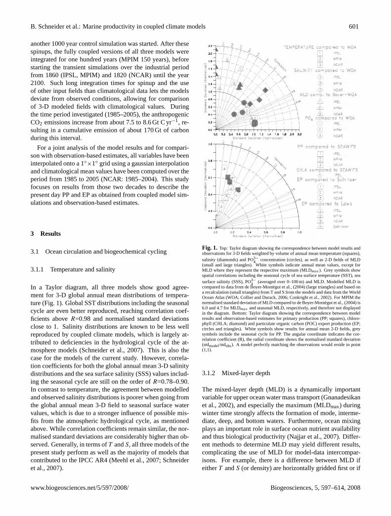
In a Taylor diagram, all three models show good agree-ment for 3-D global annual mean distributions of tempera-ture (Fig.1). Global SST distributions including the seasonalcycle are even better reproduced, reaching correlation coef-ficients aboveR=0.98 and normalised standard deviationsclose to 1. Salinity distributions are known to be less wellreproduced by coupled climate models, which is largely at-tributed to deficiencies in the hydrological cycle of the at-mosphere models (Schneider et al., 2007). This is also thecase for the models of the current study. However, correla-tion coefficients for both the global annual mean 3-D salinitydistributions and the sea surface salinity (SSS) values includ-ing the seasonal cycle are still on the order ofR=0.78–0.90.In contrast to temperature, the agreement between modelledand observed salinity distributions is poorer when going fromthe global annual mean 3-D field to seasonal surface watervalues, which is due to a stronger influence of possible mis-fits from the atmospheric hydrological cycle, as mentionedabove. While correlation coefficients remain similar, the nor-malised standard deviations are considerably higher than ob-served. Generally, in terms ofT andS, all three models of thepresent study perform as well as the majority of models thatcontributed to the IPCC AR4 (Meehl et al., 2007; Schneideret al., 2007).

Fig. 1. Top: Taylor diagram showing the correspondence between model results andobservations for 3-D fields weighted by volume of annual mean temperature (squares),salinity (diamonds) and PO3−

4 concentration (circles), as well as 2-D fields of MLD(small and large triangles). White symbols indicate annual mean values, except forMLD where they represent the respective maximum (MLDmax ). Grey symbols showspatial correlations including the seasonal cycle of sea surface temperature (SST), seasurface salinity (SSS), PO3−

4 (averaged over 0–100 m) and MLD. Modelled MLD iscompared to data from de Boyer-Montegut et al., (2004) (large triangles) and based ona recalculation (small triangles) from T and S from the models and data from the WorldOcean Atlas (WOA; Collier and Durack, 2006; Conkright et al., 2002). For MPIM thenormalised standard deviation of MLD compared to de Boyer-Montegut et al., (2004) is6.0 and 4.7 for MLDmax and seasonal MLD, respectively, and therefore not displayedin the diagram. Bottom: Taylor diagram showing the correspondence between modelresults and observation-based estimates for primary production (PP; squares), chloro-phyll (CHLA; diamond) and particulate organic carbon (POC) export production (EP;circles and triangles). White symbols show results for annual mean 2-D fields, greysymbols include the seasonal cycle for PP. The angular coordinate indicates the cor-relation coefficient (R), the radial coordinate shows the normalised standard deviation(stdmodel/stdobs). A model perfectly matching the observations would reside in point(1,1).

3.1.2 Mixed-layer depth

The mixed-layer depth (MLD) is a dynamically importantvariable for upper ocean water mass transport (Gnanadesikanet al., 2002), and especially the maximum (MLDmax) duringwinter time strongly affects the formation of mode, interme-diate, deep, and bottom waters. Furthermore, ocean mixingplays an important role in surface ocean nutrient availabilityand thus biological productivity (Najjar et al., 2007). Differ-ent methods to determine MLD may yield different results,complicating the use of MLD for model-data intercompar-isons. For example, there is a difference between MLD ifeitherT andS (or density) are horizontally gridded first or if



density is defined for individual profiles first and then inter-polated in space (de Boyer-Montegut et al., 2004).

In the current study we use results from de Boyer-Montegut et al. (2004), where MLD is defined to be the depthlevel where surface water density is offset by 0.03 kg m−3

or potential temperature is by 0.2◦C lower than SST. Thesedefinitions, applied to local profiles first and then interpo-lated in space, are suggested to be the optimal solution forobservation-based MLD. In IPSL MLD is the depth where insitu density is 0.01 kg m−3 higher than surface density. Sim-ilarly, in MPIM, it is the depth where in situ density exceedssurface water density by 0.125 kg m−3. In the NCAR modelthe vertical mixing scheme is the K-profile parameterization(KPP) scheme of Large et al. (1994), where the mixed-layerdepth depends on the depth of mixing due to turbulent veloc-ities of unresolved eddies.

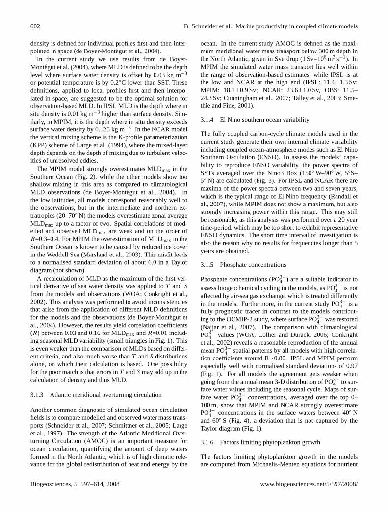
The MPIM model strongly overestimates MLDmax in theSouthern Ocean (Fig.2), while the other models show tooshallow mixing in this area as compared to climatologicalMLD observations (de Boyer-Montegut et al., 2004). Inthe low latitudes, all models correspond reasonably well tothe observations, but in the intermediate and northern ex-tratropics (20–70◦ N) the models overestimate zonal averageMLDmax up to a factor of two. Spatial correlations of mod-elled and observed MLDmax are weak and on the order ofR=0.3–0.4. For MPIM the overestimation of MLDmax in theSouthern Ocean is known to be caused by reduced ice coverin the Weddell Sea (Marsland et al., 2003). This misfit leadsto a normalised standard deviation of about 6.0 in a Taylordiagram (not shown).

A recalculation of MLD as the maximum of the first ver-tical derivative of sea water density was applied toT andS

from the models and observations (WOA; Conkright et al.,2002). This analysis was performed to avoid inconsistenciesthat arise from the application of different MLD definitionsfor the models and the observations (de Boyer-Montegut etal., 2004). However, the results yield correlation coefficients(R) between 0.03 and 0.16 for MLDmax andR=0.01 includ-ing seasonal MLD variability (small triangles in Fig.1). Thisis even weaker than the comparison of MLDs based on differ-ent criteria, and also much worse thanT andS distributionsalone, on which their calculation is based. One possibilityfor the poor match is that errors inT andS may add up in thecalculation of density and thus MLD.

3.1.3 Atlantic meridional overturning circulation

Another common diagnostic of simulated ocean circulationfields is to compare modelled and observed water mass trans-ports (Schneider et al., 2007; Schmittner et al., 2005; Largeet al., 1997). The strength of the Atlantic Meridional Over-turning Circulation (AMOC) is an important measure forocean circulation, quantifying the amount of deep watersformed in the North Atlantic, which is of high climatic rele-vance for the global redistribution of heat and energy by the

ocean. In the current study AMOC is defined as the maxi-mum meridional water mass transport below 300 m depth inthe North Atlantic, given in Sverdrup (1 Sv=106 m3 s−1). InMPIM the simulated water mass transport lies well withinthe range of observation-based estimates, while IPSL is atthe low and NCAR at the high end (IPSL: 11.4±1.3 Sv;MPIM: 18.1±0.9 Sv; NCAR: 23.6±1.0 Sv, OBS: 11.5–24.3 Sv; Cunningham et al., 2007; Talley et al., 2003; Sme-thie and Fine, 2001).

3.1.4 El Nino southern ocean variability

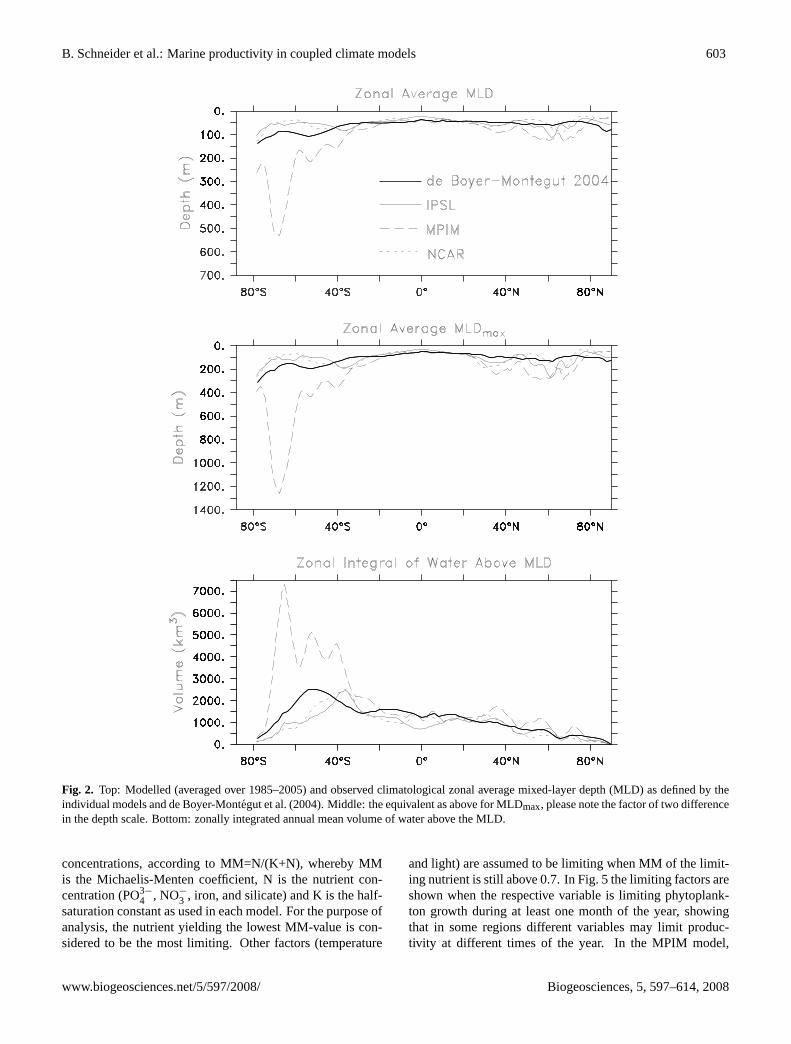
The fully coupled carbon-cycle climate models used in thecurrent study generate their own internal climate variabilityincluding coupled ocean-atmosphere modes such as El NinoSouthern Oscillation (ENSO). To assess the models’ capa-bility to reproduce ENSO variability, the power spectra ofSSTs averaged over the Nino3 Box (150◦ W–90◦ W, 5◦S–5◦ N) are calculated (Fig.3). For IPSL and NCAR there aremaxima of the power spectra between two and seven years,which is the typical range of El Nino frequency (Randall etal., 2007), while MPIM does not show a maximum, but alsostrongly increasing power within this range. This may stillbe reasonable, as this analysis was performed over a 20 yeartime-period, which may be too short to exhibit representativeENSO dynamics. The short time interval of investigation isalso the reason why no results for frequencies longer than 5years are obtained.

3.1.5 Phosphate concentrations

Phosphate concentrations (PO3−

4 ) are a suitable indicator toassess biogeochemical cycling in the models, as PO3−

4 is notaffected by air-sea gas exchange, which is treated differentlyin the models. Furthermore, in the current study PO3−

4 is afully prognostic tracer in contrast to the models contribut-ing to the OCMIP-2 study, where surface PO3−

4 was restored(Najjar et al., 2007). The comparison with climatologicalPO3−

4 values (WOA; Collier and Durack, 2006; Conkrightet al., 2002) reveals a reasonable reproduction of the annualmean PO3−

4 spatial patterns by all models with high correla-tion coefficients around R∼0.80. IPSL and MPIM performespecially well with normalised standard deviations of 0.97(Fig. 1). For all models the agreement gets weaker whengoing from the annual mean 3-D distribution of PO3−

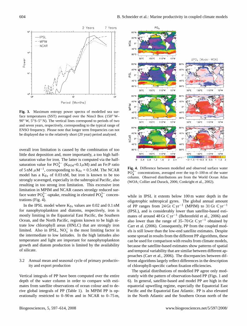
4 to sur-face water values including the seasonal cycle. Maps of sur-face water PO3−

4 concentrations, averaged over the top 0–100 m, show that MPIM and NCAR strongly overestimatePO3−

4 concentrations in the surface waters between 40◦ Nand 60◦ S (Fig. 4), a deviation that is not captured by theTaylor diagram (Fig.1).

3.1.6 Factors limiting phytoplankton growth

The factors limiting phytoplankton growth in the modelsare computed from Michaelis-Menten equations for nutrient



Fig. 2. Top: Modelled (averaged over 1985–2005) and observed climatological zonal average mixed-layer depth (MLD) as defined by theindividual models and de Boyer-Montegut et al. (2004). Middle: the equivalent as above for MLDmax, please note the factor of two differencein the depth scale. Bottom: zonally integrated annual mean volume of water above the MLD.

concentrations, according to MM=N/(K+N), whereby MMis the Michaelis-Menten coefficient, N is the nutrient con-centration (PO3−

4 , NO−

3 , iron, and silicate) and K is the half-saturation constant as used in each model. For the purpose ofanalysis, the nutrient yielding the lowest MM-value is con-sidered to be the most limiting. Other factors (temperature

and light) are assumed to be limiting when MM of the limit-ing nutrient is still above 0.7. In Fig.5 the limiting factors areshown when the respective variable is limiting phytoplank-ton growth during at least one month of the year, showingthat in some regions different variables may limit produc-tivity at different times of the year. In the MPIM model,



Fig. 3. Maximum entropy power spectra of modelled sea sur-face temperatures (SST) averaged over the Nino3 Box (150◦ W–90◦ W, 5◦S–5◦ N). The vertical lines correspond to periods of twoand seven years, respectively, corresponding to the typical range ofENSO frequency. Please note that longer term frequencies can notbe displayed due to the relatively short (20 year) period analysed.

overall iron limitation is caused by the combination of toolittle dust deposition and, more importantly, a too high half-saturation value for iron. The latter is computed via the half-saturation value for PO3−

4 (KPO4=0.1µM) and an Fe:P ratioof 5 nM µM−1, corresponding to KFe = 0.5 nM. The NCARmodel has a KFe of 0.03 nM, but iron is known to be toostrongly scavenged, especially in the subtropical Pacific, alsoresulting in too strong iron limitation. This excessive ironlimitation in MPIM and NCAR causes stronlgy reduced sur-face water PO3−

4 -uptake, resulting in elevated PO3−

4 concen-trations (Fig.4).

In the IPSL model where KFe values are 0.02 and 0.1 nMfor nanophytoplankton and diatoms, respectively, iron ismostly limiting in the Equatorial East Pacific, the SouthernOcean, and the North Pacific, regions known to be high ni-trate low chlorophyll areas (HNLC) that are strongly ironlimited. Also in IPSL, NO−

3 is the most limiting factor inthe intermediate to low latitudes. In the high latitudes alsotemperature and light are important for nanophytoplanktongrowth and diatom production is limited by the availabilityof silicate.

3.2 Annual mean and seasonal cycle of primary productiv-ity and export production

Vertical integrals of PP have been computed over the entiredepth of the water column in order to compare with esti-mates from satellite observations of ocean colour and to de-rive global integrals of PP (Table1). In MPIM PP is op-erationally restricted to 0–90 m and in NCAR to 0–75 m,

Fig. 4. Difference between modelled and observed surface waterPO3−

4 concentrations, averaged over the top 0–100 m of the watercolumn. Observed distributions are from the World Ocean Atlas(WOA; Collier and Durack, 2006; Conkright et al., 2002).

while in IPSL it extents below 100 m water depth in theoligotrophic subtropical gyres. The global annual amountof PP ranges from 24 Gt C yr−1 (MPIM) to 31 Gt C yr−1

(IPSL), and is considerably lower than satellite-based esti-mates of around 48 Gt C yr−1 (Behrenfeld et al., 2006) andalso lower than the range of 35–70 Gt C yr−1 obtained byCarr et al. (2006). Consequently, PP from the coupled mod-els is still lower than the low-end satellite estimates. Despitesome spread in results from the different PP algorithms, thesecan be used for comparison with results from climate models,because the satellite-based estimates show patterns of spatialand temporal variability that are similar between different ap-proaches (Carr et al., 2006). The discrepancies between dif-ferent algorithms largely reflect differences in the descriptionof chlorophyll-specific carbon fixation efficiencies.

The spatial distributions of modelled PP agree only mod-erately with the pattern of observation-based PP (Figs.1 and6). In general, satellite-based and model PP are high in theequatorial upwelling regime, especially the Equatorial EastPacific and the Equatorial East Atlantic. PP is also elevatedin the North Atlantic and the Southern Ocean north of the



Table 1. Modelled and observation-based depth integrated net primary production (PP) and export production (EP) of particulate organiccarbon (POC) and their relation to stratification and SST. Values in brackets correspond to one standard deviation.

PP PPgloba PPstrat

b PPstrat Areastratc PPano

d S-SLOPEe S-SLOPE T-SLOPEf T-SLOPE(Gt C yr−1) (Gt C yr−1) (%) (%) R2 (Tg C kg−1 m−3) R2 (Tg C◦C−1) R2

IPSL 30.7 (3.1) 17.7 (1.8) 58 62 0.88 –787 0.70 –246 0.67MPIM 23.7 (8.6) 17.7 (3.4) 75 67 0.85 0 0.04 0 0.03NCAR 27.4 (3.3) 17.8 (2.2) 65 66 0.78 –143 0.02 –65 0.05SEAWIFS 47.5 (2.4) 34.6g (1.3) 73g 72g 0.69g –876 0.69 –151 0.85

EP EPgloba EPstrat

b EPstrat EPanod S-SLOPEe S-SLOPE T-SLOPEf T-SLOPE

(Gt C yr−1) (Gt C yr−1) (%) R2 (Tg C kg−1 m−3) R2 (Tg C◦C−1) R2

IPSL 8.6 (0.8) 3.6 (0.3) 42 0.65 –184 0.61 –47 0.61MPIM 5.0 (1.8) 3.8 (0.7) 75 0.91 0 0.04 0 0.04NCAR 9.0 (1.1) 5.6 (0.7) 62 0.78 –57 0.03 –23 0.06Schlitzer 11.4 7.0g 61g

Laws 11.1 6.2g 56g

a global PP(EP).b PP(EP) integrated over the area of the permanently stratified, low-latitude ocean.c percentage of the permanently stratified, low-latitude ocean to the global ocean domain.d coefficient of determination for anomalies of PP(EP)glob versus anomalies of PP(EP)strat.e slope of the regression line for PP(EP)anoversus SIano.f slope of the regression line for PP(EP)anoversus SSTano.g SST data from Conkright et al. (2002).

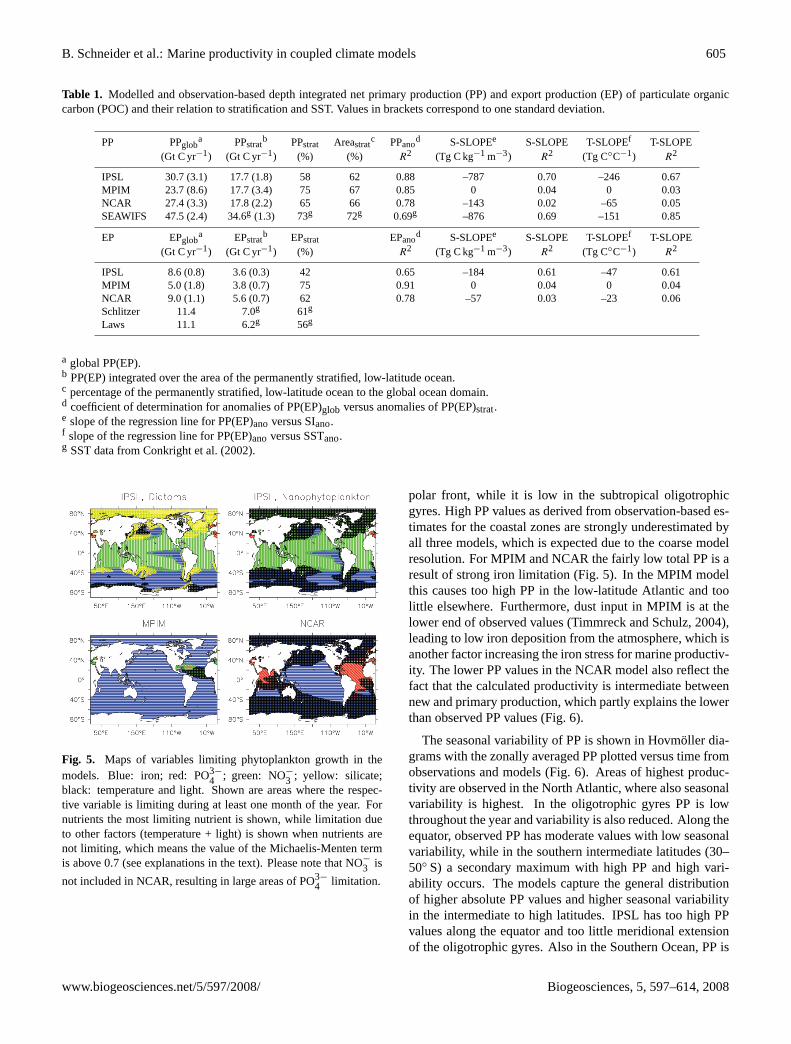
Fig. 5. Maps of variables limiting phytoplankton growth in themodels. Blue: iron; red: PO3−

4 ; green: NO−3 ; yellow: silicate;black: temperature and light. Shown are areas where the respec-tive variable is limiting during at least one month of the year. Fornutrients the most limiting nutrient is shown, while limitation dueto other factors (temperature + light) is shown when nutrients arenot limiting, which means the value of the Michaelis-Menten termis above 0.7 (see explanations in the text). Please note that NO−

3 is

not included in NCAR, resulting in large areas of PO3−

4 limitation.

polar front, while it is low in the subtropical oligotrophicgyres. High PP values as derived from observation-based es-timates for the coastal zones are strongly underestimated byall three models, which is expected due to the coarse modelresolution. For MPIM and NCAR the fairly low total PP is aresult of strong iron limitation (Fig.5). In the MPIM modelthis causes too high PP in the low-latitude Atlantic and toolittle elsewhere. Furthermore, dust input in MPIM is at thelower end of observed values (Timmreck and Schulz, 2004),leading to low iron deposition from the atmosphere, which isanother factor increasing the iron stress for marine productiv-ity. The lower PP values in the NCAR model also reflect thefact that the calculated productivity is intermediate betweennew and primary production, which partly explains the lowerthan observed PP values (Fig.6).

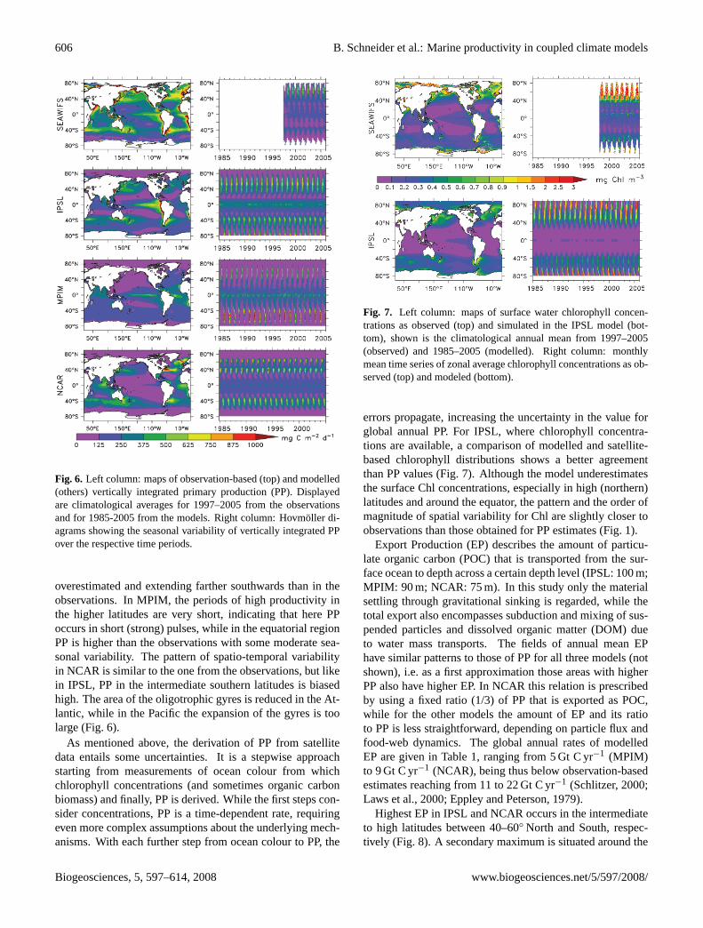
The seasonal variability of PP is shown in Hovmoller dia-grams with the zonally averaged PP plotted versus time fromobservations and models (Fig.6). Areas of highest produc-tivity are observed in the North Atlantic, where also seasonalvariability is highest. In the oligotrophic gyres PP is lowthroughout the year and variability is also reduced. Along theequator, observed PP has moderate values with low seasonalvariability, while in the southern intermediate latitudes (30–50◦ S) a secondary maximum with high PP and high vari-ability occurs. The models capture the general distributionof higher absolute PP values and higher seasonal variabilityin the intermediate to high latitudes. IPSL has too high PPvalues along the equator and too little meridional extensionof the oligotrophic gyres. Also in the Southern Ocean, PP is



Fig. 6. Left column: maps of observation-based (top) and modelled(others) vertically integrated primary production (PP). Displayedare climatological averages for 1997–2005 from the observationsand for 1985-2005 from the models. Right column: Hovmoller di-agrams showing the seasonal variability of vertically integrated PPover the respective time periods.

overestimated and extending farther southwards than in theobservations. In MPIM, the periods of high productivity inthe higher latitudes are very short, indicating that here PPoccurs in short (strong) pulses, while in the equatorial regionPP is higher than the observations with some moderate sea-sonal variability. The pattern of spatio-temporal variabilityin NCAR is similar to the one from the observations, but likein IPSL, PP in the intermediate southern latitudes is biasedhigh. The area of the oligotrophic gyres is reduced in the At-lantic, while in the Pacific the expansion of the gyres is toolarge (Fig.6).

As mentioned above, the derivation of PP from satellitedata entails some uncertainties. It is a stepwise approachstarting from measurements of ocean colour from whichchlorophyll concentrations (and sometimes organic carbonbiomass) and finally, PP is derived. While the first steps con-sider concentrations, PP is a time-dependent rate, requiringeven more complex assumptions about the underlying mech-anisms. With each further step from ocean colour to PP, the

Fig. 7. Left column: maps of surface water chlorophyll concen-trations as observed (top) and simulated in the IPSL model (bot-tom), shown is the climatological annual mean from 1997–2005(observed) and 1985–2005 (modelled). Right column: monthlymean time series of zonal average chlorophyll concentrations as ob-served (top) and modeled (bottom).

errors propagate, increasing the uncertainty in the value forglobal annual PP. For IPSL, where chlorophyll concentra-tions are available, a comparison of modelled and satellite-based chlorophyll distributions shows a better agreementthan PP values (Fig.7). Although the model underestimatesthe surface Chl concentrations, especially in high (northern)latitudes and around the equator, the pattern and the order ofmagnitude of spatial variability for Chl are slightly closer toobservations than those obtained for PP estimates (Fig.1).

Export Production (EP) describes the amount of particu-late organic carbon (POC) that is transported from the sur-face ocean to depth across a certain depth level (IPSL: 100 m;MPIM: 90 m; NCAR: 75 m). In this study only the materialsettling through gravitational sinking is regarded, while thetotal export also encompasses subduction and mixing of sus-pended particles and dissolved organic matter (DOM) dueto water mass transports. The fields of annual mean EPhave similar patterns to those of PP for all three models (notshown), i.e. as a first approximation those areas with higherPP also have higher EP. In NCAR this relation is prescribedby using a fixed ratio (1/3) of PP that is exported as POC,while for the other models the amount of EP and its ratioto PP is less straightforward, depending on particle flux andfood-web dynamics. The global annual rates of modelledEP are given in Table1, ranging from 5 Gt C yr−1 (MPIM)to 9 Gt C yr−1 (NCAR), being thus below observation-basedestimates reaching from 11 to 22 Gt C yr−1 (Schlitzer, 2000;Laws et al., 2000; Eppley and Peterson, 1979).

Highest EP in IPSL and NCAR occurs in the intermediateto high latitudes between 40–60◦ North and South, respec-tively (Fig. 8). A secondary maximum is situated around the



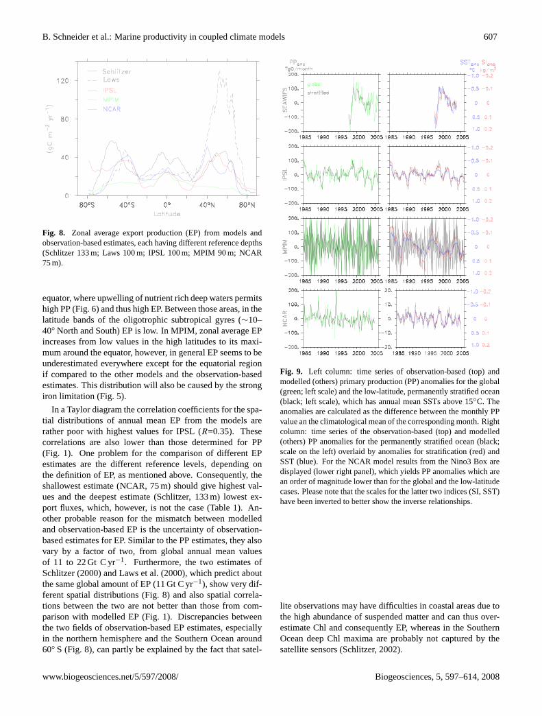
Fig. 8. Zonal average export production (EP) from models andobservation-based estimates, each having different reference depths(Schlitzer 133 m; Laws 100 m; IPSL 100 m; MPIM 90 m; NCAR75 m).

equator, where upwelling of nutrient rich deep waters permitshigh PP (Fig.6) and thus high EP. Between those areas, in thelatitude bands of the oligotrophic subtropical gyres (∼10–40◦ North and South) EP is low. In MPIM, zonal average EPincreases from low values in the high latitudes to its maxi-mum around the equator, however, in general EP seems to beunderestimated everywhere except for the equatorial regionif compared to the other models and the observation-basedestimates. This distribution will also be caused by the strongiron limitation (Fig.5).

In a Taylor diagram the correlation coefficients for the spa-tial distributions of annual mean EP from the models arerather poor with highest values for IPSL (R=0.35). Thesecorrelations are also lower than those determined for PP(Fig. 1). One problem for the comparison of different EPestimates are the different reference levels, depending onthe definition of EP, as mentioned above. Consequently, theshallowest estimate (NCAR, 75 m) should give highest val-ues and the deepest estimate (Schlitzer, 133 m) lowest ex-port fluxes, which, however, is not the case (Table1). An-other probable reason for the mismatch between modelledand observation-based EP is the uncertainty of observation-based estimates for EP. Similar to the PP estimates, they alsovary by a factor of two, from global annual mean valuesof 11 to 22 Gt C yr−1. Furthermore, the two estimates ofSchlitzer (2000) and Laws et al. (2000), which predict aboutthe same global amount of EP (11 Gt C yr−1), show very dif-ferent spatial distributions (Fig.8) and also spatial correla-tions between the two are not better than those from com-parison with modelled EP (Fig.1). Discrepancies betweenthe two fields of observation-based EP estimates, especiallyin the northern hemisphere and the Southern Ocean around60◦ S (Fig.8), can partly be explained by the fact that satel-

Fig. 9. Left column: time series of observation-based (top) andmodelled (others) primary production (PP) anomalies for the global(green; left scale) and the low-latitude, permanently stratified ocean(black; left scale), which has annual mean SSTs above 15◦C. Theanomalies are calculated as the difference between the monthly PPvalue an the climatological mean of the corresponding month. Rightcolumn: time series of the observation-based (top) and modelled(others) PP anomalies for the permanently stratified ocean (black;scale on the left) overlaid by anomalies for stratification (red) andSST (blue). For the NCAR model results from the Nino3 Box aredisplayed (lower right panel), which yields PP anomalies which arean order of magnitude lower than for the global and the low-latitudecases. Please note that the scales for the latter two indices (SI, SST)have been inverted to better show the inverse relationships.

lite observations may have difficulties in coastal areas due tothe high abundance of suspended matter and can thus over-estimate Chl and consequently EP, whereas in the SouthernOcean deep Chl maxima are probably not captured by thesatellite sensors (Schlitzer, 2002).



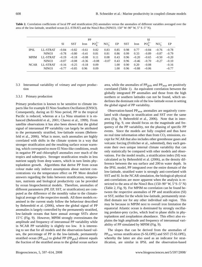
Table 2. Correlation coefficients of local PP and stratification (SI) anomalies versus the anomalies of different variables averaged over thearea of the low-latitude, stratified ocean (LL-STRAT) and the Nino3 Box (NINO3; 150◦ W–90◦ W, 5◦ S–5◦ N).

PP SISI SST Iron PO3−

4 NO−

3 EP SST Iron PO3−

4 NO−

3 EP

IPSL LL-STRAT –0.84 –0.82 –0.61 0.82 0.83 0.85 0.98 0.77 –0.84 –0.76 –0.78NINO3 –0.78 –0.80 –0.41 0.81 0.81 0.86 0.99 0.33 –0.89 –0.87 –0.79

MPIM LL-STRAT –0.19 –0.18 –0.08 0.11 0.08 0.43 0.96 –0.20 –0.65 –0.50 –0.20NINO3 –0.07 –0.08 –0.36 –0.08 –0.07 0.43 0.96 –0.46 –0.70 –0.27 –0.10

NCAR LL-STRAT –0.16 –0.25 –0.18 0.09 1.00 0.90 0.20 –0.08 –0.16NINO3 –0.77 –0.85 0.96 0.09 1.00 0.96 –0.88 –0.06 –0.77

3.3 Interannual variability of vrimary and export produc-tion

3.3.1 Primary production

Primary production is known to be sensitive to climate im-pacts like for example El Nino Southern Oscillation (ENSO).Consequently, during an El Nino period, PP in the tropicalPacific is reduced, whereas at a La Nina situation it is en-hanced (Behrenfeld et al., 2001; Chavez et al., 1999). Fromsatellite observations it has also been shown that the globalsignal of interannual PP variability can largely be attributedto the permanently stratified, low-latitude oceans (Behren-feld et al., 2006). What is more, such anomalies are highlycorrelated with shifts in the climate system in a way thatstronger stratification and the resulting surface ocean warm-ing, which correspond to more El Nino-like conditions, resultin negative PP and chlorophyll anomalies over much of thetropics and subtropics. Stronger stratification results in lessnutrient supply from deep waters, which in turn limits phy-toplankton growth. Algorithms that derive PP from oceancolour make only indirect assumptions about nutrient con-centrations via the temperature effect on PP. More detailedanswers regarding the links between stratification, tempera-ture, nutrients and biological productivity can be providedby ocean biogeochemical models. Therefore, anomalies ofdifferent parameters (PP, EP, SST, or stratification) are com-puted as the difference of the monthly value to the climato-logical average of the respective month. All three models ex-amined in the current study follow the behaviour describedby Behrenfeld et al. (2006), where the global signal of PPanomalies is largely controlled by the permanently stratified,low-latitude oceans that have annual average SSTs above15◦C (Fig. 9). However, MPIM strongly overestimates theamplitude and frequency of interannual PP variability whilein NCAR PP variability is slightly too low. It is interest-ing to see that for all models and the observation-based val-ues, the percentage of PP in the low-latitude, permanentlystratified ocean (PPstrat) to global PP (PPglob) almost equalsthe fraction of the stratified areas to the global ocean surface

area, while the anomalies of PPglob and PPstrat are positivelycorrelated (Table1). An equivalent correlation between theglobally integrated PP anomalies and those from the highnorthern or southern latitudes can not be found, which un-derlines the dominant role of the low-latitude ocean in settingthe global signal of PP variability.

Observation-based PPstrat anomalies are negatively corre-lated with changes in stratification and SST over the samearea (Fig.9; Behrenfeld et al., 2006). Note that in inter-preting Fig.9, one should focus on the magnitude and fre-quency of the PP variability, not the phasing of specific PPevents. Since the models are fully coupled and thus haveno real time information other than from CO2 emissions, ex-cept for NCAR that also includes other greenhouse gases andvolcanic forcing (Frolicher et al., submitted), they each gen-erate their own unique internal climate variability that canonly statistically be compared with other models and obser-vations. For the model results, a stratification index (SI) wascalculated as by Behrenfeld et al. (2006), as the density dif-ference between the sea surface and 200 m water depth. Inthe IPSL model, PP integrated over the entire domain of thelow-latitude, stratified water is strongly anti-correlated withSST and SI. In the NCAR simulation, the biological-physicalanti-correlations are more apparent when the analysis is re-stricted to the area of the Nino3 Box (150–90◦ W, 5◦S–5◦ N)(Table2, Fig. 9). For MPIM no correlation can be found be-tween the respective anomalies of PP and stratification (SI)or SST, neither for the whole low-latitude, permanently strat-ified domain nor for any other individual sub region. Thismay be because in MPIM next to overall iron limitation theequatorial Atlantic ocean is dominated by strongly oscillat-ing predator-prey cycles, which lead to phase shifts in phy-toplankton and zooplankton abundance. This effect also ex-plains the high amplitude and frequency of interannual vari-ability of PP simulated by MPIM (Fig.9).

The slopes that can be derived from the anomalies ofPPstrat versus stratification (S-SLOPE) and SST (T-SLOPE),whereby the latter are also used as an indicator for strat-ification, are similar in IPSL and the observation-based



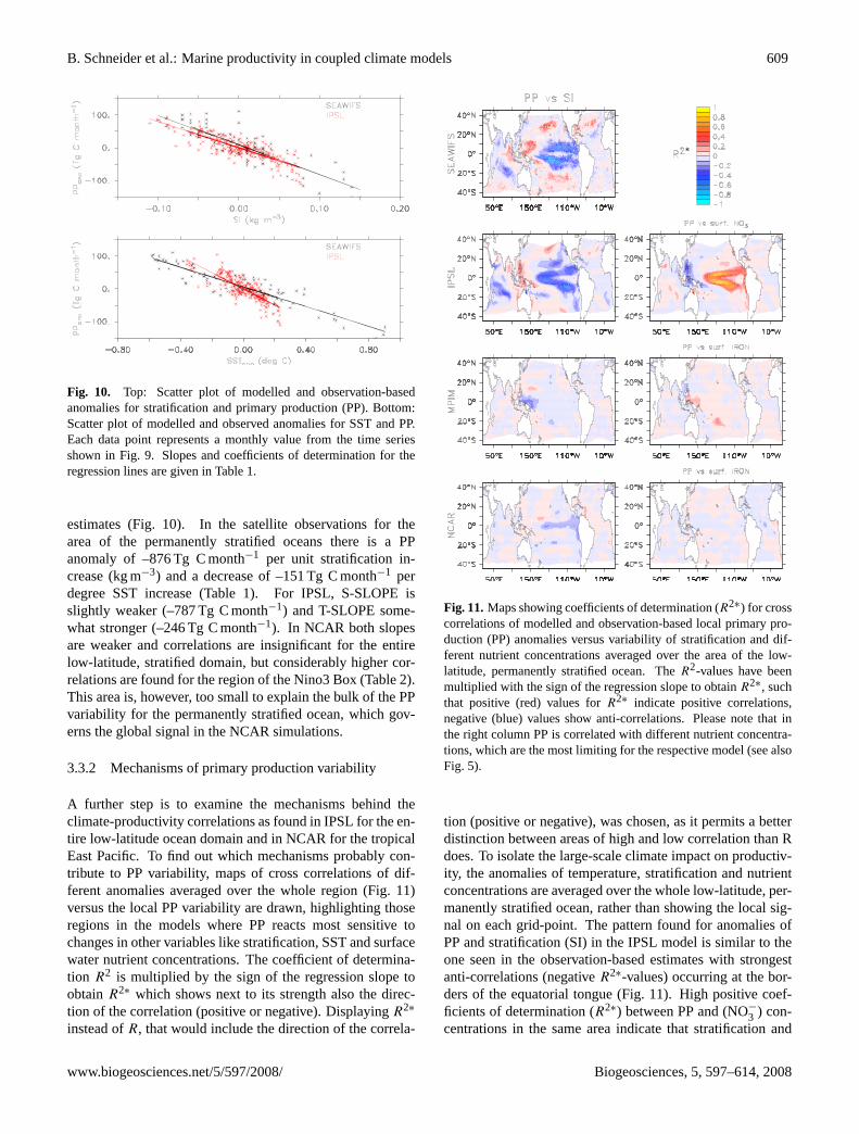
Fig. 10. Top: Scatter plot of modelled and observation-basedanomalies for stratification and primary production (PP). Bottom:Scatter plot of modelled and observed anomalies for SST and PP.Each data point represents a monthly value from the time seriesshown in Fig.9. Slopes and coefficients of determination for theregression lines are given in Table1.

estimates (Fig.10). In the satellite observations for thearea of the permanently stratified oceans there is a PPanomaly of –876 Tg C month−1 per unit stratification in-crease (kg m−3) and a decrease of –151 Tg C month−1 perdegree SST increase (Table1). For IPSL, S-SLOPE isslightly weaker (–787 Tg C month−1) and T-SLOPE some-what stronger (–246 Tg C month−1). In NCAR both slopesare weaker and correlations are insignificant for the entirelow-latitude, stratified domain, but considerably higher cor-relations are found for the region of the Nino3 Box (Table2).This area is, however, too small to explain the bulk of the PPvariability for the permanently stratified ocean, which gov-erns the global signal in the NCAR simulations.

3.3.2 Mechanisms of primary production variability

A further step is to examine the mechanisms behind theclimate-productivity correlations as found in IPSL for the en-tire low-latitude ocean domain and in NCAR for the tropicalEast Pacific. To find out which mechanisms probably con-tribute to PP variability, maps of cross correlations of dif-ferent anomalies averaged over the whole region (Fig.11)versus the local PP variability are drawn, highlighting thoseregions in the models where PP reacts most sensitive tochanges in other variables like stratification, SST and surfacewater nutrient concentrations. The coefficient of determina-tion R2 is multiplied by the sign of the regression slope toobtainR2∗ which shows next to its strength also the direc-tion of the correlation (positive or negative). DisplayingR2∗

instead ofR, that would include the direction of the correla-

Fig. 11.Maps showing coefficients of determination (R2∗) for crosscorrelations of modelled and observation-based local primary pro-duction (PP) anomalies versus variability of stratification and dif-ferent nutrient concentrations averaged over the area of the low-latitude, permanently stratified ocean. TheR2-values have beenmultiplied with the sign of the regression slope to obtainR2∗, suchthat positive (red) values forR2∗ indicate positive correlations,negative (blue) values show anti-correlations. Please note that inthe right column PP is correlated with different nutrient concentra-tions, which are the most limiting for the respective model (see alsoFig. 5).

tion (positive or negative), was chosen, as it permits a betterdistinction between areas of high and low correlation than Rdoes. To isolate the large-scale climate impact on productiv-ity, the anomalies of temperature, stratification and nutrientconcentrations are averaged over the whole low-latitude, per-manently stratified ocean, rather than showing the local sig-nal on each grid-point. The pattern found for anomalies ofPP and stratification (SI) in the IPSL model is similar to theone seen in the observation-based estimates with strongestanti-correlations (negativeR2∗-values) occurring at the bor-ders of the equatorial tongue (Fig.11). High positive coef-ficients of determination (R2∗) between PP and (NO−3 ) con-centrations in the same area indicate that stratification and



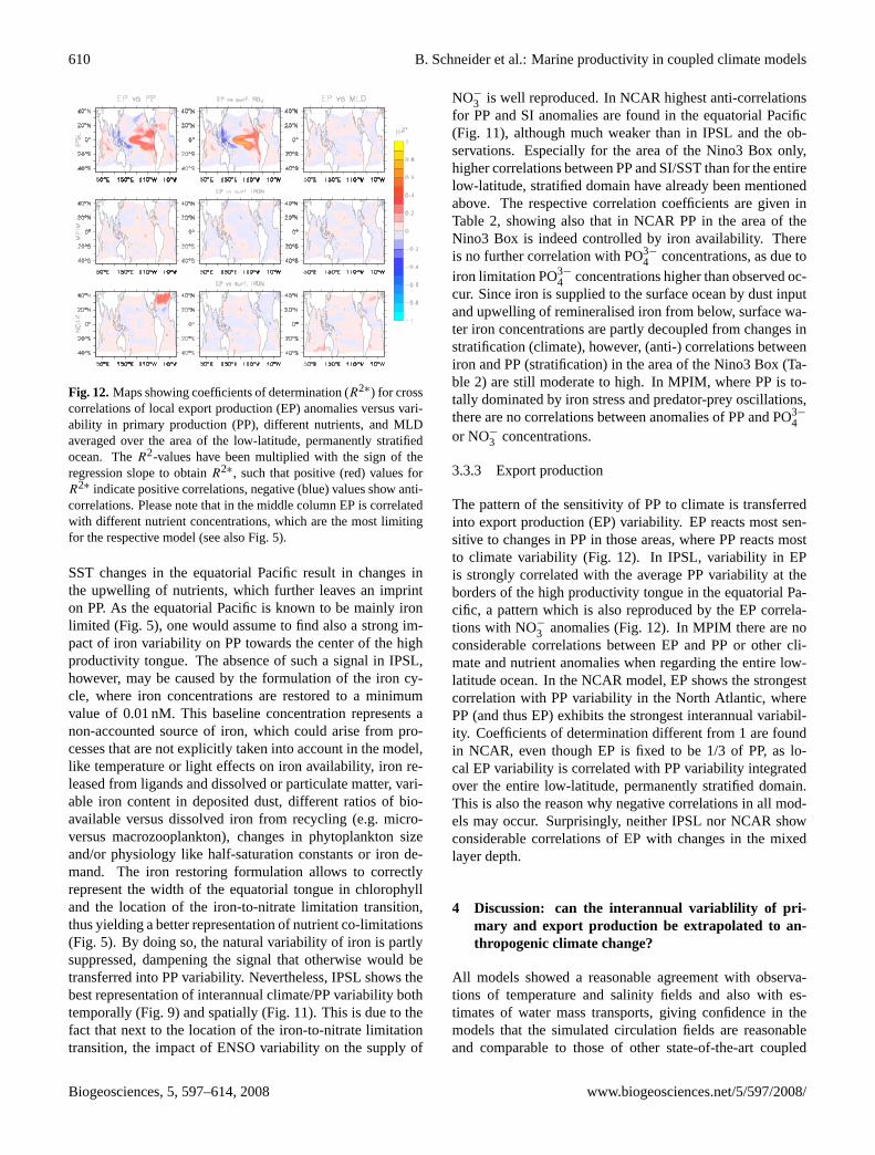
Fig. 12.Maps showing coefficients of determination (R2∗) for crosscorrelations of local export production (EP) anomalies versus vari-ability in primary production (PP), different nutrients, and MLDaveraged over the area of the low-latitude, permanently stratifiedocean. TheR2-values have been multiplied with the sign of theregression slope to obtainR2∗, such that positive (red) values forR2∗ indicate positive correlations, negative (blue) values show anti-correlations. Please note that in the middle column EP is correlatedwith different nutrient concentrations, which are the most limitingfor the respective model (see also Fig.5).

SST changes in the equatorial Pacific result in changes inthe upwelling of nutrients, which further leaves an imprinton PP. As the equatorial Pacific is known to be mainly ironlimited (Fig. 5), one would assume to find also a strong im-pact of iron variability on PP towards the center of the highproductivity tongue. The absence of such a signal in IPSL,however, may be caused by the formulation of the iron cy-cle, where iron concentrations are restored to a minimumvalue of 0.01 nM. This baseline concentration represents anon-accounted source of iron, which could arise from pro-cesses that are not explicitly taken into account in the model,like temperature or light effects on iron availability, iron re-leased from ligands and dissolved or particulate matter, vari-able iron content in deposited dust, different ratios of bio-available versus dissolved iron from recycling (e.g. micro-versus macrozooplankton), changes in phytoplankton sizeand/or physiology like half-saturation constants or iron de-mand. The iron restoring formulation allows to correctlyrepresent the width of the equatorial tongue in chlorophylland the location of the iron-to-nitrate limitation transition,thus yielding a better representation of nutrient co-limitations(Fig. 5). By doing so, the natural variability of iron is partlysuppressed, dampening the signal that otherwise would betransferred into PP variability. Nevertheless, IPSL shows thebest representation of interannual climate/PP variability bothtemporally (Fig.9) and spatially (Fig.11). This is due to thefact that next to the location of the iron-to-nitrate limitationtransition, the impact of ENSO variability on the supply of

NO−

3 is well reproduced. In NCAR highest anti-correlationsfor PP and SI anomalies are found in the equatorial Pacific(Fig. 11), although much weaker than in IPSL and the ob-servations. Especially for the area of the Nino3 Box only,higher correlations between PP and SI/SST than for the entirelow-latitude, stratified domain have already been mentionedabove. The respective correlation coefficients are given inTable2, showing also that in NCAR PP in the area of theNino3 Box is indeed controlled by iron availability. Thereis no further correlation with PO3−

4 concentrations, as due toiron limitation PO3−

4 concentrations higher than observed oc-cur. Since iron is supplied to the surface ocean by dust inputand upwelling of remineralised iron from below, surface wa-ter iron concentrations are partly decoupled from changes instratification (climate), however, (anti-) correlations betweeniron and PP (stratification) in the area of the Nino3 Box (Ta-ble 2) are still moderate to high. In MPIM, where PP is to-tally dominated by iron stress and predator-prey oscillations,there are no correlations between anomalies of PP and PO3−

4or NO−

3 concentrations.

3.3.3 Export production

The pattern of the sensitivity of PP to climate is transferredinto export production (EP) variability. EP reacts most sen-sitive to changes in PP in those areas, where PP reacts mostto climate variability (Fig.12). In IPSL, variability in EPis strongly correlated with the average PP variability at theborders of the high productivity tongue in the equatorial Pa-cific, a pattern which is also reproduced by the EP correla-tions with NO−

3 anomalies (Fig.12). In MPIM there are noconsiderable correlations between EP and PP or other cli-mate and nutrient anomalies when regarding the entire low-latitude ocean. In the NCAR model, EP shows the strongestcorrelation with PP variability in the North Atlantic, wherePP (and thus EP) exhibits the strongest interannual variabil-ity. Coefficients of determination different from 1 are foundin NCAR, even though EP is fixed to be 1/3 of PP, as lo-cal EP variability is correlated with PP variability integratedover the entire low-latitude, permanently stratified domain.This is also the reason why negative correlations in all mod-els may occur. Surprisingly, neither IPSL nor NCAR showconsiderable correlations of EP with changes in the mixedlayer depth.

4 Discussion: can the interannual variablility of pri-mary and export production be extrapolated to an-thropogenic climate change?

All models showed a reasonable agreement with observa-tions of temperature and salinity fields and also with es-timates of water mass transports, giving confidence in themodels that the simulated circulation fields are reasonableand comparable to those of other state-of-the-art coupled



climate models (Meehl et al., 2007; Randall et al., 2007).In terms of biogeochemical cycling MPIM and NCAR haveshown to be too strongly iron limited (Fig.5) and iron cyclingin the models has shown to be the central point in reproduc-ing the observed climate-productivity relations.

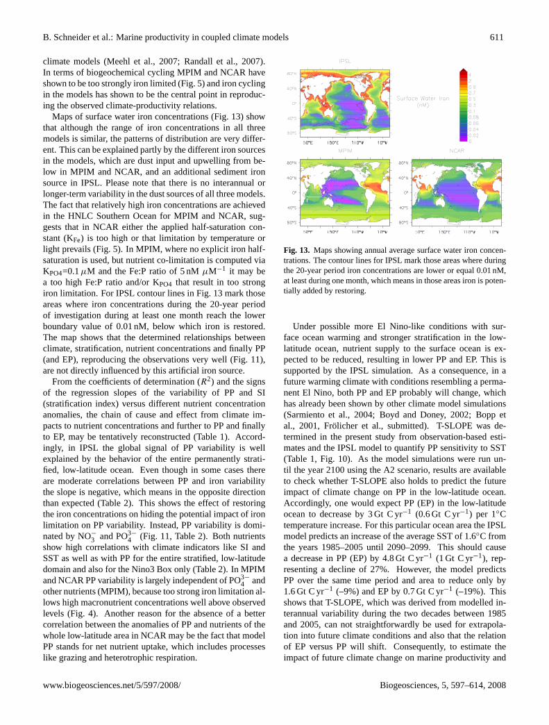
Maps of surface water iron concentrations (Fig.13) showthat although the range of iron concentrations in all threemodels is similar, the patterns of distribution are very differ-ent. This can be explained partly by the different iron sourcesin the models, which are dust input and upwelling from be-low in MPIM and NCAR, and an additional sediment ironsource in IPSL. Please note that there is no interannual orlonger-term variability in the dust sources of all three models.The fact that relatively high iron concentrations are achievedin the HNLC Southern Ocean for MPIM and NCAR, sug-gests that in NCAR either the applied half-saturation con-stant (KFe) is too high or that limitation by temperature orlight prevails (Fig.5). In MPIM, where no explicit iron half-saturation is used, but nutrient co-limitation is computed viaKPO4=0.1µM and the Fe:P ratio of 5 nMµM−1 it may bea too high Fe:P ratio and/or KPO4 that result in too strongiron limitation. For IPSL contour lines in Fig.13mark thoseareas where iron concentrations during the 20-year periodof investigation during at least one month reach the lowerboundary value of 0.01 nM, below which iron is restored.The map shows that the determined relationships betweenclimate, stratification, nutrient concentrations and finally PP(and EP), reproducing the observations very well (Fig.11),are not directly influenced by this artificial iron source.

From the coefficients of determination (R2) and the signsof the regression slopes of the variability of PP and SI(stratification index) versus different nutrient concentrationanomalies, the chain of cause and effect from climate im-pacts to nutrient concentrations and further to PP and finallyto EP, may be tentatively reconstructed (Table1). Accord-ingly, in IPSL the global signal of PP variability is wellexplained by the behavior of the entire permanently strati-fied, low-latitude ocean. Even though in some cases thereare moderate correlations between PP and iron variabilitythe slope is negative, which means in the opposite directionthan expected (Table2). This shows the effect of restoringthe iron concentrations on hiding the potential impact of ironlimitation on PP variability. Instead, PP variability is domi-nated by NO−3 and PO3−

4 (Fig. 11, Table2). Both nutrientsshow high correlations with climate indicators like SI andSST as well as with PP for the entire stratified, low-latitudedomain and also for the Nino3 Box only (Table2). In MPIMand NCAR PP variability is largely independent of PO3−

4 andother nutrients (MPIM), because too strong iron limitation al-lows high macronutrient concentrations well above observedlevels (Fig.4). Another reason for the absence of a bettercorrelation between the anomalies of PP and nutrients of thewhole low-latitude area in NCAR may be the fact that modelPP stands for net nutrient uptake, which includes processeslike grazing and heterotrophic respiration.

Fig. 13. Maps showing annual average surface water iron concen-trations. The contour lines for IPSL mark those areas where duringthe 20-year period iron concentrations are lower or equal 0.01 nM,at least during one month, which means in those areas iron is poten-tially added by restoring.

Under possible more El Nino-like conditions with sur-face ocean warming and stronger stratification in the low-latitude ocean, nutrient supply to the surface ocean is ex-pected to be reduced, resulting in lower PP and EP. This issupported by the IPSL simulation. As a consequence, in afuture warming climate with conditions resembling a perma-nent El Nino, both PP and EP probably will change, whichhas already been shown by other climate model simulations(Sarmiento et al., 2004; Boyd and Doney, 2002; Bopp etal., 2001, Frolicher et al., submitted). T-SLOPE was de-termined in the present study from observation-based esti-mates and the IPSL model to quantify PP sensitivity to SST(Table1, Fig. 10). As the model simulations were run un-til the year 2100 using the A2 scenario, results are availableto check whether T-SLOPE also holds to predict the futureimpact of climate change on PP in the low-latitude ocean.Accordingly, one would expect PP (EP) in the low-latitudeocean to decrease by 3 Gt C yr−1 (0.6 Gt C yr−1) per 1◦Ctemperature increase. For this particular ocean area the IPSLmodel predicts an increase of the average SST of 1.6◦C fromthe years 1985–2005 until 2090–2099. This should causea decrease in PP (EP) by 4.8 Gt C yr−1 (1 Gt C yr−1), rep-resenting a decline of 27%. However, the model predictsPP over the same time period and area to reduce only by1.6 Gt C yr−1 (–9%) and EP by 0.7 Gt C yr−1 (–19%). Thisshows that T-SLOPE, which was derived from modelled in-terannual variability during the two decades between 1985and 2005, can not straightforwardly be used for extrapola-tion into future climate conditions and also that the relationof EP versus PP will shift. Consequently, to estimate theimpact of future climate change on marine productivity and



carbon export further mechanisms and, of course, also thehigh latitude ocean will have to be considered. For exam-ple, Le Quere et al. (2007) demonstrated the importance ofan increase of near surface wind speeds over the SouthernOcean between 1984 and 2001 (Marshall, 2003) on the ma-rine carbon cycle, a trend that is not reproduced by the mod-els in the current study during the investigated time period.Next to a change in the air-sea CO2 exchange (Le Quere etal. 2007), such a shift may increase the supply of iron frombelow, which in turn might stimulate phytoplankton growthin the Southern Ocean. A more detailed study on the long-term shifts in marine biogeochemical cycles under climatechange will be done in a complementary analysis that usesthe continuation of the here presented model simulations ina scenario of future climate change (SRES A2) until the year2100.

5 Conclusions

The current study has illustrated a strong link between ma-rine productivity and climate variability in coupled climatecarbon cycle models, which has already been observed fromsatellite records (Behrenfeld et al., 2006). A detailed ex-amination of biogeochemical cycling in the models has re-vealed the importance of the modelled iron cycle on theimpact of climate variability on marine productivity. Onlyone model (IPSL) is able to reproduce the observed rela-tionship between climate (stratification, SST) and PP. Theuse of an iron restoring formulation in IPSL may be suit-able for simulations of the present-day situation, as the areaswith strong anti-correlations between productivity and strat-ification (SST) seem to be not directly influenced (Fig.13).Remote effects by advection, however, can not be excluded.This has to be regarded with care when applying the modelto simulations of future climate change.

Acknowledgements.We would like to thank J. Sarmiento for hisconstructive review on the manuscript, resulting in a stimulatingdiscussion about the iron cycle in global marine biogeochemicalmodels. Furthermore, we thank J. Orr and an anonymous reviewerfor their valuable comments that also helped to improve themanuscript. We thank I. Fung and K. Lindsay for their workcontributing to the set up of the NCAR model and A. Tagliabuefor many discussions. This work was supported by the EU grants511106-2 (FP6 RTD project EUR-OCEANS) and GOCE-511176(FP6 RTP project CARBOOCEAN) by the European Commission.TLF and FJ also acknowledge support from the Swiss NationalScience Foundations. SCD and MJB received support from NASANNG06G127G. This is publication number 2548 from LSCE.

Edited by: K. Caldeira

References

Anderson, L., and J. Sarmiento, Redfield ratios of remineralizationdetermined by nutrient data analysis, Glob. Biogeochem. Cy.,8(1), 65–80, 1994.

Aumont, O. and Bopp, L.: Globalizing results from ocean in situiron fertilization studies, Glob. Biogeochem. Cy., 20, GB2017,doi:10.1029/2005GB002591, 2006.

Aumont, O., Maier-Reimer, E., Blain, S., and Monfray, P.:An ecosystem model of the global ocean including Fe,Si, P colimitations, Glob. Biogeochem. Cy., 17(2), 1060,doi:10.1029/2001GB001745, 2003.

Behrenfeld, M. and Falkowski, P.: Photosynthetic rates de-rived from satellite-based chlorophyll concentration, Limnol.Oceanogr., 42, 1–20, 1997.

Behrenfeld, M. J., Boss, E., Siegel, D. A., and Shea, D.M.: Carbon-based ocean productivity and phytoplankton phys-iology from space, Glob. Biogeochem. Cy., 19, GB1006,doi:10.1029/2004GB002299, 2005.

Behrenfeld, M. J., Randerson, J. T., Mc Clain, C. R., et al.: Bio-spheric Primary Production during an ENSO Transition, Science,291, 2594–2597, 2001.

Behrenfeld, M. J., O’Malley, R. T., Siegel, D. A., et al.: Climate-driven trends in contemporary ocean productivity, Nature, 444,752–755, 2006.

Bopp, L., Monfray, P., Aumont, O., Dufresne, J. L., Le Treut, H.,Madec, G., Terray, L., and Orr, J. C.: Potential impact of climatechange on marine export production, Glob. Biogeochem. Cy., 15,81–99, 2001.

Bopp, L., Aumont, O., Cadule, P., Alvain, S., and Gehlen, M.: Re-sponse of diatoms distribution to global warming and potentialimplications: A global model study, Geophys. Res. Lett., 32,L19606, doi:10.1029/2005GL023653, 2005.

Boville, B. A. and Gent, P.: The NCAR Climate System Model,version one., J. Climate, 11, 1115–1130, 1998.

Boville, B. A., Kiehl, J., Rasch, P., and Bryan, F.: Improvements tothe NCAR CSM-1 for transient climate simulations, J. Climate,13, D02S070, doi:10.1029/2002JD003026, 2001.

Boyd, P. W. and Doney, S. C.: Modelling regional responses bymarine pelagic ecosystems to global climate change, Geophys.Res. Lett., 29(16), 1806, doi:10.1029/2001GL014130, 2002.

Boyer-Montegut, C., Madec, G., Fischer, A. S., Lazar, A., and Iudi-cone, D.: Mixed layer depth over the global ocean: An examina-tion of profile data and a profile-based climatology, J. Geophys.Res., 109, C12003, doi:10.1029/2004JC002378, 2004.

Carr, M.-E., Friedrichs, M. A. M., Schmetz, M., et al.: A compari-son of global estimates of marine primary production from oceancolour, Deep-Sea Res., 53, 741–770, 2006.

Chavez, F. P., Strutton, P. G., Friederich, G. E., Feely, R. A., Feld-man, G. C., Foley, D. G., and McPhaden, M. J.: Biological andChemical Response of the Equatorial Pacific Ocean to the 1997–98 El Nino, Science, 286, 2126–2131, 1999.

Collier, M. A. and Durack, P. J.: CSIRO netCDF version of theNODC World Ocean Atlas 2005, Marine and Atmospheric Re-search Paper 15, CSIRO, Victoria, Australia, 1-45, 2006.

Conkright, M. E., Locarnini, R. A., Garcia, H. E., O’Brien, T. D.,Boyer, T. P., Stephens, C., and Antonov, J. I.: World ocean atlas2001: Objective analyses, data statistics, and figures, CD-ROMdocumentation, NOAA, Silver Spring, 2002.

Cunningham, S. A., et al., Temporal Variability of the Atlantic



Meridional Overturning Circulation at 26.5◦N, Science, 317,935–938, 2007.

Danabasoglu, G., J. C. McWilliams, and W. G. Large, Approach toequilibrium in accelerated global oceanic models, J. Climate, 9,1092–1110, 1996.

Doney, S. C., Lindsay, K., Fung, I., and John, J.: Natural variabilityin a stable, 1000-Yr global coupled climate-carbon cycle simula-tion, J. Climate, 19, 3033–3054, 2006.

Doney, S. C., Lindsay, K., Caldeira, K., et al.: Evaluating globalocean carbon models: the importance of realistic physics, Glob.Biogeochem. Cy., 18, GB3017, doi:10.1029/2003GB002150,2004.

Dunne, J. P., R. A. Armstrong, A. Gnanadesikan, and J. L.Sarmiento, Empirical and mechanistic models for the par-ticle export ratio, Glob. Biogeochem. Cy., 19, GB4026,doi:10.1029/2004GB002390, 2005.

Eppley, R. W. and Peterson, B. J.: Particulate organic matter fluxand planktonic new production in the deep ocean, Nature, 282,677–680, 1979.

Friedlingstein, P., Cox, P., Betts, R., et al.: Climate-Carbon CycleFeedback Analysis: Results from the C4 MIP Model Intercom-parison, J. Climate, 19, 3337–3353, 2006.

Frolicher, T. L., F. Joos, G.-K. Plattner, M. Steinacher, and S. C.Doney, Variability and trends in oceanic oxygen: Detection andattribution using a coupled carbon cycle-climate model ensem-ble, Clim. Dynam., subm.

Fung, I., S. C. Doney, K. Lindsay, and J. John, Evolution of car-bon sinks in a changing climate , Proceedings of the NationalAcademy of Science, 102, 11,201–11,206, 2005.

Gehlen, M., Bopp, L., Emprin, N., Aumont, O., Heinze, C., andRagueneau, O.: Reconciling surface ocean productivity, exportfluxes and sediment composition in a global biogeochemicalocean model, Biogeosciences, 3, 521–537, 2006,http://www.biogeosciences.net/3/521/2006/.

Gent, P. R., Bryan, F. O., Danabasoglu, G., Doney, S. C., Holland,W. R., Large, W. G., and McWilliams, J. C.: The NCAR ClimateSystem Model global ocean component, J. Climate, 11, 1287–1306, 1998.

Gnanadesikan, A., Slater, R. D., Gruber, N., and Sarmiento, J.:Oceanic vertical exchange and new production: a comparison be-tween models and observations, Deep-Sea Res. II, 49, 363–401,2002.

Hourdin, F., Musat, I., Bony, S., et al.: The LMDZ4 general circula-tion model: climate performance and sensitivity to parametrizedphysics with emphasis on tropical convection, Clim. Dynam.,19(15), 3445–3482, doi:10.1007/s00382-006-0158-0, 2006.

Joos, F., Plattner, G. K., Stocker, T. F., Marchal, O., and Schmittner,A.: Global Warming and Marine Carbon Cycle Feedbacks onFuture Atmospheric CO2, Science, 284, 464–467, 1999.

Kiehl, J., Hack, J., Bonan, G., Boville, B., Williamson, D., andRasch, P.: The National Center for Atmospheric Research Com-munity Climate Model, J. Climate, 11, 1151–1178, 1998.

Krinner, G., Viovy, N., de Noblet Ducoudre, N., Ogee, J., Polcher,J., Friedlingstein, P., Ciais, S., Sitch, P., and Prentice, C.:A dynamic global vegetation model for studies of the cou-pled atmosphere-biosphere system, Glob. Biogeochem. Cy., 19,GB1015, doi:10.1029/2003GB002199, 2005.

Large, W. G., J. C. McWilliams, and S. C. Doney, Oceanic ver-tical mixing: a review and a model with a nonlocal bound-

ary layer parameterization, Reviews of Geophysics, 32(4),doi:10.1029/94RG01872, 1994.

Large, W. G., Danabasoglu, G., Doney, S. C., and McWilliams,J. C.: Sensitivity to surface forcing and boundary layer mix-ing in a global ocean model: annual-mean climatology, J. Phys.Oceanogr., 27, 2418–2447, 1997.

Laws, E. A., Falkowski, P. G., Smith, W. O., and Ducklow, H.: Tem-perature effects on export production in the open ocean, Glob.Biogeochem. Cy., 14(4), 1231–1246, 2000.

Le Quere, C., C. Rodenbeck, et al., Saturation of the SouthernOcean CO2 Sink Due to Recent Climate Change, Science, 316,1735–1738, 2007.

Madec, G., Delecluse, P., Imbard, M., and Levy, M.: OPA 8.1 oceangeneral circulation model reference manual. Notes du Pole deModelisation 11, Tech. rep., IPSL, Paris, 1998.

Maier-Reimer, E.: Geochemical cycles in an ocean general circula-tion model. Preindustrial tracer distributions, Glob. Biogeochem.Cy., 7, 645–677, 1993.

Maier-Reimer, E., Mikolajewicz, U., and Winguth, A.: Futureocean uptake of CO2: interaction between ocean circulation andbiology, Clim. Dynam., 12, 63–90, 1996.

Maier-Reimer, E., I. Kriest, J. Segschneider, and P. Wetzel, TheHAMburg Ocean Carbon Cycle model HAMOCC5.1 – Tech-nical description., Berichte zur Erdsystemforschung 14/2005,14, Max-Planck-Institut fur Meteorologie, Hamburg, Germany,available at:http://www.mpimet.mpg.de, 2005.

Marshall, G. J., Trends in the Southern Annular Mode fromObservations and Reanalyses, J. Climate, 16(24), 4134–4143,doi:10.1175/1520-0442, 2003.

Marsland, S. J., Haak, H., Jungclaus, J. H., Latif, M., and Roske, F.R.: The Max-Planck-Institute global ocean/sea ice model withorthogonal curvilinear coordinates, Ocean Model., 5, 91–127,2003.

Matsumoto, J. L., K. Sarmiento, et al., Evaluation of ocean carboncycle models with data-based metrics, Geophys. Res. Lett., 31,L07303, doi:10.1029/2003GL018970, 2004.

Meehl, G. A., Stocker, T. F., Collins, W. D., et al.: Global ClimateProjections, in: Climate Change 2007: The Physical ScienceBasis. Contribution of Working Group I to the Fourth Assess-ment Report of the Intergovernmental Panel on Climate Change,edited by: Solomon, S., Quin, D., Manning, M., Chen, Z., Mar-quis, M., Averyt, K. B., Tignor, M., and Miller, H. L., CambridgeUniversity Press, Cambridge, United Kingdom and New York,NY, USA, 2007.

Najjar, R. G., et al., Impact of circulation on export production,dissolved organic matter and dissolved oxygen in the ocean:Results from OCMIP-2, Glob. Biogeochem. Cy., 21, GB3007,doi:10.1029/2006GB002857, 2007.

Oschlies, A. and Kahler, P.: Biotic contribution to air-sea fluxes ofCO2 and O2 and its relation to new production, export produc-tion, and net community production, Glob. Biogeochem. Cy., 18,GB1015, doi:10.1029/2003GB002094, 2004.

Plattner, G.-K., Joos, F., Stocker, T. F., and Marchal, O.: Feed-back mechanisms and sensitivities of ocean carbon uptake underglobal warming, Tellus, 53B, 564–592, 2001.

Randall, D. A., Wood, R. A. , Bony, S., et al.: Climate Modelsand Their Evaluation, in: Climate Change 2007: The PhysicalScience Basis. Contribution of Working Group I to the FourthAssessment Report of the Intergovernmental Panel on Climate


http://www.biogeosciences.net/3/521/2006/

http://www.mpimet.mpg.de


Change, edited by: Solomon, S., Quin, D., Manning, M., Chen,Z., Marquis, M., Averyt, K. B., Tignor, M., and Miller, H. L.,Cambridge University Press, Cambridge, United Kingdom andNew York, NY, USA, 2007.

Randerson, J. T., Thompson, M. V., Conway, T. J. , Fung, I. Y., andField, C. B.: The contribution of terrestrial sources and sinks totrends in the seasonal cycle of atmospheric carbon dioxide, Glob.Biogeochem. Cy., 11, 535–560, 1997.

Roeckner, E., Brokopf R., Esch, M., Giorgetta, M., Hagemann, S.,Kornblueh, L., Manzini, E., Schlese, U., and Schulzweida, U.:Sensitivity of simulated climate to horizontal and vertical reso-lution in the ECHAM5 atmosphere model, J. Climate, 19, 3771–3791, 2006.

Sarmiento, J. L., Slater, R., Barber, R., et al.: Response of oceanecosystems to climate warming, Glob. Biogeochem. Cy., 18,doi:10.1029/2003GB002134, 2004.

Schlitzer, R., Applying the Adjoint Method for Global Biogeo-chemical Modeling, in: Inverse Methods in Biogeochemical Cy-cles, edited by: Kasibhatla, P., Heimann, M., Hartley, D., Ma-howald, N., Prinn, R., and Rayner, P., 107–124, AGU, USA,2000.

Schlitzer, R., Carbon export fluxes in the Southern Ocean: Resultsfrom inverse modeling and comparison with satellite based esti-mates, Deep-Sea Res., 49, 1623–1644, 2002.

Schmittner, A., Latif, M., and Schneider, B.: Model projectionsof the North Atlantic thermohaline circulation for the 21st cen-tury assessed by observations, Geophys. Res. Lett., 32, L23710,doi:10.1029/2005GL024368, 2005.

Schneider, B., Latif, M., and Schmittner, A.: Evaluation of Differ-ent Methods to Assess Model Projections of the Future Evolutionof the Atlantic Meridional Overturning Circulation, J. Climate,20(10), 2121–2132, doi:10.1175/JCLI4128.1, 2007.

Smethie, W. M. and Fine, R. A.: Rates of North Atlantic DeepWater formation calculated from chlorofluorocarbon inventories,Deep-Sea Res. I, 48, 189–215, 2001.

Solomon, S., Qin, D., Manning, M., et al.: Technical Summary, in:Climate Change 2007: The Physical Science Basis. Contributionof Working Group I to the Fourth Assessment Report of the In-tergovernmental Panel on Climate Change, edited by: Solomon,S., Qin, D., Manning, M., Chen, Z., Marquis, M., Averyt, K.B., Tignor, M., and Miller, H. L., Cambridge University Press,Cambridge, United Kingdom and New York, NY, USA, 2007.

Talley, L. D., Reid, J. L., and Robbins, P. E.: Data-based meridionaloverturning streamfunctions for the global ocean, J. Climate, 19,3213–3226, 2003.

Timmreck, C. and Schulz, M.: Significant dust simulationdifferences in nudged and climatological operation modeof the AOGCM ECHaM, J. Geophys. Res., 109, D13202,doi:10.1029/2003JD004381, 2004.

Volk, T. and Hoffert, M. I.: Ocean carbon pumps: analysis ofrelative strengths and efficiencies in ocean-driven atmosphericCO2 changes, in: The carbon cycle and atmospheric CO2: nat-ural variations Archean to Present, edited by: Sundquist, E. andBroecker, W. S., 32, Geophys. Monograph, 99–110, AGU, Wash-ington D.C., 1985.


Documents

Climate-induced interannual variability of marine ... - Biogeosciences