Seediscussions,stats,andauthorprofilesforthispublicationat:https://www.researchgate.net/publication/260520496

BiaxialnematicswithC2hsymmetrycomposedofcalamiticparticles.Amolecularfieldtheory

ARTICLE·MARCH2014

Source:arXiv

READS

38

3AUTHORS,INCLUDING:

RauzahHashim

UniversityofMalaya

78PUBLICATIONS838CITATIONS

SEEPROFILE

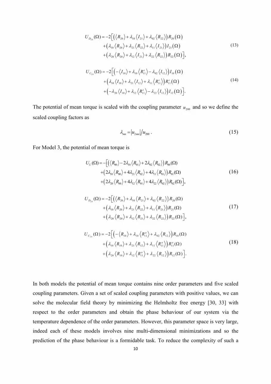
GeoffreyR.Luckhurst

UniversityofSouthampton

370PUBLICATIONS9,104CITATIONS

SEEPROFILE

Availablefrom:RauzahHashim

Retrievedon:03February2016

1

Biaxial nematics with C2h symmetry composed of calamitic particles. A

molecular field theory

Rauzah Hashim,a Geoffrey R. Luckhurst

b* and Hock-Seng Nguan(阮福成)

a,b

aDepartment of Chemistry, University of Malaya, 50603 Kuala Lumpur, Malaysia.

b School of Chemistry, University of Southampton, Highfield, Southampton, SO17 1BJ,

United Kingdom.

PACS number(s): 61.30. Gd,64.70.M-, 61.30.Cz

A molecular field theory of biaxial nematics formed by molecules with C2h point group

symmetry has been developed by Luckhurst et al. and a Monte Carlo computer simulation

study of this model has been performed by Hashim et al.. In these studies the truncated model

pair potential was only applied to molecules whose long axes are taken to be along their C2

rotation axes. The present study extends this work by assuming that the molecular long axis is

now perpendicular to the C2 axis, resulting in there being two possible choices of minor axes.

It considers the phases formed by both cases. The molecular field theory for these models is

formulated and reported here. The theoretical treatment of the present cases gives rise to a

new set of order parameters. So as to simplify the pseudo-potentials only the dominant

second rank order parameters are considered and evaluated to give the phase behaviour of

these truncated models. The predicted phase behaviour is compared with the results from the

molecular field study of the previous model potential.

I. INTRODUCTION

The first molecular field approach to nematic liquid crystals was given by Grandjean [1] in

1917, however this work went largely unnoticed [2]. Many years later, in 1958, Maier and

Saupe [3-5] developed a more detailed and complete molecular field theory. Since then the

Maier-Saupe molecular field approach for the uniaxial nematic phase remains the most

valuable and widely used. Their theory started from a simple pair-interaction for calamitic

molecules involving the orientational dependence of London’s dispersion potential. The

Maier-Saupe approach generates the pseudo-potential for one molecule interacting with an

average field produced by the anisotropic molecular interactions. From this pseudo-potential

* Corresponding author: G.R.Luckhurst@soton.ac.uk

2

the average thermodynamic and structural properties of interest for the nematic phase can be

predicted. The simple theory gives qualitatively good agreement with certain experimental

results [6, 7]. However, quantitatively their theory was found to overestimate many properties,

including the transitional entropy, the nematic-isotropic transition temperature and the

orientational order parameters [7]. Subsequently many simulation studies allowed the

approximations and assumptions in the Maier-Saupe theory to be tested in depth [8-11]. This

has lead to a whole body of research using the simple theory to improve our understanding of

the liquid crystal phases not limited simply to nematics and nematic mixtures [12-14]. Thus,

extensive investigations have been carried out and applied to many other liquid crystal phases

such as smectic A [15, 16], chiral nematic [17] and biaxial nematics [18, 19]. The last

member on this list of phases forms the focus of our investigation.

The biaxial nematic phase was first predicted by Freiser [18] who suggested, based on a

molecular field theory, that non-uniaxial nematic phases might be possible. Since the initial

prediction, there has been a huge interest in both theoretical and experimental studies of this

novel liquid crystal phase as evidenced by recent comprehensive reviews [20, 21]. The

seminal work of Freiser suggested, implicitly, that lath-like molecules with a D2h point group

symmetry could self-organize and form a biaxial nematic phase, also with D2h symmetry.

Subsequently, a theory also based on the molecular field approximation was developed by

Straley to model the biaxial nematic assuming, explicitly, that the component molecules

possessed D2h symmetry [19]. Following these seminal studies [18, 19], there were other

theories [12, 22] and simulations [13, 23, 24] of the biaxial nematic, which assumed that this

phase has D2h symmetry. However, recent NMR investigations of some nematic phases

thought to be biaxial suggested that they could have a lower symmetry, namely C2h [25, 26].

Indeed, following the suggestion by Freiser [18], there has been a number of theories

dedicated to a variety of nematic phases having a range of different point group symmetries,

such as Cnh and Dnh (where n ≥ 2) [27-29]. A succinct discussion on the subject is given in

reference [30]. However, none of these studies considered the application of the molecular

field theory to the C2h biaxial nematic until Luckhurst et al.[30] developed their theory. In

this study, the molecules that constituted the nematic phase were also taken to have C2h point

group symmetry. A more specific model based on molecules formed from four Gay-Berne

particles arranged to have C2h symmetry has been proposed by Gorkunov et al.[31]. This was

found to form uniaxial and D2h biaxial nematic phases but not a C2h biaxial nematic. It would

3

seem that the interaction parameters related to the deviation of the model molecules from

orthorhombic to monoclinic shape proved to be too small for this phase to form.

Subsequently computer simulations of the nematic phases formed by the simpler calamitic

molecules [30] have also been carried out [32] in order to complement the theory.

Within both the molecular field theory and simulations the C2 rotation axis of the calamitic

molecules was taken to be parallel to the molecular long axis, as shown in Fig. 1. In

constructing this idealised shape we start with an orthorhombic molecule with z along the

major axis, y along the larger of the minor axes and x along the smallest of these (see Fig.1).

This hypothetical object is then divided into two halves along the zy plane. These halves are

moved with respect to each other along the y axis to give the C2h shape shown in Fig. 1

together with the coordinate system.

FIG. 1. The definition of the axes for the original orthorhombic molecule and

hypothetical calamitic molecules having D2h and C2h point group symmetry

[30], respectively.

With this location of the axes, a set of nine independent second rank order parameters was

obtained, which reflected the symmetry of the three nematic phases and six intermolecular

coupling parameters. In order to make the molecular field theory of the model more

manageable, the those order parameters which vanish in the high order limit were eliminated

as were the coupling parameters which are responsible for them, as suggested by Sonnet et al.

[33] for molecules with D2h symmetry. One of the main features of this parameterization is

that it preserves the interaction between the calamitic molecules. Thus the alignment of the

molecular z-axis in the nematic phase is stronger compared to the alignment of the other two

minor molecular axes in the nematic phase.

z x

y

4

With this parameterization procedure, the simplified model of Luckhurst et al. [30] could be

related to a molecule with a monoclinic shape and its long axis parallel to the C2 rotational

symmetry axis; we shall refer to this as Model 1. In order to extend this model to other

monoclinic structures, we consider systems where the C2 axis is along one or other of the two

molecular short axes. To do this we shall build on Model 1 [30].

The layout of this paper is the following. In Sec. II we determine the coupling parameters for

molecules with C2h symmetry, where the C2 axis is defined along the x or y molecular axes.

In addition the second rank orientational order parameters for these molecules in the nematic

phases NU, ND2h and NC2h are considered. In Sec. III we construct the nematic Helmholtz

free energy for our models based on the Gibbs entropy. Variational minimisation of the free

energy with respect to the singlet orientational distribution using the analysis proposed by de

Gennes [34] gives the potential of mean torque This method is more general than the Maier-

Saupe approach, but the two results are similar[30, 35]. An extension of the Luckhurst-

Romano [36] parameterization to the C2h model is proposed. In Sec. IV we describe the

programs used to perform the calculations. Our results are given in Sec.V for the order

parameters and the phase maps for the two new simplified models which we call Models 2

and 3. We compare the phase behaviour of these models with that of Model 1 [30] where the

C2 axis is parallel to the molecular long axis. Finally, our conclusions are summarised in Sec.

VI.

II. ORDER PARAMETERS AND COUPLING PARAMETERS

We begin by defining the second rank order parameters needed to identify the three nematic

phases formed from molecules having C2h symmetry with which we are concerned. These

molecules are shown in Fig. 2 and have their C2 rotation axis aligned orthogonal to the

molecular long axis, z; in Model 2 this is along the long minor axis, x, and for Model 3 it is

5

FIG.2. The two models proposed for the monoclinic molecule with the C2 axis orthogonal to

the molecular long axis, z. (a) Model 2 is where the C2 symmetry axis is defined as the long

minor axis, x, and (b) Model 3 is where the C2 symmetry axis is defined as the short minor

axis, y.

along the shortest axis, y. These hypothetical molecules were constructed from the same

initial orthorhombic shape. For Model 2 this was cut in two halves along the xy plane and

then by moving one block with respect to the other along the y axis. This gives the C2h

molecule shown in Fig. 2(a) with the C2 axis along x. For Model 3 the orthorhombic molecule

was again cut into two halves but now one half is moved with respect to the other along the x

axis resulting in the C2 axis being along y as in Fig. 2(b). The orientational order parameters

for these molecules are defined in terms of the averages of the Wigner functions ( )2

pmD Ω

where Ω denotes the Euler angles giving the orientation of the molecular frame in the

laboratory frame described by the director orientations. The subscripts p and m in the order

parameters, 2

pmD , relate to the properties of the phase and the molecules, respectively. The

independent non-zero order parameters depend on the symmetry of the phase and of the

molecules [37]. For our systems we have obtained a set of order parameters for each of the

three distinct nematic phases, namely those with uniaxial, D2h biaxial and C2h biaxial

symmetry for both Models 2 and 3. The two possible sets of order parameters for the two

models and three phases are tabulated in Table 1. These combinations of Wigner function

based order parameters are particularly convenient. Thus in the NU nematic there are just

three non-zero order parameters, on forming the ND2h phase three more order parameters are

added, giving a total of six, and a further three appear for the NC2h nematic, giving a total of

(a) Model 2 (b) Model 3

x

z

y

x

z

y

6

nine. For comparison the corresponding order parameters for Model 1 [30] are given in Table

2.

Phase Second Rank Order Parameters for

Model 2

Second Rank Order Parameters for

Model 3

NU

( )( )

2

00 00

2 2

01 01 0 1

2 2

02 02 0 2

2

2

R D

I D D i

R D D

−

−

=

= +

= +

( )( )

2

00 00

2 2

01 01 0 1

2 2

02 02 0 2

2.

2

R D

R D D

R D D

−

−

=

= −

= +

ND2h ( )( )( )

2 2

20 20 20

2 2 2 2

21 21 2 1 21 2 1

2 2 2 2

22 22 2 2 22 2 2

2

2

2

R D D

I D D D D i

R D D D D

−

− − − −

− − − −

= −

= + + +

= + + +

( )( )( )

2 2

20 20 20

2 2 2 2

21 21 2 1 21 2 1

2 2 2 2

22 22 2 2 22 2 2

2

2

2

R D D

R D D D D

R D D D D

−

− − − −

− − − −

= −

= − + −

= + + +

NC2h ( )( )( )

2 2

10 10 10

2 2 2 2

11 11 1 1 11 1 1

2 2 2 2

12 12 1 2 12 1 2

2

2

2 .

s

I D D i

R D D D D

I D D D D i

−

− − − −

− − − −

= +

= + + +

= + + +

( )( )( )

2 2

10 10 10

2 2 2 2

11 11 1 1 11 1 1

2 2 2 2

12 12 1 2 1 2 12

2

2

2

a

R D D

R D D D D

R D D D D

−

− − − −

− − − −

= −

= + − −

= − + −

Table 1. Definition of the non-zero second rank orientational order parameters for Models 2

and 3, according to the phase symmetry.

Phase Second Rank Order Parameters

NU

( )( )

2

00 00

2 2

02 02 0 2

2 2

02 02 0 2

2

2I

R D

R D D

D D

−

−

=

= +

= −

ND2h ( )( ) ( )( ) ( )

2 2

20 20 20

2 2 2 2

22 22 2 2 22 2 2

2 2 2 2

22 2 2 22 2 222

2

2

2

a

a

D D i

R D D D D

D

I

I D D D i

−

− − − −

− − − −

= −

= + − +

= − − −

NC2h ( )( ) ( )( ) ( )

2 2

20 20 20

2 2 2 2

22 22 2 2 22 2 2

2 2 2 2

22 2 2 22 2 222

2

2

2

a

a

D D i

R D D D D

D

I

I D D D i

−

− − − −

− − − −

= −

= + − +

= − − −

Table 2. Definition of the non-zero second rank orientational order parameters for Model 1

taken from the previous study by Luckhurst et al. [30], and grouped according to the phase

symmetry .

7

According to the molecular field theory proposed by de Gennes the internal energy is given

by products of the dominant order parameters [34]; since he was only concerned with

uniaxial molecules in a uniaxial nematic phase this was fairly simple. However, for

molecules and phases of lower symmetry the situation is more complex. For these we shall

write the internal energy as a sum of invariants formed from the order parameters, 2

pmD , as

[35]

2 2

2

1

2mn pm pn

mnp

U u D D−= − ∑ . (1)

Here the proportionality or coupling parameters have the same form as the intermolecular

interaction coefficients, used in the S-function based expansion of the pair potential [38], to

which they are related.

The form of the coupling parameters is determined by the molecular symmetry [38]. In

Model 1, where the molecular long axis is parallel to the C2 axis and labelled the z-axis [30],

the symmetry elements of the molecules include inversion i, the two-fold rotation along the z-

axis (z)

2C and an xy-reflection plane, xyσ . Using the symmetry arguments given by Stone [38]

m and n in Eq.(1) can only have values of either 0 or ±2. On the other hand, when the C2 axis

is orthogonal to the molecular z-axis as shown in Fig. 2 for Models 2 and 3 , m and n can

have values of 0, ±1 and ±2.

In Model 2 (see Fig. 2(a)), the symmetry elements for a molecule are i, (x)

2C and yzσ , which

give the following relations between the coupling parameters:

210 2 10 201 20 1

211 2 11 21 1 2 1 1

221 2 21 22 1 2 2 1 212 21 2 2 12 2 1 2

220 2 20 202 20 2

222 2 22 22 2 2 2 2

,

,

,

,

.

u u u u

u u u u

u u u u u u u u

u u u u

u u u u

− −

− − − −

− − − − − − − −

− −

− − − −

= = =

= = =

= = = = = = =

= = =

= = =.

(2)

There are then six independent coupling parameters for Model 2 namely200u ,

210u , 220u ,

221u ,

211u and 222u . The total number of independent intermolecular coefficients is, necessarily, the

same as that in the previous model [30]. Similarly for Model 3 the symmetry elements are i,

(y)

2C and xzσ , resulting in slightly different relationships between the coupling parameters,

namely

8

210 2 10 201 20 1

211 2 11 21 1 2 1 1

221 2 21 22 1 2 2 1 212 21 2 2 12 2 2 1

220 2 20 202 20 2

222 2 22 22 2 2 2 2

,

,

,

,

.

u u u u

u u u u

u u u u u u u u

u u u u

u u u u

− −

− − − −

− − − − − − − −

− −

− − − −

= − = = −

= − = − =

= = − = − = = = − = −

= = =

= = =.

(3)

Even though the independent coupling parameters are the same for both Models 2 and 3, the

relationships (see Eqs.(2) and (3)) between them differ in some signs begin to emerge when

considering their reality [30]. To ensure the internal energy is real, that is the condition

*U U= must be satisfied, we require

2 2* ( 1)m n

mn m nu u+− −= − . (4)

In the case of molecules with D2h symmetry [30], all of the independent coefficients are real.

The situation for the C2h Model 1 [30], where the C2 axis is parallel to the long axis, some of

the intermolecular coefficients are complex. In Model 2, 210u and

221u are purely imaginary

while the others are real,

210 210

221 221

*

*

,

.

u u

u u

= −

= −

(5)

Interestingly, we find that for Model 3, all of the coefficients are real because the set of order

parameters defined according to the combination of the Wigner functions for Model 3 are

also real (see Table 1).

III. MOLECULAR FIELD THEORY

Armed with the order parameters and coupling parameters for Models 2 and 3 of molecules

having C2h symmetry we now construct the molecular field theories for them by applying a

methodology analogous to that used by Luckhurst et al. [30]. Initially, the averaged

anisotropic internal energy U of the system is defined using the orientational order

parameters written in terms of Wigner rotation matrices 2

mnD ,

2 2

2

1

2mn pm pn

mnp

U u D D−= − ∑ . (6)

9

Here,

2 2 ( ) ( )mn mnD D f d= Ω Ω Ω∫ ,

(7)

where ( )f Ω is the singlet orientational distribution function. The entropy of the system is

given by the Gibbs entropy formula

( ) ( )lnBS k f f d= − Ω Ω Ω∫ (8)

and Bk is the Boltzmann constant. Combining the results for the internal energy and entropy

we can construct the Helmholtz free energy, A, of the system as

2 2

2

1( ) ln ( ) .

2mn pm pn B

mnp

A u D D k T f f d−= − + Ω Ω Ω∑ ∫ , (9)

where T is the temperature. The unknown singlet orientational distribution function is now

determined by minimizing the free energy with respect to ( )f Ω . This is subject to the

constraints that the distribution function is normalised and that the order parameters are

related to the distribution function by Eq. (7); this process gives the potential of mean torque

as

2 2

2

1( ) ( )

2mn pm pn

mnp

U u D D−Ω = − Ω∑ . (10)

Using the properties of the coupling parameters and orientational order parameters derived in

Sec. II for the two models the potential of mean torque for each model is found to contain

three terms identified as the driving force for the formation of the uniaxial (NU), the D2h

biaxial (ND2h) and the C2h biaxial (NC2h) nematics, namely ( )UU Ω , 2

( )hDU Ω and

2( )

hCU Ω ,

2 2

( ) ( ) ( ) ( )h hU D CU U U UΩ = Ω + Ω + Ω . (11)

The components of the potential of mean torque for Model 2 are

( ) ( )

( ) ( )

( ) ( )

00 10 01 02 02 00

10 00 21 02 11 01 01

20 00 12 01 22 02 02

( ) 2 2

2 4 4

2 4 4 ,

UU R R R R

R R I I

R I R R

λ λ

λ λ λ

λ λ λ

Ω = − + + Ω

+ + + Ω

+ + + Ω

(12)

10

( ) ( )

( ) ( )

( ) ( )

2 20 10 21 02 22 20

10 20 21 22 11 21 21

20 20 12 21 22 22 22

( ) 2

,

hDU R I R R

R R I I

R I R R

λ λ

λ λ λ

λ λ λ

Ω = − + + Ω

+ + + Ω

+ + + Ω

(13)

( ) ( )

( ) ( )

( ) ( )

2 10 10 11 02 12 10

10 10 21 12 11 11 11

20 10 12 11 22 12 12

( ) 2

.

h

s

C

s s

s

U I R I I

I I R R

I R I I

λ λ

λ λ λ

λ λ λ

Ω = − − + − Ω

+ + + Ω

+ − + − Ω

(14)

The potential of mean torque is scaled with the coupling parameter 200u and so we define the

scaled coupling factors as

2 200mn mnu uλ = . (15)

For Model 3, the potential of mean torque is

( )( )( )

00 10 01 02 02 00

10 00 21 02 11 01 01

20 00 12 01 22 02 02

( ) 2 2 ( )

2 4 4 ( )

2 4 4 ( ) ,

UU R R R R

R R R R

R R R R

λ λ

λ λ λ

λ λ λ

Ω = − − + Ω

+ + + Ω

+ + + Ω

(16)

( )( )( )

2 20 10 21 02 22 20

10 20 21 22 11 21 21

20 20 12 21 22 22 22

( ) 2 ( )

( )

( ) ,

hDU R R R R

R R R R

R R R R

λ λ

λ λ λ

λ λ λ

Ω = − + + Ω

+ + + Ω

+ + + Ω

(17)

( )( )( )

2 10 10 11 02 12 10

10 10 21 12 11 11 11

20 10 12 11 22 12 12

( ) 2 ( )

( )

( ) .

h

a

C

a a

a

U R R R R

R R R R

R R R R

λ λ

λ λ λ

λ λ λ

Ω = − − + + Ω

+ + + Ω

+ + + Ω

(18)

In both models the potential of mean torque contains nine order parameters and five scaled

coupling parameters. Given a set of scaled coupling parameters with positive values, we can

solve the molecular field theory by minimizing the Helmholtz free energy [30, 33] with

respect to the order parameters and obtain the phase behaviour of our system via the

temperature dependence of the order parameters. However, this parameter space is very large,

indeed each of these models involves nine multi-dimensional minimizations and so the

prediction of the phase behaviour is a formidable task. To reduce the complexity of such a

11

problem, but at the same time, still to be able to capture the essential physics of the system,

following Sonnet et al. [33] and Luckhurst et al. [30], we assume that those order parameters

which vanish in the high order limit may be set to zero. The order parameters that do vanish

are those for which p ≠ m. To ensure that they remain zero the associated scaled coupling

parameter λmn, linking the order parameter involving m with the angular function containing

n, is set to zero, again when m n≠ . Those remaining terms, which involve p ≠ m, belong to

the dominant order parameters. The remaining order parameters for Model 2 after this

reduction are 00R , 11

sR and 22R , while for Model 3 they are 00R ,

11

aR and 22R . For

Model 1 [30] the surviving order parameters are 00R , 22 22

sR R≡ and 22

aR . For Model 2

in the NC2h phase all three order parameters 00R , 11

aR and 22R

are non-zero, for the ND2h

phase the two order parameters 00R and 22R are non-zero and for the NU phase only 00R

survives. The truncated pseudo-potentials for Models 2 and 3 are

2

trun 00 00 22 22 22 11 11 11( ) ( ) ( ) 2 ( )s sU R R R R R Rλ λ Ω = − Ω + Ω + Ω , (19)

3

trun 00 00 22 22 22 11 11 11( ) ( ) ( ) 2 ( )a aU R R R R R Rλ λ Ω = − Ω + Ω + Ω , (20)

respectively. With these potentials, we write their Helmholtz free energies as

( )22 2 *

200 00 22 22 11 111 2 2 lni iA u R R R T Qλ λ = + + − , (21)

where or i s a= according to the particular model (see, Tables 1 and 2), *T ( )200/Bk T u≡ is the

scaled temperature and Q is the orientational partition function

( )*

trunexp ( )jQ U T d= − Ω Ω∫ , (22)

Here j = 2 or 3 depending on which system we are considering (see Eqs. (19) and (20),

respectively). With this parameterization procedure, the behaviour of the system can be

calculated more easily and depends on only the two scaled coupling parameters 11λ and

22λ .

12

IV. COMPTUTAIONAL DETAILS

The numerical minimization of the Helmholtz free energy was performed using a FORTRAN

program, compiled by the gfortran compiler in LINUX, which also incorporates subroutines

provided by Numerical Recipes [39]. The algorithm used in the minimization program is the

Broyden-Fletcher-Goldfarb-Shanno (BFGS) algorithm. This applies to the quasi-Newton

method, where the approximated Hessian was used in calculating the direction, on the free

energy surface, along which the free energy would decrease to its local minimum. In addition,

the numerical integration employed in calculating the partition function and the first

derivatives of the free energy with respect to the three order parameters, needed to ensure that

a minimum has been reached, is based on the Gaussian quadrature method [39].

V. RESULTS AND DISCUSSION

The first step in our study of the nematic phases formed by Models 2 and 3 was the selection

of the scaled coupling parameters 11λ and

22λ in the respective potentials of mean torque. We

were guided in our choice by the values of the analogous parameters sλ and

aλ used in the

calculations for Model 1 [30]. Here sλ is equivalent to

22λ and drives the formation of the

ND2h phase; in the original calculations it was given the values 0.2, 0.3 and 0.4, accordingly

we shall use the same values for the new models. The second parameter aλ drives the

formation of the NC2h phase and was allowed to vary continuously over the range from 0 to

0.6; this was found to reveal a rich phase behaviour [30]. Its analogue for the new models is

the scaled coupling parameter,11λ , which has been studied over the same range. However, we

should note that the values of the coupling parameters for the idealised molecules in the three

models are certainly different. Unfortunately it is difficult, even knowing the dimensions of

these simple objects (see Figs. 1 and 2) to estimate the coupling supertensor, u2mn, indeed,

based on the excluded volumes, this must be undertaken numerically [40]. None the less it

might be expected that for similar and small displacements of the blocks used to construct the

C2h molecules that the coupling tensor components u200 and u2mn will be similar for the three

model molecules. It is not so easy to assess the similarity for the tensor components that drive

13

the formation of the NC2h phase for these three models but given the manipulation of the half

blocks they might well be expected to be similar.

For the particular ranges of the coupling parameters 11λ and

22λ , we have minimized,

numerically, the Helmholtz free energy in Eq. (21) at a selection of scaled temperatures by

varying the order parameters 00R , 11

sR and 22R . The most stable state was achieved for

the set of order parameters giving a global minimum of the free energy. These calculations

gave the temperature dependence of the orientational order parameters for particular choices

of 11λ and

22λ . The scaled temperature at which the order parameter defining the lower

temperature phase passes from zero to non-zero is identified as the transition temperature.

The order of this transition is determined by whether the change in the defining order

parameter is discontinuous (first order) or continuous (second order) within the

computational error.

From our results it was found that, for the same values of 11λ and

22λ , the phase behaviour of

Models 2 and 3 are quantitatively the same. This is to be expected since both models have the

C2 axis orthogonal to the molecular long axis. This equivalence is shown analytically using

the molecular field theory approach in the Appendix. In view of this we shall only consider

the results for Model 2. Never the less, at a practical level even for the same values of 11λ and

22λ , the shapes of the constituent molecules for the two models are expected to differ.

However, it is not our major concern in this paper to take account of how the molecular shape

changes but to explore how the phase behaviour changes with the orientation of the C2 axis

with respect to the molecular long axis.

14

(a) (d)

(b) (e)

(c) (f)

FIG. 3. The phase maps calculated from the truncated potential of mean torque for Model 2.

These show the transition temperatures and phase sequences when the scaled coupling

coefficient,11λ , varies from 0 to 0.6, while

22λ is fixed at (a) 0.2, (b) 0.3 and (c) 0.4. In

addition, (d), (e) and (f) show the phase maps for Model 1 when sλ is equal to 0.2, 0.3 and

0.4, respectively (adapted with permission from ref.[30]). The dashed lines indicate second

order phase transitions and the solid lines show first order phase transitions; the red circles

denote the associated tricritical points.

15

The phase maps show how the transition temperatures between the phases change with the

variation in one of the scaled coupling parameters occurring in the potential of mean torque;

they are given in Fig. 3. Those for Model 2 appear in (a), (b) and (c) where 11λ is varied

continuously while 22λ is held fixed at 0.2, 0.3 and 0.4 for the plots in Fig. 3(a), (b) and (c),

respectively. We start our discussion of these maps with that in Fig. 3(a) where 22λ is 0.2. For

11λ of zero the system shows the phase sequence ND2h – NU – I where the transition

temperatures are in agreement with those obtained previously [30, 33]. These do not change

as 11λ increases since the truncated versions of the potentials of mean torque, ( )UU Ω and

( )2 hDU Ω , do not depend on this coupling parameter (see Eq. (19)). However, as

11λ grows so

the NC2h phase is introduced into the map and increases in extent so that the phase sequences

NC2h – ND2h – NU – I, NC2h – NU – I and NC2h – I are observed. In addition, the NU – I

transition is first order whereas the ND2h – NU transition is second order, as expected [30, 33].

In contrast the NC2h – ND2h transition is second order for 11λ less than about 0.14 and then

becomes first order as is the NC2h – I transition.

The behaviour found for Model 2 with this particular parameterisation contrasts dramatically

with that found previously for Model 1 having a comparable choice of coupling parameters

[30]. The phase map for this is shown in Fig. 3(d) and reveals a new biaxial nematic labelled

ND2h(⊥) not found for Model 2. An idealised structure of this new phase is sketched in Fig.

(a) (b)

(c) (d)

16

FIG. 4. The idealised organisation of the molecules for Model 1 in (a) the ND2h(⊥) phase and

(b) the ND2h(‖) phase. (Adapted with permission from [30]). The associated composite

structures are formed by combining two molecules and shown in cross section, orthogonal to

their C2 axis, in (c) for ND2h(⊥) and (d) for ND2h(‖).

4(a) where it is seen that the equivalent short axes of neighbouring molecules are orthogonal.

In addition, the long C2 axes are antiparallel which is required because the phase has D2h

point group symmetry. For comparison we also show the idealised structure of the ND2h(‖)

phase in Fig. 4(b). Again the C2 axes of half the molecules are antiparallel to those of the

other half but now the minor axes are parallel. The key stabilising feature for these two ND2h

phases is that the molecular long axes are either parallel or anti-parallel. Another insight into

the structure of these two phases can be obtained from the composite structure formed by

merging two molecules having their C2 axes antiparallel [28, 30]. The orientation of the short

axis of one molecule with respect to the other is rotated, internally [29], by 180º to give the

structure shown as the cross section perpendicular to the C2 axis in Fig. 4(d) for the ND2h(‖)

phase and when the internal rotation is 90º the composite structure, given in Fig. 4(c), also

has D2h symmetry for the ND2h(⊥) phase.

We can use the same approach to see why it is not possible for Model 2 to form the ND2h(⊥)

phase. Since this phase has D2h point group symmetry, then in the idealised structure the C2

axes of half the molecules must be antiparallel to those of the other half. In such a three

dimensional structure, shown in Fig. 5(a), where a short and a long axis can both be parallel

the structure is stable, giving what is, in effect, the ND2h(‖) phase. However, for the case

when the short axes are perpendicular the long axes must also be perpendicular, as we can see

in Fig. 5(b), and it is this orthogonality which destabilises the ND2h(⊥) phase. The composite

structures formed from pairs of molecules with their C2 axes antiparallel also provide a

simple image to understand the stability as well as the symmetry. They are shown in Fig. 5(c)

where one short and the long axes are parallel and in Fig. 5(d) where the same axes are now

orthogonal; both structures are seen to have structures with D2h point group symmetry.

17

(a) (b)

(c) (d)

FIG. 5. The idealised organisation of the molecules for Model 2 in (a) the ND2h(‖) phase

and (b) the ND2h(⊥)phase. The composite structures, associated with the phase structures, are

formed by combining two molecules and shown in cross section, orthogonal to their C2 axis,

(c) for ND2h(‖). and (d) for ND2h(⊥)

However, it is also apparent from these two composite structures that their anisotropies are

significantly different. This is large for that in Fig. 5(c) leading to the stability of the ND2h(‖)

phase but for that in Fig.5(d) it is small leading to the instability of the ND2h(⊥) phase. As a

consequence we believe that, unlike Model 1, the ND2h(⊥) structure is not observed by Model

2 as long as it remains calamitic; that is the C2 axis is orthogonal to the molecular long axis..

In the next set of calculations for Model 2 the biaxiality coupling parameter, 22λ , was

increased to 0.3 and the phase map for this system is shown in Fig. 3(b). The phases formed

are the same as those seen in Fig. 3(a) but, as expected, the stability of the ND2h phase has

increased at the expense of the uniaxial nematic; indeed there is just a narrow band of NU

remaining. Both the NU – I and the ND2h – NU phase transitions are now predicted to be first

order, in keeping with previous studies [30, 33]. Transitions from the NC2h to the ND2h phase

are found to exhibit tricritical behaviour but after the tricritical point at 11λ of about 0.19 the

18

transitions from the NC2h to the ND2h phase and then to the isotropic phase are first order. For

comparison the phase map for Model 1 calculated with the same value of 22λ and for the

analogous parameter aλ which drives the formation of the NC2h phase is shown in Fig. 3(d).

It is clear that there is a strong similarity between these phase maps for the two models and

we shall return to this similarity later.

The final set of calculations was performed for Model 2 with 22λ set equal to 0.4; the

resultant phase map is given in Fig. 3(c). It is seen that for this large value of the scaled

biaxial coupling parameter the NU phase has been replaced entirely by the ND2h phase so that

there are just two phase sequences NC2h – ND2h – I and NC2h – I. The NC2h – ND2h phase

transition is second order except just before the onset of the NC2h – I transition which is first

order. The phase behaviour of Model 2 turns out to be essentially equivalent to that observed

for Model 1 over a comparable range of the coupling parameter driving the formation of the

NC2h phase.

To see just how similar such phase maps are we have studied the temperature dependence of

the order parameters for Model 2 and Model 1 for the same value of 22λ (

sλ≡ ) of 0.3 and for

11λ ( aλ≡ ) equal to 0.15 (see Fig. 6) and 11λ ( aλ≡ ) equal to 0.4 (see Fig. 7). Fig. 6 shows the

phase sequence NC2h – ND2h – NU – I. The results for the two order parameters, 00R and

22R , are essentially the same and indeed this has to be the case since the potentials of mean

torque are identical. However, in the NC2h phase the defining order parameters 11

sR and

22

aR are slightly different causing the shift in the NC2h – ND2h transition temperature to a

slightly higher value for Model 2. On the other hand, parameterization with a higher value of

11λ ( aλ≡ ), i.e. equal to 0.4 (see Fig. 7), gives the simple phase sequence NC2h– I. The order

parameters for this parameterization are presented separately according to the different order

parameter definitions so as to make the comparison clearer, since the values of these order

parameters come close to each other for this parameterization. Fig. 7 shows that Model 2 has,

again, a higher NC2h - I transition temperature.

19

FIG. 6. The scaled temperature dependence of the orientational order parameters for Model 1

( 00R , 22R and 22

aR ) and Model 2 ( 00R , 22R and 11

sR ) for 22λ (

sλ≡ ) = 0.3 and for 11λ

(aλ≡ ) = 0.15. The blue lines are given for Model 1, while red is for Model 2.

FIG. 7. The scaled temperature dependence of the orientational order parameters for Model 1

( 00R ,22

sR and 22

aR ) and Model 2 ( 00R , 22R and 11

sR ) for 22λ (

sλ≡ ) = 0.3 and for 11λ

(aλ≡ ) = 0.4. The blue lines are given for Model 1, while red are given for Model 2. (a) 00R

versus T*. (b) 22

sR and 22R versus T*. (c) 22

aR and 11

sR versus T*.

(a) (b)

(c)

20

The nature of these phase transitions is of interest. To determine the order of the transitions,

we have performed calculations at temperatures close to them. If an order parameter vanished

discontinuously over a series of temperatures near the transition temperature, the phase

transition was assigned as first order. If the order parameter vanished continuously, then it

was taken to be second order [30]. Our calculations show that the transition of NC2h to ND2h

was second order provided that 11λ was lower than 0.14 which is approximately the tricritical

point, while the phase transition from NC2h to ND2h is found to become first order in the

range 110.14 0.20λ≤ < of the scaled coupling parameter. The results also showed that the

phase transition from NC2h to NU is always first order. This behaviour is significantly

different from that predicted by Model 1 where 0.2sλ = (sλ in ref. [30] is comparable to

22λ

in this study). Here the phase transition from NC2h to ND2h had been predicted to be always

second order [30]. In addition, Model 1 also predicted that the phase transition from NC2h to

NU only occurred at one point when 0.2aλ = (aλ in ref. [30] is comparable to

11λ in this

study). For 0.2aλ > , Model 1 predicts a phase transition from NC2h to ND2h(⊥), followed by a

transition from ND2h(⊥) to either NU or I (see Fig. 3 (d)). The tricritical point for the model

was found to be located on the ND2h(⊥) - NU transition line where aλ is about 0.31; this is

considerably higher than the value of the tricritical point for Model 2.

As we have seen the scaled coupling parameters 11λ and

22λ can be related to the geometrical

properties of the molecule itself. One approach that can be used to establish this relationship

is through the excluded volume methodology suggested by Straley [19]; although his

approach is not strictly analytical even for orthorhombic shaped molecules. It is certainly

not feasible for the monoclinic shapes. Another problem for this approach is that, the

monoclinic shapes cannot be easily generalised as those with orthorhombic shape. So it is

difficult to establish whether the relationship of 11λ and

22λ in Model 2 to the aλ and

sλ in

Model 1, is exact or not. Never the less, qualitatively 22λ gives the degree of deviation of the

molecular shape from rod-like to orthorhombic while 11λ indicates how strongly the molecule

deviates from orthorhombic to monoclinic symmetry.

The ND2h(‖) phase exhibited by Model 1 has a biaxial D2h arrangement where the minor

axes are parallel to each other (see Fig. 4(b)), which is equivalent to the ND2h phase of Model

2. For the ND2h(⊥) phase (see Fig. 4(a)), the biaxial D2h arrangement is such that the minor

21

axes are orthogonal to each other. Our Model 2 does not give this type of biaxial phase

because one of the minor axes in Model 1 has become the principal axis in Model 1, which

by the Sonnet et al.[33] parameterization scheme, the principal axes of molecules in the

nematic phase always tend to be parallel to each other in the ND2h phase, hence the ND2h(⊥)

is not able to form in Model 2. The results given in Fig. 3 suggest that the phase behaviour

predicted by Model 1 are similar to those for our model as long as the value chosen for sλ

was not in the region where the ND2h(⊥) phase would appear.

VI. CONCLUSION

Generic models of mesogenic molecules with C2h point group symmetry which differ from

Model 1 developed by Luckhurst et al.[30] have been formulated based on different

orientations of the C2 molecular axes with respect to the molecular long axis. These models

have resulted in different identifications of the dominant second rank orientational order

parameters and the coupling parameters, where at one point, all of the intermolecular

coefficients become real. These models, based on the parameterization suggested by Sonnet

et al. [33] and used by Luckhurst et al. [30], can be employed to describe the anisotropic

interactions between molecules having a monoclinic shape with their long molecular axes

orthogonal to the C2 symmetry axis, in contrast Model 1 describes the case where the long

axis is parallel to the C2 symmetry axis. Based on these models, the molecular field theory for

their nematic phases has been developed. This theory contains nine non-zero second rank

order parameters and six non-zero coupling parameters which makes the numerical solution

of the theory a formidable task. Of the nine order parameters just three are dominant and so

are retained. The phase behaviour of Model 2 for 22 0.2, 0.3 and 0.4λ = with a range of values

for11λ have been calculated and shown as a phase map. We find that Models 2 and 3 we have

proposed are equivalent to each other in term of their phase behaviour when both share the

same value of 11λ and

22λ .This similarity can be demonstrated analytically under the

theoretical frame work of the molecular field theory. Never the less, even when the two

models shared the same values of 11λ and

22λ , both models can correspond to different shapes.

In marked contrast to Model 1 [30], our two models do not exhibit the ND2h(⊥) phase

exhibited by this model. This striking difference in phase behaviour occurs because for the

ND2h(⊥) phase of Model 1 the long axes are anti-parallel and so the configuration is stable.

22

However, if Model 2 or 3 were to form the novel ND2h(⊥) phase then with the C2 symmetry

axis orthogonal to the long axis in the molecule the long axes in neighbouring molecules

would also have to be orthogonal which would consequently destabilise the phase. Our

models offer an additional and simple way to describe the monoclinic biaxial phase, which

was appreciated but not considered by the previous study [30].

ACKNOWLEDGEMENTS

The Authors would like to thank the University of Malaya (RG072-09AFR) and the Ministry

of Higher Education UM.C/625/1/HIR/MOHE/05 for various grants which supported this

project. HSN also acknowledges a grant from Emeritus Professor G. R. Luckhurst which

enabled him to spend six months at the University of Southampton. Generous allocations of

computing resources from the University of Malaya and the University of Southampton are

acknowledged.

APPENDIX

Our aim here is to show why and under what conditions the phase behaviour of Models 2 and

3 should be equivalent. The scaled potential of mean torque for Model 2 is

2

00 00 22 22 22 11 11 11( ) ( ) 2 ( ) 2 ( )s sU R R R R R Rλ λ Ω = − Ω + Ω + Ω , (A.1)

while for Model 3 it is

3

00 00 22 22 22 11 11 11( ) ( ) 2 ( ) 2 ( )a aU R R R R R Rλ λ Ω = − Ω + Ω + Ω . (A.2)

The superscripts 1 and 2 on the U need to be replaced by 2 and 3, respectively. In addition in

these two equations the terms in λ11 and λ22 should be exchanged as well as in Eqs (A.7),

(A.8) and (A.9).

Here the angular functions associated with the dominant order parameters (see Table 1) are

2

00

11

11

2

22

1( ) (3cos 1)

2

( ) cos cos cos cos 2 sin sin

( ) cos cos 2 cos cos sin sin

1 cos( ) cos 2 cos 2 cos sin 2 sin 2

2

,

,

,

.

s

a

R

R

R

R

β

α β γ β α γ

α β γ β α γ

βα γ β α γ

Ω = −

Ω = −

Ω = −

+Ω = −

(A.3)

From the trigonometric identities

23

cos( ) sin2

cos[2( )] cos(2 ) cos 22

sin( ) cos2

sin[2( )] sin(2 ) sin 22

,

,

,

.

x x

x x x

x x

x x x

π

ππ

π

ππ

± =

± = ± =

± = ±

± = ± = −

∓

(A.4)

the transformations 2

πα α→ + and

2

πγ γ→ − ( or

2

πα α→ − and

2

πγ γ→ + ), leave

00 ( )R Ω

and 22 ( )R Ω unchanged in Eq(A.3) while the two terms 11( )sR Ω and 11( )aR Ω , would be

exchanged i.e. 11 11( ) ( )s aR RΩ ↔ Ω .

Based on these relations, we now show that, the two models are equivalent within the

theoretical frame work of the molecular field theory. We start with the molecular field theory

for Model 2 and later show that this model is equivalent to that for Model 3.

The partition function for Model 2, Q, is

( )2 *exp ( )Q U T d= − Ω Ω∫ . (A.5)

With this partition function the order parameters predicted by Model 2 can be written as

( )

( )

( )

2 *

00 00

2 *

22 22

2 *

11 11

1( )exp ( )

1( )exp ( )

1( )exp ( )

,

,

,s s

R R U T dQ

R R U T dQ

R R U T dQ

= Ω − Ω Ω

= Ω − Ω Ω

= Ω − Ω Ω

∫

∫

∫

(A.6)

From the partition function, we observe that

( )( )( )

2 *

*

00 00 22 22 22 11 11 11

*

00 00 22 22 22 11 11 11

exp ( )

exp ( ) 2 ( ) 2 ( ) /

exp ( ) 2 ( ) 2 ( ) / .

s s

s s

Q U T d

R R R R R R T d

R R R R R R T d

λ λ

λ λ

= − Ω Ω

= − Ω + Ω + Ω Ω

′ ′ ′ ′= − Ω + Ω + Ω Ω

∫∫∫∫

∫∫∫

(A.7)

where , ,2 2

π πα β γ ′Ω = + +

. Further manipulation of Eq.(A.7), based on the earlier

observation made in Eqs.(A.3), we obtain

24

( )( )

*

00 00 22 22 22 11 11 11

*

00 00 22 22 22 11 11 11

exp ( ) 2 ( ) 2 ( ) / ( ) cos ( )2 2

exp ( ) 2 ( ) 2 ( ) / cos .

s s

s a

Q R R R R R R T d d d

R R R R R R T d d d

π πλ λ α β γ

λ λ α β γ

′ ′ ′= − Ω + Ω + Ω + +

= − Ω + Ω + Ω

∫∫∫

∫∫∫

(A.8)

We denote the new expression in the exponent in Eq.(A.8) as ( )U ′ Ω , i. e.

00 00 22 22 22 11 11 11( ) ( ) 2 ( ) 2 ( )s aU R R R R R Rλ λ ′ Ω = Ω + Ω + Ω . (A.9)

With the same process used in Eqs.(A.7) and Eq.(A.8) we obtain,

( )

( )

( )

*

00 00

*

22 22

*

11 11

1( )exp ( )

1( )exp ( ) ,

1( )exp ( ) .

,

s a

R R U T dQ

R R U T dQ

R R U T dQ

′= Ω − Ω Ω

′= Ω − Ω Ω

′= Ω − Ω Ω

∫

∫

∫

(A.10)

Since,

( )*

11 11

1( ) exp ( )a aR U T d R

Q′Ω − Ω Ω =∫ , (A.11)

and in molecular field theory 11

sR can be regarded as a parameter given by the self-

consistency equation in Eq.(A.6), we can redefine or replace the parameter 11

sR by 11

aR .

With this replacement we have shown that in terms of molecular field theory, given the same

values of the scaled coefficients 11λ and

22λ , Models 2 and 3 will have exactly the same phase

behaviour.

[1] F. Grandjean, C. R. Acad. Sci., 164, 280 (1917).

[2] T. J. Sluckin, D. A. Dunmur and H. Stegemeyer, Crystals that Flow, (Taylor & Francis Inc., London

and New York, 2004) p. 333.

[3] P. Maier and A. Saupe, Z. Naturforsch., A13, 564 (1958).

[4] P. Maier and A. Saupe, Z. Naturforsch., A14, 882 (1959).

[5] P. Maier and A. Saupe, Z. Naturforsch., A15, 287 (1960).

[6] G. R. Luckhurst and C. Zannoni, Nature, 267, 412 (1977).

[7] G. R. Luckhurst, The Molecular Physics of Liquid Crystals, edited by G. R. Luckhurst and G. W. Gray

(Academic Press, London, 1979) Chap. 4.

[8] P. A. Lebwohl and G. Lasher, Phys. Rev. A, 6, 426 (1972).

[9] H. J. F. Jansen, G. Vertogen and J. G. J. Ypma, Mol. Cryst. Liq. Cryst., 38, 87 (1977).

[10] G. R. Luckhurst, S. Romano and P. Simpson, Chem. Phys., 73, 337 (1982).

[11] G. J. Fuller, G. R. Luckhurst and C. Zannoni, Chem. Phys., 92, 105 (1985).

[12] R. Alben, J. Chem. Phys., 59, 4299 (1973).

[13] R. Hashim, G. R. Luckhurst and S. Romano, Mol. Phys., 53, 1535 (1984).

25

[14] R. Hashim, G. R. Luckhurst and S. Romano, Liq. Cryst., 1, 133 (1986).

[15] W. L. McMillan, Phys. Rev. A, 4, 1238 (1971).

[16] W. L. McMillan, Phys. Rev. A, 6, 936 (1972).

[17] W. J. A. Goossens, Mol. Cryst. Liq. Cryst., 12, 237 (1971).

[18] M. J. Freiser, Phys. Rev. Lett., 24, 1041 (1970).

[19] J. P. Straley, Phys. Rev. A, 10, 1881 (1974).

[20] B. Roberto, L. Muccioli, O. Silvia, M. Ricci and C. Zannoni, J. Phys. Condens. Mat., 20, 463101

(2008).

[21] C. Tschierske and D. J. Photinos, J. Mater. Chem., 20, 4263 (2010).

[22] A. Ferrarini, G. R. Luckhurst, P. L. Nordio and S. J. Roskilly, Chem. Phys. Lett., 214, 409 (1993).

[23] A. G. Vanakaras, A. F. Terzis and D. J. Photinos, Mol. Cryst. Liq. Crys. A, 362, 67 (2001).

[24] A. Galindo, A. J. Haslam, S. Varga, G. Jackson, A. G. Vanakaras, D. J. Photinos and D. A. Dunmur, J.

Chem. Phys., 119, 5216 (2003).

[25] P. K. Karahaliou, A. G. Vanakaras and D. J. Photinos, J. Chem. Phys., 131, 124516 (2009).

[26] S. D. Peroukidis, P. K. Karahaliou, A. G. Vanakaras and D. J. Photinos, Liq. Cryst., 36, 727 (2009).

[27] N. Boccara, Ann. Phys., 76, 72 (1973).

[28] T. C. Lubensky and L. Radzihovsky, Phys. Rev. E, 66, 031704 (2002).

[29] B. Mettout, Phys. Rev. E, 74, 041701 (2006).

[30] G. R. Luckhurst, S. Naemura, T. J. Sluckin, T. B. T. To and S. Turzi, Phys. Rev. E, 84, 011704 (2011).

[31] M. V. Gorkunov, M. A. Osipov, A. Kocot and J. K. Vij, Phys. Rev. E, 81, 061702 (2010).

[32] R. Hashim, G. R. Luckhurst and H. S. Nguan, in preparation.

[33] A. Sonnet, E. Virga and G. Durand, Phys. Rev. E, 67, (2003).

[34] P. G. de Gennes, The Physics of Liquid Crystals 1st ed. (Oxford University Press, Oxford, 1974)

Chap. 2.

[35] G. R. Luckhurst, Liq. Cryst., 36, 1295 (2009).

[36] G. R. Luckhurst and S. Romano, Mol. Phys., 40, 129 (1980).

[37] C. Zannoni, The Molecular Physics of Liquid Crystals, edited by G. R. Luckhurst and G. W. Gray

(Academic Press, London 1979) Chap. 3.

[38] A. J. Stone, The Molecular Physics of Liquid Crystals, edited by G. R. Luckhurst and G. W. Gray

(Academic Press, London, 1979) Chap. 2.

[39] W. H. Press, S. A. Teukolsky, W. T. Vetterling and B. P. Flannery, Numerical Recipes in Fortran 77:

The Art of Scientific Computing, 2nd ed. (Cambridge University Press, New York, 1997) Chap. 10.

[40] F. Bisi and R. Rosso, European Journal of Applied Mathematics, 23, 29 (2012).

26