1

Bidirectional Best-fit Heuristic for Orthogonal

Rectangular Strip Packing

Önder Barış Aşık

Yeditepe University

Department of Computer Engineering

İnönü Cad. Kayışdağı Mah.

34755 Kadıköy/İstanbul TurkeyTel: +90 216 578 0423

Fax: +90 216 578 0400

oasik @cse.yeditepe.edu.tr

Ender Özcan (corresponding author)*

ASAP Research Group

School of Computer Science

University of Nottingham

Jubilee Campus, Wollaton Road, Nottingham NG8 1BB UKTel: +44 216 578 0423

Fax: +44 216 578 0400

exo@cs.nott.ac.uk

2

Abstract In a non-guillotinable rectangular strip packing problem (RF-SPP), the best orthogonal

placement of given rectangular pieces on a strip of stock sheet having fixed width and infinite

height are searched. The aim is to minimize the height of the strip while including all the pieces in

appropriate orientations. In this study, a novel bidirectional best-fit heuristic (BBF) is introduced

for solving RF-SPPs. The proposed heuristic as a new feature considers the gaps in both horizontal

and vertical directions during the placement process. The performance of BBF is compared to

some previous approaches, including one of the best heuristics from the literature. BBF achieves

better results than the existing heuristics and delivers a better or matching performance as

compared to the most of the previously proposed meta-heuristics for solving RF-SPPs.

Keywords Heuristic, sequencing, strip packing, non-guillotine cutting

Abbreviations

BBF, bidirectional best-fit heuristic;

SPP, rectangular strip packing problem;

RF, non-guillotinable, variable orientation subtype;

RF-SPP non-guillotinable, variable orientation (orthogonal) SPP

GA, genetic algorithm;

SA, simulated annealing;

GRASP, greedy randomized adaptive search procedure

BF, best fit heuristic;

BL, bottom left heuristic;

iBL, improved bottom left heuristic;

BLF, bottom left fill heuristic;

3

1 Introduction

Cutting and packing a given stock material are crucial processes in manufacturing

and producing. Paper, plastic, wood, glass, steel and leather are some of the most

commonly used stock materials in the industries. Different types of cutting and

packing problems arise due to the nature of the stock material, such as different

constraints and objectives. For example, regular shapes are to be cut in the paper

industry while irregular shapes are to be cut in the leather and textile industries.

Surveys on the cutting and packing problems can be found in Hinxman (1980),

Sarin (1983), Dyckoff (1990), Hässler and Sweeney (1991), Dowsland and

Dowsland (1992), Hopper and Turton (2001b) and Lodi, Martello and Monaci

(2002).

1.1 Problem definition

Solving a rectangular strip packing problem (SPP) requires a search for the best

placement of a set of rectangles with given widths and heights in a suitable

orientation on a strip of rectangular stock sheet with a fixed width and an infinite

height. The ultimate objective is minimizing the wastage while maximising the

material utilization. Based on the recent categorization of the cutting and packing

problems provided by Waescher, Haussner and Schumann (2007), SPP is

identified as two-dimensional, open dimension problem. If the rotation of

rectangles by 90-degrees is allowed and guillotine cutting (edge-to-edge) is not

required as constraints during the placement process, this type of problems is

referred to as RF subtype (Lodi, Martello, Vigo 1999 and Bortfeld 2006). In this

paper, a new heuristic is presented for solving orthogonal rectangular strip

packing problem of RF subtype. Orthogonal placement requires the sides of the

rectangles to be parallel to the edges of the strip. The ultimate objective is to

minimise the height of the strip on which all rectangles will be oriented without

any overlaps.

For defining the problem more formally, the following notation is used:

S is the stock sheet having a width of W and its bottom left and right

corner at locations (0, 0) and (W, 0), respectively.

4

R is the set of n rectangles to be placed; R ={r1,…, ri,…, rn}, where ri is

the ith rectangle with a width and height of (wi, hi); wi, hi Z+ and

min{wi, hi}≤W, for 1≤i≤n.

90-degrees of rotations are allowed during the placement. Let ( ii hw , ) be

the width and height of the ith rectangle after the placement. If the ith

rectangle is not rotated, then iw= wi and ih= hi. If it is rotated by 90-

degrees, then iw= hi and ih= wi.

region(ri) represents the region covered by the ith rectangle and its bottom

left corner at location (xi, yi) within the coordinate system of S after the

placement, where yi 0 and 0≤ xi ≤W.

In an RF subtype orthogonal rectangular strip packing problem (RF-SPP), the goal

is to place all rectangles in R onto S in such a way that

}}{maxmin{1 iini

hy

(1)

subject to

region(ri) region(rj)= , for 1≤i, j ≤n and ij.

1.2 Previous work

There are exact and inexact approaches in literature for RF-SPP. Beasley (1985a,

1985b) investigated tree-search for the non-guillotine cutting case and dynamic

programming approaches for the guillotine cutting case, respectively. Martello,

Monaci and Vigo (2003) proposed an exact approach based on a branch and bound

algorithm, while Lesh et al. (2004) combined a pruning method with a branch and

bound scheme for solving a subset of small RF-SPPs. Kenmochi et al. (2007) also

used a branch and bound approach, where branching is based on two placement

schemes and bounding operations are based on dynamic and linear programming.

As the number of rectangles to pack grows, exact approaches become impractical.

Due to the NP-hard nature of SPP (Garey and Johnson, 1979), researchers have

been investigating meta-heuristics, hyper-heuristics and heuristics as inexact

approaches to obtain near optimal solutions. Dagli and Poshyanonda (1997)

proposed two different hybrid approaches based on artificial neural networks for

solving RF-SPPs. Simulated annealing, tabu search and the genetic algorithms are

the most commonly used meta-heuristics in previous studies (Jakobs 1996, Liu and

Teng 1999, Hopper and Turton 2001a, 2001b, Burke, Kendall and Whitwell 2004,

5

2006). Beltran et al. (2004) hybridize greedy randomized adaptive search

procedure (GRASP) and variable neighbourhood search to solve different subtypes

of strip packing problems. A hyper-heuristic is a high level (meta-)heuristic that

explores the search space generated by a set of low level heuristics for choosing,

adapting and/or learning them (Ozcan, Bilgin and Korkmaz 2008 and Burke et al.

2003). Garrido and Riff (2007), Terashima-Marin, Moran-Saavedra and Ross

(2005), Terashima-Marin, Flores-Alvarez and Ross (2005) evolved sequences of

packing heuristics using a genetic algorithm and a classifier system, respectively,

that were used as a hyper-heuristic for solving RF-SPPs. Imahori, Yagiura and

Ibaraki (2005) investigated multi-start local search and iterated local search

approaches using different neighbourhood operators. Their experimental results

showed that the iterated local search performed better. Bortfeldt (2006)

experimented with a genetic algorithm for solving a variety of SPPs having

different constraints. Alvarez-Valdes, Parreno and Tamarit (2008) successfully

applied their GRASP approach for solving strip packing problems subject to

different constraints.

Zhang, Kang and Deng (2006) described a divide and conquer heuristic (HR)

with a worst case running time complexity of O(n3). Most commonly known

greedy heuristics with polynomial time worst case running times are: the bottom-

left (BL), the bottom-left-fill (BLF) and the best-fit (BF) proposed by Baker

(1980), Chazelle (1983) and Burke, Kendall and Whitwell (2004), respectively.

Both former heuristics are blind placement heuristics, while the latter is a smart

one. In BL and BLF, a location is determined for each rectangle from a list

provided successively in a predefined order. On the other hand, BF makes

informed decisions on which shape to place next. Lesh et al. (2005) proposed a

stochastic heuristic (BLD*) that attempts to improve bottom-left-fill approach by

perturbing the order of rectangles and moving towards a better sequence of

rectangles. In this study, these heuristics will be given focus.

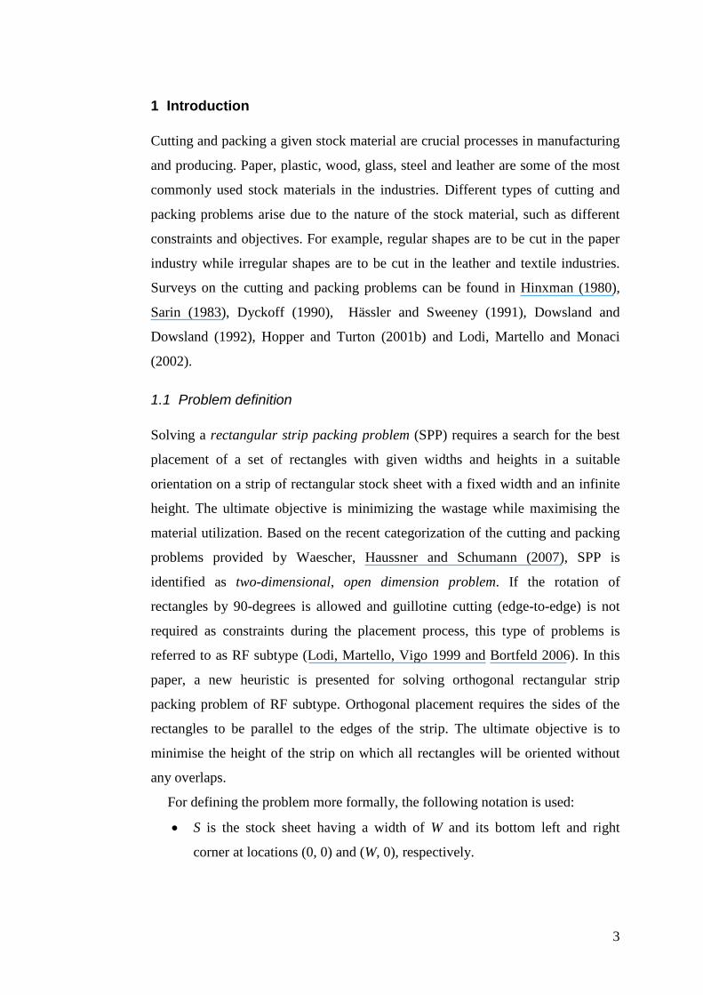
BL heuristic as described by Jakobs (1996), and illustrated in Figure 1 (a), starts

at the upper corner of the object, then the piece slides vertically, all the way down,

until it hits another piece. It continues sliding to the left (in straight line) as far as

possible. A sequence of down and left movements is repeated until the piece

reaches a stable position. Liu and Teng (1999) improved the BL heuristic to be

used as decoder based on permutation representation in meta-heuristics. Improved

6

BL (iBL), instead of moving a piece all the way and straight to the left, keeps

sliding it over the borderline of the bottom pieces until it reaches a stable position

(Figure 1 (b)). Chazelle (1983) presented a bottom left fill heuristic (BLF) that

attempts to utilize the regions left unfilled during the placement process as

illustrated in Figure 1(c), requiring a space of O(n). Being more sophisticated than

the previous two heuristics, BLF attempts to fill free spaces between pieces that

are already placed, generating better results as compared to BL (Hopper and

Turton 2001a).

Fig. 1 Placement of a shape marked with texture after the last placed shape having sides marked

with bold line style using (a) bottom left, (b) improved bottom left, and (c) bottom left fill

heuristics.

1.3 Best fit heuristic for RF-SPP

It has been reported that BF is the best heuristic for solving RF-SPPs (Burke,

Kendall and Whitwell 2004). BF consists of three stages: pre-processing, packing

and post-processing. During the pre-processing stage, the rectangles are arranged

so that the width of each rectangle is larger than its height by 90-degree rotation.

Then they are sorted by decreasing width. In case of equality, they are sorted by

decreasing height. The width of the lowest niche, referred to as gap is used to

make the decision of which rectangle (or rectangle pair) to place. After the lowest

gap is identified, BF places the best fitting rectangle into the niche.

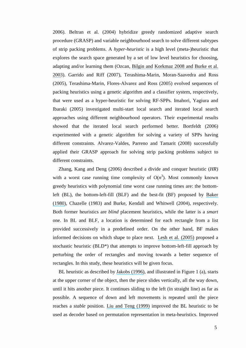
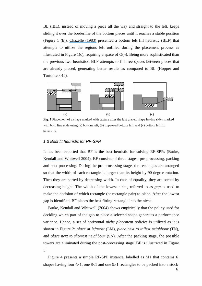
Burke, Kendall and Whitwell (2004) shows empirically that the policy used for

deciding which part of the gap to place a selected shape generates a performance

variance. Hence, a set of horizontal niche placement policies is utilized as it is

shown in Figure 2: place at leftmost (LM), place next to tallest neighbour (TN),

and place next to shortest neighbour (SN). After the packing stage, the possible

towers are eliminated during the post-processing stage. BF is illustrated in Figure

3.

Figure 4 presents a simple RF-SPP instance, labelled as M1 that contains 6

shapes having four 41, one 81 and one 91 rectangles to be packed into a stock

(a) (b) (c)

7

sheet with a width of 4. BF fails to obtain the optimal solution for this problem

instance. Although the tower elimination in BF is useful in some problem

instances, it might become useless for some other cases like M1. BF prefers to

place exact fitting rectangles first, hence four 41 are packed into the stock sheet

on top of each other, and then assuming the TN policy is used, two tall (19, 18)

rectangles are packed at each side of the stock sheet. The result does not improve

even if another placement policy is used. In this study, a new heuristic is

described that combines different policies to overcome the shortcomings of BF.

The approach is tested over a variety of benchmark problems and compared to the

previously proposed heuristics and meta-heuristics.

Fig. 2 Niche placement policies: placement next to (a) tallest (or leftmost) (b) shortest neighbour.

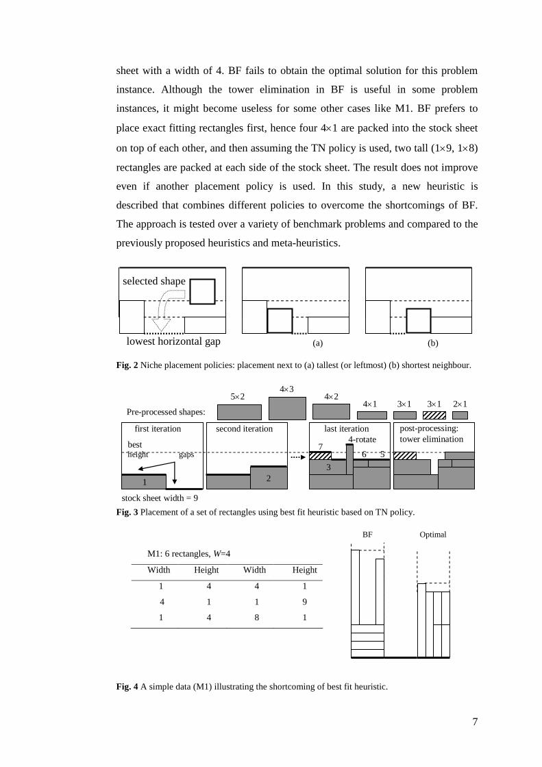
Fig. 3 Placement of a set of rectangles using best fit heuristic based on TN policy.

Fig. 4 A simple data (M1) illustrating the shortcoming of best fit heuristic.

M1: 6 rectangles, W=4

Width Height Width Height

1 4 4 1

4 1 1 9

1 4 8 1

selected shape

lowest horizontal gap (a) (b)

post-processing:tower elimination

last iterationfirst iteration second iteration

1 23

4-rotate

6 57best

height gaps

3131 214142

4352

Pre-processed shapes:

stock sheet width = 9

BF Optimal

8

2 A novel heuristic for RF-SPP

The aim of the approximation heuristics for solving RF-SPPs is to obtain an

optimal skyline (height) after the placement of rectangles. Martello and Vigo

(1998) provided better lower bounds for SPP variants. The proposed heuristic

makes use of a target height, named as expected best height. The simple lower

bound, also known as the continuous bound is preferred as the expected best

height. This bound can be computed fast in advance using Equation (2), since the

dimensions of a stock sheet and the rectangles to be placed are known before.

expected best height =

Rri

i

iW

rareaOf

,

)((2)

where R is the set of rectangles, ri is the ith rectangle and W is the width of the

stock sheet. The optimal height for an RF-SPP instance can not be lower than this

value for discrete width and height. The definition for the expected best height

requires a minor adjustment for a better bound. As a simple example, given a set of

two rectangles {82, 42} and a stock sheet of width 4, the expected best height

computes to 6. Obviously, 82 rectangle can not be placed into a gap having a

maximum width of 4 and the optimal height can not be less than 8. Therefore, the

expected best height should be updated. If the maximum side length among all

rectangles, denoted as maxl=max{i, ri S: widthOf(ri), heightOf(ri)} is larger

than both the expected best height and the width of the stock sheet, then the

expected best height is reset to maxl.

The best fit (BF) heuristic aside, bottom-left (BL) and bottom-left fill (BLF)

heuristics rely on the sequence of the rectangles provided. BL and BLF heuristics

do not require any pre-processing unless the user sorts the rectangles with respect

to their decreasing (or increasing) width (or height). However, in the best-fit

heuristic a more appropriate rectangle is chosen for placement during the packing

stage. This dynamic selection mechanism within the best fit heuristic provides an

advantage over the other placement heuristics whose performance might change

depending on the input sequence. BF heuristic requires a pre-processing time. The

rectangles are arranged by a 90-degree rotation in such a way that, the width of a

rectangle is always larger or equal to its height. Then the rectangles are sorted with

respect to their widths in decreasing order. In case of equality, they are sorted with

respect to their heights in decreasing order. This same process is also adapted by

9

our approach. Our heuristic, named as bidirectional best-fit (BBF) heuristic

improves the best-fit approach by using some additional features. Almost all

previous heuristics for RF-SPP consider the gaps for placement along a single

direction. The proposed greedy heuristic aims to select and place the most

appropriate rectangle from a list of unplaced rectangles. During this process, both

horizontal and vertical niches on the stock sheet are considered at each step. A pre-

processing phase is required by BBF that is the same as the BF approach;

nevertheless, BBF requires no post-processing like tower elimination in BF.

2.1 Maintenance of the niches

The horizontal gaps and hence the lowest niche(s) are maintained as in BF. An

array or a linked list can be used as a data structure to keep track of all gaps in

terms of their height (y-coordinate) and length as shown in Figure 5..

Additionally, a single vertical niche is also used by the proposed heuristic. A

vertical niche is a single rectangular region formed by the upper-left-most niche

between the upper-left-most horizontal gap and the expected best height. The

height and width of a vertical niche is illustrated in Figure 5.

Fig. 5 Data structures that can be utilized for maintaining niches.

2.2 Bidirectional best-fit heuristic (BBF)

After pre-processing as described previously, BBF invokes the placement process.

At each step, a rectangular region (or niche) is considered for placement and a

5 5 2 2 1 1 10 0

5 2 2 2 0 2 1 3

5

1 2 3 4 7 8 95 6

expected

best height

array

linked list

lowest horizontalgap

verticalniche

0verticalniche

height

width

1

2

3

4

5

6

10

decision is made regarding to which rectangle is to be placed, its orientation and

its precise spot within that region based on a set of policies. This decision can be

delayed, if the rectangular region (or niche) is too small for placement.

Consequently, the placement process consists of three consecutive core stages as

illustrated in Figure 6:

1. In the first stage, an exact fit is targeted based on some rectangle selection

policies by considering both the lowest horizontal gap and the vertical gap.

2. If the algorithm fails in the first stage, then a best fit is targeted in the second

stage.

3. In the third stage, the width of the horizontal gap can be so small that no

rectangle fits in. Then the horizontal gap is wasted by raising the height of the

niche to the shortest neighbour’s level. The search proceeds with the new

lowest horizontal gap, formed after this modification as described. The

vertical gap remains unchanged even if there is no fitting rectangle.

The major differences between the new heuristic and the previous approaches

are that BBF utilizes a search for a bidirectional placement and there is a clear

distinction between searching for an exact fitting and best fitting rectangle

supported by a set of new policies. The best fit in BBF indicates a fitting rectangle

that does not meet the criteria as defined for an exact fit. Performing the

placement along either dimension at earliest might affect the result; hence, this

ordering is also taken into account. Policies are arranged such that the gaps are

filled as much as possible by using the larger objects first and keeping the number

of gaps less.

1. BBF_Solve()2. Input: stock sheet dimensions:W, list of n rectangles Output: height//-- start of pre-processing

3. foreach rectangle in the list4. if (rectanglewidth > rectangleheight)5. rotate the rectangle by 90 and swap(rectanglewidth, rectangleheight)6. sort the rectangles in the list by non-increasing width and in case of equality sort them by height//-- end of pre-processing

7. foreach rectangle selection policy#1 for exact fit into the vertical niche in {enabled, disabled}{8. foreach rectangle selection policy#2 for exact fit into the horizontal niches in {TRE, NRE}{9. foreach exact-fit ordering policy#3 in {eHV, eVH} {10. foreach horizontal best-fit policy#4 in {BP, FP} {11. foreach vertical best-fit policy#5 in {FH, WR, noVB} {12. foreach best-fit ordering policy#6 in {bHV, bVH} {13. foreach placement policy#7 for a selected rectangle in {LM, TN, SN} {14. initialize gaps, reset list to sorted rectangles, fit_found=false, placed_rectangles=015. while (placed_rectangles!=n) {// stage#1: exact fit

11

16. get the lowest horizontal gap and the vertical gap17. if (policy#3==eHV){18. begin stage#1a: exact fit – horizontal gap19. fit_found = find a fitting rectangle into the horizontal gap by policy#220. if (fit_found) {21. place the exact fitting rectangle, placed_rectangles++22. update the horizonal gap23. continue // jump to the end of while loop }24. end stage#1a: exact fit – horizontal gap25. begin stage#1b: exact fit – vertical gap26. if (policy#1 is enabled){27. get the vertical niche28. fit_found = find a fitting rectangle into the vertical gap29. if (fit_found) {30. place the exact fitting rectangle, placed_rectangles++31. update the vertical gap32. continue // jump to the end of while loop } }33. end stage#1b: exact fit – vertical gap34. }else // this is the case when policy#3==eVH35. if (policy#1 is enabled)36. swap stage#1a and stage#1b and execute// stage#2: best fit

37. if (policy#6==bHV){38. begin stage#2a: best fit – horizontal gap39. fit_found = find the best fitting rectangle into the horizontal gap by policy #440. if (fit_found) {41. place the fitting rectangle using the policy #7, placed_rectangles++42. update the horizontal gap43. continue // jump to the end of while loop }44. end stage#2a: best fit – horizontal gap45. begin stage#2b: best fit – vertical gap46. fit_found = find the best fitting rectangle into the horizontal gap by policy #547. if (fit_found) {48. place the fitting rectangle using, placed_rectangles++49. update the vertical gap50. continue // jump to the end of while loop }51. end stage#2b: best fit – vertical gap52. }else // this is the case when policy#6==bVH53. swap stage#2a and stage#2b and execute// stage#3: no fitting rectangle

54. if (fit_found == false)55. raise the lowest horizontal gap to the lowest neighbour56. } // end while57. save the height based on the solution } } } } } } } // end foreach58. return the best height

Fig. 6 Pseudocode of the bidirectional best-fit heuristic.

The aim in the first stage is filling a gap entirely. This stage contains two sub-

stages: exact fit search for the horizontal gap and exact fit search for the vertical

gap. An exact fit ordering policy is administered during this stage, since filling a

vertical gap might be advantageous over filling a horizontal gap first, or vice versa

(eVH, eHV). Two different rectangle selection policies are utilized while filling

the horizontal gap. The traditional policy in BF selects the first rectangle that fits

into the lowest gap from the sorted list of single rectangles. This policy is labelled

as TRE. In BBF, an additional policy is utilized, denoted as NRE. In NRE, two

different choices are considered consecutively before the first fitting rectangle is

12

checked as illustrated in Figure 7. Initially, a rectangle having a height of the

tallest neighbour of the lowest horizontal gap is searched, and then the shortest

one. This strategy aims to generate a wider horizontal gap after the placement. If

both attempts fail, then the fitting rectangle with the tallest height is given higher

priority to be placed. The sorted list is searched for a suitable rectangle starting

from the first unused one. If there is an exact fitting rectangle, then due to the

inclusion of this last attempt, NRE turns out to be the TRE policy. If there is no

fitting rectangle, then no other action is taken during this stage.

Fig. 7 NRE rectangle selection policy steps for exact fit into the lowest horizontal niche,

consecutively, look for a rectangle: (1) having a height of the tallest neighbour, (2) having a height

of the shortest neighbour, (3) and then apply the TRE policy.

Unused large objects generate difficulty towards the end of placement, since it

becomes likely that the number of gaps increases in the horizontal direction

causing wastage. This is the main reason why a single vertical niche is considered

for placement during the first stage as another sub-stage. In this sub-stage, a

rectangle is searched in accordance with a size exactly equal to the vertical niche

width. If the attempt fails, then a search is performed for a rectangle with a height

that is as close as possible to the height of the vertical niche. If such a rectangle is

found, then the new vertical niche is constructed as shown in Figure 8. The search

for an exact fitting rectangle into the vertical niche can be enabled or disabled as a

policy.

In the second stage, the best fitting rectangle is searched for among the

unplaced rectangles. This stage also contains two sub-stages: best fit search for

the horizontal gap and the vertical gap. Similarly, an ordering policy is used to

check both possibilities of invoking the search for the horizontal gap or the

vertical gap first (bHV, bVH). The third policy disables vertical best fit, denoted

as noVB. Two different policies are used for selecting the best rectangle for

placement for the horizontal gap. The first policy denoted as BP is the traditional

one utilized by the best fit heuristic; search for a rectangle that minimizes the

remaining gap. The second policy denoted as FP places the first fitting rectangle

lowest horizontal gap

(2)

(1)

(3)

13

from the sorted list considering the rotated versions as well. Hence, possibly, the

tallest rectangle gets inserted. The search for the best rectangle that fits into the

vertical niche is based on two different rectangle selection policies. The first

policy denoted as FH fixes the height of the rectangle to be searched equal to the

height of the vertical niche. The rectangle with the largest width from the sorted

list is inserted into the niche. The second policy denoted as WR inserts the widest

rectangle that fits into the niche ignoring its height. As presented in Figure 6, the

proposed heuristic attempts to test all policy combinations summarized in Table 1

and return the best result.

Fig. 8 (a) Placement of a selected rectangle into the vertical niche, and (b) vertical niche update.

Table 1 Brief explanation of the policies utilized by BBF.

Id. Policy Value Brief explanationEnabled Placement into the vertical niche is considered

during the exact fit phase1 rectangle selection

policy for exact fit intothe vertical niche Disabled Only placement into horizontal niche is considered

for an exact fit, and policy#3 is ignored

TRE The first rectangle that fits into the niche is chosen2 rectangle selectionpolicy for exact fit intothe horizontal niche NRE An exact fit into two different rectangular regions

are considered consecutively, if not possible, thetallest rectangle that fits into the niche is chosen

eHV Possibility of an exact fit into the horizontal nicheis sought first, if it is not possible, then thepossibility of an exact fit into the vertical niche isconsidered

3 Exact fit orderingpolicy

eVH Opposite of eHVBP Choose the rectangle that minimizes the remaining

gap4 Horizontal (gap) best

fit policyFP Choose the first fitting tallest rectangleFH Fix the height, choose the rectangle with this

height and the largest width5 Vertical (gap) best fit

policyWR Chooses the widest rectangle that fits into the

vertical niche6 Best fit ordering noVB Best fit into the vertical niche is disabled

(a) (b)lowest vertical gap

vertical niche

expected best height

lowest horizontal gap

selectedrectangle forplacement

new verticalniche

14

bHV Possibility of a best fit into the horizontal niche issought first, if it is not possible, then thepossibility of a best fit into the vertical niche isconsidered

policy

bVH Opposite of bHVLM Next to the left most neighbourTN Next to the tallest neighbour

7 Placement policy(horizontal gap)

SN Next to the shortest neighbour

2.3 Illustration of how BBF executes

Given M1 problem instance (Figure 1) containing single rectangles of sizes 19,

81, two from 41 and two from 14 rectangles and a strip of width 4, BBF

obtains a solution as follows. Note that the maximum side length is 9. First, an

expected best height is computed as 9 using max{33/4, 9} (see Section 2). After

pre-processing, following sorted list of rectangles is generated {91, 81, 41

41, 41, 41}. Figure 9 shows the logical view of some internal data structures

required for representing and solving the problem just before testing a policy

combination at step 14 in Figure 6. Let’s assume that the policy combination

represented by ordered 7-tuple <Enabled, TRE, eVH, FP, WR, bHV, TN> will be

tested (see Table 7).

Fig. 9 BBF at work for solving M1 problem instance, the numbers on the final result shows the

placement order of corresponding rectangle.

Figure 9 shows the final result obtained by employing BBF to the M1 problem

instance. After BBF starts its execution, 91 is placed as it is into the vertical

niche (to the bottom-left-most of the strip) due to the choices of policies in the 7-

tuple <Enabled,*,eVH,*,*,*,*>, and since this rectangle fits exactly into the

vertical gap having a width of 9. Then, both vertical niche and horizontal gap data

structures are updated. Since no exact fitting rectangle can be found, a best fitting

rectangle is searched in the next step. First, possibility of finding a fitting

rectangle for the horizontal gap is explored due to the bHV policy. Moreover,

4

91 81 41

coord. width height

Vertical niche (0,0) 9 4

Lowest horizontal gap (0,0) 4 -

9

1 23 4

5 6

final

result

15

based on the policy FP, the tallest rectangle is chosen for placement from the

remaining rectangles in the list, that is 81. This piece is placed next to the tallest

neighbour, since the placement policy is TN. The sides of the strip are assumed to

have an infinite height. Therefore, 81 rectangle is rotated and placed next to the

right side of the strip. Again, both vertical niche and horizontal gap data structures

are updated. In a similar manner, the first 41 is rotated and placed next to the

91 rectangle. After the data structures are updated, the vertical niche has a width

of 5 and a height of 1, whereas the lowest horizontal gap has a width of 1. An

exact fitting rectangle can not be found for the vertical niche, but an exact fitting

rectangle can be found for the horizontal niche, that is the rotated version of 41.

After this item is placed, BBF continues its execution in the same way for the

remaining rectangles. Table 2 shows all the steps that leads to the final result

provided in Figure 9. Notice that this result is the optimal result for the given

problem instance.

Table 2 Execution order of BBF stages after pre-processing generating the final placement shown

in Figure 9 under ordered the policy combination <Enabled, TRE, eVH, FP, WR, bHV, TN>.

vertical nichehorizontal

lowest gapexecutionorder

last stageexecuted

placedrectangle orientation

(x, y)coord. width height

(x, y)coord. width

1 stage#1b 91 asis (1, 0) 9 3 (1, 0) 32 stage#2a 81 Rotated (1, 0) 9 2 (1, 0) 23 stage#2a 41 Rotated (1, 4) 5 1 (2, 0) 14 stage#1a 41 Rotated (1, 4) 5 2 (1, 4) 25 stage#2a 41 Rotated (1, 8) 1 1 (2, 4) 16 stage#1a 41 Rotated - - - - -

2.4 Running time complexity issues

All bottom left heuristics run in O(n2) time in the worst case for placing n

rectangles, assuming an efficient implementation. The worst case running time

complexity of the BF implementation as described in Burke, Kendall and

Whitwell (2004) is O(nlgn + n2 + Wn), where W is the width of the strip. The term

c1nlgn arises due to the sorting of rectangles during the pre-processing phase and

tower elimination at the post processing phase. The term c2n2 is due to the search

for finding the best fitting rectangle to the lowest horizontal gap at each step.

Finally, maintaining the skyline and the lowest gap takes c3Wn time. The

16

representation of the skyline is improved in Burke, Kendall and Whitwell (2006)

by a linked list structure, eliminating this term.

A given implementation of an approach can be further improved by using more

appropriate data structures. The pseudo-code provided in Figure 6 hides

implementation details. BBF is implemented in a similar fashion to the previous

implementation of BF for the experiments. In the worst case, the running time of

both BF and BBF implementations are the same; O(n2). The execution time of

BBF for each problem instance used during the experiments is provided in Section

3 to illustrate this phenomenon. Imahori and Yagiura (2009) in their recent study

show that the best fit heuristic is a ()-approximation algorithm, where = n ,

>0 and n is the number of rectangles to be placed. The same reasoning provided

in their study also applies to the bidirectional best fit heuristic. As the BBF

heuristic covers all policies that the best fit heuristic does and even more, it

follows that the bidirectional best fit heuristic is also a ()-approximation

algorithm. Moreover, Imahori and Yagiura (2009) describe an implementation in

which the running time of the BF heuristic is improved to O(nlogn).

3 Computational results

3.1 Benchmark problems and performance evaluation criteria

BBF is experimented on a set of well known benchmark problems gathered from

the previous studies in the literature for comparison. The main properties of these

problems are summarized in Table 3. Jakobs (1996) data set has two small

problem instances with known optimum heights. Burke, Kendall and Whitwell

(2004) data set contains thirteen randomly generated problems. Valenzuela and

Wang (2001) data set contains twelve problems, where rectangles have floating

point values for each dimension. Half of the problems include rectangles having

similar sizes, while the size of the rectangles in the other half differ vastly,

labelled as N (Nice) and P (Path) problems, respectively. Floating point data is

converted into integer values using a scaling factor, determined by some

precision. The problems in the Hopper and Turton (2001a) data set are grouped in

seven categories. Three problems in each category have the same optimal height

and sheet dimensions, while the number of rectangles might differ. Hopper (2000)

introduces guillotine and non-guillotine data sets, each containing seven

17

categories of five problem instances. During the computational experiments, non-

guillotine zero-waste data set having 35 total problem instances is used. Ramesh

Babu and Ramesh Babu (1999) present a single problem instance. Pinto and

Oliveira (2005) data set consists of large problem instances ranging from 50 to

15,000 rectangular pieces. The BBF algorithm is implemented using Java. The

experiments are performed on a Windows computer with an Intel Core 2 1.86

GHz CPU and 2GB RAM.

Table 3 The properties of the first class of benchmark problems used during the experiments

Data source Problem(s)Number of

rectangles

Optimal

height Sheet width

Pinto and Oliveira (2005) PO1 50

PO2 100

PO3 500

PO4 1,000

PO5 5,000

PO6 10,000

PO7 15,000

600 400

Burke, Kendall and

Whitwell (2004)N1 10 40 40

N2 20 50

N3 30 5030

N4 40 80 80

N5 50 100 100

N6 60 100 50

N7 70 100 80

N8 80 80 100

N9 100 150 50

N10 200 150

N11 300 15070

N12 500 300 100

N13 3,152 960 640

Valenzuela and Wang (2001) VN1, VP1 25

VN2, VP2 50

VN3, VP3 100

VN4, VP4 200

VN5, VP5 500

VN6, VP6 1,000

100 100

Hopper and Turton (2001a) C1P1 16 20 20

18

C1 C1P2 17

C1P3 16

C2C2-P1, P2,

P325 15 40

C3P1 28

C3 C3P2 29

C3P3 28

30 60

C4C4-P1, P2,

P349 60 60

C5P1 72

C5 C5P2 73

C5P3 72

90 60

C6C6-P1, P2,

P397 120 80

C7P1 196

C7 C7P2 197

C7P3 196

240 160

Hopper (2000) H1 17

H2 25

H3 29

Explanation: There are 5

problem instances in each

problem category H4 49

H5 73

H6 97

H7 197

200 200

Ramesh Babu and Ramesh

Babu (1999)RB 50 375 1000

Jakobs (1996) J1 25

J2 5015 40

All benchmark problem instances, Packer tool provided by Can Başaran to

view the placements and the Java code of the heuristic will be available at

http://cs.nott.ac.uk/~exo/research/SPP. Two performance evaluation measures will

be used for comparing approaches:

how much improvement an approach provides over another one

considering the best (or an average) solution, the distance to the optimum (or

lower bound).

The percentage improvement (%-imprv.) that a heuristic#1 provides over a

heuristic#2 is computed using the following formula:

%-imprv. = 100( resultant_height2 – resultant_height1)/ resultant_height2 (3)

19

where resultant_heightj is the best height obtained using the heuristic#j. A value

of 0 indicates that both heuristics generate the same result. A negative value is not

reported as it means that heuristic#1 does not improve the solution generated by

heuristic#2. The optimal solution or a lower bound for each problem instance is

known. Hence, %-gap is used to measure how much a solution obtained by using

a heuristic deviates from the optimal solution (or a lower bound) denoted as

opt_height as defined in Equation (3). A lower %-gap indicates a better

performance.

%-gap = 100( resultant_height – opt_height)/ opt_height (4)

3.2 Policy tests

If one of the policies as described in Section 2.2 and summarized in Table 1 is

left out, then the result obtained for at least one of the problem instances worsens

as illustrated in Table 4. Each policy used within BBF is essential. Yet, it is

observed that the same solution might be obtained with different policy

combinations. As an example, two optimal placements obtained from data C1P1

using BFF are shown in Figure 10. Note that, Burke, Kendall and Whitwell (2004)

already showed that different policies for placement into the horizontal gap yield

different results.

Fig. 10 Two different optimal solutions generated by BFF from data C1P1 using different policy

combinations.

Table 4 Height2 is the result obtained for a given RF-SPP instance after applying the BBF

algorithm by excluding the corresponding policy assignment. Height1 is the result obtained

whenever all policies are used

20

20

Policy id. Assignment Problem Optimal Height1 Height2Enabled N7 100 106 109

1 Disabled N2 50 52 53TRE C4P2 60 62 63

2 NRE N10 150 151 152eHV C7P3 240 244 245

3 eVH N9 150 152 160BP VN2 1000 1080 1085

4 FP N12 300 303 305FH N11 150 151 152

5 WR N4 80 82 83noVB C6P2 120 121 123bHV N1 40 40 43

6 bVH N8 80 82 83

3.3 Comparison of BBF to some previous heuristics

Table 5(a) presents the experimental results from using Zhang, Kang and Deng

(2006) heuristic, denoted as HR, bottom-left, bottom-left-fill, their variants and

our new approach over Hopper and Turton (2001a) data set. The proposed

heuristic either improves the solutions or generates a tie for all problem instances

obtained from the previous heuristics. BBF finds the optimal result for data C1P1

and C2P3. It turns out to be the best approach with an average %-gap of %2.95

over the problem instances. BBF performs still better as compared to the bottom-

left heuristic as the problem size increases (Table 5(b)) over the Pinto and

Oliveira (2005) data. Student’s paired t-test over %-gaps indicates that the

performance variation between BFF and a blind heuristic is statistically significant

within a confidence interval of 99.99% in both cases. The computational

experiments over the Hopper data as presented in Table 5(c) shows that the

average performances of BBF and BLD* are comparable based on the best

results, moreover, BBF outperforms BLD* heuristic (Lesh et al., 2005) in 4 data

sets out of 7. Jakobs (1996) reports that applying BL heuristic to J1 and J2 after

sorting the rectangles in decreasing widths yields a gap of %40 for each, while

BBF generates a gap of %6.7 for each one of these small problems (Table 5(d)).

Table 5 Comparison of the bidirectional best fit heuristic to (a) HR heuristic of Zhang, Kang and

Deng (2006) and a variety of bottom-left heuristics and the best fit heuristic over Hopper and

Turton data set based on %-gap. The bold entries mark the best performing approach(es). H and W

indicate that the list of rectangles used as input is sorted with respect to their widths and heights,

respectively in decreasing order (D), (b) the bottom left heuristic as reported in Alvarez-Valdes et

al. (2008) over Pinto and Oliveira data set, (c) BLD* of Lesh et al. (2005) over Hopper data set run

21

in 60 seconds and 3600 seconds. The bold entries mark the best performing heuristic(s) (d) BL-

DW as reported in Jakobs (1996). The execution time of BBF for each problem is provided in (b),

(c) and (d).

(a)

labelno. ofshapes BL BL-DW BL-DH BLF BLF-DW BLF-DH BBF HR

C1P1 16 45 30 15 30 10 10 0C1P2 17 40 20 10 35 15 10 5C1P3 16 35 20 5 25 15 5 5

C1 avr 40.0 23.3 10.0 30.0 13.3 8.3 3.3 8.3C2P1 25 53 13 13 47 13 13 6.7C2P2 25 80 27 73 73 20 73 6.7C2P3 25 67 27 13 47 20 13 0

C2 avr 66.7 22.3 33.0 55.7 17.7 33.0 4.4 4.5C3P1 28 40 10 10 37 10 10 0C3P2 29 43 20 10 50 13 6.7 10C3P3 28 40 17 13 33 13 13 3.3

C3 avr 41.0 15.7 11.0 40.0 12.0 9.9 4.4 6.7C4P1 49 32 17 12 25 10 10 3.3C4P2 49 37 22 13 25 5 5 3.3C4P3 49 30 22 6.7 27 10 5 1.7

C4 avr 33.0 20.33 10.57 25.67 8.33 6.7 2.8 2.2C5P1 72 27 16 4.4 20 5.6 4.4 1.1C5P2 73 32 18 10 23 6.7 5.6 2.2C5P3 72 30 13 7.8 21 5.6 4.4 1.1

C5 avr 29.7 15.7 7.4 21.3 6.0 4.8 1.5 1.9C6P1 97 33 22 8.3 20 5 5 1.7C6P2 97 39 25 8.3 18 4.2 2.5 0.8C6P3 97 34 18 9.2 21 4.2 6.7 1.7

C6 avr 35.3 21.7 8.6 19.7 4.5 4.7 1.4 2.5C7P1 196 22 16 5 15 4.6 3.8 1.2C7P2 197 41 19 10 20 3.3 2.9 1.7C7P3 196 31 17 7.1 17 2.9 3.8 1.7

C7 avr 31.3 17.3 7.4 17.3 3.6 3.5 1.5 1.8

(b)

labelno. of

shapes OptimumTime(sec) BBF BL

PO1 50 0.25 7.2 12.3PO2 100 0.61 7.5 13.2PO3 500 6.23 3.0 15.3PO4 1,000 600 17.87 0.0 15.0PO5 5,000 413.94 0.0 14.5PO6 10,000 1780.91 0.0 13.5PO7 15,000 4237.50 0.0 10.0

avr 2.5 13.4

(c)

no. of BBF BLD*label shapes optimum Mean time (sec) Mean Best 60 s 3600 sH1 17 216.6 8.3 6.0 6.0 4.5

22

H2 25 216 8.0 6.5 6.4 4.7H3 29 214.6 7.3 5.0 6.0 4.6H4 49 200 209 4.5 2.5 5.1 3.9H5 73 209.4 4.7 3.5 4.6 4.0H6 97 205.8 2.9 2.5 4.0 3.0H7 197 203.2 1.6 1.5 2.3 1.8

avr 3.9 4.9 3.8

(d)

label no. of shapes optimum Time (sec) BBF BL-DWJ1 25 15 0.06 6.7 40J2 50 0.11 6.7 40

3.4 Comparison of BBF to BF

Table 6 presents a performance comparison of BBF to BF. In 32 problem

instances, the improved heuristic outperforms the best fit heuristic. In only 3

problem instances {VN4, VP3, VP4}, the best fit heuristic has a better

performance, while in the rest of the problems, there is a tie. There are

inconsistencies between the best fit heuristic results in Burke et al. (2004) and

Burke et al. (2006) for the Valenzuela and Wang (2001) problem instances. The

reason for this phenomenon and getting better results from BF for {VN4, VP3,

VP4} as compared to BBF appears to be due to the conversion from floating point

to integer data. For future comparisons, the exact problem instances used during

the experiments are publicly available (see Section 3.1). Although the solution

qualities generated by BFF and BF are the same for data C7P2 and RB, the

resultant placements demonstrated in Figure 11 are different than the ones as

presented in Burke Kendall, and Whitwell (2004). BBF obtains optimal solutions

for four problem instances {N1, C1P1, C2P3, C3P1}. The average %-gap over all

the problem instances excluding M1 for BBF is 3.49, while it is 5.45 for BF.

Student’s paired t-test based on %-gaps shows that this performance variation is

also statistically significant within a confidence interval of 99.99%.

Table 6 Comparison of the bidirectional best fit heuristic (BBF) to the best fit heuristic (BF)

results provided in Burke et al. (2004) based on %-gap and %-impr. The execution time of BBF

for each problem is also provided. The bold entries mark the best performing heuristic(s).

label

number

of shapes

optimal

height

BBF

result

BF

result

Time

(sec)

BBF

%-gap

BF

%-gap

%-

impr.

M1 6 9 9 13 0.00 0.00 44.44 30.77

23

N1 10 40 40 45 0.03 0.00 12.50 11.11

N2 20 50 52 53 0.02 4.00 6.00 1.89

N3 30 50 52 52 0.05 4.00 4.00 0.00

N4 40 80 82 83 0.09 2.50 3.75 1.20

N5 50 100 104 105 0.14 4.00 5.00 0.95

N6 60 100 102 103 0.16 2.00 3.00 0.97

N7 70 100 106 107 0.22 6.00 7.00 0.93

N8 80 80 82 84 0.28 2.50 5.00 2.38

N9 100 150 152 152 0.33 1.33 1.33 0.00

N10 200 150 151 152 1.13 0.67 1.33 0.66

N11 300 150 151 152 2.14 0.67 1.33 0.66

N12 500 300 303 306 5.95 1.00 2.00 0.98

N13 3,152 960 964 964 163.42 0.42 0.42 0.00

C1P1 16 20 20 21 0.02 0.00 5.00 4.76

C1P2 17 20 21 22 0.02 5.00 10.00 4.55

C1P3 16 20 21 24 0.02 5.00 20.00 12.50

C2P1 25 15 16 16 0.05 6.67 6.67 0.00

C2P2 25 15 16 16 0.03 6.67 6.67 0.00

C2P3 25 15 15 16 0.03 0.00 6.67 6.25

C3P1 28 30 30 32 0.05 0.00 6.67 6.25

C3P2 29 30 33 34 0.05 10.00 13.33 2.94

C3P3 28 30 31 33 0.05 3.33 10.00 6.06

C4P1 49 60 62 63 0.11 3.33 5.00 1.59

C4P2 49 60 62 62 0.11 3.33 3.33 0.00

C4P3 49 60 61 62 0.11 1.67 3.33 1.61

C5P1 72 90 91 93 0.19 1.11 3.33 2.15

C5P2 73 90 92 92 0.19 2.22 2.22 0.00

C5P3 72 90 91 93 0.19 1.11 3.33 2.15

C6P1 97 120 122 123 0.33 1.67 2.50 0.81

C6P2 97 120 121 122 0.31 0.83 1.67 0.82

C6P3 97 120 122 124 0.38 1.67 3.33 1.61

C7P1 196 240 243 247 1.20 1.25 2.92 1.62

C7P2 197 240 244 244 1.05 1.67 1.67 0.00

C7P3 196 240 244 245 1.14 1.67 2.08 0.41

VN1 25 1000 1073 1074 0.22 7.30 7.40 0.09

VN2 50 1000 1080 1085 0.48 8.00 8.50 0.46

VN3 100 1000 1069 1070 1.14 6.90 7.00 0.09

VN4 200 1000 1056 1053 2.97 5.60 5.30 -

VN5 500 1000 1031 1035 12.02 3.10 3.50 0.39

VN6 1000 1000 1036 1037 42.20 3.60 3.70 0.10

VP1 25 1000 1093 1101 0.22 9.30 10.10 0.73

24

VP2 50 1000 1074 1138 0.44 7.40 13.80 5.62

VP3 100 1000 1080 1073 1.05 8.00 7.30 -

VP4 200 1000 1053 1041 2.61 5.30 4.10 -

VP5 500 1000 1031 1037 10.06 3.10 3.70 0.58

VP6 1000 1000 1026 1028 31.56 2.60 2.80 0.19

RB 50 375 400 400 0.36 6.67 6.67 0.00

Fig. 11 The solutions generated by BBF from data (a) C7P2 and (b) RB

3.5 Comparison of BBF to the meta-heuristics

Table 7 presents performance comparison of BBF to the genetic algorithm (GA),

simulated annealing (SA) and GRASP meta-heuristics. Jakobs (1996) searched for

an optimal ordering of rectangles using a GA. A candidate solution requires a

decoder that will place all rectangles in the given order onto the strip and the

author used BL (GA+BL). Liu and Teng (1999) proposed improved BL heuristic

as a decoder and utilised in their GA (GA+iBL). The results show that BBF

performs better than GA+BL and delivers a comparable performance to GA+iBL

for J1 and J2 (Table 7(a)). Hopper and Turton (2001a) and Burke et al. (2004)

provided a GA and SA that utilise BLF as a decoder (op+BLF). Beltrán et al.

(2004) first applied a GRASP for obtaining an optimal ordering of rectangles

using BL as a decoder and then improved the solution using a variable

244

400

(b)(a)

25

neighbourhood search (vGRASP). Bortfeldt (2006) presented a genetic algorithm

based on a layered approach (SPGAL). Alvarez-Valdes et al. (2008) obtained one

of the best results in literature by iteratively progressing towards a better solution

through constructive and improvement phases using a GRASP approach

(rGRASP) in a multi-start setting. Imahori et al. (2005) employed iterated local

search for solving RF-SPPs. Their approach perturbs a candidate solution of

sequence of rectangles and attempts to improve it at each step. The authors used a

different performance evaluation scheme in their study, for this reason an indirect

and relative comparison is provided as follows. According to their results, iterated

local search improves SA+BLF by %0.5 based on their evaluation scheme,

whereas BBF performs slightly better with a %0.8 improvement over SA+BLF

based on average %-gap considering Hopper and Turton problem instances. The

results also show that BBF performs better than six older meta-heuristics. On the

other hand, two recent meta-heuristic approaches seem to yield better

performances, namely; SPGAL and rGRASP as summarized in Table 7(b).

Table 7 Performance comparison of the bidirectional best fit heuristic (BBF) to the meta-

heuristics based on %-gap. BL-DW denotes the bottom left heuristic for which the rectangles are

sorted in decreasing width.

(a)

label BL-DW BBF GA+BL GA+iBLJ1 40 6.7 13.3 6.7J2 40 6.7 13.3 6.7

(b)

Hopper Burkelabel BBF GA+BLF SA+BLF vGRASP GA+BLF SA+BLF SPGAL rGRASPC1 3.33 4 4 14.4 1.7 1.7 1.7 0.0C2 4.44 7 6 17.3 6.7 6.7 0.0 0.0C3 4.44 5 5 12.9 6.7 6.7 2.2 1.1C4 2.78 3 3 6.8 5.0 6.1 0.0 1.6C5 1.48 4 3 4.5 5.6 5.2 0.0 1.1C6 1.39 4 3 3.6 5.3 5.3 0.3 0.8C7 1.53 5 4 2.9 5.6 6.0 0.3 1.2

avr 2.77 4.57 4.00 8.92 5.20 5.36 0.64 0.84

(c)

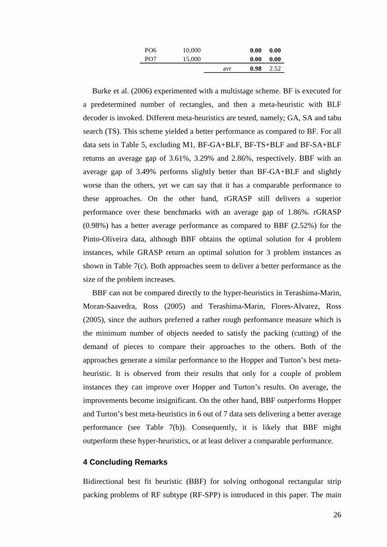
label no. of shapes optimum rGRASP BBFPO1 50 2.83 7.17PO2 100 2.83 7.50PO3 500 0.83 3.00PO4 1,000 600 0.33 0.00PO5 5,000 0.00 0.00

26

PO6 10,000 0.00 0.00PO7 15,000 0.00 0.00

avr 0.98 2.52

Burke et al. (2006) experimented with a multistage scheme. BF is executed for

a predetermined number of rectangles, and then a meta-heuristic with BLF

decoder is invoked. Different meta-heuristics are tested, namely; GA, SA and tabu

search (TS). This scheme yielded a better performance as compared to BF. For all

data sets in Table 5, excluding M1, BF-GA+BLF, BF-TS+BLF and BF-SA+BLF

returns an average gap of 3.61%, 3.29% and 2.86%, respectively. BBF with an

average gap of 3.49% performs slightly better than BF-GA+BLF and slightly

worse than the others, yet we can say that it has a comparable performance to

these approaches. On the other hand, rGRASP still delivers a superior

performance over these benchmarks with an average gap of 1.86%. rGRASP

(0.98%) has a better average performance as compared to BBF (2.52%) for the

Pinto-Oliveira data, although BBF obtains the optimal solution for 4 problem

instances, while GRASP return an optimal solution for 3 problem instances as

shown in Table 7(c). Both approaches seem to deliver a better performance as the

size of the problem increases.

BBF can not be compared directly to the hyper-heuristics in Terashima-Marin,

Moran-Saavedra, Ross (2005) and Terashima-Marin, Flores-Alvarez, Ross

(2005), since the authors preferred a rather rough performance measure which is

the minimum number of objects needed to satisfy the packing (cutting) of the

demand of pieces to compare their approaches to the others. Both of the

approaches generate a similar performance to the Hopper and Turton’s best meta-

heuristic. It is observed from their results that only for a couple of problem

instances they can improve over Hopper and Turton’s results. On average, the

improvements become insignificant. On the other hand, BBF outperforms Hopper

and Turton’s best meta-heuristics in 6 out of 7 data sets delivering a better average

performance (see Table 7(b)). Consequently, it is likely that BBF might

outperform these hyper-heuristics, or at least deliver a comparable performance.

4 Concluding Remarks

Bidirectional best fit heuristic (BBF) for solving orthogonal rectangular strip

packing problems of RF subtype (RF-SPP) is introduced in this paper. The main

27

difference of the proposed heuristic from the previous ones is that the niches are

maintained and considered for placement in both horizontal and vertical

directions. Combining this strategy with a set of useful extended policies, the

bidirectional best fit heuristic yields promising results. The performance of BBF is

compared to some previous approaches over a set of well known benchmark

problem instances with different characteristics, such as the problem size, the size

variance of the rectangles, etc. The best fit approach of Burke, Kendall and

Whitwell (2004) is reported as one of the best heuristics for solving RF-SPPs. The

experimental results indicate that the bidirectional best fit heuristic even improves

on the results obtained by them for most of the problem instances.

Although they are more general approaches, SPGAL (Bortfeldt 2006) and

GRASPr (Alvarez-Valdes et al. 2008) seem to be the best meta-heuristics for

solving SPP variants. The results show that they might perform better than BBF

for solving RF-SPPs. With these few exceptions, BBF still performs better than

most of the previously proposed meta-heuristics reported in literature. The

handicap of meta-heuristics is that a single run might not be sufficient to obtain a

good solution due to their stochastic nature. Hence, more execution time might be

needed. On the other hand, BBF is a reasonably fast heuristic with a polynomial

running time complexity. Its performance can be improved even further using the

data structures suggested by Imahori and Yagiura (2009). This is left as a future

study.

References

Alvarez-Valdes, R., Parreno, F. & Tamarit, J.M. (2008). Reactive GRASP for the strip-packing

problem. Computers and Operations Research, 35, 1065–1083.

Baker, B. S., Coffman, E. G., & Jr Rivest, R. L. (1980). Orthogonal packings in two dimensions.

SIAM J on Comput, 9(4), 808–826.

Beasley, J. E. (1985a). An exact two-dimensional non-guillotine cutting tree search procedure.

Operations Research, 33(1), 49–64.

Beasley, J. E. (1985b). Algorithms for unconstrained two-dimensional guillotine cutting. J

Operations Research Society, 36(4), 297–306.

Beltrán, J. D., Calderón, J. E. , Cabrera, R. J. , Moreno-Pérez, J. A., & Moreno-Vega, J. M. (2004).

GRASP-VNS hybrid for the Strip Packing Problem. Proc. of the workshop on Hybrid

Metaheuristics (pp. 79–90).

Bortfeld, A. (2006). A genetic algorithm fot the two-dimensional strip packing problem with

rectangular pieces. Eur J Oper Res, 172, 814–837.

28

Burke, E., Hart, E., Kendall, G., Newall, J., Ross, P., & Schulenburg, S. (2003). Hyper-heuristics:

An emerging direction in modem search technology. Handbook of Metaheuristics, Kluwer

Academic Publishers, 457–474.

Burke, E. K., Kendall, G., & Whitwell, G. (2004). A new placement heuristic for the orthogonal

stock-cutting problem. Operations Research, 52(4), 655–671.

Burke, E. K., Kendall, G., & Whitwell, G. (2006). Metaheuristic enhancements of the best-fit

heuristic for the orthogonal stock cutting problem computer science. Technical Report No

NOTTCS-TR-2006-3.

Chazelle, B. (1983). The bottom-left bin-packing heuristic: An efficient implementation. IEEE

Transactions on Computers, 32/8, 697–707.

Dagli, C. H., & Poshyanonda, P. (1997). New approaches to nesting rectangular patterns. Journal

of Intelligent Manufacturing, 8, 177–90.

Dowsland, K. A., & Dowsland, W. B. (1992). Packing Problems. Eur J Oper Res, 56, 2–14.

Garey, M. R., & Johnson, D. S. (1979). Computers and Intractability. WH Freeman and

Company: NY.

Jakobs, S. (1996). On genetic algorithms for the packing of polygons. Eur J Oper Res, 88, 165–

181.

Hässler, R. W., & Sweeney, P. E. (1991). Cutting stock problems and solution procedures. Eur J

Oper Res, 54, 141–150.

Hinxman, A. I. (1980). The trim loss and assortment problems: A survey. Eur J Oper Res 88, 1, 8–

18.

Hopper, E. (2000). Two-dimensional packing utilising evolutionary algorithms and other meta-

heuristic methods, PhD thesis, Cardiff University, School of Engineering.

Hopper, E., & Turton, B. C. H. (2001a). An empirical investigation of metaheuristic and heuristic

algorithms for a 2D packing problem. Eur J Oper Res, 128, 34–57.

Hopper, E., & Turton, B. C. H. (2001b). A review of the application of meta-heuristic algorithms

to 2D strip packing problems. Artificial Intelligence Review 257–300.

Kenmochi, M., Imamichi, T., Nonobe, K., Yagiura, M., & Nagamochi, H. (2007). Exact

algorithms for the 2-dimensional strip packing problem with and without rotations. Technical

report 2007-005, Dept of Applied Mathematics and Physics, Graduate School of Informatics,

Kyoto University, January.

Imahori, S., Yagiura, M., & Ibaraki, T. (2005). Improved local search algorithms for the rectangle

packing problem with general spatial costs. Eur J Oper Res, 167, 48–67.

Imahori, S., Yagiura, M., (2009). The best-fit heuristic for the rectangular strip packing problem:

An efficient implementation and the worst-case approximation ratio. Computers &

Operations Research. DOI:10.1016/j.cor.2009.05.008

Lesh, N., Marks, J., McMahon, A., & Mitzenmacher, M. (2004). Exhaustive approaches to 2D

rectangular perfect packings. Information Processing Letters, 90, 7–14.

Lesh, N., Marks, J., McMahon, A., & Mitzenmacher, M. (2005). New heuristic and interactive

approaches to 2D rectangular strip packing. ACM Journal of Experimental Algorithmics, 10,

1–18.

29

Liu, D., & Teng, H. (1999). An improved bottom left algorithm for genetic algorithm of the

orthogonal packing of rectangle. Eur J Oper Res, 112, 413–419.

Lodi, A., Martello, S., & Monaci, M. (2002). Two-dimensional packing problems: a survey. Eur J

Oper Res, 141(2), 241–52.

Lodi, A., Martello, S., & Vigo, D. (1999). Heuristic and metaheuristic approaches for a class of

two-dimensional bin packing problems. INFORMS J on Computing;11:345–57.

Martello, S., Monaci, M., & Vigo, D. (2003). An exact approach to the strip-packing problem.

INFORMS J on Computing, 15(3), 310–319.

Martello, S, & D Vigo (1998). Exact solution of the two-dimensional finite bin packing problem.

Management Science, 44, 388–399.

Ozcan, E., Bilgin, B., & Korkmaz, E. E. (2008). A comprehensive analysis of hyper-heuristics.

Intelligent Data Analysis, 12(1), 3–23.

Pinto, E., & Oliveira, J. F. (2005). Algorithm based on graphs for the non-guillotinable two-

dimensional packing problem, 2nd ESICUP Meeting, Southampton.

Ramesh Babu, A., & Ramesh Babu, N. (1999). Effective nesting of rectangular parts in multiple

rectangular sheets using genetic and heuristic algorithms. Int J Production Res, 37(7), 1625–

1643.

Sarin, S. C. (1983). Two-dimensional stock cutting problems and solution methodologies ASME

Transactions, Journal of Engineering for Industry, 104, 155–160.

Terashima-Marin, H., Moran-Saavedra, A., & Ross, P. (2005). Forming hyper-heuristics with GAs

when solving 2D-regular cutting stock problems. Proceedings of the IEEE Congress on

Evolutionary Computation, vol 2 (pp. 1104–1110).

Terashima-Marin, H., Flores-Alvarez, E. J., & Ross, P. (2005). Hyper-heuristics and Classifier

Systems for solving 2D-regular cutting stock problems. Proceedings of the GECCO, vol 2

(pp. 637–643).

Valenzuela, C. L., & Wang, P. Y. (2001). Heuristics for large strip packing problems with

guillotine patterns: An empirical study. Proceedings of the 4th Metaheuristics Int. Conf.,

University of Porto, Porto, Portugal (pp. 417–421).

Waescher, G., Haussner, H., & Schumann, H. (2007). An improved typology of cutting and

packing problems. Eur J Oper Res, 183, 1109–1130.

Zhang, D., Kang,Y., & Deng, A. (2006). A new heuristic recursive algorithm for the strip

rectangular packing problem. Computers & Operations Research, 33, 2209–2217.