*Corresponding author. Tel.: #1-512-471-0049; fax: #1-512-471-1720.

E-mail address: allen@che.utexas.edu (D.T. Allen).

Atmospheric Environment 34 (2000) 3419}3435

Biogenic hydrocarbon emission estimatesfor North Central Texas

Christine Wiedinmyer!, I. Wade Strange!, Mark Estes", Greg Yarwood#,David T. Allen!,*

!Department of Chemical Engineering, University of Texas at Austin, Austin, TX 87812, USA"Texas Natural Resource Conservation Commission, Austin, TX, USA

#ENVIRON International Corporation, Novato, CA, USA

Received 21 May 1999; accepted 23 September 1999

Abstract

Biogenic hydrocarbon emissions were estimated for a 37 county region in North Central Texas. The estimates werebased on several sources of land use/land cover data that were combined using geographical information systems. Fieldstudies were performed to collect species and tree diameter distribution data. These data were used to estimate biomassdensities and species distributions for each of the land use/land cover classi"cations. VOC emissions estimates for thedomain were produced using the new land use/land cover data and a biogenic emissions model. These emissions weremore spatially resolved and a factor of 2 greater in magnitude than those calculated based on the biogenic emissionslanduse database (BELD) commonly used in biogenic emissions models. ( 2000 Elsevier Science Ltd. All rightsreserved.

Keywords: Biogenic emissions; Isoprene; Land cover; GIS; Biogenic emissions modeling

1. Introduction

Vegetation is a signi"cant source of atmospheric emis-sions of volatile organic compounds (VOCs) (Guentheret al., 1995; Geron et al., 1995; Benjamin et al., 1997;Lamb et al., 1993). The USEPA has estimated that in1995, biogenic VOC emissions in the United States weregreater than anthropogenic VOC emissions (USEPA,1998). These biogenic emissions are distributed non-uni-formly and therefore are major components of the VOCinventory in some areas and are minor contributions inothers (Lamb et al., 1993; Guenther et al., 1995). One areain which biogenic emissions are expected to be substan-tial is eastern and central Texas. The dense hardwoodand coniferous forests of eastern and central Texas are

predicted to have high emissions of biogenic hydrocar-bons and these emissions may contribute to the forma-tion and transport of ozone into populated areas withinTexas. The goal of the work described in this paper wasto prepare a comprehensive inventory of biogenic emis-sions in the region surrounding the Dallas/Ft. Worthurban area.

The area chosen for study was a 37 county region inNorth Central Texas that includes the Dallas/Ft. Worthmetroplex. The Dallas/Ft. Worth urban area fails to meetthe National Ambient Air Quality Standards for ozoneand has recently been declared a serious non-attainmentregion for ozone. Preliminary estimates have indicatedthat roughly 50% of the VOC emissions in the 4-countyDallas/Ft. Worth non-attainment region are due to veg-etation (Estes et al., 1997). More accurate biogenic emis-sions estimates for the region are therefore requisite fordeveloping a sound plan for improving air quality.

The current EPA land use database used to createbiogenic emissions estimates (Biogenic Emissions LandUse Database, BELD) is a compilation of several sources

1352-2310/00/$ - see front matter ( 2000 Elsevier Science Ltd. All rights reserved.PII: S 1 3 5 2 - 2 3 1 0 ( 9 9 ) 0 0 4 4 8 - 3

Fig. 1. Counties in North Central Texas Study domain.

of vegetation data for the country. The BELD reliesespecially on the detailed USDA Forest Inventory andAnalysis data (FIA) (Kinnee et al., 1997). The FIA datacontain species and forest density data for commerciallyvaluable forests in the eastern United States and for someforests in the west. A large region encompassing Texas,Oklahoma and parts of Kansas represents a transitionzone from moist to semi-arid ecosystems with few com-mercially valuable forests. In this region, the FIA con-tains little to no data, and, therefore, the BELD is lackingdetailed species and coverage data for much of Texas.This manuscript reports the "rst detailed estimates ofspecies and land cover coverage data in North CentralTexas and these estimates have been used to predictbiogenic emissions. The following sections describe themethodologies employed and the results of the inventory.

2. Methods

The 37 North-Central Texas counties investigated areshown in Fig. 1. In completing a biogenic emission inven-tory for the Dallas/Ft. Worth photochemical modelingdomain, a land use/land cover (LULC) database was

constructed, integrating existing vegetation and landuse databases. Field surveys were performed to collectspecies and biomass distribution data, and these datawere used to estimate leaf biomass densities for each landuse classi"cation in the database. The LULC databasetogether with the estimates of leaf biomass densities fromthe ground surveys were then used to predict biogenicemissions for the region.

2.1. Land cover database development

The "rst step in estimating biogenic emissions was todevelop a comprehensive vegetation coverage map forthe region. Several potentially useful databases wereidenti"ed, and the information they provided was as-sessed for the modeling domain.

The USGS land cover characteristics (LCC) database,obtained from the US Geological Survey (US GeologicalSurvey, ca., 1976), was examined for the study domain.The LCC coverage has been used for some previousbiogenic inventories (Kinnee et al., 1997). The USGSLCC coverage utilizes 205 vegetation land cover classi-"cations; 66 of these 205 classi"cations are found in theNorth Central Texas study domain.

3420 C. Wiedinmyer et al. / Atmospheric Environment 34 (2000) 3419}3435

Table 1Texas Parks and Wildlife Department Vegetation Classi"ca-tions in the North Central Texas study domain. The area frac-tion of each classi"cation within the North-central Texas studyregion is reported here

Description Percent of totalstudy area

Crops 22.6Ashe Juniper Parks/ Woods 1.2Bluestem Grassland 7.4Cottonwood } Hackberry-SaltcedarBrush/Woods

0.2

Elm } Hackberry 3.1Live Oak } Ashe Juniper Parks 1.4Live Oak } Ashe Juniper Woods 0.3Live Oak}Mesquite } Ashe Juniper Parks 2.6Mesquite-Lotebush Brush 3.2Mesquite Brush 0.2Oak - Mesquite - Juniper Parks/Woods 8.1Other Grasslands 7.8Pine } Hardwood Forest (Loblolly Pine} Sweetgum) or Pine } Hardwood Forest(Shortleaf Pine } Post Oak }Southern Red Oak)

2.4

Post Oak Parks/Woods 2.4Post Oak Woods, Forest and Grassland 18.3Post Oak Woods/Forest 7.3Silver } Bluestem } Texas WintergrassGrassland

5.3

Urban 2.3Willow Oak } Water Oak } BlackgumForest

0.2

Water Oak } Elm } Hackberry Forest 1.4Water 2.4

A second database considered in the work, the TexasParks and Wildlife Department's (TP & WD) vegetationdatabase, utilized a very di!erent set of land cover classi-"cations. The 21 Texas Parks and Wildlife Departmentclassi"cations found in the study domain are listed inTable 1. The TP & WD vegetation coverage was deter-mined to be the most useful for this study. One of themain advantages of the TP & WD vegetation coverage isthat it emphasizes larger plant species in its vegetationdivisions. While both the LCC and TP & WD coveragesmay be technically accurate descriptions of the domain,crops and grasslands de"ne much of the USGS LCC. Ingeneral, trees are larger emitters of VOCs to the atmo-sphere, and are thus more important than crops andgrasslands when estimating biogenic emissions. Also, al-though over 60 USGS LCC classi"cations were presentin the study domain, only four classi"cations accountedfor over 83% of the total area. Therefore, the USGS LCChad a high resolution of land covers, but the coverageactually gave less detailed vegetation information thanthe TP & WD coverage. Finally, the TP & WD coverage

has been made speci"cally for the vegetation found inTexas by ecologists familiar with the state. In developingthese mappings, Landsat (earth satellite) data from theperiod of 1976}1980 were updated in 1986 with organ-ized methods to `ground-trutha the vegetation for theeastern two-thirds of the state (Texas Parks and WildlifeDepartment, 1996). Although the TP & WD data havenot been updated since 1986, the data were the mostdescriptive and speci"c to the study domain. Qualitativemap accuracy was assessed over the study domainthrough ground observations, con"rming the relativeaccuracy of the TP & WD land descriptions compared tothe LCC data.

While the TP & WD database was useful in character-izing rural regions, the urban regions in the domainrequired a di!erent approach. The information in theUnited States Geological Survey's land use land coverdatabase was investigated. However, these data werecompiled from information obtained in the 1970s, and itwas determined that, based on visual observations madeby automobile, more recent data were required to accu-rately characterize the urban areas. The North CentralCouncil of Governments (NCTCOG) developed detailedurban land use data for Tarrant, Dallas, and parts of theeight surrounding countries. This database was construc-ted in 1990 by updating the United States GeologicalSurvey's land use/land cover (USGS LULC) database.These data were more recent and represented the currentland use for the Dallas}Ft. Worth urban area moreaccurately than the USGS LULC data. The NCTCOGland coverage classi"cations used in this database arelisted in Table 2.

A "nal database used in characterizing the study do-main was the US Department of Agriculture-NationalAgricultural Statistics Service (USDA-NASS) databaseon crop species. 1995 county crop distribution data wereused (USDA, 1997).

The consolidated land use/land cover mapping used inthis study is shown in Fig. 2 and incorporated data fromthree sources: the TP & WD database, the NCTCOGdatabase and the USDA NASS crop data. TheNCTCOG land use/land cover database was used for itsdetailed and current description of the land use in theurban Dallas/ Ft. Worth area. The TP & WD vegetationcoverage was used to represent the remainder of thedomain. The USDA National Agricultural Statistics Ser-vice (NASS) database was used to further describe theregions designated as cropland in the TP & WD vegeta-tion coverage. The "nal mapping was also qualitativelycompared to Landsat imagery data. Although the satel-lite imagery did not classify vegetation species, the grass-lands and croplands could be distinguished from forest.These same trends in the Landsat data were seen in thecomposite dataset with clear divisions between the cropand grasslands versus the forest and woodlands (Strange,1998).

C. Wiedinmyer et al. / Atmospheric Environment 34 (2000) 3419}3435 3421

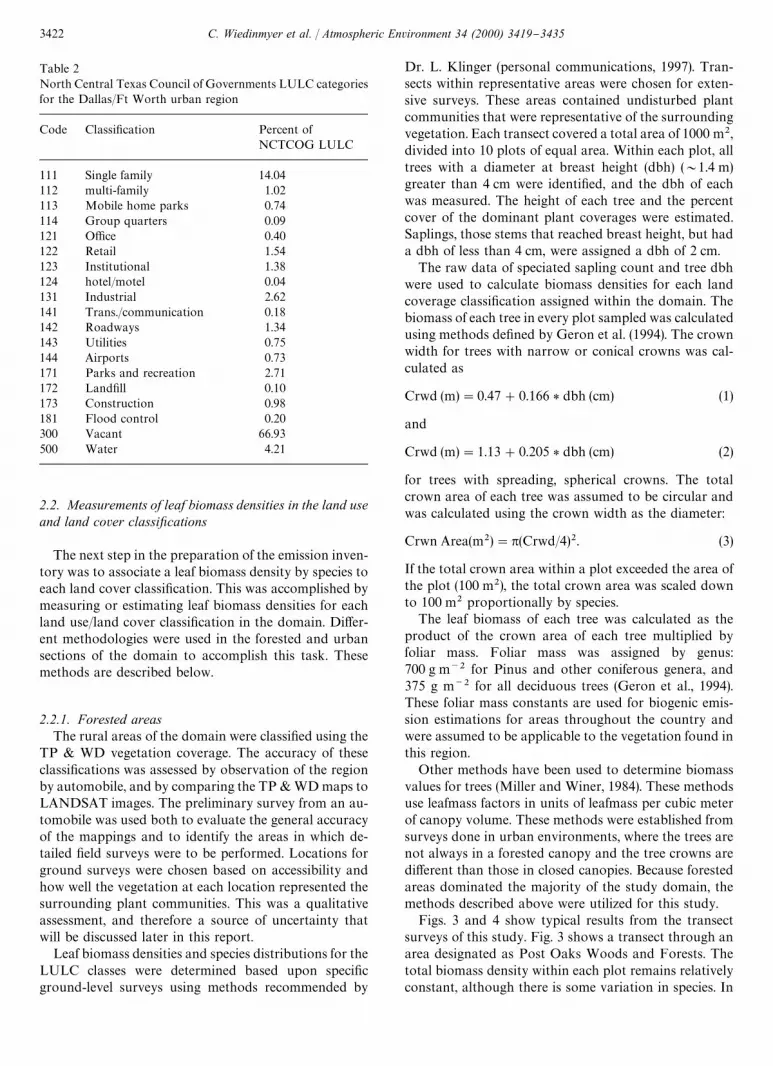
Table 2North Central Texas Council of Governments LULC categoriesfor the Dallas/Ft Worth urban region

Code Classi"cation Percent ofNCTCOG LULC

111 Single family 14.04112 multi-family 1.02113 Mobile home parks 0.74114 Group quarters 0.09121 O$ce 0.40122 Retail 1.54123 Institutional 1.38124 hotel/motel 0.04131 Industrial 2.62141 Trans./communication 0.18142 Roadways 1.34143 Utilities 0.75144 Airports 0.73171 Parks and recreation 2.71172 Land"ll 0.10173 Construction 0.98181 Flood control 0.20300 Vacant 66.93500 Water 4.21

2.2. Measurements of leaf biomass densities in the land useand land cover classixcations

The next step in the preparation of the emission inven-tory was to associate a leaf biomass density by species toeach land cover classi"cation. This was accomplished bymeasuring or estimating leaf biomass densities for eachland use/land cover classi"cation in the domain. Di!er-ent methodologies were used in the forested and urbansections of the domain to accomplish this task. Thesemethods are described below.

2.2.1. Forested areasThe rural areas of the domain were classi"ed using the

TP & WD vegetation coverage. The accuracy of theseclassi"cations was assessed by observation of the regionby automobile, and by comparing the TP & WD maps toLANDSAT images. The preliminary survey from an au-tomobile was used both to evaluate the general accuracyof the mappings and to identify the areas in which de-tailed "eld surveys were to be performed. Locations forground surveys were chosen based on accessibility andhow well the vegetation at each location represented thesurrounding plant communities. This was a qualitativeassessment, and therefore a source of uncertainty thatwill be discussed later in this report.

Leaf biomass densities and species distributions for theLULC classes were determined based upon speci"cground-level surveys using methods recommended by

Dr. L. Klinger (personal communications, 1997). Tran-sects within representative areas were chosen for exten-sive surveys. These areas contained undisturbed plantcommunities that were representative of the surroundingvegetation. Each transect covered a total area of 1000 m2,divided into 10 plots of equal area. Within each plot, alltrees with a diameter at breast height (dbh) (&1.4 m)greater than 4 cm were identi"ed, and the dbh of eachwas measured. The height of each tree and the percentcover of the dominant plant coverages were estimated.Saplings, those stems that reached breast height, but hada dbh of less than 4 cm, were assigned a dbh of 2 cm.

The raw data of speciated sapling count and tree dbhwere used to calculate biomass densities for each landcoverage classi"cation assigned within the domain. Thebiomass of each tree in every plot sampled was calculatedusing methods de"ned by Geron et al. (1994). The crownwidth for trees with narrow or conical crowns was cal-culated as

Crwd (m)"0.47#0.166 * dbh (cm) (1)

and

Crwd (m)"1.13#0.205 * dbh (cm) (2)

for trees with spreading, spherical crowns. The totalcrown area of each tree was assumed to be circular andwas calculated using the crown width as the diameter:

Crwn Area(m2)"p(Crwd/4)2. (3)

If the total crown area within a plot exceeded the area ofthe plot (100 m2), the total crown area was scaled downto 100 m2 proportionally by species.

The leaf biomass of each tree was calculated as theproduct of the crown area of each tree multiplied byfoliar mass. Foliar mass was assigned by genus:700 g m~2 for Pinus and other coniferous genera, and375 g m~2 for all deciduous trees (Geron et al., 1994).These foliar mass constants are used for biogenic emis-sion estimations for areas throughout the country andwere assumed to be applicable to the vegetation found inthis region.

Other methods have been used to determine biomassvalues for trees (Miller and Winer, 1984). These methodsuse leafmass factors in units of leafmass per cubic meterof canopy volume. These methods were established fromsurveys done in urban environments, where the trees arenot always in a forested canopy and the tree crowns aredi!erent than those in closed canopies. Because forestedareas dominated the majority of the study domain, themethods described above were utilized for this study.

Figs. 3 and 4 show typical results from the transectsurveys of this study. Fig. 3 shows a transect through anarea designated as Post Oaks Woods and Forests. Thetotal biomass density within each plot remains relativelyconstant, although there is some variation in species. In

3422 C. Wiedinmyer et al. / Atmospheric Environment 34 (2000) 3419}3435

Fig. 2. Final map of the new Land Use and Land Cover in the North Central Texas domain, showing the spatial distribution of themajor vegetation classi"cations in the domain. The location of the forest transects are shown.

C. Wiedinmyer et al. / Atmospheric Environment 34 (2000) 3419}3435 3423

Fig. 3. Biomass density values calculated for a transect taken in Fair"eld State Park. This transect was located within an area designatedas Post Oak Woods and Forests by the Texas Parks and Wildlife vegetation database. Plots 0 and 1 on the chart represent the same plotwithin the transect. The "eld measurements for this plot were repeated for quality assurance purposes.

Fig. 4. Biomass densities calculated for a transect taken inPossum Kingdom State Park. This transect was located withina region designated as Ashe Juniper Parks and Woods by theTexas Parks and Wildlife vegetation database.

contrast, the results shown in Fig. 4 exhibit the changesthat can occur within a single transect.

Each land use category within the domain was as-signed a total biomass density value and biomass densit-ies by species. This was accomplished by averaging the"nal biomass density values of all transects taken withina speci"c land use category. Some transects were repre-sentative of areas within several vegetation categoriesand were also applied in the "nal averaging for all applic-able vegetation classi"cations. Table 3 shows the TexasParks and Wildlife Classi"cations in which surveys were

performed and the number of transects taken in each ofthose categories. Although only small areas withina large domain were surveyed, the small survey areaswere chosen because they represented the larger area ofvegetation.

Certain rural regions within the domain were not sur-veyed. These areas did not contain signi"cant amounts ofleaf biomass, did not contain many VOC-emitting treespecies, or did not contribute to a signi"cant amount ofarea within the domain. The land use/land cover classi-"cations of these areas were subjectively assigned leafbiomass densities and species distributions based on thespecies anticipated for the areas and by the values ofbiomass densities for the surrounding vegetation com-munities. As an example of how leaf biomass densitiesand species distributions were assigned to a vegetationclass for which no ground survey was taken, consider theBluestem Grass classi"cation.

The Bluestem Grass classi"cation was not surveyedbecause it was expected to contain less than 10% woodycanopy coverage. The areas designated by the BluestemGrass classi"cation within the domain are primarily sur-rounded by areas designated as Oak, Mesquite and Juni-per Parks and Woods and are expected to contain thesame species of trees. Visual observations of areas desig-nated as Bluestem Grasslands con"rmed these assump-tions. The Parks and Woods classi"cation is expected tohave anywhere from 11 to 100% woody canopy cover-age, although the surveys found the woody coverage tobe closer to the upper bounds. Because of the relationship

3424 C. Wiedinmyer et al. / Atmospheric Environment 34 (2000) 3419}3435

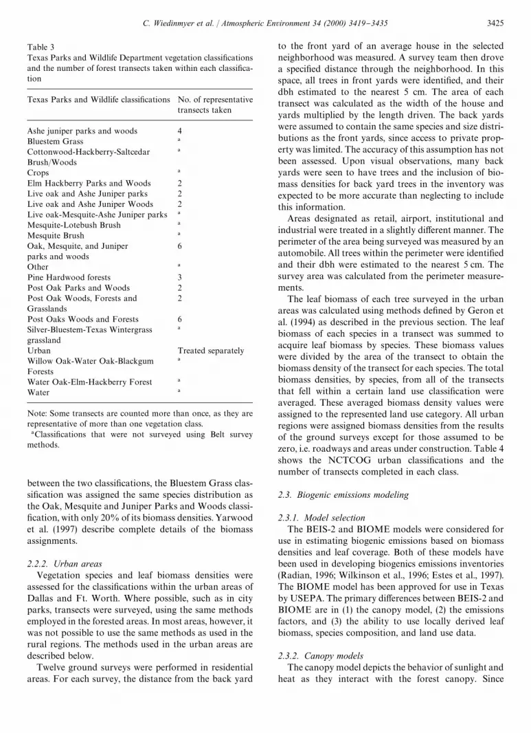
Table 3Texas Parks and Wildlife Department vegetation classi"cationsand the number of forest transects taken within each classi"ca-tion

Texas Parks and Wildlife classi"cations No. of representativetransects taken

Ashe juniper parks and woods 4Bluestem Grass !

Cottonwood-Hackberry-SaltcedarBrush/Woods

!

Crops !

Elm Hackberry Parks and Woods 2Live oak and Ashe Juniper parks 2Live oak and Ashe Juniper Woods 2Live oak-Mesquite-Ashe Juniper parks !

Mesquite-Lotebush Brush !

Mesquite Brush !

Oak, Mesquite, and Juniperparks and woods

6

Other !

Pine Hardwood forests 3Post Oak Parks and Woods 2Post Oak Woods, Forests andGrasslands

2

Post Oaks Woods and Forests 6Silver-Bluestem-Texas Wintergrassgrassland

!

Urban Treated separatelyWillow Oak-Water Oak-BlackgumForests

!

Water Oak-Elm-Hackberry Forest !

Water !

Note: Some transects are counted more than once, as they arerepresentative of more than one vegetation class.!Classi"cations that were not surveyed using Belt survey

methods.

between the two classi"cations, the Bluestem Grass clas-si"cation was assigned the same species distribution asthe Oak, Mesquite and Juniper Parks and Woods classi-"cation, with only 20% of its biomass densities. Yarwoodet al. (1997) describe complete details of the biomassassignments.

2.2.2. Urban areasVegetation species and leaf biomass densities were

assessed for the classi"cations within the urban areas ofDallas and Ft. Worth. Where possible, such as in cityparks, transects were surveyed, using the same methodsemployed in the forested areas. In most areas, however, itwas not possible to use the same methods as used in therural regions. The methods used in the urban areas aredescribed below.

Twelve ground surveys were performed in residentialareas. For each survey, the distance from the back yard

to the front yard of an average house in the selectedneighborhood was measured. A survey team then drovea speci"ed distance through the neighborhood. In thisspace, all trees in front yards were identi"ed, and theirdbh estimated to the nearest 5 cm. The area of eachtransect was calculated as the width of the house andyards multiplied by the length driven. The back yardswere assumed to contain the same species and size distri-butions as the front yards, since access to private prop-erty was limited. The accuracy of this assumption has notbeen assessed. Upon visual observations, many backyards were seen to have trees and the inclusion of bio-mass densities for back yard trees in the inventory wasexpected to be more accurate than neglecting to includethis information.

Areas designated as retail, airport, institutional andindustrial were treated in a slightly di!erent manner. Theperimeter of the area being surveyed was measured by anautomobile. All trees within the perimeter were identi"edand their dbh were estimated to the nearest 5 cm. Thesurvey area was calculated from the perimeter measure-ments.

The leaf biomass of each tree surveyed in the urbanareas was calculated using methods de"ned by Geron etal. (1994) as described in the previous section. The leafbiomass of each species in a transect was summed toacquire leaf biomass by species. These biomass valueswere divided by the area of the transect to obtain thebiomass density of the transect for each species. The totalbiomass densities, by species, from all of the transectsthat fell within a certain land use classi"cation wereaveraged. These averaged biomass density values wereassigned to the represented land use category. All urbanregions were assigned biomass densities from the resultsof the ground surveys except for those assumed to bezero, i.e. roadways and areas under construction. Table 4shows the NCTCOG urban classi"cations and thenumber of transects completed in each class.

2.3. Biogenic emissions modeling

2.3.1. Model selectionThe BEIS-2 and BIOME models were considered for

use in estimating biogenic emissions based on biomassdensities and leaf coverage. Both of these models havebeen used in developing biogenics emissions inventories(Radian, 1996; Wilkinson et al., 1996; Estes et al., 1997).The BIOME model has been approved for use in Texasby USEPA. The primary di!erences between BEIS-2 andBIOME are in (1) the canopy model, (2) the emissionsfactors, and (3) the ability to use locally derived leafbiomass, species composition, and land use data.

2.3.2. Canopy modelsThe canopy model depicts the behavior of sunlight and

heat as they interact with the forest canopy. Since

C. Wiedinmyer et al. / Atmospheric Environment 34 (2000) 3419}3435 3425

Table 4Urban land use classi"cations in the Dallas/Ft. Worth urbanregion and the number of surveys performed in each classi"ca-tion

Urban classi"cations No. of representativetransects taken

Residential: single, multi-family, groupquarters, and mobile homes

12

O$ce Not surveyedRetail 5Institutional 8Hotel/motel Not surveyedIndustrial 2Trans./Comm. Not surveyedRoadway Not surveyedUtilities Not surveyedAirport 2Parking garages Not surveyedParks and recreation 5Land"ll Not surveyedUnder construction Not surveyedFlood control Not surveyedVacant! Not surveyed

!Vacant lands in the urban region were replaced in the "naldatabase by the biomass density values of the Texas Parks andWildlife Department classi"cations that overlaid the vacantregions.

biogenic VOC emissions depend on sunlight and temper-ature, it is particularly important to estimate theseparameters accurately. Several canopy models have beenused in biogenic emission models, from very simple`look-up tablea models that reduce the solar radiationand temperature by "xed amounts as the canopy ispenetrated (Guenther et al., 1993,1994; Geron et al.,1994), to complex energy balance models that calculatethe temperatures based on many meteorological vari-ables (Vogel et al., 1995). In an important recent study,however, Lamb et al. (1996) concluded that there is littlepractical di!erence between the temperature and solarradiation pro"les developed by simple and complex can-opy models. It is much more important to accuratelyestimate the species composition and leaf biomass den-sity of the forest in question; compared to these para-meters, the choice of canopy model does not a!ect theaccuracy of the biogenic emissions estimate. Therefore,the choice of a biogenic emissions model was not basedon the canopy model used.

2.3.3. Base-rate emission factorsBEIS-2 and BIOME are accompanied by their own

base-rate biogenic emission factor databases. The term`base-ratea indicates emissions at 303C and half of fullsunlight (1000 lE m~2 s~1). However, it is possible touse either set of emission factors with each model. We

chose to use the BEIS-2 emission factors, given that thesefactors have been estimated rigorously and consistently(Guenther et al., 1993,1994; Geron et al., 1994), and thatBEIS-3 emission factors are in development.

2.3.4. Base-rate emission factor dataThe BEIS-2 base-rate emission factors for tree genera

were used to calculate the North Central Texas (NCT)biogenic emissions inventory. To use these emissionfactors in BIOME, it was necessary to convert the emis-sion factors from units of emission #ux (lg m~2 h~1)to units of emissions per gram of biomass (lg C g bi-omass~1 h~1). This conversion was e!ected using theunit leaf biomass densities in Geron et al. (1994) andRadian (1996). BEIS-2 emission factors were missing forsome genera in the NCT domain. These genera includedAlbizia, Callicarpa, Ficus, Firminia, Hibiscus, Koelreu-teria, Lagerstroemia, Ligustrum, Myrica, Photinia, Pyrus,Pistacia, Rhus, Sapindus, Sophora, Xanthoxylum, and Zel-kova. Fortunately, none of these genera were common inthe domain; many were not native. For missing genera,the taxonomic family average emission factor techniquewas used. This technique has been used by Benjaminet al. (1997), Benjamin and Winer (1998) and by the Stateof Texas. For some genera, BEIS-2 emission factorswere not available for any member of their taxonomicfamilies. In these cases, emission factors were drawn fromWilkinson and Emigh (1995), or from Benjamin andWiner (1998), or from an average of the emission factorsof genera in the same taxonomic order. Table 5 shows thebase-rate emission factors assigned to these genera.

Crop leaf biomass densities (Radian and VRC, 1994)were used to convert the BEIS2 emission #ux units toBIOME units of emission per gram of leaf biomass.

2.3.5. Use of local dataThe version of BEIS-2 available when the biogenic

model was chosen could not readily accept any land use,species composition, or leaf biomass density data otherthan the biogenic emissions landuse database (BELD).Therefore, BIOME, which has been successfully used inthe past with domain-speci"c data as input (Estes et al.,1997), was used.

2.3.6. Solar radiation dataThe algorithms included in earlier versions of BEIS-2

(EC/R Incorporated, 1995) were used for calculatinga gridded solar radiation "eld for the domain, basedupon latitude, time of year, time of day, and cloud cover(Iqbal, 1983). No direct ambient solar radiation measure-ments were available for biogenic emissions modeling ofthe two episodes that will be presented in the resultssection, therefore solar radiation was estimated. Cloudcover data were obtained for the speci"c episode daysfrom the National Climatic Data Center (NCDC). This

3426 C. Wiedinmyer et al. / Atmospheric Environment 34 (2000) 3419}3435

Table 5Emission factors assigned to genera without a BEIS-2 emission factor

Genus Data source for emissionfactor

Isoprene emissionfactor(lg/g-biomass/h)

Monoterpene emissionfactor(lg/g-biomass/h)

OVOC emissionfactor(lg/g-biomass/h)

Albizia Benjamin and Winer, 1998 1.37 0.53 1.9Callicarpa Verbenaceae family average 0.13 0.11 1.9Ficus Benjamin and Winer (1998) 8.61 0.08 1.9Firminia None found NA NA NAHibiscus Malvales order average 0.1 0.1 1.9Koelreuteria Benjamin and Winer (1998) 16.23 0 1.9Lagerstroemia Benjamin and Winer (1998) 0 0 NALigustrum Benjamin and Winer (1998) 0 0 1.9Myrica Benjamin and Winer (1998) 6.76 0.79 1.2Photinia Rosaceae family average 0.13 0.11 1.9Pistacia Benjamin and Winer (1998) 0 3.39 1.9Pyrus Benjamin and Winer (1998) 0 0 1.9Rhus Benjamin and Winer (1998) 0 0 1.9Sapindus Sapindales order average 0.1 0.57 1.9Sophora Benjamin and Winer (1998) 1.37 0.53 1.9Viburnum Benjamin and Winer (1998) 0 0.08 NAXanthoxylum Wilkinson and Emigh (1995) 0 1.49 1.9Zelkova Benjamin and Winer (1998) 0 0 1.9

cloud cover database was used to calculate solar radi-ation for both the core and the regional domains. For theJune 1995 episode described in the Results section, cloudcover observations were available for every hour; for theJuly 1996 episode described in the Results section, how-ever, observations were available for every hour on 30June, but only every 6 h beginning on 1 July. This changein the observation schedule occurred nationwide, be-cause the National Weather Service changed its methodof observing and reporting cloud cover data beginningon 1 July, 1996. For the 1996 episode, after 1 July theobservations were interpolated in time as well as space,so that during daylight hours, each observation was usedfor 6 h (the hour of observation, plus 3 h before and 2 hafter the time of observation).

The amount of transmittance through the cloud coverwas calculated by considering cloud thickness, sky cover-age, and cloud height (Iqbal, 1983; Pierce and Waldru!,1991). Although these data are the best available, thismethod is based on observations that are not continuousin space or time, and are interpolated between weatherstations. A comprehensive satellite photo study was be-yond the scope of this study, and it would be di$cult toestimate transmittance through the clouds based on ob-servations of cloud tops (McNider et al., 1995). As a sen-sitivity check, the biogenic emissions model was run withno cloud cover. Solar radiation increased greatly in theabsence of clouds, and therefore isoprene emissions esti-mates were substantially higher than emissions estimatescalculated with cloud cover. Another quality check was

performed by creating contour plots of solar radiation toensure the solar radiation "eld was reasonable. The "eldsgenerated by the UAM-BEIS2 solar radiation algorithmwere reasonable: sunset and sunrise occurred in west andeast, respectively, and maximum radiation occurred atsolar noon.

2.3.7. Temperature dataTemperature data were obtained from the NCDC.

A gridded temperature "eld was created from interpo-lated temperature observations measured at stationsacross the domain. A qualitative assessment of contourplots of the temperature "eld indicated no anomalies.

2.3.8. Other meteorological parameters neededfor input to BIOME

The wind "eld data needed for BIOME's canopymodel were obtained from the output of the systemsapplications international mesoscale model (SAIMM)meteorological model, which is based on the ColoradoState University Mesoscale Model (Mahrer and Piekle,1977,1978). Likewise, speci"c humidity data were alsotaken from the SAIMM meteorological modeling.

3. Results and discussion

3.1. Final database (coverage)

A "nal Land Use and Land Cover mapping was cre-ated from the combination of databases discussed in

C. Wiedinmyer et al. / Atmospheric Environment 34 (2000) 3419}3435 3427

Table 6Final total and oak biomass density values for each Texas Parks and Wildlife vegetation category in study domain. The standarddeviation in the biomass densities derived for each category is reported

Vegetation category Total biomassdensity (g m~2)

Standarddeviation

Total oak biomassdensity (g m~2)

Standarddeviation

Post Oak Woods, Forests and Grasslands 156 70 134 87Post Oak Woods and Forests 325 108 171 67Post Oaks Parks and Woods 251 82 230 108Live Oak and Ash Juniper Woods 339 343 44 41Live Oak and Ash Juniper Parks 153 27 9 12Oak, Mesquite, and Juniper Parks and Woods 326 181 33 73Elm-Hackberry Parks and Woods 394 37 226 129Pine Hardwood Forests 496 66 82 69Ash Juniper Parks and Woods 355 235 50 88Bluestem Grass 65 ! 13 !

Cottonwood-Hackberry-Saltcedar Brush/Woods 156 ! 134 !

Mesquite Brush 125 ! ! !

Mesquite Lotebush Brush 125 ! ! !

Silver-Bluestem-Texas Wintergrass Grassland 63 ! 54 !

Water Oak-Elm-Hackberry Forest 371 65 170 68Willow Oak-Water Oak-Blackgum Forests 371 65 170 68

!Signi"es classi"cations in which no "eld surveys were taken: biomass density assignments are based on surveys taken in otherclassi"cations.

Table 7Final biomass densities assigned to the urban land use classi"cations in the Dallas/Ft. Worth urban area

Urban land use category Total biomassdensity(g m~2)

Standarddeviation

Biomass densityof oaks (g m~2)

Standarddeviation

Institutional 11 7 3 3Vacant! 46 ! 9 !

Commercial 15 15 8 11Industrial 3 4 2 3Parks and Recreational 78 39 14 50Residential 42 25 10 6

!Vacant lands in the urban region were replaced in the "nal database by the biomass density values of the Texas Parks and WildlifeDepartment classi"cations that overlaid the vacant regions.

previous sections (Fig. 2). This "nal mapping assigns landuse classi"cations to the entire study domain. Theseclassi"cations are particular to the North Central regionin Texas and describe the land use and vegetation covermore speci"cally than any other land cover databaseavailable for the region. This improved land use databasewas used as the basis for biogenic emissions estimates.

Each of the land use and land cover classi"cationsshown in Fig. 2 was assigned biomass densities andspecies distributions. Tables 6 and 7 show the totalbiomass and density values assigned to each of theseclassi"cations. The total oak biomass density of eachclassi"cation is also included. This parameter is importantwhen estimating biogenic hydrocarbon emissions be-cause oak species are very common in the domain, andthe oak trees are the largest sources of biogenic isoprene

emissions. The magnitude of oak biomass density as-signed to a classi"cation is highly correlated with theamount of isoprene emissions expected from an areadesignated by that classi"cation. More detailed speciesassignments are reported elsewhere (Yarwood et al.,1997).

3.2. Comparison of leaf biomass estimates with the BELD

The completed vegetation database for North CentralTexas can be compared to the biogenic emissions landusedatabase (BELD). The BELD, as described in Kinneeet al. (1997), is the most current national vegetationdatabase for estimating biogenic emissions. Thisdatabase assigns species distributions and vegetationcoverage by county for the contiguous United States.

3428 C. Wiedinmyer et al. / Atmospheric Environment 34 (2000) 3419}3435

Fig. 5. The percent forest and oak coverage for the BELD3.0 data and the database created for this study in North central Texas.

Although the BELD applies very speci"c data tomany areas of the nation, especially some eastern forests,the data for North Central Texas were created from theUSGS LCC database. As reported in Section 2.1, these

data are not the most accurate for the region. Fig. 5shows the percent forest and percent oak of the BELD3.0and the database created for this study for the northcentral Texas domain.

C. Wiedinmyer et al. / Atmospheric Environment 34 (2000) 3419}3435 3429

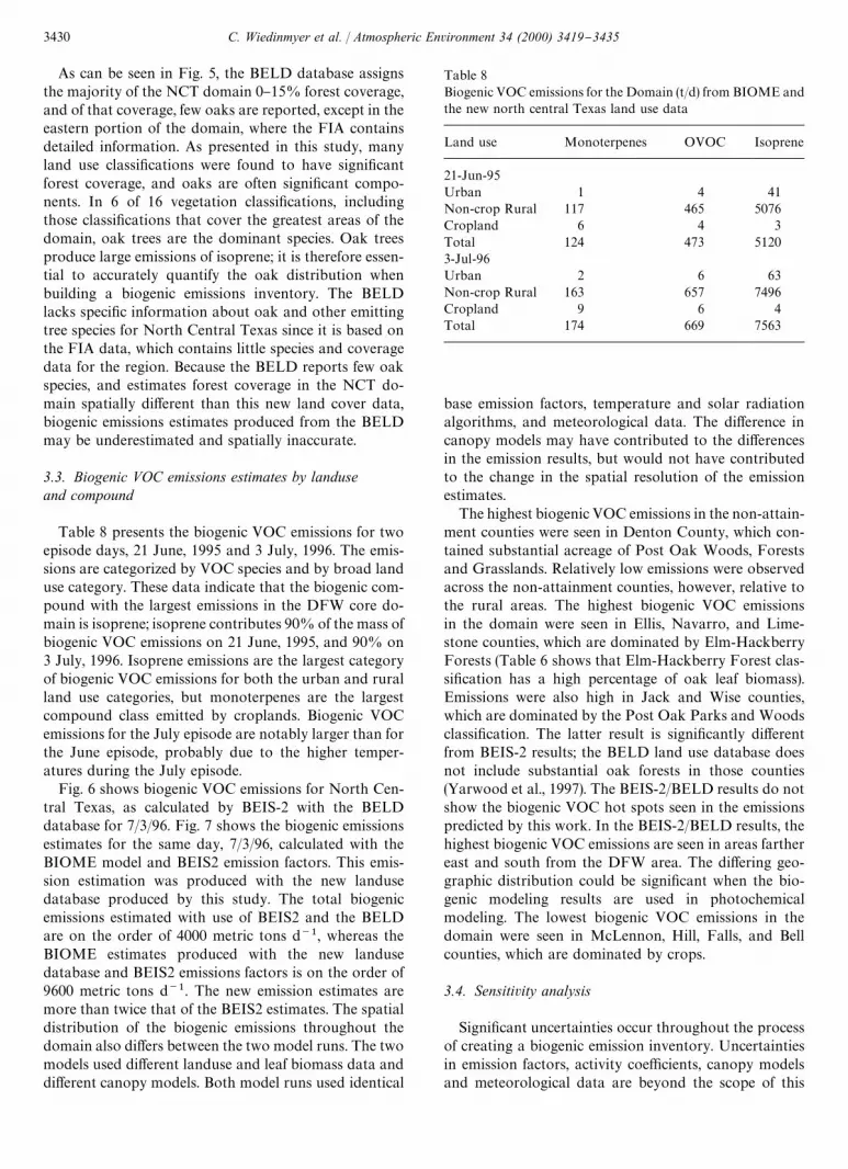
Table 8Biogenic VOC emissions for the Domain (t/d) from BIOME andthe new north central Texas land use data

Land use Monoterpenes OVOC Isoprene

21-Jun-95Urban 1 4 41Non-crop Rural 117 465 5076Cropland 6 4 3Total 124 473 51203-Jul-96Urban 2 6 63Non-crop Rural 163 657 7496Cropland 9 6 4Total 174 669 7563

As can be seen in Fig. 5, the BELD database assignsthe majority of the NCT domain 0}15% forest coverage,and of that coverage, few oaks are reported, except in theeastern portion of the domain, where the FIA containsdetailed information. As presented in this study, manyland use classi"cations were found to have signi"cantforest coverage, and oaks are often signi"cant compo-nents. In 6 of 16 vegetation classi"cations, includingthose classi"cations that cover the greatest areas of thedomain, oak trees are the dominant species. Oak treesproduce large emissions of isoprene; it is therefore essen-tial to accurately quantify the oak distribution whenbuilding a biogenic emissions inventory. The BELDlacks speci"c information about oak and other emittingtree species for North Central Texas since it is based onthe FIA data, which contains little species and coveragedata for the region. Because the BELD reports few oakspecies, and estimates forest coverage in the NCT do-main spatially di!erent than this new land cover data,biogenic emissions estimates produced from the BELDmay be underestimated and spatially inaccurate.

3.3. Biogenic VOC emissions estimates by landuseand compound

Table 8 presents the biogenic VOC emissions for twoepisode days, 21 June, 1995 and 3 July, 1996. The emis-sions are categorized by VOC species and by broad landuse category. These data indicate that the biogenic com-pound with the largest emissions in the DFW core do-main is isoprene; isoprene contributes 90% of the mass ofbiogenic VOC emissions on 21 June, 1995, and 90% on3 July, 1996. Isoprene emissions are the largest categoryof biogenic VOC emissions for both the urban and ruralland use categories, but monoterpenes are the largestcompound class emitted by croplands. Biogenic VOCemissions for the July episode are notably larger than forthe June episode, probably due to the higher temper-atures during the July episode.

Fig. 6 shows biogenic VOC emissions for North Cen-tral Texas, as calculated by BEIS-2 with the BELDdatabase for 7/3/96. Fig. 7 shows the biogenic emissionsestimates for the same day, 7/3/96, calculated with theBIOME model and BEIS2 emission factors. This emis-sion estimation was produced with the new landusedatabase produced by this study. The total biogenicemissions estimated with use of BEIS2 and the BELDare on the order of 4000 metric tons d~1, whereas theBIOME estimates produced with the new landusedatabase and BEIS2 emissions factors is on the order of9600 metric tons d~1. The new emission estimates aremore than twice that of the BEIS2 estimates. The spatialdistribution of the biogenic emissions throughout thedomain also di!ers between the two model runs. The twomodels used di!erent landuse and leaf biomass data anddi!erent canopy models. Both model runs used identical

base emission factors, temperature and solar radiationalgorithms, and meteorological data. The di!erence incanopy models may have contributed to the di!erencesin the emission results, but would not have contributedto the change in the spatial resolution of the emissionestimates.

The highest biogenic VOC emissions in the non-attain-ment counties were seen in Denton County, which con-tained substantial acreage of Post Oak Woods, Forestsand Grasslands. Relatively low emissions were observedacross the non-attainment counties, however, relative tothe rural areas. The highest biogenic VOC emissionsin the domain were seen in Ellis, Navarro, and Lime-stone counties, which are dominated by Elm-HackberryForests (Table 6 shows that Elm-Hackberry Forest clas-si"cation has a high percentage of oak leaf biomass).Emissions were also high in Jack and Wise counties,which are dominated by the Post Oak Parks and Woodsclassi"cation. The latter result is signi"cantly di!erentfrom BEIS-2 results; the BELD land use database doesnot include substantial oak forests in those counties(Yarwood et al., 1997). The BEIS-2/BELD results do notshow the biogenic VOC hot spots seen in the emissionspredicted by this work. In the BEIS-2/BELD results, thehighest biogenic VOC emissions are seen in areas farthereast and south from the DFW area. The di!ering geo-graphic distribution could be signi"cant when the bio-genic modeling results are used in photochemicalmodeling. The lowest biogenic VOC emissions in thedomain were seen in McLennon, Hill, Falls, and Bellcounties, which are dominated by crops.

3.4. Sensitivity analysis

Signi"cant uncertainties occur throughout the processof creating a biogenic emission inventory. Uncertaintiesin emission factors, activity coe$cients, canopy modelsand meteorological data are beyond the scope of this

3430 C. Wiedinmyer et al. / Atmospheric Environment 34 (2000) 3419}3435

Fig. 6. Biogenic VOC emissions for north-central Texas on 7/3/96, calculated with the BEIS2 model, using the BELD land use database.Units are tons/day of Carbon Bond IV hydrocarbons. Grids are 16]16 km (256 km2). Note that the colors are scaled to match those inFig. 7, which contains 4]4 km grid cells. Each color represents the same range of emission densities in both tileplots.

paper, but have been discussed elsewhere (Benjaminet al., 1997; Lamb et al., 1996; Lamb et al., 1993; Geronet al., 1994; Guenther et al., 1999). The analysis of un-certainties presented in this paper will focus on the

uncertainties in emission estimates due to variability inthe primary data collected in this work } forest treediameter distributions and resulting leaf biomass densityestimates.

C. Wiedinmyer et al. / Atmospheric Environment 34 (2000) 3419}3435 3431

Fig. 7. Biogenic VOC emissions for north central Texas on 7/3/96, calculated with the BIOME model, using the new land use andvegetation data. Units are tons/day of Carbon Bond IV hydrocarbons. Grids are 4]4 km (16 km2). Note that the colors are scaled tomatch those in Fig. 6, which contains 16]16 km grid cells. Each color represents the same range of emission densities in both tileplots.

The various methods used to determine biomassdensities and species distributions for each vegetationclassi"cation involved a series of assumptions and ap-proximations. The transect location selection and the

averaging techniques used to assign species distributionsand biomass densities to each land use classi"cationare subject to sample bias and uncertainty. Becausethese steps were performed with qualitative reasoning,

3432 C. Wiedinmyer et al. / Atmospheric Environment 34 (2000) 3419}3435

Table 9Biogenic (Carbon Bond IV) hydrocarbon emissions for primary episode days, as calculated by BIOME using new North Central Texasbiogenics database and BEIS2 emission factors

CB-IV emissions by county (t/d)

Date Dallas Tarrant Denton Collin Total DFW Core domain total

6/21/95 54 85 136 19 294 66436/22/95 58 93 152 22 325 72887/3/96 80 128 213 31 453 9635

statistically based uncertainties are di$cult to produce.Nevertheless, a preliminary assessment of uncertaintiesin the emission estimates can be performed.

To assess the e!ects of the choice of transect locationand averaging techniques used to assign species distribu-tions and biomass densities for the classi"cations, lowerand upper bounds of total biomass densities were cal-culated for two important vegetation classi"cations inthe domain. Two transects were surveyed in the PostOak Woods, Forests and Grasslands classi"cation. Thebiomass densities and species distributions from each ofthe two transects were averaged and used to calculate thebiogenic emissions estimates shown in Fig. 7. One tran-sect had a much lower total biomass density than theother: 106 versus 206 g m~2, with Oak biomass densitiesof 72 and 196 g m~2, respectively. This variability wasintended, since the two transects combined were expectedto accurately describe the land use classi"cation. Thevariation of Oak and total biomass densities between thetwo surveys suggest an uncertainly of a factor of approx-imately 2.

Six transects were performed at locations designatedby the Post Oak Woods and Forest classi"cation. Thesetransects had varying species and biomass densitieswhich, when combined, were assumed to be repres-entative of the Post Oak Woods and Forest classi"ca-tion. Of these six transects, the total biomass calculatedfrom the data of each ranged from 143 to 420 g m~2. Thepercentage of Oaks in the six transects ranged from 35 to100%. This suggests an uncertainty of a factor of 3 fortotal and Oak biomass densities within each landusecategory.

This method of determining upper and lower boundsof the emission estimates for vegetation classi"cationsmay not produce the true extremes. Although the lowestand highest total biomass values were chosen to deter-mine bounds on the estimates, this may not lead to trueemission bounds; nevertheless these bounds give an in-dication of the potential magnitude of the uncertainties,especially at small scales associated with forest canopycover.

4. Conclusions

A GIS land cover/ land use database for a 37 countydomain in North Central Texas was developed. Thisdatabase includes vegetation species distributions andbiomass densities, speci"c to the vegetation in Texas. Themethods employed in this study may be applied to otherareas within Texas. Similar studies could also be conduc-ted outside the state but will require the use of a ruralvegetation database other than that provided by theTexas Parks and Wildlife Department. The USGS LCCdata could be used for this purpose, but will require moreextensive ground surveying.

The vegetation database created in this work is animprovement over the data reported in the BELD for theNorth Central Texas region. This new database reportsgreater overall biomass densities and higher densities ofoak and other emitting tree species that the BELD doesnot report. This improved biomass characterization canlead to an improvement in the biogenic emissions esti-mates for the region.

A new biogenic emissions inventory was created fora modeling episode in 1996 using this information. Theemissions inventory for biogenic sources for use inphotochemical models of the North Central Texas regionis more speci"c and accurate than any data previouslyavailable. Total emissions for the region were estimatedto increase over 100% from BEIS2/BELD estimates forthe same region. The spatial variations in the emissionsinventory also changes with the use of the new landusedatabase. New `hot-spotsa of biogenic emissions in thedomain were located.

A detailed assessment of the uncertainties of themethods used to determine the vegetation species distri-butions and biomass densities should be performed. Thechoice of location, direction and averaging of the tran-sects can greatly a!ect the biogenic emissions estimates.A qualitative analysis of the uncertainty in transectselection and averaging suggests that an uncertainty of afactor of 2}3 can be applied to the biomass densitiesassigned to each land use classi"cation. But, the di!erences

C. Wiedinmyer et al. / Atmospheric Environment 34 (2000) 3419}3435 3433

in forest and oak coverage between the BELD3 and thenew land cover data are greater than this factor in manyareas of the domain. In addition, emission factor andfoliar mass data should be collected for tree species in theregion to verify the values used in this study.

Acknowledgements

The authors thank Alex Guenther, Lee Klinger, BillBaugh and Chris Geron for useful discussions and practi-cal advice on conducting "eld surveys. The authors alsothank Pryanka Bandypadha, Patrick Gri$th, DougGoldman and Todd Barkman, who participated in the"eld surveys. Dr. David Maidment provided valuableexpertise with the Geographical Information Systems.David Jacob from the Texas Natural Resource Conser-vation Commission assisted in the modeling. The authorsthank the anonymous reviewers of this manuscript fortheir advice and helpful comments. This work was sup-ported by contract dUTA97-0302 with the Texas Natu-ral Resource Conservation Commission.

References

Benjamin, M., Winer, A., 1998. Estimating the ozone-formingpotential of urban trees and shrubs. Atmospheric Environ-ment 32 (1), 53}68.

Benjamin, M., Sudol, M., Vorsatz, D., Winer, A., 1997. A spa-tially and temporally resolved biogenic hydrocarbon emis-sions inventory for the California South Coast Air Basin.Atmospheric Environment 31 (18), 3087}3100.

EC/R Incorporated, 1995. Urban Airshed Model (UAM) Bi-ogenic Emission Inventory System Version 2 (BEIS-2) User'sGuide. EPA Contract No. 68-D3-0034; prepared for RichardA. Wayland, Air Quality Modeling Group, US EPA, Sep-tember 28, 1995.

Estes, M., Jacob, D., Jarvie, J,. MacKay, J., Smith J., 1997.Biogenic emissions modeling for Southeastern Texas. Pro-ceedings of a Specialty Conference Cosponsored by the Airand Waste Management Association and the U.S.EPA, NewOrleans, Louisiana.

Geron, C.D., Pierce, T.E., Guenther, A.B., 1995. Reassessment ofbiogenic volatile organic compound emissions in the Atlantaarea. Atmospheric Environment 29 (13), 1569}1578.

Geron, C.D., Guenther, A.B., Pierce, T.E., 1994. An improvedmodel for estimating emissions of volatile organic com-pounds from forests in the eastern United States. Journal ofGeophysical Research 99, 12773}12791.

Guenther, A., Hewitt, N., Erickson, D., Fall, R., Geron, C.,Graedel, T., Harley, P., Klinger, L., Lerdau, M., McKay, W.,Pierce, T., Scholes, B., Steinbrecher, R., Tallamraju, T.,Taylor, J., Zimmerman, P., 1995. A global model of naturalvolatile organic compound emissions. Journal of Geophysi-cal Research 100 (D5), 8873}8892.

Guenther, A.B., Zimmerman, P., Wildermuth, M., 1994. Naturalvolatile organic compound emission rate estimates for US.

woodland landscapes. Atmospheric Environment 28,1197}1210.

Guenther, A.B., Zimmerman, P.R., Harley, P.C., Monson, R.,Fall, R., 1993. Isoprene and monoterpene emission ratevariability: model evaluations and sensitivity analyses. Jour-nal of Geophysical Research 98, 12609}12617.

Iqbal, M., 1983. An Introduction to Solar Radiation. AcademicPress, San Diego, California, pp. 107}277.

Kinnee, E., Geron, C., Pierce, T., 1997. United States land useinventory for estimating biogenic ozone precursor emissions.Ecological Applications 7 (1), 46}58.

Klinger, L., 1997. Personal communication.Lamb, B., Pierce, T., Baldocchi, D., Allwine, E., Dilts, S., West-

berg, H., Geron, C., Guenther, A., Klinger, L., Harley, P.,Zimmerman, P., 1996. Evaluation of forest canopy modelsfor estimating isoprene emissions. Journal of GeophysicalResearch 101, 22787}22798.

Lamb, B., Gay, D., Westberg, H., Pierce, T., 1993. A bio-genic hydrocarbon emission inventory for the USA usinga simple forest canopy model. Atmospheric Environment27A, 1}18.

Mahrer, Piekle, 1978. A test of an upstream spline interpolationtechnique for the advective terms in a numerical mesoscalemodel. month Weath Review 106, 818}830.

Mahrer, Piekle, 1977. A numerical study of the air #owover irregular terrain. Control of Atmospheric Physics 50:98}113.

McNider, R.T., Song, J.A., Kidder, S.Q., 1995. Assimilation ofGOES-derived solar insolation into a mesoscale model forstudies of cloud shading e!ects. International Journal ofRemote Sensing 16, 2207}2231.

Miller, P.E., Winer, A.M., 1984. Composition and Dominance inLos Angeles basin urban vegetation. Urban Ecology 8, 29}54.

Pierce, T., Waldru!, P., 1991. PC-BEIS: a personal computerversion of the biogenics emission inventory system.Journal of Air and Waste Management Association 41,937}941.

Radian, 1996. Biogenic Sources Preferred Methods, Final Re-port. Prepared for Area Sources Committee of the EmissionsInventory Improvement Program, May, 1996.

Radian and Valley Research Corporation, 1994. Final Report,Biogenics Emissions Factors Project, Texas Natural Re-source Conservation Commission. Prepared by Radian Cor-poration and Valley Research Corporation; prepared forTNRCC, March 7, 1994.

Strange, I.W., 1998. M.S. Thesis. University of Texas at Austin,Austin, Texas.

Texas Parks and Wildlife Department, 1996. The VegetationTypes of Texas; Introduction. Available on the Internet athttp://www.tpwd.state.tx.us/admin/veg/intro.html.

U.S. Department of Agriculture, NASS data, 1997. Data fromthe USDA National Agriculture Statistics Service. Availableon the internet at `http://www.usda.gov/nass/a

U.S. EPA, 9/3/98. National Air pollutant Emissions Trends,1990}1998. Available on the internet at http://www.epa.gov/oar/emtrnd/.

U.S. Geological Survey, ca. 1976. Land Use/Land Coverdatabases, available on the internet at `http://edcwww.cr.usgs.gov/doc/edchome/ndcdb/ndcdb.htmla.

Vogel, C., Baldocchi, D., Luhar, A., Rao, K.S., 1995. A compari-son of a hierarchy of models for determining energy balance

3434 C. Wiedinmyer et al. / Atmospheric Environment 34 (2000) 3419}3435

components over vegetation canopies. Journal of AppliedMeteorology 34, 2182}2196.

Wilkinson, J.G., Emigh, R.A., Pierce T.E., 1996. An intercom-parison of biogenic emissions estimates from BEIS2 andBIOME: Reconciling the di!erences. The Emission Inven-tory: Key to Planning, Permits, Compliance, and Reporting,Proceedings of Air and Waste Management Specialty Con-ference, September 4}6, 1996, New Orleans, Louisiana, pp.985}1009.

Wilkinson, J.G., Emigh, R.A., 1995. The Emissions ModelingSystem (EMS-95) User's Guide prepared by Alpine Geo-physics for the Texas Natural Resource Conservation Com-mission. March 13, 1995.

Yarwood, G., Allen, D., Guenther, A., Wiedinmyer, C., Baugh,B., Quigley, C., Strange, W., 1997. Leaf Biomass DensityData for North Central Texas. Prepared for the TexasNatural Resource Conservation Commission. October 15,1997.

C. Wiedinmyer et al. / Atmospheric Environment 34 (2000) 3419}3435 3435