Biogenic emission measurement and inventories determination of biogenic emissions in the eastern United States and Texas and comparison with biogenic emission inventories

Biogenic emission measurement and inventories determination

of biogenic emissions in the eastern United States and Texas

and comparison with biogenic emission inventories

C. Warneke,1,2 J. A. de Gouw,1,2 L. Del Negro,3 J. Brioude,1,2 S. McKeen,1,2 H. Stark,1,2

W. C. Kuster,1 P. D. Goldan,1 M. Trainer,1 F. C. Fehsenfeld,1,2 C. Wiedinmyer,4

A. B. Guenther,4 A. Hansel,5 A. Wisthaler,5 E. Atlas,6 J. S. Holloway,1,2 T. B. Ryerson,1

J. Peischl,1,2 L. G. Huey,7 and A. T. Case Hanks8

Received 7 May 2009; revised 1 October 2009; accepted 8 October 2009; published 9 March 2010.

[1] During the NOAA Southern Oxidant Study 1999 (SOS1999), Texas Air QualityStudy 2000 (TexAQS2000), International Consortium for Atmospheric Research onTransport and Transformation (ICARTT2004), and Texas Air Quality Study 2006(TexAQS2006) campaigns, airborne measurements of isoprene and monoterpenes weremade in the eastern United States and in Texas, and the results are used to evaluate thebiogenic emission inventories BEIS3.12, BEIS3.13, MEGAN2, and WM2001. Twomethods are used for the evaluation. First, the emissions are directly estimated from theambient isoprene and monoterpene measurements assuming a well-mixed boundarylayer and are compared with the emissions from the inventories extracted along theflight tracks. Second, BEIS3.12 is incorporated into the detailed transport modelFLEXPART, which allows the isoprene and monoterpene mixing ratios to be calculated andcompared to themeasurements. The overall agreement for all inventories is within a factor of2 and the two methods give consistent results. MEGAN2 is in most cases higher, andBEIS3.12 and BEIS3.13 lower than the emissions determined from the measurements.Regions with clear discrepancies are identified. For example, an isoprene hot spot to thenorthwest of Houston, Texas, was expected from BEIS3 but not observed in themeasurements. Interannual differences in emissions of about a factor of 2 were observed inTexas between 2000 and 2006.

Citation: Warneke, C., et al. (2010), Biogenic emission measurement and inventories determination of biogenic emissions in the

eastern United States and Texas and comparison with biogenic emission inventories, J. Geophys. Res., 115, D00F18,

doi:10.1029/2009JD012445.

1. Introduction

[2] A large number of different volatile organic com-pounds (VOCs) are emitted into the atmosphere by thebiosphere with a total of about 1150 Tg C yr�1 [Guenther etal., 1995], which represents about 80% of the total global

VOC emissions. These emissions are dominated by iso-prene with an estimated global annual emission of 440–660 Tg C yr�1 [Guenther et al., 2006]. Other large biogenicemissions include various monoterpenes with a combinedemission of about 127 Tg C yr�1 [Guenther et al., 1995],methanol with about 100–160 Tg yr�1 [Jacob et al., 2005],and acetone with about 33 Tg yr�1 [Jacob et al., 2002].While the emissions of isoprene and monoterpenes havebeen extensively studied, large uncertainties remain formany regions and most other species.[3] Because of the enormous impact of biogenic VOC

emissions on the global and regional atmospheric chemistryproducing ozone and secondary organic aerosol [Henze andSeinfeld, 2006; Pfister et al., 2008], biogenic VOCs areincluded in air quality forecast models, global chemistry andclimate models and in regulatory regional models. Themodel input is usually in the form of off-line emissioninventories. The most commonly used biogenic emissionsmodel in United States is the EPA BEIS3 (EnvironmentalProtection Agency Biogenic Emissions Inventory System 3)(http://www.epa.gov/asmdnerl/biogen.html), which includes

JOURNAL OF GEOPHYSICAL RESEARCH, VOL. 115, D00F18, doi:10.1029/2009JD012445, 2010ClickHere

for

FullArticle

1Chemical Sciences Division, ESRL, NOAA, Boulder, Colorado, USA.2CIRES, University of Colorado at Boulder, Boulder, Colorado, USA.3Department of Chemistry, Lake Forest College, Lake Forest, Illinois,

USA.4ACD, NCAR, Boulder, Colorado, USA.5Institut fur Ionenphysik und Angewandte Physik, Universitat

Innsbruck, Innsbruck, Austria.6Marine and Atmospheric Chemistry Division, Rosenstiel School of

Marine and Atmospheric Sciences, University of Miami, Miami, Florida,USA.

7School of Earth and Atmospheric Sciences, Georgia Institute ofTechnology, Atlanta, Georgia, USA.

8Department of Geosciences, University of Louisiana at Monroe,Monroe, Louisiana, USA.

Copyright 2010 by the American Geophysical Union.0148-0227/10/2009JD012445$09.00

D00F18 1 of 21

http://dx.doi.org/10.1029/2009JD012445

isoprene, the monoterpenes and many other species. Anothermodel, recently introduced by Guenther et al. [2006], iscalledMEGAN2 (Model of Emissions of Gases andAerosolsfrom Nature version 2), which is a detailed global model forisoprene and more than 100 other VOCs. MEGAN2 ispublicly available at http://cdp.ucar.edu.[4] Biogenic emission inventories have been evaluated in

a number of different ways. Above-canopy flux measure-ments using eddy covariance techniques have been usedfrequently [Guenther and Hills, 1998]. Such studies allow avery detailed evaluation of the parameterization of biogenicemissions versus light, temperature and other parametersused in the inventories, but do this for one location only.Second, inverse modeling or indirect methods have beenused to test biogenic emission inventories. For example,Millet et al. [2008] used formaldehyde columns derivedfrom the Ozone Monitoring Instrument (OMI) to deriveisoprene emissions over North America, which were 4–25% lower than predicted by MEGAN2. Earlier, formalde-hyde retrievals from GOME were used to estimate isopreneemissions with similar results [Palmer et al., 2006]. Withthe same method, but SCIAMACHY formaldehyde data,Stavrakou et al. [2009] estimate isoprene emissions about40% lower than MEGAN2 for North America. Muller et al.[2008] used MEGAN2 in a global model using ECMWFmeteorology and a detailed canopy environment model andfound an underprediction of the modeled isoprene flux byabout 30% for the Harvard forest site. Isoprene has recentlybeen modeled in Texas for two flights from the Tex-AQS2000 campaign using the Comprehensive Air QualityModel with Extensions and the Global Biosphere Emissionsand Interactions System (GLOBEIS) [Song et al., 2008]. Anoverprediction was found for areas with high isoprenemixing ratios and underpredictions for areas with lowisoprene mixing ratios. Many different variables, such asboundary layer height, temperature, photosynthetically ac-tive radiation (PAR), and chemistry, have to be modeledcorrectly for a model-measurement comparison to be suc-cessful, which makes these direct comparisons very chal-lenging. Only recently have results been published that useaircraft measurements on a somewhat larger spatial scale toquantitatively derive isoprene emissions and compare toemission inventories. For example, Karl et al. [2007] foundmeasured isoprene fluxes derived from aircraft measure-ments about 40% higher than predicted by MEGAN2 overAmazonia.[5] During the NOAA SOS1999, TexAQS2000,

ICARTT2004 and TexAQS2006 campaigns, multipleflights were performed covering many forested areas inthe eastern United States and Texas. In this work we use thein situ measurements of isoprene and monoterpenes fromthose field campaigns in an attempt to evaluate the availablebiogenic emission models EPA BEIS3.12, the latest versionEPA BEIS3.13, MEGAN2 and a model developed byWiedinmyer et al. [2001] for Texas only (WM2001). Twoapproaches are used for this evaluation. First, the emissionsare estimated from the ambient measurements assuming awell-mixed boundary layer, an entrainment flux and chem-ical loss due to OH, and compared to the emissions from theinventories extracted along the flight tracks in the boundarylayer. Second, BEIS3.12 was incorporated into the Lagrang-ian transport model FLEXPART, and the calculated iso-

prene and monoterpene mixing ratios are compared to theaircraft measurements.

2. Airborne Measurements of Biogenic VOCsin the United States

2.1. Measurement Campaigns: SOS1999,TexAQS2000, ICARTT2004, and TexAQS2006

[6] Airborne measurements of biogenic VOCs were con-ducted in the framework of four different summertimecampaigns: the Southern Oxidants Study 1999 (SOS99) inJune and July of 1999 in the southeast United States [Brocket al., 2002], the Texas Air Quality Study in August andSeptember 2000 (TexAQS2000) [Ryerson et al., 2003] andthe Texas Air Quality Study in September and October of2006 (TexAQS2006) [Parrish et al., 2009] also in Texas,and the ICARTT2004 study in July and August of 2004 inthe northeast United States [Fehsenfeld et al., 2006]. Iso-prene was measured during all four campaigns, the sum ofthe monoterpenes during ICARTT2004 and TexAQS2006.For the work presented here, we will use only the dataobtained in the boundary layer.[7] The flight tracks of the NOAA WP-3 for SOS99,

ICARTT2004 and TexAQS2006 campaigns are shown inFigure 1a on top of the EPA BEIS3.13 summer isoprenebase emissions map of the United States. Base emissions arethe isoprene emissions at standard conditions (30�C and1000 mmol m�2 h�1 for all leaves). Actual emissionsdeviate from the base emissions as a function of temperatureand light, as will be discussed in detail below. Flight tracksin the boundary layer are shown in black, the ones in thefree troposphere in red. It can be seen that the area coveredby the flight tracks includes a large part of the forestedeastern half of the United States including Texas, wherelarge isoprene emissions are predicted. The flight tracks ofthe TexAQS2000 study are shown in Figure 1b on top of theMEGAN2 isoprene base emission factors. In Figure 1c theBEIS3.13 summer monoterpene base emissions are shown.

2.2. Instrumentation

[8] During the ICARTT2004 and TexAQS2006 cam-paigns, isoprene, and its oxidation products methyl vinylketone (MVK) and methacrolein (MACR), and monoter-pene measurements were performed with the NOAA PTR-MS instrument (Proton-Transfer-Reaction Mass Spectrom-eter) on board the NOAA WP-3 aircraft during multipleflights. During TexAQS2000 isoprene was measured usingthe Innsbruck PTR-MS [Hawes et al., 2003]. A detaileddescription of the PTR-MS instrument and an intercompar-ison with gas chromatography (GC) measurements fromwhole air samples (WAS) can be found elsewhere [de Gouwand Warneke, 2007; de Gouw et al., 2006]. During theflights, isoprene, MVK + MACR, and monoterpenes weremeasured for 1 s each every 17 s. The PTR-MS wascalibrated for many VOCs between the flights using astandard mixture containing 500 ppbv of each compoundthat was diluted to single-ppbv levels. The calibrationuncertainty is estimated to be less than 15% for isoprene.PTR-MS measures only the sum of the monoterpenes andtherefore the calibration is less certain and depends on themixture of the individual monoterpenes, and the calibrationuncertainty is estimated to be less than 30%. The detection

D00F18 WARNEKE ET AL.: BIOGENIC EMISSIONS AND INVENTORIES

2 of 21

D00F18

limit of the PTR-MS for isoprene and the monoterpenes isabout 40 pptv for a 5 s measurement [de Gouw et al., 2003]and was about 70 pptv for a 1 s measurement and about 20pptv for 5 min averages. In the Houston ship channel, anarea close to Houston with a large number of petrochemicalfacilities, large amounts of anthropogenic VOCs, includingisoprene, are released and interferences from species otherthan isoprene are possible. Interferences for mass 69, onwhich mass isoprene is detected, have been studied bycombining PTR-MS with a gas chromatographic presepara-tion method [Warneke et al., 2003] and include compoundslike cyclopentene, pentanal, and 2-methyl-3-buten-2-ol(MBO). In some isolated plumes near the Houston shipchannel, the isoprene measurements have to be taken as anupper limit, but everywhere else the PTR-MS measurementsagree well with the GC analysis of the WAS and aretherefore assumed to be exclusively isoprene. The scatter-plot between the PTR-MS and WAS data using all data fromthe mission gives a slope of 0.97 and a correlation coeffi-cient of R = 0.70 for TexAQS2006 and a slope of 0.89 and

R = 0.92 for ICARTT2004 [de Gouw and Warneke, 2007].The different measurement frequencies of the two instru-ments cause a low correlation coefficient for the Tex-AQS2006 data, because of the higher variability of theisoprene mixing ratios in Texas compared to New England.The Innsbruck PTR-MS used during TexAQS2000 mea-sured isoprene for 2–5 s every 2–40 s (integrations timesvaried per flight or flight segment). Calibrations were donewith a dynamically diluted VOC standard with an estimatedaccuracy of 20% [Hawes et al., 2003]. Here we use thePTR-MS data instead of the WAS data for TexAQS2000,TexAQS2006 and ICARTT2004, because of the higher timeresolution.[9] During SOS99 isoprene was measured using an

airborne gas chromatograph with a flame ionization detector(GC-FID). A 350 cm3 STP sample was cryogenicallyacquired for 5 min every 15 min and analyzed in theremaining 10 min. The analytical column was a 30 m �0.53 mm KCl washed Al2O3 (Chrompack Inc.). A calibrat-ed whole air standard was sampled before, during and after

Figure 1. (a) The flight tracks of the NOAA WP-3 aircraft during the NOAA TexAQS2006,ICARTT2004, and SOS1999 campaigns (boundary layer in black and free troposphere in red) plotted ontop of the EPA BEIS3.13 summer isoprene base emissions map of the United States. (b) The MEGAN2isoprene emission factor map with the TexAQS2000 flight tracks. (c) The BEIS3.13 monoterpene baseemissions. The units of the emissions here and in the rest of the manuscript are moles C km�2 h�1, andthe same color scale for the base emissions is used in Figures 2, 4, 9, 10, and 12–15.


3 of 21

D00F18

the flight for calibration. The detection limit was between2 pptv and 5 pptv for all compounds. More details on theinstrument can be found elsewhere [Goldan et al., 2000].[10] Shortwave solar radiation (200–4700 nm), needed as

input for BEIS and MEGAN2, was measured using astandard pyranometer during SOS99 and TexAQS2000and estimated using data from an actinic flux spectrometerduring ICARTT2004 and TexAQS2006 [Stark et al., 2007].The jNO2 data from ICARTT2004 and TexAQS2006 and theslope of jNO2 versus shortwave solar radiation from SOS99and TexAQS2000 were used to estimate the shortwaveradiation for ICARTT2004 and TexAQS2006.[11] Sulfuric acid (H2SO4) was measured during

ICARTT2004 and TexAQS2006 using a chemical ioniza-tion mass spectrometer (CIMS) [Edwards et al., 2003;Tanner et al., 1997]. The uncertainty in the sulfuric acidmeasurement is about 40%.[12] Sulfur dioxide (SO2) was measured by pulsed UV

fluorescence [Ryerson et al., 1998] with a detection limit onthe order of a few hundred pptv. The uncertainty of themeasurement is 10% or ±0.3 ppbv.

[13] Nitrogen dioxide (NO2) was measured by UV pho-tolysis followed by ozone induced chemiluminescence witha 9% uncertainty [Ryerson et al., 2000].[14] Particle size distributions and surface were measured

with a combination of various condensation particle coun-ters (CPC) and optical particle counters (OPCs) [Brock etal., 2008].

3. Isoprene Emissions Estimated With EmissionModels

3.1. EPA BEIS3.12 and EPA BEIS3.13

[15] The most commonly used biogenic emission inven-tory for the United States is BEIS3, which is publiclyavailable at http://www.epa.gov/asmdnerl/biogen.html.BEIS was first developed in 1988 [Pierce and Waldruff,1991], and updated in the mid 1990s to BEIS2 [Pierce etal., 1998]. Those previous versions and the latest version,BEIS3, estimate volatile organic compound (VOC) emis-sions from vegetation and nitric oxide (NO) emissions fromsoils. In this paper we use the two latest versions, BEIS3.12and BEIS3.13. Both include a 1 km vegetation database thatresolves forest canopy coverage by tree species, and emis-sion factors for 34 chemicals including isoprene, 14 mono-terpenes and methanol. Changes from version BEIS3.12 toBEIS3.13 include very small updates in the base emissionfactors for isoprene and a slight increase in monoterpenes inthe northeastern United States and small decreases in thenorthwestern United States. The light adjustment factorchanged more significantly between the two versions, aswill be discussed in detail below. On average the changeresulted in a decrease of 35% in isoprene and 2% inmonoterpene emissions. The BEIS3.13 summer isopreneand BEIS3.13 monoterpene base emissions are shown inFigure 1.[16] To calculate the actual isoprene emissions from

BEIS3, the base emissions have to be multiplied with thetemperature and light adjustment factors to account forenvironmental dependence of the isoprene emissions[Guenther et al., 1995].

actual emission ¼ base emission� cT � cL; ð1Þ

where cT is the temperature adjustment factor and cL is thelight adjustment factor.[17] In this work, we extracted the base emissions and

leaf area index (LAI), needed for the calculation of cL,provided together with BEIS3, along the flight tracks, andall other necessary parameters (shortwave radiation, zenithangle, ground temperature and pressure) were determinedfrom the actual aircraft measurements. For the analysispresented here, cT and cL are determined along the flighttrack using the same formalism as used in the BEIS3.12 andBEIS3.13 emission modules in the WRF-Chem air qualityforecast model [e.g., McKeen et al., 2005]. The majorupdate from BEIS3.12 to BEIS3.13 is a difference in thecalculation of cL, which causes a reduction in the isopreneemission from version 3.12 to 3.13. In Appendix A thecalculation of cT and cL using aircraft data is described indetail.[18] An example of extracting the isoprene emissions

from BEIS3.12 along the flight tracks is shown in Figure 2.

Figure 2. (a) The flight track of the NOAAWP-3 from theTexAQS2006 flight on 16 September 2006 on top of theBEIS3.12 isoprene base emissions. (b) The base emissionsextracted along the flight track together with the aircraftaltitude. (c) The light and temperature adjustment factorscalculated as described in Appendix A. (d) The actualisoprene emissions from BEIS3.12 along the flight track inthe boundary layer as 1 s and 5 min data. The time is inUTC here and for Figures 4 and 7–10.


4 of 21

D00F18

On 16 September 2006 the NOAA WP-3 flew over adensely forested area in northeast Texas; the flight track isshown on top of the BEIS3.12 base emissions map. Thebase emissions are extracted along the flight track and areshown in Figure 2b. LAI is also extracted and shown inFigure 2c together with the isoprene emission adjustmentfactors cL and cT, calculated according to the description inAppendix A. The LAI is generally around 5 m2 m�2 innortheast Texas, only a small number of points with lowLAI values were found and are attributable to rivers, lakesand the Houston ship channel resulting in higher values ofcL due to assumed less shading of the lower leaves. Thebase emissions at these locations are also low, and this smallnumber of points does not significantly influence theanalysis here. The warm temperatures in Texas duringsummer result in large values for cT (>1) and in potentiallylarge emission. Using all those parameters, the actualemissions are calculated according to equation (1) andplotted in Figure 2d. The 1 s data are shown together with5 min averages along the flight track.[19] The scatterplots of the base and actual emissions

calculated using BEIS3.13 versus BEIS3.12 for all datafrom the TexAQS2006 campaign are shown in Figure 3.The base emissions are almost identical. The major differ-ence is in the light adjustment factor resulting in about 30%lower actual emissions in BEIS3.13. A linear fit was madeto the 5 min data using an orthogonal distance regression fitforced through zero. This type of fit was done for allscatterplots in this analysis. The correlation coefficient, R,

is 1.00. The results from the three other campaigns aresimilar and are therefore not shown here.

3.2. MEGAN2

[20] MEGAN2 is a biogenic emissions model that wasrecently introduced by Guenther et al. [2006]. It is a global-scale model with a base resolution of �1 km2 (30 s latitudeby 30 s longitude) to enable both regional and global modelsimulations. Isoprene and other trace gases and aerosolemissions at every location are estimated by

Emission ¼ e½ � g½ � r½ �; ð2Þ

where e is an emission factor for a compound at standardconditions (30�C and 1000 mmol m�2 s�1 PAR), g is anemissions activity factor that accounts for emission changesdue to deviations from standard conditions as is discussed indetail in Appendix B, and r is a factor that accounts for losswithin the canopy. We have used MEGAN code version2.04 and emission factor version 2.0 in this manuscript. TheMEGAN2 emission factor map is shown in Figure 1b.Some regional differences between MEGAN2 andBEIS3.13 base emissions are obvious and will be discussedbelow.[21] The calculation of the actual isoprene emissions from

MEGAN2 for the example flight on 16 September 2006 innortheast Texas is shown in Figure 4. The emission factormap is shown together with the flight track in Figure 4b.The emission factor is extracted along the flight track andshown in Figure 4b. It is seen that the MEGAN2 emissionfactor map has more spatial variability in this area thanBEIS3.12 shown in Figure 2b. A detailed description ofhow the emission activity factors are calculated usingmeasured data on the aircraft is given in Appendix B. Thetemperature, light and LAI emission activity factors, usingthe MEGAN2 2003 LAI data, for this flight are shown inFigure 4c and the resulting actual isoprene emissions inFigure 4d. The 1 s data and 5 min averages are shown.[22] The scatterplots of the base and actual MEGAN2

emissions versus BEIS3.12 for all data from the Tex-AQS2006 campaign are shown in Figure 3. A linear fitwas made to the 5 min data using an orthogonal distanceregression fit forced through zero. The base emission factorsin BEIS3.12 and MEGAN2 are not directly comparable. InBEIS3.12 the base emissions are the emissions expected ifall leaves in a canopy were exposed to 1000 mmol m�2 h�1

while in MEGAN2 the base emission factor is the emissionexpected if the light at the top of the canopy is 1500 mmolm�2 h�1. The difference in base emissions of about 10% istherefore not meaningful, but clear regional differencesexist, resulting in a lower correlation coefficient of R =0.76. The actual emissions from MEGAN2 are 80% higherthan BEIS3.12 as a result of the higher light emissionactivity factor. The same amount of scatter exists as forthe base emissions. The comparisons for the three othercampaigns yield similar results and are therefore not shownhere.

3.3. Wiedinmyer 2001

[23] For Texas only, a third isoprene emission model wasused to compare with the measurement data. This modelwas developed by Wiedinmyer et al. [2001] and will be

Figure 3. Scatterplots of the isoprene base and actualemissions in BEIS3.13, MEGAN2, and WM2001 versusBEIS3.12. The gray dots are the 1 s data, and the red circlesare the 5 min averages. The blue shaded areas indicate anagreement to within a factor of 2, and the solid green line isan orthogonal distance regression fit forced through zero ofthe 5 min average data.


5 of 21

D00F18

called WM2001 in the remainder of this manuscript. Usingdata from a variety of sources, the land use and vegetationin Texas were mapped with a spatial resolution of approx-imately 4 km. Over 600 classifications were used tocharacterize the land use and land cover throughout thestate and field surveys were performed to assign leafbiomass densities by species to the land cover classifica-tions. The land cover data were used as input to a biogenicemission model, GLOBEIS2. Estimates of biogenic emis-sions of isoprene based on GLOBEIS2 and the new landcover data showed significant differences when compared tobiogenic isoprene emissions estimated using previous landcover data and emission estimation procedures [Wiedinmyeret al., 2001].[24] The light and temperature dependence for the

WM2001 isoprene emission model are the same as inBEIS3.12 as described in Appendix A. The scatterplot ofthe base and actual emissions of WM2001 versus BEIS3.12are shown in Figure 3. The base emissions are about 30%lower in WM2001 than in BEIS3.12 and some regionaldifferences exist that result in a correlation coefficient ofR = 0.82. The actual emissions from WM2001 calculated

with the BEIS3.12 light dependence are therefore about30% lower in WM2001 than in BEIS3.12 as shown inFigure 3.

4. Isoprene Emissions Estimated Fromthe Aircraft Measurements

[25] The isoprene emission flux along the flight tracks inthe boundary layer can be modeled from the measuredmixing ratio using a simple mixed boundary layer approachthat takes the boundary layer height and the isoprenelifetime into account. The emissions can be estimated by

Emissionsisoprene � Fe ¼ isoprene½ � * BLheight * kOH * OH½ �; ð3Þ

where [isoprene] is the measured concentration, BLheight theobserved boundary layer height, kOH the rate coefficientswith OH, and [OH] the OH concentrations. This approachneglects horizontal advection. Fe is the entrainment fluxfrom the boundary layer into the free troposphere. The termkOH*[OH] represents the inverse lifetime of isoprene due toreaction with OH (kOH is 101 � 10�12 cm3 molecule�1 s�1

[Atkinson et al., 2005]). The entrainment flux out of theboundary is estimated to be 30% of the emission flux as wasrecently found for isoprene flux measurements from anaircraft over the Amazonian rain forest [Karl et al., 2007]using the mixed layer gradient method. This might not berepresentative for the forest in the United States and couldtherefore contribute to the error in this calculation asdiscussed below.[26] The boundary layer height was quantitatively deter-

mined for each profile flown by the WP-3 aircraft bylooking at the isoprene, potential temperature and watervapor altitude profiles. Generally the observed daytimeboundary layer heights for all three campaigns were be-tween 1500 m and 2000 m as can be expected for thecontinental United States during summer. As expected,lower values were encountered during nighttime flightsand tracks over the ocean. An altitude profile of isoprenefrom the TexAQS2006 flight on 16 September 2006 innortheast Texas is shown in Figure 5. All the data from thisflight are shown; highlighted is the part of the flight that wasa stair step profile over the same east-west track (1750 until1900 UTC in Figures 2 and 4). The average boundary layerheight for this flight was determined to be 1.4 km, whichwas lower than most other flights. For each flight anaverage boundary layer height was used, because profileswere flown too infrequently during each flight to describethe time evolution of the boundary layer. The altitudeprofile also shows the variation in the boundary layer heightand the transition from the boundary layer to the freetroposphere, which is between 1.2 km and 1.5 km. Thisflight was rather unusual; during most other flights theboundary layer height was larger (about 2 km) and thetransition sharper. Figure 5 also demonstrates that isoprenewas very well mixed throughout the boundary layer, a smalldecrease was observed that was statistically not significant.A well-mixed boundary layer, as was observed here andalmost everywhere during the different field campaigns, isnecessary for the calculation of the isoprene emissions usingthe simple mixed boundary layer approach.

Figure 4. (a) The flight track of the NOAAWP-3 from theTexAQS2006 flight on 16 September 2006 on top of theMEGAN2 isoprene base emission factor. (b) The baseemissions extracted along the flight track together with theaircraft altitude. (c) The light, temperature and LAIadjustment factors calculated as described in Appendix B.(d) The actual isoprene emissions from MEGAN2 as 1 s and5 min data.


6 of 21

D00F18

[27] OH was measured only during the ICARTT2004mission, but the data quality and coverage were very lowand instead a parameterization was used to estimate [OH]along the flight tracks [Ehhalt and Rohrer, 2000]. Theparameterization makes use of photolysis frequency meas-urements of jO1D and jNO2

as well as the measured NO2

concentrations in ppbv,

OH½ � ¼ a jO1 Dð Þa jNO2ð Þb bNO2 þ 1

cNO22 þ dNO2 þ 1

: ð4Þ

[28] The parameterization is based on data obtained in arural area in northeastern Germany during the POPCORNcampaign and accurately reproduced the measured OHvalues (R2 = 0.93). The parameters of [Ehhalt and Rohrer,2000] are a = 0.83, b = 0.19, a = 4.1 � 109, b = 140, c =0.41, and d = 1.7, indicating a strong, slightly nonlineardependence of OH on jO1D and a small but highly nonlinearcontribution from jNO2

. This OH parameterization does notinclude an influence of isoprene and other VOC changingthe OH concentration [e.g., Lelieveld et al., 2008]. Theparameterization was used previously in the New Englandarea and compared well (slope = 0.79 and R2 = 0.84) with adetailed calculation of [OH] that considered its sources andsinks [Warneke et al., 2004]. A similar approach reproduceda multiyear [OH] measurement at the HohenpeissenbergObservatory very well [Rohrer and Berresheim, 2006]. Thisparameterization was determined from ground site measure-

ments and is not applicable to the free troposphere, butboundary layer data only are used here for the determinationof the isoprene emission flux.[29] To evaluate the accuracy of the OH parameterization

we have estimated OH by a second, completely independentapproach using measured sulfuric acid, SO2 and aerosolsurface area. In the atmosphere, sulfuric acid is formed fromthe reaction of SO2 + OH and its primary sink is loss toaerosols. For this reason, H2SO4 may be used as a photo-chemical tracer within the boundary layer to estimate theOH levels. Assuming that H2SO4 is irreversibly lost toaerosol scavenging, the average lifetime was 3 min for theICARTT2004 mission. As a result, the OH concentrationcan be calculated through a steady state approximationassuming diffusion-limited uptake of H2SO4 by the aerosol,RaerosolUptake,

OH½ �SS¼RAerosolUptake

k SO2½ �

RAerosolUptake ¼4

na

� ��1

Anx;

ð5Þ

where n is the molecular speed, a is the mass accommoda-tion coefficient, A is the Fuchs surface area, and nx is[H2SO4](g) [Jacob, 2000]. For this analysis, the value of themass accommodation coefficient used was 0.7 as suggestedby Chen et al. [2005]. OH concentrations were onlycalculated for sulfur dioxide concentrations larger than1 ppbv using equation (5). This filter was applied because ofthe detection limit of SO2 on the order of a few hundredpptv. The error in the OH calculation was shown to besmaller than a factor of 2 [Chen et al., 2005]. The H2SO4

steady state model calculation will be described in moredetail elsewhere (A. T. Hanks et al., manuscript inpreparation, 2010). Figure 6 shows a scatterplot of OHcalculated using equation (4), the Ehhalt parameterization,versus OH calculated using equation (5), the SO2 steady

Figure 5. Altitude profile of isoprene from the Tex-AQS2006 flight on 16 September 2006. All the data fromthe flight are shown in gray, highlighted in red is a stair stepprofile, and averages for each level flight within the stairstep profile are given in black, where the error bars are thestandard deviation.

Figure 6. Comparison of OH calculations using the Ehhaltparameterization and the H2SO4 steady state model for theICARTT2004 flights on 20 July 2004 and 6 August 2004.The linear fits for the individual flights are shown in greenand black, and the fit through all data is shown in red.


7 of 21

D00F18

state model, for two flights during ICARTT2004. Resultsfrom only two flights over land are available for the SO2

steady state model because of the limited availability ofH2SO4, sufficiently high SO2 and surface area measure-ments. The flight on 20 July 2004 took place in NewEngland following the New York City plume over LongIsland along the coast to Massachusetts. The flight on 6August 2004 went from Boston, New York City to the OhioRiver Valley and back. The two completely independentmethods for estimating OH agree on average within 25%.The Ehhalt parameterization was not tested thoroughly inVOC rich air masses and may not be accurate under suchconditions [Lelieveld et al., 2008]. However, the goodagreement between average OH estimated from Ehhalt anddetermined from the H2SO4 measurements lends confidencein our OH estimates and also provides a better estimate ofthe OH uncertainty.[30] In Figure 7 the parameters needed for the calculation

of the emissions from the measurements for the flight on 16September 2006 are shown. The observed isoprene mixingratios in the boundary layer along the flight track in Figure 7awere high and highly variable. Figure 7b shows the bound-

ary layer height, which was estimated to be 1.4 km innortheast Texas for this flight, together with the OHconcentration calculated according to equation (4) usingthe Ehhalt parameterization. Maximum OH values for thisflight were around 1 � 107 molecules cm�3.[31] The emissions calculated from the mixing ratios are

shown in Figure 7c as 1 s data and 5 min averages togetherwith the emissions calculated from BEIS3.12 andMEGAN2 as illustrated in Figures 2 and 3. It is seen thaton average the emissions estimates from the measurementsagree well with those estimated from BEIS3.12, but that theemissions from MEGAN2 are somewhat higher. It shouldbe noted that in this region the emission estimates fromMEGAN2 were highly variable. Looking at the BEIS3.12and MEGAN2 base emissions, the high variability is alsoevident. In areas like this, a point-by-point comparison on a1 s time base (or 1 km grid), although possible with this dataset, is not extremely meaningful because of the horizontaladvection. Five minute averages, on the other hand, can becompared well.[32] The following uncertainties contribute to the total

error for this method.

Figure 7. (a) The flight track of the NOAAWP-3 from the TexAQS2006 flight on 16 September 2006color coded with isoprene mixing ratios. (b) The boundary layer height and the OH concentration usedfor modeling the emissions from the isoprene observations together with the aircraft altitude. (c) Theemissions modeled from the measurements and calculated from BEIS3.12 and MEGAN2.


8 of 21

D00F18

[33] 1. The accuracy of the isoprene measurement isabout 15%.[34] 2. Boundary layer heights were estimated using

measured profiles of potential temperature, humidity andisoprene made during profiles. Differences between multi-ple profiles during the same flight indicate that there is a�10% uncertainty in this estimate.[35] 3. The OH used in this analysis is determined from a

parameterization and for some flights from a steady statemodel using the H2SO4 measurements. The two indepen-dent methods of determining OH agree within 25%, butpoint-by-point differences are sometimes up to a factor of 2.Both methods have an estimated error of at least 50% andwe therefore assume a significant error from the use of theOH calculation of at least 50%.[36] 4. This method estimates the emissions along the

flight track by taking the isoprene lifetime into account, butdoes not consider horizontal transport. As will be discussedin more detail later, isoprene was frequently observed outover the ocean in New England after transport from theforested regions around Boston, even though emissions overthe ocean are zero in the inventories. The method describedhere will incorrectly attribute this transported isoprene toemissions from the ocean. This effect will cause a randomerror and therefore might not strongly influence the magni-tude of the emissions over a large area.[37] 5. Looking at the altitude profiles flown, no system-

atic altitude dependence was observed that indicates incom-plete vertical mixing throughout the boundary layer, butthere will be locations where incomplete mixing will causean error in the determination of the emissions.[38] 6. Another large error involves the entrainment flux

from the boundary layer. Here a constant flux of 30% fromthe emissions was used [Karl et al., 2007]. The entrainmentflux certainly will not be a constant fraction of the emissionsand will be larger or smaller than the 30% in different areasand time of day.[39] We conclude that the overall uncertainty in estimat-

ing the emissions from the measurements is a factor of 2(�50%, +100%). The uncertainties in the calculation of theemissions from the inventories are small in comparison.They include measurement uncertainties in the shortwaveradiation, influence of cloud cover on the surface radiation,and errors in determining the ground temperature fromaircraft measurements, but are assumed to be less than10%. This does not mean that the emission inventories areaccurate to within 10%: the error estimate assumes that thebase emissions and the canopy environment models arecorrect. Taking all the estimated errors into account, thedifferent emission estimates shown in Figure 7c for the 16September 2006 flight in Texas agree within the estimateduncertainties on average.

5. Isoprene Mixing Ratios Estimated WithFLEXPART Transport Model

5.1. FLEXPART Transport Model

[40] The FLEXPART Lagrangian particle dispersionmodel [Stohl et al., 2005] was used to simulate isopreneand monoterpene mixing ratios during ICARTT2004 andTexAQS2006. FLEXPART was driven by model-level datafrom the European Centre for Medium-Range Weather

Forecasts (ECMWF) with a temporal resolution of 3 h and91 vertical levels and a horizontal resolution of 0.36� �0.36�. FLEXPART parameterizes turbulence in the bound-ary layer and in the free troposphere by solving Langevinequations [Stohl and Thomson, 1999]. Isoprene emissionswere taken from BEIS3.12 with a resolution of 0.3� � 0.3�for ICARTT2004 and 0.15� � 0.15� for TexAQS2006. Thetemperature and light dependence of isoprene was calculat-ed hourly for each isoprene emission grid with the canopyenvironment model as described in Appendices A1 and A2.ECMWF 2 m above ground temperature and net solarradiation were used for this purpose and interpolated line-arly in space and time using the two nearest ECMWF fields.The same canopy environmentmodel was used inAppendixAwith measured data.[41] FLEXPART backward calculations were used to

calculate the isoprene mixing ratios along the flight tracks.In the backward mode, sets of 6500 particles are fitted intoboxes placed along the aircraft pathway with a vertical sizeof 250 m and a horizontal size of 0.1� � 0.1�. Retroplumeswere initialized by releasing particles uniformly over 10 mintime intervals. The sensitivity function to surface emissionof the particles is recorded each hour within a layer betweenthe surface and 50 m above the ground (the so-calledfootprint layer), and in an output grid with the sameresolution of the calculated isoprene surface emission.FLEXPART has been used so far for long-lived tracerssuch as CO and transport over many days is simulated. Herewe use a short-lived tracer for the first time in FLEXPARTand much shorter timescales have to be considered. Isopreneis approximated in FLEXPART by accumulating all surfaceemissions to which a Lagrangian parcel has been exposedover the previous 1 h. The FLEXPART tracer that takestransport and emissions over the last hour into account wasused to compare to the isoprene and monoterpene measure-ments, tracers with longer times will be used to compare toisoprene plus its oxidation products and for nighttimeflights.

5.2. Calculation of Isoprene Mixing RatiosWith FLEXPART

[42] Figure 8 illustrates the way FLEXPART is used tocalculate the isoprene mixing ratio along the flight track. InFigure 8a the footprint calculated with FLEXPART for onepoint along the flight track during the 16 September 2006flight is shown. The footprint is multiplied with the isopreneemissions at each location to calculate the mixing ratio. Theaircraft takes about a minute to move through each box thatis used to release the FLEXPART particles and the sameisoprene mixing ratio is prescribed for all data points withinthis box to generate 1 s data along the flight tracks. Themodel time step used is 15 min, but we calculate theresidence time of the particles in grid cells hourly. Forisoprene we look at transport times of 1 h, which is only avery small region around the star that indicates the aircraftlocation. The character 1 along the footprint indicatesroughly one day of transport. The model uses temperatureand PAR from the ECMWF meteorology to determineactual emissions from the base emissions.[43] Figure 8b demonstrates which grid cells contribute to

the overall residence time at the surface for one point alongthe flight track. The NOAA P3 aircraft was flying most of


9 of 21

D00F18

the time above 500 m in altitude and to get a largecontribution from the grid cell above which the aircraft islocated, one needs an average wind speed of less than15 km/h However, the highest contribution is generallyfound in one of the nearest grid cells. The contributionfrom each grid cell to the isoprene mixing ratio calculatedfrom FLEXPART then further depends on the actual iso-prene emissions in this grid cell.[44] In Figure 8c the measured isoprene mixing ratio is

shown together with the FLEXPART model results for thisflight. The FLEXPART data shown here are the 1 h tracer.The observed isoprene mixing ratios were extremely vari-able during this flight and the model does not capture thissmall-scale variability, but the main features and the mag-

nitude are described well. This analysis is not restricted toboundary layer data but although the free troposphere datacan be compared as well, they are basically zero in theFLEXPART calculation. The regression slopes presentedbelow are almost identical for the data with or without thefree troposphere. It should bementioned here that an isoprenespike was observed at high altitude around 2130 UTCduring this flight, which was caused by rapid verticaltransport in a convective cloud system, as shown by othertracers measured onboard the aircraft.[45] The following uncertainties contribute to the total

error for this method.[46] 1. The main uncertainty in this method is caused by

the short lifetime of isoprene during the day compared to the

Figure 8. (a) Footprint calculated with FLEXPART for one representative point along the flight track on16 September 2006. The aircraft altitude for this point was 500 m. The character ‘‘1’’ in the footprint plotindicates the average location after 1 day of transport of all the particle back trajectories calculated fromthe aircraft location. The footprint is multiplied with the isoprene emissions at each location to calculatethe mixing ratio. (b) Relative contribution on the overall residence time at the surface per grid cell within1 h of transport calculated with FLEXPART. The location of the aircraft is given with the star, which isjust north of Houston, Texas. (c) Time series of measured isoprene is in green, and calculated withFLEXPART using emissions within 1 h of transport is in red.


10 of 21

D00F18

model time steps. In Figure 7 the OH concentration for aflight in Texas (3–8 � 106 molecules cm�3) can be seen.The resulting isoprene lifetime is therefore around 0.5–1 h,which was typical for all other daytime flights as well.During ICARTT2004 the lifetimes were usually somewhatlonger, closer to 1 h, due to differences in photochemistryand latitude from the northeast UNITED STATES comparedto Texas. A considerable amount of isoprene will be lostduring the 1 h of transport, causing a possible overestima-tion of the mixing ratios. On the other hand, isopreneemitted at the end of the day, when the lifetime is long,will be still present during the night, if NO3 chemistry isslow as discussed below. This effect causes an underesti-mation of the mixing ratios by FLEXPART.[47] 2. Model uncertainties involve the errors in the 2 m

above ground temperature and net solar radiation used fordetermining the isoprene emissions from BEIS3.12. The netsolar radiation may be an overestimate or underestimatedepending on how well the ECMWF calculates the cloudcover. Furthermore, the precision of the backward trajecto-ries is affected by the precision of the ECMWF wind fields

in the boundary layer, and the fact that the wind fields arelinearly interpolated at each time step in the model (each 7.5min) between the two nearest ECMWF fields.[48] We conclude that the overall uncertainty of this

method is approximately a factor of 2 (�50%, +100%)and therefore the model results shown in Figure 8c agreewith the observations within the uncertainties.

5.3. Isoprene Transport

[49] During the day isoprene has a short lifetime of 0.5–1 h at most due to OH reactions and therefore will not betransported over large distances. Isoprene emitted at the endof the day is exposed to much lower OH and is onlyoxidized significantly if NO3 is present, but often will betransported over larger distances [Brown et al., 2005]. Oneexample is shown in Figure 9, which shows a flight track ofthe NOAA WP-3 during the ICARTT2004 campaign. Theflight started on 7 August 2004 and went into the earlymorning of 8 August 2004. The flight track in the top panelis color coded by the measured isoprene mixing ratios and isshown on top of the BEIS3.12 isoprene base emissions map.Significant parts of this flight were over water, but even inthose areas elevated mixing ratios of transported isoprenewere encountered. The time series of isoprene and theFLEXPART 1 h tracer are shown in the Figure 9b. Alsoshown is the shortwave radiation with the yellow shadedarea to indicate when the night starts and the isoprene-OHchemistry stops. During the second part of the flight, whichwas mainly over water, up to 200 pptv of isoprene werefound. FLEXPART indicates zero, which means that therewere no emissions within the last hour. FLEXPART tracerswith longer times for transport and emissions can be usedhere to compare to the measurements. The FLEXPART 12 htracer is shown in Figure 9c. For transport over many hoursthe isoprene chemistry can no longer be neglected and allthe oxidation products of isoprene have to be added to theisoprene mixing ratio. The sum of methyl vinyl ketone(MVK) and methacrolein (MACR) was also measured withthe PTR-MS during this flight. MVK and MACR aresignificantly longer lived than isoprene during day andnight: kOH is 33 � 10�12 cm3 molecule�1 s�1 and kNO3 is0.0033 � 10�12 cm3 molecule�1 s�1 for MACR and kOH is19 � 10�12 cm3 molecule�1 s�1 and kNO3 is 0.0006 �10�12 cm3 molecule�1 s�1 for MVK [Atkinson et al., 2006].Together they have a yield of about 60% [Atkinson et al.,2006], which can be used to roughly estimate the isoprenemixing ratio at the time of emission as described by [deGouw et al., 2005]:

biogenics ¼ isopreneþ 1:66� MVK þMACRð Þ: ð6Þ

[50] The biogenics signal is shown in Figure 9c and it canbe seen that it reproduces the observed biogenics over theocean well with the 12 h FLEXPART tracer for this flightclearly indicating that isoprene was transported over longdistances during the evening and the night.

6. Monoterpenes

[51] Measurements of the sum of the monoterpenes areavailable for the ICARTT2004 and TexAQS2006 cam-paigns. The largest observed mixing ratios during both

Figure 9. (a) The flight track of the NOAA WP-3 fromthe ICARTT2004 flight on 7 August 2004 color coded bythe measured isoprene mixing ratio on the BEIS3.12 baseemissions map. Elevated isoprene was found on flightsegments over the ocean. (b) Measured isoprene mixingratios and calculated from FLEXPART using transporttimes within 1 h. The yellow shaded area indicates themeasured shortwave radiation. (c) Time series of bio-genics ( = isoprene+1.66*[MVK+MACR]) together withFLEXPART calculations of isoprene using emissions and12 h of transport.


11 of 21

D00F18

campaigns were below 100 pptv, which is close to thedetection limit of PTR-MS and introduces significant uncer-tainties in the analysis. The emissions modeled from theobservations are determined in the same way as describedfor isoprene earlier and are calculated as follows:

Emissionsmonoterpenes � Fe ¼ monoterpenes½ � � BLheight

� kOH � OH½ � þ kO3� O3½ �ð Þ: ð7Þ

[52] For the monoterpenes, we also take the loss due toozone into account. The kOH and kO3 are the rate coeffi-cients with OH and ozone, respectively, and [OH] and [O3]the OH and ozone concentrations. Fe is the entrainment fluxfrom the boundary layer into the free troposphere and wasalso estimated to be 30% of the emission flux. The lifetimeof the sum of the monoterpenes was estimated using a kOHof 80 � 10�12 cm�3 molecule�1 s�1 and kO3 of 4 � 10�17

cm�3 molecule�1 s�1, based on an average monoterpenemix [Geron et al., 2000]. The lifetime during the day is alittle longer than for isoprene at 0.5–1 h in Texas and about1 h in the northeast. The emissions along the flight trackfrom BEIS3.13 are calculated according to Appendix A.Total monoterpenes were incorporated into FLEXPARTusing BEIS3.13 and mixing ratios were calculated alongthe flight tracks for emissions within the last hour oftransport. The uncertainties involved are the same as forisoprene; only the measurement uncertainty for the mono-terpenes is larger than for isoprene.[53] Figure 10 shows the flight track of the 16 September

2006 flight in Texas on top of the BEIS3.13 base emissionmap color-coded with the measured monoterpene mixingratio. Figure 10a shows the emissions determined fromBEIS3.13 and modeled from the observations and Figure 10bthe measured mixing ratio and the result of the FLEXPARTcalculation. The results for both methods agree quite wellfor this flight. This was the flight with the highest observedmixing ratios during both campaigns; the measurements andinventories agreed less well for flights with lower mixingratios.

7. Results and Discussion

7.1. Quantitative Comparison

[54] For each campaign we made scatterplots of theemissions of isoprene and monoterpenes estimated fromthe measurements versus the emissions calculated from thedifferent inventories in the same way as shown in Figure 3.Furthermore the mixing ratios calculated with FLEXPARTwere plotted versus the measured mixing ratios. The slopesand the correlation coefficients of all the linear fits are givenin Tables 1, 2, and 3 and Figure 11. The 5 min averageswere used and the linear fit was an orthogonal distanceregression forced through zero.[55] For the scatterplots all the data from the respective

campaigns were used, including nighttime data. The iso-prene emissions calculated both from the inventories (due tothe light dependence) and from the measurements (due toOH being small) are zero at night. Monoterpene emissions

Figure 10. (a) The flight track of the NOAA WP-3 fromthe TexAQS2006 flight on 16 September 2006 color codedwith monoterpene mixing ratios on top of the BEIS3.13monoterpene base emissions. (b) The emissions modeledfrom the observation and from BEIS3.13. (c) The measuredmixing ratios and the ones calculated using FLEXPARTwith emissions within 1 h.

Table 1. Slopes and Correlation Coefficients R for Linear Fits of

Scatterplots for the Isoprene Emissions Determined From the

Biogenic Emission Inventories Versus the Emissions Modeled

From the Measurements Using the Mixed Boundary Layer

Methoda

BEIS3.12Isoprene

BEIS3.13Isoprene

MEGAN2Isoprene

WM2001Isoprene

SOS1999 0.61 (0.73) 0.43 (0.75) 1.09 (0.59) N/ATexAQS2000 0.47 (0.62) 0.34 (0.64) 1.30 (0.68) 0.50 (0.52)ICARTT2004 1.65 (0.66) 0.98 (0.67) 2.83 (0.68) N/ATexAQS2006 0.98 (0.69) 0.60 (0.70) 1.81 (0.63) 0.68 (0.73)

aCorrelation coefficients R are given in brackets. Values above 1 implythat the inventories are larger. The linear fit is an orthogonal distanceregression forced through zero.


Scatterplots for the Mixing Ratios Calculated With FLEXPART

Versus Measured Mixing Ratiosa

FLEXPART Isoprene

SOS1999 N/ATexAQS2000 N/AICARTT2004 2.05 (0.61)TexAQS2006 1.30 (0.75)

aCorrelation coefficients R are given in parentheses. Values above 1imply that the inventories are larger. The linear fit is an orthogonal distanceregression forced through zero. N/A denotes not available.


12 of 21

D00F18

occurring during the night are accounted for in the usedmethods. FLEXPART should correctly predict isoprene ormonoterpenes observed during the night, if the carryoverfrom daytime emitted isoprene is not longer than 1 h. Thecarryover is usually small and does not influence the slopesand therefore the nighttime data are included in the analysispresented in Tables 1–3.[56] The two different methods used to compare the

isoprene measurements to the BEIS3.12 emissions database,the mixed boundary layer method (BEIS3.12 in Table 1)and the transport method (FLEXPART in Table 2), yieldconsistent results within about 30%. The slopes for theFLEXPART method is about 30% higher and the correlationcoefficients for both methods are similar. This gives goodconfidence in the validity of our approaches for thisemissions inventory validation. A systematic difference of30% is clearly within the uncertainties of both methods.[57] In an average sense, it can be concluded that

BEIS3.12 estimates the magnitude of the isoprene emissionsvery well in Texas in 2006, overestimates in the northeastUnited States in 2004 and underestimates in the southeast

United States in 1999 and in Texas in 2000. The correlationwas the best for the comparison of SOS1999 data in thesoutheast UNITED STATES and the worst in Texas duringTexAQS2000. BEIS3.13 has about 30% lower emissionsthan BEIS3.12 for all three campaigns, which yields under-predictions for all missions. The correlation between inven-tory and measurements is slightly improved compared toBEIS3.12.[58] As was seen earlier and also for the results in Table

1, MEGAN2 is almost a factor of 2 higher than BEIS3.12.For the southeast United States and Texas in 2000 theagreement is very good to within 30%, whereas for thenortheast United States and Texas in 2006 MEGAN2predicts higher emissions than modeled from the measure-ments. The correlation coefficients are about the same as forthe comparison with BEIS3.12 ranging from R = 0.59 toR = 0.68.[59] The WM2001 inventory under predicts emissions in

Texas in the same range as BEIS3.12 with a high correlationcoefficient in 2006 and rather low in 2000.[60] For the monoterpenes (Table 3) the comparison with

the two different methods is not as consistent as forisoprene, FLEXPART predicts TexAQS2006 within a fewpercent as does the mixed boundary layer method, but forICARTT2004 FLEXPART predicts a factor of 2 lower,whereas the mixed boundary layer method is a factor of 2higher. This is likely caused by the larger errors involvedwith the monoterpenes analysis. Overall the comparison forICARTT2004 and TexAQS2006 is close to a factor of 2, butthe correlation coefficients for all comparisons are lowerthan for isoprene.

7.2. Regional and Interannual Differences

[61] The results in the previous section demonstrated thatthe isoprene emissions calculated from the inventoriesgenerally agree within a factor of 2 with the emissions


Scatterplots for the Monoterpene Emissions Determined From the

Biogenic Emission Inventories Versus the Emissions Modeled

From the Measurements Using the Mixed Boundary Layer

Methoda

BEIS3.13 Monoterpenes FLEXPART Monoterpenes

SOS1999 N/A N/ATexAQS2000 N/A N/AICARTT2004 2.26 (0.53) 0.56 (0.55)TexAQS2006 1.22 (0.41) 0.98 (0.43)

aCorrelation coefficients R are given in parentheses. Values above 1imply that the model is larger. The linear fit is an orthogonal distanceregression forced through zero. N/A denotes not available.

Figure 11. Regression slopes of the isoprene emissions estimated from the inventories versus from themeasurements. Values above 1 imply that the inventories are larger. The values of the regression slopesare given in Table 1.


13 of 21

D00F18

estimated from the measurements. The data presented hereare especially useful for looking at systematic regionaldifferences because of the large number of flights and largearea covered. The difference between inventory emissionsand the ones modeled from measurements during Tex-AQS2006 and ICARTT2004 are used to color code theflight tracks plotted on the BEIS3.12 base emissions andMEGAN2 emission factors. For SOS1999, no significantlocal differences were observed and are therefore notshown.[62] The differences for the northeast United States are

shown in Figure 12. Along the U.S.-Canadian border thereis a large discontinuity in both the BEIS3.12 and BEIS3.13base emissions, which is the result of different land-coverdata used. This discontinuity at the border is not seen in theMEGAN2 model. Looking at the part of the flight trackover Canada, it seems that BEIS3.12 is higher andMEGAN2 somewhat lower than the emissions estimatedfrom the measurements. The same is the case for the flighttracks over the Carolinas, even though MEGAN2 is gener-ally a factor of 2 higher than BEIS3.12.[63] The Texas results are shown in Figures 13 and 14.

For BEIS3.12 and MEGAN2 some areas with significantdifferences are evident. Especially between Houston andDallas, an isoprene hot spot is present in BEIS3.12 (and inBEIS3.13 and WM2001), but only small isoprene emissionsare found in those areas from the ambient measurements.MEGAN2 on the other hand, does not predict large emis-sions in this area in better agreement with the observations.In the northeast of Texas in 2006, MEGAN2 clearly ishigher than the emissions modeled from the observations by

about a factor of 2, but in the same area in 2000 a betteragreement with about 30% difference is found as can beseen in Figure 14 showing the TexAQS2000 data.[64] On average, the inventory/measurement comparison

ratio in Texas is about a factor of 2 lower for BEIS3.12 andBEIS3.13 and about 30% lower for MEGAN2 in 2000compared to 2006 as can be seen in Table 1. This indicatesrelatively lower emissions modeled from the measurementseven after normalizing for temperature and radiation in 2006than in 2000. A possible reason for the interannual differ-ence in emission strength might be the unusual high temper-atures and a resulting drought in 2000. Long droughtperiods can reduce the local isoprene emissions significantly[Sharkey et al., 1999]. MEGAN2 includes a soil moistureparameterization, which can account for dry periods. Nosoil moisture data are available and therefore the soilmoisture activity factor was set to one in this study for2000 and 2006, even though 2000 was a hot and dry year.MEGAN2 also includes the past 15 day temperature andradiation, which might be the reason that the relativedifference between 2000 and 2006 is smaller than wasfound for the BEIS3.12 comparison.[65] Another reason for this interannual difference could

be a change in the LAI. For MEGAN2 the standard LAI forthe year 2003 was used in all the emission calculationspresented so far. LAI data are also available for Texas in2000 and clear differences between the 2000 and 2003 LAIdata were observed. Using the MEGAN2 2000 LAI data tocalculate the emissions from MEGAN2 for the Tex-

Figure 12. The flight tracks of the NOAA WP-3 duringthe ICARTT2004 campaign color coded with the differencebetween the isoprene emissions from (top) BEIS3.12 and(bottom) MEGAN2 and the emissions modeled from theobservations. Flight tracks are shown on top of theBEIS3.12 and MEGAN2 base emissions. The pink squaresindicate areas where significant differences were observed.

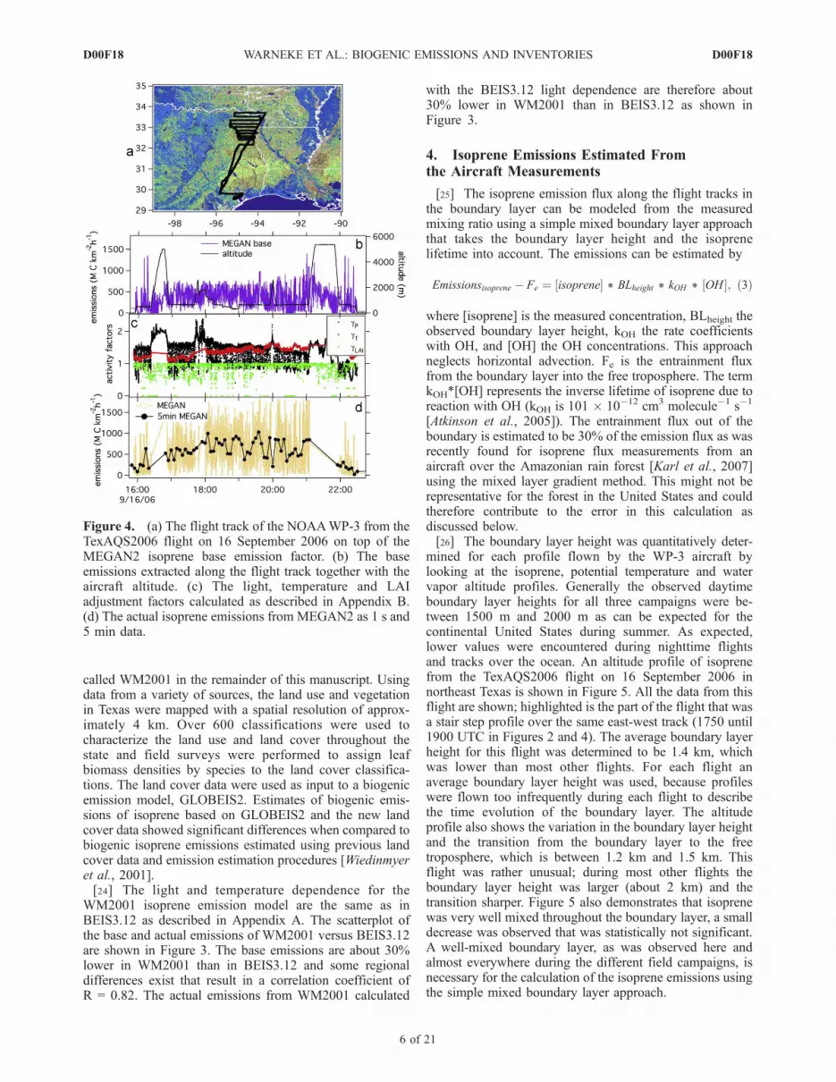
Figure 13. The flight tracks of the NOAA WP-3 duringthe TexAQS2006 campaign color coded with the differencebetween the isoprene emissions from (top) BEIS3.12 and(bottom) MEGAN2 with emissions modeled from theobservations. Flight tracks are shown on top of theBEIS3.12 and MEGAN base emissions. The pink squaresindicate areas where significant differences were observed.


14 of 21

D00F18

AQS2000 campaign results in about 10% average increasein the isoprene emissions. This changes the slope of thescatterplot of MEGAN2 versus the emissions estimatedfrom the isoprene measurements to 1.40 as compared to1.30 shown in Table 1 for this comparison. This effectreduces the interannual difference for the MEGAN2 results.[66] The results for the two campaigns in Texas show that

the interannual differences in isoprene emissions can be aslarge as a factor of 2 and are affecting large areas as well assmaller regions as was observed elsewhere [Levis et al.,2003].[67] The difference of the monoterpene measurements

and FLEXPART calculation is used to color code the flighttracks in Figure 15, which are plotted on top of theBEIS3.13 monoterpene base emissions. As was the casefor isoprene, large differences are observed at the borderbetween the United States and Canada and it appears thatBEIS3.13 predicts the emissions better on the United Statesside. In Texas north of Houston, FLEXPART predicts highmonoterpene mixing ratios using BEIS3.13, but only smallones were observed. Furthermore, during a flight to thenorth of Dallas, monoterpene mixing ratios of up to 100 pptvwere measured, but FLEXPART predicts less than 10 pptvin this area. This flight was a night flight and therefore longmonoterpene lifetimes and a shallow boundary layer couldresult in elevated mixing ratios. On the other hand, even theFLEXPART tracers that take emissions within 6 h or even12 h of transport into account are not higher than 15 pptv.

This has two possible explanations: (1) small monoterpeneemissions are present in this area that are not included inBEIS3.13 or (2) FLEXPART does not transport the mono-terpenes out of the shallow boundary layer to the aircraftaltitude.

8. Conclusions and Implications

[68] Airborne isoprene and monoterpene measurementsduring four different field campaigns in the eastern UnitedStates and in Texas were used to evaluate different availableemission models (BEIS3.12, BEIS3.12, MEGAN2 andWM2001) using two different approaches. First, a mixedboundary layer method was used: the emissions are mod-eled from the ambient measurements using the isoprene andmonoterpene lifetimes and the boundary layer height. Theemission estimates from the measurements are compared toemissions calculated from the models, which are calculatedusing observations on the aircraft of all the necessaryparameters, such as radiation and temperature. Second, atransport model was used: BEIS3.12 was incorporated intothe detailed transport model FLEXPART and isoprenemixing ratios are calculated by accumulating all the emis-sions within the last hour of transport and compared to themeasurements. Overall an agreement to better than a factorof 2 was found for all inventories and all campaigns andboth methods yielded consistent results.[69] Generally MEGAN2 is almost a factor of 2 higher

than BEIS3.12, which is in turn about 30% higher thanBEIS3.13, although there are some regions whereMEGAN2 was higher than BEIS3.12. The emissions from

Figure 14. The flight tracks of the NOAA WP-3 duringthe TexAQS2000 campaign color coded with the differencebetween the isoprene emissions from (top) BEIS3.12 and(bottom) MEGAN with emissions modeled from theobservations. Flight tracks are shown on top of theBEIS3.12 and MEGAN2 base emissions. The pink squaresindicate areas where significant differences were observed.

Figure 15. The flight tracks of the NOAA WP-3 duringthe ICART2004 and TexAQS2006 campaigns color codedwith the difference between the monoterpene mixing ratioscalculated with FLEXPART and the measured mixing ratioson top of the BEIS3.13 monoterpene base emissions.


15 of 21

D00F18

MEGAN2 were somewhat higher than the emissions mod-eled from the isoprene measurements, whereas BEIS3.12was somewhat lower. This is in contrast to a previous studythat found MEGAN to be biased low compared to obser-vations in Harvard forest [Muller et al., 2008]. Other studiesfind that isoprene emissions over North America inferredfrom OMI satellite or SCIAMACHY retrievals of formal-dehyde [Millet et al., 2008; Stavrakou et al., 2009] arelower than MEGAN.[70] Using this comparison, some areas were identified,

where the differences between the measurements and in-ventories were larger than average. Examples include theU.S.-Canada border and in Texas to the north of Houston inBEIS3.12 and BEIS3.13, where the inventories are largerthan the measurements. In the same areas only small differ-ences were found with MEGAN2, but for exampleMEGAN2 seems to over predict the emissions in northeastTexas in 2006.[71] Interannual differences in the emission strength

between 2000 and 2006 were observed in Texas, whichwere likely caused by stronger influence of temperature anddrought effects than the models can account for. MEGAN2takes the previous 15 day temperature and radiation intoaccount, which seems to improve the prediction of theinterannual variation. Further improvement was achievedby using the MEGAN2 2000 LAI data for Texas instead ofthe standard 2003 LAI.[72] Within the uncertainties of the methods, the biogenic

emission inventories that are commonly used for the UnitedStates generally agree with the observations within a factorof 2 for isoprene and the monoterpenes. Discrepancies existfor certain areas and interannual changes need to be betteraccounted for. Due to the large uncertainties, we are unableto recommend one inventory over the other, despite theirdifferences of almost a factor of 2.[73] Globally, the biosphere is by far the largest source of

reactive VOCs and an accurate representation of the emis-sions in atmospheric chemistry models is therefore criticallyimportant. The evaluation of emission inventories is mostaccurately done using eddy covariance fluxes from surfacesites, but this yields information about one location only.Different methods have been used to evaluate emissioninventories over larger spatial scales. The comparisonbetween measured and modeled biogenic VOCs can beused to evaluate emission inventories, but requires manydifferent parameters to be modeled correctly including OHconcentrations, photoactive radiation, temperatures andboundary level heights. As a result, uncertainties of a factorof 2 in emission inventories can probably not be resolvedusing this method. The same may be true for evaluations ofisoprene emission inventories using formaldehyde retrievedfrom satellite data, which method is limited by uncertaintiesin the atmospheric chemistry of formaldehyde and in thesatellite retrievals themselves.[74] Here we used aircraft observations of biogenic VOCs

to estimate the emissions in situ and compare them to anemissions inventory model that is constrained by aircraftobservations of shortwave radiation and temperature. Wealso compared observed mixing ratios to those calculatedwith a Lagrangian transport model. Our methods do still notallow uncertainties of a factor of 2 in emission inventoriesto be resolved with confidence. Improvements to our

method might involve (1) the use of in situ measurementsof OH rather than estimates from a parameterization andother measurements, and (2) the use of airborne LIDARdata to estimate boundary layer structure rather than verticalprofiles elsewhere during flight. Nevertheless, we expectthat such improvements may only provide marginally betterresults. Better constraints on emission inventories onregional scales may ultimately come from airborne eddycovariance measurements as recently demonstrated by Karlet al. [2009], who estimated uncertainties of 40% in themeasured fluxes. Such uncertainties are slightly smaller thanthe uncertainties in the emission inventories themselves andwill therefore be needed to provide useful constraints.Regardless, it is expected that significant uncertainties inbiogenic emission inventories will remain in the foreseeablefuture and that, at present, the combination of all availableevaluations gives the best assessment of these uncertainties.[75] On the other hand, given the necessary complexity of

the biogenic emission inventories and the evaluation meth-ods an uncertainty of a factor of 2 for isoprene is ratherencouraging. Other biogenic VOCs, such as the monoter-penes or oxygenated species like methanol or acetone, arefar less certain and a lot more research is needed to assessthe emissions of these compounds. Also compared toanthropogenic VOC emission inventories [Warneke et al.,2007], a factor of 2 uncertainty should be considered a goodagreement.

Appendix A

[76] The actual emissions in BEIS are calculated accord-ing to equation (1) [Guenther et al., 1995]:

actual emission ¼ base emission� cT � cL: ðA1Þ

[77] The base emissions are shown in Figure 1 and theadjustment factors, cT and cL, are calculated as described inthe following. The code described here was adapted from aFORTRAN code used in many air quality forecast modelssuch as WRF-Chem. The difference is that measurementsmade on the aircraft are used as input parameters, which arethe solar shortwave radiation, temperature, and solar zenithangle. The calculation of the actual emissions is described indetail to clearly show which assumptions are made and whatmodeling needs to be done to calculate the emissions fromeach inventory. The detailed description is also used to pointout the differences between the various inventories.

A1. Temperature Adjustment Factor for BEIS 3.12and BEIS3.13

[78] The temperature adjustment factor for isoprene is

cT ¼ e 37:711�0:398570815�dTð Þ

1þ e 91:301�dTð Þ with dT ¼ 28668:514

Tground:

[79] The temperature adjustment factor for the monoter-penes is

cT ¼ e 0:09� Tground�303ð Þð Þ:


16 of 21

D00F18

[80] In this work, the temperature on the ground (Tground)is estimated from the temperature measured onboard theaircraft during take off and landing and missed airportapproaches. The results for cT of the TexAQS2006 cam-paign are shown in Figure A1b.

A2. Light Adjustment Factor for BEIS3.12and BEIS3.13

[81] In this section the isoprene light adjustment factor forisoprene is calculated, the monoterpene emissions are not

dependent on radiation. The isoprene light adjustment factorfor BEIS3 in the WRF-Chem module is calculated with aradiation model that first takes the shortwave solar radiation(tsolar: 200–4700 mm) and calculates the photoactive radi-ation (PAR) in mmol m�2 s�1 and finds the direct beam(PARdb and PARdif) and diffuse fraction,

PAR ¼ PARdb þ PARdif ;

PARdb ¼ tsolar � fvis � fvb � 4:6;

PARdif ¼ tsolar � fvis � 1� fvbð Þ � 4:6;

where fvis is the fraction of visible to total radiation, fvb isthe fraction of visible light that is direct beam, and the factor4.6 is to convert from W/m2 to mmol m�2 s�1. To calculatefvis and fvb, the atmospheric pressure (p) in mbar and thesolar zenith angle (zen) are used. The following parametersare needed to split tsolar into visible and near IR,

ot ¼ p=1013:25

cos zenð Þ atmospheric optical thickness

rdvis ¼ 600� e �0:185�otð Þ � cos zenð Þ direct beam visible W=m2ð Þrf vis ¼ 0:42� 600� rdvisð Þ � cos zenð Þ diffuse visible W=m2ð Þwa ¼ 1320� 0:077� 2� otð Þ0:3 water absorption in near � IR W=m2ð Þrdir ¼ 720� e �0:06�otð Þ � wa

� �� cos zenð Þ direct beam near � IR W=m2

� �rf ir ¼ 0:65� 720� wa� rdirð Þ � cos zenð Þ diffuse near � IR W=m2

� �

[82] The total visible and near-IR radiation is calculatedusing

rvt ¼ rdvis þ rf vis total visible radiation

rirt ¼ rdir þ rf ir total near � IR radiation

[83] The fraction of visible to total radiation can then becalculated using

fvis ¼rvt

rvt þ rirtð Þ fraction of visible to total radiation

ratio ¼ tsolar

rvt þ rirtð Þ ratio of ‘‘actual’’ to clear sky solar radiation

[84] Now the fraction of the visible radiation that is directbeam can be calculated,

f vb ¼rdvis

rvt� 0:941124 for ratio � 0:89

fvb ¼rdvis

rvt� 9:55� 10�3 for ratio � 0:21

fvb ¼rdvis

rvt� 1� 0:9� ratio

0:7

� �2=3 !

for 0:21 � ratio � 0:89

[85] The calculated PARdb, PARdif and their sum alongthe flight track are plotted versus the measured shortwavesolar radiation in Figure A2 for the TexAQS2006 data. Itcan be seen that at low shortwave solar radiation, whichoccurs at large solar zenith angles and cloudy conditions,PAR becomes mainly diffuse.[86] Using PAR, split into direct beam and diffuse frac-

tions as shown in Figure A2, together with the LAI, whichcan be extracted from data in BEIS3 along the flight track,

Figure A1. (a) The BEIS3.12 light adjustment factor forisoprene for all data from the TexAQS2006 campaign. (b) Thetemperature adjustment factor for isoprene and the mono-terpenes. (c) Comparison of the BEIS3.12 and BEIS3.13 lightadjustment factor. The 1:1 line is shown in red.


17 of 21

D00F18

the PAR that falls on leaves in the sun and leaves in theshade can be estimated.

kbe ¼ 0:5�ffiffiffiffiffiffiffiffiffiffiffiffiffiffiffiffiffiffiffiffiffiffiffiffiffiffiffi1þ tan zenð Þ2

qextinction coefficient for direct beam

a ¼ 0:8 leaf absorptivity

kd ¼ 0:68 extinction coefficient for diffuse

canPARscat ¼ 0:5� PARdb � e �a2�kbe�LAIð Þ � e �kbe�LAIð Þ scattered PAR in the canopy mmol m�2 s�1ð Þ

canPARdif ¼0:5� PARdif � 1� e �a2�kbe�LAIð Þ

� �a2 � kbe � LAIð Þ diffuse PAR in the canopy mmol m�2 s�1ð Þ

PARshade ¼ canPARscat þ canPARdif PARon shaded leaves mmol m�2 s�1ð ÞPARsun ¼ kbe � PARdb þ PARshade PARon sunlit leaves in BEIS3:13 mmol m�2 s�1ð ÞPARsun ¼ kbe � PARdb þ PARdifð Þ þ PARshade PARon sunlit leaves in BEIS3:12 mmol m�2 s�1ð Þ

PARsun in BEIS3.12 includes PARdif, which is actually amistake that was corrected in BEIS3.13.[87] Using LAI the fraction of leaves in the sun or shade

can be estimated:

fracsun ¼1�e �kbe�LAIð Þ� �

=kbe

LAIfraction of leaves that are sunlit

fracshade ¼ 1� fracsun fraction of leaves that are shaded

[88] The isoprene emission light adjustment factor for thefraction of leaves in the sun and the fraction in the shade cannow be calculated using the formulation from Guenther etal. [1995],

cL ¼ fracsun � cguen PARsunð Þ þ fracshade � cguen PARshadeð Þlight adjustment factor:

[89] In the determination of cguen lies the major differencebetween BEIS3.12 and BEIS3.13. The newer version usesthe updated reference of Guenther et al. [1999] instead ofthe older Guenther et al. [1993] reference,

cguen PARð Þ ¼ 0:0028782 * PARffiffiffiffiffiffiffiffiffiffiffiffiffiffiffiffiffiffiffiffiffiffiffiffiffiffiffiffiffiffiffiffiffiffiffiffiffiffiffiffiffiffiffiffiffiffiffiffi1þ 0:00000729 * PAR2

p used in BEIS3:12

cguen PARð Þ ¼ 0:001 * 1:42 * PARffiffiffiffiffiffiffiffiffiffiffiffiffiffiffiffiffiffiffiffiffiffiffiffiffiffiffiffiffiffiffiffiffiffiffiffiffiffi1þ 0:0012 * PAR2

p used in BEIS3:13

[90] For PAR < 0.01 and zenith angles > 89 degrees, cL isset to zero and for very small LAI < 0.1 cL is set to

cguen(PARdb + PARdif). In Figure A1 the resulting cT andcL for the TexAQS2006 campaign are plotted versus theground temperature and the shortwave solar radiation,respectively. Shown are 1 s aircraft data for the wholecampaign, resulting in a large number of data points. InFigure A1a the light adjustment factor is color coded byLAI and it can be seen that at high LAI, when it is assumedthat leaves in the lower part of the canopy are shaded, cL isreduced relative to low LAI values. Figure A1c shows thescatterplot of the light adjustment factor from BEIS3.12versus BEIS3.13. In Figure A1b the isoprene and monoter-pene temperature adjustment factors are shown.

Appendix B

[91] The actual emissions in MEGAN2 are calculatedaccording to equation (B1)

Emission ¼ e½ � g½ � r½ �; ðB1Þ

[92] The emission factor e is taken from the data asshown in Figure 1, the canopy loss and production term ris set to 0.96 and the emission activity factor g is calculatedas described in the following. A more detailed descriptionof MEGAN and this calculation are given by Guenther et al.[2006].[93] The emission activity factor g is calculated from

g ¼ gCE � gage � gSM ¼ gP � gT � gLAI � gage � gSM;

where gCE is the canopy environment emission activityfactor, gage is the leaf age and gSM the soil moistureemission activity factor. gCE is calculated from thetemperature gT, the PPFD (photosynthetic photon fluxdensity) gP and the LAI gLAI emission activity factors. Thefollowing calculation was adapted from a FORTRAN codeused in MEGANv2.03.

B1. Leaf Area Index Emission Activity Factor

[94] The gLAI can be calculated by:

gLAI ¼0:49� LAIffiffiffiffiffiffiffiffiffiffiffiffiffiffiffiffiffiffiffiffiffiffiffiffiffiffiffiffiffiffiffiffiffiffiffi1þ 0:2� LAI2� �q ;

where leaf area index (LAI) in m2 m�2 is taken from thecurrent months LAI data used in MEGAN2 from 2003. The

Figure A2. The direct beam and diffuse PAR calculatedfor the solar radiation measured during TexAQS2006.


18 of 21

D00F18

gLAI for all data from the TexAQS2006 campaign is shownin Figure B1.

B2. Photosynthetic Photon Flux Density EmissionActivity Factor

[95] The gP can be calculated by:

gP ¼ sin selð Þ � 2:46� 1þ 0:0005� Pdaily � 400� ��

� f� 0:9� f2�

f ¼ Pac

sin selð Þ � Ptoaabove canopy PPFD transmission mmol m�2 s�1ð Þ

Pac ¼ tsolar � 4:766� 0:5 above canopy PPFD mmol m�2 s�1ð Þ

Ptoa ¼ 3000þ 99� cos 2� 3:14� DOY� 10ð Þ365

�PPFD at the top of the atmosphere mmol m�2 s�1ð Þ

where PFPD is photosynthetic photon flux density. Thesolar elevation angle (sel), the shortwave radiation (tsolar),the day of the year (DOY) and an average past shortwaveradiation (Pdaily) is required. Here, Pdaily is calculated as apast 15 day average from the ECMWF data input to theFLEXPART model, which was manipulated to outputPdaily for each grid box for each hour during the entireTexAQS2006 and ICARTT2004 campaigns. For SOS1999Pdaily was estimated using temperature measurements fromthe ground site close to Nashville and for TexAQS2000using data from the LaPorte site. The gP for all data fromTexAQS2006 is shown in Figure C.

B3. Temperature Emission Activity Factor

[96] The gT can be calculated by:

gT ¼ Eopt � cT2 � e cT1�xð Þ

cT2 � cT1 � 1� ecT2�xð Þ

� �h i

x ¼ 1

Topt

� �� 1

Tground

� � �=0:00831

Eopt ¼ 1:75� e 0:08� Tdaily�297ð Þð Þ

Topt ¼ 313þ 0:6� Tdaily � 297� �

[97] The ground temperature (Tground) in K and an aver-age past temperature (Tdaily) in K are required, where thepast 15 day average temperature was calculated in the sameway as the past solar radiation using FLEXPART and theground sites. CT1 is 80 and CT2 is 200. The result of the gTcalculation for all data from TexAQS2006 is also shown inFigure B1.

B4. Leaf Age and Soil Moisture Emission ActivityFactor

[98] The leaf age gage and the soil moisture gSM emissionactivity factors were set to:

gage ¼ gSM ¼ 1:

[99] Acknowledgments. The Air Quality and the Climate Researchand Modeling Programs of the National Oceanic and Atmospheric Admin-istration (NOAA) and the Texas Commission on Environmental Quality(TCEQ) supported the WP-3D measurements. Much of the analysis wassupported by TCEQ under grant 582-8-86246.

Figure B1. The MEGAN (a) light, (b) temperature, and(c) LAI emission activity factors for all data from theTexAQS2006 campaign.


19 of 21

D00F18

ReferencesAtkinson, R., et al. (2005), Summary of evaluated kinetic and photochemicaldata for atmospheric chemistry, report, Subcomm. on Gas Kinetic DataEval. for Atmos. Chem., Int. Union of Pure and Appl. Phys., London.(Available at http://www.iupac-kinetic.ch.cam.ac.uk/)

Atkinson, R., et al. (2006), Evaluated kinetic and photochemical data foratmospheric chemistry: Volume II—Gas phase reactions of organic species,Atmos. Chem. Phys., 6, 3625–4055.

Brock, C. A., et al. (2002), Particle growth in the plumes of coal-fired powerplants, J. Geophys. Res., 107(D12), 4155, doi:10.1029/2001JD001062.

Brock, C. A., et al. (2008), Sources of particulate matter in the northeasternUnited States in summer: 2. Evolution of chemical and microphysicalproperties, J. Geophys. Res., 113, D08302, doi:10.1029/2007JD009241.

Brown, S. S., et al. (2005), Aircraft observations of daytime NO3 and N2O5

and their implications for tropospheric chemistry, J. Photochem. Photobiol.,A, 176(1–3), 270–278.

Chen, G., et al. (2005), An investigation of the chemistry of ship emissionplumes during ITCT 2002, J. Geophys. Res., 110, D10S90, doi:10.1029/2004JD005236.

de Gouw, J., and C. Warneke (2007), Measurements of volatile organic com-pounds in the Earth’s atmosphere using proton-transfer-reaction mass spec-trometry, Mass Spectrom. Rev., 26(2), 223–257, doi:10.1002/mas.20119.

de Gouw, J. A., P. D. Goldan, C. Warneke, W. C. Kuster, J. M. Roberts,M. Marchewka, S. B. Bertman, A. A. P. Pszenny, and W. C. Keene(2003), Validation of proton transfer reaction-mass spectrometry (PTR-MS) measurements of gas-phase organic compounds in the atmosphereduring the New England Air Quality Study (NEAQS) in 2002, J. Geophys.Res., 108(D21), 4682, doi:10.1029/2003JD003863.

de Gouw, J. A., et al. (2005), Budget of organic carbon in a pollutedatmosphere: Results from the New England Air Quality Study in 2002,J. Geophys. Res., 110, D16305, doi:10.1029/2004JD005623.

de Gouw, J. A., et al. (2006), Volatile organic compounds composition ofmerged and aged forest fire plumes from Alaska and western Canada,J. Geophys. Res., 111, D10303, doi:10.1029/2005JD006175.

Edwards, G. D., et al. (2003), Chemical ionization mass spectrometerinstrument for the measurement of tropospheric HO2 and RO2, Anal.Chem., 75(20), 5317–5327, doi:10.1021/ac034402b.

Ehhalt, D. H., and F. Rohrer (2000), Dependence of the OH concentrationon solar UV, J. Geophys. Res., 105(D3), 3565–3571, doi:10.1029/1999JD901070.

Fehsenfeld, F. C., et al. (2006), International Consortium for AtmosphericResearch on Transport and Transformation (ICARTT): North America toEurope—Overview of the 2004 summer field study, J. Geophys. Res.,111, D23S01, doi:10.1029/2006JD007829.

Geron, C., et al. (2000), A review and synthesis of monoterpene speciationfrom forests in the United States, Atmos. Environ., 34, 1761–1781,doi:10.1016/S1352-2310(99)00364-7.

Goldan, P. D., D. D. Parrish, W. C. Kuster, M. Trainer, S. A. McKeen,J. Holloway, B. T. Jobson, D. T. Sueper, and F. C. Fehsenfeld (2000),Airborne measurements of isoprene, CO, and anthropogenic hydrocar-bons and their implications, J. Geophys. Res., 105(D7), 9091–9105,doi:10.1029/1999JD900429.

Guenther, A. B., and A. J. Hills (1998), Eddy covariance measurement ofisoprene fluxes, J. Geophys. Res., 103(D11), 13,145 – 13,152,doi:10.1029/97JD03283.

Guenther, A., P. R. Zimmerman, P. C. Harley, R. K. Monson, and R. Fall(1993), Isoprene and monoterpene emission rate variability: Model eva-luation and sensitivity analysis, J. Geophys. Res., 98(D7), 12,609–612,617, doi:10.1029/93JD00527.

Guenther, A., et al. (1995), A global model of natural volatile organiccompound emissions, J. Geophys. Res., 100(D5), 8873 – 8892,doi:10.1029/94JD02950.

Guenther, A., B. Baugh, G. Brasseur, J. Greenberg, P. Harley, L. Klinger,D. Serca, and L. Vierling (1999), Isoprene emission estimates anduncertainties for the Central African EXPRESSO study domain, J. Geophys.Res., 104(D23), 30,625–30,639, doi:10.1029/1999JD900391.

Guenther, A., et al. (2006), Estimates of global terrestrial isoprene emis-sions using MEGAN (Model of Emissions of Gases and Aerosols fromNature), Atmos. Chem. Phys., 6, 3181–3210.

Hawes, A. K., et al. (2003), Airborne observations of vegetation andimplications for biogenic emission characterization, J. Environ. Monit.,5(6), 977–983, doi:10.1039/b308911h.

Henze, D. K., and J. H. Seinfeld (2006), Global secondary organic aerosolfrom isoprene oxidation, Geophys. Res. Lett., 33, L09812, doi:10.1029/2006GL025976.

Jacob, D. J. (2000), Heterogeneous chemistry and tropospheric ozone,Atmos. Environ., 34, 2131–2159, doi:10.1016/S1352-2310(99)00462-8.

Jacob, D. J., B. D. Field, E. M. Jin, I. Bey, Q. Li, J. A. Logan, R. M.Yantosca, and H. B. Singh (2002), Atmospheric budget of acetone,J. Geophys. Res., 107(D10), 4100, doi:10.1029/2001JD000694.

Jacob, D. J., et al. (2005), Global budget of methanol: Constraints fromatmospheric observations, J. Geophys. Res., 110, D08303, doi:10.1029/2004JD005172.

Karl, T. G., A. Guenther, R. J. Yokelson, J. Greenberg, M. Potosnak,D. R. Blake, and P. Artaxo (2007), The tropical forest and fire emissionsexperiment: Emission, chemistry, and transport of biogenic volatile organiccompounds in the lower atmosphere over Amazonia, J. Geophys. Res., 112,D18302, doi:10.1029/2007JD008539.

Karl, T., et al. (2009), Emissions of volatile organic compounds inferredfrom airborne flux measurements over a megacity, Atmos. Chem. Phys.,9, 271–285.

Lelieveld, J., et al. (2008), Atmospheric oxidation capacity sustained by atropical forest, Nature, 452(7188), 737–740, doi:10.1038/nature06870.

Levis, S., C. Wiedinmyer, G. B. Bonan, and A. Guenther (2003), Simulat-ing biogenic volatile organic compound emissions in the CommunityClimate System Model, J. Geophys. Res. , 108(D21), 4659,doi:10.1029/2002JD003203.

McKeen, S., et al. (2005), Assessment of an ensemble of seven real-timeozone forecasts over eastern North America during the summer of 2004,J. Geophys. Res., 110, D21307, doi:10.1029/2005JD005858.

Millet, D. B., D. J. Jacob, K. F. Boersma, T.-M. Fu, T. P. Kurosu, K. Chance,C. L. Heald, and A. Guenther (2008), Spatial distribution of isopreneemissions from North America derived from formaldehyde column mea-surements by the OMI satellite sensor, J. Geophys. Res., 113, D02307,doi:10.1029/2007JD008950.

Muller, J. F., et al. (2008), Global isoprene emissions estimated usingMEGAN, ECMWF analyses and a detailed canopy environment model,Atmos. Chem. Phys., 8, 1329–1341.

Palmer, P. I., et al. (2006), Quantifying the seasonal and interannual varia-bility of North American isoprene emissions using satellite observationsof the formaldehyde column, J. Geophys. Res., 111, D12315,doi:10.1029/2005JD006689.

Parrish, D. D., et al. (2009), Overview of the Second Texas Air QualityStudy (TexAQS II) and the Gulf of Mexico Atmospheric Compositionand Climate Study (GoMACCS), J. Geophys. Res., 114, D00F13,doi:10.1029/2009JD011842.

Pfister, G. G., L. K. Emmons, P. G. Hess, J. F. Lamarque, J. J. Orlando,S. Walters, A. Guenther, P. I. Palmer, and P. J. Lawrence (2008), Con-tribution of isoprene to chemical budgets: A model tracer study with theNCAR CTM MOZART-4, J. Geophys. Res., 113, D05308, doi:10.1029/2007JD008948.

Pierce, T. E., and P. S. Waldruff (1991), Pc-Beis—A personal-computerversion of the biogenic emissions inventory system, J. Air Waste Manage.Assoc., 41(7), 937–941.

Pierce, T., C. Geron, L. Bender, R. Dennis, G. Tonnesen, and A. Guenther(1998), Influence of increased isoprene emissions on regional ozonemodeling, J. Geophys. Res., 103(D19), 25,611–25,629, doi:10.1029/98JD01804.

Rohrer, F., and H. Berresheim (2006), Strong correlation between levels oftropospheric hydroxyl radicals and solar ultraviolet radiation, Nature,442(7099), 184–187, doi:10.1038/nature04924.

Ryerson, T. B., et al. (1998), Emissions lifetimes and ozone formation inpower plant plumes, J. Geophys. Res., 103(D17), 22,569–522,583,doi:10.1029/98JD01620.

Ryerson, T. B., E. Williams, and F. Fehsenfeld (2000), An efficient photo-lysis system for fast-response NO2 measurements, J. Geophys. Res.,103(D21), 26,447–426,461, doi:10.1029/2000JD900389.

Ryerson, T. B., et al. (2003), Effect of petrochemical industrial emissions ofreactive alkenes and NOx on tropospheric ozone formation in Houston,Texas, J. Geophys. Res., 108(D8), 4249, doi:10.1029/2002JD003070.

Sharkey, T. D., et al. (1999), Weather effects on isoprene emission capacityand applications in emissions algorithms, Ecol. Appl., 9(4), 1132–1137,doi:10.1890/1051-0761(1999)009[1132:WEOIEC]2.0.CO;2.

Song, J., et al. (2008), Comparisons of modeled and observed isopreneconcentrations in southeast Texas, Atmos. Environ., 42, 1922–1940,doi:10.1016/j.atmosenv.2007.11.016.

Stark, H., B. M. Lerner, R. Schmitt, R. Jakoubek, E. J. Williams,T. B. Ryerson, D. T. Sueper, D. D. Parrish, and F. C. Fehsenfeld (2007),Atmospheric in situ measurement of nitrate radical (NO3) and otherphotolysis rates using spectroradiometry and filter radiometry, J. Geophys.Res., 112, D10S04, doi:10.1029/2006JD007578.

Stavrakou, T., et al. (2009), Global emissions of non-methane hydrocarbonsdeduced from SCIAMACHY formaldehyde columns through 2003–2006, Atmos. Chem. Phys., 9(11), 3663–3679.

Stohl, A., and D. J. Thomson (1999), A density correction for Lagrangianparticle dispersion models, Boundary Layer Meteorol., 90(1), 155–167,doi:10.1023/A:1001741110696.

Stohl, A., et al. (2005), Technical note: The Lagrangian particle dispersionmodel FLEXPART version 6.2, Atmos. Chem. Phys., 5, 2461–2474.


20 of 21

D00F18

Tanner, D. J., A. Jefferson, and F. L. Eisele (1997), Selected ion chemicalionization mass spectrometric measurement of OH, J. Geophys. Res.,102(D5), 6415–6425, doi:10.1029/96JD03919.

Warneke, C., et al. (2003), Validation of atmospheric VOC measurementsby proton-transfer-reaction mass spectrometry using a gas-chromato-graphic preseparation method, Environ. Sci. Technol., 37(11), 2494–2501, doi:10.1021/es026266i.

Warneke, C., et al. (2004), Comparison of daytime and nighttime oxidationof biogenic and anthropogenic VOCs along the New England coast insummer during New England Air Quality Study 2002, J. Geophys. Res.,109, D10309, doi:10.1029/2003JD004424.

Warneke, C., et al. (2007), Determination of urban volatile organic com-pound emission ratios and comparison with an emissions database,J. Geophys. Res., 112, D10S47, doi:10.1029/2006JD007930.

Wiedinmyer, C., et al. (2001), A land use database and examples of bio-genic isoprene emission estimates for the state of Texas, USA, Atmos.Environ., 35, 6465–6477, doi:10.1016/S1352-2310(01)00429-0.

��E. Atlas, Marine and Atmospheric Chemistry Division, Rosenstiel School

of Marine and Atmospheric Sciences, University of Miami, 4600Rickenbacker Causeway, Miami, FL 33149, USA.

J. Brioude, J. A. de Gouw, F. C. Fehsenfeld, P. D. Goldan, J. S. Holloway,W. C. Kuster, S. McKeen, J. Peischl, T. B. Ryerson, H. Stark, M. Trainer,and C. Warneke, Chemical Sciences Division, ESRL, NOAA, 325Broadway, R/CSD7, Boulder, CO 80305, USA. ([email protected])L. Del Negro, Department of Chemistry, Lake Forest College, 555 N.

Sheridan Rd., Lake Forest, IL 60045-2338, USA.A. B. Guenther and C. Wiedinmyer, ACD, NCAR, Boulder, CO 80301,

USA.A. T. C. Hanks, Department of Geosciences, University of Louisiana at

Monroe, Monroe, LA 71209, USA.A. Hansel and A. Wisthaler, Institut fur Ionenphysik und Angewandte

Physik, Universitat Innsbruck, Technikerstrasse 25, A-6020 Innsbruck,Austria.L. G. Huey, School of Earth and Atmospheric Sciences, Georgia Institute

of Technology, Atlanta, GA 30332-0340, USA.


21 of 21

D00F18

Documents

Biogenic emission measurement and inventories determination of biogenic emissions in the eastern United States and Texas and comparison with biogenic emission inventories