arX

iv:0

811.

4563

v1 [

phys

ics.

chem

-ph]

27

Nov

200

8

Bottlenecks to vibrational energy flow in OCS: Structures and mechanisms

R. Paskauskas1∗,† C. Chandre2, and T. Uzer11 Center for Nonlinear Sciences, School of Physics,

Georgia Institute of Technology, Atlanta, GA 30332-0430, U.S.A.2 Centre de Physique Theorique‡ – CNRS, Luminy - Case 907, 13288 Marseille cedex 09, France

(Dated: November 27, 2008)

Finding the causes for the nonstatistical vibrational energy relaxation in the planar carbonylsulfide (OCS) molecule is a longstanding problem in chemical physics: Not only is the relaxationincomplete long past the predicted statistical relaxation time, but it also consists of a sequence ofabrupt transitions between long-lived regions of localized energy modes. We report on the phasespace bottlenecks responsible for this slow and uneven vibrational energy flow in this Hamiltoniansystem with three degrees of freedom. They belong to a particular class of two-dimensional invarianttori which are organized around elliptic periodic orbits. We relate the trapping and transitionmechanisms with the linear stability of these structures.

PACS numbers: 34.30.+h, 34.10.+x, 82.20.Db, 82.20.Nk

I. INTRODUCTION

How does vibrational energy travel in molecules? An-swering this question succinctly seems a hopeless taskconsidering the complexity of interatomic interactionsin a molecule. Yet even before scientists were bur-dened by this knowledge, the so-called statistical theo-ries posited the answer: Vibrational energy travels “veryfast” and distributes itself statistically among the vibra-tional modes of a molecule, assumed to resemble an as-sembly of coupled oscillators, well before a reaction takesplace. Reaction rate theories based on these assump-tions – known collectively as statistical or RRKM the-ories [1, 2, 3, 4] – remain reliable working tools of thepracticing chemist because they have been vindicated inan overwhelming number of chemical reactions.

However, numerical studies of Hamiltonian systemshave provided solid evidence [5, 6, 7, 8, 9, 10] that theapproach to equilibrium usually proceeds more slowlythan predicted by statistical theories [11, 12] – and itis also nonuniform, showing intriguing fits and starts. Inparticular, for Hamiltonian systems with two degrees offreedom, the familiar picture of chaotic seas, rigid bound-aries in terms of noble tori [13], leaky barriers in termsof cantori [14, 15] has been well-established in the liter-ature, and these structures are found to be the source ofanomalous transport in such systems [16, 17].

Beyond two degrees of freedom, the transport picturein terms of phase space structures is less clear. However,the phase space of higher-dimensional systems shows sim-ilar features such as the abundance of periodic orbits, anda mixture of chaotic and regular regions, the latter being

∗Present address: Sincrotrone Trieste, AREA Science Park, 34012Basovizza Trieste, ITALY‡UMR 6207 of the CNRS, Aix-Marseille and Sud Toulon-Var Uni-versities. Affiliated with the CNRS Research Federation FRUMAM(FR 2291). CEA registered research laboratory LRC DSM-06-35.†Electronic address: rytis@gatech.edu

characterized (under some hypothesis) by invariant toriof various dimensions. The KAM theorem [13] states thatthese structures are in general robust with respect to anincrease of the perturbation or equivalently to an increaseof energy. Understanding transport properties has to relyon these robust structures which are encountered by anytypical trajectory. Roughly speaking, the presence of somany periodic orbits explains why generic trajectories,even when the system is strongly chaotic, display longintervals of near-regular behavior alternating with fits ofchaos–a hallmark of anomalous diffusion.

The slow approach to equilibrium started to be ac-knowledged a little over fifty years ago with the investi-gation of the dynamics of coupled oscillators by Fermi,Pasta and Ulam who showed that the relaxation problemis far more complex than anticipated [5, 6, 7, 8, 9, 10].In chemical physics, anomalous diffusion was first impli-cated in the intramolecular vibrational energy relaxationof the carbonyl sulfide OCS molecule [11]. The numericalstudy of a classical Hamiltonian model of OCS shows veryslow energy redistribution among the vibrational modes,even in the fully chaotic regime [11], disagreeing stronglywith the fast timescales derived from traditional statisti-cal theory. The understanding of the dynamics was suc-cessfully achieved for a collinear model of OCS which hastwo degrees of freedom [18, 19, 20, 21, 22]. However, se-vere technical difficulties [23, 24, 25] have prevented sucha level of understanding beyond two degrees of freedom,and in particular, for the planar OCS model, in whichthe molecule is allowed to bend.

In this paper, we analyze the dynamics of a model forthe planar OCS which is a Hamiltonian system with threestrongly coupled degrees of freedom. The aim is to iden-tify the relevant structures in phase space which are re-sponsible for trappings and escapes, strongly influencingthe transport properties (most prominently, the redistri-bution of intramolecular energy among the three modes).For example, rapid diffusion through phase space takesplace through the so-called accelerator modes [26]. Incontrast, sticky structures [27] like resonant islands or

2

tori influence the dynamics by strongly slowing downthe trajectories passing nearby. All these structures areresponsible for anomalous diffusion and fractal kineticsin the system (for recent surveys, see Refs. [16, 17] andreferences therein). Identifying these structures and themechanisms behind trapping, escape and roaming is es-sential for understanding the transport properties of agiven system. Given that there are many such structuresin a realistic system, the only realistic hope for forming agenerally valid picture of transport is to locate invariantstructures which are responsible for the main changes inthe transport properties.

The specific question we address is: What are thestructures in the phase space of OCS acting as dynamicalbottlenecks to the diffusion of chaotic trajectories? Whatare the structures allowing transitions to other parts ofphase space? For three degree of freedom systems, theseinvariant structures can be invariant tori with dimen-sions zero (stagnation points), one (periodic orbits), twoor three [28, 29, 30]. They can also include the stable andunstable manifolds of these objects [31]. How are invari-ant structures relevant in the phenomena of capture inchaotic systems? For planar OCS, we find that the bot-tlenecks and the transition mechanisms from trapped tohyperbolic behavior are provided by a particular class oftwo-dimensional tori and their unstable manifolds. Theseresults were recently announced in a Letter [32].

The paper is organized as follows: In Sec. II, we brieflyrecall some basics of the Hamiltonian model for the pla-nar rotationless OCS molecule. We also summarize themain results obtained on the dynamics of OCS relevant tothe transport properties (both in the planar and collinearcases). In Sec. III A, we illustrate the transitions whichoccur in the neighborhood of periodic orbits using sev-eral representations: Time series, time-frequency analy-sis, and Poincare sections. The striking common featureexhibited by many trajectories support the idea of somekind of universal transition mechanism. In Sec. III B,after summarizing our methodology, we investigate theneighboring phase space structures which strongly influ-ence the dynamics of these trajectories.

II. THE OCS MODEL

A. The Hamiltonian

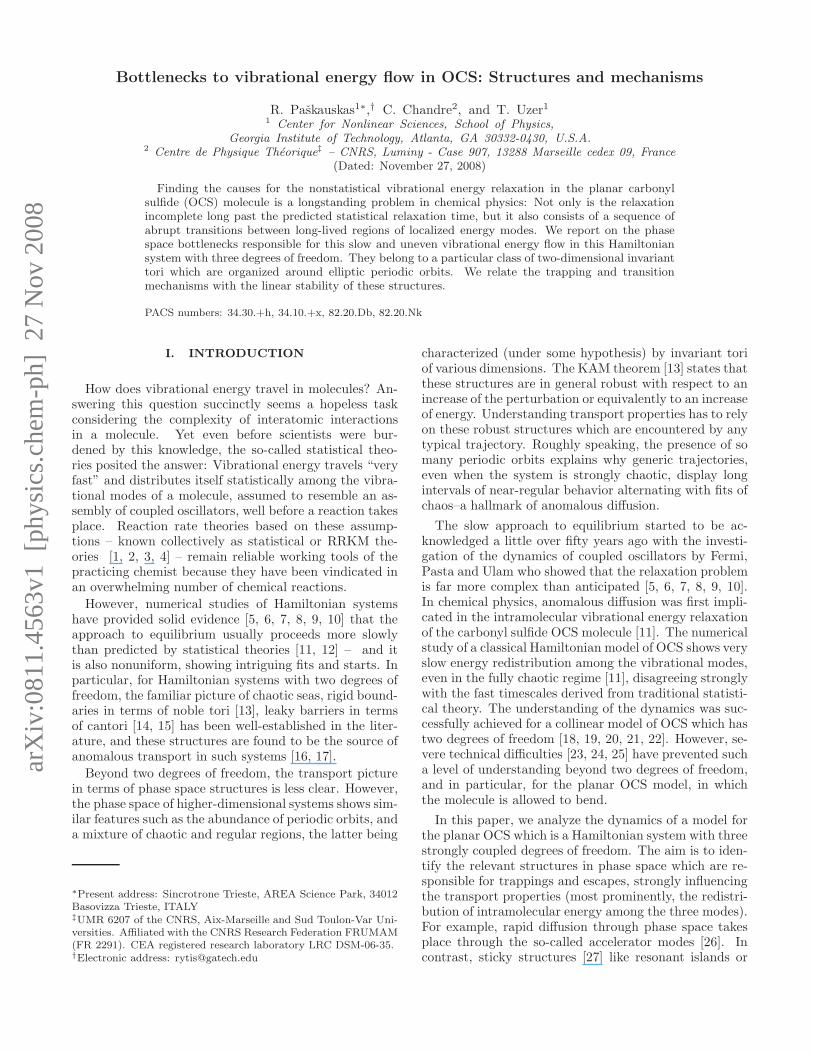
The dynamics of the planar model of carbonyl sul-fide (OCS) can be described by a Hamiltonian modelwith three degrees of freedom with three strongly cou-pled, non-separable modes: There are two stretchingmodes and one bending mode. Each mode is representedby a coordinate and momentum pair, which we defineas: R1 = d(C, S) and P1 for the CS stretching mode,R2 = d(C,O) and P2 for the CO stretching mode, andfinally, α = ∠(OCS) and Pα for the bending mode of themolecule (see Fig. 1). Hamiltonian model for the rota-tionless OCS molecule has been provided in [11, 33]. It

1.5

2

2.5

3

3.5

4

4.5

5

2 2.5 3 3.5 4 4.5 5 5.5

R2

R1

C

S OR1 R2

α⌣

FIG. 1: Equipotential surfaces of the collinear configuration,given by V (R1, R2, π) = E [see Eq. (2)]. From center out-wards, energies are E = 0.03, 0.06, 0.09, 0.10, 1.6, 1.75, 1.8,2.0. The energies studied in this article are 0.09 (below dis-sociation of the weakest bond) and 0.10 (above dissociation),and the corresponding equipotential contours are shown inbold.

has the form

H(R1, R2, α, P1, P2, Pα) =T (R1, R2, α, P1, P2, Pα)

+ V (R1, R2, α) ,(1)

where T is the kinetic energy and V is the potential en-ergy. The kinetic energy is quadratic in the momentaand is provided as

T =µ1

2P 2

1 +µ2

2P 2

2 + µ3P1P2 cosα

+P 2α

(

µ1

2R21

+µ2

2R22

− µ3 cosα

R1R2

)

−µ3Pα sinα

(

P1

R2+P2

R1

)

,

where µi are the reduced masses. Based on availableexperimental data, the analytic model for the potentialenergy surface has been proposed in [33]. In summary,V is given by

V (R1, R2, α) =

3∑

i=1

Vi(Ri) + VI(R1, R2, R3) , (2)

where Vi(Ri) are Morse potentials for each of the threeinteratomic distances R1, R2 and R3 = d(S,O), and

Vi(R) = Di

(

1 − exp [−βi(R−R0i )]

)2. (3)

Here, R0i are the equilibrium interatomic distances,

and R3 is given by R3(R1, R2, α) = (R21 + R2

2 −2R1R2 cosα)1/2. At equilibrium, the molecule is

3

collinear, therefore R03 = R0

1 + R02. Also, the interaction

potential VI assumes the Sorbie-Murrell form:

VI = AP (R1, R2, R3)

3∏

i=1

(

1 − tanh γi[Ri −R0i ]

)

,

where P (R1, R2, R3) is a quartic polynomial in each ofits variables:

P (R1, R2, R3) = 1 + c(1)i Ri + c

(2)ij RiRj

+ c(3)ijkRiRjRk + c

(4)ijklRiRjRkRl .

All the coefficients (µi, Di, βi, R0i , γi, A, c

(1)i , c

(2)ij , c

(3)ijk,

c(4)ijkl) are provided in Ref. [11]. We display the equipo-

tential surfaces of V (R1, R2, R1 + R2) of the collinearconfiguration in Fig. 1. The equations of motion can bederived from Hamiltonian (1) using the canonical Hamil-ton’s equations.

B. Summary of prior results on the OCS dynamics

The classical models of both the collinear and the pla-nar (rotationless) carbonyl sulfide OCS molecule havebeen studied in detail in Refs. [11, 18, 21, 31, 34, 35, 36].

The dynamics in the collinear configuration of OCSwas first studied by Carter and Brumer [11]. Theycharacterized the motion of this system at a number ofenergies, extending up to 20, 000 cm−1 (which amountsto E = 0.09 a.u.) A relaxation time, as defined inRefs. [37, 38, 39], was estimated at 0.17 pico-seconds.However, after integrating trajectories for 2.4 picosec-onds, no relaxation to statistical equilibrium was ob-served. When this contradiction was investigated byintegrating the equations for much longer times (up to45 picoseconds), two distinct timescales for relaxationwere found, the longer of which characterized energy re-distribution that was incomplete even after 45 picosec-onds [35]. Even on the picosecond time scale, suddentransitions between relatively long-lived regions of local-ized mode energies were observed. Since this collinearmodel has two degrees of freedom, Davis and Wagner [35]used Poincare surfaces of section as a visualizing toolfor phase space structures. These revealed that even athigh energy (E = 0.09), the system has a “divided phasespace”, with coexisting regular and chaotic regions. Theyobserved that trajectories can be trapped in restrictedregions of phase space for many vibrational periods, af-ter which they would suddenly move to other regions ofphase space to repeat the pattern.

Progress came with the recognition that the then-recent lobe dynamics [14, 15] could help to explainnon-statistical relaxation in two degree of freedom sys-tems [18]. When the strength of the perturbation (orequivalently, the total energy) is increased, the two-dimensional invariant tori of a Hamiltonian system withtwo degrees of freedom develop sets of “holes” with the

systematics of Cantor sets. These holes, dubbed “can-tori” [14], form leaky barriers which can act as bottle-necks to phase space transport. These bottlenecks are as-sociated with broken tori with irrational frequency ratios,where those with “noble” number ratios being genericallythe very last to be destroyed by an increasing perturba-tion (the supporting argument being that these numbersare the most poorly approximated by rationals [40]). ForOCS, their existence has been confirmed in Ref. [18] ina region between two resonances ωCO/ωCS = 3/1 andωCO/ωCS = 5/2. The noblest irrational number between

the rationals 5/2 and 3/1 is 2+γ, where γ = (√

5−1)/2 isthe golden mean [14, 40] and can be expressed as a con-tinued fraction of an infinite sequence of ones, also writ-ten as [1, 1, 1, 1, . . .]. These results obtained from classi-cal mechanical were confirmed using quantal wave packetcalculation [41]. However, these successful results couldnot be extended to the planar OCS due to severe tech-nical and computational difficulties [23, 24]. Yet therewere indications that this problem of intramolecular en-ergy flow in higher dimensions is also related to the reso-nant and non-resonant structures [21, 36]. In particular,the relevance of Arnold’s web in the diffusion of trajec-tories was highlighted. Among their conclusions are thattransport is most rapid along low order resonance zones;transport is slow (diffusive) along high order resonances;it was conjectured that pairwise noble frequency ratiosplay a role of inhibiting transport along resonance lines.

III. TRAPPINGS AND TRANSITIONS IN THE

PLANAR OCS: BOTTLENECKS AND

TRANSITION MECHANISMS

A. Observations

The complexity of transport processes in the collinearOCS model, revealed in the early investigations, suggeststhat a look into phase space structures such as periodicorbits or invariant tori is needed for a better understand-ing of these processes. Even if the measure of such invari-ant structures embedded into a chaotic sea is typicallyzero, the “neighborhoods” of influence around them canhave relatively large measure and their finite-time prop-erties, as characterized by Lyapunov exponents, providea quantitative picture of transport. The rationale goes asfollows : An ensemble of trajectories, described by a den-sity function, which is centered in a finite volume arounda periodic orbit, will evolve in finite time following thisperiodic orbit, and spreading predominantly in the direc-tion of unstable manifolds, exponentially in time with arate equal to the local Lyapunov exponent. An orbit inthe “neighborhood” of a periodic orbit, temporarily as-sumes or “shadows” the properties of this periodic orbitas a general consequence of dynamical continuity [42].This temporary influence of periodic orbits can also beviewed as instantaneous time-periodic forcing, exerted bya periodic orbit. It is expected that, in general, typical

4

trajectories are trapped for longer times in the neighbor-hoods of linearly stable orbits. In what follows, we drawa dynamical picture of transport in OCS based on thedetermination of invariant structures in phase space andtheir linear stability properties.

1. Density of periodic orbits

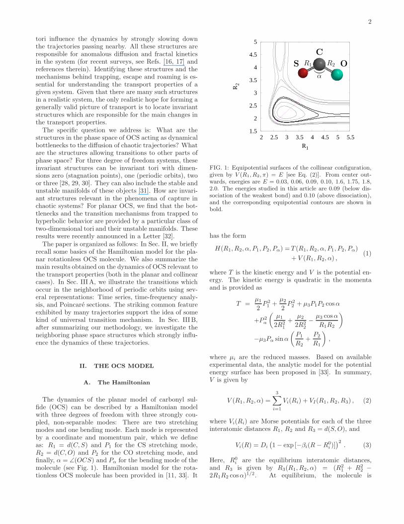
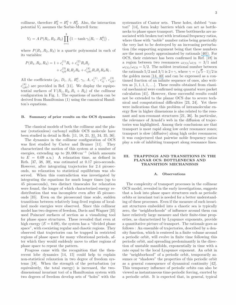
A generic feature of Hamiltonian dynamics is the abun-dance of periodic orbits in phase space. Figure 2 rep-resents the averaged density in the configuration space(R1, R2) of periodic orbit points on the Poincare sectionΣ (defined in Sec. III A 3) for planar OCS. A closer in-spection of this figure shows that the most prominentregions of stability surround short periodic orbits with el-liptic linear stability. A typical trajectory passes throughthis maze of periodic orbits, being trapped for some timeaccording to local stability properties. The aim of thismanuscript is to understand how a typical trajectory canbe trapped and released locally around a given periodicorbit. In what follows we analyze the transport proper-ties in the neighborhood of an elliptic periodic orbit, likefor instance Oa, as shown by a circle in Fig. 3.

2. Time-frequency analysis and stroboscopic mapping

To examine the temporal features of trajectorieswe use time-frequency analysis [43]. In what fol-lows, x designates a point in phase space, i.e. x =(R1, R2, α, P1, P2, Pα). A finite segment of a trajectorycan be represented by a sequence of phase space coordi-nates, {xn}n=1,...,N , xn = x(tn), visited by a trajectoryat times tn. For a stroboscopic map, we take snapshotswith a fixed time increment, tn+1 = tn + ∆. It is nat-ural to scale the time increment ∆ by the period Tp ofthe organizing periodic orbit. We select ∆ = Tp/4. Thetime series of selected orbits are displayed in the bottompanels of Figs. 4 and 6.

We study the instantaneous frequencies using waveletdecomposition. As described in Refs. [43, 44, 45], thetime-frequency analysis is based on a continuous wavelettransform of an observable f(t)

Wf(t, s) =1√s

∫ +∞

−∞

f(τ)ψ∗

(

τ − t

s

)

dτ . (4)

We choose the mother wavelet ψ, in the Morlet-Grossman

form: ψ(t) = eιηte−t2/2σ2

/(σ2π)1/4, with adjustable pa-rameters η and σ. The time-frequency representation isobtained via a relation between the scale s and the fre-quency ξ = η/s. We consider the normalized scalogram

PW f(t, ξ = η/s) = |Wf(t, s)|2/s ,which can be interpreted as the energy density in thetime-frequency plane. The ridges of PW can be inter-preted as instantaneous frequencies, or more rigorously,

0.2 0.4 0.6 0.8 1

R1

R2

2.5 3 3.5 4

2

2.5

FIG. 2: Averaged density of periodic orbit points on thePoincare surface of section, projected onto the (R1, R2)-plane,weighted by the “local escape rate” γ+

p , the sum of pos-

itive Lyapunov exponents, λ(p)i > 0 or, in terms of Lya-

punov multipliers for the periodic orbit p, given by γ+p =

Q

i:|Λ(p)i

|≥1|Λ

(p)i |−1/Tp where Λ

(p)i is an eigenvalue of DFΣ

evaluated at the periodic points. Periodic orbits with thefollowing number of returns to the Poincare sections are de-termined: 1(4), 2(9), 3(10), 5(24), 7(26), 8(101), 11(40),13(33), 17(21), 19(43), 23(41), 29(34), 31(28), 37(43) wherethe number of orbits is shown in parentheses. Energy is setat E = 0.09. Lighter areas are dominated by more regular or-bits, darker by unstable orbits. The circle indicates the regionlocated near Oa where (R1, R2) ≈ (3.6, 2.3) where trappingand roaming is analyzed in Fig. 4.

2

2.5

2.5 3 3.5 4R1

R2

-60-40-20

0 20 40 60

2.5 3 3.5 4R1

2 2.5R2

0.7 1 1.3α/π

FIG. 3: The periodic orbit Oa at E = 0.09: projections in the(R1, R2)-plane (left panel) and in the (R1, P1), (R2, P2) and(α, Pα) planes (right panels). The blue curve in the (R1, R2)projection is the boundary of the energetically accessible re-gion. Dots indicate the location of the intersection with thePoincare section Σ. The periodic orbit Oa is of elliptic-ellipticlinear stability type (see Tab. I for details).

the set of frequencies for a given time interval. In thissection, two typical trajectories (whose initial conditionsare specified in Tab. I) which are initially close to el-ementary organizing periodic orbits, are represented inFigs. 4 and 6 where the signal f(t) is chosen to be P1(t)or P2(t). It should be noticed that other choices of ob-

5

0

0.5

1

1.5

2

TpξP2

-60-30

0 30 60

0 100 200 300 400 500

t/Tp

P2

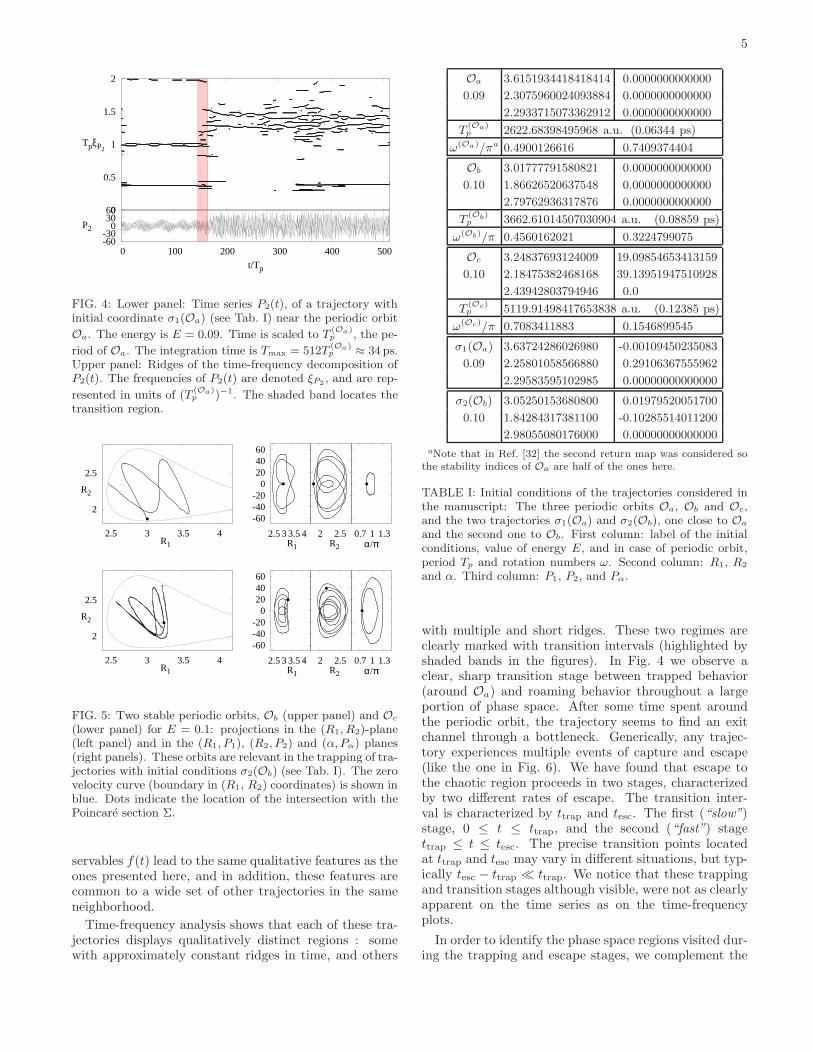
FIG. 4: Lower panel: Time series P2(t), of a trajectory withinitial coordinate σ1(Oa) (see Tab. I) near the periodic orbit

Oa. The energy is E = 0.09. Time is scaled to T(Oa)p , the pe-

riod of Oa. The integration time is Tmax = 512T(Oa)p ≈ 34 ps.

Upper panel: Ridges of the time-frequency decomposition ofP2(t). The frequencies of P2(t) are denoted ξP2 , and are rep-

resented in units of (T(Oa)p )−1. The shaded band locates the

transition region.

2

2.5

2.5 3 3.5 4R1

R2

-60-40-20

0 20 40 60

2.5 3 3.5 4R1

2 2.5R2

0.7 1 1.3α/π

2

2.5

2.5 3 3.5 4R1

R2

-60-40-20

0 20 40 60

2.5 3 3.5 4R1

2 2.5R2

0.7 1 1.3α/π

FIG. 5: Two stable periodic orbits, Ob (upper panel) and Oc

(lower panel) for E = 0.1: projections in the (R1, R2)-plane(left panel) and in the (R1, P1), (R2, P2) and (α, Pα) planes(right panels). These orbits are relevant in the trapping of tra-jectories with initial conditions σ2(Ob) (see Tab. I). The zerovelocity curve (boundary in (R1, R2) coordinates) is shown inblue. Dots indicate the location of the intersection with thePoincare section Σ.

servables f(t) lead to the same qualitative features as theones presented here, and in addition, these features arecommon to a wide set of other trajectories in the sameneighborhood.

Time-frequency analysis shows that each of these tra-jectories displays qualitatively distinct regions : somewith approximately constant ridges in time, and others

Oa 3.6151934418418414 0.0000000000000

0.09 2.3075960024093884 0.0000000000000

2.2933715073362912 0.0000000000000

T(Oa)p 2622.68398495968 a.u. (0.06344 ps)

ω(Oa)/πa 0.4900126616 0.7409374404

Ob 3.01777791580821 0.0000000000000

0.10 1.86626520637548 0.0000000000000

2.79762936317876 0.0000000000000

T(Ob)p 3662.61014507030904 a.u. (0.08859 ps)

ω(Ob)/π 0.4560162021 0.3224799075

Oc 3.24837693124009 19.09854653413159

0.10 2.18475382468168 39.13951947510928

2.43942803794946 0.0

T(Oc)p 5119.91498417653838 a.u. (0.12385 ps)

ω(Oc)/π 0.7083411883 0.1546899545

σ1(Oa) 3.63724286026980 -0.00109450235083

0.09 2.25801058566880 0.29106367555962

2.29583595102985 0.00000000000000

σ2(Ob) 3.05250153680800 0.01979520051700

0.10 1.84284317381100 -0.10285514011200

2.98055080176000 0.00000000000000

aNote that in Ref. [32] the second return map was considered sothe stability indices of Oa are half of the ones here.

TABLE I: Initial conditions of the trajectories considered inthe manuscript: The three periodic orbits Oa, Ob and Oc,and the two trajectories σ1(Oa) and σ2(Ob), one close to Oa

and the second one to Ob. First column: label of the initialconditions, value of energy E, and in case of periodic orbit,period Tp and rotation numbers ω. Second column: R1, R2

and α. Third column: P1, P2, and Pα.

with multiple and short ridges. These two regimes areclearly marked with transition intervals (highlighted byshaded bands in the figures). In Fig. 4 we observe aclear, sharp transition stage between trapped behavior(around Oa) and roaming behavior throughout a largeportion of phase space. After some time spent aroundthe periodic orbit, the trajectory seems to find an exitchannel through a bottleneck. Generically, any trajec-tory experiences multiple events of capture and escape(like the one in Fig. 6). We have found that escape tothe chaotic region proceeds in two stages, characterizedby two different rates of escape. The transition inter-val is characterized by ttrap and tesc. The first (“slow”)stage, 0 ≤ t ≤ ttrap, and the second (“fast”) stagettrap ≤ t ≤ tesc. The precise transition points locatedat ttrap and tesc may vary in different situations, but typ-ically tesc − ttrap ≪ ttrap. We notice that these trappingand transition stages although visible, were not as clearlyapparent on the time series as on the time-frequencyplots.

In order to identify the phase space regions visited dur-ing the trapping and escape stages, we complement the

6

0

0.2

0.4

0.6

0.8

1

TpξP1

-60-30

0 30 60

0 100 200 300 400 500

t/Tp

P1

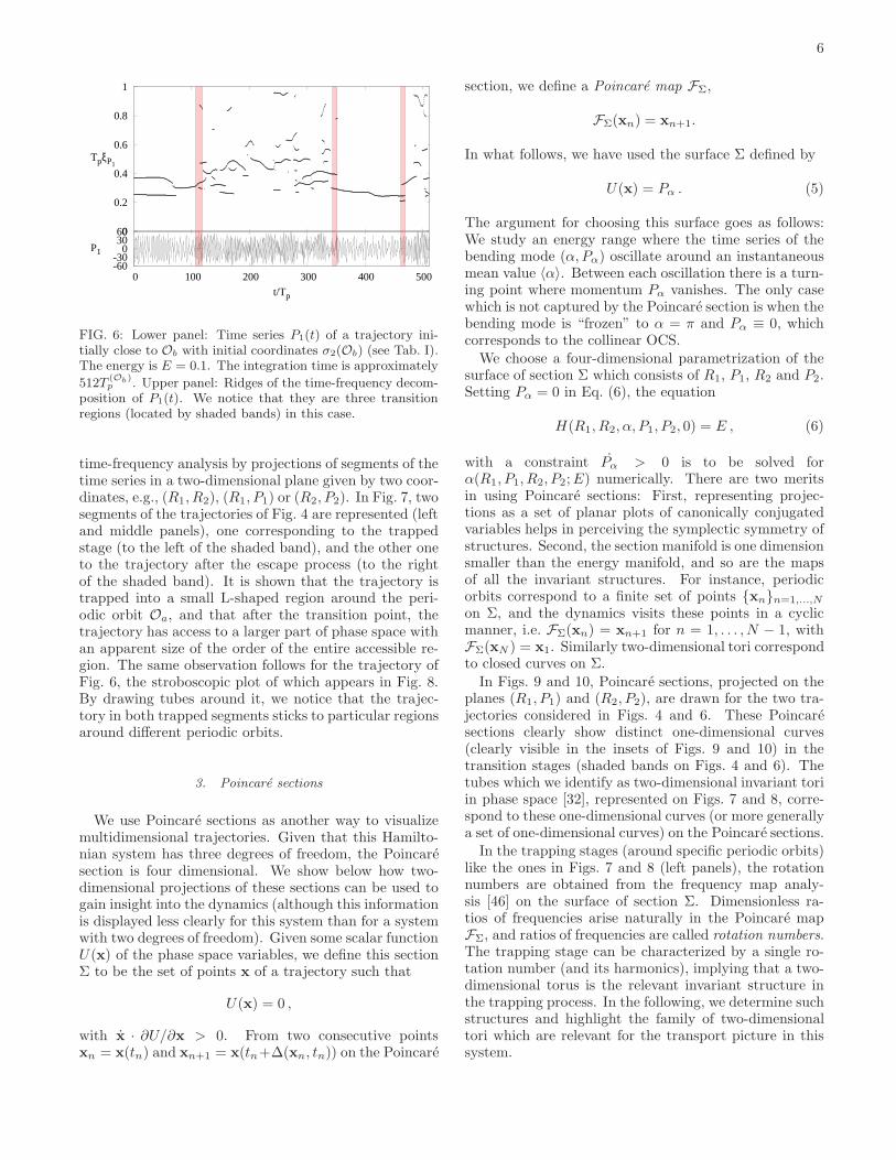
FIG. 6: Lower panel: Time series P1(t) of a trajectory ini-tially close to Ob with initial coordinates σ2(Ob) (see Tab. I).The energy is E = 0.1. The integration time is approximately

512T(Ob)p . Upper panel: Ridges of the time-frequency decom-

position of P1(t). We notice that they are three transitionregions (located by shaded bands) in this case.

time-frequency analysis by projections of segments of thetime series in a two-dimensional plane given by two coor-dinates, e.g., (R1, R2), (R1, P1) or (R2, P2). In Fig. 7, twosegments of the trajectories of Fig. 4 are represented (leftand middle panels), one corresponding to the trappedstage (to the left of the shaded band), and the other oneto the trajectory after the escape process (to the rightof the shaded band). It is shown that the trajectory istrapped into a small L-shaped region around the peri-odic orbit Oa, and that after the transition point, thetrajectory has access to a larger part of phase space withan apparent size of the order of the entire accessible re-gion. The same observation follows for the trajectory ofFig. 6, the stroboscopic plot of which appears in Fig. 8.By drawing tubes around it, we notice that the trajec-tory in both trapped segments sticks to particular regionsaround different periodic orbits.

3. Poincare sections

We use Poincare sections as another way to visualizemultidimensional trajectories. Given that this Hamilto-nian system has three degrees of freedom, the Poincaresection is four dimensional. We show below how two-dimensional projections of these sections can be used togain insight into the dynamics (although this informationis displayed less clearly for this system than for a systemwith two degrees of freedom). Given some scalar functionU(x) of the phase space variables, we define this sectionΣ to be the set of points x of a trajectory such that

U(x) = 0 ,

with x · ∂U/∂x > 0. From two consecutive pointsxn = x(tn) and xn+1 = x(tn+∆(xn, tn)) on the Poincare

section, we define a Poincare map FΣ,

FΣ(xn) = xn+1.

In what follows, we have used the surface Σ defined by

U(x) = Pα . (5)

The argument for choosing this surface goes as follows:We study an energy range where the time series of thebending mode (α, Pα) oscillate around an instantaneousmean value 〈α〉. Between each oscillation there is a turn-ing point where momentum Pα vanishes. The only casewhich is not captured by the Poincare section is when thebending mode is “frozen” to α = π and Pα ≡ 0, whichcorresponds to the collinear OCS.

We choose a four-dimensional parametrization of thesurface of section Σ which consists of R1, P1, R2 and P2.Setting Pα = 0 in Eq. (6), the equation

H(R1, R2, α, P1, P2, 0) = E , (6)

with a constraint Pα > 0 is to be solved forα(R1, P1, R2, P2;E) numerically. There are two meritsin using Poincare sections: First, representing projec-tions as a set of planar plots of canonically conjugatedvariables helps in perceiving the symplectic symmetry ofstructures. Second, the section manifold is one dimensionsmaller than the energy manifold, and so are the mapsof all the invariant structures. For instance, periodicorbits correspond to a finite set of points {xn}n=1,...,N

on Σ, and the dynamics visits these points in a cyclicmanner, i.e. FΣ(xn) = xn+1 for n = 1, . . . , N − 1, withFΣ(xN ) = x1. Similarly two-dimensional tori correspondto closed curves on Σ.

In Figs. 9 and 10, Poincare sections, projected on theplanes (R1, P1) and (R2, P2), are drawn for the two tra-jectories considered in Figs. 4 and 6. These Poincaresections clearly show distinct one-dimensional curves(clearly visible in the insets of Figs. 9 and 10) in thetransition stages (shaded bands on Figs. 4 and 6). Thetubes which we identify as two-dimensional invariant toriin phase space [32], represented on Figs. 7 and 8, corre-spond to these one-dimensional curves (or more generallya set of one-dimensional curves) on the Poincare sections.

In the trapping stages (around specific periodic orbits)like the ones in Figs. 7 and 8 (left panels), the rotationnumbers are obtained from the frequency map analy-sis [46] on the surface of section Σ. Dimensionless ra-tios of frequencies arise naturally in the Poincare mapFΣ, and ratios of frequencies are called rotation numbers.The trapping stage can be characterized by a single ro-tation number (and its harmonics), implying that a two-dimensional torus is the relevant invariant structure inthe trapping process. In the following, we determine suchstructures and highlight the family of two-dimensionaltori which are relevant for the transport picture in thissystem.

7

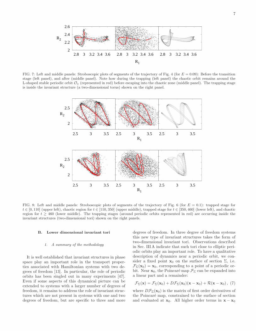
2.6

2.4

2.2

23.63.43.232.8

R2

3.63.43.232.8

R1

3.63.43.232.8

FIG. 7: Left and middle panels: Stroboscopic plots of segments of the trajectory of Fig. 4 (for E = 0.09): Before the transitionstage (left panel), and after (middle panel). Note how during the trapping (left panel) the chaotic orbit remains around theL-shaped stable periodic orbit Oa (represented in red) before escaping into the chaotic zone (middle panel). The trapping stageis inside the invariant structure (a two-dimensional torus) shown on the right panel.

2.5

2

3.532.5

R2

3.532.5R1

3.532.5

2.5

2

3.532.5

R2

3.532.5R1

3.532.5

FIG. 8: Left and middle panels: Stroboscopic plots of segments of the trajectory of Fig. 6 (for E = 0.1): trapped stage fort ∈ [0, 110] (upper left), chaotic region for t ∈ [110, 350] (upper middle), trapped stage for t ∈ [350, 460] (lower left), and chaoticregion for t ≥ 460 (lower middle). The trapping stages (around periodic orbits represented in red) are occurring inside theinvariant structures (two-dimensional tori) shown on the right panels.

B. Lower dimensional invariant tori

1. A summary of the methodology

It is well established that invariant structures in phasespace play an important role in the transport proper-ties associated with Hamiltonian systems with two de-grees of freedom [13]. In particular, the role of periodicorbits has been singled out in many experiments [47].Even if some aspects of this dynamical picture can beextended to systems with a larger number of degrees offreedom, it remains to address the role of invariant struc-tures which are not present in systems with one and twodegrees of freedom, but are specific to three and more

degrees of freedom. In three degree of freedom systemsthis new type of invariant structures takes the form oftwo-dimensional invariant tori. Observations describedin Sec. III A indicate that such tori close to elliptic peri-odic orbits play an important role. To have a qualitativedescription of dynamics near a periodic orbit, we con-sider a fixed point x0 on the surface of section Σ, i.e.FΣ(x0) = x0, corresponding to a point of a periodic or-bit. Near x0, the Poincare map FΣ can be expanded intoa linear part and a remainder:

FΣ(x) = FΣ(x0) +DFΣ(x0)(x − x0) + R(x − x0) , (7)

where DFΣ(x0) is the matrix of first order derivatives ofthe Poincare map, constrained to the surface of sectionand evaluated at x0. All higher order terms in x− x0

8

-10

-5

0

5

10

3.4 3.5 3.6 3.7

R1

P1

-20

-15

-10

-5

0

5

10

15

20

2.2 2.3 2.4

R2

P2

FIG. 9: Poincare sections of the trajectory analyzed in Fig. 4 (for E = 0.09) on the (R1, P1)-plane (left panel) and onthe (R2, P2)-plane (right panel). It is apparent (in the insets) that before escaping to the external region, the trajectory isstuck in the neighborhood of a well-localized structure. The five points (in bold) are the intersections with Σ of a partiallyhyperbolic resonant periodic orbit which is responsible for the escape to the chaotic region through its unstable manifold. Two“tentacles” starting at the upper and lower parts of the structure are marked with broken lines connecting crosses to clarifywhat happens during the escape stage (shaded band in Fig. 4). The resonant 2:5 periodic orbit has elliptic-hyperbolic stabilitywith λ = 0.113231998 per return (or λ = 0.566159992 for the entire orbit) and a rotation number ω/π = 0.35684077865194591per entire orbit.

-10

-5

0

5

10

3 3.1 3.2 3.3

R1

P1

-30

-20

-10

0

10

20

30

1.8 1.9 2 2.1 2.2

R2

P2

FIG. 10: This figure illustrates the multiple capturing which is found generically for a randomly selected trajectory, as the oneof Fig. 6 (for E = 0.1). The quasi-regular intervals are color coded: between iterations 1–47 (red) and 370–430 (blue). Notethat the second interval draws two curves, because it takes two returns to the surface of section to draw this curve (i.e. it is anapparently connected curve for F2

Σ). The two closed loops are the bottleneck torus of the bottom-right panel of Fig. 8.

are collected in R(x−x0). Finite-time dynamics near thefixed point x0 are determined by the properties of the ma-trix DFΣ(x0). Assuming that linearized approximationis effective, and discarding the remainder term from fur-ther discussions (the fully nonlinear problem with large Ris solved using the methodology outlined in Appendix B),we consider a closed curve γ(s) on the Poincare sectionΣ defined on a torus s ∈ T

1, and consider the dynamicsof x(s) = x0 + ǫγ(s) given by

FΣ(x(s)) = x0 + ǫDFΣ(x0)γ(s). (8)

If FΣ has at least one pair of eigenvalues in the formΛ = exp (±ιω), it is possible to find a γ(s) such thatDFΣγ(s) = γ(s+ωǫ) and |ω−ωǫ| = o(ǫ). Therefore theequation

FΣ(x(s)) = x(s+ ω), (9)

has a family of solutions, parametrized by the rota-tion number ω. Equation (9) defines a torus as a loopon the surface of section Σ with rotation number ω.Even if DFΣ(x0) has two pairs of eigenvalues of theform exp (±ιωi) such an invariant loop close to x0 can

9

be found. More details on the determination of two-dimensional invariant tori are given in Appendix B.

2. Invariant tori and their bifurcations: Bottlenecks

In the cases discussed in Sec. III A, trajectories un-dergo a transition (after a trapping stage) in the vicinityof a nonresonant elliptic periodic point x0, whether itis associated with Oa or Ob. For each of these periodicpoints, the matrix DFΣ(x0) has eigenvalues exp (±ιω1),exp (±ιω2) (numerical values are given in Tab. I.) Pro-cesses associated with the escape from the trapping stagecan be better understood by analyzing the tangent spaceof the elliptic periodic orbit Oa that locally has the struc-ture of a direct product (center + center) T

1×I1×T1×I2,

with the periodic orbit at the origin. The elements of thetwo intervals Ii ⊂ R are rotation numbers ωi, which arenot unique in general: The choice is fixed by requiringlimǫ→0 ωi = ω0

i , where ǫ is a measure of the “diameter”of the torus and ω0

i are stability angles of the organizingperiodic orbit. The Poincare map FΣ induces rotationson T

1, rω1 × 1 × rω2 × 1, where rω is a rotation on T1

with the rotation number ω. Partial (or complete) res-onances are determined by one (or two) resonance con-ditions nω1 +mω2 + k = 0, where (n,m, k) are integerssuch that |n| + |m| + |k| > 0. The most striking trap-ping effects are observed for partial resonances of thetype T

1 × I1 × {0}× {0}, and {0}× {0}×T1 × I2. They

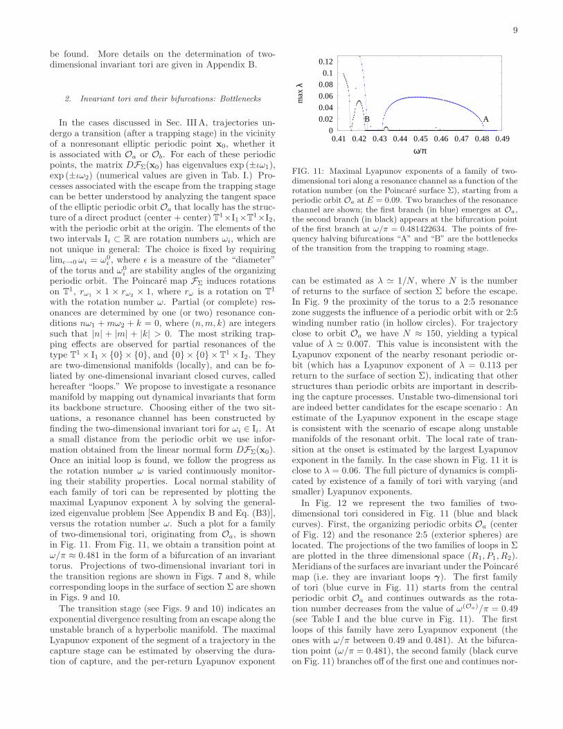
are two-dimensional manifolds (locally), and can be fo-liated by one-dimensional invariant closed curves, calledhereafter “loops.” We propose to investigate a resonancemanifold by mapping out dynamical invariants that formits backbone structure. Choosing either of the two sit-uations, a resonance channel has been constructed byfinding the two-dimensional invariant tori for ωi ∈ Ii. Ata small distance from the periodic orbit we use infor-mation obtained from the linear normal form DFΣ(x0).Once an initial loop is found, we follow the progress asthe rotation number ω is varied continuously monitor-ing their stability properties. Local normal stability ofeach family of tori can be represented by plotting themaximal Lyapunov exponent λ by solving the general-ized eigenvalue problem [See Appendix B and Eq. (B3)],versus the rotation number ω. Such a plot for a familyof two-dimensional tori, originating from Oa, is shownin Fig. 11. From Fig. 11, we obtain a transition point atω/π ≈ 0.481 in the form of a bifurcation of an invarianttorus. Projections of two-dimensional invariant tori inthe transition regions are shown in Figs. 7 and 8, whilecorresponding loops in the surface of section Σ are shownin Figs. 9 and 10.

The transition stage (see Figs. 9 and 10) indicates anexponential divergence resulting from an escape along theunstable branch of a hyperbolic manifold. The maximalLyapunov exponent of the segment of a trajectory in thecapture stage can be estimated by observing the dura-tion of capture, and the per-return Lyapunov exponent

0

0.02

0.04

0.06

0.08

0.1

0.12

0.41 0.42 0.43 0.44 0.45 0.46 0.47 0.48 0.49

max

λ

ω/π

AB

FIG. 11: Maximal Lyapunov exponents of a family of two-dimensional tori along a resonance channel as a function of therotation number (on the Poincare surface Σ), starting from aperiodic orbit Oa at E = 0.09. Two branches of the resonancechannel are shown; the first branch (in blue) emerges at Oa,the second branch (in black) appears at the bifurcation pointof the first branch at ω/π = 0.481422634. The points of fre-quency halving bifurcations “A” and “B” are the bottlenecksof the transition from the trapping to roaming stage.

can be estimated as λ ≃ 1/N , where N is the numberof returns to the surface of section Σ before the escape.In Fig. 9 the proximity of the torus to a 2:5 resonancezone suggests the influence of a periodic orbit with or 2:5winding number ratio (in hollow circles). For trajectoryclose to orbit Oa we have N ≈ 150, yielding a typicalvalue of λ ≃ 0.007. This value is inconsistent with theLyapunov exponent of the nearby resonant periodic or-bit (which has a Lyapunov exponent of λ = 0.113 perreturn to the surface of section Σ), indicating that otherstructures than periodic orbits are important in describ-ing the capture processes. Unstable two-dimensional toriare indeed better candidates for the escape scenario : Anestimate of the Lyapunov exponent in the escape stageis consistent with the scenario of escape along unstablemanifolds of the resonant orbit. The local rate of tran-sition at the onset is estimated by the largest Lyapunovexponent in the family. In the case shown in Fig. 11 it isclose to λ = 0.06. The full picture of dynamics is compli-cated by existence of a family of tori with varying (andsmaller) Lyapunov exponents.

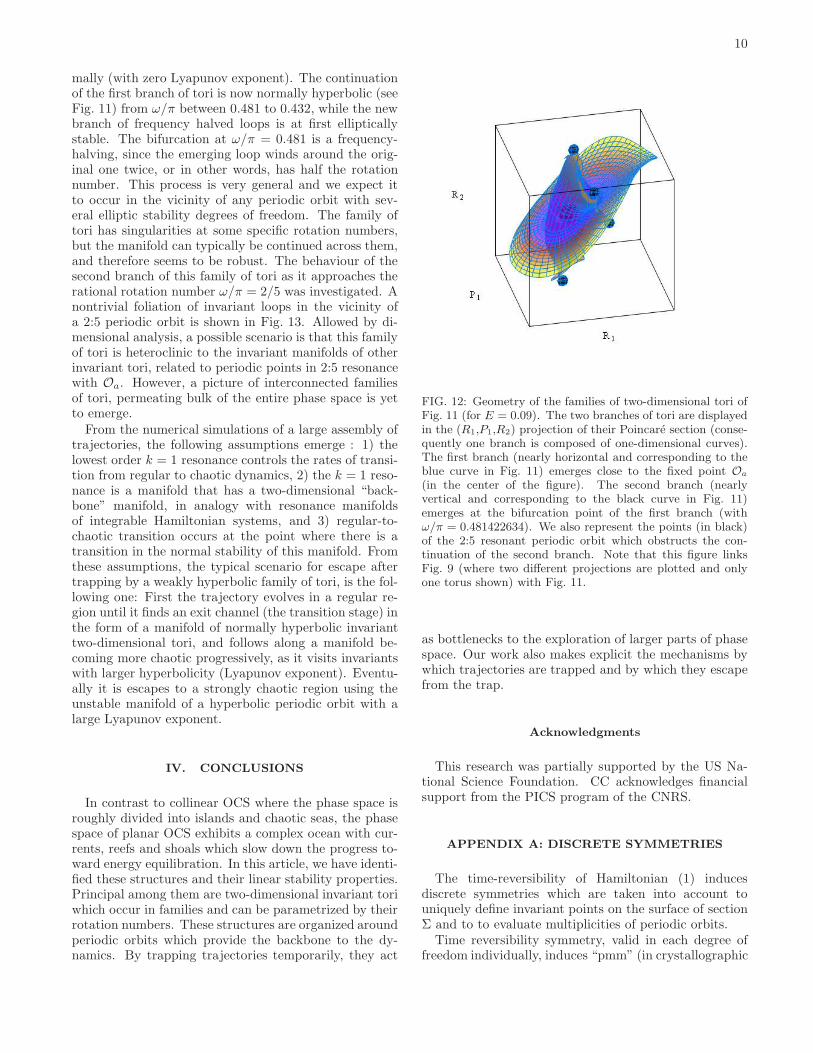
In Fig. 12 we represent the two families of two-dimensional tori considered in Fig. 11 (blue and blackcurves). First, the organizing periodic orbits Oa (centerof Fig. 12) and the resonance 2:5 (exterior spheres) arelocated. The projections of the two families of loops in Σare plotted in the three dimensional space (R1, P1, R2).Meridians of the surfaces are invariant under the Poincaremap (i.e. they are invariant loops γ). The first familyof tori (blue curve in Fig. 11) starts from the centralperiodic orbit Oa and continues outwards as the rota-tion number decreases from the value of ω(Oa)/π = 0.49(see Table I and the blue curve in Fig. 11). The firstloops of this family have zero Lyapunov exponent (theones with ω/π between 0.49 and 0.481). At the bifurca-tion point (ω/π = 0.481), the second family (black curveon Fig. 11) branches off of the first one and continues nor-

10

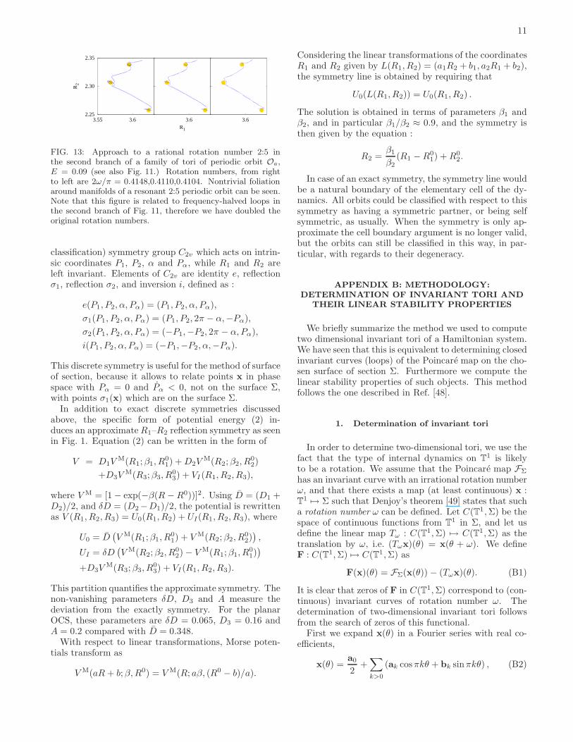
mally (with zero Lyapunov exponent). The continuationof the first branch of tori is now normally hyperbolic (seeFig. 11) from ω/π between 0.481 to 0.432, while the newbranch of frequency halved loops is at first ellipticallystable. The bifurcation at ω/π = 0.481 is a frequency-halving, since the emerging loop winds around the orig-inal one twice, or in other words, has half the rotationnumber. This process is very general and we expect itto occur in the vicinity of any periodic orbit with sev-eral elliptic stability degrees of freedom. The family oftori has singularities at some specific rotation numbers,but the manifold can typically be continued across them,and therefore seems to be robust. The behaviour of thesecond branch of this family of tori as it approaches therational rotation number ω/π = 2/5 was investigated. Anontrivial foliation of invariant loops in the vicinity ofa 2:5 periodic orbit is shown in Fig. 13. Allowed by di-mensional analysis, a possible scenario is that this familyof tori is heteroclinic to the invariant manifolds of otherinvariant tori, related to periodic points in 2:5 resonancewith Oa. However, a picture of interconnected familiesof tori, permeating bulk of the entire phase space is yetto emerge.

From the numerical simulations of a large assembly oftrajectories, the following assumptions emerge : 1) thelowest order k = 1 resonance controls the rates of transi-tion from regular to chaotic dynamics, 2) the k = 1 reso-nance is a manifold that has a two-dimensional “back-bone” manifold, in analogy with resonance manifoldsof integrable Hamiltonian systems, and 3) regular-to-chaotic transition occurs at the point where there is atransition in the normal stability of this manifold. Fromthese assumptions, the typical scenario for escape aftertrapping by a weakly hyperbolic family of tori, is the fol-lowing one: First the trajectory evolves in a regular re-gion until it finds an exit channel (the transition stage) inthe form of a manifold of normally hyperbolic invarianttwo-dimensional tori, and follows along a manifold be-coming more chaotic progressively, as it visits invariantswith larger hyperbolicity (Lyapunov exponent). Eventu-ally it is escapes to a strongly chaotic region using theunstable manifold of a hyperbolic periodic orbit with alarge Lyapunov exponent.

IV. CONCLUSIONS

In contrast to collinear OCS where the phase space isroughly divided into islands and chaotic seas, the phasespace of planar OCS exhibits a complex ocean with cur-rents, reefs and shoals which slow down the progress to-ward energy equilibration. In this article, we have identi-fied these structures and their linear stability properties.Principal among them are two-dimensional invariant toriwhich occur in families and can be parametrized by theirrotation numbers. These structures are organized aroundperiodic orbits which provide the backbone to the dy-namics. By trapping trajectories temporarily, they act

FIG. 12: Geometry of the families of two-dimensional tori ofFig. 11 (for E = 0.09). The two branches of tori are displayedin the (R1,P1,R2) projection of their Poincare section (conse-quently one branch is composed of one-dimensional curves).The first branch (nearly horizontal and corresponding to theblue curve in Fig. 11) emerges close to the fixed point Oa

(in the center of the figure). The second branch (nearlyvertical and corresponding to the black curve in Fig. 11)emerges at the bifurcation point of the first branch (withω/π = 0.481422634). We also represent the points (in black)of the 2:5 resonant periodic orbit which obstructs the con-tinuation of the second branch. Note that this figure linksFig. 9 (where two different projections are plotted and onlyone torus shown) with Fig. 11.

as bottlenecks to the exploration of larger parts of phasespace. Our work also makes explicit the mechanisms bywhich trajectories are trapped and by which they escapefrom the trap.

Acknowledgments

This research was partially supported by the US Na-tional Science Foundation. CC acknowledges financialsupport from the PICS program of the CNRS.

APPENDIX A: DISCRETE SYMMETRIES

The time-reversibility of Hamiltonian (1) inducesdiscrete symmetries which are taken into account touniquely define invariant points on the surface of sectionΣ and to to evaluate multiplicities of periodic orbits.

Time reversibility symmetry, valid in each degree offreedom individually, induces “pmm” (in crystallographic

11

2.25

2.30

2.35

3.55 3.6

R2

3.6

R1

3.6

FIG. 13: Approach to a rational rotation number 2:5 inthe second branch of a family of tori of periodic orbit Oa,E = 0.09 (see also Fig. 11.) Rotation numbers, from rightto left are 2ω/π = 0.4148,0.4110,0.4104. Nontrivial foliationaround manifolds of a resonant 2:5 periodic orbit can be seen.Note that this figure is related to frequency-halved loops inthe second branch of Fig. 11, therefore we have doubled theoriginal rotation numbers.

classification) symmetry group C2v which acts on intrin-sic coordinates P1, P2, α and Pα, while R1 and R2 areleft invariant. Elements of C2v are identity e, reflectionσ1, reflection σ2, and inversion i, defined as :

e(P1, P2, α, Pα) = (P1, P2, α, Pα),

σ1(P1, P2, α, Pα) = (P1, P2, 2π − α,−Pα),

σ2(P1, P2, α, Pα) = (−P1,−P2, 2π − α, Pα),

i(P1, P2, α, Pα) = (−P1,−P2, α,−Pα).

This discrete symmetry is useful for the method of surfaceof section, because it allows to relate points x in phasespace with Pα = 0 and Pα < 0, not on the surface Σ,with points σ1(x) which are on the surface Σ.

In addition to exact discrete symmetries discussedabove, the specific form of potential energy (2) in-duces an approximateR1–R2 reflection symmetry as seenin Fig. 1. Equation (2) can be written in the form of

V = D1VM(R1;β1, R

01) +D2V

M(R2;β2, R02)

+D3VM(R3;β3, R

03) + VI(R1, R2, R3),

where V M = [1 − exp(−β(R −R0))]2. Using D = (D1 +D2)/2, and δD = (D2−D1)/2, the potential is rewrittenas V (R1, R2, R3) = U0(R1, R2) + UI(R1, R2, R3), where

U0 = D(

V M(R1;β1, R01) + V M(R2;β2, R

02)

)

,

UI = δD(

V M(R2;β2, R02) − V M(R1;β1, R

01)

)

+D3VM(R3;β3, R

03) + VI(R1, R2, R3).

This partition quantifies the approximate symmetry. Thenon-vanishing parameters δD, D3 and A measure thedeviation from the exactly symmetry. For the planarOCS, these parameters are δD = 0.065, D3 = 0.16 andA = 0.2 compared with D = 0.348.

With respect to linear transformations, Morse poten-tials transform as

V M(aR+ b;β,R0) = V M(R; aβ, (R0 − b)/a).

Considering the linear transformations of the coordinatesR1 and R2 given by L(R1, R2) = (a1R2 + b1, a2R1 + b2),the symmetry line is obtained by requiring that

U0(L(R1, R2)) = U0(R1, R2) .

The solution is obtained in terms of parameters β1 andβ2, and in particular β1/β2 ≈ 0.9, and the symmetry isthen given by the equation :

R2 =β1

β2(R1 −R0

1) +R02.

In case of an exact symmetry, the symmetry line wouldbe a natural boundary of the elementary cell of the dy-namics. All orbits could be classified with respect to thissymmetry as having a symmetric partner, or being selfsymmetric, as usually. When the symmetry is only ap-proximate the cell boundary argument is no longer valid,but the orbits can still be classified in this way, in par-ticular, with regards to their degeneracy.

APPENDIX B: METHODOLOGY:

DETERMINATION OF INVARIANT TORI AND

THEIR LINEAR STABILITY PROPERTIES

We briefly summarize the method we used to computetwo dimensional invariant tori of a Hamiltonian system.We have seen that this is equivalent to determining closedinvariant curves (loops) of the Poincare map on the cho-sen surface of section Σ. Furthermore we compute thelinear stability properties of such objects. This methodfollows the one described in Ref. [48].

1. Determination of invariant tori

In order to determine two-dimensional tori, we use thefact that the type of internal dynamics on T

1 is likelyto be a rotation. We assume that the Poincare map FΣ

has an invariant curve with an irrational rotation numberω, and that there exists a map (at least continuous) x :T

1 7→ Σ such that Denjoy’s theorem [49] states that sucha rotation number ω can be defined. Let C(T1,Σ) be thespace of continuous functions from T

1 in Σ, and let usdefine the linear map Tω : C(T1,Σ) 7→ C(T1,Σ) as thetranslation by ω, i.e. (Tωx)(θ) = x(θ + ω). We defineF : C(T1,Σ) 7→ C(T1,Σ) as

F(x)(θ) = FΣ(x(θ)) − (Tωx)(θ). (B1)

It is clear that zeros of F in C(T1,Σ) correspond to (con-tinuous) invariant curves of rotation number ω. Thedetermination of two-dimensional invariant tori followsfrom the search of zeros of this functional.

First we expand x(θ) in a Fourier series with real co-efficients,

x(θ) =a0

2+

∑

k>0

(ak cosπkθ + bk sinπkθ) , (B2)

12

where ak,bk ∈ Rn for k ∈ N (n being the dimension of

the flow) and x(θ) is a periodic function with period 2,i.e. x(θ + 2) = x(θ). We truncate these series at a fixedvalue ofN , and determine an approximation to the 2N+1unknown coefficients a0, ak, and bk for 1 ≤ k ≤ N . Weconstruct the discretized version of Eq. (9) by consideringa mesh of 2N + 1 points on T

1:

θj =2j

2N + 1for 0 ≤ j ≤ 2N,

where we notice that for numerical stability reasons,the length of T

1 is taken as 2. Given the Fourier co-efficients ak, bk, the coordinates x(θj) are expressedas linear functions of the coefficients ak, bk, i.e.x(θj) ≡ φ({ak}, {bk}, j), given by Eq. (B2). Accord-ingly, FΣ(x(θj)) and Eq. (9) can be considered as func-tions of the coefficients ak, bk:

Fj({ak}, {bk}, ω) = FΣ(φ({ak}, {bk}, j))−φ({ak}, {bk}, j + i(ω)),

for 0 ≤ j ≤ 2N and where i(ω) = (2N + 1)ω/2. The co-efficients ak, bk are the unknowns in the above equation.

We solve F = 0 using a Newton’s iterative algorithm.At each iteration, it provides the corrections δak and δbk

to be added to the ak and bk obtained from the previousiteration. We approximate (δa, δb) as a solution of thefollowing equation:

Fj(a,b, ν) +∂Fj

∂akδak +

∂Fj

∂bkδbk +

∂Fj

∂ωδω = 0 ,

where a = (a0,a1, . . . ,aN ) and b = (b1, . . . ,bN ). Theiteration a′ = a + δa, b′ = b + δb and ω′ = ω + δωconverges if the initial guess is close enough to the truesolution. The above equation requires the inversion ofthe Jacobian of Fj . From the previous definitions it isclear that if x(θ) is a Fourier series corresponding to aninvariant curve then, for any ϕ ∈ T

1, y(θ) ≡ x(θ + ϕ)is a different Fourier series corresponding to the sameinvariant curve as x(θ). This implies that the Jacobianof Fj around the invariant curve has, at least, a one-dimensional kernel. To solve this problem we use theSingular Value Decomposition. Even if Newton’s algo-rithm has converged, we cannot claim with certainty that

a smooth two-dimensional torus has been found. We havenoticed that crude discretization can wash out the detailsof non-smooth curves. Sometimes doubling the numberof points in the discretization turns a convergent caseinto a divergent one. In most cases the reliability of a so-lution is almost certain when testing the spectrum of thesolution (and the norm of its eigenvectors weighted bythe frequency, penalizing high harmonics): a smooth so-lution should contain a unit eigenvalue. This is why it isalso important to monitor the linear stability propertiesof the curves we obtain numerically.

2. Linear stability properties

In addition to the determination of the location of theinvariant tori, we compute their linear stability proper-ties to obtain information on the dynamics in its (in-finitesimal) neighborhood, i.e. eigenvalues and eigenvec-tors which give at first order an approximation to theinvariant manifolds (stable, unstable and central) nearthe invariant curve. We consider the generalized eigen-value problem which amounts to finding (Λ,ψ) such that

DFΣ(x(θ))ψ(θ) = Λψ(θ + ω). (B3)

The eigenvalues Λ have the following properties [48]: 1)Λ = 1 is an eigenvalue of Eq. (B3); the correspondingeigenvector is the derivative of the loop x, 2) if Λ isan eigenvalue of Eq. (B3), then Λ exp (2ιkπω) is also aneigenvalue for any k ∈ Z, 3) the closure of the set ofeigenvalues of Eq. (B3) is a union of circles centered atthe origin.

There are two unit eigenvalues in the spectrum ofDFΣ. The symplectic symmetry implies that the tori aredegenerate in the linear approximation. It implies the ex-istence of a family of (smooth) two-dimensional tori. Asit is usual, we expect that this family is discontinuous andthe discontinuities are around rational rotation numbersω = m/n. Numerically, once an invariant torus with aspecific ω is found, we simply increment the frequencyparameter ω → ω + δω and restart the search. In thisway, we determine these families of two-dimensional toriparametrized by their frequency ω on the Poincare sec-tion. More details on the algorithm are given in Ref. [50].

[1] S. Glasstone, K. J. Laidler, and H. Eyring, The Theory

of Rate Processes (Wiley, NY, 1941).[2] P. J. Robinson and K. A. Holbrok, Unimolecular Reac-

tions (Wiley, NY, 1972).[3] W. Forst, Theory of Unimolecular Reactions (Academic

Press, NY, 1973).[4] P. Pechukas, in Dynamics of Molecular Collisions, Part

B, edited by W. H. Miller (Plenum, N.Y., 1976), chap. 6.[5] E. Fermi, J. R. Pasta, and S. Ulam, Tech. Rep. Report

LA-1940, Los Alamos (1955).

[6] E. Fermi, J. Pasta, and S. Ulam, in [5], pp. 977–988.[7] J. Ford, Phys. Rep. 213, 273 (1992).[8] T. Dauxois, M. Peyrard, and S. Ruffo, Eur. J. Phys. 26,

S3 (2005).[9] D. K. Campbell, P. Rosenau, and G. M. Zaslavsky, Chaos

15, 015101 (2005).[10] A. Carati, L. Galgani, and A. Giorgilli, Chaos 5, 015105

(2005).[11] D. Carter and P. Brumer, J. Chem. Phys. 77, 4208

(1982).

13

[12] T. Uzer, Phys. Rep. 199, 73 (1991).[13] A. J. Lichtenberg and M. A. Lieberman, Regular and

Chaotic Dynamics (Springer, 1992).[14] R. S. MacKay, J. D. Meiss, and I. C. Percival, Physica D

13, 55 (1984).[15] D. Bensimon and L. P. Kadanoff, Physica D 13, 82

(1984).[16] G. Zaslavsky, Phys. Rep. 371, 461 (2002).[17] G. M. Zaslavsky, Hamiltonian Chaos and Fractional Dy-

namics (Oxford University Press, Oxford, 2005).[18] M. J. Davis, J. Chem. Phys. 83, 1016 (1985).[19] M. J. Davis and S. K. Gray, J. Chem. Phys. 84, 5389

(1986).[20] S. K. Gray and S. A. Rice, J. Chem. Phys. 86, 2020

(1987).[21] C. C. Martens, M. J. Davis, and G. S. Ezra, Chem. Phys.

Lett. 142, 519 (1987).[22] R. T. Skodje and M. J. Davis, J. Chem. Phys. 88, 2429

(1988).[23] R. E. Gillilan, J. Chem. Phys. 93, 5300 (1990).[24] R. E. Gillilan and G. S. Ezra, J. Chem. Phys. 94, 2648

(1991).[25] M. Toda, Adv. Chem. Phys. 130A, 337 (2005).[26] V. Rom-Kedar and G. Zaslavsky, Chaos 9, 697 (1999).[27] G. Contopoulos, Order and Chaos in Dynamical Astron-

omy (Springer, Berlin, 2002).[28] J. Laskar, in Hamiltonian Systems with Three or More

Degrees of Freedom. NATO ASI Series, Series C: Mathe-

matical and Physical Sciences Vol. 533, edited by C. Simo(Kluwer, Dordrecht, 1999), p. 134.

[29] C. Froeschle, R. Gonczi, and E. Lega, Planet. Space Sci.45, 881 (1997).

[30] P. Cincotta and S. Simo, A&AS 147, 205 (2000).[31] S. Wiggins, Chaotic Transport in Dynamical Systems

(Springer, N.Y., 1992).[32] R. Paskauskas, C. Chandre, and T. Uzer, Phys. Rev.

Lett. 100, 083001(4) (2008).[33] A. Foord, J. G. Smith, and D. H. Whiffen, Mol. Phys.

29, 1685 (1975).[34] M. J. Davis, Chem. Phys. Lett. 110, 491 (1984).[35] M. J. Davis and A. F. Wagner, in Resonances in Electron-

Molecule Scattering, van der Waals Complexes, and Re-

active Chemical Scattering, edited by D. G. Truhlar(American Chemical Society, 1984), vol. 263 of ACS Sym-

posium Series.[36] C. C. Martens, M. J. Davis, and G. S. Ezra (1989), un-

published.[37] Y. G. Sinai, Acta. Phys. Aust. Suppl. X, 575 (1973).[38] S. C. Farantos and J. N. Murrell, Chem. Phys. 55, 205

(1981).[39] I. Hamilton and P. Brumer, J. Chem. Phys. 78, 2682

(1983).[40] G. H. Hardy and E. M. Wright, An Introduction to the

Theory of Numbers (Oxford, 1979).[41] L. L. Gibson, G. C. Schatz, M. A. Ratner, and M. J.

Davis, J. Chem. Phys. 86, 3263 (1986).[42] P. Lochak, Nonlinearity 6, 855 (1993).[43] C. Chandre, S. Wiggins, and T. Uzer, Physica D 181,

171 (2003).[44] N. Hess-Nielsen and M. V. Wickerhauser, Proc. IEEE 84,

523 (1996).[45] R. Carmona, W. L. Hwang, and B. Torresani, Practical

Time–Frequency Analysis (Academic Press, San Diego,1998).

[46] J. Laskar, Physica D 67, 257 (1993).[47] M. C. Gutzwiller, Chaos in Classical and Quantum Me-

chanics (Springer, N.Y., 1990).

[48] A. Jorba, Nonlinearity 14, 943 (2001).[49] A. Katok and B. Hasselblatt, Introduction to the Modern

Theory of Dynamical Systems, vol. 54 of Encyclopedia of

mathematics and its applications (Cambridge University,UK, 1995), 3rd ed.

[50] R. Paskauskas, Ph.D. thesis, Georgia Institute of Tech-nology (2007).