arX

iv:h

ep-t

h/05

0507

8v2

12

Sep

2005

SPhT-t05/068

Bulk correlation functions in 2D quantum gravity 1

I.K. Kostov1 and V.B. Petkova2

1 Service de Physique Theorique, CNRS – URA 2306,

C.E.A. - Saclay, F-91191 Gif-Sur-Yvette, France

2Institute for Nuclear Research and Nuclear Energy,

72 Tsarigradsko Chaussee, 1784 Sofia, Bulgaria

Abstract

We compute bulk 3- and 4-point tachyon correlators in the 2d Liouville gravity with non-rational

matter central charge c < 1, following and comparing two approaches. The continuous CFT

approach exploits the action on the tachyons of the ground ring generators deformed by Liouville

and matter “screening charges”. A by-product general formula for the matter 3-point OPE struc-

ture constants is derived. We also consider a “diagonal” CFT of 2D quantum gravity, in which

the degenerate fields are restricted to the diagonal of the semi-infinite Kac table. The discrete

formulation of the theory is a generalization of the ADE string theories, in which the target space

is the semi-infinite chain of points.

1. Introduction and summary

The observation that the operator product expansions of the physical operators in theeffective 2d CFT describing the quantum Liouville gravity reduce, modulo BRST commu-tators, to simple “fusion” relations is an old one [1]. The ghost number zero operatorswere argued to close a ring, the “ground ring”, which furthermore preserves the tachyonmodules. It is assumed that in the rational case it coincides with the fusion ring of theminimal c < 1 theories, see in particular the recent work in [2]. The action of the groundring on tachyon modules was used to derive functional recursive identities for the tachyoncorrelation functions [3,4,5,6].

1 Talk given at the International Workshop “Classical and Quantum Integrable Systems”,

January 24-28, 2005, Dubna, Russia.

1

In this work (see [7] for a more detailed presentation) we reconsider and extend thisapproach for constructing bulk tachyon correlators. We study a non-rational, or quasi-rational, CFT of 2D quantum gravity, whose effective action is that of a gaussian fieldperturbed by both Liouville and matter “screening charges”.

We start with a direct evaluation of the 3-point function as a product of Liouvilleand matter OPE structure constants. For this purpose we derive an explicit expression,formula (3.3) below, for the general matter 3-point OPE structure constants. (This resultwas independently obtained by Al. Zamolodchikov [8], with a different normalization of thefields.) Then we write difference recurrence equations for the 4-point function of tachyons.

We also consider another non-rational CFT of 2D quantum gravity, in which thedegenerate fields along the diagonal of the semi-infinite Kac table form a closed algebra.The CFT in question, which we call ‘diagonal CFT’, is described by a perturbation with thefour tachyon operators whose Liouville component has dimension one and whose mattercomponent has dimension zero.

A microscopic realization of this diagonal CFT is given by a non-rational extensionof the ADE string theories introduced in [9] with semi-infinite discrete target space. Theloop gas representation of the microscopic theory leads to a target space diagram technique[10], which allows to calculate efficiently the tachyon correlation functions [11,12]. We findagreement between the “diagonal” CFT and the discrete results.

2. Non-rational 2D gravity: effective action, local fields, ground ring

The effective action of Euclidean Liouville gravity (taken on the sphere) is a perturbationof the gaussian action

Afree =1

4π

∫

d2x[

(∂φ)2 + (∂χ)2 + (Qφ+ ie0χ)R + 4(b∂zc + b∂z c)]

(2.1)

of the Liouville φ, and matter χ, fields and a pair of reparametrization ghosts. Thebackground charges, Q = 1

b + b and e0 = 1b − b are parametrized by a real b, so that the

total central charge of this conformal theory is trivial

ctot ≡ cL + cM + cghosts =[

13 + 6(b2 + 1b2 )]

+[

13 − 6(b2 + 1b2 )]

− 26 = 0. (2.2)

The physical fields, or the “on-mass-shell” tachyons in the string theory interpretation, areproducts of Liouville and matter vertex operators of total dimension (1, 1) [13,14]

γ(1−α2+e2)π e2ieχ e2αφ = 1

πγ(ǫbǫP ) ei(e0−P )χ+(Q−ǫP )φ = V ǫα , ǫ = ±1, (2.3)

e(e− e0) + α(Q− α) = 1 ⇒ e = α− b , or, e = −α+ 1b. (2.4)

The parameters P and ǫ in (2.3) are interpreted as the tachyon target space momentumand chirality. In the “leg factor” normalization in (2.3), γ(x) = Γ(x)/Γ(1 − x).

2

The BRST invariant operators associated with (2.3) are obtained either by integratingover the world sheet, or by multiplying with the ghost field cc of dimension (−1,−1)

T (±)P = T±

α ≡∫

V ±α or W(±)

P = W±α ≡ cc V ±

α . (2.5)

In the n-point tachyon correlators n−3 vertex operators are integrated over the worldsheetand three are placed, as usual, at arbitrary points, say 0, 1 and ∞.

The ground ring of BRST invariant operators of zero dimension and zero ghost number[1] is generated by the two operators a±(x) = a±(z) a±(z) ,

a−(z) =(

b(z)c(z) − b−1∂z(φ(z) + iχ(z)))

e−b(φ(z)−iχ(z))

a+(z) = (b(z)c(z) − b ∂z(φ(z) − iχ(z))) e−b−1(φ(z)+iχ(z)).(2.6)

Unlike the tachyons, the operators (2.6) are made of Liouville and matter vertex operators,both corresponding to degenerate Virasoro representations. We will consider deformationsof these free field operators determined by pairs of Liouville and matter “screening charges”,i.e, by the interaction actions

Aint =

∫

(

µLe2bφ + µ

Me−2ibχ

)

= λLT (+)

e0+ λ

MT (+)

Q ,

Aint =

∫

(

µLe2φ/b + µ

Me2iχ/b

)

= λLT (−)

e0+ λ

MT (−)−Q .

(2.7)

The renormalized by the leg factors in (2.3) coupling constants are

λL

= πγ(b2)µ, λL

= πγ( 1b2 ) µ,

λM

= πγ(−b2)µM, λ

M= πγ(− 1

b2) µ

M.

(2.8)

The four terms in (2.7) describe perturbations that act separately on the matter andLiouville fields. In such a theory the 3-point function factorizes into a product of matterand Liouville components.

One can imagine more general perturbations by integrated tachyon fields, which affectsimultaneously the matter and Liouville fields. We will study the simplest example of sucha perturbation, which is described by the two Liouville “screening charges” as well us bya pair of tachyons related to the latter by a matter charge reflection (e, α) → (e0 − e, α),namely (0, b) → (e0, b) and (0, b−1) → (e0, b

−1). This perturbation, which we call diagonalperturbation, is described by the action

Adiagint = λ

L

(

T (+)e0

+ λMλ

MT (−)−e0

)

+ λL

(

T (−)e0

+ λMλ

MT (+)−e0

)

. (2.9)

3. The tachyon 3-point function as a product of Liouville and matter OPE

constants

The 3-point function in the non-rational CFT of 2D gravity described by the perturbation(2.7) factorizes to a product of the matter and Liouville three-point OPE constants

Gε1ε2ε3

3 (α1, α2, α3) =⟨

W(ε1)P1

W(ε2)P2

W(ε3)P3

⟩

=CLiou(α1, α2, α3)C

Matt(e1, e2, e3)

π3∏3

j=1 γ(α2j − e2j )

. (3.1)

3

Here αi and ei are solutions of the on-mass-shell condition (2.4).

For the Liouville 3-point constant we take the expression derived in [15,16]:

CLiou(α1 , α2 , α3) =(

λ1/bL

b2e0

)Q−α1−α2−α3 Υb(b) Υb(2α1) Υb(2α2) Υb(2α3)

Υb(α123 −Q) Υb(α123) Υb(α2

13) Υb(α312)(3.2)

with notation α312 = α1 + α2 − α3 , α123 = α1 + α2 + α3, etc. This constant is symmetric

with respect to the duality transformation b→ b−1, λL→ λ1/b2

L= λ

L.

For the matter 3-point OPE constant we obtain the expression

CMatt(e1 , e2 , e3) =(

λ1/bM

b2Q)e1+e2+e3−e0 Υb(0) Υb(2e1) Υb(2e2) Υb(2e3)

Υb(e123 − e0) Υb(e123) Υb(e

213) Υb(e

312)

=λ

1

b (Q−∑

iαi)

L λ− 1

b (e0−∑

iei)

M

b∑

iǫi∏3

i=1 γ(bǫi(Q− 2αi))

1

CLiou(α1 , α2 , α3), αi = ǫi ei + bǫi

(3.3)

invariant under b → −1/b , λM

→ (λM

)−1/b2 = λM

. The derivation of (3.3) repeats theone for the Liouville case in [17], where the formula (3.2) was determined for positive,irrational b2 as the unique (smooth) solution of a pair of functional relations, see [7] formore details. The second line of (3.3) holds for any choice of the three signs ǫi using thereflection properties of the Liouville OPE constant (3.2). The function in the first line isdefined as

Υb(x) :=1

Υb(x+ b)=

1

Υb(−x+ 1b )

= Υb(e0 − x) = Υ 1

b(−x) (3.4)

and satisfies the functional relations

Υb(x− b) = γ(bx) b1−2bx Υb(x) , Υb(x+1

b) = γ(−1

bx) b−1− 2

bx Υb(x) . (3.5)

Its logarithm admits an integral representation as the one for log Υb, with Q replaced bye0 (whence invariant under the change b → −1/b), which is convergent (for b > 0) in thestrip −b < Re x < 1

b . The normalization in (3.3) is fixed by the choice

CMatt(e1 , e2 , e3) = 1 , for∑

i

ei = e0 . (3.6)

For∑

i ei−e0 = mb− nb , n,m non-negative integers, the expression (3.3) is finite for generic

b2 and ei and reproduces, up to the powers (−µM

)m(−µM

)n, the 3-point Dotsenko-Fateevconstant in (B.10) of [18].

Inserting the two expressions (3.2) and (3.3) in (3.1) we obtain a simple expressionfor the tachyon 3-point function

Gε1ε2ε3

3 (α1, α2, α3) =1

π3 bε1+ε2+ε3

λ1

b(Q−∑

iαi)

L λ− 1

b(e0−

∑

iei)

M , (3.7)

4

reproducing an old result, see [19] and references therein. The partition functionZL(λ

L, λ

M, b) is conventionally determined identifying its third derivative with respect

to λL

with −G+++3 (b, b, b).

Apart from the power of λM

, this expression does not depend on the presence of matterscreening charges. On the other hand already the “neutrality” condition on the mattercharges in (3.6), being simultaneously a constraint on the Liouville charges, simplifiesdrastically the constant (3.2) to (3.7).

The “matter-Liouville product” formula (3.7) is valid for generic momenta and underthe normalization assumptions made for the two constants in the product. It is howeverformal, giving 0 × ∞, at the singular points of the constants. By the same reasons, thesimple relation obtained by combining the matter and Liouville functional relations, cannotbe expected to hold in general. Motivated by these observations we reconsider the problemof determining the tachyon 3-point function. It will be determined as the solution of a pairof difference equations which will be derived below as part of the set of functional identitiesfor the n-point tachyon correlators. These equations are weaker than the combined matterplus Liouville functional identities and (3.7) is only the simplest of their solutions. For thenormalized 3-point function NP1,P2,P3

, defined by

Gε1ε2ε3(P1 , P2 , P3) =λ

1

2b(∑

iεiPi−Q)

L λ1

2b(e0−

∑

iPi)

M

π3 bε1+ε2+ε3

NP1,P2,P3(3.8)

these equations read

NP1+bǫ,P2,P3+NP1−bǫ,P2,P3

= NP1,P2+bǫ,P3+NP1,P2−bǫ,P3

, ǫ = ±1 . (3.9)

We will see later that a possible solution of these equations is given by the sl(2) “fusionrules”, i.e., the tensor product decomposition multiplicities, which take values 1 or 0. Inthe theory corresponding to the diagonal action (2.9) the factorization to matter×Liouvilledoes not hold and the 3-point function is determined by an equation of the same type, butwith shifts of the momenta by e0.

4. The ground ring action on the tachyons

A crucial property of the operators a± (2.6) is that their derivatives ∂za± and ∂za± are

BRST exact: ∂za− = QBRST,b−1a−. Therefore, any amplitude that involves a± andother BRST invariant operators does not depend on the position of a±. This propertyallows to write recurrence equations for the tachyon correlation functions using that theBRST invariant operators W±

α form a module of the ground ring up to commutators withthe BRST charge [3]

a−W−α = −W−

α− b2

, a+W+α = −W+

α− 1

2b

a−W+α = a+W

−α = 0 .

(4.1)

5

Both relations follow from the free field OPE and are deformed in the presence of integratedtachyon vertex operators. Thus the second relation is modified to [4,5]

a−W+α T

+α1

= W+α+α1− b

2

, a+W−α T

−α1

= W−α+α1− 1

2b

. (4.2)

A particular example of (4.2) is provided by P1 = e0, i.e., α1 = b , or α1 = 1/b respectively.In this case T±

α1coincide with the Liouville interaction terms in (2.7). Treating them as

perturbations amounts to modifying the original ring generators as [6]

a− → a−(

1 − λLT+

b + ...)

, a+ → a+

(

1 − λLT−

1/b + ...)

(4.3)

Another deformation of the ring generators (2.6), involving the matter screening charges,corresponds to the choice α1 = 0, i.e., P1 = Q or P1 = −Q respectively. Furthermore theaction of the ring generators is nontrivial on some particular double integrals

a−W−α T+

α1T+

b−α1= −W−

α+ b2

, a+W+α T−

α1T−

1

b−α1

= −W+α+ 1

2b

. (4.4)

The choices α1 = b in the first and α1 = 1b in the second relation in (4.4) correspond to

the combined matter and Liouville first order perturbations.Summarizing, the relations (4.1) get deformed as follows (we keep the same notation

for the fully deformed ring generators):

a−W+α = −λ

LW+

α+ b2

− λMW+

α− b2

a−W−α = −W−

α− b2

− λLλ

MW−

α+ b2

(4.5)

a+W−α = −λ

LW−

α+ 1

2b

− λMW−

α− 1

2b

a+W+α = −W+

α− 1

2b

− λLλ

MW+

α+ 1

2b

.(4.6)

The identities (4.5), (4.6) generalize the OPE relations obtained in [3,4,5,6]. The two termsin each of these relations are in fact the only one preserving the condition (2.4), out ofthe four terms in the OPE of the fundamental matter and Liouville vertex operators in(2.6). There are further generalizations of (4.4) with m integrals of tachyon operators ofthe same chirality, if the sum of the Liouville exponents is respectively m

2b and m

2b. When

all momenta correspond to screening charges, matter or Liouville, they appear in equalnumber k = m/2. The corresponding OPE coefficients vanish for k > 1, implying no newcorrections to the two term action (4.5), (4.6) of the ring generators.

This is not the whole story, however, if each of the generators is deformed with all thefour terms in (2.7). For some momenta on the lattice kb+ l/b, k, l ∈ Z the OPE relations(4.5), (4.6) get further modified so that terms reversing the given chirality appear. Inparticular, restricting to tachyon momenta labelled by degenerate matter representations,

e0 − 2e = P = ±(−mb + n/b) , m, n ∈ Z>0 , (4.7)

6

the matter reflected images of the two terms in the r.h.s. also appear if both matter screen-ing charges are taken into account along with one of the Liouville charges2. Alternatively,one can “deform” the tachyon basis in the case of degenerate representations and considercombinations invariant under matter reflection.

For the operator a+a− perturbed by the diagonal interaction action (2.9) (to be de-noted A+−) we obtain a similar relation with shifts by e0/2, which we shall write in termsof the momenta P = ǫ(Q− 2α) = e0 − 2e:

A+− W(+)P = λ

LW(+)

P+e0+ λ

Lλ− e0

bM W(+)

P−e0

A+− W(−)α = λ

LW

(−)P+e0

+ λLλ− e0

bM W(−)

P−e0.

(4.8)

The diagonal action (2.9) is designed so that to project the four term action of the producta−a+, deformed according to (4.5) and (4.6), to the two terms in (4.8). This relation holdstrue for generic momenta, as well as when being restricted to the diagonal P = ke0, k ∈ Z,which, with the exception of the point P = 0, describes the diagonal degenerate (orderoperator) fields.

5. Solutions of the functional equation for the 3-point function

Applying (4.5), (4.6) in a 4-point function with three tachyons we obtain the functionalequations (3.9) for the tachyon 3-point functions. Analogous relation with shifts by e0follows from (4.8). We give here some examples solving these equations besides (3.7).

Restricting to tachyons labelled by degenerate matter representations (4.7) and settingλ

M= 1 we postulate that the tachyons labelled by the border lines for m = 0 or n =

0 vanish. Then one obtains as solutions of (3.9) the product of sl(2) tensor productdecomposition multiplicities of finite irreps of dimensions mi, ni

3

NP1,P2,P3= Nm1,m2,m3

Nm′

1,m′

2,m′

3, Pi = −mib+m′

i1b , (5.1)

with

Nm1,m2,m3=

1 if|m1 −m2| + 1 ≤ m3 ≤ m1 +m2 − 1

and m1 +m2 +m3 = odd;

0 otherwise .(5.2)

These multiplicities satisfy the difference identity

Nm1+1,m2,m3−Nm1−1,m2,m3

= Nm1+m2,m3,1 −Nm1−m2,m3,1 . (5.3)

the r.h.s. of which indicates the deviation from the naive matter-Liouville product func-tional relation. In the diagonal case m = n the equation implied by (4.8) is solved by onesuch factor identifying Pi = ǫimie0 .

2 More precisely this holds for (4.7) taken with the plus sign.3 In a recent derivation [2] of this result in the rational b2 case instead of computing OPE

coefficients the ground ring itself is identified with the fusion ring of the c < 1 minimal models.

7

A second example, now for P ∈ R, is given by the expression dual to (5.1),

NP1,P2,P3=∑

m=0

∑

n=0

(

2 sinπme0b sinπn e0

b

)2χP1

(m,n)χP2(m,n)χP3

(m,n) ,

χP (m,n) =sinπmPb

sinπme0b

sinπnP/b

sinπne0/b= χ−P (m,n)

(5.4)

in which the degenerate representations label the dual (boundary) variables.A solution of the diagonal difference relations is given by the multiplicity projecting

to diagonal matter charges

NP1,P2,P3=

∞∑

l=0

δ(P1 + P2 + P3 − (2l + 1)e0)

NP1+e0,P2,P3−NP1−e0,P2,P3

= δ(P1 + P2 + P3) .

(5.5)

There are analogous double sum solutions of the non-diagonal relations (3.9).

6. Functional equations for the 4-point tachyon amplitudes

The integrated tachyon vertex operators in the n-point functions, n ≥ 4, play the roleof screening charges and the OPE relations as (4.2) and (4.4) imply new channels in theaction of the ring generators besides (4.5), (4.6). This leads to additional terms with lessthan n fields; alternatively these “contact” terms are expected to account for the skippedBRST commutators in the operator identities (4.5), (4.6). We write down as an illustrationthe relation for the 4-point function G−+++

4 (α1, α2, α3, α4) =⟨

W−α1

W+α2

T+α3

W+α4

⟩

,

G−+++4 (α1 − b

2, α2, α3, α4) + λ

Lλ

MG−+++

4 (α1 + b2, α2, α3, α4)

− λLG−+++

4 (α1, α2 + b2 , α3, α4) − λ

MG−+++

4 (α1, α2 − b2 , α3, α4)

= −G−++3 (α1, α2 + α3 − b

2 , α4)

+ (λLδα3,0 + λ

Mδα3,b )G−++

3 (α1 + b2, α2, α4) .

(6.1)

The choice of which of the three chirality plus operators is represented by an integratedvertex should not be essential - this leads to a set of relations obtained from (6.1) by permu-tations of αs, s = 2, 3, 4. The analogous to (6.1) identity for the function G+−−−

4 with re-versed chiralities, resulting from (4.6), is obtained replacing b→ 1/b , λ

L→ λ

L, λ

M→ λ

M.

Similar relations, but with shifts e0/2, are obtained from the diagonal ring action (4.8).The relations for the 4-point function are expected to hold for generic tachyon mo-

menta. Besides the two special contact terms in the last line in (6.1), which come from thedouble integral relation (4.4), there are potentially more terms in the quasi-rational case,which correspond to multiple integrals generalizing (4.4). These integrals are not of thetype in [18] and the missing information on these contact terms is a main problem. Fur-thermore the functional identity (6.1) and its dual correspond each to one of the interaction

8

actions in (2.7) and they apply to a restricted class of correlators. Taking into account thefull deformation as discussed above adds new potential contact terms, including ones forgeneric momenta which modify the recurrence identities.

In the absence of matter screening charges,∑

i ei−e0 = 0, the solutions of the partiallydeformed ring relation obtained setting λ

M= 0 in (6.1), reproduce the 4-point functions

found by other means in [19]. Furthermore the functional relations admit solutions withfixed number of matter screening charges

∑

i ei − e0 = mb − n/b. Another application ofthese relations is the case of one degenerate and three generic fields. As an example wetake P2 = ( 1

b −(m+1)b) , m ∈ Z≥0 in the matter degenerate range, imposing the vanishingof the tachyon at the border value P1 = 1

b of (4.7). The equation (6.1) is solved recursively,

taking as initial condition G−+++4 (α1, b, α3, α4) = −∂λ

LG−++

3 (α1, α3, α4). Skipping the

overall normalization the result reads

G−+++4 (α1, a2 = b+ mb

2, α3, α4) = (m+ 1)(

∑

s 6=1

αs −Q+ mb2

) = (m+ 1)(4∑

i=1

αi −Q− b)

= (m+ 1)(Q2

+ mb2

) − 12

∑

s 6=2

∑mks=0 ǫs(Ps −mb+ 2ksb)

(6.2)and there is an analogous formula for the dual correlator G+−−−

4 (a1, α2 = 1b

+ n2b, α3, α4).

4

The situation with the contact terms is simpler in the theory described by the action(2.9). Consider the case of diagonal m = n degenerate matter representations with 3-pointfunction given by the multiplicity (5.2). The solution for the 4-point function has thestructure of a three channel expansion, generalizing a formula of [19] in the case of trivialmatter. It reads, skipping the universal λ

L, λ

Mprefactor

G4(α1, α2, α3, α4) = − 1

2π3be0

(

∑

m=0

(Nm1,m2,m (Q3 −me0)Nm,m3,m4

+ permutations)

)

=1

π3be0Nm1,m2,m3,m4

(

Q+ b−∑

i

αi − 12e0(Nm1,m2,m3,m4

− 1)

)

, αi = Q2−mi

e0

2.

(6.3)Assuming that the largest of the values mi is say, m1, i.e., m1 ≥ ms , s = 2, 3, 4, thesymmetric in the four arguments function (6.3) can be identified with a correlator of typeG−+++

4 . The contact term is given by a linear combination of the 3-point functions

[N ]m1,m2+m3,m4:= Nm1,m2+m3,m4

−Nm1,|m2−m3|,m4, (6.4)

which takes the values 0,±1. The second term in (6.4) reflects the fact that the fields vanishat the border m = 0 of the diagonal of (4.7) and can be interpreted as antisymmetric inP combinations so that a tachyon and its matter (plus Liouville) reflection image areidentified.

4 From these fixed chirality formulae one can extract a symmetric in the momenta (“local”)

correlator, generalizing the non-analytic expression of [19], with physical intermediate momenta

in each of the three channels.

9

7. Microscopic realization of the diagonal CFT

7.1. The SOS model as a discretization of the gaussian matter field

If the matter field is a free gaussian field with a background charge, i.e. when λM

= 0,the 2D gravity can be realized microscopically as a particular solid-on solid (SOS) modelwith complex Boltzmann weights [20]. The local fluctuation variable in the SOS modelis an integer height x ∈ Z and the acceptable height configurations are such that theheights of two nearest-neighbor points are either equal or differ by ±1. Therefore eachSOS configuration defines a set of domains of equal height covering the two-dimensionallattice. The boundaries of the domains form a pattern of non-intersecting loops on thelattice. In this way the SOS model is also described as a loop gas, i.e. as an ensembleof self-avoiding and mutually avoiding loops, which rise as the boundaries between thedomains of equal height.

The loop gas describes a whole class of solvable height models, as the restricted SOSmodels (RSOS) [21] and their ADE generalizations [22], in which the target space T, inwhich the height variable takes its values, is the ensemble of the nodes of a simply-laced(ADE-type) Dynkin graph. The local Boltzmann weights of the height models depend onthe “mass” of the loops M and on the components S = Sxx∈T of an eigenvector of theadjacency matrix A = Ax,x′ of the graph T:

∑

x′

Ax,x′Sx′ = 2 cos(πp0)Sx. (7.1)

For the unitary ADE models this is the Peron-Frobenius (PF) vector.The weight of each height configuration factorizes to a product of the weights of the

connected domains and the loops representing the domain boundaries. The weight of adomain D is

ΩD(x) = (Sx)2−n, n = # boundaries of D. (7.2)

In addition, the loops, or the domain boundaries, are weighted by a factor exp(−M× Length),similarly to the droplets in the Ising model. The sum over heights can be easily performedusing the relation (7.1) and the result is that each loop acquires a factor 2 cos(πp0).

In the SOS model, the role of the PF vector S is played by

Sx = 1√2eiπp0x (x ∈ Z) (7.3)

where p0 is any real number in the interval [0, 1]. It has been conjectured [10] using someearlier arguments of [23], that the critical behavior of the SOS-model on a lattice withcurvature defects is described in the continuum limit by a gaussian field χ theory withaction (2.1). The height variable x and the background momentum p0 are related to thegaussian field χ and the background electric charge e0 = 1

b − b as [24]5

p0 = 1b2 − 1, χ = πx/b. (7.4)

5 Here we are considering only the dilute phase of the loop gas. The correspondence in the

dense phase is p0 = 1 − b2, χ = πbx.

10

If the SOS model is considered in the ensemble of planar graphs with given topology,its continuum limit will be described by the full action (2.1). The Liouville coupling in

(2.7) is controlled by an extra factor e−λ

L×Area

in the Boltzmann weights (7.2). In thedilute phase λ

L∼M2. The detailed description of the SOS model coupled to gravity can

be found in [10].

7.2. The theory with λM

6= 0 as a semi-restricted SOS model (SRSOS)

One can argue that the microscopic realization of the theory (2.1) deformed by the term(2.9) is given for generic b by a “semi-restricted” height model coupled to gravity, withtarget space T = Z>0. The Boltzmann weights are defined by (7.2), with

Sx =√

2 sin(πp0x) (x ∈ Z>0). (7.5)

The background charge and the normalization of the field are again given by (7.4), for allvalues of b. We will see later that, with this identification, the four point functions in the‘diagonal’ CFT (2.9) and the SRSOS loop model coincide up to a numerical factor.

The order local operators in the SOS and SRSOS models are constructed by insertingthe wave functions

ψp(x) = eiπ(p−p0)x for SOS, ψp(x) =sin(πpx)

sin(πp0x)for SRSOS. (7.6)

In the continuum limit the operators (7.6) are described by conformal fields with dimen-

sions ∆p =p2−p2

0

4(1+p0)=

(P 2−e2

0)

4.

7.3. Target space diagram technique

The loop gas representation allows to build a target space diagram technique for the stringpath integral, described in [10,25,12]. The n-point functions are given by the sum of allpossible Feynman diagrams composed by vertices, propagators, tadpoles and leg factors.The rules are that the vertices can be attached either to tadpoles, or to the propagators, orto leg factors. It is forbidden to attach directly two vertices, or propagator with a tadpole.We summarize the Feynman rules in Fig. 1, where we drew the extremities of the lines insuch a way that the rules for gluing them come naturally. All the elements of the diagramtechnique depend on two types of quantum numbers: the periodic target space momentump+ 2 ≡ p and the nonnegative integers k.

• Propagator Dk,k′(p)

D00(p) = −(|p| − 12)(|p| − 3

2 )

D01(p) = −12(p2 − 1

4)(|p| − 3

2)(|p| − 5

2) = D10(p),

D11(p) = −12(p2 − 1

4)(|p| − 3

2)(|p| − 5

2)[

1 + 13(|p| − 5

2)(|p| − 7

2)]

, etc.

(7.7)

11

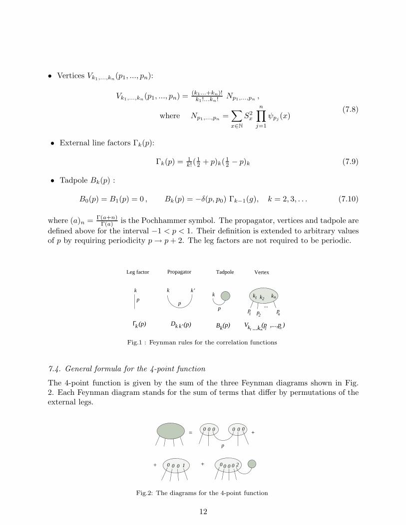
• Vertices Vk1,...,kn(p1, ..., pn):

Vk1,...,kn(p1, ..., pn) = (k1...+kn)!

k1!...kn! Np1,...,pn,

where Np1,...,pn=∑

x∈N

S2x

n∏

j=1

ψpj(x)

(7.8)

• External line factors Γk(p):

Γk(p) = 1k!(

12 + p)k( 1

2 − p)k (7.9)

• Tadpole Bk(p) :

B0(p) = B1(p) = 0 , Bk(p) = −δ(p, p0) Γk−1(g), k = 2, 3, . . . (7.10)

where (a)n = Γ(a+n)Γ(a) is the Pochhammer symbol. The propagator, vertices and tadpole are

defined above for the interval −1 < p < 1. Their definition is extended to arbitrary valuesof p by requiring periodicity p→ p+ 2. The leg factors are not required to be periodic.

Tadpole

Leg factor Propagator Vertex

p p p

k k21 kn

...

1 2 n

p

k

p

k

Γk Dk k’ Bk Vk ...k (p ,...,p )1 nn 1

p

k k’

(p) (p) (p)

Fig.1 : Feynman rules for the correlation functions

7.4. General formula for the 4-point function

The 4-point function is given by the sum of the three Feynman diagrams shown in Fig.2. Each Feynman diagram stands for the sum of terms that differ by permutations of theexternal legs.

+ +0 0 0 2000 01

00 0 0 0=

p

+0

Fig.2: The diagrams for the 4-point function

12

The corresponding analytic expression is

G(p1, p2, p3, p4) =

∫ 1

−1

dp [Γ0(p1)Γ0(p2)Np1p2pD00(p)N−pp3p4Γ0(p3)Γ0(p4) + permutations]

+[

Γ0(p1)Γ0(p2)Γ0(p3)Γ1(p4) + permutations]

Np1p2p3p4

+B2(p0)Γ0(p1)Γ0(p2)Γ0(p3)Γ0(p4)Np0p1p2p3p4

(7.11)Then, using (7.9)-(7.7) we rewrite (7.11) as

G(p1, p2, p3, p4) =[

(1 ± p0)2 − 1

4 +

4∑

s=1

(

14 − p2

s

)

]

Np1,p2,p3,p4

+

∫ 1

−1

dp (Np1,p2,pN−p,p3,p4+Np1,p3,pN−p,p2,p4

+Np1,p4,pN−p,p2,p3)(

|p| − 12

) (

|p| − 32

)

(7.12)This formula is valid for both height models, SOS and SRSOS; in the second case theintegration runs over half of the interval. It is true also for the ADE rational stringtheories, if the integral over p is replaced by the corresponding discrete sum. In the caseof degenerate fields we consider the order operators (7.6) with p = mp0, m = 1, 2, 3, . . .The integral in (7.12) is replaced by a summation over the positive integers. In the 3-point multiplicity in (7.7) the summation is replaced by an integral, xp0 ∈ [0, 2], i.e.,the multiplicity is given by the standard integral representation of (5.2). Returning to thenormalizations and notation used in the worldsheet theory, Pi = εibpi = εimibp0 , e0 = bp0,we recover precisely the 4-point formula (6.3).

Acknowledgments

We thank Al. Zamolodchikov for several valuable discussions and for communicating to us preliminary

drafts of his forthcoming paper [8]. We also thank A. Belavin, Vl. Dotsenko, V. Schomerus and J.-B. Zuber

for the interest in this work and for useful comments. This research is supported by the European TMR

Network EUCLID, contract HPRN-CT-2002-00325, and by the Bulgarian National Council for Scientific

Research, grant F-1205/02. I.K.K. thanks the Institute for Advanced Study, Princeton, and the Rutgers

University for their kind hospitality during part of this work. V.B.P. acknowledges the hospitality of

Service de Physique Theorique, CEA-Saclay.

13

References

[1] E. Witten, Nucl. Phys. B 373 (1992) 187, hep-th/9108004.

[2] N. Seiberg and D. Shih, JHEP 0402 (2004) 021, hep-th/0312170.

[3] D. Kutasov, E. Martinec and N. Seiberg, Phys. Lett. B 276 (1992) 437, hep-

th/9111048.

[4] M. Bershadsky and D. Kutasov, Nucl. Phys. B 382 (1992) 213, hep-th/9204049.

[5] S. Kachru, Mod. Phys. Lett. A7 (1992) 1419, hep-th/9201072.

[6] I.K. Kostov, Nucl. Phys. B 689 (2004) 3, hep-th/0312301.

[7] I.K. Kostov and V.B. Petkova, Non-Rational 2D Quantum gravity: Ground Ring ver-

sus Loop Gas, in preparation.

[8] Al.B. Zamolodchikov, On the Three-point Function in Minimal Liouville Gravity, hep-

th/0505063.

[9] I.K. Kostov, Nucl. Phys. B326 (1989) 583.

[10] I.K. Kostov, Nucl. Phys. B 376 (1992) 539, hep-th/9112059.

[11] I.K. Kostov and M. Staudacher, Phys. Lett. B 305 (1993) 43, hep-th/9208042.

[12] S. Higuchi and I.K. Kostov, Phys. Lett. B 357 (1995) 62, hep-th/9506022.

[13] F. David, Mod. Phys. Lett. A3 (1988) 1651.

[14] J. Distler and H. Kawai, Nucl. Phys. B 321 (1989) 509.

[15] H. Dorn and H.J. Otto: Nucl. Phys. B 429 (1994) 375, hep-th/9403141.

[16] A.B. Zamolodchikov and Al.B. Zamolodchikov, Nucl. Phys. B 477 (1996) 577, hep-

th/9506136.

[17] J. Teschner, Phys. Lett. B 363 (1995) 65, hep-th/9507109.

[18] Vl.S. Dotsenko and V.A. Fateev, Nucl. Phys. B 251 [FS13] (1985) 691.

[19] P. Di Francesco and D. Kutasov, Nucl. Phys. B 375 (1992) 119, hep-th/9109005.

[20] B. Nienhuis, “Coulomb gas formulation of 2-d phase transitions”, in Phase transitions

and critical phenomena, Vol. 11, ed. C.C. Domb and J.L. Lebowitz (Academic Press,

New York, 1987), ch.1.

[21] G. E. Andrews, R. J. Baxter and P. J. Forrester, J. Stat. Phys. 35 (1984) 193.

[22] V. Pasquier, Nucl. Phys. B 285 (1987) 162.

[23] O. Foda and B. Nienhuis, Nucl. Phys. B 324 (1989) 643.

[24] I.K. Kostov, B. Ponsot and D. Serban, Nucl. Phys. B 683 (2004) 309, hep-th/0307189.

[25] V.A. Kazakov and I.K. Kostov, Nucl. Phys. B 386 (1992) 520, hep-th/9205059.

14