Embed Size (px)
Citation preview

Ba
Ya
b
c
d
a
ARRA
KLTBP
I
oLwuitTEpwaCes
oR
h0
Land Use Policy 42 (2015) 381–391
Contents lists available at ScienceDirect
Land Use Policy
j o ur na l ho me page: www.elsev ier .com/ locate / landusepol
us stop, property price and land value tax: A multilevel hedonicnalysis with quantile calibration
iming Wanga,∗, Dimitris Potogloub,c, Scott Orfordb, Yi Gongd
The Bartlett School of Construction and Project Management, The Bartlett Faculty of Built Environment, University College London, London WC1E 7HB, UKSchool of Planning and Geography, Cardiff University, King Edward VII Avenue, Cardiff CF10 3WA, UKRAND Europe, Westbrook Centre, Milton Road, Cambridge CB4 1YG, UKSustainable Places Research Institute, Cardiff University, 33 Park Place, Cardiff CF10 3BA, UK
r t i c l e i n f o
rticle history:eceived 20 October 2013eceived in revised form 30 May 2014ccepted 26 July 2014
eywords:and value tax
a b s t r a c t
Based on a multilevel and quantile hedonic analysis regarding the local public bus system and the pricesof residential properties in Cardiff, Wales, we find strong evidence to support two research hypotheses:(a) the number of bus stops within walking distance (300–1500 m) to a property is positively associatedwith the property’s observed sale price, and (b) properties of higher market prices, compared with theircheaper counterparts, tend to benefit more from spatial proximity to the bus stop locations. Given thesestatistical findings, we argue that, land value tax (LVT), albeit a classic political idea dating back to the early
ransport infrastructureus stoproperty price
20th century, does have contemporary relevance and, with modern geographic information technologies,can be rigorously analysed and empirically justified with a view to actual implementation. Levying LVTwill not only generate additional fiscal revenues to help finance the development and maintenance oflocal public infrastructures, but will also ensure a more just distribution of the economic welfare yieldedby public investment.
© 2014 Elsevier Ltd. All rights reserved.
ntroduction
In recent years, the United Kingdom (UK) has witnessed a revivalf public interests in land value tax (LVT).1 The original idea ofVT dates back to George (1879), an American political economist,ho, partly inspired by Smith (1863), posits that the value of land,ltimately, comes from the adjacent infrastructures and amenities
nvested by the whole community. Increments in land value dueo public investment, thus, ought to be re-captured through LVT.he earliest political attempts to legislate LVT took place in the latedwardian Britain (Short, 1997, Chapter 2). LVT was officially pro-osed in the 1909 finance bill (also known as “People’s Budget”),hen David Lloyd George served as Chancellor of the Exchequer
s a member of the governing Liberal party. However, the then
onservatives-dominated House of Lords, though passing the gen-ral budget in 1910, managed to veto the LVT proposal. A similartory happened later with the 1931 Finance Act, which contained∗ Corresponding author. +44 02076791890.E-mail address: [email protected] (Y. Wang).
1 For the examples of Labour’s Land Value Campaign (http://www.labourland.rg/) and the Liberal Democratic Party’s Action for Land Taxation and Economiceform (http://libdemsalter.org.uk/).
ttp://dx.doi.org/10.1016/j.landusepol.2014.07.017264-8377/© 2014 Elsevier Ltd. All rights reserved.
a LVT initiative passed by the ruling Labour party but was rejectedagain by the Tory government in 1934 (Wenzer, 2000). One of thelatest efforts to seek legislation of LVT was in 2012 by Carolyn Lucas,a Green party member of the UK parliament (The UK Parliament,2012).
Although LVT was never implemented in Britain, its traces canbe observed in many other places around the world, such as in thecities of Pittsburgh and Harrisburg in the American State of Penn-sylvania and a number of countries such as Australia, Denmark,Estonia, Russia, and New Zealand (Andelson, 2000; Bourassa, 1990;Dye and England, 2010; Wyatt, 1994). While the actual policypractice varies among these international cases, LVT has beenincreasingly justified as a way to finance the construction andmaintenance of public transport infrastructures. The basic rationaleremains quite the same as per George original (1879), that publiclyinvested transport network can promote the values of nearby pri-vately owned land plots, given their improved accessibility. Froma political economy perspective, this part of added land value, ifsubstantiated, becomes a kind of positive externalities which canbe offset or captured through LVT. Otherwise, general tax payers
(who generate government revenues) are essentially subsidisinglandowners who “quietly” extract the values of public transportinfrastructures. Making this free-ride problem even more press-ing is the undersupply and underfunding of public transport in the
3 se Poli
pid
ttecifvw1Cs1p2mstbLasvbwo£mTw
srpoosm“ast
L
T
ttaTatic
wp2qt
82 Y. Wang et al. / Land U
resent-day UK, which has resulted in a series of social exclusionssues, faced typically by the lower income population who haveifficulties affording private transport (Lucas, 2006).
In this paper, we explore the viability of levying land valueax to finance the maintenance and development of local publicransport infrastructures within a contemporary UK context. Ourmpirical study focuses on the public bus system owned by Cardiffity council in south Wales, which saw a £0.6 million funding cutn the financial year of 2012, leading to a second increase in busares since October 2011 (Wales Online, 2012). Employing a con-entional ordinary least square (OLS) hedonic regression approach,e firstly examine the relations between the sale prices of circa
0,000 residential properties across 12 electoral wards in centralardiff from 2000 to 2009 (see Fig. 2), and the number of bustops within the radii of 300 m, 400 m, 500 m, 750 m, 1000 m and500 m of each property, based on the 2007 National Public Trans-ort Access Nodes (NaPTAN) dataset (Department for Transport,007). We then further refine the OLS results, respectively, within aultilevel modelling (Jones and Bullen, 1994) and quantile regres-
ion framework (Koenker, 2005). Our multilevel analysis suggestshe OLS estimates to be unbiased with respect to the influence ofus stop locations on the implicit land values of nearby properties.ikewise, our quantile bivariate post hoc tests confirm the over-ll robustness of the OLS outcomes. A policy implication of thesetatistical findings is to exercise a two-tier progressive local landalue taxation scheme in helping Cardiff council finance the localus system. Our estimation, based on the number of bus stopsithin a 1500 m radius of every individual property included in
ur sample data, suggests that, for a property priced below circa195,000, every additional bus stop contributes to a circa 0.11%arginal increase in property price through land value betterment.
he corresponding figure is 0.22% for a property in the second tierith a market price above £195,000.
The remainder of this paper is organised as follows. The nextection “Land value tax: from Edwardian to contemporary Britain”eviews the literature on land value tax and the related planningractices, mainly within a UK context. This is followed by the designf this research in “Research design” section, which studies the casef Cardiff Bus, by following an OLS and multilevel hedonic regres-ion approach supplemented by a quantile calibration. The data andodel results are reported in sections “The case of Cardiff bus” and
Model results”, respectively, before the study’s policy implicationsre discussed in “Policy implications” section. The conclusions areummarised in “Conclusion and future research” section, alongsidehe directions of future research.
and value tax: from Edwardian to contemporary Britain
he Edwardians
The latest global economic recession has forced many countrieso cut public spending. This is particularly the case in the UK, withhe coalition government aiming to reduce public expenditure bys much as £6.2 billion between 2010 and 2011 (Her Majesty’sreasury, 2010). Since budgetary stringency continued into 2012nd 2013, public finance has become a top challenge confrontinghe Westminster parliament, which is seeking new sources of taxncome, for example, by proposing a further rise in value-addedonsumption tax (VAT) from 20% to 25% (The Telegraph, 2012).
A century ago, the Edwardian politicians were similarly facedith a public finance challenge to fund the emerging welfare state
rogrammes, including an embryonic pension scheme (Hattersley,004). David Lloyd George, during his Chancellorship of the Exche-uer as a member of the governing Liberal party, proposed toax on tobaccos, luxurious goods, and most important of all,cy 42 (2015) 381–391
land, in the 1909 finance bill. These taxation measures were notonly intended to balance the government budget, but also totackle widespread political and economic inequalities faced bythe British society. Given its populist flavour, the 1909 budgetwas often called People’s Budget (Short, 1997). However, the thenConservatives-dominated House of Lords, though reluctantly pass-ing many initiatives included in People’s Budget one year later in1910, managed to veto the land value tax (LVT) proposal.
The original idea of LVT actually came from the other side of theAtlantic. George (1879), an American political economist born inPhiladelphia, Pennsylvania, once wrote:
“The tax upon land values is, therefore, the most just and equalof all taxes. It falls only upon those who receive from society apeculiar and valuable benefit, and upon them in proportion tothe benefit they receive. It is the taking by the community, forthe use of the community, of that value which is the creation ofthe community.” (George, 1879, Chapter 33)
George’s central tenet is that the value of land, ultimately, comesfrom the adjacent infrastructures and amenities invested by thelocal community. Increments in land value due to public invest-ment therefore ought to be re-captured through LVT. This argumentresonates with the ground rent theories by Smith (1863), Ricardo(1891), and even Marx (1867). The tax on land value can also beconsidered a kind of Pigovian (1920) tax, if one sees the added landvalue accruing from the positive externalities yielded by commu-nity investment (Petrella, 1988).
The Contemporaries
The Pigovian aspect of LVT is perhaps best featured in its con-temporary practice, as LVT has been more and more exercisedas a way to support the financing of public transport infras-tructures (Ryan, 1999; Rybeck, 2004; Smith and Gihring, 2006;Al-Mosaind et al., 1993; Bollinger and Ihlanfeldt, 1997; Bowes andIhlanfeldt, 2001; Debrezion et al., 2007, 2011; Hess and Almeida,2007). Underpinning this policy practice is a theoretical conjec-ture that publicly invested transport facilities adds significantvalues to the nearby privately owned land plots by improvingtheir spatial accessibilities to the transport network. This kind ofpublic-investment-triggered private land value betterment is a typ-ical instance of positive externalities that could be offset throughproper government intervention (Pigou, 1920).
Nonetheless, land value taxation remains unimplementedwithin the UK, even though some closely associated fiscal interven-tions do exist in the British town planning practice. For example,section (106) of the 1990 Town and Country Planning Act allowslocal planning authorities to charge developers, on a case-by-case basis and often by negotiation, a so-called section (106)payment to compensate for the potential negative externalities(e.g., congestion and crowdedness) of new development on thelocal community (The UK Parliament, 1990). Later, the BarkerReview of Land Use Planning (2006) was largely critical of sec-tion (106) for its vagueness in concept and inconsistencies inpractice. The community Infrastructure levy (CIL) was introducedin the 2008 Planning Act to partially replace section (106) (The UKParliament, 2008).
Like land value tax, section (106) and CIL are both public finan-cial measures intended for externalities, hence Pigovian by nature.However, LVT differs from section (106) and CIL in being a bet-terment tax, which tries to capture the positive externalities ofcommunity investment in local public infrastructures (Lee et al.,
2013). By comparison, the two types of planning charges areemployed to compensate for the potential negative externalitiesof new property developments with respect to the local housingand infrastructure capacities. They are thus essentially the same
se Poli
ta
peastaitrcai
R
R
aeewti
trtrpritLto
tattileat
A
sRsa(hd
ts
inherent feature of the UK local real estate industry and therefore
Y. Wang et al. / Land U
hing as what is called “impact fee” in the US (see, e.g., Ihlanfeldtnd Shaughnessy, 2004).
Given the subtle and yet important difference between LVT andlanning charges, it perhaps makes more sense to look at LVT in ref-rence to the existing UK taxation system.2 For example, Maxwellnd Vigor (2005) suggest substituting LVT for council tax and thetamp duty. They argue that LVT is a levy on land, while bothhe stamp duty and council tax are estimated by property valuend are a property tax. Taxing on property instead of land valuenvolves disincentives for homeowners to maintain and improveheir housing conditions – the more they invest in maintenance andenovation, the more property tax liable. This perspective resonateslosely with Bourassa’s (1990, 1992) earlier empirical studies about
similar topic within the US context, which identified a significantncentive effect of LVT vis-à-vis property taxation.
esearch design
esearch question
Levying land-value tax involves both substantial political as wells technical complexities and constitutes a radical reform to thexisting UK public finance regime. Our research focuses more on thempirical and technical aspects of the issue, aiming to explore theays to assess local public infrastructures’ potential contribution
o the adjacent land values and to address the according policymplications.
While the word “infrastructure” connotes a variety of facili-ies (usually of physical presence), this paper concentrates on theelationship between land values and public transport infrastruc-ure in the UK. This is because of the general consensus nowadaysegarding the ubiquitous and intimate interactions between trans-ort and land use activities (Geurs and van Wee, 2004). Anothereason is that land value taxation, in recent decades, has beenncreasingly rationalised as a value capture mechanism to financehe development and maintenance of public transport facilities.ast, given the current economic climate, public transport infras-ructures in the UK are typically short of funding and thus in needf strengthened fiscal support (Lucas, 2006).
Our specific research question centres on how to assess the spa-ial relationships between the local public transport infrastructuresnd the land values of nearby residential properties. A concep-ual issue is that housing sub-markets are a salient feature ofhe British local real estate sector (Orford, 2000). A correspond-ng methodological framework needs to be in place to capture theatent heterogeneities with regard to the characteristics of differ-nt neighbourhood environments, divergent property price levels,nd the varying relations between their implicit land values andhe nearness to public transport locations.
hedonic approach
Given our research question, we employ a hedonic regres-ion approach as the basic modelling method in this study. Whileosen’s (1974) seminal theoretical paper recommended a two-tage regression procedure, for this policy-oriented paper, we adopt
reduced-form version of the Rosen original and, as shown in Eq.
1), assume a linear semi-log function form in the first stage ofedonic regression, which allows us to simplify the second stage byirectly valuing the bus stop locations based on the corresponding2 Actually, land value tax (LVT) is also often called single tax, because accordingo Henry George, the collection of LVT should replace any other taxation schemes,uch as those on incomes and consumptions.
cy 42 (2015) 381–391 383
coefficient estimates (see a similar application, for example, byHeikkila et al. (1989), p. 223):
log(p) = F(H, Y, W, L, ε) (1)
where p denotes the property’s sale price, of which the natural logis a function of H, Y, W and L, plus an error term, ε. H stands for aset of hedonic control variables, each of which corresponds to anattribute of the observed property, in terms of whether it is freehold(r), newly built (n), detached (d), semi-detached (s), or terraced (t),floor area (f), and how far the property is located from the centralbusiness district (z). H may be specified as Eq. (2):
H = {r, n, d, s, t, f, z} (2)
Y represents another set of dummy-coded variables capturingthe year in which an observed sale transaction took place. This isintended to adjust for temporal effects, such as short term property-price inflation in the local market, with X denoting the total numberof years under observation. If the first year is noted as year 0, wehave Eq. (3):
Y = {Yu|u = 0, 1, 2, . . ., X − 1} (3)
W consists of a series of dummy-coded variables, each indicat-ing a local jurisdiction within which a property is located. Thesevariables capture average local environmental effects related toeducational and recreational amenities as well as the overall rep-utation of the area. Assuming a total of M jurisdictions within thestudy area, one of which is denoted as a reference jurisdiction, W0,we may define W as follows:
W = {Wv|v = 0, 1, 2, . . ., M − 1} (4)
It should be noted that the model specification as per Eqs. (4) and(5) may be considered following a ‘discrete-space expansion’ pro-cess (Jones and Bullen, 1994, p. 254), whereby the constant term ofa regression equation is expanded into the (X − 1) + (M − 1) dummyvariables.
L = {ı} (5)
L in Eq. (5) represents a set of target variables, which relate directlyto the location of land beneath a property. These variables aresupposed to measure spatial accessibility and proximity to pub-lic transport infrastructure. We assume in this paper that L consistsof only one element ı. ı in Eq. (5) measures the aggregate numberof public transport nodes (e.g., train stations, bus stops, airport ter-minals) within a buffer or catchment area of an observed propertylocation.3
Finally, a couple of standard econometric assumptions are asso-ciated with the error term, ε. First, we assume independence orzero autocorrelation in the observed values of ε. Nevertheless, datacollected in the real world are likely to suffer from spatial as wellas temporal autocorrelation, depending on how the collection isconducted. Second, we assume a single constant variance in theerror term or non-heteroskedasticity. However, this assumption isalso subject to post hoc test, given that housing sub-markets are an
the possibility of spatial heterogeneity in implicit prices betweensub-markets.
3 It needs to be acknowledged that recent years have seen some highly sophis-ticated accessibility measures (e.g., Ferrari et al., 2012). While these innovativemeasures are not the central topic of this paper, they can be very useful for futureresearch.
3 se Poli
M
ecgimttfi(
ˇ
ˇeaeaodw
aa(iyipfiafvm
Q
Kmvtcv2
t(otmltrti
l
wde
d
84 Y. Wang et al. / Land U
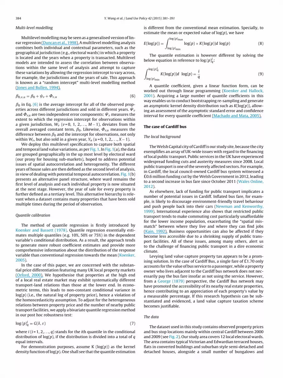
ulti-level modelling
Multilevel modelling may be seen as a generalised version of lin-ar regression (Duncan et al., 1998). A multilevel modelling analysisombines both individual and contextual parameters, such as theeographical jurisdiction (e.g., electoral wards) in which a propertys located and the years when a property is transacted. Multilevel
odels are intended to assess the correlation between observa-ions within the same level of analysis and attempt to capturehese variations by allowing the regression intercept to vary across,or example, the jurisdictions and the years of sale. This approachs known as a “random intercept” multi-level modelling methodJones and Bullen, 1994).
0,v,u = ˇ0 + v + ˚v,u (6)
0 in Eq. (6) is the average intercept for all of the observed prop-rties across different jurisdictions and sold in different years. � vnd ˚v,u are two independent error components: � v measures thextent to which the regression intercept for observations within
given jurisdiction, Wv (v = 0, 1, 2,. . ., M − 1), deviates from theverall averaged constant term, ˇ0. Likewise, ˚v,u measures theifference between ˇ0 and the intercept for observations, not onlyithin Wv, but also sold in a given year, Yu (u = 0, 1, 2,. . ., X − 1).
We deploy this multilevel specification to capture both spatialnd temporal land value variations, as per Fig. 1. In Fig. 1(a), the datare grouped geographically in the up most level by electoral wardour proxy for housing sub-markets), hoped to address potentialssues of spatial autocorrelation and heterogeneity. The differentears of house sales are then defined as the second level of analysis,n view of dealing with potential temporal autocorrelation. Fig. 1(b)resents an alternative panel structure, where ward remains therst level of analysis and each individual property is now situatedt the next stage. However, the year of sale for every property isurther defined as a tertiary level. This alternative hierarchy is rele-ant when a dataset contains many properties that have been soldultiple times during the period of observation.
uantile calibration
The method of quantile regression is firstly introduced byoenker and Bassett (1978). Quantile regression essentially esti-ates multiple quantiles (e.g. 10%, 50% or 75%) in the dependent
ariable’s conditional distribution. As a result, the approach tendso generate more robust coefficient estimates and provide moreomprehensive information about the distribution of the responseariable than conventional regression towards the mean (Koenker,005).
In the case of this paper, we are concerned with the substan-ial price differentiation featuring many UK local property marketsOrford, 2000). We hypothesise that properties at the high endf a local real estate market may exhibit systematically differentransport-land relations than those at the lower end. In econo-
etric terms, this leads to non-constant conditional variance inog(p) (i.e., the natural log of property price), hence a violation ofhe homoscedasticity assumption. To adjust for the heterogeneouselations between property price and the number of nearby publicransport facilities, we apply a bivariate quantile regression methodn our post hoc robustness test:
og (p)iq = G(ı, ε) (7)
here i (i = 1, 2,. . ., q) stands for the ith quantile in the conditional
istribution of log(p), if the distribution is divided into a total of qqual intervals.For demonstration purposes, assume K (log(p)) as the kernelensity function of log(p). One shall see that the quantile estimation
cy 42 (2015) 381–391
is different from the conventional mean estimation. Specially, toestimate the mean or expected value of log(p), we have
E(log(p)) =∫ log (p)max
log (p)min
log(p) × K(log(p))d log(p) (8)
The quantile estimation is however different by solving thebelow equation in reference to log (p)iq:
∫ log (p)iq
log (p)min
K(log(p))d log(p) = i
q(9)
A quantile coefficient, given a linear function form, can beworked out through linear programming (Koenker and Hallock,2001). Acquiring a large number of quantile coefficients in thisway enables us to conduct bootstrapping re-sampling and generatean asymptotic kernel density distribution such as K(log(p)), allow-ing an assessment of the asymptotic standard error and confidenceinterval for every quantile coefficient (Machado and Mata, 2005).
The case of Cardiff bus
The local background
The Welsh Capital city of Cardiff is our study site, because the cityexemplifies an array of UK-wide issues with regard to the financingof local public transport. Public services in the UK have experiencedwidespread funding cuts and austerity measures since 2008. Localpublic transport is one of the severely affected sectors. For example,in Cardiff, the local council-owned Cardiff bus system witnessed a£0.6 million funding cut by the Welsh Government in 2012, leadingto a second increase in bus fare since October 2011 (Wales Online,2012).
As elsewhere, lack of funding for public transport implicates anumber of potential issues in Cardiff. Inflated bus fare, for exam-ple, is likely to discourage environment-friendly travel behaviourand push people back into their cars (Newman and Kenworthy,1999). International experience also shows that restricted publictransport tends to make commuting cost particularly unaffordablefor the lower income population, exacerbating the “spatial mis-match” between where they live and where they can find jobs(Kain, 1992). Business opportunities can also be affected if theybecome less accessible due to a shrinking supply of public trans-port facilities. All of these issues, among many others, alert usto the challenge of financing public transport in a dire economicclimate.
Levying land value capture property tax appears to be a prom-ising solution. In the case of Cardiff Bus, a single fare of £1.70 onlyaccounts for the value of bus service to a passenger, while a propertyowner who lives adjacent to the Cardiff bus network does not nec-essarily pay the bus fare insofar as not using the service. However,from a George (1879) perspective, the Cardiff Bus network mayhave promoted the accessibility of its nearby real estate properties,hence contributing to an appreciation of each property’s value bya measurable percentage. If this research hypothesis can be sub-stantiated and evidenced, a land value capture taxation schemebecomes justifiable.
The data
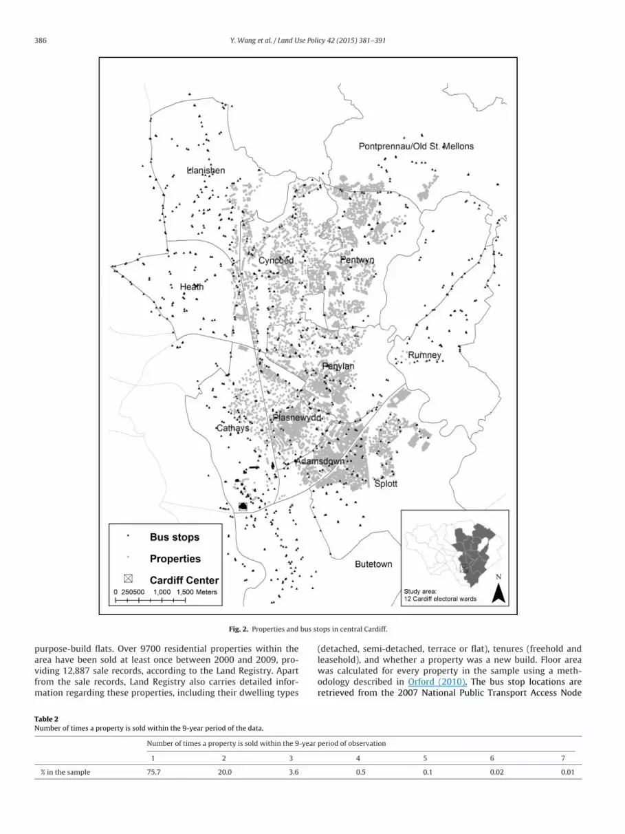
The dataset used in this study contains observed property pricesand bus stop locations mainly within central Cardiff between 2000
and 2009 (see Fig. 2). Our study area covers 12 local electoral wards.The area contains typical Victorian and Edwardian terraced houses,flats in converted buildings and suburban style semi-detached anddetached houses, alongside a small number of bungalows and
Y. Wang et al. / Land Use Policy 42 (2015) 381–391 385
Fig. 1. Cross-sectional (a) vs multilevel panel; (b) structures for property data analysis.Notes: adapted from Duncan et al. (1998).
Table 1Definition of variables and descriptive statistics.
Continuous variables Definition Mean St.dev.
p Property sale price in British pound sterling (£) 143922 87264log(p) Natural logarithm of price of the property when sold 11.725 0.5ı300 m Number of bus-stops within 300 metres (m) off the property 7.4 3.7ı400 m Number of bus-stops within 400 metres (m) off the property 13.3 5.3ı500 m Number of bus-stops within 500 metres (m) off the property 20.7 7.4ı750 m Number of bus-stops within 750 metres (m) off the property 45.2 14.8ı1000 m Number of bus-stops within 1000 metres (m) off the property 77.7 24.4ı1500 m Number of bus-stops within 1500 metres (m) off the property 167.7 57.5F Floor area of a property in square metres (m2) 105.2 48.9Z Distance to the central business district in metres (m) 3225.3 1408.7
Categorical variables Definition Proportion
r 1 if property is on freehold tenure, 0 otherwise 89.7%n 1, if property is newly built when sold, 0 otherwise 3.8%Property type
Flat as a the reference category 4.1%d 1, if property is a detached house, 0 otherwise 12.0%s 1, if property is a semi-detached house, 0 otherwise 25.6%t 1, if property is a terraced house, 0 otherwise 58.3%
YearY0 1, if property was sold in 2000, 0 otherwise (reference category) 11.2%Y1 1, if property was sold in 2001, 0 otherwise 13.4%Y2 1, if property was sold in 2002, 0 otherwise 14.5%Y3 1, if property was sold in 2003, 0 otherwise 12.6%Y4 1, if property was sold in 2004, 0 otherwise 12.3%Y5 1, if property was sold in 2005, 0 otherwise 9.6%Y6 1, if property was sold in 2006, 0 otherwise 12.9%Y7 1, if property was sold in 2007, 0 otherwise 12.4%Y8 1, if property was sold in 2008, 0 otherwise 1.1%
WardW0 1, if a property is located in Cyncoed (reference category) 11.5%W1 1, if property is located in Adamsdown or Butetown, 0 otherwise 12.1%W2 1, if property is located in Cathays, 0 otherwise 2.4%W3 1, if property is located in Heath, 0 otherwise 1.6%W4 1, if property is located in Llanishen, 0 otherwise 1.3%W5 1, if property is located in Splott or Rumney, 0 otherwise 23.1%W6 1, if property is located in Penylan, 0 otherwise 15.0%W7 1, if property is located in Pentwyn, 0 otherwise 17.6%W8 1, if property is located in Plasnewydd, 0 otherwise 13.9%W9 1, if property is located in Pontprennau, 0 otherwise 1.5%
386 Y. Wang et al. / Land Use Policy 42 (2015) 381–391
bus st
pavfm
TN
Fig. 2. Properties and
urpose-build flats. Over 9700 residential properties within therea have been sold at least once between 2000 and 2009, pro-
iding 12,887 sale records, according to the Land Registry. Apartrom the sale records, Land Registry also carries detailed infor-ation regarding these properties, including their dwelling types
able 2umber of times a property is sold within the 9-year period of the data.
Number of times a property is sold within the 9-year
1 2 3
% in the sample 75.7 20.0 3.6
ops in central Cardiff.
(detached, semi-detached, terrace or flat), tenures (freehold andleasehold), and whether a property was a new build. Floor area
was calculated for every property in the sample using a meth-odology described in Orford (2010). The bus stop locations areretrieved from the 2007 National Public Transport Access Nodeperiod of observation
4 5 6 7
0.5 0.1 0.02 0.01

Y. W
ang et
al. /
Land U
se Policy
42 (2015)
381–391
387
Table 3Results of ordinary least squares, log(p) as dependent variable.
Model 1 Model 2 Model 3 Model 4 Model 5 Model 6Within 300 m Within 400 m Within 500 m Within 750 m Within 1000 m Within 1500 m
ˇ s.e. ˇ s.e. ˇ s.e. ˇ s.e. ˇ s.e. ˇ s.e.
Constant 10.506*** 0.025 10.479*** 0.027 10.438*** 0.028 10.417*** 0.034 10.343*** 0.039 10.269*** 0.048Freehold (r) 0.120*** 0.009 0.121*** 0.009 0.123*** 0.009 0.126*** 0.009 0.127*** 0.009 0.125*** 0.009New-built (n) 0.228*** 0.013 0.230*** 0.013 0.232*** 0.013 0.230*** 0.013 0.237*** 0.013 0.217*** 0.013Detached (d) 0.651*** 0.016 0.654*** 0.016 0.654*** 0.016 0.647*** 0.016 0.644*** 0.016 0.645*** 0.016Semi-detached (s) 0.468*** 0.014 0.471*** 0.014 0.469*** 0.014 0.465*** 0.014 0.464*** 0.014 0.465*** 0.015Terraced (t) 0.360*** 0.014 0.361*** 0.014 0.359*** 0.014 0.356*** 0.014 0.354*** 0.014 0.357*** 0.014Floor area (f) 0.004*** 0.000 0.004*** 0.000 0.004*** 0.000 0.004*** 0.000 0.004*** 0.000 0.004*** 0.000Distance to CBD (z) 0.035*** 0.004 0.038*** 0.004 0.042*** 0.004 0.046*** 0.005 0.055*** 0.005 0.066*** 0.007Sale in 2001 (Y1) 0.112*** 0.009 0.110*** 0.009 0.111*** 0.009 0.112*** 0.009 0.113*** 0.009 0.110*** 0.009Sale in 2002 (Y2) 0.301*** 0.009 0.297*** 0.009 0.297*** 0.009 0.297*** 0.009 0.299*** 0.009 0.295*** 0.009Sale in 2003 (Y3) 0.526*** 0.009 0.522*** 0.009 0.524*** 0.009 0.525*** 0.009 0.522*** 0.009 0.520*** 0.009Sale in 2004 (Y4) 0.694*** 0.009 0.693*** 0.009 0.693*** 0.009 0.694*** 0.009 0.693*** 0.009 0.691*** 0.009Sale in 2005 (Y5) 0.781*** 0.010 0.778*** 0.010 0.776*** 0.009 0.778*** 0.009 0.777*** 0.009 0.776*** 0.010Sale in 2006 (Y6) 0.791*** 0.009 0.789*** 0.009 0.789*** 0.009 0.791*** 0.009 0.791*** 0.009 0.789*** 0.009Sale in 2007 (Y7) 0.842*** 0.009 0.840*** 0.009 0.840*** 0.009 0.841*** 0.009 0.840*** 0.009 0.839*** 0.009Sale in 2008 (Y8) 0.858*** 0.023 0.857*** 0.023 0.861*** 0.022 0.860*** 0.022 0.861*** 0.022 0.861*** 0.022Adamstown (W1) −0.512*** 0.014 −0.508*** 0.014 −0.502*** 0.014 −0.499*** 0.014 −0.488*** 0.014 −0.465*** 0.015Splott (W2) −0.513*** 0.012 −0.507*** 0.012 −0.493*** 0.012 −0.486*** 0.013 −0.464*** 0.014 −0.430*** 0.017Cathays (W3) −0.196*** 0.020 −0.194*** 0.020 −0.186*** 0.020 −0.182*** 0.020 −0.164*** 0.020 −0.152*** 0.021Heath (W4) −0.142*** 0.019 −0.137*** 0.019 −0.139*** 0.019 −0.143*** 0.019 −0.146*** 0.019 −0.144*** 0.019Llanishen (W5) −0.240*** 0.024 −0.250*** 0.024 −0.257*** 0.024 −0.262*** 0.025 −0.269*** 0.025 −0.276*** 0.025Penylan (W6) −0.064*** 0.011 −0.064*** 0.011 −0.062*** 0.011 −0.051*** 0.011 −0.039*** 0.011 −0.018 0.013Pentwyn (W7) −0.648*** 0.010 −0.647*** 0.010 −0.643*** 0.010 −0.644*** 0.010 −0.638*** 0.010 −0.638*** 0.010Plasnewydd (W8) −0.235*** 0.014 −0.230*** 0.014 −0.225*** 0.014 −0.229*** 0.014 −0.229*** 0.014 −0.218*** 0.014Pontprennau (W9) −0.500*** 0.020 −0.502*** 0.020 −0.502*** 0.020 −0.506*** 0.020 −0.508*** 0.020 −0.505*** 0.020Number of bus stops (ı) 0.003*** 0.001 0.003*** 0.001 0.003*** 0.000 0.001*** 0.000 0.001*** 0.000 0.001*** 0.000Sample size 9655 9650 9656 9653 9659 9669R2 0.850 0.850 0.850 0.851 0.850 0.849F-test (df) 2176 (25) 2179 (25) 2185 (25) 2195 (25) 2186 (25) 2167 (25)p-Value 0.000 0.000 0.000 0.000 0.000 0.000
*p < 0.1; **p < 0.05.*** p < 0.001.

388 Y. Wang et al. / Land Use Policy 42 (2015) 381–391
Table 4Testing autocorrelation and homoscedasticity in OLS results.
Model 1 Model 2 Model 3 Model 4 Model 5 Model 6Within 300 m Within 400 m Within 500 m Within 750 m Within 1000 m Within 1500 m
Independence of εDurbin–Watson 1.773 1.777 1.779 1.779 1.779 1.776p-Value 0.000 0.000 0.000 0.000 0.000 0.000
Spatial autocorrelationMoran’s I 0.150 0.150 0.149 0.149 0.150 0.149Expected −0.0001 −0.0001 −0.0001 −0.0001 −0.0001 −0.0001Standard deviation 0.0004 0.0004 −0.0004 0.0004 0.0004 0.0004p-Value 0.000 0.000 0.000 0.000 0.000 0.000
reusch.533(.4651
(ar1oTps
M
O
rsioldalwoitstai
retrawtdbr
ccc
ieK
Homoscedasticity B�2(df) 0.233 (1) 0.101 (1) 0p-Value 0.6293 0.7512 0
NaPTAN-v2.2) dataset (Department for Transport, 2007). Thesere also shown in Fig. 2. The number of bus stops within specifiedadii of each property (i.e., 300 m, 400 m, 500 m, 750 m, 1000 m, and500 m) was calculated using ArcGIS. Table 1 presents a summaryf the variables included in the sample of properties in the dataset.able 2 also shows that this is broadly a cross-sectional rather thananel dataset, as more than 75% of the properties have only beenold once during the 9-year period.
odel results4
LS results
Table 3 presents the results of six ordinary least square (OLS)egressions based on the conventional hedonic approach pre-cribed in “A Hedonic Approach” section. The dependent variablen every regression is the natural logarithm of price (log(p)) and allf the six models attempt to capture the effect of Cardiff Bus onand value via ı, which measures the number of bus stops withinifferent walkable radii (i.e., 300 m, 400 m, 500 m, 750 m, 1000 m,nd 1500 m) around each property contained in the dataset. Fol-owing Belsley et al. (1980) a variety of regression diagnostic tests
ere performed on the OLS models in order to check whether anyf the regression assumptions had been violated. These includeddentifying outliers that may have a disproportionate influence onhe models, and removing the corresponding observations if neces-ary; checking for serious multi-collinearity in the models; testinghe normality of the error term; and checking for heteroscedasticitynd autocorrelation in the error term. The latter tests are discussedn more detail in a later section.
Model 1, for example, includes the explanatory variable withegard to the number of bus stops within 300 m around each prop-rty. The estimated parameter corresponding to this variable showshat the effect of Cardiff Bus on property price or, more accu-ately, on land value as reflected in property price, is positivend statistically significant at the 1% significance level. In otherords, the more bus stops there are around a property, the higher
he value of land beneath that property. Similar findings are alsoiscernible from the other regressions estimating the effect of num-er of bus stops within 400 m, 500, 750 m, 1000 m and 1500 m,espectively.
By back transforming the magnitude of the estimated coeffi-
ient with regard to the number of bus stops within 300 m, wean calculate the marginal increase in land value as a result of pla-ing every extra bus stop around a property. In percentage, this4 OLS results are estimated in IBM SPSS Statistics 20, while the multi-level analysiss conducted with MLWin v.3.20 (Rasbash et al., 2012). The quantile regression isxercised using an R/SPSS interface based on the original “quantreg” R codes byoenker (2007).
and Pagan (1979) test1) 0.887(1) 1.503(1) 0.612(1)
0.3461 0.2202 0.4341
added land value equals to (e0.003 − 1) × 100 ≈ 0.3%. Examination ofthe coefficients of the number of bus-stops within different bufferzones around property in Table 3 suggests that the effect of busstops within distance is relatively stable and statistically signifi-cant. The land value benefit of every additional bus stop within acircular catchment area larger than 500 m by radius is about 0.1%of the corresponding property price. The figure rises to 0.3% if thesize of catchment shrinks to 500 m or less by radius. Overall, allmodels show that the availability of public transport infrastructurecan significantly promote land value and thereby raise propertyprice.
The coefficient of z, the distance to Cardiff’s central businessdistrict (CBD), is also positive and statistically significant. Accord-ing to some studies, this finding is counter-intuitive and againstthe conventional wisdom about urban spatial structure. Per clas-sic urban economic theory (e.g., Anas et al., 1998), property pricesshould decline alongside increase in the properties’ distance to citycentre. However, previous studies have also provided several expla-nations for the positive influence of distance to CBD on propertyprice. For example, the assumption of a declining land value asdistance increases from CBD is based on the adoption of a mono-centric location choice model (Dubin and Sung, 1987), while Cardiffappears to be a rather polycentric city.
Floor area is also a positive and statistically significant factor interms of its impact on property price. The effect of floor space isconsistent across all six models presented in Table 3. Following aback transformation of the parameter with respect to floor space,we find that every additional square metre in a property increasesits value by (e0.004 − 1) × 100 ≈ 0.4%.
We capture mean spatial variation in property price by using aseries of dummy-coded variables representing the wards in whicheach property is located. The ward named Cyncoed is used as thereference category as it is the area with the highest average prop-erty price in the data set. All models show a significant difference inproperty price from Cyncoed, although the last regression (model6 in Table 3) indicates no significant difference in property pricebetween Cyncoed and Penylan.
All other coefficients have the expected signs and agree withconventional findings in the hedonic literature (Edmonds, 1984).For example, a property under a freehold tenure is likely to show ahigher price compared with a leasehold property. Similarly, a newlybuilt property tends to have more market value than an aged prop-erty. Detached properties exhibit the highest prices, followed bysemi-detached properties and flats, of which the latter is definedas the reference property type in this analysis. Finally, the dummyvariables with regard to price differences due to the calendar yearwhen a property was sold are all significantly different from zero.
The year of 2000 is used as the reference year, while the remainingcoefficients indicate a constant increase in property price over time,partly due to inflation in pound sterling and partly due to dynamicsin the local housing market.
se Policy 42 (2015) 381–391 389
M
mcpdtsapeccB
tsOt(aHsapdbeo
y(top5sTi
Q
Ahglvdl
ippstestcw
rg
lti-
leve
l mod
elli
ng,
log(
p)
as
dep
end
ent
vari
able
.
Mod
el
7
Mod
el
8
Mod
el
9
Mod
el
10
Mod
el
11
Mod
el
12W
ith
in
300
m
Wit
hin
400
m
Wit
hin
500
m
Wit
hin
750
m
Wit
hin
1000
m
Wit
hin
1500
m
ˇ0
s.e.
ˇ0
s.e.
ˇ0
s.e.
ˇ0
s.e.
ˇ0
s.e.
ˇ0
s.e.
10.7
35**
*0.
070
10.7
10**
*0.
071
10.6
71**
*0.
071
10.6
60**
*0.
073
10.5
90**
*0.
075
10.5
20**
*0.
079
)
0.11
6***
0.00
9
0.11
7***
0.00
9
0.11
9***
0.00
9
0.12
2***
0.00
9
0.12
3***
0.00
9
0.12
1***
0.00
9(n
)
0.22
1***
0.01
3
0.22
3***
0.01
3
0.22
4***
0.01
3
0.22
1***
0.01
3
0.22
6***
0.01
3
0.20
8***
0.01
3d)
0.65
9***
0.01
6
0.66
2***
0.01
6
0.66
3***
0.01
6
0.65
5***
0.01
6
0.65
3***
0.01
6
0.65
4***
0.01
6h
ed
(s)
0.47
6***
0.01
4
0.48
0***
0.01
4
0.47
8***
0.01
4
0.47
3***
0.01
4
0.47
2***
0.01
4
0.47
4***
0.01
4)
0.36
9***
0.01
4
0.37
1***
0.01
4 0.
370**
*0.
014
0.36
6***
0.01
4
0.36
4***
0.01
4
0.36
7***
0.01
4f)
0.00
4***
0.00
0
0.00
4***
0.00
0 0.
004**
*0.
000
0.00
4***
0.00
0
0.00
4***
0.00
0
0.00
4***
0.00
0
CB
D
(z)
0.03
5***
0.00
4
0.03
8***
0.00
4 0.
042**
*0.
004
0.04
5***
0.00
5
0.05
4***
0.00
5
0.06
5***
0.00
7
bus
stop
s
(ı)
0.00
3***
0.00
1
0.00
3***
0.00
1
0.00
3***
0.00
0
0.00
1***
0.00
0
0.00
1***
0.00
0
0.00
1***
0.00
00.
034**
0.02
0
0.03
3**0.
020
0.03
3**0.
020
0.03
3**0.
020
0.03
3**0.
020
0.03
3**0.
020
0.09
9***
0.01
6
0.09
9***
0.01
6
0.09
8***
0.01
6
0.09
9***
0.01
6
0.09
8***
0.01
6
0.09
9***
0.01
60.
044**
*0.
001
0.04
4***
0.00
1
0.04
3***
0.00
1
0.04
3***
0.00
1
0.04
4***
0.00
1
0.04
4***
0.00
1n
of
�2 ward
to
�2 property
0.19
2
0.18
8 0.
190
0.18
9
0.18
9
0.18
8n
of
�2 year
to
�2 property
0.55
9
0.56
3
0.56
3
0.56
6
0.56
0
0.56
3e
9655
9650
9656
9653
9659
9669
.
Y. Wang et al. / Land U
ultilevel results
As mentioned earlier, ordinary least square (OLS) regressionay involve potential issues related to spatial and temporal auto-
orrelations. In terms of spatial autocorrelation, the prices ofroperties within a same jurisdiction (i.e., electoral wards in ourata) are likely to be more similar than those outside. In terms ofemporal autocorrelation, properties sold within the same year mayhow a convergence in sale price vis-à-vis those transacted within
different year. To account for both the geographic as well as tem-oral autocorrelations, our OLS models would have to be expandedxtensively to accommodate (M − 1) × (X − 1) interaction factors. Inontrast, multilevel modelling analysis appears to be a more effi-ient alternative to address the issue of autocorrelation (Jones andullen, 1994).
Table 4 identifies a problem of autocorrelation underlying allhe six OLS models. The Durbin–Watson test suggests an overallignificant serial interdependence of the error terms (ε) in everyLS model. Because the Durbin–Watson result is more sensitive
o temporal autocorrelation, we further exercise a Moran’s I testAnselin, 1988), of which the estimates also confirm a presence of
significant albeit weak spatial autocorrelation (Moran’s I ≈ 0.15).owever, the Breusch and Pagan (1979) test for the whole model
uggests that heteroscedasticity is not a problem in the error termsnd they have constant variance. To address the autocorrelationroblem, six multilevel regressions (models 7–12) are further con-ucted. Since over 75% of the sampled properties are sold only onceetween 2000 and 2009, we estimate the multilevel models in ref-rence to the cross-sectional hierarchy shown in Fig. 1(a) insteadf the panel structure as per Fig. 1(b).
Table 5 illustrates the results of our multilevel modelling anal-sis. Both the ward-by-ward (�2
ward) and year-to-year variance
�2year) are statistically significant, confirming the OLS finding that
here are generalisable differences across wards and years in termsf property price. Around 19% of the aggregate variance in propertyrice (�2
property) can be attributed to �2ward
, compared with around6% to �2
year . Nevertheless, ı, which measures the impact of bustops on nearby land value, remains stable and is thus unbiased.his essentially confirms the robustness of the OLS estimates, evenn face of the identified spatial and temporal autocorrelations.
uantile results
Table 6 reports the results of our quantile bivariate regressions.s noted above, we conduct this quantile analysis mainly as a postoc calibration of the OLS estimates, in case price-based hetero-eneities lead to a biased coefficient measure of ı. We thus useog(p) as the dependent variable and ı as the only independentariable to gauge the number of bus stops within different walkableistances, from 300 m to 1500 m, around every observed property
ocation.Generally speaking, Table 6 indicates relatively weak and/or
nsignificant associations between the number of bus stops androperty prices at the 10% and 20% quantiles, where the observedroperty prices are below £74,000 in the dataset. In contrast, thetrongest and most significant correlations can be found for proper-ies at the 80% quantile, priced around £195,000. Those even morexpensive properties at the 90% quantile (i.e., £250.000), however,eem to benefit no more from the number of nearby bus stops thanhose at the 80% quantile, even though they tend to be better offompared with all properties below the 80% quantile, especially
hen we increase the search radius to more than 750 m.While confirming the overall robustness of OLS estimates withegard to the mean of ı, the results of our quantile analysis do sug-est ı to be systematically volatile across different price segments. Ta
ble
5R
esu
lts
of
mu
Con
stan
t
Free
hol
d
(rN
ew-b
uil
t
Det
ach
ed
(Se
mi-
det
acTe
rrac
ed
(tFl
oor
area
(D
ista
nce
toN
um
ber
of�
2 ward
�2 year
�2 property
Con
trib
uti
oC
ontr
ibu
tio
Sam
ple
siz
*
p
<
0.1.
**p
<
0.05
.**
*p
<
0.00
1

390 Y. Wang et al. / Land Use Policy 42 (2015) 381–391
Table 6Results of quantile bivariate regressions, log(p) as dependent variable and ı as independent variable.
Quantile ı300 m ı400 m ı500 m ı750 m ı1000 m ı750 m
s.e. s.e. s.e. s.e. s.e. s.e.
10% −0.004 0.003 0.001 0.002 0.007*** 0.002 0.004*** 0.001 0.002*** 0.000 0.001*** 0.00020% 0.004 0.003 0.003* 0.002 0.005*** 0.001 0.003*** 0.000 0.002*** 0.000 0.001*** 0.00030% 0.011*** 0.002 0.007*** 0.002 0.007*** 0.001 0.003*** 0.001 0.002*** 0.000 0.001*** 0.00040% 0.013*** 0.002 0.009*** 0.001 0.009*** 0.001 0.004*** 0.001 0.002*** 0.000 0.001*** 0.00050% 0.013*** 0.001 0.013*** 0.001 0.009*** 0.001 0.004*** 0.000 0.003*** 0.000 0.001*** 0.00060% 0.010*** 0.002 0.010*** 0.002 0.009*** 0.001 0.004*** 0.000 0.002*** 0.000 0.001*** 0.00070% 0.013*** 0.002 0.013*** 0.002 0.008*** 0.001 0.003*** 0.000 0.002*** 0.000 0.001*** 0.00080% 0.020*** 0.002 0.020*** 0.002 0.010*** 0.001 0.005*** 0.001 0.003*** 0.000 0.002*** 0.00090% 0.011*** 0.002 0.011*** 0.002 0.008*** 0.001 0.005*** 0.001 0.003*** 0.000 0.002*** 0.000
**
est1aTa
P
ffmpstgtBp
mnasatsatcadpba
adttmttlw
w
Acknowledgements
* p < 0.1.* p < 0.05.** p < 0.001.
Specifically, spatial proximity to Cardiff Bus stops tends to ben-fit properties at the high end of the local real estate market. Thetrongest positive externalities can be observed in properties abovehe 80% price quantile, with every additional bus stop within a500 m buffer zone, for example, contributing to an increase bybout 0.22% in property sale price through land value betterment.he corresponding figure for the cheaper properties is halved toround 0.11%.
olicy implications
The results of our regression analysis based on empirical datarom Cardiff have some important policy implications. First andoremost, the outcomes of our ordinary least square regression and
ultilevel modelling analysis provide convincing evidence to sup-ort a classic Georgist hypothesis in the case of Cardiff Bus, that aignificant part of the added local property values does come fromhe land beneath them, or more specifically, from the land plots’eographic adjacency to the bus stop locations. This finding jus-ifies a potential policy intervention in terms of financing Cardiffus through a land value tax mechanism, given the substantiatedositive externalities yielded by Cardiff Bus.
Second, the results of our quantile calibration entail some evenore intriguing practical insights. We find that the positive exter-
alities of Cardiff Bus are distributed unevenly among propertiest different price levels in the local real estate market. Generallypeaking, according to Table 6, properties at the high end (at the 80%nd 90% quantiles) of the market tend to benefit more than those athe low end (at the 10% and 20% quantiles). This implicates a neces-ity to exercise progressive land value taxation, whereby propertiest different price levels need to be taxed at different rates, so thathe uneven distribution of positive externalities can be accordinglyaptured. Our estimation, based on the number of bus stops within
1500 m radius of every individual property included in our sampleata, suggests a tentative land value betterment tax rate of 0.11%er new bus stop for the first tier of properties which are pricedelow £195,000 and 0.22% for the second tier of properties whichre of higher market values.
We notice a somewhat similar progressive taxation mechanismlready incorporated in Cardiff’s existing council tax system, whichivides local residential properties into nine different bands byheir estimated values and applies incremental tax rates. There ishus a possibility of introducing an embryonic land value tax ele-
ent into the current council tax scheme, depending on how weranslate the quantile hedonic approach featured in this study intohe council taxation system used in practice and also on whether a
arge enough dataset covering the entire Cardiff Council jurisdictionill become available in the near future.Third, our overall empirical analysis defies a conventional
isdom that public infrastructure always serves public interest.
Arguably, the case of Cardiff Bus illustrates a free-ride scenario,wherein the most wealthy property owners, intentionally orunintentionally, end up extracting the values of publicly fundedtransport infrastructures. A similar finding has also been maderecently by Banister and Thurstain-Goodwin (2011, pp. 216–221),who suggest land value betterment created by the rail networksto be even more extensive. In this sense, levying land value taxis not only to capture economic externalities, but also to ensuresocioeconomic justice and fairness, as per the Edwardian tradition.
Conclusion and future research
In this paper, we explore the potential viability of levying landvalue tax within a local UK context. We focus on the empirical andtechnical aspects by asking how to assess the spatialised relationsbetween the local public transport infrastructures and the land val-ues of nearby residential properties. We answer this question bystudying the case of Cardiff Bus. Based on our multilevel and quan-tile hedonic analysis, we find strong evidence with regard to thepositive externalities of Cardiff Bus network towards the marketvalues of nearby residential properties. Given the uneven external-ity distribution between properties at different price levels, we callfor a progressive land value tax scheme.
Because of the political context of our study, we consider actionresearch a key direction of our future research. We would liketo take more opportunities to use our research to educate andinform the general public about why land value tax (LVT) is aneconomically as well as socially desirable idea. Potential opposi-tions to LVT are less likely from an efficiency perspective, sincemost classic research has already confirmed that purely taxing onincomes from land would not distort resource allocation (Mills,1981; Tideman, 1982; Wildasin, 1982). More recent research alsoshows that it is actually easier than thought to implement neutralor non-distortional land taxation (Arnott, 2005). Even with errorsin land valuation, the collection of LVT has been found to resultin no more distortions than the conventional property taxationscheme (Chapman et al., 2009). Resistances to LVT are thus morelikely about the distributional effects of land taxation, or put simply,regarding how to split the bills that fund public investments. Con-troversial as this question is, we hope our current study and futureresearch on land value tax will help the voters make an informeddecision.
The research reported in this paper is funded by theBritish Academy/Leverlulme Small Research Grant initiative (ref:SG122122). All errors lurking in the paper are the authors’.

se Poli
R
A
A
A
AAB
B
B
B
B
B
B
B
C
D
D
D
D
D
D
E
F
GG
HH
H
I
J
Y. Wang et al. / Land U
eferences
l-Mosaind, M.A., Dueker, K.J., Strathman, J.G., 1993. Light-rail Transit Stations andProperty Values: A Hedonic Price Approach. Center for Urban Studies, School ofUrban and Public Affairs, Portland State University, Portland, OR, USA.
nas, A., Arnott, R., Small, K., 1998. Urban spatial structure. J. Econ. Lit. 36,1426–1464.
ndelson, R.V., 2000. Land-value Taxation Around the World: Studies in EconomicReform and Social Justice. Blackwell, Oxford.
nselin, L., 1988. Spatial Econometrics: Methods and Models. Springer, London.rnott, R., 2005. Neutral property taxation. J. Public Econ. Theory 7 (1), 27–50.anister, D., Thurstain-Goodwin, M., 2011. Quantification of the non-transport ben-
efits resulting from rail investment. J. Transp. Geogr. 19 (2), 212–223.arker, K., 2006. Barker Review of Land Use Planning: Final Report, Recommenda-
tions. H.M. Treasury Stationery Office, Norwich.elsley, D.A., Kuh, K., Welsch, R.E., 1980. Regression Diagnostics: Identifying Influ-
ential Data and Sources of Collinearity. John Wiley & Sons, New York.ollinger, C.R., Ihlanfeldt, K.R., 1997. The impact of rapid rail transit on economic
development: the case of Atlanta’s MARTA. J. Urban Econ. 42, 179–204.ourassa, S.C., 1990. Land value taxation and housing development: effects of the
property tax reform in three types of cities. Am. J. Econ. Sociol. 49 (1), 101–111.ourassa, S.C., 1992. Economic effects of taxes on land. Am. J. Econ. Sociol. 51 (1),
109–113.owes, D.R., Ihlanfeldt, K.R., 2001. Identifying the impacts of rail transit stations on
residential property values. J. Urban Econ. 50 (1), 1–25.reusch, T.S., Pagan, A.R., 1979. A simple test for heteroscedasticity and random
coefficient variation. Econometrica 47 (5), 1287–1294.hapman, J.I., Johnston, R.J., Tyrrell, T.J., 2009. Implications of a land value tax with
error in assessed values. Land Econ. 85 (4), 576–586.ebrezion, G., Pels, E., Rietveld, P., 2007. The impact of railway stations on residential
and commercial property value: a meta-analysis. J. Real Estate Financ. Econ. 35,161–180.
ebrezion, G., Pels, E., Rietveld, P., 2011. The impact of rail transport on real estateprices an empirical analysis of the dutch housing market. Urban Stud. 48 (5),997–1015.
epartment for Transport, 2007. National Public Transport Access Nodes, v2.2.http://www.dft.gov.uk/naptan/schema/schemas.htm (accessed 14.08.13).
ubin, R.A., Sung, C.-H., 1987. Spatial variation in the price of housing: rent gradientsin non-monocentric cities. Urban Stud. 24, 193–204.
uncan, C., Jones, K., Moon, G., 1998. Context, composition and heterogeneity: usingmultilevel models in health research. Soc. Sci. Med. 46 (1), 97–117.
ye, R.F., England, R.W., 2010. Assessing the Theory and Practice of Land ValueTaxation. Lincoln Institute of Land Policy, MA, USA.
dmonds, R.G., 1984. A theoretical basis for hedonic regression: a research primer.Real Estate Econ. 12 (1), 72–85.
errari, L., Berlingerio, M., et al., 2012. Measuring the accessibility of public transportusing pervasive mobility data. IEEE Pervasive Comput. 12 (1), 26–33.
eorge, H., 1879. Progress and Poverty. Schalkenberg, New York, Reprinted 1962.eurs, K., van Wee, B., 2004. Accessibility evaluation of land-use and transport
strategies: review and research directions. J. Transp. Geogr. 12 (2), 127–140.attersley, R., 2004. The Edwardians. Little Brown, London.eikkila, E., Gordon, P., Kim, J.I., Peiser, R.B., Richardson, H.W., Dale-Johnson, D., 1989.
What happened to the CBD-distance gradient? Land values in a polycentric city.Environ. Plan. A 21 (2), 221–232.
ess, D.B., Almeida, T.M., 2007. Impact of proximity to light rail rapid transiton station-area property values in Buffalo, New York. Urban Stud. 44 (5–6),1041–1068.
hlanfeldt, K.R., Shaughnessy, T.M., 2004. An empirical investigation of the effects
of impact fees on housing and land markets. Reg. Sci. Urban Econ. 34 (8),639–661.ones, J., Bullen, N., 1994. Contextual models of urban house prices: a comparison offixed and random-coefficient models developed by expansion. Econ. Geogr. 70(3), 252–272.
cy 42 (2015) 381–391 391
Kain, J.K., 1992. The spatial mismatch hypothesis: three decades later. Hous. PolicyDebate. 3 (2), 371–392.
Koenker, R., 2005. Quantile Regression. Cambridge University Press, Cambridge.Koenker, R., 2007. quantreg: Quantile Regression. R package version 4.10.Koenker, K., Bassett, G., 1978. Regression quantiles. Econometrica. 46 (1), 33–50.Koenker, R., Hallock, K., 2001. Quantile regression: an introduction. J. Econ. Perspect.
15 (4), 43–56.Lee, S.S., Webster, C.J., Melián, G., Calzada, G., Carr, R., 2013. A property rights analysis
of urban planning in Spain and UK. Eur. Plan. Stud. 21 (10), 1475–1490.Lucas, K., 2006. Providing transport for social inclusion within a framework for
environmental justice in the UK. Transp. Res. A: Policy Pract. 40 (10), 801–809.Machado, J.A.F., Mata, J., 2005. Counterfactual decomposition of changes in wage
distribution using quantile regression. J. Appl. Econom. 20 (4), 445–465.Marx, K., 1867. Das Kapital, Bd. 1. MEW, Bd. 23., pp. 405.Maxwell, D., Vigor, A., 2005. Time for Land Value Tax? Institute for Public Policy
Research, London.Mills, D.E., 1981. The non-neutrality of land value taxation. Natl. Tax J. 34 (1),
125–129.Newman, P., Kenworthy, J.R., 1999. Sustainability and Cities: Overcoming Automo-
bile Dependence. Island Press, Washington DC.Orford, S., 2000. Modelling spatial structures in local housing market dynamics: a
multi-level perspecitive. Urban Stud. 13 (9), 1643–1671.Orford, S., 2010. Towards a data-rich infrastructure for housing-market research:
deriving floor-area estimates for individual properties from secondary datasources. Environ. Plan. B: Plan. Des. 37 (2), 248–264.
Petrella, F., 1988. Henry George and the classical scientific research program:George’s modification of it and his real significance for future generations. Am.J. Econ. Sociol. 47 (3), 371–384.
Pigou, A.C., 1920. The Economics of Welfare, 4th ed. Macmillan, London.Rasbash, J., Steele, F., Browne, W.J., Goldstein, H., 2012. A User’s Guide to MLwiN,
v2.26. Centre for Multilevel Modelling, University of Bristol, Bristol, UK.Ricardo, D., 1891. Principles of Political Economy and Taxation. G. Bell and Sons,
London.Rosen, S., 1974. Hedonic prices and implicit markets: product differentiation in pure
competition. J. Polit. Econ. 82 (1), 34–55.Ryan, S., 1999. Property values and transportation facilities: finding the
transportation-land use connection. J. Plan. Lit. 13 (4), 412–427.Rybeck, R., 2004. Using value capture to finance infrastructure and encourage com-
pact development. Public Works Manag. Policy 8 (4), 249–260.Short, B., 1997. Land and Society in Edwardian Britain. Cambridge University Press,
Cambridge.Smith, A., 1863. An Inquiry into the Nature and Causes of the Wealth of Nations. A.
and C. Black, London.Smith, J.J., Gihring, T.A., 2006. Financing transit systems through value capture. Am.
J. Econ. Sociol. 65 (3), 751–786.The Telegraph, 2012. George Osborne May Have to Raise VAT to 25% to Balance
the Budget, Retrieved from: http://www.telegraph.co.uk/news/uknews/9701989/IFS-George-Osborne-may-have-to-raise-VAT-to-25-to-balance-the-budget.html (17.05.13).
The UK Parliament, 1990. Town and Country Planning Act.The UK Parliament, 2008. Planning Act.The UK Parliament, 2012. Land Value Tax Bill.Tideman, T.N., 1982. A tax on land value is neutral. Natl. Tax J. 35 (1), 109–111.Wales Online, 2012. Cardiff Bus Fares Could Rise for Second Time in Four Months,
Retrieved from: http://yourcardiff.walesonline.co.uk/2012/02/27/cardiff-bus-could-rise-for-second-time-in-four-months/ (18.05.12).
Wenzer, K.C., 2000. Land-value Taxation: The Equitable and Efficient Source of PublicFinance. ME Sharpe, New York.
Wildasin, D.E., 1982. More on the neutrality of land taxation. Natl. Tax J. 35 (1),105–108.
Wyatt, M.D., 1994. A critical view of land value taxation as a progressive strategy forurban revitalization, rational land use, and tax relief. Rev. Radic. Polit. Econ. 26,1–25.


