Embed Size (px)
Citation preview

Care on Demand in Nursing Homes:
A Queueing Theoretic Approach
Abstract
Nursing homes face ever-tightening healthcare budgets and are searching for ways to increase
the efficiency of their healthcare processes without losing sight of the needs of their residents. Opti-
mizing the allocation of care workers plays a key role in this search as care workers are responsible
for the daily care of the residents and account for a significant proportion of total labor expenses.
In practice, the lack of reliable data makes it difficult for nursing home managers to make informed
staffing decisions. The focus of this study lies on the ‘care on demand’ process in a Belgian nursing
home. Based on the analysis of real-life ‘call button’ data, a queueing model is presented which
can be used by nursing home managers to determine the number of care workers required to meet a
specific service level. To the best of our knowledge, this is the first attempt to develop a quantitative
model for the ‘care on demand’ process in a nursing home.
1 Introduction
The Western world is facing an aging [21] and, in many cases, a more dependent population [23].
Consequently, the demand for long-term care is increasing and expected to increase further over the next
couple of decades [4, 9]. Moreover, the provision of long-term care is becoming more complex as the
prevalence of multimorbidity increases with age [30]. Keeping pace with this rising, and increasingly
complex, demand has become a central issue for policymakers in both the U.S. and the countries of the
European Union [4, 5, 8, 9]. Under pressure of these developments, long-term care facilities face the
challenge of providing high-quality care whereas budgets do not increase at the same pace, or often even
decrease.
Nursing homes are an important component of the long-term care system for elderly people with
disabilities [26]. Most nursing homes are searching for ways to further streamline their (health)care and
support activities1 with the purpose of lowering costs while maintaining an appropriate quality level of
care. From a client-centered perspective, in which the client’s needs and wishes are the starting point1From now on we use the term ‘healthcare activities’ instead of ‘(health)care and support activities’.
1

for the delivery of care [2], ‘quality of care’ can be defined as the extent to which needs and preferences
of the nursing home residents are being met [20]. According to Moeke et al. [19] an important aspect of
client-centered care is that nursing home residents do not want to adjust their lives to the schedule of care
workers, but want to have influence on the moment (day and time) at which care will be delivered. In
practice, nursing homes face ever-tightening financial constraints. Hence, they have to balance the need
for client-centered care with a more efficient use of resources. As care workers are the most prominent
resource, staffing decisions play an important role in the search for more efficiency.
When it comes to healthcare delivery in a nursing home environment, a distinction should be made
between two types of healthcare activities. For some of the care activities it is possible, based on the
needs and preferences of the residents, to make a fairly detailed planning in advance. Examples of this
type of activities are ‘giving medicine’ and ‘help with getting out of bed in the morning’. These activities
can be defined as ‘care by appointment’. On the other hand, there are healthcare activities which are
carried out in response to random, unexpected demand such as assistance with toileting. This type of
activities can be defined as ‘care on demand’. The focus of this study lies on ‘care on demand’ activities.
A considerable part of the ‘care on demand’ activities in nursing homes consists of responding to
requests of nursing home residents made through the use of call buttons. Most nursing homes struggle
with determining the appropriate number of care workers needed to respond to these call button requests.
The main reason for this is that a well-founded quantitative approach is generally lacking. Staffing
decisions concerning ‘care on demand’ are often made without a sound rational basis. In the ideal
situation staffing decisions are based on a quantification of the needs and preferences of the nursing
home residents, in other words the demand, and the duration of the healthcare tasks associated with these
needs and preferences. Unfortunately, in most nursing homes this type of information is not available.
Even basic staffing information as information about actual staffing hours is often of poor quality [14]
or not available at all [13]. Our experience is that the lack of reliable data is a common problem in
healthcare facilities. However, it is a more pronounced problem in nursing home facilities as they are
often low-tech, paper based organizations.
In this paper a queueing model is developed, using data of a Belgian nursing home, to gain more
insight in the ‘care on demand’ process and its performance. Thereby, this study provides better under-
standing of the number of resources (i.e. the number of care workers) required to sufficiently meet the
needs of the nursing home residents regarding ‘care on demand’. We analyze demand patterns over the
course of a day, whereas our main focus is on the night shift. The reason for this is that the ‘care by
appointment’ activities are scarce during the night, which minimizes the risk that the ‘care on demand’
data is compromised by ‘care by appointment’ tasks.
This paper is both of practical and scientific value. Clearly, this study addresses an issue of great
2

societal relevance. More specific, in order to increase the efficiency without loosing sight of the needs
of residents, it should be possible for nursing home managers to analyse and monitor the performance of
healthcare processes. From a scientific point of view there is hardly any insight in demand processes in
nursing homes. To the best of our knowledge this is the first attempt to study ‘care on demand’ activities
in a nursing home setting using a queueing theoretic approach.
The paper is structured as follows. In the next section, we outline and justify the study by looking at
related literature. In addition, we describe the nursing home context and its relation to queueing theory
and propose a performance measure for ‘care on demand’ in nursing homes. In Section 3, we analyze the
‘care on demand’ data of a single Belgian nursing home. Based on this analysis we present a queueing
model in Section 4. In Section 5 the constructed queueing model is used to analyze different scenario’s.
Finally, in Section 6, we present our conclusions and directions for future work.
2 Nursing home context
In this section the ‘care on demand’ process is described in more detail. First, we justify the use of a
queueing theoretic approach. Next, we provide more insight into the empirical context regarding the
‘care on demand’ activities in a Belgian nursing home. In the final subsection we define a performance
measure which can be used for assessing the ‘care on demand’ process.
2.1 A queueing theoretic approach
Waiting lines or queues occur whenever the demand for a service exceeds the system’s capacity to
provide that service. From a client perspective, long queues have a detrimental effect on the perceived
quality of service. Unfortunately, congestion is commonplace in many areas of healthcare and has
become an important issue in the provision of healthcare services. In addition to diminished patient
satisfaction, waiting can have a serious impact on the well-being of patients or clients. In the case of
nursing home residents, excessive waiting for care and/or support limits their freedom of living the life
they prefer as they are often in need of ongoing assistance with activities in daily living.
Queueing theory is the mathematical study of waiting lines or queues and can be useful in describing
and analyzing healthcare processes [12], where ‘healthcare process’ refers to a set of activities and/or
procedures that a client takes part in to receive the necessary care. A growing number of studies shows
that queueing models can be helpful in assessing the performance of healthcare processes in terms of
waiting time and utilization of critical resources [7, 17]. The most common resources in a healthcare
process are physicians, care workers, beds, and (specialized) equipment. When it comes to the delivery
of healthcare in a nursing home setting, care workers can be regarded as the most important resource
3

Figure 1: The ‘care on demand’ queueing system.
as they are responsible for the daily care and supervision of clients. Furthermore, they account for a
significant proportion of the total costs of nursing home care [19].
By now, there is a considerable amount of literature on queueing models for capacity decisions in
hospitals. Mostly related to our setting are two studies proposing models for nurse staffing levels in
hospital wards. Yankovic and Green [34] use a two-dimensional Markov model to describe nursing
workload due to admissions and discharges in addition to the fluctuations in needs of patients that arise
while a patient occupies a bed. The model can be numerically analyzed and is applied to a specific
hospital setting. De Vericourt and Jennings [6] study a similar model, but consider a fixed number of
patients. Their analysis is based on many-server asymptotics. Although queueing theory has been shown
useful in assessing staffing levels in hospitals, the use of queueing models in guiding staffing decisions
in a nursing home setting is still very limited. To our knowledge this is the first study which examines
the healthcare delivery process in a nursing home using a queueing theoretic approach.
2.2 Empirical context
From a queueing theoretic perspective, healthcare processes can be viewed as a system in which clients
have to wait for the care they need, receive the necessary care and then depart [7]. The ‘care on demand’
process in a nursing home can be described as follows: when a nursing home resident needs care or
support he/she pushes the call button in his/her room and waits until a care worker is available. Next, the
available care worker moves to the room of the concerning nursing home resident. When the required
care or assistance has been delivered, the resident leaves the ‘care on demand’ process (see Figure 1).
Queueing theory is an appropriate and useful method for modeling and analyzing this ‘care on demand’
process because it can handle the random character of call button requests and the variability in duration
of healthcare tasks.
The Belgian nursing home under study provides long-term residential care for up to 180 clients
who are aged 65 and over. Although all residents need some assistance with activities of daily living
4

most of them are still largely self-sufficient. There are six care-providing departments, each of which
are responsible for the care and support of a fixed number of residents. This nursing home uses a
high-tech registration system for ‘care on demand’. In particular, every call button request is registered
automatically in a central data base. In addition, all care workers are equiped with a keycard. Every time
a care worker enters or leaves the room of a resident, the keycard is swiped along an electronic keypad,
registering the timestamp and the location.
In this study we focus on the ‘care on demand’ activities between 22:45 and 5:45. The care is
provided by only a small number of care workers, as the total need for care or support is limited during
this period of the day. The assigned care workers only have to handle call button requests which are
being received in a single call center.
2.3 Performance measure
In order to make it possible for nursing home managers to monitor the performance of the ‘care on
demand’ process they need a performance measure and an objective. A performance measure, as defined
in this paper, refers to a metric used to quantify the efficiency and/or effectiveness of a process [22]. For
‘care on demand’ we find that from the standpoint of the client, waiting for care and/or support should
be avoided as much as possible. Here, waiting refers to the time between call request and the moment a
care worker is present, to be called response time. The response time should be below some threshold
for most of the clients.
In line with other service sectors, such as call centers, we propose to measure response times in
terms of service levels. Specifically, we define a targeted time window Y during which a care worker
should be present at the client. The service level is defined as follows.
Definition. The service level X/Y denotes that X% of the clients has a response time at or below Y
minutes.
Based on Pareto’s principle, a typical value for X is 80. Using a time window Y of 10 minutes then
yields an 80/10 service level, meaning that in 80% of the requests a care worker is present at the client
within 10 minutes after the request is generated. The queueing model presented in this paper can be
used as a tool to measure the performance of the ‘care on demand’ process and to determine the number
of care workers required to meet a specific service level. Although performance management is widely
used in the field of healthcare as a means to improve the quality and efficiency, to our knowledge, this
is the first endeavor to measure and investigate the performance of the ‘care on demand’ process in a
nursing home context.
5

3 Data analysis
To provide insight in the ‘care on demand’ activities, we analyze the arrival process of call button
requests and the actual care delivery process.
3.1 The arrival process of call requests
In this study we analyze call button requests that are made during a period of three months, ranging
from February 1, 2013 till May 1, 2013. During this period in total 19,996 requests arrived. As a first
indication Figure 2 shows the number of arrivals per day. Observe that the number of arrivals fluctuates
over time: during March more call requests were made than during February and April. Unfortunately,
the time window of the data set is restricted to three months excluding the option to be conclusive about
seasonal patterns. Given the state and mobility of residents, it seems likely that these fluctuations occur
naturally; this idea is further supported by the huge variability in requests between residents and for
requests over time.
Figure 3 shows the average number of arrivals per quarter. For instance, the first data point means
that on average 1.6 call requests were made between 00:00 and 00:15. From this figure it can be seen that
around 8:30, 12:00, and 17:00 on average less were made than during surrounding periods. Probably,
these are moments in which the residents enjoy a joint activity like breakfast, lunch or diner, whereby
they generate fewer calls. Moreover, it can be seen that the number of arrivals during the night2 are
fairly constant. In Figure 4 a boxplot is given for the number of arrivals during each 15-minute interval.
A data point that exceeds 1.5 times the interquartile range is defined as outlier, and is drawn as a circle.
These boxplots confirm that the arrival rate over the course of a full day is inhomogeneous.
For each day of the week a similar arrival pattern has been observed, as shown in Figure 5. Each line
represents another weekday; it can be seen that the arrival patterns correspond with the overall arrival
pattern, as shown in Figure 3. This suggests that there is no structural weekly-pattern.
A common way to deal with the daily cycle of call requests is to consider intervals for which the
number of arrivals is relatively stable. A prominent example of such a method is the stationary indepen-
dent period-by-period (SIPP) approach, where the arrival rate is averaged over the staffing interval, see
e.g. [10, 11]. We follow this method, but restrict the analysis to staffing decisions overnight. The two
main reasons are that (i) the data are not compromised by ‘care by appointment’ related data, and (ii) in
the day time, staff may not be solely dedicated to ‘care on demand’.
To confirm statistically whether the arrivals are constant during the night, i.e., between 22:45 and
5:45, the Kolmogorov-Smirnov test is used. This is done by testing for each combination of two 15-2The term ‘night’ refers to the time period between 22:45 and 5:45. This is the largest possible range in which the average
number of arrivals per quarter does not exceed 2.2.
6

Number
ofcallrequests
Day
10 20 30 40 50 60 70 80 90
180
200
220
240
260
280
Figure 2: Number of call requests per day.
Averagenumber
ofcallrequests
Time (in hours)
0 5 10 15 200
0.5
1
1.5
2
2.5
3
3.5
4
Figure 3: Average number of call requests per quarter.
7

Number
ofcallrequests
Time (in hours)0 4 8 12 16 20 24
0
2
4
6
8
10
12
14
Figure 4: Boxplots of the number of call requests per quarter.
Averagenumber
ofcallrequests
Time (in hours)
0 4 8 12 16 20 240
2
4
6
8
10
Figure 5: Average number of call requests per weekday per quarter. Each line represents a different
weekday.
8

minute intervals the null hypothesis that the number of arrivals originate from the same underlying
distribution. By using a significance level of 0.05 and applying the Bonferroni correction for the many
tests that are done, this results in 0 out of 378 null hypotheses to be rejected. However, the Bonferroni
correction is known to be conservative. A more powerful testing procedure is the positive false discovery
rate (pFDR), introduced by Storey [27, 28]. This procedure also results in 0 null hypotheses to be
rejected. Hence, it can be assumed that the arrival rate is constant during the night. In the remaining part
of this paper we consider call requests that take place during this period, i.e. between 22:45 and 5:45.
Other time intervals of the day can be analyzed in a similar way.
During the night, in total 3,891 call requests were made with an average interarrival time of 9.37
minutes. The interarrival time is here defined as the difference between the arrival times of two consec-
utive call requests. The standard deviation of the interarrival times is given by 9.83 and the coefficient
of variation equals 1.05. In Figure 6 (left) a histogram of the interarrival times is shown. From this
figure it can be seen that the underlying distribution of the interarrival times corresponds with a right-
tailed distribution. The exponential distribution, Gamma distribution and hyperexponential distribution
have similar properties and are fitted to the data. The parameters of the exponential distribution and
Gamma distribution are obtained by minimizing the mean squared error between the empirical and the-
oretical distribution, and the parameters of the hyperexponential distribution are obtained by using a
three-moment fit, as given by Tijms [29].
For each fitted distribution, the Kolmogorov-Smirnov (KS) test is used to test the null hypothesis that
the underlying distribution of the interarrival times is equal to the specified distribution. The estimated
parameters and the p-values of the KS tests are given in Table 1. These results show that all of the fitted
distributions are rejected, using a significance level of 0.05. This is not surprising given the considerable
number of data points. To consider smaller sample sizes, we also conducted the KS test for the 15-
minute intervals between 22:45 and 5:45 separately, resulting in 28 tests. On average, a 15-minute
interval has 139 call button requests during these 3 months, which is a more suitable sample size for
statistical testing. Using the KS test again and using a significance level of 0.05, the null hypothesis
that the underlying distribution of the interarrival times is equal to the specified distribution is rejected
for 11 intervals for the exponential and hyperexponential distribution and for all 28 intervals for the
Gamma distribution. Based on the above, we may conclude that the interarrival times closely resemble
an exponential distribution, but the match is not perfect. This is also confirmed by the exponential
QQ-plot (which we omitted here).
In Figure 6 a scaled probability density function (left) and cumulative distribution function (right)
are shown of the interarrival times fitted with the exponential distribution. The plots of the Gamma
distribution and hyperexponential distribution are similar. Figure 6 visually shows a good fit with the
9

Distribution Parameters p-value
Exponential λ = 0.11 1.47e-11
Gamma k = 0.91, θ = 9.92 3.02e-13
Hyperexponential p1 = 0.14, p2 = 0.86, λ1 = 0.07, λ2 = 0.12 1.47e-11
Table 1: Parameters and p-values for different distributions fitted with the interarrival times. The unit of
time is minutes.
Exponential
Empirical
Frequen
cy
Interarrival time (in minutes)
0 20 40 60 80 100 1200
100
200
300
400
500
600
700
800
Exponential
Empirical
Cumulativedistribution
function
Interarrival time (in minutes)
0 20 40 60 80 100 1200
0.2
0.4
0.6
0.8
1
Figure 6: Scaled probability density function (left) and cumulative distribution function (right) of the
interarrival times fitted with the exponential distribution.
exponential distribution. Despite the fact that each of the fitted distributions are rejected by some of the
KS tests, it seems practically useful to assume that the interarrival times are exponentially distributed.
3.2 Duration of care delivery
Upon a call button request, delivery of care is assumed to take place between the arrival and departure
time of a care worker at the room of the client that did a request. In Figure 7 the average time for care
delivery per quarter is plotted. Clearly, between 6:45 and 9:45 these times are larger than during other
periods of the day. Around this time the residents wake up and mainly receive ‘care by appointment’. In
practice, call requests around this time are often related to the scheduled activities, which causes higher
care delivery times. For each 15-minute interval the average care delivery times are determined. Figure
8 shows for each 15-minute interval a boxplot of the average care delivery times, each based on roughly
90 data points. These boxplots show that the durations of care delivery are highly variable during certain
periods of the day. Moreover, the average duration of care delivery is fairly stable across the night.
To estimate the distribution of the care delivery times, the same approach is used as in Subsection
10

Averagecare
deliverytime(inminutes)
Time (in hours)
0 4 8 12 16 20 240
1
2
3
4
5
6
7
8
9
Figure 7: Average care delivery time per quarter.
Averagecare
deliverytime(inminutes)
Time (in hours)0 4 8 12 16 20 24
0
10
20
30
40
50
60
Figure 8: Boxplots of the average care delivery time per quarter.
11

Distribution Parameters p-value
Exponential µ = 0.43 2.24e-125
Gamma k = 0.53, θ = 4.78 1.56e-88
Hyperexponential p1 = 0.10, p2 = 0.90, µ1 = 0.11, µ2 = 0.56 1.59e-45
Table 2: Parameters and p-values for different distributions fitted to the care delivery times. The unit of
time is minutes.
3.1. The KS test combined with the Bonferroni correction confirms that in each combination of the
15-minute intervals between 22:45 and 5:45 the care delivery times originate from the same underlying
distribution. When using a significance level of 0.05, 0 out of 378 null hypotheses are rejected. The
same results are obtained when using positive false discovery rates.
During the night, in total 3,863 care delivery times were registered, with an average care delivery
time of 2.56 minutes. The standard deviation of the care delivery times is 4.12 and the coefficient of
variation is equal to 1.61. The histogram in Figure 9 shows that the underlying distribution of the care
delivery times is right-tailed. Obviously, a large number of call requests have a care delivery time below
1 minute. Probably, these are either ‘false’ requests that do not require assistance or are short questions.
The coefficient of variation of 1.61 indicates that the underlying distribution of the care delivery times
shows considerable variation, more than e.g. the exponential distribution. Nonetheless, the exponential
distribution, Gamma distribution and hyperexponential distribution are fitted to the data; the estimated
parameters and the p-values of the KS tests are given in Table 2. These parameters are estimated in the
same way as in Subsection 3.1. The null hypothesis is tested that the underlying distribution of the care
delivery times is equal to the specified distribution. At a significance level of 0.05, the null hypothesis is
rejected. As in Subsection 3.1, we carried out the KS test for the 15-minute intervals separately resulting
in 28 rejections out of 28 tests for all three distributions.
Based on the tests above, it is clear that the care delivery times do not match well to any of the
proposed distributions from a statistical viewpoint. The hyperexponential distribution has the highest
p-value, which is an indication that this distribution gives the best fit with the data compared to the other
fitted distributions. This is also confirmed by plots of the scaled probability density function, cumulative
distribution function and QQ-plot made for each of the distributions. Plots of the former two are given for
the hyperexponential distribution in Figure 9. These plots indicate that the hyperexponential distribution
might be of some practical value. In that case, the parameters of the hyperexponential distribution as
given in Table 2 can be interpreted as follows: with probability p2 = 0.90, the client has a minor request
taken on average 1/µ2 = 1.79 minutes, whereas with probability p1 = 0.10 the client has a large request
taking 1/µ1 = 9.28 minutes on average.
12

Hyperexponential
EmpiricalFrequen
cy
Care delivery time (in minutes)
0 10 20 30 40 50 600
500
1000
1500
2000
Hyperexponential
Empirical
Cumulativedistribution
function
Care delivery time (in minutes)
0 10 20 30 40 50 600
0.2
0.4
0.6
0.8
1
Figure 9: Scaled probability density function (left) and cumulative distribution function (right) of the
care delivery times fitted with the hyperexponential distribution.
4 Queueing model
The number of call requests and care delivery times are key ingredients for a model that may be applied
to determine staffing levels overnight. Such a model should be useful for management at a strategic or
tactical level. We approximate the service level of the proposed model in Subsection 4.1 and validate
the model in Subsection 4.2.
4.1 Model and performance analysis
We identify three important features that the model should obey:
(i) The random nature of call requests and service times should be reflected in the model.
(ii) Time for traveling of care workers to a client should be taken into account.
(iii) The model should be sufficiently simple to be useful in practice.
Queueing models are the natural candidate in view of feature (i). We note that detailed simulation models
may also capture the stochastic nature, but due to the limited availability of data and process information
we opt for simple models that reflect the key characteristics of the health delivery process. Such simple
models demonstrate the important principles for supporting staffing decisions on a strategic or tactical
level and are sufficiently simple to implement.
Below, we discuss the elements of the queueing model.
Arrivals As discussed in Subsection 3.1, the interarrival times overnight are well approximated by an
exponential distribution. The arrival of call requests are therefore assumed to follow a Poisson process
13

with rate λ. We note that the number of residents is bounded, suggesting that a finite-source queueing
model may be applicable when we assume that a resident does not generate any new calls when he/she
is waiting. However, closed queueing models are much more difficult to analyze. Moreover, the number
of residents is large enough (180 residents), such that the difference between open and closed models is
negligible. For small-scale living facilities having in the order of 10 residents, some further analysis is
required though, see also Remark 3.
Service times The time for care delivery is yet not entirely clear from Subsection 3.2. Moreover,
the time required for care workers to react to call requests and travel to the corresponding room may be
considerable. We refer to this combination as travel time. The service time S is then defined as S = S1+
S2, with S1 the overall travel time and S2 the time for care delivery. Unfortunately, information about
travel times can not be derived from the data; such durations also highly depend on the local situation.
In the light of (iii), we propose to use a two-phase hypoexponential distribution with parameters γ1 6= γ2
for S1, that is the sum of two exponential durations. The first phase may be interpreted as time to react
(e.g. notice the call, finish current task) and the second phase as actual traveling time. The two-phase
hypoexponential distribution has coefficient of variation between 0.5 and 1, and the peak in probability
mass is at a point larger than zero if γ1, γ2 <∞. We consider this approximation to be reasonable. Note
that the above implies that the full service time S is general, as we did not yet make an assumption for
S2.
Servers Let s be the number of servers, representing the care workers. We assume that the care
workers are dedicated to ‘care on demand’ tasks. This is reasonable overnight due to the limited ‘care
by appointment’ activities. By day, it depends on how the care process is organized whether ‘care on
demand’ and ‘care by appointment’ are mixed or separated.
The arguments above suggest to use the M/G/s queueing model. At this point we like to make two
relevant remarks. First, the M/G/s model is intractable and for its analysis we rely on approximations
available in the literature. Second, the waiting time in the M/G/s queue corresponds to the time when
a care worker is available to visit a client. In line with the queueing literature, we refer to this as WQ.
The time that a client is actually waiting for a care worker includes traveling time, i.e., the performance
measure of interest is R =WQ + S1, with R referring to response time.
We now first consider approximations for the waiting time WQ in the M/G/s queue. An important
point of reference is the M/M/s queue. As the coefficient of variation of S2 is 1.61, see Subsection 3.2,
and the coefficient of variation of S1 is between 0.5 and 1, approximating the service time S = S1 + S2
by an exponential random variable may not be that bad (the coefficient of variation of S is likely not too
14

far off from 1).
We follow the approximation proposed by Whitt [32, 33] and consider the probability of delay
P(WQ > 0) and the waiting time distribution separately. As noted in [33, p. 134], the probability of
waiting in the M/M/s model is usually an excellent approximation, hence we have
P(WQ > 0) ≈ as
(s− 1)!(s− a)
[s−1∑i=0
ai
i!+
as
(s− 1)!(s− a)
]−1
, (1)
where a = λES is the offered load. Let ρ = a/s denote the load per care worker and assume that ρ < 1.
In heavy traffic, the conditional waiting time (WQ|WQ > 0) has an exponential distribution. Moreover,
for the M/M/s queue the waiting time is also exponential. In line with [1, 15, 32] we suggest a simple
exponential approximation. In particular, based on the index of dispersion [32], we use
P(WQ > t) ≈ P(WQ > 0)e−βt,
with
β =2
c2A + c2S(1− ρ)s.
Here the squared coefficient of variation of the interarrival times c2A equals 1, because arrivals are as-
sumed to follow a Poisson process; the squared coefficient of variation of the overall service time S is
given by
c2S =VarS(ES)2
=VarS1 +VarS2(ES1 +ES2)2
=1/γ21 + 1/γ22 + 16.94
(1/γ1 + 1/γ2 + 2.56)2,
assuming that S1 and S2 are independent and ES2 andVarS2 follow from Subsection 3.2.
Now, we turn to the response time, which is the convolution of the waiting time with the travel time.
Let FS1(·) be the distribution function of S1, which is given by, for t ≥ 0,
FS1(t) = 1− 1
γ2 − γ1(γ2e
−γ1t − γ1e−γ2t).
Conditioning on the waiting time and combining the results above provides an approximation for the
quantity of interest: for t ≥ 0,
P(R ≤ t) = P(WQ = 0)FS1(t) +
∫ t
0FS1(t− u)dP(WQ ≤ u)
≈ (1−P(WQ > 0))
[1− 1
γ2 − γ1(γ2e
−γ1t − γ1e−γ2t)]
+P(WQ > 0)
×∫ t
0
(βe−βu − βγ2
γ2 − γ1e−γ1te−u(β−γ1) +
βγ1γ2 − γ1
e−γ2te−u(β−γ2))du
= 1− (1−P(WQ > 0))1
γ2 − γ1(γ2e
−γ1t − γ1e−γ2t)
+P(WQ > 0)
(−γ1γ2
(β − γ1)(β − γ2)e−βt − βγ2
(γ2 − γ1)(β − γ1)e−γ1t (2)
+βγ1
(γ2 − γ1)(β − γ2)e−γ2t
).
15

This simple formula thus provides the approximate service level, i.e., the fraction of clients that wait no
longer than t minutes for receiving care.
Remark 1. The most involved part in the performance analysis may beP(WQ > 0). A more elementary
approximation for this is due to Sakasegawa [24]
P(WQ > 0) ≈ ρ√
2(s+1)−1.
As this approximation is mainly accurate for high loads, we advocate to use Equation (1).
Remark 2. Kimura also suggests an exponential distribution for the conditional waiting time, but pro-
poses a refined parameter β that is also exact in light traffic, see Equation (5.12) of [15]. Since the more
elementary β above suffices, see also the next subsection, we advocate to use the simpler one here.
Remark 3. Assuming that the number of residents is fixed at N and that they do not to generate any new
calls during waiting, the relevant model is in fact the finite-source M/G/s//N system. For exponential
service times the number of customers in such a system is a birth-and-death process from which the
stationary distribution of the number of waiting customers πi is easily derived, see for instance Kleinrock
[16]. The waiting time distribution is then
P(WQ > t) = e−sµtn∑k=s
(n− k)πk∑ni=0 (n− i)πi
k−s∑j=0
(sµt)j
j!.
This also leads to closed-form results, but the convolution with the travel time is now more involved.
For small-scale living facilities, the M/M/s//N model is more appropriate. Caution is required when the
coefficient of variation is far off from 1. In that case, a viable option is to rely on relations between open
and closed queueing systems, as in e.g. [25, 31].
4.2 Model validation
We validated the model using the time frame between 22:45 and 5:45 again. Most parameters can be
derived from Section 3. For this nursing home we assumed the number of care workers fixed at three
during the night. In practice, the number of care workers is seldomly fixed throughout the year due
to illnesses, deficient scheduling during leaves, and other care activities such as ‘care by appointment’.
As mentioned, the parameters γ1 and γ2 can not be estimated directly as there is no data available for
travel times. We estimated the parameters γ1 and γ2 by minimizing the mean squared error between the
empirical cumulative distribution function of the response times and P(R ≤ t) as presented in (2). For
s = 3, this yields γ1 = 2.87 and γ2 = 0.20, which was found reasonable.
The probability density function (pdf) and the cumulative distribution function (cdf) of the response
time R are displayed in Figure 10 along with the empirical versions. Because the response time is the
16

Theoretical
EmpiricalFrequen
cy
Response time (in minutes)
0 10 20 30 40 50 600
100
200
300
400
500
600
700
Theoretical
Empirical
Cumulativedistribution
function
Response time (in minutes)
0 10 20 30 40 50 600
0.2
0.4
0.6
0.8
1
Figure 10: Scaled probability density function (left) and cumulative distribution function (right) of the
empirical response times with the response time distribution based on the M/G/3 model.
convolution of WQ with the travel time S1, it has no probability mass in zero. In other words, every
client has to wait at least until a care worker is present in the room. Overall, the theoretical model
fits fairly well to the empirical distribution. For very small response times, there is a difference in
pdf. In particular, the peak of the empirical distribution is shifted a little to the right compared to our
approximate queueing model. This indicates that the two-phase phase hypoexponential assumption for
S1 may not be perfect. For the cdf, the largest difference occurs for response time about twenty minutes,
although the differences are modest. For the empirical distribution also a small peak seems to emerge
around this time window.
To verify the approximation, we also simulated the finite source M/G/s//N model with N = 180
residents. For the travel time S1, we used the two-phase hypoexponential distribution and for the care
delivery time S2, we randomly draw from the empirical data. The simulation results are very similar
to the response-time approximation. We omitted the simulation results in Figure 10 as the lines for the
simulation and the approximation are indistinguishable.
Our experience is that nursing homes are not managed based on service level agreements. However,
a typical quantity of interest is the fraction of clients that wait no longer than ten minutes, which may be
defined as the service level (see Subsection 2.3). For both the approximate queueing model and the data,
this is slightly over 80%. In this region, the approximation is rather accurate. Our general conclusion is
that for any practical purposes the M/G/s model seems to suffice. More specifically, the service levels
based on our M/G/s approximation are not far off from the realized service levels in the data. In the next
section, we exploit the queueing model to evaluate the impact of different practical scenario’s.
17

5 Numerical scenario’s
In this section we use the approximate queueing model to obtain insight in different nursing home
scenario’s. Specifically, we investigate the impact of care delivery times, call requests and scale on the
response timeR. As introduced in Subsection 2.3, we focus on the service level (SL) as our performance
measure. A SL of X/Y denotes that
P(R ≤ Y ) =X
100,
that is, the response time is below Y minutes for X percent of the clients. In the current situation an
80/10 SL is met as the probability that the response time is larger than 10 minutes is slightly below 0.2.
In view of the changing landscape for long-term care, nursing homes will increasingly face questions
related to capacity decisions and retaining nursing staff. As noted in [3, 18], and references therein, el-
derly people living in long-term care facilities have increasingly complex care needs. This may manifest
in longer durations of care delivery, an increased number of call button requests, or both. In turn, this
will affect appropriate staffing levels. Below, we briefly investigate the relations between service levels
and the intensity of care.
90% SL
80% SL
70% SL
60% SL
Respon
setime(inminutes)
Mean care delivery time (in minutes)
0 5 10 15 200
10
20
30
40
50
60
90% SL
80% SL
70% SL
60% SL
Respon
setime(inminutes)
Number of call requests (per quarter)
0 1 2 3 4 5 60
10
20
30
40
50
60
Figure 11: The impact of mean care delivery time (left) and intensity of call requests per quarter (right)
on the response time Y to achieve some fixed service level X ∈ {60, 70, 80, 90}.
For all figures, we use the situation and parameters as described in Section 4 as our basic scenario.
In Figure 11, we plotted the response time Y for different service levels as the mean duration of care
delivery ES2 varies (left) or the number of call requests λ varies (right). For example, for the current
situation the mean care delivery time is 2.56 minutes and on average 1.6 call requests arrive per quarter.
We can read from the vertical axis that a 60% SL is achieved at roughly 5.2 minutes, i.e. P(R ≤ 5.2) '
0.6. The 70, 80 and 90% service levels are achieved at approximately 6.7, 8.8, and 12.4 minutes. As
18

such, for every mean care delivery time (left) and arrivals of call requests (right), the impact of different
choices for the SL target may be read along the vertical axis. For the SL displayed the difference between
a SL of 80 and 90% is the largest, which resembles that the target time is increasing faster as the fraction
of clients that should meet the response target increases. In other words, the amount of extra capacity
requirements are increasing as the SL becomes more tight.
Reading Figure 11 along the horizontal axis, you may see the impact of increasing the mean time
for care delivery (left) and intensity of call requests (right). The impact on the SL is rather modest as
the parameters change slightly (which is due to the relatively small load of the system). Even if ES2 is
10 minutes, then in 80% of the cases a care worker is present within 15 minutes. Note that the impact is
largest for the 90% SL.
20 minutes
15 minutes
10 minutes
5 minutes
Servicelevel
Mean care delivery time (in minutes)
0 5 10 150
20
40
60
80
100
Figure 12: The impact of mean care delivery time on the service level X for different values of the
response target Y ∈ {5, 10, 15, 20}.
Figure 12 shows the relation between the SL (for four different target response times Y ) and mean
care delivery time. For instance, for the current mean care delivery time of 2.56 minutes and a target
time of 5 minutes the SL is only 59%, whereas the SL is 84, 94 and 98% for target times Y of 10, 15,
and 20 minutes, respectively. From the above it follows directly that a target time of 5 minutes is not
very useful. Even if the mean care delivery time is negligible, the SL is then still only 60%. This is
due to the traveling time. Again, for a fixed mean care delivery time, the SL for different response time
targets may be read along the vertical axis. Using these curves a target in the range of 10-15 minutes
seems appropriate. Reading Figure 12 along the horizontal axis, it can be seen which mean care delivery
times can be handled while maintaining a specified SL target. As an example, the mean care delivery
time may rise up to about 6 minutes to maintain an 80/10 SL. Based on the insights from the figures
above, we advocate to use 80/10 SL.
19
Factor 0.5
Factor 0.2
Factor 0.1
Factor 0
Utilization
Number of employees
30%
25%
20%
15%
10%
5%
0%0 2 4 6 8 10
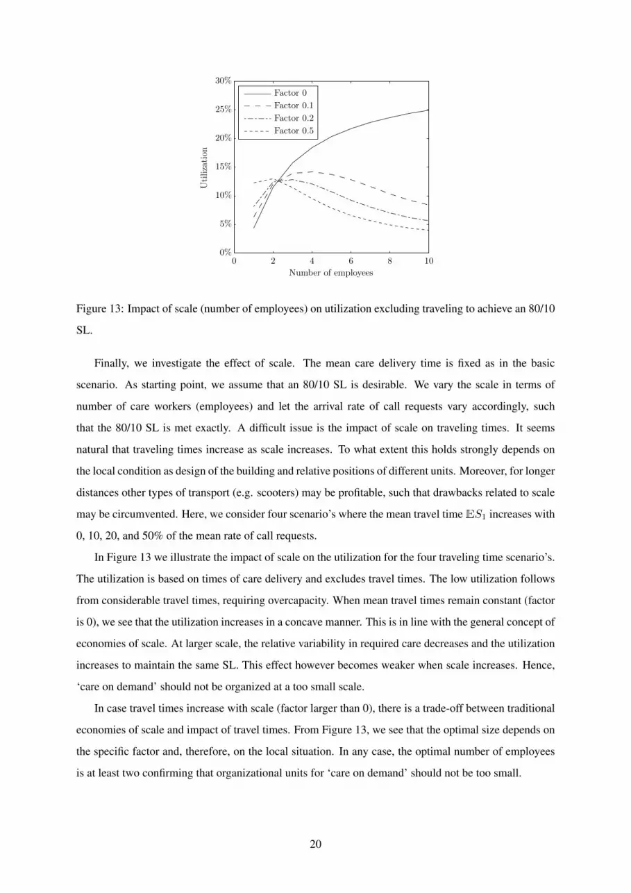
Figure 13: Impact of scale (number of employees) on utilization excluding traveling to achieve an 80/10
SL.
Finally, we investigate the effect of scale. The mean care delivery time is fixed as in the basic
scenario. As starting point, we assume that an 80/10 SL is desirable. We vary the scale in terms of
number of care workers (employees) and let the arrival rate of call requests vary accordingly, such
that the 80/10 SL is met exactly. A difficult issue is the impact of scale on traveling times. It seems
natural that traveling times increase as scale increases. To what extent this holds strongly depends on
the local condition as design of the building and relative positions of different units. Moreover, for longer
distances other types of transport (e.g. scooters) may be profitable, such that drawbacks related to scale
may be circumvented. Here, we consider four scenario’s where the mean travel timeES1 increases with
0, 10, 20, and 50% of the mean rate of call requests.
In Figure 13 we illustrate the impact of scale on the utilization for the four traveling time scenario’s.
The utilization is based on times of care delivery and excludes travel times. The low utilization follows
from considerable travel times, requiring overcapacity. When mean travel times remain constant (factor
is 0), we see that the utilization increases in a concave manner. This is in line with the general concept of
economies of scale. At larger scale, the relative variability in required care decreases and the utilization
increases to maintain the same SL. This effect however becomes weaker when scale increases. Hence,
‘care on demand’ should not be organized at a too small scale.
In case travel times increase with scale (factor larger than 0), there is a trade-off between traditional
economies of scale and impact of travel times. From Figure 13, we see that the optimal size depends on
the specific factor and, therefore, on the local situation. In any case, the optimal number of employees
is at least two confirming that organizational units for ‘care on demand’ should not be too small.
20

6 Conclusions and discussion
In this paper we made a first step in trying to understand the real-life performance of the ‘care on de-
mand’ process in a Belgian nursing home facility using a queueing theoretic approach. From a method-
ological point of view, the contribution of this study is twofold. First, by using real-life data we obtain
insight in the number of call requests and care delivery times for ‘care on demand’ activities. Secondly,
we developed a queueing model to support capacity decisions. Based on numerical experiments, we
propose an 80/10 service level, meaning that at least 80% of the clients should receive care within 10
minutes after a call button request.
From a practical perspective, this study provides a basis on which it is possible to develop a staffing
support tool for ‘care on demand’ activities which would allow nursing home managers to 1) deter-
mine the number of care workers required to sufficiently meet the needs and preferences of the nursing
home residents when it comes to ‘care on demand’ and 2) to better understand the implications of their
decisions (i.e. what-if scenario’s). We think that such a tool has the potential to make an important
contribution in the quest for more efficiency, without losing sight of the needs of residents.
A model is never a complete representation of reality and the queueing model presented in this paper
is no exception. First of all, this study is limited in scope because it only addresses the night care. A
similar approach could be taken for the ‘care on demand’ process during day time. During day time,
the amount of ‘care by appointment’ activities are much larger compared to the night, which may lead
to compromised ‘care on demand’ data. Moreover, data on traveling times is lacking. Although travel
times may vary depending on the local situation, it would be of interest to model this in more detail.
Finally, we used an approximation for the queueing model. This approximation is expected to work
well in most nursing-home situations, but the accuracy may decrease when e.g. the number of clients is
getting very small.
Despite the fact that long-term elderly care will become increasingly important in the next decades,
the body operations research (OR) literature directed on this topic is still very limited. Therefore we
would like to challenge researchers in the field of OR to put more emphasis on research in long-term
elderly care. Finding usable data will be an important first step for future research in this promising field,
as reliable and valid information is scarce and seldomly collected. Nevertheless, the most important
challenge for future research will be to not overemphasize the importance of efficiency as the needs and
preferences of the clients should always be kept in mind when conducting research in this area.
Acknowledgements
The authors would like to thank Niko Projects for providing us with a dataset and Jan-Pieter Dorsman
for the simulation of the finite-source queueing model.
21

References
[1] J. Abate, G.L. Choudhury, and W. Whitt. Exponential approximations for tail probabilities in queues, I:
waiting times. Operations Research, 43(5):885–901, 1995.
[2] R. Bosman, G. Bours, J. Engels, and P. De Wit. Client-centred care perceived by clients of two Dutch
homecare agencies: A questionary survey. International Journal of Nursing Studies, 45(5):518–525, 2008.
[3] K. Brazil, J. Maitland, J. Ploeg, and M. Denton. Identifying research priorities in long term care homes.
Journal of the American Medical Directors Association, 13(1):84–e1, 2012.
[4] F. Colombo, A.L. Nozal, J. Mercier, and F. Tjadens. Help Wanted? Providing and Paying for Long-Term
Care. OECD Health Policy Studies. OECD publishing, 2012.
[5] European Commission. Long-Term Care and Use an Supply in Europe. European Union, 2008.
[6] F. de Vericourt and O.B. Jennings. Nurse staffing in medical units: A queueing perspective. Operations
Research, 59(6):1320–1331, 2011.
[7] S. Fomundam and J. Herrmann. A survey of queuing theory applications in health care. ISR Technical
Report, 24, 2007.
[8] R. Fujisawa and F. Colombo. The long-term care workforce: overview and strategies to adapt supply to a
growing demand. OECD publishing, 2009.
[9] J. Geerts, P. Willem, and E. Mot. Long-Term Care Use and Supply in Europe: Projections for Germany, The
Netherlands, Spain and Poland. ENEPRI, 2012.
[10] L.V. Green, P.J. Kolesar, and J. Soares. Improving the SIPP approach for staffing service systems that have
cyclic demands. Operations Research, 49(4):549–564, 2001.
[11] L.V. Green, P.J. Kolesar, and W. Whitt. Coping with time-varying demand when setting staffing requirements
for a service system. Production and Operations Management, 16(1):13–39, 2007.
[12] R. Hall. Handbook of Healthcare System Scheduling. International Series in Operations Research & Man-
agement Science. Springer, 2012.
[13] C. Harrington, J. Choiniere, M. Goldmann, F.F. Jacobsen, L. Lloyds, M. McGregor, V. Stamatopoulos, and
M. Szebehely. Nursing home staffing standards and staffing levels in six countries. Journal of Nursing
Scholarship, 44(1):88–98, 2012.
[14] K. Havig, A. Skogstad, L.E. Kjekhus, and T.I Romoren. Leadership, staffing and quality of care in nursing
homes. BMC Health Services Research, 11(1):327, 2011.
[15] T. Kimura. Approximations for multi-server queues: system interpolations. Queueing Systems, 17(3-4):347–
382, 1994.
[16] L. Kleinrock. Queueing systems. volume 1: Theory. 1975.
[17] C. Lakshmi and S. Appa lyer. Application of queueing theory in health care: A literature review. Operations
Research for Health Care, 2(1):25–39, 2013.
22

[18] K.S. McGilton, A. Tourangeau, C. Kavcic, and W.P. Wodchis. Determinants of regulated nurses’ intention
to stay in long-term care homes. Journal of Nursing Management, 21(5):771–781, 2013.
[19] D. Moeke, G.M. Koole, and H.E.C. Verkooijen. Scale and skill-mix efficiencies in nursing home staffing.
Health Systems, 3(1):18–28, 2014.
[20] D. Moeke and H.E.C. Verkooijen. Doing more with less: A client-centred approach to healthcare logistics
in a nursing home setting. Journal of Social Intervention: Theory and Practice, 22(2):167–187, 2013.
[21] United Nations. World population ageing 2013, 2013.
[22] A. Neely, M. Gregory, and K. Platts. Performance measurement system design: A literature review and
research agenda. International Journal of Operations and Production Management, 25(12):1228–1263,
2005.
[23] E. Reitinger, K. Froggatt, K. Brazil, K. Heimerl, J. Hockley, R. Kunz, H. Morbey, D. Parker, and B.S.
Husebo. Palliative care in long-term care settings for older people: findings from an EAPC taskforce.
European Journal of Palliative Care, 20(5):251–253, 2013.
[24] H. Sakasegawa. An approximation formula Lq ' α · ρβ/(1 − ρ). Annals of the Institute of Statistical
Mathematics, 29(1):67–75, 1977.
[25] K. Satyam, A. Krishnamurthy, and M. Kamath. Solving general multi-class closed queuing networks using
parametric decomposition. Computers & Operations Research, 40(7):1777–1789, 2013.
[26] K. Spilsbury, C. Hewitt, L. Stirk, and C. Bowman. The relationship between nurse staffing and quality of
care in nursing homes: A systematic review. International Journal of Nursing Studies, 48(6):732–750, 2011.
[27] J.D. Storey. A direct approach to false discovery rates. Journal of the Royal Statistical Society, Series B,
64(3):479–498, 2002.
[28] J.D. Storey. The positive false discovery rate: A Bayesian interpretation and the q-value. The Annals of
Statistics, 31(6):2013–2035, 2003.
[29] H.C. Tijms. A First Course in Stochastic Models. Wiley, 2003.
[30] M. van den Akker, F. Buntinx, J.F.M. Metsemakers, S. Roos, and J.A. Knottnerus. Multimorbidity in general
practice: Prevalence, incidence, and determinants of co-occurring chronic and recurrent diseases. Journal of
Clinical Epidemiology, 51(5):367–375, 1998.
[31] W. Whitt. Open and closed models for networks of queues. AT&T Bell Laboratories Technical Journal,
63(9):1911–1979, 1984.
[32] W. Whitt. Understanding the efficiency of multi-server service systems. Management Science, 38(5), 1992.
[33] W. Whitt. Approximations for the GI/G/m queue. Production and Operations Management, 2(2):114–161,
1993.
[34] N. Yankovic and L.V. Green. Identifying good nursing levels: A queuing approach. Operations Research,
59(4):942–955, 2011.
23