Harmen W. van den Berg

Rutger H.R. Bolt

October 2010

Catchment analysis in

the Migina marshlands,

southern Rwanda

1

VU University Amsterdam

Faculty of Earth and Life Sciences Department of Hydrology and Geo-environmental Sciences Boelelaan 1085 1081 HV Amsterdam The Netherlands http://www.vu.nl UNESCO-IHE

Institute for Water Education PO Box 3015 2601 DA Delft The Netherlands

http://www.unesco-ihe.org

National University of Rwanda

Faculty of Applied Sciences Department of Civil Engineering BP 117 Butare Rwanda http://www.nur.ac.rw

Master Thesis Hydrogeology (O-variant) course code AM 450122 ECTS 27 status Final date October 26th 2009 authors Harmen W. van den Berg Rutger R.H. Bolt supervisors prof.dr. S. Uhlenbrook (UNESCO-IHE) dr. M.J. Waterloo (VU Univerisity)

dr. J.W. Wenninger (UNESCO-IHE)

Catchment analysis in

the Migina marshlands,

southern Rwanda

2

1

Index

List of Appendices ________________________________________3

List of Figures ____________________________________________4

List of Tables ____________________________________________7

Abstract ________________________________________________9

1 Background_____________________________________________11

1.1 Introduction___________________________________________________ 11 1.2 Structure of this report __________________________________________ 11 1.3 Acknowledgements _____________________________________________ 12

2 Regional setting _________________________________________13

2.1 Rwanda ______________________________________________________ 13 2.1.1 Topography ______________________________________________ 13 2.1.2 Climate _________________________________________________ 14 2.1.3 Hydrology _______________________________________________ 14 2.1.4 Geology _________________________________________________ 15

2.2 Migina catchment ______________________________________________ 17 2.2.1 Topography ______________________________________________ 17 2.2.2 Climate _________________________________________________ 17 2.2.3 Hydrology _______________________________________________ 19 2.2.4 Geology and soils _________________________________________ 19 2.2.5 Geomorphology ___________________________________________ 22 2.2.6 Vegetation and land use ____________________________________ 22

3 Methodology ____________________________________________27

3.1 Atmospheric water _____________________________________________ 28 3.1.1 Precipitation _____________________________________________ 28 3.1.2 Evaporation ______________________________________________ 29

3.2 Surface water _________________________________________________ 30 3.2.1 Gauging stations __________________________________________ 30 3.2.2 Rating curves and time series ________________________________ 32

3.3 Groundwater __________________________________________________ 33 3.3.1 Springs _________________________________________________ 33 3.3.2 Piezometers ______________________________________________ 35 3.3.3 Water levels _____________________________________________ 38 3.3.4 Hydrochemical sampling of groundwater _______________________ 38

3.4 Soil properties _________________________________________________ 39 3.4.1 Bore- and dugholes ________________________________________ 39 3.4.2 Field permeability _________________________________________ 40 3.4.3 Infiltration capacity ________________________________________ 42 3.4.4 Soil water permeability _____________________________________ 43 3.4.5 Soil moisture, porosity and bulk density ________________________ 44 3.4.6 Grainsize ________________________________________________ 45

3.5 Hydrochemistry ________________________________________________ 47 3.5.1 Field measurements _______________________________________ 47 3.5.2 Lab hydrochemical composition ______________________________ 47 3.5.3 Isotopes ________________________________________________ 48 3.5.4 Field sampling ____________________________________________ 48

2

4 Results ________________________________________________49

4.1 Atmospheric water _____________________________________________ 49 4.1.1 Precipitation _____________________________________________ 49 4.1.2 Evaporation ______________________________________________ 58

4.2 Surface water _________________________________________________ 62 4.2.1 Rating curves ____________________________________________ 62 4.2.2 Discharge time series ______________________________________ 66 4.2.3 Hydrograph analysis _______________________________________ 71 4.2.4 Baseflow ________________________________________________ 73 4.2.5 Specific discharge _________________________________________ 80 4.2.6 River routing _____________________________________________ 86

4.3 Groundwater __________________________________________________ 89 4.3.1 Springs _________________________________________________ 89 4.3.2 Continuous water levels piezometers __________________________ 92 4.3.3 Daily fluctuations in water levels piezometers ___________________ 94 4.3.4 Groundwater temperature ___________________________________ 97 4.3.5 Hydrochemistry ___________________________________________ 99 4.3.6 Isotopes _______________________________________________ 103 4.3.7 Flow rate spring Kadahokwa ________________________________ 104

4.4 Soil properties ________________________________________________ 105 4.4.1 Bore- and dughole descriptions ______________________________ 105 4.4.2 Horizontal saturated permeability ____________________________ 110 4.4.3 Vertical saturated permeability ______________________________ 113 4.4.4 Infiltration capacity _______________________________________ 113 4.4.5 pF curve, porosity and bulk density __________________________ 114 4.4.6 Grain size ______________________________________________ 116

5 Discussion____________________________________________ 123

6 Conclusions and recommendations ________________________ 139

References ___________________________________________ 143

3

List of Appendices

I. Historical rainfall measurements in Butare II. Measurement of atmospheric water III. Gauging stations IV. Level surveying V. OTT-propeller VI. Evaporation measurements VII. Monthly precipitation tipping bucket Butare VIII. Time series precipitation totalizers IX. Time series surface water X. Daily pattern baseflow XI. Coordinates XII. Grainsize distribution XIII. Hydrochemistry – field measurements XIV. Hydrochemistry – lab analysis XV. Hydrochemistry – electrical balance XVI. Bore- and dughole descriptions XVII. Geological profiles XVIII. River routing XIX. Saturated vertical permeability soil samples XX. Bulk density soil samples XXI. pF measurements XXII. Water treatment plant Electrogaz XXIII. Isotopical signature Butare catchment XXIV. Total daily amounts of precipitation XXV. Levelling piezometers transects

4

List of Figures

Figure 1: Location of Rwanda in Africa, marked with the red square __________ 13 Figure 2: Annual temperature distribution ______________________________ 14 Figure 3: Mean annual rainfall distribution ______________________________ 14 Figure 4: Geological map of Rwanda __________________________________ 16 Figure 5: Location of Migina catchment ________________________________ 17 Figure 6: Digital elevation model (DEM) of Migina catchment _______________ 17 Figure 7: Average rainfall and temperatures at Butare airport: 1969-1992 ____ 18 Figure 8: Main rivers in Migina catchment ______________________________ 19 Figure 9: Photo of deeply weathered shales (left) and deeply weathered

phyllite rock in which the metamorphic origin is still visible (right) ___ 21 Figure 10: Two photo’s of the sand-gravel debris layer (III) with on top red

soils (IV) ________________________________________________ 22 Figure 11: Photo of banana trees (left) and irrigated rice fields in the valley to

the southwest of Butare, with trees on the hillslope (right) _________ 23 Figure 12: Photo of the urban area of Butare (left) and natural vegetation on

a hillslope to the west of Butare (right) ________________________ 23 Figure 13: Land use types in Migina catchment ___________________________ 24 Figure 14: Overview of all the measuring stations installed in Migina

catchment _______________________________________________ 27 Figure 15: Two photographs from open springs in Migina catchment; used to

collect drinking water from in plastic jerrycans___________________ 33 Figure 16: Locations of springs in Migina catchment _______________________ 34 Figure 17: Locations of the piezometer transects A1 - A7 and B1 – B4 _________ 35 Figure 18: Topography and piezometers of transect A ______________________ 36 Figure 19: Topography and piezometers of transect B ______________________ 36 Figure 20: Photo piezometers A3 - A7 __________________________________ 37 Figure 21: Kadahokwa spring _________________________________________ 37 Figure 22: Soil sample locations _______________________________________ 39 Figure 23: Dughole 2 (C2) ___________________________________________ 40 Figure 24: Permeability test __________________________________________ 40 Figure 25: An improvised double-ring infiltrometer ________________________ 42 Figure 26: Photo of the closed system __________________________________ 43 Figure 27: Photo’s of the membrane press used for measurements of pF = 3 -

4.2. ____________________________________________________ 45 Figure 28: Heating the beakers with the samples _______________________ 46 Figure 29: Samples are left standing over for hours so the sediment can settle __ 43 Figure 30: Analysing the grainsize with the laser __________________________ 46 Figure 31: Time series of precipitation, measured with the tipping bucket at

the CGIS-centre in Butare, for the period of the 1st of May until the 8th of June 2009 __________________________________________ 49

Figure 32: Locations of the 10 totalizers and their Thiessen polygons that cover Butare catchment ____________________________________ 51

Figure 33: Rainfall time series of the wet season for the three different subcatchments ___________________________________________ 52

Figure 34: Spatial distribution of rainfall, presented in mm, for the first rainy period (left) and the second rainy period (right) _________________ 54

Figure 35: δ2H plotted against δ18O for eight rainwater samples (A-H) measured in Butare catchment _______________________________ 57

Figure 36: Results from the ‘Class A’ pan evaporation measurements _________ 58 Figure 37: Landuse map used for calculating the potential evaporation ________ 61 Figure 38: The relationship between discharge (Q) and water level (h) at

gauging station 1 _________________________________________ 63 Figure 39: The relationship between discharge (Q) and water level (h) at

gauging station 2 _________________________________________ 64

5

Figure 40: The relationship between discharge (Q) and water level (h) at gauging station 3 _________________________________________ 65

Figure 41: Hydrograph of the Gyezuboro river, measured at gauging station 1, plotted together with the time series of the local measured water temperature and with the precipitation recorded in Butare at the CGIS station with a tipping bucket _________________________ 67

Figure 42: Hydrograph of the Kadahokwa river measured at gauging station 2, plotted together with the time series of the local measured water temperature and with the precipitation recorded in Butare at the CGIS station with a tipping bucket _________________________ 68

Figure 43: Comparison between the variation in air temperature and water temperature _____________________________________________ 70

Figure 44: Hydrograph of the Migina river measured at gauging station 3, plotted against the precipitation recorded in Butare at the CGIS station with a tipping bucket _________________________________ 71

Figure 45: Baseflow pattern for all three gauging station plotted with two very small rainfall events measured by the totalizers __________________ 74

Figure 46: Sectionwise approximation of a semi-logarithmic baseflow recession curve by linear reservoirs ___________________________ 75

Figure 47: Measured versus calculated baseflow of GS2 and GS3 _____________ 76 Figure 48: Baseflow pattern plotted as water level time series for all three

gauging stations __________________________________________ 78 Figure 49: Averaged daily pattern of the relative water level at all three

gauging station for the whole baseflow period ___________________ 78 Figure 50: Specific discharge for the whole study period ____________________ 80 Figure 51: Specific discharge for the period of the 11th – 25th of May 2009 _____ 81 Figure 52: Specific discharge for the period of 25th May – 8th June 2009 ______ 81 Figure 53: Specific discharge and hydrograph separation (analytical approach)

for gauging station 1 _______________________________________ 83 Figure 54: Specific discharge and hydrograph separation (analytical approach)

for gauging station 2 _______________________________________ 83 Figure 55: Specific discharge and hydrograph separation (analytical approach)

for gauging station 3 _______________________________________ 83 Figure 56: River routing in Butare catchment ____________________________ 86 Figure 57: Results of river routing in Butare catchment ____________________ 87 Figure 58: Waste water in a river near NUR campus _______________________ 87 Figure 59: EC of water from springs in Butare catchment ___________________ 89 Figure 60: Nitrate concentrations (in mg l-1) _____________________________ 90 Figure 61: Silica concentrations (in mg l-1) ______________________________ 91 Figure 62: Water level in piezometers A5, A6 and A7 ______________________ 92 Figure 63: Water level in piezometers A3 and A4 _________________________ 92 Figure 64: Water level in piezometers A1 and A2 _________________________ 93 Figure 65: Water level in piezometer B3 ________________________________ 93 Figure 66: Water level in piezometer B1 and B2 __________________________ 94 Figure 67: Daily average water level fluctuations, transect A ________________ 95 Figure 68: Daily average waterlevel fluctuations, transect B _________________ 96 Figure 69: Temperature groundwater transect A __________________________ 97 Figure 70: Temperature groundwater transect B __________________________ 98 Figure 71: EC variations in time at transect A ___________________________ 100 Figure 72: Average EC values along transect A __________________________ 101 Figure 73: Average Silica (SiO2) values along transect A ___________________ 102 Figure 74: Isotopic composition of groundwater samples __________________ 103 Figure 75: Discharge rate Kadahokwa spring ____________________________ 104 Figure 76: Borehole descriptions of borehole A1 until A4___________________ 105 Figure 77: Borehole descriptions of borehole A5 until A7___________________ 107 Figure 78: Borehole descriptions of borehole B1 until B4___________________ 108 Figure 79: Dughole C1 and C2 _______________________________________ 109

6

Figure 80: Stratigraphy Kadahokwa valley ______________________________ 110 Figure 81: Falling head tests of piezometers A1 – A7 _____________________ 112 Figure 82: Soil water retention curve for twelve soil-cores _________________ 114 Figure 83: Grain size analysis of red/brown soils _________________________ 117 Figure 84: Grain size of samples from borehole A5 _______________________ 117 Figure 85: Grain size of samples from borehole A7 _______________________ 118 Figure 86: Grain size of samples from borehole B4 _______________________ 118 Figure 87: Grain size of samples from dughole C2 ________________________ 119 Figure 88: Grain size analysis of clays/silt ______________________________ 119 Figure 89: Grain size of samples borehole B3 ___________________________ 120 Figure 90: Grainsize distribution of sand deposits ________________________ 120 Figure 91: grainsize distribution of gravels _____________________________ 121 Figure 92: Positive lineair relationship between NO3

- and EC ________________ 123

Figure 93: Specific discharge and plausible hydrograph separation for gauging station 3 _______________________________________________ 126

Figure 94: Schematized and simplified representation of the groundwater level variations in Butare catchment __________________________ 128

Figure 95: Isotopic signature of the seven piezometers from transect A _______ 131 Figure 96: Daily barometric fluctuations, measured at groundwater transect ___ 132 Figure 97: Topography of transect A and B _____________________________ 135 Figure 98: Preferential flow in subsurface, caused by stretching and

compression ____________________________________________ 135 Figure 99: Shallow and deeper groundwater flow along transect A and B ______ 136

7

List of Tables

Table 1: Different types of land use in Migina catchment ___________________ 24 Table 2: UTM coordinates of springs in Migina catchment __________________ 34 Table 3: Overview of the coordinates, lengths and filter depths of piezometers _ 37 Table 4: Dates when water from the piezometers was sampled ______________ 38 Table 5: Soil sample locations ________________________________________ 39 Table 6: Coordinates and depth of the dugholes__________________________ 40 Table 7: Coordinates of infiltration test locations _________________________ 42 Table 8: Accuracy of the ion-chromatography ___________________________ 47 Table 9: Accuracy of the aquakem analysis _____________________________ 48 Table 10: Percentage ratio of the Thiessen polygons distribution for each of the

three subcatchments ________________________________________ 51 Table 11: Amounts of rainfall for 12 different totalizers _____________________ 53 Table 12: Hydrochemical composition of rainwater ________________________ 55 Table 13: Calculation of the potential total evaporation, based on the landuse

persubcatchment with associated dominating crop species and crop factors ___________________________________________________ 60

Table 14: Time to peak analysis of the discharge and water temperature as a response to rainfall events ___________________________________ 72

Table 15: Overview of the selected points in the hydrograph where ___________ 82 Table 16: The differences in baseflow and direct runoff quantified for different time

periods for subcatchment 2 and Butare catchment ________________ 84 Table 17: Runoff coefficients for the different periods of direct runoff, calculated

with the direct runoff measured at gauging station 2 and gauging station 3 and the amount of precipitation measured at subcatchment 2 and Butare catchment respectively ________________________________ 85

Table 18: Results of chemical analysis of riverwater close to NUR campus ______ 88 Table 19: Chemical contents (major cations and anions) and Electrical Balance

(E.B.) of springs in Migina catchment ___________________________ 89 Table 20: Average concentrations and Electrical Balance (E.B.) for water from

piezometers of transect A ____________________________________ 99 Table 21: Average concentrations in water from piezometers of transect B ______ 99 Table 22: Average SiO2 concentrations _________________________________ 101 Table 23: Saturated hydraulic conductivity, in m d-1 ______________________ 111 Table 24: Results of vertical saturated permeability measurements __________ 113 Table 25: Results of double ring infiltrometer tests _______________________ 114 Table 26: The 12 soil-cores and their main soil properties __________________ 115 Table 27: Results of grain size analysis ________________________________ 116 Table 28: Chemical content in springwater near Butare, in 2007 and 2009 _____ 124 Table 29: Results of chemical analysis of 4 springs near Butare, Kasanziki 2007 124 Table 30: Microbiological content in water sampled from springs near Butare ___ 125 Table 31: Water balance for the study period of 15th May until 15th July 2009 __ 127

8

9

Abstract Rwanda is a small country in Central Africa, a little south from the equator. The country has a population density of approximately 400 km-2, and a population growth which is close to 3 percent. As the population dependents on agriculture for their livelihood, Rwanda faces the challenge to provide all its inhabitants with enough food; today and tomorrow. Therefore, Rwanda is planning to reform the agriculture, for example by the introduction of different rice crops and the construction of irrigation systems. Knowledge about the watersystem, which will get already more and more under stress by the population growth, is therefore necessary. Knowledge about the watersystem, wateravailability and development of the waterquality will be necessary to ensure human health nowadays and in the future. Not much hydrological data is present in Rwanda nowadays; mainly as a result of the civil war in 1994. During this period, a lot of knowhow and equipment was destroyed. Therefore UNESCO-IHE Institute for Water Education started a capacity building programme1 in 2004, with the goal to train water specialists at the National University of Rwanda (NUR). Omar Munyaneza is doing a PhD research about the space-time patterns of hydrological processes and water resources in Rwanda, with a special focus on the mesoscale Migina catchment, located in southern Rwanda. In support of this research, a hydrological fieldwork was carried out for the MSc Hydrology at the VU University. From 16th April 2009 until 31st July 2009 a field study was carried out in Migina catchment, in southern Rwanda. The Migina catchment is a meso-scale catchment of 147 km2, in which Butare, the second city in Rwanda is located in the northern part. The outlet of Migina catchment is located at the border between Rwanda and Burundi, where the river Migina drains into the river Akanyaru. During the fieldwork, Migina catchment has been equipped with hydrological instruments in order to be able to measure main hydrological processes. Therefore five gauging stations were built, eleven piezometers were installed, a meteorological tower was built up (in addition to one that was already present in Butare), thirteen totalizer rainfall stations were set up as well as four tipping buckets, and one evaporation pan was installed (in addition to one that was already present in Butare). Besides, several soil- and water samples have been taken which were analysed in the field and in the lab. With the installation of the equipment it was possible to measure and quantify important hydrological parameters such as river discharge, groundwater flow and amounts and distribution of rainfall and total evaporation. In total, 125 mm of rainfall was recorded on average during the research period, mainly concentrated in the month of May, but highly variable in space. An average of 3 mm d-1 of evaporation was calculated, based on measurements with evaporation pans. A relationship between waterlevel and discharge has been made for three gauging stations that are located in Butare catchment, the northern part of Migina catchment. At these gauging stations, a runoff coefficient around 10% was measured during wet season, showing that groundwater is the most important source of the water in the river. For the period of dry season, a baseflow recession curve could be made, showing a decreasing decline in baseflow, becoming almost constant at a rate of 190 l s-1 for the main outlet during the end of the dry season.

1 http://www.unesco-ihe.org/Project-activities/Project-database/Capacity-Building-in-Water-Resources-and-Environmental-Management-in-Rwanda

10

Without the input of precipitation, a significant flow from (deep) groundwater has to be the source of this water. In the absence of rainfall, the watertable in the river dropped on average 7 mm d-1 at gauging station 1, 2 mm d-1 at gauging station 2 and 6 mm d-1 at gauging station 3. The rivers in Migina catchment contain water throughout the year, even after the main dry season lasting two months. Therefore groundwater is an important factor. The flow of groundwater from hillside towards streams is observed by the installation of two transects with piezometers. Water levels are monitored and samples are taken weekly during a month under baseflow conditions. It appears that water levels at the transition between hillslope and valley floor decrease linearly with a speed of 3 mm day-1. The water level reduces through transpiration by vegetation, as a clear daily fluctuation in the water levels is present. Within the valley, the groundwater flow becomes mixed with surface water, through former riverbeds. The water level decreases exponential, as the vegetation has problems in reaching the groundwater. As a result, the groundwater table decreases 13 mm-1 day in the middle of June and only 4 mm day-1 at the end of July. The daily fluctuations in the valley are different from the fluctuations, which are present in surface water and piezometers near the hillslope. The daily level has two maximum levels and two minimum levels. The typical ‘red earth’ soils have a low conductivity. Some particular layers, such as former river beds filled with sands and gravels and layers with relatively coarse material have relative higher conductivities. As a result, preferential flowpath along the valleys are assumed to take place. Closer to the river, the groundwater experiences more influence by the river. As a result, the water levels do not decrease during the last four weeks of the study period as the water gets blocked and even gets mixed with water from the river. The temperature of groundwater is warmer than surface water, and increases in time. Surface water is in contrast relatively cold, and even became colder during the dry season. An explanation for this difference might be seepage from deeper groundwater towards the river, which is colder than the shallow groundwater. The deeper groundwater is separated from shallow groundwater by a impermeable layer which is present in the valleys, at two until four meter below the surface. The water quality of water from springs in Butare catchment is good, when looking at hydrochemical content. Some of the springs have high concentrations of nitrate, close to the limit of the WHO. The high nitrate concentration is related to human activities, such as agriculture and waste water from septic tanks. Monitoring of the water quality is needed, to see how the water quality of the springs changes in time. As the population is expected to grow, the activities of humans in the Butare and Migina catchment will increase. As a result, the water quality of the springwater, which is used by many people for drinking water and domestic usage, might get worse. Another aspect of the drinking water quality is microbiological activity. Analysis of the water quality of four springs around Butare in the past proves that water from the springs is contaminated with coliforms and aerobic flora above standards of WHO. More frequent microbiological analysis of preferably all springs in Butare catchment is therefore suggested.

11

1 Background

1.1 Introduction Rwanda is a small country in Central Africa, a little south from the equator. The country has a population density of approximately 400 km-2, which makes Rwanda the most densely populated country on the African continent. With a population growth which is close to 3 percent, the population will be doubled within twenty years. As the population is mainly dependent on agriculture for their livelihood, Rwanda faces the challenge to provide all its inhabitants with enough food; today and tomorrow. Therefore, Rwanda is planning to reform the agriculture, for example by the introduction of different rice crops and the construction of irrigation systems. Knowledge about the watersystem, which will get already more and more under stress by the enormous population growth, is therefore necessary. The risk of severe water shortage during dry season as well as increasing pollution of the water resources is imminent. Knowledge about the watersystem, wateravailability and development of the waterquality will be necessary to ensure human health nowadays and in the future. Not much hydrological data is present in Rwanda nowadays; mainly as a result of the civil war in 1994. During this period, a lot of knowhow and equipment was destroyed. Therefore UNESCO-IHE Institute for Water Education started a capacity building programme2 in 2004, with the goal to train water specialists at the National University of Rwanda (NUR). One of the achievements of the programme is a Master of Science Degree in Water Resources and Environmental Management (WREM). As part of this programme, Omar Munyaneza is doing a PhD research about the space-time patterns of hydrological processes and water resources in Rwanda, with a special focus on the mesoscale Migina catchment, located in southern Rwanda. In support of this research, a hydrological fieldwork was carried out for the MSc Hydrology at the VU University Amsterdam. The fieldwork was carried out in Migina catchment from 16th April until 31st July 2009. The objective of this fieldwork was to equip the Migina catchment with hydrological instruments in order to be able to measure the main hydrological processes. Therefore, gauging stations were built, a meteorological tower was installed, rainfall stations were set up and several soil- and water samples have been taken. One of the objectives of the study was to quantify important hydrological parameters such as river discharge, amounts and distribution of rainfall and total evaporation. With these parameters, insight in runoff generation processes will be obtained and important hydrogeochemical processes will be identified. Another objective of this study is getting insight in interactions between groundwater and surface water. As the rivers in Rwanda contain water throughout the year, even after the main dry season of two months, groundwater is an important factor. To be able to measure the variations in groundwater level in detail, two transects with piezometers were installed in one of the valleys. In this area, also permeability tests have been carried out.

1.2 Structure of this report In this report the results of the fieldwork from 16th April 2009 until 31st July 2009 are reported. In chapter 2 the regional setting of Rwanda in general and more specific of Migina catchment are described. Chapter 3 is about the methods that were used to obtain the results that are described and presented in chapter 4. The results are discussed in chapter 5. Conclusions and recommendations are drawn in chapter 6.

2 http://www.unesco-ihe.org/Project-activities/Project-database/Capacity-Building-in-Water-Resources-and-Environmental-Management-in-Rwanda

12

1.3 Acknowledgements First of all, we would like to thank our supervisors Stephan Uhlenbrook (UNESCO-IHE/TU Delft/VU University Amsterdam), Jochen Wenninger (UNESCO-IHE/TU Delft) and Maarten Waterloo (VU University Amsterdam). Also we would like to thank in special Omar Munyaneza and Wali Umaru Garba (WREM - NUR) for their help and support during the fieldwork in Rwanda. Besides we would like to thank Don van Galen, Jan Willem Foppen and Jeltje Kemerink (UNESCO-IHE), John Visser, Martin Konert, Frans Backer and Michel Groen (VU University Amsterdam), W.M.J. de Lange (Hogeschool Inholland Alkmaar), Eric and Deo Rutamu (CGIS Butare), Digne Rwabuhungu, Abias Uwimana, Dominique Ingabire, Flora Umuhire, Gafishe Clément, Devota and Theobalt (WREM - NUR), the ‘concrete man’ (Butare market), and all the others which made this MSc Thesis possible.

13

2 Regional setting The regional setting is described for Rwanda in general (chapter 2.1) and more specific for the Migina catchment (chapter 2.2). In succession, the topography, climate, hydrology and geology will be discussed, with for Migina catchment also a focus on soils, geomorphology, vegetation and land use.

2.1 Rwanda Rwanda is situated in Central Africa, just south from the equator. Rwanda borders Uganda in the North, Tanzania in the east, Burundi in the south and the Democratic Republic of Congo in the west (figure 1). Rwanda is a relatively small country, with a surface area of 26,338 km2. The country has more than 10.7 million inhabitants in July 20103. With a population density of approximately 400 km-2, it is the most densely populated country on the African continent. The population growth is close to 3% which means that the population is doubled within 20 years. More than 90% of the population depends on agriculture for their livelihood (Van Straaten, 2002). The production is characterised by a diversity of food crops. The most important crops are bananas, beans, (sweet) potatoes, sorghum, cassava, maize, and rice (FAO, 2010).

Figure 1: Location of Rwanda in Africa, marked with the red square (U.S. CIA, 1997).

2.1.1 Topography

Rwanda is known as “the land of the thousand hills”. The landscape is characterized by highlands in the central and eastern part of the country. The western part of Rwanda is a rifted area, where the landscape consists of volcanic mountains and rifted-lakes. The central area of Rwanda consists of a hilly plateau with an average elevation of 1,700 meter above sea level (m.a.s.l.). Towards the east, the land slopes downwards towards the river Akagera. This river forms the eastern border, between Rwanda and Tanzania. In the eastern border region, a number of marshy lakes and swamps are present. The western part of Rwanda is more mountainous and has an average elevation of 2,750 m.a.s.l. Towards the western border, the elevation drops towards Lake Kivu, which has an elevation of approximately 1,450 m.a.s.l. Lake Kivu and the Ruzizi River valley are part of the Great Rift Valley. In the

3 http://en.wikipedia.org/wiki/Rwanda

14

� N

� N

northwest, the Virunga chain of volcanoes is present. The Karisimbi is the highest volcano, with an elevation of 4,507 m.a.s.l.

2.1.2 Climate

The climate of Rwanda is, despite its location close to the equator, temperate tropical. This temperate climate is the result of the relatively high elevation of the country. The average annual temperature ranges between 16°C and 24°C and is strongly related to the altitude. The annual temperature distribution in Rwanda is presented in figure 2 (Verdoodt and Van Ranst, 2003). The average temperatures can be refined per geographical unit. The higher elevated areas have temperatures that vary between 15°C and 17°C on average. Figure 2: Annual temperature distribution, (Verdoodt and Van Ranst, 2003).

At the central plateaus, tempera-tures that are recorded vary between 18°C and 20°C. The lowlands in the east are the warmest regions, with an average annual temperature above 21°C. The climate of Rwanda is made up of two wet and two dry seasons. The short wet season lasts from October until November. The main rainy season lasts from the second half of March until the end of May. The average annual rainfall in Rwanda varies between 900 mm a-1 and 1,600 mm a-1, and is shown in figure 3 (Verdoodt and Van Ranst, 2003). The amount of rainfall decreases in general from west to east.

Figure 3: Mean annual rainfall distribution (Verdoodt and Van Ranst, 2003).

2.1.3 Hydrology

The drainage system in Rwanda can be divided in two systems. The divide between the two systems is called the “Congo-Nile divide”. It is located in the high elevated regions in the western part of Rwanda. The area west from this divide, drains towards Lake Kivu. The area east from the divide, which covers most of Rwanda, drains towards the Kagera, a major river in the south and eastern part of Rwanda. The Kagera forms much of the boundary between Rwanda, Burundi, and Tanzania. Water that drains into the Kagera flows towards Lake Victoria, and further into the Nile. As a result, a big part of Rwanda (approximately 70%) is part of the Nile catchment.

15

The discharge of the Akagera river was measured between 1965 and 1984, near Rusumo. The average discharge of the Akagera is 220 m3 s-1 with a standard deviation of 35 m3 s-1 (University of Wiscon-Madison, 2010).

2.1.4 Geology

Rwanda is located on the Congo Craton, from which the Precambrium shield mainly consists of crystalline basement with igneous intrusions. The upper geology of Rwanda is generally made up of sandstones alternating with shales, which are all assigned to the Mesoproterozoic Burundian Supergroup, sometimes intercalated by granitic intrusions. In the east of the country older granites and gneisses predominate. Neogene volcanics are found in the north-western and south-western parts of Rwanda. Young alluvials and lake sediments occur along the rivers and lakes. In various localities of Rwanda, for instance to the south and southwest of Butare, pre-Burundian supergroup migmatites and gneisses accompanied by crystalline whitish quartzites occur. Some of these rocks in the Butare area have been retrometamorphosed and slightly cataclassed by a later deformation. [République Rwandaise, Ministère des Ressources Naturelles, 1981] Because Rwanda is situated in the marginal zone of the Western Rift Valley, the area has been tectonically active since the Miocene. The bottom of the rift valley has subsided below and the shoulders have risen above the East African Plateau. Rwanda is therefore relatively high located, varying from the Rusizi valley (1,000 m.a.s.l.) to the top of Karimbi volcano (4,507 m.a.s.l.). The study area of Migina catchment is located in the south, which according to the official geological map (figure 4) consists mainly of granites, orthogneiss and paragneiss with local intrusions of pegmatites and quartzites. On this area will be further focused in chapter 2.2.4.

16

Figure 4: Geological map of Rwanda. The study area of Migina catchment is located in the black

square (© Ministère des ressources naturelles, Carte Lithologique du Rwanda, 1963).

17

2.2 Migina catchment A hydrological study is conducted in the Migina catchment, which is a mesoscale catchment of approximately 260 km2. The Migina catchment is located in the southern province of Rwanda (figure 5). The city Butare, with a population of approximately 103,000 inhabitants (20094), is located in the northern part of the catchment. From Butare, the catchment extends approximately 20 km towards the south, until it drains into the Akanyaru River. This river forms the border between Rwanda and Burundi.

Figure 5: Location of Migina catchment.

2.2.1 Topography

In the western part of the Migina catchment, a chain of mountains is present. The ‘Mont Huye’ is located at the edge of the catchment, and has an elevation of 2,278 m.a.s.l. In figure 6 the elevation of the study area is presented with a digital elevation model, with a resolution of 60 m. The relative low areas are displayed in blue colours, which correspond with an elevation between 1,375 and 1,550 m.a.s.l. The highest elevations are coloured red, which corresponds with an elevation between 2,100 and 2,626 m.a.s.l. In general, the western part of Migina catchment has a higher elevation than the eastern part. Towards the south, the hills and elevation becomes lower, with maximum elevations up to 1,900 m.a.s.l. The eastern side of the catchment is relatively low. Not only hills but also marshlands form the border of the catchment. The river valleys have an elevation of approximately 1,650 m.a.s.l. Figure 6: Digital elevation model (DEM) of Migina catchment.

2.2.2 Climate

The average temperature in the southern part of Rwanda is relatively stable. The seasonal variations of the average temperatures are negligible. The average annual temperature varies between 19.1°C and 19.6°C. The minimum average temperatures are recorded in November (18.1°C - 19.1°C) where the maximum average temperatures are recorded in July and August (20.0°C - 20.3°C) (S.H.E.R.

4 http://de.wikipedia.org/wiki/Butare

South

North

Kigali

East West

18

2003). The diurnal fluctuations however, can exceed 12°C and can be an important factor (Verdoodt en Van Ranst, 2003). Near Butare, in the northern part of the Migina catchment, annual precipitation varies on average between 1,170 and 1,270 mm a-1. The average is based on meteorological data that was recorded from 1969 to 1992 at the airport of Butare (S.H.E.R., 2003). Figure 7 is taken from this report, from which the data is presented in appendix I. It shows that April is the wettest month, with on average 215 mm precipitation, while July is the driest month with on average less than 10 mm precipitation.

Figure 7: Average rainfall and temperatures at Butare airport: 1969-1992 (SHER, 2003). The total evaporation in the southern part of Rwanda can only be estimated, as no measured data is available. In the Karuzi Basin (Burundi) the amount of total evaporation is estimated as 1,175 mm a-1 (Bodeux, 1972). The annual actual evaporation in the southern part of Rwanda is estimated between 860 and 1,050 mm a-1 (UN Environmental Programme5).

5 http://www.grid.unep.ch/product/map/images/nile_evapotranspib.gif

19

2.2.3 Hydrology

The Migina catchment is drained by perennial streams. The main flow direction in the catchment is from north to south. The main stream is located in the eastern part of the catchment. Therefore, most of the valleys drain from north-west to south-east towards the main stream. In the northern part, the three main rivers are called Ruranga, Ndobogo and Rwantama. Those rivers drain into the Cyenzubuhoro, which is the river in the valley that is situated east from Butare. The Kadahokwa drains through the Mukura into the Migina, which is the name of the river until the outlet into the Akanyaru. South of Kadahokwa catchment, a river called the Kagera drains the water coming from the surrounding area into the Migina. Upstream the Kagera gains water from three smaller streams: Musizi, Umukura and Nyiranda (figure 8). The Migina catchment drains into the Akanyaru river, which forms the border between Rwanda and Burundi. The discharge of the Akanyaru river is 21 m3 s-1 on average, based on measurements from a monitoring weir between 1971 and 1988. The discharge follows the seasonality of precipitation and is highest in April (29 m3 s-1) and lowest in August (16 m3 s-1). [Pajunen, 1996] Figure 8: Main rivers in Migina catchment. In the whole Migina catchment, open springs are present. Most of them are located at the contact between the hillslope and the valley. The springs flow throughout the year, also in the dry season.

2.2.4 Geology and soils

The geology of the Migina catchment consists of very old granite rocks, overlain by substrates of grey quartzites and schists. These geological differences result in differences in topography. The mountain chain, with Mont Huye (2,278 m.a.s.l.), the Mont Tare, and some other hills in the western part of Migina, consists of quartz, which is very resistant against erosion. As a result, the isolated benches of hard rock that form the mountains have relatively steep slopes. The hills are in contrast with the approximately 100 m wide flat valley floors, which are mainly filled with shales, phyllite rock and alluvium. [Harorimana et al., 2007] The soils in the valleys are often ferrallitic, carrying a 50 cm thick humic A-horizon which are sometimes buried below actively colluviating deposits. The clay content of the A-horizon varies between 12% and 19% (Moeyersons, 2003). The hydraulic conductivity is estimated between 1 and 10 m d-1 (Moeyersons, 1991). The ferralitic soil is the result of physical and chemical weathering of the parent material, which mainly consists of schists, gneisses, quartzites and granites. The red-brown subsoil is often thicker than 1.5 m and has a clay content (particles with a diameter < 2 µm) between 23% and 33% of its weight (Moeyersons, 2003). The hydraulic conductivity is estimated at 0.1 m d-1 and less (Moeyersons, 1991). Underneath the brown-red subsoil weathered substrate is present, which is in many places strongly

20

enriched with iron oxides. As a result, the substrate became impermeable. (Moeyersons, 2003). These soils occur in tropical climates, and are typically red coloured. Ferralsols are mostly deep soils, as intensity and duration of weathering have been considerable. The subsoil is mostly chemical poor, but physically stable (FAO, 2010). Ferralization is an advanced stage of hydrolysis. Hydrolysis is the process in which hydrogen ions penetrate minerals such as feldspars and replace ions such as potassium, sodium, calcium and magnesium. As a result of the replacement, the structure of the feldspar becomes weaker, as the hydrogen ion is relatively small. Ferralization is very slow, but can occur if soil temperature is high and if the climate is humid enough. In case of ferralization, all weatherable minerals are dissolved and will be removed from the soil mass. With the downward movement of water, the dissolved minerals leach deeper into the soil. [FAO, 2010] Transitions between one horizont to another may be interrupted by a layer of gravelly material, which can be rich in quartz or ironstone. The clays which are the weathering product of the parent material are dominated by kaolinite, hematite, and gibbsite. Hematite results in a typical reddish colour of the soil, gibbsite results in a more yellowish colour. The occurrence depends on the parent material and drainage conditions. [FAO, 2010] In Rwanda a lot of peat deposits are present. The majority of them originate from the Holocene. Pajunen (1996) described the accumulation and characteristics of peat in some Rwandan mires, including the Akanyaru swamp complex. This swamp is located in the lower part of the Ananyaru valley, east from the Migina catchment. The swamp has an elevation of 1,350 m.a.s.l., which is close to the elevation of the lower elevated parts of the Migina catchment (1,375 m.a.s.l.). Within the Akanyaru swamp, peat is described for the Rwamiko area (south) and the Nyagahuru area (north). The Rwamiko area is located about 10 km east of Butare. At some places in the swamp, peat is found from the surface to a depth of 14 m. The water content of both the peat near the surface and the peat at the base is about 90% in the central part of the valley. At another location the peat has a water content of 93% - 95% at the top, and a water content of approximately 92% near the base. The peat deposits are underlain by gyttja layers. Based on 14C measurement of a peat sample that was taken from the contact between peat and gyttja, the peat began to accumulate in the central part of the swamp approximately 7,700 B.P. On the surface of the swamp, alluvial sediments have accumulated. The contact between the alluvial layer and the peat is too recent to be dated by the 14C method. Based on the accumulation rate of the peat (2.33 mm a-1), the age of the contact is estimated as approximately 100 B.P. As the flood plain of the Akagera started to increase the deposition of mineral matter in time, the concentrations of most of the main elements in the peat decrease with depth. [Pajunen, 1996] The stratigraphy of the deposits is studied in more detail near the Buyongwe swamp, which is located approximately 20 km to the south. The Akanyaru followed a winding course in its main valley. The river channel shifted gradually in time, due to uneven erosion of the riverbanks. Deposition areas of the fluvial and alluvial sediments and areas of peat formation shifted at the same time. Ancient river channels show the location of ancient river channels. [Pajunen, 1996] The sediments in one of the valleys in the Migina catchment have been studied by Moeyersons (1989) around Rwaza Hill, located in the middle of Kadahokwa valley.

21

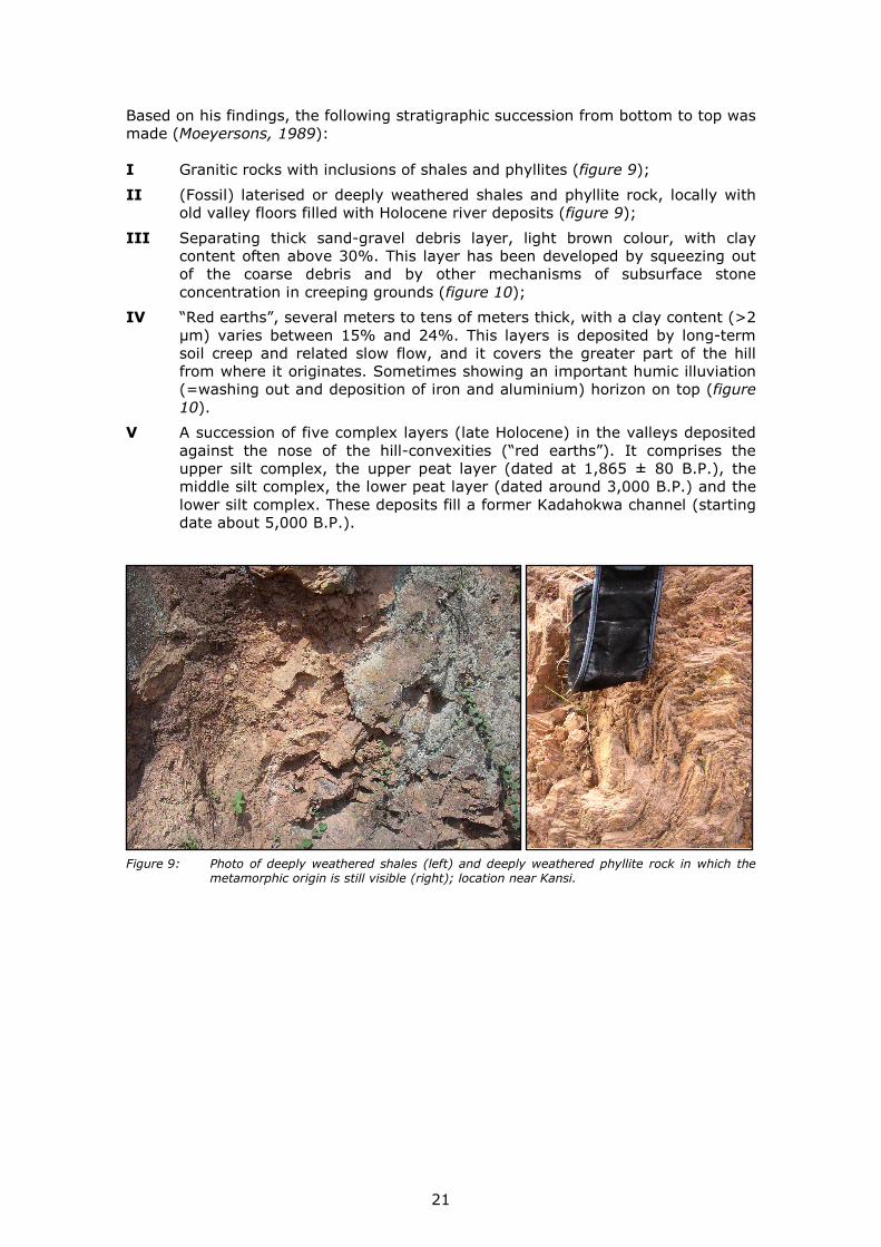
Based on his findings, the following stratigraphic succession from bottom to top was made (Moeyersons, 1989): I Granitic rocks with inclusions of shales and phyllites (figure 9);

II (Fossil) laterised or deeply weathered shales and phyllite rock, locally with old valley floors filled with Holocene river deposits (figure 9);

III Separating thick sand-gravel debris layer, light brown colour, with clay content often above 30%. This layer has been developed by squeezing out of the coarse debris and by other mechanisms of subsurface stone concentration in creeping grounds (figure 10);

IV “Red earths”, several meters to tens of meters thick, with a clay content (>2 µm) varies between 15% and 24%. This layers is deposited by long-term soil creep and related slow flow, and it covers the greater part of the hill from where it originates. Sometimes showing an important humic illuviation (=washing out and deposition of iron and aluminium) horizon on top (figure 10).

V A succession of five complex layers (late Holocene) in the valleys deposited against the nose of the hill-convexities (“red earths”). It comprises the upper silt complex, the upper peat layer (dated at 1,865 ± 80 B.P.), the middle silt complex, the lower peat layer (dated around 3,000 B.P.) and the lower silt complex. These deposits fill a former Kadahokwa channel (starting date about 5,000 B.P.).

Figure 9: Photo of deeply weathered shales (left) and deeply weathered phyllite rock in which the metamorphic origin is still visible (right); location near Kansi.

22

Figure 10: Two photo’s of the sand-gravel debris layer (III) with on top red soils (IV); location near Kansi.

2.2.5 Geomorphology

The Butare plateau in Rwanda was affected by slope and river erosion during the last glacial maximum (approximately 18,000 B.P.). During this period the conditions were relatively dry, and water tables were lower than today. The valleys were wider and occupied by braiding rivers with an important gravel bedload. Conditions that favour braided channel formations are for example large sediment loads, rapid and frequent variations in water discharge and a high stream gradient. During the period between approximately 15,000 B.P. until 5,000 B.P., the annual precipitation became more evenly distributed over the year. The water tables rose and erosion was reduced. The soils on the hillslopes were affected by weathering processes, which lead to the forming of thick humic ferallitic soils (’red earths’), which started to creep from the hills into the valleys, often on top of old fluvial deposits of braided river systems or old laterite soils. The colour of the red earths is in contrast with the light brown colour of the fossil valley bottom. Around 5,000 B.P., the water tables became lower and mass wasting came to an end. Peat formation took place around 3,000 and 1,850 B.P., indicating stable conditions. Hills were covered with a protective vegetation cover. Silt layers that intercalate the peat layers, are related to slope erosion, probably caused by human impacts on the vegetation, for example the intense use of wood for iron melting and associated forest clearing around 1,850 B.P. Nowadays the ’red-earth mantle’ is actively undercut by the rivers in the valleys. [Moeyersons, 2001]

2.2.6 Vegetation and land use

In Rwanda, more than 80% of the inhabitants depend on agriculture for their livelihood (FAO, 2010). A large part of the surface area is used for agriculture. In the southern province, the most common crops are rice, sweet potato, sorghum, beans, cassava and banana6. The Rwandan government is planning to develop and transform the agricultural sector drastically. The aspirations for economical growth are expressed in the ‘2020 vision’. Until 2020 an annual growth of 5.3% is needed. Therefore it is expected that in the near future, the use of fertilizers will increase drastically7.

6 http://www.huye.gov.rw 7 http://www.minagri.gov.rw

23

Most of the agricultural activities take place in the valleys. Close to the rivers, the agricultural fields are often irrigated (figure 11). Further away from the rivers, the fields are fed by rain- and groundwater. The productivity of these fields is lower than the irrigated fields. On hills and at the hillslopes, banana trees (figure 11) or small plots with for example sorghum, cassava or maize are planted. On the hills, small villages and residents are present.

Figure 11: Photo of banana trees (left) and irrigated rice fields in the valley to the southwest of Butare, with trees on the hillslope (right).

Butare is a city with more than 100,000 inhabitants in 2009. The area of Butare is classified as ‘urban area’. A photo of the urban area of Butare is presented in figure 12. Not all the areas in the Migina catchment are used for agriculture or occupied by trees. An example of the natural vegetation on one of the hillslopes in the area is shown in figure 12.

Figure 12: Photo of the urban area of Butare (left) and natural vegetation on a hillslope to the west of

Butare (right).

24

Table 1: Different types of land use in Migina catchment.

The ministry of Agriculture of Rwanda has provided land use maps for Rwanda. The maps are based on data that was collected in 2006. For the Migina catchment the areas with the different land use types (with different dominating crops) that were classified are shown in table 1 and figure 13.

Figure 13: Land use types in Migina catchment.

Description Area (km2) %

Forest plantation 7.207 2.8

Forest, scattered fields 6.497 2.5

Irrigated, herbaceous crops 19.477 7.5

Banana trees 70.439 27.1

Rainfed herbaceous crops 75.007 28.9

Rainfed shrub crops 76.080 29.3

Savannah, trees and shrubs 0.160 0.1

Urban area 5.066 1.9

Total 259.933 100.0

Butare

Save

25

The classified land use types consist of the following crops (Minagri, 2006):

Forest plantation or scattered fields (10% - 40%)

Around Butare, for example near the University campus of the NUR, a forest plantation is present. The forest exists mainly out of Eucalyptus, Pinus and Cypress trees. In one of the valleys, north from the NUR campus, the valley is mainly covered by bamboo trees. Areas with less dense tree coverage are classified as scattered forest plantations, with a density of approximately 10% - 40% of the surface area. The remaining area is covered by natural vegetation (figure 13). Irrigated, herbaceous crops

On the cultivated irrigated fields, in the valleys in the northern part of the catchment, rice and maize are the most common crops. Banana trees

In the northern part of the study area, the land is mostly used to grow banana trees (60% - 70%). Rainfed herbaceous crops (30% - 40%) and natural vegetation cover the remaining surface. Rainfed herbaceous crops

Fields with mainly coffee, banana trees, some rice and maize (40% - 60%) and shrub plantations (20% - 40%). The natural vegetation occupies the remaining area. The fields are not irrigated but fed by rain- and groundwater. Rainfed shrub crops

Fields, also fed by rain- and groundwater, but with a majority of the crops existing mainly out of potato, sorghum, beans and cassava (40% - 60%). A smaller amount of the land is used for the rainfed herbaceous crops (20% - 40%) and remaining natural vegetation. These areas are not as intensive used for agricultural purposes as the two previous land use classes. Savannah, trees and shrubs

A very small area of the catchment is classified as tree and shrubs, savannah. The density of trees and shrubs is lower than the previous land use class. Urban Area

Butare (figure 13) is an important urban area in the northern part of the Migina catchment. Another small urban area is called Save, located in the north-western part of Migina.

26

27

3 Methodology During the study period, a hydrological measurement network was built up. In total five gauging stations, one meteorological station, eleven piezometers, twelve totalizers and four tipping buckets were installed throughout Migina catchment. In addition there was already a meteorological station present at the CGIS-centre in Butare, and a totalizer at the Rwasave fishpond. In figure 14, an overview of all the measuring stations is given.

Figure 14: Overview of all the measuring stations installed in Migina catchment.

28

3.1 Atmospheric water For the investigation of the hydrology of Migina catchment, the atmospheric water component was studied during the research period. Seen from the perspective of this catchment, the input of water from the atmosphere, the precipitation (P), and the output of water towards the atmosphere, the total evaporation (E), was measured.

3.1.1 Precipitation

In order to obtain proper quantitative measurements of precipitation, twelve totalizers have been installed throughout the catchment in the period of 24th April until 19th May. The totalizers (appendix II-1) were made from cheap materials to discourage theft as much as possible. A plastic PVC tube, where a funnel with a diameter of 12.3 cm exactly fitted, was dug in the soil and fixed with concrete. To collect the daily amounts of rainfall, a simple cut open plastic bottle with a volume of at least 400 ml was placed under the funnel. To measure the amount of rainfall, a plastic measuring cylinder, together with a fill-in form and instructions was given to the person in charge of the totalizer. The locations of these totalizers were initially selected in such a way that a proportional distributed network of totalizers was installed to cover the whole of Migina catchment. Primary schools turned out to be the ideal location for placing a totalizer, because these areas are most of the time protected by a guard and a fence and simultaneously have quite some ‘open area’ where disturbances of high buildings and trees are low. To avoid the possible disturbing effect of curious school kids, most of the time the totalizers where installed in the school garden, where children are not allowed to enter. Teachers were instructed to read out and write down the amount of rainfall every day at 07:00 in the morning, in exchange for small financial compensation. To stimulate the participation and also for educational purposes, easy understandable instruction forms as well as the results after each month were provided to the teachers. In total, ten totalizers were installed at the primary schools of the towns of (from north to south) Save, Sovu, Mpare, Vumbi, Muyira, Rango, Kibilizi, Mubumbano, Kansi and Murama. One totalizer was installed in a big garden of the Butares quarter Taba (400 m to the east of the meteorological station at the CGIS-centre) and one totalizer was already present at the NUR fishpond of Rwasave. However, about the latter came clear that repeatedly the amount of rainfall was not read out properly and sometimes not even read out every day, so the decision was made to exclude the Rwasave totalizer from further analysis. A 13th totalizer was installed at 10th June, next to the newly build meteorological station at Nyaruteja. To get a better idea about the structure and evolution of single rainfall events, a tipping bucket8 was installed next to the totalizer of Kibilizi, Mubumbano and Murama. Unfortunately, the tipping buckets (appendix II-2) arrived only after the long rainy season had already stopped. A fourth tipping bucket was installed at the meteorological station at 25th June. A fifth tipping bucket, which was found as part of the meteorological station at the CGIS-centre of Butare, fortunately did register a big part of the rainy season with a time interval of half an hour. The tipping bucket fell out however on 8th June, due to the disappearance of its energy source. Much needed maintenance work also demonstrated that the tipping bucket was grown full with algae, which was removed, but undoubtedly had a major influence on the early results. For quantitative analysis, the results of this tipping bucket will therefore not be used, but the timing is assumed to be still acceptable and will therefore be presented in the time series analysis.

8 HOBO RG3 Data Logging Rain Gauge:

http://www.tempcon.co.uk/html/D233%20HOBO%20RG3%20&%20RG3-M%20Rain%20Gauges.pdf

29

As a result, a time series of the total amount of rainfall is measured by various totalizers for the period of 24th April until 29th July. The exact timing of these rainfall events is measured by one tipping bucket for the period until 8th June. From 25th June onwards 4 tipping buckets has registered the dry season. For all rainfall measuring stations longer time series are available nowadays, but this report will focus on the study period which lasts up to 31st July 2009.

3.1.2 Evaporation

Evaporation is the loss of water from a wet surface through its conversion into water vapor and its transfer away from the surface into the atmosphere. Evaporation may occur from open water, bare soil or vegetation. In addition to the evaporation of intercepted water held upon plant surfaces during and directly after a rainfall event, there is also direct water use by plants termed transpiration. Transpiration is the water taken up by plant roots from the soil which moves up the plant and hence into the atmosphere principally through the leaves in a process closely linked to photosynthesis. Total evaporation (E, expressed in mm) is the combined process of all these kinds of evaporation and transpiration, and this term will be used here from now on. To get an idea about the amount of E in Migina catchment, two evaporation pans has been installed, which give a measure of the pan evaporation (Epan). Evaporation pans provide a measurement of the combined effect of temperature, humidity, wind speed and sunshine on the Epan. Two self-made replications of the U.S. Weather Bureau ‘Class A’ evaporation pans were made (appendix VI-1), of which one was installed at the Rwasave fishpond and one at the meteorological station of Nyaruteja. These iron pans were made circular, with a diameter of 120 cm and a depth of 25 cm and were filled to 5 cm from the pan top. The pan rests on a wooden base, to be able to install the pan carefully leveled and to minimize the effects of ground heat. The scale bar inside the pan was read out manually every day to determine the change in water level and thus the amount of pan evaporation (Epan). Instructions were given to refill the pan every day towards its original level, but this did not happen. Also a number of times exuberant algae bloom and other organics have been observed inside the pan (appendix VI-2), which were subsequently removed but undoubtedly had an effect on the measurements of the days before because of the change in reflectivity. A full month measuring series was obtained in June for both locations, and these results will be presented in chapter 4.1.2.

30

3.2 Surface water For qualitative and quantitative description of surface water in the Migina catchment, several types of hydraulic and hydrochemical measurements have been carried out. To investigate the outflow of surface water, in total five gauging stations has been installed (GS1-GS5 in figure 14) where continuous water level measurements were executed. This will be further explained in chapter 3.2.1. During the study period of this research, detailed analyses of river discharge have been done at gauging station 1, 2 and 3 (GS1-GS3). At these gauging stations, discharge measurements have been carried out at different water levels, to establish a water level-discharge relationship. This relationship is used to make time series of continuous river discharge, so called hydrographs. With these hydrographs, insight will be gained into runoff generation processes, surface water-groundwater interactions and meteoric water responses (chapter 3.2.2).

3.2.1 Gauging stations

In Migina catchment, six old gauging stations are present, which were installed in 1993, but fell into disrepair during the civil war of 1994. The intention of this field campaign was to rehabilitate these old stations, but only one station near the municipality of Rwabuye proved to be suitable for rehabilitation. The other five gauging stations all fell dry due to severe erosion in the past 15 years, which lowered the level of the rivers dramatically. Next to the rehabilitated old gauging station, gauging station 1 (GS1), two new gauging stations have been built up: gauging station 2 (GS2) and gauging station 3 (GS3). The locations of these three gauging stations can be found in figure 14. Location selection criteria Accessibility, security and the possibility of maintenance were the three main practical criteria for the selection of the location of GS2 and GS3. Within these boundary conditions a hydrological acceptable location was sought, based on the criteria as described by Waterloo et al (2007). This means that the gauging station should be preferably on a straight part of the channel with laminar flow and without too much disturbances like vegetation or human activities (e.g. gravel digging, washing of clothes or a drinking spot for cattle). Special attention was paid to the level of the gauging station, which should be high enough to be able to measure the water level also during the expected high flows. First of all, a subcatchment of the Migina catchment was selected as study area, so that all locations within the study area would be accessible by car within one hour driving. The catchment which is studied in this research is called Butare catchment from now on. Butare catchment is thus a subcatchment of the bigger Migina catchment (figure 14). Within Butare catchment, the main outlet and two outlets of subcatchments were selected to be gauged. All three gauging stations are close to a road, so that they are good accessible, but also under ‘social control’ of the people passing by every day. To increase the protection, a guard was paid for every gauging station to keep an eye on it. Also the local people were involved by explaining them about the project and by letting them participate where possible. Gauging station 1 (GS1) is located at the North of Butare, in the municipality of Rwabuye, where the tar-road between Kigali (RWA) and Butare (RWA) crosses the river Gyezuboro. Its location is in the middle of a wide valley full with rice fields, 10 m downstream of the truncation between the river Nyagashubi (coming from the north) and the river Kidobogo (coming from the north-west). The gauging station already existed, but has been out of use since 1994. Therefore, an intense cleaning of the housing and the tube was needed, after which the old station could be rehabilitated. Gauging station 2 (GS2) was installed at the place where the river Kadahokwa is flowing underneath the tar-road between Butare (RWA) and Bujumbura (BUR). The

31

river Kadahokwa is one of the main contributories of the river Migina in the west of Butare catchment. This location was selected for its high accessibility and because no gravel digging activities (which are expected to influence the cross sectional area of the river) close to the foundations of the bridge are allowed by law. Gauging station 3 (GS3) was installed in the river Migina at the main outlet of the Butare catchment, 20 m downstream of the truncation between the river Rwanganiro (a continuation of the river Kadahokwa) and the river Kihene (the river coming from the north, passing by the city of Butare). The accessibility of this location was reasonable, located on the dirt road between Butare (RWA) and Ngozi (BUR). More importantly, the local people of the nearby municipality of Kansi proved to be very helpful in building and protecting the gauging station. Installation Instead of measuring the water level directly in the river, a construction was made for on-land measurement of the water level (appendix III). This was the only solution for building a cheap and well-protected gauging station that would be resistant against theft of useful parts and/or vandalism. With the help of local people, a narrow ditch was dug perpendicular to the river with a depth corresponding to the lowest expected water level in the river. In this ditch, an L-shaped PVC-tube was constructed with one opening at the bottom of the river and the other opening on-land. In this way, the water level variations in the tube would correspond with the water level variations in the river. Around and above the on-land opening of this tube, a metal casing was installed, fixed in the soil with concrete and with a moveable cap with lock on top. At the opening on the riverside, a screen was constructed to avoid plants or animals to enter the tube. In the river, next to the tube, a staff gauge was installed on which the real water levels could be read out. The scale of the staff gauge was made by measuring tape, which was fixed on a wooden post with nails. The post was put in a big block of concrete (>200 kg) to keep the staff gauge stable, straight and immovable in the river. Measurements At these gauging stations, systematic observations of water levels were obtained by combining manual staff gauge readings with continuous automatic water pressure measurements. The water pressure was measured automatically with a D or TD-Diver9 at an interval of 15 minutes. This diver was constructed at the deepest point of the L-shaped PVC-tube and data was read out and stored on a laptop once in two weeks. Manual staff gauge readings were done as often as logistically possible; resulting in an average read out of once a week, with a higher frequency in the beginning of the study period during the rainy season with greater variations in water level. To provide reference measurements of the river stage, the level of the staff gauge was surveyed relative to a local benchmark, by using a theodolite10 and a scale-bar. The local benchmarks are marked points on or nearby bridges, which can be seen in appendix IV. Data management The water pressure measurements of the TD-Divers have been corrected for atmospheric pressure variations. Therefore, a Baro-Diver11 was installed in Butare of which the measured daily variation in atmospheric pressure has been subtracted from the water pressure measurements of the TD-Divers.

9 TD1/TD2/D2 Diver - former Van Essen Instruments (nowadays: Schlumberger Water Services) 10 Sokkia – Electronic Digital Theodolite DTX20 series - DT520:

http://www.sokkia.com/Products/Detail/DT620.aspx 11 Baro Diver – former Van Essen Instruments (nowadays: Schlumberger Water Services)

32

Also corrections by hand have been made for outliers, for example non-situ measurements during the read out of the diver, and for sudden shifts in water pressure, caused by a change in installation depth of the TD-Diver. After these corrections, the automatic measured water level variations have been compared with the manual staff gauge readings, which proved to be highly comparable to each other. Because the manual readings of the water level from the staff gauge have a high accuracy (±0.5 cm) and are in-situ measurements, the automatic water level measurements have been corrected also for the manual readings. The result is a reliable continuous time series of water level, which will be presented in chapter 4.2. To reference the final river stages, a water level of 0.000 m on the staff gauge corresponds to:

• 2.907 m below the benchmark for gauging station 1 • 2.484 m below the benchmark for gauging station 2 • 5.424 m below the benchmark for gauging station 3

3.2.2 Rating curves and time series

The discharge of the rivers has been measured with an Ott-propeller (VU University Amsterdam; appendix V-1) at varying water levels. Before the field measurements, this Ott-propeller was calibrated in a flow machine (appendix V-2) to be able to correlate the speed of rotation of the propeller to the velocity of the water that is causing this rotation. To create a velocity profile of the river, velocities were measured at every 20 cm along a cross-sectional profile of the river. At these locations the velocity of the water was measured at 60% of the channel depth, after which the total discharge has been calculated using the velocity-area method as described in van Breukelen et al, 2007. After subsequently plotting this single measurements of discharge Q [m3 s-1] against the corresponding water level h [m], a mathematical relationship between Q and h was obtained, using a regression line function in the spreadsheet programme Excel. This so called rating curve is a unique characteristic for a single river and is needed to convert the water level time series from the gauging station to a discharge time series.

33

3.3 Groundwater For the qualitative and quantitative description of the groundwater in the Migina catchment, several piezometers were installed and several types of measurements have been carried out. The quality of the groundwater is studied by sampling and analyzing the water coming from some of the springs that were found in Migina catchment. More information about the springs is presented in chapter 3.3.1. To investigate the level changes of the groundwater, two transects with piezometers were installed where continuous water level measurements were carried out. More details about the piezometers is included in chapter 3.3.2, where in chapter 3.3.3 details about the water level measurements are described. From this data, daily fluctuations were obtained. How this was done can be found in chapter 3.3.4.

3.3.1 Springs

In the rural areas around Butare, water from springs is mainly used as a source of drinking water. Electrogaz, a state owned public company that treats and supplies water, is only able to deliver its treated water to Butare and some of their urbanized areas nearby. Therefore, the water quality of the springs is very important for the health of the people that live in the rural areas. In accordance to statistical data that was obtained by Kasanziki (2008) 8% of the people in the area around Butare use piped water as their main water source and 81% of the people use springs as main source of water. The remaining 11% relies on water from rivers (5%), lakes/ponds (5%) and other sources (1%). In the whole Migina catchment, a lot of those springs are present. The springs are mostly located at the foot of the hills. In most cases, the spring is made of a pipe, which is connected to the groundwatertable (figure 15). The constructions of the springs are relatively new. The spring of Gahenerezo was for example constructed in 2000 and the Rwasave spring in 2003. The springs of Mpare and Mpazi are a little older and were constructed in 1991 (Kasanziki, 2008).

Figure 15: Two photographs from open springs in Migina catchment; used to collect drinking water from in plastic jerrycans.

The water that comes from the springs is shallow groundwater, mostly located at the contact between the hillslope and the valley floor. On top of these hills, a lot of residents can be found. Their waste is disposed directly into the ground, in some

34

cases by using septic tanks. In this way, the groundwater, which feeds the springs, might be affected. In the Migina catchment, more than fifty springs might be present. This number is a rough estimation, as precise numbers and locations are not available. During this study, a select number of the springs are located. Also the electrical conductivity and the pH of the water are measured. Some are sampled and analyzed for its chemical contents. The results can be found in chapter 4.3.1. In table 2 the coordinates of the selected springs are presented. The numbers is the Table refer to the numbers in the map of the catchment. This study focused mainly on the northern part of the Migina catchment, the so called Butare catchment. As a result, in the northern part, 12 springs are located and in the south only 3. It is expected that some more springs can be found in the north, and much more in the south.

Figure 16: Locations of springs in Migina catchment. Table 2: UTM coordinates of springs in Migina catchment; the numbers in the Table correspond to the numbers in the map (figure 16).

UTM coordinates, zone 35S

# Name East (m)

North (m)

Altitude (m.a.s.l.)

1 Sovu 0800948 9717210 1733 2 Ghahenerezo 0804136 9714635 1671 3 Nabagado 0806274 9714124 1652 4 Kinteko 0806973 9713221 1643 5 Rwasave 0806184 9712510 1665 6 Mpare 0803405 9710842 1652 7 Kamugegemge 0802604 9710041 1682 8 Runyinya 0803703 9709864 1644 9 Gakombe 0801008 9708431 1694 10 Kadahokwa 0802179 9708263 1646 11 Mpazi 0805879 9707830 1633 12 Irango 0804610 9707503 1614 13 Kibingo 0801597 9699935 1575 14 Nyamugali 0801646 9693089 1536 15 Nyarunazi 0802291 9693333 1542

35

3.3.2 Piezometers

In one of the small valleys near Butare, changes in groundwater level are monitored. The selected valley is located in an area called “Kadahokwa marshland”, which is located southwest from Butare. To be able to measure the groundwater levels, a couple of piezometers (open wells, made from PVC tubes) are installed. The piezometers are placed in two parallel transects, between the hillslope and river. The distance between the two transects is approximately 60 m. Transect ‘A’ consists of 7 piezometers, transect ‘B’ consists of 4 piezometers. An overview of the locations of the piezometers is given in figure 17.

Figure 17: Locations of the piezometer transects A1 - A7 and B1 – B4, shown on a aerial photograph (left, © Google Earth) and on a map (right).

The piezometers are constructed from polyvinyl chloride (PVC) pipes. The bottoms of the tubes are closed with concrete. The tubes are provided with a screen of small slots over a length that varies between 0.3 and 1.6 m. The screen is made by perforating the PVC tube with a saw. The length of the screen is chosen depending mainly on soil material and the thickness of permeable layers that are found. If possible, the screen is located at a depth where permeable layers are present. The permeable layers that are found contain sands and gravels. Before installing, filter stocking is put over the slots to prevent the tube against sedimentation. After preparation, the tube is placed in the drilled hole. Then the borehole (along the tube) is filled up. First, next to the screen, the borehole is filled up with a gravel pack, to prevent the filter from clogging. On top of these gravels, the original material is replaced. Finally, the top of the piezometer is filled up with clays, to prevent the flow of for example rainwater along the tube. On top of the tubes metal casings are placed, that can be closed with a lock. The casings are fixed in concrete.

B1 B2

B3

B4

A5 A6 A7

spring

A11

A2 A3 A4

bridge

� N

River Road

36

A handheld GPS receiver12 was used to measure the UTM coordinates of the locations. This GPS receiver has an indicated error for the x and y coordinates of approximately 3 m. The topography and the locations of the piezometers of transect A are presented in figure 18. The river is located at the origin of the graph.

Figure 18: Topography and piezometers of transect A. The topography and the locations of the piezometer of transect B are presented in figure 19. The topography of transect B is lower and more flat than transect A. Piezometer B4 is located in the transition zone between the valley and the hillslope. The location of piezometer B4 is relatively wet, compared to the surrounding area.

Figure 19: Topography and piezometers of transect B.

12 Garmin eTrex Vista HCx

http://www.garmin.nl/product/?pid=010-00630-01

37

The locations of the different piezometers are displayed in figure 17, figure 18 and figure 19. Table 3 shows the coordinates of all the piezometers, from which A3 – A7 are recorded on photo (figure 20). The lengths of the piezometers, lengths of the screens and coordinates of the piezometers are included in table 3. Table 3: Overview of the coordinates, lengths and screen lengths of the piezometers, as well as the coordinates of Kadahokwa spring.

UTM coordinates zone 35S

Length Screen length

Code East (m)

North (m)

Z (m.a.s.l.)

(m) (m)

A1 0802282 9708167 1640.7 1.37 0.8 A2 0802275 9708165 1642.6 3.16 0.8 A3 0802253 9708164 1642.6 2.92 0.8 A4 0802247 9708163 1643.2 4.59 1.6 A5 0802232 9708165 1644.5 3.25 0.8 A6 0802224 9708159 1645.8 2.92 0.8 A7 0802211 9708156 1647.4 4.10 0.8 B1 0802230 9708232 1642.2 2.21 0.5 B2 0802214 9708225 1642.4 2.26 0.5 B3 0802199 9708217 1642.4 2.62 0.5 B4 0802190 9708204 1643.2 1.12 0.3

Spring 0802179 9708263 1646.0

Figure 20: Photo piezometers A3 - A7.

Kadahokwa spring Approximately 50 m north from transect B an open spring is present (figure 21). According to the local people, the spring flows throughout the year. The study period was almost completely dry, nevertheless the spring kept flowing.

The location of the spring near the piezometer transects is given in UTM coordinates in table 3. During the study period the flow rate of the spring was measured. The flow rate is determined by volumetric measure-ments. The time needed to fill a small bottle of 0.6 l was measured with a stopwatch. The measurements are carried out 8 times, starting at 28th May 2009 and ending at 15th July 2009. The water of the spring was also sampled and analyzed for its chemical content.

Figure 21: Kadahokwa spring. During the study period, the water from the spring was sampled 6 times during a period of 6 weeks, starting at 28th May.

38

3.3.3 Water levels

The groundwater levels in the tubes are measured twice a week, using water level sounding tape. Pressure transducers (Mini-Diver13) are installed to obtain automatic water level and temperature records every 15 minutes. In one of the piezometers (piezometer A4) a Baro-Diver14 is installed to obtain barometric data. The data of the Baro-Diver is used to correct the groundwater level measurements for changes in air pressure. The water levels are also corrected by using the hand measurements that were carried out. On 24th June, the casing of one of the piezometers was destructed. Therefore, all the divers were removed until the security of the equipment was secured. On 29th June, the divers were replaced, and the continuous measurements continued. To be able to relate the water levels in the different piezometers to each other, the elevations of the top of the piezometers are levelled using the theodolite. The elevations are given in appendix XXV.

Daily fluctuations The compensated 15 minute water level records are used to obtain daily data. Therefore the data is sorted per day and changes are observed in accordance to the water level at midnight (00:00).

3.3.4 Hydrochemical sampling of groundwater

After the construction of the piezometers, the water in the tubes is removed by using a handpump. Then, the tube is filled with water from the river. This procedure was carried out at least three times, to be certain that the water from the piezometers was not influenced by the materials that were used to build the piezometer. After a week, the water in the piezometer is removed with the pump, to get fresh water in the tube. In this way, the influence of the introduced river water is supposed to be negligible. The water in the tubes is now supposed to be the original water and ready to be sampled. Most of the piezometers of transect A are sampled at least 5 times. The piezometers of transect B weren’t ready at that time. As a result, the piezometers of transect B are only sampled 1 time. The sample dates per piezometer are presented in table 4. The river, close to piezometer A1 is sampled 7 times, the spring 6 times. Table 4: Dates when water from the piezometers was sampled.

# Date river A1 A2 A3 A4 A5 A6 A7 B1 B2 B3 B4 spring

7 22/05 � 6 28/05 � � � � � 5 13/06 � � � � � � � 4 20/06 � � � � � � � 3 27/06 � � � � � � � � 2 04/07 � � � � � � � � � 1 11/07 � � � � � � � � � � � �

13 Schlumberger Water Services

http://www.swstechnology.com/groundwater-monitoring/groundwater-dataloggers/mini-diver 14 Schlumberger Water Services

http://www.swstechnology.com/groundwater-monitoring/groundwater-dataloggers/baro-diver

39

3.4 Soil properties The hydraulic functions of the unsaturated soil are important parameters to understand hydrological, ecological and agricultural processes and interactions. Knowledge about the factors controlling water storage and movement in the soil is essential to understand the supply of water to plants but also the generation of runoff, the recharge to the underlying groundwater and the movement and accumulation of pollutants. In this field study, the vertical conductivity or infiltration capacity was measured with a double ring infiltrometer. Also 22 soil aggregates has been taken, from which a grain size analysis has been done in the VU University soil lab. Besides these bulk soil samples, also twelve small undisturbed soil-cores with a known volume has been stuck, from which porosity, bulk density, permeability and the water retention capacity are obtained. The samples (cores and bulk samples) are taken from the locations as presented in table 5 and figure 22. Table 5: Soil sample locations.

Location Depth (m) Core Bulk Dughole C1

- SS 4 0.95 - 1.00 � � - SS 1 1.65 - 1.70 � � - SS 2 1.90 - 1.95 � � - SS 3 2.05 - 2.10 � � Dughole C2

- SS 5 1.05 - 1.10 � � - SS 7 1.20 - 1.25 � � - SS 8 1.75 - 1.80 � � - SS 6 2.15 - 2.20 � � Piezometer A5

- 2.1 0.25 - 0.30 � � - 2.2 0.75 - 0.80 � � - 2.3 2.25 - 2.30 � Piezometer A7

- 1.1 0.25 - 0.30 � - 1.2 0.95 - 1.00 � - 1.3 2.55 - 2.60 � - 1.4 3.95 - 4.00 � Piezometer B1

- 3.1 1.15 - 1.20 � - 3.2 1.95 - 2.00 � - 3.3 2.20 - 2.25 � - 3.4 2.45 - 2.50 � Piezometer B2

- 4.1 2.00 - 2.05 � Piezometer B3

- 5.1 2.80 - 2.85 � Piezometer B4

- P11a 0.40 - 0.45 � � - P11b 0.60 - 0.65 � �

Figure 22: Soil sample locations.

3.4.1 Bore- and dugholes

For the installation of the piezometers in the valley of the river Kadahokwa, boreholes had to be made. The holes were drilled using an Edelman hand auger. During the drilling of these holes, the soil material was placed next to a measuring scale and described. At some depths, samples were taken for further analysis. In addition to the 11 boreholes for the piezometers, two holes were dug. The holes have a size of 2 m by 1 m, and a depth of approximately 2 m. Bulk samples from the soil and undisturbed samples were taken from the different layers that were found. The samples are used for lab analysis, to obtain some important soil characteristics, such as permeability, grain size distribution and bulk weight. The

C2

C1

A2

B1

A5 A6 A7 A1 A4 A3

B2 B3

B4

spring

bridge

40

coordinates of the dug holes are given in Table 6. Figure 23 shows a photograph of one of the dug holes. Table 6: Coordinates and depth of the dugholes.

Figure 23: Dughole 2 (C2).

3.4.2 Field permeability

The functioning of the subsurface drainage system depends on a great extent on the soil’s saturated hydraulic conductivity (Oosterbaan and Nijland, 1994). Various methods have been developed to determine the hydraulic conductivity of soils. In this study, the horizontal saturated hydraulic conductivity (Ks;h) of the soil layers around the screens of the different piezometers is estimated by carrying out falling head tests. This test is based on introducing water into a piezometer. The decline of the watertable is monitored as a function of time. To be able to measure the watertable inside the piezometer, a pressure transducer (Mini-Diver) is installed inside the piezometer. The time interval of the pressure transducer is set to a relatively small time interval. In the tests that are performed for this study, the time interval is set at half a second. After installing the Mini-Diver, the watertable in the piezometer is raised in a couple of seconds by filling it instantaneously with buckets of water. It is preferable, but proved to be not always possible in case of too high transmissivity, to fill the piezometer as soon as possible until the top. The measured water levels in the tube are recalculated to the increase according to the normal watertable (h0 in figure 24). The increase is expressed in cm. The highest watertable is the water level at time step 0. The development of the watertable in time is expressed in seconds. The decline of the watertable is plotted on a logarithmic scale against a linear timescale. The slope of the first straight part of the graph is used for the calculation of the hydraulic conductivity.

Figure 24: Permeability test. This means that in most of the cases, only the part of the graph is used until a quarter of the increase of the watertable has disappeared. Formulas for field permeability test in piezometers with an open basal section (a screen or injection zone) in non consolidated soils are first described by Hvorslev (1951). An overview of the different formulas that can be applied is given by

UTM COORDINATES, zone 35S Length

East (m) North (m) (m)

C1 0802286 9708162 2.15 C2 0802268 9708146 2.20

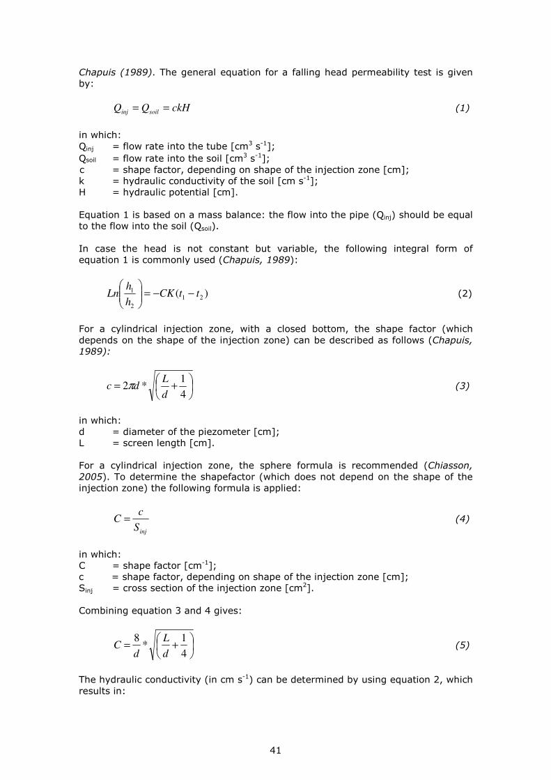
41

Chapuis (1989). The general equation for a falling head permeability test is given by:

ckHQQ soilinj == (1)

in which: Qinj = flow rate into the tube [cm3 s-1]; Qsoil = flow rate into the soil [cm3 s-1]; c = shape factor, depending on shape of the injection zone [cm]; k = hydraulic conductivity of the soil [cm s-1]; H = hydraulic potential [cm]. Equation 1 is based on a mass balance: the flow into the pipe (Qinj) should be equal to the flow into the soil (Qsoil). In case the head is not constant but variable, the following integral form of equation 1 is commonly used (Chapuis, 1989):

)( 21

2

1 ttCKh

hLn −−=

(2)

For a cylindrical injection zone, with a closed bottom, the shape factor (which depends on the shape of the injection zone) can be described as follows (Chapuis, 1989):

+=

4

1*2

d

Ldc π (3)

in which: d = diameter of the piezometer [cm]; L = screen length [cm]. For a cylindrical injection zone, the sphere formula is recommended (Chiasson, 2005). To determine the shapefactor (which does not depend on the shape of the injection zone) the following formula is applied:

injS

cC = (4)

in which: C = shape factor [cm-1]; c = shape factor, depending on shape of the injection zone [cm]; Sinj = cross section of the injection zone [cm2]. Combining equation 3 and 4 gives:

+=

4

1*

8

d

L

dC (5)

The hydraulic conductivity (in cm s-1) can be determined by using equation 2, which results in:

42

16.5 cm

33.0 cm

C

tth

h

K

tt )/(ln 0

0

−

=− (6)

As the diameters of the piezometers are all the same (5 cm) and the length of the screen is in most cases 0.8 m, equation 5 can be simplified into: C = 8/5 * √(80/5 + ¼) from which follows that C = 6.45 [cm-1].

3.4.3 Infiltration capacity

The saturated hydraulic conductivity of the soil surface can be determined by using a double-ring infiltrometer. A double-ring infiltro-meter consists of an inner and an outer ring, which are inserted into the soil for approximately half its height. The outer ring is used to obtain only a vertical flow into the soil in the inner ring. The outer ring, also contributes to lateral flow. A standard double-ring infiltrometer is made of stainless steel, and has diameter dimensions of 30 cm (inner ring) and 60 cm (outer ring).

Figure 25: An improvised double-ring infiltrometer, made of three cooking pans. The infiltrometer that was used for this study is made of a big and a small cooking pan (figure 25) as there was no standard one available. The outer ring has a diameter of 33.0 cm and the inner ring has a diameter of approximately 16.5 cm. In both rings a constant head of water is obtained by adding water when the watertable drops. When the water flow rate in the inner ring has become constant, the hydraulic conductivity of the soil surface can be estimated (van Breukelen et al, 2008). The test was therefore carried out approximately ten times at every location. The infiltration capacity was determined at 4 different locations, near piezometer transect A. The locations are included in table 7. Table 7: Coordinates of infiltration test locations.

UTM coordinates, zone 35S

# Name East (m)

North (m)

Elevation (m.a.s.l.)

1 location 1 802282 9708167 1633

2 location 2 802232 9708165 1645

3 location 3 802253 9708164 1634

4 location 4 802275 9708165 1643

43

3.4.4 Soil water permeability

The undisturbed soil sample rings are used to measure the saturated hydraulic conductivity (Ksat) at the soil lab of the VU University Amsterdam. The Ksat values are obtained in a so called closed system permeameter (figure 26). The methodology is described in the ’operating instructions laboratory permeameter’ (Eijkelkamp, 2008). In a closed system, water is pumped up from a storage cistern into a container with a certain stable watertable level, through a filter. A saturated ring is placed inside a ring holder, which is placed inside the container with the regulated, stable watertable. Depending on the permeability of the soil sample, a certain amount of water will flow through the sample into a burette, in which the total amount of water can be determined. The permeability of the samples is measured by using 2 different methods: one for samples with a high or moderate permeability and one for samples with a low permeability. Constant head method: Samples with a high or moderate permeability are measured by using the constant head method. A constant water level difference is maintained between inside and outside of the sample. The volume of water that is drained through the sample will flow into the burette, and can be measured in time. The flow has to become stationary, which means that the volume of water that flows through the sample in a certain time has to become constant. The head difference inside and outside the sample can be measured by using a measuring bridge with a metering pin, which has an accuracy of 0.5 mm. Figure 26: Photo of the closed system permeameter. Based on Darcy’s law, the head difference is used to calculate the saturated permeability coefficient:

hTA

LVK

**

*= (7)

in which: K = permeability coefficient (cm d-1); V = volume of water flowing through the sample (cm3); L = length of the soil sample (cm); A = cross-section surface of the sample (cm2); T = length of time lapse (d); h = water level difference inside and outside the sample (cm). Falling head method The falling head method is used for samples with a low permeability, such as clay and peat. The change in water level (dh) is measured during a certain time (dt).

44

The water level difference is used to calculate the saturated permeability coefficient. For the falling head method an adjustment of Darcy’s law formula is used:

)2*1(*

**

2

1ln*

)12(*

*

hhA

Lax

h

h

ttA

LaK +

−

= (8)

in which: K = permeability coefficient (cm d-1); V = volume of water flowing through the sample (cm3); L = length of the soil sample (cm); a = cross-section surface of the ringholder (cm2); A = cross-section surface of the sample (cm2); t = length of time lapse (d); h = water level difference inside and outside the sample (cm). [Operating instructions laboratory permeameter, March 2008, Eijkelkamp]

3.4.5 Soil moisture, porosity and bulk density

As a soil dries out due to drainage and total evaporation, progressively smaller pores are emptied and pressures become increasingly negative. Suction is the force with which water is held in the pores between the soil particles. The main suction forces responsible for holding water in the soil are those of capillarity, adsorption and osmosis. The relationship between suction pressure and soil moisture content can be graphically presented by means of the so-called water retention curve (or pF-curve), in which the soil moisture content (θ) is expressed in volumetric percent and plotted against the logarithmic suction pressure (pF), expressed in centimetres water column. It can be expected that different relations exist for different sediments, depending on their characteristics, such as pore geometry and mineralogy. For the measurement of soil moisture retention, twelve small soil-core rings with an exact volume of 100 cm3 were taken. To determine the amount of soil moisture that in one sample can be retained at a certain suction pressure, a sandbox (Eijkelkamp)15 working on water pressure was used (pF values of 0 - 2), in which moisture tensions are obtained by creating a series of under-pressures and over-pressures. A membrane press16 working on nitrogen gas pressure (figure 27) was used for pF values between 3 and 4.2. Unfortunately, the sandbox working on water/mercury pressure, used to measure pF values between 2 and 3, was not working, so pF-values within this range could not be determined empirically. A pF value of 5 was measured by air-drying the samples for a few months, and a pF value of 7 was measured by oven-drying (105°C) the samples for 24 hours, which is assumed to dry the soil samples completely. In this way, the volumetric soil moisture content was obtained for pF values of 0.0, 0.4, 1.0, 1.5, 1.8, 2.0, 3.0, 3.7, 4.2, 5.0 and 7.0, which corresponds respectively with a suction pressure of 0.001, 0.0025, 0.01, 0.032, 0.064, 0.1, 1, 5, 15, 100 and 10,000 bar. 15 Eijkelkamp Agrisearch Equipment, 08.01 Sandbox for pF determination (pF 0 - 2.0)

http://www.eijkelkamp.com/Portals/2/Eijkelkamp/Presentations/pF%measurements%20in%20the%lab.pdf 16 Eijkelkamp Agrisearch Equipment, 08.03 Membrane apparatus for pF determination (pF 3 – 4.2)

http://www.eijkelkamp.com/Portals/2/Eijkelkamp/Presentations/pF%measurements%20in%20the%lab.pdf

45

Figure 27: Photo’s of the membrane press used for measurements of pF = 3 - 4.2. On the left photo,

the membrane press is in use, at a pressure of 5 bar (corresponding to pF = 3.7), the membrane and the samples inside the press, can be seen on the right photo.

Unfortunately, the measurements with the membrane press proved to give some difficulties. To be able to get rid of the water in the samples but build up the air pressure inside the press at the same time, a special membrane was used which allows water to pass but not air. For some reason this membrane started to leak at a pressure of 15 bar after some days; most probably related to damage gained by hard and unrounded quartz particles inside the samples. Repeatedly these measurements were carried out, even with a double or triple membrane, but time after time the membrane broke (through what the required pressure could not be build up in the press anymore). Therefore, a complete measurement of pF = 4.2, for which the pressure should be at a constant level at least for a week, could not be done. In the end, the soil moisture content was measured after only a few days of constant pressure in the press. Because the membrane was broken, the results gives significant outliers with for some samples even a higher soil moisture content than for pF = 3.7. Therefore, the measured results of pF = 4.2 are assumed to be unreliable and are not plotted in the pF retention curve (chapter 4.4.2). The porosity was measured for the 12 small soil-core rings by subtracting the oven dry weight of the samples (pF = 7) from the total weight of the saturated samples (pF = 0), and dividing this weight (assuming 1 gram of water = 1 cm3 of water) by the total volume of the sample (= 100 cm3). The resulting porosity is actually the ‘effective porosity’, because closed pore spaces where water is not able to enter is not taken into account. The bulk density of the 12 small soil-core rings was obtained by dividing the oven dry weight of the samples (pF = 7) with the total volume of the samples (= 100 cm3). Correction was made for small missing parts in the soil-cores by estimating the missing volume.

3.4.6 Grainsize

At several locations samples were taken for a grainsize distribution analysis. Therefore an amount of circa 250 gram of material was collected at a certain depth of a borehole profile. The samples were collected in sample bags. The grainsize distribution of the bulk samples were analyzed at the soil laboratory of the VU University Amsterdam. Grain sizes from 0.1 µm until 20 mm are analyzed by using laser diffraction17. The distribution of the grains which are bigger than 20 mm (gravels) are analyzed separately by using a sieve.

17 Sympatec, Helos/KR QUIXEL (http://www.sympatec.com/LaserDiffraction/HELOS.html)

46

Figure 28: Heating the beakers with the samples. Figure 29: Samples are left standing over for eight hours so the sediment can settle.

Small fraction (0.1 µm until 20 mm) To be able to analyse the samples by laser diffraction, the soil needs to be prepared carefully. Therefore a certain amount of soil needs to be taken, to achieve a certain beam observation (of 20% to 25%) of the laser. The sample is put in a beaker and distilled water is added. Oxidation is carried out by adding 5 ml of 30% H2O2 and heating the sample. After cooling and cleaning the beaker, 5 ml of HCL 10% is added. More acid is added when a violent reaction takes place. The sample is heated and boiled for 1 minute (figure 28). After boiling, the beakers are filled up to the top (figure 29). Then the beakers are left standing over for approximately 8 hours. Then, the water in the beaker is removed, and refilled to 100 ml again. About 300 mg of Na4P2O710H2O is added and the beaker is heated until boiling point is reached. After cooling down, the sample is ready to be analysed by laser diffraction (figure 30). Figure 30: Analysing the grainsize with the laser.

Gravel fraction (>2mm) To determine the amount of gravels in a sample, a small amount of soil is taken, weighted and sieved. The grains that are bigger than 20 mm are collected by using a sieve. The grains that remain are dried and weighted. The amount of gravels (>20 mm) is calculated with the relative dry weight of the gravels in according to the total dry weight of the sample.

47

3.5 Hydrochemistry To investigate the water quality and to get better insight into the different sources and pathways of the surface water and groundwater, hydrochemical field analyses as well as sampling for hydrochemical lab analysis have been executed. Water samples were taken and analyzed in the field or the same day and analyzed for certain parameters. Water samples are analyzed for their full chemical composition at the Laboratory for Water Analysis of the VU University Amsterdam18. At UNESCO-IHE in Delft, the isotopic composition of the water is determined.

3.5.1 Field measurements

In the field, the electrical conductivity (EC) and temperature were measured with an EC-meter and pH and temperature were measured with a pH-meter. Calibration of the EC-meter took place every month; calibration of the pH-meter took place before every measurement. EC measurements were standardized automatically to 25°C. For some parameters the concentrations were determined at home at the same day as the samples were taken. These measurements were carried out with titrations and a colorimeter. Titrator The concentrations of bicarbonate (HCO3

-), calcium (Ca2+) magnesium (Mg2+) and chloride (Cl-) were determined using a digital titrator19. Colorimeter The concentrations of nitrate (NO3

-), Silica (SiO2), Ammonium (NH4+) and

Phosphate (PO43-) were determined using a portable colorimeter20.

3.5.2 Lab hydrochemical composition

The water samples that are collected in the field are analyzed for their full hydrochemical composition at the Laboratory of Water Chemistry from the Department of Hydrology and Geo-environmental Sciences from the VU University Amsterdam. In the laboratory the different elements and complexes are measured by an ion chromatograph, a spectrometer and an aquakem, as described below. Table 8: Accuracy of the ion- chromatography analysis.

Ion chromatograph21 An ion chromatograph was used to measure the ions fluoride, chloride, bromide, nitrate and sulfate. The accuracy of the different measured ions can be found in table 8.

18 http://ecohydro.falw.vu.nl/hydrolab/ 19 Hach - Digital Titrator: http://www.hach.com/hc/search.product.details.invoker/PackagingCode=1690001 20 Hach - DR/890 Portable Colorimeter: http://www.hach.com/hc/search.product.details.invoker/PackagingCode=4847000 21 Dionex - DX-120 Ion Chromatograph: http://www.dionex.com/en-us/webdocs/4520-31183-03.pdf

Element accuracy

Fluoride Fl 0.01 mg l-1 Chloride Cl 0.05 mg l-1 Bromide Br 0.03 mg l-1 Nitrate NO3 0.03 mg l-1 Sulfate SO4 0.05 mg l-1

48

Table 9: Accuracy of the aquakem analysis.

Aquakem22 The Aquakem is a fully automated discrete photometric analyzer, which is used to determine the concentrations of bicarbonate, ammonium, nitrite and phosphate. The accuracies of the different measurements are displayed in table 9. Inductively coupled plasma optical emission spectrometer (ICP-OES)23 In total 42 macrocations and trace elements like heavy metals were measured with an inductively coupled plasma optical emission spectrometer. There are no accuracy details about the different ions available.

3.5.3 Isotopes

The water samples are analyzed for their isotopic signature at the laboratory at UNESCO-IHE in Delft. The isotopes are analyzed with a liquid-water isotope analyzer24, which provides measurements of δ18O and δ2H in liquid-water samples with accuracy better than 0.2‰ for 18O/16O and better than 0.6‰ for 2H/1H. The measuring strategy is based on a high-resolution spectroscope.

3.5.4 Field sampling

Water samples for analysis with the ion chromatograph and aquakem were filtered in the field (0.45 µm membrane filter) and taken in a virtually airtight 10 ml bottle without conservation. For ICP-OES analysis, filtered samples (0.45 µm membrane filter) were taken in a virtually airtight 50 ml bottle without conservation. Before lab analysis, 3 till 14 weeks after field sampling, these samples have been acidified with 0.35 ml 65% HNO3 suprapure to reverse the precipitation of cations and dissolve the flocks again. Water samples for isotope analysis were taken unfiltered and without conservation in airtight 2 ml bottles. All samples were cooled (7°C) within 8 hours after sampling until lab analysis took place. Sampling from piezometers took place after refreshing the volume of the piezometers at least three times with use of a hand-pulse pump. Surface water was sampled directly with use of a clean and preflushed 60 ml syringe, which was filled directly from the open water. Precipitation was sampled directly from totalizers, which were cleaned in advance with deionized water.

22 LabMedics - Aquakem 250 discrete analyser: http://www.labmedics.com.au/aquakem_250.html 23 Varian - 720-ES ICP Optical Emission Spectrometer + SPS3 Sample preparation unit: http://www.varianinc.com/cgi-bin/nav?products/spectr/icpoes/720-ES_and_730-ES_Series/index&cid=KKHHJKIPFL 24 Los Gatos Research - LWIA-24d Liquid Water Isotope Analyzer: http://www.lgrinc.com/analyzers/overview.php?prodid=16&type=isotope

Element accuracy

Bicarbonate HCO3 5.000 mg l-1

Ammonium NH4 0.010 mg l-1

Nitrite NO2 0.005 mg l-1

Phosphate PO4 0.005 mg l-1

49

4 Results All the results obtained during the research period from the hydrological field campaign in Migina catchment, with focus on Butare catchment, will be presented in this chapter. Successively, the atmospheric water (chapter 4.1), surface water (chapter 4.2), groundwater (chapter 4.3) and the soil properties (chapter 4.4) will be addressed. An overview with the coordinates of all the measuring locations is given in appendix XI.

4.1 Atmospheric water

4.1.1 Precipitation

Continuous automatic precipitation measurements have been recorded at the CGIS-centre in Butare with a tipping bucket. During the research period, this tipping bucket has measured the total amount of rainfall with a 30 minute interval until the 8th of June, as presented in figure 31.

Figure 31: Time series of precipitation, measured with the tipping bucket at the CGIS-centre in Butare, for the period of the 1st of May until the 8th of June 2009. The measuring interval is 30 minutes.

Concerning the precipitation pattern of the study period, nine big rainfall events can been distinguished. Because the second until fifth rainfall event are taking place in a very short period of time (14th - 16th of May) and do have therefore an amplified effect on for example soil moisture content and river discharge, they are considered as one multiple rainfall event named 2a – 2d. The other rainfall events are thus named from 1 until 6. The tipping bucket in Butare has already been recording since March 2006. The results of these continuous precipitation measurements for more than three years are presented in appendix VII. The plotted average, minimum and maximum values for monthly precipitation in these graph are based on old measurements 1 km further away at Butare airport in the period of 1969-1993 (S.H.E.R. 2003). As can be seen in the graph presented in appendix VII, 2009 was a relative dry year so

50

far, with lower total amounts than previous years. Only January 2009 was relatively wet. The rainfall in February, March, April and May 2009 was between 32% and 42% lower than the average monthly precipitation as measured at Butare airport. It even looks like the average monthly precipitation of the recent years is in general less than in the period between 1969 and 1993. This is especially valid for the month of April. March 2008 and particularly May 2006 are however a big exception with for the latter one more than 394 mm of precipitation. This monthly amount of precipitation has even never been recorded before in the period of 1969-1993 for the month of May. Based on only these two data series, no hard conclusions can be drown about the general trend in precipitation, but it looks like if the amount of precipitation is getting more extreme the recent years. It should be noted that due to the found algae bloom inside the tipping bucket at the CGIS-centre (described in chapter 3.1.1 and shown on the photo in appendix II-2) care has to be taken with the interpretation of the total amounts of precipitation. Precipitation has also been measured with a totalizer at twelve different locations throughout Migina catchment. The time series of these measurements are presented for each totalizer in appendix VIII. Based on these time series, broadly two wet periods followed by a long dry period can be distinguished. The first wet period takes place between the 11th and 20th of May, the second period lasts from the 27th of May until the 2nd of June. For time to peak analysis, these wet periods are further subdivided into six different rainfall events, as shown in Figure 31, but this will be further discussed in chapter 4.2.4. Comparing the amounts of precipitation measured with the tipping bucket at the CGIS-centre in Butare (figure 31) with the precipitation measured with the totalizer at Butare-Taba 400 m away (appendix VIII-1), it becomes clear that the tipping bucket is highly underestimating the total amount of rainfall. At high intensity rainfall events, like event 1, 2 and 5, the tipping bucket records amounts more than 50% lower than the totalizer. This underestimation of the amount of rainfall by the tipping bucket is due to a systematic error that comes with the measuring method of the tipping principle (Habib et al, 2001). In addition, the measuring error of the tipping bucket is further enhanced by the algae growth that was discovered inside. For quantitative analysis of the precipitation, only the measurements of the totalizer are therefore used. Because of the much higher measuring interval of the tipping bucket compared to that of the totalizers (once every 30 minutes versus once a day), the data of the tipping bucket is used from now on for analysis where detailed timing of precipitation events is needed. In order to quantify the amount of precipitation that has been fallen in each of the three subcatchments, the Thiessen polygon method is used to extrapolate the point measurements to the whole area that is gauged. Thiessen polygons have the unique property that each polygon contains only one input point, and any location within a polygon is closer to its associated point than to the point of any other polygon. Precipitation measured at a certain totalizer is therefore valid for the entire area that covers its corresponding Thiessen polygon. Based on this assumption, the total amounts of precipitation are calculated for each subcatchment. For the quantitative analysis of the precipitation, the focus will be on Butare catchment from now on. Therefore online the totalizers as presented in figure 32 with their relative contribution as presented in Table 10 will be examined.

51

Figure 32: Locations of the 10 totalizers and their Thiessen polygons that cover Butare catchment. Table 10: Percentage ratio of the Thiessen polygons distribution for each of the three subcatchments.

Corresponding to the average rainfall pattern measured at Butare Airport of the period of 1969 – 1993, the total amount of rainfall was much higher in May, which is the last month of the long wet season, than in June and July, which are part of the long dry season. In general, during the research period it was a little drier than average, with a weighted average for Butare catchment of 116 mm against normal 130 mm for May, 7 mm against normal 30 mm for June, and 1 mm against normal 8 mm for July. Comparing however the historical average of Butare Airport with the measurements of the nearest single totalizer (Butare-Taba station), May 2009 was even wetter than the historical average with 141 mm. Furthermore, no precipitation data is available for the period since 1992. Therefore, it cannot be said that during the research period it was significant drier than before.

52

The boundary between ‘wet season’ and ‘dry season’ is put for this research at 6 June 2009, which was the first day of a sustained period of time without any rainfall. Based on the Thiessen polygon method, the average rainfall distribution pattern was calculated for the three different subcatchments for the period of May, June and July, as presented in figure 33.

Spatial variation in precipitation for the three subcatchments of Butare catchment

0.0

4.0

8.0

12.0

16.0

20.0

01/05/2009 15/05/2009 29/05/2009 12/06/2009 26/06/2009 10/07/2009 24/07/2009

Date

Pre

cip

itati

on

[m

m d

-1]

Subcatchment 1

Subcatchment 2

Subcatchment 3

Figure 33: Rainfall time series of the wet season for the three different subcatchments. In total, the amount of precipitation in subcatchment 2 (99.4 mm) was 20% lower than the weighted average of Butare catchment (124.6 mm). This is compensated by subcatchment 3 (131.5 mm) and subcatchment 1 (139.9 mm), with respectively 6% and 12% higher amounts of precipitation. The difference in amount of rainfall between the three subcatchments is varying even more per day. For example on the 13th of May, 8 mm of rain was recorded in subcatchment 2, 11 mm in subcatchment 3 but only 2 mm in subcatchment 1. These local differences for separate rainfall events will be examined in more detail in the contemplation of figure 34. Note that for calculation of proper daily rainfall values, 7/24 part of the precipitation read out at 07:00 of a certain day is taken for the amount of precipitation of the same day, and 17/24 part is taken for the previous day. This is averaging out certain rainfall events automatically because the measuring interval makes rainfall events to be distributed over two days.

53

Table 11: Amounts of rainfall for 12 different totalizers. *Event 2a and 2b took both place at the 14th of May, and can therefore not be distinguished separately.

In Table 11, the coordinates and elevation of all twelve totalizers are given. The total amount of rainfall (column 5) varies quite a lot per station. This is predominantly due to the different starting date of measurements, which gives the stations starting their measurements halfway May or even later much lower total amounts. The totalizer located near the meteorological station in Nyaretuja, did only record 0.2 mm of rain in 52 days. A comparison based on the average rainfall per day (column 7) is also not making sense, because the relative contribution of a few rainy days is much bigger than the contribution of the long dry period. If we distinguish within the ‘wet season’ two rainy periods, a good comparison between all stations can be made with comparing the total amounts of the second rainy period (column 9 in Table 12 and right part of figure 34) which was recorded by all totalizers except the one in Nyaretuja. The local differences between the stations are however varying quite a lot on temporal scale, which can be seen comparing the total amount of the second rainy period with the total amounts of the first rainy period (column 8 in Table 12 and left part of figure 34). For example the station of Rango did record the 8th amount of rainfall in total during the second rainy period, but the same station is with 101 mm responsible for the largest amount of rainfall in the first rainy period. This comparison between the first and second rainy period can however only be done for seven of the twelve totalizers. Therefore, for a useful comparison between all stations, some kind of a relative contribution has to be calculated. This is done in column 10, where a relative contribution compared to the average value of both rainy periods is given. To give an example: the totalizer of Butare-Taba recorded 85 mm in the first rainy period, which is 113% of the 75 mm recorded on average per station in this period. In the second rainy period, 68 mm of rain was recorded which is up to 267% of the average of 25 mm. The relative contribution of the Butare-Taba station for the overall average of all stations for both rainy periods is thus 190%. In the same

54

way, 31 mm against 25 mm on average results in a relative contribution of 122% for the station of Muyira etc. Figure 34: Spatial distribution of rainfall, presented in mm, for the first rainy period (left) and the

second rainy period (right). For the first rainy period, the totalizers of Muyira, Save, Kibilizi and Kansi were not recording yet.

Assuming this relative contribution is the best way to compare the amounts of rainfall of different totalizers with each other on a spatial scale, properties can be sought to explain this spatial pattern. As Table 11, sorted by decreasing relative contribution, already shows, no clear relationship can be found. It looks like the amount of rainfall is decreasing going from north to south. However, Save and Muyira are clear exceptions of this statement. The major-scale pattern of rainfall distribution in Rwanda, with decreasing amounts of rainfall to the east as presented in figure 3, is on the meso-scale of Butare-catchment not visible. A relationship with the elevation should be more obvious, instinctively expecting more rain in the valleys and less rain on top of the hills. The elevation as shown in Table 11 seems to follow this trend to some extent, but again there are some clear exceptions (Sovu and Kibilizi). The difference between valley and hill is however not a matter of absolute elevation alone. For example the stations of Nyaretuja, Vumbi and Mubumbano are known to be on top of a hill in open area, where less rain is expected because the wind is blowing it away, while the stations of Butare-Taba, Rango and Kansi are on flat and covered terrain, where the air gets ‘captured’ and is raining out. This can explain partly the rainfall distribution pattern. Another explanation can be that with prevailing west winds (which were dominant in the rainy period, according to the wind measurements of the weather station at the CGIS-centre in Butare), the stations of Vumbi, Mubumbano, Rango and Kibilizi are in the leeward side of Month Huye, and therefore receiving less rainfall than the other stations.

91

/

85

57 65

101 /

/ 69

/

23

21

68

36

9

19

12 22

24

31

55

Hydrochemistry of rainwater

The heavy rainfall event (~21 mm) of the 11th of May (rainfall event 1) started at 11:15 and lasted until 15:30, with its maximum peak around 15:15. This event was sampled at the totalizer of Butare-Taba at 19:15 on the same day. Because the totalizer was completely cleaned with deionised water a few hours before the event, this rainfall sample is assumed to be a ‘wet precipitation’ sample, which means that it a pure rainwater sample without the dry deposition of aerosols or dust. This is also reflected by the very low EC (6.2 µS cm-1) that was measured directly after sampling. The rainfall event in the evening of the 15th of May (rainfall event 2c), at 22:45 with some after-shower at 01:15, was sampled the next morning around 11:00. Because of the dry day before, and possibly some remnants of the previous rainfall events, this sample is assumed to be a ‘bulk precipitation’ sample, which means that it may also contain some dry deposition and dust. Because precipitation contains so little solutes, especially tropical rain, the effect of ‘pollution’ with some solids by dry deposition is relatively big. An overview of the hydrochemistry of these two rainwater samples is given in Table 12: Table 12: Hydrochemical composition of rainwater (chemicals with a * are measured in situ by

means of titration (HCO3) and colorimetry (PO4 and SiO2), the other chemicals aremeasured 3 months after sampling in the lab).

Precipitation gets its initial chemical composition by particulate material that act as nuclei for raindrop formation. As the precipitation moves through the atmosphere it will accumulate further particulates by entrainment and various gases in the atmosphere will dissolve in the droplets. This results in the final chemical composition as presented in Table 12. The chemical concentration [mg l-1] in wet precipitation follow the order of calcium (Ca) > sodium (Na) > potassium (K) > magnesium (Mg). Higher concentrations of Ca over K and Mg has also been reported by Khan (1999) and others. The source of airborne chemicals may be identified from the Ca:Mg ratio in rainfall (Eriksson, 1952). Air masses directly from the ocean contain these in the ratio less than 0.2, whereas, in continental precipitation, the ratio is much higher. The ratio in this study is 5.2 and 3.7 for the wet and bulk rainwater samples respectively, demonstrating a continental origin of the airborne chemicals. This is also confirmed by the relatively low concentrations of Na, Cl, Mg and K, which are mainly derived from marine sources. The high PO4 content in the wet precipitation sample is very remarkable, especially when noticing that it is the only chemical which has a higher content in the wet than in the bulk precipitation sample, and that even with a factor 35. A colorimetric measuring error is the most likely explanation. However, Visser (1961), who studied the origin of rainwater in Kampala (Uganda, 450 km to the northwest of Butare), shows that Lake Victoria is a plausible source of airborne chemicals like Na, Cl, SO4 and also PO4. Thus, rains coming from Lake Victoria with a coincidental enrichment of PO4 could also be an explanation.

56

Comparing the bulk precipitation sample with the wet precipitation sample, an overall enrichment in all chemicals (except for PO4) is visible. This is most likely due to ‘pollution’ of the totalizer with windblown dry deposition of aerosols. K and Ca are known be derived mainly from soil dust (Visser, 1961), and show enrichment with a factor 4.0 and 6.2 respectively compared to wet precipitation. A nearby source, like the dusty streets of Butare, could be responsible for this soil dust, which is also proved by the higher amount of dissolved silica in the bulk precipitation, which can only come from a nearby source. Na, Mg and NH4 are however also enriched in the bulk precipitation sample, even with a factor of 4.7, 8.8 and 1.3 respectively, but are not likely to come from soil dust. Forti and Neal (1992) give a possible solution, by proving that Na and Mg can, apart from marine, also be derived from biogenic sources and the same yields for reduced nitrogen. Leaching from the canopy of the trees in and around the garden, in which the totalizer was installed, could be an explanation for this. In an unindustrialised country like Rwanda, a high atmospheric input of sulphur dioxide (SO2) and nitrogen oxides (NOx), which are produced by the burning of fossil fuels, is not expected. All the traffic in and around the city of Butare could however be responsible for some local atmospheric sulphuric and nitric acids. This does however not explain the heavy enrichment of SO4 in the bulk precipitation by almost a factor 10 compared to the wet precipitation. The extra incoming sulphate may be originated from the dry deposition of long-distance transport of biogenic emissions or even volcanic sources. Also NO3 is 4.7 times higher; most probably due to dry deposition of ricefield-related nitrous oxide emission. The reference state for the pH of rainfall, 5.6, is defined by the equilibrium of atmospheric CO2 with pure water. The relative contribution of organic acids to the total acidity of rain water is however greater in tropical than in temperate forests (Forti and Neal, 1992) and the pH of tropical rain is therefore mainly less than 5.6. This is also shown by the low pH of the wet precipitation sample. The value of 4.5 corresponds to pH’s found for example in the tropical forests of Venezuela (Steinhardt and Fassbender, 1979) which is located at the same latitude as Rwanda. The bulk precipitation sample has a pH of 5.5, which is due to its higher mineral content.

Isotopes

From eight rainwater samples also the isotopic content was measured. In Figure 35, the δ2H and δ18O of sample A – H is plotted against the Global Meteoric Water Line (GMWL) and several Local Meteoric Water Lines (LMWL) which has been obtained from the International Atomic Energy Agency (IAEA). As can be seen, the rainwater samples from two single but big rainfall events in Butare, as well as the average monthly samples of the totalizers of Butare, Kibilizi and Rwasave fishpond do plot on a straight line. For this line, the LMWL Butare, the following relationship between δ2H and δ18O has been found: δ2H = 8.9 * δ18O + 25.1 (9) Rainwater sample G and H do deviated quite significant from this LMWL. This can be explained by evaporation that took place from the rainwater before sampling. In both cases the samples were obtained from small single rainfall events that were samples at the end of the day. Because evaporation will relatively enrich the residual water in isotopic composition (because the ‘heavy’ 2H and 18O prefer to stay in the liquid phase relatively compared to 1H and 16O), sample G and H are deviating from the LMWL Butare.

57

The isotopic composition can vary quite a lot throughout the season along the LMWL. As expected, the heaviest rain in Butare (from 11th of May) is relatively ‘light’ in isotopic composition.

Rainsamples

-40

-20

0

20

40

60

-6 -4 -2 0 2 4 6

δ18

O [0/00 VSMOW]

δ2H

[0/0

0 V

SM

OW

]

GMWL Rainsamples KISORGO (UG)

LMWL Entebbe (UG) RUKUNGIRI (UG) MASAKA (UG)

Rukungiri (UG) Kisoro (UG) Masaka (UG)

GMWL: δ2H = 8 * δ

18O + 10

Evaporation line

LMWL Entebbe (UG): δ2H = 7.7 * δ

18O + 11.9

LMWL Butare (RW):

δ2H = 8.9 * δ

18O + 25.1

A = 11/05/2009 (Butare)

B = May 2009 (Kibilizi)

C = 16/05/2009 (Butare)

D = May 2009 (Butare)

E = May 2009 (Rwasave fishpond)

F = Unknown

G = 14/07/09 (Butare)

(small rain event)

H = 25/07/09 (Butare)

(small rain event)

A

B

C

D

E F

G

H

Figure 35: δ2H plotted against δ18O for eight rainwater samples (A-H) measured in Butare catchment.

58

4.1.2 Evaporation

The measurements with the ‘Class A’ evaporation pan are compensated for two small precipitation events and the results are plotted in figure 36. The average daily decline in water level can be deduced from this figure, showing that the pan evaporation (Epan) is 5.1 mm d-1 for Rwasave and 4.7 mm d-1 for Nyaretuja.

Figure 36: Results from the ‘Class A’ pan evaporation measurements, performed in June 2009 at the

fishpond of Rwasave and at the weather station of Nyaruteja. A trendline is drawn by the dataseries to determine the average decline in water level per day, which is the slope of the trendline; highlighted with red circles.

When using the evaporation pan to estimate the total evaporation, in fact, a comparison is made between the evaporation from the water surface in the pan and the reference evaporation of open water. Of course the water in the pan and open water do not react in exactly the same way to the climate (mainly because of radiation on the sides of the raised pan and because of advection). Therefore the measured Epan has to be compensated with a pan factor (fpan) to obtain the real open water evaporation. The pan factor depends on the type of pan used, the pan environment and the climate. For the ‘Class A’ evaporation pan, the fpan varies between 0.35 and 0.85 with an average value of 0.70. Based on a relative high humidity (>70%), moderate wind speed and green crops on a windward side distance in the order of 10 m, an empirical derived pan factor of 0.65 is used25. For well watered and vegetated areas, like Rwanda, the transpiration from plants will generally provide most of the total evaporation. Due to the high seasonal rainfall regime with short but heavy rain showers, the (vegetated) land surface is most of the time dry and ‘wet land surface evaporation’ only rarely takes place. In addition, the highly vegetated area of Butare catchment ensures that direct soil evaporation is also minimal. The interception losses are therefore generally quite modest, compared to transpiration. Looking for example to the Eucalyptus species, which is the most common tree in Butare catchment and is known for its little stomatal control and thus high transpiration rate, the interception/transpiration ratio can even be as small as 0.1, as shown by Ward and Robinson (2000). Insight in the transpiration rates of different types of vegetation is necessary to make a good estimation of the total evaporation. Therefore, a comparison with a reference crop is used. 25 http://www.fao.org/docrep/s2022e/s2022e0a.htm#annex i pan coefficients for class a pan and sunken colorado pan

59

Erc = fpanEpan (10)

Erc is the total reference crop evaporation [mm d-1] which is defined as the rate of evaporation from an idealised grass crop with a fixed crop height of 0.12 m, an albedo of 0.23, and a surface resistance of 69 s m-1. Note that we are dealing here with an idealised grass crop, which means that the availability of water and nutrients is assumed to be unlimited. Using 0.65 as pan factor in equation 11, the

Erc for Rwasave becomes 3.3 mm d-1 and for Nyaretuja becomes 3.0 mm d-1. Based on these two stations, an assumed average value of 3.16 mm d-1 will be used for further calculations. The total evaporation of the reference crop in turn is used to estimate the potential evaporation rate (Epot) for different indicative crops. The relationship between the reference grass crop and the crop actually grown is given by a crop factor as shown in the following equation: Epot = fcropErc (11)

in which fcrop is the crop factor which is a function of vegetation type and cover, maturing stage and soil moisture availability. By FAO, tables26 are provided with the duration of the initial stage, crop development stage, mid season stage and late season stage for all kinds of crops and their associated fcrop. Based on these tables, indicative values of fcrop are determined for the most abundant types of vegetation in Butare catchment. For this purpose a weighted average has been made for the crop factors of the four different crop stages according to their average durations, resulting in: 0.71 for dry beans, 0.83 for maize, 0.95 for coffee, 0.81 for potato, 0.78 for sorghum, 1.10 for a mature banana plantation, 0.70 for eucalyptus trees and 1.16 for rice paddies. Assumed is that ‘natural vegetation’ like grass and shrubs do have an fcrop of 0.70. The rate of evaporation from soils is less than that from a free water surface under the same meteorological conditions because the supply of water in the soil may be limited by the amount of water in the soil and by the ability of the soil to transmit water to the surface. On average, an fcrop of 0.30 is used for bare soil. The same fcrop is used for ‘unpaved surface’ according to STOWA (2009). The landuse type ‘urban area’ can for a city like Butare be described as a combination of bare soils and paved surfaces and therefore has an fcrop of 0.30. For open water, an fcrop of 1.30 was used (STOWA, 2009). By making a percentage estimation of the different types of landuse and associated

vegetation, a total estimation of the Epot in Butare catchment can thus be made. This is done in table 13, from which the landuse distribution is based on the landuse map as presented in figure 37.

The fcrop used for rainfed herbaceous crops (0.89) is the average value for coffee and maize. For shrub plantation (fcrop= 0.77), the average value for sorghum, potato and beans is used, assuming that they occur in equal proportions.

26 http://www.fao.org/docrep/s2022e/s2022e07.htm

60

Table 13: Calculation of the potential total evaporation, based on the landuse per subcatchment with associated dominating crop species and crop factors.

The results show that the average potential total evaporation in the gauged area of Butare catchment is 2.92 mm d-1. Between the subcatchments are some notable differences although. The vast majority of total evaporation takes place in subcatchment 1, in which 63% of the land surface is covered by banana plantation and another important 12% of rice paddies. These crop types both use a lot of water inducing a high rate of total evaporation up to 3.26 mm d-1. Subcatchment 2 contrasts in only 1.5% of banana plantation and 1.6% of rice paddies. The most abundant shrub plantations and rainfed herbaceous crops do have a significantly lower fcrop resulting in an average daily potential total evaporation of only 2.51 mm d-1. Subcatchment 3 is the average in landuse of the other two subcatchments, with both high water needing rice paddies and banana plantations, but also most part of the low evaporative urban area of Butare and also quite some rainfed herbaceous crops and shrub plantations. The resulting average daily potential total evaporation is 2.98 mm d-1. However, it is important to notice that the total evaporation calculated here is the potential evaporation, or the maximum total evaporation which can take place under the prevailing meteorological conditions and landuse distribution. As mentioned before, by using the reference crop evaporation it is assumed that all crops are not affected by water stress and nutrient deficiency. In reality this is however not the case, and it can be expected that especially during the dry months of June and July water stress was an issue. The amount of water which has been evaporated in reality, the actual evaporation Eact, should therefore be lower than the average daily Epot of 2.92 mm d-1. This is however hard to quantify. What can be said is that the Eact in the wet period will approximate 3 mm d-1, and the Eact in the subsequent dry period (from the 6th of June onward) will be increasingly lower.

61

Figure 37: Landuse map, based on the Landuse and landcover database (MINAGRI, 2006), used for calculating the potential evaporation.

So far the direct evaporation of water during and immediately after a rainfall event is also not taken into account. In the dry months of June and July this factor will be negligible. For the wet month of May this interception evaporation (IE) can be significant though. Given that most rainfall falls during the night and the rain periods are of relatively short duration, the land surface will only for a short amount of time be directly exposed to the sun as wet surface. The IE in Butare catchment will therefore be on the low side of the range. Based on values for interception evaporation given in literature, including Groen and Savenije (2003), ranging between 10-70% of the total precipitation, the IE for Butare catchment is assumed to be maximal 20%. With an average rainfall for May of 116 mm, an IE around 0.75 mm d-1 should be taken into account for the month of May. To sum things up, an average potential evaporation of 2.92 mm d-1 was found, ranging from 2.51 mm d-1 to 3.26 mm d-1 for different subcatchments. The actual evaporation is expected to be lower, especially in the months of June and July. For the month of May, the interception evaporation will also be of significant importance, making the actual evaporation probably higher than 3 mm d-1. Because the relative influence of both factors is unknown, the average potential evaporation will be used in the water balance (chapter 5), being understood that the uncertainty is quite large.

2

3

1

62

4.2 Surface water For time series analyses, precipitation data from the tipping bucket at CGIS is used because this tipping bucket measured the timing of precipitation at a 30 minute interval. During the study period, three other tipping buckets have been installed, but only started recording after the heavy rains of the wet season. For quantitative analysis, precipitation data from the 13 totalizers is used because they give the most accurate measurements for the total amount of rainfall every day.

4.2.1 Rating curves

The following relationships between discharge and water level have been found:

Gauging station 1: Q = 0.62h8.10 (12)

Gauging station 2: Q = 1.82h5.49 (13)

Gauging station 3: Q = 1.58h1.77 (14) in which Q = discharge [m3 s-1] and h = water level [m]. The regression lines for the discharge measurements at all three gauging stations are presented in figure 38, figure 39 and figure 40. The obtained rating curves will be discussed below for each gauging station. It should be said that the presented level of confidence for the rating curves is very high, shown by the R2 which is close to 1. This level of confidence is however pure statistically, and doesn’t say anything about the real physical meaning of the relationship. In general, an increase in water level will cause an exponential increase in discharge, which is also shown by the equations. This is because water flows faster with higher water level (due to relative less friction) and because the width of the river is increasing with higher water level. As can be seen in figure 38, the discharge at GS1 approximates zero at water levels lower than 0.5 m. This is due to the man-made dam in the river, which is blocking all the water in times of low flow. For higher water levels, the discharge is increasing with a power of 8.1 according to equation 12. This is partly due to the very wide valley with little difference in height, where the river Gyezuboro is flowing through. At high water levels, an increase in discharge will therefore induce only a very small increase in water level. However, the highly exponential relationship does not have a high physical importance in times of low flow, because it is based on a river that is actually behaving like a lake. The water level will in fact only drop below 0.5 m after an artificial opening of the dam. If that is the case, the water will flow with much higher rate than the rating curve predicts. Shifting the rating curve, as presented in figure 38, with 0.5 m towards the y-axis will thus be more physical reliable for the low flow situation. This would drastically decrease the power to which the discharge is increasing with increasing water level. Whatever the case, one must be aware that equation 12 is largely determined by the dam and caution is needed in extrapolating equation 12 to water levels which have not been measured during the study period. Equation 13 shows that the discharge at gauging station 2 (GS2) is highly exponential related to the water level. This is mainly due to the cross sectional area of the river Kadahokwa, which is more or less V-shaped (figure 39). The extra water that is accompanied by an increase in discharge can therefore be accommodated mostly sideward. The river is expanding much more to the sides than to the height. However, at water levels higher than 1.1 m, which was not measured at the staff gauge during the study period, the cross sectional area of the river becomes more U-shaped because of the man-made foundation of the bridge. Equation 13 is therefore only valid for water levels smaller than 1.1 m.

63

Figure 40 shows the rating curve for the river Migina at the main outlet of the study area. At this location, the discharge is only increasing with a power of 1.7 times the water level. This can be explained by the much more U-shaped cross sectional area of the river at GS3. The extra water that is accompanied by an increase in discharge will therefore be accommodated much more to the height instead of to the sides as the river does at GS1 and GS2. The extreme increase of the water level with increasing discharge was also observed in the field after some heavy rainfall, and the river Migina even flooded the staff gauge and made discharge measurements impossible.

Ratingcurve gauging station 1 Q = 0.62h8.10

R² = 0.9877

0.0

0.4

0.8

1.2

1.6

0.0 0.2 0.4 0.6 0.8 1.0 1.2

h [m]

Q [

m3 s

-1]

Figure 38: The relationship between discharge (Q) and water level (h) at gauging station 1. Above:

the graphically obtained rating curve, based on six discharge measurements plotted as blue diamonds. Left: cross section of the river at the location of the discharge measurements. Right: picture of a discharge measurement, with left in front the new staff gauge before installation. The picture was taken to the north, with the Gyezuboro river flowing to the right.

64

Ratingcurve gauging station 2 Q = 1.82h5.49

R² = 0.9975

0.0

0.4

0.8

1.2

1.6

0.0 0.2 0.4 0.6 0.8 1.0 1.2

h [m]

Q [

m3 s

-1]

Figure 39: The relationship between discharge (Q) and water level (h) at gauging station 2. Above:

the graphically obtained rating curve, based on five discharge measurements plotted as blue diamonds. Left: cross section of the river at the location of the discharge measurements. Right: WNW-faced picture (facing upstream of the Kadahokwa river) of a discharge measurement during high flow.

65

Ratingcurve gauging station 3Q = 1.58h1.77

R² = 0.9861

0.0

0.4

0.8

1.2

1.6

2.0

2.4

2.8

0.0 0.2 0.4 0.6 0.8 1.0 1.2 1.4 1.6h [m]

Q [

m3 s

-1]

Figure 40: The relationship between discharge (Q) and water level (h) at gauging station 3. Above:

the graphically obtained rating curve, based on six discharge measurements plotted as blue diamonds. Left: cross section of the river at the location of the discharge measurements. Right: picture orientated to the west of the location of the discharge measurement during low flow. On the picture, the flow of the Migina river is going to the left.

In figure 38, the water level as shown in the cross section is the highest water level (h = 1.100 m at the staff gauge) where a discharge measurement was performed. The highest water level measured at the staff gauge was 1.184 m, so +0.084 m in the cross section. In figure 39, the water level as shown in the cross section is the highest water level (h = 0.975 m at the staff gauge) where a discharge measurement was performed. The highest water level measured at the staff gauge was 1.015 m, so +0.040 m in the cross section. In figure 40, the water level as shown in the cross section is the highest water level (h = 1.365 m at the staff gauge) where a discharge measurement was performed.

66

The highest water level measured at the staff gauge was 1.797 m, so +0.432 m in the cross section.

Flood risk

Based on the wetted perimeter of the river, the highest measured water level and the rating curves of all three gauging station, the following flood risk assessment can be made:

• At gauging station 1, waterlevels above 1.3 m become critical, with a serious risk of significant flooding of adjacent agricultural fields. This water level corresponds to a discharge of 5.2 m3 s-1. For comparison, the highest recorded water level during the research period was 1.184 m, corresponding to 2.4 m3 s-1.

• At gauging station 2, the strengthened banks under the bridge give a distorted picture of the wetted perimeter for the surrounding area. Based on field observations is estimated that water levels above 1.2 m become critical, with a serious risk of significant flooding of adjacent meadows. This water level corresponds to a discharge of 4.9 m3 s-1. For comparison, the highest recorded water level during the research period was 1.015 m, corresponding to 2.0 m3 s-1.

• At gauging station 3, the main outlet of Butare catchment, waterlevels above 2.0 m become critical, with a serious risk of significant flooding of adjacent agricultural fields. This water level corresponds to a discharge of 5.4 m3 s-1. For comparison, the highest recorded water level during the research period was 1.797 m, corresponding to 4.5 m3 s-1.

Based on the discharge measurements obtained during the research period, the flood risk is relatively biggest for the area around gauging station 3, with a critical discharge of only 21% higher than measured so far. This corresponds to the fact that already small parts of agricultural field were flooded during the peak flow at gauging station 3 measured at 15th May 2009. The critical discharge for gauging station 1 and 2 are respectively 2.1 and 2.5 times higher than recorded during the research period so far. In general, there is no big risk for direct flooding of the houses of people living nearby, as most of the villages and townships are build on the hill(side)s.

4.2.2 Discharge time series

With the found relationships between discharge and water level as presented in chapter 4.2.1, time series of continuous discharge measurements (hydrographs) have been made of the corrected diver measurements for all three gauging stations. To get insight in the rainfall-runoff response, the hydrographs of all three gauging stations are plotted together with precipitation and water temperature (figure 41, figure 42 and figure 44). In general dry periods are interrupted by rainfall events during which a rapid increase in discharge occurs, followed by a somewhat less rapid decrease after the rainfall ends. These peaks in the hydrograph are called stormflow events, which take place from the 11th until 19th of May and from the 27th of May until the 2nd of June. From the 6th of June, a period of baseflow takes place, which will be discussed in chapter 4.2.4. Gauging station 1 (GS1)

Gauging station 1 (GS1) was the only old gauging station suitable for rehabilitation. After taking GS1 into reuse, it was noticed that the location of this gauging station was not ideal, because 30 m downstream local people constructed some kind of a dam in the river. In this way, the local people were able to divert the river into three different flows with manageable input: one flow irrigating the nearby rice fields, one flow going towards the fishpond, and one flow continuing further downstream leading into the river Migina. During high flow the influence of the dam

67

was almost negligible because all the water was passing through. In times of low flow however, most of the incoming water accumulated behind the dam during the evening and the night, after which the water was released in the early morning (around 09.00) to irrigate the rice fields. This artificial water level variation proved to be as big as a drop of 30 cm in 3 hours, measured on the 14th of June. Because of this dam, the river at GS1 was more behaving like a lake during low flow. For this reason, the discharge measurements as well as the continuous water level measurements (and thus also the discharge time series) during low flow are not of high significance in terms of water quantification. This also applies to the temperature data, which will be influenced by the temporary stagnant water. The recorded data during high flow is however assumed to make sense. The time series of discharge (Q), water temperature (T) and precipitation (P) for GS1 is plotted below (figure 41). A more detailed graph of all the six events is presented in appendix IX.

Figure 41: Hydrograph of the Gyezuboro river, measured at gauging station 1, plotted together with the time series of the local measured water temperature and with the precipitation recorded in Butare at the CGIS station with a tipping bucket.

The discharge at GS1 varies between 2.4 m3 s-1 (in the morning of 15th of May) and almost no flow in the period of the 1st of July onward. The latter is due to the ‘lake-behaviour’ of the river, as mentioned before. Except for the rainy periods of 14-18 and 30-31 May, which will be discussed in more detail in chapter 4.1.3, the discharge pattern is mainly unnatural and therefore will not be discussed. The same yields for the temperature time series, especially after the rainy periods. However, comparing this temperature time series to the temperature data from gauging station 2 (figure 42), it can be concluded that the absolute water temperature at gauging station 1 is significant lower (19.3ºC – 20.3ºC) than at gauging station 2 (21.8ºC – 23.1ºC). This can be an indication that the relative contribution of (cold) groundwater seems to be higher at gauging station 1 than at gauging station 2. The daily variation in water temperature is however much higher at gauging station 1 than at gauging station 2, especially during periods of low flow. This is probably due to the much higher impact of the sun and of the daily variations in air temperature on the water temperature at gauging station 1 due to the ‘lake behaviour’.

Timeseries gauging station 1

discharge + temperature + precipitation

0.0

0.5

1.0

1.5

2.0

2.5

14/05/09 21/05/09 28/05/09 04/06/09 11/06/09 18/06/09 25/06/09 02/07/09 09/07/09 16/07/09 23/07/09

Date

Dis

ch

arg

e [

m3

s-1

]

0

2

4

6

8

10

12

14

Discharge

Temperature

Precipitation

2 a b c d 3 4 5 6

19.35

19.59

19.83

20.07

20.31

20.55

Te

mp

era

ture

[°C

]

a b c d 3 4 5 6

Pre

cip

itatio

n [m

m 3

0m

in-1]

68

Gauging station 2 (GS2)

The time series of discharge (Q), water temperature (T) and precipitation (P) for GS2 are plotted below (figure 42). A more detailed graph of the six events is presented in appendix IX.

Figure 42: Hydrograph of the Kadahokwa river measured at gauging station 2, plotted together with the time series of the local measured water temperature and with the precipitation recorded in Butare at the CGIS station with a tipping bucket.

As figure 42 shows, rainfall event 1, 3 and 5 give a clear single-peak response in discharge. Multiple rainfall event 2 results in the highest peak in discharge (up to almost 2.0 m3 s-1 in the morning of 15th of May) that can be considered as one multiple peak with a deviation of four days and with four single peaks at its crest. Rainfall events 4 and 6 give only a small peak in discharge; namely an increase in discharge of only 50 l s-1. The water temperature varies between 21.8ºC and 23.0ºC, which is only a small absolute difference. That notwithstanding, the water temperature shows a clear response to variations in discharge. In general the temperature pattern is lagging behind the discharge pattern, because it takes some time for water to warm up or cool down. Also, this lag will be caused by the fact that the time for a certain ‘warmed up’ water molecule to arrive at the gauging station will always be longer than the travel time of water molecules replacing each other (‘new’ water pushing the ‘old’ water out) that is causing the initial peak in discharge. The peaks of temperature are asymmetrical, with a short rising limb and a long falling limb. Especially for event 1, 4, 5 and 6 it is clearly visible that the water temperature is initially rising, but looking in more detail (appendix IX) will show that the falling limb continues towards lower water temperatures than the pre-event situation. The net effect of a discharge peak is thus a lowering of the water temperature, which is in figure 42 most clearly visible at event 1 and 5. A relationship with the air temperature, which is very constant over the days but varying with day and night, could not be found, since there seems to be no correlation between the timing of the rainfall events and the (absence of) a clear rising limb in water temperature. There could be two other explanations for the initial rise but final fall of the water temperature:

21.80

21.95

22.10

22.25

22.40

22.55

22.70

22.85

23.00

23.15

23.30

Te

mp

era

ture

[°C

]

a b c d 3 4 5 6

Timeseries gauging station 2

discharge + temperature + precipitation

0.0

0.2

0.4

0.6

0.8

1.0

1.2

1.4

1.6

1.8

2.0

04/05/09 11/05/09 18/05/09 25/05/09 01/06/09 08/06/09 15/06/09 22/06/09 29/06/09 06/07/09 13/07/09

Date

Dis

ch

arg

e [

m3 s

-1]

0

2

4

6

8

10

12

14

Discharge

Temperature

Precipitation

2 1 a b c d 3 4 5 6

Pre

cip

itatio

n [m

m 3

0m

in-1]

69

(I) The initial positive peak of the water temperature in the river is due to the quick arrival of overland flow (Qo) that is warmed up by the landsurface. After some time, the infiltrated remaining part of the effective precipitation (Peff) is arriving in the river as shallow subsurface flow (throughflow, Qt) or as deep subsurface flow (groundwater flow, Qg). This water is taking over the role of most important source of input and therefore lowers the water temperature of the river, because this water has cooled down during its subsurface flowpath.

(II) The initial positive peak of the water temperature in the river is due to the

mobilization of pre-event shallow groundwater (old water) from close proximity to the river when percolating rain water (new water) raises the level and hydraulic head of the shallow groundwater reservoir. This ‘old water’ is relatively warm because it has stayed in the shallow soil already for some time where it was warmed up by the sun. The ‘new water’ is however relatively cold, because it rained out as cold water on the land surface, and didn’t have the time to warm up that much because of its short travel time. After a while ‘new water’ is exfiltrating in the river, taking over the role of most important source of input and lowering the temperature of the water. This continues until most of the event water has flown into the river. At this moment, the river water starts warming up again to average temperatures.

If (I) would be true, a continuous decreasing water temperature would be expected in times of no precipitation. This is however not the case, as can be seen in the period between rainfall event 3 and 4 (figure 42). For (II) the assumption is that precipitation is relatively cold but also that the temperature is not depending on the timing of single rainfall event. This appears to be substantiated by Table 14 and the Figures in appendix IX. Also the statement that ‘old water’ is relatively warm does not need to be substantiated. More problematic however seems to be the amount of ‘old water’ that is needed to be pushed out to obtain the warm peak in water temperature. The peak in temperature is delayed to the peak in discharge, thus most of the water has already passed by before the highest water temperatures are reached. This means that most of the water that is responsible for the peak in discharge should be stored already in the shallow soil before the rainfall event takes place. Because this shallow soil is very clayey, this seems not to be very likely. Therefore, a combination of explanation (I) and (II) seems to be most likely. During and immediately after a rainfall event, overland flow in combination with replaced ‘old water’ will warm up the water in the river. Hereafter, the cold event water becomes dominant, exfiltrating in the river as throughflow and groundwater flow. After all the event water has passed by, the water temperature recovers again to average temperatures. To make sure the pattern in water temperature as described above is related to discharge and not for example to surface temperature variations, a plot is made of the air temperature, measured at the meteotower at the CGIS station in Butare, and the water temperature, measured at gauging station 2, for the period of 11th May to 14th May 2009 (figure 43). In this period rainfall event 1 takes place, causing the surface water temperature at gauging station 2 to increase initially and decrease hereafter even stronger. As can be seen in figure 43, the air temperature shows a nice day-night pattern, that is somewhat disturbed by variations in sunshine versus cloud cover, varying from 13ºC at night and 22ºC during the day. The water temperature however, seems not to care this variation and shows no day-night pattern et all. It can be concluded that there is no evidence for a relationship between water temperature and air temperature, and thus the variations in water temperature are due to variations in the origin and travel path of the water entering the river.

70

Figure 43: Comparison between the variation in air temperature (blue line) and water temperature

(pink line), measured at the meteotower at the CGIS centre in Butare and at gauging station 2 respectively, for the time period of 11th May until 14th of May, in which rainfall event 1 took place. Note that the scale for the air temperature is five times bigger than the scale for water temperature.

Approximately from 6th June onward, a long period without influence of precipitation on discharge or water temperature is going on. During this period, the discharge is decreasing continuously until an almost constant rate of 75 l s-1. The temperature signal however shows a continuous variation. The variations in temperature are however less intense than during high flow. Furthermore, the general trend is going downward, matching with the increasing travel time and cooling down of groundwater in periods of low flow. A more detailed look to this period of baseflow will be given in chapter 4.2.4. Gauging station 3 (GS3)

No temperature data was recorded at gauging station 3 (GS3). The time series of discharge (Q) and precipitation (P) for GS3 is plotted below (figure 44). A more detailed graph of all the six events is presented in appendix IX. In general, the discharge at GS3 is higher than for GS1 or GS2. The multiple rainfall event 2 is causing a maximum peak in discharge of 4.5 m3 s-1 in the afternoon of 15th May. As a response to rainfall event 4 and 6, GS3 also shows a salient peak in discharge. The delay between discharge and precipitation is higher for GS3 than for GS1 and GS2, which will be examined in more detail in chapter 4.2.3. In times of baseflow, from 6th June onwards, the discharge at GS3 gradually decreases until an almost constant rate of 190 l s-1.

Temperature pattern during event 1

12.5

14.5

16.5

18.5

20.5

22.5

11/05/09 00:00 11/05/09 12:00 12/05/09 00:00 12/05/09 12:00 13/05/09 00:00 13/05/09 12:00 14/05/09 00:00 14/05/09 12:00 15/05/09 00:00

Date + time [dd/mm/yy hh:mm]

Air

te

mp

era

ture

[ºC

]

22.0

22.2

22.4

22.6

22.8

23.0

Wa

ter te

mp

era

ture

[ºC]

Meteotower Butare (CGIS)

Gauging station 2

Day

Day

Day

Day

Night

Night

Night

Night

71

Pre

cip

itatio

n [m

m 3

0m

in-1]

Timeseries gauging station 3

discharge + precipitation

0.0

1.0

2.0

3.0

4.0

5.0

11/05/09 18/05/09 25/05/09 01/06/09 08/06/09 15/06/09 22/06/09 29/06/09 06/07/09 13/07/09 20/07/09 27/07/09

Date

Dis

ch

arg

e [

m3 s

-1]

0

2

4

6

8

10

12

14

Discharge

Precipitation

2 1 a b c d 3 4 5 6

Figure 44: Hydrograph of the Migina river measured at gauging station 3, plotted against the

precipitation recorded in Butare at the CGIS station with a tipping bucket.

4.2.3 Hydrograph analysis

In Table 14 the exact times and dates are given for the rainfall events and their corresponding peaks in discharge and temperature which they induce. In this way, a time to peak analysis can be made which gives insight in the runoff response mechanisms. Some peaks are clearer and more obvious related to a certain rainfall event than others. Therefore, an arbitrary distinction have been made between peaks with a high level of confidence (yellow) and peaks with a low level of confidence (red). For all three gauging stations, a more detailed graph of events 1 - 6 is plotted in appendix IX. In these graphs, the peaks that are shown in Table 14 are represented by dotted lines. On average, the time to peak for GS1 is 7.6 ± 1.2 hours, for GS2 is 14.8 ± 5.7 hours and for GS3 is 7.9 ± 3.5 hours. GS1 and GS3 almost have the same time to peak and they also have almost the same catchment size (41.6 km2 and 38.1 km2 respectively). The catchment size of GS2 is much bigger (147.5 km2) and therefore water raining out in this area needs on average more travel time to reach the outlet of the river.

72

Table 14: Time to peak analysis of the discharge and water temperature as a response to rainfall events.

Looking at the differences in time to peak between single rainfall events (appendix IX), the pattern is not clear. For the first rainfall event after a dry period it is expected that a certain part of the water will be needed to fill the storage (for example open pore space in the unsaturated zone (soil storage) and canopy storage) which will cause a delay in the travel time towards the river. A precipitation event that just has been preceded by earlier rains is meanwhile expected to reach the river at an earlier state. If the storage is already filled, soils get saturated earlier, causing saturated overland flow to occur, moving quick to the river. For all three gauging stations indeed a relative long time to peak for rainfall event 4 (which is preceded by 9 dry days) is noticed. The time to peaks for rainfall event 2d and 3 are however not shorter than average. Another noteworthy event is rainfall event 5, where GS1 and GS2 has relative short times to peak (6.7 and 4.2 hours respectively), but at GS3 it takes more than a day. Apparently the rainfall was concentrated in the northern part of Butare catchment, not causing a lot of runoff close to GS3, through what GS3 had to ‘wait’ for all its water coming by the river, which took around 20 hours. Table 12 shows that for rainfall event 5, most of the rainfall was concentrated in the middle of Butare catchment, with very high amounts of rainfall measured at Mpare and Butare station. At GS1 there is already a peak in discharge during rainfall event 2b, 2c, and 5, which can be seen in graph 4 and 6 in appendix IX clearly. This immediate discharge peak is a result of channel precipitation (Qp) and/or infiltration-excess overland flow (Qo) which both can be worth mentioning runoff components at GS1 during bigger rainfall events. Because of the damming of the river 30 m downstream of GS1, the river has the appearance of a small reservoir and therefore has a little bigger surface area, capturing more water (Qp) during a single rainfall event than GS2 and GS3 do. Even of bigger influence is the very fast part of the Qo runoff component. The surrounding area of GS1 consists of the big Kigali-Butare tar road on the west and south, and Rwabuye city on the hillside at the north. The low infiltration capacity of this urban area in combination with the bowl-shape of this surrounding area, causes an immediate overland flow towards the river. This Hortonian overland flow is concentrated in man-made drainage channels besides the big tar road and small city roads, leading the event water immediate to the river. Therefore, already during a rainfall event the discharge in the river will increase.

73

If you look in more detail to rainfall event 5 at GS1, the rainfall event has a duration of 1 hour, with a maximum peak after 30 minutes. The discharge pre-peaks 45 minutes after the start of the rainfall event, meaning it is 15 minutes delayed from the peak in precipitation. Therefore, infiltration-excess overland flow (Qo) is the most reasonable explanation, because channel precipitation you would expect to occur simultaneously with the peak in precipitation. Supporting this view is the peak in water temperature of event 5 – GS1, which is appearing only 25 minutes after the peak in precipitation and almost 4 hours before the peak in discharge (appendix IX (12)). This is a remarkable difference with the timing of the temperature peak for other rainfall events (Table 14) which is normal to occur some hours after the peak in discharge. This very early peak in water temperature can only be explained by water that has warmed up by surface runoff flowing very quick into the river. That these surface runoff is only so abundant for rainfall event 5, is caused by the enormous amount of water of this rainfall event (11 mm in 30 minutes) that far exceeded the infiltration capacity of the soil, leading to saturated overland flow. As the rainy period lasts, the delay of the peak in temperature compared to the peak in precipitation is generally increasing. This is especially visible in the increase from rainfall event 1 to 3. However, the timing of the peak in discharge remains quite constant. This means that the relative contribution of warm surface runoff (Qo) decreases compared to the contribution of cold throughflow (Qt) and groundwater flow (Qg). The timing of a certain rainfall event, during the day or during the night, do seem to have an influence on the resulting water temperature as well. Table 14 shows that rainfall event 2b, 2c, 2d, 3 and 4 take place during the night (with relatively cold air temperatures) and rainfall event 1, 2a, 5 and 6 take place during the day (with relatively warm air temperatures). Figure 42 and appendix IX figure 4, 6 and 10, clearly show that the daily precipitation of event 1 and 5 result in an increase in surface water temperature. The opposite is however not clearly true, as the small peaks in temperature in for example the first graph in appendix IX shows. Event 2a as well as event 2b and 2c do show a similar initial positive peak in temperature, despite the different timing. The idea between the relationship between the type of water and the water temperature thus stands still standing.

4.2.4 Baseflow

Based on the hydrographs, the dry period from 6th June onwards is defined as a period of baseflow. By the almost complete absence of rainfall, the system is without any additional recharge and thus purely drained. Shallow subsurface flow (throughflow, Qt) and deep subsurface flow (groundwater flow, Qg) together form this baseflow. During baseflow, the hydrograph consists of slowly decreasing discharge over time, which is called the baseflow recession. It determines the quantity of water available during dry periods. In figure 45, the measured baseflow for all three gauging stations is plotted.

74

Baseflow timeseries

0.0

0.1

0.2

0.3

0.4

0.5

0.6

05/06/09 12/06/09 19/06/09 26/06/09 03/07/09 10/07/09 17/07/09 24/07/09

Date

Dis

ch

arg

e [

m3 s

-1]

0.0

1.0

2.0

3.0

4.0

5.0

Pre

cip

itatio

n [m

m d

-1]

Precipitation

Gauging Station 1

Gauging Station 2

Gauging Station 3

2

1

3

4

Figure 45: Baseflow pattern for all three gauging station plotted with two very small rainfall events

measured by the totalizers. The red circles and arrows are explained in the text below. The first thing to notice is that the amount of baseflow at gauging station 3 stabilizes around a constant flow of 190 l s-1, at gauging station 2 around a semi-constant flow of 75 l s-1 and at gauging station 1 almost becomes zero. Please notice the unnatural signal of the discharge measured at GS1, which is due to the management of the water there. Because the discharge is directly derived from the water level, the parts plotted here as high discharge corresponds to a high water level with almost no flow (because the dam is closed), while the low peaks that occur every day are due to the opening of the dam and actually represent short periods of high discharge (because of the outflow of the ‘lake-reservoir’). The entire discharge pattern at GS1 is totally unnatural, and will therefore not be included in further analysis. As can be seen from Figure 45, two very small rainfall events take place on 29th – 30th of June and 24th – 26th of July, with precipitation amounts of ~0.4 and ~1.1 mm (figure 33). As a consequence, some small recharge occurs which is responsible for a small increase in discharge. These ‘peaks’, in figure 45 pointed with a red arrow for GS3, are therefore excluded from the baseflow recession curve analysis. It seems however that there are more irregularities in the baseflow pattern of GS3 that can’t be directly linked to a certain rainfall event. This can be due to some small rainfall events that coincidentally were not measured by the totalizers, or by some artificial influences like damming. The first of these irregularities, circled in red with number 1, is characterised at GS3 by sudden changes in discharge which are not visible at GS2. Hitting the diver several times at GS3 can be an explanation for this, but this does not explain the gradual increase in discharge that is visible at GS2 for the same period. Because the increase in discharge is very gradual, also a rainfall-event seems to be no proper explanation, so some kind of human influence is most likely to must have occurred. Irregularity number 2 and 3 both contain two small but clear peaks in discharge that look like the typical peaks caused by rainfall. Because irregularity 2 gives exactly the same ‘peak’ at GS2 and GS3, this sounds like a reasonable explanation. Finally, irregularity 4 looks like a sudden release of water, as if local people were damming the river somewhere and releasing the water afterwards.

75

Because all these four irregularities are not a natural baseflow pattern, they are excluded from further baseflow recession curve analysis. Baseflow recession curve

The curve representing the runoff depletion rate of the shallow groundwater is called the baseflow recession curve. This recession curve is more or less characteristic for the storage properties of the catchment. To quantify the storage properties of Butare catchment, a simulation of the measured baseflow has to be made. Based on the original findings of Maillet (1905), we assume that the recession curve behaves as a linear reservoir and that the storage volume S of the reservoir is proportional to the discharge Q:

S = k * Q (15) in which the retention constant k [days] represents the drainage resistance. The depletion of such a linear reservoir can be described by an exponential function:

Qt = Q0 * exp(-t/k) (16) in which Qt is the discharge at time t [m

3 s-1] and Q0 is the discharge at time t0 [m3

s-1]. A plot with semi-logarithmic axis of Qt against t would yield a straight line from which k is obtained as the reciprocal negative value of the slope. Retention-discharge characteristics in nature, however, are hardly linear. Therefore the baseflow recession curve is approximated sectionwise by several linear reservoirs with different retention constants. Thus, there is not only one k-value to describe the recession, but an arbitrary number of k-values which increase continuously with the recession of the discharge. This is demonstrated in figure 46, where for GS2 two and for GS3 three different linear reservoirs have been distinguished.

Figure 46: Sectionwise approximation of a semi-logarithmic baseflow recession curve by linear

reservoirs. The x-axis is the time in days, where the 6th of June 2009 runs from 0 to 1, the 7th of June 2009 from 1 to 2 and so on.

76

Dis

ch

arg

e [

m3 s

-1]

In general, the baseflow recession curve of GS2 shows a higher variability than GS3. This higher deviation from the trendline is also shown by a lower R2 for k1 and k2 at GS2. The more constant baseflow curve at GS3 corresponds with a larger draining area which is smoothing variations in time and space scale. The third section of GS3 shows almost a constant discharge over time, which means mathematically that the drainage resistance increases almost to infinity. Because the slope of the trendline is almost zero, the level of confidence (R2) also approaches zero. A very small shift of the trendline will change the k3-value therefore enormously. Thus, the k3-value for GS3 does not make sense in absolute terms, but represents a minimal baseflow of almost constant discharge, which means that during low flow the river is fed by a very large reservoir. “For catchments covering areas of several tens of km2, the value of k varies in general between a few days for catchments with low water yields to several tens of days for catchments with high yields.” (Coursereader C.R.A., van der Griendt et al, 2008). The k1-values and k2-values for GS2 and GS3 are approximately similar to each other, with little higher retention constants for GS2. It seems like the reservoir of the catchment corresponding to GS3 is draining its water a little faster than the reservoir corresponding to GS2. Thus, the relative contribution in yield for the subcatchment of GS2 is higher than the average yield for the total catchment at GS3. Assuming that recession flow is the superposition of different flow components representing the outflow of a linear reservoir, k1 corresponds with shallow subsurface flow (throughflow, Qt) and k2 corresponds with deep subsurface flow (groundwater flow, Qg). The k3 of GS3 corresponds apparently to subsurface flow from another (deeper) groundwater reservoir that could not be distinguished as such at GS2. This runoff component will be called deep groundwater flow (Qdg) from now on. Combining equation 16 with the found retention constants, a simulation of the measured baseflow can be made.

Figure 47: Measured versus calculated baseflow of GS2 and GS3. The x-axis is the time in days, where the 6th of June 2009 runs from 0 to 1, the 7th of June 2009 from 1 to 2 and so on.

77

With the given retention constants, the best possible fit was determined in optical way to select the exact time periods for the three different reservoir flows. According to figure 47, the period of shallow subsurface flow (throughflow, Qt) lasts until the end of 20th of June, after a two week period without any rain. The period of deep subsurface flow (groundwater flow, Qg) lasts at least until the end of the measuring period (16th of July) for GS2 and until midnight between the 10th and 11th of July for GS3. The period of deep groundwater flow (Qdg) starts at GS3 after a period of five very dry weeks and will be likely to continue until the first rains of the short wet season. With the retention constants, time periods and the associated amounts of discharge, the change in drainable storage of the different reservoirs can now be quantified. It is important to keep in mind that the storage (S) in soil and groundwater reservoirs can be divided in drainable storage (S’) and non-drainable storage (S’’). The drainable storage can drain freely and as such contributes to the baseflow recession, including in principle all subsystems where moisture is held at a suction above field capacity (pF=2.5). The non-drainable storage cannot drain freely under gravity and therefore do not contribute to the baseflow recession. Based on the principle of a linear reservoir (equation 15) the change in drainable storage equals:

∆S’ = S’2 – S’1 = k (Q2 – Q1) (17) Equation 17 gives for GS2 a decrease in drainable storage of 0.15 * 106 m3 for the upper reservoir, due to throughflow (Qt) and 0.21 * 10

6 m3 for the lower reservoir, due to groundwater flow (Qg). In total, the change in drainable storage was -0.36 * 106 m3 for the period of the 6th of June until 16th of July. For GS3 the decrease in drainable storage for the upper reservoir (Qt) was 0.46 * 106 m3, for the middle reservoir (Qg) 0.44 * 106 m3 and for the lower reservoir (Qdg) 0.31 * 106 m3. In total, the change in drainable storage was -1.21 * 106 m3 for the period of the 6th of June until 16th of July. As can be seen from figure 47, the trend of the computed recession curve matches fairly well with the real data. The average deviation from the curves, expressed in terms of the coefficient of variation (standard deviation divided by the mean, corresponding to the least squares criterion) is 8.5% for GS2 and even 5.2% for GS3. Alongside the general trend, there is however another small-scale fluctuation visible in the measured baseflow curve. This apparent daily pattern will be examined in the next section. Baseflow daily pattern

Baseflow plotted as water level versus time (figure 48) shows that the water level at GS1 is the highest of all three gauging stations, but is also declining the most. The former is due to the accumulation of the water at the dam, the latter is due to the high consumption of water in the rice fields and at banana plantations, which are most present in subcatchment 1. The water level in GS3 seems to be the lowest, but this is due to a replaced scaling of the staff gauge, after the original scaling was stolen, which is not representing the ‘real’ water levels. The ‘measured’ water levels as presented in figure 48 are thus relatively. Actual depth profiles of the rivers at all three gauging stations are shown in figure 38, figure 39 and figure 40. In figure 48 perpetual big drawdowns in water level are observed for GS1. Looking in more detail, these drawdowns appear to start every day around 09:00 and recover from 14:00 onwards. This corresponds with the opening of the dam in the morning, letting water flow in the rice fields, after which the dam is closed again in the early afternoon.

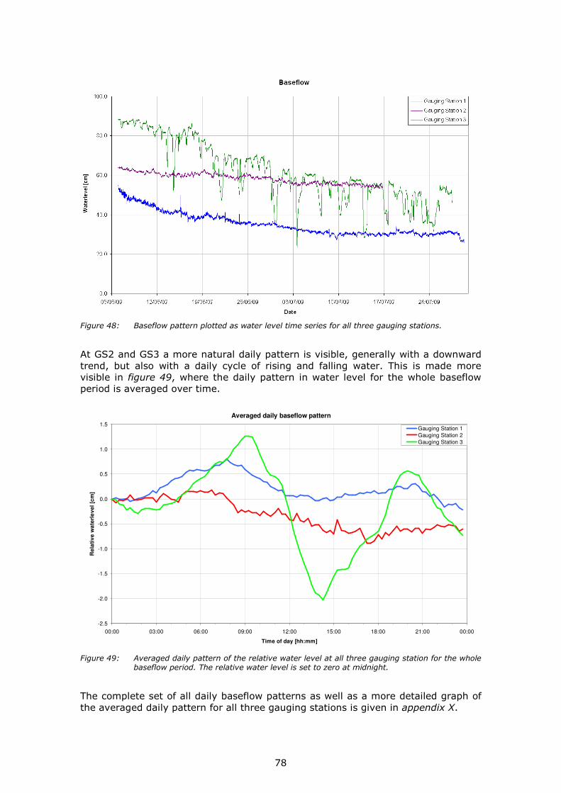
78

Figure 48: Baseflow pattern plotted as water level time series for all three gauging stations. At GS2 and GS3 a more natural daily pattern is visible, generally with a downward trend, but also with a daily cycle of rising and falling water. This is made more visible in figure 49, where the daily pattern in water level for the whole baseflow period is averaged over time.

Averaged daily baseflow pattern

-2.5

-2.0

-1.5

-1.0

-0.5

0.0

0.5

1.0

1.5

00:00 03:00 06:00 09:00 12:00 15:00 18:00 21:00 00:00

Time of day [hh:mm]

Re

lati

ve

wa

terl

ev

el

[cm

]

Gauging Station 1

Gauging Station 2

Gauging Station 3

Figure 49: Averaged daily pattern of the relative water level at all three gauging station for the whole

baseflow period. The relative water level is set to zero at midnight. The complete set of all daily baseflow patterns as well as a more detailed graph of the averaged daily pattern for all three gauging stations is given in appendix X.

79

At GS3, a daily pattern is visible largely driven by the daily uptake and use of water by phreatophytes and hydrophytes in the riparian zone. The vegetated zone on both sides of the stream is characterized by seepage water that crops out steadily. This steady flow is diminished during the daytime and restored during the night when evaporation is minimal. One hour after sunrise, around 07:00, plants in and around the river become active, starting to take up and use water from the soil or river itself. This can be seen by a decrease in the amount of water flowing in the river, resulting in a gradual drop in water level up to 10 mm d-1. Around 17:00, one hour before sunset, the plants become inactive. Because they are no longer abstracting water, the water level in the river is able to recover. This gradual increase in water level, up to 4 mm d-1, takes place during the whole night after which the decrease in water level starts again around 07:00. The daily patterns in baseflow at GS1 and GS2 are more influenced by local phenomena, because of their smaller catchment size. A very clear daily pattern is visible for GS1 with an enormous drop in water level at 09:00 and a recovery at 14:00, as explained earlier. The amplitude of this daily variation is 33 mm on average, but can run up to 300 mm as measured on the 14th of June. There is however a second drop in water level visible which is not mentioned before so far. This drawdown starts around 20:00 and recovers from 01:30 onwards. In appendix X (5) it becomes visible that this second cycle is only visible on days in the last part of the period (with the lowest water levels), which also corresponds to the more disturbed signal of the baseflow in this period as shown in figure 48. A possible explanation can be a second use of the water stored behind the dam, for example the Rwasave fishponds, needed in the final and most dry part of the study period. Another explanation can be that it is the delayed signal of the water used during the day for irrigation the rice fields more upstream. “Based on the principle of travel time one may conclude that the responsible partial areas must be located in the vicinity of the drainage system. If this would not be the case, the effects of all partial areas would reach the channel delayed with respect to each other, such that the daily course would be flattened and invisible.” (Coursereader C.R.A., van der Griendt et al, 2008) The ricefields of Rwabuye, directly surrounding the gauging station, are thus the most probable partial areas if this explanation is really the case. At GS2 also a two-daily cycle in baseflow is visible, though the pattern is less clear. appendix X (1) shows that the variations are very gradual, making a natural cause more likely than human influence. Between 01:00 and 08:00 the water level is increasing 8 mm d-1 on average, which is most probably due to normal recovery of the water level during the night. Between 08:00 and 14:00, the water level drops 8 mm d-1 again, due to the uptake of water by plants. Why the water is recovering from 14:00 onwards, while the vegetation is still active during that time, is not clear. A big difference with the subcatchment of GS1 is that in the subcatchment of GS2 almost no rice fields are present so irrigating practices do not take place. More discussion about this two-daily pattern in the baseflow of the river and groundwater variations in adjacent piezometers will take place in chapter 4.3.4. In general it can be concluded that the daily course of total evaporation as well as the daily course of irrigating practices can be traced from the daily baseflow pattern. In the absence of rainfall, the watertable dropped 7 mm d-1 at GS1, 2 mm d-1 at GS2 and 6 mm d-1 at GS3 on average. In the discussion (chapter 5) a comparison between this drawdown in the rivers and the drawdown of groundwater will be made.

80

4.2.5 Specific discharge

The specific discharge is defined as the rate of discharge per unit area [m3 s-1 km-2] or [mm] and is sometimes also named ‘yield’. It is thus a relative discharge, compensated for the size of the catchment. Specific discharge is very useful in determining the relationship of one catchment to another and to assess the discharge potential of a catchment. Because specific discharge and precipitation are both expressed in mm, an absolute comparison between input and output can be made. In figure 50, the complete time series of specific discharge for all three gauging stations is plotted together with the precipitation measurements of the tipping bucket in Butare (CGIS). To make a proper comparison, the discharge is plotted with the same time interval as the precipitation measurements, so in mm per 30 minutes. A more detailed plot of the specific discharge during the first and second period of direct runoff is presented in figure 51 and figure 52.

Specific discharge

0.00

0.03

0.06

0.09

0.12

04/05/09 11/05/09 18/05/09 25/05/09 01/06/09 08/06/09 15/06/09 22/06/09 29/06/09 06/07/09 13/07/09 20/07/09 27/07/09

Date

Sp

ec

ific

dis

ch

arg

e [

mm

30

min

-1]

0

3

6

9

12

15

Pre

cip

itatio

n [m

m 3

0m

in-1]

Gauging Station 1

Gauging Station 2

Gauging Station 3

Precipitation

2 1 a b c d 3 4 5 6

Figure 50: Specific discharge for the whole study period. Precipitation and specific discharge are

expressed in mm, measured on a 30-minute time interval. As can be seen in figure 50, the catchments of GS2 and GS3 exhibit more or less the same relative yields throughout the whole study period. During baseflow, the catchment of GS2 is yielding a little more water relatively, which is pointing out that its discharge conditions are a little more favourable. Assuming the natural conditions (like geology and soils, weather conditions and geomorphology) are the same for all catchments, this means that human influence has to be the cause of this small difference for example because the infiltration capacity is higher and/or the evaporation rates are lower. This is in agreement with the landuse map (figure 13) of the study area, where can be seen that GS2 has relatively the lowest part of irrigated crops (which have a high evaporation rate) and also urban area (which has a low infiltration capacity). Figure 50 makes however also clear that the yield during baseflow for catchment GS1 is much, much lower than for the other catchments (for reasons mentioned before). Because the catchment of GS2 is producing almost the same amount of yield than the Butare catchment (GS3), this means that the remaining catchment (subcatchment 3) has to be the relative biggest producer of yield during baseflow. With the same assumption as above, this means that a human influence has to be

81

the cause of this. Thinking about the wastewater the agglomeration of Butare is producing (more about this in that is exfiltrating in subcatchment 3 by septic tanks, there is a constant extra source input in this subcatchment that is especially during times of baseflow significant.

Specific discharge

11 - 25 May 2009

0.00

0.03

0.06

0.09

0.12

11/05/09 12/05/09 13/05/09 14/05/09 15/05/09 16/05/09 17/05/09 18/05/09 19/05/09 20/05/09 21/05/09 22/05/09 23/05/09 24/05/09 25/05/09

Date

Sp

ec

ific

Dis

ch

arg

e [

mm

30

min

-1]

0

3

6

9

12

15

Pre

cip

itatio

n [m

m 3

0m

in-1]

Gauging Station 1

Gauging Station 2

Gauging Station 3

Precipitation

1 2a 2b 2c 2d 3

Figure 51: Specific discharge for the period of the 11th – 25th of May 2009. Precipitation and specific

discharge are expressed in mm, measured on a 30-minute time interval.

Specific discharge

25 May - 8 June 2009

0.00

0.01

0.02

0.04

0.05

0.06

25/05/09 26/05/09 27/05/09 28/05/09 29/05/09 30/05/09 31/05/09 01/06/09 02/06/09 03/06/09 04/06/09 05/06/09 06/06/09 07/06/09 08/06/09

Date

Sp

ec

ific

dis

ch

arg

e [

mm

30

min

-1]

0

3

6

9

12

15

Pre

cip

itatio

n [m

m 3

0m

in-1]

Gauging Station 1

Gauging Station 2

Gauging Station 3

Precipitation

4 5 6

Figure 52: Specific discharge for the period of 25th May – 8th June 2009. Precipitation and specific

discharge are expressed in mm, measured on a 30-minute time interval. If we take a closer look to the periods of direct runoff, figure 51 and figure 52, it becomes clear that the catchment of GS1 exhibits the highest yields. This is most probably due to the additional source of urban runoff in and around the municipality

82

of Rwabuye. However, it looks like a certain threshold value has to be overcome to activate this surface runoff, because this relatively high yields only take place after heavy rainfall (e.g. event 2a, 2b, 5 and 6) and not after intermediate rainfall (e.g. event 2d and 3). During direct runoff the response in yield is the slowest for the catchment of GS3 (e.g. event 1, 2b and 5) which is due to longer travel times as the size of a catchment is bigger. The catchment of GS1 reacts more extreme than GS2 or GS3, yielding relatively most of the water directly after a rainfall event, but giving relatively low yields during periods of baseflow (for reasons mentioned before). Hydrograph separation

Looking at the specific discharge of the entire study period, a separation between the direct runoff and baseflow component can be made. Hydrograph separation methods can be empirical, analytical, or both, but the empirical approach is used here due to their ease and affordability. This empirical method, based on graphical separation, gives however only a very rough indication of the hydrograph separation. For a more accurate analytical approach, for example by use of major ions or isotopes to identify old and new water contributions, a more detailed and highly frequent hydrochemical field campaign during one or preferably more peak events is needed. During the research period this was however not possible, so the rough empirical approach will be used here. In the discussion (chapter 5) and the recommendations (chapter 6), this analytical approach will come back. For the empirical approach, a dividing line has to be generated to separate direct runoff from baseflow. This straight line starts at the rising arm of the hydrograph from the sharp break of the slope were discharge begins to increase (point X), and extends to the recession limb of the hydrograph to the point of greatest curvature near the lower end of the recession limb (point Z; inflection point). The portion of the hydrograph above this line represents direct runoff, while the portion of the hydrograph below this line represents baseflow. In table 16, the arbitrary selected points and corresponding specific discharges are given. The hydrograph separation for all three gauging stations is shown in figure 53, figure 54 and figure 55. Table 15: Overview of the selected points in the hydrograph where direct runoff starts (point X) and direct runoff ends (point Z) for gauging station 2 and 3.

GS2 Point X Q [mm d-1] Point Z Q [mm d-1]

11/05/2009 07:11 0.24 13-05-2009 00:56 0.68

14/05/2009 08:26 0.77 21-05-2009 00:26 0.57

30/05/2009 12:26 0.34 31-05-2009 23:56 0.45

GS3 Point X Q [mm d-1] Point Z Q [mm d-1]

11-05-2009 12:05 0.26 22-05-2009 01:35 0.49

30-05-2009 18:05 0.35 04-06-2009 14:50 0.31

Once the direct runoff component has been separated from the baseflow component, the direct runoff discharge volume can be calculated by integrating the area under the hydrograph and above the baseflow line. To make a quantitative comparison between the specific discharge [mm d-1] and precipitation, the rainfall data from the tipping bucket in Butare is no longer used. Instead, the daily measured precipitation of the totalizers is used, averaged per subcatchment (appendix XXIV), which in absolute terms give the most reliable measurements of rainfall.

83

Figure 53: Specific discharge and hydrograph separation (analytical approach) for gauging station 1.

Figure 54: Specific discharge and hydrograph separation (analytical approach) for gauging station 2.

Figure 55: Specific discharge and hydrograph separation (analytical approach) for gauging station 3.

84

As can be seen in figure 53, no substantiated dividing line could be generated for gauging station 1. Once the direct runoff component has been separated from the baseflow component, the direct runoff discharge volume can be calculated by integrating the area under the hydrograph and above the baseflow line. Based on this empirical approach, direct runoff dominates the catchment’s initial response to precipitation, and is responsible for much of the increase in discharge compared to the background level. The results are presented in Table 16. Table 16: The differences in baseflow and direct runoff quantified for different time periods for

subcatchment 2 and Butare catchment.

To make a good comparison between subcatchment 2 and Butare catchment (measured at gauging station 3) possible, a so called ‘water balance period’ has been selected. This period lasts from the 15th of May until the 15th of July, and within this period complete measurements of precipitation and discharge have been done throughout the gauged catchment. During this water balance period, a total of 45.59 mm precipitation was measured in subcatchment 2 and 62.34 mm in Butare catchment. The corresponding amounts of direct runoff amount 6.52 mm and 9.13 mm respectively (table 15). This brings the runoff coefficient, the percentage of excess precipitation represented by direct runoff, on 14.3% for subcatchment 2 and 14.6% for Butare catchment. So, the generation of runoff after a rainfall event is comparable for both subcatchment 2 and Butare catchment. However, the water balance period as selected here starts during the first rainy period and because the response of discharge to precipitation is delayed, a distorted result of the runoff coefficient is given. It is therefore worthwhile to have a look at the runoff coefficient of the complete data series, which will make less sense in the comparison between the different subcatchments (because they are valid for different time periods), but make more sense in absolute way. Taking the total measured period of discharge into account and the corresponding precipitation for those days, a total of 91.18 mm of precipitation was measured in subcatchment 2 for the period of the 4th of May until the 16th of July. Together with the total amount of direct runoff of 7.84 mm, this results in a runoff coefficient for subcatchment 2 of 8.6%. For Butare catchment a total of 109.54 mm precipitation was measured and 11.95 mm of direct runoff, resulting in a runoff coefficient of 10.9%.

85

Finally, it is also possible to have a look at the runoff coefficient for single rainfall periods, for which three periods of direct runoff can be distinguished at gauging station 2 (figure 54) and two periods of direct runoff can be distinguished at gauging station 3 (figure 55). Table 17: Runoff coefficients for the different periods of direct runoff, calculated with the direct

runoff measured at gauging station 2 and gauging station 3 and the amount of precipitation measured at subcatchment 2 and Butare catchment respectively.

Table 17 and figure 54 show for subcatchment 2 that after the first rainfall event the direct runoff is relatively small, resulting in a runoff coefficient of 3.5%. This direct runoff is however increasing with the continuing rainfall in the subsequent days, resulting in a runoff coefficient of 16.2% for the period of 14th until 20th May. This relative increase in direct runoff is due to the fact that the soils are getting saturated earlier because of the rainfall of the preceding days (on 12th and 13th May); causing more precipitation water to become direct runoff. After the approximately dry period between 21st and 29th May, the direct runoff produced after the rainfall of 30th and 31st May is relatively low again with a runoff coefficient of 5.2%. For Butare catchment, only two different periods in direct runoff can be distinguished (figure 55), which are both relatively long in duration. The difference in initial fill up of the soil storage (producing low direct runoff) and the subsequent more easily saturated soil (producing higher direct runoff) as has been found for subcatchment 2 can therefore not be distinguished for Butare catchment. For both periods of direct runoff, the runoff coefficients (10.0% and 12.8%) are comparable with the coefficients found earlier for Butare catchment. Note that more detail in which direct runoff is due to a specific rainfall event cannot be made, because with only the discharge measurements it is not clear which part of the direct runoff is caused by which part of the precipitation. It can be concluded that the differences in runoff generating abilities is not significantly different for the varying subcatchments, no matter which unit of time period is selected. In general, the runoff coefficient in Butare catchment is in the order of 10% ± 5%. Note that the presented results above are based on an empirical hydrograph separation approach. In chapter 5, an alternative approach will be discussed.

86

Save

Butare

Rango

Muyira Vumbi

Mpare

Mubumbano

Kansi

Kibilizi

Sovu

(µS cm-1)

4.2.6 River routing

A river routing survey was carried out in Butare catchment, under baseflow conditions. The measurements were carried out at the end of the dry season, from 19th July until 22nd July. In total more than hundred electrical conductivity (EC) measurements and pH measurements were carried out. The measurements are included in appendix XVIII. The objective of the survey is to get insight in the local changes in water quality within the catchment. The measurements were taken in streams that contribute to the river that flows to the outlet near Kansi (figure 56).

Figure 56: River routing in Butare catchment. The measured EC values vary from 50 µS cm-1 until more than 420 µS cm-1. The average EC that is measured is 112 µS cm-1. The results of the EC measurements are plotted in figure 57 against the distance towards the outlet in Kansi (gauging station 3). At the right side of the graph, the results of the measurements near Vumbi are plotted. Vumbi is located circa 11 km from Kansi, Rango is located approximately 5 km from Kansi. Measurements that are taken from the stream that for example comes from Mpare, are plotted as a tributary that joins the main stream near Rango. At the left side of the graph, the results of the EC measurements near Sovu are plotted. Sovu is located approximately 21 km from Kansi. The results of EC measurements near Sovu are followed by the results of measurements near Butare. Rwabuye, which is the outlet of subcatchment 1 is located approximately 12.5 km north from the outlet in Kansi. The lines that plot above the red line are tributaries with a relative high EC, compared to the EC of the main stream, which is plotted as a red line. Lines and points that plot below the red line are tributaries with a relatively low electrical conductivity.

87

Figure 57: Results of river routing in Butare catchment. In general, the conductivity of the surface water is relatively low with values that are lower than 100 mg l-1. From Vumbi, the EC in the river increases towards the outlet in Kansi. From Sovu, the EC increases up to a value above 150 mg l-1, due to some tributaries with a relatively high EC. The influence is not very big, as the conductivity of the water reduces quite fast. At a distance of ca 5 km from Kansi, the river water already has an EC of 110 µS cm-1. In one of the tributaries between Sovu and Rwabuye, a relative high EC is measured. This sidestream is located near the prison of Butare, and has an EC of more than 200 µS cm-1. This relatively high EC can be explained by the input of human wastewater from the approximately 10,000 prisoners. The influence of this waste water input is relatively small, as the EC of the main stream increases only from 78 to 90 µS cm-1. From the prison, the EC of the water in the main stream increases around Butare from ca. 90 µS cm-1 up to a value close to 100 µS cm-1.

Figure 58: Waste water in a river near NUR campus.

88

Another water stream with a relative high electrical conductivity is located in the valley north from the NUR campus (south from Butare). The water in the small stream is black (figure 58) and has an EC that is higher than 400 µS cm-1. The water from the stream is sampled for a chemical analyse of the contents. In table 18, the content of the most important anions and cations is presented. Table 18: Results of chemical analysis of riverwater close to NUR campus.

anions cations Electrical EC pH Cl SO4 HCO3 NO3 K Mg Na Ca Balance µS cm-1 - mg l-1 mg l-1 mg l-1 mg l-1 mg l-1 mg l-1 mg l-1 mg l-1 % NUR campus 427.0 6.4 37.3 4.4 118.3 2.2 16.8 6.1 28.2 15.4 2.5

Besides the most common anions and cations, the water contains also 16.8 mg l-1

ammonium (NH4+), 45.3 mg l

-1 nitrite (NO2-) and 3.2 mg l-1 phosphorus (PO4

-). Other important ions that were found are 13.8 mg l-1 of silica (SiO2) and 0.4 mg l

-1 aluminium (Al3+). Nutrients that contain nitrogen (N) such as nitrate (NO3

-), nitrite (NO2-) and

ammonium (NH4+) can be the result of agricultural practices including the use of

fertilizers or is caused by sewage that enters the groundwater from for example septic tanks. The major sources of phosphorus (P) are soil applied fertilizers and waste water. In this case, the contamination seems to be related to the leakage of wastewater from the septic tanks of the NUR university campus. The influence of the waste water input is relatively small, as the EC of the water reduces fast. In general, the waterquality in Butare catchment is good when looking at their chemical contents. The absolute concentrations as well as the differences in space and time are relatively small. At two locations, near the Butare prison and the NUR campus, concentrations increase. The pollution is related to human wastewater, as it contains relatively high amounts of ammonium, phosphate and nitrite. The influence of the polluted water is not very big, as the conductivity of the water reduces fast in the surroundings.

89

4.3 Groundwater

4.3.1 Springs

The Electrical conductivity (EC) and the pH of the water is measured and determined in the field. The concentration of bicarbonate (HCO3

-) is also obtained from measurements in the field, by titrations. From the fifteen springs that were located in the Migina catchment, ten of them are sampled and analysed in a laboratory for their complete chemical content. The total chemical content of the water from the different springs can be found in appendix XIV. The concentrations of the most important anions and cations are presented in table 19. For five of the springs, only results of EC and pH measurements can be presented. In the last column, the electrical balance of the samples that were completely analysed is presented. Table 19: Chemical contents (major cations and anions) and Electrical Balance (E.B.) of springs in

Migina catchment.

anions cations EC pH Cl SO4 HCO3 NO3 K Mg Na Ca E.B. # Name µS cm-1 - mg l-1 mg l-1 mg l-1 mg l-1 mg l-1 mg l-1 mg l-1 mg l-1 % 1 Sovu 140.5 3.7 9.02 4.98 1.2 44.55 4.36 4.65 3.87 9.02 10.4 2 Ghahenerezo 132.0 5.4 4.77 9.24 2.4 33.65 5.06 3.59 5.14 7.77 0.2 3 Nabagado 146.7 4.7 8.57 7.87 0.0 42.77 2.23 4.82 6.60 8.57 -1.7 4 Kinteko 111.0 5.5 - - - - - - - - - 5 Rwasave 143.5 4.3 8.03 5.80 1.2 36.41 3.19 3.62 9.42 8.03 2.0 6 Mpare 85.3 4.6 4.94 5.10 0.0 22.71 1.29 2.33 4.00 4.94 9.3 7 Kamugegemge 158.0 4.1 10.30 5.45 0.0 52.70 5.44 4.26 6.12 10.30 3.5 8 Runyinya 106.4 4.8 6.36 4.09 0.0 30.51 2.09 3.29 4.96 6.36 6.1 9 Gakombe 67.8 - - - - - - - - - - 10 Kadahokwa 126.5 5.7 4.31 2.37 20.5 27.46 1.68 2.81 5.80 11.37 -1.7 11 Mpazi - - - - - - - - - - - 12 Irango 76.3 3.9 4.08 5.89 0.0 17.56 1.23 1.74 3.28 4.08 13.9 13 Kibingo 156.1 6.1 11.50 12.99 12.2 35.42 1.39 5.64 5.72 11.50 0.9 14 Nyamugali 69.0 4.6 - - - - - - - - - 15 Nyarunazi 52.1 4.6 - - - - - - - - -

Electrical conductivity

Water from the springs in the Migina catchment have electrical conductivities that range between 52 µS cm-1 and 158 µS cm-1 (figure 59). In Butare catchment, the electrical conductivities are relatively high in subcatchment 1. Water from the springs near Sovu (1), Ghanhanerezo (2) and Nabagado (3) have EC values of 141, 132 and 147 µS cm-1 respectively. Figure 59: EC of water from springs in Butare catchment.

1

2 3

4 5

6

7 8

12 10

9

EC (µS cm-1)

90

In subcatchment 2, the differences in the measured EC values are much higher. The EC of the water from the spring near Gakombe (9) has an EC of 68 µS cm-1. The springs of Mpare (6) and Irango (12) are relatively low, with values of 85 and 76 µS cm-1 respectively. The spring of Runyinya (8) has an average EC of 106 µS cm-1. The highest values were measured at the spring of Kadahokwa (10) and the spring near Kamugegemge (7), which have an EC of 127 µS cm-1 and 158 µS cm-1 respectively. The three springs that are located south of Butare catchment have very different EC values. The water from the spring near Kibingo (13) has a relatively high EC of 156 µS cm-1, the springs that are located in southern Migina (close to gauging station 5) have relatively low electrical conductivities, with values of 69 µS cm-1 (Nyamugali, 14) and 52 µS cm-1 (Nyarunazi, 15).

pH

The water from all the springs have a pH value less than 6.2, which means that the water is at least slightly acidic. Most of the water from the springs is acidic, with a pH between 4.2 and 5.0. Three of the sampled springs are even strongly acid, as their pH is lower than 4.2. This applies to the spring of Sovu (1), Kamugegemge (7) and Irango (12). The pH of all the springs are out of range of the drinking water limits of the WHO. The pH of drinking water has to be between 6.5 and 8.5. Low pH values can be a problem as the metal pipes of the springs can start to corrode.

Nitrate (NO3-)

The spring water contains relatively high concentrations of nitrate (NO3

-) (figure 60). The drinking water norm of the WHO with respect to nitrate is 50 mg l-1. The spring in Kamugegemge (7) exceeds this limit with a concentration of 53 mg l-1. The springs of Sovu (1) and Nabagado (3) are close to the limit, with nitrate concentrations of 45 mg l-1 and 43 mg l-1. Most of the springs have a nitrate concentration between 31 mg l-1 and 40 mg l-1. Figure 60: Nitrate concentrations (in mg l-1) of springs in Butare catchment.

The springs of Ghanenerezo (2), Rwasave (5), Runyinya (8) and Kibingo (13) have nitrate concentrations of 34, 36, 31 and 36 mg l-1 respectively. Springs with a relatively low nitrate concentration are Mpare (6), Kadahokwa (10) and Irango (12). The measured concentrations are respectively 23, 27 and 18 mg l-1. Bicarbonate (HCO3

-) In some of the spring water, bicarbonate (HCO3

-) is present. As there are no indications that the sediments of the weathered parent material (schist, quartzite) contain carbonates, the bicarbonate might be the result of the dissolution of carbon dioxide (CO2) in the groundwater. In the soil, CO2 is generated by root transpiration and the decay of labile organic material (Appelo and Postma, 2005). In the springs of Kadahokwa (10) and the spring Kibingo (13) the concentrations of bicarbonate (HCO3) is relatively high. This might be related to the pH of the water.

8

1

2 3

5

7

12 10

6

(mg l-1)

91

The other springs have pH values below 5. As a result, the available carbonic acid (HCO3

-) is probably present as carbonic acid (H2CO3), which is not measured. Silica (SiO2)

The silica content in the water from the springs varies between 16.5 mg l-1 near Rwasave (5) to 37.7 mg l-1 in the water from the spring near Kamugegemge (7). The differences in concentrations of silica are quite small (figure 61). Despite these small differences, it seems that the springs in subcatchment 1 have lower silica content than the water from the springs in the subcatchment 2.

Figure 61: Silica concentrations (in mg l-1) of

the springs in Butare catchment. In the north, the spring of Sovu (1) has a concentration of silica of 18.1 mg l-1, and the spring near Gahenerezo (2) of 19.2 mg l-1. In the southern part, the concentration of silica is 27.2 mg l-1 on average. The spring of Kamugegemge (7) has a higher silica concentration of 37.7 mg l-1.

Other elements

The other elements that are measured in the water from the springs originate mainly from the weathered parent material. The differences that are found are rather small. This is due to the high age of the parent material. For this reason, a lot of elements have already been washed out. Many open springs are present in Butare catchment. The EC of the springwater ranges between 52 µS cm-1 and 158 µS cm-1. The EC values are relatively high in the northern part, and low in the southern part of Butare catchment. The water is slighly acidic at all springs, as the pH is less than 6.2. This can cause problems, for example when metal pipes of the springs start to corrode. One spring exceeds the WHO limits for nitrate concentration. Two other springs have nitrate concentrations close to the WHO limit.

(mg l-1)

7

1

2 3

5

12 10

6

8

92

4.3.2 Continuous water levels piezometers

The water level of the groundwater in the installed piezometers in the valley of the river Kadahokwa was monitored from 12th of June until 28th July. Until 25th July, no rainfall was recorded by the tipping bucket in Mubumbano and the rain gauge in Vumbi. At two other rain gauges that are close to the area with the piezometers, only a very small amount of rainfall was measured at 26th of July. In Rango and Mpare, 1.0 mm and 0.2 mm precipitation was measured respectively. The locations of the rain gauges can be found in figure 14. As there was hardly any rainfall during the study period, the results of the water level measurements are representative for the baseflow conditions of the groundwatertable. The waterlevels are plotted with the watertable of the river, measured at gauging station 2, as a reference. The water levels are compensated for barometric pressure changes (measured with a Baro-Diver) and hand measurements, which were carried out at least every week. Transect A

Transect A consists of seven piezometers, which are located between the hillside and the river Kadahokwa. The locations are presented in figure 17.

Piezometer A5, A6 and A7 The piezometers that are located close to the hillslope have a watertable that decreases more or less linear in time. As can be seen in figure 62, the water level has a daily variation with a maximum level in the morning and a minimum value in the evening. More about these variations can be found in chapter 4.3.3. Figure 62: Water level in piezometers A5, A6 and A7.

In general, the decrease in watertable is approximately 3 mm day-1 for piezometer A7 and A6. The water level in piezometer A5 decreased on average 2 mm day-1. In the last week of the measurements (23rd July – 28th July) the watertable of the groundwater increases less than a cm. This is probably the result of a small rainfall event, recorded by the nearest raingauge in Rango but not in the raingauge in Vumbi and tipping bucket in Mubumbano. Piezometer A3 and A4 The two piezometers that are located in the valley floor show an exponential decline in watertable level (figure 63). When the measurements start, the decline in piezometers A4 and A3 is approximately 13 mm day-1. In the end of July, the watertable decreases approximately 4 mm day-1.

Figure 63: Water level in piezometers A3 and A4.

93

The daily variation in piezometer A3 and A4 are smaller than observed in piezometers A5, A6 and A7. The water level record of piezometer A4 is scattered, as it takes a long time until the water level in this piezometer recovers, for example after a sample of water was taken. The increase in water level, which can be observed in the records of A6 and A7, is not present in the records of piezometer A3 and A4. Piezometer A1 and A2 The water levels of the piezometers that are closest to the river show the biggest fluctuations (figure 64). This might be caused by the watertable of the river, which is also fluctuating in time. The fluctuations in the river are caused by the water treatment plant. This treatment plant is located less than 2 km upstream in the Kadahokwa valley (appendix XXII).

Figure 64: Water level in piezometers A1 and A2. Water from the river is used as an addition in the groundwater treatment activities. The plant does not continuously pump water from the river, as a result the water level in the river changes in time. In the last week of the measurements, the watertable in both records increases. This might be the result of the local rainfall event.

Transect B

From 4th July until 27th July, piezometers B1, B2 and B3 were equipped with Mini-Divers to measure water levels continuously. No continuous data is available of the watertable variations of piezometer B4 (closest to the hillslope), as this piezometer was finished in the end of the study period. The locations of the piezometers of transect B are presented in figure 17. Piezometer B3 Piezometer B3 has a watertable that decreases more or less linear in time. The decrease in watertable is approximately 3 mm day-1. The level of the watertable of piezometer B3 is in correspondence with the level of the water tables that are measured in piezometer A7 and A6. Figure 65: Water level in piezometer B3.

In the last week of the study period (between 23rd and 28th July) the watertable increases approximately 2 cm. The increase is caused by the small rainfall event.

94

Piezometer B1 and B2 Despite the relative big distance between the river and piezometer B2, the waterlevels of piezometer B1 and B2 show some similarities as some of the peeks in water level can be found in both time series (figure 66). Both records don not have a linear decrease that is observed in the piezometers closer to the hillslope. Both water tables fluctuate in time, probably caused by the influence of the river.

Figure 66: Water level in piezometer B1 and B2.

4.3.3 Daily fluctuations in water levels piezometers

In the continuous water level records that were measured in the different piezometers and corrected for barometric changes, daily fluctuations are observed. These fluctuations are studied in more detail by sorting the data per day and set the water level to 0 at midnight (00:00). During the day, the differences of the water level in according to the water level at midnight are plotted against time (appendix X). The results are averaged and plotted (figure 67 and figure 68). Transect A

Transect A consists of seven piezometers, in which 3 different daily patterns can be observed. Piezometers A1 and A2 The water level of the two piezometers of transect A that are located the closest to the river show no clear daily pattern. The distance between piezometer A1 and the river is 5.2 m, the distance between piezometer A2 and the river is 11.4 m. The lack in daily signal in the two piezometers can be due to the presence of a water treatment plant upstream the river. According to employees of this plant, the water from the river is sometimes used as additional water in the drinking water process. Therefore, the watertable in the river is not constant but changes in time. According to the daily water level measurements, the river has impact on the water tables in piezometer A1 and A2.

95

Figure 67: Daily average water level fluctuations, transect A. Piezometer A3 and A4 The water levels in the piezometers that are located in the middle of the valley have a daily pattern that is different than the daily patterns in the piezometers that are located the closest to the hillslope. The daily records have two maximum and two minimum values. The first peak in piezometer A3 can be found around 03:00 in the morning. From then the watertable declines until 09:00. After that moment, the watertable rises again until 15:00 when the second peak is present. From 15:00 until 22:00 the watertable drops until its second minimum level. The peaks in the watertable of piezometer A4 deviates a little from piezometer A3. The first peak appears around 05:00, the first minimum level appears around 12:00. From then, the watertable rises until 17:00 after which the level drops again until 00:00. The daily pattern of piezometer A4 is shifted approximately two hours in time. The daily changes in the water levels of piezometer A3 and A4 might be the result of the influence of air pressure. When the barometric pressure is high, the watertable in the piezometer is relatively low. The opposite correlation can also be recognized: when barometric pressure is low the watertable in the piezometers is relatively high. This is remarkable as the water levels of all the piezometers already have been corrected for changes in barometric pressure. Another possible explanation for the fluctuations is the influence of roots. As the groundwatertable lowers during the dry season, it is to expect that the vegetation would have difficulties in reaching the groundwatertable. The drawdown of the groundwatertable slows down at the end of the dry season, which is an indication that the vegetation is not longer able to reach the groundwater. However, the water level fluctuations don not reduce at the end of the dry period.

96

Piezometer A5 A6 and A7 The water levels in the piezometers that are located closest to the hillslope show a clear daily pattern. In the early morning, around 09:00, the watertable reaches its daily maximum. In the afternoon, around 19:00, the watertable reaches its daily minimum. During the day, between 9:00 and 20:00, the watertable decreases. From then, the watertable rises until 09:00 in the morning. The changes in groundwatertable are 2 cm on average. Daily signals in groundwater levels that are caused by evaporation are characterized by early morning maximum and an afternoon minimum (Gribovszki et al., 2010). Trees on the hillslope are connected to the groundwater by their roots. During the day, the trees subtract water which causes a decreasing watertable. During the night the groundwatertable recovers, as the trees do not subtract water anymore. Transect B

The daily patterns that are obtained from the water level data from the four piezometers of transect B show the same 3 signals as found in transect A. However, the daily patterns show some differences as well (figure 68). Piezometer B1 and B2 In accordance with transect A, the water levels in the two piezometers closest to the river of transect B show no clear daily pattern. Piezometer B1 is located at a distance of 5.0 m from the river. The distance between the river and piezometer B2 is 26.0 m. The distance of the last one is hereby twice as far from the river than piezometer A2. Piezometer B3 The waterlevel in piezometer B3 rises until 08:00 in the morning. From then, the watertable goes down until approximately 20:00. The daily pattern is in accordance with piezometers A5, A6 and A7, with the difference that the average fluctuation in piezometer B3 is relatively small. The difference between the maximum and minimum watertable is approximately 1 cm, the differences in transect A are on average 2 cm.

Figure 68: Daily average waterlevel fluctuations, transect B.

97

Piezometer B4 The daily variation in groundwater level in piezometer B4 reaches its maximum around 08:00 in the morning. From then, the watertable drops more than 4 cm on average until 15:00. From then the watertable starts to rise again. The daily variation of piezometer B4 contains a maximum and a minimum value. Piezometer B4 is the located the closest to the hillslope of transect B. Compared to piezometers A5, A6 and A7 of transect A, piezometer B4 has a much bigger drop down in water level. The decrease of 4 cm on average is twice as much as the decreases in water tables in transect A that are on average 2 cm. Another difference in the daily pattern is the increasing level from 15:00. The watertable starts to rise three hours earlier than the watertable rises that are observed in piezometers A5, A6 and A7.

4.3.4 Groundwater temperature

The temperatures of the water in the different piezometers are plotted in a graph against time, transect A in figure 69 and transect B in figure 70, with the same axes-scale. The temperature of the river, measured at Mukura (gauging station 2, downstream from the transects) is also plotted as a reference. Transect A

The water in the piezometers A6 and A7 have the highest temperature. The temperature of the water in both piezometers is higher than 22˚C. The temperature in piezometer A7 is relatively constant whereas the temperature in piezometer A6 increases from 22.0˚C at 13th June until 22.5˚C at the end of July. In piezometer A4, the temperature of the water is close to 21.6˚C at 13th June and increases until the end of July towards a temperature of 21.9˚C. The measurements of the temperature of the water in piezometer A5 start at the 4th of July. From then, the temperature is stable around 21.4˚C. From 18th July, the temperature starts to increase until 21.7˚C at 28th July.

Figure 69: Temperature groundwater transect A.

98

The temperature of the water in piezometer A2 is relatively stable. When the measurements start, the temperature is approximately 21.3˚C. Towards the end of the measuring period, the temperature decreases towards 21.2˚C. In according to the measurements in piezometer A3 and A1, the temperature of the water in these piezometers shows small fluctuations, more than is observed in other piezometers. The temperature of the water in piezometer A3 remains constant around 21.1˚C as the temperature of the water in piezometer A1 decreases towards less than 21.0˚C at 28th July. The temperature of the surface water (measured near the bridge at Mukura, a little downstream from the river in the Kadahokwa valley) is lower than the temperature of that is measured in the piezometers. At 13th June, the temperature is 21.0˚C. The temperature decreases towards 20.2˚C in the end of July. Based on these temperature measurements, the surface water might be connected to the water of piezometer A1. When the temperature in this piezometer decreases, the temperature of the surface water is also decreasing. The temperature record of piezometer A1 shows a peak at 17th Juy around 08:00 in the morning. The surface water reaches its maximum temperature a little later. The maximum temperature in the surface water is recorded at 18th July around 16:00 in the afternoon.

Transect B

The temperature of the water that is measured in the piezometers in transect B are in general a little lower than the temperatures that are measured in transect A. The results are plotted in figure 70. The temperatures that are measured in piezometer B1 and piezometer B2 are relatively constant. The temperature in piezometer B1 is stable at 21.2˚C. The temperature of the water in piezometer B2 is 21.3˚C at 4th July and increases to 21.4˚C in the end of July. The water in piezometer B3 is the coldest with a varying temperature between 20.4˚C and 20.6˚C.

Figure 70: Temperature groundwater transect B.

99

4.3.5 Hydrochemistry

The water of the different piezometers was sampled several times (table 4) and analyzed in a laboratory afterwards. In the field, hand measurements for the electrical conductivity and pH were carried out. In addition, samples were taken and analyzed the same day by titrations and the use of a colorimeter. The results of these field measurements are presented in appendix XIII.

Transect A

The most important anions and cations in the water of the piezometers in transect A are displayed in table 20. A complete overview of the hydrochemical labresults can be found in appendix XIV. Table 20: Average concentrations and Electrical Balance (E.B.) for water from piezometers of transect A.

anions cations EC pH Cl SO4 HCO3 NO3 K Mg Na Ca SiO2 E.B. # µS cm-1 - mg l-1 mg l-1 mg l-1 mg l-1 mg l-1 mg l-1 mg l-1 mg l-1 mg l-1 % river 93.0 6.6 3.13 13.18 16.21 4.50 1.37 2.64 3.47 7.85 19.07 1.2 A1 224.9 5.6 4.73 6.62 64.07 2.26 1.37 1.80 3.47 7.85 25.41 1.3 A2 189.2 5.3 4.13 10.36 39.05 21.69 4.55 2.58 7.47 14.35 22.29 1.3 A3 250.7 5.8 3.27 1.22 119.28 0.22 0.84 1.52 7.30 9.58 24.71 0.6 A4 283.8 5.9 4.90 1.16 110.00 0.17 2.96 4.15 8.41 22.97 32.48 7.0 A5 190.6 6.6 7.37 6.42 94.55 6.66 7.14 2.24 12.25 43.85 29.31 7.7 A6 146.6 5.1 4.66 5.10 56.47 10.48 2.92 2.55 8.22 13.53 25.22 1.1 A7 184.2 6.0 5.83 8.76 58.57 10.50 5.60 2.68 11.44 20.40 22.44 6.8 spring 126.5 5.7 4.31 2.37 20.53 27.46 1.68 2.81 5.80 11.37 24.39 -1.7

Transect B

The results of hydrochemical analysis of the groundwater that was sampled from transect B is presented in table 21. The results show some irregularities in relation to the results of transect A. The sampling of water from the piezometers of transect B started much later than the measurements in the piezometers of transect A, which make the results of transect B less reliable. The irregularities might be due to the influence of the construction material (for example concrete) on the hydrochemical contents of the water in the piezometers. Apparently, the time period between the construction of piezometers and the sampling of the water was too short. The electrical conductivity that was measured in the water from piezometer B1 (450 µS cm-1) is almost twice as high as the highest EC of transect A (piezometer A4 which has an EC of 284 µS cm-1). Besides the relatively high EC, the pH values for piezometer B1 and B2 are also much higher than the pH values that were measured at transect A. Table 21: Average concentrations in water from piezometers of transect B.

anions cations EC pH Cl SO4 HCO3 NO3 K Mg Na Ca SiO2 E.B. # uS cm-1 - mg l-1 mg l-1 mg l-1 mg l-1 mg l-1 mg l-1 mg l-1 mg l-1 mg l-1 % B1 450.0 9.4 7.61 54.07 - 0.39 21.00 2.34 19.40 68.20 40.01 6.0 B2 277.0 7.1 7.95 2.61 132.98 0.25 3.91 6.23 17.00 33.00 34.02 13.6 B3 213.0 5.9 4.88 2.16 85.4 0.21 3.70 3.72 16.10 21.80 30.81 2.2 B4 - - - - - - - - - - -

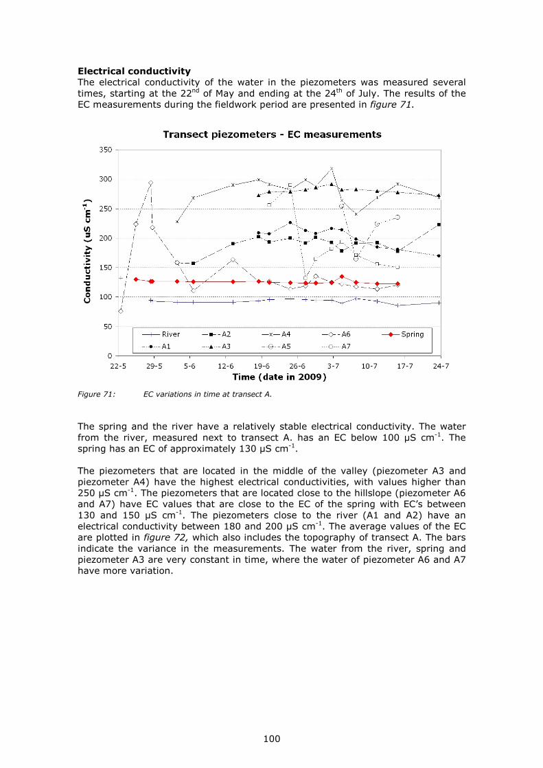
100

Electrical conductivity

The electrical conductivity of the water in the piezometers was measured several times, starting at the 22nd of May and ending at the 24th of July. The results of the EC measurements during the fieldwork period are presented in figure 71.

Figure 71: EC variations in time at transect A.

The spring and the river have a relatively stable electrical conductivity. The water from the river, measured next to transect A. has an EC below 100 µS cm-1. The spring has an EC of approximately 130 µS cm-1. The piezometers that are located in the middle of the valley (piezometer A3 and piezometer A4) have the highest electrical conductivities, with values higher than 250 µS cm-1. The piezometers that are located close to the hillslope (piezometer A6 and A7) have EC values that are close to the EC of the spring with EC’s between 130 and 150 µS cm-1. The piezometers close to the river (A1 and A2) have an electrical conductivity between 180 and 200 µS cm-1. The average values of the EC are plotted in figure 72, which also includes the topography of transect A. The bars indicate the variance in the measurements. The water from the river, spring and piezometer A3 are very constant in time, where the water of piezometer A6 and A7 have more variation.

101

Figure 72: Average EC values along transect A.

Bicarbonate (HCO3

-) The concentration of HCO3

- that is present in all the piezometers is much higher than the concentration that is present in the water from the springs. In piezometer A3 and A4 for example, the concentration exceeds 100 mg l-1. This might be due to the oxidation of organical matter (CH2O).

Silica (SiO2)

Table 22: Average SiO2 concentrations.

The concentrations of silica in the water that was sampled from the different piezometers of transect A are presented in table 22. The concentrations are plotted in figure 73, together with the topography of transect A. Going from the hillslope towards the river, from piezometer A7 to piezometer A4, the concentrations of silica in the water is increasing. The concentration of silica in the water from piezometer A7 contains 22.4 mg l-1, the water from piezometer A4 contains 33.1 mg l-1 silica. Piezometers A3, A2 and A1 have lower amounts of silica in their water, with concentrations between 22.4 and 25.4 mg l-1 on average. The river water contains the lowest

concentration, with 19.1 mg l-1 on average.

SiO2. St.dev.

mg l-1

River 19.07 0.67

A1 25.41 1.81

A2 22.29 0.50

A3 24.71 0.12

A4 32.48 2.31

A5 29.31 1.51

A6 25.22 0.75

A7 22.44 1.90

Spring 24.39 0.27

102

Figure 73: Average Silica (SiO2) values along transect A.

Iron (Fe3+)

Most of the groundwater that is sampled from the piezometers contains a relatively high concentration of iron. The water from piezometer A3 is sampled 4 times and analyzed for its chemical contents. The concentration of iron exceeds in all cases 50 mg l-1. The water from piezometer A4 is sampled 5 times and contains also relatively high concentrations of iron. The average concentration in piezometer A4 is 28 mg l-1. In piezometer A2 the average concentration is 9.0 mg l-1, in piezometer A1 the average concentration is 25.8 mg l-1. In piezometer A5, A6 and A7 almost no iron is present. The iron in the sample seems to be dissolved in the sample bottles, after acidifying the samples for lab analysis. Based on the electrical balance (appendix XV), there are too many cations in the samples in according to the anions. Therefore, it is to expect that the iron was not present in the water as a dissolved ion, but present as undissolved particles. Despite of filtering the water samples during the sampling, the particles were able to enter the sample bottles. The iron is only present in the water that was sampled from piezometers A1, A2, A3 and A4. The piezometers that are located closer to the hillslope (A5, A6 and A7) do hardly contain any iron. As the iron is present in the samples from different sample times, it is not expected that the iron concentrations is due to mistakes during the sampling procedure. Apparently, the iron particles in the surrounding of piezometers A1 until A4 are very small, smaller than the filter that was used (0.45 µm).

103

4.3.6 Isotopes

The piezometers, open spring and the river next to the transect in the Kadahokwa valley are sampled and analyzed for stable oxygen and hydrogen isotopes (appendix XXIII). The concentrations of the different stable isotopes are compared with the concentrations of a certain standard: in this case the Vienna Standard Mean Ocean Water (VSMOW). The results are presented as delta (δ) values. In case of a positive delta value, the sample has more heavy isotopes than the standard. If a sample has less heavy isotopes than the standard, the delta value will be negative. Delta values for the isotopic composition are given in per mille (‰), parts per thousands. The spring, surface water and most of the piezometers are sampled 4 times, with a time gap of a week. The samples were taken at the following dates: 20-06-2009, 27-06-2009, 04-07-2009 and 11-07-2009. The results are plotted in figure 74. The numbers reflect to the corresponding sample date. In some graphs the previous or next measurement of the same location are plotted in grey, to show how the composition changed in time. Figure 74: Isotopic composition of groundwater samples.

The water that is sampled from the river and piezometers A2 and A3 have a different isotopic composition than the spring water and the other piezometers. The water seems to be related to surface water. The water from the other piezometers (A1, A4, A5, A6 and A7) seems to be more related to the spring water. The water from the open spring has a different isotopic composition than the surface water. The oxygen and hydrogen delta values of the spring water is more

20-06-2009

04-07-2009

27-06-2009

11-07-2009

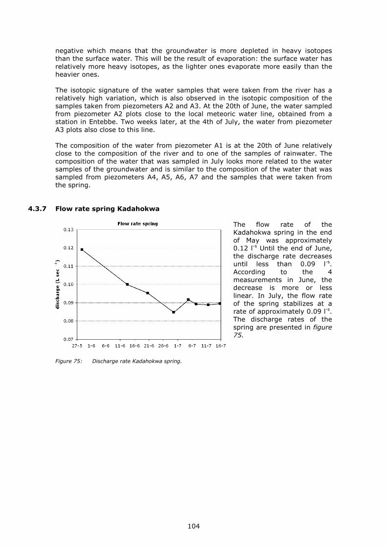
104

negative which means that the groundwater is more depleted in heavy isotopes than the surface water. This will be the result of evaporation: the surface water has relatively more heavy isotopes, as the lighter ones evaporate more easily than the heavier ones. The isotopic signature of the water samples that were taken from the river has a relatively high variation, which is also observed in the isotopic composition of the samples taken from piezometers A2 and A3. At the 20th of June, the water sampled from piezometer A2 plots close to the local meteoric water line, obtained from a station in Entebbe. Two weeks later, at the 4th of July, the water from piezometer A3 plots also close to this line. The composition of the water from piezometer A1 is at the 20th of June relatively close to the composition of the river and to one of the samples of rainwater. The composition of the water that was sampled in July looks more related to the water samples of the groundwater and is similar to the composition of the water that was sampled from piezometers A4, A5, A6, A7 and the samples that were taken from the spring.

4.3.7 Flow rate spring Kadahokwa

The flow rate of the Kadahokwa spring in the end of May was approximately 0.12 l-s Until the end of June, the discharge rate decreases until less than 0.09 l-s. According to the 4 measurements in June, the decrease is more or less linear. In July, the flow rate of the spring stabilizes at a rate of approximately 0.09 l-s. The discharge rates of the spring are presented in figure 75.

Figure 75: Discharge rate Kadahokwa spring.

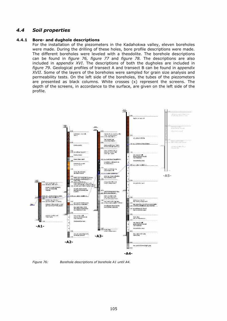
105

-A1-

-A2-

-A3-

-A4-

-A5-

� �

�

�

4.4 Soil properties

4.4.1 Bore- and dughole descriptions

For the installation of the piezometers in the Kadahokwa valley, eleven boreholes were made. During the drilling of these holes, bore profile descriptions were made. The different boreholes were leveled with a theodolite. The borehole descriptions can be found in figure 76, figure 77 and figure 78. The descriptions are also included in appendix XVI. The descriptions of both the dugholes are included in figure 79. Geological profiles of transect A and transect B can be found in appendix XVII. Some of the layers of the boreholes were sampled for grain size analysis and permeability tests. On the left side of the boreholes, the tubes of the piezometers are presented as black columns. White crosses (x) represent the screens. The depth of the screens, in accordance to the surface, are given on the left side of the profile.

Figure 76: Borehole descriptions of borehole A1 until A4.

106

Transect A: borehole A1 – borehole A4

Borehole A1 The watertable in the borehole of piezometer A1 was reached after 45 cm of drilling, below the surface. The watertable is 25 cm higher than the watertable that is measured in the river. The first 60 cm of the borehole consist of brown gravels which vary in size, between 1 and 20 mm. The grains are badly sorted and badly rounded. The deposits did only travel a short distance and didn’t have time to get rounded. Under these gravels, a 10 cm thick brown clay layer is present with relatively small quartzite grains (1 a 2 mm). The next 50 cm consist of a mixture of fine sands (smaller than 1 mm) and medium coarse sands (of approximately 5 mm). The last 20 cm consist of sediments that become coarser, with grain sizes up to 30 mm.

Borehole A2 The surface at the location of borehole A2 is 1.80 m higher than the location of borehole A1. The first 1.70 m of the borehole consists of different sandy layers, with some small coarser and finer layers. Under the sands, a 10 cm thick clay layer is present. The clay is very sticky and homogeneous. The layer below consists of coarse sands (grainsize up to 10 mm) and mica’s. The layer also contains black clay, probably leached from the layer above. At a depth of 1.95 m below the surface, a mixture of sands and gravels are present with a grain size that varies between 10 and 30 mm. The groundwatertable is present at a depth of 2.35 m from the surface, which is 30 cm above the watertable of the river. At a depth of 2.6 m below the surface, a layer of 30 cm with light grey fine sands is present. Below this layer, no material was detected during the drilling; it was possible to push the auger 60 cm deeper into the soil. From this depth, a layer of approximately 20 cm was detected, consisting of very wet grey clay/sand. Borehole A3 The surface area at the location of borehole A3 is more or less the same as the level of the ground near borehole A2. The first m consists of an alternation of sandy and more clayey layers, which contain a high amount of mica’s. From a depth of 1.0 m until a depth of 1.5 m, a dark grey clay layer is present, which is very sticky and homogeneous. Until the groundwatertable is reached, which is present at a depth of 1.5 m, the clay becomes wetter. Until a depth of 2.1 m below the surface, the clay is more cohesive and sticky than above the groundwatertable. Underneath the clay, a 2.2 m thick layer with a mixture of sand and clay is present. At a depth of 3.5 m below the surface, a black homogeneous clay layer starts, with an unknown thickness. Borehole A4 The ground near piezometer A4 has an elevation that is 55 cm higher than piezometers A2 and A3. The first 70 cm consists of dry, brown clayey topsoil. Under this layer, a 60 cm thick wet grey sand/clay layer is present. From a depth of 1.30 m, it was possible to push the auger until a depth of 2.90 m. From this depth, a 20 cm thick light grey, fine sand layer is present, followed by a 20 cm thick layer with dark grey clay layer, which contains some quartz grains. From 3.2 m depth, a 30 cm thick layer is present, containing badly rounded quarts gravels. From there, the auger was pushed until a depth of 4.1 m. At this depth, a 30 cm thick dark grey/black coloured sandy clay layer is found. The last layer consists of a light gray layer with fine sands.

107

-A5- -A6-

-A7-

-A5-

�

� �

�

Transect A: borehole A5, borehole A6 and borehole A7

Borehole A5 The elevation of the surface area of piezometer A5 is 1.35 m higher than the elevation of the surface near piezometer A4. The first 60 cm of the soil consists of the brown red top soil, consisting of a mixture of sands, clay, mica’s and organic material. From a depth of 60 cm until a depth of 120 cm dark grey clay with small quartz grains are present. The watertable is present at a depth of 1.0 m below the surface, which is 3.55 m above the watertable in the river. Between a depth of 1.2 m until a depth of 1.7 m, light grey sandy clays are present, with mica’s. From there the auger was pushed until a depth of 2.2 m. From there, the deposits consist of badly sorted coarse sands and clay.

Figure 77: Borehole descriptions of borehole A5 until A7. Borehole A6 In according to the surface area of borehole A5, the elevation of the surface area near borehole A6 is 1.3 m higher. The first 2.0 m of the borehole consists of a mix of red clay, sand and gravel. From there, the soil becomes grey coloured and more clayey. The groundwatertable was found at a depth of 2.2 m, 3.6 m above the watertable of the river. From 2.3 m below the surface, a 10 cm thick grey clay layer is present, followed by a 60 cm thick layer with red coloured clay with some quarts grains.

108

Borehole A7 The surface area around the borehole A7 is 1.6 m higher than the previous borehole A6. Until a depth of approximately 1.2 m below the surface, the soil is red/brown and consists of a mixture of clay, silt and sand. From there, the colour of the soil becomes lighter and contains more quartz fragments, which are sometimes completely weathered. The watertable is reached at a depth of 3.8 m below the surface, which is 3.65 m above the watertable level of the river. From the watertable, the soil becomes yellow and consists of weathered quarts fragments. Transect B: borehole B1 – borehole B4

Borehole B1 The location of borehole B1 is relative close to the river. During the drilling of the first 65 cm, red brown clay is found. From there, the sediments become more clayey with a lot of organic material and the colour turns into dark grey. Until the watertable is reached (at a depth of 1.95 m below the surface), the clay becomes wetter. The level of the watertable is 20 cm above the water level of the river. The bore profile reaches its maximum depth at 2.15 m below the surface, as drilling was not possible anymore.

Figure 78: Borehole descriptions of borehole B1 until B4.

-B2-

-B3-

-B1-

-B4-

�

�

�

�

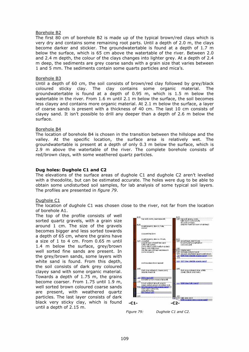
109

-C1- -C2-

Borehole B2 The first 80 cm of borehole B2 is made up of the typical brown/red clays which is very dry and contains some remaining root parts. Until a depth of 2.0 m, the clays become darker and stickier. The groundwatertable is found at a depth of 1.7 m below the surface, which is 65 cm above the watertable of the river. Between 2.0 and 2.4 m depth, the colour of the clays changes into lighter grey. At a depth of 2.4 m deep, the sediments are grey coarse sands with a grain size that varies between 1 and 5 mm. The sediments contain some quarts particles and mica’s. Borehole B3 Until a depth of 60 cm, the soil consists of brown/red clay followed by grey/black coloured sticky clay. The clay contains some organic material. The groundwatertable is found at a depth of 0.95 m, which is 1.5 m below the watertable in the river. From 1.6 m until 2.1 m below the surface, the soil becomes less clayey and contains more organic material. At 2.1 m below the surface, a layer of coarse sands is present with a thickness of 40 cm. The last 10 cm consists of clayey sand. It isn’t possible to drill any deeper than a depth of 2.6 m below the surface. Borehole B4 The location of borehole B4 is chosen in the transition between the hillslope and the valley. At the specific location, the surface area is relatively wet. The groundwatertable is present at a depth of only 0.3 m below the surface, which is 2.9 m above the watertable of the river. The complete borehole consists of red/brown clays, with some weathered quartz particles. Dug holes: Dughole C1 and C2

The elevations of the surface areas of dughole C1 and dughole C2 aren’t levelled with a theodolite, but can be estimated accurate. The holes were dug to be able to obtain some undisturbed soil samples, for lab analysis of some typical soil layers. The profiles are presented in figure 79. Dughole C1 The location of dughole C1 was chosen close to the river, not far from the location of borehole A1. The top of the profile consists of well sorted quartz gravels, with a grain size around 1 cm. The size of the gravels becomes bigger and less sorted towards a depth of 65 cm, where the grains have a size of 1 to 4 cm. From 0.65 m until 1.4 m below the surface, grey/brown well sorted fine sands are present. In the grey/brown sands, some layers with white sand is found. From this depth, the soil consists of dark grey coloured clayey sand with some organic material. Towards a depth of 1.75 m, the grains become coarser. From 1.75 until 1.9 m, well sorted brown coloured coarse sands are present, with weathered quartz particles. The last layer consists of dark black very sticky clay, which is found until a depth of 2.15 m. Figure 79: Dughole C1 and C2.

110

Stratigraphy in Kadahokwa marshland: - Upper silt complex - Upper peat complex (1865 BP) - Middle silt complex - Lower peat complex (3000 BP) - Lower silt complex

Dug hole C2 The location of dug hole C2 was chosen in the ditch next to the road (at the side of the river) near transect A. The first 60 cm of the hole consists of light brown coloured silt, which is very dry. The topsoil layer contains a lot of root remainings. At a depth between 60 and 65 cm below the surface a 5 cm thick gravel layer is present. The grains have a size that varies between 1 and 2 cm. Until a depth of 85 cm sands are found, with different colours (brown, grey, orange en yellow). The sand that is present between 85 and 90 cm below the surface is more clayey. The next 50 cm consists of red sands, with weathered quartz and mica’s. At a depth of 1.4 m below the surface, the sediments turn into dark grey and even sticky black clay. The last 5 cm of the bore profile, between 2.15 an 2.20 m below the surface, consists of light grey sands. Interpretation of the stratigraphy

The stratigraphy of the soil layers in one of the valleys in the Kadahokwa marshland is described by Moeyersons (2001). Against the nose of the Rwaza hill, a hill which is located a little downstream from the area where the piezometers were installed, a certain succession of complex layers is found, which is presented in Figure 80.

This succession was found on top of former Holocene riverbed deposits. (Moeyersons, 2001). The layers that were found in the profiles of transect A can be interpreted in the same way. This interpretation can be found in appendix XVII.

Figure 80: Stratigraphy Kadahokwa valley.

4.4.2 Horizontal saturated permeability

The hydraulic conductivities of the soil layers around the screens of the piezometers of transect A are estimated by performing falling head tests. The test is based on introducing water into a piezometer and measuring the decline of the watertable as a function of time. Pressure transducers (Mini-Divers) are used to measure the drawdown of the water level, after the tubes are filled with water. The results are presented in figure 81. The hydraulic conductivity that is calculated based on the used equations have an accuracy of 10%. [Chapuis, 1999] Figure 81 shows the decline of the watertable after the raising of the watertable in a relatively short time period (a couple of seconds). The highest point of the increase in watertable is the water level at time step 0. The decrease of the watertable is plotted on a logarithmic scale against time on a linear scale. According to literature, the result should be a straight line (Chiasson, 2005). In the graphs that are shown in figure 81 the part of the drawdown that is used to determine the hydraulic conductivity is marked with a dotted box. The measured drawdown in the selected time period can now be used to calculate the hydraulic conductivity. The hydraulic conductivity is recalculated to the unit of meters per day. In table 23 the results for the hydraulic conductivity of the different series are given, the averaged values and in the last column the standard deviation.

111

Table 23: Saturated hydraulic conductivity, in m d-1.

1 2 3 4 5 avg s.d.

(m d-1) (m d-1) (m d-1) (m d-1) (m d-1) (m d-1) A1 4.9 4.8 5.1 - - 4.9 0.15 A2 1.3 1.7 1.6 1.7 1.5 1.6 0.18 A3 0.9 0.8 0.8 - - 0.8 0.05 A4 - - - - - - - A5 0.01 0.01 - - - - - A6 1.0 0.9 - - - 1.0 0.10 A7 0.4 0.6 - - - 0.5 0.15

Not all the screens of the piezometers are completely located underneath the watertable. As a result, the hydraulic conductivity will in some cases be overestimated. When the screen is not completely in the saturated zone, the pores of some of the soil layers are not saturated. As a result, the first amount of water will flow into the empty pores (the unsaturated zone). This applies for piezometers A2, A6 and A7. Piezometer A2 As the first part of the graph of piezometer A2 is straight, the effect of the unsaturated part on the estimation of the unsaturated zone might be relatively small. As the unsaturated part doesn’t seem to contribute to the injection zone, the screen length at this piezometer is considered to be 65 cm instead of 80 cm. Piezometer A6 In case of piezometer A6, the drawdown of the watertable shows an offset after approximately 75 seconds. As the zone next to the screen is not completely saturated, the decline of the watertable from 75 seconds until 150 seconds is considered to be representative. Piezometer A7 The soil layers that are located at the depth of the screen consist of red “mantle” clays, similar to the layers that are found in case of piezometer A5. In according to the estimated hydraulic conductivity of piezometer A5, the value for piezometer A7 looks much too high. After the increased watertable is reduced to approximately 40 cm above its normal level, the watertable seems to experience some resistance. During a period of approximately 20 seconds, the watertable is not lowering. After the period, the decrease of the watertable continues. This phenomenon can be observed in both tests that were performed.

112

Figure 81: Falling head tests of piezometers A1 – A7.

Time (seconds)

Falling head test – piezometer A7

Increased w

ate

rtable (cm)

Falling head test – piezometer A1

Time (seconds)

Increased w

ate

rtable (cm)

Falling head test – piezometer A2

Time (seconds)

Increased w

ate

rtable (cm)

Falling head test

-piezometer A5

Time (seconds)

Increased w

ate

rtable (cm)

Time (seconds)

Increased w

ate

rtable (cm)

Falling head test – piezometer A3

Falling head test – piezometer A6

Time (seconds)

Increased w

ate

rtable (cm)

113

4.4.3 Vertical saturated permeability

Twelve undisturbed soil samples were analyzed for their vertical saturated permeability in the VU university soil laboratory. The results of the measurements are displayed in table 24. An overview of the results of all the measurements that were carried out can be found in appendix XIX. Most of the samples have vertical hydraulic conductivities that are rather small. 8 samples have a conductivity that is smaller than 0.10 m day-1. The samples are taken from the borehole of piezometer A5, the borehole of B4 and the dugholes C1 and C2. The soil sample locations are presented in figure 15. Table 24: Results of vertical saturated permeability measurements.

# code Depth (m)

Ksat (m d-1)

St. dev. Description

1 A5 0.20 - 0.25 1.310 ± 0.350 Brown/red clayey soil, mica's, roots 2 0.75 - 0.80 0.008 ± 0.005 Grey clay, containing quartz (<1mm) 3 B4 0.40 - 0.45 0.055 ± 0.035 Brown/red soil, clayey 4 0.60 - 0.65 0.068 ± 0.010 Brown/red soil, clayey 5 0.90 - 0.95 0.630 ± 0.560 Fine white/grey sand 6 C1 1.60 - 1.65 0.630 ± 0.130 Dark grey clay, gravels, some roots 7 1.80 - 1.85 0.033 ± 0.066 Brown gravel/sand 8 2.00 - 2.05 0.011 ± 0.008 Black dark equal clay 9 C2 1.00 - 1.05 2.930 ± 3.500 Brown/red soil, weathered quartz 10 1.15 - 1.20 0.013 ± 0.009 Dark grey clay, a little sandy 11 1.75 - 1.80 0.002 ± 0.001 Wet clay 12 2.15 - 2.20 0.024 ± 0.021 Light grey sandy clay

The brown/red soil that is very typical for the Migina catchment was sampled and analyzed at 3 different locations. At location B4, the soil was sampled at 2 different depths. The soil has a vertical saturated permeability of 0.055 m day-1 and 0.068 m day-1. The brown/red soil that was sampled at the location of piezometer A5 has a much higher permeability. This might be due to human and biological activities. The soil near piezometer A5 is used for crop production, therefore the land is managed by people. Some of the clay layers that were sampled have also very low saturated conductivities. Layers that don’t contain quartz particles have permeability less than 0.03 m day-1. Layers that contain clay and quartz gravels or sand have the highest permeability. For example 2 of the layers that are present in borehole C1 have a permeability of 0.63 m day-1. The peat that was found in some of the boreholes, is not sampled and analysed. The permeability of the peat, that contains a lot of water, might be relatively high. Peat deposits that were found and analyzed in the neighbourhood (12 km east of Butare, in the Akanyaru swamp complex) have on average a water content of 91.1% and a hydraulic conductivity of 1.6 m day-1 and 7.2 m day-1 (Pajunen, 1997).

4.4.4 Infiltration capacity

The results of the double ring infiltrometer tests are displayed in table 25. The results vary between 5 m day-1 close to borehole A1 and A2 and up to more than 30 m day-1 close to borehole A3 and A5. The tests were conducted at locations where the land is used for agriculture. At these locations, the infiltration rates are relatively high. Closer to the river, the soil is compacted and not cultivated. Here, the infiltration rate is much lower, and the rates are relatively high. As the double ring infiltometer

114

was improvised, the exact results should be used with care. The results show however that the rate is much higher at locations where the land is cultivated. Table 25: Results of double ring infiltrometer tests.

test Infiltration rate Location

1 5 m day-1 Near borehole A1 4 5 m day-1 Near borehole A2 3 31 m day-1 Near borehole A3 2 27 m day-1 Near borehole A5

4.4.5 pF curve, porosity and bulk density

After the small soil-cores were measured in the soil lab, a pF-curve could be obtained, with a plot of the soil moisture content of the twelve different samples at varying suction pressures. With increasing suction, large pores will empty first, while narrow pores (supporting air-water interfaces of much greater curvature) will not empty until larger suctions are imposed. Therefore, sandy soils will lose their water first, since most of the pores are relatively large and once they are emptied there is little water remaining. Clayey soils, in contrast, have a wider distribution of pore sizes and consequently do longer keep their water. In figure 82, the soil water retention curve (pF curve) is plotted for all twelve soil-cores, from which coordinates and a short description is given in table 26.

Figure 82: Soil water retention curve for twelve soil-cores.

Indeed the sand-gravel samples (like #6) contain less water than more clayey samples, and do lose their water also more quick with increasing suction pressure. As can be seen, organic rich (“peaty”) clay (#7 and #12) contains the highest amount of water at low suction pressures. Their porosity is also remarkably high (60–70%), which ensures that the bulk density of this two samples is even lower than 1 g cm-3. With locally occurring sediments even lighter than water, it is not surprising that during the drilling process repeated the drill dropped 1.0 m without getting material to the surface by tapping them.

Plant available water

115

Table 26: The 12 soil-cores and their main soil properties.

More detailed calculations for bulk density are presented in appendix XX and calculations for pF in appendix XXI. Because the bulk density of pure quartz is 2.65 g cm-3, samples containing a high amount of quartz grains give relatively high bulk densities. This is for example the case for the “red soils” (Moeyersons, 1993) containing aggregates of quartz grains and clay minerals as a result of weathering of the parent rock (#3, #4 and #9), resulting in a bulk density of 1.3 - 1.7 g cm-3, which seems to be decreasing with depth. Also pure gravel and sand (#6 and #10) have a bulk density around 1.7 g cm-3. Table 26 also shows results for the field capacity and wilting point. Field capacity is the name in soil science for the amount of water that is retained in a certain soil when gravitational drainage stops. Depending on the type of soil, this happens at a pF of 2 - 2.5. Under the influence of gravity, water drains from the unsaturated zone to the watertable. This water, called drainage water in table 26, is ‘lost’ for root uptake. The water that remains in the soil is available for plants. However, plants have to apply suction to overcome the tension that is due to the forces that work to retain the water in the pores. The higher the suction that plant roots need to apply to get water from the soil pores the higher the growth stress. The maximum suction that plants can apply is circa 16,000 cm, which corresponds to pF = 4.2. The volumetric moisture content at this value is referred to as the wilting point, because in a soil moisture situation below this level plants will permanently wilt. Thus, the wilting point is defined as the minimum water content of the soil at which plants can extract water and the field capacity is regarded as the amount of water held in a draining soil after gravity movement of water has largely ceased. The available water capacity is the difference between the wilting point and the field capacity. The remaining water in the soil is called the unavailable water. As expected, most of the plant available water content comes from the peat and clay layers. These layers are also in another way important for the growth of plants.

116

In the valleys, these layers appear at a depth of around 2.0 m and are not very permeable. Therefore they collect the drainage water leaking from upper layers, keeping the water from deeper infiltration. Because they can hold up to 60-70% of water, they form an important shallow subsurface storage, which makes agriculture even in dry periods possible. On the hillsides, the “red soils” are dominant, which are compact and not very permeable but have nevertheless porosities around 0.35. This is due to the relatively high clay content, which increases the porosity, but lowers the infiltration capacity. Therefore, rainwater will hardly infiltrate on the hillsides, and will consequently flow as overland flow downward to the valleys.

4.4.6 Grain size

The grain size distribution is determined from undisturbed soil samples at the VU soil laboratory in Amsterdam. The results of this analysis are presented in appendix XII, which is summarised in table 26. In this table the percentages of the different grain size categories are presented, as a percentage of their total weight. The samples are taken from the boreholes A5, A6, A7, B1, B2, B3 and B4 and from the dugholes C1 and C2. The locations of these bore- and dugholes can be found in figure 22. The analysed samples can be subdivided in 4 categories: the typical red/brown soils, clay or silt deposits, sand deposits and layers that contain a lot of gravel. The categories can be found in the last column ‘soil layer description’ of table 27. Table 27: Results of grain size analysis.

name Depth % Clay % Silt % Sand % Gravel soil layer

(m) < 8µm 8-63µm 63µm-20mm >20mm description

A5 0.25 - 0.30 18.6 13.4 64.4 3.7 Red brown soil, clay/sand

0.75 - 0.80 17.6 13.4 65.4 3.5 Red brown soil, clay/sand

2.25 - 2.30 5.4 3.8 51.2 39.6 Red brown soil, gravel

A7 0.25 - 0.30 19.8 16.7 58.2 5.3 Red brown soil, clay/silt/sand

0.95 - 1.00 6.9 8.9 53.0 31.2 Red brown soil, sand/gravel

2.55 - 2.60 20.0 17.3 50.6 12.1 Red orange clay/sand

3.95 - 4.00 5.5 5.5 64.5 24.5 Yellow brown sand/gravel

B1 2.00 - 2.05 1.2 1.4 45.3 52.1 Grey gravel

B2 2.80 - 2.85 1.6 2.7 83.1 12.6 Grey sand

B3 1.15 - 1.20 42.8 42.4 14.8 0.0 Black clay/silt

1.95 - 2.00 29.9 47.0 23.1 0.0 Black clay/silt

2.20 - 2.25 0.7 1.4 40.1 57.8 Black coarse gravel

2.45 - 2.50 1.3 2.4 72.4 23.9 Coarse sand

B4 0.40 - 0.45 7.9 7.3 42.3 42.5 Red brown soil, gravel

0.60 - 0.65 10.2 11.4 51.2 27.2 Red brown soil, sand

C1 1.65 - 1.70 47.0 43.1 9.9 0.0 Grey clay silt

1.90 - 1.95 1.5 1.0 37.9 59.6 Brown gravel

2.05 - 2.10 45.6 39.1 15.3 0.0 Black clay/silt

C2 1.05 - 1.10 16.0 10.9 54.1 19.1 Red brown clay/sand

1.20 - 1.25 28.2 24.7 47.1 0.0 Clay/silt/sand

1.75 - 1.80 35.4 33.6 31.0 0.0 Grey clay/sand

2.15 - 2.20 10.4 10.1 60.4 19.2 Light grey sand/gravel

117

Red/brown soil The typical red/brown soil was sampled at the boreholes of piezometer A5, A7 and B4 and dughole C2. The grain size distributions of these samples are presented in figure 82. The clay content of the typical red earths varies between 7.9% (borehole B4) and 19.8% (borehole A7) of their total weight. Besides relatively high clay content, most of the samples contain a significant sand fraction. Some of the samples contain a gravel content of more than 20% of its total weight.

According to Moeyersons (2001), the clay content (smaller than 2 µm) of “the red earths” varies between 15 and 24%. A gradual increase in clay content occurs around the transition between the humic A-horizon and the more clayey subsoil. Another increase in clay content occurs in the basal clayey gravel layer, which covers the bedrock. [Moeyersons, 1991]

Figure 83: Grain size analysis of red/brown soils.

At the location of borehole A5, the red brown soil is sampled at a depth of 0.25, 0.75 and 2.25 m below the surface (figure 84). The first sample, taken from a depth of 0.25 m below the surface, contains a clay content of 19% of the total

weight. The sample also contains middle coarse and coarse sand. The content is very similar to the soil which is sampled at a depth of 0.75 m below the surface. This sample has a clay content of 18% and contains also middle coarse and coarse sand. The sediment has a greyer colour. At a depth of 2.2 m below the surface, the soil is again typical red/brown. The clay content is only 5% of its total weight and contains more than 40% gravels.

Figure 84: Grain size of samples from borehole A5.

Near the borehole of piezometer A7, the red/brown soil is sampled at 4 different depths, the results are plotted in figure 85. The clay content near the surface is 20%. The sample contains also 20% of coarse sands. The second sample is taken at a depth of 1.0 m below the surface, and contains only 7% clay particles.

118

The sample contains 35% grains bigger than 2 mm (gravels). At a depth of 2.6 m below the surface, the clay content is more than 20% of its total weight. The sample also contains 20% of coarse sands. The fourth sample is taken from a depth of 4 m below the surface, and has a low clay content of 5.5%. The sample contains a lot of coarse sands and gravels.

Figure 85: Grain size of samples from borehole A7.

The sequence of soil with a relative high clay content followed by soil with lower clay content is similar to the sequence that is found in the borehole of piezometer A5. At borehole A7, the sequence of the clay content of the first and second sample (a relatively high clay content followed by relatively low clay content) are more or less similar to the contents of the third and fourth sample. Near borehole B4 the red/brown soil is sampled at a depth of 0.4 m and 0.6 m below the surface, the results are included in figure 86. The first sample, taken from a depth of 0.4 m below the surface, has a clay content of 8%. The second sample is taken from a depth of 0.6 m and has a clay content of 10%, which is a

gradual increase with depth. The content is different than the content that was found at the locations of boreholes A5 and A7. The samples that were taken closest to the surface have at the locations of borehole A5 and A7 higher clay content. This might be due to the depth of the sample, as the sample of borehole B4 is taken from a depth that is a little deeper below the surface (0.40 m) than the samples of borehole A5 and A7 (0.25 m).

Figure 86: Grain size of samples from borehole B4.

The sample that was taken from a depth of 0.4 m below the surface contains more gravel (close to 60% of its total weight) than the sample from a depth of 0.6 m (25% gravel).

119

From dughole C2, samples with red/brown soil are taken from a depth of 1.0 m and 1.2 m below the surface (figure 87). The clay content of the sample closest to the surface is 16%, which is in the range of the clay content of other samples, for example the second sample of borehole A5, which was taken from a depth of 0.75 m below the surface. Besides the 16% of clay, the sample contains also coarse sands (17%) and gravels (20%).

Figure 87: Grain size of samples from dughole C2.

The sample that was taken a little deeper in the soil (0.4 m below the surface) has a much higher clay content of 28%. The sample contains also a high content of middle coarse sand (20%), but contains no gravel at all. Clay and silt Clays and silts are present in different boreholes, for example in the boreholes of the piezometers A2, A3, A4, B2 and B3. Black sticky clays are also present in

dugholes C1 and C2. Black clays/silts are sampled from the borehole of piezometer B3 and dugholes C1 and C2. The results are presented in Figure 88. The clay content (particles smaller than 8mµ) of most of the samples is more than 40% of their total weight. The clay content of samples that also contain sands is around the 30% of their total weight.

Figure 88: Grain size analysis of clays/silt.

The sample from borehole B3 that was taken closest to the surface (1.2 m) has a clay content of 43% (figure 88). The sample contains also a lot of silt, approximately 40% of its total weight. The total sand content of the sample is 15% of its total weight. The sample from borehole B3 that was taken from a depth of 2.0 m below the surface has a clay content of 30%. The total silt content of the sample is 47%, the total sand content 23%. The grain size distribution of the samples taken from borehole B3 is presented in figure 89.

120

The clay content of the samples taken from borehole C1 at a depth of 1.7 m is 47% and at a depth of 2.1 m 46%. The total silt content of the first sample is 43% of its total weight, and 10% total sand. The second sample from C1, from a depth of 2.1 m, contains less silt (39%) and more sand (15%). Clays and silts are sampled from borehole C2 at a depth of 1.2 m and 1.8 m below

the surface (figure 78). The clay content of the sample closest to the surface is 28% of its total weight. The total silt content of the sample is 25%. The sample contains relatively a high amount of sand. The total sand content is 47%. The sample that is taken from a depth of 2.2 m below the surface contains more than 35% of clay and has a total silt content of 10%. The total sand content is 31%.

Figure 89: Grain size of samples borehole B3.

The clay/silt from piezometer C2 are different than the other clay/silt samples, as they contain a relatively high amount of sand. This pattern was also observed at the red/brown soils, which are presented before. Sand In different bore- and dugholes sand deposits are present. The sands are relatively well sorted, in contrast with gravel layers that were found. Most of the sandy layers also contain relatively low amounts of small clay particles (figure 90).

The sand deposits might be related to the silt complexes that are described by Moeyersons. These complexes are formed in former river channels. The sandy deposits might be related to human impact on the vegetation cover. Deforestation, linked to a period of iron melting, might have caused an increase in the erosion of material from the hillslopes. [Moeyersons, 2001]

Figure 90: Grainsize distribution of sand deposits.

121

Gravels Most of the gravels that are found in the different boreholes are very poor sorted and hardly rounded. Most of the gravels are river deposits, but as the travel distance and time was relatively short, there wasn’t enough time to round and sort the sediments. Moeyersons (2001) describes a clayey gravel layer with angular quartz or quartzite gravels separates the base of the “red earths” from the top of old lateritic soils, at a depth of 2 m up to more than 4 m. The grainsize distribution of the samples that contain mainly sands and gravels is presented in figure 91. Some of the

distributions seem to be related to each other. The coarse sand/gravel layer that is sampled at borehole B1 appears to be similar to the sample of the coarse sand/gravel sample of dughole C1. The sample B2 and B3 (from a depth of 2.5m) have also a similar grain size distribution. Although the sample from B3 contains more gravels than the sample from B2. The grain size distribution of the sample from C2 is very different from the other samples.

Figure 91: Grainsize distribution of gravels.

122

123

5 Discussion Springs

Many open springs are present in Migina catchment (figure 16). During this research, 11 springs in Butare catchment (the northern part of the Migina catchment) are sampled and analysed for their chemical content. Most of the springwater appeared to be acidic, as the measured pH lies in general between 4.2 and 5.0. The electrical conductivity (EC) of the water is 112.2 µS cm-1 on average. The lowest EC measured in Butare catchment is 68 µS cm-

1 (Gakombe), the highest EC 158 µS cm-1 (Kamugegemge). The EC of the springwater has a positive linear relation with nitrate (NO3

-) concentration. When the EC is relatively high, NO3

- concentration is in most cases high as well (figure 92). The spring of Kamugemge has for example an EC of 158 µS cm-1 and NO3

- concentration of 53 mg l-1. The spring of Kadahokwa has an average EC of 127 µS cm-1, and a NO3

- concentration of 27 mg l-1.

Figure 92: Positive lineair relationship between NO3- and EC.

Differences in EC might be related with aspects such as a different geology or soil profile. In the field, no significant differences in surface geology have been observed, but they will be in the subsurface, as for example quartzites and pegmatites do occur locally inside the main schist/gneiss-belt in which Butare catchment is located. Springwater with relatively low EC’s are Gakombe (68 µS cm-

1) and Irango (76 µS cm-1), which are both located in the southern part of subcatchment 2 (figure 59). This low EC can be due to a different geology, but also to a different degree of weathering. In the southern part of subcatchment 2, a higher degree of ferralization may have occured, causing all weatherable minerals to dissolve and being removed from the soil by leaching. The high concentrations of iron that have been measured locally at some piezometers near Kadahokwa (for location of piezometers see figure 17), which is also located in the southern part of subcatchment 2, can be an indication of this high stage of ferralization here. However, it is likely that differences in NO3

- concentration and EC are mainly caused by human activities. NO3

- originates from natural reactions of atmospheric forms of nitrogen with rainwater. Besides the natural processes, anthropogenic sources might increase NO3

- concentrations. Examples are septic tanks, application of certain fertilizers, animal waste and agricultural processes. The springs are located at the foot of hills. As the groundwater flows from the hillslope towards the stream, it appears that the contamination of the groundwater originates from the hills. On these hills, residents are present, agriculture is practiced and livestock is kept. The extensive agriculture that is practiced in the valleys can only cause pollution of the groundwater inside the valley and of surface water.

124

Differences in water quality in time

To see if the quality of the springwater changes in time, the water from the springs which have been sampled analysed in this research, should also be sampled and analyzed in the future. The springs of Ghahenerezo, Rwasave and Mpare have been analysed for chemical contents in the past. Kasanziki analysed the water quality in the dry and wet season of 2007. Chemical parameters that were measured are electrical conductivity (µS cm-1), pH, ammonium (NH4

+), nitrate (NO3-) and nitrite

(NO2-). The results of the analysis of the dry season and the results of the same

springs that were analysed during this study in 2009 are presented in table 28. Table 28: Chemical content in water from springs near Butare in 2007 (Kasanziki) and 2009.

Dry season (29/05/2007) Dry season (2009) EC pH NH4

+ NO3- NO2

- EC pH NH4+ NO3

- NO2-

Name µS cm-1 - mg l-1 mg l-1 mg l-1 µS cm-1 - mg l-1 mg l-1 mg l-1 Ghahenerezo 131.8 6.25 0.01 39.0 0.00 132.0 5.4 0.00 33.7 0.00 Rwasave 129.1 5.81 0.02 33.2 0.01 143.5 4.3 0.41 36.4 0.00 Mpare 121.1 6.10 0.02 20.5 0.01 85.3 4.6 0.00 33.7 0.00

The pH of the water from the springs became lower in the dry season of 2009 compared to the results of Kasanziki in 2007. The concentrations of NO3

- in the springs of Gahenerezo, Rwasave and Mpare increased slightly between 2007 and 2009. The average concentration of NO3

- was 31 mg l-1 in 2007 and 35 mg l-1 in 2009. The EC of the water from the spring of Mpare decreased from 121 µS cm-1 to 85 µS cm-1. The EC of the spring of Ghahenerezo remained stable (132 µS cm-1), where the EC of Rwasave increased from 129 µS cm-1 in 2007 to 144 µS cm-1 in 2009. As the results are different for all three springs, no hard conclusions can be drawn based on these double measurements only. The measured differences might for example be the result of a different sample time within the dry season, as the springs were sampled earlier in the dry season in 2007 than in 2009. Differences dry and wet season

The discharge of springs decreases during the dry period, based on measurements of the discharge of the Kadahokwa spring (figure 75). This can be subscribed to a decrease in water pressure that occurs, as the watertable in the hills lowers during the dry period presumably. As a result, the discharge of the springs decreases. It is plausible that the water quality changes in time as well, as the influence of rainwater on the water quality decreases during the dry season. In this research, comparison cannot be made, as hydrochemical measurements were only carried out during the dry season. Kasanziki sampled and analysed however four springs around Butare both in the dry and wet season of 2007. The results of the dry and wet season are presented in table 29.

Table 29: Results of chemical analysis of 4 springs near Butare, Kasanziki 2007.

Dry season (29/05/2007) Wet season (05/11/2007) EC pH NH4

+ NO3- NO2 EC pH NH4

+ NO3- NO2

- Name µS cm-1 - mg l-1 mg l-1 mg l-1 µS cm-1 - mg l-1 mg l-1 mg l-1 Ghahenerezo 131.8 6.25 0.01 39.0 0.00 111.6 8.02 0.04 29.6 0.11 Rwasave 129.1 5.81 0.02 33.2 0.01 134.5 7.90 0.04 0.3 0.08 Agasharu 121.1 6.10 0.02 20.5 0.01 69.8 6.80 0.00 18.1 0.12 Mpazi 74.7 6.68 0.05 15.8 0.01 121.9 7.10 0.07 36.6 0.08

125

At two springs, the EC and other hydrochemical parameters are much lower in wet season than in dry season. This is probably the result of mixing with infiltrating rainwater, which has a low chemical content (chapter 4.1.1). However, the pH of the water from all the four springs increased in the wet season, while the rainwater that was sampled for this research shows that rain is slightly acidic, with a pH around 5. The reduction in chemical content in the wet season is not observed in the springs of Rwasave and Mpazi. In contradiction to the other springs, the EC in the wet season is higher than the EC in the dry season. The differences might be the result of different infiltration rates in the area around the spring or different travel times of the groundwater. In general, the water quality of springs in Butare catchment is good, which is mainly due to the very low concentrations of dissolved solids. The very low pH that was measured at some springs, can however indirectly cause health problems due to corrosion of water tubes and associated release of heavy metals like lead (Pb) and zinc (Zn), which are both toxic. Microbiological activity

Besides the analysis on hydrochemical quality, also microbiological activity is an important measure for water quality. The analyses of the four springs by Kasanziki in 2007 included not only the chemical contents of the water from the springs, but also for bacteriological species. The water was analysed for the presence of:

• total germs (aerobic total flora); • total coliforms; • faecal coliforms.

The values are expressed in colony-forming units (cfu), which is a measure for viable bacteria or fungal numbers. The results are displayed in table 30. Table 30: Microbiological content in water sampled from springs near Butare.

Dry season (29/05/2007) Wet season (5/11/2007) aerobic flora

(at 37°C) coliforms (at 37°C)

Streptococcus aerobic flora (at 37°C)

coliforms (at 37°C)

Streptococcus

Name cfu 100 ml-1 cfu 100 ml-1 cfu 100 ml-1 cfu 100 ml-1 cfu 100 ml-1 cfu 100 ml-1 Ghahenerezo <1 4 <1 2.1 >5.1 2.1 Rwasave 25 100 <1 5.1 >5.1 >5.1 Agasharu 3 24 2.1 5.1 >5.1 >5.1 Mpazi 124 1000 <1 3.1 >5.1 >5.1

The springs are all contaminated with coliforms, while the WHO standard for coliforms is complete absence per 100 ml for domestic use of water and even complete absence per 300 ml for drinking water. Two of the four springs are contaminated with aerobic flora, in the dry season and in wet season. One more spring only contains too much aerobic flora in the wet season. In most cases, the water that is collected from the springs is stored in containers. Kasanziki (2007) show that in these containers, a very big increase in microbiological content occurs. This means that water used from springs in Butare catchment most probably does not meet WHO requirements for drinking water and domestic use. Hydrograph separation

Hydrograph separation techniques rely largely on an arbitrary division between direct runoff and baseflow which is simple based on the time of arrival of water at

126

the stream channel. In chapter 4.2.5 the rough empirical method was used for hydrograph separation. As was discussed, an analytical approach should give more reliable results, but the necessary data for such an analysis is not present yet (see the recommendations in chapter 6). It can however be expected that because of the relative high increase in river stage during a peak discharge event, especially for gauging station 3 (figure 55), a significant proportion of the direct runoff volume may be temporarily retained in the floodplain material, resulting in the flow of water from the channel into the adjacent floodplain. This bank storage begins to drain back into the channel as the peak passes and the channel water level falls back to lower stages. This bank storage thus mitigates the height of the peak and extends the time base of its hydrograph. In these circumstances a straight-line separation between direct runoff and baseflow is clearly inappropriate like presented in Ward and Robinson, 2000 - figure 7.13. In addition, the hydrograph separation would be more reliable if the direct runoff could be subdivided into more different events; according to the different rainfall events. With the conditions used for the dividing line in the empirical method as used in chapter 4.2.5 this is however not possible, because the point of greatest curvature near the lower end of the recession limb is not reached before the next increase in discharge takes place. Based on these findings and supported by literature on hydrograph separation, like summarized by Brodie and Hostetler (2005), a plausible estimation of such an improved hydrograph separation line can be made (figure 93). Please note that this separation line is not based on any measurements.

Figure 93: Specific discharge and plausible hydrograph separation for gauging station 3.

From figure 93 it becomes clear that the fraction of baseflow is likely to be bigger than presented in chapter 4.5.2. Attendant, it is also likely that the runoff coefficient will be less than 10%. Water balance

To be able to analyse the hydrological behaviour of Butare catchment, a water balance is made, based on the results as presented in chapter 4. For this water balance, the following simplified water balance equation is used:

P – Etot – Q = ∆S (18)

127

in which the assumption is made that no groundwater in- and outflow takes place across the borders of Butare catchment. To make proper comparison possible, a study period has to be chosen such that complete measurements of precipitation, total evaporation and river discharge are covered. Therefore the measurements of 15th May until 15th July, a period of 62 days, are selected to make up the water balance. For this period a total of 76.4, 45.6 and 64.8 mm of precipitation was recorded in respectively subcatchment 1, 2 and 3; summing up to an averaged total of 62.3 mm for Butare catchment (chapter 4.1.1, Appendix XXIV). The total evaporation shows an average value of 2.92 mm d-1 for Butare catchment, subdivided in 3.26, 2.51 and 2.98 mm d-1 for subcatchment 1, 2 and 3 respectively (chapter 4.1.2, table 13). For the study period of 62 days, the total evaporation is thus 202.1, 155.8 and 184.9 mm for subcatchment 1, 2 and 3, and 181.1 mm for Butare catchment. The total discharge for the period of 15th May until 15th July is 0.8, 1.1 and 1.6 *106 m3 for subcatchment 1, 2 and 3 (based on the calculated surface area underneath the discharge graphs in figure 41, 42 and 44); corresponding with 20.8, 25.3 and 23.9 mm respectively. The total discharge for Butare catchment sums up to 3.5 *106 m3 or 23.5 mm. With the input of precipitation, total evaporation and river discharge, the total change in storage is calculated, as presented in table 31.

Table 31: Water balance for the study period of 15th of May until the 15th of July 2009.

Table 31 shows that relative to the surface area of the subcatchments, most of the precipitation but the lowest rate of discharge occurs in subcatchment 1. This apparent discrepancy is mainly solved by the high rate of evaporation, which is 11% higher than the average of Butare catchment. The reverse is the case with subcatchment 2, where the 27% lower amount of precipitation is even strengthened by an 8% higher discharge rate. The evaporation in subcatchment 2 is however 14% lower than the average of Butare catchment. Subcatchment 3 is much more moderate in all inputs and outputs. The most important conclusion from table 31 is that almost 20.9 *106 m3 of water has released from soilwater- and groundwater storage in Butare catchment during the period of 15th of May until 15th of July. With the surface area of 147.1 km2 this corresponds to a layer of water of 14.2 cm on average for the total area of Butare catchment. Assuming this water is released predominately from the groundwater storage, and using an effective porosity ranging from 0.31 to 0.46 for the soils samples taken around the watertable (chapter 4.4.5, table 25, soil sample # 2, 4, 6 and 10), an overall drop in groundwater level during the water balance period between 46 cm and 31 cm can be expected. It is likely that until the final day with heavy rain of the water balance period, 2nd of June 2009, rather an increase than a decrease in storage can be expected. So, from 2nd of June onward, there are 43 days left until the end of the water balance

128

period in which the groundwater level on average for the whole Butare catchment decreased 31 to 46 cm. This corresponds to 7 to 11 mm d-1. Looking at the measured groundwater levels in the piezometers near Kadahokwa (chapter 4.3.2), the piezometers close to the hill slope show a quite linear decline of 3 to 2 mm d-1 in the period of halfway June to July (figure 62). The piezometers more central in the valley show a more exponential decline in groundwater levels, decreasing from 13 to 4 mm d-1 in the period of halfway June to July (figure 63). The piezometers that are located close to the river are mainly influenced by the river itself. Chapter 4.2.4 shows that during baseflow the water tables in the rivers, and thus also the groundwater levels in the adjacent floodplains, dropped 2 to 7 mm d-1 on average (figure 49). Although the order of magnitude is matching reasonable well, the decline in groundwater levels of the field measurements are somewhat lower than the decline calculated so far based on the water balance. There are however some more refinements that still has to be made. First of all, it is most likely that the decline in groundwater level was the highest immediately after the last heavy rains did fell (>02-06-2009). The emptying of the catchment will increasingly happen more slowly with time during dry season. Losses in soil storage and groundwater storage will also be highest in the beginning because of the decreasing impact of direct evaporation from soil- and groundwater with continuing drawdown. For this early June period, there are no measurements of groundwater levels, but figure 63 shows that it is likely that the decline in groundwater level is even higher than the measured 13 mm d-1. Secondly, the amount of soil water loss will also contribute to the total negative change in storage by itself. There are however no measurements available to quantify this component. Thirdly, and probably most importantly, the decrease in groundwater level of 7 to 11 mm d-1 is an average for the total of Butare catchment. This includes rivers and roads, villages and rice fields, hills and valleys, all of them with their own local water inputs and outputs. The decrease in storage, expressed as decrease in groundwater level, will therefore not be the same everywhere. When water is removed from the catchment during dry season, the decrease in groundwater level in the valley is expected to be lower than on the hills for example. This principle is shown in figure 94, which can be seen as an extremely simplified and schematized profile of Butare catchment.

Figure 94: Schematized and simplified representation of the groundwater level variations in Butare catchment, with in A the initial situation and in B the situation after a significant decline of the groundwatertable.

A

B

129

The upper part A in figure 94 shows the situation in Butare catchment at the beginning of the dry season. After some weeks without any recharge, the watertables in surface water and groundwater have been dropped, as is shown in situation B. Even in dry season, the rivers still contain quite some water however, due to continuous recharge of (deep) groundwater. Therefore the watertables in the valley have been dropped less dramatically than the watertable in the hills. Thus, the calculated average decrease in groundwater level of 7 to 11 mm d-1 is mostly accommodated by the hills; not by the valleys. This reasoning is confirmed by the observation that baseflow in the rivers, as measured at three gauging stations in Butare catchment is becoming almost stable during dry season (chapter 4.2.4). The rivers will therefore never fall dry because of the continuous recharge coming from the hills. This ‘hill reservoir’ in turn will be supplied during wet season again by abundant rainfall, in which case the change in storage will be positive. Over the whole year, the positive and negative changes in storage will therefore sum up and average out around zero. This corresponds to the annual water balance for southern Rwanda ranging between 0 and -250 mm year-1 as derived from the water balance model of the United Nations Environmental Programme for the Nile region27. With a decreasing groundwatertable in the hills during dry season, a continuous lower amount of discharge coming from the springs would be expected during dry season as well. The discharge from the springs is declining indeed during dry season, but this takes place with only very small amounts. According to local people, all the springs in Butare catchment are discharging water whole year through and with quit constant flow. This can only be the case when the ‘hill-reservoir’, where this springwater comes from, is quite big and therefore replenished by infiltrating rainwater at the top of the concave hills. No measurements of infiltration and groundwater flow have been carried out on top of the hill so far, but his would be an interesting topic for future research. Another factor influencing the water balance that has to be mentioned is the water treatment plant in subcatchment 2, which influence is already described in appendix XXII. As mentioned in chapter 4.1.2, the total evaporation as measured in this research and as it has been used in the water balance, is actually the potential evaporation, in which the assumption is included that all crops are not affected by water stress and nutrient deficiency. Especially during dry season this is not the case, so plants are able to transpire less water in reality. It is hard to quantify this ‘water stress factor’, however, but in any case it will lower the total amount of evaporated water in the water balance, therefore making the total change in storage less negative. Groundwater

To quantify the flow of groundwater between hillslope and stream, 2 transects with in total 11 piezometers were installed (figure 17). Inside the piezometers, changes in hydraulic head and temperature of the groundwater were monitored. Samples were taken at different times and analysed for chemical content en isotopic signature. In general a distinction can be made based on the location of the piezometers: piezometers at the hillslope, piezometers inside the valley and piezometers close to the river. The results of the different measurements are discussed below, grouped per location and starting with transect A.

27 http://www.grid.unep.ch/product/map/images/nile_waterbalanceb.gif

130

Transect A. hillslope: piezometers A5, A6 and A7 The groundwater flow from the hillside towards the valley floor is measured in piezometers A7, A6 and A5. The water levels, daily fluctuations, water quality and isotopic signature of those 3 piezometers give a relatively uniform picture: - The daily variation in water levels reaches their daily maximum around 09:00 in

the morning and their daily minimum around 19:00 in the evening. This daily pattern is typical for changes mainly driven by total evaporation, for example caused by the uptake and transpiration of water by vegetation.

- The water level decreases linearly, with an average rate of 3 mm day-1. - The concentration of dissolved silica (SiO2) increases from piezometer A7, to A6

and A5. The increase in dissolved silica is the result of a longer traveltime of the water: as the pathway becomes longer, more silica is able to dissolve.

- The isotopic signature of the water is in the same order as the isotopic signature of the open spring that is nearby (δ2H = 9 – 13‰, δ18O = 3 – 3.6‰. Although figure 95 shows that initially piezometer A6 and A7 show less depleted values for δ2H and δ18O, more corresponding to the isotopic signature of the river (presented in blue). This signature is however shifting in time more and more towards the signature of the nearby spring (presented in pink) and with the final measurements, on 11th July 2009, even are almost identically the same. Most probably, these final isotopical measurements are most reliable as the initial ‘river water signature’ in piezometer A6 and A7 is not the real water in situ. Probably, remnants of river water that was used to flush the piezometer after installation was left behind in the soil around the screen of the piezometers. This is not unlikely as the tough ‘red soils’ in which these piezometers were build are far from permeable. This artificially input of river water was expected to be removed completely after repeatedly pumping the piezometers, but the isotopic signature shows this was apparently not the case. Anyhow, the final measurements of piezometer A6 and A7, as well as all the measurements of piezometer A5, do completely fit within the isotopical signature range of the spring water. This suggests a corresponding origin of this water, coming from uphill.

- The temperature of the groundwater in piezometer A6 and A7 is approximately 22.0˚C when the measurements start (13th June) and increases towards 22.5˚C at the end of the research period (28th July). The temperature in A5 is lower, 21.4˚C when the measurements start (3rd July). The temperature in A5 increases towards 21.7˚C at the end of the study period (28th July). An increase in shallow groundwater temperature during dry season is foreseen, as the shallow groundwater is not refreshed with relatively cold rainwater. Because of the cloudless weather during dry season, the subsoil is heated significantly by the influence of abundant incoming solar radiation which is causing the shallow groundwater to warm up. During dry season, the temperature of groundwater is even higher than the airtemperature, which is 19.5˚C on average.

- The EC of the water from the piezometers is much higher than the EC of the water from the spring. The spring has an average EC of 126 µS cm-1, which is very constant in time. The average EC in A6 and A7 (147 µS cm-1, 186 µS cm-1 respectively) are higher than the EC of the spring, partly caused by a higher concentration of bicarbonate. This increase might be due to the oxidation of organic material (CH2O). The EC and concentration of bicarbonate increases further towards piezometer A5.

131

Figure 95: Isotopic signature of the seven piezometers from transect A, combined with the nearby

spring (range given in purple) and the nearby river (range given in blue). Different measurements at one location are connected with each other, with the first measurement marked with a number 1. The measurements as presented in this figure can be found in appendix XXIII.

Transect A, valley floor: piezometer A3 and A4 When the valley floor is reached, the hydraulic head decreases. The difference in water level between piezometer A5 and A4 is in accordance to the other differences relatively big. When the measurements start, the difference in hydraulic head is approximately 190 cm (at the beginning of June) and increases until more than 205 cm at the end of July. The measurements of the groundwater in piezometer A3 and A4 have some characteristics: - The increasing difference in hydraulic head between the piezometers near the

hillslope and piezometers A3 and A4 in the valley is the result of the exponential decline of the water tables. The decrease is approximately 13 mm day-1 when the measurements start and are only 4 mm day-1 at the end of the study period, which is close to the decline of 3 mm day-1 that was observed in piezometers A7, A6 and A5. An explanation for this exponential decline is the use of water by the vegetation. Roots of the vegetation are connected to the water table and transpire water. At the end of the study period, it appears that the vegetation has problems reaching the water table, as the decline of the water table reduces.

- The water from piezometer A3 and A4 have both a relatively high EC and a relative high concentration of bicarbonate. This increase is already observed between A6 and A5. The increase in EC and bicarbonate might be related to the oxidation of organic matter (CH2O). The organic matter originates either from the vegetation on the valleyfloor or from peat deposits which are present in the subsoil near piezometer A3 and A4.

132

- The samples taken from piezometer A3 and A4 contain a significant amount of iron. Based on the electrical balance of the analyses, the iron was not dissolved in the water originally. Probably, the iron dissolved afterwards, after acidifying the sample bottles for lab analyses. As the iron concentration is present in all the four samples that were taken during the study period, it seems that very small particles of undissolved iron were able to enter the sample bottles, despite of filtering the water with a 0.45 µm when the samples are taken.

- The daily fluctuations in piezometer A4 and A3 both have two maximum and two minimum values. The first maximum in A3 takes place around 03:00 in the morning, the first minimum around 09:00 in the morning. The second maximum is recorded around 15:00 in the afternoon, which is followed by a minimum value around 21:00 in the evening. The daily pattern of piezometer A4 seems to be shifted three hours later in time in according to piezometer A3.

It is not clear how this different daily pattern arises. One possibility is different root depths of the vegetation. As a result the vegetation uses groundwater at different moments, whereby different maximum and minimum water levels arise. Along transect A most vegetation is present near piezometer A3 and A4. As the exponential decrease in water table decreases in time, it is to expect that the daily variation also reduce in time, which is not the case. In the agricultural field in which piezometer 3 and 4 were installed, sweet potato and cassava were cultivated, which do have a root depth of approximately 30 cm and 100 cm respectively. Another possibility is a relation with barometric changes (figure 96). The water table is relatively high when barometric pressure is relatively low, and vice versa. Because the water levels are already compensated for barometric changes by the use of a Baro-Diver, this effect is supposed to be ruled out. For some reason, this correction might be insufficient to compensate the barometric changes in waterlevels of piezometers A3 and A4. Figure 96: Daily barometric fluctuations, measured at

groundwater transect.

The water level in A4 recovers very slowly after the water from the piezometer is removed. It takes more than a day before the water in the tube reaches its normal hydraulic head again. As water level and electrical conductivity are high in both piezometers, it appears that the screens of the tubes are connected, for example through some small soil layers. As a result, the deviating daily pattern of A3 and A4 are similar, but shifted in time. The water quality in A3 is however different than in A4. Piezometer A3 might get water from another source, for example older river water from an old riverbed. The temperature of the water in A3 is relatively cold (in accordance to the other piezometers), which might be the result of the mixing with relatively cold surface water. The water level in piezometer A3 shows some small fluctuations in time. The gravel deposits, which are present at a depth between 2.55 and 3.45 meter below the surface, might be connected with the river, upstream from transect A.

133

Besides these common characteristics, also some differences between piezometer A3 and A4 are found: - The concentration dissolved silica (SiO2) (figure 61) in the groundwater is

expected to increase along the transect. As the travel time of the water becomes longer, more silica is able to dissolve. The silica concentration increases from piezometer A7 towards A4, but is suddenly lower in piezometer A3. The concentration of silica in piezometer A3 fluctuates in time.

- The isotopic signature of the water from piezometer A3 and A4 differ from each other (figure 95). The signature of A4 is relatively stable in time and seems to be related to the groundwater, corresponding to the signature of the nearby spring and of the piezometers uphill. The water from A3 on the other hand is more related to the water in the river nearby. This corresponds with the idea of an old river bed in the subsoil which is hydrologically connected to the river nowadays. In this way, the groundwater around piezometer 3 and piezometer 2 contains the signature of the river water, while piezometer 4 is located a little more uphill just outside the old riverbed and therefore dominated by the water coming from the hill.

- The temperature of the water in A4 increases from 21.6˚C towards almost 22.0˚C at the end of the study period. This is a little colder than the temperatures that were measured in A6 and A7 (22.4˚C) but is warmer than the temperature in A5 (21.6˚C). The temperature in A3 is colder, with an average temperature of 21.2˚C.

Transect A, riverside: piezometers A1 and A2 The decrease of the hydraulic head between piezometer A3 and piezometer A2 is approximately 100 cm at the beginning of the study period and less than 80 cm at the end of July. The measurements of the water from piezometers A1 and A2 have some similarities, which are different than the measurements observed in piezometer A3, and A4: - The difference in water level becomes less during the study period, as the water

levels in A1 and A2 only decrease in the last 2 week of June and remain stable in July.

- No clear patterns in the daily fluctuation of waterlevels are present. - The average dissolved silica concentration in piezometer A2 is 22.3 mg l-1,

which increases towards A1 to an average concentration of 25.4 mg l-1. Between the piezometers A1 and A2 the following differences are present: - The water from A1 has a different isotopic composition than surface water and

the water from A2 and A3 (figure 95). At the first 2 sample dates (20th June and 27th June), the composition of the water is a mixture and in between the composition of surface water and groundwater. The signature is close to the composition of piezometer A3. At the third and fourth sample date (4th July and 11th July), the water from A1 seems to be more related to groundwater, with a composition which is more related to the signature of the water from the spring and piezometer A5 – A7. The first measurements of isotopes in piezometer A1 were obtained in the beginning of the dry season with relatively high waterlevel in the river. This high waterlevel in the river is flowing partly sidewards in the riverbanks, influencing the water signature in piezometer A1 significantly. With continuing dry season, the waterlevel in the river drops significantly, so the flow direction of the water is only from the hill towards the river and not the other way around. Therefore, the water in the river has less and less influence on the groundwater in the riverbanks nearby, with continuing dry season. The water measured at piezometer A1 at the third and fourth sample date (4th and 11th July 2009) is the water coming from the hill, flowing towards the river.

134

- The temperature of the water in A1 is higher than the surface water in the river, but lower than the water in the other piezometers. The changes in water temperature that are observed in the surface water are also observed in piezometer A1. The temperature in A2 is 21.3˚C (which is close to the temperature in piezometer A3) and more or less stable in time.

The fluctuations of water level which are present in surface water and in piezometer A1 might be the result of the influence of the water treatment plant that is present upstream in the valley (see Appendix XXII). Old riverbed deposits in the valley might be connected to the river, upstream from the location of the transects. These former riverbeds contain river water, which travels through the sand and gravel layers. As a result, A2 and A3 are not only fed by groundwater, but are mixed with water from the river. The river water in the piezometers is older riverwater, as the conductivity and the path length of the ancient riverbeds are different. When more data is available from different moments in time, it will be possible to verify this hypothesis and to see how long it takes before water from the river might reach the different piezometers. Transect B, hillslope: piezometer B3 The piezometers of transect B were only finished near the end of the study period. As a result not much data from the hydrochemical analysis is present and not all the results can be compared with the results from transect A. Measurements such as water levels and temperatures are reliable enough to be used for the comparison however. The water level of B3 looks similar to the water level in some of the piezometers of transect A. The water table decreases linear in time with a rate of 3 mm day-1 on average. This linear drawdown is also observed in A5, A6 and A7. The temperature in B1 and B2 is 21.2˚C and 21.4˚C respectively, which is lower than the average temperature of 22.4˚C of A6 and A7. Transect B, valley floor/riverside: piezometers B1 and B2 The water levels of B1 and B2 have the same pattern as the levels of A1 and A2. The levels fluctuate in time, and remain more or less stable during the last weeks of July. The temperature of the water in piezometer B3 is the lowest, with a temperature of 20.5˚C. The lower temperature in piezometers of transect B are lower than at transect A. This might be related to the air temperature, which is on average 19.5°C. As the water level is closer to the surface, the air might have a bigger influence on the groundwater temperature. At transect B no groundwater with the same characteristics as piezometer A3 and A4 is found, with the typical daily pattern of groundwater fluctuations and the exponential decline. Possibly this is also present along transect B, for example somewhere between piezometer B3 and B2.

135

Soil profile Kadahokwa marshland The elevation of transect B is lower than transect A (figure 97). The difference in elevation of the transects is more than 1 meter. The higher topography near transect A might be the result of late Pleistocene and Holocene creep processes (Moeyersons, 2001). As a result of the relatively low topography near transect B, the groundwater table is closer to the surface. As can be seen in figure 17, the soil is much greener around transect B than around transect A. Figure 97: Topography of transect A and B.

This might be an explanation for the lower groundwater temperatures that are measured along transect B than along transect A. The air temperature is 19.5°C, which is lower than the temperature of the groundwater. As the groundwater is along transect B closer to the surface, air might cool the groundwater. Valley floor deposits The Holocene deposits that fill the valleys are diverse and consist of different layers consisting of gravels, sands, silts, clays and even peat. Some of the deposits, such as the typical red/brown clayey soils have a very low hydraulic conductivity. The typical brown/red soil, which is present in many places in the catchment, has a hydraulic conductivity in the order of 0.06 m day-1. The black sticky clays that are found even have a smaller vertical conductivity, in the order of 0.01 m day-1. Other deposits, such as sand/gravel layers have a higher hydraulic conductivity, of more than 0.5 m day-1. Peat deposits are found in the boreholes of piezometers A2, A4 and A5. In most of the cases, no material was drilled up, as it was possible to push the hand auger through these layers. It is expected that the peat have a very low bulk density, high water content and a relatively high hydraulic conductivity. The relatively low hydraulic conductivity of the typical red/brown clayey soils near the surface causes surface runoff, for example during rainfall events. The differences in hydraulic conductivity might result in important preferential flow pathways.

Figure 98: Preferential flow in subsurface, caused by stretching and compression, Moeyersons, 1991.

136

Those pathways are evidenced at different locations in the southern part of Rwanda, during previous research. The pathways are found in the transition zones for example between the humic horizon and the subsoil and a transitional clayey gravely layer separating the soil from weathered bedrock. Tunnels, macro pores and cavities, originating from stretching and compression of the subsurface, may lead to significant underflow. Important lateral flow is expected to occur in layers that contain stony fragments (figure 10). [Moeyersons, 1991] During the drilling of the boreholes of piezometer B1 and B3, it was not possible to go deeper than approximately 2 meter below the surface. This might be due to a so called ‘laterite soil’, which is present at many locations. The layer is impermeable due to the oxidation of iron oxide (Moeyersons, 2001). The presence of such a layer in the valley might cause a significant division of the groundwater; shallow groundwater above the ‘laterite’ soil, deep groundwater underneath the impermeable layer.

Figure 99: Shallow and deeper groundwater flow along transect A and B.

137

Evidence for the division of shallow and deep groundwater

Besides the description of an impermeable layer in the subsurface by Moeyersons, there are arguments to adopt this theory to explain the groundwater flow in the Kadahokwa marshland: - During the dry period in July, the rivers in the Migina catchment still carry

water, as the rivers are fed by groundwater. During the dry period, the temperature of the surface water decreases in time. At 13th June, the temperature near SG 2 is for example 21.0°C, at the end of July, the temperature decreased until 20.2°C. The decrease of the temperature of the surface water is in contrast with the increasing temperatures that are observed in the piezometers. It is possible that the river is fed by deeper groundwater, which is colder. This colder groundwater is separated from the shallow groundwater, which was observed with piezometers by an impermeable ‘laterite’ layer.

- Piezometer A1 is located closest to the river. The isotopic signature is different than the water from the river, A2 and A3. It appears that there is another source of water, which explains this deviation.

- The temperature of the water in piezometer A1 is lower than in all the other piezometers. The temperature record has the same pattern as record from the river water. Piezometers A2 and A3 have low temperatures as well, but these piezometers gain water from the river. Their isotopical signature is related to surface water, in contrast with the signature of A1.

- During the installation of piezometer B1 and B3 it was not possible to drill deeper than approximately 2 m below the surface. This might be due to the impermeable ‘laterite’ layer.

138

139

6 Conclusions and recommendations The water quality of water from springs in Butare catchment is good, when looking at hydrochemical content. Some of the springs have nitrate concentrations close to the limit of WHO (50 mg l-1). The high nitrate concentration is related to human activities, such as agriculture. Monitoring of the water quality is needed, to see how the water quality of the springs changes in time. As the population is expected to grow, the activities of humans in the Butare and Migina catchment will increase. As a result, the water quality of the springwater, which is used by many people for drinking water and domestic usage, might get worse. Another aspect of the drinking water quality is microbiological activity. Analysis of the water quality of four springs around Butare by Kasanziki in 2007 proves that water from the springs is contaminated with coliforms and aerobic flora above standards of WHO. More frequent microbiological analysis of preferably all springs in Butare catchment is therefore suggested. The flow of groundwater from hillside towards streams is observed by the installation of two transects with piezometers. It appears that water levels at the transition between hillslope and valley floor decrease linearly with a speed of 3 mm day-1 during dry season. The water level reduces through transpiration by vegetation, as a clear daily fluctuation in the water levels is present. Within the valley, the ground water flow becomes mixed with surface water, through former riverbeds. The water level decreases exponential, as the vegetation has problems in reaching the groundwater. As a result, the groundwater table decreases 13 mm-1 day in the middle of June and only 4 mm day-1 in the middle of July. The daily fluctuations in the valley are different from the fluctuations that are present in surface water and piezometers near the hillslope. The daily level has two maximum levels, and two minimum levels. Closer to the river, the piezometers experience more influence by the river. As a result, the waterlevels do not decrease during the last four weeks of the study period as the water gets blocked and even gets mixed with water from the river. The temperature of groundwater is warmer than surface water, and increases in time. Surface water is relatively cold, and even becomes colder during the dry period. An explanation for this difference might be seepage from deeper groundwater towards the river, which is colder than the shallow groundwater, which is observed inside the piezometers. The division between the shallow and deeper groundwater is the result of a impermeable ‘laterite’ layer, which might be present at a depth of 2 until 4 meter below the surface. The piezometer that is located closest to the river has a different isotopic signature than the river and the piezometers that are nearby. Apparently, this piezometer obtains water from another source, which might be seepage from deeper groundwater. The water quality of the water in the Migina catchment is generally good, when looked at their chemical contents. The water is slightly acidic, which might cause problems that are related to for example the corrosion of iron tubes. The concentration of nitrate in the groundwater is close to the limits that are determined by the WHO. A previous study shows that the water is contaminated by microbiological contents. In some springs around Butare, aerobic flora, coliforms, faecal coliforms and streptococcus were present. In general the concentrations that are measured are low. As a result, the differences that are found are relatively small and very sensitive for errors in the measurements.

140

Based on surface water routing (EC and pH) in the Butare catchment during the dry season, changes in water quality are small. Near the NUR campus water with a much higher electrical conductivity is found. The increase is linked to human waste water, as the water contained relatively high concentrations of ammonium, phosphate and nitrite. The influence of the polluted water is not very big, as the conductivity of the water reduces fast. During the research period, a much higher rate of evaporation and discharge was calculated than the amount of precipitation that was entering Butare catchment. Therefore, a significant change in storage took place, corresponding with a decline in groundwatertable in the order of 7-11 mm day-1. This corresponds partly with the drop in waterlevel that was recorded in the rivers (2-7 mm day-1) and in the piezometers (2 – 14 mm day-1). Most of this change in groundwater storage is expected to take place in the hills however. At the gauging stations, a runoff coefficient around 10% was measured during wet season, showing that groundwater is the most important source of the water in the river. Unless the fact that topsoils in Butare catchment are clayey and not very permeable, a significant part of the precipitation water is infiltrating in the ground (probably on the sides and top of the hills). Hortonian overland flow does not play a significant role as main factor in the catchment hydrology of Butare, but does has its impact due to severe erosion. For the period of dry season, a baseflow recession curve could be made, showing a decreasing decline in baseflow, becoming almost constant at a rate of 190 l s-1 for the main outlet during the end of the dry season. Without the input of precipitation, a significant flow from (deep) groundwater has to be the source of this water. During dry season, the influence of human activity on the discharge of the rivers is very big as well; mainly due to irrigation practices. Besides the dry season, good relationship between Q and h, and Q and EC is observed. Recommendations

More data of the quality of the groundwater and isotopic signature should be obtained at different time steps. With this data, it might be possible to link differences in water quality to former river- and groundwater. When the changes in quality of surface water and groundwater become clearer, the changes of the quality of the groundwater will lead to the estimation of for example the travel time of the groundwater. The analysis of the flow of the groundwater will also be improved by the installation of more piezometers. The installation of more piezometers is recommended, especially in the valley at places where a relatively high jump in the hydraulic head is observed. Suitable locations are for example between piezometers A4 and A5, and between piezometers A3 and A2. More research about the groundwater level variations on the hills, as well as measurements of infiltration capacity and permeability on the hill is suggested. In this way the significance of (deep) groundwater as source of river baseflow as well as springwater during dry season can be investigated. For a better understanding of the groundwaterflow between hillslope and valley, a geophysical survey along the transect of piezometers would be helpfull as well, to get better insight in the subsurface geometry and geology. A hydrochemical hydrograph investigation, in which the river water is sampled and analysed every hour during the complete stage of rising and falling of the

141

hydrograph, is highly recommended. In this way, much better understanding of surfacewater-groundwater interaction can be obtained, as well as the different sources and pathways of the water before it ends up in the river. An analytical approach of hydrograph separation should be possible than. Hydrochemical analysis should be carried out at least on parameters like EC, SiO2, pH, T and Cl and most importantly on δ18O and δ2H. Isotopes can be significant help in this hydrochemical hydrograph investigation, as they can be used to identify old and new water contributions to streamflow. Between storm events the stream comprises baseflow which carries the isotopic signature of old water. During runoff events however, the isotopic character of the stream is diluted by the addition of new water. The overall water budget and management regime for the river needs to be considered when evaluating the significance of groundwater to the baseflow signal. This may mean that other methods such as environmental tracers (like major ions, stable isotopes or radon) or hydrometric analysis (comparing river levels with nearby groundwater levels to define hydraulic gradients) may need to be used to confirm groundwater discharge to the river. Water use and water management activities in Butare catchment, like the influence of irrigation for rice field or the water treatment plant near Kadahokwa, should be carefully considered.

142

143

References

Literature

AHT, 1991, “Precipitation data from Butare (1971-1992)”, Agrar und Hydrotechnik GMBH Bodeux, A., 1972, “Hydrologie et bilan de l’ eau du basin versant de la Karuzi au Burundi”, Koninklijke Academie voor Overzeese Wetenschappen, Klasse voor Natuur- en Geneeskundige Wetenschappen, N.R., XVIII-7 en laatste, Brussel, 3-39 Brodie R.S. and Hostetler S., 2005, “A review of techniques for analysing baseflow from stream hydrographs”, Managing Connected Water Resources Project, Bureau of Rural Sciences and Centre for Resource and Environmental Studies Australian National University Chapuis, R., 1989, “Shape factors for permeability tests in boreholes and piezometers”, volume 27, number 5, Groundwater, September/October Chiasson, P., 2005, “Methods of interpretation of borehole falling-head tests performed in compacted clay liners”, Can. Geotech. J. 42: 79-90 Cristina Forti, M. and Neal, C., 1992, “Hydrochemical cycles in tropical rainforests: an overview with emphasis on Central Amazonia”, Journal of Hydrology, 134: 103-115 Eriksson, E., 1952, “Composition of atmospheric precipitation, II, sulphur, chloride, iodine compounds”, Tellus, 4: 280-303 Forti, M.C. and Neal, C., 1992, “Hydrogeochemistry of a Small Catchment in Northeastern Amazonia: a Comparison Between Natural with Deforested Parts of the Catchment (Serra do Navio, Amapá State, Brazil)” Water, air & soil pollution, volume 118, numbers 3-4, p. 263-279 Gribovszki et al., 2010, “Diurnal fluctuations in shallow groundwater levels and streamflow rates and their interpretation,” A review Journal of Hydrology Groen, M.M. and Savenije, H.H.G., “Modelling interception and transpiration at monthly time steps: introducing daily variability through Markov chains”, PhD publication TU Delft Harorimana, Deogratias et al., 2007, “Le Cafe et les cafeiculteurs au Rwanda, Cas du district Maraba (Butare) dans la province du sud”, Scienes Humaines et Sociales, Publibook.com, Paris Ingabire, Dominique, June 2009, “Quantification of nutrient and sediment retention functions in Rwanda upland valley systems; a case study of Migina catchment”, MSc thesis in Water Resources and Environmental Management, UNESCO-IHE Water Education (Delft) and National University of Rwanda (Butare), ES 09.26 Kasanziki, Charles, January 2008, “Assessment of water quality of springs; study of some springs around Butare town: Gahenerezo, Rwasave, Agasharu and Mpazi”, MSc Thesis in Water Resources and Environmental Management

144

Khan, M.A., 1999, “Water balance and hydrochemistry of precipitation components in forested ecosystems in the arid zone of Rajasthan, India”, Hydrological Sciences 44 (2) Maillet, E., 1905. “Essai d'Hydraulique Souterraine et Fluviale“”, Librairie scientifique, A. Hermann, Paris. Moeyersons, J., 1991, “Ravine formation on steep slopes: forward versus regressive erosion. Some case studies from Rwanda”, Catena volume 18, page 309 – 324 Moeyersons, J., 2001, “The paleoenvironmental significance of Late Pleistocene and Holocene creep and other geomorphic processes, Butare, Rwanda”, Palaeoecology of Africa and Surrounding Islands, 2001, 27:37-50 Moeyersons, J., 2003, “The topographic tresholds of hillslope incisions in southwestern Rwanda”, Royal Museum for Central Africa, Tervuren, Belgium. Murengerantwari, Gustaphe Adolphe, 2007, “Selected technical and social aspects of irrigation management in Migina marshland, Rwanda”, MSc thesis in Water Resources and Environmental Management, National University of Rwanda, Butare Nahayo, Deogratias, 2007, “Irrigation practices and water conservation opportunities in Migina marshlands”, MSc thesis in Water Resources and Environmental Management, National University of Rwanda, Butare Oosterbaan, R.J. and Nijland H.J., 1994, “Determining the saturated hydraulic conductivity”, Chapter 12 in H.P. Ritzema “Drainage principles and applications”, ILRI publication 16, second revised version, Wageningen Pajunen, Hannu, 1996, “Mires as late Quaternary accumulatiobn basins in Rwanda and Burundi, Central Africa”, Geological Survey of Finland, bulletin 384, Espoo Pajunen, Hannu, 1997, “Physical and chemical properties of peat in Rwanda, Central Africa”, Geological Survey of Finland, bulletin 394, Espoo République Rwandaise, Ministère des Ressources Naturelles, 1981, “Carte Lithologique of Rwanda” S.H.E.R. ingenieurs-conseils, 2003, “Report provisoire phase 2. etudes de faisabilite, Marais de la Migina”, Ministere de l’agriculture, de l’elevage et des forets Steinhardt, V., and Fassbender, H.W., 1979, “Caracteristicas y composicion quimica da las lluvias de los Andes Occidentales de Venezuela”, Turriaiba, 29: 175-182 STOWA, 2009, “Verbetering bepaling actuele verdamping voor het strategisch waterbeheer“, definitiestudie, rapport 11 Straaten, P., van, 2002, “Rocks for Crops: Agrominerals of sub-Saharan Africa”, ICRAF, Nairobi, Kenya, 338pp Verdoodt, A. and Van Ranst, E., 2006, “Soil information system of Rwanda, a usefull tool to indentify guidelines towards sustainable land management”, Laboratory of Soil Science, Ghent University, Afrika Focus, Vol. 19, nr.1-2 Verdoodt, Ann and Van Ranst, Eric, 2003, “Land Evaluation for Agricultural Production in the Tropics”, Laboratory of Soil Science, Ghent University

145

Visser, S., 1961, “Chemical composition of rainwater in Kampala, Uganda, and its relation to meteorological and topographical conditions”, Journal of Geophysics, 66: 3759-3765 World Bank, 2005, “Republic of Rwanda: Integrated Management of Critical Ecosystems Project”, Africa Regional Office, Environmental, Rural and Social Development Cental Africa, 1 - 86 World Bank, 2008, “Second Rural Sector Support Project to Support Intensification of Agricultural Production Systems and Commercialization of Agricultural Products”, World Bank Press Release, No: 2008/407/AFR Zaag, van der, P.R., S. Yost, B.B. Trangmar, K. Hayashi, and R. L. Fox, 1984, “An assessment of chemical properties for soils of Rwanda with the use of geostatistical techniques”, Geoderma 34: 293-314 Books, readers and manuals

Appelo, C.A.J. and Postma, D., 2005, “Geochemistry, Groundwater and Pollution”, 2nd edition, A.A. Balkema Publishers, Leiden, The Netherlands Breukelen, van B.M., Groen, M.M.A., Groen, J., van Huissteden, J., de Jeu, R.A.M., Post, V.E.A., Schellekens, J., Smit, P. and Waterloo, M.M., 2008, Handbook for Field Hydrological Measurements, Field course Netherlands Reader, Faculty of Earth and Life Sciences, VU University Amsterdam Eijkelkamp, 2008, “Operating instructions laboratory permeameter”, 09.02 Griend, van der A.A., Waterloo, M.J. and Uhlenbrook, S., 2008, Hydrodynamics, surface water hydraulics and catchment rainfall–runoff response analysis, Coursereader Catchment Respons Analysis, Faculty of Earth and Life Sciences, Deptartment of Hydrology and Geo-environmental Sciences, VU University Amsterdam Ward, R.C. and Robinson, M., 2000, “Principles of Hydrology”, 4th edition, McGraw-Hill International, ISBN 0077095022 Waterloo M.J., Post V.E.A., Horner K., 2007, Introduction to hydrology, VU Course 450024 Reader, Faculty of Earth and Life Sciences, Deptartment of Hydrology and Geo-environmental Sciences, VU University Amsterdam

146

Internet

CGIS-centre Butare http://www.cgisnur.org Food and Agriculture Organization http://www.fao.org Huye district (local government) http://www.huye.gov.rw International Atomic Energy Agency http://www.iaea.org/ National University of Rwanda (NUR) http://www.nur.ac.rw/ Rwanda Development Gateway http://www.rwandagateway.org Rwanda government http://www.minagri.gov.rw Ministry of Agriculture Landuse and landcover database (2006) University of Wiscon-Madison http://www.sage.wisc.edu/riverdata And last but not least: the only online Kinyarwanda–English dictionary: http://morganinafrica.blogspot.com/2006/02/rwandan-dictionary-kinyarwanda-english.html