CENTRE FOR APPLIED MACROECONOMIC ANALYSIS

The Australian National University

________________________________________________________________ CAMA Working Paper Series September, 2009 ________________________________________________________________

HOW MUCH DID THE 2009 FISCAL STIMULUS BOOST SPENDING? EVIDENCE FROM A HOUSEHOLD SURVEY Andrew Leigh Australian National University ___________________________________________________________________________

CAMA Working Paper 22/2009 http://cama.anu.edu.au

How Much Did the 2009 Fiscal Stimulus Boost Spending? Evidence from a Household Survey*

Andrew Leigh

Economics Program Research School of Social Sciences

Australian National University Address: RSSS, ANU, ACT 0200, Australia

Email: andrew.leigh@anu.edu.au Web: http://econrsss.anu.edu.au/~aleigh/

This version: 25 August 2009

Abstract

Using survey evidence, I estimate the impact of a $12 billion package of household payments

delivered in Australia between March and May 2009. Forty percent of households who said

that they received the payment reported having spent it. This is approximately twice the

spending rate that has been recorded in surveys assessing the 2001 and 2008 tax rebates in the

United States. Using an approach for converting spending rates into an aggregate marginal

propensity to consume (MPC), this is consistent with an aggregate MPC of 0.41−0.42. Since

this estimate is based only on first-quarter spending, it may be an underestimate of the longer-

run impact of the package on consumer expenditure.

Keywords: fiscal stimulus, marginal propensity to consume, household expenditure JEL Codes: H24, H31

                                                            * I am grateful to Susanne Schmidt for outstanding research assistance.

1. Introduction

In response to the global financial crisis of 2008-09, Australia put in place one of the largest

fiscal policy packages in the developed world. According to the OECD (2009), Australia’s

fiscal package over the period 2008 to 2010 amounted to 4.6 percent of its 2008 GDP. Of the

30 OECD members, only the United States and Korea initiated larger fiscal stimulus

packages (OECD 2009, 109-110).

The impact of this fiscal stimulus on aggregate spending in Australia and elsewhere has been

hotly debated. While some claimed that putting additional cash in the pockets of

householders would be an effective means of stimulating the economy, others argue that if

handouts are funded by increased government debt, rational households will simply save the

money. In the pithy words of George Mason University economist Russell Roberts, fiscal

policy is akin to “taking a bucket of water from the deep end of a pool and dumping it into

the shallow end.” Similar arguments have been made in the Australian policy debate.1

To date, most analysis of the impact of the fiscal stimulus on expenditure has focused on

analysing the time series patterns of retail spending or household savings. Such an approach

suffers from the limitation that it is difficult to know the counterfactual – what would have

happened to expenditure and savings patterns in the absence of the policy change? With only

                                                            1 Speaking on the PM program on 4 February 2009, the Opposition’s Treasury spokeswoman, Julie Bishop, argued “cash handouts, however attractive they might be to Australian people, do not achieve the desired outcome of a fiscal stimulus package”. Similarly, speaking on the 7.30 Report on 3 February 2009, Opposition Leader, Malcolm Turnbull, argued that “John Taylor from Stanford has made this point eloquently before the US Congress in explaining how the one-off payments were ineffective as a stimulus and why increases in permanent income are more effective.”

2  

monthly or quarterly data, it is extremely difficult to separate the impact of the government’s

policy response from the shock caused by the global downturn.

In this paper, I therefore take a different approach to estimating the impact of the fiscal

stimulus – using stated preference evidence from a survey that asked households whether

they spent or saved the money that they received from the household stimulus package.

While economists are typically sceptical of survey responses, such evidence nonetheless

provides a useful supplement to time series analysis. Indeed, even if one is inclined to believe

that households systematically underreport or overreport their propensity to save a

government payment, it is possible to use survey data to make comparisons across nations

(assuming that the misreporting patterns remain the same).

To preview the results, I find that in the quarter in which the payments were delivered, 40

percent of respondents said that they saved the money they received from the household

stimulus package. On reasonable assumptions about the distribution of marginal propensities

to consume (MPC) across the population, this translates into an average MPC of 0.41−0.42.

The remainder of this paper is structured as follows. In section 2, I outline the Australian

fiscal stimulus package that is the subject of this analysis. In section 3, I discuss the survey

instrument, present aggregate results, and compare them with earlier estimates from the

United States. In section 4, I analyse the cross-sectional variation in the survey, as a way of

checking that the variation in the survey is somewhat reasonable. The final section concludes

with a discussion of the results and some caveats.

3  

2. Australia’s Fiscal Response to the Global Financial Crisis

According to calculations by the OECD, about two-fifths of Australia’s fiscal package

consisted of reduced taxes and transfers to households. This money was largely delivered in

two tranches: on 14 October 2008, the government announced a package that it termed the

‘Economic Security Strategy’. The two largest household payments in this package were paid

in December 2008, and focused on pensioners (single pensioners received $1400; pensioner

couples $2100), Carer Allowance recipients ($1000) and families eligible for Family Tax

Benefit A (FTB-A eligibility depends on family income and the number of children, and

ceases at around $100,000 for a one-child family, or at about $125,000 for a three-child

family). Together, these payments totalled around $8.8 billion. While the impact of the 2008

payments is not the focus of this paper, they are important to put the 2009 payments in

context.

The 2009 package (termed the ‘Nation Building and Jobs Plan’) was announced on 3

February 2009, and revised on 13 February 2009 following negotiations with non-

government Senators. The package included a range of measures, but the three key household

payments – totalling around $12 billion – were:2

Tax Bonus for Working Australians: A payment based on taxable income in the 2007-

08 tax year. The payment was $900 for individuals with taxable incomes of $80,000

or less, $600 for individuals with taxable incomes of $80,001-$90,000, and $250 for

taxpayers with incomes of $90,000-$100,000. In Australia, tax is assessed on an

                                                            2 The two other household payments were the Farmer’s Hardship Bonus and the Training and Learning Bonus. These were substantially smaller than the three payments detailed above. Together, they constituted only around half a billion of the $12 billion in family payments announced in the overall Nation Building and Jobs Plan package

4  

individual basis, so it was possible for both adults in a family to receive the payment.

This payment was estimated to cover 8.7 million taxpayers (about three-quarters of all

taxpayers).

Back to School Bonus: $950 per child for low-income and middle-income families

receiving Family Tax Benefit A who have school-aged children (ages 4-18). This

payment was estimated to cover 2.8 million children.

Single-Income Family Bonus: $900 per family to those families entitled to Family Tax

Benefit B (around 1½ million families). FTB-B eligible families are single parents or

couples where the primary earner has an income of less than about $150,000, and the

secondary earner has an income below about $20,000 (both thresholds vary according

to the number of children).

The Tax Bonus for Working Australians was delivered by the Australian Taxation Office in

April and May 2009, while the Back to School Bonus and the Single-Income Family Bonus

were delivered by Centrelink in March 2009. The payments were not taxable, and were

ignored for the purposes of calculating other income support payments. It was also possible

for households to receive multiple payments. For example, a husband and wife who each

earned $40,000 and had two school-aged children would each have received a Tax Bonus of

$900, plus $1900 in Back to School Bonus, resulting in an overall non-taxable bonus of

$3700 for the household, or about 4 percent of that household’s annual market income. In this

paper, I look at the combined impact of the household payments delivered between March

and May 2009.

5  

3. Using a Survey to Assess the Impact of the 2009 Payments on Consumption

From 17-30 June 2009, the Social Research Centre in Melbourne conducted a telephone

survey of 1201 individuals on the topic of the economy and the global financial crisis. The

survey was conducted on behalf of the Australian National University (ANU), and had a

response rate of 32 percent. Although the primary focus of the survey was on attitudes

towards taxation, it also included two questions about the fiscal stimulus. Respondents were

asked whether they received a payment from the government “as part of the household

stimulus package”. Of the 1201 individuals surveyed, 817 (68 percent) said that they did

receive a payment. This is less than the official estimate from the Australian government that

“just under 80 percent” of families and singles would receive a payment under this package

(Swan 2009). The three most likely explanations for the discrepancy are that some

individuals were yet to receive their payment at the time of the survey; that some respondents

did not regard family payments as theirs (perhaps because they were paid into a spouse’s

bank account); or that some respondents forgot about the payment or did not realise that they

had received it.3 However, while the mean receipt rate is likely understated, the differences

across households are consistent with the policy design. For example, at least 80 percent of

households with children who have incomes below $60,000 reported receiving a payment,

but only around 50 percent of childless households with incomes over $150,000 reported

having received a payment. (Since the survey did not ask about individual incomes, it is

difficult to be sure about a given household’s eligibility, but many households with a

                                                            3 It is also possible that some respondents mistakenly answered the question in relation to the 2008 payments, since the question did not specifically refer to those payments delivered in 2009. It is difficult to know how to check this, since our demographic questions are not sufficiently precise to identify the subset of individuals who were eligible for a 2008 payment but not a 2009 payment. (Doing so would require knowing pension status, carer status, farming status, ages and study status of all children, and precise individual and household incomes for all adults in the household in tax years 2007-08 and 2008-09.)

6  

combined income over $150,000 would likely be eligible for the Tax Bonus for Working

Australians).

Respondents who said they had received the payment were then asked “Thinking of the

money you received from the household stimulus package, did you spend it, use it to pay

bills, save it, or invest it?”4 Table 1 shows the distribution of responses. In Panel A, I show

the precise tabulation from the survey, which included seven possible responses, plus ‘Don’t

know/ Not sure’ and ‘Refused’. In Panel B, I drop the unsure/refused respondents, and

collapse the seven categories into three standard responses: spent (40.5 percent), saved (24

percent), and used it to pay off debt (35.5 percent).

Table 1: What Did Australian Households Do with Their Stimulus Money? Panel A: Detailed Categories ‘Thinking of the money you received from the household stimulus package, did you spend it, use it to pay bills, save it, or invest it?’

%

Spent it [on things other than bills or other debts] 39.8Used it to pay bills [utilities (phone, electricity etc), medical, other services]

30.2

Credit cards 1.5Mortgage 2.9Personal/short-term loans [e.g. car payment] 0.3Saved it 18.7Invested it 4.9Don’t know / Not sure 1.2Refused 0.4Total 100.0Sample size 817Panel B: Collapsed Categories % Spent 40.5% Saved 24.0% Paid off debt 35.5Note: All percentages use population weights. In Panel B, ‘Saved’ includes ‘Invested it’, and ‘Paid off debt’ includes all answers from ‘Used it to pay bills’ to ‘Personal/short-term loans’. Shares in Panel B exclude respondents who answered ‘Don’t know/Not sure’ or who refused to answer the question.

                                                            4 The ANU survey’s question wording followed a CBS News/New York Times Poll conducted in the United States on 18-22 February 2009 (CBS News/New York Times 2009). While some other studies have asked respondents to nominate the percentage of the payment that they spent, the drawback of that approach is that some respondents may baulk at answering such a specific question.

7  

In Table 2, I compare these responses with survey responses from the 2001 and 2008 US

stimulus payments, as reported in Shapiro and Slemrod (2003a, 2009). Strikingly, the share

of Australians who said that they spent the 2009 payment is around twice as large as the share

of US respondents who said that they spent either the 2001 or 2008 tax rebates.

Table 2: Comparing Spending Propensities Across Countries US 2001 US 2008 Australia 2009% Spent 21.8 19.9 40.5% Saved 32.0 31.8 24.0% Paid off debt 46.2 48.2 35.5Sample size 1,444 2,245 805Implied MPC 0.33–0.36 0.32–0.35 0.41–0.42Note: All percentages use population weights, except for the 2008 survey, which is unweighted. The 2001 US survey asked ‘Earlier this year a Federal law was passed cutting income tax rates and expanding certain credits and deductions. The tax cuts will be phased in over the next ten years. This year many households will receive a tax rebate check in the mail. In most cases, the tax rebate will be $300 for single individuals and $600 for married couples. Thinking about your (family’s) financial situation this year, will the tax rebate lead you mostly to increase spending, mostly to increase saving, or mostly to pay off debt?’. The 2008 US survey asked ‘Under this year’s economic stimulus program tax rebates will be mailed or directly deposited into a taxpayer’s bank account. In most cases, the tax rebate will be $600 for individuals and $1200 for married couples. Those with dependent children will receive an additional $300 per child. Individuals earning more than $75,000 and married couples earning more than $150,000 will get smaller tax rebates or no rebate at all. Thinking about your (family’s) financial situation this year, will the tax rebate lead you mostly to increase spending, mostly to increase saving, or mostly to pay off debt?’. Both US surveys were conducted by telephone. Implied MPC is calculated using the methodology set out in Shapiro and Slemrod (2003b). A key parameter in understanding the impact of a fiscal stimulus on the macroeconomy is the

MPC. Shapiro and Slemrod (2003b) propose a formula for translating the share of

respondents who report spending a payment into the aggregate MPC, using the assumption

that respondents will tell a survey researcher that they mostly spend if their individual MPC

exceeds 0.5. Specifically, converting individual responses into an aggregate MPC is based

upon certain assumptions about the probability density function of the MPC across the

population: most importantly, that the probability density function increases linearly until

some maximum point and decreases linearly thereafter, and that each individual has the same

weight in calculating the aggregate MPC.

8  

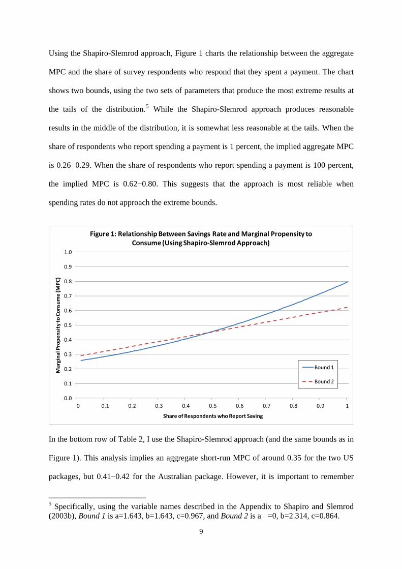
Using the Shapiro-Slemrod approach, Figure 1 charts the relationship between the aggregate

MPC and the share of survey respondents who respond that they spent a payment. The chart

shows two bounds, using the two sets of parameters that produce the most extreme results at

the tails of the distribution.5 While the Shapiro-Slemrod approach produces reasonable

results in the middle of the distribution, it is somewhat less reasonable at the tails. When the

share of respondents who report spending a payment is 1 percent, the implied aggregate MPC

is 0.26−0.29. When the share of respondents who report spending a payment is 100 percent,

the implied MPC is 0.62−0.80. This suggests that the approach is most reliable when

spending rates do not approach the extreme bounds.

0.0

0.1

0.2

0.3

0.4

0.5

0.6

0.7

0.8

0.9

1.0

0 0.1 0.2 0.3 0.4 0.5 0.6 0.7 0.8 0.9 1

Marginal Propensity to Consume (M

PC)

Share of Respondents who Report Saving

Figure 1: Relationship Between Savings Rate and Marginal Propensity to Consume (Using Shapiro‐Slemrod Approach)

Bound 1

Bound 2

In the bottom row of Table 2, I use the Shapiro-Slemrod approach (and the same bounds as in

Figure 1). This analysis implies an aggregate short-run MPC of around 0.35 for the two US

packages, but 0.41−0.42 for the Australian package. However, it is important to remember

                                                            5 Specifically, using the variable names described in the Appendix to Shapiro and Slemrod (2003b), Bound 1 is a=1.643, b=1.643, c=0.967, and Bound 2 is a =0, b=2.314, c=0.864.

9  

that all these estimates are for the first quarter, and that the long-run MPC is likely to be

higher.

Moreover, studies that have relied on direct measures of expenditure (exploiting the random

timing in the payment of the 2001 and 2008 US tax rebates) have estimated higher MPCs. In

their analysis of the 2001 rebate, Johnson, Parker and Souleles (2006) use the Consumer

Expenditure Survey, which asks households a set of detailed questions about their recent

purchases. Restricting the analysis to non-durable goods, they estimate an MPC of 0.37 in the

quarter of receipt, or 0.69 if expenditure in the following quarter is also included. Similarly,

in an analysis of the 2008 rebate using AC Nielsen Homescan data, Broda and Parker (2008)

estimate a first-quarter MPC of about 0.6 and a two-quarter MPC of about 1.6

Although the survey approach seems to imply a higher MPC for the 2009 Australian payment

than for the 2001 and 2008 US rebates, it is worth considering whether this is merely due to

differences in question wording. In particular, one might be concerned that the US questions

asked respondents whether the rebate would lead them to increase spending, while the

Australian question asked respondents whether they would spend the money. In theory,

Australian respondents who did not think that the money would increase their overall

spending might nonetheless have told the interviewer that they would “spend it”, if they

thought that the question related to cash flow rather than net expenditure.

                                                            6 Since the Homescan data include only a subset of non-durable goods, and covers only a one-month interval, Broda and Parker scale up their results using the estimates in Johnson, Parker and Souleles (2006). The MPCs reported in the text above are based on the reported impact on personal consumption expenditure (PCE) of a tax rebate equivalent to 4 percent of PCE: +2.4 percent in the first quarter, and +4.1 percent in the first two quarters.

10  

However, US questions that are worded in a more similar manner to the Australian question

appear to have recorded similar results to those set out in Table 2. For example, a Gallup Poll

released on 24 July 2001 found that only 17 percent of respondents said that they would

spend that year’s tax rebate. Similarly, a CBS News/New York Times Poll conducted in the

United States from 18-22 February 2009 asked respondents “If you receive money from a tax

cut, will you spend it, or use it to pay bills, save it, or invest it?” 19 percent of US

respondents answered “spend it”, compared with 40 percent in the Australian poll. Moreover,

it is not the case that US surveys of this kind invariably show low spending rates: polls

following the 1964 tax cut and prior to the 1982 tax cut both recorded a 50 percent spending

rate, while a poll following the 1992 change in tax withholding recorded a 43 percent

spending rate (cited in Shapiro and Slemrod 2003b).

The only other publicly reported Australian survey of which I am aware is a poll conducted

by Westpac and the Melbourne Institute in August 2009, which asked respondents “If you

received a one-off payment from the Federal Government over the last 6-12 months how

much of it have you spent?”. The two key differences between that survey and the one

analysed in this paper is that the Westpac survey referred to any payments received in the

previous year (thereby including the December 2008 payments), and that it asked about the

share of the payment that was spent, rather than for the primary purpose to which the money

was put. However, the Westpac survey is consistent with the ANU estimate in that it

estimated a very high expenditure rate. Of those respondents who said that they had received

a payment, only 20.2 percent said they had spent none of it, 9.8 percent said they had spent

less than half of it, 7.8 percent said they had spent more than half of it, and 62.2 percent said

they had spent all of it. Assuming that spending is normally distributed around the range

midpoints, and that payments were evenly spread across respondents, the researchers estimate

11  

an MPC of 0.7 (Westpac Group 2009). Although it is difficult to attribute this estimate to a

particular time horizon (since it captures both 2008 and 2009 payments), it is consistent with

a higher MPC for the 2009 Australian payments than the 2001 and 2008 US payments.

4. Is the Cross-Sectional Variation Reasonable?

Economists are understandably reluctant to prefer ‘stated preference’ evidence to ‘revealed

preference’ data. One way to address this concern is to analyse the cross-sectional variation

in the 2009 Australian survey, and see whether it accords with theory and similar empirical

studies.

In Table 3, I tabulate the spending rate across five variables: household income, respondent

age, degree of worry about government debt (“How worried are you that increasing

government debt will harm the financial future of future generations?”), degree of worry

about household unemployment (“How worried are you that in the next 12 months you or

someone else in your household might be out of work and looking for a job for any reason?”),

and voting intention. For each variable, I also estimate an F-test on the hypothesis of equality

across the categories, and report the p-value on this F-test. I also report a multivariate F-test,

from a regression including all five variables.

12  

 

Table 3: Exploring Cross-Sectional Variation in Spending Patterns Spending

RateN Univariate

p-value Multivariate

p-valueHousehold income Less than $20,00 0.40 80 P=0.17 P=0.22$20,000-$39,999 0.45 119 $40,000-$59,999 0.31 115 $60,000-$79,999 0.39 114 $80,000-$99,999 0.35 106 $100,000-$149,999 0.49 121 $150,000 or more 0.44 55 Don't know/ can't say 0.38 55 Refused 0.51 40 Age 18-24 0.41 56 P=0.86 P=0.4225-34 0.38 138 35-44 0.40 191 45-54 0.35 161 55-64 0.46 146 65-74 0.44 78 75+ 0.48 35 Degree of worry about government debt Very worried 0.25 218 P<0.01 P=0.03Somewhat worried 0.42 312 Not too worried 0.51 199 Not at all worried 0.46 71 Don't know/ not sure 0.17 4 Refused 0.00 1 Worry about unemployment Very worried 0.30 118 P=0.06 P=0.23Somewhat worried 0.40 238 Not at all worried 0.44 436 Don't know/ not sure 0.15 10 Refused 0.71 3 Voting intention Liberal 0.29 259 P<0.01 P<0.01Nationals 0.24 28 Labor 0.50 325 Greens 0.46 110 Don't know/ not sure 0.44 62 Refused 0.39 21 Note: Univariate p-value is from an F-test on a linear probability regression of whether the respondent spent the rebate (0/1) on a set of indicator variables denoting each possible response category. The regression is estimated without a constant, and with all categories included. The null hypothesis in the F-test is that the spending rate is the same across all categories. The multivariate p-value conducts a similar exercise, but includes all variables in the table (again with an indicator for each category), and then conducts an F-test on each variable, again with the null hypothesis being that the spending rate is the same across all categories.

13  

The results from the first variable indicate that there is no systematic relationship between

household income and spending rates. While this may be surprising at first blush, it is

consistent with the results of Shapiro and Slemrod, who argue that “low-income individuals

are needy today, but because they are also likely to be needy in the future, they do not

necessarily use the windfall for current consumption” (2009, 376).

By respondent age, the spending rate trends upwards, though the relationship is not

monotonic. Among respondents aged under 65, the average spending rate is 40 percent,

compared to 45 percent for respondents aged 65 or over. However, while the age differences

are consistent with a life-cycle model, they are not statistically significant.

The third variable tabulates the spending rate against respondents’ degree of worry about

government debt. This is a loose test of Ricardian equivalence – the theory that consumers

will only spend a payment if it is accompanied by a reduction in government expenditure.

Respondents who are more worried about government debt (and therefore perhaps more

concerned that government payments now will lead to tax increases in the future) are

significantly less likely to spend the rebate. For example, only 25 percent of respondents who

are “very worried” about government debt spent the rebate, as compared with 46 percent of

respondents who are “not at all worried” about government debt. This difference remains

significant even in a multivariate regression.

The fourth question looks at the relationship between spending rates and households’ worry

that they or a member of their family will become unemployed. Thirty percent of respondents

who are “very worried” about unemployment spent the rebate, as compared with 44 percent

of respondents who are “not at all worried” about household unemployment. Although this is

14  

consistent with the liquidity hypothesis (in which households are more likely to spend if they

are optimistic about the future), the difference between categories is only statistically

significant in the univariate specification, and not in the multivariate specification.

The final variable against which I tabulate spending rates is voting intention. Somewhat

surprisingly, those who said that they would vote for Labor (the incumbent party) were much

more likely to spend the rebate than those who said that they would vote for the opposition

Liberal or National parties. This result is not merely an artefact of the income, age, or debt

attitudes of the respondents, since it remains statistically significant (at the 1 percent level) in

a multivariate regression. One possible interpretation is that individuals’ willingness to

respond to government exhortations to spend the payment is partly a function of their

political views. Another possibility is reverse causality: respondents with a predisposition

towards spending the payment might have been more inclined to think that the payment was

good policy, and therefore more inclined to support the government.

Overall, the cross-sectional variation provides weak support for the life-cycle hypothesis and

the liquidity hypothesis, and strong support for the notion that beliefs in Ricardian

equivalence explains differences in spending patterns across individuals. Intriguingly, the

cross-sectional variation also suggests some role for partisan beliefs in explaining spending

differences.

5. Conclusion

Using survey responses, I estimate the impact of $12 billion in household payments delivered

to Australian households from March 2009 to May 2009. According to the survey results,

15  

about 40 percent of Australians said that they spent the payment; a share that is

approximately twice as large as in the case of the 2001 and 2008 US tax rebates.

What might explain why the spending rate is higher for a fiscal stimulus in Australia in 2009

than for one in the US in 2001 or 2008? One possibility is that at the relevant times,

Australian households had more bullish expectations for the economy than their US

counterparts. While comparable measures of expectations are difficult to obtain, one possible

approach is to look at the actual change in unemployment. From 2000 to 2002, the US

unemployment rate rose from 4 percent to 6 percent. From mid-2007 to mid-2009, the

unemployment rate in the US jumped from 5 percent to 10 percent, while the rise in Australia

was only from 4 percent to 6 percent. These data suggest that one might have expected

Australians in 2008 to be more optimistic than US residents in 2008, but do not explain why

US residents in 2001 should have been more pessimistic than Australians in 2008.7

Adapting the Shapiro/Slemrod approach for converting spending rates into MPCs suggests a

first-quarter MPC for the Australian payments of 0.41−0.42. However, there are two

important limitations of this estimate. The first is that it is based only on a single survey

question. Ideally, one would wish to have both an MPC estimate from expenditure surveys

(or scanner data) and another from a survey question of the kind used in this paper. Christian

Broda and Jonathan Parker (2008) adopt the useful strategy of adding a “what did you do

with the stimulus?”-type question to a consumer expenditure survey. In conjunction with

random timing in the rollout of the tax rebate, this permits a comparison of the two

                                                            7 Another possible explanation is that household debt ratios explain differences in the MPC. However, the ratio of household debt to household disposable income in Australia and the United States is quite similar during this period.

16  

methodological approaches, with the advantage that the two approaches are estimated from

the same respondents.

The other limitation of the approach used in this paper is that it only estimates the short-term

impact of the 2009 payments on household spending. Although it is likely that the total effect

of the payments on consumer expenditure exceeds the first-quarter impact, the survey

approach is not well suited to estimating the long-run effect, since it relies on households

accurately recollecting what they did with a payment that was received up to 6 months before

the survey. Unless the payment constitutes a large share of household income, longer-run

estimates are likely to be more noisily measured than short-run estimates.

17  

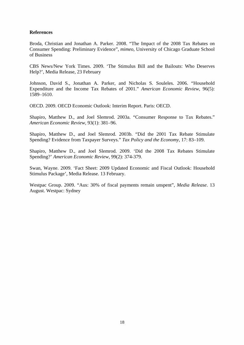
References Broda, Christian and Jonathan A. Parker. 2008. “The Impact of the 2008 Tax Rebates on Consumer Spending: Preliminary Evidence”, mimeo, University of Chicago Graduate School of Business CBS News/New York Times. 2009. ‘The Stimulus Bill and the Bailouts: Who Deserves Help?’, Media Release, 23 February Johnson, David S., Jonathan A. Parker, and Nicholas S. Souleles. 2006. “Household Expenditure and the Income Tax Rebates of 2001.” American Economic Review, 96(5): 1589–1610. OECD. 2009. OECD Economic Outlook: Interim Report. Paris: OECD. Shapiro, Matthew D., and Joel Slemrod. 2003a. “Consumer Response to Tax Rebates.” American Economic Review, 93(1): 381–96. Shapiro, Matthew D., and Joel Slemrod. 2003b. “Did the 2001 Tax Rebate Stimulate Spending? Evidence from Taxpayer Surveys.” Tax Policy and the Economy, 17: 83–109. Shapiro, Matthew D., and Joel Slemrod. 2009. ‘Did the 2008 Tax Rebates Stimulate Spending?’ American Economic Review, 99(2): 374-379. Swan, Wayne. 2009. ‘Fact Sheet: 2009 Updated Economic and Fiscal Outlook: Household Stimulus Package’, Media Release. 13 February. Westpac Group. 2009. “Aus: 30% of fiscal payments remain unspent”, Media Release. 13 August. Westpac: Sydney

18  

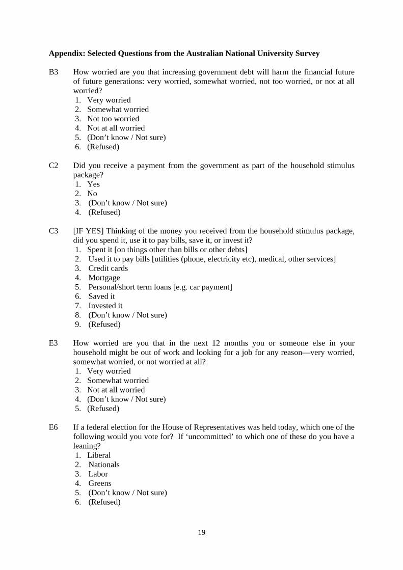
Appendix: Selected Questions from the Australian National University Survey B3 How worried are you that increasing government debt will harm the financial future

of future generations: very worried, somewhat worried, not too worried, or not at all worried? 1. Very worried 2. Somewhat worried 3. Not too worried 4. Not at all worried 5. (Don’t know / Not sure) 6. (Refused)

C2 Did you receive a payment from the government as part of the household stimulus

package? 1. Yes 2. No 3. (Don’t know / Not sure) 4. (Refused)

C3 [IF YES] Thinking of the money you received from the household stimulus package,

did you spend it, use it to pay bills, save it, or invest it? 1. Spent it [on things other than bills or other debts] 2. Used it to pay bills [utilities (phone, electricity etc), medical, other services] 3. Credit cards 4. Mortgage 5. Personal/short term loans [e.g. car payment] 6. Saved it 7. Invested it 8. (Don’t know / Not sure) 9. (Refused)

E3 How worried are you that in the next 12 months you or someone else in your

household might be out of work and looking for a job for any reason—very worried, somewhat worried, or not worried at all? 1. Very worried 2. Somewhat worried 3. Not at all worried 4. (Don’t know / Not sure) 5. (Refused)

E6 If a federal election for the House of Representatives was held today, which one of the

following would you vote for? If ‘uncommitted’ to which one of these do you have a leaning? 1. Liberal 2. Nationals 3. Labor 4. Greens 5. (Don’t know / Not sure) 6. (Refused)

19  

20  

Dem5 Would you mind telling me how old you are? 1. Age given (RECORD AGE IN YEARS (RANGE 18 TO 99) 2. (Refused)

(IF RESPONDENT REFUSES TO ANSWER DEM5) Dem6 Would you mind telling me which of the following age groups are you in? READ OUT

1. 18 - 24 years 2. 25 - 34 years 3. 35 - 44 years 4. 45 – 54 years 5. 55 – 64 years 6. 65 – 74 years, or 7. 75 + years 8. (Refused)

Dem9a. What is your total annual household income before tax or anything else is taken out?

Would it be… (READ OUT) 1. Less than $20,000 2. $20,000 to less than $40,000 3. $40,000 to less than $60,000 4. $60,000 to less than $80,000 5. $80,000 to less than $100,000 6. $100, 000 to less than $150,000, or 7. $150,000 or more 8. (Don’t know / can’t say) 9. (Refused)