Embed Size (px)
Citation preview
UNIVERSITY OF PIRAEUS
DEPARTMENT OF BANKING AND FINANCIAL MANAGEMENT M.Sc. IN FINANCIAL ANALYSIS FOR EXECUTIVES
MASTER’S THESIS
MACROECONOMIC FACTORS AND OIL FUTURES PRICES
STUDENT: KOSTAS KONSTANTATOS MXAN0922
SUPERVISOR: Dr. NICHOLAS APERGIS
COMMITTEE
NICHOLAS APERGIS
ANGELOS ANTZOULATOS
GEORGE DIACOGIANNIS
FEBRUARY 2011
1 Abstract
The main purpose of this paper is to determine the relationships between various
macroeconomic factors and oil futures, with underline commodity the WTI light
sweet crude oil, trading in NYMEX. In this effort we use five oil futures’ maturities
and specifically the generic form contracts of 1, 3, 6, 9 and 12 months. We try to
determine the interdependencies of certain macroeconomic factors and the price of
each one contract starting from January 1990 until May of 2010. We test for Granger
causality and then apply VAR specification accompanied by impulse response
analysis and variance decomposition. We find evidence that there is a solid
relationship between certain macroeconomic factors and oil variables.
Key words: oil futures, macroeconomic factors, VAR, transmission mechanism,
variance decomposition.
2 TABLE OF CONTENTS
Abstract ........................................................................................................................ 1
CHAPTER 1: INTRODUCTION ......................................................................... 3
1.1 Presentation of the selected macroeconomic variables ................................... 3
1.2 Data and symbols ............................................................................................ 5
1.3 Brief oil pricing history ................................................................................... 5
1.4 Impact of oil price on economy....................................................................... 7
1.5 Transmission mechanism & oil futures ......................................................... 11
1.6 Relevant literature ......................................................................................... 22
1.7 Expected effect of macroeconomic factors to oil futures .............................. 28
CHAPTER 2: METHODOLOGY ...................................................................... 30
2.1 Unit root tests ................................................................................................ 30
2.2 Ordinary Least Squares (OLS) ...................................................................... 32
2.3 Granger causality........................................................................................... 36
2.4 Cointegration ................................................................................................. 39
2.5 VAR and VEC ............................................................................................... 40
2.6 Impulse response analysis & Variance decomposition ................................. 43
CHAPTER 3: EMPIRICAL RESULTS ............................................................ 44
3.1 Granger causality results ............................................................................... 44
3.2 Vector autoregression results ........................................................................ 52
3.3 Impulse response results................................................................................ 70
3.4 Variance decomposition results .................................................................... 71
3.5 Vector Autoregression Conclusions – Remarks ............................................... 73
References ................................................................................................................. 76
Appendix A ............................................................................................................... 80
Appendix B ............................................................................................................... 83
Appendix C ............................................................................................................... 89
3 CHAPTER 1: INTRODUCTION
1.1 Presentation of the selected macroeconomic variables
We choose a particular set of macroeconomic variables because there aren’t many
studies that deal with them explicitly, although all of them are reliable proxies and
expressions of very important real economic events and motions that happen
worldwide. So in that sense there are no previous studies that much exactly this paper
except only partially. That’s why we try to capture relations between them and the oil
variables in order to discover correlations and interdependencies that are not known.
In order to quantify these various macroeconomic factors we used a set of indices
as proxies that each one represents a certain factor. Some of these proxies are
announced once a month, so we had to take monthly prices for every other index and
also for the futures prices in order to make a coherent set that could be processed.
These proxies are:
1. S& P 500 stock index.
2. S & P Europe 350 stock index.
3. Nikkei 225 stock index.
4. Hang Seng stock index.
5. FED target funds rate.
6. Dry Bulk index.
7. US industrial production (MoM 2007=100, sa).
8. European Union industrial production (MoM, sa).
9. Capacity utilization for the US economy.
The first one, Standard & Poor’s 500 contains 500 median and big US companies
based on their market size, liquidity and sector. It is considered by many market
participants as a benchmark for the overall US equity market. It can be used as a
proxy for the overall health of the US economy. S & P 350 index is tracking almost
70% of the European market capitalization and therefore it can be used as a proxy for
the European economy. Nikkei is a stock market index for the Tokyo stock exchange
and it is consisted of 225 prominent Japanese stocks. It can be used as a major
4 indicator for the Japanese economy. Hang Seng index consists of the 45 largest
companies of the Hong Kong stock exchange and it represents almost 67% of its
capitalization. Most of them are big Chinese companies and it is a good indicator of
the Chinese economy. Fed effective funds rate is the target rate at which depository
institutions lend balances at the Federal Reserve to other depository institutions
overnight. This is very close to the target rate that we use in this paper. Using the
intention of Fed about funds rate, which is the target funds rate that we use, is an
approximation of the certain point that the US economy is during an economic cycle.
Low target funds rates means that US economy is not strong enough, so the Fed
decreases target rate in order to motivate economic participants and strengthen
economic activity. Dry bulk index (BDI) tracks worldwide shipping prices of various
dry bulk carriers. It is assessed by taking into account 50 global shipping routes and it
is an indicator of supply and demand in global transportation of raw materials. When
global economy is robust the value of the index rises and vice versa. The next two
indicators, US and EU industrial production, track industrial output in America and
European Union. Industrial activity consumes a large amount of produced oil and
changes in the level of industrial output affect oil prices. Capacity utilization is the
extent to which the productive capacity of an economy is used to generate goods and
services. Intuitively we can assume that the stronger the economy the more productive
capacity uses, leading the value of the index upwards.
The main idea underlines the choice of the indices is firstly, the global character of
the oil market and secondly, the correlation of global economy in such a way that the
slowdown of a major economy such as US or Europe, could not be considered
irrelevant of a slowdown in global economy. In contemporary world, economies are
intertwined so much that even the bankruptcy of a small country like Greece could
cause crackles in the globalised monetary system, something that couldn’t be happen
before 30 years. In that sense, if, let’s say, the FED key interest rate are below 1%,
we can safely assume that the US economy are in crisis and the same is almost certain
for the rest of the world, with some unavoidable exceptions of course.
5 1.2 Data and symbols
For practical purposes we assign symbols to the various macroeconomic factors
and the futures contracts that will be used.
spot= spot WTI oil price at Cushing, Oklahoma
cl1= futures contract matures in 1 month
cl3= futures contract matures in 3 months
cl6= futures contract matures in 6 months
cl9= futures contract matures in 9 months
cl12= futures contract matures in 12 months
sp500= S & P 500 stock index
sp350= S & P 350 stock index
nikk= Nikkei stock index
hase= hang seng stock index
fedr= Fed target funds rate
bdi= dry bulk index
indpreu= industrial production index for European union
indprusa= industrial production index for US
caput= capacity utilization for US
When letter d is in front of a symbol, it denotes logarithmic returns. Cl1, cl3, cl6,
cl9, cl12, are the generic forms of futures contracts for maturities 1, 3, 6, 9 and 12
months respectively and have been downloaded from Bloomberg. Spot is the spot
price of WTI crude oil as it is trading at Cushing, Oklahoma.
1.3 Brief oil pricing history
Pricing in the oil market evolved, as the significance of oil as an input in the
production procedure increased dramatically, mostly after the Second World War.
The use of oil can be traced back to ancient years where people used it for lighting,
construction or even as a cure for kidney stones. Technological advances that took
place after the industrial revolution in Europe convert oil from a low importance and
usefulness commodity, to the main factor in production activity worldwide.
6 After World War II and until the 1970s major participants in the crude oil market
were determining the prices. These participants were the big western oil companies,
the seven sisters as they were been named at the time being and oil producing nations
such as US, Mexico, Saudi Arabia. It was a market that was driven by supply and
demand for spot oil and was characterized by monopolies and their power to
determine oil price. But as oil became more important as an input in economy, more
countries join the game and the companies that engaged in the production and
distribution of oil increased dramatically. This led to a more globalized and fair
pricing mechanism. In 1980s the monopoly was gradually broken and on March 30
1983 oil futures contracts with fixed characteristics started trading in the NYMEX.
The number of market participants had increased during the previous years in such an
extent that spot oil prices were determined by active trading in organized markets
rather than by agreements between a few companies. From that date and on, futures
contracts gain exponentially in significance and today their role as a pricing
mechanism is without question unexceptionable. The biggest markets for oil futures
today are the NYMEX, where WTI (West Texas Intermediate) light sweet is trading
and the ICE (Intercontinental Exchange) where Brent oil futures are trading.
WTI futures contracts at NYMEX refer to 1000 or 500 barrels of crude oil and
today anyone that has the money to cover the margin requirements can buy a contract.
This indeed is a major change compared to the time that only big companies paying
millions of dollars could trade crude oil.
Oil contracts in NYMEX extend up to nine years and for the first six years
(including the current) there are monthly consecutive maturities. After the sixth year
we have only June and December contracts. New contracts are added after the
December contract of each year matures, so the term structure is continuously
renewed.
7 1.4 Impact of oil price on economy
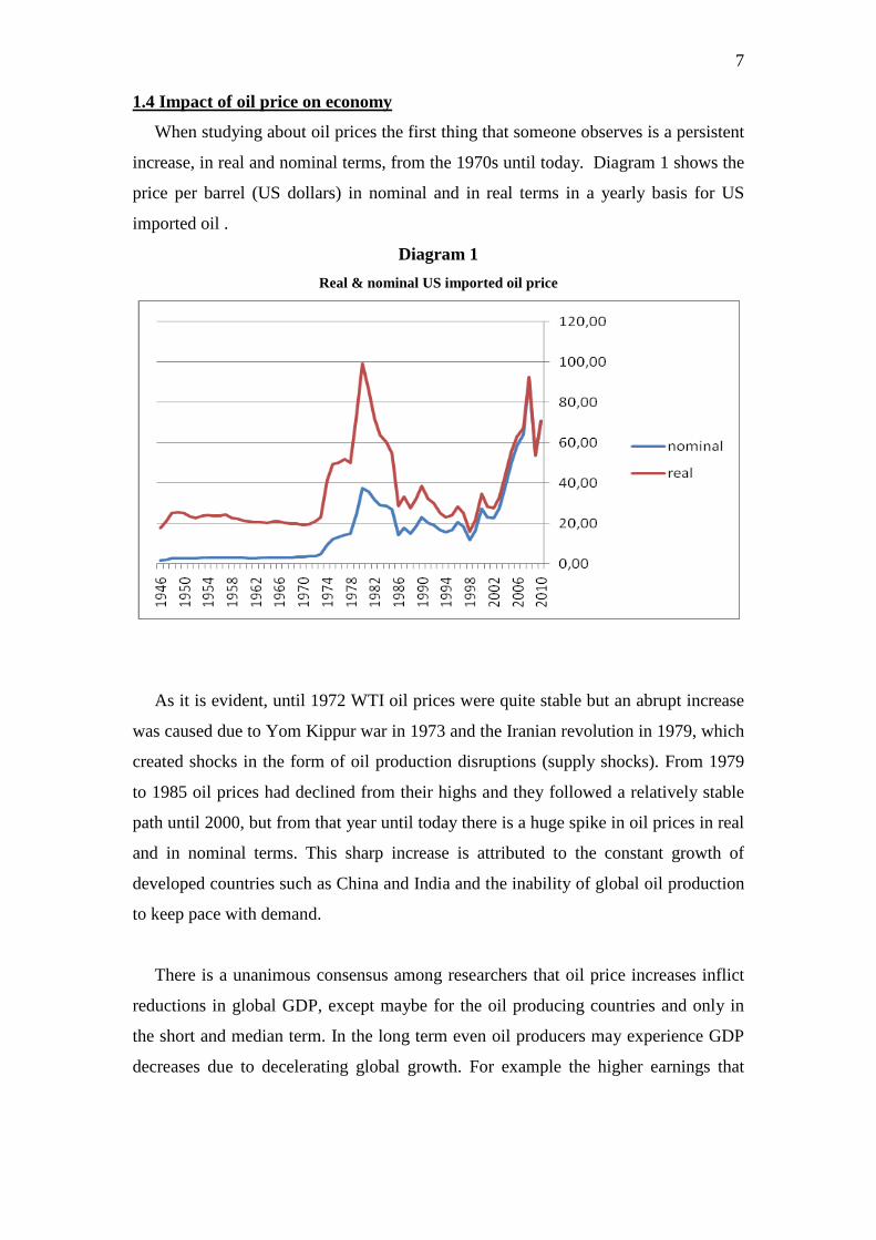
When studying about oil prices the first thing that someone observes is a persistent
increase, in real and nominal terms, from the 1970s until today. Diagram 1 shows the
price per barrel (US dollars) in nominal and in real terms in a yearly basis for US
imported oil .
Diagram 1 Real & nominal US imported oil price
As it is evident, until 1972 WTI oil prices were quite stable but an abrupt increase
was caused due to Yom Kippur war in 1973 and the Iranian revolution in 1979, which
created shocks in the form of oil production disruptions (supply shocks). From 1979
to 1985 oil prices had declined from their highs and they followed a relatively stable
path until 2000, but from that year until today there is a huge spike in oil prices in real
and in nominal terms. This sharp increase is attributed to the constant growth of
developed countries such as China and India and the inability of global oil production
to keep pace with demand.
There is a unanimous consensus among researchers that oil price increases inflict
reductions in global GDP, except maybe for the oil producing countries and only in
the short and median term. In the long term even oil producers may experience GDP
decreases due to decelerating global growth. For example the higher earnings that
8 OPEC would have from increased oil prices in the short term could be outweighed by
decrease in world production and subsequently less demand for oil. The estimates of
the short term effect of oil prices on the economy vary. According to Huntington
(2005) in a survey of several macroeconomic models conducted in 2005, a 10 dollars
per barrel increase is expected to reduce output in US by about 0.25 percentage points
in the first year and 0.5 percentage points in the second year. A study of the
International Monetary Fund (2005), showed that an increase of $5 per barrel can
reduce real world GDP by 0.25 percentage points for the next four years and by about
0.3 percentage points the US GDP. In another research which conducted in 2004 by
IEA (International Energy Agency) in collaboration with OECD and IMF, an increase
of 10 dollars in oil prices would result in a 0.4 percentage points loss of GDP per
year, for two years, for all OECD countries and additionally in a 0.5 percentage points
increase in inflation. Unemployment would also increase. OECD countries with high
dependence on imported oil such as the European Union would suffer more losses in
the short term than countries with less dependence such as US. The effects of the
shock starting to diminish after about three years.
There is a difference on the impact of oil price shocks between developed and
developing or underdeveloped countries. The results of a shock would be greater in
developing and underdeveloped due to lower productivity of energy use. On average
oil importing developing countries use twice as much oil to produce a product unit
than OECD countries, meaning that they are more energy-consuming and energy-
inefficient. For example in Asia a 10 dollars increase in oil price would result in a
0.8% loss in GDP and for the poorer and more indebted developing countries of the
world, 1.6% loss. In sub-Saharan Africa the loss would be even greater than 3%.
Although there is consensus about the negative impact of oil prices in the economy
there is a different level of responsiveness for every particular country which depends
on many other factors. Oil imports as a percentage of GDP is a very important factor
which shows how much an economy depends on foreign oil. Countries with total
dependence on foreign oil suffer only disadvantages relatively to countries that
produce even a small amount of oil which counteracts the negative effects of the price
9 increase. Another factor is the ability of households and companies to substitute oil
with other energy sources such as gas and the correlation of oil prices to gas prices.
Oil price shocks also affect negatively the exchange rates due to deterioration in
the balance of payments. In order for a country to buy the same amount of oil as
before the price spike, it has to sell more of its domestic currency to buy dollars, so its
currency depreciates. Imports then become more expensive and exports yield less in
terms of foreign currency, although here there is also a positive effect from the
increase in exports due to the fact that domestic currency depreciation makes
domestic products cheaper.
The effects of oil price spikes at first, act on a microeconomic level. Due to high
correlation among oil and gasoline prices households have increased expenses for
gasoline and heating oil which reduces their consumption for other goods and services
leading companies to lower profits. Companies on the other hand except from reduced
sales, they have also increased input costs, especially those which use oil as a primary
input such as industrials and transportation companies. Lower profits means decline in
stock exchanges, lower job vacancies or even layoffs and generally the triggering of a
self-feed mechanism which produces economic depression. Also except inflation that
is caused directly from the increased oil prices, (oil price is a parameter in the
inflation estimation), the rise in input costs may be transferred to consumers through
higher product prices. The employees on the other hand might ask for higher wages to
counteract the decrease in their purchase power and all these factors lead to a self-feed
inflation procedure.
The described recession mechanism needs to be unexpected in order to be
powerful and effective. That is one of the reasons why the world economy keeps
developing instead of the increase in oil prices. The oil price spike is already
discounted and accounted for so it inflicts less turbulence in the economic system.
A common question that derives from the dependencies between oil price and the
economy is its stability and power through time. Blanchard and Gali (2007) conclude
10 that although the oil price shocks of 2000s are comparable in magnitude to the 1970s
shocks, their effect on economy wasn’t as strong as in 1970s suggesting that the
relation between fluctuations in oil price and real economy after 2000 has been
smoothed out. Hooker (2002) in his study suggests that in late 1980s a structural
brake occurred between oil price and inflation and their dependence reduced in
magnitude. Also Blanchard and Gali (2007) come down to a similar conclusion that
there is a structural brake at the responses of output, wage inflation, prices and
employment relatively to shocks in oil prices, from mid 1980s and on.
Many explanations have been given why the relation between oil prices and
inflation has weakened. Blanchard and Gali (2007) suggest increased flexibility in
labor markets, monetary policy improvements and adverse concurrent shocks such as
a concurrent productivity increase. Central banks response is also a logical
explanation especially concerning the US Fed. Before 2000, Fed used to concentrate
more on the consequences of oil prices on output rather than on inflation. This stance
were producing inflationary expectations to households and companies and these
expectations were triggering the inflation cycle. After 2000 where Fed’s attention on
inflation became more important and it adjusted its policy in order to stabilize
inflation, the consequences of oil prices shocks to economy have reduced as also the
inflationary expectations of households and companies which trigger the inflation
cycle. So by deteriorating inflation consciously Fed has reduced the correlation
between oil shocks and inflation.
Sill (2007) alleges that five out of seven recessions that have happened in the last
30 years were preceded by spikes in oil prices. At all these periods there were also
other variables which simultaneously affected the economy such as hikes in
commodity prices in 1970s and a strong global increase in productivity and output in
the 2000s. These parameters obscure the real effect of oil price fluctuations in
economy and someone have to employ econometric analysis in order to raise the
possibility to conclude more reliably in the relation between oil and economy.
An interesting effect of high oil prices is reallocation of capital and production
inputs among different industries. Alternative sources of energy which antagonize oil,
11 gain advantage relatively to oil although not rapidly. Solar, wind or geothermal
energy owe some of their development and usefulness in everyday life, to high oil
prices. These sources of energy become relatively cheaper as oil prices increase and
tend to operate as substitutes. Another example is the car industry. Major car
manufacturers develop new ‘clean’ technologies in order to produce car engines
which work without gasoline. Such reallocation is extended in other industries that
produce car parts for the new ‘clean’ cars, such as batteries, solar cells or even
biofuels. Especially biofuels can reallocate the whole agricultural production of an
area or even a country by stimulating farmers to produce plants for biofuels instead of
consumption, if the price is to their advantage.
The relation between oil price and the economy is also relative to the certain point
that we are in the economic cycle. Huntington (2005) claims that oil price shocks that
occur in an environment of low interest rates and low inflation are less interactive
with economy than shocks that happen in an environment of high interests and high
inflation.
1.5 Transmission mechanism & oil futures
The effect of various macroeconomic factors to oil futures is transmitted in two
stages. At the first stage, there is a strong positive correlation of spot prices to futures
prices that moves the term structure up or down. If for example we have a very strong
global growth that demands great quantities of oil then the supply-demand mechanism
will boost upward the spot price and the same will happen to futures contracts at all
maturities. At this stage we have the primary reason that affects futures prices
indirectly through spot prices. The second stage is as important as the first because
most of the time we observe high deviation between the spot and future prices which
become greater as time to maturity increases (ceteris paribus). This deviation could be
attributed to the combination of cost of carry and convenience yield. When
convenience yield becomes greater than the cost of carry, spot prices are higher than
futures prices and the term structure is determined as backwardation (downward
sloping). The opposite gives a term structure described as contango where futures
prices are higher than spot prices (upward sloping term structure). This is visible in
the pricing equation for commodity futures held for consumption:
12
TycetStF
−
=
c=cost of carry
y=convenience yield
F t =future contract price at time t
S t =spot price at time t
T=time to maturity annualized
e=base of natural logarithm (implies continuous compounding)
Cost of carry can be analyzed in two components for oil futures. The first is the
risk free rate r f , and the second is the storage cost per year as a percentage of oil
price u. The equation that describes these components is:
uc r f +=
As we said, when global economy is robust, central banks tend to increase their
key interest rates. On the other hand when we have a growing global economy, there
is a great possibility that storage cost will increase. This is due to higher rents for
storage areas (the opposite holds true when global economy is in slowdown). Cost of
carry in this case will increase and in combination with convenience yield the price of
the futures contracts at all maturities changes. This is an indirect way where various
macroeconomic factors that lead to an increase or decrease in global growth, affect oil
futures prices. So the possible outcomes are infinite, depending on the values that cost
of carry and convenience yield will take.
From the primary mechanism of supply and demand in spot market which is the
first consequence in oil price if a change in a certain macroeconomic factor occurs,
we passed to the deviation of spot price to futures price and its determinants. The
spread of this deviation must be considered thoroughly if we are to find a reliable
13 relationship between macroeconomic factors and futures oil prices. Because of the
complexity of the mechanism we can only observe indirectly these effects to oil
futures markets. Let’s say that global economy in the near term is expected to grow
rapidly and oil buyers want to pile into inventories in order to correspond to the
upcoming demand for oil. Then the convenience yield will increase (ceteris paribus),
and the more it increases the more futures contracts at all maturities deviate from spot
prices heading downwards (backwardation). This deviation can be quite important
and is a significant determinant of the futures contracts prices.
We observe that a key contributor to the change of convenience yield is
expectations which play an important role to the transmission of macroeconomic
effects to oil futures. Expectations that affect futures prices are not only concern
macroeconomic factors but also geopolitical conflicts, weather changes, spare oil
capacity, OPEC decisions about supply and numerous other factors.
One of the theories that have been proposed to explain the spike in oil prices after
2002 is peak oil theory. According to this, oil production will reach a peak at the near
future when global demand will continue to rise, so there will be a shortage that will
increase oil price. The peak oil theory advocates chart the amount of oil discovered
over time and extrapolate this trend into the future. Evidence exists that the number of
wells drilled, has been significantly reduced from 1980 until today, but it is not at all
sure that this is due to lack of oil reserves instead of unwillingness to drill, from big
oil companies. If this theory holds true, which is not at all sure, or even if market
participants believe that it is true, we can see how expectations can affect futures
prices in a direct way. Under these circumstances we will have a permanent contango
because market participants will expect oil prices to keep rising in the future so they
will buy futures in order to hedge rising oil prices.
There is a very important difference between expectations and other
macroeconomic factors and this is the straightforward way in which expectations
affect futures prices. In the first paragraphs of this paper we saw the indirect way
witch various factors affect futures prices via 1.Spot prices and the current supply-
demand mechanism. 2. Cost of carry and convenience yield. We implied a one way
14 direction from spot prices to futures prices. Via expectations it is transformed into a
two directions mechanism.
Many financial institutions (including ECB and IMF) and market participants use
futures contracts prices as a proxy for expected spot prices (predictors). This implies
that a change in futures contracts prices determines spot prices. Baek and Brock
(1992) employed a nonlinear causality model to evaluate the lead lag relationship
between spot and futures prices. In this paper they found that a two way feedback
relationship exists, where futures prices always lead spot prices (efficiency of crude
oil market). Also Kaufmann & Ullman (2008) investigated from where changes in the
price of crude oil originate and how they spread, by examining causal relationships
among prices for crude oil from North America, Europe, Africa and the Middle East
on both spot and futures markets. One of their conclusions was that the spike in oil
prices at the end of 2008 was generated by changes in market fundamentals as well as
speculation. At first, increased demand and inelastic supply of oil caused a big hike in
oil spot prices and then speculators came in by buying futures contracts to anticipate
continuation of price hiking. The increased demand in futures contracts raised their
price and this rise transmitted to the spot market at a level that couldn’t be justified by
the existing supply-demand balance. So in that case we can clearly see the two
directions mechanism for oil pricing and also how macroeconomic factors indirectly
affect oil futures prices.
Bekiros & Diks (2007) using a nonlinear model, conclude that the pattern of leads
and lags between futures and spot market, changes over time in a way that we cannot
say if the spot or the futures market always lead. This means that causality is
bidirectional.
An important way by which expectations determine oil futures prices is through
the use of contracts for hedging purposes, which indirectly relates to macroeconomic
factors. If for example a company that uses oil as a production input expects
continuous rise in oil prices due to constant growth in global industrial production, it
might buy futures contracts to lock in current prices. Other market participants might
15 expect a slowdown, so they sell oil contracts to lock in selling prices. The effect of
buying and selling for hedging purposes, cause changes in oil futures prices.
Bwo-Nung Huang, C.W. Yang and M.J. Hwang (2007) study the effect of
speculative strategies on the term structure of oil futures. They defined the term
‘basis’ as the difference between futures price and spot price and they discovered that
there is a critical threshold band of basis values, out of which there are arbitrage
opportunities that when exercised tend to move the oil market towards equilibrium. In
other words if basis is positive and greater than the upper limit of the threshold, then
investors will start the arbitrage by selling futures contracts and buying oil in the spot
market. When basis is negative (futures contracts price smaller than spot price) and
bigger in absolute value from the lower bound of the threshold, then investors sell oil
in spot market and buy futures contracts. The paper captures the interactions between
spot and futures prices, at least to the extent that speculation opportunities exist.
There is no consensus for the magnitude of the change that hedging and
speculation cause. There are opinions that attribute the current high price of oil to
speculators and hedgers and others that support a small change in spot and futures
prices due to speculative or hedging purposes.
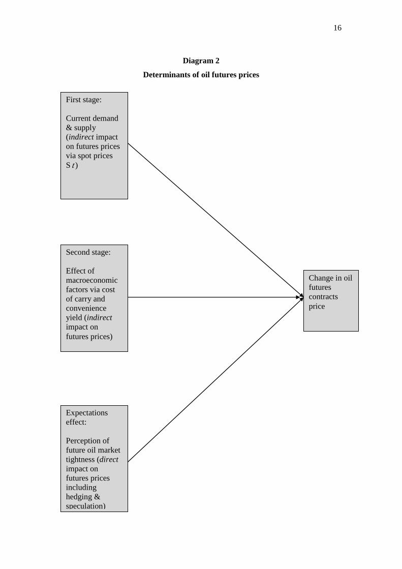
We can draw the mechanism that has been described in the above paragraphs, for
simplification reasons, as below:
16
Diagram 2
Determinants of oil futures prices
First stage: Current demand & supply (indirect impact on futures prices via spot prices S t )
Second stage: Effect of macroeconomic factors via cost of carry and convenience yield (indirect impact on futures prices)
Expectations effect: Perception of future oil market tightness (direct impact on futures prices including hedging & speculation)
Change in oil futures contracts price
17
The above mechanism could be enriched to include other factors than
macroeconomic, such as proven world oil reserves, geopolitical conflicts, spare oil
capacity, expectations for supplemental alternative energy sources, etc, which are out
of the scope of this paper.
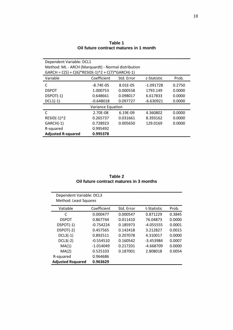
In order to capture the importance of spot prices in the configuration of futures
prices we run five regressions with dependent variables the returns of futures
contracts of 1, 3, 6, 9, 12 months and independent variables:
1. The contemporaneous spot returns and three lags of spot returns,
2. Three lags of the dependent variable itself AR(3) and
3. Three lags of the moving average of the error term MA(3).
By using the adjusted R-squared of every regression we will depict the explicative
power of the above three groups of variables to every WTI future price. We perform
general to specific procedure by subtracting gradually the statistically insignificant
coefficients (prob.>0.05) and after obtaining statistical significance of all coefficients
we perform misspecification testing to correct for serial correlation and
heteroskedasticity of the error term, if needed. An adjusted R-squared equals to 1
means that the independent variables explain 100% the dependent variable whereas an
adjusted R-squared below 1 indicates that the remaining 1-R2 can be explained by
other unknown variables. We use logarithmic returns in order to avoid the unit root
problem that exists if we just take the time series data as they are. The results of the
regression for the 5 aforementioned contracts are shown below.
18
Table 1 Oil future contract matures in 1 month
Dependent Variable: DCL1 Method: ML - ARCH (Marquardt) - Normal distribution GARCH = C(5) + C(6)*RESID(-1)^2 + C(7)*GARCH(-1) Variable Coefficient Std. Error z-Statistic Prob. C -8.74E-05 8.01E-05 -1.091728 0.2750 DSPOT 1.000753 0.000558 1793.149 0.0000 DSPOT(-1) 0.648661 0.098017 6.617833 0.0000 DCL1(-1) -0.648018 0.097727 -6.630921 0.0000 Variance Equation C 2.70E-08 6.19E-09 4.360802 0.0000 RESID(-1)^2 0.265737 0.031661 8.393162 0.0000 GARCH(-1) 0.728923 0.005650 129.0169 0.0000 R-squared 0.995492 Adjusted R-squared 0.995378
Table 2 Oil future contract matures in 3 months
Dependent Variable: DCL3 Method: Least Squares
Vatiable Coefficient Std. Error t-Statistic Prob.
C 0.000477 0.000547 0.871229 0.3845 DSPOT 0.867744 0.011410 76.04873 0.0000
DSPOT(-1) -0.754224 0.185973 -4.055555 0.0001 DSPOT(-2) 0.457565 0.142418 3.212827 0.0015 DCL3(-1) 0.892511 0.207078 4.310017 0.0000 DCL3(-2) -0.554510 0.160542 -3.453984 0.0007
MA(1) -1.014049 0.217201 -4.668709 0.0000 MA(2) 0.525103 0.187001 2.808018 0.0054
R-squared 0.964686 Adjusted Rsquared 0.963629
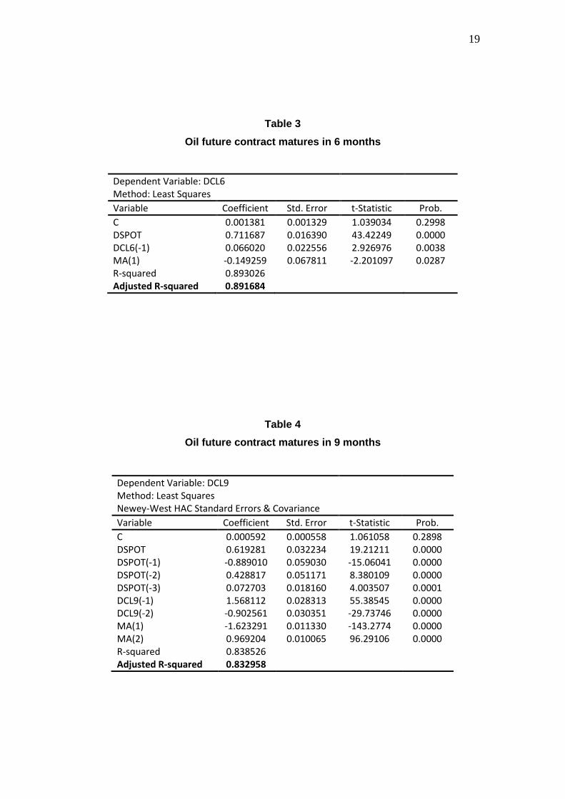
19
Table 3 Oil future contract matures in 6 months
Dependent Variable: DCL6 Method: Least Squares Variable Coefficient Std. Error t-Statistic Prob. C 0.001381 0.001329 1.039034 0.2998 DSPOT 0.711687 0.016390 43.42249 0.0000 DCL6(-1) 0.066020 0.022556 2.926976 0.0038 MA(1) -0.149259 0.067811 -2.201097 0.0287 R-squared 0.893026 Adjusted R-squared 0.891684
Table 4 Oil future contract matures in 9 months
Dependent Variable: DCL9 Method: Least Squares Newey-West HAC Standard Errors & Covariance Variable Coefficient Std. Error t-Statistic Prob. C 0.000592 0.000558 1.061058 0.2898 DSPOT 0.619281 0.032234 19.21211 0.0000 DSPOT(-1) -0.889010 0.059030 -15.06041 0.0000 DSPOT(-2) 0.428817 0.051171 8.380109 0.0000 DSPOT(-3) 0.072703 0.018160 4.003507 0.0001 DCL9(-1) 1.568112 0.028313 55.38545 0.0000 DCL9(-2) -0.902561 0.030351 -29.73746 0.0000 MA(1) -1.623291 0.011330 -143.2774 0.0000 MA(2) 0.969204 0.010065 96.29106 0.0000 R-squared 0.838526 Adjusted R-squared 0.832958
20
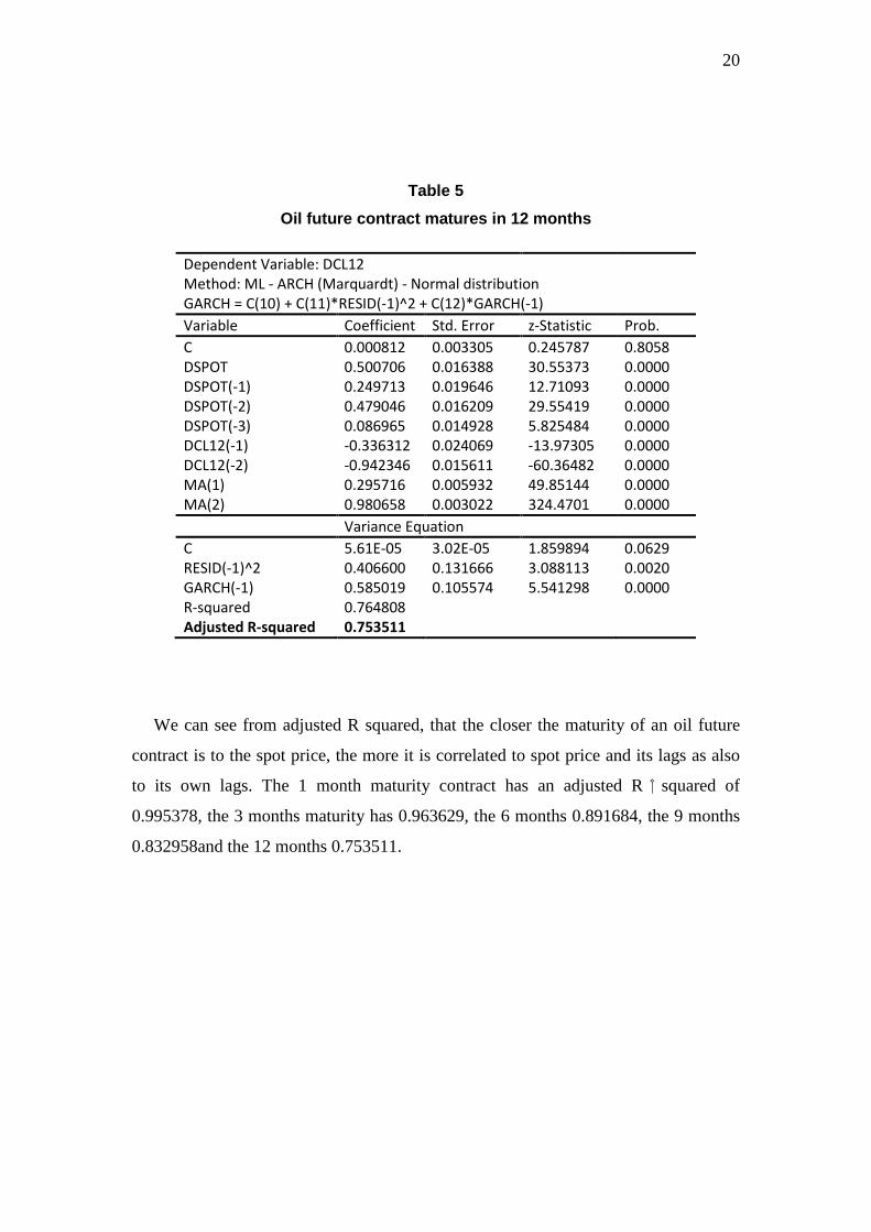
Table 5 Oil future contract matures in 12 months
Dependent Variable: DCL12 Method: ML - ARCH (Marquardt) - Normal distribution GARCH = C(10) + C(11)*RESID(-1)^2 + C(12)*GARCH(-1) Variable Coefficient Std. Error z-Statistic Prob. C 0.000812 0.003305 0.245787 0.8058 DSPOT 0.500706 0.016388 30.55373 0.0000 DSPOT(-1) 0.249713 0.019646 12.71093 0.0000 DSPOT(-2) 0.479046 0.016209 29.55419 0.0000 DSPOT(-3) 0.086965 0.014928 5.825484 0.0000 DCL12(-1) -0.336312 0.024069 -13.97305 0.0000 DCL12(-2) -0.942346 0.015611 -60.36482 0.0000 MA(1) 0.295716 0.005932 49.85144 0.0000 MA(2) 0.980658 0.003022 324.4701 0.0000 Variance Equation C 5.61E-05 3.02E-05 1.859894 0.0629 RESID(-1)^2 0.406600 0.131666 3.088113 0.0020 GARCH(-1) 0.585019 0.105574 5.541298 0.0000 R-squared 0.764808 Adjusted R-squared 0.753511
We can see from adjusted R squared, that the closer the maturity of an oil future
contract is to the spot price, the more it is correlated to spot price and its lags as also
to its own lags. The 1 month maturity contract has an adjusted R squared of
0.995378, the 3 months maturity has 0.963629, the 6 months 0.891684, the 9 months
0.832958and the 12 months 0.753511.
21
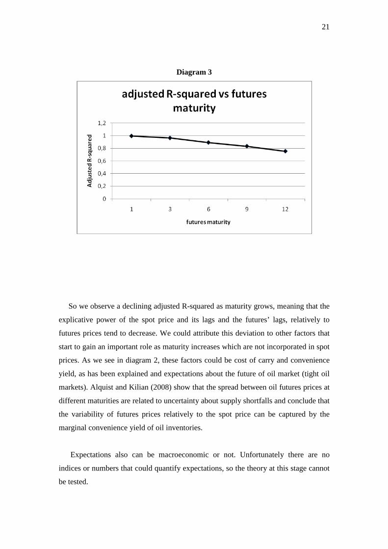
Diagram 3
So we observe a declining adjusted R-squared as maturity grows, meaning that the
explicative power of the spot price and its lags and the futures’ lags, relatively to
futures prices tend to decrease. We could attribute this deviation to other factors that
start to gain an important role as maturity increases which are not incorporated in spot
prices. As we see in diagram 2, these factors could be cost of carry and convenience
yield, as has been explained and expectations about the future of oil market (tight oil
markets). Alquist and Kilian (2008) show that the spread between oil futures prices at
different maturities are related to uncertainty about supply shortfalls and conclude that
the variability of futures prices relatively to the spot price can be captured by the
marginal convenience yield of oil inventories.
Expectations also can be macroeconomic or not. Unfortunately there are no
indices or numbers that could quantify expectations, so the theory at this stage cannot
be tested.
22
1.6 Relevant literature
We can roughly categorize the studies about oil in two categories. The first one
which is the most abundant examines the term structure of oil futures and the causal
relationship between spot and futures prices. It also studies the efficiency of the term
structure, that is the predictive power of futures contracts as indicators of future spot
prices. Some of them have been already referred to at the transmission mechanism
section and others have also contributed in a better understanding of oil market and its
interdependencies. Abosedra & Baghestani (2003) for example, tested the
predictability of WTI 1, 3, 6, 9 and 12 months maturity futures contracts relatively to
a naive forecast procedure and they conclude that the 1 and 12 months contracts are
the best unbiased predictors of future prices.
Ripple and Moosa (2007) studied the determinants of the volatility of oil futures
prices. They tested the significance of maturity, trading volume and open interest in a
contract to contract analysis using daily prices for 131 WTI contracts traded on
NYMEX. They used high and low intraday prices in order to construct a measure of
volatility. Their findings suggest that trading volume and open interest are significant
in determining price volatility whereas in the presence of these two the maturity
variable can be excluded.
The second category examines the effects of various financial or generally
economic factors relatively to oil futures prices and it is more fragmented than the
first one because it tends to concentrate on the economic variables of particular
countries. This paper can be considered as belonging in this category.
Samuel Imarhiagbe (2010) examined the relation of oil prices to stock prices and
exchange rates in the long run for six countries, three oil producers and three oil
consumers, from 2000 to 2010. The producers were Saudi Arabia , Russia and Mexico
and the consumers were US, China and India. After using the Augmented Dickey-
Fuller test for unit roots he performed the study for every country separately using
five tests:
23
1. Johansen cointegration test to detect cointegration.
2. Forecast error variance decomposition to observe the proportion of variance to
oil prices due to shocks in oil prices, exchange rates, stock markets and vice
versa.
3. Impulse response analysis.
4. VECM pair-wise Granger causality to study if there are lead-lag relations
among the three variables in every country.
5. Exclusion and weak exogeneity test to study the persistence of long-term
cointegration relations between the variables.
By using the Schwarz information criterion he chose from 1 to 7 lags depending on
the country. Evidence of cointegration exist in five countries, except Mexico, and that
suggests that oil prices, exchange rates and stock market in these countries move
together in the long run. Impulse response analysis shows that stock prices in all six
countries are responsive to changes in exchange rates and shocks in oil prices and also
that the impact of oil prices are greater for the exporting countries. Weak exogeneity
evidence is only present in China and the long run exclusion test suggests that none of
the variables can be excluded from the cointegration relation in five countries, except
Mexico.
J. Park and R.Ratti (2007) investigated the relationships between real oil price
shocks, real stock returns, industrial production and short term interest rates in 13
countries from 1986 to 2005. They started by conducting unit root tests and after
finding non-stationarity they tested for cointegration among the variables for every
country. From the 13 countries they studied only in UK the null hypothesis of no
cointegration rejected meaning that there is a long term relation among the variables
in this country. Their methodology comprises of a vector autoregression model for
each country and subsequently impulse response analysis and variance
decomposition. The effect of real oil prices to stock markets proved to be insensitive
to reasonable changes in the VAR models such as inclusion of additional variables,
which gives their results more credibility. According to impulse response analysis for
ten of the thirteen countries (excluding Norway, Finland and UK), there is a negative
impact of real oil price shocks to real stock prices which develops contemporaneously
or within one month. In the next months there are positive or negative signs in the
24 impulse response which some of them are statistically significant, but generally the
variable returns to its mean after about 12 periods.
Park and Ratti also test for asymmetric effects of oil price shocks. We have
asymmetric effects when an increase of oil prices has stronger impact on economy
than a decrease. Until now most of the research that has been done on this field
suggests a stronger impact of increases than of decreases, but Park and Ratti suggest
that there is no evidence of asymmetric effects at least in the European countries
under consideration.
Instead of studying the results of oil price shocks Park and Ratti investigate the
response of real stock returns to oil price volatility. After defining monthly volatility
as the log difference of daily oil price divided by the square root of the relevant month
trading days, they incorporate this new variable in the vector autoregressive models
and they run the same tests as with oil price shocks. They conclude that in more than
half of the countries under consideration volatility has a negative statistically
significant effect on the real stock prices, which develops contemporaneously or with
one month lag.
Park and Ratti also use forecast error variance decomposition to conclude about
the effect of real oil price changes in stock market prices. They found that in a 24
months horizon the variance of stock price which is due to oil prices, ranges from 3%
for UK to 10% for Sweden and there is statistical significance in twelve cases.
The impact of real oil price changes to short term interest rates also studied in the
context of a VAR model. The results of the impulse response analysis indicate that oil
price has a positive correlation to short term interest rates and the effect develops
within one or two months. The economic interpretation of an increase in interest rates
after an increase in oil price is that the authorities are tightening their monetary policy
to avoid inflation. Finally by comparing the contribution of oil price and interest rates
variance to the real stock market returns variance, they concluded that oil prices have
a greater effect than interest rates on stock markets.
25 Sadorsky (1999) examines the dynamics of industrial production, interest rates,
real oil price, volatility of oil price and real stock returns in US from 1947 to 1996
using monthly data. After conducting unit root tests he takes the logarithmic returns of
industrial production, interest rates and oil price to make them stationary. He employs
a VAR model and consequently tests the impulse response functions and performs
variance decomposition. Interest rate variance decomposition suggests that 87%, 6%,
5%, 2% of its variance, after 24 months, arises from itself, industrial production, real
stock returns and real oil price respectively. The oil price variance decomposition
suggests that almost all variance is caused by itself meaning that the other variables
don’t affect strongly oil price. For industrial production there is a 79%, 10%, 7% and
4% variance caused by itself, interest rates, real stock returns and oil price
respectively. Regarding real stock returns there is an over 50%, 5% and 6% variance
caused by itself, oil price and interest rates. Impulse response analysis shows the
negative effect of oil prices on stock returns and the positive effect on interest rates at
least at the first lag. Also industrial production has small impact on oil prices and
stock returns.
Sadorsky also splits the sample in two periods after checking for structural brakes.
The first period is from 1947 to 1986 and the second from 1987 to 1996. He discovers
that in the second sample, the effect of oil price to real stock returns is higher than the
effect of interest rates which is in accordance to Park and Ratti results in 2007. Also
the variance decomposition indicates that in the second sample the change of variance
to each variable due to itself declines, suggesting structural changes among the
samples. Contrary though to Park and Ratti (2007), Sadorsky finds that oil price
shocks are asymmetric and an increase in oil price affects economy more than a
decline.
Rong-Gang Cong, Yi-Ming Wei, Jian Lin Jiao and Ying Fan (2008) investigate the
effect of real oil price shocks and oil price volatility to Chinese real stock prices by
taking monthly data from 1996 to 2007. They used the price of Brent crude oil,
Shanghai and Shenzhen composite indices, ten sector indices and four oil stocks.
They also consider short term interest rates, consumer price index and industrial
production as these may influence the relations between oil prices and real stock
26 market returns. They conducted unit root tests and after finding that interest rate, real
oil price and industrial production at level are not stationary, they performed a
Johansen cointegration test but found no evidence of cointegration between these
variables. So they continue with vector autoregression, impulse response analysis and
variance decomposition. Impulse response analysis shows that the only Chinese
indices that are affected from oil price shocks are the manufacturing sector index and
two oil companies stocks. The relation is positive and it develops within three months.
The impulse responses revert to zero after 12 periods.
Relevantly to oil price volatility there is a statistically significant relation to
manufacturing index (negative) and mining and petrochemicals sector indices
(positive). Also in accordance with other studies they found by performing variance
decomposition that the oil price effect is greater than the interest rate effect on real
stock market prices.
George Filis (2009) investigate the relationship between oil prices and consumer
price index, industrial production and stock market for Greece and found the
interdependencies between these factors by employing a VAR model. One of his
findings was that oil prices have a significant negative impact in Greek stock market.
Miller and Ratti (2008) studied the effects between world oil prices and the stock
market of six OECD countries and they discovered that in the long run there is a
negative relationship between oil prices and stock market indices. In particular they
investigated the real stock market prices of Canada, US, France, Italy, Germany and
U.K relatively to real crude oil prices with and without structural brakes.
Sadorsky (2000) investigated the interaction between futures prices for WTI crude
oil, heating oil and unleaded gasoline with a trade-weighted index of exchange rates.
He employed a vector error correction model (VECM) and investigated Granger
causality relationships. His findings suggest that movements in exchange rates
precede movements in heating oil futures price in the short and long run whereas
movements in exchange rates precede movements in crude oil prices only in the short
run. He also conducted unit root tests to check for nonstationarity of the time series
27 and after finding that the variables were integrated of order 1, I(1), he run tests for
cointegration. His findings suggest that there is not only Granger causality among the
four variables but also cointegration which means that there is long run equilibrium
between the four variables.
Zagaglia (2009) studies the dynamics of WTI spot and oil futures contracts returns
for maturities of 1, 6 and 12 months, in the NYMEX, relatively to a dataset that
consists of 239 time series. These series are categorized as price data, such as cost of
crude oil imports from U.K. or Persian Gulf etc. stock and flow data such as
petroleum consumed by the commercial sector, crude oil production of US, share
price of big oil companies stocks etc. and macroeconomic and financial data such as
S&P 500 stock index, capital utilization rate, US CPI index etc. After extracting
common factors that determine oil returns he finds that the first eight common factors
accounted for the 80% of the variance, but he uses the first four factors to run a factor
augmented vector autoregression model (FAVAR) in order to much parsimony and
fitness of the model. He concludes that the best determinants of oil prices are a) a
price index of crude oil imports which can be interpreted as a cost indicator of the
price pressure on oil futures, b) stock volumes of oil related products which have to
do with the immediate demand for crude oil and c) purely financial factors that are
disconnected from real developments in oil markets and as it seems contribute to the
determination of oil prices.
The present paper can be considered as specified in the investigation of purely
financial or macroeconomic data that affect WTI futures contracts, in order to achieve
a better understanding of the interdependencies of these data relatively to crude oil
market.
28 1.7 Expected effect of macroeconomic factors to oil futures
There is no certain theory about the effect of these macroeconomic factors to oil
futures prices, but according to previous studies we could have some expectations
although we cannot be absolutely positive about them.
Relatively to the four stock indices (S&P500, S&P350, Nikkei, Hang Seng), we
expect a negative correlation between them and oil futures. These indices represent
the economy of four of the more energy consuming economies in the world. They
consume collectively almost 50% of global oil production and our expectation is that
when there is an increase in oil prices their economies are affected negatively and the
same happens to stock indices which are mirrors of the real economy. This is also
consistent with other studies that assess the consequences of oil price shocks to stock
market indices.
Regarding FED target rate we expect that high rates result to decreasing prices in
oil futures. This happens because the purpose of increasing FED’s target rate is to
cool down an overheated economy. If Fed’s policy is effective then total demand for
goods and services should slow down and likewise should the demand for oil. But this
isn’t always the case. Total growth could be so strong that a spike in oil futures prices
can take place despite of the FED’s policy like it has happened in late 2007 when
price per barrel reached $100 and not to mention other geopolitical or weather factors
that can cause irregularities in our expected theory.
Dry bulk index is a proxy for the level of demand in dry bulk cargos. Dry bulk
cargos can be coal, iron, bauxite, cement, chemicals, grain (wheat, rise, etc) and many
other products that are used as basic inputs in the production of other goods. High
prices of dry bulk index, means strong global production as companies need to
produce more and more goods to keep up with demand. Strong growth means demand
for oil, so we expect a positive relationship between dry bulk index and WTI futures
in the sense that freight increases due to robust transportation services demand,
precede oil price increases.
29 Relatively to the opposite direction, the effect of oil price to bdi, we know that dry
bulk index measures the price of freights for dry bulk commodities and as oil is the
primary input for a dry bulk carrier we would expect a positive correlation as the ship-
owners try to maintain their profit intact by rising freights. But there is also the
opposite opinion which states that a rise in oil prices will have a negative effect in
world economy and as a result the demand for transportation services for raw
materials will decline causing dry bulk index to also decline.
Industrial production indices for US and European Union indicate growth in the
two economies, thus greater oil consumption. So we would expect a positive
relationship regarding the effect of industrial production to oil variables and a
negative relationship in the opposite direction and the same holds true for capacity
utilization.
However we cannot assume anything about the lag structure of their dependence,
meaning that we have no clue about the speed that changes in macroeconomic factors
affect WTI futures and vice versa. This remains to be seen by the specification that we
are going to use in order to capture the interdependencies of the variables.
30
CHAPTER 2: METHODOLOGY
2.1 Unit root tests
One major problem that someone has to deal with before starting modeling time
series data is the non-stationarity problem. In order for the time series under
consideration to have an explicative or predictive power beyond the time horizon that
they refer to, they must fulfill three concurrent conditions. For a time series Yt these
conditions are:
1. E(Yt)=μ → the mean of the time series is constant
2. Var(Yt)=σ2 →variance of the time series is constant
3. Cov(Yt,Yt+s)=E(Yt-μ)(Yt+s-μ)=constant →covariance of Yt and Yt+s ,where s
is the number of periods apart, must be constant.
So if Yt is stationary, then mean, variance and covariance must be time
invariant and the same as Yt+s. In other words if Yt is a time series with yearly data
that starts from 2001 and ends at 2010 and we shift the origin to 2005, then the
new time series Yt+s, (s=4) from 2005 until 2010 must have the same mean,
variance and covariance as Yt if we want the last one to be stationary, and this
must hold true for every s. The above type of stationarity is the weak form. There
is also the first order stationarity where only the first condition must hold. Unit
root is another name for non-stationarity.
There is a problem with regressions that involve non-stationary data because
the standard errors that they produce are biased. This means that by regressing the
data, we might find a significant relation that in reality doesn’t exist. We refer to
such regressions as spurious. This also means that the standard criteria we use to
judge if there is causal relation between variables are not reliable.
Many economic series are not stationary, therefore the first step before
econometric modeling is unit root tests. The most popular tests are the Augmented
31
Dickey-Fuller and the Phillips-Perron test. The Augmented Dickey Fuller test
(ADF) is based on the following regression:
The term 0
N
t ii
y −=
∆∑ eliminates the autocorrelation of residuals. The value of the
ADF test is compared with the critical values of the Dickey-Fuller table instead of the
t-distribution. The ADF test has the disadvantage of low power, which means that
many times it accepts the null of a unit root whilst it shouldn’t. It is also more reliable
when the time span of the data is wider.
If time series has a unit root then we transform it to stationary by taking first,
second or more differences depending on the order of their integration, which means
how many times we must differentiate them to make them stationary. If a time series
is denoted as integrated of order two, I(2), then we have to differentiate it 2 times to
make it stationary etc. Specifically in economic time series it is better to take
logarithmic returns because instead of making them stationary, they also have
meaningful empirical interpretation. The disadvantage of making time series
stationary is the loss of an amount of information.
In this thesis in order to test for unit roots we use the Augmented Dickey-Fuller
test with Schwarz info criterion and intercept. Unit root tests are exposed analytically
in Appendix A but here we will mention the results. From the 15 series, six relative to
oil and nine relative to macroeconomic factors, we detected four that are stationary,
industrial production of European Union and US, Nikkei and dry bulk index. The rest
eleven had unit roots and in order to proceed to the next level which is Granger
causality, we make them stationary by taking logarithmic returns of the form:
10
N
t t t i ti
y y y uβ − −=
∆ = + ∆ +∑
32 d(series)=log(series)-log(series(-1))
where (-1) denotes the previous price and d(series) is the name we assign.
For example dsp500 is defined by equation
dsp500=log(sp500)-log(sp500(-1))
We could alternatively take first differences of the form
dsp500=sp500-sp500(-1)
in order to make them stationary but since we have economic series we prefer
logarithmic returns which have also economic meaning and are easiest to
comprehend. So in that part we construct eleven new series that are stationary.
2.2 Ordinary Least Squares (OLS)
At this point and before we proceed to the analytic representation of the
methodology used in this thesis, we find it useful to make a brief reference to the
Ordinary Least Squares method (OLS) as it is the foundation of the results that the
econometric analysis in this paper will produce.
The OLS is generally a mathematical procedure used to approximate systems of
equations that have no solution. One such case is when we have more equations in a
system than unknown parameters. The majority of such systems have no solution so
we employ OLS in order to approximate a decent and relative reliable answer as to
what values the unknown parameters should take. We will demonstrate how this
method works using simple equations in order to be more comprehensive. So suppose
that we have the three below equations:
33
1 2
1 2
1 2
213
x xx xx x
+ =− =+ =
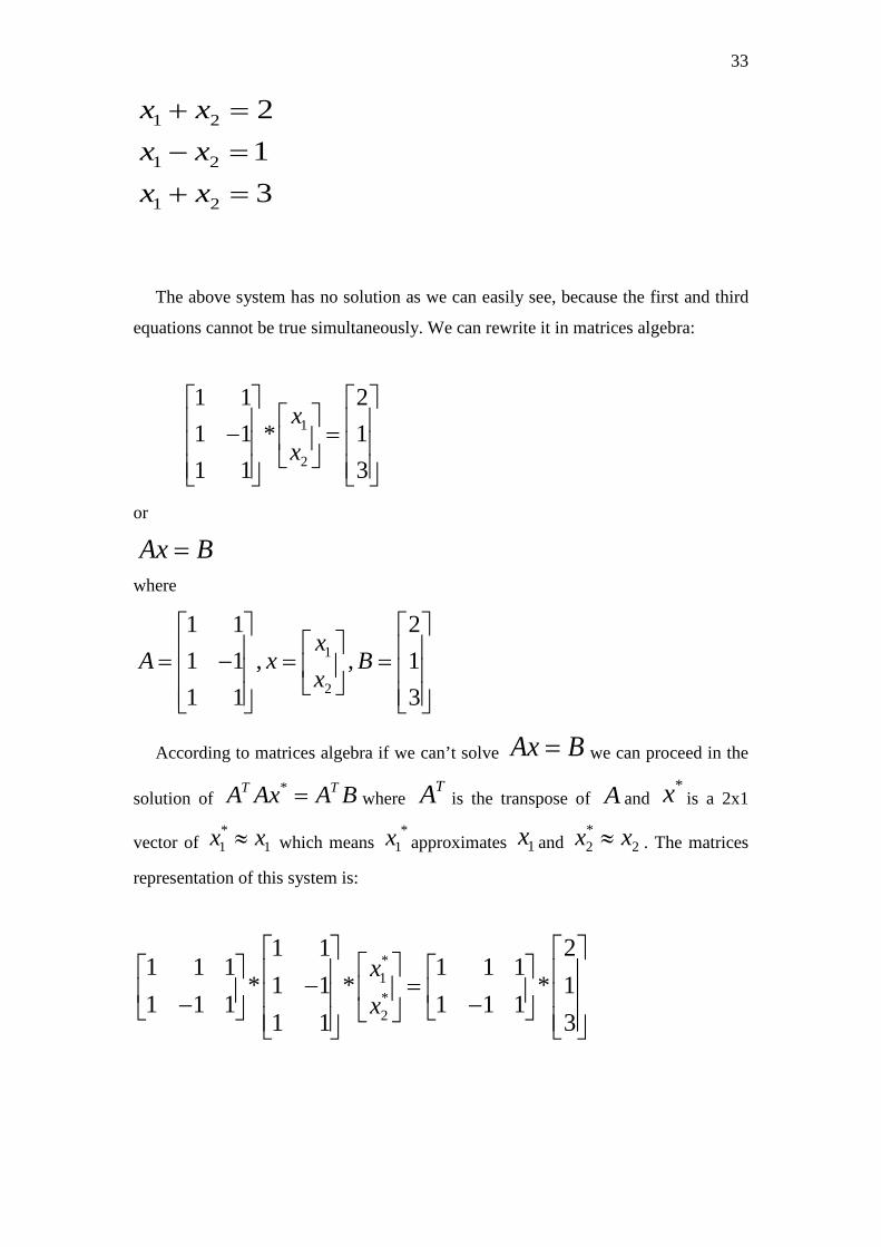
The above system has no solution as we can easily see, because the first and third
equations cannot be true simultaneously. We can rewrite it in matrices algebra:
1
2
1 1 21 1 * 11 1 3
xx
− =
or
Ax B=
where
1
2
1 1 21 1 , , 11 1 3
xA x B
x
= − = =
According to matrices algebra if we can’t solve Ax B= we can proceed in the
solution of *T TA Ax A B= where
TA is the transpose of A and *x is a 2x1
vector of *1 1x x≈ which means
*1x approximates 1x and
*2 2x x≈ . The matrices
representation of this system is:
*1*2
1 1 21 1 1 1 1 1
* 1 1 * * 11 1 1 1 1 1
1 1 3
xx
− = − −
34
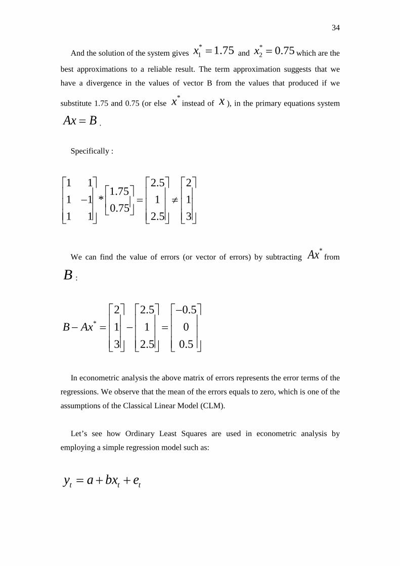
And the solution of the system gives *1 1.75x = and
*2 0.75x = which are the
best approximations to a reliable result. The term approximation suggests that we
have a divergence in the values of vector B from the values that produced if we
substitute 1.75 and 0.75 (or else *x instead of x ), in the primary equations system
Ax B= .
Specifically :
1 1 2.5 21.75
1 1 * 1 10.75
1 1 2.5 3
− = ≠
We can find the value of errors (or vector of errors) by subtracting *Ax from
B :
*
2 2.5 0.51 1 03 2.5 0.5
B Ax−
− = − =
In econometric analysis the above matrix of errors represents the error terms of the
regressions. We observe that the mean of the errors equals to zero, which is one of the
assumptions of the Classical Linear Model (CLM).
Let’s see how Ordinary Least Squares are used in econometric analysis by
employing a simple regression model such as:
t t ty a bx e= + +
35
We solve for te and we have:
t t te y a bx= − −
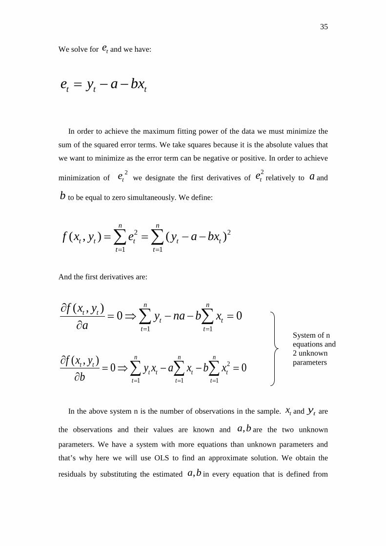
In order to achieve the maximum fitting power of the data we must minimize the
sum of the squared error terms. We take squares because it is the absolute values that
we want to minimize as the error term can be negative or positive. In order to achieve
minimization of 2
te we designate the first derivatives of 2te relatively to a and
b to be equal to zero simultaneously. We define:
2 2
1 1( , ) ( )
n n
t t t t tt t
f x y e y a bx= =
= = − −∑ ∑
And the first derivatives are:
1 1
( , ) 0 0n n
t tt t
t t
f x y y na b xa = =
∂= ⇒ − − =
∂ ∑ ∑
2
1 1 1
( , ) 0 0n n n
t tt t t t
t t t
f x y y x a x b xb = = =
∂= ⇒ − − =
∂ ∑ ∑ ∑
In the above system n is the number of observations in the sample. tx and ty are
the observations and their values are known and ,a b are the two unknown
parameters. We have a system with more equations than unknown parameters and
that’s why here we will use OLS to find an approximate solution. We obtain the
residuals by substituting the estimated ,a b in every equation that is defined from
System of n equations and 2 unknown parameters
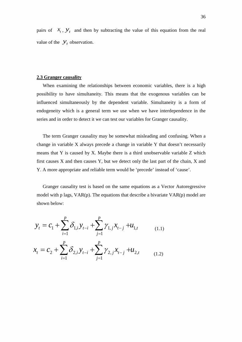
36 pairs of tx , ty and then by subtracting the value of this equation from the real
value of the ty observation.
2.3 Granger causality
When examining the relationships between economic variables, there is a high
possibility to have simultaneity. This means that the exogenous variables can be
influenced simultaneously by the dependent variable. Simultaneity is a form of
endogeneity which is a general term we use when we have interdependence in the
series and in order to detect it we can test our variables for Granger causality.
The term Granger causality may be somewhat misleading and confusing. When a
change in variable X always precede a change in variable Y that doesn’t necessarily
means that Y is caused by X. Maybe there is a third unobservable variable Z which
first causes X and then causes Y, but we detect only the last part of the chain, X and
Y. A more appropriate and reliable term would be ‘precede’ instead of ‘cause’.
Granger causality test is based on the same equations as a Vector Autoregressive
model with p lags, VAR(p). The equations that describe a bivariate VAR(p) model are
shown below:
(1.1)
(1.2)
1 1, 1, 1,1 1
2 2, 2, 2,1 1
p p
t i t i j t j ti j
p p
t i t i j t j ti j
y c y x u
x c y x u
δ γ
δ γ
− −= =
− −= =
= + + +
= + + +
∑ ∑
∑ ∑
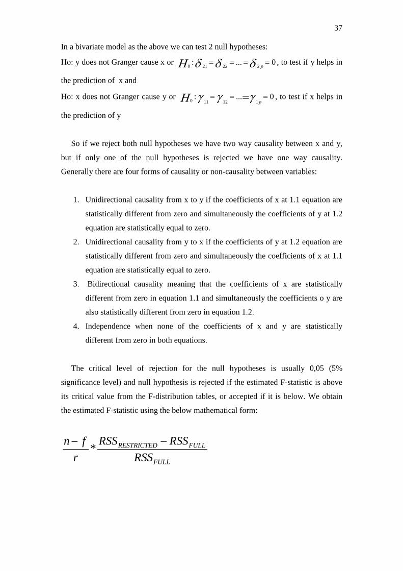
37 In a bivariate model as the above we can test 2 null hypotheses:
Ho: y does not Granger cause x or 0...: 222210 ==== δδδ pH , to test if y helps in
the prediction of x and
Ho: x does not Granger cause y or 0...:112110 === =γγγ pH , to test if x helps in
the prediction of y
So if we reject both null hypotheses we have two way causality between x and y,
but if only one of the null hypotheses is rejected we have one way causality.
Generally there are four forms of causality or non-causality between variables:
1. Unidirectional causality from x to y if the coefficients of x at 1.1 equation are
statistically different from zero and simultaneously the coefficients of y at 1.2
equation are statistically equal to zero.
2. Unidirectional causality from y to x if the coefficients of y at 1.2 equation are
statistically different from zero and simultaneously the coefficients of x at 1.1
equation are statistically equal to zero.
3. Bidirectional causality meaning that the coefficients of x are statistically
different from zero in equation 1.1 and simultaneously the coefficients o y are
also statistically different from zero in equation 1.2.
4. Independence when none of the coefficients of x and y are statistically
different from zero in both equations.
The critical level of rejection for the null hypotheses is usually 0,05 (5%
significance level) and null hypothesis is rejected if the estimated F-statistic is above
its critical value from the F-distribution tables, or accepted if it is below. We obtain
the estimated F-statistic using the below mathematical form:
* RESTRICTED FULL
FULL
RSS RSSn fr RSS
−−
38 Where:
RESTRICTED
FULL
n= number of observationsf= number of parameters for full modelr= number of parameters for restricted modelRSS = sum of squared residuals for the restricted modelRSS = sum of squared residuals for the full model
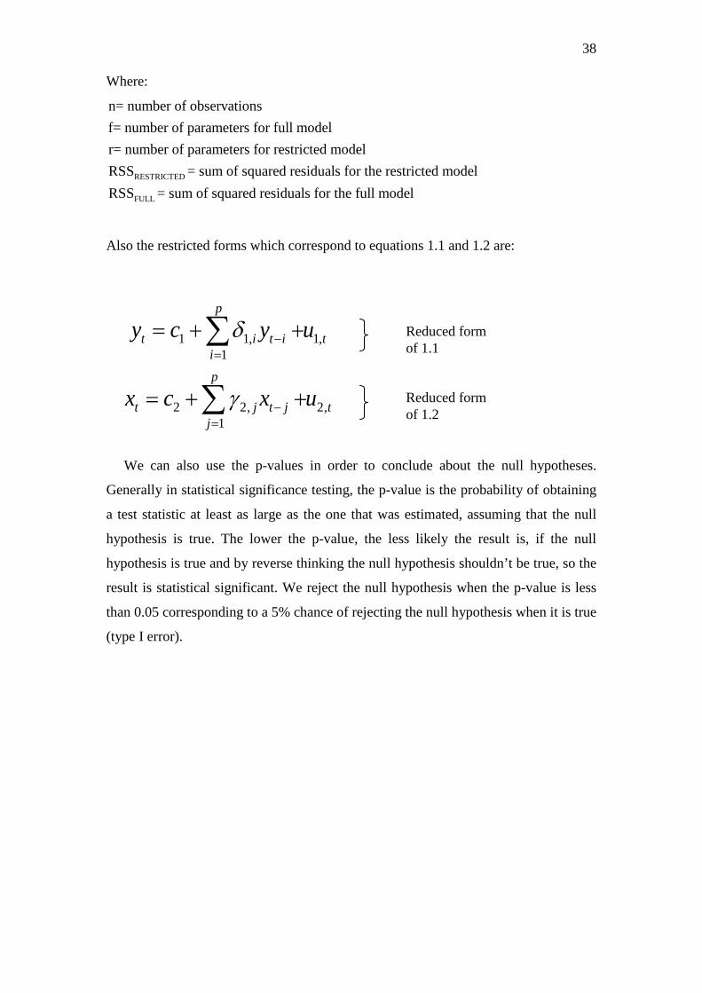
Also the restricted forms which correspond to equations 1.1 and 1.2 are:
We can also use the p-values in order to conclude about the null hypotheses.
Generally in statistical significance testing, the p-value is the probability of obtaining
a test statistic at least as large as the one that was estimated, assuming that the null
hypothesis is true. The lower the p-value, the less likely the result is, if the null
hypothesis is true and by reverse thinking the null hypothesis shouldn’t be true, so the
result is statistical significant. We reject the null hypothesis when the p-value is less
than 0.05 corresponding to a 5% chance of rejecting the null hypothesis when it is true
(type I error).
1 1, 1,1
2 2, 2,1
p
t i t i tip
t j t j tj
y c y u
x c x u
δ
γ
−=
−=
= + +
= + +
∑
∑
Reduced form of 1.1
Reduced form of 1.2
39 2.4 Cointegration
We have cointegration under three concurrent circumstances:
a. The series under consideration must not be stationary or I(0).
b. The series under consideration must be integrated of the same order I(p). This
means that in order to make them stationary we have to differentiate them 1
time if they are integrated of order one, I(1) or p times if they are integrated of
order p, I(p)
c. There must be a linear combination of these series that produce a stationary
series.
The economic interpretation of cointegration is that the distance between two or
more economic variables is the same in the long run. So no matter how big is the short
run divergence between the variables, in the long run they tend to converge.
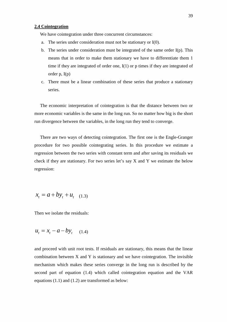
There are two ways of detecting cointegration. The first one is the Engle-Granger
procedure for two possible cointegrating series. In this procedure we estimate a
regression between the two series with constant term and after saving its residuals we
check if they are stationary. For two series let’s say X and Y we estimate the below
regression:
t t tx a by u= + + (1.3)
Then we isolate the residuals:
t t tu x a by= − − (1.4)
and proceed with unit root tests. If residuals are stationary, this means that the linear
combination between X and Y is stationary and we have cointegration. The invisible
mechanism which makes these series converge in the long run is described by the
second part of equation (1.4) which called cointegration equation and the VAR
equations (1.1) and (1.2) are transformed as below:
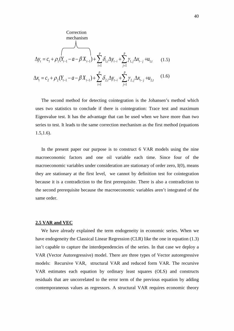
40
(1.5)
(1.6)
The second method for detecting cointegration is the Johansen’s method which
uses two statistics to conclude if there is cointegration: Trace test and maximum
Eigenvalue test. It has the advantage that can be used when we have more than two
series to test. It leads to the same correction mechanism as the first method (equations
1.5,1.6).
In the present paper our purpose is to construct 6 VAR models using the nine
macroeconomic factors and one oil variable each time. Since four of the
macroeconomic variables under consideration are stationary of order zero, I(0), means
they are stationary at the first level, we cannot by definition test for cointegration
because it is a contradiction to the first prerequisite. There is also a contradiction to
the second prerequisite because the macroeconomic variables aren’t integrated of the
same order.
2.5 VAR and VEC
We have already explained the term endogeneity in economic series. When we
have endogeneity the Classical Linear Regression (CLR) like the one in equation (1.3)
isn’t capable to capture the interdependencies of the series. In that case we deploy a
VAR (Vector Autoregressive) model. There are three types of Vector autoregressive
models: Recursive VAR, structural VAR and reduced form VAR. The recursive
VAR estimates each equation by ordinary least squares (OLS) and constructs
residuals that are uncorrelated to the error term of the previous equation by adding
contemporaneous values as regressors. A structural VAR requires economic theory
1 1 1 1 1, 1, 1,1 1
2 2 1 1 2, 2, 2,1 1
( )
( )
p p
t t t i t i j t j ti j
p p
t t t i t i j t j ti j
y c Y a X y x u
x c Y a X y x u
ρ β δ γ
ρ β δ γ
− − − −= =
− − − −= =
∆ = + − − + ∆ + ∆ +
∆ = + − − + ∆ + ∆ +
∑ ∑
∑ ∑
Correction mechanism
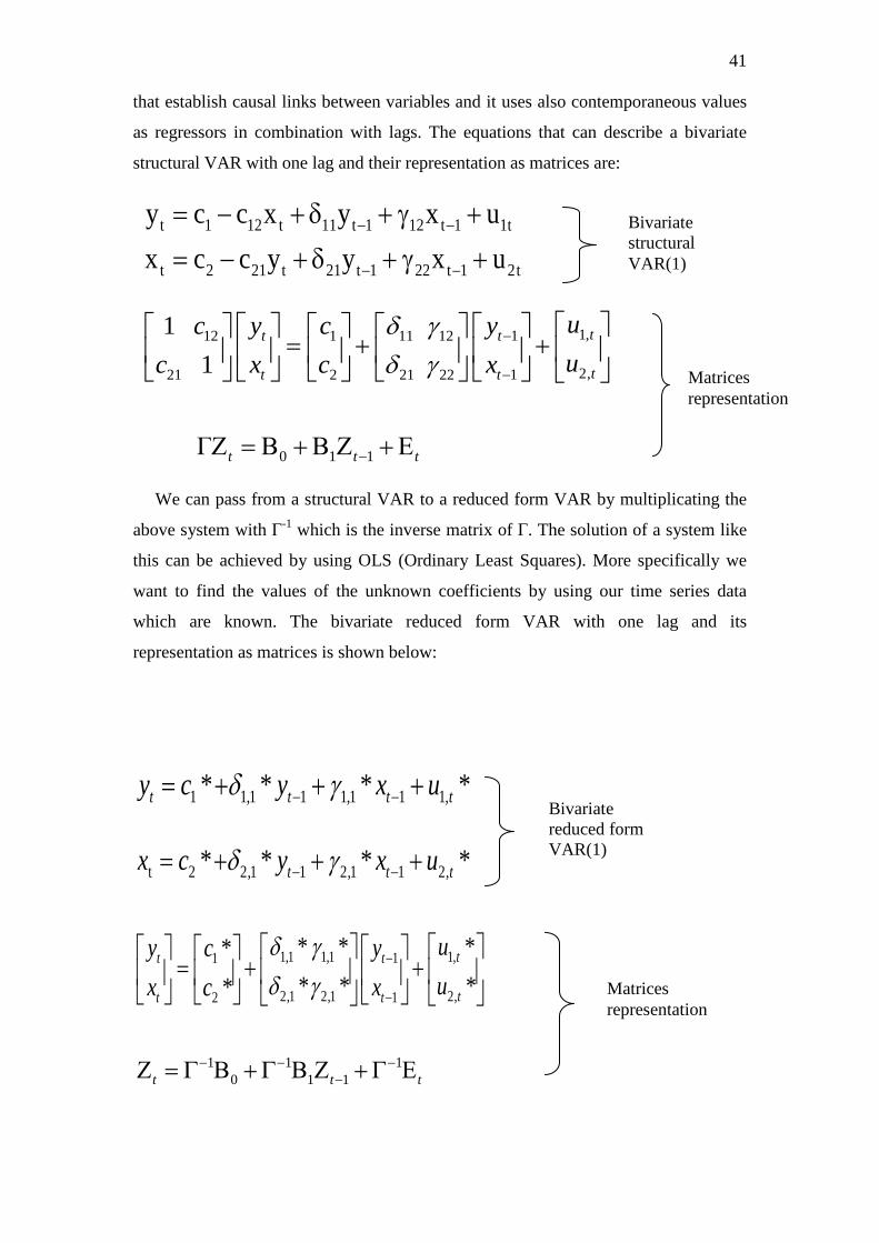
41 that establish causal links between variables and it uses also contemporaneous values
as regressors in combination with lags. The equations that can describe a bivariate
structural VAR with one lag and their representation as matrices are:
We can pass from a structural VAR to a reduced form VAR by multiplicating the
above system with Γ-1 which is the inverse matrix of Γ. The solution of a system like
this can be achieved by using OLS (Ordinary Least Squares). More specifically we
want to find the values of the unknown coefficients by using our time series data
which are known. The bivariate reduced form VAR with one lag and its
representation as matrices is shown below:
1 1,1 1 1,1 1 1,* * * *t t t ty c y x uδ γ− −= + + +
t 2 2,1 1 2,1 1 2,* * * *t t tx c y x uδ γ− −= + + +
1,1 1,1 1,11
2,1 2,1 2,12
* * *** * **
tt t
tt t
uy ycux xc
δ γδ γ
−
−
= + +
1 1 10 1 1t t t
− − −−Ζ = Γ Β +Γ Β Ζ +Γ Ε
Bivariate reduced form VAR(1)
Matrices representation
t 1 12 t 11 t 1 12 t 1 1t
t 2 21 t 21 t 1 22 t 1 2t
y c c x y x ux c c y y x u
− −
− −
= − + δ + γ += − + δ + γ +
Bivariate structural VAR(1)
1,112 1 11 12
2,121 2 21 22
0 1 1
11
Γ
tt t
tt t
t t t
uy yc cux xc c
δ γδ γ
−
−
−
= + +
Ζ = Β +Β Ζ +Ε
Matrices representation
42
The solution of the above algebraic representation of equations by using OLS
produces the coefficients of the endogenous variables and then we can test their
statistical significance by using the t-statistic.
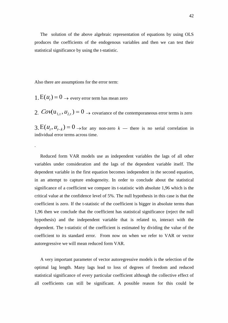
Also there are assumptions for the error term:
1. 0)( =Ε tu → every error term has mean zero
2. 0),u( t2,t1, =uCov → covariance of the contemporaneous error terms is zero
3. 0),( =Ε −ktt uu → for any non-zero k — there is no serial correlation in individual error terms across time.
.
Reduced form VAR models use as independent variables the lags of all other
variables under consideration and the lags of the dependent variable itself. The
dependent variable in the first equation becomes independent in the second equation,
in an attempt to capture endogeneity. In order to conclude about the statistical
significance of a coefficient we compare its t-statistic with absolute 1,96 which is the
critical value at the confidence level of 5%. The null hypothesis in this case is that the
coefficient is zero. If the t-statistic of the coefficient is bigger in absolute terms than
1,96 then we conclude that the coefficient has statistical significance (reject the null
hypothesis) and the independent variable that is related to, interact with the
dependent. The t-statistic of the coefficient is estimated by dividing the value of the
coefficient to its standard error. From now on when we refer to VAR or vector
autoregressive we will mean reduced form VAR.
A very important parameter of vector autoregressive models is the selection of the
optimal lag length. Many lags lead to loss of degrees of freedom and reduced
statistical significance of every particular coefficient although the collective effect of
all coefficients can still be significant. A possible reason for this could be
43 multicollinearity which means that there is linear relation between the coefficients. On
the other hand too few lags lead to specification errors. We can use lag length criteria
such as Akaike before we starting modeling, or use trial and error method to first run
VAR regressions with different lags and then by comparison choose the regression
with the smallest Akaike.
VEC (Vector Error Correction) is a variation of VAR which takes into account
cointegration to some or to all series under examination. The error correction
mechanism together with the cointegrating equation corrects the model in such a way
to take into account the invisible mechanism of cointegration. The error correction
mechanism is the coefficient in front of the cointegrating equation (first part of
equation (1.4)).
So to model endogeneity between series we use VAR if there is no cointegration
and VEC if there is cointegration between any of the variables. We have already
explained why we will not test for cointegration, so we will use VAR models to study
the interdependencies of the time series. For the purpose of this paper we will specify
6 VAR models each one with one time series relative to oil (spot, cl1, cl3, cl6, cl9,
cl12) and all the other nine macroeconomic factors. We have already made non
stationary series stationary by taking the logarithmic returns and we will use them in
the construction of VAR. The Akaike lag length criterion suggests 4 lags in each one
of the VAR.
2.6 Impulse response analysis & Variance decomposition
We will also conduct impulse response analysis for every VAR model relatively to
FED’s funds rate, S&P 500, S&P 350 and EU industrial production which are
statistically significant in every VAR. Impulse response analysis generally measures
and depicts the response of a variable to an exogenous shock and also the response on
the other endogenous variables of the model which occurs from the same exogenous
shock. The exogenous shock to one variable is transmitted to all the other variables
via the certain VAR specification and lag structure of the model. Analytically we can
present the mechanism through a bivariate reduced form VAR(1):
44
A shock in innovation u2t will cause a direct change in variable xt through the
second equation, which in turn will alter the value of yt+1 through the first equation.
Also the disturbance of u2t will cause change in u1t due to no zero covariance between
the error terms, so the effect of the initial shock will multiply.
The shock of the exogenous variable is one standard deviation and on the vertical
axis of the diagram we can see the response that a particular variable will have. On
the horizontal axis we will assume 20 time intervals which is a sufficient time period
in order to observe the responses.
Variance Decomposition or Forecast error variance decomposition reflects the
amount of information each variable contributes to the other variables in a Vector
autoregressive model. Variance decomposition determines how much of the total
variance of each variable can be explained by the variance of other variables due to
exogenous shocks. This estimation is produced in the context of a certain VAR
model and it uses all the interdependencies that have been produced through the
equations of the VAR model. The variance contribution of all the other variables to
the one under consideration are processed period by period. We will use 10 time
periods.
CHAPTER 3: EMPIRICAL RESULTS
3.1 Granger causality results
We will now test if there is Granger causality between WTI oil returns (spot and
futures) and macroeconomic factors. By using the Akaike lag length criterion we will
take four lags for the Granger causality testing. The column prob. denotes the
estimated probability value that has to be below 0.05 in order to reject the null
t 1 11 t 1 12 t 1 1t
t 2 21 t 1 22 t 1 2t
y c y x ux c y x u
− −
− −
= + δ + γ += + δ + γ +
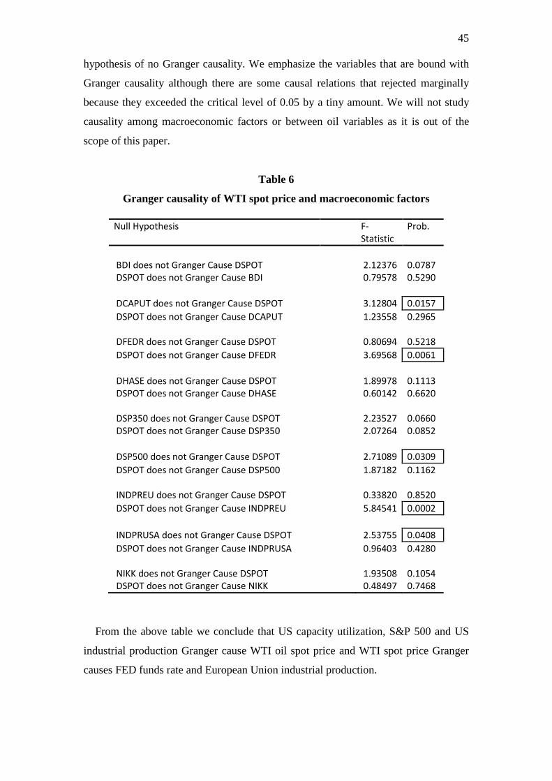
45 hypothesis of no Granger causality. We emphasize the variables that are bound with
Granger causality although there are some causal relations that rejected marginally
because they exceeded the critical level of 0.05 by a tiny amount. We will not study
causality among macroeconomic factors or between oil variables as it is out of the
scope of this paper.
Table 6
Granger causality of WTI spot price and macroeconomic factors
Null Hypothesis F-Statistic
Prob.
BDI does not Granger Cause DSPOT 2.12376 0.0787 DSPOT does not Granger Cause BDI 0.79578 0.5290 DCAPUT does not Granger Cause DSPOT 3.12804 0.0157 DSPOT does not Granger Cause DCAPUT 1.23558 0.2965 DFEDR does not Granger Cause DSPOT 0.80694 0.5218 DSPOT does not Granger Cause DFEDR 3.69568 0.0061 DHASE does not Granger Cause DSPOT 1.89978 0.1113 DSPOT does not Granger Cause DHASE 0.60142 0.6620 DSP350 does not Granger Cause DSPOT 2.23527 0.0660 DSPOT does not Granger Cause DSP350 2.07264 0.0852 DSP500 does not Granger Cause DSPOT 2.71089 0.0309 DSPOT does not Granger Cause DSP500 1.87182 0.1162 INDPREU does not Granger Cause DSPOT 0.33820 0.8520 DSPOT does not Granger Cause INDPREU 5.84541 0.0002 INDPRUSA does not Granger Cause DSPOT 2.53755 0.0408 DSPOT does not Granger Cause INDPRUSA 0.96403 0.4280 NIKK does not Granger Cause DSPOT 1.93508 0.1054 DSPOT does not Granger Cause NIKK 0.48497 0.7468
From the above table we conclude that US capacity utilization, S&P 500 and US
industrial production Granger cause WTI oil spot price and WTI spot price Granger
causes FED funds rate and European Union industrial production.
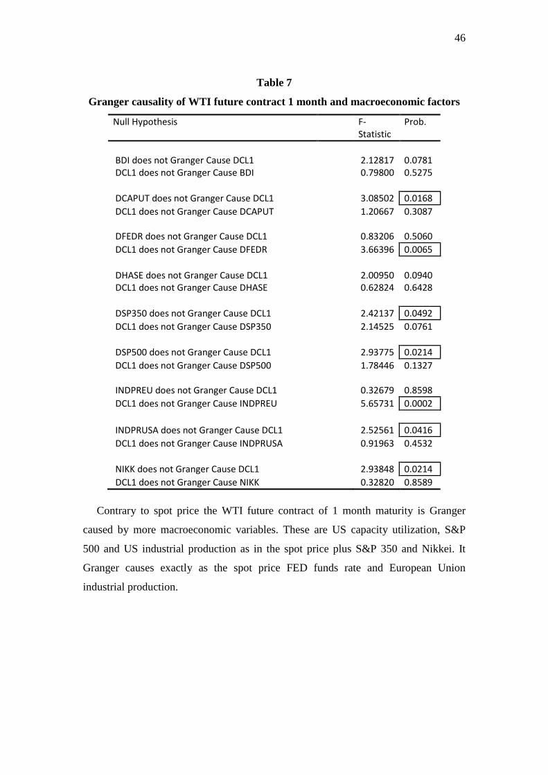
46
Table 7
Granger causality of WTI future contract 1 month and macroeconomic factors
Null Hypothesis F-Statistic
Prob.
BDI does not Granger Cause DCL1 2.12817 0.0781 DCL1 does not Granger Cause BDI 0.79800 0.5275 DCAPUT does not Granger Cause DCL1 3.08502 0.0168 DCL1 does not Granger Cause DCAPUT 1.20667 0.3087 DFEDR does not Granger Cause DCL1 0.83206 0.5060 DCL1 does not Granger Cause DFEDR 3.66396 0.0065 DHASE does not Granger Cause DCL1 2.00950 0.0940 DCL1 does not Granger Cause DHASE 0.62824 0.6428 DSP350 does not Granger Cause DCL1 2.42137 0.0492 DCL1 does not Granger Cause DSP350 2.14525 0.0761 DSP500 does not Granger Cause DCL1 2.93775 0.0214 DCL1 does not Granger Cause DSP500 1.78446 0.1327 INDPREU does not Granger Cause DCL1 0.32679 0.8598 DCL1 does not Granger Cause INDPREU 5.65731 0.0002 INDPRUSA does not Granger Cause DCL1 2.52561 0.0416 DCL1 does not Granger Cause INDPRUSA 0.91963 0.4532 NIKK does not Granger Cause DCL1 2.93848 0.0214 DCL1 does not Granger Cause NIKK 0.32820 0.8589
Contrary to spot price the WTI future contract of 1 month maturity is Granger
caused by more macroeconomic variables. These are US capacity utilization, S&P
500 and US industrial production as in the spot price plus S&P 350 and Nikkei. It
Granger causes exactly as the spot price FED funds rate and European Union
industrial production.
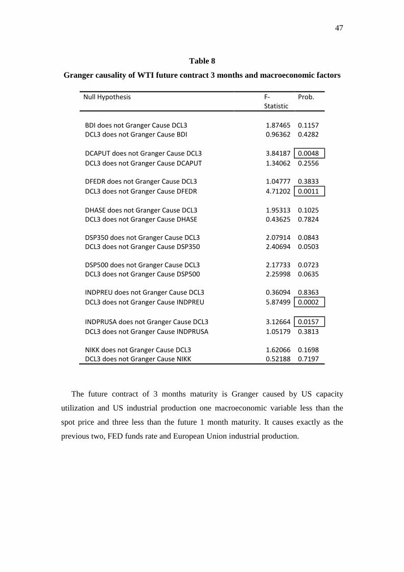
47
Table 8
Granger causality of WTI future contract 3 months and macroeconomic factors
Null Hypothesis F-Statistic
Prob.
BDI does not Granger Cause DCL3 1.87465 0.1157 DCL3 does not Granger Cause BDI 0.96362 0.4282 DCAPUT does not Granger Cause DCL3 3.84187 0.0048 DCL3 does not Granger Cause DCAPUT 1.34062 0.2556 DFEDR does not Granger Cause DCL3 1.04777 0.3833 DCL3 does not Granger Cause DFEDR 4.71202 0.0011 DHASE does not Granger Cause DCL3 1.95313 0.1025 DCL3 does not Granger Cause DHASE 0.43625 0.7824 DSP350 does not Granger Cause DCL3 2.07914 0.0843 DCL3 does not Granger Cause DSP350 2.40694 0.0503 DSP500 does not Granger Cause DCL3 2.17733 0.0723 DCL3 does not Granger Cause DSP500 2.25998 0.0635 INDPREU does not Granger Cause DCL3 0.36094 0.8363 DCL3 does not Granger Cause INDPREU 5.87499 0.0002 INDPRUSA does not Granger Cause DCL3 3.12664 0.0157 DCL3 does not Granger Cause INDPRUSA 1.05179 0.3813 NIKK does not Granger Cause DCL3 1.62066 0.1698 DCL3 does not Granger Cause NIKK 0.52188 0.7197
The future contract of 3 months maturity is Granger caused by US capacity
utilization and US industrial production one macroeconomic variable less than the
spot price and three less than the future 1 month maturity. It causes exactly as the
previous two, FED funds rate and European Union industrial production.
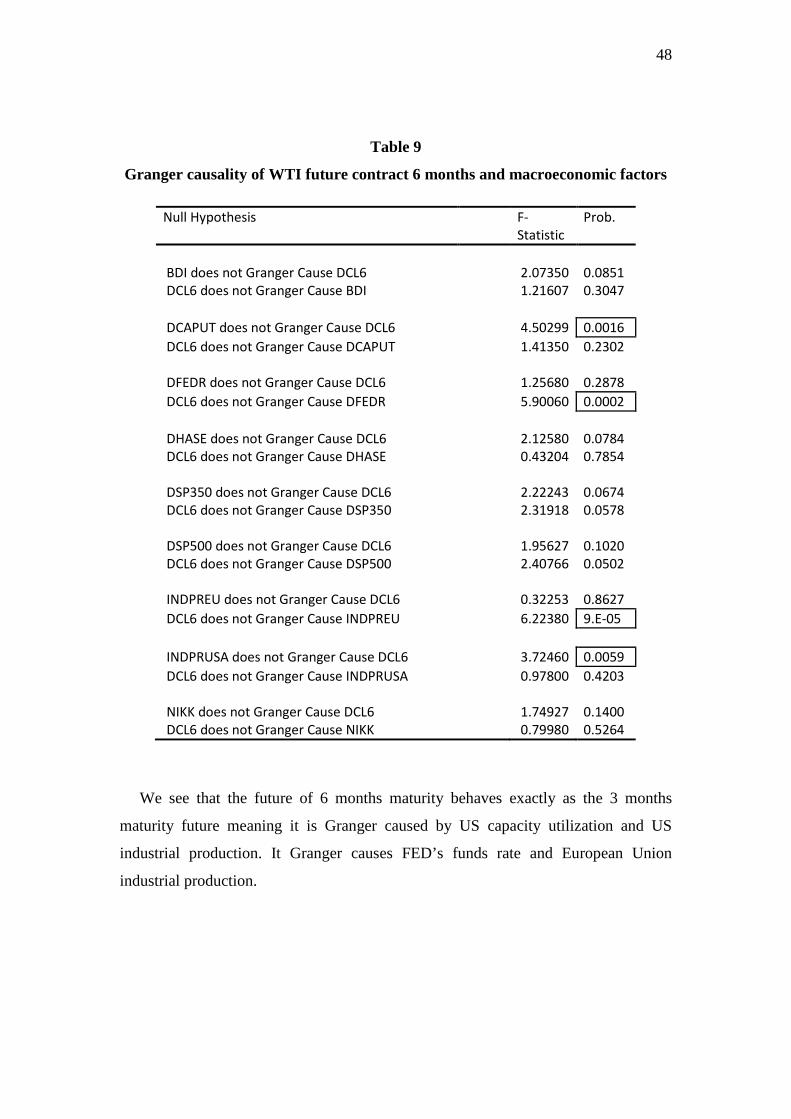
48
Table 9
Granger causality of WTI future contract 6 months and macroeconomic factors
Null Hypothesis F-Statistic
Prob.
BDI does not Granger Cause DCL6 2.07350 0.0851 DCL6 does not Granger Cause BDI 1.21607 0.3047 DCAPUT does not Granger Cause DCL6 4.50299 0.0016 DCL6 does not Granger Cause DCAPUT 1.41350 0.2302 DFEDR does not Granger Cause DCL6 1.25680 0.2878 DCL6 does not Granger Cause DFEDR 5.90060 0.0002 DHASE does not Granger Cause DCL6 2.12580 0.0784 DCL6 does not Granger Cause DHASE 0.43204 0.7854 DSP350 does not Granger Cause DCL6 2.22243 0.0674 DCL6 does not Granger Cause DSP350 2.31918 0.0578 DSP500 does not Granger Cause DCL6 1.95627 0.1020 DCL6 does not Granger Cause DSP500 2.40766 0.0502 INDPREU does not Granger Cause DCL6 0.32253 0.8627 DCL6 does not Granger Cause INDPREU 6.22380 9.E-05 INDPRUSA does not Granger Cause DCL6 3.72460 0.0059 DCL6 does not Granger Cause INDPRUSA 0.97800 0.4203 NIKK does not Granger Cause DCL6 1.74927 0.1400 DCL6 does not Granger Cause NIKK 0.79980 0.5264
We see that the future of 6 months maturity behaves exactly as the 3 months
maturity future meaning it is Granger caused by US capacity utilization and US
industrial production. It Granger causes FED’s funds rate and European Union
industrial production.
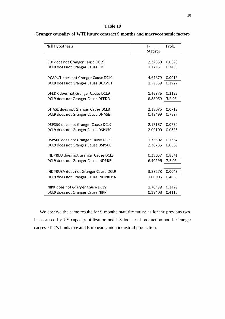
49
Table 10
Granger causality of WTI future contract 9 months and macroeconomic factors
Null Hypothesis F-Statistic
Prob.
BDI does not Granger Cause DCL9 2.27550 0.0620 DCL9 does not Granger Cause BDI 1.37451 0.2435 DCAPUT does not Granger Cause DCL9 4.64879 0.0013 DCL9 does not Granger Cause DCAPUT 1.53558 0.1927 DFEDR does not Granger Cause DCL9 1.46876 0.2125 DCL9 does not Granger Cause DFEDR 6.88069 3.E-05 DHASE does not Granger Cause DCL9 2.18075 0.0719 DCL9 does not Granger Cause DHASE 0.45499 0.7687 DSP350 does not Granger Cause DCL9 2.17167 0.0730 DCL9 does not Granger Cause DSP350 2.09100 0.0828 DSP500 does not Granger Cause DCL9 1.76502 0.1367 DCL9 does not Granger Cause DSP500 2.30735 0.0589 INDPREU does not Granger Cause DCL9 0.29037 0.8841 DCL9 does not Granger Cause INDPREU 6.40296 7.E-05 INDPRUSA does not Granger Cause DCL9 3.88278 0.0045 DCL9 does not Granger Cause INDPRUSA 1.00005 0.4083 NIKK does not Granger Cause DCL9 1.70438 0.1498 DCL9 does not Granger Cause NIKK 0.99408 0.4115
We observe the same results for 9 months maturity future as for the previous two.
It is caused by US capacity utilization and US industrial production and it Granger
causes FED’s funds rate and European Union industrial production.
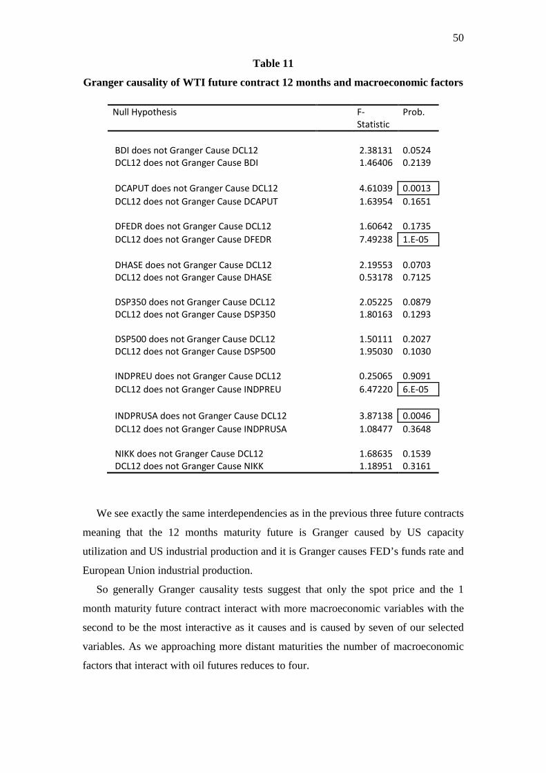
50
Table 11
Granger causality of WTI future contract 12 months and macroeconomic factors
Null Hypothesis F-Statistic
Prob.
BDI does not Granger Cause DCL12 2.38131 0.0524 DCL12 does not Granger Cause BDI 1.46406 0.2139 DCAPUT does not Granger Cause DCL12 4.61039 0.0013 DCL12 does not Granger Cause DCAPUT 1.63954 0.1651 DFEDR does not Granger Cause DCL12 1.60642 0.1735 DCL12 does not Granger Cause DFEDR 7.49238 1.E-05 DHASE does not Granger Cause DCL12 2.19553 0.0703 DCL12 does not Granger Cause DHASE 0.53178 0.7125 DSP350 does not Granger Cause DCL12 2.05225 0.0879 DCL12 does not Granger Cause DSP350 1.80163 0.1293 DSP500 does not Granger Cause DCL12 1.50111 0.2027 DCL12 does not Granger Cause DSP500 1.95030 0.1030 INDPREU does not Granger Cause DCL12 0.25065 0.9091 DCL12 does not Granger Cause INDPREU 6.47220 6.E-05 INDPRUSA does not Granger Cause DCL12 3.87138 0.0046 DCL12 does not Granger Cause INDPRUSA 1.08477 0.3648 NIKK does not Granger Cause DCL12 1.68635 0.1539 DCL12 does not Granger Cause NIKK 1.18951 0.3161
We see exactly the same interdependencies as in the previous three future contracts
meaning that the 12 months maturity future is Granger caused by US capacity
utilization and US industrial production and it is Granger causes FED’s funds rate and
European Union industrial production.
So generally Granger causality tests suggest that only the spot price and the 1
month maturity future contract interact with more macroeconomic variables with the
second to be the most interactive as it causes and is caused by seven of our selected
variables. As we approaching more distant maturities the number of macroeconomic
factors that interact with oil futures reduces to four.
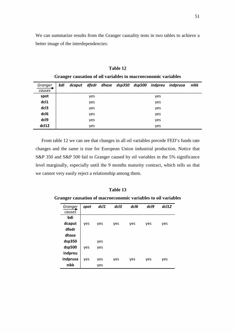
51
We can summarize results from the Granger causality tests in two tables to achieve a
better image of the interdependencies:
Table 12
Granger causation of oil variables to macroeconomic variables
Granger causes
bdi dcaput dfedr dhase dsp350 dsp500 indpreu indprusa nikk
spot yes yes dcl1 yes yes dcl3 yes yes dcl6 yes yes dcl9 yes yes
dcl12 yes yes
From table 12 we can see that changes in all oil variables precede FED’s funds rate
changes and the same is true for European Union industrial production. Notice that
S&P 350 and S&P 500 fail to Granger caused by oil variables in the 5% significance
level marginally, especially until the 9 months maturity contract, which tells us that
we cannot very easily reject a relationship among them.
Table 13
Granger causation of macroeconomic variables to oil variables
Granger causes
spot dcl1 dcl3 dcl6 dcl9 dcl12
bdi dcaput yes yes yes yes yes yes dfedr dhase
dsp350 yes dsp500 yes yes indpreu indprusa yes yes yes yes yes yes
nikk yes
52 The stronger causation in table 13 occurs between US capacity utilization and
industrial production to all oil variables. This suggests a solid relation among these
parameters contrary to the causation of S&P 350, S&P 500 and Nikkei to the 1 month
maturity contract which in our opinion could be provoked by a third unobservable
factor such as strong global demand.
3.2 Vector autoregression results
We will now proceed with the vector autoregression analysis. In every table there
is one oil variable and all the macroeconomic factors. We will examine only the
coefficients of oil prices relatively to the macroeconomic factors and vice versa.
Coefficients that are statistically significant and relative to our study are put into
frames. Below every table there is the relevant annotation.
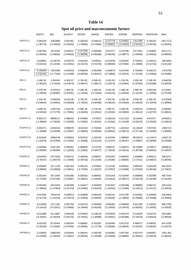
53
Table 14
Spot oil price and macroeconomic factors DSPOT BDI DCAPUT DFEDR DHASE DSP350 DSP500 INDPREU INDPRUSA NIKK DSPOT(-1) 0.084158 -108.8980 0.001491 0.108158 -0.048132 -0.127778 -0.104852 1.817496 0.135220 -353.7172 [ 1.09778] [-0.25820] [ 0.33455] [ 1.49950] [-0.75802] [-3.48887] [-3.14603] [ 2.91351] [ 0.30720] [-0.39181] DSPOT(-2) -0.067063 164.9394 0.000221 0.147239 -0.056380 0.022277 0.016798 0.677691 0.184892 -915.1171 [-0.85003] [ 0.38002] [ 0.04816] [ 1.98358] [-0.86280] [ 0.59105] [ 0.48977] [ 1.05563] [ 0.40816] [-0.98500] DSPOT(-3) 0.049853 61.68749 -0.001076 -0.016032 0.045912 -0.033239 0.002632 0.745544 -0.189215 196.6658 [ 0.63114] [ 0.14196] [-0.23431] [-0.21572] [ 0.70176] [-0.88084] [ 0.07666] [ 1.15994] [-0.41721] [ 0.21143] DSPOT(-4) -0.156459 -759.6368 -0.005518 -0.048638 -0.052989 -0.028574 0.010783 0.732939 -0.548110 -178.5783 [-2.01043] [-1.77426] [-1.21999] [-0.66426] [-0.82207] [-0.76855] [ 0.31870] [ 1.15740] [-1.22663] [-0.19486] BDI(-1) 2.19E-05 1.354334 -4.45E-07 2.74E-05 2.30E-05 1.22E-05 1.71E-05 2.33E-05 -7.33E-05 0.046239 [ 1.56314] [ 17.5918] [-0.54673] [ 2.08447] [ 1.98677] [ 1.81873] [ 2.81684] [ 0.20433] [-0.91286] [ 0.28059] BDI(-2) -2.37E-05 -0.479412 1.30E-06 -2.43E-05 -1.36E-05 -7.01E-06 -1.40E-05 2.46E-05 0.000146 0.214901 [-1.03553] [-3.80887] [ 0.97851] [-1.13042] [-0.71664] [-0.64143] [-1.40945] [ 0.13197] [ 1.10945] [ 0.79765] BDI(-3) 1.34E-05 0.006258 -8.21E-08 3.74E-05 -1.54E-05 -7.32E-06 -1.32E-06 2.93E-05 -1.34E-05 -0.370468 [ 0.59625] [ 0.05061] [-0.06283] [ 1.76932] [-0.82988] [-0.68191] [-0.13534] [ 0.16023] [-0.10376] [-1.39965] BDI(-4) -1.00E-05 0.057189 -1.51E-06 -4.59E-05 2.71E-06 7.29E-07 -3.39E-06 -0.000125 -0.000135 0.065900 [-0.69362] [ 0.71779] [-1.79991] [-3.36635] [ 0.22612] [ 0.10543] [-0.53834] [-1.06112] [-1.62737] [ 0.38641] DCAPUT(-1) 8.961173 98608.27 0.386232 9.276969 7.572875 -4.335136 -3.217122 32.44635 9.037477 -154932.0 [ 1.39500] [ 2.79026] [ 1.03456] [ 1.53493] [ 1.42331] [-1.41261] [-1.15199] [ 0.62073] [ 0.24503] [-2.04813] DCAPUT(-2) -9.892271 -24043.60 0.080678 -18.53194 -2.732934 -1.907715 -1.033152 -31.49344 -7.507432 190673.0 [-1.45989] [-0.64498] [ 0.20487] [-2.90683] [-0.48695] [-0.58932] [-0.35072] [-0.57118] [-0.19296] [ 2.38958] DCAPUT(-3) 8.212540 -35964.96 0.055855 9.037524 -1.223762 -0.419766 1.398959 89.04572 -11.15574 -19187.25 [ 1.22979] [-0.97894] [ 0.14392] [ 1.43838] [-0.22125] [-0.13157] [ 0.48187] [ 1.63867] [-0.29094] [-0.24399] DCAPUT(-4) -2.346949 2102.283 0.395352 6.386839 2.213734 4.898137 1.050474 -81.03990 12.65977 -30808.61 [-0.39055] [ 0.06359] [ 1.13203] [ 1.12962] [ 0.44477] [ 1.70615] [ 0.40210] [-1.65730] [ 0.36691] [-0.43537] DFEDR(-1) 0.054534 -767.5526 0.004712 -0.180639 0.006817 0.041023 0.058033 1.266899 0.384211 328.5477 [ 0.76327] [-1.95273] [ 1.13469] [-2.68718] [ 0.11520] [ 1.20186] [ 1.86834] [ 2.17911] [ 0.93657] [ 0.39050] DFEDR(-2) 0.006505 -217.1135 0.001192 0.260143 0.070552 0.114728 0.083532 0.995192 0.034248 645.4024 [ 0.08883] [-0.53895] [ 0.28021] [ 3.77590] [ 1.16327] [ 3.27957] [ 2.62398] [ 1.67020] [ 0.08146] [ 0.74847] DFEDR(-3) -0.052194 347.2556 0.001086 0.025016 0.084931 0.021318 -0.012094 -0.308858 0.152398 460.7044 [-0.72302] [ 0.87438] [ 0.25887] [ 0.36831] [ 1.42045] [ 0.61814] [-0.38537] [-0.52579] [ 0.36768] [ 0.54195] DFEDR(-4) -0.091494 -915.5015 -0.002495 -0.154317 -0.003609 -0.047637 -0.037089 -0.088859 0.060731 254.6102 [-1.30802] [-2.37904] [-0.61370] [-2.34480] [-0.06229] [-1.42552] [-1.21966] [-0.15612] [ 0.15121] [ 0.30910] DHASE(-1) 0.047562 758.8719 -0.000972 -0.129698 0.065146 0.026741 0.071195 -0.415601 -0.159946 -532.6902 [ 0.41724] [ 1.21010] [-0.14673] [-1.20930] [ 0.69000] [ 0.49105] [ 1.43664] [-0.44806] [-0.24438] [-0.39684] DHASE(-2) -0.015858 -137.1251 0.001756 -0.016713 -0.005868 0.008383 -0.009583 -0.611392 0.126024 568.2759 [-0.14010] [-0.22021] [ 0.26689] [-0.15694] [-0.06260] [ 0.15503] [-0.19475] [-0.66382] [ 0.19392] [ 0.42635] DHASE(-3) -0.011868 -211.6827 0.006158 -0.079302 -0.139143 -0.024609 -0.041970 -0.144220 0.544723 526.2862 [-0.10497] [-0.34033] [ 0.93726] [-0.74551] [-1.48588] [-0.45561] [-0.85388] [-0.15676] [ 0.83913] [ 0.39530] DHASE(-4) 0.032333 87.50443 0.006254 0.036892 -0.102387 0.033495 0.017310 0.480077 0.438352 541.4209 [ 0.29236] [ 0.14382] [ 0.97306] [ 0.35455] [-1.11776] [ 0.63396] [ 0.36004] [ 0.53347] [ 0.69032] [ 0.41573] DSP350(-1) 0.126933 -1998.903 0.002569 0.248244 -0.290785 -0.032881 0.057335 -0.627570 0.846907 1501.352 [ 0.47830] [-1.36910] [ 0.16657] [ 0.99420] [-1.32289] [-0.25935] [ 0.49695] [-0.29061] [ 0.55579] [ 0.48041]
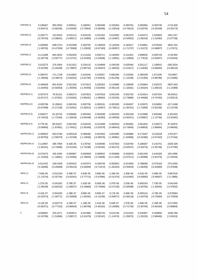
54
DSP350(-2) 0.248467 959.3933 0.000511 0.180001 0.083498 -0.155364 -0.090781 0.050894 -0.304735 -1710.605 [ 0.94371] [ 0.66235] [ 0.03340] [ 0.72664] [ 0.38289] [-1.23519] [-0.79312] [ 0.02376] [-0.20158] [-0.55173] DSP350(-3) -0.205777 123.6553 0.015114 -0.034100 0.031352 0.013092 -0.061976 4.425273 1.525829 238.1157 [-0.78743] [ 0.08601] [ 0.99517] [-0.13869] [ 0.14485] [ 0.10487] [-0.54552] [ 2.08104] [ 1.01690] [ 0.07738] DSP350(-4) 0.269480 -638.3724 -0.010498 0.283750 -0.136628 -0.116546 -0.183317 2.418961 -0.970026 3691.443 [ 1.09753] [-0.47259] [-0.73569] [ 1.22828] [-0.67183] [-0.99357] [-1.71737] [ 1.21072] [-0.68807] [ 1.27671] DSP500(-1) -0.111689 840.4810 0.002028 -0.114162 0.055711 0.145050 -0.131941 3.958635 -0.000743 1718.950 [-0.40778] [ 0.55777] [ 0.12741] [-0.44300] [ 0.24558] [ 1.10851] [-1.10805] [ 1.77615] [-0.00047] [ 0.53294] DSP500(-2) 0.013273 276.3404 0.011912 0.234115 -0.104868 0.194158 0.025946 3.201117 1.108910 -268.3204 [ 0.04785] [ 0.18109] [ 0.73897] [ 0.89710] [-0.45647] [ 1.46523] [ 0.21517] [ 1.41830] [ 0.69630] [-0.08215] DSP500(-3) 0.358707 -711.1738 0.013562 0.161045 0.103037 0.081056 0.132583 -2.285208 1.571195 716.8927 [ 1.29509] [-0.46672] [ 0.84252] [ 0.61799] [ 0.44915] [ 0.61258] [ 1.10109] [-1.01394] [ 0.98798] [ 0.21980] DSP500(-4) -0.446648 -841.8194 0.021318 -0.371612 0.182304 0.124686 0.139508 -2.216664 2.432375 -3657.603 [-1.64492] [-0.56353] [ 1.35093] [-1.45459] [ 0.81060] [ 0.96119] [ 1.18181] [-1.00324] [ 1.56015] [-1.14389] INDPREU(-1) -0.007575 79.91151 0.000274 0.007823 0.007818 0.001339 0.002793 -0.314614 0.037334 56.63412 [-0.87127] [ 1.67061] [ 0.54304] [ 0.95632] [ 1.08563] [ 0.32245] [ 0.73889] [-4.44680] [ 0.74783] [ 0.55313] INDPREU(-2) -0.005796 8.139610 0.000156 0.002756 -0.009191 -0.003285 -0.004007 0.120675 0.024850 -217.4188 [-0.67098] [ 0.17129] [ 0.31061] [ 0.33914] [-1.28467] [-0.79611] [-1.06701] [ 1.71689] [ 0.50106] [-2.13749] INDPREU(-3) 0.006377 81.53733 0.000665 -0.005350 -0.003288 -0.002025 -0.002248 0.313988 0.055396 -2.501402 [ 0.74518] [ 1.73184] [ 1.33618] [-0.66448] [-0.46393] [-0.49536] [-0.60421] [ 4.50887] [ 1.12736] [-0.02482] INDPREU(-4) 6.77E-05 86.51627 0.001345 -0.018140 -0.014099 -0.003540 -0.002681 0.061843 0.129073 97.62975 [ 0.00809] [ 1.87891] [ 2.76421] [-2.30349] [-2.03379] [-0.88543] [-0.73694] [ 0.90803] [ 2.68584] [ 0.99055] INDPRUSA(-1) -0.059522 -923.5780 -0.005418 -0.068365 -0.051952 0.051985 0.045886 -0.173297 -0.216228 1753.877 [-0.90793] [-2.56075] [-1.42199] [-1.10836] [-0.95676] [ 1.65981] [ 1.60998] [-0.32485] [-0.57443] [ 2.27184] INDPRUSA(-2) 0.114857 285.7959 -5.42E-05 0.178792 0.034098 0.027003 0.018760 0.188307 0.142741 -2029.339 [ 1.65151] [ 0.74696] [-0.01340] [ 2.73238] [ 0.59194] [ 0.81272] [ 0.62047] [ 0.33275] [ 0.35746] [-2.47790] INDPRUSA(-3) -0.075275 445.4295 0.000967 -0.050608 0.008932 -0.003686 -0.020023 -0.921435 0.244328 155.4396 [-1.10340] [ 1.18681] [ 0.24383] [-0.78845] [ 0.15808] [-0.11309] [-0.67511] [-1.65985] [ 0.62375] [ 0.19349] INDPRUSA(-4) 0.011442 -100.4209 -0.003422 -0.037074 -0.036746 -0.053922 -0.014950 0.788069 -0.073163 274.4259 [ 0.18485] [-0.29489] [-0.95123] [-0.63659] [-0.71672] [-1.82344] [-0.55553] [ 1.56459] [-0.20585] [ 0.37648] NIKK(-1) -7.65E-06 0.012159 -2.49E-07 4.94E-06 3.80E-06 -1.33E-06 -1.83E-06 -3.51E-05 -2.68E-05 0.897518 [-1.13276] [ 0.32734] [-0.63341] [ 0.77713] [ 0.67966] [-0.41374] [-0.62482] [-0.63893] [-0.69057] [ 11.2886] NIKK(-2) 1.27E-05 -0.041552 5.79E-07 -1.62E-06 -5.65E-06 -2.07E-06 2.03E-06 0.000154 7.73E-05 0.041049 [ 1.38109] [-0.82015] [ 1.08227] [-0.18669] [-0.74096] [-0.47135] [ 0.50598] [ 2.05794] [ 1.46250] [ 0.37852] NIKK(-3) -2.31E-07 0.054185 -1.38E-07 8.80E-06 9.84E-07 2.17E-06 -2.66E-06 -0.000141 -3.79E-05 -0.076664 [-0.02573] [ 1.09771] [-0.26559] [ 1.04200] [ 0.13239] [ 0.50677] [-0.68116] [-1.92478] [-0.73584] [-0.72558] NIKK(-4) -4.12E-06 -0.026770 -3.18E-07 -1.18E-05 2.41E-06 5.54E-07 1.97E-06 1.84E-05 -2.29E-05 0.071955 [-0.65371] [-0.77152] [-0.86634] [-1.98708] [ 0.46162] [ 0.18385] [ 0.71720] [ 0.35794] [-0.63184] [ 0.96883] C -0.006687 225.2271 0.004674 -0.007885 0.006733 0.014736 0.012424 0.226367 0.459806 1036.298 [-0.24795] [ 1.51806] [ 2.98217] [-0.31076] [ 0.30142] [ 1.14374] [ 1.05970] [ 1.03153] [ 2.96946] [ 3.26315]
55 We are interested in the first column and the four first rows of the above table as
the interdependencies between the macroeconomic factors will not studied in this
thesis. The templates denote that a certain coefficient is statistical significant where
the first value is the coefficient and the second in brackets is the t-statistic.
So at first we observe that WTI spot price is affected by its forth lag negatively
with a coefficient of -0,156. This means that if before 4 months the returns on spot oil
price were positive at the present month the returns will be negative and vice versa.
For example if the present month is December and spot oil returns were positive in
August then we expect that December returns will be negative by a factor of 0,156 per
return unit relatively to August returns.
FED’s funds rate have a positive correlation to the second lag of spot oil price and
its coefficient is 0,147. This means that at the present month FED’s fund rate is
expected to be increased by a factor of 0,147 per return unit if before two months the
returns on oil spot price were positive and vice versa.
Returns on S&P 350 have a negative correlation to the first lag of WTI spot price
with a coefficient of -0,128 meaning that if returns of spot price are negative in the
previous month S&P 350 will be positive in the end of the current month by a factor
of 0,128 per return unit.
The same reaction to oil spot price can be observed to the S&P 500 but with a
smaller coefficient of -0,105 meaning that returns on S&P 500 are expected to be
positive by a factor of 0,105 given that returns on spot oil price the previous month
were negative.
The last one, European Union industrial production, is affected positively by the
first lag of spot oil price and the coefficient is 1,817, a quite strong correlation. This
means that if oil spot returns in the previous month is up by one point then European
Union industrial production will be up by 1,817 points at the end of current month and
vice versa if returns on WTI oil spot price are negative.
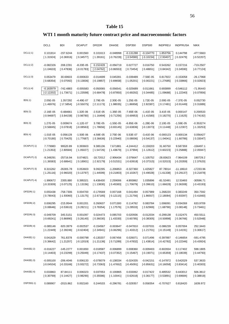
56
Table 15
WTI 1 month maturity future contract price and macroeconomic factors
DCL1 BDI DCAPUT DFEDR DHASE DSP350 DSP500 INDPREU INDPRUSA NIKK DCL1(-1) 0.101814 -157.6244 0.001560 0.101613 -0.048998 -0.131288 -0.104770 1.853756 0.144798 -477.5663 [ 1.31924] [-0.36916] [ 0.34577] [ 1.39161] [-0.76228] [-3.54580] [-3.10234] [ 2.93407] [ 0.32479] [-0.52207] DCL1(-2) -0.082326 208.2291 -8.20E-05 0.152428 -0.056719 0.027727 0.016750 0.543262 0.157216 -719.2507 [-1.04633] [ 0.47836] [-0.01783] [ 2.04762] [-0.86553] [ 0.73454] [ 0.48651] [ 0.84342] [ 0.34590] [-0.77124] DCL1(-3) 0.053479 30.69603 -0.000633 -0.014699 0.045391 -0.039489 -7.56E-05 0.817822 -0.153058 -26.17968 [ 0.68354] [ 0.07092] [-0.13836] [-0.19857] [ 0.69658] [-1.05201] [-0.00221] [ 1.27685] [-0.33866] [-0.02823] DCL1(-4) -0.163979 -742.4883 -0.005583 -0.050065 -0.056541 -0.025689 0.011661 0.693899 -0.546112 -71.95443 [-2.12202] [-1.73671] [-1.23598] [-0.68478] [-0.87850] [-0.69292] [ 0.34485] [ 1.09688] [-1.22340] [-0.07856] BDI(-1) 2.05E-05 1.357292 -4.49E-07 2.79E-05 2.30E-05 1.25E-05 1.72E-05 2.00E-05 -7.37E-05 0.052730 [ 1.46976] [ 17.5854] [-0.55075] [ 2.11173] [ 1.98035] [ 1.86958] [ 2.82387] [ 0.17481] [-0.91449] [ 0.31889] BDI(-2) -2.16E-05 -0.484661 1.32E-06 -2.51E-05 -1.35E-05 -7.65E-06 -1.41E-05 3.41E-05 0.000147 0.200533 [-0.94697] [-3.84158] [ 0.98780] [-1.16494] [-0.71256] [-0.69953] [-1.41580] [ 0.18270] [ 1.11625] [ 0.74192] BDI(-3) 1.27E-05 0.009674 -1.12E-07 3.78E-05 -1.55E-05 -6.85E-06 -1.28E-06 2.10E-05 -1.59E-05 -0.353274 [ 0.56845] [ 0.07818] [-0.08563] [ 1.78656] [-0.83145] [-0.63836] [-0.13073] [ 0.11448] [-0.12307] [-1.33253] BDI(-4) -1.01E-05 0.056128 -1.50E-06 -4.59E-05 2.75E-06 5.53E-07 -3.41E-06 -0.000123 -0.000134 0.056427 [-0.70180] [ 0.70425] [-1.77687] [-3.36636] [ 0.22940] [ 0.08006] [-0.54137] [-1.04041] [-1.60786] [ 0.33047] DCAPUT(-1) 7.779983 99520.89 0.393603 9.385136 7.671881 -4.244412 -3.159203 31.60750 9.587359 -156497.1 [ 1.21353] [ 2.80584] [ 1.05027] [ 1.54726] [ 1.43679] [-1.37994] [-1.12612] [ 0.60223] [ 0.25888] [-2.05947] DCAPUT(-2) -9.249291 -25716.94 0.074821 -18.72012 -2.906434 -2.076647 -1.105752 -28.83623 -7.964109 190729.2 [-1.36583] [-0.68641] [ 0.18901] [-2.92179] [-0.51531] [-0.63918] [-0.37315] [-0.52015] [-0.20359] [ 2.37620] DCAPUT(-3) 8.315262 -35305.78 0.053603 9.092295 -1.206853 -0.327360 1.425827 87.78014 -11.18610 -17233.96 [ 1.25116] [-0.96020] [ 0.13797] [ 1.44599] [-0.21803] [-0.10267] [ 0.49028] [ 1.61338] [-0.29137] [-0.21878] DCAPUT(-4) -1.990672 2355.880 0.395321 6.436430 2.259006 4.893862 1.035896 -81.52491 12.53493 -30596.71 [-0.33309] [ 0.07125] [ 1.13156] [ 1.13830] [ 0.45383] [ 1.70679] [ 0.39610] [-1.66628] [ 0.36308] [-0.43193] DFEDR(-1) 0.055438 -758.7306 0.004700 -0.179569 0.007168 0.041494 0.057989 1.268220 0.383249 350.7592 [ 0.78043] [-1.93060] [ 1.13175] [-2.67185] [ 0.12115] [ 1.21756] [ 1.86557] [ 2.18084] [ 0.93397] [ 0.41660] DFEDR(-2) 0.006295 -215.9544 0.001201 0.260637 0.071300 0.114762 0.083784 1.006091 0.034269 633.9709 [ 0.08646] [-0.53610] [ 0.28211] [ 3.78354] [ 1.17576] [ 3.28533] [ 2.62969] [ 1.68790] [ 0.08148] [ 0.73461] DFEDR(-3) -0.049709 345.5151 0.001097 0.024473 0.085703 0.020936 -0.012034 -0.299138 0.152475 450.5511 [-0.69241] [ 0.86990] [ 0.26140] [ 0.36030] [ 1.43330] [ 0.60785] [-0.38305] [-0.50898] [ 0.36766] [ 0.52948] DFEDR(-4) -0.085146 -920.3979 -0.002537 -0.154567 -0.003647 -0.047810 -0.037031 -0.086239 0.057004 252.3443 [-1.22449] [-2.39246] [-0.62404] [-2.34941] [-0.06296] [-1.43312] [-1.21701] [-0.15149] [ 0.14191] [ 0.30617] DHASE(-1) 0.041629 761.8378 -0.000798 -0.130207 0.067456 0.026071 0.071496 -0.397897 -0.146654 -591.4795 [ 0.36642] [ 1.21207] [-0.12019] [-1.21136] [ 0.71289] [ 0.47832] [ 1.43814] [-0.42782] [-0.22346] [-0.43924] DHASE(-2) -0.016227 -145.2277 0.001650 -0.018587 -0.006899 0.008360 -0.009403 -0.602834 0.117402 598.1805 [-0.14403] [-0.23299] [ 0.25049] [-0.17437] [-0.07352] [ 0.15467] [-0.19071] [-0.65359] [ 0.18039] [ 0.44793] DHASE(-3) -0.005100 -206.4046 0.006133 -0.078079 -0.138334 -0.024335 -0.042151 -0.147872 0.542029 537.3633 [-0.04534] [-0.33166] [ 0.93272] [-0.73363] [-1.47652] [-0.45091] [-0.85631] [-0.16058] [ 0.83414] [ 0.40303] DHASE(-4) 0.033863 87.84111 0.006323 0.037053 -0.100865 0.033062 0.017422 0.485532 0.443012 506.3612 [ 0.30769] [ 0.14427] [ 0.98290] [ 0.35586] [-1.10041] [ 0.62618] [ 0.36177] [ 0.53891] [ 0.69684] [ 0.38818] DSP350(-1) 0.089907 -2015.862 0.002160 0.244533 -0.296781 -0.029357 0.058354 -0.707627 0.818420 1639.972
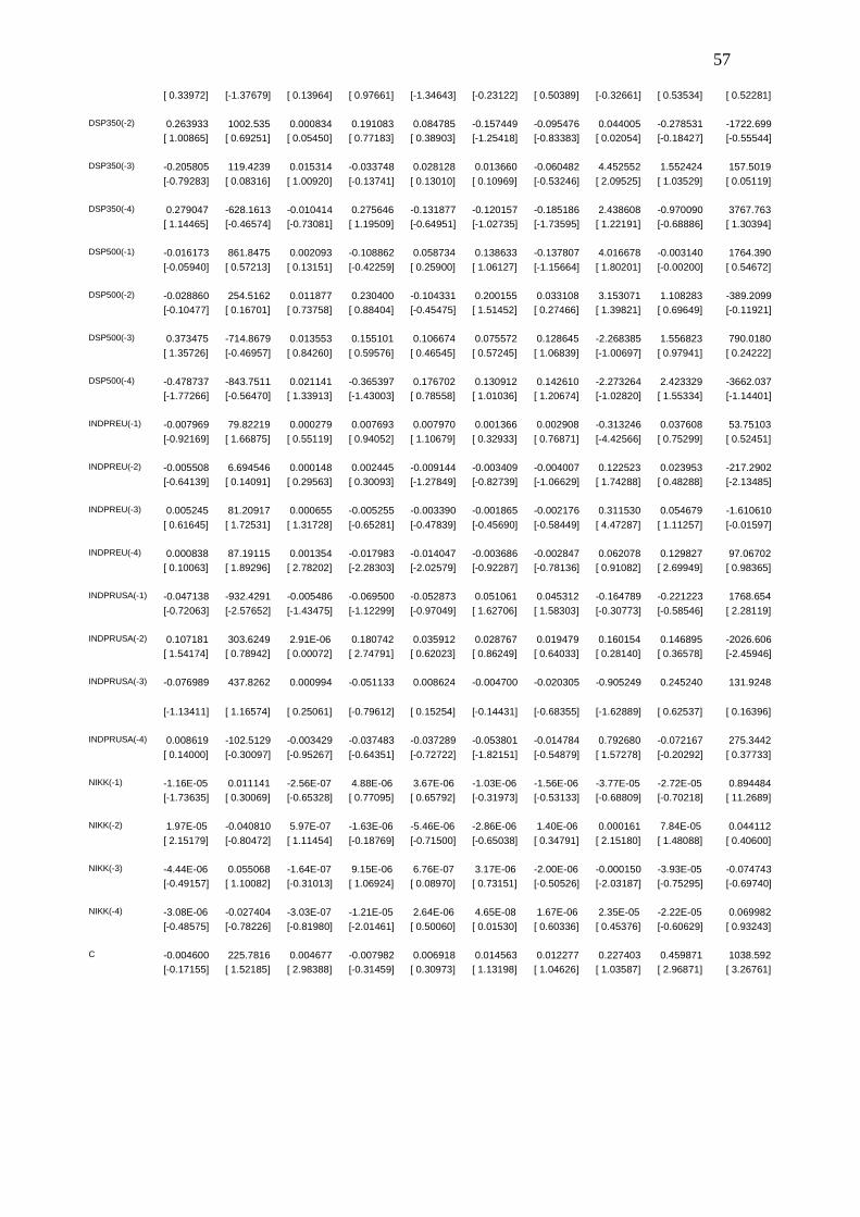
57
[ 0.33972] [-1.37679] [ 0.13964] [ 0.97661] [-1.34643] [-0.23122] [ 0.50389] [-0.32661] [ 0.53534] [ 0.52281] DSP350(-2) 0.263933 1002.535 0.000834 0.191083 0.084785 -0.157449 -0.095476 0.044005 -0.278531 -1722.699 [ 1.00865] [ 0.69251] [ 0.05450] [ 0.77183] [ 0.38903] [-1.25418] [-0.83383] [ 0.02054] [-0.18427] [-0.55544] DSP350(-3) -0.205805 119.4239 0.015314 -0.033748 0.028128 0.013660 -0.060482 4.452552 1.552424 157.5019 [-0.79283] [ 0.08316] [ 1.00920] [-0.13741] [ 0.13010] [ 0.10969] [-0.53246] [ 2.09525] [ 1.03529] [ 0.05119] DSP350(-4) 0.279047 -628.1613 -0.010414 0.275646 -0.131877 -0.120157 -0.185186 2.438608 -0.970090 3767.763 [ 1.14465] [-0.46574] [-0.73081] [ 1.19509] [-0.64951] [-1.02735] [-1.73595] [ 1.22191] [-0.68886] [ 1.30394] DSP500(-1) -0.016173 861.8475 0.002093 -0.108862 0.058734 0.138633 -0.137807 4.016678 -0.003140 1764.390 [-0.05940] [ 0.57213] [ 0.13151] [-0.42259] [ 0.25900] [ 1.06127] [-1.15664] [ 1.80201] [-0.00200] [ 0.54672] DSP500(-2) -0.028860 254.5162 0.011877 0.230400 -0.104331 0.200155 0.033108 3.153071 1.108283 -389.2099 [-0.10477] [ 0.16701] [ 0.73758] [ 0.88404] [-0.45475] [ 1.51452] [ 0.27466] [ 1.39821] [ 0.69649] [-0.11921] DSP500(-3) 0.373475 -714.8679 0.013553 0.155101 0.106674 0.075572 0.128645 -2.268385 1.556823 790.0180 [ 1.35726] [-0.46957] [ 0.84260] [ 0.59576] [ 0.46545] [ 0.57245] [ 1.06839] [-1.00697] [ 0.97941] [ 0.24222] DSP500(-4) -0.478737 -843.7511 0.021141 -0.365397 0.176702 0.130912 0.142610 -2.273264 2.423329 -3662.037 [-1.77266] [-0.56470] [ 1.33913] [-1.43003] [ 0.78558] [ 1.01036] [ 1.20674] [-1.02820] [ 1.55334] [-1.14401] INDPREU(-1) -0.007969 79.82219 0.000279 0.007693 0.007970 0.001366 0.002908 -0.313246 0.037608 53.75103 [-0.92169] [ 1.66875] [ 0.55119] [ 0.94052] [ 1.10679] [ 0.32933] [ 0.76871] [-4.42566] [ 0.75299] [ 0.52451] INDPREU(-2) -0.005508 6.694546 0.000148 0.002445 -0.009144 -0.003409 -0.004007 0.122523 0.023953 -217.2902 [-0.64139] [ 0.14091] [ 0.29563] [ 0.30093] [-1.27849] [-0.82739] [-1.06629] [ 1.74288] [ 0.48288] [-2.13485] INDPREU(-3) 0.005245 81.20917 0.000655 -0.005255 -0.003390 -0.001865 -0.002176 0.311530 0.054679 -1.610610 [ 0.61645] [ 1.72531] [ 1.31728] [-0.65281] [-0.47839] [-0.45690] [-0.58449] [ 4.47287] [ 1.11257] [-0.01597] INDPREU(-4) 0.000838 87.19115 0.001354 -0.017983 -0.014047 -0.003686 -0.002847 0.062078 0.129827 97.06702 [ 0.10063] [ 1.89296] [ 2.78202] [-2.28303] [-2.02579] [-0.92287] [-0.78136] [ 0.91082] [ 2.69949] [ 0.98365] INDPRUSA(-1) -0.047138 -932.4291 -0.005486 -0.069500 -0.052873 0.051061 0.045312 -0.164789 -0.221223 1768.654 [-0.72063] [-2.57652] [-1.43475] [-1.12299] [-0.97049] [ 1.62706] [ 1.58303] [-0.30773] [-0.58546] [ 2.28119] INDPRUSA(-2) 0.107181 303.6249 2.91E-06 0.180742 0.035912 0.028767 0.019479 0.160154 0.146895 -2026.606 [ 1.54174] [ 0.78942] [ 0.00072] [ 2.74791] [ 0.62023] [ 0.86249] [ 0.64033] [ 0.28140] [ 0.36578] [-2.45946] INDPRUSA(-3) -0.076989 437.8262 0.000994 -0.051133 0.008624 -0.004700 -0.020305 -0.905249 0.245240 131.9248
[-1.13411] [ 1.16574] [ 0.25061] [-0.79612] [ 0.15254] [-0.14431] [-0.68355] [-1.62889] [ 0.62537] [ 0.16396] INDPRUSA(-4) 0.008619 -102.5129 -0.003429 -0.037483 -0.037289 -0.053801 -0.014784 0.792680 -0.072167 275.3442 [ 0.14000] [-0.30097] [-0.95267] [-0.64351] [-0.72722] [-1.82151] [-0.54879] [ 1.57278] [-0.20292] [ 0.37733] NIKK(-1) -1.16E-05 0.011141 -2.56E-07 4.88E-06 3.67E-06 -1.03E-06 -1.56E-06 -3.77E-05 -2.72E-05 0.894484 [-1.73635] [ 0.30069] [-0.65328] [ 0.77095] [ 0.65792] [-0.31973] [-0.53133] [-0.68809] [-0.70218] [ 11.2689] NIKK(-2) 1.97E-05 -0.040810 5.97E-07 -1.63E-06 -5.46E-06 -2.86E-06 1.40E-06 0.000161 7.84E-05 0.044112 [ 2.15179] [-0.80472] [ 1.11454] [-0.18769] [-0.71500] [-0.65038] [ 0.34791] [ 2.15180] [ 1.48088] [ 0.40600] NIKK(-3) -4.44E-06 0.055068 -1.64E-07 9.15E-06 6.76E-07 3.17E-06 -2.00E-06 -0.000150 -3.93E-05 -0.074743 [-0.49157] [ 1.10082] [-0.31013] [ 1.06924] [ 0.08970] [ 0.73151] [-0.50526] [-2.03187] [-0.75295] [-0.69740] NIKK(-4) -3.08E-06 -0.027404 -3.03E-07 -1.21E-05 2.64E-06 4.65E-08 1.67E-06 2.35E-05 -2.22E-05 0.069982 [-0.48575] [-0.78226] [-0.81980] [-2.01461] [ 0.50060] [ 0.01530] [ 0.60336] [ 0.45376] [-0.60629] [ 0.93243] C -0.004600 225.7816 0.004677 -0.007982 0.006918 0.014563 0.012277 0.227403 0.459871 1038.592 [-0.17155] [ 1.52185] [ 2.98388] [-0.31459] [ 0.30973] [ 1.13198] [ 1.04626] [ 1.03587] [ 2.96871] [ 3.26761]
58
We observe that we have exactly the same interdependencies as to the spot price
but with slightly different coefficients. The 1 month maturity contract is affected by
its forth lag negatively with a coefficient of -0,164. So if the present month is
December and the 1 month future returns were positive in August then we expect that
December returns will be negative by a factor of 0,164 per return unit relatively to
August returns and vice versa if returns in August were negative .
FED’s funds rate have a positive correlation to the second lag of spot oil price and
its coefficient is 0,152. This means that at the present month FED’s fund rate is
expected to be increased by a factor of 0,152 if before two months the returns on 1
month future contract were up by one unit and vice versa.
Returns on S&P 350 have a negative correlation to the first lag of WTI spot price
with a coefficient of -0,131 meaning that if returns of 1 month future contract are
negative in the previous month S&P 350 will be positive in the end of the current
month by a factor of 0,131 per return unit.
S&P 500 has a coefficient of -0,105 exactly the same as the spot price, meaning
that returns on S&P 500 are expected to be positive by a factor of 0,105 given that
returns on 1 month future contract the previous month were negative by one point.
European Union industrial production, is affected positively by the first lag of the
contract and the coefficient is 1,854. This means that if the contract returns in the
previous month is up by one point then European Union industrial production will be
up by 1,854 points at the end of current month and vice versa if returns on the contract
are negative.
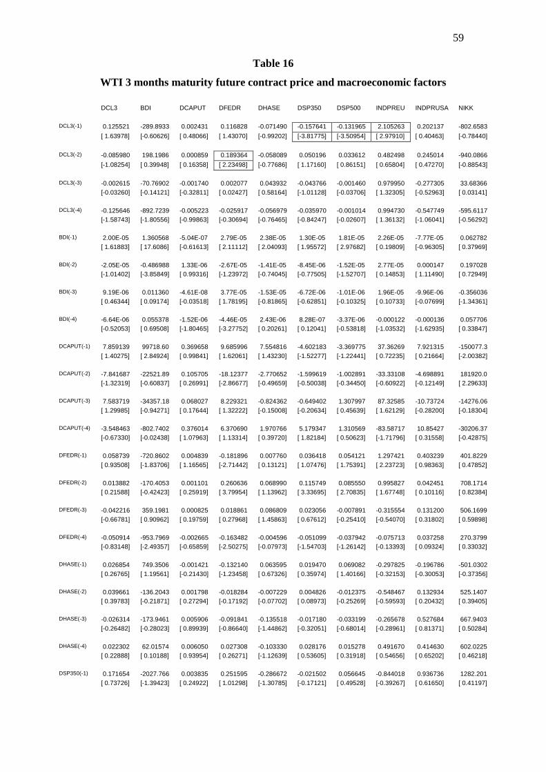
59
Table 16
WTI 3 months maturity future contract price and macroeconomic factors
DCL3 BDI DCAPUT DFEDR DHASE DSP350 DSP500 INDPREU INDPRUSA NIKK DCL3(-1) 0.125521 -289.8933 0.002431 0.116828 -0.071490 -0.157641 -0.131965 2.105263 0.202137 -802.6583 [ 1.63978] [-0.60626] [ 0.48066] [ 1.43070] [-0.99202] [-3.81775] [-3.50954] [ 2.97910] [ 0.40463] [-0.78440] DCL3(-2) -0.085980 198.1986 0.000859 0.189364 -0.058089 0.050196 0.033612 0.482498 0.245014 -940.0866 [-1.08254] [ 0.39948] [ 0.16358] [ 2.23498] [-0.77686] [ 1.17160] [ 0.86151] [ 0.65804] [ 0.47270] [-0.88543] DCL3(-3) -0.002615 -70.76902 -0.001740 0.002077 0.043932 -0.043766 -0.001460 0.979950 -0.277305 33.68366 [-0.03260] [-0.14121] [-0.32811] [ 0.02427] [ 0.58164] [-1.01128] [-0.03706] [ 1.32305] [-0.52963] [ 0.03141] DCL3(-4) -0.125646 -892.7239 -0.005223 -0.025917 -0.056979 -0.035970 -0.001014 0.994730 -0.547749 -595.6117 [-1.58743] [-1.80556] [-0.99863] [-0.30694] [-0.76465] [-0.84247] [-0.02607] [ 1.36132] [-1.06041] [-0.56292] BDI(-1) 2.00E-05 1.360568 -5.04E-07 2.79E-05 2.38E-05 1.30E-05 1.81E-05 2.26E-05 -7.77E-05 0.062782 [ 1.61883] [ 17.6086] [-0.61613] [ 2.11112] [ 2.04093] [ 1.95572] [ 2.97682] [ 0.19809] [-0.96305] [ 0.37969] BDI(-2) -2.05E-05 -0.486988 1.33E-06 -2.67E-05 -1.41E-05 -8.45E-06 -1.52E-05 2.77E-05 0.000147 0.197028 [-1.01402] [-3.85849] [ 0.99316] [-1.23972] [-0.74045] [-0.77505] [-1.52707] [ 0.14853] [ 1.11490] [ 0.72949] BDI(-3) 9.19E-06 0.011360 -4.61E-08 3.77E-05 -1.53E-05 -6.72E-06 -1.01E-06 1.96E-05 -9.96E-06 -0.356036 [ 0.46344] [ 0.09174] [-0.03518] [ 1.78195] [-0.81865] [-0.62851] [-0.10325] [ 0.10733] [-0.07699] [-1.34361] BDI(-4) -6.64E-06 0.055378 -1.52E-06 -4.46E-05 2.43E-06 8.28E-07 -3.37E-06 -0.000122 -0.000136 0.057706 [-0.52053] [ 0.69508] [-1.80465] [-3.27752] [ 0.20261] [ 0.12041] [-0.53818] [-1.03532] [-1.62935] [ 0.33847] DCAPUT(-1) 7.859139 99718.60 0.369658 9.685996 7.554816 -4.602183 -3.369775 37.36269 7.921315 -150077.3 [ 1.40275] [ 2.84924] [ 0.99841] [ 1.62061] [ 1.43230] [-1.52277] [-1.22441] [ 0.72235] [ 0.21664] [-2.00382] DCAPUT(-2) -7.841687 -22521.89 0.105705 -18.12377 -2.770652 -1.599619 -1.002891 -33.33108 -4.698891 181920.0 [-1.32319] [-0.60837] [ 0.26991] [-2.86677] [-0.49659] [-0.50038] [-0.34450] [-0.60922] [-0.12149] [ 2.29633] DCAPUT(-3) 7.583719 -34357.18 0.068027 8.229321 -0.824362 -0.649402 1.307997 87.32585 -10.73724 -14276.06 [ 1.29985] [-0.94271] [ 0.17644] [ 1.32222] [-0.15008] [-0.20634] [ 0.45639] [ 1.62129] [-0.28200] [-0.18304] DCAPUT(-4) -3.548463 -802.7402 0.376014 6.370690 1.970766 5.179347 1.310569 -83.58717 10.85427 -30206.37 [-0.67330] [-0.02438] [ 1.07963] [ 1.13314] [ 0.39720] [ 1.82184] [ 0.50623] [-1.71796] [ 0.31558] [-0.42875] DFEDR(-1) 0.058739 -720.8602 0.004839 -0.181896 0.007760 0.036418 0.054121 1.297421 0.403239 401.8229 [ 0.93508] [-1.83706] [ 1.16565] [-2.71442] [ 0.13121] [ 1.07476] [ 1.75391] [ 2.23723] [ 0.98363] [ 0.47852] DFEDR(-2) 0.013882 -170.4053 0.001101 0.260636 0.068990 0.115749 0.085550 0.995827 0.042451 708.1714 [ 0.21588] [-0.42423] [ 0.25919] [ 3.79954] [ 1.13962] [ 3.33695] [ 2.70835] [ 1.67748] [ 0.10116] [ 0.82384] DFEDR(-3) -0.042216 359.1981 0.000825 0.018861 0.086809 0.023056 -0.007891 -0.315554 0.131200 506.1699 [-0.66781] [ 0.90962] [ 0.19759] [ 0.27968] [ 1.45863] [ 0.67612] [-0.25410] [-0.54070] [ 0.31802] [ 0.59898] DFEDR(-4) -0.050914 -953.7969 -0.002665 -0.163482 -0.004596 -0.051099 -0.037942 -0.075713 0.037258 270.3799 [-0.83148] [-2.49357] [-0.65859] [-2.50275] [-0.07973] [-1.54703] [-1.26142] [-0.13393] [ 0.09324] [ 0.33032] DHASE(-1) 0.026854 749.3506 -0.001421 -0.132140 0.063595 0.019470 0.069082 -0.297825 -0.196786 -501.0302 [ 0.26765] [ 1.19561] [-0.21430] [-1.23458] [ 0.67326] [ 0.35974] [ 1.40166] [-0.32153] [-0.30053] [-0.37356] DHASE(-2) 0.039661 -136.2043 0.001798 -0.018284 -0.007229 0.004826 -0.012375 -0.548467 0.132934 525.1407 [ 0.39783] [-0.21871] [ 0.27294] [-0.17192] [-0.07702] [ 0.08973] [-0.25269] [-0.59593] [ 0.20432] [ 0.39405] DHASE(-3) -0.026314 -173.9461 0.005906 -0.091841 -0.135518 -0.017180 -0.033199 -0.265678 0.527684 667.9403 [-0.26482] [-0.28023] [ 0.89939] [-0.86640] [-1.44862] [-0.32051] [-0.68014] [-0.28961] [ 0.81371] [ 0.50284] DHASE(-4) 0.022302 62.01574 0.006050 0.027308 -0.103330 0.028176 0.015278 0.491670 0.414630 602.0225 [ 0.22888] [ 0.10188] [ 0.93954] [ 0.26271] [-1.12639] [ 0.53605] [ 0.31918] [ 0.54656] [ 0.65202] [ 0.46218] DSP350(-1) 0.171654 -2027.766 0.003835 0.251595 -0.286672 -0.021502 0.056645 -0.844018 0.936736 1282.201 [ 0.73726] [-1.39423] [ 0.24922] [ 1.01298] [-1.30785] [-0.17121] [ 0.49528] [-0.39267] [ 0.61650] [ 0.41197]
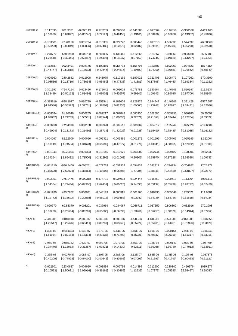
60
DSP350(-2) 0.117336 981.3321 -0.000113 0.178209 0.092580 -0.141386 -0.077669 -0.146850 -0.368538 -1419.163 [ 0.50660] [ 0.67827] [-0.00740] [ 0.72127] [ 0.42458] [-1.13165] [-0.68266] [-0.06868] [-0.24382] [-0.45836] DSP350(-3) -0.133581 72.28150 0.015724 -0.018305 0.027772 0.003446 -0.077818 4.556533 1.574597 -76.88560 [-0.58293] [ 0.05049] [ 1.03836] [-0.07488] [ 0.12873] [ 0.02787] [-0.69131] [ 2.15384] [ 1.05290] [-0.02510] DSP350(-4) 0.278772 -570.9990 -0.009798 0.285805 -0.130460 -0.112865 -0.184857 2.368262 -0.903368 3585.789 [ 1.29448] [-0.42446] [-0.68847] [ 1.24408] [-0.64347] [-0.97157] [-1.74745] [ 1.19120] [-0.64277] [ 1.24558] DSP500(-1) -0.112887 902.3491 0.002176 -0.109859 0.055734 0.155796 -0.123607 3.802260 0.024623 1877.154 [-0.46747] [ 0.59818] [ 0.13633] [-0.42645] [ 0.24515] [ 1.19600] [-1.04200] [ 1.70551] [ 0.01562] [ 0.58149] DSP500(-2) -0.020963 240.2882 0.011908 0.243975 -0.110196 0.187022 0.021403 3.308479 1.107262 -370.3590 [-0.08566] [ 0.15719] [ 0.73634] [ 0.93460] [-0.47833] [ 1.41681] [ 0.17805] [ 1.46450] [ 0.69334] [-0.11322] DSP500(-3) 0.301397 -764.7164 0.013466 0.179642 0.098008 0.078783 0.130964 -2.140708 1.556147 613.5237 [ 1.23499] [-0.50162] [ 0.83494] [ 0.69002] [ 0.42657] [ 0.59845] [ 1.09245] [-0.95015] [ 0.97706] [ 0.18806] DSP500(-4) -0.385816 -828.1977 0.020789 -0.353541 0.182608 0.128875 0.144547 -2.140306 2.391428 -3577.587 [-1.61586] [-0.55527] [ 1.31751] [-1.38801] [ 0.81236] [ 1.00060] [ 1.23241] [-0.97097] [ 1.53471] [-1.12086] INDPREU(-1) -0.008334 81.96040 0.000255 0.007217 0.007843 0.000930 0.002686 -0.309953 0.036280 60.79097 [-1.09082] [ 1.71733] [ 0.50531] [ 0.88544] [ 1.09035] [ 0.22571] [ 0.71568] [-4.39444] [ 0.72764] [ 0.59522] INDPREU(-2)
-0.003268 7.204390 0.000158 0.002328 -0.009512 -0.003769 -0.004312 0.125249 0.025326 -219.6604
[-0.42994] [ 0.15173] [ 0.31460] [ 0.28714] [-1.32927] [-0.91928] [-1.15490] [ 1.78489] [ 0.51055] [-2.16182] INDPREU(-3)
0.004067 82.22509 0.000656 -0.005311 -0.003386 -0.001272 -0.001595 0.305466 0.055145 1.522064
[ 0.53919] [ 1.74504] [ 1.31673] [-0.65999] [-0.47677] [-0.31270] [-0.43041] [ 4.38655] [ 1.12022] [ 0.01509] INDPREU(-4)
0.001048 85.21004 0.001353 -0.018145 -0.013920 -0.003582 -0.002744 0.059422 0.128906 99.02539
[ 0.14254] [ 1.85492] [ 2.78500] [-2.31295] [-2.01061] [-0.90305] [-0.75970] [ 0.87526] [ 2.68598] [ 1.00733] INDPRUSA(-1)
-0.051210 -936.5400 -0.005251 -0.072763 -0.051932 0.054632 0.047317 -0.224234 -0.204992 1702.477
[-0.89500] [-2.62023] [-1.38864] [-1.19208] [-0.96406] [ 1.77004] [ 1.68345] [-0.42450] [-0.54897] [ 2.22579] INDPRUSA(-2)
0.093953 275.1476 -0.000318 0.174791 0.034933 0.024448 0.018860 0.200619 0.113964 -1930.111
[ 1.54504] [ 0.72434] [-0.07906] [ 2.69451] [ 0.61020] [ 0.74533] [ 0.63137] [ 0.35736] [ 0.28717] [-2.37439] INDPRUSA(-3)
-0.071289 433.7202 0.000821 -0.043199 0.005315 -0.001266 -0.018930 -0.905549 0.239021 111.6881
[-1.19742] [ 1.16622] [ 0.20868] [-0.68018] [ 0.09482] [-0.03942] [-0.64729] [-1.64756] [ 0.61518] [ 0.14034] INDPRUSA(-4)
0.020770 -69.83379 -0.003201 -0.037969 -0.034067 -0.056711 -0.017659 0.806302 -0.052916 270.1908
[ 0.38280] [-0.20604] [-0.89281] [-0.65600] [-0.66693] [-1.93766] [-0.66257] [ 1.60970] [-0.14944] [ 0.37252] NIKK(-1) -7.44E-06 0.010918 -2.68E-07 5.08E-06 3.63E-06 -1.14E-06 -1.61E-06 -3.52E-05 -2.82E-05 0.896656 [-1.25547] [ 0.29476] [-0.68411] [ 0.80260] [ 0.65048] [-0.35724] [-0.55401] [-0.64351] [-0.72926] [ 11.3120] NIKK(-2) 1.30E-05 -0.041493 6.16E-07 -1.87E-06 -5.44E-06 -2.40E-06 1.60E-06 0.000154 7.98E-05 0.036643 [ 1.61064] [-0.82183] [ 1.15334] [-0.21637] [-0.71490] [-0.55021] [ 0.40337] [ 2.06919] [ 1.51317] [ 0.33915] NIKK(-3) -2.96E-06 0.055782 -1.63E-07 9.09E-06 1.07E-06 2.65E-06 -2.18E-06 -0.000143 -3.97E-05 -0.067484 [-0.37446] [ 1.13053] [-0.31257] [ 1.07821] [ 0.14330] [ 0.62311] [-0.56088] [-1.96780] [-0.77012] [-0.63911] NIKK(-4) -2.23E-06 -0.027045 -3.08E-07 -1.19E-05 2.28E-06 2.13E-07 1.68E-06 2.14E-05 -2.19E-05 0.067675 [-0.40209] [-0.77928] [-0.84000] [-2.00345] [ 0.43608] [ 0.07096] [ 0.61391] [ 0.41790] [-0.60483] [ 0.91121] C -0.002501 223.0687 0.004650 -0.008894 0.006795 0.014399 0.012500 0.230340 0.456976 1039.277 [-0.10553] [ 1.50681] [ 2.96916] [-0.35181] [ 0.30456] [ 1.12632] [ 1.07373] [ 1.05280] [ 2.95467] [ 3.28050]
61 We observe similar interdependencies to the previous two contracts. Fed’s funds
rate is affected positively by the second lag of the 3 months maturity oil future and its
coefficient is 0,189. So if the returns of this certain future contract are up by one
point, we will have an upward movement to FED’ funds rate of 0,189 points.
S&P 350 and S&P 500 are affected negatively by the first lag of the oil future and
their coefficients are -0,158 and -0,132 respectively meaning that one point increase
in the returns of the oil future at the present month will result to a decline of 0,158 and
0,132 respectively for the two indices next month.
European union industrial production is affected positively by the first lag of the 3
months maturity future and has a coefficient of 2,105.
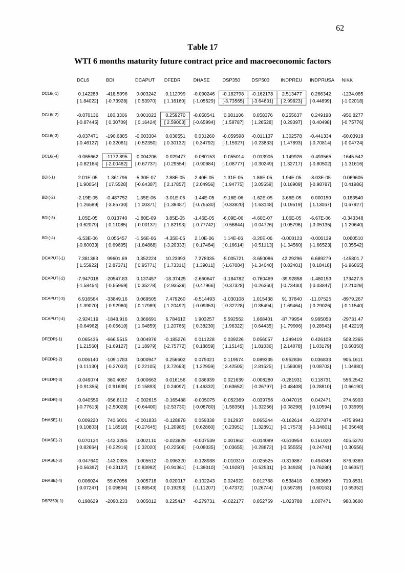
62
Table 17
WTI 6 months maturity future contract price and macroeconomic factors
DCL6 BDI DCAPUT DFEDR DHASE DSP350 DSP500 INDPREU INDPRUSA NIKK DCL6(-1) 0.142288 -418.5096 0.003242 0.112099 -0.090246 -0.182798 -0.162178 2.513477 0.266342 -1234.085 [ 1.84022] [-0.73928] [ 0.53970] [ 1.16160] [-1.05529] [-3.73565] [-3.64631] [ 2.99823] [ 0.44899] [-1.02018] DCL6(-2) -0.070136 180.3306 0.001023 0.259270 -0.058541 0.081106 0.058376 0.255637 0.249198 -950.8277 [-0.87445] [ 0.30709] [ 0.16424] [ 2.59003] [-0.65994] [ 1.59787] [ 1.26528] [ 0.29397] [ 0.40498] [-0.75776] DCL6(-3) -0.037471 -190.6885 -0.003304 0.030551 0.031260 -0.059598 -0.011137 1.302578 -0.441334 -60.03919 [-0.46127] [-0.32061] [-0.52350] [ 0.30132] [ 0.34792] [-1.15927] [-0.23833] [ 1.47893] [-0.70814] [-0.04724] DCL6(-4) -0.065662 -1172.895 -0.004206 -0.029477 -0.080153 -0.055014 -0.013905 1.149926 -0.493565 -1645.542 [-0.82164] [-2.00462] [-0.67737] [-0.29554] [-0.90684] [-1.08777] [-0.30249] [ 1.32717] [-0.80502] [-1.31616] BDI(-1) 2.01E-05 1.361796 -5.30E-07 2.88E-05 2.40E-05 1.31E-05 1.86E-05 1.94E-05 -8.03E-05 0.069605 [ 1.90054] [ 17.5528] [-0.64387] [ 2.17857] [ 2.04956] [ 1.94775] [ 3.05559] [ 0.16909] [-0.98787] [ 0.41986] BDI(-2) -2.19E-05 -0.487752 1.35E-06 -3.01E-05 -1.44E-05 -9.16E-06 -1.62E-05 3.66E-05 0.000150 0.183540 [-1.26589] [-3.85730] [ 1.00371] [-1.39487] [-0.75530] [-0.83820] [-1.63148] [ 0.19519] [ 1.13067] [ 0.67927] BDI(-3) 1.05E-05 0.013740 -1.80E-09 3.85E-05 -1.46E-05 -6.09E-06 -4.60E-07 1.06E-05 -6.67E-06 -0.343348 [ 0.62079] [ 0.11085] [-0.00137] [ 1.82193] [-0.77742] [-0.56844] [-0.04726] [ 0.05796] [-0.05135] [-1.29640] BDI(-4) -6.53E-06 0.055457 -1.56E-06 -4.35E-05 2.10E-06 1.14E-06 -3.20E-06 -0.000123 -0.000139 0.060510 [-0.60033] [ 0.69605] [-1.84868] [-3.20333] [ 0.17484] [ 0.16614] [-0.51113] [-1.04560] [-1.66523] [ 0.35542] DCAPUT(-1) 7.381363 99601.69 0.352224 10.23993 7.278335 -5.005721 -3.650086 42.29296 6.689279 -145801.7 [ 1.55922] [ 2.87371] [ 0.95771] [ 1.73311] [ 1.39011] [-1.67084] [-1.34040] [ 0.82401] [ 0.18418] [-1.96865] DCAPUT(-2) -7.947018 -20547.83 0.137457 -18.37425 -2.660647 -1.184782 -0.760469 -39.92858 -1.480153 173427.5 [-1.58454] [-0.55959] [ 0.35278] [-2.93539] [-0.47966] [-0.37328] [-0.26360] [-0.73430] [-0.03847] [ 2.21029] DCAPUT(-3) 6.916564 -33849.16 0.069505 7.479260 -0.514493 -1.030108 1.015438 91.37840 -11.07525 -8979.267 [ 1.39070] [-0.92960] [ 0.17989] [ 1.20492] [-0.09353] [-0.32728] [ 0.35494] [ 1.69464] [-0.29026] [-0.11540] DCAPUT(-4) -2.924119 -1848.916 0.366691 6.784612 1.903257 5.592562 1.668401 -87.79954 9.995053 -29731.47 [-0.64962] [-0.05610] [ 1.04859] [ 1.20766] [ 0.38230] [ 1.96322] [ 0.64435] [-1.79906] [ 0.28943] [-0.42219] DFEDR(-1) 0.065436 -666.5515 0.004976 -0.185276 0.011228 0.039226 0.056057 1.249419 0.426108 508.2365 [ 1.21560] [-1.69127] [ 1.18979] [-2.75772] [ 0.18859] [ 1.15145] [ 1.81036] [ 2.14078] [ 1.03179] [ 0.60350] DFEDR(-2) 0.006140 -109.1783 0.000947 0.256602 0.075021 0.119574 0.089335 0.952836 0.036833 905.1611 [ 0.11130] [-0.27032] [ 0.22105] [ 3.72693] [ 1.22959] [ 3.42505] [ 2.81525] [ 1.59309] [ 0.08703] [ 1.04880] DFEDR(-3) -0.049074 360.4087 0.000663 0.016156 0.086939 0.021639 -0.008280 -0.281931 0.118731 556.2542 [-0.91355] [ 0.91639] [ 0.15893] [ 0.24097] [ 1.46332] [ 0.63652] [-0.26797] [-0.48408] [ 0.28810] [ 0.66190] DFEDR(-4) -0.040559 -956.6112 -0.002615 -0.165488 -0.005075 -0.052369 -0.039756 -0.047015 0.042471 274.6903 [-0.77613] [-2.50028] [-0.64400] [-2.53730] [-0.08780] [-1.58350] [-1.32256] [-0.08298] [ 0.10594] [ 0.33599] DHASE(-1) 0.009220 740.6001 -0.001833 -0.128878 0.059338 0.012937 0.065244 -0.162614 -0.227874 -475.9943 [ 0.10803] [ 1.18518] [-0.27645] [-1.20985] [ 0.62860] [ 0.23951] [ 1.32891] [-0.17573] [-0.34801] [-0.35648] DHASE(-2) 0.070124 -142.3285 0.002110 -0.023829 -0.007539 0.001962 -0.014089 -0.510954 0.161020 405.5270 [ 0.82664] [-0.22916] [ 0.32020] [-0.22506] [-0.08035] [ 0.03655] [-0.28872] [-0.55555] [ 0.24741] [ 0.30556] DHASE(-3) -0.047640 -143.0935 0.005512 -0.096320 -0.128938 -0.010310 -0.025525 -0.319887 0.494340 876.9369 [-0.56397] [-0.23137] [ 0.83992] [-0.91361] [-1.38010] [-0.19287] [-0.52531] [-0.34928] [ 0.76280] [ 0.66357] DHASE(-4) 0.006024 59.67056 0.005718 0.020017 -0.102243 0.024922 0.012788 0.538418 0.383689 719.8531 [ 0.07247] [ 0.09804] [ 0.88543] [ 0.19293] [-1.11207] [ 0.47372] [ 0.26744] [ 0.59739] [ 0.60163] [ 0.55352] DSP350(-1) 0.198629 -2090.233 0.005012 0.225417 -0.279731 -0.022177 0.052759 -1.023788 1.007471 980.3600
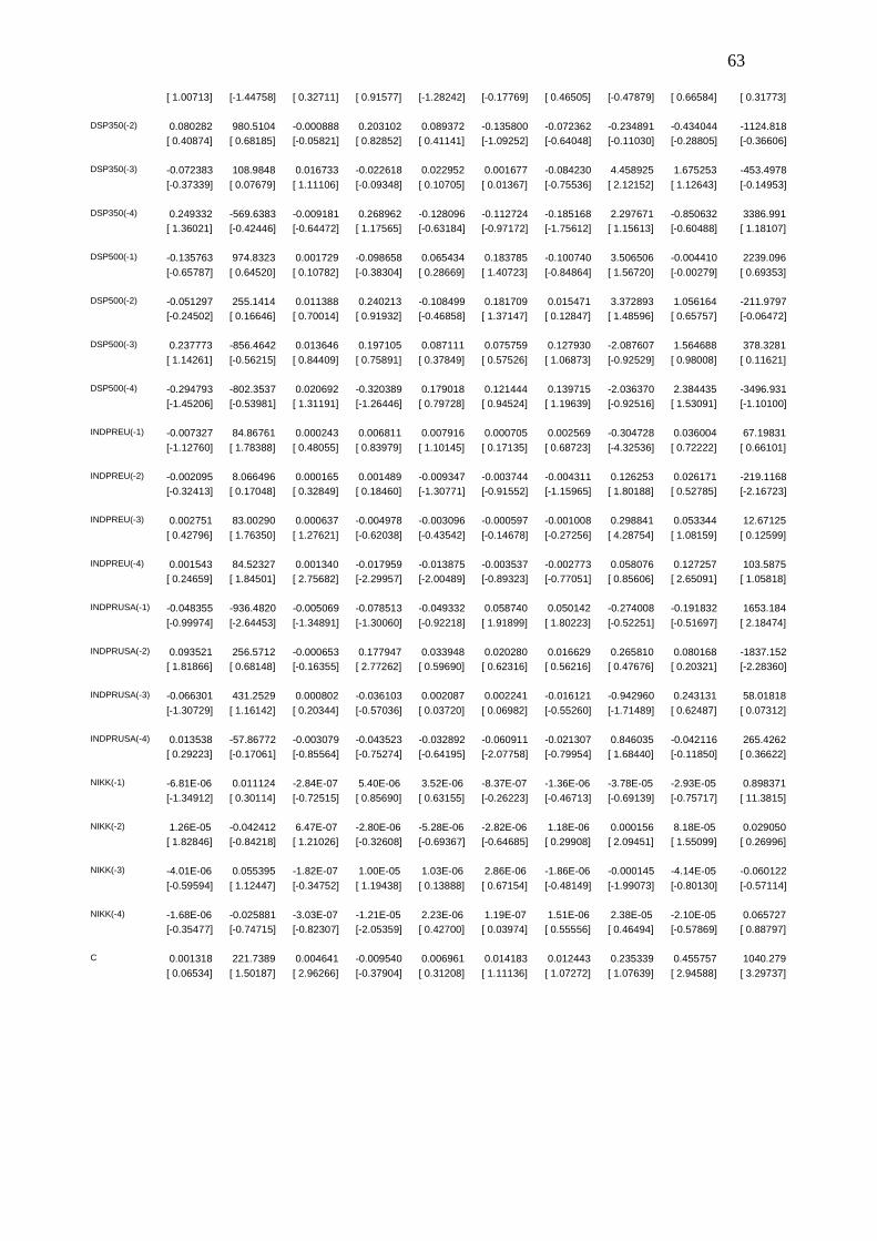
63
[ 1.00713] [-1.44758] [ 0.32711] [ 0.91577] [-1.28242] [-0.17769] [ 0.46505] [-0.47879] [ 0.66584] [ 0.31773] DSP350(-2) 0.080282 980.5104 -0.000888 0.203102 0.089372 -0.135800 -0.072362 -0.234891 -0.434044 -1124.818 [ 0.40874] [ 0.68185] [-0.05821] [ 0.82852] [ 0.41141] [-1.09252] [-0.64048] [-0.11030] [-0.28805] [-0.36606] DSP350(-3) -0.072383 108.9848 0.016733 -0.022618 0.022952 0.001677 -0.084230 4.458925 1.675253 -453.4978 [-0.37339] [ 0.07679] [ 1.11106] [-0.09348] [ 0.10705] [ 0.01367] [-0.75536] [ 2.12152] [ 1.12643] [-0.14953] DSP350(-4) 0.249332 -569.6383 -0.009181 0.268962 -0.128096 -0.112724 -0.185168 2.297671 -0.850632 3386.991 [ 1.36021] [-0.42446] [-0.64472] [ 1.17565] [-0.63184] [-0.97172] [-1.75612] [ 1.15613] [-0.60488] [ 1.18107] DSP500(-1) -0.135763 974.8323 0.001729 -0.098658 0.065434 0.183785 -0.100740 3.506506 -0.004410 2239.096 [-0.65787] [ 0.64520] [ 0.10782] [-0.38304] [ 0.28669] [ 1.40723] [-0.84864] [ 1.56720] [-0.00279] [ 0.69353] DSP500(-2) -0.051297 255.1414 0.011388 0.240213 -0.108499 0.181709 0.015471 3.372893 1.056164 -211.9797 [-0.24502] [ 0.16646] [ 0.70014] [ 0.91932] [-0.46858] [ 1.37147] [ 0.12847] [ 1.48596] [ 0.65757] [-0.06472] DSP500(-3) 0.237773 -856.4642 0.013646 0.197105 0.087111 0.075759 0.127930 -2.087607 1.564688 378.3281 [ 1.14261] [-0.56215] [ 0.84409] [ 0.75891] [ 0.37849] [ 0.57526] [ 1.06873] [-0.92529] [ 0.98008] [ 0.11621] DSP500(-4) -0.294793 -802.3537 0.020692 -0.320389 0.179018 0.121444 0.139715 -2.036370 2.384435 -3496.931 [-1.45206] [-0.53981] [ 1.31191] [-1.26446] [ 0.79728] [ 0.94524] [ 1.19639] [-0.92516] [ 1.53091] [-1.10100] INDPREU(-1) -0.007327 84.86761 0.000243 0.006811 0.007916 0.000705 0.002569 -0.304728 0.036004 67.19831 [-1.12760] [ 1.78388] [ 0.48055] [ 0.83979] [ 1.10145] [ 0.17135] [ 0.68723] [-4.32536] [ 0.72222] [ 0.66101] INDPREU(-2) -0.002095 8.066496 0.000165 0.001489 -0.009347 -0.003744 -0.004311 0.126253 0.026171 -219.1168 [-0.32413] [ 0.17048] [ 0.32849] [ 0.18460] [-1.30771] [-0.91552] [-1.15965] [ 1.80188] [ 0.52785] [-2.16723] INDPREU(-3) 0.002751 83.00290 0.000637 -0.004978 -0.003096 -0.000597 -0.001008 0.298841 0.053344 12.67125 [ 0.42796] [ 1.76350] [ 1.27621] [-0.62038] [-0.43542] [-0.14678] [-0.27256] [ 4.28754] [ 1.08159] [ 0.12599] INDPREU(-4) 0.001543 84.52327 0.001340 -0.017959 -0.013875 -0.003537 -0.002773 0.058076 0.127257 103.5875 [ 0.24659] [ 1.84501] [ 2.75682] [-2.29957] [-2.00489] [-0.89323] [-0.77051] [ 0.85606] [ 2.65091] [ 1.05818] INDPRUSA(-1) -0.048355 -936.4820 -0.005069 -0.078513 -0.049332 0.058740 0.050142 -0.274008 -0.191832 1653.184 [-0.99974] [-2.64453] [-1.34891] [-1.30060] [-0.92218] [ 1.91899] [ 1.80223] [-0.52251] [-0.51697] [ 2.18474] INDPRUSA(-2) 0.093521 256.5712 -0.000653 0.177947 0.033948 0.020280 0.016629 0.265810 0.080168 -1837.152 [ 1.81866] [ 0.68148] [-0.16355] [ 2.77262] [ 0.59690] [ 0.62316] [ 0.56216] [ 0.47676] [ 0.20321] [-2.28360] INDPRUSA(-3) -0.066301 431.2529 0.000802 -0.036103 0.002087 0.002241 -0.016121 -0.942960 0.243131 58.01818 [-1.30729] [ 1.16142] [ 0.20344] [-0.57036] [ 0.03720] [ 0.06982] [-0.55260] [-1.71489] [ 0.62487] [ 0.07312] INDPRUSA(-4) 0.013538 -57.86772 -0.003079 -0.043523 -0.032892 -0.060911 -0.021307 0.846035 -0.042116 265.4262 [ 0.29223] [-0.17061] [-0.85564] [-0.75274] [-0.64195] [-2.07758] [-0.79954] [ 1.68440] [-0.11850] [ 0.36622] NIKK(-1) -6.81E-06 0.011124 -2.84E-07 5.40E-06 3.52E-06 -8.37E-07 -1.36E-06 -3.78E-05 -2.93E-05 0.898371 [-1.34912] [ 0.30114] [-0.72515] [ 0.85690] [ 0.63155] [-0.26223] [-0.46713] [-0.69139] [-0.75717] [ 11.3815] NIKK(-2) 1.26E-05 -0.042412 6.47E-07 -2.80E-06 -5.28E-06 -2.82E-06 1.18E-06 0.000156 8.18E-05 0.029050 [ 1.82846] [-0.84218] [ 1.21026] [-0.32608] [-0.69367] [-0.64685] [ 0.29908] [ 2.09451] [ 1.55099] [ 0.26996] NIKK(-3) -4.01E-06 0.055395 -1.82E-07 1.00E-05 1.03E-06 2.86E-06 -1.86E-06 -0.000145 -4.14E-05 -0.060122 [-0.59594] [ 1.12447] [-0.34752] [ 1.19438] [ 0.13888] [ 0.67154] [-0.48149] [-1.99073] [-0.80130] [-0.57114] NIKK(-4) -1.68E-06 -0.025881 -3.03E-07 -1.21E-05 2.23E-06 1.19E-07 1.51E-06 2.38E-05 -2.10E-05 0.065727 [-0.35477] [-0.74715] [-0.82307] [-2.05359] [ 0.42700] [ 0.03974] [ 0.55556] [ 0.46494] [-0.57869] [ 0.88797] C 0.001318 221.7389 0.004641 -0.009540 0.006961 0.014183 0.012443 0.235339 0.455757 1040.279 [ 0.06534] [ 1.50187] [ 2.96266] [-0.37904] [ 0.31208] [ 1.11136] [ 1.07272] [ 1.07639] [ 2.94588] [ 3.29737]
64
We observe that S&P 350 and S&P 500 are affected negatively by the first lag of
the 6 months future contract with coefficients of -0,183 and -0,162 respectively.
European Union industrial production is affected positively by the first lag of the
future contract with a coefficient of 2,513 and FED’s funds rate is affected positively
by the second lag of the future contract.
The new element in this VAR is that the dry bulk index has a negative correlation
to the fourth lag of the 6 months maturity future contract and has a coefficient of
-1172,9. This translates to an increase of 1172,9 points in dry bulk index the current
month if before 4 months the returns of the future contract had been decreased by one
point.
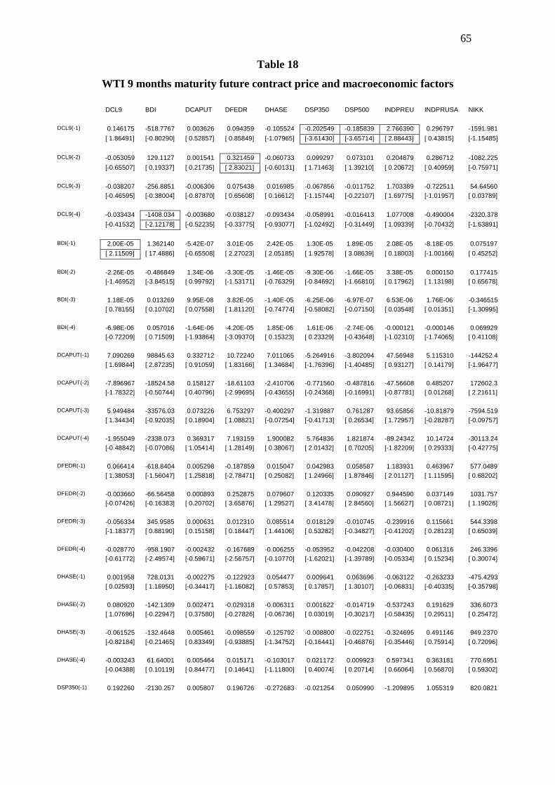
65
Table 18
WTI 9 months maturity future contract price and macroeconomic factors
DCL9 BDI DCAPUT DFEDR DHASE DSP350 DSP500 INDPREU INDPRUSA NIKK DCL9(-1) 0.146175 -518.7767 0.003626 0.094359 -0.105524 -0.202549 -0.185839 2.766390 0.296797 -1591.981 [ 1.86491] [-0.80290] [ 0.52857] [ 0.85849] [-1.07965] [-3.61430] [-3.65714] [ 2.88443] [ 0.43815] [-1.15485] DCL9(-2) -0.053059 129.1127 0.001541 0.321459 -0.060733 0.099297 0.073101 0.204879 0.286712 -1082.225 [-0.65507] [ 0.19337] [ 0.21735] [ 2.83021] [-0.60131] [ 1.71463] [ 1.39210] [ 0.20672] [ 0.40959] [-0.75971] DCL9(-3) -0.038207 -256.8851 -0.006306 0.075438 0.016985 -0.067856 -0.011752 1.703389 -0.722511 54.64560 [-0.46595] [-0.38004] [-0.87870] [ 0.65608] [ 0.16612] [-1.15744] [-0.22107] [ 1.69775] [-1.01957] [ 0.03789] DCL9(-4) -0.033434 -1408.034 -0.003680 -0.038127 -0.093434 -0.058991 -0.016413 1.077008 -0.490004 -2320.378 [-0.41532] [-2.12178] [-0.52235] [-0.33775] [-0.93077] [-1.02492] [-0.31449] [ 1.09339] [-0.70432] [-1.63891] BDI(-1) 2.00E-05 1.362140 -5.42E-07 3.01E-05 2.42E-05 1.30E-05 1.89E-05 2.08E-05 -8.18E-05 0.075197 [ 2.11509] [ 17.4886] [-0.65508] [ 2.27023] [ 2.05185] [ 1.92578] [ 3.08639] [ 0.18003] [-1.00166] [ 0.45252] BDI(-2) -2.26E-05 -0.486849 1.34E-06 -3.30E-05 -1.46E-05 -9.30E-06 -1.66E-05 3.38E-05 0.000150 0.177415 [-1.46952] [-3.84515] [ 0.99792] [-1.53171] [-0.76329] [-0.84692] [-1.66810] [ 0.17962] [ 1.13198] [ 0.65678] BDI(-3) 1.18E-05 0.013269 9.95E-08 3.82E-05 -1.40E-05 -6.25E-06 -6.97E-07 6.53E-06 1.76E-06 -0.346515 [ 0.78155] [ 0.10702] [ 0.07558] [ 1.81120] [-0.74774] [-0.58082] [-0.07150] [ 0.03548] [ 0.01351] [-1.30995] BDI(-4) -6.98E-06 0.057016 -1.64E-06 -4.20E-05 1.85E-06 1.61E-06 -2.74E-06 -0.000121 -0.000146 0.069929 [-0.72209] [ 0.71509] [-1.93864] [-3.09370] [ 0.15323] [ 0.23329] [-0.43648] [-1.02310] [-1.74065] [ 0.41108] DCAPUT(-1) 7.090269 98845.63 0.332712 10.72240 7.011065 -5.264916 -3.802094 47.56948 5.115310 -144252.4 [ 1.69844] [ 2.87235] [ 0.91059] [ 1.83166] [ 1.34684] [-1.76396] [-1.40485] [ 0.93127] [ 0.14179] [-1.96477] DCAPUT(-2) -7.896967 -18524.58 0.158127 -18.61103 -2.410706 -0.771560 -0.487816 -47.56608 0.485207 172602.3 [-1.78322] [-0.50744] [ 0.40796] [-2.99695] [-0.43655] [-0.24368] [-0.16991] [-0.87781] [ 0.01268] [ 2.21611] DCAPUT(-3) 5.949484 -33576.03 0.073226 6.753297 -0.400297 -1.319887 0.761287 93.65856 -10.81879 -7594.519 [ 1.34434] [-0.92035] [ 0.18904] [ 1.08821] [-0.07254] [-0.41713] [ 0.26534] [ 1.72957] [-0.28287] [-0.09757] DCAPUT(-4) -1.955049 -2338.073 0.369317 7.193159 1.900082 5.764836 1.821874 -89.24342 10.14724 -30113.24 [-0.48842] [-0.07086] [ 1.05414] [ 1.28149] [ 0.38067] [ 2.01432] [ 0.70205] [-1.82209] [ 0.29333] [-0.42775] DFEDR(-1) 0.066414 -618.8404 0.005298 -0.187859 0.015047 0.042983 0.058587 1.183931 0.463967 577.0489 [ 1.38053] [-1.56047] [ 1.25818] [-2.78471] [ 0.25082] [ 1.24966] [ 1.87846] [ 2.01127] [ 1.11595] [ 0.68202] DFEDR(-2) -0.003660 -66.56458 0.000893 0.252875 0.079607 0.120335 0.090927 0.944590 0.037149 1031.757 [-0.07426] [-0.16383] [ 0.20702] [ 3.65876] [ 1.29527] [ 3.41478] [ 2.84560] [ 1.56627] [ 0.08721] [ 1.19026] DFEDR(-3) -0.056334 345.9585 0.000631 0.012310 0.085514 0.018129 -0.010745 -0.239916 0.115661 544.3398 [-1.18377] [ 0.88190] [ 0.15158] [ 0.18447] [ 1.44106] [ 0.53282] [-0.34827] [-0.41202] [ 0.28123] [ 0.65039] DFEDR(-4) -0.028770 -958.1907 -0.002432 -0.167689 -0.006255 -0.053952 -0.042208 -0.030400 0.061316 246.3396 [-0.61772] [-2.49574] [-0.59671] [-2.56757] [-0.10770] [-1.62021] [-1.39789] [-0.05334] [ 0.15234] [ 0.30074] DHASE(-1) 0.001958 728.0131 -0.002275 -0.122923 0.054477 0.009641 0.063696 -0.063122 -0.263233 -475.4293 [ 0.02593] [ 1.16950] [-0.34417] [-1.16082] [ 0.57853] [ 0.17857] [ 1.30107] [-0.06831] [-0.40335] [-0.35798] DHASE(-2) 0.080920 -142.1309 0.002471 -0.029318 -0.006311 0.001622 -0.014719 -0.537243 0.191629 336.6073 [ 1.07696] [-0.22947] [ 0.37580] [-0.27826] [-0.06736] [ 0.03019] [-0.30217] [-0.58435] [ 0.29511] [ 0.25472] DHASE(-3) -0.061525 -132.4648 0.005461 -0.098559 -0.125792 -0.008800 -0.022751 -0.324695 0.491146 949.2370 [-0.82184] [-0.21465] [ 0.83349] [-0.93885] [-1.34752] [-0.16441] [-0.46876] [-0.35446] [ 0.75914] [ 0.72096] DHASE(-4) -0.003243 61.64001 0.005464 0.015171 -0.103017 0.021172 0.009923 0.597341 0.363181 770.6951 [-0.04388] [ 0.10119] [ 0.84477] [ 0.14641] [-1.11800] [ 0.40074] [ 0.20714] [ 0.66064] [ 0.56870] [ 0.59302] DSP350(-1) 0.192260 -2130.257 0.005807 0.196726 -0.272683 -0.021254 0.050990 -1.209895 1.055319 820.0821
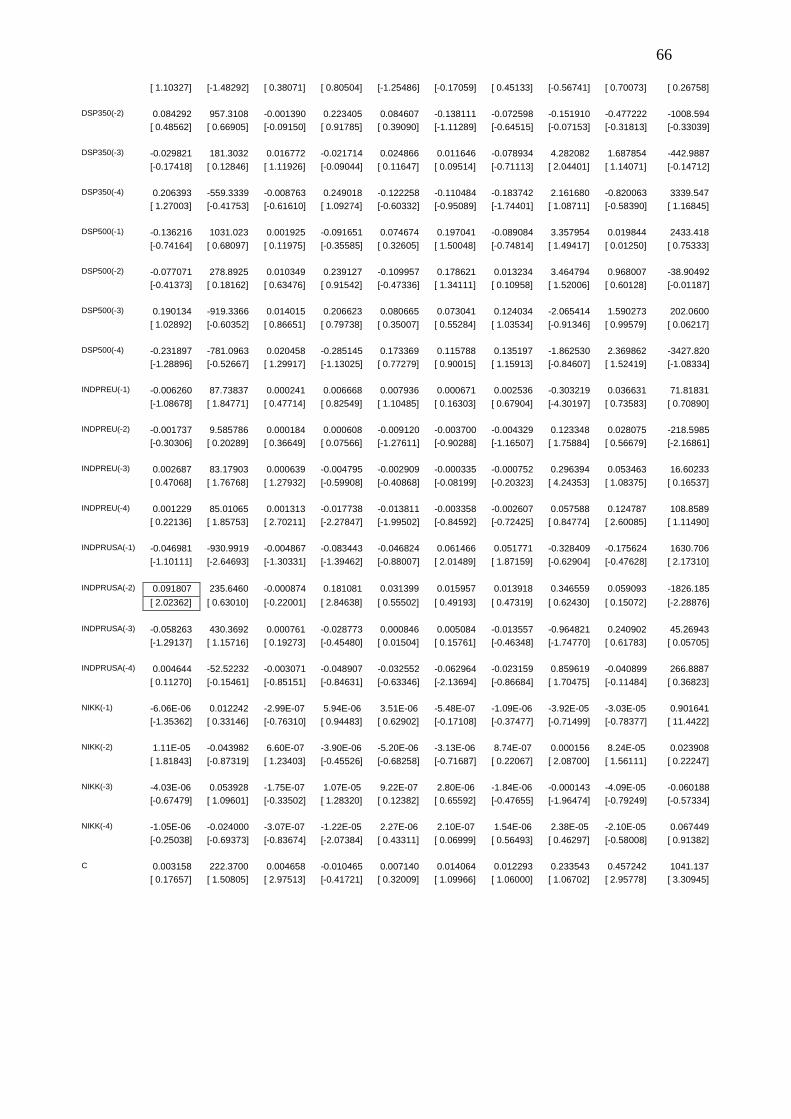
66
[ 1.10327] [-1.48292] [ 0.38071] [ 0.80504] [-1.25486] [-0.17059] [ 0.45133] [-0.56741] [ 0.70073] [ 0.26758] DSP350(-2) 0.084292 957.3108 -0.001390 0.223405 0.084607 -0.138111 -0.072598 -0.151910 -0.477222 -1008.594 [ 0.48562] [ 0.66905] [-0.09150] [ 0.91785] [ 0.39090] [-1.11289] [-0.64515] [-0.07153] [-0.31813] [-0.33039] DSP350(-3) -0.029821 181.3032 0.016772 -0.021714 0.024866 0.011646 -0.078934 4.282082 1.687854 -442.9887 [-0.17418] [ 0.12846] [ 1.11926] [-0.09044] [ 0.11647] [ 0.09514] [-0.71113] [ 2.04401] [ 1.14071] [-0.14712] DSP350(-4) 0.206393 -559.3339 -0.008763 0.249018 -0.122258 -0.110484 -0.183742 2.161680 -0.820063 3339.547 [ 1.27003] [-0.41753] [-0.61610] [ 1.09274] [-0.60332] [-0.95089] [-1.74401] [ 1.08711] [-0.58390] [ 1.16845] DSP500(-1) -0.136216 1031.023 0.001925 -0.091651 0.074674 0.197041 -0.089084 3.357954 0.019844 2433.418 [-0.74164] [ 0.68097] [ 0.11975] [-0.35585] [ 0.32605] [ 1.50048] [-0.74814] [ 1.49417] [ 0.01250] [ 0.75333] DSP500(-2) -0.077071 278.8925 0.010349 0.239127 -0.109957 0.178621 0.013234 3.464794 0.968007 -38.90492 [-0.41373] [ 0.18162] [ 0.63476] [ 0.91542] [-0.47336] [ 1.34111] [ 0.10958] [ 1.52006] [ 0.60128] [-0.01187] DSP500(-3) 0.190134 -919.3366 0.014015 0.206623 0.080665 0.073041 0.124034 -2.065414 1.590273 202.0600 [ 1.02892] [-0.60352] [ 0.86651] [ 0.79738] [ 0.35007] [ 0.55284] [ 1.03534] [-0.91346] [ 0.99579] [ 0.06217] DSP500(-4) -0.231897 -781.0963 0.020458 -0.285145 0.173369 0.115788 0.135197 -1.862530 2.369862 -3427.820 [-1.28896] [-0.52667] [ 1.29917] [-1.13025] [ 0.77279] [ 0.90015] [ 1.15913] [-0.84607] [ 1.52419] [-1.08334] INDPREU(-1) -0.006260 87.73837 0.000241 0.006668 0.007936 0.000671 0.002536 -0.303219 0.036631 71.81831 [-1.08678] [ 1.84771] [ 0.47714] [ 0.82549] [ 1.10485] [ 0.16303] [ 0.67904] [-4.30197] [ 0.73583] [ 0.70890] INDPREU(-2) -0.001737 9.585786 0.000184 0.000608 -0.009120 -0.003700 -0.004329 0.123348 0.028075 -218.5985 [-0.30306] [ 0.20289] [ 0.36649] [ 0.07566] [-1.27611] [-0.90288] [-1.16507] [ 1.75884] [ 0.56679] [-2.16861] INDPREU(-3) 0.002687 83.17903 0.000639 -0.004795 -0.002909 -0.000335 -0.000752 0.296394 0.053463 16.60233 [ 0.47068] [ 1.76768] [ 1.27932] [-0.59908] [-0.40868] [-0.08199] [-0.20323] [ 4.24353] [ 1.08375] [ 0.16537] INDPREU(-4) 0.001229 85.01065 0.001313 -0.017738 -0.013811 -0.003358 -0.002607 0.057588 0.124787 108.8589 [ 0.22136] [ 1.85753] [ 2.70211] [-2.27847] [-1.99502] [-0.84592] [-0.72425] [ 0.84774] [ 2.60085] [ 1.11490] INDPRUSA(-1) -0.046981 -930.9919 -0.004867 -0.083443 -0.046824 0.061466 0.051771 -0.328409 -0.175624 1630.706 [-1.10111] [-2.64693] [-1.30331] [-1.39462] [-0.88007] [ 2.01489] [ 1.87159] [-0.62904] [-0.47628] [ 2.17310] INDPRUSA(-2) 0.091807 235.6460 -0.000874 0.181081 0.031399 0.015957 0.013918 0.346559 0.059093 -1826.185 [ 2.02362] [ 0.63010] [-0.22001] [ 2.84638] [ 0.55502] [ 0.49193] [ 0.47319] [ 0.62430] [ 0.15072] [-2.28876] INDPRUSA(-3) -0.058263 430.3692 0.000761 -0.028773 0.000846 0.005084 -0.013557 -0.964821 0.240902 45.26943 [-1.29137] [ 1.15716] [ 0.19273] [-0.45480] [ 0.01504] [ 0.15761] [-0.46348] [-1.74770] [ 0.61783] [ 0.05705] INDPRUSA(-4) 0.004644 -52.52232 -0.003071 -0.048907 -0.032552 -0.062964 -0.023159 0.859619 -0.040899 266.8887 [ 0.11270] [-0.15461] [-0.85151] [-0.84631] [-0.63346] [-2.13694] [-0.86684] [ 1.70475] [-0.11484] [ 0.36823] NIKK(-1) -6.06E-06 0.012242 -2.99E-07 5.94E-06 3.51E-06 -5.48E-07 -1.09E-06 -3.92E-05 -3.03E-05 0.901641 [-1.35362] [ 0.33146] [-0.76310] [ 0.94483] [ 0.62902] [-0.17108] [-0.37477] [-0.71499] [-0.78377] [ 11.4422] NIKK(-2) 1.11E-05 -0.043982 6.60E-07 -3.90E-06 -5.20E-06 -3.13E-06 8.74E-07 0.000156 8.24E-05 0.023908 [ 1.81843] [-0.87319] [ 1.23403] [-0.45526] [-0.68258] [-0.71687] [ 0.22067] [ 2.08700] [ 1.56111] [ 0.22247] NIKK(-3) -4.03E-06 0.053928 -1.75E-07 1.07E-05 9.22E-07 2.80E-06 -1.84E-06 -0.000143 -4.09E-05 -0.060188 [-0.67479] [ 1.09601] [-0.33502] [ 1.28320] [ 0.12382] [ 0.65592] [-0.47655] [-1.96474] [-0.79249] [-0.57334] NIKK(-4) -1.05E-06 -0.024000 -3.07E-07 -1.22E-05 2.27E-06 2.10E-07 1.54E-06 2.38E-05 -2.10E-05 0.067449 [-0.25038] [-0.69373] [-0.83674] [-2.07384] [ 0.43311] [ 0.06999] [ 0.56493] [ 0.46297] [-0.58008] [ 0.91382] C 0.003158 222.3700 0.004658 -0.010465 0.007140 0.014064 0.012293 0.233543 0.457242 1041.137 [ 0.17657] [ 1.50805] [ 2.97513] [-0.41721] [ 0.32009] [ 1.09966] [ 1.06000] [ 1.06702] [ 2.95778] [ 3.30945]
67 WTI 9 months future contract first lag affects negatively S&P 350 and S&P 500
with coefficients -0,202 and -0,186 respectively and affects positively European
Union industrial production (first lag) and FED’s funds rate (second lag) with
coefficients of 2,726 and 0,321. As in the previous VAR its fourth lag also affects
negatively dry bulk index with a coefficient of -1408.
A new element in this VAR is the effect that the second lag of US industrial
production has on the 9 months future contract. We observe a positive coefficient of
0,092 which means that if US industrial production increased by one point the returns
of the 9 months future contract will increase, after two months, by 0,092 and vice
versa if US industrial production decreased. Also the first lag of dry bulk index affects
positively the future contract with a very small coefficient due to the fact that we
didn’t take logarithmic returns because it was already stationary.
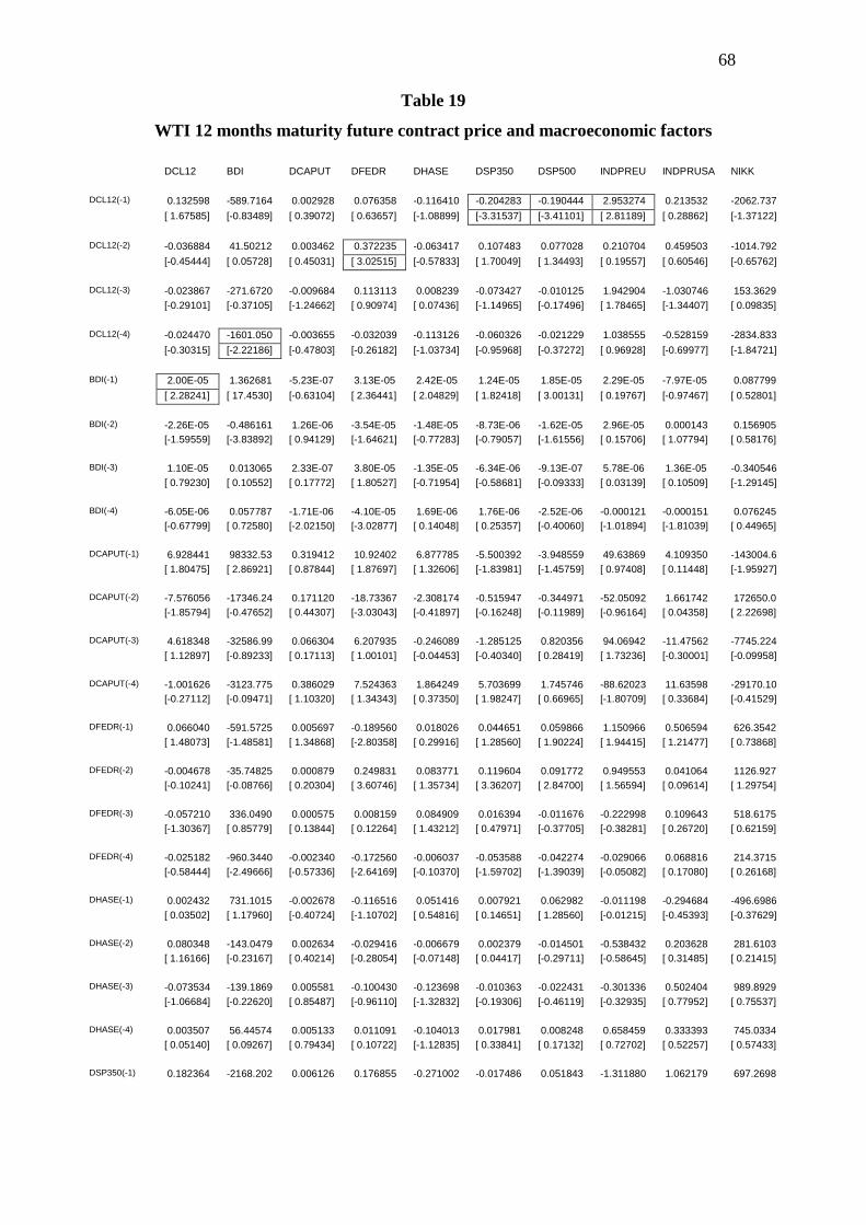
68
Table 19
WTI 12 months maturity future contract price and macroeconomic factors
DCL12 BDI DCAPUT DFEDR DHASE DSP350 DSP500 INDPREU INDPRUSA NIKK DCL12(-1) 0.132598 -589.7164 0.002928 0.076358 -0.116410 -0.204283 -0.190444 2.953274 0.213532 -2062.737 [ 1.67585] [-0.83489] [ 0.39072] [ 0.63657] [-1.08899] [-3.31537] [-3.41101] [ 2.81189] [ 0.28862] [-1.37122] DCL12(-2) -0.036884 41.50212 0.003462 0.372235 -0.063417 0.107483 0.077028 0.210704 0.459503 -1014.792 [-0.45444] [ 0.05728] [ 0.45031] [ 3.02515] [-0.57833] [ 1.70049] [ 1.34493] [ 0.19557] [ 0.60546] [-0.65762] DCL12(-3) -0.023867 -271.6720 -0.009684 0.113113 0.008239 -0.073427 -0.010125 1.942904 -1.030746 153.3629 [-0.29101] [-0.37105] [-1.24662] [ 0.90974] [ 0.07436] [-1.14965] [-0.17496] [ 1.78465] [-1.34407] [ 0.09835] DCL12(-4) -0.024470 -1601.050 -0.003655 -0.032039 -0.113126 -0.060326 -0.021229 1.038555 -0.528159 -2834.833 [-0.30315] [-2.22186] [-0.47803] [-0.26182] [-1.03734] [-0.95968] [-0.37272] [ 0.96928] [-0.69977] [-1.84721] BDI(-1) 2.00E-05 1.362681 -5.23E-07 3.13E-05 2.42E-05 1.24E-05 1.85E-05 2.29E-05 -7.97E-05 0.087799 [ 2.28241] [ 17.4530] [-0.63104] [ 2.36441] [ 2.04829] [ 1.82418] [ 3.00131] [ 0.19767] [-0.97467] [ 0.52801] BDI(-2) -2.26E-05 -0.486161 1.26E-06 -3.54E-05 -1.48E-05 -8.73E-06 -1.62E-05 2.96E-05 0.000143 0.156905 [-1.59559] [-3.83892] [ 0.94129] [-1.64621] [-0.77283] [-0.79057] [-1.61556] [ 0.15706] [ 1.07794] [ 0.58176] BDI(-3) 1.10E-05 0.013065 2.33E-07 3.80E-05 -1.35E-05 -6.34E-06 -9.13E-07 5.78E-06 1.36E-05 -0.340546 [ 0.79230] [ 0.10552] [ 0.17772] [ 1.80527] [-0.71954] [-0.58681] [-0.09333] [ 0.03139] [ 0.10509] [-1.29145] BDI(-4) -6.05E-06 0.057787 -1.71E-06 -4.10E-05 1.69E-06 1.76E-06 -2.52E-06 -0.000121 -0.000151 0.076245 [-0.67799] [ 0.72580] [-2.02150] [-3.02877] [ 0.14048] [ 0.25357] [-0.40060] [-1.01894] [-1.81039] [ 0.44965] DCAPUT(-1) 6.928441 98332.53 0.319412 10.92402 6.877785 -5.500392 -3.948559 49.63869 4.109350 -143004.6 [ 1.80475] [ 2.86921] [ 0.87844] [ 1.87697] [ 1.32606] [-1.83981] [-1.45759] [ 0.97408] [ 0.11448] [-1.95927] DCAPUT(-2) -7.576056 -17346.24 0.171120 -18.73367 -2.308174 -0.515947 -0.344971 -52.05092 1.661742 172650.0 [-1.85794] [-0.47652] [ 0.44307] [-3.03043] [-0.41897] [-0.16248] [-0.11989] [-0.96164] [ 0.04358] [ 2.22698] DCAPUT(-3) 4.618348 -32586.99 0.066304 6.207935 -0.246089 -1.285125 0.820356 94.06942 -11.47562 -7745.224 [ 1.12897] [-0.89233] [ 0.17113] [ 1.00101] [-0.04453] [-0.40340] [ 0.28419] [ 1.73236] [-0.30001] [-0.09958] DCAPUT(-4) -1.001626 -3123.775 0.386029 7.524363 1.864249 5.703699 1.745746 -88.62023 11.63598 -29170.10 [-0.27112] [-0.09471] [ 1.10320] [ 1.34343] [ 0.37350] [ 1.98247] [ 0.66965] [-1.80709] [ 0.33684] [-0.41529] DFEDR(-1) 0.066040 -591.5725 0.005697 -0.189560 0.018026 0.044651 0.059866 1.150966 0.506594 626.3542 [ 1.48073] [-1.48581] [ 1.34868] [-2.80358] [ 0.29916] [ 1.28560] [ 1.90224] [ 1.94415] [ 1.21477] [ 0.73868] DFEDR(-2) -0.004678 -35.74825 0.000879 0.249831 0.083771 0.119604 0.091772 0.949553 0.041064 1126.927 [-0.10241] [-0.08766] [ 0.20304] [ 3.60746] [ 1.35734] [ 3.36207] [ 2.84700] [ 1.56594] [ 0.09614] [ 1.29754] DFEDR(-3) -0.057210 336.0490 0.000575 0.008159 0.084909 0.016394 -0.011676 -0.222998 0.109643 518.6175 [-1.30367] [ 0.85779] [ 0.13844] [ 0.12264] [ 1.43212] [ 0.47971] [-0.37705] [-0.38281] [ 0.26720] [ 0.62159] DFEDR(-4) -0.025182 -960.3440 -0.002340 -0.172560 -0.006037 -0.053588 -0.042274 -0.029066 0.068816 214.3715 [-0.58444] [-2.49666] [-0.57336] [-2.64169] [-0.10370] [-1.59702] [-1.39039] [-0.05082] [ 0.17080] [ 0.26168] DHASE(-1) 0.002432 731.1015 -0.002678 -0.116516 0.051416 0.007921 0.062982 -0.011198 -0.294684 -496.6986 [ 0.03502] [ 1.17960] [-0.40724] [-1.10702] [ 0.54816] [ 0.14651] [ 1.28560] [-0.01215] [-0.45393] [-0.37629] DHASE(-2) 0.080348 -143.0479 0.002634 -0.029416 -0.006679 0.002379 -0.014501 -0.538432 0.203628 281.6103 [ 1.16166] [-0.23167] [ 0.40214] [-0.28054] [-0.07148] [ 0.04417] [-0.29711] [-0.58645] [ 0.31485] [ 0.21415] DHASE(-3) -0.073534 -139.1869 0.005581 -0.100430 -0.123698 -0.010363 -0.022431 -0.301336 0.502404 989.8929 [-1.06684] [-0.22620] [ 0.85487] [-0.96110] [-1.32832] [-0.19306] [-0.46119] [-0.32935] [ 0.77952] [ 0.75537] DHASE(-4) 0.003507 56.44574 0.005133 0.011091 -0.104013 0.017981 0.008248 0.658459 0.333393 745.0334 [ 0.05140] [ 0.09267] [ 0.79434] [ 0.10722] [-1.12835] [ 0.33841] [ 0.17132] [ 0.72702] [ 0.52257] [ 0.57433] DSP350(-1) 0.182364 -2168.202 0.006126 0.176855 -0.271002 -0.017486 0.051843 -1.311880 1.062179 697.2698
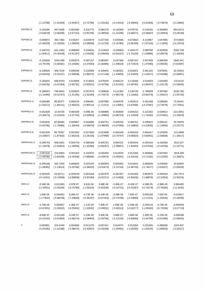
69
[ 1.13788] [-1.51545] [ 0.40357] [ 0.72790] [-1.25160] [-0.14010] [ 0.45842] [-0.61666] [ 0.70879] [ 0.22883] DSP350(-2) 0.102266 947.0188 -0.001082 0.231775 0.084179 -0.143306 -0.076731 -0.145191 -0.439955 -854.6272 [ 0.64019] [ 0.66408] [-0.07151] [ 0.95706] [ 0.39004] [-1.15196] [-0.68071] [-0.06847] [-0.29454] [-0.28139] DSP350(-3) -0.009972 260.7383 0.016257 -0.020679 0.027106 0.020596 -0.073563 4.123967 1.647695 -374.8925 [-0.06328] [ 0.18536] [ 1.08930] [-0.08656] [ 0.12733] [ 0.16784] [-0.66159] [ 1.97163] [ 1.11830] [-0.12514] DSP350(-4) 0.158743 -541.2262 -0.008683 0.234626 -0.119543 -0.109903 -0.184172 2.088768 -0.819535 3320.708 [ 1.05911] [-0.40449] [-0.61167] [ 1.03256] [-0.59033] [-0.94157] [-1.74134] [ 1.04985] [-0.58476] [ 1.16530] DSP500(-1) -0.128306 1034.058 0.002674 -0.097157 0.083497 0.197369 -0.087167 3.307459 0.089258 2640.441 [-0.75745] [ 0.68381] [ 0.16665] [-0.37833] [ 0.36485] [ 1.49618] [-0.72924] [ 1.47095] [ 0.05635] [ 0.81987] DSP500(-2) -0.106526 308.7518 0.009248 0.232968 -0.109401 0.180301 0.016001 3.461102 0.875041 22.43315 [-0.62025] [ 0.20137] [ 0.56848] [ 0.89475] [-0.47148] [ 1.34805] [ 0.13203] [ 1.51817] [ 0.54488] [ 0.00687] DSP500(-3) 0.160633 -948.9703 0.014658 0.213503 0.075525 0.068123 0.116408 -2.018403 1.644469 116.8120 [ 0.94239] [-0.62364] [ 0.90792] [ 0.82622] [ 0.32796] [ 0.51320] [ 0.96782] [-0.89207] [ 1.03178] [ 0.03605] DSP500(-4) -0.188323 -766.8641 0.020620 -0.257679 0.169648 0.111363 0.130749 -1.768268 2.397660 -3334.782 [-1.13490] [-0.51767] [ 1.31195] [-1.02430] [ 0.75672] [ 0.86178] [ 1.11662] [-0.80278] [ 1.54527] [-1.05702] INDPREU(-1) -0.005480 89.65377 0.000229 0.006481 0.007985 0.000578 0.002513 -0.301438 0.036084 72.63441 [-1.03211] [ 1.89141] [ 0.45623] [ 0.80513] [ 1.11312] [ 0.13981] [ 0.67066] [-4.27687] [ 0.72679] [ 0.71951] INDPREU(-2) -0.001928 10.34729 0.000189 -5.09E-06 -0.008985 -0.003569 -0.004213 0.122302 0.028513 -221.0001 [-0.36475] [ 0.21925] [ 0.37794] [-0.00063] [-1.25800] [-0.86703] [-1.12949] [ 1.74283] [ 0.57681] [-2.19878] INDPREU(-3) 0.002835 82.80090 0.000667 -0.004680 -0.002751 -0.000290 -0.000701 0.295823 0.056101 20.76978 [ 0.53796] [ 1.75980] [ 1.33644] [-0.58576] [-0.38635] [-0.07058] [-0.18850] [ 4.22835] [ 1.13835] [ 0.20727] INDPREU(-4) 0.001209 85.75367 0.001292 -0.017565 -0.013698 -0.003180 -0.002416 0.056417 0.123035 113.4898 [ 0.23607] [ 1.87502] [ 2.66310] [-2.26155] [-1.97899] [-0.79707] [-0.66823] [ 0.82961] [ 2.56839] [ 1.16517] INDPRUSA(-1) -0.046743 -928.0451 -0.004719 -0.085269 -0.045751 0.064152 0.053444 -0.352416 -0.164300 1610.327 [-1.19078] [-2.64832] [-1.26936] [-1.43286] [-0.86267] [ 2.09857] [ 1.92944] [-0.67634] [-0.44763] [ 2.15771] INDPRUSA(-2) 0.087628 224.6963 -0.001002 0.182976 0.030459 0.013029 0.012266 0.394680 0.047652 -1818.385 [ 2.09785] [ 0.60258] [-0.25336] [ 2.88949] [ 0.53973] [ 0.40052] [ 0.41616] [ 0.71182] [ 0.12200] [-2.28971] INDPRUSA(-3) -0.045196 420.7263 0.000820 -0.023155 -0.000943 0.004463 -0.014341 -0.966930 0.246932 43.82604 [-1.08381] [ 1.13014] [ 0.20768] [-0.36625] [-0.01673] [ 0.13744] [-0.48735] [-1.74677] [ 0.63327] [ 0.05528] INDPRUSA(-4) -0.004205 -43.93711 -0.003229 -0.053169 -0.031978 -0.062357 -0.022400 0.852879 -0.055329 254.7973 [-0.11051] [-0.12936] [-0.89608] [-0.92180] [-0.62211] [-2.10458] [-0.83436] [ 1.68876] [-0.15553] [ 0.35224] NIKK(-1) -5.54E-06 0.013363 -2.97E-07 6.61E-06 3.48E-06 -3.46E-07 -9.42E-07 -4.08E-05 -2.96E-05 0.904490 [-1.33931] [ 0.36199] [-0.75786] [ 1.05424] [ 0.62330] [-0.10731] [-0.32287] [-0.74279] [-0.76565] [ 11.5045] NIKK(-2) 1.00E-05 -0.044691 6.35E-07 -4.72E-06 -5.14E-06 -3.28E-06 7.92E-07 0.000158 7.93E-05 0.019517 [ 1.77820] [-0.88758] [ 1.18849] [-0.55187] [-0.67403] [-0.74709] [ 0.19890] [ 2.11161] [ 1.50434] [ 0.18200] NIKK(-3) -3.74E-06 0.050857 -1.35E-07 1.11E-05 7.40E-07 2.59E-06 -2.03E-06 -0.000143 -3.73E-05 -0.060506 [-0.67801] [ 1.03322] [-0.25901] [ 1.32632] [ 0.09931] [ 0.60314] [-0.52277] [-1.95562] [-0.72256] [-0.57719] NIKK(-4) -8.60E-07 -0.021449 -3.24E-07 -1.23E-05 2.40E-06 3.66E-07 1.66E-06 2.30E-05 -2.23E-05 0.069188 [-0.22162] [-0.61950] [-0.88274] [-2.09903] [ 0.45794] [ 0.12126] [ 0.60684] [ 0.44759] [-0.61480] [ 0.93832] C 0.003991 224.2440 0.004669 -0.011475 0.007411 0.014074 0.012264 0.231000 0.458269 1042.837 [ 0.24180] [ 1.52188] [ 2.98675] [-0.45857] [ 0.33236] [ 1.09492] [ 1.05295] [ 1.05434] [ 2.96933] [ 3.32317]
70 We observe that S&P 350 and S&P 500 are affected by the first lag of the 12
months future contract negatively with coefficients -0,204 and -0,190 while European
Union industrial production (first lag) and FED’s funds rate (second lag) are affected
positively with coefficients 2,953 and 0,372 respectively. Dry bulk index is affected
negatively with coefficient -1601 and affects positively dcl12. Also as in the previous
VAR, the second lag of US industrial production affects the WTI contract positively
and has a coefficient of 0,087.
3.3 Impulse response results
In appendix B we present analytically the results of impulse response analysis. The
returns of S&P 500 and S&P 350 have almost identical impulse responses. They react
negatively contemporaneously and in the first lag to an oil price increase, until the 3
months maturity contract. From the 6 months maturity contract and on, they react
positively contemporaneously and negatively in the first lag. They revert to their
mean non monotonically in about 8 periods.
Federal reserve funds rate reacts positively contemporaneously and for the first
two lags for all maturities. We observe a higher responsiveness as maturity of the
futures contracts increases. This is consistent with the idea that FED uses long
maturity oil contracts as predictors of real economic activity. It returns to each mean
non monotonically in about 12 periods.
European union industrial production is affected positively contemporaneously and
at the first lag by oil price shocks at all futures contracts maturities. Then it reverts to
each mean monotonically after about 12 periods.
71
3.4 Variance decomposition results
In order to avoid quoting too many variance decomposition tables we present a
concise table below which shows the variance of S&P 500, S&P 350, FED’s funds
rate and EU industrial production, that is caused by the oil spot and futures prices
variance after 10 periods. In other words the values of the table are the contribution of
the oil variables to the total variance of these four macroeconomic factors after an
innovation shock on the relative equations. They are expressed in percentage points.
Note that we also quote the variance of S&P 500 which caused by FED’s funds rate in
order to conclude about the effect of oil price changes to the four macroeconomic
variables, relatively to the effect of FED’s funds rate changes and compare our results
with other studies.
The first observation which also confirms the results of impulse response analysis
is that the contribution of oil variance to the total variance of FED’s rate increases as
maturity of oil variables increases. This is consistent, as we also note in impulse
response analysis, with the fact that FED uses long maturity oil futures as predictors
of future economic activity and adapt its monetary policy accordingly. The variance
of the 12 months maturity contract is 9.22 which is quite high. The same happens in
EU industrial production but we can’t be sure about the reasons.
The variance of oil variables to the total variance of S&P 500 and S&P 350 is also
significant and it ranges from 4.26 to 5.94. Also from table 18 we can see that the
effect of oil price changes in S&P 500 is bigger than the effect of interest rates
changes which is in agreement with the studies of Park and Ratti (2007). Cong, Wei,
Jiao and Fan (2008) found that the same is true for Chinese stock market returns.
The variance decomposition of the oil variables in the six VAR models shows that
the greater percentage change in total variance comes from the oil variables
themselves and that none of the macroeconomic factors has a great contribution
except from the dry bulk index which reaches 5.52% and capacity utilization which
reaches 5.22%, in the 9 and 12 months maturity contracts.
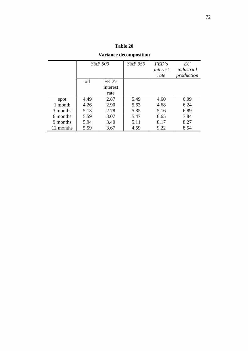
72
Table 20
Variance decomposition
S&P 500 S&P 350 FED’s interest
rate
EU industrial production
oil FED’s interest
rate
spot 4.49 2.87 5.49 4.60 6.09 1 month 4.26 2.90 5.63 4.68 6.24 3 months 5.13 2.78 5.85 5.16 6.89 6 months 5.59 3.07 5.47 6.65 7.84 9 months 5.94 3.40 5.11 8.17 8.27 12 months 5.59 3.67 4.59 9.22 8.54
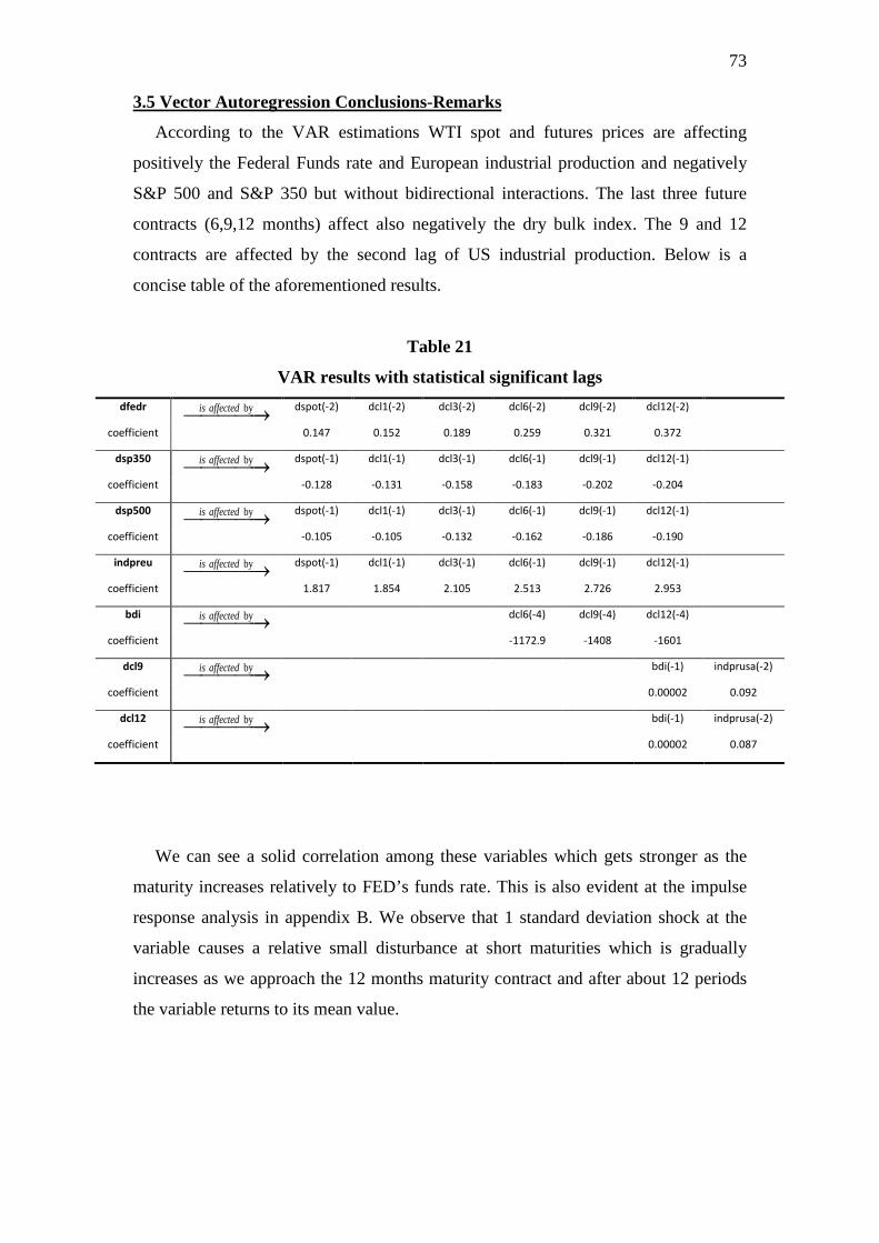
73 3.5 Vector Autoregression Conclusions-Remarks
According to the VAR estimations WTI spot and futures prices are affecting
positively the Federal Funds rate and European industrial production and negatively
S&P 500 and S&P 350 but without bidirectional interactions. The last three future
contracts (6,9,12 months) affect also negatively the dry bulk index. The 9 and 12
contracts are affected by the second lag of US industrial production. Below is a
concise table of the aforementioned results.
Table 21
VAR results with statistical significant lags dfedr byis affected→
dspot(-2) dcl1(-2) dcl3(-2) dcl6(-2) dcl9(-2) dcl12(-2)
coefficient 0.147 0.152 0.189 0.259 0.321 0.372
dsp350 byis affected→ dspot(-1) dcl1(-1) dcl3(-1) dcl6(-1) dcl9(-1) dcl12(-1)
coefficient -0.128 -0.131 -0.158 -0.183 -0.202 -0.204
dsp500 byis affected→ dspot(-1) dcl1(-1) dcl3(-1) dcl6(-1) dcl9(-1) dcl12(-1)
coefficient -0.105 -0.105 -0.132 -0.162 -0.186 -0.190
indpreu byis affected→ dspot(-1) dcl1(-1) dcl3(-1) dcl6(-1) dcl9(-1) dcl12(-1)
coefficient 1.817 1.854 2.105 2.513 2.726 2.953
bdi byis affected→ dcl6(-4) dcl9(-4) dcl12(-4)
coefficient -1172.9 -1408 -1601
dcl9 byis affected→ bdi(-1) indprusa(-2)
coefficient 0.00002 0.092
dcl12 byis affected→ bdi(-1) indprusa(-2)
coefficient 0.00002 0.087
We can see a solid correlation among these variables which gets stronger as the
maturity increases relatively to FED’s funds rate. This is also evident at the impulse
response analysis in appendix B. We observe that 1 standard deviation shock at the
variable causes a relative small disturbance at short maturities which is gradually
increases as we approach the 12 months maturity contract and after about 12 periods
the variable returns to its mean value.
74 Regarding FED’s funds rate and European industrial production the positive
correlation denotes that in upward or downward economic cycles these move in
tandem with oil prices. In an anodic cycle world economy consumes more and more
oil and the higher oil prices seem to precede EU industrial production by one month
which is not according to our expectations. We would expect a decline in EU
industrial production due to higher input costs. Maybe this is a result of late
responsiveness of EU industrial production to oil prices but there is no proof for this.
On the other hand FED rises interest rates in order to cool down the overheating
economy and avoid bubbles and these result is in full accordance to the results of Park
and Ratti (2007) and Sadorsky (1999), not only relatively to the positive sign of
correlation but also relatively to the lags.
In accordance to our expectations and relative literature the negative coefficients of
S&P 500 and S&P 350 can be attributed to the negative effects that rising oil prices
have in the production procedure due to higher production input costs and generally
GDP. We have already referred to some studies that examine the exact decrease in
GDP which caused by a rise in oil prices. Our VAR results for these two indices are
also coincide to those of Park and Ratti (2007) regarding the sign of the relation and
the lags.
The negative coefficient of the effect of oil price to dry bulk index was more or
less expected because as it has been said rising oil prices cause decline in world GDP
and that is transformed into lower demand for cargo transfers and accordingly
freights. Dry bulk index is affected only by 6, 9 and 12 months maturity futures
contracts and this suggests, that the relationship between them incorporates
expectations about future oil prices. The expectations about the opposite direction are
confirmed and we conclude that a rise in dry bulk index precedes a rise in 9 and 12
months maturity oil contracts with one month lag.
From the aspect of the impact of macroeconomic factors to oil variables we
observe that the second lag of US industrial production precedes rising prices in
future contracts of 9 and 12 months maturity. This at first glance can be attributed to
75 increased oil consumption and demand from industrial companies but maybe it is also
a result of hedging in order to anticipate higher oil price in the future.
Relatively to Hang Seng, we find no evidence of interaction with oil variables.
Maybe this is a result of inefficiencies in the Chinese stock market due to Government
interference which causes non-responsiveness. One field of interference might be the
exchange rate policy which doesn’t allow Yuan to revaluate relatively to the dollar.
So without revaluation the capacity of Chinese economy to import more oil is
confined. The lack of interaction between the Chinese stock market and oil price
changes is in agreement with the study of Cong, Wei, Jiao and Fan (2008).
Nikkei also shows unresponsiveness to change in oil prices and maybe this can be
attributed to the stagnancy of the Japanese economy from the ‘90s and onwards. In
econometric analysis it is very rare to find a stock exchange index to be stationary but
this is the case for Nikkei. So an index that doesn’t present high movability for almost
two decades maybe is less responsive to oil price changes.
Another finding that we came across in this thesis and was unexpected, is that the
explicative power of WTI oil futures, at least relatively to the certain macroeconomic
variables, is increasing as the maturity of contracts increasing. We observe from table
18 that the statistical significant coefficients between the variables are increasing
following maturity. There are explicit graphic depictions of this finding in appendix
C. A possible explanation is that greater maturities of WTI futures are better
predictors of macroeconomic variables than earlier maturities but this is something
that needs further investigation.
76 References O. Blanchard-J. Gali (2007). The macroeconomic effects of oil price shocks: why are
2000s so different from the 1970?
Jianjun Cui (2007). Analysis on the oil price mechanism and its fluctuation.
Demirer Riza-Kutan Ali (2010). The behavior of crude oil spot and futures prices
around OPEC and SPR announcements: An event study perspective.
Bahram Adranzi, Arjun Chatrath, Kanwalroop Kathy Dhanda, Kambiz Raffiee
(2001). Chaos in oil prices? Evidence from futures markets, energy economics
23(2001) 405-425.
Mikael Hook, Robert Hirsch, Kjell Aleklett (2008). Giant oil field decline rates and
their influence in world oil production.
Ferdinand E. Banks (1991). ‘Paper’ oil, ‘real’ oil and the price of oil, energy policy
July/August 1991.
International Energy Agency, May 2004. Analysis of the impact of high oil prices on
the global economy.
Nick A. Owen, Oliver R. Inderwildi, David A. King (2010). The status of
conventional oil reserves-Hype or cause for concern, energy policy 38 (2010) 4743-
4729.
Kjell Aleklett, Mikael Hook, Kristofer Jakobsson, Michael Lardelli, Simon Snowden,
Bengt Soderbergh (2009). The peak oil age-Analyzing the world oil production
reference scenario in world energy outlook 2008, energy policy 38 (2010) 1398-1414.
Sharon Xiaowen Lin, Michael N. Tamvakis (2001). Spillover effects in energy futures
markets, energy economics 23 (2001) 43-56.
77 Sveltlana Maslyuk, Russel Smyth (2007). Unit root properties of crude oil spot and
futures prices, energy policy 36 (2008) 2591-2600.
Kevin L. Kliesen (2008). Oil & US macroeconomy: An update and a simple
forecasting exercise, Federal Reserve Bank of St. Louis review September/October
2008 pp. 505-516.
J. Isaac Miller, Ronald S. Ratti (2008). Crude oil and stock markets: Stability,
instability and bubbles, energy economics 36 (2009) 559-568.
George Filis (2009). Macroeconomy, stock market and oil prices: Do meaningful
relationships exist among their cyclical fluctuations? Energy economics 32 (2010)
877-886.
William E. Shambora, Rosemary Rossiter (2007). Are there exploitable inefficiencies
in the futures market for oil? Energy economics 29 (2007) 18-27.
Thalia Chanziara, George Skiadopoulos (2006). Can the dynamics of the term
structure of petroleum futures be forecasted? Evidence from major markets.
Sveltlana Maslyuk, Russell Smyth (2008). Cointegration between oil spot and futures
prices of the same and different grades in the presence of structural change, energy
policy 37 (2009) 1687-1693.
S. Gurcan Gulen (1998). Efficiency in the crude oil futures market.
Alessandro Lanza, Matteo Manera, Michael Mc Aleer (2006). Modeling dynamic
conditional correlations in WTI oil forward and futures returns, finance research
letters 3 (2006) 114-132.
Robert Kaufmann, Ben Ullman (2008). Oil prices, speculation and fundamentals:
Interpreting causal relations among spot and futures prices, energy economics 31
(2009) 550-558.
78
Salah Abosedra, Hamid Baghestani (2004). On the predictive accuracy of crude oil
futures prices, energy policy 32 (2004) 1389-1393.
Stelios Bekiros, Cees Diks (2007). The relationship between crude oil spot and futures
prices: Cointegration, linear and nonlinear causality, energy economics 30 (2008)
2673-2685.
Gonzalo Cortazar, Eduardo Schwartz (2002). Implementing a stochastic model for oil
futures prices.
Ron Alquist, Lutz Kilian (2008). What do we learn from the price of crude oil
futures?
Cetin Ciner (2001). Information content of volume: An investigation of Tokyo
commodity futures markets, Pacific-basin finance journal 10 (2002) 201-215.
Ronald Ripple, Imad Moosa (2007). The effect of maturity, trading volume and open
interest on crude oil futures price range-based volatility.
Perry Sadorsky (2000). The empirical relationship between energy futures prices and
exchange rates, energy economics 22 (2000) 253-266.
Cong R.G., Wei Y.M., Jiao J.L., Fan Y. (2008). Relationships between oil price
shocks and stock market. An empirical analysis from China, energy policy 36 (2008)
3544-3553.
Gogineni S. (2010). Oil and stock market: An industry level analysis.
Park J., Ratti R. (2007). Oil price shocks and stock markets in the US and 13
European countries.
79 Samuel Imarhiagbe (2010). Impact of oil prices on stock markets: Empirical evidence
from selected major oil producing and consuming countries, global journal of finance
and banking issues Vol. 4 (2010).
Perry Sadorsky (1999). Oil price shocks and stock market activity, energy economics
21 (1999) 449-469.
Shawkat Hammoudeh, Eisa Aleisa (2002). Dynamic relationships among GCC stock
markets and NYMEX oil futures.
William E. Shambora, Rosemary Rossiter (2004). Are there exploitable inefficiencies
in the futures market for oil? Energy economics 29 (2007) 18-27.
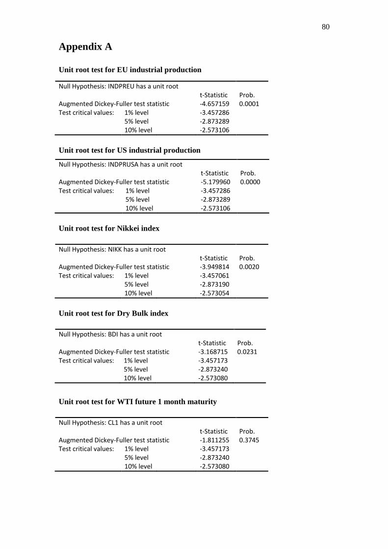
80 Appendix A Unit root test for EU industrial production Null Hypothesis: INDPREU has a unit root t-Statistic Prob. Augmented Dickey-Fuller test statistic -4.657159 0.0001 Test critical values: 1% level -3.457286 5% level -2.873289 10% level -2.573106
Unit root test for US industrial production
Null Hypothesis: INDPRUSA has a unit root t-Statistic Prob. Augmented Dickey-Fuller test statistic -5.179960 0.0000 Test critical values: 1% level -3.457286 5% level -2.873289 10% level -2.573106
Unit root test for Nikkei index Null Hypothesis: NIKK has a unit root t-Statistic Prob. Augmented Dickey-Fuller test statistic -3.949814 0.0020 Test critical values: 1% level -3.457061 5% level -2.873190 10% level -2.573054
Unit root test for Dry Bulk index Null Hypothesis: BDI has a unit root t-Statistic Prob. Augmented Dickey-Fuller test statistic -3.168715 0.0231 Test critical values: 1% level -3.457173 5% level -2.873240 10% level -2.573080
Unit root test for WTI future 1 month maturity Null Hypothesis: CL1 has a unit root t-Statistic Prob. Augmented Dickey-Fuller test statistic -1.811255 0.3745 Test critical values: 1% level -3.457173 5% level -2.873240 10% level -2.573080
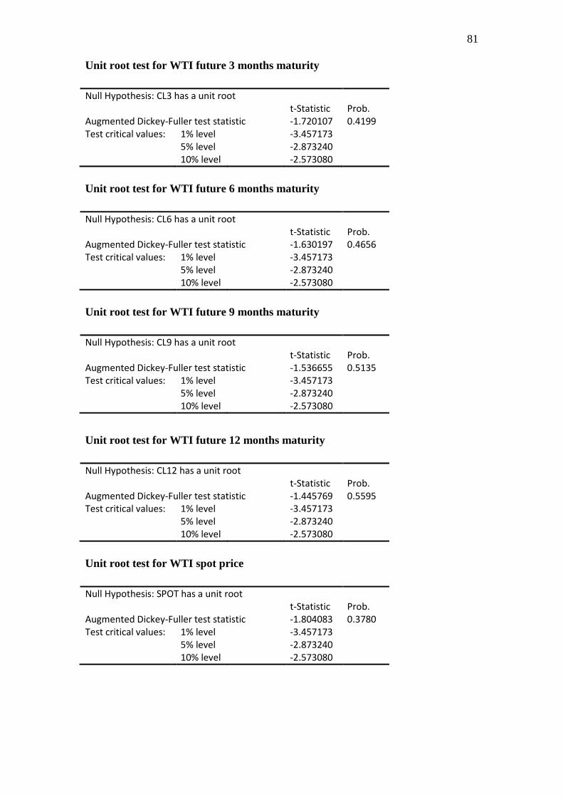
81 Unit root test for WTI future 3 months maturity Null Hypothesis: CL3 has a unit root t-Statistic Prob. Augmented Dickey-Fuller test statistic -1.720107 0.4199 Test critical values: 1% level -3.457173 5% level -2.873240 10% level -2.573080
Unit root test for WTI future 6 months maturity Null Hypothesis: CL6 has a unit root t-Statistic Prob. Augmented Dickey-Fuller test statistic -1.630197 0.4656 Test critical values: 1% level -3.457173 5% level -2.873240 10% level -2.573080
Unit root test for WTI future 9 months maturity
Null Hypothesis: CL9 has a unit root t-Statistic Prob. Augmented Dickey-Fuller test statistic -1.536655 0.5135 Test critical values: 1% level -3.457173 5% level -2.873240 10% level -2.573080
Unit root test for WTI future 12 months maturity Null Hypothesis: CL12 has a unit root t-Statistic Prob. Augmented Dickey-Fuller test statistic -1.445769 0.5595 Test critical values: 1% level -3.457173 5% level -2.873240 10% level -2.573080
Unit root test for WTI spot price Null Hypothesis: SPOT has a unit root t-Statistic Prob. Augmented Dickey-Fuller test statistic -1.804083 0.3780 Test critical values: 1% level -3.457173 5% level -2.873240 10% level -2.573080
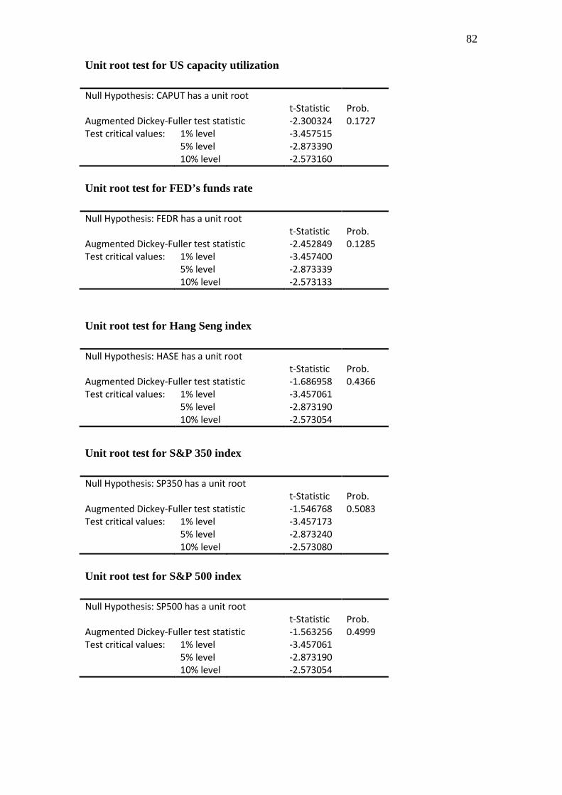
82 Unit root test for US capacity utilization Null Hypothesis: CAPUT has a unit root t-Statistic Prob. Augmented Dickey-Fuller test statistic -2.300324 0.1727 Test critical values: 1% level -3.457515 5% level -2.873390 10% level -2.573160
Unit root test for FED’s funds rate Null Hypothesis: FEDR has a unit root t-Statistic Prob. Augmented Dickey-Fuller test statistic -2.452849 0.1285 Test critical values: 1% level -3.457400 5% level -2.873339 10% level -2.573133
Unit root test for Hang Seng index Null Hypothesis: HASE has a unit root t-Statistic Prob. Augmented Dickey-Fuller test statistic -1.686958 0.4366 Test critical values: 1% level -3.457061 5% level -2.873190 10% level -2.573054
Unit root test for S&P 350 index Null Hypothesis: SP350 has a unit root t-Statistic Prob. Augmented Dickey-Fuller test statistic -1.546768 0.5083 Test critical values: 1% level -3.457173 5% level -2.873240 10% level -2.573080
Unit root test for S&P 500 index Null Hypothesis: SP500 has a unit root t-Statistic Prob. Augmented Dickey-Fuller test statistic -1.563256 0.4999 Test critical values: 1% level -3.457061 5% level -2.873190 10% level -2.573054
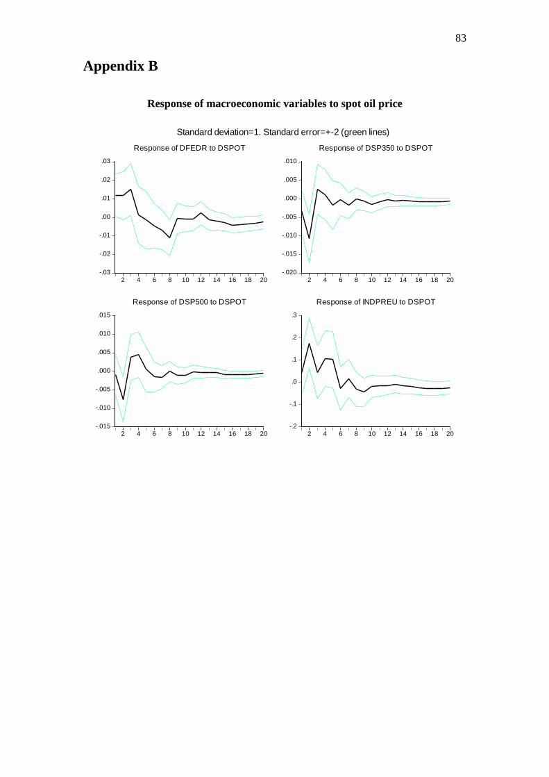
83 Appendix B
Response of macroeconomic variables to spot oil price
-.03
-.02
-.01
.00
.01
.02
.03
2 4 6 8 10 12 14 16 18 20
Response of DFEDR to DSPOT
-.020
-.015
-.010
-.005
.000
.005
.010
2 4 6 8 10 12 14 16 18 20
Response of DSP350 to DSPOT
-.015
-.010
-.005
.000
.005
.010
.015
2 4 6 8 10 12 14 16 18 20
Response of DSP500 to DSPOT
-.2
-.1
.0
.1
.2
.3
2 4 6 8 10 12 14 16 18 20
Response of INDPREU to DSPOT
Standard deviation=1. Standard error=+-2 (green lines)
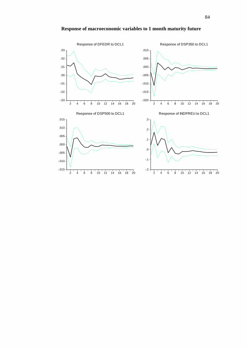
84
Response of macroeconomic variables to 1 month maturity future
-.03
-.02
-.01
.00
.01
.02
.03
2 4 6 8 10 12 14 16 18 20
Response of DFEDR to DCL1
-.020
-.015
-.010
-.005
.000
.005
.010
2 4 6 8 10 12 14 16 18 20
Response of DSP350 to DCL1
-.015
-.010
-.005
.000
.005
.010
.015
2 4 6 8 10 12 14 16 18 20
Response of DSP500 to DCL1
-.2
-.1
.0
.1
.2
.3
2 4 6 8 10 12 14 16 18 20
Response of INDPREU to DCL1
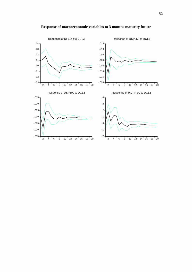
85
Response of macroeconomic variables to 3 months maturity future
-.03
-.02
-.01
.00
.01
.02
.03
.04
2 4 6 8 10 12 14 16 18 20
Response of DFEDR to DCL3
-.020
-.015
-.010
-.005
.000
.005
.010
.015
2 4 6 8 10 12 14 16 18 20
Response of DSP350 to DCL3
-.015
-.010
-.005
.000
.005
.010
.015
2 4 6 8 10 12 14 16 18 20
Response of DSP500 to DCL3
-.2
-.1
.0
.1
.2
.3
.4
2 4 6 8 10 12 14 16 18 20
Response of INDPREU to DCL3
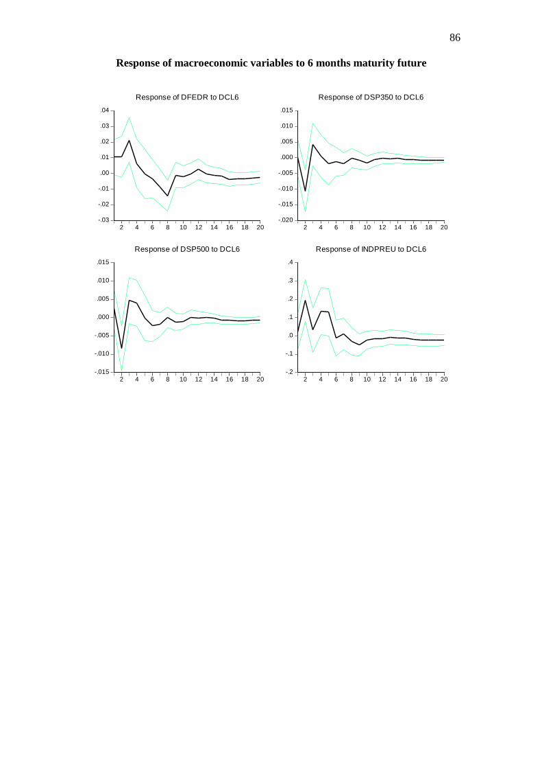
86
Response of macroeconomic variables to 6 months maturity future
-.03
-.02
-.01
.00
.01
.02
.03
.04
2 4 6 8 10 12 14 16 18 20
Response of DFEDR to DCL6
-.020
-.015
-.010
-.005
.000
.005
.010
.015
2 4 6 8 10 12 14 16 18 20
Response of DSP350 to DCL6
-.015
-.010
-.005
.000
.005
.010
.015
2 4 6 8 10 12 14 16 18 20
Response of DSP500 to DCL6
-.2
-.1
.0
.1
.2
.3
.4
2 4 6 8 10 12 14 16 18 20
Response of INDPREU to DCL6
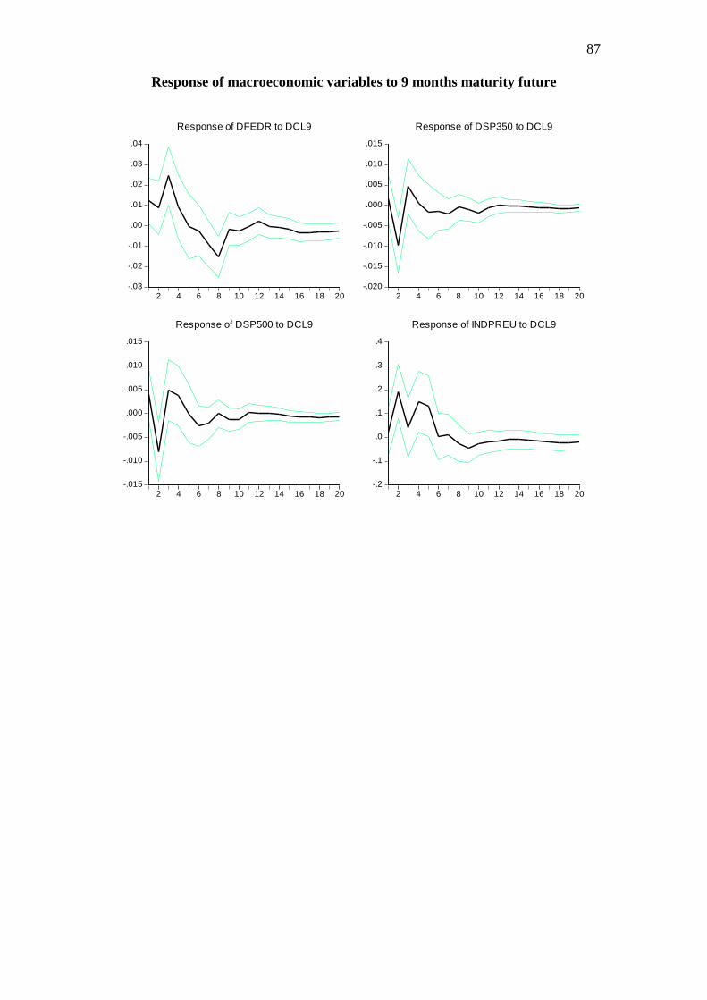
87
Response of macroeconomic variables to 9 months maturity future
-.03
-.02
-.01
.00
.01
.02
.03
.04
2 4 6 8 10 12 14 16 18 20
Response of DFEDR to DCL9
-.020
-.015
-.010
-.005
.000
.005
.010
.015
2 4 6 8 10 12 14 16 18 20
Response of DSP350 to DCL9
-.015
-.010
-.005
.000
.005
.010
.015
2 4 6 8 10 12 14 16 18 20
Response of DSP500 to DCL9
-.2
-.1
.0
.1
.2
.3
.4
2 4 6 8 10 12 14 16 18 20
Response of INDPREU to DCL9
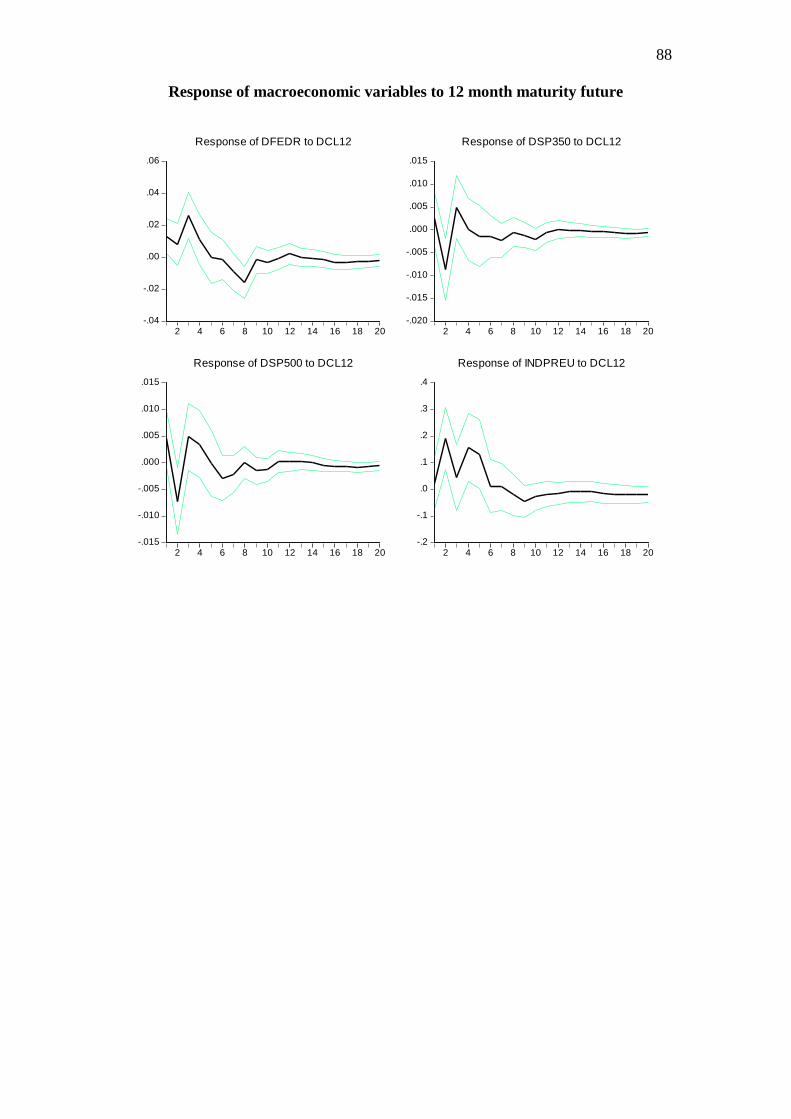
88
Response of macroeconomic variables to 12 month maturity future
-.04
-.02
.00
.02
.04
.06
2 4 6 8 10 12 14 16 18 20
Response of DFEDR to DCL12
-.020
-.015
-.010
-.005
.000
.005
.010
.015
2 4 6 8 10 12 14 16 18 20
Response of DSP350 to DCL12
-.015
-.010
-.005
.000
.005
.010
.015
2 4 6 8 10 12 14 16 18 20
Response of DSP500 to DCL12
-.2
-.1
.0
.1
.2
.3
.4
2 4 6 8 10 12 14 16 18 20
Response of INDPREU to DCL12
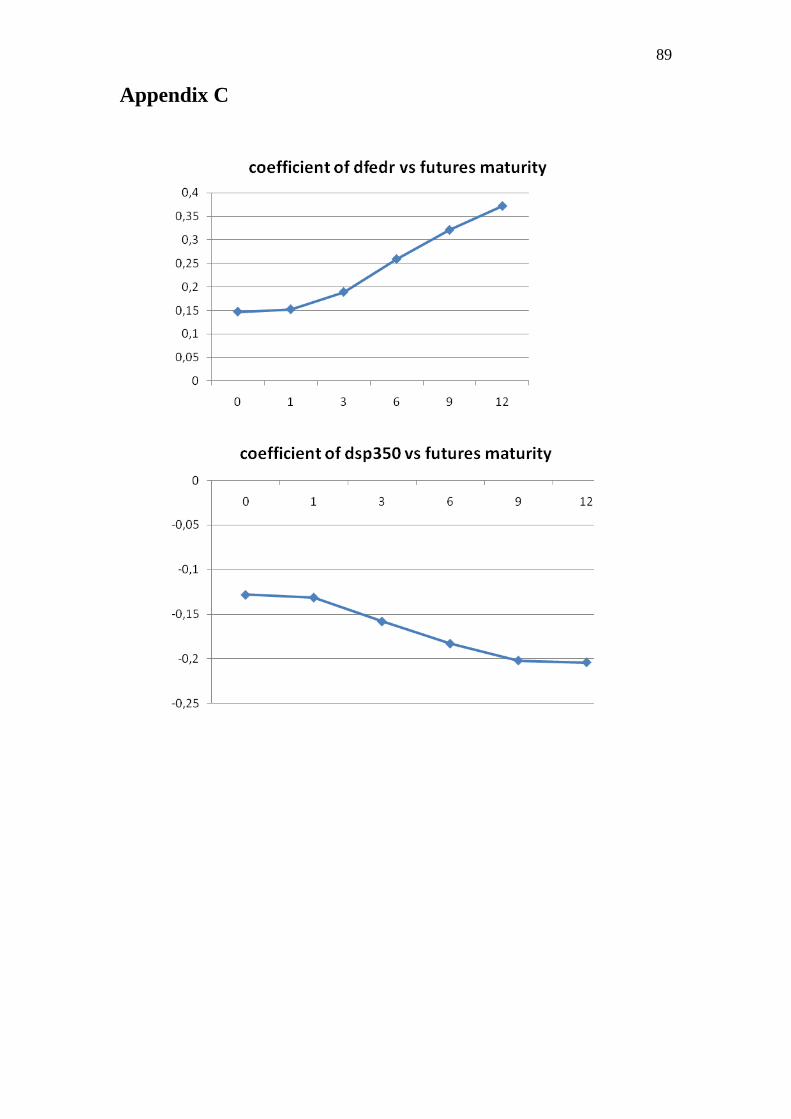
89 Appendix C
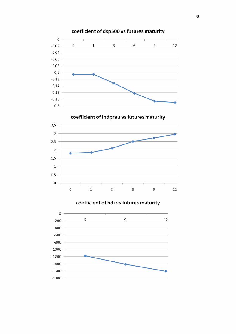
90

91


