CHAPTER 3 - UW Canvas

BLBS113-c03 BLBS113-Brooks Trim: 244mm×172mm August 25, 2012 13:15

CHAPTER 3 Precipitation

INTRODUCTIONPrecipitation affects the amount, timing, spatial distribution, and quality of water added toa watershed from the atmosphere. Hydrologists view precipitation as the major input to awatershed and a key to its water-yielding characteristics. Ecologists recognize the role ofprecipitation in determining the types of soils and vegetation that occur on a watershed.Farmers, foresters, and rangeland managers view precipitation as an essential ingredient tovegetative production on the land. The annual amount of precipitation and the high and lowextremes of precipitation affect people and their use of land and water. The uncertainty offloods and droughts becomes apparent when we examine climatic variability of the past.Climatic change and variability add to this uncertainty. Most people have only a cursoryunderstanding of the variability of precipitation, why precipitation occurs, and why it occurswhere it does. Consequently an understanding of precipitation is fundamental to the studyof hydrology and integrated watershed management.

In this chapter we discuss the measurement of precipitation and analysis of data that areimportant to the day-to-day activities of people and for the planning of future developmentand management of land and water resources. Rainfall affects more people globally thansnow; however, information about snowfall, snow accumulation, and melt is needed onwatersheds that are located in higher latitudes and at high elevations of mountainousregions. The process of precipitation, its occurrence in time and space, and the methods ofmeasuring and analyzing rainfall and snowmelt inputs to watersheds are discussed in thischapter.

Hydrology and the Management of Watersheds, Fourth Edition. Kenneth N. Brooks, Peter F. Ffolliott and Joseph A. Magner.C© 2013 John Wiley & Sons, Inc. Published 2013 by John Wiley & Sons, Inc.

49


50 Part 1 Watersheds, Hydrologic Processes, and Pathways

PRECIPITATION PROCESSPrecipitation is the result of meteorological factors and is, therefore, largely outside humancontrol. Air masses take on the temperature and moisture characteristics of underlyingsurfaces, particularly when they are stationary or move slowly over large water or landsurfaces. Air masses moving from an ocean to land bring to that land surface a source ofmoisture. Air masses from polar regions will be dry and cold. Air masses from the humidtropics are warm and moist. The pathways of jet streams in the upper atmosphere govern themovement of air masses and thus affect the amount and distribution of precipitation. Move-ment of air masses modifies the temperature and moisture characteristics of the atmosphereover a watershed and determines the climatic and, more specifically, the precipitationconditions that occur. Precipitation occurs in many forms (see Box 3.1) but most commonlyoccurs as either rain or snow, depending on air temperature. The relationship betweenatmospheric moisture and temperature must be understood to understand the precipitationprocess.

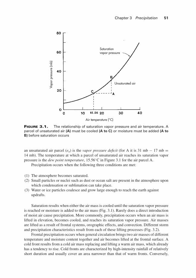
The relationships among moisture content in the atmosphere, temperature, and vaporpressure determine the occurrence and amounts of evaporation and precipitation (Fig. 3.1).A parcel of unsaturated air (point A in Fig. 3.1) can become saturated by either cooling(A to C) or the addition of moisture to the air mass (A to B). Unsaturated air can becharacterized by its relative humidity – the ratio of vapor pressure of the air to saturationvapor pressure at a specified temperature, which is expressed as a percentage. For example,at 25◦C in Figure 3.1, the relative humidity of air parcel A is 100(17 mb/31 mb) = 55%.The difference between the saturation vapor pressure (es) and the actual vapor pressure of

Box 3.1

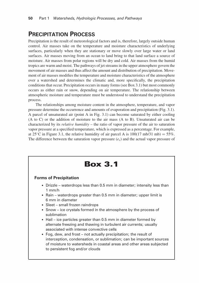
Forms of Precipitation� Drizzle – waterdrops less than 0.5 mm in diameter; intensity less than

1 mm/h� Rain – waterdrops greater than 0.5 mm in diameter; upper limit is

6 mm in diameter� Sleet – small frozen raindrops� Snow – ice crystals formed in the atmosphere by the process of

sublimation� Hail – ice particles greater than 0.5 mm in diameter formed by

alternate freezing and thawing in turbulent air currents; usuallyassociated with intense convective cells

� Fog, dew, and frost – not actually precipitation; the result ofinterception, condensation, or sublimation; can be important sourcesof moisture to watersheds in coastal areas and other areas subjectedto persistent fog and/or clouds


Chapter 3 Precipitation 51

Vapo

r pr

essu

re (m

b)

Air temperature (°C)

Unsaturated air

Saturationvapor pressure

FIGURE 3.1. The relationship of saturation vapor pressure and air temperature. Aparcel of unsaturated air (A) must be cooled (A to C) or moisture must be added (A toB) before saturation occurs

an unsaturated air parcel (ea) is the vapor pressure deficit (for A it is 31 mb − 17 mb =14 mb). The temperature at which a parcel of unsaturated air reaches its saturation vaporpressure is the dew point temperature, 15.56◦C in Figure 3.1 for the air parcel A.

Precipitation occurs when the following three conditions are met:

(1) The atmosphere becomes saturated.(2) Small particles or nuclei such as dust or ocean salt are present in the atmosphere upon

which condensation or sublimation can take place.(3) Water or ice particles coalesce and grow large enough to reach the earth against

updrafts.

Saturation results when either the air mass is cooled until the saturation vapor pressureis reached or moisture is added to the air mass (Fig. 3.1). Rarely does a direct introductionof moist air cause precipitation. More commonly, precipitation occurs when an air mass islifted in elevation, becomes cooled, and reaches its saturation vapor pressure. Air massesare lifted as a result of frontal systems, orographic effects, and convection. Different stormand precipitation characteristics result from each of these lifting processes (Fig. 3.2).

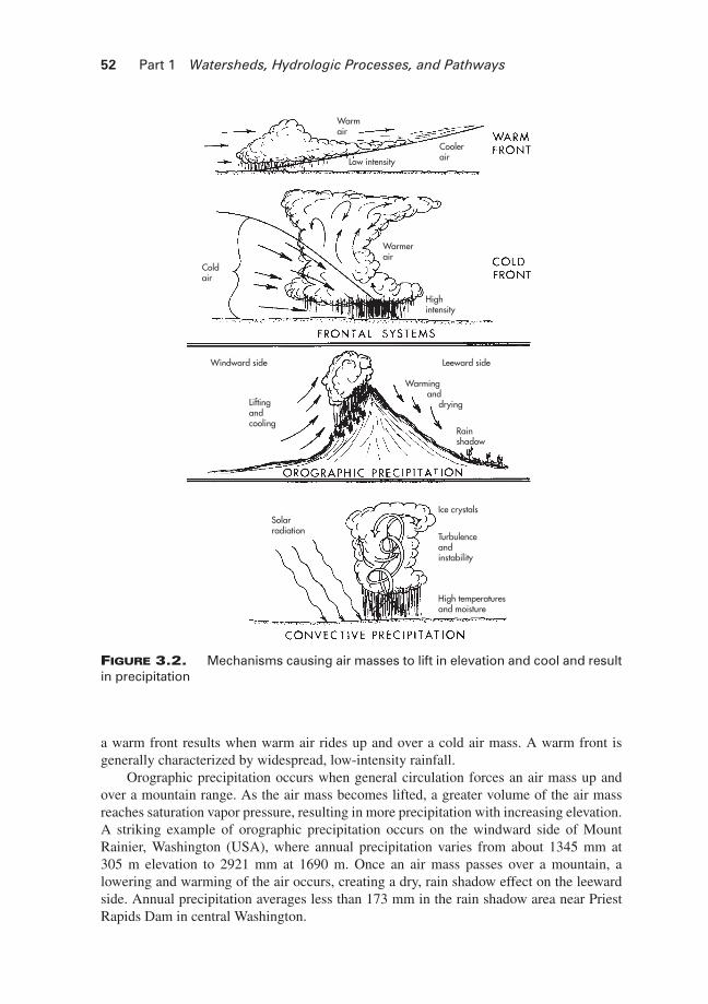
Frontal precipitation occurs when general circulation brings two air masses of differenttemperature and moisture content together and air becomes lifted at the frontal surface. Acold front results from a cold air mass replacing and lifting a warm air mass, which alreadyhas a tendency to rise. Cold fronts are characterized by high-intensity rainfall of relativelyshort duration and usually cover an area narrower than that of warm fronts. Conversely,



Warmair

Low intensity

Coolerair

Warmerair

Highintensity

Leeward sideWindward side

Rainshadow

Liftingandcooling

Solarradiation

Ice crystals

Turbulenceandinstability

High temperaturesand moisture

Warming and drying

Coldair

FIGURE 3.2. Mechanisms causing air masses to lift in elevation and cool and resultin precipitation

a warm front results when warm air rides up and over a cold air mass. A warm front isgenerally characterized by widespread, low-intensity rainfall.

Orographic precipitation occurs when general circulation forces an air mass up andover a mountain range. As the air mass becomes lifted, a greater volume of the air massreaches saturation vapor pressure, resulting in more precipitation with increasing elevation.A striking example of orographic precipitation occurs on the windward side of MountRainier, Washington (USA), where annual precipitation varies from about 1345 mm at305 m elevation to 2921 mm at 1690 m. Once an air mass passes over a mountain, alowering and warming of the air occurs, creating a dry, rain shadow effect on the leewardside. Annual precipitation averages less than 173 mm in the rain shadow area near PriestRapids Dam in central Washington.



Convective precipitation, characterized by summer thunderstorms, is the result ofexcessive heating of the earth’s surface. When the moist air immediately above the surfacebecomes warmer than the air mass above it, lifting occurs. As the air mass rises, it cools andcondensation takes place, releasing the latent heat of vaporization which adds more energyto the rising air mass, and, consequently, more lifting occurs. Rapidly uplifted air can reachhigh altitudes where water droplets become frozen and hail forms or becomes intermixedwith rainfall. Such rainstorms or hailstorms are some of the most severe precipitationevents anywhere and are characterized by high-intensity, short-duration rainfall overrelatively limited areas. Flash flooding can result when thunderstorms occur over a largeenough area.

RAINFALLRainfall is a meteorological event throughout most of the world. It is the primary input inthe hydrologic cycle of many watersheds and larger river basins. While rainfall is often akey source of water to people, excessive rainfall amounts can lead to downstream flooding.It is necessary, therefore, that hydrologists and watershed managers know how to measurerainfall and analyze the measurements that are obtained.

Methods of Rainfall MeasurementMeasurements of rainfall are needed for many hydrologic applications that are discussedin this book. Weather forecasting and flood forecasting require estimates of rainfall occur-ring in “real time,” meaning as it falls to the earth’s surface, or shortly thereafter. Radarprovides qualitative estimates of rainfall amounts and intensities over large areas duringa storm, provided that radar coverage is sufficient. Radar senses the backscatter of radiowaves caused by water droplets and ice crystals in the atmosphere. The area of cover-age and relative intensity rainfall can be estimated up to a distance of 250 km. Radarechoes can often be correlated with measured rainfall, but this calibration is hampered byground barriers, raindrop size, distribution of rainfall, and other storm factors resultingin large errors (Sauvageot, 1994). An evaluation of errors associated with the WRS-88DPrecipitation Processing Subsystem (PPS) of the National Weather Service (USA) in-dicates that there are potential remedies to overcome the major errors associated withradar (http://www.srh.noaa.gov/mrx/research/precip/precip.php). Readers are encouragedto search the National Weather Service website for applications of radar to estimate rainfall(see www.nws.noaa.gov/).

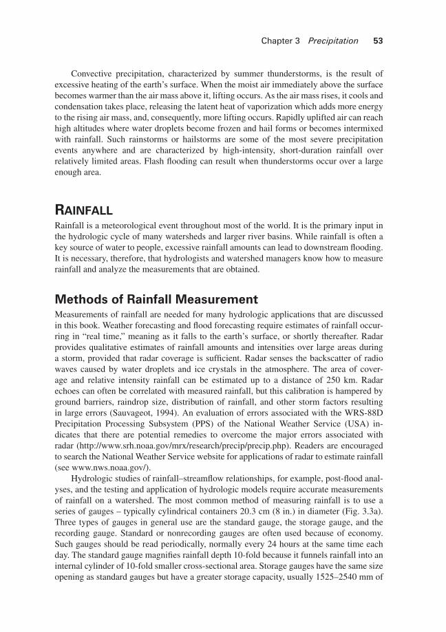
Hydrologic studies of rainfall–streamflow relationships, for example, post-flood anal-yses, and the testing and application of hydrologic models require accurate measurementsof rainfall on a watershed. The most common method of measuring rainfall is to use aseries of gauges – typically cylindrical containers 20.3 cm (8 in.) in diameter (Fig. 3.3a).Three types of gauges in general use are the standard gauge, the storage gauge, and therecording gauge. Standard or nonrecording gauges are often used because of economy.Such gauges should be read periodically, normally every 24 hours at the same time eachday. The standard gauge magnifies rainfall depth 10-fold because it funnels rainfall into aninternal cylinder of 10-fold smaller cross-sectional area. Storage gauges have the same sizeopening as standard gauges but have a greater storage capacity, usually 1525–2540 mm of



FIGURE 3.3. Types of rain gauges. (a) Cutaway of the standard (Weather Service)gauge. (b) A weighing-type recording gauge with its cover removed to show the springhousing, recording pen, and storage bucket (from Hewlett, 1982, C© University of GeorgiaPress, with permission)

rainfall. These gauges can be read periodically, for example, once a week, once a month,or seasonally. A small amount of oil is usually added to gauges that are read less frequentlythan every 24 hours to suppress evaporation.

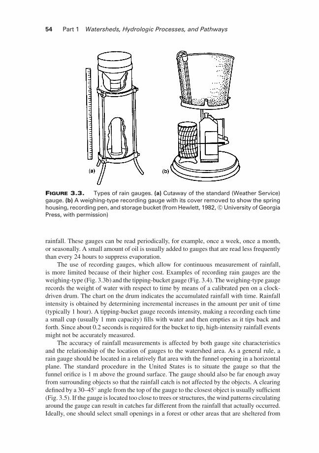
The use of recording gauges, which allow for continuous measurement of rainfall,is more limited because of their higher cost. Examples of recording rain gauges are theweighing-type (Fig. 3.3b) and the tipping-bucket gauge (Fig. 3.4). The weighing-type gaugerecords the weight of water with respect to time by means of a calibrated pen on a clock-driven drum. The chart on the drum indicates the accumulated rainfall with time. Rainfallintensity is obtained by determining incremental increases in the amount per unit of time(typically 1 hour). A tipping-bucket gauge records intensity, making a recording each timea small cup (usually 1 mm capacity) fills with water and then empties as it tips back andforth. Since about 0.2 seconds is required for the bucket to tip, high-intensity rainfall eventsmight not be accurately measured.

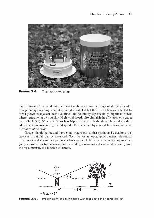
The accuracy of rainfall measurements is affected by both gauge site characteristicsand the relationship of the location of gauges to the watershed area. As a general rule, arain gauge should be located in a relatively flat area with the funnel opening in a horizontalplane. The standard procedure in the United States is to situate the gauge so that thefunnel orifice is 1 m above the ground surface. The gauge should also be far enough awayfrom surrounding objects so that the rainfall catch is not affected by the objects. A clearingdefined by a 30–45◦ angle from the top of the gauge to the closest object is usually sufficient(Fig. 3.5). If the gauge is located too close to trees or structures, the wind patterns circulatingaround the gauge can result in catches far different from the rainfall that actually occurred.Ideally, one should select small openings in a forest or other areas that are sheltered from



FIGURE 3.4. Tipping-bucket gauge

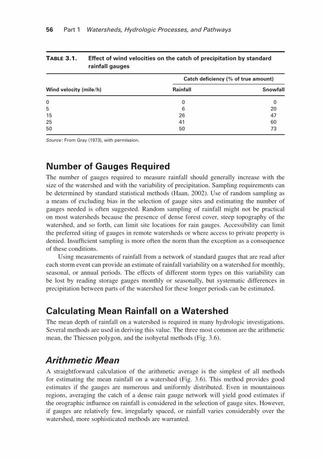
the full force of the wind but that meet the above criteria. A gauge might be located ina large enough opening when it is initially installed but then it can become affected byforest growth in adjacent areas over time. This possibility is particularly important in areaswhere vegetation grows quickly. High wind speeds also diminish the efficiency of a gaugecatch (Table 3.1). Wind shields, such as Nipher or Alter shields, should be used to reduceeddy effects in areas of high wind speeds. Errors caused by catch deficiencies are calledinstrumentation errors.

Gauges should be located throughout watersheds so that spatial and elevational dif-ferences in rainfall can be measured. Such factors as topographic barriers, elevationaldifferences, and storm-track patterns or tracking should be considered in developing a raingauge network. Practical considerations including economics and accessibility usually limitthe type, number, and location of gauges.

Viewof

gaugeαα

α

FIGURE 3.5. Proper siting of a rain gauge with respect to the nearest object



TABLE 3.1. Effect of wind velocities on the catch of precipitation by standardrainfall gauges

Catch deficiency (% of true amount)

Wind velocity (mile/h) Rainfall Snowfall

0 0 05 6 2015 26 4725 41 6050 50 73

Source: From Gray (1973), with permission.

Number of Gauges RequiredThe number of gauges required to measure rainfall should generally increase with thesize of the watershed and with the variability of precipitation. Sampling requirements canbe determined by standard statistical methods (Haan, 2002). Use of random sampling asa means of excluding bias in the selection of gauge sites and estimating the number ofgauges needed is often suggested. Random sampling of rainfall might not be practicalon most watersheds because the presence of dense forest cover, steep topography of thewatershed, and so forth, can limit site locations for rain gauges. Accessibility can limitthe preferred siting of gauges in remote watersheds or where access to private property isdenied. Insufficient sampling is more often the norm than the exception as a consequenceof these conditions.

Using measurements of rainfall from a network of standard gauges that are read aftereach storm event can provide an estimate of rainfall variability on a watershed for monthly,seasonal, or annual periods. The effects of different storm types on this variability canbe lost by reading storage gauges monthly or seasonally, but systematic differences inprecipitation between parts of the watershed for these longer periods can be estimated.

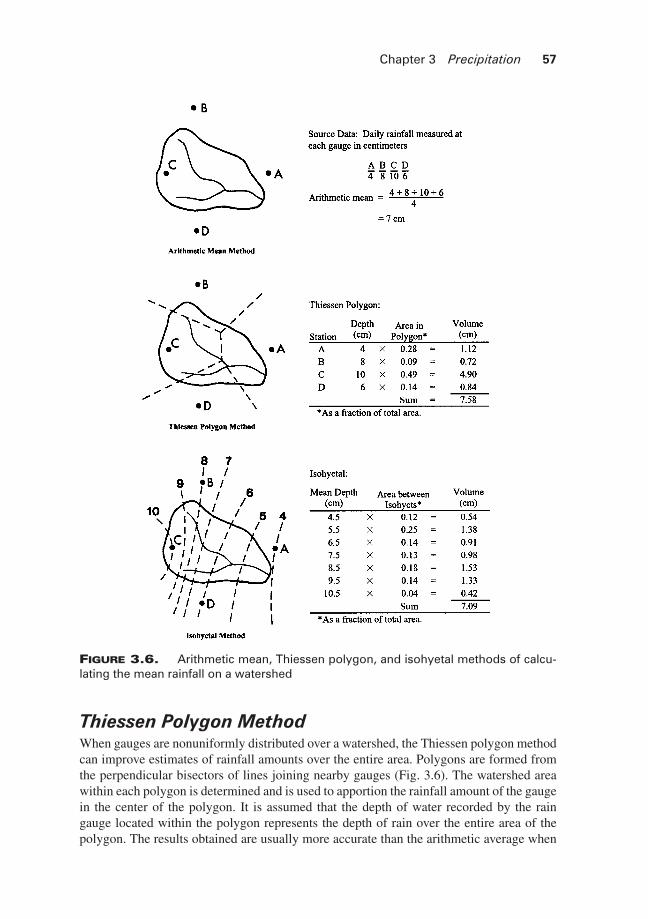
Calculating Mean Rainfall on a WatershedThe mean depth of rainfall on a watershed is required in many hydrologic investigations.Several methods are used in deriving this value. The three most common are the arithmeticmean, the Thiessen polygon, and the isohyetal methods (Fig. 3.6).

Arithmetic MeanA straightforward calculation of the arithmetic average is the simplest of all methodsfor estimating the mean rainfall on a watershed (Fig. 3.6). This method provides goodestimates if the gauges are numerous and uniformly distributed. Even in mountainousregions, averaging the catch of a dense rain gauge network will yield good estimates ifthe orographic influence on rainfall is considered in the selection of gauge sites. However,if gauges are relatively few, irregularly spaced, or rainfall varies considerably over thewatershed, more sophisticated methods are warranted.



FIGURE 3.6. Arithmetic mean, Thiessen polygon, and isohyetal methods of calcu-lating the mean rainfall on a watershed

Thiessen Polygon MethodWhen gauges are nonuniformly distributed over a watershed, the Thiessen polygon methodcan improve estimates of rainfall amounts over the entire area. Polygons are formed fromthe perpendicular bisectors of lines joining nearby gauges (Fig. 3.6). The watershed areawithin each polygon is determined and is used to apportion the rainfall amount of the gaugein the center of the polygon. It is assumed that the depth of water recorded by the raingauge located within the polygon represents the depth of rain over the entire area of thepolygon. The results obtained are usually more accurate than the arithmetic average when



the number of gauges on a watershed are limited and when one or more gauges are locatedoutside the watershed boundary.

The Thiessen method allows for nonuniform distribution of gauges but assumes linearvariation of rainfall between gauges and makes no attempt to allow for orographic influ-ences. Once the area-weighing coefficients are determined for each station, they becomefixed and the method is as simple to apply as the arithmetic method.

Isohyetal MethodWith the isohyetal method, gauge location and amounts are plotted on a suitable map,and contours of equal rainfall (isohyets) are drawn (Fig. 3.6). Rainfall measured withinand outside the watershed can be used to estimate the pattern of rainfall, and isohyets aredrawn according to gauge catches. The average depth is then determined by computing thedepth between isohyets on the watershed and dividing by the total area. Many hydrologistsbelieve that this is theoretically the most accurate method of determining mean watershedprecipitation, but it is also by far the most laborious.

The isohyetal method is particularly useful when investigating the influence of stormpatterns on streamflow and for areas where orographic rainfall occurs. In some instances,relationships between rainfall and elevation can be used advantageously, and only a fewgauges need to be set out such as at accessible elevations. Where orographic rainfall occurs,contour intervals can sometimes be used to help estimate the location of the lines of equalrainfall. Precipitation amounts are then determined for each elevation zone or band, and therespective areas are weighed to obtain estimates for the entire watershed. Rainfall–elevationrelationships would be different for watersheds on the windward side of a mountain rangethan on the leeward side of a mountain range.

The accuracy of the isohyetal method depends largely on the skill of the analyst.An improper analysis can lead to serious errors. The results obtained with the isohyetalmethod will be essentially the same as those obtained with the Thiessen method if a linearinterpolation between stations is used.

Other MethodsOther methods of calculating the mean rainfall on a watershed and examples of theirapplication can be found on the website for the National Weather Service (NWS) RiverForecast Center (http://srh.noaa.gov/abrfc/?n=map).

Errors Associated with Rainfall MeasurementHydrologic studies of watersheds are often constrained by an inadequate number of rainfallgauges, the absence of long-term precipitation records, or both. Two types of errors shouldbe considered when obtaining rainfall measurements. Instrumentation error is related tothe accuracy with which a gauge catches the true rainfall amount at a point while samplingerror is associated with how well the gauges on a watershed represent the rainfall over theentire watershed area.

Taking care in siting a gauge correctly and proper maintenance can minimize instru-mentation errors. For standard 20.3 cm (8 in.) precipitation gauges in the United States,there are biases in gauge catch from the effects of wind and from wetting of the gauge



orifice. Legates and DeLiberty (1993) reported up to 18 mm per month of systematic un-dercatch bias for winter precipitation in the northeastern and northwestern United States. A28% undercatch bias was reported for winter precipitation in the northern Rocky Mountainsand Upper Midwest. The biases can be corrected by using

Pc = kr(Pgr + dPwr

) + ks(Pgs + dPws

)(3.1)

where Pc is the gauge-corrected precipitation; Pg is the measured precipitation; k is thewind correction coefficient (usually ≥1); dPw is the correction for wetting loss (usually0.15 for rain events and half this value for snowfall); and subscripts “r” and “s” denoterainfall and snowfall, respectively. The wetting loss refers to the amount of rain or snowthat is initially stored on the interior surface of the rain gauge at the beginning of the storm.

The wind correction coefficient for rainfall (Sevruk and Hamon, 1984) is

kr = 100

100 − 2.12whp(3.2)

and for snowfall (Goodison, 1978) it is

ks = e0.1338whp (3.3)

where whp is the wind speed at the height of the gauge orifice.Properly designing a network with an adequate number of gauges, on the other hand,

minimizes sampling error. Accessibility and economic considerations usually determinethe extent to which sampling errors can be reduced.

Analysis of Rainfall MeasurementsOnce we have obtained rainfall records, a number of analyses can be performed to enhanceour knowledge of hydrology and climate. This section of the chapter describes some of themore common types of rainfall analysis.

Estimating Missing DataOne or more gauges in a rainfall network can become nonfunctioning for a period of time.One way to estimate the missing record for such a gauge is to use existing relationshipswith adjacent gauges. For example, if the rainfall for a storm is missing for station C andif rainfall at C (seasonal or annual) is correlated with that at stations A and B, the normalratio method can estimate the storm rainfall for station C:

PC = 1

2

(NC

NAPA + NC

NBPB

)(3.4)

where PC is the estimated storm rainfall for station C (mm); NA, NB, and NC are normalannual (or seasonal) rainfall for stations A, B, and C (mm), respectively; and PA and PB

are storm rainfall for stations A and B (mm), respectively.



The generalized equation for missing data is

Px = 1

n

(Nx

N1P1 + · · · + Nx

NnPn

)(3.5)

Equation 3.5 is recommended only if there is a high correlation with other stations.

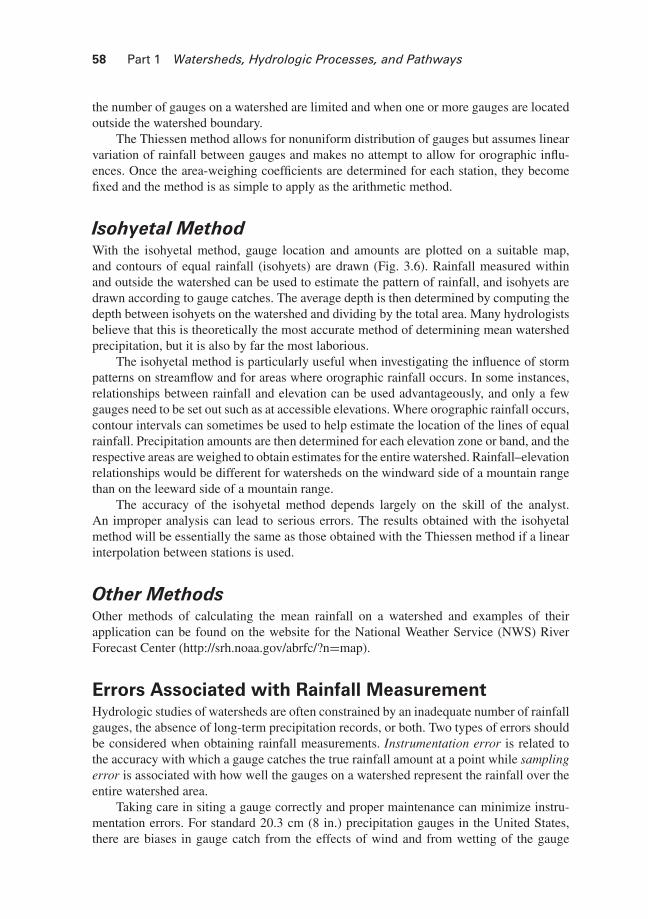
Double Mass AnalysisDouble mass analysis is a method of checking the consistency of measurements at a rainfallstation against those of one or more nearby stations. An example helps to explain theapplication of this method. Consider that station E has been collecting rainfall data for 45years. Originally, the station was located in a large opening in a conifer forest, but overthe years the surrounding forest has grown to the point where you suspect that the catchof this gauge is now affected. Based on one’s knowledge of the precipitation patterns inthe region, you recognize that the same storm patterns influence stations H and I, althoughtheir elevational differences and other factors cause annual rainfall to differ. There was aconsistent correlation between the average of stations H and I and that of E in the earlyyears of station E. By plotting the accumulated annual rainfall of E against the accumulatedaverage annual rainfall of H and I, we find that the relationship clearly changed after 1970in this example (Fig. 3.7). The relationship then can be used to correct existing rainfallcatch at E so that it better represents the true catch at the location without the interferenceof nearby trees.

Frequency AnalysisWater resource systems, such as waterways, small reservoirs, irrigation networks, anddrainage systems for roads, should be planned and designed for future precipitation events,

Accumulated rainfall,average for stations H and I (mm)

Acc

umul

ated

rain

fall

at s

tatio

n E

(mm

)

Estimated "True"rainfall

Rainfall catch

FIGURE 3.7. A double mass plot of the annual rainfall at station E relative to theaverage annual rainfall at stations H and I



Recurrence interval (years)

Probability ≥ Ordinate value

Max

imum

24

- ho

ur r

ainf

all (

mm

)

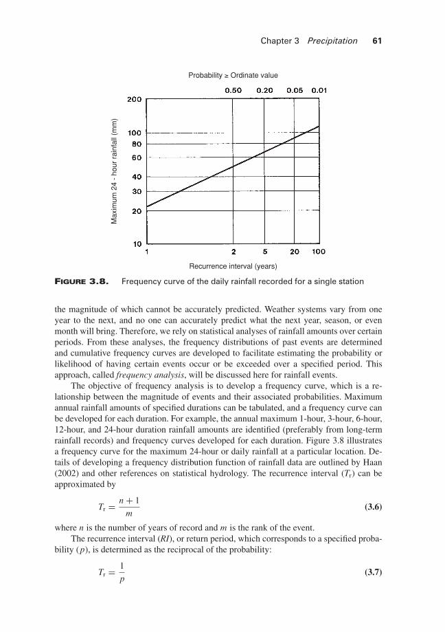
FIGURE 3.8. Frequency curve of the daily rainfall recorded for a single station

the magnitude of which cannot be accurately predicted. Weather systems vary from oneyear to the next, and no one can accurately predict what the next year, season, or evenmonth will bring. Therefore, we rely on statistical analyses of rainfall amounts over certainperiods. From these analyses, the frequency distributions of past events are determinedand cumulative frequency curves are developed to facilitate estimating the probability orlikelihood of having certain events occur or be exceeded over a specified period. Thisapproach, called frequency analysis, will be discussed here for rainfall events.

The objective of frequency analysis is to develop a frequency curve, which is a re-lationship between the magnitude of events and their associated probabilities. Maximumannual rainfall amounts of specified durations can be tabulated, and a frequency curve canbe developed for each duration. For example, the annual maximum 1-hour, 3-hour, 6-hour,12-hour, and 24-hour duration rainfall amounts are identified (preferably from long-termrainfall records) and frequency curves developed for each duration. Figure 3.8 illustratesa frequency curve for the maximum 24-hour or daily rainfall at a particular location. De-tails of developing a frequency distribution function of rainfall data are outlined by Haan(2002) and other references on statistical hydrology. The recurrence interval (Tr) can beapproximated by

Tr = n + 1

m(3.6)

where n is the number of years of record and m is the rank of the event.The recurrence interval (RI), or return period, which corresponds to a specified proba-

bility (p), is determined as the reciprocal of the probability:

Tr = 1

p(3.7)



0.1

1

10

1001010.1

Recurrence interval (years)

Rain

fall

(inch

es)

18hours6 hours

3 hours

1 hour

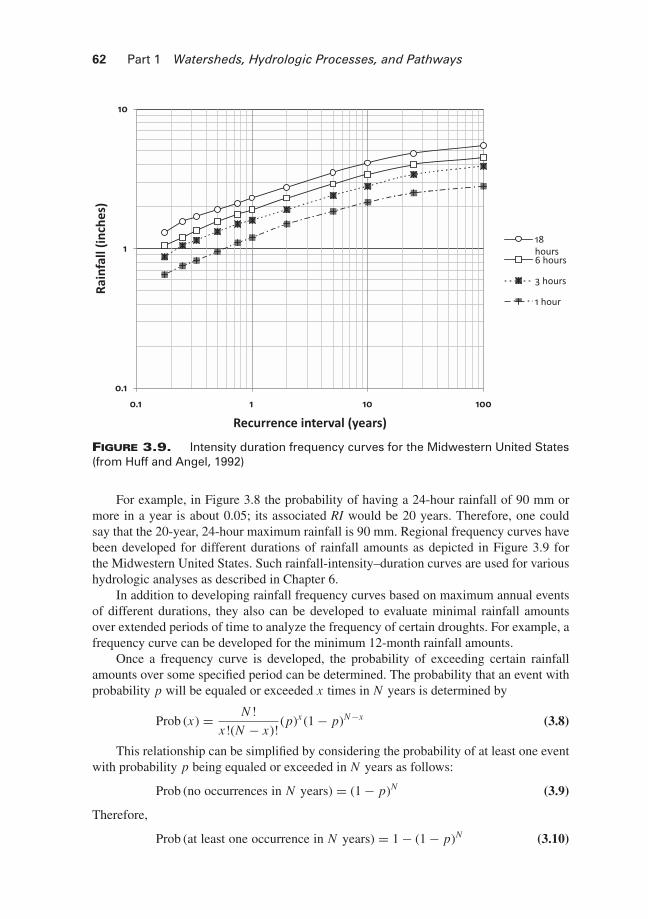
FIGURE 3.9. Intensity duration frequency curves for the Midwestern United States(from Huff and Angel, 1992)

For example, in Figure 3.8 the probability of having a 24-hour rainfall of 90 mm ormore in a year is about 0.05; its associated RI would be 20 years. Therefore, one couldsay that the 20-year, 24-hour maximum rainfall is 90 mm. Regional frequency curves havebeen developed for different durations of rainfall amounts as depicted in Figure 3.9 forthe Midwestern United States. Such rainfall-intensity–duration curves are used for varioushydrologic analyses as described in Chapter 6.

In addition to developing rainfall frequency curves based on maximum annual eventsof different durations, they also can be developed to evaluate minimal rainfall amountsover extended periods of time to analyze the frequency of certain droughts. For example, afrequency curve can be developed for the minimum 12-month rainfall amounts.

Once a frequency curve is developed, the probability of exceeding certain rainfallamounts over some specified period can be determined. The probability that an event withprobability p will be equaled or exceeded x times in N years is determined by

Prob (x) = N !

x!(N − x)!(p)x (1 − p)N−x (3.8)

This relationship can be simplified by considering the probability of at least one eventwith probability p being equaled or exceeded in N years as follows:

Prob (no occurrences in N years) = (1 − p)N (3.9)

Therefore,

Prob (at least one occurrence in N years) = 1 − (1 − p)N (3.10)



72-hr Storm

Area (km2 × 1000)

Max

imu

m r

ain

fall

of

reco

rd (

mm

× 1

00)

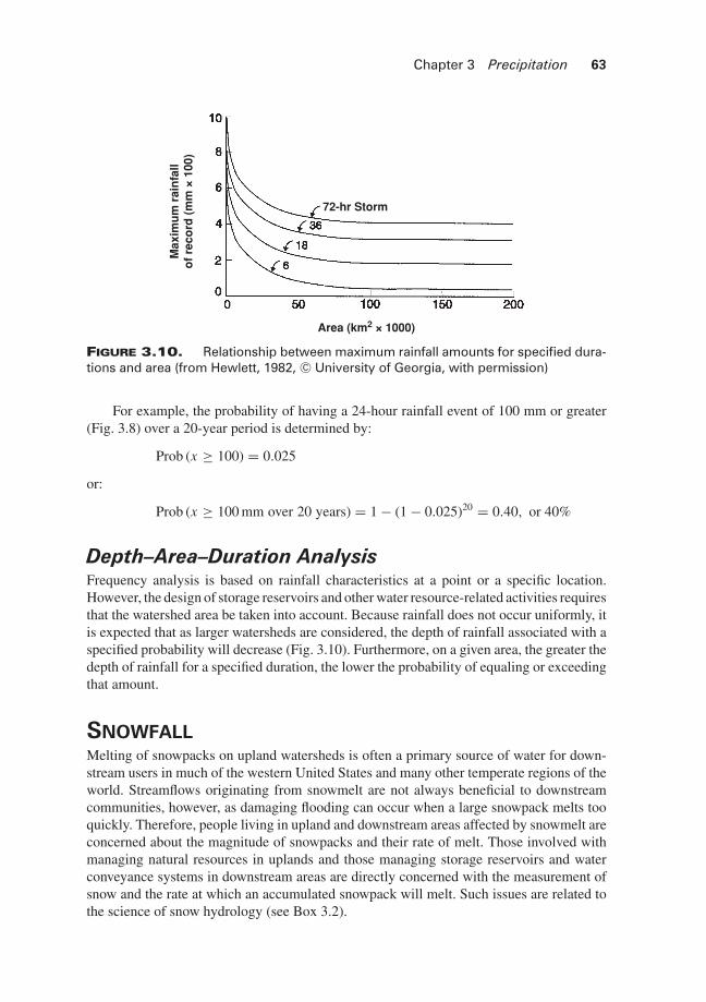
FIGURE 3.10. Relationship between maximum rainfall amounts for specified dura-tions and area (from Hewlett, 1982, C© University of Georgia, with permission)

For example, the probability of having a 24-hour rainfall event of 100 mm or greater(Fig. 3.8) over a 20-year period is determined by:

Prob (x ≥ 100) = 0.025

or:

Prob (x ≥ 100 mm over 20 years) = 1 − (1 − 0.025)20 = 0.40, or 40%

Depth–Area–Duration AnalysisFrequency analysis is based on rainfall characteristics at a point or a specific location.However, the design of storage reservoirs and other water resource-related activities requiresthat the watershed area be taken into account. Because rainfall does not occur uniformly, itis expected that as larger watersheds are considered, the depth of rainfall associated with aspecified probability will decrease (Fig. 3.10). Furthermore, on a given area, the greater thedepth of rainfall for a specified duration, the lower the probability of equaling or exceedingthat amount.

SNOWFALLMelting of snowpacks on upland watersheds is often a primary source of water for down-stream users in much of the western United States and many other temperate regions of theworld. Streamflows originating from snowmelt are not always beneficial to downstreamcommunities, however, as damaging flooding can occur when a large snowpack melts tooquickly. Therefore, people living in upland and downstream areas affected by snowmelt areconcerned about the magnitude of snowpacks and their rate of melt. Those involved withmanaging natural resources in uplands and those managing storage reservoirs and waterconveyance systems in downstream areas are directly concerned with the measurement ofsnow and the rate at which an accumulated snowpack will melt. Such issues are related tothe science of snow hydrology (see Box 3.2).



Box 3.2

Terminology Used in Snow Hydrology� Snowpack – mixture of ice crystals, air impurities, and liquid water if

melting� Snowpack density – weight per unit volume; the density of pure ice

is 0.92 g/cm3 and it can vary from <0.10 g/cm3 to >0.40 g/cm3

� Snow water equivalent (WE) – weight of snow expressed as thedepth of liquid water over a unit of area = density (ρ) × depth (D)

� Cold snow – snow with a temperature below 0◦C� Temperature deficit (Ts) – snowpack temperature below 0◦C� Thermal deficiency – heat required to raise the temperature of 1 cm

WE of cold snow by 1◦C, the heat capacity of water is 1 cal/g/◦C; forice it is 0.5 cal/g/◦C; for air it is 0.24 cal/g/◦C

� Liquid-water-holding capacity – analogous to soil moisture, it is thewater held against gravity on snow crystals and the capillarychannels in a snowpack ( f ); it varies with density, crystal size andshape, and capillarity; f = 0.03 on average, generally less than 0.05;at 0◦C, f = 1 − B (B is the thermal quality defined below)

� Ripe snowpack – a snowpack that has reached its maximumliquid-water-holding capacity; a snowpack is isothermal at 0◦C and itis primed to transmit liquid water

� Cold content (Hc) – heat required to raise the temperature of a coldsnow layer of depth D to 0◦C; Hc = 0.5ρDTs

� Latent heat of fusion – heat required to change 1 g of dry snow at 0◦Cto a liquid state without changing the temperature or from a liquid tosolid at 0◦C = 80 cal/g = 80 cal/cm3

� Water equivalent of cold content Wc = (WE)Ts/160� Thermal quality (B) – the ratio of heat required to melt snow to the

heat required to melt an equal mass of pure ice at 0◦C (B); for a wet,melting snow at 0◦C, B < 1; for a dry snow at 0◦C, B = 1; for a cold,dry snow B > 1

Methods of Snowfall MeasurementSnowfall can be measured with the standard gauges, but it is more difficult to obtain reliablemeasurements than for rainfall. Snowfall is more susceptible to wind than rainfall becauseof its low density and high surface area, which results in rain gauges catching less than thetrue snowfall. In addition, snow tends to bridge over the orifice of a rain gauge and clingto the sides of containers. If snowfall is to be measured in a standard gauge, the funnel andcylinder are removed and a carefully measured volume of antifreeze is put in the canister.Snow falling into the canister melts in the antifreeze. The difference between the volume



of snowfall plus antifreeze and the initially measured volume of the antifreeze represents ameasurement of snowfall.

Since snow often remains on the ground for some time, it does not need to be measuredas it falls. The most common method of determining the magnitude of a snowpack is tomeasure its depth on the ground and, if possible, its weight. Such measurements can bemade adjacent to standard gauges or they can be obtained in snow surveys over a watershedin which several measurements are taken to estimate the mean snowfall on an area basis.

Snow SurveysSnow surveys are used to estimate the amount of water in the snowpack and the conditionof the snowpack such as its melting potential during the periods of accumulation and melton courses with a few to 20 or more sampling points along a transect. Snow depth and snowwater equivalent (WE) are measured at the sampling points on a course by using cylindricaltubes with a cutting edge. These snow tubes are graduated in inches or centimeters onthe outside of the tube to measure depth. Large-diameter tubes (7.6 cm) are used in areaswith shallow snowpacks. Smaller diameter snow tubes (3.8 cm), such as the Mount Rosesampler, are preferable for measuring snowpacks that exceed 1 m in depth.

The manner in which a snow course is laid out depends mostly on how the surveyinformation obtained is to be used. If the purpose of a snow survey is to provide an indexof snowpack water equivalent to predict subsequent snowmelt volumes, then regressionmethods are used. The course need not be representative of the average snowpack for thewatershed in question. Instead, a snow course should be located in an accessible area that isrelatively flat, is protected from wind, and retains a deep snowpack even in the drier years.The volume of snowmelt is then estimated with a regression relationship based on selectedsnow course data. The simple regression equations developed are of the general form:

Spring snowmelt runoff volume = P I − L I (3.11)

where PI is the index of precipitation inputs such as snow water equivalent, spring rainfall,or fall rainfall and LI is the index of losses, for example, evapotranspiration (ET) estimates.

Multiple regression equations are often developed that have the following components:

Y = a + b1 X1 + b2 X2 + b3 X3 − b4 X4 + · · · + bn Xn (3.12)

where Y is the volume of snowmelt runoff; X1 is the maximum snow water equivalentbased on snow survey data for April 1, for example; X2 is the fall precipitation (October toNovember rainfall); X3 is the spring rainfall (April); X4 is the pan evaporation for Octoberto April; and bi is the regression coefficient.

Multiple regressions such as Equation 3.12 are used widely by the Natural ResourcesConservation Service (NRCS) in the western United States.

If the purpose of a snow survey is to provide an estimate of the mean depth of snowpackwater equivalent over a watershed, the snow course should be designed to obtain an estimateof the spatial distribution of a snowpack over the watershed area. The same principles thatwere discussed earlier in estimating the mean depth of rainfall on a watershed should beapplied to estimate the mean depth of the snowpack water equivalent on the watersheds.

Snow surveys are often conducted during the periods that normally have maximumsnow accumulations, for example, in the western United States from early March through



Box 3.3

Forecasting Future Water Supplies from a Snow SurveyInformation obtained from a snow survey can be used to forecast future watersupplies. For example, the snow survey administered by the NRCS providesinformation on the depth and water equivalent of snowpacks at more than1200 sites in the western states and Alaska to individuals, organizations, andstate and federal agencies. This information then becomes a basis to forecastannual water availability, spring snowmelt runoff, and summer streamflowsfor making decisions relating to flood control, power generation, agriculturalcrop production, municipal and industrial water supplies, and other water-related uses. Further information on forecasting water supplies from theinformation obtained in this snow survey is available on the NRCS website(http://www.nrcs.usda.gov/partnerships/links_wsfs.html).

late April. A snow survey can also be conducted at other times in the period that a snow-pack is accumulating on a watershed to accommodate other hydrologic objectives such asforecasting future water supplies (Box 3.3).

Remote Sensing MethodsAvailability of telemetry and satellite systems has expanded the methods of measuringsnowpacks. Telemetry has been particularly useful in transmitting data collected by pressurepillows, called snow pillows, located at remote sites. A snow pillow consists of metalplates that sense the weight of the overlying snowpack usually by means of pressuretransducers. The weight of the snowpack is then converted into units of snowpack waterequivalent. A network called the Snow Data Telemetry System (SNOTEL), operationalin the United States, uses radio telemetry to transmit snow pillow data, temperature, andother climatological data from remote mountain areas to processing centers. The dataobtained from SNOTEL sites complement snow course data and, importantly, have theadvantage of representing current snowpack conditions on the watershed. Hydrologists orwatershed managers can retrieve data from SNOTEL any time they wish. For example,the conditions that might lead to a rapid snowmelt can be detected as they evolve and, indoing so, allow for real-time predictions of snowmelt runoff. Additional information aboutthis telemetry system for transmitting snowpack conditions can be found on the SNOTELwebsite (www.wcc.nrcs.usda.gov/snow/about.html).

Reliable snowpack water equivalent measurements are provided in real time to theNWS offices upon request from NWS hydrologists through the Airborne Snow Survey Pro-gram (Carroll, 1987). The airborne measurement technique uses the attenuation of naturalterrestrial gamma radiation by the mass of a snow cover to obtain airborne measurementsof snow water equivalent often by fixed-wing aircraft. The gamma radiation flux near the



ground originates primarily from natural radioisotopes in the soil. In a typical soil, 96% ofthe gamma radiation is emitted from the upper 20 cm of soil. After a background measure-ment of radiation and soil moisture is made over a specific flight line, that is, a measurementin the absence of a snow cover, the attenuation of the radiation signal due to the snowpackoverburden is used to integrate the average areal amount of water in the snow cover over theflight line. Flight-line surveys have been established for operational streamflow forecastingby the NWS with a network of more than 1900 flight lines in 29 states and 7 Canadianprovinces. More information on the NWS Airborne Snow Survey Program is available onthe website for the program (www.nohrsc.noaa.gov/snowsurvey/).

Satellite imagery can be useful to assess the extent of snow-covered areas, particularlyfor large river basins. Resolution of the sensor is used to determine the minimum basin sizesfor various satellite systems. Hydrologists and watershed managers in the United States useNOAA-AVHRR (Advanced Very High Resolution Radiometer) data on basins as small as200 km2, Landsat MSS (Multispectral Scanner Systems) data on basins as small as 10 km2,and Landsat TM (Thermal Mapper) data on basins as small as 2.5 km2 (Rango, 1994). Moreimportant than the resolution is the frequency of coverage. The frequency of coverage formany applications is adequate only with the NOAA-AVHRR data, which represents onevisible overpass of an area a day. Cloud cover is always a potential problem. However,estimates of snow cover under a partial cloud cover can often be obtained by extrapolationfrom a cloud-free portion of the basin if available. Relationships are sometimes developedbetween the percentage of area in a watershed covered with snow and subsequent streamflowdue to snowmelt. As applications of satellite technology continue to expand, there will beopportunities for relating many types of spectral characteristics to snowpack condition,melt, and other related processes.

Analysis of Snowfall MeasurementsSnowfall data are analyzed for many of the same purposes as rainfall data (discussedabove). Long-term representative snowfall data from watersheds or river basins are valuablefor water resource managers, streamflow forecasters, and planners to understand currentconditions relative to conditions of the past. To improve the accuracy and usefulness ofsnow data can require one or more of the following:

(1) Missing snowpack measurements on a course can be estimated by regression or otherrelationships with snowpack measurements from nearby courses.

(2) The consistency of measurements obtained on one snow course relative to themeasurements at another course can be determined with double mass analysis.

(3) The recurrence interval of snowfall amounts and the resulting snowmelt runoff can beestimated and compared through frequency analysis.

Snow Accumulation and MetamorphismThe factors affecting the distribution of rainfall on a watershed also affect the deposition ofsnow on the watershed. However, snowfall on a site can be quite variable on a microscalebecause its deposition is influenced by wind, topography, forest overstory vegetation, andphysical obstructions such as fences. Newly fallen snow usually has a low density, often



assumed to be 0.1 g/cm3, which makes the snowpack susceptible to wind action. It alsohas a high albedo, ranging from 80% to 95%. Between snowfall and subsequent snowmeltrunoff, several changes take place within the snowpack. These changes, called snowpackmetamorphism, are largely the result of energy exchange and involve changes in the snowstructure, density, temperature, albedo, and liquid-water content.

A snowpack undergoes many changes from the time snow falls until snowmelt occurs.Snow particles, which are initially crystalline in shape, become more granular as wind,solar, and sensible-heat energy, and liquid water alter the snowpack. Snow crystals becomedisplaced as the snowpack settles, resulting in an increase in density. Alternate thawing andfreezing at the surface of a snowpack followed by periods of snowfall can cause ice planesor lenses to form within the pack. In addition, the temperature of the snowpack changes inresponse to long periods of either warm or cold weather. When warmer weather dominates,there is a progressive warming of the snowpack but never in excess of a temperature of 0◦C.The albedo of snow diminishes over the time that the snowpack is exposed to atmosphericdeposition of forest litter, dust, and rainfall. As stated earlier, a new snowpack can have analbedo in excess of 90%. An older snowpack can have an albedo value of less than 45%.

The above discussion provides a qualitative sense of what snowpack metamorphismentails. However, what is needed is a way to quantify snowpack metamorphism to determinewhen a snowpack is ready to melt and yield liquid water. A snowpack is considered ripewhen it is primed to release liquid water, that is, when the temperature of the snowpack is0◦C and the liquid-water-holding capacity of the snowpack has been reached. Any additionalinput of either energy or liquid water to the snowpack will then result in a correspondingamount of liquid water being released from the bottom of the pack.

Cold Content. The energy needed to raise the temperature of a snowpack to 0◦Cper unit area is called the cold content. It is often convenient to express the cold contentas the equivalent depth of water entering the snowpack at the surface as rain that uponfreezing will raise the temperature of the pack to 0◦C by releasing the latent heat of fusion80 cal/g. Taking the specific heat of ice to be 0.5 cal/g/◦C, the following relationship isobtained (Box 3.4):

Wc = � DTs

160= (WE)Ts

160(3.13)

where Wc is the cold content as equivalent depth of liquid water (cm); � is the density ofsnow (g/cm3); D is the depth of snow (cm); WE is the snow water equivalent (cm); and Ts

is the average temperature deficit of the snowpack below 0◦C.

Liquid-Water-Holding Capacity. Like soil, a snowpack can retain a certainamount of liquid water. This liquid water occurs as hygroscopic water, capillary water, andgravitational water. The liquid-water-holding capacity of a snowpack (Wg) is calculated by

Wg = f (WE + Wc) (3.14)

where f is the hygroscopic and capillary water held per unit mass of snow after gravitydrainage, usually varying from 0.03 to 0.05 g/g; WE is the snow water equivalent (cm); andWc is the cold content (cm).



Box 3.4

Cold Content Calculation for a Snowpack of Depth = 100 cm,Snow Density = 0.1 g/cm3, Temperature Deficit (Ts) = −10◦CSince the heat of fusion equals 80 cal/g and the specific heat of ice equals0.5 cal/g/◦C, the amount of energy required to bring the temperature ofa snowpack up to 0◦C can be determined by the following sequence ofcalculations:

WE = (0.1 g/cm3)(100 cm) = 10 g/cm2

To raise the temperature of the pack (which at −10◦C would be solid ice) byjust 1◦C would require:

(10 g/cm2)(0.5 cal/g/◦C) = 5 cal/cm2/◦C

To raise the temperature of the snowpack from −10◦C to 0◦C then wouldrequire:

[0◦C − (−10◦C)](5 cal/cm2/◦C) = 50 cal/cm2

To express the energy requirement in terms of equivalent inches ofsnowmelt:

(50 cal/cm2)(1 g/80 cal)(1 cm3/g) = 0.63 cm

Cold content could have been calculated directly by Equation 3.13:

Wc = (0.1)(100)(10)160

= 0.63 cm

Total Retention Storage. The total amount of melt or rain that must be addedto a snowpack before liquid water is released is the total retention storage (Sf):

Sf = Wc + f (WE + Wc) (3.15)

The snowpack is said to be ripe when the total retention storage is satisfied.

SnowmeltOnce the snowpack is ripe, any additional input of energy will result in meltwater beingreleased from the bottom of the snowpack. The main sources of energy for snowmelt tooccur are essentially the same as those required for ET. To calculate snowmelt, therefore,requires application of either an energy budget approach or the empirical approximation ofthe energy available for snowmelt.



Energy Budget and Snowmelt RelationshipsThe energy that is available either to ripen a snowpack or to melt snow can be determinedwith an energy budget analysis. The energy budget can be used to determine the availableenergy for ripening or melting as follows:

M = Wi(1 − �) + Wa − Wg + H + G + L E + Hr (3.16)

where M is the energy available for snowmelt (cal/cm2); Wi is the total incoming shortwave(solar) radiation (cal/cm2); � is the albedo of snowpack (fraction); Wa is the incominglongwave radiation (cal/cm2); Wg is the outgoing longwave radiation (cal/cm2); H is theconvective transfer of sensible heat at the snowpack surface (cal/cm2), which can be + or −as a function of gradient; G is the conduction at the snow–ground interface (cal/cm2); LEis the flow of latent heat (condensation [ + ], evaporation or sublimation [–]) (cal/cm2); andHr is the advective heat from rain or fog (cal/cm2).

Snowmelt can be determined directly if all the above energy components can bemeasured. The amount of snow that melts from a specific quantity of heat energy dependson the condition of the snowpack which can be expressed in terms of its thermal quality.Thermal quality is the ratio of heat energy required to melt 1 g of snow to that required tomelt 1 g of pure ice at 0◦C, and is expressed as a percentage (Box 3.5). A thermal qualityless than 100% indicates the snowpack is at 0◦C and contains liquid water. Conversely,a thermal quality greater than 100% indicates the snowpack temperature is less than 0◦Cwith no liquid water. Snowmelt, therefore, can be determined by:

M = Total Energy (cal/cm3)

B (80 cal/g)(3.17)

where M is the snowmelt (cm) and B is the thermal quality expressed as a fraction.Under most conditions, however, total energy cannot be measured. Therefore, approx-

imations of this energy (M), such as obtained by applications of the generalized snowmeltequations or the temperature index (degree-day) method, are used to estimate snowmelt.

Generalized Snowmelt EquationsThe generalized snowmelt equations were developed from extensive field measurementsat snow research laboratories throughout the western United States (USACE, 1956, 1998).All of the major energy components considered in their development are outlined in thefollowing discussion by considering each major source of energy separately.

Solar Radiation. Solar radiation is the major source of energy for snowmelt. Theamount of solar radiation reaching a snowpack surface is dependent upon the slope andaspect of the surface, cloud cover, and forest cover. In the Northern Hemisphere, south-facing slopes receive more radiation than north-facing slopes. The more moderate theslope, the more moderate the effect that the slope has on solar radiation. The correspondingpotential solar radiation for a specified latitude can be determined by knowing the slopeand aspect of an area.

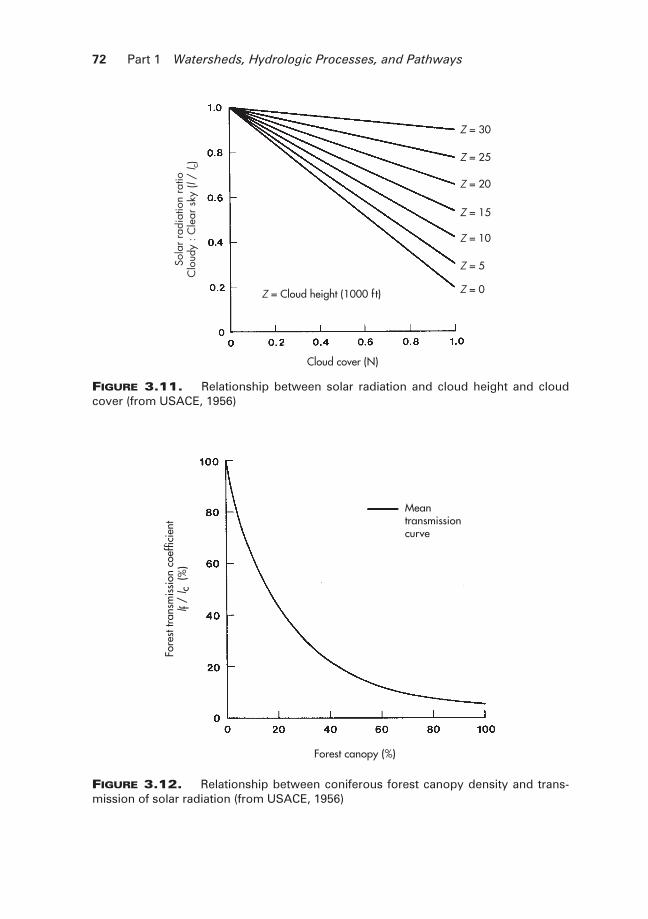
The amount of solar radiation striking the surface of a snowpack in the open is a functionof the percentage of cloud cover and the height of the clouds (Fig. 3.11). The percentageof incoming solar radiation that reaches the snow surface on a forested watershed dependslargely on the type of cover, density, and condition of the forest canopy. As the density



Box 3.5

Determining Snow Thermal Quality by the Calorimeter Method(Snow Depth = 60 cm, Volume of Snow Sample Taken = 15,000cm3, and Weight of Sample = 2000 g) (modified from Hewlett 1982)The above sample was placed in a thermos which initially contained 7000 gof water at a temperature of 32◦C. After adding the snow sample, and afterall the snow melted, the temperature of the water in the thermos was 8◦C.The following calculations were made:

Snow density = 2000 g15,000 cm3

= 0.133 g/cm3

Snow water equivalent (WE) = (0.133)(60 cm) = 8.0 cm

First, determine the heat energy needed to raise the temperature of themelted snow water from 0◦C to 8◦C:

(2000 g)(8◦C)(1 cal/g/◦C) = 16,000 cal

The heat available energy was:

(7000 g)(32 − 8◦C)(1 cal/g/◦C) = 168,000 cal

The heat available to melt ice would equal:

168,000 cal − 16,000 cal = 152,000 cal

Therefore,

Ice content = 152,000 cal80 cal/g

= 1900 g

Thermal quality (B) = 1900 g2000 g

= 0.95 = 95%

The snowpack contained 5% liquid water and was at a temperature of 0◦C.

of a forest canopy increases, incoming solar radiation decreases exponentially (Fig. 3.12).As a result, with dense canopies, the effect of forest cover overrides the effects of cloudcover. Coniferous forest cover can reduce substantially the amount of solar radiation thatreaches a snow surface, while deciduous forests have less of an effect on solar radiation. Foreither open or forested conditions, the solar radiation (Wi) reaching the snowpack surfaceis further reduced by the snowpack albedo (�). Snowmelt from solar radiation (M) is thendefined as

M = Wi(1 − �)

B(80)(3.18)



Cloud cover (N)

Z = Cloud height (1000 f t)

Sola

r ra

diat

ion

ratio

Clo

udy

: Cle

ar s

ky (l

/ l c

)

Z = 30

Z = 25

Z = 20

Z = 15

Z = 10

Z = 5

Z = 0

FIGURE 3.11. Relationship between solar radiation and cloud height and cloudcover (from USACE, 1956)

Meantransmissioncurve

Forest canopy (%)

Fore

st tr

ansm

issi

on c

oeffi

cien

tl f

/ l c

(%

)

FIGURE 3.12. Relationship between coniferous forest canopy density and trans-mission of solar radiation (from USACE, 1956)



Longwave Radiation. Snow absorbs and emits nearly all of the incident long-wave or terrestrial radiation. Net longwave radiation at a snow surface is determined largelyby overhead back radiation from the earth’s atmosphere, clouds, and forest canopies.

Under clear skies, back radiation from the atmosphere is a function of the water contentof air. Over snowpacks, the vapor pressure of air usually varies between 3 and 9 mb pressure,resulting in a fairly constant rate of longwave radiation of 0.757 cal/cm2/min. The narrowrange of snowpack temperatures limits the amount of radiation emitted from a snowpack.Since a snowpack temperature cannot exceed 0◦C, the maximum longwave radiation a ripesnowpack can emit is 0.459 cal/cm2/min. Therefore, under clear skies, the net longwaveradiation at a snow surface is approximately:

Rc = 0.757�T 4a − 0.459 (3.19)

where Rc is the net longwave radiation (cal/cm2/min); � is the Stefan–Boltzmann constant,which is equal to 0.826 × 10−10 (cal/cm2/min/K4); and Ta is the air temperature (K).

When clouds are present, the temperature at the base of the clouds determines the backradiation to the snow surface, and the net longwave radiation becomes:

Rcl = �(T 4

c − T 4s

)(3.20)

where Rcl is the net longwave radiation under cloudy skies; Tc is the temperature at the baseof clouds (K); and Ts is the snowpack temperature (K).

Similarly, the net longwave radiation (Rf) for a snowpack beneath a dense conifercanopy is:

Rf = �(T 4

f − T 4s

)(3.21)

where Tf is the temperature of the underside of the forest canopy (K).Because temperatures of the trees are rarely known, Tf is often estimated from air tem-

perature (Ta). Under clear-sky conditions and a ripe snowpack, the net longwave radiationunder a conifer forest canopy is:

Rlw = �T 4a [F + 0.757(1 − F)] − 0.459 (3.22)

where F is the canopy density expressed as a decimal fraction.

Net Radiation. The net (all-wave) radiation that is available for snowmelt is gov-erned largely by forest-cover conditions and cloud conditions. For conditions of little or noforest cover, clouds strongly affect the net radiation at the snowpack surface. Under partialor dense forest conditions, forest cover governs net radiation at the snowpack surface.

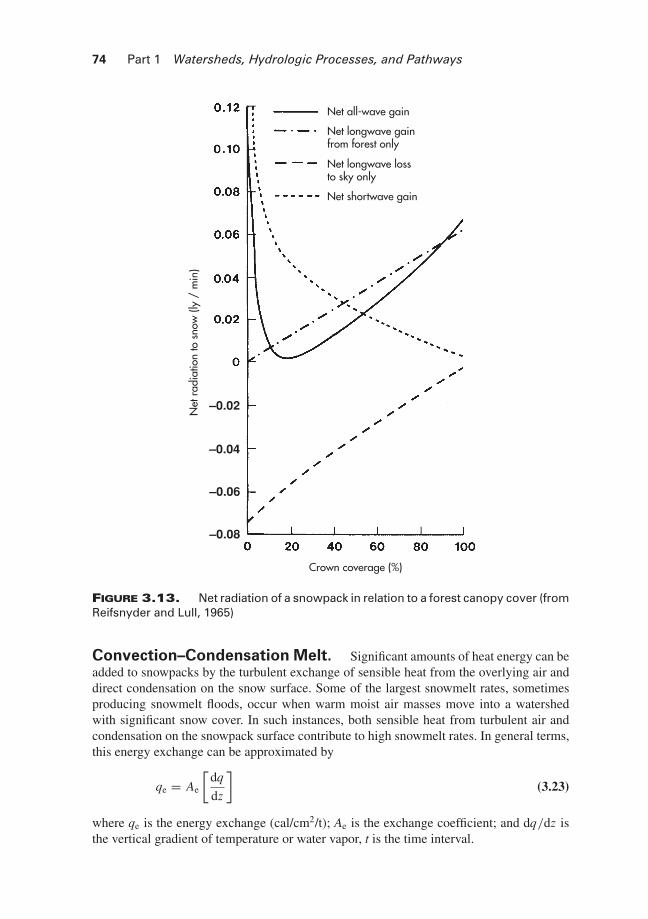
There is a tradeoff between shortwave and longwave radiation at a snowpack surfaceas forest cover changes. As forest cover increases, the solar radiation at the snowpacksurface is reduced greatly; the longwave radiation loss from the snowpack is reduced; andthe longwave gain component from the canopy increases (Fig. 3.13). Net radiation at thesnowpack surface is at a minimum between 15% and 30% canopy cover, but increases atdense forest canopy conditions because of the much higher net longwave radiation. Netradiation is highest at 0% cover with large inputs of solar radiation. These relationshipshave implications for the management of forested watersheds in snow-dominatedregions.



Crown coverage (%)

–0.08

–0.06

–0.04

–0.02

Net all-wave gain

Net longwave lossto sky only

Net shortwave gain

Net longwave gainfrom forest only

Net

rad

iatio

n to

sno

w (l

y /

min

)

FIGURE 3.13. Net radiation of a snowpack in relation to a forest canopy cover (fromReifsnyder and Lull, 1965)

Convection–Condensation Melt. Significant amounts of heat energy can beadded to snowpacks by the turbulent exchange of sensible heat from the overlying air anddirect condensation on the snow surface. Some of the largest snowmelt rates, sometimesproducing snowmelt floods, occur when warm moist air masses move into a watershedwith significant snow cover. In such instances, both sensible heat from turbulent air andcondensation on the snowpack surface contribute to high snowmelt rates. In general terms,this energy exchange can be approximated by

qe = Ae

[dq

dz

](3.23)

where qe is the energy exchange (cal/cm2/t); Ae is the exchange coefficient; and dq/dz isthe vertical gradient of temperature or water vapor, t is the time interval.



For a ripe snowpack, the snow surface would have a temperature of 0◦C with acorresponding vapor pressure of 6.11 mb. Using these values for the snow surface andmeasurements of air temperature and relative humidity of the air above the snow surface,the melt caused by the energy exchange from convection and condensation can be estimated.

Rain Melt. Snowmelt caused by the addition of sensible heat from rainfall to asnowpack is relatively small in magnitude. It can be estimated from air temperature andrainfall measurements for a snowpack with a thermal quality of 100% as

Mp = PrTa

80 cal/g= 0.013PrTa (3.24)

where Mp is the daily snowmelt (cm); Pr is the daily rainfall (cm); and Ta is the averagedaily air temperature (◦C).

Again, the above equation holds for a ripe snowpack. If the snowpack has a temperaturebelow 0◦C, additional energy can be released to the pack by virtue of the release of the heatof fusion, which is 80 cal for every 1 cm of rain that freezes.

Conduction Melt. Heat energy can be added to the base of a snowpack by conduc-tion from the underlying ground. For any day, the amount of energy available by conductionand, hence, the amount of melt are relatively small. Daily values of 0.5 mm are frequentlyassumed, and sometimes this component is simply ignored if snowmelt is being estimatedover a short period. However, conduction melt (ground melt) can be significant for seasonalestimates of snowmelt. For example, monthly snowmelt totals in the central Sierra Nevadain California ranged from 0.3 cm in January to 2.4 cm in May (USACE, 1956).

Combined Snowmelt Equations. The energy–snowmelt relationships de-rived above provide the foundation for a set of generalized equations that can be used toestimate snowmelt for forested watersheds (USACE, 1998). Because of the influence ofa forest cover on energy exchange, the forest-cover condition of a watershed determineswhich equation to use. For rain-free periods, the daily melt from a ripe snowpack (isother-mal at 0◦C, with a 3% liquid-water content) is calculated by one of the following equations,which are differentiated on the basis of the forest canopy cover (F):

Heavily Forested Area (F � 0.80):

M = 0.19 Ta + 0.17 Td (3.25)

Forested Area (F = 0.60–0.80):

M = k(0.00078 v)(0.42 Ta + 1.51 Td) + 0.14 Ta (3.26)

Partly Forested Area (F = 0.10–0.60):

M = k ′(1 − F)0.01 Wi(1 − �) + k(0.00078 v)

× (0.42 Ta + 1.51 Td) + F(0.14 Ta) (3.27)

Open Area (F � 0.10):

M = k ′(0.0125 Wi)(1 − �) + (1 − N )(0.014 Ta − 2.13)

+ N (0.013 Tc) + k(0.00078 v)(0.42 Ta + 1.51 Td) (3.28)



where M is the daily melt (cm); Ta is the air temperature (◦C) at 2 m above the snowsurface; Td is the dew point temperature (◦C) at 2 m above the snow surface; v is thewind speed (km/day); Wi is the observed or estimated solar radiation (cal/cm2/day); � isthe snow surface albedo (decimal fraction); k′ is the basin shortwave radiation melt factor,which depends on the average exposure of the open areas to solar radiation compared toan unshielded horizontal surface; F is the average forest canopy cover a for watershed(expressed as a decimal fraction); Tc is the cloud-base temperature (◦C); N is the cloudcover expressed as a decimal fraction; and k is the basin convective–condensation meltfactor, which depends on the relative exposure of the watershed to wind.

The only empirically fitted parameters in the above equations are k and k′. The basinshortwave radiation melt factor (k′) can be estimated from solar radiation data for a specifiedlatitude, slope, and aspect. Because one has to average several slopes and aspects for awatershed, the k′ value represents an average for the watershed. Watersheds with a southernexposure would tend to have a k′ � 1, while those with northern exposures would have ak′ � 1. A watershed that has a balance between north- and south-facing slopes would havea k′ = 1.0. The basin convective–condensation melt factor (k) is similarly an average valuefor a particular watershed that indicates the exposure of the snowpack to wind. These valuesrange from k = 1.0 for open areas to k = 0.8 for dense forest cover.

Temperature Index (Degree-Day) MethodThe data that are required to apply the generalized snowmelt equations can restrict the useof these equations in many situations, such as in remote areas and for day-to-day operationalconditions. As a result, a method that depends solely on knowledge of air temperature canbe used to estimate snowmelt.

The temperature index method is based on the following empirically derived equationof the form:

M = MR (Ta − Tb) (3.29)

where M is the daily snowmelt (cm); MR is the melt-rate index or degree-day factor(cm/◦C/day); Ta is the daily air temperature value, usually either the average daily or themaximum daily temperature (◦C); and Tb is the base temperature, at which no snowmelt isobserved (◦C).

The difference Ta–Tb represents the degree-days of heat energy available for meltinga snowpack. The melt-rate index relates this heat energy to snowmelt on the watershed.Although we know that the air temperature is but one source of energy for snowmelt, itcorrelates well with radiation inputs, particularly in the snowmelt season, and it is also areasonable index for forested watersheds.

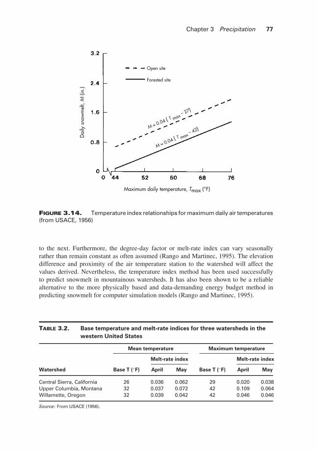
The equation for the temperature index method (Equation 3.29) is derived from re-gression analysis of daily snowmelt versus air temperature (Fig. 3.14). The melt-rate indexis the slope of the regression line, and the base temperature (Tb) is that air temperature atwhich no melt is observed. Examples of temperature index coefficients for three watershedsare presented in Table 3.2.

Since the temperature index method is developed for a specified watershed, both themelt-rate index and the base-temperature values are likely to differ from one watershed



Open site

Forested site

M = 0.04 ( T max – 27)

M = 0.04 ( T max – 42)

Maximum daily temperature, Tmax (°F)

Dai

ly s

now

mel

t, M

(in.

)

FIGURE 3.14. Temperature index relationships for maximum daily air temperatures(from USACE, 1956)

to the next. Furthermore, the degree-day factor or melt-rate index can vary seasonallyrather than remain constant as often assumed (Rango and Martinec, 1995). The elevationdifference and proximity of the air temperature station to the watershed will affect thevalues derived. Nevertheless, the temperature index method has been used successfullyto predict snowmelt in mountainous watersheds. It has also been shown to be a reliablealternative to the more physically based and data-demanding energy budget method inpredicting snowmelt for computer simulation models (Rango and Martinec, 1995).

TABLE 3.2. Base temperature and melt-rate indices for three watersheds in thewestern United States

Mean temperature Maximum temperature

Melt-rate index Melt-rate index

Watershed Base T (◦F) April May Base T (◦F) April May

Central Sierra, California 26 0.036 0.062 29 0.020 0.038Upper Columbia, Montana 32 0.037 0.072 42 0.109 0.064Willamette, Oregon 32 0.039 0.042 42 0.046 0.046

Source: From USACE (1956).



SUMMARY AND LEARNING POINTSPrecipitation input to a watershed can be in the form of rainfall or as the amount of meltresulting from snowfall. You should have gained a general understanding of the factorsthat influence the occurrence of a precipitation, including rainfall, snowfall, and snowmelt.Specifically, you should be able to

(1) Describe the conditions necessary for precipitation to occur.(2) Explain the different precipitation and storm characteristics associated with frontal

storm systems, orographic influences, and convective storms.(3) Understand how rainfall can be measured at a point and how these measurements can

be used to estimate the average depth of rainwater over a watershed area.(4) Estimate the values of rainfall that are missing for a storm.(5) Explain the purpose of performing double mass analysis and frequency analysis.(6) Understand how snowfall can be measured and the purpose of a snow survey.(7) Explain the causal factors affecting snow accumulation, snow ripening, and snowmelt.(8) Explain and be able to quantify the snow-ripening process of a snowpack and explain

the effects of snowpack condition on spring snowmelt floods.(9) Describe the differences between snowmelt under a conifer forest and that in an open

field using an energy budget approach.(10) Calculate snowmelt using either the appropriate generalized snowmelt equation or the

temperature index method and discuss the advantages and disadvantages of these twomethods.

REFERENCESArmstrong, R.L. & Brun, E. (eds.) (2008) Snow and climate: Physical processes, surface energy

exchanges and modeling. New York: Cambridge University Press.Carroll, T.R. (1987) Operational airborne measurements of snow water equivalent and soil moisture

using terrestrial gamma radiation in the United States. In Proceedings of symposium onlarge-scale effects of seasonal snow cover, 213–223. International Association ofHydrologists Scientific Publication 166. Vancouver, British Columbia, Canada:International Association of Hydrologists.

Goodison, B.E. (1978) Accuracy of Canadian snow gage measurements. J. Appl. Meteorol.17:1542–1548.

Gray, D.M. (ed.) (1973) Handbook on the principles of hydrology. Port Washington, NY: WaterInformation Center, Inc. Reprint.

Gray, D.M. & Male, D.H. (eds.) (1981) Handbook of snow. New York: Pergamon Press.Haan, C.T. (2002) Statistical methods in hydrology. Ames, IA: Iowa State University Press.Hewlett, J.D. (1982) Principles of forest hydrology. Athens, GA: University of Georgia Press.Huff, F.A. & Angel, J.A. (1992) Rainfall frequency atlas of the Midwest. Bulletin 71. Champaign,

IL: Illinois State Water Survey.Legates, D.R. & DeLiberty, T.L. (1993) Precipitation measurement biases in the United States.

Water Resour. Bull. 29:855–861.Michaelides, S. (2008) Precipitation: Advances in measurement, estimation, and prediction. Berlin,

Germany: Springer.Rango, A. (1994) Application of remote sensing methods to hydrology and water resources. J. des

Sciences Hydrologiques 39:309–320.



Rango, A. & Martinec, J. (1995) Revisiting the degree-day method for snowmelt computations.Water Resour. Bull. 31:657–669.

Reifsnyder, W.E. & Lull, H.W. (1965) Radiant energy in relation to forests. USDA For. Serv. Tech.Bull. 1344.

Sauvageot, H. (1994) Rainfall measurement by radar: A review. Atmospheric Res. 35:27–54.Sevruk, B. & Hamon, W.R. (1984) International comparison of national precipitation gauges with a

reference pit gauge. Instruments and Observing Methods, Report 17. Geneva,Switzerland: World Meteorological Organization.

Strangeways, I. (2007) Precipitation: Theory, measurement and distribution. New York: CambridgeUniversity Press.

U.S. Army Corps of Engineers (USACE) (1956) Snow hydrology. Portland, OR: U.S. Army Corpsof Engineers, North Pacific Division. (Available from U.S. Department of Commerce,Clearinghouse for Federal Scientific and Technical Information, PB 151660.)

U.S. Army Corps of Engineers (USACE). 1998. Engineering and design: runoff from snowmelt.Engineering Manual 1110-2-1406.

WEBLIOGRAPHYwww.nohrsc.noaa.gov/snowsurvey/ – Airborne Snow Survey Program of National Weather Service.

Accessed November 15, 2011.www.nws.noaa.gov/ – Site to update current precipitation measurement methods, precipitation data,

and weather forecasts in the USA.www.srh.noaa.gov/abrfc/?n=map – U.S. National Weather Service, Point precipitation

measurement, areal precipitation estimates and relationships to hydrologic models.Accessed November 15, 2011.

www.srh.noaa.gov/mrx/research/precip/precip.php – Study indicating the errors associated with theuse of radar to measure rainfall and suggested remedies. Accessed June 15, 2011.

www.wcc.nrcs.usda.gov/partnerships/links_wsfs.html – Natural Resources Conservation Service,Snow Survey & Water Supply Forecasting Programs. Accessed November 14, 2011.

www.wcc.nrcs.usda.gov/snow/about.html – SNOTEL website, information about this telemetrysystem for transmitting snowpack conditions. Accessed November 14, 2011.

Documents

CHAPTER 3 - UW Canvas