accuracy assessment - Canvas

408

Chapter FOUrteen

accuracy assessment

14.1. Definition and Significance

Prospective users of maps and data derived from remotely sensed images quite naturally ask about the accuracy of the information they will use. Yet questions concerning accu-racy are surprisingly difficult to address in a convincing manner. This chapter describes how the accuracy of a thematic map can be evaluated and how two maps can be com-pared to determine whether they are statistically different from one another.

Accuracy and Precision

Accuracy defines “correctness”; it measures the agreement between a standard assumed to be correct and a classified image of unknown quality. If the image classification cor-responds closely with the standard, it is said to be “accurate.” There are several methods for measuring the degree of correspondence, all described in later sections.

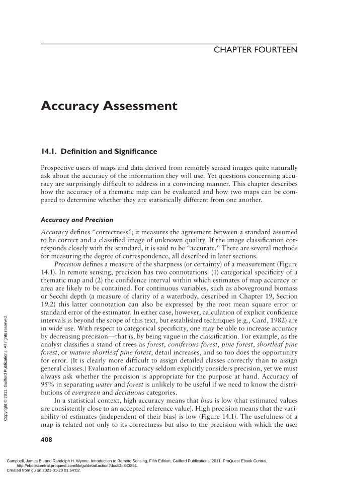
Precision defines a measure of the sharpness (or certainty) of a measurement (Figure 14.1). In remote sensing, precision has two connotations: (1) categorical specificity of a thematic map and (2) the confidence interval within which estimates of map accuracy or area are likely to be contained. For continuous variables, such as aboveground biomass or Secchi depth (a measure of clarity of a waterbody, described in Chapter 19, Section 19.2) this latter connotation can also be expressed by the root mean square error or standard error of the estimator. In either case, however, calculation of explicit confidence intervals is beyond the scope of this text, but established techniques (e.g., Card, 1982) are in wide use. With respect to categorical specificity, one may be able to increase accuracy by decreasing precision—that is, by being vague in the classification. For example, as the analyst classifies a stand of trees as forest, coniferous forest, pine forest, shortleaf pine forest, or mature shortleaf pine forest, detail increases, and so too does the opportunity for error. (It is clearly more difficult to assign detailed classes correctly than to assign general classes.) Evaluation of accuracy seldom explicitly considers precision, yet we must always ask whether the precision is appropriate for the purpose at hand. Accuracy of 95% in separating water and forest is unlikely to be useful if we need to know the distri-butions of evergreen and deciduous categories.

In a statistical context, high accuracy means that bias is low (that estimated values are consistently close to an accepted reference value). High precision means that the vari-ability of estimates (independent of their bias) is low (Figure 14.1). The usefulness of a map is related not only to its correctness but also to the precision with which the user

Campbell, James B., and Randolph H. Wynne. Introduction to Remote Sensing, Fifth Edition, Guilford Publications, 2011. ProQuest Ebook Central, http://ebookcentral.proquest.com/lib/gu/detail.action?docID=843851.Created from gu on 2021-01-20 01:54:02.

Cop

yrig

ht ©

201

1. G

uilfo

rd P

ublic

atio

ns. A

ll rig

hts

rese

rved

.

14. accuracy assessment 409

can make statements about specific points depicted on the map. A map that offers only general classes (even if correct) enables users to make only vague statements about any given point represented on the map; one that uses detailed classes permits the user to make more precise statements (Webster and Beckett, 1968).

Significance

Accuracy has many practical implications; for example, it affects the legal standing of maps and reports derived from remotely sensed data, the operational usefulness of such data for land management, and their validity as a basis for scientific research. Analyses of accuracies of alternative classification strategies have significance for everyday uses of remotely sensed data. There have, however, been few systematic investigations of relative accuracies of manual and machine classifications, of different individuals, of the same interpreter at different times, of alternative preprocessing and classification algorithms, or of accuracies associated with different images of the same area. As a result, accuracy studies would be valuable research in both practical and theoretical aspects of remote sensing.

Often people assess accuracy from the appearance of a map, from past experience, or from personal knowledge of the areas represented. These can all be misleading, as overall accuracy may be unrelated to the map’s cosmetic qualities, and often personal experience may be unavoidably confined to a few unrepresentative sites. Instead, accu-racy should be evaluated through a well-defined effort to assess the map in a manner

FIGURE 14.1. Bias and precision. Accuracy consists of bias and precision. Consistent dif-ferences between estimated values and true values create bias (top diagram). The lower diagram illustrates the concept of precision. High variability of estimates leads to poor precision; low variability of estimates creates high precision.


Cop

yrig

ht ©

201

1. G

uilfo

rd P

ublic

atio

ns. A

ll rig

hts

rese

rved

.

410 iii. anaLYsis

that permits quantitative measure of accuracy and comparisons with alternative images of the same area.

Evaluation of accuracies of information derived from remotely sensed images has long been of interest, but a new concern regarding the accuracies of digital classifica-tions has stimulated research on accuracy assessment. When digital classifications were first offered in the 1970s as replacements for more traditional products, many found the methods of machine classification to be abstract and removed from the direct control of the analyst; their validity could not be accepted without evidence. This concern prompted much of the research outlined in this chapter.

Users should not be expected to accept at face value the validity of any map, regard-less of its origin or appearance, without supporting evidence. We shall see in this chapter how difficult it can be to compile the data necessary to support credible statements con-cerning map accuracy.

14.2. Sources of Classification Error

Errors are present in any classification. In manual interpretations, errors are caused by misidentification of parcels, excessive generalization, errors in registration, variations in detail of interpretation, and other factors. Perhaps the simplest causes of error are related to the misassignment of informational categories to spectral categories (Chapter 12). Bare granite in mountainous areas, for example, can be easily confused with the spectral response of concrete in urban areas. However, most errors are probably more complex. Mixed pixels occur as resolution elements fall on the boundaries between land-scape parcels; these pixels may well have digital values unlike either of the two categories represented and may be misclassified even by the most robust and accurate classification procedures. Such errors may appear in digital classification products as chains of misclas-sified pixels that parallel the borders of large, homogeneous parcels (Figure 14.2).

In this manner the character of the landscape contributes to the potential for error through the complex patterns of parcels that form the scene. A very simple landscape composed of large, uniform, distinct categories is likely to be easier to classify accurately than one with small, heterogeneous, indistinct parcels arranged in a complex pattern. Key landscape variables are likely to include:

Parcel size••Variation in parcel size••Parcel identities••Number of categories••Arrangement of categories••Number of parcels per category••Shapes of parcel••Radiometric and spectral contrast with surrounding parcels••

These variables change from one region to another (Podwysocki, 1976; Simonett and Coiner, 1971) and within a given region from season to season. As a result, errors present in a given image are not necessarily predictable from previous experience in other regions or on other dates.


Cop

yrig

ht ©

201

1. G

uilfo

rd P

ublic

atio

ns. A

ll rig

hts

rese

rved

.


14.3. error Characteristics

Classification error is the assignment of a pixel belonging to one category (as determined by ground observation) to another category during the classification process. There are few if any systematic studies of geographic characteristics of these errors, but experience and logic suggest that errors are likely to possess at least some of the characteristics listed below:

Errors are not distributed over the image at random but display a degree of sys-••tematic, ordered occurrence in space. Likewise, errors are not assigned at random to the various categories on the image but are likely to be preferentially associated with certain classes.Often erroneously assigned pixels are not spatially isolated but occur grouped in ••areas of varied size and shape (Campbell, 1981).Errors may have specific spatial relationships to the parcels to which they pertain; ••for example, they may tend to occur at the edges or in the interiors of parcels.

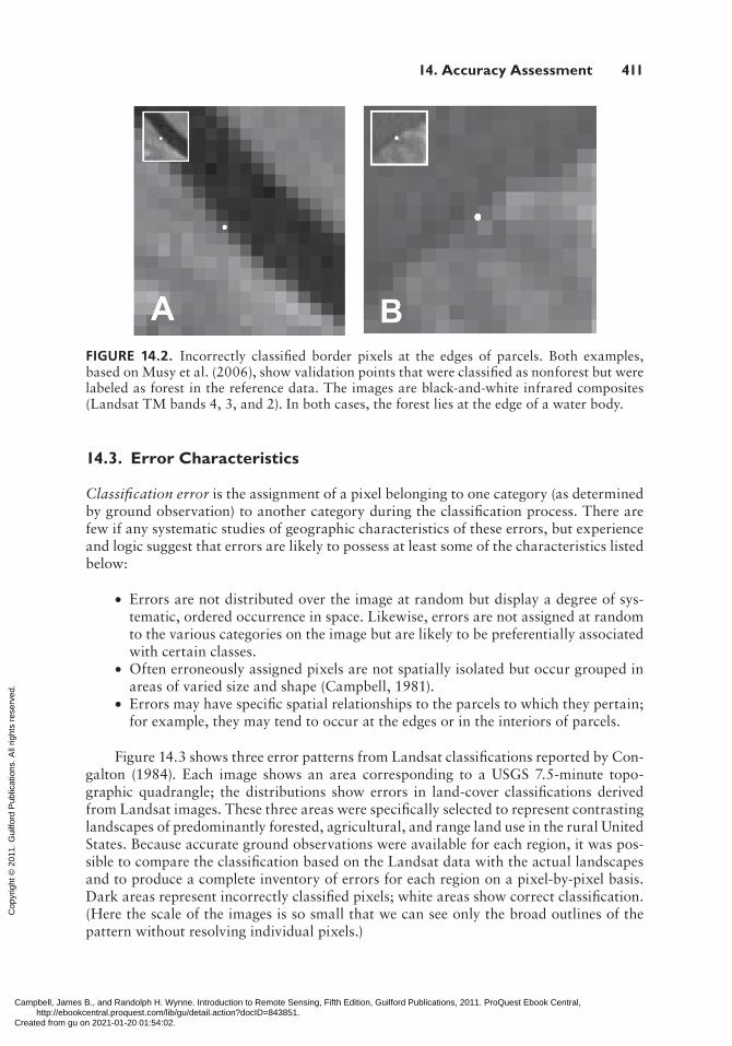
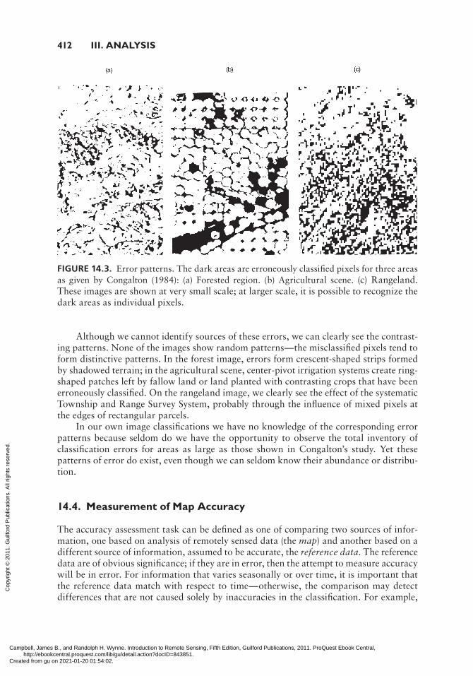
Figure 14.3 shows three error patterns from Landsat classifications reported by Con-galton (1984). Each image shows an area corresponding to a USGS 7.5-minute topo-graphic quadrangle; the distributions show errors in land-cover classifications derived from Landsat images. These three areas were specifically selected to represent contrasting landscapes of predominantly forested, agricultural, and range land use in the rural United States. Because accurate ground observations were available for each region, it was pos-sible to compare the classification based on the Landsat data with the actual landscapes and to produce a complete inventory of errors for each region on a pixel-by-pixel basis. Dark areas represent incorrectly classified pixels; white areas show correct classification. (Here the scale of the images is so small that we can see only the broad outlines of the pattern without resolving individual pixels.)

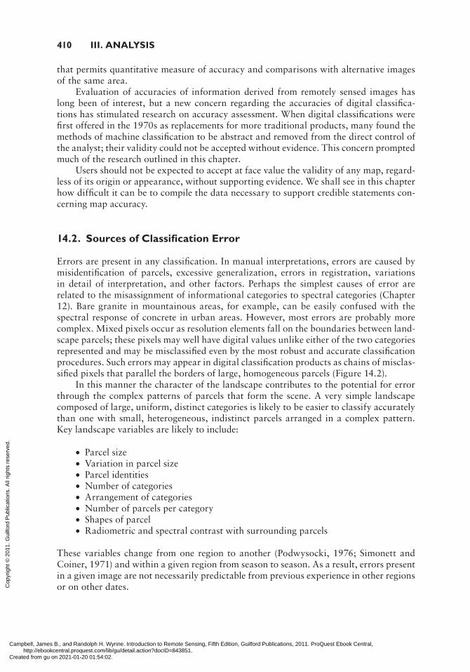
FIGURE 14.2. Incorrectly classified border pixels at the edges of parcels. Both examples, based on Musy et al. (2006), show validation points that were classified as nonforest but were labeled as forest in the reference data. The images are black-and-white infrared composites (Landsat TM bands 4, 3, and 2). In both cases, the forest lies at the edge of a water body.


Cop

yrig

ht ©

201

1. G

uilfo

rd P

ublic

atio

ns. A

ll rig

hts

rese

rved

.

412 iii. anaLYsis

Although we cannot identify sources of these errors, we can clearly see the contrast-ing patterns. None of the images show random patterns—the misclassified pixels tend to form distinctive patterns. In the forest image, errors form crescent-shaped strips formed by shadowed terrain; in the agricultural scene, center-pivot irrigation systems create ring-shaped patches left by fallow land or land planted with contrasting crops that have been erroneously classified. On the rangeland image, we clearly see the effect of the systematic Township and Range Survey System, probably through the influence of mixed pixels at the edges of rectangular parcels.

In our own image classifications we have no knowledge of the corresponding error patterns because seldom do we have the opportunity to observe the total inventory of classification errors for areas as large as those shown in Congalton’s study. Yet these patterns of error do exist, even though we can seldom know their abundance or distribu-tion.

14.4. Measurement of Map accuracy

The accuracy assessment task can be defined as one of comparing two sources of infor-mation, one based on analysis of remotely sensed data (the map) and another based on a different source of information, assumed to be accurate, the reference data. The reference data are of obvious significance; if they are in error, then the attempt to measure accuracy will be in error. For information that varies seasonally or over time, it is important that the reference data match with respect to time—otherwise, the comparison may detect differences that are not caused solely by inaccuracies in the classification. For example,

FIGURE 14.3. Error patterns. The dark areas are erroneously classified pixels for three areas as given by Congalton (1984): (a) Forested region. (b) Agricultural scene. (c) Rangeland. These images are shown at very small scale; at larger scale, it is possible to recognize the dark areas as individual pixels.


Cop

yrig

ht ©

201

1. G

uilfo

rd P

ublic

atio

ns. A

ll rig

hts

rese

rved

.


some of the differences may not really be errors but simply changes that have occurred during the interval that elapsed between image acquisition and reference data acquisition. In some instances, we may examine two maps simply to decide whether there is a differ-ence, without concluding that one is more accurate than the other. For example, we may compare maps of the same area made from data acquired by different sensors or using different classification protocols. More commonly in such cases, however, we will use reference data applicable to both classifications to determine whether one map is more accurate than the other.

To assess the accuracy of a map, it is necessary that the map and reference data be coregistered, that they both use the same classification system and minimum mapping unit, and that they have been classified at comparable levels of detail. The strategies described here are not appropriate if the two data sources differ with respect to detail, number of categories, or meanings of the categories.

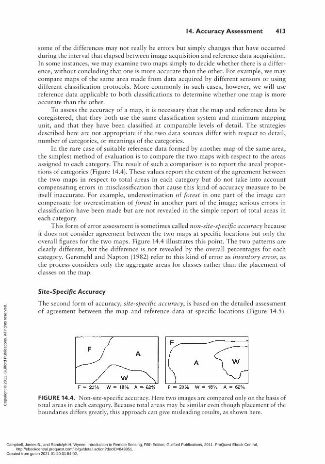
In the rare case of suitable reference data formed by another map of the same area, the simplest method of evaluation is to compare the two maps with respect to the areas assigned to each category. The result of such a comparison is to report the areal propor-tions of categories (Figure 14.4). These values report the extent of the agreement between the two maps in respect to total areas in each category but do not take into account compensating errors in misclassification that cause this kind of accuracy measure to be itself inaccurate. For example, underestimation of forest in one part of the image can compensate for overestimation of forest in another part of the image; serious errors in classification have been made but are not revealed in the simple report of total areas in each category.

This form of error assessment is sometimes called non-site-specific accuracy because it does not consider agreement between the two maps at specific locations but only the overall figures for the two maps. Figure 14.4 illustrates this point. The two patterns are clearly different, but the difference is not revealed by the overall percentages for each category. Gersmehl and Napton (1982) refer to this kind of error as inventory error, as the process considers only the aggregate areas for classes rather than the placement of classes on the map.

Site-Specific Accuracy

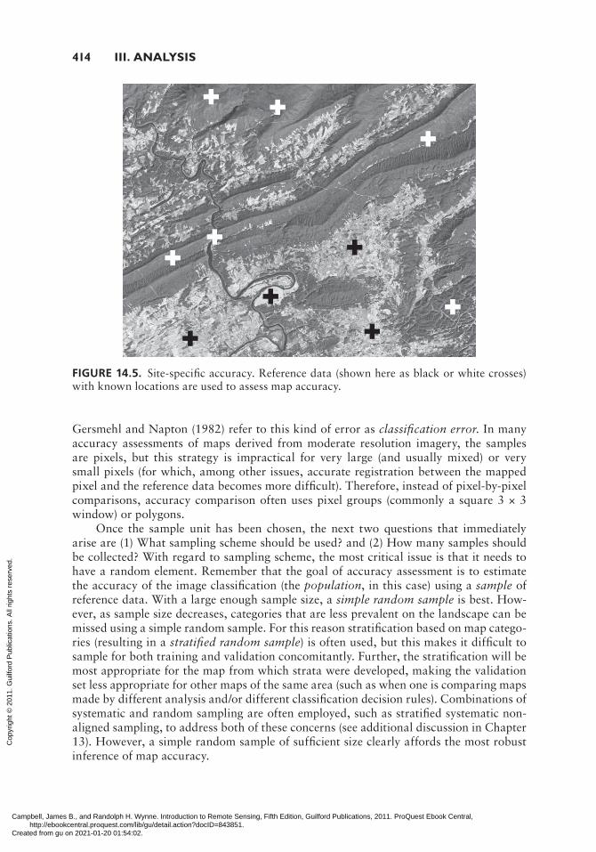
The second form of accuracy, site-specific accuracy, is based on the detailed assessment of agreement between the map and reference data at specific locations (Figure 14.5).

FIGURE 14.4. Non-site-specific accuracy. Here two images are compared only on the basis of total areas in each category. Because total areas may be similar even though placement of the boundaries differs greatly, this approach can give misleading results, as shown here.


Cop

yrig

ht ©

201

1. G

uilfo

rd P

ublic

atio

ns. A

ll rig

hts

rese

rved

.

414 iii. anaLYsis

Gersmehl and Napton (1982) refer to this kind of error as classification error. In many accuracy assessments of maps derived from moderate resolution imagery, the samples are pixels, but this strategy is impractical for very large (and usually mixed) or very small pixels (for which, among other issues, accurate registration between the mapped pixel and the reference data becomes more difficult). Therefore, instead of pixel-by-pixel comparisons, accuracy comparison often uses pixel groups (commonly a square 3 × 3 window) or polygons.

Once the sample unit has been chosen, the next two questions that immediately arise are (1) What sampling scheme should be used? and (2) How many samples should be collected? With regard to sampling scheme, the most critical issue is that it needs to have a random element. Remember that the goal of accuracy assessment is to estimate the accuracy of the image classification (the population, in this case) using a sample of reference data. With a large enough sample size, a simple random sample is best. How-ever, as sample size decreases, categories that are less prevalent on the landscape can be missed using a simple random sample. For this reason stratification based on map catego-ries (resulting in a stratified random sample) is often used, but this makes it difficult to sample for both training and validation concomitantly. Further, the stratification will be most appropriate for the map from which strata were developed, making the validation set less appropriate for other maps of the same area (such as when one is comparing maps made by different analysis and/or different classification decision rules). Combinations of systematic and random sampling are often employed, such as stratified systematic non-aligned sampling, to address both of these concerns (see additional discussion in Chapter 13). However, a simple random sample of sufficient size clearly affords the most robust inference of map accuracy.

FIGURE 14.5. Site-specific accuracy. Reference data (shown here as black or white crosses) with known locations are used to assess map accuracy.


Cop

yrig

ht ©

201

1. G

uilfo

rd P

ublic

atio

ns. A

ll rig

hts

rese

rved

.


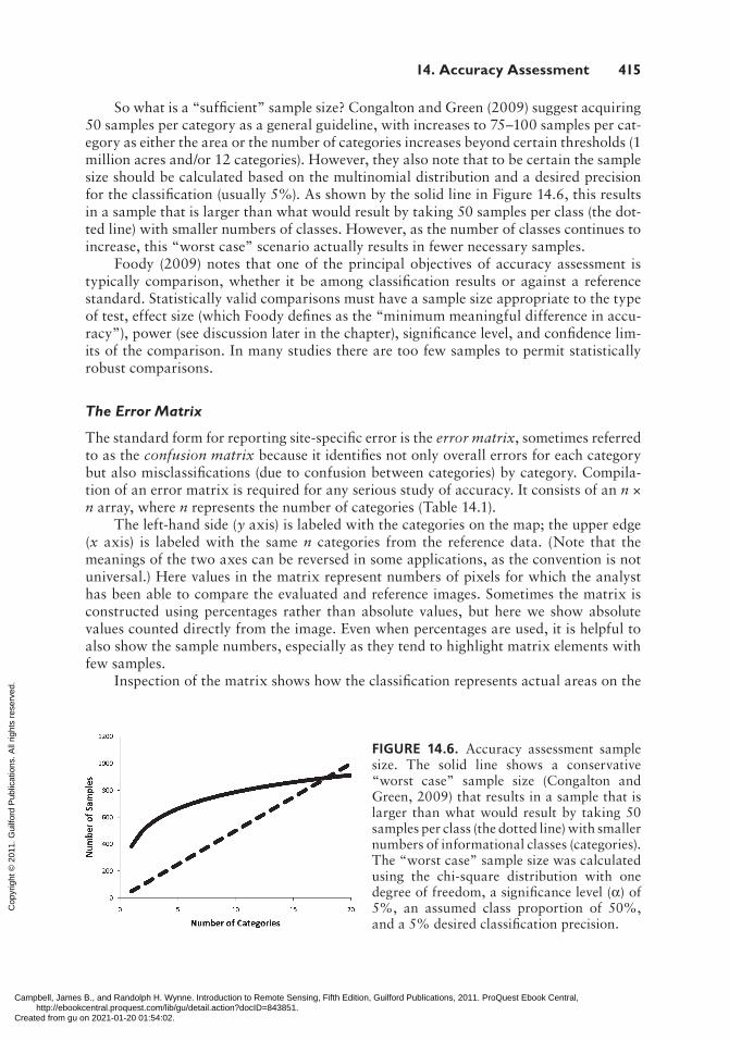
So what is a “sufficient” sample size? Congalton and Green (2009) suggest acquiring 50 samples per category as a general guideline, with increases to 75–100 samples per cat-egory as either the area or the number of categories increases beyond certain thresholds (1 million acres and/or 12 categories). However, they also note that to be certain the sample size should be calculated based on the multinomial distribution and a desired precision for the classification (usually 5%). As shown by the solid line in Figure 14.6, this results in a sample that is larger than what would result by taking 50 samples per class (the dot-ted line) with smaller numbers of classes. However, as the number of classes continues to increase, this “worst case” scenario actually results in fewer necessary samples.

Foody (2009) notes that one of the principal objectives of accuracy assessment is typically comparison, whether it be among classification results or against a reference standard. Statistically valid comparisons must have a sample size appropriate to the type of test, effect size (which Foody defines as the “minimum meaningful difference in accu-racy”), power (see discussion later in the chapter), significance level, and confidence lim-its of the comparison. In many studies there are too few samples to permit statistically robust comparisons.

The Error Matrix

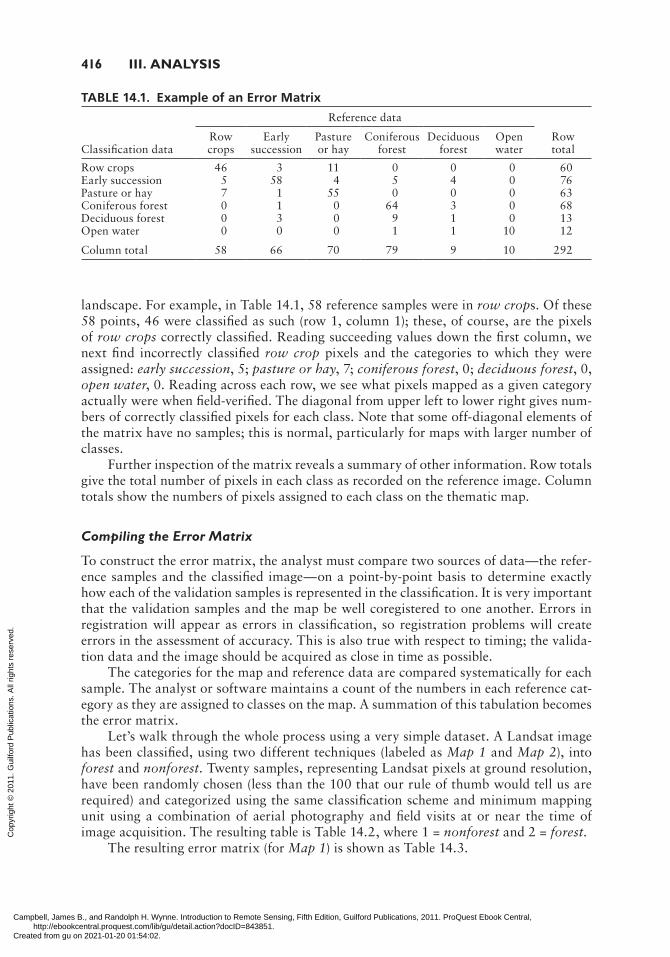
The standard form for reporting site-specific error is the error matrix, sometimes referred to as the confusion matrix because it identifies not only overall errors for each category but also misclassifications (due to confusion between categories) by category. Compila-tion of an error matrix is required for any serious study of accuracy. It consists of an n × n array, where n represents the number of categories (Table 14.1).

The left-hand side (y axis) is labeled with the categories on the map; the upper edge (x axis) is labeled with the same n categories from the reference data. (Note that the meanings of the two axes can be reversed in some applications, as the convention is not universal.) Here values in the matrix represent numbers of pixels for which the analyst has been able to compare the evaluated and reference images. Sometimes the matrix is constructed using percentages rather than absolute values, but here we show absolute values counted directly from the image. Even when percentages are used, it is helpful to also show the sample numbers, especially as they tend to highlight matrix elements with few samples.

Inspection of the matrix shows how the classification represents actual areas on the

FIGURE 14.6. Accuracy assessment sample size. The solid line shows a conservative “worst case” sample size (Congalton and Green, 2009) that results in a sample that is larger than what would result by taking 50 samples per class (the dotted line) with smaller numbers of informational classes (categories). The “worst case” sample size was calculated using the chi-square distribution with one degree of freedom, a significance level (α) of 5%, an assumed class proportion of 50%, and a 5% desired classification precision.


Cop

yrig

ht ©

201

1. G

uilfo

rd P

ublic

atio

ns. A

ll rig

hts

rese

rved

.

416 III. ANALYSIS

landscape. For example, in Table 14.1, 58 reference samples were in row crops. Of these 58 points, 46 were classified as such (row 1, column 1); these, of course, are the pixels of row crops correctly classified. Reading succeeding values down the first column, we next find incorrectly classified row crop pixels and the categories to which they were assigned: early succession, 5; pasture or hay, 7; coniferous forest, 0; deciduous forest, 0, open water, 0. Reading across each row, we see what pixels mapped as a given category actually were when field-verified. The diagonal from upper left to lower right gives num-bers of correctly classified pixels for each class. Note that some off-diagonal elements of the matrix have no samples; this is normal, particularly for maps with larger number of classes.

Further inspection of the matrix reveals a summary of other information. Row totals give the total number of pixels in each class as recorded on the reference image. Column totals show the numbers of pixels assigned to each class on the thematic map.

Compiling the Error Matrix

To construct the error matrix, the analyst must compare two sources of data—the refer-ence samples and the classified image—on a point-by-point basis to determine exactly how each of the validation samples is represented in the classification. It is very important that the validation samples and the map be well coregistered to one another. Errors in registration will appear as errors in classification, so registration problems will create errors in the assessment of accuracy. This is also true with respect to timing; the valida-tion data and the image should be acquired as close in time as possible.

The categories for the map and reference data are compared systematically for each sample. The analyst or software maintains a count of the numbers in each reference cat-egory as they are assigned to classes on the map. A summation of this tabulation becomes the error matrix.

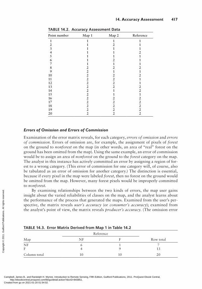
Let’s walk through the whole process using a very simple dataset. A Landsat image has been classified, using two different techniques (labeled as Map 1 and Map 2), into forest and nonforest. Twenty samples, representing Landsat pixels at ground resolution, have been randomly chosen (less than the 100 that our rule of thumb would tell us are required) and categorized using the same classification scheme and minimum mapping unit using a combination of aerial photography and field visits at or near the time of image acquisition. The resulting table is Table 14.2, where 1 = nonforest and 2 = forest.

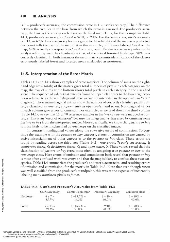
The resulting error matrix (for Map 1) is shown as Table 14.3.

TABLE 14.1. Example of an Error Matrix

Reference data

Classification data

Row crops

Early succession

Pasture or hay

Coniferous forest

Deciduous forest

Open water

Row total

Row crops 46 3 11 0 0 0 60Early succession 5 58 4 5 4 0 76Pasture or hay 7 1 55 0 0 0 63Coniferous forest 0 1 0 64 3 0 68Deciduous forest 0 3 0 9 1 0 13Open water 0 0 0 1 1 10 12

Column total 58 66 70 79 9 10 292


Cop

yrig

ht ©

201

1. G

uilfo

rd P

ublic

atio

ns. A

ll rig

hts

rese

rved

.


Errors of Omission and Errors of Commission

Examination of the error matrix reveals, for each category, errors of omission and errors of commission. Errors of omission are, for example, the assignment of pixels of forest on the ground to nonforest on the map (in other words, an area of “real” forest on the ground has been omitted from the map). Using the same example, an error of commission would be to assign an area of nonforest on the ground to the forest category on the map. The analyst in this instance has actively committed an error by assigning a region of for-est to a wrong category. (This error of commission for one category will, of course, also be tabulated as an error of omission for another category.) The distinction is essential, because if every pixel in the map were labeled forest, then no forest on the ground would be omitted from the map. However, many forest pixels would be improperly committed to nonforest.

By examining relationships between the two kinds of errors, the map user gains insight about the varied reliabilities of classes on the map, and the analyst learns about the performance of the process that generated the maps. Examined from the user’s per-spective, the matrix reveals user’s accuracy (or consumer’s accuracy); examined from the analyst’s point of view, the matrix reveals producer’s accuracy. (The omission error

TABLE 14.2. Accuracy Assessment Data

Point number Map 1 Map 2 Reference

1 1 1 1 2 1 2 1 3 1 1 1 4 1 1 2 5 1 1 1 6 1 2 1 7 1 1 1 8 2 2 2 9 2 1 110 2 2 211 2 2 112 2 2 113 2 2 214 2 1 215 2 1 116 2 2 217 2 2 218 2 2 219 2 2 220 2 2 2

TABLE 14.3. Error Matrix Derived from Map 1 in Table 14.2

Reference

Map NF F Row total

NF 6 1 7F 4 9 13

Column total 10 10 20


Cop

yrig

ht ©

201

1. G

uilfo

rd P

ublic

atio

ns. A

ll rig

hts

rese

rved

.

418 iii. anaLYsis

is 1 – producer’s accuracy; the commission error is 1 – user’s accuracy.) The difference between the two lies in the base from which the error is assessed. For producer’s accu-racy, the base is the area in each class on the final map. Thus, for the example in Table 14.3, producer’s accuracy for forest is 9/10, or 90%. For the same class, user’s accuracy is 9/13, or 69%. User’s accuracy forms a guide to the reliability of the map as a predictive device—it tells the user of the map that in this example, of the area labeled forest on the map, 69% actually corresponds to forest on the ground. Producer’s accuracy informs the analyst who prepared the classification that, of the actual forested landscape, 90% was correctly classified. In both instances the error matrix permits identification of the classes erroneously labeled forest and forested areas mislabeled as nonforest.

14.5. interpretation of the error Matrix

Tables 14.1 and 14.3 show examples of error matrices. The column of sums on the right-hand edge (row totals) of the matrix gives total numbers of pixels in each category on the map; the row of sums at the bottom shows total pixels in each category in the classified scene. The sequence of values that extends from the upper left corner to the lower right cor-ner is referred to as the main diagonal (here we are not interested in the opposite, or “anti” diagonal). These main diagonal entries show the number of correctly classified pixels: row crops classified as row crops, open water as open water, and so on. Nondiagonal values in each column give errors of omission. For example, as we read down the third column (Table 14.1), we see that 11 of 70 reference samples in pasture or hay were mapped as row crops. This is an “error of omission” because the image analyst has erred by omitting some pasture or hay from the interpreted image. More specifically, we know that pasture or hay is most likely to be misclassified as row crops on the classified image.

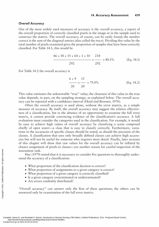
In contrast, nondiagonal values along the rows give errors of commission. To con-tinue the example with the pasture or hay category, errors of commission are caused by active misassignment of other categories to the pasture or hay class. These errors are found by reading across the third row (Table 14.1): row crops, 7; early succession, 1; coniferous forest, 0; deciduous forest, 0; and open water, 0. These values reveal that the classification of pasture or hay erred most often by assigning true pasture or hay to the row crops class. Here errors of omission and commission both reveal that pasture or hay is most often confused with row crops and that the map is likely to confuse these two cat-egories. Table 14.4 summarizes the producer’s and user’s accuracies, and resulting errors of omission and commission, for the matrix in Table 14.3. Note that even though forest was well classified from the producer’s standpoint, this was at the expense of incorrectly labeling many nonforest pixels as forest.

TABLE 14.4. User’s and Producer’s Accuracies from Table 14.3

User’s accuracy Commission error Producer’s accuracy Omission error

Nonforest 6 ÷ 7 = 85.7%

1 –85.7% = 14.3%

6 ÷ 10 = 60.0%

1 – 60% = 40.0%

Forest 9 ÷ 13 = 69.2%

1 –69.2% = 30.8%

9/10 90.0%

1 – 90% = 10.0%


Cop

yrig

ht ©

201

1. G

uilfo

rd P

ublic

atio

ns. A

ll rig

hts

rese

rved

.


Overall Accuracy

One of the most widely used measures of accuracy is the overall accuracy, a report of the overall proportion of correctly classified pixels in the image or in the sample used to construct the matrix. The overall accuracy, of course, can be easily found; the number correct is the sum of the diagonal entries (also called the trace). Dividing this value by the total number of pixels examined gives the proportion of samples that have been correctly classified. For Table 14.1, this would be

46 + 58 + 55 + 64 + 1 + 10 234 (Eq. 14.1)

= = 80.1% 292 292

For Table 14.2 the overall accuracy is

6 + 9 15 (Eq. 14.2)

= = 75.0% 20 20

This value estimates the unknowable “true” value; the closeness of this value to the true value depends, in part, on the sampling strategy, as explained below. The overall accu-racy can be reported with a confidence interval (Hord and Brooner, 1976).

Often the overall accuracy is used alone, without the error matrix, as a simple measure of accuracy. By itself, the overall accuracy may suggest the relative effective-ness of a classification, but in the absence of an opportunity to examine the full error matrix, it cannot provide convincing evidence of the classification’s accuracy. A full evaluation must consider the categories used in the classification. For example, it would be easy to achieve high values of overall accuracy by classifying a scene composed chiefly of open water—a class that is easy to classify correctly. Furthermore, varia-tions in the accuracies of specific classes should be noted, as should the precision of the classes. A classification that uses only broadly defined classes can achieve high accura-cies but will not be useful for someone who requires more detail. Finally, later sections of this chapter will show that raw values for the overall accuracy can be inflated by chance assignment of pixels to classes—yet another reason for careful inspection of the assessment task.

Hay (1979) stated that it is necessary to consider five questions to thoroughly under-stand the accuracy of a classification:

What proportion of the classification decision is correct?••What proportion of assignments to a given category is correct?••What proportion of a given category is correctly classified?••Is a given category overestimated or underestimated?••Are errors randomly distributed?••

“Overall accuracy” can answer only the first of these questions; the others can be answered only by examination of the full error matrix.


Cop

yrig

ht ©

201

1. G

uilfo

rd P

ublic

atio

ns. A

ll rig

hts

rese

rved

.

420 iii. anaLYsis

Quantitative Assessment of the Error Matrix

After an initial inspection of the error matrix reveals the overall nature of the errors present, there is often a need for a more objective assessment of the classification. For example, we may ask if the two maps are in agreement—a question that is very difficult to answer because the notion of “agreement” may be difficult to define and implement. The error matrix is an example of a more general class of matrices, known as contingency tables, which summarize classifications analogous to those considered here. Some of the procedures that have been developed for analyzing contingency tables can be applied to examination of the error matrix.

Chrisman (1980), Congalton and Mead (1983), and Congalton et al. (1983) pro-pose application of techniques described by Bishop et al. (1975) and Cohen (1960) as a means of improving interpretation of the error matrix. A shortcoming of usual inter-pretations of the error matrix is that even chance assignments of pixels to classes can result in surprisingly good results, as measured by overall accuracy. Hord and Brooner (1976) and others have noted that the use of such measures is highly dependent on the samples, and therefore on the sampling strategy used to derive the observations used in the analysis.

κ (kappa) is a measure of the difference between the observed agreement between two maps (as reported by the diagonal entries in the error matrix) and the agreement that might be attained solely by chance matching of the two maps. Not all agreement can be attributed to the success of the classification. κ attempts to provide a measure of agree-ment that is adjusted for chance agreement. κ is estimated by κ̂ (“k hat”):

Observed – expected (Eq. 14.3)

κ̂ = 1 – expected

This form of the equation, given by Chrisman (1980) and others, is a simplified version of the more complete form given by Bishop et al. (1975). Here observed designates the accuracy reported in the error matrix, and expected designates the correct classification that can be anticipated by change agreement between the two images.

Observed is the value for “overall accuracy” defined previously: the sum of the diagonal entries divided by the total number of samples. Expected is an estimate of the contribution of chance agreement to the observed overall accuracy. Expected values are calculated using the row and column totals. Products of row and column totals (Table 14.5) estimate the numbers of pixels assigned to each cell in the confusion matrix, given that pixels are assigned by chance to each category. This is perhaps clearer if we consider the situation in its spatial context (Figure 14.7). The row and column totals can be seen

TABLE 14.5. Calculating Products of Row and Column Totals Using Table 14.3

Nonforest column total Forest column total

Nonforest row total 10 × 7 = 70

10 × 7 = 70

Forest row total 10 × 13 = 130

10 × 13 = 130


Cop

yrig

ht ©

201

1. G

uilfo

rd P

ublic

atio

ns. A

ll rig

hts

rese

rved

.


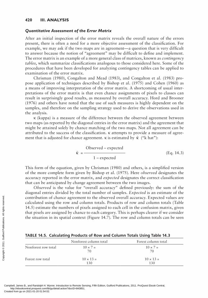
to represent areas occupied by each of the categories on the reference map and the image, and the chance mapping of any two categories is the product of their proportional extents on the two maps.

The expected correct, based on chance mapping, is found by summing the diagonals in the (row total × column total) product matrix, then dividing by the grand total of prod-ucts of row and column totals, for example,

Trace of product matrix 70 + 130 200 (Eq. 14.4)

= = = 50.0% Cumulative sum of product matrix 70 + 70 + 130 + 130 400

This estimate for expected correct can be compared with the overall accuracy or observed value (75%) calculated in Equation 14.2. κ̂ for the error matrix shown in Table 14.2 is then calculated as follows:

Observed – expected 75% – 50% 25% (Eq. 14.5)

κ̂ = = = = 50.0% 1 – expected 100% – 50% 50%

κ̂ in effect adjusts the overall accuracy measure by subtracting the estimated con-tribution of chance agreement. Thus κ̂ = 0.50 can be interpreted to mean that the clas-sification achieved an accuracy that is 50% better than would be expected from chance assignment of pixels to categories. As the overall accuracy approaches 100, and as the contribution of chance agreement approaches 0, the value of κ̂ approaches positive 1.0 (100%), indicating the perfect effectiveness of the classification (Table 14.6). On the other hand, as the effect of chance agreement increases and the overall accuracy decreases, κ̂ can assume negative values.

FIGURE 14.7. Contrived example illustrating computation of chance agreement of two cat-egories when two images are superimposed. Here p(A) and p(B) would correspond to row and column marginals; their product estimates the agreement expected by chance matching of the two areas.


Cop

yrig

ht ©

201

1. G

uilfo

rd P

ublic

atio

ns. A

ll rig

hts

rese

rved

.

422 iii. anaLYsis

κ̂ and related coefficients have been discussed by Rosenfield and Fitzpatrick-Lins (1986), Foody (1992), and Ma and Redmond (1995). According to Cohen (1960), any negative value indicates a poor classification, but the possible range of negative values depends on the specific matrix evaluated. Thus the magnitude of a negative value should not be closely interpreted as an indication of the performance of the classification. Values near zero suggest that the contribution of chance is equal to the effect of the classification and that the classification process yields no better results than would a chance assignment of pixels to classes. κ̂ is asymptotically normally distributed.

One of the substantial benefits of calculating kappa is that the large sample variance can be estimated, then used in a z test to determine whether individual κ̂ scores differ

TABLE 14.6. Contrived Matrices Illustrating


Cop

yrig

ht ©

201

1. G

uilfo

rd P

ublic

atio

ns. A

ll rig

hts

rese

rved

.


significantly from one another. Students should read the article by Hudson and Ramm (1987) as they consider using these methods, especially as the variance equation was incorrect in the original (Cohen, 1960) paper (Foody, 2009). Unfortunately, even if one uses the appropriate method for sample variance calculation, comparing two classifica-tions using κ̂ and its variance 2ˆ

κs for each requires sample independence. The McNemar test (Foody, 2004; Foody, 2009) is extensively used as a nonparametric alternative for comparing thematic maps using the same validation dataset. The test requires a particu-lar “cross-tabulation” of the thematic maps, as shown in Table 14.7.

The McNemar calculation of z (the standard score) is then given as Equation 14.6:

b c

zb c

−=+

(Eq. 14.6)

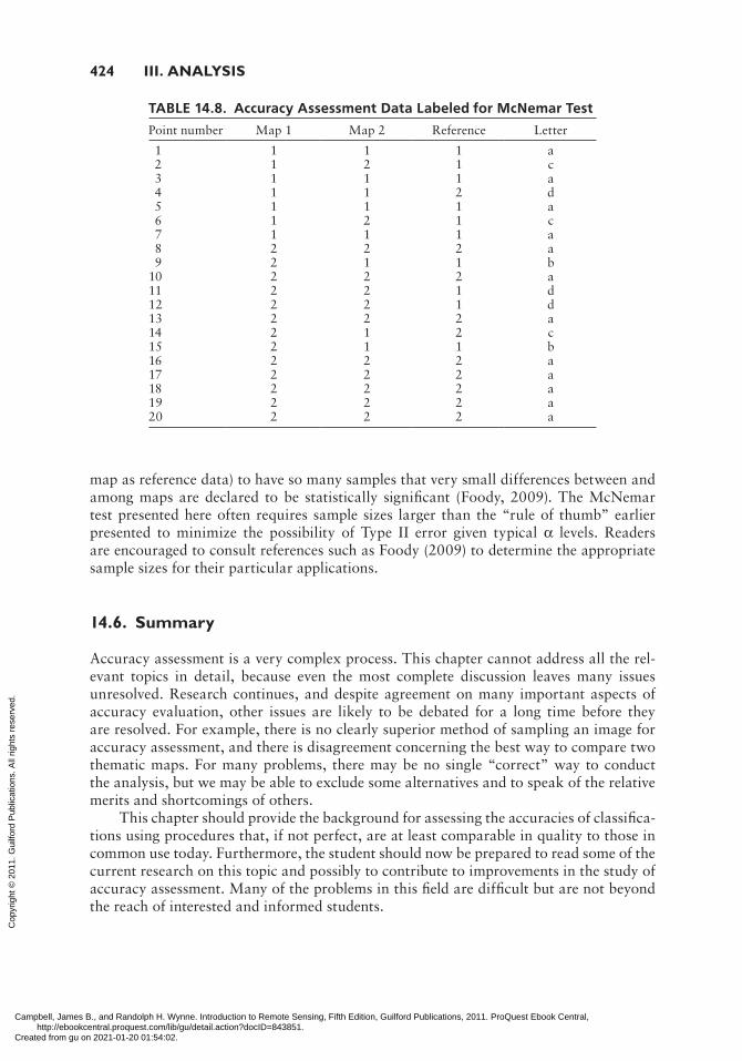
Let’s look at an example using the data in Table 14.2, repeated as Table 14.8 with an additional column added to denote the appropriate matrix element (denoted by letter a, b, c, or d) in Table 14.7 (again with the caveat that the sample size is far too small). Let’s look at the first and second rows as examples. In the first row, both maps are correct (both they and the validation point were placed in category 1, nonforest). Looking at Table 14.7, if both maps are correct, then the appropriate matrix element is a, so we place an a in the Letter column. In the second row, the first map is correct, and the second map is not. In Table 14.7, this would make it matrix element c.

The McNemar statistic is now easily calculated using equation 14.6 and the number of b’s (2) and c’s (3) we found in constructing Table 14.8, to wit:

2 3

0.452 3

b cz

b c

− −= = = −+ −

(Eq. 14.7)

Let’s assume, per Foody (2009), that the maps will be stated to be statistically different from one another at α (the predetermined probability of making a Type I error, defined in this instance as incorrectly stating that the maps are different when in fact they are not) = 0.05 if |z| > 1.96 (two-tailed test). As such, since |–0.45| is not greater than 1.96, the maps are not different from one another. It should be noted that although this is a common a level, there is no one level that is appropriate for all studies. Besides α = 0.05, another common value for α is 0.01, in which case (for the two-tailed test) |z| must be greater than 2.58.

Although it is often ignored by researchers and practitioners, Type II error (its prob-ability denoted by β) occurs when there really is a noteworthy difference between maps that is not detected. The power of the test is then 1 – β. As one increases the desired power and decreases the desired α, a larger sample size is required. Many, if not most, accuracy assessments contain too few samples, though it is possible (when, say, using another

TABLE 14.7. McNemar’s Test Cross Tabulation

Map 1

Map 2 Correct Incorrect

Correct a b

Incorrect c d


Cop

yrig

ht ©

201

1. G

uilfo

rd P

ublic

atio

ns. A

ll rig

hts

rese

rved

.

424 iii. anaLYsis

map as reference data) to have so many samples that very small differences between and among maps are declared to be statistically significant (Foody, 2009). The McNemar test presented here often requires sample sizes larger than the “rule of thumb” earlier presented to minimize the possibility of Type II error given typical α levels. Readers are encouraged to consult references such as Foody (2009) to determine the appropriate sample sizes for their particular applications.

14.6. summary

Accuracy assessment is a very complex process. This chapter cannot address all the rel-evant topics in detail, because even the most complete discussion leaves many issues unresolved. Research continues, and despite agreement on many important aspects of accuracy evaluation, other issues are likely to be debated for a long time before they are resolved. For example, there is no clearly superior method of sampling an image for accuracy assessment, and there is disagreement concerning the best way to compare two thematic maps. For many problems, there may be no single “correct” way to conduct the analysis, but we may be able to exclude some alternatives and to speak of the relative merits and shortcomings of others.

This chapter should provide the background for assessing the accuracies of classifica-tions using procedures that, if not perfect, are at least comparable in quality to those in common use today. Furthermore, the student should now be prepared to read some of the current research on this topic and possibly to contribute to improvements in the study of accuracy assessment. Many of the problems in this field are difficult but are not beyond the reach of interested and informed students.

TABLE 14.8. Accuracy Assessment Data Labeled for McNemar Test

Point number Map 1 Map 2 Reference Letter

1 1 1 1 a 2 1 2 1 c 3 1 1 1 a 4 1 1 2 d 5 1 1 1 a 6 1 2 1 c 7 1 1 1 a 8 2 2 2 a 9 2 1 1 b10 2 2 2 a11 2 2 1 d12 2 2 1 d13 2 2 2 a14 2 1 2 c15 2 1 1 b16 2 2 2 a17 2 2 2 a18 2 2 2 a19 2 2 2 a20 2 2 2 a


Cop

yrig

ht ©

201

1. G

uilfo

rd P

ublic

atio

ns. A

ll rig

hts

rese

rved

.

14. Accuracy Assessment 425

Review Questions

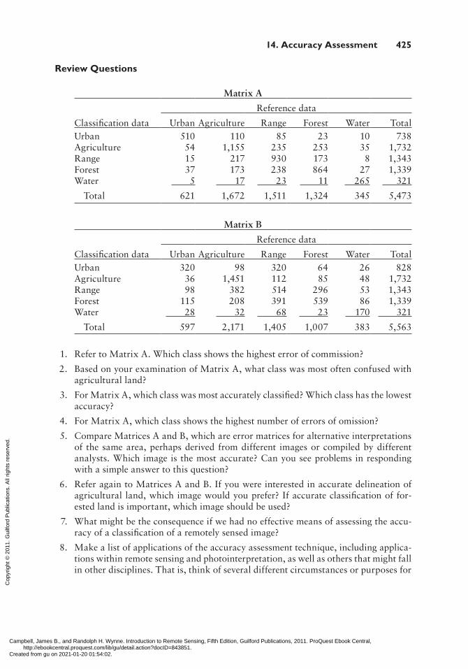
Matrix A

Reference data

Classification data Urban Agriculture Range Forest Water TotalUrban 510 110 85 23 10 738Agriculture 54 1,155 235 253 35 1,732Range 15 217 930 173 8 1,343Forest 37 173 238 864 27 1,339Water 5 17 23 11 265 321

Total 621 1,672 1,511 1,324 345 5,473

Matrix B

Reference data

Classification data Urban Agriculture Range Forest Water TotalUrban 320 98 320 64 26 828Agriculture 36 1,451 112 85 48 1,732Range 98 382 514 296 53 1,343Forest 115 208 391 539 86 1,339Water 28 32 68 23 170 321

Total 597 2,171 1,405 1,007 383 5,563

1. Refer to Matrix A. Which class shows the highest error of commission?

2. Based on your examination of Matrix A, what class was most often confused with agricultural land?

3. For Matrix A, which class was most accurately classified? Which class has the lowest accuracy?

4. For Matrix A, which class shows the highest number of errors of omission?

5. Compare Matrices A and B, which are error matrices for alternative interpretations of the same area, perhaps derived from different images or compiled by different analysts. Which image is the most accurate? Can you see problems in responding with a simple answer to this question?

6. Refer again to Matrices A and B. If you were interested in accurate delineation of agricultural land, which image would you prefer? If accurate classification of for-ested land is important, which image should be used?

7. What might be the consequence if we had no effective means of assessing the accu-racy of a classification of a remotely sensed image?

8. Make a list of applications of the accuracy assessment technique, including applica-tions within remote sensing and photointerpretation, as well as others that might fall in other disciplines. That is, think of several different circumstances or purposes for


Cop

yrig

ht ©

201

1. G

uilfo

rd P

ublic

atio

ns. A

ll rig

hts

rese

rved

.

426 iii. anaLYsis

which it might be useful to determine which of two alternative classifications is the more accurate.

9. Discuss key considerations for deciding the sample size appropriate for accuracy assessment of a specific remote sensing project.

10. Calculate producer’s and consumer’s accuracies for agriculture and forested lands as reported in Matrix A.

11. Inspect the contrived matrices shown in Table 14.6, and make a general statement concerning the overall appearance of the matrix and its relationship to the corre-sponding value of kappa for that matrix.

12. Why might the usual statements concerning desired sample sizes for an experiment not be satisfactory in the context of accuracy assessment?

13. If producer’s accuracy and user’s accuracy differ (as they usually do), how can mak-ers and users ever have a common interest in the preparation and use of a specific map?

14. Can you make an argument that, for accuracy assessment, there might be practical value in favoring Type I error over Type II error?

references

Anderson, J. R., E. E. Hardy, J. T. Roach, and R. E. Witmer. 1976. A Land Use and Land Cover Classification for Use with Remote Sensor Data (U.S. Geological Survey Profes-sional Paper 964). Washington, DC: U.S. Government Printing Office, 28 pp.

Bishop, Y. M. M., S. E. Fienber, and P. W. Holland. 1975. Discrete Multivariate Analysis: Theory and Practice. Cambridge, MA: MIT Press, 557 pp.

Campbell, J. B. 1981. Spatial Correlation Effects upon Accuracy of Supervised Classifica-tion of Land Cover. Photogrammetric Engineering and Remote Sensing, Vol. 47, pp. 355–363.

Card, D. H. 1982. Using Known Map Category Marginal Frequencies to Improve Estimates of Thematic Map Accuracy. Photogrammetric Engineering and Remote Sensing, Vol. 48. pp. 431–439.

Chrisman, N. R. 1980. Assessing Landsat Accuracy: A Geographic Application of Misclas-sification Analysis. In Second Colloquium on Quantitative and Theoretical Geography. Cambridge, UK.

Cohen, J. 1960. A Coefficient of Agreement for Nominal Scales. Educational and Psychologi-cal Measurement, Vol. 20, No. 1, pp. 37–40.

Congalton, R. G. 1984. A Comparison of Five Sampling Schemes Used in Assessing the Accuracy of Land Cover/Land Use Maps Derived from Remotely Sensed Data. PhD. Dissertation, Virginia Polytechnic Institute and State University, Blacksburg, VA. 147 pp.

Congalton, R. G. 1988. A Comparison of Sampling Schemes Used in Generating Error Matri-ces for Assessing the Accuracy Maps Generated from Remotely Sensed Data. Photo-grammetric Engineering and Remote Sensing, Vol. 54, pp. 593–600.

Congalton, R. G. 1988. Using Spatial Autocorrelation Analysis to Explore the Errors in Maps Generated from Remotely Sensed Data. Photogrammetric Engineering and Remote Sensing, Vol. 54, pp. 587–592.


Cop

yrig

ht ©

201

1. G

uilfo

rd P

ublic

atio

ns. A

ll rig

hts

rese

rved

.


Congalton, R. G., and K. Green. 2009. Assessing the Accuracy of Remotely Sensed Data: Principles and Practices (2nd ed.). Boca Raton, FL: CRC Press, 183 pp.

Congalton, R. G., and R. A. Mead. 1983. A Quantitative Method to Test for Consistency and Correctness in Photointerpretation. Photogrammetric Engineering and Remote Sensing, Vol. 49, pp. 69–74.

Congalton, R. G., R. G. Oderwald, and R. A. Mead. 1983. Assessing Landsat Classification Accuracy Using Discrete Multivariate Analysis Statistical Techniques. Photogrammetric Engineering and Remote Sensing, Vol. 49, pp. 1671–1687.

Fitzpatrick-Lins, K. 1978. Accuracy and Consistency Comparisons of Land Use and Land Cover Maps Made from High-Altitude Photographs and Landsat Multispectral Imagery. Journal of Research, U.S. Geological Survey, Vol. 6, pp. 23–40.

Foody, G. M. 1992. On the Compensation for Chance Agreement in Image Classification Accuracy Assessment. Photogrammetric Engineering and Remote Sensing, Vol. 58, pp. 1459–1460.

Foody, G. M. 2004. Thematic Map Comparison: Evaluating the Statistical Significance of Differences in Classification Accuracy. Photogrammetric Engineering and Remote Sens-ing, Vol. 70, pp. 627–633.

Foody, G. M. 2009. Sample size determination for image classification accuracy assessment and comparison. International Journal of Remote Sensing, Vol. 30, pp. 5273–5291.

Ginevan, M. E. 1979. Testing Land-Use Map Accuracy: Another Look. Photogrammetric Engineering and Remote Sensing, Vol. 45, pp. 1371–1377.

Hay, A. 1979. Sampling Designs to Test Land Use Map Accuracy. Photogrammetric Engi-neering and Remote Sensing, Vol. 45, pp. 529–533.

Hord, R. M., and W. Brooner. 1976. Land Use Map Accuracy Criteria. Photogrammetric Engineering and Remote Sensing, Vol. 46, pp. 671–677.

Hudson, W. D., and C. W. Ramm. 1987. Correct Formulation of the Kappa Coefficient of Agreement. Photogrammetric Engineering and Remote Sensing, Vol. 53, pp. 421–422.

Janssen, L. L. F., and F. J. M. van der Wel. 1994. Accuracy Assessment of Satellite Derived Land Cover Data: A Review. Photogrammetric Engineering and Remote Sensing, Vol. 60, pp. 419–426.

Lhermitte, S., J. Verbesselt, I. Jonckheere, K. Nachaerts, J. A. N. Van Aardt, W. W. Verstra-eten, and P. Coppin. 2008. Hierarchical Image Segmentation Based upon Similarity of NDVI Time Series. Remote Sensing of Environment, Vol. 112, pp. 506–521.

Ma, Z., and R. L. Redmond. 1995. Tau Coefficients for Accuracy Assessment of Classifica-tion of Remotely Sensed Data. Photogrammetric Engineering and Remote Sensing, Vol. 61, pp. 435–439.

McNemar, Q. 1947. Note on the Sampling Error of the Difference between Correlated pro-portions or Percentages. Psychometrika, Vol. 12, pp. 153–157.

Musy, R. F., R. H. Wynne, C. E. Blinn, and J. A. Scrivani. 2006. Automated Forest Area Estimation via Iterative Guided Spectral Class Rejection. Photogrammetric Engineering and Remote Sensing, Vol. 72 pp. 949–960.

Podwysocki, M. H. 1976. An Estimate of Field Size Distribution for Selected Sites in Major Grain Producing Countries (Publication No. X-923-76-93). Greenbelt, MD: Goddard Space Flight Center, 34 pp.

Quirk, B. K., and F. L. Scarpace. 1980. A Method of Assessing Accuracy of a Digital Clas-sification. Photogrammetric Engineering and Remote Sensing, Vol. 46, pp. 1427–1431.

Rosenfield, G. H., and K. Fitzpatrick-Lins. 1986. A Coefficient of Agreement as a Measure of Thematic Map Classification Accuracy. Photogrammetric Engineering and Remote Sensing, Vol. 52, pp. 223–227.


Cop

yrig

ht ©

201

1. G

uilfo

rd P

ublic

atio

ns. A

ll rig

hts

rese

rved

.

428 iii. anaLYsis

Rosenfield, G. H., K. Fitzpatrick-Lins, and H. S. Ling. 1982. Sampling for Thematic Map Accuracy Testing. Photogrammetric Engineering and Remote Sensing, Vol. 48, pp. 131–137.

Simonett, D. S., and J. C. Coiner. 1971. Susceptibility of Environments to Low Resolution Imaging for Land Use Mapping. In Proceedings of the Seventh International Sympo-sium on Remote Sensing of Environment. Ann Arbor: University of Michigan Press, pp. 373–394.

Skidmore, A. K., and B. J. Turner. 1992. Map Accuracy Assessment Using Line Intersect Sam-pling. Photogrammetric Engineering and Remote Sensing, Vol. 58, pp. 1453–1457.

Stehman, S. V. 1992. Comparison of Systematic and Random Sampling for Estimating the Accuracy of Maps Generated from Remotely Sensed Data. Photogrammetric Engineer-ing and Remote Sensing, Vol. 58, pp. 1343–1350.

Stehman, S. 1997. Selecting and Interpreting Measures of Thematic Map Accuracy. Remote Sensing of Environment, Vol. 62, pp. 77–89.

Stehman, S. V. 2004. A Critical Evaluation of the Normalized Error Matrix in Map Accuracy Assessment. Photogrammetric Engineering and Remote Sensing, Vol. 70, pp. 743–751.

Stehman, S. V., and R. L. Czaplewski. 1998. Design and Analysis for Thematic Map Accu-racy Assessment: Fundamental Principles. Remote Sensing of Environment, Vol. 64, pp. 331–344.

Story, M., and R. G. Congalton. 1986. Accuracy Assessment: A User’s Perspective. Photo-grammetric Engineering and Remote Sensing, Vol. 52, pp. 397–399.

Todd, W. J., D. G. Gehring, and J. F. Haman. 1980. Landsat Wildland Mapping Accuracy. Photogrammetric Engineering and Remote Sensing, Vol. 46, pp. 509–520.

Tom, C., L. D. Miller, and J. W. Christenson. 1978. Spatial Land-Use Inventory, Model-ing, and Projection: Denver Metropolitan Area, with Inputs from Existing Maps, Air-photos, and Landsat Imagery (NASA Technical Memorandum 79710). Greenbelt, MD: Goddard Space Flight Center, 225 pp.

Turk, G. 1979. GT Index: A Measure of the Success of Prediction. Remote Sensing of Envi-ronment, Vol. 8, pp. 65–75.

Van der Wel, F. J. M., and L. L. F. Janssen. 1994. A Short Note on Pixel Sampling of Remotely Sensed Digital Imagery. Computers and Geosciences, Vol. 20, pp. 1263–1264.

Van Genderen, J., and B. Lock. 1977. Testing Map Use Accuracy. Photogrammetric Engi-neering and Remote Sensing, Vol. 43, pp. 1135–1137.

Webster, R., and P. H. T. Beckett. 1968. Quality and Usefulness of Soil Maps. Nature, Vol. 219, pp. 680–682.


Cop

yrig

ht ©

201

1. G

uilfo

rd P

ublic

atio

ns. A

ll rig

hts

rese

rved

.

Documents

accuracy assessment - Canvas