Probability and Statistics with Reliability, Queuing and

Computer Science Applications: Chapter 6 on Stochastic Processes

Kishor S. TrivediVisiting Professor

Dept. of Computer Science and Engineering

Indian Institute of Technology, Kanpur

What is a Stochastic Process? Stochastic Process: is a family of random

variables {X(t) | t ε T} (T is an index set; it may be discrete or continuous)

Values assumed by X(t) are called states. State space (I): set of all possible states Sometimes called a random process or a

chance process

Stochastic Process Characterization At a fixed time t=t1, we have a random variable

X(t1). Similarly, we have X(t2), .., X(tk). X(t1) can be characterized by its distribution

function,

We can also consider the joint distribution function,

Discrete and continuous cases: States X(t) (i.e. time t) may be

discrete/continuous State space I may be discrete/continuous

Classification of Stochastic Processes Four classes of stochastic processes:

discrete-state process chain discrete-time process stochastic sequence {Xn |

n є T} (e.g., probing a system every 10 ms.)

Example: a Queuing Systemm

servers

Queue (waiting station)Random arrivalsInter arrival time

distribution fn. FY

Service timedistribution fn. FS

Interarrival times Y1, Y2, … (common dist. Fn. FY)

Service times: S1, S2, … (iid with a common cdf FS)

Notation for a queuing system: FY /FS/m

Some interarrival/service time distributions types are: M: Memoryless (i.e., EXP) D: Deterministic Ek: k-stage Erlang etc. Hk: k-stage Hyper exponential distribution G: General distribution GI: General independent inter arrival times

M/M/1 Memoryless interarrival/service times with a single server

Discrete/Continuous Stochastic Processes Nk: Number of jobs waiting in the system at the time of kth

job’s departure Stochastic process {Nk| k=1,2,…}: Discrete time, discrete state

Nk

k

Disc

ret

e

Discrete

Continuous Time, Discrete Space X(t): Number of jobs in the system at time t. {X(t) | t є T}

forms a continuous-time, discrete-state stochastic process, with,

X(t)

Disc

rete

Continuous

Discrete Time, Continuous Space Wk: waiting time for the kth job. Then {Wk | k є T} forms a

Discrete-time, Continuous-state stochastic process, where,

Wk

kDiscrete

Cont

inuo

us

Continuous Time, Continuous Space Y(t): total service time for all jobs in the system at time t. Y(t) forms a continuous-time,

continuous-state stochastic process, Where,

Y(t)

t

Further Classification

Similarly, we can define nth order distribution:

Formidable task to provide nth order distribution for all n.

(1st order distribution)

(2nd order distribution)

Further Classification (contd.) Can the nth order distribution be simplified? Yes. Under some simplifying assumptions:

Independence

As example, we have the Renewal Process Discrete time independent process {Xn | n=1,2,…} (X1, X2, ..

are iid, non-negative rvs), e.g., repair/replacement after a failure.

Markov process introduces a limited form of dependence Markov Process

Stochastic proc. {X(t) | t є T} is Markov if for any t0 < t1< … < tn< t, the conditional distribution satisfies the Markov property:

Markov Process We will only deal with discrete state Markov

processes i.e., Markov chains In some situations, a Markov chain may also exhibit

time-homogeneity

Future of process (probabilistically) determined by its current state, independent of how it reached this particular state; but in a non homogeneous case, current time can also determine the future.

For a homogeneous Markov chain current time is also not needed to determine the future.

Let Y: time spent in a given state in a hom. CTMC

Homogeneous CTMC-Sojourn time Since Y, the sojourn time, has the memoryless prop.

This result says that for a homogeneous continuous time Markov chain, sojourn time in a state follows EXP( ) distribution (not true for non-hom CTMC)

Hom. DTMC sojourn time dist. Is geometric. Semi-Markov process is one in which the sojourn time in a state is generally

distributed.

Bernoulli Process A sequence of iid Bernoulli rvs, {Yi | i=1,2,3,..}, Yi =1 or 0 {Yi} forms a Bernoulli Process, an example of a renewal

process. Define another stochastic process , {Sn | n=1,2,3,..}, where

Sn = Y1 + Y2 +…+ Yn (i.e. Sn :sequence of partial sums) Sn = Sn-1+ Yn (recursive form) P[Sn = k | Sn-1= k] = P[Yn = 0] = (1-p) and, P[Sn = k | Sn-1= k-1] = P[Yn = 1] = p {Sn |n=1,2,3,..}, forms a Binomial process, an example

of a homogeneous DTMC

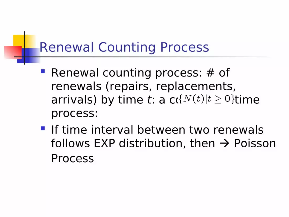
Renewal Counting Process Renewal counting process: # of

renewals (repairs, replacements, arrivals) by time t: a continuous time process:

If time interval between two renewals follows EXP distribution, then Poisson Process

Note:For a fixed t, N(t) is a random variable (in this case a discrete random variable known as the Poisson random variable) The family {N(t), t 0} is a stochastic process, in this case, the homogeneous Poisson process{N(t), t 0} is a homogeneous CTMC as well

Poisson Process A continuous time, discrete state process. N(t): no. of events occurring in time (0, t]. Events may be,

1. # of packets arriving at a router port2. # of incoming telephone calls at a switch3. # of jobs arriving at file/compute server 4. Number of component failures

Events occurs successively and that intervals between these successive events are iid rvs, each following EXP( )

1. λ: arrival rate (1/ λ: average time between arrivals)2. λ: failure rate (1/ λ: average time between failures)

Poisson Process (contd.) N(t) forms a Poisson process provided:

1. N(0) = 02. Events within non-overlapping intervals are

independent3. In a very small interval h, only one event may occur

(prob. p(h))

1. Letting, pn(t) = P[N(t)=n],

For a Poisson process, interarrival times follow EXP( ) (memoryless) distribution.

E[N(t)] = Var[N(t)] = λt ; What about E[N(t)/t], as t infinity?

Merged Multiple Poisson Process Streams Consider the system,

Proof: Using z-transform. Letting, α = λt,

+

Decomposing a Poisson Stream Decompose a Poisson process using a prob. switch

N arrivals decomposed into {N1, N2, .., Nk}; N= N1+N2, ..,+Nk Cond. pmf

Since, The uncond. pmf

Non-Homogeneous Poisson Process (NHPP)

Poisson Process

Generalizing the Poisson Process

Non-Homogeneous Poisson Process (NHPP)If the expected number of events per unit time, , changes with age (time), we have a non-homogeneous Poisson model. We assume that: 1. If 0 t, the pmf of N(t) is given by:

where m(t) 0 is the expected number of events in the time period [0, t]

2. Counts of events in non-overlapping time periods are

mutually independent. m(t) : the mean value function. (x) :the time-dependent rate of occurrence of events or time-dependent failure rate

t

0dx (x) )( tm

etm tmk kktNP !/ ...,2,1,0k

NHPP(cont.)

Non-Homogeneous Poisson Process (NHPP)

Poisson Process

Renewal CountingProcess

Generalizing Poisson Process

Poisson process EXP( ) distributed interarrival times. What if the EXP( ) assumption is removed renewal proc. Renewal proc. : {Xi | i=1,2,…} (Xi’s are iid non-EXP rvs) Xi : time gap between the occurrence of (i-1) st and ith event

Sk = X1 + X2 + .. + Xk time to occurrence of the kth event.

N(t)- Renewal counting process is a discrete-state, continuous-time stochastic process. N(t) denotes no. of renewals in the interval (0, t].

Renewal Counting Process

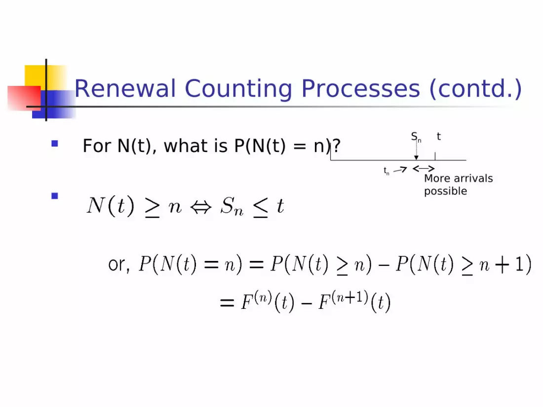
Renewal Counting Processes (contd.) For N(t), what is P(N(t) = n)?

Sn t

More arrivals possible

tn

Renewal Counting Process Expectation Let, m(t) = E[N(t)]. Then, m(t) = mean

no. of arrivals in time (0,t]. m(t) is called the renewal function.

Renewal Density Function Renewal density function:

For example, if the renewal interval X is EXP(λ), then d(t) = λ , t >= 0 and m(t) = λ t , t >= 0. P[N(t)=n] = Fn(t) will turn out to be n-stage Erlang

e–λ t (λ t)n/n! i.e Poisson pmf

Alternating Renewal Process

Where:Failure times T1, T2, … are mutually independent with a common distribution function W

Restoration times D1, D2, … are mutually independent with a common distribution function G

The sequences {Tn} and {Dn} are independent

1

0

I(t)

Operating Restoration

Time

Availability Analysis Availability: is defined is the ability of a system to

provide the desired service. If no

repair/replacement,Availability(t)=Reliability(t) If repairs are possible, then above is pessimistic.

MTBF = E[Di+Ti+1] = E[Ti+Di]=E[Xi]=MTTF+MTTR

T1 D1 T2 D2 T3 D3 T4 D4 …….

MTBF

Availability Analysis (contd.)

Two mutually exclusive situations:1. System does not fail before time t A(t)

= R(t)2. System fails, but the repair is completed

before time t Therefore, A(t) = sum of these two

probabilities

t

Repair is completed with in this intervalrenewal

x

Availability Expression dA(x) : Incremental availability

dA(x) = Prob(that after renewal, life time is > (t-x) & that the renewal occurs in the interval (x,x+dx])

Repair is completed with in this interval

xRenewed life time >= (t-x)

0 x+dx t

Availability Expression (contd.) A(t) can also be expressed in the Laplace domain.

Since, R(t) = 1-W(t) or LR(s) = 1/s – LW(s) = 1/s –Lw(s)/s

What happens when t becomes very large?

However,

Availability, MTTF and MTTR Steady state availability A is:

Taking the expression of sLA(s) and taking the limit via L’Hospital rule and using the moment generating property of the LT, we get the required result for the steady-state

A=MTTF/(MTTF+MTTR)

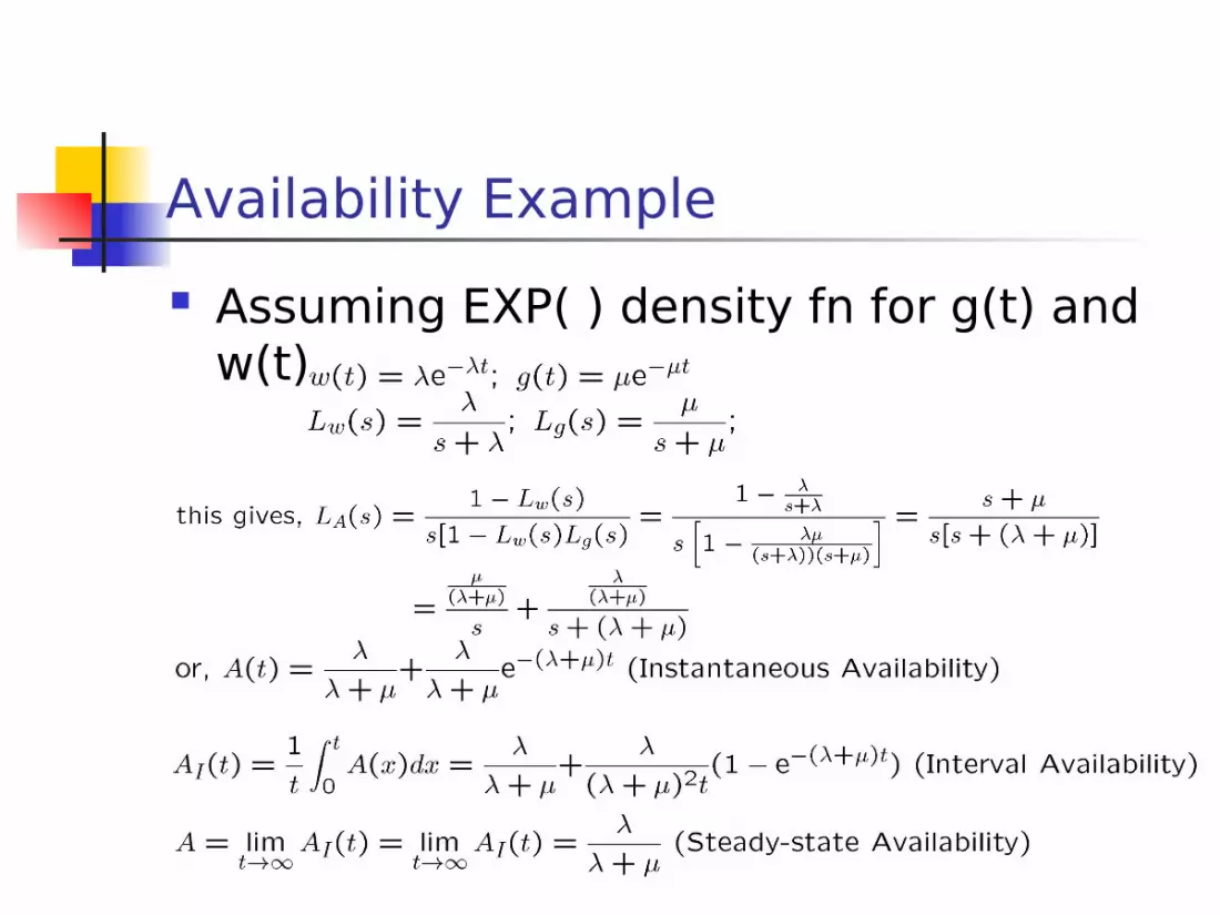
Availability Example Assuming EXP( ) density fn for g(t) and

w(t)

Non-Homogeneous Poisson Process (NHPP)

Poisson Process

Renewal CountingProcess

HomogeneousContinuous TimeMarkov Chain

HomogeneousDiscrete TimeMarkov Chain

Semi-Markov Process

Markov RegenerativeProcess

Non-HomogeneousContinuous TimeMarkov Chain

Compound Poisson Process

Generalizing Poisson Process

Bernoulli Process