Chapter  7    Steady-­‐State  Heat  Condi2on  

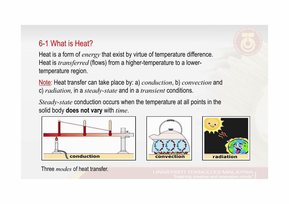
6-1 What is Heat? Heat is a form of energy that exist by virtue of temperature difference. Heat is transferred (flows) from a higher-temperature to a lower-temperature region. Note: Heat transfer can take place by: a) conduction, b) convection and c) radiation, in a steady-state and in a transient conditions. Steady-state conduction occurs when the temperature at all points in the solid body does not vary with time.

Three modes of heat transfer.

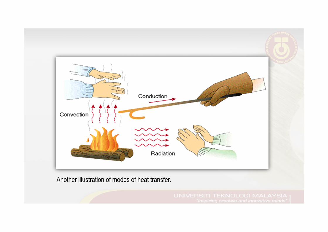
Another illustration of modes of heat transfer.

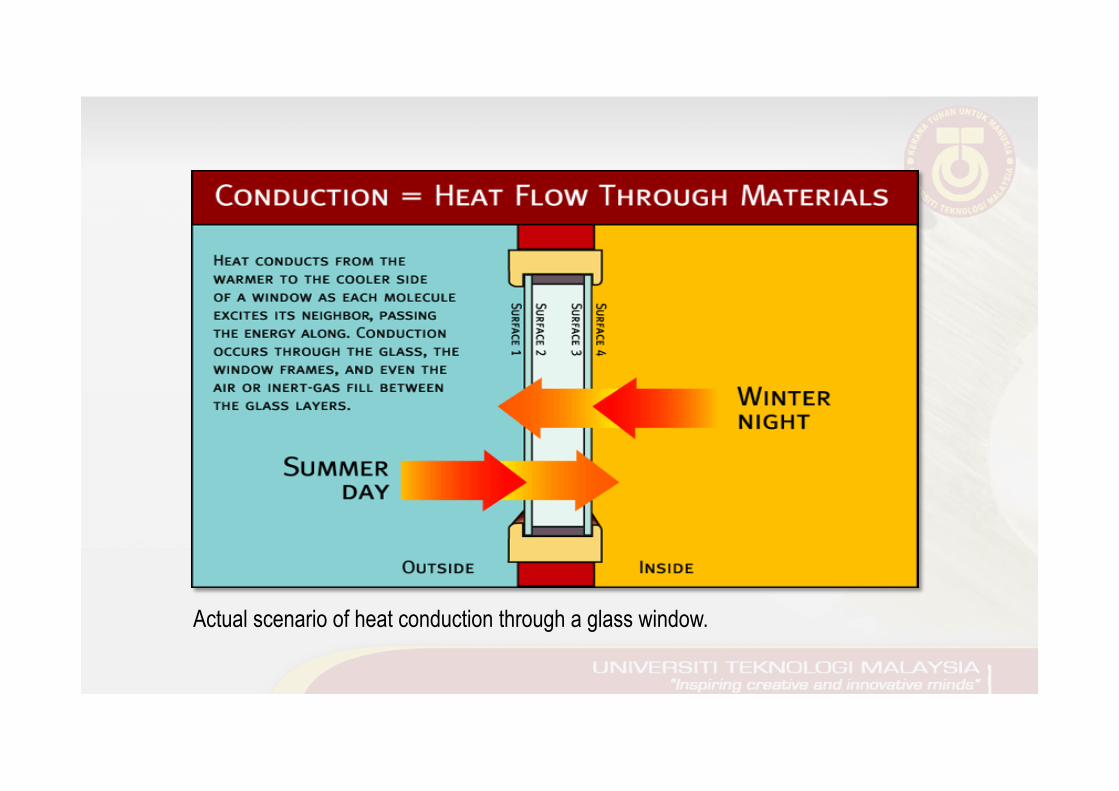
Actual scenario of heat conduction through a glass window.

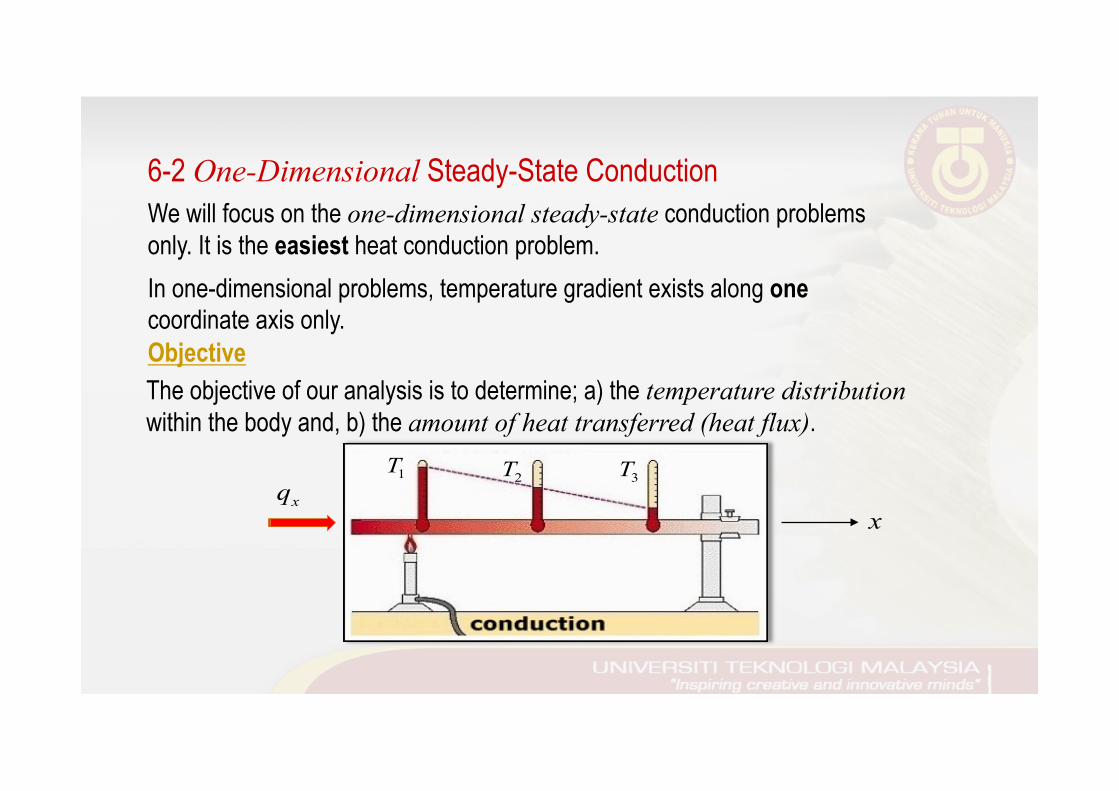
6-2 One-Dimensional Steady-State Conduction We will focus on the one-dimensional steady-state conduction problems only. It is the easiest heat conduction problem. In one-dimensional problems, temperature gradient exists along one coordinate axis only. Objective The objective of our analysis is to determine; a) the temperature distribution within the body and, b) the amount of heat transferred (heat flux).

1T 2T 3Txq

x

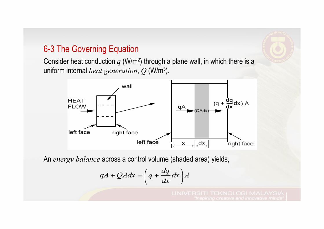
An energy balance across a control volume (shaded area) yields,

AdxdxdqqQAdxqA ⎟

⎠

⎞⎜⎝

⎛ +=+

6-3 The Governing Equation Consider heat conduction q (W/m2) through a plane wall, in which there is a uniform internal heat generation, Q (W/m3).

where q = heat flux per unit area (W/m2) A = area normal to the direction of heat flow (m2) Q = internal heat generated per unit volume (W/m3)

Cancelling term qA and rearranging, we obtain,

dxdqQ =

For one-dimensional heat conduction, the heat flux q is governed by the Fourier’s law, which states that,

dTq kdx

⎛ ⎞= − ⋅⎜ ⎟⎝ ⎠

where k = thermal conductivity of the material (W/m.K) (dT/dx) = temperature gradient in x-direction (K/m)

Note: The –ve sign is due to the fact that heat flows from a high-temperature to low- temperature region.

… (i)

… (ii)

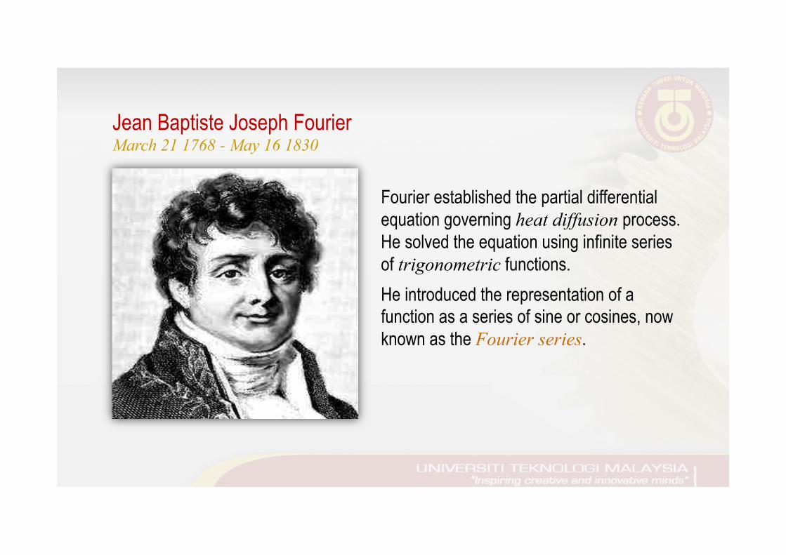
Fourier established the partial differential equation governing heat diffusion process. He solved the equation using infinite series of trigonometric functions. He introduced the representation of a function as a series of sine or cosines, now known as the Fourier series.

Jean Baptiste Joseph Fourier March 21 1768 - May 16 1830

Substituting eq.(ii) into eq.(i) yields,

0=+⎟⎠

⎞⎜⎝

⎛ QdxdTk

dxd

The governing equation has to be solved with appropriate boundary conditions to get the desired temperature distribution, T. Note: Q is called a source when it is +ve (heat is generated), and is called a sink when it is -ve (heat is consumed).

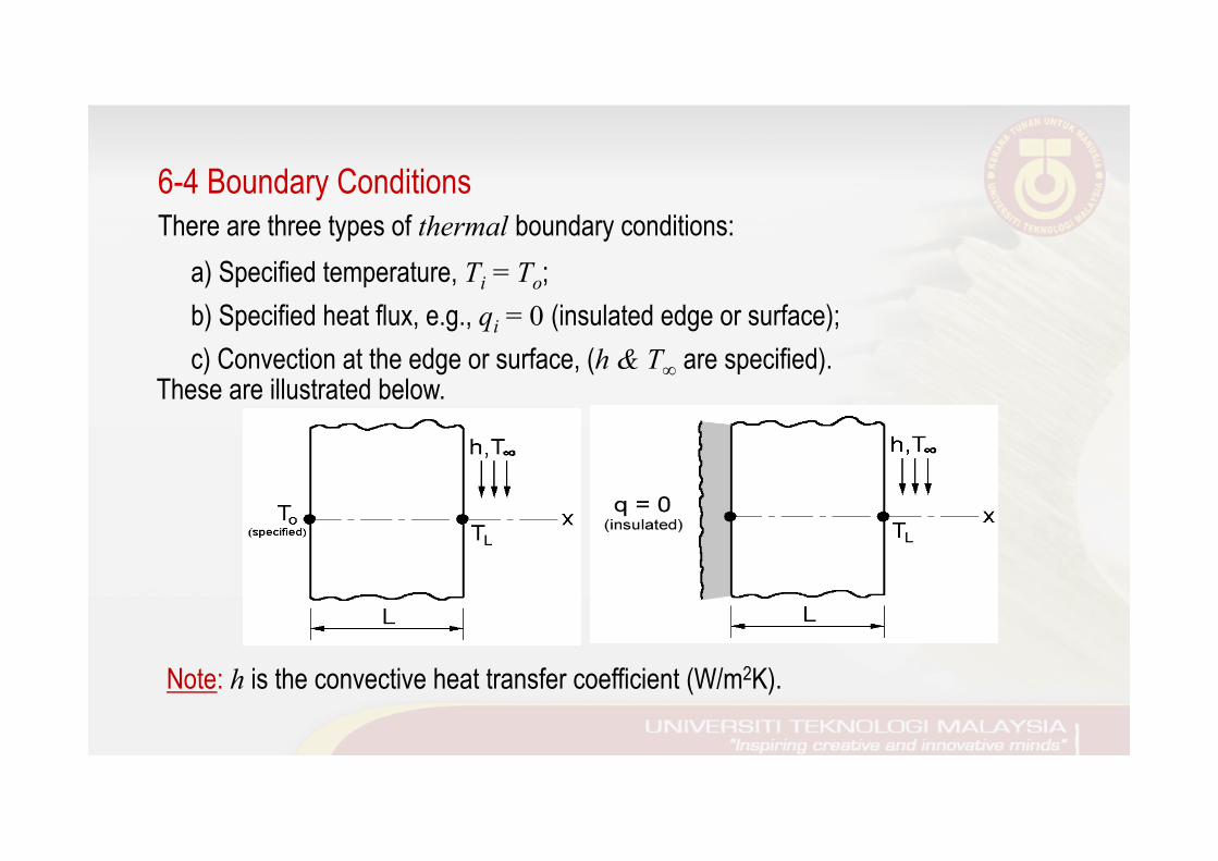
6-4 Boundary Conditions There are three types of thermal boundary conditions: a) Specified temperature, Ti = To; b) Specified heat flux, e.g., qi = 0 (insulated edge or surface); c) Convection at the edge or surface, (h & T∞ are specified). These are illustrated below.

Note: h is the convective heat transfer coefficient (W/m2K).

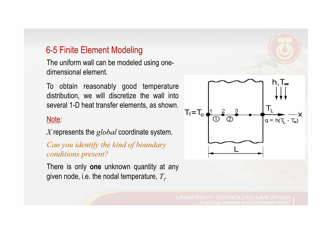
6-5 Finite Element Modeling The uniform wall can be modeled using one-dimensional element.

To obtain reasonably good temperature distribution, we will discretize the wall into several 1-D heat transfer elements, as shown.

Note: X represents the global coordinate system. Can you identify the kind of boundary conditions present? There is only one unknown quantity at any given node, i.e. the nodal temperature, Ti.

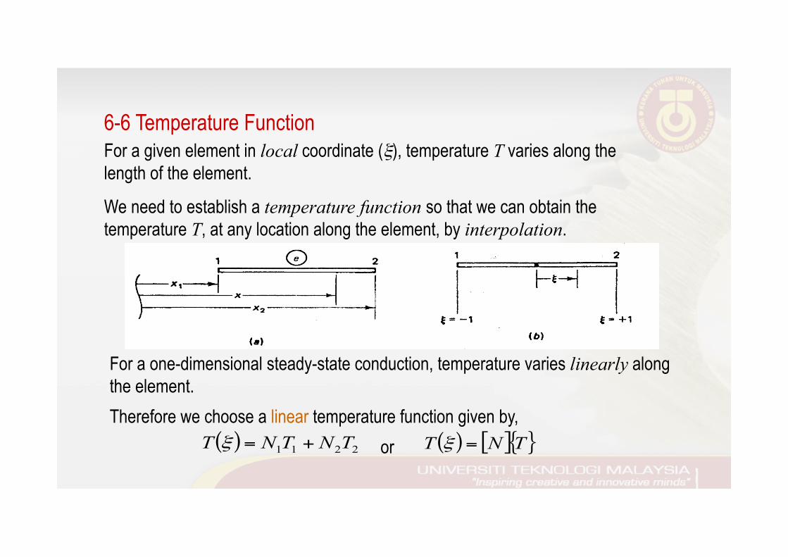
For a one-dimensional steady-state conduction, temperature varies linearly along the element. Therefore we choose a linear temperature function given by,

( ) 2211 TNTNT +=ξ or ( ) [ ]{ }TNT =ξ

6-6 Temperature Function For a given element in local coordinate (ξ), temperature T varies along the length of the element.

We need to establish a temperature function so that we can obtain the temperature T, at any location along the element, by interpolation.

( )( )

( )12 1 2 1

2 21 dx xx x dx x x

ξξ = − − ⇒ =

− −

We wish to express the (dT/dx) term in the governing equation in terms of element length, le, and the nodal temperature vector, {T}. Using the chain rule of differentiation

ξξξ

ξ ddT

dxd

dxd

ddT

dxdT

⋅=⋅=

( ) ( ) ( ) 2121 21

211

211

21 TT

ddTTTT +−=⇒++−=ξ

ξξξ

Substitute eq.(ii) and eq.(iii) into eq.(i) we get,

( )2112

2112

121

212 TT

xxTT

xxdxdT

+−−

=⎟⎠

⎞⎜⎝

⎛ +−−

=

where ( )ξ−= 121

1N ( )ξ+= 121

2Nand

Recall, …(ii)

…(iii)

…(i)

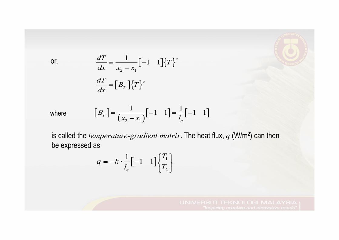
or, [ ]{ }

[ ]{ }

2 1

1 1 1 e

eT

dT Tdx x x

dT B Tdx

= −−

=

where [ ]( )

[ ] [ ]2 1

1 11 1 1 1Te

Bx x l

= − = −−

is called the temperature-gradient matrix. The heat flux, q (W/m2) can then be expressed as

[ ] 1

2

1 1 1e

Tq k

Tl⎧ ⎫

= − ⋅ − ⎨ ⎬⎩ ⎭

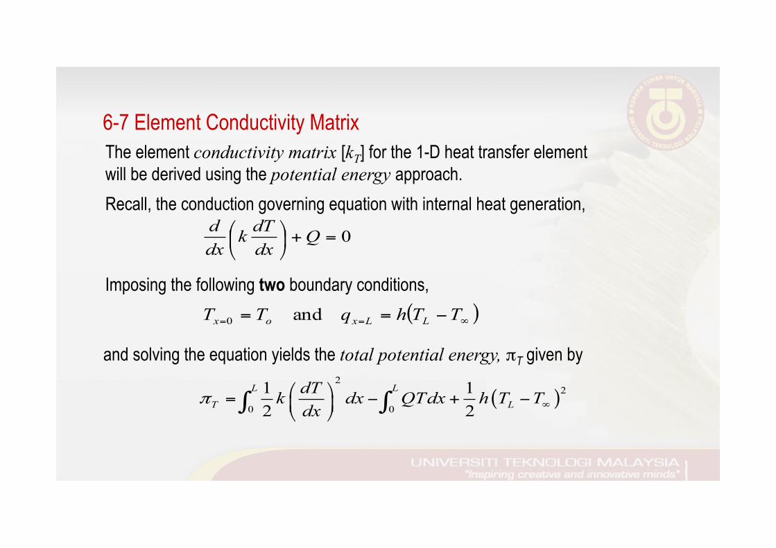
The element conductivity matrix [kT] for the 1-D heat transfer element will be derived using the potential energy approach. Recall, the conduction governing equation with internal heat generation,

0=+⎟⎠

⎞⎜⎝

⎛ QdxdTk

dxd

Imposing the following two boundary conditions, ( )∞== −== TThqTT LLxox and0

6-7 Element Conductivity Matrix

and solving the equation yields the total potential energy, πT given by

( )2

2

0 0

1 12 2

L L

T LdTk dx QTdx h T Tdx

π ∞⎛ ⎞= − + −⎜ ⎟⎝ ⎠∫ ∫

2 1

2 1

22 2

elx xd dx dx d dx x

ξ ξ ξ−

= ⇒ = =−

[ ]{ } [ ]{ }( ) ( )ande eT

dTT N T B Tdx

= =

Assuming that heat source Q = Qe and thermal conductivity k = ke are constant within the element, the functional πT becomes

{ } [ ] [ ] { }

[ ] { } ( )

1( ) ( )

1

1 ( ) 2

1

12 2

1 2 2

e T ee eT T T

e

ee eL

e

k lT B B d T

Q l N d T h T T

π ξ

ξ

−

∞−

⎡ ⎤= −⎢ ⎥⎣ ⎦

⎡ ⎤+ −⎢ ⎥⎣ ⎦

∑ ∫

∑ ∫

Note: The first term of the above equation is equivalent to the internal strain energy for structural problem. We identify the element conductivity matrix,

[ ] [ ] [ ]1

12Te e

T T Tk lk B B dξ

−= ⋅∫

Substitute for dx and (dT/dx) in terms of ξ and {T}e,

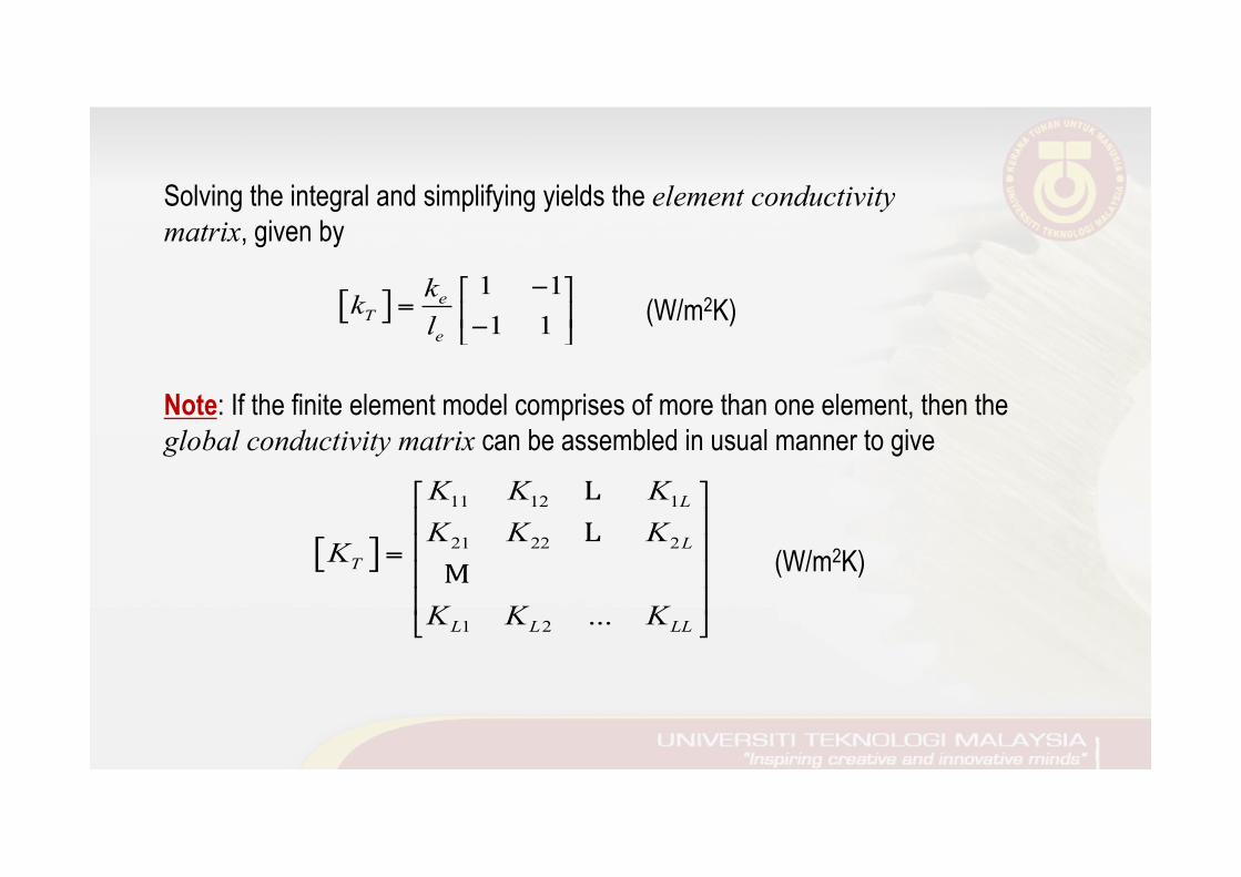
Solving the integral and simplifying yields the element conductivity matrix, given by

[ ]1 11 1

eT

e

kkl

−⎡ ⎤= ⎢ ⎥−⎣ ⎦

Note: If the finite element model comprises of more than one element, then the global conductivity matrix can be assembled in usual manner to give

[ ]

11 12 1

21 22 2

1 2 ...

L

LT

L L LL

K K KK K K

K

K K K

⎡ ⎤⎢ ⎥⎢ ⎥=⎢ ⎥⎢ ⎥⎣ ⎦

LL

M

(W/m2K)

(W/m2K)

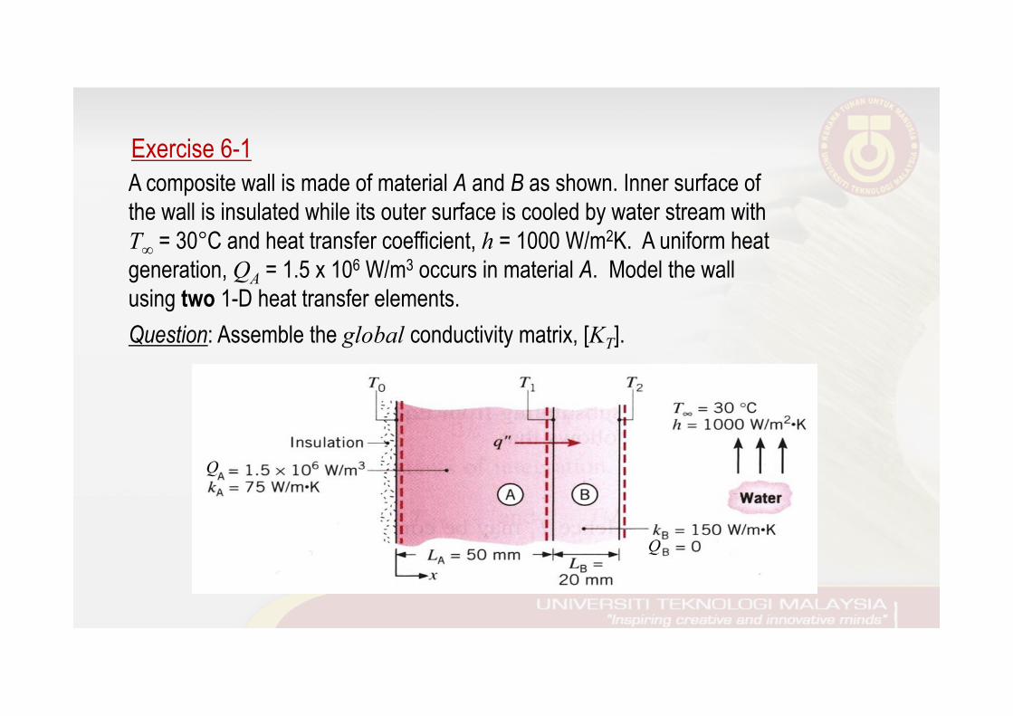
Exercise 6-1 A composite wall is made of material A and B as shown. Inner surface of the wall is insulated while its outer surface is cooled by water stream with T∞ = 30°C and heat transfer coefficient, h = 1000 W/m2K. A uniform heat generation, QA = 1.5 x 106 W/m3 occurs in material A. Model the wall using two 1-D heat transfer elements. Question: Assemble the global conductivity matrix, [KT].

If there is an internal heat generation, Qe (W/m3) within the element, then it can be shown that the element heat rate vector due to the internal heat generation is given by

{ } 2

1 W12 m

e e eQ

Q lr ⎧ ⎫⋅= ⎨ ⎬

⎩ ⎭Note: 1. If there is no internal heat generation in the element, then the heat rate vector for that element will be,

2. If there are more than one element in the finite element model, the global heat rate vector, {RQ} is assembled in the usual manner.

6-8 Element Heat Rate Vector

{ } ( )2

1 00 W1 02 m

e eQ

lr

⋅ ⎧ ⎫ ⎧ ⎫= =⎨ ⎬ ⎨ ⎬

⎩ ⎭ ⎩ ⎭

111 12 1 1

221 22 2 2

1 2 ...

QL

QL

QLL L LL L

RK K K TRK K K T

RK K K T

⎧ ⎫⎡ ⎤ ⎧ ⎫⎪ ⎪⎢ ⎥ ⎪ ⎪

⎪ ⎪ ⎪ ⎪⎢ ⎥ =⎨ ⎬ ⎨ ⎬⎢ ⎥ ⎪ ⎪ ⎪ ⎪⎢ ⎥ ⎪ ⎪ ⎪ ⎪⎣ ⎦ ⎩ ⎭ ⎩ ⎭

LL

MM M

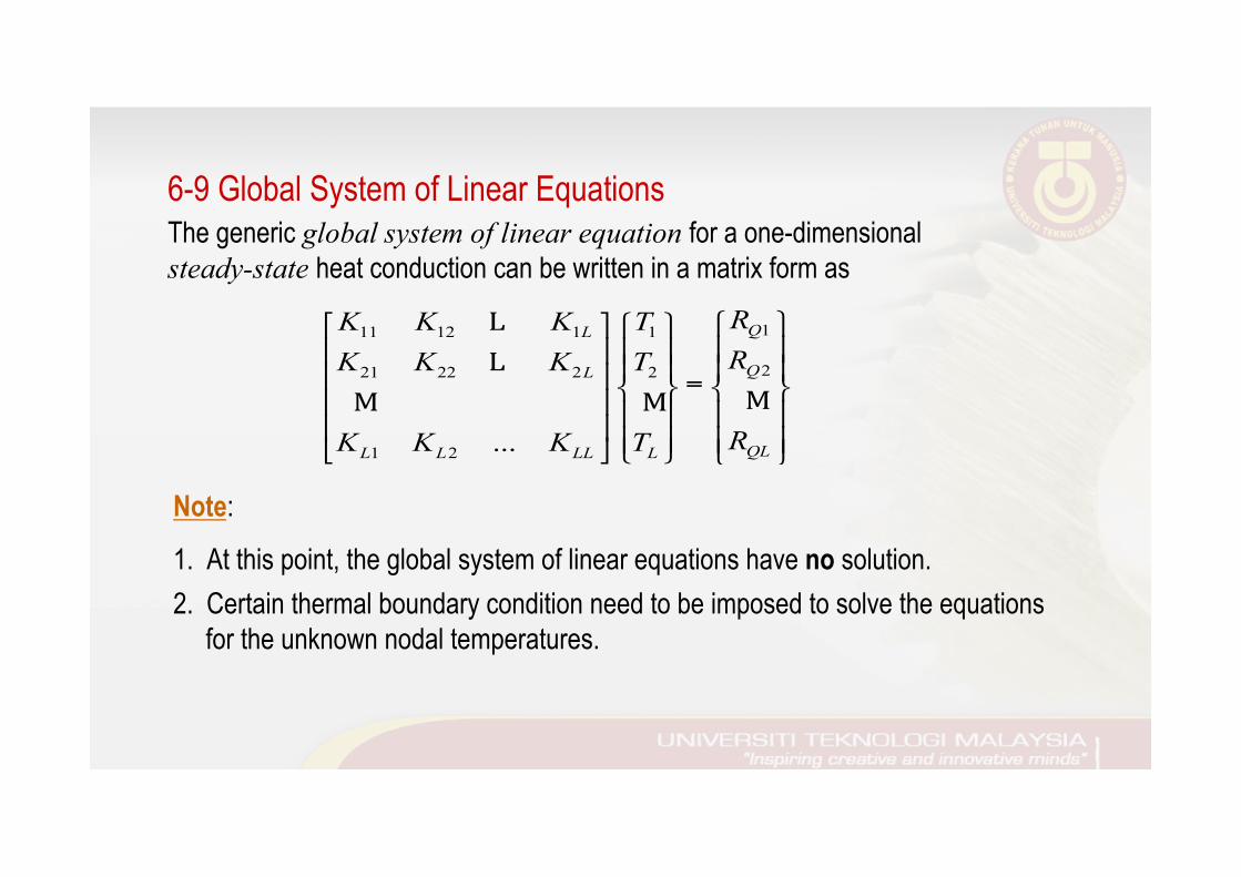
6-9 Global System of Linear Equations The generic global system of linear equation for a one-dimensional steady-state heat conduction can be written in a matrix form as

Note:

1.  At this point, the global system of linear equations have no solution. 2.  Certain thermal boundary condition need to be imposed to solve the equations

for the unknown nodal temperatures.

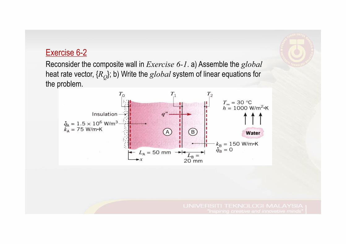
Exercise 6-2 Reconsider the composite wall in Exercise 6-1. a) Assemble the global heat rate vector, {RQ}; b) Write the global system of linear equations for the problem.

111 12 1 11

221 22 2 2 21

1 2 1...

QL

QL

QLL L LL L L

RK K K KRK K K T K

RK K K T K

θ θθ

θ

⎧ ⎫⎡ ⎤ ⎧ ⎫ ⎧ ⎫⎪ ⎪⎢ ⎥ ⎪ ⎪ ⎪ ⎪

⎪ ⎪ ⎪ ⎪ ⎪ ⎪⎢ ⎥ = −⎨ ⎬ ⎨ ⎬ ⎨ ⎬⎢ ⎥ ⎪ ⎪ ⎪ ⎪ ⎪ ⎪⎢ ⎥ ⎪ ⎪ ⎪ ⎪ ⎪ ⎪⎣ ⎦ ⎩ ⎭ ⎩ ⎭⎩ ⎭

LL

MM M M

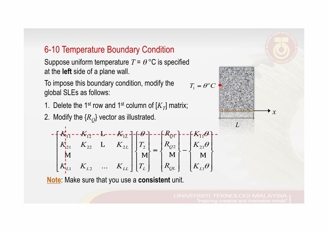
Suppose uniform temperature T = θ °C is specified at the left side of a plane wall. To impose this boundary condition, modify the global SLEs as follows: 1.  Delete the 1st row and 1st column of [KT] matrix; 2.  Modify the {RQ} vector as illustrated.

Note: Make sure that you use a consistent unit.

6-10 Temperature Boundary Condition

x L

1oT Cθ=

( ) ( )

111 12 1 1

221 22 2 2

1 2 ...

QL

QL

L L LL QLL

RK K K TRK K K T

K K K h R hTT ∞

⎧ ⎫⎡ ⎤ ⎧ ⎫⎪ ⎪⎢ ⎥ ⎪ ⎪

⎪ ⎪ ⎪ ⎪⎢ ⎥ =⎨ ⎬ ⎨ ⎬⎢ ⎥ ⎪ ⎪ ⎪ ⎪⎢ ⎥ ⎪ ⎪ ⎪ ⎪+ +⎩ ⎭⎣ ⎦ ⎩ ⎭

LL

MM M

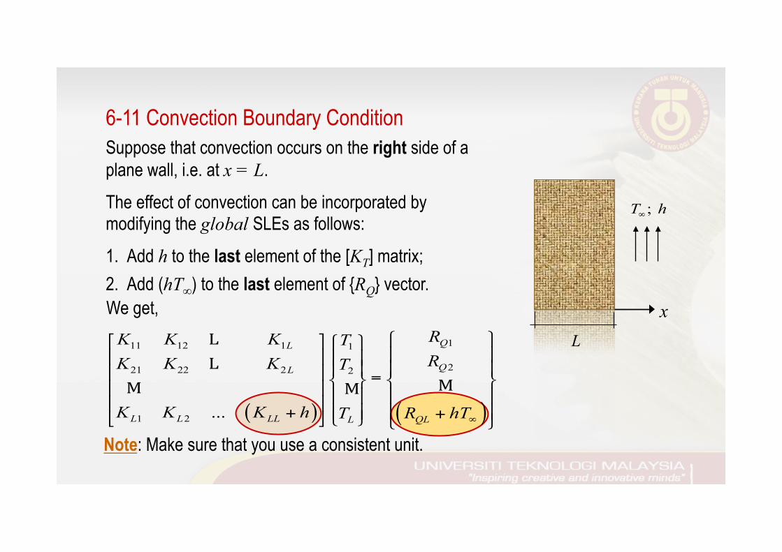
Suppose that convection occurs on the right side of a plane wall, i.e. at x = L. The effect of convection can be incorporated by modifying the global SLEs as follows: 1.  Add h to the last element of the [KT] matrix; 2.  Add (hT∞) to the last element of {RQ} vector.

Note: Make sure that you use a consistent unit.

6-11 Convection Boundary Condition

x L

We get,

; T h∞

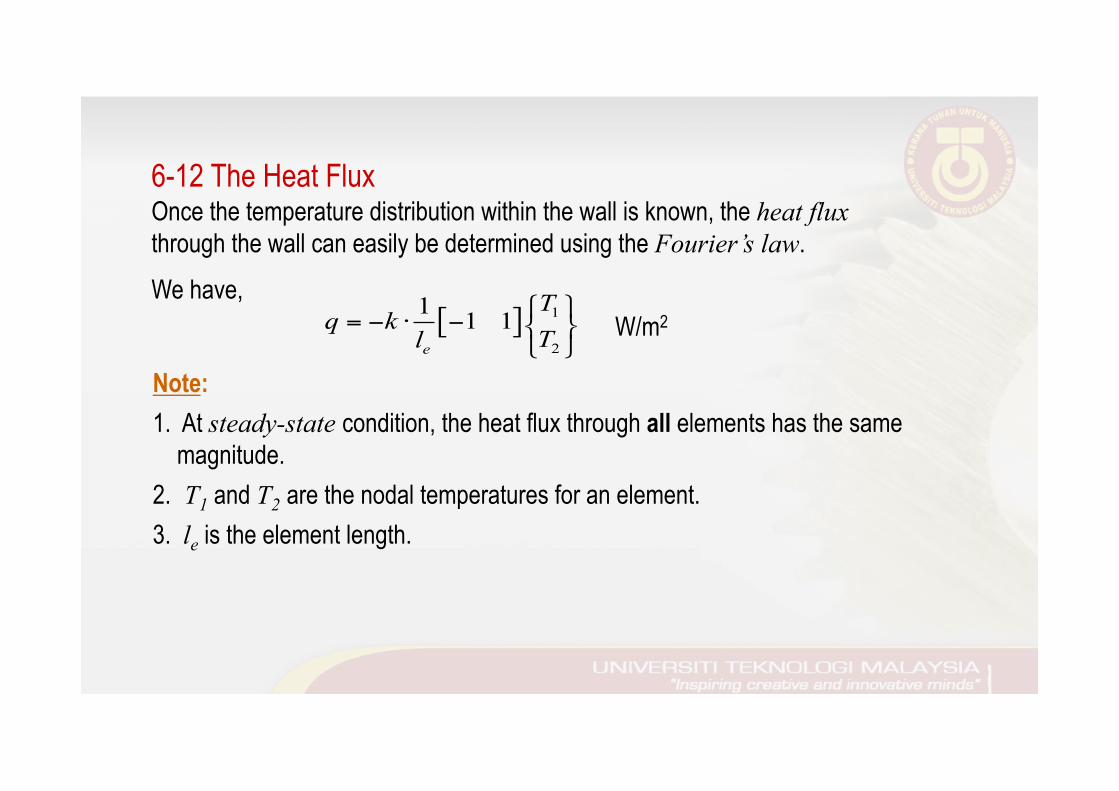
Once the temperature distribution within the wall is known, the heat flux through the wall can easily be determined using the Fourier’s law. We have,

Note:

1. At steady-state condition, the heat flux through all elements has the same magnitude. 2. T1 and T2 are the nodal temperatures for an element. 3. le is the element length.

6-12 The Heat Flux

[ ] 1

2

1 1 1e

Tq k

Tl⎧ ⎫

= − ⋅ − ⎨ ⎬⎩ ⎭

W/m2

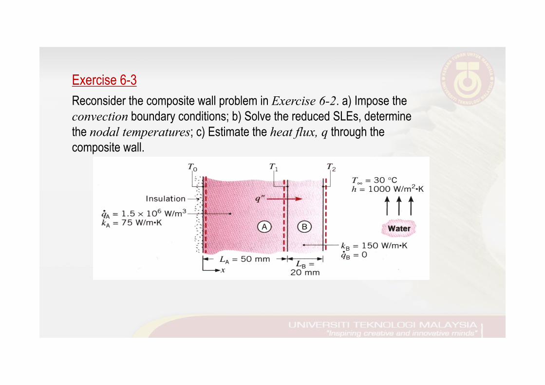
Exercise 6-3 Reconsider the composite wall problem in Exercise 6-2. a) Impose the convection boundary conditions; b) Solve the reduced SLEs, determine the nodal temperatures; c) Estimate the heat flux, q through the composite wall.

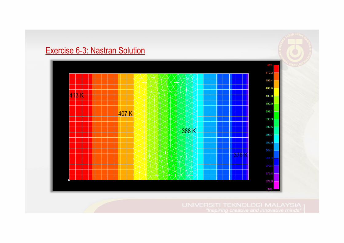
Exercise 6-3: Nastran Solution

413 K

407 K

388 K

378 K

( )111 12 1 1

221 22 2 2

1 2

0

... 0

QL o

QL

QLL L LL L

RK K K T qRK K K T

RK K K T

⎧ ⎫ ⎧ ⎫−⎡ ⎤ ⎧ ⎫⎪ ⎪ ⎪ ⎪⎢ ⎥ ⎪ ⎪

⎪ ⎪ ⎪ ⎪ ⎪ ⎪⎢ ⎥ = +⎨ ⎬ ⎨ ⎬ ⎨ ⎬⎢ ⎥ ⎪ ⎪ ⎪ ⎪ ⎪ ⎪⎢ ⎥ ⎪ ⎪ ⎪ ⎪ ⎪ ⎪⎣ ⎦ ⎩ ⎭ ⎩ ⎭⎩ ⎭

LL

MM M M M

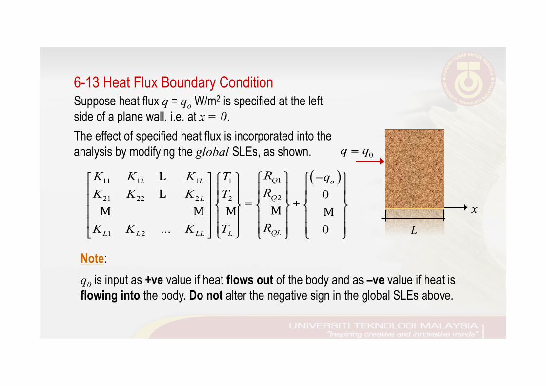
Suppose heat flux q = qo W/m2 is specified at the left side of a plane wall, i.e. at x = 0. The effect of specified heat flux is incorporated into the analysis by modifying the global SLEs, as shown.

6-13 Heat Flux Boundary Condition

x L

0q q=

Note: q0 is input as +ve value if heat flows out of the body and as –ve value if heat is flowing into the body. Do not alter the negative sign in the global SLEs above.

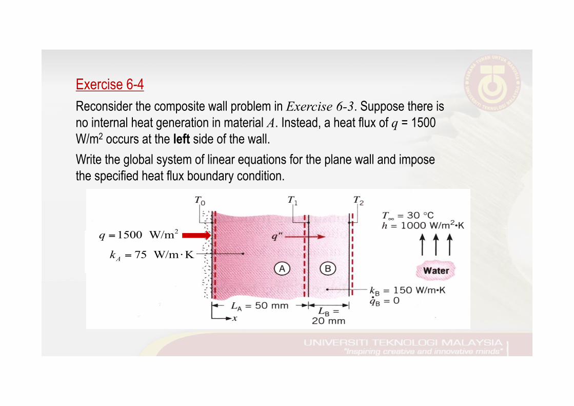
Exercise 6-4 Reconsider the composite wall problem in Exercise 6-3. Suppose there is no internal heat generation in material A. Instead, a heat flux of q = 1500 W/m2 occurs at the left side of the wall. Write the global system of linear equations for the plane wall and impose the specified heat flux boundary condition.

75 W/m KAk = ⋅

21500 W/mq =

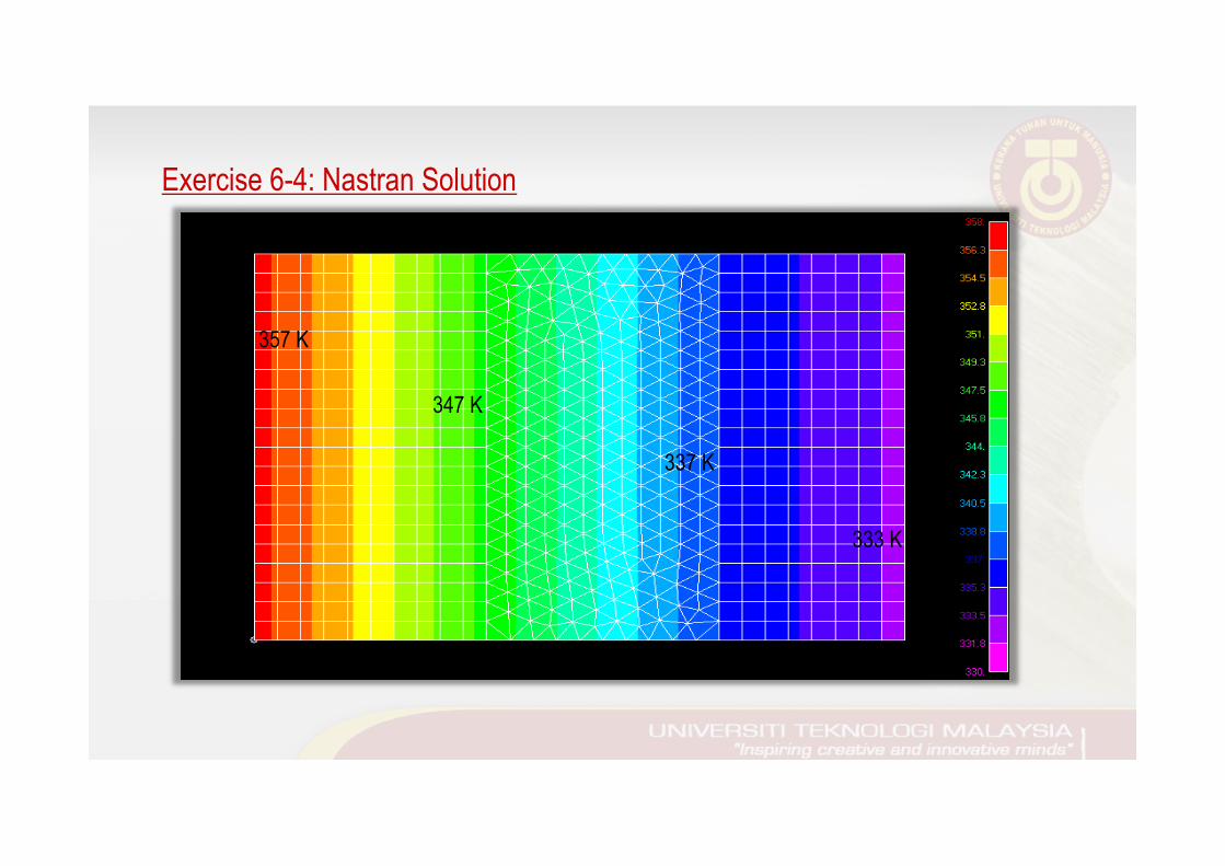
Exercise 6-4: Nastran Solution

357 K

347 K

337 K

333 K

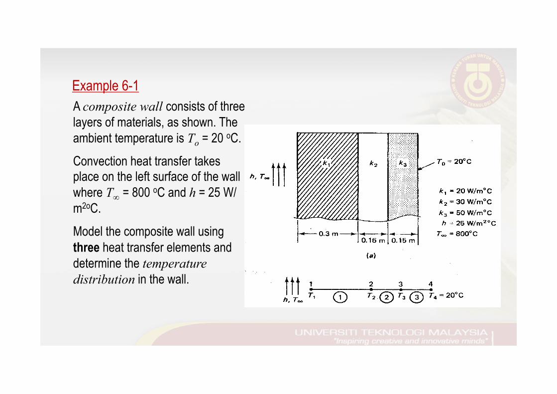
Example 6-1 A composite wall consists of three layers of materials, as shown. The ambient temperature is To = 20 oC. Convection heat transfer takes place on the left surface of the wall where T∞ = 800 oC and h = 25 W/m2oC. Model the composite wall using three heat transfer elements and determine the temperature distribution in the wall.

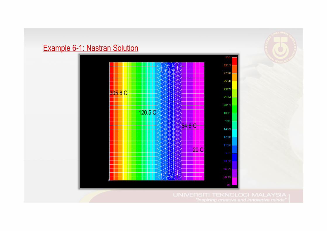
Example 6-1: Nastran Solution

305.8 C

120.5 C

54.6 C

20 C

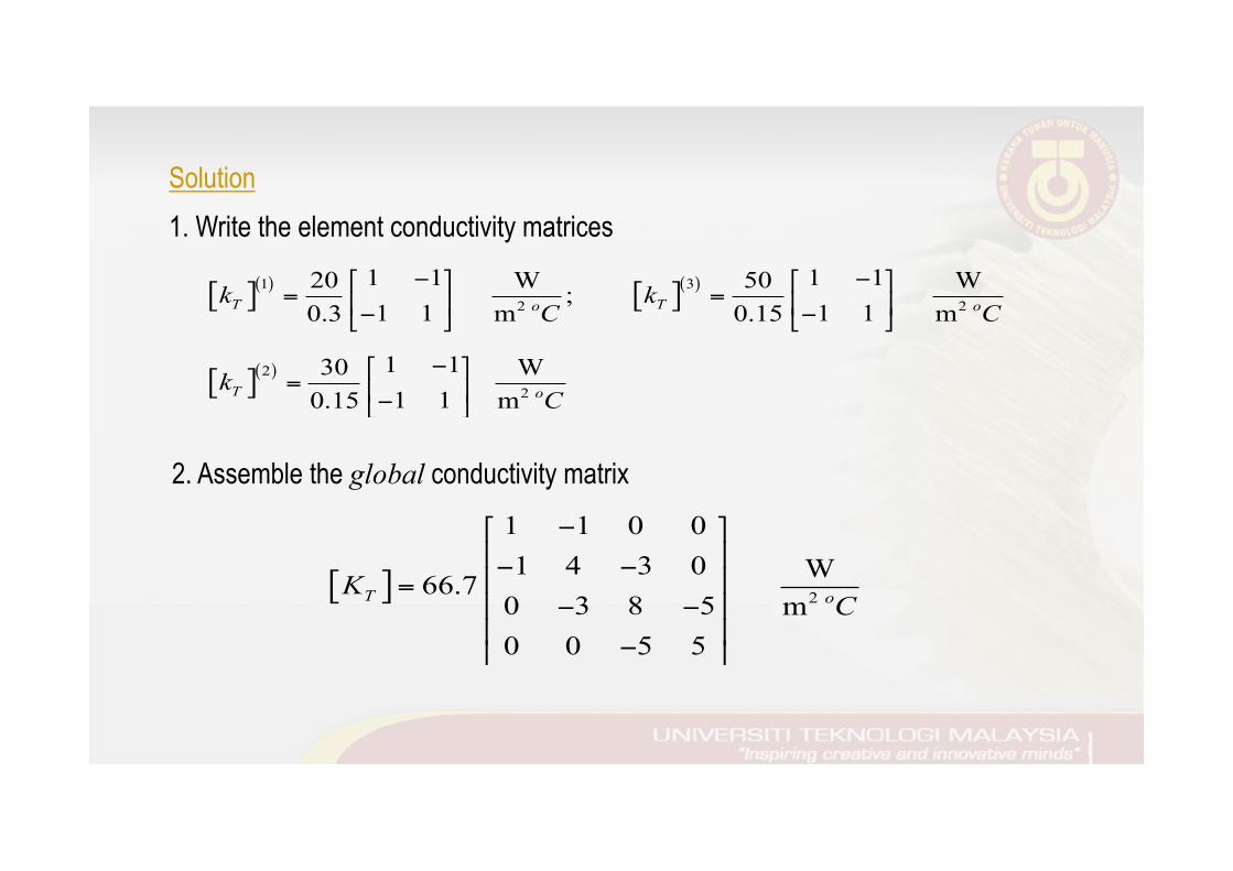
Solution 1. Write the element conductivity matrices

[ ]( ) [ ]( )

[ ]( )

1 32 2

22

1 1 1 120 W 50 W ; 1 1 1 10.3 m 0.15 m

1 130 W 1 10.15 m

T To o

T o

k kC C

kC

− −⎡ ⎤ ⎡ ⎤= =⎢ ⎥ ⎢ ⎥− −⎣ ⎦ ⎣ ⎦

−⎡ ⎤= ⎢ ⎥−⎣ ⎦

2. Assemble the global conductivity matrix

[ ] 2

1 1 0 01 4 3 0 W66.7

0 3 8 5 m0 0 5 5

T oKC

−⎡ ⎤⎢ ⎥− −⎢ ⎥=⎢ ⎥− −⎢ ⎥

−⎣ ⎦

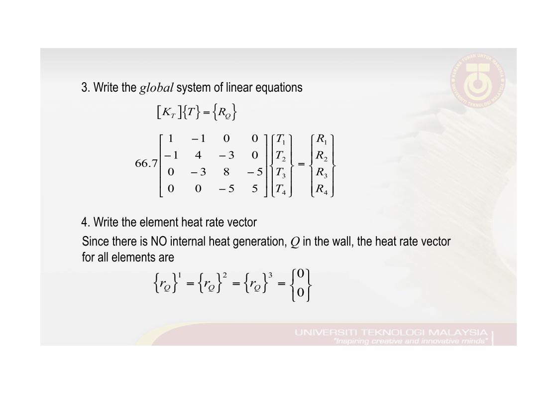
3. Write the global system of linear equations

[ ]{ } { }T QK T R=

⎪⎪⎭

⎪⎪⎬

⎫

⎪⎪⎩

⎪⎪⎨

⎧

=

⎪⎪⎭

⎪⎪⎬

⎫

⎪⎪⎩

⎪⎪⎨

⎧

⎥⎥⎥⎥

⎦

⎤

⎢⎢⎢⎢

⎣

⎡

−

−−

−−

−

4

3

2

1

4

3

2

1

5500583003410011

7.66

RRRR

TTTT

4. Write the element heat rate vector Since there is NO internal heat generation, Q in the wall, the heat rate vector for all elements are

{ } { } { }1 2 3 00Q Q Qr r r ⎧ ⎫

= = = ⎨ ⎬⎩ ⎭

5. Write the global system of linear equations

1

2

3

4

1 1 0 0 01 4 3 0 0

66.70 3 8 5 00 0 5 5 0

TTTT

− ⎧ ⎫⎡ ⎤ ⎧ ⎫⎪ ⎪⎢ ⎥ ⎪ ⎪− − ⎪ ⎪ ⎪ ⎪⎢ ⎥ =⎨ ⎬ ⎨ ⎬⎢ ⎥− − ⎪ ⎪ ⎪ ⎪⎢ ⎥ ⎪ ⎪ ⎪ ⎪−⎣ ⎦ ⎩ ⎭⎩ ⎭

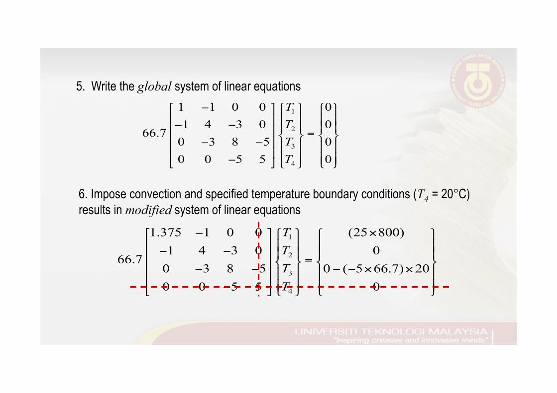
6. Impose convection and specified temperature boundary conditions (T4 = 20°C) results in modified system of linear equations

1

2

3

4

1.375 1 0 0 (25 800)1 4 3 0 0

66.70 3 8 5 0 ( 5 66.7) 200 0 5 5 0

TTTT

− ×⎧ ⎫⎡ ⎤ ⎧ ⎫⎪ ⎪⎢ ⎥ ⎪ ⎪− − ⎪ ⎪ ⎪ ⎪⎢ ⎥ =⎨ ⎬ ⎨ ⎬⎢ ⎥− − − − × ×⎪ ⎪ ⎪ ⎪⎢ ⎥ ⎪ ⎪ ⎪ ⎪−⎣ ⎦ ⎩ ⎭⎩ ⎭

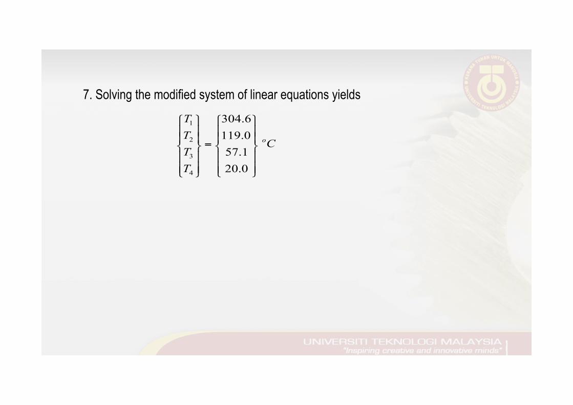
7. Solving the modified system of linear equations yields

1

2

3

4

304.6119.057.120.0

o

TT

CTT

⎧ ⎫ ⎧ ⎫⎪ ⎪ ⎪ ⎪⎪ ⎪ ⎪ ⎪

=⎨ ⎬ ⎨ ⎬⎪ ⎪ ⎪ ⎪⎪ ⎪ ⎪ ⎪⎩ ⎭⎩ ⎭

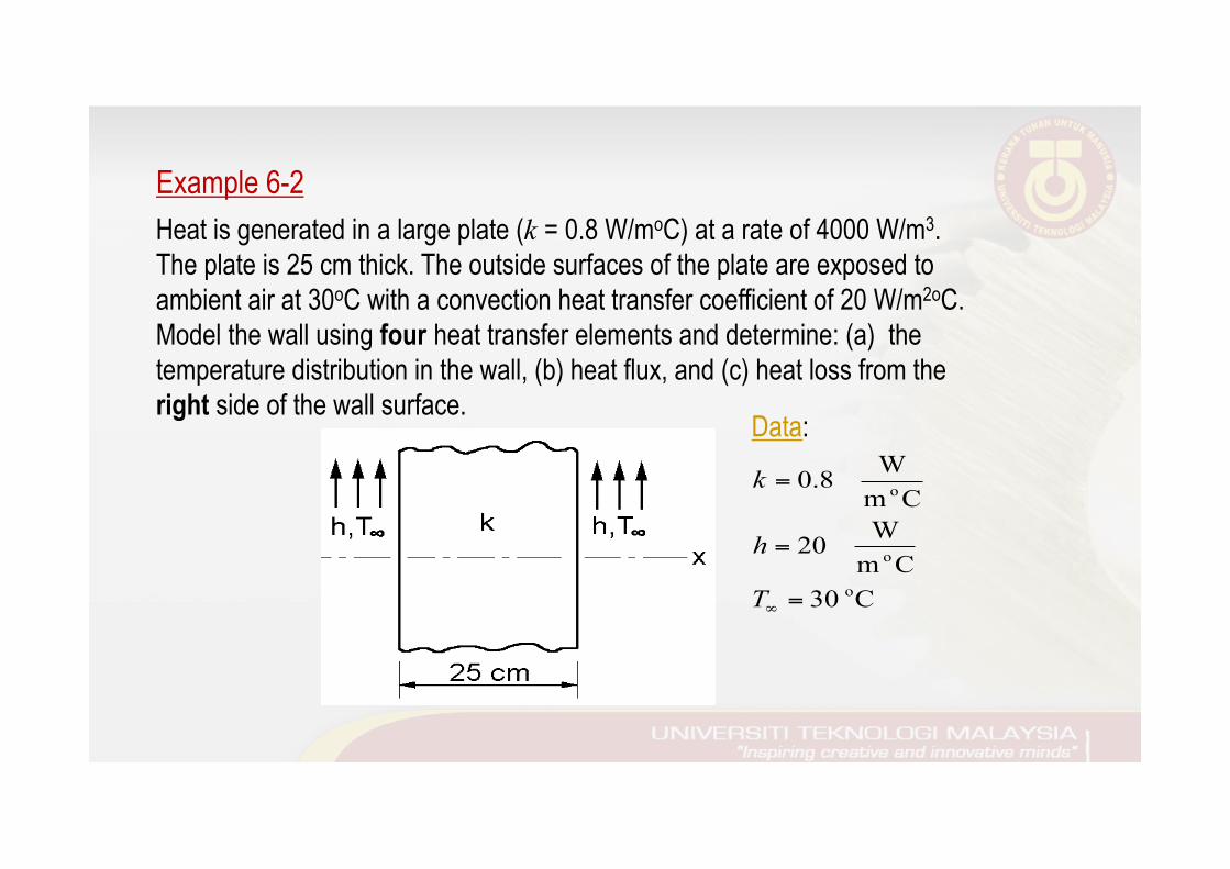
Example 6-2 Heat is generated in a large plate (k = 0.8 W/moC) at a rate of 4000 W/m3. The plate is 25 cm thick. The outside surfaces of the plate are exposed to ambient air at 30oC with a convection heat transfer coefficient of 20 W/m2oC. Model the wall using four heat transfer elements and determine: (a) the temperature distribution in the wall, (b) heat flux, and (c) heat loss from the right side of the wall surface.

o

o

o

W0.8m CW20m C

30 C

k

h

T∞

=

=

=

Data:

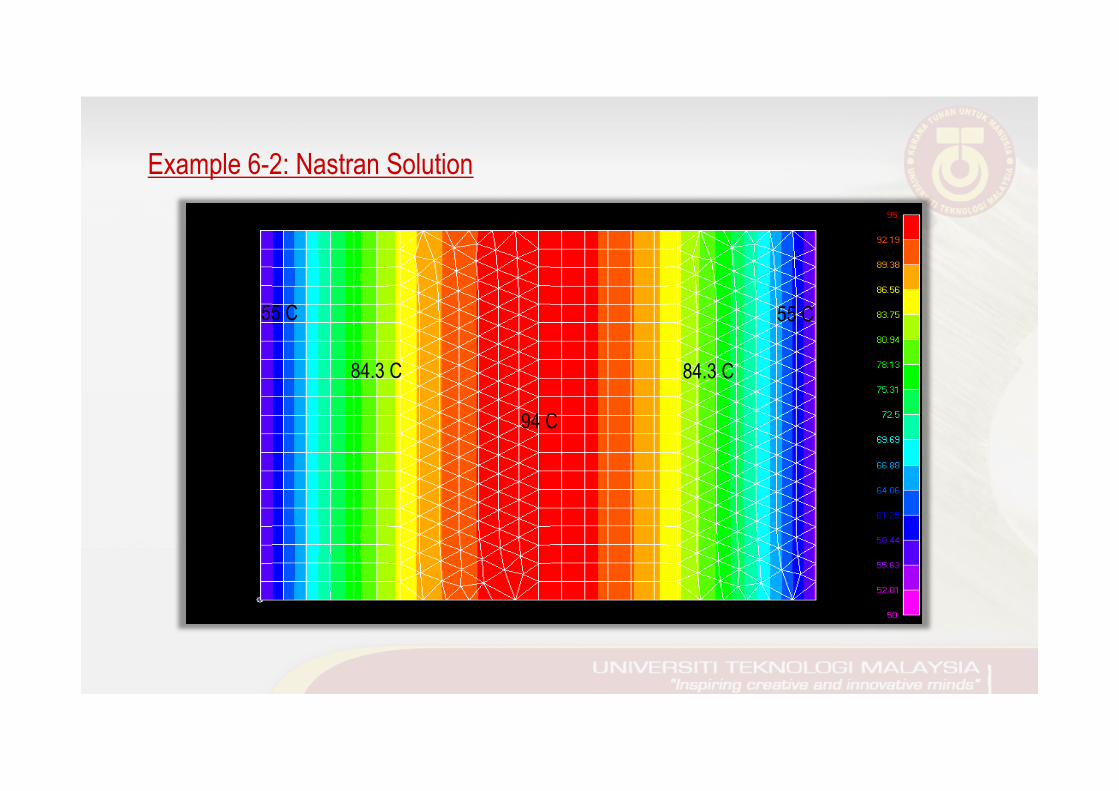
Example 6-2: Nastran Solution

84.3 C

94 C

84.3 C

55 C 55 C

Solution

[ ]( )

[ ]( )

12

22

12.8 12.8 W 12.8 12.8 m

12.8 12.8 W 12.8 12.8 m

T o

T o

kC

kC

−⎡ ⎤= ⎢ ⎥−⎣ ⎦

−⎡ ⎤= ⎢ ⎥−⎣ ⎦

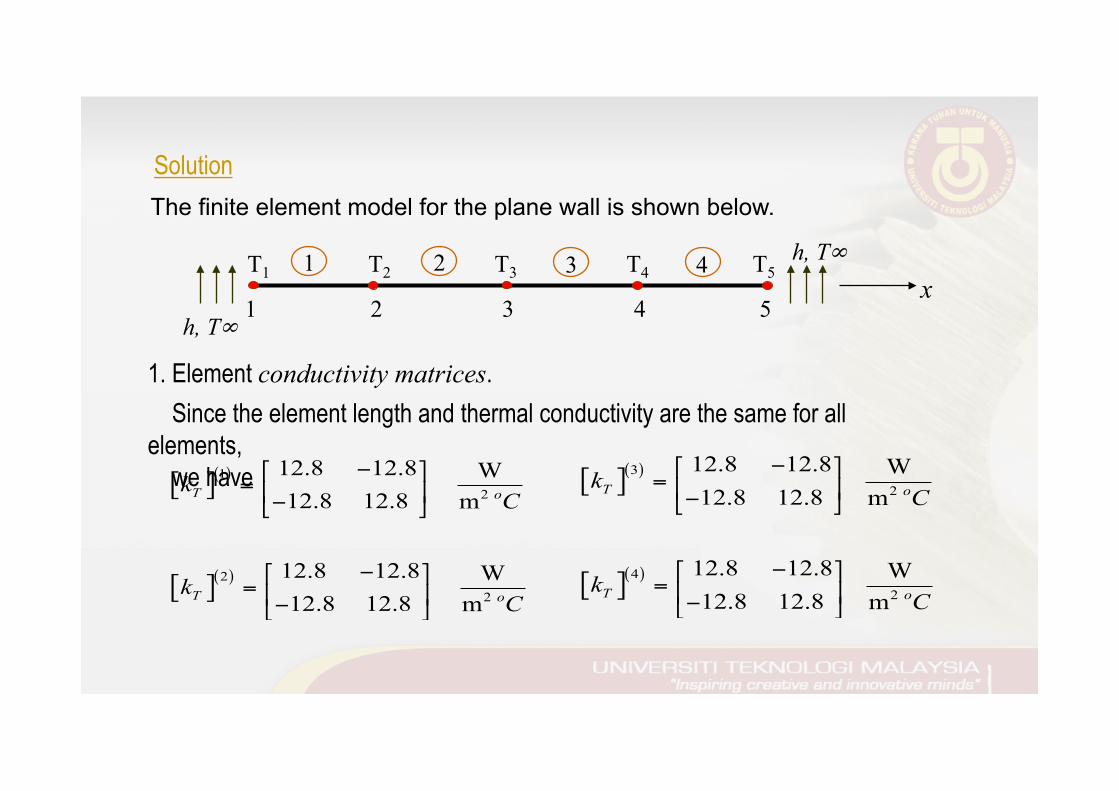
1. Element conductivity matrices. Since the element length and thermal conductivity are the same for all elements, we have [ ]( )

[ ]( )

32

42

12.8 12.8 W 12.8 12.8 m

12.8 12.8 W 12.8 12.8 m

T o

T o

kC

kC

−⎡ ⎤= ⎢ ⎥−⎣ ⎦

−⎡ ⎤= ⎢ ⎥−⎣ ⎦

1 2 3 4 5

T1 T2 T3 T4 T5 h, T∞

h, T∞

x

The finite element model for the plane wall is shown below.

1 2 3 4

[ ]

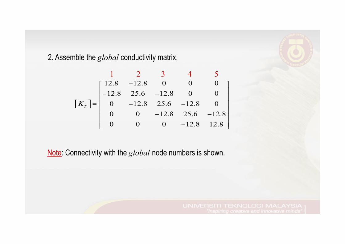
12.8 12.8 0 0 012.8 25.6 12.8 0 00 12.8 25.6 12.8 00 0 12.8 25.6 12.80 0 0 12.8 12.8

TK

−⎡ ⎤⎢ ⎥− −⎢ ⎥⎢ ⎥= − −⎢ ⎥

− −⎢ ⎥⎢ ⎥−⎣ ⎦

2. Assemble the global conductivity matrix,

1 2 3 4 5

Note: Connectivity with the global node numbers is shown.

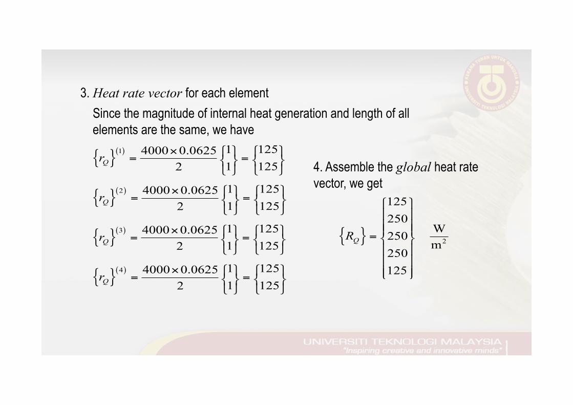
3. Heat rate vector for each element Since the magnitude of internal heat generation and length of all elements are the same, we have

{ }( )

{ }( )

{ }( )

{ }( )

1

2

3

4

1 1254000 0.06251 1252

1 1254000 0.06251 1252

1 1254000 0.06251 1252

1 1254000 0.06251 1252

Q

Q

Q

Q

r

r

r

r

⎧ ⎫ ⎧ ⎫×= =⎨ ⎬ ⎨ ⎬

⎩ ⎭ ⎩ ⎭

⎧ ⎫ ⎧ ⎫×= =⎨ ⎬ ⎨ ⎬

⎩ ⎭ ⎩ ⎭

⎧ ⎫ ⎧ ⎫×= =⎨ ⎬ ⎨ ⎬

⎩ ⎭ ⎩ ⎭

⎧ ⎫ ⎧ ⎫×= =⎨ ⎬ ⎨ ⎬

⎩ ⎭ ⎩ ⎭

{ } 2

125250

W 250m

250125

QR

⎧ ⎫⎪ ⎪⎪ ⎪⎪ ⎪

= ⎨ ⎬⎪ ⎪⎪ ⎪⎪ ⎪⎩ ⎭

4. Assemble the global heat rate vector, we get

5. Write the system of linear equation, [ ]{ } { }T QK T R=

⎪⎪⎪

⎭

⎪⎪⎪

⎬

⎫

⎪⎪⎪

⎩

⎪⎪⎪

⎨

⎧

=

⎪⎪⎪

⎭

⎪⎪⎪

⎬

⎫

⎪⎪⎪

⎩

⎪⎪⎪

⎨

⎧

⎥⎥⎥⎥⎥⎥

⎦

⎤

⎢⎢⎢⎢⎢⎢

⎣

⎡

−

−−

−−

−−

−

125250250250125

8.128.120008.126.258.1200

08.126.258.120008.126.258.120008.128.12

5

4

3

2

1

TTTTT

6. Impose convection boundary conditions on both sides of the wall,

( )

( )⎪⎪⎪

⎭

⎪⎪⎪

⎬

⎫

⎪⎪⎪

⎩

⎪⎪⎪

⎨

⎧

+

+

=

⎪⎪⎪

⎭

⎪⎪⎪

⎬

⎫

⎪⎪⎪

⎩

⎪⎪⎪

⎨

⎧

⎥⎥⎥⎥⎥⎥

⎦

⎤

⎢⎢⎢⎢⎢⎢

⎣

⎡

+−

−−

−−

−−

−+

3020125250250250

3020125

208.128.120008.126.258.1200

08.126.258.120008.126.258.120008.12208.12

5

4

3

2

1

TTTTT

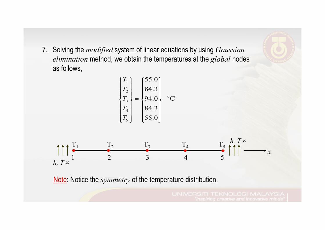
7.  Solving the modified system of linear equations by using Gaussian elimination method, we obtain the temperatures at the global nodes as follows,

1

2o

3

4

5

55.084.3

C94.084.355.0

TTTTT

⎧ ⎫ ⎧ ⎫⎪ ⎪ ⎪ ⎪⎪ ⎪ ⎪ ⎪⎪ ⎪ ⎪ ⎪

=⎨ ⎬ ⎨ ⎬⎪ ⎪ ⎪ ⎪⎪ ⎪ ⎪ ⎪⎪ ⎪ ⎪ ⎪⎩ ⎭⎩ ⎭

1 2 3 4 5

T1 T2 T3 T4 T5 h, T∞

h, T∞

x

Note: Notice the symmetry of the temperature distribution.

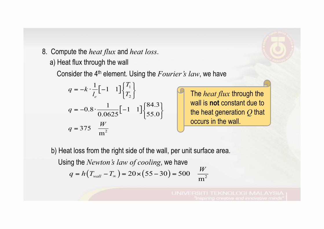
8. Compute the heat flux and heat loss. a) Heat flux through the wall Consider the 4th element. Using the Fourier’s law, we have

[ ]

[ ]

1

2

2

1 1 1

84.310.8 1 155.00.0625

375 m

e

Tq k

Tl

q

Wq

⎧ ⎫= − ⋅ − ⎨ ⎬

⎩ ⎭

⎧ ⎫= − ⋅ − ⎨ ⎬

⎩ ⎭

=

b) Heat loss from the right side of the wall, per unit surface area. Using the Newton’s law of cooling, we have

( ) ( ) 220 55 30 500 mwallWq h T T∞= − = × − =

The heat flux through the wall is not constant due to the heat generation Q that occurs in the wall.