CIRCLE FITTING FROM THE POLARITY TRANSFORMATION

REGRESSION

Roque Calvo a, Emilio Gómez b, Rosario Domingo c

a Dpt. Mechanical Engineering and Construction. Universidad Politécnica de Madrid. Ronda de Valencia, 3; 28012 Madrid, Spain. Corresponding author. Phone: +34 913367564. Fax +34 913367676. E-mail: roque.calvo@upm.es b Dpt. Mechanical Engineering and Construction. Universidad Politécnica de Madrid. Ronda de Valencia, 3; 28012 Madrid, Spain. E-mail: emilio.gomez@upm.es c Dpt. Construction and Manufacturing Engineering. Universidad Nacional de Educación a Distancia (UNED). Juan del Rosal, 12; 28040 Madrid, Spain. E-mail: rdomingo@ind.uned.es

Geometrical fitting is useful in different fields of science and technology, in particular

least squares minimum (LSM) methods are widespread in contact probing for

coordinate measuring machines, as well as a reference shape for surface metrology. We

present a new intuitive and simple LSM algorithm for circle fitting, the polarity

transformation regression. It is a non-linear algebraic method from a generic geometric

transformation. We derive the explicit expression of the model estimators from the data

points. Then, the algorithm is compared with other methods based on simulation and

some literature data sets. The proposed algorithm presents a comparable accuracy, low

computational effort and good behavior with outliers based on the initial test,

outperforming other well-known algebraic methods in some of the studied data sets.

The basis of the algorithm is finally suggested for other potential uses.

Key words: circle fitting; least squares fit; regression; projective transformation

1. Introduction and background.

The fitting of measured data points or image pixels to simple geometric primitives is a

basic task for quality inspection [1][2], computer graphics [3], archaeology [4],

astronomy or geodesy [5], metrology at sub-micrometer scale [6], high-energy physics

[7] or signal processing [8], just to mention some different fields of application. The

digital revolution and computer assistance since the 1980’s has supplied these areas of

interest by contact measurement (coordinate measuring machines or stylus) of primary

importance in applied dimensional metrology, as well as signals for image data

processing –non-contact–, from sub-micrometer level to astronomical distances. The

capability of reduction from a set of data points to fit a geometric shape is of increasing

importance for decision-making, modeling or ulterior processing.

The problem of fitting a data set of points in a plane to a circle or partially to a

circumference arc has been investigated deeply, as the circle is a main geometrical

shape. Apart from some specific algorithms, the two main groups of methods to fit a

circle are the algebraic fitting and the geometric fitting. They differ in the definition of

the error distance under consideration. The algebraic error is defined by the deviation

from the implicit equation of a circle (1) at each point. This deviation or non-equality

indicates that the point does not belong to the circle.

We face the problem of fitting a set of n points of rectangular coordinates (xi,yi) to a

circle of center (a,b) and radius R. It may be formulated minimizing the sum of

algebraic distances (2).

0)()(:0),,;,( 222 RbyaxRbayxF (1)

n

iii

n

ii RbyaxRR

1

2222

1

222 )()(minmin (2)

n

ii

n

i

n

ii dRbyaxRR

1

2

1

222

1

2 min)()(minmin (3)

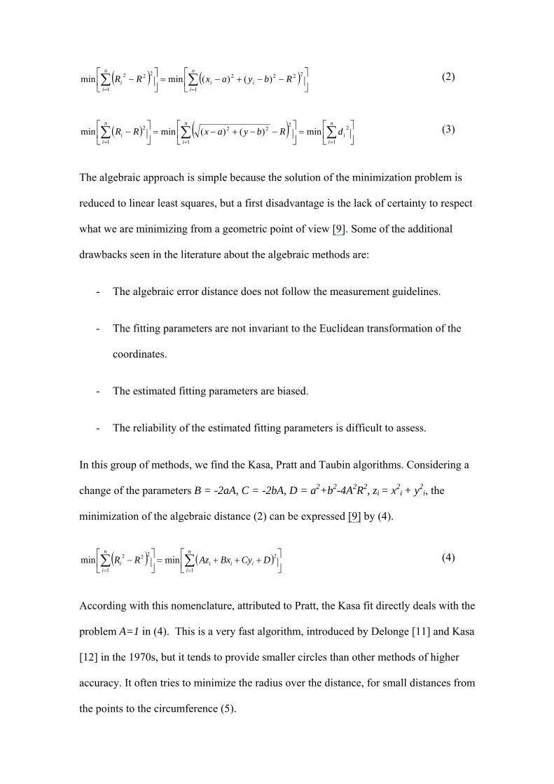
The algebraic approach is simple because the solution of the minimization problem is

reduced to linear least squares, but a first disadvantage is the lack of certainty to respect

what we are minimizing from a geometric point of view [9]. Some of the additional

drawbacks seen in the literature about the algebraic methods are:

- The algebraic error distance does not follow the measurement guidelines.

- The fitting parameters are not invariant to the Euclidean transformation of the

coordinates.

- The estimated fitting parameters are biased.

- The reliability of the estimated fitting parameters is difficult to assess.

In this group of methods, we find the Kasa, Pratt and Taubin algorithms. Considering a

change of the parameters B = -2aA, C = -2bA, D = a2+b2-4A2R2, zi = x2i + y2

i, the

minimization of the algebraic distance (2) can be expressed [9] by (4).

n

iiii

n

ii DCyBxAzRR

1

2

1

222 minmin (4)

According with this nomenclature, attributed to Pratt, the Kasa fit directly deals with the

problem A=1 in (4). This is a very fast algorithm, introduced by Delonge [11] and Kasa

[12] in the 1970s, but it tends to provide smaller circles than other methods of higher

accuracy. It often tries to minimize the radius over the distance, for small distances from

the points to the circumference (5).

n

ii

n

iii

n

iii

n

ii dRdRdRRRRRR

1

22

1

22

1

22

1

222 4min2minminmin (5)

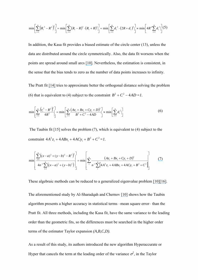
In addition, the Kasa fit provides a biased estimate of the circle center (13), unless the

data are distributed around the circle symmetrically. Also, the data fit worsens when the

points are spread around small arcs [10]. Nevertheless, the estimation is consistent, in

the sense that the bias tends to zero as the number of data points increases to infinity.

The Pratt fit [14] tries to approximate better the orthogonal distance solving the problem

(6) that is equivalent to (4) subject to the constraint ADCB 422 =1.

n

ii

n

i

iiin

i

i dADCB

DCyBxAz

R

Rr

1

2

122

2

12

222

min4

min4

min (6)

The Taubin fit [15] solves the problem (7), which is equivalent to (4) subject to the

constraint 222 444 CBACyABxzA iii =1.

n

in

iiii

iiin

i

n

i

CBACyABxzAn

DCyBxAz

byaxn

Rbyax

2221

2

1

221

1

2222

444min

)()(4

)()(min (7)

These algebraic methods can be reduced to a generalized eigenvalue problem [10][16].

The aforementioned study by Al-Sharadqah and Chernov [10] shows how the Taubin

algorithm presents a higher accuracy in statistical terms –mean square error– than the

Pratt fit. All three methods, including the Kasa fit, have the same variance to the leading

order than the geometric fits, so the differences must be searched in the higher order

terms of the estimator Taylor expansion (A,B,C,D).

As a result of this study, its authors introduced the new algorithm Hyperaccurate or

Hyper that cancels the term at the leading order of the variance 2, in the Taylor

expansion of the mean square error of the estimators. The terms of order 2/n2 and

higher remain. These terms are important when the variance (noise) is high and the

number of points is reduced. Rangarajan and Kanatani [16][17] have recently improved

the accuracy of the Hyper canceling also the terms 2/n2, so the method outperforms the

former algorithms for high noise (2) in small (n) data set. They compare also the

performance with the orthogonal geometric fitting, which fails in convergence for high

2/n2 and with partial small arcs. Nevertheless, the geometric fit remains slightly better

for semicircles than the improved Hyper algorithm.

The geometric fit is also named orthogonal least squares fit or orthogonal distance

regression. It considers the minimization problem (3). This regression estimator has its

origin in Gauss, back in the 18th century [18]. The orthogonal algorithms are applied to

different geometries [19]. Specifically for circles, we find the Landau algorithm [20]

that uses a fixed-point iterative scheme, or the Späth algorithm [21], with a slower

convergence than the former one. The Levenberg-Marquardt algorithm [22] [23],

introduces a correction on the classical non-linear least squares Gauss-Newton method

[24]. It is reliable although it requires initialization. All three deal with the minimization

of the non-linear problem in an iterative way, with similar computational effort per

iteration, but with superior performance of the Levenberg-Marquardt method for small

circular arcs [25]. Its superior performance in statistical terms is also remarked in [10]

and [16], upon comparison with some algebraic methods, although the convergence can

fail for high noise and small data sets.

The performance of a circle fit in terms of accuracy is ordinary assessed through the

root mean squares error (RMSE) of the estimated radius. The statistical foundation is

that the maximum likelihood estimator of the curve parameters is reached minimizing

the sum of squares of orthogonal distances to the data points [24]. The normal

distribution of the noise gives robustness to the statistical approach, but it derives in

poor results with the presence of outliers. Other estimators can be more appropriated in

this case. Ladrón de Guevara [9] considers the sum of the absolute distances as a better

regression estimator when outliers are present. Even so, the robustness of this estimator

was previously questioned by Rousseeuw [26] at the time of introducing the least

median squares regression. Midway, in order to reduce the outliers effect, the data set

can be previously filtered [6]. In overall terms, orthogonal geometric fits are usually

regarded as the most accurate, in spite of that they are computational intensive and

occasionally prone to divergence. The bias of the geometric fit tends to produce bigger

circles of a radius difference at the leading order of 2/R, where R is the estimated

radius [27] [10]. This leads to correct the raw method to weighted least squares in the

case of small radius and high noise, a frequent situation at small-scale metrology [6].

Some other specific methods have been proposed. Although an extensive review is out

of the scope of this work, some of them will be mentioned later when testing the

algorithm we propose.

The existence and uniqueness of the solution could be just a formal point for the

practitioner. The general problem of circle fitting has not a unique solution nor exists in

all cases [28], but this cannot reduce the interest of getting a useful good fitting.

The choice of one method instead to another would be a balance between the necessary

speed for the application and the accuracy expected from the method on the real set of

data, including the presence of outliers or the sensitiveness to fit small arcs. Finally, the

use of an algorithm can depend on the availability of the code or the routine function

inside the final user's software program in different disciplines.

In the next section, we present the basic projective transformation that gives origin in

section 3 to the algorithm. In section 4, the proposed method is initially tested and its

results are discussed.

2. Projective transformation of a circle into a straight line

A circle C is a conic with center that in algebraic terms is a quadratic variety w(x) from

a bilinear form f(x,x) of equation (8) in the Euclidean plane, where x notes the position

vector of the point, Fig 1.

0)()()()(: 222 RbyaxfwC xx,x (8)

The set of conjugate points of a generic point xp in plane are given by f(x,xp)=0. The

equation (9) is the tangent T to the circle at the point xp of rectangular coordinates

(xp,yp), when the point xp belongs to the circle.

0)()()()()(: 2 RaybyaxaxfT pppxx, (9)

Considering the application of the equation (9) to a point xv (xv,yv) outside the circle, it

also represents the conjugate points of xv. It is the polar line L of the circle (8) regarding

the point xv, see Fig 1. Polarity is the transformation that associates a circle to its polar.

It can also be interpreted as a point-to-point transformation that associates to each point

xp of a circle a point on its polar xp’, result of the intersection of the polar and the

tangent to the circle at xp. That point xp’ will be the solution of the pair of equations

(10). In this correspondence, the point of the infinite is the homologue of the

intersection points with the circle of the line defined by xv and the center of the circle

(a,b), points (xv’,yv’) and (xv’’,yv’’). This situation can be formally handled in

homogeneous coordinates. The two intersection points D1 and D2 of the circumference

and its polar are double.

0)()()()()(:

0)()()()()(:

2

2

RbybyaxaxfT

RbybyaxaxfL

pp

vv

p

v

xx,

xx, (10)

In plane terms, this point-to-point correspondence transforms points from a circle into a

line. Intuitively, we “open and straighten” the circle projecting its points into its polar.

Even when the geometric interpretation of polarity has been used from an external point

to the circle, this transformation comes from the conjugate relation that establishes the

bilinear form (9), so the conjugate of inner points to the circumference will be on

straight lines without intersection with the circle. In algebraic terms, the tangents from

an inner point to the circle are imaginaries, instead of real lines.

Let’s consider the problem of a set of points that we want to fit to a circle. They are

outside the circle that we assume they approach. It can be because of uncertainty in the

measurement process –taking the most probable value of the measured point-. We can

also assume the point is out of the circle because the real form does not correspond to a

circle, so the physical loci in the contour is precise but it does not lay on a circle along

some other points. Assuming a solution circle exists, we have n points in the plane

around it and we can construct a set of concentric circles to the solution circle, so with

null intersection. Each point is a priori on a different circle. Therefore, when we apply

the projective transformation of every point of the data set, their homologues are on

their different polar lines, all of them parallel lines. They are all parallel, because by

construction the projective transformation conserves the incidence relationships, so

those concentric circles will have parallel polar lines. In case that two points are on the

same circle, we consider that two different circles exist with the same radius, so their

two respective polar lines already exist, but collapsed into the same one in the Euclidean

plane.

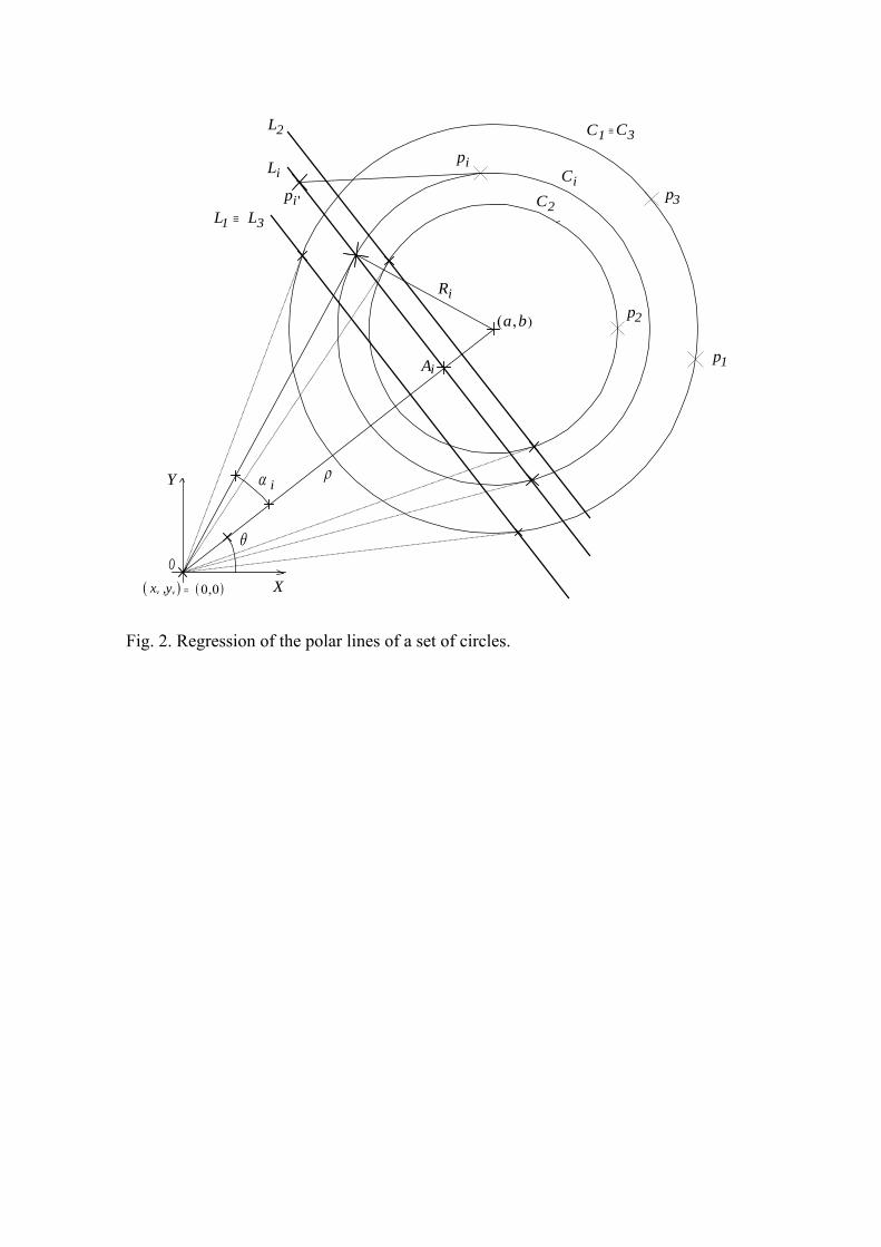
As a result of the construction, we pass from a data set of p1…pn points to their

homologues p’1…p’n, on their polars, Fig.2. Since every point is in its own

circumference, we can consider the transformation passes from n points to n polar lines.

After the transformation, we consider the fitting problem of a set of parallel straight

lines L1, … Ln with non-linear least squares. The transformation is done in an implicit

way with the unknowns of the center and the fitted circle radius. Geometrically, when a

point approaches the solution circle of radius R, its polar approaches the polar solution

L. This is evident by the geometric construction, but also analytically we can find a

polar arbitrary close to L, let’s say , as providing Ri is close enough to R, let’s say i,

since we can always find a ball of radius Rext that includes all the data points (11). Note

in Fig. 2, the segment OAi = fi , the distance to the polar Li from the origin O. In general,

for each point pi, on a circle of radius Ri , its polar line is Li . The center of the circle and

the polar line are at a distance and fi, respectively, from the origin of coordinates,

ext

iiext

soliexti

ii

i R

RRR

RRRff

Rf

2

22;

222

(11)

In the following section we will develop the equations of the fitting for the set of

parallel polar lines.

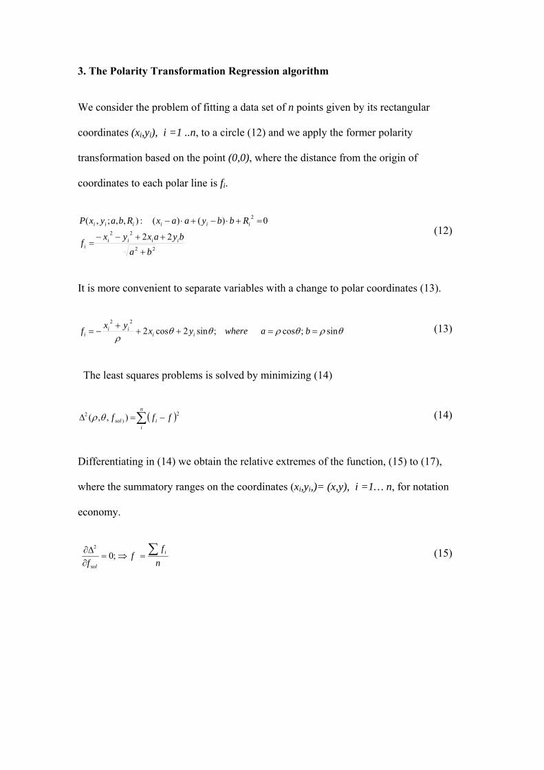
3. The Polarity Transformation Regression algorithm

We consider the problem of fitting a data set of n points given by its rectangular

coordinates (xi,yi), i =1 ..n, to a circle (12) and we apply the former polarity

transformation based on the point (0,0), where the distance from the origin of

coordinates to each polar line is fi.

22

22

2

22

0)()(:),,;,(

ba

byaxyxf

RbbyaaxRbayxP

iiiii

iiiiii

(12)

It is more convenient to separate variables with a change to polar coordinates (13).

sin;cos;sin2cos222

bawhereyxyx

f iiii

i (13)

The least squares problems is solved by minimizing (14)

n

iisol fff 2

)2 ),,( (14)

Differentiating in (14) we obtain the relative extremes of the function, (15) to (17),

where the summatory ranges on the coordinates (xi,yi,)= (x,y), i =1… n, for notation

economy.

n

ff

fi

sol

;02

(15)

n

yxyx

n

yy

n

xx

n

yxyx

n

yy

n

xxn

yxyx

2222

22222

22222

2

sincos2

*

0sin2cos2;0

(16)

22222

222222

2

222

22

222

222

22222

2222

2222

1

2

1

2

1

2

22222

2

where

21

2*tan

0sin2cos2;0

n

yxyx

n

yy

n

yxyx

n

xx

n

yxyx

n

yy

n

yxyx

n

xxk

n

yxyx

n

yy

n

xx

n

yxyx

n

yy

n

yxyx

n

xxk

k

k

k

k

n

yy

n

xxn

yxyx

(17)

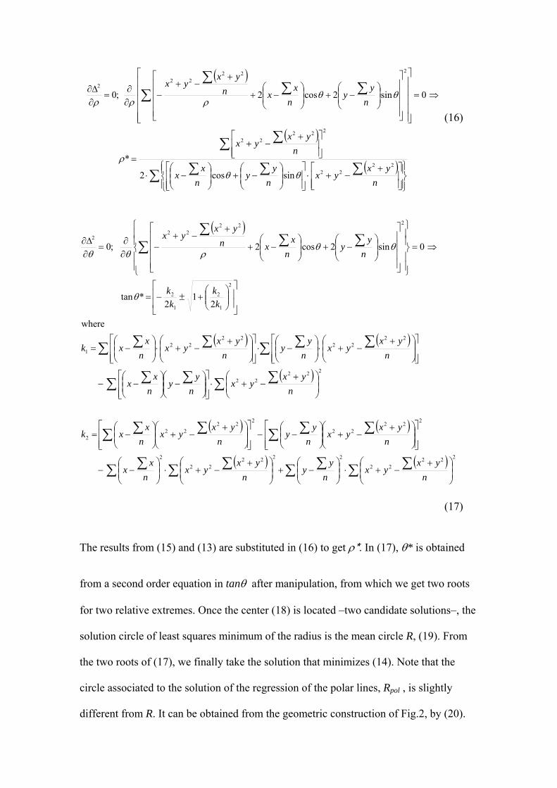
The results from (15) and (13) are substituted in (16) to get *. In (17), * is obtained

from a second order equation in tan after manipulation, from which we get two roots

for two relative extremes. Once the center (18) is located –two candidate solutions–, the

solution circle of least squares minimum of the radius is the mean circle R, (19). From

the two roots of (17), we finally take the solution that minimizes (14). Note that the

circle associated to the solution of the regression of the polar lines, Rpol , is slightly

different from R. It can be obtained from the geometric construction of Fig.2, by (20).

RMSEminfor (17) from*tan

*tan

*tan2

*tan2

2222

22222

2222

22222

n

yxyx

n

yy

n

xx

n

yxyx

b

n

yxyx

n

yy

n

xx

n

yxyx

a

(18)

n

byax

n

RR i

22 )()( (19)

bn

ya

n

x

n

yxbaR

R

n

ff

Rf iiii

pol

polipol

ii

22;22

2222

(20)

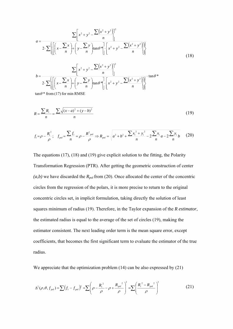
The equations (17), (18) and (19) give explicit solution to the fitting, the Polarity

Transformation Regression (PTR). After getting the geometric construction of center

(a,b) we have discarded the Rpol from (20). Once allocated the center of the concentric

circles from the regression of the polars, it is more precise to return to the original

concentric circles set, in implicit formulation, taking directly the solution of least

squares minimum of radius (19). Therefore, in the Taylor expansion of the R estimator,

the estimated radius is equal to the average of the set of circles (19), making the

estimator consistent. The next leading order term is the mean square error, except

coefficients, that becomes the first significant term to evaluate the estimator of the true

radius.

We appreciate that the optimization problem (14) can be also expressed by (21)

22222222 ),,(

polipoli

polipol

RRRRfff (21)

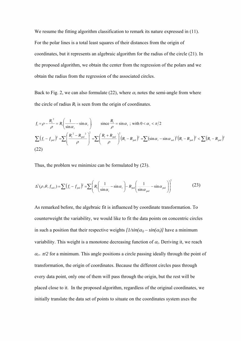
We resume the fitting algorithm classification to remark its nature expressed in (11).

For the polar lines is a total least squares of their distances from the origin of

coordinates, but it represents an algebraic algorithm for the radius of the circle (21). In

the proposed algorithm, we obtain the center from the regression of the polars and we

obtain the radius from the regression of the associated circles.

Back to Fig. 2, we can also formulate (22), where i notes the semi-angle from where

the circle of radius Ri is seen from the origin of coordinates.

2222

22222

2

sinsin

20with ;sin since;sinsin

1

polipolisolipolipolipoli

poli

iii

ii

ii

i

RRRRRRRRRR

ff

RR

Rf

(22)

Thus, the problem we minimize can be formulated by (23).

2

2)

2 sinsin

1sin

sin

1),,( pol

polpoli

iipolisol RRfff

(23)

As remarked before, the algebraic fit is influenced by coordinate transformation. To

counterweight the variability, we would like to fit the data points on concentric circles

in such a position that their respective weights [1/sin(i) – sin(i)] have a minimum

variability. This weight is a monotone decreasing function of i. Deriving it, we reach

i= /2 for a minimum. This angle positions a circle passing ideally through the point of

transformation, the origin of coordinates. Because the different circles pass through

every data point, only one of them will pass through the origin, but the rest will be

placed close to it. In the proposed algorithm, regardless of the original coordinates, we

initially translate the data set of points to situate on the coordinates system axes the

points of minimum abscise and ordinate, so all the points are in the first quadrant and

near to the origin. This translation looks for a high i, which reduces [1/sin(i)– sin(i)]

variability. The limit of i very near to /2 is not considered. At this limit the [1/sin(i)

– sin(i)] factors are very similar and close to 0. Therefore, the polars are all very close

each other, with small distance resolution. We face at this limit the computational

problem of handing small differences of very small numbers.

We note also that the algebraic fitting problem (23) would approach at the limit the

orthogonal problem (3), when [1/sin(i) – sin(i)] 1 and [1/sin(pol) – sin(pol)] =1.

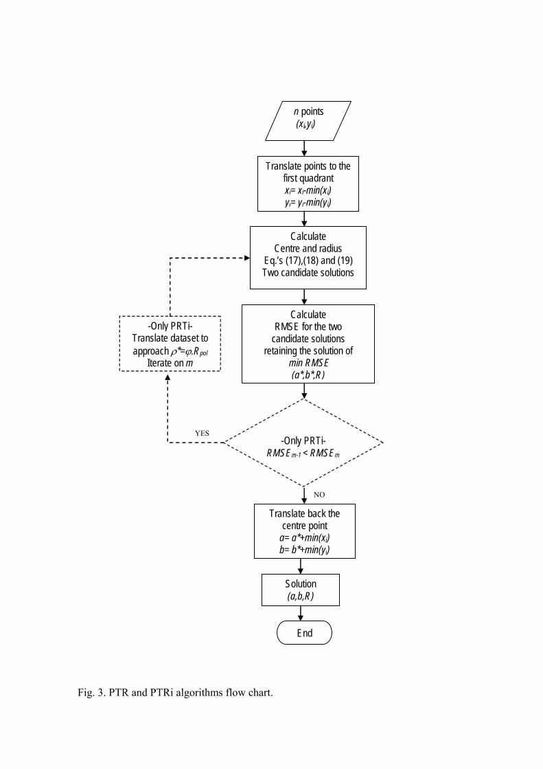
That is sin(pol)= Rpol/ =(5½-1)/2=1/ , where denotes the golden number. This can

be used to translate iteratively the data points to a distance from the origin * = Rpol .,

looking for a RMSE reduction, with the trade-off of a slower algorithm. We call PRTi

the iterative version of the algorithm.

At this point we can reference the method of Brandon and Cowley [29], based on the

inversion of the circle to respect one of its points: If a set of points lays approximately

on a circle, their transformed by inversion lay approximately on a straight line. The

original method uses total least squares of the transformed points to calculate the

straight line that is transformed back to obtain the fitted circle, with influence in the

results depending on the choice of the inversion pole. The modification introduced by

Rusu et al. [30] tries to reduce this effect using iterative weighted least squares. The

method is compared in the next section to our proposed algorithm and some others.

Complementing the functional analysis, the PTR formulation allows checking the nature

of the relative extremes. It can be obtained from the second order derivatives and the

sign of the determinant of the Hessian matrix, H(,), (24). Since 2>0, the solution

of the optimization will be a relative minimum when det(H(,))>0. In the case of

det[H(,)]<0 the checking is inconclusive.

sincos2;

cossin2;2

;6

12),(det

3221

2222

2312

32

2222

22

2222

14

212

2

22

4

221312

32

24

21

222

22

22

2

22

n

yy

n

xxg

gg

n

yy

n

xxg

gggg

n

yxyxg

g

Where

gggggg

gH

(24)

Nevertheless, when focusing on the fitting, the proposed algorithm directly takes the

value that minimizes the objective function out of the two relative extreme candidates.

The adopted algorithm is sketched in the Fig. 3 flow chart.

4. Algorithm testing and discussion of results

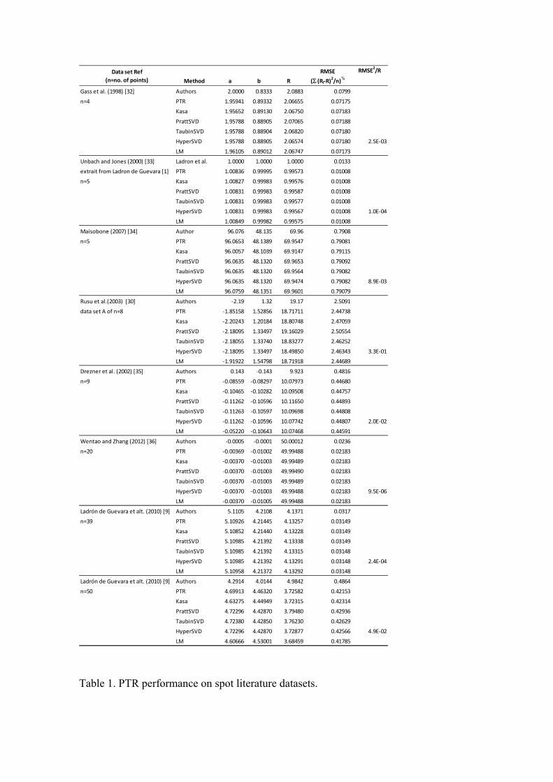
We summarize the initial tests carried out with some data sets from the literature, Table

1. The number of points ranges from 4 to 50. The performance of the PTR is good

between the algebraic fittings. Even when it does not reach the accuracy of the

orthogonal regression Levenberg-Marquardt (LM), it is not far away. The Matlab code

of the Kasa, Pratt, Taubin, Hyper and LM has been retrieved from Chernov web page

[31]. We must note that the differences of the PTR to respect other algebraic fits,

approaching the LM, is more pronounced for big ratios of RMSE to R, namely the data

sets of Maisonobe (2008) and Rusu et al. (2003). The data set of Ladrón de Guevara et

al.[9] has 50 points of a semicircle from the contour of a digital image of the Moon and

it contains outliers. The other data set of 39 points is the former one after outlier

filtering. The behavior of the PTR in this big arc in the presence of outliers is

outstanding. When the outliers are removed, dataset of 39 points, the different methods

converge in their results. We must remark that the Ladrón de Guevara et al.’s method

and tabulated solution pursuits the optimization of the mean absolute error instead of the

mean square error.

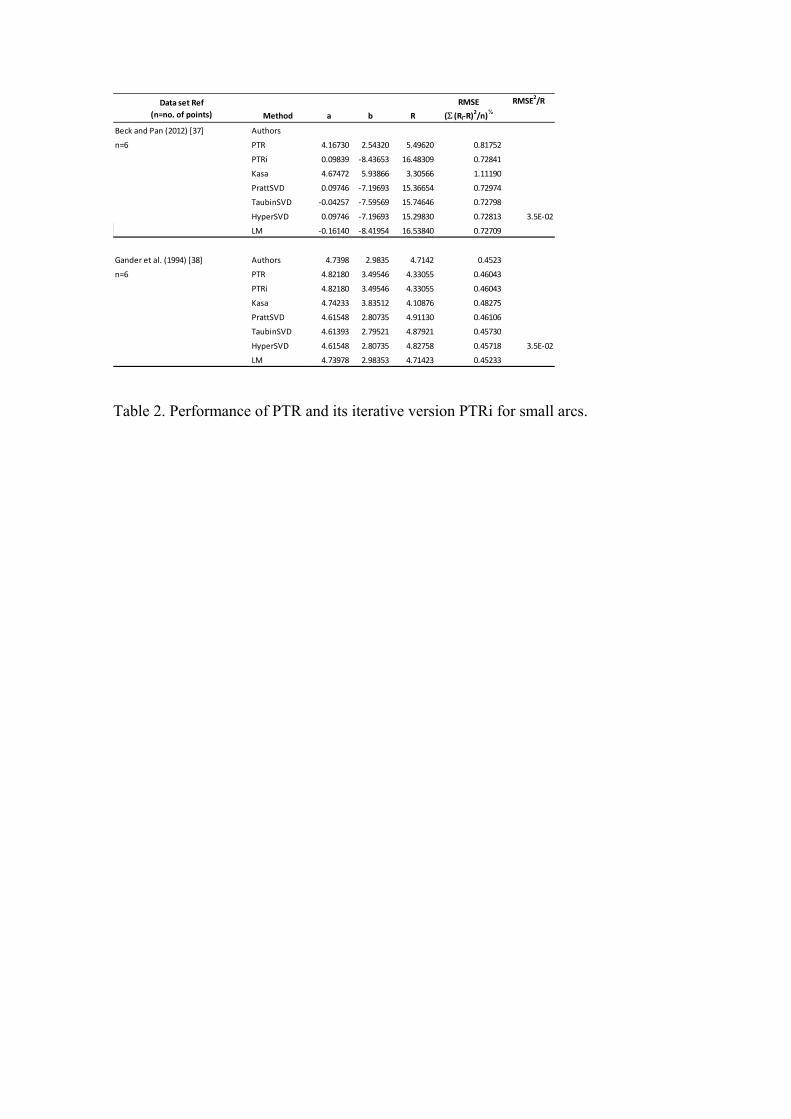
In the Table 2 we have tried the fitting of small arcs, also from two literature datasets.

As the arc becomes smaller, PTR presents a similar problem as the Kasa method

towards smaller circles, but less pronounced. The use of the iterative version PTRi

improves the fitting results, close to the other methods without that bias.

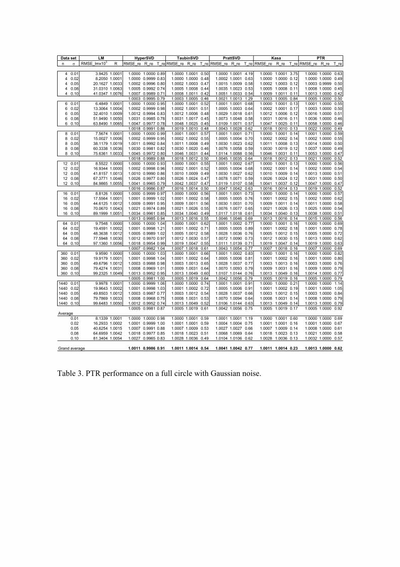
Next, we tried the behavior for data sets generated from a circle of radius 1 and

Gaussian noise. The data sets were obtained from a uniform distribution of n true

points. The noise has been generated in abscise and ordinate directions by the pseudo-

random number generator of Matlab under a normal standard distribution of mean 0

around the circle point, with standard deviation . Each line in Table 3 shows the mean

result obtained for 1000 dataset shots. Noteworthy is that the thousand points are

exactly the same for each algorithm, so the results of the algorithms are for the same

input and the bias from sampling would equally affect all of them. The table includes

the values for the LM method of the RMSE of the 1000 fits and the results of the mean

radius R. The baseline for comparison of the computation time inside the group of trials

–a line of the table– has been set as 1 for the LM method. For instance the computation

time of the 1000 trials with (n, )=(4,0.01) is 89% of the computing time of LM when

running HyperSVD, or TaubinSVD requires 48% of the time that LM uses for the data

set (n, )=(4,0.02). The trials were always carried out in the same computer. The

relative ratios of the RMSE, radius size and computing time to respect the LM values are

respectively RMSE_re, R_re and T_re. The LM algorithm was always initialized in the

same point (2,2), while the center of the true circle is (1,1). The trials do not intend to

deploy a precise speed comparison test or a ranking, but to estimate the algorithm

relative behavior, in particular of the proposed PTR algorithm. A grand average by

number of points and noise level is finally included in order to give bulk estimation

across the 40,000 fits calculated under each method. The faster results are obtained from

Kasa followed by TaubinSVD, both taking advantage of fast matrix algorithms of

Matlab. PTR comes next, with its analytical formulation and no special code

optimization in Matlab. Note how the size of the estimated circle of the algebraic fits

has a trend toward bigger circles than LM, except the HyperSVD. The PTR algorithm

gives in average an estimator of the radius almost equal to the LM. The trend of the

orthogonal fittings to bigger circles must be considered, as mentioned in the first

section. Also remarkable is the good behavior of the Kasa fitting in speed and accuracy

for those uniform data sets with statistical distributed noise with no partial arcs or

outliers. The accuracy of the different algebraic methods to respect the LM is good and

very similar, in general with less than 1% differences.

5. Conclusions

The proposed PTR algorithm gives an explicit analytical formulation that allows an

easy encoding in any computer language. From the initial tests, its accuracy is similar to

other algebraic fittings for full circles and with a less pronounced bias towards smaller

circles for small arcs than the Kasa fit exhibits. The iterative variant PTRi mitigates this

trend to approach other algebraic fittings. In a first trial, PTR has a good behavior,

above other algebraic fits when the data set includes outliers, and it outperformed other

well-known algebraic fits in some particular trials of this study. In summary, the

proposed algorithm presents a good performance in terms of speed, accuracy and radius

estimation, paying attention to small arcs.

Conversely to pure numerical algorithm like LM, the proposed method gives explicit

expression of the center and radius, function of the data point coordinates. This can

facilitate the error study of the estimators.

Considering the two main groups of algorithms, the basic connection of the algebraic

fitting and the orthogonal regression is a common objective of reaching a good fitting

with low effort. The proposed algorithm PTR establishes a graphical relationship: The

orthogonal fit is the regression of a set of concentric circles, while the algebraic fit

represents the regression of the corresponding polar lines.

Circle fitting algorithms have been worked out in depth, with accurate and efficient

algorithms nowadays available. In most of the situations, the Levenberg-Marquardt

method outperforms the algebraic fittings, but it requires initialization and it is slower

than these are. The basis of the PTR algorithm is the polarity transformation, a concrete

case of homography, which is quite familiar in image processing and it could be

eventually used in the field for other related applications. Algebraic curves and surfaces

less investigated –conics and quadrics– could benefit from the transformation of the

data points in a set of hyperplanes –lines or planes– in order to obtain quick algorithms

of adequate accuracy.

6. References

[1] Gosavi A, Cudney E. Form Errors in Precision Metrology: A Survey of

Measurement Techniques, Qual Eng 2012; 24(3) 369-380

[2] Phillips SD, Borchardt B, Estler WT, Buttress J . The estimation of measurement

uncertainty of small circular features measured by coordinate measuring machines. Prec

Eng 1998; 22; 87-97

[3] Rama MPM, Kurfess TR, Tucker TM. Least squares fitting of analytic primitives

on a GPU. J Manuf Syst 2008; 27; 130-135

[4] Rorres, C, Romano, DG. Finding the centre of a circular starting line in an ancient

Greek Stadium. SIAM Rev. 1997; 39(4); 745–754.

[5] Nievergelt Y. A tutorial history of least squares with applications to astronomy and

geodesy. J Comput Appl Math 2000; 121; 37-72

[6] Kühn O, Linß G , Töpfer S, Nehse U, Robust and accurate fitting of geometrical

primitives, to image data of microstructures, Measurement 2007; 40; 129-144

[7] Karimäki V. Effective circle fitting for particle trajectories. Nucl Instrum Meth A

1991; 305; 187–191

[8] Jiménez F, Aparicio F, Estrada G. Measurement uncertainty determination and

curve-fitting algorithms for development of accurate digital maps for advanced driver

assistance systems. Transport Res C-Emer 2009; 17; 225-239

[9] Ladrón de Guevara I, Muñoz J, de Cózar OD, Blázquez EB. Robust Fitting of

Circle Arcs. J Math Imaging Vis 2011; 40 (2); 147-161

[10] Al-Sharadqah A, Chernov N. Error analysis for circle fitting algorithms.

Electron J Stat 2009; 3; 886–911

[11] Delogne P. Computer optimization of Deschamps’ method and error cancellation

in reflectometry. In: Proc. IMEKO-Symp. Microwave Measurement, Budapest. 1972.

117–123

[12] Kåsa I. A curve fitting procedure and its error analysis. IEEE T Instrum Meas.

1976; 25; 8–14

[13] Rusu C, Tico C, Kuosmanen P, Delp EJ. Classical geometrical approach to

circle fitting – review and new developments. J Electron Imaging 2003; 12; 179–193

[14] Pratt V. Direct least squares fitting of algebraic surfaces. Comp Graph 1987; 21;

145–152

[15] Taubin G. Estimation of planar curves, surfaces and nonplanar space curves

defined by implicit equations, with applications to edge and range image segmentation.

IEEE T Pattern Anal 1991; 13; 1115–1138

[16] Rangarajan P, Kanatani K. Improved algebraic methods for circle fitting. Electron J

Stat 2009; 3; 1075-1082

[17] Kanatani K, Rangarajan P. Hyper least squares fitting of circles and ellipses. Comp

Stat Data An 2011; 55; 2197-2208

[18] Åke Björck, Numerical methods for least-squares problems. SIAM, Philadelphia,

1996.

[19] Shakarji CM. Least-Squares Fitting Algorithms of the NIST Algorithm Testing

System. J Res Natl Inst Stand Technol 1998; 103; 633

[20] Landau UM. Estimation of a circular arc center and its radius. Comput Vis Image

Und 1987; 38; 317–326

[21] Späth H. Least-squares fitting by circles. Computing 1986; 57; 179–185

[22] Levenberg K. A method for the solution of certain non-linear problems in least

squares. Q Appl Math 1944; 2;164–168

[23] Marquardt D. An algorithm for least squares estimation of nonlinear parameters.

SIAM J Appl Math 1963; 11; 431–441

[24] N. Chernov, Circular and Linear Regression: Fitting Circles and Lines by Least

Squares, Taylor & Francis Inc (US), 2010.

[25] Chernov N, Lesort C. Least squares fitting of circles. Vision J Math Imaging Vis

2005; 23; 239–251

[26] Rousseeuw PJ. Least median of squares regression. J Am Stat Assoc 1984;

79(388); 871–880

[27] Newsam GN, Redding NJ. Fitting the most probable curve to noisy observations.

In: IEEE Proc. ICIP 1997. 752–755

[28] Chernov N, Huang Q, Ma H. Does the best fit always exist?. ISRN Probability and

Statistics 2012

[29] Brandon JA, Cowley A. A weighted least squares method for circle fitting to

frequency response data. J Sound Vib 1983; 89(3); 419-424

[30] Rusu C, Tico M, Kuosmanen P, Delp EJ . Classical geometrical approach to circle

fitting—review and new developments. J Electron Imaging 2003; 12(1); 179–193

[31] Chernov N, http://www.math.uab.edu/~chernov/cl/, last accessed Jun’2012.

[32] Gass SI, Witzgall C, Harary HH. Fitting Circles and Spheres to Coordinate

Measuring Machine Data. Int J Flex Manuf Sys 1998; 10; 5-25

[33] Umbach D., Jones K.N., IEEE T Instrum Meas, 52(6) (2003),1881-1885.

[34] Maisonobe, L. Finding the circle that best fits a set of points, 2007.

http://www.spaceroots.org/documents/circle/circle-fitting.pdf , last accessed Jun’2012.

[35] Drezner Z, Steiner S, Wesolowsky GO. On the circle closest to a set of points.

Comput Oper Res 2002; 29; 637-650

[36] Wentao S, Dan Z. Four Methods for Roundness Evaluation. Physics Procedia

2012; 24; 2159 – 2164

[37] Beck A, Pan D. On the solution of the GPS localization and circle fitting problems.

SIAM J Optimiz 2012; 22(1); 108–134

[38] Gander W, Golub GH, Strebel R. Least-Squares Fitting of Circles and Ellipses. Bit

1994; 34(4); 558-578

' ' ),( pypx ),( pypx 02)()()()(: RapybyapxaxT

022)(2)(: RbyaxC

02)()()()(: RavybyavxaxL

),( vyvx

),( ba

X)0,0(

Y

),( v'yv'x

),( v''yv''x

1D

2D

Fig. 1. Polarity transformation of a circle C into its polar L from xv.

X

Y

1p

3p

2p

iC

2C

ip

1C 3C

),( ba

A

iR

O

0,0vv ,yx

i

31 LL 'ip

iL

2L

i

Fig. 2. Regression of the polar lines of a set of circles.

n points (xi,yi)

Translate points to the first quadrant xi= xi-min(xi) yi= yi-min(yi)

Calculate Centre and radius

Eq.’s (17),(18) and (19) Two candidate solutions

Calculate RMSE for the two

candidate solutions retaining the solution of

min RMSE (a*,b*,R)

Translate back the centre point

a= a*+min(xi) b= b*+min(yi)

Solution (a,b,R)

End

-Only PRTi- Translate dataset to approach *=.Rpol

Iterate on m

-Only PRTi-

RMSEm-1 < RMSEm

YES

NO

Fig. 3. PTR and PTRi algorithms flow chart.

Data set Ref

(n=no. of points) Method  a b R

RMSE

( (Ri‐R)2/n)

½

RMSE2/R

Gass et al. (1998) [32] Authors  2.0000 0.8333 2.0883 0.0799

n=4 PTR  1.95941 0.89332 2.06655 0.07175

Kasa 1.95652 0.89130 2.06750 0.07183

PrattSVD 1.95788 0.88905 2.07065 0.07188

  TaubinSVD 1.95788 0.88904 2.06820 0.07180

HyperSVD 1.95788 0.88905 2.06574 0.07180 2.5E‐03

LM 1.96105 0.89012 2.06747 0.07173

Unbach and Jones (2000) [33] Ladron et al. 1.0000 1.0000 1.0000 0.0133

extrait from Ladron de Guevara [1] PTR 1.00836 0.99995 0.99573 0.01008

n=5 Kasa 1.00827 0.99983 0.99576 0.01008

PrattSVD 1.00831 0.99983 0.99587 0.01008

  TaubinSVD 1.00831 0.99983 0.99577 0.01008

HyperSVD 1.00831 0.99983 0.99567 0.01008 1.0E‐04

LM 1.00849 0.99982 0.99575 0.01008

Maisobone (2007) [34] Author 96.076 48.135 69.96 0.7908

n=5 PTR  96.0653 48.1389 69.9547 0.79081

Kasa 96.0057 48.1039 69.9147 0.79115

PrattSVD 96.0635 48.1320 69.9653 0.79092

  TaubinSVD 96.0635 48.1320 69.9564 0.79082

HyperSVD 96.0635 48.1320 69.9474 0.79082 8.9E‐03

LM 96.0759 48.1351 69.9601 0.79079

Rusu et al.(2003)  [30] Authors  ‐2.19 1.32 19.17 2.5091

data set A of n=8 PTR ‐1.85158 1.52856 18.71711 2.44738

  Kasa ‐2.20243 1.20184 18.80748 2.47059

PrattSVD ‐2.18095 1.33497 19.16029 2.50554

TaubinSVD ‐2.18055 1.33740 18.83277 2.46252

HyperSVD ‐2.18095 1.33497 18.49850 2.46343 3.3E‐01

LM ‐1.91922 1.54798 18.71918 2.44689

Drezner et al. (2002) [35] Authors  0.143 ‐0.143 9.923 0.4816

n=9 PTR ‐0.08559 ‐0.08297 10.07973 0.44680

Kasa ‐0.10465 ‐0.10282 10.09508 0.44757

PrattSVD ‐0.11262 ‐0.10596 10.11650 0.44893

  TaubinSVD ‐0.11263 ‐0.10597 10.09698 0.44808

HyperSVD ‐0.11262 ‐0.10596 10.07742 0.44807 2.0E‐02

LM ‐0.05220 ‐0.10643 10.07468 0.44591

Wentao and Zhang (2012) [36] Authors  ‐0.0005 ‐0.0001 50.00012 0.0236

n=20 PTR ‐0.00369 ‐0.01002 49.99488 0.02183

Kasa ‐0.00370 ‐0.01003 49.99489 0.02183

PrattSVD ‐0.00370 ‐0.01003 49.99490 0.02183

  TaubinSVD ‐0.00370 ‐0.01003 49.99489 0.02183

HyperSVD ‐0.00370 ‐0.01003 49.99488 0.02183 9.5E‐06

LM ‐0.00370 ‐0.01005 49.99488 0.02183

Ladrón de Guevara et alt. (2010) [9] Authors  5.1105 4.2108 4.1371 0.0317

n=39  PTR 5.10926 4.21445 4.13257 0.03149

Kasa 5.10852 4.21440 4.13228 0.03149

PrattSVD 5.10985 4.21392 4.13338 0.03149

  TaubinSVD 5.10985 4.21392 4.13315 0.03148

HyperSVD 5.10985 4.21392 4.13291 0.03148 2.4E‐04

LM 5.10958 4.21372 4.13292 0.03148

Ladrón de Guevara et alt. (2010) [9] Authors 4.2914 4.0144 4.9842 0.4864

n=50 PTR 4.69913 4.46320 3.72582 0.42153

Kasa 4.63275 4.44949 3.72315 0.42314

PrattSVD 4.72296 4.42870 3.79480 0.42936

  TaubinSVD 4.72380 4.42850 3.76230 0.42629

HyperSVD 4.72296 4.42870 3.72877 0.42566 4.9E‐02

LM 4.60666 4.53001 3.68459 0.41785

Table 1. PTR performance on spot literature datasets.

Data set Ref

(n=no. of points) Method  a b R

RMSE

( (Ri‐R)2/n)

½

RMSE2/R

Beck and Pan (2012) [37] Authors

n=6 PTR 4.16730 2.54320 5.49620 0.81752

PTRi 0.09839 ‐8.43653 16.48309 0.72841

Kasa 4.67472 5.93866 3.30566 1.11190

PrattSVD 0.09746 ‐7.19693 15.36654 0.72974

  TaubinSVD ‐0.04257 ‐7.59569 15.74646 0.72798

HyperSVD 0.09746 ‐7.19693 15.29830 0.72813 3.5E‐02

LM ‐0.16140 ‐8.41954 16.53840 0.72709

Gander et al. (1994) [38] Authors 4.7398 2.9835 4.7142 0.4523

n=6 PTR 4.82180 3.49546 4.33055 0.46043

PTRi 4.82180 3.49546 4.33055 0.46043

Kasa 4.74233 3.83512 4.10876 0.48275

PrattSVD 4.61548 2.80735 4.91130 0.46106

  TaubinSVD 4.61393 2.79521 4.87921 0.45730

HyperSVD 4.61548 2.80735 4.82758 0.45718 3.5E‐02

LM 4.73978 2.98353 4.71423 0.45233

Table 2. Performance of PTR and its iterative version PTRi for small arcs.

n RMSE_lmx103 R RMSE_re R_re T_re RMSE_re R_re T_re RMSE_re R_re T_re RMSE_re R_re T_re RMSE_re R_re T_re

4 0.01 3.9425 1.0001 1.0000 1.0000 0.89 1.0000 1.0001 0.50 1.0000 1.0001 4.19 1.0000 1.0001 3.75 1.0000 1.0000 0.634 0.02 8.2050 1.0001 1.0000 0.9999 0.83 1.0000 1.0000 0.48 1.0002 1.0001 0.63 1.0000 1.0000 0.12 1.0000 1.0000 0.494 0.05 20.1627 1.0033 1.0002 0.9996 0.80 1.0002 1.0003 0.47 1.0015 1.0009 0.58 1.0002 1.0003 0.12 1.0003 0.9999 0.504 0.08 31.0310 1.0063 1.0005 0.9992 0.74 1.0005 1.0008 0.44 1.0035 1.0023 0.53 1.0005 1.0008 0.11 1.0008 1.0000 0.454 0.10 41.0347 1.0076 1.0007 0.9989 0.71 1.0008 1.0011 0.42 1.0051 1.0033 0.54 1.0009 1.0011 0.11 1.0013 1.0000 0.42

1.0003 0.9995 0.79 1.0003 1.0005 0.46 1.0021 1.0013 1.29 1.0003 1.0005 0.84 1.0005 1.0000 0.506 0.01 6.4849 1.0001 1.0000 1.0000 0.95 1.0000 1.0001 0.52 1.0001 1.0001 0.68 1.0000 1.0001 0.13 1.0001 1.0000 0.556 0.02 13.3064 1.0004 1.0002 0.9999 0.98 1.0002 1.0001 0.51 1.0005 1.0003 0.64 1.0002 1.0001 0.17 1.0003 1.0000 0.506 0.05 32.4010 1.0009 1.0012 0.9994 0.83 1.0012 1.0006 0.48 1.0029 1.0018 0.61 1.0012 1.0006 0.12 1.0016 1.0000 0.516 0.08 51.9490 1.0050 1.0031 0.9985 0.78 1.0031 1.0017 0.45 1.0073 1.0048 0.58 1.0031 1.0016 0.11 1.0036 1.0000 0.466 0.10 63.8490 1.0065 1.0047 0.9977 0.78 1.0048 1.0025 0.45 1.0109 1.0071 0.57 1.0047 1.0025 0.11 1.0058 1.0000 0.46

1.0018 0.9991 0.86 1.0019 1.0010 0.48 1.0043 1.0028 0.62 1.0018 1.0010 0.13 1.0022 1.0000 0.498 0.01 7.5674 1.0001 1.0000 1.0000 0.99 1.0001 1.0001 0.57 1.0001 1.0001 0.71 1.0000 1.0001 0.14 1.0001 1.0000 0.598 0.02 15.0027 1.0006 1.0002 0.9999 0.95 1.0002 1.0002 0.55 1.0005 1.0004 0.70 1.0002 1.0002 0.14 1.0002 1.0000 0.558 0.05 38.1179 1.0019 1.0011 0.9992 0.84 1.0011 1.0008 0.49 1.0030 1.0023 0.62 1.0011 1.0008 0.13 1.0014 1.0000 0.508 0.08 60.3338 1.0036 1.0030 0.9981 0.82 1.0030 1.0020 0.46 1.0076 1.0058 0.59 1.0030 1.0019 0.12 1.0037 1.0000 0.498 0.10 75.6361 1.0033 1.0045 0.9972 0.80 1.0046 1.0031 0.44 1.0114 1.0088 0.56 1.0046 1.0031 0.11 1.0053 1.0000 0.47

1.0018 0.9989 0.88 1.0018 1.0012 0.50 1.0045 1.0035 0.64 1.0018 1.0012 0.13 1.0021 1.0000 0.5212 0.01 8.5522 1.0000 1.0000 1.0000 0.93 1.0000 1.0001 0.55 1.0001 1.0002 0.67 1.0000 1.0001 0.13 1.0000 1.0000 0.5612 0.02 16.9344 1.0000 1.0002 0.9998 0.96 1.0002 1.0001 0.52 1.0005 1.0004 0.68 1.0002 1.0001 0.14 1.0002 1.0000 0.5412 0.05 41.8157 1.0013 1.0010 0.9990 0.86 1.0010 1.0009 0.49 1.0030 1.0027 0.62 1.0010 1.0009 0.14 1.0013 1.0000 0.5112 0.08 67.3771 1.0046 1.0026 0.9977 0.80 1.0026 1.0024 0.47 1.0078 1.0071 0.59 1.0026 1.0024 0.12 1.0031 1.0000 0.5012 0.10 84.9865 1.0055 1.0041 0.9965 0.79 1.0042 1.0037 0.47 1.0119 1.0107 0.58 1.0041 1.0037 0.12 1.0047 1.0000 0.47

1.0016 0.9986 0.87 1.0016 1.0014 0.50 1.0047 1.0042 0.63 1.0016 1.0014 0.13 1.0019 1.0000 0.5216 0.01 8.8126 1.0000 1.0000 0.9999 0.97 1.0000 1.0000 0.56 1.0001 1.0001 0.73 1.0000 1.0000 0.14 1.0000 1.0000 0.5716 0.02 17.5564 1.0001 1.0001 0.9999 1.02 1.0001 1.0002 0.58 1.0005 1.0005 0.76 1.0001 1.0002 0.15 1.0002 1.0000 0.6216 0.05 44.6125 1.0012 1.0009 0.9991 0.95 1.0009 1.0011 0.56 1.0030 1.0031 0.70 1.0009 1.0011 0.14 1.0011 1.0000 0.5816 0.08 70.0670 1.0043 1.0021 0.9974 0.89 1.0021 1.0026 0.55 1.0076 1.0077 0.65 1.0021 1.0026 0.13 1.0025 1.0000 0.5416 0.10 89.1999 1.0051 1.0034 0.9961 0.85 1.0034 1.0040 0.49 1.0117 1.0118 0.61 1.0034 1.0040 0.13 1.0038 1.0000 0.51

1.0013 0.9985 0.94 1.0013 1.0016 0.55 1.0046 1.0046 0.69 1.0013 1.0016 0.14 1.0015 1.0000 0.5664 0.01 9.7548 1.0000 1.0000 1.0000 1.04 1.0000 1.0001 0.62 1.0001 1.0002 0.77 1.0000 1.0001 0.16 1.0000 1.0000 0.6964 0.02 19.4591 1.0002 1.0001 0.9998 1.21 1.0001 1.0002 0.71 1.0005 1.0005 0.89 1.0001 1.0002 0.18 1.0001 1.0000 0.7864 0.05 48.3638 1.0012 1.0005 0.9989 1.02 1.0005 1.0012 0.58 1.0028 1.0036 0.76 1.0005 1.0012 0.15 1.0005 1.0000 0.7264 0.08 77.5948 1.0030 1.0012 0.9970 0.97 1.0012 1.0030 0.57 1.0072 1.0090 0.73 1.0012 1.0030 0.15 1.0013 1.0000 0.6264 0.10 97.1360 1.0056 1.0018 0.9954 0.99 1.0019 1.0047 0.55 1.0111 1.0139 0.71 1.0019 1.0047 0.14 1.0019 1.0000 0.63

1.0007 0.9982 1.04 1.0007 1.0018 0.61 1.0043 1.0054 0.77 1.0007 1.0018 0.16 1.0007 1.0000 0.69360 0.01 9.9590 1.0000 1.0000 1.0000 1.03 1.0000 1.0001 0.66 1.0001 1.0002 0.83 1.0000 1.0001 0.16 1.0000 1.0000 0.82360 0.02 19.9179 1.0001 1.0001 0.9998 1.04 1.0001 1.0002 0.64 1.0005 1.0006 0.81 1.0001 1.0002 0.16 1.0001 1.0000 0.80360 0.05 49.6796 1.0012 1.0003 0.9988 0.98 1.0003 1.0013 0.65 1.0028 1.0037 0.77 1.0003 1.0013 0.16 1.0003 1.0000 0.76360 0.08 79.4274 1.0031 1.0008 0.9969 1.01 1.0009 1.0031 0.64 1.0070 1.0093 0.79 1.0009 1.0031 0.16 1.0009 1.0000 0.79360 0.10 99.2325 1.0049 1.0013 0.9952 0.95 1.0013 1.0049 0.60 1.0107 1.0144 0.76 1.0013 1.0049 0.16 1.0014 1.0000 0.77

1.0005 0.9981 1.00 1.0005 1.0019 0.64 1.0042 1.0056 0.79 1.0005 1.0019 0.16 1.0005 1.0000 0.791440 0.01 9.9978 1.0001 1.0000 0.9999 1.06 1.0000 1.0000 0.74 1.0001 1.0001 0.91 1.0000 1.0000 0.21 1.0000 1.0000 1.141440 0.02 19.9643 1.0002 1.0001 0.9998 1.03 1.0001 1.0002 0.72 1.0005 1.0006 0.91 1.0001 1.0002 0.19 1.0001 1.0000 1.051440 0.05 49.8503 1.0012 1.0003 0.9987 0.77 1.0003 1.0012 0.54 1.0028 1.0037 0.66 1.0003 1.0012 0.15 1.0003 1.0000 0.841440 0.08 79.7869 1.0033 1.0008 0.9968 0.75 1.0008 1.0031 0.53 1.0070 1.0094 0.64 1.0008 1.0031 0.14 1.0008 1.0000 0.791440 0.10 99.6483 1.0050 1.0012 0.9952 0.74 1.0013 1.0049 0.52 1.0106 1.0144 0.63 1.0013 1.0049 0.14 1.0013 1.0000 0.79

1.0005 0.9981 0.87 1.0005 1.0019 0.61 1.0042 1.0056 0.75 1.0005 1.0019 0.17 1.0005 1.0000 0.92Average 0.01 8.1339 1.0001 1.0000 1.0000 0.98 1.0000 1.0001 0.59 1.0001 1.0001 1.19 1.0000 1.0001 0.60 1.0000 1.0000 0.69

0.02 16.2933 1.0002 1.0001 0.9999 1.00 1.0001 1.0001 0.59 1.0004 1.0004 0.75 1.0001 1.0001 0.16 1.0001 1.0000 0.670.05 40.6254 1.0015 1.0007 0.9991 0.88 1.0007 1.0009 0.53 1.0027 1.0027 0.66 1.0007 1.0009 0.14 1.0008 1.0000 0.610.08 64.6959 1.0042 1.0018 0.9977 0.85 1.0018 1.0023 0.51 1.0068 1.0069 0.64 1.0018 1.0023 0.13 1.0021 1.0000 0.580.10 81.3404 1.0054 1.0027 0.9965 0.83 1.0028 1.0036 0.49 1.0104 1.0106 0.62 1.0028 1.0036 0.13 1.0032 1.0000 0.57

Grand average 1.0011 0.9986 0.91 1.0011 1.0014 0.54 1.0041 1.0042 0.77 1.0011 1.0014 0.23 1.0013 1.0000 0.62

Kasa PTRData set LM HyperSVD TaubinSVD PrattSVD

Table 3. PTR performance on a full circle with Gaussian noise.