Embed Size (px)
Citation preview

arX
iv:0
807.
2161
v2 [
mat
h-ph
] 1
6 Ju
l 200
8
Classical tensors from quantum states
P. Aniello1,2, G. Marmo1, G. F. Volkert1
1Dipartimento di Scienze Fisiche dell’Universita di Napoli Federico II
and Istituto Nazionale di Fisica Nucleare (INFN) – Sezione di Napoli
Complesso Universitario di Monte S. Angelo, via Cintia, I-80126 Napoli, Italy.
2Facolta di Scienze Biotecnologiche, Universita di Napoli Federico II
E-mail: [email protected], [email protected], [email protected]
July 16, 2008
Abstract
The embedding of a manifold M into a Hilbert-space H induces,
via the pull-back, a tensor field on M out of the Hermitian tensor
on H. We propose a general procedure to compute these tensors in
particular for manifolds admitting a Lie-group structure.
1 Introduction
The geometrical identification of mathematical structures of quantum me-chanics goes back to Dirac [1] [2], with the introduction of quantum Poissonbrackets, and to Weyl, Segal and Mackey [3] [4] [5] [6] [7] [8] [9] who iden-tified the role of the symplectic structure both in quantum mechanics andquantum field theory. In the same circle of ideas one may include the paperby Strocchi [10]. A strict geometrical formulation, however, is more recent(Heslot, Rowe, Cantoni, Cirelli et al., Ashtekar, Gibbons, Brody, Hughston,de Gosson) [11] [12] [13] [15] [15] [16] [17] [18] [19] [20] [21] [22] [23] [24], andit has also been used systematically to introduce and analyze in the quantumsetting the role of bi-Hamiltonian description of evolution equations [25] [26].The geometrical formulation of quantum mechanics in the Dirac approachgoes along the following lines. As a first step, one replaces the Hilbert space
1

H with the tangent bundle TH constructed on the real differential Hilbertmanifold HR := Re(H)⊕ Im(H), which replaces the usual complex separableHilbert space. The Hermitian inner product H × H → C on quantum statesis then replaced by an Hermitian tensor on quantum-state-valued sectionsof the tangent bundle TH defining a Riemannian tensor for the real part,and a symplectic structure for the imaginary part. Roughly speaking, thisamounts to identify the Hilbert space H with the tangent space TφH at eachpoint φ of the base manifold. By using the Hermitian strucure one may startequally well with H∗, the dual vector space of H. By using sections of T ∗H
we define a Riemannian tensor in contravariant form and a Poisson tensor(i.e. a symplectic form written in contravariant form).It has been remarked several times that in this formulation, quantum evo-lution described by the Schrodinger equation defines a Hamiltonian vectorfield which, in addition, preserves a complex structure and a related Riema-nian metrics. With other words, vector fields representing quantum systemsare not only Hamiltonian, they are also Killing vector fields. These remarkspoint out that several aspects of Hamiltomian dynamics may be also usedwith advantages in connection with quantum mechanics. On the other hand,it is well known that classical dynamics is fully described by using sym-plectic manifolds or, more generally, by means of Poisson manifolds whenconstraints are also taken into account. However on a selected family ofquantum states parametrized by a real differential manifold M some shad-ows of the additional structures existing in quantum mechanics appear alsoin this ”classical framework” (This point of view has been emphasized manytimes by J. Klauder [27][28][29][30]).In this paper, we would like to investigate how to define classical tensorsfrom quantum states by considering in particular manifolds admitting a Lie-Group structure G ∼= M . Thus our procedure may be considered as way toimplement Klauder’s point of view. This approach is closely related to themathematical setting appearing in the generalized coherent states [31][32][33].The identified manifold will depend on the initial fiducial state we start withto define the orbit. In this way we will have the possibility to define embed-dings M → H and the associated pull-backs in a natural framework by usingunitary (vector or ray) representations G → U(H). To clearly illustrate ourprocedure, we shall consider first the action of a group G on a finite dimen-sional Hilbert-space. Then we shall move to the more realistic case of infinitedimensions by means of specific examples rather than dealing with generalaspects. Depending on the particular nature of these Lie-group-manifolds we
2

may identify them with configuration spaces or phase spaces. Of course, theseconstructions are not without relations with the quantum-classical transition,nevertheless they should not be considered equivalent to the classical coun-terpart. To be specific, finite-level quantum systems prevalently consideredfor quantum computing and quantum information are systems defined on fi-nite dimensional manifolds, or even stratified real differential manifolds [34],and do not correspond to any classical limit - for this reason one should avoidconsidering our procedure as a way to explicitly define classical dynamicalsystems corresponding to quantum ones. Moreover the tensor fields definedhere will have only a kinematical interpretation. The family of quantum evo-lutions or transformations admitting a counterpart on the finite dimensionalmanifolds has to be analyzed separately.
2 Hermitian tensor fields on the Hilbert man-
ifold
We consider a separable complex Hilbert space H. On its realification HR we
construct then tangent and cotangent bundles THR and T ∗HR. To introducecoordinate functions we use an orthonormal basis {|ej〉}j∈J where the indexset may be finite or infinite dimensional (J := N). For any vector |ψ〉 weset:
zj(ψ) =⟨
ej∣
∣ψ⟩
= qj(ψ) + ipj(ψ) . (2.1)
Usually we shall simply write zj or (qj, pj), respectively, for complex or realcoordinates, and drop the argument. When we need to use a continuousbasis, say for the coordinate or momentum representation, we write
|ψ〉 =
∫
dx |x〉 〈x |ψ〉 =
∫
dx |x〉ψ(x) (2.2)
with dx representing the Lebesque-measure. In what follows our statementsshould be considered to be always mathematically well defined wheneverthe Hilbert space we are considering is finite dimensional. In the case ofan infinite-dimensional Hilbert space, additional qualifications are neededwhenever we have to deal with unbounded operators; these cases will behandled separately when it is the case instead of making general claims. Tomake computations easy to follow we shall use symbols like d |ψ〉 := |dψ〉.
3

They should be understood as defining vector-valued differential forms, i.e.
|dψ〉 = d(zj |ej〉) = dzj |ej〉 . (2.3)
Specifically, we assume that an orthonormal basis has been selected onceand it does not depend on the base point. To deal with ”moving frames”one should introduce a connection. Of course this can be done and in somespecific situations it is useful and convenient. This is the case when we dealwith Berry phases or the non-abeliean generalization of Wilczek and Zee [35][36].In this respect, |dψ〉 should be thought of as a section of the cotangent bundleH → T ∗H ∼= H×H∗ tensored with the Hilbert space H. With this notation,the usual Hermitian inner product
〈ψ |ψ〉 =⟨
zjej∣
∣zkek⟩
= 〈ej |ek〉 zjzk = δjkz
jzk (2.4)
is easily promoted to a tensor field (Hermitian or Kahlerian tensor field) bysetting
〈dψ ⊗ dψ〉 := 〈ej |ek〉 dzj ⊗ dzk = δjkdz
j ⊗ dzk . (2.5)
By factoring out real and imaginary part we find:
〈dψ ⊗ dψ〉 = δjk(dqj ⊗ dqk + dpj ⊗ dpk) + iδjk(dq
j ⊗ dpk − dpj ⊗ dqk) . (2.6)
Thus the Hermitian tensor decomposes into an Euclidean metric and a sym-plectic form. Clearly, infinitesimal generators of one-parameter groups ofunitary transformations will be at the same time Hamiltonian vector fields.In this sense for quantum evolution we may be able to use most of the mathe-matical tools which have been elaborated for Hamiltonian dynamics (Arnold,Abraham-Mardsen, Marmo et al., Lieberman-Marle) [37][38][39][40].If with any vector |ψ〉 we associate a vector field
Xψ : H → TH; φ 7→ (φ, ψ), (2.7)
then it is possible to write a contravariant Hermitian tensor which we maywrite in the form
⟨
δ
δψ⊗
δ
δψ
⟩
:= 〈ej |ek〉∂
∂zj⊗
∂
∂zk(2.8)
Again, the decomposition into real and imaginary part would give
δjk(∂
∂qj⊗
∂
∂qk+
∂
∂pj⊗
∂
∂pk) (2.9)
4

for the real part, and
δjk(∂
∂qj⊗
∂
∂pk−
∂
∂pj⊗
∂
∂qk) , (2.10)
for the imaginary part. As the probabilistic interpretation of quantum me-chanics requires that the identification of quantum states is made of withrays of H (one dimensional complex vector spaces) rather than with vectors,our tensors should be defined on the ray space R(H); i.e. the complex pro-jective space CP(H), instead of H. Equivalence classes of vectors are definedby ψ ∼ ϕ iff ψ = λϕ for λ ∈ C0 := C − {0}. At the infinitesimal level, theaction of the group C0 is generated by the vector fields
△ := qj∂
∂qj+ pj
∂
∂pj: H → TH; ψ 7→ (ψ, ψ) (2.11)
and
Γ := pj∂
∂qj+ qj
∂
∂pj: H → TH; ψ 7→ (ψ, Jψ) . (2.12)
Here J is the one-one tensor field representing the complex structure on therealified version of the complex Hilbert space. For contravariant tensor fieldsτ on H to be projectable onto R(H) one has to require that L△τ = 0 andLΓτ = 0. On the other hand, for covariant tensor fields, to be the pull-backof tensor fields on R(H) it is necessary that L△α = 0, LΓα = 0 and moreoveri△α = 0, iΓα = 0.These remarks allow to conclude that the Hermitian tensor on H0 (the Hilbertspace H without the zero vector), which is the pull-back of the Kahleriantensor on R(H), has the form
〈dψ ⊗ dψ〉
〈ψ |ψ〉−
〈ψ |dψ〉
〈ψ |ψ〉⊗
〈dψ |ψ〉
〈ψ |ψ〉. (2.13)
For further details on these tensors we refer the reader to [18] [19] [20] [21][25] [41].
3 Tensors on Lie groups from finite dimen-
sional representations
Let us consider a Lie group G acting on a vector space V . This means thatthere exists a Lie-Group homomorphism
π : G→ Aut(V ) (3.14)
5

or an actionφ : G× V → V . (3.15)
For each fiducial vector v0 ∈ V we define a submanifold in V given by
φ(G× {v0}) = {π(g) · v0} ⊂ V . (3.16)
By considering the tangent bundle construction, we find an action of TG onTV = V × V
Tφ : TG× TV → TV . (3.17)
Because TG ∼= G× g, g being the Lie-Algebra of G, the tangent map Tφ re-quires the existence of a representation on V of the Lie algebra g. In general,in the finite dimensional case, the representation of g extends naturally to arepresentation of the enveloping algebra U(g) on V . In infinite dimensionswhen we start with unitary representations of G on H, the fiducial vectorshould be chosen to be smooth or analytic, so that again we have a naturalextension of the representation of the Lie-algebra to the enveloping algebra[42].The main idea we use to construct covariant tensors on G out of covarianttensors on V is to consider the map
φv0 : G→ V (3.18)
as an embedding so that we may pull-back to G the algebra of functionsφ∗v0(F(V )) ⊂ F(G), and, along with the relation connecting with the exterior
differential on the two spaces
dφ∗v0 = φ∗
v0d , (3.19)
we are able to pull-back all the algebra of exterior forms, but also the tensoralgebra generated by one-forms with real or complex valued functions ascoefficients.When the group acts directly on the space of rays, R(V ), for a complexvector space V , by means of
φ(g) · [v] = [π(g) · v] , (3.20)
the corresponding action on V , by means of π(g), need not be a true repre-sentation but it is enough that is defined up to a multiplier, i.e.
π(g) · π(h) = m(g, h)π(g, h) (3.21)
6

with m(g, h) a non zero complex number. Thus the quantum mechanicalprobabilistic interpretation does not require that π is a vector representationbut only that it is a ray-representation. In many cases we have to deal withthis additional freedom.In his seminal paper [43], Bargmann associated a vector-representation of acentral extension of G by means of the multiplier m (the so called Bargmanngroup of G) with a ray representation of G. The most important exampleis provided by the Abelian vector group which may be centrally extended tothe Heisenberg-Weyl group. Another important example is provided by theGalilei group.Let us start with a vector representation of G on a vector space V . The orbitof the action of G on V , starting with the fiducial vector v0 will be denotedby M = φ(G×{v0}) ⊂ V . We shall use for convenience the bra-ket notationsof Dirac. We have
U(g) |0〉 = |g〉 ; {|g〉}g∈G = M . (3.22)
It should be noticed that M will not be a vector space and may be givena manifold structure by using the differential structure on G. If G0 is theisotropy group of |0〉, we find M := G/G0. The vectors parametrized byM may generate the full vector space by means of linear combinations.We may use an orthonormal basis for V and define coordinate functionszj(g) = 〈ej |g〉, The vector-valued one-forms we obtain by taking the exte-rior derivative
d |g〉 = dU(g) |0〉 = dU(g)U−1(g) |g〉 (3.23)
and the Hermitian tensor 〈dψ ⊗ dψ〉, when calculated on the manifold M(the pulled-back tensor) will be
〈dg ⊗ dg〉 := 〈g| (dU(g)U−1(g))† ⊗ dU(g)U−1(g) |g〉 . (3.24)
If we denote by X1, X2, ..., Xn the generators of the left action of G onitself, i.e. the right invariant infinitesimal generators and by θ1, θ2, ...θn thecorresponding dual basis of one forms, i.e. θj(X
k) = δkj , we consider U(t) =
eitR(X) and we finddU(g)U−1(g) = iR(Xj)θj (3.25)
along with(dU(g)U−1(g))† = −iR(Xj)θj (3.26)
7
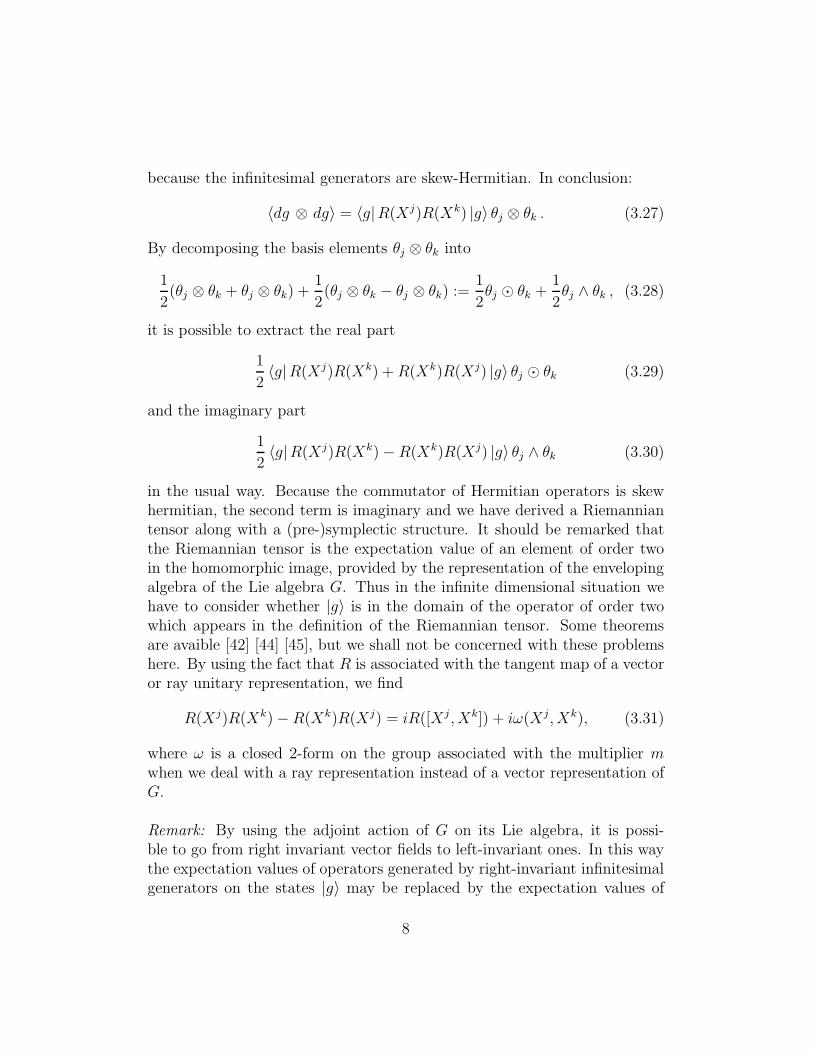
because the infinitesimal generators are skew-Hermitian. In conclusion:
〈dg ⊗ dg〉 = 〈g|R(Xj)R(Xk) |g〉 θj ⊗ θk . (3.27)
By decomposing the basis elements θj ⊗ θk into
1
2(θj ⊗ θk + θj ⊗ θk) +
1
2(θj ⊗ θk − θj ⊗ θk) :=
1
2θj ⊙ θk +
1
2θj ∧ θk , (3.28)
it is possible to extract the real part
1
2〈g|R(Xj)R(Xk) +R(Xk)R(Xj) |g〉 θj ⊙ θk (3.29)
and the imaginary part
1
2〈g|R(Xj)R(Xk) − R(Xk)R(Xj) |g〉 θj ∧ θk (3.30)
in the usual way. Because the commutator of Hermitian operators is skewhermitian, the second term is imaginary and we have derived a Riemanniantensor along with a (pre-)symplectic structure. It should be remarked thatthe Riemannian tensor is the expectation value of an element of order twoin the homomorphic image, provided by the representation of the envelopingalgebra of the Lie algebra G. Thus in the infinite dimensional situation wehave to consider whether |g〉 is in the domain of the operator of order twowhich appears in the definition of the Riemannian tensor. Some theoremsare avaible [42] [44] [45], but we shall not be concerned with these problemshere. By using the fact that R is associated with the tangent map of a vectoror ray unitary representation, we find
R(Xj)R(Xk) −R(Xk)R(Xj) = iR([Xj , Xk]) + iω(Xj, Xk), (3.31)
where ω is a closed 2-form on the group associated with the multiplier mwhen we deal with a ray representation instead of a vector representation ofG.
Remark: By using the adjoint action of G on its Lie algebra, it is possi-ble to go from right invariant vector fields to left-invariant ones. In this waythe expectation values of operators generated by right-invariant infinitesimalgenerators on the states |g〉 may be replaced by the expectation values of
8

the corresponding operators written in terms of left-invariant infinitesimalgenerators evaluated on the initial fiducial state |0〉.
If we introduce Y 1, Y 2, ...Y n generators of the right action along withα1, α2, ..., αn dual one-forms, αj(Y
k) = δkj , we have also
〈dg ⊗ dg〉 = 〈0|R(Y j)R(Y k) |0〉αj ⊗ αk . (3.32)
In this way the role of the fiducial vector and the requirement that it shouldbe in the domain of the operators of order two in the enveloping algebra ofthe left invariant generators becomes more clear. It may be convenient toderive in general form the pull-back Kahlerian tensor when we start with anaction on the ray space, the complex projective space, instead of the Hilbertspace.Here we have to start not with 〈dψ ⊗ dψ〉 in (2.5) but with
〈dψ ⊗ dψ〉
〈ψ |ψ〉−
〈ψ |dψ〉
〈ψ |ψ〉⊗
〈dψ |ψ〉
〈ψ |ψ〉(3.33)
in (2.13). Therefore the pulled-back tensor becomes
〈dg ⊗ dg〉
〈g |g〉−
〈g |dg〉
〈g |g〉⊗
〈dg |g〉
〈g |g〉(3.34)
After simple computations we find(
〈g|R(Y j)R(Y k) |g〉
〈g |g〉−
〈g|R(Y j) |g〉
〈g |g〉
〈g|R(Y k) |g〉
〈g |g〉
)
θj ⊗ θk (3.35)
The net result is that the closed 2-form will not be effected, except for thenormalization, while the metric tensor will be modified by the addition of anextra term
〈g|R(Y j) |g〉 〈g|R(Y k) |g〉 θj ⊙ θk (3.36)
Few comments are in order. From the expression of the jk−th coefficient ofthe pulled back tensor
〈0|R(Y j)R(Y k) |0〉 − 〈0|R(Y j) |0〉 〈0|R(Y k) |0〉 (3.37)
we notice that whenR(Y k) |0〉 = λk |0〉 (3.38)
9

we findλk 〈0|R(Y j) |0〉 − 〈0|R(Y j) |0〉λk = 0 . (3.39)
It means that the subalgebra of g of the subgroup of G which acts on |0〉simply by multiplication by a phase will give rise to ”degeneracy directions”for the Hermitian tensor. In more specific terms the tensor we are pullingback provides a tensor on G/G0, i.e. on the homogeneous space defined bythe isotropy subgroup (up to a phase) of the fiducial vector.In the coming sections we are going to consider some specific examples whichhave been selected because of their relevance for physical problems.
4 Pulled-back tensors on a compact space:
SU(2)
The simplest non-trivial compact Lie-group is given by SU(2) ∼= S3. Anembedding of this group into the Hilbert space
H = L2(SU(2)) :=⊕
s
C2s+1, s integer or half integer (4.40)
can be realized in different ways, since it will depend on the choice of thespin-s-representations
Us : SU(2) → Aut(C2s+1), g 7→ Us(g). (4.41)
By usingdUs(g)† = −Us(g)†dUs(g)Us(g)† (4.42)
the pulled back tensor reads
〈0| (dUs(g))† ⊗ dUs(g) |0〉 = 〈0|Rs(Y j)Rs(Y k) |0〉 θj ⊗ θk . (4.43)
The pulled back tensor associated to the pulled back tensor on SU(2)/U(1) ∼=S2 provides on the other hand the structure
(
〈0|Rs(Y j)Rs(Y k) |0〉 − 〈0|Rs(Y j) |0〉 〈0|Rs(Y k) |0〉)
θj ⊗ θk . (4.44)
If we choose |0〉 to be an eigenvector of Rs(Y 3) it follows that the symmetrictensor and skew-symmetric form are both degenerate.Let us compute this pulled back tensors in the defining representation s = 1/2
10
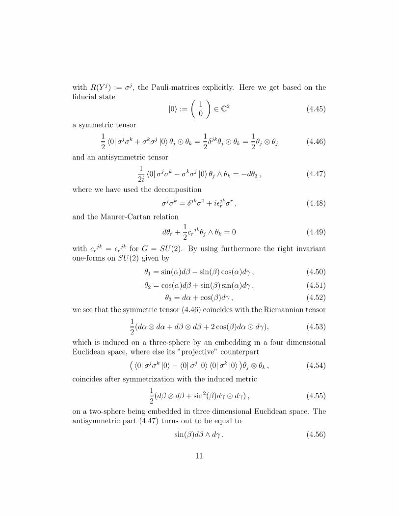
with R(Y j) := σj , the Pauli-matrices explicitly. Here we get based on thefiducial state
|0〉 :=
(
10
)
∈ C2 (4.45)
a symmetric tensor
1
2〈0|σjσk + σkσj |0〉 θj ⊙ θk =
1
2δjkθj ⊙ θk =
1
2θj ⊗ θj (4.46)
and an antisymmetric tensor
1
2i〈0|σjσk − σkσj |0〉 θj ∧ θk = −dθ3 , (4.47)
where we have used the decomposition
σjσk = δjkσ0 + iǫjkr σr , (4.48)
and the Maurer-Cartan relation
dθr +1
2crjkθj ∧ θk = 0 (4.49)
with crjk = ǫr
jk for G = SU(2). By using furthermore the right invariantone-forms on SU(2) given by
θ1 = sin(α)dβ − sin(β) cos(α)dγ , (4.50)
θ2 = cos(α)dβ + sin(β) sin(α)dγ , (4.51)
θ3 = dα + cos(β)dγ , (4.52)
we see that the symmetric tensor (4.46) coincides with the Riemannian tensor
1
2(dα⊗ dα+ dβ ⊗ dβ + 2 cos(β)dα⊙ dγ), (4.53)
which is induced on a three-sphere by an embedding in a four dimensionalEuclidean space, where else its ”projective” counterpart
(
〈0|σjσk |0〉 − 〈0| σj |0〉 〈0|σk |0〉)
θj ⊗ θk , (4.54)
coincides after symmetrization with the induced metric
1
2(dβ ⊗ dβ + sin2(β)dγ ⊙ dγ) , (4.55)
on a two-sphere being embedded in three dimensional Euclidean space. Theantisymmetric part (4.47) turns out to be equal to
sin(β)dβ ∧ dγ . (4.56)
11

5 Weyl systems and pulled-back tensors on a
symplectic vector space
We consider now a symplectic vector space (V, ω). A Weyl system is definedby a map from V to the set of unitary operators on a Hilbert space H.This map is required to be strongly continuous and satisfying the followingproperties:
1. W (v) ∈ U(H) , for all v ∈ V ;
2. W (v1)W (v2)W†(v1)W
†(v2) = eiω(v1,v2)I .
Here ω is the symplectic structure on V [47]. The symplectic structure is the”infinitesimal form” of the multiplier m(v1, v2) appearing in the definitionof ”ray-representations” for the abeliean vector group V [46]. It should beremarked that for different orderings, the symplectic structure is actuallyreplaced by an Hermitian product on V . Let us now carry on the generalprocedure on this specific example - For simplicity we introduce a basis inV , say {e1, e2, ..., e2n}, so that v = vjej .With the help of the Stone-von Neumann theorem it is possible to write
W (v) = eiR(v) . (5.57)
In particular this relation implies
[R(v1), R(v2)] = iω(v1, v2) (5.58)
Now, after the selection of a fiducial vector |0〉, we have to compute
〈0| (dW )† ⊗ dW |0〉 (5.59)
First we notice that unitarity of W (v) implies that d(W †) = (dW )†. Than,by using the decomposition v = vjej , we find for the pulled back tensor:
〈0|R(ej)R(ek) |0〉 dvj ⊗ dvk . (5.60)
By considering the real part and the imaginary part respectively, we find
1
2〈0|R(ej)R(ek) +R(ek)R(ej) |0〉 dv
j ⊙ dvk (5.61)
12

and
1
2i〈0|R(ej)R(ek) − R(ek)R(ej) |0〉 dv
j ∧ dvk = ωjkdvj ∧ dvk . (5.62)
If, as we should for physical interpretation, we consider the pull-back of theKahlerian tensor from the complex projective space associated with H, weshould find the same imaginary term, but the symmetric part should beevaluated as
1
2〈0|R(ej)R(ek) +R(ek)R(ej) |0〉 − 〈0|R(ej) |0〉 〈0|R(ek) |0〉 . (5.63)
From this expression it follows clearly that the fiducial vector |0〉 should beselected such that it belongs to the domain of R(ej) for all j ∈ {1, 2, ...2n}and to the domain of the elements of order two in the enveloping algebra.
Remark: Note that, when we consider only an Abelian vector subgroup ofV which is a Lagrangian subspace, the pull-back tensor only contains theEuclidean part because ωjk restricted to the subgroup will vanish identically.
To evaluate (5.61) and (5.63) we have to give a realization of H. This isdone by considering the decomposition of the symplectic vector space intoV = R
n ⊕ (Rn)∗. In the realization H = L2(Rn) we may compute the expec-tation values of R(ej), R(ek) and combination of these based on a Gaussianfunction
|0〉 := Ne−1
2q2 ∈ L2 ∩ C∞(Rn) . (5.64)
Here we get due to the realizations
R(ej) |0〉 := Qj |0〉 = Qj(Ne−1
2q2) = qj |0〉 (5.65)
for j ∈ {1, 2, ..., n} and
R(ej) |0〉 := P j |0〉 = i∂
∂qj(Ne−
1
2q2) = −iqj |0〉 (5.66)
for j ∈ {n+ 1, n+ 2, ..., 2n} the L2(Rn) inner products
〈0|QjP k |0〉 = −i 〈0| qjqk |0〉 (5.67)
〈0|P jQk |0〉 = i 〈0| qjqk |0〉 (5.68)
13

〈0|QjQk |0〉 = 〈0| qjqk |0〉 (5.69)
〈0|P jP k |0〉 = 〈0| qjqk |0〉 , (5.70)
which can be made explicit by the the integrals
Ijk := 〈0| qjqk |0〉 = N2
∫ ∞
−∞
dnqe−q2
qjqk . (5.71)
They get zero for j 6= k due to
Ijk = N2
(∫ ∞
−∞
dqie−q2i
)n−2(∫ ∞
−∞
dqje−q2
j qj
)2
= 0 (5.72)
and non-zero for j = k due to
Ijj = N2
(∫ ∞
−∞
dqie−q2
i
)n−1 ∫ ∞
−∞
dqje−q2
j q2j =
1
2N2πn/2. (5.73)
By setting N2πn/2 ≡ 1 we can summarise this into
Ijk =1
2δjk (5.74)
and since we have furthermore 〈P j〉 = 〈Qj〉 = 0 we can conclude that bothrelatations in (5.61) and (5.63) define each of them a metric tensor field
gjkdvj ⊙ dvk =
1
2δjkdv
j ⊙ dvk, (5.75)
giving rise to an Euclidean metric on R2n.
6 The pull-back on a manifold without group
structure
We consider a family of Hamiltonian operators H(λ) with λ ∈M , a smoothmanifold and the eigenvalue problem
H(λ) |ψ0(λ)〉 = E0(λ) |ψ0(λ)〉 , (6.76)
14

where E0 defines the lowest nonzero eigenvalue which is supposed to be non-degenerate. This association λ 7→ |ψ0(λ)〉 defines an embedding of M intoR(H), the ray space of H. Using the Hermitian tensor (2.13), we find
〈dψ0(λ) ⊗ dψ0(λ)〉
〈ψ0(λ) |ψ0(λ)〉−
〈ψ0(λ) |dψ0(λ)〉
〈ψ0(λ) |ψ0(λ)〉⊗
〈dψ0(λ) |ψ0(λ)〉
〈ψ0(λ) |ψ0(λ)〉. (6.77)
The external derivative d is meant to act on functions on M . By usingd = dλµ ⊗ ∂
∂λµ , we find
hµν = 〈∂µψ0 |∂νψ0〉 − 〈ψ0 |∂νψ0〉 〈∂µψ0 |ψ0〉 (6.78)
with the requirement 〈ψ0 |ψ0〉 = 1. Using more generally the spectrum ofH(λ), say
H(λ) |a;λ〉 = Ea(λ) |a;λ〉 , (6.79)
we have
dH(λ) |a;λ〉 = dEa(λ) |a;λ〉 + Ea(λ)d |a;λ〉 −Hd |a;λ〉 . (6.80)
Taking the scalar product with 〈b;λ| we obtain
〈b;λ| dH(λ) |a;λ〉 = (Ea − Eb) 〈b;λ| d |a;λ〉 , (6.81)
i.e.
d |a;λ〉 =∑
b6=a
|b;λ〉 〈b;λ| dH |a, λ〉
Ea − Eb(6.82)
Using this expression for a = 0, we get
d |ψ(λ)0〉 =∑
b6=a
|b;λ〉 〈b;λ| dH |ψλ0〉
E0 − Eb, (6.83)
which allows to write the pull-back of the Hermitian tensor given by (6.77).It should be mentioned that a particular interesting application to physicalsystems has been provided by Zanardi et al.[48].
7 Conclusions and outlook
We have seen that, out of any unitary representation of a group on someHilbert space, it is possible to identify a manifold by acting with the group
15

on some fiducial state. It is also possible to identify submanifolds by otherprocedures. On each submanifold, it is possible to consider the pullbackof the Hermitian tensor and therefore obtain classical tensors out of thequantum states. In some sense, this procedure may give rise to a kind of”dequantization”. As a matter of fact, this is not connected to any dy-namics resp. quantum classical transition and we have to accept that thereare quantum and classical-like structures in every quantum system, whichshould be considered as coexistent. In particular, when we consider the im-mersion of a symplectic vector space by means of a Weyl system, we obtainnot only the original symplectic structure but also an Euclidean tensor andtherefore a complex structure. With the help of this structure it is possi-ble to define complex coordinates and a correspondence between them andcreation/annihilation operators. We should stress that while the symplecticstructure turns out to be independent of the fiducial vector we start with,the Riemannian tensor does depend on it. More likey it is this particularaspect that makes the symplectic structure more fundamental than the met-ric structure in classical mechanics. On the other hand, when we considerthe imbedding of a Lagrangian subspace in the Hilbert space identified by aWeyl system, we find no symplectic structure but we find a metric tensor,this available metric tensor, intrinsically built, permits to define the veloc-ity field associated with a wave function in Bohmian mechanics. Thus thisprocedure will allow us to define a Bohmian vector field on any manifold wemay immerse in the Hilbert space. In a future paper we shall consider moreclosely this problem and provide a general setting for Bohmian vector fields.
Acknowledgments
This work was financially supported by the German Academic ExchangeService (DAAD) and the National Institute of Nuclear Physics (INFN).
References
[1] P. A. M. Dirac, The Principles of Quantum Mechanics (Clarendon Press,Oxford, 1936).
[2] P. A. M. Dirac, On the Analogy Between Classical and Quantum Me-chanics, Rev. Mod. Phys. 17 (1945), 195–199.
16

[3] H. Weyl, Quantenmechanik und Gruppentheorie, Zeitsch. Phys. 46
(1927), pp. 1–46.
[4] H. Weyl, The theory of groups and Quantum Mechanics, (Dover, NewYork, 1931).
[5] E. Segal, Postulates for general Quantum Mechanics, Ann. Math. 48
(1947), 930–948.
[6] G. W. Mackey, The mathematical foundations of Quantum Mechanics,(W. A. Benjamin, New York, 1963).
[7] G. W. Mackey, Quantum Mechanics and Hilbert space, The AmericanMathematica Monthly 64 (1957), pp. 45–57.
[8] G. W. Mackey, Weyl’s program and modern physics, Differential geo-
metric methods in theoretical physics, (Kluwer Acad. Publ., Dordrecht,1988).
[9] G. W. Mackey, The Relationship Between Classical mechanics and Quan-tum Mechanics, Contem. Math. 214 (1998), 91–109.
[10] F. Strocchi, Complex coordinates and Quantum Mechanics, Rev. Mod.
Phys. 38 (1956), 36–40.
[11] A. Heslot, Quantum mechanics as a classical theory, Phys. Rev. D 31
(1985), 1341–1348.
[12] D. J. Rowe, A. Ryman and G. Rosensteel, Many body quantum mechan-ics as a symplectic dynamical system, Phys Rev A 22 (1980), 2362–2372.
[13] V. Cantoni, Generalized transition probability, Comm. Math. Phys. 44
(1975), 125–128.
[14] V. Cantoni, The Riemannian structure on the space of quantum-likesystems, Comm. Math. Phys. 56 (1977), 189–193.
[15] V. Cantoni, Intrinsic geometry of the quantum-mechanical phase space,Hamiltonian systems and Correspondence Principle, Rend. Accad. Naz.
Lincei 62 (1977), 628–636.
17

[16] V. Cantoni, Geometric aspects of Quantum Systems, Rend. sem. Mat.
Fis. Milano 48 (1980), 35–42.
[17] V. Cantoni, Superposition of physical states: a metric viewpoint, Helv.
Phys. Acta 58 (1985. ), 956–968.
[18] R. Cirelli, P. Lanzavecchia and A. Mania, Normal pure states of the vonNeumann algebra of bounded operator as Kahler manifold, J. Phys. A:
Math. Gen. 16 (1983), 3829–3835.
[19] R. Cirelli and P. Lanzavecchia, Hamiltonian vector fields in QuantumMechanics, Nuovo Cimento B 79 (1984), 271–283.
[20] M. C. Abbati, R. Cirelli, P. Lanzavecchia and A. Mania, Pure states ofgeneral quantum mechanical systems as Kahler bundle, Nuovo Cimento
B 83 (1984), 43–60.
[21] A. Ashtekar and T. A. Shilling, Geometrical formulation of QuantumMechanics, in On Einsteins path, Ed. A. Harvey (Springer, Berlin, 1998)
[22] G. W. Gibbson, Typical states and density matrices, J. Geom. Phys. 8
(1992), 147–162.
[23] D. Brody and L.P. Hughston, Geometric quantum mechanics, J. Geom.
Phys. 38 (2001), 19–53.
[24] M. de Gosson, The principles of Newtonian and quantum mechanics
(Imperial College Press, London, 2001).
[25] J. F. Carinena, J. Grabowski and G. Marmo, Quantum Bi-HamiltonianSystems, Int. J. Mod. Phys. A 15 (2000), 4797–4810.
[26] G. Marmo, G. Morandi, A. Simoni and F. Ventriglia, Alternative Struc-tures and bi-Hamiltonian Systems, J. Phys. A: Math. Gen. 35 (2002),8393–8406.
[27] J. R. Klauder, Quantization without quantization, Ann. of Phys. 237
(1995), 147–160.
[28] J. R. Klauder, Understanding Quantization, Found. Phys. 27 (1997),1467–1483.
18

[29] J. R. Klauder, Phase space geometry in classical and quantum mechan-ics, quant-ph/0112010.
[30] D. Abernethy, J. R. Klauder, The distance between classical and quan-tum systems, Found. Phys. 35 (2005), 881–895.
[31] A. M. Perelomov, Coherent States for Arbitrary Lie Groups, Commun.
math. Phys. 26 (1972), 222–236.
[32] F. T. Arecchi, E. Courtens, R. Gilmore, H. Thomas, Atomic CoherentStates in Quantum Optics, Phys. Rev. A 6 (1972), 2211–2237.
[33] E. Onofri, A note on coherent state representations on Lie groups, Journ.
Math. Phys.. 16 (1975), 1087.
[34] J. Grabowski, M. Kus, G. Marmo, Geometry of quantum systems: den-sity states and entanglement, J. of Phys. A: Math. Gen., 38 (2005),10217–10244.
[35] M. V. Berry, Quantal phase factors accompanying adiabatic changes,Proc. R. Soc. A 392 (1984), 45–57.
[36] F. Wilczek and A. Zee, Appearance of Gauge Structure in Simple Dy-namical Systems, Phys. Rev. Lett. 52 (1984), 2111–2114.
[37] V. I. Arnold, Les methodes mathematiques de la Mecanique Classique
(Mir, Moscow 1976).
[38] R. Abraham, J. E. Marsden, Foundations of Mechanics (Benjamin,Reading, MA, 1978).
[39] G. Marmo, E. J. Saletan, A. Simoni, B. Vitale: Dynamical Systems –
A Differential Geometric Approach to Symmetry and Reduction (JohnWiley & Sons, Chichester, 1985).
[40] P. Libermann, C. M. Marle, Symplectic Geometry and Analytical Me-
chanics (Reidel, Dordrecht, 1987).
[41] J. Clemente-Gallardo, G. Marmo, Basics of Quantum Mechanics, Ge-ometrization and some Applications to Quantum Information, Int. J.
Geom. Meth. Modern Physics 5 (2008).
19

[42] E. Nelson, Analytic Vectors, Ann. of Math., 2nd ser., 70 (1959), 572–615.
[43] V. Bargmann, On unitary ray representations of continuous groups,Ann. of Math. 59 (1954), 1–46.
[44] E. Nelson, Stinespring, W. Forest, Representation of elliptic operatorsin an enveloping algebra, Amer. J. Math. 81 (1959), 547–560.
[45] E. B. Davies, Hilbert space representations of Lie algebras, Comm.
Math. Phys. 23 (1971), 159–168.
[46] P. Aniello, V. Manko, G. Marmo, S. Solimeno, F. Zaccaria, J. Opt. B:
Quantum Semiclass. Opt. 2 (2000), 718–725.
[47] G. Esposito, G. Marmo, G. Sudarshan: From Classical to Quantum
Mechanics (Cambridge University Press, Cambridge, 2004).
[48] P. Zanardi, P. Giorda, M. Cozzini, The differential information-geometryof quantum phase transitions, quant-ph/0701061.
20


