IN DEGREE PROJECT COMPUTER SCIENCE AND ENGINEERING,SECOND CYCLE, 30 CREDITS

, STOCKHOLM SWEDEN 2018

Classification of explicit music content using lyrics and music metadata

LINN BERGELID

KTH ROYAL INSTITUTE OF TECHNOLOGYSCHOOL OF ELECTRICAL ENGINEERING AND COMPUTER SCIENCE

Classification of explicitmusic content using lyricsand music metadata

LINN BERGELID

Master in Computer ScienceDate: June 28, 2018Supervisor: Iman SayyaddelshadExaminer: Örjan EkebergHost company: Petter Machado, Soundtrack Your BrandSwedish title: Klassificering av stötande innehåll i musik med hjälpav låttexter och musik-metadataSchool of Electrical Engineering and Computer Science

iii

Abstract

In a world where online information is growing rapidly, the need formore efficient methods to search for and create music collections islarger than ever. Looking at the most recent trends, the application ofmachine learning to automate different categorization problems suchas genre and mood classification has shown promising results.

In this thesis we investigate the problem of classifying explicit musiccontent using machine learning. Different data sets containing lyricsand music metadata, vectorization methods and algorithms includ-ing Support Vector Machine, Random Forest, k-Nearest Neighbor andMultinomial Naive Bayes are combined to create 32 different config-urations. The configurations are then evaluated using precision-recallcurves.

The investigation shows that the configuration with the lyric data settogether with TF-IDF vectorization and Random Forest as algorithmoutperforms all other configurations.

iv

Sammanfattning

I en värld där online-information växer snabbt, ökar behovet av ef-fektivare metoder för att söka i och skapa musiksamlingar. De senastetrenderna visar att användandet av maskininlärning för att automati-sera olika kategoriseringsproblem så som klassificering av genre ochhumör har gett lovande resultat.

I denna rapport undersöker vi problemet att klassificera stötande in-nehåll i musik med maskininlärning. Genom att kombinera olika da-tamängder med låttexter och musik-metadata, vektoriseringsmetodersamt algoritmer så som Support Vector Machine, Random Forest, k-NearestNeighbor och Multinomial Naive Bayes skapas 32 olika konfigurationersom tränas och utvärderas med precision-recall-kurvor.

Resultaten visar att konfigurationen med datamängden som endastinnehåller låttexter tillsammans med TF-IDF-vektorisering och algo-ritmen Random Forest presterar bättre än alla andra konfigurationer.

Contents

1 Introduction 11.1 Background . . . . . . . . . . . . . . . . . . . . . . . . . . 11.2 Aim and Objective . . . . . . . . . . . . . . . . . . . . . . 21.3 Problem definition and statement . . . . . . . . . . . . . . 31.4 Ethical considerations . . . . . . . . . . . . . . . . . . . . 31.5 Thesis outline . . . . . . . . . . . . . . . . . . . . . . . . . 4

2 Theory 52.1 Word embeddings . . . . . . . . . . . . . . . . . . . . . . . 5

2.1.1 Frequency based embedding . . . . . . . . . . . . 52.1.2 Prediction based embedding . . . . . . . . . . . . 8

2.2 Supervised learning . . . . . . . . . . . . . . . . . . . . . . 102.2.1 Support Vector Machine . . . . . . . . . . . . . . . 102.2.2 Naive Bayes . . . . . . . . . . . . . . . . . . . . . . 112.2.3 k-Nearest Neighbors . . . . . . . . . . . . . . . . . 122.2.4 Random Forest . . . . . . . . . . . . . . . . . . . . 14

2.3 Evaluation . . . . . . . . . . . . . . . . . . . . . . . . . . . 152.3.1 Methodology . . . . . . . . . . . . . . . . . . . . . 152.3.2 Metrics . . . . . . . . . . . . . . . . . . . . . . . . . 16

2.4 Imbalanced classification . . . . . . . . . . . . . . . . . . . 192.4.1 Oversampling . . . . . . . . . . . . . . . . . . . . . 192.4.2 Undersampling . . . . . . . . . . . . . . . . . . . . 19

2.5 Related work . . . . . . . . . . . . . . . . . . . . . . . . . . 202.5.1 Music Information Retrieval . . . . . . . . . . . . 202.5.2 Mood classification . . . . . . . . . . . . . . . . . . 212.5.3 Genre classification . . . . . . . . . . . . . . . . . . 222.5.4 Topic classification . . . . . . . . . . . . . . . . . . 24

v

vi CONTENTS

3 Method 253.1 Work flow . . . . . . . . . . . . . . . . . . . . . . . . . . . 253.2 Data set . . . . . . . . . . . . . . . . . . . . . . . . . . . . . 25

3.2.1 Lyrics and explicit tags . . . . . . . . . . . . . . . . 253.2.2 Music metadata . . . . . . . . . . . . . . . . . . . . 27

3.3 Software . . . . . . . . . . . . . . . . . . . . . . . . . . . . 283.4 Pre-processing . . . . . . . . . . . . . . . . . . . . . . . . . 28

3.4.1 Data cleaning . . . . . . . . . . . . . . . . . . . . . 283.4.2 Feature selection and transformation . . . . . . . 293.4.3 Feature extraction . . . . . . . . . . . . . . . . . . . 293.4.4 Sampling . . . . . . . . . . . . . . . . . . . . . . . . 31

3.5 Model selection . . . . . . . . . . . . . . . . . . . . . . . . 313.6 Evaluation . . . . . . . . . . . . . . . . . . . . . . . . . . . 32

3.6.1 Parameter tuning . . . . . . . . . . . . . . . . . . . 333.6.2 Classification . . . . . . . . . . . . . . . . . . . . . 33

4 Results 344.1 Results per classifier . . . . . . . . . . . . . . . . . . . . . 35

4.1.1 Linear Support Vector Machine . . . . . . . . . . . 354.1.2 Multinomial Naive Bayes . . . . . . . . . . . . . . 354.1.3 k-Nearest Neighbor . . . . . . . . . . . . . . . . . 354.1.4 Random Forest . . . . . . . . . . . . . . . . . . . . 35

4.2 Results per data set and sampling . . . . . . . . . . . . . . 354.2.1 Lyrics . . . . . . . . . . . . . . . . . . . . . . . . . . 364.2.2 Lyrics + Music Metadata . . . . . . . . . . . . . . . 36

5 Discussion 395.1 Model evaluation . . . . . . . . . . . . . . . . . . . . . . . 405.2 Sampling vs. No Sampling . . . . . . . . . . . . . . . . . . 405.3 TF-IDF vs. Doc2Vec Vectorization . . . . . . . . . . . . . . 405.4 Data set evaluation . . . . . . . . . . . . . . . . . . . . . . 41

6 Conclusion and Future work 42

Bibliography 44

A Numerical results of all configurations 50

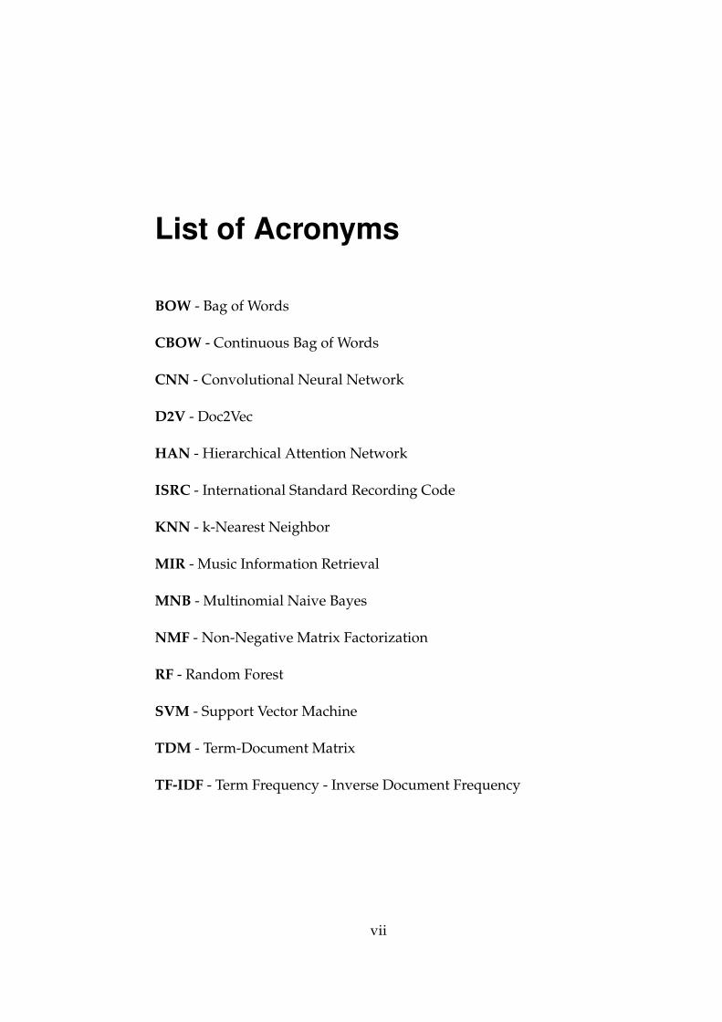
List of Acronyms

BOW - Bag of Words

CBOW - Continuous Bag of Words

CNN - Convolutional Neural Network

D2V - Doc2Vec

HAN - Hierarchical Attention Network

ISRC - International Standard Recording Code

KNN - k-Nearest Neighbor

MIR - Music Information Retrieval

MNB - Multinomial Naive Bayes

NMF - Non-Negative Matrix Factorization

RF - Random Forest

SVM - Support Vector Machine

TDM - Term-Document Matrix

TF-IDF - Term Frequency - Inverse Document Frequency

vii

List of Tables

2.1 Example of similarity measures used for k-Nearest Neighbor. . 13

3.1 Summary of the data structure of the lyrics and explicit dataset. . . . . . . . . . . . . . . . . . . . . . . . . . . . . . . . . 27

3.2 The parameter setting used for tuning the TF-IDF vectoriza-tion model. . . . . . . . . . . . . . . . . . . . . . . . . . . . 30

3.3 The parameter setting used for the Doc2Vec vectorization model. 303.4 Summary of the models used and their corresponding func-

tion in Scikit Learn. . . . . . . . . . . . . . . . . . . . . . . . 32

4.1 Abbreviations for the classifiers used when presenting the re-sults. . . . . . . . . . . . . . . . . . . . . . . . . . . . . . . . 34

A.1 The results of the classification for each configuration. . . . . . 51

viii

List of Figures

2.1 Example of a term-document matrix. . . . . . . . . . . . . . . 62.2 Example of a term-document matrix with TF-IDF weights. . . 72.3 Example of a context window where the words in green are

the context of the word in yellow. . . . . . . . . . . . . . . . . 82.4 Example of networks for the CBOW model (left) and Skip-

Gram model (right) [2]. . . . . . . . . . . . . . . . . . . . . . 92.5 Example of a SVM with linear kernel. Two classes are pre-

sented, one with blue circles and one with red squares. Theblack line corresponds to the hyperplane and the filled squareand circle are the support vectors. . . . . . . . . . . . . . . . 11

2.6 Example of a k-Nearest Neighbor classifier with k = 6. Theblue circles and red squares corresponds to data points of twodifferent classes. The green circle would be classified as redsince 5 out of 6 of the closest neighbors are red. . . . . . . . . 13

2.7 Example of a decision tree that decides whether or not to playtennis based on the weather. . . . . . . . . . . . . . . . . . . 14

2.8 A confusion matrix for a binary classifier. . . . . . . . . . . . 182.9 Example of a precision-recall curve. Algorithm 2 performs

slightly better than Algorithm 1 since the area is larger underthe former one [10]. . . . . . . . . . . . . . . . . . . . . . . . 18

3.1 A summary of the work flow of this thesis. . . . . . . . . . . . 263.2 A summary of the distribution of the classes in the data set. . . 313.3 A summary of the combinations of data, pre-processing and

classifiers that has been evaluated. . . . . . . . . . . . . . . . 32

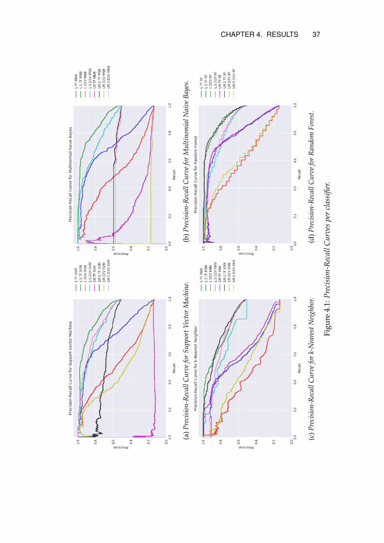
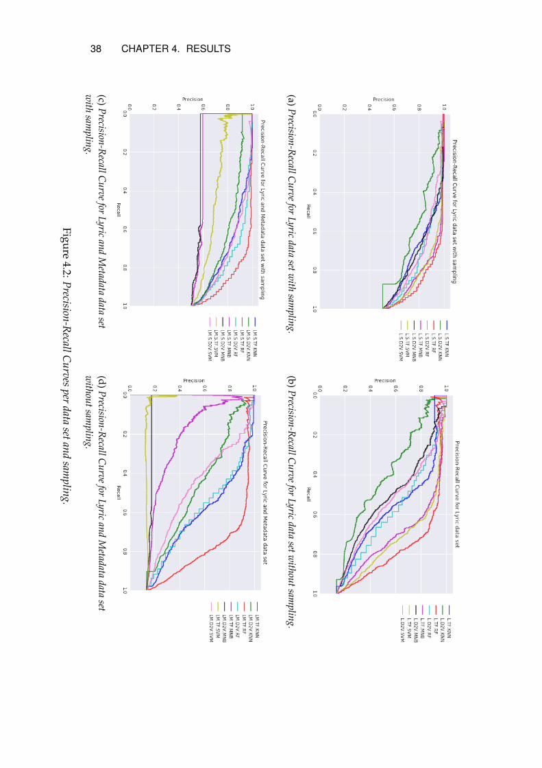
4.1 Precision-Recall Curves per classifier. . . . . . . . . . . . . . 374.2 Precision-Recall Curves per data set and sampling. . . . . . . 38

ix

Chapter 1

Introduction

This chapter introduces the objective and aim of this degree project togetherwith the problem definition. It ends with a small discussion about the ethicalconsiderations of the project followed by a thesis outline.

Over the last couple of years music has become one of the largest typesof online information. The increasing size of digital music collectionshas posed a major challenge and need to find more efficient methodsfor searching and organizing music collections [9]. The growth hasextended music search methods from more traditional methods suchas artists and album names to more advanced properties includingmood, genre or similar artists based on previous listening. One prop-erty that has been requested multiple times recently is the property ofbeing able to filter out explicit content [7, 47].

1.1 Background

The research for this thesis has been conducted at the company Sound-track Your Brand1. Soundtrack Your Brand provides a music stream-ing service for companies to play music in their public areas. Thecustomers are able to control and schedule music by using hardwareplayers, mobile applications or a web interface. In addition to this thecompany has an expert team within music that helps each customerfind their own soundtrack that matches their core values.

1https://www.soundtrackyourbrand.com/

1

2 CHAPTER 1. INTRODUCTION

The company works with many markets including the US market. Akey feature for this market is to filter out explicit content such as sex,drugs, alcohol and violence as some customers do not identify withsuch content for their core values. To manually annotate songs hasmultiple drawbacks. It is time consuming and thus costly, error proneand partly a subjective task which creates a need for an automated so-lution.

The idea is that an automated solution will both enhance speed andaccuracy. An automated system would not only be useful for Sound-track Your Brand and other music streaming services (such as Spotify2

and Apple music3), but may also be applied to other kinds of mediawhere explicitness occurs such as within movies or books. To the bestof the author’s knowledge, there exists no automatic technology whereit does the whole process of explicit filtering and thus it will be the en-try point of this thesis.

A small but growing research field called Music Information Retrieval(MIR) focuses on research and development of computational systemsto retrieve music information. Currently the focus within this area hasbeen on mood or genre classification of songs [17, 24, 30, 33, 49] orfinding approaches on how to automatically generate play lists thatfit a specific user [12]. The presented models are mostly built usinglyrical or audio features or a combination of both. What seems to bemissing is work on how to automatically filter out songs with explicitcontent.

1.2 Aim and Objective

The main aim of the thesis is to target an automated tool which pro-vides a practical feature of filtering explicit music. On the way ofachieving the aim, the following objectives play a significant role:

• Research of text classification in order to select relevant algo-rithms and pre-processing methods.

2https://www.spotify.com/3https://www.apple.com/lae/music/

CHAPTER 1. INTRODUCTION 3

• Extracting and pre-processing of data to be used for the classifi-cation.

• Implementing the selected algorithms and evaluating if they areuseful for classifying explicit content.

1.3 Problem definition and statement

The project entails finding a machine learning algorithm that based ontext features is able to classify song tracks with explicit content. Themain feature used for this purpose will be lyrics of the songs, but sincelyrics differ a lot from ordinary text like news in that it uses rhyme andis presented in poetic form, using lyrics only can be difficult for natu-ral language processing. In [4] and [27], tags and musical reviews havebeen used as a complement to get a better classification. Therefore thisthesis will investigate music metadata as an additional feature to en-rich the lyrics. Music metadata may include everything from informa-tion produced by the community, such as user annotations of what asong is about, to information about the artist and album or acousticfeatures of the track.

The question this thesis aims to answer is:

What is an efficient method for classifying explicit music using machine learn-ing?

1.4 Ethical considerations

As the area of machine learning is growing more than ever, it is impor-tant to discuss different ethical aspects in relation to it. Creating au-tomated systems could possibly remove jobs from humans who usedto perform a task manually, or it could help them focus on more ad-vanced tasks where they make more use.

Another aspect is that of privacy. The data used in this thesis containsno personal information and thus anonymization or removal of sensi-tive information has not been a concern.

4 CHAPTER 1. INTRODUCTION

Regarding explicit content there are a lot of views on what should becalled explicit or not. This could potentially be a problem within forexample religious or political music where some people would findthis music explicit whereas some would feel like their view is dis-criminated if such music would be filtered out. One way to solve thatwould be by doing a multi-label classification based on different cate-gories within explicit and leave the choice to the customer on what isconsidered explicit or not.

1.5 Thesis outline

The thesis is structured as follows. Chapter 2 covers relevant theoryand background of the thesis. It ends with a section about previouswork within MIR where machine learning algorithms and textual fea-tures have been used. Chapter 3 describes the methods used in thisthesis. In chapter 4 the results of the classification are presented. Chap-ter 5 covers an analysis of the results. The thesis ends with a conclusionand ideas for future work in chapter 6.

Chapter 2

Theory

This chapter starts with a presentation of how to pre-process text before it canbe used as a feature. It then describes the theory behind the relevant classifi-cation algorithms used in this degree project followed by a short descriptionof different evaluation methods. It ends with a summary of previous work.

2.1 Word embeddings

This section describes how the data is processed before it can be usedas a feature in a classifier. Most classifiers are not able to use raw textstrings as input and thus the text has to be converted into a suitableformat before it can be used. Several methods exist and these can gen-erally be divided into two categories, frequency based embedding andprediction based embedding which are elaborated in the following sec-tions.

2.1.1 Frequency based embedding

Bag of Words

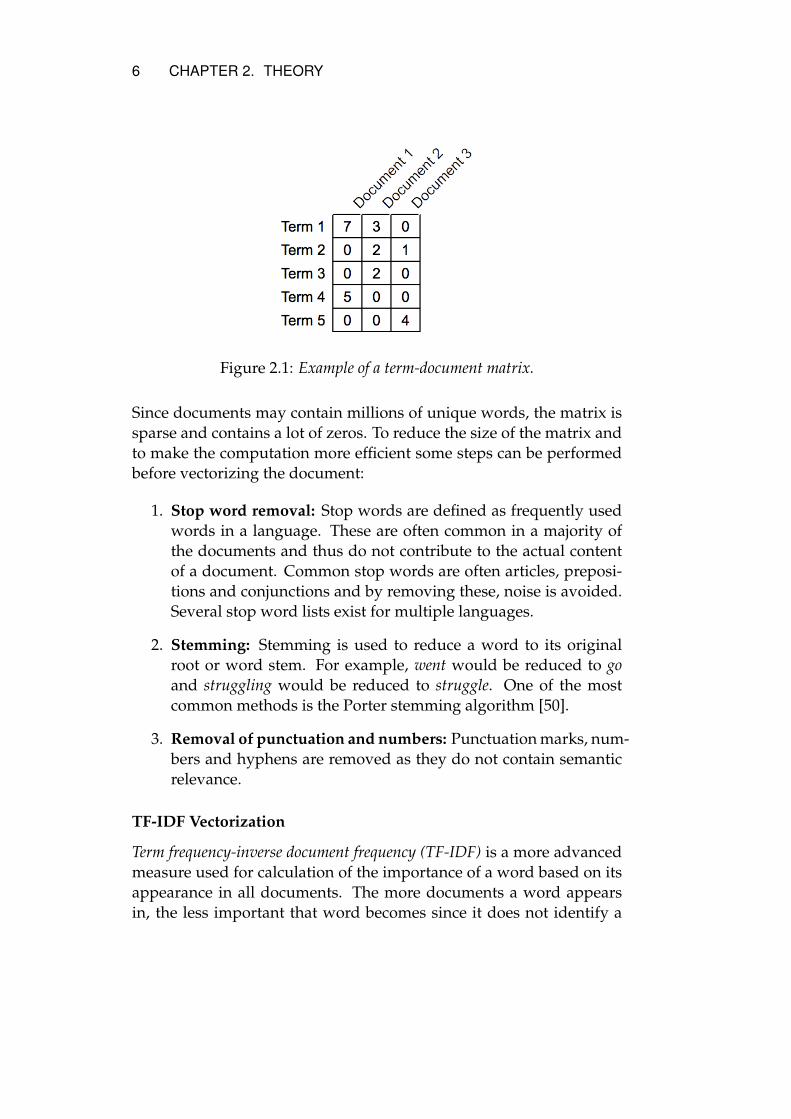
One of the most simple vector representations of a text is based on thefrequency of all words. The frequency of each word in a documentis calculated and the ordering between the words are removed. Theresult is stored in a term-document matrix (TDM) where each row cor-responds to a term and each column corresponds to a document, seeFigure 2.1. This model is referred to as bag of words (BOW) [1].

5

6 CHAPTER 2. THEORY

Figure 2.1: Example of a term-document matrix.

Since documents may contain millions of unique words, the matrix issparse and contains a lot of zeros. To reduce the size of the matrix andto make the computation more efficient some steps can be performedbefore vectorizing the document:

1. Stop word removal: Stop words are defined as frequently usedwords in a language. These are often common in a majority ofthe documents and thus do not contribute to the actual contentof a document. Common stop words are often articles, preposi-tions and conjunctions and by removing these, noise is avoided.Several stop word lists exist for multiple languages.

2. Stemming: Stemming is used to reduce a word to its originalroot or word stem. For example, went would be reduced to goand struggling would be reduced to struggle. One of the mostcommon methods is the Porter stemming algorithm [50].

3. Removal of punctuation and numbers: Punctuation marks, num-bers and hyphens are removed as they do not contain semanticrelevance.

TF-IDF Vectorization

Term frequency-inverse document frequency (TF-IDF) is a more advancedmeasure used for calculation of the importance of a word based on itsappearance in all documents. The more documents a word appearsin, the less important that word becomes since it does not identify a

CHAPTER 2. THEORY 7

specific document. The measure also addresses the problem wheretwo documents are of different length and terms might appear moretimes in a long document than in a short one [1]. This value, whichis calculated in two steps, is then used instead of the raw frequencyin the term-document matrix to provide a more balanced view of thefrequencies.

The first step, term frequency, measures how frequent a term is in adocument and is defined as follows:

TFt,d =ft,d∑

t′∈dft′,d

(2.1)

where t is the term, d is the document and ft,d the raw frequency of theselected word. The second part, inverse documented frequency measureshow important a term is and is defined as follows:

IDFt,D = logN

|{d ∈ D : t ∈ d}|. (2.2)

where D is the set of all documents and N = |D|. Thus, if a termoccurs in many documents the inverse document frequency will besmall. These numbers are combined into TF-IDF by taking the productof them:

TF − IDFt,d,D = TFt,d × IDFt,D. (2.3)

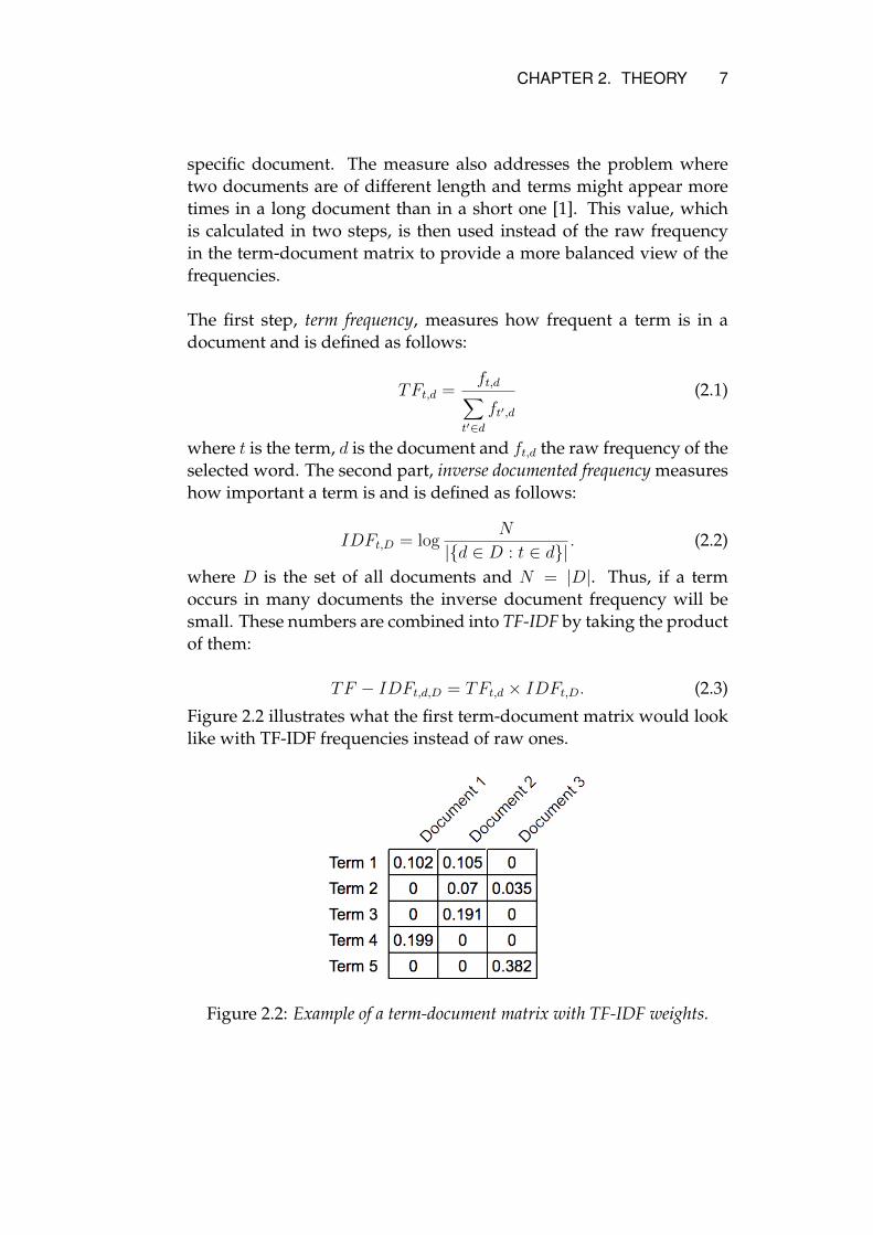
Figure 2.2 illustrates what the first term-document matrix would looklike with TF-IDF frequencies instead of raw ones.

Figure 2.2: Example of a term-document matrix with TF-IDF weights.

8 CHAPTER 2. THEORY

N-grams

N-grams are a set of N words occurring together in a text. For ex-ample, given the sentence "The moon shines bright." and N = 2, the 2-grams (also known as bigrams) of the sentence would be "The moon","moon shines" and "shines bright". Instead of counting each word onits own, N-grams can be used in the TDM in frequency based embed-ding. The original bag of words approach is basically N-grams withN = 1 (also known as unigrams). N-grams with different values of Ncan be combined in the same TDM, helping an algorithm understandthe context while still preserving the information given by the termson their own.

2.1.2 Prediction based embedding

Prediction based embedding is more complex than frequency basedembedding as it takes the relationship between words into considera-tion. The most famous algorithm that is prediction based is Word2Vecwhich creates a vector for each word based on the semantic relation-ship between the words in a text [35].

Word2Vec

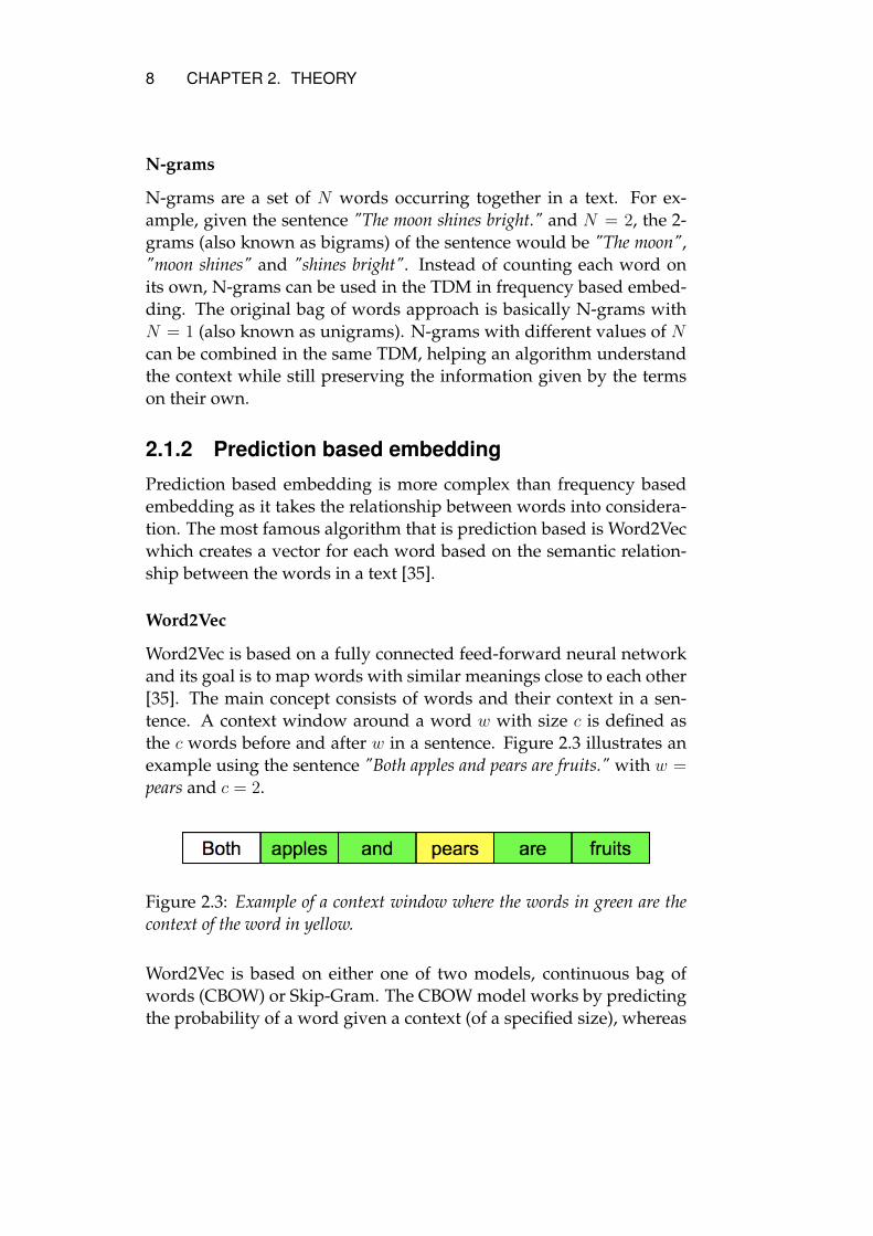
Word2Vec is based on a fully connected feed-forward neural networkand its goal is to map words with similar meanings close to each other[35]. The main concept consists of words and their context in a sen-tence. A context window around a word w with size c is defined asthe c words before and after w in a sentence. Figure 2.3 illustrates anexample using the sentence "Both apples and pears are fruits." with w =

pears and c = 2.

Figure 2.3: Example of a context window where the words in green are thecontext of the word in yellow.

Word2Vec is based on either one of two models, continuous bag ofwords (CBOW) or Skip-Gram. The CBOW model works by predictingthe probability of a word given a context (of a specified size), whereas

CHAPTER 2. THEORY 9

Skip-Gram is the inverse of CBOW where a context is predicted givena word [2].

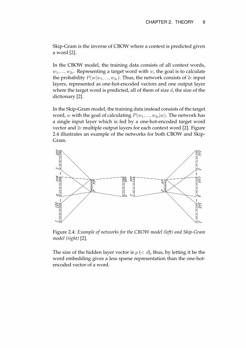
In the CBOW model, the training data consists of all context words,w1, ..., w2c. Representing a target word with w, the goal is to calculatethe probability P (w|w1, ..., w2c). Thus, the network consists of 2c inputlayers, represented as one-hot-encoded vectors and one output layerwhere the target word is predicted, all of them of size d, the size of thedictionary [2].

In the Skip-Gram model, the training data instead consists of the targetword, w with the goal of calculating P (w1, ..., w2c|w). The network hasa single input layer which is fed by a one-hot-encoded target wordvector and 2c multiple output layers for each context word [2]. Figure2.4 illustrates an example of the networks for both CBOW and Skip-Gram.

Figure 2.4: Example of networks for the CBOW model (left) and Skip-Grammodel (right) [2].

The size of the hidden layer vector is p (< d), thus, by letting it be theword embedding gives a less sparse representation than the one-hot-encoded vector of a word.

10 CHAPTER 2. THEORY

Doc2Vec

Doc2Vec is an extension of Word2Vec which instead of creating a vec-tor for each word, creates a vector representing an entire document[25]. It works by adding an additional vector that identifies a specificdocument. When the word vectors are trained, the document vector istrained at the same time and can then be used as a document embed-ding.

2.2 Supervised learning

Machine learning is divided into two main approaches, supervised learn-ing and unsupervised learning. Supervised learning uses labeled data,that is a set of features and their corresponding labels, as input to fit amodel. The model can then be used to classify unlabeled data. If nosuch labeled data exists, unsupervised learning can be used instead.Unsupervised learning is used to understand the relationship betweenthe unlabeled data for example by clustering [19].

Supervised learning is further divided into classification and regres-sion depending on if the labeled data is numerical or categorical. If thelabeled data has numerical values such as a person’s height or weight,it is a regression problem and if it has categorical values, such as a per-son’s gender, it is a classification problem [19].

In the following subsections common classification algorithms withintext categorization are presented. The idea is to provide a general de-scription, describe in what ways they differ as well as their advantagesand disadvantages when used for text analysis.

2.2.1 Support Vector Machine

Support Vector Machine (SVM) is a model that produces hyperplanesto separate the data into classes. It aims to find the hyperplane whichmaximizes the sum of distances between the hyperplane and eachtraining instance. The instances closest to the hyperplane are calledsupport vectors. After the model has been trained and hyperplanesare created it can easily be used to classify new instances.

CHAPTER 2. THEORY 11

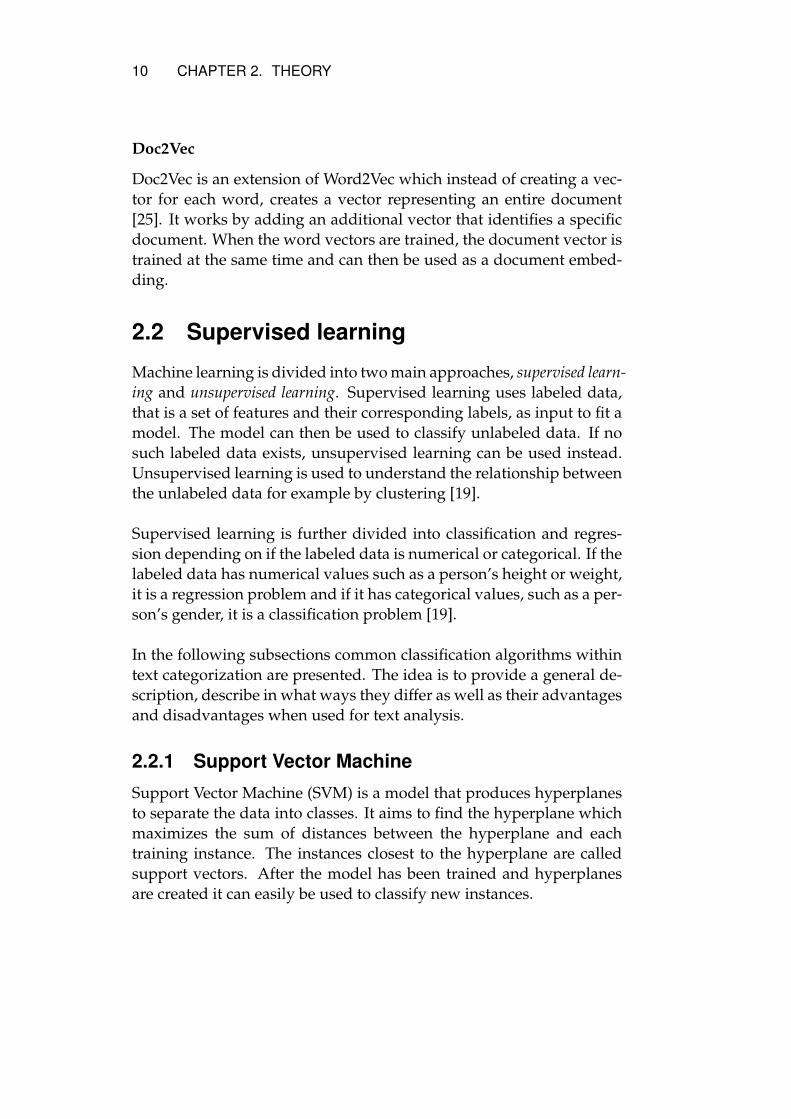
Some data sets may not be linearly separable and since the originalalgorithm only included a linear classifier, a non-linear solution wasintroduced using kernel functions to describe non-linear hyperplanes[6]. The most common kernel functions, except the linear, includepolynomial kernel, Gaussian radial basis kernel and the sigmoid ker-nel. Figure 2.5 shows an example of a SVM with a linear kernel.

Figure 2.5: Example of a SVM with linear kernel. Two classes are presented,one with blue circles and one with red squares. The black line corresponds tothe hyperplane and the filled square and circle are the support vectors.

One big advantage of SVM is that it has proven to perform well inmany text categorization problems specifically in terms of accuracies[3, 20, 37]. It also handles overfitting well since the model’s complexityis not dependent on the number of features [41]. One disadvantage isthat the implementation of the model scales badly with the number ofdocuments [37].

2.2.2 Naive Bayes

Naive Bayes is a group of probabilistic classifiers based on Bayes’ the-orem combined with a strong independence assumption between thefeatures. Bayes’ theorem states the probability of an event given con-ditions related to the event and is defined as

12 CHAPTER 2. THEORY

P (Ck|F1, ..., Fn) =P (Ck)× P (F1, ..., Fn|Ck)

P (F1, ..., Fn)(2.4)

where Ck is a class and F1, ..., Fn is a set of features. P (Ck|F1, ..., Fn)

denotes the probability of the set of features with values F1, ..., Fn be-longing to class Ck. Adding the independence assumption means as-suming that all features are conditionally independent from each otherand the probability model can instead be formulated as

P (Ck|F1, ..., Fn) =P (Ck)×

∏ni=1 P (Fi|Ck)

P (F1, ..., Fn). (2.5)

To estimate P (Fi|Ck), different event models are used that describe thedistribution of the features. The two most common models used fortext classification are a multivariate Bernoulli model and a multino-mial model [21]. In the Bernoulli event model each document is repre-sented using a binary vector which indicates whether a word occurs ornot in the document and thus, ignores the frequency. In the multino-mial event model the document is represented using a vector of wordoccurrences. The order of the words is ignored in both event models[31]. The model is then combined with a decision rule to build theclassifier. The most common rule is called maximum a posteriori whichmeans choosing to most probable class as the prediction.

The benefits of using Naive Bayes is that it is computationally fast,easy to implement and performs well in high dimensions [44]. Ac-cording to [31], the multinomial model is best for large vocabularysizes. The disadvantage is the strong assumption of independence be-tween the features [37].

2.2.3 k-Nearest Neighbors

k-Nearest Neighbor (KNN) is an instance-based and non-parametricmethod that is based on feature similarity. Instance-based means thatthere is no explicit training phase to configure a model before the clas-sification [1]. Non-parametric means that all data points are needed inorder to predict a test point and that no assumptions are made on theunderlying data distribution which makes it good to use when thereis little or no prior knowledge on the distribution of the data.

CHAPTER 2. THEORY 13

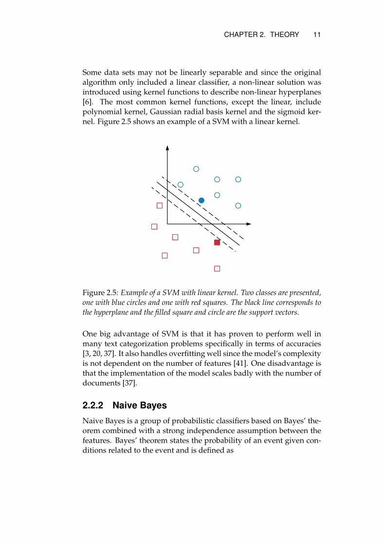
The KNN classifier is one of the simplest classifiers, for a given in-stance the k closest training samples are determined and the dominantclass among the k samples is predicted by the classifier, see Figure 2.6.To calculate the distance between the samples a similarity measure hasto be used. Some of the existing measures can be seen in Table 2.1 be-low where the Euclidean distance is the most common.

Table 2.1: Example of similarity measures used for k-Nearest Neighbor.

Measure FormulaEuclidean D(x, y) =

√∑ni=1(xi − yi)2

Manhattan D(x, y) =∑n

i=1 |xi − yi|Minkowski D(x, y) = (

∑ni=1 |xi − yi|p)1/p, p ≥ 1

where x = (x1, ..., xn) and y = (y1, ..., yn) are feature vectors of twosamples.

Figure 2.6: Example of a k-Nearest Neighbor classifier with k = 6. The bluecircles and red squares corresponds to data points of two different classes. Thegreen circle would be classified as red since 5 out of 6 of the closest neighborsare red.

One of the major disadvantages with the KNN model is that it suf-fers from high storage requirements since all training data is neededduring the test phase. However, it benefits of its simplicity, noise ro-bustness and that no assumptions has to be done on the data [37, 42].

14 CHAPTER 2. THEORY

2.2.4 Random Forest

In order to understand how a Random Forest (RF) classifier works,first the concept of decision trees and ensemble methods has to be in-troduced.

Decision Trees

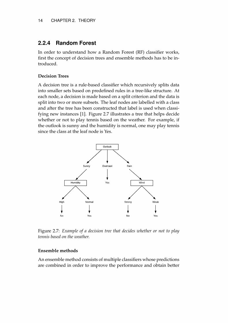
A decision tree is a rule-based classifier which recursively splits datainto smaller sets based on predefined rules in a tree-like structure. Ateach node, a decision is made based on a split criterion and the data issplit into two or more subsets. The leaf nodes are labelled with a classand after the tree has been constructed that label is used when classi-fying new instances [1]. Figure 2.7 illustrates a tree that helps decidewhether or not to play tennis based on the weather. For example, ifthe outlook is sunny and the humidity is normal, one may play tennissince the class at the leaf node is Yes.

Figure 2.7: Example of a decision tree that decides whether or not to playtennis based on the weather.

Ensemble methods

An ensemble method consists of multiple classifiers whose predictionsare combined in order to improve the performance and obtain better

CHAPTER 2. THEORY 15

accuracy than the single classifiers would have on their own. Thereare two main techniques within ensemble learning called bagging andboosting. Bagging (bootstrap aggregating) randomly divides the train-ing set in partitions with replacement and uses each set for each clas-sifier. In boosting each set is chosen based on the performance of theprevious classifier. Data that were incorrectly classified in a previousclassifier is prioritized in the next run in order to improve the predic-tion of data that gave poor performance in an earlier run [45].

Random Forest

Random forest combines the above concepts by using a large set of de-cision trees and outputs the resulting class based on a majority votebetween the results of the different trees [45]. The benefits of using RFclassifiers includes simplicity and good performance for data sets withhigh dimensions. They rarely overfit since there are multiple trees thathelps to reduce the variance. One disadvantage is that using a largeamount of trees can be very computationally heavy and ineffective[52].

2.3 Evaluation

After a model has been created, its performance has to be evaluated.In this section multiple evaluation methods and metrics are presented.

2.3.1 Methodology

The goal for all classifiers is to predict the output as accurately as pos-sible. Labeled data called ground truth is often used to compare withthe classifier output. It is important that this data has not been usedfor training since that would lead to an overestimation of the accuracydue to overfitting. Therefore, all labeled data needs to be divided intoa training and a test set before it can be used. Depending on how thedata is divided it may effect the results. Small labeled data sets areextra sensitive and if the test data is not representative it will lead topoor results. Multiple methods exist in order to prevent this which arepresented below.

16 CHAPTER 2. THEORY

Holdout

The holdout method partitions the labeled data into two sets for train-ing and testing. The model is built using the training data and theaccuracy of the model is calculated using the test data. This ensuresthat the model is not overestimated due to overfitting. However, itmight instead lead to an underestimation of the accuracy if the classdistributions in the test and training data are not equal [1].

Cross Validation

The cross validation method partitions the data into k parts of equalsize. One part will be used for testing and the rest (k − 1 parts) areused as training data. This is then repeated k times using all k parts astest data one time each. The final accuracy is usually an average of allk results.

2.3.2 Metrics

Several metrics exist to evaluate the performance of a classifier. Thissection lists the most common ones which are all based on the termi-nology of true positives, false positives, true negatives and false neg-atives. The terminology is described using an example of a binaryclassification with two classes, A and B.

• True Positive (TP) - True positives are items of class A that arecorrectly predicted as items of class A.

• False Positive (FP) - False positives are items of class B that areincorrectly predicted as items of class A.

• True Negative (TN) - True negatives are items of class B that arecorrectly predicted as items of class B.

• False Negative (FN) - False negatives are items of class A thatare incorrectly predicted as items of class B.

Accuracy

Accuracy is used as an overall measure of a classifier and is defined asthe ratio between all correctly predicted items and all items.

CHAPTER 2. THEORY 17

Accuracy =TP + TN

TP + FP + TN + FN(2.6)

Precision

Precision is a measure of what percentage of items predicted to belongto class A actually belongs to class A.

Precision =TP

TP + FP(2.7)

Recall

Recall is a measure of what percentage of items belonging to class Awhere predicted correctly. This is also known as sensitivity or truepositive rate.

Recall =TP

TP + FN(2.8)

F1 score

The F1-score is defined as the harmonic mean between precision andrecall.

F1 = 2 ∗ Precision ∗Recall

Precision+Recall(2.9)

Confusion Matrix

A confusion matrix can be used to summarize and illustrate the per-formance of a classifier. Each row represents the actual classes whereaseach column represents the prediction of the classifier. Figure 2.8 illus-trates an example with a binary classifier with a positive and a nega-tive class.

18 CHAPTER 2. THEORY

Figure 2.8: A confusion matrix for a binary classifier.

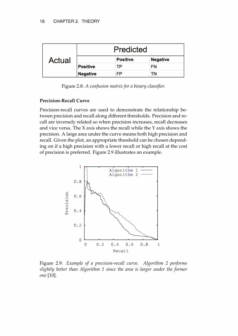
Precision-Recall Curve

Precision-recall curves are used to demonstrate the relationship be-tween precision and recall along different thresholds. Precision and re-call are inversely related so when precision increases, recall decreasesand vice versa. The X axis shows the recall while the Y axis shows theprecision. A large area under the curve means both high precision andrecall. Given the plot, an appropriate threshold can be chosen depend-ing on if a high precision with a lower recall or high recall at the costof precision is preferred. Figure 2.9 illustrates an example.

Figure 2.9: Example of a precision-recall curve. Algorithm 2 performsslightly better than Algorithm 1 since the area is larger under the formerone [10].

CHAPTER 2. THEORY 19

2.4 Imbalanced classification

Imbalanced classification arises when the classes in a data set are un-equally distributed. Training an algorithm with imbalanced data oftenleads to reduced accuracy. This is due to the imbalanced distributionof the dependent variable which causes the classifier to get biased to-wards the larger class [11, 14]. Classifier algorithms assume that thedifferent class errors are equal and aim to minimize the total errorwhich will be dominated by the larger class and thus the error of thesmaller class will not be seen. Multiple methods exist to deal with theimbalance issue by altering the size of the data set to create subsetsof data of each class of more equal sizes. The group of methods areknown as sampling methods. They are further divided into groups ofoversampling and undersampling.

2.4.1 Oversampling

Oversampling works by replicating samples of the smaller class. Anadvantage of this type of sampling is that no information is lost [28].Several techniques exist with different approaches of replicating.

2.4.2 Undersampling

Undersampling works by reducing the size of the larger class to makethe data set more balanced. Since data is removed this method workswell for large data sets. Several techniques within under-sampling ex-ist regarding how to select what samples of the data set to remove [28].

Random Undersampling

Random undersampling is the simplest technique which balances thedata by randomly selecting a subset equal to the size of the underrep-resented class. The parameter setting allows the user to bootstrap thedata if wanted by selecting samples with replacement [28].

NearMiss

NearMiss works by adding one out of three heuristic rules to selectsamples. The first rule selects samples of the larger class with thesmallest average distance to the smaller class. The second rule is the

20 CHAPTER 2. THEORY

same as the first rule except that it selects samples with the largest av-erage distance instead. The third rule consists of two steps. The M

nearest neighbors of each sample in the smaller class will be kept. Forthe rest of the samples in the larger class, the ones will be kept whoseaverage distance to their N nearest neighbors are the closest [18].

TomekLinks

A Tomek’s Link between two samples of different classes means thatthe samples are the nearest neighbors of each other. That is, (a, b) isa Tomek’s Link if there exist no sample c such that d(a, c) < d(a, b) ord(b, c) < d(b, a) where a and b belong to different classes and d() is thedistance between two samples. Depending on the parameter settingof the method either the sample of the larger class or both samples ina Tomek’s Link will be removed [14].

Edited Nearest Neighbor

Edited Nearest Neighbor uses a nearest neighbor algorithm to removesamples that are not close enough to other samples of the same class.Two settings of the method exists, one where a majority of the N clos-est neighbors have to belong to the same class and one where all of theN closest neighbors have to belong to the same class [18].

2.5 Related work

This section covers earlier research within text classification where fo-cus has been on lyrics as data.

2.5.1 Music Information Retrieval

Studies within Music Information Retrieval (MIR) have focused on dif-ferent forms of classification including genre and mood, with artistsimilarity and music annotation being more recently studied subjectswithin this area. Primary focus has been on audio features, but grad-ually, text features have become more popular. To the best of the au-thor’s knowledge, no scientific studies on explicit filtering has beenfound. The most relevant research studies are work on genre and topicclassification with lyrical features as main features. Below follows a

CHAPTER 2. THEORY 21

summary on the work within MIR over the last decade. The work isdivided in sections based on the classification subject.

2.5.2 Mood classification

Hui et al. [17] were some of the first to use lyrics for mood classifica-tion. They used the n-gram model and part-of-speech tagging to tacklethe difficulties when working with lyrics as text since lyrics often lackemotion words. For feature selection and weighting they tried booleanvalue, absolute term frequency and TF-IDF. They used Naïve Bayes,Maximum Entropy and SVM algorithms and evaluated the problemwith all combinations of algorithms and pre-processing. The resultsdemonstrated that Maximum Entropy and SVM performed better thanNaïve Bayes and that TF-IDF was better than the other feature weight-ing methods.

In 2009, Hu et al. [16] tried to build a ground truth data set of songswith mood by comparing different experiments of using only lyricalfeatures, only audio features and a hybrid of both. The experimentevaluated three different text processing methods, bag of words (withand without stemming), part-of-speech tagging and removal of stopwords. The classifier used was a SVM as it has shown strong per-formance within earlier reports on text classification within MIR. Theresults showed that bag of words and TF-IDF weighting perform bestfor lyric analysis in terms of accuracy and that the stemming did notplay a meaningful role.

An extensive research using audio, lyrics and social tags as featureshas been reported in [24]. Expectation Maximization was used forclustering of the tags. For lyrical and audio features eight differentclassifiers were evaluated where SVM with polynomial kernel per-formed best. The results showed that audio was stronger than lyrics asa feature but both features together were complementary. Other workusing tags as feature is [27] where they use emotion and genre tagsfrom allmusic.com1 to build an emotion classifier and [8], which useslast.fm2 tags, to create two data sets, one containing categorization ofsongs into 4 different emotions and the other discriminating between

1https://www.allmusic.com/2https://www.last.fm/

22 CHAPTER 2. THEORY

positive and negative songs.

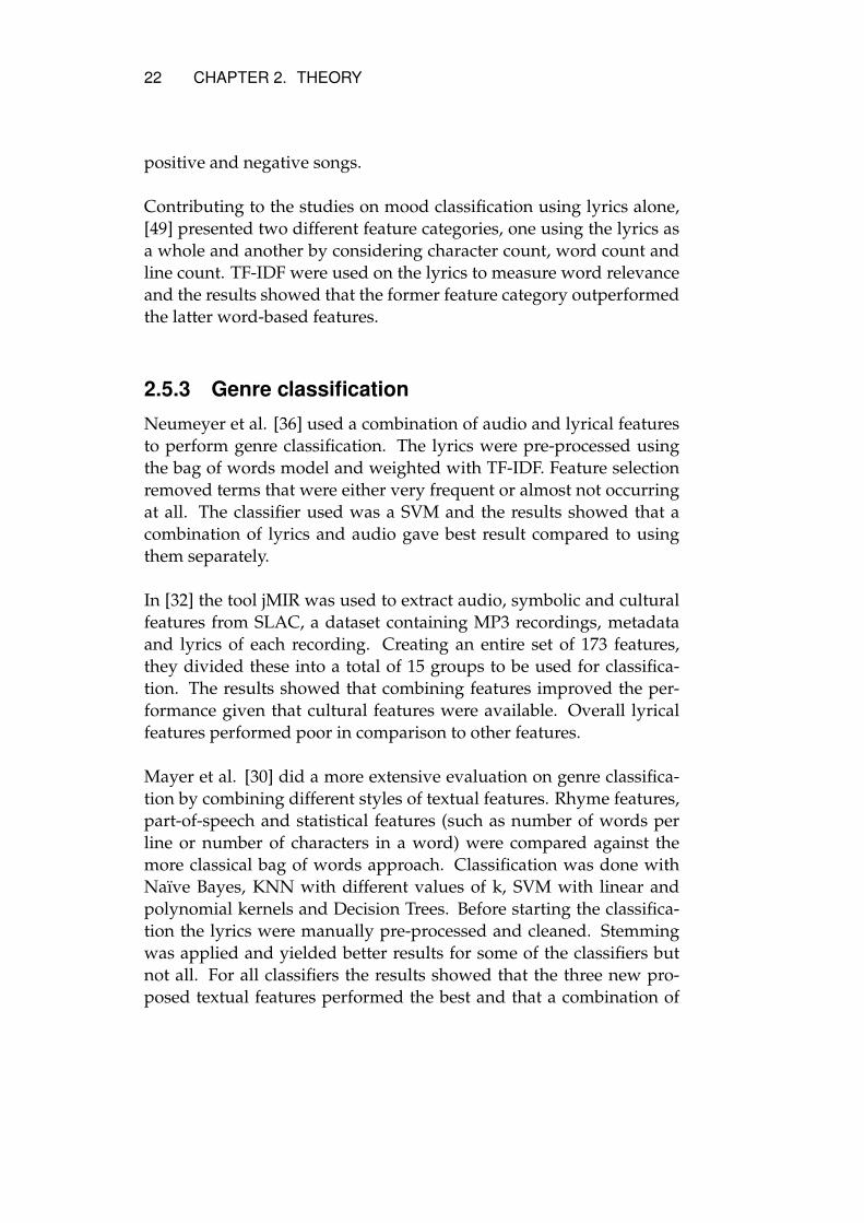
Contributing to the studies on mood classification using lyrics alone,[49] presented two different feature categories, one using the lyrics asa whole and another by considering character count, word count andline count. TF-IDF were used on the lyrics to measure word relevanceand the results showed that the former feature category outperformedthe latter word-based features.

2.5.3 Genre classification

Neumeyer et al. [36] used a combination of audio and lyrical featuresto perform genre classification. The lyrics were pre-processed usingthe bag of words model and weighted with TF-IDF. Feature selectionremoved terms that were either very frequent or almost not occurringat all. The classifier used was a SVM and the results showed that acombination of lyrics and audio gave best result compared to usingthem separately.

In [32] the tool jMIR was used to extract audio, symbolic and culturalfeatures from SLAC, a dataset containing MP3 recordings, metadataand lyrics of each recording. Creating an entire set of 173 features,they divided these into a total of 15 groups to be used for classifica-tion. The results showed that combining features improved the per-formance given that cultural features were available. Overall lyricalfeatures performed poor in comparison to other features.

Mayer et al. [30] did a more extensive evaluation on genre classifica-tion by combining different styles of textual features. Rhyme features,part-of-speech and statistical features (such as number of words perline or number of characters in a word) were compared against themore classical bag of words approach. Classification was done withNaïve Bayes, KNN with different values of k, SVM with linear andpolynomial kernels and Decision Trees. Before starting the classifica-tion the lyrics were manually pre-processed and cleaned. Stemmingwas applied and yielded better results for some of the classifiers butnot all. For all classifiers the results showed that the three new pro-posed textual features performed the best and that a combination of

CHAPTER 2. THEORY 23

these features with the classical bag of words approach outperformedusing only bag of words.

In 2016 Oramas et al. [38] tried to add sentiment features by using acombination of customer reviews from Amazon3, metadata from Mu-sicBrainz4 and audio descriptors from AcousticBrainz5. Text process-ing was performed by doing sentiment analysis followed by entitylinking. A bag of words model with TF-IDF were used and stop wordswere removed. The vectors were enriched with information from theentity linking step. During the sentiment analysis a sentiment scorewas assigned creating a group of sentiment features. The model wasevaluated using Naïve Bayes and SVM using different combinationsof features. The result showed that adding sentiment features outper-forms using purely text-based features.

During last year two different papers used deep networks for genreclassification. In [39] audio, text and images were used as features andinput for a convolutional neural network (CNN). To create the text fea-tures all reviews of an album were concatenated to one text and thentruncated to the same size. A vector space model with TF-IDF wereapplied to create a feature vector of each album. To enrich the text atool called Babelfy6 was used to map words to Wikipedia categories.The results showed that text-based features outperformed audio andimage features and that the enriched version of the text was superior tothe other one. It also showed that using neural networks outperformmore traditional approaches. The other paper [48] used hierarchicalattention networks (HAN) with lyrical features for genre classificationand compared them with non-neural approaches. The performance ofHAN were compared to four other baseline models including a major-ity classifier, logistic regression, long short-term memory and hierar-chical networks. The results showed that HAN performs better thanall earlier attempts on classifying genre using lyrical features.

3https://www.amazon.com/4https://musicbrainz.org/5https://acousticbrainz.org/6http://babelfy.org/

24 CHAPTER 2. THEORY

2.5.4 Topic classification

Mahedero et al. [29] have explored how natural language processingtools can be applied to lyrics in order to perform language identifica-tion, structure extraction, categorization and artist similarity searches.For the thematic categorization the goal was to build a classifier thatcould recognize five categories: love, violent, protest, christian anddrugs. The algorithm used for this purpose was Naïve Bayes whichyielded promising results. Overall the report concluded that lyrics canbe a good complement to audio and cultural metadata features.

Kleedorfer et al. [22] created a vector space model out of lyrics andused non-negative matrix factorization (NMF) to identify clusters oftopics and then labeled these manually. The lyrical pre-processing wasdone by tokenizing the lyrics and creating a term-document matrix.Stop words and terms with very high or very low document frequencywere removed and term weighting was done using TF-IDF. The resultsshowed that a reasonable portion of the clusters described distinguish-able topics and that they were reliably tagged.

In [5], topic analysis was performed by using data in forms of au-dio features and social annotations on last.fm. The authors foundthat SVM performed best on audio features whereas Naïve Bayes per-formed best on tag features. The result showed that these two typesof features are complementary and should be used together for bestresults.

Chapter 3

Method

This chapter describes the work flow during the thesis and the methods used.This includes description of data sets, chosen algorithms and how the evalua-tion was carried out.

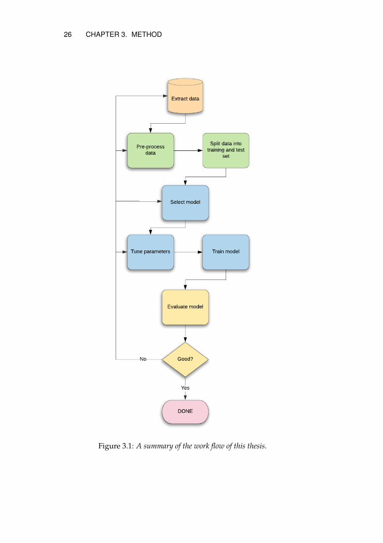
3.1 Work flow

After defining the problem, necessary data is extracted from differentsources. The data is pre-processed and vectorized for the text classi-fiers and then split into training and test data. The training set is thenused to train each classifier and the classifier is evaluated using thetest data to plot a precision-recall curve. Figure 3.1 presents a sum-mary from data collection to result.

3.2 Data set

In this degree project two different data sets are used. One contain-ing the lyrics of the songs and the explicit tags that has been used asground truth and the other containing additional data about each songto help enrich the lyrics.

3.2.1 Lyrics and explicit tags

Lyrics is obtained through the LyricFind API1. The API provides ex-cept for lyrics, the song name, artist name, lyric language and a song

1http://lyricfind.com/

25

26 CHAPTER 3. METHOD

Figure 3.1: A summary of the work flow of this thesis.

CHAPTER 3. METHOD 27

identification number called ISRC which is internationally used forsongs in general. 2

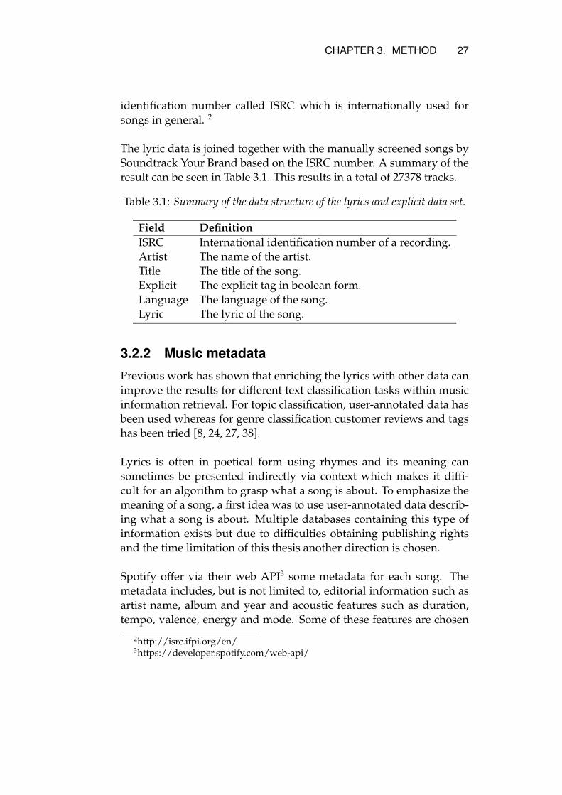
The lyric data is joined together with the manually screened songs bySoundtrack Your Brand based on the ISRC number. A summary of theresult can be seen in Table 3.1. This results in a total of 27378 tracks.

Table 3.1: Summary of the data structure of the lyrics and explicit data set.

Field DefinitionISRC International identification number of a recording.Artist The name of the artist.Title The title of the song.Explicit The explicit tag in boolean form.Language The language of the song.Lyric The lyric of the song.

3.2.2 Music metadata

Previous work has shown that enriching the lyrics with other data canimprove the results for different text classification tasks within musicinformation retrieval. For topic classification, user-annotated data hasbeen used whereas for genre classification customer reviews and tagshas been tried [8, 24, 27, 38].

Lyrics is often in poetical form using rhymes and its meaning cansometimes be presented indirectly via context which makes it diffi-cult for an algorithm to grasp what a song is about. To emphasize themeaning of a song, a first idea was to use user-annotated data describ-ing what a song is about. Multiple databases containing this type ofinformation exists but due to difficulties obtaining publishing rightsand the time limitation of this thesis another direction is chosen.

Spotify offer via their web API3 some metadata for each song. Themetadata includes, but is not limited to, editorial information such asartist name, album and year and acoustic features such as duration,tempo, valence, energy and mode. Some of these features are chosen

2http://isrc.ifpi.org/en/3https://developer.spotify.com/web-api/

28 CHAPTER 3. METHOD

for enrichment of the lyrics to see if it will improve the results. Theextracted features are:

• Artist name - The artist of a song.

• Release year - The year a song was released.

• Energy level - A measure from 0.0 to 1.0 that describes the inten-sity of a song.

• Valence - A measure from 0.0 to 1.0 that describes the positive-ness of a song. Higher value means positive and happy, whereasa low value corresponds to a negative and sad song.

3.3 Software

All code in this thesis is written in Python (version 3.6). The classi-fiers are built using the Python module Scikit Learn which integratesseveral machine learning algorithms for both supervised and unsu-pervised problems [40]. The Doc2Vec vectorization is made using thelibrary Gensim [43]. An API called Imbalanced-learn is used to handlethe imbalance issues with sampling methods [26]. For hyper parame-ter optimization, a library called Scikit-Optimize is used [13].

3.4 Pre-processing

Pre-processing is used to extract the feature vectors for building andevaluating the model.

3.4.1 Data cleaning

The first step consists of cleaning the lyric data set. The lyrics providedby LyricFind comes in multiple languages and thus all non-Englishsongs have to be removed. The data set provided has a language fieldbut many entries are missing and thus the language is detected manu-ally for these records.

Records with lyrics shorter than 100 characters are removed as theydo not contain the correct or complete lyric of the song. This includes

CHAPTER 3. METHOD 29

for example all records with an empty lyric field or instrumental songswhich has the word "Instrumental" in the lyric field. After these steps25488 songs are left in the data set.

3.4.2 Feature selection and transformation

The classifiers use two different data sets; one containing only lyrics,and the other one, containing lyrics, artist name, energy, valence andyear. Both data sets use the explicit tag as label.

To combine multiple features as one input, Scikit Learn’s FeatureUnionis used, which provides the ability to combine different feature extrac-tion methods for different features and the features used are a com-bination of text and numbers with different pre-processing require-ments. Since the artist feature consisted of a string, each artist wasmapped to a unique numerical id to be used instead.

3.4.3 Feature extraction

To transform the lyrics to a suitable format for the classifiers two dif-ferent approaches are used, TF-IDF vectorization and Doc2Vec vec-torization. As explained in chapter 2, the first approach is based onword frequency whereas the second one is based on neural networksto calculate the relationship between the words. Since they are verydifferent it is interesting to use both to see which one is best suited forexplicit classification.

Both approaches come with different sets of parameters. The param-eters of the TF-IDF approach are tuned together with the parametersof the classifier using a parameter grid search. The details of this stepis explained in section 3.6. The parameters of the Doc2Vec approachare based on the results of [23] who have done an empirical evaluationof Doc2Vec and provided recommendations on parameter settings forsemantic textual similarity tasks. The recommended settings are usedfor the Doc2Vec model in this degree project. The reason for not tuningthe parameters of the Doc2Vec approach is that building the Doc2Vecmodel takes time and thus rebuilding the model with new parameterswithin each iteration of a grid search would not be feasible within thetime limitation of this degree project.

30 CHAPTER 3. METHOD

TF-IDF Vectorization

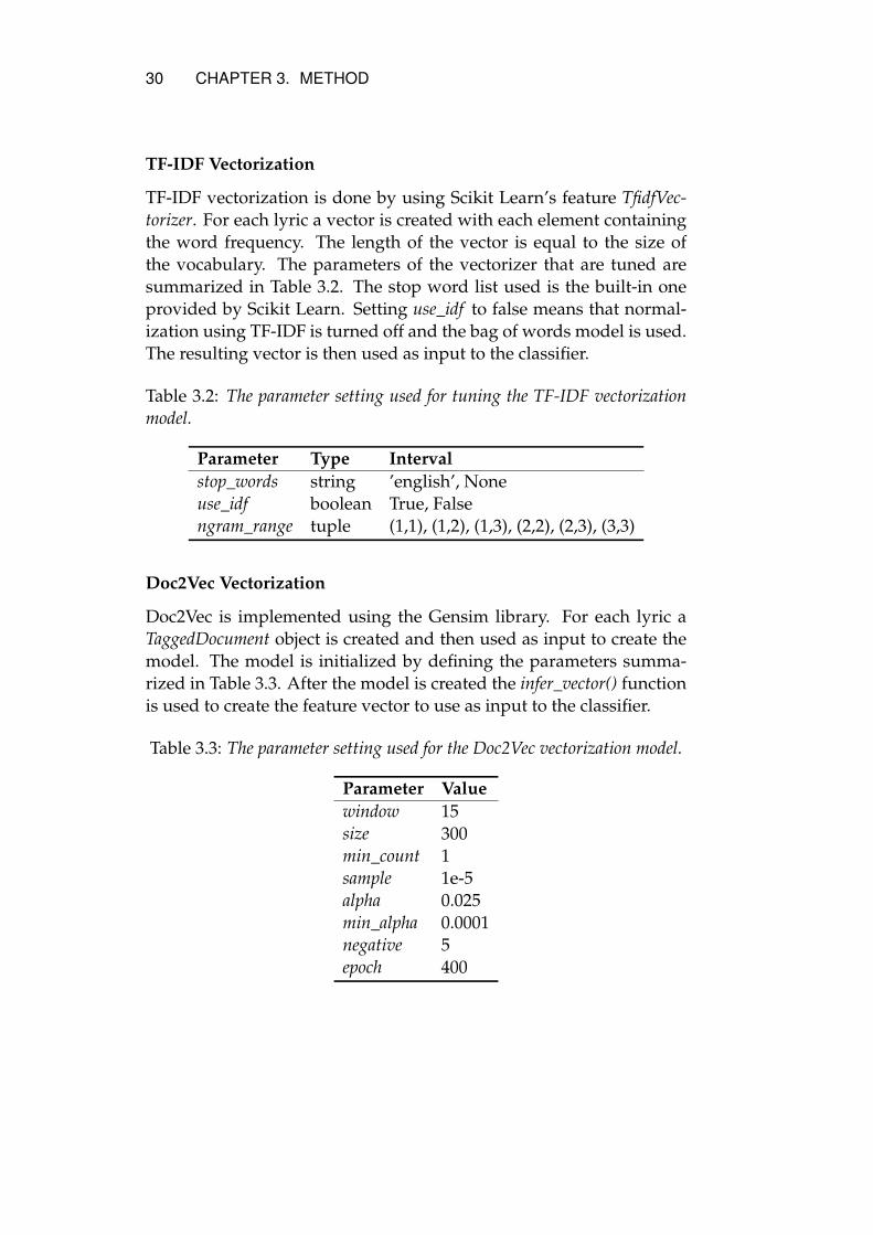
TF-IDF vectorization is done by using Scikit Learn’s feature TfidfVec-torizer. For each lyric a vector is created with each element containingthe word frequency. The length of the vector is equal to the size ofthe vocabulary. The parameters of the vectorizer that are tuned aresummarized in Table 3.2. The stop word list used is the built-in oneprovided by Scikit Learn. Setting use_idf to false means that normal-ization using TF-IDF is turned off and the bag of words model is used.The resulting vector is then used as input to the classifier.

Table 3.2: The parameter setting used for tuning the TF-IDF vectorizationmodel.

Parameter Type Intervalstop_words string ’english’, Noneuse_idf boolean True, Falsengram_range tuple (1,1), (1,2), (1,3), (2,2), (2,3), (3,3)

Doc2Vec Vectorization

Doc2Vec is implemented using the Gensim library. For each lyric aTaggedDocument object is created and then used as input to create themodel. The model is initialized by defining the parameters summa-rized in Table 3.3. After the model is created the infer_vector() functionis used to create the feature vector to use as input to the classifier.

Table 3.3: The parameter setting used for the Doc2Vec vectorization model.

Parameter Valuewindow 15size 300min_count 1sample 1e-5alpha 0.025min_alpha 0.0001negative 5epoch 400

CHAPTER 3. METHOD 31

3.4.4 Sampling

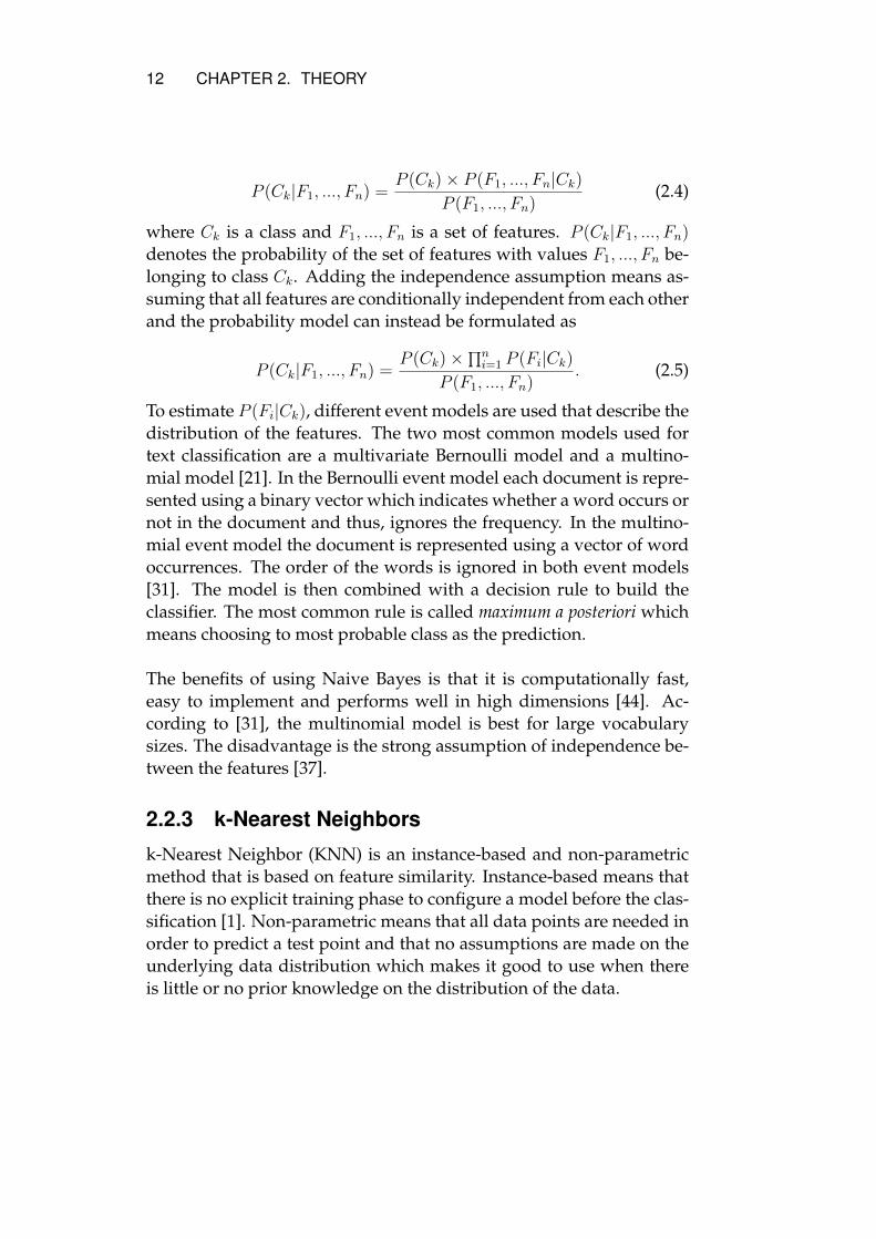
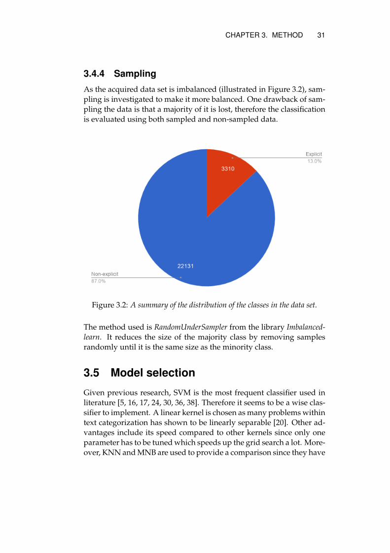
As the acquired data set is imbalanced (illustrated in Figure 3.2), sam-pling is investigated to make it more balanced. One drawback of sam-pling the data is that a majority of it is lost, therefore the classificationis evaluated using both sampled and non-sampled data.

Figure 3.2: A summary of the distribution of the classes in the data set.

The method used is RandomUnderSampler from the library Imbalanced-learn. It reduces the size of the majority class by removing samplesrandomly until it is the same size as the minority class.

3.5 Model selection

Given previous research, SVM is the most frequent classifier used inliterature [5, 16, 17, 24, 30, 36, 38]. Therefore it seems to be a wise clas-sifier to implement. A linear kernel is chosen as many problems withintext categorization has shown to be linearly separable [20]. Other ad-vantages include its speed compared to other kernels since only oneparameter has to be tuned which speeds up the grid search a lot. More-over, KNN and MNB are used to provide a comparison since they have

32 CHAPTER 3. METHOD

been used before as well [5, 17, 29, 30, 38]. RF is chosen as it has showngood performance in other text classification problems [51, 52].

A summary of selected classifiers and their corresponding function inScikit Learn is presented in Table 3.4.

Table 3.4: Summary of the models used and their corresponding function inScikit Learn.

Classifier Scikit LearnLinear Support Vector Machine SVC(kernel=’linear’)Multinomial Naive Bayes MultinomialNB()k-Nearest Neighbors KNeighborsClassifier()Random Forest RandomForestClassifier()

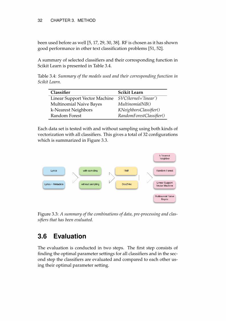
Each data set is tested with and without sampling using both kinds ofvectorization with all classifiers. This gives a total of 32 configurationswhich is summarized in Figure 3.3.

Figure 3.3: A summary of the combinations of data, pre-processing and clas-sifiers that has been evaluated.

3.6 Evaluation

The evaluation is conducted in two steps. The first step consists offinding the optimal parameter settings for all classifiers and in the sec-ond step the classifiers are evaluated and compared to each other us-ing their optimal parameter setting.

CHAPTER 3. METHOD 33

3.6.1 Parameter tuning

To tune the parameters of each classifier Scikit Learn provides a func-tion called GridSearchCV which takes a set of values for each parameterand then performs a total search of all combinations of the values ofthe parameters. However, the complexity grows exponentially and fora classifier with parameters with a large set of values (e.g. parameterswith values within a continuous range) it is not very scalable.

Instead, a library called scikit-optimize is used for parameter tuning. Itprovides a function called BayesSearchCV which replaces Scikit Learn’sGridSearchCV. It uses Bayesian optimization where the search space ismodelled as a function with the aim of finding the optimal parame-ter values in as few iterations as possible. It works by constructing aposterior distribution of functions that describes the function that is tobe optimized. For each iteration, the model becomes more certain ofwhich ranges of the parameters that are stronger and which are not.Thus, it does not have to test all combinations in order to find out themost optimal one. All parameters are evaluated using 10-fold strati-fied cross-validation.

3.6.2 Classification

After the tuning, all models are trained and evaluated using the opti-mized parameters. The metric used for evaluation is precision-recallcurves as they work well with imbalanced data [10].

Chapter 4

Results

This chapter presents the results of the classification. The results are presentedusing precision-recall curves and divided into sections per algorithm and perdata set.

As mentioned in section 3.5, each data set is evaluated with all clas-sifiers with all combinations of sampling and vectorization, givinga total of 32 configurations. To simplify the presentation of the re-sults, abbreviations are introduced for each classifier, data set and pre-processing method. Table 4.1 presents the abbreviations for each clas-sifier.

Table 4.1: Abbreviations for the classifiers used when presenting the results.

Classifier AbbreviationLinear Support Vector Machine SVMMultinomial Naive Bayes MNBk-Neareast Neighbor KNNRandom Forest RF

Further, the data sets are denoted by ’L’ for lyrics only and ’LM’ forlyrics combined with music metadata, sampling is denoted by ’S’ andvectorization is denoted by ’TF’ for TF-IDF and ’D2V’ for Doc2Vec.For each configuration a pattern is used where the abbreviations areconcatenated with a dot in between, e.g. using the lyric data set withsampling, TF-IDF and the classifier RF would be ’L.S.TF.RF’ and usingthe lyric data set without sampling, with Doc2Vec and the classifier

34

CHAPTER 4. RESULTS 35

SVM would be ’L.D2V.SVM’.

The following sections present the results using precision-recall curves.For numerical results with accuracy, precision, recall and F1-score, seeAppendix A.

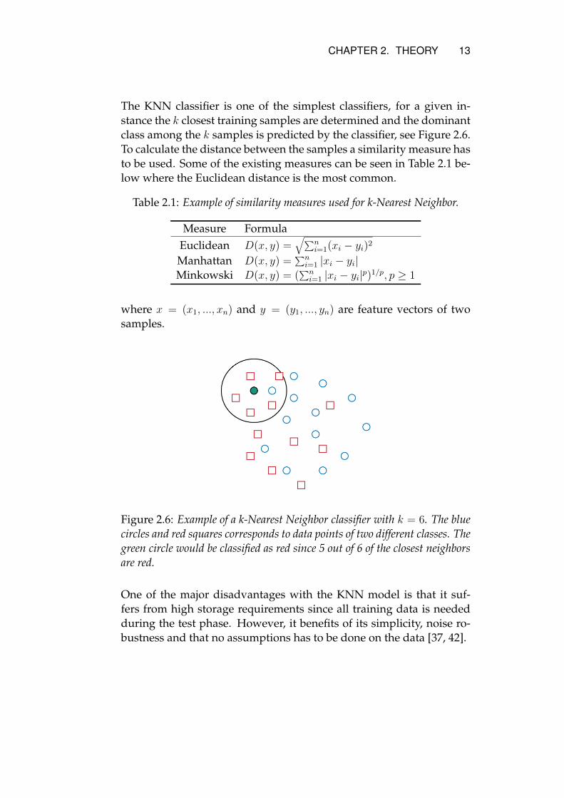
4.1 Results per classifier

This section provides precision-recall curves for each classifier.

4.1.1 Linear Support Vector Machine

The precision-recall curves for all configurations using SVM are pre-sented in Figure 4.1a. Of the presented configurations ’L.S.TF.SVM’has the best performance and ’LM.TF.SVM’ the worst.

4.1.2 Multinomial Naive Bayes

The precision-recall curves for all configurations with MNB are pre-sented in Figure 4.1b. As for SVM, the configuration with the sampledlyric data set and TF-IDF vectorization performs best. ’LM.D2V.MNB’has the worst performance.

4.1.3 k-Nearest Neighbor

Figure 4.1c presents the precision-recall curves for the KNN classifier.’L.S.TF.KNN’ and ’LM.S.TF.KNN’ perform best and ’L.D2V.KNN’ hasthe worst performance.

4.1.4 Random Forest

Figure 4.1d presents the precision-recall curves for all configurationsusing the RF classifier. As for KNN, ’L.S.TF.RF’ and ’LM.S.TF.RF’ per-forms best and ’L.D2V.RF’ has the worst performance.

4.2 Results per data set and sampling

This section presents the result per each data set and whether or notsampling was used.

36 CHAPTER 4. RESULTS

4.2.1 Lyrics

With sampling

For the configurations that use the sampled lyric data set, RF performsbest and KNN performs worst, see Figure 4.2a. Looking at the vector-ization, configurations using TF-IDF perform better than those usingD2V except for ’L.S.TF.KNN’ which performs worse than three of theconfigurations using D2V.

Without sampling

Figure 4.2b presents the precision-recall curves for the configurationsthat use the lyric data set without sampling. As for the lyric dataset with sampling, RF together with TF-IDF vectorization has the bestperformance and KNN with D2V vectorization has the worst perfor-mance.

4.2.2 Lyrics + Music Metadata

With sampling

Figure 4.2c presents the precision-recall curves for the configurationsthat are using the lyric and metadata data set with sampling. RF withTF-IDF vectorization performs the best, while MNB with D2V vector-ization performs the worst.

Without sampling

Precision-recall curves for the lyric and metadata data set without sam-pling are presented in Figure 4.2d. As for the data set with sampling,RF with TF-IDF vectorization performs the best. ’LM.TF.SVM’ has theworst performance.

CHAPTER 4. RESULTS 37

(a)P

reci

sion

-Rec

allC

urve

for

Supp

ortV

ecto

rM

achi

ne.b

bb(b

)Pre

cisi

on-R

ecal

lCur

vefo

rM

ultin

omia

lNai

veBa

yes.

(c)P

reci

sion

-Rec

allC

urve

for

k-N

eare

stN

eigh

bor.b

bbbb

bbb

(d)P

reci

sion

-Rec

allC

urve

for

Ran

dom

Fore

st.b

bbbb

bbbb

Figu

re4.

1:Pr

ecis

ion-

Rec

allC

urve

spe

rcl

assi

fier.

38 CHAPTER 4. RESULTS

(a)Precision-RecallC

urvefor

Lyricdata

setwith

sampling.

bbbbbbb(b)Precision-R

ecallCurve

forLyric

datasetw

ithoutsampling.

bbbbb

(c)Precision-RecallC

urvefor

Lyricand

Metadata

dataset

with

sampling.

(d)Precision-RecallC

urvefor

Lyricand

Metadata

dataset

withoutsam

pling.

Figure4.2:Precision-R

ecallCurves

perdata

setandsam

pling.

Chapter 5

Discussion

In this chapter the results of the degree project are discussed and the problemquestion answered.

The goal of this thesis was to evaluate the possibilities of using ma-chine learning for explicit classification of song lyrics. To the best ofthe author’s knowledge no previous research within explicit text clas-sification using lyrics exist. The closest research areas that have beenfound include mood and genre classification. Most of the researchwithin those areas are either based on audio only or a combination ofaudio and lyrics, where audio or the combination have been strongerthan lyrics only [5, 15, 16, 24, 34, 36, 46]. Since explicit classificationhas to do mostly with the textual content, audio was not reasonable touse in this study.

However, looking at research within mood and genre classificationmade it clear that lyrics sometimes can be hard to interpret due to itspoetical style, using slang words and rhyme. [30, 32, 38] all used ex-ternal features to enrich the lyrics with good results, which motivatedthe use of it in this study as well.

Two of the newest reports within these areas were [39] and [48] whomboth used neural networks which made it interesting to look at it inthis project as well. The reason for not doing that was partly that thedata sets were too small, but also the time limitation of the degreeproject.

39

40 CHAPTER 5. DISCUSSION

5.1 Model evaluation

As illustrated by the precision-recall curves in Figure 4.2 it is clear thatthe RF classifier has the best performance where it performs the best inall configurations regardless of data set or using sampling or not. Thetop performing configurations are "LM.S.TF.RF" and "L.S.TF.RF". Theworst performing algorithms are KNN when looking at the lyric dataset and MNB when looking at the lyric and metadata data set. RF per-forming well was expected since that classifier is known to have goodperformance on sets with high dimensions, such as text. The reasonfor why MNB performed so bad when combining different kinds offeatures might be that the classifier is sensitive to feature selection andthat not all features fit to the multinomial distribution.

5.2 Sampling vs. No Sampling

The biggest differences seen between configurations using sampledand non-sampled data is that using sampled data reduces the accu-racy but increases precision and recall (Table A.1). The reason for thisis most likely due to that the classifier favors the majority class whenthey are imbalanced which leads to a high number of correct classi-fications on the majority class but few on the minority class. This inturn means a high accuracy since the majority class makes up almostall data records. The curves in Figure 4.1 indicates this as well wheremost of the configurations using sampled data perform better than theones with data sets without sampling.

5.3 TF-IDF vs. Doc2Vec Vectorization

The results in Figure 4.2 show that TF-IDF vectorization outperformsDoc2Vec vectorization in almost all configurations. One possible rea-son is that the Doc2Vec model is not trained with enough data, sinceit is built on a neural network which is sensitive to too small data sets.One way to solve it would be to use a larger data set for building theDoc2Vec models.

CHAPTER 5. DISCUSSION 41

5.4 Data set evaluation

The biggest difference between the two data sets was that the LM dataset included features that were categorical whereas the lyric data setonly included numerical data. Different machine learning models han-dle categorically data differently well, where KNN and SVM are basedon Euclidean distance and thus should not perform well with categor-ical data.

Figure 4.1a and 4.2d show that the ’LM.TF.SVM’ performed the worstof all configurations. All other configurations using SVM and the LMdata set performed worse than the SVM configurations using the lyricdata set except for ’LM.S.D2V.SVM’ which performed the second best(Figure 4.1a). The worst performance using the LM data set had MNB(Figure 4.1b) where all configurations using the lyric data set perform-ed better than the configurations using the LM data set.

Oddly, the configurations using the LM data set performed well inKNN and RF as can be seen in Figure 4.1c and 4.1d where the curvesfor the configurations using the LM data set are almost the same as theones using the lyric data set. Thus, the conclusion that can be drawnis that the data set to use is very dependent on the algorithm chosen.

One way to get around categorical data is to use a one-hot encoderfor the artists. This means that one would create one feature per artistand set it to 1 for the correct artist and all other features fields to 0.However, since there were over 7000 different artists this would haveincreased the dimensionality so much that it would be very impracti-cal to use. In addition to this one-hot encoded data would not performwell with MNB since the features that are encoded would depend oneach other.

Chapter 6

Conclusion and Future work

In this thesis 32 configurations using different data sets, vectoriza-tion methods and algorithms have been implemented and evaluatedwith the purpose of classifying explicit music content. The resultsshow that the best configurations in terms of precision recall curvesare ’LM.S.TF.RF’ and ’L.S.TF.RF’. Overall the two data sets used gavemixed performance based on algorithm, the sampled data sets outper-formed the ones without sampling and TF-IDF vectorization outper-formed D2V vectorization.

For future work one should firstly focus on collecting more data. Oneway to expand the data set is to join the LyricFind database with theexplicit database using other fields than ISRC as ISRC is unique foreach recording and same song can have different recordings but stillhave the same lyrics. This means that right now same songs with dif-ferent recordings would not match.

Another way to expand the data is to include more or other features.One original idea for this project was to make use of user annotateddata on what a song is about. The idea is that this would help under-standing the context of a song since lyrics are poetical with a meaningthat sometimes is presented indirectly.

Some lyrics contained words that were not part of the actual song text,e.g. "Chorus x2" and "Intro". These were not excluded in this projectas it would have required to manually go through all lyrics which wasnot feasible due to the time limitations in this project. To manually

42

CHAPTER 6. CONCLUSION AND FUTURE WORK 43

clean the songs and perform stemming would be interesting to look atto see if the results could be improved.

It would also be interesting to explore a multi-label version of theproblem where different kinds of explicit language could be detected.However, this requires creation of ground truth for each explicit classbefore being able to train and evaluate a classifier, something that wasnot available for this project.

Bibliography

[1] C. C. Aggarwal. Data Mining: The Textbook. Springer InternationalPublishing, 2015. ISBN: 978-3-319-14141-1.

[2] C. C. Aggarwal. Machine Learning for Text. Springer InternationalPublishing, 2018. ISBN: 978-3-319-73530-6.

[3] A. Basu, C. Watters, and M. Shepherd. “Support Vector Machinesfor Text Categorization”. In: Proceedings of the 36th Annual HawaiiInternational Conference on System Sciences (HICSS’03) - Track 4 -Volume 4. 2003. ISBN: 0-7695-1874-5.

[4] S. Baumann and O. Hummel. “Using cultural metadata for artistrecommendations”. In: 3rd International Conference on WEB Deliv-ering of Music ·WEDELMUSIC 2003. 2003. ISBN: 0-7695-1935-0.

[5] K. Bischoff et al. “Music Mood and Theme Classification - A Hy-brid Approach”. In: 10th International Society for Music Informa-tion Retrieval Conference (ISMIR 2009). 2009, pp. 657–662.

[6] B. E. Boser, I. M. Guyon, and V. N. Vapnik. “A Training Algo-rithm for Optimal Margin Classifiers”. In: Proceedings of the FifthAnnual Workshop on Computational Learning Theory. 1992, pp. 144–152. ISBN: 0-89791-497-X.

[7] J. Bouwmeester. As 2018 approaches, the Spotify explicit filter is stillMIA. URL: https://techaeris.com/2017/12/27/as-2018- approaches-the- spotify-explicit- filter-is-still-mia/. (accessed: 12.02.2018).

[8] E. Çano and M. Morisio. “Music Mood Dataset Creation Basedon Last.fm Tags”. In: Fourth International Conference on ArtificialIntelligence and Applications (AIAP 2017). 2017, pp. 15–26.

[9] M. A. Casey et al. “Content-Based Music Information Retrieval:Current Directions and Future Challenges”. In: Proceedings of theIEEE 96.4 (2008), pp. 668–696.

44

BIBLIOGRAPHY 45

[10] J. Davis and M. Goadrich. “The Relationship Between Precision-Recall and ROC Curves”. In: Proceedings of the 23rd InternationalConference on Machine Learning. 2006, pp. 233–240. ISBN: 1-59593-383-2.

[11] X. Deng et al. “An imbalanced data classification method basedon automatic clustering under-sampling”. In: Performance Com-puting and Communications Conference (IPCCC), 2016 IEEE 35thInternational. 2016.

[12] L. Espinosa-Anke et al. “ELMDist: A Vector Space Model withWords and MusicBrainz Entities”. In: The Semantic Web: ESWC2017 Satellite Events. 2017, pp. 355–366.

[13] T. Head et al. scikit-optimize/scikit-optimize: v0.5.2. 2018. DOI: https://doi.org/10.5281/zenodo.1207017. URL: https://scikit-optimize.github.io/.

[14] T. R. Hoens and N. V. Chawla. “Imbalanced Datasets: From Sam-pling to Classifiers”. In: Imbalanced Learning: Foundations, Algo-rithms, and Applications. Ed. by H. He and Y. Ma. Wiley-IEEEPress, 2013. Chap. 3, pp. 43–59. ISBN: 9781118074626.

[15] X. Hu et al. “Improving mood classification in music digital li-braries by combining lyrics and audio”. In: JCDL ’10 Proceedingsof the 10th annual joint conference on Digital libraries. 2010, pp. 159–168.

[16] X. Hu et al. “Lyric Text Mining in Music Mood Classification”.In: 10th International Society for Music Information Retrieval Confer-ence (ISMIR 2009). 2009, pp. 411–416.

[17] H. Hui et al. “Language Feature Mining for Music Emotion Clas-sification via Supervised Learning from Lyrics”. In: ISICA 2008:Advances in Computation and Intelligence. 2008, pp. 426–435. ISBN:978-3-540-92136-3.

[18] imbalanced-learn. 3. Under-sampling. URL: http://contrib.scikit-learn.org/imbalanced-learn/stable/under_sampling.html. (accessed: 02.05.2018).

[19] G. James et al. An Introduction to Statistical Learning. Springer Sci-ence+Business Media, 2013. ISBN: 978-1-4614-7137-0.

46 BIBLIOGRAPHY

[20] T. Joachims. “Text categorization with Support Vector Machines:Learning with many relevant features”. In: Machine Learning: ECML-98. 1998, pp. 137–142. ISBN: 978-3-540-69781-7.

[21] A. M. Kibriya et al. “Multinomial Naive Bayes for Text Catego-rization Revisited”. In: AI 2004: Advances in Artificial Intelligence.2005, pp. 488–499. ISBN: 978-3-540-30549-1.

[22] F. Kleedorfer, P. Knees, and T. Pohle. “Oh Oh Oh Whoah! To-wards Automatic Topic Detection In Song Lyrics”. In: ISMIR 2008– Session 2d – Social and Music Networks. 2008, pp. 287–292. ISBN:978-0-615-24849-3.

[23] J. Han Lau and T. Baldwin. “An Empirical Evaluation of doc2vecwith Practical Insights into Document Embedding Generation”.In: Proceedings of the 1st Workshop on Representation Learning forNLP. 2016, pp. 78–86.

[24] C. Laurier. “Automatic Classification of Musical Mood by Content-Based Analysis”. PhD thesis. Universitat Pompeu Fabra, Barcelona,Spain, 2011.

[25] Q. V. Le and T. Mikolov. “Distributed Representations of Sen-tences and Documents”. In: ICML’14 Proceedings of the 31st Inter-national Conference on International Conference on Machine Learn-ing. 2014, pp. 1188–1196.

[26] G. Lemaître, F. Nogueira, and C. K. Aridas. “Imbalanced-learn:A Python Toolbox to Tackle the Curse of Imbalanced Datasets inMachine Learning”. In: Journal of Machine Learning Research 18.17(2017), pp. 1–5.

[27] Y. Lin, Y. Yang, and H. H. Chen. “Exploiting online music tagsfor music emotion classification”. In: ACM Transactions on Multi-media Computing, Communications, and Applications 7.1 (2011).

[28] A. Y. Liu. “The Effect of Oversampling and Undersampling onClassifying Imbalanced Text Datasets”. MA thesis. The Univer-sity of Texas at Austin, 2004.

[29] J. P. G. Mahedero et al. “Natural Language Processing of Lyrics”.In: Proceeding MM ’05 Proceedings of the 13th annual ACM interna-tional conference on Multimedia. 2005, pp. 475–478.

BIBLIOGRAPHY 47

[30] R. Mayer, R. Neumayer, and A. Rauber. “Combination of Au-dio and Lyrics Features for Genre Classification in Digital AudioCollections”. In: Proceeding MM ’08 Proceedings of the 16th ACMinternational conference on Multimedia. 2008, pp. 159–168.

[31] A. McCallum and K. Nigam. “A Comparison of Event Modelsfor Naive Bayes Text Classification”. In: Learning for Text Catego-rization: Papers from the 1998 AAAI Workshop. 1998, pp. 41–48.

[32] C. McKay et al. “Evaluating the Genre Classification Performanceof Lyrical Features Relative to Audio, Symbolic and CulturalFeatures”. In: Int. Society for Music Information Retrieval Confer-ence. 2010.

[33] O. C. Meyers. “A Mood-Based Music Classification and Explo-ration System”. MA thesis. Massachusetts Institute of Technol-ogy, 2007.

[34] R. Mihalcea and C. Strapparava. “Lyrics, music, and emotions”.In: Proceeding EMNLP-CoNLL ’12 Proceedings of the 2012 Joint Con-ference on Empirical Methods in Natural Language Processing andComputational Natural Language Learning. 2012, pp. 590–599.

[35] T. Mikolov et al. “Efficient Estimation of Word Representationsin Vector Space”. In: ArXiv e-prints (2013). arXiv: 1301.3781.

[36] R. Neumayer and A. Rauber. “Integration of Text and AudioFeatures for Genre Classification in Music Information Retrieval”.In: European Conference on Information Retrieval, ECIR 2007: Ad-vances in Information Retrieval. 2007, pp. 724–727.

[37] Nidhi and V. Gupta. “Recent Trends in Text Classification Tech-niques”. In: International Journal of Computer Applications 35.6 (2011),pp. 45–51.

[38] S. Oramas et al. “Exploring Customer Reviews for Music GenreClassification and Evolutionary Studies”. In: 17th InternationalSociety for Music Information Retrieval Conference (ISMIR 2016).2016, pp. 150–156.

[39] S. Oramas et al. “Multi-Label Music Genre Classification FromAudio, Text, and Images using Deep Features”. In: In Proceed-ings of the 18th International Society of Music Information RetrievalConference (ISMIR 2017). 2017.

48 BIBLIOGRAPHY

[40] F. Pedregosa et al. “Scikit-learn: Machine Learning in Python”.In: Journal of Machine Learning Research 12 (2011), pp. 2825–2830.

[41] S. A. Rahman et al. “Exploring Feature Selection and SupportVector Machine in Text Categorization”. In: 2013 IEEE 16th Inter-national Conference on Computational Science and Engineering. 2013,pp. 1101–1104.

[42] Z. E. Rasjid and R. Setiawan. “Performance Comparison andOptimization of Text Document Classification using k-NN andNaïve Bayes Classification Techniques”. In: Procedia ComputerScience. 2017, pp. 107–112.

[43] R. Rehurek and P. Sojka. “Software Framework for Topic Mod-elling with Large Corpora”. In: Proceedings of the LREC 2010 Work-shop on New Challenges for NLP Frameworks. 2010, pp. 45–50.

[44] J. D. M. Rennie et al. “Tackling the Poor Assumptions of NaiveBayes Text Classifiers”. In: Proceedings of the Twentieth Interna-tional Conference on International Conference on Machine Learning.2003, pp. 616–623. ISBN: 1-57735-189-4.

[45] L. Rokach. “Ensemble-based classifiers”. In: Artificial IntelligenceReview 33.1 (2010), pp. 1–39.

[46] B. Schuller. “Determination of Nonprototypical Valence and Arousalin Popular Music: Features and Performances”. In: EURASIP Jour-nal on Audio, Speech, and Music Processing (2010).

[47] Spotify. Explicit Button. URL: https://community.spotify.com/t5/Live-Ideas/Explicit-button/idi-p/3869.(accessed: 12.02.2018).

[48] A. Tsaptsinos. “Lyrics-Based Music Genre Classification Using aHierarchical Attention Network”. In: 18th International Society forMusic Information Retrieval Conference. 2017.

[49] M. van Zaanen and P. Kanters. “Autmatic Mood ClassificationUsing TF*IDF Based On Lyrics”. In: 11th International Society forMusic Information Retrieval Conference. 2010.

[50] P. Willett. “The Porter stemming algorithm: Then and now”. In:Program electronic library and information systems 40 (2006), pp. 219–223.

BIBLIOGRAPHY 49

[51] Q. Wu et al. “ForesTexter: An efficient random forest algorithmfor imbalanced text categorization”. In: Knowledge-Based Systems67 (2014), pp. 105–116.

[52] B. Xu et al. “An Improved Random Forest Classifier for Text Cat-egorization”. In: Journal of Computers 7.12 (2012), pp. 2913–2920.

Appendix A

Numerical results of all config-urations

Table A.1 presents the accuracy, precision, recall and F1-score of eachconfiguration based on the threshold chosen by Scikit-Learn. The bestconfiguration of each metric is presented in bold style.

50

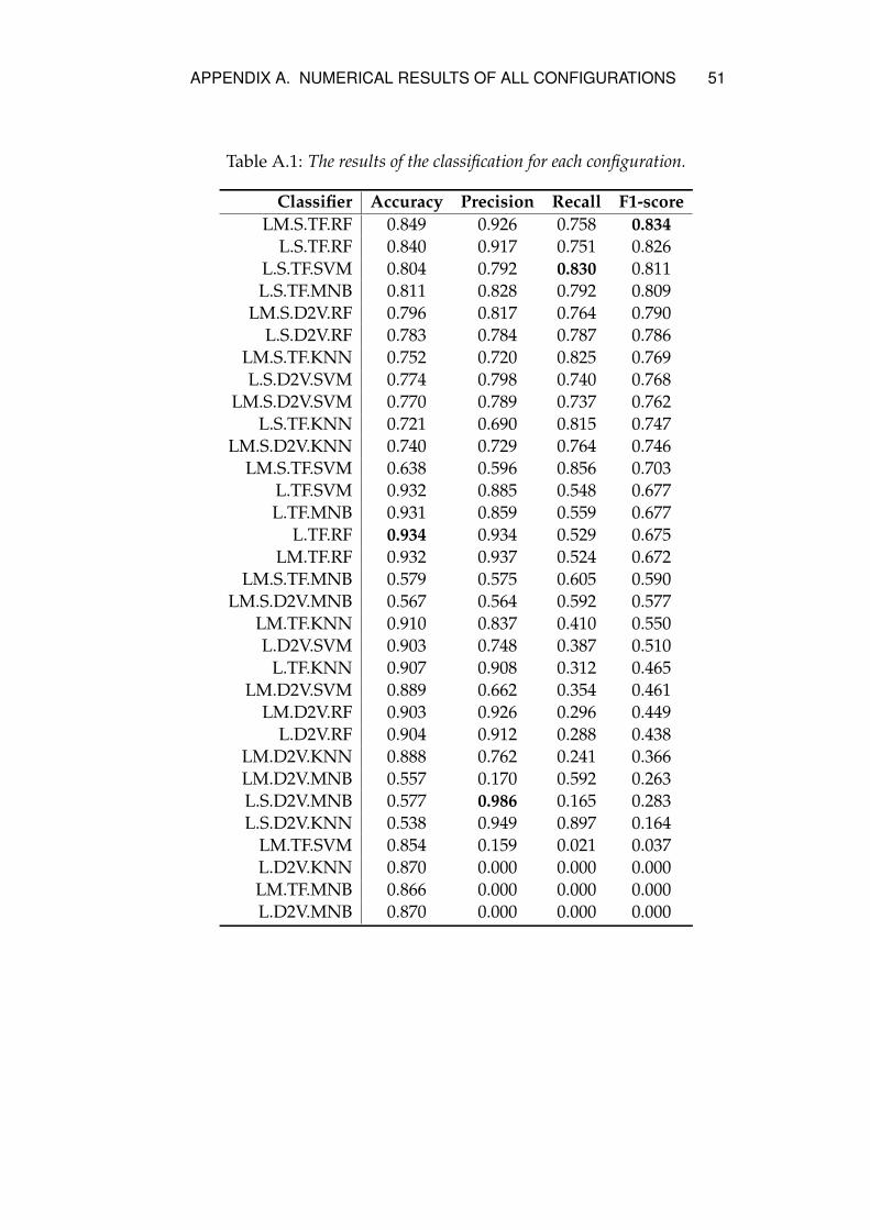
APPENDIX A. NUMERICAL RESULTS OF ALL CONFIGURATIONS 51

Table A.1: The results of the classification for each configuration.

Classifier Accuracy Precision Recall F1-scoreLM.S.TF.RF 0.849 0.926 0.758 0.834

L.S.TF.RF 0.840 0.917 0.751 0.826L.S.TF.SVM 0.804 0.792 0.830 0.811L.S.TF.MNB 0.811 0.828 0.792 0.809

LM.S.D2V.RF 0.796 0.817 0.764 0.790L.S.D2V.RF 0.783 0.784 0.787 0.786

LM.S.TF.KNN 0.752 0.720 0.825 0.769L.S.D2V.SVM 0.774 0.798 0.740 0.768

LM.S.D2V.SVM 0.770 0.789 0.737 0.762L.S.TF.KNN 0.721 0.690 0.815 0.747

LM.S.D2V.KNN 0.740 0.729 0.764 0.746LM.S.TF.SVM 0.638 0.596 0.856 0.703

L.TF.SVM 0.932 0.885 0.548 0.677L.TF.MNB 0.931 0.859 0.559 0.677

L.TF.RF 0.934 0.934 0.529 0.675LM.TF.RF 0.932 0.937 0.524 0.672

LM.S.TF.MNB 0.579 0.575 0.605 0.590LM.S.D2V.MNB 0.567 0.564 0.592 0.577

LM.TF.KNN 0.910 0.837 0.410 0.550L.D2V.SVM 0.903 0.748 0.387 0.510

L.TF.KNN 0.907 0.908 0.312 0.465LM.D2V.SVM 0.889 0.662 0.354 0.461

LM.D2V.RF 0.903 0.926 0.296 0.449L.D2V.RF 0.904 0.912 0.288 0.438

LM.D2V.KNN 0.888 0.762 0.241 0.366LM.D2V.MNB 0.557 0.170 0.592 0.263L.S.D2V.MNB 0.577 0.986 0.165 0.283L.S.D2V.KNN 0.538 0.949 0.897 0.164

LM.TF.SVM 0.854 0.159 0.021 0.037L.D2V.KNN 0.870 0.000 0.000 0.000LM.TF.MNB 0.866 0.000 0.000 0.000L.D2V.MNB 0.870 0.000 0.000 0.000

www.kth.se