Embed Size (px)
Citation preview

arX
iv:0
906.
2660
v1 [
astr
o-ph
.CO
] 1
5 Ju
n 20
09
Clumpy Galaxies in GOODS and GEMS: Massive Analogs of
Local Dwarf Irregulars
Debra Meloy Elmegreen
Vassar College, Dept. of Physics & Astronomy, Box 745, Poughkeepsie, NY 12604
Bruce G. Elmegreen
IBM Research Division, T.J. Watson Research Center, P.O. Box 218, Yorktown Heights,
NY 10598
Max T. Marcus
Vassar College, Dept. of Physics & Astronomy, Box 745, Poughkeepsie, NY 12604
Karlen Shahinyan
Wesleyan University, Dept. of Astronomy, Middletown, CT 06459
Andrew Yau
Vassar College, Dept. of Physics & Astronomy, Box 745, Poughkeepsie, NY 12604
Michael Petersen
Colgate University, Dept. of Physics & Astronomy, Hamilton, NY 13346
ABSTRACT

– 2 –
Clumpy galaxies in the GEMS and GOODS fields are examined for clues to
their evolution into modern spirals. The magnitudes of the clumps and the sur-
face brightnesses of the interclump regions are measured and fitted to models of
stellar age and mass. There is an evolutionary trend from clump clusters with
no evident interclump emission to clump clusters with faint red disks, to spiral
galaxies of the flocculent or grand design types. Along this sequence, the inter-
clump surface density increases and the mass surface density contrast between
the clumps and the interclump regions decreases, suggesting a gradual dispersal
of clumps to form disks. Also along this sequence, the bulge-to-clump mass ratios
and age ratios increase, suggesting a gradual formation of bulges. All of these
morphological types occur in the same redshift range, indicating that the clump
cluster morphology is not the result of bandshifting. This redshift range also
includes clear examples of interacting galaxies with tidal tails and other charac-
teristic features, indicating that clump clusters, which do not have these features,
are not generally interacting. Comparisons to local galaxies with the same rest
wavelength and spatial resolution show that clump clusters are unlike local floccu-
lent and spiral galaxies primarily because of the high clump/interclump contrasts
in the clump clusters. They bear a striking resemblance to local dwarf Irregu-
lars, however. This resemblance is consistent with a model in which the clumpy
morphology comes from gravitational instabilities in gas with a high turbulent
speed compared to the rotation speed and a high mass fraction compared to the
stars. The morphology does not depend on galaxy mass as much as it depends
on evolutionary stage: clump clusters are 100 times more massive than local
dwarfs. The apparent lack of star formation in damped Lyman alpha absorbers
may result from fast turbulence.
Subject headings: galaxies: evolution — galaxies: high-redshift — galaxies: ir-
regular — galaxies: peculiar — galaxies:starburst
1. Introduction
Star-forming galaxies become increasingly irregular at higher redshift with blue clumpy
structure, asymmetry, and a lack of central concentration (Glazebrook et al. 1995; Abraham,
et al. 1996a,b; van den Bergh et al. 1996; Driver et al. 1995, 1998; Im et al. 1999). These
three features are included in the CAS classification system (Conselice 2003), which has
identified such irregularities in a large fraction of galaxies in deep fields (e.g., Conselice,
Blackburne, & Papovich 2005; Menanteau et al. 2006). Similar observations of irregular

– 3 –
structures were obtained from color dispersions in high redshift galaxies (Papovich, et al.
2005), Gini coefficients (Lotz et al. 2006), Sersic indices (Cassata et al. 2005; Ravindranath
et al 2006), UV imaging (de Mello et al. 2006), and various combined methods (e.g., Neichel
et al. 2008).
The kinematics of disks at intermediate redshifts also show irregular structures (Erb
et al. 2004; Yang et al. 2008), suggesting an important contribution from unstable gas
dynamics (Law et al. 2009). Turbulent motions are large compared to the rotation speed
(Forster-Schreiber et al. 2006; Weiner et al. 2006; Genzel et al. 2006, 2008; Puech et al.
2007), although there can be underlying systematic rotation too (e.g., Bournaud et al. 2008).
During the last few years, we have examined the properties of clumps in high redshift
irregular galaxies, including chain galaxies (Cowie, Hu, & Songaila 1995) and their likely
face-on counterparts, the clump-clusters (Elmegreen, Elmegreen, & Hirst 2004), in an effort
to understand star formation and to look for signs of evolution toward modern Hubble
types. We have determined clump masses and ages from population synthesis models and
suggested the clumps form by gravitational instabilities in a gas-rich disk (Elmegreen &
Elmegreen 2005; Bournaud, Elmegreen & Elmegreen 2007, hereafter BEE). The clumps are
generally more massive than star complexes (Efremov 1995) in local galaxies, which suggests
that the turbulent speed in the neutral and molecular gas is large as well, perhaps in the
range of 20 to 50 km s−1, considering the characteristic mass of a disk instability (and as
measured in a z=1.6 clump cluster, Bournaud et al. 2008). Gas column densities have
to be large too, around 100 M⊙ pc−2 (Elmegreen, et al. 2009, hereafter EEFL). These
properties are reasonable considering the youthful stage of the systems we are studying.
The high turbulence may come from gas accretion because it has to be in place before the
clumps form in order to define the clump mass, and because the star formation feedback that
generates turbulence in local galaxies is relatively ineffective when the velocity dispersion of
the whole interstellar medium is large. High dispersion star-forming clouds are tightly bound
and not easily disrupted by star-formation pressures (Elmegreen, Bournaud, & Elmegreen
2008). Clumps also produce high velocity dispersions by themselves in the surrounding gas
(BEE).
This interpretation of asymmetric clumpy structure as an indication of instabilities in
a gas-rich disk is not the only possibility. When asymmetry and clumpiness are observed
in a local L∗ galaxy, they are usually indicative of a merger. Faint peripheral structures
such as tails and bridges contribute to this identification locally. As a result, asymmetric
and clumpy structure in high redshift galaxies has also been considered to be the result of
mergers (e.g., Conselice et al. 2003, Treu et al. 2005; Lotz et al. 2008; Conselice, Yang,
& Bluck 2009, and references therein). This interpretation is reinforced by expectations

– 4 –
from the ΛCDM model, in which dark matter halos grow by hierarchical merging (Davis
et al. 1985). For example, a recent study by Jogee et al. (2009) suggested that 16% and
45% of galaxies with stellar masses larger than 2 × 10¹⁰ M⊙ had a major or minor merger,
respectively, at redshifts between 0.24 and 0.80. Jogee et al. identified these galaxies as
mergers based only on their asymmetric and clumpy structure, as determined both by eye
and by the CAS system. The actual fraction of galaxies that are clumpy in this redshift
range is smaller than the Jogee et al. merger fractions, because they, like others, correct the
observed fractions upward to compensate for the low fraction of time during which a merger
morphology should be visible. Lopez-Sanjuan et al. (2009) also used the asymmetry index
for galaxies in the range 0.35 < z < 0.85 and derived a corrected major merger fraction of
20%-35% for MB < 20 galaxies.
The key assumption for these and other merger interpretations is that baryons come
together in a clumpy fashion like the cold dark matter, and star formation occurs early and
efficiently in the baryonic clumps, which then merge as little galaxies rather than as smooth
gaseous flows. Early numerical simulations reinforced this view, although the results of these
simulations depended strongly on the recipes for thermal equilibrium and star formation,
which are uncertain. Significant merging is untenable in the instability model of clump
formation because then the pre-existing stars would make a spheroidal component in the
remnant (e.g., Abadi et al. 2003), and this component would cause the instabilities to
appear as spiral arms rather than discrete clumps (Bournaud & Elmegreen 2009).
Other aspects of galaxies expected from mergers are not generally observed. Law et
al. (2007) noted that the UV morphology of a galaxy is not related to the star formation
rate, which led them to conclude that the irregular structure is probably not the result of a
merger. Jogee et al. (2009) also found that the star formation rate is not correlated with
galaxy morphology. In local gas-rich mergers, even with weak tidal forces, there is usually
a significant increase in the star formation rate compared to isolated galaxies (Larson &
Tinsley 1978; see reviews in Sanders & Mirabel 1996; Kennicutt 1998).
The thermodynamics of cosmic gas is the key issue in the theoretical side of this debate.
Whether the gas, which tends to follow the dark matter, cools enough to form stars in
clumps before it assembles into M∗ galaxies, or instead enters the M∗ halos in smooth flows,
depends on the balance between atomic collisional cooling and compressional and radiative
heating. Recent simulations that treat this thermodynamics in detail now seriously question
the baryonic merger scenario. Murali et al. (2002) first did cosmological simulations with
enough resolution to include both large-scale flows and individual galaxies. They found that
cold flows of unprocessed gas can get directly down to the M∗ scale without clumping into
little galaxies first. They suggested that galaxy growth is dominated by smooth flows rather

– 5 –
than mergers of pre-existing galaxies. Birnboim & Dekel (2003) confirmed in spherically
symmetric collapse calculations that gas cooling can be faster than compressional heating
for low mass galaxies (see also Binney 1977; Kay, et al. 2000), in which case the inflowing
material does not shock to the dark matter virial temperature. Semelin & Combes (2005)
found the same dominance of cold cosmological inflow to a disk, and noted that the final
accretion tends to align to the disk plane. Dekel & Birnboim (2006) subsequently studied
the stability of halo shocks and showed simulations where cold gas streams penetrated the
hot halos. They found that the maximum halo mass for the cold flows is comparable to the
mass dividing blue and red galaxies in the local universe and suggested that the difference
between these two types of galaxies is the result of a difference in the gas accretion mode.
Massive dark matter potentials shock their accreted gas to a high temperature, which slows
or prevents in situ star formation and tips the balance of processes contributing to stellar
growth in favor of mergers. More recently, Dekel et al. (2009a) showed detailed simulations
and concluded that 2/3 of the inflow mass is smooth gas accretion and the rest is clumpy
merger-like accretion; they concluded that most of the stars in the universe form in the disks
of massive (> 1011 M⊙) “stream-fed” galaxies during the redshift interval from 1.5 to 4.
Dekel et al. (2009b) and Agertz, Teyssier, & Moore (2009) now find that cold flows can lead
to the formation of clumpy galaxies via gravitational instabilities in the accreted disks.
Following Murali et al. (2002), the same team now led by Kere et al. (2005) also
did SPH simulations in a cosmological context. They showed that accretion to low mass
galaxies (baryonic mass < 1010.3 M⊙; halo mass < 1011.4 M⊙) along cosmological filaments
remains cold and gets all the way to the central disk, while high mass galaxies shock-heat the
accreting gas before it cools. They suggested that because of this mass dependence, the cold
mode dominates all galaxies at high redshift and is most important for low density galaxies
at low redshift. Recently, Kere et al. (2009) confirmed these results in a larger simulation
and suggested that cold flows dominate the star formation rate at all redshifts. In another
study, Ocvirk, Pichon, & Teyssier (2008) included the effects of metallicity. They derived the
same threshold mass for virial shocks as the other groups but suggested that the threshold
mass for cold flow penetration of hot halos increases with redshift as a result of changes in
the metal-dominated cooling rate. At higher resolution, Brooks et al. (2009) were able to
study the time development of a galaxy disk subject to shocked and unshocked inflows and
to mergers of smaller galaxies in a cosmological context. They found that unshocked gas
builds the disk much faster than shocked gas, which eventually accretes slowly and for long
times after cooling. In their model for a galaxy the size of the Milky Way, the fraction of
the disk stars coming from merged galaxies is small, ∼ 25%.
The distinction between clumpy disk structure that results from gravitational instabili-
ties in a highly turbulent interstellar medium and clumpy disk structure that results from the

– 6 –
merger of two or more galaxies should be evident at moderate-to-low redshifts in the Great
Observatories Origins Deep Survey (GOODS; Giavalisco et al. 2004) and Galaxy Evolution
from Morphology and SEDs (GEMS; Rix et al. 2004) fields. These surveys have exposure
times that highlight the z < 1 universe and are large enough to contain the relevant types
as well as rare intermediate cases. Galaxies with asymmetric clumps, galaxies with double
cores and tidal features (Elmegreen et al. 2007b), and galaxies with smooth spiral arms, are
all present in GEMS and GOODS over the same redshift range. This mixture minimizes the
bias from bandshifting and surface brightness dimming.
With this in mind, we searched GEMS and GOODS for clump clusters, chain galaxies,
and spiral galaxies. For the clump clusters and face-on spirals, we measured the magnitudes
of star-forming clumps and their adjacent interclump regions in the available ACS passbands.
For the chains and edge-on spirals, we measured the thicknesses of the disks. There is
generally an evolution toward smaller clumps and smoother disks at lower redshifts. The
relative number of combined clump clusters and chains found in GOODS and GEMS is only
∼ 10% compared to spiral galaxies, while it is ∼50% in the UDF out to z ∼ 4 (Elmegreen et
al. 2005). We also found evidence for a progression in relative clump mass, surface density,
and age along the morphological sequence from clumpy systems with no visible interclump
stars, to clumpy systems with red underlying disks, to spirals with relatively smooth disks.
This is the same evolutionary trend found in the UDF for more distant galaxies (EEFL). The
trend seems to illustrate how modern disks and bulges form from the evolution, migration,
and dispersal of star-forming clumps.
The motivation in other studies to interpret high-redshift clumpy asymmetric galaxies as
merger remnants stems primarily from the analogous morphology of local merger remnants,
as discussed above. However, there is another type of local galaxy with this morphology
that is not a merger remnant, the dwarf Irregular. We consider in Sections 5 and 6.3 the
possibility that the internal structure of high-redshift clumpy galaxies is a scaled-up version
of that in local dwarf Irregulars. The local dwarfs get their clumpy structure from large
values of two dimensionless quantities: the relative gas fraction in the disk and the relative
length scale for disk gravitational instabilities. The large unstable length compared to the
disk radius follows from another dimensionless quantity, the ratio of the gas turbulent speed
to the galaxy rotation speed. In the case of dwarf Irregulars, the large value for this speed
ratio is the result of a low rotation speed (50−100 km s−1) combined with a normal turbulent
speed (∼ 10 km s−1). If high redshift galaxies have an equally large ratio, then it would arise
from a high turbulent speed at the normal rotation speed in an M∗ galaxy.
The disk instability model for clump formation also requires the gas accretion rate to
be larger than the star formation rate for at least an orbit time. Otherwise, star formation

– 7 –
would reduce the gas density and make the layer more stable. Such high temporary rates
could be the result of irregular inflows, where the gas and dark matter enter a galaxy in
separate bursts. Clumpy disks form or reform after the most recent gas accretion event.
Such a dependence between morphology and accretion history may explain why clumpy
disks exist over a wide range of redshifts (Elmegreen et al. 2007a); i.e., clumpy structure
at late times could be initiated by a recent gas accretion event. Murali et al. (2002) also
consider late-time galaxy formation by recent cold flows. Evidence for late stage galaxy
formation was presented by Noeske et al. (2007), based on the star formation rate versus
mass for different redshifts.
In what follows, the data used for the analysis of GOODS images are described in
Section 2, the clump masses, surface densities, ages, and star formation rates are discussed
in Section 3, and the disk thicknesses are in Section 4. Section 5 makes a comparison between
two clumpy, high-redshift galaxies and a local flocculent galaxy observed with the same rest
wavelength and convolved to the same spatial resolution, and another similar comparison
between a high redshift galaxy and a local dwarf Irregular. The local flocculent is clearly
different from clump cluster galaxies in terms of the clump-to-interclump mass contrast and
brightness contrast, but the local dwarf Irregular is indistinguishable except for a factor
of ∼ 30 in mass. A discussion of the implications of our study is in Section 6: Section
6.1 reviews clump origins and trends with redshift, Section 6.2 considers clump coalescence
to make a bulge, Section 6.3 explores further the analogy with local dwarf Irregulars, and
Section 6.4 offers a solution to the lack of star formation in damped Lyman alpha absorbers.
The conclusions are in Section 7.
2. Data, Morphology, and General Implications of the Morphology
The GOODS survey comprises images of 18 ACS fields surrounding the UDF in 4
passbands, B435, V606, and i775, and z850 to z ∼ 1.5. We searched all of these fields for
clumpy galaxies of various types and selected ∼ 100 for closer study. We also searched 5
GOODS fields for spiral galaxies and selected representative cases to cover the same redshift
range as the clumpy galaxies. Examination of the clump cluster images suggested that some
were questionable as individual galaxies: some could be foreground-background pairs and
others could be interacting galaxies with tidal features. These were rejected from the current
study. Galaxies that were too highly inclined to measure or distinguish the clumps were also
rejected. This left a sample of 93 galaxies: 26 spirals with clear spiral arms and bulges,
35 flocculent spirals with central red bulges, 15 clump clusters without central red bulges
but with an underlying red disk, and 17 clump clusters with neither central red bulges nor

– 8 –
obvious underlying disks. Disk vertical scale heights were measured in an additional 62
chains and edge-on spirals from GOODS.
The GEMS survey consists of 63 fields surrounding the GOODS fields to slightly shal-
lower depths (z ∼ 1.2) in 2 passbands (V606 and z850). We selected a sample of 166 edge-on
spirals and chain galaxies larger than 10 pixels in diameter and measured their perpendicular
scale heights. We also selected a sample of 213 clump clusters and measured 810 star-forming
clumps. Because the accuracy of the population synthesis fits is lower with only two pass-
bands in GEMS, their measurements were done as a check on the more detailed GOODS
measurements.
Figure 1 shows four morphologies of GOODS galaxies that are useful for consideration
here. On the left are two spiral galaxies that are somewhat normal-looking compared to
modern spirals. Next are two galaxies with clumpy star formation and small red bulges.
They resemble local flocculent galaxies but have larger and fewer clumps than the local
analogs (see Section 5). The galaxies in the third image from the left have clumpy star
formation without an obvious bulge, but there is still a red underlying disk in each. The two
on the right are clumpy without any obvious underlying disk. These four galaxy types extend
our previous classifications to more modern systems. In Elmegreen et al. (2005), we classified
disk galaxies in the Ultra Deep Field (UDF) as either spirals or clump clusters, considering
that a third class, chain galaxies, represents an edge-on version of the clump clusters. All
but the leftmost pair in Figure 1 would have been called clump clusters according to that
classification, especially in the UDF where the bulges in the two second-from-the-left galaxies
would most likely have been missed because of bandshifting and faintness. The presence of
bulges in some clump clusters was recognized in EEFL using NICMOS images of the UDF.
The three pairs on the right in Figure 1 have classifications like galaxies in that EEFL
paper: clump clusters with bulge-like clumps, clump clusters with red disks and no bulge-
like clumps, and clump clusters without any evident red component. The first of these, the
flocculent class, has not been distinguished in our high redshift surveys before. These are
evidently normal disks that have weak or no stellar density waves, like local galaxies with
the same appearance.
Figures 2-5 show more examples of each morphology, presented in order of increasing
COMBO17 spectrophotometric redshift (Wolf et al. 2008). The presence of each type over
a wide range of redshifts suggests that clump clusters are not bandshifted spiral galaxies. A
similar redshift comparison was made for 6 morphological classes in the UDF (Elmegreen
et al. 2007a). If the clumpy phase is short-lived, as simulations suggest, then either galaxy
formation is prolonged so that clumpy galaxies appear even as late at z ∼ 0.1, or clump
morphology is transient, possibly following a significant event of gas accretion late in the

– 9 –
galaxy’s life.
3. Clump Properties
3.1. Method of Analysis
The magnitudes of 373 clumps were measured in four passbands for all of the 93 selected
galaxies in GOODS. Measurement was done using the program imstat in the Image Reduc-
tion and Analysis Facility (IRAF1) with the same field position and size for each passband
(see discussion in EEFL). Clump boundaries were typically ∼ 10σ above the noise and mea-
surement errors were ∼ 0.1 mag. Boxes were used to define magnitudes because the clumps
are pixelated; a typical clump diameter is 3 to 5 pixels with a box shape close to square.
Clump color is much less variable than the clump magnitude. Slight shifts in selecting the
boundaries of these fields would yield ∼ 0.05 magnitude deviations in the colors.
We measured the surface brightnesses of detectable interclump regions that are adjacent
to the clumps. This was done using the IRAF task pvector , which takes a pixel-wide intensity
cut through the galaxy, and it was also done using selected rectangular regions with the
IRAF task imstat . Contours made with the IRAF task contour provided further checks on
the interclump brightness. The choice of which interclump region to measure is subjective.
We picked regions fairly close to the clumps in most cases, and used the same interclump
measurements for several clumps if there were limited options. Clump clusters are extremely
clumpy and the surface brightness in the interclump region varies a lot, from something
that might be representative of a clump pedestal to something too faint to detect at all.
Because we only measured regions considerably above the background noise, there is a lower
limit to the intrinsic interclump surface brightness that increases as (1 + z)4, which is the
cosmological surface brightness dimming factor.
Figure 6 shows histograms of the difference between the i775 surface brightness at a level
of 1σ noise in the sky and the i775 surface brightness of each interclump region. Solid blue
lines are for spirals and dashed red lines are for clumpy galaxies of various types. This figure
indicates that the average interclump region chosen for our study is about 2 mag arcsec−2
above the 1σ level of the sky, which is 25.2 mag arcsec−2 in the i775 band. This difference
corresponds to a factor of 6.3 above the 1σ noise level. The interclump surface brightness
1IRAF is distributed by the National Optical Astronomy Observatories, which are operated by the As-
sociation of Universities for Research in Astronomy, Inc., under cooperative agreement with the National
Science Foundation.

– 10 –
is 2 to 3 times more accurate than 6.3σ because each measured interclump region contains
4 to 10 pixels. The peaked nature of the distribution illustrates the point of the previous
paragraph; i.e., that most interclump measurements have about the same surface brightness
above the background noise level, in which case the intrinsic interclump surface brightness,
after correcting for cosmological dimming, increases about as (1 + z)4.
The relative uncertainty per pixel in the surface brightness is approximately the inverse
square root of the counts. We noted above that the clump boundaries are at about the 10σ
level for background noise σ, which makes the average count for the clumps ∼ 20σ, and we
also showed that the interclump regions are at an average level of 6.3σ. The ratio of these
two mean intensities is ∼ 3, and the inverse square root of this is ∼ 60%.
The flux from each star-forming region was determined by subtracting the surface bright-
ness of the adjacent interclump region from the average surface brightness of the clump, and
then multiplying the result by the area of the clump (that is, the area of the box used to
determine the average surface brightness of the clump). Clump colors were determined from
the differences between the background-subtracted clump magnitudes. For the purpose of
understanding clump dynamics, the total clump mass, including the older stars inside the
clump, should be used, but for the purpose of understanding star formation, only the excess
young mass above the background should be used. Our previous studies of clumps in UDF
galaxies did not subtract the background disk because it was generally very faint.
The observed colors B435−V606, V606−i775, and i775−z850 of each background-subtracted
clump and each interclump region were fitted to three model parameters: age, star formation
decay time in an exponentially decaying model, and extinction (see EEFL). We used the stel-
lar evolution models of Bruzual & Charlot (2003) for the Chabrier initial mass function and
a metallicity of 0.008 (equal to 0.4 solar). Estimates of dust absorption used the wavelength
dependence in Calzetti et al. (2000) with the short-wavelength modification in Leitherer et
al. (2002), considering as templates six multiples (MA = 0.25, 0.5, 1, 2, 4, and 8) of the
redshift-dependent intrinsic AV in Rowan-Robinson (2003). Corrections to the model spectra
were made to account for intervening hydrogen absorption, following Madau (1995). Spec-
trophotometric redshift measurements come from the COMBO17 survey (Wolf et al. 2003;
2008). The templates considered decay times of τ = 107, 3× 10⁷, 108, 3× 10⁸, 109, 3× 10⁹
and 1010 years. Region ages were sampled at every timestep in the Bruzual & Charlot (2003)
tabulation back to the age at a maximum assumed region formation redshift equal to 10.
For each template, the mass was determined from the age and the background-subtracted
brightness in the i775 band.
The best fit results for age, decay time, extinction, and mass were taken to be the
exp (−0.5χ2)-weighted average values among all solutions, where χ2 is the sum of the squares

– 11 –
of the observed 3 ACS colors divided by the corresponding measurement errors. Measurement
errors were determined for each clump from the total count of emission in that clump, after
first scaling count rms to count value using a large number of sample clumps (there is an
approximately square root relationship between the count rms and the count value).
Age and extinction are inversely correlated so each has a relatively large uncertainty,
but the effects of these two uncertainties compensate for each other in the determination of
mass, which is more robust. The mass errors resulting from uncertainties in metallicity and
extinction are relatively small and were discussed in detail in EEFL. Here we estimate that
the derived ages are uncertain (3σ) to within a factor of 4 and the masses are uncertain to
within a factor of 2, based on 3 times the rms in the log of age and mass in the model fits.
Systematic uncertainties are larger and more difficult to estimate, particularly regarding the
star formation history, which is not likely to be as simple as the exponential decay model
assumed here.
A potential problem with fitting a number of parameters equal to the number of measure-
ments (three in our case) is that the most insensitive parameter can vary evenly throughout
the range and then the weighted average value used for the fit is the average of the range.
We checked for this by plotting versus age the restframe B-V color over the redshift range
from 0 to 0.65, which allows interpolation of the observed magnitudes over the ACS bands
to give the restframe apparent magnitudes mB and mV . Figure 7 shows the result, with
clump fits on the left and bulge or bulge-like clump fits on the right. There is a correlation,
indicating that the fitting procedure is giving a sensible age that is younger for intrinsically
bluer regions. The scatter in the age is about half an order of magnitude for the bluest colors
and a few tenths of an order of magnitude for the reddest colors. This half magnitude is
consistent with the factor of 4 for the 3σ age error mentioned above. Other tests of the same
fitting procedure were given in EEFL.
3.2. Results
3.2.1. Clump Masses
Figure 8 shows the best-fit masses for the clumps versus the redshifts for galaxy types
in the four divisions defined in Figure 1. The bulges or bulge-like clumps are indicated by
open red squares and the clumps that are not bulge-like are indicated by blue crosses. The
bulges are generally more massive than the clumps; they are much more massive than the
clumps in the spiral and flocculent galaxies, while only a little more massive than the clumps
in the clump clusters. This is consistent with our findings for the UDF discussed in EEFL.

– 12 –
Beyond redshift z ∼ 0.5, the average logarithms of the non-bulge clump masses (in M⊙) for
spirals, flocculents, clump clusters with red disks, and clump clusters without red disks are
respectively, 7.4 ± 0.4, 7.3 ± 0.4, 7.4 ± 0.5, and 7.4 ± 0.3. The average log bulge masses at
z > 0.5 for the same galaxy types are 8.9± 0.5, 8.2± 0.4, 7.9± 0.6, and 7.6± 0.2. Thus the
bulges in spirals and flocculents are larger than the clumps by an average factor of 16, while
the bulges in the two clumpy types are larger than the clumps by an average factor of only
2.2. This is consistent with UDF galaxies, where bulges are more similar to clumps in the
clumpiest galaxies than they are in the more modern morphologies (EEFL).
The right-hand side of Figure 8 shows the ratios of the clump or bulge masses to the
whole-galaxy pseudo-luminosities, measured as 10−0.4Brest for restframe absolute magnitudes
Brest given in COMBO17 (Wolf et al. 2008). This ratio is convenient for scaling the clump
masses to the masses of star-forming regions in local galaxies. The ratio is also useful for
understanding a selection effect evident in the left-hand panels; i.e., the drop in clump mass
at lower redshift. This drop is not present in the right-hand panels, indicating that the low
clump masses at low redshift are the result of systematically smaller and fainter galaxies at
low redshift, with essentially no change in the clump mass for a galaxy of a given brightness.
The decrease in galaxy size for lower redshift is presumably the result of a smaller sampling
volume in the universe.
The log of the ratio of the clump mass to the galaxy pseudo-luminosity averages −1.1±
0.5, −0.7±0.5, −0.4±0.5, and −0.1±0.4 for the spirals, flocculents, clump clusters with red
disks, and clump clusters, respectively. For the bulges, the logs of these ratios are higher:
0.6 ± 0.6, 0.3 ± 0.5, −0.1 ± 0.6, and 0.2 ± 0.4. These averages consider all redshifts, so the
differences between the logs for the clumps and bulges in this case are slightly different than
the differences for the case of mass given above (which was for z > 0.5). The masses in clump
clusters are larger than in spirals and flocculents, relative to the galaxy luminosities, by a
factor of 10−0.1−[−1.1−0.7]/2 = 6. Relative bulge masses compared to relative clump masses
are larger in spirals and flocculents than they are in either type of clump cluster by a factor
of ∼ 11, which is 10 to the power 0.5(0.6+0.3− [−1.1−0.7])−0.5(−0.1+0.2− [−0.4−0.1]).
In a typical local galaxy with MB ∼ −20.3 mag, the largest regions of star formation
contain ∼ 105 M⊙. In Figure 8, an average galaxy with Brest = −20.3 mag has a clump
mass of 10, 26, 52 and 105 million solar masses for the four galaxy types. These are ∼ 100
to ∼ 1000 times larger than the largest star-forming regions in local galaxies, and larger still
if we consider that the same galaxies in GOODS would be fainter today because of stellar
evolution. Locally, the value of log(
M/10−0.4MB
)
is −3.1 if M = 105 M⊙ and MB = −20.3,
much lower than the plotted values in Figure 8.
Some clumps in GOODS galaxies are 10 or more times larger than these average values,

– 13 –
considering the upper range of the points in Figure 8. The maximum (non bulge-like) clump
masses reach log(
M/10−0.4Brest)
∼ 1. At this value, a MB = −20.3 mag galaxy would have
a clump mass of 109 M⊙. The trend toward higher clump mass with redshift continues in the
UDF. This trend contains a selection effect determined by the observable limits of surface
brightness and physical size. An important question is whether the clumps define a physical
scale, like a Jeans length, or a blending scale at the limit of resolution in a distribution of
smaller clumps. We return to this question in Section 6.1. Most likely, both effects are
present: the clumps probably contain unresolved substructure, but the spacings between
most giant clumps are resolved well enough to determine the clump luminosities and masses.
Figure 9 shows masses and mass-to-light ratios for 810 clumps in 213 clump cluster
galaxies in the GEMS fields. These masses were estimated from the V606 and z850 filters used
for GEMS in the manner described by Elmegreen et al. (2007b). This method makes the
same assumptions as in the rest of the current paper, and uses the same Bruzual & Charlot
(2003) models with exponentially decaying star formation rates. The method works because
for any given redshift, all of the ages and decay times in the models give about the same
track on a plot of clump apparent magnitude V606 versus color V606 − z850 per unit stellar
mass. These tracks differ for each redshift, so we assign each galaxy to a redshift interval
of ∆z = ±0.125, where the tracks are determined. Given the clump color on the abscissa
of the plot, the deviation between the clump apparent magnitude and the track apparent
magnitude is proportional to the log of the clump mass. To find the best case, we take the
average in the log of clump mass from all of the different tracks, which in fact have only small
differences between them (see Figs. 10 and 11 in Elmegreen et al. 2007b). The error in the
mass is estimated to be a factor of ∼ 3 from the relative deviations between the tracks. For
the GEMS clump masses, we do not subtract the underlying disk light in the V606 and z850
filters, as we do for the GOODS masses. As a result, the GEMS masses tend to be larger
than the GOODS masses because the clump colors are slightly redder and the clump fluxes
are slightly larger without background subtraction.
Figure 9 shows that in GEMS also, the clump masses increase with redshift yet have a
nearly constant ratio of mass to total galaxy light. The average quantity log(
M/10−0.4Brest)
for GEMS clumps equals 0.24±0.53, which is larger than the equivalent quantity for GOODS
clump cluster clumps (−0.1 ± 0.4) by 0.3 in the log. This difference corresponds to a factor
of ∼ 2 in mass, which is not unexpected considering that the background is not subtracted
for GEMS clumps.

– 14 –
3.2.2. Clump Surface Densities
The surface density of each clump was determined from its mass and size. The size
is the area of the region used to measure the clump flux and is usually comparable to the
size of the brightest part of the clump. Because of angular resolution limits, each clump
is likely to have substructure where the surface density is larger than what we derive here.
Each clump has a nearby interclump region assigned to it, but some clumps share the same
region. The surface density of each interclump region was determined from its color and
surface brightness assuming the usual conversions between size and magnitude for a ΛCDM
cosmology (Carroll, Press & Turner 1992; Spergel et al. 2003). Each fit to the interclump
surface density included the mass, age, exponential decay time, and extinction, as for the
clump fits.
The left-hand side of Figure 10 shows the redshift distribution of the excess surface
density of each clump, written as the total in each clump area minus the interclump surface
density. The units are M⊙ pc−2. Bulges have higher surface densities than clumps by a
factor of 10 to 100 for spirals and flocculents, but the two are about the same for clump
clusters. The right-hand part of the figure shows the interclump surface density for the bulge
and clump regions (symbols as before). Both the clump and interclump surface densities
increase with redshift as (1 + z)4, which is the blue curve, because of a detection limit: we
can only measure detectable surface densities (cf. Fig. 6 and Sect. 3.1) and these tend to
be a constant value above the sky noise.
The average vertical deviations between the points in Figure 10 and the log(1 + z)4
curves are a measure of the relative surface densities for the four galaxy types. This quantity
may be written as 〈 log(
[Σclump − Σinterclump] / [1 + z]4)
〉. For non-bulge clumps in spirals,
flocculents, clump clusters with red disks, and clump clusters, the average values of this
quantity are 0.7 ± 0.4, 0.4 ± 0.4, 0.6 ± 0.4, and 0.7 ± 0.4. For the bulges, it is 1.7 ± 0.4,
1.1±0.5, 0.6±0.6, and 0.7±0.4, respectively. Again we see that the excess surface densities
are higher for bulges than clumps, and they are higher yet for the spiral bulges and flocculent
bulges (average factor of 7) than for the clump cluster bulges (average factor of 1). This
latter result implies that if clump clusters evolve into spirals, then the bulges in clump
clusters have to get denser with time (by an average factor of 6, which is 10 to the power
0.5 [1.7 + 1.1 − 0.6 − 0.7]).
Similarly for the interclump regions, the averages of log(
[Σinterclump] / (1 + z)4) for the
four galaxy types are 0.9 ± 0.5, 0.7 ± 0.5, 0.8 ± 0.7, and 0.3 ± 0.6, respectively. Evidently,
the interclump surface density is a factor of ∼ 3 higher for spirals, flocculents, and clump
clusters with red disks than for clump clusters without red disks. This excess is consistent
with the conversion of clump cluster galaxies into spiral galaxies as some fraction of the

– 15 –
clump mass disperses into the interclump medium.
Figure 11 shows the results again for the GOODS clump clusters, but now including
several higher redshift UDF galaxies of the same morphological type. The UDF galaxies
are from Elmegreen & Elmegreen (2005), with photometric redshifts from Elmegreen et al.
(2007a) and analyzed in the same way as the GOODS galaxies. The minimum detectable
surface density continues to increase as (1 + z)4 because of the brightness detection limit.
For the interclump regions, the UDF points are slightly below the curve while the GOODS
points are slightly above, reflecting the longer exposure time for the UDF.
The increase of intrinsic surface density with redshift is opposite to the trend expected.
Surface density should decrease with increasing redshift as younger versions of galaxies are
observed. Observations of higher surface densities imply that we are seeing only the brightest
parts of the disks. At higher redshifts, these parts should come more and more from the inner
regions of the galaxies. Thus the trend of increasing surface density should correspond to a
trend of decreasing observable galaxy size. Many studies have shown that galaxies appear to
be physically smaller at z > 1 because we are observing primarily the brighter inner regions
of their disks (e.g., Buitrago et al. 2008; Azzollini, et al. 2009 and references therein).
Figure 12 shows histograms of the ratio of the clump star formation surface density
to the interclump surface density. Each count in the histogram is one clump. There is a
wide range in ratios, but generally the clump clusters have higher ratios than the spirals
and flocculents. For clump clusters, the typical star formation region has a mass surface
density that is a factor of ∼ 2 larger than the interclump surface density. This is considered
to be a lower limit to the true clump contrast for two reasons: (1) the measured interclump
surface density is always just above the sky noise (cf. Fig. 6) and therefore higher than
the minimum interclump surface density in the disk, which is probably unobservable; and
(2) the clumps are barely resolved and probably contain substructure or peaks with higher
surface densities. For spirals and flocculents, the clump/interclump contrast is ∼ 0.3 with
a wide range. Clump-cluster bulges have about the same surface density contrast as the
clumps, which is consistent with their having comparable masses, shown above. Spiral and
flocculent bulges have much higher contrasts than the clumps, by factors of ∼ 3 to ∼ 30.
A contrast of ∼ 2 between the surface density of the star formation part of a clump and
the surface density of the nearby interclump region implies that the total clump/interclump
surface density contrast, which means the star formation plus the background in the clump,
compared to the background alone, is a factor of 2+1 = 3. Evidently, the star-forming clumps
are significant gravitational perturbations in the disks of clump clusters. This contrast is
much larger than in local galaxies. In the Milky Way, the average mass column density of a
molecular cloud is ∼ 170 M⊙ pc−2 (Solomon et al 1987), which is comparable to the stellar

– 16 –
mass column density in the inner regions of the disk. The star formation efficiency in such
a cloud is only a few percent, so the surface density of an OB association or star complex is
only a few percent of the background. As a result, it takes ∼ 100 events of star formation
in local molecular clouds to significantly increase the surface density of a local stellar disk.
However, in clump clusters, a single event of star formation will significantly increase the disk
stellar surface density. For the clumps to be so dense, the associated gas column density in
the disk must be comparable to or larger than the stellar surface density. Such high gas mass
fractions were also derived from the conditions required to make the clumps by gravitational
instabilities in the disk (BEE).
3.2.3. Clump Ages
Figure 13 shows the ages in Gyr of the excess emission from each clump (blue cross)
and bulge (red square) versus redshift in the left-hand panels, and the ages of the associated
interclump regions in the right-hand panels. The scatter in age is larger than the uncertainty
in each fit, which is a factor of ∼ 4 (Sect. 3.1). This scatter is a result of continuous star
formation in these disks, so some regions are intrinsically younger than others.
Bulge ages are significantly older than clump ages for spirals and flocculents, but about
the same as clump ages for clump clusters. This is consistent with our findings in EEFL.
There is a slight trend toward decreasing clump age with increasing redshift. We found this
trend in the UDF also (EEFL). In that previous paper, where the galaxies spanned a wide
range in redshifts, the age trend paralleled the age of the local universe and so was partly
a result of a real physical effect, namely, that clumps and bulges in a young universe have
to be young themselves. In the present study, with a smaller redshift range, this effect is
expected to be smaller. There could also be some selection effect involved because higher
redshifts highlight bluer regions in the disk, and bluer regions are younger.
Figure 14 shows histograms of the logarithm of the ratio of the age of the excess emission
from each clump (indicated by the subscript “clump-interclump”) to the age of the associated
interclump region. The histograms scatter around a ratio of ∼ 1 (log ∼ 0) for clump clusters
with no red underlying disks (bottom of the figure), and ∼ 0.3 (log ∼ −0.5) for clump
clusters with underlying red disks, spirals, and flocculents.
The age and surface brightness trends suggest an evolution from clump clusters without
red underlying disks to clump clusters with red underlying disks, presumably as the clumps
dissolve, age, and mix into the disks. The trend continues to the spirals and flocculents.

– 17 –
3.2.4. Clump Star Formation Rates
Figure 15 shows average clump star formation rates determined from the ratio of each
clump mass (above the background) to its age (in M⊙ yr−1). The rates increase sharply with
redshift because of a combination of two selection effects: clump masses increase with the
galaxy detection limits, and clump ages decrease because of an increasing bias toward the
youngest components of a clump at decreasing rest wavelength. The increase in clump mass
with redshift is probably from a combination of effects: increased clump blending as the
physical resolution gets worse, an increased Jeans length as the turbulent speed increases,
an increase in absolute clump surface brightness at the detection threshold, and an increase
in average galaxy luminosity with increasing cosmological volume. While blending must
be important for some considerations, blending does not drive the increasing clump mass
beyond z ∼ 1.6 (e.g., EEFL) because the physical resolution begins to improve. Also for
z < 1, blending does not cause the distinction between clump clusters and spiral galaxies
because both occur at the same redshift (Figs. 2-5).
Generally the clumps we measure are well separated so they are resolved from each
other. They also have a high contrast to the interclump medium so we are not selecting
marginally resolved local peaks in a slowly varying background. The fact that the ratio
of the clump mass to the total galaxy light is independent of redshift indicates that we
are not progressively smoothing over bigger and bigger subregions within a galaxy as the
spatial resolution worsens. More likely, most of the clumps are identified correctly as discrete
objects, and their masses are measured correctly without severe blending effects, but the
whole galaxies are suffering a selection problem related to angular resolution and surface
brightness limitations. That is, we choose to examine only galaxies that we resolve spatially
(we limit our survey to galaxies larger than 10 pixels in diameter) and that we see above the
sky noise surface brightness limit. These galaxy luminosities increase with redshift by this
selection effect (see Fig. 9 in EEFL), but for each galaxy, the large clumps are distinct and
the clump masses are not themselves suffering an additional selection effect.
Fits to the redshift dependence of the star formation rate as ∝ (1 + z)α are shown
in Figure 15, with blue curves for the clumps and red curves for the bulges or bulge-like
clumps. The average of all of the slopes α gives SFR ∝ (1 + z)8. This sharp increase with
redshift is the result of an increase in clump mass and a decrease in clump age, both of
which vary by 1 or 2 orders of magnitude over the redshift range from 0 to 1. The relation
makes sense if we consider that the clump mass scales with the galaxy luminosity (Fig.
8) and the galaxy luminosity scales with the limiting surface brightness multiplied by the
limiting resolved physical area, which is approximately a scaling of ∝ (1 + z)4 × z2 for small
redshifts. The clump age should scale with the characteristic age of a star at the central

– 18 –
restframe wavelength for the ACS. Stellar ages scale with their surface temperatures T as
age ∝ T−4 ∝ (1 + z)−4. Thus the ratio of clump mass to age should scale with ∼ z2(1 + z)8
if the observations are dominated by selection effects. This is close to what we see, which
means that the individual clump masses, ages, and formation rates are not characteristic
of all star formation in these galaxies (i.e., there are smaller and older clumps that are not
measured).
The right-hand side of Figure 15 shows the product of the clump age and the clump
dynamical rate, (Gρ)1/2, where density ρ comes from 3M/(4πR3) for clump mass M and
radius R = (M/πΣclump−interclump)1/2. This product is approximately constant, or perhaps
decreases slowly with redshift, within the observed redshift range. According to the analysis
in the previous paragraph, it should decrease approximately as (1+z)−2z−1/2. The point-to-
point scatter is much larger than this factor. Thus, selection effects are much smaller for this
dimensionless ratio than for the star formation rate itself. The average clump age is about 1
dynamical time, with a scatter of a factor of ∼ 10 either way. Bulges are significantly older
than clumps in units of their dynamical time. This implies that star formation in bulges has
slowed down or stopped, and it also implies that bulges are gravitationally bound.
The average value of unity for the product of age and dynamical rate is reasonable
considering that local star formation has about this same value (Elmegreen 2007). However,
another selection effect could be present: fainter star-forming regions observed with the same
physical resolution limit would have lower densities and longer dynamical times. If they are
older, then they are redder and even fainter in restframe blue passbands. Thus we tend to
see the densest and youngest regions at blue restframes. The youngest that any physically
meaningful star-forming region can be for its density is the dynamical age, because this is
how long it takes star formation to begin. Thus the value of unity is selected in any survey
of the most easily observed star-forming regions.
Figure 16 shows the average clump star formation rate again for the clump clusters, but
now with the UDF values added to extend the redshift range. The product of the age and
the dynamical rate is on the right. The UDF points extend the trend seen in the previous
figure, considering that the spatial resolution scale stops increasing and levels off at z ∼ 1.6.
4. Disk Thickness
The intrinsic thicknesses of edge-on disk galaxies in the GEMS and GOODS surveys
were measured by fitting perpendicular profiles made with the IRAF routine pvector to
Gaussian-blurred sech2 (z/z0) functions (see Elmegreen & Elmegreen 2006). The Gaussian
– 19 –
blur accounts for the point spread function of the ACS. Measurements of this function for
ten stars in GOODS gave FWHM dispersions of 3.21 px, 3.08 px, 2.87 px, and 3.18 px in
B435, V606, i775, and z850 filters, respectively. (Note a typographical error in Elmegreen &
Elmegreen [2006] where we quote a Gaussian sigma for the ACS stellar images of about 3
px but actually mean and use a FWHM equal to this value.) At redshifts of 0.1, 0.3, and 1,
a FWHM of 3 pixels corresponds to a projected distance of 160, 400, and 720 pc. At higher
redshift in the UDF, the projected distance gets slightly smaller; e.g., it is 640 pc at z = 4.
For chain galaxies, the perpendicular profiles were taken to be as wide in the parallel-to-disk
direction as the major axes, to minimize the pixel noise. For edge-on spirals (distinguished
by their bulges in the ACS images), two wide profiles were taken, one on each side of the
bulge, and then averaged. All ACS passbands were measured and fit, but here we discuss
only the fit to the observed V606-band image. There is a slight increase in disk thickness with
wavelength (see Elmegreen & Elmegreen 2006).
The top right panel of Figure 17 shows the resultant thicknesses z0 versus the absolute
restframe B-band magnitudes, from COMBO17 (Wolf et al. 2008). Each symbol represents
a GEMS or GOODS edge-on galaxy. Spirals (plus symbols) and chains (dots) have about
the same thicknesses (as in the UDF; Elmegreen & Elmegreen 2006). The other panels in
Figure 17 show: local galaxies in the top left, UDF chains in the lower left, and UDF spirals
in the lower right. Each panel has a solid line showing the indicated linear fit to the points
in that panel, and three dashed lines showing the linear fits to the points in the other panels
(color coded), for comparison. The UDF results are from our previous paper; the dots with
circles represent the best cases for measurement (the linear fits include all galaxies plotted).
The local scale heights were determined from a sech2 fit to R-band images; plus symbols are
from Yoachim & Dalcanton (2006), x−symbols are from Barteldrees & Dettmar (1994), and
open circles are from Bizyaev & Kajsin (2004).
The left-hand panel of Figure 18 shows the scale height z0 versus redshift for GEMS and
GOODS spirals (plus symbols) and chain galaxies (dots) and UDF chain galaxies (crosses).
The two groups have similar dependencies. There is a decrease in z0 for low redshift, as there
was a decrease in clump mass for low redshift in Figure 8. Both decreases arise because the
galaxies in these surveys are intrinsically fainter at lower redshifts. The green curve shows the
FWHM of point sources in the GOODS images, taken to be a constant 3.0 px. The lower
envelope of the point distribution is about the FWHM, so the thinnest disks are barely
resolved. The right-hand panel of Figure 18 shows the difference between the measured scale
height and the scale height at the restframe MB of the galaxy that comes from the linear fit
in Figure 17. This MB−corrected scale height has no redshift dependence and is the same
for GEMS, GOODS, and UDF chains.

– 20 –
According to the linear fits in Figure 17, the scale height of an MB = −20.3 mag galaxy
is ∼ 1.2 kpc locally, ∼ 1.2 kpc in GEMS and GOODS, ∼ 0.86 kpc for UDF chains, and
∼ 1.0 kpc for UDF spirals, with ∼ 30% variations around these values. These scale heights
are all about the same at this absolute magnitude. Galaxies tend to be thinner at fainter
magnitudes, and local faint galaxies appear thinner than high redshift faint galaxies by about
30%. This difference is too small to be significant considering the relatively poor angular
resolution of the high redshift disks.
Figures 17 and 18 suggest that clumpy galaxies and spiral galaxies in GEMS and
GOODS have about the same thickness when viewed edge-on. This is also about the same
as the thickness of galaxies in the local universe when scaled to the same absolute restframe
blue magnitude. High redshift galaxies should fade over time, however, and the thickness
of the parts currently observed at high redshift could change as well, with disk accretion
increasing the gravitational force and causing a shrinkage, and satellite accretion or stellar
scattering off clouds and spiral waves stirring the disk and causing an expansion.
To estimate fading over time, we use the population evolution models in Bruzual &
Charlot (2003) for a Chabrier IMF and a metallicity of 0.4 solar (as elsewhere in this paper).
In one of their tables, the absolute B-band magnitude per unit solar mass of stars varies with
age T in Gyrs approximately as MB = 4.88 + 2.37 log(T ) mag. Then a change in T from 1
Gyr to 5 Gyr corresponds to an increase in MB by 1.66 mag; a change in T from 3 Gyr to 10
Gyr increases MB by 1.24 mag. If we consider these values to be typical and take 1.5 mag of
fading for this population in the restframe B band, and if we combine this fading magnitude
with the fitted relation in Figure 17, log z0 = −1.312− 0.067MB, then the thickness ends up
too large for its faded magnitude by 0.067 × 1.5 = 0.10 in the log, or a factor of 1.26 in z0.
This argument suggests a way in which old components of today’s disks, viewed directly in
GEMS and GOODS, can end up thicker than the young components by the time they are
viewed in a modern galaxy. Satellite stirring and stellar scattering in the disk would do the
same thickening with age, but here we see the thicker components of the main disk before
subsequent kinematical evolution. We do not believe we are seeing what is called a thick-disk
component, however. That would be thicker than our observed values by a factor of 2 for a
given MB, considering the thick disk measurements in Yoachim & Dalcanton (2006).
To check disk thickness in another way, we measured the major and minor axes lengths
from IRAF pvector scans in the V606 band for 46 chain galaxies and clumpy edge-on spirals in
GOODS that had reliable redshifts in Wolf et al. (2008). The perpendicular scans used for
this were the same wide scans used to determine z0; these scans are as wide as the galaxies
are long. For the spirals, there are two scans, one on each side of the bulge, and the average
of the two widths was used. The parallel scans are as wide as the galaxies are thick. The

– 21 –
axes endpoints were determined at intensities equal to half of the local peak. For a minor
axis, this was generally half of the total peak, but for a major axis, this was half of the peak
intensity of the part at each end, even if there was a brighter part in the center. The point
of this procedure is that it allows us to subtract the FWHM of a stellar image from the
measured axis length in quadrature, to correct for the instrument point spread function. We
take a FWHM of 3.08 px from Gaussian fits to stars in the V606 band. The average minor
axis width after correction for the point spread function is 8.1 ± 2.3 px, which is enough
larger than the FWHM of a star for us to be confident that we have resolved this length.
The average ratio of minor to major axis is 0.16 ± 0.06. The range of ratios is 0.06 to 0.33.
There was no significant difference between the chains and the spirals in these ratios. This
value of 0.16 is somewhat large compared to local edge-on, late-type spiral galaxies, where
a typical minimum ratio for edge-on cases is ∼ 0.1 (from the de Vaucouleurs et al. 1991
atlas; see Figure 9 in Elmegreen et al. 2005). It is larger still compared to the flattest local
galaxies (Karachentsev et al. 2000). The difference between the GOODS and local galaxies
is not considered to be significant, however, given the poor resolution in GOODS and the
unknown inclinations of clumpy systems.
The observed axial ratios for the outer isophotes of these edge-on galaxies are larger
without the correction for instrument point spread function. At the level of 2σ sky noise,
the average axial ratio for the same galaxies is 0.270 ± 0.078.
In another test of disk thickness, we measured the radial exponential scale lengths, hR, of
most of the edge-on spirals in GEMS and GOODS that are larger than 10 pixels, which is 113
galaxies. This was done in all ACS passbands, but we discuss the V606 measurements here.
These lengths were determined from thick parallel scans using pvector as above, and fit to a
Gaussian-blurred model of an exponential disk viewed edge on. The Gaussian blur corrected
for the point spread function, taken to be 3.08 px from stellar images. The halfwidths z0
were also determined for these spiral galaxies by fitting to a Gaussian-blurred sech2(z/z0)
function, as above. Then we determined the ratio of the scale height to the scale length,
z0/hR. The average value was 0.43 ± 0.20. Comparing this to the ratio for local galaxies in
Figure 5 of Yoachim & Dalcanton (2006), we see that the ratio in GOODS is larger than
the ratio for local spirals by a factor of 2 to 3. It is larger even than the ratio for local
galaxies with low circular velocities (dwarf Irregulars), which has the largest ratio among
local types, equal to ∼ 0.2 on average. This result does not mean that the GOODS galaxies
are particularly thick, however, as there should be extinction corrections from dust in the
midplane. The average ratio is therefore viewed to be unreliable.
The above three paragraphs suggest that the disks in GEMS and GOODS could be
slightly thicker for their magnitudes or lengths than the disks in local spirals. We are highly

– 22 –
constrained by the available resolution of the ACS, however. We find, for example, that the
physical lengths of both the minor and major axes (in kpc) increase with redshift (as on the
left in Figure 18). Presumably the thinnest disks at high redshift are too faint to include in
our survey.
The scale height from Figure 18 and the mass column density of the interclump medium
from Figure 10 can be combined to give a velocity dispersion, σ. Using the thin disk formula,
σ2 = πGΣtotalz0, we get σ = 20 (Σtotal/30 M⊙ pc−2)1/2
(z0/kpc)1/2 km s−1. This normaliza-
tion value of Σtotal = 30 M⊙ pc−2 is comparable to the stellar value Σinterclump in Figure
10. If there is a significant amount of gas, then the total column density would be larger,
possibly making σ ∼ 30 km s−1 or more. This is comparable to the velocity dispersion of
stars in the solar neighborhood.
5. A Comparison between GOODS Galaxies, a Local Flocculent Galaxy, and a
Local Dwarf Irregular Galaxy
The clumpy appearance of some galaxies in this study is reminiscent of that in local
flocculent galaxies. Figure 19 shows a comparison between two GOODS galaxies and the
local flocculent NGC 7793, blurred to the same spatial resolution and viewed at the same
restframe wavelength. The top left panel shows a IIIa-J (3950 A) image of NGC 7793
taken with the UK Schmidt telescope and obtained from the Digital Sky Survey at the
Space Telescope Science Institute (MAST). The top right panel shows the B435 image of the
GOODS galaxy 34443, which has a redshift of z = 0.139 (Wolf et al. 2008). The restframe
wavelength for this galaxy is 4350/1.139 = 3819A, close to the wavelength of the NGC 7793
image to its left.
The blurring of NGC 7793 was done as follows. For z = 0.139 in the GOODS galaxy,
one pixel in the ACS camera, which is 0.03”, corresponds to a projected spatial size of 72.6
pc. The average FWHM of stars in the ACS image at B435 band was measured to be 3.2
pixels, so the FWHM of point sources appears to have a size of 230 pc in the image of 34443.
To make a blurred image of NGC 7793 with the same physical scale for the FWHM of a point
source, we first note that the original image scale is 1.7” per pixel, and the average FWHM
of several stars in the field is 2.05 pixels. NGC 7793 is at a distance of 3.1 Mpc (NASA/IPAC
Extragalactic Database), and at this distance, the desired FWHM resolution scale of 230
pc subtends 15.5,” which is 9.1 px. Thus we blur the original image of NGC 7793 with
the routine Gauss in IRAF using a Gaussian convolution function with a Gaussian sigma
that produces a net FWHM of 9.1 px. Considering that the original image has a FWHM of
2.05 px, this means we have to blur it with an additional FWHM of (9.12 − 2.052)1/2
= 8.87

– 23 –
pixels. The corresponding Gaussian sigma for the blur is 8.87/ (8 ln 2) = 3.77 pixels.
The image of NGC 7793 is further degraded to make the pixel scale and the noise level
about the same as for 34443. As mentioned above, the number of pixels in a resolution
FWHM for the blurred image of NGC 7793 is 9.1 px, and the number in 34443 is 3.2 px.
The ratio of these is 2.8, so we re-pixelate the blurred NGC 7793 image by converting each
block of 3 × 3 pixels into a single pixel using the blkavg routine in IRAF. Also, the ratio of
the number of counts in the peaks of 34443 to the rms of the sky was measured to be about
10, so we subtracted sky from the blurred re-pixelated image of NGC 7793 and added noise
using the IRAF routine mknoise, giving it the same ratio of peak intensity to sky rms. The
result of all of these steps is an image of the local flocculent galaxy NGC 7793 that has the
same rest wavelength, physical resolution, pixelation, and noise level as the GOODS galaxy
34443. Figure 19 shows the two images with about the same linear and angular scales.
The bottom two panels in Figure 19 make a similar comparison between NGC 7793 and
the GOODS galaxy COMBO17 17969 at z = 1.08. In this case, the image on the left is the
NUV (2267 A) image of NGC 7793 from the Galaxy Evolution Explorer satellite (GALEX;
Martin et al. 2005). It has an image scale of 1.5” per pixel and a FWHM measured for
several point sources of ∼ 3.38 px. The image on the right is the B435 image of 17969, which
has a restframe wavelength of 4350/2.08 = 2090A, close to that of the NGC 7793 image. At
z = 1.08, one px in the ACS corresponds to 245 pc, so the FWHM of a point source in 17969
has a spatial scale of 790 pc. We want to blur the NGC 7793 image to the same physical
scale. At a distance of 3.1 Mpc, 790 pc subtends an angle of 52.7,” which is 35.1 px. The
intrinsic FWHM of the GALEX image is 3.38 px, so we have to blur it with an additional
(35.12 − 3.382)1/2
= 35.0 pixels FWHM. Converting this to a Gaussian, we get σ = 14.9
px for the IRAF routine Gauss. Then the physical resolution of the NGC 7793 and 17969
images are the same (790 pc). Next we re-pixelate NGC 7793 using the routine blkavg with
a box size equal to the ratio of the FWHM of a point source in NGC 7793, 35.1 px, to the
FWHM of a point source in 17969, 3.2 px; the closest integer to this ratio is 11. Finally we
subtract sky and add noise to the NGC 7793 image. The ratio of the intensity of a typical
peak in 17969 to the rms of the sky is ∼ 20, so we add noise to the degraded image of NGC
7793 to give this same ratio. The result is the image of NGC 7793 in the lower left of Figure
19, with the same rest wavelength, physical resolution, pixelation, noise level, and scale as
the GOODS galaxy 17969.
The blurred images of NGC 7793 have blended star formation regions that are about
the same diameter as the star formation regions in the GOODS galaxies. NGC 7793 has a
prominent exponential disk, however, so the central region looks like a big clump. This is
not the case for the clump clusters. Also, in the bottom left of Figure 19, the two biggest
– 24 –
clumps in NGC 7793 look like projection-enhanced parts of the exponential disk because
they are on the minor axis. If such disks are also present in high redshift clumpy galaxies,
then they have to be much fainter relative to the clumps than in local galaxies in order to
have the high clump/interclump contrast shown in Figures 12 and 19. For GOODS galaxy
COMBO17 17969 in the bottom right of Figure 19, the clumps stand out sharply from the
rest of the disk in the restframe UV, much more than the clumps in NGC 7793 at the same
NUV wavelength. Thus a primary difference between the GOODS clump clusters and a local
flocculent galaxy is the high surface density contrast of the clumps in the GOODS sample.
We made the same point in Section 3.2.2. Other differences are the small number and high
mass of distinct clumps in the GOODS galaxies compared with local spirals.
Figure 20 shows a comparison between a GOODS clump cluster and a local dwarf
Irregular, Ho II, at a distance of 3.48 Mpc (NASA/IPAC Extragalactic Database). On the
left is the NUV image (2267 A) of Ho II at full resolution, which is 1.5” per pixel with a
FWHM of 3.4 px for a point source. In the center is Ho II blurred with a Gaussian σ = 13.1
px so that the FWHM of a point source has a size of 780 pc. On the right is the V606 ACS
image of COMBO17 18561, which has a photometric redshift of 1.367 (Wolf et al. 2008). The
rest wavelength is 6060/2.367 = 2560A, about the same as in the Ho II image. The FWHM
of a point source is 3.08 px, with a 0.03” pixel. At its redshift, this FWHM corresponds to
780 pc, the same FWHM as for Ho II. Thus the GOODS image of 18561 on the right has
the same resolution and restframe wavelength as the blurred NUV image of Ho II in the
center. The two also have about the same pixel scale, relative noise level, and page scale,
as discussed for Figure 19. Evidently the degraded local dwarf Irregular in Figure 20 looks
qualitatively similar to a clump cluster, unlike the flocculent spiral in Figure 19.
Quantitatively, Ho II and COMBO17 18561 are very different, however. The apparent
B magnitude of Ho II is 11.13 (Bureau & Carignan 2002) and the distance is 3.48 Mpc, so
the absolute B magnitude is −16.6. According to Wolf et al. (2008), the restframe absolute
B magnitude of 18561 is −20.37, a factor of ∼ 30 brighter. The prominent clump in the
upper part of 18561 has an apparent z850 magnitude of 25.4 without background subtraction.
This passband corresponds to a restframe wavelength of 3600 A, similar to U-band. For the
redshift of 1.367, the distance modulus is 44.96 so the absolute restframe U magnitude of
the clump is −19.6. The U-B color of Ho II is -0.1 (Stewart et al. 2000) so the U-band
magnitude of Ho II is −16.7. Thus the prominent clump in 18561 is 2.9 magnitudes, or a
factor of 14, brighter than all of Ho II in the restframe U band. The mass we derive for the
star-forming part of this clump is 1.3 × 10⁸ M⊙ and the age we get is ∼ 3 Myr. This is the
same age as the central clump in Ho II, which contains ∼ 170 O stars and is ∼ 100 pc across
(Stewart et al. 2000).

– 25 –
There have been several studies of local galaxies blurred, dimmed, and bandshifted to
see what high redshift galaxies might look like (e.g., Brinchmann et al 1998; Burgarella et
al. 2001; Smith et al. 2001; Papovich et al. 2003; Taylor-Mager et al. 2007). Burgarella
et al. found that the largest change in morphology comes from viewing a galaxy in the
restframe UV, which makes a galaxy more asymmetric and less centrally concentrated than
in a visible band image. In their examples of redshifted local galaxies, however, the spiral
arms are usually still visible and the star-forming regions are only slightly higher contrast
than they are locally. They do not look like the clump clusters shown here in Figures 4 and
5.
Overzier et al. (2008) showed that local compact UV-luminous galaxies are similar to
Lyman Break galaxies when convolved to the same spatial resolution and viewed in the same
restframe. They suggested that the Lyman Break galaxies are collisional starbursts, like the
local galaxies. It may be that some clump clusters are collisional starbursts too. COMBO17
28751, 39638, 26313, 44885 and perhaps others in Figure 5, have extended features that could
be tidal in origin. However, if chain galaxies are the edge-on counterparts to clump clusters,
then these galaxies are generally too flat to be tidally distorted in a collision (Elmegreen &
Elmegreen 2006). We examined collisional galaxies in GOODS (Elmegreen et al. 2007b) and
at these modest redshifts, they still look like local collisions. Also, the clump cluster UDF
6462 has extended features like some clump clusters in Figure 5, but it has a continuous
rotation curve and a metallicity gradient, suggesting it is a single clumpy disk (Bournaud et
al. 2008).
6. Discussion
6.1. Giant Clumps: Bandshifting, Selection Effects, and Origins
The GOODS field offers a view of young galaxy morphology at redshifts z < 1 with
selection effects caused by bandshifting, variable spatial resolution, and variable surface
brightness dimming. The effects of bandshifting are not so bad at these redshifts, though.
GOODS galaxies observed in the z850 ACS band are bandshifted only to their restframe V
or B-band, where we know what local galaxies look like. UDF bandshifting for z ∼ 2 − 3
galaxies is much worse, as it takes a z850 image into the restframe UV, where even the
local morphologies are uncertain and, in some cases, quite different than in the optical
bands. Variable spatial resolution is more of a problem for GOODS than the UDF because
the spatial scale per pixel increases strongly with redshift at z < 1.6; the increase slows
and reverses beyond that. Surface brightness dimming is a problem in both near and far
redshift surveys, limiting what can be seen to the brightest resolved features and producing a

– 26 –
strong correlation between measured surface brightness and redshift. Here we discuss several
properties of young disk galaxies that are relatively insensitive to these three selection effects.
First of all, the two new morphologies found at z ∼ 2 in the UDF, i.e., chain galaxies and
clump clusters, are still present in GOODS in the redshift range from 0 to 1, alongside normal-
looking spirals. This demonstrates that bandshifting alone does not cause the appearance
of clumpy structure. Clumpy galaxies still have no spirals or regular exponential disks in
GOODS, and about half still have no bulges. The clump/interclump contrast in total mass
surface density is large for these galaxies, e.g., ∼ 2 − 5, even in the restframe B-band. It
is significantly smaller, ∼ 1.1 − 2, for spirals and flocculent galaxies at the same redshift in
GOODS. Bulges are more massive than star-forming clumps in spirals by a factor of ∼ 16 and
older by a factor of ∼ 10, whereas bulges are more massive than clumps in clump clusters by
a factor of only 2.2 and they are not significantly older. Spirals and flocculents have higher
interclump mass surface densities than clump clusters too, by a factor of ∼ 3 at the same
redshift. All of these results suggest that clumpy galaxies are younger versions of spiral and
flocculent galaxies, and that this youthful appearance extends even to objects observed at
recent cosmological times (z < 0.2).
The redshift dependencies of surface brightness, physical resolution, and restframe wave-
length all contribute to a strong redshift dependence for the choice of galaxy in this survey,
and ultimately, to the derived average star formation rate in a clump, given that clump
mass scales with galaxy luminosity. This rate therefore has little utility in understanding
the star formation process. However, our result that the age of a clump is comparable to
its dynamical time, as determined by the average clump density, is relatively insensitive to
these selection effects. This result confirms our assumption that the clumps are star-forming
regions and it suggests that star formation is a dynamical process involving disk self-gravity,
as it is locally.
The similarity between the star formation age and the dynamical time also makes a
strong statement about the origin of the clumps: they are not separate galaxies brought
in from outside and settling into a common disk. If they were, then their background-
subtracted ages would be significantly larger than their dynamical times, i.e., they would be
older, self-bound, and more independent of each other.
The suggested origin of disk clumps by gravitational instabilities is analogous to the pro-
cess commonly thought to trigger large-scale star formation in local galaxies (e.g., Elmegreen
2002). If we take the analogy to local galaxies further, then we can compare the largest scales
of star formation in the two cases. For local galaxies, the largest scale of coherent star for-
mation is about the disk Jeans length, LJ = σ2/ (πGΣ), for velocity dispersion σ and mass
column density Σ (which includes stars if the stellar and gaseous dispersions are compa-

– 27 –
rable). The mass on this scale is about the Jeans mass, MJ = σ4/ (G2Σ). That this is a
characteristic scale for star formation and not a preferentially sampled scale has been shown
by power spectra of optical galaxy images (Elmegreen et al. 2003a,b), fractal structure anal-
ysis of optical and HII region images (Elmegreen et al. 2006), and autocorrelation analysis
of cluster positions (Zhang et al. 2001). In these studies, the structure involved with star
formation itself is scale free, i.e., it has a power law power spectrum, but that power law only
extends up to a scale of about 1 kpc, which is the characteristic or outer scale. Beyond that,
star-forming regions appear somewhat independent and uncorrelated. We also note that for
star formation on a dynamical time, the largest region that has a clump-like shape rather
than a spiral shape, distorted by shear, is this same Jeans length (Elmegreen & Efremov
1996). This is because the dynamical time is less than the shear time on scales smaller than
LJ in a marginally stable disk. Thus, whether a star-forming clump is the result of inter-
stellar condensation from a gravitational instability or the result of widespread turbulence
compression in a shearing environment, there is an outer scale comparable to LJ .
In the context of high redshift galaxies, there is a selection effect where we only see
structures larger than the limiting spatial resolution. This structure would not generally
have a characteristic length representative of the star-formation process, and in fact we
cannot measure such a length if the structure is unresolved. However, we have the fortunate
circumstance for young galaxies that the contrast between the bright features (clumps) and
the regions between the bright features (interclump stars) is very large, giving these galaxies
the appearance, even in optical restframes (Fig. 4 and 5), of extreme clumpiness. Then
the clump masses can be measured from their luminosities and colors even if the clumps
are unresolved, without severe blending problems. To demonstrate this difference with local
galaxies, we compared in Figure 19 a local flocculent galaxy with two clumpy GOODS
galaxies, viewed with the same spatial resolution and restframe wavelength. In the local
galaxy, star formation patches on the scale of LJ are everywhere in an exponential disk, and
their contrast is not particularly large. In the clumpy GOODS galaxy, however, there are
only a few very bright regions that are well separated from each other. In this sense, they
are resolvable (from each other) and measurable in mass. After subtracting the light from
the surrounding disk, we found that the star-forming parts of these clumps have masses of
107 to 108 M⊙ in young stars, with a few clumps as massive as 109 M⊙. If there is gas in
these clumps as well as stars, then the masses would be larger, perhaps by a factor of 2 or
more. Because we identify this outer-scale mass with MJ , by analogy with local galaxies, we
conclude that MJ is larger for star-forming clumps in the clumpiest high redshift galaxies
than it is in spiral galaxies locally. This case is more compelling for the GOODS clump
clusters than the UDF clump clusters (EEFL) because bandshifting is not as severe for the
GOODS galaxies, which means that the morphological contrast to spiral galaxies is more

– 28 –
clear.
There is still a surface brightness limit in the GOODS and UDF clump clusters that
limits the clumps we can measure to only those with the highest surface densities. There
should be many more fainter and smaller young regions in clump cluster galaxies than we
can observe in these surveys. Thus we know little about typical star-forming regions or
luminosity functions. Our conclusion is only that the maximum mass of a coherent unit
of star formation increases with redshift. If we identify this mass with MJ , as proposed
above, then such a result would follow most sensitively from an increase in σ, the velocity
dispersion of the ambient neutral medium. We have made the same point for UDF galaxies
before (EEFL) and noted how observations of random gas motions tend to support this
higher dispersion (Forster-Schreiber et al. 2006; Weiner et al. 2006; Genzel et al. 2006,
2008), although the dispersion in the ambient neutral medium has not yet been measured
with high angular resolution.
6.2. On Clump Migration to make a Bulge
We are interested in whether the clumps we observe are so massive and dense compared
to their surrounding disks that they interact with each other and the halo, losing angular
momentum and spiraling into the center (e.g., Noguchi 1999; Immeli et al. 2004a,b; BEE).
To study this, we estimate the ratio of clump mass to galaxy mass and compare this with
the ratio in simulations where the clumps do migrate to the center. In BEE, we found that
the total clump mass was ∼ 30% of the disk mass (gas+stars), and the simulations formed
∼ 6 giant clumps which moved to the center in ∼ 1 Gyr. Thus each clump was ∼ 5% of
the disk mass. For the GOODS galaxies, we use the right-hand side of Figure 8, which
shows the ratio of the clump mass to a measure of the galaxy luminosity, 10−0.4Brest. To
convert this luminosity to mass, we again use the population evolution models in Bruzual
& Charlot (2003) for a Chabrier IMF and a metallicity of 0.4 solar. Recall from Section
4 that MB = 4.88 + 2.37 log(T ) mag per unit solar mass of stars with age T in Gyrs.
The residual stellar mass of this population varies with age as M = 0.60 × 10−0.078 log T M⊙.
If we write M = A10−0.4MB in analogy with the formulation in Figure 8, then we derive
A = 50×100.87 log T M⊙. As a consistency check, note that this gives a galaxy luminous mass
M = 2.7 × 10¹⁰ M⊙ for Brest = −20.3 mag and a mean population age of T = 5 Gyr. The
total galaxy mass would be larger because of dark matter.
In Figure 8, Mc ∼ 10−0.1±0.4×10−0.4Brest M⊙ for clump masses Mc in clump clusters with
no obvious underlying disk. The ratio of the clump mass to the galaxy mass is therefore
10−0.1±0.4/A = 10−1.8±0.4−0.87 log T for average galaxy population age T , in Gyr. For the

– 29 –
average clump studied here, this mass ratio (= 1.6%) is smaller than the ratio for the BEE
simulations (5%) by a factor of ∼ 3 for T = 1. Clumps that are more massive than average
by one standard deviation have a clump-to-galaxy mass ratio of 4%, which is close to the
simulation ratio. Considering that the BEE simulations did not determine a mass limit
for accretion to the center but only had clump masses that automatically came from the
disk instability, the observed clumps in clump cluster galaxies could be massive enough to
spiral in for some of the distance, maybe even to the center if they are also dense enough
to withstand the higher tidal forces there. The clumps in the spiral and flocculent galaxies
studied here are considerably lower in mass than this value for clump clusters, by another
factor of 6, and are therefore not likely to spiral in significantly. The spiral clumps will
probably disperse where they are, as in modern spiral and flocculent galaxies.
6.3. Clump Clusters as Massive versions of Local Dwarf Irregulars
The comparisons in section 5 between two local galaxies without prominent spiral den-
sity waves and GOODS clump clusters, viewed at the same spatial resolution and rest wave-
length, illustrate two key differences. First, for similar size galaxies (flocculents versus clump
clusters), the GOODS galaxies have higher intrinsic clump/interclump brightness contrasts.
Second, for similar morphologies (dwarf Irregulars versus clump clusters), the GOODS galax-
ies are intrinsically brighter by a factor of 10 to 100.
Evidently, some clump clusters resemble massive versions of local dwarf Irregulars. If
the star-forming regions in both result from gravitational instabilities, then the clumps have
to be relatively large in each type. This is presumably because of a relatively high gas
fraction and a relatively large Jeans length compared to the galaxy size. The Jeans length
in a gas-rich system is LJ = σ2/πGΣ for turbulent speed σ and mass column density Σ. For
a disk-to-halo mass ratio fD, πGΣ = V 2/ (R [1 + 1/fD]) for rotation speed V and disk scale
R. Thus LJ/R ∼ (σ/V )2 for moderate to large fD. When LJ/R is large, σ/V must be large,
and there is a small number of relatively large star formation clumps in a galaxy.
A large gravitational length should also be evident in the disk thickness, which is the
same as LJ = σ2/πGΣ for a single-component system, or ∼ σ2/πGΣtotal for the gas in a
gas+star system with total Σtotal inside the gas layer. For dwarf Irregulars, both the clump
size and the disk thickness are indeed large compared to the radial scale length (Binggeli &
Popescu 1995; Sung et al. 1998). The thicknesses of clump clusters are difficult to determine
because of selection and resolution effects, but they appear to be large compared to the
radial sizes too (Sect. 4).

– 30 –
Dwarf Irregulars have both a thick disk and a clumpy structure because of their large
value of σ/V , which results from a small rotation speed V < 100 km s−1 and a normal
dispersion, σ ∼ 10 km s−1. Clump clusters are apparently massive galaxies with about the
same ratio of LJ/R and σ/V , but in this case, V is probably typical of M∗ galaxies, namely
V ∼ 150−200 km s−1. This means that the gaseous velocity dispersion has to be high, > 20
km s−1. This is not unrealistic considering observations of high velocity dispersions in the
ionized gas (Sect. 1) and other constraints mentioned in the previous two subsections.
Another similarity between clump clusters and dwarf Irregulars is that neither have
prominent spiral arms. Locally, this characteristic results from a lack of strong tidal or
other asymmetric forces and, in the case of dwarfs, from a large stellar velocity dispersion
compared to the rotation speed. The first of these points suggests that when there are no
tidal arms the clump cluster morphology results from internal processes. This emphasizes
again a likely analogy to local dwarf Irregulars, rather than local mergers.
Collisions are necessary in the local universe to make a superstarburst because collisions
are the only way that a local galaxy can rapidly accrete a large amount of gas. The primary
ingredient for a superstarburst is rapid gas accretion – much faster than the gas consumption
rate by star formation, which is only several percent of the galaxy-wide dynamical rate.
Interactions can bring in gas to the inner disk of a galaxy through tidal torques and through
direct contact, perhaps doubling the gas mass surface density in one dynamical time. This
is much faster than the burn-off rate from normal star formation. At high redshift, however,
cosmological accretion through a cold flow might double the amount of gas in a dynamical
time without any other galaxy involved (Sect. 1). The resulting gas and starburst will
generally have an irregular structure as the cold flow is not likely to be symmetric and the
young disk is likely to be unstable. Thus it is possible that a high fraction of clump cluster
galaxies, and perhaps some clumpy Lyman Break galaxies too, have their morphology and
large star formation rates because of a high gas accretion rate and a high gas turbulent
speed in an intrinsically dense disk, rather than because of a current merger. This makes
them high-density and high-mass analogs of local dwarf Irregulars, rather than high-redshift
analogs of ULIRGS.
Clumpy galaxies are observed in a young state, so they can have a high gas fraction and
high state of turbulence. The rate of star formation is high in them because the density is
high, unlike the situation in local dwarf Irregulars where the intrinsic density is low and the
star formation rate is low.
– 31 –
6.4. Disk Stability and Damped Lyman Alpha Limits on the Star Formation
Rate
A high velocity dispersion normally stabilizes a disk but clump clusters also need a high
gas column density to simultaneously match the sizes and the masses of the giant clumps
(EEFL). Recall that the Jeans length scales with σ2/Σ and the Jeans mass scales with σ4/Σ,
so the mass per unit length scales with σ2. Regions that are larger by a factor of ∼ 3 and
more massive by a factor of ∼ 100 require a dispersion that is larger by a factor of ∼ 5 and a
mass column density that is larger by a factor of ∼ 10 (EEFL). They are unstable even with
the high dispersion. The required Σ ∼ 100 M⊙ pc−2 is comparable to the column density in
the inner parts of modern spirals, and suggests again that clump clusters are young, gas-rich
versions of local galaxies.
The high dispersion suggests a solution to the problem raised by Wolfe & Chen (2006),
that damped Lyman alpha absorption (DLA) in quasars often indicates a column density
of HI (N > 2 × 1020 cm−2) that is unstable in the local universe but has no associated star
formation in the high redshift universe. Wolfe & Chen noted that the observed gas has to be
at least 10 times less efficient at forming stars than local galaxies, according to the Kennicutt
(1998) relation. The local star formation threshold is ∼ 5 M⊙ pc−2 (∼ 2.6 × 10²⁰ H cm−2
including He). Many DLA systems have higher column densities than this with no evident
emission.
Wolfe & Chen suggested that the column density threshold could be high in DLA galax-
ies because at high redshift only the dense inner parts of galaxies are well formed, and these
parts have high angular rotation rates (i.e., for a fixed galaxy density relative to the aver-
age density of the universe, the angular rotation rate scales approximately inversely with the
Universe’s age). High angular rotation rates stabilize the gas through the epicyclic frequency
κ in the Toomre expression for the critical column density, Σcrit = σκ/ (3.36G). In this in-
terpretation, stability occurs essentially because the galaxies are small. Our observations of
clump clusters in the UDF do not find a size that correlates well with redshift (Elmegreen et
al. 2007a), but we agree in principle with the Wolfe & Chen suggestion that the most active
parts of clump clusters probably correspond to the inner regions of today’s disks, primarily
because that is all we can observe at the surface brightness limit.
Wolfe & Chen also suggested that the molecular fraction could be low in DLA gas as a
result of low metallicities, thereby requiring higher Σcrit to get molecules and star formation.
Local dwarf irregulars have low metallicities and molecular fractions too, but Σcrit is lower
for them than it is for spirals (Hunter et al. 1998). Other stabilizing mechanisms such as
disk flaring or a lack of cold gas were ruled out by Wolfe & Chen.
– 32 –
The present observations suggest an additional solution to this problem. Young galaxies
seem to have higher turbulent speeds than modern galaxies by a factor of ∼ 5 or more, and
Σcrit increases in direct proportion to this speed. When star formation occurs in the unstable
part of a gas-rich, highly-turbulent disk, it should be fast, violent, and make massive star
complexes. This is what we observe in clump clusters. For the same dispersion, regions with
lower column densities should be more stable and relatively quiescent. This is apparently
what Wolfe & Chen find. We suggested in Section 6.3 that the turbulent speed in the disks
of young massive galaxies is ∼ 20 km s−1 or more. This makes them stable at column
densities that would be unstable in local spirals. Measurements of DLA line widths (Wolfe
& Prochaska 1998) include cases with such high values, but the overall DLA profile could be
contaminated by disk rotation, making the turbulent speed uncertain.
If we consider star-forming instabilities in the context of clump cluster morphology, we
can use the analogy with local dwarfs to infer that σ/V ∼ (LJ/R)1/2 for velocity dispersion
σ, rotation speed V , star formation scale LJ , and galaxy size R (Sect. 6.3). Then the critical
column density is Σcrit ∼ (LJ/R)1/2 (V 2/R) /1.7G for κ ∼ 2V/R in the case of solid body
rotation (use κ = 1.4V/R for a flat rotation curve). With equally clumpy morphologies,
(LJ/R)1/2 should be the same for clump clusters and local dwarf irregulars, making Σcrit
scale with the square of the rotation speed. It should therefore be much larger in turbulent,
high-redshift galaxies of normal size than it is in local dwarfs. In a galaxy with less clumpy
structure, such as local spirals, Σcrit should be smaller for the same V because (LJ/R)1/2
is small. Local dwarfs have the lowest Σcrit because their lower V offsets the increase in
(LJ/R)1/2.
7. Conclusions
Clumpy galaxies have been examined in GOODS and GEMS and their clump properties
and disk thicknesses measured. We are interested in the transition between these irregular
types and modern disk systems. Our results may be summarized as follows:
1. Chains and clump clusters are present at photometric redshifts down to ∼ 0.1 or
lower, along with spiral galaxies with the same magnitudes and redshifts. This observation
indicates that the clumpy morphology is not the result of bandshifting. That is, chains
and clump clusters are not normal spiral galaxies simply viewed in the extreme ultraviolet
restframe. There is a tendency for star formation to look more clumpy at shorter wavelengths,
but the clump cluster morphology is generally more extreme than that.
2. The primary difference between clumpy galaxies and local spiral galaxies is the
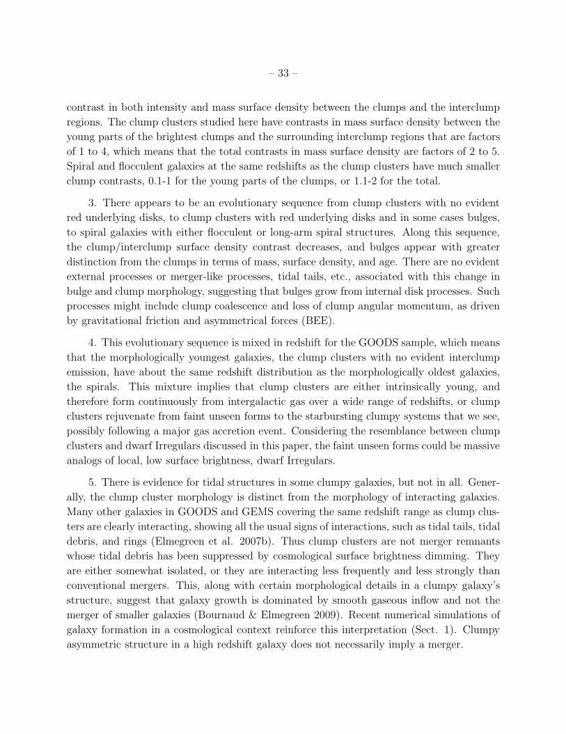
– 33 –
contrast in both intensity and mass surface density between the clumps and the interclump
regions. The clump clusters studied here have contrasts in mass surface density between the
young parts of the brightest clumps and the surrounding interclump regions that are factors
of 1 to 4, which means that the total contrasts in mass surface density are factors of 2 to 5.
Spiral and flocculent galaxies at the same redshifts as the clump clusters have much smaller
clump contrasts, 0.1-1 for the young parts of the clumps, or 1.1-2 for the total.
3. There appears to be an evolutionary sequence from clump clusters with no evident
red underlying disks, to clump clusters with red underlying disks and in some cases bulges,
to spiral galaxies with either flocculent or long-arm spiral structures. Along this sequence,
the clump/interclump surface density contrast decreases, and bulges appear with greater
distinction from the clumps in terms of mass, surface density, and age. There are no evident
external processes or merger-like processes, tidal tails, etc., associated with this change in
bulge and clump morphology, suggesting that bulges grow from internal disk processes. Such
processes might include clump coalescence and loss of clump angular momentum, as driven
by gravitational friction and asymmetrical forces (BEE).
4. This evolutionary sequence is mixed in redshift for the GOODS sample, which means
that the morphologically youngest galaxies, the clump clusters with no evident interclump
emission, have about the same redshift distribution as the morphologically oldest galaxies,
the spirals. This mixture implies that clump clusters are either intrinsically young, and
therefore form continuously from intergalactic gas over a wide range of redshifts, or clump
clusters rejuvenate from faint unseen forms to the starbursting clumpy systems that we see,
possibly following a major gas accretion event. Considering the resemblance between clump
clusters and dwarf Irregulars discussed in this paper, the faint unseen forms could be massive
analogs of local, low surface brightness, dwarf Irregulars.
5. There is evidence for tidal structures in some clumpy galaxies, but not in all. Gener-
ally, the clump cluster morphology is distinct from the morphology of interacting galaxies.
Many other galaxies in GOODS and GEMS covering the same redshift range as clump clus-
ters are clearly interacting, showing all the usual signs of interactions, such as tidal tails, tidal
debris, and rings (Elmegreen et al. 2007b). Thus clump clusters are not merger remnants
whose tidal debris has been suppressed by cosmological surface brightness dimming. They
are either somewhat isolated, or they are interacting less frequently and less strongly than
conventional mergers. This, along with certain morphological details in a clumpy galaxy’s
structure, suggest that galaxy growth is dominated by smooth gaseous inflow and not the
merger of smaller galaxies (Bournaud & Elmegreen 2009). Recent numerical simulations of
galaxy formation in a cosmological context reinforce this interpretation (Sect. 1). Clumpy
asymmetric structure in a high redshift galaxy does not necessarily imply a merger.

– 34 –
6. Clump clusters resemble local dwarf Irregulars in restframe morphology far better
than they resemble flocculent spirals and mergers. However, clump clusters have the lumi-
nosities and masses of normal spiral galaxies, which are 10 to 100 times larger than local
dwarf Irregulars. Thus clump clusters represent a unique galaxy stage: they are as massive
as normal spirals but as irregular as dwarfs. This unique property is probably connected
with their extreme youth. Although neutral gas in clump clusters is not widely observed yet,
we feel confident in predicting that these galaxies will be found to have high gas fractions,
as do dwarf Irregulars, and high gas velocity dispersions relative to their rotation speeds,
as do dwarf Irregulars. The velocity dispersions of the ionized gas components are already
observed to be high (Sect. 1).
7. Local dwarf Irregulars are not a perfect analog to high redshift clumpy galaxies. The
dwarfs have low star formation rates and evolve slowly, whereas the high redshift systems
are massive, star-bursting, and in extreme cases, evolve quickly to symmetric galaxies with
bulges and exponential disks (BEE). The slow evolution for local dwarfs follows in part from
their low disk surface density, and this helps explain why they still have high gas fractions
after a Hubble time. The difference between the two cases seems to be partly a matter of
scale – not an indication of different physical processes. Scaling issues have selection effects
that depend the epoch of the system and the sensitivity of the observations. At early times,
massive disk galaxies take the form of clump clusters and can be as unevolved as today’s
dwarf Irregulars. Lower mass galaxies at these early times would not be observable. At late
times, the massive clumpy disks have evolved into smooth disks, and the low mass versions,
the dwarf Irregulars, are the only visible remnants of this phase.
8. The masses of star-forming regions relative to the surrounding galaxy appear to
be larger by a factor of ∼ 6 in clump clusters than in spirals at the same redshift (Sect.
3.2.1). The clump masses also increase with redshift, although selection and resolution
effects could contribute somewhat to this mass increase. More likely, the increase in relative
clump mass parallels the observed increase in relative clump separation that defines the
clumpy morphology (i.e., compared to the galaxy radius), and both are the result of an
increase in gas turbulent speed relative to the galaxy rotation speed. The turbulent speed of
the neutral gas component in high redshift galaxies is not yet observed, but it is predicted
to be high, 20 − 50 km s−1.
9. A high gas velocity dispersion relatively to the rotation speed increases the threshold
column density for gravitational instabilities. This can explain the observed lack of star
formation in gas that produces damped Lyman alpha absorption. A comparable ratio of
dispersion to rotation speed in local dwarf Irregulars and in high redshift clump clusters, as
suggested by their similar morphologies, also explains the low threshold column density for

– 35 –
star formation in local dwarfs.
We are grateful to the referee for useful comments. DME thanks the National Science
Foundation for research support for KS and MP through the Keck Northeast Astronomy
Consortium REU program, and Vassar College for support for MM and AY through the
Undergraduate Research Summer Institute (URSI) program, and for publication support
through the Research Committee and the Maud Makemson fund. Some of the data presented
in this paper were obtained from the Multimission Archive at the Space Telescope Science
Institute (MAST). STScI is operated by the Association of Universities for Research in
Astronomy, Inc., under NASA contract NAS5-26555. Support for MAST for non-HST data is
provided by the NASA Office of Space Science via grant NAG5-7584 and by other grants and
contracts. This research has made use of the NASA/IPAC Extragalactic Database (NED)
which is operated by the Jet Propulsion Laboratory, California Institute of Technology, under
contract with the National Aeronautics and Space Administration.
REFERENCES
Abadi, M.G., Navarro, J.F., Steinmetz, M., & Eke, V.R. 2003, ApJ, 597, 21
Abraham, R., Tanvir, N., Santiago, B., Ellis, R., Glazebrook, K., & van den Bergh, S. 1996a,
MNRAS, 279, L47
Abraham, R., van den Bergh, S., Glazebrook, K., Ellis, R., Santiago, B., Surma, P., &
Griffiths, R. 1996b, ApJS, 107, 1
Agertz, O., Teyssier, R., Moore, B. 2009, arXiv0901.2536
Azzollini, R.. Beckman, J.E., & Trujillo, I 2009, A&A, in press arXiv0903.4140
Barteldrees, A., & Dettmar, R.-J. 1994, A&AS, 103, 475
Beckwith, S.V.W., et al. 2006, AJ, 132, 1729
Binggeli, B., & Popescu, C. C. 1995, A&A, 298, 63
Binney J., 1977, ApJ, 215, 483
Birnboim Y., & Dekel A., 2003, MNRAS, 345, 349
Bizyaev, D., & Kajsin, S. 2004, ApJ, 613, 886
Bournaud, F., Elmegreen, B.G., & Elmegreen, D.M. 2007, ApJ, 670, 237 (BEE)

– 36 –
Bournaud, F., & Elmegreen, B.G. 2009, ApJ, 694, L158
Bournaud, F., Daddi, E., Elmegreen, B. G., Elmegreen, D. M., Nesvadba, N., Vanzella, E.,
de Matteo, P., Le Tiran, L.,Lehnert, M., & Elbaz, D. 2008, A&A, 486, 741
Brinchmann, J., Abraham, R., Schade, D., et al. 1998, ApJ, 499, 112
Bruzual, G. & Charlot, S. 2003, MNRAS, 344, 1000
Buitrago, F., Trujillo, I., Conselice, C.J., Bouwens, R.J., Dickinson, M., & Yan, H. 2008,
ApJ, 687, L61
Bureau, M., & Carignan, C. 2002, AJ, 123, 1316
Burgarella, D., Buat, V., Donas, J., Milliard, B., & Chapelon, S. 2001, A&A, 369, 421
Carroll, S. M., Press, W. H., & Turner, E. L. 1992, ARAA, 30, 499
Calzetti, D., Armus, L., Bohlin, R., Kinney, A., Koornneef, J., & Storchi-Bergmann, T.
2000, ApJ, 533, 682
Cassata, P., Cimatti, A., Franceschini, A., Daddi, E., Pignatelli, E., Fasano, G., Rodighiero,
G., Pozzetti, L., Mignoli, M., & Renzini, A. 2005, MNRAS, 357, 903
Chabrier, G. 2003, PASP, 115, 763
Conselice, C. J. 2003, ApJS, 147, 1
Conselice, C.J., Bershady, M.A., Dickinson, M., & Papovich, C. 2003, AJ, 126, 1183
Conselice, C. J., Blackburne, J. A., Papovich, C. 2005, ApJ, 620, 564
Conselice, C.J., Yang, C., & Bluck, A.F.L. 2009, MNRAS, 361, in press
Cowie, L., Hu, E., & Songaila, A. 1995, AJ, 110, 1576
Davis, M., Efstathiou, G., Frenk, C. S., & White, S. D. M. 1985, ApJ, 292, 371
Dekel A., Birnboim Y., 2006, MNRAS, 368, 2
Dekel, A., et al. 2009a, Nature, 457, 451
Dekel, A., Sari, R., & Ceverino, D. 2009b, ApJ submitted, arXiv:0901.2458
de Mello, D. F., Wadadekar, Y., Dahlen, T., Casertano, S., & Gardner, J. P. 2006, AJ, 131,
216

– 37 –
de Vaucouleurs, G., de Vaucouleurs, A., Corwin, H. G., Jr., Buta, R. J., Paturel, G., &
Fouque, P. 1991, Third Reference Catalogue of Bright Galaxies (New York: Springer)
Driver, S. P., Windhorst, R. A., Ostrander, E. J., Keel, W. C., Griffiths, R. E., & Ratnatunga,
K. U. 1995, ApJ, 449, L23
Driver, S. P., Fernandez-Soto, A., Couch, W. J., Odewahn, S. C., Windhorst, R. A., Phillips,
S., Lanzetta, K., & Yahil, A. 1998, ApJ, 496, L93
Efremov, Y.N. 1995, AJ, 110, 2757
Elmegreen, B.G. 2002, ApJ, 577, 206
Elmegreen, B.G. 2007, ApJ, 668, 1064
Elmegreen, B.G, & Efremov, Y.N, 1996, ApJ, 466, 802
Elmegreen, B. G., Elmegreen, D. M., & Leitner, S. N. 2003a, ApJ, 590, 271
Elmegreen, B. G., Leitner, S. N., Elmegreen, D. M., & Cuillandre, J.-C. 2003b, ApJ, 593,
333
Elmegreen, B.G., & Elmegreen, D.M. 2005, ApJ, 627, 632
Elmegreen, B.G., & Elmegreen, D.M. 2006, ApJ, 650, 644
Elmegreen, B.G., Elmegreen, D.M., Chandar, R., Whitmore, B., & Regan, M. 2006, ApJ,
644, 879
Elmegreen, B.G., Bournaud, F., & Elmegreen, D.M. 2008, ApJ, 688, 67
Elmegreen, D.M., Elmegreen, B.G., Fernandez, M.X., & Lemonias, J.J., 2009, ApJ, 692, 12
Elmegreen, D.M., Elmegreen, B.G., & Hirst, A.C. 2004, ApJ, 604, L21
Elmegreen, D.M., Elmegreen, B.G., Rubin, D.S., & Schaffer, M.A. 2005, ApJ, 631, 85
Elmegreen, D.M., Elmegreen, B.G., Ravindranath, S., & Coe, D. 2007a, ApJ, 658, 763
Elmegreen, D.M., Elmegreen, B.G., Ferguson, T., & Mullan, B. 2007b, ApJ, 663, 734
Erb, D.K., Steidel, C.C., Shapley, A.E., Pettini, M., & Adelberger, K.L. 2004, 612, 122
Forster-Schreiber, N. M., et al. 2006, ApJ, 645, 1062
Genzel, R. et al. 2006, Nature, 442, 786

– 38 –
Genzel, R., et al. 2008, ApJ, 687, 59
Giavalisco, M., et al. 2004, ApJ, 600, L103
Glazebrook, K., Ellis, R., Santiago, B., & Griffiths, R. 1995, MNRAS, 275, L19
Hunter, D.A., Elmegreen, B.G., & Baker, A.L. 1998, ApJ, 493, 595
Hunter, D.A., & Elmegreen, B.G. 2004, ApJ, 128, 2170
Im, M., Griffiths, R. E., Naim, A., Ratnatunga, K. U., Roche, N., Green, R. F., & Sarajedini,
V. 1999, ApJ, 510, 82
Immeli, A., Samland, M., Westera, P., & Gerhard, O. 2004a, ApJ, 611, 20
Immeli, A., Samland, M., Gerhard, O., & Westera, P. 2004b, A&A, 413, 547
Jogee, S. et al. 2009, arXiv0903.3700
Karachentsev, I. D., Karachentseva, V. E., Kudrya, Y. N., Sharina, M. E., & Parnovsky, S.
L. 2000, Revised Flat Galaxy Catalogue, VizieR On-line Data Catalog: VII/219
Kay, S. T., Pearce, F. R., Jenkins, A., Frenk, C. S., White, S. D. M., Thomas, P. A., &
Couchman, H. M. P. 2000, MNRAS, 316, 374
Kennicutt, R. 1998, ARAA, 36, 189
Kere, D., Katz, N., Weinberg, D.H., Dave, R. 2005, MNRAS, 363, 2
Kere, D., Katz, N., Fardal, M., Dave, R., & Weinberg, D. H. 2009, MNRAS, tmp, 375
Larson, R. B., & Tinsley, B. M. 1978, ApJ, 219, 46
Law, D. R., Steidel, C.C., Erb, D.K., Pettini, M., Reddy, N.A., Shapley, A.E., Adelberger,
K.L., & Simenc, D. J. 2007, ApJ, 656, 1
Law, D.R. et al. 2009, arXiv0901.2930
Leitherer, C., Li, I.-H., Calzetti, D., Heckman, T.M. 2002, ApJS, 140, 303
Lopez-Sanjuan, C., Balcells, M., Garcıa-Dabo, C. E., Prieto, M., Cristobal-Hornillos, D.,
Eliche-Moral, M. C., Abreu, D., Erwin, P., & Guzman, R. 2009, ApJ, 694, 643
Lotz, J. M., Madau, P., Giavalisco, M., Primack, J., & Ferguson, H. 2006, ApJ, 636, 592
Lotz, J.M. et al. 2008, ApJ, 672, 177
– 39 –
Madau, P. 1995, ApJ, 441, 18
Martin, D. C., et al. 2005, ApJ, 619, L1
Menanteau, F., Ford, H.C., Motta, V., Benıtez, N., Martel, A.R., Blakeslee, J.P., & Infante,
L. 2006, AJ, 131, 208
Murali, C., Katz, N., Hernquist, L., Weinberg, D.H., & Dave, R. 2002, ApJ, 571, 1
Neichel, B., et al. 2008, A&A, 484, 159
Noeske, K. et al. 2007, ApJ, L47
Noguchi, M. 1999, ApJ, 514, 77
Ocvirk, P., Pichon, C., & Teyssier, R. 2008, MNRAS, 390, 1326
Overzier, R.A., et al. 2008, ApJ., 677, 37
Papovich, C., Giavalisco, M., Dickinson, M., Conselice, C.J., & Ferguson, H.C. 2003, ApJ,
598, 827
Papovich, C., Dickinson, M., Giavalisco, M., Conselice, C. J., & Ferguson, H. C. 2005, ApJ,
631, 101
Puech, M., Hammer, F., Lehnert, M. D., & Flores, H. 2007, A&A, 466, 83
Ravindranath, S., Giavalisco, M., Ferguson, H.C., Conselice, C., Katz, N., Weinberg, M.,
Lotz, J., Dickinson, M., Fall, S. M., Mobasher, B., & Papovich, C. 2006, ApJ, 652,
963
Rix, H.W., et al. 2004, ApJS, 152, 163
Rowan-Robinson, M. 2003, MNRAS, 345, 819
Sanders, D. B.; Mirabel, I. F. 1996, ARAA, 34, 749
Semelin, B., & Combes, F. 2005, A&A, 441, 55
Smith, A.M., et al. 2001, ApJ, 546, 829
Solomon, P. M., Rivolo, A. R., Barrett, J., & Yahil, A. 1987, ApJ, 319, 730
Spergel, D. N., et al. 2003, ApJS, 148, 175
Stewart, S.G., et al. 2000 ApJ 529 201

– 40 –
Sung, E.-C., Han, C., Ryden, B. S., Patterson, R. J., Chun, M.-S., Kim, H.-I., Lee, W.-B.,
& Kim, D.-J. 1998, ApJ, 505, 199
Taylor-Mager, V.A., Conselice, C.J., Windhorst, R.A., & Jansen, R.A. 2007, ApJ, 659, 162
Treu, T., Ellis, R.S., Liao, T.X., & van Dokkum, P.G. 2005, ApJ, 622, L5
van den Bergh, S., Abraham, R.G., Ellis, R.S.,Tanvir, N.R.,Santiago, B.X., & Glazebrook,
K.G. 1996, AJ 112, 359
Weiner, B. J., et al. 2006, ApJ, 653, 1027
Wolf, C., Meisenheimer, K., Rix, H.-W., Borch, A., Dye, S., & Kleinheinrich, M. 2003, A&A,
401, 73
Wolf, C., Hildebrandt, H., Taylor, E. N., & Meisenheimer, K. 2008, A&A, 492, 933
Wolfe, A.M. & Prochaska, J.X. 1998, ApJ, 494, L15
Wolfe, A.M., & Chen, H.-W. 2006, ApJ, 652, 981
Yang, Y., et al. 2008, A&A, 477, 789
Yoachim, P., & Dalcanton, J.J. 2006, AJ, 131, 226
Zhang, Q., Fall, S. M., & Whitmore, B. C. 2001, ApJ, 561, 727
This preprint was prepared with the AAS LATEX macros v5.2.

– 41 –
Fig. 1.— Color ACS Skywalker images of two spiral galaxies on the left, flocculent spi-
ral galaxies second left, clump clusters with red underlying disks next, and clump clusters
with no evident underlying red disks on the right. Their Wolf et al. (2008) redshifts and
COMBO17 catalog identification numbers are given, along with scale bars representing 2
kpc. [image degraded for arXiv preprint]
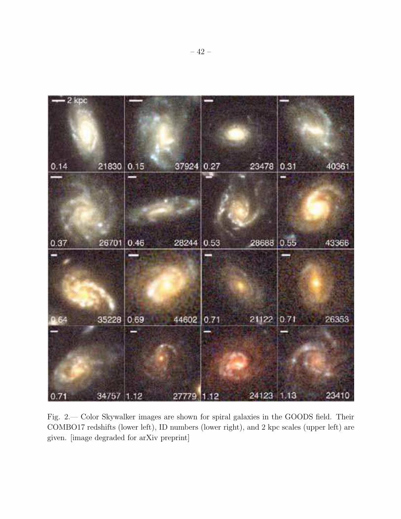
– 42 –
Fig. 2.— Color Skywalker images are shown for spiral galaxies in the GOODS field. Their
COMBO17 redshifts (lower left), ID numbers (lower right), and 2 kpc scales (upper left) are
given. [image degraded for arXiv preprint]
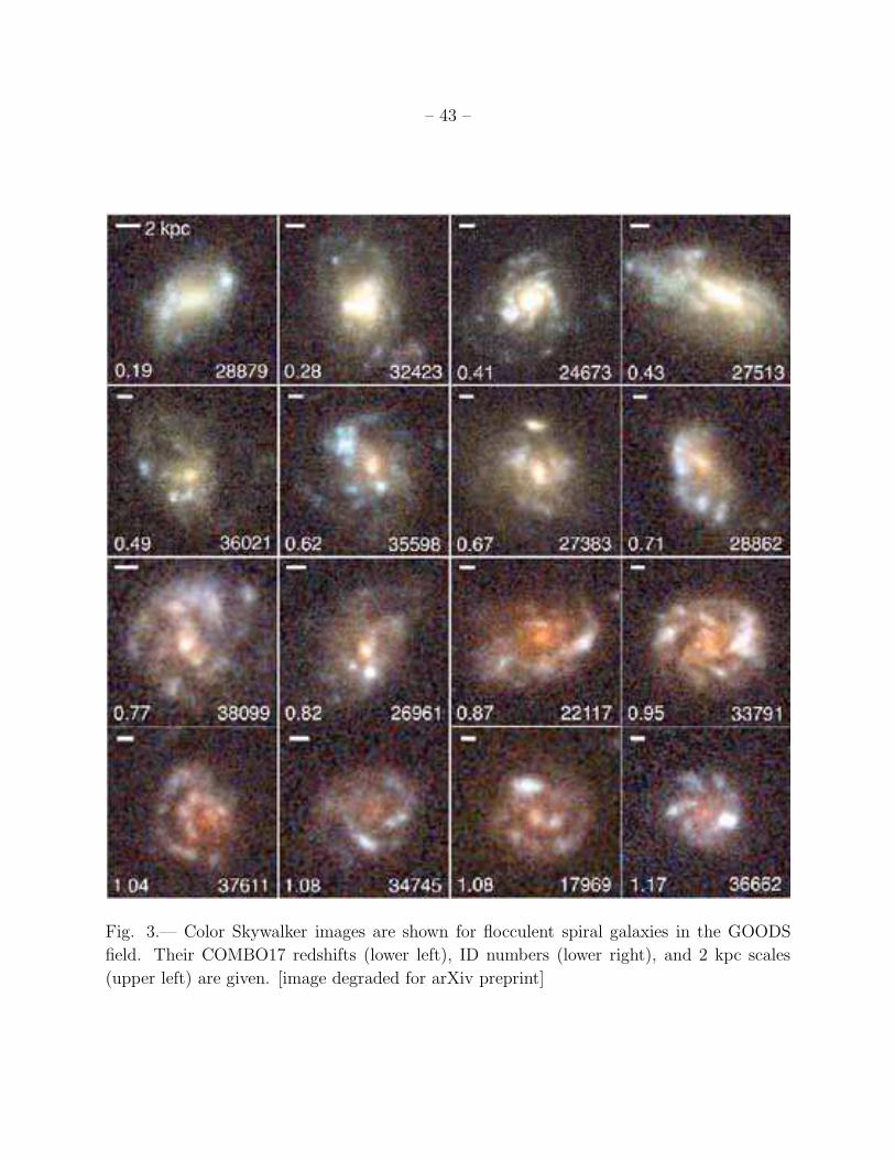
– 43 –
Fig. 3.— Color Skywalker images are shown for flocculent spiral galaxies in the GOODS
field. Their COMBO17 redshifts (lower left), ID numbers (lower right), and 2 kpc scales
(upper left) are given. [image degraded for arXiv preprint]

– 44 –
Fig. 4.— Color Skywalker images are shown for clumpy galaxies in the GOODS field with
red underlying disks. Their COMBO17 redshifts (lower left), ID numbers (lower right), and
2 kpc scales (upper left) are given. [image degraded for arXiv preprint]

– 45 –
Fig. 5.— Color Skywalker images are shown for clump clusters in the GOODS field. Their
COMBO17 redshifts (lower left), ID numbers (lower right), and 2 kpc scales (upper left) are
given. Their appearance is dominated by blue clumps, with no evidence for a red underly-
ing disk. Some could be mergers; others are probably in-situ disk star formation. [image
degraded for arXiv preprint]

– 46 –
–2 –1 0 1 2 3 4 50
20
40
60
80
100
µ1σ–sky – µinterclump
Num
ber
i775 Interclump SB above 1σ Sky Noise,µ1σ–sky = 25.2 mag arcsec–2 at i775
Spirals
Clump Clusters
Fig. 6.— Histograms of the differences between the surface brightness equivalent to 1σ sky
noise and the surface brightness of each interclump region. Interclump regions were chosen
close to the clumps. The typical interclump region is about 2 mag arcsec−2 above the sky
noise. The value at −1.25 mag arcsec−2 corresponds to a region near a clump where the
image count was negative, meaning it was fainter than the average sky value.

– 47 –
–2 –1 0 1–3
–2
–1
0
1
2
B–V restframe
log
Age
Clumps
–2 –1 0 1 2B–V restframe
Interclump Regions
Fig. 7.— As a check on the model fits, we show the expected correlation between restframe
color and clump age (on the left) and interclump age (on the right). The ages are in Gyr.
The fitting procedure is giving a sensible age that is younger for intrinsically bluer regions.

– 48 –
0 0.5 1 1.52
4
6
8
10
Redshift
log
Mas
s
Clump Cluster2
4
6
8
10
log
Mas
s
Clump Cluster, Red Disk
2
4
6
8
10
log
Mas
s
Spiral
Bulge–like Clump
Clump
2
4
6
8
10
log
Mas
s
Flocculent
0 0.5 1 1.5–3
–2
–1
0
1
Redshift
log
(Mas
s/10
–0.4
Bre
st) Clump Cluster
–3
–2
–1
0
1
log
(Mas
s/10
–0.4
Bre
st) Clump Cluster, Red Disk
–3
–2
–1
0
1
log
(Mas
s/10
–0.4
Bre
st) Spiral
–3
–2
–1
0
1
log
(Mas
s/10
–0.4
Bre
st) Flocculent
Fig. 8.— Clump mass (left) and clump mass per unit galaxy light (right) are shown versus
redshift. Red squares are for bulges in the case of spirals and flocculents, and bulge-like,
or centralized clumps in the case of clump clusters. Blue crosses are for clumps outside the
bulge regions. All mass determinations have had the underlying disk light removed using
surface brightness measurements of adjacent regions. Bulges are more massive than clumps
by a factor of ∼ 20 in spirals and flocculents, but only by a factor of ∼ 2 in clump clusters.
The decrease in clump mass for lower redshift is mostly the result of a decrease in general
galaxy brightness, which is a cosmological selection effect. The distributions on the right
suggest the clump mass per unit galaxy light is nearly independent of redshift.

– 49 –
0 0.5 1 1.54
6
8
10
Redshift
log
Mas
s
GEMS Clump Clusters
0 0.5 1 1.5–2
–1
0
1
2
3
Redshift
log
(Mas
s/10
–0.4
Bre
st)
Fig. 9.— Clump mass (left) and ratio of clump mass to total galaxy light (right) versus
redshift for clumps in the GEMS survey that could be measured in V606 and z850 passbands.
Background light from the interclump region is not subtracted from the clump light in this
case, so these masses are larger than the pure star-formation masses plotted in the previous
figure. The decrease in clump mass for small redshift, combined with the constant clump
mass per unit galaxy light, indicate that the galaxies are suffering a selection effect based on
angular resolution and surface brightness, but the clumps inside the galaxies are not.

– 50 –
0 0.5 1 1.5–1
0
1
2
3
Redshift
log
Σ inte
rclu
mp
Clump Cluster
–1
0
1
2
3lo
g Σ in
terc
lum
pClump Cluster, Red Disk
–1
0
1
2
3
4
log
Σ inte
rclu
mp
Spiral
–1
0
1
2
3
log
Σ inte
rclu
mp
Flocculent
0 0.5 1 1.5–1
0
1
2
3
Redshift
log
Σ clu
mp–
Σ inte
rclu
mp
Clump Cluster
–1
0
1
2
3
log
Σ clu
mp–
Σ inte
rclu
mp
Clump Cluster, Red Disk
–1
0
1
2
3
4
log
Σ clu
mp–
Σ inte
rclu
mp
Spiral
Bulge–like ClumpClump
–1
0
1
2
3
log
Σ clu
mp–
Σ inte
rclu
mp
Flocculent
Fig. 10.— The redshift distribution of the excess surface density of each clump (left) and
the surface density of each interclump region (right), both in M⊙ pc−2. Red squares are for
bulges or bulge-like clumps, blue crosses are for non-bulge clumps (for an interclump region,
this distinction is based on whether the region was used to subtract the background for a
bulge or a clump; overlap of a cross and a square on the right means that an interclump
region was used for both). Bulges have higher surface densities than clumps by a factor of
∼ 7 for spirals and flocculents, and about the same surface densities as clumps for clump
clusters. The curves plot log(1 + z)4, which is proportional to the log of the detection limit.
The bulges in spirals and flocculents have higher surface densities than the bulges in clump
clusters by a factor of ∼ 6. On the right, the interclump surface density is a factor of ∼ 3
times higher for spirals, flocculents, and clump clusters with red disks than for clump clusters
without red disks. This excess is consistent with the conversion of clump clusters into spiral
galaxies over time.

– 51 –
0 0.5 1 1.5 2 2.5 3–1
0
1
2
3
4
Redshift
log
Σ inte
rclu
mp
Clump Cluster
UDF
0 0.5 1 1.5 2 2.5 3–1
0
1
2
3
4
Redshift
log
Σ clu
mp–
Σ inte
rclu
mp
Clump Cluster
UDF
Fig. 11.— The redshift distribution of the excess surface density of each clump (left) and the
surface density of each interclump region (right) for clump clusters with no obvious red disks,
combining the GOODS measurements from the previous figure with UDF measurements
from a small sample of clump clusters (open circles). The curve traces a constant surface
brightness limit.

– 52 –
–2 –1 0 10
2
4
6
8
Num
ber
log([Σclump–Σinterclump]/Σinterclump)
CC, Clumps
–2 –1 0 1 2
CC, BLCs
0
2
4
6
8
Num
ber
CC, Red Disk, Clumps CC, Red Disk, BLCs
0
5
10
15
20
Num
ber
Spiral Clumps Spiral Bulges
0
5
10
15
Num
ber
Flocculent Clumps Flocculent Bulges
Fig. 12.— Histograms showing the ratio of the surface mass density for the star-forming part
of each clump to the surface density of the interclump region, with non-bulge clumps on the
left and bulges or bulge-like clumps (BLC) on the right. The non-bulge clumps in clump
clusters have higher ratios than they do in spirals and flocculents, which means that the
clumps are more significant mass perturbations in the clump clusters. Clump-cluster bulges
have about the same surface density contrasts as the clumps, while spiral and flocculent
bulges have much higher contrasts than the clumps.

– 53 –
0 0.5 1 1.5–3
–2
–1
0
1
Redshift
log
Age
Clump Cluster
–3
–2
–1
0
1
log
Age
Clump Cluster, Red Disk
–3
–2
–1
0
1
2
log
Age
Spiral
–3
–2
–1
0
1
log
Age
Flocculent
0 0.5 1 1.5–3
–2
–1
0
1
Redshift
log
Age
Clump Cluster
–3
–2
–1
0
1
log
Age
Clump Cluster, Red Disk
–3
–2
–1
0
1
2lo
g A
ge
Spiral
–3
–2
–1
0
1
log
Age
Flocculent
Fig. 13.— Ages in Gyr of the excess emission from each clump (blue cross) and bulge (red
square) versus redshift (left) and ages of the interclump regions (right). Bulges are ∼ 10×
older than clumps in spirals and flocculents, but about the same age as clumps in clump
clusters.

– 54 –
–4 –3 –2 –1 0 1 20
5
10
Num
ber
CC, Clumps
–4 –3 –2 –1 0 1 2 3
log ( Age[clump–interclump] / Ageinterclump )
CC, BLC
0
5
10
Num
ber
CC, Red Disk, Clumps CC, Red Disk, BLC
0
5
10
15
20
25
Num
ber
SpiralClumps
Spiral Bulges
0
5
10
15
20
Num
ber
FlocculentClumps
Flocculent Bulges
Fig. 14.— Histograms of the log of the ratio of the age of the excess emission from each
clump to the age of the associated interclump region. Clumps are on the left and bulges
or bulge-like clumps (BLC) are on the right. In clump clusters without obvious red disks,
the clumps have about the same age as the interclump regions. Clump clusters with red
underlying disks and the spiral and flocculent types have interclump regions older than the
clumps by a factor of ∼ 3. Bulges have about the same age as their nearby interclump
regions in all cases.

– 55 –
0 0.5 1 1.5–3
–2
–1
0
1
2
3
Redshift
log
age
x (G
ρ)1/
2
Clump Cluster–3
–2
–1
0
1
2
3
log
age
x (G
ρ)1/
2
Clump Cluster, Red Disk
–3
–2
–1
0
1
2
3
4
log
age
x (G
ρ)1/
2
Spiral
–3
–2
–1
0
1
2
3
log
age
x (G
ρ)1/
2
Flocculent
0 0.5 1 1.5–5
–4
–3
–2
–1
0
1
2
Redshift
log
SFR
Clump Cluster–5
–4
–3
–2
–1
0
1
2
log
SFR
Clump Cluster, Red Disk
–5
–4
–3
–2
–1
0
1
2
3lo
g S
FRSpiral
Bulge–like ClumpClump
–5
–4
–3
–2
–1
0
1
2
log
SFR
Flocculent
Fig. 15.— (Left) Clump star formation rates from the ratio of mass above background to
age (in M⊙ yr−1), versus the redshift. The trends are fit with power laws that have an
average dependence of SFR ∝ (1 + z)8; selection effects are discussed in the text. (Right)
The product of the clump age and the clump dynamical rate is approximately constant over
redshift and averages about unity. Bulges are significantly older than clumps in units of
their dynamical time for spirals and flocculents.

– 56 –
0 0.5 1 1.5 2 2.5 3–3
–2
–1
0
1
2
3
Redshift
log
age
x (G
ρ)1/
2
Clump Cluster
UDF
0 0.5 1 1.5 2 2.5 3–5
–4
–3
–2
–1
0
1
2
Redshift
log
SFR
Clump Cluster
UDF
Fig. 16.— The average clump star formation rate for clump clusters is extended to higher
redshifts by including several UDF galaxies measured and fit to models in the same way.

– 57 –
–20–15–100.1
0.2
0.4
1
2
4
Restframe MB
z 0 (
kpc)
UDF Chains
log z0 = –0.998 – 0.046MB
0.1
0.2
0.4
1
2
4
z 0 (
kpc)
log z0 = –2.633 – 0.134MB
Local Galaxies
–25–20–15–10
Restframe MB
log z0 = –1.196 – 0.059MB
UDF Spirals
GEMS, GOODS
log z0 = –1.312 – 0.067MB
Fig. 17.— The scale height versus restframe absolute magnitude is shown for local galaxies
in the top left, GEMS and GOODS spirals (plus symbols) and chains (dots) in the top right,
UDF chains in the bottom left and UDF spirals in the bottom right. For the UDF, dots with
circles are used for the best examples of these classes. Each panel has a linear fit indicated
by a solid line with the same color as the points (and indicated by the equation), and it also
has the fits from the other panels in matching colors. For MB ∼ −20 mag, all galaxies in
these samples have about the same thickness, ∼ 1 kpc. For GEMS, GOODS, and UDF, all
measurements are in the V606 band. Local galaxies were measured in the R band by various
authors.

– 58 –
0.1 0.2 0.4 1 2 40
1
2
Redshift
z 0 (
kpc)
ObservedGEMS, GOODS (Ch, Sp)
UDF chains
0.1 0.2 0.4 1 2 4–1
0
1
2
Redshift
z 0 –
z0,
fit (
kpc)
Corrected for Restframe MB
Fig. 18.— (Left) Scale height versus redshift for GEMS and GOODS spirals (plus symbols)
and chain galaxies (dots) and UDF chain galaxies (crosses). The decrease in z0 for low
redshift arises because the galaxies are intrinsically fainter at lower redshifts. The green
curve shows the scale corresponding to 3 pixels, which is about the FWHM of a point source
in the GOODS image. (Right) The difference between the measured scale height and the
average scale height at the same restframe MB is plotted versus redshift; there is no obvious
dependence.

– 59 –
Fig. 19.— Blurred images of the flocculent galaxy NGC 7793 are shown on the left using the
same restframe wavelengths as the GOODS images of two clump clusters, 34443 (z = 0.139,
top) and 17969 (z = 1.08, bottom), shown on the right. The top left image of NGC 7793
is with a IIIa-J emulsion at 3950 A and has a spatial resolution (FWHM) of 230 pc. The
top right image of 34443 is in B435 and has the same rest wavelength and spatial resolution.
The bottom left image of NGC 7793 is in the NUV at 2267 A and has a spatial resolution
of 790 pc. The lower right image of 17969 is in B435 and has the same rest wavelength and
spatial resolution. The image of NGC 7793 was degraded to give the same pixel scale and
relative background noise as the corresponding clump cluster. Clump cluster galaxies have
higher clump-interclump contrasts than local flocculent galaxies. [image degraded for arXiv
preprint]

– 60 –
Fig. 20.— A NUV image of the local dwarf Irregular Ho II is shown on the left and a blurred
version is in the middle for comparison to the GOODS clump cluster 18561, seen in the V606
band on the right. The spatial resolution (780 pc) and restframe wavelength (∼ 2400 A) of
the blurred image of Ho II and the ACS image of 18561 are the same. Local dwarf Irregular
galaxies like Ho II resemble high redshift clump cluster galaxies in their asymmetry and
clumpy structure. The local Irregulars are lower in mass by a factor of 10 to 100. [image
degraded for arXiv preprint]


