Center for Turbulence ResearchProceedings of the Summer Program 2010

87

Coherent vorticity extraction in turbulentboundary layers using orthogonal wavelets

By George Khujadze†, Romain Nguyen van yen‡, Kai Schneider¶,Martin Oberlack†‖††, Marie Farge‡

High-resolution data obtained by direct numerical simulation of turbulent boundarylayers are analysed by means of orthogonal wavelets. The data, originally given on aChebychev grid, are first interpolated onto an adapted dyadic grid. Then, they are de-composed using a wavelet basis, which accounts for the anisotropy of the flow by usingdifferent scales in the wall-normal direction and in the planes parallel to the wall. Thusthe vorticity field is decomposed into coherent and incoherent contributions using thresh-olding of the wavelet coefficients. It is shown that less than 1% of the coefficients retainthe coherent structures of the flow, while the majority of the coefficients corresponds toa structureless, i.e., noise-like background flow. Scale- and direction-dependent statisticsin wavelet space quantify the flow properties at different wall distances.

1. Introduction

This study is motivated by the importance of turbulent boundary layers in many fieldsof applied physics, for example, flows around technological devices such as airplanes, carsor golf balls, where determining the drag coefficient is directly related to this thin layeraround the obstacle. In geophysical flows, the atmospheric boundary layer also plays aprevailing role. For a review on the subject we refer the reader to the classical textbookby Schlichting & Gersten (2003). Direct numerical simulations of turbulent boundarylayers are still a challenging problem and constitute a major challenge in computationalfluid dynamics for both numerical discretization schemes and computer resources. Thestiffness is due to the very high resolution which is required to resolve all dynamicallyactive scales of the flow. Spalart (1988) did the first numerical simulations of turbulentboundary layers. Over the past several years, a number of simulations of such flows forhigher Reynolds numbers have became available (see Skote (2001); Khujadze & Oberlack(2004, 2007); Simens et al. (2009); Schlatter et al. (2009)). One important research subjectis the identification and extraction of coherent structures in turbulent boundary layers.This is inspired by the existence of horseshoe vortices first observed by Theodorsen(1952). The observation of forests of horseshoe vortices in experimental data by Adrianet al. (2000) and in direct numerical simulations (DNS) recently performed by Wu &Moin (2009) gave a second wind to this topic.

Wavelet techniques have been developed for more than 20 years (see, e.g., Farge (1992)for an early review) to analyse, model, and compute turbulent flows. The multiscale rep-resentation obtained by wavelet decompositions is useful in understanding the physics of

† Chair of Fluid Dynamics, TU Darmstadt, Petersenstr. 30, 64287 Darmstadt, Germany‡ LMD-IPSL-CNRS, Ecole Normale Superieure, 24 rue Lhomond, 75231 Paris Cedex 5, France¶ M2P2-CNRS & CMI Universite de Provence, 39 rue Joliot-Curie, 13453 Marseille Cedex

13, France‖ Center of Smart Interfaces, TU Darmstadt, Petersenstr. 32, 64287 Darmstadt, Germany†† GS Computational Engineering, TU Darmstadt, Dolivostr. 15, 64293 Darmstadt, Germany

88 Khujadze et al.

turbulent flows as locality in both space and scale is preserved. Thus localised featuresof turbulent flows, such as coherent structures and intermittency can be extracted andanalysed. Coherent Vorticity Extraction (CVE) has been introduced for two- and three-dimensional turbulent flows in Farge et al. (1999) and Farge et al. (2001), respectively.The underlying idea is that coherent structures are defined as what remains after de-noising and hence only a hypothesis on the noise has to be made. In the present studywe assume the noise to be Gaussian and white. Preliminary results of CVE appliedto wall-bounded flows, for a channel flow, have been reported in Weller et al. (2006).Scale-dependent and directional statistics in wavelet space have been presented in Boset al. (2007) to quantify the intermittency of anisotropic flows. Mixing layers have beenanalysed in Schneider et al. (2005) and sheared and rotating flows more recently in Ja-cobitz et al. (2010). An up-to-date review on wavelet techniques in computational fluiddynamics can be found in Schneider & Vasilyev (2010).

In the present paper we apply orthogonal wavelet analysis for the first time to new DNSdata of three-dimensional turbulent boundary layers computed with the code of KTH(Lundbladh et al. (1999)) for higher Reynolds numbers as published in Khujadze &Oberlack (2004, 2007). Additional difficulties are encountered due to the non-equidistantgrid in the wall-normal direction. The aim of this paper is to extract coherent structuresout of high-resolution DNS of zero-pressure-gradient turbulent boundary layer flow atReθ = 1470. The vorticity of the flow is decomposed into coherent and incoherent partsand scale-dependent statistics, i.e., variance, flatness and probability distribution func-tions, are computed at different wall-normal positions. These analyses are only a firststep as they are limited to flow snapshots. A detailed investigation of the dynamics ofthe coherent and incoherent flow contributions is left for future work.

The paper is organised as follows. Section 2 presents the flow configuration and thecomputational approach. Some visualisation and analyses of the DNS data are also given.The CVE methodology is described in Section 3, mentioning technical details like the re-quired interpolation on a dyadic adapted grid, the adaptive anisotropic wavelet transformand the wavelet-based statistics which are applied in the numerical results in Section 4.The latter discusses the total, coherent, and incoherent flows using both flow visualisa-tion and statistical analyses. The efficiency of CVE is also assessed. Finally, conclusionsare drawn in Section 5 and some perspectives for future investigations are given.

2. Flow configuration and parameters

Here we give some details on the DNS code for solving the incompressible Navier–Stokes equations which was developed at KTH, Stockholm; for details we refer the readerto Lundbladh et al. (1999). A spectral method with a Fourier decomposition is used inthe horizontal directions, while a Chebyshev discretization is applied in the wall-normaldirection. Third-order explicit Runge-Kutta and Crank-Nicolson schemes were used forthe time integration for the advective and the viscous terms correspondingly. Since theboundary layer is developing in the downstream direction, a fringe region (where theoutflow is forced by a volume force to the laminar inflow Blasius profile) has to be addedto the physical domain to satisfy the periodic boundary condition. A wall-normal tripforce is used to trigger the transition to turbulence. Since the first study by Spalart(1988), several other authors have also used this approach for simulating zero-pressure-gradient (ZPG) turbulent boundary layer flows. Note that is assumes that the boundarylayer thickness remains sufficiently small in the whole computational domain. Extensive

CVE in turbulent boundary layer flow 89

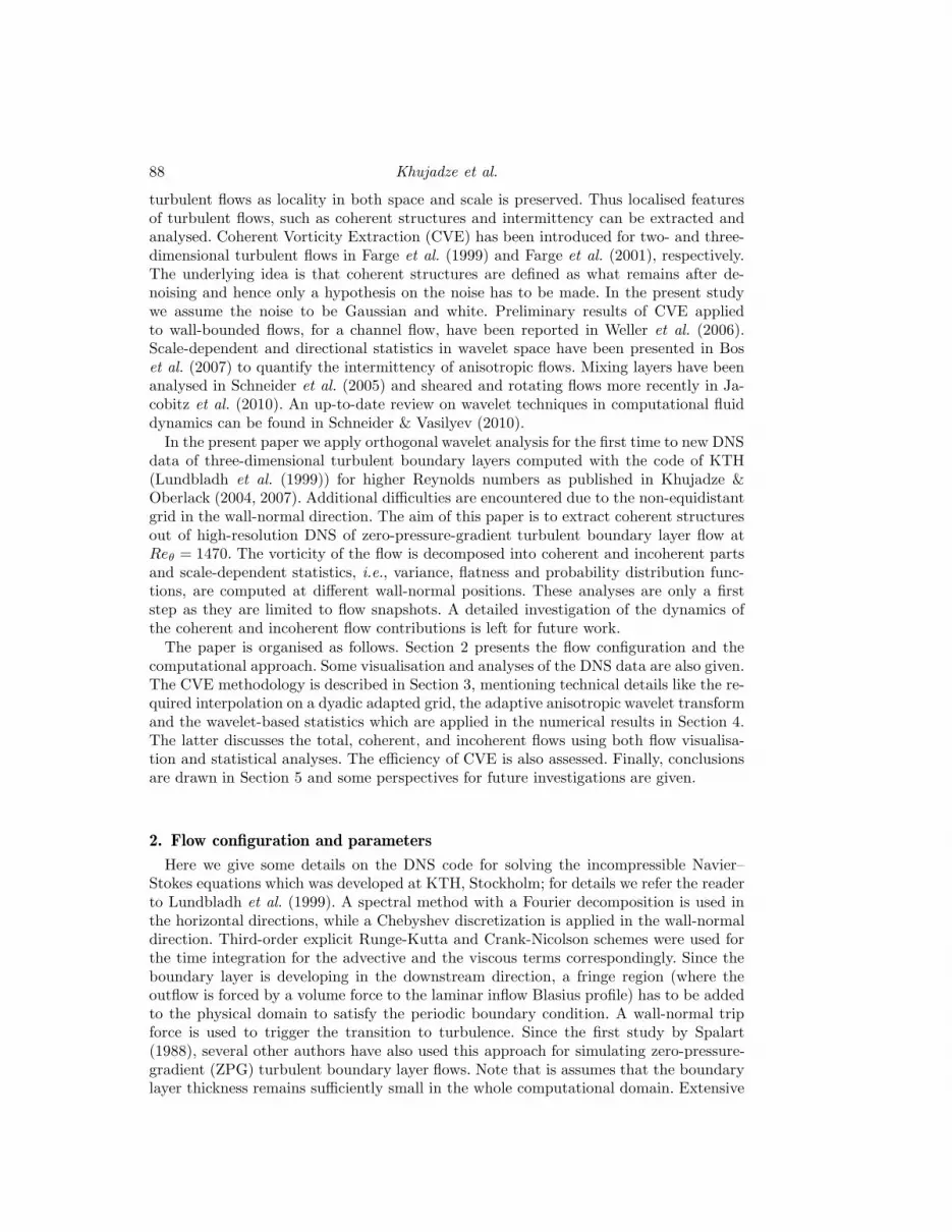
Figure 1. Two-dimensional slices of ωy at z = 0 for x ∈ [0, 200] (top) and for x ∈ [200, 400](bottom).

studies of turbulent boundary layer flows were performed by Skote (2001). Here we givesome details about the simulations used in our study. DNS of ZPG turbulent boundarylayer flow was performed for a number of grid points Nx ×Ny ×Nz = 2048× 513× 256

at starting laminar Reynolds number Reδ∗ |x=0 ≡ u∞δ∗|x=0

ν = 600. All quantities werenon-dimensionalized by the free-stream velocity u∞ and the displacement thickness δ∗ atx = 0, where the flow is laminar. The size of the computational box was Lx ×Ly ×Lz =1000 δ∗|x=0 × 30 δ∗|x=0 × 34 δ∗|x=0. Figure 1 represents only part of the computationaldomain, i.e., for 0 ≤ x ≤ 400. The axes x, y and z correspond to the streamwise, wall-normal, and spanwise directions respectively. The flow is assumed to extend to an infinitedistance perpendicular to the wall. However, the discretization used in the code can onlyhandle a finite domain size. Therefore, the flow domain is truncated and an artificialboundary condition is applied in the freestream at the wall-normal position yL. In thepresent computations we use a generalisation of the boundary condition introduced byMalik et al. (1985) which allows the boundary to be placed closer to the wall. Theboundary condition exactly represents a potential flow solution decaying away from thewall. It is essentially equivalent to requiring that the vorticity is zero at the boundary.Thus, it can be applied immediately outside the vortical part of the flow.

The simulations were run for a total of 11500 time units (δ∗|x=0/u∞). The range ofReynolds numbers was Reθ ≈ 500-1470 with Reθ = u∞θ

ν and where θ is the momentumloss thickness. The grid resolution in viscous or plus units (∆x+ ≡ ∆x/uτν, where uτ isthe friction velocity) was ∆x+ × ∆y+ × ∆z+ = 12.8 × (0.018 to 5) × 3.5.

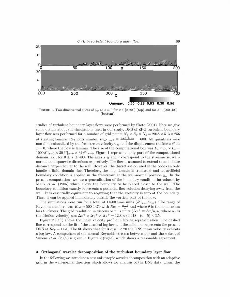
Figure 2 (left) shows the mean velocity profile in lin-log representation. The dashedline corresponds to the fit of the classical log-law and the solid line represents the presentDNS at Reθ = 1470. The fit shows that for 3 < y+ < 20 the DNS mean velocity exhibitsa log-law. A comparison of the normal Reynolds stresses between our and those data ofSimens et al. (2009) is given in Figure 2 (right), which shows a reasonable agreement.

3. Orthogonal wavelet decomposition of the turbulent boundary layer flow

In the following we introduce a new anisotropic wavelet decomposition with an adaptivegrid in the wall-normal direction which allows for analysis of the DNS data. Then, the

90 Khujadze et al.

u+

y+

uiu

i+

y+

Figure 2. Left plot : Mean velocity profile in lin-log representation at Reθ = 1470.1/κ log y+ + B with κ = 0.41 and B = 5.2; Right plot : Diagonal components of Reynolds

stress tensor for the present DNS ( ) and from Simens et al. (2009) ( ) at the Re ≈ 1550,with u1u1

+ > u3u3+ > u2u2

+.

dyad

position

ω2

y

Figure 3. Left plot: Adapted dyadic grid by the position of the corresponding wavelets. Rightplot: Interpolation of vorticity ωy in the wall-normal direction. Original/Chebyshev grid, dyadic grid, × reinterpolated on Chebyshev grid.

coherent vorticity extraction is presented and different scale-dependent wavelet basedstatistics are described.

3.1. Adaptive anisotropic wavelet decomposition

From the velocity field u = (u1, u2, u3) we compute the vorticity field ω = (ω1, ω2, ω3) =∇ × u. Both fields are given on discrete grid points (xi, yn, zk) for i = 1, ..., Nx, n =1, ..., Ny, and k = 1, ..., Nz. The grid is equidistant in the wall-parallel directions x andz, while in the wall-normal direction y a Chebyshev grid is used, i.e., yn = cos(πθn) withθn = (n− 1)/(Ny − 1) for n = 1, . . . , Ny, and rescaled to (0, Ly).

Each component ωℓ of the vorticity vector is then decomposed into a two-dimensionalorthogonal wavelet series in the wall-parallel directions x-z using a two-dimensional mul-tiresolution analysis. The number of scales Jxz is defined as the maximum integer suchthat Nx = k2Jxz andNz = k′2Jxz where k and k′ are any integers. For a fixed wall-normalposition yn we thus obtain for ℓ = 1, 2, 3,

ωℓ(x, yn, z) =

Jxz−1∑

jxz=0

2Jxz−1∑

ix=0

2Jxz−1∑

iz=0

3∑

µ=1

〈ωℓ(yn), ψµjxz ,ix,iz

〉xz ψµjxz,ix,iz

(x, z) , (3.1)

CVE in turbulent boundary layer flow 91

with the wavelet

ψµjxz ,ix,iz

(x, z) =

ψjxz ,ix(x)φjxz ,iz

(z) for µ = 1φjxz ,ix

(x)ψjxz ,iz(z) for µ = 2

ψjxz ,ix(x)ψjxz ,iz

(z) for µ = 3(3.2)

where φ and ψ are the one-dimensional scaling function and wavelet, respectively, andµ = 1, 2 and 3 corresponds to the direction of wavelets in the x, z and xz direction, re-spectively. The scalar product is defined in the x-z plane, 〈f, g〉xz =

∫f(x, z)g(x, z)dxdz.

Here we use Coiflet 12 wavelets (see e.g. Farge 1992) and the scaling coefficients on thefinest scale are identified with the grid point values.

Before performing a one-dimensional wavelet transform in the y-direction (while fixingthe x-z direction), the vorticity components ωℓ have to be interpolated from the Cheby-shev grid onto a locally refined dyadic grid. For that a Lagrange interpolation of 4-thorder is used and a Haar wavelet transform is applied to the Chebyshev grid arccos(yn) todefine the locally refined dyadic grid yn = iy/2

jy (rescaled to [0, 1]) for jy = 0, ..., Jy − 1and iy = 0, ..., 2jy − 1 using nonlinear approximation. The number of grid points in they-direction is fixed, here to Ny = 1024. The maximal scale in y-direction, Jy, is thendetermined from the Haar wavelet analysis retaining the Ny strongest coefficients. In thepresent case we obtain Jy = 13. The resulting dyadic grid is shown in Figure 3 (left)which yields the best approximation of the Chebyshev grid using a dyadic grid withNy = 1024 grid points. The one-dimensional vorticity cuts in the y-direction in Figure3 (right) show the original data on the Chebyshev grid, the data interpolated onto therefined dyadic grid and after reinterpolation onto the Chebyshev grid. The agreement be-tween the curves is satisfactory and thus we can conclude that the interpolation betweenthe different grids can be performed with little loss of information.

A wavelet decomposition using Daubechies 4 wavelets (Farge 1992) is then applied tothe data on the adaptive dyadic grid and the scaling coefficients at the finest scale arecomputed using a quadrature rule. Thereafter an adaptive wavelet transform is performedon the adaptive dyadic grid and we obtain a full wavelet decomposition in all three spacedirections,

ωℓ(x, y, z) =

Jxz−1∑

jxz=0

Jy−1∑

jy=0

2Jxz−1∑

ix=0

2Jy−1∑

iy=0

2Jxz−1∑

iz=0

3∑

µ=1

ωℓ,µjxz ,jy,ix,iy,iz

ψµjxz,ix,iz

(x, z)ψjy ,iy(y)

(3.3)for ℓ = 1, 2, 3. Note that the wavelet coefficients

ωℓ,µjxz,jy,ix,iy,iz

=

∫ ∫ ∫ωℓ(x, y, z)ψ

µjxz ,ix,iz

(x, z) dxdz ψjy,iy(y)dy

contain different scales in the wall-parallel (x-z) and the wall normal (y) direction. Thisproperty allows to take into account the anisotropy of the structures observed in theDNS data.

3.2. Coherent vorticity extraction

The starting point of the coherent vorticity extraction is the wavelet representation ofvorticity in Eq. (3.3). The underlying idea is to perform denoising of vorticity in waveletcoefficient space. Thresholding the wavelet coefficients then determines which coefficientsbelong to the coherent and to the incoherent contributions. The latter are assumed to be

noise-like. First we compute Ω =

(∑3

ℓ=1

(ωℓ,µ

jxz,jy,ix,iy,iz

)2)1/2

and then we reconstruct

92 Khujadze et al.

the coherent vorticity ωc from those wavelet coefficients for which Ω > ǫ using Eq. (3.3).The incoherent vorticity ωi is obtained from the remaining weak wavelet coefficients. Inthe first iteration the threshold ǫ is determined from the total enstrophy Z = 1

2〈ω ·ω〉xyz

and the total number of grid points N = NxNyNz, i.e., ǫ =√

4Z lnN . Subsequently,a new threshold is determined using the incoherent enstrophy computed from the weakwavelet coefficients instead of the total enstrophy. Then the thresholding is applied againand improved estimators of the coherent and incoherent vorticities are obtained. Formore details on the iterative procedure we refer to Farge et al. (1999). We note thatthanks to the orthogonality of the decomposition, the enstrophy and thus the thresholdcan be directly computed in coefficient space using Parseval’s relation. Only at the endof the iterative procedure are the coherent and incoherent vorticities reconstructed byinverse wavelet transform in physical space, in the x-z direction on a regular grid andin the y direction on the locally refined dyadic grid. Afterwards the vorticity fields arereinterpolated in y-direction onto the Chebyshev grid.

Finally, we thus obtain ω = ωc + ωi and by construction we also have Z = Zc +Zi. For future work we anticipate that the corresponding velocity fields can also bereconstructed by applying Biot-Savart’s kernel, which necessitates the solution of threePoisson equations.

3.3. Scale-dependent statistics

The wavelet-based scale-dependent statistics are built on the two-dimensional waveletrepresentation (Eq. 3.1) for a fixed position in the wall-normal direction yn. First wedefine the scale-dependent p-th order moments of the three vorticity components ωℓ inwavelet coefficient space by

Mp,ℓjxz

(yn) =

2jxz−1∑

ix=0

2jxz−1∑

iz=0

(〈ωℓ(yn), ψµ

jxz ,ix,iz〉xz

)p. (3.4)

The scale-dependent variance of the vorticity components corresponds to p = 2. Dividingit by two the scalogram of enstrophy is obtained, which yields a scale distribution ofenstrophy for a given position yn. Scale-dependent flatness of each vorticity componentωℓ can be defined as

Fℓjxz

(yn) =M4,ℓ

jxz(yn)

(M2,ℓ

jxz(yn)

)2. (3.5)

Note that for Gaussian statistics the flatness equals three on all scales. The flatness(Eq. 3.5) quantifies the intermittency of the flow and is directionally related to spatialfluctuations in the x-z plane of the enstrophy. Indeed, as shown in Bos et al. (2007),increasing flatness values for finer scale are an indicator of intermittency.

Finally, we also consider the probability distribution functions (pdfs) of the waveletcoefficients at given scale jxz and wall-normal position yn estimated by histograms using128 bins. As the number of wavelet coefficients decreases at each larger scale by a factor4, we only consider the last three scales jxz = 6, 7, 8 in order to have sufficient statistics.

4. Numerical results

Visualisations of the modulus of vorticity |ω| are shown in Figure 4 for the total (top),coherent (middle) and incoherent contributions (bottom). It can be observed that the

CVE in turbulent boundary layer flow 93

Figure 4. Visualisation of the modulus of vorticity |ω| for the analysed subdomain[500, 750] × [0, 60] × [0, 34]. The visualisations show a zoom for y ∈ [0, 30]: total (top), coherent(middle), and incoherent contributions (bottom).

94 Khujadze et al.

0 1 2 3 4 5 6 710

−13

10−12

10−11

10−10

10−9

10−8

scale

varia

nce

0 1 2 3 4 5 6 710

0

101

102

scale

flatn

ess

Figure 5. Scale-dependent second-order moments (left) and scale-dependent flatness (right) ofthe vorticity component ωz for the total (circles), coherent (squares) and incoherent (triangles)flows at two different wall distances, y+ = 30 ( ) and y+ = 153 ( ).

coherent vortices present in the total field are well preserved in the coherent field usingonly 0.84 % of the total number of wavelet coefficients NxNyNz, which retain 99.61%of the total enstrophy of the flow. In contrast, the incoherent vorticity field has weakeramplitude and is almost structureless.

The statistics of the different flow contributions are quantified in Figure 5 by consid-ering the second-order moments and the flatness as a function of scale of the vorticitycomponent ωz for the total, coherent, and incoherent flows at two different wall distances,at y+ = 30, which is at the beginning of the log-layer and at y+ = 153, which is insidethe log-layer. The variance illustrates the good agreement between the total and coherentvorticity, while the variance of the incoherent one is more than three orders of magnitudesmaller. The latter also only weakly depends on scale, which indicates an equipartitionof enstrophy and thus confirms that the incoherent part is close to white noise. The flat-ness for both the total and coherent vorticity increases with scale, which is a signatureof intermittency. The flatness of the incoherent part features values around 3, which ischaracteristic for Gaussian noise. The probability distribution functions of the waveletcoefficients at scales jxz = 6 and 7 are plotted in Figure 6 at two different wall distances.Close to the wall, for y+ = 30, we observe an algebraic decay of the pdf tails with slope−2, which is close to a Cauchy distribution and corresponds to strong intermittency. Fordistances further away from the wall, y+ = 153, the tails of the pdf become exponentialwhich shows that the flow becomes less intermittent. We can also observe that the pdfsdo not differ much for the two scales considered here.

5. Conclusions and perspectives

A zero-pressure-gradient three-dimensional turbulent boundary layer was studied bymeans of high-resolution DNS at Reθ = 1470. The flow data were shown to be in agree-ment with previous DNS results by Simens et al. (2009) and visualisations gave someevidence for the existence of horseshoe vortices.

A new adaptive three-dimensional wavelet transform was developed which accountsfor the flow anisotropy by using different scales in the wall-normal and wall-paralleldirections. Coherent vorticity extraction was applied and the obtained results showedthat fewer wavelet coefficients (< 1%N) are sufficient to retain the coherent flow struc-tures, while the large majority of coefficients corresponds to the incoherent background

CVE in turbulent boundary layer flow 95

10−1

100

101

102

10−4

10−3

10−2

10−1

100

101

rescaled wavelet coefficient

prob

abili

ty

j=7j=6

x−2

1 2 3 4 5 6 7 8 910

−4

10−3

10−2

10−1

100

rescaled wavelet coefficient

prob

abili

ty

j=7j=6

Figure 6. Probability distribution functions of the wavelet coefficients of ωz in the xz-planeat scales jxz = 6 and 7 estimated by histograms using 128 bins at two different wall distances,y+ = 30 (left) and y+ = 153 (right).

flow which is unstructured and noise-like. Scale-dependent statistics quantified the total,coherent and incoherent flows for different wall-normal positions and showed that thestatistics of the total and coherent flows are in good agreement. The scale-dependentflatness allowed the flow intermittency at different wall distances to be quantified andshowed that, in contrast to the total and coherent flows, the incoherent flow is Gaussianlike.

The current work is limited to time snapshots of vorticity. The reconstruction of thevelocity fields from the total, coherent, and incoherent vorticity is a prerequisite to per-form dynamical analyses of the flow, such as determining the energy transfer between thedifferent flow contributions. In future work we plan to rerun three simulations initialisedwith either the total, coherent or incoherent flow and to compare their dynamics. Ona longer term perspective we also envisage performing Coherent Vorticity Simulation ofturbulent boundary layer flows by advancing only the coherent contributions in time.

GK and MO gratefully acknowledge funding from Deutsche Forschungsgemeinschaft(DFG) under grant number OB 96/13-2. GK, MO and KS acknowledge financial supportand hospitality from the Center for Turbulence Research, Stanford University/NASAAmes, during the summer program 2010. MF and KS gratefully acknowledge financialsupport from the ANR, project M2TFP and MF thanks the Wissenschaftskolleg zuBerlin. RNY, KS and MF are grateful to CNRS supporting their work under a contractPEPS-INSMI-CNRS.

REFERENCES

Adrian, R.J., Meinhart, C.D. & Tomkins, C.D. 2000 Vortex organization in theouter region of the turbulent layer. J. Fluid Mech. 422, 1–54.

Bos, W.J.T., Liechtenstein, L. & Schneider, K. 2007 Small scale intermittency inanisotropic turbulence. Phys. Rev. E 76, 046310.

Farge, M. 1992 Wavelet transforms and their applications to turbulence. Annu. Rev.

Fluid Mech. 24, 395.

Farge, M., Pellegrino, G. & Schneider, K. 2001 Coherent vortex extraction in 3Dturbulent flows using orthogonal wavelets. Phys. Rev. Lett. 87 (5), 45011–45014.

96 Khujadze et al.

Farge, M., Schneider, K. & Kevlahan, N. 1999 Non–Gaussianity and coherentvortex simulation for two–dimensional turbulence using an adaptive orthonormalwavelet basis. Phys. Fluids 11 (8), 2187–2201.

Jacobitz, F., Schneider, K., Bos, W.J.T. & Farge., M. 2010 On the structure anddynamics of sheared and rotating turbulence: Anisotropy properties and geometricalscale-dependent statistics. Phys. Fluids 22, 085101.

Khujadze, G. & Oberlack, M. 2004 DNS and scaling laws from new symmetry groupsof ZPG turbulent boundary layer flow. Theor. Comput. Fluid Dyn. 18, 391–411.

Khujadze, G. & Oberlack, M. 2007 New scaling laws in ZPG turbulent boundarylayer flow. In Proceedings of 5th Int. Symp. on Turbul. Shear Flow Phenom., pp.443–448, Munich, Germany.

Lundbladh, A., Berlin, S., Skote, M., Hildings, C., Choi, J., Kim, J. & Hen-

ningson, D.S. 1999 An efficient spectral method for simulation of incompressibleflow over a flat plate. Tech. Rep. 1999:11. KTH, Stockholm.

Malik, M. R., Zang, T. A, & Hussaini, M. Y. 1985 A spectral collocation methodfor the Navier-Stokes equations. J. Comp. Physics 61, 64–88.

Schlatter, P., Orlu, R., Q. Li, G. Brethouwer, Fransson, J.H.M., Johansson,

A.V., Alfredsson, P.H & Henningson, D.S. 2009 Turbulent boudary layers upto Reθ = 2500 studied through simulation and experiment. Phys. Fluids 21, 051702.

Schlichting, H. & Gersten, K. 2003 Boundary Layer Theory, 8th edn. Springer.

Schneider, K., Farge, M., Pellegrino, G. & Rogers, M. 2005 Coherent vortexsimulation of three-dimensional turbulent mixing layers using orthogonal wavelets.J. Fluid Mech. 534, 39–66.

Schneider, K. & Vasilyev, O. 2010 Wavelet methods in computational fluid dynamics.Annu. Rev. Fluid Mech. 42, 473–503.

Simens, M. P., Jimenez, J., Hoyas, S. & Mizuno, Y. 2009 A high-resolution codefor turbulent boundary layers. J. Comput. Phys. 228, 4218–4231.

Skote, M. 2001 Studies of turbulent boundary layer flow through direct numericalsimulation. PhD thesis, Royal Institute of Technology (KTH), Stockholm, Sweden.

Spalart, P.R. 1988 Direct simulation of a turbulent boundary layer up to Reθ = 1410.J. Fluid Mech. 187, 61–98.

Theodorsen, T. 1952 Mechanism of turbulence. In Proc. 2nd Midwestern Conf. Fluid

Mech.. Ohio State University, Columbus, OH.

Weller, T., Schneider, K., Oberlack, M. & Farge, M. 2006 DNS and waveletanalysis of a turbulent channel flow rotating about the streamwise direction. InTurbulence, Heat and Mass Transfer 5 (eds. K. Hanjalic, Y. Nagano & S. Jarkirlic),vol. 1, pp. 163 –166.

Wu, X. & Moin, P. 2009 DNS statistics data of zero-pressure-gradient flat-plate bound-ary layer. J. Fluid Mech. 630, 5–41.