ORTHOGONAL POLYNOMIALS AND CUBATURE

ORTHOGONAL POLYNOMIALS AND CUBATURE FORMULAE ONSPHERES AND ON BALLS∗

YUAN XU†

SIAM J. MATH. ANAL. c© 1998 Society for Industrial and Applied MathematicsVol. 29, No. 3, pp. 779–793, May 1998 015

Abstract. Orthogonal polynomials on the unit sphere in Rd+1 and on the unit ball in Rd areshown to be closely related to each other for symmetric weight functions. Furthermore, it is shownthat a large class of cubature formulae on the unit sphere can be derived from those on the unit balland vice versa. The results provide a new approach to study orthogonal polynomials and cubatureformulae on spheres.

Key words. orthogonal polynomials in several variables, on spheres, on balls, spherical har-monics, cubature formulae

AMS subject classifications. 33C50, 33C55, 65D32

PII. S0036141096307357

1. Introduction. We are interested in orthogonal polynomials in several vari-ables with emphasis on those orthogonal with respect to a given measure on the unitsphere Sd in Rd+1. In contrast to orthogonal polynomials with respect to measuresdefined on the unit ball Bd in Rd, there have been relatively few studies on the struc-ture of orthogonal polynomials on Sd beyond the ordinary spherical harmonics whichare orthogonal with respect to the surface (Lebesgue) measure (cf. [2, 3, 4, 5, 6, 8]).The classical theory of spherical harmonics is primarily based on the fact that theordinary harmonics satisfy the Laplace equation. Recently Dunkl (cf. [2, 3, 4, 5] andthe references therein) opened a way to study orthogonal polynomials on the sphereswith respect to measures invariant under a finite reflection group by developing atheory of spherical harmonics analogous to the classical one. In this important the-ory the role of Laplacian operator is replaced by a differential-difference operator inthe commutative algebra generated by a family of commuting first-order differential-difference operators (Dunkl’s operators). Other than these results, however, we arenot aware of any other method of studying orthogonal polynomials on spheres.

A closely related question is constructing cubature formulae on spheres and onballs. Cubature formulae with a minimal number of nodes are known to be relatedto orthogonal polynomials. Over the years, a lot of effort has been put into the studyof cubature formulae for measures supported on the unit ball, or on other geometricdomains with nonempty interior in Rd. In contrast, the study of cubature formulae onthe unit sphere has been more or less focused on the surface measure on the sphere;there is little work on the construction of cubature formulae with respect to othermeasures. This is partly due to the importance of cubature formulae with respect tothe surface measure, which play a role in several fields in mathematics, and perhapspartly due to the lack of study of orthogonal polynomials with respect to a generalmeasure on the sphere.

One main purpose of this paper is to provide an elementary approach towards thestudy of orthogonal polynomials on Sd for a large class of measures. This approach is

∗ Received by the editors July 26, 1996; accepted for publication (in revised form) January 9,1997. This research was supported by the National Science Foundation under grant DMS-9500532.

http://www.siam.org/journals/sima/29-3/30735.html†Department of Mathematics, University of Oregon, Eugene, OR 97403-1222 (yuan@math.

uoregon.edu).

779

780 YUAN XU

based on a close connection between orthogonal polynomials on Sd and those on theunit ball Bd; a prototype of the connection is the following elementary example.

For d = 1, the spherical harmonics of degree n are given in the standard polarcoordinates by

Y (1)n (x1, x2) = rn cosnθ and Y (2)

n (x1, x2) = rn sinnθ.(1.1)

Under the transform x = cos θ, the polynomials Tn(x) = cosnθ and Un(x) = sinnθ/ sin θare the Chebyshev polynomials of the first and the second kind, orthogonal with re-spect to 1/

√1− x2 and

√1− x2, respectively, on the unit ball [−1, 1] in R. Hence,

the spherical harmonics on S1 can be derived from orthogonal polynomials on B1.We shall show that for a large class of weight functions on Rd+1 we can con-

struct homogeneous orthogonal polynomials on Sd from the corresponding orthog-onal polynomials on Bd in a similar way. This allows us to derive properties oforthogonal polynomials on Sd from those on Bd; the latter have been studied muchmore extensively. Although the approach is elementary and there is no differentialor differential-difference operator involved, the result offers a new way to study thestructure of orthogonal polynomials on Sd.

Our approach depends on an elementary formula that links the integration on Bd

to the integration on Sd. The same formula yields an important connection betweencubature formulae on Sd and those on Bd; the result states roughly that a large classof cubature formulae on Sd is generated by cubature formulae on Bd and vice versa.In particular, it allows us to shift our attention from the study of cubature formulaeon the unit sphere to the study of cubature formulae on the unit ball; there has beenmuch more understanding towards the structure of the latter one. Although the resultis simple and elementary, its importance is apparent. It yields, in particular, manynew cubature formulae on spheres and on balls. Because the main focus of this paperis on the relation between orthogonal polynomials and cubature formulae on spheresand those on balls, we will present examples of cubature formulae in a separate paper.

The paper is organized as follows. In section 2 we introduce notation and presentthe necessary preliminaries, where we also prove the basic lemma. In section 3 weshow how to construct orthogonal polynomials on Sd from those on Bd. In section4 we discuss the relation between cubature formulae on the unit sphere and those onthe unit ball.

2. Preliminary and basic lemma. For x,y ∈ Rd we let x ·y denote the usualinner product of Rd and |x| = (x ·x)1/2 the Euclidean norm of x. Let Bd be the unitball of Rd and Sd be the unit sphere on Rd+1; that is,

Bd = {x ∈ Rd : |x| ≤ 1} and Sd = {y ∈ Rd+1 : |y| = 1}.

Polynomial spaces. Let N0 be the set of nonnegative integers. For α = (α1, . . . , αd) ∈Nd0 and x = (x1, . . . , xd) ∈ Rd we write xα = xα1

1 · · ·xαdd . The number |α|1 =

α1 + · · ·+αd is called the total degree of xα. We denote by Πd the set of polynomialsin d variables on Rd and by Πd

n the subset of polynomials of total degree at most n.We also denote by Pdn the space of homogeneous polynomials of degree n on Rd andwe let rdn = dimPdn. It is well known that

dim Πdn =

(n+ dn

)and rdn =

(n+ d− 1

n

).

Orthogonal polynomials on Bd. Let W be a nonnegative weight function on Bd

and assume∫BdW (x)dx <∞. It is known that for each n ∈ N0 the set of polynomials

ORTHOGONAL POLYNOMIALS AND CUBATURE FORMULAE 781

of degree n that are orthogonal to all polynomials of lower degree forms a vector spaceVn whose dimension is rdn. We denote by {Pnk }, 1 ≤ k ≤ rdn and n ∈ N0, one family oforthonormal polynomials with respect to W on Bd that forms a basis of Πd

n, wherethe superscript n means that Pnk ∈ Πd

n. The orthonormality means that∫BdPnk (x)Pmj (x)W (x)dx = δj,kδm,n.

A useful notation is Pn = (Pn1 , . . . , Pnrdn

)T , which is a vector with Pnj as components(cf. [22, 24]). For each n ∈ N0, the polynomials Pnk , 1 ≤ k ≤ rdn, form an orthonormalbasis of Vn. We note that there are many bases of Vn; if Q is an invertible matrix ofsize rdn, then the components of QPn form another basis of Vn which is orthonormalif Q is an orthogonal matrix. For general results on orthogonal polynomials in severalvariables, including some of the recent development, we refer to the survey [24] andthe references therein. One family of weight functions on Bd whose correspondingorthogonal polynomials have been studied in detail is (1 − |x|2)µ−1/2, µ ≥ 0, whichwe will refer to as classical orthogonal polynomials on Bd (cf. [1, 6, 25]).

Ordinary spherical harmonics. The harmonic polynomials on Rd are the homo-geneous polynomials satisfying the Laplace equation ∆P = 0, where

∆ = ∂21 + · · ·+ ∂2

d on Rd

and ∂i is the ordinary partial derivative with respect to the ith coordinate. Theyspan a subspace Hdn = ker ∆ ∩ Pdn of dimension dimPdn − dimPdn−2. The sphericalharmonics are the restriction of harmonic polynomials on Sd−1. If Yn ∈ Hdn, then Ynis orthogonal to Q ∈ Pdk , 0 ≤ k < n, with respect to the surface measure dω on Sd−1.

Dunkl’s h-harmonics. For a nonzero vector v ∈ Rd we define the reflection σv by

xσv := x− 2(x · v)v/|v|2, x ∈ Rd.

Suppose that G is a finite reflection group on Rd with the set {vi : i = 1, 2, ...,m} ofpositive roots; assume that |vi| = |vj | whenever σi is conjugate to σj in G, where wewrite σi = σvi , 1 ≤ i ≤ m. Then G is a subgroup of the orthogonal group generatedby the reflections {σvi : 1 ≤ i ≤ m}.

The h-harmonics yield orthogonal polynomials on Sd−1 with respect to h2αdω,

where the weight function hα is defined by

hα(x) :=m∏i=1

|x · vi|αi , αi ≥ 0,(2.1)

with αi = αj whenever σi is conjugate to σj in G. The function hα is a positivelyhomogeneous G-invariant function of degree |α|1 = α1 + · · ·+αm. The key ingredientof the theory is a family of commuting first-order differential-difference operators, Di(Dunkl’s operators), defined by

Dif(x) := ∂if(x) +m∑j=1

αjf(x)− f(xσj)

x · vjvj · ei, 1 ≤ i ≤ d,(2.2)

where e1, . . . , ed are the standard unit vectors of Rd. The h-Laplacian is defined by(see [3])

∆h = D21 + · · ·+D2

d,(2.3)

782 YUAN XU

which plays the role of Laplacian in the theory of the ordinary harmonics. In par-ticular, the h-harmonics are the homogeneous polynomials satisfying the equation∆hY = 0; in other words, they are the elements of the polynomial subspaceHdn(h2) :=Pdn ∩ ker ∆h. The h-spherical harmonics are the restriction of h-harmonics on thesphere.

Basic lemma. We let dω = dωd denote the surface measure on Sd, and the surfacearea

ω = ωd =∫Sddωd = 2π(d+1)/2/Γ((d+ 1)/2).

The standard change of variables from x ∈ Rd to polar coordinates rx′, x′ ∈ Sd−1,yields the following useful formula:∫

Bdf(x)W (x)dx =

∫ 1

0rd−1

∫Sd−1

f(rx′)W (rx′)dωd−1dr.(2.4)

This formula connects the integral on Bd to Sd−1 in a natural way. Our basic formulain the following establishes another relation between integrations over the unit sphereand over the unit ball.

Lemma 2.1. Let H be defined on Rd+1. Assume that H is symmetric with respectto xd+1; i.e., H(x, xd+1) = H(x,−xd+1), where x ∈ Rd. Then for any continuousfunction f defined on Sd,∫

Sdf(y)H(y)dωd =

∫Bd

[f(x,

√1− |x|2) + f(x,−

√1− |x|2)

]×H(x,

√1− |x|2)dx

/√1− |x|2.

(2.5)

Proof. For y ∈ Sd, we write y = (√

1− t2x, t), where x ∈ Sd−1 and −1 ≤ t ≤ 1.Then it follows that (cf. [21, p. 436])

dωd = (1− t2)(d−2)/2dt dωd−1.

Starting from the change of variables y = (√

1− t2x, t) in the integral, we get∫Sdf(y)H(y)dωd =

∫ 1

−1

∫Sd−1

f(√

1− t2x, t)H(√

1− t2x, t)dωd−1(1− t2)(d−2)/2dt

=∫ 1

0

∫Sd−1

[f(√

1− t2x, t) + f(√

1− t2x,−t)]H(√

1− t2x, t)dωd−1(1− t2)(d−2)/2dt

=∫ 1

0

∫Sd−1

[f(rx,

√1− r2) + f(rx,−

√1− r2)

]H(rx,

√1− r2)dωd−1r

d−1 dr√1− r2

=∫Bd

[f(x,

√1− |x|2) + f(x,−

√1− |x|2)

]H(x,

√1− |x|2)

dx√1− |x|2

,

where in the second step we have used the symmetry of H with respect to xd+1, inthe third step we have changed the variable t 7→

√1− r2, and in the last step we have

used (2.4).As a special case of this theorem, we notice that the Lebesgue measure on Sd is

related to the Chebyshev weight function 1/√

1− |x|2 over Bd.


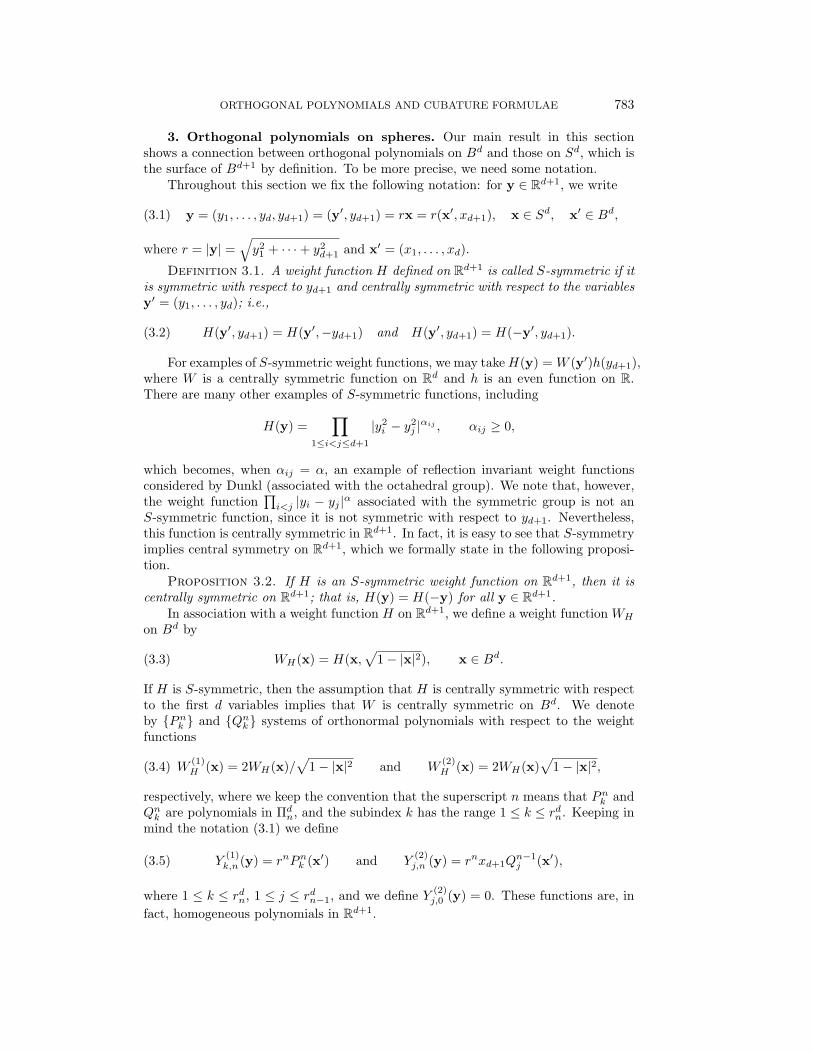
3. Orthogonal polynomials on spheres. Our main result in this sectionshows a connection between orthogonal polynomials on Bd and those on Sd, which isthe surface of Bd+1 by definition. To be more precise, we need some notation.

Throughout this section we fix the following notation: for y ∈ Rd+1, we write

y = (y1, . . . , yd, yd+1) = (y′, yd+1) = rx = r(x′, xd+1), x ∈ Sd, x′ ∈ Bd,(3.1)

where r = |y| =√y2

1 + · · ·+ y2d+1 and x′ = (x1, . . . , xd).

Definition 3.1. A weight function H defined on Rd+1 is called S-symmetric if itis symmetric with respect to yd+1 and centrally symmetric with respect to the variablesy′ = (y1, . . . , yd); i.e.,

H(y′, yd+1) = H(y′,−yd+1) and H(y′, yd+1) = H(−y′, yd+1).(3.2)

For examples of S-symmetric weight functions, we may takeH(y) = W (y′)h(yd+1),where W is a centrally symmetric function on Rd and h is an even function on R.There are many other examples of S-symmetric functions, including

H(y) =∏

1≤i<j≤d+1

|y2i − y2

j |αij , αij ≥ 0,

which becomes, when αij = α, an example of reflection invariant weight functionsconsidered by Dunkl (associated with the octahedral group). We note that, however,the weight function

∏i<j |yi − yj |α associated with the symmetric group is not an

S-symmetric function, since it is not symmetric with respect to yd+1. Nevertheless,this function is centrally symmetric in Rd+1. In fact, it is easy to see that S-symmetryimplies central symmetry on Rd+1, which we formally state in the following proposi-tion.

Proposition 3.2. If H is an S-symmetric weight function on Rd+1, then it iscentrally symmetric on Rd+1; that is, H(y) = H(−y) for all y ∈ Rd+1.

In association with a weight function H on Rd+1, we define a weight function WH

on Bd by

WH(x) = H(x,√

1− |x|2), x ∈ Bd.(3.3)

If H is S-symmetric, then the assumption that H is centrally symmetric with respectto the first d variables implies that W is centrally symmetric on Bd. We denoteby {Pnk } and {Qnk} systems of orthonormal polynomials with respect to the weightfunctions

W(1)H (x) = 2WH(x)/

√1− |x|2 and W

(2)H (x) = 2WH(x)

√1− |x|2,(3.4)

respectively, where we keep the convention that the superscript n means that Pnk andQnk are polynomials in Πd

n, and the subindex k has the range 1 ≤ k ≤ rdn. Keeping inmind the notation (3.1) we define

Y(1)k,n (y) = rnPnk (x′) and Y

(2)j,n (y) = rnxd+1Q

n−1j (x′),(3.5)

where 1 ≤ k ≤ rdn, 1 ≤ j ≤ rdn−1, and we define Y (2)j,0 (y) = 0. These functions are, in

fact, homogeneous polynomials in Rd+1.

784 YUAN XU

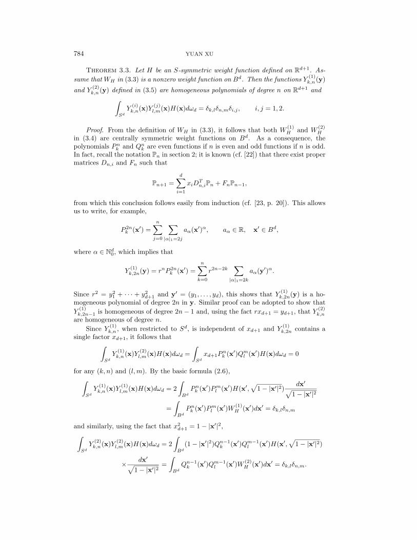
Theorem 3.3. Let H be an S-symmetric weight function defined on Rd+1. As-sume that WH in (3.3) is a nonzero weight function on Bd. Then the functions Y (1)

k,n (y)

and Y (2)k,n (y) defined in (3.5) are homogeneous polynomials of degree n on Rd+1 and∫

SdY

(i)k,n(x)Y (j)

l,m(x)H(x)dωd = δk,lδn,mδi,j , i, j = 1, 2.

Proof. From the definition of WH in (3.3), it follows that both W(1)H and W

(2)H

in (3.4) are centrally symmetric weight functions on Bd. As a consequence, thepolynomials Pnk and Qnk are even functions if n is even and odd functions if n is odd.In fact, recall the notation Pn in section 2; it is known (cf. [22]) that there exist propermatrices Dn,i and Fn such that

Pn+1 =d∑i=1

xiDTn,iPn + FnPn−1,

from which this conclusion follows easily from induction (cf. [23, p. 20]). This allowsus to write, for example,

P 2nk (x′) =

n∑j=0

∑|α|1=2j

aα(x′)α, aα ∈ R, x′ ∈ Bd,

where α ∈ Nd0, which implies that

Y(1)k,2n(y) = rnP 2n

k (x′) =n∑k=0

r2n−2k∑|α|1=2k

aα(y′)α.

Since r2 = y21 + · · · + y2

d+1 and y′ = (y1, . . . , yd), this shows that Y (1)k,2n(y) is a ho-

mogeneous polynomial of degree 2n in y. Similar proof can be adopted to show thatY

(1)k,2n−1 is homogeneous of degree 2n− 1 and, using the fact rxd+1 = yd+1, that Y (2)

k,n

are homogeneous of degree n.Since Y (1)

k,n , when restricted to Sd, is independent of xd+1 and Y(1)k,2n contains a

single factor xd+1, it follows that∫SdY

(1)k,n (x)Y (2)

l,m(x)H(x)dωd =∫Sdxd+1P

nk (x′)Qml (x′)H(x)dωd = 0

for any (k, n) and (l,m). By the basic formula (2.6),∫SdY

(1)k,n (x)Y (1)

l,m(x)H(x)dωd = 2∫BdPnk (x′)Pml (x′)H(x′,

√1− |x′|2)

dx′√1− |x′|2

=∫BdPnk (x′)Pml (x′)W (1)

H (x′)dx′ = δk,lδn,m

and similarly, using the fact that x2d+1 = 1− |x′|2,∫

SdY

(2)k,n (x)Y (2)

l,m(x)H(x)dωd = 2∫Bd

(1− |x′|2)Qn−1k (x′)Qm−1

l (x′)H(x′,√

1− |x′|2)

× dx′√1− |x′|2

=∫BdQn−1k (x′)Qm−1

l (x′)W (2)H (x′)dx′ = δk,lδn,m.


This completes the proof.The assumption that H is S-symmetry in Theorem 3.3 is necessary; it is used to

show that Y (1)k,n and Y

(2)k,n in (3.5) are indeed polynomials in y.

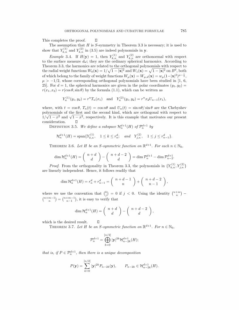
Example 3.4. If H(y) = 1, then Y(1)k,n and Y

(2)k,n are orthonormal with respect

to the surface measure dω; they are the ordinary spherical harmonics. According toTheorem 3.3, the harmonics are related to the orthogonal polynomials with respect tothe radial weight functions W0(x) = 1/

√1− |x|2 and W1(x) =

√1− |x|2 on Bd, both

of which belong to the family of weight functions Wµ(x) = Wµ,d(x) = wµ(1−|x|2)µ−12 ,

µ > −1/2, whose corresponding orthogonal polynomials have been studied in [1, 6,25]. For d = 1, the spherical harmonics are given in the polar coordinates (y1, y2) =r(x1, x2) = r(cos θ, sin θ) by the formula (1.1), which can be written as

Y (1)n (y1, y2) = rnTn(x1) and Y (2)

n (y1, y2) = rnx2Un−1(x1),

where, with t = cos θ, Tn(t) = cosnθ and Un(t) = sinnθ/ sin θ are the Chebyshevpolynomials of the first and the second kind, which are orthogonal with respect to1/√

1− x2 and√

1− x2, respectively. It is this example that motivates our presentconsideration.

Definition 3.5. We define a subspace Hd+1n (H) of Pd+1

n by

Hd+1n (H) = span{Y (1)

k,n , 1 ≤ k ≤ rdn; and Y(2)j,n , 1 ≤ j ≤ rdn−1}.

Theorem 3.6. Let H be an S-symmetric function on Rd+1. For each n ∈ N0,

dimHd+1n (H) =

(n+ dd

)−(n+ d− 2

d

)= dimPd+1

n − dimPd+1n−2.

Proof. From the orthogonality in Theorem 3.3, the polynomials in {Y (1)k,n , Y

(2)j,n }

are linearly independent. Hence, it follows readily that

dimHd+1n (H) = rdn + rdn−1 =

(n+ d− 1

n

)+(n+ d− 2n− 1

),

where we use the convention that(kj

)= 0 if j < 0. Using the identity

(n+mn

)−(

n+m−1n

)=(n+m−1n−1

), it is easy to verify that

dimHd+1n (H) =

(n+ dd

)−(n+ d− 2

d

),

which is the desired result.Theorem 3.7. Let H be an S-symmetric function on Rd+1. For n ∈ N0,

Pd+1n =

[n/2]⊕k=0

|y|2kHd+1n−2k(H);

that is, if P ∈ Pd+1n , then there is a unique decomposition

P (y) =[n/2]∑k=0

|y|2kPn−2k(y), Pn−2k ∈ Hd+1n−2k(H).

786 YUAN XU

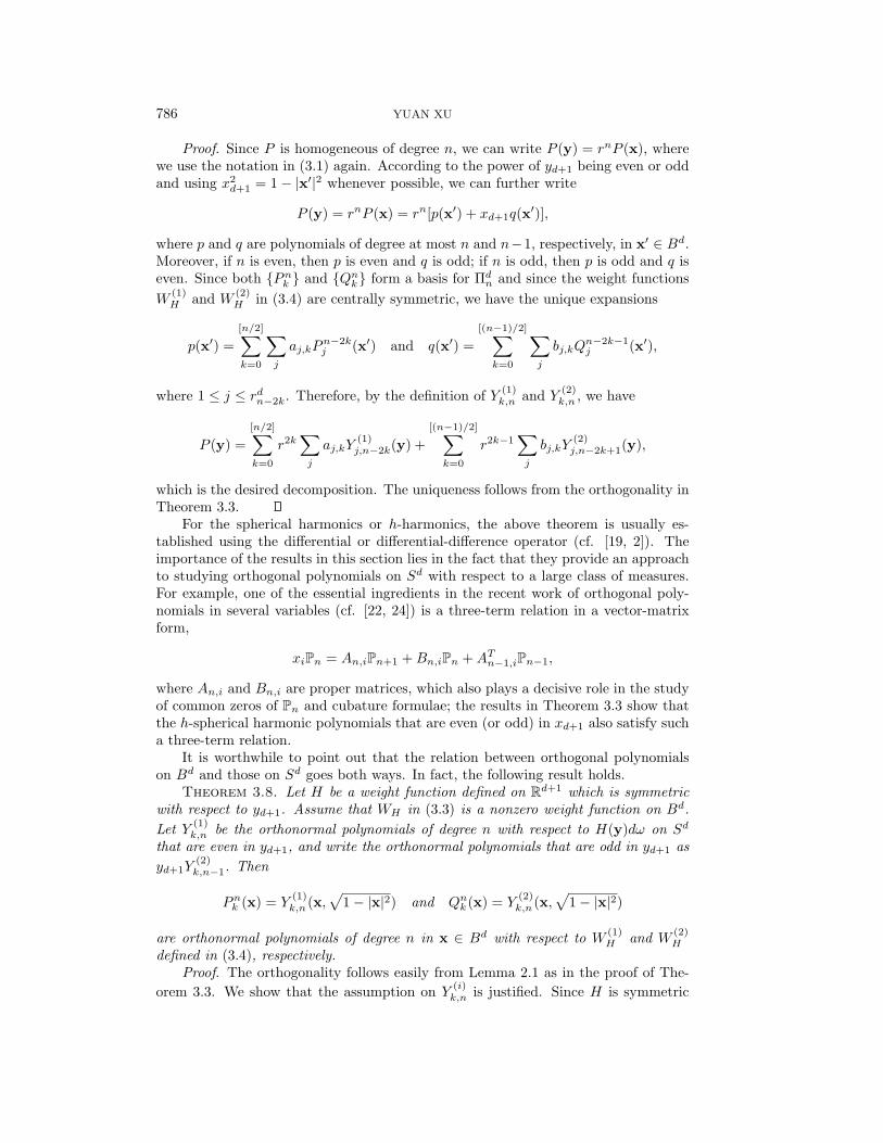
Proof. Since P is homogeneous of degree n, we can write P (y) = rnP (x), wherewe use the notation in (3.1) again. According to the power of yd+1 being even or oddand using x2

d+1 = 1− |x′|2 whenever possible, we can further write

P (y) = rnP (x) = rn[p(x′) + xd+1q(x′)],

where p and q are polynomials of degree at most n and n−1, respectively, in x′ ∈ Bd.Moreover, if n is even, then p is even and q is odd; if n is odd, then p is odd and q iseven. Since both {Pnk } and {Qnk} form a basis for Πd

n and since the weight functionsW

(1)H and W

(2)H in (3.4) are centrally symmetric, we have the unique expansions

p(x′) =[n/2]∑k=0

∑j

aj,kPn−2kj (x′) and q(x′) =

[(n−1)/2]∑k=0

∑j

bj,kQn−2k−1j (x′),

where 1 ≤ j ≤ rdn−2k. Therefore, by the definition of Y (1)k,n and Y

(2)k,n , we have

P (y) =[n/2]∑k=0

r2k∑j

aj,kY(1)j,n−2k(y) +

[(n−1)/2]∑k=0

r2k−1∑j

bj,kY(2)j,n−2k+1(y),

which is the desired decomposition. The uniqueness follows from the orthogonality inTheorem 3.3.

For the spherical harmonics or h-harmonics, the above theorem is usually es-tablished using the differential or differential-difference operator (cf. [19, 2]). Theimportance of the results in this section lies in the fact that they provide an approachto studying orthogonal polynomials on Sd with respect to a large class of measures.For example, one of the essential ingredients in the recent work of orthogonal poly-nomials in several variables (cf. [22, 24]) is a three-term relation in a vector-matrixform,

xiPn = An,iPn+1 +Bn,iPn +ATn−1,iPn−1,

where An,i and Bn,i are proper matrices, which also plays a decisive role in the studyof common zeros of Pn and cubature formulae; the results in Theorem 3.3 show thatthe h-spherical harmonic polynomials that are even (or odd) in xd+1 also satisfy sucha three-term relation.

It is worthwhile to point out that the relation between orthogonal polynomialson Bd and those on Sd goes both ways. In fact, the following result holds.

Theorem 3.8. Let H be a weight function defined on Rd+1 which is symmetricwith respect to yd+1. Assume that WH in (3.3) is a nonzero weight function on Bd.Let Y (1)

k,n be the orthonormal polynomials of degree n with respect to H(y)dω on Sd

that are even in yd+1, and write the orthonormal polynomials that are odd in yd+1 asyd+1Y

(2)k,n−1. Then

Pnk (x) = Y(1)k,n (x,

√1− |x|2) and Qnk (x) = Y

(2)k,n (x,

√1− |x|2)

are orthonormal polynomials of degree n in x ∈ Bd with respect to W(1)H and W

(2)H

defined in (3.4), respectively.Proof. The orthogonality follows easily from Lemma 2.1 as in the proof of The-

orem 3.3. We show that the assumption on Y(i)k,n is justified. Since H is symmetric


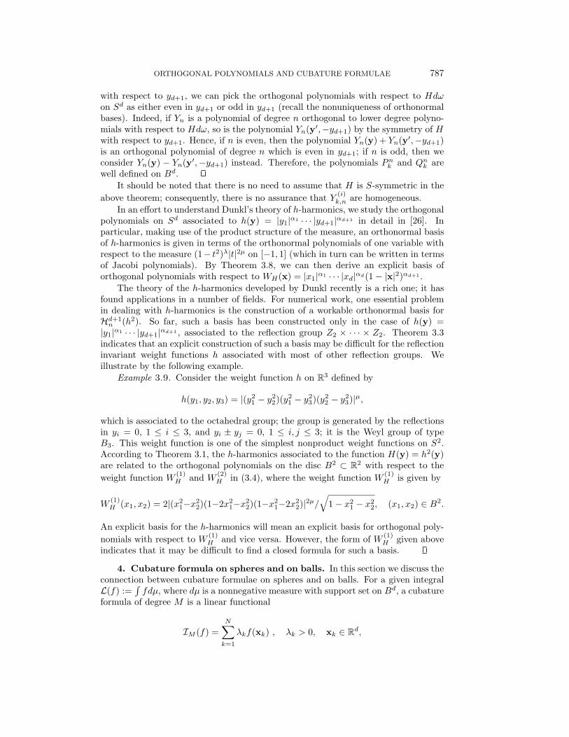
with respect to yd+1, we can pick the orthogonal polynomials with respect to Hdωon Sd as either even in yd+1 or odd in yd+1 (recall the nonuniqueness of orthonormalbases). Indeed, if Yn is a polynomial of degree n orthogonal to lower degree polyno-mials with respect to Hdω, so is the polynomial Yn(y′,−yd+1) by the symmetry of Hwith respect to yd+1. Hence, if n is even, then the polynomial Yn(y) + Yn(y′,−yd+1)is an orthogonal polynomial of degree n which is even in yd+1; if n is odd, then weconsider Yn(y) − Yn(y′,−yd+1) instead. Therefore, the polynomials Pnk and Qnk arewell defined on Bd.

It should be noted that there is no need to assume that H is S-symmetric in theabove theorem; consequently, there is no assurance that Y (i)

k,n are homogeneous.In an effort to understand Dunkl’s theory of h-harmonics, we study the orthogonal

polynomials on Sd associated to h(y) = |y1|α1 · · · |yd+1|αd+1 in detail in [26]. Inparticular, making use of the product structure of the measure, an orthonormal basisof h-harmonics is given in terms of the orthonormal polynomials of one variable withrespect to the measure (1− t2)λ|t|2µ on [−1, 1] (which in turn can be written in termsof Jacobi polynomials). By Theorem 3.8, we can then derive an explicit basis oforthogonal polynomials with respect to WH(x) = |x1|α1 · · · |xd|αd(1− |x|2)αd+1 .

The theory of the h-harmonics developed by Dunkl recently is a rich one; it hasfound applications in a number of fields. For numerical work, one essential problemin dealing with h-harmonics is the construction of a workable orthonormal basis forHd+1n (h2). So far, such a basis has been constructed only in the case of h(y) =|y1|α1 · · · |yd+1|αd+1 , associated to the reflection group Z2 × · · · × Z2. Theorem 3.3indicates that an explicit construction of such a basis may be difficult for the reflectioninvariant weight functions h associated with most of other reflection groups. Weillustrate by the following example.

Example 3.9. Consider the weight function h on R3 defined by

h(y1, y2, y3) = |(y21 − y2

2)(y21 − y2

3)(y22 − y2

3)|µ,

which is associated to the octahedral group; the group is generated by the reflectionsin yi = 0, 1 ≤ i ≤ 3, and yi ± yj = 0, 1 ≤ i, j ≤ 3; it is the Weyl group of typeB3. This weight function is one of the simplest nonproduct weight functions on S2.According to Theorem 3.1, the h-harmonics associated to the function H(y) = h2(y)are related to the orthogonal polynomials on the disc B2 ⊂ R2 with respect to theweight function W

(1)H and W

(2)H in (3.4), where the weight function W

(1)H is given by

W(1)H (x1, x2) = 2|(x2

1−x22)(1−2x2

1−x22)(1−x2

1−2x22)|2µ/

√1− x2

1 − x22, (x1, x2) ∈ B2.

An explicit basis for the h-harmonics will mean an explicit basis for orthogonal poly-nomials with respect to W (1)

H and vice versa. However, the form of W (1)H given above

indicates that it may be difficult to find a closed formula for such a basis.

4. Cubature formula on spheres and on balls. In this section we discuss theconnection between cubature formulae on spheres and on balls. For a given integralL(f) :=

∫fdµ, where dµ is a nonnegative measure with support set on Bd, a cubature

formula of degree M is a linear functional

IM (f) =N∑k=1

λkf(xk) , λk > 0, xk ∈ Rd,

788 YUAN XU

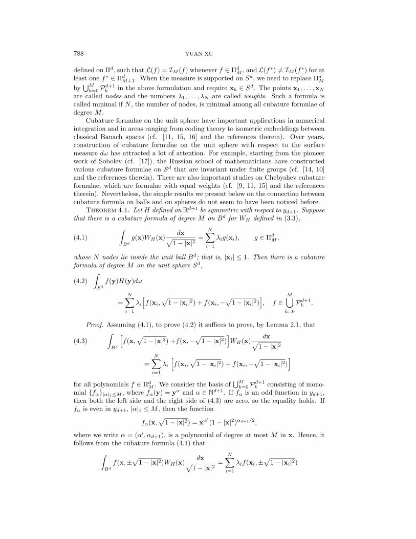
defined on Πd, such that L(f) = IM (f) whenever f ∈ ΠdM , and L(f∗) 6= IM (f∗) for at

least one f∗ ∈ ΠdM+1. When the measure is supported on Sd, we need to replace Πd

M

by⋃Mk=0 P

d+1k in the above formulation and require xk ∈ Sd. The points x1, . . . ,xN

are called nodes and the numbers λ1, . . . , λN are called weights. Such a formula iscalled minimal if N , the number of nodes, is minimal among all cubature formulae ofdegree M .

Cubature formulae on the unit sphere have important applications in numericalintegration and in areas ranging from coding theory to isometric embeddings betweenclassical Banach spaces (cf. [11, 15, 16] and the references therein). Over years,construction of cubature formulae on the unit sphere with respect to the surfacemeasure dω has attracted a lot of attention. For example, starting from the pioneerwork of Sobolev (cf. [17]), the Russian school of mathematicians have constructedvarious cubature formulae on Sd that are invariant under finite groups (cf. [14, 10]and the references therein). There are also important studies on Chebyshev cubatureformulae, which are formulae with equal weights (cf. [9, 11, 15] and the referencestherein). Nevertheless, the simple results we present below on the connection betweencubature formula on balls and on spheres do not seem to have been noticed before.

Theorem 4.1. Let H defined on Rd+1 be symmetric with respect to yd+1. Supposethat there is a cubature formula of degree M on Bd for WH defined in (3.3),∫

Bdg(x)WH(x)

dx√1− |x|2

=N∑i=1

λig(xi), g ∈ ΠdM ,(4.1)

whose N nodes lie inside the unit ball Bd; that is, |xi| ≤ 1. Then there is a cubatureformula of degree M on the unit sphere Sd,∫

Sdf(y)H(y)dω

=N∑i=1

λi

[f(xi,

√1− |xi|2) + f(xi,−

√1− |xi|2)

], f ∈

M⋃k=0

Pd+1k .

(4.2)

Proof. Assuming (4.1), to prove (4.2) it suffices to prove, by Lemma 2.1, that

(4.3)∫Bd

[f(x,

√1− |x|2) +f(x,−

√1− |x|2)

]WH(x)

dx√1− |x|2

=N∑i=1

λi

[f(xi,

√1− |xi|2) + f(xi,−

√1− |xi|2)

]for all polynomials f ∈ Πd

M . We consider the basis of⋃Mk=0 P

d+1k consisting of mono-

mial {fα}|α|1≤M , where fα(y) = yα and α ∈ Nd+1. If fα is an odd function in yd+1,then both the left side and the right side of (4.3) are zero, so the equality holds. Iffα is even in yd+1, |α|1 ≤M , then the function

fα(x,√

1− |x|2) = xα′(1− |x|2)αd+1/2,

where we write α = (α′, αd+1), is a polynomial of degree at most M in x. Hence, itfollows from the cubature formula (4.1) that∫

Bdf(x,±

√1− |x|2)WH(x)

dx√1− |x|2

=N∑i=1

λif(xi,±√

1− |xi|2)


holds. Adding the above equations for f(x,√

1− |x|2) and for f(x,−√

1− |x|2)together proves (4.3).

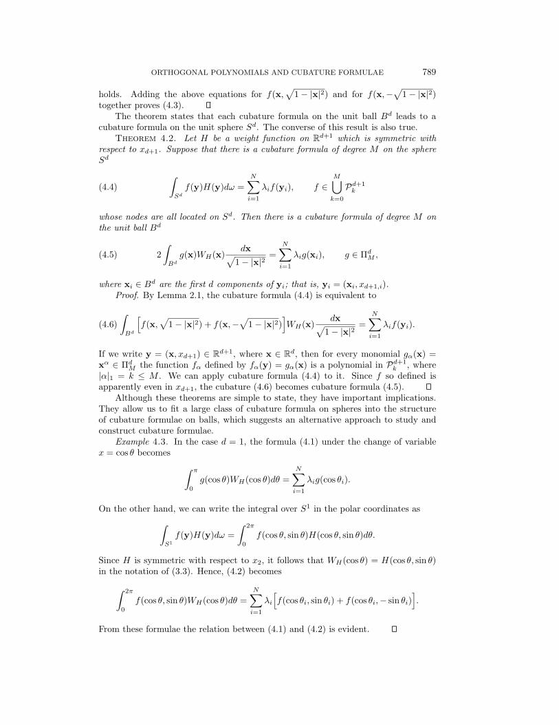
The theorem states that each cubature formula on the unit ball Bd leads to acubature formula on the unit sphere Sd. The converse of this result is also true.

Theorem 4.2. Let H be a weight function on Rd+1 which is symmetric withrespect to xd+1. Suppose that there is a cubature formula of degree M on the sphereSd ∫

Sdf(y)H(y)dω =

N∑i=1

λif(yi), f ∈M⋃k=0

Pd+1k(4.4)

whose nodes are all located on Sd. Then there is a cubature formula of degree M onthe unit ball Bd

2∫Bdg(x)WH(x)

dx√1− |x|2

=N∑i=1

λig(xi), g ∈ ΠdM ,(4.5)

where xi ∈ Bd are the first d components of yi; that is, yi = (xi, xd+1,i).Proof. By Lemma 2.1, the cubature formula (4.4) is equivalent to∫

Bd

[f(x,

√1− |x|2) + f(x,−

√1− |x|2)

]WH(x)

dx√1− |x|2

=N∑i=1

λif(yi).(4.6)

If we write y = (x, xd+1) ∈ Rd+1, where x ∈ Rd, then for every monomial gα(x) =xα ∈ Πd

M the function fα defined by fα(y) = gα(x) is a polynomial in Pd+1k , where

|α|1 = k ≤ M . We can apply cubature formula (4.4) to it. Since f so defined isapparently even in xd+1, the cubature (4.6) becomes cubature formula (4.5).

Although these theorems are simple to state, they have important implications.They allow us to fit a large class of cubature formula on spheres into the structureof cubature formulae on balls, which suggests an alternative approach to study andconstruct cubature formulae.

Example 4.3. In the case d = 1, the formula (4.1) under the change of variablex = cos θ becomes ∫ π

0g(cos θ)WH(cos θ)dθ =

N∑i=1

λig(cos θi).

On the other hand, we can write the integral over S1 in the polar coordinates as∫S1f(y)H(y)dω =

∫ 2π

0f(cos θ, sin θ)H(cos θ, sin θ)dθ.

Since H is symmetric with respect to x2, it follows that WH(cos θ) = H(cos θ, sin θ)in the notation of (3.3). Hence, (4.2) becomes∫ 2π

0f(cos θ, sin θ)WH(cos θ)dθ =

N∑i=1

λi

[f(cos θi, sin θi) + f(cos θi,− sin θi)

].

From these formulae the relation between (4.1) and (4.2) is evident.

790 YUAN XU

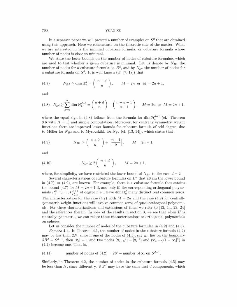
In a separate paper we will present a number of examples on S2 that are obtainedusing this approach. Here we concentrate on the theoretic side of the matter. Whatwe are interested in is the minimal cubature formula, or cubature formula whosenumber of nodes is close to minimal.

We state the lower bounds on the number of nodes of cubature formulae, whichare used to test whether a given cubature is minimal. Let us denote by NBd thenumber of nodes for a cubature formula on Bd, and by NSd the number of nodes fora cubature formula on Sd. It is well known (cf. [7, 18]) that

NBd ≥ dim Πdn =

(n+ dn

), M = 2n or M = 2n+ 1,(4.7)

and

NSd ≥n∑k=0

dimHd+1k =

(n+ dn

)+(n+ d− 1n− 1

), M = 2n or M = 2n+ 1,(4.8)

where the equal sign in (4.8) follows from the formula for dimHd+1k (cf. Theorem

3.6 with H = 1) and simple computation. Moreover, for centrally symmetric weightfunctions there are improved lower bounds for cubature formula of odd degree, dueto Moller for NBd and to Mysovskikh for NSd (cf. [13, 14]), which states that

NB2 ≥(n+ 2n

)+[n+ 1

2

], M = 2n+ 1,(4.9)

and

NSd ≥ 2(n+ dn

), M = 2n+ 1,(4.10)

where, for simplicity, we have restricted the lower bound of NBd to the case d = 2.Several characterizations of cubature formulas on Bd that attain the lower bound

in (4.7), or (4.9), are known. For example, there is a cubature formula that attainsthe bound (4.7) for M = 2n+ 1 if, and only if, the corresponding orthogonal polyno-mials Pn+1

1 , . . . , Pn+1rdn+1

of degree n+ 1 have dim Πdn many distinct real common zeros.

The characterization for the case (4.7) with M = 2n and the case (4.9) for centrallysymmetric weight functions will involve common zeros of quasi-orthogonal polynomi-als. For these characterizations and extensions of them we refer to [12, 14, 23, 24]and the references therein. In view of the results in section 3, we see that when H iscentrally symmetric, we can relate these characterizations to orthogonal polynomialson spheres.

Let us consider the number of nodes of the cubature formulae in (4.2) and (4.5).Remark 4.4. In Theorem 4.1, the number of nodes in the cubature formula (4.2)

may be less than 2N , since if one of the nodes of (4.1), say xi, lies on the boundary∂Bd = Sd−1, then |xi| = 1 and two nodes (xi,

√1− |xi|2) and (xi,−

√1− |xi|2) in

(4.2) become one. That is,

number of nodes of (4.2) = 2N − number of xi on Sd−1.(4.11)

Similarly, in Theorem 4.2, the number of nodes in the cubature formula (4.5) maybe less than N , since different yi ∈ Sd may have the same first d components, which


happens when yi and yj form a symmetric pair with respect to the last component;i.e., yi = (xi, xd+1) and yj = (xi,−xd+1) with xd+1 6= 0. We conclude that

number of nodes of (4.5) = N − number of symmetric pairs among yi.(4.12)

Clearly, the number of nodes in (4.5) satisfies a lower bound N/2, which is attainedwhen the nodes of (4.4) consist of only symmetric pairs.

It is important to remark that even if the cubature formula (4.1) onBd in Theorem4.1 attains the lower bound (4.7) or (4.9), the cubature formula (4.2) on Sd may notattain the lower bound (4.8) or (4.10), respectively. For example, when d = 1, theformula (4.1) for M = 2n+ 1 attains the lower bound (4.7) with NB1 = n+ 1, whichis the classical Gaussian quadrature formula. On the other hand, the correspondingformula in (4.2) attains the lower bound (4.8) with NS1 = 2n + 1 only when x = 1or x = −1 is a node of (4.1), which does not hold in general since the nodes of aGaussian quadrature formula on [−1, 1] are zeros of orthogonal polynomials and arelocated in (−1, 1).

As an immediate consequence of these lower bounds and Theorems 4.1 and 4.2,we formulate a corollary that seems to be of independent interest.

Corollary 4.5. Let H be an S-symmetric weight function on R3. If there isa cubature formula of degree 2n + 1 with respect to H on S2 that attains the lowerbound in (4.10), then it contains at least 2[(n+ 1)/2] nodes which are not symmetricwith respect to x3.

Proof. Assume that a cubature formula with respect to H on S2 exists whichattains the lower bound in (4.10). Let E be the number of symmetric pairs amongthe nodes of the cubature. By Theorem 4.2 and (4.12), there is a cubature formula onB2 with NS2−E = 2

(n+2n

)−E many nodes. Moreover, the weight function associated

with the new cubature formula is centrally symmetric on B2. Hence, by (4.9), we havethe inequality that

NS2 − E = 2(n+ 2n

)− E ≥

(n+ 2n

)+[n+ 1

2

],

from which we get an upper bound for E. Evidently, the number of nodes that do notcontain symmetric pairs is equal to NS2 − 2E. Hence, the upper bound for E leadsto a lower bound on the number of nodes that are not symmetric with respect to x3,which gives the desired result.

In particular, if the cubature formula on S2 is symmetric with respect to x3,which means that the node of the cubature always contains the pair (x1, x2, x3) and(x1, x2,−x3) whenever x3 > 0, then there are at least 2[(n+ 1)/2] many nodes on thelargest circle x2

1 + x22 = 1 which is perpendicular to x3 axis. Results as such provide

necessary conditions on the minimal cubature formulae; they may provide insight inthe construction of the minimal formula or can be used to prove that such a formuladoes not exist. An analogue of Corollary 4.5 is as follows.

Corollary 4.6. If there is a cubature formula on B2 that attains the lowerbound in (4.9) with all nodes in B2, then it can have no more than 2[(n+ 1)/2] pointson the boundary ∂B2 = S1.

Proof. If a cubature formula on B2 as stated exists which attains the lower bound(4.9), then by Theorem 4.1 and (4.11) there is a cubature formula on S2 with

NS2 = 2(n+ 2n

)+ 2[n+ 1

2

]− number of nodes on S1.

792 YUAN XU

The desired result then follows from the lower bound (4.10).We conclude this paper with another simple application dealing with Chebyshev

cubature formulae, which are cubature formulae with equal weights. It is proved in [9]that the number of nodes of a Chebyshev cubature formula of degree M with respectto 1/

√1− |x|2on B2 is of order O(M3). Furthermore, it is conjectured there that

the number of nodes of a Chebyshev cubature formula of degree M with respect tothe surface measure on S2 is of order O(M2).

Corollary 4.7. If there is a Chebyshev cubature formula of degree M withrespect to the surface measure on S2 whose number of nodes is of order O(M2), thenits nodes cannot all be symmetric with respect to a plane that contains one largestcircle of S2 and none of the nodes.

Indeed, if such a cubature formula exists, we may assume that the plane is thecoordinate plane perpendicular to the x3 axis since the integral is invariant underrotation. Then there are an even number of nodes and all nodes form symmetricpairs. Therefore, by Theorem 4.2, there would be a Chebyshev cubature formula ofdegree M with respect to 1/

√1− |x|2 on B2 with the number of nodes in the order

of O(M2), which leads to a contradiction.

Acknowledgment. The author thanks a referee for his careful review and help-ful suggestions.

REFERENCES

[1] P. Appell and J. K. de Feriet, Fonctions hypergeometriques et hyperspheriques, Polynomesd’Hermite, Gauthier-Villars, Paris, 1926.

[2] C. Dunkl, Reflection groups and orthogonal polynomials on the sphere, Math. Z., 197 (1988),pp. 33–60.

[3] C. Dunkl, Differential-difference operators associated to reflection groups, Trans. Amer. Math.Soc., 311 (1989), pp. 167–183.

[4] C. Dunkl, Integral kernels with reflection group invariance, Canad. J. Math., 43 (1991), pp.1213–1227.

[5] C. Dunkl, Intertwining operators associated to the group S3, Trans. Amer. Math. Soc., 347(1995), pp. 3347–3374.

[6] A. Erdelyi, W. Magnus, F. Oberhettinger, and F. G. Tricomi, Higher TranscendentalFunctions, McGraw–Hill, New York, 1953.

[7] H. Engles, Numerical quadrature and cubature, Academic Press, New York, 1980.[8] E.G. Kalnins, W. Miller, Jr., and M. V. Tratnik, Families of orthogonal and biorthogonal

polynomials on the n-sphere, SIAM J. Math. Anal., 22 (1991), pp. 272–294.[9] J. Korevaar and J. L. H. Meyers, Chebyshev-type quadrature on multidimensional domains,

J. Approx. Theory, 79 (1994), pp. 144–164.[10] V.I. Lebedev, A quadrature formula for the sphere of 56th algebraic order of accuracy, Russian

Acad. Sci. Dokl. Math., 50 (1995), pp. 283–286.[11] Yu. Lyubich and L.N. Vaserstein, Isometric embeddings between classical Banach spaces,

cubature formulas, and spherical designs, Geom. Dedicata, 47 (1993), pp. 327–362.[12] H. M. Moller, Kubaturformeln mit minimaler Knotenzahl, Numer. Math., 35 (1976), pp.

185–200.[13] H. M. Moller, Lower bounds for the number of nodes in cubature formulae, Numerical In-

tegration, Internat. Ser. Numer. Math. Vol. 45, G. Hammerlin, ed., Birkhauser, Basel,1979.

[14] I. P. Mysovskikh, Interpolatory Cubature Formulas, “Nauka,” Moscow, 1981 (in Russian).[15] B. Reznick, Sums of even powers of real linear forms, Memoir Amer. Math. Soc., 96 (1992),

no. 463, viii + 155 pp.[16] J. J. Seidel, Isometric embeddings and geometric designs. Trends in discrete mathematics,

Discrete Math., 136 (1994), pp. 281–293.[17] S. L. Sobolev, Cubature formulas on the sphere invariant under finite groups of rotations,

Sov. Math. Dokl., 3 (1962), pp. 1307–1310.


[18] A. Stroud, Approximate Calculation of Multiple Integrals, Prentice–Hall, Englewood Cliffs,NJ, 1971.

[19] E. M. Stein and G. Weiss, Introduction to Fourier Analysis on Euclidean Spaces, PrincetonUniversity Press, Princeton, NJ, 1971.

[20] H. Szego, Orthogonal polynomials, 4th ed., Amer. Math. Soc. Colloq. Publ. 23, AmericanMathematical Society, Providence, RI, 1975.

[21] N. J. Vilenkin, Special Functions and the Theory of Group Representations, Amer. Math.Soc. Trans. Math. Monographs 22, American Mathematical Society, Providence, RI, 1968.

[22] Y. Xu, On multivariate orthogonal polynomials, SIAM J. Math. Anal., 24 (1993), pp. 783–794.[23] Y. Xu, Common Zeros of Polynomials in Several Variables and Higher Dimensional Quadra-

ture, Pitman Research Notes in Mathematics Series, Longman, Essex, 1994.[24] Y. Xu, On orthogonal polynomials in several variables, in Special Functions, q-series, and

Related Topics, Fields Institute Communications, vol. 14, 1997, pp. 247–270.[25] Y. Xu, Summability of Fourier orthogonal series for Jacobi polynomials on a ball in Rd, Trans.

Amer. Math. Soc., to appear.[26] Y. Xu, Orthogonal polynomials for a family of product weight functions on the spheres, Canad.

J. Math., 49 (1997), pp. 175–192.

Documents

ORTHOGONAL POLYNOMIALS AND CUBATURE