Combined processing and mutual interpretation of radiometry and fluorimetry from autonomous profiling Bio-Argo floats: Chlorophyll a retrieval

Combined processing and mutual interpretation of radiometryand fluorimetry from autonomous profiling Bio‐Argo floats:Chlorophyll a retrieval

Xiaogang Xing,1 André Morel,1 Hervé Claustre,1 David Antoine,1 Fabrizio D’Ortenzio,1

Antoine Poteau,1 and Alexandre Mignot1

Received 21 December 2010; revised 7 March 2011; accepted 28 March 2011; published 28 June 2011.

[1] Eight autonomous profiling floats equipped with miniaturized radiometers andfluorimeters have collected data in Pacific, Atlantic, and Mediterranean offshore zones.They measured in particular 0–400 m vertical profiles of the downward irradiance at threewavelengths (412, 490, and 555 nm) and of the chlorophyll a fluorescence. Suchautonomous sensors collect radiometric data regardless of sky conditions and collectessentially uncalibrated fluorescence data. Usual processing and calibration techniques areno longer usable in such remote conditions and have to be adapted. The proposition hereis an interwoven processing by which missing parts of irradiance profiles (due tointermittent cloud occurrence) are interpolated by accounting for possible changes inoptical properties (detected by the fluorescence signal) and by which the attenuationcoefficient for downward irradiance, used as proxy for [Chl a] (the chlorophyll aconcentration), allows the fluorescence signal to be calibrated in absolute units (mg m−3).This method is successfully applied to about 600 irradiance and fluorescence profiles.Validation of the results in terms of [Chl a] is made by matchup with satellite (MODIS‐A)chlorophyll (24.3% RMSE, N = 358). Validation of the method is obtained by applyingit on similar field data acquired from ships, which, in addition to irradiance andfluorescence profiles, include the [Chl a] HPLC determination, used for final verification.

Citation: Xing, X., A. Morel, H. Claustre, D. Antoine, F. D’Ortenzio, A. Poteau, and A. Mignot (2011), Combined processingand mutual interpretation of radiometry and fluorimetry from autonomous profiling Bio‐Argo floats: Chlorophyll a retrieval,J. Geophys. Res., 116, C06020, doi:10.1029/2010JC006899.

1. Introduction

[2] Launched in 1999, the Argo project is a great successin the advancement of Physical Oceanography. With pres-ently an array of about 3000 free‐drifting profiling floats,the project delivers in quasi‐real time quality‐controlledtemperature and salinity data for the upper 2000 m of theglobal ocean.[3] The miniaturization of optical and bio‐optical sensors

is such that their implementation on robotic platforms, likeprofiling floats and gliders, is now possible. Based on theArgo program, the perspective of global‐scale monitoring ofsome biological and optical parameters of the ocean’sinterior is presently becoming a reality [Claustre et al.,2010; Johnson et al., 2009]. With these emerging tools, avertical resolution for the bio‐optical properties, similar tothe resolution typical of the hydrological parameters, is nowachievable. Actually, an even better resolution (meter scale)is reachable thanks to iridium telemetry.

[4] New challenges arise from the automated way ofobserving the bio‐optical properties of the ocean. Indeed,conversely to what happens when the same kinds ofequipments are operated from a ship, these bio‐optical dataare collected in environmental conditions which are out ofthe operator’s control. Calibrations/characterizations, asinitially provided by manufacturers, are the only piece ofinformation available for the rest of the platform life.Therefore, and under these constraints, new specific dataprocessing and management procedures have to be devel-oped. They are needed for the delivery of quality‐controlleddata, both in quasi‐real time and in delayed mode (in thesame manner as the Argo project proceeds for physicalparameters). The internal consistency of the final products isa great challenge to fulfill the scientific requirements, inparticular to allow the future extraction of climatic trendsfrom such an automated “bio” platforms array. The devel-opment of adequate procedures is needed in the early stageof the observing system implementation.[5] In the present paper, we examine only the way of

processing the data of two specific bio‐optical sensors: onemeasures the stimulated fluorescence of chlorophyllouspigments (excitation at 470 nm, emission at 690 nm), whilethe second one measures the downward irradiance at three

1Laboratoire d’Océanographie de Villefranche, UMR 7093, UniversitéPierre et Marie Curie, CNRS, Villefranche‐sur‐Mer, France.

Copyright 2011 by the American Geophysical Union.0148‐0227/11/2010JC006899

JOURNAL OF GEOPHYSICAL RESEARCH, VOL. 116, C06020, doi:10.1029/2010JC006899, 2011

C06020 1 of 14

http://dx.doi.org/10.1029/2010JC006899

wavelengths (l = 412, 490, and 555 nm). Two kinds ofdifficulties arise when transforming the raw data into robustgeophysical products.[6] The first and practical problem is related to the large

amount of data expected from a long‐term deployment ofmany autonomous profilers. There is no need to elaborate onthis aspect; suffice it to say that the answer is in developing,as far as possible, quasi‐automatic processing techniques,even if at the end of the process a visual quality control willinevitably be needed. The second difficulty is more funda-mental and lies in the use of self‐operating sensors thatcollect data in uncontrolled conditions. The answer to thisproblem is more complex and depends on the parameters, asexamined below.[7] The transformation of the raw fluorescence signal into

a so‐called “Chl a equivalent concentration,” as madethrough the use of the manufacturer’s constant scale factor,provides only a rough indication. Indeed, the in vivo fluo-rescence signal and its diel variability depend on manyfactors: first on the taxonomical composition of the localspecies assemblage and then on the physiological state ofthis algal community (life cycle, division rate, light regimeand history, nutrient availability, etc.) [Althuis et al., 1994;Babin, 2008; Claustre et al., 1999; Cunningham, 1996;Falkowski and Kiefer, 1985; Kiefer, 1973a, 1973b; Marra,1997]. Therefore, the calibration of the fluorimeter interms of realistic chlorophyll a concentration, [Chl a]remains to be made on a local basis. When such a similarfluorescence sensor is operated from a ship, an associatedsampling protocol is (optimally) set up to collect quasi‐simultaneously discrete samples, that are thereafter submit-ted to laboratory analysis (HPLC, for instance). By this wayand through appropriate interpolation, each individualfluorescence profile can be, in principle, quantitatively“calibrated.” Nothing equivalent can be made when a sen-sor, embarked on a profiling float, is left alone.[8] Beside the need for such a local calibration, there are

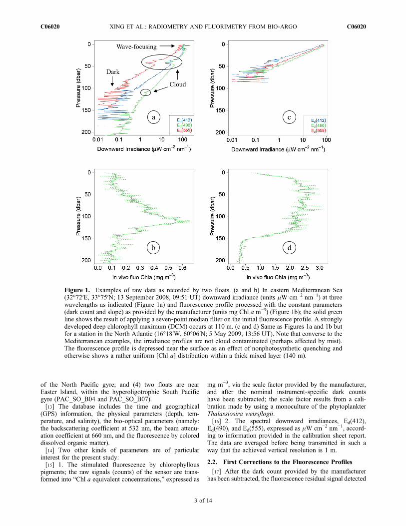
two other flaws affecting the fluorescence data, as illustratedby Figures 1b and 1d. Ostensibly, the nominal “dark count”provided by the manufacturer which is subtracted from theoutput signal is often insufficient to remove the notableChl a equivalent values still found at depth where the algalbiomass is normally vanishingly low (apart perhaps fromexceptional conditions of deep convective mixing). Thesecond problem is of photophysiological origin, and lies inthe well known occurrence of the daytime nonphotochemicalquenching (NPQ) at high irradiance [see, e.g., Cullen andLewis, 1995]. Regardless of the underlying causes (see,e.g., description by Sackmann et al. [2008, and referencestherein]), the net effect of this phenomenon is a decrease ofthe fluorescence emission (per unit of Chl a), when thephytoplanktonic cells are exposed to high, over saturating,solar illumination (an instance is provided by Figure 1d).Such conditions are encountered within the upper layers ofthe ocean, and for sunny days. In total, converting the signalinto a true chlorophyll a concentration is not straightforward.[9] With regard to irradiance (Figure 1a), three kinds of

perturbations generally affect the vertical profiles. First, belowa certain level of irradiance (about 0.5 mW cm−2 nm−1), thesignal is drowned inside the dark noise and is no longeruseful. According to typical irradiance values at the surface

(∼102 mW cm−2 nm−1), the profiles can still reach the 0.5%light level before entering the dark noise background.Second, the verticality of the sensor is adversely affected bythe wave’s motion near the surface; in addition, these wavesinduce “lens effects,” i.e., a focusing and defocusing of thedownward radiant flux [Zaneveld et al., 2001]. These lenseffects result in fast fluctuations which propagate downwardat depths which depend on (actually increase with) theclarity of the water. Finally, the third source of noise isessential due to intermittent cloud occurrences. The down-ward irradiance vertical profiles are captured at a pre-determined time (generally at local noon), regardless ofexternal conditions (clouds, sky and sea state). During suchan autonomous acquisition, passing clouds induce pertur-bations, easily recognizable for they affect synchronously allspectral channels. In case of thin clouds, the perturbation isless detectable. When similar measurements are performedfrom a ship, beside the visual control of the sky state and thepossibility of selecting the most favorable window for theradiometric measurements, there is normally an above sur-face reference sensor monitoring the incident irradiation onthe deck. Appropriate corrections, allowing the variations inthe incident solar flux during the cast to be accounted for,are thus possible. With a float, however, the absence of suchan above surface device prevents an autonomous cloudcorrection from being performed.[10] The present study attempts to circumvent the various

difficulties mentioned above.

2. Materials and Methods

2.1. Instruments and Data

[11] The “PROVBIO” free‐drifting profiler is a PROVORprofiler, additionally equipped with autonomous and inde-pendent bio‐optical sensors, namely, a (Satlantic) OC4radiometer, a (WET Labs) ECO triplet puck comprising achlorophyll fluorimeter, a sensor for the CDOM fluores-cence and a backscattering detector, and a (WET LabsC‐Rover) beam transmissometer. The nominal missionincludes acquisition of a CTD profile from the depth cor-responding to 1000 m up to the surface, whereas the bio‐optical sensors operate from about 400 m up to the surface.The frequency of bio‐optical casts can be modified;depending on season and location, upward casts have beenprogrammed every 2, 5, or 10 days. According to the normalprotocol, the float emerges from the sea around local noon;thanks to iridium two‐way communication, three upwardcasts have been exceptionally programmed on the morning,noon, and evening of the same day.[12] Since 2008, eight PROVBIO floats have been

deployed and have collected data over a time period ofabout 2 years (see also Table 1): (1) two floats are in theMediterranean Sea, with a view of comparing the trophicregimes in the northwestern basin and in the eastern levantinebasin (floats denoted MED_NW_B02 and MED_LV_B06,respectively); (2) two floats are in the North Atlantic,namely, in the Irminger Sea (NAT_IS_B01), and in theIceland Basin (NAT_IB_B03), with the particular aim ofstudying the progression and fate of the spring phyto-plankton bloom; (3) two floats are north of Hawaii(PAC_NO_B05 and PAC_NO_B08), in the eastern sector

XING ET AL.: RADIOMETRY AND FLUORIMETRY FROM BIO‐ARGO C06020C06020

2 of 14

of the North Pacific gyre; and (4) two floats are nearEaster Island, within the hyperoligotrophic South Pacificgyre (PAC_SO_B04 and PAC_SO_B07).[13] The database includes the time and geographical

(GPS) information, the physical parameters (depth, tem-perature, and salinity), the bio‐optical parameters (namely:the backscattering coefficient at 532 nm, the beam attenu-ation coefficient at 660 nm, and the fluorescence by coloreddissolved organic matter).[14] Two other kinds of parameters are of particular

interest for the present study:[15] 1. The stimulated fluorescence by chlorophyllous

pigments; the raw signals (counts) of the sensor are trans-formed into “Chl a equivalent concentrations,” expressed as

mg m−3, via the scale factor provided by the manufacturer,and after the nominal instrument‐specific dark countshave been subtracted; the scale factor results from a cali-bration made by using a monoculture of the phytoplankterThalassiosira weissflogii.[16] 2. The spectral downward irradiances, Ed(412),

Ed(490), and Ed(555), expressed as mW cm−2 nm−1, accord-ing to information provided in the calibration sheet report.The data are averaged before being transmitted in such away that the achieved vertical resolution is 1 m.

2.2. First Corrections to the Fluorescence Profiles

[17] After the dark count provided by the manufacturerhas been subtracted, the fluorescence residual signal detected

Figure 1. Examples of raw data as recorded by two floats. (a and b) In eastern Mediterranean Sea(32°72′E, 33°75′N; 13 September 2008, 09:51 UT) downward irradiance (units mW cm−2 nm−1) at threewavelengths as indicated (Figure 1a) and fluorescence profile processed with the constant parameters(dark count and slope) as provided by the manufacturer (units mg Chl a m−3) (Figure 1b); the solid greenline shows the result of applying a seven‐point median filter on the initial fluorescence profile. A stronglydeveloped deep chlorophyll maximum (DCM) occurs at 110 m. (c and d) Same as Figures 1a and 1b butfor a station in the North Atlantic (16°18′W, 60°06′N; 5 May 2009, 13:56 UT). Note that converse to theMediterranean examples, the irradiance profiles are not cloud contaminated (perhaps affected by mist).The fluorescence profile is depressed near the surface as an effect of nonphotosynthetic quenching andotherwise shows a rather uniform [Chl a] distribution within a thick mixed layer (140 m).


3 of 14

at depth is still nonnull and is considered as an instrumentalnoise (see Appendix A). Indeed, it can be safely assumedthat the chlorophyll a concentration at depths larger than300 m is zero, so that the fluorescence profile is simplyreset to zero beyond this level; this deep signal is subtractedas an offset along the whole profile. It was expected thatthis dark noise could be considered as constant and typicalof each fluorometer; in reality, it is not exactly the case, sothat the correction is to be made profile by profile. The rawdata contain spikes and noises which are smoothed byapplying a median filter extended over seven consecutivepoints.[18] The correction for nonphotochemical quenching is

more problematic. A correction may be envisaged in theoccurrence of a well‐mixed upper layer. In such a case, itcan reasonably be assumed that [Chl a] is constant withinthis layer and that the depressed fluorescence signal is onlya consequence of quenching when approaching the surface.The density profile is generated from the temperature andsalinity profiles, and the depth where a density increment of0.03 kg m−3 (in reference to the density at 10 m) is observedis considered as the basis of the mixed layer. The fluores-cence signal around this depth is extrapolated toward thesurface. This correction is optional, because the homoge-neity within the mixed layer is a plausible presumption, butit is not a certainty. In case of stratified waters, there is nolonger a logical basis for such a correction.[19] After the above corrections are made, a fluorescence

profile, denoted fluo(z) where z is depth, is obtained. It issupposed that the true chlorophyll a concentration along thevertical, denoted [Chl a](z) (units mg m−3), is linearlyrelated to the fluorescence signal, via a proportionalityfactor F

Chl a½ � zð Þ ¼ F fluo zð Þ ð1Þ

In the following, F will be considered as constant overdepth; this simplifying assumption will be discussed lateron. The factor F cannot be considered only as a typicalfeature of the instrument; it must be considered also as alocal property. Indeed, the stimulated fluorescence emissionper unit of chlorophyll a concentration may (and generallydoes) vary according to composition, physiological state of

the algal population, and ambient light [see, e.g., Fennel andBoss, 2003]. As previously shown [Maritorena et al., 2000;Morrison, 2003], the in situ quantum yield of Sun‐induced(“natural”) fluorescence is notably varying with algalassemblages, light regime, and depth. If this yield and thepresent factor F differ, they are certainly not completelydisconnected. Therefore, F is to be determined profile perprofile. Its assessment is examined below in conjunctionwith the processing of the irradiance profiles.

2.3. Fluorescence Profiles and Irradiance ProfileConnections

[20] By using the definition of the diffuse attenuation fordownward irradiance Kd(l, z), the irradiance at the wave-length l, and a depth Z, Ed(l, Z), can be expressed as afunction of the irradiance just below the surface, Ed(l, 0−),according to

Ed �;Zð Þ ¼ Ed �; 0�ð Þ exp �Zz

0

Kd �; zð Þdz0@

1A ð2Þ

where the integral represents the (dimensionless) “opticaldepth” corresponding to the geometric 0‐Z depth interval,and where Kd(l, z) is allowed to vary with depth. Theirradiance profiles are obtained as a series of discrete datawith a vertical resolution Dz of about 1 m; the above rela-tionship can thus be written

ln Ed �;Zð Þ ¼ ln Ed �; 0�ð Þ �Xn1

Kd �; zð ÞDz ð3Þ

where the summation extends over the n layers of thicknessDz, between 0 and Z.[21] This equation is an analytical formulation of the

actual in situ irradiance profiles (see, e.g., Figures 1a and 1b),and their comparison suggests two remarks: (1) in theportions where the profile is “clean” (no cloud perturbation),Kd is well defined and the above expression accounts forthe entire profile; conversely, in case of cloud shadowing(e.g., some portions in Figure 1a), equation (3) becomesinappropriate, and (2) because of the recurrent near‐surfacenoise, the initial Ed(0−) value is experimentally ill deter-mined, but it is derivable from equation (3) if the upper partof the profile is cloud free.[22] The proposition at this stage is to try to find out a

help for restoring the entire irradiance profile by using thefluorescence profile. Fluorescence can detect a change inchlorophyll a concentration, which impacts the opticalproperties, and thus the attenuation coefficient Kd (andhence the irradiance profile). Reciprocally, Kd, seen as aproxy of [Chl a], can help in calibrating the fluorescencedata (in finding F, equation (1)). The rationale is thus to takeadvantage of this link that exists, at least in case 1 waters,between the attenuation coefficient Kd and [Chl a] [Morel,1988; Morel and Maritorena, 2001]. By approximation,Kd can be seen as the sum of two terms

Kd �ð Þ ¼ Kw �ð Þ þ Kbio �ð Þ ð4aÞ

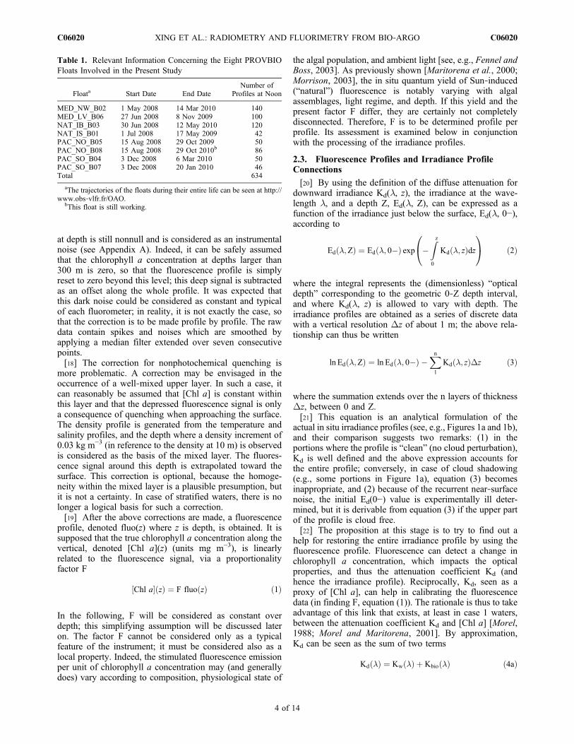
Table 1. Relevant Information Concerning the Eight PROVBIOFloats Involved in the Present Study

Floata Start Date End DateNumber of

Profiles at Noon

MED_NW_B02 1 May 2008 14 Mar 2010 140MED_LV_B06 27 Jun 2008 8 Nov 2009 100NAT_IB_B03 30 Jun 2008 12 May 2010 120NAT_IS_B01 1 Jul 2008 17 May 2009 42PAC_NO_B05 15 Aug 2008 29 Oct 2009 50PAC_NO_B08 15 Aug 2008 29 Oct 2010b 86PAC_SO_B04 3 Dec 2008 6 Mar 2010 50PAC_SO_B07 3 Dec 2008 20 Jan 2010 46Total 634

aThe trajectories of the floats during their entire life can be seen at http://www.obs‐vlfr.fr/OAO.

bThis float is still working.


4 of 14

where Kw(l) represents that part of attenuation due to the(pure) seawater, which is a constant for a given wavelength,and Kbio, represents the other part of attenuation, whichresults from the presence of biological material (phyto-plankton plus accompanying particulate and dissolved sub-stances). Regression analyses (between the log‐transformedof the quantities Kbio at eachwavelength, and [Chl a]) showedthat Kbio(l) varies as a nonlinear function of the [Chl a],according to [Morel, 1988; Morel and Maritorena, 2001]

Kd �ð Þ ¼ Kw �ð Þ þ � �ð Þ Chl a½ �e �ð Þ ð4bÞand these analyses provided the coefficients c(l) andexponents e(l).[23] By introducing equation (4b) into equation (3), and

considering that [Chl a] varies with depth, it becomes

ln Ed �; zð Þ ¼ ln Ed �; 0�ð Þ �Xn1

Kw �ð Þ þ � �ð Þ Chl a; z½ �e �ð Þh i

Dz

ð5Þ[Chl a] is still unknown at this stage, as the factor F inequation (1) has not been determined. By using fluo as a

surrogate for [Chl a], and reassembling equations (1) and (5),the final expression is

ln Ed �; zð Þ þXn1

Kw �ð ÞDz ¼ ln Ed �; 0�ð Þ

� Fe �ð Þ Xn1

� �ð Þfluo zð Þe �ð Þh i

Dz ð6aÞ

The mutual help expected from the simultaneous consider-ation of the two quantities, irradiance and fluorescence is notself‐evident, since an additional unknown (F) has beenintroduced. The solution of the system cannot be analytical,but is conceivably reachable through an iterative process.Equation (6a) can be represented under the simple form

An ¼ B0 � S Cn ð6bÞ

A series of n similar equations is obtained by incrementingthe order n, and so by increasing the thickness of the layerunder consideration. All these relationships are linear andcontain the same unknown S = Fe(l). Each of them containsa known term, An, which is computed from the successive

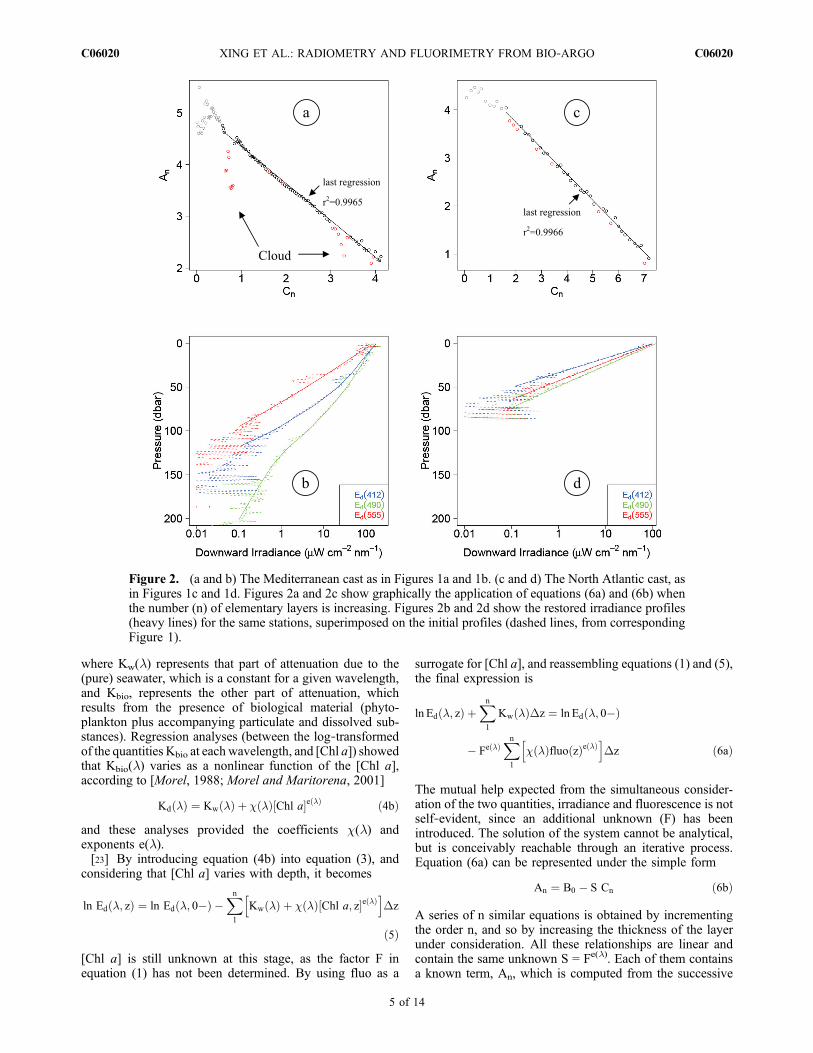
Figure 2. (a and b) The Mediterranean cast as in Figures 1a and 1b. (c and d) The North Atlantic cast, asin Figures 1c and 1d. Figures 2a and 2c show graphically the application of equations (6a) and (6b) whenthe number (n) of elementary layers is increasing. Figures 2b and 2d show the restored irradiance profiles(heavy lines) for the same stations, superimposed on the initial profiles (dashed lines, from correspondingFigure 1).


5 of 14

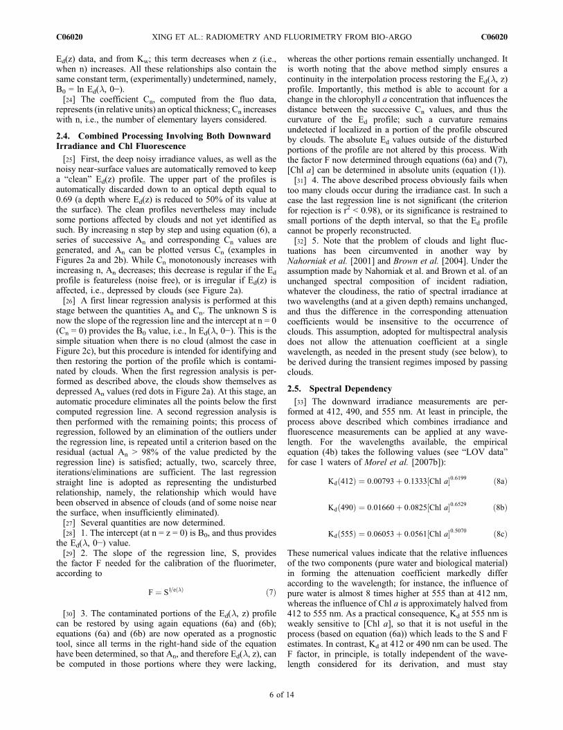
Ed(z) data, and from Kw; this term decreases when z (i.e.,when n) increases. All these relationships also contain thesame constant term, (experimentally) undetermined, namely,B0 = ln Ed(l, 0−).[24] The coefficient Cn, computed from the fluo data,

represents (in relative units) an optical thickness; Cn increaseswith n, i.e., the number of elementary layers considered.

2.4. Combined Processing Involving Both DownwardIrradiance and Chl Fluorescence

[25] First, the deep noisy irradiance values, as well as thenoisy near‐surface values are automatically removed to keepa “clean” Ed(z) profile. The upper part of the profiles isautomatically discarded down to an optical depth equal to0.69 (a depth where Ed(z) is reduced to 50% of its value atthe surface). The clean profiles nevertheless may includesome portions affected by clouds and not yet identified assuch. By increasing n step by step and using equation (6), aseries of successive An and corresponding Cn values aregenerated, and An can be plotted versus Cn (examples inFigures 2a and 2b). While Cn monotonously increases withincreasing n, An decreases; this decrease is regular if the Ed

profile is featureless (noise free), or is irregular if Ed(z) isaffected, i.e., depressed by clouds (see Figure 2a).[26] A first linear regression analysis is performed at this

stage between the quantities An and Cn. The unknown S isnow the slope of the regression line and the intercept at n = 0(Cn = 0) provides the B0 value, i.e., ln Ed(l, 0−). This is thesimple situation when there is no cloud (almost the case inFigure 2c), but this procedure is intended for identifying andthen restoring the portion of the profile which is contami-nated by clouds. When the first regression analysis is per-formed as described above, the clouds show themselves asdepressed An values (red dots in Figure 2a). At this stage, anautomatic procedure eliminates all the points below the firstcomputed regression line. A second regression analysis isthen performed with the remaining points; this process ofregression, followed by an elimination of the outliers underthe regression line, is repeated until a criterion based on theresidual (actual An > 98% of the value predicted by theregression line) is satisfied; actually, two, scarcely three,iterations/eliminations are sufficient. The last regressionstraight line is adopted as representing the undisturbedrelationship, namely, the relationship which would havebeen observed in absence of clouds (and of some noise nearthe surface, when insufficiently eliminated).[27] Several quantities are now determined.[28] 1. The intercept (at n = z = 0) is B0, and thus provides

the Ed(l, 0−) value.[29] 2. The slope of the regression line, S, provides

the factor F needed for the calibration of the fluorimeter,according to

F ¼ S1=e �ð Þ ð7Þ

[30] 3. The contaminated portions of the Ed(l, z) profilecan be restored by using again equations (6a) and (6b);equations (6a) and (6b) are now operated as a prognostictool, since all terms in the right‐hand side of the equationhave been determined, so that An, and therefore Ed(l, z), canbe computed in those portions where they were lacking,

whereas the other portions remain essentially unchanged. Itis worth noting that the above method simply ensures acontinuity in the interpolation process restoring the Ed(l, z)profile. Importantly, this method is able to account for achange in the chlorophyll a concentration that influences thedistance between the successive Cn values, and thus thecurvature of the Ed profile; such a curvature remainsundetected if localized in a portion of the profile obscuredby clouds. The absolute Ed values outside of the disturbedportions of the profile are not altered by this process. Withthe factor F now determined through equations (6a) and (7),[Chl a] can be determined in absolute units (equation (1)).[31] 4. The above described process obviously fails when

too many clouds occur during the irradiance cast. In such acase the last regression line is not significant (the criterionfor rejection is r2 < 0.98), or its significance is restrained tosmall portions of the depth interval, so that the Ed profilecannot be properly reconstructed.[32] 5. Note that the problem of clouds and light fluc-

tuations has been circumvented in another way byNahorniak et al. [2001] and Brown et al. [2004]. Under theassumption made by Nahorniak et al. and Brown et al. of anunchanged spectral composition of incident radiation,whatever the cloudiness, the ratio of spectral irradiance attwo wavelengths (and at a given depth) remains unchanged,and thus the difference in the corresponding attenuationcoefficients would be insensitive to the occurrence ofclouds. This assumption, adopted for multispectral analysisdoes not allow the attenuation coefficient at a singlewavelength, as needed in the present study (see below), tobe derived during the transient regimes imposed by passingclouds.

2.5. Spectral Dependency

[33] The downward irradiance measurements are per-formed at 412, 490, and 555 nm. At least in principle, theprocess above described which combines irradiance andfluorescence measurements can be applied at any wave-length. For the wavelengths available, the empiricalequation (4b) takes the following values (see “LOV data”for case 1 waters of Morel et al. [2007b]):

Kd 412ð Þ ¼ 0:00793þ 0:1333 Chl a½ �0:6199 ð8aÞ

Kd 490ð Þ ¼ 0:01660þ 0:0825 Chl a½ �0:6529 ð8bÞ

Kd 555ð Þ ¼ 0:06053þ 0:0561 Chl a½ �0:5070 ð8cÞ

These numerical values indicate that the relative influencesof the two components (pure water and biological material)in forming the attenuation coefficient markedly differaccording to the wavelength; for instance, the influence ofpure water is almost 8 times higher at 555 than at 412 nm,whereas the influence of Chl a is approximately halved from412 to 555 nm. As a practical consequence, Kd at 555 nm isweakly sensitive to [Chl a], so that it is not useful in theprocess (based on equation (6a)) which leads to the S and Festimates. In contrast, Kd at 412 or 490 nm can be used. TheF factor, in principle, is totally independent of the wave-length considered for its derivation, and must stay


6 of 14

unchanged whether 412 or 490 nm are used when operatingequation (6a) and (7). Such a statement, however, wouldimply that equations (8a) and (8b) are strictly exact and fullycompatible; rigorously, it is never the case. As being sta-tistical products, these expressions are representative of anaverage bio‐optical situation, so that statistical fluctuationsaround the mean trends and between their spectral expres-sions are to be expected [Morel and Maritorena, 2001; seealso Ciotti et al., 1999]. Actually, systematic deviations,affecting Kd(412), have already been detected in somespecific environments [Morel et al., 2007a] and discussed insection 3.3.

3. Results and First Discussion

[34] The total number of profiles (for irradiance andfluorescence) collected near noon by the eight floatsamounts to 634 (Table 1), among which 508 can be suc-cessfully processed. The processing cannot be completed incase of sensor failure or when the cloud cover is too muchunstable. Profiles occasionally obtained close to sunset andsunrise for other (and specific) purposes are discarded.

3.1. Irradiance Profiles

[35] Together with the regression significance (r2), thevisual inspection of the initial raw irradiance profile, andthen of the intermediate steps in the processing (compareFigure 2) are subjective ways of assessing the quality of therestored profile. More appropriate tools for an automatictreatment are nonetheless needed.[36] A first possible verification consists in examining if

the irradiance values, when extrapolated above the surface,

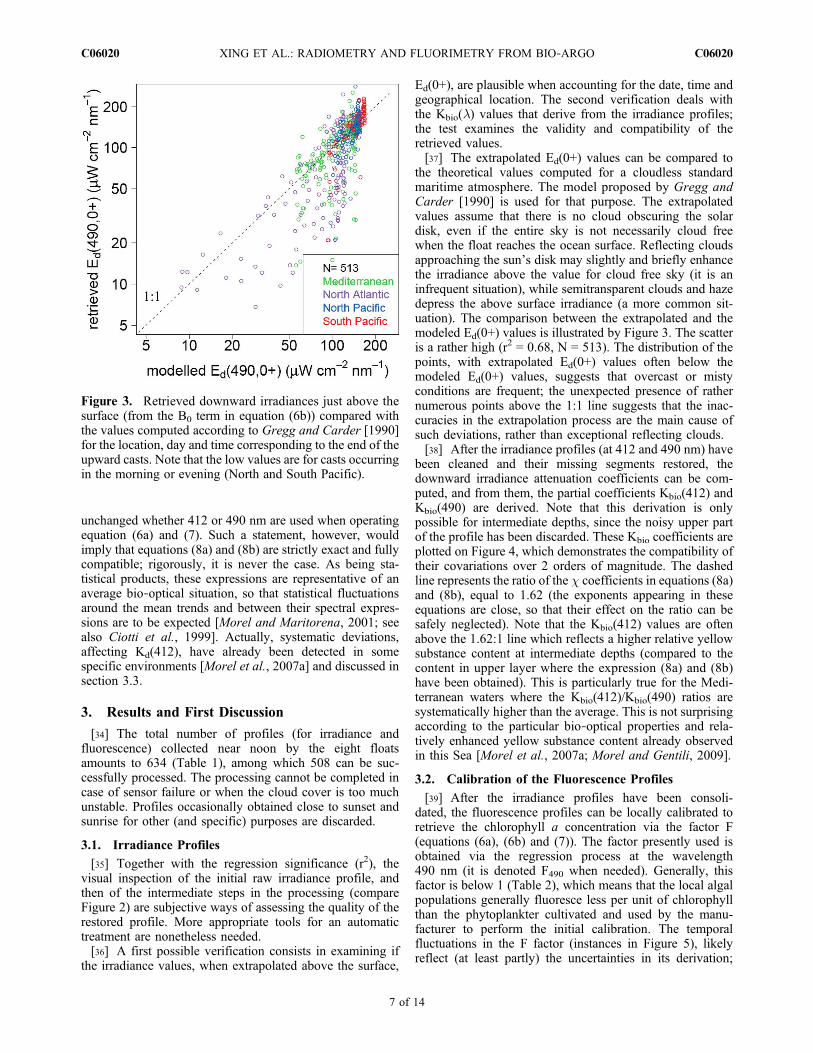
Ed(0+), are plausible when accounting for the date, time andgeographical location. The second verification deals withthe Kbio(l) values that derive from the irradiance profiles;the test examines the validity and compatibility of theretrieved values.[37] The extrapolated Ed(0+) values can be compared to

the theoretical values computed for a cloudless standardmaritime atmosphere. The model proposed by Gregg andCarder [1990] is used for that purpose. The extrapolatedvalues assume that there is no cloud obscuring the solardisk, even if the entire sky is not necessarily cloud freewhen the float reaches the ocean surface. Reflecting cloudsapproaching the sun’s disk may slightly and briefly enhancethe irradiance above the value for cloud free sky (it is aninfrequent situation), while semitransparent clouds and hazedepress the above surface irradiance (a more common sit-uation). The comparison between the extrapolated and themodeled Ed(0+) values is illustrated by Figure 3. The scatteris a rather high (r2 = 0.68, N = 513). The distribution of thepoints, with extrapolated Ed(0+) values often below themodeled Ed(0+) values, suggests that overcast or mistyconditions are frequent; the unexpected presence of rathernumerous points above the 1:1 line suggests that the inac-curacies in the extrapolation process are the main cause ofsuch deviations, rather than exceptional reflecting clouds.[38] After the irradiance profiles (at 412 and 490 nm) have

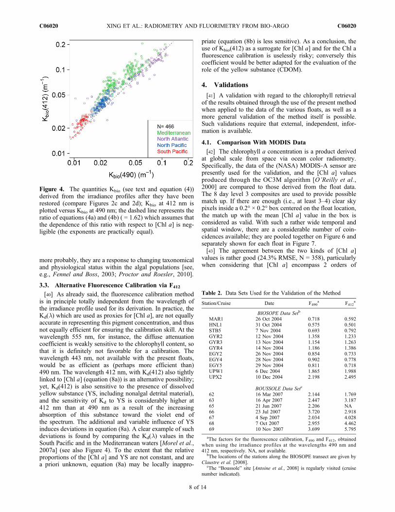
been cleaned and their missing segments restored, thedownward irradiance attenuation coefficients can be com-puted, and from them, the partial coefficients Kbio(412) andKbio(490) are derived. Note that this derivation is onlypossible for intermediate depths, since the noisy upper partof the profile has been discarded. These Kbio coefficients areplotted on Figure 4, which demonstrates the compatibility oftheir covariations over 2 orders of magnitude. The dashedline represents the ratio of the c coefficients in equations (8a)and (8b), equal to 1.62 (the exponents appearing in theseequations are close, so that their effect on the ratio can besafely neglected). Note that the Kbio(412) values are oftenabove the 1.62:1 line which reflects a higher relative yellowsubstance content at intermediate depths (compared to thecontent in upper layer where the expression (8a) and (8b)have been obtained). This is particularly true for the Medi-terranean waters where the Kbio(412)/Kbio(490) ratios aresystematically higher than the average. This is not surprisingaccording to the particular bio‐optical properties and rela-tively enhanced yellow substance content already observedin this Sea [Morel et al., 2007a; Morel and Gentili, 2009].

3.2. Calibration of the Fluorescence Profiles

[39] After the irradiance profiles have been consoli-dated, the fluorescence profiles can be locally calibrated toretrieve the chlorophyll a concentration via the factor F(equations (6a), (6b) and (7)). The factor presently used isobtained via the regression process at the wavelength490 nm (it is denoted F490 when needed). Generally, thisfactor is below 1 (Table 2), which means that the local algalpopulations generally fluoresce less per unit of chlorophyllthan the phytoplankter cultivated and used by the manu-facturer to perform the initial calibration. The temporalfluctuations in the F factor (instances in Figure 5), likelyreflect (at least partly) the uncertainties in its derivation;

Figure 3. Retrieved downward irradiances just above thesurface (from the B0 term in equation (6b)) compared withthe values computed according to Gregg and Carder [1990]for the location, day and time corresponding to the end of theupward casts. Note that the low values are for casts occurringin the morning or evening (North and South Pacific).


7 of 14

more probably, they are a response to changing taxonomicaland physiological status within the algal populations [see,e.g., Fennel and Boss, 2003; Proctor and Roesler, 2010].

3.3. Alternative Fluorescence Calibration via F412

[40] As already said, the fluorescence calibration methodis in principle totally independent from the wavelength ofthe irradiance profile used for its derivation. In practice, theKd(l) which are used as proxies for [Chl a], are not equallyaccurate in representing this pigment concentration, and thusnot equally efficient for ensuring the calibration skill. At thewavelength 555 nm, for instance, the diffuse attenuationcoefficient is weakly sensitive to the chlorophyll content, sothat it is definitely not favorable for a calibration. Thewavelength 443 nm, not available with the present floats,would be as efficient as (perhaps more efficient than)490 nm. The wavelength 412 nm, with Kd(412) also tightlylinked to [Chl a] (equation (8a)) is an alternative possibility;yet, Kd(412) is also sensitive to the presence of dissolvedyellow substance (YS, including nonalgal detrital material),and the sensitivity of Kd to YS is considerably higher at412 nm than at 490 nm as a result of the increasingabsorption of this substance toward the violet end ofthe spectrum. The additional and variable influence of YSinduces deviations in equation (8a). A clear example of suchdeviations is found by comparing the Kd(l) values in theSouth Pacific and in the Mediterranean waters [Morel et al.,2007a] (see also Figure 4). To the extent that the relativeproportions of the [Chl a] and YS are not constant, and area priori unknown, equation (8a) may be locally inappro-

priate (equation (8b) is less sensitive). As a conclusion, theuse of Kbio(412) as a surrogate for [Chl a] and for the Chl afluorescence calibration is uselessly risky; conversely thiscoefficient would be better adapted for the evaluation of therole of the yellow substance (CDOM).

4. Validations

[41] A validation with regard to the chlorophyll retrievalof the results obtained through the use of the present methodwhen applied to the data of the various floats, as well as amore general validation of the method itself is possible.Such validations require that external, independent, infor-mation is available.

4.1. Comparison With MODIS Data

[42] The chlorophyll a concentration is a product derivedat global scale from space via ocean color radiometry.Specifically, the data of the (NASA) MODIS‐A sensor arepresently used for the validation, and the [Chl a] valuesproduced through the OC3M algorithm [O’Reilly et al.,2000] are compared to those derived from the float data.The 8 day level 3 composites are used to provide possiblematch up. If there are enough (i.e., at least 3–4) clear skypixels inside a 0.2° × 0.2° box centered on the float location,the match up with the mean [Chl a] value in the box isconsidered as valid. With such a rather wide temporal andspatial window, there are a considerable number of coin-cidences available; they are pooled together on Figure 6 andseparately shown for each float in Figure 7.[43] The agreement between the two kinds of [Chl a]

values is rather good (24.3% RMSE, N = 358), particularlywhen considering that [Chl a] encompass 2 orders of

Figure 4. The quantities Kbio (see text and equation (4))derived from the irradiance profiles after they have beenrestored (compare Figures 2c and 2d); Kbio at 412 nm isplotted versus Kbio at 490 nm; the dashed line represents theratio of equations (4a) and (4b) ( = 1.62) which assumes thatthe dependence of this ratio with respect to [Chl a] is neg-ligible (the exponents are practically equal).

Table 2. Data Sets Used for the Validation of the Method

Station/Cruise Date F490a F412

a

BIOSOPE Data Setb

MAR1 26 Oct 2004 0.718 0.592HNL1 31 Oct 2004 0.575 0.501STB5 7 Nov 2004 0.693 0.792GYR2 12 Nov 2004 1.358 1.233GYR3 13 Nov 2004 1.154 1.263GYR4 14 Nov 2004 1.186 1.386EGY2 26 Nov 2004 0.854 0.733EGY4 28 Nov 2004 0.902 0.778EGY5 29 Nov 2004 0.811 0.718UPW1 6 Dec 2004 1.865 1.988UPX2 10 Dec 2004 2.198 2.495

BOUSSOLE Data Setc

62 16 Mar 2007 2.144 1.76963 16 Apr 2007 2.447 3.18765 21 Jun 2007 2.206 NA66 23 Jul 2007 3.720 2.91867 4 Sep 2007 2.034 4.02868 7 Oct 2007 2.955 4.46269 10 Nov 2007 3.699 5.795

aThe factors for the fluorescence calibration, F490 and F412, obtainedwhen using the irradiance profiles at the wavelengths 490 nm and412 nm, respectively. NA, not available.

bThe locations of the stations along the BIOSOPE transect are given byClaustre et al. [2008].

cThe “Boussole” site [Antoine et al., 2008] is regularly visited (cruisenumber indicated).


8 of 14

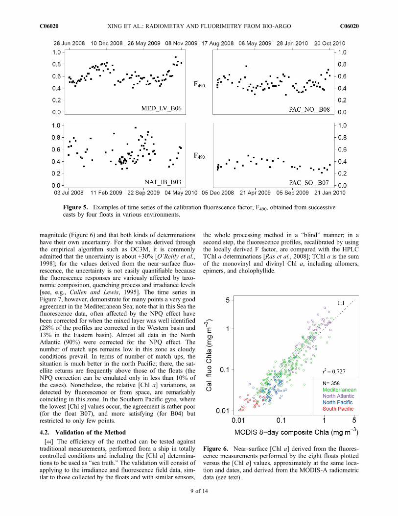
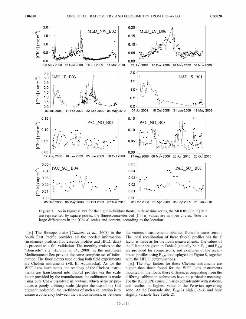
magnitude (Figure 6) and that both kinds of determinationshave their own uncertainty. For the values derived throughthe empirical algorithm such as OC3M, it is commonlyadmitted that the uncertainty is about ±30% [O’Reilly et al.,1998]; for the values derived from the near‐surface fluo-rescence, the uncertainty is not easily quantifiable becausethe fluorescence responses are variously affected by taxo-nomic composition, quenching process and irradiance levels[see, e.g., Cullen and Lewis, 1995]. The time series inFigure 7, however, demonstrate for many points a very goodagreement in the Mediterranean Sea; note that in this Sea thefluorescence data, often affected by the NPQ effect havebeen corrected for when the mixed layer was well identified(28% of the profiles are corrected in the Western basin and13% in the Eastern basin). Almost all data in the NorthAtlantic (90%) were corrected for the NPQ effect. Thenumber of match ups remains low in this zone as cloudyconditions prevail. In terms of number of match ups, thesituation is much better in the north Pacific; there, the sat-ellite returns are frequently above those of the floats (theNPQ correction can be emulated only in less than 10% ofthe cases). Nonetheless, the relative [Chl a] variations, asdetected by fluorescence or from space, are remarkablycoinciding in this zone. In the Southern Pacific gyre, wherethe lowest [Chl a] values occur, the agreement is rather poor(for the float B07), and more satisfying (for B04) butrestricted to only few points.

4.2. Validation of the Method

[44] The efficiency of the method can be tested againsttraditional measurements, performed from a ship in totallycontrolled conditions and including the [Chl a] determina-tions to be used as “sea truth.” The validation will consist ofapplying to the irradiance and fluorescence field data, sim-ilar to those collected by the floats and with similar sensors,

the whole processing method in a “blind” manner; in asecond step, the fluorescence profiles, recalibrated by usingthe locally derived F factor, are compared with the HPLCTChl a determinations [Ras et al., 2008]; TChl a is the sumof the monovinyl and divinyl Chl a, including allomers,epimers, and cholophyllide.

Figure 6. Near‐surface [Chl a] derived from the fluores-cence measurements performed by the eight floats plottedversus the [Chl a] values, approximately at the same loca-tion and dates, and derived from the MODIS‐A radiometricdata (see text).

Figure 5. Examples of time series of the calibration fluorescence factor, F490, obtained from successivecasts by four floats in various environments.


9 of 14

[45] The Biosope cruise [Claustre et al., 2008] in theSouth East Pacific provides all the needed information(irradiances profiles, fluorescence profiles and HPLC data)to proceed to a full validation. The monthly cruises to the“Boussole” site [Antoine et al., 2008] in the northwestMediterranean Sea provide the same complete set of infor-mation. The fluorimeters used during both field experimentsare Chelsea instruments (Mk III Aquatracka). As for theWET Labs instruments, the readings of the Chelsea instru-ments are transformed into fluo(z) profiles via the scalefactor provided by the manufacturer; the calibration is madeusing pure Chl a dissolved in acetone, which actually pro-duces a purely arbitrary scale (despite the use of the Chlpigment molecule); the usefulness of such a calibration is toensure a coherency between the various sensors, or between

the various measurements obtained from the same sensor.The local recalibration of these fluo(z) profiles via the Ffactor is made as for the floats measurements. The values ofthe F factor are given in Table 2 (actually both F412 and F490are provided for comparison), and examples of the recali-brated profiles using F490 are displayed on Figure 8, togetherwith the HPLC determinations.[46] The F490 factors for these Chelsea instruments are

higher than those found for the WET Labs instrumentsmounted on the floats; these differences originating from thediffering calibration techniques have no particular meaning.For the BIOSOPE cruise, F varies considerably with stations,and reaches its highest value in the Peruvian upwellingzone. At the Boussole site, F490 is high (∼2–3) and onlyslightly variable (see Table 2).

Figure 7. As in Figure 6, but for the eight individual floats; in these time series, the MODIS [Chl a] dataare represented by square points, the fluorescence‐derived [Chl a] values are as open circles. Note thelarge differences in the [Chl a] scales and content, according to the location.


10 of 14

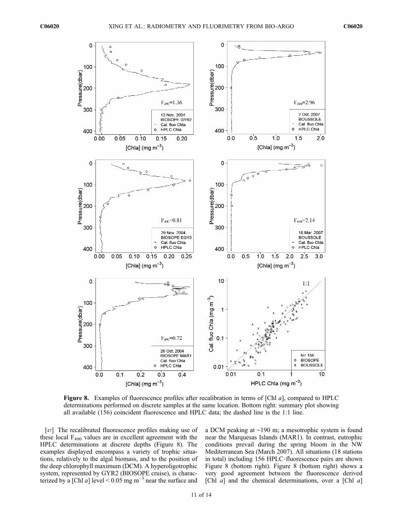
[47] The recalibrated fluorescence profiles making use ofthese local F490 values are in excellent agreement with theHPLC determinations at discrete depths (Figure 8). Theexamples displayed encompass a variety of trophic situa-tions, relatively to the algal biomass, and to the position ofthe deep chlorophyll maximum (DCM). A hyperoligotrophicsystem, represented by GYR2 (BIOSOPE cruise), is charac-terized by a [Chl a] level < 0.05 mg m−3 near the surface and

a DCM peaking at ∼190 m; a mesotrophic system is foundnear the Marquesas Islands (MAR1). In contrast, eutrophicconditions prevail during the spring bloom in the NWMediterranean Sea (March 2007). All situations (18 stationsin total) including 156 HPLC‐fluorescence pairs are shownFigure 8 (bottom right). Figure 8 (bottom right) shows avery good agreement between the fluorescence derived[Chl a] and the chemical determinations, over a [Chl a]

Figure 8. Examples of fluorescence profiles after recalibration in terms of [Chl a], compared to HPLCdeterminations performed on discrete samples at the same location. Bottom right: summary plot showingall available (156) coincident fluorescence and HPLC data; the dashed line is the 1:1 line.


11 of 14

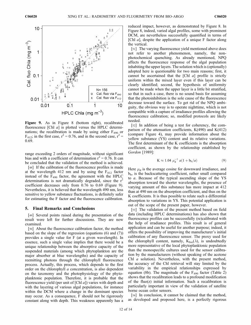
range exceeding 2 orders of magnitude, without significantbias and with a coefficient of determination r2 = 0.76. It canbe concluded that the validation of the method is achieved.[48] If the calibration of the fluorescence profiles is made

at the wavelength 412 nm and by using the F412 factorinstead of the F490 factor, the agreement with the HPLCdeterminations is not dramatically degraded, since the r2

coefficient decreases only from 0.76 to 0.69 (Figure 9).Nevertheless, it is believed that the wavelength 490 nm, lesssensitive to yellow substance fluctuations, is definitely saferfor estimating the F factor and the fluorescence calibration.

5. Final Remarks and Conclusions

[49] Several points raised during the presentation of theresult were left for further discussions. They are nowexamined.[50] About the fluorescence calibration factor, the method

based on the slope of the regression (equations (6) and (7))provides a single value for F (at a given wavelength). Inessence, such a single value implies that there would be aunique relationship between the absorptive capacity of thesuspended materials (among which phytoplankton are themajor absorber at blue wavelengths) and the capacity ofreemitting photons through the chlorophyll fluorescenceprocess. Actually, this process, which depends to the firstorder on the chlorophyll a concentration, is also dependenton the taxonomy and the photophysiology of the phyto-planktonic population. Therefore, it is probable that thefluorescence yield (per unit of [Chl a]) varies with depth andwith the layering of various algal populations, for instancewithin the DCM where a change in the dominant speciesmay occur. As a consequence, F should not be rigorouslyconstant along with depth. This weakness apparently has a

reduced impact, however, as demonstrated by Figure 8. InFigure 8, indeed, varied algal profiles, some with prominentDCM, are nevertheless successfully quantified in terms of[Chl a], despite the application of a unique F factor alongthe vertical.[51] The varying fluorescence yield mentioned above does

not refer to another phenomenon, namely, the non-photochemical quenching. As already mentioned, NPQaffects the fluorescence response of the algal populationinhabiting the upper layers. The solution which is (optionally)adopted here is questionable for two main reasons; first, itcannot be ascertained that the [Chl a] profile is strictlyuniform within the mixed layer even if this layer can beclearly identified; second, the hypothesis of uniformitycannot be made when the upper layer is a little bit stratified,so that in such a case, there is no sound basis for assumingthat the photoinhibition is the sole cause of the fluorescencedecrease toward the surface. To get rid of the NPQ ambi-guity, the obvious way is to operate nighttime, which is notcompatible with a capture of irradiance profiles allowing thefluorescence calibration; so, modified protocols are likelyneeded.[52] In addition of being a test for coherency, the com-

parison of the attenuation coefficients, K(490) and K(412)(compare Figure 4), may provide information about theyellow substance (YS) content and its relative variations.The first determinant of the K coefficients is the absorptioncoefficient, as shown by the relationship established byGordon [1989]:

K � 1:04 ��1d a 1þ bb=að Þ ð9Þ

Here md is the average cosine for downward irradiance, andbb, is the backscattering coefficient, rather small comparedto a. Because of the typical ascending slope of the YSabsorption toward the shorter wavelengths, the presence ofvarying amount of this substance has more impact at 412than at 490 nm on the absorption coefficient, and thus on theK coefficients. It is thus possible to relate such a differentialabsorption to variations in YS. This potential application isout of the scope of the present paper, however.[53] The validation of the present method based on field

data (including HPLC determinations) has also shown thatfluorescence profiles can be successfully (re)calibrated withthe help of irradiance profiles. This result is of generalapplication and can be useful for another purpose; indeed, itoffers the possibility of improving the manufacturer’s initialcalibration of any fluorescence sensor. The proxy used forthe chlorophyll content, namely, Kbio(l), is undoubtedlymore representative of the local phytoplanktonic populationthan the monospecific cultures used for the sensor calibra-tion by the manufacturers (without speaking of the acetoneChl a solution). Nevertheless, with the present method,the accuracy of the Chl retrieval will stay limited by thevariability in the empirical relationships expressed byequation (8b). The magnitude of the F490 factor (Table 2)shows that the recalibration leads to a profound modificationof the fluo(z) initial information. Such a recalibration isparticularly important in view of the validation of satelliteborne ocean color sensors.[54] In conclusion, it cannot be claimed that the method,

as developed and proposed here, is a perfectly rigorous

Figure 9. As in Figure 8 (bottom right), recalibratedfluorescence [Chl a] is plotted versus the HPLC determi-nations; the recalibration is made by using either F490 orF412; in the first case, r2 = 0.76, and in the second case, r2 =0.69.


12 of 14

solution; it is an operational tool, which has been satisfac-torily validated. Other kinds of information are also avail-able with the floats as they are presently equipped, such asthe backscattering coefficient or the beam attenuationcoefficient. These parameters can help in the specification ofthe mixed layer thickness, for instance [Sackmann et al.,2008]. They, however, cannot bring decisive advantagesin the specific issues of cleaning the irradiance profiles orquantifying the fluorescence data; indeed, the relationshipsbetween these inherent optical properties and the chlorophylla concentration, or the diffuse attenuation coefficient, are notbetter than those already represented by equations (8a)–(8c).If the improvements to be expected from their use cannot beconsiderable, these coefficients can provide useful confir-mation, and anyway are useful for other purposes (e.g.,granulometry and composition of the particulate material)out of the scope of the present study.

Appendix A

[55] After the dark correction that follows the manu-facturer’s recommendations has been applied, the residualdeep fluorescence signal (say beyond 300 m) is not zero;actually, it remains always positive and differs according tothe sensor. Proctor and Roesler [2010] have recently studiedthe effects on the dark count of temperature and of fluo-rescence by dissolved organic material in shallow fresh-waters where this material is extremely abundant, which isnever the case here. For all floats except the NAT_IB_B03,the temperature at the parking depth (∼1000 m) was rathersteady so that a temperature effect on the dark count wasnever observed. In contrast, the NAT_IB_B03 float hasdrifted from the Island Basin to the Norwegian Basin, and alarge temperature change was observed at ∼1000 m, from∼6°C to <0°C. Even under such conditions, the dark currentremained unchanged. The average values of the dark signalsobserved for the various floats are between 0.02 and0.11 mg m−3 when directly expressed in chlorophyll aconcentration. These values may appear rather high, par-ticularly when considering that for the six floats in oligo-trophic environments they are similar to the chlorophyll aconcentration generally encountered in the upper layers. Interms of digital counts, however, these residual dark signalsrepresent a few counts (2 to 9), to be compared with the darkcounts provided by the manufacturer (between 50 and60 counts) and also with the nominal resolution (equivalentto ∼0.03 mg m−3). These last remarks point out that thepresent fluorimeters are at the limit of their capability whendealing with oligotrophic waters.

[56] Acknowledgments. This paper represents a contribution to theremOcean project, funded by the European Research Council, to thePABO project funded by Agence Nationale de la Recherche (ANR),to the BIOSOPE project of the LEFE/CYBER program, and to the BOUS-SOLE project. We express our gratitude to Bernard Gentili for help inprogramming and to John Cullen for helpful suggestions and constructivecomments on a first version of this paper. We also would like to thankthe NASA Ocean Biology Processing Group (OBPG) for processing andefficient distribution of the MODIS‐A data.

ReferencesAlthuis, I., W. W. C. Gieskes, L. Villerius, and F. Colijn (1994), Inter-pretation of fluorometric chlorophyll registrations with algal pigment

analysis along a ferry transect in the southern North Sea, Neth. J. SeaRes., 33(1), 37–46, doi:10.1016/0077-7579(94)90049-3.

Antoine, D., F. d’Ortenzio, S. B. Hooker, G. Bécu, B. Gentili, D. Tailliez,and A. J. Scott (2008), Assessment of uncertainty in the ocean reflectancedetermined by three satellite ocean color sensors (MERIS, SeaWiFS andMODIS‐A) at an offshore site in the Mediterranean Sea (BOUSSOLEproject), J. Geophys. Res., 113, C07013, doi:10.1029/2007JC004472.

Babin, M. (2008), Phytoplankton fluorescence: Theory, current literatureand in situ measurements, in Real‐Time Coastal Observing Systems forMarine Ecosystem Dynamics and Harmful Algal Blooms, edited byM. Babin, C. Roesler, and J. J. Cullen, pp. 237–280, UNESCO, Paris.

Brown, C. A., Y. Huot, M. J. Purcell, J. J. Cullen, and M. R. Lewis (2004),Mapping coastal optical and biogeochemical variability using an autono-mous underwater vehicle and a new bio‐optical inversion algorithm,Limnol. Oceanogr. Methods, 2, 262–281.

Ciotti, A. M., J. J. Cullen, and M. R. Lewis (1999), A semi‐analyticalmodel of the influence of phytoplankton community structure on therelationship between light attenuation and ocean color, J. Geophys. Res.,104(C1), 1559–1578, doi:10.1029/1998JC900021.

Claustre, H., A. Morel, M. Babin, C. Cailliau, D. Marie, J. C. Marty,D. Tailliez, and D. Vaulot (1999), Variability in particle attenuation andchlorophyll fluorescence in the tropical Pacific: Scales, patterns, and bio-geochemical implications, J. Geophys. Res., 104(C2), 3401–3422,doi:10.1029/98JC01334.

Claustre, H., A. Sciandra, and D. Vaulot (2008), Introduction to the specialsection: Bio‐optical and biogeochemical conditions in the south eastPacific in late 2004: The BIOSOPE program, Biogeosciences, 5, 679–691, doi:10.5194/bg-5-679-2008.

Claustre, H., et al. (2010), Biol.‐optical profiling floats as new observa-tional tools for biogeochemical and ecosystem studies, in Proceedingsof the OceanObs’09: Sustained Ocean Observations and Informationfor Society Conference, edited by J. Hall, D. E. Harrison, and D. Stammer,ESA Publ., WPP‐306. (Available at http://www.obs‐vlfr.fr/LOV/OMT/fichiers_PDF/Claustre_et_al._OO09.pdf.)

Cullen, J. J., and M. R. Lewis (1995), Biological processes and opticalmeasurements near the sea‐surface: Some issues relevant to remote sens-ing, J. Geophys. Res., 100(C7), 13,255–13,266, doi:10.1029/95JC00454.

Cunningham, A. (1996), Variability of in vivo chlorophyll fluorescence andits implications for instrument development in bio‐optical oceanography,Sci. Mar., 60, suppl. 1, 309–315.

Falkowski, P., and D. A. Kiefer (1985), Chlorophyll a fluorescence in phy-toplankton: Relationship to photosynthesis and biomass, J. PlanktonRes., 7, 715–731, doi:10.1093/plankt/7.5.715.

Fennel, K., and E. Boss (2003), Subsurface maxima of phytoplanktonand chlorophyll: Steady‐state solutions from a simple model, Limnol.Oceanogr., 48(4), 1521–1534, doi:10.4319/lo.2003.48.4.1521.

Gordon, H. R. (1989), Can the Lambert‐Beer law be applied to the diffuseattenuation coefficient of ocean water?, Limnol. Oceanogr., 34, 1389–1409, doi:10.4319/lo.1989.34.8.1389.

Gregg, W. W., and K. L. Carder (1990), A simple spectral solar irradiancemodel for cloudless maritime atmospheres, Limnol. Oceanogr., 35(8),1657–1675, doi:10.4319/lo.1990.35.8.1657.

Johnson, K. S., W. M. Berelson, E. S. Boss, Z. Chase, H. Claustre, S. R.Emerson, N. Gruber, A. Körtzinger, M. J. Perry, and S. C. Riser(2009), Observing biogeochemical cycles at global scales with profilingfloats and gliders: Prospects for a global array, Oceanography, 22(3),216–225.

Kiefer, D. A. (1973a), Fluoresence properties of natural phytoplanktonpopulations, Mar. Biol., 22, 263–269, doi:10.1007/BF00389180.

Kiefer, D. A. (1973b), Chlorophyll a fluorescence in marine centricdiatoms: Responses of chloroplasts to light and nutrient stress, Mar.Biol., 23, 39–46, doi:10.1007/BF00394110.

Maritorena, S., A. Morel, and B. Gentili (2000), Determination of the fluo-rescence quantum yield by oceanic phytoplankton in their natural habitat,Appl. Opt., 39, 6725–6737, doi:10.1364/AO.39.006725.

Marra, J. (1997), Analysis of diel variability in chlorophyll fluorescence,J. Mar. Res., 55, 767–784, doi:10.1357/0022240973224274.

Morel, A. (1988), Optical modeling of the upper ocean in relation to itsbiogenous matter content (case I waters), J. Geophys. Res., 93(C9),10,749–10,768, doi:10.1029/JC093iC09p10749.

Morel, A., and B. Gentili (2009), The dissolved yellow substance and theshades of blue in the Mediterranean Sea, Biogeosciences, 6, 2625–2636,doi:10.5194/bg-6-2625-2009.

Morel, A., and S. Maritorena (2001), Bio‐optical properties of oceanicwaters: A reappraisal, J. Geophys. Res., 106(C4), 7163–7180,doi:10.1029/2000JC000319.

Morel, A., H. Claustre, D. Antoine, and B. Gentili (2007a), Naturalvariability of bio‐optical properties in case 1 waters: Attenuation andreflectance within the visible and near‐UV spectral domains, as observed


13 of 14

in South Pacific and Mediterranean waters, Biogeosciences, 4, 913–925,doi:10.5194/bg-4-913-2007.

Morel, A., Y. Huot, B. Gentili, P. J. Werdell, S. B. Hooker, and B. A. Franz(2007b), Examining the consistency of products derived from variousocean color sensors in open ocean (case 1) waters in the perspective ofa multi‐sensor approach, Remote Sens. Environ., 111, 69–88, doi:10.1016/j.rse.2007.03.012.

Morrison, J. R. (2003), In situ determination of the quantum yield of phy-toplankton chlorophyll a fluorescence: A simple algorithm, observations,and a model, Limnol. Oceanogr., 48(2), 618–631, doi:10.4319/lo.2003.48.2.0618.

Nahorniak, J. S., M. R. Abbott, R. M. Letelier, and W. S. Pegau (2001),Analysis of a method to estimate chlorophyll‐a concentration from irra-diance measurements at varying depths, J. Atmos. Oceanic Technol., 18,2063–2073, doi:10.1175/1520-0426(2001)018<2063:AOAMTE>2.0.CO;2.

O’Reilly, J. E., et al. (2000), Ocean color chlorophyll a algorithms forSeaWiFS, OC2, and OC4: Version 4, SeaWiFS postlaunch calibrationand validation analyses, Part 3, NASA Tech. Memo., TM‐206892,vol. 11, 9–23.

O’Reilly, J. E., S. Maritorena, B. G. Mitchell, D. A. Siegel, K. L. Carder,S. A. Garver, M. Kahru, and C. McClain (1998), Ocean color chlorophyll

algorithms for SeaWiFS, J. Geophys. Res., 103(C11), 24,937–24,953,doi:10.1029/98JC02160.

Proctor, C. W., and C. S. Roesler (2010), New insights on obtaining phy-toplankton concentration and composition from in situ multispectralchlorophyll fluorescence, Limnol. Oceanogr. Methods, 8, 695–708,doi:10.4319/lom.2010.8.695.

Ras, J., H. Claustre, and J. Uitz (2008), Spatial variability of phytoplanktonpigment distributions in the subtropical South Pacific Ocean: Compari-son between in situ and predicted data, Biogeosciences, 5(2), 353–369,doi:10.5194/bg-5-353-2008.

Sackmann, B. S.,M. J. Perry, andC. C. Eriksen (2008), Seaglider observationsof variability in daytime fluorescence quenching of chlorophyll‐a in north-eastern Pacific coastal waters, Biogeosciences Discuss., 5, 2839–2865,doi:10.5194/bgd-5-2839-2008.

Zaneveld, J. R. V., E. Boss, and A. Barnard (2001), Influence of surfacewaves on measured and modeled irradiance profiles, Appl. Opt., 40(9),1442–1449, doi:10.1364/AO.40.001442.

D. Antoine, H. Claustre, F. D’Ortenzio, A. Mignot, A. Morel, A. Poteau,and X. Xing, Laboratoire d’Océanographie de Villefranche, Marine Opticsand Remote Sensing Lab, BP 8, Quai de la Darse, F‐06230 Villefranche‐sur‐Mer, France. (xingxiaogang@obs‐vlfr.fr)


14 of 14

Documents

Combined processing and mutual interpretation of radiometry and fluorimetry from autonomous profiling Bio-Argo floats: Chlorophyll a retrieval