Common Shocks, Common Dynamics and the International Business Cycle

Marco Centoni, Gianluca Cubbadda, Alain Hecq

CEIS Tor Vergata - Research Paper Series, Vol. 29, No. 85, July 2006

This paper can be downloaded without charge from the Social Science Research Network Electronic Paper Collection:

http://papers.ssrn.com/abstract=921582

CEIS Tor Vergata

RESEARCH PAPER SERIES

Working Paper No. 85 July 2006

Common Shocks, Common Dynamics and the International Business Cycle

Marco Centoni, Gianluca Cubadda, Alain Hecq

CEIS Tor Vergata - Research Paper Series, Vol. 29, No. 85, July 2006

This paper can be downloaded without charge from the Social Science Research Network Electronic Paper Collection:

http://papers.ssrn.com/abstract=921582

CEIS Tor Vergata

RESEARCH PAPER SERIES

Working Paper No. 85 July 2006

Common Shocks, Common Dynamics, and the

International Business Cycle∗

Marco CentoniUniversità del Molise

Gianluca CubaddaUniversità di Roma "Tor Vergata"†

Alain HecqUniversity of Maastricht

July 20, 2006

Abstract

This paper proposes an econometric framework to assess the importance of common

shocks and common transmission mechanisms in generating international business cycles.

Then we show how to decompose the cyclical effects of permanent-transitory shocks into

those due to their domestic and those due to foreign components. Our empirical analysis

reveals that the business cycles of the US, Japan, Canada are clearly dominated by their

domestic components. The Euro area is more sensitive to foreign shocks compared to the

other three countries of our analysis.

Keywords: International business cycles; Permanent-transitory decomposition; Serial cor-

relation common features; Frequency domain analysis.

JEL: C32, E32

∗Previous versions of this paper were presented at the 58th European Meeting of the Econometric Soci-ety in Stockholm, at the Latin American Meeting of the Econometric Society in Panama City, and the 4thEurostat Colloquium on Modern Tools for Business Cycle Analysis in Luxembourg. We wish to thank ananonymous referee for helpful comments and suggestions. Marco Centoni and Gianluca Cubadda grate-fully acknowledge financial support from MIUR. Alain Hecq gratefully acknowledges financial supportfrom METEOR through the research project ”Macroeconomic Consequences of Financial Instability” aswell as the hospitality of the department SEGeS, University of Molise, for the period during which a firstdraft of this paper was written.

†Corresponding author: Gianluca Cubadda Dipartimento SEFEMEQ, Universita’ di Roma "Tor Ver-gata", Via Columbia 2, 00133 Roma, Italy. E-mail: gianluca.cubadda@uniroma2.it.

1

1 Introduction

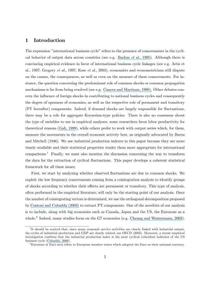
The expression ”international business cycle” refers to the presence of comovements in the cycli-

cal behavior of output data across countries (see e.g. Backus et al., 1995). Although there is

convincing empirical evidence in favor of international business cycle linkages (see e.g. Artis et

al., 1997; Gregory et al., 1997; Kose et al., 2003), economists and econometricians still dispute

on the causes, the consequences, as well as even on the measure of these comovements. For in-

stance, the question concerning the predominant role of common shocks or common propagation

mechanisms is far from being resolved (see e.g. Canova and Marrinan, 1998). Other debates con-

cern the influence of foreign shocks in contributing to national business cycles and consequently

the degree of openness of economies, as well as the respective role of permanent and transitory

(PT hereafter) components. Indeed, if demand shocks are largely responsible for fluctuations,

there may be a role for aggregate Keynesian-type policies. There is also no consensus about

the type of variables to use in empirical analyses: some researchers favor labor productivity for

theoretical reasons (Galì, 1999), while others prefer to work with output series which, for them,

measure the movements in the overall economic activity best, as originally advocated by Burns

and Mitchell (1946). We use industrial production indexes in this paper because they are more

timely available and their statistical properties render them more appropriate for international

comparisons.1 Finally, we must also mention the discussion concerning the way to transform

the data for the extraction of cyclical fluctuations. This paper develops a coherent statistical

framework for all these issues.

First, we start by analyzing whether observed fluctuations are due to common shocks. We

exploit the low frequency comovements coming from a cointegration analysis to identify groups

of shocks according to whether their effects are permanent or transitory. This type of analysis,

often performed in the empirical literature, will only be the starting point of our analysis. Once

the number of cointegrating vectors is determined, we use the orthogonal decomposition proposed

by Centoni and Cubadda (2003) to extract PT components. One of the novelties of our analysis

is to include, along with big economies such as Canada, Japan and the US, the Eurozone as a

whole.2 Indeed, many studies focus on the G7 economies (e.g. Cheung and Westermann, 2002),

1 It should be noticed that, since many economic service activities are closely linked with industrial output,the cycles of industrial production and GDP are closely related, see OECD (2003). Moreover, a recent empiricalinvestigation confirms that the industrial production index is the most cyclical coincident indicator of the USbusiness cycle (Cubadda, 2006).

2Eurozone or Euro area refers to European member states which adopted the Euro as their national currency.

2

and consequently they compare the US with European countries individually. The difference in

the size of countries induces inevitably asymmetries of treatment.

Second, we add a common cyclical feature analysis (Engle and Kozicki, 1993) to the study

of common trends. Indeed, the presence of common cycles (Vahid and Engle, 1993) will play

a double role. On one hand, this shows whether there exist some common dynamics, namely

some common transmission mechanisms of the shocks. One the other hand, imposing the implied

restrictions to the estimated model also helps to estimate more accurately the responses to shocks

because redundant parameters are excluded. In particular, it is well known that a misleading

detection of the number of cointegrating vectors might occur with small sample sizes, and hence

can damage the conclusions about the nature and the importance of common shocks. Using

an iterative strategy that switches between the cointegrating and cyclical cofeature spaces, we

obtain a more precise picture of the number of permanent and transitory components (see Hecq,

2006).

Third, after having carefully detected the number and the type of common shocks, we pro-

pose to further decompose the permanent and transitory shocks into a domestic and foreign

component. For each country we consequently obtain four types of shocks which contribute

to business cycle fluctuations. In particular, we identify the permanent [transitory] country-

specific domestic shock as the component of the common permanent [transitory] shocks that has

contemporaneous effect on domestic output. Also the permanent [transitory] country-specific

foreign shocks will be the component of the common permanent [transitory] shocks that has no

contemporaneous effect on domestic output.

Finally, we asses the importance of such PT domestic and foreign shocks in contributing

to national business cycles. So doing we consider fluctuations with a 2-8 year period using

a parametric spectrum decomposition (see Centoni and Cubadda, 2003). In our opinion this

approach evaluates the contribution of domestic and foreign shocks to the business cycles more

appropriately than the traditional impulse responses or variance decompositions in the time

domain.

The proposed approach allows us to answer a series of questions such as: 1) Do international

outputs comove because of the existence of common shocks, common dynamics or both? 2)

What is the importance of foreign shocks over national business cycles, and consequently what

is the degree of openness of economies? 3) Are business cycles mainly affected by permanent

or transitory components?

3

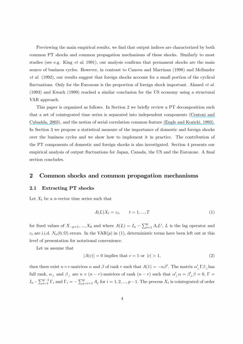
Previewing the main empirical results, we find that output indices are characterized by both

common PT shocks and common propagation mechanisms of these shocks. Similarly to most

studies (see e.g. King et al, 1991), our analysis confirms that permanent shocks are the main

source of business cycles. However, in contrast to Canova and Marrinan (1998) and Mellander

et al. (1992), our results suggest that foreign shocks account for a small portion of the cyclical

fluctuations. Only for the Eurozone is the proportion of foreign shock important. Ahmed et al.

(1993) and Kwark (1999) reached a similar conclusion for the US economy using a structural

VAR approach.

This paper is organized as follows. In Section 2 we briefly review a PT decomposition such

that a set of cointegrated time series is separated into independent components (Centoni and

Cubadda, 2003), and the notion of serial correlation common feature (Engle and Kozicki, 1993).

In Section 3 we propose a statistical measure of the importance of domestic and foreign shocks

over the business cycles and we show how to implement it in practice. The contribution of

the PT components of domestic and foreign shocks is also investigated. Section 4 presents our

empirical analysis of output fluctuations for Japan, Canada, the US and the Eurozone. A final

section concludes.

2 Common shocks and common propagation mechanisms

2.1 Extracting PT shocks

Let Xt be a n-vector time series such that

A(L)Xt = εt, t = 1, ..., T (1)

for fixed values of X−p+1, ...,X0 and where A(L) = In −Pp

i=1AiLi, L is the lag operator and

εt are i.i.d. Nn(0,Ω) errors. In the VAR(p) in (1), deterministic terms have been left out at this

level of presentation for notational convenience.

Let us assume that

|A(c)| = 0 implies that c = 1 or |c| > 1, (2)

then there exist n×r-matrices α and β of rank r such that A(1) = −αβ0. The matrix α0⊥Γβ⊥hasfull rank, α⊥ and β⊥ are n × (n− r)-matrices of rank (n− r) such that α0⊥α = β0⊥β = 0, Γ =

In−Pp−1

i=1 Γi and Γi = −Pp

j=i+1Aj for i = 1, 2, ..., p−1. The process Xt is cointegrated of order

4

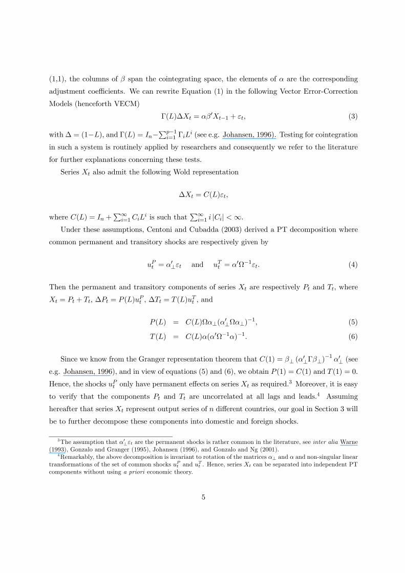
(1,1), the columns of β span the cointegrating space, the elements of α are the corresponding

adjustment coefficients. We can rewrite Equation (1) in the following Vector Error-Correction

Models (henceforth VECM)

Γ(L)∆Xt = αβ0Xt−1 + εt, (3)

with∆ = (1−L), and Γ(L) = In−Pp−1

i=1 ΓiLi (see e.g. Johansen, 1996). Testing for cointegration

in such a system is routinely applied by researchers and consequently we refer to the literature

for further explanations concerning these tests.

Series Xt also admit the following Wold representation

∆Xt = C(L)εt,

where C(L) = In +P∞

i=1CiLi is such that

P∞i=1 i |Ci| <∞.

Under these assumptions, Centoni and Cubadda (2003) derived a PT decomposition where

common permanent and transitory shocks are respectively given by

uPt = α0⊥εt and uTt = α0Ω−1εt. (4)

Then the permanent and transitory components of series Xt are respectively Pt and Tt, where

Xt = Pt + Tt, ∆Pt = P (L)uPt , ∆Tt = T (L)uTt , and

P (L) = C(L)Ωα⊥(α0⊥Ωα⊥)−1, (5)

T (L) = C(L)α(α0Ω−1α)−1. (6)

Since we know from the Granger representation theorem that C(1) = β⊥ (α0⊥Γβ⊥)−1 α0⊥ (see

e.g. Johansen, 1996), and in view of equations (5) and (6), we obtain P (1) = C(1) and T (1) = 0.

Hence, the shocks uPt only have permanent effects on series Xt as required.3 Moreover, it is easy

to verify that the components Pt and Tt are uncorrelated at all lags and leads.4 Assuming

hereafter that series Xt represent output series of n different countries, our goal in Section 3 will

be to further decompose these components into domestic and foreign shocks.

3The assumption that α0⊥εt are the permanent shocks is rather common in the literature, see inter alia Warne(1993), Gonzalo and Granger (1995), Johansen (1996), and Gonzalo and Ng (2001).

4Remarkably, the above decomposition is invariant to rotation of the matrices α⊥ and α and non-singular lineartransformations of the set of common shocks uPt and u

Tt . Hence, series Xt can be separated into independent PT

components without using a priori economic theory.

5

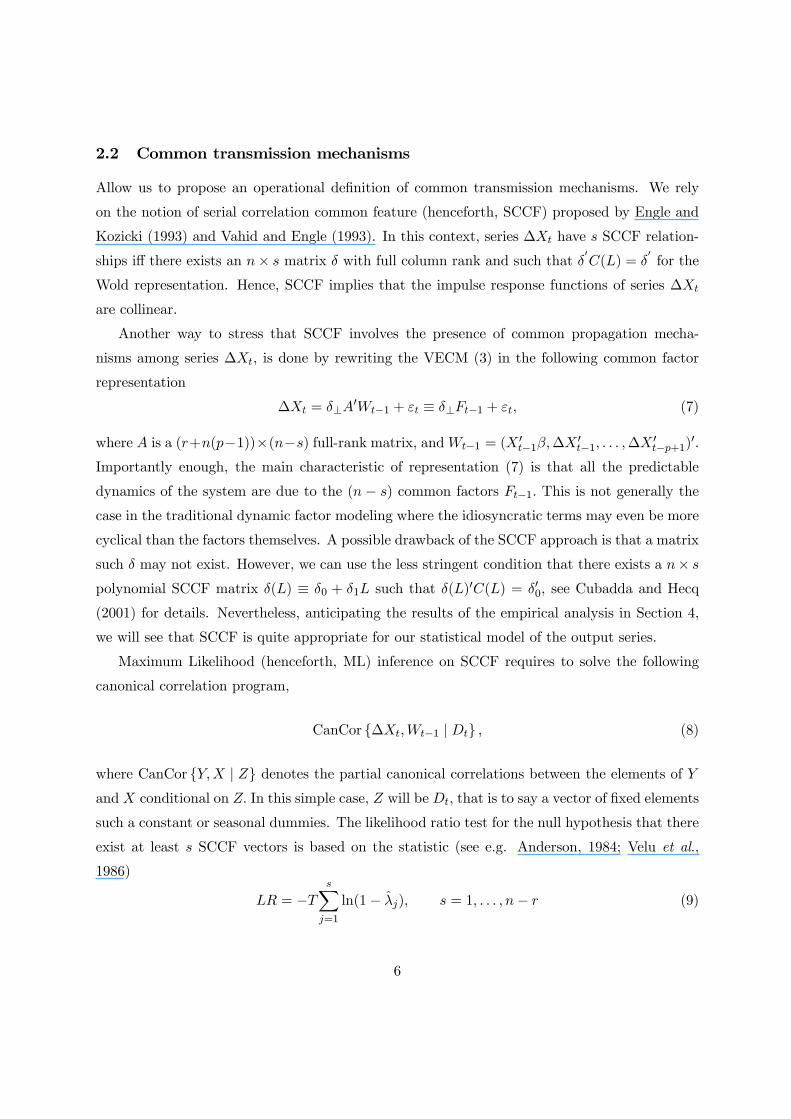
2.2 Common transmission mechanisms

Allow us to propose an operational definition of common transmission mechanisms. We rely

on the notion of serial correlation common feature (henceforth, SCCF) proposed by Engle and

Kozicki (1993) and Vahid and Engle (1993). In this context, series ∆Xt have s SCCF relation-

ships iff there exists an n× s matrix δ with full column rank and such that δ0C(L) = δ

0for the

Wold representation. Hence, SCCF implies that the impulse response functions of series ∆Xt

are collinear.

Another way to stress that SCCF involves the presence of common propagation mecha-

nisms among series ∆Xt, is done by rewriting the VECM (3) in the following common factor

representation

∆Xt = δ⊥A0Wt−1 + εt ≡ δ⊥Ft−1 + εt, (7)

where A is a (r+n(p−1))×(n−s) full-rank matrix, andWt−1 = (X 0t−1β,∆X 0

t−1, . . . ,∆X 0t−p+1)0.

Importantly enough, the main characteristic of representation (7) is that all the predictable

dynamics of the system are due to the (n − s) common factors Ft−1. This is not generally the

case in the traditional dynamic factor modeling where the idiosyncratic terms may even be more

cyclical than the factors themselves. A possible drawback of the SCCF approach is that a matrix

such δ may not exist. However, we can use the less stringent condition that there exists a n× s

polynomial SCCF matrix δ(L) ≡ δ0 + δ1L such that δ(L)0C(L) = δ00, see Cubadda and Hecq

(2001) for details. Nevertheless, anticipating the results of the empirical analysis in Section 4,

we will see that SCCF is quite appropriate for our statistical model of the output series.

Maximum Likelihood (henceforth, ML) inference on SCCF requires to solve the following

canonical correlation program,

CanCor ∆Xt,Wt−1 | Dt , (8)

where CanCor Y,X | Z denotes the partial canonical correlations between the elements of Yand X conditional on Z. In this simple case, Z will be Dt, that is to say a vector of fixed elements

such a constant or seasonal dummies. The likelihood ratio test for the null hypothesis that there

exist at least s SCCF vectors is based on the statistic (see e.g. Anderson, 1984; Velu et al.,

1986)

LR = −TsX

j=1

ln(1− λj), s = 1, . . . , n− r (9)

6

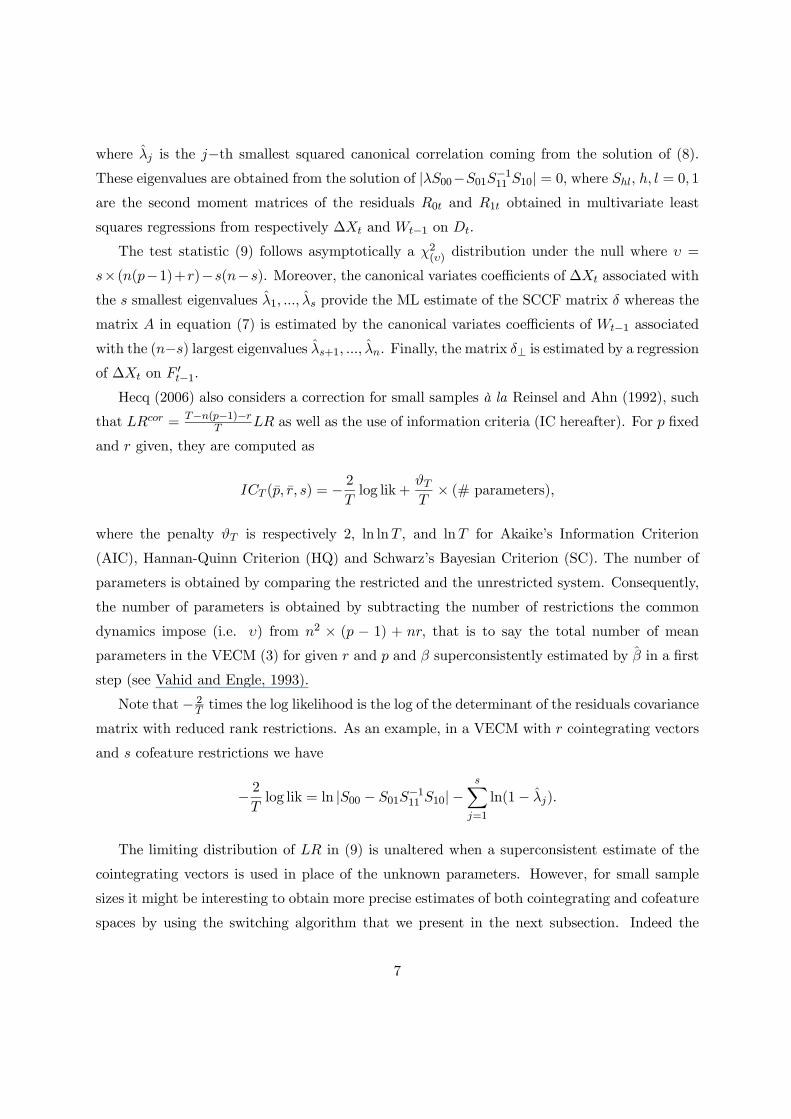
where λj is the j−th smallest squared canonical correlation coming from the solution of (8).

These eigenvalues are obtained from the solution of |λS00−S01S−111 S10| = 0, where Shl, h, l = 0, 1are the second moment matrices of the residuals R0t and R1t obtained in multivariate least

squares regressions from respectively ∆Xt and Wt−1 on Dt.

The test statistic (9) follows asymptotically a χ2(υ) distribution under the null where υ =

s× (n(p−1)+r)−s(n−s). Moreover, the canonical variates coefficients of ∆Xt associated with

the s smallest eigenvalues λ1, ..., λs provide the ML estimate of the SCCF matrix δ whereas the

matrix A in equation (7) is estimated by the canonical variates coefficients of Wt−1 associated

with the (n−s) largest eigenvalues λs+1, ..., λn. Finally, the matrix δ⊥ is estimated by a regressionof ∆Xt on F 0t−1.

Hecq (2006) also considers a correction for small samples à la Reinsel and Ahn (1992), such

that LRcor = T−n(p−1)−rT LR as well as the use of information criteria (IC hereafter). For p fixed

and r given, they are computed as

ICT (p, r, s) = − 2Tlog lik+

ϑTT× (# parameters),

where the penalty ϑT is respectively 2, ln lnT , and lnT for Akaike’s Information Criterion

(AIC), Hannan-Quinn Criterion (HQ) and Schwarz’s Bayesian Criterion (SC). The number of

parameters is obtained by comparing the restricted and the unrestricted system. Consequently,

the number of parameters is obtained by subtracting the number of restrictions the common

dynamics impose (i.e. υ) from n2 × (p − 1) + nr, that is to say the total number of mean

parameters in the VECM (3) for given r and p and β superconsistently estimated by β in a first

step (see Vahid and Engle, 1993).

Note that − 2T times the log likelihood is the log of the determinant of the residuals covariance

matrix with reduced rank restrictions. As an example, in a VECM with r cointegrating vectors

and s cofeature restrictions we have

− 2Tlog lik = ln |S00 − S01S

−111 S10|−

sXj=1

ln(1− λj).

The limiting distribution of LR in (9) is unaltered when a superconsistent estimate of the

cointegrating vectors is used in place of the unknown parameters. However, for small sample

sizes it might be interesting to obtain more precise estimates of both cointegrating and cofeature

spaces by using the switching algorithm that we present in the next subsection. Indeed the

7

PT decomposition crucially depends on r and consequently it is important to estimate it as

accurately as possible.

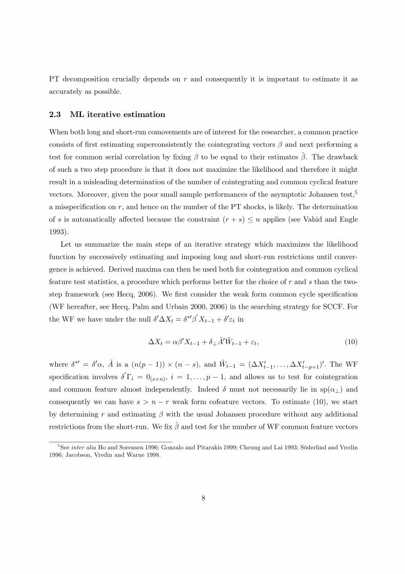
2.3 ML iterative estimation

When both long and short-run comovements are of interest for the researcher, a common practice

consists of first estimating superconsistently the cointegrating vectors β and next performing a

test for common serial correlation by fixing β to be equal to their estimates β. The drawback

of such a two step procedure is that it does not maximize the likelihood and therefore it might

result in a misleading determination of the number of cointegrating and common cyclical feature

vectors. Moreover, given the poor small sample performances of the asymptotic Johansen test,5

a misspecification on r, and hence on the number of the PT shocks, is likely. The determination

of s is automatically affected because the constraint (r + s) ≤ n applies (see Vahid and Engle

1993).

Let us summarize the main steps of an iterative strategy which maximizes the likelihood

function by successively estimating and imposing long and short-run restrictions until conver-

gence is achieved. Derived maxima can then be used both for cointegration and common cyclical

feature test statistics, a procedure which performs better for the choice of r and s than the two-

step framework (see Hecq, 2006). We first consider the weak form common cycle specification

(WF hereafter, see Hecq, Palm and Urbain 2000, 2006) in the searching strategy for SCCF. For

the WF we have under the null δ0∆Xt = δ∗0β0Xt−1 + δ0εt in

∆Xt = αβ0Xt−1 + δ⊥A0Wt−1 + εt, (10)

where δ∗0 = δ0α, A is a (n(p − 1)) × (n − s), and Wt−1 = (∆X 0t−1, . . . ,∆X 0

t−p+1)0. The WF

specification involves δ0Γi = 0(s×n), i = 1, . . . , p − 1, and allows us to test for cointegration

and common feature almost independently. Indeed δ must not necessarily lie in sp(α⊥) and

consequently we can have s > n − r weak form cofeature vectors. To estimate (10), we start

by determining r and estimating β with the usual Johansen procedure without any additional

restrictions from the short-run. We fix β and test for the number of WF common feature vectors

5See inter alia Ho and Sorensen 1996; Gonzalo and Pitarakis 1999; Cheung and Lai 1993; Söderlind and Vredin1996; Jacobson, Vredin and Warne 1998.

8

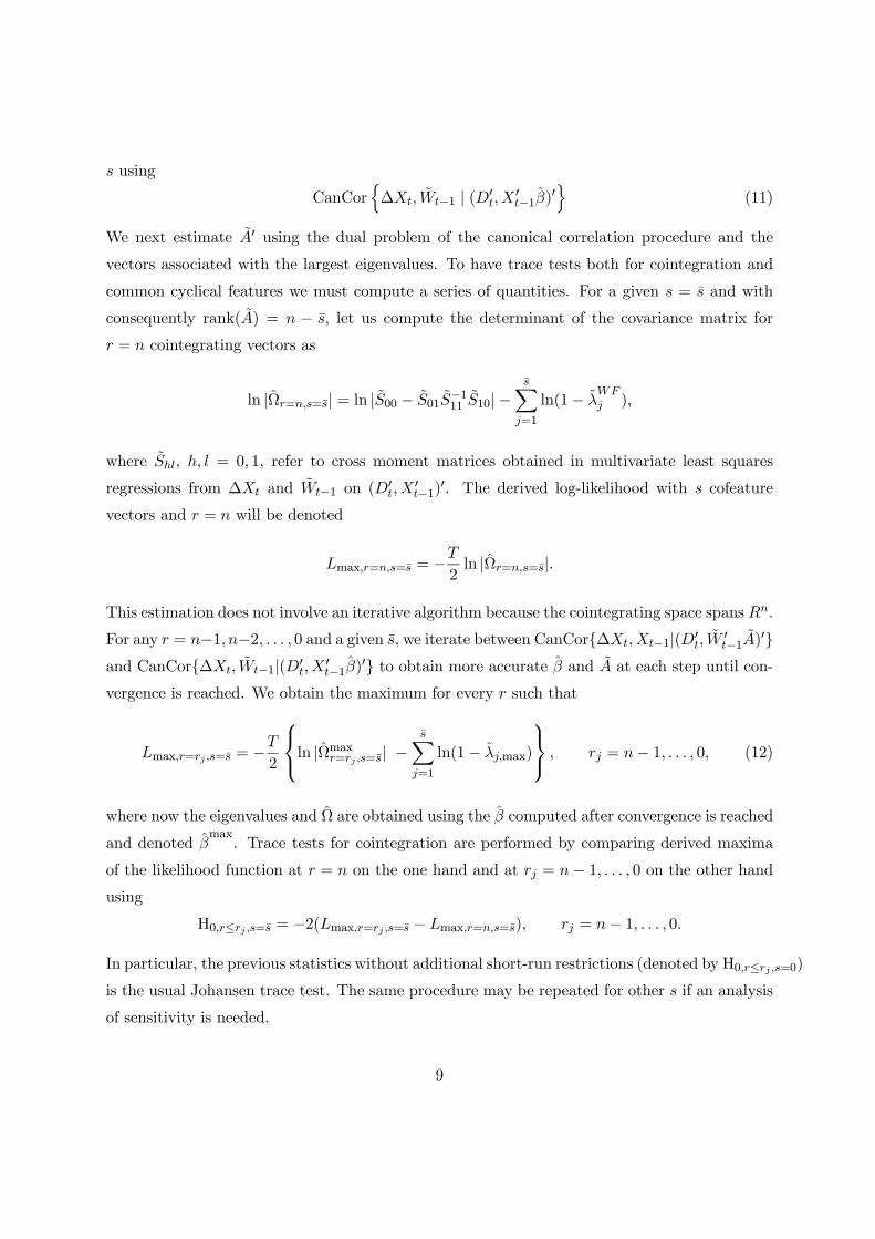
s using

CanCorn∆Xt, Wt−1 | (D0

t,X0t−1β)

0o

(11)

We next estimate A0 using the dual problem of the canonical correlation procedure and the

vectors associated with the largest eigenvalues. To have trace tests both for cointegration and

common cyclical features we must compute a series of quantities. For a given s = s and with

consequently rank(A) = n − s, let us compute the determinant of the covariance matrix for

r = n cointegrating vectors as

ln |Ωr=n,s=s| = ln |S00 − S01S−111 S10|−

sXj=1

ln(1− λWFj ),

where Shl, h, l = 0, 1, refer to cross moment matrices obtained in multivariate least squares

regressions from ∆Xt and Wt−1 on (D0t,X

0t−1)0. The derived log-likelihood with s cofeature

vectors and r = n will be denoted

Lmax,r=n,s=s = −T2ln |Ωr=n,s=s|.

This estimation does not involve an iterative algorithm because the cointegrating space spans Rn.

For any r = n−1, n−2, . . . , 0 and a given s, we iterate between CanCor∆Xt,Xt−1|(D0t, W

0t−1A)0

and CanCor∆Xt, Wt−1|(D0t,X

0t−1β)0 to obtain more accurate β and A at each step until con-

vergence is reached. We obtain the maximum for every r such that

Lmax,r=rj ,s=s = −T

2

ln |Ωmaxr=rj ,s=s| −sX

j=1

ln(1− λj,max)

, rj = n− 1, . . . , 0, (12)

where now the eigenvalues and Ω are obtained using the β computed after convergence is reached

and denoted βmax. Trace tests for cointegration are performed by comparing derived maxima

of the likelihood function at r = n on the one hand and at rj = n− 1, . . . , 0 on the other handusing

H0,r≤rj ,s=s = −2(Lmax,r=rj ,s=s − Lmax,r=n,s=s), rj = n− 1, . . . , 0.

In particular, the previous statistics without additional short-run restrictions (denoted byH0,r≤rj ,s=0)

is the usual Johansen trace test. The same procedure may be repeated for other s if an analysis

of sensitivity is needed.

9

Similarly, tests for common features can be obtained by evaluating the log-likelihood func-

tions at their maxima for one particular r = r = 1, . . . , n for s = 0, . . . , n and by consider-

ing twice their differences at derived maxima. Namely for r fixed we compute H0,r=r,s=sj= −2(Lmax,r=r,s=sj−Lmax,r=r,s=0), where only Lmax,r=r,s=sj needs to be found by iteration from (12),while Lmax,r=r,s=0 is the usual log likelihood obtained in the Johansen test without additional

short-run restrictions.

It is shown in Hecq (2006) how to extend this iterative strategy for SCCF based on Hansen

and Johansen (1998). As that latter procedure is more tedious to apply we take an approximation

in this paper: (i) we take the r and the estimated βmax

obtained with the WF restrictions at

the end of the iteration process and (ii) we test for SCCF using that ”final” βmax.

3 Measuring the business cycle effects of foreign and domestic

shocks

In this section we propose a new statistical measure of the importance of foreign and domestic

shocks over the business cycle. In particular, we show that the statistics proposed by Centoni

and Cubadda (2003) can be modified to decompose the business cycle effects of PT shocks into

those due to their domestic and foreign components.

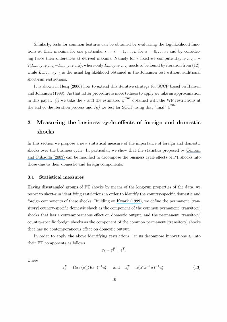
3.1 Statistical measures

Having disentangled groups of PT shocks by means of the long-run properties of the data, we

resort to short-run identifying restrictions in order to identify the country-specific domestic and

foreign components of these shocks. Building on Kwark (1999), we define the permanent [tran-

sitory] country-specific domestic shock as the component of the common permanent [transitory]

shocks that has a contemporaneous effect on domestic output, and the permanent [transitory]

country-specific foreign shocks as the component of the common permanent [transitory] shocks

that has no contemporaneous effect on domestic output.

In order to apply the above identifying restrictions, let us decompose innovations εt into

their PT components as follows

εt = εPt + εTt ,

where

εPt = Ωα⊥(α0⊥Ωα⊥)

−1uPt and εTt = α(α0Ω−1α)−1uTt . (13)

10

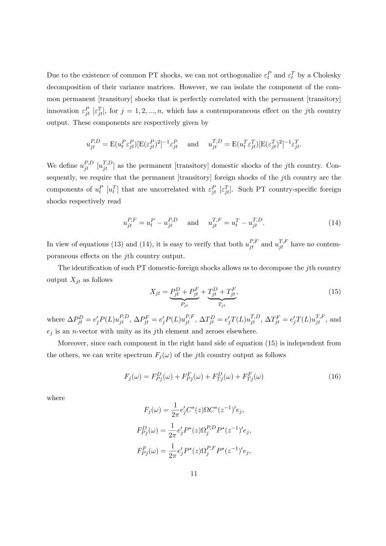
Due to the existence of common PT shocks, we can not orthogonalize εPt and εTt by a Cholesky

decomposition of their variance matrices. However, we can isolate the component of the com-

mon permanent [transitory] shocks that is perfectly correlated with the permanent [transitory]

innovation εPjt [εTjt], for j = 1, 2, ..., n, which has a contemporaneous effect on the jth country

output. These components are respectively given by

uP,Djt = E(uPt εPjt)[E(ε

Pjt)2]−1εPjt and uT,Djt = E(uTt ε

Tjt)[E(ε

Tjt)2]−1εTjt.

We define uP,Djt [uT,Djt ] as the permanent [transitory] domestic shocks of the jth country. Con-

sequently, we require that the permanent [transitory] foreign shocks of the jth country are the

components of uPt [uTt ] that are uncorrelated with εPjt [εTjt]. Such PT country-specific foreign

shocks respectively read

uP,Fjt = uPt − uP,Djt and uT,Fjt = uTt − uT,Djt . (14)

In view of equations (13) and (14), it is easy to verify that both uP,Fjt and uT,Fjt have no contem-

poraneous effects on the jth country output.

The identification of such PT domestic-foreign shocks allows us to decompose the jth country

output Xjt as follows

Xjt = PDjt + PF

jt| z Pjt

+ TDjt + TF

jt| z Tjt

, (15)

where ∆PDjt = e0jP (L)u

P,Djt , ∆PF

jt = e0jP (L)uP,Fjt , ∆T

Djt = e0jT (L)u

T,Djt , ∆TF

jt = e0jT (L)uT,Fjt , and

ej is an n-vector with unity as its jth element and zeroes elsewhere.

Moreover, since each component in the right hand side of equation (15) is independent from

the others, we can write spectrum Fj(ω) of the jth country output as follows

Fj(ω) = FDPj(ω) + FF

Pj(ω) + FDTj(ω) + FF

Tj(ω) (16)

where

Fj(ω) =1

2πe0jC

∗(z)ΩC∗(z−1)0ej ,

FDPj(ω) =

1

2πe0jP

∗(z)ΩP,Dj P ∗(z−1)0ej ,

FFPj(ω) =

1

2πe0jP

∗(z)ΩP,Fj P ∗(z−1)0ej ,

11

FDTj(ω) =

1

2πe0jT

∗(z)ΩT,Dj T ∗(z−1)0ej ,

FFTj(ω) =

1

2πe0jT

∗(z)ΩT,Fj T ∗(z−1)0ej ,

ΩP,Dj = E(uP,Djt uP,D0jt ), ΩT,Dj = E(uT,Djt uT,D0jt ), ΩP,Fj = E(uP,Fjt uP,F 0jt ), ΩT,Fj = E(uT,Fjt uT,F 0jt ),

∆C∗(L) = C(L), ∆P ∗(L) = P (L), ∆T ∗(L) = T (L), z = exp(−iω) for ω ∈ (0, π],6 and

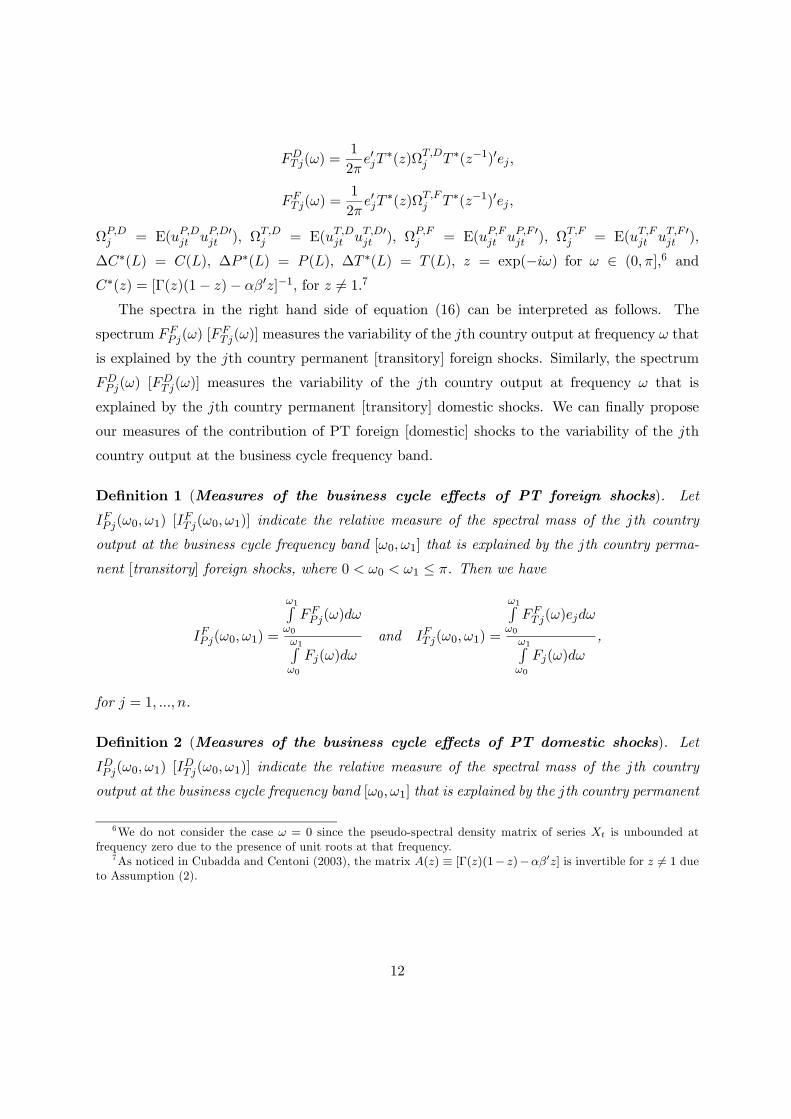
C∗(z) = [Γ(z)(1− z)− αβ0z]−1, for z 6= 1.7The spectra in the right hand side of equation (16) can be interpreted as follows. The

spectrum FFPj(ω) [F

FTj(ω)] measures the variability of the jth country output at frequency ω that

is explained by the jth country permanent [transitory] foreign shocks. Similarly, the spectrum

FDPj(ω) [F

DTj(ω)] measures the variability of the jth country output at frequency ω that is

explained by the jth country permanent [transitory] domestic shocks. We can finally propose

our measures of the contribution of PT foreign [domestic] shocks to the variability of the jth

country output at the business cycle frequency band.

Definition 1 (Measures of the business cycle effects of PT foreign shocks). Let

IFPj(ω0, ω1) [IFTj(ω0, ω1)] indicate the relative measure of the spectral mass of the jth country

output at the business cycle frequency band [ω0, ω1] that is explained by the jth country perma-

nent [transitory] foreign shocks, where 0 < ω0 < ω1 ≤ π. Then we have

IFPj(ω0, ω1) =

ω1Rω0

FFPj(ω)dω

ω1Rω0

Fj(ω)dω

and IFTj(ω0, ω1) =

ω1Rω0

FFTj(ω)ejdω

ω1Rω0

Fj(ω)dω

,

for j = 1, ..., n.

Definition 2 (Measures of the business cycle effects of PT domestic shocks). Let

IDPj(ω0, ω1) [IDTj(ω0, ω1)] indicate the relative measure of the spectral mass of the jth country

output at the business cycle frequency band [ω0, ω1] that is explained by the jth country permanent

6We do not consider the case ω = 0 since the pseudo-spectral density matrix of series Xt is unbounded atfrequency zero due to the presence of unit roots at that frequency.

7As noticed in Cubadda and Centoni (2003), the matrix A(z) ≡ [Γ(z)(1− z)−αβ0z] is invertible for z 6= 1 dueto Assumption (2).

12

[transitory] domestic shocks. Then we have

IDPj(ω0, ω1) =

ω1Rω0

FDPj(ω)dω

ω1Rω0

Fj(ω)dω

and IDTj(ω0, ω1) =

ω1Rω0

FDTj(ω)dω

ω1Rω0

Fj(ω)dω

,

for j = 1, ..., n.

Remark 3 In view of equations (15) and (16), we see that the measures of the business cycle

effects of the PT shocks proposed by Centoni and Cubadda (2003) are respectively given by

IPj(ω0, ω1) = IFPj(ω0, ω1) + IDPj(ω0, ω1) and ITj(ω0, ω1) = IFTj(ω0, ω1) + IDTj(ω0, ω1)

for j = 1, ..., n.

Remark 4 Based on decomposition (15), the relative contributions of foreign and domestic

shocks to the variability of the jth country business cycle respectively read

IFj (ω0, ω1) = IFPj(ω0, ω1) + IFTj(ω0, ω1) and IDj (ω0, ω1) = IDPj(ω0, ω1) + IDTj(ω0, ω1)

for j = 1, ..., n.

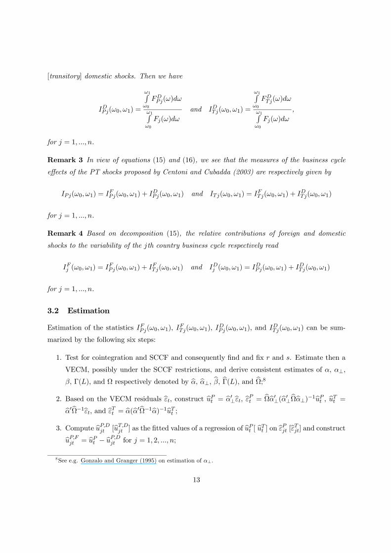
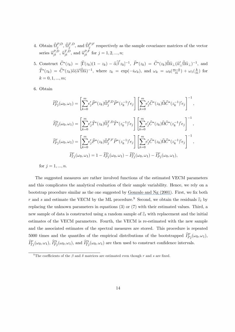
3.2 Estimation

Estimation of the statistics IFPj(ω0, ω1), IFTj(ω0, ω1), I

DPj(ω0, ω1), and IDTj(ω0, ω1) can be sum-

marized by the following six steps:

1. Test for cointegration and SCCF and consequently find and fix r and s. Estimate then a

VECM, possibly under the SCCF restrictions, and derive consistent estimates of α, α⊥,

β, Γ(L), and Ω respectively denoted by bα, bα⊥, bβ, bΓ(L), and bΩ;82. Based on the VECM residuals bεt, construct buPt = bα0⊥bεt, bεPt = bΩbα0⊥(bα0⊥bΩbα⊥)−1buPt , buTt =bα0bΩ−1bεt, and bεTt = bα(bα0bΩ−1bα)−1buTt ;3. Compute buP,Djt [buT,Djt ] as the fitted values of a regression of buPt [ buTt ] on bεPjt [bεTjt] and constructbuP,Fjt = buPt − buP,Djt for j = 1, 2, ..., n;

8See e.g. Gonzalo and Granger (1995) on estimation of α⊥.

13

4. Obtain bΩP,Dj , bΩT,Dj , and bΩP,Fj respectively as the sample covariance matrices of the vector

series buP,Djt , buT,Djt , and buP,Fjt for j = 1, 2, ..., n;

5. Construct bC∗(zk) = [bΓ(zk)(1 − zk) − bαbβ0zk]−1, bP ∗(zk) = bC∗(zk)bΩbα⊥(bα0⊥bΩbα⊥)−1, andbT ∗(zk) = bC∗(zk)bα(bα0bΩbα)−1, where zk = exp(−iωk), and ωk = ω0(m−km ) + ω1(

km) for

k = 0, 1, ...,m;

6. Obtain

bIDPj(ω0, ω1) ="

mXk=0

e0j bP ∗(zk)bΩP,DjbP ∗(z−1k )0ej

#"mXk=0

e0j bC∗(zk)bΩ bC∗(z−1k )0ej

#−1,

bIDTj(ω0, ω1) ="

mXk=0

e0j bT ∗(zk)bΩT,DjbT ∗(z−1k )0ej

#"mXk=0

e0j bC∗(zk)bΩ bC∗(z−1k )0ej

#−1,

bIFPj(ω0, ω1) ="

mXk=0

e0j bP ∗(zk)bΩP,FjbP ∗(z−1k )0ej

#"mXk=0

e0j bC∗(zk)bΩ bC∗(z−1k )0ej

#−1,

bIFTj(ω0, ω1) = 1− bIDPj(ω0, ω1)− bIDTj(ω0, ω1)− bIFPj(ω0, ω1),for j = 1, ..., n.

The suggested measures are rather involved functions of the estimated VECM parameters

and this complicates the analytical evaluation of their sample variability. Hence, we rely on a

bootstrap procedure similar as the one suggested by Gonzalo and Ng (2001). First, we fix both

r and s and estimate the VECM by the ML procedure.9 Second, we obtain the residuals bεt byreplacing the unknown parameters in equations (3) or (7) with their estimated values. Third, a

new sample of data is constructed using a random sample of bεt with replacement and the initialestimates of the VECM parameters. Fourth, the VECM is re-estimated with the new sample

and the associated estimates of the spectral measures are stored. This procedure is repeated

5000 times and the quantiles of the empirical distributions of the bootstrapped bIFPj(ω0, ω1),bIFTj(ω0, ω1), bIDPj(ω0, ω1), and bIDTj(ω0, ω1) are then used to construct confidence intervals.9The coefficients of the β and δ matrices are estimated even though r and s are fixed.

14

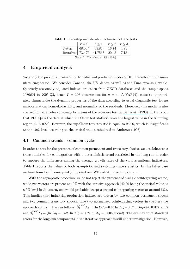
Table 1: Two-step and iterative Johansen’s trace testsr = 0 r ≤ 1 r ≤ 2 r ≤ 3

2-step 68.00* 35.86 16.74 4.81iterative 73.42* 41.75** 20.48 7.18

Note: * (**) reject at 5% (10%)

4 Empirical analysis

We apply the previous measures to the industrial production indexes (IPI hereafter) in the man-

ufacturing sector. We consider Canada, the US, Japan as well as the Euro area as a whole.

Quarterly seasonally adjusted indexes are taken from OECD databases and the sample spans

1980:Q1 to 2005:Q3, hence T = 103 observations for n = 4. A VAR(4) seems to appropri-

ately characterize the dynamic properties of the data according to usual diagnostic test for no

autocorrelation, homoskedasticity, and normality of the residuals. Moreover, this model is also

checked for parameter constancy by means of the recursive test by Bai et al. (1998). It turns out

that 1993:Q4 is the date at which the Chow test statistic takes the largest value in the trimming

region [0.15, 0.85]. However, the sup-Chow test statistic is equal to 26.96, which is insignificant

at the 10% level according to the critical values tabulated in Andrews (1993).

4.1 Common trends - common cycles

In order to test for the presence of common permanent and transitory shocks, we use Johansen’s

trace statistics for cointegration with a deterministic trend restricted in the long-run in order

to capture the differences among the average growth rates of the various national indicators.

Table 1 reports the values of both asymptotic and switching trace statistics. In this latter case

we have found and consequently imposed one WF cofeature vector, i.e. s = 1.

With the asymptotic procedure we do not reject the presence of a single cointegrating vector,

while two vectors are present at 10% with the iterative approach (42.20 being the critical value at

a 5% level in Johansen, one would probably accept a second cointegrating vector at around 6%).

This implies that industrial production indexes are driven by two common permanent shocks

and two common transitory shocks. The two normalized cointegrating vectors in the iterative

approach with s = 1 are as follows: βmax01 Xt = (lnEUt−0.65 lnUSt−0.37 lnJapt+0.0017trend)

and βmax02 Xt = (lnCat − 0.523 lnUSt + 0.69 lnEUt − 0.0068trend). The estimation of standard

errors for the long-run components in the iterative approach is still under investigation. However,

15

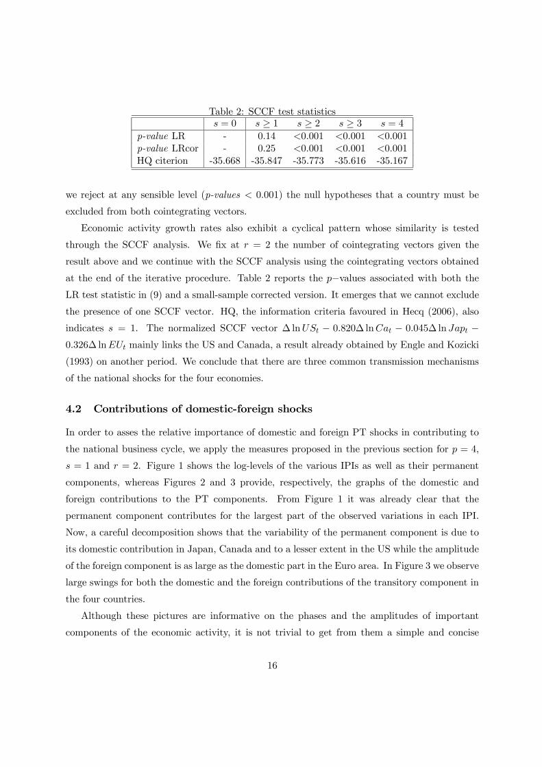
Table 2: SCCF test statisticss = 0 s ≥ 1 s ≥ 2 s ≥ 3 s = 4

p-value LR - 0.14 <0.001 <0.001 <0.001p-value LRcor - 0.25 <0.001 <0.001 <0.001HQ citerion -35.668 -35.847 -35.773 -35.616 -35.167

we reject at any sensible level (p-values < 0.001) the null hypotheses that a country must be

excluded from both cointegrating vectors.

Economic activity growth rates also exhibit a cyclical pattern whose similarity is tested

through the SCCF analysis. We fix at r = 2 the number of cointegrating vectors given the

result above and we continue with the SCCF analysis using the cointegrating vectors obtained

at the end of the iterative procedure. Table 2 reports the p−values associated with both theLR test statistic in (9) and a small-sample corrected version. It emerges that we cannot exclude

the presence of one SCCF vector. HQ, the information criteria favoured in Hecq (2006), also

indicates s = 1. The normalized SCCF vector ∆ lnUSt − 0.820∆ lnCat − 0.045∆ lnJapt −0.326∆ lnEUt mainly links the US and Canada, a result already obtained by Engle and Kozicki

(1993) on another period. We conclude that there are three common transmission mechanisms

of the national shocks for the four economies.

4.2 Contributions of domestic-foreign shocks

In order to asses the relative importance of domestic and foreign PT shocks in contributing to

the national business cycle, we apply the measures proposed in the previous section for p = 4,

s = 1 and r = 2. Figure 1 shows the log-levels of the various IPIs as well as their permanent

components, whereas Figures 2 and 3 provide, respectively, the graphs of the domestic and

foreign contributions to the PT components. From Figure 1 it was already clear that the

permanent component contributes for the largest part of the observed variations in each IPI.

Now, a careful decomposition shows that the variability of the permanent component is due to

its domestic contribution in Japan, Canada and to a lesser extent in the US while the amplitude

of the foreign component is as large as the domestic part in the Euro area. In Figure 3 we observe

large swings for both the domestic and the foreign contributions of the transitory component in

the four countries.

Although these pictures are informative on the phases and the amplitudes of important

components of the economic activity, it is not trivial to get from them a simple and concise

16

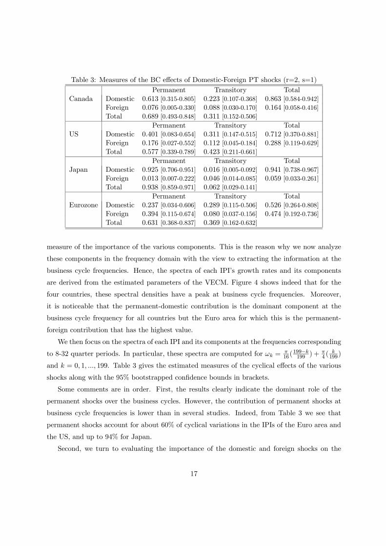
Table 3: Measures of the BC effects of Domestic-Foreign PT shocks (r=2, s=1)Permanent Transitory Total

Canada Domestic 0.613 [0.315-0.805] 0.223 [0.107-0.368] 0.863 [0.584-0.942]Foreign 0.076 [0.005-0.330] 0.088 [0.030-0.170] 0.164 [0.058-0.416]Total 0.689 [0.493-0.848] 0.311 [0.152-0.506]

Permanent Transitory TotalUS Domestic 0.401 [0.083-0.654] 0.311 [0.147-0.515] 0.712 [0.370-0.881]

Foreign 0.176 [0.027-0.552] 0.112 [0.045-0.184] 0.288 [0.119-0.629]Total 0.577 [0.339-0.789] 0.423 [0.211-0.661]

Permanent Transitory TotalJapan Domestic 0.925 [0.706-0.951] 0.016 [0.005-0.092] 0.941 [0.738-0.967]

Foreign 0.013 [0.007-0.222] 0.046 [0.014-0.085] 0.059 [0.033-0.261]Total 0.938 [0.859-0.971] 0.062 [0.029-0.141]

Permanent Transitory TotalEurozone Domestic 0.237 [0.034-0.606] 0.289 [0.115-0.506] 0.526 [0.264-0.808]

Foreign 0.394 [0.115-0.674] 0.080 [0.037-0.156] 0.474 [0.192-0.736]Total 0.631 [0.368-0.837] 0.369 [0.162-0.632]

measure of the importance of the various components. This is the reason why we now analyze

these components in the frequency domain with the view to extracting the information at the

business cycle frequencies. Hence, the spectra of each IPI’s growth rates and its components

are derived from the estimated parameters of the VECM. Figure 4 shows indeed that for the

four countries, these spectral densities have a peak at business cycle frequencies. Moreover,

it is noticeable that the permanent-domestic contribution is the dominant component at the

business cycle frequency for all countries but the Euro area for which this is the permanent-

foreign contribution that has the highest value.

We then focus on the spectra of each IPI and its components at the frequencies corresponding

to 8-32 quarter periods. In particular, these spectra are computed for ωk = π16(

199−k199 ) +

π4 (

k199)

and k = 0, 1, ..., 199. Table 3 gives the estimated measures of the cyclical effects of the various

shocks along with the 95% bootstrapped confidence bounds in brackets.

Some comments are in order. First, the results clearly indicate the dominant role of the

permanent shocks over the business cycles. However, the contribution of permanent shocks at

business cycle frequencies is lower than in several studies. Indeed, from Table 3 we see that

permanent shocks account for about 60% of cyclical variations in the IPIs of the Euro area and

the US, and up to 94% for Japan.

Second, we turn to evaluating the importance of the domestic and foreign shocks on the

17

different economies at the business cycle frequencies. It emerges that for Japan, Canada, and

the US the foreign component of the business cycle is small. Due to its higher degree of openness,

the Eurozone is more sensitive to foreign shocks with a proportion around 47%.

Third, the larger the degree of exposition to foreign shocks, the larger the contribution

of permanent shocks to the foreign component of the business cycle. If one makes the usual

assumption that only productivity shocks have permanent effects on the level of output (see e.g.

Dufourt, 2005), this result is consistent with the view that international technology diffusion is

an important propagation mechanism of permanent shocks across countries. An important force

that generates technology spillovers among countries is international trade of input goods, see

e.g. Coe and Helpman (1995), and Eaton and Kortum (2001).10

Fourth, for all the countries but Japan the domestic component clearly dominates the cyclical

effects of transitory shocks. This finding is in line with the interpretation that transitory shocks

are mainly connected to country-specific monetary and fiscal policies.

It is of interest to compare the above results with previous atheoretical analysis based on

dynamic factor models, even though most of those studies focused on the distinction between

country-specific and international shocks rather than between domestic and foreign shocks. Gre-

gory et al. (1997) and Kose et al. (2003) attributed a more limited role to country-specific shocks

over the national business cycles. A possible explanation of these differences is that our specifi-

cation of the domestic and foreign shocks does not require the overidentifying restrictions that

a factor model imposes to the data.

5 Conclusions

The empirical example of the previous section shows that the methods proposed in this paper

are useful to tackle, in a coherent and integrated setting, issues that were often analyzed in-

dependently in previous studies. These issues are precise and testable definitions of common

shocks and common propagation mechanisms across countries as well as an assessment of the

relative importances of the sources of the business cycles, namely domestic-permanent, foreign-

permanent, domestic-transitory and foreign-transitory shocks. With these elements at hand, it

is thus possible to provide a detailed statistical picture of the international comovements that

theoretical models should account for.

10See e.g. Keller (2004) for a detailed survey on the importance of various channels of international technologydiffusion.

18

We think that our methodology offers two significative advantages over existing approaches

for the analysis of international business cycle. First, differently from most previous studies based

on structural VAR’s (see e.g. Mellander et al., 1992; Ahmed et al., 1993; Kwark, 1999), our

framework allows for unravelling domestic and foreign PT shocks from a set of national outputs

without limiting the analysis to two-country models. Second, we mainly propose an atheoritical

setting. There are pros and cons concerning the use of an atheoritical framework. On the one

hand, we believe that theoretical reasoning can help to disentangle the source of the various

shocks within a structural VAR analysis of different variables for a country. This is the case

when modelling, for instance, output, money, interest rates and prices. In our setting, in which

we want to consider the same variable such as output for a set of countries, not having a priory

may be of value added. On the other hand, differently from other atheoretical analyses based

on dynamic factor models (see e.g. Gregory et al., 1997; Kose et al., 2003), our study allows for

identifying a pair of PT foreign shocks for each country rather than a common worldwide shock

that can have both permanent and transitory effects on output data of a set of countries.

References

[1] Ahmed, S., Ickes, B., Wang, P., and B. Yoo (1993), International Business Cycles,

American Economic Review, 83, 335-359.

[2] Anderson, T.W. (1984), An Introduction to Multivariate Statistical Analysis, 2nd Ed.

(John Wiley & Sons).

[3] Andrews, D.K. (1993), Tests for Parameter Instability and Structural Change with Un-

known Change Point, Econometrica, 61,4, 821-856.

[4] Artis, M.J., Kontolemis, Z., and D. Osborn (1997), Business Cycles for G7 and

European Countries, Journal of Business, 70, 249-79.

[5] Backus, D.K., Kehoe, P.J., and F.E. Kydland (1995), International Business Cycles:

Theory and Evidence, in T. F. Cooley, ed., Frontiers of Business Cycle Research (Princeton

University Press), 331—56.

[6] Bai, J., Lumsdaine, R.L. and J.H. Stock (1998), Testing for and Dating Common

Breaks in Multivariate Time Series, Review of Economic Studies, 65, 395-432.

19

[7] Burns, A.F. and W.C. Mitchell (1946), Measuring Business Cycles, New York:

NBER, 1946, 3.

[8] Canova, F., and J. Marrinan (1998), Sources and Propagation of International Output

Cycles: Common Shocks or Transmission?, Journal of International Economics, 46, 133-

166.

[9] Centoni, M., and G. Cubadda (2003), Measuring the Business Cycle Effects of Per-

manent and Transitory Shocks in Cointegrated Time Series, Economics Letters, 80, 45-51.

[10] Cheung Y.-W., and Lai, K.S. (1993), Finite-sample Sizes of Johansen’s Likelihood

Ratio Tests for Cointegration, Oxford Bulletin of Economics and Statistics, 55, 313-28.

[11] Cheung, Y.-W., and F. Westermann (2002), Output Dynamics of the G7 Countries

- Stochastic Trends and Cyclical Movements, Applied Economics, 34, 2239-2247.

[12] Coe, D.T., and E. Helpman (1995), International R&D Spillovers, European Economic

Review, 39, 859-887.

[13] Cubadda, G., and A. Hecq (2001), On Non-Contemporaneous Short-Run Comove-

ments, Economics Letters, 73, 389-397.

[14] Cubadda G. (2006), A Reduced Rank Regression Approach to Coincident and Leading

Indexes Building, forthcoming in the Oxford Bulletin of Economics and Statistics.

[15] Dufourt, F. (2005), Demand and productivity components of business cycles: Estimates

and implications, Journal of Monetary Economics, 52, 1089-1105

[16] Eaton, J., and S. Kortum (2001), Trade in Capital Goods, European Economic Review,

45, 1195-1235.

[17] Engle, R.F., and S. Kozicki (1993), Testing for Common Features (with comments),

Journal of Business and Economic Statistics, 11, 369-395.

[18] Galì , J. (1999), Technology, Employment, and the Business Cycle: Do Technology Shocks

Explain Aggregate Fluctuations? American Economic Review, 89, 249—271.

[19] Gonzalo, J., and Pitarakis, J.Y. (1999), Dimensionality Effect in Cointegration

Analysis, Chapter 9 in Engle R. and H. White (Ed.), Cointegration, Causality, and Fore-

casting. A Festschrift in Honour of Clive W.J Granger, (Oxford University Press).

20

[20] Gonzalo, J., and C.W.J. Granger (1995), Estimation of Common Long-Memory

Components in Cointegrated Systems, Journal of Business and Economic Statistics, 33,

27-35.

[21] Gonzalo, J., and S. Ng (2001), A Systematic Framework for Analyzing the Dynamic

Effects of Permanent and Transitory Shocks, Journal of Economic Dynamics and Control,

25, 1527-46.

[22] Gregory, A., Head, A., and J. Raynaud (1997), Measuring Word Business Cycles,

International Economic Review, 38, 677-701.

[23] Hansen, P.R. and Johansen, S. (1998),Workbook on Cointegration, (Oxford University

Press: Oxford).

[24] Hecq, A. (2006), Cointegration and Common Cyclical Features in VAR Models: Com-

paring Small Sample Performances of the 2-Step and Iterative Approaches, University of

Maastricht reseach memorandum.

[25] Hecq, A., Palm, F.C. and J.P. Urbain (2000), Permanent-Transitory Decomposition

in VAR Models with Cointegration and Common Cycles, Oxford Bulletin of Economics &

Statistics, 62, 511—532.

[26] Hecq, A., Palm, F.C. and J.P. Urbain (2006), Common Cyclical Features Analysis in

VAR Models with Cointegration, Journal of Econometrics, 132, 117-141.

[27] Ho, M., and Sorensen, B. (1996), Finding Cointegrating Rank in high dimensional sys-

tems Using the Johansen Test. An Illustration Using Data Based Monte Carlo Simulations,

The Review of Economics and Statistics, 78, 726-732.

[28] Jacobson, T., Vredin, A., and Warne, A. (1998), Are Real Wages and Unemployment

Related?, Economica, 65, 69-96.

[29] Johansen, S. (1996), Likelihood-Based Inference in Cointegrated Vector Autoregressive

Models, Oxford University Press.

[30] Keller, W. (2004), International Technology Diffusion, Journal of Economic Literature,

42, 752-82.

21

[31] King, R., Plosser, C., Stock, J., and M. Watson (1991), Stochastic Trends and

Economic Fluctuations, American Economic Review, 81, 819-840.

[32] Kose, M.A., Otrok, C., and C.H. Whiteman (2003), International Business Cycles:

World, Region, and Country-Specific Factors, American Economic Review, 93, 1216-39.

[33] Kwark, N.S. (1999), Sources of International Business Fluctuations: Country-specific

Shocks or Worldwide Shocks?, Journal of International Economics, 48, 367-385.

[34] Mellander, E., Vredin, A., and A. Warne (1992), Stochastic Trends and Economic

Fluctuations in a Small Open Economy, Journal of Applied Econometrics, 7, 369-394.

[35] OECD (2003), Business Tendency Surveys: A Handbook.

[36] Reinsel, G.C. and S.K. Ahn (1992), Vector autoregressive models with unit roots and

reduced rank structure: Estimation, likelihood ratio test, and forecasting, Journal of Time

Series Analysis, Vol. 13, pp. 352-375.

[37] Söderlind, P., and Vredin, A. (1996), Applied Cointegration Analysis in the Mirror

of Macroeconomic Theory, Journal of Applied Econometrics, 11, 363-81.

[38] Vahid, F., and R.F. Engle (1993), Common Trends and Common Cycles, Journal of

Applied Econometrics, 8, 341-360.

[39] Velu, R.P., Reinsel, G.C., and D. W. Wichern (1986), Reduced Rank Models for

Multivariate Time Series, Biometrika, 73, 105-118.

[40] Warne, A. (1993), A Common Trends Model: Identification, Estimation and Inference,

Mimeo, Stockholm School of Economics.

22

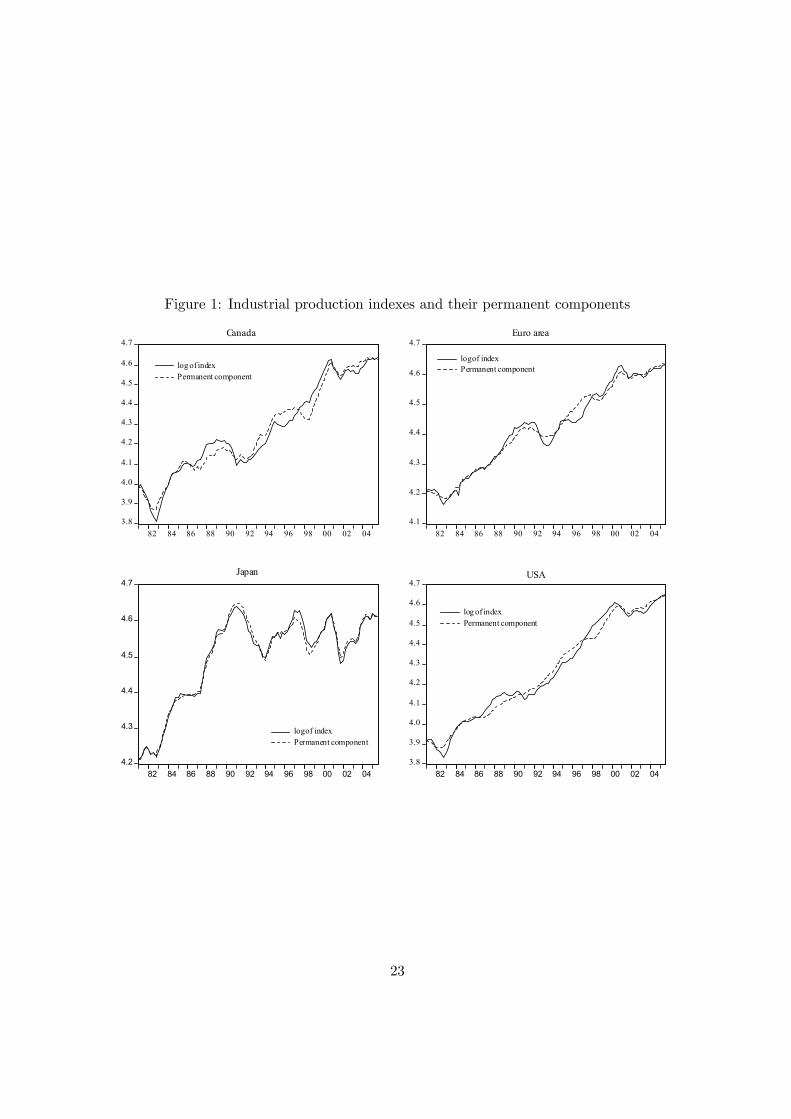
Figure 1: Industrial production indexes and their permanent components

3.8

3.9

4.0

4.1

4.2

4.3

4.4

4.5

4.6

4.7

82 84 86 88 90 92 94 96 98 00 02 04

log of indexPermanent component

Canada

4.1

4.2

4.3

4.4

4.5

4.6

4.7

82 84 86 88 90 92 94 96 98 00 02 04

log of indexPermanent component

Euro area

4.2

4.3

4.4

4.5

4.6

4.7

82 84 86 88 90 92 94 96 98 00 02 04

log of indexPermanent component

Japan

3.8

3.9

4.0

4.1

4.2

4.3

4.4

4.5

4.6

4.7

82 84 86 88 90 92 94 96 98 00 02 04

log of indexPermanent component

USA

23

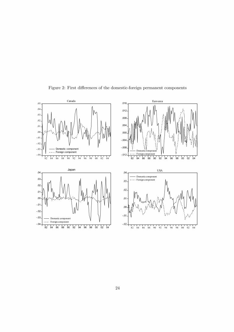
Figure 2: First differences of the domestic-foreign permanent components

-.04

-.03

-.02

-.01

.00

.01

.02

.03

.04

.05

82 84 86 88 90 92 94 96 98 00 02 04

Domestic componentForeign component

Canada

-.012

-.008

-.004

.000

.004

.008

.012

.016

82 84 86 88 90 92 94 96 98 00 02 04

Domestic componentForeign component

Euro area

-.04

-.03

-.02

-.01

.00

.01

.02

.03

.04

82 84 86 88 90 92 94 96 98 00 02 04

Domestic componentForeign component

Japan

-.02

-.01

.00

.01

.02

.03

.04

82 84 86 88 90 92 94 96 98 00 02 04

Domestic componentForeign component

USA

24

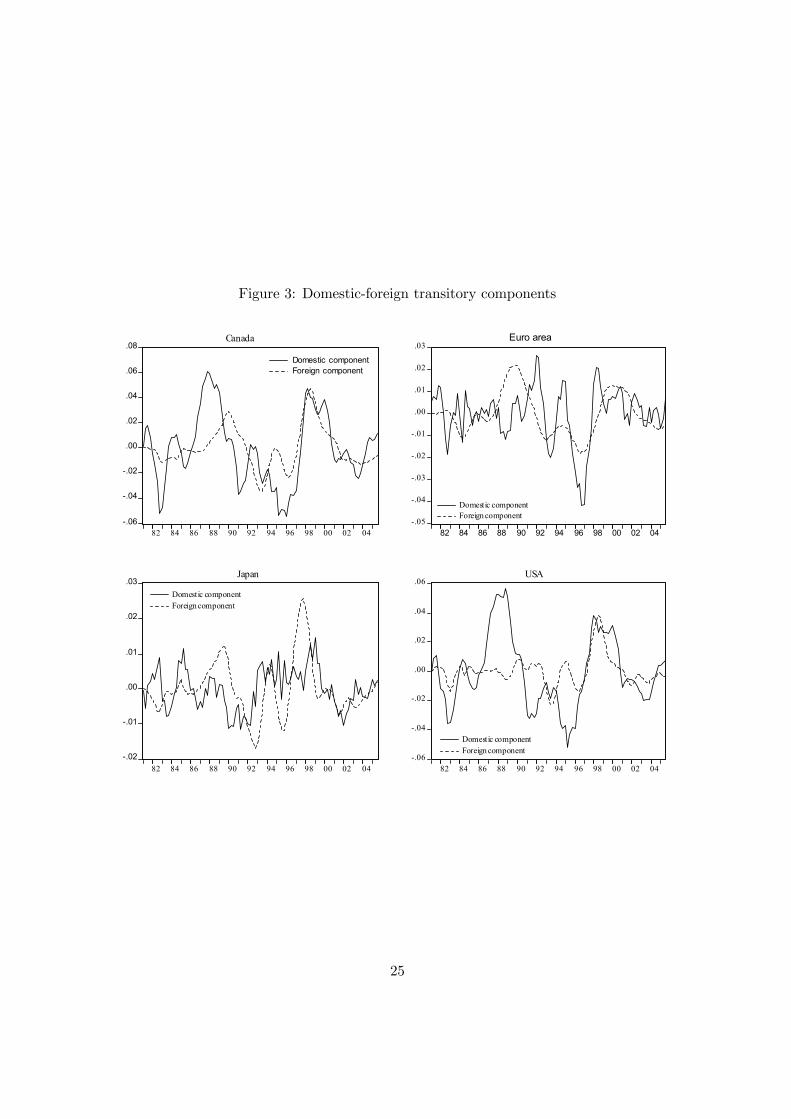
Figure 3: Domestic-foreign transitory components

-.06

-.04

-.02

.00

.02

.04

.06

.08

82 84 86 88 90 92 94 96 98 00 02 04

Domestic componentForeign component

Canada

-.05

-.04

-.03

-.02

-.01

.00

.01

.02

.03

82 84 86 88 90 92 94 96 98 00 02 04

Domestic componentForeign component

Euro area

-.02

-.01

.00

.01

.02

.03

82 84 86 88 90 92 94 96 98 00 02 04

Domestic componentForeign component

Japan

-.06

-.04

-.02

.00

.02

.04

.06

82 84 86 88 90 92 94 96 98 00 02 04

Domestic componentForeign component

USA

25

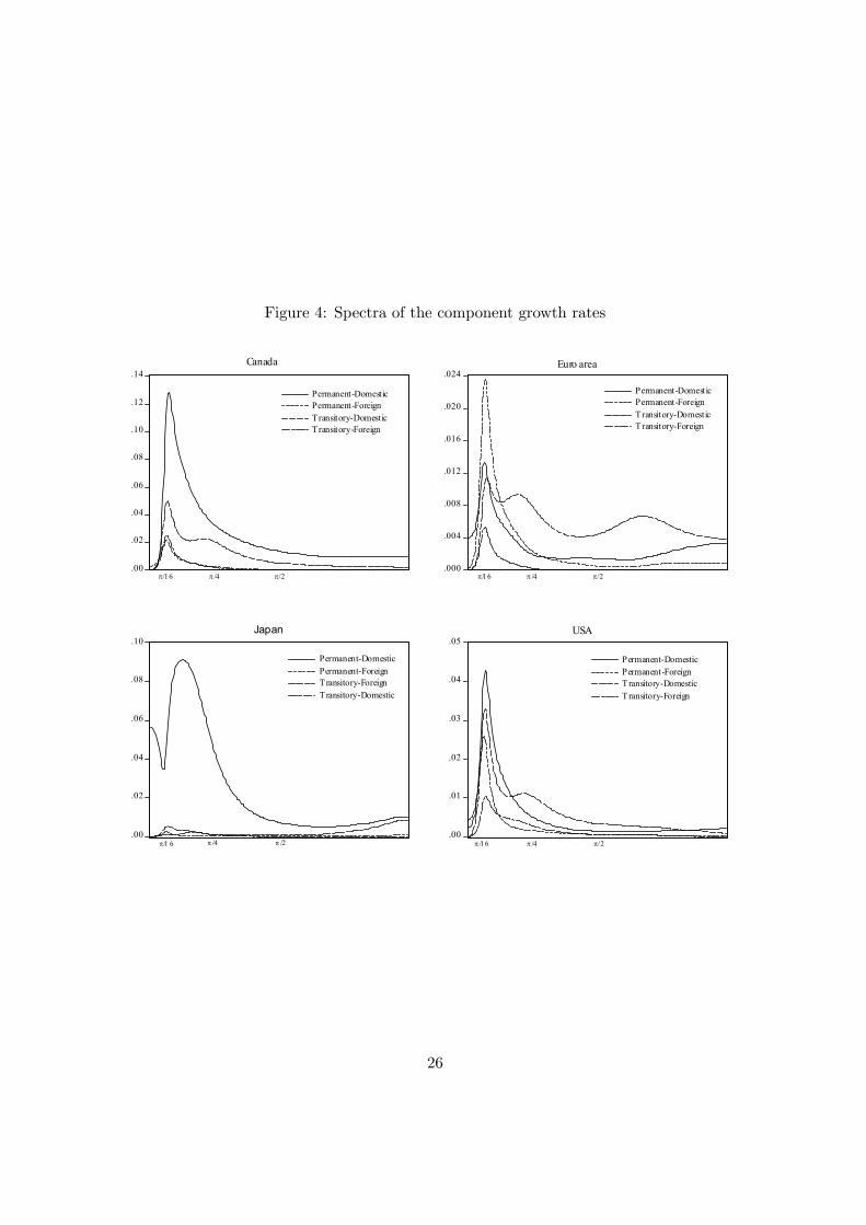
Figure 4: Spectra of the component growth rates

.00

.02

.04

.06

.08

.10

.12

.14

Permanent-DomesticPermanent-ForeignTransitory-DomesticTransitory-Foreign

π/16 π/4 π/2

Canada

.000

.004

.008

.012

.016

.020

.024

Permanent-DomesticPermanent-ForeignTransitory-DomesticTransitory-Foreign

π/16 π/4 π/2

Euro area

.00

.02

.04

.06

.08

.10

Permanent-DomesticPermanent-ForeignTransitory-ForeignTransitory-Domestic

π/1 6 π/4 π /2

Japan

.00

.01

.02

.03

.04

.05

Permanent-DomesticPermanent-ForeignTransitory-DomesticTransitory-Foreign

π/16 π/4 π/2

USA

26