COMPARATIVE ANALYSIS OF SOFTWARE COST AND EFFORT ESTIMATION METHODS: A REVIEW

Omprakash Tailor et al, International Journal of Computer Science and Mobile Computing, Vol.3 Issue.4, April- 2014, pg. 1364-1374

© 2014, IJCSMC All Rights Reserved 1364

Available Online at www.ijcsmc.com

International Journal of Computer Science and Mobile Computing

A Monthly Journal of Computer Science and Information Technology

ISSN 2320–088X

IJCSMC, Vol. 3, Issue. 4, April 2014, pg.1364 – 1374

REVIEW ARTICLE

COMPARATIVE ANALYSIS OF

SOFTWARE COST AND EFFORT

ESTIMATION METHODS: A REVIEW

OMPRAKASH TAILOR1, JYOTI SAINI

2, Mrs. POONAM RIJWANI

3

Student M.Tech, Department of Computer Science and Engineering, Pratap University, Jaipur, India1&2

Assistant Professor & HOD Department of Computer Science and Engineering, Pratap University, Jaipur, India3

[email protected], [email protected], [email protected]

ABSTRACT

Project planning is one of the most important activities in software project. Poor planning often lead to project faults and dramatic

outcomes for the project team. Software effort estimation is a very critical task in the software engineering and to control quality

and efficiency a suitable estimation technique is crucial. This paper gives a comparative analysis of various available software

effort estimation methods. These methods can be widely categorized under algorithmic model, non – algorithmic model, parametric

model and machine learning model. These existing methods for software cost estimation are illustrated and their aspect will be

discussed. No single technique is best for all situations, and thus a careful comparison of the results of several approaches is most

likely to produce realistic estimation. In this paper an example of estimation is also presented in actual software project.

KEYWORDS: Software cost estimation, Delphi, Software Effort Estimation, COCOMO, Machine Learning, Accuracy

I. INTRODUCTION: Software effort estimation is one of the most critical and complex but a key activity in the software development

processes. Generally, the effort and cost estimation are difficult in the software projects . The reason is that software projects are often not unique

and there is no background or previous experience about them. Therefore, prediction seems complicated. In addition, requirements of the

software projects are changing continuously which will cause changing of the prediction. Because of mentioned problems, projects manager

usually try to avoid from using cost or effort estimation or at least do the estimations at a limited domain. It is realized that the importance of all

these models lies in estimating the software development costs and preparing the schedule more quickly and easily in the anticipated

environments. The accuracy of individual model decides their applicability in the projected environments, whereas the accuracy can be defined

based on understanding the calibration of software data, many estimation model have been proposed and can be categorized based on their basic

formulation schemes; estimation by non-algorithmic methods expert, analogy based estimation scheme-algorithmic methods SLOC, FPA, COCOMO,

SEER, SLIM, including machine learning models like artificial neural network based approaches and fuzzy logic based estimation scheme. There are

no best methods for all different environments; they depends upon specific environment available. The main objective of this paper is

demonstrating the abilities of software cost estimation methods and clustering them based on their features which makes helps readers to better



understanding the full paper organized as follows: In section three after introduction and background we briefly overview the estimation

techniques, section four include the comparison of existing methods and finally the conclusion is illustrated is section five.

II. BACKGROUND: Software project failure has been an important subject in the last decade. Software projects usually don’t fail during the

implementation and most project fails during the implementation and most project fails are related to the planning and estimation steps despite

going to over time and cost, approximately between 30% and 40% of the software projects are completed and the other fail(Molokken and

Jorgenson,2003). During the last decade several studies have been done in term of finding the reason of the software project failure. Galorath and

Evans(2006) performed and intensive search between 2100 internet site and found 5500 reason for software project failures. Among the found

reasons, insufficient requirements engineering, poor planning the projects, suddenly decision at the early stages of the project and inaccurate

estimations were the most important reasons. The other researches regarding the reason of project fails show that inaccurate estimation is the

root factor of fail in the most software project fails(Jones,2007; Jorgensen, 2003 ). Despite the indicated statistics may be pessimistic, inaccurate

estimation is a real problem in the software production’s world which should be solved. Presenting the efficient techniques and reliable models

seems required regarding the mentioned problems. The conditions of the software projects are not stable and the state is continuously changing so

several methods should be presented for estimation that each method is appropriate for a special project.

III. ESTIMATION TECHNIQUES: Generally, there are many methods for software cost estimation, which are divided into four categories:

Algorithmic, Non-Algorithmic, Parametric and Machine learning Models. All categories is required for performing the accurate estimation. If the

requirements are known better, their performance will be better. In this section some popular estimation methods are discussed.

A. Algorithmic Models These models work based on the especial algorithm. These model usually need data at first and make result by using the mathematical

relation. Nowadays, many software estimation methods use these models. Algorithm models are classified into some different models.

Each algorithmic model uses an equation to do the estimation: Effort=f(x1,x2,……….,xn) where (x1……xn) is the vector of the cost factor.

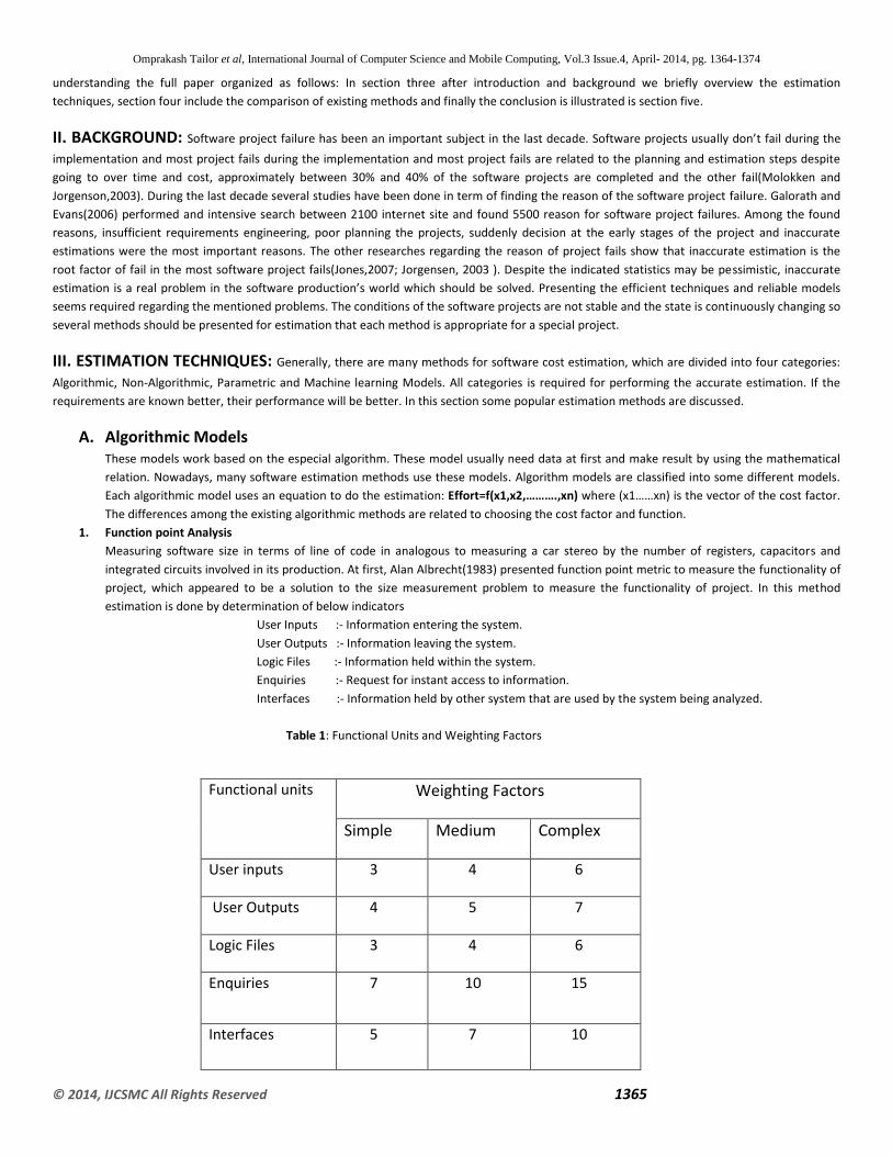
The differences among the existing algorithmic methods are related to choosing the cost factor and function. 1. Function point Analysis

Measuring software size in terms of line of code in analogous to measuring a car stereo by the number of registers, capacitors and

integrated circuits involved in its production. At first, Alan Albrecht(1983) presented function point metric to measure the functionality of

project, which appeared to be a solution to the size measurement problem to measure the functionality of project. In this method

estimation is done by determination of below indicators

User Inputs :- Information entering the system.

User Outputs :- Information leaving the system.

Logic Files :- Information held within the system.

Enquiries :- Request for instant access to information.

Interfaces :- Information held by other system that are used by the system being analyzed.

Table 1: Functional Units and Weighting Factors

Functional units

Weighting Factors

Simple Medium Complex

User inputs 3 4 6

User Outputs 4 5 7

Logic Files 3 4 6

Enquiries 7 10 15

Interfaces 5 7 10



At first, the number of each mentioned indicators should be tallied and then complexity degree and weight are multiplied by each other.

Generally, the unadjusted function point count is defined as below:

UFC=∑ ∑ NijWij i=1 to 5,j=1 to 3

Where Nij= is the number of indicator i with complexity j

Wij= is the weight indicator i with complexity j

According to the previous experiences, function point could be useful for software estimations because it could be computed based on

requirement specification in early stages of the project to compute the FP, UFC should be multiplied by the technical complexity factor which is

obtained from the component in the table 2

Table 2: Technical Complexity Factor Component

F1 Reliable back-up and recovery F5 Complex interface F9 Performance F13 Installation ease

F2 Distributed Function F6 Reusability F10 Online Data Entry F14 Facilitate Change

F3 Heavily used configuration F7 Multiple rites F11 Complex Processing

F4 Operational ease F8 Data Communication F12 Online Update

Each component can change from 0 to 5 and 0 indicate that the component has no effect on the project and the component is

compulsory and very important respectively. Finally, the TCP is calculated as:

TCF=0.65+0.01(∑(Fi))

The range of TCF is between 0.65 and 1.35. Ultimately, function point computed as:

FP=UFC*TCF

2. Source Line Of Code (SLOC)

SLOC is an estimation parameter that illustrates the number of all commands and data definition but it does not include instruction such

as comment, blanks, and continuation lines. This parameter usually used an analogy based on an approach for the estimation after

computing the SLOC for software, its amount is compared with other projects which their SLOC has been computed before, and the size

of project is estimated. SLOC measures the size of project easily. After completing the project, all estimations are compared with the

actual ones. Thousand lines of code(KSLOC) are used for estimation in large scale. SLOC measure seems very difficult at the early stage of

the project. Because of the lack of the information about requirements. Since SLOC computed based on language instructions, comparing

the size of software which uses different languages is too hard. Anyway SLOC is the base of the estimation model in many complicated

software estimation methods. SLOC is usually computed by

S=(SOPT+4SM+SPESS)/6

Where, S=Estimated size, SOPT=Optimistic Value, SM=Most Likely Value, SPESS=Pessimistic Value



3. SEER-SEM(Software Evaluation and Estimation of Resources-Software Estimation Model)

SEER-SEM model has been proposed in 1980 by Galorath Inc(Galorath,2006). Most parameter in this method are commercial and,

business projects usually use SEER-SEM as their main estimation method. Size of the software is the most important features in this

method and a parameter namely so is defined as effective size. Se is computed by determining by determining the five indicators: new

size, existing size, reimpl, and retest as below:-

Se=New size+ Existing Size(0.4Redesign+0.25Reimpl+0.35Retest)

After computing Se the estimated effort is calculated as below:

Effort=D^0.4*(Se/Cte)^1.2

Where D= Relevant to the staffing aspects

Se= Effective size introduced earlier

Cte= effective technology

Once effort is obtained, duration is solved using the following equation

Td=D^-0.2*(Se/Cte)^4

This equation relates the effective size of the system and the technology being applied by the developer to the implementation of the

system.

SEER-SEM has two main limitations on effort estimation

1. There are over 50 input parameter related to the various factors of a project, which increases the complexity of SEER-SEM, especially

for managing the uncertainty from these outputs.

2. The specific details of SEER-SEM increases the difficulty of discovering the nonlinear relationship between parameter inputs and

corresponding outputs. Overall, these two major limitation can lead to a lower accuracy in effort estimation by SEER-SEM.

4. Linear Model

Commonly linear models have the simple structure a trace a clear equation as below:

Effort=a0+∑aixi i=1 to n

Where a1,a2…………an are selected according to the project information.

5. Multiplicative Model

The form of this model is as below

Effort=a0∏ aixi i=1 to n

Where a1………..an are selected according to the project information, only allowed values for xi are -1, 0, +1.

6. Putnam Model

This method has been proposed by Putnam according to manpower distribution and the examination of many software project. The

main equation for Putnam model is

S=(Effort)^1/3 td^4/3………………………………..1

E=Environment indicator



Td= Time of Delivery

S= person year and time of code

Putnam presented another formula for effort as follows:

Effort=Do x td^3………………………………………..2

Do=Manpower build-up factor varies from 8(new software) to 27(Rebuild software)

By Equation 1 & 2

Effort=(Do^4/7 x E^-9/7) x s^9/7……………….3

Td=(Do^-1/7 x E^-3/7) x s^3/7…………………..4

SLIM is a tool that acts according to Putnam model.

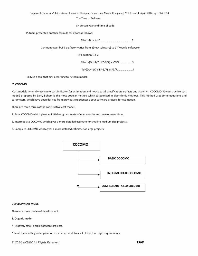
7. COCOMO

Cost models generally use some cost indicator for estimation and notice to all specification artifacts and activities. COCOMO 81(constructive cost

model) proposed by Barry Bohem is the most popular method which categorized in algorithmic methods. This method uses some equations and

parameters, which have been derived from previous experiences about software projects for estimation.

There are three forms of the constructive cost model:

1. Basic COCOMO which gives an initial rough estimate of man months and development time.

2. Intermediate COCOMO which gives a more detailed estimate for small to medium size projects .

3. Complete COCOMO which gives a more detailed estimate for large projects.

DEVELOPMENT MODE

There are three modes of development.

1. Organic mode

* Relatively small simple software projects.

* Small team with good application experience work to a set of less than rigid requirements.

COCOMO

BASIC COCOMO

INTERMEDIATE COCOMO

COMPLETE/DETAILED COCOMO



* Similar to previous developed projects.

* Relatively small and require little innovation.

2. Semi-Detached mode

* Intermediate(in size and complexity) software projects in which team with mixed experience level must meet a mix of rigid and less than rigid

requirements.

3. Embedded mode

Software project that must be developed within set of tight hardware software and operational constraints.

BASIC COCOMO

Basic COCMO is an empirical estimation for estimating effort, cost, and schedule for software projects. It was derived from the large data set from

63 software projects ranging in size from 200 to 100000 lines of code, and programming languages ranging from assembly to PL/I. This data were

analyze to discover a set of formula that were the best fit to the observation these formula link the size of the system. In COCOMO 81 effort is

expressed as person-month and it can be calculated as:

PM= a*Size^6∏Emi i=1 to 15

Where a & b are the domain constant in the model. It contains 15 effort multipliers. This estimation scheme accounts the experience and data of

the past projects which is extremely complex to understand and apply the same.

INTERMEDIATE COCMO

In 1997, an enhanced scheme for estimating the effort for software development activities, which is called as COCOMO II. COCOMO II has some

special features whish distinguish for other one the uses of this method is very hide and its result usually accurate. In COCOMO II effort

requirements can be calculated as:

PM=a* size ^B*∏Emi i=1 to 17

Where E=B+0.01*∑SFj j=1 to 5

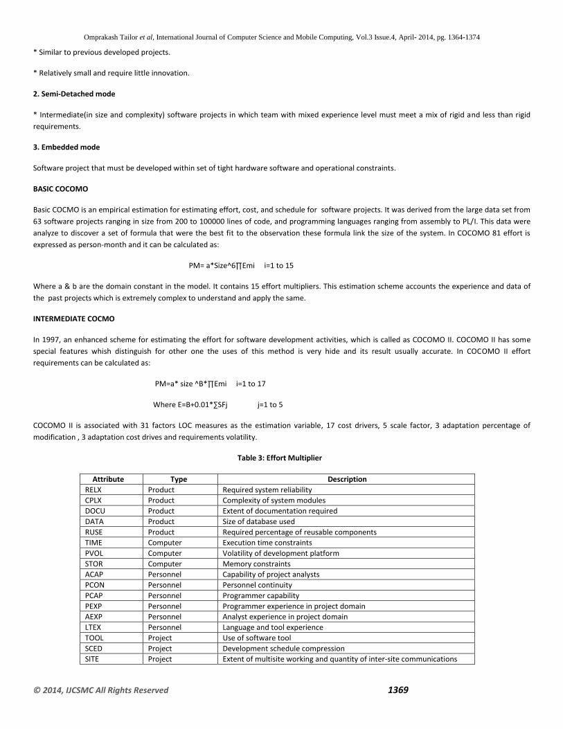
COCOMO II is associated with 31 factors LOC measures as the estimation variable, 17 cost drivers, 5 scale factor, 3 adaptation percentage of

modification , 3 adaptation cost drives and requirements volatility.

Table 3: Effort Multiplier

Attribute Type Description

RELX Product Required system reliability

CPLX Product Complexity of system modules

DOCU Product Extent of documentation required

DATA Product Size of database used

RUSE Product Required percentage of reusable components

TIME Computer Execution time constraints

PVOL Computer Volatility of development platform

STOR Computer Memory constraints

ACAP Personnel Capability of project analysts

PCON Personnel Personnel continuity

PCAP Personnel Programmer capability

PEXP Personnel Programmer experience in project domain

AEXP Personnel Analyst experience in project domain

LTEX Personnel Language and tool experience

TOOL Project Use of software tool

SCED Project Development schedule compression

SITE Project Extent of multisite working and quantity of inter-site communications



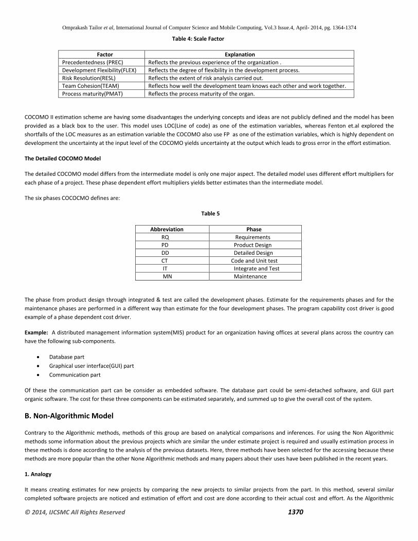
Table 4: Scale Factor

Factor Explanation

Precedentedness (PREC) Reflects the previous experience of the organization .

Development Flexibility(FLEX) Reflects the degree of flexibility in the development process.

Risk Resolution(RESL) Reflects the extent of risk analysis carried out.

Team Cohesion(TEAM) Reflects how well the development team knows each other and work together.

Process maturity(PMAT) Reflects the process maturity of the organ.

COCOMO II estimation scheme are having some disadvantages the underlying concepts and ideas are not publicly defined and the model has been

provided as a black box to the user. This model uses LOC(Line of code) as one of the estimation variables, whereas Fenton et.al explored the

shortfalls of the LOC measures as an estimation variable the COCOMO also use FP as one of the estimation variables, which is highly dependent on

development the uncertainty at the input level of the COCOMO yields uncertainty at the output which leads to gross error in the effort estimation.

The Detailed COCOMO Model

The detailed COCOMO model differs from the intermediate model is only one major aspect. The detailed model uses different effort multipliers for

each phase of a project. These phase dependent effort multipliers yields better estimates than the intermediate model.

The six phases COCOCMO defines are:

Table 5

Abbreviation Phase

RQ Requirements

PD Product Design

DD Detailed Design

CT Code and Unit test

IT Integrate and Test

MN Maintenance

The phase from product design through integrated & test are called the development phases. Estimate for the requirements phases and for the

maintenance phases are performed in a different way than estimate for the four development phases. The program capability cost driver is good

example of a phase dependent cost driver.

Example: A distributed management information system(MIS) product for an organization having offices at several plans across the country can

have the following sub-components.

Database part

Graphical user interface(GUI) part

Communication part

Of these the communication part can be consider as embedded software. The database part could be semi-detached software, and GUI part

organic software. The cost for these three components can be estimated separately, and summed up to give the overall cost of the system.

B. Non-Algorithmic Model

Contrary to the Algorithmic methods, methods of this group are based on analytical comparisons and inferences. For using the Non Algorithmic

methods some information about the previous projects which are similar the under estimate project is required and usually estimation process in

these methods is done according to the analysis of the previous datasets. Here, three methods have been selected for the accessing because these

methods are more popular than the other None Algorithmic methods and many papers about their uses have been published in the recent years.

1. Analogy

It means creating estimates for new projects by comparing the new projects to similar projects from the part. In this method, several similar

completed software projects are noticed and estimation of effort and cost are done according to their actual cost and effort. As the Algorithmic



technique have a disadvantages of the need to calibrate the model. So the alternative approach is ‘Analogy by Estimation’. Estimation based on

analogy is accomplished at the total system levels and subsystem levels. By accessing the result of previous actual projects. We can estimate the

cost and effort of a similar project. The steps of this method are considered as:

1. Choosing the analogy

2. Investigating similarities and differences

3. Examining of analogy quality.

4. providing the estimation.

2. Expert Judgment

Estimation based on Expert Judgment is done by getting advices from experts who have extensive experiences in similar projects. This method is

usually used when there is limitation in finding data and gathering requirements. Consultation is the basic issue in this method. One of the most

common methods which work according to this techniques in Delphi. Delphi arranges an especial meeting among the project experts and tries to

achieve the true information about project from there debates. Delphi includes some steps:

The coordinator gives an estimation from the each expert.

Each expert presents his own estimation

The coordinator gathers all forms and sums up them on a form and ask experts to start another iteration.

Steps (ii-iii) are repeated until an approval is gained.

3. Machine Learning Methods

Most technique about software cost estimation use statistical methods, which are not able to present reason and result. During the last two

decades researcher have been focused on exploring a new approach using AI based techniques for accurate effort estimation. This approach uses

ML a sub field of AI. It is difficult to determine which technique gives more accurate result on which datasets. However, a lot of research has been

done in machine learning technique of estimation and literature suggest that ML methods are capable of providing adequate estimation models as

compare to traditional models especially GSD projects.

ML algorithm offers a practical alternative to the existing approaches to many SE issues. Below we will describe some commonly used methods of

ML for measuring effort and in the next section we will compare these methods. So that this paper may help the practitioners and researchers in

selection of suitable effort estimation methods. Machine learning methods could be categorized into two main methods which are explained in

next sub section.

A. Artificial Neural Network

ANN is a computational or mathematical method that is simulated by the biological human brain. ANN includes several layers. Each layer is

composed of several elements called neurons. Neurons, by investigating the weights defined for inputs produce the outputs. Outputs will be the

actual effort, which is the main goals of estimation. Through learning process ANN can be configured for a specific application, such as pattern

reorganization or data clarification.

Feed Forward Neural Network (FFNN)

Many Neurons are used in the construction of FFNN. These neuron are connected with each other through specific network architecture. There is

no self loop or backward feed in this network. Back propagation neural network is the best selection for software estimation problem. Because it

adjust the weight by comparing the network outputs and actual result. In addition, training is done effectively.

B. Fuzzy Method

All system which work based on the fuzzy logic try to simulate human behavior and reasoning. In many problem which decision making is very

difficult and condition vague. fuzzy system are an efficient tool in such situation. This technique always support that may be ignored. There are four

stages in the fuzzy approach:

1. Fuzzification: To produce trapezoidal number for the linguistic term.



2. To develop the complexity matrix by producing a new linguistic term.

3. To determine the productivity rate and the attempt for the new linguistic term.

4. Defuzzification- To determine effort required to complete a task and to compare the existing method.

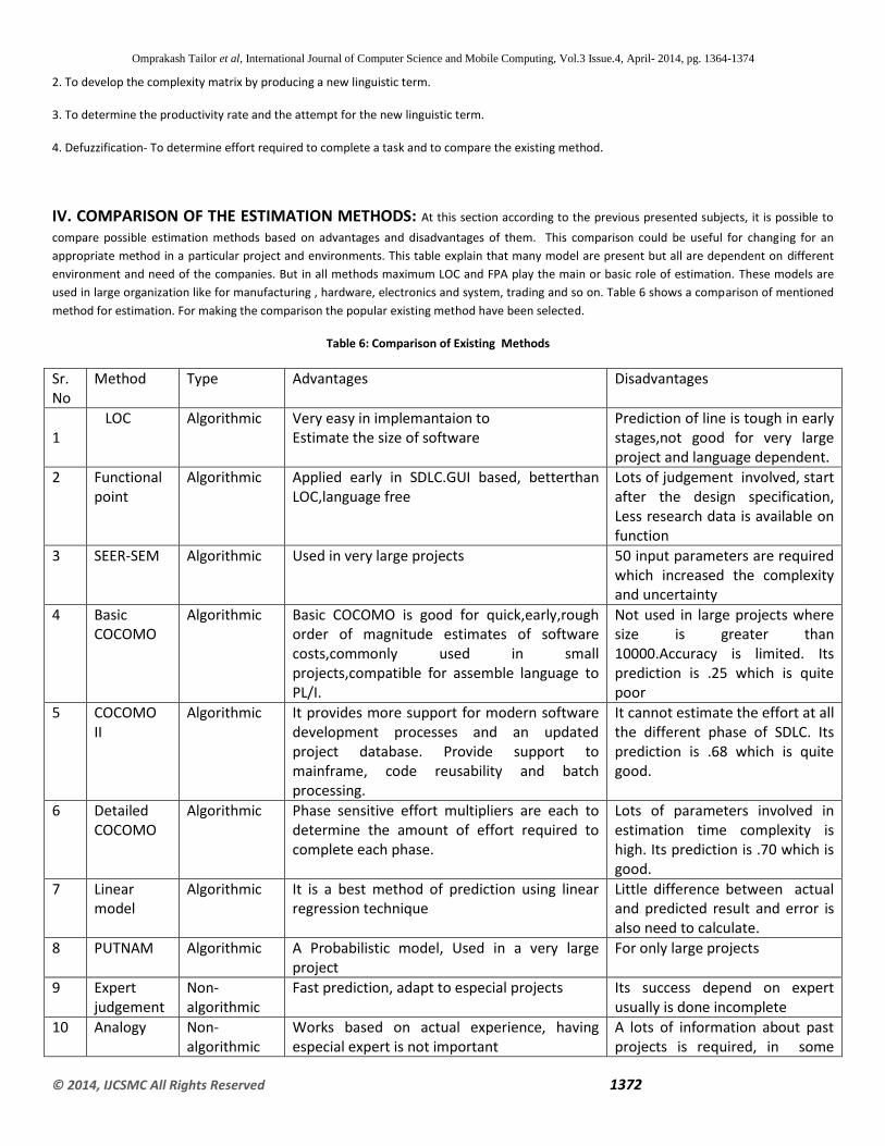
IV. COMPARISON OF THE ESTIMATION METHODS: At this section according to the previous presented subjects, it is possible to

compare possible estimation methods based on advantages and disadvantages of them. This comparison could be useful for changing for an

appropriate method in a particular project and environments. This table explain that many model are present but all are dependent on different

environment and need of the companies. But in all methods maximum LOC and FPA play the main or basic role of estimation. These models are

used in large organization like for manufacturing , hardware, electronics and system, trading and so on. Table 6 shows a comparison of mentioned

method for estimation. For making the comparison the popular existing method have been selected.

Table 6: Comparison of Existing Methods

Sr. No

Method Type Advantages Disadvantages

1

LOC Algorithmic Very easy in implemantaion to Estimate the size of software

Prediction of line is tough in early stages,not good for very large project and language dependent.

2 Functional point

Algorithmic Applied early in SDLC.GUI based, betterthan LOC,language free

Lots of judgement involved, start after the design specification, Less research data is available on function

3 SEER-SEM Algorithmic Used in very large projects 50 input parameters are required which increased the complexity and uncertainty

4 Basic COCOMO

Algorithmic Basic COCOMO is good for quick,early,rough order of magnitude estimates of software costs,commonly used in small projects,compatible for assemble language to PL/I.

Not used in large projects where size is greater than 10000.Accuracy is limited. Its prediction is .25 which is quite poor

5 COCOMO II

Algorithmic It provides more support for modern software development processes and an updated project database. Provide support to mainframe, code reusability and batch processing.

It cannot estimate the effort at all the different phase of SDLC. Its prediction is .68 which is quite good.

6 Detailed COCOMO

Algorithmic Phase sensitive effort multipliers are each to determine the amount of effort required to complete each phase.

Lots of parameters involved in estimation time complexity is high. Its prediction is .70 which is good.

7 Linear model

Algorithmic It is a best method of prediction using linear regression technique

Little difference between actual and predicted result and error is also need to calculate.

8 PUTNAM Algorithmic A Probabilistic model, Used in a very large project

For only large projects

9 Expert judgement

Non-algorithmic

Fast prediction, adapt to especial projects Its success depend on expert usually is done incomplete

10 Analogy Non- algorithmic

Works based on actual experience, having especial expert is not important

A lots of information about past projects is required, in some



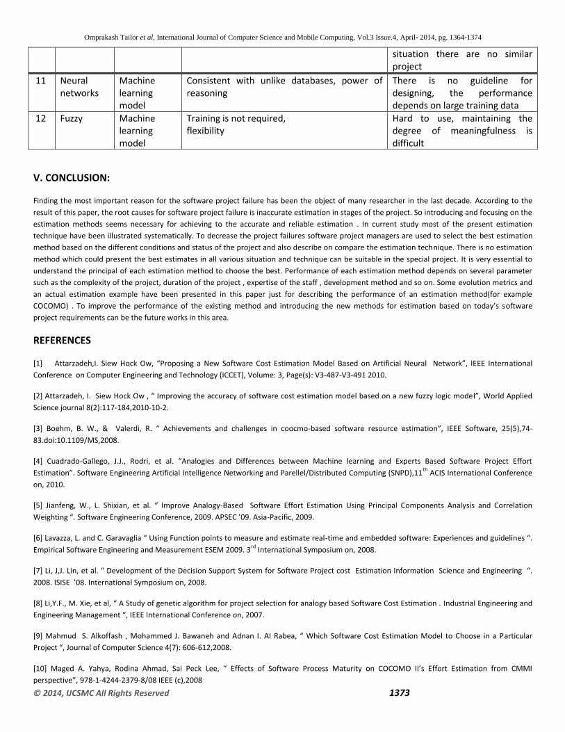
situation there are no similar project

11 Neural networks

Machine learning model

Consistent with unlike databases, power of reasoning

There is no guideline for designing, the performance depends on large training data

12 Fuzzy Machine learning model

Training is not required, flexibility

Hard to use, maintaining the degree of meaningfulness is difficult

V. CONCLUSION:

Finding the most important reason for the software project failure has been the object of many researcher in the last decade. According to the

result of this paper, the root causes for software project failure is inaccurate estimation in stages of the project. So introducing and focusing on the

estimation methods seems necessary for achieving to the accurate and reliable estimation . In current study most of the present estimation

technique have been illustrated systematically. To decrease the project failures software project managers are used to select the best estimation

method based on the different conditions and status of the project and also describe on compare the estimation technique. There is no estimation

method which could present the best estimates in all various situation and technique can be suitable in the special project. It is very essential to

understand the principal of each estimation method to choose the best. Performance of each estimation method depends on several parameter

such as the complexity of the project, duration of the project , expertise of the staff , development method and so on. Some evolution metrics and

an actual estimation example have been presented in this paper just for describing the performance of an estimation method(for example

COCOMO) . To improve the performance of the existing method and introducing the new methods for estimation based on today’s software

project requirements can be the future works in this area.

REFERENCES

[1] Attarzadeh,I. Siew Hock Ow, “Proposing a New Software Cost Estimation Model Based on Artificial Neural Network”, IEEE International

Conference on Computer Engineering and Technology (ICCET), Volume: 3, Page(s): V3-487-V3-491 2010.

*2+ Attarzadeh, I. Siew Hock Ow , “ Improving the accuracy of software cost estimation model based on a new fuzzy logic model”, World Applied

Science journal 8(2):117-184,2010-10-2.

*3+ Boehm, B. W., & Valerdi, R. “ Achievements and challenges in coocmo-based software resource estimation”, IEEE Software, 25(5),74-

83.doi:10.1109/MS,2008.

[4] Cuadrado-Gallego, J.J., Rodri, et al. “Analogies and Differences between Machine learning and Experts Based Software Project Effort

Estimation”. Software Engineering Artificial Intelligence Networking and Parellel/Distributed Computing (SNPD),11th

ACIS International Conference

on, 2010.

*5+ Jianfeng, W., L. Shixian, et al. “ Improve Analogy-Based Software Effort Estimation Using Principal Components Analysis and Correlation

Weighting “. Software Engineering Conference, 2009. APSEC ’09. Asia-Pacific, 2009.

*6+ Lavazza, L. and C. Garavaglia “ Using Function points to measure and estimate real-time and embedded software: Experiences and guidelines “.

Empirical Software Engineering and Measurement ESEM 2009. 3rd

International Symposium on, 2008.

*7+ Li, J,J. Lin, et al. “ Development of the Decision Support System for Software Project cost Estimation Information Science and Engineering “.

2008. ISISE ’08. International Symposium on, 2008.

*8+ Li,Y.F., M. Xie, et al, “ A Study of genetic algorithm for project selection for analogy based Software Cost Estimation . Industrial Engineering and

Engineering Management “, IEEE International Conference on, 2007.

*9+ Mahmud S. Alkoffash , Mohammed J. Bawaneh and Adnan I. AI Rabea, “ Which Software Cost Estimation Model to Choose in a Particular

Project “, Journal of Computer Science 4(7): 606-612,2008.

*10+ Maged A. Yahya, Rodina Ahmad, Sai Peck Lee, “ Effects of Software Process Maturity on COCOMO II’s Effort Estimation from CMMI

perspective”, 978-1-4244-2379-8/08 IEEE (c),2008



*11+ Sikka, G., A. Kaur, et al. “ Estimating function points: Using machine learning and regression models”. Education Technology and Computer

(ICETC), 2nd

International Conference on, 2010.

*12+ Yahya, M. A., R. Ahmad et al. “ Effects of software process maturity on COCOMO II’s effort estimation from CMMI perspective “.

Research Innovation and vision for the future , RIVF. IEEE International Conference on, 2008.

*13+ Yinhuan, Z.,W. Beizhan ,et al. “ Estimation of software projects effort based on function point”. Computer Science & Education ICCSE. 4th

International Conference on, 2009.

[14] Jovan Popovic and Dragan Bojic, “ A Comparative Evolution of Effort Estimation Methods is the Software Life Cycle “, Com SIS Vol. 9, No. 1,

January 2012.

*15+ Mamoona Humayun and Cui Gang , “ Estimating Effort in Global Software Development Projects Using Machine Learning Techniques”,

International Journal of Information and Education Technology , Vol. 2, No. 3, june 2012.

*16+ P.K. Suri, Pallavi Ranjan, “Comparative Analysis of Software Effort Estimation Techniques, International journal of Computer Applications

(0975-8887) volume 48- No. 21, june 2012.

Documents

COMPARATIVE ANALYSIS OF SOFTWARE COST AND EFFORT ESTIMATION METHODS: A REVIEW