water

Article

Compensating Water Service Interruptions toImplement a Safe-to-Fail Approach to ClimateChange Adaptation in Urban Water Supply

Rafael Undurraga 1,*, Sebastián Vicuña 1,2,3 and Oscar Melo 2,4,5

1 Department of Hydraulic and Environmental Engineering, School of Engineering,Pontificia Universidad Católica de Chile, Santiago 7820436, Chile; svicuna@ing.puc.cl

2 Centro Interdisciplinario de Cambio Global, Pontificia Universidad Católica de Chile,Santiago 7820436, Chile; omelo@uc.cl

3 Centro de Investigación para la Gestión Integrada del Riesgo de Desastres, ANID/Fondap/15110017,Santiago 7820436, Chile

4 Department of Agricultural Economics, Pontificia Universidad Católica de Chile, Santiago 7820436, Chile5 Millennium Nucleus Center for the Socioeconomic Impact of Environmental Policies (CESIEP),

Santiago 7820436, Chile* Correspondence: rundurraga1@uc.cl

Received: 27 March 2020; Accepted: 6 May 2020; Published: 27 May 2020�����������������

Abstract: A city resilient to climate change is characterized by effectively responding to and recoveringfrom the negative impacts of climate hazards. In the city of Santiago, Chile, extreme weather thatcan be associated with a nascent manifestation of climate change has caused high-turbidity events,repeatedly forcing the main water company to interrupt the supply of drinking water, affectingmillions of people. This study proposes a transformative response to reduce harm from extreme eventsdue to climate change. The traditional approach of increasing resilience through large infrastructureworks can be complemented by one-off reductions in water use during emergencies, in exchangefor economic compensation. This alternative seeks to transfer the individual responsibility of watercompanies to a collective one, where the community is an active agent that reduces damage in the faceof extreme events resulting from climate change. In the assessment of this response, we used a choiceexperiment to estimate the minimum amount users are willing to accept in compensation for waterservice interruptions. The results show that willingness to accept compensation is significant (closeto 0.6 USD/hour) and decreases when users have experienced additional unplanned interruptions.The aggregate cost of the compensation is lower than infrastructure investments required to avoidservice interruptions under various future hypothetical hydroclimatic scenarios associated withclimate change impacts. Therefore, compensation-based instruments for water service interruptionscould be a more flexible and cost-effective alternative to infrastructure-based measures to cope withfuture climate hazards.

Keywords: climate change; adaptation; willingness to accept compensation; choice experiment;unplanned water interruptions; safe-to-fail

1. Introduction

Climate change presents various scenarios that threaten the continuity of drinking water supplyin cities. The Intergovernmental Panel on Climate Change (IPCC) projects that droughts, increasedrainfall, rising temperatures, and natural hazards will become more frequent and more intense, affectingthe availability and quality of drinking water [1]. Extreme weather events could increase in frequencyand intensity because of climate change [2,3], leading to negative effects not only on water quality

Water 2020, 12, 1540; doi:10.3390/w12061540 www.mdpi.com/journal/water

Water 2020, 12, 1540 2 of 18

but also on the availability of drinking water [4,5]. Risk identification and management are centralelements of adaptation to the projected changes [6]. Water operators must be aware of the possibilitiesof unplanned infrastructure or operational failure, and therefore must have management proceduresto ensure a rapid and adequate response [7].

As cities and urban populations continue to grow, people increasingly depend on the operationof complex water production and distribution systems. Water treatment plants are the cornerstoneof these systems and must operate continuously to meet the demand. Traditionally, the focus ofcity infrastructure in relation to climate hazards has been on fail-safe design (i.e., designing tocontain the hazard and thus avoid the corresponding damage). However, the fail-safe concept isconsidered a dangerous illusion, being unrealistic due to the uncertain and unpredictable nature ofsuch hazards [8]. Given the possibility of the increasing intensity and frequency of extreme events dueto climate change, authorities should question safety planning in cities based on mitigation effortsusing the fail-safe approach.

In addition, planners must address the safe-development paradox [9], where infrastructure-basedadaptation solutions tend to increase the number of people affected if the threat exceeds theinfrastructure’s capacity to prevent damage. Similarly, using reservoirs to increase resilience duringperiods of water shortage can cause greater damage in the face of a failure due to increased demandand the resulting dependence on that infrastructure [10]. Resilience is defined as “the degree to whichthe system minimizes the level of service failure magnitude and duration over its design life whensubject to exceptional conditions” [11] (p. 349). A city resilient to climate change is characterized byeffectively responding to and recovering from the negative impacts of climate hazards.

Unlike the fail-safe approach, Ahern [12] proposes changing the mentality towards a safe-to-failconcept, that is, not to design the systems to avoid failures but to design them to be safe in case theyhappen. In this way, the damage would be controlled and minimized through multifunctionality,redundancy, and modularization strategies. According to the author, the concept of resilience relates tothat of safe-to-fail, where the risk is spread over several interconnected systems so that if one fails, thena support network allows the system to resist, absorb and recover quickly from the negative effects ofthe corresponding threat. Resilience-based designs include adaptive measures, which are defined as“any action taken to modify specific properties of the water system to enhance its capability to maintainlevels of service under varying conditions” [13] (p. 70). Adaptation measures are interventions thatcorrespond to the relationship between the system and the impacts caused by failures that are aconsequence of threats that cannot be mitigated [12,13]. Given the uncertainty regarding the frequencyand magnitude of extreme weather events related to climate change, adaptation strategies can beimplemented to reduce the corresponding impacts.

Policymakers often prefer demand-side management options to supply-side ones, for botheconomic and environmental reasons [14]. Conservation demand measures can significantly reducethe need for investments in supply infrastructure, especially if demand reductions are made firmlyduring periods of shortage. This demonstrates the great potential of demand management and pointsto the need for a more rigorous analysis of infrastructure expansion decisions along with demandmanagement options [15]. To adapt to short-term events resulting from climate change, Vicuña etal. [16] propose demand reduction measures based on a water-savings option-contract. According tothe authors, the objective of this instrument is to give the water utility the right to restrict waterprovision to some users in exchange for monetary compensation, which would extend the drinkingwater service. Therefore, water restrictions that impose prohibitive costs and costly investments instorage infrastructure are avoided. The possibility of reducing consumption in a short time could giveflexibility to the system because it could adapt to events that exceed the design capacity of the storageworks by increasing the autonomy of the system. However, this type of instrument could only beeffective to the extent that it provides a cost-effective solution.

To assess the costs and benefits of a measure such as the one proposed by Vicuña et al. [16],determining users’ willingness to accept compensation (WTAC) is key. Choice modeling is one of the

Water 2020, 12, 1540 3 of 18

methods used to determine WTAC [17]. Under this approach, one of the most widely used techniquesto determine willingness to pay for improved service attributes is the choice experiment [18–20].Using the choice experiment method, these authors studied the variation in the preference for differentwater service attributes and the willingness to pay for improved services through a questionnaire.Few papers using the choice experiment have studied WTAC for a worsening of the water service.MacDonald et al. [21] determined Australian users’ WTAC if the water company is unable to provide acertain level of service. However, this technique has not been used to determine WTAC for voluntaryinterruptions, nor has it been used to evaluate the distribution of compensation based on the differencein cut-off experiences resulting from unforeseen interruptions of drinking water supply. In thesepapers, different econometric models were used to determine preference coefficients, namely, themultinomial probit model [21,22], the conditional logit model [19,20], and the mixed logit model [18,19],which captured the expected deviations in respondents’ preferences.

This study seeks to determine the costs associated with compensation for water serviceinterruptions in the design of adaptation measures for unforeseen but potential disruptions inwater production resulting from climate-change-related extreme turbidity events in the city of Santiago.Specifically, the study seeks to estimate the minimum amount of compensation people are willing toaccept for water service interruptions through the choice experiment method and then compare thecost of the cut-off compensations with the cost of infrastructure under various potential scenarios ofunforeseen interruptions in water production. In the second section, the description and backgroundof the study area are presented in relation to unplanned interruptions in the production of drinkingwater. The third section details the methodology for estimating WTAC and the comparison of costsassociated with compensation for cuts and infrastructure alternatives. The fourth section presentsthe main results, and finally, the fifth section discusses the results found and summarizes the majorconclusions of this study.

2. Description and Background of the Study Area

The city of Santiago, Chile, has about 7 million inhabitants and produces about 40% of Chile’sGDP [16]. Three water companies, which are part of the Aguas Group, are responsible for supplyingdrinking water to 90% of the city’s population: Aguas Andinas S.A., which produces 80%, and AguasCordillera S.A. and Aguas Manquehue S.A., which produce 10%. Servicio Municipal de Agua Potabley Alcantarillado (SMAPA), a municipal service located in the western zone, is in charge of supplyingwater to the remaining 10% of the population. The study area corresponds to the Aguas Group’sconcession area in the city of Santiago located in the Maipo basin (see Figure 1).

Since 2008, the city has been affected by high-turbidity events in the Maipo River, the main sourceof water, located in the southeast of Santiago. The Maipo contributes around 80% of all surface waterresources. A possible cause of the high-turbidity events can be associated with high-temperaturelevels in the Andean zone where the Maipo River headwaters are located. The high-temperaturelevels are associated with a high 0◦ isotherm, which implies a greater area exposed to erosion whenreceiving liquid precipitation instead of snow precipitation. This phenomenon, known as warm storms,is plausibly associated with an early expression of climate change, especially as a result of increasedtemperatures [23,24]. As a result of the river’s high level of turbidity Aguas Andinas (from nowon “the water company”) has had to temporarily interrupt the production of drinking water at itsprimary drinking water plants, Las Vizcachas and La Florida. In some events, water turbidity hasreached more than 380,000 nephelometric turbidity units (NTU), with 3,000 NTU being the maximumpossible turbidity treatable in their water production plants. Currently, the water company has storageinfrastructure that gives it an average autonomy (duration of water supply without production) of 11 h;however, the duration and magnitude of the turbidity events have generated supply cuts affecting alarge portion of the city.

Water 2020, 12, 1540 4 of 18Water 2019, 11, x FOR PEER REVIEW 4 of 18

Figure 1. Study Area: (a) City of Santiago and the Maipo basin; (b) Grupo Aguas’ areas of operation

in Santiago. Modified from Aguas Andinas [22] and Vicuña et al. [16].

Between April 2016 and April 2017, three high-turbidity events (April 2016, February 2017, and

April 2017) caused several hours of service interruption. The duration of the February 2017 event

exceeded 48 hours, affecting more than 1,400,000 homes (customers). In the cases of April 2016 and

April 2017, 1,000,000 and 1,400,000 customers were left without service, respectively. The affected

zones are defined based on the average autonomy of each sector, the number of critical clients (e.g.,

hospitals), and the alternative supply capacity to the Maipo River. It should be noted that the Maipo

River is the major supplier of the affected areas so that in the event of an interruption in water

production due to extreme turbidity events, these areas are left without their main source of raw

water, resulting in supply cuts. This dependence on the Maipo River largely explains the study area’s

vulnerability to unplanned interruptions in water production due to high-turbidity events in the river.

Andean regions such as the headwaters of the Maipo basin are prone to a potential increase of

such events due to climate change, as Pörtner et al. [25] described in depth. Specific scenarios

involving the occurrence of such events in the Maipo basin are not available. According to studies in

nearby basins that show a connection between extreme events such as floods and cryosphere effects

of temperature-related climate change [26,27], it is likely that these types of events will occur more

frequently in the future. However, we are uncertain of the likelihood of such events. It is in this

context of deep uncertainty that city and water resource planners have to decide on the

implementation of solutions that could cope with the current, but also the future, risk of the

occurrence of such events.

3. Methodology

Figure 1. Study Area: (a) City of Santiago and the Maipo basin; (b) Grupo Aguas’ areas of operation inSantiago. Modified from Aguas Andinas [22] and Vicuña et al. [16].

Between April 2016 and April 2017, three high-turbidity events (April 2016, February 2017,and April 2017) caused several hours of service interruption. The duration of the February 2017 eventexceeded 48 h, affecting more than 1,400,000 homes (customers). In the cases of April 2016 and April2017, 1,000,000 and 1,400,000 customers were left without service, respectively. The affected zones aredefined based on the average autonomy of each sector, the number of critical clients (e.g., hospitals),and the alternative supply capacity to the Maipo River. It should be noted that the Maipo River is themajor supplier of the affected areas so that in the event of an interruption in water production dueto extreme turbidity events, these areas are left without their main source of raw water, resulting insupply cuts. This dependence on the Maipo River largely explains the study area’s vulnerability tounplanned interruptions in water production due to high-turbidity events in the river.

Andean regions such as the headwaters of the Maipo basin are prone to a potential increaseof such events due to climate change, as Pörtner et al. [25] described in depth. Specific scenariosinvolving the occurrence of such events in the Maipo basin are not available. According to studies innearby basins that show a connection between extreme events such as floods and cryosphere effectsof temperature-related climate change [26,27], it is likely that these types of events will occur morefrequently in the future. However, we are uncertain of the likelihood of such events. It is in this contextof deep uncertainty that city and water resource planners have to decide on the implementation ofsolutions that could cope with the current, but also the future, risk of the occurrence of such events.

Water 2020, 12, 1540 5 of 18

3. Methodology

3.1. Choice Experiment

3.1.1. Choice Sample

In this study, 606 households in the city of Santiago were randomly selected and surveyed.A face-to-face questionnaire was applied, which is presented in the next section. Because 67 respondentsdid not finish the survey, the final number of completed questionnaires was 539. Figure 2 shows thespatial distribution of the surveyed households according to the number of service interruption eventsthey faced between April 2016 and April 2017. Of the completed questionnaires, 387 correspondedto clients in areas that faced three service interruptions, 122 corresponded to clients in areas withonly one service interruption, and 30 clients resided in an area without service interruptions in theaforementioned period. Figure 2 also presents the zones of the city that endured one and three serviceinterruptions in the period. It can be seen that these events affected almost the entire city, except for thewestern zone, which is supplied by underground extractions of the municipal water company SMAPA(outside of the shaded polygon). Sectors of the northwest, north, and northeast zones were not affectedsince they have alternative sources of supply to the Maipo River, such as wells and the contributions ofthe Mapocho River.

Water 2019, 11, x FOR PEER REVIEW 5 of 18

3.1. Choice Experiment

3.1.1. Choice Sample

In this study, 606 households in the city of Santiago were randomly selected and surveyed. A

face-to-face questionnaire was applied, which is presented in the next section. Because 67

respondents did not finish the survey, the final number of completed questionnaires was 539. Figure

2 shows the spatial distribution of the surveyed households according to the number of service

interruption events they faced between April 2016 and April 2017. Of the completed questionnaires,

387 corresponded to clients in areas that faced three service interruptions, 122 corresponded to clients

in areas with only one service interruption, and 30 clients resided in an area without service

interruptions in the aforementioned period. Figure 2 also presents the zones of the city that endured

one and three service interruptions in the period. It can be seen that these events affected almost the

entire city, except for the western zone, which is supplied by underground extractions of the

municipal water company SMAPA (outside of the shaded polygon). Sectors of the northwest, north,

and northeast zones were not affected since they have alternative sources of supply to the Maipo

River, such as wells and the contributions of the Mapocho River.

Figure 2. Spatial distribution of surveyed households by the number of water service interruptions.

3.1.2. Description of the Questionnaire

Figure 2. Spatial distribution of surveyed households by the number of water service interruptions.

Water 2020, 12, 1540 6 of 18

3.1.2. Description of the Questionnaire

The survey gathered information about participants’ perceptions of climate (e.g., temperature,intensity, and amount of rain), the unplanned water service interruptions, and water service preferences.In addition, a discrete choice exercise was also included at the end of the questionnaire. More precisely,the exercise consisted of presenting the respondents with different contracts with the water company,renewable every three years, where the customer voluntarily accepts temporary water cuts in exchangefor financial compensation. The compensation would translate into a monthly reduction of clients’water bills during the three years from the start of the contract. The contract also specifies the durationand frequency of the proposed cuts. Respondents had the option of declining to accept the contract,maintaining their current household situation without compensation. The methodology used forthe choice experiment follows [28], who proposed six stages for implementing the method (Table 1).The first stage is the selection of attributes to be included in the choice exercise. In this case, we selectedthe frequency and duration of the service interruptions, and compensation translated into a reductionof the water bill. These attributes were determined based on the existing literature [18,21] and thenadapted to the study area and type of measure proposed. The frequency was presented as the numberof service interruptions in the next three years, the duration referred to the duration of each serviceinterruption, and the compensation was presented as monthly bill reduction for the next three years.

Table 1. Stages of the choice experiment methodology.

N Stage Description

1 Attribute selection Identification of relevant attributes to be evaluated2 Level assignment Assignment of levels for each attribute

3 Choice of experimental design Choice of theoretical statistical design to combine attribute levels inseveral scenarios with various choice alternatives

4 Construction of options Identification of the experimental design groups and selection of thenumber of choice scenarios to be presented to each respondent

5 Measurement of preferences Choice of survey procedure to measure individual preferences6 Estimation procedure Choice of the estimation procedure and corresponding model

Note: Adapted from Hanley [28].

In the second stage, the levels of each attribute were constructed according to the characteristicsand particularities of the turbidity-related service interruptions in recent years. Then, based on differentpilot surveys carried out previously, the values of the levels were adjusted based on expert judgements,comments, and suggestions from the respondents (see Table 2).

Table 2. Attributes and levels of the exercise.

Attributes Unit Levels

Frequency Cuts in three years 2 3 4Duration hour/cut 12 24 36

Compensation LC USD 1/month 2.9 5.7 8.6Compensation HC USD/month 4.3 8.6 12.9

Note: 1 Approximate value of the dollar in June 2019 (1 USD = 700 CLP).

The levels of the frequency and duration attribute were common to all respondents, whereas thelevels of compensation varied according to the average declared monthly water bill. Two types ofusers were distinguished: low consumption (LC), whose average monthly cost was less than 28.6 USD,and high consumption (HC), whose average monthly cost was greater than 28.6 USD. Based on theseamounts, the compensation levels for LC users were set to 2.9, 5.7, and 8.6 USD per month, whereasfor HC users, they were 4.3, 8.6, and 12.9 USD per month. The differentiation was intended to adjustthe proposed compensation values to a significant percentage of the respondents’ monthly bills.

Water 2020, 12, 1540 7 of 18

In the third stage, an orthogonal experimental design was created using Ngene software [29],with three attributes (three levels each), two choice alternatives, and 18 choice scenarios (divided intothree blocks of six choice scenarios). One of the limitations of this design is that it does not maintaina balance of levels in each block, and, in certain choice scenarios, it delivers alternatives that areobjectively superior to others (equal or better levels in each of the attributes). Levels were exchangedbetween the different blocks and alternatives to balance the levels at both the situation and block level.After such exchanges, the correlations between the attributes of the different alternatives were verified(Table 3), trying to maintain the correlations of the original orthogonal design and ensure they did notexceed the value of 0.5. Attribute A1 refers to the frequency of Alternative A, A2 refers to the durationattribute, and A3 refers to the compensation attribute, whereas the attributes of Alternative B are similar.Although there is an orthogonality loss, the correlations between attributes of the alternatives remainedlow (less than 0.5), so this design was used to construct the choice scenarios for the respondents.

Table 3. Correlation between attributes of the experimental design alternatives.

Alternative A1 A2 A3 B1 B2 B3

A1 1.000A2 0.000 1.000A3 0.333 −0.167 1.000B1 −0.333 −0.250 0.083 1.000B2 −0.250 −0.083 0.250 0.083 1.000B3 −0.333 0.000 0.083 0.250 0.000 1.000

Note: Results derived from calculations using Ngene software.

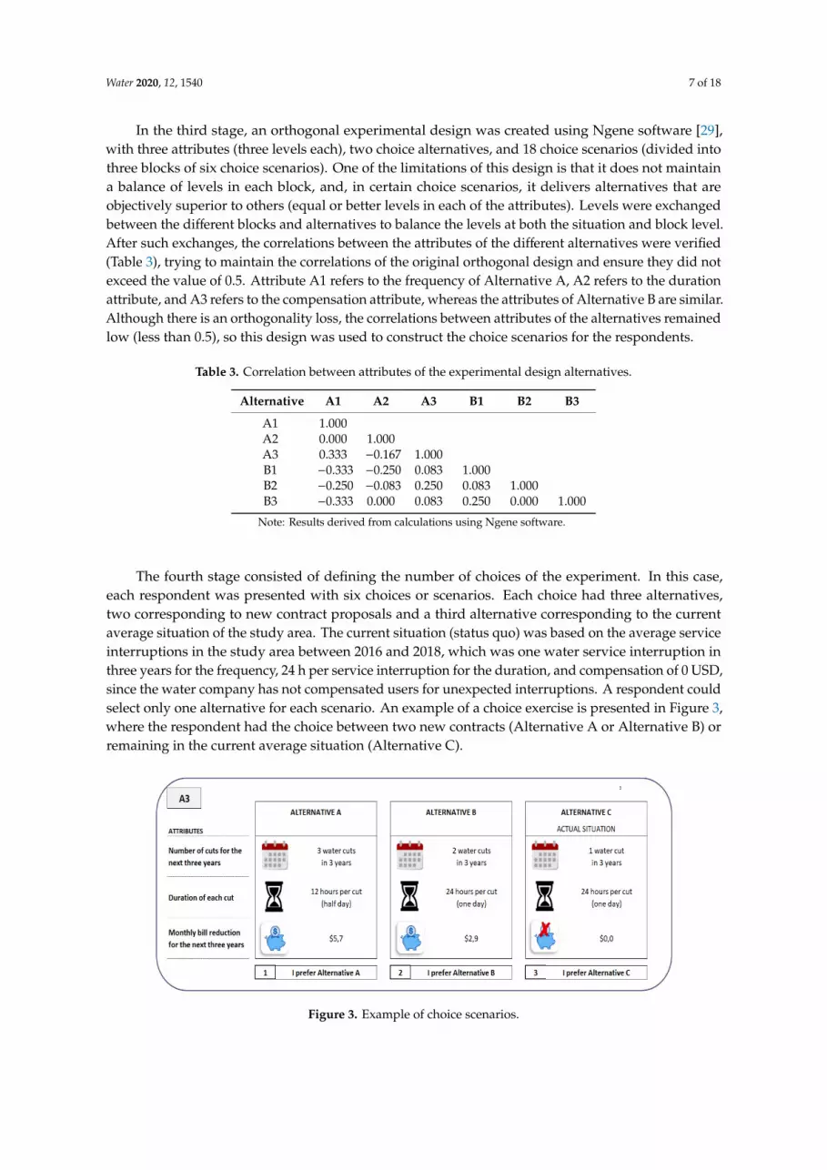
The fourth stage consisted of defining the number of choices of the experiment. In this case,each respondent was presented with six choices or scenarios. Each choice had three alternatives,two corresponding to new contract proposals and a third alternative corresponding to the currentaverage situation of the study area. The current situation (status quo) was based on the average serviceinterruptions in the study area between 2016 and 2018, which was one water service interruption inthree years for the frequency, 24 h per service interruption for the duration, and compensation of 0 USD,since the water company has not compensated users for unexpected interruptions. A respondent couldselect only one alternative for each scenario. An example of a choice exercise is presented in Figure 3,where the respondent had the choice between two new contracts (Alternative A or Alternative B) orremaining in the current average situation (Alternative C).

Water 2019, 11, x FOR PEER REVIEW 7 of 18

In the third stage, an orthogonal experimental design was created using Ngene software [29],

with three attributes (three levels each), two choice alternatives, and 18 choice scenarios (divided into

three blocks of six choice scenarios). One of the limitations of this design is that it does not maintain

a balance of levels in each block, and, in certain choice scenarios, it delivers alternatives that are

objectively superior to others (equal or better levels in each of the attributes). Levels were exchanged

between the different blocks and alternatives to balance the levels at both the situation and block

level. After such exchanges, the correlations between the attributes of the different alternatives were

verified (Table 3), trying to maintain the correlations of the original orthogonal design and ensure

they did not exceed the value of 0.5. Attribute A1 refers to the frequency of Alternative A, A2 refers

to the duration attribute, and A3 refers to the compensation attribute, whereas the attributes of

Alternative B are similar. Although there is an orthogonality loss, the correlations between attributes

of the alternatives remained low (less than 0.5), so this design was used to construct the choice

scenarios for the respondents.

Table 3. Correlation between attributes of the experimental design alternatives.

Alternative A1 A2 A3 B1 B2 B3

A1 1.000

A2 0.000 1.000

A3 0.333 −0.167 1.000

B1 −0.333 −0.250 0.083 1.000

B2 −0.250 −0.083 0.250 0.083 1.000

B3 −0.333 0.000 0.083 0.250 0.000 1.000

Note. Results derived from calculations using Ngene software.

The fourth stage consisted of defining the number of choices of the experiment. In this case, each

respondent was presented with six choices or scenarios. Each choice had three alternatives, two

corresponding to new contract proposals and a third alternative corresponding to the current average

situation of the study area. The current situation (status quo) was based on the average service

interruptions in the study area between 2016 and 2018, which was one water service interruption in

three years for the frequency, 24 hours per service interruption for the duration, and compensation

of 0 USD, since the water company has not compensated users for unexpected interruptions. A

respondent could select only one alternative for each scenario. An example of a choice exercise is

presented in Figure 3, where the respondent had the choice between two new contracts (Alternative

Figure 3. Example of choice scenarios.

3.1.3. Description of the Econometric Model

The econometric model used to determine the WTAC corresponds to the mixed logit model,

which captures the expected deviations in respondents’ preferences [18,19]. According to the theory

Figure 3. Example of choice scenarios.

Water 2020, 12, 1540 8 of 18

3.1.3. Description of the Econometric Model

The econometric model used to determine the WTAC corresponds to the mixed logit model,which captures the expected deviations in respondents’ preferences [18,19]. According to the theory ofrandom utility [30], the utility function Ui j associated with individual i choosing alternative j is givenby Equation (1):

Ui j = V(Xi j

)+ εi j (1)

The vector of the attributes (Xi j) varies for each individual i and alternative j, V (*) represents theindirect utility function, and εi j represents the error component that varies for each individual i andalternative j. Since the mixed logit model considers the heterogeneity between individuals, the utilityfunction is modified according to Equation (2):

Ui j = V(Xi j ∗ βi

)+ εi j (2)

βi = β+ δi (3)

The term (βi) is the vector of preferences coefficients associated with attributes that vary foreach individual i, β represents the vector of the preference coefficients of the attributes, invariantbetween individuals, and δi corresponds to the preference deviations that vary for each individual i (3).The utility function can then be written according to Equation (4):

Ui j = V(Xi j ∗ β+ Xi j ∗ δi

)+ εi j (4)

The probability of individual i selecting alternative j from a set of K alternatives can be writtenaccording to Equation (5):

Pri j =exp

[Xi j ∗ β+ Xi j ∗ δi

]∑K

k=1 exp [Xik ∗ β+ Xik ∗ δi](5)

The parameters of the mixed logit model were estimated using the statistical software Stata12 [31]. The implemented routine is based on the examples of the mixed logit model developedby [32]. Deviations in preferences between individuals are assumed for the three selected attributes.WTAC for a marginal change in duration for the different groups can be calculated using Equation (6),which is derived from the marginal replacement rate [18]. The coefficients of the vector β (βduration andβcompensation) stand for the attributes of duration and compensation, respectively.

WTAC =−βduration

βcompensation(6)

3.2. Comparison of Infrastructure and Compensation Costs

This study proposes the use of net present value (NPV) to compare the value of future flows ofdifferent alternatives in the present. The expression of NPV (USD) is presented in Equation (7):

NPV =T∑

t=0

Ct

(1 + r)t (7)

where Ct (USD) is the cost at time t, r is the discount rate, and T (years) is the study period. The expressionof the cost Ct (USD) is presented in Equation (8):

Ct = Cc ∗Ncl ∗DE ft (8)

Water 2020, 12, 1540 9 of 18

where Cc (USD/hr ∗Cl) is the hourly compensation cost for each client, Nclients (Cl) is the number ofcustomers to be compensated, and DE ft (hr) is the effective duration of the cut at time t. The expressionof the effective duration DE ft (hr) is presented in Equation (9):

DE ft = Dt −At (9)

where Dt (hr) is the potential duration of the cutting event without autonomy at time t, and At (hr) is theautonomy of the system at time t. Only investment cost is considered for the infrastructure alternativesIn at t = 0. Operating and maintenance costs are not contemplated due to the lack of information.

4. Results

4.1. Sample Description

Regarding the respondents’ characteristics, 61% have an educational level of middle schoolor lower, 73% declared monthly income of less than or equal to USD 1143, and 90% represents asocioeconomic level observed by the surveyors as medium or low. In addition, 88% of respondentslived in houses and 12% lived in apartments; 74% of the houses were owned and 20% were rented.Furthermore, 86% of the respondents paid less than 43 USD per month for drinking water service,with 47% paying between USD 16 and 26. Eighty-two percent of the respondents considered theamount they paid per month to be regular or very high (above 3 on a scale of 1 to 5). Overall,respondents perceive that in the last 10 years, the climate has permanently changed, with a higheraverage temperature, less (but more intense) rain, and an increase in the number of alluviums. It isworth mentioning that 94% of the respondents considered that the climate will change in the next10 years, following the same trend as in the last 10 years.

The results show that most of the respondents understand the effects of climate change on climatevariables and the threats affecting the continuity of the drinking water supply in the study area.The results may be relevant when analyzing the percentage of respondents who are willing to acceptcompensation for cuts. Given this, by perceiving a change in the future climate, the relevance ofthe proposed exercise could increase since these future events would be perceived as more intenseand frequent than those that have occurred recently. Of the 539 valid responses, 81% of householdswere willing to accept service interruption compensation (i.e., at least one choice of Alternative A orB within the six choice scenarios presented to each respondent). Factoring in 67 discarded surveys,the percentage of respondents who were willing to accept compensation drops to 72%. Of the remaining19%, 12% considered the proposed service interruptions to be too long, 4% considered the serviceinterruption frequency to be too high, and 3% considered the proposed compensation amounts to betoo low. With respect to the distribution of responses between alternatives, 31% chose Alternative C,the status quo. In contrast, when respondents were asked if they would be willing to pay to avoidsupply cuts, 79% answered that they would not be willing, whereas 12% would be.

Table 4 presents a description of the sample for the different subsamples analyzed. Sample Arepresents the respondents with the most experience in water service interruptions against turbidityevents, Sample B incorporates those of Sample A plus the clients with one service interruption,Sample C contains only the respondents with one service interruption, and Sample D contains all therespondents (zero, one, and three service interruptions). We did not select a sample with only the zeroservice interruption respondents because it was too small (N = 30).

Water 2020, 12, 1540 10 of 18

Table 4. Subsample description.

Subsample Description N

A Three cuts zone 387B One or three cuts zone 509C One cut zone 122D All the zones 539

Note: N = the number of households surveyed.

4.2. Estimated Results of Willingness to Accept Compensation (WTAC)

Table 5 presents the results of the mixed logit model estimation for the different subsamples.We see that in all subsamples, the frequency and duration have a negative coefficient (i.e., the higher thefrequency or duration of a choice alternative, the lower the probability that the respondent will selectit). Conversely, the compensation coefficient has a positive sign (i.e., the greater the compensationof a choice alternative, the greater the probability that the respondent will select it). The signs of theattribute coefficients are consistent and in line with those found in the literature. Most coefficients aresignificant at the 1% level, except for the frequency for Samples A and C and the compensation forSample C (significant at 5%). With respect to standard deviation, all coefficients show 1% significance,which demonstrates deviations in respondent preferences for each of the attributes studied.

Table 5. Mixed logit model results.

Attributes Mean Standard Deviation

Sample A Coef. z P > |z| Coef. z P > |z|Frequency −0.1328462 −2.21 * 0.027 0.394129 2.84 ** 0.005Duration −0.0364866 −6.10 ** 0.000 0.0744567 10.78 ** 0.000

Compensation 0.0001064 2.89 ** 0.004 −0.0005028 −11.33 ** 0.000Sample BFrequency −0.148164 −2.80 ** 0.005 −0.4711221 −6.17 ** 0.000Duration −0.0376577 −7.41 ** 0.000 0.0699749 11.76 ** 0.000

Compensation 0.0001052 3.52 ** 0.000 0.0004669 14.50 ** 0.000Sample CFrequency −0.1369232 −1.30 0.193 0.4440935 2.75 ** 0.006Duration −0.0424213 −4.42 ** 0.000 0.0586499 5.34 ** 0.000

Compensation 0.0001136 1.97 * 0.049 0.0004342 7.11 ** 0.000Sample DFrequency −0.1408596 −2.83 ** 0.005 −0.3491639 −3.25 ** 0.001Duration −0.0400017 −8.08 ** 0.000 0.0712369 12.46 ** 0.000

Compensation 0.0000978 3.25 ** 0.001 −0.000507 −14.36 ** 0.000

Note: * significant at 5%, ** significant at 1%.

WTAC is assumed to be linear within the range of proposed durations. Similarly, for thecompensation values available in [33], linearity is assumed in the compensation up to 24 h of serviceinterruption. The WTAC for each subsample is presented in Table 6, and they all have values close to0.55 USD/hour. Compared to Subsample A, which represents the WTAC from respondents with greaterexperience of water service interruptions due to turbidity events, the other subsamples (B and C)and the full sample (D) have higher average WTAC. Subsample C (one cut zone) has an 8.9% higherWTAC than Subsample A (three cuts zone). Thus, as respondents with fewer experiences of cuts areincorporated into a sample, the WTAC increases as in the sequence of Samples A, B and D with avariation of +0, +4.4, and +19.3%, respectively. As stated above, it was not feasible to have a samplewith only the zero interruption zone because the sample was not large enough (N = 30).

Water 2020, 12, 1540 11 of 18

Table 6. Willingness to accept compensation results.

Sample USD/hour Variation 1

A 0.49 0%B 0.51 +4.4%C 0.53 +8.9%D 0.58 +19.3%

Note: 1 Variation relative to sample A.

The results suggest that a difference exists in the WTAC based on the experience of unplannedinterruptions in drinking water production due to turbidity events: the greater the experience,the lower the amount respondents are willing to accept as compensation. This result is akin to theone found by Hensher et al. [18] with respect to the difference in willingness to pay to avoid outages,where willingness to pay was lower when respondents had experienced more outages. The authorsexplain this difference as follows: if clients face more frequent disruptions, then they are more likely toadapt by taking measures to reduce their impact. Additionally, the WTAC was calculated for sampleswith different educational and income levels. The WTAC for respondents who have an educationallevel up to elementary school or lower (N = 330) was 0.54 USD/hour, and it was 0.70 USD/hour for thosewith higher education (N = 209). Similarly, the WTAC for the respondents whose declared monthlyincome was 714 USD or less (N = 169) was 1.19 USD/hour, and it was 2.68 USD/hour for those whosedeclared monthly income was more than USD 714 (N = 222). The results for the educational variablewere significant at 10%, whilst for income, they were not significant, and a considerable number ofinterviewees did not declare their monthly income (N = 148). The results suggest that respondentswith higher educational levels or incomes were willing to accept higher amounts of compensation.

The values presented in Table 6 are close to values identified in the literature and used as areference for user compensation. Table 7 compares the WTAC from Sample D (average sampleWTAC) with reference values for various countries. Table 7 also presents the combined drinkingwater and wastewater tariff based on a consumption of 15 m3/month, as well as the ratio between thecompensation and the tariff. The compensation amounts presented in the studies of Australia andEngland are higher than the ones in Chile. However, the current study, as well as [21], presents the twohighest compensation amounts when the relationship between compensation and the combined rate iscompared. This variation may be explained by the different methods used to determine the amount.The methodology implemented in [21] and this study is choice modeling, whereas a technique basedon shadow price is used in [34]. Additionally, the value presented in [34] was estimated for a balancedpanel from the 23 main Chilean water companies over the period of 2010–2014. The compensationpresented in [33] was fixed by the English government according to its “guaranteed standards scheme,”which is paid when the water and sewerage companies do not meet its service standards. It is worthmentioning that this compensation may not apply “when severe or exceptional weather has preventedthem (water and sewerage companies) from meeting their standards” [33].

Table 7. References for compensation and combined rate relationship.

Compensation(USD/hour)

Country ofStudy

CombinedRate 1

(USD/m3)

Compensation/CombinedRate Reference

2.86 Australia 4.84 0.59 [21]0.89 England 3.35 0.27 [33]0.15 Chile 1.31 0.11 [34]0.58 Chile 1.31 0.42 This study

Note: 1 Combined rate for drinking water and wastewater based on the consumption of 15 m3/month for the city ofthe country of study: Sydney, Australia; London, England; Santiago, Chile [35].

Water 2020, 12, 1540 12 of 18

4.3. Cost Comparison Results

The following are the results of the cost comparison between the use of cut-off compensation andinfrastructure alternatives. Starting their operation in 2020, the Pirque Ponds provide the capacity tostore about 1.5 million cubic meters of water, which would increase the city’s basic autonomy (At) from11 to 34 h in the event of unplanned interruptions in the production of drinking water. As previouslymentioned, since it is likely that climate change could increase the likelihood and magnitude of suchevents, the company is assessing various infrastructure alternatives with the aim of achieving autonomy(At) of 48 h (14 additional hours). Four alternatives, which were evaluated in early considerations, arepresented in Table 8. The additional hours of autonomy are calculated for demand of approximately1.5 million clients corresponding to the water company’s concession area in the city.

Table 8. Alternative infrastructure evaluated by the water company.

IDAdditionalAutonomy

(hours)

EstimatedInvestment(M USD)

I1 14 115I2 14 238I3 14 410I4 14 500

Note: Estimated investment does not include maintenance data. Modified from Aguas Andinas [36].

For the NPV calculation (Equation (7)) of cut-off compensation costs, it is assumed that theperiod T is equal to the useful life of hydraulic works (e.g., dam embankments); in this case, equal to50 years [37], therefore T = 50 years. The social discount rate considered is r = 6%, proposed by theMinistry of Social Development and the Family of the Government of Chile [38]. Additionally, it isassumed that the hourly compensation cost per customer (Cc) is equal to the average WTAC estimatedabove at a cost of Cc = 0.58 USD/hour *Cl and that for each cutting event 1.5 million customers areaffected, Ncl = 1.5 M Cl. Finally, because Pirque Ponds were available for use at t = 0, the basicautonomy (At) equals 34 h, At = 34 h, andthere is no compensation at t = 0, so C0 = 0. The parametersof the compensation NPV are presented in Table 9.

Table 9. NPV parameters compensation.

Parameter Unit Value

r percentage 6T years 50

Cc USD/hour/Cl 0.58NCl M Cl 1.5At

1 hours 34C0 USD 0

Note: 1∀t = {0, T}

.For the calculation of NPV (7) of infrastructure costs, it is assumed that T = 50 years is the lifetime

of the four infrastructures. Additionally, it is assumed that the investment of the N alternatives (In)is counted at t = 0, so C0 = In. Moreover, there is no cost of maintenance or operation in the works,Ct = 0 USD, for all t from t = 1. Finally, the infrastructure alternatives are in normal operation from yeart = 0 (strong assumption due to the time of construction and start-up), with which the base autonomywould be At = 48 h from t = 0. The NPV parameters of the infrastructure alternatives are presented inTable 10.

Water 2020, 12, 1540 13 of 18

Table 10. Infrastructure NPV parameters.

Parameter Unit I1 I2 I3 I4

At1 hours 48 48 48 48

C0 M USD 115 238 410 500Ct

2 M USD 0 0 0 0T years 50 50 50 50

Note: 1∀t = {0, T}, 2

∀t = {1, T}.

Figure 4 shows the comparison of the NPV of the four infrastructure alternatives and thecompensation during the study period T = 50 years. It should be noted that in this case, the NPVis negative because the flows correspond to costs; however, they are presented as positive for bettervisualization. In the case of compensation, cost estimates that represent different potential scenarios ofthe occurrence of extreme events are considered. These scenarios combine the magnitude with thelikelihood of such events. In terms of frequency, the scenarios consider that the events occur annually(one event every 1 year), biennially (one event every 2 years), triennially (one event every 3 years),and quadrennially (one event every 4 years). In terms of magnitude, different scenarios of effectivelength cut (measured in hours) were considered, ranging from 4 to 23 h. The effective duration of eachcutting event is shown on the x-axis, DE ft (9) in hours, in addition to the 34 h of autonomy At forcompensation. That is, a potential cutting event Dt of 42 h corresponds to 8 h of effective cut, DE ft,and likewise, potential events of 48 and 57 h correspond to 14 and 23 h, respectively. The effectiveduration values represent reference values for upcoming hypothetical events. The 23 h effectiveduration corresponds approximately to the magnitude of the event of February 2017, which meant a cutDE ft of 48 h considering the 9 h of autonomy At to date (potential cut Dt of 57 h). On the other hand,14 effective hours represent the goal of 48 h of autonomy through the infrastructure options presentedearlier, and finally, 4, 8, and 17 effective hours correspond to events of intermediate magnitude betweenbasal autonomy, additional autonomy through infrastructure, and the largest event of the last 10 years.Although the likely magnitude and frequency of these events in the future are mediated by the potentialimpacts of climate change, such information is not currently available. In this regard, the study doesnot expect to show the expected cost of implementing different measures but rather compares the costsgiven the occurrence of hypothetical but plausible future extreme events. On the y-axis of Figure 4, theNPV of the different alternatives is presented in millions of USD, represented by the rhombuses, whilethe compensation values are represented by circles according to the frequency of the events.

It can be noted that, for events with a duration, DE ft, of 4 and 8 effective hours, the NPV is belowthe infrastructure investments for all frequency scenarios. That is, the use of compensation for eventsless than 8 effective hours for annual to quadrennial frequencies represents a lower cost than theinfrastructure alternatives for the 50-year study period. As reference values, the investment of thefour alternatives, In (i.e., 115, 238, 410, and 500 million USD), corresponds approximately to the NPVin T = 50 years of annual events lasting 8, 17, 30, and 36 effective hours, respectively. For example,the investment of I3 = 410 million USD is equivalent in present value to the cost of compensating1.5 million customers for an event of 30 effective hours (potential cut of 34 + 30 = 64 h) that occursonce a year for the next 50 years. With respect to events of duration, DE ft, of 14 effective hours, whichwould be fully covered by the infrastructure alternatives, it is observed that the compensation cost forthe biennial, triennial and quadrennial frequency is less than I1 = 115 million USD. However, for theannual frequency, the infrastructure investment is less than the compensation cost.

Water 2020, 12, 1540 14 of 18

Water 2019, 11, x FOR PEER REVIEW 13 of 18

to show the expected cost of implementing different measures but rather compares the costs given

the occurrence of hypothetical but plausible future extreme events. On the y-axis of Figure 4, the NPV

of the different alternatives is presented in millions of USD, represented by the rhombuses, while

Figure 4. Net present value (NPV) infrastructure costs vs compensation, r = 6%.

It can be noted that, for events with a duration, 𝐷𝐸𝑓𝑡, of 4 and 8 effective hours, the NPV is

the infrastructure investments for all frequency scenarios. That is, the use of compensation for events

less than 8 effective hours for annual to quadrennial frequencies represents a lower cost than the

infrastructure alternatives for the 50-year study period. As reference values, the investment of the

four alternatives, 𝐼𝑛 (i.e., 115, 238, 410, and 500 million USD), corresponds approximately to the NPV

in T = 50 years of annual events lasting 8, 17, 30, and 36 effective hours, respectively. For example,

the investment of 𝐼3 = 410 million USD is equivalent in present value to the cost of compensating 1.5

million customers for an event of 30 effective hours (potential cut of 34 + 30 = 64 hours) that occurs

once a year for the next 50 years. With respect to events of duration, 𝐷𝐸𝑓𝑡, of 14 effective hours, which

would be fully covered by the infrastructure alternatives, it is observed that the compensation cost

for the biennial, triennial and quadrennial frequency is less than 𝐼1 = 115 million USD. However, for

the annual frequency, the infrastructure investment is less than the compensation cost.

Finally, for events of duration, 𝐷𝐸𝑓𝑡 , of 17 effective hours, it is observed that the cost of

compensating for the annual frequency is close to the investment of 𝐼2 = 238 million USD and the

cost for the biennial frequency is close to the 𝐼1 = 115 million USD. However, since 17 and 23 effective

hours exceed the capacity of the infrastructure (14 hours), the infrastructure is not able to respond for

the entire duration of the event. Therefore, the cost of compensating for the remaining 3 and 9

effective hours, respectively, should be considered, returning to the same cost ratio as for the 14-hour

effective event. Thus, the use of compensation for cuts can be a complement to the infrastructure by

giving it the flexibility to respond to events that exceed the design capacity of the works. It should be

noted that in a case where no event exceeds 34 hours of base autonomy during the study period, the

compensation cost would be zero while the infrastructure works would maintain their investment

cost since this is independent of the duration and frequency of future events.

Figure 4. Net present value (NPV) infrastructure costs vs compensation, r = 6%.

Finally, for events of duration, DE ft, of 17 effective hours, it is observed that the cost of compensatingfor the annual frequency is close to the investment of I2 = 238 million USD and the cost for the biennialfrequency is close to the I1 = 115 million USD. However, since 17 and 23 effective hours exceed thecapacity of the infrastructure (14 h), the infrastructure is not able to respond for the entire duration ofthe event. Therefore, the cost of compensating for the remaining 3 and 9 effective hours, respectively,should be considered, returning to the same cost ratio as for the 14-hour effective event. Thus, theuse of compensation for cuts can be a complement to the infrastructure by giving it the flexibility torespond to events that exceed the design capacity of the works. It should be noted that in a case whereno event exceeds 34 h of base autonomy during the study period, the compensation cost would be zerowhile the infrastructure works would maintain their investment cost since this is independent of theduration and frequency of future events.

Figure 5 shows the sensitivity analysis of NPV with respect to the discount rate r. It should berecalled that the reference rate corresponds to the current social discount rate of r = 6%. Results arepresented for lower rates (r = 4% and 5%) and for higher rates (r = 7% and 8%), where the higher the rate,the higher the discount of the compensation flows, and therefore the lower the absolute value of theNPV. It can be seen that for shorter effective durations (4 and 8 h), NPV does not change considerablyin the face of changes in the discount rate, whereas for longer effective durations (17 and 23 h), NPV ismore sensitive given the magnitude of the discount of the compensation flows. In turn, the scenarioswith the highest frequencies are those that change the most due to the number of discounted flows.For example, at an annual and biennial frequency, 50 (one per year) and 25 (every 2 years) flows arediscounted, respectively. The value of the discount rate is relevant when comparing compensation andinfrastructure costs in different scenarios.

Water 2020, 12, 1540 15 of 18

Water 2019, 11, x FOR PEER REVIEW 14 of 18

Figure 5 shows the sensitivity analysis of NPV with respect to the discount rate r. It should be

recalled that the reference rate corresponds to the current social discount rate of r = 6%. Results are

presented for lower rates (r = 4% and 5%) and for higher rates (r = 7% and 8%), where the higher the

rate, the higher the discount of the compensation flows, and therefore the lower the absolute value

of the NPV. It can be seen that for shorter effective durations (4 and 8 hours), NPV does not change

considerably in the face of changes in the discount rate, whereas for longer effective durations (17

and 23 hours), NPV is more sensitive given the magnitude of the discount of the compensation flows.

In turn, the scenarios with the highest frequencies are those that change the most due to the number

of discounted flows. For example, at an annual and biennial frequency, 50 (one per year) and 25

(every 2 years) flows are discounted, respectively. The value of the discount rate is relevant when

comparing compensation and infrastructure costs in different scenarios.

(a) (b)

(c) (d)

Figure 5. NPV sensitivity analysis of discount rate (a) r = 4%; (b) r = 5%; (c) r = 7%; (d) r = 8%.

5. Discussion

From the empirical results, it can be concluded that surveyed users in the city of Santiago are

willing to accept compensation for emergency drinking water supply interruptions resulting from

turbidity events. The WTAC varies among the different users depending on the experience of outages

due to unplanned interruptions in drinking water production. The more outages they experience

from these events, the lower the amount of compensation they are willing to accept. This result is

Figure 5. NPV sensitivity analysis of discount rate (a) r = 4%; (b) r = 5%; (c) r = 7%; (d) r = 8%.

5. Discussion

From the empirical results, it can be concluded that surveyed users in the city of Santiago arewilling to accept compensation for emergency drinking water supply interruptions resulting fromturbidity events. The WTAC varies among the different users depending on the experience of outagesdue to unplanned interruptions in drinking water production. The more outages they experiencefrom these events, the lower the amount of compensation they are willing to accept. This result issimilar to the difference in the willingness to pay for improved drinking water attributes studiedby Vicuña et al. [18], where the greater the experience of outages, the lower the willingness to pay.The average amount of compensation per hour of cut was approximately 0.58 USD/hour, which is inthe range found in previous studies.

The compensation cost can be compared to the infrastructure alternatives proposed by the watercompany to increase the autonomy of the drinking water system in the face of risks of high-turbidityevents that could occur due to climate change. As Fletcher et al. [15] point out, demand managementcan significantly reduce the need for infrastructure investment. The results of the cost comparisonshow that the design of adaptation instruments based on cut-off compensation could be a more flexibleand cost-effective alternative to the infrastructure-based measures proposed by the water company todeal with future climate threats, while the investment cost of infrastructure alternatives is fixed since itdoes not depend on the magnitude or frequency of future events. The design of this infrastructureneeds to make commitments to assessing the likelihood of very uncertain events. In turn, instrumentsbased on the use of compensation for service interruptions could complement the infrastructure incases where its design capacity is exceeded.

Water 2020, 12, 1540 16 of 18

The results show that the design of instruments based on service interruption compensationcould be a cost-effective and flexible adaptation measure to interruptions in drinking water production.This result supports Vicuña et al. [16] statement about the cost-effectiveness of “water savings optioncontracts” as a measure of adaptation to climate change. A compensation instrument could addflexibility to the drinking water supply system, given the possibility of reducing demand in a short time,thus being able to balance supply and demand quickly during unplanned interruptions in drinkingwater production.

This proposal seeks to modify the traditional approach to address natural threats to the drinkingwater supply. Authorities and companies are currently responsible for building infrastructure toensure the operational continuity of the service. However, by means of instruments based on serviceinterruption compensation, the aim is to change this paradigm so that network users can activelytake charge of adaptation in the face of the possibility of increasingly intense and frequent eventsresulting from climate change. This type of approach indirectly encourages users to implement theirown measures to reduce the effects of supply interruptions. A possible individual initiative couldbe the prioritization of water use during emergencies, where the water reserves of each householdwould be used for priority consumption (drinking, hygiene, or cooking) and not for use in secondaryconsumption (watering gardens, filling swimming pools or washing cars). Another possible measurecould be the organization and cooperation between members of the same residential community,where they collectively finance some type of local storage (e.g., medium-sized pond) from the samecompensation provided by the water company. This could increase the resilience of the systembecause redundancy and distribution of multiple local alternative supplies would replace currentcentralized solutions.

Although this study compares the cost-effectiveness of instruments based on compensation forinterruptions and that of alternative infrastructure in the face of different scenarios of unplannedinterruptions in drinking water production, we have not projected or incorporated uncertaintyregarding the magnitude and frequency of these events in the future. At the same time, the design ofinstruments based on compensation for cuts and the corresponding contingency plans for differentsimulations of water-production interruption based on projections of the magnitude and frequency ofevents is proposed for future studies.

Finally, another aspect to be considered in future research is the applicability and politicalacceptance of this type of instrument based on compensation for water cuts. The implementationof these instruments could be evaluated in conjunction with awareness campaigns to increase theirpolitical and social acceptability during emergencies. These campaigns have been widely used duringdroughts and periods of scarcity [39,40]. The main objective of these measures is to make the populationaware of the reasonable use of the resource and the importance of saving water before and duringperiods of limited availability. Diversification and implementation of new adaptation measures toincrease resilience could be a necessity in the future in view of the possibility of increased extremeevents due to climate change.

Author Contributions: Conceptualization, S.V. and R.U.; methodology, O.M. and R.U.; software, R.U. and O.M.;validation, O.M. and R.U.; formal analysis, O.M. and S.V.; investigation, R.U. and S.V.; resources, R.U. and S.V.;data curation, R.U.; writing—original draft preparation, R.U. and S.V.; writing—review and editing, R.U., S.V.and O.M.; visualization, R.U., S.V. and O.M.; supervision, S.V. and O.M.; project administration, S.V. and O.M.;funding acquisition, S.V. All authors have read and agreed to the published version of the manuscript.

Funding: The authors are thankful for the funding from Centro de Cambio Global UC, ANID through projectFONDECYT N◦1171133, and ANID/FONDAP Grant Nos. 15110017 (CIGIDEN) and 15110020 (CEDEUS).

Acknowledgments: Special thanks to María Molinos-Senante.

Conflicts of Interest: The authors declare no conflict of interest.

Water 2020, 12, 1540 17 of 18

References

1. Bates, B.C.; Kundzewicz, Z.W.; Wu, S.; Palutikof, J.P. Climate Change and Water; Technical Paper; InternationalPanel on Climate Change (IPCC) Secretariat: Geneva, Switzerland, 2008.

2. Rosenzweig, C.; Solecki, W.D.; Romero-Lankao, P.; Mehrotra, S.; Dhakal, S.; Ibrahim, S.A. Urban WaterSystems. In Climate Change and Cities: Second Assessment Report of the Urban Climate Change Research Network;Cambridge University Press: Cambridge, UK, 2018; pp. 519–552. [CrossRef]

3. Pachauri, R.K.; Allen, M.R.; Barros, V.R.; Broome, J.; Cramer, W.; Christ, R.; Church, J.A.; Clarke, L.; Dahe, Q.;Dasgupta, P.; et al. Contribution of Working Groups I, II and III to the Fifth Assessment Report of theIntergovernmental Panel on Climate Change. In Climate Change 2014: Synthesis Report; IPCC: Geneva,Switzerland, 2014; pp. 117–130.

4. Luh, J.; Christenson, E.C.; Toregozhina, A.; Holcomb, D.A.; Witsil, T.; Hamrick, L.R.; Ojomo, E.; Bartram, J.Vulnerability assessment for loss of access to drinking water due to extreme weather events. Clim. Chang.2015, 133, 665–679. [CrossRef]

5. Wheeler, T.; Von Braun, J. Climate change impacts on global food security. Science 2013, 341, 508–513.[CrossRef] [PubMed]

6. Füssel, H.M. Adaptation planning for climate change: Concepts, assessment approaches, and key lessons.Sustain. Sci. 2007, 2, 265–275. [CrossRef]

7. Pollard, S. Risk Management for Water and Wastewater Utilities; IWA Publishing: London, UK, 2016; Availableonline: https://iwaponline.com/ebooks/book/42/Risk-Management-for-Water-and-Wastewater-Utilities(accessed on 16 October 2018). [CrossRef]

8. Wharton, K. Resilient Cities: From Fail-Safe to Safe-To-Fail. Research Matters. Available online: https://researchmatters.asu.edu/stories/resilient-cities-fail-safe-safe-fail-3929 (accessed on 16 May 2019).

9. Stevens, M.R.; Song, Y.; Berke, P.R. New Urbanist developments in flood-prone areas: Safe development, orsafe development paradox? Nat. Hazards 2010, 53, 605–629. [CrossRef]

10. Vicuna, S.; Alvarez, P.; Melo, O.; Dale, L.; Meza, F. Irrigation infrastructure development in the Limarí Basinin Central Chile: Implications for adaptation to climate variability and climate change. Water Int. 2014, 39,620–634. [CrossRef]

11. Butler, D.; Farmani, R.; Fu, G.; Ward, S.; Diao, K.; Astaraie-Imani, M. A new approach to urban watermanagement: Safe and sure. Procedia Eng. 2014, 89, 347–354. [CrossRef]

12. Ahern, J. From fail-safe to safe-to-fail: Sustainability and resilience in the new urban world. Landsc. UrbanPlan. 2011, 100, 341–343. [CrossRef]

13. Butler, D.; Ward, S.; Sweetapple, C.; Astaraie-Imani, M.; Diao, K.; Farmani, R.; Fu, G. Reliable, resilient andsustainable water management: The Safe & SuRe approach. Glob. Chall. 2017, 1, 63–77. [CrossRef]

14. Gleick, P.H. Global freshwater resources: Soft-path solutions for the 21st century. Science 2003, 302, 1524–1528.[CrossRef]

15. Fletcher, S.M.; Miotti, M.; Swaminathan, J.; Klemun, M.M.; Strzepek, K.; Siddiqi, A. Water supplyinfrastructure planning: Decision-making framework to classify multiple uncertainties and evaluateflexible design. J. Water Resour. Plan. Manag. 2017, 143, 04017061. [CrossRef]

16. Vicuña, S.; Gil, M.; Melo, O.; Donoso, G.; Merino, P. Water option contracts for climate change adaptation inSantiago, Chile. Water Int. 2018, 43, 237–256. [CrossRef]

17. Hensher, D.A.; Johnson, L.W. Applied Discrete-Choice Modelling; Routledge: London, UK, 2018; Availableonline: https://www.taylorfrancis.com/books/9781351140768 (accessed on 11 May 2020).

18. Hensher, D.; Shore, N.; Train, K. Households’ willingness to pay for water service attributes. Environ. Resour.Econ. 2005, 32, 509–531. [CrossRef]

19. Wang, J.; Ge, J.; Gao, Z. Consumers’ preferences and derived willingness-to-pay for water supply safetyimprovement: The analysis of pricing and incentive strategies. Sustainability 2018, 10, 1704. [CrossRef]

20. Latinopoulos, D. Using a choice experiment to estimate the social benefits from improved water supplyservices. J. Integr. Environ. Sci. 2014, 11, 187–204. [CrossRef]

21. MacDonald, D.H.; Morrison, M.D.; Barnes, M.B. Willingness to pay and willingness to accept compensationfor changes in urban water customer service standards. Water Resour. Manag. 2010, 24, 3145–3158. [CrossRef]

22. Aguas Andinas, S.A. Reporte Integrado 2018. Available online: https://www.aguasandinasinversionistas.cl/es/informacion-financiera/memorias. (accessed on 16 June 2019).

Water 2020, 12, 1540 18 of 18

23. Garreaud, R. Warm winter storms in Central Chile. J. Hydrometeorol. 2013, 14, 1515–1534. [CrossRef]24. Vicuña, S.; Gironás, J.; Meza, F.J.; Cruzat, M.L.; Jelinek, M.; Bustos, E.; Poblete, D.; Bambach, N. Exploring

possible connections between hydrological extreme events and climate change in central south Chile. Hydrol.Sci. J. 2013, 58, 1598–1619. [CrossRef]

25. Pörtner, H.-O.; Roberts, D.C.; Masson-Delmotte, V.; Zhai, P.; Tignor, M.; Poloczanska, E.; Mintenbeck, K.;Alegría, A.; Nicolai, M.; Okem, A.; et al. High Mountain Areas. IPCC Special Report on the Ocean andCryosphere in a Changing Climate. IPCC Intergov. Panel Clim. Chang. 2019. Available online: https://www.ipcc.ch/site/assets/uploads/sites/3/2019/11/06_SROCC_Ch02_FINAL.pdf (accessed on 20 February2020).

26. Bozkurt, D.; Rojas, M.; Boisier, J.P.; Valdivieso, J. Climate change impacts on hydroclimatic regimes andextremes over Andean basins in central Chile. Hydrol. Earth Syst. Sci. Discuss 2017, 2017, 1–29. [CrossRef]

27. Demaria, E.M.C.; Maurer, E.P.; Thrasher, B.; Vicuña, S.; Meza, F.J. Climate change impacts on an alpinewatershed in Chile: Do new model projections change the story? J. Hydrol. 2013, 502, 128–138. [CrossRef]

28. Hanley, N.; Mourato, S.; Wright, R.E. Choice modelling approaches: A superior alternative for environmentalvaluation? J. Econ. Surv. 2001, 15, 435–462. [CrossRef]

29. Choice Metrics 2011, Ngene 1.1 User Manual and Reference Guide. Choice Metrics. Available online:http://www.choice-metrics.com/download.html (accessed on 10 December 2018).

30. McFadden, D. Conditional logit analysis of qualitative choice behavior. In Frontiers in Economics; Zarembka, P.,Ed.; Academic Press: New York, NY, USA, 1973; Available online: https://eml.berkeley.edu/reprints/mcfadden/

zarembka.pdf (accessed on 15 December 2018).31. StataCorp, L.P. Stata Statistical Software, Release 12; StataCorp LP: College Station, TX, USA, 2011.32. Katchova Ani, L. Mixed Logit Model in Stata. Available online: https://sites.google.com/site/

econometricsacademy/ (accessed on 12 January 2019).33. OFWAT. Standards of Service in England and Wales. Available online: http://www.ofwat.gov.uk/households/

supply-and-standards/standards-of-service (accessed on 14 June 2019).34. Molinos-Senante, M.; Sala-Garrido, R. How much should customers be compensated for interruptions in the

drinking water supply? Sci. Total Environ. 2017, 586, 642–649. [CrossRef] [PubMed]35. GWI, Global Water Intelligence. Water Tariff Survey. Available online: https://www.globalwaterintel.com/

global-water-tariff-survey (accessed on 17 June 2019).36. Aguas Andinas, S.A. Memoria Anual 2017. Available online: https://www.aguasandinasinversionistas.cl/es/

informacion-financiera/memorias. (accessed on 17 June 2019).37. SII, Servicio De Impuesto Internos De Chile. Nueva Tabla De Vida Útil De Los Bienes Físicos Del Activo

Inmovilizado. Available online: http://www.sii.cl/pagina/valores/bienes/tabla_vida_enero.htm (accessed on17 June 2019).

38. MIDESO, Ministerio de Desarrollo Social y Familia, Gobierno de Chile. Precios Sociales 2018. Availableonline: http://sni.ministeriodesarrollosocial.gob.cl/download/precios-sociales-vigentes-2017/?wpdmdl=2392(accessed on 5 June 2019).

39. Kenney, D.S.; Klein, R.A.; Clark, M.P. Use and Effectiveness of Municipal Water Restrictions During Droughtin Colorado 1. JAWRA J. Am. Water Resour. Assoc. 2004, 40, 77–87. [CrossRef]

40. Syme, G.J.; Nancarrow, B.E.; Seligman, C. The evaluation of information campaigns to promote voluntaryhousehold water conservation. Eval. Rev. 2000, 24, 539–578. [CrossRef]

© 2020 by the authors. Licensee MDPI, Basel, Switzerland. This article is an open accessarticle distributed under the terms and conditions of the Creative Commons Attribution(CC BY) license (http://creativecommons.org/licenses/by/4.0/).