Complete electrode model in EEG: Relationship and

differences to the point electrode model

S. Pursiainen†, F. Lucka§,‡ and C. H. Wolters§

†Aalto University, Mathematics, P.O. Box 11100, FI-00076 Aalto, Finland

§Institute for Biomagnetism and Biosignalanalysis, Westfälische Wilhelms-Universität

Münster, Malmedyweg 15, 48149 Münster, Germany

‡Institute for Computational and Applied Mathematics, Westfälische

Wilhelms-Universität Münster, Einsteinstrasse 62, 48149 Münster, Germany

E-mail: Sampsa.Pursiainen@tkk.fi

Abstract. In electroencephalography (EEG) source analysis, a primary current

density generated by the neural activity of the brain is reconstructed from external

electrode voltage measurements. This paper focuses on accurate and effective

simulations of EEG through the complete electrode model (CEM). The CEM allows

for the incorporation of the electrode size, shape and effective contact impedance (ECI)

into the forward simulation. Both neural currents in the brain and shunting currents

between the electrodes and the skin can affect the measured voltages in the CEM. The

goal of this study was to investigate the CEM by comparing it to the point electrode

model (PEM), which is the current standard electrode model for EEG. We used a three-

dimensional, realistic and high-resolution finite element head model as the reference

computational domain in the comparison. The PEM could be formulated as a limit of

the CEM, in which the effective impedance of each electrode goes to infinity and the

size tends to zero. Numerical results concerning the forward and inverse errors and

electrode voltage strengths with different impedances and electrode sizes are presented.

Based on the results obtained, limits for extremely high and low impedance values of

the shunting currents are suggested.

PACS numbers: 87.19.le, 87.10.Kn, 02.30.Zz

AMS classification scheme numbers: 35Q60, 65M60, 15A29

1. Introduction

Nowadays electroencephalography (EEG) and magnetoencephalography (MEG) are

widely used in various applications because of their non-invasiveness and their high

spatio-temporal resolution (see e.g. (Niedermeyer & da Silva 2004, Hämäläinen et al.

1993)). In EEG and MEG source analysis (Sarvas 1987, Hämäläinen et al. 1993),

a primary current density that is generated by the neural activity of the brain can

be reconstructed by utilizing non-invasive field measurements on the surface of the

head. Recovery of the primary current density is an ill-posed inverse problem, therefore

CEM in EEG: Relationship and differences to the PEM 2

effective inversion (reconstruction) (Dale & Sereno 1993, Phillips et al. 2002, Calvetti

et al. 2009, Wipf & Nagarajan 2009) and forward simulation (data) (Schimpf et al. 2002,

Hallez et al. 2005, Kybic et al. 2005, Tanzer et al. 2005, Wolters et al. 2007, Vallaghé &

Papadopoulo 2010) methods are needed to produce appropriate reconstructions. Source

analysis has already emerged as a promising tool for clinical applications. For example,

it has been used in presurgical epilepsy diagnosis (Boon et al. 2002, Stefan et al. 2003)

and in cognitive research (Hämäläinen et al. 1993, Haueisen & Knösche 2001). Due to

the complementary sensitivities of EEG and MEG (Dassios et al. 2007), it was recently

shown that simultaneous measurements (Heers et al. 2010) and a combined source

analysis (Fuchs et al. 1998, Baillet et al. 1999, Huang et al. 2007, Sharon et al. 2007)

of EEG and MEG are advantageous. However, the forward problem has to be modeled

accurately in the combined analysis, in order to take into account the different sensitivity

profiles of both modalities (Huang et al. 2007, Wolters et al. 2010).

The focus of this paper is on the accurate forward simulation of the electric

potential, which is especially important for EEG and, to a lesser degree, also for MEG

due to the dependence of MEG on the return currents (Wolters & de Munck 2007).

Specifically, the boundary conditions of the complete electrode model (CEM) (Somersalo

et al. 1992), that incorporates the electrode size, shape and effective contact impedance

(ECI) into the forward simulation, were evaluated. The goal was to find out whether the

CEM can lead to substantially different forward simulations for the electric potential

or EEG inverse estimates as compared to the point electrode model (PEM), which is

presently the most often utilized approach. In the PEM, the electrodes are associated

with points (e.g., (Sarvas 1987, Hämäläinen et al. 1993, Schimpf et al. 2002, Hallez

et al. 2005, Kybic et al. 2005, Wolters et al. 2007, Vallaghé & Papadopoulo 2010)) and

neither the electrode size nor the impedance can be controlled. The CEM originates from

electrical impedance tomography (EIT) (Cheney et al. 1999) and has been previously

applied to EEG (Ollikainen et al. 2000, Pursiainen 2008a, Pursiainen 2008b, Calvetti

et al. 2009). It has been shown (Ollikainen et al. 2000) that both the impedance and

the surface area have an effect on the simulation of the electric potential in the case of

a two dimensional domain. The present study investigates the described effect via finite

element method (FEM) computations (Braess 2001) in 3D space.

In addition to using accurate boundary conditions, a realistic volume conductor

model of a human head is needed to achieve the goal of accurate simulations for the

electric potential. Therefore, in this present study, a considerable effort was made to

model the head as realistically as possible. In line with the investigations of (Akhtari

et al. 2002, Sadleir & Argibay 2007, Dannhauer et al. 2010), the skull in our realistic

head model was modeled as consisting of three layers of outer and inner compacta

that encloses the less resistive spongiosa. Taking into account that skull’s apertures

play an important role in source analysis (van den Broek et al. 1998, Oostenveld

& Oostendorp 2002), the foramen magnum and the two optic canals were correctly

modelled as skull openings. Furthermore, our head model included an accurate

compartment for the highly conducting cerebrospinal fluid (CSF) (Baumann et al. 1997).

CEM in EEG: Relationship and differences to the PEM 3

The importance of modeling the CSF as being situated between the sources in

the brain and the measurement sensors was shown in sensitivity studies (Ramon

et al. 2004, Wolters et al. 2006, Wendel et al. 2008). Finally, the inferior part of the

model was not directly cut below the skull, as is often done in source analysis, but was

realistically extended to avoid volume conduction modeling errors as reported previously

(Bruno et al. 2003, Bruno et al. 2004, Lanfer et al. 2010).

The PEM and the corresponding forward simulation can be interpreted as a limit

of the CEM, in which the impedance (ECI) of each electrode goes to infinity and the

size tends to zero, as shown in this paper. Further, differences between the PEM and

the CEM in the realistic head model were investigated using the PEM as the reference.

This comparison utilizes lead-field matrices, which map the discretized primary current

density x to the simulated electrode voltages y according to y = Lx. First, the

forward simulation data that results from the CEM was studied for three alternative

electrode diameters and various ECI values by examining column- and matrix-wise

relative difference measures between CEM and PEM based lead-field matrices. Next, the

performance of the CEM approach versus the PEM reference approach was investigated

for inverse EEG source analysis scenarios.

In this paper, the theory section describes the CEM in combination with the

resulting forward simulation, and shows how the infinite impedances and the PEM

can be derived from the CEM. The method section describes model generation and

parameter choices. The results section reports the forward and inverse source analysis

experiments by focusing on the differences between the reference PEM and the different

CEM results for the realistic head model. Finally, the discussion section summarizes

and discusses the results and suggests possible topics for future work.

2. Theory

The EEG forward model associates a given primary current density Jp in the head Ω

with a measurement data vector y containing electric potential values (Sarvas 1987,

Hämäläinen et al. 1993). The data are obtained using a set of electrodes lying on

the boundary ∂Ω, i.e., the skin. A forward model that determines the voltage vector

U = (U1, U2, . . . , UL) associated with the set of electrodes e1, e2, . . . , eL given Jp plays

a central role in the process of reconstructing Jp from noisy measurements of U. The

electric field E and the electric potential field u in Ω satisfy E = −∇u, and the total

current density is given by J = Jp + Js = Jp − σ∇u, in which σ is the conductivity

distribution in Ω and Js = −σ∇u is the secondary current density. Substituting the total

current density into the charge conservation law ∇·J = 0 results into ∇·(σ∇u) = ∇·Jp in

Ω. With appropriate primary current densities and boundary conditions, this equation

is uniquely solvable (Evans 1998, Wolters et al. 2007) and can be used to model the

potential distribution evoked by Jp.

CEM in EEG: Relationship and differences to the PEM 4

2.1. Forward simulation through CEM

This work concentrates on the boundary conditions of the CEM originally developed for

EIT (Cheng et al. 1989, Somersalo et al. 1992). In the CEM, the contact electrodes are

modeled as surface patches lying on the boundary ∂Ω. Each electrode eℓ is associated

with a real valued ECI denoted by Zℓ [Ωm2]. The equation ∇ · (σ∇u) = ∇ · Jp is

equipped with the boundary conditions

σ∇u ·n|∂Ω\∪ℓeℓ= 0,

∫

eℓ

σ∇u ·n dS = 0 and (u+Zℓσ∇u ·n)|eℓ= Uℓ, (1)

where ℓ = 1, 2, . . . , L. The first one ensures that the current flowing out or into

the domain is zero over that part of the boundary which is not within the union

e1 ∪ e2 ∪ · · · ∪ eL. The second one states that the net current flowing through each

electrode is zero. The third one describes how the electrode voltage Uℓ depends on

the potential field u, the normal derivative σ∇u · n and Zℓ. Together these boundary

conditions imply that the ℓ-th electrode voltage Uℓ is the integral mean of u over eℓ

given by Uℓ = (∫

eℓ

u dS)/(∫

eℓ

dS), which can be verified through a straightforward

calculation. Furthermore, defining the average contact impedance (ACI) of eℓ as

(∫

eℓ

|Uℓ − u| dS)/(∫

eℓ

dS∫

eℓ

σ|∇u · n| dS), i.e., as the average voltage difference divided

by the integrated absolute value of the normal current density, the ECI equals to the

ACI multiplied by the electrode surface area.

The boundary value problem of the CEM has the weak form (Somersalo et al. 1992,

Vauhkonen 1997)

∫

Ω

σ∇u ·∇v dV +L∑

ℓ=1

1

Zℓ

∫

eℓ

u v dS−L∑

ℓ=1

1

Zℓ

∫

eℓ

u dS∫

eℓ

v dS∫

eℓ

dS= −

∫

Ω

(∇·Jp)v dV, (2)

(Appendix) which, if we assume a sufficiently smooth primary current density Jp, is

uniquely solvable with u ∈ H1(Ω) = w ∈ L2(Ω) : ∂w/∂xi ∈ L2(Ω), i = 1, 2, 3

satisfying (2) for all v ∈ H1(Ω). The weak form constitutes the present EEG forward

model, i.e., the dependence of u on Jp, which is linear with respect to Jp and well-

defined for any Jp with a square integrable divergence. This study concentrates on the

finite element discretizations of u and Jp given by uT =∑N

i=1ziψi and J

pT =

∑M

i=1xi wi

associated with the coordinate vectors z = (z1, z2, . . . , zN) and x = (x1, x2, . . . , xM),

respectively. The functions ψ1, ψ2, . . . , ψN and w1,w2, . . . ,wM are scalar and vector

valued finite element basis functions defined on the finite element mesh T (Braess 2001)

and the vectors z and x are linked through the linear system(

A −B

−BT C

)(

z

u

)

=

(

−Gx

0

)

, (3)

which results from the Ritz-Galerkin type finite element discretization (Braess 2001)

of the weak form (2), and is to be solved with respect to the electrode voltage vector

u = (U1,U2, . . . ,UL). If ψi′ is a single arbitrary basis function lying on the part of the

CEM in EEG: Relationship and differences to the PEM 5

boundary ∂Ω\∪ℓeℓ not covered by the electrodes, the matrix A ∈ RN×N can be defined

by

ai,j =

∫

Ω

σ∇ψi · ∇ψj dV +L∑

ℓ=1

1

Zℓ

∫

eℓ

ψiψj dS, (4)

if neither i nor j equals i′, and by ai′,i′ = 1 and ai′,j = aj,i′ = 0, which hold if j 6= i′.

The entries of B ∈ RN×L, C ∈ R

L×L and G ∈ RN×M are given by

bi,ℓ =1

Zj

∫

eℓ

ψi dS, (5)

cℓ,ℓ =1

Zℓ

∫

eℓ

dS and ci,ℓ = 0, if i 6= ℓ, (6)

gi,k =

∫

Ω

(∇ · wk)ψi dV. (7)

The measurement data vector, given by y = Ru, contains the electrode voltages with

respect to the potential zero reference level, that is here the sum of the electrode

voltages. The entries of R ∈ RL×L are given by rj,j = 1 − 1/L for j = 1, 2, . . . , L,

and ri,j = −1/L for i 6= j. Solving u from (3) results into the equation y =

R(BTA−1B − C)−1BTA−1Gx, which yields the lead field matrix

LCEM = R(BTA−1B − C)−1BTA−1G. (8)

In equation (8), because N ≫ L (in this paper, we have N = 628 032 and L = 79),

efficient computation of T := BTA−1 ∈ RL×N is obtained through BT = TA ⇔ B =

ATT T = AT T , where the symmetry of A is used in the last step. The transfer matrix T

can then be computed efficiently using iterative solver methods (Wolters et al. 2004, Lew

et al. 2009).

2.2. Shunting effects

As the electrodes are used to passively measure the potential distribution evoked by the

primary source current, it is assumed that the net current flowing through each electrode

eℓ is zero, i.e.,∫

eℓ

σ∇u · n dS = 0. In addition to the net current, the CEM allows the

existence of a nonzero shunting (Ollikainen et al. 2000) current density (σ∇u · n)|eℓ

between the electrode eℓ and the skin. Shunting effects cause a power loss of the

simulated signal and alter the voltage pattern in the measurements. The magnitude of

(σ∇u ·n)|eℓis affected by Zℓ: the lower the ECI the higher the current. Further, if each

ECI goes to infinity, then the boundedness of the weak form (2) enforces (σ∇u · n)|eℓ

to tend to zero for ℓ = 1, 2, ..., L, i.e., the power loss due to the electrodes vanishes

resulting into the strongest possible simulated signal. Note that extremely high ECIs

(e.g. 106 Ωm2) are, however, disadvantageous for the practical signal strength, since the

EEG amplifier has a finite input-impedance and signal-to-noise ratio (Niedermeyer &

da Silva 2004).

CEM in EEG: Relationship and differences to the PEM 6

2.3. Infinite impedances

If Z1 = Z2 = · · · = ZL = ∞ the CEM boundary conditions (1) reduce to the standard

Neumann condition (σ∇u · n)|∂Ω = 0, i.e., the current flowing out or into the domain

is zero everywhere. Similar to the case of finite impedances, the ℓ-th electrode voltage

is the integral mean of u over eℓ. Defining the matrices A′ ∈ RN×N , B′ ∈ R

N×L and

C′ ∈ RL×L by replacing the expressions for ai,j, bi,ℓ and ci,ℓ in (4), (5) and (6) with

a′i,j =∫

Ωσ∇ψi · ∇ψj dV , b′i,ℓ =

∫

eℓ

ψi dS and c′ℓ,ℓ =∫

eℓ

dS, the lead field matrix can be

written as

LCEM∞ = −RC′−1B′TA′−1G. (9)

This matrix can be derived from the weak form (2) omitting the terms involving

the impedances or from (8) by choosing Z1 = Z2 = · · · = ZL = t → ∞ and

calculating the limit limt→∞ LCEM = limt→∞ R(t−2B′TA−1B′T−t−1C′)−1t−1B′TA−1G =

limt→∞ R(t−1B′TA−1B′T − C′)−1B′TA−1G = LCEM∞.

2.4. Forward simulation through PEM

In the classical point electrode model (PEM), the electrodes e1, e2, . . . , eL are assumed

to coincide with the points p1, p2, . . ., pL, respectively, and the Neumann boundary

condition (∂σ∇u/∂n)|∂Ω = 0 is used instead of (1). Defining B′′ by replacing (5) with

b′′i,ℓ = ψi(pℓ) the PEM lead field matrix is given by

LPEM = −RB′′TA′−1G, (10)

which is also the limit of LCEM∞ as e1, e2, . . . , eL shrink to p1, p2, . . . , pL. Namely,

according to the integral mean value theorem, b′i,ℓ/c′ℓ,ℓ = (

∫

eℓ

ψi dS)/(∫

eℓ

dS) → ψi(pℓ) =

b′′i,ℓ if eℓ shrinks continuously to pℓ and ψi is continuous.

3. Methods

3.1. Head model generation

T1- and T2- weighted magnetic resonance images (MRI) of a healthy 24 year old male

subject were measured on a 3T MR scanner. A T1w pulse sequence with fat suppression

and a T2w pulse sequence with minimal water-fat-shift, both with an isotropic resolution

of 1, 17 × 1, 17 × 1, 17 mm, were used. The T2-MRI was registered onto the T1-MRI

using an affine registration approach and mutual information as a cost-function as

implemented in FSL ‡. The compartments skin, skull compacta and skull spongiosa

were segmented using a grey-value based active contour model (Vese & Chan 2002)

and thresholding techniques. The segmentation was carefully checked and corrected

manually. Because of the importance of skull holes on source analysis (van den Broek

et al. 1998, Oostenveld & Oostendorp 2002), the foramen magnum and the two optic

canals were correctly modelled as skull openings. Following (Bruno et al. 2003, Bruno

‡ FLIRT - FMRIB’s Linear Image Registration Tool, http://www.fmrib.ox.ac.uk/fsl/flirt/index.html

CEM in EEG: Relationship and differences to the PEM 7

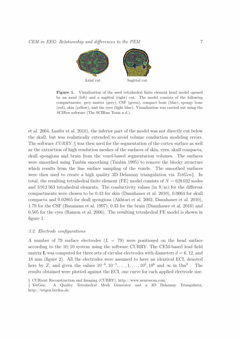
Axial cut Sagittal cut

Figure 1. Visualization of the used tetrahedral finite element head model opened

by an axial (left) and a sagittal (right) cut. The model consists of the following

compartments: grey matter (grey), CSF (green), compact bone (blue), spongy bone

(red), skin (yellow), and the eyes (light blue). Visualization was carried out using the

SCIRun software (The SCIRun Team n.d.).

et al. 2004, Lanfer et al. 2010), the inferior part of the model was not directly cut below

the skull, but was realistically extended to avoid volume conduction modeling errors.

The software CURRY § was then used for the segmentation of the cortex surface as well

as the extraction of high resolution meshes of the surfaces of skin, eyes, skull compacta,

skull spongiosa and brain from the voxel-based segmentation volumes. The surfaces

were smoothed using Taubin smoothing (Taubin 1995) to remove the blocky structure

which results from the fine surface sampling of the voxels. The smoothed surfaces

were then used to create a high quality 3D Delaunay triangulation via TetGen‖. In

total, the resulting tetrahedral finite element (FE) model consists of N = 628 032 nodes

and 3 912 563 tetrahedral elements. The conductivity values (in S/m) for the different

compartments were chosen to be 0.43 for skin (Dannhauer et al. 2010), 0.0064 for skull

compacta and 0.02865 for skull spongiosa (Akhtari et al. 2002, Dannhauer et al. 2010),

1.79 for the CSF (Baumann et al. 1997), 0.33 for the brain (Dannhauer et al. 2010) and

0.505 for the eyes (Ramon et al. 2006). The resulting tetrahedral FE model is shown in

figure 1.

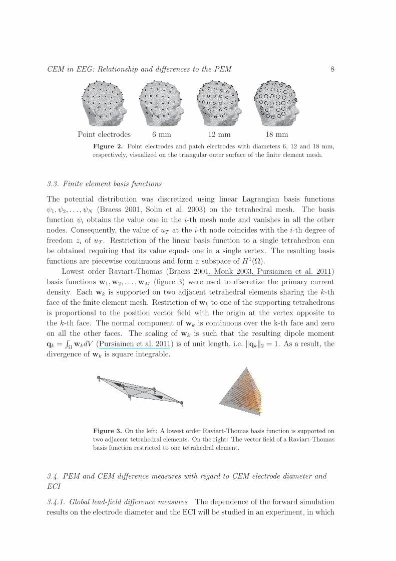
3.2. Electrode configurations

A number of 79 surface electrodes (L = 79) were positioned on the head surface

according to the 10/10 system using the software CURRY. The CEM-based lead field

matrix L was computed for three sets of circular electrodes with diameters d = 6, 12, and

18 mm (figure 2). All the electrodes were assumed to have an identical ECI, denoted

here by Z, and given the values 10−6, 10−5, . . . , 1, . . . , 105, 106 and ∞ in Ωm2 . The

results obtained were plotted against the ECI, one curve for each applied electrode size.

§ CURrent Reconstruction and Imaging (CURRY), http://www.neuroscan.com/‖ TetGen: A Quality Tetrahedral Mesh Generator and a 3D Delaunay Triangulator,

http://tetgen.berlios.de/

CEM in EEG: Relationship and differences to the PEM 8

Point electrodes 6 mm 12 mm 18 mm

Figure 2. Point electrodes and patch electrodes with diameters 6, 12 and 18 mm,

respectively, visualized on the triangular outer surface of the finite element mesh.

3.3. Finite element basis functions

The potential distribution was discretized using linear Lagrangian basis functions

ψ1, ψ2, . . . , ψN (Braess 2001, Solin et al. 2003) on the tetrahedral mesh. The basis

function ψi obtains the value one in the i-th mesh node and vanishes in all the other

nodes. Consequently, the value of uT at the i-th node coincides with the i-th degree of

freedom zi of uT . Restriction of the linear basis function to a single tetrahedron can

be obtained requiring that its value equals one in a single vertex. The resulting basis

functions are piecewise continuous and form a subspace of H1(Ω).

Lowest order Raviart-Thomas (Braess 2001, Monk 2003, Pursiainen et al. 2011)

basis functions w1,w2, . . . ,wM (figure 3) were used to discretize the primary current

density. Each wk is supported on two adjacent tetrahedral elements sharing the k-th

face of the finite element mesh. Restriction of wk to one of the supporting tetrahedrons

is proportional to the position vector field with the origin at the vertex opposite to

the k-th face. The normal component of wk is continuous over the k-th face and zero

on all the other faces. The scaling of wk is such that the resulting dipole moment

qk =∫

ΩwkdV (Pursiainen et al. 2011) is of unit length, i.e. ‖qk‖2 = 1. As a result, the

divergence of wk is square integrable.

Figure 3. On the left: A lowest order Raviart-Thomas basis function is supported on

two adjacent tetrahedral elements. On the right: The vector field of a Raviart-Thomas

basis function restricted to one tetrahedral element.

3.4. PEM and CEM difference measures with regard to CEM electrode diameter and

ECI

3.4.1. Global lead-field difference measures The dependence of the forward simulation

results on the electrode diameter and the ECI will be studied in an experiment, in which

CEM in EEG: Relationship and differences to the PEM 9

the lead-field matrices are compared in terms of the global difference measures (global

with regard to the whole brain influence space) RE (relative error), RDM (relative-

difference measure) and RN (relative norm) given by

RE =

√

√

√

√

M∑

k=1

‖lk − lREF

k ‖22

/

M∑

k=1

‖lREF

k ‖22, (11)

RDM =

√

√

√

√

1

M

M∑

k=1

∥

∥

∥lk/‖lk‖2 − lREF

k /‖lREF

k ‖2

∥

∥

∥

2

2

, (12)

RN =

√

√

√

√

M∑

k=1

‖lk‖22

/

M∑

k=1

‖lREF

k ‖22. (13)

Because the PEM is currently the standard electrode model in source analysis, we

defined it as our reference. The vector lREF

k is the k-th column of the reference matrix

LREF computed through the PEM with the same conductivity distribution and set of

dipole moment and location pairs as in the computation of L, for which the CEM will be

used. Similar to the measures introduced by (Meijs et al. 1989), the RE is sensitive to

both topography as well as magnitude differences between PEM and CEM lead-fields,

the RDM is a measure of lead-field topography differences and the RN is sensitive to

differences in PEM and CEM lead-field magnitudes. A PEM and a CEM lead-field

are maximally similar, i.e., identical, if RE and RDM are at 0 and RN is at 1. The

maximum for the RDM is a value of 2 (Lew et al. 2009).

3.4.2. Local lead-field difference measures In the second experiment, the distribution

of the local or column-wise forward and inverse errors in the brain compartment will be

studied. As the forward error, the column-wise relative difference measure

RDMk =∥

∥

∥lk/‖lk‖2 − lREF

k /‖lREF

k ‖2

∥

∥

∥

2

(14)

will be used as a measure of topography differences between PEM and CEM forward

simulation results for the k-th source. A PEM and a CEM forward simulation for source

k is maximally similar, i.e., identical, if RDMk is at 0, and the difference is maximal if

RDMk is at 2 (Lew et al. 2009).

3.4.3. Inverse localization difference measures The inverse single source analysis aspect

will be examined utilizing the PE (placement error) and the AE (angular error) for

the Raviart-Thomas type source (qk, rk) (Pursiainen et al. 2011) with position rk and

moment qk, i.e.,

PEk = ‖rjk− rk‖2 and AEk = | arccos(qjk

· qk)|, (15)

in which jk = arg minj ‖lj − lREF

k ‖2 corresponds to the Raviart-Thomas type source

(qjk, rjk

) that best reproduces the reference data lREF

k in terms of the maximum

likelihood.

CEM in EEG: Relationship and differences to the PEM 10

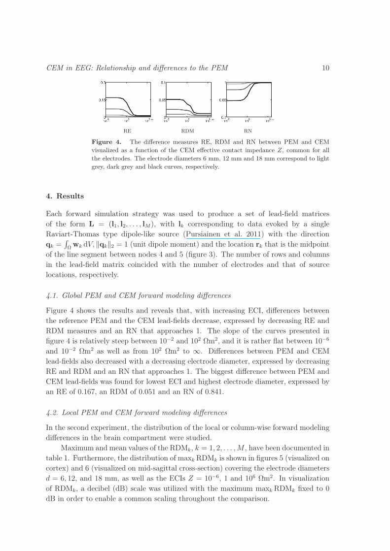
RE RDM RN

Figure 4. The difference measures RE, RDM and RN between PEM and CEM

visualized as a function of the CEM effective contact impedance Z, common for all

the electrodes. The electrode diameters 6 mm, 12 mm and 18 mm correspond to light

grey, dark grey and black curves, respectively.

4. Results

Each forward simulation strategy was used to produce a set of lead-field matrices

of the form L = (l1, l2, . . . , lM), with lk corresponding to data evoked by a single

Raviart-Thomas type dipole-like source (Pursiainen et al. 2011) with the direction

qk =∫

Ωwk dV, ‖qk‖2 = 1 (unit dipole moment) and the location rk that is the midpoint

of the line segment between nodes 4 and 5 (figure 3). The number of rows and columns

in the lead-field matrix coincided with the number of electrodes and that of source

locations, respectively.

4.1. Global PEM and CEM forward modeling differences

Figure 4 shows the results and reveals that, with increasing ECI, differences between

the reference PEM and the CEM lead-fields decrease, expressed by decreasing RE and

RDM measures and an RN that approaches 1. The slope of the curves presented in

figure 4 is relatively steep between 10−2 and 102 Ωm2, and it is rather flat between 10−6

and 10−2 Ωm2 as well as from 102 Ωm2 to ∞. Differences between PEM and CEM

lead-fields also decreased with a decreasing electrode diameter, expressed by decreasing

RE and RDM and an RN that approaches 1. The biggest difference between PEM and

CEM lead-fields was found for lowest ECI and highest electrode diameter, expressed by

an RE of 0.167, an RDM of 0.051 and an RN of 0.841.

4.2. Local PEM and CEM forward modeling differences

In the second experiment, the distribution of the local or column-wise forward modeling

differences in the brain compartment were studied.

Maximum and mean values of the RDMk, k = 1, 2, . . . ,M , have been documented in

table 1. Furthermore, the distribution of maxk RDMk is shown in figures 5 (visualized on

cortex) and 6 (visualized on mid-sagittal cross-section) covering the electrode diameters

d = 6, 12, and 18 mm, as well as the ECIs Z = 10−6, 1 and 106 Ωm2. In visualization

of RDMk, a decibel (dB) scale was utilized with the maximum maxk RDMk fixed to 0

dB in order to enable a common scaling throughout the comparison.

CEM in EEG: Relationship and differences to the PEM 11

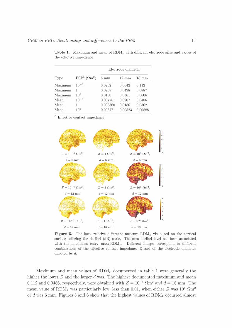
Table 1. Maximum and mean of RDMk with different electrode sizes and values of

the effective impedance.

Electrode diameter

Type ECIa (Ωm2) 6 mm 12 mm 18 mm

Maximum 10−6 0.0262 0.0642 0.112

Maximum 1 0.0238 0.0498 0.0887

Maximum 106 0.0180 0.0361 0.0606

Mean 10−6 0.00775 0.0207 0.0486

Mean 1 0.008360 0.0186 0.0362

Mean 106 0.00377 0.00523 0.00888

a Effective contact impedance

Z = 10−6 Ωm2,

d = 6 mm

Z = 1 Ωm2,

d = 6 mm

Z = 106 Ωm2,

d = 6 mm

Z = 10−6 Ωm2,

d = 12 mm

Z = 1 Ωm2,

d = 12 mm

Z = 106 Ωm2,

d = 12 mm

Z = 10−6 Ωm2,

d = 18 mm

Z = 1 Ωm2,

d = 18 mm

Z = 106 Ωm2,

d = 18 mm

Figure 5. The local relative difference measure RDMk visualized on the cortical

surface utilizing the decibel (dB) scale. The zero decibel level has been associated

with the maximum entry maxk RDMk. Different images correspond to different

combinations of the effective contact impedance Z and of the electrode diameter

denoted by d.

Maximum and mean values of RDMk documented in table 1 were generally the

higher the lower Z and the larger d was. The highest documented maximum and mean

0.112 and 0.0486, respectively, were obtained with Z = 10−6 Ωm2 and d = 18 mm. The

mean value of RDMk was particularly low, less than 0.01, when either Z was 106 Ωm2

or d was 6 mm. Figures 5 and 6 show that the highest values of RDMk occurred almost

CEM in EEG: Relationship and differences to the PEM 12

Z = 10−6 Ωm2,

d = 6 mm

Z = 1 Ωm2,

d = 6 mm

Z = 106 Ωm2,

d = 6 mm

Z = 10−6 Ωm2,

d = 12 mm

Z = 1 Ωm2,

d = 12 mm

Z = 106 Ωm2,

d = 12 mm

Z = 10−6 Ωm2,

d = 18 mm

Z = 1 Ωm2,

d = 18 mm

Z = 106 Ωm2,

d = 18 mm

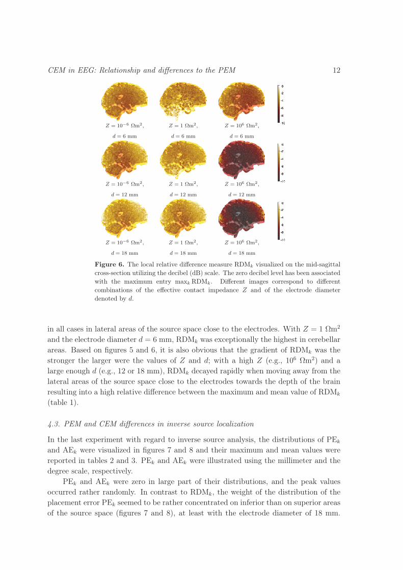
Figure 6. The local relative difference measure RDMk visualized on the mid-sagittal

cross-section utilizing the decibel (dB) scale. The zero decibel level has been associated

with the maximum entry maxk RDMk. Different images correspond to different

combinations of the effective contact impedance Z and of the electrode diameter

denoted by d.

in all cases in lateral areas of the source space close to the electrodes. With Z = 1 Ωm2

and the electrode diameter d = 6 mm, RDMk was exceptionally the highest in cerebellar

areas. Based on figures 5 and 6, it is also obvious that the gradient of RDMk was the

stronger the larger were the values of Z and d; with a high Z (e.g., 106 Ωm2) and a

large enough d (e.g., 12 or 18 mm), RDMk decayed rapidly when moving away from the

lateral areas of the source space close to the electrodes towards the depth of the brain

resulting into a high relative difference between the maximum and mean value of RDMk

(table 1).

4.3. PEM and CEM differences in inverse source localization

In the last experiment with regard to inverse source analysis, the distributions of PEk

and AEk were visualized in figures 7 and 8 and their maximum and mean values were

reported in tables 2 and 3. PEk and AEk were illustrated using the millimeter and the

degree scale, respectively.

PEk and AEk were zero in large part of their distributions, and the peak values

occurred rather randomly. In contrast to RDMk, the weight of the distribution of the

placement error PEk seemed to be rather concentrated on inferior than on superior areas

of the source space (figures 7 and 8), at least with the electrode diameter of 18 mm.

CEM in EEG: Relationship and differences to the PEM 13

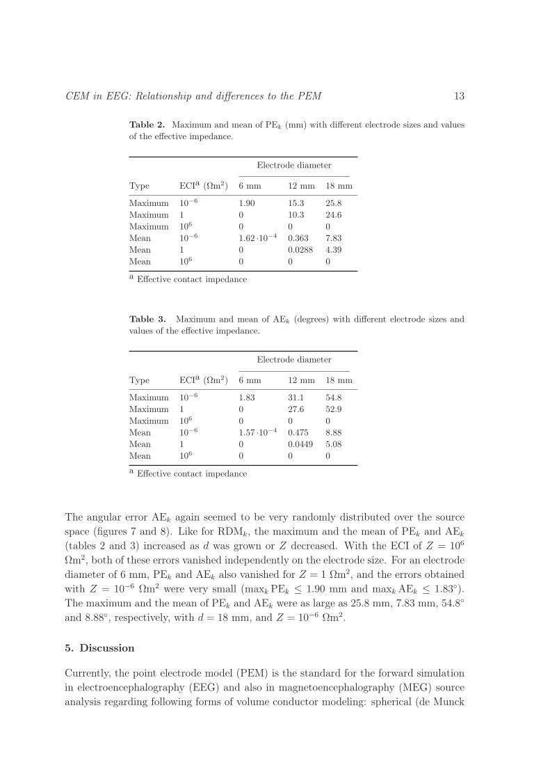
Table 2. Maximum and mean of PEk (mm) with different electrode sizes and values

of the effective impedance.

Electrode diameter

Type ECIa (Ωm2) 6 mm 12 mm 18 mm

Maximum 10−6 1.90 15.3 25.8

Maximum 1 0 10.3 24.6

Maximum 106 0 0 0

Mean 10−6 1.62 ·10−4 0.363 7.83

Mean 1 0 0.0288 4.39

Mean 106 0 0 0

a Effective contact impedance

Table 3. Maximum and mean of AEk (degrees) with different electrode sizes and

values of the effective impedance.

Electrode diameter

Type ECIa (Ωm2) 6 mm 12 mm 18 mm

Maximum 10−6 1.83 31.1 54.8

Maximum 1 0 27.6 52.9

Maximum 106 0 0 0

Mean 10−6 1.57 ·10−4 0.475 8.88

Mean 1 0 0.0449 5.08

Mean 106 0 0 0

a Effective contact impedance

The angular error AEk again seemed to be very randomly distributed over the source

space (figures 7 and 8). Like for RDMk, the maximum and the mean of PEk and AEk

(tables 2 and 3) increased as d was grown or Z decreased. With the ECI of Z = 106

Ωm2, both of these errors vanished independently on the electrode size. For an electrode

diameter of 6 mm, PEk and AEk also vanished for Z = 1 Ωm2, and the errors obtained

with Z = 10−6 Ωm2 were very small (maxk PEk ≤ 1.90 mm and maxk AEk ≤ 1.83).

The maximum and the mean of PEk and AEk were as large as 25.8 mm, 7.83 mm, 54.8

and 8.88, respectively, with d = 18 mm, and Z = 10−6 Ωm2.

5. Discussion

Currently, the point electrode model (PEM) is the standard for the forward simulation

in electroencephalography (EEG) and also in magnetoencephalography (MEG) source

analysis regarding following forms of volume conductor modeling: spherical (de Munck

CEM in EEG: Relationship and differences to the PEM 14

Z=10−6 Ωm2,

d=12 mm

Z=1 Ωm2,

d=12 mm

Z=10−6 Ωm2,

d=18 mm

Z=1 Ωm2,

d=18 mm

(I),Z=10−6 Ωm2,

d=12 mm

Z=1 Ωm2,

d=12 mm

Z=10−6 Ωm2,

d=18 mm

Z=1 Ωm2,

d=18 mm

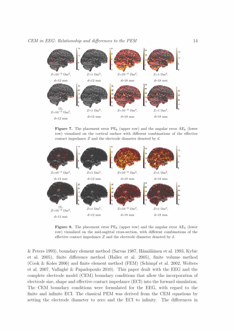
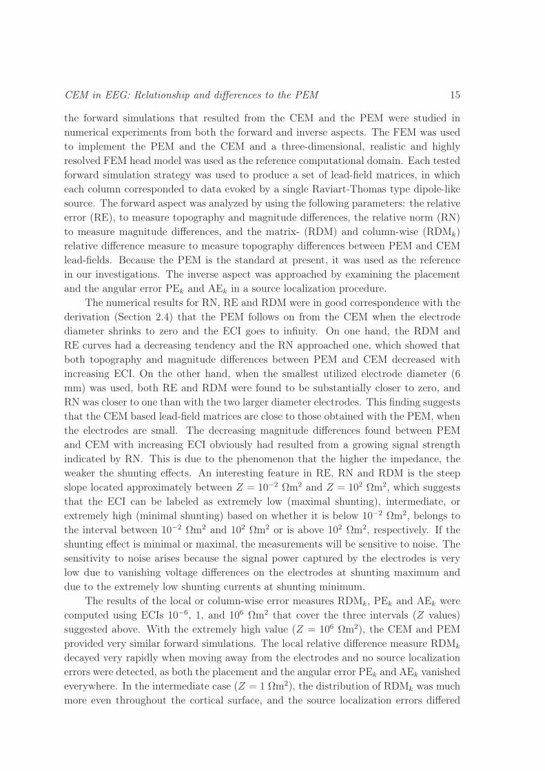
Figure 7. The placement error PEk (upper row) and the angular error AEk (lower

row) visualized on the cortical surface with different combinations of the effective

contact impedance Z and the electrode diameter denoted by d.

Z=10−6 Ωm2,

d=12 mm

Z=1 Ωm2,

d=12 mm

Z=10−6 Ωm2,

d=18 mm

Z=1 Ωm2,

d=18 mm

(I),Z=10−6 Ωm2,

d=12 mm

Z=1 Ωm2,

d=12 mm

Z=10−6 Ωm2,

d=18 mm

Z=1 Ωm2,

d=18 mm

Figure 8. The placement error PEk (upper row) and the angular error AEk (lower

row) visualized on the mid-sagittal cross-section, with different combinations of the

effective contact impedance Z and the electrode diameter denoted by d.

& Peters 1993), boundary element method (Sarvas 1987, Hämäläinen et al. 1993, Kybic

et al. 2005), finite difference method (Hallez et al. 2005), finite volume method

(Cook & Koles 2006) and finite element method (FEM) (Schimpf et al. 2002, Wolters

et al. 2007, Vallaghé & Papadopoulo 2010). This paper dealt with the EEG and the

complete electrode model (CEM) boundary conditions that allow the incorporation of

electrode size, shape and effective contact impedance (ECI) into the forward simulation.

The CEM boundary conditions were formulated for the EEG, with regard to the

finite and infinite ECI. The classical PEM was derived from the CEM equations by

setting the electrode diameter to zero and the ECI to infinity. The differences in

CEM in EEG: Relationship and differences to the PEM 15

the forward simulations that resulted from the CEM and the PEM were studied in

numerical experiments from both the forward and inverse aspects. The FEM was used

to implement the PEM and the CEM and a three-dimensional, realistic and highly

resolved FEM head model was used as the reference computational domain. Each tested

forward simulation strategy was used to produce a set of lead-field matrices, in which

each column corresponded to data evoked by a single Raviart-Thomas type dipole-like

source. The forward aspect was analyzed by using the following parameters: the relative

error (RE), to measure topography and magnitude differences, the relative norm (RN)

to measure magnitude differences, and the matrix- (RDM) and column-wise (RDMk)

relative difference measure to measure topography differences between PEM and CEM

lead-fields. Because the PEM is the standard at present, it was used as the reference

in our investigations. The inverse aspect was approached by examining the placement

and the angular error PEk and AEk in a source localization procedure.

The numerical results for RN, RE and RDM were in good correspondence with the

derivation (Section 2.4) that the PEM follows on from the CEM when the electrode

diameter shrinks to zero and the ECI goes to infinity. On one hand, the RDM and

RE curves had a decreasing tendency and the RN approached one, which showed that

both topography and magnitude differences between PEM and CEM decreased with

increasing ECI. On the other hand, when the smallest utilized electrode diameter (6

mm) was used, both RE and RDM were found to be substantially closer to zero, and

RN was closer to one than with the two larger diameter electrodes. This finding suggests

that the CEM based lead-field matrices are close to those obtained with the PEM, when

the electrodes are small. The decreasing magnitude differences found between PEM

and CEM with increasing ECI obviously had resulted from a growing signal strength

indicated by RN. This is due to the phenomenon that the higher the impedance, the

weaker the shunting effects. An interesting feature in RE, RN and RDM is the steep

slope located approximately between Z = 10−2 Ωm2 and Z = 102 Ωm2, which suggests

that the ECI can be labeled as extremely low (maximal shunting), intermediate, or

extremely high (minimal shunting) based on whether it is below 10−2 Ωm2, belongs to

the interval between 10−2 Ωm2 and 102 Ωm2 or is above 102 Ωm2, respectively. If the

shunting effect is minimal or maximal, the measurements will be sensitive to noise. The

sensitivity to noise arises because the signal power captured by the electrodes is very

low due to vanishing voltage differences on the electrodes at shunting maximum and

due to the extremely low shunting currents at shunting minimum.

The results of the local or column-wise error measures RDMk, PEk and AEk were

computed using ECIs 10−6, 1, and 106 Ωm2 that cover the three intervals (Z values)

suggested above. With the extremely high value (Z = 106 Ωm2), the CEM and PEM

provided very similar forward simulations. The local relative difference measure RDMk

decayed very rapidly when moving away from the electrodes and no source localization

errors were detected, as both the placement and the angular error PEk and AEk vanished

everywhere. In the intermediate case (Z = 1 Ωm2), the distribution of RDMk was much

more even throughout the cortical surface, and the source localization errors differed

CEM in EEG: Relationship and differences to the PEM 16

from zero for the two largest electrode sizes. Again, with the extremely low value

(Z = 10−6 Ωm2), the distribution of RDMk was relatively high everywhere, and PEk

and AEk were non-zero, independent of the electrode size.

As shown by figures 5 and 6, the forward errors are not simply below the electrodes

due to a complicated interplay between impedance value, electrode surface and volume

conduction, especially the effect of the strongly folded cortical surface in our realistic

head model. Even if figure 6, especially the case with high impedance and large

electrode surface, show the tendency that the CEM-PEM differences rapidly decrease

with distance to the electrodes, the effects are not simply limited to the cortical areas

directly beneath the electrodes. Further, it is natural that the largest placement errors

were rather concentrated on inferior than on superior areas of the source space, since the

source localization problem is particularly ill-conditioned for sources lying deep within

the brain. The fact that the inverse errors do not clearly follow any other pattern is at

least partially due to the applied source localization strategy.

Namely, although the forward simulation differences presented above are

comprehensively due to the differences between PEM and CEM modeling, the situation

is more complex for the inverse reconstruction results. It is inherent that the differences

in the forward modeling and limitations of the chosen inverse procedure are intermixed.

Consequently, the placement and angular errors obtained in our investigations are

mainly due to two aspects: namely the differences between PEM and CEM and also

the errors introduced by the inverse reconstruction procedure. The Raviart-Thomas

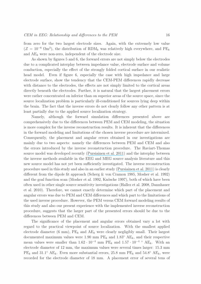
source model was developed recently (Pursiainen et al. 2011) and the interplay between

the inverse methods available in the EEG and MEG source analysis literature and this

new source model has not yet been sufficiently investigated. The inverse reconstruction

procedure used in this study and also in an earlier study (Pursiainen et al. 2011) is clearly

different from the dipole fit approach (Scherg & von Cramon 1985, Mosher et al. 1992)

and the goal function scan (Mosher et al. 1992, Knösche 1997), both of which have been

often used in other single source sensitivity investigations (Hallez et al. 2008, Dannhauer

et al. 2010). Therefore, we cannot exactly determine which part of the placement and

angular errors was due to PEM and CEM differences and which part to the limitations of

the used inverse procedure. However, the PEM versus CEM forward modeling results of

this study and also our present experience with the implemented inverse reconstruction

procedure, suggests that the larger part of the presented errors should be due to the

differences between PEM and CEM.

The significance of the placement and angular errors obtained vary a lot with

regard to the practical viewpoint of source localization. With the smallest applied

electrode diameter (6 mm), PEk and AEk were clearly negligibly small. Their largest

documented maximum values were 1.90 mm PEk and 1.83 AEk, and their respective

mean values were smaller than 1.62 · 10−4 mm PEk and 1.57 · 10−4 AEk. With an

electrode diameter of 12 mm, the maximum values were several times larger: 15.3 mm

PEk and 31.1 AEk. Even more substantial errors, 25.8 mm PEk and 54.8 AEk, were

recorded for the electrode diameter of 18 mm. A placement error of several tens of

CEM in EEG: Relationship and differences to the PEM 17

millimeters, which occurred with the 12 mm and 18 mm diameters, is a crucial error

in many clinical applications as the sources can be localized in the wrong brain areas.

It seems reasonable to us, that since a maximum and mean RDMk of about 0.11 and

0.05, respectively (see table 1) can lead to single source localization errors as discussed

above, our assumption, that the larger part of the presented placement and angular

errors are due to the differences between PEM and CEM, seems to be strengthened.

A recent study (Dannhauer et al. 2010) related similar RDM forward modeling errors

(see their figure 2) to goal function scan inverse reconstruction errors in the same range

(see their figure 5). Hence, using the CEM instead of the PEM in forward simulation

might lead to essential differences in inverse estimates, when the electrode diameter is

at least 12 mm and the applied ECI is low enough (Z ≤ 1 Ωm2). Additionally, the mean

values of PEk and AEk reveals that the amount of the centimeter-scale placement errors

was much higher for the 18 mm electrode than for its 12 mm counterpart. The largest

reported mean values were 0.363 mm PEk and 0.475 AEk, for the 12 mm electrode,

whereas with 18 mm diameter electrode, they were 7.83 mm PEk and 8.88 AEk.

The ECIs can be coarsely related to the electrode impedances expressed in Ohms

via the concept of ACI defined in Section 2.1. Using a round value of 1 cm2 as the

electrode surface area, the suggested limits of the extremely low and high impedances,

i.e. 10−2 Ωm2 and 102 Ωm2, correspond to ACIs 100 Ω and 1 MΩ, respectively. Of these,

the lower limit (100 Ω) coincides with the guideline value given by the American Clinical

Neurophysiology Society (American Clinical Neurophysiology Society 2006b) for clinical

EEG, whereas the upper limit suggested here is much higher than that given in the

corresponding guidelines (10 kΩ and ≤ 5 kΩ pre-measurement) in (American Clinical

Neurophysiology Society 2006b, American Clinical Neurophysiology Society 2006a). The

guidelines for the maximal impedance have been determined mainly based on the

average performance of an EEG amplifier (Niedermeyer & da Silva 2004). However,

an earlier study (Ferree et al. 2001) shows that excellent EEG signals can be recorded

with electrode impedances many times higher (e.g. 40 kΩ) than the guideline values,

if the input-impedance is high enough (e.g. 200 MΩ). With regard to the impedances

of around 5 kΩ, frequently found in clinical studies, the most relevant value utilized

in this study for the electrode diameters of 12 mm and 18 mm can be estimated to be

Z = 1 Ωm2, which corresponds to ACI of 8.8 and 3.9 kΩ, respectively. With the smallest

diameter electrode 6 mm, the best correspondence to 5 kΩ was obtained at Z = 0.1

Ωm2 (3.5 kΩ ACI).

Finally, the skin-electrode contact impedance of dry electrodes, that function

without any "wet" gel electrolyte on the electrode contact surfaces, can be many times

higher than that of the conventional electrodes, e.g. several tens of kΩ, and the diameter

can be rather large, e.g. 16 mm (Fiedler et al. 2011). With regard to dry electrodes,

the present results suggest the following two points. Firstly, since the relative norm

RN, which indicates the captured signal power, was found to grow along with the

impedance, the signal amplitudes measured with high-impedance electrodes can be

slightly higher than those measured with conventional ones, as observed in (Fiedler

CEM in EEG: Relationship and differences to the PEM 18

et al. 2011). Secondly, it seems that even with ACIs considerably over 10 kΩ the

differences between the CEM and PEM forward simulations can be essential, if the

electrode diameter is large. For example, RE and RDM obtained with 18 mm diameter

and Z = 10 Ωm2 (ACI 39 kΩ) were slightly larger (0.0643 and 0.0318) than those (0.0464

and 0.0192) obtained with 12 mm diameter and Z = 1 Ωm2 (ACI 8.8 kΩ), respectively.

In addition to dry and wet skin contact electrodes there exists various other electrode

types as well, such as subdermal needle electrodes and depth electrodes, which are used

to record electric potentials beneath the skin and directly from the brain, respectively.

Applying the CEM for those may be possible but requires further work.

6. Conclusion and outlook

According to the present numerical results, it is suggested that the ECI can be labeled as

extremely low (maximal shunting), intermediate, or extremely high (minimal shunting)

based on whether it is below 10−2 Ωm2, between 10−2 Ωm2 and 102 Ωm2 or above 102

Ωm2, respectively. It is also suggested that, from the viewpoint of the EEG inverse

problem, essential differences between the CEM and the PEM can occur with ECI of

≤ 1 Ωm2 and ACI of ≤ 5 kΩ together with an electrode diameter ≥ 12 mm. Further, the

shunting effects that cause the differences will be close to maximal below an ECI value

of 10−2 Ωm2 and ACI of 100 Ω. It also seems that the use of high-impedance electrodes

can be advantageous for the captured signal power, and that the differences between

the CEM and PEM forward simulations can be essential even with ACIs considerably

over 10 kΩ, if the electrode diameter is large, e.g. ≥ 18 mm.

Our results raise the prospect of the following future investigations: As the

impedances and the electrode surfaces that cause larger differences are realistic, and

comparable to those of clinical studies, comparing the CEM and the PEM with clinical

study data may provide important direction for the future work. Another future

approach may be a deeper study on the association between the ECI and ohmic

electrode impedances, especially, concerning different electrode shapes, such as the

rings in addition to the disks. Additionally, utilizing the CEM to optimize the contact

impedance, for parameters such as the signal-to-noise ratio, can provide an interesting

new research target. A current limitation of our inverse effect results is that we

could not yet quantify which part of the localization and orientation errors is due

to the sophisticated interplay between impedance value, electrode surface and volume

conduction, especially the effect of the strongly folded cortical surface in our realistic

headmodel, and which part is due to the limitations of our current implementation to

the inverse problem. For these reasons, we are planning to implement other inverse

approaches and better quantify through a comparison of inverse results of the new

implementations and their interplay with the Raviart-Thomas sources and the CEM

forward approach in the realistic FE head model.

CEM in EEG: Relationship and differences to the PEM 19

7. Acknowledgements

This research was supported by the Academy of Finland, project no 136412, and

by the German Research Foundation (DFG), projects WO1425/2-1 and WO1425/3-

1. The authors would like to thank H. Kugel (Department of Clinical Radiology,

University of Münster, Germany) for the measurement of the MRI and A. Janssen,

S. Rampersad (both Department of Neurology and Clinical Neurophysiology, Radboud

University Nijmegen, the Netherlands) and B. Lanfer (Institute for Biomagnetism and

Biosignalanalysis, University of Münster, Germany) for their help in setting up the

realistic head model.

Appendix. Weak form of the CEM boundary value problem

The weak form (2) can be obtained by first integrating by parts the equation ∇·(σ∇u) =

∇·Jp multiplied by v ∈ H1(Ω), and after that, applying the CEM boundary conditions

(1) to the resulting boundary integral term. Integration by parts yields the equation∫

Ωσ∇u ·∇v dV −

∫

∂Ωv(σ∇u) ·n dS = −

∫

Ω(∇·Jp)v dV , in which the second integral term

on the left-hand side can be written as∫

∂Ωv(σ∇u) · n dS =

∑L

ℓ=1

∫

eℓ

v(σ∇u) · n dS =∑L

ℓ=1

∫

eℓ

v(Uℓ − u)/Zℓ dS resulting from the first boundary condition in (1) as well as

from the third one written in the form σ∇u · n = (Uℓ − u)/Zℓ. Now, it follows from

Uℓ = (∫

eℓ

u dS)/(∫

eℓ

dS) or equivalently from∫

eℓ

(Uℓ − u) dS = 0, implied by the second

and third condition in (1), that further∑L

ℓ=1

∫

eℓ

v(Uℓ − u)/Zℓ dS = −∑L

ℓ=1

∫

eℓ

(u −

Uℓ)(v − Vℓ)/Zℓ dS for any set of real-valued constants V1, V2, . . . , VL. That is, the weak

form∫

Ω

σ∇u · ∇v dV +L∑

ℓ=1

1

Zℓ

∫

eℓ

(Uℓ − u)(Vℓ − v) dS = −

∫

Ω

(∇ · Jp)v dV (A.1)

must be satisfied for all v ∈ H1(Ω) and Vℓ ∈ R, ℓ = 1, 2, . . . , L. The left-hand

side of (A.1) can be shown to constitute a continuous and coercive bilinear form in

H1(Ω) ⊕ RL (Vauhkonen 1997, Somersalo et al. 1992), and hence (A.1) is uniquely

solvable for any Jp with a square integrable divergence according to the Lax-Milgram

theorem (Braess 2001). Furthermore, substituting Uℓ = (∫

eℓ

u dS)/(∫

eℓ

dS) into (A.1)

yields the form (2), which in turn gives the formulas (4)–(7) via the Ritz-Galerkin

method (Braess 2001).

References

Akhtari M, Bryant H, Marmelak A, Flynn E, Heller L, Shih J, Mandelkern M, Matlachov A, Ranken

D, Best E, DiMauro M, Lee R & Sutherling W 2002 Brain Top. 14(3), 151–167.

American Clinical Neurophysiology Society 2006a Journal of Clinical Neurophysiology 23(2), 86–91.

American Clinical Neurophysiology Society 2006b Journal of Clinical Neurophysiology 23(2), 97–104.

Baillet S, Marin G, Garnero L & Hugonin J 1999 IEEE Trans. Biomed. Eng. 46(5), 522–534.

Baumann S, Wozny D, Kelly S & Meno F 1997 IEEE Trans Biomed. Eng. 44(3), 220–223.

CEM in EEG: Relationship and differences to the PEM 20

Boon P, D’Have M, Vanrumste B, Van Hoey G, Vonck K, Van Walleghem P, Caemart J, Achten E &

De Reuck J 2002 J. Clin. Neurophysiol. 19(5), 461–468.

Braess D 2001 Finite Elements Cambridge University Press Cambridge.

Bruno P, Vatta F, Minimel S & Inchingolo P 2004 in ‘Proc. of the 26th Annual Int. Conf.

IEEE Engineering in Medicine and Biology Society’ San Francisco, USA, Sep. 1-5,

http://www.ucsfresno.edu/embs2004.

Bruno P, Vatta F, Mininel S & Inchingolo P 2003 Biomedical Sciences Instrumentation 39, 59–64.

Calvetti D, Hakula H, Pursiainen S & Somersalo E 2009 SIAM J. Imaging Sci. 2(3), 879–909.

Cheney M, Isaacson D & Newell J C 1999 SIAM Review 41, 85–101.

Cheng K S, Isaacson D, Newell J C & Gisser D G 1989 IEEE Transactions on Biomedical Engineering

36(9), 918–924.

Cook M & Koles Z 2006 in ‘Proc. of the 28th Annual Int. Conf. of the IEEE Engineering in Medicine

and Biology Society’ pp. 4536–4539.

Dale A M & Sereno M I 1993 J. Cogn. Neurosci 5, 162–176.

Dannhauer M, Lanfer B, Wolters C & Knösche T 2010 Human Brain Mapping 32(9), 1383–1399. DOI:

10.1002/hbm.21114, PMID: 20690140.

Dassios G, Fokas A & Hadjiloizi D 2007 Inverse Problems 23, 2541–2549.

de Munck J & Peters M 1993 IEEE Trans Biomed. Eng. 40(11), 1166–1174.

Evans L C 1998 Partial differential equations American Mathematical Society Rhode Island.

Ferree T C, Luu P, Russell G S & Tucker D M 2001 Clinical Neurophysiology 112(3), 536–544.

Fiedler P, Cunha L T, Pedrosa P, Brodkorb S, Fonseca C, Vaz F & Haueisen J 2011 Meas. Sci. Technol.

22, 124007.

Fuchs M, Wagner M, Wischmann H A, Kohler T, Theissen A, Drenckhahn R & Buchner H 1998

Electroencephalography and Clinical Neurophysiology 107, 93–111.

Hallez H, Vanrumste B, Hese P V, D’Asseler Y, Lemahieu I & de Walle R V 2005 Phys.Med.Biol.

50, 3787–3806.

Hallez H, Vanrumste B, Van Hese P, Delputte S & Lemahieu I 2008 Phys.Med.Biol. 53, 1877–1894.

Haueisen J & Knösche T 2001 Journal of Cognitive Neuroscience 13, 786–792.

Heers M, Rampp S, Kaltenhäuser M, Pauli E, Rauch C, Dölken M & Stefan H 2010 Seizure 19, 397–403.

Hämäläinen M, Hari R, Ilmoniemi R J, Knuutila J & Lounasmaa O V 1993 Reviews of Modern Physics

65, 413–498.

Huang M, Song T, Hagler D, Podgorny I, Jousmaki V, L.Cui, K.Gaa, D.L.Harrington, Dale A, R.R.Lee,

J.Elman & E.Halgren 2007 NeuroImage 37, 731–748.

Knösche T 1997 Solutions of the neuroelectromagnetic inverse problem PhD thesis University of Twente,

The Netherlands.

Kybic J, Clerc M, Abboud T, Faugeras O, Keriven R & Papadopoulo T 2005 IEEE Trans. Med. Imag.

24(1), 12–18.

Lanfer B, Scherg M, Dannhauer M, Knösche T & Wolters C 2010 in ‘Proc. of the 16th Annual

Meeting of the Organization for Human Brain Mapping’ Barcelona, Spain, June 6-10.

http://www.humanbrainmapping.org/barcelona2010/.

Lew S, Wolters C, Dierkes T, Röer C & MacLeod R 2009 Applied Numerical Mathematics

59(8), 1970–1988. http://dx.doi.org/10.1016/j.apnum.2009.02.006, NIHMSID 120338, PMCID:

PMC2791331.

Meijs J, Weier O, Peters M & van Oosterom A 1989 IEEE Trans Biomed. Eng. 36, 1038–1049.

Monk P 2003 Finite Element Methods for Maxwell’s Equations Clarendon Press Oxford, UK.

Mosher J, Lewis P & Leahy R 1992 IEEE Trans Biomed. Eng. 39(6), 541–557.

Niedermeyer E & da Silva F 2004 Electroencephalography: Basic Principles, Clinical Applications, and

Related Fields Lippincot Williams & Wilkins.

Ollikainen J, Vauhkonen M, Karjalainen P A & Kaipio J P 2000 Medical Engineering & Physics

22, 535–545.

Oostenveld R & Oostendorp T 2002 Hum Brain Map. 17(3), 179–192.

CEM in EEG: Relationship and differences to the PEM 21

Phillips C, Rugg M D & Friston K J 2002 NeuroImage 17, 287–301.

Pursiainen S 2008a Computational methods in electromagnetic biomedical inverse problems Vol. Espoo

Dissertation Helsinki University of Technology.

Pursiainen S 2008b Journal of Physics: Conference Series 124(1), 012041 (11pp).

Pursiainen S, Sorrentino A, Campi C & Piana M 2011 Inverse Problems 27(4), 045003 (18pp).

Ramon C, Schimpf P & Haueisen J 2006 BioMedical Engineering OnLine 5(10). doi:10.1186/1475-

925X-5-10.

Ramon C, Schimpf P, Haueisen J, Holmes M & Ishimaru A 2004 Brain Topography 16(4), 245–248.

Sadleir R & Argibay A 2007 Ann.Biomed.Eng. 35(10), 1699–1712.

Sarvas J 1987 Physics in Medicine and Biology 32(1), 11.

Scherg M & von Cramon D 1985 Electroenc. Clin. Neurophysiol. 62, 32–44.

Schimpf P, Ramon C & Haueisen J 2002 IEEE Trans Biomed. Eng. 49(5), 409–418.

Sharon D, Hämäläinen M S, Tootell R, Halgren E & Belliveau J W 2007 NeuroImage 36(4), 1225–1235.

Solin P, Segeth K & Dolezel I 2003 Higher-Order Finite Element Methods Chapman & Hall / CRC

Boca Raton.

Somersalo E, Cheney M & Isaacson D 1992 SIAM J. Appl. Math. 52, 1023–1040.

Stefan H, Hummel C, Scheler G, Genow A, Druschky K, Tilz C, Kaltenhauser M, Hopfengartner R,

Buchfelder M & Romstock J 2003 Brain 126(Pt 11), 2396–2405.

Tanzer O, Järvenpää S, Nenonen J & Somersalo E 2005 Physics in Medicine and Biology 50, 3023–3039.

Taubin G 1995 in ‘Proceedings of the 22nd annual conference on Computer graphics and interactive

techniques’ ACM pp. 351–358.

The SCIRun Team n.d. SCIRun: A Scientific Computing Problem Solving Environment, Scientific

Computing and Imaging Institute (SCI).

Vallaghé S & Papadopoulo T 2010 SIAM J. Sci. Comput. 32(4), 2379–2394.

van den Broek S, Reinders F, Donderwinkel M & Peters M 1998 Electroenc. Clin. Neurophysiol.

106, 522–534.

Vauhkonen M 1997 Electrical Impedance Tomography and Prior Information University of Kuopio

Kuopio. Dissertation.

Vese L & Chan T 2002 International Journal of Computer Vision 50(3), 271–293.

Wendel K, Narra N, Hannula M, Kauppinen P & Malmivuo J 2008 IEEE Trans. Biomed. Eng.

55(4), 1454–1456.

Wipf D & Nagarajan S 2009 NeuroImage 44, 947–966.

Wolters C, Anwander A, Weinstein D, Koch M, Tricoche X & MacLeod R 2006 NeuroImage 30(3), 813–

826. http://dx.doi.org/10.1016/j.neuroimage.2005.10.014, PMID: 16364662.

Wolters C & de Munck J 2007 Encyclopedia of Computational Neuroscience, Scholarpedia. 40(2), 1738.

invited review, http://www.scholarpedia.org/article/Volume_Conduction.

Wolters C, Grasedyck L & Hackbusch W 2004 Inverse Problems 20(4), 1099–1116.

http://dx.doi.org/10.1088/0266-5611/20/4/007.

Wolters C, Köstler H, Möller C, Härtlein J, Grasedyck L & Hackbusch W 2007 SIAM J. on Scientific

Computing 30(1), 24–45. http://dx.doi.org/10.1137/060659053.

Wolters C, Lew S, MacLeod R & Hämäläinen M 2010 in ‘Proc. of the 44th Annual Meeting, DGBMT’

Rostock-Warnemünde, Germany, Oct.5-8, 2010. http://conference.vde.com/bmt-2010.