Complex Fuzzy Abstraction: The Brain Logic

Subhajit Ganguly

Email: gangulysubhajit63@gmail.com

© 2013 Subhajit Ganguly

Abstract:

Taking abstraction as the starting point, we build a complex, self-organizing fuzzy logic

system. Such a system, being built on top of abstraction as the base, turns out to be just a

special outcome of the laws of abstraction. As the system is self-organizing, it runs

automatically towards optimization. Using such a system in neural networks, we may

come as close as possible to the workings of the human brain. The abstract fuzzy

optimization is seen to follow a Gaussian distribution.

Introduction:

There are quite a large number of differences between the way present day computers

work and the way the brain works. The very way in which basic processing is done by

computers varies vastly from the way the brain processes information. Computers,

working on binary logic, can take into account only high or low states. They can have a

number of inputs that are processed by a single processing unit. After being processed,

the input(s) can have a single output or a number of outputs. On the other hand, brain

cells seem to be able to process information using abstract fuzzy logic that leads to more

energy optimization. In fact, estimates suggest that present day computers use up ten

million times more energy to process the same amount of information that the human

brain does.

This does not take into account, however, the accuracy and speed of decision making by

the two systems for large enough data inputs. The basic difference between the today’s

computers and the brain lie in the fact that while computers have only two logical

states, the brain uses can have many such states and in-between states simultaneously

generating patterns similar to attractor maps. Decisions are asymptotic functions of

such maps in the case of the brain, while in computers the decisions are only

approximate points in the output space. As such, all waypoints in the input system

itself can act as decision making units inside the brain. The way in which this happens

is no longer linear (as in computers), but nonlinear. This nonlinear information

processing by the brain is vastly superior to the linear processing used by computers in

arriving at decisions.

Abstraction lies at the heart of the complex, self-organizing fuzzy logic that is used by

the brain. In fact, this logic is the direct fallout and a special case of abstraction. The

Theory of Abstraction and the principle of Zero Postulation describes directivity towards

optimized solutions and cluster formation in the decision making space as inherent

properties of the system itself. They must also be able to describe the formation of

various structures and patterns in the decisions that the system can arrive at. As such, it

is of great interest for us to investigate how these structures are formed in the decision

space. A theory that is able to describe the world in totality has to keep the number of

basic postulates it depends upon to zero or near zero.

Reductionism hits a dead end in this regard. On the other hand, abstraction as the

starting point of building up a theory may be seen to be of fitting use. It would be much

more than a new way of tackling the problem. Even abstract postulates do away with

the shackles that bind our theories into the system and bar them from being total

descriptions of the system. The abstraction we are talking about here may be defined as,

‚Postulation of non-postulation‛ or, in other words, ‚A system of postulation that gives

equal weights to all possible solutions inside the system and favors none of such

solutions over others.‛

Abstraction automatically gives rise to optimized solutions within the universal set of

all possible solutions, as has been shown in this book. It is these optimized solutions

that make up and drive the non-abstract parts of the world, while the non-optimized

solutions remain ‘hidden’ from the material world, inside the abstract world. Zero

postulation or abstraction as the basis of theory synthesis allows us to explore even

imaginary and chaotic non-favored solutions as possibilities. With no postulation as the

fundamental basis, we are thus able to pile up postulated results or favored results, but

not the other way round. We keep describing such implications of abstraction in this

book. We deal with the abstraction of observable parameters involved in a given system

and formulate a similar basis of understanding them.

Let us consider the example of a three-point isolated system. Let the points be ‘A’, ‘B’

and ‘C’. Let A and B be decision points, whereas, C be situated anywhere on the straight

line joining A and B. The decision flow of both A and B tends to move in all possible

directions. These possible directions include the directions towards each other. Thus, at

point C, for obvious reasons, an additional effect will be felt due to the tendency of

decision to flow from A to B and from B to A, as compared to all other directions.

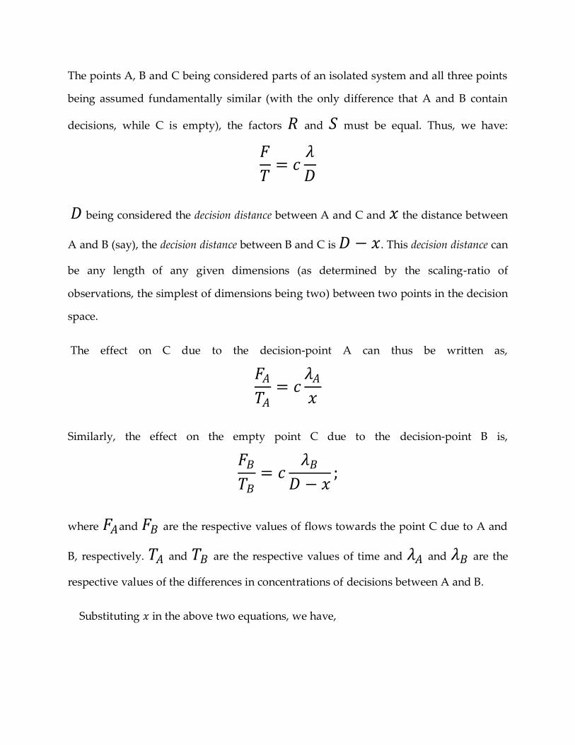
The points A, B and C being considered parts of an isolated system and all three points

being assumed fundamentally similar (with the only difference that A and B contain

decisions, while C is empty), the factors 𝑅 and 𝑆 must be equal. Thus, we have:

𝐹

𝑇= 𝑐

𝜆

𝐷

𝐷 being considered the decision distance between A and C and 𝑥 the distance between

A and B (say), the decision distance between B and C is 𝐷 − 𝑥. This decision distance can

be any length of any given dimensions (as determined by the scaling-ratio of

observations, the simplest of dimensions being two) between two points in the decision

space.

The effect on C due to the decision-point A can thus be written as,

𝐹𝐴

𝑇𝐴= 𝑐

𝜆𝐴

𝑥

Similarly, the effect on the empty point C due to the decision-point B is,

𝐹𝐵

𝑇𝐵= 𝑐

𝜆𝐵

𝐷 − 𝑥;

where 𝐹𝐴and 𝐹𝐵 are the respective values of flows towards the point C due to A and

B, respectively. 𝑇𝐴 and 𝑇𝐵 are the respective values of time and 𝜆𝐴 and 𝜆𝐵 are the

respective values of the differences in concentrations of decisions between A and B.

Substituting 𝑥 in the above two equations, we have,

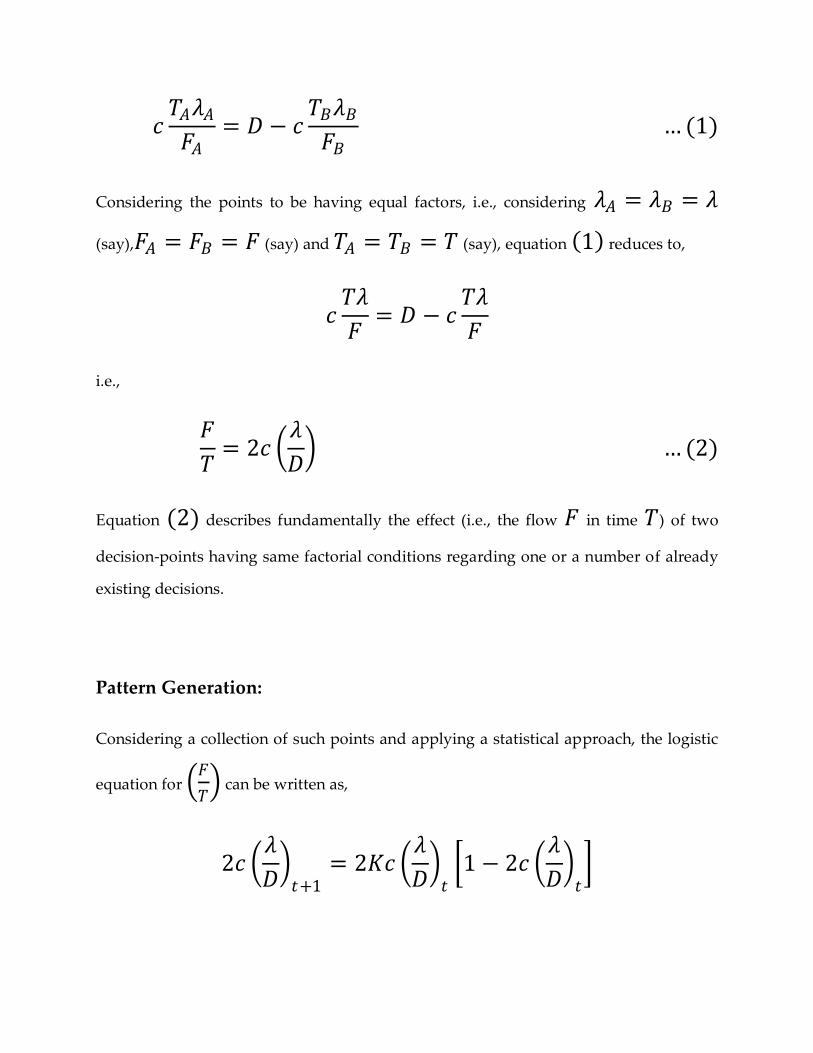
𝑐𝑇𝐴𝜆𝐴

𝐹𝐴= 𝐷 − 𝑐

𝑇𝐵𝜆𝐵

𝐹𝐵 … (1)

Considering the points to be having equal factors, i.e., considering 𝜆𝐴 = 𝜆𝐵 = 𝜆

(say),𝐹𝐴 = 𝐹𝐵 = 𝐹 (say) and 𝑇𝐴 = 𝑇𝐵 = 𝑇 (say), equation 1 reduces to,

𝑐𝑇𝜆

𝐹= 𝐷 − 𝑐

𝑇𝜆

𝐹

i.e.,

𝐹

𝑇= 2𝑐

𝜆

𝐷 … (2)

Equation (2) describes fundamentally the effect (i.e., the flow 𝐹 in time 𝑇) of two

decision-points having same factorial conditions regarding one or a number of already

existing decisions.

Pattern Generation:

Considering a collection of such points and applying a statistical approach, the logistic

equation for 𝐹

𝑇 can be written as,

2𝑐 𝜆

𝐷 𝑡+1

= 2𝐾𝑐 𝜆

𝐷 𝑡 1 − 2𝑐

𝜆

𝐷 𝑡

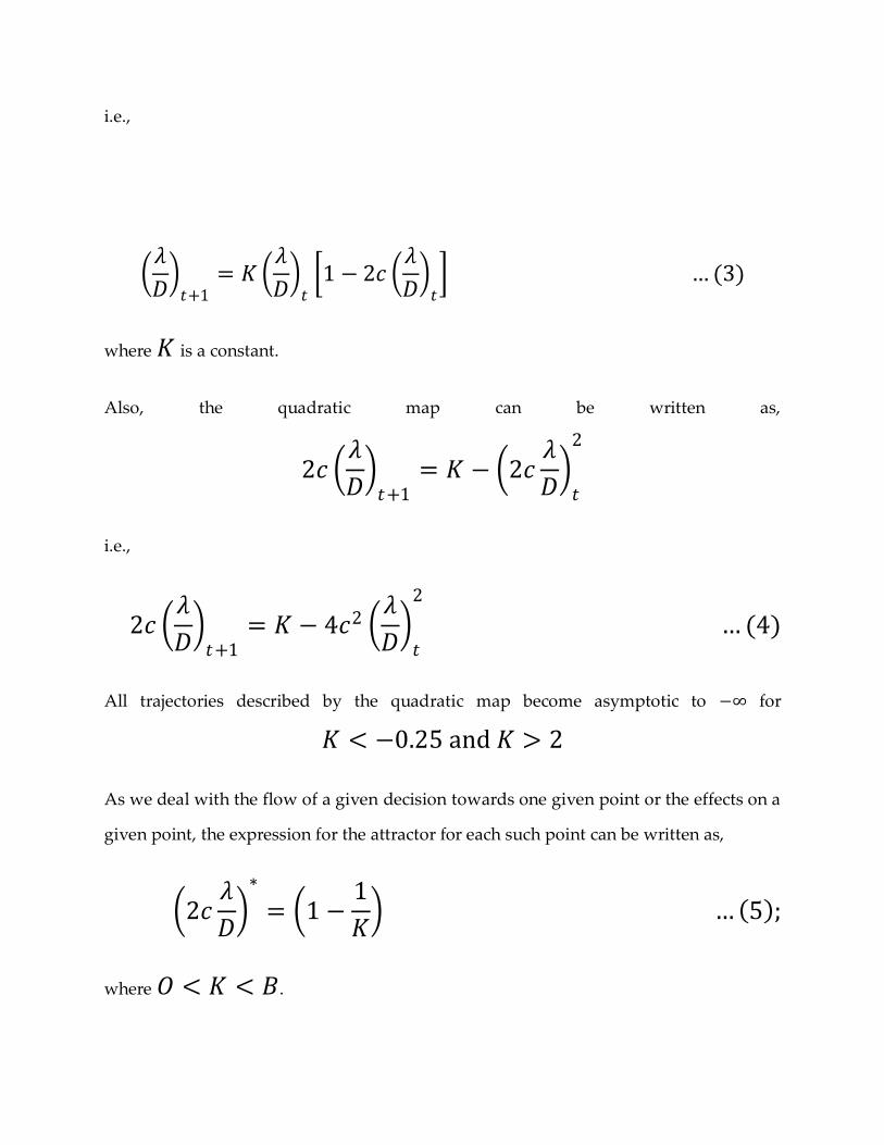
i.e.,

𝜆

𝐷 𝑡+1

= 𝐾 𝜆

𝐷 𝑡 1 − 2𝑐

𝜆

𝐷 𝑡 … (3)

where 𝐾 is a constant.

Also, the quadratic map can be written as,

2𝑐 𝜆

𝐷 𝑡+1

= 𝐾 − 2𝑐𝜆

𝐷 𝑡

2

i.e.,

2𝑐 𝜆

𝐷 𝑡+1

= 𝐾 − 4𝑐2 𝜆

𝐷 𝑡

2

… (4)

All trajectories described by the quadratic map become asymptotic to −∞ for

𝐾 < −0.25 and 𝐾 > 2

As we deal with the flow of a given decision towards one given point or the effects on a

given point, the expression for the attractor for each such point can be written as,

2𝑐𝜆

𝐷 ∗

= 1 −1

𝐾 … 5 ;

where 𝑂 < 𝐾 < 𝐵.

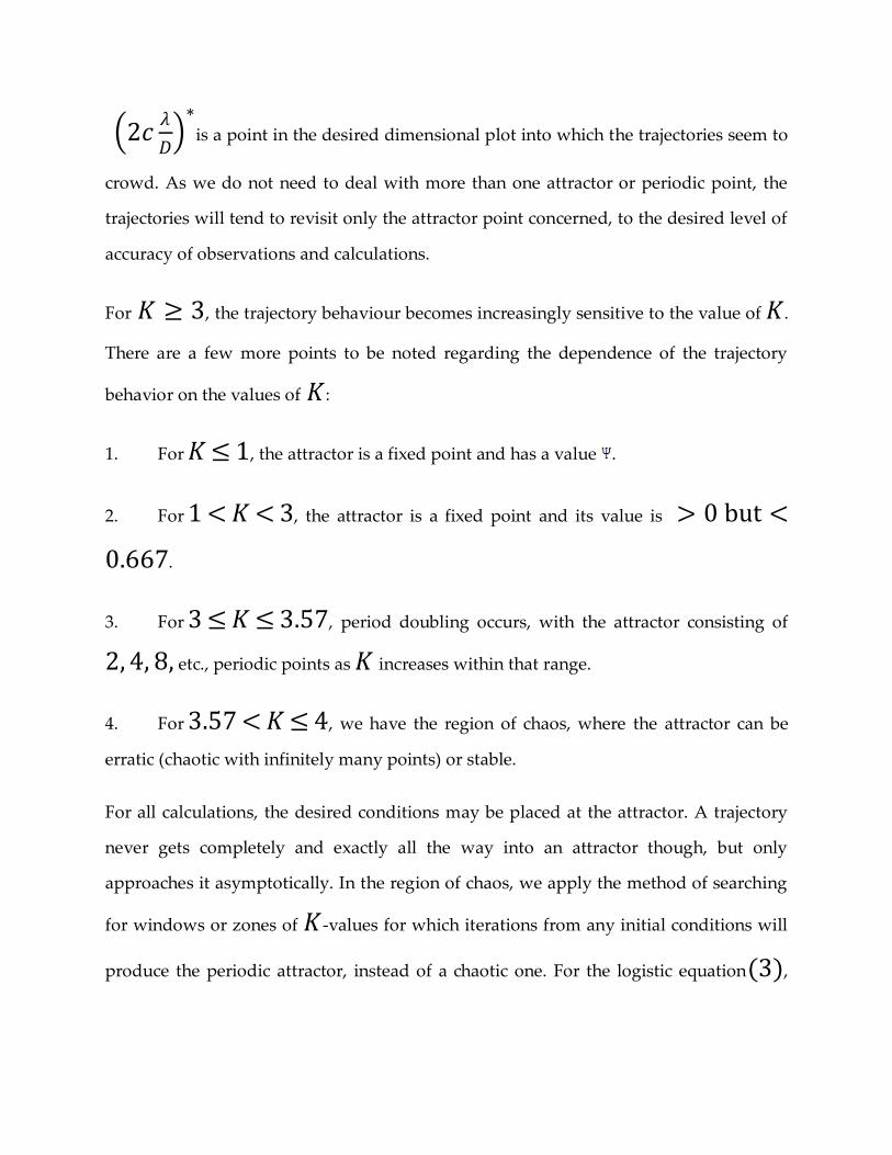
2𝑐𝜆

𝐷 ∗

is a point in the desired dimensional plot into which the trajectories seem to

crowd. As we do not need to deal with more than one attractor or periodic point, the

trajectories will tend to revisit only the attractor point concerned, to the desired level of

accuracy of observations and calculations.

For 𝐾 ≥ 3, the trajectory behaviour becomes increasingly sensitive to the value of 𝐾.

There are a few more points to be noted regarding the dependence of the trajectory

behavior on the values of 𝐾:

1. For 𝐾≤ 1, the attractor is a fixed point and has a value .

2. For 1 < 𝐾 < 3, the attractor is a fixed point and its value is > 0 but <

0.667.

3. For 3 ≤ 𝐾 ≤ 3.57, period doubling occurs, with the attractor consisting of

2, 4, 8, etc., periodic points as 𝐾 increases within that range.

4. For 3.57 < 𝐾≤ 4, we have the region of chaos, where the attractor can be

erratic (chaotic with infinitely many points) or stable.

For all calculations, the desired conditions may be placed at the attractor. A trajectory

never gets completely and exactly all the way into an attractor though, but only

approaches it asymptotically. In the region of chaos, we apply the method of searching

for windows or zones of 𝐾-values for which iterations from any initial conditions will

produce the periodic attractor, instead of a chaotic one. For the logistic equation(3),

the most common such zone lies at 𝐾 ≈ 3.83 and for the quadratic map(4),

at 𝐾 ≈ 1.76.

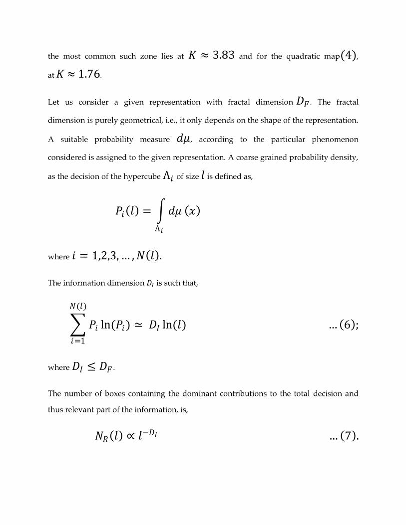
Let us consider a given representation with fractal dimension 𝐷𝐹 . The fractal

dimension is purely geometrical, i.e., it only depends on the shape of the representation.

A suitable probability measure 𝑑𝜇, according to the particular phenomenon

considered is assigned to the given representation. A coarse grained probability density,

as the decision of the hypercube Λ𝑖 of size 𝑙 is defined as,

𝑃𝑖 𝑙 = 𝑑𝜇

Λ 𝑖

𝑥

where 𝑖 = 1,2,3, … , 𝑁 𝑙 .

The information dimension 𝐷𝐼 is such that,

𝑃𝑖 ln(𝑃𝑖)

𝑁(𝑙)

𝑖=1

≃ 𝐷𝐼 ln(𝑙) … 6 ;

where 𝐷𝐼 ≤ 𝐷𝐹 .

The number of boxes containing the dominant contributions to the total decision and

thus relevant part of the information, is,

𝑁𝑅 𝑙 ∝ 𝑙−𝐷𝐼 … 7 .

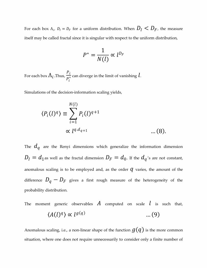
For each box Λ𝑖 , 𝐷𝐼 = 𝐷𝐹 for a uniform distribution. When 𝐷𝐼 < 𝐷𝐹 , the measure

itself may be called fractal since it is singular with respect to the uniform distribution,

𝑃∗ =1

𝑁(𝑙)∝ 𝑙𝐷𝐹

For each box Λ𝑖 .Thus, 𝑃𝑖

𝑃𝑖∗ can diverge in the limit of vanishing 𝑙.

Simulations of the decision-information scaling yields,

𝑃𝑖 𝑙 𝑞 ≡ 𝑃𝑖 𝑙

𝑞+1

𝑁(𝑙)

𝑖=1

∝ 𝑙𝑞 .𝑑𝑞+1 … 8 .

The 𝑑𝑞 are the Renyi dimensions which generalize the information dimension

𝐷𝐼 = 𝑑1as well as the fractal dimension 𝐷𝐹 = 𝑑0 . If the 𝑑𝑞 ’s are not constant,

anomalous scaling is to be employed and, as the order 𝑞 varies, the amount of the

difference 𝐷𝑞 − 𝐷𝐹 gives a first rough measure of the heterogeneity of the

probability distribution.

The moment generic observables 𝐴 computed on scale 𝑙 is such that,

𝐴 𝑙 𝑞 ∝ 𝑙𝑔 𝑞 … 9

Anomalous scaling, i.e., a non-linear shape of the function 𝑔(𝑞) is the more common

situation, where one does not require unnecessarily to consider only a finite number of

scaling components. In some cases, one may observe strong time variations in the

degree of chaoticity. This intermittency phenomenon involves an anomalous scaling

with respect to time-dilations identifying the parameter 𝑒−𝑡 with the parameter 𝑙 used

in spatial dialations of the decision space. A measure of the degree of intermittency

requires the introduction of infinite sets of exponents which are analogous to the Renyi

dimensions and can be related to a multifractal structure given by the dynamical system

in the functional trajectory space.

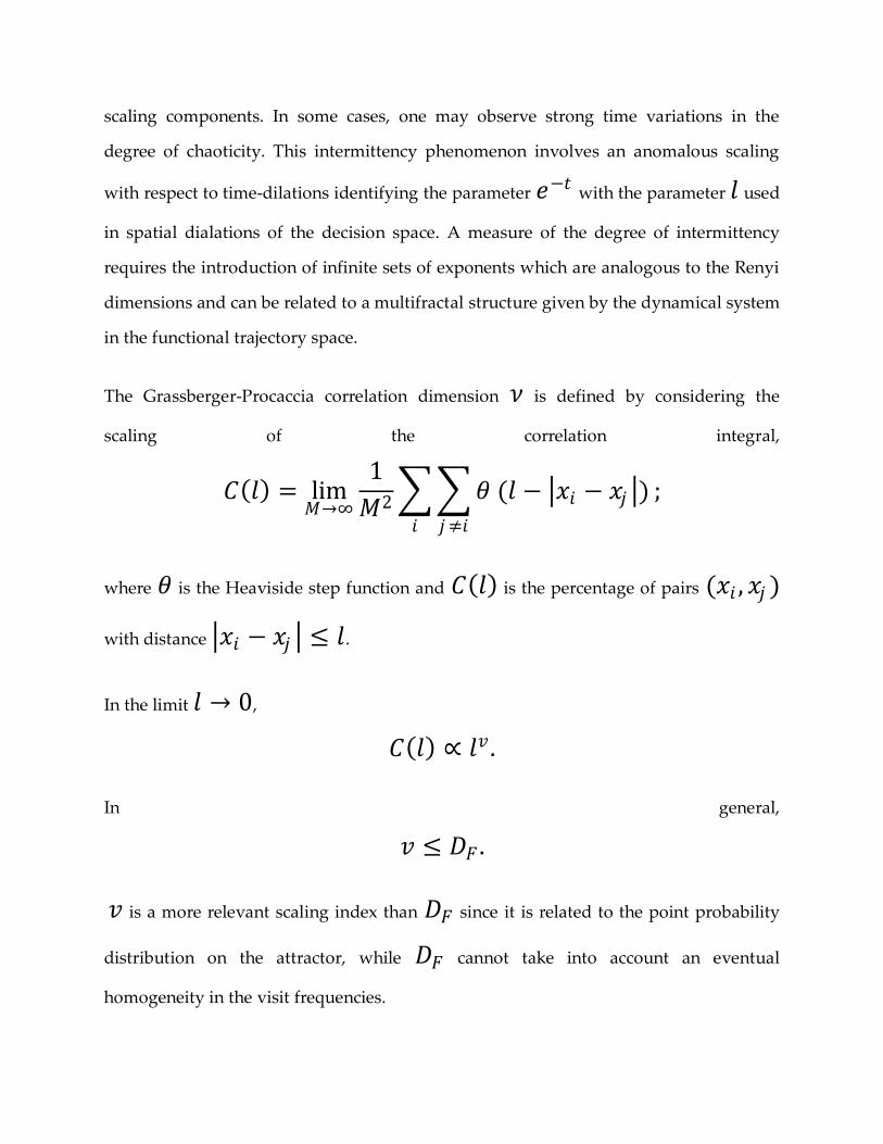
The Grassberger-Procaccia correlation dimension 𝜈 is defined by considering the

scaling of the correlation integral,

𝐶 𝑙 = lim𝑀→∞

1

𝑀2 𝜃 (𝑙 − 𝑥𝑖 − 𝑥𝑗 )

𝑗≠𝑖𝑖

;

where 𝜃 is the Heaviside step function and 𝐶 𝑙 is the percentage of pairs (𝑥𝑖 , 𝑥𝑗 )

with distance 𝑥𝑖 − 𝑥𝑗 ≤ 𝑙.

In the limit 𝑙 → 0,

𝐶 𝑙 ∝ 𝑙𝑣 .

In general,

𝑣 ≤ 𝐷𝐹 .

𝑣 is a more relevant scaling index than 𝐷𝐹 since it is related to the point probability

distribution on the attractor, while 𝐷𝐹 cannot take into account an eventual

homogeneity in the visit frequencies.

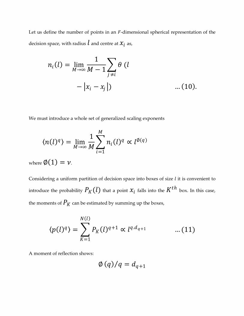
Let us define the number of points in an 𝐹-dimensional spherical representation of the

decision space, with radius 𝑙 and centre at 𝑥𝑖 as,

𝑛𝑖 𝑙 = lim𝑀→∞

1

𝑀 − 1 𝜃 (𝑙

𝑗 ≠𝑖

− 𝑥𝑖 − 𝑥𝑗 ) … 10 .

We must introduce a whole set of generalized scaling exponents

𝑛 𝑙 𝑞 = lim𝑀→∞

1

𝑀 𝑛𝑖 𝑙

𝑞 ∝ 𝑙∅(𝑞)

𝑀

𝑖=1

where ∅ 1 = 𝜈.

Considering a uniform partition of decision space into boxes of size 𝑙 it is convenient to

introduce the probability 𝑃𝐾(𝑙) that a point 𝑥𝑖 falls into the 𝐾𝑡𝑕 box. In this case,

the moments of 𝑃𝐾 can be estimated by summing up the boxes,

𝑝 𝑙 𝑞 = 𝑃𝐾 𝑙 𝑞+1

𝑁 𝑙

𝐾=1

∝ 𝑙𝑞 .𝑑𝑞+1 … (11)

A moment of reflection shows:

∅ 𝑞 𝑞 = 𝑑𝑞+1

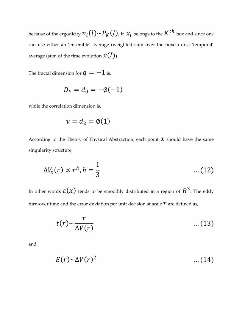
because of the ergodicity 𝑛𝑖 𝑙 ~𝑃𝐾 𝑙 , if 𝑥𝑖 belongs to the 𝐾𝑡𝑕 box and since one

can use either an ‘ensemble’ average (weighted sum over the boxes) or a ‘temporal’

average (sum of the time evolution 𝑥(𝑙)).

The fractal dimension for 𝑞 = −1 is,

𝐷𝐹 = 𝑑0 = −∅ −1

while the correlation dimension is,

𝜈 = 𝑑2 = ∅ 1

According to the Theory of Physical Abstraction, each point 𝑥 should have the same

singularity structure,

Δ𝑉𝑥 𝑟 ∝ 𝑟𝑕 , 𝑕 =1

3 … (12)

In other words 휀 𝑥 tends to be smoothly distributed in a region of 𝑅3. The eddy

turn-over time and the error deviation per unit decision at scale 𝑟 are defined as,

𝑡 𝑟 ~𝑟

Δ𝑉 𝑟 … (13)

and

𝐸 𝑟 ~Δ𝑉 𝑟 2 … (14)

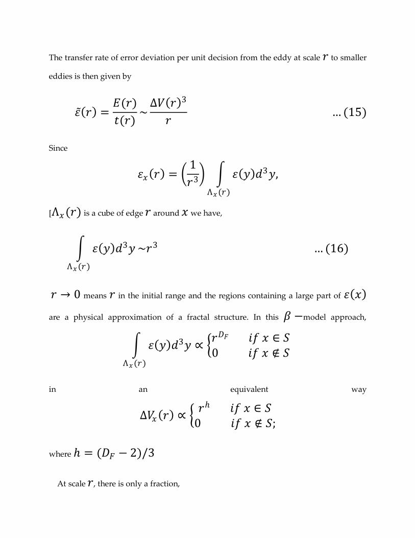
The transfer rate of error deviation per unit decision from the eddy at scale 𝑟 to smaller

eddies is then given by

휀 𝑟 =𝐸(𝑟)

𝑡(𝑟)~

Δ𝑉 𝑟 3

𝑟 … (15)

Since

휀𝑥 𝑟 = 1

𝑟3 휀 𝑦 𝑑3𝑦

Λ𝑥(𝑟)

,

[Λ𝑥(𝑟) is a cube of edge 𝑟 around 𝑥 we have,

휀 𝑦 𝑑3𝑦

Λ𝑥(𝑟)

~𝑟3 … (16)

𝑟 → 0 means 𝑟 in the initial range and the regions containing a large part of 휀 𝑥

are a physical approximation of a fractal structure. In this 𝛽 −model approach,

휀 𝑦 𝑑3𝑦

Λ𝑥(𝑟)

∝ 𝑟𝐷𝐹 𝑖𝑓 𝑥 ∈ 𝑆0 𝑖𝑓 𝑥 ∉ 𝑆

in an equivalent way

Δ𝑉𝑥 𝑟 ∝ 𝑟𝑕 𝑖𝑓 𝑥 ∈ 𝑆

0 𝑖𝑓 𝑥 ∉ 𝑆;

where 𝑕 = (𝐷𝐹 − 2)/3

At scale 𝑟, there is only a fraction,

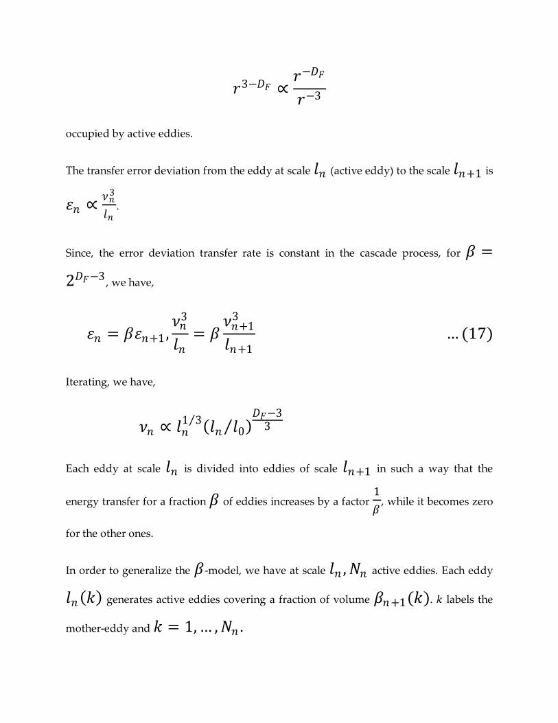
𝑟3−𝐷𝐹 ∝𝑟−𝐷𝐹

𝑟−3

occupied by active eddies.

The transfer error deviation from the eddy at scale 𝑙𝑛 (active eddy) to the scale 𝑙𝑛+1 is

휀𝑛 ∝𝜈𝑛

3

𝑙𝑛.

Since, the error deviation transfer rate is constant in the cascade process, for 𝛽 =

2𝐷𝐹−3, we have,

휀𝑛 = 𝛽휀𝑛+1 ,𝜈𝑛

3

𝑙𝑛= 𝛽

𝜈𝑛+13

𝑙𝑛+1 … (17)

Iterating, we have,

𝜈𝑛 ∝ 𝑙𝑛1 3 𝑙𝑛 𝑙0

𝐷𝐹−33

Each eddy at scale 𝑙𝑛 is divided into eddies of scale 𝑙𝑛+1 in such a way that the

energy transfer for a fraction 𝛽 of eddies increases by a factor 1

𝛽, while it becomes zero

for the other ones.

In order to generalize the 𝛽-model, we have at scale 𝑙𝑛 , 𝑁𝑛 active eddies. Each eddy

𝑙𝑛 𝑘 generates active eddies covering a fraction of volume 𝛽𝑛+1(𝑘). 𝑘 labels the

mother-eddy and 𝑘 = 1, … , 𝑁𝑛 .

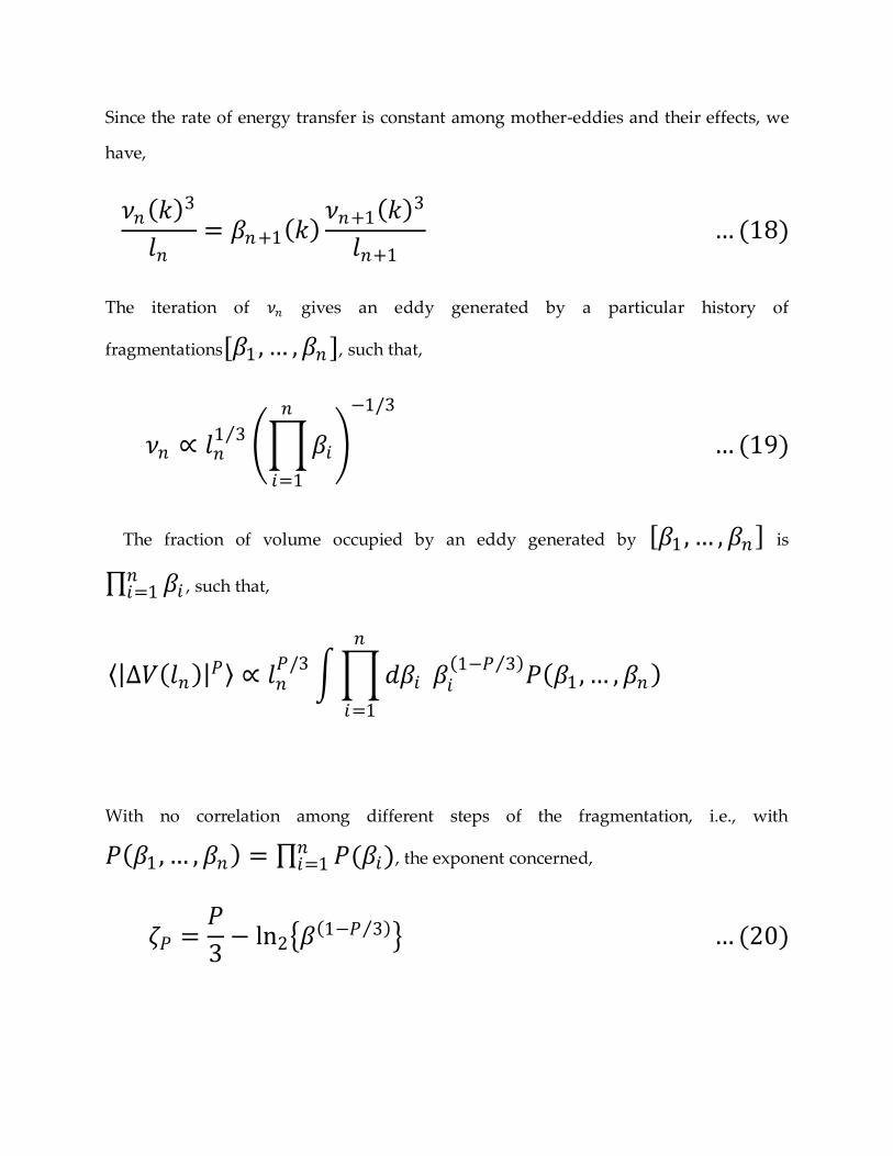
Since the rate of energy transfer is constant among mother-eddies and their effects, we

have,

𝜈𝑛 𝑘 3

𝑙𝑛= 𝛽𝑛+1 𝑘

𝜈𝑛+1 𝑘 3

𝑙𝑛+1 … (18)

The iteration of 𝜈𝑛 gives an eddy generated by a particular history of

fragmentations[𝛽1 , … , 𝛽𝑛 ], such that,

𝜈𝑛 ∝ 𝑙𝑛1 3

𝛽𝑖

𝑛

𝑖=1

−1/3

… (19)

The fraction of volume occupied by an eddy generated by 𝛽1 , … , 𝛽𝑛 is

𝛽𝑖𝑛𝑖=1 , such that,

∆𝑉 𝑙𝑛 𝑃 ∝ 𝑙𝑛

𝑃/3 𝑑𝛽𝑖

𝑛

𝑖=1

𝛽𝑖 1−𝑃 3

𝑃 𝛽1 , … , 𝛽𝑛

With no correlation among different steps of the fragmentation, i.e., with

𝑃 𝛽1 , … , 𝛽𝑛 = 𝑃(𝛽𝑖)𝑛𝑖=1 , the exponent concerned,

휁𝑃 =𝑃

3− ln2 𝛽

1−𝑃 3 … (20)

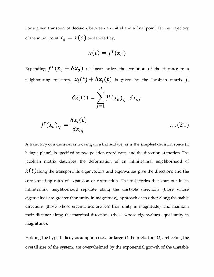
For a given transport of decision, between an initial and a final point, let the trajectory

of the initial point 𝑥𝑜 = 𝑥(𝑜) be denoted by,

𝑥 𝑡 = 𝑓𝑡(𝑥𝑜)

Expanding 𝑓𝑡(𝑥𝑜 + 𝛿𝑥𝑜) to linear order, the evolution of the distance to a

neighbouring trajectory 𝑥𝑖(𝑡) + 𝛿𝑥𝑖(𝑡) is given by the Jacobian matrix 𝐽,

𝛿𝑥𝑖 𝑡 = 𝐽𝑡(𝑥𝑜)𝑖𝑗

𝑑

𝑗 =1

𝛿𝑥𝑜𝑗 ,

𝐽𝑡(𝑥𝑜)𝑖𝑗 =𝛿𝑥𝑖 𝑡

𝛿𝑥𝑜𝑗 . . . (21)

A trajectory of a decision as moving on a flat surface, as is the simplest decision space (it

being a plane), is specified by two position coordinates and the direction of motion. The

Jacobian matrix describes the deformation of an infinitesimal neighborhood of

𝑥 𝑡 along the transport. Its eigenvectors and eigenvalues give the directions and the

corresponding rates of expansion or contraction. The trajectories that start out in an

infinitesimal neighborhood separate along the unstable directions (those whose

eigenvalues are greater than unity in magnitude), approach each other along the stable

directions (those whose eigenvalues are less than unity in magnitude), and maintain

their distance along the marginal directions (those whose eigenvalues equal unity in

magnitude).

Holding the hyperbolicity assumption (i.e., for large 𝑛 the prefactors 𝑎𝑖 , reflecting the

overall size of the system, are overwhelmed by the exponential growth of the unstable

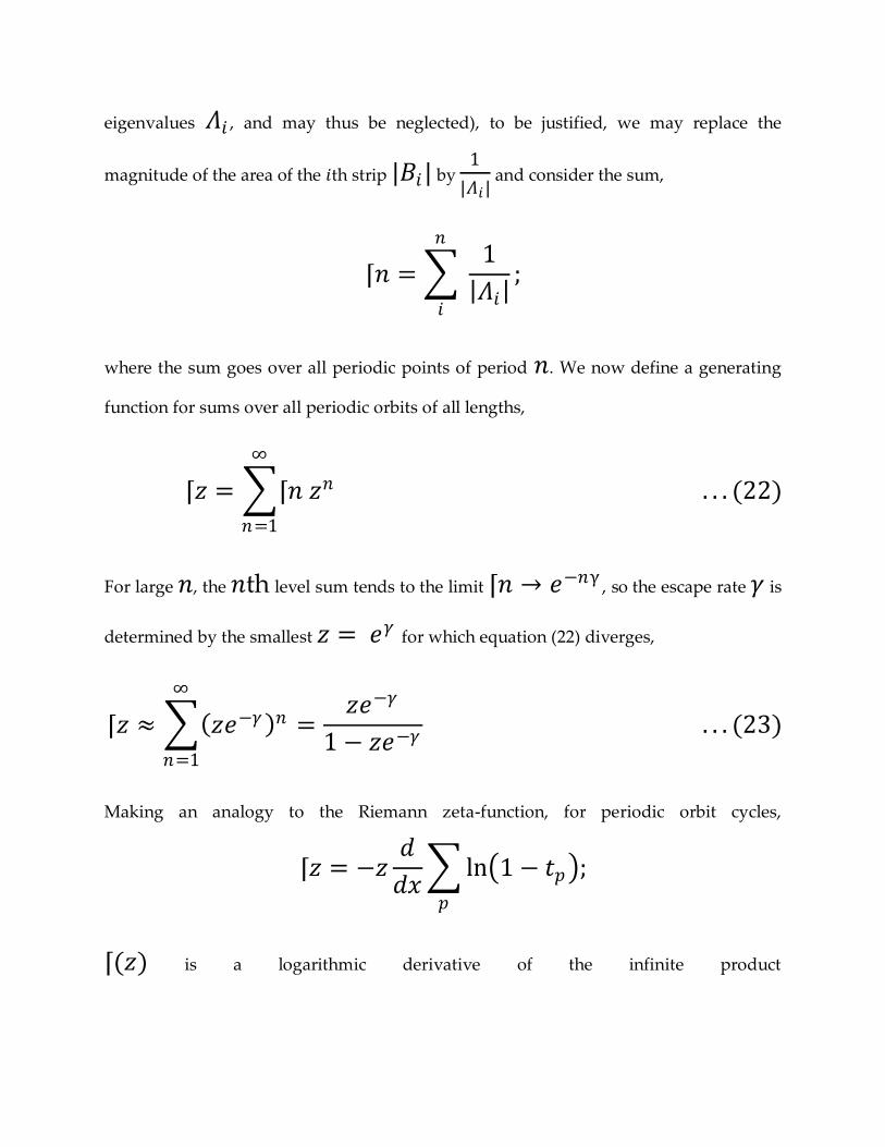
eigenvalues 𝛬𝑖 , and may thus be neglected), to be justified, we may replace the

magnitude of the area of the 𝑖th strip |𝐵𝑖| by 1

|𝛬𝑖| and consider the sum,

⌈𝑛 = 1

𝛬𝑖

𝑛

𝑖

;

where the sum goes over all periodic points of period 𝑛. We now define a generating

function for sums over all periodic orbits of all lengths,

⌈𝑧 = ⌈𝑛 𝑧𝑛

∞

𝑛=1

. . . (22)

For large 𝑛, the 𝑛th level sum tends to the limit ⌈𝑛 → 𝑒−𝑛γ, so the escape rate 𝛾 is

determined by the smallest 𝑧 = 𝑒𝛾 for which equation (22) diverges,

⌈𝑧 ≈ 𝑧𝑒−𝛾 𝑛∞

𝑛=1

=𝑧𝑒−𝛾

1 − 𝑧𝑒−𝛾 . . . (23)

Making an analogy to the Riemann zeta-function, for periodic orbit cycles,

⌈𝑧 = −𝑧𝑑

𝑑𝑥 ln 1 − 𝑡𝑝 ;

𝑝

⌈(𝑧) is a logarithmic derivative of the infinite product

1

휁(𝑧)= 1 − 𝑡𝑝 ,

𝑝

𝑡𝑝 =𝑧𝑛𝑝

|𝛬𝑝 | … (24)

This represents the dynamical zeta function for the escape rate of the trajectories of

decision-transport.

Abstraction says that points inside the decision space cluster to form decision directions

of a given property, at the desired scaling-ratio. Let us consider one such system of

decision making, inside which its constituent points have the tendency to form clusters.

Prediction:

In such transactions, the family of evolution-maps 𝑓𝑡 form a group. The evolution rule

𝑓𝑡 is a family of mappings of strips of transport 𝐵, that we may consider, such that,

1) 𝑓0 𝑥 = 𝑥

2) 𝑓𝑡[𝑓𝑡 ′ 𝑥 ] = 𝑓𝑡+𝑡 ′

(𝑥)

3) (𝑥, 𝑡) → 𝑓𝑡(𝑥) from 𝐵 × 𝑅 into 𝐵 is continuous;

where 𝑡 represents a time interval and 𝑡 ∈ 𝑅.

For infinitesimal times, we may write the trajectory of a given transaction as,

𝑥 𝑡 + 𝜏 = 𝑓𝑡+𝜏 𝑥0

= 𝑓[𝑓 𝑥0, 𝑡 , 𝜏] … (25)

The time derivative of this trajectory at point 𝑥(𝑡) is,

𝑑𝑥

𝑑𝜏 𝜏=0

= 𝜕𝜏𝑓[𝑓 𝑥0 , 𝑡 , 𝜏] 𝜏=0 = 𝑥 𝑡 … (26)

The vector field is a generalized velocity field,

𝑥 𝑡 = 𝑣 𝑥

If 𝑥𝑞 represents an equilibrium point, the trajectory remains stuck at 𝑥𝑞 forever.

Otherwise, the trajectory passing through 𝑥0 at time 𝑡 = 0 may be obtained by,

𝑥 𝑡 = 𝑓𝑡 𝑥0 = 𝑥0 + 𝑑𝜏 𝑣 𝑥 𝜏 ,

𝑡

0

𝑥 0

= 𝑥0 … (27)

The Euler integrator, which advances the trajectory by 𝛿𝜏 × velocity at each time

step is,

𝑥𝑖 = 𝑥𝑖 + 𝑣𝑖 𝑥 𝛿𝜏.

This may be used to integrate the equations of the dynamics concerned.

In our decision/perception plane a fuzzy set LF may be defined as:

LF : L→[0,1], …(28).

where L is a domain of elements (universe of discourse).

For every particular value of a variable Li ∈ L the degree of membership to fuzzy set

LF is LF (Li ).

Equation (28) describes how we can incorporate a fuzzy complex number or FCN in our

decision/perception plane.

LF in the universe of discourse L is defined by the complex membership grade

function 𝜇LF (Li ). The complex membership grade function or CMG is defined as:

𝜇LF(Li)= LF(Li)𝑒𝑖𝑐 …(29).

The Cartesian representation of CMG for 𝜇LF(Li)= 𝜇LF(𝑐𝑖+i𝑟𝑖) is:

𝜇(𝑐𝑖 , 𝑟𝑖)= 𝜇(𝑐𝑖)+i𝑟𝑖 …(30)

And, the polar representation is:

𝑐𝑖𝑒𝑖𝑠𝑟 …(31),

the scaling factor s being in the interval (0,2𝜋].

The degree of fulfillment or DOF of any given proposition follows CMG and lies in the

interval [0,1].

According to the definition of transformation of coordinates:

𝜇(𝑐𝑖 , 𝑟𝑖) 𝑐𝑖𝑒𝑖𝑠𝑟

The operators ∧ and ∨ defining t-norm and s-norm respectively and Li being the set

of fuzzy numbers concerned, the fuzzy set of a function of Li has the membership

function:

𝜇 𝑐𝑖′ , 𝑟𝑖

′ = [𝜇(𝑐1 , 𝑟1𝑐𝑖′ =𝑓(Li ) ) 𝜇(𝑐2 , 𝑟2) 𝜇(𝑐3 , 𝑟3)… 𝜇(𝑐𝑛 , 𝑟𝑛)]

Using Lyapunov exponents for the measure L, and replacing 2𝑐 𝜆

𝐷 by a

quantity′𝜏′, we have:

𝑑

𝑑𝜏𝑓𝑛 𝐿 =

𝛿𝑛

𝛿𝑜

i.e.,

𝛿𝑛

𝛿𝑜= 𝑓′ (𝐿𝑖)

𝑛𝑖=1 …(32).

𝑏 =1

𝑛log𝑒

𝛿𝑛

𝛿𝑜

i.e.,

𝑏 =1

𝑛 log𝑒 𝑓

′ (𝐿𝑖) 𝑛−1𝑖=1 …(33).

where 𝑏 is a constant (the local slope of all possible measures), and

Ψ = lim𝑛→∞1

𝑛 log𝑒 𝑓

′(𝐿𝑖) 𝑛−1𝑖=0 …(34).

where Ψ is a constant.

Distribution:

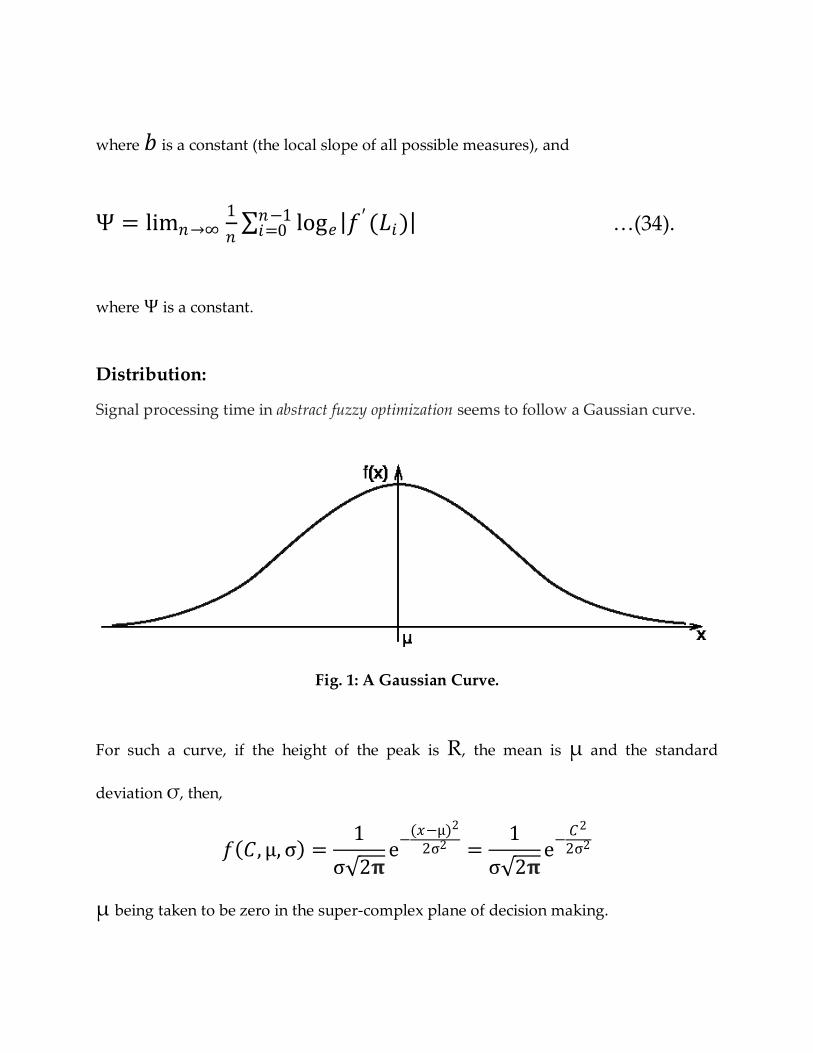
Signal processing time in abstract fuzzy optimization seems to follow a Gaussian curve.

Fig. 1: A Gaussian Curve.

For such a curve, if the height of the peak is R, the mean is μ and the standard

deviation σ, then,

𝑓 𝐶,μ,σ =1

σ 2𝛑e−

(𝑥−μ)2

2σ2 =1

σ 2𝛑e−

𝐶2

2σ2

μ being taken to be zero in the super-complex plane of decision making.

For the simplest case of a two dimensional decision plane,

𝐿𝑖 =1

2𝛑σ2 e−

(𝐶2+R2)2σ2 … 35 .

A two-dimensional elliptical Gaussian function for such a case, may be expressed as:

𝑓 𝐶, R = Lie−𝑎(𝐶−C0)2+2𝑏 𝐶−𝐶0 𝑅−𝑅0 +𝑐(𝑅−R0)2

where a, b and c forms a positive definite matrix as:

𝑎 𝑏𝑏 𝑐

A measure for precision in any given direction of decision making is given by the covariance matrix,

𝑉 =𝜎2

2𝑃𝐶𝑃2

3

2𝑐0

−1

𝑎

02𝑐

𝑎20

−1

𝑎0

2𝑐

𝑎2

Where, the precision of the system is represented by P.

Depending upon the value of precision involved, the number of activated states follows a sigmoid

distribution:

𝑛 𝑡 =1

1 + 𝑒−𝑡

Conclusion:

Natural processes, including decision making follows non-linear pathways that give

rise to emergence phenomena. Patterns arise in the whole that cannot be wholly

attributed to the sum of the parts. The whole decision making process is way more than

the sum of the individual processes involved. From the Theory of Abstraction, we know

how information energy changes with changes in the scaling ratio. The same can be

observed in the decision making process too. The difference in dissipation energy

information (and as such deviation in a given direction of decision making), which

tends to infinity as the number of constituent points inside it tends to infinity. In this

respect, at large enough scaling-ratios, the universe seems to work in a similar way as

the brain does.

References

1. A. Connes, Trace formula in noncommutative geometry and the zeros of

the Riemann zeta function, Selecta Math. (NS) 5 (1999), 29–106.

2. J.B. Conrey, More than two fifths of the zeros of the Riemann zeta

function are on the critical line, J. reine angew. Math. 399 (1989), 1–26.

3. P. Deligne, La Conjecture deWeil I, Publications Math. IHES 43 (1974),

273–308.

4. P. Deligne, La Conjecture de Weil II, Publications Math. IHES 52

(1980), 137–252.

5. Browder, Felix, ed. Mathematical Developments Arising from Hilbert Problems.

American Mathematical Society, 1976.

6. Kantor, Jean-Michel. ‚Hilbert’s Problems and Their Sequel‛, Mathematical

Intelligencer 18 (1996): 21 – 30.

7. Smale, Stephen. ‚Mathematical Problems for the Next Century‛, Mathematical

Intelligencer 20 (1998): 7 – 15.

8. Pier, Jean-Paul, ed. The Development of Mathematics, 1950 – 2000. Birkhauser,

2000.

9. Arnol’d, Vladimir, Michael Atiyah, Peter Lax, Barry Mazur, eds. Mathematics

Tomorrow. International Mathematical Union, 2000.

10. C. Deninger, Some analogies between number theory and dynamical

systems on foliated spaces, Proc. Int. Congress Math. Berlin 1998, Vol. I, 163–186.

11. H.M. Edwards, Riemann’s Zeta Function, Academic Press, New York -

London 1974.

12. S. Haran, Index theory, potential theory, and the Riemann hypothesis,

L-functions and Arithmetic, Durham 1990, LMS Lecture Notes 153 (1991), 257–

270.

13. G.H. Hardy, Divergent Series, Oxford Univ. Press 1949, Ch. II, 23–26.

14. H. Iwaniec and P. Sarnak, Perspectives on the Analytic Theory of

L-Functions, to appear in proceedings of the conference Visions 2000, Tel Aviv.

15. A. Iviˇc , The Riemann Zeta-Function - The Theory of the Riemann Zeta-

Function with Applications, John Wiley & Sons Inc., New York - Chichester -

Brisbane - Toronto - Singapore 1985.

16. N.M. Katz and P. Sarnak, Random matrices, Frobenius eigenvalues

and monodromy, Amer. Math. Soc. Coll. Publ. 49, Amer. Math. Soc., Providence

RI 1999.

17. E. Landau, Primzahlen, Zwei Bd., IInd ed., with an Appendix by Dr.

Paul T. Bateman, Chelsea, New York 1953.

18. N. Levinson, More than one-third of the zeros of the Riemann zetafunction

are on σ = 1/2, Adv. Math. 13 (1974), 383–436.

19. J. van de Lune, J.J. te Riele and D.T. Winter, On the zeros of

the Riemann zeta function in the critical strip, IV, Math. of Comp. 46 (1986),

667–681.

20. H.L. Montgomery, Distribution of the Zeros of the Riemann Zeta Function,

Proceedings Int. Cong. Math. Vancouver 1974, Vol. I, 379–381.

21. A.M. Odlyzko, Supercomputers and the Riemann zeta function, Supercomputing

89: Supercomputing Structures & Computations, Proc. 4-th Intern.

Conf. on Supercomputing, L.P. Kartashev and S.I. Kartashev (eds.), International

Supercomputing Institute 1989, 348–352.

22. B. Riemann, Ueber die Anzahl der Primzahlen unter einer gegebenen

Gr¨osse, Monat. der K¨onigl. Preuss. Akad. der Wissen. zu Berlin aus der Jahre

1859 (1860), 671–680; also, Gesammelte math. Werke und wissensch. Nachlass, 2.

Aufl. 1892, 145–155.

23. Z. Rudnick and P. Sarnak, Zeros of principal L-functions and random

matrix theory, Duke Math. J. 82 (1996), 269–322.

24. A. Selberg, On the zeros of the zeta-function of Riemann, Der Kong.

Norske Vidensk. Selsk. Forhand. 15 (1942), 59–62; also, Collected Papers, Springer-

Verlag, Berlin - Heidelberg - New York 1989, Vol. I, 156–159.

25. F. Severi, Sulla totalit`a delle curve algebriche tracciate sopra una superficie

algebrica, Math. Annalen 62 (1906), 194–225.

26. C.L. Siegel, ¨Uber Riemanns Nachlaß zur analytischen Zahlentheorie,

Quellen und Studien zur Geschichte der Mathematik, Astronomie und Physik 2

(1932), 45–80; also Gesammelte Abhandlungen, Springer-Verlag, Berlin - Heidelberg

- New York 1966, Bd. I, 275–310.

27. E.C. Titchmarsh, The Theory of the Riemann Zeta Function, 2nd ed.

revised by R.D. Heath-Brown, Oxford Univ. Press 1986.

28. R. Taylor and A. Wiles, Ring theoretic properties of certain Hecke

algebras, Annals of Math. 141 (1995), 553–572.

29. A. Weil, OEuvres Scientifiques–Collected Papers, corrected 2nd printing,

Springer-Verlag, New York - Berlin 1980, Vol. I, 280-298.

30. A. Weil, Sur les Courbes Alg´ebriques et les Vari´et´es qui s’en d´eduisent,

Hermann & Cie , Paris 1948.

31. A. Weil, Sur les ‚formules explicites‛ de la th´eorie des nombres premiers,

Meddelanden Fr°an Lunds Univ. Mat. Sem. (dedi´e `a M. Riesz), (1952), 252-

265; also, OEuvres Scientifiques–Collected Papers, corrected 2nd printing, Springer-

Verlag, New York - Berlin 1980, Vol. II, 48–61.

32. A. Wiles, Modular elliptic curves and Fermat’s Last Theorem, Annals

of Math. 141 (1995), 443–551.

33. Ganguly, Subhajit (2012): Distribution of Prime Numbers,twin Primes and Goldbach

Conjecture. figshare.

http://dx.doi.org/10.6084/m9.figshare.91653

34. Dave Carr, Jeff Shearer, Nonlinear Control and Decision Making Using Fuzzy Logic

in Logix.

35. D.E. Tamir, A. Kandel, Axiomatic Theory of Complex Fuzzy Logic and Complex

Fuzzy Classes, Int. J. of Computers, Communications & Control, ISSN 1841-9836, E-

ISSN 1841-9844 Vol. VI (2011), No. 3 (September), pp. 562-576.

36. Li Renjun, Yuan Shaoquiang, Li Baowen, Fu Weihai, Fuzzy Complex Number.

37. Xin Fu, Qiang Shen, Fuzzy Complex Numbers and their Application for Classifiers

Performance Evaluation.

38. Ramot, D., Milo, R., Friedman, M., Kandel, A., Complex fuzzy sets. IEEE

Transactions on Fuzzy Systems 2002, 10(2): p. 171-186.

38. Ramot, D., Friedman, M., Langholz, G., Kandel, A., Complex fuzzy logic. IEEE

Transactions on Fuzzy Systems, 2003, 11(4): p. 450-461

39. Ganguly, Subhajit (2014): Building a Foolproof Navigation System: Fuzzy Logic

Emulating the Brain. figshare.

http://dx.doi.org/10.6084/m9.figshare.1093898

40. Arthur, J.V.; Boahen, K. "Recurrently connected silicon neurons with active

dendrites for one-shot learning", Neural Networks, 2004. Proceedings. 2004 IEEE

International Joint Conference on, On page(s): 1699 - 1704 vol.3 Volume: 3, 25-29 July 2004