Computer simulation of dragging with rotation of a drill string in 3D

Vol.:(0123456789)

SN Applied Sciences (2019) 1:126 | https://doi.org/10.1007/s42452-018-0121-9

Research Article

Computer simulation of dragging with rotation of a drill string in 3D inclined tortuous bore‑hole

Valery Gulyayev1 · Elena Andrusenko1 · Sergey Glazunov1

© Springer Nature Switzerland AG 2018

AbstractThis paper deals with the problem on determination of resistance forces impeding a drill string dragging in a deep cur-vilinear bore-hole channel. The bore-hole axis geometry is considered to be prescribed discretely at its separate points with the use of the results of geophysical measurements (bore-hole navigation). A “3D stiff-string differential model” for simulation of the drag/torque phenomena accompanying hoisting, lowering and drilling operations is proposed. The system of ordinary differential equations is derived based on the theory of curvilinear flexible elastic rods. The transfer from the tabular to analytic description of the bore-hole trajectory geometry is performed with the application of the cubic spline interpolation. The elaborated approach can be used for simulation of the drill string dragging with rotation, its contact and frictional interaction with the bore-hole surface and prognostication of the string lock up situations. Numerical examples are presented to illustrate the proposed techniques advantages.

Keywords Curvilinear drilling · Drill string raising · Contact forces · Resistance forces

List of symbolsa DS sliding velocityak , bk , ck , dk Interpolation coefficientsD Metric multiplierDS Drill stringE Elasticity module� (s) Vector of external distributed forces�gr , � cont , � fr Vectors of distributed external forces of

gravity, contact and frictionf (xi) Values of y(x) function at xi points�(s) Principal vector of internal elastic forcesF(xi) Interpolated functionFn , Fb , Ft Appropriate components of the � forceh Depth of the bore-hole�, �, � Unit vectors of the Cartesian coordinate

systemI Inertia moment of the DS tubek(s) Natural parametrization of the bore-hole

curvature

k(�) Dimensionless parametrization of the bore-hole curvature

kR Main curvature of a spatial curvekT Torsion of a spatial curvel Horizontal distance�(s) Vector of distributed external moment�(s) Principal vector of internal elastic

momentsMn , Mb , Mt Appropriate components of the �

moment�, �, � Unit vectors of the Frenet trihedronN Number of interpolation pointsOxyz Cartesian coordinate systemPn(x) Interpolating polynomialr External radius of the DS tube�0 Radius-vector of the bore-hole curve

pointsr1 , r2 External and internal radii of the DS tubes Natural parameter of the bore-hole curveS Bore-hole trajectory length

Received: 27 August 2018 / Accepted: 12 December 2018 / Published online: 24 December 2018

* Valery Gulyayev, [email protected] | 1Department of Mathematics, National Transport University, 1, M. Omelianovycha-Pavlenka Str., Kiev 01010, Ukraine.

http://orcid.org/0000-0002-5388-006X

http://orcid.org/0000-0001-9986-5888

http://orcid.org/0000-0002-1920-0040

Vol:.(1234567890)

Research Article SN Applied Sciences (2019) 1:126 | https://doi.org/10.1007/s42452-018-0121-9

tz Appropriate component of the � vectorxi Discrete values of independent variableyi Discrete values of the interpolated

functionx0 , y0 , z0 Planned coordinates of the bore-hole

trajectory� Linear weight of the DS tube� Symbol of small variationΔ Symbol of small increment� Eccentricity of the hyperbola� Dimentional parameter of the bore-hole

curve� Friction coefficient� Ratio of the axial and circumferential

velocities of the DS tube�k(xk) Interpolating functions� Angular velocity of the DS rotation� Darboux vector

1 Introduction

One of the most important factors, impeding drilling the hyper deep and extensional bore-holes with curvilinear trajectories, is specified by the resistive (frictional) forces. In their generating, the great role is played by the bending stiffness of a drill string (DS), bore-hole tortuosity and its length, as well as by the type of the technological opera-tion [3, 19]. These forces hamper permeability of the force on bit and torque on bit, provoke buckling of the drill string [6, 10] and can result in dead lock situations.

To predict and eliminate these effects, the mathematic models and software should be elaborated for simulation of the drilling processes in long 3D tortuous bores.

Appearance of these emergency situations is princi-pally caused by three factors. First of all, this is the large length of the DSs. Under conditions of the geometric simi-larity, they are equivalent to a human hair. Therefore, the phenomena, occurring at one end of a DS, can influence, poorly influence and do not influence on the effects, tak-ing place at its other end. In mathematics, the equations, describing such effects, are named singularly perturbed. They are characterized by poorly converging solutions with the modes, possessing singularities in the shapes of boundary effects or internal irregularities.

The second factor is connected with the special char-acter of frictional effects, showing themselves in tortu-ous curvilinear bore-holes. The matter is that in them, the friction force depends on the pressure force between the contacting bodies. But in the curvilinear pieces of the trajectory, the pressure force is determined by the axial force of the DS tension and the bore curvature. In this case, it is said in mechanics that the friction forces have

a multiplicative (i.e., they are multiplied) but not additive (they are not added) nature, as it occurs in sliding of one body on the shaggy plane surface of another one [19].

Finally, the third factor is associated with the fact that the problems on mathematic simulation of mechanical phenomena, attending the drilling processes, are mul-tiparametric, as they depend on large number of geo-metric and mechanic values. Therefore, the questions become very important which are associated with analysis of these phenomena under specific particular values of the constitutive parameters and establishment of general regularities of the proceeding processes. Some additional detrimental effects are generated by dynamic phenomena [18, 23].

Because of this, the drilling technology for inclined and horizontal bore-holes is featured by its complexity and is not completely mature. The world statistics indicates that the accident rate is 1 in 3 for driving bore-holes of this type [16]. It is associated to a large extent with the complexity of mechanical and physical phenomena accompanying the drilling process and the lack of reliable methods of computer simulation that enables us to predict the emer-gency situations and to prevent them beforehand.

The efforts to simulate the inclined drill problems with the use of computer models present considerable difficul-ties determined by a number of factors [5, 11, 12, 14, 15, 17]. Among them the relatively complex geometry of the drill string is the main concern. Being founded on the geo-metrical similarity, the drill columns can be compared to a very flexible rod with negligible bending stiffness. Early, this circumstance permitted to simulate the internal and external forces acting on them with the use of simplified mathematical models based on the theory of absolutely flexible threads [1, 2, 21]. Analysis of these forces was per-formed only on the basis of investigations of geometrical peculiarities of the bore-hole axis line without considering the contribution of elastic forces and contact effects gen-erated during raising–lowering operations and rotation of the drill string. With the use of this approach, a number of researches on the designs of bore-holes with the simplest outlines have been presented [1, 20, 21].

In papers [4, 22], a more general approach called the minimum curvature method has been adopted, by con-sidering the well axis outline as a smooth curve made up of segments of straight lines and circular or catenary curves. By this approach, explicit analytical equations were derived to model the drill string (thread) with tension and friction forces for tripping in and out operations. In addition, explicit expressions were developed for the drill column to include the effects of drag and torque under the combined axial motion and rotation. Using the equali-ties, the total drag and torque were derived as the sum of their separate contributions from each section of the

Vol.:(0123456789)

SN Applied Sciences (2019) 1:126 | https://doi.org/10.1007/s42452-018-0121-9 Research Article

hole. Different algorithms and software programs were presented. Several examples were prepared to demon-strate the use of the analytical models. It was shown that any change of direction in the well path contributed to increased friction.

The conclusion achieved based on assumption of well trajectory smoothness and negligible bending stiffness of the drill string tube may underline the weakness of the theory used. In practice, the axial trajectories of bore-holes cannot be represented as lines with smooth geometry because of the geometrical imperfections involved in drill-ing. They can be caused by distortions of the bit geometry, dynamic imbalance of the bottom-hole-assembly, and physical non-homogeneities of the drilled rock medium. These factors impact on mobility of the drill string inside that sort of bore-holes and can be investigated only with the use of 3D stiff string drag and toque models elabo-rated on the basis of the theory of curvilinear flexible rods and methods of differential geometry. The model of that kind and software were elaborated by [7, 8]. Through their application, different examples of bore-holes with local-ized spiral, harmonic, and irregular (dog leg) imperfections described by analytic correlations were considered. It was demonstrated that additional short-pitched tortuosities led to essential enlargement of contact and resistance forces, provoking decrease of the dill string mobility and appearance of dead lock states.

Yet, in practice, the situation is much more complicated. The point is that the imperfections incorporated into the bore-hole geometry during drilling are not well-ordered and cannot be represented by analytic correlations. They are established by means of geophysical measurements performed at separate points with certain step throughout the bore-hole axis line length and can be rendered only in a tabular (discrete) form.

Therefore, if to take into account that the effects of the DS bending can be described only with the use of differ-ential equations based on the continuity hypotheses, it becomes evident that the geometry of the planned or drilled bore-holes must be restructured to the analytical form.

Considered below is the problem of computer simula-tion of a drill string dragging with rotation in the chan-nel of a curvilinear tortuous bore-hole with the center-line prescribed in a tabular form. To create the analytical mathematic model of the DS dragging with allowance made for the resistance (gravity, contact, and friction) forces, the transfer from the discrete description of the bore-hole axis to its continuous (differentiable) presenta-tion was performed. It was done via utilization of methods of spline interpolation, differential geometry, mechanics of structures, and methods of numerical integration. This smoothing of the trajectory geometry enabled us for the

first time to create a universal 3D stiff string drag and torque model based on application of a spatial theory of elastic curvilinear flexible rods. With its application, the constitutive differential equations were deduced. They can be used for prognostication of resistance forces and exclusion of emergency (sticking) situations at the stages of the bore-hole design and drivage. The results of the performed computer analysis confirmed efficiency of the proposed approach.

2 Analytic presentation of the bore‑hole axis line geometry

In the applied mathematics the interpolation procedure is associated with construction of an interpolating function, passing through the prescribed points of tabular data [13]. This procedure essence consists in prescription of a set of points xi ( 1 ≤ i ≤ N ) from some domain and assumption that the values of some desired function f are known only at these points

The interpolation task consists in selection of some interpolating F(x) function, which satisfies conditions

and can be used instead of the sought—for function f (x).In practice, usually a polynomial interpolation is used

as it is easy to calculate derivatives of these functions with the help of analytical approaches. In this case, interpolat-ing function F(x) is constructed as a linear combination of some polynomials

where �k(x) are some specified functions; ak are the unknown coefficients.

It issues from this equality that interpolating function F(x) should coincide with the desired f (x) function at some points xi . These conditions are reduced to system

But this approach has one essential disadvantage because the matrix of coefficients �k(xi) in Eq. (4) is poorly conditioned and, as a rule, solutions of system (4) have significant miscalculations. In this connection, the spline interpolations are of great utility in applied mathematics. Unlike the polynomial approximation, the spline interpo-lation is constructed separately in every segment [ xk−1 ,

(1)f (xi) = yi (1 ≤ i ≤ N).

(2)F(xi) = yi (1 ≤ i ≤ N)

(3)F(x) =

N∑

k=1

ak �k(x),

(4)N∑

k=1

ak �k(xi) = f (xi) = yi (1 ≤ i ≤ N).

Vol:.(1234567890)


xk ], satisfying certain conditions of smoothness at node points xk . In computing mathematics, the most com-monly encountered splines are cubic ones, which can be described by expression

here coefficients ak , bk , ck , dk are found from the condi-tions of continuity of function P(x) and its first and second derivatives.

The noted properties of the cubic splines render them convenient for interpolation of the tabular data on the cur-vilinear bore-hole axis geometry, because in this event, its curvature described by equalities [13]

is also continuous.Here, x(s) , x(�) , y(s) , y(�),z(s) , z(�) are the axis line coor-

dinates; s is the natural parameter measured by the length of the axis line from some initial point till the current one; � is the dimensionless parameter; the symbol prime des-ignates the derivative with respect to s ; the dot denotes the differentiation operation relative to �.

As the right parts of Eqs. (6) contain only the first and second derivatives (which are continuous), curvatures k(s) or k(�) are also continuous.

2.1 3D stiff string drag and torque model of the drill string axial motion with rotation

Assume that a drill string performs axial motion with rota-tion inside a bore-hole cavity with curvilinear axial line. Its planned axis line is described by equation

where �, �, � are the unit vectors of the Cartesian coordi-nate system Oxyz.

During the drilling process, the table of real val-u e s x(Si) = x0(Si) + � x(Si) , y(Si) = y0(Si) + � y(Si) , z(Si) = z0(Si) + � z(Si) of the real drilled bore-hole trajec-tory points is formed through the use of geonavigation measurements. They are converted to analytic relations xi = xi(s) , yi = yi(s) , zi = zi(s) by interpolation with the cubic splines help within the limits of every segment Δ Si = Si+1 − Si = S∕(N − 1) throughout the bore-hole length 0 ≤ s ≤ S.

Assume that axis lines of the bore-hole and drill string coincide. There is a need to deduce the differential equa-tions of quasi static equilibrium of the drill sting in its axial motion with rotation and to calculate internal forces and

(5)Pk(x) = ak + bk(x − xk) +ck

2(x − xk)

2 +dk

6(x − xk)

3.

(6)

k(s) =√(x��)2 + (y��)2 + (z��)2 or

k(𝜗) =

�(x2 + y2 + z2)(x2 + y2 + z2) − (xx + yy + zz)2

(x2 + y2 + z2)3

(7)�0 = �0(s) = x0� + y0� + z0�,

moments, as well as distributed external contact and fric-tion forces, hindering its motion.

This problem has a distinctive feature associated with the consideration about coincidence of axial lines of the DS and bore-hole. Then, some of the components of the internal forces can be expressed immediately through the DS stiffness and the bore-hole geometry parameters. In mechanics of structures, the similar problems are known as inverse ones. Yet, at the same time, the internal axial force Ft(s) and torque Mt(s) in the DS are unknown and they should be calculated. Therefore, the considered prob-lem is partially inverse and partially direct.

To deduce the constitutive equations of elastic deform-ing a curvilinear rod, a concomitant reference frame mov-ing along its axial line with parameter s change should be introduced. Study of these equations is most convenient with the use of the Frenet natural trihedron with unit vec-tors of the principal normal � , binormal � , and tangent �.

At any cross-section of the DS, the principal vectors of internal forces �(s) and moments �(s) and the vectors of distributed external forces � (s) and moments �(s) satisfy the following equilibrium equations [9]

Since the Frenet reference frame rotates with its mov-ing along the DS axis, the total derivatives d�∕ds , d�∕ds should be expressed in the following form

here d…∕ds is the local derivative; � is the Darboux vec-tor, determined through the expression

With allowance made for Eq. (10), one can represent Eq. (8) as follows:

Consider that the process of the DS dragging inside the bore-hole channel is operated with constant axial velocity a and rotation velocity � . Then, the external distributed forces � (s) and moments �(s) can be represented by the equalities

here fgr is the gravity, fcont is the force of contact interaction between the surfaces of the DS and bore-hole, ffr is the force of friction interaction between these surfaces, mfr is the distributed moment of friction forces.

(8)d�

ds= − � ,

d�

ds= − � × � −�.

(9)d�

ds=

d�

ds+� × �,

d�

ds=

d�

ds+� ×�.

(10)� = kR� + kT �.

(11)d�

ds= −� × � − � ,

d�

ds= −� ×� − � × � −�.

(12)� = �gr + � cont + � fr , � = �fr = �fr��.

Vol.:(0123456789)


It is convenient to represent the vector force values at the �, �, � basis

where bending moment Mb is

here � is the linear weight of the DS tube calculated with allowance made for the buoyancy effect of the mud, � is the friction coefficient, E is the elasticity module of the DS material, I is the inertia moment of the DS tube cross-section.

Then, equilibrium Eq. (11) can be transformed to the scalar form:

Via the use of Eq. (16), internal shear forces Fn and Fb are expressed in the form:

Thereafter, distributed contact forces f contn

and f contb

are determined

Consider that the DS is being dragged with axial veloc-ity a and rotates with angular velocity � . Then, the total friction force is [3]

(13)

� = Fn� + Fb� + Ft�, � = Mb� +Mt�,

�gr = −�nz� − �bz� − �tz�, � cont = f contn

� + f contn

�

� fr = ±�

√(f contn

)2+(f contb

)2�,

(14)Mb = EIkR .

(15)

dFn

ds= −kRFt + kT Fb − f gr

n− f cont

n,

dFb

ds= −kT Fn − f

gr

b− f cont

b,

dFt

ds= kRFn − f

gr

t − f frt,

(16)

0 = −kRMt + EIkRkT + Fb,

dkR

ds= −

1

EIFn,

dMt

ds= −mfr

t.

(17)Fn = −EIdkR

ds, Fb = kRMt − EIkRkT .

(18)f contn

= −kRFt + kRkTMt − EIkRk2

T+ EI

d2kR

ds2− f gr

n,

f contb

= kRmfrt+ 2EIk

T

dkR

ds−Mt

dkR

ds+ EIkR

dkT

ds− f

gr

b.

(19)|||� fr|||= � |

|�cont|

| = �

√(f contn

)2+(f contb

)2.

and it is resolved to the lengthwise and rotary constituents [8]

here � is the Coulomb friction coefficient, r is the DS tube radius, signs “+” and “−” are selected depending on direc-tions of the DS axial movement and rotation. Coefficient � is determined by mechanical properties of the tube mate-rial, rock formation and mud viscosity. It can vary in some diapason depending on combination of these factors.

Based on Eqs. (13)–(18), the system of constitutive equa-tions of the DS dragging with rotation is deduced as follows:

Under this approach, the problem of calculation of the bore-hole axis geometry parameters becomes the principal complexity. To determine the coefficients of the differential Eqs. (17)–(21), methods of differential geometry should be used for determination of the components of unit vectors �, �, � and magnitudes kR and kT . To define the first ones, the correlations

are used [13].Here, R = 1∕kR is the curvature radius. It is calculated via

the formula

After this, the kT torsion is found as follows:

It is apparent that the transformations represented by correlations (22)–(24) cannot be performed analytically. Therefore, in the elaborated software, they are fulfilled numerically at every discrete point si through the use of finite difference method:

(20)

f frt= ±�f cont

a√a2 + (�r)2

, f frb= ±�f cont

�r√a2 + (�r)2

.

(21)

dFt

ds= kRFn + �tz ∓ �f cont

a√a2 + (�r)2

,

dMt

ds= ∓�f cont

�r2√a2 + (�r)2

.

(22)� = d �∕ds, � = Rd�∕ds, � = � × �

(23)kR = 1∕R =

√(d2x

ds2

)2

+

(d2y

ds2

)2

+

(d2z

ds2

)2

.

(24)kT = R2

|||||||

x� y� z�

x�� y�� z��

x�� y�� z��

|||||||

.

Vol:.(1234567890)


Derivatives dkR∕ds , d2kR/ds2 , dkT∕ds used in Eqs. (17),

(18) are calculated analogously

Since the geometric functions calculated with the use of Eqs. (22)–(26) are changing fast at the points of the vari-ables �x , �y , �z irregularities, to achieve satisfactory con-vergente of their computing, it is necessary to select suf-ficiently small values of the Δs increments. In our analysis it was chosen to be S∕1000.

3 Analysis of the numerical results of the generated resistance forces simulation

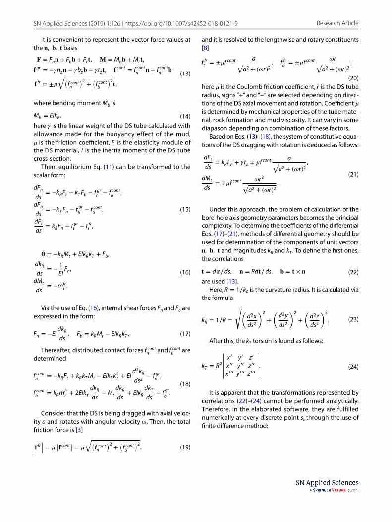
The elaborated techniques were used for numerical inves-tigation of resistance forces generated in the channel of a bore-hole with geometric imperfections. Firstly, the case was considered when the planned trajectory of the bore-hole was ideal and was represented by smooth planar hyperbolic curve x0(�) , y0(�) , z0(�) described by equali-ties (Fig. 1)

(25)

tx||i =

dx

ds

||||i=

xi+1 − xi−1

2Δs, ty

|||i=

dy

ds

||||i=

yi+1 − yi−1

2Δs, tz

||i =

dz

ds

||||i=

zi+1 − zi−1

2Δs,

kR||i =

√(xi+1 − 2xi + xi−1

Δs2

)2

+

(yi+1 − 2yi + yi−1

Δs2

)2

+

(zi+1 − 2zi + zi−1

Δs2

)2

.

(26)

dkR

ds

||||i≈

(kR)i+1 − (kR)i−1

2Δs,

d2kR

ds2

|||||i≈

(kR)i+1 − 2(kR)i + (kR)i−1

Δs2,

dkT

ds

||||i≈

(kT )i+1 − (kT )i−1

2Δs.

(27)x0 =

l(1 + �) cos �

1 + � cos�, y0 = 0, z0 =

h sin �

1 + � cos �

(3�∕2 ≤ � ≤ 2�).

Its lower point A corresponds to initial values of con-stitutive parameters � = 3�∕2 , s = 0 . At this end the drill-ing bit is attached and during drilling operation the DS is loaded by axial force Ft(0) (FOB—force on bit) and torque Mt(0) (TOB—torque on bit). The DS is suspended at its top end B where � = 2� and s = S . Here, it is powered by driv-ing force Ft(S) and torque Mt(S).

In Eq. (27), l = 8000 m is the horizontal distance between the lower and top points of the trajectory, h = 4000 m is the bore-hole depth, � is the hyperbola eccentricity, dimensionless parameter � is connected with natural parameter s through metric multiplier

Under these parameters values, the DS length measures

Then, the natural parameter s was introduced in lim-its 0 ≤ s ≤ S and step Δs = S∕1000 of numeric integra-tion was selected. Inside segment 0 ≤ s ≤ S , points si = Δs ⋅ (i − 1) ( 1 ≤ i ≤ n + 1 ) were preassigned. At these points, the corresponding values �i of parameter � were calculated with the help of formula

This enabled the coordinate values x0(�i) , y0(�i) , z0(�i) to be found through the use of Eq. (27) at every point �i (and accordingly, si ) and subsequently to transfer to pre-setting the same values x0(si) , y0(si) , z0(si) at the same points si (Fig. 1). Thereupon, it became possible to calcu-late all geometric characteristics (22)–(24) by finite differ-ence approximations (25), (26) usage, to compute internal and external forces (17)–(20), and to integrate Eq. (21) by the Runge–Kutta method.

Initially, this approach was utilized to analysis of a trip-ping out operation in a curvilinear bore-hole. It is char-acterized by the feature connected with the same orien-tations of the gravity f gr(s) and friction f fr(s) forces and

(28)

D =√x2 + y2 + z2 =

√l2(1 + 𝜀)2 sin2 𝜗 + h2(cos 𝜗 + 𝜀)2

(1 + 𝜀 cos 𝜗)2.

S =

2�

∫3�∕2

D d� = 9220 m.

(29)�i =3�

2+

si

∫0

1

Dds.

Fig. 1 Geometric scheme of the planned bore-hole trajectory

Vol.:(0123456789)


addition of their resisting effects. For these reason, the resistance forces achieve their maximal values.

The external and internal radii of the DS tube were assumed to be r1 = 0.08415m and r2 = 0.07415m , corre-spondingly. Its material was steel with the elasticity mod-ule E = 2.1 ⋅ 1011 Pa , the tube linear gravity determined taking into account the mud buoyancy effect was consid-ered to equal � = 310.79N/m.

The calculations were performed at three values of the ratio � of the axial velocity a to the circumferential velocity � r1 of the points on the outer surface of the tube: � = a∕� r1 = 100, 2, and 0.01. The stated problem for Eq. (21) was solved by the Runge–Kutta method with the step value Δ s = S∕1000 . As a consequence of the per-formed computations, the distribution diagrams for the

external gravity, contact, and friction forces, as well as the internal elastic forces and moments were constructed.

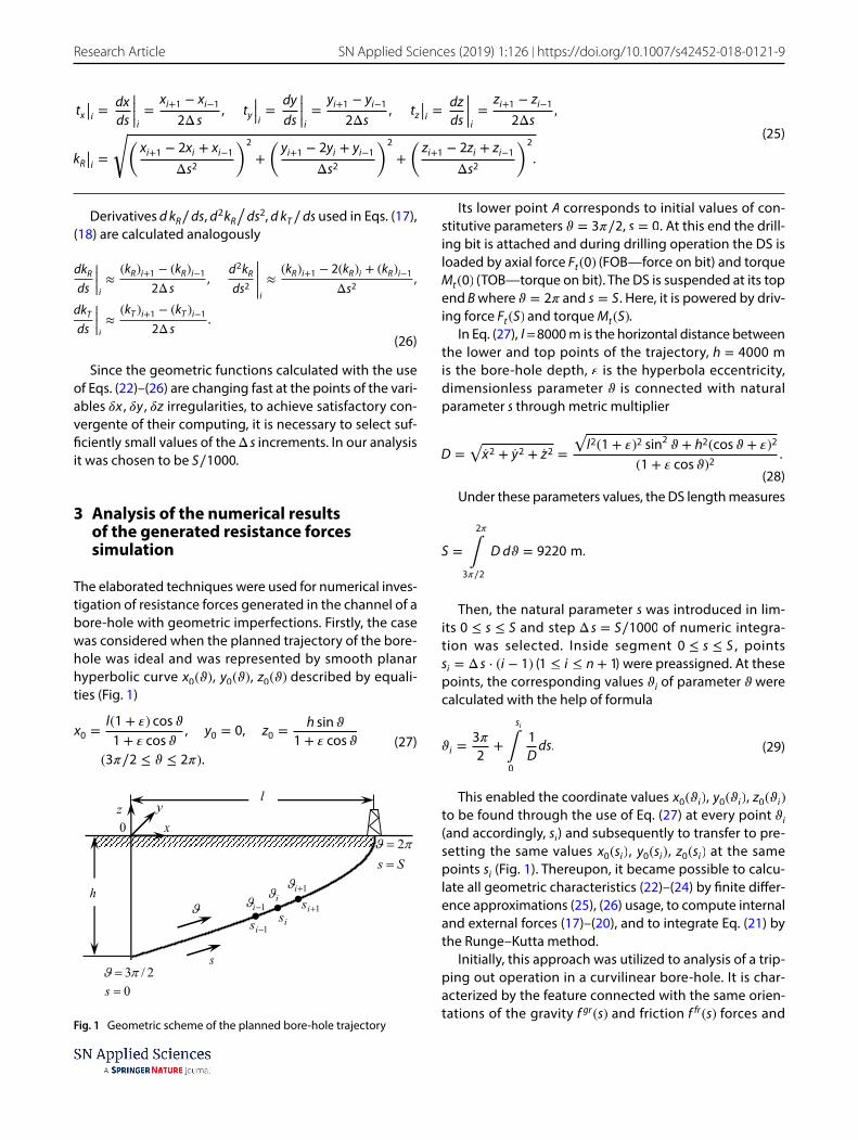
After completion of this analysis, the supposition was done that during the bore-hole drivage, some geomet-ric deviations � x(s) , � y(s) , � z(s) were allowed because of technological factors and the rock heterogeneity. These deviations were measured by the methods of geophysic navigation and processed in tabular form with the Δ sj step equal S∕70 = 131.7 m. Two cases of the tabular distortions were considered. The first set of their values is represented in Table 1. The second set can be gained by simple dou-bling of the first values.

The graphic representation of the digital distortions � x(sj) , � y(sj) , � z(sj) is shown in Fig. 2.

It should be emphasized that though the distortions outlined on the basis of discrete tabular data are intro-duced in the form of broken lines, in reality, they look like even differentiable (although, tortuous) curves.

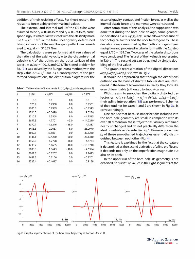
With the aim to smoothen the digitally distorted tra-jectories x0(sj) + � x(sj) , y0(sj) + � y(sj) , z0(sj) + � z(sj) , their spline interpolation (15) was performed. Schemes of their outlines for cases 1 and 2 are shown in Fig. 3a, b, correspondingly.

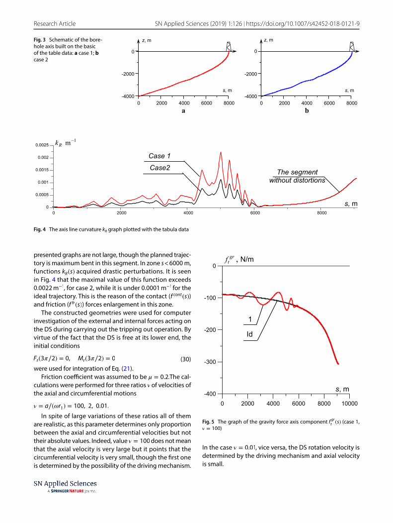
One can see that because imperfections included into the bore-hole geometry are small in comparion with its over all dimension these trajectories visually remained nearly unchanged and do not practically differ from the ideal bore-hole represented in Fig. 1. However curvatures kR of these smoothened trajectories essentially distin-guished between each other (Fig. 4).

This feature is explained by the fact that the curvature is determined as the second derivative of a line profile and it depends not only on the imperfection magnitude but also on its pitch.

In the upper run of the bore-hole, its geometry is not distorted, so curvature values in the right segments of the

Table 1 Table values of increments � x(sj) , � y(sj) , and � z(sj) (case 1)

j sj (m) � xj (m) � yj (m) � zj (m)

1 0.0 0.0 0.0 0.02 626.9 0.2930 0.0 0.95613 1200.3 0.2989 − 1.0 − 0.95434 1726.5 − 3.0499 0.0 9.52365 2210.7 1.5568 8.0 − 4.75156 2657.5 4.7701 − 3.0 − 14.22107 3070.7 − 1.6246 − 18.0 4.72878 3453.8 − 9.9637 − 8.0 28.29709 3809.8 − 13.5851 0.0 37.623010 4141.1 − 10.4230 20.0 28.131011 4450.0 − 1.7778 38.0 4.673312 4738.7 5.4605 10.0 − 13.971013 5008.8 1.8643 − 18.0 − 4.639414 5261.8 − 3.8207 0.0 9.241315 5499.3 0.3166 5.0 − 0.920116 5722.4 − 0.4017 0.0 0.9158

yδ , m

s, m0 2000 4000 6000 8000 10000

-20

0

20

40 zδ , m

s, m0 2000 4000 6000 8000 10000

-20

0

20

40xδ , m

s, m0 2000 4000 6000 8000 10000

-16

-12

-8

-4

0

4

8

Fig. 2 Graphic representation of the bore-hole trajectory distortions (case 1)

Vol:.(1234567890)


presented graphs are not large, though the planned trajec-tory is maximum bent in this segment. In zone s < 6000 m, functions kR(s) acquired drastic perturbations. It is seen in Fig. 4 that the maximal value of this function exceeds 0.0022 m−1 , for case 2, while it is under 0.0001 m−1 for the ideal trajectory. This is the reason of the contact ( f cont(s) ) and friction ( f fr(s) ) forces enlargement in this zone.

The constructed geometries were used for computer investigation of the external and internal forces acting on the DS during carrying out the tripping out operation. By virtue of the fact that the DS is free at its lower end, the initial conditions

were used for integration of Eq. (21).Friction coefficient was assumed to be � = 0.2.The cal-

culations were performed for three ratios � of velocities of the axial and circumferential motions

In spite of large variations of these ratios all of them are realistic, as this parameter determines only proportion between the axial and circumferential velocities but not their absolute values. Indeed, value � = 100 does not mean that the axial velocity is very large but it points that the circumferential velocity is very small, though the first one is determined by the possibility of the driving mechanism.

(30)Ft(3�∕2) = 0, Mt(3�∕2) = 0

� = a∕(�r1) = 100, 2, 0.01.

In the case � = 0.01 , vice versa, the DS rotation velocity is determined by the driving mechanism and axial velocity is small.

Fig. 3 Schematic of the bore-hole axis built on the basic of the table data: a case 1; b case 2

a b0 2000 4000 6000 8000

-4000

-2000

s, m

z, m

0

0 2000 4000 6000 8000-4000

-2000

0

s, m

z, m

0 2000 4000 6000 80000

0.0005

0.001

0.0015

0.002

0.0025

Case2

Case 1

The segmentwithout distortions

s, m

1m−Rk

Fig. 4 The axis line curvature kR graph plotted with the tabula data

0 2000 4000 6000 8000 10000-400

-300

-200

-100

0grtf , N/m

s, m

Id

1

Fig. 5 The graph of the gravity force axis component f grt (s) (case 1, � = 100)

Vol.:(0123456789)


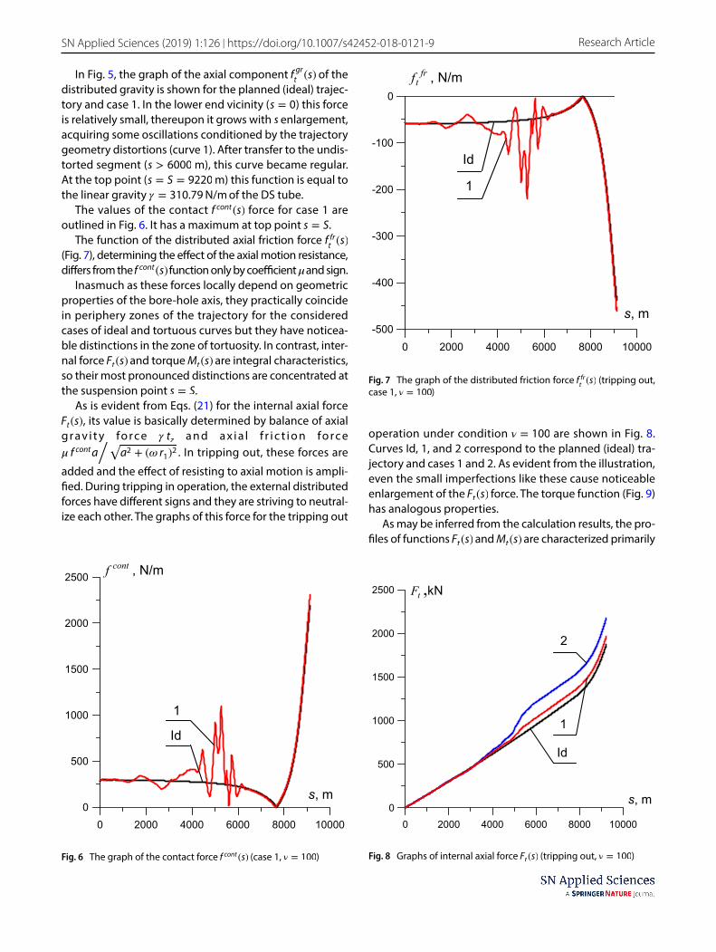
In Fig. 5, the graph of the axial component f grt (s) of the distributed gravity is shown for the planned (ideal) trajec-tory and case 1. In the lower end vicinity ( s = 0 ) this force is relatively small, thereupon it grows with s enlargement, acquiring some oscillations conditioned by the trajectory geometry distortions (curve 1). After transfer to the undis-torted segment ( s > 6000 m), this curve became regular. At the top point ( s = S = 9220 m) this function is equal to the linear gravity � = 310.79N/m of the DS tube.

The values of the contact f cont(s) force for case 1 are outlined in Fig. 6. It has a maximum at top point s = S.

The function of the distributed axial friction force f frt(s)

(Fig. 7), determining the effect of the axial motion resistance, differs from the f cont(s) function only by coefficient � and sign.

Inasmuch as these forces locally depend on geometric properties of the bore-hole axis, they practically coincide in periphery zones of the trajectory for the considered cases of ideal and tortuous curves but they have noticea-ble distinctions in the zone of tortuosity. In contrast, inter-nal force Ft(s) and torque Mt(s) are integral characteristics, so their most pronounced distinctions are concentrated at the suspension point s = S.

As is evident from Eqs. (21) for the internal axial force Ft(s) , its value is basically determined by balance of axial g r a v i t y fo rc e � tz a n d a x i a l f r i c t i o n fo rc e � f conta

�√a2 + (� r1)

2 . In tripping out, these forces are

added and the effect of resisting to axial motion is ampli-fied. During tripping in operation, the external distributed forces have different signs and they are striving to neutral-ize each other. The graphs of this force for the tripping out

operation under condition � = 100 are shown in Fig. 8. Curves Id, 1, and 2 correspond to the planned (ideal) tra-jectory and cases 1 and 2. As evident from the illustration, even the small imperfections like these cause noticeable enlargement of the Ft(s) force. The torque function (Fig. 9) has analogous properties.

As may be inferred from the calculation results, the pro-files of functions Ft(s) and Mt(s) are characterized primarily

0 2000 4000 6000 8000 100000

500

1000

1500

2000

2500contf , N/m

s, m

Id

1

Fig. 6 The graph of the contact force f cont(s) (case 1, � = 100)

s, m

Id

1

0 2000 4000 6000 8000 10000-500

-400

-300

-200

-100

0

frtf , N/m

Fig. 7 The graph of the distributed friction force f frt(s) (tripping out,

case 1, � = 100)

tF ,kN

s, m

0 2000 4000 6000 8000 100000

500

1000

1500

2000

2500

1

2

Id

Fig. 8 Graphs of internal axial force Ft(s) (tripping out, � = 100)

Vol:.(1234567890)


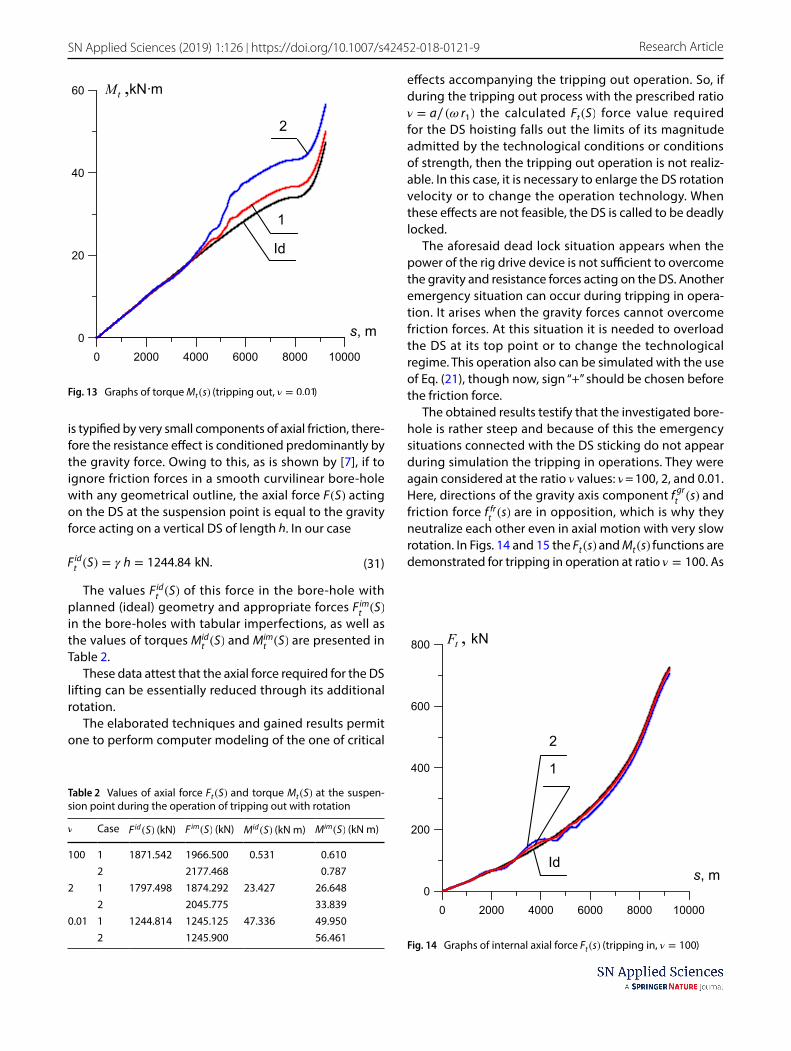
by ratio � and the form of technological operation (trip-ping in/out and drilling). Clearly, the � reduction is asso-ciated with axial velocity decrease and increase of the circumferential velocity. Therefore, it causes reduction of axial force Ft(s) and enlargement of torque Mt(s) (compare Fig. 8 for � = 100 and Figs. 10, 12 for � = 2 and � = 0.01 , as well as Figs. 9, 11, 13).

These results are of immediate interest to practice because values Ft(S) and Mt(S) are the force and torque applied to the DS top which are required for realiza-tion of the DS lifting and rotating. With enlargement

of the rotation velocity � ( � = a∕(� r1) = 2 ), the lifting force Ft(S) diminishes and driving torque Mt(S) increases (Figs. 10, 11).

As previously, the curves labeled Id, 1, and 2 correspond to the ideal geometry and cases 1 and 2. The possibility to regulate the forces, resisting to axial motion of the DS, by way of its concurrent rotation is underlined by the numeri-cal calculation performed at � = a∕(� r1) = 0.01 (Figs. 12, 13).

Then, the DS is lifted with very small velocity a and rotates with high angular velocity � . This driving regime

tM ,kN·m

s, m

0 2000 4000 6000 8000 100000

0.2

0.4

0.6

0.8

1

2

Id

Fig. 9 Graphs of torque Mt(s) (tripping out, � = 100)

tF ,kN

s, m

0 2000 4000 6000 8000 100000

500

1000

1500

2000

2500

1

2

Id

Fig. 10 Graphs of internal axial force Ft(s) (tripping out, � = 2)

tM ,kN·m

s, m

0 2000 4000 6000 8000 100000

10

20

30

40

1

2

Id

Fig. 11 Graphs of torque Mt(s) (tripping out, � = 2)

tF ,kN

s, m

0 2000 4000 6000 8000 100000

400

800

1200

1600

1

2

Id

Fig. 12 Graphs of internal axial force Ft(s) (tripping out, � = 0.01)

Vol.:(0123456789)


is typified by very small components of axial friction, there-fore the resistance effect is conditioned predominantly by the gravity force. Owing to this, as is shown by [7], if to ignore friction forces in a smooth curvilinear bore-hole with any geometrical outline, the axial force F(S) acting on the DS at the suspension point is equal to the gravity force acting on a vertical DS of length h . In our case

The values Fidt(S) of this force in the bore-hole with

planned (ideal) geometry and appropriate forces Fimt(S)

in the bore-holes with tabular imperfections, as well as the values of torques Mid

t(S) and Mim

t(S) are presented in

Table 2.These data attest that the axial force required for the DS

lifting can be essentially reduced through its additional rotation.

The elaborated techniques and gained results permit one to perform computer modeling of the one of critical

(31)Fidt(S) = � h = 1244.84 kN.

effects accompanying the tripping out operation. So, if during the tripping out process with the prescribed ratio � = a∕(� r1) the calculated Ft(S) force value required for the DS hoisting falls out the limits of its magnitude admitted by the technological conditions or conditions of strength, then the tripping out operation is not realiz-able. In this case, it is necessary to enlarge the DS rotation velocity or to change the operation technology. When these effects are not feasible, the DS is called to be deadly locked.

The aforesaid dead lock situation appears when the power of the rig drive device is not sufficient to overcome the gravity and resistance forces acting on the DS. Another emergency situation can occur during tripping in opera-tion. It arises when the gravity forces cannot overcome friction forces. At this situation it is needed to overload the DS at its top point or to change the technological regime. This operation also can be simulated with the use of Eq. (21), though now, sign “+” should be chosen before the friction force.

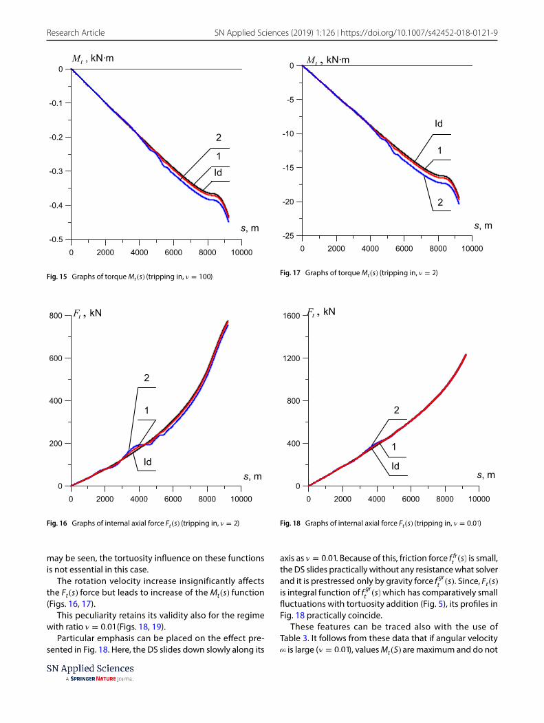
The obtained results testify that the investigated bore-hole is rather steep and because of this the emergency situations connected with the DS sticking do not appear during simulation the tripping in operations. They were again considered at the ratio � values: � = 100, 2, and 0.01. Here, directions of the gravity axis component f grt (s) and friction force f fr

t(s) are in opposition, which is why they

neutralize each other even in axial motion with very slow rotation. In Figs. 14 and 15 the Ft(s) and Mt(s) functions are demonstrated for tripping in operation at ratio � = 100 . As

tM ,kN·m

s, m

0 2000 4000 6000 8000 100000

20

40

60

1

2

Id

Fig. 13 Graphs of torque Mt(s) (tripping out, � = 0.01)

Table 2 Values of axial force Ft(S) and torque Mt(S) at the suspen-sion point during the operation of tripping out with rotation

� Case Fid(S) (kN) Fim(S) (kN) Mid(S) (kN m) Mim(S) (kN m)

100 1 1871.542 1966.500 0.531 0.6102 2177.468 0.787

2 1 1797.498 1874.292 23.427 26.6482 2045.775 33.839

0.01 1 1244.814 1245.125 47.336 49.9502 1245.900 56.461

0 2000 4000 6000 8000 100000

200

400

600

800 tF , kN

s, m

1

2

Id

Fig. 14 Graphs of internal axial force Ft(s) (tripping in, � = 100)

Vol:.(1234567890)


may be seen, the tortuosity influence on these functions is not essential in this case.

The rotation velocity increase insignificantly affects the Ft(s) force but leads to increase of the Mt(s) function (Figs. 16, 17).

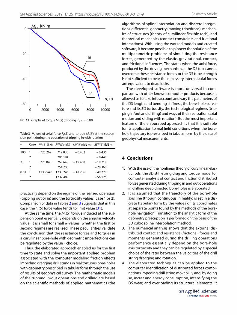
This peculiarity retains its validity also for the regime with ratio � = 0.01 (Figs. 18, 19).

Particular emphasis can be placed on the effect pre-sented in Fig. 18. Here, the DS slides down slowly along its

axis as � = 0.01 . Because of this, friction force f frt(s) is small,

the DS slides practically without any resistance what solver and it is prestressed only by gravity force f grt (s) . Since, Ft(s) is integral function of f grt (s) which has comparatively small fluctuations with tortuosity addition (Fig. 5), its profiles in Fig. 18 practically coincide.

These features can be traced also with the use of Table 3. It follows from these data that if angular velocity � is large ( � = 0.01 ), values Mt(S) are maximum and do not

tM , kN·m

s, m

0 2000 4000 6000 8000 10000-0.5

-0.4

-0.3

-0.2

-0.1

0

1

2

Id

Fig. 15 Graphs of torque Mt(s) (tripping in, � = 100)

tF , kN

s, m

0 2000 4000 6000 8000 100000

200

400

600

800

1

2

Id

Fig. 16 Graphs of internal axial force Ft(s) (tripping in, � = 2)

tM , kN·m

s, m

0 2000 4000 6000 8000 10000-25

-20

-15

-10

-5

0

1

2

Id

Fig. 17 Graphs of torque Mt(s) (tripping in, � = 2)

tF , kN

s, m

0 2000 4000 6000 8000 100000

400

800

1200

1600

1

2

Id

Fig. 18 Graphs of internal axial force Ft(s) (tripping in, � = 0.01)

Vol.:(0123456789)


practically depend on the regime of the realized operation (tripping out or in) and the tortuosity values (case 1 or 2). Comparison of data in Tables 2 and 3 suggests that in this case, the Ft(S) force value tends to limit value (31).

At the same time, the Mt(S) torque induced at the sus-pension point essentially depends on the angular velocity value. It is small for small � values, whether the first or second regimes are realized. These peculiarities validate the conclusion that the resistance forces and torques in a curvilinear bore-hole with geometric imperfections can be regulated by the value � choice.

Thus, the elaborated approach enabled us for the first time to state and solve the important applied problem associated with the computer modeling friction effects impeding dragging drill strings in real tortuous bore-holes with geometry prescribed in tabular form through the use of results of geophysical survey. The mathematic models of the tripping in/out operations and drilling are based on the scientific methods of applied mathematics (the

algorithms of spline interpolation and discrete integra-tion), differential geometry (moving trihedrons), mechan-ics of structures (theory of curvilinear flexible rods), and theoretical mechanics (contact constraints and frictional interactions). With using the worked models and created software, it became possible to pioneer the solution of the multiparametric problems of simulating the resistance forces, generated by the elastic, gravitational, contact, and frictional influences. The states when the axial force, produced by the driving mechanism at the DS top, cannot overcome these resistance forces or the DS tube strength is not sufficient to bear the necessary internal axial forces are equivalent to dead locks.

The developed software is more universal in com-parison with other known computer products because it allowed us to take into account and vary the parameters of the DS length and bending stiffness, the bore-hole curva-ture and its 3D tortuosity, the technological regimes (trip-ping in/out and drilling) and ways of their realization (axial motion and sliding with rotation). But the most important feature of the elaborabed approach is that it is suitable for its application to real field conditions when the bore-hole trajectory is prescribed in tabular form by the data of geophysical measurements.

4 Conclusions

1. With the use of the nonlinear theory of curvilinear elas-tic rods, the 3D stiff-string drag and torque model for computer analysis of contact and friction distributed forces generated during tripping in and out operations in drilling deep directed bore-holes is elaborated.

2. It is assumed that the trajectory of the bore-hole axis line (though continuous in reality) is set in a dis-crete (tabular) form by the values of its coordinates at separate points found by the methods of the bore-hole navigation. Transition to the analytic form of the geometry prescription is performed on the basis of the 3D cubic spline interpolation method.

3. The numerical analysis shows that the external dis-tributed contact and resistance (frictional) forces and moments generated during the drilling operations performance essentially depend on the bore-hole axis tortuosity and they can be regulated by a special choice of the ratio between the velocities of the drill string dragging and rotation.

4. The elaborated techniques can be applied to the computer identification of distributed forces combi-nations impeding drill string movabilily and, by doing so, increasing energy consumption, intensifying the DS wear, and overloading its structural elements. It

tM , kN·m

s, m

0 2000 4000 6000 8000 10000-60

-40

-20

0

2

1

Id

Fig. 19 Graphs of torque Mt(s) (tripping in, � = 0.01)

Table 3 Values of axial force Ft(S) and torque Mt(S) at the suspen-sion point during the operation of tripping in with rotation

� Case Fid(S) (kN) Fim(S) (kN) Mid(S) (kN m) Mim(S) (kN m)

100 1 725.269 719.835 − 0.432 − 0.4362 706.194 − 0.448

2 1 775.840 769.648 − 19.458 − 19.7192 754.200 − 20.368

0.01 1 1233.549 1233.246 − 47.236 − 49.7792 1232.489 − 56.126

Vol:.(1234567890)


gives also the possibility to recognize the dead lock situations when the rig engine power is not sufficient to break through the generated force drag.

Compliance with ethical standards

Conflict of interest On behalf of all authors, the corresponding au-thor states that there is no conflict of interest.

References

1. Aadnoy BS, Andersen K (2001) Design of oil wells using analyti-cal friction models. J Pet Sci Eng 32:53–71

2. Aadnoy BS, Larsen K, Berg PC (2003) Analysis of stuck pipe in deviated boreholes. J Pet Sci Eng 37:195–212

3. Berger EJ (2002) Friction modeling for dynamic system simula-tion. Appl Mech Rev 56(6):535–577

4. Brett JF, Beckett AD, Holt CA et al (1989) Uses and limitations of drill string tension and torque models for monitoring hole conditions. SPE Drill Eng 4:223–229

5. Choe J, Schubert JJ, Juvkam-Wold HC (2005) Well-control analy-ses on extended-reach and multilateral trajectories. SPE Drill Complet 20:101–108

6. Gao DL, Huang WJ (2015) A review of down-hole tubular string buckling in well engineering. Pet Sci 12(3):443–457

7. Gulyayev VI, Andrusenko EN (2013) Theoretical simulation of geometric imperfections influence on drilling operations at drivage of curvilinear bore-holes. J Pet Sci Eng 112:170–177

8. Gulyayev VI, Gaidaichuk VV, Andrusenko EN et al (2015) Mode-ling the energy-saving regimes of curvilinear bore-hole drivage. J Offshore Arct Eng 137(1):011402-1–011402-8

9. Gulyayev VI, Gaidaichuk VV, Koshkin VL (1992) Elastic deform-ing, stability and vibrations of flexible curvilinear rods. Naukova Dumka, Kiev (in Russian)

10. Gulyayev VI, Shlyun NV (2016) Influence of friction on buckling of a drill string in the circular channel of a bore-hole. J Pet Sci Eng 13(4):698–711

11. Hinze WJ, Frese RR, Saad AH (2013) Gravity and magnetic explo-ration: principles, practices, and applications. Cambridge Uni-versity Press, Cambridge

12. Iyoho AW, Meize RA, Millheim KK et al (2005) Lessons from inte-grated analysis of GOM drilling performance. SPE Drill Complet 20:6–16

13. Korn GA, Korn TM (2000) Mathematical handbook for scientists and engineers: definitions, theorems, and formulas for reference and review. Dover Publications, New York

14. Mirhaj SA, Kaarstad E, Aadnoy BS (2011) Improvement of torque-and-drag modeling in long-reach wells. Mod Appl Sci 5(5):10–28

15. Mitchell RF, Samuel R (2009) How good is torque/drag model? SPE Drill Complet 24(1):62–71

16. Mohiuddin MA, Khan K, Abdulraheem A et al (2006) Analysis of wellbore instability in vertical, directional and horizontal wells using field data. J Pet Sci Eng 55:83–92

17. Pourcian RD, Fisk JH, Descant FJ et al (2005) Completion and well-performance results, genesis field, deepwater Gulf of Mex-ico. SPE Drill Complet 20:147–155

18. Ritto TG, Aguiar RR, Hbaieb S (2017) Validation of a drill string dynamical model and torsional stability. Meccanica 52:2959–2967

19. Samuel R (2010) Friction factors: What are they for torque, drag, vibration, bottom hole assembly and transient surge/swab anal-yses? J Pet Sci Eng 73:258–266

20. Sawaryn SJ, Thorogood JL (2005) A compendium of directional calculations based on the minimum curvature method. SPE Drill Complet 20:24–36

21. Sheppard MC (1987) Designing well paths to reduce drag and torque. SPE Drill Eng 2:344–350

22. Stuart D, Hamer CD, Henderson C et al (2003) New drilling tech-nology reduces torque and drag by drilling a smooth wellbore. In: SPE IADC Drilling Conference. Amsterdam, Netherlands, pp 83–88

23. Vijayan K, Vlajic N, Friswell MI (2017) Drillstring-borehole interac-tion: backward whirl instabilities and axial loading. Meccanica 52:2945–2957

Documents

Computer simulation of dragging with rotation of a drill string in 3D